Molecular
Quantum
Mechanics
Molecular Quantum Mechanics
Third Edition
P. W. Atkins, Professor of Chemistry, University of
Oxford, and Fellow, Lincoln College, Oxford, and
R S. Friedman, Assistant Professor of Chemistry,
Purdue University, Fort Wayne, USA
0-19-855947-X
Publication date: 31 October 1996
562 pages, two-colour line figures, tables, 252mm x 197mm
P. W. Ai kms R. S. Fr.edman
Description
Molecular Quantum Mechanics, an accessible introduction to the foundations of quantum
chemistry, established itself as a classic as soon as the original best-selling edition appeared.
This new third edition will ensure its place is maintained in the forefront of its field. Entirely
rewritten to present the subject more clearly than ever before, this new edition includes two
completely new chapters - one on computational techniques in quantum chemistry, and another
on scattering theory. Most of the material on the calculations of electionic structure is entirely
new, and the discussions in the second edition have been enhanced with more mathematical
rigour. With 330 two-colour illustrations, numerous worked examples, in-text exercises, an
extensive further information section, and a wide range of applications tieated consistentiy, this
will surely prove to be an invaluable book for all senior chemistry undergraduates.
Readership: Chemistry students; UK: 3/4 year undergraduate and postgraduates, USA: senior
undergraduate/graduate. Also students studying physics, materials, chemical physics.
Con ten ts/con tribu tors
D Introduction and orientation
D 1 The foundations of quantum mechanics
D 2 Linear motion and the harmonic oscillator
D 3 Rotational motion and the hydrogen atom
D 4 Angular momentum
D 5 Group theory
D 6 Techniques of approximation
D 7 Atomic spectra and atomic structure
D 9 The calculation of electionic structures
D 10 Molecular rotations and vibrations
D 11 Molecular electionic transitions
D 12 The electionic properties of molecules
D 13 The magnetic properties of molecules
D 14 Scattering theory
D Further inform ation
D Further reading
D Appendix
D Answers to Problems
D Index

Preface
In the universe we inhabit, the pendulum swings with a period of about 13.5
years. The first edition of this book appeared in 1970; the second in 1983; now
the third edition is published. Many changes have taken place through the edi-
editions, but we hope the essential spirit of the earlier editions has been preserved:
there should be as much interpretation as straightforward mathematical presen-
presentation in this as in the earlier editions. Another strong feature of the earlier
editions has been preserved and extended in this: the emphasis on visualization
of often abstract material.
First, the major changes. The whole book has been rewritten. There are two
new chapters and a reformulation of other chapters. One entirely new chapter is
on the calculation of electronic structure (Chapter 9). No other field in quantum
chemistry has made such vigorous strides forwards—into usefulness as well as
complexity—as this. It would be hopeless to consider giving a detailed account
of this highly technical field, but improper to leave out a discussion of what is
now the field of major endeavour in the subject. We have sought to give a
survey of the basis of the techniques that are now so widely available in com-
commercial and academic packages so that people can understand the variety of ab
initio and semiempirical approaches that are now available.
The second entirely new chapter is the one on scattering theory (Chapter 14).
We consider that the major analytical advances in molecular quantum
mechanics have occurred in this field, under the impetus of advances in experi-
experimental procedures (molecular beams and lasers) but also in a shift in attention
from structure to the processes of reaction. Once again, here is a topic where a
deluge of algebra can readily wash away comprehension. However, we have
sought to concentrate on highlights, and to give visualizations of material wher-
wherever appropriate. We have drawn the line at a discussion of reactive collisions,
for even the slight straying over into this terrain that ends this text shows what a
minefield of notation and subtlety it is.
Another feature of this edition is that we have elected to adopt a more sys-
systematic approach to quantum mechanics. Now Chapter 1 proceeds
axiomatically (but at a highly accessible level, we believe) rather than histori-
historically. However, to make this approach accessible, we have given a short
historical introduction (in the unnumbered chapter entitled Introduction and
orientation) so that readers will feel, we hope, that in stepping off into the
unknown they are at least stepping off familiar territory.
There are many organizational changes in the text, ranging from the layout of
chapters to the choice of words. This edition is in fact a complete rewrite of the
second edition. In the rewriting, we have aimed for clarity and precision. Where
the depth of the presentation started to seem too great in our judgment for our
audience, we have sent material to the back of the book in an extensive and
rearranged collection of Further information sections.
No text can be, and perhaps even should not aim to be, complete. We know
that there are omissions from this text. However, we also believe that no other

vi Preface
text is as complete as this. We have aimed to give a balanced account of the
electronic structures of atoms and molecules (which other comparable texts also
do), but we have also presented a lot of material on spectroscopy of many kinds
(which some other texts do too). In addition though, we have presented a lot of
material on the electric and magnetic properties of molecules, which is an
important zone of quantum chemistry but which is rarely included at this level.
We owe a considerable debt to many people; not least to one another! Our
publishers have been helpful and understanding, as always. Our particular
thanks are due to a variety of reviewers of the manuscript at several stages of
presentation. In particular, we should like to thank Ronald Duchovic (IPFW)
and David Schwenke (NASA, Ames) who have been most helpful and generous
with their advice. We would also like to thank the readers of the first draft of the
text, who were Steven Bernasek (Princeton University), Patrick Fowler
(University of Exeter), David Micha (University of Florida), Ian Mills
(University of Reading), Robert Sharp (University of Michigan), Charles
Trapp (University of Louisville), and Rama Viswanathan (Beloit College).
They spotted many points that were best spotted in private, and made valuable
suggestions about the organization and content of the book. Over the years,
many users have offered advice: they are too numerous to name here, but
they will all know how valuable we view their advice and in many cases will
see it incorporated into this edition.
PWA, Oxford
RSF, Indiana University Purdue University Fort Wayne
May 1996

Contents
Introduction and orientation 1
Black-body radiation 1
Heat capacities 2
The photoelectric and Compton effects 3
Atomic spectra 4
The duality of matter 6
Problems 7
Further reading 8
1 The foundations of quantum mechanics 9
Operators in quantum mechanics 9
1.1 Eigenfunctions and eigenvalues 9
1.2 Representations 11
1.3 Commutation and non-commutation 11
1.4 The construction of operators 12
1.5 Linear operators 14
1.6 Integrals over operators 14
The postulates of quantum mechanics 15
1.7 States and wavefunctions 15
1.8 The fundamental prescription 16
1.9 The outcome of measurements 16
1.10 The interpretation of the wavefunction 18
1.11 The equation for the wavefunction 18
1.12 The separation of the Schrodinger equation 19
Hermitian operators 21
1.13 Definitions 21
1.14 Dirac bracket notation 22
1.15 The properties of hermitian operators 23
The specification of states: complementarity 24
The uncertainty principle 25
1.16 Formal derivation of the principle 25
1.17 Consequences of the uncertainty principle 27
1.18 The uncertainty in energy and time 28
Time-evolution and conservation laws 29
Matrices in quantum mechanics 30
1.19 Matrix elements 31
1.20 The diagonalization of the hamiltonian 32

viii Contents
The plausibility of the Schrodinger equation 34
1.21 The propagation of light 34
1.22 The propagation of particles 37
1.23 The transition to quantum mechanics 37
Problems 39
Further reading 41
2 Linear motion and the harmonic oscillator 42
The characteristics of acceptable wavefunctions 42
Some general remarks on the Schrodinger equation 43
2.1 The curvature of the wavefunction 43
2.2 Qualitative solutions 44
2.3 The emergence of quantization 44
2.4 Penetration into nonclassical regions 45
Translational motion 46
2.5 Energy and momentum 46
2.6 The significance of the coefficients 47
2.7 The flux density 48
2.8 Wavepackets 49
Penetration into and through barriers 50
2.9 An infinitely thick potential wall 50
2.10 A barrier of finite width 51
2.11 The Eckart potential barrier 54
Particle in a box 54
2.12 The solutions 54
2.13 Features of the solutions 56
2.14 The two-dimensional square well 56
2.15 Degeneracy 58
The harmonic oscillator 59
2.16 The solutions 61
2.17 Properties of the solutions 62
2.18 The classical limit 64
Translation revisited: the scattering matrix 65
Problems 67
Further reading 70
3 Rotational motion and the hydrogen atom 71
Particle on a ring 71

Contents ix
3.1 The hamiltonian and the Schrodinger equation 71
3.2 The angular momentum 73
3.3 The shapes of the wavefunctions 74
3.4 The classical limit 76
Particle on a sphere 76
3.5 The Schrodinger equation and its solution 76
3.6 The angular momentum of the particle 79
3.7 Properties of the solutions 81
3.8 The rigid rotor 81
Motion in a Coulombic field 84
3.9 The Schrodinger equation for hydrogenic atoms 84
3.10 The separation of the relative coordinates 84
3.11 The radial Schrodinger equation 85
3.12 Probabilities and the radial distribution function 89
3.13 Atomic orbitals 90
3.14 The degeneracy of hydrogenic atoms 94
Problems 95
Further reading 97
4 Angular momentum 98
The angular momentum operators 98
4.1 The operators and their commutation relations 98
4.2 Angular momentum observables 100
4.3 The shift operators 101
The definition of the states 102
4.4 The effect of the shift operators 102
4.5 The eigenvalues of the angular momentum 103
4.6 The matrix elements of the angular momentum 103
4.7 The angular momentum eigenfunctions 107
4.8 Spin 109
The angular momenta of composite systems 110
4.9 The specification of coupled states 110
4.10 The permitted values of the total angular momentum 111
4.11 The vector model of coupled angular momenta 113
4.12 The relation between schemes 115
4.13 The coupling of several angular momenta 119
Problems 119
Further reading 121

Contents
5 Group theory 122
The symmetries of objects 122
5.1 Symmetry operations and elements 122
5.2 The classification of molecules 124
The calculus of symmetry 125
5.3 The definition of a group 126
5.4 Group multiplication tables 127
5.5 Matrix representations 128
5.6 The properties of matrix representations 132
5.7 The characters of representations 135
5.8 Characters and classes 136
5.9 Irreducible representations 137
5.10 The great and little orthogonality theorems 139
Reduced representations 143
5.11 The reduction of representations 143
5.12 Symmetry-adapted bases 145
The symmetry properties of functions 148
5.13 The transformation of p-orbitals 148
5.14 The decomposition of direct-product bases 149
5.15 Direct-product groups 152
5.16 Vanishing integrals 154
5.17 Symmetry and degeneracy 156
The full rotation group 157
5.18 The generators of rotations 157
5.19 The representation of the full rotation group 159
5.20 Coupled angular momenta 161
Applications 161
Problems 162
Further reading 163
6 Techniques of approximation 164
Time-independent perturbation theory 164
6.1 Perturbation of a two-level system 164
6.2 Many-level systems 166
6.3 The first-order correction to the energy 168
6.4 The first-order correction to the wavefunction 169
6.5 The second-order correction to the energy 170
6.6 Comments on the perturbation expressions 171
6.7 The closure approximation 173
6.8 Perturbation theory for degenerate states 175

Contents xi
Variation theory 178
6.9 The Rayleigh ratio 178
6.10 The Rayleigh-Ritz method 180
The Hellmann-Feynman theorem 182
Time-dependent perturbation theory 184
6.11 The time-dependent behaviour of a two-level system 184
6.12 The Rabi formula 187
6.13 Many-level systems: the variation of constants 188
6.14 The effect of a slowly switched constant perturbation 190
6.15 The effect of an oscillating perturbation 192
6.16 Transition rates to continuum states 193
6.17 The Einstein transition probabilities 195
6.18 Lifetime and energy uncertainty 198
Problems 199
Further reading 201
7 Atomic spectra and atomic structure 202
The spectrum of atomic hydrogen 202
7.1 The energies of the transitions 202
7.2 Selection rules 203
7.3 Orbital and spin magnetic moments 206
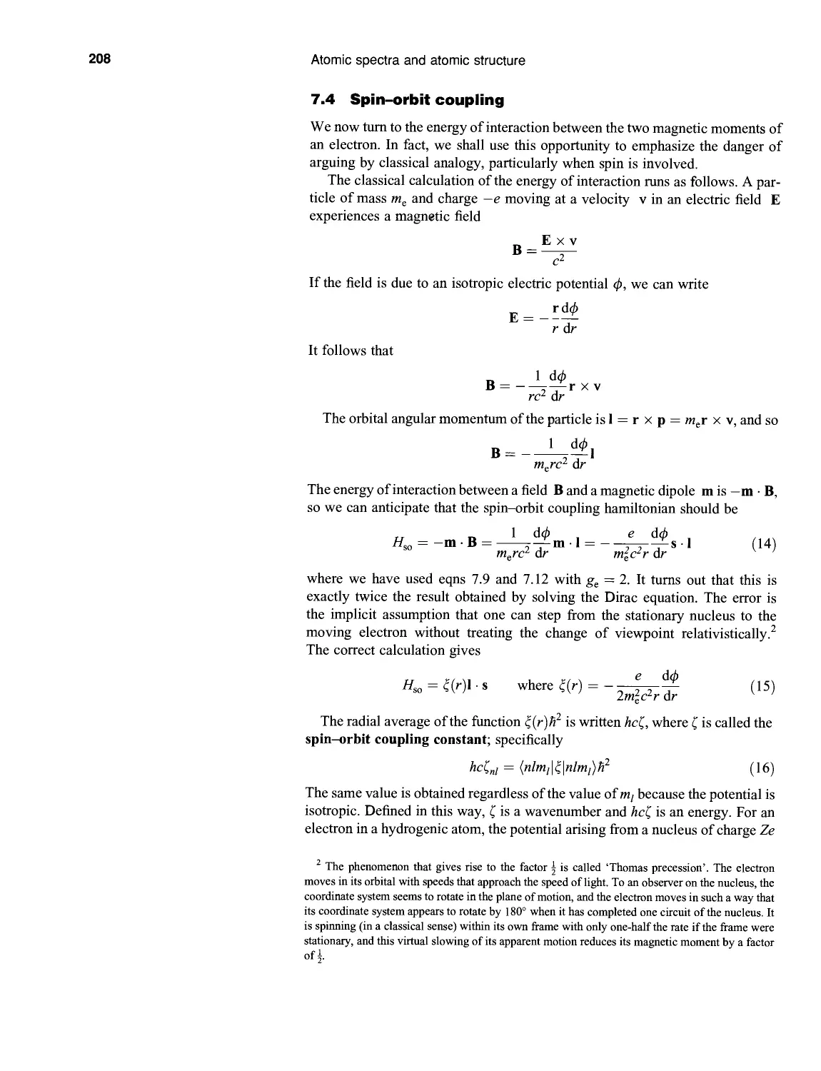
7.4 Spin-orbit coupling 208
7.5 The fine-structure of spectra 209
7.6 Term symbols and spectral details 210
7.7 The detailed spectrum of hydrogen 211
The structure of helium 212
7.8 The helium atom 212
7.9 Excited states of helium 215
7.10 The spectrum of helium 217
7.11 The Pauli principle 218
Many-electron atoms 221
7.12 Penetration and shielding 221
7.13 Periodicity 223
7.14 Slater atomic orbitals 225
7.15 Self-consistent fields 225
7.16 Term symbols and transitions of many-electron atoms 228
7.17 Hund's rules and the relative energies of terms 231
7.18 Alternative coupling schemes 232
Atoms in external fields 233
7.19 The normal Zeeman effect 233
7.20 The anomalous Zeeman effect 234

xii Contents
7.21 The Stark effect 236
Problems 237
Further reading 239
8 An introduction to molecular structure 240
The Born-Oppenheimer approximation 240
8.1 The formulation of the approximation 241
8.2 An application: the hydrogen molecule-ion 242
Molecular orbital theory 244
8.3 Linear combinations of atomic orbitals 244
8.4 The hydrogen molecule 248
8.5 Configuration interaction 250
8.6 Diatomic molecules 251
8.7 Heteronuclear diatomic molecules 254
Molecular orbital theory of polyatomic molecules 255
8.8 Symmetry-adapted linear combinations 255
8.9 Conjugated тг-systems 258
8.10 Ligand field theory 262
8.11 Further aspects of ligand field theory 265
The band theory of solids 266
8.12 The tight-binding approximation 267
8.13 The Kronig-Penney model 269
8.14 Brillouin zones 271
Problems 273
Further reading 275
9 The calculation of electronic structure 276
The Hartree-Fock self-consistent field method 277
9.1 The formulation of the approach 277
9.2 The Hartree-Fock approach 278
9.3 Restricted and unrestricted Hartree-Fock calculations 279
9.4 The Roothaan equations 281
9.5 The selection of basis sets 285
9.6 Calculational accuracy and the basis set 290
Electron correlation 291
9.7 Configuration state functions 291
9.8 Configuration interaction 292
9.9 CI calculations 293
9.10 Multiconfiguration and multireference methods 297

Contents xiii
9.11 Moller-Plesset many-body perturbation theory 298
Density functional theory 301
Gradient methods and molecular properties 304
Semiempirical methods 307
9.12 Conjugated тг-electron systems 308
9.13 Neglect of differential overlap 311
Software packages for electronic structure calculations 314
Problems 316
Further reading 318
10 Molecular rotations and vibrations 320
Spectroscopic transitions 320
10.1 Absorption and emission 320
10.2 Raman processes 322
Molecular rotation 322
10.3 Rotational energy levels 323
10.4 Centrifugal distortion 326
10.5 Pure rotational selection rules 328
10.6 Rotational Raman selection rules 330
10.7 Nuclear statistics 331
Molecular vibration 335
10.8 The vibrational energy levels of diatomic molecules 335
10.9 Anharmonic oscillation 337
10.10 Vibrational selection rules 338
10.11 Vibration-rotation spectra of diatomic molecules 340
10.12 Vibrational Raman transitions of diatomic molecules 341
The vibrations of polyatomic molecules 342
10.13 Normal modes 343
10.14 Vibrational selection rules for polyatomic molecules 346
10.15 Group theory and molecular vibrations 347
10.16 The effects of anharmonicity 351
10.17 Coriolis forces 353
10.18 Inversion doubling 354
Problems 355
Further reading 357
11 Molecular electronic transitions 358
The states of diatomic molecules 358

xiv Contents
11.1 The Hund coupling cases 358
11.2 Decoupling and Л-doubling 360
11.3 Selection rules 361
Vibronic transitions 362
11.4 The Franck-Condon principle 362
11.5 The structure of vibronic transitions 364
The electronic spectra of polyatomic molecules 365
11.6 Symmetry considerations 365
11.7 Chromophores 366
11.8 Vibronically allowed transitions 367
11.9 Singlet-triplet transitions 370
The fates of excited species 371
11.10 Non-radiative decay 371
11.11 Radiative decay 372
11.12 The conservation of orbital symmetry 374
11.13 Electrocyclic reactions 374
11.14 Cycloaddition reactions 376
11.15 Photochemically induced electrocyclic reactions 377
11.16 Photochemically induced cycloaddition reactions 379
Problems 380
Further reading 381
12 The electric properties of molecules 382
The response to electric fields 382
12.1 Molecular response parameters 382
12.2 The static electric polarizability 384
12.3 Polarizability and molecular properties 386
12.4 Polarizabilities and molecular spectroscopy 388
12.5 Polarizabilities and dispersion forces 389
12.6 Retardation effects 392
Bulk electrical properties 393
12.7 The relative permittivity and the electric susceptibility 393
12.8 Polar molecules 395
12.9 Refractive index 397
Optical activity 401
12.10 Circular birefringence and optical rotation 402
12.11 Magnetically induced polarization 404
12.12 Rotational strength 405
Problems 409
Further reading 410

Contents xv
13 The magnetic properties of molecules 411
The description of magnetic fields 411
13.1 The magnetic susceptibility 411
13.2 Paramagnetism 412
13.3 Vector functions 414
13.4 Derivatives of vector functions 415
13.5 The vector potential 416
Magnetic perturbations 417
13.6 The perturbation hamiltonian 418
13.7 The magnetic susceptibility 419
13.8 The current density 422
13.9 The diamagnetic current density 425
13.10 The paramagnetic current density 426
Magnetic resonance parameters 427
13.11 Shielding constants 427
13.12 The diamagnetic contribution to shielding 431
13.13 The paramagnetic contribution to shielding 433
13.14 The g-value 434
13.15 Spin-spin coupling 437
13.16 Hyperfine interactions 438
13.17 Nuclear spin-spin coupling 442
Problems 445 "
Further reading 447
14 Scattering theory 448
The formulation of scattering events 448
14.1 The scattering cross-section 448
14.2 Stationary scattering states 449
14.3 The integral scattering equation 453
14.4 The Born approximation 455
Partial-wave stationary scattering states 457
14.5 Partial waves 457
14.6 The partial-wave equation 458
14.7 Free-particle radial wavefunctions 459
14.8 The scattering phase shift 460
14.9 Phase shifts and scattering cross-sections 462
14.10 Scattering by a spherical square well 464
14.11 Backgrounds and resonances 466
14.12 The Breit-Wigner formula 468
14.13 The scattering matrix element 470

xvi Contents
Multichannel scattering 472
14.14 Channels for scattering 472
14.15 Multichannel stationary scattering states 474
14.16 Inelastic collisions 474
14.17 Reactive scattering 478
14.18 The S matrix and multichannel resonances 479
Problems 480
Further reading 483
Further information 484
Classical mechanics 484
1 Action 484
2 The canonical momentum 486
3 The virial theorem 487
4 Reduced mass 488
Solutions of the Schrodinger equation 490
5 The motion of wavepackets 490
6 The harmonic oscillator: solution by factorization 492
7 The harmonic oscillator: the standard solution 494
8 The radial wave equation 496
9 The angular wavefunction 497
10 Molecular integrals 498
11 The Hartree-Fock equations 499
12 Green's functions 502
13 The unitarity of the S matrix 504
Group theory and angular momentum 505
14 The orthogonality of basis functions 505
15 Vector coupling coefficients 506
Spectroscopic properties 507
16 Electric dipole transitions 507
17 Oscillator strength 509
18 Sum rules 510
19 Normal modes: an example 512
The electromagnetic field 514
20 The Maxwell equations 514
21 The dipolar vector potential 516
Mathematical relations 518
22 Vector properties 518
23 Matrices 519

Contents xvii
Appendix 523
1 Character tables and direct products 523
2 Vector coupling coefficients 527
Answers to selected problems 528
Index 533

Introduction and orientation
Pinhole
Container
at a
temperature T
Fig. 0.1 A black-body emitter can be
simulated by a heated container with a
pinhole in the wall. The electromagnetic
radiation is reflected many times inside the
container and reaches thermal equilibrium
with the walls.
There are two approaches to quantum mechanics. One is to follow the historical
development of the theory from the first indications that the whole fabric of
classical mechanics and electrodynamics should be held in doubt to the resolu-
resolution of the problem in the work of Planck, Einstein, Heisenberg, Schrodinger,
and Dirac. The other is to stand back at a point late in the development of the
theory and to see its underlying theoretical structure. The first is interesting and
compelling because the theory is seen gradually emerging from confusion and
dilemma. We see experiment and intuition jointly determining the form of the
theory and, above all, we come to appreciate the need for a new theory of
matter. The second, more formal approach is exciting and compelling in a dif-
different sense: there is logic and elegance in a scheme that starts from only a few
postulates, yet reveals as their implications are unfolded, a rich, experimentally
verifiable structure.3
This book takes that latter route through the subject. However, to set the
scene we shall take a few moments to review the steps that led to the revolutions
of the early twentieth century, when some of the most fundamental concepts of
the nature of matter and its behaviour were overthrown and replaced by a puz-
puzzling but powerful new description.
Black-body radiation
In retrospect—and as will become clear—we can now see that theoretical
physics hovered on the edge of formulating a quantum mechanical description
of matter as it was developed during the nineteenth century. However, it was a
series of experimental observations that motivated the revolution. Of these
observations, the most important historically was the study of black-body
radiation, the radiation in thermal equilibrium with a body that absorbs and
emits without favouring particular frequencies. A pin-hole in an otherwise
sealed container is a good approximation (Fig. 0.1).
Two characteristics of the radiation had been identified by the end of the
century and summarized in two laws. According to the Stefan-Boltzmann
law, the excitance, M, the power emitted divided by the area of the emitting
region, is proportional to the fourth power of the temperature:
A)
The Stefan-Boltzmann constant, a, is independent of the material from which
the body is composed, and its modern value is 5.67 x 10~8 Wm~2K~4. So, a
region of area 1 cm2 of a black body at 1000 К radiates about 6 W if all fre-
frequencies are taken into account.
Not all frequencies (or wavelengths, with X = c/v), though, are equally
represented in the radiation, and the observed peak moves to shorter wave-

Introduction and orientation
Fig. 0.2 The Planck distribution.
lengths as the temperature is raised. According to Wien's displacement law,
Лпах7' = Constant B)
with the constant equal to 2.9 mm K.
One of the most challenging problems in physics at the end of the nineteenth
century was to explain these two laws. Lord Rayleigh, with minor help from
James Jeans,1 brought his formidable experience of classical physics to bear on
the problem, and formulated the theoretical Rayleigh-Jeans law for the energy
density {?, the energy divided by the volume) in the wavelength range dA:
d? = pdX
P =
SnkT
C)
where к is Boltzmann's constant (k = 1.381 x 10 23JK '). This formula sum-
summarizes the failure of classical physics. It suggests that regardless of the
temperature, there should be an infinite energy density at very short wave-
wavelengths. This absurd result was termed the ultraviolet catastrophe by
Ehrenfest.
At this point, Planck made his historic contribution. His suggestion was
equivalent to proposing that an oscillation of the electromagnetic field of fre-
frequency v could be excited only in steps of energy of magnitude hv, where h is a
new fundamental constant of nature now known as the Planck constant.
According to this quantization of energy, the oscillator can have the energies
0, hv, 2hv,... and no other energy. Classical physics allowed a continuous
variation in energy, so even a very high frequency oscillator could be excited
with a very small energy: that was the root of the ultraviolet catastrophe.
Quantum theory is characterized by discreteness in energies (and, as we shall
see, of other properties), and the need for a minimum excitation energy effec-
effectively switches off oscillators of very high frequency, and hence eliminates the
ultraviolet catastrophe.
When Planck implemented his suggestion, he derived the following Planck
distribution for the energy density of a black-body radiator:
d? =
9 =
_ (8nhc\
\ A5 ) 1 - Q~hclm
D)
This expression, which is plotted in Fig. 0.2, avoids the ultraviolet catastrophe,
and fits the observed energy distribution extraordinarily well if we take
h = 6.626 x 10~34 Js. Just as the Rayleigh-Jeans law epitomizes the failure
of classical physics, the Planck distribution epitomizes the inception of
quantum theory. It began the new century as well as a new era, for it was pub-
published in 1900.
Heat capacities
In 1819, science had a deceptive simplicity. Dulong and Petit, for example,
were able to propose their law that 'the atoms of all simple bodies have
1 'It seems to me,' said Jeans, 'that Lord Rayleigh has introduced an unnecessary factor 8 by
counting negative as well as positive values of his integers.'

The photoelectric and Compton effects
Debye
0.5
776
1.5
Fig. 0 J The Einstein and Debye molar
heat capacities. The symbol в denotes the
Einstein and Debye temperatures,
respectively. Close to T = 0 the Debye
heat capacity is proportional to Г3.
exactly the same heat capacity'. In modern terms, we would phrase the law in
terms of the molar isochoric (constant volume) heat capacity, CVm, and write
Cv m и 3R for a solid element, where R is the gas constant (R = NAk, with NA
the Avogadro constant). Dulong and Petit's rather primitive observations,
though, were done at room temperature, and it was unfortunate for them and
for classical physics when measurements were extended to lower temperatures.
It was found that all elements had heat capacities lower than predicted by
Dulong and Petit's law, and the values tended toward zero as T —> 0.
Dulong and Petit's law was easy to explain in terms of classical physics. All
it was necessary to do was to suppose that each atom acted as an oscillator in
three dimensions, and then to use classical physics to calculate the corre-
corresponding heat capacity. That the heat capacities were smaller than predicted
was a serious embarrassment. Einstein recognized the similarity between this
problem and black-body radiation, for if each atomic oscillator required a
certain minimum energy before it would actively oscillate and hence contribute
to the heat capacity, then at low temperatures some would be inactive and the
heat capacity would be smaller than expected. He applied Planck's suggestion
for electromagnetic oscillators to the material, atomic oscillators of the solid,
and deduced the following expression:
cv,m = W2 f =
1 -
Ea)
where the Einstein temperature, 6E, is related to the frequency of atomic oscil-
oscillators by 9E = hv/k. This function is plotted in Fig. 0.3, and closely reproduces
the experimental curve. In fact, the fit is not particularly good at very low tem-
temperatures, but that can be traced to Einstein's assumption that all the atoms
oscillated with the same frequency. When this restriction was removed by
Debye, he obtained
= 3Rf / = 3 -
eD/r
dx
Eb)
where the Debye temperature, f?D, is related to the maximum frequency of the
oscillations that can be supported by the solid. This expression gives a very
good fit with observation.
The importance of Einstein's contribution is that it complemented Planck's.
Planck had shown that the energy of radiation is quantized; Einstein showed
that matter is quantized too. Quantization appears to be universal. Neither
was able to justify the form that quantization took (with oscillators excitable
in steps of hi/), but that is a problem we shall solve later in the text.
The photoelectric and Compton effects
In those enormously productive months of 1905-6, when Einstein formulated
not only his theory of heat capacities but also the special theory of relativity, he
found time to make another fundamental contribution to modern physics. His
achievement was to relate Planck's quantum hypothesis to the phenomenon of
the photoelectric effect, the emission of electrons from metals when they are
exposed to ultraviolet radiation. The puzzling features of the effect were that the
emission was instantaneous when the radiation was applied, however low its

Introduction and orientation
intensity, but there was no emission, whatever the intensity of the radiation,
unless its frequency exceeded a threshold value typical of each element. It
was also known that the kinetic energy of the ejected electrons varied linearly
with the frequency of the incident radiation. Einstein pointed out that all the
observations fell into place if the electromagnetic field was quantized, and
that it consisted of bundles of energy of magnitude hu.
These bundles were later named photons by G.N. Lewis, and we shall use
that term from now on. Einstein viewed the photoelectric effect as the outcome
of a collision between an incoming projectile, a photon of energy hu, and an
electron buried in the metal. This picture accounts for the instantaneous char-
character of the effect, because even one photon can participate in one collision. It
also accounted for the frequency threshold, because a minimum energy (which
is normally denoted Ф and called the 'work function' for the metal) must be
supplied in a collision before photoejection can occur; hence, only radiation for
which hu > Ф can be successful. The linear dependence of the kinetic energy,
T, of the photoelectron on the frequency of the radiation is a simple conse-
consequence of the conservation of energy, which implies that
T = hu-<P F)
If photons do have a particle-like character, then they should possess a linear
momentum,p. The relativistic expression relating a particle's energy to its mass
and momentum is
E = (m2c* +p2c2f2 G)
where с is the speed of light. In the case of a photon, E = hu and m = 0, so
This linear momentum should be detectable if radiation falls on an electron, for
a partial transfer of momentum during the collision should appear as a change in
wavelength of the photons. In 1923, A.H. Compton performed the experiment
with X-rays scattered from the electrons in a graphite target, and found the
results fitted the following formula for the shift in wavelength, 81 = Af — A;,
when the radiation was scattered through an angle в:
EA = 2Acsin2i0 Ac=— (9)
where Ac is called the Compton wavelength of the electron. This formula is
derived on the supposition that a photon does indeed have a linear momentum
h/X and that the scattering event is like a collision between two particles. There
seems little doubt, therefore, that electromagnetic radiation has properties that
classically would have been characteristic of particles.
The photon hypothesis seems to be a denial of the extensive accumulation of
data that apparently provided unequivocal support for the view that electromag-
electromagnetic radiation is wavelike. By following the implications of experiments and
quantum concepts, we have accounted quantitatively for observations for which
classical physics could not supply even a qualitative explanation.

Atomic spectra 5
Atomic spectra
There was yet another body of data that classical physics could not elucidate
before the introduction of quantum theory. This puzzle was the observation that
the radiation emitted by atoms was not continuous but consisted of discrete
frequencies, or spectral lines. The spectrum of atomic hydrogen had a very
simple appearance, and by 1885 J. Balmer had already noticed that their wave-
numbers, v, where v = u/c, fitted the expression
where Ии has come to be known as the Rydberg constant for hydrogen
(Ии = 1.097 x 105 cm) and n = 3,4, Rydberg's name is commemorated
because he generalized this expression in his combination principle, which
states that the frequency of any spectral line could be expressed as the differ-
difference between two quantities, or terms:
v=Tx-T2 A1)
This expression strongly suggests that the energy levels of atoms are confined to
discrete values, because a transition from one term of energy hcTx to another of
energy hcT2 can be expected to release a photon of energy hcv, or hv, equal to
the difference in energy between the two terms: this argument leads directly to
the expression for the wavenumber of the spectroscopic transitions.
But why should the energy of an atom be confined to discrete values? In
classical physics, all energies are permissible. The first attempt to weld together
Planck's quantization hypothesis and a mechanical model of an atom was made
by Niels Bohr in 1913. By arbitrarily assuming that the angular momentum of
an electron around a central nucleus (the picture of an atom that had emerged
from Rutherford's experiments in 1910) was confined to certain values, he was
able to deduce the following expression for the permitted energy levels of an
electron in a hydrogen atom:
Е = и = 12
where 1/^=1 /me + 1 /mp and e0 is the vacuum permittivity, a fundamental
constant. This formula marks the first appearance in quantum mechanics of a
quantum number, n, which identifies the state of the system and is used to
calculate its energy. Equation 12 is consistent with Balmer's formula and
accounted with high precision for all the transitions of hydrogen that were
then known.
Bohr's achievement was the union of theories of radiation and models of
mechanics. However, it was an arbitrary union, and we now know that it is
conceptually untenable (for instance, it is based on the view that an electron
travels in a circular path around the nucleus). Nevertheless, the fact that he
was able to account quantitatively for the appearance of the spectrum of
hydrogen indicated that quantum mechanics was central to any description of
atomic phenomena and properties.

Introduction and orientation
The duality of matter
The grand synthesis of these ideas and the demonstration of the deep links that
exist between electromagnetic radiation and matter began with Louis
de Broglie, who proposed on the basis of relativistic considerations that with
any moving body there is 'associated a wave', and that the momentum of the
body and the wavelength are related by the de Broglie relation:
l
We have seen this formula already, in connection with the properties of
photons. De Broglie proposed that it is universally applicable.
The significance of the de Broglie relation is that it summarizes a fusion of
opposites: the momentum is a property of particles; the wavelength is a property
of waves. This duality, the possession of properties which in classical physics
are characteristic of both particles and waves, is a persistent theme in the inter-
interpretation of quantum mechanics. It is probably best to regard the terms 'wave'
and 'particle' as remnants of a language based on a false (classical) model of the
universe, and the term 'duality' as a late attempt to bring the language into line
with a current (quantum mechanical) model.
The experimental results that confirmed de Broglie's conjecture are the
observation of the diffraction of electrons by the ranks of atoms in a metal
crystal acting as a diffraction grating. Davisson and Germer, who performed
this experiment in 1925 using a crystal of nickel, found that the diffraction
pattern was consistent with the electrons having a wavelength given by the
de Broglie relation. Shortly afterwards, G.P. Thomson also succeeded in
demonstrating the diffraction of electrons by thin films of celluloid and gold.2
If electrons—if all particles—have wavelike character, then we should
expect there to be observational consequences. In particular, just as a wave
of definite wavelength cannot be localized at a point, we should not expect
an electron in a state of definite linear momentum (and hence wavelength) to
be localized at a single point. It was pursuit of this idea that led Werner
Heisenberg to his celebrated uncertainty principle, that it is impossible to
specify the location and linear momentum of a particle simultaneously with
arbitrary precision. In other words, information about location is at the
expense of information about momentum, and vice versa. This complemen-
complementarity of observables, the mutual exclusion of the specification of one
property by the specification of another, is also a major theme of quantum
mechanics, and almost an icon of the difference between it and classical
mechanics, in which the specification of exact trajectories was a central theme.
The consummation of all this faltering progress came in 1926 when Werner
Heisenberg and Erwin Schrodinger formulated their seemingly different but
equally successful versions of quantum mechanics. These days, we step
between the two formalisms as the fancy takes us, for they are mathematically
equivalent, and each one has particular advantages in different types of calcula-
calculation. Although Heisenberg's formulation preceded Schrodinger's by a few
2 It has been pointed out by M. Jammer that J.J. Thomson was awarded the Nobel Prize for
showing that the electron is a particle, and G.P. Thomson, his son, was awarded the Prize for
showing that the electron is a wave.

Problems 7
months, it seemed more abstract and was expressed in the then unfamiliar voca-
vocabulary of matrices. Still today it is more suited for the more formal
manipulations and deductions of the theory, and in the following pages we
shall employ it in that manner. Schrodinger's formulation, which was in
terms of functions and differential equations, was more familiar in style, but
still equally revolutionary in implication. It is more suited to elementary manip-
manipulations and to the calculation of numerical results, and we shall employ it in
that manner.
'Experiments,' said Planck, 'are the only means of knowledge at our dis-
disposal. The rest is poetry, imagination.' It is time for that imagination to unfold.
Problems
0.1 Calculate the size of the quanta involved in the excitation of (a) an electronic
motion of period 1.0 x 10~15s, (b) a molecular vibration of period 1.0 x 10~14s, and
(c) a pendulum of period 1.0 s.
0.2 Find the wavelength corresponding to the maximum in the Planck distribution for a
given temperature, and show that the expression reduces to the Wien displacement law
at short wavelengths. Determine an expression for the constant in the law in terms of
fundamental constants. (This constant is called the second radiation constant.)
0.3 Use the Planck distribution to confirm the Stefan-Boltzmann law and to derive an
expression for the Stefan-Boltzmann constant a.
0.4 The peak in the Sun's emitted energy occurs at about 480 nm. Estimate the
temperature of its surface on the basis of it being regarded as a black-body emitter.
0.5 Derive the Einstein formula for the heat capacity of a collection of harmonic
oscillators. To do so, use the quantum mechanical result that the energy of a harmonic
oscillator of force constant к and mass m is one of the values (v + Qhv, with
v = (\/2n)\Jk/m and v = 0,1,2.... Hint. Calculate the mean energy, E, of a
collection of oscillators by substituting these energies into the Boltzmann distribution,
and then evaluate С = дЕ/АТ.
0.6 Find the (a) low temperature, (b) high temperature forms of the Einstein heat
capacity function.
0.7 Show that the Debye expression is proportional to T3 as T —> 0.
0.8 Estimate the molar heat capacities of metallic sodium (9D = 150K) and diamond
@D = 1860K) at room temperature C00 K).
0.9 Calculate the molar entropy of an Einstein solid at T = вЕ. Hint. The entropy is
S = jl(Cv/T) AT. Evaluate the integral numerically.
0.10 How many photons would be emitted per second by a sodium lamp rated at 100 W
which radiated all its energy with 100 per cent efficiency as yellow light of wavelength
589 nm?
0.11 Calculate the speed of an electron emitted from a clean potassium surface
(Ф = 2.3 eV) by light of wavelength (a) 300 nm, (b) 600 nm.
0.12 At what wavelength of incident radiation do the relativistic and non-relativistic
expressions for the ejection of electrons from potassium differ by 10 per cent. Use
<2> = 2.3eV.
0.13 Deduce eqn 9 for the Compton effect on the basis of the conservation of energy
and linear momentum. Hint. Use the relativistic expressions. Initially the electron is at
rest with energy mec2. When it is travelling with momentum p its energy is
(p2c? + m^c4I/2. The photon, with initial momentum /г/Я( and energy hv%, strikes the
stationary electron, is deflected through an angle в, and emerges with momentum h/kf

Introduction and orientation
and energy huf. The electron is initially stationary (p = 0) but moves off with an angle
в' to the incident photon. Conserve energy and both components of linear momentum.
Eliminate в', then p, and so arrive at an expression for 5L
0.14 The first few lines of the visible (Balmer) series in the spectrum of atomic
hydrogen lie at Я/nm = 656.46,486.27,434.17,410.29,.... Find a value of KH, the
Rydberg constant for hydrogen. The ionization energy, /, is the minimum energy
required to remove the electron. Find it from the data and express its value in electron
volts. How is / related to 72.H? Hint. The ionization limit corresponds to n —» oo for the
final state of the electron.
0.15 Calculate the deBroglie wavelength of (a) a mass of 1.0 g travelling at 1.0 cms,
(b) the same at 95 per cent of the speed of light, (c) a hydrogen atom at room
temperature C00 K); estimate the mean speed from the equipartition principle (which
implies that the mean kinetic energy of an atom is equal to \kT, where к is the
Boltzmann constant), (d) an electron accelerated from rest through a potential difference
of (i) 1.0 V, (ii) 10 kV. Hint. For the momentum in (b) usep = mev/{\ - v2/c2f12 and
for the speed in (d) use ^mev2 = eV, where V is the potential difference.
Further reading
The conceptual development of quantum mechanics. M. Jammer; McGraw-Hill, New
York A966).
Black-body theory and the quantum discontinuity, 1894-1912. T.S. Kuhn; Oxford
University Press, New York A978).
The history of quantum theory. F. Hund; Harrap, London A974).
The historical development of quantum theory. Vols 1-5. J. Mehra and H. Rechenberg
(ed.); Springer, New York A982 et seq).
Physical chemistry. P.W. Atkins; Oxford University Press, Oxford and W.H. Freeman
and Co., New York A994).
Quanta: a handbook of concepts. P.W. Atkins; Oxford University Press, Oxford A991).
Modern atomic physics. B. Cagnac and J.C. Pebay-Peyroula, Macmillan, London and
Wiley, New York A975).

1 The foundations of quantum
mechanics
The whole of quantum mechanics can be expressed in terms of a small set of
postulates. When their consequences are developed, they embrace the
behaviour of all known forms of matter, including the molecules, atoms, and
electrons that will be at the centre of our attention in this book. This chapter
introduces the postulates, and illustrates how they are used. The remaining
chapters build on them, and show how to apply them to problems of chemical
interest, such as atomic and molecular structure and the properties of
molecules. We assume that you have already met the concepts of 'hamiltonian'
and 'wavefunction' in an elementary introduction, and have seen the
Schrodinger equation written in the form
This chapter establishes the full significance of this equation, and provides a
foundation for its application in the following chapters.
Operators in quantum mechanics
An observable is any dynamical variable that can be measured. The principal
difference between classical mechanics and quantum mechanics is that
whereas in the former physical observables are represented by functions (such
as position as a function of time), in quantum mechanics they are represented
by mathematical operators. An operator is a symbol for an instruction to carry
out some action, an operation, on a function. In most of the examples we shall
meet, the action will be nothing more complicated than multiplication or
differentiation. Thus, one typical operation might be multiplication by x, which
is represented by the operator xx. Another operation might be differentiation
with respect to x, represented by the operator d/dx. We shall represent
operators by the symbol Q in general, but use A, B,... when we want to refer
to a series of operators. We shall not in general distinguish between the
observable and the operator that represents that observable; so the position of a
particle along the x-axis will be denoted x and the corresponding operator will
also be denoted x (with multiplication implied). We shall always make it clear
whether we are referring to the observable or the operator.
We shall need a number of concepts related to operators and functions on
which they operate, and this first section introduces some of the more important
features.
1.1 Eigenfunctions and eigenvalues
In general, when an operator operates on a function, the outcome is another
function. Differentiation of sinx, for instance, gives cosx. However, in certain
cases, the outcome of an operation is the same function, multiplied by a

10 Foundations of quantum mechanics
constant. Functions of this kind are called 'eigenfunctions' of the operator.
More formally, a function/ (which may be complex) is an eigenfunction of an
operator Q if it satisfies an equation of the form
Qf = cof A)
where со is a constant. Such an equation is called an eigenvalue equation. The
function e"* is an eigenfunction of the operator d/dx because (d/dx)ea]C = ae™,
which is a constant (a) multiplying the original function. In contrast, e°*2 is not
an eigenfunction of d/dx, because (d/dx)eax2 = 2axea*2 which is a constant Ba)
times a different function of x (the function xe"*2). The constant со in an eigen-
eigenvalue equation is called the eigenvalue of the operator Q.
An important point is that a general function can be expanded in terms of all
the eigenfunctions of an operator, a so-called complete set of functions. That is,
if fn is an eigenfunction of an operator Q with eigenvalue con (so Qfn = со„/п),
then1 a general function g can be expressed as the linear combination
* = !>/« B)
я
where the cn are coefficients and the sum is over a complete set of functions. For
instance, the straight line g = ax can be recreated over a certain range by super-
superimposing an infinite number of sine functions, each of which is an eigenfunction
of the operator d2/dx2. Alternatively, the same function may be constructed
from an infinite number of exponential functions, which are eigenfunctions of
d/dx. The advantage of expressing a general function as a linear combination of
a set of eigenfunctions is that it allows us to deduce the effect of an operator on a
function that is not one of its own eigenfunctions. Thus, the effect of Q on g in
eqn 1.2 is simply
QS =
A special case of these linear combinations is when we have a set of degen-
degenerate eigenfunctions, which means a set of functions with the same eigenvalue.
Thus, suppose that f\, fi, ¦ • •, fk are all eigenfunctions of the operator Q, and
that they all correspond to the same eigenvalue со:
Qfn = cofn with n = 1, 2,..., к C)
Then it is quite easy to show that any linear combination of the functions/„ is
also an eigenfunction of Q with the same eigenvalue со. The proof is as follows.
For an arbitrary linear combination g of the degenerate set of functions, we can
write
n=\ n=\ n=\
This expression has the form of an eigenvalue equation (Qg = cog).
A further technical point is that from n basis functions it is possible to con-
construct n linearly independent combinations. A set of functions gx ,g2,.. ¦ ,gn is
'See P.M. Morse and H. Feschbach, Methods of theoretical physics, McGraw-Hill, New York
A953).

1.3 Commutation and non-commutation 11
said to be linearly independent if we cannot find a set of constants
Cj, c2,..., cn for which
A set of functions that is not linearly independent is said to be linearly depen-
dependent. From a set of n linearly independent functions, it is possible to construct
an infinite number of sets of linearly independent combinations, but each set can
have no more than n members. For example, from three 2p orbitals of an atom it
is possible to form any number of sets of linearly independent combinations, but
each set has no more than three members.
1.2 Representations
The remaining work of this section is to put forward some explicit forms of the
operators we shall meet. Much of quantum mechanics can be developed in
terms of an abstract set of operators, as we shall see later. However, it is often
fruitful to adopt an explicit form for particular operators and to express them in
terms of the mathematical operations of multiplication, differentiation, and so
on. Different choices of the operators that correspond to a particular observable
give rise to the different representations of quantum mechanics, because the
explicit forms of the operators represent the abstract structure of the theory in
terms of actual manipulations.
One of the most common representations is the position representation, in
which the position operator is represented by multiplication by x (or whatever
coordinate is specified) and the linear momentum parallel to x is represented by
differentiation with respect to x. Explicitly:
hd
position representation: x —> x x Px~^ ~~]Г И)
where h = h/2n. Why the linear momentum should be represented in precisely
this manner will be explained in the following section. For the time being, it
may be taken to be a basic postulate of quantum mechanics. An alternative
choice of operators is the momentum representation, in which the linear
momentum parallel to x is represented by the operation of multiplication by
px and the position operator is represented by differentiation with respect to
px. Explicitly:
П д
momentum representation: x —>—-—— p —> ox E)
There are other representations. We shall normally use the position representa-
representation when the adoption of a representation is appropriate, but we shall also see
that many of the calculations in quantum mechanics can be done independently
of a representation.
1.3 Commutation and non-commutation
An important feature of operators is that in general the outcome of successive
operations (A followed by B, which is denoted BA, or В followed by A, denoted
AB) depends on the order in which the operations are carried out. That is, in

12
Foundations of quantum mechanics
general BA ф АВ. We say that, in general, operators do not commute. The
quantity AB — В A is called the commutator of A and В and is denoted [-4,5]:
[A,B]=AB-BA F)
It is instructive to evaluate the commutator of the position and linear
momentum operators in the two representations shown above; the procedure
is illustrated in the following example.
Example 1.1 The evaluation of a commutator
Evaluate the commutator \x,px] in the position representation.
Method. To evaluate the commutator [A, B] we need to remember that the
operators operate on some function, which we shall write/. So, evaluate
[B, A]f for an arbitrary function /, and then cancel / at the end of the
calculation.
Answer. Substitution of the explicit expressions for the operators into
[x,px] proceeds as follows:
hdf Я д
hdf hf hdf
i ox i i ox
= ihxf
This derivation is true for any function /, so in terms of the operators
themselves,
[x,px] = i/i
The right-hand side should be interpreted as the operator 'multiply by the
constant iff.
Exercise 1.1. Evaluate the same commutator in the momentum
representation. [Same]
1.4 The construction of operators
Operators for other observables of interest can be constructed from the
operators for position and momentum. For example, the kinetic energy
operator T can be constructed by noting that kinetic energy is related to linear
momentum by T = p2 /2m where m is the mass of the particle. It follows that in
one dimension and in the position representation
G)
rp J'X I _____ \ ___ _ _ _
~ 2m ~ 2m V i dx) ~ 2m dx2

1.4 The construction of operators 13
In three dimensions the operator in the position representation is
pl+pj+pl __ J_ f [*д\2,{*д\2,{*<? Г
2m 2m\\\dx) \idy) \\ dzj
П2 (д2 д2 д2
The operator V2, which is read 'del squared' and called the laplacian, is the sum
of the three second derivatives.
The potential energy of a particle in one dimension, V(x), becomes multi-
multiplication by the function V{x) in the position representation. The same is true of
the potential energy operator in three dimensions. For example, in the position
representation the operator for the Coulomb potential energy of an electron in
the field of a nucleus of atomic number Z is the multiplicative operator
^ .(9)
4ne0r
where r is the distance from the nucleus to the electron. It is usual to omit the
multiplication sign from multiplicative operators, but it should not be forgotten
that such expressions are multiplications.
The operator for the total energy of a system is called the hamiltonian
operator and is denoted H:
H=T+V A0)
The name commemorates W.R. Hamilton's contribution to the formulation of
classical mechanics. To write the explicit form of this operator we simply sub-
substitute the appropriate expressions for the kinetic and potential energy operators
in the chosen representation. For example, the hamiltonian for a particle of mass
m able to move in one dimension is
where V(x) is the operator for the potential energy. Similarly, the hamiltonian
operator for an electron of mass me in a hydrogen atom is
H =-?-*--?- A2)
2me 4ne0r v '
The general prescription for constructing operators in the position representa-
representation should be clear from these examples. In short:
1. Write the classical expression for the observable in terms of position
coordinates and the linear momentum.
2. Replace x by multiplication by x, and replace px by (h/i)d/dx (and
likewise for the other coordinates).

14 Foundations of quantum mechanics
1.5 Linear operators
The operators we meet in quantum mechanics are all linear. A linear operator
is one for which the following statement is true:
Q{af + bg) = aQf + bug
where a and b are constants. Multiplication is a linear operation; so is differ-
differentiation and integration. An example of a nonlinear operation is that of taking
the logarithm of a function, because it is not true, for example, that
Iog2x == 2logx.
1.6 Integrals over operators
When we want to make contact between a calculation done using operators and
the actual outcome of an experiment, we need to evaluate certain integrals.
These integrals all have the form
/= f*QgdT A3)
where /* is the complex conjugate of /. In this integral Ax is the volume
element. In one dimension, di can be identified as dx; in three dimensions it
is dxdydz. The integral is taken over the entire space available to the system,
which is typically from x = — oo to x = +00 (and similarly for the other coor-
coordinates). A glance at the later pages of this book will show that many molecular
properties are expressed as combinations of integrals of this form (often in a
notation which will be explained later). Certain special cases of this type of
integral have special names, and we shall introduce them here.
When the operator Q in eqn 1.13 is simply multiplication by 1, the integral is
called an overlap integral and commonly denoted S:
S= ff*gdt A4)
It is helpful to regard 5 as a measure of the similarity of two functions: when
S = 0, the functions are classified as orthogonal, rather like two perpendicular
vectors. When 5 is close to 1, the two functions are almost identical. The recog-
recognition of mutually orthogonal functions often helps to reduce the amount of
calculation considerably, and rules will emerge in later sections and chapters.
The normalization integral is the special case of eqn 1.14 for/ == g. A
function/ is said to be normalized (strictly, normalized to 1) if
Г/dt = 1 A5)
It is almost always easy to ensure that a function is normalized by multiplying it
by an appropriate numerical factor, which is called a normalization factor and
typically denoted N and taken to be real. The procedure is illustrated in the
following example.

1.7 States and wavefunctions 15
Example 1.2 How to normalize a function
A certain function is sin (nx/L) between x = 0 and x = L and is zero
elsewhere. Find the normalized form of the function.
Method. We need to find the factor N such that N sin (nx/L) is normal-
normalized to 1. To find N we substitute this expression into eqn 1.15, evaluate
the integral, and select N to ensure normalization. Note that 'all space'
extends from x = 0 to x = L.
Answer. The necessary integration is
//*/ di = f N2 sin2 (nx/L) dx = \LN2
For this integral to be equal to 1, we require N = B/L) ' . The normal-
normalized function is therefore/ = B/LI^2 sin (nx/L).
Comment. We shall see later that this function describes the distribution
of a particle in a square well, and we shall need its normalized form there.
Exercise 1.2. Normalize the function/ = e"^, where ф ranges from 0 to
In. [N= i/2
A set of functions/, that are (a) normalized and (b) mutually orthogonal are
said to satisfy the orthonormality condition:
It = 5nm A6)
In this expression, 8nm denotes the Kronecker delta, which is 1 when m = n
and 0 otherwise.
The postulates of quantum mechanics
Now we turn to an application of the preceding material, and move into the
foundations of quantum mechanics.
Postulates in science may be of two kinds. There is the obvious kind, the kind
based on direct observation, in which the content is self-evident. An example is
the Second Law of thermodynamics in the form 'heat flows spontaneously from
a hot to a cold body'. Then there is the subtle kind, from which the content has
to be unfolded by a chain of argument. An example is the Second Law in the
form 'the entropy of an isolated system increases during a spontaneous change'.
The postulates we use as a basis for quantum mechanics are of the second,
subtle, sort. They are by no means the most subtle that have been devised,
but they are strong enough for what we have to do.
1.7 States and wavefunctions
The first postulate concerns the information we can know about a state:
Postulate 1. The state of a system is fully described by a function

16 Foundations of quantum mechanics
In this statement, rbr2,... are the spatial coordinates of particles 1,2,... that
constitute the system and t is the time. The function f plays a central role in
quantum mechanics, and is called the wavefunction of the system. When we
are not interested in how the system changes in time we shall denote the wave-
function ^(ri,r2, ...)• The state of the system may also depend on some
internal variable of the particles (their spin states); we ignore that for now
and return to it later. By 'describe' we mean that the wavefunction contains
information about all the properties of the system that are open to experimental
determination.
The wavefunction of a system will turn out to be specified by a set of labels
called quantum numbers, and may then be written фа b , where a,b,... are
the quantum numbers. The values of these quantum numbers specify the wave-
function and thus allow the values of various physical observables to be
calculated. It is often convenient to refer to the state of the system without
referring to the corresponding wavefunction; the state is specified by listing
the values of the quantum numbers that define it.
1.8 The fundamental prescription
The next postulate concerns the selection of operators:
Postulate 2. Observables are represented by operators chosen to satisfy the
commutation relations
[q,Pj] = itiSqq, [q, q'} = 0. \pq,Pg>] = 0
where q and q' each denote one of the coordinates x,y,z and pq andpq, the
corresponding linear momenta.
This commutation relation is a basic, improvable, and underivable postulate. It
is the basis of the selection of the form of the operators in the position and
momentum representations for all observables that depend on the position and
the momentum.2 Thus, if we define the position representation as the
representation in which the position operator is multiplication by the position
coordinate, then as we saw in Example l.l, it follows that the momentum
operator must be derivation with respect to x, as specified earlier. Similarly, if
the momentum representation is denned as the representation in which the
linear momentum is represented by multiplication, then the form of the
position operator is fixed as a derivative with respect to the linear momentum.
1.9 The outcome of measurements
The next postulate brings together the wavefunction and the operators and
establishes the link between formal calculations and experimental observa-
observations:
Postulate 3. When a system is described by a wavefunction ф, the mean
value of the observable Q in a series of measurements is equal to the expec-
expectation value of the corresponding operator.
2This prescription excludes intrinsic observables, such as spin (Section 4.8).

1.9 The outcome of measurements 17
The expectation value of an operator Q for an arbitrary state ф is denoted (Q)
and denned as
If the wavefunction is chosen to be normalized to 1, then the expectation value
is simply
(Q) = Iф*Оф dT A8)
Unless we state otherwise, from now on we shall assume that the wavefunction
is normalized to 1.
The meaning of Postulate 3 can be unravelled as follows. First, suppose that
ф is an eigenfunction of Q with eigenvalue со; then
(Q) = I ф*Оф dx= f ф*соф dT = со f ф*фdт = со A9)
That is, a series of experiments on identical systems to determine Q will give the
average value со. Now suppose that although the system is in an eigenstate of the
hamiltonian it is not in an eigenstate of Q. In this case the wavefunction can be
expressed as a linear combination of eigenfunctions of Q:
In this case, the expectation value is
(O>= [( ТстфЛо
m,n
Because the eigenfunctions form an orthonormal set, the integral in the last
expression is zero if n =/= m and the double sum reduces to a single sum:
n B0)
(Q) = J2<cncon f ф*пф^т = J2<cncon = J
n •> n n
That is, the expectation value is a weighted sum of the eigenvalues of Q, the
contribution of a particular eigenvalue to the sum being determined by the
square modulus of the corresponding coefficient in the expansion of the wave-
function.
We can now interpret the difference between eqns 1.19 and 1.20 in the form
of a subsidiary postulate:
Postulate 3'. When ф is an eigenfunction of the operator Q, the determi-
determination of the property Q always yields one result, namely the
corresponding eigenvalue со. When ф is not an eigenfunction of Q, a
single measurement of the property yields a single outcome which is
one of the eigenvalues of Q, and the probability that a particular eigenvalue

18 Foundations of quantum mechanics
n is measured is equal to \cn\ , where cn is the coefficient of the eigenfunc-
tion фп in the expansion of the wavefunction.
One measurement can give only one result: a pointer can indicate only one
value on a dial at any instant. A series of determinations can lead to a series of
results with some mean value. The subsidiary postulate asserts that a
measurement of the observable Q always results in the pointer indicating
one of the eigenvalues of the corresponding operator. If the function that
describes the state of the system is an eigenfunction of Q, then every pointer
reading is precisely to and the mean value is also to. If the system has been
prepared in a state that is not an eigenfunction of Q, then different
measurements give different values, but every individual measurement is
one of the eigenvalues of Q, and the probability that a particular outcome ton is
obtained is determined by the value of \cn | .In this case, the mean value of all
the observations is the weighted average of the eigenvalues.
1.10 The interpretation of the wavefunction
The next postulate concerns the interpretation of the wavefunction itself, and is
commonly called the Born interpretation:
Postulate 4. The probability that a particle will be found in the volume
element dr at the point r is proportional to ||^(г)| dr.
As we have already remarked, in one dimension the volume element is dx. In
three dimensions the volume element is dxdydz. It follows from this interpreta-
interpretation that | ф (r) | is a probability density, in the sense that it yields a probability
when multiplied by the volume of a region. The wavefunction itself is a prob-
probability amplitude, and has no direct physical meaning. Note that whereas the
probability density is real and non-negative, the wavefunction (amplitude) may
be complex and negative. It is usually convenient to use a normalized wave-
function; then the Born interpretation becomes an equality rather than a
proportionality. The implication of the Born interpretation is that the wavefunc-
wavefunction should be square integrable, that is
/|2dr<oo
because there must be a finite probability of finding the particle somewhere in
the whole of space (and that probability is 1 for a normalized wavefunction).
This postulate in turn implies that ф —> 0 as x —> ±oo, for otherwise the integral
of \ф\2 would be infinite. We shall make frequent use of this implication
throughout the text.
1.11 The equation for the wavefunction
The final postulate concerns the dynamical evolution of the wavefunction with
time:

1.12 The separation of the Schrodinger equation 19
Postulate 5. The wavefunction ?(r{, r2,...,?) evolves in time according
to the equation
d?
Я-Ш = Н? B1)
This partial differential equation is the celebrated Schrodinger equation,
which was introduced by Erwin Schrodinger in 1926. At this stage, we are
treating the equation as an unsubstantiated postulate. However, in Section
1.23 we shall advance arguments in support of its plausibility. The operator
H in the Schrodinger equation is the hamiltonian operator for the system, the
operator corresponding to the total energy. For example, by using the expres-
expression in eqn 1.11, we obtain the time-dependent Schrodinger equation in one
dimension (x) with a time-independent potential energy for a single particle:
We shall have a great deal to say about the Schrodinger equation and its solu-
solutions in the rest of the text.
1.12 The separation of the Schrodinger equation
The Schrodinger equation can often be separated into equations for the time
and space variation of the wavefunction. The separation is possible when the
potential energy is independent of the time, and in one dimension the equation
has the form
H2 &? d?
Equations of this form can be solved by the technique of separation of vari-
variables, in which a trial solution takes the form
When this substitution is made, we obtain
at
Division of both sides of this equation by фв gives
h2 1 dfy J7I . . Л dd
Only the left-hand side of this equation is a function of x, so when x changes,
only the left can change. But as the left-hand side is equal to the right-hand side,
and the latter does not change, the left-hand side must be equal to a constant.
Because the dimensions of the constant are those of an energy (the same as
those of V), we shall write it E. It follows that the time-dependent equation

20
Foundations of quantum mechanics
separates into the following two differential equations:
B3a)
Fig. 1.1. A wavefunction corresponding to
an energy E rotates in the complex plane
from real to imaginary and back to real at
a circular frequency E/h.
dt
The second of these equations has the solution
в ос
Therefore, the complete wavefunction {W = ij/6) has the form
B3b)
B4)
B5)
The constant of proportionality in eqn 1.24 has been absorbed into the normal-
normalization constant for ф. The time-independent wavefunction ф satisfies eqn
1.23a, which may be written in the form
Нф=Еф
This is the time-independent Schrodinger equation, on which much of the
following development will be based.
This calculation stimulates several remarks. First, eqn 1.23a has the form of
a standing-wave equation. Therefore, so long as we are interested only in the
spatial dependence of the wavefunction, it is legitimate to regard the time-inde-
time-independent Schrodinger equation as a wave equation. Second, when the potential
energy of the system does not depend on the time, and the system is in a state of
energy E, it is a very simple matter to construct the time-dependent wavefunc-
wavefunction from the time-independent wavefunction simply by multiplying the latter
by е"ш/й. The time dependence of such a wavefunction is simply a modulation
of its phase, because we can write
e-iEt/n _ CQS (Et/h) - i sin (Et/h)
It follows that the time-dependent factor oscillates periodically from 1 to —i to
-1 to i and back to 1 with a frequency E/h and period h/E. This behaviour is
depicted in Fig. 1.1. Therefore, to imagine the time-variation of a wavefunction
of a definite energy, think of it as flickering from positive through imaginary to
negative amplitudes with a frequency proportional to the energy.
Although the phase of a wavefunction f with definite energy E oscillates in
time, the product f *f (or |f |2) remains constant:
= ф*ф
States of this kind are called stationary states. From what we have seen so far,
it follows that systems with a specific, precise energy and in which the potential
energy does not vary with time are in stationary states. Although their wave-
functions flicker from one phase to another in a repetitive manner, the value of
!P* f remains constant.

1.13 Definitions 21
Hermitian operators
With the basic foundation of quantum mechanics laid, we can start to develop
some technical points about the operators that are widely encountered. The
operators known as hermitian operators play a very special role in quantum
mechanics because their eigenvalues are real. Hence, it is the hermitian
operators that are used to represent observables, because the outcome of an
observation must be a real number. We shall meet non-hermitian operators, but
as their eigenvalues are not guaranteed to be real, they do not correspond to
observables.
1.13 Definitions
An operator is hermitian if it satisfies the following relation:
B6)
for any two wavefunctions фт and фп. An alternative version of this definition
is
r r
B7)
This expression is obtained by taking the complex conjugate of each term on the
right-hand side of eqn 1.26.
Example 1.3 How to confirm the hermiticity of operators
Show that the position and momentum operators in the position
representation are hermitian.
Method. We need to show that the operators satisfy eqn 1.27 for a general
wavefunction. In some cases (the position operator, for instance), the her-
hermiticity is obvious as soon as the integral is written down. When a
differential operator is used, it may be necessary to use integration by
parts at some stage in the argument to transfer the differentiation from
one function to another:
udv = uv — vdu
Answer. That the position operator is hermitian is obvious from inspec-
inspection:
J ф*тхфп dr = J фпхф*т dr = У ф*пхфт drj
We have used the facts that {ф")* = ф and* is real. The demonstration of
the hermiticity ofpx, a differential operator in the position representation,

22
Foundations of quantum mechanics
involves an integration by parts:
= f rm\^
x=oo
x=-oo
The first term on the right is zero (because when x is infinite, a square-
integrable wavefunction is vanishingly small). Therefore,
J
Hence, the operator is hermitian.
Exercise 1.3. Show that the two operators are hermitian in the momentum
representation.
1.14 Dirac bracket notation
We are on the edge of getting lost in a complicated notation. The appearance of
many quantum mechanical expressions is greatly simplified by adopting the
Dirac bracket notation in which integrals are written as follows:
(m\Q\n) = J
B8)
The symbol \n) is called a ket, and denotes the state with wavefunction фп.
Similarly, the symbol (n\ is called a bra, and denotes the complex conjugate
of the wavefunction, ф*п. When a bra and ket are strung together with an
operator between them, as in the bracket (m\Q\n), the integral in eqn 1.28 is
to be understood. When the operator is simply multiplication by 1, the 1 is
omitted and we use the convention
(m
") = / Ф*тФп<
B9)
This notation is very elegant. For example, the normalization integral
becomes (n\n) = 1 and the orthonormality condition (eqn 1.16) becomes
(m
n) = 0 for m ф n. The combined orthonormality condition is then
(m\n) = bmn
C0)
A final point is that, as can readily be deduced from the definition of a Dirac
bracket,
(m\n) = (n\m)*

1.15 The properties of hermitian operators 23
1.15 The properties of hermitian operators
In terms of the Dirac notation, the definition of hermiticity is
(m\Q\n) = {n\Q\m)* C1)
As we shall now see, this property has far-reaching implications. First, we shall
establish the following property:
Property 1. The eigenvalues of hermitian operators are real.
To prove this result, we consider the eigenvalue equation
Q\co) = co\co)
The ket |co) denotes an eigenstate of the operator Q in the sense that the corre-
corresponding wavefunction is an eigenfunction of the operator and we are labelling
the eigenstates with the eigenvalue со of the operator Q. It is often convenient to
use the eigenvalues as labels in this way. Multiplication from the left by (со
results in the equation
(co|?2|co) = co(co|co) = со
Now take the complex conjugate of both sides:
(co\Q\co)* = со*
However, by hermiticity, (co|B|co)* = (co|fl|co). Therefore, it follows that
со = со*, which implies that the eigenvalue со is real.
The second property we shall prove is as follows:
Property 2. Eigenfunctions corresponding to different eigenvalues of an
hermitian operator are orthogonal.
That is, if we have two eigenfunctions of an hermitian operator Q with
eigenvalues со and со', with со ф со', then (co\co') = 0. For example, it follows
at once that all the wavefunctions of a harmonic oscillator are mutually
orthogonal, for each one corresponds to a different energy (the eigenvalue of
the hamiltonian, an hermitian operator).
The proof of this property runs as follows. Suppose we have the two eigen-
eigenstates \co) and |со') that satisfy the following relations:
fl|co) = ю|ю) and Q\co') = co'\co')
Then multiplication of the first relation by (co'| and the second by (co| gives
(co'|0|co) = co(co'|co) and (co|fl|co') = ca'(co|co')
Next, we take the complex conjugate of the second relation and subtract it from
the first:
(co'|fl|co) - (co|fl|co')* = co(co'|co) - co'(co|co')*
Because Q is hermitian, the left-hand side of this expression is zero; so (noting
that со' is real and using (co|co')* = (co'|co) as explained earlier) we arrive at
(co-co')(co'|co) =0
However, because the two eigenvalues are different, the only way of satisfying
this relation is for (co'|co) = 0, as was to be proved.

24 Foundations of quantum mechanics
The specification of states: complementarity
The question that now arises is the following. Let us suppose for the moment
that the state of a system can be specified as \a, b,...}, where each of the eigen-
eigenvalues a, b,... corresponds to the operators representing different observables
A, B,... of the system. If the system is in the state \a, b,...), then when we
measure the property A we shall get exactly a as an outcome, and likewise for
the other properties. But can a state be specified arbitrarily fully? That is, can it
be simultaneously an eigenstate of all possible observables A, B,... without
restriction? With this question we are moving into the domain of the uncertainty
principle.
As a first step, we establish the conditions under which two observables may
be specified simultaneously with arbitrary precision. That is, we establish the
conditions for a state \ф) corresponding to the wavefunction ф to be simulta-
simultaneously an eigenstate of two operators A and B. In fact, we shall prove the
following:
Property 3. If two observables are to have simultaneously precisely
defined values, then their corresponding operators must commute.
That is, AB must equal В A, or equivalently, [A,B] = 0.
To prove this assertion, we assume that \ф) is an eigenstate of both operators,
so we start by knowing that A\\j/) = a\\j/) and В\ф) — b\il/). That being so, we
can write the following chain of relations:
АВ\ф) = АЬ\ф) = ЬА\ф) = Ъа\ф) = аЬ\ф) = аВ\ф) = Ва\ф) = ВА\ф)
Therefore, if \ф) is an eigenstate of both A and B, and if the same is true for all
functions ф of a complete set, then it is certainly necessary that [A,B] = 0.
However, does the condition [A,B] = 0 actually guarantee that A and В have
simultaneous eigenvalues? In other words, if А\ф) = а\ф) and [А, В] = 0, can
we be confident that \ф) is also an eigenstate of Bl We confirm this as follows.
Because А\ф) = а\ф), we can write
ВА\ф) =Ва\ф) =аВ\ф)
Because A and В commute, the first term on the left is equal to АВ\ф).
Therefore, this relation has the form
А{В\ф))=а{В\ф))
However, on comparison of this eigenvalue equation with А \ф) = а\ф),у/е can
conclude that В\ф) ос \ф), or В\ф) = Ь\ф), where b is a coefficient of propor-
proportionality. That is, \ф) is an eigenstate of B, as was to be proved.
It follows from this discussion that we are now in a position to determine
which observables may be specified simultaneously. All we need do is to
inspect the commutator [A, B]: if it is zero, then A and В may be specified simul-
simultaneously.
Example 1.4 How to decide whether observables may be
specified simultaneously
What restrictions are there on the simultaneous specification of the
position and the linear momentum of a particle?

1.16 Formal derivation of the principle
25
Fig. 1.2. A summary of the position and
momentum observables that can be
specified simultaneously with arbitrary
precision (joined by lines) and those that
cannot (not joined).
Method. To answer this question we have to determine whether the posi-
position coordinates can be specified simultaneously, whether the momentum
components can be specified simultaneously, and whether the position
and momentum can be specified simultaneously. The answer is found
by examining the commutators of the corresponding operators.
Answer. All three position operators x, y, and z commute with one
another, so there is no constraint on the complete specification of position.
The same is true of the three operators for the components of linear
momenta. So all three components can be determined simultaneously.
However, x and px do not commute, and so these two observables
cannot be specified simultaneously, and likewise for y, py and z, pz.
The consequent pattern of permitted simultaneous specifications is illu-
illustrated in Fig. 1.2.
Exercise 1.4. Can the kinetic energy and the linear momentum be speci-
specified simultaneously? [Yes]
Observables that cannot be determined simultaneously are said to be com-
complementary. Thus, position along the x-axis and linear momentum parallel to
that axis are complementary observables. Classical physics made the mistake of
presuming that there was no restriction on the simultaneous determination of
observables, that there was no complementarity. Quantum mechanics forces us
to choose a selection of all possible observables if we seek to specify a state
fully.
The uncertainty principle
Although we cannot specify the eigenvalues of two non-commuting operators
simultaneously, it is possible to give up precision in the specification of one
property in order to acquire greater precision in the specification of a
complementary property. For example, if we know the location of a particle to
within a range Ax, then we can specify the linear momentum parallel to x to
within a range Apx subject to the constraint
AxApx > \h C2)
Thus, as Ax increases (an increased uncertainty in x), the uncertainty in/>x can
decrease, and vice versa. This relation between the uncertainties in the specifi-
specification of two complementary observables is a special case of the uncertainty
principle proposed by W. Heisenberg in 1927.
1.16 Formal derivation of the principle
A very general form of the uncertainty principle was developed by
H.P. Robertson in 1929, and runs as follows. We shall suppose that we are
interested in the simultaneous specification of two observables A and В that
obey the commutation relation [A,B] =\C. (The i is included for future
convenience; for A = x and В = рх it follows from the fundamental
commutation relation that С = п.) We shall suppose that the system is

26 Foundations of quantum mechanics
prepared in a normalized but otherwise arbitrary state \ф), which is not
necessarily an eigenstate of either operator A or B. The mean results of
determining A and В separately are expressed by the expectation values
(A) = {ф\А\ф) and {В) = {ф\В\ф)
The operators for the spread of individual determinations of A and В around
their mean values are
5A=A- {A) and 5B = В - {В)
It is easy to verify that the commutation relation for these deviation operators is
[дА,ёВ] = [A-(A),B- (B)} = [A,B] = \C
because the expectation values (A) and (B) are simple numbers and commute
with operators.
When Robertson developed his version of the uncertainty principle, he
started by considering the properties of the following integral, where a is a
real but otherwise arbitrary number:
/*
/= / \{адА - \дВ)ф\2 dz
The integral / is clearly non-negative as the integrand is positive everywhere.
The integral can be developed as follows:
= [
= / ф*(<х5А + i5B)(a5A - [дВ)фdr
In the second step we have used the hermitian character of the two operators (as
expressed in eqn 1.27). At this point it is convenient to recognize that the final
expression is an expectation value, and to write it in the form
/ = {{xdA + i5B)(xdA - idB))
This expression expands to
/ = x2{{5AJ) + {{SBJ) - ш{дАдВ - 5B5A) = а2((<5ЛJ) + ({SBJ) + a(C)
In the second step we have recognized the presence of the commutator. The
integral is still non-negative, even though that is no longer obvious. At this
point we recognize that / has the general form of a quadratic expression in a,
and so express it as a square:
/ = (EAJ) (a + (CJ 1 + {EBJ) ^^
(We have 'completed the square' for the first term.) This expression is still non-
negative whatever the value of a, and remains non-negative even if we choose a
value for a that corresponds to the minimum value of /. That value of a is the
value that ensures that the first term on the right is zero (because that term
always supplies a positive contribution to /). Therefore, with that choice of a,

1.17 Consequences of the uncertainty principle 27
we obtain
= (EBJ) - ^ > 0
4{EAJ)
The inequality rearranges to
{{5АJ){{Щ2)>\{СJ
and a familiar expression is starting to emerge.
The expectation values on the left can be put into a simpler form by writing
them as follows:
= (A2 - 2A(A) + (AJ) = (A2) - 2(A)(A) + (AJ
= (A2) - (AJ
We see that ((SA) ) is the mean square deviation of A from its mean value (and
likewise for B). We shall now define the root mean square deviation of A as
the square-root of this quantity:
AA = {{A2) - {AJ}1'2 C3)
and likewise for B. Then the inequality becomes
AAAB>\\{C)\
Then, because [A, B] = iC, we obtain the final form of the uncertainty principle:
AAAB>\\([A,B})\ C4)
This is an exact and precise form of the uncertainty principle: the precise form
of the 'uncertainties' AA and AB are given (they are root mean square devia-
deviations) and the right-hand side gives a precise lower bound on the value of the
product of uncertainties.
1.17 Consequences of the uncertainty principle
The first point to note is that the uncertainty principle is consistent with
Property 3, for if A and В commute, then С is zero and there is no constraint on
the uncertainties: there is no inconsistency in having both AA = 0 and AB = 0.
On the other hand, when A and В do not commute, the values of AA and AB are
related. For instance, while it may be possible to prepare a system in a state in
which AA = 0, the uncertainty then implies that AS must be infinite in order to
ensure that AAAB is not less than j|([^,5])|. In the particular case of the
simultaneous specification of x and px, as we have seen, [x,px] = 1%, so the
lower bound on the simultaneous specification of these two complementary
observables is j/г.

28
Foundations of quantum mechanics
Example 1.5
observables
How to calculate the joint uncertainty in two
A particle was prepared in a state with wavefunction ф — N,
where N = {\/пГI'л. Evaluate Ax and Apx, and confirm that the
uncertainty principle is satisfied.
Method. We must evaluate the expectation values (x), {x2), (px), and (p2)
by integration and then combine their values to obtain Ax and Apx. There
are two short cuts. For (x), we note that ф is symmetrical around x = 0,
and so {x) = 0. The value of (px) can be obtained by noting that px is an
imaginary hermitian operator and \\i is real. Because hermiticity implies
that (px)* — (px) but the imaginary character of px implies that
(px)* = —ipx), we can conclude that ipx) = 0. For the remaining inte-
integrals we use
Answer. The following integrals are obtained:
It follows that (because (x) = 0 and (px) = 0)
AxApx = (x2I/2(pJI/2=i»
Comment. In this example, AxApx has its minimum permitted value. This
is a special feature of gaussian wavefunctions. A gaussian wavefunction
is encountered in the ground state of a harmonic oscillator (see Section
2.16).
Exercise 1.5. Calculate the value of AxApx for a wavefunction that is zero
everywhere except in a region of space of length L, where it has the form
^/2 /L sin (nx/L).
The uncertainty principle in the form given in eqn 1.34 can be applied to all
pairs of complementary observables. We shall see additional examples in later
chapters.
1.18 The uncertainty in energy and time
Finally, it is appropriate at this point to make a few remarks about the so-called
energy-time uncertainty relation, which is often expressed in the form
AEAt > fi and interpreted as implying a complementarity between energy and
time. As we have seen, for this relation to be a true uncertainty relation, it

1.18 The uncertainty in energy and time 29
would be necessary for there to be a nonzero commutator for energy and time.
However, although the energy operator is well denned (it is the hamiltonian for
the system), there is no operator for time in quantum mechanics. Time is a
parameter, not an observable. Therefore, strictly speaking, there is no
uncertainty relation between energy and time. In Section 6.18 we shall see
the true significance of the energy-time 'uncertainty principle', and see that it
is a relation between the uncertainty in the energy of a system that has a finite
lifetime т, and is of the form ёЕ « Й/2т.
Time-evolution and conservation laws
As well as determining which operators are complementary, the commutator of
two operators also plays a role in determining the time-evolution of systems
and in particular the time-evolution of the expectation values of observables.
The precise relation for operators that do not have an intrinsic dependence on
the time (in the sense that dQ/dt = 0) is
We see that if the operator for the observable commutes with the hamiltonian,
then the expectation value of the operator does not change with time. An obser-
observable that commutes with the hamiltonian for the system, and which therefore
has an expectation value that does not change with time, is called a constant of
the motion, and its expectation value is said to be conserved.
The proof of this relation is as follows. Differentiation of (Q) with respect to
time gives
because only the two states (not the operator Q) depend on the time. The
Schrodinger equation lets us write
In the second line we have used the hermiticity of the hamiltonian (in the form
of eqn 1.27). It then follows, by combining these two expressions, that
as was to be proved.
As an important example, consider the rate of change of the expectation
value of the linear momentum of a particle in a one-dimensional system. The

30 Foundations of quantum mechanics
commutator of H andp^. is
because the derivatives commute. The remaining commutator can be evaluated
by remembering that there is an unwritten function on the right on which the
operators operate, and writing
] [dx dx dx
fidV ,
This relation is true for all functions ф; therefore the commutator itself is
It follows that the linear momentum is a constant of the motion if the potential
energy does not vary with position, when dV/dx = 0. Specifically, we can con-
conclude that the rate of change of the expectation value of linear momentum is
Then, because the negative slope of the potential energy is by definition the
force that is acting (F = —dK/dx), the rate of change of the expectation
value of linear momentum is given by
^<Px) = (F) C8)
That is, the rate of change of the expectation value of the linear momentum is
equal to the expectation value of the force. It is also quite easy to prove in the
same way that
5» = ^ <39>
which shows that the rate of change of the mean position can be identified with
the mean velocity along the x-axis. These two relations jointly constitute
Ehrenfest's theorem. Ehrenfest's theorem clarifies the relation between clas-
classical and quantum mechanics: classical mechanics deals with average values
(expectation values); quantum mechanics deals with the underlying details.
Matrices in quantum mechanics
As we have seen, the fundamental commutation relation of quantum
mechanics, [x, px\ = '&, implies that x and px are to be treated as operators.
However, there is an alternative interpretation: that x and px should be regarded
as matrices, for matrix multiplication is also non-commutative. We shall
introduce this approach here as it introduces a language that is widely used
throughout quantum mechanics even though matrices are not being used
explicitly.

1.19 Matrix elements 31
1.19 Matrix elements
A matrix, M, is an array of numbers (which may be complex), called matrix
elements. Each element is specified by quoting the row (r) and column (c) that
it occupies, and denoting the matrix element as Mrc. The rules of matrix
algebra are set out in Further information 23. For our present purposes it is
sufficient to emphasize the rule of matrix multiplication: the product of two
matrices M and N is another matrix P = MN with elements given by the rule
L^sc D0)
The order of matrix multiplication is important, and it is essential to note that
MN is not necessarily equal to NM. Hence, MN — NM is not in general zero.
Heisenberg formulated his version of quantum mechanics, which is called
matrix mechanics, by representing position and linear momentum by the
matrices x and px, and requiring that xpx - pxx = Ш where 1 is the unit
matrix, a square matrix with all diagonal elements (those for which r = c)
equal to 1 and all others 0.
Throughout this chapter we have encountered quantities of the form (m\Q\n).
These quantities are commonly abbreviated to ?2mn, which immediately sug-
suggests that they are elements of a matrix. For this reason, the Dirac bracket
{m\Q\n) is often called a matrix element of the operator Q. A diagonal
matrix element Qnn is then a bracket of the form (и|?2|и) with the bra and
the ket referring to the same state. We shall often encounter sums over products
of Dirac brackets that have the form
If the brackets that appear in this expression are interpreted as matrix elements,
then we see that it has the form of a matrix multiplication, and we may write
= (r\AB\c) D1)
That is, the sum is equal to the single matrix element (bracket) of the product of
operators AB. Comparison of the first and last terms in this line of equations also
allows us to write the symbolic relation
D2)
This completeness relation is exceptionally useful for developing quantum
mechanical equations. It is often used in reverse: the matrix element (r\AB\c)
can always be split into a sum of two factors by regarding it as (r\A\B\c) and
then replacing the 1 by a sum over a complete set of states of the form in
eqn 1.42.
Example 1.6 How to make use of the completeness relation
Use the completeness relation to prove that the eigenvalues of the square
of an hermitian operator are non-negative.

32
Foundations of quantum mechanics
Method. We have to prove that for ?22|w) = (o\a>), со > 0 if Q is hermi-
tian. If both sides of the eigenvalue equation are multiplied by (co\,
converting it to (tolft^co) = со, we see that the proof requires us to
show that the expectation value on the left is non-negative. As it has
the form (co\QQ\co), it suggests that the completeness relation might
provide a way forward. The hermiticity of О implies that it will be appro-
appropriate to use the property {m\Q\n) = (n\Q\m)* at some stage in the
argument.
Answer. The diagonal matrix element (ш|О2|ш) can be developed as
follows:
(co\tf\co) = (co\QQ\co) = Y^{a>\O\s){s\Q\(o)
The final inequality follows from the fact that all the terms in the sum are
non-negative.
Exercise 1.6. Show that if (Qf)* = -Qf*, then (Q) = 0 for any real func-
function.
The origin of the completeness relation, which is also known as the closure
relation, can be demonstrated by the following argument. Suppose we have a
complete set of orthonormal states \st). Then, by definition of complete, we can
expand an arbitrary function \j/ as a linear combination:
Multiplication from the left by the bra (sj\ and use of the orthonormality of the
complete basis set gives
Cj =
Thus
which immediately implies the completeness relation.
1.20 The diagonalization of the hamiltonian
The time-independent form of the Schrodinger equation, H\j/ = Еф, can be
given a matrix interpretation. First, we express \ф) as a linear combination of a
complete set of states |n):
These two lines are equal to one another. Next, multiply from the left by an

1.20 The diagonalization of the hamiltonian 33
arbitrary bra (m\ and use the orthonormality of the states to obtain
(m\n) = Ecm
D3)
n
In matrix notation this is
Now suppose that we can find the set of states such that Hmn = 0 unless m = n;
that is, when using this set, the hamiltonian has a diagonal matrix. Then this
expression becomes
Hmmcm = Ecm D4)
and the energy E is seen to be the diagonal element of the hamiltonian. In other
words, solving the Schrddinger equation is equivalent to diagonalizing the
hamiltonian matrix (see Further information 23). This is yet another link
between the Schrodinger and Heisenberg formulations of quantum mechanics.
Indeed, it was reported that when Heisenberg was looking for ways of diago-
diagonalizing his matrices, the mathematician David Hilbert suggested to him that he
should look for the corresponding differential equation instead. Had he done so,
Schrodinger's wave mechanics would have been Heisenberg's too.
Example 1.7 How to diagonalize a simple hamiltonian
In a system that consists of only two states (such as an electron spin in
a magnetic field, when the electron spin can be in one of two orienta-
orientations), the hamiltonian has the following matrix elements: Hu = a,
H22 = b, H12 = H2\ = d. Find the energy levels and the eigenstates of
the system.
Method. The energy levels are the eigenvalues of the matrix. Use the
procedure explained in Further information 23 to find them (by solving
the secular determinant det|H — ES\ = 0). Find the eigenstates in the
form CjII) + c2|2) by solving the secular equations for each eigenvalue
in turn. The best procedure is to express the eigenstates as
\a) = 11) cos ? — |2) sin ? and \b) = 11) sin ? + |2) cos ?, where ? is a para-
parameter, for this parametrization ensures that the two states are orthonormal
for all values of ?. These forms of the eigenstates let us establish the
transformation matrix T such that T~'HT is diagonal, its diagonal ele-
elements being the required eigenvalues. Therefore, we form T~'HT, equate
it to the matrix El, and then solve for ?.
Answer. Because the states |1) and |2) are orthonormal,
det |H - ES\ =
a-E d
= {a - E){b - E) - d2 = 0
d b-E
This quadratic equation for E has the roots
E± = \{a + b)± i{(a - bf + Ad2}1'2 =±{a + b)±A
where A = |{(a - bJ + Ad2}1'2. These are the eigenvalues, and hence

34
Foundations of quantum mechanics
they are the energy levels. According to Further information 23, the
matrix that diagonalizes H is formed from the coefficients of the states
|1) and 12) as follows. First, form the transformation matrix and its
reciprocal:
/cosС -sinA j-\ _ ( C0SC sint
\sinC cos С J \-sin? cost
Then construct the following matrix equation:
Ег ° N\ t-Itit ( cos? sinC\/a i\/cos? -sin?\
I = 1 ill = [ II I I
0 Ex J \ — sin С cos С) \d b) \ sin ? cos f /
С a cos2 С + b sin2 С + 2d cos f sin ?
J(cos2 С — sin2 0 + (b — a) cos f sin С
d(cos2 С - sin2 Q + (b - a) cos С sin M
Consequently, by equating matching off-diagonal elements, we obtain
J(cos2 С - sin2 0 + (b~ a) cos С sin С = О
which solves to
_ _i / 2d
C--2arctan^_^
Comment. The two-level system occurs widely in quantum mechanics,
and we shall return to it in Chapter 6. The parametrization of the states in
terms of the angle f is a very useful device, and we shall encounter it
again.
The plausibility of the Schrodinger equation
The Schrodinger equation is properly regarded as a postulate of quantum
mechanics, and hence we should not ask for a deeper justification. However, it
is often more satisfying to set postulates in the framework of the familiar. In
this section we shall see that the Schrodinger equation is a plausible description
of the behaviour of matter by going back to the formulation of classical
mechanics devised by W.R. Hamilton in the nineteenth century. We shall
concentrate on the qualitative aspects of the approach: the calculations
supporting these remarks will be found in Further information 1.
1.21 The propagation of light
In geometrical optics light travels in straight lines in a uniform medium, and
we know that the physical nature of light is a wave motion. In classical
mechanics particles travel in straight lines unless a force is present. Moreover,
we know from the experiments performed at the end of the nineteenth century
and the start of the twentieth that particles have a wave character. There are
clearly deep analogies here. We shall therefore first establish how, in optics,

1.21 The propagation of light
35
Fig. 1.3. When light reflects from a
surface, the angle of reflection is equal to
the angle of incidence.
Fig. 1.4. When light is refracted at the
interface of two transparent media, the
angle of refraction, вт, and the angle of
incidence, #;, are related by Snell's law.
wave motion can result in straight-line motion, and then argue by analogy
about the wave nature of particles.
The basic rule governing light propagation in geometrical optics is Fermat's
principle of least time. A simple form of the principle is that the path taken by a
ray of light through a medium is such that its time of passage is a minimum. As
an illustration, consider the relation between the angles of incidence and reflec-
reflection for light falling on a mirror (Fig. 1.3). The briefest path between source,
mirror, and observer is clearly the one corresponding to equal angles of inci-
incidence and reflection. In the case of refraction, it is necessary to take into account
the different speeds of propagation in the two media. In Fig. 1.4, the geometri-
geometrically straight path is not necessarily the briefest, because the light travels
relatively slowly through the denser medium. The briefest path is in fact
easily shown to be the one in which the angles of incidence 9{ and refraction
вт are related by Snell's law, that sinf^/sinf^ = И]/и2. (The refractive indexes
«! and n2 enter because the speed of light in a medium of refractive index n is
с/и, where с is the speed of light in a vacuum.)
How can the wave nature of light account for this behaviour? Consider the
case illustrated in Fig. 1.5, where we are interested in the propagation of light
between two fixed points P! and P2. A wave of electromagnetic radiation travel-
travelling along some general path A arrives at P2 with a particular phase that depends
on its path length. A wave travelling along a neighbouring path A' travels a
different distance and arrives with a different phase. Path A has very many
neighbouring paths, and there is destructive interference between the waves.
Hence, an observer concludes that the light does not travel along a path like
A. The same argument applies to every path between the two points, with
one exception: the straight line path B. The neighbours of В do not interfere
destructively with В itself, and it survives. The mathematical reason for this
exceptional behaviour can be seen as follows.
The amplitude of a wave at some point x can be written ae2nvc^, where X is
the wavelength. It follows that the amplitude at P! is ае2пщ/л and that at P2 it is
2/я two amplitudes are therefore related as follows:
This relation between the two amplitudes can be written more simply as
V(?2)=j+n?i) with0= "У\ Л1> D5)
The function ф is the phase length of the straight line path: The relative phases
at P2 and Pt for waves that travel by curved paths are related by an expression of
the same kind, but with the phase length determined by the length, L, of the
path:
Ф =
2nL
D6)
Now we consider how the path length varies with the distortion of the path
from a straight line. If we distort the path from В to A in Fig. 1.5, ф changes as
depicted in Fig. 1.6. Obviously, ф goes through a minimum at B. Now we arrive
at the crux of the argument. Consider the phase length of the paths in the vicinity
of A. The phase length of A' is related to the phase length at A by the following

36
Foundations of quantum mechanics
(a)
Taylor expansion:
Fig. 1.5. (a) A curved path through a
uniform medium has neighbours with
significantly different phases at the
destination point, and there is destructive
interference between them, (b) A straight
path between two points has neighbours
with almost the same phase, and these
paths do not interfere destructively.
Displacement, s
Fig. 1.6. The variation of phase length
with displacement from a straight line
path. The phase length at A' differs from
that at A by a first-order term; the phase
lengths at В and B' differ only to second
order in the displacement.
ф(А') = ф(А)
йф
5s2
D7)
where 5s is a measure of the distortion of the path. This expression should be
compared with the similar expression for the path lengths of В and its neigh-
neighbours:
^]Ss + U^Ms2 + ...
dsJB 2\ds2JB
D8)
= ф(B) + U^-Ms2 + ...
V / В
The term in 5s is zero because the first derivative is zero at the minimum of the
curve. In other words, to first order in the displacement, straight line paths have
neighbours with the same phase length. On the other hand, curved paths have
neighbours with different phase lengths. This difference is the reason why
straight line propagation survives whereas curved paths do not: the latter
have annihilating neighbours.
Two further points now need to be made. When the medium is not uniform,
the wavelength of a wave varies with position. Because X = v/v, and v, the
speed of propagation is equal to с/и, where the refractive index n varies with
position, a more general form of the phase length is
ф = 2n / — = / их d*
D9)
The same argument applies, but because of the dependence of the refractive
index on position, a curved or kinked path may turn out to correspond to the
minimum phase length, and therefore have, to first order at least, no destructive
neighbours. Hence, the path adopted by the light will be curved or kinked. The
focusing caused by a lens is a manifestation of this effect.
The second point concerns the stringency of the conclusion that the
minimum-phase-length paths have non-destructive neighbours. Because the
wavelength of the radiation occurs in the denominator of the expression
defining the phase length, waves of short wavelength will have larger phase
lengths for a given path than radiation of long wavelength. The variation of
phase length with wavelength is indicated in Fig. 1.7. It should be clear that
neighbours annihilate themselves much more strongly when the light has a
short wavelength than when it is long. Therefore, the rule that light (or any
other form of wave motion) propagates itself in straight lines becomes more
stringent as its wavelength shortens. Sound waves travel only in approximately
straight lines; light waves travel in almost exactly straight lines. Geometrical
optics is the limit of infinitely short wavelengths, where the annihilation by
neighbours is so effective that the light appears to travel in perfectly straight
lines.

1.23 The transition to quantum mechanics
37
Displacement, s
Fig. 1.7. The variation of phase length
with wavelength. Interference between
neighbours is most acute for short
wavelengths. The geometrical limit
corresponds to zero wavelength, where
even infinitesimal neighbours interfere
destructively and completely.
1.22 The propagation of particles
The path taken by a particle in classical mechanics is determined by Newton's
laws. However, it turns out that these laws are equivalent to Hamilton's
principle, which states that particles adopt paths between two given points
such that the action S associated with the path is a minimum. There is clearly a
striking analogy between Fermat's principle of least time and Hamilton's
principle of least action.
The formal definition of action is given in Further information 1, where it is
seen to be an integral taken along the path of the particle, just like the phase
length in optics. When we turn to the question of why particles adopt the path of
least action, we can hardly avoid the conclusion that the reason must be the
same as why light adopts the path of least phase length. But to apply that argu-
argument to particles, we have to suppose that particles have an associated wave
character. You can see that this attempt to 'explain' classical mechanics leads
almost unavoidably to the heart of quantum mechanics and the duality of
matter. We have the experimental evidence to encourage us to pursue the
analogy; Hamilton did not.
1.23 The transition to quantum mechanics
The hypothesis we now make is that a particle is described by some kind of
amplitude Ч', and that amplitudes at different points are related by an
expression of the form f (P2) = e1*f(P1). By analogy with optics, we say that
the wave is propagated along the path that makes ф a minimum. But we also
know that in the classical limit, the particle propagates along a path that
corresponds to least action. As ф is dimensionless (because it appears as an
exponent), the constant of proportionality between ф and S must have the
dimensions of 1/action. Furthermore, we have seen that geometrical optics, the
classical form of optics, corresponds to the limit of short wavelengths and very
large phase lengths. In classical mechanics, particles travel along 'geometrical'
trajectories, corresponding to large ф. Hence, the constant with the dimensions
of action must be very small. The natural quantity to introduce is Planck's
constant, or some small multiple of it. It turns out that agreement with
experiment (that is, the correct form of the Schrodinger equation) is obtained if
we use Й; we therefore conclude that we should write ф = S/fi.
You should notice the relation between this approach and Heisenberg's. In
his, a 0 was replaced by n (in the commutator [x,px]), and classical mechanics
evolved into quantum mechanics. In the approach we are presenting here, a 0
has also been replaced by n, for had we wanted precise geometrical trajectories,
then we would have divided S by 0.
We have arrived at the stage where the amplitude associated with a particle is
described by a relation of the form
E0)
where S is the action associated with the path from P, (at xx, t:) to P2 (at x2, t2)-
This expression lets us develop an equation of motion, because we can differ-

38 Foundations of quantum mechanics
entiate lF with respect to the time /2:
One of the results derived in Further information 1 is that the rate of change of
the action is equal to —E, where E is the total energy, T + V:
Therefore, the equation of motion at all points of a trajectory is
~dt~ ~h
The final step involves replacing E by its corresponding operator H, which then
results in the time-dependent Schrodinger equation, eqn 1.21.
There are a few points that are worth noting about this justification. First, we
have argued by analogy with classical optics, and have sought to formulate
equations that are consistent with classical mechanics. It should therefore not
be surprising that the approach might not generate some purely quantum
mechanical properties. Indeed, we shall see later that the property of electron
spin has been missed, for despite its evocative name, it has no classical counter-
counterpart. A related point is that the derivation has been entirely non-relativistic: at
no point have we tried to ensure that space and time are treated on an equal
footing. The alignment of relativity and quantum mechanics was achieved by
P. A.M. Dirac, who found a way of treating space and time symmetrically, and
in the process accounted for the existence of electron spin. Finally, it should be
noted that the time-dependent Schrodinger equation is not a wave equation. A
wave equation has a second derivative with respect to time, whereas the
Schrodinger equation has a first derivative. We have to conclude that the
time-dependent Schrodinger equation is therefore a kind of diffusion equation,
an equation of the form
-L = DV2f E2)
where/ is a probability density and D is a diffusion coefficient. There is perhaps
an intuitive satisfaction in the notion that the solutions of the basic equation of
quantum mechanics evolve by some kind of diffusion.

Problems 39
Problems
1.1 Which of the following operations are linear and which are nonlinear? (a)
integration, (b) extraction of a square root, (c) translation (replacement of x by x + a,
where a is a constant), (d) inversion (replacement of л; by —x).
1.2 Find the operator for position x if the operator for momentum p is taken to be
(h/2m)^2(A + 5), with [A,B] = 1 and all other commutators zero.
1.3 Which of the following functions are eigenfunctions of (a) d/dx, (b) d2/dx2: (i) e"*,
(ii) e*\ (iii) x, (iv) x2, (v) ax + b, (vi) sinx?
1.4 Construct quantum mechanical operators in the position representation for the
following observables: (a) kinetic energy in one and in three dimensions, (b) the inverse
separation, 1 /x, (c) electric dipole moment, (d) z-component of angular momentum, (e)
the mean square deviations of the position and momentum of a particle from the mean
values.
1.5 Repeat Problem 1.4, but find operators in the momentum representation. Hint. The
observable 1/x should be regarded as лГ1; hence the operator required is the inverse of
the operator for x.
1.6 In relativistic mechanics, energy and momentum are related by the expression
E2 =p2c2 +m2c4. Show that when p2c2 < mV this reduces to E =p2/2m +ИС2.
Construct the relativistic analogue of the Schrodinger equation from the relativistic
expression. What can be said about the conservation of probability?
1.7 Confirm that the operators (a) T = -(h2/2m)(d2/dx2) and (b) /z = (/z/i)(d/dc/>)
are hermitian. Hint. Consider the integrals Jo ф*Тф dx and Jon ф*12ф d<f> and integrate
by parts.
1.8 Demonstrate that the linear combinations A + \B and A - \B are not hermitian if A
and В are hermitian operators.
1.9 Evaluate the expectation values of the operators px and p2 for a particle with
wavefunction \J2/L sin (nxjL) in the range 0 to L.
1.10 Are the linear combinations 2x — у — z, 2y -x — z, 2z — x—y linearly indepen-
independent or not?
1.11 Evaluate the commutators (a) [x,y], (b) \px,py], (c) [x,px], (d) [x2,px], (e) [xn,p].
1.12 Evaluate the commutators (a) [{\/x),px\, (b) [{l/x),p2}, (c) [xp -ypx,ypz - zp],
(d) [x2(d2/dy2),y(d/dx)}.
1.13 Show that (a) \A,B] = -[B,A], (b) [Am,A"} = 0 for all m, n, (c)
[A2,B] = A[A,B] + \A,B]A, (d) [A, [B, C]] + [S, [C,A]] + [C, [A,B]] = 0.
1.14 Evaluate the commutator [/¦, [L, lz\] given that [lx,L] = iMz, [L,lz] = Mx, and
[iz,ix] = miy.
1.15 The operator e* has a meaning if it is expanded as a power series:
e4 = ~52n(l/nl)A". Show that if \a) is an eigenstate of A with eigenvalue a, then it is
also an eigenstate of e4. Find the latter's eigenvalue.
1.16 (a) Show that e^eB = e4^ only if [A,B}=0. (b) If [А,В]ф0 but
[A, [A,B]} = [B, [A,B]] = 0, show that e4^ = eA+Bef, where/ is a simple function of
[A,B]. Hint. This is another example of the differences between operators (^-numbers)
and ordinary numbers (c-numbers). The simplest approach is to expand the exponentials
and to collect and compare terms on both sides of the equality. Note that e^eB will give
terms like 2AB-while e^+B will give AB + BA. Be careful with order.
1.17 Evaluate the commutators (a) [H,px] and (b) [H,x\, where H =p2/2m + V(x).
Choose (i) V(x) = V, a constant, (ii) V{x) = \kx2, (iii) V(x) -> V{r) = e2/4nz0r.
1.18 Evaluate (via eqn 1.34) the limitation on the simultaneous specification of the
following observables: (a) the position and momentum of a particle, (b) the three

40 Foundations of quantum mechanics
components of linear momentum of a particle, (c) the kinetic energy and potential
energy of a particle, (d) the electric dipole moment and the total energy of a one-
dimensional system, (e) the kinetic energy and the position of a particle in one
dimension.
1.19 Use eqn 1.35 to find expressions for the rate of change of the expectation values of
position and momentum of a harmonic oscillator; solve the pair of differential
equations, and show that the expectation values change in time in the same way as for a
classical oscillator.
1.20 Confirm that the z-component of angular momentum, lz = (Н/1)й/6ф, is a
constant of the motion for a particle on a ring with uniform potential energy V(<j>) = V.
1.21 The only nonzero matrix elements of x and^ for a harmonic oscillator are
1/2
(y + l|x|u> =
(!>+l|p»=lf—J (»+lI/2 (V-1\PX\V)=-[^J
(and their hermitian conjugates). Write out the matrices of x and^ explicitly (label the
rows and columns v = 0,1,2,...) up to v = 4, and confirm by matrix multiplication
that they satisfy the commutation rule. Construct the hamiltonian matrix by forming
pi/2m + \ Ax2 by matrix multiplication and addition, and infer the eigenvalues.
1.22 Use the completeness relation, eqn 1.42, and the information in Problem 1.21 to
deduce the value of the matrix element {u\xp^x\u).
1.23 Write the time-independent Schrodinger equations for (a) the hydrogen atom, (b)
the helium atom, (c) the hydrogen molecule, (d) a free particle, (e) a particle subjected
to a constant, uniform force.
1.24 The time-dependent Schrodinger equation is separable when V is independent of
time, (a) Show that it is also separable when К is a function only of time and uniform in
space, (b) Solve the pair of equations. Let V(t) = V cos wt; find an expression for
W(x,t) in terms of W(x,0). (c) Is f(jc, /) stationary in the sense specified in
Section 1.12?
1.25 The ground-state wavefunction of a hydrogen atom has the form ф (r) = Nc~ar, a
being a collection of fundamental constants with the magnitude 53 pm. Normalize this
spherically symmetrical function. Hint. The volume element is dz = sin в 6в йф i^-ir,
with 0 <в <n, 0 < ф < 2n, and 0 < r < oo. 'Normalize' always means 'normalize to
unity' in this text.
1.26 A particle in an infinite one-dimensional system was described by the
wavefunction ф(х) =iVe ^Z27^. Normalize this function. Calculate the probability of
finding the particle in the range — Г < x < Г. Hint. The integral encountered in the
second part is the error function. It is defined and tabulated in M. Abramowitz and
LA. Stegun, Handbook of mathematical functions, Dover A965).
1.27 An excited state of the system in the previous problem is described by the
wavefunction ф(х) = Nxe 11Г . Where is the most probable location of the particle?
1.28 On the basis of the information in Problem 1.25, calculate the probability density
of finding the electron (a) at the nucleus, (b) at a point in space 53 pm from the nucleus.
Calculate the probabilities of finding the electron inside a region of volume 1.0 pm3
located at these points.
1.29 (a) Calculate the probability of the electron being found anywhere within a sphere
of radius 53 pm for the atom defined in Problem 1.25. (b) If the radius of the atom is
defined as the radius of the sphere inside which there is a 90 per cent probability of
finding the electron, what is the atom's radius?

Further reading 41
1.30 Explore the concept of phase length as follows. First, consider two points Pj and
P2 separated by a distance /, and let the paths taken by waves of wavelength л be a
straight line from Pj to a point a distance d above the midpoint of the line P1P2, and
then on to P2. Find an expression for the phase length and sketch it as a function of d for
various values of /. Confirm explicitly that ф' = 0 at d = 0.
1.31 Confirm that the path of minimum phase length for light passing from one medium
to another corresponds to the refraction of light at their interface as given by Snell's law
(Section 1.21).
1.32 Show that if the Schrodinger equation had the form of a true wave equation, then
the integrated probability would be time-dependent. Hint. A wave equation has кд2 /dt1
in place ofd/dt, where к is a constant with the appropriate dimensions (what are they?).
Solve the time component of the separable equation and investigate the behaviour of
Further reading
Introduction to quantum mechanics. B.H. Bransden and CJ. Joachain; Longman,
London and Wiley, New York A989).
Introduction to quantum mechanics. D.J. Griffiths; Prentice-Hall, Englewood Cliffs
A995).
Quantum mechanics. L.E. Ballentine; Prentice-Hall, Englewood Cliffs A990).
Quantum mechanics. W. Greiner; Springer, New York A994).
Quantum mechanics. P.J.E. Peebles; Princeton University Press, Princeton A992).
Quantum mechanics. A.I.M. Rae; Institute of Physics, Bristol A992).
Quantum mechanics: a first course. B.C. Reed; Wuerz Publishing, Winnipeg A994).
Quantum mechanics II: a second course in quantum theory. R.H. Landau; Wiley, New
York A995).
Quantum mechanics. A.S. Davydov; Pergamon Press, Oxford A976).
Foundations of quantum mechanics. J.M. Jauch; Addison-Wesley, Reading, Mass.
A968).
The principles of quantum mechanics. P.A.M. Dirac; Clarendon Press, Oxford A958).
Mathematical foundations of quantum mechanics. J. von Neumann; Princeton
University Press, Princeton A955).
Matrix mechanics. H.S. Green; Noordhoff, Groningen A965).
Linear operators for quantum mechanics. T.F. Jordan; Wiley, New York A969).
Quantum mechanics in simple matrix form. T.F. Jordan; Wiley, New York A986).
The uncertainty principle and foundations of quantum mechanics. W.C. Price and
.S.S. Chissick (ed.); Wiley, London A977).
Mathematical methods in the physical sciences. M.L. Boas; Wiley, New York A983).
Mathematics in chemistry: an introduction to modern methods. H.G. Hecht; Prentice-
Hall, Englewood Cliffs A990).

2 Linear motion and the
harmonic oscillator
t
(b)
t
Fig. 2.1. (a) A wavefunction must not be
infinite over a finite range because it is
then not square-integrable. (b) However,
it may be infinite over an infinitesimal
range for such a function is square-
integrable (it corresponds to a Dirac
E-function).
In this chapter we consider the quantum mechanics of translation and vibration.
Both types of motion can be solved exactly in certain cases, and both are impor-
important not only in their own right but also because they form a basis for the
description of the more complicated types of motion encountered in quantum
chemistry. Translational motion also has the advantage of introducing in a
simple way many of the striking features of quantum mechanics. However,
there are certain features of wavefunctions that are common to all the problems
we shall encounter, and we start by considering them. As we shall see, it is the
combination of these features with the solution of the Schrodinger equation that
results in one of the most characteristic features of quantum mechanics, the
quantization of energy.
The characteristics of acceptable
wavefunctions
We have seen that the Born interpretation of the wavefunction ф, like that of its
time-dependent version f, is that i//*t// is a probability density. It must therefore
be square-integrable (Section 1.10), and specifically the wavefunction must
satisfy the normalization condition
A)
The implication of this condition is that the wavefunction cannot become infi-
infinite over a finite region of space, as in Fig. 2.1. If it did become infinite, the
integral would be infinite, and the Born interpretation would be untenable. This
restriction does not rale out the possibility that the wavefunction could be infi-
infinite over an infinitesimal region of space because then its integral may remain
finite (the integral is the area under the curve of ф*ф, and infinitely high x
infinitely narrow may result in a finite area). Such a wavefunction corresponds
to the localization of a particle at a single, precise point, like the centre of mass
of a speck of dust on a table at absolute zero. By the uncertainty principle, we
know that a particle described by a wavefunction of this kind would have an
infinitely uncertain linear momentum.
Another implication of the Born interpretation is that for ф*ф to be a valid
probability density, it must be single valued; that is, have one value at each
point. The Born interpretation would be untenable if ф*ф could take more
than one value at each point of space. In simple applications, the single-
valued character of ф*ф implies that ф itself must be single valued, and we
shall normally impose that condition on the wavefunction. (The exceptions
arise when electron spin is taken into account.)
There are two other conditions on the form of the wavefunction that stem

2.1 The curvature of the wavefunction
43
(a)
Fig. 2.2. Three unacceptable
wavefunctions. (a) A wavefunction that is
not single valued everywhere, (b) A
discontinuous wavefunction. (с) А
wavefunction with a discontinuous slope.
from the requirement that ф is a solution of a second-order differential equation,
and therefore that its second derivative should exist. In the first place, in order to
define a second derivative of a function, it is necessary that the function itself
should be continuous (Fig. 2.2). A weaker requirement is that the first derivative
should also be continuous. This condition is weaker because there are
systems—those with certain ill-behaved potential energies—where the restric-
restriction is too severe. For example, when we deal with a particle in a box, we shall
encounter a potential energy that is excessively ill-behaved because it jumps
from zero to infinity in an infinitesimal distance (when the particle touches
the wall of the box). In such a case there is no need for the particle to have a
continuous first derivative.
In summary, in general a wavefunction must satisfy the following condi-
conditions:
1. It must be single valued (strictly, ф*ф should be single valued).
2. It must not be infinite over a finite range.
3. It must be continuous everywhere.
4. It must have a continuous first derivative, except at ill-behaved regions of
the potential.
Some general remarks on the Schrodinger
equation
The time-independent Schrodinger equation is an equation for the curvature of
the wavefunction. With this idea established, it is possible to guess the form of
its solutions even when the form of the potential energy is complicated.
The curvature of a function is its second derivative.1 A function with positive
curvature looks like •—' and one with negative cuvature looks like ^. The one-
dimensional Schrodinger equation expresses the curvature of the wavefunction
as
B)
Therefore, if we know the values of V - E and ф at a particular point, we can
state the curvature of the wavefunction there. In this section, we concentrate on
the qualitative features of the equations, because they show us how to unfold the
qualitative features of the solutions without the clutter of detail.
2.1 The curvature of the wavefunction
First, we should note that the curvature ofф is proportional to the amplitude of
ф. Therefore, for a given value ofV — E when ф is large, the curvature is large.
Where ф falls towards zero its curvature decreases (Fig. 2.3). Where ф is zero,
'This use of the term curvature is colloquial. In fact, in mathematics, curvature is a precisely
defined concept in the theory of surfaces: in one dimension the curvature of a function/is equal to
curvature of / =
2,3/2
{1 + (df/dxf}
We shall invariably adopt the colloquial meaning, and identify curvature with the second derivative
d2./7d*2.

44
Linear motion and the harmonic oscillator
Fig. 23. The variation of the curvature of a
wavefunction with its amplitude, for
constant energy.
\|/>0
E<V
\J
Л
E>V
Л
\J
Fig. 2.4. The variation of the curvature of
a wavefunction with the sign of the
wavefunction at the point in question and
the relative size of the energy and
potential energy at the point.
its curvature is zero.
Next, note that where E is greater than V, the factor V - E is negative, and so
the sign of the curvature of ф is opposite to the sign of ф itself. That is, if E > V
and ф > 0, then ф has negative curvature and looks like <•—*. On the other hand,
where E is smaller than V, V — E is positive, and the curvature of ф has the
same sign as its amplitude. A wavefunction with positive amplitude would then
have a positive curvature, and look like -—¦. Finally, the curvature is proportional
to the difference | V — E\. If the total energy is greatly in excess of the potential
energy, then the curvature is large. These features are summarized in Fig. 2.4,
which contains all the information we need to solve the Schrodinger equation
qualitatively for a one-particle, one-dimensional system.
2.2 Qualitative solutions
Consider a system in which the potential energy depends on position as depicted
in Fig. 2.5. Suppose that at x" the wavefunction has the amplitude and slope as
shown as A, and that the energy of the particle is E. Note that E < V for posi-
positions to the right of x1 but that E > V to the left of x1: the sign ofE-V therefore
changes at x1. Because фА is positive at x" and V < E, the curvature of фА is
negative. The wavefunction remains positive at x1, but to the right of that point
V > E. Its curvature therefore becomes positive, and it bends away from the x-
axis and rises to infinity as x increases. Therefore, according to the Born inter-
interpretation, ф is an inadmissable wavefunction.
With this failure in mind, we select a function фв that has a different slope at
x" but the same amplitude. This function has a negative curvature (because
E > V). Its curvature becomes positive to the right of x1 because its amplitude
is positive but now E < V. The change in curvature is insufficient to stop фъ
falling through zero to a negative value, and as it does so its curvature changes
sign. This negative curvature forces фв to a negatively infinite value as x
increases, and it is therefore an inadmissable wavefunction.
Learning from our mistakes, we now select a wavefunction фс that has a
slope intermediate between those of фк and фв. Its curvature changes sign at
x1 but it does so in such a way that фс approaches zero asymptotically as x
increases. As it does so, its curvature lessens (because the curvature is propor-
proportional to the amplitude) and it curls off to neither positive nor negative infinity.
Such a wavefunction is acceptable. Note that for the potential shown in Fig. 2.5,
a well-behaved wavefunction can be found for any value of E simply by
adjusting the amplitude or slope of the function at x". Therefore, the energies
of such systems are not quantized.
2.3 The emergence of quantization
Now that we have seen the sensitivity of the wavefunction to a potential that
rises to a large value only on one side, it should be easy to appreciate the diffi-
difficulty of fitting a function to a system in which the potential confines the particle
on both sides (Fig. 2.6). The function фс that was acceptable in the system
shown in Fig. 2.5 has been traced to x1" to the left of which V rises above E
again. We see that its behaviour at this boundary means that фс is unacceptable.
In fact, in general it is impossible to find an acceptable solution for an arbitrary
value of E. Only for some values ofE is it possible to construct a well-behaved

2.4 Penetration into nonclassical regions
45
Fig. 2.5. The acceptability of a
wavefunction is determined by the
amplitude and slope at a particular point
and the consequent implications on the
behaviour of the wavefunction at the
boundary. Only С is acceptable.
function. One such function is фо in Fig. 2.6. In other words, the energy is
quantized in a system with a boundary on each side.
The considerable importance of this conclusion cannot be overemphasized.
The Schrodinger equation, being a differential equation, has an infinite number
of solutions. It has mathematically acceptable solutions for any value of E.
However, the Born interpretation imposes restrictions on the solutions. When
the system has boundaries that confine the particle to a finite region, almost all
the solutions are unacceptable: acceptable solutions occur only for special
values of E. That is, energy quantization is a consequence of boundary condi-
conditions.
The diagram in Fig. 2.7 depicts the effect of boundaries on the quantization
of the energy of a particle. Quantization occurs only when the particle is con-
confined to a finite region of space. When its energy exceeds E' the particle can
escape to positive values of x, and when its energy exceeds E" the particle can
travel indefinitely to positive and negative values of x. Furthermore, as the
potential becomes less confining (that is, when the region for which E > V
becomes larger), the separation between neighbouring quantized levels is
reduced because it gets progressively easier to find energies that give well-
behaved functions. The region of quantized energy is generally taken to
signify that we are dealing with bound states of a system, in which the wave-
wavefunction is localized in a definite region (like an electron in a hydrogen atom).
The region of non-quantized energy is typically associated with scattering pro-
problems in which projectiles collide and then travel off to infinity. We introduce
both types of solution in this chapter, but delay the complications of scattering
problems until Chapter 14 at the end of the book.
Fig. 2.6. When there are two boundary
conditions to satisfy (in the sense that the
particle is bounded), then it is possible to
find acceptable solutions only for certain
values of E. That is, the need to satisfy
boundary conditions implies the
quantization of the energy of the system.
2.4 Penetration into nonclassical regions
A glance at Fig. 2.6 shows that a wavefunction may be nonzero even where
E < V; that is, ф need not vanish where the kinetic energy is negative. A nega-
negative kinetic energy is forbidden classically, and the fact that a particle may be
found in a region where the kinetic energy is negative is an example of quantum
mechanical 'penetration'. We shall elaborate on this term in the course of this
chapter.
The penetration of a particle into a region where the kinetic energy is nega-
negative is no particular cause for alarm. We have seen that observed energies are
the expectation values of operators, and the expectation value of the kinetic
energy operator is invariably positive (it is proportional to the square of an
hermitian operator, px). Secondly, because the eigenvalues of the squares of
hermitian operators are always positive (Example 1.6), each individual deter-
determination of the kinetic energy will have a positive outcome. Finally, any
attempt to confine a particle within a nonclassical region, and then to
measure its kinetic energy, will be doomed by the uncertainty principle. The
confinement would have to be to such a small region that the corresponding
uncertainty in momentum, and hence in kinetic energy, would be so great
that we would be unable to conclude that the kinetic energy was iadeedjiega-
tive.

46
Linear motion and the harmonic oscillator
Unquantized
energies
Fig. 2.7. A general summary of the role
of boundaries: the system is quantized
only if it is confined to a finite region of
space. A single boundary does not entail
quantization.
Translational motion
The easiest type of motion to consider is that of a completely free particle tra-
travelling in an unbounded one-dimensional region. Because the potential is
constant, and may be chosen to be zero, the hamiltonian for the system is
2m 6x2
C)
The time-independent Schrodinger equation, Нф = Еф, therefore has the form
D)
The general solutions of this equation are
1/2
Vй/
E)
as may readily be checked by substitution. Because <
alternative form of this solution is
ф = С cos kx + D sin kx
= cos kx + i sin kx, an
F)
In both forms, the solutions of the coefficients А, В, С, and D are to be found by
considering the boundary conditions (see below). However, an important point
is that functions of the form e±lix are not square-integrable (Section 1.10), and
so care needs to be taken with their interpretation. Indeed, because they corre-
correspond to a uniform probability distribution throughout space, they cannot be a
description of real physical systems. To cope with this problem we need the
concept of wavepacket (Section 2.8).
2.5 Energy and momentum
The first point to note about the solutions is that, as the motion is completely
unconfined, the energy of the particle is not quantized. An acceptable solution
exists for any value of E: we simply use the appropriate value of к in eqn 2.5.
The relation between the energy of a free particle and its linear momentum is
E = p2/2m. According to eqn 2.5, the energy is related to the parameter к by
E = k2h2/2m. It follows that the magnitude of the linear momentum of a par-
particle described by the wavefunctions in eqn 2.5 is
p = kh G)
This expression can be developed in a number of ways. For example, we can
turn it round, and say that the form of the wavefunction of a particle with linear
momentum of magnitude p is given by eqn 2.5 with к = p/h. A second point is
that the wavefunctions in eqn 2.5 have a definite wavelength. This may be easier
to see in the case of eqn 2.6, because a wave of wavelength X is commonly
written as cosB7cc//l) or as smBitx/X). It follows that the wavelength of the
wavefunction in eqn 2.6 is X = 2n/k. That is, the wavefunction for a particle
with linear momentum p = kti has a wavelength X = 2n/k. It follows that the

2.6 The significance of the coefficients
47
= e
= +kfi
p=-kb
= e
Fig. 2.8. Wavefunctions for a particle
travelling to the right (positive x) and left
(negative x) with a given magnitude of
linear momentum (kh) are each other's
complex conjugate.
wavelength and linear momentum are related by
n-2nxh-h m
This is the de Broglie relation.
2.6 The significance of the coefficients
The significance of the coefficients in the wavefunction can be determined by
considering the effect of the linear momentum operator in the position repre-
representation, p — (h/i)d/dx. Suppose initially that В = 0, then
(9)
рф = -^t = khAe[b = Ыф
We see that the wavefunction is an eigenfunction of the linear momentum
operator, and that its eigenvalue is kfi. Alternatively, if A = 0, then
рф = -ГГ = -khBe~ikx = -ktoli
i dx
The distinction between the two solutions is the sign of the eigenvalue. Because
linear momentum is a vector quantity, we are immediately led to the conclusion
that the two wavefunctions correspond to states of the particle with the same
magnitude of linear momentum but in opposite directions. This is a very impor-
important point, for it lets us write down the wavefunctions for particles that not only
have a definite kinetic energy and therefore magnitude of linear momentum, but
for which we can also specify directions of travel (Fig. 2.8).
The significance of the coefficients A and В should now be clearer: they
depend on how the state of the particle was prepared. If it was shot from a
gun in the direction of positive x, then В = 0. If it had been shot in the opposite
direction (by the duelling partner), then its state would be described by a wave-
function with A — 0.
Now we turn to the significance of the coefficients С and D in the alternative
form of the wavefunction. Suppose D = 0, so that the particle is described by
the wavefunction С cos Ax. When we examine the effect of the momentum
operator we find
p\i/ = С cos kx = \kfiC sin kx
l dx
We see that the wavefunction is not an eigenfunction of the linear momentum
operator. However, by writing
ф = jCe + jCe
we see that the wavefunction is a superposition of the two linear momentum
eigenstates with equal coefficients. From the general considerations set out in
Section 1.9, we can conclude that in a series of observations, we would obtain
the linear momentum +kh half the time and — kn half the time, but we would
not be able to predict which direction we would detect in any given observation.
The expectation value of the linear momentum, its average value, is zero if its
wavefunction is a sine (or a cosine) function.
An important general point illustrated by this discussion is that a complex

48
Linear motion and the harmonic oscillator
Re у
lm\|;
Fig. 2.9. The relative phase of the
imaginary and real components of a
wavefunction determine the direction of
propagation of the particle: the real
component seems to chase the imaginary
component. The sign of the function is
depicted by different shading.
wavefunction (such as e1**), or any function that cannot be made real simply by
multiplication by a constant, corresponds to a definite state of linear momentum
(in direction as well as in magnitude), whereas a real function (such as cos kx)
does not (Fig. 2.9; see also Exercise 1.6).
2.7 The flux density
Further insight into the form of the general solutions of the Schrodinger equa-
equation for free particles can be obtained by introducing a quantity called the flux
density, Jx. The full usefulness of this quantity will become clear in later chap-
chapters where we are interested in the flow of charge in a molecule and the impact
of beams of molecules on one another. The flux density in the x-direction is
defined as follows:
2mi
дх
дх
A0)
For a state with a definite energy, the time-dependent phase factors in 4> cancel,
and the flux density is
2mi
dx
dx
To see its significance, we shall calculate the flux density for a system that is
described by the wavefunction in eqn 2.5 with В = 0:
2wi
{e-ikx(ik)eikx -
kfi\A\2
m
For the wavefunction with A = 0 we find
kh\B\2
m
We should now note that ±kfi/m is the classical velocity of the particle, so the
flux density is the velocity multiplied by the probability that the particle is in
that particular state.
Example 2.1 The uniformity of the flux density
Show that the flux density associated with a wavefunction of definite
energy is independent of location.
Method. The question implies that we need to consider the form of Jx
given in eqn 2.10 in conjunction with the time-dependent Schrodinger
equation. To show that Jx is independent of x we need to establish an
equation for dJJdx by using the Schrodinger equation and show that it
is zero.
Answer. The derivative oiJx is
дх 2т\
~

2.8 Wavepackets 49
(Two terms have cancelled when the derivative was taken.) We can now
use the Schrodinger equation in the form
h2 cP-V r ir ..дЧ>
2m dx2+ dt
This argument leads to
dx V dt dt J dt
However, we know that if the energy is well defined and V is independent
off, then |!P|2 is independent of time; consequently,
This derivation is in fact the justification of the definition of flux density
in eqn 2.10.
Comment. The general equation for dJx/dx is the same as the continuity
equation for the flow of an incompressible fluid of density p, which in
three dimensions is
Exercise 2.1. Show that the flux density associated with a real wavefunc-
wavefunction is zero.
2.8 Wavepackets
So far we have considered a case in which the energy of the particle is specified
exactly. But suppose that the particle had been prepared with an imprecisely
specified energy. Because the energy is imprecise, the wavefunction that
describes the particle must be a superposition of functions corresponding to
different energies. Such a superposition is called a wavepacket. For example,
suppose the particle is a projectile fired towards positive x; then we know that
the wavefunction of the projectile must be a superposition of functions of the
form elfoc with a range of values of к corresponding to the range of linear
momenta (and hence kinetic energies) possessed by the particle.
A wavepacket is a wavefunction that has a nonzero amplitude in a small
region of space and is close to zero elsewhere. In general, wavepackets move
through space in a manner that resembles the motion of a classical particle. To
see both these features, we consider a superposition of time-dependent wave-
functions of the form
?k(x,t)=Ad*xe-iElt/ A2)
The superposition is a linear combination of such functions, each one of which
is weighted by a coefficient g(k) called the shape function of the packet.

50
Linear motion and the harmonic oscillator
Fig. 2.10. A wavepacket formed by the
superposition of many waves with
different wavelengths. Twenty waves
have been superimposed to produce this
figure.
Fig. 2.11. Because each wave in a
superposition oscillates with a different
frequency, the point of constructive
interference moves as time increases.
Because к is a continuously variable parameter, the sum is actually an integral
over k, and so the wavepacket has the form
,t) = Jg(kL>k(x,t)dk
A3)
The pictorial form of such a packet is shown in Fig. 2.10. It can be seen that as a
result of the interference between the component waves at one instant the wave-
wavepacket has a large amplitude at one region of space, but because the time-
dependent factor affects the phases of the waves that contribute to the super-
superposition, the region of constructive interference changes with time (Fig. 2.11). It
should not be hard to believe that the centre of the packet moves to the right, and
this is confirmed by a mathematical analysis of the motion (see Further infor-
information 5). The classical motion of a projectile is captured by the motion of the
wavepacket, and once again we see how classical mechanics emerges from
quantum mechanics.
Penetration into and through barriers
A highly instructive extension of the results for free translational motion is to
the case where the potential energy of a particle rises sharply to a high, constant
value, perhaps to decline to zero again after a finite distance. Classically we
know what happens: if a particle approaches the barrier from the left, then it
will pass over it only if its initial energy is greater than the potential energy it
possesses when it is inside the barrier. If its energy is lower than the height of
the barrier, then the particle is reflected. To see what quantum mechanics pre-
predicts, we shall consider three types of barrier of increasing difficulty.
2.9 An infinitely thick potential wall
The Schrodinger equation for the problem falls apart into two equations, one for
each zone in Fig. 2.12. The hamiltonians for the two zones are
Zone I (x < 0) :
Zone II (x > 0) :
Я = --*-*-
2m dx2
A4)
The corresponding equations are free-particle Schrodinger equations, except for
the replacement of E by E - V in Zone II. Therefore, the general solutions can
be written down by referring to eqn 2.5:
-~ikx '-* = BmE)l/2
k'ti = {2m{E- F)}1/2
Zone I: \j/ = Ае1ЮС + Be
.ihc
Zone II: ip=A'elk'x +B'e-'lk'x
We shall concentrate on the case when E is less than V, so that classically the
particle cannot be found at x > 0 (inside the wall). The condition E < V implies
that k' is imaginary; so we shall write к' = \к, where к is real. It then follows
that
Zone II: ф = A'e-KX + В'екх кЬ = {2m{V - E)}1/2 A6)
This wavefunction is a mixture of decaying and increasing exponentials: we see

2.10 A barrier of finite width
51
Zone I
Zone II
Fig. 2.12. The potential energy of a
barrier of finite height but of
semi-infinite extent.
Zone 1
Zone I
Zone II!
0
Fig. 2.13. The potential energy of a finite
barrier. Particles incident from one side
may be found on the opposite side of the
barrier. According to classical mechanics,
that is possible only if E is not less than V.
According to quantum mechanics,
however, barrier penetration may occur
whatever the energy.
that a wavefunction does not oscillate when E < V.
Because the barrier is infinitely wide, the increasing exponential must be
ruled out because it leads to an infinite amplitude. Therefore, inside a barrier
like that shown in Fig. 2.12, the wavefunction must be simply an exponentially
decaying function, erKX. One important point about this conclusion is that the
particle may be found inside a classically forbidden region. This effect is an
example of penetration into a barrier. The rapidity with which the wavefunc-
wavefunction decays to zero is determined by the value of к, for the amplitude of the
wavefunction decreases to 1/e of its value at the edge of the barrier in a distance
l/к, which is called the penetration depth. The penetration depth decreases
with the mass of the particle and the height of the barrier above the energy of the
incident particle. Macroscopic particles have such large masses that their pene-
penetration depth is almost zero whatever the height of the barrier, and for all
practical purposes they are not found in classically forbidden regions. An elec-
electron or a proton, on the other hand, may penetrate into a forbidden zone to an
appreciable extent. For example, an electron that has been accelerated through a
potential difference of 1.0 V, and which has acquired a kinetic energy of
1.0 eV, incident on a potential barrier equivalent to 2.0 eV, will have a wave-
wavefunction that decays to 1/e of its initial amplitude after 0.20 nm, which is
comparable to the diameter of one atom. Hence, penetration can have very
important effects on processes at surfaces, such as electrodes, and for all
events on an atomic scale.
2.10 A barrier of finite width
We now consider the case of a barrier of a finite width (Fig. 2.13). In particular,
the potential energy, V{x), has the form:
Zone I (x < 0) : V(x) = 0
Zone II @ < x < L) : V(x) = V A7)
Zone III (x>L): V(x) = 0
The general solutions of the time-independent Schrodinger equation can imme-
immediately be written down:
Zone I: ф = Aeikx + 5e~ifa
Zone II: ф = A'eik'x + B'q~Xx A8)
Zone III: ф = A"eikx + В"е~1кх
where к and k! are defined in the previous section. In scattering problems, of
which this is a simple example, it is common to distinguish between 'incoming'
and 'outgoing' waves. An incoming wave is a contribution to the total wave-
function with a component of linear momentum towards the target (from any
direction). An outgoing wave is a contribution with a component of linear
momentum away from the target. Each contribution corresponds to a flux of
particles either towards or away from the target. In the problem we are currently
considering, in Zone I the component A is the coefficient of the incoming wave
and В the coefficient of the outgoing wave. In Zone III, A" is the coefficient of
the outgoing wave and B" the coefficient of the incoming wave.
In this section we first consider solutions for E < V. Classically, the particle

52 Linear motion and the harmonic oscillator
does not have enough energy to overcome the potential barrier. Therefore, for a
particle incident from the left, the probability is exactly zero that it will be found
on the right of the barrier (x > L). Quantum mechanically, however, the particle
can be found on the right of the barrier even though E < V. In Zone II, the
wavefunction has the form given in eqn 2.16. We need to note that the
increasing exponential function in the wavefunction in this zone will not rise
to infinity before the potential has fallen to zero again and oscillations resume.
Therefore, the coefficient B' will not be zero. The values of the coefficients are
established by using the acceptablity criteria for wavefunctions set out at the
beginning of this chapter, and in particular the requirement that they and their
slopes must be continuous. The continuity condition lets us match the wave-
wavefunction at the points where the zones meet, and therefore to find conditions
for the coefficients. For example, the continuity of the amplitude at x — 0
and at x = L leads to the two conditions
A+B=A' + B'
Similarly, the continuity of slopes at the same two points leads to the two con-
conditions
ikA - \kB = -kA' + kB'
-KA'e-KL + KB'eKL = ikA"eikL - \
These four equations give four conditions for finding six unknowns. The
remaining conditions include a normalization requirement (one more condition)
and a statement about the initial- state of the particle (such as the fact that it
approaches the barrier from the left).
Consider the case where the particles are prepared in Zone I with a linear
momentum that carries them to the right. It then follows that the coefficient
B" = 0, because the exponential function it multiplies corresponds to particles
with linear momentum towards the left on the right-hand side of the barrier, and
there can be no such particles. That is, there is no incoming wave, no inward
flux of particles, in Zone III. There may be particles travelling to the left on the
left of the barrier because reflection can take place at the barrier. We can there-
therefore identify the coefficient В as determining (via \B\ ) the flux density of
particles reflected from the barrier in Zone I. The reflection probability, R,
is the ratio of the reflected flux density to the incident flux density:
Ml2
Similarly, the coefficient A", the coefficient of the outgoing wave in Zone III,
determines (via \A"\2) the flux of particles streaming away from the barrier on
the right. The transmission probability, P, is the ratio of the transmitted flux
density to the incident flux density, and is given by
\A"\2
P = ГЦ- B2)
Ml2
The complete calculation of P involves only elementary manipulations of the

2.10 A barrier of finite width
53
0.1 -
0.6 0.8 1
EIV
Fig. 2.14. The tunnelling probability
through a finite rectangular barrier as a
function of incident energy. The curves are
labelled with the value of LBmV)l/1/h.
Fig. 2.15. The same as in the preceding
illustration, but for E > V. Note that
according to quantum mechanics, the
particle may be reflected back from the
barrier (so that P < 1) even though
classically it has enough energy to pass
over it.
relations given above, and the result is
(ек? - е^
16(E/V.)(l-E/V)t
B3)
and R= \ —P. Because we have been considering energies E < V, P repre-
represents the probability that a particle incident on one side of the barrier will
penetrate the barrier and emerge on the opposite side. That is, P is the
probability of tunnelling, nonclassical penetration, through the barrier
(Fig. 2.14).
We now deal with energies E > V. Classically, the particle now has suffi-
sufficient energy to overcome the potential barrier. A particle incident from the left
would have unit probability of being found on the right of the barrier. Once
again, though, quantum mechanics gives a different result. To determine the
expressions for P and R we could proceed as we did above for energies
E < V, write down four relations for the six coefficients, and then manipulate
them. However, it is considerably easier to take the expression for P given
above and replace к by k'/i = -ik'. This procedure2 gives
P=\l
smz(k'L)
4{E/V){E/V-\)
-l
fik' = {2mV{E/V-\)}
1/2
B4)
and, again, R ~ 1 — P. This function is plotted in Fig. 2.15.
The transmission coefficient, P, takes on its maximum value of 1 when
sin (k'L) = 0. In other words, at energies E corresponding to
where и is a positive integer, there is a maximum in the transmission coefficient
and transmission is complete. Furthermore, P has minima near
2L
B6)
At high energies (E 3> V), P approaches its classical value of 1. We see in
Fig. 2.15 how the transmission coefficient for energies above the barrier
height fluctuates between maxima and minima.
You should take note of two striking differences between the quantum
mechanical and classical results. First, even when E > V, there is still a prob-
probability of the particle being reflected by the potential barrier even though
classically it has enough energy to travel over the barrier. This phenomenon
is known as antitunnelling or nonclassical reflection. Secondly, the strong
variation of P with the energy of the incident particle is a purely quantum
mechanical effect. The peaks in the transmssion coefficient for energies
above V are examples of scattering resonances. We shall have more
to say concerning resonances in Chapter 14 when we discuss scattering in
general.
2 We have used the relation 2i sin* = eu - e'a.

54
Linear motion and the harmonic oscillator
Fig. 2.16. The Eckart potential barrier,
as described in the text.
1
P
0.8
0.6 -
0.4-
0.2-
0.5
1.5
2
sv0
2.5
Fig. 2.17. The tunnelling probability for
an Eckart barrier and its variation with
energy. The curves are labelled with the
value of BmV0I/2/pii.
2.11 The Eckart potential barrier
The rectangular barrier we have been considering is obviously not very realistic,
but it does serve to introduce a number of concepts, and it has properties that are
found in more realistic models. In fact, there are only a few realistic potentials
for which analytical expressions for the reflection and transmission coefficients
are available. One such potential is the Eckart potential barrier:
V{x) =
B7)
where Fo and fi are constants with dimensions of energy and inverse length,
respectively. This barrier was investigated by C. Eckart in 1930.3 It is shown
in Fig. 2.16; we see that it is symmetric in x with a maximum value of Fo at
x = 0, and approaches zero as \x\ —> oo. The Schrodinger equation associated
with this potential can be solved, but its solutions are the so-called hypergeo-
metric functions, which are beyond the scope of this book. All we shall do is
quote the analytical expression for the transmission coefficient P:
P =
cosh Dлу/2тЁ/Щ - 1
coshDпл/2тЁ/Щ + coshBnyJSmV0 - (ПР/2J/ПР)
B8)
We have plotted P as a function of energy E in Fig. 2.17. Notice that for ener-
energies E <C Fo, P « 0; as the energy approaches the top of the barrier, the
transmission probability increases. This increase corresponds to the tunnelling
of the particle through the classically forbidden region of the barrier and its
emergence on the other side. As the energy increases beyond Fo, P approaches
1. Notice that P < 1 even when E > Vo. There is still a probability of the par-
particle being reflected by the barrier even when classically it can pass over the
barrier. This behaviour is another example of the antitunnelling displayed by the
rectangular barrier. Finally, when E ;s> Fo, P « 1 as is expected classically.
Particle in a box
We now turn to a case in which a particle is confined by walls to a region of
space of length L. The walls are represented by a potential energy that is zero
inside the region and which rises abruptly to infinity at the edges (Fig. 2.18).
This system is called a one-dimensional square well or a particle in a box.
The squareness in the former name refers to the steepness with which the poten-
potential energy goes to infinity at the ends of the box. Because the particle is
confined, its energy is quantized, and the boundary conditions determine
which energies are permitted.
2.12 The solutions
The hamiltonian for the system is
oo
for 0 <x <L
otherwise
B9)
3For details, see С Eckart, Phys. Rev., 1303, 35 A930).

2.14 The two-dimensional square well
55
Fig. 2.18. The infinite square-well
potential characteristic of a particle in
a box.
Because the potential energy of a particle that touches the walls is infinite, the
particle cannot in fact penetrate them. This result is justified by the behaviour of
the wavefunctions described in Section 2.9. It follows that the hamiltonian for
the region where the potential is not infinite, and therefore the only region where
the wavefunction is nonzero, is
2m dx2
C0)
This expression is the same as the hamiltonian for free translational motion, and
therefore we know at once that the solutions are those given earlier (eqn 2.6).
However, in this case there are boundary conditions to satisfy, and they will
have the effect of eliminating most of the possible solutions.
The wavefunctions are zero outside the box where x < 0 or x > L.
Wavefunctions are everywhere continuous. Therefore, the wavefunctions
must be zero at the walls. The boundary conditions are therefore |Д@) = О
and \j/(L) = 0. We now apply each condition in turn to a general solution of
the form
ф(х) = С cos kx + D sin kx kfi = {2mE)
1/2
First, at x = 0, because cos 0 = 1 and sin 0 = 0, ф@) = C. Therefore, to satisfy
the condition i^@) = 0 we require С = 0. Next, at x = L
фA) = DsinkL = 0
One way to achieve this condition is to set D = 0, but then the wavefunction
would be zero everywhere and the particle found nowhere. The alternative is to
require that the sine function itself vanishes. It does so if kL is equal to an
integral multiple of n. That is, we must require к to take the values
И7Г
C1)
The value n = 0 is excluded because it would give sin kx = 0 for all x, and the
particle would not be found anywhere. The integer n is an example of a
quantum number, a number that labels a state of the system and which, by
the use of an appropriate formula, can be used to calculate the value of an
observable of the system. For instance, because E = k2fi2 /2m, it follows that
the energy is related to n by
n2ti2n2 n2h2
2mL2 SmL2
C2)
A major conclusion of this calculation at this stage is that the energy of the
particle is quantized; that is, confined to a series of discrete values.
There now remains only the constant D to determine before the solution is
complete. The probability of finding the particle somewhere within the box
must be 1, so the integral of ф2 over the region between x = 0 and x = L
must be equal to 1:
fL , * , , 2 fL ¦ 2 (n™\ . 1,2
1= / ф*фАх = Ег I sin I )dx = ±LEr
Jo Jo \ L J 2

56
Linear motion and the harmonic oscillator
Fig. 2.19. The first six energy levels and
the corresponding wavefiinctions for a
particle in a box. Notice that the levels are
more widely separated as the energy
increases; the maximum amplitude of the
wavefiinctions is the same in all cases.
L x
Fig. 2.20. The probability distribution of
a particle in a box. Two techniques have
been used to display the probability
density: the lines show the value of ф2,
and the ribbons depict the probability
density by shading. Note that the
distribution becomes more uniform as the
energy increases.
Therefore, as we saw in Example 1.2, D = B/LI'2. The complete solution is
C3)
= 1,1 sm(—)
n2h2
We see that there is a single quantum number, n, which determines the wave-
functions and the energies.
Some of the solutions are illustrated in Fig. 2.19. The squares of the wave-
functions are shown in Fig. 2.20: they represent the probability densities for
finding the particle in each state. Note how the particle seems to avoid the
walls in the low energy states but becomes increasingly uniformly distributed
as n increases. A point where a wavefunction-passes through zero (not simply
approaches zero without passing through) is called a node. We see from
Fig. 2.19 that the lowest energy state has no nodes, and that the number
increases as n increases (and is equal to n — 1). It is a common feature of wave-
functions that the higher the number of nodes, the higher the energy.
2.13 Features of the solutions
The lowest energy that the particle can have is Ex = h2/8mL2. This irremovable
energy is called the zero-point energy. It is a purely quantum mechanical prop-
property, and in a hypothetical universe in which h = 0 there would be no zero-point
energy. The uncertainty principle gives some insight into its origin, because the
uncertainty in the position of the particle is finite (it is somewhere between 0
and L), so the uncertainty in the momentum of the particle cannot be zero.
Because Ap / 0, it follows that {p2) / 0 and consequently that the average
kinetic energy, which is proportional to {p2}, also cannot be zero. A more funda-
fundamental way of understanding the origin of the zero-point energy, though, is to
note that the wavefunction is necessarily curved if it is to be zero at each wall
but not zero throughout the interior of the box. We have already seen that the
curvature of a wavefunction signifies the possession of kinetic energy, so the
particle necessarily possesses nonzero kinetic energy if it is inside the box.
The energy separation of neighbouring states decreases as the walls move
back and give the particle more freedom:
= B*+l)A C4)
v J8mL2 K '
As the length of the box approaches infinity (corresponding to a box of macro-
macroscopic dimensions), the separation of neighbouring levels approaches zero, and
the effects of quantization become completely negligible. In effect, the particle
becomes unbounded and free, and its state is described by the wavefunctions in
eqn 2.5.
2.14 The two-dimensional square well
Interesting new features arise when we consider a particle confined to a rectan-
rectangular planar surface with linear dimensions Lx in the x direction and L2 in the у
direction. The potential energy for such an arrangement is illustrated in

58
Linear motion and the harmonic oscillator
Fig. 2.22. Three
particle in a two
(а) л, = l,n2 =
(с)л, =2,л2 =
wavefiinctions for a
-dimensional square well:
1, (b) n, = l,n2 = 2, and
2.15 Degeneracy
One feature found in two dimensions but not in one dimension is apparent when
the box is geometrically square. Then Lx = L2= L and the energies are given
by
h2 ,
/7 —
«1«2 ~~
-4)
C8)
This expression implies that a state with the quantum numbers nx= a and
n2 = b (which we could denote \a,b)) has exactly the same energy as one
with nl — b and n2=a (the state \b, a)) even when а ф b. This is an
example of the degeneracy of states mentioned in Section 1.1. For example,
the two states |1,2) and |2,1) both have the energy 5h2/SmL2 but their two
wavefiinctions are different:
sin
¦¦> = z
Inspection of Fig. 2.24 shows the origin of this degeneracy: one wavefunction
can be transformed into the other by rotation of the box through 90°. We should
always expect degeneracies to be present in systems that have a high degree of
symmetry, as we shall see in more detail in Chapter 5.
In the case of a rectangular but not square box, the symmetry and the degen-
degeneracy are lost. However, sometimes degeneracy is encountered where there is
no rotation that transforms one wavefunction into another; it is then called acci-
accidental degeneracy. In certain cases, accidental degeneracy is known to arise
when the full symmetry of the system has not been recognized, and a deeper
analysis of the system shows the presence of a hidden symmetry that does
interrelate the degenerate functions. It may be the case that all accidental degen-
degeneracies can be traced to the existence of hidden symmetries. Accidental
degeneracy occurs in the hydrogen atom, and we shall continue the discussion
there.
Example 2.2 Hidden symmetry and accidental degeneracy
Show that in a rectangular box with sides Lx= L and L2 = 2L there is an
accidental degeneracy between the states |1,4) and |2,2).
Method. To confirm the degeneracy, all we need do is to substitute the
data into the expression for the energy, eqn 2.38.
Answer. The two states have the following energies:
h2 (\2 42 "\ _ 5h2
~ SmL2
5h2
SmL2
The energies are the same, despite the lack of symmetry.

The harmonic oscillator
59
Fig. 2.23. Three probability distributions
for a particle in a two-dimensional square
well: (а) щ = 1, n2 = 1, (b) и, = 1,
л2 = 2, and (с) и, = 2,n2 = 2 (as in the
previous illustration).
Comment. In fact, inspection of the wavefunctions (Fig. 2.25) shows that
there is a kind of hidden symmetry, as one half of the box can be rotated
relative to the other half, and as a result the two wavefunctions are inter-
converted, including their behaviour at their nodes and at the walls.
Exercise 2.2. Find other examples of degeneracy in this system.
[For instance, |2,8),|4,4)]
(b)
Fig. 2.24. A contour representation of the two degenerate states (a) n1 = 2, n2 = 1 and (b)
nx = 1, n2 = 2 for a particle in a square square well. Note that one wavefunction is rotated into the
other by a symmetry transformation of the box (its rotation through 90° about a perpendicular axis).
The harmonic oscillator
We now turn to one of the most important individual topics in quantum
mechanics, the harmonic oscillator. Harmonic oscillations occur when a
system contains a part that experiences a restoring force proportional to the
displacement from equilibrium. Pendulums and vibrating strings are familiar
examples. An example of chemical importance is the vibration of atoms in a
molecule. Another example is the electromagnetic field, which can be treated as
a collection of harmonic oscillators, one for each frequency of radiation present.
The importance of the harmonic oscillator also lies in the way that the same
algebra occurs in a variety of different problems; for example, it also occurs
in the treatment of rotational motion.
The restoring force in a one-dimensional harmonic oscillator is —Ax, where
the constant of proportionality к is called the force constant. Because the force
acting on a particle is the negative gradient of the potential energy
(F = — dF/dx), it follows that the potential energy of the oscillator varies

60
Linear motion and the harmonic oscillator
Displacement, x
Fig. 2.26. The parabolic potential energy
characteristic of a harmonic oscillator
and the evenly spaced ladder of allowed
energies (which continues up to infinity).
(b)
Fig. 2.25. An example of accidental degeneracy: the two functions shown here are degenerate even
though one cannot be transformed into the other by a symmetry transformation of the system. Note,
however, that a hidden symmetry (the separate rotation of the two halves of the box) does
interconvert them.
with displacement as
V(x) = i
C9)
This parabolic potential is illustrated in Fig. 2.26; it is zero at x = 0 because
we are interested only in the potential energy with respect to zero displacement,
not its absolute value. The difference between this potential and the square-well
potential is the rapidity with which it rises to infinity: the 'walls' of the oscillator
are much softer, and so we should expect the wavefiinctions of the oscillator to
penetrate them slightly. In other respects the two potentials are similar, and we
can imagine the slow deformation of the square well into the smooth parabola of
the oscillator. The wavefiinctions of one system should change slowly into those
of the other: they will have the same general form, but will penetrate into clas-
classically disallowed displacements.
Another point about the harmonic oscillator is that it is really much too

2.16 The solutions
61
Fig. 2.27. The wavefunctions of a
harmonic oscillator for v up to 6: (a) even
values, (b) odd values. Note that the
number of nodes increases with v, and
that even v functions are symmetric
whereas odd v functions are
antisymmetric about x = 0.
simple. Its simplicity arises from the symmetrical occurrence of momentum and
displacement in the expression for the total energy. Classically, the energy is
E = p2/2m + kx2/2, and both/? and x occur as their squares. This hidden sym-
symmetry has important implications, one being that if one has a new theory that
can be applied to the harmonic oscillator and solved, then it may still be unsol-
vable for other systems. Another implication involves the uncertainty principle,
for in the ground state of the harmonic oscillator, the product of the uncertain-
uncertainties Ap and Лх is equal to | ti (see Problem 2.29).
2.16 The solutions
Because the potential energy is V = \kx2, the hamiltonian operator for the har-
harmonic oscillator is
The Schrodinger equation is therefore
D0)
D1)
The best method for solving this equation—a method that also works for rota-
rotational motion and the hydrogen atom—is set out in Further information 6. This
method depends on looking for a way of factorizing the hamiltonian and intro-
introduces the concepts of 'creation and annihilation operators'. The conventional
solution, which involves expressing the solutions as polynomials in the dis-
displacement, is described in Further information 7. That algebra, however,
need not deflect us from the main thread of this chapter, the discussions of
the solutions themselves. It turns out that their properties are remarkably simple.
The energy of a harmonic oscillator is quantized (as expected from the shape
of the potential) and limited to the values
fk\l/2
where со = I — I
\ml
Ev = (y + j)
ia>
v = 0,1,2,...
D2)
These energy levels are illustrated in Fig. 2.26. The wavefunctions are no
longer the simple sine functions of the square well, but do show a family resem-
resemblance to them. They can be pictured as sine waves that collapse towards zero at
large displacements (Fig. 2.27). Their precise form is that of a bell-shaped gaus-
sian function, a function of the form e~*2, multiplied by a polynomial in the
displacement:
\mk)
where N.. is a normalization constant:
N,,=
1
2vv\nl/2a
1/2
D3)
D4)
TheHv{y) are Hermite polynomials. Because H0(y) — 1, the wavefunction for
the state with v = 0 is proportional to the gaussian function e '/2. When v = 1,

62
Linear motion and the harmonic oscillator
because Hx (y) = 2y, the wavefunction is the same gaussian function multiplied
by 2y. The Hermite polynomials get progressively more complicated as v
increases, and the first few are set out in Table 2.1.
Table 2.1 Hermite polynomials
0 1
1 2y
2 4/-2
3 8/ - Yly
4 16/-48/+ 12
5 32/ - 160/ + 120y
6 64/ - 480/ + 720/ - 120
7 128/-1344/+ 3360/-1680^
8 256/-3584/+ 13440/-13440/+ 1680
Differential equation: Hi - 2yH"v + 2v#0 = 0
Recursion relation: Я„+1 = 2yHv — 2vHv_t
Orthogonality relation:]^ Я„Я„,е~^ dy = 0 for v ^ v'
Normalization: f^Hfe^ dy = nll22"v\
-3
1
1, I
1 1
1
-1
-2
I
II
I.
1
1
|
-1
I
II
f
|
|
I
I
I
f.
|
I
I
0
I
I
|
|
I
I
I
+1
|
I
II
I
I ,
I I
|
1
I
+2
I
M
I
I I
I ,
I
I
+3
|
I
I ,
I I
|
У
I
Example 2.3 The nodes of harmonic oscillator wavefunctions
Locate the nodes of the harmonic oscillator wavefunction with v = 4.
Method. The gaussian function has no nodes, so we need to determine the
nodes of the Hermite polynomials by determining the values of>> at which
they pass through 0. The polynomials are listed in Table 2.1.
Answer. Because H4(y) = 16y4 — 48>^ + 12, we need to solve
16/ -48/ +12 = 0
This is a quadratic equation in z = / with roots
= -4xl6xl2) =
2 x 16
The nodes are therefore at ±1.6507 and ±0.5246 (see Fig. 2.27).
Comment. For more complicated polynomials it is best and sometimes
essential to use numerical methods (the root extracting program of a
mathematics package). The graph in Fig. 2.28 shows the pattern of
nodes: note how they spread away from the origin but become more uni-
uniformly distributed as v increases.
Exercise 2.3. Identify the location of the five nodes of Hs.
[At y = 0, ±0.959, ±2.020]
Fig. 2.28. The distribution of nodes in the
first 13 states of a harmonic oscillator (up 2.17 Properties of the solutions
to v = 12). The white regions show where
the wavefunction is negative and the The properties of the harmonic oscillator are summarized in Table 2.2. The
shaded regions where it is positive. most significant point about the energy levels is that they form a ladder with

2.17 Properties of the solutions 63
Table 2.2 Properties of the harmonic oscillator
Energies: Ev = (v + \)h<x> with со = (k/m)l/2
и = 0,1.2,...
Wavefunctions: фи(х) = Л^Я^е^-1', with у = x/y., a = (Ь2/ткI/4
Nv = B»v\TzV2ay1/2 for /^ tf(x) dx = 1
Other relations: (T) = (V)
(v + l\x\v) = (h/2mwI/2(u + 1I/2 (v - \\x\v) = {h/2mw)'/2u^2
{v + l|p» = i(mw/2)[/2(v + 1I/2 (v - l\px\v) = -i(/nco/2I/2u1/2
equal spacing. The energy separation between neighbours is Ev+l — Ev = tia>
regardless of the value of v. The equal spacing of the energy levels is another
consequence of the hidden x2,p2 symmetry of the harmonic oscillator.
As the force constant к increases, so the separation between neighbouring
levels also increases (ш ос \/k). As к decreases or the mass increases, so to
decreases, and the separation between neighbouring levels decreases too. In
the limit of zero force constant the parabolic potential fails to confine the par-
particle (it corresponds to an infinitely weak spring) and the energy can vary
continuously. There is no quantization in this limit of an unconstrained, free
particle.
When thinking about the contributions to the total energy of a harmonic
oscillator we have to take into account both the kinetic energy (which
depends on the curvature of the wavefunction) and the potential energy
(which depends on the probability of the particle being found at large displace-
displacements from equilibrium). The greater the force constant, the more confining the
potential, and therefore the more sharply curved the wavefunctions. But
whereas in the square well the walls are stringent limitations on the distribution
of the particle, in the harmonic oscillator they can be penetrated. Therefore, as
the force constant increases, the curvature need not follow the confinement so
obediently, and some of the sharpness of the curvature can be lost by the wave-
function spreading further out into greater displacements, but at the cost of
acquiring a greater average potential energy.
The discussion of the balance between the kinetic and potential contributions
to the total energy is greatly simplified by the virial theorem, which although
originally derived from classical mechanics has a quantum mechanical counter-
counterpart (see Further information 3). The virial theorem implies that if the potential
energy can be expressed in the form V = ax*, where a is a constant, then the
mean kinetic and potential energies are related by
ЦТ) = s(V) D5)
It follows that the total mean energy is
E=(T) + (V)=(l+fj(T) D6)
For the harmonic oscillator, ^ = 2, so (T) = {V) (hidden symmetry again), and
therefore E = 2{T). Therefore, as the total energy increases (as it does as к
increases for a given quantum state), both the kinetic and the potential energy
increase. Not only does the curvature of the wavefunction increase, but it also
spreads into regions of higher potential energy. In classical terms, this beha-

64
Linear motion and the harmonic oscillator
viour corresponds to a pendulum swinging more rapidly and with greater ampli-
amplitude as its energy is increased.
A harmonic oscillator has a zero-point energy of magnitude Eo = ^fico. The
classical interpretation of such a conclusion is that the oscillator never stops
fluctuating about its equilibrium position. The reason for its existence is the
same as for a particle in a box: the wavefunctions must be zero at large dis-
displacements in either direction (because the potential energy is confining), non-
nonzero in between (because the particle must be somewhere), and continuous (as
for all wavefunctions). These conditions can be satisfied only if the wavefunc-
tion has curvature; hence the oscillator must possess kinetic energy in all its
states. By the virial theorem, it must also possess the same potential energy;
hence it must possess a nonzero energy even in its lowest state. This argument
can also be turned round: if ? = 0, then for an oscillator (T) = (V) =0, which
implies that both (p2) = 0 and (x2) = 0. For these to be possible mean values,
both/? and x must be zero, which is contrary to the uncertainty principle.
Displacement
Fig. 2.29. A comparison of the probability
distribution for a highly excited state of a
harmonic oscillator (v = 12) and that of a
classical oscillator with the same energy.
Note how the former is starting to
resemble the latter.
2.18 The classical limit
The shapes of the wavefunctions have already been drawn in Fig. 2.27. Their
similarities to the square-well wavefunctions should be noted. The major dif-
difference between the two is the penetration of the harmonic oscillator
wavefunctions into classically forbidden regions where E < V. In the same
way as for the square well, the particle clusters away from the walls (and
stays close to x = 0) in its lowest energy states. This is the behaviour to be
expected classically of a stationary particle, for such a particle will be found
at zero displacement and nowhere else. When the oscillator is moving, the clas-
classical prediction is that it has the highest probability of being found at its
maximum displacement, the turning points of its classical trajectory, where
it is briefly stationary. The behaviour of the quantum oscillator is quite different
for low energy levels, but the two descriptions become increasingly similar as it
is excited into higher levels. We see from Fig. 2.29 that at high v, the wavefunc-
wavefunctions have their dominant maxima close to the classical turning points and
resemble the classical distribution.
When the energy levels of the oscillator are close in comparison with the
precision with which its state can be prepared (for example, when the parabola
is so broad or the mass so great that the levels lie close together), the state of the
oscillator must be expressed as a superposition of the wavefunctions considered
so far. For example, because the energy levels are only about 104 J apart for a
pendulum of period 1 s, we cannot hope to set it swinging with such precision
that we can be confident that only one level is occupied. Setting the pendulum
swinging results in its being described by a superposition of wavefunctions, and
the interference between the components of the superposition results in the for-
formation of a wavepacket. The time-dependence of the components results in a
region of constructive interference that moves from one side of the potential to
the other with an angular frequency со. That is, for coarse preparations of initial
states, there is a sharply defined wavepacket which oscillates in the potential
with the angular frequency со = (k/mI'2. This is precisely the classical beha-
behaviour of an oscillator, with the wavepacket denoting the location of the classical
particle. In other words, when we see a pendulum swing, we are seeing a display

rifiripii \
1V H \ \
Fig. 2.30. The trajectory of a wavepacket.
This particular wavepacket oscillates
backwards and forwards with the classical
frequency, and although it spreads and
contracts with time, at the end of each
period it has its initial shape and location.
(The spreading and contraction of the
wavepacket are hard to see in this
illustration.)
Translation revisited: the scattering matrix
of the separation of its quantized energy levels.
65
Example 2.4 The construction and motion of a wavepacket
Show that whatever superposition of harmonic oscillator states is used to
construct a wavepacket, it is localized at the same place at the times
0, T, 2T,..., where T is the classical period of the oscillator.
Method. The classical period is T = 2tl/oj. We need to form a time-
dependent wavepacket by superimposing the Wv for the oscillator, and
then evaluate it at t = nT, with n = 0, 1, 2,....
Answer. The wavepacket has the following form:
«P(x, t) = ?>„¦?„(*, t) = 5>ЖМе-*»'/Я
It follows that
«P(x, nT) =
because e2ni = 1 and eiir = -1.
. 0)
Comment. The wavefunction changes sign after each period T, but is
otherwise unchanged. Because the probability density is proportional to
the square of the amplitude, it follows that the original distribution of the
particle is recovered after each successive period (Fig. 2.30).
Exercise 2.4. Construct the explicit form of У at x — 0 and discuss its
time behaviour.
Translation revisited: the scattering matrix
In this concluding brief section of the chapter we return to the discussion of
unbound translational motion and show that it can be expressed more suc-
succinctly. The aim of this section is to introduce one of the most important
concepts in scattering theory, namely the scattering matrix. To do so, we
shall redevelop the finite-barrier problem treated in Section 2.10, and express
it in a way that utilizes this concept. The material here will be developed further
in Chapter 14 and could be ignored at this stage.
We pick up the finite-barrier story at eqn 2.19 and express the relations
between the coefficients in forms of matrices. The coefficients will be
written as follows:
'Л'Л ~" fC) D7)
в
ff
C" =
B"
for Zones I, II, and III, respectively. The two equations relating the coefficients
4 The properties of matrices are reviewed in Further information 23; in this section we deal only
with 2x2 matrices, and the manipulations required are very straightforward. Only matrix
multiplication is required.

66
Linear motion and the harmonic oscillator
A, B, A', and B' for the wavefunction in Zones I and II can now be expressed in
matrix form as:
C' = MC
/к I - ik
D8)
Likewise, the relations between the coefficients A', B', A", and B" in Zones II
and III can be expressed as another matrix expression:
-ОС О
-gc g-
We have the connection between Zone I and Zone II and between Zone II and
Zone III in matrix form. The connection between the coefficients in Zones III
and I is now easy to deduce by combining the two relations:
С" = ТС Т = QM E0)
In exactly the same way, we can set up a matrix relation between the coeffi-
coefficients of the outgoing and incoming waves. First we write
c,n=
Then the two are related by
С . = SC E2s!
'-'out kJ*-'in W^v
Some straightforward algebra shows that the matrices S and T are related by
11 ^12 I _ / 12\l122 1\\~ 12\1\2I122
n S22 I
The matrix S is called the scattering matrix, or S matrix. It will play a central
role in the discussion of scattering in Chapter 14.
One of the many advantages of introducing the scattering matrix is that
reflection and transmission coefficients can be easily expressed in terms of its
elements. For example, if the particle is incident from the left, so that B" = 0,
then it follows from eqn 2.52 that
A" = SnA В = S22A
Therefore, the reflection and transmission probabilities are
R = \S
22\
P = \S
U\
E4)
Example 2.5 Properties of the S matrix
A property of the S matrix is that it is unitary (see below). Show that the
unitarity of the S matrix implies that P + R= 1.
Method. The unitarity of the S matrix means that
SfS = S(Sf) = 1
where S^ is the adjoint of S (the complex conjugate of its transpose). This
property of the S matrix is established in Further information 13. The
condition P + R = 1 can be expressed in terms of the elements of the S

Problems 67
matrix by using eqn 2.54. We should inspect the relation and see if it is
implied by the unitarity condition by writing the latter out in terms of the
elements of S.
Answer. In terms of the elements of the S matrix, the condition
P + R= 1 is
The condition S^S = 1, when written out in full, is
•$22/ 4^21 "^22/ \S*2S\\ +^22^21 ^2^*12+'
1 О4
,0 1
Comparison of the B,2)-elements implies that
S12S12 + S22S22 — 1
which is the same as P + R = 1.
Comment. As this calculation suggests, the unitarity of the S matrix is
essentially a way of saying that the number of particles is preserved
during the scattering event, because P + R = 1 expresses the fact that
the sum of the probabilities of transmission and reflection is 1.
Whenever you see 'unitarity' referred to, you should think of it as
implying the conservation of probability. Conversely, if you want to
ensure that probability is conserved, then you should impose the property
of unitarity on the matrices you are using.
Exercise 2.5. Suppose the particle flux is incident from the right of the
barrier. Define P and R in terms of the appropriate S matrix elements and
confirm that P + R = 1.
Problems
2.1 Write the wavefunctions for (a) an electron travelling to the right (x > 0) after
being accelerated from rest through a potential difference of (i) 1.0 V, (ii) 10 kV, (b) a
particle of mass 1.0 g travelling to the right at 10ms~'.
2.2 Find expressions for the probability densities of the particles in the preceding
problem.
2.3 Use the qualitative 'wavefunction generator', Fig. 2.4, to sketch the wavefunctions
for (a) a particle with a potential energy that decreases linearly to the right, (b) a particle
with a potential energy that is constant to x = 0, then falls in the shape of a semicircle to
a low value to climb back to its original constant value at x = L, (c) the same as in (b),
but with the dip replaced by a hump.
2.4 Express the coefficients С and D in eqn 2.6 in terms of the coefficients A and В in
eqn 2.5.
2.5 Calculate the flux density (eqn 2.11) for a particle with a wavefunction with
coefficients A = Ao cos С and В = Ao sin С for a particle undergoing free motion in one
dimension, with С a parameter, and plot Jx as a function of f.

68 Linear motion and the harmonic oscillator
2.6 A particle was prepared travelling to the right with all momenta between
(k — \Ak)h and (k + ±Ak)h contributing equally to the wavepacket. Find the explicit
form of the wavepacket at t = 0, normalize it, and estimate the range of positions, Ax,
within which the particle is likely to be found. Compare the last conclusion with a
prediction based on the uncertainty principle. Hint. Use eqn 2.13 with g = B, a constant,
inside the range к — ^Ak to к + jAk and zero elsewhere, and eqn 2.12 with t = 0 for
Wi. To evaluate J | Wk \ dx (for the normalization step) use the integral
f_x(sin2 x/x2)dx = n. Take Ax to be determined by the locations where |f|2 falls
to half its value at x = 0. For the last part use Apx и hAk.
2.7 Sketch the form of the wavepacket constructed in Problem 2.6. Sketch its form a
short time after, when t is nonzero but still small. Hint. For the second part use eqn 2.13,
but with e~'* '/2m ~ 1 — ik2t/2m. Use a computer to draw the wavepacket at longer
times, evaluating the appropriate integrals numerically.
2.8 Repeat the evaluation leading to eqn 2.23 for the case E > V and calculate the
tunnelling probability.
2.9 A particle of mass m is incident from the left on a wall of infinite thickness and
which may be represented by a potential energy V. Calculate the reflection coefficient
for (a) E < V, (b) E > V. For electrons incident on a metal surface F= lOeV.
Evaluate and plot the reflection coefficient. Hint. Proceed as in Problem 2.8 but consider
only two domains, inside the barrier and outside it. The reflection coefficient is the ratio
\B\ /\A\2 in the notation of eqn 2.21.
2.10 A particle of mass m is confined to a one-dimensional box of length L. Calculate
the probability of finding it in the following regions: (a) 0 < x < \L, (b) 0 < x < \L, (c)
\L - bx < x < \L + dx. Deduce the expressions for general values of n, and then
specialize to n = 1.
2.11 An electron is confined to a one-dimensional box of length L. What should be the
length of the box in order for its zero-point energy to be equal to its rest mass energy
(mec2)? Express the result in terms of the Compton wavelength, lc = h/mec.
2.12 Energy is required to compress the box when a particle is inside: this suggests that
the particle exerts a force on the walls, (a) On the basis that when the length of the box
changes by AL the energy changes by 6E = FdL, find an expression for the force, (b) At
what length does F = 1N when an electron is in the state n = 1?
2.13 The mean position (л:) of a particle in a one-dimensional well can be calculated by
weighting its position x by the probability that it will be found in the region dx at x,
which is ip2(x) dx, and then summing (i.e. integrating) these values. Show that {x) = j?
for all values of n. Hint. Evaluate /0 x\j/ (x) dx.
2.14 The root mean square deviation of the particle from its mean position
isAx = {{x2} — {x}2}1/2. Evaluate this quantity for a particle in a well and show that
it approaches its classical value as n —> oo. Hint. Evaluate (x2) = /0 x2\j/2(x) dx. In the
classical case the distribution is uniform across the box, and so in effect ф(х) = 1/%/Z.
2.15 The mean value and mean square value of the linear momentum are given
by/o Ф*РФ dx and L ф*р21р dx, respectively. Evaluate these quantities, form the r.m.s.
deviation Ap = {{p") - {p}2}1 and investigate the consistency of the outcome with
the uncertainty principle. Hint. Usep = (#/i)d/dx. For (p2) notice that E = p2/2m and
we already know E for each n. For the last part, form АхД^> and show that AxAp >\h,
the precise form of the principle, for all и; evaluate AxAp for n = \.
2.16 Calculate the energies and wavefunctions for a particle in a one-dimensional
square well in which the potential energy rises to a finite value V at each end, and is
zero inside the well. Show that for any V and L there is always at least one bound level,
and that as V —» oo the solutions coincide with those in eqn 2.32. Hint. This is a difficult
problem. Divide space into three zones, solve the Schrodinger equations, and impose
the boundary conditions (finiteness of \j/ and its continuity and the continuity of d\j//dx

Problems 69
across the zone boundaries: combine the latter requirements into the continuity of the
logarithmic derivatives (\/\l/)(d\j//dx)). After some algebra arrive at
kL + 2 arcsin \ ^ \ = nn, kh = BmEI/2
lBmFI/2J
Solve this expression graphically for к and hence find the energies for each value of the
integer n.
2.17 (a) Confirm eqn 2.23 and eqn 2.24 for the one-dimensional transmission
probability, (b) Demonstrate that the two expressions coincide at E = V and identify the
value of P at that energy.
2.18 Identify the locations of the nodes in the wavefunction with n = 4 for a particle in
a one-dimensional square well.
2.19 A very simple model of polyenes is the free electron molecular orbital model.
Regard a chain of N conjugated carbon atoms, bond length Rcc, as forming a box of
length L = (N — \)Rqc- Find the wavefunctions and their energies. Suppose that the
electrons enter the states in pairs so that the lowest ^N states are occupied. Estimate the
wavelength of the lowest energy transition. Sometimes the length of the chain is taken
to be (N + l)i?cc> allowing for electrons to spill over the ends slightly.
2.20 (a) Show that the variables in the Schrodinger equation for a cubic box may be
separated and the overall wavefunctions expressed as X{x)Y{y)Z{z). (b) Deduce the
energy levels and wavefunctions. (c) Show that the functions are orthonormal. (d) What
is the degeneracy of the level with E = 14(A2/8mL2)?
2.21 (a) Demonstrate that accidental degeneracies can exist in a rectangular infinite
square-well potential provided that the lengths of the sides are in a rational proportion.
(b) What are the degeneracies when I, = )L2, with к an integer?
2.22 Find the form of the ground-state wavefunction of a particle of mass m in an
infinitely deep circular square well of radius R. Hint. Separate the Schrodinger equation
for the system; the radial wavefunctions are related to Bessel functions.
2.23 The Hermite polynomials Hv(y) satisfy the differential equation
Confirm that the wavefunctions in eqn 2.43 are solutions of the harmonic oscillator
Schrodinger equation.
2.24 Locate the nodes of the harmonic oscillator wavefunction for the state with v = 6.
2.25 Confirm the expression for the normalization factor of a harmonic oscillator
wavefunction, eqn 2.44.
2.26 Evaluate the matrix elements (a) (v + 1 \x\v) and (b) (v + 2\x1\v) of a harmonic
oscillator by using the recursion relations of the Hermite polynomials.
2.27 The oscillation of the atoms around their equilibrium positions in the molecule HI
can be modelled as a harmonic oscillator of mass m « mH (the iodine atom is almost
stationary) and force constant к = 313.8Nm~'. Evaluate the separation of the energy
levels and predict the wavelength of the light needed to induce a transition between
neighbouring levels.
2.28 What is the relative probability of finding the HI molecule with its bond length 10
per cent greater than its equilibrium value A61 pm) when it is in (a) the v = 0 state, (b)
the v = 4 state? Use the information in Problem 2.27.

70 Linear motion and the harmonic oscillator
2.29 Calculate the values of (a) (x), (b) {x2}, (c) (px), (d) (p2x) for a harmonic oscillator
in its ground state and examine the value of AxApx in the light of the uncertainty
principle. Hint. Use the integrals
/ xe °* dx =— /
Jo 2a У_0
2.30 Use the information in eqns 2.47-2.52 to write down the form of the S matrix for a
one-dimensional system in which a particle is scattered from a finite rectangular region
of nonzero potential energy.
Further reading
Introduction to quantum mechanics with applications to chemistry. L. Pauling and
E.B. Wilson; McGraw-Hill, New York A935).
The tunnel effect in chemistry. R.P. Bell; Chapman and Hall, London A980).
Solvable models in quantum mechanics. S. Albeverio; Springer, New York A988).
Introduction to quantum mechanics. B.H. Bransden and C.J. Joachain; Longman,
London and Wiley, New York A989).
Introduction to quantum mechanics. D.J. Griffiths; Prentice-Hall, Englewood Cliffs
A995).
Quantum mechanics. L.E. Ballentine; Prentice-Hall, Englewood Cliffs A990).
Quantum mechanics. W. Greiner; Springer, New York A994).
Quantum mechanics. P.J.E. Peebles; Princeton University Press, Princeton A992).
Quantum mechanics. A.I.M. Rae; Institute of Physics, Bristol A992).
Quantum mechanics: a first course. B.C. Reed; Wuerz Publishing, Winnipeg A994).
Quantum mechanics II: a second course in quantum theory. R.H. Landau; Wiley, New
York A995).

3 Rotational motion and the
hydrogen atom
Fig. 3.1 The rotational characteristics
of a uniform disk are represented by
the motion of a single mass point at its
radius of gyration.
The second class of motion we consider is rotational motion, the motion of an
object around a fixed point. With this problem we encounter 'angular
momentum', which is one of the most important topics in quantum mechanics.
In this chapter we discuss rotational motion and angular momentum in terms of
solutions of the Schrodinger equation, but we return to the topic in the next
chapter and see how its properties emerge from the operators for angular
momentum. This is a chapter for pictures; the next provides the algebra
beneath the pictures.
The material we describe here occurs throughout quantum mechanics. In
particular, it crops up wherever we are interested in the motion of a particle
in a central potential, in which the potential energy depends only on the dis-
distance from a single point. One example is the central potential experienced by
an electron in a hydrogen atom. That problem is also exactly solvable, and we
shall consider it in this chapter too.
Particle on a ring
As a first step, we consider the quantum mechanical description of a particle
travelling on a circular ring. This problem is more general than it might seem,
for as well as applying to the motion of a bead on a circle of wire, it also applies
to any body rotating in a plane (e.g. a compact disk, Fig. 3.1). This generality
stems from the fact that any such body can be represented by a mass point
moving in a circle of radius r, its radius of gyration about the centre of
mass. We shall see, in fact, that the property that determines the characteristics
of the rotational motion of a body is the moment of inertia, / = /иг2, and it is
not necessary to enquire into whether the value of / for a body is that of an
actual particle moving on a ring of radius r or is that of a body of mass m
and radius of gyration r rotating about its own centre of mass.
3.1 The hamiltonian and the Schrodinger equation
The particle of mass m travels on a circle of radius r in the xy-plane. Its potential
energy is constant, and may be taken to be zero. The hamiltonian is therefore
32 " ¦ <D
H = -
2/и Vftt2 dy2
Because the motion is confined to a circle, a simpler expression is obtained by
adopting cylindrical coordinates and writing x = r cos ф and у = г sin ф. The
laplacian in two dimensions is
дх2+ду2
\d

72
Rotational motion and the hydrogen atom
Then, with r constant so that derivatives with respect to r can be discarded, the
hamiltonian is
#= -
П2 d2
2mr2 Аф2
П2 d2
C)
The wavefunction depends only on the angle ф, and so we denote it Ф. The
Schrodinger equation is therefore
Аф2
2IE
~ж1
The general solutions are
Ф = Аё"
m, =
1/2
n2)
D)
E)
The quantity mi is a dimensionless number, and at this stage it is completely
unrestricted in value; the significance of the subscript / will become apparent
later.
Example 3.1 The separation of the Schrodinger equation
The wavefunctions for a particle on a ring also arise in connection with a
particle confined to a circular region of zero potential energy by potential
walls of infinite height (a 'circular square well'). Show that the
Schrodinger equation is separable, and find equations for the radial and
angular components.
Method. We try to separate the equation by proposing a solution in the
form ф(г, ф) = R(r)<P(<f>). The hamiltonian for the problem has only a
kinetic energy contribution in the region where the particle may be found.
It follows from the symmetry of the problem that it is sensible to express
the hamiltonian in cylindrical coordinates. The laplacian in two dimen-
dimensions, which is needed to write the hamiltonian, is given in eqn 3.2.
Answer. It follows from eqn 3.2 that the Schrodinger equation inside the
well is
Substitution ofi(/=R0 and then division of both sides by ЯФ gives
П2 Ф"
1
where R' and R" are first and second derivatives with respect to r and Ф" is
a second derivative with respect to ф. The 1/r2 in the second term can be
eliminated by multiplication through by r2, and after a little rearrange-
rearrangement the equation becomes

3.2 The angular momentum 73
This equation is separable, because the left is a function only of r and the
right is a function only of ф. We therefore write
ф" = ~т}Ф
which implies that
Exercise 3.1. Go on to solve the radial equation by identifying the form of
the equation by reference to Chapter 9 of M. Abramowitz and
LA. Stegun, Handbook of mathematical functions, Dover A965), or a
similar source.
Now we introduce the boundary conditions. There are no barriers to the par-
particle's motion so long as it remains on the ring, and so there is no requirement
for the wavefunctions to vanish at any point. However, wavefunctions must be
single-valued (Chapter 2), and so it follows that Ф(ф + 2п) = Ф(ф). This
requirement is an example of a cyclic boundary condition. It follows that
This relation is satisfied only if mt is an integer, for then e27tlm; = 1. The
boundary conditions therefore imply that
m, = 0,±l,±2,...
It follows that the allowed energies are
Ещ =^- within, = 0,±l, ±2,... F)
3.2 The angular momentum
The significance of the different signs of mt can be discovered in exactly the
same way as for linear motion, and by analogy with the discussion of wavefunc-
wavefunctions for linear momenta p = kH with opposite signs of k, it can be anticipated
that opposite signs correspond to opposite direction of travel. To confirm that
this is so, we take the classical expression for the z-component of angular
momentum, which is derived from the classical expression1
I = r x p =
i j к
x у z
Px Py Pz
G)
The z-component (the coefficient of k) can be picked out by expanding the
determinant, and is
lz=xpy-ypx (8)
1 This relation is discussed in detail in Chapter 4.

74
Rotational motion and the hydrogen atom
:> 0
Fig. 3.2 The vector representation of
angular momentum of a particle (or an
effective particle) confined to a plane.
Note the right-hand screw convention for
the orientation of the vector.
Fig. 3.3 The wavefunction must satisfy
cyclic boundary conditions; only the dark
curve of these three is acceptable. The
horizontal coordinate corresponds to an
entire circumference of the ring, and the
end points should be considered to be
joined.
At this point we express the classical observable as an operator in the position
representation:
(h\ д (h\ д
Substitution of the polar coordinates defined above results in the expression
Now consider the effect of this operator on the wavefunction with 5 = 0:
= т,ПФт
A0)
This is an eigenvalue equation, and we see that the wavefunction corresponds to
an angular momentum mfi. If m, > 0, then the angular momentum is positive,
and if ml < 0, then the angular momentum is negative (Fig. 3.2).
The remaining task is to normalize the wavefunctions. For the function with
В = 0, we write
/•27Г /*27T
I Ф*Фдф = \А\2
Jo Jo
= \А\
pz.1l
Jo
= 2n\A\2 =
)''2
It follows that \A\ = 1/Bтг) /z, and^ is conventionally chosen to be real (so the
modulus bars can be dropped from this relation). It is easy to go on to show that
the wavefunctions with different values of ml are mutually orthogonal (see
Problem 3.4).
3.3 The shapes of the wavefunctions
The physical basis of the quantization of rotation becomes clear when we
inspect the shapes of the wavefunctions. The wavefunction corresponding to
a state of definite angular momentum mfi is
>/2 /,\ 1/2
{cosm/0 + isinm^} A1)
Note that the wavefunction is complex (for mt ф 0), which is another illustra-
illustration of the fact that wavefunctions corresponding to definite states of motion
(other than being stationary in the sense that mt = 0) are complex. We shall
consider explicitly only the cosine component of the function, but similar
remarks apply to the sine component too: the two components are 90° out of
phase.
When ml is an integer, the cosine functions form a wave with an integral
number of wavelengths wrapped round the circular ring. The 'ends' of the
wave join at ф and ф + 2п, and the function reproduces itself on the next
circuit (Fig. 3.3). When ml is not an integer (for one of the disallowed solutions),
the wavefunction has an incomplete number of wavelengths between 0 and 2тг,
and does not reproduce itself on the next circuit of the ring. At any point, it is
double-valued, and hence must be rejected.
A glance at the expression for the energy shows that all the levels except the
lowest (ml = 0) are doubly degenerate: because Ещ ос mj, the states +|m/| and

3.3 The shapes of the wavefunctions
75
Fig. 3.4 One wavefiinction for a particle on
a ring (with ntj = ±1). Only the real part is
shown.
Fig. 3.5 A wavefiinction corresponding to
a definite state of motion is complex. The
real and imaginary components shown
here correspond to m, = +1. Note that the
real component seems to chase the
imaginary one. The state with m, = -1 has
the imaginary component shifted in phase
by л (that is, the component is multiplied
by -1).
— /И/1 have the same energy. This degeneracy stems from the fact that the par-
particle can travel in either direction around the ring with the same magnitude of
angular momentum, and hence with the same kinetic energy. The ground state is
non-degenerate because when ml = 0 the particle is stationary and the question
of alternative directions of travel does not arise.
There are several ways of depicting the wavefunctions. The simplest proce-
procedure is to plot the real part of Ф on the perimeter of the ring (Fig. 3.4). It should
be noted that in general the wavefunction is complex, and so it has real and
imaginary components displaced by 90°. It is therefore easier to unwrap the
ring into a straight line in the range 0 < ф < 2% and to plot the wavefunctions
on this line (Fig. 3.5). Drawing the two components helps to remind us that
although the amplitude varies from point to point, the probability density is
uniform:
A2)
In a state of definite angular momentum, the particle is distributed uniformly
round the ring: certainty in the value of the angular momentum implies total
uncertainty in the location of the particle. A second point is that as the energy
and the angular momentum increase, so the number of nodes in the real and
imaginary components of the wavefunction increases too. This is an example
of the behaviour we have already discussed: as the number of nodes is
increased, the wavefunction is buckled backwards and forwards more sharply
to fit into the perimeter of the ring, and consequently the kinetic energy of the
particle increases. A further point that will prove to be of significance later is
that the wavefunctions have the following symmetry properties:
1/2
A3)
That is, points separated by 180° across the diameter of the ring have the same
amplitude but differ in sign if m, is odd.
A particle on a ring has no zero-point energy (Eo = 0). The particle can
satisfy the cyclic boundary conditions without its wavefunction needing to be
curved, so one possible state has zero kinetic energy. The same argument is
sometimes expressed in terms of the uncertainty principle in the form that as
the particle may be anywhere in an infinite range of angles, its angular
momentum can be specified precisely, and may be zero. However, great care
must be taken when applying the uncertainty principle to periodic variables. In
such cases it is appropriate to use more elaborate forms of the observables than
simply ф itself, and then2
A/ZA sin ф > Щ (cos ф) |
A4)
: See P. Carruthers and MM. Nieto in Rev. Mod. Phys., 411, 40 A968).

76
Rotational motion and the hydrogen atom
Fig. 3.6 A wavepacket formed from the
superposition of many angular momentum
eigenfunctions moves round the ring like
the location of a classical particle.
However, it also spreads with time.
3.4 The classical limit
When a particle is prepared with an energy that is imprecise in comparison with
the energy-level separations, as when a macroscopic disk is set spinning, the
correct description of the system is as a superposition of angular momentum
eigenfunctions. The superposition results in a wavepacket. The amplitude of
the wavepacket may represent the location of the actual particle or of a point
representing the mass of the spinning disk. Because each component has the
form
/ 1 \ 1/2
A5)
the point of maximum interference rotates around the ring (Fig. 3.6). This
motion corresponds to the classical description of a rotating body.
Rotating motion in classical physics is normally denoted by a vector that
represents the state of angular momentum of the body. For motion confined
to the xy-plane, the vector lies parallel to the z-axis. The length of the vector
represents the magnitude of the angular momentum, and its direction indicates
the direction of motion. The right-hand screw convention is adopted: a vector
pointing towards positive z represents clockwise rotation seen from below (as in
Fig. 3.2). A vector pointing towards negative z represents motion in a counter-
counterclockwise sense seen from below. The same representation can be used in
quantum mechanics, the only difference being that in this case the length of
the vector is confined to discrete values corresponding to the allowed values
of ml whereas in classical physics the length is continuously variable.
Fig. 3.7 Spherical polar coordinates. The
angle в is called the colatitude and the
angle ф is the azimuth.
Particle on a sphere
Now we consider the case of a particle free to move over the surface of a sphere.
The mass point can be an actual particle or a point in a solid body that represents
the motion of the whole body. For example, a solid uniform sphere of mass m
and radius R can be represented by the motion of a single point of mass m at a
distance r = B/5) R (the radius of gyration) from the centre of the sphere.
This problem will build on the material done in the previous section and prove
to be the foundation for many applications in later chapters.
3.5 The Schrodinger equation and its solution
The potential energy of the particle is a constant taken to be zero, so the hamil-
tonian for the problem is simply
2m
A6)
It is convenient to mirror the spherical symmetry of the problem by expressing
the derivatives in terms of spherical polar coordinates (Fig. 3.7):
x = r sin в cos ф у = г sin в sin ф z = rcosd
A7)
Standard manipulation of the differentials leads to the following expression for

3.5 The Schrodinger equation and its solution
77
Fig. 3.8 The motion of a particle on the
surface of a sphere is like its motion on a
stack of rings with the ability to pass
between the rings.
the laplacian operator:
rdr2
where the legendrian, A2, is defined as
2 1 д2 , 1 д .
A8)
A9)
The legendrian is the angular part of the laplacian. The condition that the par-
particle is confined to the surface of fixed radius is equivalent to ignoring the radial
derivatives, so we retain only the legendrian part of the laplacian and treat r as a
constant. The hamiltonian is therefore
H= -
2mr2
A2
B0)
Then, because the moment of inertia is / = mr2, the Schrodinger equation we
have to solve is
B1)
where ф is a function of the angles в and 0.
There are three ways of solving this second-order partial differential equa-
equation. One is to realize that the functions should resemble the solutions we have
already found for the particle on a ring, for from one point of view (from any
point of view, in fact) a sphere can be regarded as a stack of rings (Fig. 3.8). The
difference is that for a sphere, the particle can travel from ring to ring. This view
suggests that the wavefunction ought to be separable and of the form
ф(в, ф) = &{в)Ф(ф). Indeed, it is easy to verify that the Schrodinger equation
does separate, and that the component for Ф is
й2Ф
—T = constant x Ф
This equation is the same as the one for a particle on a ring, and the cyclic
boundary conditions are the same. The solutions are therefore the same as
before, and are specified by the quantum number mh with integral values.
The equation for в is much more involved and its solution by elementary tech-
techniques is cumbersome (it is given in Further information 9). The second method
of solution is to avoid dealing with the Schrodinger equation directly, and to use
the properties of the angular momentum operators themselves. The latter is a
succinct and powerful approach, and will be described in Chapter 4. The third
method of solution is to make the straightforward claim that we recognize eqn
3.21 as a well-known equation in mathematics, so that we can simply refer to
tables for its solutions.3 Indeed, solution by recognition is in fact the way that
many differential equations are tackled by professional theoreticians, and it is a
method not to be scorned!
3This is in practice a common way of solving differential equations, and the Handbook of
mathematical functions mentioned in Exercise 3.1 is an excellent source of the appropriate
information. It is an ideal desert-island book for shipwrecked quantum chemists.

78
Rotational motion and the hydrogen atom
As we show in Further information 9, the solutions of eqn 3.21 are the func-
functions called spherical harmonics, У/тД#, ф)- These highly important functions
satisfy the equation
B2)
where the labels / and ml have the following values:
/ = 0,1,2,... m, = l,l-l,...,-l
Equation 3.22 has the same form as eqn 3.21, and so the wavefunctions ф are
proportional to the spherical harmonics. The spherical harmonics are composed
of two factors:
У1т1(О,ф) = вШ1(в)ФЯ1(ф) B3)
in accord with the separability of the Schrodinger equation. The functions Ф are
the same as those already described for a particle on a ring. The functions 0 are
called associated Legendre functions. The first few spherical harmonics are
listed in Table 3.1.
Table 3.1 Spherical harmonics
/ и, Г1щ(в, ф)
0
1
2
3
0
0
±1
0
±1
±2
0
±1
±2
±3
i©1/2B-5sin20)cos0
Example 3.2 How to confirm that a spherical harmonic is a solution
Confirm that the spherical harmonic 710 is a solution of eqn 3.22.
Method. The direct method is to substitute the explicit expression for the
spherical harmonic, taken from Table 3.1, into the left-hand side of eqn
3.22 and to verify that it is equal to the expression given on the right-hand
side. The expression for the legendrian operator is given in eqn 3.19;
because Yl0 is independent of ф (see Table 3.1), the partial derivatives
with respect to ф are zero, and we need consider only the derivatives
with respect to в.

3.6 The angular momentum of the particle 79
Answer. It follows from Table 3.1 (writing N for the normalization con-
constant) that
= -2N-Д-г sin0 cos в = -2Г10
sin У
This result is consistent with eqn 3.22 when / = 1.
Exercise 3.2. Confirm that Y2i is a solution.
Comparison of eqns 3.21 and 3.22 shows that the energies of the particle are
confined to the values
B4)
The quantum number / is a label for the energy of the particle. Notice that Elm is
independent of the value of mt. Therefore, because for a given value of / there
are 21 + 1 values of mh we conclude that each energy level is B/ + 1 )-fold
degenerate.
3.6 The angular momentum of the particle
The quantum numbers / and ntj have a further significance. The rotational
energy of a spherical body of moment of inertia / and angular velocity со is
given by classical physics as E = \lco2. Because the magnitude of the
angular momentum is related to the angular velocity by / = Ico, this energy
can be expressed as E = I2/21. Comparison of this expression with the one
in eqn 3.24 shows that
magnitude of the angular momentum = {/(/ + 1)}l'2H B5)
Thus, the magnitude of the angular momentum is quantized in quantum
mechanics. Indeed, / is called the angular momentum quantum number.
This result will be confirmed formally in Chapter 4.
The spherical harmonics are also eigenfunctions of /z:
*№*, B6)
This result too will be derived more formally in Chapter 4. We see from it that
ml specifies the component of the angular momentum around the z-axis, the
contribution to the total angular momentum that can be ascribed to rotation
around that axis. However, because ml is restricted to certain values, the z-com-
ponent of the angular momentum is also restricted to 2/ + 1 discrete values for a
given value of /. This restriction of the component of angular momentum is
called space quantization. The name stems from the vector representation
of angular momentum in which the angular momentum is represented by a
vector of length {/(/+ 1)} orientated so that its component on the z-axis is
of length mb The vector can adopt only 2/ + 1 orientations (Fig. 3.9), in contrast
to the classical description in which the orientation of the rotating body is con-

80
Rotational motion and the hydrogen atom
-1
-2
Fig. 3.9 The five (that is, 2/ + 1) allowed
orientations of the angular momentum
with / = 2. The length of the vector is
y/l(l+ 1), which in this case is \Д>.
t
/
К z
+?
+ 1"
-1
-2
Fig. 3.10 To represent the fact that if the
z-component of angular momentum is
specified, the x- and ^-components cannot
in general be specified, the angular
momentum vector is supposed to lie at an
indeterminate position on one of the cones
shown here (for / = 2).
tinuously variable.
The quantum numbers / and w, do not enable us to specify the x- and y-
components of the angular momentum. Indeed, as we shall see later (Section
4.1), the operators corresponding to these components do not commute with the
operator for the z-component, and so these components cannot in general be
specified if the z-component is known. Therefore, a better representation of
the states of angular momentum of a body is in terms of the cones shown in
Fig. 3.10, in which no attempt is made to display any components other than the
z-component. At this stage you should not think of the angular momentum
vector as sweeping around the cones but simply as lying at some unspecified
position on them.
It is a feature of space quantization that the angular momentum vector cannot
lie exactly parallel to an arbitrarily specified z-axis. Its maximum z-component
is Ш, which in general is less than its magnitude, {/(/ + 1)}''2Й. Only for very
large values of/ (in the classical limit) is {/(/ + 1)} ^ a/, and then rotation can
take place around a single axis.
Example 3.3 The quantization of angular momentum for a macroscopic
body
A solid ball of mass 250 g and radius 4.0 cm is spinning at 5.0
revolutions per second. Estimate the value of / and the minimum angle
its angular momentum vector can make with respect to a selected axis.
Method. We need to calculate first its angular momentum, by using
I = Ia> and the expression for / = mr2, with r the radius of gyration
given in the text for a solid sphere of radius R, which is r = B/5) ' R.
Then identify / by setting the calculated value of angular momentum
equal to the expression in eqn 3.25. The minimum angle can be obtained
by trigonometry for a general value of ni[ and then setting ni[ = /.
Answer. The angular velocity of the ball is a> = 2n x E.0s). Its
moment of inertia is / = \mR2, so its angular momentum is the product
of these two quantities:
{l(l+l)}i/2n=lmR2 x Bл x 5.0s)
5.0 x 1(T
It follows that l рл A.I x 1031. For general values of/ and mh it follows
from the vector representation that
When nil = I and '> 1 we can write
/ 1 1
COS0 =
{!+?+•¦¦}

3.8 The rigid rotor
81
Positive
amplitude
Node
Negative
amplitude
Fig. 3.11 One representation of the
wavefunction of a particle on a sphere
(with / = 1, /и/ = 0) plots the function in
terms of a height above or below the
surface of the sphere.
Fig. 3.12 In another representation of the
same wavefunction as in the preceding
illustration, the function is plotted along a
radius to the point in question. In this case,
the resulting surface consists of two
touching spheres.
and, because 0< 1, equate this expression to cos0 = 1 — ^в2 + .... It
follows that
8m^=1.5x 106rad
Comment. This angle is virtually zero. Hence a macroscopic object can
rotate effectively solely around a single specified axis.
Exercise 3.3. Show that the difference between the angles в for the
vectors with mt = I and mt = l — \ becomes zero as / becomes infinite.
3.7 Properties of the solutions
The wavefiinctions for a particle on a sphere—the spherical harmonics—can be
represented diagramatically in a variety of ways. The most cumbersome method
is to plot the amplitude of the function relative to the surface of the sphere, by
analogy with the wavefunctions for a particle on a ring (Fig. 3.11). It is more
convenient, however, to plot the amplitudes of the spherical harmonics as a
surface, the distance from the origin indicating the amplitude at that orientation
(Fig. 3.12). The spherical harmonics are complex functions for ml ф 0, and the
diagrams show only their real components. As for the particle on a ring, the
complex function consists of a real and an imaginary component, the latter
being the same shape as the former but rotated by 90° around the z-axis. Ал
example is shown in Fig. 3.13. This illustration is included to emphasize the
point that if m, is specified, then the azimuthal distribution of the particle (the
distribution with respect to the azimuth ф) is uniform: it is impossible to specify
the azimuthal location of a particle with a well-defined component of angular
momentum around the z-axis.
The probability densities | Ylm/ |2 for / = 0, 1, and 2 are illustrated in Fig. 3.14,
and the azimuthal uniformity is clearly apparent. Notice too how the distribu-
distribution shifts towards the equator as |m/| approaches /. This change corresponds to
a reduced tilt in the plane of classical rotation.
It should be noticed that there is no zero-point energy (Eq0 = 0) because the
wavefunction need not be curved (relative to the surface of the sphere); indeed,
Yqo is a constant and all its derivatives are zero. The classical description of a
rotating particle is achieved when the particle is set rotating with an imprecisely
defined energy. In that case, its wavefunction is a wavepacket formed from a
superposition of the spherical harmonics. This wavepacket moves in accord
with the predictions of classical physics and migrates through all angles, but
spreads with time (Fig. 3.15).
3.8 The rigid rotor
It is convenient at this point to introduce a variation on the topic of a particle on
a sphere, to see how the same results apply to a body made up of two masses ml
and m2 at a fixed separation R. We have seen that any rigid object will be
described by the same equations as for a single effective particle, but it is appro-

82
Rotational motion and the hydrogen atom
Real
component
Imaginary
component
Fig. 3.13 The wavefunctions
corresponding to / = 1, m, = ± 1 are
complex, with real and imaginary
components like those shown here. The
direction of motion is determined by the
relative phases of the two components: the
real chases the imaginary.
- -f4
priate to present the argument more formally. As we shall see, the separation of
variables technique is the key.
The hamiltonian for two particles moving in free space is
H = -
2otj ' 2m2
B7)
where vf differentiates with respect to the coordinates of particle i. As we show
in Further information 4, this expression may be transformed by using
mx
m2
m
B8)
¦ - i"
i
\ = 2,ml=±\
Fig. 3.15 The motion of a wavepacket on 1=2, гП/= О
the surface of a sphere. As the wavepacket
traces out the path like that of a classical Fig. 3.14 The boundary surfaces for \ф\2 corresponding to / = 0,1,2 and the allowed values of
particle, it also spreads. \m,\ in each case.

3.8 The rigid rotor 83
where m — mx +m2 and
I-J- + -L B9)
\i ml m2
The quantity \x is called the reduced mass of the system; the subscript 'cm' on
the first laplacian on the right indicates that the derivatives are with respect to
the centre of mass coordinates of the joint system, and the absence of subscripts
on the second laplacian indicates that it is composed of derivatives with respect
to the relative coordinates of the pair.
At this stage, the Schrodinger equation has become
-h^-blx*=E^ C0)
This equation can be separated into equations for the motion of the centre of
mass and for the relative motion of the particles. To do so we write f = фстф,
and by the same arguments as we have used several times before, find that the
two factors separately satisfy the equations
- — V2il/=E\j/
with ^totai = ^cm + E- The first of these equations should be recognized as the
translational motion of a free particle of mass m, which we solved in Chapter 2.
The second equation needs a little more work, for although it looks as simple
as the first equation, the fact that r is a constant must be taken into account by
working in spherical coordinates. Because the separation r of the two particles
is constant (for a rigid rotor), the derivative with respect to r plays no role in
eqn 3.18. Consequently, only the legendrian component need be retained, and
we obtain
'^Л2ф = Щ C2)
At this stage we write
/ = fir2 C3)
and obtain exactly the equation we have already considered (eqn 3.21). The
solutions of this equation require two quantum numbers playing the role of /
and mt, and f°r tne rigid rotor it is common to use J and Mj. The wavefunctions
of the diatomic rigid rotor are the spherical harmonics YJM , and the energy
levels are
Ejm^AJ+I)^ C4)
with / = 0,1,2,... and Mj = 0, ±1,..., ±J. Note that each energy level is
B/ + l)-fold degenerate (because the energy is independent of Mj and there
are U + 1 values of Mj for each value of/). All the other features of the par-
particle on a sphere apply equally to the rigid diatomic rotor, including the
quantization of the angular momentum and space quantization.

84
Rotational motion and the hydrogen atom
Fig. 3.16 The motion of a particle in a
central field of force is like its motion on a
stack of spheres with the ability to pass
between the spheres.
Motion in a Coulombic field
The motion of an electron in a Coulombic field, one in which the potential
varies as 1 /r, is of central importance in chemistry because it includes the struc-
structure of hydrogenic atoms, or one-electron species with arbitrary atomic
number Z (Z = 1 for hydrogen itself). Most of the work of solving the
Schrodinger equation has in fact already been done, for the motion can be
regarded as that of an electron on a series of concentric spheres (Fig. 3.16). It
follows that the wavefunctions can be expected to contain factors that corre-
correspond to the motion of a particle on a sphere. The additional work we must
do is to account for the radial dependence of the motion, the extra degree of
freedom that allows the electron to travel between the nested spherical surfaces.
3.9 The Schrodinger equation for hydrogenic atoms
The hamiltonian for the two-particle electron-nucleus system is
-v2-
Ze2
4тге0г
C5)
where me is the mass of the electron, mN is the mass of the nucleus, and V2 and
Vn are the laplacian operators that act on the electron and nuclear coordinates,
respectively. The quantity e0 is the vacuum permittivity, a fundamental constant
(see inside front cover). Apart from the Coulombic potential energy term, this
hamiltonian is the same as we considered for the two-particle rotor. When we
convert to centre-of-mass and relative coordinates, the potential energy term
remains unchanged because it depends only on the separation of the particles.
Therefore, we can use the work in Further information 4 to write
t. 2 Ze2
2ц 4ле0г
C6)
The resulting Schrodinger equation is separable on account of the dependence
of the potential energy on the particle separation alone, and by the same argu-
argument as above, the Schrodinger equation for the relative motion of the electron
and nucleus is
'2ц
Ze2
4ле0г
C7)
The other component of the Schrodinger equation is that for the translational
motion of the atom as a whole, and we do not need to consider it further.
Unlike the rigid rotor, the electron and nucleus are not constrained to have a
fixed separation. We have to include the radial derivative in the laplacian, and
so write the Schrodinger equation as
Id2 1 2 Ze2n _ ПцЕ\
г дг2 г2 2л?0П2г \h2 )
C8)
3.10 The separation of the relative coordinates
We have anticipated that the Schrodinger equation for the relative motion will
be separable into angular and radial components, with the former being the

3.11 The radial Schrodinger equation
85
equation for a particle on a sphere. We therefore attempt a solution of the form
) C9)
When this trial solution is substituted into the Schrodinger equation and we use
A2Y = -1A + 1O, it turns into
i a2
r2
\2ne0h2r
The function Y may be cancelled throughout, and that leaves an equation for the
radial wavefunction, R:
1 d2(rR)
~r dr2
2пеЛ2г) r2
At this stage we write П = rR, and so obtain
This is the one-dimensional Schrodinger equation in the coordinate r that would
have been obtained if, instead of the Coulomb potential, we had used an effec-
effective potential energy Feff:
v =-.
eff
4ns0r+ 2цг2
D1)
Radius, r
Fig. 3.17 The effective potential
experienced by an electron in a hydrogen
atom. When / Ф 0 there is a centrifugal
contribution to the potential that prevents
the close approach of the electron to the
nucleus, as it increases more rapidly (as
l/r2) than the Coulomb attraction (which
varies as — 1 jr).
3.11 The radial Schrodinger equation
The effective potential energy may be given a simple physical interpretation.
The first part is the attractive Coulomb potential energy. The second part is a
repulsive contribution that corresponds to the existence of a centrifugal force
that impels the particle away from the nucleus by virtue of its motion. When
/ = 0 the electron has no orbital angular momentum and the force—now solely
the Coulombic force-—is everywhere attractive. The potential energy for this
special case is everywhere negative (Fig. 3.17). When / > 0 the electron pos-
possesses an orbital angular momentum which tends to fling it away from the
vicinity of the nucleus, and there is a competition between this effect and the
attractive part of the potential. At very short distances from the nucleus, the
repulsive component tends more strongly to infinity (as r2) than the attractive
part (which varies as 1 /r), and the former dominates. The two effective poten-
potentials (for 1 = 0 and / ф 0) are qualitatively quite different near r = 0, and we
shall investigate them separately.
When / = 0, the repulsive part of the effective potential energy is absent and
the potential is everywhere attractive, even close to r = 0. When r is close to
zero, the potential energy is locally so much larger than E that the latter may be
neglected in eqn 3.40. The equation then becomes
dr2
Ш^п
4ne0rJ
0
for / = 0 and r » 0

86
Rotational motion and the hydrogen atom
A solution of this equation is
П и Ar + Br2 + higher-order terms
as can be verified by substitution of the solution and taking the limit r —> 0.
Therefore, close to r = 0 the radial wavefunction itself has the form
R = П/r и A, which may be nonzero. Therefore, when / = 0, there may be a
nonzero probability of finding the electron at the nucleus.
When / ф 0, the large repulsive component of the effective potential energy
of the electron when it is close to the nucleus has the effect of excluding it from
that region. In classical terms, the centrifugal force on an electron with nonzero
angular momentum is strong enough at short distances to overcome the attrac-
attractive Coulomb force. When l ф 0 and r is close to zero, eqn 3.40 becomes
D2)
dr2 "
because 1/r2 is the dominant term. The solution has the form
В
Я « Ar + —. for / ф 0 and r « 0
r
Because Я = ri?, at г = 0 we know that Я = 0; so it follows that 5 = 0.
Therefore, the radial wavefunction has the form
Я
R = — « Ar for / ф 0 and г и 0
This function implies that the amplitude is zero at r = 0 for all wavefunctions
with / ф 0, and that the electron described by such a wavefunction will not be
found at the nucleus.4
Example 3.4 The asymptotic form of atomic wavefunctions at large
distances
Show that at large distances from the nucleus, bound-state atomic
wavefunctions decay exponentially towards zero.
Method. We need to identify the terms in eqn 3.40 that survive as
r —> со, and then solve the resulting equation. When solving such asymp-
asymptotic equations, the solutions should also be tested in the limit r —> со.
Answer. When r —>¦ со, eqn 3.40 reduces to
(The sign c^ means 'asymptotically equal to'.) However, because П = rR,
in the same limit this equation becomes
4 Note that the radial wavefunction does not have a node at r = 0: a node is a point where a
function passes through zero.

3.11 The radial Schrodinger equation 87
d2R d2 П П" 2П' 2П
dr2 dr2 r r
where we have made use of the fact that E < 0 for bound states. This
equation is satisfied (asymptotically) by
Л ~ e-Bn\E\/-h2)l/2r
The alternative solution, with a positive exponent, is not square-integrable
and so can be rejected. Hence, we can conclude that the wavefunction
decays exponentially at large distances.
Comment. All atomic wavefunctions, even those for many-electron
atoms, decay exponentially at large distances.
Exercise 3.4. Show that the unbound states (for which E > 0) are travel-
travelling waves at large distances from the nucleus.
[R ~ e(W2'/2
Explicit solutions of the radial wave equation can be found in a variety of
ways. The most elementary method of solution is given in Further information
8. As explained there, the acceptable solutions are the associated Laguerre
functions; the solutions are acceptable in the sense of being well-behaved
and corresponding to states of negative energy (bound states of the atom).
The first few hydrogenic wavefunctions are listed in Table 3.2.5 They consist
of a decaying exponential function multiplied by a simple polynomial in r. Each
one is specified by the labels n and /, with
n = 1,2,... / = 0,1,...,и- 1
Table 3.2 Hydrogenic radial wavefunctions
i KM
1 0 (Is) (fK/22e-"/2
2 0B.) (fK/2^B-p)e-^
0Cs)
p = BZ/na)r with a = 47t?0/z2//xe2.
For an infinitely heavy nucleus, /x = me and a = a0, the Bohr radius.
Relation to associated Laguerre functions:
See M. Abramowitz and I.A. Stegun, Handbook of mathematical functions, Dover, New York
A965), Chapter 22.

88
-0.2
Fig. 3.18 Hydrogenic radial
wavefiinctions: (a) \s, (b) 2*, (c) 3*,
(d) 2p, (e) 3/>, (f) 3</.
Rotational motion and the hydrogen atom
0.4 г
10
15
0.15r
-0.05
10
15
0.05 h
Some of the radial wavefunctions are plotted as functions of p = 2Zr/na0 in
Fig. 3.18, where a0 is the Bohr radius:6
4ne0fi2
mee2
D3)
The numerical value of a0 is approximately 52.9 pm. Note that the functions
with / = 0 are nonzero (and finite) at r = 0, whereas all the functions with / ф 0
are zero at r = 0.
Each radial wavefunction has л — / — 1 nodes (the zero amplitude at r = 0
for functions with / ф 0 are not nodes; recall the definition in Section 2.12). The
locations of these nodes are found by determining where the polynomial in the
associated Laguerre function is equal to zero. For example, the zeros of the
6 In a precise calculation, the Bohr radius a0, which depends on the mass of the electron, should
be replaced by a, in which the reduced mass ft appears instead. Very little error is introduced by
using a0 in place of a in this and the other equations in this chapter.

3.12 Probabilities and the radial distribution function
89
function with n = 3 and / = 0 occur where
/22
6 - 6p + p1 = 0 with p = -— r
\3ao/
The zeros of this polynomial occur at p = 3 ± \/3, which corresponds to
Insertion of the radial wavefunctions into eqn 3.40 gives the following
expression for the energy:
D4)
The same values are obtained whatever the value of/ or mt. Therefore, in hydro-
hydrogenic atoms (but not in any other kind of atom) the energy depends only on the
principal quantum number n and is independent of the values of/ and mh and
each level is «2-fold degenerate (that being the total number of wavefunctions
for a given и). This degeneracy is peculiar to the Coulomb potential in a non-
relativistic system, and we shall return to it shortly.
The roles of the quantum numbers in the hydrogen atom should now be clear,
but may be summarized as follows:
1. The principal quantum number, n, specifies the energy through eqn 3.44
and controls the range of values of / = 0,1,..., n - 1; it also gives the
total number of orbitals with the specified value of n as n2 and gives the
total number of radial and angular nodes as n — 1.
2. The orbital angular momentum quantum number, /, specifies the orbital
angular momentum of the electron through eqn 3.25, and determines the
number of orbitals with a given n and / as 2/ + 1. There are / angular nodes
in the wavefunction.
3. The magnetic quantum number, m^ specifies the component of orbital
angular momentum of an electron through mfi (see eqn 3.26) and, for a
given n and /, specifies an individual orbital.
Fig. 3.19 The radial distribution function
gives the probability that an electron will
be found anywhere between two con-
concentric spheres with radii that differ by dr.
3.12 Probabilities and the radial distribution function
The complete wavefunctions of the electron in a hydrogenic atom have the form
фп/т = RniYimi, where the Rn! are related to the (real) associated Laguerre func-
functions and the Ylmi are the (in general, complex) spherical harmonics. The
probability of finding an electron in a volume element dt = r2 sin в d6d<j>dr at
a point specified by the polar coordinates г, в, ф when it is described by the
wavefunction фп1щ is \ф„,т1(г,в,ф)\26г.
Although the wavefunction gives the probability of finding an electron at a
specified location, it is sometimes more helpful to know the probability of
finding the particle at a given radius regardless of the direction. This probability
is obtained by integration over the volume contained between two concentric
spheres of radii r and r + dr (Fig. 3.19):
P(r)dr=
[
surface
= Г ['&\Г\
JO JO
D5)

90
0.6
0.4
0.2
0 2 rla0 *
Fig. 3.20 The radial distribution function
for a ls-electron. The function passes
through a maximum at the Bohr radius, a0.
Fig. 3.21 Two representations of the
probability density corresponding to a \s-
orbital: (a) the density represented by the
darkness of shading, (b) the boundary
surface of the orbital.
Rotational motion and the hydrogen atom
The spherical harmonics are normalized to 1 in the sense that
/П pin
I |y|2sin0d0d(/)= 1
Jo
Therefore,
D6)
The quantity P(r) = i?2(r)r2 is the radial distribution function: when multi-
multiplied by dr it gives the probability that the electron will be found between r and
r + dr.7 For an orbital with n = 1 and / = 0, it follows from Table 3.2 that
p(r) =4[ —]
\aoj
D7)
This function is illustrated in Fig. 3.20. Note that it is zero at r = 0 (on account
of the factor r2) and approaches zero as r —* oo on account of the exponential
factor. By differentiation with respect to r and setting dP/dr = 0 it is easy to
show that it goes through a maximum at
max f-r
Z
For a hydrogen atom (Z = 1), rmax = a0. Therefore, the radius that Bohr calcu-
calculated for the orbital of lowest energy in a hydrogen atom in his early pre-
quantum mechanical model of the atom is in fact the most probable distance
of the electron from the nucleus in the quantum mechanical model. Note that
this most probable radius decreases in hydrogenic atoms as Z increases, because
the electron is drawn closer to the nucleus as the charge of the latter increases.
3.13 Atomic orbitals
One-electron wavefunctions in atoms are called atomic orbitals; this name was
chosen because it conveys a sense of less certainty than the term 'orbit' of
classical theory. For historical reasons, atomic orbitals with / = 0 are called
s-orbitals, those with 1=1 are called /;-orbitals, those with 1 = 2 are called
rf-orbitals, and those with / = 3 are called /-orbitals. When an electron is
described by the wavefunction \j/nlmi we say that that electron occupies the
orbital. An electron that occupies an s-orbital is called an s-electron, and simi-
similarly for electrons that occupy other types of orbitals.
The shapes of atomic orbitals can be expressed in a number of ways. One
way is to denote the probability of finding an electron in a region by the density
of shading there (Fig. 3.21). A simpler and generally adequate procedure is to
draw the boundary surface, the surface of constant probability within which
there is a specified proportion of the probability density (typically 90 per cent).
For real forms of the orbitals, the sign of the wavefunction itself is often indi-
indicated either by tinting the positive amplitude part of the boundary surface or by
attaching + and - signs to the relevant lobes of the orbitals. There are few
occasions when a precise portrayal of either the amplitude or the probability
density is required, and the qualitative boundary surfaces shown in Fig. 3.22
7 For an i-orbital, R2!2 is equivalent to

3.13 Atomic orbitals
91
Fig. 3.22 Boundary surfaces for s-, p-, and rf-orbitals.
are generally adequate.
The boundary surfaces in Fig. 3.22 show that s-orbitals are spherically sym-
symmetrical with Foo a constant independent of angle; we have also already seen
that 5-orbitals differ from other types of orbitals insofar as they have a nonzero
amplitude at the nucleus. This feature stems from their lack of orbital angular
momentum. It may be puzzling why, with no orbital angular momentum, an s-
orbital can exist, because a classical electron without angular momentum would
plunge into the nucleus as a result of the nuclear attraction. The answer is found
in a quantum mechanical competition between kinetic and potential energies.
For an 5-electron to cluster close to the nucleus and hence minimize its potential
energy, it needs a wavefunction that peaks strongly at the nucleus and is zero
elsewhere. However, such a wavefunction is sharply curved, and hence corre-
corresponds to a very high kinetic energy for the electron. If, instead, the
wavefunction spreads over a very wide region with a gentle curvature, then
although its kinetic energy will be low, its potential energy will be high
because it spends so much time far from the nucleus. The lowest total energy
is obtained when the wavefunction is a compromise between confined-but-
curved and dispersed-but-gently-curved.

92
Rotational motion and the hydrogen atom
The three p-orbitals with a given value of n correspond to the three values
that ml may have, namely 0 and ± 1. The orbital with ml = 0 is real and has zero
component of angular momentum around the z-axis; it is called a /?z-orbital.
The other two orbitals, p+ andp_, are complex, and have their maximum ampli-
amplitude in the xy-plane (recall Fig. 3.14):
1/2
RnX{r) cos0
P+ = -\ZZ
1/2
Ди1(г)8ш0е*
D8)
= Ш
1/2
It is usual to depict the real and imaginary components, and to call these orbitals
pxandpy:
Py = ^д(Р-
= (D
I)
1/2
Rni (r) sin в cos ф
1/2
D9)
Rnl (r) sin в sin ф
The complex orbitals are the appropriate forms to use in atoms and linear mole-
molecules where there are no well defined x- and y-axes; the real forms are more
appropriate when x- and y-axes are well defined, such as in nonlinear molecules.
All three real orbitals (px, py, and pz) have the same double-lobed shape, but
aligned along the х-, у-, and z-axes, respectively.
Example 3.5 How to analyse the probability distribution of an electron
What is the most probable point at which a hydrogenic 2pz-electron will
be found, and what is the probability of finding the electron inside a
sphere of radius R centred on the nucleus?
Method. For the first part, we need to inspect the form of the wavefunc-
wavefunction and identify the location of the maximum amplitude by considering
the maxima in г, в, and ф separately. The wavefunction itself is given by
combining the information in Tables 3.1 and 3.2, and using n = 2,1 = 1,
and ml = 0. For the second part, we integrate \ф\ over a sphere of radius
R. To do so, make use of the fact that the spherical harmonics are normal-
normalized (to 1) under integration over the surface of a sphere.
Answer. The wavefunction we require is ф2\о = ^21 ^io- The spherical
harmonic is proportional to cos в, and its maximum amplitude therefore
lies at в = 0 or n, which is along the z-axis. The wavefunction is constant
with respect to the azimuth </>. The radial wavefunction is proportional to
pe~pl2 with p = (Z/ao)r. To find the location of the maximum of this
function we differentiate with respect to p (which is proportional to r)
and set the result equal to zero:
d _„/->

3.13 Atomic orbitals
93
/ = 2, Ш, = 0
/=2,
Fig. 3.23 The real parts of the
wavefunctions for the five atomic orbitals
with / = 2. Note that depicted in this way
the unique form of the wavefimction with
m( = 0 is seen to be a part of a family of
cylindrically symmetrical functions.
It follows that the maximum occurs at p = 2, or at r = 2ao/Z. There are
two points at which the probability reaches a maximum, at p = 2, в = О
on the positive z-axis and at p = 2, в = п on the negative z-axis.
For the second part of the question, we need to integrate:
P(R)= f R22X\YW\2dx = f R2X
J Sphere of radius R JO
We have used the fact that the spherical harmonics are normalized to 1
when integrated over the surface of a sphere. It then follows from Table
3.2 that
3 rR
with p = Zr/a0. Therefore,
s f*
* fR
Jo
ZR/щ
For a hydrogen atom with Z = 1, we find that the probability of the elec-
electron being within a sphere of radius 2a0 is
PBa0) = 1 - 7e~2 = 0.053
Exercise 3.5. Repeat the calculation for a 2s-electron in a hydrogenic
atom and evaluate PBa0) for a hydrogen atom.
There are five 6?-orbitals (/ = 2) for each n > 3. All except the orbital with
mi = 0 are complex, and correspond to definite states of orbital angular
momentum around the z-axis. These complex orbitals have cylindrical sym-
symmetry around the z-axis, and can be depicted as shown in Fig. 3.23.
However, it is more common to display them as their real components, as in
Fig. 3.22:
= -
\l6n)
\16n
N 1/2
¦j Rn2(r)Ccos2e-l)
= -д {d
+2
1/2
I6n
1/2

94 Rotational motion and the hydrogen atom
dyz =
=
1 /кч1/?
dyz
The notation stems from the identification of the angular dependence of the
orbitals with the relations x = rsin#cos</> and so on (eqn 3.17). In deriving
these results, we have used the phases of the spherical harmonics specified in
Table 3.1.8
Once the wavefunctions of orbitals are available it is a simple matter to cal-
calculate various properties of the electron distributions they represent. For
example, the mean radius of an orbital can be evaluated by calculating the
expectation value of r by using one of the radial wavefunctions given in
Table 3.2. However, it is usually easier to use one of the following general
expressions that are obtained by using the general properties of associated
Laguerre functions to evaluate the expectation values:
i y\ — ;
V/nlnii у
А __L* ч " " E0)
'him, a0
Note that the first of these expressions shows that the mean radius of an ns-
orbital is greater than that of an ир-orbital, which is contrary to what one
might expect on the basis of the centrifugal effect of orbital angular momentum.
It is due to the existence of an additional radial node in the ns-orbital, which
tends to extend its radial distribution function out to greater distances. The fact
that the average value of \/r is independent of/ is in line with the degeneracy of
hydrogenic atoms, for the Coulomb potential energy of the electron is propor-
proportional to the mean value of 1 /r, and the result implies that all orbitals with a
given value of n have the same potential energy.
3.14 The degeneracy of hydrogenic atoms
We have already seen that the energies of hydrogenic orbitals depend only on
the principal quantum number n. To appreciate this conclusion, we can note that
the virial theorem (Section 2.17) for a system in which the potential is
Coulombic (s = — 1) implies that
IT\ — — 1IV) E11
However, we have just seen that the mean value of 1/r is independent of /;
therefore both the average potential energy and (by the virial theorem) the
average kinetic energy are independent of /. Hence the total energy is indepen-
independent of/, and all orbitals with a given value of и have the same energy. Because
the permissible values of / are / = 0, 1,..., л — 1, and for each value of/ there
8 We have also used the trigonometric relations cos 1ф = cos2 ф — sin ф and
sin 20 = 2 sin 0 cos ф.

Problems
95
are 2/ + 1 orbitals, the degeneracy of a level with quantum number n is
(a)
V,
(b)
(c)
Fig. 3.24 A representation of the origin of
the degeneracy of 25- and 2p-orbitals in
hydrogenic atoms. The object (a) can be
rotated into (b), corresponding (when the
projection on the two-dimensional plane is
inspected) to the rotation of a 2/>v-orbital
into a 2px-orbital. However, rotation about
another axis results in a projection that
corresponds to a 2s-orbital (c). Thus, in a
space of higher dimension, rotations can
interconvert 2s- and 2p-orbitals.
И-1
E2)
1=0
The degeneracy of orbitals with the same value of и but different / is unique to
hydrogenic atoms, and is lost in the presence of more than one electron.
However, the degeneracy of the orbitals with different values of mt but the
same values of n and / remains even in the presence of many electrons
because orbitals with different mt differ only in the orientation of their
angular momentum relative to an arbitrary axis.
The high degeneracy of a hydrogenic atom is an example of an accidental
degeneracy, because there is no obvious rotation of the atom that allows an s-
orbital to be transformed into a p-orbital, or some other orbital (recall
Section 2.15). However, the Coulomb potential does have a hidden symmetry,
a symmetry that is not immediately apparent. This hidden symmetry shows up
in spaces of dimension higher than 3. It implies that a four-dimensional being
would be able to see at a glance that a 2s-orbital can be rotated into a 2p-orbital,
and would therefore not be surprised at their degeneracy, any more than we are
surprised at the degeneracy of the three 2p-orbitals. A way of illustrating this
hidden symmetry is shown in Fig. 3.24, where we have imagined how a two-
dimensional being might experience the projection of a patterned sphere. It is
quite easy for us to see that one of the rotations of the sphere results in a change
in the projection of the sphere which would lead a Flatlander to think that ap-
orbital has been transformed into an s-orbital. We, in our three dimensions, can
easily see that the orbitals are related by symmetry; the low-dimensional being,
however, might not, and would remain puzzled about the degeneracy. The
hydrogen atom has exactly the same kind of higher-dimensional symmetry.
Problems
3.1 The rotation of the HI molecule can be pictured as an orbiting of the hydrogen atom
at a radius of 160 pm about a virtually stationary I atom. If the rotation is thought of as
taking place in a plane (a restriction removed later), what are the rotational energy
levels? What wavelength radiation is emitted in the transition m, = +1 —> m, = 0?
3.2 Confirm eqn 3.2 for the laplacian in two dimensions.
3.3 Show that lz — {Ь/\)й./йф (that is, confirm eqn 3.9) for a particle confined to a
planar surface.
3.4 Show that the wavefunctions in eqn 3.11 are mutually orthogonal.
3.5 Calculate the rotational energy levels of a compact disk of radius 10 cm and mass
50 g free to rotate in a plane. To what value of m, does a rotation rate of 100 Hz
correspond?
3.6 Construct the analogues of Fig. 3.4 for the states of a rotor with m, = +3 and +4.
3.7 (a) Construct a wavepacket 4> =-W$3^=<)(l/w/!)e""'* and normalize it to unity.
Sketch the form of\4>\2 for 0 < ф < In. (b) Calculate (</>), (sin ф), and (/2). (c) Why is
(/z) < Й? Hint. Draw on a variety of pieces of information, including Y^Lox"/nl- = e*>
and the following integrals:
/
f
with /0B) = 2.280..., /, B) = 1.591...; the I(z) are modified Bessel functions.

96 Rotational motion and the hydrogen atom
3.8 Investigate the properties of the wavepacket W = TV Y^=o(<x"'' /т1-)е'т'Ф < and snow
that when a is large (lz) « ah. Hint. Proceed as in Problem 3.7. The large-value
expansions of/0(z) and I\(z) are I0(z) ~ I\{z) ~ ezj\/2nz.
3.9 Confirm that the wavefunctions for a particle on a sphere may be written
ф@, ф) = 0(в)Ф(ф) by the method of separation of variables, and find the equation for
0.
3.10 Confirm eqn 3.18 for the Iaplacian in three dimensions.
3.11 Confirm that the Schrodinger equation for a particle free to rotate in three
dimensions does indeed separate into equations for the variation with в and ф.
3.12 (a) Confirm that Yl+l and У2,о as listed in Table 3.1 are solutions of the
Schrodinger equation for a particle on a sphere, (b) Confirm by explicit integration that
У] +1 and У2,о аге normalized and mutually orthogonal. Hint. The volume element for
the integration is sin 9 АО Аф, with 0 < ф < 2n and 0 < в < п.
3.13 (a) Confirm that the radius of gyration of a solid uniform sphere of radius R is
r = ^JljSR. (b) What is the radius of gyration of a solid uniform cylinder of radius R
and length /?
3.14 Modify Problem 3.1 so that the molecule is free to rotate in three dimensions.
Calculate the energies and degeneracies of the lowest three rotational levels, and predict
the wavelength of radiation involved in the / = 1 —> 0 transition.
3.15 Calculate the angle that the angular momentum vector makes with the z-axis when
the system is described by the wavefunction ф1т . Show that the minimum angle
approaches zero as / approaches infinity. Calculate the allowed angles when /is 1,2,
and 3.
3.16 Draw the analogues of Fig. 3.23 for / = 3. Observe how the maxima of \Y\2
migrate into the equatorial plane as \m,\ increases.
3.17 Calculate the mean kinetic and potential energies of an electron in the ground state
of the hydrogen atom, and confirm that the virial theorem is satisfied. Hint. Evaluate
(T) = -(п2/2[1Iф;Уфьйт and (F) = -(е2/4ке0Iф*и(\/г)фиАт. The Iaplacian
is given in eqn 3.18, and the virial theorem is dealt with in Further information 3.
3.18 Confirm that the radial wavefunctions Ri0, R2o, and R3i satisfy the radial wave
equation, eqn 3.40. Use Table 3.2.
3.19 Locate the radial nodes of the (a) 2s-orbital, (b) 3s-orbital.
3.20 Calculate (a) the mean radius, (b) the mean square radius, and (c) the most
probable radius of the Is-, Is-, and 3s-orbitals of a hydrogenic atom of atomic number
Z. Hint. For the most probable radius look for the principal maximum of the radial
distribution function.
3.21 Calculate the probability of finding an electron within a sphere of radius a0 for (a)
a 3s-orbital, (b) a 3/j-orbital.
3.22 Calculate the values of (a) (r) and (b) (l/r) for a 3s- and a 3/j-orbital.
3.23 Confirm that фи and фъ are mutually orthogonal.
3.24 A quantity important in some branches of spectroscopy (Section 13.16) is the
probability of an electron being found at the same location as the nucleus. Evaluate this
probability density for an electron in the Is-, Is-, and 3s-orbitals of a hydrogenic atom.
3.25 Another quantity of interest in spectroscopy is the average value of l/r3 (for
example, the average magnetic dipole interaction between the electron and nuclear
magnetic moments depends on it). Evaluate (l/r3) for an electron in a 2/j-orbital of a
hydrogenic atom.
3.26 Calculate the difference in ionization energies of 'H and 2H on the basis of
differences in their reduced masses.

Further reading 97
3.27 For a given principal quantum number n, I takes the values 0,1,...,«— 1 and for
each /, mt takes the values /, / — 1,..., —/. Confirm that the degeneracy of the term with
principal quantum number n is equal to n1 in a hydrogenic atom.
3.28 Confirm, by drawing pictures like those in Fig. 3.24, that a whimsical Flatlander
might be shown that 3s-, 3p-, and 3if-orbitals are degenerate.
Further reading
Atomic structure. E.U. Condon and H. Odabasi; Cambridge University Press,
Cambridge A980).
Angular momentum: an illustrated guide to rotational symmetries for physical systems.
W.J. Thompson; Wiley, New York A994).
Symmetry and the hydrogen atom. H.V. Macintosh; Group theory and its applications,
II, (ed. E.M. Loebl), Academic Press, New York A971).
Group theory and the hydrogen atom. M. Bander and С Itzykson; Rev. mod. Phys., 38,
330 and 346 A966).
Group theory and the Coulomb problem. M.J. Englefield; Wiley, New York A972).
Quantum mechanics, Vol. I. A. Messiah; North-Holland, Amsterdam A961).
Quantum mechanics. E. Merzbacher; Wiley, New York A970).

4 Angular momentum
In this chapter, we develop the material introduced in Chapter 3 by showing that
many of the results obtained there can be inferred from the properties of opera-
operators, as introduced in Chapter 1. For instance, although we have seen that
solving the Schrodinger equation leads to the conclusion that orbital angular
momentum is quantized, the same conclusion can in fact be reached from the
form of the angular momentum operators directly, without solving the
Schrodinger equation. A further point is that as the development will be
based solely on the commutation properties of the angular momentum opera-
operators, it follows that the same conclusions apply to observables that are described
by operators with the same commutation properties. Therefore, whenever we
meet a set of operators with the angular momentum commutation rales, we will
immediately know all the properties of the corresponding observables. This
generality is one of the reasons why angular momentum is of such central
importance in quantum mechanics.
Angular momentum has many more mundane applications. It is central to the
discussion of the structures of atoms (we have already caught a glimpse of that
in the discussion of hydrogenic atoms), to the discussion of the rotation of mole-
molecules, as well as to virtually all forms of spectroscopy. We shall draw heavily on
this material when we turn to the applications of quantum mechanics in Chapter
7 onwards.
Fig. 4.1 The definition of orbital angular
momentum as 1 = г х p. Note that the
angular momentum vector 1 stands
perpendicular to the plane of the motion of
the particle.
The angular momentum operators
It follows from the general introduction to quantum mechanics in Chapter 1,
that the quantum mechanical operators for angular momentum can be con-
constructed by replacing the position, q, and linear momentum, pq, variables by
operators that satisfy the commutation relation
\q,pq] = rt5qq' (i)
We shall set up these operators and then show how to determine their commu-
commutation relations.
4.1 The operators and their commutation relations
In classical mechanics, the angular momentum 1 is defined as the vector product
1 = r x p (Fig. 4.1). Note that 1 displays the sense of rotation according to the
right-hand screw rale: it points in the direction a right-hand (conventional)
screw travels when it is turned in the same sense as the rotation.
If the position of the particle is expressed in terms of the components of the
vector r = xi+y j + zk where i, j, and к are orthogonal unit vectors, and
the linear momentum is expressed in terms of its components,
p = px i + py j + pz k, then it follows that the angular momentum can be
expressed in terms of its components 1 = lx i + / j + /z к by means of the stan-

B)
4.1 The operators and their commutation relations 99
dard definition of the vector product as a determinant:
j к
у z
Px Py Pz
= (yPz - zpy) i + (zpx - xpz) j + (xpy - ypx) к
We can therefore identify the three components of the angular momentum as
h=yPz-zPy ly=ZPx~XPz h=Xpy-yPx C)
Note how each one can be generated from its predecessor by cyclic permutation
of x, y, andz.
The magnitude of the angular momentum, /, is related to its components by
the normal expression for constructing the magnitude of a vector:
/2 = I2 + I2 + I2 D)
Classical mechanics puts no constraints on the magnitude of angular
momentum, which is consistent with the energy E = I2/21 being unconstrained
too. Nor does it put any constraints on the components of angular momentum
about the three axes, other than the requirement that the components do not
exceed the magnitude.
The definitions of the components and the magnitude carry over into
quantum mechanics, with the q and pq in the definitions of the lq interpreted
as operators. The operators lq in the position representation are obtained, as
explained in Section 1.4, by replacing q by qx and/?g by {h/'\)d/dq:
lx • I У я_ * a..
д
%~Удх
However, instead of developing the properties of angular momentum in a spe-
specific representation, it is more general, more powerful, and more time-saving to
develop them without selecting a representation. Later in the chapter we shall
make use of the fact that because the operators lq and I2 correspond to obser-
vables, they must be hermitian (Section 1.13). The property of hermiticity could
be demonstrated explicitly in the position representation, as was illustrated in
Example 1.3; but it must be true in any representation if the operators are to
stand for observables.
To make progress, we need to establish the commutation relations of the lq
operators. Consider first the commutator of lx and L:
. ly\ = y
= \yPz, zPxl - \yPzi xPz) - [фу, zpx] + [zpy, xpz]
= y\Pz, zK - 0 - 0 + xpy[z, pz) = ih{-ypx + xpy)
= \hiz

100 Angular momentum
In line 1 we have inserted the definitions. In line 2 we have expanded the com-
commutators term by term. In line 3 we have used the fact that у and px commute
with each other and also with z and pz. The same is true of x and py. The
remaining commutators can be derived in the same way, but it is more efficient
to note that because the three operators lq are obtained from one another by
cyclic permutation, the commutators can be obtained in the same way. We
therefore conclude that
[ix,iy] = mz [1у,1,] = шх [iz,ix] = my F)
The remaining operator is I2, the operator corresponding to the square of the
magnitude of the angular momentum. We need its commutator with the opera-
operators lq, and proceed as follows. First, we write
We have used the fact that the commutator of lz and lz is zero:
I'z ) lz\ — lZ »2 lZlZ »Z »2 "
Next, consider the following commutator, which we develop by drawing on the
three fundamental relations derived above:
[t lz] = lxlxlz - lzlxlx
= lxlxlz - lxlzlx + lxlzlx - lzlxlx
Similarly,
The sum of the two terms is zero, so we can conclude that the commutator of/2
with lz is zero. However, because lx, ly, and lz occur symmetrically in /2, all three
operators must commute with /2 if any one of them does. That is,
\l2, У = 0 (?)
The commutation relations in eqns 4.6 and 4.7 are the foundations for the
entire theory of angular momentum. Whenever we encounter four operators
having these commutation relations, we know that the properties of the obser-
vables they represent are identical to the properties we are about to derive.
Therefore, we shall say that an observable is an angular momentum if its opera-
operators satisfy these commutation relations.1
4.2 Angular momentum observables
The immediate conclusion from the commutation relations is that only one
component of angular momentum can be specified precisely. We saw in
1 Because all the properties of the observables are the same, this seems to be an appropriate
course of action. However, the procedure does capture some strange bed-fellows. The electric
charge of fundamental particles is described by operators that satisfy the same set of commutation
relations, but should we regard it—or imagine it—as an angular momentum? Electron spin is also
described by the same set of commutation relations, but should we regard it—or imagine it—as an
angular momentum?

4.3 The shift operators
101
Eigenvalue
of/,
Square-root
of the eigenvalue
of/2
Fig. 4.2 The cone used to represent a state
of angular momentum with specified
magnitude and z-component.
Section 1.16 that observables are complementary and restricted by the uncer-
uncertainty relation if their operators do not commute, and lz does not commute with
either lx or / However, I2 does commute with all three components, so the
magnitude of the angular momentum may be specified simultaneously with
any of its components. These conclusions are the quantum mechanical basis
of the vector model of angular momentum introduced in Section 3.6, where
we represent an angular momentum state by a vector of indeterminate orienta-
orientation on a cone of given side (the magnitude of the momentum) and height (the
eigenvalue of/z, Fig. 4.2).
At this point, though, we can begin to see that the vector model must be
regarded with caution. The commutation relations in eqn 4.6 can be written
in a compact fashion as follows:
1x1 = ib\
(8)
To confirm that this is so, write the left-hand side as a determinant and expand
it; then compare it term by term with the expression on the right-hand side: this
procedure reproduces the three commutation relations (see Problem 4.3).
However, it is an elementary feature of vector algebra that the vector product
of a vector with itself is zero (the magnitude of a x b is ab sin0, where в is the
angle between the vectors a and b; but when the two vectors are identical that
angle is zero). Therefore, because the vector product of 1 with itself is not zero,
we have to conclude that 1 is not a vector. The vector model is useful only if we
realize that it is not the whole truth, and note that 1 is a vector operator, not a
classical vector.
4.3 The shift operators
It will prove expedient to introduce two new operators, called the shift opera-
operators. One operator, /+, is called the raising operator; the other, /_, is called the
lowering operator. They are denned as follows:
/+=/,
The inverse relations
2i
(9)
A0)
are also sometimes useful.
We shall require the commutators of the shift operators. They are easily
derived from the fundamental commutation relations. For example,
The other commutation relations are obtained similarly, and all three are
[lz,l+]=til+ [lz,Q = -hl_ [l+,l_] = 2Mz A1)
Furthermore, because I2 commutes with each of its components, it also com-
commutes with /±. Therefore, we can add to these relations the rule
A2)

102 Angular momentum
The definition of the states
The next task is to see how the commutation relations govern the values of the
permitted eigenvalues of/2 and one of the components lq. It is conventional to
call the selected component lz, but that is entirely arbitrary (as is the choice of
the direction denoted z). In the course of this development we shall discover that
the solutions found in Chapter 3 are incomplete in a very important respect. We
shall also set up an elegant way of constructing the spherical harmonics, and
find a simple way of evaluating the matrix elements of angular momentum
operators.
4.4 The effect of the shift operators
We shall suppose that the simultaneous eigenstates of/2 and lz are distinguished
by two quantum numbers, which for the time being we shall denote /' and w;.
The eigenstates are therefore denoted |/',те,). We shall define те, through the
relation
4|/>,) = те,Й|/',те,) A3)
This relation must be true, because ft has the same dimensions as an angular
momentum (ML2 T), and so the eigenvalue of/z must be a numerical mul-
multiple of Й; we are not presupposing that те, is restricted to discrete values, but
that will emerge in due course. All we know is that те, is a real number: that
follows from the hermiticity of/z. Because /2 commutes with /z, the state |/', mj)
is also an eigenstate of/2. At this stage we shall allow for the possibility that the
eigenvalues of /2 depend on both quantum numbers, and write
I2\l',m,) =/(/', т,)/г2|/',те;)
where / is a function that we need to determine: from the work we did in
Chapter 3 we know that it will turn out to be equal to /(/ + 1) where / is the
maximum value of \m,\, but that is something we shall derive. All we know at
this stage is that because /2 is hermitian, / is real. Moreover, because Z2 is the
sum of squares of hermitian operators, we also know (recall Example 1.6) that
its eigenvalues are non-negative.
Because /2 - /2 = /2 + /2, it follows that the eigenvalues of the operator
I2 — /2 are non-negative:
However, we also know from the definitions of the effects of /2 and /2 that
For these two relations to be consistent, it follows that
/(/', те,) > те2 A4)
To take the next step we use the commutation relations to establish the effect
of the shift operators (and see why they are so-called). Consider the effect of the
operator /+ on |/', те,). Because |/', те,) is an eigenstate of neither lx nor ly, when
/+ acts on it, it generates a new state. First, we show that /+|/', те,) is an eigen-
eigenstate of/2 with the same value of/; that is |/', те,) and /+|/', те,) share the same
eigenvalue of/2. To do so, consider the effect of /2 on the state obtained by

4.5 The eigenvalues of the angular momentum
103
acting with /+:
=f(l\ml)n2l+\r,ml)
where the first equality follows from the commutability of/2 and /+. It follows,
because the eigenvalue of I2 for the state l+\V, mt) is the same as that for the
original state |/',те,), that /+ leaves the magnitude of the angular momentum
unchanged when it acts.
Now consider the same argument applied to \l', w,) treated as an eigenstate of
/z. The conclusion will be different, because /+ and /z do not commute. Instead,
we must use the following string of equalities to find the effect of lz on I+ \l', m^:
m.
mr1
l+)\l',m,) =
+)\l',те,)
Fig. 4.3 The effect of the shift operators
Land/..
However, we know from eqn 4.13 that
Therefore, the state l+\l', т^ must be proportional to the state \l', w, + 1) and
we can write
where c+(l\ mt) is a dimensionless numerical coefficient. We now see why /+ is
called a raising operator: when it operates on a state with z-component mfi, it
generates from it a state with the same magnitude of angular momentum but
with a z-component one unit greater, (те, + 1)й (Fig. 4.3). In exactly the same
way, the effect of the operator /_ can be shown to lower the z-component from
mfi to (те, — 1)Й:
ч,-1) A6)
4.5 The eigenvalues of the angular momentum
The shift operators step те, by ±1 each time they operate. However, we have
already established from the hermiticity of the operators that mf cannot exceed
/(/', nti); it follows that w, must have a maximum value, which we shall denote
/. When we operate with /+ on a state in which те, = /, we generate nothing,
because there is no state with a larger value of m(.
This relation will give us the value of the unknown function/. When acted on
by /_, it gives
However, the product /_/+ can be expanded as follows:
/_/+ = (/, - Uy)(lx + Uy) = l2x + 1) + UJy - Uylx
A7)

104 Angular momentum
Therefore, the last equation can be written
(l2-l2~Mz)\l',l)=0
When we rearrange this expression and use the definition of the effect of lz on a
state, we obtain
It follows that
/(/',/) = /(/+1) A8)
We have already established that when /_ acts on a state, it leaves the eigen-
eigenvalue of/2 unchanged. Therefore, all the states \l',l), \l',l - 1), etc. have the
same eigenvalue of I2. Therefore,
/(/>,) =/(/+1) form, = /,/-l,...
We know that there is a lower bound on те, because the eigenvalue of /^
cannot exceed the eigenvalue of I2, and for the moment we denote this lower
bound by k. It is quite easy to show that к = —/. To see that this is the case, we
start from /_ |/', k) — 0, and by a similar argument but using l+l_\l', k) = 0, con-
conclude that/(/', k) = k(k - 1). However, because/(/', те,) is independent of те,,
we must have /(/ + 1) = k(k - 1). Of the two solutions к = -I and к — I + 1,
only the former is acceptable (the lower bound must be below the upper
bound!). Therefore,
/(/', те,) = /(/ + 1) for те, = /,/ - 1,...,-/
At this point we can put the spare quantum number /' to work, and identify it
as /, the maximum value of |те,|. Then,
f(l,m,) = l(l+l) form, = 1,1-I,...,-I A9)
That is, we now know that
/2|/,те,) = /(/+1)Й2|/,те,) B0)
and we now see that the value of / (the maximum value of те,) determines the
magnitude of the angular momentum. We already know that
4|/,те,)=ш,Й|/,те,) B1)
and so we have an effectively complete description of angular momentum.
Finally, we need to decide on the allowed values of / and те,. As we have
seen, the shift operators step the states \l, m,) from |/, +/) to \l, —I) in unit steps.
The symmetry of this ladder of states allows for only two types of value for /: it
may be integral or half-integral. For example, we can have / = 2, to give the
ladder те, = +2, +1,0, — 1, -2, or we could have I = \, to give
те, = +§!+|i~5;~§- We cannot obtain a symmetrical ladder with any
other type of value (/ = |, for instance, would give the unsymmetrical ladder
We can summarize the conclusions so far. On the basis of the hermiticity of
the angular momentum operators and their commutation relations, we have

4.6 The matrix elements of the angular momentum 105
shown that the magnitude of the angular momentum is confined to the values
{/(/ + 1)}''2Й, with / = 0,j, 1,..., and its component on an arbitrary z-axis is
limited to the 2/ + 1 values mfi with mt = I, I - 1,..., —/. These conclusions
differ in one detail from those obtained by solving the Schrodinger equation in
Chapter 3. There we saw that / was confined to the integral values
/ = 0,1,2, In that analysis, we obtained the permitted values of / by
imposing cyclic boundary conditions. What the present analysis does is to
show that angular momentum may be described by half-integral quantum
numbers, but such quantum numbers do not necessarily apply to a particular
physical situation. For orbital angular momentum, where the Born interpreta-
interpretation requires cyclic boundary conditions to be satisfied, only integral values are
admissible. Where cyclic boundary conditions are not relevant, as for the
intrinsic angular momentum known as spin, the half-integral values may be
appropriate.
To emphasize that there is a distinction between angular momenta according
to the boundary conditions that have to be satisfied, we shall use the following
notation. For orbital angular momenta, when the boundary conditions on the
wavefunctions allow only integral quantum numbers, we shall use the notation
/ and тг anc^ write states as |/, те;). When internal angular momentum (spin) is
being considered, we shall use the notation s and ms for the (possibly half-inte-
half-integral) quantum numbers and write the states \s,ms). When the discussion is
general and applicable to either kind of angular momentum, we shall use the
quantum numbers j and ntj, and write the states as \j, mj). The expressions we
have deduced so far may therefore be written in this general notation as
J2\j,mj)=j(j+l)h2\j\mj)
Jz\j,mj) ='«/%¦>'«/>
with my =7,7- \,...,-j.
4.6 The matrix elements of the angular momentum
One outstanding problem at this point is the value of the coefficient c± intro-
introduced in connection with the effect of the shift operators:
J± \J, mj) = c± I/. mj)K \h m}±\) B3)
Because the states |/, my-) form an orthonormal set, multiplication from the left
by the bra G, m,- ± 11 gives
G, m,- ± 117±\J, т^ = c± (j, mj)h B4)
So, we need to know the coefficients if we want to know the values of these
matrix elements. Matrix elements of this kind occur in connection with the
calculation of magnetic properties and the intensities of transitions in magnetic
resonance (Chapter 13).
The first step involves finding two expressions for the matrix elements of the
operator 7_7+. First, we can use eqn 4.17 to write
JJ+\j,mj) = (/ ~fz - bjz)\j,mj)

106 Angular momentum
Alternatively, we can use eqn 4.23 to write
= c+(J, mj)c_(j, ntj + l)H2\j, mj)
Comparison of the two expressions shows that
c+ (j, mj)c_ (j, щ + \)= j(j + 1) - mj(mj + 1) B5)
The next step is to find a relation between the two coefficients that occur in
the last expression. We shall base the calculation on the matrix element
U, mj\j-\j, mj + 1) = c_(j, rrij + \)h
and the hermiticity of jx and jy. Consider the following string of changes:
U, ™j\j-\j,ntj+\) = (/, ntj\jx - ijy\j, m,- + 1)
= (/, f"j\Jx\J, '«/¦+1)- i(y. mj\Jy\J, mj+l)
= (j, mj + 1 }jx\j, mj)* - i(j, rtij + 1 \jy\j, mj)* B6)
= {(У. mj + l\Jx\J> mj) + 1(У> mj + l\Jy\j, mj)T
= (J\mj+\\j+\j,mj)*
The symbol H means that we have invoked the property of hermiticity. The
relation
(j, rtij \j_ \j, mj+\) = (j, mj + 11 j+ \j, mj)* B7)
shows that _/_ and j+ are each other's hermitian conjugate. Neither operator is
hermitian, and so neither operator corresponds to a physical observable.
The relation we have just derived implies a relation between the coefficients
c±. Because the matrix element on the left is equal to c_ (j, m^ + 1 )Й and that on
the right is equal to c*+(j, mj)h, it follows that
c_G,m/ + l)=<(;>y) B8)
It then follows from eqn 4.25 that
\c+U, mj)\2 =j(j + 1) - mj(mj + 1)
If we make a convenient choice of phase (choosing c+ to be real and positive), it
follows that
c+C/.«/) = HU + О - fj(mj + 1)}1/2 B9)
Moreover, because c_(j, ntj) = c*+{j, mj — 1), we can also write
C-U, mj) = bXJ + 1) - mj(mj - 1)}1/2 C0)
With these matrix elements established, we can calculate a wide range of other
quantities, as illustrated in the following example.

4.7 The angular momentum eigenfunctions 107
Example 4.1 How to evaluate matrix elements of the angular momentum
Evaluate the matrix elements (a) (j, rtij + \\jx\j,mj), (b)
(j, mj + 2\jx\j, nij), and (c) (j, те, + 2\fx}j,mj).
Method. Because we know the matrix elements of the shift operators, one
approach is to express all the operators in the questions in terms of them
and then to use eqns 4.24, 4.29, and 4.30. Note that j\ =jjx and
{f,m'j\j,mj) =Sfj5m,m..
Answer.
(a) {j, ntj + 1 \jx\j, mj) = \{J, ntj + 1 \j+ +j_\j, ntj)
= 5G. mj + ! \J+17. mj) + \U, mj +l\J-1>, mj)
= \c+(j,mj)h
because (j, mj + 1 \j_ \j, ntj) oc (j, т} + 1 \j, т} - 1) = 0.
(b) (j,mj + 2\jx\j,mj)=0
because /± step rrij only by one unit, and the resulting states are
orthogonal to the state \j,ntj + 2).
(c) (/,mj + 2\fx\j,ntj) = \{j,ntj + 2\j\ +/_ +jj_ +jj+\j,mj)
= l(j,ntj+2\j2+\j,mj)
= \{JU + 1) - («, + !)(«,- + 2)}1/2{/t/ + 1)
Comment. Note that it is quite easy to spot short-cuts, as in (c), where it
should be obvious that only Д can contribute to the matrix element.
Exercise 4.1. Evaluate the matrix element (j,mj + l\jl\j,ntj).
4.7 The angular momentum eigenfunctions
Now we shall consider orbital angular momentum explicitly. This version of the
general theory refers to the angular momentum arising from the distribution of a
particle in space, and so it is subject to cyclic boundary conditions on the wave-
functions. These conditions limit the angular momentum quantum numbers to
integral values, and we denote them / and те,. In Chapter 3 we saw that the
wavefunctions are solutions of a second-order differential equation, and we
asserted (and proved in Further information 9) that they were the spherical
harmonics. With the work done in this chapter, we can show that they can
also be obtained by solving a first-order differential equation, which is a
much simpler task.
We begin by finding the wavefunction for the state |/, /) (for which те, = /).
Once this wavefunction has been determined, the wavefunctions for the states
|/, те,) can be generated by acting on |/, /) with /_ the appropriate number of

108 Angular momentum
times. The equation we have to solve is
To express this equation as a differential equation, we must adopt a representa-
representation for the operators. In the position representation, the orbital angular
momentum operators are
д
2 [дф
/
2
These operators are obtained from the cartesian forms given in eqn 4.5 by
expressing them in terms of spherical polar coordinates. It follows that the
shift operators in the position representation are
C2)
To obtain these expressions we have used the relation e±!* — cos ф ± i sin ф.
It follows from the equation l+\l,l) = 0 that
),11(е,ф) = о (зз)
This partial differential equation can be separated by writing \j/ = 0Ф, for in the
normal way we then obtain
tan0d<9 i АФ
According to the usual separation of variables argument, both sides are equal to
a constant, which we shall denote с The equation therefore separates into the
following two first-order ordinary differential equations:
Лв n АФ .
tan В —- = c0 -—- = \сФ
do аф
The two equations integrate immediately to
в ос sinc в Ф ос ёсф
The value of с is found to be / by requiring that lz\\il t = 1Щ1,. Therefore, the
complete solution is
\ltll=Nsinlee1<l' C4)
where N is a normalization constant. This is the explicit form of the spherical
harmonic Yn given in Table 3.1, apart from the normalization constant, which
can be obtained by integration over the surface of a sphere. With this function
found, it is a straightforward matter to apply the operator /_ to obtain the rest of
the functions with a given value of /.

4.8 Spin 109
Example 4.2 How to construct wavefunctions for states with m, < I
Construct the wavefunction for the state |/, / - 1).
Method. We know that l_\l,l) =c_H\l,l— 1). We also know the position
representation form of /_ (eqn 4.32). We need to combine the two expres-
expressions.
Answer. In the position representation we have
= -№е~{ф{1 sin' 9 cos в - i(i/) cot 0 sin' в}еиф
= -2Nlh sin' 9 cos 9 e'C'*
However, we also know that
L\l,l) = {1A+ 1) -/(/- 1)}1/2Й|/,/- 1) = B1I/2Щ1,1- 1)
Therefore,
Comment. If \j/u is normalized to unity, then so is фц_\ and all the other
states that can be generated in this way. The normalization constant is
B'/)!\
B/+l)!I/2
Exercise 4.2. Derive an expression for the wavefunction with ml = I -2
in the same way.
4.8 Spin
The Dutch physicists George Uhlenbeck and Samuel Goudsmit realized in 1925
that a great simplification of the description of atomic spectra could be obtained
if it was assumed that an electron possessed an intrinsic angular momentum
with quantum number s = |, and which could exist in two states with
ms = +|, denoted a or j, and ms = —|, denoted fi or'J.. This intrinsic
angular momentum is called the spin of the electron, but footnote 1 of this
chapter should be recalled.
Spin is a purely quantum mechanical phenomenon in the sense that in a
universe in which h —> 0 the spin angular momentum would be zero. Orbital
angular momentum survives in a classical world, because / can be allowed to
approach infinity as h —> 0 and the quantity {/(/ + 1)} Й ~ Ш can be finite.
Uhlenbeck and Goudsmit's proposal was no more than a hypothesis, but when
Dirac showed how to combine quantum mechanics and special relativity, the
existence of particles with half-integral angular momentum quantum numbers
appeared automatically.
The angular momentum operators describe spin, but for s = | they do so in a

110 Angular momentum
very simple way. If we denote the state | j, +1) by a and the state 11, — |) by /J,
then the general expressions given earlier become
s2a = +\M sj = -\hfi s2a = \n2<x s2fi = \h2fi C5)
and the effects of the shift operators are
s+a = 0 s+$ = M s_a = np s_fi = 0 C6)
It follows that the only nonzero matrix elements of the shift operators are
(*\s+\P)=h (fi\s-\*)=n C7)
The angular momenta of composite systems
We now consider a system in which there are two sources of angular
momentum, which we denote }l and j2. The system might be a single particle
that possesses both spin and orbital angular momentum, or it might consist of
two particles with spin or orbital momentum. The question we investigate here
is what the commutation rules imply for the total angular momentum j of the
system.
4.9 The specification of coupled states
The state of particle 1 is fully specified by reporting the quantum numbers j\
and rrijl, and the same is true of particle 2 in terms of its quantum numbers j2
and trip. If we are to be able to specify the overall state as \)\т^\Jт]-2),we need
to know whether all the corresponding operators commute with one another. In
fact, operators for independent sources of angular momentum do commute with
one another, and we can write
[JiM = 0 C8)
for all components q and q'. One way to see that this is so is to note that in the
position representation the operators are expressed in terms of the coordinates
and derivatives of each particle separately, and the derivatives for one particle
treat the coordinates of the other particle as constants. Operators that refer to
independent components of a system always commute with one another.
Because the operators j2 and j\ are defined in terms of their components,
which commute, so too do these two operators. Hence, all four operators j\,
j\z, j\, and j2z commute with one another, and it is permissible to express the
state as \jlmjX;j2mj2).
We now explore whether the total angular momentum, j = jj +J2, can
also be specified. First, we investigate whether j is indeed an angular
momentum. To do so, we evaluate the commutators of its components, such as
[JxJy] = Ulx +J2xJly +hy]
= [JlxJlyl + [J2xJ2y] + [JixJly] + [J2xJly] C9)
0 + о = щг
This commutation relation, and the other two that can be derived from it by
cyclic permutation of the coordinate labels, is characteristic of angular

4.10 The permitted values of the total angular momentum 111
momentum, so j is an angular momentum (jj - j2, on the other hand, is not).
Because j is an angular momentum, we can conclude without further work that
its magnitude is {/(/+ 1)} ^ wim J integral or half-integral, and its z
component has the values mjh with rrij = j,j — 1,..., —j.
We now need to work towards discovering which values of j can exist in the
system. The initial question is whether we can actually specify j if j\ and j2
have been specified. Because j2 commutes with all its components, and j\ does
likewise, and because j2 can be expressed in terms of those same components,
it follows that
[/>/?] = [f,A\ = 0 D0)
Therefore, we can conclude that the eigenvalues of j\, j\, and j2 can be spe-
specified simultaneously. For instance, a/»-electron (for which / = 1 and s = |) can
be regarded as having a well-defined total angular momentum with a magnitude
given by some value of j (the actual permitted values of which we have yet to
find).
Because j2 commutes with its own components, in particular it commutes
with jz — y,z +j2z. Therefore, we know that we can specify the value of rrij as
well as j. At this point, we have established that a state of coupled angular
momentum can be denoted \JiJ2'Jmj)- Note, however, that we have not yet
established that it can be specified more fully as \j\mj^J2mjiiimj) because we
have not yet established whether j2 commutes with jlz and j2z.
To explore this point we proceed as follows:
[yW2] = Ulz,fx} + UlzJy} + [JbJl]
= [jlz, U\x +J2xf] + [Jlz, U\y +J2y?] + [jlz, C/lz f
= [JlzJbc + VlJlx] + [jlzJty + 2Jl}J2y]
\y] + 2[j\zJlx]J2x + 2[j\zJly]
= [jlzAx +j\y] + 2[j\zJlx]J2x + 2[j\zJly]J2y
= [j\zj\ ~f\
The commutator is not zero, and so we cannot specify тд (or nip) if we specify
the value of j.
It follows from this analysis that we have to make a choice when specifying
the system. Either we use the uncoupled picture \j\т^\ j^nip), which leaves
the total angular momentum unspecified and therefore, in effect, says nothing
about the relative orientation of the two momenta, or we use the coupled
picture \j\J2'Jmj) which leaves the individual components unspecified. At
this stage, which choice we make is arbitrary. Later, when we consider the
energy of interaction between different angular momenta we shall see that
one picture is more natural than the other. At this stage, the two pictures are
simply alternative ways of specifying a composite system.
4.10 The permitted values of the total angular momentum
If we decide to use the coupled picture, the question arises as to the permissible
values of j and rrij. We know that the commutation relations permit j to have
any positive integral or half-integral values, but we need to determine which of

112
Angular momentum
Fig. 4.4 A representation of the
requirement that nij — m^ + тд.
these many values actually occur for a given jx and j2. For example, the total
angular momentum of ap-electron (/ — 1 and s = ?) is unlikely to exceed j = |.
The allowed values of nij follow immediately from the relation
Jz=J\z+J2z> and are
ij = /Ид + mj2
D2)
That is, the total component of angular momentum about an axis is the sum of
the components of the two contributing momenta (Fig. 4.4).
To determine the allowed values of j, we first note that the total number of
states in the uncoupled picture is Bjx + l)B/2 + 1) = 4jJ2 + 2jx + 2/2 + 1.
There is only one state in which both components have their maximum
values, гпд = jx and nij2 =j2, and this state corresponds to m} =jx +j2.
However, the maximum value of nij is by definition j, so the maximum
value of j is j =jx +j2- There are 2/ + 1 = 2jx + 2/2 + 1 states corresponding
to this value of j, and so there are a further 4jJ2 states to find.
Although the state with nij — jx +j2 can arise in only one way, the state with
nij —jx +j2 - 1 can arise in two ways, from nijX ~jx — 1 and m^ ~j2 and
from гид — j\ and mj2 ~j2 - 1. The state with j ~jx +j2 accounts for only
one of these states (or for one of their two linear combinations), and so there
must be another coupled state for which the maximum value of nij is
nij —y'j +j2 — 1. This state corresponds to a state with j =Ji+j2-l- A
system with this value of j accounts for a further 2/ + 1 = 2Д + 2/2 — 1
states. The process can be continued by considering the next lower value of
nij, which is nij —jx +j2 - 2, and which can be produced in three ways. The
two states with j = j\ +j2 and j ~jx +j2 — 1 account for two of them; the
third (or the third linear combination) must arise from the state with
j =jx +j2 — 2. This argument can be continued, and all the states are
accounted for by the time we have reached j= \jx —j2\ (j is a positive
number, hence the modulus signs). Therefore, the permitted states of angular
momentum that can arise from a system composed of two sources of angular
momentum are given by the Clebsch-Gordan series:
j =J\ +Ы\ +J2 - 1> • • ч \J\ -Л I
D3)
To verify that this series does indeed account for all 4jJ2 + 2Д + 2/2 + 1 states,
we sum the number of states B/ +1) for each permitted value of j. For jx >j2
the sum is
2
By + 1) = 4jJ2 + 2jx + 2y2 + 1 - BД + 1) B/2 + 1) D4)
as required.
J=h-h
2
The sum of an arithmetical progression with n terms starting at a, and terminating at a, is
aj +а„); the number of terms in the sum is 2/2 + 1 wheny'i >J2-

4.11 The vector model of coupled angular momenta
113
^-—
h
A
—-_
A
/
\
i
>
/a
\
+ /2-
/
-3
Fig. 4.5 The triangle condition
corresponding to the Clebsch-Gordan
series. The allowed values of у are those
for which lines of length j,jx, andy2 can be
used to form a triangle.
Example 4.3 Using the Clebsch-Gordan series
What angular momentum states can arise from a system with two sources
of angular momentum, one with jx = i and the other with j2 — |?
Specify the states.
Method. Use the Clebsch-Gordan series in eqn 4.43 to find the highest
and lowest values of j first, and then complete the series. The composite
system has Bj\ + 1) B/2 + 1) states, which may either be specified as
\jxmn\ j2mj2) or as \jJ2;jmj).
Answer. The highest and lowest values of j are 3 + 5 = 2 and
15 — 21 = 1 > respectively. So the complete Clebsch-Gordan series is
7 = 2,1
A specification of the 4x2 = 8 states in the uncoupled representation is:
II +1-3 i 3\ II ,1.3 , 1\ И ,1.3 _1\ |i , КЗ _3\
12'^2'2'^2' I2'^2'2'^2' l2'^2'2' 2' 12'^2'2' 2'
11 _1.3 , 3\ 11 _j..3 ,
12' 2'2'"T2/ 12' 2'2'^
12' "^2'2'
II _I-2 .
12' 2'2'
Ц _l-3
\2i 2'2'
The alternative specification, in the coupled representation, is
I1 3-
I1 3-1 1\
13' 2' ^' ~11
Comment. The eight states in the coupled representation are linear com-
combinations of the eight states in the uncoupled representation. We explore
the relation between them in Section 4.13.
Exercise 4.3. Repeat the question for j\ = 1 and j2 = 2.
The Clebsch-Gordan series can be expressed in a simple pictorial way.
Suppose we are given rods of lengths jY and j2 and are asked for the lengths
j of the third side of a triangle that can be formed using these two rods (with all
three lengths integers or half-integers). Then the answer would be precisely
those given by the Clebsch-Gordan series (Fig. 4.5). For example, jY = 1
and j2 = 1 require rods of lengths у = 2,1,0 to form a triangle. Although
the triangle condition is no more than a simple and helpful mnemonic, it
does suggest that angular momenta in quantum mechanics do in some respects
behave like vectors and that the total angular momentum can be regarded as the
resultant of the contributing momenta. The exploration of this point leads to the
vector model of coupled angular momenta.
4.11 The vector model of coupled angular momenta
The vector model of coupled angular momentum is an attempt to represent
pictorially the features of coupled angular momenta that we have deduced
from the commutation relations. The approach gives insight into the signifi-
significance of various coupling schemes and is often a helpful guide to the
imagination: it puts visual flesh on the operator bones.
The features that the vector diagrams of coupled momenta must express are

114
Angular momentum
Fig. 4.6 Two possible states of total
angular momentum that can arise from two
specified contributing momenta with
quantum numbers/] andy2- The relative
orientations of the contributing momenta
on their cones determine the total
magnitude.
as follows:
1. The length of the vector representing the total angular momentum is
{j{j + 1)} , with j one of the values permitted by the Clebsch-Gordan
series.
2. This vector must lie at an indeterminate angle on a cone about the z-axis
(because jx and jy cannot be specified if jz has been specified).
3. The lengths of the contributing angular momentum vectors are
{/lC/i + !)}1/2 and ViUi + I)}1 ¦ These lengths have definite values
even when j is specified.
4. The projection of the total angular momentum on the z-axis is т}; in the
coupled picture (in which j is specified), the values of mjX and mj2 are
indefinite, but their sum is equal to my
5. In the uncoupled picture (in which j is not specified), the individual
components mjX and mj2 may be specified, and their sum is equal to my
The diagrams in Fig. 4.6 and Fig. 4.7 capture these points. In Fig. 4.6(a) is
shown one of the states of the uncoupled picture: both mjX and тд are specified,
but there is no indication of the relative orientation of jx and j2 apart from the
fact that they lie on their respective cones. The total angular momentum is
therefore indeterminate, for it could be either of the resultants shown in (a) or
(b) or anything in between. In Fig. 4.7 is shown one of the states of the coupled
picture. Now the resultant, the total angular momentum, has a well-defined
magnitude and resultant on the z-axis, but the individual components mjX and
тд are indeterminate. It is important not to think of the vectors as precessing
around their cones: at this stage the vector model is a display of possible but
unspecifiable orientations.
An important example, and one that we shall encounter many times in later
chapters, is the case of two particles with spin s = |, such as two electrons or
two protons. For each particle, s = | and ms = ± |. In the uncoupled picture, the
electrons may be in any of the four states
ОС20^2 **1 H2 Pi 2 Plr2
These four states are illustrated in Fig. 4.8. The individual angular momenta lie
at unspecified positions on their cones and the total angular momentum is inde-
indeterminate.
Now consider the coupled picture. The triangle condition (or the Clebsch-
Gordan series) tells us that the total spin S (upper-case letters are used to denote
the angular momenta of collections of particles) can take the values 1 and 0.
When 5 = 0, there is only one possible value of its z-component, namely 0,
corresponding to Ms = 0. Such a coupled state is called a singlet. When
5=1, Ms = +1,0, — 1, and so this coupled arrangement is called a triplet.
The vector model of the triplet is shown in Fig. 4.9. The cones have been
drawn to scale, and several points should be apparent. One is that to arrive at a
resultant corresponding to 5 = 1 (of length y/2) using component vectors cor-
corresponding to j = \ (of length I л/Ъ), the vectors must lie at a definite angle
relative to one another. In fact, they must lie in the same plane, as shown in
the illustration, for only that orientation results in a vector of the correct length.
Note that although spins are said to be 'parallel' in a triplet state (and repre-
represented t|), they are in fact at an acute angle (of close to 70°). The two spins

4.12 The relation between schemes
115
mj
j2
Fig. 4.7 If the two contributing momenta
are locked together so that they give rise to
a specified total, the projections of the
contributing momenta span a range (as
depicted by the vertical bars) and although
(heir sum can be specified, their individual
values cannot be specified.
make the same angle to one another in the states with Ms = ± 1; that is neces-
necessary if they are to have the same resultant.
The vector model of the singlet must represent a state in which the spin
angular momentum vectors sum to give a zero resultant (Fig. 4.10). It is clear
from the illustration that the two spins are truly antiparallel (Tj) in this state. As
in the triplet states, only the relative orientation of the vectors is fixed; the abso-
absolute orientation is completely indeterminate.
4.12 The relation between schemes
The state \j\J2'Jmj) ls built from all values of mjX and mJ2 such that
тд + ntj2 = rrij. This remark suggests that it should be possible to express the
coupled state as a sum over all the uncoupled states \j\mj\ \J2mji) that conform
to тпд + nij2 = nij. It follows that we should be able to write
D5)
The coefficients Cm.tm^ are called vector coupling coefficients. Alternative
names are 'Clebsch-Gordan coefficients', 'Wigner coefficients', and (in a
slightly modified form), the '3/-symbols'.
We shall illustrate the use of vector coupling coefficients by considering the
singlet and triplet states of two spin-i particles. The values are set out in Table
4.1 (more values for other cases will be found in Appendix 2). The values in the
a,(x,
Fig. 4.8 The four uncoupled states of a system consisting of two spin-5 particles (such as
electrons).

116
Fig. 4.9 Three of the four coupled states of
a system consisting of two spin-j particles.
These states all correspond to S = 1. The
relative orientations of the individual
angular momenta are the same in each case
(the angle is about 70°).
Angular momentum
table imply that, using the notation \S,MS),
There are two points to note. One is that even a 'spin-parallel' triplet state, can
be composed of 'opposite' spins (see the composition of 11,0)). Secondly, the +
in 11,0) is taken to signify that the a and /? spins from which it is built are in
phase with one another (as suggested by the vector diagram for this state),
whereas the - sign in |0,0) signifies that they are out of phase. This too is
captured by the antiparallel arrangement of vectors in the vector diagram.
General expressions for the vector coupling coefficients can be derived, but
they are very complicated and it is usually simplest to use tables of numerical
values. These values can be derived quite simply in special cases, and we shall
indicate the procedure for the values in Table 4.1. The general point to note is
that the coefficients are in fact the overlap integrals for coupled states with
Table 4.1 Vector coupling coefficients for sx = \,s2 = \
i
2"
5
2-
1
2
+ j
-1
1
0
0
0
0
75
73
0
0
75
2
0
0
0
0
1
uncoupled states. To see that this is so, multiply both sides of eqn 4.45 from
the left by l\i\m'jl;j1r^jl\: the only term that survives on the right is the one with
' d (b h hli f h )
rri
ijl
= т'д and тд = т„ (by the orthogonality of the states), so
D6)
Thus, the coefficient Ст.1(И2 can be interpreted as the extent to which the
coupled state \jJ2'Jmj) resembles the uncoupled state \j\mj\iiimj2)-
The state |1, +1) must be composed of <хга2, because only this state corre-
corresponds to Ms = +1. It follows that
|l,+l) = a1o2 D7)
The effect of the lowering operator 5_ on |1,+1) is given by eqns 4.23 and
4.30, which in the current notation reads
S_\S,Ms) = {S(S+l)-Ms(Ms-
D8)
and so
= y/2h\l,0)

4.12 The relation between schemes
117
s=o,
Ms=0
Fig. 4.10 The remaining coupled state of
two spin-j particles. This state corresponds
to S = 0. Note that the two contributing
momenta are perfectly antiparallel.
However, because S_ = sl_ + s2_, the effect of S_ can also be written
Comparison of these two expressions results in
D9)
as found from Table 4.1. The third state of the triplet is obtained by repeating
the procedure:
+=
It follows that
E0)
as we found from the table and exactly as would be expected on physical
grounds (namely, that there is only one way of achieving a state with
Ms = -1 from two spin-| systems).
Only the singlet state remains to be found. Because it necessarily has Ms — 0
and Ms = msl + ms2, it is constructed from xip2 and /?joc2. However, it must (by
the hermiticity of S2) be orthogonal to the state |1,0). Therefore, we can write
immediately that
E1)
as was given by the use of Table 4.1.
Example 4.4 How to confirm that a state is correctly labelled
Confirm that the state |0,0) = -т= (щР2 — P\<t2) does in fact correspond
to S = 0 and Ms = 0.
Method. To determine the value of Ms we determine the eigenvalue of
^z — s\z + S2z- To evaluate the eigenvalue of S2, we can make use of the
relation
S2 = (s, +s2)-(s, +s2)=s2l+s2-+2sl -s2
to express S2 in terms of the individual spin operators. We then need to
recognize that
S, • S2 = SlzS2z + fa1+S2_ + 5!_52+)
Answer. First, we use
Sz|0,0) = —(su + s2z)(ctlp2 - j8,a2)
= -7=(
- 0

118
Angular momentum
It follows
S2|0
Hence, S
Exercise
that Ms =
0) =
= 0
4.4.
+ .
= 0
Apply
0.
«i/
the
For the eigenstate of S2, we
%\$2zr2 ^ izP \^2z^2 ' ^1+-^
^2+r2 — ^ 1-J-P1 *^2 — ^2 — ^1 —/¦
ai& + 0i«2)
same analysis to the state 11
proceed as
1^2—P 2
?!52+a2)
,0).
follows:
As a second illustration, consider two (/-electrons. The Clebsch-Gordan
series gives the total orbital angular momentum, L, as
1 = 4,3,2,1,0
With these states there are associated 25 states, so the problem is somewhat
larger than before. The state with L = 4 must have ML = +4 as one of its com-
components, and this state can be obtained in only one way, when mlx = +2 and
mn = +2. It follows that
14,-1-4) = |+2,+2)
where the notation on the left is \L, ML) and that on the right is \mn, mj2). To
avoid this rather confusing symbolism, we shall denote the states with
L = 0,1,... ,4 by the letters S, P, D, F, G (by analogy with the labels for
atomic orbitals). Then instead of the line above we can write
We may now proceed to generate the remaining eight states with L = 4 by
applying the operator Z,_ = /j_ + /2_. From Z,_ applied to the left of the last
equation we get
I_|G,+4) = \/8/j|G,+3)
and from /, _ +12_ applied to the right we get
(/,_ + /2-)|+2, +2) = л/?й(|+1, +2) + |+2, +1))
from which it follows that
1
The remaining seven states of this set may be generated similarly. The state
|F, +3) also arises from the states |+1, +2) and |+2, +1) and must be ortho-
orthogonal to |G, +3). Therefore, we can immediately write

Problems 119
The remaining six states of this set can now be generated. The same argument
may then be applied to generate the D, P, and S states and the table of coeffi-
coefficients given in Appendix 2 compiled.
Example 4.5 How to use vector coupling coefficients
Construct the state with j = \ and /n, — - \ for a p-electron.
Method. For a/7-electron, / = 1 ands = \. The state with j = | is a linear
combination of the states \\,mi\\,ma) with ml + ms = —^. Use
Appendix 2 for the vector coupling coefficients.
Answer. We write the coupled state in the form
12' 2' ~ \3J I1'uj2' 2/ + \з) I ' 1'2'+2/
Exercise 4.5. Find the expression for the state |D, 0} arising from the
orbital angular momenta of two /^-electrons. Use the tables in
Appendix 2.
4.13 The coupling of several angular momenta
The final point we need to make in this section concerns the case where three or
more momenta are coupled together. In the case of three momenta, we have the
choice of first coupling j\ to j2 to form jl2 and then coupling _/3 to that to give
the overall resultant j. As an illustration, consider the total orbital angular
momenta of three p-electrons. The coupling of one pair gives ll2 = 2,1,0.
Then the third couples with each of these resultants in turn: ll2 = 2 gives rise
to L = 3,2,1; /12 = 1 gives rise to L = 2,1,0; and /12 = 0 gives rise to only
L=\. The angular momentum states are therefore F + 2D + 3P + S.
When there are more than two sources of angular momentum, the overall
states may be formed in different ways. Thus, instead of the scheme described
above, .j\ and j3 can first be coupled to form jl3, and then j2 coupled to y3 to
form j. The triangle condition applies to each step in the coupling procedure,
but the compositions of the states obtained are different. The states obtained by
the first coupling procedure can be expressed as linear combinations of the
states obtained by the second procedure, and the expansion coefficients are
known as Racah coefficients or, in slightly modified form, as '6/-symbols'.
The question of alternative coupling schemes, and how to select the most appro-
appropriate ones, arises in discussions of atomic and molecular spectra, and we shall
meet it again there.
Problems
4.1 Evaluate the commutator [lx,ly] in (a) the position representation, (b) the
momentum representation.
4.2 Evaluate the commutators (a) [l$,lx], (b) Щ,%\, and (c) [lx,[lx,ly\]. Hint. Use the
basic commutators in eqn 4.6.

120 Angular momentum
4.3 Verify that eqn 4.8 expresses the basic angular momentum commutation rules.
Hint. Expand the left of eqn 4.8 and compare coefficients of the unit vectors. Be careful
with the ordering of the vector components when expanding the determinant: the
operators in the second row always precede those in the third.
4.4 (a) Confirm that the Pauli matrices
/0 l\ /0 -i\ /1 0
( 0J *=(i OJ '-(о -1,
satisfy the angular momentum commutation relations when we write sq = \h<rr and
hence provide a matrix representation of angular momentum, (b) Why does the
representation correspond to s = ^? Hint. For the second part, form the matrix
representing s2 and establish its eigenvalues.
4.5 Using the Pauli matrix representation, reduce each of the operators (a) sxsy, (b)
sxs2s2, and (c) s2s2s2 to a single spin operator.
4.6 Evaluate the effect of (a) eis^, (b) е^/я, and (с) е^я on an a spin state. Hint.
Expand the exponential operators as in Problem 1.15 and use arguments like those in
Problem 4.5.
4.7 Suppose that in place of the actual angular momentum commutation rules, the
operators obeyed [lx,ly] = -Ш2. What would be the roles of/±?
4.8 Calculate the matrix elements (a) @,0|/2|0,0), (b) B, l|/+|2,0>, (c) <2,2|^.|2,0>,
(d) <2,0|/+/_|2,0), (e) {2,0|/_/+|2,0>, and (f) <2,0|?/Д|2,0).
4.9 Demonstrate that j, — j2 is not an angular momentum.
4.10 Calculate the values of the following matrix elements between />-orbitals:
(a) (px%\Py), (b) ipx\l+]py)' W fclOx). (Ф <P,\lx\py), and (e) (p,\lx\px).
4.11 Evaluate the matrix elements (a) {J,mj + l\jl\j,mj) and (b) {j, rtij + 3\jl\j,mj).
4.12 Confirm that the spherical polar forms of the orbital angular momentum operators
in eqn 4.31 satisfy the angular momentum commutation relation [/x, ly] = fflz and that
the shift operators in eqn 4.32 satisfy [l+,L] = 2filz.
4.13 Verify that successive application of /_ to фд with 1 = 2 generates the five
normalized spherical harmonics Y2mi as set out in Table 3.1.
4.14 (a) Demonstrate that if [j\q,J2if\ = 0 for all q, q1, then j, x j2 = —j2 x j,. (b) Go
on to show that if j, x \x = i/ij, and j2 x j2 = Щ2, then j x j = Щ where j = j, + j2.
4.15 In some cases m;1 aid m,2 may be specified at the same time as j because although
[j2,j\z] is nonzero, the effect of [j2j\z] on the state with m^ =jit mj2 =J2 is zero.
Confirm that [j2,ju}\jj]\j2ji) = 0 and [j2,Jiz]\j\,-j\\J2,-Ji) = 0.
4.16 Determine what total angular momenta may arise in the following composite
systems: (a) j\ = 3, j2 = 4; (b) the orbital momenta of two electrons (i) both in p-
orbitals, (ii) both in rf-orbitals, (iii) in the configuration pxdl; (c) the spin angular
momenta of four electrons. Hint. Use the Clebsch-Gordan series, eqn 4.43; apply it
successively in (c).
4.17 Construct the vector coupling coefficients for a system with j\ = 1 and j2 = \ and
evaluate the matrix elements \frrlj\jXz\jm>). Hint. Proceed as in Section 4.12 and check
the answer against the values in Appendix 2. For the matrix element, express the
coupled states in the uncoupled representation, and then operate with jlz.
4.18 Use the vector model of angular momentum to derive the value of the angle
between the vectors representing (a) two a spins, (b) an a and a /? spin in a state with
S = 1 and Ms = +1 and Ms = 0, respectively.
4.19 Set up a quantum mechanical expression that can be used to derive the same result
as in Problem 4.18. Hint. Consider the expectation value of s, • s2.
4.20 Apply both procedures (of the preceding two problems) to calculate the angle
between a spins in the aaa state with S = |.

Further reading 121
4.21 Consider a system of two electrons that can have either paired or unpaired spins
(e.g. a biradical). The energy of the system depends on the relative orientation of their
spins. Show that the operator (hJ/fi )sl ¦ s2 distinguishes between singlet and triplet
states. The system is now exposed to a magnetic field in the z-direction. Because the two
electrons are in different environments, they experience different local fields and their
interaction energy can be written (ns/^)^(Sisu + Siste) witn g\ ?= §2> А*в 's tne Bohr
magneton and g is the electron g-value; these two quantities are discussed in detail in
Chapter 13. Establish the matrix of the total hamiltonian, and demonstrate that when
hJ » fiBB, the coupled representation is 'better', but that when fiBB > hJ the
uncoupled representation is 'better'. Find the eigenvalues and eigenstates of the system
in each case.
4.22 What is the expectation value of the z-component of orbital angular momentum of
electron 1 in the |G, ML) state of the configuration d1! Hint. Express the coupled state in
terms of the uncoupled states, find (G,ML\lu\Q,ML) in terms of the vector coupling
coefficients, and evaluate it for ML = +4, +3,..., —4.
4.23 Prove that Ц \Cmnmp |2 = 1 for a given j\, j2, and j. Hint. Use eqn 4.45 and
form UiJ2-Jmj\jJ2;jmj}.
Further reading
Elementary theory of angular momentum. M.E. Rose; Wiley, New York A975).
Angular momentum. D.M. Brink and G.R. Satchler; Clarendon Press, Oxford A993).
Angular momentum in quantum mechanics. A.R. Edmonds; Princeton University Press,
Princeton A960).
Atomic structure. E.U. Condon and H. Odaba§i; Cambridge University Press,
Cambridge A980).
Operator techniques in atomic spectroscopy. B.R. Judd; McGraw-Hill, New York
A963).
Angular momentum for diatomic molecules. B.R. Judd; Academic Press, New York
A975).
Angular momentum in quantum physics: theory and application. L.C. Biedenham and
J.D. Louck; Addison-Wesley, New York A981).
Quantum theory of angular momentum. L.C. Biedenham and H. van Dam (ed.);
Academic Press, New York A965).
Angular momentum: Understanding spatial aspects in chemistry and physics. R.N.
Zare; Wiley, New York A988).
Quantum mechanics, Vol. 1. C. Cohen-Tannoudji, B. Diu, and F. Laloe; Wiley, New
York A977).
The 3/- and 6j-symbols. M. Rotenberg, R. Bivins, N. Metropolis, and J.R. Wooten; MIT
Press, Cambridge, Mass. A959).
Quantum theory of angular momentum: irreducible tensors, spherical harmonics,
vector coupling coefficients, 3j-symbols. D.A. Varshalovich, A.N. Moskalev, and
V.K. Khersonskii; World Scientific, Singapore A988).

5 Group theory
The subject of this chapter—the mathematical theory of symmetry—is one of
the most remarkable in quantum mechanics. Not only does it simplify calcula-
calculations, but it also reveals unexpected connections between apparently disparate
phenomena. Whole regions of study are brought together in terms of its con-
concepts. Angular momentum is a part of group theory; so too are the properties of
the harmonic oscillator. The conservation of energy and of momentum can be
discussed in terms of group theory. Group theory is used to classify the funda-
fundamental particles, to discuss the selection rules that govern what spectroscopic
transitions are allowed, and to formulate molecular orbitals. The subject simply
glitters with power and achievements.
What are the capabilities of group theory within quantum chemistry? We
shall see that group theory is particularly helpful for deciding whether an inte-
integral is zero. Integrals occur throughout quantum chemistry, for they include
expectation values, overlap integrals, and matrix elements. It is particularly
helpful to know, with minimum effort, whether these integrals are necessarily
zero. A limitation of group theory, though, is that it cannot give the magnitude
of integrals that it cannot show to be necessarily zero. The values of nonzero
integrals typically depend on a variety of fundamental constants, and group
theory is silent on them. One particular type of matrix element is the
'transition dipole moment' between two states. This quantity determines the
intensities of spectroscopic transitions, and if we know that they are necessarily
zero, then we have established a selection rule for the transition. In Chapter 2
we encountered the phenomenon of degeneracy and saw qualitatively at least
that it is related to the symmetry of the system; group theory lets us anticipate
the occurrence and degree of degeneracy that may exist in a system. Finally, we
shall see that group theory, by making use of the full symmetry of a system,
provides a very powerful way of constructing and classifying molecular orbi-
orbitals.
The symmetries of objects
We shall begin by establishing the qualitative aspects of the symmetries of
objects. This will enable us to classify molecules according to their symmetry.
Once molecules have been classified, many properties follow immediately.
Moreover, this is a first step to the mathematical formulation of the theory,
from which its full power flows.
5.1 Symmetry operations and elements
An operation applied to an object is an act of doing something to it, such as
rotating it through some angle. A symmetry operation is an operation that
leaves an object apparently unchanged. For example, the rotation of a sphere
through any angle around its centre leaves it apparently unchanged, and is thus a
symmetry operation. The translation of the function sinx through an interval 2n

5.1 Symmetry operations and elements
123
Fig. 5.1 Some of the rotational axes of a
regular hexagon, such as a benzene
molecule.
0,,
(a)
(Ы
@
Fig. 5.2 (a) Two vertical mirror planes,
(b) a horizontal mirror plane, and
(c) a dihedral mirror plane.
leaves it apparently unchanged, and so it is a symmetry operation of the func-
function. Not all operations are symmetry operations. The rotation of a rectangle
through 90° is only a symmetry operation if the rectangle happens to be a
square. Every object has at least one symmetry operation: the identity, the
operation of doing nothing.
To each symmetry operation there corresponds a symmetry element, the
point, line, or plane with respect to which the operation is carried out. For
example, a rotation is carried out with respect to a line called an 'axis of sym-
symmetry', and a reflection is carried out with respect to a plane called a 'mirror
plane'. If we disregard translational symmetry operations, then there are five
types of symmetry operations that leave the object apparently unchanged, and
five corresponding types of symmetry element:
C.
The identity operation, the act of doing nothing. The corresponding
symmetry element is the object itself.
An и-fold rotation, the operation, a rotation by 2n/n around an axis of
symmetry, the element.
A hexagon, or a hexagonal molecule such as benzene, has two-, three-, and six-
sixfold axes (C2, C3, and C6) perpendicular to the plane and several two-fold axes
(C2) in the plane (Fig. 5.1). For n > 2 the direction of rotation is significant,
and the n orientations of the object are visited in a different order depending on
whether the rotation is clockwise as seen from below (C+) or counter-
counterclockwise (C~). Therefore, for n > 2, there are two rotations associated with
each symmetry axis. If an object (such as a hexagon) has several axes of
rotation, then the one with the largest value of n is called the principal axis,
provided it is unique.
a A reflection, the operation, in a mirror plane, the element.
When the mirror plane includes the principal axis of symmetry, it is termed a
vertical plane and denoted ay. If the principal axis is perpendicular to the
mirror plane, then the latter symmetry element is called a horizontal plane and
denoted erh. A dihedral plane, ad, is a vertical plane that bisects the angle
between two C2 axes that lie perpendicular to the principal axis (Fig. 5.2).
i An inversion, the operation, through a centre of symmetry, the element.
The inversion operation is a hypothetical operation which consists of taking
each point of an object through its centre and out to an equal distance on the
other side (Fig. 5.3).
Sn An и-fold improper rotation, the operation (which is also called a
'rotary-reflection') occurs about an axis of improper rotation, the
symmetry element (or 'rotary-reflection axis').
An improper rotation is a composite operation consisting of щ и-fold rotation
followed by a horizontal reflection in a plane perpendicular to the «-fold axis.
Neither operation alone is in general a symmetry operation, but the overall
outcome is. A methane molecule, for example, has three 5*4 axes (Fig. 5.4).
Care should be taken to recognize improper rotations in disguised form. Thus,
5*! is equivalent to a reflection, and S2 is equivalent to an inversion.

124
Group theory
Fig. 5.3 The centre of inversion of a
regular octahedron.
Fig. 5.4 An axis of improper rotation in a
tetrahedral molecule (such as methane).
5.2 The classification of molecules
To classify a molecule according to its symmetry, we list all its symmetry
operations, and then ascribe a label based on the list of those operations. In
other words, we use the list of symmetry operations to identify the point
group of the molecule. The term 'point' indicates that we are considering
only the operations corresponding to symmetry elements that intersect in at
least one point. That point is not moved by any operation. To classify crystals,
we would also need to consider translational symmetry, which would lead us to
classify them according to their space group.
The name of the point group is expressed using either the Schoenflies system
or the International system (which is also called the 'Hermann-Mauguin
system'). It is common to use the former for individual molecules and the
latter when considering species in solids. We shall describe and use the
Schoenflies system here, but a translation table is given in Table 5.1. In the
Table S.I Schoenflies and International notation for point groups
Q : 1
С, : 1
Q : m
C2:2
C2v : 2mm
C2h : 2/m
D2 : 222
C3:3
Qv ¦ 3m
C3h:6
?>, :32
C4:4
Qv :4mm
Qh : 4/m
?>4 : 422
Q:6
C6v : 6mm
Qh = 6/m
D6 :622
, : mmm Dih : 62m ZLh : 4/mmm ZNh : 6/mmm
Г :23
2d : 42m
, :43m
54:4
O:432
S6:3
: m3m
The entries in the table are in the form Schoenflies:International. The International system is also
known as the Hermann-Mauguin system. The group D2 : 222 is sometimes denoted V and called
the Vierer group (the group of four).
Schoenflies system, the name of the point group is based on a dominant
feature of the symmetry of the molecule, and the label given to the group is
in some cases the same as the label of that feature. This double use of a
symbol is actually quite helpful, and rarely leads to confusion.
1. The groups C,, Cs, and Q. These groups consist of the identity alone (C,),
the identity and a reflection (Cs), and the identity and an inversion (Q)
(Fig. 5.5).
2. The groups Cn. These groups consist of the identity and an «-fold rotation
(Fig. 5.6).
3. The groups CnY. In addition to the operations of the groups С„, these
groups also contain n vertical reflections (Fig. 5.7). An important example
is the group Coov, the group to which a cone and a heteronuclear diatomic
molecule belong.
4. The groups Cnh. In addition to the operations of the groups С„, these
groups contain a horizontal reflection together with whatever operations
the presence of these operations implies (Fig. 5.8).
It is important to note, as remarked in the last definition, that the presence of
a particular set of operations may imply the presence of other operations that are

The calculus of symmetry
125
(a)
(W
(c)
Fig. 5.5 Objects belonging to the groups
(a)C1>(b)Cs,and(c)Ci.
Fig. 5.6 An object belonging to the group
Q. In this and the following illustrations
(up to Fig. 5.15), the shading should not be
taken into account when considering the
symmetry operations.
not mentioned explicitly in the definition. For example, С2ъ automatically pos-
possesses an inversion, because rotation by 180° followed by a horizontal reflection
is equivalent to inversion. The full set of operations in each group can be found
by referring to the tables (the 'character tables') listed in Appendix 1. These
tables contain a mass of additional information, and they will gradually move
to centre stage as the chapter progresses.
5. The groups Dn. In addition to the operations of the groups С„, these groups
possess n two-fold rotations perpendicular to the и-fold (principal) axis,
together with whatever operations the presence of these operations implies
(Fig. 5.9).
6. The groups Dnh. These groups consist of the operations present in Dn
together with a horizontal reflection, together with whatever operations the
presence of these operations implies (Fig. 5.10). An important example is
A»!,, the group to which a uniform cylinder and a homonuclear diatomic
molecule belong.
7. The groups Dnd. These groups contain the operations of the groups Dn and
n dihedral reflections, together with whatever operations the presence of
these operations implies (Fig. 5.11).
8. The groups Sn, with n even. These groups contain the identity and an n-
fold improper rotation, together with whatever operations the presence of
these operations implies (Fig. 5.12).
Only the even values of n need be considered, because groups with odd n are
identical to the groups Cnh, which have already been classified. Note also that
the group 5*2 is equivalent to the group C,.
9. The cubic and icosahedral groups. These groups contain more than one n-
fold rotation with n > 3. The cubic groups are labelled T (for tetrahedral)
and О for octahedral; the icosahedral group is labelled /. The group Td is
the group of the regular tetrahedron; T is the same group but without the
reflections of the tetrahedron; Тъ is a tetrahedral group with an inversion.
The group of the regular octahedron is called Oh; if it lacks reflections it is
called O. The group of the regular icosahedron is called /h; if it lacks
inversion it is called/. Some of these groups are summarized in Fig. 5.13,
Fig. 5.14, and Fig. 5.15.
10. The full rotation group, R3. This group consists of all rotations through any
angle and in any orientation. It is the symmetry group of the sphere.
Atoms belong to R3, but no molecule does. The properties of R3 turn out to be
the properties of angular momentum. This is the deep link between this chapter
and Chapter 4, and we explore it later.
There are two simple ways of determining to what point group a molecule
belongs. One way is to work through the decision tree illustrated in Fig. 5.16.
The other is to recognize the group by comparing the molecule with the objects
in Fig. 5.17.
The calculus of symmetry
Power comes to group theory from its mathematical structure. We shall present
the material in two stages. The first considers the symmetry operations them-

126
Group theory
selves, and shows how they may be combined together. The second stage shows
how to associate matrices with each symmetry operation and to draw on the
properties of matrices to establish several important results.
Fig. 5.7 An object belonging to the group
5.3 The definition of a group
Symmetry operations can be performed consecutively. We shall use the con-
convention that the operation R followed by the operation S is denoted SR. The
order of operations is important because in general the outcome of the operation
SR is not the same as the outcome of the operation RS. However, a general
feature of symmetry operations is that the outcome of a joint symmetry opera-
operation is always equivalent to a single symmetry operation. We have already seen
this property when we saw that a two-fold rotation followed by a reflection in a
plane perpendicular to the two-fold axis is equivalent to an inversion:
Fig. 5.8 An object belonging to the group
Fig. 5.9 An object belonging to the group
In general, it is true that for all the symmetry operations of an object, we can
write
RS =T
A)
where T is an operation of the group.
A further point about symmetry operations is that there is no difference
between the outcomes of the operations (RS)T and R(ST), where (RS) is the
outcome of the joint operation S followed by R and (ST) is the outcome of the
joint operation T followed by S. In other words, (RS)T = R(ST) and the multi-
multiplication of symmetry operations is associative.
These observations, together with two others which are true by inspection,
can be summarized as follows:
1. The identity is a symmetry operation.
2. Symmetry operations combine in accord with the associative law of
multiplication.
3. If/? and S are symmetry operations, then RS is also a symmetry operation.
4. The inverse of each symmetry operation is also a symmetry operation.
The third observation implies that R2 (which is shorthand for RR) is a
symmetry operation. In observation 4, the inverse of an operation R is
generally denoted Z? and is defined such that
nn = К К = с [ZJ
The remarkable point to notice is that in mathematics a set of entities called
elements form a group if they satisfy the following conditions:
1. The identity is an element of the set.
2. The elements multiply associatively.
3. If/? and S are elements, then RS is also an element of the set.
4. The inverse of each element is a member of the set.
That is, the set of symmetry operations of an object fulfill conditions that
ensure they form a group in the mathematical sense. Consequently, the
mathematical theory of groups, which is called group theory, may be applied

5.4 Group multiplication tables
127
Fig. 5.10 An object belonging to the group
Fig. 5.11 An object belonging to the group
Fig. 5.12 An object belonging to the group
5,.
to the study of the symmetry of molecules. This is the justification for the title
of this chapter.'
5.4 Group multiplication tables
A table showing the outcome of forming the products RS for all symmetry
operations in a group is called a group multiplication table. The procedure
used to construct such tables can be illustrated by the group C3v. The symmetry
operations for this group are illustrated in Fig. 5.18. We see that there are six
members of the group, so it is said to have order 6, which we write h = 6.
To determine the outcome of a sequence of symmetry operations, we con-
consider diagrams like those in Fig. 5.19. You should note that the sequence of
changes takes place against a constant background of symmetry elements, in
the sense that if a Cf operation is performed, the line representing the ffv
plane remains in the same position on the page and is not rotated through
120° by the C/ operation. Thus it follows that
C7Ct = E
ffvC, =
The complete set of 36 (in general, h2) products is shown in Table 5.2. As can be
seen, each product is equivalent to a single element of the group. Note that RS is
Table 5.2 The C,v group multiplication table
First: E Cj Cj av &y &'s
Second
E E Cf C} av <j[ a"
Ct C3+ Cj E oC < trv
not always the same as 57?. Similar tables can be constructed for all the point
groups.
Example 5.1 How to construct a group multiplication table
Construct the group multiplication table for the group C2v, the elements
of which are shown in Fig. 5.20.
Method. Consider a single point, and the effect on the point of each pair
of symmetry operations (RS). Identify the single operation that repro-
reproduces the effect of the joint application (RS = T), and enter it into the
table. Note that ER = R for all R, where E is the identity operation.
The orientation on the page of the symmetry elements is unchanged by
all the operations.
1 The unfortunate double meaning of the term 'element' should be noted. It is important to
distinguish 'element', in the sense of a member of a group, from 'symmetry element', as defined
earlier. The symmetry operations are the elements that comprise the group.

128
Group theory
Fig. 5.13 Objects belonging to the groups
(a) Td, (b) T, and (c) Th.
Answer. The group multiplication table is as follows:
Сг
Е
Е
Сг
Сг
Е
Comment. Note that in this group RS = SR for all entries in the table.
Groups of this kind, in which the elements commute, are called 'Abelian'.
The group C3v is an example of a 'non-Abelian group'.
Exercise 5.1. Construct the group multiplication table for the group D3,
with the elements shown in Fig. 5.21.
5.5 Matrix representations
Relations such as RS = T are symbolic summaries of the effect of actions
carried out on objects. We can enrich this symbolic representation of symmetry
operations by representing the operations by entities that can be manipulated
just like ordinary algebra. However, because symmetry operations are in
general non-commutative (that is, their outcome depends on the order in
which they are applied), we should expect to need to use matrices rather than
simple numbers, for matrix multiplication is also non-commutative in general.
The matrix representative of a symmetry operation is a matrix that reproduces
the effect of the symmetry operation (in a manner we describe below). A matrix
representation is a set of representatives, one for each element of the group,
which multiply together as summarized by the group multiplication table.
To set up a matrix representative for a particular operation of a group, we
need to choose a basis, a set of functions on which the operation takes place. To
illustrate the procedure, we shall consider the set of s-orbitals sA, sB, sc, andsN
on an NH3 molecule (Fig. 5.22), which belongs to the group C3v. We have
chosen this basis partly because it is simple enough to illustrate a number of
points in a straightforward fashion but also because it will be used in the dis-
discussion of the electronic structure of an ammonia molecule when we construct
molecular orbitals in Chapter 8. The dimension of this basis, the number of
members, is 4. We can write the basis as a four-component vector
(%, sA, sB, sc). In general, a basis of dimension d can be written as the
vector f, where
f=(f,,f2, ¦¦-,&)
Under the operation erv, the vector changes from (sN, sA, sB, sc) to
cv(s-N, sA, sB, sc) = (%, sA, sc, sB). This transformation can be represented
by a matrix multiplication:
SC) —
SB: sc)
10 0 0
0 10 0
0 0 0 1
0 0 10
C)

5.5 Matrix representations
129
(a)
(b)
Fig. 5.14 Objects belonging to the groups
(a) Oh and (b) 0.
Fig. 5.15 An object belonging to the
group /.
This portrayal of the effect of the symmetry operation can be verified by car-
carrying out the matrix multiplication. (For information on matrices, see Further
information 23.) The matrix in this expression is the representative of the opera-
operation <7V for the chosen basis, and is denoted D(<rv). Note that a four-dimensional
basis gives rise to a 4 x 4-dimensional representative, and that in general a d-
dimensional basis gives rise to ad x J-dimensional representative. In terms of
the explicit rules for matrix multiplication, the effect of an operation if on the
general basis f is to convert the component^ into
R) D)
where D(R) is the representative of the operation if. For example,
avsB = sNx0 + sAx0 + sBx0+scxl=sc
The representatives of the other operations of the group can be found in the
same way. Note that because Ef = f, the representative of the identity operation
is always the unit matrix.
Example 5.2 How to formulate a matrix representative
Find the matrix representative for the operation C3+ in the group C3v for
the 5-orbital basis used above.
Method. Examine Fig. 5.22 to decide how each member of the basis is
transformed under the operation, and write it in the form iff = f. Then
construct a d x d matrix D(if) which generates f when fD(if) is formed
and multiplied out.
Answer. Inspection of the illustration shows that under the operation,
,i sc) =
sBi
l
This transformation can be expressed as the matrix product
5А; sBi SC) = (sNi sAi 5Bi SC>
Therefore, the 4x4 matrix in this expression is the representative of the
operation C^ in the basis.
Exercise 5.2. Find the matrix representative of the operation Cf in the
same basis.
1
0
0
0
0
0
1
0
0
0
0
1
0
1
0
0
The complete set of representatives for this basis are displayed in Table 5.3.
We now arrive at a centrally important point. Consider the effect of the con-
consecutive operations C% followed by av. From the group multiplication table we
know that the effect of the joint operation crvC^ is the same as the effect of the
reflection a". That is,

130
Group theory
* Select Cn with
highest n; then, is nC2
perpendicular to Cn?
Fig. 5.16 A flow chart for deciding on the name of a point group to which an object belongs.

5.5 Matrix representations 131
n= 2 3 4 5 6
Fig. 5.17 Representative shapes for a variety of point groups.
Table 5.3 The matrix representation of C3v in the basis

0
0
0
0
1
0
0
0
0
1
0
0'
0
0
1

0
0
0
0
0
1
0
0
0
0
1
0'
1
0
0
1
0
0
0
0
0
0
1
0
1
0
0
0"
0
1
0
Fig. 5.18 The symmetry elements of the
group C3v.
D(?)
I 0
) 1
) 0
) 0
X(E) = 4
i оvo о
0 10 0
0 0 0 1
0 0 10
УМ = 2
D(C3+)
0
Э
1
0
x(ct) =
i о' о о
0 0 10
0 10 0
0 0 0 1
D(C3-)
о о
0 1
0 о
1 0
Х(Сг) = 1
i o"o о
0 0 0 1
0 0 10
0 10 0
Z«) = 2

132
Group theory
Now consider this joint operation in terms of the matrix representatives.
Fig. 5.19 The effect of the operation C3+
followed by <rv is equivalent to the single
operation <r".
Fig. 5.20 The symmetry elements of the
group C2v.
D(<rv)D(C3+) =
1
0
0
.0
0
1
0
0
0
0
0
1
0
0
1
0.
1
0
0
.0
0
0
1
0
0
0
0
1
?"
1
0
0
10 0 0
0 0 0 1
0 0 10
0 10 0
That is, the matrix representatives multiply together in exactly the same way as
the operations of the group. This is true whichever operations are considered,
and so the set of six 4x4 matrices in Table 5.3 form a matrix representation of
the group for the selected basis in the sense that
if RS = T, then D(R)D(S) = D(T) E)
for all members of the group.
The formal proof that the representatives multiply in the same way as the
symmetry operations gives a taste of the kind of manipulation that will be
needed later. Once again we consider two elements if and S which multiply
together to give the element T. It follows from eqn 5.4 that for the general
basis f,
Щ =
The sum over у of Dkj(R)Djj(S) is the definition of a matrix product, and so
However, we also know that RS = T, so we can also write
RSf, = Tfi =
Fig. 5.21 The symmetry elements of the
group ?>3.
By comparing the two equations we see that
{D(R)D(S)}U =
for all elements к and i. Therefore,
D(R)D(S) = D(T)
This shows that the representatives do indeed multiply like the group elements,
as we set out to prove. In particular, the representatives of an operation if and its
inverse if are related by
D(if)=D(if)-1 F)
where D denotes the inverse of the matrix D. For instance, because
ifif = E, it follows that
D(if)D(if-') = D(if)D(if)-' = 1 = D(?)
5.6 The properties of matrix representations
To develop the content of matrix representations, we need to introduce some of
their properties. In each case we shall introduce the concept using the s-orbital

5.6 The properties of matrix representations
133
Fig. 5.22 One basis for a discussion of the
representation of the group C3v; each
sphere can be regarded as an s-orbital
centred on an atom.
basis for C3v to fix our ideas, and then we shall generalize the concept to any
basis for any group.
To begin, we introduce the concept of'similarity transformation'. Suppose
that instead of the 5-orbital basis, we select a linear combination of these orbi-
tals. One such set might be (,sN, sx, s2, 53), where sx = sA + sB + sc,
s2 — 2sA — sB — sc, and s3 = sB — sc (apart from the requirement that the com-
combinations are linearly independent, the choice is arbitrary, but later we shall see
that this set has a special significance). The combinations are illustrated in
Fig. 5.23. We should expect the matrix representation in this basis to be
similar to that in the original basis. This similarity can be given a formal defini-
definition as follows.
Because the new basis f = (f{,f2', ¦ ¦ ¦ ,fd) is a linear combination of the
original basis f = (fx, f2,..., fd), we can express any member as
f! =
G)
where the Cjt are coefficients. This expansion can be expressed as a matrix
product by writing
f' = fc
(8)
where с is the matrix formed of the coefficients Cjt. Now suppose that in the
original basis the representative of the element if is DG?) in the sense that
or Rf = fD(R)
(9)
Fig. 5.23 The symmetry-adapted linear
combinations of the peripheral atom
orbitals in a C3v molecule.
Likewise, the effect of the same operation on a member of the transformed basis
set is
Rf! =
or R? = f'D' (R)
The relation between the two 'similar' representatives can be found by substi-
substituting f = fc into the last equation, which then becomes
Rfc = fcD'(if)
If we then multiply through from the right by c, the reciprocal of the matrix с
(in the sense that cc = c"'c = 1), then we obtain
Rf = fcD'(if)c-'
Comparison of this expression with eqn 5.9 shows that the representatives for
the two bases are related by the similarity transformation
D(R) = cD'(R)t
-l
A0)
The inverse relation is obtained by multiplication from the left by с ' and from
the right by c:
D'(*) = .
(И)

134
Group theory
Example 5.3 How to construct a similarity transformation
The representative of the operation C? in C3v for the s-orbital basis is
given in Table 5.3. Derive an expression for the representative in the
transformed basis given at the start of this subsection.
Method. To implement the recipe in eqn 5.11, we need to construct the
matrices с and c-1. Therefore, begin by expressing the relation between
the two bases in matrix form (as f = fc), and find the reciprocal of с by
the methods described in Further information 23. Finally, evaluate the
matrix product c~1D(if)c.
Answer. The relation between the two bases,
can be expressed as the
si — sh
s2 = 2s
s3 =sB
following
= (%> *A
+ SB+S
с
A *^B ^C
-sc
matrix relation:
, sB, sc)
1
0
0
0
0
1
1
1
0
2
-1
-1
0
0
1
-1
which lets us identify the matrix c. The reciprocal of this matrix is
 0 0 0"
0 2
0 2
0 0
2
_i
3
2
-1
-3
The representative of CJ" in the new basis is therefore
6
Exercise 5.3. Find the representative for the operation av in the trans-
transformed basis. [See Table 5.4]

0
0
.0
¦6
0
0
.0
0
2
2
0
0
6
0
0
0
2
-1
3
0
0
-3
9
0"
2
-1
-3.
0"
0
-3
-3.

0
0
.0
0
0
1
0
¦1
0
0
.0
0
0
0
1
0
1
0
0
0
1
0
0
-

0
0
.0
0
0
1
2
3
2
-
0 0
(Г
0
1
2
1
2-1
2
-1
-1
0
0
1
-1
The same technique as that illustrated in the example may be applied to the
other representatives, and the results are collected in Table 5.4.

5.7 The characters of representations
135
Table 5.4 The matrix representation of C3v in the basis
1
0
0
0
ЩЕ)
0
1
0
0
0
0
1
0
0"
0
0
1
D(C3+)
0 0 0
1 0 0
о о
D(C3")
1 0 0
0 1 0
0 0-1
0 0-
X(E) = 4
D(«rv)
10 0 0
0 10 0
0 0 10
0 0 0-1
Z(*v) = 2
о
о
i -l2
х(Сг) =
10 0 0
0 10 0
0 ° i \
Х{<) = 2
1 0
0 1
0 0 -1 -I
1
2
о о -I
Z«) = 2
5.7 The characters of representations
There is one striking feature of the two representations in Tables 5.3 and 5.4.
Although the matrices differ for the two bases, for a given operation the sum of
the diagonal elements of the representative is the same in the two bases. The
diagonal sum of matrix elements is called the character of the matrix, and is
denoted by the symbol #(if). We see, therefore, that the character of an opera-
operation is invariant under a similarity transformation of the basis.
The definition of the character of an operation in a basis is formally
',-,(if) A2)
In matrix algebra, the sum of diagonal elements is called the trace of the matrix,
and denoted tr. So, a succinct definition of the character of the operation if is
X(R) = trD(if) A3)
The general proof that the character of an operation is invariant under a simi-
similarity transformation makes use of the fact that the trace of a product of matrices
is invariant under cyclic permutation of their order:
trABC = trCAB = trBCA A4)
The proof of this invariance (which we shall use several times in the following
discussion) runs as follows. First, we express the trace as a diagonal sum:
trABC =
Then we expand the matrix product by the rules of matrix multiplication:
trABC =
Matrix elements are simple numbers that may be multiplied in any order. If they
are permuted cyclically in this expression, neighbouring subscripts continue to
match, and so the matrix product may be reformulated with the matrices in a
permuted order:
trABC
ttBCA
ijk

136
Group theory
as required.
Now we apply this general result to establish the invariance of the character
under a similarity transformation brought about by the matrix c:
X(R) = trD(if) = trcD'(if)c~'
= trD'(if)c-'c = trD'(if) = /(if)
A5)
That is, the characters of if in the two representations, x(R) and /(if), are equal,
as we wanted to prove.
5.8 Characters and classes
One feature of the characters shown in Tables 5.3 and 5.4 is that the characters
of the two rotations are the same, as are the characters of the three reflections.
This suggests that the operations fall into various classes that can be distin-
distinguished by their characters.
The formal definition of the class of a symmetry operation is that two opera-
operations if and if' belong to the same class if there is some symmetry operation S of
the group such that
R'=S'lRS A6)
The elements if and if' are said to be conjugate. Conjugate members belong to
the same class. The physical interpretation of conjugacy and membership of a
class is that if and if' are the same kind of operation (such as a rotation) but
performed with respect to symmetry elements that are related by a symmetry
operation.
Example 5.4 How to show that two symmetry operations are conjugate
Show that the symmetry operations C^ and C3 are conjugate in the
group C3v.
Method. We need to show that there is a symmetry transformation of the
group that transforms C% into C3". Intuitively, we know that the reflection
of a rotation in a vertical plane reverses the sense of the rotation, so we
can suspect that a reflection is the necessary operation. To work out the
effect of a succession of operations, we use the information in the group
multiplication table (Table 5.2); to find the reciprocal of an operation, we
look for the element that produces the identity E in the group multiplica-
multiplication table.
Answer. We consider the joint operation a~xC^aw. According to
Table 5.2, the reciprocal of <rv is av itself. Therefore, from the group mul-
multiplication table we can write
a;]C+ay = av(C3+<rv) = ava'v = C3~
Hence, the two rotations belong to the same class.
Exercise 5.4. Show that <rv and a^ are members of the same class in C3v.

5.9 Irreducible representations
137
With the concept of conjugacy established, it is now straightforward to
demonstrate that symmetry operations in the same class have the same character
in a given representation. To do so, we use the cyclic invariance of the trace of
the product of representatives (eqn 5.14):
X(R') = trD(if') =
= trD(if)DEr)D-1Er) = trD(if)
A word of warning: although it is true that all members of the same class have
the same character in a given representation, the characters of different classes
may be the same as one another. For example, as we shall see, one matrix repre-
representation of a group consists of 1 x 1 matrices each with the single element 1.
Such a representation certainly reproduces the group multiplication table, but
does so in a trivial way, and hence is called the unfaithful representation of the
group. We shall see later that this representation is in fact one of the most impor-
important of all possible representations. The characters of all the operations of the
group are 1 in the unfaithful representation, and although it is true that members
of the same class have the same character A in each case), different classes also
share that character.
5.9 Irreducible representations
Inspection of the representation of the group C3v in Table 5.3 for the original
5-orbital basis shows that all the matrices have a block-diagonal form:

0
0
0
0
ч -
0
,;.
#/
.*'
0'
у-\
As a consequence, we see that the original four-dimensional basis may be
broken into two, one consisting of % alone and the other of the three-dimen-
three-dimensional basis (sA, sB, sc):

0
0
Е
1
0
1
0
0"
0
1
0
1
0
3
1
0
0
1
г
0
0
0
0
1
с3-
1
1
0
0
0'
1
0

0
0
1
0
0
1
0'
1
0
0
1
0
1
1
0
0
0"
0
1
"о
0
1
1
0
1
0
г
0
0
The first row in each case is the one-dimensional representation spanned by sN
and the 3 x 3 matrices form the three-dimensional representation spanned by
the three'dimensional basis (sA, sB, sc).
The separation of the representation into sets of matrices of lower dimension

138 Group theory
is called the reduction of the representation. In this case, we write
DO A7)
and say that the four-dimensional representation has been reduced to a direct
sum (the significance of the sign ®) of a three-dimensional and a one-dimen-
one-dimensional representation. The term 'direct sum' is used because we are not simply
adding together matrices in the normal way but creating a matrix of high dimen-
dimension from matrices of lower dimension.
There are several points that should be noted about the reduction. First, we
see that one of the representations obtained is the unfaithful representation men-
mentioned earlier, in which all the representatives are 1 x 1 matrices with the same
single element, 1, in each case. Another point is that the characters of the repre-
representatives of symmetry operations of the same class are the same, as we proved
earlier. That is true of D^4', D^3', and D^1' (although the characters do have
different values for each representation).
The question that we now confront is whether D^3' is reducible. A glance at
the representation in Table 5.4 shows that the similarity transformation we dis-
discussed earlier converts D^4' to a block-diagonal form of structure
10 0 0
0 10 0
0 0
0 0
which corresponds to the reduction
The two one-dimensional representations in this expression are the same as the
single one-dimensional (and unfaithful) representation introduced above, so in
effect the new feature we have achieved is the reduction of the 3-dimensional
representation:
In this case, D^1' is spanned by the linear combination sl whereas before it was
spanned by the single orbital sN. A glance at Fig. 5.23 shows the physical basis
of this analogy: the orbital % has the 'same symmetry' as sx. However, we are
now moving to a position where we can say what we mean by the colloquial
term 'same symmetry': we mean act as a basis of the same matrix representa-
representation.
The question that immediately arises is whether the two-dimensional repre-
representation can be reduced to the direct sum of two one-dimensional
representations by another choice of similarity transformation. As we shall
see shortly, group theory can be used to confirm that D^2' is an irreducible
representation, or 'irrep', of the molecular point group in the sense that no
similarity transformation (that is, linear combination of basis functions) can
be found that simultaneously converts the representatives to block-diagonal
form. The unfaithful D^1' representation is another example of an irreducible
representation.
Each irreducible representation of a group has a label called a symmetry
species. The symmetry species is ascribed on the basis of the list of characters

5.10 The great and little orthogonality theorems 139
of the representation. Thus, the unfaithful representation has the list of charac-
characters A,1,1,1,1,1) and belongs to the symmetry species named Aj. The two-
dimensional irreducible representation has characters B,-1,-1,0,0,0), and
its label is E. The letters A and В are used for the symmetry species of one-
dimensional irreducible representations, E is used for two-dimensional irredu-
irreducible representations, and T is used for three-dimensional irreducible
representations. The irreducible representations labelled Ax and E are also
labelled Г^ and Г^\ respectively (we meet Г^ shortly: the numbers on Г
do not refer to the dimension of the irreducible representation, they are just
labels). We shall use the Г notation for general expressions and the A, B,...
labels in particular cases. If a particular set of functions is a basis for an irre-
irreducible representation Г, then we say that the basis spans that irreducible
representation. The complete list of characters of all possible irreducible repre-
representations of a group is called a character table. As we shall shortly show,
there are only a finite number of irreducible representations for groups of
finite order, and we shall see that these tables are of enormous importance
and usefulness.
We are now left with three tasks. One is to determine which symmetry
species of irreducible representation may occur in a group and establish their
characters. The second is to determine to what direct sum of irreducible repre-
representations an arbitrary matrix representation can be reduced—that is equivalent
to deciding which irreducible representations an arbitrary basis spans. The third
is to construct the linear combinations of members of an arbitrary basis that
span a particular irreducible representation. This work requires some powerful
machinery, which the next subsection provides.
5.10 The great and little orthogonality theorems
The quantitative development of group theory is based on the Great
Orthogonality Theorem (GOT), which states the following. Consider a
group of order h, and let D^(R) be the representative of the operation R in a
u?rdimensional irreducible representation of symmetry species Г^ of the group.
Then
f(R)*D(ff\R)=jSll,SffSJf A8)
Note that this form of the theorem allows for the possibility that the representa-
representatives have complex elements; in the applications in this chapter, however, they
will in fact be real and complex conjugation has no effect. Although this expres-
expression may look fearsome, it is simple to apply. In words, it states that if you select
any location in a matrix of one irreducible representation, and any location in a
matrix of the same or different irreducible representation of the group, multiply
together the numbers found in those two locations, and then sum the products
over all the operations of the group, then the answer is zero unless the locations
of the elements are the same in both sets of matrices, and indeed the same set of
matrices (the same irreducible representations) are chosen. If the locations are
the same, and the two irreducible representations are the same, then the result of
the calculation is h/dt.

140
Group theory
Example 5.5 How to use the Great Orthogonality Theorem
Illustrate the validity of the GOT by choosing two examples from
Table 5.3 that (a) give a nonzero and (b) a zero value according to the
theorem.
Method. For a nonzero outcome, we must choose the same location in the
same matrix representation: a simple example would be to use the one-
dimensional unfaithful representation Ax. For the outcome zero, we can
choose either different locations in a single irreducible representation or
arbitrary locations in two different irreducible representations. Refer to
Table 5.3 for the specific values of the matrix elements.
Answer, (a) For C3v, for which h = 6, take the irreducible representation
Aj (which has d = 1), in which the matrices are 1, 1, 1, 1, 1, 1. The sum
on the left of the GOT with each matrix element taken with itself is
^iRYD^iR) = 1x1 + 1x1 + 1x1
+1x1+1x1+1x1=6
which is equal to 6/1 = 6, as required by the theorem, (b) Consider two
different locations in the two-dimensional irreducible representation E.
For example, take the 34 and 33 elements of the matrices in Table 5.3:
=0x1+0x0+1x0+1x0
+ 0 x0 + 0 x1
= 0
which is also in accord with the theorem.
Exercise 5.5. Confirm the validity of the GOT by using the irreducible
representation A, and any element of the irreducible representation E for
the matrices in Table 5.4.
The Great Orthogonality Theorem is too great for most of our purposes, and
it is possible to derive from it a weaker statement in terms of the characters of
irreducible representations. To derive this version, we set i =j and/ = /', to
obtain diagonal elements on the left of eqn 5.18, and then sum over all these
diagonal elements. The left of eqn 5.18 becomes
Under the same manipulations, the right-hand side of eqn 5.18 becomes
There are dt values of the index i in a matrix of dimension dh and so the sum on

5.10 The great and little orthogonality theorems 141
the right is the sum of 1 taken dt times, or d, itself. Hence, on combining the two
halves of the equation, we arrive at the little orthogonality theorem:
Аг„, A9)
The little orthogonality theorem (LOT) can be expressed slightly more
simply by making use of the fact that all operations of the same class have
the same character. Suppose that the number of symmetry operations in a
class с is g{c), so that g(C3) = 2 and g(<rv) = 3 in the group C3v. Then
Y.si.c)lA){cri(ll){c)=h5w B0)
С
where the sum is now over the classes. When /' = /, this expression becomes
|Z(°(C)|2=* B1)
which signifies that the sum of the squares of the characters of any irreducible
representation of a group is equal to the order of the group.
The form of the LOT suggests the following analogy. Suppose we interpret
the quantity \/g(c)xc as a component v['ofa vector v^, with each component
distinguished by the index c, then the LOT can be written
»4''>=v»*-v<''> = /,E/,, B2)
This expression shows that the LOT is equivalent to the statement that two
vectors are orthogonal unless /' = /. However, the number of orthogonal
vectors in a space of dimension ./V cannot exceed N (think of the three ortho-
orthogonal vectors in ordinary space). In the present case, the dimensionality of the
'space' occupied by the vectors is equal to the number of classes of the group.
Therefore, the number of values of/ which distinguish the different orthogonal
vectors cannot exceed the number of classes of the group. Because / labels the
symmetry species of the irreducible representations of the group, it follows that
the number of symmetry species cannot exceed the number of classes of the
group. In fact, it follows from a more detailed analysis of the GOT (as distinct
from the LOT) that these two numbers are equal. Hence, we arrive at the fol-
following restriction on the structure of a group:
The number of symmetry species is equal to the number of classes.
The vector interpretation can be applied to the GOT itself. To do so, we
identify Dy (R) as the Rth component of a vector v identified by the three
indices /, i, and/. The orthogonality condition is then
V(W)* . V(W) = ^д,^, B3)
This condition implies that any pair of vectors with different labels are ortho-
orthogonal. The orthogonality condition is expressed in terms of a sum over all h
elements of a group, so the vectors are /«-dimensional. The total number of
vectors of a given irreducible representation is df because the labels / and j
can each take d\ values in a dt x dl matrix. The total dimensionality of the
space is therefore the sum of dj over all the symmetry species. The resulting
number (?), df) cannot exceed the dimension h of the space the vectors inhabit,
and it may be shown that the two numbers are in fact equal. Therefore, we have

142
Group theory
the following further restriction on the structure of the group:
B4)
Example 5.6 How to construct a character table
Use the restrictions derived above and the LOT to complete the C3v
character table.
Method. We have identified two of the irreducible representations of the
six-dimensional group, Ax and E. The restriction given above will give us
the number of symmetry species to look for, and we can use eqn 5.24 to
determine their dimensions. The characters themselves can be found from
the LOT by ensuring that they are orthogonal to the two irreducible repre-
representations we have already found.
Answer. The order of the group is h = 6 and there are three classes of
operation; therefore, we expect there to be three symmetry species of
irreducible representation. The dimensionality, d, of the unidentified irre-
irreducible representation must be such as to satisfy
12+22
= 6
With / = A2 and /' = Аг we obtain
X{Al\E)x{Al)W +2Z^)(C3)Z^
and with / = A2 and /' = E
Hence, d = 1, and the missing irreducible representation is one-dimen-
one-dimensional. We shall call it A2. At this stage we can use the LOT to construct
three equations for the three unknown characters. With / = /' = A2,
eqn 5.21 is
= 0
.) =0
When the known values of the characters of A, and E are substituted,
these two equations become
and
The three equations are enough to determine the three unknown charac-
characters, and we find x(Al)(E) = 1, x{Al)(C3) = 1, and x^M = -1. The
complete set of characters is displayed in Table 5.5.
Comment. The character of the identity in a one-dimensional irreducible
representation is 1, so that value could have been obtained without any
calculation.
Exercise 5.6. Construct the character table for the group C2v.
[See Table 5.6]

5.11 The reduction of representations 143
Table 5.5 The C3v character table
c3.
A,
A2
E
Table 5.6
C2v
A,
A2
B,
B2
, E
1
1
2
The C2v
1
1
1
1
2CS
1
1
-1
3trv
1
-1
0
character table
c2
1
1
-1
-1
ai
1
-1
1
-1
<
1
-1
-1
1
The character table for any symmetry group can be constructed as we have
illustrated, and a selection is given in Appendix 1.
Reduced representations
A great deal depends on being able to establish what irreducible representations
are spanned by a given basis. This problem leads us into the applications of
group theory that we shall use throughout the text.
5.11 The reduction of representations
The question we now tackle is, given a general set of basis functions, how do we
find the symmetry species of the irreducible representations they span? Often,
as we shall see, we are interested more in the symmetry species and its char-
characters than in the actual irreducible representation (the set of matrices). We have
seen that a representation may be expressed as a direct sum of irreducible repre-
representations
D(R)=D(r^(R)®D(-r^(R)(B... B5)
by finding a similarity transformation that simultaneously converts the matrix
representatives to block-diagonal form. It is notationally simpler to express this
reduction in terms of the symmetry species of the irreducible representations
that occur in the reduction:
$>/*> B6)
where at is the number of times the irreducible representation of symmetry
species Г^ appears in the direct sum. For example, the reduction of the s-
orbital basis we have been considering would be written Г = 2Aj + E.
Our task is to find the coefficients ah To do so, we make use of the fact that
because the character of an operation is invariant under a similarity transforma-
transformation, the character of the original representative is the sum of the characters of

144
Group theory
«X
Fig. 5,24 A diagrammatic representation
of the reduction of a matrix to block-
diagonal form. The sum of the diagonal
elements remains unchanged by the
reduction.
Fig. 5.25 The symmetry elements of the
group Тд used in Example 5.7.
the irreducible representations into which it is reduced (Fig. 5.24). Therefore,
B7)
Now we use the LOT to determine the coefficients. To do so, we multiply both
sides of this equation by Х^'Ч^-У and sum over au me elements of the group:
--YYajX^iRy^'HR)
R I
R
= h^2a,e
jdn,
= hay
That is, the coefficients are given by the rale
B8)
Because the characters of members of the same class of operation are the same,
we can express this equation in terms of the characters of the classes:
*X(c) B9)
Although the last two expressions provide a formal procedure for finding the
reduction coefficients, in many cases it is possible to find them by inspection.
For example, in the s-orbital basis for C3v, the characters are D, 1, 2) for the
classes {E, 2C3, 3<rv). By inspection of the character table (Table 5.5), it is
immediately clear that the reduction is 2A[ + E. However, in more complicated
cases, the formal procedure is almost essential.
Example 5.7 How to determine the reduction of a representation
What symmetry species do the four РШ-orbitals of methane span?
Method. Methane belongs to the group Td; the character table will be
found in Appendix 1. The character of each operation in the four-dimen-
four-dimensional basis (Ha, Hb, Hc, Hd) can be determined by noting the number
(N) of members left in their original location after the application of
each operation: a 1 occurs in the diagonal of the representative in each
case, and so the character is the sum of 1 taken N times. Only one opera-
operation from each class need be considered because the characters are the
same for all members of a class. With the characters x(c) established,
apply eqn 5.29 to determine the reduction.
Answer. Refer to Fig. 5.25. The numbers of unchanged basis members
under the operations E, C3, C2, S4, <rd are 4,1,0,0,2, respectively. The
order of the group is h = 24. It follows from eqn 5.29 that
«(Ai) = ША x 1) + 8A x 1) + 3@ x 1) + 6@ x 1) + 6B x 1)} = 1
e(A2) = Jj{D x 1) + 8A x 1) + 3@ x 1) - 6@ x 1) - 6B x 1)} = 0
o(E) - ^{D x 2) - 8A x 1) +3@ x 2) + 6@ x 0) + 6B x 0)} = 0
a(T,) = ^{D x 3) + 8A x 0) - 3@ x 1) + 6@ x 1) - 6B x 1)} = 0
a(T2) = 2д{D x 3) + 8A x 0) - 3@ x 1) - 6@ x 1) + 6B x 1)} = 1
Hence, the four orbitals span A[ + T2.

5.12 Symmetry-adapted bases 145
Comment. In some cases, an operation changes the sign of a member of
the basis without moving its location (an example is the O2px-orbital in
H2O under the operation C2). This results in —1 appearing on the diag-
diagonal. In other cases, such as for the basis (px, py) on the central atom in a
molecule belonging to the group C3v, a fractional value appears on the
diagonal: see Section 5.13.
Exercise 5.7. What symmetry species do the five CBs-orbitals of PC15, a
trigonal bipyramidal molecule in the gas phase, span?
5.12 Symmetry-adapted bases
We now establish how to find the linear combinations of the members of a basis
that span an irreducible representation of a given symmetry species. This pro-
procedure is called finding a symmetry-adapted basis. The next couple of pages
will bristle with subscripts; if you do not wish to pick your way through the
thicket, you will be able to use the final result (eqn 5.39).
Consider the set of functions f(/) = (f}r), /2('' >,.. .,fp) that form a basis
for a dv-dimensional irreducible representation D^ of symmetry species Г^
of a group of order h. We can express the effect of any operation of the group as
The GOT may now be invoked. First we multiply by the complex conjugate of
an element D}y (R) of a representative of the same operation, and then sum over
the elements, using the GOT to simplify the outcome:
We then define a projection operator:
>?№** C2)
This operator can be thought of as a mixture of the operations of the group, with
a weight given by the value of the matrix elements of the representation. It
follows from eqns 5.31 and 5.32 that the effect of the projection operator is
as follows:
If/P =№**„ C3)
The reason why P is called a projection operator can now be made clear. In
the first case, suppose that either l ф I' or j Ф j'\ then when P\j acts on some
member/; , it gives zero. That is, when p\j acts on a function that is not a

Symmetry-
adapted basis >
1 и
f
i
\
\
Fig. 5.26 A schematic diagram to illustrate
the effect of the various projection
operators.
Group theory
member of the set that spans Г''), or—if it is a member—is not at the location/
in the set, then it gives zero. On the other hand, if the member is at the location/
of the set that does span Г^'\ then it converts the function standing at the loca-
location/ into the function standing at the location /. That is, P projects a member
from one location to another location (Fig. 5.26). The importance of this result
is that if we know only one member of a basis of a representation, then we can
project all the other members out of it.
In the special case of/' = / and / =/, the effect of the projection operator on
some member of the basis is
pV)Al) _ f^S-, C4)
ru Jf Ji "if \J4/
That is, P then generates either 0 (if i //) or regenerates the original function
(if i =/)• The significance of this special case will be apparent soon.
Now suppose that we are given a linearly independent but otherwise arbi-
arbitrary set of functions f = (/j, /2,...). An example might be the s-orbital basis
we considered earlier. What is the effect of the projection operator P;-' on any
one member? Just as any member of the symmetry-adapted basis can be
expressed as the appropriate linear combination of the members of the arbitrary
basis, we can express anyj^ as a linear combination of all the/,
(П.
C5)
/in
(The expansion coefficients have been absorbed into the/, .) If we now operate
on this expression with the projection operator P\t , we obtain
/1^" C6)
That is, when PJ,- operates on any member of the arbitrary initial basis, it gen-
generates the rth member of the basis for the irreducible representation of symmetry
species Г^. With that member obtained, we can act on it with Pj/ to construct
the /th member of the set. This solves the problem of finding a symmetry-
adapted basis.
The problem with the method is that to set up the projection operators we
need to know the elements of all the representatives of the irreducible represen-
representation. It is normally the case that only the characters (the sums of the diagonal
elements) are available. However, even that limited information can be useful.
Consider the projection operatorp^> formed by summing P^ over its diagonal
elements:
C7)
The sum over the diagonal elements of a representative is the character of the
corresponding operation, so
ЛГУС)
(R)*R
C8)
This operator can therefore be constructed from the character tables alone. Its
effect is to generate a sum of the members of a basis spanning an irreducible

5.12 Symmetry-adapted bases
147
Basis set
А В С D E
Symmetry-
adapted basis
Li
f
+
t
t
Fig. 5.27 The projection operator p
generates a sum of the symmetry-adapted
basis functions when it is applied to any
member of the original basis.
representation (Fig. 5.27):
C9)
The fact that a sum is generated is of no consequence for one-dimensional
irreducible representations because in such cases there is only one member of
the basis set. However, for two- and higher-dimensional irreducible representa-
representations the projection operator gives a sum of two or more members of the basis.
Nevertheless, because we are generally concerned only with low-dimensional
irreducible representations, this is rarely a severe complication, and the fol-
following example shows how any ambiguity can be resolved.
Example 5.8 How to use projection operators
Construct the symmetry-adapated bases for the group C3v using the
s-orbital basis.
Method. We have already established that the s-orbital basis spans 2A[ +
E, so we can use eqn 5.39 to construct the appropriate symmetry-adapted
bases by projection. We shall take all the characters to be real. The sim-
simplest way to use eqn 5.39 is to follow this recipe:
1. Draw up a table headed by the basis and showing in the columns the
effect of the operations. (A given column is headed by Jj and an
entry in the table shows Rfj.)
2. Multiply each member of the column by the character of the
corresponding operation. (This step produces x{R)Rf/ at each
location.)
3. Add the entries within each column. (This produces ?)я x{R)Rfj for
a given./;.)
4. Multiply by dimension/order. (This produces pfj.)
For the group C3v, h = 6.
Answer. The table to construct is as follows:
Original set: $N sA sB sc
Under E % sA
C3+ sN ,B
Cf % sc
<rv sN sA
SC
«A
For the irreducible representation of symmetry species A1; d = 1 and all
X(R) = 1. Hence, the first column gives
The second column gives
g
t(sA+sB+sc+sA+sB+sc)=±(sA+sB+sc)

148
Group theory
The remaining two columns give the same outcome. For E, d = 2 and for
the six operations / = B, — 1, — 1, 0, 0, 0) for the six operations. The
first column gives
§BsN - sN -*N +0 + 0 + 0) =0
The second column gives
§B*a -sB-sc+0 + 0 + 0)= iBsA -sB- sc)
The remaining columns produce j BsB - sc — sA) and j Bsc - sA - sB).
These three linear combinations are not linearly independent (the sum of
them is zero), so we can form a linear combination of the second two
combinations that is orthogonal to the first. The combination
*з = jOb -sc- sa) - \{2sc -sA- sB) = sB - sc
is orthogonal to s2 = 5 BsA — sB — sc). Note that the two orbitals s2 and
s3 have a different character under <rv (+1 and — 1, respectively).
Exercise 5.8. Find the symmetry-adapted linear combinations of the p-
orbitals in NO2.
The symmetry properties of functions
We now turn to a consideration of the transformation properties of functions in
general. To set the scene, we shall investigate how the three j9-orbitals of the
nitrogen atom in NH3 transform under the operations of the group C3v. The
basis for the representation we shall develop is (px, py, pz). Intuitively, we
can expect the representation to reduce to an irreducible representation
spanned by pz because pz —> pz under all operations of the group (but is it of
symmetry species A^ or A2?) and a two-dimensional irreducible representation
spanned by (px, py), because these orbitals are mixed by the symmetry opera-
operations, which is of symmetry species E. But suppose the basis was extended to
include c?-orbitals on the central atom—what irreducible representations would
then be spanned? To answer questions like that, we need a systematic procedure
that can be applied even when—especially when—the conclusions are not
obvious. The systematic approach is set out below. The procedures are essen-
essentially the same as we have already described, but they are more generally
applicable than the calculations done above.
5.13 The transformation of p-orbitals
Consider the basis (px, py, pz) for C3v. We know from Section 3.13 that the
orbitals have the form
Px = xf(r) Py = yf(r)
= zf{r)
where r is the distance from the nucleus. All operations of a point group leave r
unchanged, and so the orbitals transform in the same way as the basis (x, y, z).
Some of the transformations of this basis are illustrated in Fig. 5.28.

5.14 The decomposition of direct-product bases
149
The effect of <rv on the basis is
Fig. 5.28 The effect of certain symmetry
operations of the group C3v on the
functions x and y.
av(x, у, z) = (-x, у, z) = (x, у, z)
-1 0 0
0 1 0
0 0 1
This relation identifies D(<rv) in this basis. Under the rotation C^ we have
C+(x,y,z) = {-\x + \y/by, -\y/bx-\y,z)
" _1 _I
= № У, z)
0
0
0 1
and we can identify D(C^) for the basis. The complete representation can be
established in this way, and is set out in Table 5.7, together with the characters.
Table 5.7 The matrix representation of C3v in the basis (x,y. z)
D(C3+)
1 0 0
0 1 0
0 0 1
Х(Щ = 3
D(<rv)
-10 0
0 1 0
0 0 1
0
= о
D(C3-)
-| j\/3 0
|\/3 -\ 0
0 0 1
х(Сг) = 0
о
-i
о
| |V3 0
|^ -I о
0 0 1
x{<) = i
The characters of the operations E, 2C3, <rv in the basis (*, y, z) are 3,0, and
1, respectively. This corresponds to the reduction Ax + E. The function z is a
basis for A], and the pair (x,y) span E. We therefore now also know that the
three/7-orbitals also span Al + E, and that/?z is a basis for A, and (px, py) is a
basis for E.
The identities of the symmetry species of the irreducible representations
spanned by x, y, and z are so important that they are normally given specifically
in the character tables (see Appendix 1). Exactly the same procedure may be
applied to the quadratic forms x2, xy, etc. that arise when the J-orbitals are
expressed in cartesian coordinates (Section 3.13):
dyz = yzf{r) d^ = zxf(r)
dxy =
^ = (x2-
= (З22 - r2]f(r)
and the symmetry species these functions span are also normally reported: in
C3v the five functions span A, + IE.
5.14 The decomposition of direct-product bases
The question that now arises is stimulated by noticing that the quadratic forms
that govern the symmetry properties of the J-orbitals are expressed as products
of the linear terms that govern the symmetry properties of/7-orbitals. We can

150 Group theory
now explore whether it is possible to find the symmetry species of the quadratic
forms such as xy, for instance, directly from the properties of x and у without
having to go through the business of setting up the symmetry transformations
and their representatives all over again. In more general terms, if we know what
symmetry species are spanned by a basis (/j, f2,. ¦ ¦), can we state the symmetry
species spanned by their products, such as (/f, fif2,...)? We shall now show
that this information is carried by the character tables.
Suppose that fj is a member of a basis for an irreducible representation of
symmetry species Г*'' of dimension d,, and that/J, ' is a member of a basis for
an irreducible representation of symmetry species Г^ of dimension dv. That
being so, under an operation R of a group they transform as follows:
Ч Y.f^iR) D0)
j f
It follows that their product transforms as
jf
which is a linear combination of the products fj f} . It follows that the pro-
products also form a basis for a representation, which is called a direct-product
representation. Its dimension is dtdt,.
To discover whether the direct-product representation is reducible, we need
to work out its characters. The matrix representative of the operation R in the
direct-product basis is D^ (R)Dj!i) (R), where the pair of indices^/ now label the
row of the matrix and the indices ii' label the column. The diagonal elements are
the elements withy = / and/ = i'. It follows that the character of the operation
R is
This is a very simple and useful result: it states that the characters of the opera-
operations in the direct-product basis are the products of the corresponding characters
for the original bases. With the characters of the representation established, we
can then use the standard techniques described above to decide on the reduction
of the representation. This procedure is illustrated in the following example.
Example 5.9 The reduction of a direct-product representation
Determine the symmetry species of the irreducible representations
spanned by (a) the quadratic'forms and (b) the basis (xz, yz) in the group
Method. For both parts of the problem we use the result set out in
eqn 5.42 to establish the characters of the direct-product representation,
and then reconstruct that set of characters as a linear combination of the

5.14 The decomposition of direct-product bases 151
characters of the irreducible representations of the group. If the
decomposition of the characters is not obvious, use the procedure set
out in Example 5.7.
Answer, (a) The basis (x, y, z) spans a (reducible) representation with
characters 3, 0, 1 (in the usual order). The direct-product basis therefore
spans a representation with characters 9,0, 1. This set of characters cor-
corresponds to 2A, + A2 + 3E. (b) The basis (xz, yz) is the direct product of
the bases z and (x, y) which span Al and E, respectively. The direct-
product basis therefore has characters
A 1 1) x B -10) = B -1 0)
which we recognize as the characters of E itself. Therefore, (xz, yz) is a
basis for E.
Comment. The fact that the direct product of bases that span A, and E
spans E is normally written
A] x E = E
Exercise 5.9. What irreducible representations are spanned by the direct
product of (x, y) with itself in the group C3v?
In the example we have shown that A, x E = E, which is a formal way of
expressing the fact that the direct-product basis (xz, yz) spans E. In the same
way, the direct product of (x,y) with itself, which consists of the basis
(x2,xy,yx,y2), spans
ExE = A,+A2 + E
(The significance of the appearance of both xy and yx is discussed below.)
Tables of decompositions of direct products like these are called direct-
product tables. They can be worked out once and for all, and some are
listed in Appendix 1. We shall see that they are often as important as the char-
character tables themselves! A particularly important point to note from the tables is
that the product Г^ х Г^1' contains the totally symmetric irreducible represen-
representation (Aj in many groups) only if/' = /.
Finally, we need to account for the presence of both xy and yx in the direct-
product basis. We need to note that the symmetrized direct product
t^^f+jf^} D3)
and the antisymmetrized direct product
fr^WlV-ffl} D4)
of a basis taken with itself also form bases for the group. Clearly, the latter
vanish identically in this case because xy — yx = 0. We need to establish
which irreducible representations are spanned by the antisymmetrized direct
product and discard them from the decomposition. The characters of the pro-
products are given by the following expressions:2
{ D5)
Group theory and its applications to physical pro
Addison-Wesley, Reading, Mass. A962).
2 For a derivation, see M. Hamermesh, Group theory and its applications to physical problems,

152 Group theory
In the direct-product tables the symmetry species of the antisymmetrized
product is denoted [Г]. The fact that it is reported at all signifies that it has
some use: we shall see what it is in Section 7.16. In the present case
ExE = A[ + [A2] + E
and so we now know that (x2, xy, y2) spans Aj + E. One of the most important
applications of this type of procedure is to the determination of selection rules
(see below, Section 5.16).
5.15 Direct-product groups
We can now consider another example of using group theory to build up infor-
information from existing results. Here we shall show how to build up the properties
of larger groups by cementing together the character tables for smaller groups.
Suppose there exists a group G of order h with elements Rlt R2, ¦. ¦, R/, and
another group G' of order Ы with elements R[, R'2,..., R!K. Let the groups
satisfy the following two conditions:
1. The only element in common is the identity.
2. The elements of group G commute with the elements of group G'.
'Commutation' here has the same meaning as in the chapter on operators:
RR1 = R'R. Examples of two such groups are Cs and C3v. Then the products
RR' of each element of G with each element of G' form a group called the
direct-product group:
G" = G <g> G' D6)
That G" is in fact a group can be verified by checking that the group property is
obeyed for all pairs of elements. Then, because RtRj = Rk (because G is a
group) and R'rR's = R1, (for a similar reason), in G" with elements RtR'r:
(RjR'r)(RjR's) = RjR'fRjR's = RjRjR',.^ = RkR't
and the element so generated is a member of G". The order of the direct-product
group is hh' (so the order of Cs <E> C3v is 2 x 6 = 12).
The direct-product group can be identified by constructing its elements
(Cs <E> C3v will turn out to be D3h), and the character table can be constructed
from the character tables of the component groups. To do so, we proceed as
follows. Let (fi,f2,---) be a basis for an irreducible representation of G and
(/j',/2',...) be a basis for an irreducible representation of G'. It follows that
we can write
Тм R'fr =
Then the effect of RR' on the direct-product basis is
The character of the operation RR' is the sum of the diagonal elements:
X{RR') = ^Ы^ОЛЯ) = X(R)X{#) D8)
Therefore, the character table of the direct-product group can be written down
simply by multiplying together the appropriate characters of the two contri-
contributing groups.

5.15 Direct-product groups
153
,o
Fig. 5.29 A combination of the operations
<7h and C} is equivalent to the operation
Fig. 5.30 A combination of the operations
(Tb and ctv is equivalent to the operation C2.
c3v
Ai
A2
E
cs
A'
A"
E
1
1
2
?
1
1
2C3
1
1
-1
*h
1
-1
3ctv
1
-1
0
Example 5.10 How to construct the character table of a direct-product
group
Construct the direct-product group Cs ® C3v, identify it, and build its
character table from the constituent groups.
Method. To construct the direct-product group, we form elements by
combining each element of one group with each element of the other
group in turn. It is often sufficient to deal with the products of classes
of operation rather than each individual operation. The resulting group
is recognized by noting its composition and referring to Fig. 5.16. The
characters are constructed by multiplying together the characters contri-
contributing to each operation.
Answer. The groups Cs and C3v have, respectively, 2 and 3 classes, so the
direct-product group has 2x3 = 6 classes. It follows that it also has six
symmetry species of irreducible representations. The classes of Q are
(E,ah) and those of C3v are (E,2C3Kav). When each class of C3v is
multiplied by the identity operation of Cs, the same three classes,
(is, 2C3,3<7V), are reproduced. Each of these classes is also multiplied
by <rh. The operation ?<rh is the same as <rh itself. The operations C^ah
and C3~~<xh are the improper rotations S3+ and S3~, respectively (see Fig.
5.29). The operations <?v<?h are the same as two-fold rotations about the
bisectors of the angles of the triangular object (Fig. 5.30) and are denoted
C2. The direct-product group is therefore formed as follows:
C3v: E ' 2C3 3<rv
Cs: E <7K E <т„ Е ab
C3v ® Cs: E <7h 2C3 2S3 3<xv 3C2
According to the system of nomenclature described in Section 5.2, this
set of operations corresponds to the group ?>3h. At this point, we use the
rule about characters to construct the character table. The two component
group character tables are shown in the margin. On taking all the
appropriate products we obtain the following table:
E = <7h = 2C3 = 2S3 = 3<7V = 3C2 =
ЕЕ Еаь EBC3) <7KBC3) ?C<7V) ffhCffv)
Ai(=A,A') 1 1111 1
A5'(=A,A") 1 -11-1-1 1
A2(=A2A') 1 111-1 -1
A2'(=A2A") 1 -11-11 -1
E'(=EA') 2 2-1-10 0
E"(=EA") 2 -2-1 1 0 0
This is the table for this group given in Appendix 1.
Comment. The procedure described here is an important and easy way of
constructing the character tables for more complex groups, such as
D6h = D6 ® q and Ob = O® Cv
Exercise 5.10. Construct the character table for the group D6h = D6® Q.

154
Group theory
(a)
Fig. 5.31 (a) An antisymmetric function
with necessarily zero integral over a
symmetric range about the origin, (b) A
symmetric function with nonzero integral
over a symmetric range, (c) The integral of
this symmetric function, however, is zero.
5.16 Vanishing integrals
One of the more important applications of group theory is to the problem of
deciding when integrals are necessarily zero on account of the symmetry of
the system. This application can be illustrated quite simply by considering
two functions f(x) and g(x), and the integral over a symmetrical range
around x — 0.
Let f(x) be a function that is antisymmetric with respect to x —> —x, so
f(—x) = —/(*). The integral of this function over a range from x = -a to
x = +a is zero (Fig. 5.31). On the other hand, if g{x) is a symmetrical function
in the sense that g{—x) = g(x), then its integral over the same range is not
necessarily zero. Note that the integral of g may, by accident, be zero,
whereas the integral of/ is necessarily zero. Now consider another way of
looking at the two functions. The range (-a, a) is an 'object' with two sym-
symmetry elements: the identity and a mirror plane perpendicular to the лг-axis
(Fig. 5.32). Such an object belongs to the point group Cs. The function /
spans the irreducible representation of symmetry species A" because Ef =f
and a^f = -/. On the other hand, g spans A' because Eg = g and <rhg = g.
That is, if the integrand is not a basis for the totally symmetric irreducible
representation of the group, then the integral is necessarily zero. If the inte-
integrand is a basis for the totally symmetric irreducible representation, then the
integral is not necessarily zero (but may, by accident, be zero).
This simple example also introduces a further point that generalizes to all
groups. The integrals of/2 and g2 are not zero, but the integral offg is necessa-
necessarily zero. This feature is consistent with the discussion above, because /2 is a
basis for A" x A" = A', which is the totally symmetric irreducible representa-
representation; likewise g2 is a basis for A' x A' = A', which is also the totally symmetric
irreducible representation. However/? is a basis for A" x A' = A", which is not
totally symmetric, so the integral necessarily vanishes. Another way of looking
at this result is to note that/ spans one species of irreducible representation, g
spans another. Then, basis functions that span irreducible representations of
different symmetry species are orthogonal.
More formally: if/ ' is the rth member of a basis that spans the irreducible
representation of symmetry species Г*') of a group, and fj is the/th member of
a basis that spans the irreducible representation of symmetry species Г^ of the
same group, then for a symmetric range of integration:
D9)
The proof of this conclusion is based on the GOT, and is given in Further
information 14. Note that the integral may be zero even though /' = / and
i =j, because the theorem is silent on the value of the proportionality constant.
We have now arrived at one of the most important results of group theory.
The conclusion can be summarized as follows:
An integral Jf^*f^ di over a symmetric range is necessarily zero unless
the integrand is a basis for the totally symmetric irreducible representation
of the group. This is the case only if Г{[) = Г{1'\

5.16 Vanishing integrals
155
-a
Fig. 5.32 The symmetry element of a
symmetric integration range.
Example 5.11 The identification of zero integrals
Determine which orbitals of nitrogen in ammonia may have non-
vanishing overlap with the symmetry-adapted linear combination of
hydrogen ls-orbitals.
Method. The overlap integral has the form /i/ri/^di; hence it is non-
vanishing only if Г/ x Fj includes Aj. Begin by identifying the symmetry
species of the N2s- and N2p-orbitals by using the character table in
Appendix 1 and noting that px transforms as x, etc., and decide which
can have non-vanishing overlap with the symmetry-adapted linear com-
combinations of the Hls-orbitals. Use the direct-product tables in
Appendix 1.
Answer. In C3v, the N2/>-orbitals span A{(pz) and E(px,py). Because
A] x Aj = A] and ExE = Ai +A2 + E, the pz orbital can have
nonzero overlap with the combination si, and the px and py orbitals can
have nonzero overlap with s2 and s3. The N2s-orbital also spans Aj, and
so may also overlap with s{.
Comment. Note that whether the s{ combination has nonzero overlap
with N2pz depends on the bond angle: when the molecule is flat, s1 lies
in the nodal plane of N2p2 and the overlap is zero.
Exercise 5.11. Show group theoretically that the overlap of s^ and N2pz is
necessarily zero when the molecule is planar.
An integral of the form
= /
E0)
over all space is also necessarily zero unless the integrand is a basis for the
totally symmetric irreducible representation (such as A(). To determine
whether that is so, we first form Г^ х Г''' and expand it in the normal way.
Then we take each F^ in the expansion and form the direct product
p(k) x р(Г)_ jf д] (-or jts equivalent) occurs nowhere in the resulting expression,
then the integral / is necessarily zero. This conclusion is of the greatest impor-
importance in quantum mechanics because we often encounter integrals of the form
(a\Q\b) = J
Therefore, we can use group theory to decide when matrix elements are neces-
necessarily zero. This often results in an immense simplification of the construction
of molecular orbitals, the interpretation of spectra, and the calculation of mole-
molecular properties.
Example 5.12 The identification of vanishing matrix elements
Do the integrals (a)
molecule?
and (b)
vanish in a C4v

156
Group theory
Method. We need to assess whether Г(;) х Г(/) х Г^ contains Ab To
do so, we use the character tables in Appendix 1 to identify the symmetry
species of each function in the integral. Angular momenta transform as
rotations (so lz transforms as the rotation Rz which is listed in the tables).
Use Appendix 1 for the direct-product decomposition.
Answer. In C4v, dxy and ф_у span B2 and Bb respectively, z spans Ab
and /2 spans A2. (a) The integral spans
B2 x A, x B, = B2 x B, = A2
and hence the matrix element must vanish, (b) The integrand spans
B2 x A2 x B, = B2 x B2 = A,
and hence the integral is not necessarily zero.
Comment. Matrix elements of this kind are particularly important for
discussing electronic spectra: we shall see that they occur in the formula-
formulation of selection rules.
5.17 Symmetry and degeneracy
We have already mentioned (in Section 2.15) that the presence of degeneracy is
a consequence of the symmetry of a system. We are now in a position to discuss
the relation. To do so, we note that the hamiltonian of a system must be invar-
invariant under every operation of the relevant point group:
(RH)=H E1)
A qualitative interpretation of this result is that the hamiltonian is the operator
for the energy, and energy does not change under a symmetry operation. An
example is the hamiltonian for the harmonic oscillator: the kinetic energy
operator is proportional to d2/dx2 and the potential energy operator is propor-
proportional to x2. Both terms are invariant under the replacement x —> —x, and so the
hamiltonian spans the totally symmetric irreducible representation of the point
group Cs. Because H is invariant under a similarity transformation of the group
(that is, any symmetry operation leaves it unchanged), we can write
RHR~l =H
Multiplication from the right by R gives RH = HR, so we can conclude that
symmetry operations must commute with the hamiltonian.
Now consider an eigenfunction ф( of H with eigenvalue E. That is,
Нф/ = Eij/j. We can multiply this equation from the left by R, giving
RH\\ii = ER^i, and insert R~XR for the identity, to obtain
From the invariance of H it then follows that
HR\l/t = ERijii
Therefore, \j/t and R\j/t correspond to the same energy E. Thus we conclude that
functions that can be generated from one another by any symmetry operation of
the system, have the same energy. That is:

5.18 The generators of rotations
157
Fig. 533 The effect on the functions x and
у of an infinitesimal rotation Ьф about the
z-axis.
Eigenfunctions that are related by symmetry transformations of the system
are degenerate.
We have already seen an example in the discussion of the geometrically square
two-dimensional square-well eigenfunctions in Section 2.15.
We can go on to formulate a rale for the maximum degree of degeneracy that
can occur in a system of given symmetry. Consider a member \j/j of a basis for
an irreducible representation of dimension d of the point group for the system,
and suppose it has an energy E. We have already seen that all the other members
of the basis can be generated by acting on this function with the projection
operator Py defined in eqn 5.32. However, because Ptj is a linear combination
of the symmetry operations of the group, it commutes with the hamiltonian.
Therefore,
PtJH*j =
Нф, and
tj = Еф1
and hence Нфг = Еф{, and ф{ has the same eigenvalue as ф^. But we can gen-
generate all d members of the d-dimensional basis by choosing the index i
appropriately, and so all d basis functions have the same energy. We can con-
conclude that:
The degree of degeneracy of a set of functions is equal to the dimension of
the irreducible representation they span.
This dimension is always given by /(?), the character of the identity.
In the harmonic oscillator, with point group Cs, the only irreducible repre-
representations are one-dimensional, and so all the eigenfunctions are non-
degenerate. For a geometrically square two-dimensional square-well potential,
with point group C4v, two-dimensional irreducible representations are allowed,
and so some levels can be doubly degenerate. Triply degenerate levels occur in
systems with cubic point-group symmetry, and five-fold degeneracy is encoun-
encountered in icosahedral systems. The full rotation group, R3, has irreducible
representations of arbitrarily high dimension, and so degeneracies of any
degree can occur.
The full rotation group
We shall now consider the full rotation groups in two and three dimensions (R2
and Rj) and discover the deep connection between group theory and the
quantum mechanics of angular momentum. The techniques are no different in
principle from those introduced earlier in the chapter, but there are some inter-
interesting points of detail.
5.18 The generators of rotations
Consider first the full rotation group in two dimensions, the point group of a
circular system (Fig. 5.33). You should bear in mind the analogous illustration
for the equilateral triangle (Fig. 5.28) to see the analogies between the treatment
of finite and infinite rotation groups. The difference is that in R2 (which is a
synonym of C^,,) a rotation through any angle is a symmetry operation. In
particular, rotations through infinitesimal angles are symmetry operations.
We shall first establish the effect of an infinitesimal counter-clockwise rota-

158
Group theory
Fig. 5.34 The non-commutation of
perpendicular rotations. Notice that the
outcome of the combined rotation CvJc
is different from the outcome fJf
tion through an angle ёф about the z-axis on the basis (x,y). It will be conve-
convenient to work in polar coordinates and to write the basis as (rcos0,rsin<^>),
with r a constant under all operations of the group. Under the infinitesimal rota-
rotation ёф, which we denote Qj,, the basis transforms as follows:
сЗф(х>У) = {г со5(ф - ёф), г &т(ф - ёф)}
= {r cos ф cos ёф + г sin ф sin ёф, г sin ф cos ёф — г cos ф sin
= {rcos0 + гЬфsinф Л- ¦ ¦. ,гъ\пф — гёфcosф + ...}
= (х+уёф + ... ,у - хёф + ...) = (х,у) - (-у,х)ёф + ...
We have used the expansions sinx = x - ^x3 + ... and cosx = 1 - \хг + ...
and have kept only lowest-order terms in the infinitesimal angle ёф. That is:
СЗф{х,у) = {x,y) - {-у,х)ёф + ...
Now we identify an important fact. Consider the effect of the angular
momentum operator
4 = - [x^--y^-
\ ay
E2)
on the basis:
By comparing this result with the effect of Q^, we see that
i
and that the operator itself can be written
E3)
E4)
The infinitesimal rotation operator therefore differs from the identity to first
order in ёф by a term that is proportional to the operator /2. The operator
1 — (х/Щёф^ is therefore called the generator of the infinitesimal rotation
about the z-axis. In a similar way, the operators /-,. and ly are the generators
for rotations about the x- and j-axes in R3.
We know that the angular momentum operators satisfy a set of commutation
relations. These can be seen in a different light as follows. The effect of a
sequence of rotations about different axes depends on the order in which they
are applied (Fig. 5.34). Under a rotation by Sot about x followed by a rotation by
efi about y, we have
l
~v
i
П

5.19 The representation of the full rotation group
159
However, if the rotations are applied in the opposite order the outcome is
•\ 2
= 1 - - (Щ + 8adx) + у 8a80lxly + ...
The difference between these two operations to second order is
E5)
where the last equality follows from the commutation relation [lx, I] = \hlz.
The result we have established is that the difference between two infinite-
infinitesimal rotations is equivalent to a single infinitesimal rotation through the angle
—дсидр about the z-axis, which is geometrically plausible (Fig. 5.34). The
reverse argument, that it is geometrically obvious that the difference is a
single rotation therefore implies that [lx, ly] = \MZ. Hence, the angular
momentum commutation relations can be regarded as a direct consequence of
the geometrical properties of composite rotations.
5.19 The representation of the full rotation group
We shall now look for the irreducible representations of the full rotation group
Л3. As a starting point, we note that the spherical harmonics Ytm for a given /
transform into linear combinations of one another under a rotation. (For
example, p-orbitals rotate into one another, J-orbitals do likewise, and so on,
but p-orbitals do not rotate into af-orbitals.) Therefore, the functions
Yin Yi,i-i> • ¦ • > Yi,-i form a basis for a B1 + 1)-dimensional (and it turns out,
irreducible) representation of the group. Each spherical harmonic has the
form Ylm/ = P@)em'^, and so, as a result of a rotation by a. around the z-axis,
each one transforms into Р{в)ът№~л\ The entire basis therefore transforms as
follows:
0
0
0
0
J-i(/-l)«
0
0
0 .
0 .
.. 0
.. 0
e"
E6)
This expression lets us recognize the matrix representative of the rotation in the
basis.
The character of a rotation through the angle a about the z-axis (and therefore
about any axis, because in R3 all rotations through a given angle belong to the

160
Group theory
same class) is the following sum:
= 1 +2cosa + 2cos2a
2cos(/-
2cos/a
E7)
To obtain this expression, we have used eK + e a = 2cosx; the leading 1
comes from the term with ml = 0. This simple expression can be used to estab-
establish the character of any rotation for a B1 + 1)-dimensional basis. An even
simpler version is obtained by recognizing that the first line is a geometric
series.3 Hence, it is the sum
E8)
This slightly awkward expression can be manipulated into
x(ca) =
sin (/ + i)a
E9)
When a = 0, the character is 2/ + 1 (take the limit asm 0), and so the levels
with quantum number / are B/ + l)-fold degenerate in a spherical system.
Example 5.13 How to determine the symmetry species of atoms in
various environments
An atom has a configuration that gives rise to an F term. What symmetry
species would it give rise to in an octahedral environment?
Method. We need to identify the rotations that are common to both R3
and O, and then to calculate their characters from eqn 5.59 with 1 = 3.
Then, by referring to the character table for О in Appendix 1 we can
identify the symmetry species spanned by the term in the reduced sym-
symmetry environment.
Answer. The rotation angles in О are a = 0 for E,a = |тг(С3), п(Сг),
\n(C4), n(C2). Because
sinGa/2)
~~ sin (a/2)
we find x = G,1,-1,-1,-1) for (E,C3,C2,C4,C2). Then, use of
eqn 5.29 with h = 24 gives a(A2) = 1, a(T{) = 1, and a(T2) = 1.
Therefore, F ->• A2 + Tj + T2.
Comment. The step down from a group to its subgroup is called 'descent
in symmetry'. It is a particularly important technique in the theory of the
structure and spectra of af-metal complexes (see Chapter 8).
Exercise 5.13. What irreducible representations does a G term span in
tetrahedral symmetry?
3 The sum of a series a + ar + or2 + ... + ar" is a(r"+i — l)/(r — 1). In the present case,
a = e~il", r = eia, and n = 21.

Applications 161
5.20 Coupled angular momenta
We now explore the group-theoretical description of the coupling of two
angular momenta. We suppose that we have two sets of functions that are the
bases for irreducible representations Г^'1' and Г^2' of the full rotation group.
The functions will be denoted^, andfi,^ , respectively. The products/^,1 y^,2'
provide a basis for the direct-product representation Г^'1' х Г^'г\ This repre-
representation is in general reducible, and we can reduce it as explained in Section
5.14.
First, we write
j
To determine the coefficients we consider the characters:
mj\—~J\ mjl—~J1
The question we now address is whether the right-hand side of this equation can
be expressed as a sum over Y^m emja and, if so, how many times each term in
the sum appears. We shall now demonstrate that each term appears exactly
once, and that./ varies from^ +j2 down to \j\ —j2\.
The argument runs as follows. Because \тд + тр\ <jx +j2, it follows that
\mj\ <jl +j2, and so j<jl+j2. Therefore, ay = 0 if j>j\+J2- The
maximum value of rrij may be obtained from mjX and mj2 in only one way:
when Шд ~jx and mJ2 =j2. Therefore, a^+j = 1. The next value of nij,
which is j— 1, may be obtained in two ways, namely wyl =jx - 1 and
mj2 =Ji or mji =Ji an(l mji — Ji ~~ U one of these ways is accounted for by
the representation withy =jx +j2, and so we can conclude that ajl+J-2-i = 1-
This argument can be continued down to j = \jx —j2\, and so eqn 5.61 is
equivalent to
j\+h J j\+h
(Ca) F2)
Therefore, we can conclude that the direct product decomposes as follows:
p(h) x pUi) — p(j\+h) _|_ pUi+h-1) _|_ _ _ _|_ p(\Ji~J2\) F3)
which is nothing other than the Clebsch-Gordan series, eqn 4.43. This result
shows, in effect, that the whole of angular momentum theory can be regarded as
an aspect of group theory and the symmetry properties of rotations.
Applications
There are numerous applications of group theory, both explicit and implicit. We
shall encounter many of them in the following pages. That being so, we shall
only indicate here the types of applications that are encountered, and where in
the text. The application of the rotation groups (R3, D^, and C^) will appear
wherever we discuss the angular momentum of atoms and molecules (Chapters
h+h
E
j
h+Ji
= E
y=l/i -h

162 Group theory
7, 10, and 11). Finite groups play an important role in the discussion of mole-
molecular structure and properties, both in the setting up of molecular orbitals
(Chapter 8) and in the evaluation of the matrix elements and expectation
values that are needed to evaluate molecular properties (Chapter 6). When an
atom or ion is embedded in a local environment, as in a crystal or a complex, the
degeneracy of its orbitals is removed with important consequences for its spec-
troscopic features (Chapter 11). Spectroscopy in general relies heavily on
group-theoretical arguments in its classification of states, the construction of
normal modes of vibration, and the derivation of selection rules. The calculation
of the electric and magnetic properties of molecules relies heavily on the eva-
evaluation of matrix elements, and group theory helps by eliminating many
integrals on the basis of symmetry alone (Chapters 12 and 13). The following
chapters will confirm that group theory does indeed pervade the whole of
quantum chemistry.
Problems
5.1 Classify the following molecules according to their point symmetry group: (a) H2O,
(b) CO2) (c) C2H4, (d) cw-C1HC=CHC1, (e) &ww-C1CH=CHC1, (f) benzene,
(g) naphthalene, (h) CHClFBr, (i) B(OHK.
5.2 Which of the molecules listed above may possess a permanent electric dipole
moment? Hint. Decide on the criterion for the non-vanishing of {p.) = j^i* ц.фАх and
refer to the tables in Appendix 1; p. transforms as r = (x,y,z).
5.3 Find the representatives of the operations of the group C2v using as a basis the
valence orbitals of H and О in H2O (that is, HbA, HbB, O2s, three O2p). Hint. The
group is of order 4 and so there are four six-dimensional matrices to find.
5.4 Confirm that the representatives established in Problem 5.3 reproduce the group
multiplications C\ = E, ayC2 = a'Y.
5.5 Determine which symmetry species are spanned by the six orbitals of H2O
described in Problem 5.3. Find the symmetry-adapted linear combinations, and confirm
that the representatives are in block-diagonal form.
5.6 Find the representatives of the operations of the group Td by using as a basis four
Ь-orbitals, one at each apex of a regular tetrahedron (as in CH4). Hint. The basis is
four-dimensional; the order of the group is 24, and so there are 24 matrices to find.
5.7 Confirm that the representations established in Problem 5.6 reproduce the group
multiplications C^C^ = E, S4C3 = S'A, and S4C3 = od.
5.8 Determine which irreducible representations are spanned by the four ls-orbitals in
methane. Find the symmetry-adapted linear combinations, and confirm that the
representatives for C^ and S4 are in block-diagonal form. Hint. Decompose the
representation into irreducible representations by analysing the characters. Use the
projection operator in eqn 5.32 to establish the symmetry-adapted bases.
5.9 Analyse the following direct products into the symmetry species they span: (a) C2v:
A2xB,xB2, (b) C3v: A,xA2xE, (c) C6v: B2xE,, (d) C^: Ef, (e) O:
T| x T2 x E.
5.10 Show that 3x2y — y3 is a basis for an Aj irreducible representation of C3v. Hint.
Use the information in Section 5.13 to show that CfCx2y — у3) ос 3x2y — y3; likewise
for the other elements of the group.
5.11 A function f(x,y,z) was found to be a basis for a representation of C2v, the
characters being D,0,0,0). What symmetry species of irreducible representation does it
span? Hint. Proceed by inspection to find the at in eqn 5.26 or use eqn 5.28.

Further reading 163
5.12 Find the components of the function f(x,y,z) in Problem 5.11 acting as a basis for
each irreducible representation it spans. Hint. Use eqn 5.28. The basis for A1; for
example, turns out to be \{f{x,y,z) +f(-x, -y, -z) +f{x, -y, -z) +f(-x,y,z)}.
5.13 Regard the naphthalene molecule as having C2v symmetry (with the C2 axis
perpendicular to the plane), which is a subgroup of its full symmetry group. Consider
the p-orbitals on each carbon as a basis. What symmetry species do they span?
Construct the symmetry-adapted bases.
5.14 Repeat the process for benzene, using the subgroup C6v of the full symmetry
group. After constructing the symmetry-adapted linear combinations, refer to the D6h
character table to label them according to the full group.
5.15 Show that in an octahedral array, hydrogen ls-orbitals span Alg + Eg + Tlu of the
group Oh.
5.16 Classify the terms that may arise from the following configurations: (a) C2v:
a\b\b\\ (b) C3v: a\e\ e2; (c) Td: a\el, e4\, t\t\, i\, ф (d) O: e2, ext\, t\. Hint. Use the
direct product tables; triplet terms have antisymmetric spatial functions.
5.17 Construct the character tables for the groups Ok and D6^. Hint. Use D^ = D6 x Q
and Оъ = О х Cj and the procedure in Section 5.15.
5.18 Demonstrate that there are no nonzero integrals of the form §ф'Нфйт when ф'
and ф belong to different symmetry species.
5.19 The ground states of the C2v molecules NO2 and C1O2 are 2Aj and 2Bj,
respectively; the ground state of O2 is 3Z~. To what states may (a) electric-dipole, (b)
magnetic-dipole transitions take place? Hint. The electric-dipole operator transforms as
translations, the magnetic as rotations.
5.20 What is the maximum degeneracy of the energy levels of a particle confined to the
interior of a regular tetrahedron?
5.21 Demonstrate that the linear momentum operator/? = (h/i)(d/dx) is the generator
of infinitesimal translations. Hint. Proceed as in Section 5.18.
5.22 An atom bearing a single p-electron is trapped in an environment with C3v
symmetry. What symmetry species does it span? Hint. Use eqn 5.59 with a = 120°.
Further reading
Chemical applications of group theory. F.A. Cotton; Wiley, New York A990).
Symmetry in molecules and crystals. M.F.C. Ladd; Wiley, New York A989).
Group theory and its applications to physical problems. M. Hamermesh; Addison-
Wesley, Reading, Mass. A962).
Tables for group theory. P.W. Atkins, M.S. Child, and C.S.G. Phillips; Oxford
University Press, Oxford A970).
Symmetry in bonding and spectra: an introduction. B.E. Douglas and C.A. Hollings-
worth; Academic Press, Orlando A985).
Group theory in spectroscopy: with applications to magnetic circular dichroism.
S.B. Piepho and P.N. Schatz; Wiley, New York A983).
Symmetry principles of molecules. G.S. Ezra; Springer, Berlin A982).
Group theory and its applications in physics. T. Inui, Y. Tanabe, and Y. Onodera;
Springer, New York A990).
Icons and symmetries. S.L. Altmann; Oxford University Press, Oxford A992).

6 Techniques of approximation
This is a sad but necessary chapter. It is sad because we have reached the point
at which the hope of finding exact solutions is set aside and we begin to look for
methods of approximation. It is necessary, because most of the problems of
quantum chemistry cannot be solved exactly, and so we must learn how to
tackle them. There are very few problems for which the Schrodinger equation
can be solved exactly, and the examples in previous chapters almost exhaust the
list. As soon as the shape of the potential is distorted from the forms already
considered, or more than two particles interact with one another (as in a helium
atom), the equation cannot be solved exactly.
There are three ways of making progress. The first is to try to guess the shape
of the wavefunction of the system. Even people with profound insight need a
criterion of success, and this is provided by the variation principle, which we
specify below. It is useful to be guided to the form of the wavefunction by a
knowledge of the distortion of the system induced by the complicating aspects
of the potential or the interactions. For example, the exact solutions of the
system that resembles the true system may be known and can be used as a
guide to the true solutions by noting how the hamiltonians of the two systems
differ. This procedure is the province of perturbation theory. Perturbation
theory is particularly useful when we are interested in the response of atoms
and molecules to electric and magnetic fields. When these fields change with
time (as in a light wave) we have to deal with time-dependent perturbation
theory. The third important method of approximation, which is dealt with in
detail in Chapters 7 and 9, makes use of self-consistent field procedures,
which is an iterative method for solving the Schrodinger equation for systems
of many particles.
Time-independent perturbation theory
Our first concern is with time-independent perturbation theory. In this
technique we make use of the fact that the hamiltonians for the true and
simpler model system, H and H(°\ respectively, differ by a contribution that is
independent of the time:
(l)
We refer to H^ as the perturbation.
6.1 Perturbation of a two-level system
Consider first a system that has only two eigenstates. We suppose that the two
eigenstates ofH^ are known, and denote them 11) and |2). The corresponding
wavefunctions are \//f' and щ , respectively. These states and functions form a
complete orthonormal basis. They correspond to the energies El and E2:
ЕЯ№ т=1,2

6.1 Perturbation of a two-level system
165
Fig. 6.1 The variation of the energies of a
two-level system with a constant
perturbation as the separation of the
unperturbed levels is increased. The pale
lines show the energies according to
second-order perturbation theory.
(b)
Fig. 6.2 (a) When the unperturbed levels
are far apart in energy, the shift in energy
caused by a perturbation of strength г is
±t?/AE. (b) If the levels are initially
degenerate, then the shift in energy is
much larger, and is equal to ±e.
The wavefiinctions of the true system differ only slightly from those of the
model system, and we can hope to solve the equation
Щ = Exjj B)
in terms of them by writing
l,(°)
C)
where al and a2 are constants.
To find the constants am we insert the linear combination into the
Schrodinger equation and obtain (using ket notation)
ai(H-E)\l)+a2(H-E)\2)=0
When this equation is multiplied from the left by the bras A1 and B1 in turn, and
use is made of the orthonormality of the two states, we obtain the two equations
a, (#n -E)+ a2Hn = 0 axH2l + a2(H22 - E) = 0 D)
where Hmn = (m\H\n).
The condition for the existence of non-trivial solutions of this pair of equa-
equations is that the determinant of the coefficients of the constants al and a2 should
disappear:
Hn-E
#21
Hl2
H22-E
= 0
This condition is satisfied for the following values of E:
E±=UHn +Н22)±ШНп -H22J + 4Hl2H2l}1/2
E)
In the special but common case of a perturbation for which the diagonal matrix
elements are zero (Щт = О), this expression simplifies to
E± = \{E, + E2) ± \{{E, - E2f + 4e2}'/2 F)
where e2 =н\12>Н2[\\ Because H^ is hermitian, we can write e2 = {нЦ^2.
When the perturbation is absent, e = 0 and E+=EX,E_= E2, the two unper-
unperturbed energies.
The variation of the energies of the system as the separation of the states of
the model system is increased is illustrated in Fig. 6.1. As can be seen, the lower
of the two levels is lowered in energy whereas that of the upper level is raised.
In other words, the effect of the perturbation is to drive the energy levels apart
and to prevent their crossing. This non-crossing rule is a common feature of all
perturbations. A second general feature can also be seen from the illustration:
the effect of the perturbation is greater the smaller the energy separation of the
unperturbed levels. For instance, when the two original energies have the same
energy (?j = E2), then
E+ - E_ = 2e
Equation 6.6 also shows that the stronger the perturbation, the stronger the
effective repulsion of the levels (Fig. 6.2). In summary:
1. When a perturbation is applied, the lower level moves down in energy and
the upper level moves up.

166 Techniques of approximation
2. The closer the unperturbed states are in energy, the greater the effect of a
perturbation.
3. The stronger the perturbation, the greater the effect on the energies of the
levels.
The effect of the perturbation can be seen in more detail by considering the
case of a perturbation that is weak compared with the separation of the energy
levels in the sense that e2 <C {Ex — E2) . When this condition holds, eqn 6.6
can be expanded by making use of A + x) = 1 + \x + ..., to obtain
E±=\{El +E2)±\(El -E
where AE = E2— Ex. Then, to second-order in e we have
These two solutions converge on the exact solutions when Be/AE) <C 1, as
shown in Fig. 6.1. A general feature of all perturbation theory calculations is
that the shifts in energy are of the order of e2/AE.
The perturbed wavefunctions are obtained by solving eqn 6.4 for the coeffi-
coefficients setting in turn E = E+ (to obtain ф+) and E = E_ (to obtain \jj_). A
convenient way to express the solutions is to write
^+ = ^A0)cosC + ^°)sinC ^_ = -^0)smC + ^,0)cosC (8)
and then it is found that1
tan2C = -P^ (9)
For a degenerate model system (E{ = E2), we have tan 2? = oo, corresponding
to С = л/4. In this case the perturbed wavefunctions are
><>) A0)
It follows that each perturbed state is a 50 per cent mixture of the two model
states. In contrast, for a perturbation acting on two widely separated states we
can write tan2? « 2? = — 2\Щ2 |/АЕ. Furthermore, because sinC~C and
cos С ~ 1, it follows that
I tr(l)| rj(l)
/ /@) ГМ2 ; @) , / @) , -2 ,@) /,..,
We see that each model state is slightly contaminated by the other state.
6.2 Many-level systems
Now we generalize these results to a system in which there are numerous
(possibly infinite) levels. Special precautions have to be taken if the state of
interest is degenerate, and we consider that possibility in Section 6.8.
1 In general, a complex matrix element Hn can be written as \н\\ le1*. In the following, we
suppose that ф = 0.

6.2 Many-level systems 167
We suppose that we know all the eigenfunctions and eigenvalues of a model
system with hamiltonian Я*0' that differs from the true system to a small extent.
An example might be an anharmonic oscillator or a molecule in a weak electric
field: the model systems would then be a harmonic oscillator or a molecule in
the absence of a field, respectively. We therefore suppose that we have found
the solutions of the equations
H^\n)=En\n) A2)
with n = 0,1,2,..., and \n) a member of an orthonormal basis. We shall
suppose that we are calculating the perturbed form of the state |0) of energy
Eo, but this state is not necessarily the ground state of the system.
The hamiltonian of the perturbed system will be written
H = Я(°> + W^ + Д2#B) + ... A3)
The only significance of the parameter Я is that it keeps track of the order of the
perturbation, and will enable us to identify all first-order terms in the energy, all
second-order terms, and so on. At the end of the calculation we set Я = 1
because by then it will have served its purpose. Similarly, the perturbed wave-
function of the system will be written
ф = фо + Лф$)+Х2ф$) + ... A4)
which shows how the unperturbed function (ф0) is corrected by terms that are of
various orders in the perturbation. The energy of the perturbed state also has
correction terms of various orders, and we write
We shall refer to Eq ' as the first-order correction to the energy, to Eq ' as the
second-order correction, and so on.
The equation we need to solve is
Нф = Еф A6)
Insertion of the preceding equations into this equation, followed by collecting
terms that have the same power of Я, then results in
" BVo -
Because Я is an arbitrary parameter, the coefficient of each power of Я must
equal zero separately, and so we have the following set of equations:
A7)
and so on.

168
Techniques of approximation
6.3 The first-order correction to the energy
The solution of the first of these equations is assumed known (it is eqn 6.12).
The first-order correction to the wavefunction is written as a linear combination
of the unperturbed wavefunctions of the system:
фМ = Va л1/Д0) A8)
The sum is over all states of the model system including those belonging to the
continuum, if there is one. When this expansion is inserted into the equation for
щ\ we obtain (in ket notation)
„ -E0}\n)
A9)
When this expression is multiplied from the left by the bra @|, we obtain
energy,
iai
'otent
0
\c a >
T
L
X
Fig. 6.3 The perturbation to a square-well
potential used in Example 6.1.
The left-hand side of this equation is zero, so we can conclude that the first-
order correction to the energy of the state |0) is
B0)
'
The matrix element Hq0' is the average value of the first-order perturbation over
the unperturbed state |0). An analogy is the first-order shift in the frequency of a
violin string when small weights are added along its length: those at the nodes
have no effect on the frequency, those at the antinodes (the points of maximum
amplitude) affect the frequency most strongly, and the overall effect is an
average taking into account the displacement of the string at the location of
each weight.
Example 6.1 How to calculate the first-order correction to the energy
A small step in the potential energy is introduced into the one-
dimensional square-well problem as illustrated in Fig. 6.3. Calculate the
first-order correction to the energy of a particle confined to the well and
evaluate it for a — L/10, so the blip in the potential occupies the central
10 per cent of the well, and for (a) n = 1, (b) n = 2.
Method. We need to evaluate eqn 6.20 by using
\\ )
0 if x is outside this region
The wavefunctions are given in eqn 2.33. We should anticipate that the
effect of the perturbation will be much smaller for n = 2 than for n — 1
because in the former it is applied in the vicinity of a node. A useful
integral is
/¦
sin kx dx = be - —- sin 2kx + constant
* 4k

6.4 The first-order correction to the wavefunction 169
Answer. The integral required is
=— sin2( Id*
L Jl(L-a) \ L J
Jl(L-a)
fa „( \
(a) For n = 1, ?W = 0.1984e; (b) for и = 2, ?(I) = 0.0065e.
Comment. The relative sizes of the two answers are consistent with the
perturbation being close to an antinode and a node, respectively. When n
is very large, E^ » {a/L)e, independent of n. At such high quantum
numbers, the probability of finding the particle in the region a is a/L
regardless of n. Note that if s > 0, then the energy of the states is
increased from the unperturbed values.
Exercise 6.1. Evaluate the first-order correction to the energy of a particle
in a box for a perturbation of the form e sinxn/L for я = 1 and n = 2.
6.4 The first-order correction to the wavefunction
Now we look for the first-order correction to the state of the system. To find it,
we multiply eqn 6.19 from the left by the bra (k\, where к ф 0. The orthonorm-
ality of the states again simplifies the resulting expression, and we obtain the
following expression:
= ak{Ek - Eo} = 41}
Because the state |0) is non-degenerate, the differences Ek - Eo are all non-
nonzero for к ф 0. Therefore, the coefficients are given by
It follows that the wavefunction of the system corrected to first-order in the
perturbation is
where the prime on the sum means that the state with к = 0 should be omitted.
The last equation echoes the expression derived for the two-level system in
the limit of a weak perturbation and widely separated energy levels. As in that
case, perturbation theory guides us towards the form of the perturbed state of the
system. In this case, the procedure simulates the distortion of the state by
mixing into it the other states of the system. This is expressed by saying that
the perturbation induces virtual transitions to these other states of the model
system. However, that is only a pictorial way of speaking: in fact, the distorted

170
Techniques of approximation
state is being simulated as a linear superposition of the unperturbed states of the
system. The equation shows that a particular state к makes no contribution to
the superposition ifHk0 = 0, and (for a given magnitude of the matrix element)
the contribution of a state is smaller the larger the energy difference \E0 — Ek\.
6.5 The second-order correction to the energy
We use the same technique to extract the second-order correction to the energy
from eqn 6.17. The second-order correction to the wavefunction is written as
the linear combination
t,(°)
B3)
and this expansion is substituted into the third equation in eqn 6.17, which in ket
notation becomes
This equation is multiplied through from the left by @|, which gives
{?„ -Ео}ёОп = 42) - <о|#<2)|о) + ]Г>Й{4%Й
The left-hand side is zero, and so
42> = @|tfB)|0)-
с
Ш
о
о.
Fig. 6.4 The perturbation to a square-well
potential used in Example 6.2.
because when n = 0 in the sum, the term in braces is zero (by eqn 6,20), and
when n ф 0 the term E^5On disappears.
At this point we can import eqn 6.21 for the coefficient an, and obtain the
following expression for the second-order correction to the energy:
FB)
:/B)
эоо
B4)
The prime on the sum signifies omission of the state with n = 0. This is a very
important result, and we shall use it frequently. It is a generalization of the
approximate form of the solutions for the two-level problem, and consists of
two parts. One, H$, is the same kind of average as occurs for the first-order
correction, and is an average of the second-order perturbation over the unper-
unperturbed wavefunction of the system. The second term is more involved, but can
be interpreted as the average of the first-order perturbation taking into account
the first-order distortion of the original wavefunction. It should be noticed that
the sum in eqn 6.24 gives a negative contribution (lowers the energy) if
En > Eq for all n, which is the case if |0) is the ground state.
Example 6.2 How to evaluate a second-order correction to the energy
The square-well potential was modified by the addition of a contribution
of the form -e sin (nx/L) (Fig. 6.4). Find the second-order correction to
the energy of the state with n = 1 by numerical evaluation of the
perturbation sum.

6.6 Comments on the perturbation expressions 171
Method. Evaluate the matrix elements Н„о analytically using the wave-
functions given in eqn 2.33. Tabulate their numerical values. The
denominator in eqn 6.24 is obtained from the energy expression in
eqn 2.33 and is proportional to 1 - я2. Evaluate the terms in the perturba-
perturbation sum up to about я = 9. By symmetry, only odd values of я contribute.
In this problem, #B> = 0 and H$ is real.
Answer. The matrix elements we require are as follows:
tL ЧтМт) Ч
?,-?„ = A-я2)
%mL2
The following terms are then found:
я 3 5 7 9
H$/e 0.1698 0.0243 0.0081 0.0037
3.62 x 10~3 2.45 x 10 1.36 xlO~6 1.69 x 10~7
Я2-1
It follows that
?<2) = -3.62 x 10 3
Comment. The energy of the ground state is lowered by the perturbation:
this is a general feature of the H'1'2 term in second-order perturbation
theory. The distorted wavefunction can be calculated from eqn 6.22
and is
This wavefunction corresponds to a greater accumulation of amplitude in
the middle of the well.
Exercise 6.2. Repeat the calculation for a perturbation of the form
e sin Bnx/L).
6.6 Comments on the perturbation expressions
We could now go on to find the second-order correction to the wavefunction,
and use that result to deduce the third-order correction to the energy, and so on.
However, such high-order corrections are only rarely needed and more
advanced techniques are generally employed. Furthermore, a useful theorem
states that to know the energy correct to order 2я + 1 in the perturbation, it is
sufficient to know the wavefunctions only to nth order in the perturbation.
Thus, from the first-order wavefunction, we can calculate the energy up to third

172 Techniques of approximation
order. A final technical problem is to know whether the perturbation theory
expansion actually converges. This is answered affirmatively for most common
cases by a theorem due to Rellich and Kato,2 but it is normally simply assumed
that convergence occurs. The Further reading section suggests places where
this delicate question can be pursued.
The practical difficulty with eqn 6.24 is that we do not normally have
detailed information about the states and energies that occur in the sum. The
sum extends, for instance, over all the states of the system, which includes the
continuum, if that exists. There are, happily, several aspects of the formulation
that alleviate this problem.
In the first place, the contribution can be expected to be small for states that
differ by a large energy from the state of interest, and so their contribution will
be small on account of the appearance of energy differences in the denominator.
Other things being equal, only energetically nearby states contribute appreci-
appreciably to the sum. The continuum states are generally so high in energy (they
correspond, for instance, to ionized states of the system), that they can often
safely be ignored.
A further apparent difficulty is that although states that are high in energy
make only small individual contributions to the sum, there may be very many of
them, so their total contribution may be significant. For the hydrogen atom, the
number of states of a given energy increases as n2, and when n = 103 there are
106 states of the same energy, each one making a small contribution to the sum.
However, it often turns out that the matrix elements in the numerators of the
perturbation sum vanish identically for many states. For instance, for a
hydrogen atom in a uniform electric field in the z-direction, for each n only
one of the n2 states of the same energy has nonvanishing matrix elements to
the ground state of the atom. Thus, although there may be 106 states lining up to
be included, only one of them is selected.
The vanishing of matrix elements that so greatly simplifies the perturbation
formulas and helps to guarantee convergence of perturbation expansions
depends on the symmetry properties of the system. This is where group
theory plays such a striking role. The matrix elements of interest are in fact
integrals:
B5)
We saw in Section 5.16 that such integrals are necessarily zero unless the direct
product Г^ x r(pert) x Г^ contains the totally symmetric irreducible repre-
representation (for instance, A] or its equivalent). The physical basis of this
important conclusion can be understood by considering the distortion of the
wavefunction induced by the perturbation. Suppose that the state of interest
(the state |0)) is totally symmetric (it might be the 1 s-orbital of a hydrogenic
atom). Then
r@) x r(pert) x Г(„) = A[ x r(pert) x r(n) = r(pert) x p(n)
2 See the volume edited by C.H. Wilcox, Perturbation theory and its applications in quantum
mechanics, Wiley, New York A966), for a discussion of these matters.

6.7 The closure approximation
173
Fig. 6.5 The qualitative basis of the
closure approximation, in which it is
supposed that the individual excitation
energies can all be set equal to a single
average value.
and this product must contain A] (or its equivalent). It does so only if
/-(pen) _ y»_ It fonows tjjat the only states that are mixed into the ground
state by the perturbation are those with the same symmetry as the perturbation.
In other words: the distortion impressed on the system has the same symmetry
as the perturbation; the perturbation leaves its footprint on the system. For
example, if the perturbation is an electric field in the z-direction, then only
the ?>z-orbitals of the atom have the correct symmetry to mirror the effect of
the perturbation and are the only orbitals to be included in the sum.
Example 6.3 How to determine the states to include in a perturbation
calculation
What orbitals should be mixed into a dzx orbital when it is perturbed by
the application of an electric field in the x-direction?
Method. An electric field of strength ? in the x-direction corresponds to
the perturbation H^ = —\ix?, where jxx is the x-component of the electric
dipole moment operator: \xx = -ex. Therefore, we need to decide which
matrix elements (с1а\х\п) are nonzero. To do so, we decide on the sym-
symmetry species that gives a component A[ when we evaluate
F(dzx) x Г(х) x r("h We use the full rotation group, the group to
which atoms belong, for the analysis, and refer to Appendix 1 for its char-
characters.
Answer. The function dzx is a component of the basis for J^2' and x is
likewise a component of the basis for Г^\ Because
fB) x ГA) = ГC) + rB) + r(l); at thJs gtage we can infer thaty.; ^
and /7-orbitals can be mixed into the ^-orbital. However, under inver-
inversion, d^ is even and x is odd, so the admixed function must be odd, which
eliminates of-orbitals. The functional form of the product of da and x is
zx2 times a radial function. Reflection in the xy-plane changes the sign of
this product, so the admixed function must also change sign under this
reflection. The appropriate functions are therefore^ andpz.
Exercise 6.3. Consider the same system. What orbitals would be mixed in
for a field applied in the jy-direction?
6.7 The closure approximation
It is often the case that a quantum chemist wants a 'back-of-the-envelope'
assessment of the magnitude of a property without evaluating the perturbation
sum in detail. If the spectrum of energy levels of the system resembles that
shown in Fig. 6.5, then we can make the approximation that all the energy
differences En - Eo in the perturbation expression can be replaced by their
average value AE. Then the expression for the second-order correction to the
energy becomes

174 Techniques of approximation
The sum is almost in the form of a matrix product. It would be such a product if
the sum extended over all n, including n = 0. So, we extend the sum, but cancel
the term that should not be present:
B) ^ jjB) 1 V~^ „(I) „(I) 1 „(I) „(I)
AE n " " AE B6)
~ #B) - —- (яA)я A)NI +—#AJ
~ 00 AE V / oo AE 00
The energy correction is now expressed solely in terms of integrals over the
ground state of the system, and so we need no information about excited
states other than their average energy above the ground state. Because the
approximation effectively 'closes' the sum over matrix elements down into a
single term, it is called the closure approximation.
The closure approximation for the second-order energy can be expressed
succinctly by introducing the term
e2 = @|tfA>2|0)- @|#A)|0J
for then it becomes
We shall use this expression several times later in the text.
Two comments are in order at this point. One is that the closure approxima-
approximation is a very crude procedure in most instances, because the array of energy
levels often differs quite significantly from that supposed in Fig. 6.5. The energy
levels of a particle in a box are an example of an array of levels that is much
more uniform than the bunching supposed in the approximation. However, an
alternative way of regarding the approximation is to identify AE not with a
mean energy but with the following ratio:
- B8)
With this definition of AE, the closure approximation is exact; but of course the
net effect is to create more work, and the formal procedure is only useful in so
far as it establishes the significance of AE somewhat more precisely.
Example 6.4 How to use the closure approximation
Derive an approximate expression for the ground-state energy of a
hydrogen atom in the presence of an electric field of strength E applied in
the 2-direction by using the closure approximation.
Method. The perturbation hamiltonian is Я'1' = ez?. The first-order cor-
correction to the energy is zero because e?@|z|0) = 0. There is no second-
order hamiltonian, so the energy expression is slightly simplified in so far
as it has no terms in H^. Set up the expression for E^ and then apply
closure. The resulting expression can be simplified by taking into account

6.8 Perturbation theory for degenerate states
175
Perturbed wavefunctions
Fig. 6.6 A representation of the importance
of making the correct choice of basis when
considering the effect of a perturbation on
degenerate states. In this diagram, the
perturbation is represented by the
squashing of the circle in a vertical
direction, (a) A good choice of basis,
because the wavefunctions undergo least
change, (b) A poor choice, because both
linear combinations are extensively
distorted by the perturbation.
the spherical symmetry of the atom in its ground state and relating the
expectation value of z2 to the expectation value of r2.
Answer. The full perturbation expression is
: y^ / z0nzn0
2-^i e — E
n 0 n
We now apply closure, and note that @|z|0) = 0 by symmetry; therefore,
e2 =e2?2@|z2|0)
The expectation value of z2 in a spherical system is the same as the expec-
expectation values of x2 andjy2, and because r1 = x2 +У1 +Z2 it follows that
where (r2) is the mean square radius of the atom in its ground state. It
follows from eqn 6.27 that
{2)
3AE
Comment. This is a very much simpler expression than the full perturba-
perturbation formula. The mean excitation energy may be identified with the
ionization energy of the atom, which is close to hclZH, where 7?H is the
Rydberg constant of the hydrogen atom (see Section 7.1).
Exercise 6.4. Derive a similar expression for the effect of an electric field
on a one-dimensional harmonic oscillator treated as an electric dipole of
magnitude eR and force constant k.
6.8 Perturbation theory for degenerate states
Figure 6.1 warns that the totally wrong result may be obtained for systems in
which perturbations are applied to degenerate states, because the denominators
En — Eo then stand the risk of becoming zero. Another problem with
degeneracies is that a small perturbation can induce very large changes in
the forms of functions. This point is illustrated schematically in Fig. 6.6, where
we see that the perturbation (which is represented by the conversion of a circle
to an ellipse) leads to a large change in the initial pair of degenerate states for
one particular choice of starting functions, but to a much more modest change
for another choice in which the nodes remain in the same locations. The fact
that any linear combination of degenerate functions is also an eigenfiinction of
the hamiltonian means that we have the freedom to select the combination that
most closely resembles the final form of the functions once the perturbation has
been applied. We shall now show that both these problems—the selection of
optimum starting combinations and the avoidance of zeros in the energy
denominators—can be solved by a single procedure.
We suppose that the system is r-fold degenerate and that the states

176 Techniques of approximation
corresponding to the energy Eo are |0, /}, with / = 1,2,..., r; the correspond-
corresponding wavefunctions are ф$. All r states satisfy
#«»|0,/}=?0|0,/} B9)
The linear combinations of the degenerate states that most closely resemble the
perturbed states are
When the perturbation is applied, we suppose the state фш is distorted into ф{,
which it closely resembles, and its energy changes from Eo to Eh which has a
similar value. The index i is needed on the new energy ?, because the degen-
degeneracy may be removed by the perturbation. As in Section 6.2, we write
E, = E0+ *?$ + ...
Substitution of these expansions into Нф1 = E$t and collection of powers of k,
just as for the non-degenerate case, gives (up to first order in X)
нЮф„=Еофш
As before, we attempt to express the first-order correction to the wavefunc-
tion as a sum over all functions. The simplest procedure is to divide the sum into
two parts, one being a sum over the members of the degenerate set |0, /}, and the
other the sum over all the other states (which may or may not have degeneracies
among themselves):
On insertion of this expression into eqn 6.31 and conversion to ket notation, we
obtain
>«R -E0}\n) = J2ci№oi -яA)}1°''>
The first term is plainly zero. On multiplying the remaining terms from the left
by the bra @, k\, we obtain zero on the left (because the states |л) are orthogonal
to the states |0, k)), and hence we are left with
^l)} = 0
The degenerate functions need not be orthogonal, so we introduce the following
overlap integral:
Sa=@,*|0,/> C2)
and similarly write
^ ^) C3)

6.8 Perturbation theory for degenerate states 177
and so obtain
/D4-41)} = o C4)
The linear combinations can always be chosen to be mutually orthogonal, and if
that is done, the overlap integral Sk/ = Su. These equations (there is one for each
value of i) are called the secular equations. They are a set of r simultaneous
equations for the coefficients cih and therefore have non-trivial solutions only if
the determinant of the factors of the cn vanish:
C5)
This determinant is called the secular determinant. The solution of this equa-
equation gives the energies E^/ that we seek. The solution of the secular equations
for each of these values of the energy then gives the coefficients that define the
optimum form of the linear combinations to use for any subsequent perturbation
distortion.
Example 6.5 The perturbation of degenerate states
What is the first-order correction to the energies of a doubly degenerate
pair of states?
Method. We set up the secular determinant and solve it for the energies
by expanding it and looking for the roots of the resulting polynomial in E.
We suppose that the linear combinations of the degenerate states have
been chosen to be orthogonal, which is the case for the combinations
Answer. The secular determinant is
^11 ~ Eot Hn =Q
^21 ^22 ~ -^0;
This equation expands to
22 ~ h0i ) - 2 1 - U
which corresponds to the following polynomial in the energy:
b0i - \MU +W22 )b0i + \Mll W22 ~ MU Щ\ ) - U
The roots of this quadratic equation are
h0i — 21-" 11 +2 J±2U1 +2J ~4l"ll2 ~ 2 1 Я
Comment. This result is the same as we obtained for the two-level
problem in Section 6.1.

178
Techniques of approximation
Variation theory
Perturbation theory is not the only approximate procedure when the exact
energies and wavefunctions are unknown. Another very useful method for
estimating the energy and approximating the wavefunction of a known
hamiltonian is based on variation theory. Variation theory is a way of assessing
and improving guesses about the forms of wavefunctions in complicated
systems. The first step is to guess the form of a trial function, |Дйа1, and then
the procedure shows how to optimize it.
Optimum
parameters
Fig. 6.7 The variation principle seeks the
values of the parameters (two are shown
here) that minimize the energy. The
resulting wavefunction is the optimum
wavefunction of the selected form.
6.9 The Rayleigh ratio
We suppose the system is described by a hamiltonian H and denote the lowest
eigenvalue of this hamiltonian as Eo. The Rayleigh ratio, ?, is then defined as
C6)
C7)
с __
Then the variation theorem states that
? > Eo for any
,dt
The equality holds only if the trial function is identical to the true ground state
wavefunction of the system.
The proof of the theorem runs as follows. The trial function can be written as
a linear combination of the true (but unknown) eigenfunctions of the hamilto-
hamiltonian (which form a complete set):
where
Now consider the integral
= f tin
n,n>
n,n'
The final inequality follows from Е„ > Eo and \с„\2 > 0. It follows that
which rearranges into ? > Eo, so completing the proof.
The significance of the variation theorem is that it enables us to modify the
trial function so as to lower the Rayleigh ratio towards the true energy, and the
trial function that gives the lowest energy is the optimum function of that form.
We also know that the value of the Rayleigh ratio is not less than the true
ground-state energy of the system: that is, we have a way of calculating an
upper bound to the true energy of the system. Typically, the trial function is
expressed in terms of one or more parameters that are varied until the Rayleigh

6.9 The Rayleigh ratio 179
ratio is minimized (Fig. 6.7). The procedure is illustrated in the following
example.
Example 6.6 The use of the variation theorem to find an optimized
wavefu notion
Find the optimum form of a trial function e ^ and the upper bound to the
ground-state energy of a hydrogenic atom.
Method. Begin by writing the hamiltonian for the problem and then eval-
evaluate the integrals that occur in the expression for the Rayleigh ratio. The
ratio will be obtained as a function of the parameter k, so to find the
minimum value of the ratio we need to find the value of к that corresponds
to d?/dk = 0.
Answer. The hamiltonian for the atom is
2ц 4ns0r
However, because the trial function is independent of angle, we need con-
consider only the radial derivatives in the laplacian (see eqn 3.18). The
integrals we require are therefore
e'^r2 dr = tt
= ?* йф j* sin в dd
J Фш^Фы* dt = J ф*ш (l?) («-*") dr
= f Г
% 2%
==k~T
Therefore,
<1г =
and so the Rayleigh ratio is
(П2л/2цк) -
To find the minimum value of this ratio we differentiate with respect to k:
d? _ П2к Ze2
йк ц 4ле0
= 0 when к =
4яе0Й2

180
Techniques of approximation
The best value of S is therefore
? = -:
and the optimum form of the wavefunction has
Comment. This optimum value of the Rayleigh ratio turns out to be the
exact ground-state energy and the corresponding trial function is the true
wavefunction for the atom. This special result follows from the fact that
the trial function happens to include the exact wavefunction as a special
case.
Exercise 6.6. Repeat the calculation for a trial function of the form e"*^
and confirm that the Rayleigh ratio lies above the true energy of the
ground state.
6.10 The Rayleigh-Ritz method
The variation procedure we have described was devised by Lord Rayleigh. A
modification called the Rayleigh-Ritz method replaces the parametrization of
the trial function by a linear combination of fixed basis functions with variable
coefficients; these coefficients are treated as the variables to be changed until
an optimized set is obtained.
The trial function is taken to be
'/'trial = У]
L^i
C8)
with only the coefficients variable; we shall suppose that all coefficients and
basis functions are real. The Rayleigh ratio is
ы dr
dr
/'/'Mai'/'
trial
C9)
^ijcicJSij
To find the minimum value of this ratio, we differentiate with respect to each
coefficient in turn and set д?/дск = О in each case:
= 0

6.10 The Rayleigh-Ritz method 181
This expression is satisfied if the numerators vanish, which means that we must
solve the secular equations
(Ял-ед=0 D0)
This is a set of simultaneous equations for the coefficients ct. The condition for
the existence of solutions is that the secular determinant should be zero:
det|Htt-?S,t|=0 D1)
Solution of the last equation leads to a set of values of ? as the roots of the
corresponding polynomial, and the lowest value is the best value of the ground
state of the system with a basis set of the selected form. The coefficients in the
linear combination are then found by solving the set of secular equations with
this value of ?. The procedure is illustrated in the following example.
Example 6.7 An application of the Rayleigh-Ritz method
Suppose we were investigating the effect of mass of the nucleus on the
ground-state wavefunctions of the hydrogen atom. One approach might
be to use as a trial function a linear combination of the Is- and 2s-orbitals
of a hydrogen atom with an infinitely heavy nucleus but to use the true
hamiltonian for the atom. Find the optimum linear combination of these
orbitals and the ground-state energy of the atom.
Method. We use the wavefunctions of a hydrogen atom with an infinitely
heavy nucleus as the basis, and the hamiltonian of the actual hydrogen
atom: neither orbital is an eigenfunction of the hamiltonian, but a linear
combination of them can be expected to be a reasonable approximation to
an eigenfunction. The first step is to evaluate the matrix elements needed
for the secular determinant: these can be expressed in terms of the
Rydberg constant H with a suitable correction for the energy. Then set
the secular determinant equal to zero and find the lowest root of the
resulting polynomial in ?. Use this value in the secular equations for
the coefficients.
Answer. The basis functions are
l/2 / i \ 1/2/
\Ъ2па1) \ a
The trial function is then i/rtrial = cji/^ +с2ф2- The basis functions are
orthonormal, so Sn = S22 — 1 and Si2 = S2\ = 0. The hamiltonian is
2л'
The basis functions are independent of angles, so only the radial deriva-
derivatives need be retained. Express the energies in terms ofhcTZ = ti2/2alme.

182
Techniques of approximation
The integrals required are quite straightforward to evaluate and are as
follows:
I6y
Hn=(y-1 )hc1l H22 = l(-y — I )hcR Hn = H2l =
with у = те/тр. The secular determinant expands as follows:
hell
-TZ21 —
я21 я22 -
= ? — (Нп+ Н22)? + (НпН22 - НХ2Н21)
= 0
^ У
Substitution of the matrix elements gives the lower root
? = \{y- 1){5 + 3A + 2r2)l/2}hcTZ where Г =
Because Г = -0.00043, it follows that ? = -0.999 46hcll. The secular
equations are
cx(Hn -?) + c2H2l = 0 c,Hn + c2(H22 -?) = 0
and for the trial function to be normalized we also know that c\ + c2 = 1.
It follows that with the value of ? found above,
cx к 1.00000 c2 =-0.000 54
Comment. The wavefunction has a 3.0 x 10 per cent admixture of 2s-
orbital into the ls-orbital, with a negative sign for the coefficient. The
latter signifies a small decrease in amplitude of the overall wavefunction
at the nucleus. The explanation of this reduction can be traced to the fact
that the reduced mass is slightly less than the mass of the electron, and so
the 'effective particle' has slightly more freedom than an electron.
It should be noted that the variation principle leads to an upper bound for the
energy of the system. It is also possible to use the principle to determine an
upper bound for the first excited state by formulating a trial function that is
orthogonal to the ground-state function. There are also variational techniques
for finding lower bounds, and so the true energy can be sandwiched above and
below and hence located reasonably precisely. These calculations, though, are
often quite difficult because they involve integrals over the square of the hamil-
hamiltonian. A further remark is that although the variation principle may give a good
value for the energy, there is no guarantee that the optimum trial function will
give a good value for some other property of the system, such as its dipole
moment.
The Hellmann-Feynman theorem
Whereas the variation theorem takes a fixed hamiltonian and investigates how
the energy (more precisely, the Rayleigh ratio) varies as the trial function is
modified, the Hellmann-Feynman theorem investigates how the energy varies
as the hamiltonian varies.

The Hellmann-Feynman theorem 183
Consider a system characterized by a hamiltonian that depends on a para-
parameter P. This parameter might be the internuclear distance in a molecule or the
strength of the electric field to which the molecule is exposed. The exact (not
trial) wavefunction for the system is a solution of the Schrodinger equation, and
so it and its energy also depend on the parameter P. The question we tackle is
how the energy of the system varies as the parameter is varied, and we shall now
prove the following relation, which is the Hellmann-Feynman theorem:
6E /dH\ , .
w D2)
The proof of the theorem is as follows. We shall suppose that the wavefunc-
wavefunction is normalized to 1 for all values of P, in which case
E(P) =
The derivative of E with respect to P is
The first term is zero because the integral is equal to 1 for all values of P. The
second term is the expectation value of the first-derivative of the hamiltonian.
(In the second line of the proof, we have employed the hermiticity of Я to let it
operate on the function standing to its left.)
The great advantage of the Hellmann-Feynman theorem is that the operator
дН/дР might be very simple. For example, if the total hamiltonian is
H = Я(°) + Px, then дН/дР = x, and there is no mention of Я<0), which
might be a very complicated operator. In this case,
AE
and the calculation is apparently very simple.
There is, as always, a complication. The proof of the theorem has supposed
that the wavefunctions are the exact eigenfunctions of the total hamiltonian.
Therefore, to evaluate the expectation value of even a simple operator like x,
we need to have solved the Schrodinger equation for the complete, complicated
hamiltonian. Nevertheless, we can use the perturbation theory described earlier
in the chapter to arrive at successively better approximations to the true wave-
functions, and therefore can calculate successively better approximations to the
value of dE/dP, the response of the system to changes in the hamiltonian. We
shall use this technique in Chapters 12 and 13 to calculate the properties of
molecules in electric and magnetic fields.

184 Techniques of approximation
Time-dependent perturbation theory
Just about every perturbation in chemistry is time-dependent, even those that
appear to be stationary. Even stationary perturbations have to be turned on:
samples are inserted into electric and magnetic fields, the shapes of vessels are
changed, and so on. The reason why time-independent perturbation theory can
often be applied in these cases is that the response of a molecule is so rapid that
for all practical purposes the systems forget that they were ever unperturbed
and settle rapidly into their final perturbed states. Nevertheless, if we really
want to understand the properties of molecules, we need to see how systems
respond to newly imposed perturbations and then settle into stationary states
after an interval.
But there is a much more important reason for studying time-dependent per-
perturbations. Many important perturbations never 'settle down' to a constant
value. A molecule exposed to electromagnetic radiation, for instance, experi-
experiences an electromagnetic field that oscillates for as long as the perturbation is
imposed. Time-dependent perturbation theory is essential for such problems,
and is used to calculate transition probabilities in spectroscopy and the inten-
intensities of spectral lines.
We shall adopt the same approach as for time-dependent perturbation theory.
First, we consider a two-level system. Then we generalize that special case to
systems of arbitrary complexity.
6.11 The time-dependent behaviour of a two-level system
The total hamiltonian of the system is
^ D3)
A typical example of a time-dependent perturbation is one that oscillates at an
angular frequency <x>, in which case
H^(t)=2Hmcoso)t D4)
where H^ is a time-independent operator and the 2 is present for future con-
convenience. We need to deal with the time-dependent Schrodinger equation:
dW
НЧ> = Л— D5)
As in the earlier part of the chapter, we denote the energies of the two states as
El and E2 and the corresponding time-independent wavefunctions as \j/i and ф2-
These wavefunctions are the solutions of
D6)
and are related to the time-dependent unperturbed wavefunctions by
4>H(t) = ^e-*."* D7)
In the presence of the perturbation H^\t), the state of the system is
expressed as a linear combination of the basis functions:
t) D8)

6.11 The time-dependent behaviour of a two-level system 185
Notice that the coefficients are also time-dependent because the composition of
the state may evolve with time. The total time-dependence of the wavefiinction
therefore arises from the oscillation of the basis functions and the evolution of
the coefficients. The probability that at any time t the system is in state n is
k@l2-
Substitution of the linear combination into the Schrodinger equation,
eqn 6.45, leads to the following expression:
.. d4>x ..,„ da, .r dV2 .rm da2
dt dt dt dt
Each basis function satisfies
so the last equation simplifies to
+a2H{l)(t)>F2 =\haxWx +\M2V2
where a = da/dt.
The next step is to extract equations for the time-variation of the coefficients.
To do so, we write the time-dependence of the wavefunctions explicitly:
^Я^СОМе-*1'/» + в2яЮ@|2>е-^'/*
D9)
= Ш,|1)е-Ш''/Й + йв2|2)е-^'/*
We have also taken this opportunity to express the wavefunctions фп as the kets
\n). Now multiply through from the left by A1 and use the orthonormality of the
states to obtain
E0)
where
H^(t) = (i\H^(t)y) E1)
The expression we have obtained can be simplified in a number of ways. In
the first place, we shall write ha>2l = E2 — ?,, and so obtain
e^ftO + rfWe-^'^ei E2)
Next, it is commonly the case that the perturbation has no diagonal elements,
and so we can set HxX{t) = H22{t) = 0. The equation then reduces to
which may be rearranged to
E3)

186 Techniques of approximation
This differential equation for ax depends on a2, so we need an equation for that
coefficient too. The same procedure, but with multiplication by B|, leads to
fl2=ifll4I)@e^" E4)
First, suppose the perturbation is absent, so its matrix elements are zero. In
that simple case d\ = 0 and a2 = 0. The coefficients do not change from their
initial values and the state is
•P = fl^fV*"/» + ^fe^* E5)
with al and a2 constants. Although У oscillates with time, the probability of
finding the system in either of the states is constant, because the square modulus
of the coefficients of either a, is constant. That is, in the absence of a perturba-
perturbation, the state of the system is frozen at whatever was its initial composition.
Now consider the case of a constant perturbation applied at t = 0. We shall
write Hyi{t) = JiV andCbyhermiticity)^!^) = hV* when the perturbation is
present. Then
d, = -iVa2e-iw^ a2 = -iV*^^' E6)
There are several ways of solving coupled differential equations such as these.
The most elementary method (which we employ here) is to substitute one equa-
equation into the other.3 On differentiation of d2 and then using the expression for ax
we obtain
d2 = -id, Ге^' + (o2lax V*ei<0»'
= -a2VV + i(o2ld2
The corresponding expression for at is obtained by differentiating d1. Note that
two coupled first-order equations lead to one second-order differential equation
for either a\ or a2. The general solutions of this second-order differential equa-
equation are
a2(t) = [Аёш + B^iQt)^' Q = \{ш\х + 4| V\2)V1 E8)
where A and В are constants determined by the initial conditions. A similar
expression holds for a,.
Now suppose that at t = 0 the system is definitely in state 1. Then a\ @) = 1
and a2@) = 0. These initial conditions are enough to determine the two con-
constants in the general solution, and after some straightforward algebra we find the
following two particular solutions:
e,@ - ^
E9)
These are the exact solutions for the problem: we have made no approximations
in their derivation.
3 A much more powerful method is to use Laplace transforms.

6.12 The Rabi formula
187
Time, f
Fig. 6.8 The variation with time of the
probability of being in an initially empty
state of a two-level degenerate system that
is subjected to a constant perturbation
turned on at / = 0 and extinguished at
t = T.
Time, f
Fig. 6.9 The variation with time of the
probability of being in an initially empty
state of a two-level non-degenerate system
that is subjected to a constant perturbation
turned on at t = 0 and extinguished at
t = T. The variation labelled (a)
corresponds to a small energy separation
and that in (b) corresponds to a large
separation. Note that the latter oscillates
more rapidly than the former.
6.12 The Rabi formula
We are interested in the probability of finding the system in one of the two
states as a function of time. These probabilities are P\{t) = |fli@|2 and
P2(t) = |a2(OP- F°r state 2, the initially unoccupied state, we find the Rabi
formula:
P2(t) =
F0)
This expression will be at the centre of the following discussion. The probability
of the system being in state 1 is of course P^t) = 1 — Pi{i), so we do not need
to make a special calculation for its value.
The first case we consider is that of a degenerate pair of states, so (O2\ = 0-
The probability that the system will be found in state 2 if at t = 0 it was
certainly in state 1 is then
P2(t)= sin2 \V\t
F1)
This function is plotted in Fig. 6.8. We see that the system oscillates between
the two states, and periodically is certainly in state 2. Because the frequency of
the oscillation is governed by | V\, we also see that strong perturbations drive the
system between its two states more rapidly than weak perturbations. However,
provided we wait long enough (specifically, for a time t = n/2\ V\), then, what-
whatever the perturbation, in due course the system will be found with certainty in
state 2. This responsiveness is a special characteristic of degenerate systems.
Degenerate systems are 'loose' in the sense that the populations of their states
may be transferred completely even by weak stimuli.
Now consider the other extreme, when the energy levels are widely separated
in comparison with the strength of the perturbation, in the sense ш\х Э- 4|F|2.
In this case, 4| V\2 can be ignored in both the denominator and the argument of
the sine function, and we obtain
2
Sln
F2)
The behaviour of the system is now quite different (Fig. 6.9). The populations
oscillate, but.P2@ never rises above 4| V\ /m\lt which is very much less than 1.
There is now only a very small probability that the perturbation will drive the
system from state 1 to state 2. Moreover, the frequency of oscillation of the
population is determined solely by the separation of the states and is indepen-
independent of the strength of the perturbation. That is like the behaviour of a bell that is
struck by a hammer: the frequency is largely independent of the strength of the
blow. (Indeed, there is a deep connection between the two phenomena.) The
only role of the perturbation, other than its role in causing the transitions, is
to govern the maximum extent to which population transfer occurs. If the per-
perturbation is strong (but still weak in comparison with the energy separation of
the states), then there is a higher probability of finding the system in state 2 than
when the perturbation is weak.

188
Techniques of approximation
Example 6.8 How to prepare systems in specified states
Suggest how you could prepare a degenerate two-level system in a mixed
state in which there is equal likelihood of finding it in either state.
Method. We know that a state, once prepared, persists with constant
composition in the absence of a perturbation. This suggests that we
should use the Rabi formula to find the time for which a perturbation
should be applied to result in P2(t) = 0.5, and then immediately extin-
extinguish the perturbation.
Answer. The Rabi formula shows that P2{t) = 0.5 when t = n/4\V\.
Therefore, the perturbation should be applied to a system that is known
to be in state 1 initially, and removed at t = n/A\V\. Although the wave-
function of the system will oscillate, the probability of finding the system
in either state will remain 0.5 until another perturbation is applied.
Comment. This state preparation procedure is the quantum mechanical
basis of pulse techniques in nuclear magnetic resonance.
Exercise 6.8. For how long should the perturbation be applied to the same
system to obtain a state with probability 0.25 of being in state 2?
6.13 Many-level systems: the variation of constants
The discussion of the two-level system has revealed two rather depressing
features. One is that even very simple systems lead to very complicated
differential equations. For a two-level system the problem requires the solution
of a second-order differential equation; for an и-level system, the solution
requires dealing with an «th-order differential equation, which is largely
hopeless. The second point is that even for a two-level system, the differential
equation could be solved only for a trivially simple perturbation, one that did
not vary with time. The differential equation is very much more complicated to
solve when the perturbation has a realistic time-dependence, such as an
oscillation in time. Even the case cos cot is very complicated. Clearly, we need
to set up an approximation technique for dealing with systems of many levels
and which can cope with realistic perturbations.
We shall describe the technique invented by P.A.M. Dirac and known
(agreeably paradoxically) as the variation of constants. It is a generalization
of the two-level problem, and that relationship should be held in mind as we go
through the material.
As before, the hamiltonian is taken to be H = tf(°) +H^l1(t). The eigen-
states of Я(°) will be denoted by the ket \n) or by the corresponding
wavemnction ф^ as convenient, where
4>n{t) =
dt
F3)

6.13 Many-level systems: the variation of constants 189
The state of the perturbed system is W. As before, we express it as a time-depen-
time-dependent linear combination of the time-dependent unperturbed states:
am
= **-& F4)
Our problem, as for the two-level case, is to find how the linear combination
evolves with time. To do so, we set up and then solve the differential equations
satisfied by the coefficients an.
We proceed as before. Substitution of 4f into the Schrodinger equation leads
to the following expressions:
The terms in the two boxes on the left are equal (by the Schrodinger equation),
and those in the two boxes on the right are also equal (by eqn 6.63). Therefore,
In terms of the time-independent kets, this equation is
At this point we have to extract one of the an on the right. To do so, we make
use of the orthonormality of the eigenstates, and multiply through by (k\:
This expression can be simplified by writing HjJ(t) = (k\H^(t)\n) and
hcOfa = Ek — En, when it becomes
It is easy to verify that this equation reduces to eqn 6.54 in the case of a two-
level system with vanishing diagonal elements of the perturbation.
The last equation is exact. We can move towards finding exact solutions and
from this point on the development diverges from the exact two-level calcula-
calculation described earlier. To solve a first-order differential equation, we integrate it
from t = 0, when the coefficients had the values а„@), to the time t of interest:
ak(t) — ak@) = — 2_j / an(t)Hicn (t)ela>hl'dt F6)
This equation is still exact.
The trouble with the last equation is that although it appears to give an
expression for any coefficient ak{t), it does so in terms of all the coefficients,
including ak itself. These other coefficients are unknown, and must be deter-
determined from equations of a similar form. So, to solve eqn 6.66, it appears that we
must already know all the coefficients! A way out of this cyclic problem is to

190
Techniques of approximation
(a)
(b)
V
@
V
i
Fig. 6.10 The procedure described in the
text corresponds to considering only direct
transitions between the initial and final
states (as in (a)), and ignoring indirect
transitions (as in (b) and (c)), which
correspond to higher-order processes.
(a)
Fig. 6.11 Diagrams for (a) first-order and
(b) second-order contributions to the
perturbation of a system.
make an approximation. We shall base the approximation on the supposition
that the perturbation is so weak and applied for so short a time that all the
coefficients remain close to their initial values. Then, if the system is certainly
in state |i) at t = 0, all coefficients other than a; are close to zero throughout the
period for which the perturbation is applied, and any single coefficient, such as
the coefficient of state |f) that is zero initially, is given by
)fi' d/
because all terms in the sum are zero (an(t) w 0) except for the term corre-
corresponding to the initial state. We have also made use in the sum of the fact
that af (?) « af @) = 0. However, the coefficient of the initial state remains
close to 1 for all the time of interest, so we can set at (?) « 1, and obtain
af(?)«- / H^(t)c^'dt
F7)
This is an explicit expression for the value of the coefficient of a state that was
initially unoccupied and will be the formula that we employ in the following
discussion.
The nature of the approximation can be seen quite simply. It ignores the
possibility that the perturbation can take the system from its initial state |i) to
some final state |f) by an indirect route in which the perturbation induces a
sequence of several transitions (Fig. 6.10). Put another way: the approximation
assumes that the perturbation acts only once, and that we are therefore dealing
with first-order perturbation theory. In modern books you will often see dia-
diagrams like those in Fig. 6.11. The intersection of the sloping and horizontal
lines is intended to convey the idea that the perturbation (the sloping line)
acts on the molecular states (the horizontal line) only once. This diagrammatic
perturbation theory has been extensively developed, and many calculations
can be performed by analysing the diagrams themselves. In the present case,
the upper diagram in Fig. 6.11 can be regarded as a succinct expression for the
right-hand side of eqn 6.67. Second-order perturbation theory (which we are not
doing here) would give rise to diagrams like the one shown in the lower part of
Fig. 6.11. These diagrams are sometimes associated with the name of
R.P. Feynman, who introduced similar diagrams in the context of fundamental
particle interactions, and are called Feynman diagrams.
6.14 The effect of a slowly switched constant
perturbation
As a first example of the use of eqn 6.67, consider a perturbation that rises
slowly from zero to a steady final value (Fig. 6.12). Such a switched
perturbation is
0 for t < 0
tf«(l-e-*') for?>0
F8)
where H^ is a time-independent operator and, for slow switching, к is small
(and positive). The coefficient of an initially unoccupied state is given by

6.14 The effect of a slowly switched constant perturbation
191
Time, f
Fig. 6.12 An exponentially switched but
otherwise constant perturbation.
eqn 6.67 as
af(t)=
1/A) ft
— / A
Л к
н,
A)
i/г
/el0V 1 |е "°"' U
\ iojfi Л: — icofl J
F9)
This result, which is exact within first-order perturbation theory, can be sim-
simplified by supposing that we are interested in times very long after the
perturbation has reached its final value, which means t 3> l/k, and that the
perturbation is switched slowly in the sense that k2 <gc to\. Then the \af\ in
eqn 6.69 simplifies to
G0)
Ч,
We can now see why time-independent perturbation theory can be used for
most problems of chemical interest, except where the perturbation continues to
change after it has been applied. When a 'constant' perturbation is switched on,
it is done very slowly in comparison with the frequencies associated with the
transitions in atoms and molecules (k « 103 s, c% rs 1015 s~'). Furthermore,
we are normally interested in a system's properties at times long after the
switching is complete {t 3> 10~3 s; and in general kt;» 1). These are the con-
conditions under which time-dependent perturbation theory has effectively settled
down into time-independent perturbation theory. All the transients stimulated
by the switching have subsided and the populations of states are steady.
20
Fig. 6.13 The time variation of the
probability of occupying an initially
unoccupied state when the perturbation is
switched on at different rates; see Example
6.9.
Example 6.9 The effect of a constant perturbation
A constant perturbation was switched on exponentially starting at t = 0.
Evaluate the probability of finding a system in state 2 given that initially
it was in state 1, and illustrate the role of transients.
Method. The perturbation is given by eqn 6.68 and the solution is
expressed by eqn 6.69. To find the probability that the system is in
state 2, we need to form P2 = \a2(t)\2 for a general value of A: and then
to plot P2 against t. For example plots, set X = k/co2l and plot
P2/(\V\/co2lf, with \V\ = H$/h, for Я = 0.01, 0.1, and 1, which corre-
corresponds to switching rates increasing in 10-fold steps.
Answer. From eqn 6.69 with X = k/co2l and * = co2lt,
\V\2/co221 \1+.
- [2X2 cos* + B - e"Aj:)e^Aj: + 2лA - e"^) sin*] I
This function is plotted for X = 0.01,0.1,1 in Fig. 6.13.

192 Techniques of approximation
Comment. Notice how slow switching (X = 0.01) generates hardly any
transients, whereas rapid switching (X = 1) is like an impulsive shock to
the system, and causes the population to oscillate violently between the
two states. For very rapid switching (X ;» 1), Pz/{\V^/(>>\\) varies as
2A - cosx), and so it oscillates between 0 and 4 with an average value
of 2: such rapid switching is like a hammer blow.
Exercise 6.9. Suppose the constant perturbation was switched on as XHVt
for 0 < Xt < 1 and remained at %V for kt > 1. Investigate how the tran-
transients behave.
6.15 The effect of an oscillating perturbation
We now consider a system that is exposed to an oscillating perturbation, such
as an atom may experience when it is exposed to electromagnetic radiation in a
spectrometer or in sunlight. Once we can deal with oscillating perturbations,
we can deal with all perturbations, for a general time-dependent perturbation
can be expressed as a superposition of harmonically oscillating functions. In
the first stage of the discussion we shall consider transitions between discrete
states |i) and |f). In the next section we shall allow the final state to be
embedded in a continuum.
A perturbation oscillating with an angular frequency <x> = 2nv and turned on
at t = 0 has the form
H{l\t) = 2#C> cos Ш = #('> (еш + е-'1Ш) G1)
for t > 0. If this perturbation is inserted into eqn 6.67 we obtain
af(t) = -^- / (eia" + e4fi")eiWfi' d?
0 G2)
i(cofi + со) i(cofl - со)
As it stands, the last equation is quite obscure (but it is quite easy to
compute). However, it can be simplified to bring out its principal content by
taking note of the conditions under which it is normally used. In applications
in electronic spectroscopy, the frequencies cofl and oo are of the order of
1015 s~'; in NMR, the lowest frequency form of spectroscopy generally encoun-
encountered, the frequencies are still higher than 106 s~l. The exponential functions in
the numerator of the term in braces are of the order of 1 regardless of the fre-
frequencies in its argument (because eK = cosx + isinx, and neither harmonic
function can exceed 1). However, the denominator in the first term is of the
order of the frequencies, and so the first term is unlikely to be larger than
about 10 and may be of the order of 105 in electronic spectroscopy. In
contrast, the denominator in the second term can come arbitrarily close to 0
as the external perturbation approaches a transition frequency of the system.
Therefore, the second term is normally larger than the first for absorption,
and overwhelms it completely as the frequencies approach one another.
Consequently, we can be confident about ignoring the first term. When that is

6.16 Transition rates to continuum states
193
fico
?; = fi(o)j + со)
?f =
Fig. 6.14 The use of an oscillating
perturbation effectively modifies the
energy separation between the initial and
final states, and at resonance the overall
system is effectively degenerate and hence
highly responsive.
ity
bil
@
.Q >
о :
a ;
с :
о -
sit
с •
:.
4
V? Time3
0
cofi-co
Fig. 6.15 The variation of transition
probability with offset frequency and time.
Note that the central portion of the curve
becomes taller but narrower with time.
done, it is easy to conclude that the probability of finding the system in the
discrete state |f) after a time t if initially it was in state |i) at t — 0 is
ад =
4H,
С)
»>fi - соI
г sin
- co)t
Once again we write Щ ' = %2\ Vu\ , in which case we obtain
ад =
4\V{
(fflfi - CO)
г sin2 i(
ji — co)t
G3)
G4)
The last expression should be familiar. Apart from a small but significant
modification, it is exactly the same as eqn 6.62, the expression for a static per-
perturbation applied to a two-level system. The one significant difference is that
instead of the actual frequency difference cofi appearing in the expression, it is
replaced throughout by cofi — со. This replacement can be interpreted as an
effective shift in the energy differences involved in exciting the system as a
result of the presence of a photon in the electromagnetic field. As depicted in
Fig. 6.14, where the wavy line now represents an oscillating perturbation, the
energy difference Ef — E{ would actually be thought of as
Ef - Ei= ^(excited molecule, no photon)
- ^(ground state molecule, photon of energy fico)
= Цсоп - со)
The time-dependence of the probability of being found in state |f) depends on
the frequency offset, cor — со (Fig. 6.15). When the frequency offset is zero, the
field and the system are said to be in resonance, and the transition probability
increases most rapidly with time. To obtain the quantitative form of the time-
dependence at resonance, we take the limit of eqn 6.74 as со —> cofi by using
sinx х-\хъ
hm = hm
= 1
Then, with x — \ (cofl - co)t,
and the probability increases quadratically with time. This conclusion is valid so
long as |FfJ t2 <C 1, because that is the underlying assumption of first-order
perturbation theory. It follows that the transition probability may approach
(and, indeed, in this approximation, unphysically exceed) 1 as the applied fre-
frequency approaches a transition frequency. This behaviour can be interpreted in
terms of the system then becoming, in effect, a loose, degenerate system which
can be nudged fully from state to state even by gentle perturbations.
6.16 Transition rates to continuum states
We now turn to the case in which the final state is a part of a continuum of states.
Although we can still use eqn 6.74 to calculate the transition probability to one
member of the continuum, the observed transition rate is an integral over all the
transition probabilities to which the perturbation can drive the system.

194
Techniques of approximation
fflfj- CO
Fig. 6.16 The extension of the range of
integration from the actual range (blue
shading) to infinity (grey shading) barely
affects the value of the integral.
Specifically, if the density of states is written p(E), where p(E)dE is the
number of states in the range E to E + d?, then the total transition probability,
P{t), is
P(t)= / Pf(t)p(E)<iE
G5)
range
In this expression 'range' means that the integration is over all final states acces-
accessible under the influence of the perturbation.
To evaluate the integral, we first express the transition frequency cofi in terms
of the energy E by writing cofi = E/%
P(t) = / 4|Ffi|
Grange
2 sin2 \{Ejh - co)t
p{E)dE
(E/ti - coy
The integral can be simplified by noting that the factor sin2 x/x2 is sharply
peaked close to E/fi = со, the frequency of the radiation. However, for an appre-
appreciable transition probability, the frequency of the incident radiation must be
close to the transition frequency co^, so we can set E/fi и cofi wherever E
occurs. In other words, we can evaluate the density of states at ?fi = ЙЮд,
and treat it as a constant. Moreover, although the matrix elements |Ffi| vary
with E, such a narrow range of energies contributes to the integral that it is
permissible to treat |FfJ as a constant. The integral then simplifies to
) f
Jia
4sm2\(E/h-co)t
range (Е/П - CO)
Ал additional approximation that stems from the narrowness of the function
remaining in the integrand is to extend the limits from the actual range to infi-
infinity: the integrand is so small outside the actual range that this extension
introduces no significant error (Fig. 6.16). At this point it is also convenient
to set x = \ (E/H - co)t, which implies that d? = Bh/t)dx. Consequently, the
integral becomes
л) / x2
J-oc л
dx
The integral is standard:
Therefore, we conclude that
dx =
P(t)=2nht\VR\2p(Eri)
G6)
G7)
The transition rate, W, is the rate of change of probability of being in an
initially empty state:
and the intensities of spectral lines are proportional to these transition rates
because they depend on the rate of transfer of energy between the system and

6.17 The Einstein transition probabilities
195
Fig. 6.17 All photons within a distance cAt
can reach the right-hand wall in an interval
At.
the electromagnetic field. It follows that, at resonance,
W = 2nh\Vu\2p(Eu)
G8)
This succinct expression is called Fermi's golden rule. It asserts that to calcu-
calculate a transition rate, all we need do is to multiply the square modulus of the
transition matrix element between the two states by the density of states at the
transition frequency.
6.17 The Einstein transition probabilities
Einstein considered the problem of the transfer of energy between the
electromagnetic field and matter and arrived at the conclusion that although
eqn 6.78 correctly accounts for the absorption of radiation, it fails to take into
account all contribution to the emission of radiation from an excited state. He
considered a collection of atoms that were in thermal equilibrium with the
electromagnetic field at a temperature T.
First, we note that the quantity |Ffi|2 is proportional to the square of the elec-
electric field strength of the incident radiation (for a perturbation of the form —fi?),
and hence is proportional to the intensity, /, of the radiation at the frequency of
the transition. The intensity is defined so that the energy of radiation in the
frequency range v to v + dv that passes through an area A in an interval At is
= I{v)AAtdv
G9)
Because all the radiation within a distance с At can pass through the area in that
time interval (Fig. 6.17), the energy density, pai{v)dv, in that frequency range
is
rra<n ' Ac At с
Therefore, the energy density of radiation, the energy per unit volume per unit
frequency range, is
Prad = — (80)
С
Consequently, | Kfi|2 is proportional to pmd evaluated at the transition frequency,
or equivalently through the relation Ей =hvfl, at the transition energy. It
follows that we can write
where B[{ is the Einstein coefficient of stimulated absorption.
Einstein also recognized that the rate at which an excited state |f) is induced
to make transitions down to the ground state |i) is also proportional to the inten-
intensity of radiation at the transition frequency:
i(Sfi) (82)
The coefficient Sfi is the Einstein coefficient of stimulated emission. We can
infer from eqns 6.78, 6.81, and 6.82 that 2?if = Sfl. The argument is based on the
hermiticity of the perturbation hamiltonian, which lets us write the following:
Bif ex Vi{V*f = V[tVu ex Вй

196 Techniques of approximation
Einstein, however, was able to infer this equality in a different way, as we shall
now see. Specifically, for electric-dipole allowed transitions, we show in
Further information 16 that
if ft2
ОБпЛ
where fi,fl is the transition dipole moment:
¦xdx (84)
with ju the electric dipole moment operator.
The transition probabilities we have derived refer to individual atoms. If
there are N{ atoms in the state |i) and Nf in the state |f), then at thermal equili-
equilibrium, when there is no net transfer of energy between the system and the field,
NiWf(-i = NtWf_>i. However, because the two transition rates are equal, the
populations are implied to be equal, which is in conflict with the Boltzmann
distribution, which requires from very general principles that
Nf _F_ IVT
Einstein therefore proposed that there was an additional contribution to the
emission process that is independent of the presence of radiation of the transi-
transition frequency. This additional contribution he wrote
К?=Ай (85)
where AR is the Einstein coefficient of spontaneous emission. The total rate of
emission is therefore
(86)
and the condition for thermal equilibrium is now
This expression is no longer in conflict with the Boltzmann distribution. Indeed,
if we accept the Boltzmann distribution, it can be rearranged into
However, it is also known from very general considerations that at equilibrium,
the density of states of the electromagnetic field is given by the Planck distribu-
distribution (see the Introduction):
«-<*.>-Ж (87)
Comparison of the last two expressions confirms that Sif = 5fi and, moreover,
gives a relation between the coefficients of stimulated and spontaneous emis-
emission:
Ай - ^3 tffl (88)

6.17 The Einstein transition probabilities 197
The important point about eqn 6.88 is that it shows that the relative impor-
importance of spontaneous emission increases as the cube of the transition frequency,
and that it is therefore potentially of great importance at very high frequencies.
That is one reason why X-ray lasers are so difficult to make: highly excited
populations are difficult to maintain and discard their energy at random
instead of cooperating in a stimulated emission process.
Example 6.10 The calculation of transition probabilities
Calculate the rates of stimulated and spontaneous emission for the
3p —> 2s transition in hydrogen: this is the Ha line in its spectrum, the
line responsible for the red glow. Suppose that the atoms are exposed to
radiation from a source at 1000 K.
Method. We use eqn 6.82 for the rate of stimulated emission, taking the
value of В from eqn 6.83 and the density of states of the radiation field
from the Planck distribution in eqn 6.87. The transition moment is calcu-
calculated by using the hydrogen orbitals listed in Tables 3.1 and 3.2 and the
transition energy is taken from eqn 3.44. For the rate of spontaneous
emission, we use the relation between A and В in eqn 6.88.
Answer. The transition dipole moment for the 3pz —> 2s transition is
/33 x 210
= -1.769ea0 = -1.500 x 10~29C m
The square of the transition moment for all three transitions (from 3px,
Ъру, and 3p2) is therefore
И2 = \цх\2 + \цу\2 + \ц2\2 - 3 x 3.Ule2al = 6.752 x 10^58C2m2
All three contributions are the same because the lower state of the atom is
spherically symmetrical. The Einstein coefficient of stimulated emission
is therefore
The frequency of the transition is
v = (~ - ^W = 4.567 x 1014Hz
and so it follows that
At 1000 К and for the transition frequency,
= 1-782 xlO

198
Techniques of approximation
Fig. 6.18 A wavefunction corresponding to
a precise energy has a constant maximum
amplitude; if the wavefunction decays,
then it no longer corresponds to a precise
energy.
«
с
-a 1
"@
о
Fig. 6.19 The spectral density function for
two wavefunctions that decay at different
rates. The labels of the lines are the values
of й/2т, with х = Е-Ё (in the same
units).
-2 „-1
It follows that the rate of stimulated emission is Bpmd = 2.036 x 10 2 s
whereas that of spontaneous emission is A = 6.728 x 107 s.
Comment. The lifetime of the upper state due to spontaneous emission is
I/A, or 14.9 ns, whereas the lifetime due to stimulated emission is 49 s
under the conditions prevailing.
Exercise 6.10. Repeat the question for the 2p —> Is transition.
The presence of the spontaneous emission process can be viewed as the
outcome of the presence of zero-point fluctuations of the electromagnetic
field. As indicated in footnote 1 in Section 7.3, the electromagnetic field has
zero-point oscillations even though there are no photons present, and these fluc-
fluctuations perturb the excited state and induce the transition to a lower state.
'Spontaneous' transitions are actually caused by these zero-point fluctuations
of the electromagnetic vacuum.
6.18 Lifetime and energy uncertainty
We are now in a position to establish the relation between the lifetime of a state
and the range of energies that it may possess. We have seen that if a state has a
precise energy, then its time-dependent wavefunction has the form
f = \jjQrlEtl%; such states are steady states in the sense that |f|2 = \ф^, a
time-independent probability density. However, if the wavefunction decays
with time, perhaps because the system is making transitions to other states,
then its energy is imprecise.
We suppose that the probability of finding the system in a particular excited
state decays exponentially with time with a time-constant r.
|f|2 = |i^|V/T (89)
The justification of this assumption can be found in the references in Further
reading and Section 14.13. The amplitude therefore has the form
m _ j.^-iEt/b-t/lT /пп\
I — I^/C V /
This wavefunction decays as it oscillates (Fig. 6.18), and its energy is not imme-
immediately obvious. However, such a function can be modelled as a superposition of
oscillating functions by using the techniques of Fourier transform theory, and
we write
dt
where
g(E') =
Й/т
(91)
This expression shows that the decaying function corresponds to a range of
energies (all the values that appear in the superposition), and therefore it
implies that any state that has a finite lifetime must be regarded as having an
imprecise energy.

Problems 199
We can arrive at the quantitative relation between lifetime and energy by
considering the shape of the spectral density function, g (Fig. 6.19). The
width at half-height is readily shown to be equal to Й/2т, and this quantity
can be taken as an indication of the range of energies SE present in the state.
It follows that
reE w \П (92)
This lifetime broadening relation is reminiscent of the uncertainty principle
(Sections 1.16 and 1.18). It shows that the shorter the lifetime of the state (the
shorter the time-constant т for its decay), then the less precise its energy. When
a state has zero lifetime, we can say nothing about its energy. Only when the
lifetime of a state is infinite can the energy be specified exactly.
Problems
6.1 One excited state of the sodium atom lies at 25 739.86 cm above the ground
state, another lies at 50266.88 cm. Suppose they are connected by a perturbation
equivalent in energy to (a) 100cm, (b) 1000 cm, (c) 5000 cm. Calculate the
energies and composition of the states of the perturbed system. Hint. Use eqn 6.6 for the
energies and eqn 6.8 for the states, and express the composition as the contribution of
the unperturbed states.
6.2 A simple calculation of the energy of the helium atom supposes that each electron
occupies the same hydrogenic ls-orbital (but with Z = 2). The electron-electron
interaction is regarded as a perturbation, and calculation gives
Estimate (a) the binding energy of helium, (b) its first ionization energy. Hint. Use
eqn 6.6 with El= E2 = Els. Be careful not to count the electron-electron interaction
energy twice.
6.3 Show that the energy of the perturbed levels is related to the mean energy of the
unperturbed levels Ё = j {Ex + E2) by E± — Ё = ±| [Ei — E2) sec 2(, where f is the
parameter in eqn 6.9. Devise a diagrammatic method of showing how E±. — Ё depends
on Ei - E2 and f.
6.4 We normally think of the one-dimensional well as being horizontal. Suppose it is
vertical; then the potential energy of the particle depends on x because of the presence
of the gravitational field. Calculate the first-order correction to the zero-point energy,
and evaluate it for an electron in a box on the surface of the Earth. Account for the
result. Hint. The energy of the particle depends on its height as mgx where
g = 9.81 шг2. Because g is so small, the energy correction is tiny; but it would be
significant if the box were on the surface of a neutron star.
6.5 Calculate the second-order correction to the energy for the system described in
Problem 6.4 and calculate the ground-state wavefunction. Account for the shape of the
distortion caused by the perturbation. Hint. Use eqn 6.24 for the energy and eqn 6.22
for the wavefunction. The integral involved is of the form
/x sin ax sin bx Ax = / cos ax sin bx Ax
daj
cos(a - b)x cos(a + b)x
I
cos ax sin bx Ax =
2(a - b) 2(a + b)
Evaluate the sum over n numerically.
6.6 In the free-electron molecular orbital model (Problem 2.19) the potential energy
may be made slightly more realistic by supposing that it varies sinusoidally along the
polyene chain. Select a potential energy with suitable periodicity, and calculate the first-
order correction to the wavelength of the lowest energy transition.

200 Techniques of approximation
6.7 Show group-theoretically that when a perturbation of the form Я*1' = az is applied
to a hydrogen atom, the ls-orbital is contaminated by the admixture of «/?z-orbitals.
Deduce which orbitals mix into (a) 2^-orbitals, (b) 2pz-orbitals, (c) Saf^-orbitals.
6.8 The symmetry of the ground electronic state of the water molecule is Ab (a) An
electric field, (b) a magnetic field is applied perpendicular to the molecular plane. What
symmetry species of excited states may be mixed into the ground state by the
perturbations? Hint. The electric interaction has the form #O = ax; the magnetic
interaction has the form #O = Ых.
6.9 Repeat Problem 6.5, but estimate the second-order energy correction using the
closure approximation. Compare the two calculations and deduce the appropriate value
of AE.
6.10 Calculate the second-order energy correction to the ground state of a particle in a
box for a perturbation of the form H^ = —esin(nx/L) by using the closure
approximation. Infer a value of AE by comparison with the numerical calculation in
Example 6.2. This and the previous problem show that the parameter AE depends on the
perturbation and is not simply a characteristic of the system itself.
6.11 The potential energy of a particle on a ring depended on the angle ф as
i/O = esin ф. Calculate the first-order corrections to the energy of the degenerate
m; = ±1 states, and find the correct linear combinations for the perturbation calculation.
Go on to find the second-order correction to the energy. Hint. This is an example of
degenerate-state perturbation theory, and so find the correct linear combinations by
solving eqn 6.35 after deducing the energies from the roots of the secular determinant.
For the matrix elements, express sinc^ as (l/2i)(e'* — e~'*). Do not forget the тг = 0
state lying beneath the degenerate pair when evaluating eqn 6.35. Energies go as
mjh2llrnr1; use фщ = A/2пI/2е'т'ф for the unperturbed states.
6.12 A particle of mass m is confined to a one-dimensional square well of the type
treated in Chapter 2. Choose trial functions of the form (a) sin for, (b)
(x-x2/L)+k(x~x2/LJ, (c) e-^-M-e-P- for x>\L, and Sx ^ - e4tt for
x < \L. Find the optimum values of A: and the corresponding energies.
6.13 Consider the hypothetical linear H3 molecule. The wavemnctions may be
modelled by expressing them as ф = cA*A + cBsB + ccsc, the .$, denoting hydrogen Is-
orbitals of the relevant atom. Use the Rayleigh-Ritz method to find the optimum values
of the coefficients and the energies of the orbital. Make the approximations Hss = a,
Hss, = fS for neighbours but 0 for non-neighbours, Sss = 1, and Sss, = 0. Hint. Although
the basis can be used as it stands, it leads to a 3 x 3 determinant, and hence to a cubic
equation for the energies. A better procedure is to set up symmetry-adapted
combinations, and then to use the vanishing of Щ unless Ft = Fj.
6.14 Repeat the last problem but set HSaSq = у and Sss, ф 0. Evaluate the overlap
integrals between ls-orbitals on centres separated by R; use
Suppose that /?/y = 51д5в/55д^с. For a numerical result, take R = 80 pm, a0 = 53 pm.
6.15 A hydrogen atom in a 2s[ configuration passes into a region where it experiences
an electric field in the z-direction for a time т. What is its electric dipole moment during
its exposure and after it emerges? Hint. Use eqn 6.59 with co21 = 0; the dipole moment
is the expectation value of ez. The integral ^Ф^^гр ^T 's equal to 3a0.
6.16 A biradical is prepared with its two electrons in a singlet state. A magnetic field is
present, and because the two electrons are in different environments their interaction
with the field is {nB/K)B{giSu + g2s2z) with g^ ф g2. Evaluate the time-dependence of
the probability that the electron spins will take on a triplet configuration (i.e. that the
S = \,MS = 0 state will be populated). Examine the role of the energy separation hJ of
the singlet state and the Ms = 0 state of the triplet. Suppose g{ — g2 ~ 1 x 10~3 and

Further reading 201
J m 0; how long does it take for the triplet state to emerge in a field of 1.0 T? Hint. Use
eqn6.60; take |0,0) = (l/\/2)(aj8 - j8a) and 11,0} = A/y/2)(<xj8 + jga). See Pro-
Problem 4.21 for a note on the significance of цъ and g.
6.17 An electric field in the z-direction is increased linearly from zero. What is the
probability that a hydrogen atom, initially in the ground state, will be found with its
electron in a 2/?z-orbital at a time ?? Hint. Use eqn 6.60 with Щр oc t.
6.18 At t = \T the strength of the field used in Problem 6.17 begins to decrease
linearly. What is the probability that the electron is in the 2/?z-orbital at t = Tl What
would the probability be if initially the electron was in a 2.s-orbital?
6.19 Instead of the perturbation being switched linearly it was switched on and off
exponentially and slowly, the switching off commencing long after the switching on
was complete. Calculate the probabilities, long after the perturbation has been
extinguished, of the 2/?z-orbital being occupied, the initial states being as in
Problem 6.17. Яш?. Take ffC oc 1 - e~fa for 0 < t < T and #<>) oc e-A<'-r> for
t > T. Interpret 'slow' as к <C w and 'long after' as both kT ;S> 1 (for 'long after
switching on') and k(t — T) з> 1 (for 'long after switching off).
6.20 Find the complete atomic-number dependence of the A and В coefficients for the
2p —> \s transitions of hydrogenic atoms. Calculate how the stimulated emission rate
depends on Z when the atom is exposed to black-body radiation at 1000 K. Hint. The
relevant density of states also depends on Z.
6.21 Examine how the A and В coefficients depend on the length of a one-dimensional
square well for the transition n + 1 —> n.
Further reading
Recent developments in perturbation theory. J.O. Hirschfelder, W. Byers Brown, and
S.T. Epstein; Adv. Quantum Chem., 1, 255 A964).
Perturbation theory and its applications in quantum mechanics. C.H. Wilcox (ed.);
Wiley, New York A966).
Quantum mechanics, Vols 1 and 2. C. Cohen-Tannoudji, B. Diu, and F. Laloe; Wiley,
New York A977).
Intermediate quantum mechanics. H.A. Bethe and R.W. Jackiw; Benjamin/Cummings,
Menlo Park A986).
Quantum mechanics. F. Mandl; Wiley, New York A992).
Algebraic approach to simple quantum systems: with applications to perturbation
theory. B.G. Adams; Springer, New York A994).
Intermolecular forces and their evaluation by perturbation theory. P. Arrighini;
Springer, New York A981).
Large order perturbation theory and summation methods in quantum mechanics. G.A.
Arteca, F.M. Fernandez, and E.A. Castro; Springer, New York A990).
Quantum theory of finite systems. J.-P. Blaizot and G. Ripka; MIT Press, Cambridge,
Mass. A986).
The mathematics of physics and chemistry. H. Margenau and G.M. Murphy; van
Nostrand, Princeton A956).

7 Atomic spectra and atomic
structure
0
1/16
-1/9
-1/4
Is
О)
с
ш
-1
S
р d f
4
2
- 1
Fig. 7.1 The energy levels of the hydrogen
atom. Hydrogenic atoms in general have
the same spectrum, but with the energy
scale magnified by a factor of Z2.
A great deal of chemically interesting information can be obtained by inter-
interpreting the line spectra of atoms, the frequencies of the electromagnetic
radiation that atoms emit when they are excited. We can use the information
to establish the electronic structures of the atoms, and then use that information
as a basis for discussing the periodicity of the elements and the structures of the
bonds they form. Atomic spectra were also of considerable historical impor-
importance, because their study led to the formulation of the Pauli principle,
without which it would be impossible to understand atomic structure, chemical
periodicity, and molecular structure. The information provided by atoms is of
considerable importance for the discussion of molecular structure. For example,
we need values of ionization energies and spin-orbit coupling parameters if we
are to understand the structures of molecules and their properties, particularly
their photochemical reactions.
As in the preceding chapters, we begin by describing a system that can be
solved exactly: the hydrogen atom. Then we build on our knowledge of that
atom's structure and spectra to discuss the properties and structures of many-
electron atoms.
The spectrum of atomic hydrogen
So long as we ignore electron spin, the state of an electron in a hydrogen atom is
specified by three quantum numbers, n, I, and ml (Section 3.13) and its energy is
given by
E=-
32n2E20H2n2
и=1,2,...
This expression is normally written
E =
A)
B)
where 7?.H is the Rydberg constant for hydrogen. The origin of this expression
was explained in Chapter 3 and there is no need to repeat the arguments here,
but for convenience the array of energy levels is shown in Fig. 7.1.
7.1 The energies of the transitions
The spectrum of atomic hydrogen arises from transitions between its permitted
states, and the difference in energy, AE, is discarded as a photon of energy hv
and wavenumber v, where v = v/c. For the transition n2 —> nx, the wave-

7.2 Selection rules 203
number of the emitted radiation is
For a given value of щ, the set of transitions from n2 = Щ + 1, «j +2,... con-
constitutes a series of lines, and these series bear the names of their discoverers or
principal investigators:
nl = 1, n2 — 2,3,... Lyman series, ultraviolet
щ — 2,n2 = 3,4,... Balmer series, visible
И] = 3, n2 — 4,5,... Paschen series, infrared
И] — 4, n2 — 5,6,... Brackett series, far infrared
nx — 5, и2 = 6,7,... Pfund series, far infrared
и, = 6, и2 = 7,8,... Humphreys series, far infrared
The limit of each series is the wavenumber of the transition that just succeeds
in ionizing the atom. This limit corresponds to n2 = oo in each case, and there-
therefore
The ionization energy, /, of the atom is the minimum energy required to ionize
it from its ground state, the state with nx = 1. Hence,
1 = ксПя E)
The numerical value of the ionization energy is 2.179 aJ, which corresponds to
1312Ыто1-! and 13.60 eV.
7.2 Selection rules
Not all transitions between states are allowed. The selection rules for electric-
dipole transitions, the rules that specify the specific transitions that may occur,
are based on an examination of the transition dipole moment (Section 6.17)
between the two states of interest. They are established by identifying the con-
conditions under which the transition dipole moment is nonzero, corresponding to
an allowed transition, or zero, for a forbidden transition. The transition
dipole moment for a transition between states |i) and |f) is defined as
Aif = (ilAlf) F)
where ц = —ex is the electric dipole operator. The transition dipole moment can
be regarded as a measure of the size of the electromagnetic jolt that the electron
delivers to the electromagnetic field when it makes a transition between orbitals.
Large shifts of charge through large distances can deliver strong impulses pro-
provided they have a dipolar character (as in the transition between s- and p-
orbitals but not between s-orbitals where the shift of charge is spherically sym-
symmetric), and such transitions give rise to intense lines.
Group theory (Section 5.16) tells us that a transition dipole moment must be
zero unless the integrand is totally symmetric under the symmetry operations of
the system, which for atoms is the full rotation group, i?3. The easiest operation
to consider is inversion, under which r —> -r. Under inversion, an atomic
orbital with quantum number / has parity (-1)', as can be appreciated by
noting that orbitals with even / (s- and u?-orbitals) do not change sign

204
Atomic spectra and atomic structure
Fig. 7.2 The basis of the Д/ = ±1 selection
rule is the conservation of angular
momentum and the fact that a photon has a
helicity (the projection of its spin on its
direction of propagation) of ± 1. Note that
the absorption of a photon (as depicted in
both instances here) can result in either an
increase or a decrease of /.
= +1
Fig. 7.3 The change in mt that
accompanies the absorption of a photon;
the z-axis is taken to be the line of flight of
the photon.
whereas those with odd / (p- and/-orbitals) do change sign. This behaviour is
also apparent from the mathematical form of the spherical harmonics (see Table
3.1). The parity of the integrand is therefore (-1) '{-\)(~\)lf, which is even if
the two orbitals have opposite parity (one odd, the other even). This argument is
the basis of the Laporte selection rule:
The only allowed electric-dipole transitions are those involving a change
in parity.
Next, consider the rotational characteristics of the components of the inte-
integrand. The atomic orbitals are angular momentum wavefunctions and span
the irreducible representations Г^1" and Г^ of the full rotation group. The elec-
electric dipole moment operator behaves like a translation, and so it spans the
irreducible representation Г^ of the group. The product of Г^ and Г^ there-
therefore spans
as explained in Section 5.20. Therefore, for the product of all three factors in the
integrand to span the totally symmetric irreducible representation Г^°\ we
require T(/f) to be equal to Г№+1), Г№), or Г^). In other words,
l{ = /; - 1,/j, or /; + 1. However, we have already ruled out transitions that
do not change parity, so the only allowed transitions are those to the states
with If = /; ± 1. That is:
A/ = ±l G)
The origin of this selection rule can be put on a more physical basis by noting
that the intrinsic spin angular momentum of a photon is 1. Therefore, when it is
absorbed or emitted, to conserve total angular momentum, the orbital angular
momentum of the electron in the atom must change by ± 1. An increase in
orbital angular momentum (A/ = +1) can accompany either an absorption or
an emission of a photon, depending on the orientation of the angular momentum
of the photon relative to the angular momentum of the electron in the atom
(Fig. 7.2).
It is quite easy to extend these pictures to obtain the selection rules for mh the
magnetic orbital quantum number. Now we need to know that a photon has an
intrinsic helicity, a, the spin angular momentum relative to its line of flight, of
a = ±1 (Fig. 7.3). We shall suppose that mt labels the component of orbital
angular momentum on the axis defined by the line of flight of the photon.
Then, absorption of a left-circularly polarized photon (with helicity a = +1)
results in Am; = +1 to preserve overall angular momentum, and its emission
results in Am; = — 1. The opposite holds for a right-circularly polarized photon.
The maximum change in ml is therefore ± 1. It follows that for an atom that has
its electron with a definite value of ml for the component of angular momentum
relative to an arbitrary axis, not necessarily the line of flight of the photon, the
maximum change in mt is still ± 1 but an allowed intermediate value may also
occur if the photon is travelling in an intermediate direction. Therefore, the
general selection rule is
А/и, = 0,±1 (8)
The selection rule on mt can also be deduced algebraically. Suppose the
radiation is plane-polarized with the electric field in the z-direction, then

7.2 Selection rules 205
only the z-component of the dipole moment is relevant, and we can write
Hz = -er cos в. The ф integral in the transition moment is then proportional to
l <>г'т"ф(-егссяв)ёщ'фйф<х I ё{щ-т1!)фйф
Jo Jo
The integral over ф is zero unless Шц = mK. Therefore, for z-polarized radia-
radiation, А/И; = 0. The selection rales Am; = ± 1 arise similarly for radiation
polarized in the xy-plane.
Example 7.1 The calculation of transition moments
Calculate the electric dipole transition moment for the transition
2p2 —> 2s in a hydrogenic atom.
Method. We use the wavefunctions set out in Tables 3.1 and 3.2 to eval-
evaluate the integral Bpz\fiz\2s) with jiz = — er cos 9.
Answer. The wavefunctions for the orbitals are
1/2
The integral we require is therefore
cos20sin0d0 /
Jo
"коп
For a hydrogen atom itself, Bpz|/iz|2s) = —Ъеа0.
Comment. There is no physical significance in the sign of the transition
dipole moment because the relative signs of the wavefunctions used to
calculate it are arbitrary. The physical observable, the transition intensity,
depends on the square modulus of the transition dipole moment.
Exercise 7.1. Repeat the calculation for the transition 2pz —> Is.
Electric dipole transitions are not the only types of transition that may occur.
Light is an electromagnetic phenomenon, and the perturbation arising from the
effect of the magnetic component of the field can induce magnetic dipole tran-
transitions. Such transitions have intensities that are proportional to the squares of
matrix elements like (i|/z|f). Such transitions are typically about 105 times
weaker than allowed electric dipole transitions, but because they obey different
selection rules, they may give rise to spectral lines where the electric dipole
transition is forbidden. Another type of transition is an electric quadrupole
transition in which the spatial variation of the electric field interacts with the
electric quadrupole moment operator. Such transitions have intensities that are
proportional to the squares of matrix elements like (i|xy|f). These transitions are

206 Atomic spectra and atomic structure
about 108 times weaker than electric dipole transitions. Their selection rule is
A/ = 0, ±2. The large change in angular momentum that accompanies the tran-
transition arises from the fact that the quadrupole transition imparts an orbital
angular momentum to the photon (that is, generates it with a non-spherically
symmetric wavefunction) in addition to its intrinsic spin. The weakness of mag-
magnetic dipole and electric quadrupole transitions stems from the fact that both
depend on the variation of the electromagnetic wave over the extent of the
atom. As atomic diameters are much smaller than typical wavelengths of radia-
radiation, this variation is typically very small and the intensity is correspondingly
weak.
In some systems, a transition can result in the generation of two photons by
an electric dipole mechanism more efficiently than a single photon is generated
by a magnetic dipole transition. An example of this multiple-quantum dipole
transition is provided by the excited Is12s1 'S state of helium: the two-photon
process governs the lifetime of the state because the magnetic dipole transition
probability is so low.
7.3 Orbital and spin magnetic moments
So far, we have ignored the spin of the electron. Now we consider its effect on
the structure and spectra of hydrogenic atoms. Its effect is not very pronounced
on the energy levels of hydrogen itself, but it can be of great importance for
atoms of high atomic number. We note that an electron has spin quantum
number s = \ and that the spin magnetic quantum number can have the two
values ms = ± |.
An electron is a charged particle, and with its angular momentum there is
associated a magnetic moment. Because the electron in an atom may have two
types of angular momentum, its spin and its orbital angular momentum, there
are two sources of magnetic moment. These two magnetic moments can interact
and give rise to shifts in the energies of the states of the atom, and these shifts in
energy will affect the appearance of the spectrum of the atom. The resulting
shifts and splitting of lines is called the fine structure of the spectrum.
First, consider the magnetic moment arising from the orbital angular
momentum of the electron. The quantum mechanical derivation of its orbital
magnetic moment is described in Section 13.6; here we shall use the following
classical argument. If a charge —e circulates in an orbit of radius r in the xy-
plane at a speed v, the current is
This current gives rise to a magnetic dipole moment with z-component m2 = IA,
where A is the area enclosed by the orbit, A — nr2. It follows that
evnr2 .
mt=IA = -—=-&r
The z-component of the orbital angular momentum of the electron is lz = mevr,
so
тг = -~—h
2me

7.3 Orbital and spin magnetic moments 207
The same argument applies to orbital motion in other planes, and we can there-
therefore write
e
m = ye\ where ye = — -— (9)
The constant ye is called the magnetogyric ratio of the electron.
The properties of the orbital magnetic moment follow from those of the
angular momentum itself. In particular, its z-component is quantized and
restricted to the values
m2 = ytmfi rtij = 1,1 - 1,..., —/ A0)
The positive quantity
is called the Bohr magneton, and is often regarded as the elementary unit of
magnetic moment. Its value is 9.274 x 10~24 JT. In terms of the Bohr mag-
magneton, the z-component of orbital magnetic moment is
mz = ~
Now we consider the magnetic moment that arises from the spin of the elec-
electron. By analogy with the orbital magnetic moment, we might expect the spin
magnetic moment to be related to the spin angular momentum by m = yes, but
this turns out not to be the case. This should not be too surprising, because spin
has no classical analogue, yet here we are trying to argue by analogy with
orbital angular momentum, which does have a classical analogue. The relation
between the spin and its magnetic moment can be derived from the relativistic
Dirac equation, which gives m = 2yes, with an additional factor of 2: the mag-
magnetic moment due to spin is twice the value expected on the basis of a classical
analogy. The experimental value of the magnetic moment can be determined by
observing the effect of a magnetic field on the motion of an electron beam, and
it is found that
m = geyes where ge = 2.002319314 A2)
The factor ge is called the g-factor of the electron. The small discrepancy
between the experimental value and the Dirac value of exactly 2 is accounted
for by the more sophisticated theory of quantum electrodynamics, in which
charged particles are allowed to interact with the quantized electromagnetic
field.1 As for the orbital magnetic moment, the spin magnetic moment has
quantized components on the z-axis, and we write
Щ = -g^s^s ms = ±\ A3)
1 The following classical picture might be helpfiil. Quantum electrodynamics expresses the
electromagnetic field as a collection of harmonic oscillators. We have seen that a harmonic
oscillator has a zero-point energy, and so the electromagnetic vacuum has fluctuating electric and
magnetic fields even if no photons are present. These vacuum fluctuations interact with the
electron, and instead of moving smoothly it jitterbugs (technically, this motion is called
Zitterbewegung). It also wobbles as it spins (in so far as spin has any such significance), for the
same reason, and the wobble increases its magnetic moment above the value that would be
expected for a smoothly spinning object.

208 Atomic spectra and atomic structure
7.4 Spin-orbit coupling
We now turn to the energy of interaction between the two magnetic moments of
an electron. In fact, we shall use this opportunity to emphasize the danger of
arguing by classical analogy, particularly when spin is involved.
The classical calculation of the energy of interaction runs as follows. A par-
particle of mass me and charge —e moving at a velocity v in an electric field E
experiences a magnetic field
Exv
B = ^^
If the field is due to an isotropic electric potential ф, we can write
E = -'-«*
r dr
It follows that
1 йф
B = -— -f- r xv
rcl dr
The orbital angular momentum of the particle is 1 = r x p = mer x v, and so
merc2 dr
The energy of interaction between a field В and a magnetic dipole m is —m - B,
so we can anticipate that the spin-orbit coupling hamiltonian should be
^ ^^ A4)
merc2 dr mlc2r dr
where we have used eqns 7.9 and 7.12 with ge = 2. It turns out that this is
exactly twice the result obtained by solving the Dirac equation. The error is
the implicit assumption that one can step from the stationary nucleus to the
moving electron without treating the change of viewpoint relativistically.2
The correct calculation gives
Яю = {(гI.. where ^(r) = -^-^ A5)
The radial average of the function ?(r)H2 is written hcC, where ? is called the
spin-orbit coupling constant; specifically
hcCnl = {nlm^nlm^h2 A6)
The same value is obtained regardless of the value of/и; because the potential is
isotropic. Defined in this way, С is a wavenumber and hcC is an energy. For an
electron in a hydrogenic atom, the potential arising from a nucleus of charge Ze
2 The phenomenon that gives rise to the factor \ is called 'Thomas precession'. The electron
moves in its orbital with speeds that approach the speed of light. To an observer on the nucleus, the
coordinate system seems to rotate in the plane of motion, and the electron moves in such a way that
its coordinate system appears to rotate by 180° when it has completed one circuit of the nucleus. It
is spinning (in a classical sense) within its own frame with only one-half the rate if the frame were
stationary, and this virtual slowing of its apparent motion reduces its magnetic moment by a factor
ofi

7.5 The fine-structure of spectra
209
energy
Fig. 7.4 (a) High and (b) low energy
relative orientations of spin and orbital
angular momenta of an electron as a result
of the interaction of the corresponding
angular momenta. The black arrows
denote angular momenta and the blue
arrows denote magnetic moments.
is Coulombic, and ф = Ze/4ns0r. Consequently
Ze2
The expectation value of r for hydrogenic orbitals is
(nlmi\r \nlntj) =
A7)
A8)
where a0 is the Bohr radius (a0 = 4ne0ft2/mee2). Therefore, the spin-orbit
coupling constant for a hydrogenic atom is
74р2П2
-птгт^ A9)
It proves useful to express this ungainly formula in terms of the fine-structure
constant, a, which is defined as
e2
a =
4ns0frc
B0)
This dimensionless collection of fundamental constants has a value close to
1/137 (more precisely, a = 7.297 35 x 10~3) and is of extraordinarily broad
significance because it is a fundamental constant for the strength of the coupling
of a charge to the electromagnetic field. In the present context, we can use it to
write
u21ZZ4
B1)
where TZ is the Rydberg constant obtained by replacing /л in eqn 7.2 by me.
For hydrogen itself, Z—\, and for a 2p-electron С = <x2TZ/24, which is
about 2.22 x 10~6 x TZ. Energy level separations and the wavenumbers of tran-
transitions are of the order of 72. itself, so the fine structure of the spectrum of atomic
hydrogen is a factor of about 2 x 10~6 times smaller, or of the order of 0.2
cm, as observed. In passing, note that as ? ос Z4, spin-orbit coupling
effects are very much larger in heavy atoms than in light atoms. What may
be seen as a niggling problem in hydrogen can be of dominating importance
in heavy elements, and the work we are doing here will prepare us for them.
7.5 The fine-structure of spectra
We can now explore how the spin-orbit coupling affects the appearance of
spectra. Consider Fig. 7.4. When the spin and orbital angular momenta are par-
parallel, the total angular momentum quantum number, j, takes its highest value
(j = | for / = 1 and s = j, and / +1 in general). The corresponding magnetic
moments are also parallel, which is a high-energy arrangement. When the two
angular momenta are antiparallel, j has its minimum value (j — \ when 1=1,
and j = I — j in general). The corresponding magnetic moments are now anti-
parallel, which is a low-energy arrangement. We conclude that the energy of the
level withy = l + \ should lie above the level withy = / — i, and that the separa-
separation should be of the order of the spin-orbit coupling constant since that is a

210
Atomic spectra and atomic structure
i=
/ = 1 s = V
y=V2
Fig. 7.5 The splitting of the states of a p-
electron by spin-art* coupling. Note that
the centre of gravity of the levels is
unshifted.
measure of the strength of the magnetic interaction between momenta. Note that
the high energy of a state with highy does not stem directly from the fact that the
total angular momentum is high, but from the fact that a highy indicates that two
magnetic moments are parallel and hence interacting adversely. Without that
interaction, highy and low_/ would have the same energy.
Because the spin-orbit interaction is so weak in comparison with the energy-
level separations of the atom, we can use first-order perturbation theory to
assess its effect. The first-order correction to the energy of the state \lsjmj) is
?so = (isjmjlHjlsjmj) = (lsjmj\Z(r)l ¦ s\lsjm}) B2)
(In the language of Section 4.9, note that we are using the coupled representa-
representation of the state, which is the natural one to use for the problem.) The matrix
elements of a scalar product can be evaluated very simply by noting that
21-s B3)
Therefore,
l-S\lSjmj)=±(j2-l2-S2)\lSjmj)
= \h2{j{j+\)-l{l+\)-s{s+\)}\lsjmj)
Consequently, the interaction energy is
W 1) - /(' + 1) - s{s + l)}(lsjmj\i(r)\lsjmj}
Ю + 1) - /(/ + 1) - ф + 1)}
Note that the energy is independent of ntj, the orientation of the total angular
momentum in space, as is physically plausible, so each level is B/ + l)-fold
degenerate. The matrix element {lsjmj\?\lsjmj) is independent of s, j, and nij
because t; depends only on the radius r; as a result, the matrix element may
be identified with hc(,nl/h2.
For an s-electron, the spin-orbit interaction is zero because there it has no
orbital angular momentum. Specifically, because j = s when / = 0,
{0ssms\l ¦ s\0ssms) = \h2{s{s + 1) - 0 - s(s + 1)} = 0
For a /«-electron, the separation between levels with j = \ and j = \ is
Z4a2Ac72./2n3, and so it rapidly becomes negligible as n increases. For a
hydrogen 2p-electron the splitting is a27?/16 и 0.365 cm. It should be
noted that the centre of gravity of the split levels, with each one weighted by
its degeneracy, is at the same energy as the unsplit term (Fig. 7.5).
7.6 Term symbols and spectral details
To simplify the discussion of the spectrum that arises from these energy levels
we need to mtroduce some more notation. Spectral lines arise from transitions
between terms, which is another name for energy levels. The wavenumber, v,
of a transition is the difference between the energies of two terms expressed as

7.7 The detailed spectrum of hydrogen
211
Configuration
wavenumbers:
nteractior
tatic
ctros
plit by ele
teractions
tic ir
agne
Split by rr
fields
erna
v
> States
Levels^
CO
Terms
Fig. 7.6 The hierarchy of names and the
origin of the splittings that occur in atoms.
Fig. 7.7 The energy levels of a hydrogen
atom showing the fine structure and the
transitions that give rise to certain features
in the spectrum. Note that in this
approximation some degeneracies remain
(for states of the same/).
v = T'-T
B6)
T for absorption, with
lar momentum
A transition is denoted T' —> T for emission and T
the term V higher in energy than the term T.
The configuration of an atom is the specification of the orbitals that the
electrons occupy. There is only one electron in hydrogen, so we speak of the
configuration Is1 if the electron occupies a b-orbital, 2s1 if it occupies a 2s-
orbital, and so on. A single configuration (such as 2px) may give rise to several
terms. For hydrogen, each configuration with / > 0 gives rise to a doublet term
in the sense that each term splits into two levels with different values of j,
namely j = I + \ and j = I — \. For example, the configuration 2pl gives rise
to a doublet term with the levels) —\ and j = j, the configuration 3dx gives
rise to a doublet term with the levels j = \ and j = |, and so on. Each level
labelled by the quantum number j consists of 2/ + 1 individual states distin-
distinguished by the quantum number /иу. The hierarchy of concepts is summarized
in Fig. 7.6.
The level of each term arising from a particular configuration is summarized
by a term symbol:
multiplicity-25+i r?}
1 J/«-level
where {L} is a letter (S, P, D, F, etc.) corresponding to the value of L @,1,2,3,
etc.). For a hydrogen atom, L = /, so a configuration nsx gives rise to an S term,
a configuration npx gives rise to a P term, and so on. The multiplicity of a term
is the value of 25 + 1, and provided that L > S, is the number of levels of the
term. For hydrogen, S = s = j, so 2S + 1 = 2, and all terms are doublets and
are denoted 2S,2P, etc. As we saw earlier, all terms other than 2S have two
levels distinguished by the value of/, and for hydrogen J =j. A2S term has
only a single level, withy = s = j. The precise level of a term is specified by the
right subscript of the term symbol, as in 2S^2 and 2Рз/2- Each of these levels
consists of 2/ + 1 states, but these are rarely specified in a term symbol as they
are degenerate in the absence of external electric and magnetic fields.
7.7 The detailed spectrum of hydrogen
The transitions responsible for the spectrum of hydrogen can be expressed using
term symbols (Fig. 7.7). Consider, for instance, the transitions responsible for
the Ha line in the Balmer series (the line responsible for the red glow of excited
hydrogen atoms). The upper terms have n = 3 and the lower have n = 2. The
configuration 3s1 gives rise to the 2Sj/2 term with a single level. The configura-
configuration Ърх gives rise to 2Рз/2 and 2Pi/2> with a уегУ small spin-orbit splitting
between the two levels. The 3d1 configuration gives rise to the levels 2D5/2
and 2D3/2- In each case, the level with the lower value of / lies lower in
energy. The configuration 2s1 similarly gives rise to the term 2S^2 and the con-
configuration 2px gives rise to 2P3;2 and 2P[ ,2 with a splitting of about 0.36 cm
-l
as explained before.
One somewhat confusing point is that, according to the Dirac theory of the
hydrogen atom, the energy of the nsx 2f&x/2 term is the same as that of the
npl 2^xj2 term (see Fig. 7.7). One way to view this degeneracy is that the

212
Atomic spectra and atomic structure
Schrodinger equation ignores the relativistic increase in mass of the electron;
when this increase is taken into account (as it is by the Dirac equation), it gives
rise to a contribution to the energy which is of the same order of magnitude as
the spin-orbit interaction (which is also a relativistic phenomenon), with the
result that levels of the same value of j but different values of / are degenerate.
Nevertheless, although the Dirac equation predicts exact degeneracy, there is
experimentally a small splitting between 2S]/2 and 2Pi/2> which is known as the
Lamb shift. As in the case of other discrepancies between experiment and the
Dirac equation, we have to look for an explanation in the role of the electro-
electromagnetic vacuum in which the atom is immersed, and quantum
electrodynamics accounts fully for the Lamb shift. The pictorial explanation
appeals to the role of the zero-point fluctuations of the oscillations of the elec-
electromagnetic field, and their influence on the motion of the electron. This
jitterbugging motion of the electron tends to smear its location over a region
of space. The effect of this smearing on the energy is most pronounced for s-
electrons, for they spend a high proportion of their time close to the nucleus.
The smearing tends to reduce the probability that the electron will be found at
the nucleus itself, and so the energy of the orbital is raised slightly. There is less
effect on the energy of a /«-electron because it spends less time close to the
nucleus and its interaction with the nucleus is less sensitive to the smearing.
The allowed transitions between terms arising from the configurations with
n = 3,2, and 1 are shown in Fig. 7.7 (the selection rules on which this illustra-
illustration is based are discussed later). Because the only appreciable spin-orbit
splitting occurs in the 2px configuration, the transitions contributing to the Ha
line fall into two groups separated by 0.36 cm. The doublet structure in the
spectrum is therefore a compound doublet arising from two almost coincident
groups of transitions.
The structure of helium
We now move towards a discussion of many-electron atoms by setting up an
approximate description of the simplest example: a helium atom. We shall then
use the features that this atom introduces to discuss more complex atoms.
7.8 The helium atom
The hamiltonian for the helium atom (Z = 2) is
H = -
2/и„
2e2
2e2
4яе0г2
e2
B7)
Fig. 7.8 The distances involved in the
potential energy of a two-electron atom.
with the distances defined in Fig. 7.8. The first two terms are the kinetic energy
operators for the two electrons, the following two are the potential energies of
the two electrons in the field of the nucleus of charge 2e, and the final term is the
potential energy arising from the repulsion of the two electrons when they are
separated by a distance rn. In a very precise calculation we should use the
reduced mass of the electron, but the calculation will be so crude that this refine-
refinement is unnecessary.
The Schrodinger equation has the form
Нф(гиг2) = Еф(гиг2) B8)

7.8 The helium atom
213
and the waveftinction depends on the coordinates of both electrons. It appears to
be impossible to find analytical solutions of such a complicated partial differ-
differential equation in six variables, and almost all work has been directed towards
finding increasingly refined numerical solutions. The simplest version of these
approximate solutions is based on a perturbation approach, and this is the line
we shall initially take here. The obvious candidate to use as the perturbation is
the electron-electron interaction, but as it is not particularly small compared
with the other terms in the hamiltonian we should not expect very good agree-
agreement with experiment, and will need to make further refinements.
The unperturbed system is described by a hamiltonian that is the sum of two
hydrogenic hamiltonians:
2m.
2e2
B9)
Whenever a hamiltonian is expressed as the sum of two independent terms, the
eigenfunction is the product of two factors. This assertion can be proved as
follows by writing ф ~ ф\ф2, then
Electron density
in orbital 1
Electron density
in orbital 2
Fig. 7.9 The physical interpretation of the
Coulomb integral, J.
(Я, +Н2)ф = (Я, +
= Ехфхф2+Е2фхф2 = (?, +Е2)ф
That is, the product ф x \j/2 is an eigenfunction of Hx + H2. It follows that for
helium the wavefunction of the two electrons (with their repulsion disregarded)
is the product of two hydrogenic wavefunctions:
and that, from eqn 3.44, the energies are
C0)
C1)
We are using 72. because we are using the electron mass, not the true reduced
mass.
Now consider the influence of the electron-electron repulsion term. The
first-order correction to the energy is
e2
C2)
= J
The term J is called the Coulomb integral:
J =
C3)
This integral (which is positive) has a very simple interpretation (Fig. 7.9). The
term \фп i m (i"j)| dij is the probability of finding the electron in the volume
element dij, and so when multiplied by — e it is the charge associated with that
region. Likewise, —е\ф„71гта (r2)| dx2 is the charge associated with the volume
element dr2. The integrand is therefore the Coulombic potential energy of inter-
interaction between the charges in these two elements and / is the total contribution
to the potential energy arising from electrons in the two orbitals.

214
Atomic spectra and atomic structure
Example 7.2 Evaluation of a Coulomb integral
Evaluate the Coulomb integral for the configuration Is2 of a hydrogenic
atom given the following expansion:
when r2 > rx, and with rx and r2 interchanged when r2 < rx.
Method. The integral should be evaluated using \j> = (Z3/nal)l/1e-Zr/a°
for each electron. Because the wavefunctions are independent of angle,
the integration over the angles is straightforward: the integration over Y
gives zero except when / = 0 and /И; = О. Hence, the sum given above
reduces to a single term inside the integral, namely l/r12 = l/^i when
/*! > r2 and 1 /rn = 1 /r2 when r2 > rx. The radial integrations should be
divided into two parts, one with rx > r2 and the other with r2 > rx.
Answer. The integration is as follows:
/ e2 \ / Z3 \2 f2n f2n fn Г
J = —т / d<6, / d<6, / sin 6, dd, / sin 02 dw2
V47ie0/ \nalJ Jo Jo Jo Jo
/¦oc /-oo e-2Z(r!+r2)/e0
JO Jo r\2
r\rk dr, dr,
/If"
Jo Jo
dr, +
¦dr,
2 огг
'Г2/а° dr9
For helium, Z = 2, and so
:5.45aJ
(where 1 aJ = 108 J).
Comment. Take care with the expansion when orbitals other than s-orbi-
tals are involved, because additional terms then survive.
Exercise 7.2. Evaluate / for the configuration lsl2sl.
It is shown in the example that / « 5.45 aJ, which corresponds to 34 eV or
2.50hclZ. The total energy of the ground state of the atom in this approximation
is therefore
E = (-4 - 4 + 2.50)hcTZ = ~5.50hcTZ

7.9 Excited states of helium
215
This value corresponds to -12.0 aJ, or -7220kJmol~1. The experimental
value, which is equal to the sum of the first and second ionization energies of
the atom, is -Тб^ИтоГ1 (-12.65 aJ, ~5.S04hcTZ). The agreement is not
brilliant, but the calculation is obviously on the right track. One of the
reasons for the disagreement is that the perturbation is not small, and so first-
order perturbation theory cannot be expected to lead to a reliable result.
7.9 Excited states of helium
A new feature comes into play when we consider the excited states of the
atom. When the two electrons occupy different orbitals (as in the config-
configuration ls^s1), the wavefonctions are either </'«1;,mn(ri)l/'«2z2m,2(r2) or
Фп212т12(Г\)ФП111тп(г2), which we shall denote a(l)b{2) and 6(l)eB),
respectively. Both wavefunctions have the same energy and their unperturbed
energies are Ea+ Eb. To calculate the perturbed energy, we use the form of
perturbation theory appropriate to degenerate states (Section 6.8), and
therefore set up the secular determinant. To do so, we need the following
matrix elements, in which we identify state 1 with a(l)bB) and state 2 with
^
Hn = (a(l)bB)\Hl+H2+-^-\a(l)bB))=Ea+Eb+J
H22=Ea+Eb
Hn = (вAЖ2)|Я, + tf2
12
=tf
21
The first of the integrals in #12 is zero because the orbitals a and b are ortho-
orthogonal:
|eB)> =0
The remaining integral is called the exchange integral, K:
\—\
Г12
Like /, this integral is positive. The secular determinant is therefore
C4)
Hl2— ES
H2\ - ES2] #22 - ES
n
2\
22 - ES22
Hn-E Hn
#21 #22 ~ '
Ea+Eb+J-E К
К Ea+Eb+J-E
C5)
= 0
The solutions are
= Ea+Eb+J±K
C6)

216
Atomic spectra and atomic structure
and the corresponding wavefunctions are
C7)
or, in more detail,
Fig. 7.10 (a) The formation of a Fermi
hole by spin-correlation and (b) the
formation of a Fermi heap when the spins
are paired.
±
where the individual functions are hydrogenic atomic orbitals with Z = 2.
The striking feature of this result is that the degeneracy of the two product
functions {ab and ba) is removed by the electron repulsion, and their two linear
combinations ф± differ in energy by 2K. The exchange integral has no classical
counterpart, and should be regarded as a quantum mechanical correction to the
Coulomb integral. However, despite its quantum mechanical origin, it is pos-
possible to discern the origin of this correction by considering the amplitudes ф± as
one electron approaches the other. The crucial point is that ф _ = 0 when
i-j = r2 whereas ф+ does not necessarily vanish. The corresponding differences
in the probability densities are illustrated in Fig. 7.10. We see that there is zero
probability of finding the two electrons in the same infinitesimal region of space
if they are described by the wavefunction ij/_, but there is no such restriction if
their wavefunction is ф+ (indeed, there is a small enhancement in the prob-
probability that they will both be found together). The dip in the probability
density \ф_\2 wherever i-j « r2 is called a Fermi hole. It is a purely quantum
mechanical phenomenon, and has nothing to do with the charge of the electrons,
and even 'uncharged electrons' would show the phenomenon.
It follows from the existence of the Fermi hole, that electrons that occupy ф_
tend to avoid one another. Therefore, the average of the electron-electron repul-
repulsion energy can be expected to be lower for ф_ than for ф+, for in the latter the
electrons tend to be found near one another. The effect on the energy accounts
for the reduction of the Coulombic potential energy from J to / — К for elec-
electrons in ф_ and its increase from J to / + К for electrons in ф+.
It is appropriate at this point to mention something that will prove to be of
crucial importance shortly. The wavefunction ф_ is antisymmetric under the
interchange of the names of the electrons:
= -±{a(l)bB) -
whereas ф+ is symmetric under particle interchange:

7.10 The spectrum of helium 217
7.10 The spectrum of helium
At this stage we have seen that when both electrons are in the same orbital (as in
Is2, the ground state), the configuration gives rise to a single term with energy
2Ea + J, with both Ea and J depending on the orbital that is occupied. When the
two electrons occupy different orbitals (as in Is12s1), then the configuration
gives rise to two terms, one with energy Ea + Eb +J - К and the other with
energy Ea + Eb + J + K. The separation of the terms by 2K should be detect-
detectable in the spectrum, and so we shall now consider the transitions in more detail.
The ground configuration is Is2. Its total orbital angular momentum is zero
(because lx = l2 = 0), so L = 0 and it gives rise to an S term. The only excited
configurations that we need consider in practice are those involving the excita-
excitation of a single electron, and therefore having the form Is1 и/1, because the
excitation of two electrons exceeds the ionization energy of the atom. The con-
configuration Is1 и/1 gives rise to terms with L = I because only one of the electrons
has a nonzero orbital angular momentum. Therefore, the terms we have to con-
consider are Is12s1 S, \sl2px P, and so on. The selection rule A/ = ±1 implies that
transitions may occur between S and P terms, between P and D, etc., but not
between S and D.
We need to consider the selection rules governing transitions between states
of the form ij/+ and \j/_ described above. It turns out (as we demonstrate below)
that the selection rules are
symmetrical <—> symmetrical anti symmetrical <—* anti symmetrical
but transitions between symmetrical and antisymmetrical combinations are not
allowed. The basis of this selection rule is the vanishing of the transition dipole
moment for states with different permutation symmetry. The electric dipole
moment operator for a two-electron system is equal to —erl - er2, which is
symmetric under the permutation of the labels 1 and 2. The dipole moment
for the transition between states of different permutation symmetry is
/*+- = ~e lA+(ri>r2)(ri + r2)lA-(ri; гг) dTidT2
However, under the permutation of labels, the integrand changes sign. As the
value of an integral cannot depend on the names that we give to the electrons, it
follows that the only possible value for the integral is zero. Hence, there can be
no transitions between symmetric and antisymmetric combinations.
Finally, we need to consider the multiplicities of the terms. Because each
electron has s = ±, we expect S = 0 and 1, corresponding to singlet and
triplet terms, respectively. For the singlet terms, J = L; for the triplet terms,
the Clebsch-Gordan series gives J = L+ l,L,L — 1 provided that L > 0.
Thus, we can expect the levels such as 'Pj, 3P2, 3P], and 3P0 to stem from
each \sxnpx configuration, and these levels are expected to be split by the
spin-orbit coupling. At this stage (a phrase intended to strike a note of
warning), we expect each of these terms to exist as the symmetric and antisym-
antisymmetric combinations. So we can expect eight terms to stem from a lslnp1
configuration, with a symmetric and antisymmetric combination for each of
!РЬ 3P2, 3Pb and 3P0. Similarly we can expect (but see below) four terms
from a Is1 its1 configuration, corresponding to the symmetric and antisymmetric

218
Atomic spectra and atomic structure
Orbitally
symmetric
Orbitally
antisymmetric
1s'3s
Allowed
Fig. 7.11 The energy levels of a helium
atom, their classification as singlets and
triplets, and some of the allowed and
forbidden transitions.
combinations for each of'S and 3S.
The observed spectrum of helium is, to some extent, consistent with these
remarks. Each \slnlx configuration gives rise to two types of term (Fig. 7.11),
one symmetric and the other antisymmetric. We know which is which, because
the ground configuration must be symmetric (both electrons occupy the same
orbital), and only symmetric states have appreciable transition intensity to the
ground state. Furthermore, wherever both types of term can be identified, the
antisymmetrical combination (the one that does not make transitions to the
ground state) lies lower in energy than the symmetrical combination, in
accord with the discussion in Section 7.9.3 There is, however, an extraordinary
feature. An analysis of the spectrum shows that all the symmetric states are
singlets and all the antisymmetric states are triplets. There are no symmetric
triplets and no antisymmetric singlets. Moreover, there are only four terms from
each lslnpl configuration, not eight. In fact, half of all possible terms appear to
be excluded.
7.11 The Pauli principle
The explanation of the omission of half the expected terms requires the intro-
introduction of an entirely new fundamental feature of nature. This was recognized
by Wolfgang Pauli, who proposed the following solution.
Consider the state of the system when the spins of the electrons are taken into
account. In Section 4.12 we saw that the spin state of two electrons corre-
corresponding to S = 0 is
where, as usual, a denotes the state with ms = + \ and /J denotes the state with
ms = -1. The state a_ is antisymmetric under particle exchange:
On the other hand, the three states that correspond to S = 1 are all symmetric
under particle interchange:
3 Not too much should be made of this point. Although the analysis has shown that it is plausible
that an antisymmetric combination, with its Fermi hole, should lie lower in energy, the conclusion
was based on first-order perturbation theory and therefore ignored the distortion of the
wavefunction that may occur. It turns out that this distortion, which corresponds to the shrinkage
of the antisymmetric combination wavefunction so that the electrons lie closer to the nucleus than
they do in the symmetric combination wavefunction, is of dominating importance for determining
the order of energy levels. It remains true that the antisymmetric combination has a lower energy,
but the reason is more complicated than the first-order argument suggests.

7.11 The Pauli principle 219
(The superscript is the value of Ms.) We can now list all combinations of orbital
and spin states that might occur:
The experimentally observed states have been printed with a tinted background.
It is clear that there is a common feature: the allowed states are all antisym-
metrical overall under particle interchange. This observation has been elevated
to a general law of nature:
The Pauli principle: The total wavefunction (including spin) must be
antisymmetric with respect to the interchange of any pair of electrons.
In fact, the Pauli principle can be expressed more broadly by recognising that
elementary particles can be classified as fermions or bosons. A fermion is a
particle with half-integral spin; examples are electrons and protons. A boson
is a particle with integral spin, including 0. Examples of bosons are photons
(spin 1) and a-particles (helium-^ nuclei, spin 0). The more general form of
the Pauli principle is then as follows:
The total wavefunction must be antisymmetric under the interchange of
any pair of identical fermions and symmetrical under the interchange of
any pair of identical bosons.
We shall consider only the restricted 'electron' form of the principle here, but
use the full principle later (in Section 10.7). The principle should be regarded
as one more fundamental postulate of quantum mechanics in addition to those
presented in Chapter 1. However, it does have a deeper basis, for it can be
rationalized to some extent by using relativistic arguments and the requirement
that the total energy of the universe be positive. For us, it is a succinct, subtle,
summary of experience (the spectrum of helium) which, as we shall see, has
wide and never transgressed implications for the structure and properties of
matter.
It is a direct consequence of the Pauli principle that there is a restriction on
the number of electrons that can occupy the same state. This implication of the
Pauli principle is called the Pauli exclusion principle:
No two electrons can occupy the same state.
In its simplest form, the derivation of the exclusion principle from the Pauli
principle runs as follows. Suppose the spin states of two electrons are the same.
We can always choose the z-direction such that their joint spin state is а.^а2,
which is a symmetric state under particle interchange. According to the Pauli
principle, the orbital part of the overall wavefunction must be antisymmetric,
and hence of the form a{\)b{2) - b(l)aB). But if a and b are the same
wavefunctions, then this combination is identically zero for all locations of the
two electrons. Therefore, such a state does not exist, and we cannot have two
electrons with the same spins in the same orbital. If the two electrons do not

220
Atomic spectra and atomic structure
have the same spin, then there does not exist a direction where their joint spin
state is axa2, so the argument fails. It follows that if two electrons do occupy
the same spatial orbital, then they must pair; that is, have opposed spins.
Overall wavefunctions that satisfy the Pauli principle are often written as a
Slater determinant. To see how such a determinant is constructed, consider
another way of expressing the (overall antisymmetric) wavefunction of the
ground state of helium:
1
It is easy to show that the expansion of the determinant generates the preceding
line. We now introduce the concept of a spinorbital, a joint spin-space state of
the electron:
Then the ground state can be expressed as the following determinant:
This is an example of a Slater determinant. The determinant displays the
overall antisymmetry of the wavefunction very neatly, because if the labels 1
and 2 are interchanged, then the rows of the determinant are interchanged, and it
is a general property of determinants that the interchange of two rows results in
a change of sign.
Now suppose that the electrons have the same spin and occupy the same
orbitals. The Slater determinant for such a state would be
Because a determinant with two identical columns has the value 0, this Slater
determinant is identically zero. Such a state, therefore, does not exist.
The general form of a Slater determinant composed of the spinorbitals
фа,фь,.,. and containing N electrons is
фа(\) фь{\) ... фг(\)
фаB) фь{2) ... фгB)
1/2
N\
Фа(Ю ФЬ(Ю
ФАЮ
C8)
A Slater determinant has N rows and N columns because there is one spinorbital
for each of the N electrons present. The state is fully antisymmetric under the
interchange of any pair of electrons, because that operation corresponds to the
interchange of a pair of rows in the determinant. Furthermore, if any two spi-
spinorbitals are the same, then the determinant vanishes because it has two
columns in common. Instead of writing out the determinant in full, which is

7.12 Penetration and shielding 221
tiresome, it is normally summarized by its principal diagonal:
C9)
We are now in a position to return to the helium spectrum. We have seen that
two electrons tend to avoid each other if they are described by an antisymmetric
spatial wavefunction. However, if the two electrons are described by such a
wavefunction, it follows that their spins must be in a symmetrical state, and
hence have 5=1. Therefore, we can summarize the effect by saying that par-
parallel spins tend to avoid one another. This effect is called spin correlation.
However, the preceding discussion has shown that spin correlation is only an
indirect consequence of spin working through the Pauli principle. That is, if the
spins are parallel, then the Pauli principle requires them to have an antisym-
antisymmetric wavefunction, which implies that they cannot be found at the same
point simultaneously.
A consequence of spin correlation is, as we have seen, that the triplet term
arising from a configuration lies lower in energy than the singlet term of the
same configuration. The point should be noted, however, that the difference in
energy is a similar indirect consequence of the relative spin orientations of the
electrons and does not imply a direct interaction between spins. The difference
in energy of terms of different multiplicity is a purely Coulombic effect that
reflects the influence of spin correlation on the relative spatial distribution of
the electrons.
Many-electron atoms
We have seen that a crude description of the ground state of the helium atom is
\s2 with both electrons in hydrogenic b-orbitals with Z = 2. An improved
description takes into account the repulsion between the electrons and the con-
consequent swelling of the atom to minimize this disadvantageous contribution to
the energy. It turns out that the effect of this repulsion on the orbitals occupied
can be simulated to some extent by replacing the true nuclear charge, Ze, by an
effective nuclear charge, Zeffe. The optimum value for helium, in the sense of
corresponding to the lowest energy (recall the variation principle, Section 6.9},
is Zeff и 1.3. This approach to the description of atomic structure can be
extended to other many-electron atoms, and we shall give a brief description
of what is involved. Some of the principles will be familiar from elementary
chemistry and we shall not dwell on them unduly.
7.12 Penetration and shielding
Most descriptions of atomic structure are based on the orbital approximation,
where it is supposed that each electron occupies its own atomic orbital, and that
orbital bears a close resemblance to one of the hydrogenic orbitals. This is the
justification of expressing the structure of an atom in terms of a configuration,
such as Is22s22pe for neon. Thus, we write the wavefunction for this atom as the

222
Atomic spectra and atomic structure
approximation
"¦¦'¦i[-? ¦-¦;.;.¦¦
Fig. 7.12 According to classical
electrostatics, the charge of a spherically
symmetrical distribution can be
represented by a point charge equal in
value to the total charge of the region and
placed at its centre.
Ф =
1/2
10!/
It must clearly be understood that this expression is an approximation, because
the actual many-electron wavefunction is not a simple product but is a more
general function of 3N variables and two spin states for each electron. To repro-
reproduce the exact wavefunction, we would have to take a superposition of an
infinite number of antisymmetric products, as discussed in Chapter 9.
According to the Pauli exclusion principle, a maximum of two electrons can
occupy any one atomic orbital. As a result, the electronic structure of an atom
consists of a series of concentric shells of electron density, where a shell con-
consists of all the orbitals of a given value of л. We refer to the ЛГ-shell for n = 1,
the L-shell for n = 2, the M-shell for n = 3, and so on. The Li atom (Z = 3), for
instance, consists of a complete ЛГ-shell and one electron in one of the orbitals of
the Z--shell. Each shell consists of n subshells, which are the orbitals with a
common value of /. There are 21 + 1 individual orbitals in a subshell. In a
hydrogenic atom, all subshells of a given shell are degenerate, but the presence
of electron-electron interactions in many-electron atoms removes this degen-
degeneracy, and although the members of a given subshell remain degenerate (so the
three 2p-orbitals are degenerate in all atoms), the subshells correspond to dif-
different energies. It is typically found, for valence (outermost) electrons at least,
that subshells lie in the order s < p < d </, but there are deviations from this
simple rule.
The explanation of the order of subshells is based on the central-field
approximation, in which the highly complicated inter-electronic contribution
to the energy, which for electron 1 is
^ = 2^ 'aZTZ" D0)
with the term i = 1 excluded from the sum, is replaced by a single point nega-
negative charge on the nucleus, so
ae
4ne0rl
D1)
where -ae is an effective charge that repels the charge —e of the electron of
interest. As a result of this approximation, the nuclear charge Ze is reduced to
(Z — a)e, and hence we can write
Zett=Z-a D2)
The quantity a is called the nuclear screening constant and is characteristic of
the orbital that the electron (which we are calling 1) occupies. Thus, a is dif-
different for 2s- and 2p-orbitals. It also depends on the configuration of the atom,
and a for a given orbital has different values in the ground and excited states.
The partial justification for this seemingly (and actually) drastic approxima-
approximation comes from classical electrostatics. According to classical electrostatics,
when an electron is outside a spherical region of electric charge, the potential
it experiences is the same as that generated by a single point charge at the centre

7.13 Periodicity
223
I
Ш
с
ш
2P 2D
Fig. 7.13 A schematic indication of the
orbital energy levels of a many-electron
atom (lithium, in fact) showing the
removal of the degeneracy characteristic of
hydrogenic atoms.
Fig. 7.14 The order of occupation of
energy levels as envisaged in the building-
up principle. At the end of each period,
revert to the start of the next period.
of the region with a magnitude equal to the total charge within a sphere that cuts
through the position of the electron (Fig. 7.12). Thus, if the A^-shell is full and
very compact, the effect of its two electrons can be simulated by placing a point
charge —2e on the nucleus provided that the electron of interest stays wholly
outside the core region of the atom. If the electron of interest wanders into the
core, then its interaction increases the closer it is to the nucleus, and when it is at
the nucleus, it experiences the full nuclear charge.
The reduction of the nuclear charge due to the presence of the other electrons
in an atom is called shielding, and its magnitude is determined by the extent of
penetration of core regions of the atom, the extent to which the electron of
interest will be found close to the nucleus and inside spherical shells of
charge. Strictly speaking, the shielding constant varies with distance, and an
electron does not have a single value of a. However, in the next approximation
we replace the varying value of a by its average value, and hence treat Zeff as a
constant typical of the atom and of the orbital occupied by the electron of
interest. This is the basis of replacing Z = 2 by Z = 1.3 for each electron in
a He atom, for we are ascribing the average value a = 0.7 to each electron.
It follows from the discussion of the radial distribution functions for elec-
electrons in atoms (Section 3.12) that an да-electron penetrates closer to the nucleus
than does an и^-electron. Hence we can expect an «s-electron to be less shielded
by the core electrons than an яр-electron, and hence to have a lower energy.
There is a similar difference between np- and «^-electrons, for the wavefunc-
tions of the latter are proportional to r2 whereas those of the former are
proportional to r close to the nucleus; hence, «^-electrons are excluded more
strongly from the nucleus than ир-electrons. These effects can be seen in the
atomic energy-level diagram for Li (Fig. 7.13), which has been inferred from an
analysis of its emission spectrum.
7.13 Periodicity
The ground-state electron configurations are determined experimentally by an
analysis of their spectra or, in some cases, by magnetic measurements. These
configurations show a periodicity that mirrors the block, group, and period struc-
structure of the periodic table. The rationalization of the observed configurations is
normally expressed in terms of the building-up principle. According to this
principle, electrons are allowed to occupy atomic orbitals in an order that
mirrors the structure of the periodic table (Fig. 7.14) and subject to the Pauli
exclusion principle that no more than two electrons can occupy any one
orbital, and if two do occupy an orbital, then their spins must be paired. The
order of occupation largely follows the order of energy levels as determined
by penetration and shielding, with «s-orbitals being occupied before ир-orbitals.
The lowering of energy of «s-orbitals is so great that in certain regions of the table
they lie below the (и - l)fi?-orbitals of an inner shell: the occupation of 4s-orbi-
tals before 3u?-orbitals is a well-known example of this phenomenon, and it
accounts for the intrusion of the d-block into the structure of the periodic table.
It is too much to expect such a simple procedure based on the energies of
one-electron orbitals to account for all the subtleties of the periodic table. What
matters is the attainment of the lowest total energy of the atom, not the lowest
sum of one-electron energies, for that largely ignores electron-electron inter-

224
Atomic spectra and atomic structure
actions (except implicitly). Thus, it is found in some cases that the lowest total
energy of the atom is attained by shipping electrons around: the favouring of d5
and d10 configurations is an example of a manner in which the atom can relocate
electrons to minimize the total energy, perhaps at the expense of having to
occupy an orbital of higher energy. There are various regions of the periodic
table where it is necessary to adjust the configuration suggested by the building-
up principle, but it is a remarkably simple and generally reliable principle for
accounting for the subtleties of the properties of atoms.
There are two features of the building-up principle that should be kept in
mind. One is that when more than one orbital is available for occupation,
then electrons occupy separate orbitals before entering an already half-occupied
orbital. This gives them a greater spatial separation, and hence minimizes the
total energy of the atom. Secondly, when electrons occupy separate orbitals,
they do so with parallel spins. This rale is often called Hund's rule of
maximum multiplicity, and it can be traced to the effects of spin correlation,
as we have already seen for helium.
Example 7.3 The ground-state electron configurations of atoms
What is the ground-state electron configuration of carbon?
Method. This example is a recapitulation of material normally encoun-
encountered in introductory chemistry courses, but is included to illustrate the
foregoing material. Decide on the number of electrons in the atom, then
let them occupy the available orbitals in accord with the scheme in
Fig. 7.14 and the restrictions of the Pauli principle. When dealing with
the outermost electrons, allow electrons to occupy separate degenerate
orbitals, and take note of Hund's rule.
Answer. Carbon has Z = 6, so its six electrons give rise to the config-
configuration \s22s22p2. However, in more detail, we expect the configuration
\^-2$22р\2рху, with the two 2/7-electrons having parallel spins. A triplet is
therefore expected for the ground term of the atom.
Comment. It should always be remembered that an electron configura-
configuration only has meaning within the orbital approximation.
Exercise 7.3. What is the ground-state electron configuration of an О
atom?
р1, a triplet term]
Once the ground-state electron configuration of an atom is known, it is pos-
possible to go on to rationalize a number of the properties. For example, the
ionization energy, /, of an element, the minimum energy needed to remove
an electron from a gas-phase atom,
generally increases across a period because the effect of nuclear attraction on
the outermost electron increases more rapidly than the repulsion from the
additional electrons that are present. However, the variation is not uniform

7.15 Self-consistent fields
225
?
<D
С
<D
С
О
s
pi
I
8
iii
8
CO
1—
Й
•t
—
H He Li Be В С N О F NeNa
Fig. 7.15 The variation of the first
ionization energy through Period 2 of the
periodic table.
(Fig. 7.15), because account must be taken of the identity of the orbitals from
which the outermost electron is removed and the energy of the ion remaining
after the loss of the electron. The dip between Be and B, for instance, can be
explained on the grounds that their electron configurations are Is22s2 and
Is22s22pl, respectively; so ionization takes place from a 2p orbital in В but a
2s orbital in Be, and the latter orbital has a lower energy on account of its
shielding and penetration. The decrease between N and О reflects the fact
that in N (Is22s22pl2py2pl) the electron is removed from a half-filled 2p-
orbital, whereas in О (\s22s22p22py2p\) the electron is helped on its way by
another electron that is present in the 2px-orbital and the fact that the resulting
2p3 configuration has a low energy. The steep fall in ionization energy between
He and Li, and between Ne and Na, reflects the fact that the electron is being
removed from a new shell and so is more distant from the nucleus.
7.14 Slater atomic orbitals
No definitive analytical form can be given for the atomic orbitals of many-elec-
many-electron atoms because the orbital approximation is very primitive. Nevertheless, it
is often helpful to have available a set of approximate atomic orbitals which
model the actual wavefunctions found by using the more sophisticated numer-
numerical techniques that we describe in Chapter 9. These Slater type orbitals (STO)
are constructed as follows:
1. An orbital with quantum numbers n, I, and mj belonging to a nucleus of an
atom of atomic number Z is written
where N is a normalization constant, Ylmi is a spherical harmonic (Table
3.1), and p = r/a0.
2. The effective principal quantum number, «eff, is related to the true
principal quantum number, n, by the following mapping:
n -> «eff : 1 -> 1 2-^2 3-^3 4 -> 3.7 5 -> 4.0 6 -> 4.2
3. The effective atomic number, Zeff, is taken from Table 7.1.
The values in Table 7.1 have been constructed by fitting STOs to numerically
computed wavefunctions, and they supersede the values that were originally
given by Slater in terms of a set of rules. Care should be taken when using
STOs because orbitals with different values of n but the same values of / and
mx are not orthogonal to one another. Another deficiency of STOs is that ns-
orbitals with n > 1 have zero amplitude at the nucleus.
7.15 Self-consistent fields
The best atomic orbitals are found by numerical solution of the Schrodinger
equation. The original procedure was introduced by D.R. Hartree and is
known as the method of self-consistent fields (SCF). The procedure was
improved by V. Fock and J.C. Slater to include the effects of electron
exchange, and the orbitals obtained by their methods are called Hartree-
Fock orbitals.4
' See Chapter 9 for a more detailed account of the Hartree-Fock procedure.

226
Atomic spectra and atomic structure
Table 7.1 Values of Zefr = Z - a for neutral ground-state atoms
\s
Is
2s
2p
\s
2s
2p
3s
H
1
Li
2.6906
1.2792
Na
10.6259
6.5714
6.8018
2.5074
Be
3.6848
1.9120
Mg
11.6089
7.3920
7.8258
3.3075
В
4.6795
2.5762
2.4214
Al
12.5910
8.2136
8.9634
4.1172
4.0656
С
5.6727
3.2166
3.1358
Si
13.5754
9.0200
9.9450
4.9032
4.2852
N
6.6651
3.8474
3.8340
P
14.5578
9.8250
10.9612
5.6418
4.8864
О
7.6579
4.4916
4.4532
S
15.5409
10.6288
11.9770
6.3669
5.4819
F
8.6501
5.1276
5.1000
Cl
16.5239
11.4304
12.9932
7.0683
6.1161
He
1.6875
Ne
9.6421
5.7584
5.7584
Ar
17.5075
12.2304
14.0082
7.7568
6.7641
Values are from E. Clementi and D.L. Raimondi, Atomic screening constants from SCF functions.
IBM Res. Note NJ-27 A963).
The assumption behind the technique is that any one electron moves in a
potential which is a spherical average of the potential due to all the other elec-
electrons and the nucleus, and which can be expressed as a single charge centred on
the nucleus (this is the central-field approximation; but it is not assumed that the
charge has a fixed value). Then the Schrodinger equation is integrated numeri-
numerically for that electron and that spherically averaged potential, taking into
account the fact that the total charge inside the sphere defined by the position
of the electron varies as the distance of the electron from the nucleus varies
(recall Fig. 7.12). This approach supposes that the wavefunctions of all the
other electrons are already known so that the spherically averaged potential
can be calculated. That is not in general true, so the calculation starts out
from some approximate form of the wavefunctions, such as approximating
them by STOs. The Schrodinger equation for the electron is then solved, and
the procedure is repeated for all the electrons in the atom. At the end of this first
round of calculation, we have a set of improved wavefunctions for all the elec-
electrons. These improved wavefunctions are then used to calculate the spherically
averaged potential, and the cycle of computation is performed again. The cycle
is repeated until the improved set of wavefunctions does not differ significantly
from the wavefunctions at the start of the cycle. The wavefunctions are then
self-consistent, and are accepted as good approximations to the true many-elec-
many-electron wavefunction.
The Hartree-Fock equations on which the procedure is based are slightly
tricky to derive (see Further information 11) but they are reasonably easy to
interpret. The hamiltonian that we need to consider is
D3)
where /г, is a hydrogenic hamiltonian for electron i in the field of a bare nucleus
of charge Ze. This operator is called the core hamiltonian. The factor of \ in the
double sum is to prevent the double-counting of interactions. The prime on the
summation excludes terms for which i =j as electrons do not interact with

7.8 Self-consistent fields 227
themselves. The Hartree-Fock equation for a space orbital ф5 occupied by
electron 1 is
The sum is over all occupied spatial wavefunctions. The terms Jr and Kr are
operators that have the following effects. The Coulomb operator, Jr, is defined
as follows:
{](^}) D5)
This operator represents the Coulombic interaction of electron 1 with electron 2
in the orbital фг. The exchange operator, Kr, is defined similarly:
A) D6)
This operator takes into account the effects of spin correlation. The quantity ss
in eqn 7.44 is the one-electron orbital energy. Equations 7.45 and 7.46 show
that it is necessary to know all the other wavefunctions in order to set up the
operators J and К and hence to find the form of each wavefunction.
Once the final, self-consistent form of the orbitals has been established, we
can find the orbital energies by multiplying both sides of eqn 7.44 by ф*3 A) and
integrating over all space. The right-hand side is simply ss, and so
e, = / VsWK^sdt, + ?B/- -Ksr) D7)
J r
where
Jsr =
г /i\ D8)
j ^A)^B)^—J^B)^A) dTldT2
which, after reorganizing the integrand a little, is seen to be the Coulomb inte-
integral introduced in connection with the structure of helium (eqn 7.33). It is the
average potential energy of interaction between an electron in 4/s and an elec-
electron in фг. Similarly,
Ksr
= / ^A)^,A) dr,
= —
This integral is recognizable, after some reorganization, as the exchange inte-
integral (eqn 7.34). In passing, note that Kn = J^.
The sum of the orbital energies is not the total energy of the atom, for such a
sum counts all electron-electron interactions twice. So, to obtain the total

228
Atomic spectra and atomic structure
energy we need to eliminate the effects of double counting:
Distance from nucleus, r
Fig. 7.16 A representation of the electron
density calculated for a many-electron
atom. Note that the shell structure is
apparent, but that the total electron density
falls to zero monotonically. The graph is a
plot of the electron density along a radius,
not the radial distribution function.
E0)
where the sum is over the occupied orbitals (each of which is doubly occupied
in a closed-shell species). We can verify that this procedure gives the correct
result for helium in the configuration Is2. The one-electron energy is
~ K
ls,ls
— Els + J
ls,ls
and the total energy is
E = 2eu - BJU:
= 2Els +JlStls
-KUiU) = 2(Els
exactly as before.
The energy required to remove an electron from an orbital фг, on the
assumption that the remaining electrons do not adjust their distributions, is
the one-electron energy sr. Therefore, we may equate the one-electron orbital
energy with the ionization energy of the electron from that orbital. This identi-
identification is the content of Koopmans' theorem:
Ir*-sr E1)
The theorem is only an approximation, because in reality the remaining elec-
electrons do relax into a new distribution when one electron is removed.
Solutions of the Hartree-Fock equations are generally given either as numer-
numerical tables or fitted to sets of simple functions. Once they are available, the total
electron density in an atom may be calculated very simply by summing the
squares of the wavefunctions for each electron. As Fig. 7.16 shows, the calcu-
calculated value exhibits the shell structure of the atom that more primitive theories
have led us to expect. Note that the total electron density shows the shell struc-
structure as a series of inflections: it decreases monotonically without intermediate
maxima and minima.
Hartree-Fock SCF atomic orbitals are by no means the most refined orbitals
that can be obtained. They are rooted in the orbital approximation and therefore
to an approximate central-field form of the potential. The true wavefunction for
an atom, whatever that may be, depends explicitly on the separations of the
electrons, not merely their distances from the nucleus. The incorporation of
the separations Гц explicitly into the wavefunction is the background of the
correlation problem, which is at the centre of much modern work (Chapter
9). Another route to improvement is to use the Dirac equation for the calculation
rather than the non-relativistic Schrodinger equation. Relativistic effects are of
considerable importance for heavy atoms, and are needed to account for various
properties of the elements, including the colour of gold, the lanthanide contrac-
contraction, the inert-pair effect, and even the liquid character of mercury.
7.16 Term symbols and transitions of many-electron
atoms
The state of a many-electron atom is expressed by a term symbol of exactly the
same kind as we have already described. To construct the symbol, we need to

7.16 Term symbols and transitions of many-electron atoms 229
know the total spin, S, the total orbital angular momentum, L, and the total
angular momentum, J, of the atom. These quantities are constructed by an
appropriate application of the Clebsch-Gordan series. For instance, in the
Russell-Saunders coupling scheme, the total angular momenta of the
valence electrons are constructed as follows:
S = sl+s2,sl+s2-\,...,\sl-s2\
L = /1+/2,/1+/2-l,...,|/1-/2|
J = L+S,L + S- 1,...,|L-5|
Each of these series may need to be applied several times if there are more than
two electrons in the valence shell. The core electrons can be neglected because
the angular momentum of a closed shell is zero.
Example 7.4 The construction of term symbols
Construct the term symbols that can arise from the configurations (a)
2p12p1 and(bJp5.
Method. First, construct the possible values of L by using the Clebsch-
Gordan series and identify the corresponding letters. Then construct the
possible values of S similarly, and work out the multiplicities. Finally,
construct the values of J from the values of L and S for each term by
using the Clebsch-Gordan series again. A useful trick for shells that are
more than half full is to consider the holes in the shell as particles, and to
construct the term symbol for the holes. That is equivalent to treating the
electrons, because a closed shell has zero angular momentum, and the
angular momentum of the electrons must be equal to (in the sense of
cancelling) the angular momentum of the holes.
Answer, (a) For this configuration /, = 1 and l2 — 1, so L = 2,1,0, and
the configuration gives rise to D, P, and S terms. Two electrons have
S = 1,0, giving rise to triplet and singlet terms, respectively, so the com-
complete set of terms is 3D, 'D,3P, ^S, and 1S. The values of J that can
arise are formed from J = L + S,L + S — 1,...,\L — S\, and so the com-
complete list of term symbols is
(b) The configuration 2p5 is equivalent to a single hole in a shell, so
L = I = 1, corresponding to a P term. Because S = s = \ for the hole,
the term symbol is 2P. The two levels of this terms are 2P3/2 and 2Pi/2-
Comment. The configuration Ip1 does not give rise to all the terms that
2рхЪр1 generates because the Pauli principle forbids the occurrence of
certain combinations of spin and orbital angular momentum. This point
is taken up below.
Exercise 7.4. Construct the term symbols that can arise from the config-
configurations (a) 3c?1 V and (b) 3d9.

230 Atomic spectra and atomic structure
As indicated in the Comment in the example, some care is needed when
deriving the term symbols arising from configurations of equivalent electrons,
as in the 2p2 configuration of carbon. For instance, although the configuration
gives rise to D, P, and S terms, and S = 0,1, it is easy to see that 3D is excluded.
For this term to occur, we need to obtain a state with ML = +2, as well as the
other states that belong to L = 2. To obtain ML — +2 means that both electrons
must occupy orbitals with rrif = +1. However, because the two electrons are in
the same orbital, they cannot have the same spins, so the S = 1 state is excluded.
A quick way to decide which combinations of L and S are allowed is to use
group theory and to identify the antisymmetrized direct product (Section 5.14).
For the 2p2 configuration we need to form
= ГB) + ГГA)] + Г@)
where we have used the notation introduced in Sections 5.14 and 5.20. To
ensure that the overall state is antisymmetric, we need to associate symmetric
with antisymmetric combinations. In this case the terms are 'D, 3P, and :S.
A more pedestrian procedure is to draw up a table of microstates, or com-
combinations of orbital and spin angular momenta of each electron, and then to
identify the values of L and 5 to which they belong. We shall denote the spin-
orbital as mt if the spin is a and m; if the spin is /?. Then one typical microstate
of two electrons would be A, T) if one electron occupies an orbital with
mt = +1 with a spin and the second electron occupies the same orbital with
P spin. This microstate has ML = +2 and Ms = 0, and is put into the appro-
Table 7.2 The microstates of p2
ML,MS.
+2
+1
0
-1
-2
+1
A,0)
A,-1)
(-1,0)
0
A,1)
A,0), A,0)
(i,-T), (T,-i), @,0)
(-1,0), (-1,0)
(-1,-1)
-1
(T,
A.
(-
0)
-T)
1,0)
priate cell in Table 7.2. The complete set of microstates can be compiled in this
way, and ascribed to the appropriate cells in the table. Note that microstates
such as A,1), which correspond to the two a-spins in an orbital with
rrif = +1, are excluded by the Pauli principle and have been omitted.
Now we analyse the microstates to see to which values of L and S they
belong. The microstate A,T) must belong to L = 2,5 = 0, which identifies it
as a state of a 'D term. There are five states with L = 2, so we can strike out one
microstate in each row of the column headed Ms = 0; which one we strike out
in each case is immaterial as this is only a book-keeping exercise, and striking
out one state is equivalent to striking out one possible linear combination. The
next row shows that there is a microstate with ML = +1 and Ms = +1. This
state must belong to L = 1 and S = 1 and hence to the term 3P. The nine states
of this term span ML = +1,0,-1 andMs = +1,0,-1, and so we can strike out

7.17 Hund's rules and the relative energies of terms 231
nine microstates in this block of nine. Only one microstate remains: it has
ML = 0 and Ms = 0, and hence belongs to L — 0 and S = 0, and is therefore
a ' S term. Now we have accounted for all the microstates, and have identified
the terms as 1D, 3P, and 'S, as we had anticipated.
The transitions that are allowed by the selection rules for a many-electron
atom are
AJ = 0, ±1 but J = 0 +> J = 0
The rules about AJ and AL express the general point about the conservation of
angular momentum. The rule about A/ is based on the conservation of angular
momentum for the actual electron that is excited in the transition and its acqui-
acquisition of the angular momentum of the photon; it is relevant when using a single
Slater determinant to represent a state. The rule about AS reflects the fact that
the electric component of the electromagnetic field can have no effect on the
spin angular momentum of the electron, and in particular that it cannot induce
transitions between wavefimctions that have different permutation symmetry
(see Section 7.10). The selection rules on J are exact: those concerning /, L,
and S presume that these individual angular momenta are well-defined.
7.17 Hund's rules and the relative energies of terms
Friedrich Hund devised a set of rules for identifying the lowest energy term of a
configuration with the minimum of calculation.
1. The term with the maximum multiplicity lies lowest in energy.
For the configuration 2p2, we expect the 3P term to lie lowest in energy. The
explanation of the rule can be traced to the effects of spin correlation. On
account of the existence of a Fermi hole, orbitals containing electrons with the
same spin can contract towards the nucleus without an undue increase in
electron-electron repulsion. The Fermi hole acts as a kind of protective halo
around the electrons.
2. For a given multiplicity, the term with the highest value of L lies lowest in
energy.
For example, if we had to choose between 3P and 3F in a particular
configuration, then we would select the latter as the lower energy term. The
classical basis of this rule is essentially that if electrons are orbiting in the same
direction (and so have a high value of L), then they will meet less often than
when they are orbiting in opposite directions (and so have a low value of L).
Because they meet less often, their repulsion is less.
3. For atoms with less than half-filled shells, the level with the lowest value
of J lies lowest in energy.
For the 2p2 configuration, which corresponds to a shell that is less than half-
full, the ground term is 3P. It has three levels, with J = 2,1,0. We therefore
predict that the lowest energy level is 3P0. When a shell is more than half full,
the opposite rule applies (highest/ lies lowest). The origin of this rule, in both
its forms, is the spin-orbit coupling, and was discussed in Section 7.5.

232
Atomic spectra and atomic structure
3P2
Fig. 7.17 The effect of configuration
interaction between two D terms of the
same multiplicity and the consequent
reversal of the order of the terms of a
configuration predicted by Hund's rules.
r>
svs2
Fig. 7.18 A vector representation of
Russell-Saunders (LS) coupling in a two-
electron atom.
Fig. 7.19 A vector representation of jj-
coupling in a two-electron atom.
The rules are reasonably reliable for predicting the term of lowest energy, but
are not particularly reliable for ranking all the terms according to their energy.
One reason for their failure may be that the structure of an atom is inaccurately
described by a single configuration, and a better description is in terms of con-
configuration interaction, a superposition of several configurations. An example is
found among the excited states of magnesium, and in particular the configura-
configuration 3sl3d\ which is expected to have 3D < 'D whereas the opposite is found
to be the case. An explanation is that the 'D term is actually a mixture of about
75 per cent З^13<sf' and 25 per cent Ър2 (which can also give rise to a' D term). If
the two configurations have a similar energy, the electron-electron repulsion
term perturbs them and, as for any two-level system, they move apart in
energy (Fig. 7.17). The lower combination is pressed down in energy, and as
a result may fall below the 3D term, which is unchanged because there is no
Ър13D term. Configuration interaction is discussed in more detail in Chapter 9.
7.18 Alternative coupling schemes
We have just seen that a configuration should not be taken too literally; the same
is true of term symbols too. The statement of a term symbol implies that L and S
have definite values, but that may not be true when spin-orbit coupling is appre-
appreciable, particularly in heavy atoms.
The term symbols we have introduced are based on Russell-Saunders (LS)
coupling, which is applicable when spin-orbit coupling is weak in comparison
with Coulombic interactions between electrons. When the latter are dominant,
they result in the coupling of orbital angular momenta into a resultant with
quantum number L and the spin angular momenta into a resultant with
quantum number S. The weak spin-orbit interaction finally couples these com-
composite angular momenta together into J (Fig. 7.18). To represent the relative
strengths of the coupling of the angular momenta, we imagine the component
vectors as precessing, or migrating around their cones, at a rate proportional to
the strength of the coupling. When Russell-Saunders coupling is appropriate,
the individual orbital momenta and the spin momenta precess rapidly around
their resultants, but the two resultants L and S precess only slowly around their
resultant, J.
When spin-orbit coupling is strong, as it is in heavy atoms, we use jj-cou-
pling. In this scheme, the orbital and spin angular momenta of individual
electrons couple to give a combined angular momentum j, and then these com-
combined angular momenta couple to give a total angular momentum J. Now 1 and s
each precess rapidly around their resultant j, and the various js precess slowly
around their resultant J (Fig. 7.19). In this scheme, L and S are not specified and
so the term symbol loses its significance.
Although the significance of the term symbol is lost whenj/'-coupling is rele-
relevant, they can still be used to label the terms because there is a correlation
between Russell-Saunders and^/'-coupled terms. To see that this is so, consider
the np2 configurations of the Group 14 elements carbon to lead. In the Russell-
Saunders scheme we expect 'S, 3P, and :D terms, and the levels 3P2,3Р1; and
3P0 of the 3P term. The energies of these terms are indicated on the left of
Fig. 7.20. On the other hand, in j/'-coupling, each /^-electron can have either

7.19 The normal Zeeman effect
233
Pure LS
coupling
Pure jj
coupling
Ge Sn
Pb
Fig. 7.20 The correlation diagram for арг
configuration and the approximate location
of Group 14 atoms. Note that Russell-
Saunders terms can be used to label the
atoms regardless of the extent of jj-
coupling.
ML
AML = -1
-+1
- 0
--1
+ 1
Fig. 7.21 The splitting of energy levels of
an atom in the normal Zeeman effect, and
the splitting of the transitions into three
groups of coincident lines.
j = \ or/ = \. The resulting total angular momenta will be
r@)
гC/2) х гC/2) =
гB)
Because an electron with/ = | can be expected to have a lower energy than one
with/ = | on the basis of spin-orbit coupling in a less than half-filled shell, we
expect the order of energies indicated on the right of the illustration. Note that
the Pauli principle excludes J = 3, because to achieve it, both electrons would
need to occupy the same orbital with the same spin.
The states on the two sides can be correlated because J is well-defined in
both coupling schemes and we know (Section 6.1) that states of the same sym-
symmetry (in this case, the same J) do not cross when perturbations are present. The
resulting correlation of states is shown in the illustration, which is called a cor-
correlation diagram. As can be seen, even though Russell-Saunders coupling is
inappropriate for the heavier members of the group, it can still be used to con-
construct labels for the terms.
Atoms in external fields
In this final section, we shall consider how the application of electric and mag-
magnetic fields can affect the energy levels and hence the spectra of atoms. We shall
describe two effects: the Zeeman effect is the response to a magnetic field; the
Stark effect is the response to an electric field.
7.19 The normal Zeeman effect
Electrons possess magnetic moments as a result of their orbital and spin angular
momenta. These moments will interact with an externally applied magnetic
field, and the resulting shifts in energy should be apparent in the spectrum of
the atom.
Consider first the effect of a magnetic field on a singlet term, such as 'P.
Because 5 = 0, the magnetic moment of the atom arises solely from the
orbital angular momentum. For a field of magnitude В in the z-direction the
hamiltonian is
tf(l) = -mzB = -yJzB
If several electrons are present,
E2)
E3)
E4)
where ^B is the Bohr magneton. A term ' S has neither orbital nor spin angular
momentum, so it is unaffected by a magnetic field. It follows that the transition
1P —> ' S should be split into three lines (Fig. 7.21), with a splitting of magnitude
faB. AIT magnetic field splits lines by only 0.5 cm, so the effect is very
= -mzB = -Te(/Zl + /z2 + .. .)B = -yeL2B
The first-order correction to the energy of the P term is therefore
Em _ ^ip^i^oi'p^)
= -yeMLhB =

234
Atomic spectra and atomic structure
(orbital)
(a) 'm(total)
(orbital)
(b)
m(total)
Fig. 7.22 (a) If the spin magnetic moment
of an electron bore the same relation to the
spin as the orbital moment bears to the
orbital angular momentum, the total
magnetic moment would be collinear with
the total angular momentum, (b) However,
because the spin has an anomalous
magnetic moment, the total moment is not
collinear with the total angular
momentum. The surviving component,
after allowing for precession, is
determined by the Lande g-factor.
small. This splitting of a spectral line into three components is an example of the
normal Zeeman effect.
The three transitions that make up ' P —> ' S correspond to different values of
AML. We have already seen that transitions with different values of AML cor-
correspond to different polarization of electromagnetic radiation. In the present
case, an observer perpendicular to the magnetic field sees that the outer lines
of the trio (those corresponding to &ML = ±1) are circularly polarized in oppo-
opposite senses. These lines are called the <r-lines. The central line (which is due
to &ML = 0) is linearly polarized parallel to the applied field. It is called the
TT-line.
The normal Zeeman effect is observed wherever spin is not present. It occurs
even for transitions such as ' D —> ' P, in which the upper term is split into five
states and the lower is split into three. In this case, the splittings are the same in
the two terms, and the selection rules AML = 0, ± 1 limit the transitions to three
groups of coincident lines.
7.20 The anomalous Zeeman effect
The anomalous Zeeman effect, in which a more elaborate pattern of lines is
observed, is in fact more common than the normal Zeeman effect. It is observed
when the spin angular momentum is nonzero and stems from the unequal split-
splitting of the energy levels in the two terms involved in the transition. That
unequal splitting stems in turn from the anomalous magnetic moment of the
electron (Section 7.3).
If the g-value of an electron were 1 and not 2, then the total magnetic
moment of the electron would be collinear with its total angular momentum
(Fig. 7.22). But in fact, because of the anomaly, the two are not collinear.
The spin and orbital momenta precess about their resultant (as a result of
spin-orbit coupling), and as a result, the magnetic moment is swept around
too. This motion has the effect of averaging to zero all except the component
collinear with the direction of J, but the magnitude of this surviving magnetic
moment depends on the values of L, S, and J because vectors of different
lengths will lie at different angles to one another and give rise to different non-
vanishing components of the angular momentum.
The calculation of the surviving component of the magnetic moment runs as
follows. The hamiltonian for the interaction of a magnetic field В with orbital
and spin angular momenta is
= -m,
orbital
E5)
where we have used 2 in place of ge. At this point, we look for a way of expres-
expressing the hamiltonian as proportional to J by writing
#A) = -
в
E6)
where gj is a constant. The two hamiltonians are not equivalent in general, but
for a first-order calculation we need only ensure that they have the same diag-
diagonal elements.
Consider Fig. 7.23. There are three precessional motions: S about J, L about
J, and J about B. The effective magnetic moment can be found by projecting L
on to J and then J on to B, and then doing the same for S. The precession

7.20 The anomalous Zeeman effect
235
Fig. 7.23 The vector diagram used to
calculate the Lande g-factor.
9=4/5
1/2
9=2/3
ML
-+3/2
-+1/2
¦-1/2
-3/2
+ 1/2
-1/2
II li
Fig. 7.24 The anomalous Zeeman effect.
The splitting of energy levels with
different g-values leads to a more complex
pattern of lines than in the normal Zeeman
effect.
averages to zero all the components perpendicular to this motion (this classical
averaging is equivalent to ignoring all off-diagonal components in a quantum
mechanical calculation). If к is a unit vector along J, it follows that the only
surviving terms are
L В
В)
S B^ (S-k)(k-B) =
(L-J)(J-B)
(S-J)(J-B)
И2
Because J = L + S, it follows that
2L-5=J2+L2 -S2
2S • J = 72 + S2 - L2
If these quantities are now inserted into eqn 7.55 and the quantum mechanical
expressions for magnitudes replace the classical values (so that 72 is replaced by
7G + \)h2, etc), we find
#0) = -ye(
= "Те
27G+1)
J В
This is the form we sought. It enables us to identify the Lande g-factor as
J(J+l)+S(S+\)-L(L+l)
gj(L,S) =
27G+1)
E7)
When S = 0, gj = 1 because then 7 must equal L. In this case, the magnetic
moment is independent of L, and so all singlet terms are split to the same extent.
This uniform splitting results in the normal Zeeman effect. When S ^ 0, the
value of gj depends on the values of L and S, and so different terms are split
to different extents (Fig. 7.24). The selection rule AM, = 0, ±1 continues to
limit the transitions, but the lines no longer coincide and form three neat groups.
Example 7.5 How to analyse the anomalous Zeeman effect
Account for the form of the Zeeman effect when a magnetic field is
applied to the transition 2D3/2 —> 2Pj/2-
Method. Begin by calculating the Lande g-factor for each level, and then
split the states by an energy that is proportional to its g-value. Then apply
the selection rule AM, = 0, ±1 to decide which transitions are allowed.
Answer. For the level 2D3/2 we have L = 2, S = \, and 7 = \. It follows
that g3/2B, j) = \. For the lower level, 2P1/2, we have g1/2(l, \) = §. The
splittings are therefore of magnitude j^BB in the 2D3/2 term and ^fiBB in
2 i lld ii
the 2P,/2 term. The six allowed transitions are summarized in Fig. 7.24,
where it is seen that they form three doublets.
Exercise 7.5. Construct a diagram showing the form of the Zeeman effect
when a field is applied to a 3D2 —> 3Pj transition.

236
Atomic spectra and atomic structure
(a)
Fig. 7.25 As the strength of the applied
field is increased, the precession of angular
momenta about their resultant (as in (a))
gives way to precession about the
magnetic field (as in (b)).
(a)
Fig. 7.26 The origin of the first-order Stark
effect. The two mixed states give rise to
two electron distributions that differ in
energy.
When the applied field is very strong, the coupling between L and S may be
broken in favour of their direct coupling to the magnetic field.5 The individual
momenta, and therefore their magnetic moments, now precess independently
about the field direction (Fig. 7.25). As the electromagnetic field couples to
the spatial distribution of the electrons, not to the magnetic moment due to
the spin, the presence of the spin now makes no difference to the energies of
the transitions. As a result, the anomalous Zeeman effect gives way to the
normal Zeeman effect. This switch from the anomalous effect to the normal
effect is called the Paschen-Back effect.
7.21 The Stark effect
The hamiltonian for the interaction with an electric field of strength ? in the z-
direction is
= -nz? = ez?
E8)
where fiz is the z-component of the electric dipole moment operator, \iz = -ez.
This operator has matrix elements between orbitals that differ in / by 1 but
which have the same value of ml (recall Sections 5.16 and 7.2).
The linear Stark effect is a modification of the spectrum that is proportional
to the strength of the applied electric field. It arises when there is a degeneracy
between the two wavefunctions that the perturbation mixes, as for the 2s and 2pz
orbitals of hydrogen. The matrix element of the perturbation is
and from Fig. 6.2 (or more formally from eqn 6.6) we know that the two degen-
degenerate orbitals mix and give rise to a splitting of magnitude 6eao?. The two
functions that diagonalize the hamiltonian are NBs ± 2pz), with N = \/V2
(Fig. 7.26). It is easy to see that they correspond to a shift of charge density
into and out of the direction of the field, and this difference in distribution
accounts for their difference in energy. The splitting is very small: even for
fields of 1.0 MV irT1, the splitting corresponds to only 2.6 cm.
The linear Stark effect depends on the peculiar degeneracy characteristic of
hydrogenic atoms, and is not observed for many-electron atoms where that
degeneracy is absent. In these atoms, it is replaced by the quadratic Stark
effect, which is weaker still. The origin of the effect is the same, but now the
distortion of the charge distribution occurs only as a perturbation and the
resulting shifts in energy are proportional to ?2. The field has to distort a
non-degenerate and hence 'tight' system, and then interact with the dipole pro-
produced by that distortion.
At very high field strengths the Ня line is seen to broaden and its intensity to
decrease. These effects are traced to the tunnelling of the electron. In high fields
the potential experienced by the electron has the form shown in Fig. 7.27. The
tails of the atomic orbitals seep through the region of high potential and pene-
penetrate into the external region, where the potential can strip the electron away
5 This feature is examined in Further information 15, where the full significance of the
recoupling is seen to be the search for the representation that gave matrices with the smallest off-
diagonal elements: the vector recoupling diagram is a pictorial representation of that effect.

Problems
237
Energy due to
externally
applied
.potential
Coulomb
potential
energy
\_
Fig. 7.27 When the applied field is very
strong, its contribution to the total
potential energy is such as to provide a
tunnelling escape route for the originally
bound state of an electron.
from the atom. This ionization results in fewer atoms being able to participate in
emission, and so the intensity is decreased. Moreover, as the upper state has a
shorter lifetime, its energy is less precise and the transition becomes diffuse.
Problems
7.1 Calculate the wavenumbers of the transitions of He+ for the analogue of the Balmer
series of hydrogen. Hint. Use eqn 7.2 with the Rydberg constant modified to account for
the mass and charge differences.
7.2 Predict the form of the spectrum of the muonic atom formed from a proton in
association with a /x-meson (m^ = 207me, charge — e).
7.3 Which of the following transitions are electric-dipole allowed: (a) Is —> 2s, (b)
Is -> 2p, (c) 2p -»¦ 3d, (d) 3s -» 5d, (e) 3s -+ 5pl
7.4 The spectrum of a one-electron ion of an element showed that its Hs-orbitals were at
0, 2057972cm, 2439156cm1, and 2572 563cm for n = 1,2,3,4, respectively.
Identify the species and predict its ionization energy.
7.5 Demonstrate that for one-electron atoms the selection rules are A/ = ±1,
Am; = 0, ±1, and Аи unlimited. Hint. Evaluate the electric-dipole transition moment
(n'l'm'jl/ilnlmj) using fix = — er sin в cos ф, fiy = —er sin в sin ф, and /xz = — ercosO.
The easiest way of evaluating the angular integrals is to recognize that the components
just listed are proportional to Y!m with 1=1, and to analyse the resulting integral group-
theoretically.
7.6 Confirm that in hydrogenic atoms, the spin-orbit coupling constant depends on n
and / as in eqn 7.21.
7.7 Calculate the spin-orbit coupling constant for a 2p-electron in a Slater type atomic
orbital, and evaluate it for the neutral atoms of Period 2 of the periodic table (from В to
F).
7.8 Deduce the Lande interval rule, which states that for a given / and s, the energy
difference between two levels differing in у by unity is proportional toy. Hint. Evaluate
Ew in eqn 7.25 for у and/ — 1; use the second line in the equation (in terms of ().
7.9 The ground configuration of an iron atom is 3d6 As2, and the 5D term has five levels
(/ = 4,3,...,0) at relative wavenumbers 0, 415.9, 704.0, 888.1, and 978.1cm.
Investigate how well the Lande interval rule is obeyed. Deduce a value of r.
7.10 Calculate the energy difference between the levels with the greatest and smallest
values of/ for given / and s. Each term of a level is B/+ l)-fold degenerate.
Demonstrate that the centre of gravity of the energy of a term is the same as the energy
in the absence of spin-orbit coupling. Hint. Weight each level with 2/ + 1 and sum the
energies given in eqn 7.25 from/ = \l — s\ to j = I + s. Use the relations
IJ
s=0
7.11 Deduce what terms may arise from the ground configurations of the atoms of
elements of Period 2, and suggest the order of their energies. Hint. Construct the term
symbols as explained in Section 7.6 and use Hund's rules to arrive at their relative
orders. Recall the hole-particle rule explained in Example 7.4.
7.12 Find the first-order corrections to the energies of the hydrogen atom that result
from the relativistic mass increase of the electron. Hint. The energy is related to the
momentum by E = (p2c2 + m2c*I/2 + V. When /?2c2 < m2c4, ?»/xc2+
P2/2jx+ V — p4/8/x3c2, where the reduced mass ц has replaced m. Ignore the rest
energy /xc2, which simply fixes the zero. The term -p4/8/xic2 is a perturbation;

238 Atomic spectra and atomic structure
hence calculate {nlm,\H^\nlm,} = -A/2/хс2)(и/т,|(р2/2/хJ|и/т;) = -A/2/xc2)
(nlmi\(Enlmi — VJ\nlmi). We know Enlmi; therefore calculate the matrix elements of
V = -e2/4ns0r and V2.
7.13 Write the hamiltonian for the lithium atom (Z = 3) and confirm that when
electron-electron repulsions are neglected the wavefunction can be written as a product
фA)фB)фC) of hydrogenic orbitals and the energy is a sum of the corresponding
energies.
7.14 The Slater atomic orbitals are normalized but not mutually orthogonal. In the
Schmidt orthogonalization procedure one orbital ф is made orthogonal to another
orbital ф' by forming ф" = ф — сф', with с = $Ф*Ф' dr. Confirm that ф" and ф' are
orthogonal and construct a 2s-orbital that is orthogonal to a ls-orbital from an STO
basis.
7.15 Take a trial function for the helium atom as ф = фA)фB), with
1^A) = (С3/пI/2е~^ and фB) = (С3/яI/2е"^, ? being a parameter, and find the
best ground-state energy for a function of this form, and the corresponding value of (.
Calculate the first and second ionization energies. Hint. Use the variation theorem. All
the integrals are standard; the electron repulsion term is calculated in Example 7.2.
Interpret Z in terms of a shielding constant. The experimental ionization energies are
24.850 eV and 54.40 eV.
7.16 On the basis of the same kind of calculation as in Problem 7.15, but for general Z,
account for the first ionization energies of the ions Li+, Be2+, B3+, C4+. The
experimental values are 73.5, 153, 258, and 389 eV, respectively.
7.17 Consider a one-dimensional square well containing two electrons. One electron
has л = 1 and the other has n = 2. Plot a two-dimensional contour diagram of the
probability distribution of the electrons when their spins are (a) parallel, (b) antiparallel.
Devise a measure of the radius of the Fermi hole. Hint. When the spins are parallel (for
example, oca) the antisymmetric space combination, ф1A)ф2B) — ф2A)ф[B), must be
taken, and when antiparallel, the symmetric combination. In each case plot ф against
axes labelled jcj and x2. Computer graphics may be used to obtain striking diagrams, but
a sketch is sufficient.
7.18 The first few S terms of helium lie at the following wavenumbers: Is2 'S : 0;
ls^'S: 166272cm; Is12s13S : 159850cm-1; lsl3sl !S : 184859cm;
li!3i13S: 183 231cm. What are the values of К in the lsl2s] and W3sl
configurations?
7.19 What levels may arise from the following terms: !S, 2P, 3P, 3D, 2D, 1D, 4D?
Arrange in order of increasing energy the terms that may arise from the following
configurations: lsl2pl, 2pl3pl, 3pl3dl. What terms may arise from (a) a d2
configuration, (b) an/2 configuration?
7.20 Write down the Slater determinant for the ground term of the beryllium atom, and
find an expression for its energy in terms of Coulomb and exchange integrals. Find
expressions for the energy in terms of the Hartree-Fock expression, eqn 7.50. Hint. Use
eqn 7.50 for the configuration Is22s2; evaluate the expectation value (ф\Н\ф).
7.21 Calculate the magnetic field required to produce a splitting of 1 cm between the
states of a *P term. Calculate the Lande g-factor for (a) a term in which J has its
maximum value for a given L and S; (b) a term in which J has its minimum value.
7.22 Transitions are observed and ascribed to !F —» 'D. How many lines will be
observed in a magnetic field of 4 T? Calculate the form of the spectrum for the Zeeman
effect on a 3P —» 3S transition.

Further reading 239
Further reading
Atomic spectra. H.G. Kuhn; Longman, London A969).
Atomic structure. E.U. Condon and H. Odabasj; Cambridge University Press, Cam-
Cambridge A980).
The theory of atomic structure and spectra. R.D. Cowan; University of California Press,
Berkeley A981).
Orbitals, terms, and states. M. Gerloch; Wiley, Chichester A986).
The theory of atomic spectra. E.U. Condon and G. Shortley; Cambridge University
Press, Cambridge A964).
Atomic spectra and atomic structure. G. Herzberg; Dover, New York A944).
Data:
American Institute of Physics Handbook. D.E. Gray (ed.) McGraw-Hill, New York
A972).
Atomic energy levels. Vols 1-3. C.E. Moore; NBS-Circ. 467, Washington, DC A949-
58).
Tables of spectral lines of neutral and ionized atoms. A.R. Striganov and
N.S. Sventitskii; Plenum, New York A968).
Atomic energy levels and Grotrian diagrams. S. Bashkin and J.O. Stoner Jr; North-
Holland, Amsterdam A978 et seq.).

8 An introduction to molecular
structure
Now we come to the heart of chemistry. If we can understand the forces that
hold atoms together in molecules, we may also be able to understand why, under
certain conditions, initial arrangements of atoms change into new ones in the
course of the events we call chemical reactions. The aim of this chapter is to
introduce some of the features of valence theory, the theory of the formation of
chemical bonds. The description of bonding has been greatly enriched by
numerical techniques, and these more quantitative aspects of the subject are
described in the following chapter.
There are two principal models of molecular structure: molecular orbital
theory and valence bond theory. Both models contribute concepts to the
everyday language of chemistry and so it is worthwhile to examine them
both. However, molecular orbital theory has undergone much more develop-
development than valence bond theory, and we shall largely concentrate on it; it will
be the most sophisticated of the various approaches outlined in Chapter 9.
Valence bond theory (which we shall not consider) has also undergone devel-
development in recent years, but even in its newer, more sophisticated form it has not
yet displaced molecular orbital theory as the principal mode of molecular struc-
structure calculation.
Fig. 8.1 A typical molecular potential
energy curve for a diatomic species.
The Born-Oppenheimer approximation
It is an unfortunate fact that, having arrived in sight of the promised land, we are
forced to make an approximation at the outset. Even the simplest molecule, Hj,
consists of three particles, and its Schrodinger equation cannot be solved ana-
analytically. To overcome this difficulty, we adopt the Born-Oppenheimer
approximation, which takes note of the great difference in masses of electrons
and nuclei. Because of this difference, the electrons can respond almost instan-
instantaneously to displacement of the nuclei. Therefore, instead of trying to solve the
Schrodinger equation for all the particles simultaneously, it is possible to regard
the nuclei as fixed in position and to solve the Schrodinger equation for the
electrons in the static electric potential arising from the nuclei in that particular
arrangement. Different arrangements of nuclei may then be adopted and the
calculation repeated. The set of solutions so obtained allows us to construct
the molecular potential energy curve of a diatomic molecule (Fig. 8.1), and
in general a potential energy surface of a polyatomic species, and to identify the
equilibrium conformation of the molecule with the lowest point on this curve
(or surface). The Born-Oppenheimer approximation is very reliable for ground
electronic states, but it is less reliable for excited states.

8.1 The formulation of the approximation
241
•e ¦ 2
-О—Ф-
Fig. 8.2 The coordinates used in the
discussion of the Born-Oppenheimer
approximation.
8.1 The formulation of the approximation
The approximations involved in the Born-Oppenheimer procedure can be seen
more sharply by formulating the problem quantitatively. The simplest approach
is to consider a one-dimensional analogue of the hydrogen molecule-ion
(Fig. 8.2), in which all motion is confined to the x-axis. The full hamiltonian,
7i, for the problem is
f-1 j2 *-2 j2
2me
A)
where x is the location of the electron and^-, withy =1,2, the locations of the
two nuclei. The Schrodinger equation is
ЧЧ>{х,ХъХ2)=?Ч>{х,ХъХ2) B)
We attempt a solution of the form
?(х,ХъХ2) = ф(х;ХиХ2)Х(ХиХ2) (З)
where the notation ф(х;Х1,Х2) means that the wavefunction for the electron
depends parametrically on the coordinates of the two nuclei in the sense that
we get a different wavefunction ф{х) for each arrangement of the nuclei. When
this trial solution is substituted into eqn 8.2 we obtain
2medx2A *y2
+ У(х,ХиХ2)фХ
which can be written as
idxf
where ?' is the eigenvalue of the equation
and E is the eigenvalue obtained by solving
= Е(ХиХ2)ф
D)
E)
F)
The Schrodinger equation in eqn 8.4 has almost the form we require, and
would have the correct form if the final term
G)
were zero. It is not zero, but it is very small compared with ?'ф% on account of
the appearance of the nuclear masses in the denominator. So, the essence of the
Born-Oppenheimer approximation is to set this term equal to zero, in which
case eqns 8.5 and 8.6 constitute a solution of the problem. We can interpret
these equations as follows.

242
An introduction to molecular structure
Fig. 8.3 The coordinates used to specify
the hamiltonian for the hydrogen
molecule-ion.
= constant
= constant
Fig. 8.4 The elliptical coordinates fi, v, and
ф used for the separation of variables in
the exact treatment (within the Born-
Oppenheimer approximation) of the
hydrogen molecule-ion.
Equation 8.6 is the Schrodinger equation for the electron in a potential
V(x,Xi ,X2) that depends on the fixed locations of the two nuclei. The solution
is the electronic wavefunction ф, and the eigenvalue E(Xl,X2) is the electronic
contribution to the total energy of the molecule plus the potential energy of
internuclear repulsion. It is this function that when plotted against the nuclear
position (against X2 — Xl in this case) gives the molecular potential energy
curve. Equation 8.5 is the Schrodinger equation for the wavefunction % of the
nuclei when the potential energy has the form of the molecular potential energy
curve. Its eigenvalue is the total energy of the molecule within the Born-
Oppenheimer approximation.
From now on (in this chapter) we shall concentrate on eqn 8.6, but write it
more simply and generally as
Щ =E\jj
H = --
2отв
(8)
where V is the potential energy of the electron in the field of the stationary
nuclei plus the nuclear interaction contribution and E is the total electronic
and nucleus-nucleus repulsion energy for a stationary nuclear conformation.
If we needed to investigate departures from the Born-Oppenheimer approxima-
approximation, we would need to investigate the effect of the neglected part of the
hamiltonian, which (in three dimensions) has the following structure:
¦?-
j2mj
8.2 An application: the hydrogen molecule-ion
(9)
Even within the Born-Oppenheimer approximation there is only one molecular
species for which the Schrodinger equation can be solved exactly, which is the
hydrogen molecule-ion, Щ. The (Born-Oppenheimer) hamiltonian for this
species is
2me
+
4ns0rB 4ns0R
A0)
where the distances are denned in Fig. 8.3. The final term represents the repul-
repulsive interaction between the two nuclei, and within the Born-Oppenheimer
approximation it is a constant for a given relative location of the nuclei.
As U2 has only one electron, it has a status in valence theory analogous to
the hydrogen atom in the theory of atomic structure. Indeed, just as the
Schrodinger equation for the hydrogen atom is separable and solvable if it is
expressed in spherical polar coordinates, so the equation for Щ is separable and
solvable if it is expressed in ellipsoidal coordinates in which the two nuclei lie
at the foci of ellipses (Fig. 8.4). The resulting solutions are called molecular
orbitals and resemble atomic orbitals but spread over both nuclei.
The 'exact' molecular orbitals of H2 are mathematically much more com-
complicated than the atomic orbitals of hydrogen, and as we shall shortly make yet
another approximation, there is little point in giving their detailed form.1
1 A reference to their form is provided in the Further reading section.

8.2 An application: the hydrogen molecule-ion
243
Fig. 8.5 The molecular potential energy
curves for the hydrogen molecule-ion.
However, some of their features are very important and will occur in other con-
contexts.
The molecular potential energy curves vary with intemuclear distance, R, as
shown in Fig. 8.5. The two lowest curves are of the greatest interest, and we
concentrate on them. The steep rise in energy as R —> 0 is largely due to the
increase in the nucleus-nucleus potential energy as the two nuclei are brought
close together. At large distances, as R —> oo, the curves tend towards the values
typical of a hydrogen atom (with a proton a long way away). The lowest curve
passes through a minimum close to R = 2a0, and its energy then lies about 0.20
hcTZ B.7 eV) below the energy of a separated hydrogen atom and proton. This
result suggests that Hj" is a stable species (in the sense of having a lower energy
than its dissociation products, but not in a chemical sense of being non-reac-
non-reactive), and that its bond length will be close to 2aQ A06 pm). The species is
known spectroscopically: its minimum lies at 2.648 eV and its bond length is
106 pm, in very good agreement.
The origin of the lowering of energy can, to some extent, be discovered by
examining the form of the wavefunctions. The two molecular orbitals of lowest
energy are drawn as contour diagrams in Fig. 8.6 for various values of R. The
striking difference between them is that the higher energy orbital Ba) has an
intemuclear node whereas the lower energy orbital (la) does not. There is there-
therefore a much greater probability of finding the electron in the intemuclear region
if it is described by the wavefunction la than if it is described by 2a. The con-
conventional argument then runs that because the electron can interact with both
(a)
(b)
Fig. 8.6 Contour diagrams of the (a) bonding and (b) antibonding orbitals (Ict and 2a,
respectively) of the hydrogen molecule-ion.
nuclei if its wavefunction is 1 a, then it is in a favourable electrostatic environ-
environment and will have a lower energy than that of a separated hydrogen atom and
proton. It is on the basis of such a simplistic argument that chemical bond for-
formation is generally associated with the accumulation of electron density in an
intemuclear region.
The actual interpretation of the wavefunctions is, however, a much more
delicate problem. The total energy of a molecule has contributions from

244 An introduction to molecular structure
several sources, including the kinetic energy of the electron. What appears to
happen on bond formation (in Щ at least), is that as R is reduced from a large
value, the lowest energy wavefunction shrinks on to the nuclei slightly as well
as accumulating in the internuclear region. The transfer of electron density into
the internuclear region is ^«advantageous, because it is removed from close to
the nuclei. However, the shrinkage of the orbitals overcomes this disadvantage,
for although a slight increase in kinetic energy accompanies the shrinking
(because the wavefunction becomes more sharply curved), a significant reduc-
reduction in potential energy overcomes all these unwanted effects, and the net
outcome is a lowering of energy. The formation of 2a, on the other hand,
results in a small expansion of the electron distribution around the nuclei,
and that has a net energy-raising effect. In other words, it is not the shift of
electron density into the internuclear region that lowers the energy of the mole-
molecule but the freedom that this redistribution gives for the wavefunction to shrink
in the vicinity of the two nuclei.
In what follows, we shall anticipate the formation of a bond whenever there
is an enhanced probability density in the internuclear region, but accept that this
might be no more than a correlation rather than a direct effect on the energy of
the molecule. A detailed analysis has been performed only for Щ, and the argu-
argument might be quite different in other molecules.2
Molecular orbital theory
A difficulty will already have become apparent: the solution of the Schrodinger
equation for Щ ls so complicated (even after making the Born-Oppenheimer
approximation) that there can be little hope that solutions can be found for more
complicated molecules. Therefore, we must resort to another approximation,
but using the exact solutions for Щ as a guide. Another reason why making
a further approximation is quite sensible is that we already have available quite
good atomic orbitals for many-electron atoms, and it seems appropriate to try to
use them as a starting point for the description of many-electron molecules built
from those atoms.
8.3 Linear combinations of atomic orbitals
Inspection of the form of the wavefunctions for Щ shown in Fig. 8.6 suggests
that they can be simulated by forming linear combinations of hydrogen atomic
orbitals:
\оъфа + фь 2акфа-фь A1)
where фа is a Hls-orbital on nucleus A and фь its analogue on nucleus B.3 In the
first case, the accumulation of electron density in the internuclear region is
simulated by the constructive interference, or addition of amplitudes, that
2 See M.J. Feinberg, K. Ruedenberg, and E.L. Mehler, The origin of binding and antibinding in
the hydrogen molecule-ion. Adv. Quantum Chem., 27, 5 A970).
3 In this chapter, we use ф to denote an atomic orbital and ф to denote a molecular orbital.

8.3 Linear combinations of atomic orbitals 245
takes place between the two waves centred on neighbouring atoms. The nodal
plane in the true 2a wavefunction is recreated by the destructive interference,
or subtraction of amplitudes, that takes place when two waves are superimposed
with opposite signs.
The partial justification for simulating molecular orbitals as a linear combi-
combination of atomic orbitals can be appreciated by examining the hamiltonian for
the problem, which is
+
rA rB R
where the distances are denned in Fig. 8.3. When the electron is close to
nucleus A, rA -C rB, and the hamiltonian is then approximately
2me 4ne0rA 4nsQR
Apart from the final, constant term, this hamiltonian is the same as that for a
hydrogen atom. So, close to nucleus A, the wavefunction of the electron will
resemble a hydrogen atomic orbital. The same is true close to B, and this form
of the solution is captured by the two linear combinations constructed above.
The same conclusions can be reached in a more formal way, and which is
more readily extended to other species, by writing the molecular orbitals as the
following linear combinations of atomic orbitals (LCAO):
The atomic orbitals used in this expansion constitute the basis set for the cal-
calculation. In principle, we should use an infinite basis set for a precise recreation
of the molecular orbital, but in practice only a finite basis set is used.
Throughout this chapter we shall assume that the members of the basis set
are real and that each one is normalized to 1. The optimum values of the coeffi-
coefficients are found by applying the variation principle, which means
(Section 6.10) that we have to solve the secular equations
(Яи-Д5и) = 0 A4)
where Hn is a matrix element of the hamiltonian and Sn is an overlap matrix
element. These secular equations have non-trivial solutions if
det\Hn-ESj = 0 A5)
To make progress with finding the roots of the secular determinant, we need to
evaluate the relevant matrix elements. We shall use the following notation and
values:
where S is the overlap integral, and

246
An introduction to molecular structure
Fig. 8.7 The interpretation of the integral/
as the total Coulombic potential energy
arising from a charge distribution on A
with nucleus B.
where a is the molecular Coulomb integral and fi is the resonance integral.
The secular determinant then becomes
ol-E
The roots of this equation are
a.-E
\±S
= 0
A6)
and the corresponding values for the real coefficients of the normalized wave-
functions are
1
Сд = Cn
Сд = ¦
for E, =
С к =
1+5
for E_ =
A7)
1 -S
The detailed form of the Coulomb and resonance integrals can be established
as follows. On inserting the explicit form of the hamiltonian into their defini-
definitions, we find that
A8)
The first term follows because фА is an eigenfunction of the atomic hamilto-
nian. The second term corresponds to the total Coulombic energy of interaction
between an electron density фА and the second nucleus В (Fig. 8.7). We shall
call this contribution/:
e2 fd>2
/ = ir/-dT A9)
B0)
This integral is positive, and the total Coulomb integral is
Example 8.1 The evaluation of overlap and Coulomb integrals
Evaluate (a) the overlap integral S and (b) the integral/ for an electron in
la composed of two hydrogenic ls-orbitals.
Method. To evaluate integrals of this kind, it is natural to use ellipsoidal
coordinates {ц, v, ф) (Fig. 8.4), where
R
v =
R
and the volume element is
5 \r / i т
with 1 < /j, < oo, —1 < v < 1, and 0 < ф < 2n. The atomic wavefunc-
tions we use are ф(г) = G?/na\) ' e~Zr/a° centred on either nucleus. All
the integrations are straightforward in ellipsoidal coordinates; we write

8.3 Linear combinations of atomic orbitals
247
Fig. 8.8 The variation of the overlap
integral of two Hls-orbitals with
internuclear distance in the hydrogen
molecule-ion.
70 = e2/4ne0.
Answer, (a) The overlap integral is
уЪоЪ [2% /-oo p
= 8^зУ J J
, ZR ,(ZR\2\ ZRIa
= { 1+ — + \ — }e~ZR^
(b) The contribution/ is similarly
Z3 f2n f°° [1№(/л2-
_l(Z\ 2 Г
2\ao) J\
«0
J
Comment. These two functions are plotted in Fig. 8.8 and Fig. 8.9. Both
S and/ decrease as Z increases because the higher nuclear charge shrinks
the orbitals down on to their respective nuclei. A more detailed account of
the calculation of molecular integrals is given in S.P. McGlynn,
L.G. Vanquickenborne, M. Kinoshita, and D.G. Carroll, Introduction to
applied quantum chemistry, Holt, Rinehart, and Winston, New York
A972).
Exercise 8.1. Evaluate the overlap integral between two Slater 2s-orbitals
on different atoms.
For the resonance integral fi, we use the fact that фв is an eigenfunction of the
hamiltonian for hydrogen atom В with eigenvalue Eis, and write
P = (Фа\ЩФв)
e2
e2
Fig. 8.9 The variation of the integral /
with internuclear distance in the hydrogen wViere
molecule-ion.
4тг?о ^f
S-k'
;(Фа\Фв)
k' =
4л:ег
B1)
B2)
The integral к', which in this case is positive, has no classical analogue.
However, an indication of its significance is that we can think of it as repre-
representing the interaction of the overlap charge density, —ефАфв, with nucleus A
(Fig. 8.10). By symmetry, the interaction with nucleus В has the same value.
The analytical expression for к' for two Hls-orbitals is
\ ao
B3)

248
An introduction to molecular structure
Fig. 8.10 The interpretation of the integral
к as the interaction of an overlap charge
distribution with one of the nuclei.
2a
Fig. 8.11 The molecular orbital energy
level diagram of the hydrogen molecule-
ion in the LCAO approximation. Note that
the 2<7-orbital is slightly more antibonding
than the l<7-orbital is bonding.
-0.1
10
Fig. 8.12 The calculated molecular
potential energy curves of the two lowest
energy molecular orbitals of the hydrogen
molecule-ion within the LCAO
approximation. Note the change in scale
between the bonding and antibonding
It follows that the energies of the two LC AO-MOs are
e1 f + k!
E+ = Eu +
4ne0R
„2
1+5
f-fc
B4)
ls ' 4ne0R 1-5
The integrals/ and k! are both positive, with/ > k!, and so the lower of the two
energies is E+ (Fig. 8.11). The ladder of energy levels is called a molecular
orbital energy level diagram. The lower-energy orbital, which has the form
la = фА + фв, is called a bonding orbital. The higher-energy orbital, which
has the form 2a = фА — фв, is called an antibonding orbital. Occupation of a
bonding orbital lowers the energy of a molecule and helps to draw the two
nuclei together; when an antibonding orbital is occupied, the energy of the
molecule is raised and the two nuclei tend to be forced apart. One feature that
should be noticed is that the diagram is not quite symmetrical: the antibonding
orbital lies further above the energy of a hydrogen atom than the bonding
orbital lies below it. This asymmetry is largely due to the repulsion between
the two nuclei, which pushes both orbitals up in energy. In other words, an
antibonding orbital is more antibonding than a bonding orbital is bonding.
The analytical expressions for the energies are plotted in Fig. 8.12. As can be
seen, the molecular potential energy curve has a minimum close to R = 2.5a0
A30 pm) at a depth of 0A3hcTZ (HOkJinol). The experimental values are
2.0a0 A06 pm) and O.l95hcTZ B55 kJ mol l), and so the agreement is not spec-
spectacularly good. The principal source of error is that the basis is insufficiently
flexible: we saw in the discussion of the exact solutions that a major contribu-
contribution to the bonding comes from a shrinkage of the orbitals on to their respective
nuclei, but this feature cannot be captured by the model.
One final detail of the molecular orbitals can usefully be introduced at this
stage. The two molecular orbitals we have constructed can be classified
according to their parity, their symmetry properties under inversion of the elec-
electron coordinates. As indicated in Fig. 8.13, under inversion the orbital la
remains indistinguishable from itself, and hence it is classified as having
gerade symmetry, denoted g, where gerade is the German word meaning
'even'. In contrast, 2a becomes the negative of itself under inversion, so it is
classified as ungerade, the German word for 'odd', and denoted u. The full-
dress versions of the orbitals are therefore l<rg and 2<ru. We already know that
the symmetry classification is important for the discussion of selection rules
(Section 7.2); shortly we shall see that the same classification also helps us to
understand the electronic structures of molecules.
8.4 The hydrogen molecule
The electronic structure of the hydrogen molecule, H2, is modelled by the addi-
addition of a second electron to the la orbital, to give the configuration la2. The
orbital description is therefore l<r(l)lo-B), where the 1 and 2 in parentheses are
short for Г] and r2, respectively. This spatial wavefunction is symmetric under
particle interchange, so the spin component must be proportional to
a(l)j6B) - j6(l)aB) to guarantee that the overall wavefunction is antisymme-
trical. Therefore, when the two electrons enter a molecular orbital, they do so

8.4 The hydrogen molecule
249
(a)
Fig. 8.13 The parity classification of
orbitals in a homonuclear diatomic
molecule: (a) g, (b) u.
with paired spins (| J.). Spin-pairing is thus seen not to be an end in itself, but the
way that electrons must arrange themselves in order to pack into the lowest
energy orbital.
The ground-state configuration of H2 is classified as ' Zg in an echo of the
term symbols used for atoms. The superscript 1 is the multiplicity of the state,
which in this instance corresponds to 5 = 0 because the two electrons are
paired. The X (the Greek letter E is the analogue of the letter S used to
denote full spherical rotational symmetry) indicates that the total orbital
angular momentum around the internuclear axis is zero because both electrons
occupy (T-orbitals, and so neither has orbital angular momentum about the axis.
More formally, we denote the component of orbital angular momentum about
the axis as X for each electron, and the total as A:
A = X{+X2 B5)
and in this case have X{ = X2 = 0, so A = 0, corresponding to a E term. The
subscript g indicates that the overall parity of the state is g. To calculate it from
the individual values for each electron we use
gxg = g gxu = u uxu = g B6)
which follow from the mathematical properties of the products of odd and even
functions, and use the first of these results for this two-electron system in which
both electrons occupy g orbitals. Had one electron occupied a 2<ru orbital, then
the term would have been of overall u parity.
The full form of the H2 wavefunction is
where the factor a_ is the spin contribution (l/\Z2){a(l)j8B) - aB)j8(l)}. The
energy of the molecule is found by evaluating the expectation value of the
hamiltonian. The resulting expression is
r, „r, e1 2/ + 2kl j + 2k + m + 4l
j? = 2E -\ - (- - B8)
ls 4ns0R 1+5 2A+5J
where, in addition to the integrals already defined,
Jlh-J
m-j
ru
= (AA|BB)
фАAJфАB)фвB)
= (AB|AB)
B9)
= (AA|AB)
r12
= I
= (AA|AA)
The values for these integrals are given in Further information 10; the notation
on the right will be used again in Chapter 9. The molecular potential energy
curve calculated from this expression is shown in Fig. 8.14. It has a
minimum at R = 1 Aa0 G4 pm), and the minimum lies at 0.27hc1Z
C50kJmol~') below 2Els, the energy of two separated hydrogen atoms. The
experimental values are 1.40a0 G4.1 pm) and 033hc1Z D30kJmol~'), respec-
respectively, and although there is a fair measure of agreement, there is room for
improvement. The kind of improvement that can be made includes the use of

250
An introduction to molecular structure
0.4 r
-0.4 -
Fig. 8.14 The calculated molecular
potential energy curve for the lowest
energy orbital of a hydrogen molecule in
the LCAO approximation.
Fig. 8.15 The variation of the energies of
four states of the hydrogen molecule with
changing internuclear distance and the
effect of configuration interaction which
pushes the two pale curves apart.
a more flexible basis set, the use of SCF procedures, and the incorporation of
electron correlation (see Chapter 9).
8.5 Configuration interaction
One procedure that is widely used and which can be illustrated here is the
method of configuration interaction, first mentioned in connection with atoms
in Section 7.17. If we continue to stick with the two atomic orbital basis set, then
there are two molecular orbitals for the two electrons of H2 to occupy. The
following four configurations are possible:
ler(l)lerB) ler(lJerB) 2er(l)lerB) 2<тAJ<тB)
To ensure that the states are antisymmetric overall, we need to form symmetric
and antisymmetric products of the two central terms (the first and last are sym-
symmetric), and then multiply each term by the appropriate spin state. There are
four possible overall antisymmetric states:
Y3A,2;%)=2<tAJ<tB)<t_A,2)
^4A,2;Su) = -L
Each state has been classified according to the procedure indicated in Section
8.4.
The MO description given above considered only 4? i(l,2). When the ener-
energies of all four terms are calculated, we obtain the molecular potential energy
curves shown in Fig. 8.15. One important feature is that two of them, ^A,2)
and !P3 A,2), converge on the same energy as R -+ oo. Moreover, they are both
'Eg terms. We have already seen that states of the same symmetry never cross
because the hamiltonian always has nonzero matrix elements between them. As
a result, configuration interaction, CI, the mixing of configurations of the
same overall symmetry, occurs, and instead of crossing the two terms move
apart as shown in Fig. 8.15. Configuration interaction lowers the energy of
the lower term because their interaction in effect pushes the two states apart
(as in the by-now-famous Fig. 6.1), and hence leads to an improved description
of the ground state and a lowering of its energy.
The wavefunction of the lower state becomes
as a result of CI, and the orbital structure of this function is
Ф * fa + с3){фАA)фАB) + фвB)фвA)}
It is revealing to compare this wavefunction with the form it has in the absence
ofCI:
ф*Ш1)фАB)+ивB)фв(\)+±фАA)фвB)+\фвA)фАB)

8.6 Diatomic molecules
251
The key point is that the former wavefunction is more flexible because the coef-
coefficients c{ + c3 and c{ - c3 are variable; there is no such flexibility in the latter
wavefunction. This relaxation of constraint is an improvement and is reflected
in the lowering of energy.
(a)
(b)
(c)
8.6 Diatomic molecules
It is not a long step, at least at the current level of exposition, from H2 to the
molecular-orbital description of other homonuclear diatomic molecules. The
basic principle for the construction of molecular orbitals is that linear combina-
combinations are formed that have the same symmetry with respect to rotations about
the internuclear axis. More formally, we form linear combinations of atomic
orbitals that have the same symmetry species (that is, span the same irreducible
representation) within the molecular point group. As we established in Section
5.16, only orbitals of the same symmetry species may have nonzero overlap
E ф 0) and hence contribute to bonding. Thus, with the internuclear axis
taken as the z-axis, s-, pz-, and dzi -orbitals all have symmetry species X in
СЖУ and may contribute to u-orbitals. Similarly, px- and py-orbitals jointly
span П in Сжу, and hence may contribute to rc-orbitals (Fig. 8.16); dyz- and
dzx-orbitals also span irreducible representations of symmetry species П, and
they too may contribute to 7i-orbitals. It is rarely necessary to consider E-orbi-
tals, but the same principles can be applied: we select atomic orbitals of
symmetry species A, and form linear combinations of them.
We have stressed that group theory provides techniques for selecting atomic
orbitals that may contribute to bonding, but other types of arguments must be
used to decide whether these orbitals do in fact contribute, and to what extent.
There are essentially two criteria to keep in mind in this connection.
First, to participate significantly to bond formation, atomic orbitals must be
neither too diffuse nor too compact. In either case, there would be only feeble
constructive or destructive overlap between neighbours, and only feeble bonds
would result. It follows that in Period 2, (Is, ls)-overlap can be largely
neglected in comparison with Bs, 2s)-overlap. Indeed, it is generally safe, for
qualitative discussions at least, to consider only overlap between orbitals of the
valence shell, for only these orbitals are neither too compact nor too diffuse to
have significant overlap.
Second, the energies of the orbitals should be similar. To see why this is so,
consider the following secular determinant for the bond formed between two
different atoms:
aA - E P-E
P-ES aB -
= 0
C0)
The roots may be found by solving the quadratic equation for the energy, and
when a.A - aB 3> ft and S = 0 they are
E+ ss aA E_&aB-\ C1)
aB-«A «b-«a
Fig. 8.16 Examples of varieties of
molecular orbitals: (a) and (b) a-orbitals, These results (which are illustrated in Fig. 8.17) show that the molecular orbital
(c) and (d) 7r-orbitals. energies are shifted from the atomic orbital energies (aA and aB) by only a small

252
An introduction to molecular structure
(a)
aA
p /(OCd ~~
V
>
1
aB
т
p7(aB-aA)
(b)
т
Fig. 8.17 The molecular orbital energy
levels stemming from atomic orbitals of
(a) the same energy, (b) different energy.
27ca
У
Energy
=
Ne2
O,,F,
4au
3ag N2
1tu B2, C;
2ou Be2
la Li
1tcu
2au
1°g
amount when aA and aB are very different. The implication is that in homo-
nuclear diatomic molecules, the atomic orbitals of identical energy dominate
the bonding. The strongest bonds will therefore have compositions such as
Bs, 2s) and Bp,2p), and there is no need (for qualitative discussions, at
least) to consider Bs, Is) and Bp, Is) contributions. There is normally insuffi-
insufficient energy difference between 2s- and 2p-orbitals for it to be safe to ignore
Bs, 2p) contributions, although in elementary accounts that is often adopted as
an initial approximation.
With these rules in mind, it is quite easy to set up a plausible molecular
orbital energy level diagram for the Period 2 homonuclear diatomic molecules
(Fig. 8.18). We consider only the valence orbitals (and, in due course, the elec-
electrons they contain). From the four atomic orbitals of ? symmetry (the 2s- and
2pz-orbitals on each atom), we can form four linear combinations; these are the
four (T-orbitals marked on the diagram. To a first approximation we can think of
the 2s-orbitals as forming bonding and antibonding combinations and the 2pz-
orbitals as doing the same. However, it is better to think of four combinations
emerging from the four atomic orbitals, with increasing energy from the most
bonding combination (l<rg) to the most antibonding combination D<ru). All four
(T-orbitals have mixed 2s- and 2pz-orbital character, with the lowest energy
combination predominantly 2s-orbital in character and the highest energy com-
combination predominantly 2pz. The four orbitals with П symmetry likewise form
four combinations, but because they span the two-dimensional irreducible
representation, they fall into two doubly degenerate sets, which we call l7iu
and 2ng. It is hard to predict the order of energy levels, particularly the relative
ordering of the с and % sets, but it is found experimentally and confirmed by
more detailed calculations that the order shown on the left of Fig. 8.18 applies
from Li2 to N2, whereas the order shown on the right applies to O2 and F2.
To arrive at the electron configuration of the neutral molecule, we add the
appropriate number of valence electrons to each set of energy levels. The pro-
procedure mirrors the building-up principle for atoms in that the electrons are
added to the lowest energy available orbital subject to the requirement of the
Pauli exclusion principle. If more than one orbital is available (as is the case
when electrons occupy the 7i-orbitals), then electrons first occupy separate orbi-
orbitals so as to minimize electron-electron repulsions; moreover, to benefit from
spin correlation (Section 7.11), they do so with parallel spins. For instance, for
N2 we need to accommodate 10 valence electrons, and the ground-state config-
configuration is
Fig. 8.18 The molecular orbital energy
levels of diatomic molecules of the Period
2 elements. The labels indicate the highest
occupied level of the specified species.
Note the change in the order that appears
between dinitrogen and dioxygen.
N,
For O2, there are 12 valence electrons to accommodate, and the expected con-
configuration is
Note that because only two electrons occupy the 2%% orbital, they will be in
separate orbitals and have parallel spins. Hence the ground state is predicted
to be a triplet (S = 1). The possession of nonzero spin is consistent with the
paramagnetic character of oxygen gas. The terms HOMO and LUMO are
used to refer to the highest occupied and lowest unoccupied molecular orbitals,

8.6 Diatomic molecules
253
-4 -
200 300
Я/pm
Fig. 8.19 The experimentally determined
molecular potential energy curves of some
of the lower energy states of dioxygen.
(a)
(I
Fig. 8.20 The origin of the ± symmetry
classification: (a) a 7r~-orbital, (b) а к+-
orbital.
respectively. The HOMO and LUMO are referred to jointly as the frontier
orbitals: the frontier is the site of much of the reactive and spectroscopic
activity of the species.
The term symbols that have been attached to the configurations listed above
have been worked out in the manner already sketched for H2. However, the
symbol for O2 is quite instructive (and incomplete!). To determine the value
of A, the total orbital angular momentum around the internuclear axis, we
add together all the individual As. For u-orbitals (and each electron they
contain), к = 0. For тг-orbitals, к = ± 1 because each orbital corresponds to a
different sense of rotation about the axis. It follows that a n4 configuration
necessarily contributes 0 to Л, because it has equal numbers of electrons
orbiting clockwise and counter-clockwise. A n2 configuration, as in O2,
however, can contribute 0 or ±2 because the two electrons can be in different
orbitals or the same orbital, respectively. Hence, the configuration can give rise
to a S and a A term, respectively. Because we expect the two electrons to
occupy different orbitals (to minimize their mutual repulsion), it follows that
we expect the ground term to be ?, with A higher in energy. Moreover, because
the electrons are in different rc-orbitals, they can have either S = 0 or S = 1, so
we expect 'X and 3S terms, with the latter lower in energy. On the other hand,
the A term must have paired spins because both electrons occupy the same n-
orbital, and so it must have S = 0, so giving a 'A term. The experimental mole-
molecular potential energy curves for O2 are illustrated in Fig. 8.19, and these terms
can be identified.
We remarked that the term symbol for O2 given above is incomplete. Terms
designated X also require a label to distinguish their behaviour under reflection
in a plane that contains the internuclear axis (see the СЖЛ1 character table in
Appendix 1). Each u-orbital has the character +1 under this operation. A n-
orbital, however, may have the character +1 or -1 (Fig. 8.20). If the two elec-
electrons of interest occupy different 7i-orbitals, then one of them will be +1 and the
other will be — 1, and overall the character of the configuration will be
(+1) x (-1) = — 1. This symmetry is denoted by a right superscript, so the
full term symbol for the ground state of O2 is 3S~.
The case of C2 is equally instructive. The straightforward application of the
building-up principle suggests the ground-state configuration
However, we have to be circumspect, because we are dealing with a many-elec-
many-electron molecule, and the occupation of the lowest energy orbitals does not
necessarily lead to the lowest energy. We need to allow for the possibility
that excitation of an electron to a nearby orbital, as illustrated in Fig. 8.21,
might lower the electron-electron repulsion and result in a lower overall
energy despite the occupation of a higher energy orbital. The resulting config-
configuration ... 2(Tyl7t^3(Tg would result in а 3Пи term, with the lowering of energy
aided by the presence of spin correlation. Provided that the l7iu and 3<rg orbitals
are quite close in energy, there is no unambiguous way of predicting which is
the lower state. Indeed, even the experimental situation was unclear for many
years, but it has now been resolved in favour of a '?+ ground state.
It must be understood that this qualitative approach to the electronic structure
of diatomic molecules is only a first stage in reaching an understanding. Modern

254
(a)
¦Зо„
(Ы
¦3cn
:1л:..
Fig. 8.21 When orbitals have similar
energies, there may be a competition to
determine whether (a) the lowest energy
orbitals are occupied or (b) a higher energy
orbital is occupied, with the advantage of
the effects of spin correlation.
Fig. 8.22 A schematic depiction of the
molecular orbital energy levels of the
carbon monoxide molecule.
An introduction to molecular structure
quantitative theories of structure are based on detailed numerical (SCF) calcula-
calculations, and are described in Chapter 9.
8.7 Heteronuclear diatomic molecules
The qualitative effect of the presence of two different atoms in a molecule is for
there to be a nonuniform distribution of electron density. Specifically, for orbi-
orbitals of the form
Ф =
it will no longer be true that ]cA| = |cB
f свфв C2)
. A useful rale of thumb is that if A is
the more electronegative atom of the two, then the bonding combination will
have |cA|2 > |cB|2, as it is a contribution to the lowering of energy for the elec-
electron to be found predominantly on A. On the other hand, for the antibonding
combination, \cA\ < \cB\2, and an electron in this orbital will be found predo-
predominantly on B. Its occupation of an orbital on В is a contribution to the raising
of the energy of this molecular orbital.
A second feature of heteronuclear bonding is that because, except by acci-
accident, the energies of the orbitals of one atom do not coincide with those of the
second atom, the extent to which the molecular orbitals are shifted in energy
from the atomic orbitals is less than for homonuclear species. To borrow a term
from classical physics, in homonuclear molecules the orbitals of the same des-
designation 'resonate' with one another and hence couple strongly, whereas the
resonance is imperfect in heteronuclear species and the coupling is weaker.
These features suggest that a heteronuclear bonding system can be generated
from the homonuclear system by reducing the shifts in energy represented by
the molecular orbital energy levels, and moving bonding orbitals towards the
lower energy contributing atomic orbitals to represent their greater contribu-
contribution; antibonding orbitals are similarly shifted towards the higher energy
orbitals. The resulting scheme (for CO) is illustrated in Fig. 8.22. Note also
that, because a heteronuclear diatomic molecule lacks a centre of inversion,
the parity designation (g and u) is no longer relevant.4 The electron configura-
configuration of CO can now be deduced by adding the 10 valence electrons to the lowest
five orbitals:
CO 1<t22<t21ti43<t2 'S+
The HOMO is 3a, which is in fact a largely nonbonding orbital on the С atom,
so 3<r2 corresponds to a lone pair on С The LUMO is 2n, which is a doubly
degenerate pair of orbitals of largely С 2p-orbital character. This combination
of a HOMO that can provide two electrons and a LUMO that can accept them is
potent, and accounts for the widespread occurrence of metal carbonyl com-
complexes (and for the ability of carbon monoxide to act as a poison).
Once again, it must be stressed that arguments such as these are little more
than a qualitative rule of thumb for rationalizing certain features of the elec-
electronic structures of diatomic molecules. For accurate energies and electron
4 The advantage of numbering the homonuclear molecular orbitals regardless of their parity
designation, rather than numbering the g set separately ftom the u set, is now apparent: the
correlation between the homonuclear and heteronuclear orbitals is immediate. However, many
authors adopt the alternative numbering scheme.

8.8 Symmetry-adapted linear combinations
255
distributions, and from these wavefunctions reliable molecular properties, it is
necessary to use the numerical techniques described in Chapter 9.
Molecular orbital theory of polyatomic molecules
The molecular orbitals of polyatomic species are linear combinations of atomic
orbitals:
Ф = /^ ci4>i C3)
f
The main difference is now that the molecular orbital extends, in principle, over
all the atoms of the molecule. However, as for diatomic molecules, only atomic
orbitals that have the appropriate symmetry make a contribution, because only
they have net overlap with one another. When a molecule lacks any symmetry
elements (other than the identity), there is no way of avoiding assembling each
molecular orbital from the entire basis set. However, when the molecule has
elements of symmetry, group theory can be particularly helpful in deciding
which orbitals can contribute to each molecular orbital, and in classifying the
resulting orbitals according to their symmetry species. Indeed, the symmetry
designations for polyatomic species are the analogues of the a and л labels
for diatomic molecules.
8.8 Symmetry-adapted linear combinations
The concept behind the construction of a symmetry-adapted linear combina-
combination (SALC) is to identify two or more equivalent atoms in a molecule, such as
the two H atoms in H2O, and to form combinations of the atomic orbitals they
provide that belong to specific symmetry species. Then molecular orbitals are
constructed by forming linear combinations of each SALC with an atomic
orbital of the same symmetry species on the central atom (the О atom in
H2O). We can be confident that only the SALC with a given symmetry
species will have a net overlap with an atomic orbital of the same symmetry
species. The effect of using SALCs instead of the raw basis is to factorize the
secular determinant into block-diagonal form, because all elements Htj and Sy
are zero except between orbitals of the same symmetry species. The secular
determinant is thereby factorized into a product of smaller determinants, and
we need find the roots of these determinants, which is in general a much simpler
task.
An example should make this clear. Consider the H2O molecule, which
belongs to the C2v point group. If we take the basis (HlsA, HlsB, O2s,
O2px,O2py,O2pz), then we should expect a 6 x 6 determinant and a sixth-
order equation to solve for E. However, it should be clear from Fig. 8.23,
that the two linear combinations
Fig. 8.23 The symmetry classification of ч-v w a ¦ a v\ 2> А В
the oxygen atomic orbitals in H2O a C2 can haye Qy оъ ^ for ^(д } and ^& (f ^( }
molecule, and the two symmetry-adapted r fn T* "' ry\ r\ iin
linear combinations of the His orbitals. but not with 02A- This observation suggests that molecular orbitals in H2O will

256
An introduction to molecular structure
fall into the following groups:
ф(Ах) = cx02s +
ф(В{)=О2Рх
ф(В2) = слО2Ру
c2O2pz + с3ф(Ах)
с5ф(В2)
and that when the secular determinant is constructed it will consist of three
blocks, one being three-dimensional (involving the solution of a cubic equation
for E), one being one-dimensional (involving only a trivial statement of the
energy), and one being two-dimensional (and requiring the solution of a quad-
quadratic equation). In each case we have identified the symmetry species of the
SALC by reference to the character table and have combined it with atomic
orbitals of the same symmetry species to form a molecular orbital of the spe-
specified symmetry species. The molecular orbitals (not the S ALCs) are labelled by
lower case italic letters corresponding to the symmetry species, so in H2O we
can expect the orbitals аъ bu and b2. Each orbital of a particular symmetry
species is then numbered sequentially in order of increasing energy, to give a
notation such as lal,2al, and so on.
The formal procedure for the construction of SALCs was explained in
Section 5.12, where we saw that a character table is used to formulate a projec-
projection operator, and then that projection operator is applied to a member of the
basis. The procedure is illustrated in the following example.
Example 8.2 The construction of symmetry-adapted linear combinations
Construct the SALCs for the basis set given above for H2O.
Method. Follow the method set out in Example 5.8. The point group is
C2v and h = 4.
Answer. The effect of the operations of the group on the basis is set out in
the following table:
02s 02px
E 02s 02px
C2 02s -02px
<jv 02s -02px
</у 02s 02px
02Py O2p2 HbA HbB
02Py 02Pz HbA UlsB
-02py O2p2
02^ O2p2
-O2py O2p2 HbB
For A\,d= 1 and all x(R) = + 1- Hence, column 1 gives 02$, column 2
and column 3 give 0, column 4 gives 02pz and column 5 gives
j(HbA+HlsB). This set of orbitals combine to give the molecular
orbital ф(А{) listed in the text. For A2, with characters A,1,-1,-1),
no column survives. For B, with characters A,-1,-1,1), column 2
gives 02px, and all other columns give 0. The B[ orbital is therefore a
nonbonding orbital confined to the О atom, as no other orbitals present
have net overlap with it (see Fig. 8.23). For B2, with characters
A,-1,1,-1), column 3 gives O2py and columns 5 or 6 give
5 (HlsA - HbB). Hence, the B2 orbital has the form given in the text.

8.8 Symmetry-adapted linear combinations
257
Fig. 8.24 The molecular orbitals of H2O at
its equilibrium bond angle of 104°.
Comment. If there were cf-orbitals available (as in H2S), the dzi- and
dx2_y2-orbitals would contribute to A[ orbitals, d^ would contribute to
B2, and d^. and d^ would be nonbonding.
Exercise 8.2. Construct SALCs from the His orbitals of NHV
The energies of the orbitals and the values of the coefficients are found by
solving the secular equations in the normal way. However, there is the added
complication that both the bond lengths and the bond angle are variable. These
parameters are varied systematically, until the total energy of the molecule is a
minimum, and that lowest energy arrangement of the atoms is accepted as the
normal state of the molecule. Alternatively, if the geometry of the molecule is
known, then a single calculation may be carried out for that arrangement of
nuclei. For H2O, for instance, the bond angle is 104°, and the molecular
orbital energy level diagram is as shown in Fig. 8.24. As there are eight
valence electrons to accommodate, the ground-state electron configuration of
H2O is expected to be
H2O • \d\\b\2d\\b\ 'A!
The overall term symbol is calculated by multiplying together the characters of
the occupied orbitals, and then identifying the overall symmetry species of the
molecule from the character table. As all the orbitals are doubly occupied, and
their characters are ±1, the outcome is the set A,1,1,1), which corresponds to
A[. All electrons are paired, so S = 0 and the multiplicity is 1.
The same technique may be applied to ammonia, NH3, which belongs to the
point group C3v. Now the minimum basis set, the basis set employing only the
valence orbitals, consists of N2s, N2p, and three His, giving seven members in
all. Without adopting symmetry arguments, we would expect to have to solve a
7x7 secular determinant. With symmetry taken into account, we would expect
the problem to be reduced to a series of bite-sized determinants. Intuitively, we
should expect the N2s- and N2pz-orbitals to belong to one symmetry species
and N2^ and N2py to belong to another. This separation can indeed be seen at a
glance by looking at the C3v character table in Appendix 1, because an s-orbital
and apz-orbital on the central atom both span A[ whereas (px,py) jointly span E.
The symmetry species of the three H atoms were established in Example 5.8,
and we know that the SALCs, which there were called sl5 s2, and s3, span
A[ + E. These points can be verified by reference to Fig. 8.25 or by reviewing
the work that was done in Example 5.8.
The complete 7x7 secular determinant for NH3 factorizes into a 3 x 3
determinant (for the A] orbitals) and a 4 x 4 determinant (for the E orbitals).
The molecular orbitals are therefore of the form
= clSl
ф(Е) =
(The e-orbitals are distinguished by their reflection symmetry.) The solution of
the secular determinant for the observed bond angle of 107° gives a set of

258
An introduction to molecular structure
Fig. 8.25 The symmetry classification of
the nitrogen atomic orbitals in NH3, a C3v
molecule, and the three symmetry-adapted
linear combinations of the His orbitals.
energy levels shown in Fig. 8.26. There are eight electrons to accommodate, and
so the configuration of the ground state is expected to be
NH3 \a\\ea\ 'Aj
The HOMO is the 2a x -orbital, which is largely a nonbonding orbital composed
of N25- and N2pz-orbitals: the electrons that occupy it therefore constitute a
lone pair on the N atom.
8.9 Conjugated n-systems
A special class of polyatomic molecules consists of those containing я-bonded
atoms, particularly conjugated polyenes and arenes. They fall into a unique
class because the orbitals with local a and n symmetry can be discussed sepa-
separately. By 'local' symmetry we mean symmetry with respect to one internuclear
axis rather than the global symmetry of the molecule. For global symmetry we
have to classify orbitals according to the overall point group of the molecule,
and the a, n designation is relevant only for linear species. However, if we focus
on an individual A—В fragment of the molecule, then the orbitals do have a
characteristic rotational symmetry about that axis, and they can be classified as
locally a or n.
One reason for the separate treatment of locally a- and rc-orbitals is that the
electrons in 7i-orbitals are typically less strongly bound than those in u-orbitals,
so there is little interaction between the two types of orbital (recall the principles
set out in Section 8.6). Another reason for the separation is that as я-orbitals are
typically found in planar molecules, they have global symmetry properties that
distinguish them from ст-orbitals, and therefore span different irreducible repre-
representations of the molecular point group. As a consequence, they factorize and
can be discussed separately.
The simplest organic 7i-system is the ethene molecule, CH2=CH2. The a-
orbitals in ethene are molecular orbitals composed of various symmetry-
adapted linear combinations of C2s, C2px, C2py, and His orbitals; the 7i-orbitals
are formed by overlap between C2pz orbitals (Fig. 8.27). This model immedi-
immediately accounts for the torsional rigidity of the molecule, because (C2pz> C2pz)-
overlap is greatest when the molecule is planar. The 7i-orbital energies are found
by solving a 2 x 2 secular determinant, and the solutions given in eqn 8.17 may
be employed as the carbon-carbon fragment is homonuclear.
When the тг-system is conjugated, which means that the я-system extends
over several neighbouring atoms, the simplest description of the bonding is in
terms of the Hiickel approximation. This drastic approximation makes the
following assumptions in the formulation of the secular determinant
det|H-?S|:
1. All overlap integrals are set equal to zero: Stj = by.
This is in fact a poor approximation, because actual overlap integrals are
typically close to 0.2. Nevertheless, when the rule is relaxed, the energies are
shifted in a simple way and their relative order is not greatly disturbed.
2. All diagonal matrix elements of the hamiltonian are ascribed the same
value: #„ = a.

8.9 Conjugated тс-systems
259
За,
1a,
Fig. 8.26 The molecular orbitals of NH3 at
its equilibrium bond angle of 107°.
Figure 8.27 The structure of the 7t-orbital
in ethene.
The parameter a is negative. This approximation is reasonable for species that
do not contain heteroatoms because all the conjugated atoms are electronically
similar. Some justification comes from the Coulson-Rushbrooke theorem,
which states that in alternant hydrocarbons5 the charge density on all the atoms
is the same.
3. All off-diagonal elements of the hamiltonian are set equal to zero except
for those between neighbouring atoms, all of which are set equal to f}.
The parameter jS is negative. It is the important parameter characteristic of
Hiickel theory, in so far as it governs the spacing of the molecular orbital
energy levels.
Example 8.3 The implementation of the Huckel approximation
Set up and solve the secular determinant for л-orbitals of the butadiene
molecule in the Huckel approximation.
Method. Construct the secular determinant by setting all diagonal ele-
elements equal to a - E and off-diagonal elements between neighbouring
atoms equal to /?; all other elements are zero. Set the secular determinant
equal to zero, and solve the resulting quartic equation in дг = a — E for дг
and hence E.
Answer. The equation to solve is
a-E 0 0 0
P a-E p 0
0 P a-E P
OOP a-E
= 0
On setting x = a — E and expanding the determinant, we obtain
x4 - 3)9V + p* = 0
This quartic in дг is in fact a quadratic equation in у = х2, so its roots can
be found by elementary methods:
^— J P * = ±±(\/5±l))9
2 )
We conclude that the energy levels are
E = a± 1.618)9 «±0.618)9
as shown in Fig. 8.28.
Comment. The secular determinant for butadiene is an example of a so-
called 'tridiagonal determinant', in which the nonzero elements all lie
along three neighbouring diagonal lines. From the theory of determinants,
an N x N tridiagonal determinant has the following roots:
5 An alternant hydrocarbon is one in which the atoms can be divided into two groups by putting a
star on alternate atoms and not having any neighbouring stars when the numbering is complete.
Benzene A) is alternant, azulene B) is nonalternant.

260
a-1.618ft
An introduction to molecular structure
a-0.618ft
a + 0.618ft
a + 1.618ft
Fig. 8.28 The Htickel molecular orbitals
and their energies in butadiene (as viewed
down the axis of the p-orbitals).
Fig. 8.29 The contributions of the
p-orbitals to each я-orbital matches the
amplitude of a sine wave (the
wavefunction for a particle in a box) at the
parent carbon atom.
Ek-
Exercise 8.3. Find
of cyclobutadiene.
.+
the
о f kn \
О ft ЛЛГ I 1
\N + \)
roots of the secular
?-1,2,..
determinant
.,N
for the л-orbitals
[a±2)9,a±)9]
The worked example has shown how to calculate the molecular orbital
energy levels in a simple case. The coefficients of the orbitals can be found
by substituting these energies into the secular equations. However, in practice
it is much easier to employ a computer: the roots we have found are the eigen-
eigenvalues of the secular matrix and the corresponding eigenfunctions of the matrix
are the coefficients of the atomic orbitals that contribute to each molecular
orbital. For example, the four molecular orbitals of butadiene are found in
this way to be
In = О.3720Д + O.6O20B + O.6O20C + O.3720D
2n = -O.6O20A - 0.3720b + 0.372фс + 0.602<?D
Ъп = -O.6O20A + 0.372фв + O.3720C - 0.602<?D
- 0.602<?B + 0.602фс ~ O.3720D
where the ф} is a 2pz-orbital on atom J. The composition of these molecular
orbitals is independent of the values of a and fi. You should notice that the
energy of the orbital increases with the number of nodes, and that the amplitude
of each coefficient follows a sine wave fitted to the length of the molecule
(Fig. 8.29).
The ground state configuration of the molecule is \n22n2, which corresponds
to a total тг-electron energy of 4a + 2л/5 fi. The energy of a single unconjugated
7r-orbital is a + fi, and so if the molecule were described as having two uncon-
unconjugated тг-bonds, its total 7r-electron energy would have been 4a + 4)9. The
difference, which in this case is 2(\/5 — 2)/? = 0.472)9, is called the delocaliza-
tion energy of the molecule. The delocalization energy is independent of a
within the Htickel approximation largely because all atoms are equivalent
and the total electron density on them is the same regardless of the extent of
delocalization of the orbitals.
The Htickel procedure leads to secular determinants of large dimension.
However, they may often be factorized into more manageable dimensions by
making use of the symmetry of the system beyond the simple mirror plane that
enables the 7r-system to be distinguished from the <r-system. This additional
factorization follows from the usual arguments about the hamiltonian having
no nonzero elements between linear combinations of orbitals that belong to
different symmetry species of the molecular point group. For benzene, for
instance, the 6x6 determinant can be simplified very considerably by
making use of the D6il symmetry of the molecule. In fact, because every 2pz-
orbital changes sign under reflection in the molecular plane, we lose no infor-
information by using the Qv subgroup of the molecule. The procedure involves
treating the С atoms as the peripheral atoms of a molecule, and setting up
SALCs of their 2/?z-orbitals; however as there is no 'central' atom, these
SALCs are in this instance the actual n molecular orbitals of the molecule.
The projection operator technique described in Section 5.12 leads to the fol-

8.9 Conjugated я-systems
261
g-2p
J J
C2u
Fig. 8.30 The Hiickel molecular orbitals
and their energies in benzene.
lowing linear combinations (labelled according to the symmetry species of the
group ?>6h):
( +Pd +Pe
. 1
а) ~1т^ \2Ра +Рв~Рс- 2Pd ~Pe +P?>
BPa -Pb~Pc+ 2Pd ~Pe ~
+PE ~
These orbitals are sketched in Fig. 8.30. Note that the form of the orbitals is
determined solely by the symmetry of the molecule and makes no reference to
the values of a or jS. As we show in the following example, the energy levels are
As we have already remarked,
shown in the illustration.
is negative, so the orbitals lie in the order
Example 8.4 The energy levels of the benzene molecule
Determine the n-electron energy levels of the benzene molecule within
the Hiickel approximation.
Method. The molecular orbitals are specified above. We need form
secular determinants for each orbital species separately as the hamiltonian
has no off-diagonal elements between orbitals of different symmetry
species. Use the Hiickel rules for writing the matrix elements after
expanding the Щ in terms of the linear combinations of 2/?z-orbitals.
The orbitals that span one-dimensional irreducible representations will
give simple 1 x 1 determinants, which are trivial to solve. The orbitals
that span two-dimensional irreducible representations will give 2x2
determinants, which will lead to quadratic equations. However, because
the e-orbitals of each set have different reflection symmetry, they too give
diagonal determinants, so the roots can be found trivially.
Answer. The matrix elements we require are as follows:
(a2j#|a2u) = i(pA + ... +pF\H\pA + ... +pT) = a + 2)9
F2g|^|^2g) = \{Pk — ¦ ¦ ¦ ~Pf\H\pa — ¦ ¦ ¦ ~Pf) = a — 2)9
(elg(a)\H\elg(a))=a + p
{els(b)\H\elg(b))=* + p
Ы«)№и(«)> = «-/*
(e2u(b)\H\e2u(b))=a-P
(e(a)\H\e(b)) = 0 for both types of e orbital

262 An introduction to molecular structure
The resulting energies are those quoted in the text and displayed in
Fig. 8.30.
Exercise 8.4. Use the C2v subgroup of naphthalene to find the л-electron
molecular orbital energy levels within the Huckel approximation.
The ground-state electron configuration of benzene is
с6н6 4Л 'Alg
and the delocalization energy is
You should notice that the six electrons just complete the molecular orbitals
with net bonding effect, leaving unfilled the orbitals with net antibonding char-
character. To some extent this configuration echoes the configuration of N2, and
both molecules have a pronounced chemical inactivity. Another feature of
the energy levels of benzene is that the array of levels is symmetrical: to
every bonding level there corresponds an antibonding level. This symmetry is
a characteristic feature of alternant hydrocarbons and can be traced to the topo-
logical character of the molecules. Indeed, many of the results of Huckel theory
can be established on the basis of graph theory, the branch of topology con-
concerned with the properties of networks. One particular result of this kind of
analysis is the justification of the 'Dn + 2)-rule' for the anticipation of aromatic
character, where n is the number of л-electrons.
As we have stressed, Huckel theory, which virtually hijacks the disagreeable
integrals that appear in a full treatment, is only the most primitive stage of
discussing л-electron molecules. The modern, far more reliable numerical
approaches are described in Chapter 9.
8.10 Ligand field theory
The success of Huckel theory is rooted in the fact that the orbitals themselves
are determined by the symmetry of the system. These symmetry-determined
orbitals are then put into an order of energies, essentially by counting the
number and noting the importance of their nodes. The energy differences
between the orbitals are typically so large that the coarseness of this procedure
does not unduly misrepresent their order. A similar situation occurs in the com-
complexes of of-metal ions. These complexes consist of a central metal ion
surrounded by a three-dimensional array of ligands. The compositions of the
orbitals of the complex are largely determined by the symmetry of the environ-
environment, and a single parameter can be used to give a rough indication of the order
of the energies of the molecular orbitals of the complex. Ligand field theory is
a kind of three-dimensional version of Huckel theory, in which symmetry plays
a central role, and in which structural, spectroscopic, magnetic, and thermody-
namic properties are parametrized in terms of the ligand field splitting
parameter, Д.
We shall denote the central metal ion by M and assume that it has the con-
configuration d". The ligands will be denoted L, and we shall confine attention to
ML6 octahedral complexes with Oh symmetry. The orbitals of the ligands will
be denoted A. In particular, we shall suppose that each ligand i supplies an

8.10 Ligand field theory
263
orbital A,- that has local о symmetry with respect to the M—L bond. Thus, in
ligand field theory, each Lewis-base ligand is simulated by a single orbital that
supplies two electrons. Later we shall allow for the possibility that the ligands
can supply electrons from or accept electrons into their л-orbitals, and will
denote the latter by kf].
The first step in ligand field theory is to set up symmetry-adapted linear
combinations and to identify the symmetry species of the <af-orbitals on the
central metal ion. A glance at the Oh character table in Appendix 1 shows
that in an octahedral environment, two of the uf-orbitals (namely dzi and
dxi_yi) span Eg and the remaining three (dxy, dyz, and da) transform as T2g.
The standard techniques of group theory show that the ligand cr-orbitals span
Alg + Eg + Tlu in Oh, and projection operator techniques give the following
explicit forms of the corresponding SALCs:
<A(Tlu) =
These SALCs are illustrated in Fig. 8.31. Note that there is no T2g combination.
These combinations differ in energy slightly when we take into account overlap
between ligand orbitals (as distinct from the (M,L) overlap that is predomi-
predominantly responsible for bonding).
Now we form molecular orbitals as linear combinations of the SALCs and
the of-orbitals of the same symmetry species, for only these combinations have
nonzero net overlap:
«ig = <A(Alg)
= <A(Tiu)
hg = { (b) d.
/ We have not included overlap with s- and/?-orbitals: they transform as A]g and
Fig. 8.31 A depiction of the symmetry- Tiu> respectively, and so would combine with the SALCs of those symmetry
adapted linear combination of ligand
atomic orbitals in an octahedral complex.
species. Within the uf-orbital-only approximation, we see that we can expect an
array of energy levels like that shown in Fig. 8.32. The bonding e combination

264
An introduction to molecular structure
Metal Complex Ligands
Fig. 8.32 The molecular orbital energy
level diagram for an octahedral complex.
For accounting purposes, the ligand
electrons occupy all the bonding orbitals;
the electrons supplied by the metal atom
occupy the orbitals in the box.
is largely confined to the ligands (the lower energy orbitals) and the antibonding
combination is largely confined to the metal ion. The alg and flu combinations
are nonbonding, and confined entirely to the ligands. The t2g orbitals are non-
bonding atomic orbitals on the metal ion.
There are 12 electrons to accommodate that are supplied by the ligands (two
from each Lewis base), and n electrons supplied by the metal ion. Of these
12 + n electrons, 12 fill the two bonding eg and four nonbonding alg and flu
orbitals: these electrons are largely confined to the ligands. Up to six of the
remaining n electrons are free to occupy the three t2g orbitals on the metal
ion and the remainder will occupy the antibonding eg combination, which is
largely confined to the metal ion too.
However, at this point there is a complication. The ground-state electron
configuration of the complex is the configuration that corresponds to the
lowest total energy. When the separation between t2g and the antibonding eg
orbitals is small, it may be advantageous to occupy the latter orbital before
completely filling the former, because then the electrons occupy spatially dis-
distinct regions and may do so with parallel spins and so benefit from spin
correlation. The crucial quantity is the ligand field splitting parameter, Д, the
energy separation between eg and t2g. If this splitting is large, then a d4
complex, for instance, will adopt the configuration t2g with one orbital
doubly occupied. However, if the splitting is small, then it may be energetically
advantageous for the complex to adopt the configuration t\ eg with all four
electrons in separate orbitals with parallel spins.
It follows from this discussion that we should distinguish between the fol-
following two cases:
1. The strong-field case, in which the ligand field splitting parameter is large
and it is energetically favourable to occupy the t2g orbitals first.
2. The weak-field case, in which the ligand field splitting parameter is small
and it is energetically favourable to occupy the eg orbitals before the t2g
orbitals are completed.
The second category is sometimes further divided into 'weak field' itself and
very weak field, according to whether the ligand field splitting parameter is
stronger or weaker, respectively, than the spin-orbit interaction. The very weak
field case is applicable to the /-block elements in which the /-electrons are
embedded deeply in the atom and experience the surrounding ligands only very
weakly. We shall not consider it further.
The ambiguity in ground-state configuration is found for d4, d5, d6, and d1
complexes. When the ligand field is so large that a t% , t2g, t2g, t%geg configura-
configuration is adopted, the spins need to pair. As a result, such complexes are classified
as low-spin complexes. As may be verified from Fig. 8.33, they have 2, 1, 0,
and 1 unpaired spins, respectively. When the ligand field is weak, the complexes
can be expected to be t2geg, t2ge^, t2geg, and t2geg, with 4, 5, 4, and 3 unpaired
spins. Such complexes are classified as high-spin complexes. Because the
number of unpaired electrons is responsible for the magnetic properties of com-
complexes, we see that modification of the ligands and consequently the size of A
may influence the magnetic properties of the species.

8.11 Further aspects of ligand field theory
265
Strong
field
Weak
field
Fig. 8.33 The high- and low-spin
arrangements that arise from weak and
strong ligand fields for complexes with
four to seven d-electrons.
8.11 Further aspects of ligand field theory
There are three aspects of ligand field theory that need to be touched on here. In
the first place, we need to be aware that the weak-field case can be quite tricky to
handle because the ^ge^' configurations are so strongly perturbed by electron-
electron interactions. We shall illustrate the difference between high-field and
low-field cases by considering a d2 configuration.
In a free ion, a d2 configuration can give rise to the terms 1G, 3F, *D, 3P, and
1S. From Hund's rules, we can expect the 3F term to lie lowest in energy, with
perhaps the 3P next above it. When the ligand field is weak, we can think of the
formation of molecular orbitals as a small perturbation on the free-ion levels. To
determine the effect of this perturbation, we consider the effect of the reduction
in symmetry from R3 to Oh and identify the symmetry species that 3F and 3P
become in the octahedral environment. The technique required was described in
Section 5.19 and illustrated in Example 5.13:
3p ^ Зт 3c1 . 3 a i Зт* i З44
Г —> llg t —> A2g + l!g+ l2g
The separation of the terms stemming from 3F increases as the perturbation
becomes stronger (Fig. 8.34). In the strong-field case we can discuss the con-
configurations in terms of occupation of the t2g and eg orbitals, and we can have
\g
Л „i з
Tlg+ T
2g
(we have retained only the triplet terms). The order of energies can be antici-
anticipated by referring to Fig. 8.32, and they are shown on the right of Fig. 8.34.
At this point, we can construct the correlation diagram by connecting states
of the same symmetry but allowing for the noncrossing rule. The diagram in
Fig. 8.34 is in fact a part of a Tanabe-Sugano diagram for the correlation of
strong and weak field states of a complex. The actual state of a complex corre-
corresponds to an intermediate stage of the diagram, and the location can be
determined by fitting the observed spectroscopic transitions to the energy
levels. In practice, a Tanabe-Sugano diagram is expressed in terms of quantities
that parametrize the strengths of the electron-electron repulsion and the ligand
field splitting parameter, so these quantities can be determined. More informa-
information on the procedures will be found in the books referred to in the Further
reading section for this chapter.
The second feature we need to mention concerns deviations from octahedral
symmetry that arise spontaneously in certain complexes. Their occurrence is
summarized by the Jahn-Teller theorem:
In any nonlinear system, there exists a vibrational mode that removes the
degeneracy of an orbitally degenerate state.
The theorem can be illustrated by considering a d9 octahedral complex. The
ground-state configuration is expected to be t\%e^, it is orbitally degenerate
because the 'hole' in the d10 configuration can occupy either dzi or dxi_^.. If the
complex were to distort so that it lengthened along a C4 axis, then the
degeneracy of the antibonding eg orbital would be removed by the change in
overlap. We would expect the antibonding character of the orbital formed by
overlap with the d^ -orbital to be reduced as the M—L length increases, so this

266
An introduction to molecular structure
d23p
Weak
field
Strong
field
Fig. 8.34 A Tanabe-Sugano type of
correlation diagram for the states of an
octahedral two-electron complex.
Fig. 8.35 The effect of the distortions
envisaged in the Jahn-Teller effect.
molecular orbital will become lower in energy (Fig. 8.35). Alternatively, if the
M—L length were to shorten, the same eg orbital would become higher in
energy. In either case, the complex will remain in the distorted shape, because
it then has a lower energy than in the undistorted, regular octahedral shape.
A final detail concerns the role of тг-bonding between the metal ion and the
ligands. We shall suppose that on each ligand there are two orbitals with local n
symmetry with respect to the M—L axis. They span Tlu + T2u + Tlg + T2g
(Fig. 8.36), and only the last can have net overlap with the t2g orbitals of the
ion. The explicit structures of the SALCs of these orbitals are as follows:
'^(Pix+PAx+PSx+Рбх)
\(Р\у+Р2у+Р5у+Рбу)
. \iP\z +P2z
+P4z)
\iP\y ~ РЪх ~ Ply + Pax)
= { &5y-P6y+P3z-P4z)
^(P\y - P2y + P3x ~ P4x)
\(РЪу+Рбу-Р\у-Р2у)
hu = { \iP\z +P2z -P3z ~Paz)
Two cases may be distinguished, and are illustrated in Fig. 8.37. In the first,
the ligand л-orbitals are full (the ligands act as л-donors). In this case, the ligand
field splitting parameter is reduced by the formation of (M,L) л-orbitals because
the original nonbonding t2g orbitals become slightly antibonding. In the second
case, in which the л-orbitals of the ligands are initially empty (so the ligands act
as л-acceptors), the t2g orbitals are made slightly bonding, with the result that
the ligand field splitting parameter is increased. The correlation of the value of
A with the identity of the ligand and the metal ion depends critically on the
ability of the species to form тг-orbitals. Moreover, the stability of complexes
such as those formed by CO (a тг-acceptor ligand, recall the discussion in
Section 8.7) can also be traced to the involvement of тг-orbitals.
The band theory of solids
The electronic structures of solids can be regarded as an extension of molecular
orbital theory to aggregates consisting of virtually infinite numbers of atoms.
However, there are certain features that are unique to solids, particularly the
formation of continuous bands of energy levels instead of discrete levels, and
the role of the translational symmetry of the lattice. There are in fact two
starting points for the discussion of solids. One is the particle-in-a-box
wavefunctions described in Chapter 2. The other is the discussion of
conjugated molecules presented earlier in this chapter. We shall give a brief
introduction to both and see how one mirrors the other. We shall confine our
attention to one-dimensional solids because they are so much simpler to treat.

8.12 The tight-binding approximation
267
6
V
4.2
5
Kg. 836 A representation of the
symmetry-adapted linear combinations of
ligand 7i-orbitals. Each arrow can be
regarded as indicating ар-orbital, the head
indicating the positive lobe.
However, such solids do not show all the properties of a true solid, and this
material must be regarded as no more than introductory.
8.12 The tight-binding approximation
The tight-binding approximation treats a solid as an extended molecule, and
takes as its starting point orbitals that are confined to individual atoms (hence
the name of the approach). Then molecular orbitals are formed that spread
throughout the solid.
The simplest approach of all is to adopt the Huckel approximation and to
consider a line of N atoms, each of which has one valence s-orbital that can
overlap only its two immediate neighbours (Fig. 8.38). The wavefunctions
will be
0i C4)
where the index i runs over all the atoms in the line. The N x N secular deter-
determinant has the form
a-E P 0 0
P a-E P 0
0 P a-E P
= 0
This determinant is tridiagonal (see Example 8.3), so we can write down the
roots immediately:
k=l,2,...,N
C5)
Notice that as N —> oo the energy separation between neighbouring levels
approaches zero but the width of the band remains finite (Fig. 8.39):
lim EM - E, =
C6)
The lowest energy corresponds to a rally bonding linear combination of atomic
orbitals and the highest energy corresponds to a molecular orbital that has a
node between each neighbour. The molecular orbitals of intermediate energy
have к — I nodes distributed along the chain of atoms.
Example 8.5 The density of states of a linear solid
Inspection of the diagram in Fig. 8.39 indicates that the density of states,
p(E), the number of states in an energy range divided by the width of the
range, increases towards the edges of the bands. Confirm this conclusion
analytically.
Method. First, we need to define the density of states analytically. When
the states are packed together so closely that to a good approximation they
form a continuum, we can write
dk = p(E)dE

268
An introduction to molecular structure
(a)
Fig. 8.37 The effect of я-bonding on the
ligand field splitting in an octahedral
complex: (a) occupied ligand я-orbitals (a
я-donor ligand) and (b) unoccupied ligand
я-orbitals (a я-acceptor ligand).
Fig. 8.38 The string of s-orbitals used to
discuss the formation of bands in a one-
dimensional solid.
because an increase in energy by dE results in an increase in the quantum
number к by dk. Therefore, calculate p(E) = dk/dE. It is simpler to
express the energy as e = E — a.
Answer. We write the energy expression as
kn
e = 2)9 cos
JV+ 1
from which it follows that
, (N+l\ (г
The density of states is therefore
This function (noting that /? < 0) becomes infinite at the edges of the
band, where e = ±2)9 (Fig. 8.40).
Comment. The increase of the density of states towards the edge of the
band is uncharacteristic of higher-dimensional solids. In them, the density
is highest towards the centre of the band, and is least at the edges. This
difference arises from the possibility of degeneracies in dimensions
greater than 1.
Exercise 8.5. Derive an expression for the mean energy of a band that is
half full.
The band of orbitals we have constructed is called an s-band because it is
formed by the linear combination of s-orbitals. If the atoms have valence p-
orbitals too, then a similar superposition can take place, with the formation
of a />-band. In a typical solid, the energy separation of the s- and /?-orbitals
of the free atoms will be quite large, and as a result the two bands will not
overlap. The orbital structure of the solid will therefore consist of two (or
more) bands separated by a band gap, a region of energy to which no orbitals
belong.
If each atom provides one electron, the .s-band will be half full. The band is
then known as a conduction band because the electrons in the highest filled
orbitals can travel through the solid in response to the application of electric
fields. If, however, each atom provides two electrons, then the .s-band will be
full. It is then called a valence band. Its uppermost electrons are separated by a
substantial energy gap from the /?-band, and so they are not mobile. Such a
material is classified as a semiconductor. If the band gap is large compared
with kT so that the conductivity is very low, then a material is termed an insu-
insulator. Semiconductors are characterized by an increase in their electrical
conductivity with temperature, because electrons are excited thermally across
the band gap, and hence become sufficiently mobile to act as carriers. The arti-
artificial manipulation of the properties of conduction and valence bands by the
insertion of foreign atoms is the basis of the semiconductor industry, and
further information can be found in the references given in Further reading.

8.13 The Kronig-Penney model
269
.10
Fig. 8.39 The formation of molecular
orbitals from a chain of N atomic orbitals.
Note that the separation of the most
bonding and most antibonding orbitals
remains finite and that the density of
orbitals is greatest at the edges of the band.
Fig. 8.40 The density of states in a band
formed from an infinite chain of atomic
orbitals.
-b 0 a x
Fig. 8.41 The potential energy of an
electron in the Kronig-Penney model.
8.13 The Kronig-Penney model
We now turn to a seemingly entirely different attack on the same problem. This
approach will echo the material in Chapter 2, and—most surprisingly—results
in a description of solids which, despite the entirely different starting point,
mirrors the molecular-orbital approach. The origin of that similarity of conclu-
conclusion is another manifestation of the power of symmetry, in this case
translational symmetry, in determining the general structure of energy levels
regardless of the details of physical interactions.
If we were to disregard the variation in the potential energy of an electron as
it travels through the lattice, the solutions of the Schrodinger equation would be
those of a free particle, and we would write
= e
C7)
Notice how the energy varies quadratically with the wavevector k. In an actual
solid, the potential energy varies periodically, and the Schrodinger equation is
--——y + V{x)\j/ = E\j/ C8)
with V(x + a) = V(x), where a is the spacing of the lattice points. According to
the Bloch theorem, the solutions of the Schrodinger equation for a periodic
potential of this kind have the form
uk(x)eikx щ(х + a) = uk(x)
C9)
The periodic functions uk(x) are called Bloch functions. Substitution of the
function uk(x)elkx into the Schrodinger equation leads to the following equation
for the Bloch function:
4 + 2\ku'k - <fe (V(x) - E) + к2
= О
D0)
where и' = дм /их and и" = d2u/dx2. We shall establish the form of the Bloch
functions in the particular case of a periodic potential energy like that shown in
Fig. 8.41, which is called the Kronig-Penney model. It is plainly a great sim-
simplification of the true potential energy, but it establishes certain important
features that are found in practice.
There are two types of region, one in which the potential is zero and the other
in which it has the constant value V. We shall consider solutions for which
E < V and shortly simplify the problem still further by letting V —> oo and
b -? 0 in such a way that Vb (the area of the rectangular region of nonzero
potential energy) remains constant. It will be convenient to introduce the two
real parameters
or =
2meE
—f—
П2
D1)
and then to write the equations for the two regions as
(a) V = 0 : u'k' + 2iku'k + (a2 - k2)^ = 0
{Ъ)УфО: 4 + 2iku'k-(l]2+k2)uk = 0

270
An introduction to molecular structure
subject to the requirement that the wavefunctions and their first derivatives are
continuous at the interfaces between the regions.
The solutions of the two differential equations have the form
(a) щ = Аё{«-к)х + Ве~^+к)х
(b) uk = Ceils-ik>+De-(l!+^x
The conditions of continuity of и and u' at the two boundaries of each zone,
namely uk{a) =uk{-b) and u'k{a) =u'k{—b), lead to the following four equa-
equations:
A+B-C-D=0
Aei{x-k)a _|_ 2je-i(a+*)a _ c&-{fi-ik)b _ De(fi+ik)b _ q
i(a - k)A - i(a + k)B - {fi - \k)C + (fi + \k)D = 0
= 0
For these four simultaneous equations to have a solution, the determinant of the
coefficients must be zero, and the condition
1
ei(a-i)a
i(a - к)
1
-1
-1
= 0
D2)
This rather horrendous determinant reduces (as can best be shown by use of a
symbolic algebra program, but patience and a pencil also work) to the condition
sinh fib sin <xa + cosh fib cos oca = cos к (a + b) D3)
We promised to use the simplifying condition of V
Vb = constant. Equation 8.43 then simplifies to
meVba
sin oca
у —¦ h cos ош = cos ka
oca
y = .
oo, b —* 0,
D4)
Fig. 8.42 The solution of the equation for
the energy levels of the Kronig-Penney
model. The only permitted solutions are
those that correspond to the regions in У. whlch « a measure of the height and width of the barrier between neigh-
which the curve lies between +1 and -l. bouring wells, and one such graph is shown in Fig. 8.42, where we have used
This is still a transcendental equation, but we can understand its implications by
plotting the left-hand side against oca. The left-hand side depends on the value of
\
The essential point can now be made clear. Because the right-hand side of
eqn 8.44 lies between —1 and +1, only certain values of aa (that is, only certain
values of E, because ос ос \[~Ё) give rise to solutions. It follows that the solutions
of the Schrodinger equation for a periodic potential correspond to a series of
allowed bands separated by gaps in which there are no solutions. Moreover, as
can be seen from Fig. 8.42 and Fig. 8.43, the widths of the allowed bands
increase with increasing energy. A final important point can be seen by com-
comparing the diagrams in Fig. 8.43, which show the effect of changing y, the depth

8.14 Brillouin zones
271
Fig. 8.43 The formation of bands as a
function of the parameter у in the Kronig-
Penney model. The limit у = О
corresponds to the absence of barriers, and
there is no discrete band structure (the
levels are those of a free particle, so there
is one infinitely wide band). The other
limit, у = oo, corresponds to a series of
independent infinitely deep square wells,
and each energy level corresponds to those
of a particle in a box of width a.
-5-4-3-2-1012345
of the potential wells. As can be seen, as the depth increases, the allowed
regions become narrower and converge on those of a particle in a square well.
Example 8.6 The asymptotic behaviour of a periodic solid
Show that for infinitely deep wells, the energy spectrum of a periodic
solid becomes that of a collection of independent wells.
Method. When examining an equation for its asymptotic solutions, iden-
identify the terms that dominate the others as the selected parameter becomes
infinite, and retain only them. Find the solution of the remaining terms.
Answer. As у —» oo, eqn 8.44 becomes
у sin oca
which has solutions only for oca = ±nn with я = 1,2,.... It follows that
the allowed energies are
_ h2oc2 _ n2h2
n 2me 8mea2
exactly as for a particle in a single box.
Comment. The electron cannot tunnel between neighbouring boxes when
the wells are infinitely deep.
Exercise 8.6. Derive an expression for the width of the allowed band.
[ 2 arctan (y/act)]
Equation 8.44 can be solved numerically for a as a function of k, and hence
the variation of the energy with к can be determined. The variation for у = | n is
shown in Fig. 8.44. The discontinuities occur at
k =
8.14 Brillouin zones
nn
n = ±l,±2,...
D5)
Fig. 8.44 The band structure represented as
a plot of energy against the parameter k.
Each region between the discontinuities in eqn 8.45 is called a Brillouin zone.
The discontinuities occur at the edges of the Brillouin zones, and towards the
centres of the zones the variation of E with к is parabolic, exactly as in a free
particle model. This observation, together with eqn 8.45, is a clue to the origin
of the existence of band gaps, because they occur where the periodicity of the
lattice matches the periodicity of the wavefunctions. In the centres of the zones,
there is no match between the two, and the combinations cos kx and sin kx of the
complex wave elfa are degenerate because, averaged over the lattice, each com-
combination samples favourable regions of the potential equally. However, when
the periods match, the cosine function (for instance) has maximum probability
in the wells throughout the solid and the sine function has nodes in the wells
everywhere. The two combinations are now no longer degenerate, and the per-
perturbation caused by the lattice has driven them apart (just as in famous Fig 6.1).

272
An introduction to molecular structure
It should be noted that к in the right-hand side of eqn 8.44 can be changed to
к ± 2nn/a without changing the value of the right-hand side. So we can adjust
the value of к by this amount at will, yet still obtain the same energies. In the
reduced wavevector representation, к is modified by a different amount in
each Brillouin zone to bring its value into the range
—n/a < к < n/a
This reduction has the effect of compressing Fig. 8.44 into the form shown in
Fig. 8.45, where all the values of A; lie in a range of width 2n/a.
Finally, we impose a further constraint on the wavefunctions. When there are
many atoms (wells) in the lattice, there is little error introduced if we assume
that the ends of the lattice can be brought round into a circle and joined. This
preserves the translational symmetry of the system throughout its length rather
than introducing awkward end effects. (If we were interested in the surface
states of metals, such a procedure would be invalid, of course.) The circularity
of the system implies that the wavefunctions must satisfy cyclic boundary con-
conditions (Section 3.1), and that
In terms of the Bloch functions, this condition is
ik(x+L) =uk{x)clkx
-5 -4 -3 -2 -1
Fig. 8.45 In this depiction of the band
structure, the curves illustrated in the
previous diagram have all been transferred
into the central zone to give a more
compact representation.
However, because uk(x + L) = uk(x) (as one location is an integral number of
lattice periods a away from the other), this condition is equivalent to
2nn 2nn
к — —-j- = -jrj— и = 0, ±1, ±2,...
where N is the number of atoms in the ring (L = Na).
We have seen, however, that an entire zone is expressed by values of к that
lie within a length 2n/a. It follows that \n\ cannot exceed \N, for otherwise к
would lie outside the range. Therefore the number of spatial states in any band
of the system is N. Another way of accepting the validity of this result is to
consider the limit of very deep wells, when we have seen that the solid is
then equivalent to N independent wells. Each band then consists of an infinitely
narrow band ofN levels of the same energy (recall Fig. 8.43), and this number
is preserved when interactions are allowed between the wells.
The conclusion we have just drawn concerning the number of levels in a
band is of the greatest importance for understanding the electronic structure
of solids, for it implies that each Brillouin zone can accommodate up to 2N
electrons. When each atom provides one electron, the zone is only half full
and the solid is a metallic conductor. When each atom provides two electrons,
the lowest zone is full and there is an energy gap before the next zone becomes
available; such a material is a semiconductor (and an effective insulator if the
gap is large). This description mirrors exactly the conclusions of the molecular
orbital, tight-binding description of solids.

Problems 273
Problems
8.1 The Л-dependences of the molecular integrals /, Id, and S for the hydrogen
molecule-ion are specified in Section 8.3. (a) Plot the Л-dependences of the integrals a
and p. (b) Plot E+ and E_ against R and identify the equilibrium bond length and the
dissociation energy of the molecule-ion.
8.2 Confirm that j (E_ + E+) — Els is a positive quantity, and hence that the effect of
an antibonding orbital outweighs the effect of a bonding orbital. Hint. Set up
expressions for the quantity by using eqn 8.17, and then plot it against R.
8.3 Evaluate the probability density of the electron in Hj at the mid-point of the bond,
and plot it as a function of R. Evaluate the difference densities p± = ф\ — \ (фа + ф1)
at points along the line joining the two nuclei (including the regions outside the nuclei)
for R = 130pm. The difference density shows the modification to the electron
distribution brought about by constructive (or destructive) overlap. Hint. Use the ф± in
eqn 8.17. The overlap integral S is given in Example 8.1. Repeat the calculation for
several values of R.
8.4 We shall see in Chapter 10 that the vibrational frequency of a chemical bond is
со = y/k/fi, where к = (d2E/dR2H is the force constant and \i is the effective mass; for
a homonuclear diatomic molecule of atoms of mass m,\i = \m. Estimate the vibrational
frequency of the hydrogen molecule-ion.
8.5 Take the hydrogen molecule wavefunction in eqn 8.27 and find an expression for
the expectation value of the hamiltonian in terms of molecular integrals. Hint. The
outcome of this calculation is eqn 8.28.
8.6 All the integrals involved in the H2 molecular orbital calculation are listed in
eqn 8.29 and Further information 10. Write and run a program to calculate E — 2Eis as
a function of R, and identify the equilibrium bond length and the dissociation energy.
8.7 Evaluate the probability density for a single electron at a point on a line running
between the two nuclei in H2, and plot the difference density px — \{фа + Фь) f°r
R = 74pm. Hint. Use eqn 8.27. The probability density of electron 1, p,, is obtained
from ф A,2) by integrating over all locations of electron 2, because the latter's position
is irrelevant. Therefore, begin by forming p, = J\j/2(l,2) dt2.
8.8 Confirm that the CI wavefunction ф = cjlfj + c2!F2 in Section 8.5 can be
expressed as shown there, in terms of the sums and differences of the coefficients c,.
8.9 Predict the ground configuration of (a) C2, (b) C\, (c) Cj, (d) Щ, (e) N2, (f) F+,
and (g) NeJ. Decide which terms can arise in each case, and suggest which lies lowest
in energy.
8.10 Predict the ground configuration of (a) CO, (b) NO. Decide which terms can arise
in each case, and suggest which lies lowest in energy.
8.11 Use a minimal basis set for the MO description of the molecule H2O to show that
the secular determinant factorizes into A x 1) + B x 2) + C x 3) determinants. Set up
the secular determinant, denoting the Coulomb integrals aH, a'o, and a0 for His, O2s,
and O2p, respectively, and writing the (O2p, His) and (O2s, His) resonance integrals as
P and p'. Neglect overlap. Neglect the 2s-orbital, and find expressions for the energies
of the molecular orbitals for a bond angle of 90°.
8.12 Now develop the calculation in Problem 8.11 by taking into account the O2s-
orbital. Set up the secular determinant with the bond angle © as a parameter. Find
expressions for the energies of the molecular orbitals and of the entire molecule. As a
first step in analysing the expressions, set aH ss a0 s=s ao< and /?«/?'. Can you devise
improvements to the values of the Coulomb integrals on the basis of atomic spectral
data?
8.13 Set up and solve the secular determinants for (a) hexatriene, (b) the
cyclopentadienyl radical in the Hiickel я-electron scheme; find the energy levels and

274
An introduction to molecular structure
molecular orbitals, and estimate the delocalization energy. Hint. Use the groups C2 or
C5v to factorize the determinants.
8.14 (a) Confirm that the symmetry-adapted linear combinations of 2p-orbitals for
benzene are those set out above Example 8.4. (b) Find the corresponding combinations
for naphthalene.
8.15 Confirm that the roots of a tridiagonal determinant are those given in Example 8.3.
8.16 Show that the roots of the secular determinant for a cyclic polyene of N atoms can
be constructed by inscribing a regular N-gon in a circle and noting the locations of the
corners of the polygon, as in C) and D). Hint. See A.A. Frost and B. Musulin, J. Chem.
Phys., 21, 572 A953).
8.17 Heterocyclic molecules may be incorporated into the Huckel scheme by
modifying the Coulomb integral of the atom concerned and the resonance integrals to
which it contributes. Consider pyridine, its symmetry group being C2v. Construct and
solve the Huckel secular determinant with /?cc « /?CN « /? and aN = ac + \ p. Estimate
the electron energy and the delocalization energy. Hint. The roots of the determinants
are best found on a computer.
8.18 Explore the role of />-orbital overlap in я-electron calculations. Take the
cyclobutadiene secular determinant, but construct it without neglect of overlap between
neighbouring atoms. Show that in place of x = (a — E)/ft and 1 the elements of the
determinant become w = (a — E) /'(/J — ES) and 1 respectively. Hence the roots in
terms of iv are the same as the roots in terms of x. Solve for E. Typically S = 0.25.
8.19 Find the effect of including neighbouring atom overlap on the я-electron energy
levels of benzene. Use a computer to explore how the energies depend on the bond
lengths, using /J oc S and
SBpn, 2pn) = {1 + s
Consider the difference in delocalization energy between the cases where the molecule
has six equivalent С—С bond lengths of 140 pm (the experimental value) and where it
has alternating lengths of 133 pm and 153 pm (typical C=C and С—С lengths,
respectively).
8.20 Determine which symmetry species are spanned by u?-orbitals in a tetrahedral
complex.
8.21 An ion with the configuration/2 enters an environment of octahedral symmetry.
What terms arise in the free ion, and which terms do they correlate with in the complex?
Hint. Follow the discussion in Section 8.11.
8.22 In the strong field case, the ^-configuration gives rise to е2,, 4geg> and 'L- (a)
What terms may arise? (b) How do the singlet terms of the complex correlate with the
singlet terms of the free ion? (c) What configurations arise in a tetrahedral complex, and
what are the correlations?
8.23 Find the symmetry-adapted linear combinations of (a) ст-orbitals, (b) я-orbitals on
the ligands of an octahedral complex. Hint. Set Cartesian axes on each ligand site, with
z pointing towards the central ion, determine how the orbitals are transformed under the
operations of the group O, and use the procedures for establishing symmetry-adapted
orbitals as described in Chapter 5.
8.24 Repeat Problem 8.23 for a tetrahedral complex. What is the role of я-bonding in
such complexes?
8.25 Verify that the Kronig-Penney model results in eqn 8.42, and show that this
condition can be expressed as eqn 8.43.
8.26 Explore the effect of changing the depth of the potential well by finding the
solutions of eqn 8.44 for different values of y. Solve the equations numerically for (a)
у = к and (b) у = 2к.

Further reading 275
Further reading
Coulson's valence. R. McWeeny; Oxford University Press, Oxford A979).
Chemical structure and bonding. R.L. DeKock and H.B. Gray; Benjamin/Cummings,
Menlo Park A980).
The chemical bond. J.N. Murrell, S.F.A. Kettle, and J.M. Tedder; Wiley, Chichester
A985).
Valence theory. J.N. Murrell, S.F.A. Kettle, and J.M. Tedder; Wiley, Chichester
A975).
Chemical bonding theory. B. Webster; Blackwell Scientific, Oxford A990).
Introduction to applied quantum chemistry. S.P. McGlynn, L.G. Vanquickenborne,
M. Kinoshita, and D.G. Carroll; Holt, Rinehart, and Winston, New York A972).
Chemical applications of group theory. F.A. Cotton; Wiley, New York A990).
The theory of transition metal ions. J.S. Griffith; Cambridge University Press,
Cambridge A964).
The Jahn-Teller effect in molecules and crystals. R. Englman; Wiley, New York
A972).
Electronic structure and the properties of solids: The physics of the chemical bond.
W.A. Harrison; W.H. Freeman and Co., New York A980).
An introduction to molecular orbitals. Y. Jean and F. Volatron; Oxford University
Press, New York A993).
Orbital interactions in chemistry. T.A. Albright, J.K Burdett, and M.-H. Whangbo;
Wiley, New York A985).
The electronic structure and chemistry of solids. P. A. Cox; Oxford University Press,
Oxford A987).
Bonding, energy levels, and bands in inorganic solids. J.A. Duffy; Longman, London
A990).
The origin of binding and antibinding in the hydrogen molecule-ion. MJ. Feinberg,
К Ruedenberg, and E.L. Mehler; Adv. Quantum Chem., 5, 27 A970).
Aromaticity. P.J. Garratt; Wiley, Chichester A986).
Huckel molecular orbital theory. K. Yates; Academic Press, New York A978).
Problems in molecular orbital theory. T.A. Albright and J.K. Burdett; Oxford
University Press, New York A992).
The chemical bond: structure and dynamics. A. Zewail (ed.); Academic Press, Boston
A992).
The concept of the chemical bond. Z.B. Maksic (ed.); Springer, New York A990).
Electronic structure of materials. A.P. Sutton; Oxford University Press, New York
A993).
Symmetry and structure: readable group theory for chemists. S.F.A. Kettle; Wiley,
New York A995).

9 The calculation of electronic
structure
A primary objective of molecular quantum mechanics is the solution of the
nonrelativistic, time-independent Schrodinger equation, and in particular the
calculation of the electronic structures of atoms and molecules. Chapter 8 estab-
established the qualitative features of molecular structure calculations in terms of
visualizable concepts. In this chapter, we introduce some of the techniques
that are used to solve the Schrodinger equation for electrons in molecules.
All such techniques make heavy use of computers, and it would be out of
place to go into the technical details of the computations. Instead, we establish
the equations that are the basis of such computations and describe some of the
approximations that are used to make the computations feasible.
All the material in this chapter is based on the Born-Oppenheimer approx-
approximation (Section 8.1) and focuses on the solution of the electronic Schrodinger
equation
tf<Kr;R)=?(R)«Kr;R) (la)
for a fixed set of locations R of the nuclei. The hamiltonian is
In molecular structure calculations it is conventional not to include the nucleus-
nucleus repulsion energy in H, but to add it as a classical term at the end of the
calculation. There are two main approaches to the solution of this equation. In
ab initio calculations,1 a model is chosen for the electronic wavefunction and
eqn 9.1 is solved using as input only the values of the fundamental constants
and the atomic numbers of the nuclei. The accuracy of this approach is deter-
determined principally by the model chosen for the wavefunction. For large
molecules, accurate ab initio calculations are computationally expensive and
semiempirical methods have been developed in an attempt to treat a wider
variety of chemical species. A semiempirical method makes use of a simpli-
simplified form for the hamiltonian as well as adjustable parameters with values
obtained from experimental data. In both cases it is a challenging task to
compute 'chemically accurate' energies, that is, energies calculated within
about 0.01 eV (about 1 kJmol) of the exact values.
This chapter concentrates on the calculation of the electronic wavefunction
and the electronic energy E(R). However, it should be clear that once those
quantities are known, a wide range of chemically and physically important
properties can be determined. For example, by finding the minimum of the
potential energy surface of a stable molecule, it is possible to characterize the
1 The term ab initio comes from the Latin words for 'from the beginning'.

9.1 The formulation of the approach 277
equilibrium structure of the species in terms of its bond lengths and bond angles.
The modern trend is to broaden the range of properties that are calculated to
include the location of the stationary points of the surface describing a reactive
system, and hence to characterize activated complexes and transition states.
The Hartree-Fock self-consistent field method
The self-consistent field method was described in Section 7.15. However,
because it is the starting point of many of the ab initio methods, we consider
it again here in more detail and generalize some of the previous discussion.
9.1 The formulation of the approach
The crucial complication in all electronic structure calculations is the presence
of the electron-electron potential energy, which depends on the electron-elec-
electron-electron separations rtj as given by the third term in eqn 9.1(b). As a first step, we
suppose that the true electronic wavefunction, \j/, is similar in form to the wave-
function \j/° that would be obtained if this complicating feature were neglected.
That is, \j/° is a solution of
1=1
where ht is the core hamiltonian for electron i (see Section 7.15). This «-elec-
«-electron equation can be separated into n one-electron equations, so we can
immediately write \j/° as a product of n one-electron wavefunctions (orbitals)
of the form iA°(r,; R). To simplify the notation, we shall denote the orbital occu-
occupied by electron i with coordinate r, and parametrically depending on the
nuclear arrangement R as \j/°a{i). It is a solution of
0 C)
where E° is the energy of an electron in orbital a in this independent electron
model. The overall wavefunction \j/° is the following product of one-electron
wavefunctions:
f = C(i)«B)...^;w D)
The function \j/° depends on all the electron coordinates and, parametrically, on
the nuclear locations.
At this stage, we have taken into account neither the spin of the electron nor
the requirement that the electronic wavefunction must obey the Pauli principle.
To do so, we re-introduce the concept of the spinorbital, 4>а(г), first encoun-
encountered in Section 7.11. A spinorbital is a product of an orbital wavefunction and a
spin function, and in a more elaborate notation would be denoted <^a(x,;R),
where x,- represents the joint space and spin coordinates of electron i. The
overall wavefunction is then written as the following Slater determinant
(Section 7.11):
(A°(x;R) = (n!)-1/2de#a(l)^B).. A(n)| E)
The фи, with u = a,b,...,z, are orthonormal and the label и now incorporates
the spin state as well as the spatial state.

278 The calculation of electronic structure
9.2 The Hartree-Fock approach
Electron-electron repulsions are significant and must be included in any accu-
accurate treatment. In the Hartree-Fock method (HF),2 a product wavefunction of
the form of eqn 9.5 is sought, with the electron-electron repulsions treated in an
average way. Each electron is considered to be moving in the field of the nuclei
and the average field of the other я — 1 electrons. The spinorbitals that give the
'best' «-electron determinantal wavefunction are found by using variation
theory (Section 6.9), which involves minimizing the Rayleigh ratio
j>*(x;R)«Kx;R)dx ¦ W
subject to the constraint that the spinorbitals are orthonormal. The lowest value
of ? is identified with the electronic energy for the selected nuclear configura-
configuration.
The application of this procedure leads to the Hartree-Fock equations for
the individual spinorbitals (see Further information 11). The Hartree-Fock
equation for spinorbital фаA), where we have arbitrarily assigned electron 1
to spinorbital фа, is
G)
where ea is the orbital energy of the spinorbital and/j is the Fock operator:
(8)
In this expression, hx is the core hamiltonian for electron 1, the sum is over all
spinorbitals и = a,b,...,z, and the Coulomb operator, Ju, and exchange
operator, Ku, are defined as follows:
^^^A) (9)
„A) A0)
The Coulomb and exchange operators are defined in terms of spinorbitals rather
than in terms of spatial wavefunctions, as in Section 7.15,3 but their meaning is
essentially the same: the Coulomb operator takes into account the Coulombic
repulsion between electrons, and the exchange operator represents the modifi-
modification of this energy that can be ascribed to the effects of spin correlation. It
follows that the sum in eqn 9.8 represents the average potential energy of
2 Electronic structure calculations are littered with acronyms: the terms we use in this chapter are
collected together in Box 9.1 at the end of the chapter.
3 To compare eqn 9.8 with eqn 7.44, we need to note that the factor of 2 accompanying У arises
when the Hartree-Fock equations for the spinorbitals are converted to equations for spatial orbitals,
with each spatial orbital doubly occupied.

9.3 Restricted and unrestricted Hartree-Fock calculations 279
electron 1 due to the presence of the other n — 1 electrons. Note that because
the summation in eqn 9.8 includes contributions from all spinorbitals фи except
the фа being computed.
Each spinorbital must be obtained by solving an equation of the form of
eqn 9.7 with the corresponding Fock operator ft. However, because fi
depends on the spinorbitals of all the other n — 1 electrons, it appears that to
set up the HF equations, one must already know the solutions beforehand! This
is a common dilemma in electronic structure calculations, and it is commonly
attacked by adopting an iterative style of solution, and stopping when the solu-
solutions are self-consistent, hence the name self-consistent field (SCF) for this
approach. In a self-consistent procedure, a trial set of spinorbitals is formulated
and used to formulate the Fock operator, then the HF equations are solved to
obtain a new set of spinorbitals which are used to construct a revised Fock
operator, and so on. The cycle of calculation and reformulation is repeated
until a convergence criterion is satisfied.4
The Fock operator defined in eqn 9.8 depends on the n occupied spinorbitals.
However, once these spinorbitals have been determined, the Fock operator can
be treated as a well-defined hermitian operator. As for other hermitian operators
(for example the hamiltonian operator), there is an infinite number of eigenfunc-
tions of the Fock operator. In other words, there is an infinite number of
spinorbitals фи, each having an energy su. In practice, of course, we have to
be content with solving for a finite number m of spinorbitals with m > n.
The m optimized spinorbitals obtained on completion of the Hartee-Fock
SCF procedure are arranged in order of increasing orbital energy, and the n
lowest energy spinorbitals are called the occupied orbitals. The remaining
unoccupied m — n spinorbitals are called virtual orbitals. The Slater determi-
determinant (of the form given in eqn 9.5) composed of the occupied spinorbitals is the
Hartree-Fock ground-state wavefunction for the molecule; we shall denote it
Ф0.5 By ordering the orbital energies and analysing the radial and angular nodal
patterns of the spatial parts of the spinorbitals, a spinorbital can be identified as
a ls-spinorbital, a 2s-spinorbital, and so on.
9.3 Restricted and unrestricted Hartree-Fock
calculations
It is customary in SCF calculations on closed-shell states of atoms (for which
the number of electrons, и, is always even) to suppose that the spatial compo-
components of the spinorbitals are identical for each member of a pair of electrons.
There are then \ n spatial orbitals of the form i/»ra(r1) and the HF wavefunction is
I/2 ^3)...^(и)| A1)
4 Convergence problems are sometimes encountered but they usually are not a major problem for
many calculations. Several methods have been developed to improve convergence; these include
the 'level shifter method'of V.R. Saunders and I.H. Hillier, Int. J. Quantum Chem., 699, 7 A973),
and the direct inversion of the iterative subspace, P. Pulay, Chem. Phys. Lett, 393, 73 A980).
5 The HF ground-state wavefunction, <P0, is either a single determinant or a linear combination of
a small number of Slater determinants chosen to give the correct symmetry of the electronic state.

280
The calculation of electronic structure
where we have used the same notation as in Section 7.11. Such a function is
called a restricted Hartree-Fock (RHF) wavefunction. The HF equations for
the spinorbitals are converted to the set of spatial eigenvalue equations given in
eqns 7.44-46 by integration over the spin functions and using the orthonorm-
ality of a and (i.6
Two procedures are commonly used for open-shell states of atoms. In the
restricted open-shell formalism, all the electrons except those occupying
open-shell orbitals are forced to occupy doubly occupied spatial orbitals. For
example, the restricted open-shell wavefunction for atomic lithium would be of
the form
in which the first two spinorbitals in the Slater determinant (which we identify
as ls-spinorbitals) have the same spatial wavefunction. However, the restricted
wavefunction imposes a severe constraint on the solution. Whereas the Isa. elec-
electron has an exchange interaction with the 2sa electron, the lsfi electron does
not. In the unrestricted open-shell Hartree-Fock (UHF) formalism the two
ls-electrons are not constrained to the same spatial wavefunction. For instance,
the UHF wavefunction for Li would be of the form
in which all three spatial orbitals are different. By relaxing the constraint of
occupying orbitals in pairs, the open-shell UHF formalism gives a lower varia-
tional energy than the open-shell RHF formalism. One disadvantage of the UHF
approach is that whereas the RHF wavefunction is an eigenfunction of S2, the
UHF function is not; that is, the total spin angular momentum is not a well-
defined quantity for a UHF wavefunction.
Example 9.1 Showing that the RHF wavefunction is an eigenfunction
of S2
Consider the restricted Hartree-Fock wavefunction for the helium atom
Show that this Slater determinant is an eigenfunction of S2 and evaluate
its eigenvalue.
Method. We need to expand the Slater determinant and consider the
effect of the spin operator, which acts only on the spin states a and /8
and not on the spatial function \j/a. Because we are dealing with a two-
electron system, S = S[ + s2, where s, acts only on electron /. We use the
relation given in Example 4.4
S2 = s2 + s\ + 2slzs2z + sl+s2- + Si_s2+
with the results of the operations of s2, sz, s+, and s_ on a and /J given in
Section 4.8.
6 The details of the conversion are given in Section 3.4.1 of the excellent book A. Szabo and
N.S. Ostlund, Modern quantum chemistry: introduction to advanced electronic structure,
Macmillan, New York A982). This text should be consulted for many of the details of the
discussions in this chapter.

9.4 The Roothaan equations 281
Answer. First, we expand the determinant:
Фо = B)-1/2{фаA)аA)фаB)AB) - фаB)аB)фаA)рA)}
The effect of S2 on the first term in Фо is
+ 0 + Ь2
П2фа{\Щ\)фа{2)а{2)
A similar analysis of the effect of S2 on the second term in Фо yields
= Ь2фаB)аB)фаA)РA) + Ь2фаB)рB)фаA)иA)
Collecting terms, we obtain
S2<P0 = B)"'/2{(й2 - Ь2)фаA)аA)фаBЩ2)
Therefore, Фо is an eigenfunction of S2 with an eigenvalue of zero, as is to
be expected because the ground state of the closed-shell helium atom is a
singlet.
Exercise 9.1. Confirm that the unrestricted Hartree-Fock wavefunction
for helium of the form Фо = B)/2det \фаA)хA)г1/ьB)РB)\ where
\j/l ф \j/2 is not an eigenfunction of S2.
In practice, the expectation value of S2 for the unrestricted wavefunction is
computed and compared with the true value S(S + 1)Й2 for the ground state. If
the discrepancy is not significant, the UHF method has given a reasonable mole-
molecular wavefunction. The UHF wavefunction is often used as a first
approximation to the true wavefunction even if the discrepancy is significant.
9.4 The Roothaan equations
We have concealed a difficulty up to this point. The HF procedure is relatively
simple to implement for atoms, for their spherical symmetry means that the HF
equations can be solved numerically for the spinorbitals. However, such numer-
numerical solution is still not computationally feasible for molecules, and a
modification of the technique must be used. As long ago as 1951,
C.C.J. Roothaan and G.G. Hall independently suggested using a known set of
basis functions with which to expand the spinorbitals (or more properly, the
spatial parts of the spinorbitals). In this section, which is limited to a discussion
of the restricted closed-shell Hartree-Fock formalism, we show how this

282 The calculation of electronic structure
suggestion transforms the coupled HF equations into a matrix problem which
can be solved by using matrix manipulations.
We begin with eqn 7.44 for the spatial function фаA) occupied by electron 1
and write it in the notation of this chapter as
1) = е>вA) A2)
where/i is the Fock operator expressed in terms of the spatial wavefunctions:
and the Coulomb and exchange operators are defined in eqns 7.45^-6, solely in
terms of spatial coordinates.
Next, we introduce a set of M basis functions, 6j (the form of which we
justify in Section 9.5 and which are usually taken to be real), and express
each spatial wavefunction |Д,- as a linear combination of these functions:
м
where Cjt are as yet unknown coefficients. From a set of M basis functions, we
can obtain M linearly independent spatial wavefunctions, and the problem of
calculating the wavefunctions has been transformed to one of computing the
coefficients Cjt.
When the expansion in eqn 9.14 is substituted into eqn 9.12, we obtain
м м
i=\
Multiplication of both sides of this equation by the basis function в*(I) and
integration over drj yields
M n M
/ dr, =
j=\
Mr.
^cja / 0/*AH/A)dr, A6)
As so often in quantum chemistry, the structure of a set of equations becomes
clear if we introduce a more compact notation. In this case, it proves sensible to
introduce the overlap matrix, S, with elements
Stj = Je*(\)ej{\)&r, A7)
(this matrix is not in general the unit matrix because the basis functions are not
necessarily orthogonal) and the Fock matrix, F, with elements
y Jj A8)
Then eqn 9.16 becomes
м м

9.4 The Roothaan equations
283
This expression is one in a set of M simultaneous equations (one for each value
of г) that are known as the Roothaan equations. The entire set of equations can
be written as the single matrix equation
Fc = Sec
B0)
where с is an M x M matrix composed of elements cja and 8 is an M x M
diagonal matrix of the orbital energies za.
At this stage we can make progress by drawing on some of the properties of
matrix equations (see Further information 23). The Roothaan equations have a
non-trivial solution only if the following secular equation is satisfied:
det|F-eaS| =0
B1)
This equation cannot be solved directly because the matrix elements Fy involve
Coulomb and exchange integrals which themselves depend on the spatial wave-
functions. Therefore, as before, we must adopt a self-consistent field approach,
obtaining with each iteration a new set of coefficients Cja and continuing until a
convergence criterion has been reached (Fig. 9.1).
It is instructive to examine the matrix elements of the Fock operator, for in
that way we can begin to appreciate some of the computational difficulties of
obtaining Hartree-Fock SCF wavefunctions. The explicit form of the matrix
Choose set of
basis functions
Energies, ea
coefficients, c;-.
Formulate set of trial
coefficients cjB (and
therefore wavefunctions ya
(Teqn 9.18^)
Fock matrix, I
F
Fig. 9.1 A summary of the iteration procedure for a Hartree-Fock self consistent field
calculation.

284 The calculation of electronic structure
element Ftj is obtained from eqns 9.13, 7.45, and 7.46, and is
+ 2> / в*A)ф*иB) - Ы„ BH,(l)dr,dr2 cy>\
The first term on the right is a one-electron integral that we shall denote hg.
Insertion of the expansion in eqn 9.14 results in the following expression for
Fy solely in terms of integrals over the known basis functions:
p — hr
+ 2Tc*lucmu [в*{\Щ{2)(-J!—)emBNf{l)dr,dr2
B3)
0К\)в*,{2)( -r^— )вЛ2)втA)dr,dr2
«,/,m
The appearance of this rather horrendous expression can be greatly simplified
by introducing the following notation for the two-electron integrals over the
basis functions:
(ab\cd)= / d*a(l)eb(l)(j— J0*BHdB)dr,dr2 B4)
for it then becomes
FV = 4 + E c*lucmu{l(tj\lm) - (im\lj)} B5)
u,I,m
This expression is usually written as
F4 = h + ЕР*-{('У1И - №*№)} B6)
l,m
where the P,m are defined as follows:
Yucmu B7)
The Plm are referred to as density matrix elements, and are interpreted as the
total electron density in the overlap region of 0/ and 9m. The one-electron matrix
elements htj need to be evaluated only once because they remain unchanged
during each iteration. However, the P!m, which depend on the expansion coeffi-
coefficients clu and cmu, do need to be re-evaluated at each iteration. Because there are
of the order of M4 two-electron integrals to evaluate—so even small basis sets
for moderately sized molecules can rapidly approach millions—their efficient
calculation poses the greatest challenge in an Hartree-Fock SCF calculation.
The problem is alleviated somewhat by the possibility that a number of integrals
may be identically zero due to symmetry, some of the nonzero integrals may be
equal by symmetry, and some of the integrals may be negligibly small because
the basis functions may be centred on atomic nuclei separated by a large dis-

9.5 The selection of basis sets 285
tance. Nevertheless, in general, there will be many more two-electron integrals
than can be stored in the core memory of the computer, and a large body of work
has been done in trying to develop efficient approaches to the calculation of
two-electron integrals.7
9.5 The selection of basis sets
In principle, a complete set of basis functions must be used to represent spinor-
bitals exactly, and the use of an infinite number of functions would result in a
Hartree-Fock energy equal to that given by the variational expression, eqn 9.6.
This limiting energy is called the Hartree-Fock limit. The HF limit is not the
exact ground-state energy of the molecule because it still ignores effects of
electron correlation (a point discussed below). Because an infinite basis set is
not computationally feasible, a finite basis set is always used, and the error due
to the incompleteness of the basis set is called the basis-set truncation error.
The difference between the Hartree-Fock limit and the computed lowest energy
in an Hartree-Fock SCF calculation is a measure of the basis-set truncation
error. A key computational consideration therefore will be to keep the
number of basis functions low (to minimize the number of two-electron inte-
integrals to evaluate), to choose them cleverly (to minimize the computational
effort for the evaluation of each integral), but nevertheless achieve a small
basis-set truncation error.
One choice of basis functions for use in eqn 9.14 are the Slater type orbitals
(STO) introduced in Section 7.14. The set of STOs with all permitted integral
values of n,l, and w; and all positive values of the orbital exponents, ?, the
parameter that occurs in the radial part of the STO (\j/ ex e~fr) forms a complete
set. In practice, only a small number of all possible functions are used. The best
values of ? are determined by fitting STOs to the numerically computed atomic
wavefunctions. For atomic SCF calculations, STO basis functions are centred
on the atomic nucleus. For diatomic and polyatomic species, STOs are centred
on each of the atoms. However, for Hartree-Fock SCF calculations on mole-
molecules with three or more atoms, the evaluation of the many two-electron
integrals (ab\cd) is impractical. Indeed, this 'two-electron integral problem'
was once considered to be one of the greatest problems in quantum chemistry.
The introduction of Gaussian-type orbitals (GTO) by S.F. Boys8 played a
major role in making ab initio calculations computationally feasible. Cartesian
Gaussians are functions of the form
Mri -rc) = (*i -*с)'(У1 -*/(*! -OV^-'-l2 B8)
where (xc,yc,zc) are the Cartesian coordinates of the centre of the Gaussian at
rc; (xl,yuzl) are the Cartesian coordinates of an electron at r^ ij, and к are
non-negative integers; and a is a positive exponent. When i = j — к = 0, the
Cartesian Gaussian is an s-type Gaussian; when i +j + к = 1, it is a p-type
Gaussian; when i +j + к = 2, it is a «/-type Gaussian, and so on (Fig. 9.2).
There are six d-type Gaussians. If preferred, one can use instead six linear
7 For a discussion of some of these approaches, see Section 2.3 of D.M. Hirst, A computational
approach to chemistry, Blackwell Scientific Publications, Oxford A990) and references therein.
8 S.F. Boys, Proc. R. Soc. (London), 542, A200 A950).

286
The calculation of electronic structure
(d)
Fig. 9.2 Gaussian orbitals. (a), (b), and (c) show the contour plots for s-, p-, and rf-type
Gaussians, respectively, with the form e
three wavefunctions.
, xe , and xye ^. (d) Cross-sections through the
combinations of these Gaussians, five of them having the angular behaviour of
the five real 3u?-hydrogenic orbitals and the sixth being spherically symmetrical
like an .y-function. This sixth linear combination is sometimes eliminated from
the basis set, but its elimination is not essential because it will be recalled that
we have not assumed that the basis is orthogonal. Spherical Gaussians, in which
factors like хг - хс are replaced by spherical harmonics, are also used.
The central advantage of GTOs is that the product of two Gaussians at dif-
different centres is equivalent to a single Gaussian function centred at a point
between the two centres (Fig. 9.3). Therefore, two-electron integrals on three
and four different atomic centres can be reduced to integrals over two different
centres, which are much easier to compute. However, there is also a disadvan-
disadvantage to using GTOs which in part negates the computational advantage. A Is
hydrogenic atomic orbital has a cusp at the atomic nucleus; an n — 1 STO also
has a cusp there, but a GTO does not (Fig. 9.4). Because a GTO gives a poorer
representation of the orbitals at the atomic nuclei, a larger basis must be used to

9.1 The selection of basis sets
287
Fig. 9.3 The product of two Gaussians is
itself a Gaussian lying between the two
original functions. In this illustration, the
amplitude of the product has been
multiplied by 100.
Distance from nucleus
Fig. 9.4 A hydrogenic Ь-orbital is an
exponential function, so there is a cusp at
the nucleus. A Gaussian does not have a
cusp at the nucleus.
achieve an accuracy comparable to that obtained from STOs.
To alleviate the latter problem, several GTOs are often grouped together to
form what are known as contracted Gaussian functions. In particular, each
contracted Gaussian, %, is taken to be a fixed linear combination of the original
or primitive Gaussian functions, g, centred on the same atomic nucleus:
with the contraction coefficients djt and the parameters characterizing g held
fixed during the calculation. The spatial orbitals are then expanded in terms
of the contracted Gaussians:
j
The use of contracted rather than primitive Gaussians reduces the number of
unknown coefficients cjt to be determined in the HF calculation. For example, if
each contracted Gaussian is composed of three primitives from a set of 30 pri-
primitive basis functions, then whereas the expansion in eqn 9.14 involves 30
unknown Cji coefficients, the corresponding expansion in eqn 9.30 has only
10 unknown coefficients. This decrease in the number of coefficients leads to
potentially large savings in computer time with little loss of accuracy if the
contracted Gaussians are well-chosen.
We now need to see how the primitives and the contracted Gaussians are
constructed. In most applications, a set of basis functions is chosen and an
atomic SCF calculation is performed, resulting in an optimized set of exponents
for the basis functions, which can then be used in molecular structure calcula-
calculations. The simplest type of basis set is a minimal basis set in which one
function is used to represent each of the orbitals of elementary valence theory.
A minimal basis set would include one function each for H and He (for the Is
orbital); five basis functions each for Li to Ne (for the Is, 2s, and three 2p orbi-
orbitals); nine functions each for Na to Ar, and so on. For instance, a minimal basis set
for H2O consists of seven functions, and includes two basis functions to represent
the two His orbitals, and one basis function each for the Is, 2s, 2px, 2py, and 2pz
orbitals of oxygen. It is found that a calculation with such a minimal basis set
results in wavefunctions and energies that are not very close to the Hartree-
Fock limits. Accurate calculations need more extensive basis sets.
A significant improvement is made by adopting a double-zeta basis set
(DZ), in which each basis function in the minimal basis set is replaced by
two basis functions. Compared to a minimal basis set, the number of basis func-
functions has doubled and with it the number of variationally determined expansion
coefficients cy,. A DZ basis set for H2O, for instance, would involve 14 func-
functions. In a triple-zeta basis set (TZ), three basis functions are used to represent
each of the orbitals encountered in elementary valence theory.
A split-valence basis set (SV) is a compromise between the inadequacy of a
minimal basis set and the computational demands of DZ and TZ basis sets. Each
valence atomic orbital is represented by two basis functions while each inner-
shell atomic orbital is represented by a single basis function. For example, for
an atomic SCF calculation on С using contracted Gaussians, there is one con-
contracted function representing the ls-orbital, two representing the 2s-orbital, and
two each for the three 2/>-orbitals.

288
The calculation of electronic structure
(O
Fig. 9.5 Distortions are introduced into
Gaussians to emulate the true angular
dependence of p- and tf-orbitals (shown by
the outline shapes).
The basis sets we have described have ignored possible contributions from
functions that represent orbitals for which the value of the quantum number / is
larger than the maximum value considered in elementary valence theory.
However, when bonds form in molecules, atomic orbitals are distorted (or
polarized) by adjacent atoms. This distortion can be taken into account by
including basis functions representing orbitals with high values of /. For
example, the inclusion of p-type basis functions can model reasonably well
the distortion of a la-orbital, and d-type functions are used to describe distortion
of /j-orbitals (Fig. 9.5). The addition of these polarization functions to a DZ
basis set results in what is called a double-zeta plus polarization basis
(DZP). For example, in a DZP basis for methane, a set of three 2/>-functions
is added to each hydrogen atom and a set of six 3^-functions is added to the
carbon atom.
One approach to the construction of a contracted Gaussian set is to make a
least-squares fit ofN primitive Gaussians to a set of STOs that have been opti-
optimized in an atomic SCF calculation. For example, an atomic SCF calculation is
performed on carbon using STOs to find the contracted Gaussians best repre-
representing the Is, 2s, and 2p STOs, and then these contracted Gaussians are used in
a subsequent SCF calculation on methane. The expansion of an STO in terms of
N primitive Gaussians is designated STO-iVG. A common choice is N = 3,
giving a set of contracted Gaussians referred to as STO-3G. Alternatively, an
atomic SCF calculation can be carried out using a relatively large basis of
Gaussian primitives. This procedure results in a set of optimized Gaussian
exponents (a) as well as a set of variationally determined SCF coefficients
(Cp) for the primitives of each spatial orbital \jit. The optimized exponents
and coefficients of the primitive Gaussians can then be used to obtain contracted
Gaussian basis sets for use in molecular calculations. In the Ds)/[2s] contrac-
contraction scheme,9 four primitive s-type Gaussians are used to construct two basis
set functions for atomic hydrogen. As in many contraction schemes, the most
diffuse primitive (the one with the smallest value of the exponent a) is left
uncontracted, and each of the remaining primitives appears in only one con-
contracted Gaussian. That is, in the Ds)/[2s] scheme, three of the primitives are
used to form a contracted Gaussian basis set function.
In the (9s5p)/[3s2p] contraction scheme,10 nine 5-type and five p-type
primitive Gaussians (which have been optimized in an atomic SCF calculation
on a Period 2 element) are contracted into three and two basis functions, respec-
respectively. This contraction scheme usually results in a split-valence basis set
containing one basis function representing the inner shell ls-orbital, two
basis functions for the valence 25-orbital, and two for each of the three 2/?-orbi-
tals. Therefore, it reduces the total number of basis functions from 24 (five
p-type primitives for each of 2px, 2py, and 2pz, and nine 5-type primitives) to
nine. This reduction achieves substantial decrease in computer time because
the number of two-electron integrals to be evaluated is proportional to the
fourth power of the number of basis functions.
9 S. Huzinaga, J. Chem. Phys., 1293, 42 A965).
10 Т.Н. Dunning, J. Chem. Phys., 2823, 53 A970).

9.5 The selection of basis sets 289
Other contraction schemes have also given valuable savings. In the 3-21G
basis set,11 one contracted Gaussian composed of three primitives is used to
represent each inner shell atomic orbital. Each valence shell orbital is repre-
represented by two functions, one a contracted Gaussian of two primitives and one
a single (and usually diffuse) primitive. The primitives are first optimized in a
prior SCF calculation on the atoms, and the contracted sets are then used in the
molecular calculation. The 6-31G* basis set adds polarization functions in the
form of six uf-type functions for each atom other than H to the split-valence 6-
31G basis. Another star, an additional polarization function: 6-31G** indicates
the addition to 6-31G* of a set of threes-type polarization functions for each H
atom.
Example 9.2 Determining the number of basis set functions in a molecular
structure calculation
Determine the total number of Gaussian basis set functions in an ab initio
calculation of C2H2 using a 6-31G* basis set.
Method. Start with the 6-31G basis, which, for each atom in the mole-
molecule, consists of (a) one contracted Gaussian composed of six primitives
for each inner shell orbital and (b) two functions for each valence shell
orbital, a contracted Gaussian of three primitives and a single uncon-
tracted primitive. Then add six cf-type polarization functions for each
atom other than hydrogen.
Answer. Each ls-orbital of H is represented by two basis set functions,
using a total of four primitive Gaussians. Each ls-orbital of С is repre-
represented by one contracted Gaussian of six primitives. The 2s-, 2px-, 2py-,
and 2pz-orbitals of each С atom are each represented by two basis set
functions, one a contraction of three primitives and one a single uncon-
tracted primitive. In addition, each С atom will also have six cf-type
polarization functions. Therefore, the total number of 6-31G* basis set
functions for C2H2 is
2(l+4x2 + 6)+2x2 = 34
and the total number of primitives used is
2{6 + 4 x C + 1) + 6} + 2 x 4 = 64
Exercise 9.2. How many functions in a 6-31G** basis set would there be
in a molecular structure calculation on H2O? [25 basis functions com-
composed of 42 primitives]
An additional contribution to the inaccuracy of calculations that stems from
the use of a finite basis set is the basis-set superposition error which may arise
in the calculation of the interaction energy of two weakly bound systems. For
example, suppose we were interested in characterizing the energetics of the
11 WJ. Hehre, L. Radom, P.v.R. Schleyer, and J.A. Pople, Ab initio molecular orbital theory,
Wiley, New York A986).

290 The calculation of electronic structure
dimerization of hydrogen fluoride and defined the interaction energy as the
energy of the dimer minus the energies of the two infinitely separated mono-
monomers. If one used, for example, a 6-31G basis set for each of the atoms in
hydrogen fluoride, it might seem that the obvious choice would be to use a 6-
31G basis set on each of the four atoms of the dimer. However, when the energy
of an individual hydrogen fluoride molecule is computed, only the basis set
functions on two atoms are used to describe each electronic spatial orbital ф.
On the other hand, the electrons in the dimer have associated orbitals composed
of linear combinations of the basis set functions on all four atoms. In other
words, the basis set for the dimer is larger than that of either monomer, and
this enlargement of the basis results in a nonphysical lowering of the energy
of the dissociated dimer relative to the separated monomers.
A common method used to correct the basis-set superposition error is the
counterpoise correction,12 in which the energies of the monomer systems
are computed by using the full basis set used for the dimer. For example, in
the case of the hydrogen fluoride dimer, when computing the energy of an indi-
individual molecule, one would use a basis set for each nucleus of the monomer as
well as the same basis set functions centered at the two points in space that
would correspond to the equilibrium positions of the other two nuclei in the
dimer,
9.6 Calculational accuracy and the basis set
Table 9.1 presents results of ab initio Hartree-Fock SCF calculations on the
ground states of several closed-shell molecules and shows how the SCF
energy varies with the basis set used in the calculation. The reported SCF ener-
energies correspond to geometries at or nearly at equilibrium. The energies
represent the sum of the electronic energy (the result of the ab initio calculation)
and the nucleus-nucleus repulsion energy for the selected geometry. We see
clearly from the table that as the basis set becomes more complete, the
energy approaches the Hartree-Fock limit.
We have already mentioned that the electronic potential energy surface (or
curve for a diatomic molecule) can be used to predict the equilibrium geome-
geometries of molecules. This prediction can then be compared directly with the best
experimental values. Table 9.2 shows a number of calculated equilibrium bond
lengths using the basis sets used in Table 9.1. A good ab initio SCF calculation
Table 9.1 Self-consistent field energies with a variety of basis sets*
Basis set
STO-3G
4-31G
6-31G*
6-31G**
HF limit
H2
-1.117
-1.127
-1.127
-1.131
-1.134
N2
-107.496
-108.754
-108.942
-108.942
-108.997
CH4
-39.727
-40.140
-40.195
-40.202
-40.225
NH3
-55.454
-56.102
-56.184
-56.195
-56.225
H2O
-74.963
-75.907
-76.011
-76.023
-76.065
*The energies are expressed as multiples of the hartree (Eh = 2hcTZ), where 1 ?b = 4.359 75 aJ.
12 S.F. Boys and F. Bernardi, Mol. Phys., 553, 19 A970).

9.7 Configuration state functions
291
Table 9.2 Self-consistent field equilibrium bond lengths with a variety of basis sets*
Basis set
H2
CH4
NH3
H2O
STO-3G
4-31G
6-31G*
6-31G**
Observed
1.346
1.380
1.380
1.385
1.401
2.143
2.050
2.039
2.039
2.074
2.047
2.043
2.048
2.048
2.050
1.952
1.873
1.897
1.897
1.912
1.871
1.797
1.791
1.782
1.809
*The bond lengths are expressed as multiples of the Bohr radius (ao = 52.91772pm).
typically is in error by 0.02-0.04a0 and bond lengths shorten as more basis
functions are added.
Electron correlation
However good Фо may appear to be, it is not the 'exact' wavefunction. The
Hartree-Fock method relies on averages: it does not consider the instantaneous
electrostatic interactions between electrons; nor does it take into account the
quantum mechanical effects on electron distributions because the effect of
n - 1 electrons on an electron of interest is treated in an average way. We sum-
summarize these deficiencies by saying that the HF method ignores electron
correlation. A great deal of modern work in the field of electronic structure
calculation is aimed at taking electron correlation into account.
9.7 Configuration state functions
The HF method yields a finite set of spinorbitals when a finite basis set expan-
expansion is used. In general, a basis with M members results in 2Л/ different
spinorbitals. As we have already mentioned, by ordering the spinorbitals ener-
energetically and taking the n lowest in energy (to be occupied by the n electrons),
we form the Hartree-Fock wavefunction Фо. However, there remain 2Л/ - n
virtual orbitals. Clearly, many Slater determinants can be formed from the
2M spinorbitals; Фо is just one of them. By using the single determinantal wave-
wavefunction Фо as a convenient reference, it is possible to classify all other
determinants according to how many electrons have been promoted from occu-
occupied orbitals to virtual orbitals. To simplify the appearance of the following
expressions, we omit the normalization factors from the Slater determinants,
and hence denote Фо as
Ф0 = \фхф2...фафь...фп\
where фа and фь are among the n occupied spinorbitals for the HF ground state.
A singly excited determinant corresponds to one for which a single electron
in occupied spinorbital фа has been promoted to a virtual spinorbital фр
(Fig. 9.6):
Fig. 9.6 The notation for excited
determinants.

292 The calculation of electronic structure
A doubly excited determinant is one in which two electrons have been pro-
promoted, one from фа to фр and one from фь to фд
Ф%=\фхф2...фрФГ.-Фп\
In a similar manner, we can form other multiply excited determinants. Each of
the determinants, or a linear combination of a small number of them constructed
so as to have the correct electronic symmetry (for example, to be an eigenfunc-
tion of S2), is called a configuration state function (CSF). More precisely, a
CSF is an eigenfunction of all the operators that commute with H. These excited
CSFs can be taken to approximate excited-state wavefunctions or, as we now
see, they can be used in linear combination with Фо to improve the representa-
representation of the ground-state (or any excited-state) wavefunction.
9.8 Configuration interaction
The exact ground-state and excited-state wavefunctions can be expressed as a
linear combination of all possible и-electron Slater determinants arising from a
complete set of spinorbitals.13 Therefore, we can write the exact electronic
wavefunction \j/ for any state of the system in the form
aj> a<b a<b<c
p<q P<4<r
where the Cs are expansion coefficients and where the limits in the summations
ensure that we sum over all unique pairs of spinorbitals in doubly excited deter-
determinants, over all unique triplets of spinorbitals in triply excited determinants,
and so on. In other words, a given excited determinant appears only once in the
summation. An ab initio method in which the wavefunction is expressed as a
linear combination of determinants is called configuration interaction (CI). A
primitive example of CI was described in Section 8.5 in connection with the
structure of H2.
The energy associated with the exact ground-state wavefunction of the form
of eqn 9.31 is the exact nonrelativistic ground-state energy (within the Born-
Oppenheimer approximation.) The difference between this exact energy and the
HF limit is called the correlation energy. Configuration interaction accounts
for the electron correlation neglected in the Hartree-Fock method.
At this point the familiar refrain is inevitable: in practice, it is not computa-
computationally possible to handle an infinite basis set of и-electron determinants with
each determinant constructed from an infinite set of spinorbitals. Furthermore, it
becomes computationally very demanding (both in computer time and storage)
to handle extremely large numbers of determinants. The latter problem is
slightly alleviated by the observation that a number of the determinants in
eqn 9.31 can be eliminated on the basis of symmetry. For example, if we are
interested in computing an accurate wavefunction for the 'E^ ground state of
H2, we do not need to include CSFs that do not correspond to the required 'Sg
symmetry. For instance, we can neglect CSFs that have u parity or which have
nonzero eigenvalues of Sz.
13 A proof of this statement can be found in P.-O. Lowdin, Adv. Chem. Phys., 207, 2 A959), a
classic review on electron correlation.

9.9 Cl calculations
293
У
О)
О
|
!
о
"Б
I
Е
3
Z
10
Full
Cl
Exact
Hartree-Fock
limit
I I I I I I
5 10 15 20 25 30
Number of basis functions
Fig. 9.7 The approach to the exact energy
of a system as the numbers of basis
functions and configuration state functions
There is another point that emphasizes—if further emphasis is required—the
difficulty of carrying out molecular structure calculations reliably. Even if we
could include all CSFs of the desired symmetry in eqn 9.31, we must also
remember that the CSFs themselves are constructed from a finite set of one-
electron spinorbitals. A calculation is classified as full Cl if all CSFs of the
appropriate symmetry are used for a given finite basis set. For a given basis,
full Cl is the best Cl calculation we can do. The difference between the ground-
state energies obtained from a Hartree-Fock SCF calculation and a full Cl cal-
calculation using the same basis set is called the basis-set correlation energy
(Fig. 9.7). As the number of one-electron spinorbitals computed from the HF
equations gets larger and larger, the basis-set correlation energy gets closer and
closer to the exact correlation energy.
Unfortunately, even with a small number (n) of electrons and a relatively
small number (M) of basis set functions в (and subsequently a small number
2A/ of spinorbitals), the total number of determinants can be extremely large.
For example, with 10 electrons and 20 basis set functions, the number of deter-
determinants to consider is
2M\
)
= 8.477... x 108
In practice, therefore, the expansion in eqn 9.31 must almost always be trun-
truncated. Nonetheless, although the calculation is limited to a finite set of
spinorbitals and only a fraction of all possible determinants, Cl is a popular
method for the calculation of accurate molecular wavefunctions and potential
energy surfaces. Even with a small number of CSFs it can correct for one of the
deficiencies that stem from the use of only doubly occupied orbitals in the
restricted HF method, the incorrect behaviour for the dissociation of a molecule.
This point was illustrated in Section 8.5. A calculation in which the incorrect
behaviour of the HF wavefunction upon dissociation is corrected accounts for
an important part of the correlation energy called nondynamic correlation or
structural correlation. On the other hand, dynamic correlation accounts for
the incorrect HF wavefunction at short interatomic distances.
9.9 Cl calculations
In Cl calculations, the ground- or excited-state wavefunction, \j/, for state s
(which we will denote for the remainder of this chapter by ?s to avoid confu-
confusion with the spatial function \j/t) is represented as a linear combination of n-
electron Slater determinants. Equation 9.31 can be written in a notationally
simpler form as
C2)
7=1
where the sum is over a finite number L of determinants Ф3 with expansion
coefficients CJs for the state s. The expansion coefficients CJs are determined
variationally by minimizing the Rayleigh ratio as given by eqn 9.6 but using XFS
as the trial function. As in all applications of variation theory (see Sections 6.9
and 6.10), this minimization is equivalent to solving the following set of

294
The calculation of electronic structure
Spatial wave-
functions, Ш:
I Basis functions, 9,
Fig. 9.8 Matrix elements between Slater
detenninants can ultimately be expressed
in terms of matrix elements between basis
functions.
simultaneous equations for the coefficients Cjs for each state *
I L
where
and
The set of equations can be written in matrix notation as
HC = ESC
C3)
C4)
C5)
C6)
where the elements of the L x L square matrices H and S are Hu and StJ,
respectively; E is the diagonal matrix of energies Es; and С is an L x L
matrix of coefficients. Because the Slater determinants form an orthonormal
set (Su = 5U), eqn 9.36 becomes
HC = EC C7)
This matrix equation can be solved by diagonalizing H, and yields a total of L
wavefunctions (eigenfunctions) *FS with energies (eigenvalues) Es. The lowest
energy eigenvalue represents an upper bound to the ground-state energy of the
molecule; it would be the exact ground-state energy in a full CI calculation with
an infinite number of spinorbitals. Provided the excited-state wavefunction is
orthogonal to the ground-state wavefunction, the next lowest energy eigenvalue
represents an upper bound for the first excited-state energy of the molecule, and
so on.
The evaluation of the matrix elements HrJ is critically important in CI cal-
calculations. These matrix elements can ultimately be expressed in terms of the
basis functions в, because the determinants are composed of spinorbitals
expressed in terms of the basis functions (Fig. 9.8). For a large number of deter-
determinants, there may be too many one- and two-electron integrals to hold in the
memory of the computer simultaneously, so their computation may have to be
done in groups. In any event, conventional CI calculations are usually limited to
a number of CSFs of the order of 104, and because full CI usually results in a list
far exceeding this number, it is necessary to employ a truncation scheme so that
the list of CSFs is kept at a manageable size.
The use of a truncated CSF list is referred to as limited CI. A systematic
approach to the selection of determinants for use in eqn 9.32 is to include all
those differing from the HF wavefunction Фо by no more than some predeter-
predetermined number of spinorbitals. Because the spinorbitals cannot be improved
once the SCF calculation has been completed, the best we can do is system-
systematically to include more and more excited determinants in the expansion in
eqn 9.31. Hamiltonian matrix elements Нш between the HF wavefunction Фо
and determinants Ф3 that are more than doubly excited are zero. In addition, by
Brillouin's theorem,14 hamiltonian matrix elements between Фо and all singly
14 See Problem 9.17.

9.9 Cl calculations 295
excited determinants also vanish. Thus, a first approach (which can be expected
to be reasonably accurate when Фо is an approximation to the exact wavefunc-
tion) is to limit the list of excited determinants to those that are singly and
doubly excited.15 Limitation of the list of determinants to Фо and determinants
that are singly and doubly excited with respect to Фо is denoted SDCI. If only
Фо and doubly excited determinants are used, then the technique is denoted
DO.
Table 9.3 presents results for CI calculations on H2 using the various basis
sets of Table 9.1. In particular, we compare results from DCI and SDCI. As
dihydrogen is a two-electron species, SDCI on H2 is the same as full CI. The
entries for the energies in Table 9.3 represent the differences between the SCF
and CI ground-state energies, both computed using the same basis set. There are
several things to be noted from the table. First, the single excitations make an
insignificant contribution to the energy. Secondly, the contribution to the energy
from the double excitations very much depends on the basis set. As the basis set
gets larger, so we recover a larger fraction of the exact correlation energy of
-O.Q4Q9BhcTZ) from the doubly excited configurations. Even the largest basis
set of Table 9.3, 6-31G**, gives an energy that is significantly different from the
correlation energy, primarily because / > 2 functions have not been included in
the basis.
Table 9.3 also presents the equilibrium bond length of H2 obtained by
finding the minimum in the calculated potential energy curve as a function of
the bond length. We see that as the basis set is improved, the computed bond
length is closer to the experimental result of 1.401 a0. By comparing Tables 9.2
and 9.3, one can see that for a given basis set, the full CI calculation is superior
to the Hartree-Fock SCF result.
Table 9.3
Basis set
STO-3G
4-31G
6-31G**
Calculated properties
{E(DCl) - ?(SCF)}
/(КГ3Е„)
-20.56
-24.87
-33.73
of dihydrogen*
{E(SDCI) - E(SCF)}
/(ИГ3?„)
-20.56
-24.94
-33.87
«e(SDCI)
/a0
1.389
1.410
1.396
*The energy difference (in hartrees, Table 9.1) are calculated at 1.4a0.
Configuration interaction calculations that include single, double, triple, and
quadruple excitations are designated SDTQCI. However, for basis sets large
enough to recover most of the correlation energy, SDTQCI involves too
many determinants to be computationally practicable. As the quadruply
excited determinants can be important in computing the correlation energy, a
simple formula known as the Davidson correction has been proposed for esti-
estimating the contribution AEq of quadruply excited determinants to the
15 Singly excited determinants will have a small but nonzero effect on the calculation of the
ground-state energy because they have nonzero matrix elements with doubly excited determinants,
which themselves mix with Фо. Moreover, single excitations do affect the electronic charge
distribution and therefore properties such as the dipole moment.

296
The calculation of electronic structure
correlation energy:
= (l-C20)(EDC1-ESCF)
C8)
where EDCl is the ground-state energy computed in a CI calculation using Фо
and all its double excitations; Co is the coefficient of Фо for the normalized
wavefunction of eqn 9.32 obtained in the DCI calculation; iiSCF is the
ground-state energy associated with Фо obtained in a Hartree-Fock SCF calcu-
calculation. By using eqn 9.38 in a CI study of the ground state of N2, Langhoff and
Davidson estimated that the contribution of quadruple excitations to the corre-
correlation energy was 7.6 per cent or 0.048hc1Z.
We conclude this section by mentioning one serious deficiency that plagues
limited CI calculations, that of the lack of size-consistency. A method is size-
consistent if the energy of a many-electron system is proportional to the number
of electrons n in the limit of n —> oo; in particular, the energy of a system AB
computed when subsystems A and В are infinitely far apart should be equal to
the sum of the energies of A and В separately computed using the same method.
That the physical requirement of size-consistency is not satisfied, for example,
by a SDCI wavefunction is demonstrated in the following example.
Example 9.3 Demonstrating the lack of size-consistency
Demonstrate that the SDCI calculation of the energy of the dimer He2 is
not size-consistent.
Method. To show that the calculation is not size-consistent, we need to
show that the energy of two infinitely separated He atoms is not equal to
the energy of the dimer He2 when the internuclear distance in the dimer is
infinite. Recalling that a full CI is size-consistent but limited CI is not, we
should compare SDCI calculations to full CI calculations on both
He + He and He2.
Answer. First, consider the energies of the two helium atoms separately
computed via SDCI. The infinitely separated helium atoms each have a
(restricted) HF wavefunction given by
Because He has only two electrons, a calculation involving all single and
double excitations would involve all possible determinants: it would be a
full CI calculation for each individual helium atom. Therefore, the SDCI
four-electron calculation on the two independent two-electron He systems
includes' contributions from quadruply excited determinants in which
both electrons on each independent He atom are excited. Now consider
the SDCI calculation on the composite four-electron dimer with an infi-
infinite internuclear distance. A SDCI calculation involving only singly and
doubly excited determinants will not be the same as full CI; in particular,
it will not include contributions from quadruply excited determinants.
Therefore, the SDCI calculation on the composite four-electron system
1 S.R. Langhoff and E.R. Davidson, Int. J. Quantum Chem., 61, 8 A974).

9.10 Multiconfiguration and multireference methods 297
He2 will result in both a different wavefunction and a different energy
than the SDCI treatment of the two independent two-electron He
systems. Thus, the limited CI calculation is not size-consistent.
Exercise 9.3. What level of CI calculation is necessary to ensure that the
He2 dimer CI calculation is size-consistent? [SDTQCI]
It should be noted that the magnitude of the size-consistency error increases
as the size of the molecule increases. However, using the Davidson correction
can reduce the error significantly.
9.10 Multiconfiguration and multireference methods
In the multiconfiguration self-consistent field method (MCSCF), in addition
to optimizing the coefficients CJs in eqn 9.32, the expansion coefficients Cjt in
eqn 9.14 are also optimized.17 This simultaneous optimization of both sets of
expansion coefficients makes MCSCF computationally demanding, but by opti-
optimizing Cjj, accurate results can be obtained with the inclusion of even a
relatively small number of CSFs.
The development of efficient MCSCF methods is actively being pursued and
is particularly important for excited states. One such scheme is the complete
active-space self-consistent field method (CASSCF).18 In this approach, the
spinorbitals (which are themselves optimized during the calculation by deter-
determining the optimal values of the Cjt) are divided into three classes:
1. A set of inactive orbitals composed of the lowest energy spinorbitals
which are doubly occupied in all determinants.
2. A set of virtual orbitals of very high energy spinorbitals which are
unoccupied in all determinants.
3. A set of active orbitals which are energetically intermediate between the
inactive and virtual orbitals.
The active electrons are the electrons that are not in the doubly occupied
inactive orbital set. The CSFs included in the CASSCF calculation are
configurations (of the appropriate symmetry and spin) that arise from all
possible ways of distributing the active electrons over the active orbitals.
There is a choice as to which orbitals to include as active orbitals. One
approach is to take the active orbitals as those (bonding, nonbonding, and anti-
bonding) orbitals that arise in qualitative MO theory from the valence atomic
orbitals forming the molecule. For example, in a CASSCF calculation of the
ground-state wavefunction and energy of the homonuclear diatomic B2, one
might take the inactive orbitals to be the cr-orbitals formed from the Bis
atomic orbitals and the active orbitals to be the a- and тг-orbitals that are
formed from the 2s and 2p atomic orbitals. The choice of active orbitals is cri-
critical because the number of CSFs rises very quickly as the number of active
orbitals increases.
17 In the CI method described previously, the coefficients cyl are held fixed during the calculation
once they have been determined by an initial Hartree—Fock SCF calculation.
18 B.O. Roos, Int. J. Quantum Chem. Symp., 175, 14 A980); L.M. Cheung, K.R. Sundberg, and
K. Ruedenberg, Int. J. Quantum Chem., 1103, 16 A979).

298 The calculation of electronic structure
In the conventional CI methods described above, the Hartree-Fock SCF
wavefunction Фо is used as a reference configuration and configuration state
functions are formed by moving electrons out of the occupied spinorbitals of
Фо into unoccupied spinorbitals. In multireference configuration interaction
(MRCI), a set of reference configurations is created, from which excited deter-
determinants are formed for use in a CI calculation. For example, an MCSCF
calculation could be carried out and a set of reference configurations composed
of those determinants having a coefficient CJs larger than some threshold value
(such as 0.05 or 0.1) in the final normalized MCSCF wavefunction. For each of
the reference determinants, electrons are moved from occupied spinorbitals to
unoccupied spinorbitals to create more determinants for inclusion in the CI
expansion in eqn 9.32. Then CI is performed, optimizing all the coefficients
Cjs of the determinants that have been included. The reference determinants
will themselves often be singly and doubly excited determinants with respect
to Фо and single and double excitations from the reference determinants are
included. Therefore, the final MRCI wavefunction will include determinants
that are triply and quadruply excited from Фо. Because MRCI calculations
often include the most important quadruply excited determinants, they
usually significantly reduce the size-consistency error encountered in SDCI cal-
calculations. In addition, it is often the case that a large fraction of the exact
correlation energy can be recovered from MRCI calculations with a much
smaller number of determinants.
9.11 Moller-Plesset many-body perturbation theory
Configuration interaction calculations provide a systematic approach for going
beyond the Hartree-Fock level, by including determinants that are successively
singly excited, doubly excited, triply excited, and so on, from a reference con-
configuration. One important feature of the method is that it is variational, but one
disadvantage is its lack of size-consistency (with the exception of full CI).
Perturbation theory (PT, Section 6.2) provides an alternative systematic
approach to finding the correlation energy: whereas its calculations are size-
consistent, they are not variational in the sense that it does not in general
give energies that are upper bounds to the exact energy.
The application of PT to a system composed of many interacting particles is
generally called many-body perturbation theory (MBPT). Because we want
to find the correlation energy for the ground state, we take the zero-order hamil-
tonian from the Fock operators of the Hartree-Fock SCF method. This choice of
#(°) was made in the early days of quantum mechanics (in 1934) by С Moller
and M.S. Plesset, and the procedure is called Meller-Plesset perturbation
theory (MPPT). Applications of MPPT to molecular systems did not actually
begin till some 40 years later.19
In MPPT, the zero-order hamiltonian #(°) (in this context denoted #HF) is
given by the sum of one-electron Fock operators defined in eqn 9.8:
#HF =
1=1
19 See J.A. Pople, J.S. Binkley, and R. Seeger, Int. J. Quant. Chem. Symp., 1, 10 A976) for an
early reference.

9.11 Ми Пег—Plesset many-body perturbation theory 299
The HF ground-state wavefunction Фо is an eigenfunction of i/HF with an eigen-
eigenvalue E^ given by the sum of the orbital energies of all the occupied
spinorbitals, as demonstrated in the next worked example.
Example 9.4 Showing that Фо is an eigenfunction of HHF and determining
its eigenvalue
Show that the HF ground-state wavefunction is an eigenfunction of the
zero-order MPPT hamiltonian and that its eigenvalue equals the sum of
the occupied spinorbital energies.
Method. Consider the hamiltonian #HF given in eqn 9.39 and the effect
of the one-electron Fock operator^ on the spinorbital фа{\) as given in
eqn 9.7. Analyse the effect of #HF on each term in the expansion of Фо.
Use the fact that a linear combination of eigenfunctions of an hermitian
operator all having an identical eigenvalue is itself an eigenfunction with
the same eigenvalue.
Answer. The HF ground-state wavefunction is denoted
Ф0 = \фаA)фьB)...фг(п)\
An expansion of the Slater determinant yields a sum of terms, each of
which involves a product of the n spinorbitals фаф{,- ¦ -ф2 with the elec-
electrons 1,2,.. .n distributed differently in each term in the summation.
Consider the effect of #HF on one of these terms, the principal diagonal
of the determinant, using eqns 9.39 and 9.7:
Нтфа{\)фь{2)...ф2{п)
= (Ш1)Ш2). • AW + Ф„{ШФьШ ¦ -ФМ) + ¦¦¦
+ фаA)фьB)...{Г„ф2(п)}
Because each term in the expansion of Фо has each occupied spinorbital
appearing once, each term in the expansion is an eigenfunction of H^
with the same eigenvalue ea + гь + ... + ez. Therefore, we can immedi-
immediately conclude that Фо is an eigenfunction of the MPPT zero-order
hamiltonian with an eigenvalue given by the sum of the orbital energies
of all occupied spinorbitals.
Exercise 9.4. Show that all singly and multiply excited determinants Фу
are also eigenfunctions of #HF with eigenvalues Ej equal to the sums of the
orbital energies of the spinorbitals occupied in that particular deterrninant.
The perturbation H^ is given by

300 The calculation of electronic structure
where, as before, H is the electronic hamiltonian. The HF energy EHF associated
with the (normalized) ground-state HF wavefunction Фо is the expectation
value
Ew = (Ф0\Н\Ф0) D1)
or, equivalently,
Н^\ФО) D2)
It is easy to show that Euf is equal to the sum of the zero-order energy E^
and the first-order energy correction E^. From eqns 6.12 and 6.20 and the fact
that Фо is an eigenfunction of Нш, we have
= (ФО\НШ\ФО) D3)
?@ = (ФО\НМ\ФО) D4)
From eqns 9.42^4, we conclude that
Therefore, the first correction to the ground-state energy is given by second-
order perturbation theory as (see eqn 6.24)
B) _
h
To evaluate eqn 9.45, we need to be able to evaluate the off-diagonal matrix
elements (Фу|ЯО|Ф0). First, note that the matrix element
(Фу|ЯНР|Ф0>=0
because Фо is an eigenfunction of/fHF and the spinorbitals, and hence the deter-
determinants, are orthogonal. Therefore,
if (ФУ|Я|ФО) = 0, then (Ф1/|ЯA)|Ф0)=0
From Brillouin's theorem and the discussion in Section 9.9, we conclude that
only the doubly excited determinants have nonzero H^ matrix elements with
Фо and therefore only double excitations contribute to EP\ An analysis of these
nonvanishing matrix elements20 yields the following expression:
where
J
D7)
20 See, for example, Section 2.3.4.3 of D.M. Hirst, A computational approach to chemistry,
Blackwell Scientific Publications, Oxford A990).

Density functional theory 301
with фа, фь occupied spinorbitals and фр, фд virtual spinorbitals. The inclusion
of the second-order energy correction is designated MP2.
In general, bond lengths based on MP2 are in excellent agreement with
experiment for bonds involving hydrogen. However, the same cannot be said
in general for multiple bonds. For example, the bond lengths for N2 from MP2
are 2.322a0 (STO-3G basis), 2.171a0 D-31G basis), and 2.133a0 F-31G**
basis) compared to the experimental result of 2.074a0.
It is possible to extend the MPPT to include third- and fourth-order energy
corrections, and the procedures are then referred to as MP3 and MP4.21 As one
moves to higher orders of perturbation theory, the algebra involved becomes
more and more complicated and it is common to use diagrammatic techniques
to classify and represent the various terms that appear in the perturbation series
expressions. These diagrammatic representations can be used to prove that
MPPT is size-consistent in all orders.
Density functional theory
The ab initio methods described above all start with the Hartree-Fock approx-
approximation in that the HF equations are first solved to obtain spinorbitals, which
can then be used to construct configuration state functions. These methods are
widely used by quantum chemists today. However, they do have limitations, in
particular the computational difficulty of performing accurate calculations with
large basis sets on molecules containing many atoms.
An alternative to the HF methods that has been growing in popularity over
the past decade is density functional theory (DFT). In contrast to the methods
described above, which use CSFs, DFT begins with the concept of the electron
probability density. One reason for the growing popularity is that DFT, which
takes into account electron correlation, is less demanding computationally than,
for example, CI and MP2. It can be used to do calculations on molecules of 100
or more atoms in significantly less time than these HF methods. Furthermore,
for systems involving d-block metals, DFT yields results that very frequently
agree more closely with experiment than HF calculations do.
The basic idea behind DFT is that the energy of an electronic system can be
written in terms of the electron probability density, p.22 For a system of n elec-
electrons, p(r) denotes the total electron density at a particular point in space r. The
electronic energy E is said to be a functional of the electron density, denoted
E[p], in the sense that for a given function p(r), there is a single corresponding
energy.23
The concept of a density functional for the energy was the basis of some
early but useful approximate models such as the Thomas-Fermi method
(which emerged from work in the late 1920s by E. Fermi and L.H. Thomas)
21 For a detailed discussion, see S. Wilson, Electron correlation in molecules, Clarendon Press,
Oxford A984).
22 For more extensive treatments, the reader is encouraged to see the qualitative discussion in
S. Borman, Chem. Eng. News, April 9, 1990, p22 and a more detailed quantitative discussion in the
review by T. Ziegler, Chem. Rev., 651, 91A991).
23 We have encountered the idea of a functional before, but we did not use this name. An
expectation value of a hamiltonian is the energy as a functional of the wavefunction, ф: each well-
behaved function ф is associated with a single expectation value of the energy.

302 The calculation of electronic structure
and the Hartree-Fock-Slater or Xa method, which emerged from the work of
J.C. Slater in the 1950s. However, it was not until 1964 that a formal proof was
given24 that the ground-state energy and all other ground-state electronic prop-
properties are uniquely determined by the electron density. Unfortunately, the
Hohenberg-Kohn theorem does not tell us the form of the functional depen-
dependence of energy on the density: it confirms only that such a functional exists.
The next major step in the development of DFT came with the derivation of a
set of one-electron equations from which in theory the electron density p could
be obtained25.
We shall focus exclusively on systems in which paired electrons have the
same spatial one-electron orbitals (as in restricted Hartree-Fock theory). As
shown by Kohn and Sham, the exact ground-state electronic energy E of an
и-electron system can be written as
where the one-electron spatial orbitals ф,¦ (i = 1,2,.. .ri) are the Kohn-Sham
orbitals, the solutions of the equations given below. The exact ground-state
charge density p at a location r is given by
P(r) = X>@|2 D9)
where the sum is over all the occupied Kohn-Sham orbitals and is known once
these orbitals have been computed. The first term in eqn 9.48 represents the
kinetic energy of the electrons; the second term represents the electron-
nucleus attraction with the sum over all N nuclei with index / and atomic
number Zt; the third term represents the Coulomb interaction between the
total charge distribution (summed over all orbitals) at i^ and r2; the last term
is the exchange-correlation energy of the system which is also a functional of
the density and takes into account all nonclassical electron-electron interac-
interactions. Of the four terms, Exc is the one we do not know how to obtain
exactly. Although the Hohenberg-Kohn theorem tells us that E and therefore
Exc must be functionals of electron density, we do not know the latter's exact
analytical form, and so are forced to use approximate forms for it.
The Kohn-Sham (KS) orbitals are found by solving the Kohn-Sham equa-
equations, which can be derived by applying a variational principle to the electronic
energy E[p] with the charge density given by eqn 9.49. The KS equations for the
one-electron orbitals ф((гх) have the form
E0)
24 P. Hohenberg and W. Kohn, Phys. Rev., 864, ВШ A964).
25 W. Kohn and L.J. Sham, Phys. Rev., 1133, A140 A965).

Density functional theory 303
where e, are the KS orbital energies and the exchange-correlation potential,
Vxc, is the functional derivative of the exchange-correlation energy:26
V,M=^ E1)
If Exc is known, then Vxc is readily obtained. The significance of the KS orbi-
tals is that they allow the density p to be computed from eqn 9.49.
The KS equations are solved in a self-consistent fashion. Initially, we guess
the charge density p (to do so, a superposition of atomic densities for molecular
systems is often used). By using some approximate form (which is fixed during
all iterations) for the functional dependence of Exc on density, we next compute
Vxc as a function of r. The set of KS equations is then solved to obtain an initial
set of KS orbitals. This set of orbitals is then used to compute an improved
density from eqn 9.49, and the process is repeated until the density and
exchange-correlation energy have converged to within some tolerance. The
electronic energy is then computed from eqn 9.48.
The KS orbitals on each iteration can be computed numerically or they can
be expressed in terms of a set of basis functions; in the case of the latter, solving
the KS equations amounts to finding the coefficients in the basis set expansion.
As in the HF methods, a variety of basis set functions can be used and the wealth
of experience gained in HF calculations can prove to be useful in the choice of
DFT basis sets. The computation time required for a DFT calculation formally
scales as the third power of the number of basis functions.
Several different schemes have been developed for obtaining approximate
forms for the functional for the exchange-correlation energy. The main source
of error in DFT usually arises from the approximate nature of Exc. In the local
density approximation (LDA), it is
Exc= / i°(r)exc[/)(r)]dr E2)
where exc[p(r)] is the exchange-correlation energy per electron in a homoge-
homogeneous electron gas of constant density. In a hypothetical homogeneous electron
gas, an infinite number of electrons travel throughout a space of infinite volume
in which there is a uniform and continuous distribution of positive charge to
retain electroneutrality.27
This expression for the exchange-correlation energy is clearly an approxima-
approximation because neither positive charge nor electronic charge are uniformly
distributed in actual molecules. To account for the inhomogeneity of the elec-
electron density, a nonlocal correction involving the gradient of p is often added to
the exchange-correlation energy of eqn 9.52. The LDA with nonlocal
26 Consider a functional G\f] which depends on the function /(r). When г undergoes an
arbitrarily small change <5r and the function changes to / + <5/, the functional undergoes a
corresponding change to G\f + Sf]. We then define the functional derivative SG/Sf as
SG G\f + Sf} — G\f]
5f ил-* \Sf\
where the manner in which \Sf\ —» 0 must be specified explicitly.
27 An accurate expression for ?xcM wi" be found in R.G. Parr and W. Yang, Density-
functional theory of atoms and molecules, Oxford University Press, Oxford A989).

304 The calculation of electronic structure
corrections (LDA-NL) appears to be one of the most accurate and efficient
methods for calculations involving c?-metal complexes within DFT. Table 9.4
compares calculated and experimental values of M—CO bond strengths for
several d-block metals. The calculated metal-ligand mean bond energies are
almost of chemical accuracy (±20kJmol~1).
Table 9.4 Calculated and experimental metal-ligand mean bond energies*
Calculated Observed
Cr(CON 107 110
Mo(CON 126 151
W(CON 156 179
* Energies are in kilojoules per mole of M—L bonds (kJmoP1).
Gradient methods and molecular properties
Although this chapter has been concerned primarily with the solution of the
electronic Schrodinger equation within the Born-Oppenheimer approximation,
the resulting potential energy surface (or curve for a diatomic) is invaluable for
computing a number of molecular properties, perhaps the most important being
the equilibrium molecular geometry. The calculation of molecular structures
can be a valuable supplement to experimental data in areas of structural chem-
chemistry, including X-ray crystallography, electron diffraction, and microwave
spectroscopy. Calculation of derivatives of the potential energy with respect
to nuclear coordinates is crucial to the efficient determination of equilibrium
structures. The derivatives can be computed numerically by calculating the
potential energy at many geometries and determining the change in energy as
each nuclear coordinate is varied. However, gradient methods, which deter-
determine energy derivatives analytically?* are computationally faster and more
accurate than numerical differentiation. Since 1969, when P. Pulay wrote the
first computer program for determining first derivatives of SCF energies analy-
analytically, gradient methods have developed into one of the most vigorously
studied areas of modern quantum chemistry. First applied to closed-shell SCF
calculations, gradient methods were then generalized to open-shell RHF and
UHF calculations. In addition to the development of gradient methods for ab
initio techniques based on Slater determinants, analytical expressions have also
been derived for DFT. In general, analytical first and second energy derivatives
are now available for a number of levels of ab initio calculations.
For a diatomic molecule, the molecular potential energy, E, depends only on
the internuclear distance, R; therefore, to find the potential minimum (more
generally, any stationary point) we need to locate a zero in dE/dR.29 The
search is more complicated for polyatomic molecules because the potential
energy is a function of many nuclear coordinates, qt. At the equilibrium
28 The gradient of a function of several variables is defined in Further information 22.
29 In this section, nucleus-nucleus repulsion is included in the potential energy.

Gradient methods and molecular properties 305
geometry, each of the forces ft exerted on a nucleus by electrons and other
nuclei must vanish:
Therefore, in principle, the equilibrium geometry can be found by computing all
the forces at a given molecular geometry and seeing if they vanish. If they do
not vanish, we vary the geometry until it does correspond to zero forces (a
gradient vector of zero length). Computationally, the forces will not vanish
identically, but by computing their magnitudes we can stop the iterative
search for the equilibrium geometry when the magnitudes are close to zero.
Typically, to obtain (bond and torsional) angles and bond distances within Г
and 0.002a0, respectively, of their optimal computed equilibrium values, all
forces should be below about 10 pN. Such tolerances typically require
between ./V and 27V cycles.
Before one optimizes the equilibrium geometry, a coordinate system must be
chosen to represent the potential surface and molecular structure. This choice is
important because it affects the ease of optimization, and the internal coordi-
coordinates (the bond lengths, bond angles, and torsional angles) are often used. An
additional point is that it is important to recognize that experimental data
usually refer to averaged molecular quantities. Therefore, the comparison
should use vibrationally averaged bond lengths and bond angles. The differ-
differences between experimental and computed equilibrium geometries for a
series of related compounds are often found to be very consistent. For instance,
in a Hartree-Fock SCF study of 30 organic compounds using a 4-21G basis, the
optimized CH bond distance tended to be consistently about 0.07a0 smaller than
the experimental value.30 This consistency makes it possible in many cases to
construct a set of empirical corrections for ab initio geometries yielding abso-
absolute accuracies of about 0.02a0.
A zero gradient characterizes a stationary point on the surface but does not
differentiate among minima, maxima, or saddle points.31 Therefore, the
searching procedure lets us identify not only an equilibrium geometry but
also the transition state of a chemical reaction, the latter corresponding to a
saddle point on the surface. To distinguish the types of stationary points, it is
necessary to consider the second derivatives of the energy with respect to the
nuclear coordinates. The quantities d^E/dqjdqj comprise the Hessian matrix.
Whereas a minimum (maximum) of a curve corresponds to a positive (negative)
second derivative, a minimum (maximum) of a multidimensional potential
energy surface is characterized by the eigenvalues of the Hessian matrix all
being positive (negative). A transition state (a first-order saddle point) corre-
corresponds to one negative eigenvalue and all the rest positive.
There are a number of algorithms available for finding stationary points of a
potential surface. In general, the stability, reliability, and computational cost of
the algorithm as well as its speed of convergence should be considered. The
30 An extensive comparison of theory and experiment is made in W.J. Hehre, L. Radom,
P.v.R. Schleyer, and J.A. Pople, Ab initio molecular orbital theory, Wiley, New York A986).
31 A (first-order) saddle point is a potential maximum along one nuclear coordinate and a
potential minimum along all others.

306 The calculation of electronic structure
algorithms can be broadly classified into three groups. Those using only the
energy are the slowest to converge but are useful if analytical derivatives are
unavailable. Those using both the energy and its analytical first derivatives are
significantly more efficient (by almost an order of magnitude). Furthermore,
their rate of convergence can be improved if one has a good initial estimate
of the Hessian matrix, perhaps obtained from lower level ab initio calculations
(for example, one that uses smaller basis sets). Algorithms that use the energy
together with its analytical first and second derivatives are the most accurate and
efficient methods. Whichever algorithm is used, all nuclear coordinates should
be optimized; this optimization is especially important for transition states'
where optimizing a subset of all the nuclear coordinates might locate a
saddle point that changes significantly when all coordinates are optimized.
Energy derivatives are also useful for determining molecular properties other
than equilibrium and transition state geometries. The second derivatives of the
energy with respect to nuclear coordinates (the Hessian matrix elements) are the
force constants for normal mode frequencies within the harmonic approxima-
approximation (Section 10.13). The third, fourth, and higher derivatives give anharmonic
corrections to vibrational frequencies (Section 10.16). Energy derivatives are
not limited to nuclear coordinates; for example, it is sometimes useful to con-
consider derivatives with respect to electric field components. Mixed second
derivatives with respect to one nuclear coordinate and one electric field compo-
component yield dipole moment derivatives which are used to determine infrared
intensities within the harmonic approximation (see Section 10.10).
To calculate the analytical derivatives of the energy with respect to nuclear
coordinates it is necessary to compute derivatives of one- and two-electron inte-
integrals over basis functions. Because the basis functions are centred on atomic
nuclei, when derivatives of the integrals are determined, we need the derivatives
of the basis set functions with respect to nuclear coordinates. Whether or not
derivatives of various expansion coefficients are also required depends on if
they were determined variationally and on the order of the energy derivative
under consideration.
As an example, consider derivatives of an expansion coefficient which in
general we denote Cj. The contribution to the first derivative of the energy
with respect to qt from the derivative of Cj will include (by the chain rule) a
contribution of the form (dE/dCj)(dCj/dqj). However, for variationally deter-
determined Cj, (dE/dcj) is zero; therefore, we have the important result that to
evaluate the gradient (first derivative) of the energy, we do not need derivatives
of variationally determined coefficients. As a result, in HF and MCSCF, the
analytical determination of the energy gradient requires derivatives of only
the one- and two-electron integrals. Similarly, evaluation of the second deriva-
derivative of the energy does not require the second derivative of the variationally
determined coefficients. However, it does require their first derivatives,
(dcj/dq,), which are computed by solving the coupled perturbed Hartree-
Fock equations (CPHF) for those ab initio methods that use a single reference
CSF (for instance, SDCI and MP2) or by solving the coupled perturbed
MCSCF equations (CPMCSCFK2 for those using multiple reference CSFs
32 When the expansion coefficients are constrained, for example by orthonormality, appropriate
Lagrangian multipliers must be introduced into the coupled perturbed equations.

Semiempirical methods 307
(for instance, MCSCF and MRCI). In general, to compute energy derivatives
through order Bn+ 1) requires derivatives of variationally determined coeffi-
coefficients through order и.33 Therefore, the third derivative of the energy requires
first derivatives of variational coefficients. An efficient method for solving the
CPHF equations was first developed by J. A. Pople and coworkers in 1979 that
made energy second derivative calculations practicable for RHF and UHF.
Analytical first derivatives of the energy do require determination of the first
derivatives of non-variationally determined coefficients. The latter derivatives
are obtained by solving the appropriate coupled perturbed equations. However,
a significant simplification in the solution of the coupled perturbed equations
was discovered by N.C. Handy and H.F. Schaefer in 1984, who showed that
rather than solving all the CPHF or CPMCSCF equations, it is in fact necessary
to solve only a much smaller set of equations. This simplification is also applic-
applicable to higher energy derivatives; for example, when determining second
derivatives of the energy, the full set of coupled perturbed equations for the
second derivatives of the non-variational coefficients can also be reduced to a
smaller set.
A critical step in calculating analytical derivatives of the energy is the eva-
evaluation of the derivatives of the one- and two-electron integrals. These
derivatives require evaluation of derivatives of the basis functions with
respect to the nuclear coordinates of their centres. For Gaussian-type orbitals
(eqn 9.28), the derivatives of the basis functions may be computed analytically
and result in other GTOs. For example, the first derivative of an s-type Gaussian
with respect to xc yields a p-type GTO; the first derivative of the p-type GTO
6m yields an s- and a d-type GTO. Much work has gone into the efficient
evaluation of integral derivatives (see Further reading). The efficiency can
be increased by using translational and rotational invariance properties and
by using molecular symmetry.
Semiempirical methods
It should be apparent by now that there are computational limitations in the
accurate treatment of molecular systems with large numbers of electrons.
Even with increases in computer speed and memory and the development of
efficient algorithms, ab initio methods are not applied routinely to molecules
with several dozen atoms. On the other hand, semiempirical methods are both
accurate and fast enough to be applied routinely to larger systems. Thus, semi-
empirical methods make electronic structure calculations available for a wider
range of molecules. Nevertheless, ab initio methods represent a more theoreti-
theoretically 'pure' approach, and one of the limitations to the accuracy of the
semiempirical methods in addition to the approximations inherent in their for-
formulation is the accuracy of experimental data used to obtain the parameters.
However, in large part because adjustable parameters are optimized to repro-
reproduce a number of important chemical properties, semiempirical methods have
become widely popular.
33 The analogy to perturbation theory (Section 6.6) should be noted. In fact, the connection
between PT and gradient methods runs deeper than may be apparent; early investigations of SCF
derivatives were often described in the language of PT.

308 The calculation of electronic structure
The optimization of parameters is, in general, a difficult task for several
reasons. For one, accurate experimental data are often not available. Also, the
simultaneous optimization of several parameters for a large number of mole-
molecules is very time-consuming. The parameters are interconnected in the sense
that significantly varying the value of one parameter in a nearly optimal para-
parameter set needs to be accompanied by variations in several other parameters too.
The successive optimization of each parameter is not feasible. Semiempirical
methods were first developed for conjugated я-electron systems. We shall there-
therefore begin our discussion with them and later describe more general methods.
9.12 Conjugated ^-electron systems
We consider the case of a conjugated 7t-system with a total of nn 7t-electrons.
The я-electrons are dealt with separately from the ^-electrons partly because
their energies are so different and partly on account of the different symmetries
of their orbitals. The effective тс-electron hamiltonian Нл is given by
+ 2 nn nn «я 2
# V^ E3)
where the first term is the kinetic energy operator for the тс-electrons, V*'e is
the effective potential energy for 7t-electron i resulting from the potential field
of the nuclei and all ^-electrons, and the final term represents the repulsive
potential energy due to тс-interelectronic interactions. The core hamiltonian
hf for тг-electron i is defined by
й? = - —V? + Ffcff E4)
so we can write
«7Г «7Г 2
ir— E5)
The analogy with eqn 7.43 is apparent. The hamiltonian Hn is approximate
because the к- and ^-electrons have been treated separately and the effect of
the latter in Нл appears only in the effective potential Ff'eff. The use of
an approximate form for the hamiltonian in eqn 9.1 is characteristic of semi-
empirical methods.
The most famous semiempirical я-electron theory is Hiickel molecular
orbital theory (HMO). As this method has already been described in some
detail in Section 8.9, here we shall only point out some of the features of this
method that characterize it as semiempirical. In the HMO method, Нж is
approximated as a sum of one-electron terms:
Xeff E6)
1=1
where /г"е is an effective hamiltonian for тс-electron i. The form of h*'e is left
unspecified; only its matrix elements appear in HMO. Because Hn is a sum of
one-electron terms, the wavefunction f л can be written in terms of a product of
one-electron (molecular) orbitals ij/h each of which is a solution of the eigen-
eigenvalue equation
^ E7)

9.12 Conjugated л-electron systems 309
where Et is the energy associated with the molecular orbital labelled i. Each
molecular orbital is written as a linear combination of atomic orbitals
(LCAO). For example, in an HMO treatment of a conjugated hydrocarbon
(such as benzene), the atomic orbitals are usually composed of the set of
C2pz atomic orbitals. The variation principle is then applied, and gives rise to
a set of secular equations, which have non-trivial solutions only if
det \W^ - ?S| = 0 E8)
where A?/ff is the matrix element of h7teff between the atomic orbitals of the
conjugated atoms r and s and Srs is their overlap integral. This expression is the
analogue of the Roothaan equations, eqn 9.21, but differs in the restriction of
the hamiltonian to a sum of one-electron terms and the orbitals to 7r-orbitals.
Solution of the secular determinant then yields the set of molecular orbital ener-
energies Et as well as the expansion coefficients of the LCAO. As described in
Section 8.9, HMO makes some assumptions about the values of the matrix ele-
elements hrf^ and Srs
Srs:
6rs.
1. For all overlap integrals, Srs = 6r
2. Diagonal elements /&eff = a.
3. Off-diagonal elements A?/ff = /8 if atoms r and s are neighbours and 0
otherwise.
The setting of selected matrix elements to zero and the parametrizing of
nonzero matrix elements are also common features in semiempirical methods.
Because Нл is written as a sum of one-electron terms with explicit forms left
unspecified, the HMO method treats repulsions between the тг-electrons very
poorly (if at all!). As a result, it is only useful for qualitative discussions of
я-conjugated systems.
The Pariser-Parr-Pople method (PPP) is a much more substantial proce-
procedure, but nevertheless quite primitive when compared with current
semiempirical procedures. It starts with the hamiltonian HK of eqn 9.55,
which includes л-interelectronic repulsions, and writes the л-electron wave-
function ?ж as a Slater determinant of л-electron spinorbitals ф*\
пж)\ E9)
The optimal spinorbitals are determined by using the variation principle, and
satisfy
/,"#(!) = ?#A) F0)
where e" is the orbital energy of spinorbital фпа, and where
F1)
The Coulomb (Ju) and exchange (Ku) operators are denned as in eqns 9.9 and
9.10.
At this stage, the calculation is following the ab initio route described in
Sections 9.1 and 9.2. Indeed, proceeding as in Section 9.4 for the closed-shell
case, we can write the л-electron spinorbital as a product of a spin function and
a space function; the space function is then expanded in a basis of known
functions. The space functions are the л molecular orbitals and the known

310 The calculation of electronic structure
basis functions are atomic orbitals 0, centred on each я-conjugated atom i. For
example, in a conjugated hydrocarbon, a basis set consisting of C2pz atomic
orbitals is typically employed. The use of the basis set results in a set of equa-
equations analogous to the Roothaan equations, eqn 9.19, with Fy in the latter
replaced by the matrix elements FJj:
Ffj = f e*{\Y^j{\)uT, F2)
and with ea replaced by ej. Next, we simplify the notation by defining the one-
electron integral
j F3)
and using the symbol (ab\cd) to represent two-electron integrals over the
atomic orbitals, we can write the matrix element F," as
Fl = Щ + Eрь*№«) - kiinW) F4)
l,m
where Plm is defined in eqn 9.27.
At this point the PPP method makes some approximations beyond the
separation of л and a orbitals. First, we set Sy = Sy, as in HMO theory. Then
we set some of the two-electron integrals
(ab\cd) =
to zero too, but in a more subtle way than in HMO. The product 6*( 1)^A) in
which i ф] is designated a differential overlap term (it is the integrand of an
overlap integral, so can formally be obtained from an overlap integral by differ-
differentiation; hence the name). In the zero differential overlap approximation
(ZDO), the two-electron integral vanishes unless a — b and с = d. In other
words, we set the product of atomic orbitals
0S(lHft(l) = O if a^b F5)
As a result, the two-electron integrals are given by
(ab\cd) = 5abdcd(aa\cc) F6)
and the integral (aa\cc), which could be computed theoretically, is often treated
as an empirical parameter. In the ZDO approximation, all three-centre and four-
centre two-electron integrals are neglected.
In addition, the PPP method usually does not calculate the integrals Щ the-
theoretically but instead takes some to be empirical parameters and sets the
remainder to zero. In particular, for atomic orbitals 9, and 9j centred on
atoms / and j which are not bonded together, Ц is set to zero, and for atomic
orbitals centred on atoms which are bonded together, the matrix element is
taken to be an empirical parameter /J,- which varies with the nature of the
atoms / and/ The diagonal elements hf{ are usually set to an empirical para-
parameter a,. (Note the resemblance to HMO theory at this point.)
If all two-electron integrals (ab\cd) are set to zero and the matrix elements Щ
replaced by the matrix elements A?.'ef, then the PPP method (an SCF treatment)
is 'reduced' to the HMO method (which is not an SCF treatment).

9.13 Neglect of differential overlap 311
9.13 Neglect off differential overlap
The development of semiempirical methods to treat general molecular systems
(and not just л-conjugated systems) has made significant progress due, in large
part, to the efforts of J.A. Pople and M.J.S. Dewar and their coworkers. These
methods explicitly treat valence electrons and the names of the various methods
are suggestive of which two-electron integrals are set to zero in the treatment.
We shall first set up the general equations for the treatment of the valence elec-
electrons and then describe some of these semiempirical methods without going into
too much detail.34 One point to keep in mind in the following discussion is that
(except for hydrogen) there will be several basis functions (atomic orbitals) on
each atom; this was not the case for conjugated systems and it makes the book-
bookkeeping of neglected and non-neglected two-electron integrals more compli-
complicated.
Consider a closed-shell molecule with wv valence electrons. The valence-
electron hamiltonian #v is given by
#v = VAj4?yV— F7)
where hj is the core hamiltonian for valence electron i given by
h7 = -&J>+V?'ett F8)
and pjv'efF is the effective potential energy for valence electron / resulting from
the potential field of the nuclei and all of the inner-shell electrons. We then
proceed exactly as we did in Section 9.12 for the PPP method, and so obtain
a set of equations identical to those of eqns 9.59-64 but with all the quantities
previously labelled л now labelled V. This procedure results in a set of equa-
equations analogous to the Roothaan equations (eqn 9.19) to be solved in a self-
consistent fashion with Fy in eqn 9.26 replaced by
F9)
The most primitive approach is to use the zero differential overlap approx-
approximation, as in the PPP method. In the level of approximation known as the
complete neglect of differential overlap (CNDO) we write
= дудьШ G0)
The two-electron integral is taken to be zero even when different atomic orbitals
0,- and 6j belong to the same atom. The surviving integrals are often taken to be
parameters with values that are adjusted until the results of the CNDO calcula-
calculations resemble those of Hartree-Fock SCF minimal basis set calculations.
To discuss the next level of approximation, which is not as drastic as CNDO,
we need to introduce some terminology. The 'exchange integral' was defined in
eqn 7.34 in terms of the spatial parts of the spinorbitals; here we shall refer to
the two-electron integrals over basis functions 0,- as exchange integrals if they
34 For details about the following procedures, see J.A. Pople and D.L. Beveridge, Approximate
molecular orbital theory, McGraw-Hill, New York A970).

312
The calculation of electronic structure
are of the form (ij\ij) (which, we note, is equal to {ij\ji) if the basis functions are
real). In the level of approximation known as intermediate neglect of differ-
differential overlap (INDO) we retain exchange integrals (y|y) for which atomic
orbitals 0, and 6j belong to the same atom. These one-centre exchange integrals
turn out to be important for explaining the splitting between electronic states
that come from the same electronic configuration; thus INDO will give vastly
improved results over CNDO when spectroscopic terms are of interest.
We shall now show in a little detail which two-electron integrals are retained
in INDO. Consider a diagonal element F%. The first integral in the summation
(ij\lm) becomes (ii\lm) and the only contribution comes from the integral with
I = m. This integral (ii\ll) would also be retained in CNDO. The second integral
in the summation (im\lj) becomes (im\li), and there are two contributions to it.
One contribution comes from i = I = m, giving the integral (ii\u); the other
contribution comes from m = I with the stipulation that atomic orbital m
belongs to the same atom as atomic orbital i. This one-centre exchange integral
(im\mi) would not be retained in CNDO.
Example 9.5 Identifying nonzero two-electron integrals in INDO
What two-electron integrals should be retained in the off-diagonal
elements of Fj if atomic orbitals i and у are centred on the same atom?
Method. We need to examine eqn 9.69 and consider each term in the
summation separately. We retain one-centre exchange integrals (ij\ij) in
addition to those two-electron integrals (ii\ll) retained in CNDO.
Answer. The two-electron integral (ij\lm) (the first term in the summa-
summation of eqn 9.69) contributes when /' = / and у = m, or i = m and/ = /,
giving one-centre exchange integrals. The second term in the summation
(im\lj) contributes A) when i = m andy = /, giving an integral (ii\ll) that
is also retained in CNDO or B) when / = / and m =j, giving the one-
centre two-electron integral (ij\ij).
Exercise 9.5. What two-electron integrals contribute to the off-diagonal
elements Fv when atomic orbitals i and у belong to different atoms?
[First term (ij\lm) never contributes; second term
(im\lj) contributes only when i = m and / =y\]
As in CNDO, parameters are chosen in INDO to give as close agreement as
possible to the results of minimal basis set Hartree-Fock SCF calculations.
Thus, although CNDO and INDO calculations give reasonable equilibrium geo-
geometries when compared to experiment, they give poor results (as do Hartree-
Fock SCF methods) when compared with experimental quantities such as stan-
standard enthalpies of formation. During the past three decades, Dewar and his
coworkers have developed a variety of semiempirical methods with the aim
of reproducing not Hartree-Fock SCF wavefunctions but rather four gas-
phase molecular properties, namely molecular geometries, enthalpies of forma-
formation, dipole moments, and ionization energies. The hope was to achieve this
goal by careful selection (that is, optimization) of the values of the parameters.

9.13 Neglect of differential overlap 313
Dewar first used the INDO approach and produced several versions of a
semiempirical method he termed modified intermediate neglect of differen-
differential overlap (MINDO). The first two versions were called MINDO/1 and
MINDO/2; a much improved version is MINDO/3.35
A much less severe approximation than INDO is the neglect of diatomic
differential overlap (NDDO) in which only diatomic differential overlap is
not retained: that is, differential overlap 0*(l)fy(l) is neglected only when
the basis functions belong to different atoms. Therefore, in the NDDO form-
formalism, we retain all one-centre two-electron integrals involving differential
overlap and not just the one-centre exchange integrals; for example, we
retain (im\li) where i, /, m are different basis functions on the same atom.
Also retained, for example, are two-centre integrals of the form (ab\cd)
where a and b are different orbitals on one atom and с and d are different orbi-
tals on a different atom.
The NDDO method was proposed by Pople in the mid 1960s; however, it
was not until Dewar developed the modified neglect of differential overlap
method (MNDO) based on the NDDO formalism that the latter became more
widely used as a predictive semiempirical method. In general, the MNDO
method gives substantially better agreement with experiment than the
MINDO/3 method. For example, in a study of 138 closed-shell molecules,36
the mean absolute error in enthalpies of formation decreased from about
50Ыто1"' in MINDO/3 to 30kJmol ' in MNDO. It should be mentioned
that molecules were deliberately included in the study that had presented diffi-
difficulties in earlier calculations and therefore the reported errors are larger than
they would have been for a randomly selected set of molecules. Similarly, in a
treatment of 80 different molecules and a total of 228 bonds,36 the mean abso-
absolute error in equilibrium bond length decreased from 2.2 pm in MINDO/3 to
1.4 pm in MNDO.
Although MNDO was a significant improvement over MINDO/3, there
remained deficiencies in the MNDO method, such as an inadequate description
of systems with hydrogen bonds. In 1985, Dewar developed an improved
version of MNDO called Austin model 1 (AMI; the procedure is named
after the University of Texas at Austin) which overcomes the major weaknesses
of MNDO, in particular the failure to reproduce hydrogen bonds, without any
significant increase in computing time. The method also provides more accurate
enthalpies of formation and (through the application of Koopmans' theorem,
Section 7.15) ionization energies than MNDO.
Semiempirical methods continue to be developed because there is always
room for improvement of the parametrization scheme and the use of experi-
experimental data. For instance, a third parametrization, designated PM3, of the
MNDO method (MNDO and AMI being versions 1 and 2) has been devel-
developed,37 and in general has been found to give better bond lengths, ionization
energies, and enthalpies of formation than the two other MNDO schemes.
35 For a discussion of the parametrization of MINDO/3, see R.C. Bingham, M.J.S. Dewar and
D.H. Lo, J. Am. Chem. Soc, 1285, 97 A975) and Section 2.4.1 of D.M. Hirst, A computational
approach to chemistry, Blackwell Scientific Publications, Oxford A990).
36 M.J.S. Dewar and W. Thiel, J. Am. Chem. Soc, 4907, 99 A977).
37 J.J.P. Stewart, J. Comput. Chem., 209, 10 A989); idem., 221, 10 A989).

314 The calculation of electronic structure
Nevertheless, despite this progress, it is not uniform: there are cases where PM3
is much worse than MNDO, and AMI can result in the prediction of some very
peculiar geometries for hydrogen bonds. It is essential to compare the outcome
of several methods.
Software packages for electronic structure
calculations
Sophisticated software packages have been developed over the past three
decades to perform electronic structure calculations using the ab initio and
semiempirical methods we have described. These packages are widely available
and are becoming increasingly easy to use. They are often accompanied by
sophisticated graphical user interfaces that allow visualization of results of cal-
calculations. Many packages can be used to compute both potential energies and
analytic derivatives, and so are useful for determining equilibrium geometries,
transition state geometries, and vibrational frequencies. We mention here only
some of the available packages and emphasize methods we have discussed in
this chapter. See the Further reading section for a more complete discussion,
including sources for the software packages.
Packages capable of self-consistent field, Meller-Plesset, and configuration
interaction calculations include Gaussian, GAMESS (General Atomic and
Molecular Electronic Structure System), CADPAC (Cambridge Analytical
Derivatives Package), and HONDO. Several other ab initio software programs
with strengths in particular types of approach that we have described are
MOLCAS (for CASSCF), COLUMBUS (for MRCI), ACES II (for MBPT),
and MOLPRO (for MRCI). Density functional theory software includes
DGauss, deMon, and DMol. Gaussian is also capable of DFT.
Two widely-used semiempirical packages are MOP AC and AMP AC. Both
packages include MINDO/3, MNDO, AMI, and PM3, as does MNDO94, a very
sophisticated semiempirical package. The semiempirical package AMSOL
includes solvation models for water and alkane solvents. Semiempirical cap-
capabilities are also available in both Gaussian and GAMESS. Be aware,
however, that because the semiempirical methodologies are parametrization-
dependent, AMI in one software package, for example, need not be the same
as AMI in another software package.
The availability of all of these software packages, together with a variety of
commercial versions (such as SPARTAN, HyperChem, and Mulliken), have
made electronic structure calculations accessible to a wide range of scientists.

Software packages
315
Box 9.1 Acronyms
Acronym
AMI
CASSCF
CI
CNDO
CPHF
CPMCSCF
CSF
DCI
DFT
DZ
DZP
GTO
HF
HMO
INDO
KS
LCAO
LDA
LDA-NL
MBPT
MCSCF
MINDO
MNDO
MPn
MPPT
MRCI
NDDO
PM3
ppp
PT
RHF
SCF
SDCI
SDTQCI
STO
STO-NG
sv
TZ
UHF
ZDO
m-npG
m-npG*
m-npG**
for electronic structure calculations
Name/Description
Austin model 1 (version 2 of MNDO)
complete active-space self-consistent field
configuration interaction
complete neglect of differential overlap
coupled perturbed Hartree-Fock
coupled perturbed MCSCF
configuration state function
CI including doubly excited Slater determinants
density functional theory
double-zeta basis
double-zeta plus polarization basis
Gaussian-type orbital
Hartree-Fock
Huckel molecular orbital
intermediate neglect of differential overlap
Kohn-Sham
linear combination of atomic orbitals
local density approximation
local density approximation with nonlocal corrections
many-body perturbation theory
multiconfiguration self-consistent field
modified intermediate neglect of differential overlap
modified neglect of differential overlap
Moller-Plesset perturbation theory
including nth-order energy correction
Moller-Plesset perturbation theory
multireference configuration interaction
neglect of diatomic differential overlap
parametrization model 3 (version 3 of MNDO)
Pariser-Parr-Pople
perturbation theory
restricted Hartree-Fock
self-consistent field
CI including singly and doubly excited Slater determinants
CI including singly, doubly, triply, and
quadruply excited Slater determinants
Slater type orbital
representation of STO as linear combination
of N primitive Gaussians
split-valence basis
triple-zeta basis
unrestricted Hartree-Fock
zero differential overlap
one contracted Gaussian composed of m primitives
for each inner shell atomic orbital;
two contracted Gaussians of n and p primitives,
respectively, for each valence shell atomic orbital
m-npG basis plus uf-type polarization functions
for non-hydrogen atoms
m-npG* basis plus p-type polarization
functions for hydrogen atoms

316 The calculation of electronic structure
Problems
9.1 Confirm that the product in eqn 9.4 of one-electron wavefunctions is an
eigenfunction of the hamiltonian H° of eqn 9.2 and determine its corresponding
eigenvalue.
9.2 Show that (n!) is the correct normalization factor for a single Slater determinant
consisting of n orthonormal spinorbitals.
9.3 Show that the Slater determinant Ф = F)^1/2 detji^^(l)»А^B)iA^C)j for the He-
ion is identically zero.
9.4 Show that in the closed-shell restricted Hartree-Fock case the general spinorbital
Hartree-Fock equation (eqns 9.7 and 9.8) can be converted to the HF equation in
eqn 7.44 for the spatial wavefunction ф. Hint. To convert from spinorbitals to spatial
orbitals, you will need to integrate out the spin functions. Begin with eqn 9.7 and let
фаA) = ЙО); an identical result will be obtained if you assume that фа{\) = ^i{\).
9.5 Give an example of a restricted Hartree-Fock wavefunction and an unrestricted
Hartree-Fock wavefunction for an aluminium atom.
9.6 In a Hartree-Fock SCF calculation on the chlorine atom using 20 (spatial) basis
functions, how many virtual orbitals are determined?
9.7 Consider the two-electron integrals over the basis functions specified in eqn 9.24. If
the basis functions are taken to be real, a number of the integrals are equivalent; for
example, (ab\cd) = (ba\cd). Find the other integrals that are equal to (ab\cd).
9.8 Show that the product of an .s-type Gaussian centred at RA with exponent aA and
an .s-type Gaussian centred at RB with exponent aB can be written in terms of a single
s-type Gaussian centred between RA and RB.
9.9 In an electronic structure calculation on chloromethane, CH3C1, describe briefly
what would be meant by (i) a minimal basis set, (ii) a split-valence basis set, (iii) a DZP
basis set. How many basis functions are needed in each basis case?
9.10 In a Hartree-Fock calculation on atomic hydrogen using four primitive s-type
Gaussian functions, S. Huzinaga (/. Chem. Phys.,1293, 42 A965)) found that optimized
results were obtained with a linear combination of Gaussians with coefficients c,-, and
exponents a of 0.50907, 0.123317; 0.47449, 0.453757; 0.13424, 2.01330; and 0.01906,
13.3615. Describe how these primitives would be utilized in a Ds)/[2s\ contraction
scheme.
9.11 Determine the number of basis set functions in a molecular electronic structure
calculation on ethanol, CH3CH2OH, using (i) a 6-31G; (ii) a 6-31G *; (iii) a 6-31G "
basis.
9.12 Determine the total number of different Slater determinants for an electronic
structure calculation on ethanol, CH3CH2OH, that can be formed from a 6-31G ** basis
set.
9.13 A single Slater determinant is not necessarily an eigenfunction of the total electron
spin operator. Therefore, even within the Hartree-Fock approximation, for the
wavefunction Фо to be an eigenfunction of S2, it might have to be expressed as a
linear combination of Slater determinants. The linear combination is referred to as a
spin-adapted configuration. As a simple example, consider a two-electron system
with the four possible Slater determinants Ф, = BrI/2de#i(l)$!B)|,
Ф2 = BГ1/2/е#«A)^B)|, Ф3 = B)^1/2de#f A)^B)|, and Ф4 =
B) ' det|^(l)^B)|. First, show that the Slater determinants Фх and Ф4 are
themselves eigenfunctions of S2 with eigenvalue 2h2 (corresponding to S = 1). Then,
from Ф2 and Ф3, determine two linear combinations, one of which corresponds to
S = \,MS = 0 and the other of which corresponds to S = 0,Ms = 0.

Problems 317
9.14 In a CI calculation on the 2S ground state of lithium, which of the following Slater
determinants can contribute to the ground-state wavefunction? (a) {ф'зФ^ФъЬ (b)
ЮМ; («О Ш1Ф1Р\\ (Ф Ю^,<1; (e) 1ИЙ1; Ф ЮЖ1-
9.15 In a CI calculation on the excited 3SU electronic state of H2, which of the
following Slater determinants can contribute to the excited-state wavefunction? (a)
|; (b) |l<x°l<|; (c) |l<l4|; (d) |1о?3о?|; (е) |1<1тг«|; (f) 55
9.16 Consider a configuration interaction calculation which employs three orthonormal
n-electron Slater determinants Ф), Ф2, and Ф3. Write out the secular determinant from
which the three lowest energies would be found.
9.17 Prove Brillouin's theorem; that is, show that hamiltonian matrix elements between
the HF wavefunction Фо and singly excited determinants are identically zero.
9.18 Hamiltonian matrix elements between two n-electron Slater determinants can be
conveniently expressed in terms of integrals over the orthonormal spinorbitals of which
the determinants are comprised. This was first done by E.U. Condon and J.C. Slater and
the resulting expressions are sometimes referred to as the Slater-Condon rules.
Consider two Slater determinants Фх and Ф2 that differ by only one spinorbital; that is,
Ф, = («!)/2 det |... фтф,... | Ф2 = («!)-1/2det|... фрф,... |
Derive the following Slater-Condon rule.
i
where we have used the notation (see Further information 11)
[ФаФь\ФсФА=
9.19 Using the notation [ФаФь\ФсФА given in Problem 9.18 for a two-electron integral
over the spinorbitals, show that [ФаФ^ФсФА = [ФсФАФаФь\ and \ФаФь\ФсФА =
Т
9.20 For a CASSCF calculation of the ground-state wavefunction of the diatomic
molecule C2, describe a reasonable choice for the distribution of a and n molecular
orbitals into active, inactive, and virtual orbitals. How many inactive and active
electrons are there in the calculation?
9.21 Show that the Moller-Plesset perturbation Я*1' can be written in terms of the
Coulomb and exchange operators as
9.22 Use Moller-Plesset perturbation theory to obtain an expression for the ground-
state wavefunction corrected to first order in the perturbation.
9.23 (a) Which of the following methods are capable of yielding an energy below the
exact ground-state energy? (b) Which of the following methods are not assured of being
size-consistent? (i) Hartree-Fock SCF; (ii) full CI; (iii) SDCI; (iv) MP2; (v) MRCI;
(vi) MP4.
9.24 In a SDCI calculation using gradient methods to compute the force constants of
NH3, which analytical derivatives are needed to calculate the required energy
derivatives?
9.25 Show that the derivative of an .s-type GTO with respect to the nuclear coordinate
xc yields ар-type GTO and that the derivative of thep-type Gaussian 01OO yields a sum
of s- and uf-type Gaussians. (The GTO is given in eqn 9.28.)
9.26 Demonstrate explicitly the relation between the PPP and the HMO methods
described in the last paragraph of Section 9.12.

318 The calculation of electronic structure
9.27 Which of the following two-electron integrals (over real basis functions) are not
neglected in (i) CNDO; (ii) INDO; (iii) MNDO? (a) (ii\jj) with 0,- and 0,- belonging to
different atoms; (b) (ij\ji) with 0, and 0,- belonging to the same atom; (c) (ij\ji) with 9,
and dj belonging to different atoms; (d) (ij\ki) with 0b dj, and dk belonging to the same
atom; (e) (ij\kl) with 0,- and 0,- belonging to one atom and 0k and 07 belonging to
another; (f) (н|н).
Further reading
E.R. Davidson (ed.), Chem. Rev., 91, 649-1108 A991), a special issue on theoretical
chemistry.
A computational approach to chemistry. D.M. Hirst; Blackwell Scientific, Oxford
A990).
A handbook of computational chemistry: A practical guide to chemical structure and
energy calculations. T. Clark; Wiley, New York A985).
Acronyms used in theoretical chemistry. R.D. Brown, J.E. Boggs, R. Hilderbrandt, K.F.
Lim, I.M. Mills, E. Nikitin, and M.H. Palmer, Pure and Applied Chemistry, 68 B), 387-
456 A966).
A b initio methods
Modern electronic structure theory. D.R. Yarkony (ed.); World Scientific, London
A995).
Ab initio calculation of the structures and properties of molecules. C.E. Dykstra;
Elsevier, Amsterdam A988).
Ab initio methods in quantum chemistry Parts I and II. K.P. Lawley (ed.); Wiley,
Chichester A987).
Electron correlation in molecules. S. Wilson; Clarendon Press, Oxford A984).
Modern quantum chemistry: introduction to advanced electronic structure theory.
A. Szabo and N.S. Ostlund; Macmillan, New York A982).
The historical development of the electron correlation problem. P.-O. Lowdin, Int. J.
Quant. Chem., 55, 77 A995).
Handbook of Gaussian basis sets: A compendium for ab initio molecular orbital
calculations. R. Poirier, R. Kari, and I.G. Csizmadia; Elsevier, Amsterdam A985).
A new dimension to quantum chemistry. Analytical derivative methods in ab initio
molecular electonic structure theory. Y. Yamaguchi, Y. Osamura, J. Goddard, and H.F.
Schaefer III; Oxford University Press, Oxford A994).
Semiempirical methods
AMI: A new general purpose quantum mechanical molecular model. M.J.S. Dewar,
E.G. Zoebisch, E.F. Healy, and J.J.P. Stewart; /. Am. Chem. Soc, 107, 3902 A985).
Approximate molecular orbital theory. J.A. Pople and D.L. Beveridge; McGraw-Hill,
New York A970).
Semi-empirical methods of quantum chemistry. J. Sadlej; Halstead Press, New York
A985).
Density functional theory
Modern density functional theory: a tool for chemistry. J.M. Seminario and P. Politzer
(ed.); Elsevier, Amsterdam A995).
Density-functional theory of atoms and molecules. R.G. Parr and W. Yang; Oxford
University Press, New York A989).
Software packages
Compendium of software for molecular modeling. D.B. Boyd; Rev. Сотр. Chem., 6,
383 A995).
The following are some software packages currently available and their sources: ACES
II (Quantum Theory Project, University of Florida, USA); AMPAC (Semichem,
Shawnee, Kansas, USA); AMSOL (Quantum Chemistry Program Exchange (QCPE),

Further reading 319
Indiana University, USA); CADPAC (Lynxvale WCIU Programs, Cambridge, England;
it is available from Cray Research, Inc., Eagen, Minnesota, USA, as part of the
UniChem software package and from Oxford Molecular Ltd., Oxford, UK);
COLUMBUS (Ohio State University, USA); deMon (University of Montreal, Canada);
DGauss (part of the UniChem package); DMol (BIOSYM/Molecular Simulations, Inc.,
San Diego, California, USA); GAMESS (Iowa State University, USA); GAMESS-UK
(Engineering and Physical Sciences Research Council, Daresbury Laboratory,
Warrington, UK); Gaussian (Gaussian, Inc., Pittsburgh, Pennsylvania, USA); HONDO
(QCPE); HyperChem (Hypercube, Inc., Waterloo, Ontario, Canada); MNDO94 (part of
the UniChem package); MOLCAS (University of Lund, Sweden); MOLPRO
(University of Sussex, UK and University of Bielefeld, Germany); MOP AC (QCPE);
Mulliken (IBM Almaden Research Center, San Jose, California, USA); SPARTAN
(Wavefunction, Inc., Irvine, California, USA).

10 Molecular rotations and
vibrations
Molecular spectra are both more complex and richer in information than atomic
spectra. Their greater complexity arises from the more complicated structure!
of molecules, for whereas the spectra of atoms are due only to their electronic
transitions, the spectra of molecules arise from electronic, vibrational, and rota-
rotational transitions. These modes are not independent of one another, and tru
complexity of the spectra is enriched by the interactions between them. We
shall see that an interpretation of molecular spectra yields a great deal of infor-
information about the shapes and sizes of molecules, the strengths and stiffnesses o:
their bonds, and other information that is needed to account for chemical reac
tions.
The energy associated with rotational transitions is usually less than tha
involved in vibrational transitions, and the energy of vibrational transitions is
usually less than that of electronic transitions. As a consequence of this hier-
hierarchy, although it is possible to observe pure rotational transitions, a vibrationa
transition is normally accompanied by rotational transitions. Electronic transi-
transitions are accompanied by both vibrational and rotational transitions, and ar<
correspondingly complicated. Because of this hierarchy, we shall deal witr
transitions in order of increasing size of the quanta involved.
Spectroscopic transitions
There are certain features that are common to all forms of spectroscopy, parti-
particularly relating to the intensities of lines. The background to this material was
presented in Chapter 6. We shall need to distinguish between the gross selec-
selection rules, which are statements about the properties that a molecule musi
possess in order for it to be capable of showing a particular type of transition
and the specific selection rules, the changes in quantum numbers that maj
occur during such a transition.
10.1 Absorption and emission
We saw in Chapters 6 and 7 that the most intense transitions are induced by the
interaction of the electric component of the electromagnetic field with the elec-
electric dipole associated with the transition. We also saw that the intensity of the
transition is proportional to the square of the transition dipole moment, fiu.
where
Mn = <f|/i|i) A)
in which ц is the electric dipole moment operator (a vector). The selection rules
for absorption and emission of radiation are based on the criteria for this integral
being nonzero, as explained in Section 5.16. The physical interpretation of the
transition dipole moment is that it is a measure of the magnitude of the dipolai

10.1 Absorption and emission
321
Fig. 10.1 In order for a transition to be
electric-dipole allowed, it must possess a
degree of dipolar character. A purely
spherically symmetrical (or some other
non-dipolar) redistribution of charge
cannot interact with the electric field
vector of the electromagnetic field.
migration of charge that accompanies the transition (Fig. 10.1). Molecular colli-
collisions obey different selection rules, and may induce a wide variety of
transitions. Their effect is usually to establish thermal equilibrium populations
of rotational, vibrational, and electronic states. Collisions affect the appearance
of spectra, because spectral intensities depend on the populations of the states
involved in the transition, and lifetime broadening (Section 6.18) affects their
widths.
Once a transition dipole moment has been calculated it can be used in the
expressions derived in Section 6.17 for the rates of transitions:
Stimulated: W = Bpad(E) Spontaneous: W — A
with
B =
Ы2
B)
C)
If it is safe to ignore spontaneous emission (for transition frequencies of less
than about 1 THz, or when considering systems in which only the ground state is
significantly populated), the net rate of absorption of energy is the difference
between the rate of absorption and the rate of stimulated emission multiplied by
the energy change that accompanies each transition (hv^ = E)\
= (Nl-Na)hvBpmd(E)
D)
where Nu is the population of the upper state and N{ is the population of the
lower state. That is, the net rate of energy extraction from the incident radiation
is proportional to the population difference between the two states. For elec-
electronic transitions and most vibrational transitions the upper state is virtually
unpopulated at normal temperatures, and so only absorption processes are sig-
significant; then
~d7
= NhvBPrjE)
E)
where N is the total number of molecules in the sample. If the sample is at
thermal equilibrium at a temperature T, and the transitions are such that
hv <C kT (as is the case for most rotational transitions), then the population
difference can be expressed in terms of a Boltzmann distribution,
— = e
_ Q-hvjkT
and the exponential term expanded:
In that case it follows that
dt
F)

322 Molecular rotations and vibrations
and the absorption intensity is lower the higher the temperature because as T
increases the two states involved in the transition acquire equal populations.
10.2 Raman processes
A special class of transitions gives rise to Raman spectra. The process involves
the inelastic scattering of a photon when it is incident on a molecule. The photoji
loses some of its energy to the molecule or gains some from it, and so leaves tbe
molecule with a lower or a higher frequency, respectively. The lower frequency
components of the scattered radiation are called the Stokes lines and the higher
frequency components are called the anti-Stokes lines.
The selection rules for Raman transitions are based on aspects of the polar-
izability of the molecule, the measure of its response to an electric field (see
Section 12.1). Their origin can be appreciated by a classical argument in which
we consider the time-variation of the magnitude of the dipole moment induced
in a molecule by an electromagnetic field ?(t):
fi(t) = a{t)?(t) G)
where a(t) is the polarizability. If the incident radiation has frequency со and (he
polarizability of the molecule changes between amin and amax at a frequency о)-ш
as a result of its rotation or vibration, we can write
H(t) = (a + ±Aa cos cointt)?0 cos cot
where a is the mean polarizability and Aa = amax — amin is its range of varia-
variation. This product expands to
fi(t) — tx?0 cos cot + iAa?0{cos (со + coint)t + cos (со - coM)t} (8)
We see that the induced dipole moment has three components. One has the
incident frequency and gives rise to the unshifted Rayleigh line in the spectrum.
The other two are shifted in frequency by the frequency at which the molecular
motion causes the polarizability to oscillate and give rise to the Stokes and anti-
Stokes lines. It is clear that these Raman frequencies will be observed only if
Aa ф 0, so rotational Raman transitions require the molecule to have an aniso-
tropic polarizability. Vibrational Raman transitions require the polarizability to
change as the molecule vibrates.
Molecular rotation
The strategy for each section of this chapter will be to establish the energy leveb
of molecules for each mode of motion, and then to apply the selection rules to
determine the appearance of the relevant spectrum. We begin here with the
rotations of molecules. The treatment is considerably simplified by drawing
on the properties of angular momentum obtained in Chapter 4.
We shall need the concept of the moment of inertia, /, of a body, a property
first introduced in connection with rotational motion in Chapter 3. The moment
of inertia about an axis q set in the molecule is denned as
/w = X>**to) (9)

10.3 Rotational energy levels
323
Fig. 10.2 The basis of the definition of the
moment of inertia about a selected axis in
terms of the mass of a particle and its
vertical distance from the axis.
where Xj{q) is the perpendicular distance of the atom i of mass m{ from the axis
q (Fig. 10.2). The double subscript is used on / for technical reasons, but
broadly speaking it echoes the presence of the distances х,(д) as their
squares. The moment of inertia of a diatomic molecule with bond length R
and atomic masses mA and mB is particularly simple and will be useful later.
For rotation about an axis perpendicular to the bond it is:
г
1 1 1
=_ , i
ц mA mB
A0)
д molecule with heavy atoms well away from its centre of mass has a large
moment of inertia and, in classical physics, accelerates only slowly when sub-
subjected to a torque (a turning force), T:
dco T
where ш is the angular velocity (the rate of change of orientation). In this
respect, the moment of inertia plays in rotational motion the same role as iner-
tial mass plays in linear motion. The expressions for the moments of inertia of
other molecules are more complex (Table 10.1).
10.3 Rotational energy levels
According to classical physics, the kinetic energy of rotation of a body of
moment of inertia Iqq about an axis q is
f ,„2 _
(И)
where a>q is the angular frequency about the axis and we have used the classical
expression for the component of angular momentum around each axis,
Jq = Iqqa>q. There is no contribution from the potential energy, so the hamilto-
nian for the problem is
J}
with each Jq to be interpreted as an operator for the q component of angular
momentum.
Consider first a symmetric rotor, which is a rigid body with one symmetry
axis Cn with n > 3.1 As a consequence of this symmetry, two of the moments of
inertia are the same, and we shall write Ц = 1^ and /j_ = /„ = Iyy, where z is the
figure axis of the molecule (the axis parallel to Cn). It follows that
# =
2/,
1 Asymmetric rotors, which are rigid bodies with three different moments of inertia, are too
difficult to treat by elementary methods, and we shall not consider them. For an account, see the
references in Further reading.

324
Molecular rotations and vibrations
Table 10.1
1. Diatomics
/~\я_
U1—
mA
Moments
mB
2. Linear rotors
'-N Я Г"
of inertiaj
m
I = тАД2 + mcR'2
{mAR - mcR
>'\2
m
I = 2mAR2
3. Symmetric rotors
Ц = 2mAR2{\ - cos в)
I± =mAR2(l -cos в)
-^ (wB + mc)R2A + 2 cos S)
m
6mAJ?g(l+2cos0)]1/2}
mr
=2wA/?2(l-cos 0)
±=/иАЛ2A -cos в)
m
2mcRa
4. Spherical rotors
/=§шАЯ2
/=4m.fl2
* In each case m is the total mass of the molecule.

10.3 Rotational energy levels
325
M
Kg. 103 The physical significance of the
quantum numbers J, K, and Mj for a
rotating nonlinear molecule.
Fig. 10.4 When К = 0 the rotation of the
molecule is entirely about an axis that is
perpendicular to its figure axis. When К
has its maximum value (of J), most of the
rotational motion is around the figure axis.
This hamiltonian can be expressed in terms of the operator J2 = J2 + J2 + J2
for the magnitude of the angular momentum, when it becomes
j2
A2)
It follows that in order to establish the eigenvalues of this hamiltonian, all we
need do is to import the eigenvalues of the operators J2 and Jz, which were
established in Chapter 4. It is conventional to use К for the quantum number
specifying the component of angular momentum on the internal figure axis of a
molecule and to reserve Mj for its component on the laboratory fixed z-axis.
Then we can write the eigenvalues of H as
E{J,K,Mj)=-
2/j.
A3)
with
J = 0,1,2,... K = J,J- \,...,-J Mj=J,J-l,...,-J
It is important to note that although the component of angular momentum on
the laboratory axis does not appear explicitly in the hamiltonian, it is neverthe-
nevertheless required to specify the complete angular momentum state of the molecule
(Fig. 10.3). Its absence from the expression for E is consistent with the fact that
in the absence of external fields, the energy of the molecule is independent of
the orientation of its angular momentum in space. The significance of the
quantum number К is that it tells us how the total angular momentum of the
molecule is distributed over the molecular axes: when \K\ » J, then almost the
whole of the molecule's angular momentum is around its figure axis (Fig. 10.4);
if \K\ и 0, then most of its angular momentum is about an axis perpendicular to
the figure axis. Note that the energy depends on K2, so the energy is independent
of the direction of rotation about the figure axis, as is physically plausible.
It is a further convention in the discussion of molecular rotation to express
the energy in terms of the rotational constants A and B:
A=-
(.4)
4псЦ 4ncl±
Then, with E(J,K,Mj) = hcF(J,K,Mj), where F is a wavenumber,
F(J, K,Mj)=BJ(J+l) + (A- B)K2 A5)
The degeneracy of each level with К ф 0 is gj = 2(Z/ + 1), because Mj can
take U + 1 different values for a given value of J, and К can be either positive
or negative. If К = 0, gj = U + 1 because К then has only a single value.
When К = 0, the motion is entirely around an axis perpendicular to the
figure axis, and
F(J,0,Mj)=BJ{J+l) A6)
As expected, the energy of rotation now depends solely on the moment of
inertia about that perpendicular axis. When \K\ — J, its maximum value,
F{J, ±J,Mj) = AJ2 + BJ A7)

326
Molecular rotations and vibrations
42
s
a
с
30
20
12
О
81
Fig. 10.5 The rotational energy levels and
their degeneracies of a spherical rotor.
Note the very rapid increase in degeneracy
(which at high values of У is proportional
to J2).
Now the main contribution (the term proportional to J2) comes from (he
moment of inertia about the figure axis. The perpendicular component continues
to contribute because the component of angular momentum about the figure axis
is always less than the magnitude of the angular momentum, so even if \K\ = J,
the molecule continues to rotate at least slowly around the perpendicular axis.
There are two special cases that we need to consider. A spherical rotor is a
rigid molecule that belongs to a cubic (tetrahedral and octahedral) or icosahe-
dral point group. Such molecules have all three moments of inertia equal, so
A = B. It follows that
F(J,K,Mj)=BJ(J+l)
A8)
and the energy of the molecule is independent of both К and Mj. However, as
both quantum numbers are still needed to specify the angular momentum of the
molecule, each level is now (Z/+ lJ-fold degenerate (Fig. 10.5). The K-
degeneracy reflects the fact that it is immaterial what component the angular
momentum has on the now arbitrary molecular z-axis. A linear rotor is a rigid;
linear molecule, one that belongs to the point group CTOV or Dxh. In such mole-
molecules, the angular momentum vector is necessarily perpendicular to the axis of
the molecule, and so К = 0 in all states. Substitution of this value in eqn 10.15
gives
F{J,Mj)=BJ{J+l)
A9)
This equation resembles the last one, but note that К does not appear in (he
specification of the state as it is identically zero. One implication of the
absence of AT is that the degeneracy of a linear rotor is only gj = Z/ + 1, for
now only Mj can range over a series of values and К is fixed at zero (Fig. 10.6).
10.4 Centrifugal distortion
The treatment of a molecule as a rigid rotor is only an approximation. As the
degree of rotational excitation increases, the bonds are put under stress and are
stretched. The increase in moment of inertia that accompanies this centrifugal
distortion results in a lowering of the rotational constants, and so the energy
levels are less far apart at high J than expected on the basis of the rigid rotor
assumption. We shall now show that a first approximation to the effect of cen-
centrifugal distortion on the energy levels of a linear rotor is obtained by writing
F(J,Mj) = BJ(J +l)-DJ2(J+iy
B0)
where D, which is called the centrifugal distortion constant, depends on the,
stiffness of the bonds.
Consider a diatomic molecule of reduced mass ц (see eqn 10.10). If it is
rotating at an angular velocity ш, it will experience a centrifugal force of mag-
magnitude fiRoj2 that tends to stretch the bond. A bond acts like a spring, and the
restoring force obeys Hooke's law to a good approximation, that it is propor-
proportional to the displacement from equilibrium, Ro; the magnitude of this restoring
force is written k(R - Ro) where к is the force constant (this molecular para-
parameter will figure in the discussion of molecular vibrations later in the chapter).
At equilibrium the centrifugal and restoring forces are in balance, and from (he

42
30
20
12
Degeneracy
13
11
Kg. 10.6 The rotational energy levels and
their degeneracies of a linear rotor. Note
that the degeneracy increases more slowly
(at high values of J the number is
proportional to J) than for a spherical
rotor, and the rotational states are much
more sparse.
10.4 Centrifugal distortion
condition
we can deduce that
txRa>2 = k{R - Ro)
' Лл
327
B1)
B2)
This approximation holds for ца>2/к <C 1, which corresponds to small displace-
displacements (R — Rо <§C Ro). The classical hamiltonian for the molecule is
J2
H =
2fiR2
where the first term is the rotational kinetic energy and the second is the poten-
potential energy arising from the stretching of the bond (recall that F = -dV/dR). It
follows from the introduction of eqn 10.21 into this equation and the use of
J = fiR2co that
J2 JA
Н + B3)
Now we confine attention to small displacements and use eqn 10.22 in the form
¦ ±_±Л /^
R2 R2\ к
which, with J = fxR2co, is equivalent to
J2 \2 1 2J2
"ЦУ1- к
R2 R
With this expression substituted into the first term of eqn 10.23 and R6 in the
second term approximated by R%, we obtain
J2 J4 J4 J2 J4
H
1 2kfi2R60
We can now interpret the J2 and J4 terms as operators and immediately write
down the eigenvalues:
\2fc4
J{j+\)hz J2(j+iyn
It follows that the wavenumbers of the rotational terms have the form
F(J,Mj) ss BJ(J + 1) - DJ2(J -
D =
B4)
where D is the centrifugal distortion constant.
The centrifugal distortion constant is larger for molecules with bonds that
have low force constants, for then the centrifugal distortion caused by a
given angular momentum is large. However, because a small force constant
is often associated with long bond lengths and high reduced mass, the effect
of the latter terms may overcome the effect of changes in к itself.

328 Molecular rotations and vibrations
10.5 Pure rotational selection rules
Consider a linear molecule in the state \e,J,Mj), where s is a label for the
electronic (and possibly vibrational state) of the molecule. The electric transi-
transition dipole matrix element that we need to consider to establish the rotational
selection rales is (e,J\Mj\ju\s,J,Mj), where /i is the electric dipole moment
operator. According to the Born-Oppenheimer approximation (Section 8.1), we
can separate the rotation of the molecule as a whole from the motion of the
electrons, and presume that because the vibrations are so much faster than
the rotations, we may also separate them too. Therefore, we write the overall
wavefunction of the molecule as the product \e)\J,Mj). The transition matrix
element then factorizes into
(e, . j№, , j) - ( , j (ОДе)I , j) ^
where /ic is the permanent electric dipole moment of the molecule in the state e.
In other words, the transition matrix element is the matrix element of the per-
permanent electric dipole moment between the two states connected by the
transition. We can immediately conclude that only polar molecules (those
with a nonzero permanent electric dipole moment) can have a pure rotational
spectrum.
To establish the specific selection rales governing rotational transitions, we
have to investigate the values of J' and M'j for which the matrix element
{J',M'j\/il\J,Mj) is nonzero for given values of/ and Mj. For a linear mole-
molecule, the rotational wavefunctions are eigenfunctions of the operators J2 and Jz
(where Z denotes the laboratory axis). As we established in Section 4.7 in con-
connection with orbital angular momenta, these eigenfunctions are the spherical
harmonics YJMjF, ф). It follows that for a component Q (where Q = X, Y, or
Z in the laboratory-fixed axes)
</) = / / V'M-HeQbM; йпвйвйф B6)
Jo Jo
The most efficient way to evaluate this integral is to recognize that the compo-
components of the dipole moment operator may be written in terms of spherical
harmonics (by using the information in Table 3.1):
/8я\ 1/2
Hzx = Це sin в cos ф = — 41 — 1
J ^eGi,+i yi,-i)
/8л\I/2
=5i(yJ ft^i.+i + Fi,-i) B7)
So, to evaluate the matrix elements we need to evaluate integrals of the form
1м= Г I Y},M,YlMYMj sin вйвйф B8)
Jo Jo J

10.5 Pure rotational selection rules
329
The integral IM is in an ideal form for the application of group theoretical
arguments. We saw in Section 5.19 that YJM is a member of the basis that spans
the irreducible representation Г^ of the full rotation group. The integrand
therefore spans the completely symmetric irreducible representation only if
ъ
r(D x r(J) = r@)
B9)
J—И / which it does only if J' = J, J ± 1 (Fig. 10.7). Therefore, one selection rule is
AJ = ± 1. (The integral with J' =J does not correspond to an observable tran-
Fig. 10.7 The vector basis of the selection siti°n m Pure rotational spectroscopy.) The integral over ф has the form
rale for rotational transitions of polar
molecules.
6
5
4
3
2
1
J
I
Wavenumber, v
Fig. 10.8 The first few rotational
transitions of a linear molecule. The pale
lines indicate the effect of centrifugal
distortion, which leads to a reduction in the
separation of the energy levels at high
rotational quantum numbers.
Г2\
Jo
This integrand is completely symmetric (that is, independent of ф) only if
Mj + M — M'j = 0, so we can conclude that the selection rule for Mj is
AMj = 0, ±1. The joint selection rules are therefore
AJ = ±l AMj = 0,±l C0)
for a polar linear rotor.
For symmetric rotors we need to consider the possibility of transitions that
involve changes in the quantum number K. Because in a symmetric rotor any
permanent electric dipole moment must lie parallel to the С„ axis, there is no
component perpendicular to the principal axis. Hence, the electromagnetic field
cannot couple to transitions that correspond to changes in the component of
angular momentum around the principal axis, and hence to changes in K. In
a sense, there is no 'handle' perpendicular to the principal axis on which an
electric field can exert a torque. The selection rules for polar symmetric
rotors are therefore
AK =
C1)
Spherical rotors do not have permanent dipole moments (by symmetry), so they
do not show pure rotational transitions.
When the selection rules are applied to the expressions for the energy levels
of linear and symmetric rotors, we find the following expressions for the wave-
numbers of the transitions:
uj=F(J+l,K,Mj) - F(J,K,Mj) = 2B(J + 1)
C2)
with J = 0,1,2,.... For a diatomic linear rotor that displays centrifugal distor-
distortion we would use eqn 10.24 to write
= F(J + \,Mj) - F{J,Mj) « 2S(J + 1) - 4D(J + IK
C3)
A pure rotational spectrum therefore consists of a series of lines, which in the
absence of centrifugal distortion have uniform spacing IB (Fig. 10.8). Such
transitions typically lie in the microwave region of the electromagnetic spec-
spectrum.

330
Molecular rotations and vibrations
71/2
3jr/2
Fig. 10.9 Whereas the electric dipole
moment of a molecule reqnires a rotation
through 2л to restore it to its initial value,
the polarizability requires a rotation of
only n. Thus, the polarizability tensor
appears to rotate at twice the rate of the
electric dipole.
Fig. 10.10 The quantities used to relate the
component of electric dipole moment in
the laboratory axes to the component in the
molecular axes.
10.6 Rotational Raman selection rules
Molecules with anisotropic electric polarizabilities can show pure rotational
Raman lines. The selection rules are now
A/ = ±2,±l ДА: = 0 but К = 0-^0 is forbidden for AJ = ±l C4)
Note that the restriction on transitions between states with К = 0 rules out
A/ = ± 1 for linear molecules.
There are several ways of understanding the occurrence of 2 in the selection
rule for/. In the first place, we saw in Section 10.2 that the classical origin of
the Raman effect depends on the polarizability of a molecule changing with
time as
a(t) = a + =Aa cos coiatt
C5)
where a>int is some 'internal' frequency of the molecule. For rotation, the polar-
polarizability returns to its original value twice per revolution (Fig. 10.9), so we
should interpret «int as 2a>rot. From the point of view of the polarizability,
the molecule appears to be rotating twice as fast as its mechanical motion.
As a result, lines at со ± 2 a>rot are observed in the scattered radiation. For sym-
symmetric tops the possibility of angular momentum around the figure axis
complicates the analysis and allows for transitions with A/ = ±1 also.
The more formal procedure for establishing the selection rules is to recog-
recognize that the anisotropy of the polarizability has components that vary with
angle as У2М(9,ф). То see that this is so, we consider a diatomic molecule
with polarizabilities ац and a± and an electric field ? applied in the laboratory
Z-direction. The induced dipole moment will be parallel to the Z-axis, so we can
write nz = a.zz?- ш the molecular frame, the components of the dipole moment
will be fix, [x , and \iz, and from Fig. 10.10 we see that
\iz = fix sin в cos ф +
?x = ? sin в cos ф
sin в sin ф + \iz cos в
?y =
?z = ?cos9
C6)
Because the molecular component of the induced electric dipole moment is
related to the molecular component of the electric field by \iq = agq?q, ii
follows that
Hz = a^^,. sin в cos ф + o-yy?y sin в sin ф + aa?z cos в
C7)
= x±? sin2 9 + an ? cos2 в
where we have identified a± = a^ = aw and ац = azz. The mean polarizability
is а = }(ац+2а±); therefore, with Y10 = E/16rcI/2Ccos20-1) from
Table 3.1 and Аа = ац - ax, it follows that
-н©
,/n\'P
Аа?20(в,ф)}?

10.7 Nuclear statistics
331
The first term does not contribute any off-diagonal elements, but the second
term gives a contribution to the transition dipole moment of the form
J
7
1
t
diilj
\
\6B
6
4
, 3
, 2
f 1
1
¦ 46 °
H'n,.
vo Wavenumber, v
C9)
The integral that determines whether or not this matrix element vanishes is
I= [" f' Ъ'м^ Ф)Ыв, <t>)YJMj(e, ф) sin0d0d0 D0)
Jo Jo
By the same argument as before, and as illustrated in the following example, the
integral is zero unless J' = J ± 2.
Example 10.1 The deduction of the rotational Raman selection rules
Show that the rotational Raman selection rules for a linear rotor are
AJ=±2.
Method. We have to investigate the conditions under which the integral /
in eqn 10.40 is nonzero. Group theory is the tool: we need to decide the
conditions under which the integrand is a basis for the totally symmetric
irreducible representation of the full rotation group. Some care must be
taken to take into account the full symmetry of the system.
Answer. The irreducible representation spanned by the integrand is
r(J') x rB) x r(J). this ^ге^ product includes Г(о) if
J' = J, J ± 1, J ± 2. However, J' = J ± 1 is excluded by the fact that
the spherical harmonics change phase by (-l)J when в is increased by
n, so the overall change in the integrand under this symmetry operation is
a change of phase by (-l)J+2+J, which is +1 only if J + J' is an even
number, which rales out J' = J ± 1. The contribution J' = J is also
excluded for rotational Raman spectra because it does not correspond
to a change in energy of the system.
Exercise 10.1. Establish the selection rales on Mj for pure rotational
Raman transitions.
Kg. 10.11 The rotational Raman
transitions of a linear molecule.
It follows from the selection rale AJ = ±2 that rotational Raman lines can
be expected at the following wavenumbers:
Stokes lines (AJ = +2) : Vj = iH - 4B(J + \) J = 0,1,2,...
Anti-Stokes lines (AJ = -2) : Vj - ?0 + 4B(J-i) 7 = 2,3,...
where г>0 is the wavenumber of the incident radiation (Fig. 10.11).
10.7 Nuclear statistics
The rotational Raman spectra of certain molecules show a peculiar alternation
in intensity. A linear molecule of C^y symmetry, such as HC1 or OCS, displays
the intensity distribution that would be expected on the basis of a Boltzmann

332
Molecular rotations and vibrations
j
7
Fig. 10.12 A representation of the
Boltzmann distribution of populations in
the rotational energy levels of a linear
rotor. The populations pass through a
maximum on account of the increasing
degeneracy of the levels.
Fig. 10.13 A representation of the (real
parts of the) rotational wavefunctions of a
rotor for J = 0,1,2; these wavefunctions
are in fact the spherical harmonics
encountered in Chapter 3.
distribution of populations over the rotational states:
ty _ B^+1) -hcBJ(J+\)/kT
N
q
D1)
(Nj is the total population of a rotational energy level J, which consists of
2/ + 1 individual, degenerate states, and q is the rotational partition function.)
Although the transition matrix elements depend on J, the dependence is not
very strong and to a good approximation the intensity distribution in the spec-
spectrum follows the distribution of populations (Fig. 10.12). The population, and
hence the intensity, passes through a maximum at
D2)
In contrast to this behaviour, a linear molecule of D^ symmetry, such as H2 or
CO2, shows an alternation in intensity. Indeed, in CO2 alternate lines are com-
completely missing, and there are no transitions from states with J odd. We shall
now see, in fact, that certain states of symmetrical molecules are not populated
and hence make no contribution to spectra.
The key to understanding the absence of certain rotational states is the Pauli
principle (Section 7.11) and the fact that the rotation of a molecule may inter-
interchange identical nuclei. Nuclei have spin (denoted by the quantum number /,
the analogue of s for electrons), which may be integral or half integral
depending on the specific nuclide. According to the Pauli principle the inter-
interchange of identical fermions (fractional-spin particles, such as protons or
carbon-13 nuclei) or bosons (integral-spin particles, such as carbon-12 or
oxygen-16 nuclei) must obey the following relation:
'.) for bosons
!) for fermions
and we must ensure that these symmetries are obeyed when a molecule rotates
through n (or some other equivalent angle for symmetric rotors such as NH3).
Consider CO2 first. The two 16O nuclei are bosons, so the total wavefunction
of the molecule must be unchanged when they are interchanged. However, rota-
rotation of the molecule by л about a perpendicular axis results in a change in phase
of the rotational wavefunction by (—l/ (Fig. 10.13):
Therefore, to be consistent with the Pauli principle, only even values of / are
allowed. This argument accounts for the absence of alternate lines in the rota-
rotational Raman spectrum of CO2.
The discussion of CO2 that we have just given is in fact somewhat simplistic
and does not apply to molecules with nuclei having spin greater than 0; nor does
it apply to molecules with incomplete shells or in vibrationally excited states.
Consider ' H2, in which the two nuclei are spin-| protons. The interchange of the
two protons (which are fermions) must result in a change in sign of the overall
wavefunction of the molecule. But by 'overall wavefunction' is not meant
simply the rotational component: it means the entire wavefunction for all the

10.7 Nuclear statistics
333
Fig. 10.14 The sequence of
transformations involved in the
examination of the role of nuclear statistics
on the existence of rotational states. The
symbol ^nuc denotes the permutation of
nuclear spin states.
modes of motion:
where E, V, R, and N denote the electronic, vibrational, rotational, and nuclear
spin degrees of freedom. This factorization is valid provided the modes can be
separated. When the molecule is rotated by ж, the rotational wavefunction is
multiplied by (—1) and the nuclei are interchanged. However, the electronic
wavefunction is also rotated, whereas we want only to interchange the nuclei.
The electronic wavefunction can be returned to its original position by an inver-
inversion (гЕ) followed by a reflection (<rE) in a plane perpendicular to the rotation
(Fig. 10.14). As we saw in Section 8.4, the outcome of the first operation is ±1
according to whether the molecular state is g or u; similarly, the outcome of the
second operation is ±1 according to whether the state is S* (see Section 8.6).
For H2, which has a '?+ ground state, both operations give a factor of+ 1. The
rotation of the molecule also changes the relative displacement coordinate of
the atoms into the negative of itself. Oscillator wavefunctions for diatomic
molecules depend only on the separation of the nuclei. However, we must dis-
distinguish the behaviour of the Hermite polynomials, which have parity (—1)"
under replacement of x by — x (that is, by the replacement of extension of the
bond by compression), from the separation itself: a compression is still a com-
compression regardless of the labels on the nuclei. Because фу is even for all v, we
can ignore it when considering nuclear statistics for diatomics (but not for
polyatomics in general).
So far, only factors of+1 have occurred other than the factor of (— 1) for the
rotational wavefunction. However, we now need to consider i)/N, the nuclear
spin state. There are four possible spin states for two spin-j nuclei:
fa(l)aB)
The three states labelled cr+ are symmetric under relabelling whereas the single
state <7_ is antisymmetrical.
We can now bring these features together for H2. Suppose the two nuclei
happen to have antiparallel spins, in which case they will be described by the
singlet nuclear state a_. Relabelling the two nuclei introduces a phase factor of
(-1) for the rotational wavefunction and -1 for the nuclear state, giving a
factor of (-l)y+1 overall. For the overall wavefunction to be antisymmetric,
it follows that J must be even. On the other hand, if the nuclear spins are par-
parallel, in which case they would be described by one of the three symmetric
states <7+, then the overall phase factor would be (—1) , and J would be
allowed only odd values.
This argument leads to the following remarkable conclusion. Dihydrogen
consists of two types of molecule. One, in which the nuclear spins are parallel,
is called ortAo-hydrogen and can exist only in rotational states with odd values
of J {J = 1,3,5,...). The other, in which the nuclear spins are antiparallel, is
calledpara-hydrogen and can exist only in rotational states with even values of
J (J = 0,2,4,...). Because there are three symmetric nuclear spin states and

334
Molecular rotations and vibrations
only one antisymmetric state, in a sample at thermal equilibrium at high tem-
temperatures we should expect ort/jo-hydrogen to be three times as abundant as
para-hydrogen. This in turn implies that the Raman lines should show a 3:1
alternation in intensity, with odd J transitions dominant.
At very low temperatures, we would expect only / = 0 to be occupied, so the
thermal equilibrium sample should consist of pure para-hydrogen at low tem-
temperatures. However, the conversion of ortho-hydrogen to para-hydrogen is very
slow because it involves the reorientation of one nuclear spin relative to the
other, and nuclear magnetic moments are so small that they interact only
weakly with external perturbations. Therefore, when a sample of hydrogen
gas at room temperature is cooled, the ог/Ло-hydrogen component settles into
its lowest rotational state (J = 1) but cannot readily undergo conversion to
para-hydrogen. To bring about the conversion more rapidly, a catalyst may
be introduced. The gas chemisorbs on the surface of the catalyst as atoms,
and the atoms, and their nuclear spins, recombine at random; in due course
the equilibrium populations are attained. Interconversion can also be brought
about non-dissociatively by bubbling the gas through a solution of a paramag-
paramagnetic species. The species gives rise to a magnetic field that is inhomogeneous
on an atomic scale, and this field can induce the relative reorientation of nuclear
spins (as in singlet-triplet transitions between electronic states, Section 11.9).
Example 10.2 The nuclear statistics of linear molecules
What rotational states are occupied in the ground state of dioxygen?
Method. We first decide whether rotation interchanges bosons or fer-
mions. Then we consider the effect of interchanging the labels of the
nuclei, considering the electronic, vibrational, rotational, and nuclear
components in turn. The electronic ground state of O2 was deduced in
Section 8.6.
Answer. Oxygen-16 nuclei are bosons, so overall the wavemnction must
not change sign when the nuclei are relabelled. The electronic ground
state is 3?g\ so the electronic wavemnction changes sign under of/E.
The vibrational wavemnction contributes a factor of +1. The nuclear
spin state is necessarily symmetric, as both nuclei have zero spin and
the only spin state is |0,0). Overall, therefore, a rotation of я results in
a phase factor of (-1)'
allowed.
j+i
. For this factor to be even, only odd J states are
Comment. It follows that in the rotational Raman spectrum of <O2, only
transitions between odd J states will occur. This is in contrast to CO2 in
which only even J states contribute.
Exercise 10.2. What rotational states may be occupied by (a) 12C2 and (b)
BC2? Carbon-12 and carbon-13 nuclei have spin 0 and \, respectively.
[(a) Even J only, (b) as for H2]
Similar arguments can be applied to molecules with nuclei of general spin /,
and it is quite easy to derive a general rule for "Lt linear molecules in their

10.8 The vibrational energy levels of diatomic molecules 335
vibrational ground states. If both nuclei that are interchanged have spin /, there
are B1 + IJ product functions of the form \I\mnI2m[2)¦ Of these products,
2/ + 1 will have mn = mn and hence will be symmetric. Of the remaining
states, which number
half will be symmetric (and have the form \I\mnI2mI2) + \hmi2hmn))ап^ half
will be antisymmetric (\limnl2mj2) — \l2mnlxmji)). Therefore, the total
numbers of each type are
N+ = B/ + 1) +1B1 + 1) = (/ + 1)B/ +1) N_ = 1B1 + 1)
The ratio of the numbers is
Thus, when I — \, the ratio is 3:1, as we have already seen. For dideuterium
BH2), for which / = 1, the ratio is 2:1. Moreover, because deuterium is a
boson, it is the symmetrical states that are associated with even values of J.
The rotational Raman spectrum of 2H2 will therefore show an alternation of
intensities with even-J lines having about twice the intensity of their neigh-
neighbouring odd-./ lines.
These arguments can be applied to molecules containing more than two iden-
identical nuclei (such as NH3 and CH4), but the considerations rapidly become quite
complicated. Nevertheless, their correct investigation is crucial to a full inter-
interpretation of spectra and to the proper implementation of statistical mechanical
calculations of thermodynamic properties, which depend on the correct
counting of available states.
Molecular vibration
Once again, we pursue the strategy of establishing the energy levels of a mole-
molecule, this time of its vibration, and then derive and apply the selection rules for
pure vibrational and vibrational Raman transitions. However, there are two
main elaborations. One is that we shall need to generalize our conclusions
from diatomic molecules, in which there is only one degree of vibrational
freedom (the stretching of the bond) to polyatomic molecules, in which there
are more. We shall also need to consider the possibility of rotational transitions
accompanying vibrational transitions.
10.8 The vibrational energy levels of diatomic molecules
The molecular potential energy of a diatomic molecule increases if the nuclei
are displaced from their equilibrium positions. When the displacement
x = R - Re is small, we can express the potential energy as the first few
terms of a Taylor series:

336 Molecular rotations and vibrations
where the subscript 0 indicates that the derivatives are to be evaluated at the
equilibrium bond length (at x = 0). We are not interested in the absolute poten-
potential energy of the molecule for the present purposes, and so we can set
F@) = 0. The first derivative is zero at the equilibrium separation, for there
the molecular potential energy curve goes through a minimum. Provided the
displacement from equilibrium is small, the third-order term may be neglected.
The only remaining term is the one proportional to x2, and so we may write
V(x)=\kx2 *=@) D6)
and the potential energy close to equilibrium is parabolic. It follows that the
hamiltonian for the two atoms of masses mx and m2 is
П2 d2 П2 d2 „ 2
Я = - — -j - — -j + \kx2
2mx ax\ 2m2ax2
We saw in connection with the discussion of the hydrogen atom m Section 3.9
that when the potential energy depends only on the separation of the particles,
the hamiltonian can be expressed as a sum, one term referring to the motion of
the centre of mass of the system and the other to the relative motion. The former
is of no concern here; the latter is
H = r- + kr2 D7)
2ц doc2 l
where \x is the effective mass:2
- = — + — D8)
ц mx m2
The appearance of ц in the hamiltonian is physically plausible, because we
expect the motion to be dominated by the lighter atom. When mx » m2,
ц яа m2, the mass of the lighter particle. Think of a small particle attached by
a spring to a brick wall: it is the mass of the particle that determines the vibra-
tional characteristics of the system, not the mass of the wall.
A hamiltonian with a parabolic potential energy is characteristic of a har-
harmonic oscillator, and so we may immediately adopt the solutions found for
the harmonic oscillator in Section 2.16:
со = I -
with v = 0,1,2, These levels lie in a uniform ladder with separation ftco.
The corresponding wavefunctions are bell-shaped gaussian functions multiplied
by an Hermite polynomial (Section 2.16 and Fig. 2.27). All the remarks we
made about the properties of the solutions of the harmonic oscillator are applic-
applicable to small displacements of diatomic molecules from their equilibrium bond
lengths.
2 This quantity is termed the 'reduced mass' in the hydrogen atom, and most people use that
name in this connection too. There are, however, advantages in the more general term 'effective
mass' as will become apparent when we consider polyatomic molecules.

10.9 Anharmonic oscillation
337
I.U
0.8
0.6
0.4
0.2
0
-
-f
/
/
/
7
/
J
0 2 4
а(Я-Яе)
Fig. 10.15 The vibrational energy levels of
a molecular oscillator. Note the
convergence of levels as the potential
becomes less confining. The curve is a plot
of the Morse potential.
10.9 Anharmonic oscillation
The trancation of the Taylor expansion of the molecular potential energy after
the quadratic term is only an approximation, and in real molecules the neglected
terms are important, particularly for large displacements from equilibrium. The
typical form of the potential energy is shown in Fig. 10.15, and because at high
excitations it is less confining than a parabola, the energy levels converge
instead of staying uniformly separated. It follows that anharmonic vibration,
vibrational behaviour that differs from that of a harmonic oscillator, is increas-
increasingly important as the degree of vibrational excitation of a molecule is
increased.
One procedure for coping with anharmonicities is to solve the Schrodinger
equation with a potential energy term that matches the true potential energy
over a wider range better than does a parabola. One of the most useful, but
still very approximate, functions is the Morse potential energy:
V{x) =hcDe{\ -e~ax}2
2hcDt
1/2
D9)
The parameter Z)e is the depth of the minimum of the curve. The Schrodinger
equation can be solved analytically with this potential energy (although the
techniques required are quite advanced), and the quantized energy levels are
with
Ev = (v + \)fta> — (v + j) Hcoxe
а2П
E0)
E1)
The quantity xe is called the anharmonicity constant. The additional term sub-
subtracts from the harmonic expression and becomes more important as v becomes
large, which corresponds to the convergence of levels at high excitations. One
feature of the Morse potential energy is that the number of bound levels is finite,
andu = 0,1,2, ...,ivax where
hcDe
Па,/2'
E2)
(See Problem 10.24.) The zero-point energy of a Morse oscillator is
and the dissociation energy, hcD0, is related to the depth of the well by
D0=De- EJhc
As we have remarked, the Morse oscillator is only an approximation to an
actual molecular oscillator. The form of its solution points towards the fol-
following polynomial to which experimental data can be fitted:
Modern computer methods for the treatment of data and the use of polynomials
of this kind are described in the books referred to in Further reading.

338 Molecular rotations and vibrations
10.10 Vibrational selection rules
The transition dipole moment for i/ «— v is (e, v'\fi\s, v) because at this stage we
are interested only in transitions within a given electronic state e. The integra-
integration over the electron coordinates can be carried out as before, because we are
assuming the validity of the Born-Oppenheimer approximation and the separ-
separability of electron and nuclear motion. The transition matrix element is
therefore
fv'v = (V'\/1\V)
where now /i is the dipole moment of the molecule when it is in the electronic
state e and has a bond length R. Because the dipole moment depends on R
(because the electronic wavefunction depends parametrically on the internuc-
lear separation) we can express its variation with displacement of the nuclei
from equilibrium as
®)Ф)*+- <53)
where /i0 is the dipole moment when the displacement is zero. The transition
matrix element is therefore
Mv>v = .
E4)
The term proportional to /i0 is zero on account of the orthogonality of the states
when v' Ф v. The first conclusion we can draw, therefore, is that the transition
matrix is nonzero only if the molecular dipole moment varies with displacement
for otherwise the derivatives in eqn 10.54 would be zero. The gross selection
rale for the vibrational transitions of diatomic molecules is that they must have a
dipole moment that varies with extension. It follows that homonuclear diatomic
molecules do not undergo electric dipole vibrational transitions.
For small displacements, the electric dipole moment of a molecule can be
expected to vary linearly with the extension of the bond. This would be the case
for a heteronuclear molecule in which the partial charges on the two atoms were
independent of the internuclear distance. In such cases, the quadratic and higher
terms in the expansion can be ignored and
№> E5)
The specific selection rule can be established by investigating the conditions
under which the matrix element in this equation is nonzero. The elementary
procedure is to express the matrix element in terms of the harmonic oscillator
wavefunctions, and to use the following property of Hermite polynomials:
2yHv(y) = Яо+1 (у) + 2vHv_x (у) E6)
(In this expression, у is proportional to the displacement x: see eqn 2.43.) Even
without going into details of the calculation, it can be seen that x\v) can be

10.10 Vibrational selection rules 339
expected to produce two terms, one proportional to | v + 1) and the other to
v — 1). That being so, we can anticipate that the only nonzero contributions
to fiv,v will be obtained when v' = v ± 1, and hence conclude that the selection
rule for electric dipole transitions within the harmonic approximation is
Av = ±1 E7)
The detailed calculation is left as an exercise (see Problem 10.16). The alter-
alternative procedure for establishing this selection rule makes use of the
annihilation and creation operators introduced in Further information 6, and
is illustrated in the following example.
Example 10.3 The selection rules for a harmonic oscillator
Use the annihilation and creation operators introduced in Further
information 6 to establish the selection rules for electric dipole
transitions of a harmonic oscillator, and deduce the explicit forms of
the transition dipole moments.
Method. The displacement x can be expressed in terms of annihilation (a)
and creation (a+) operators by using eqn 3 of Further information 6. The
matrix elements of these operators are given in eqn 10 of the same
section, so it is a simple matter to glue the pieces of the calculation
together.
Answer. The displacement x is related to the operators by
]
Because a\v) oc \v - 1) and a+\v) oc \v + 1), we know immediately that
fiv,v = 0 unless v' = v ± 1. For the explicit form of the matrix elements
we use
a\v) = vl?2\v - 1) a+\v) = -(v + l)i/2\v + 1)
to write
Comment. This procedure is readily extended to the evaluation of matrix
elements of higher powers of the displacement, such as we meet in a
moment. Note that transition matrix elements are proportional to v]I1
or (v + II/2: this is another example of the population of a state not
being the sole determinant of the transition intensity in a spectrum.
Exercise 10.3. Evaluate the value of /iv±2 v by taking into account the
quadratic term in eqn 10.54.

340 Molecular rotations and vibrations
From these considerations it follows that the wavenumbers of the transitions
that can be observed by electric dipole transitions in a harmonic oscillator are
_ = Ev+l-Ev=neo = Jo_
he he 2nc
and that the spectrum should therefore consist of a single line regardless of the
initial vibrational state. However, in practice anharmonicities need to be taken
into account, so that different transitions occur with different wavemumbers.
A further complication is that it may be necessary to use the quadratic (and
higher) terms in the expression for the transition dipole moment. There is no
guarantee that the electric dipole moment of the molecule is proportional to the
displacement from equilibrium, and for large displacements the partial charges
adjust as the internuclear distance changes. As a result, contributions to the
matrix element arising from terms in x2, etc. play a role. These electrical
anharmonicities permit transitions with Аи = ±2 (for x2 contributions) and
so on. Transitions with Av = ±2 are the first overtones or second harmonics
of the vibrational spectrum. Even without electrical anharmonicity, overtones
can occur if the oscillator is anharmonic, because then the wavefunctions differ
from those of a harmonic oscillator, and the selection rales then relax and allow
Аи = ±2, etc.
10.11 Vibration-rotation spectra of diatomic molecules
The vibrational transition of a diatomic molecule is accompanied by a simulta-
simultaneous rotational transition in which AJ = ±1. The total energy change, and
hence the frequency of the transition, then depends on the rotational constant,
B, of the molecule and the initial value of J. We also need to note that the
rotational constant depends on the vibrational state of the molecule, because
vibrations modify the average value of R~2, and so we need to attach a label
to В and write it Bv.
The energy of a rotating, vibrating molecule is
E(v,J) = (v + \)tm -(v+ ±)Hwxe + - -.
+ hcBvJ(J + 1) - hcDvJ2{J + IJ + ...
The transitions with Av = +1 and A/ = — 1 give rise to the P-branch of the
vibrational spectrum. The wavenumbers of the transitions are
t(v,J) = D-2(v+\)Dxe + ...
-(Bv+l+Bv)J+(Bv+1-Bv)J2 + ...
A series of lines is obtained because many initial rotational states are occupied.
Transitions with AJ = 0 give rise to the Q-branch of the vibrational spectrum.
This branch is allowed only when the molecule possesses angular momentum
parallel to the internuclear axis, and so a diatomic molecule can possess a Q-
branch only if А ф 0 (where A is the total orbital angular momentum of the
electrons around the internuclear axis). The wavenumbers of this branch,

10.12 Vibrational Raman transitions of diatomic molecules
341
J
4
J
4
v=Q
Wavenumber, v
Fig. 10.16 The formation of P and R
branches in a linear vibrating rotor and the
location of the (usually invisible) Q
branch.
when it is allowed, are
?Q(i;,/) = 9-2(v + 1)йсе + ... + (Bv+l - BV)J + (Bv+l - BV)J2 + ...
F1)
The transitions with A/ = +1 give rise to the R-branch of the vibrational spec-
spectrum. The wavenumbers are
i>R(v,J) = {E(v+l,J+l)-E(v,J)}/hc
= i>-2(v+l)vxe + ...+ 2BV+X + CB0+l - BV)J F2)
When the rotational constants are the same in the upper and lower vibrational
states (Bv+l = Bv = B) and we can disregard the effects of anharmonicity and
centrifugal distortion, these three expressions simplify to
i?{v,J)=i>-2BJ У =1,2,...
i>Q(M) = ? / = 0,1,2... F3)
?>R(v,J) = i> + 2B(J+l) / = 0,1,2,...
These expressions show that the P- and R-branches consist of a series of lines
separated by 2B with an intensity distribution that mirrors the thermal popula-
population of the rotational states (Fig. 10.16). The Q-branch, if it is present, consists
of a single line at the vibrational wavenumber (and, in practice, of a narrow
band of many lines).
When the rotational constants are markedly different in the two vibrational
states, the spacing within the branches is no longer regular, and one of the
branches may start to converge. If at high values of / the quantity
{Bv+\ — BV)J2 becomes large enough, it may dominate the term linear in /
and the branch may pass through a head, a turning point in the spectrum,
after which successive lines approach the location of the Q-branch instead of
moving away from it. The effect is much more pronounced when transitions are
between different electronic states.
10.12 Vibrational Raman transitions of diatomic
molecules
The gross selection rule for the observation of vibrational Raman spectra of
diatomic molecules is that the molecular polarizability should vary with inter-
nuclear separation. That is universally the case with diatomic molecules
regardless of their polarity, and so all diatomic molecules, including homonuc-
lear diatomic molecules, are vibrationally Raman active.
The origin of the gross selection rule, and the derivation of the particular
selection rules, can be discovered by considering once again the transition
dipole moment in much the same way as we did in Section 10.6 but without,
at this stage, troubling about the orientation dependence of the interaction
between the electromagnetic field and the molecule:
/Vt, = (e, v'\n\e, v) = {e, v'\a.\e, v)?
Within the Born-Oppenheimer approximation we are free to separate the elec-
electronic and vibrational wavefunctions, and hence to evaluate a(x) = (e|a|e) for а

Fig. 10.17 The electric dipole and the
polarizability vary with time at the same
rate as a result of a molecular vibration.
Fig. 10.18 Three angles are needed to
specify the orientation of a nonlinear
molecule. In other words, a nonlinear
molecule has three degrees of rotational
freedom.
Molecular rotations and vibrations
series of selected displacements, x, from equilibrium. Then, as in the treatment
of pure vibrational transitions, we can expand the polarizability as a Taylor
series in the displacement:
= (V
v)a(O)?+[~) (v'\x\v)?+...
The first matrix element is zero on account of the orthogonality of the vibra-
vibrational states when v' ф v. Therefore,
F4)
Vv'v » -7-
This equation shows explicitly that the transition dipole moment is zero unless
the polarizability varies with the displacement of the nuclei. Moreover, because
the same matrix element occurs on the right as for vibrational transitions, we
can also conclude that the selection rale is
Au = ±l F5)
The selection rale is the same as for vibrational absorption and emission
because the polarizability, like the electric dipole moment, returns to its
initial value once during each oscillation (Fig. 10.17), not twice. So, in the
classical picture presented in Section 10.2, a>int = covib. The transitions with
Av = +1 give rise to the Stokes lines in the spectrum, and those with
Av = — 1 give the anti-Stokes lines. Only the Stokes lines are normally
observed, because most molecules have v = 0 initially.
In the gas phase, both the Stokes and the anti-Stokes lines of the vibrational
Raman spectrum show branch structure. The selection rales for diatomic mole-
molecules are
AJ = 0, ±2
F6)
and in addition to the Q-branch, there are also O- and S-branches for AJ = — 2
and AJ = +2, respectively. Note that a Q-branch is observed for all diatomic
molecules regardless of their orbital angular momentum.
The vibrations of polyatomic molecules
For a nonlinear molecule consisting of N atoms, there are 3N - 6 displacements
corresponding to vibrations of the molecule. This figure is arrived at as follows.
To specify the locations of N atoms we need to specify 3N coordinates. These
coordinates can be grouped together in a physically sensible manner. Three of
them, for instance, can be used to specify the centre of mass of the molecule,
leaving 3N — 3 coordinates for the location of the atoms relative to the centre of
mass. The orientation of a nonlinear molecule requires the specification of three
angles (Fig. 10.18), so leaving 3N — 6 coordinates which, when varied, neither
change the location of the centre of mass nor the orientation of the molecule.
Displacements along these coordinates therefore correspond to vibrations of the
molecule. If the molecule is linear, then only two angles are needed to specify
its orientation (Fig. 10.19), and so the number of coordinates that correspond to

10.13 Normal modes
343
Fig. 10.19 Only two angles are needed to
specify the orientation of a linear
molecule. In other words, a linear
molecule has two degrees of rotational
freedom.
vibrational modes of the molecule is 3>N — 5.
The first problem we must tackle is the description of vibrations in mole-
molecules. As we shall see, it is possible to express the numerous vibrations of
polyatomic species in a manner that brings out clear analogies with the material
covered so far. We shall also see that group theory is of the greatest usefulness
in deciding which of these vibrational modes are active spectroscopically.
10.13 Normal modes
In principle, all the atoms participate in the vibrations of a polyatomic molecule.
Thus, if one bond of a triatomic molecule is vibrationally excited, the energy of
vibration will rapidly be transferred to the other bond through the motion of the
central atom. Moreover, the potential energy of a nonlinear polyatomic mole-
molecule depends on all the displacements of the atoms from their equilibrium
positions, and we should write
F7)
as a generalization of eqn 10.45. The sum is over all 3N displacements of the N
atoms, so some displacements (those corresponding to translation and rotation
of the molecule as a whole) will turn out to have zero force constant. As for
diatomic molecules, V@) may be set equal to 0 and the first derivatives are all
zero at x = 0. Therefore, for small displacements from equilibrium,
V — 2
F8)
Here, kjj is a generalized force constant. When there is only one vibrational
displacement, this expression reduces to eqn 10.46. When there is more than
one vibrational displacement, a displacement of one atom may influence the
restoring force experienced by another: this possibility is reflected in the occur-
occurrence of partial derivatives with respect to two displacements (bothx,- andx,) in
the definition of kg.
As a first step in the simplification of the problem we introduce the mass-
weighted coordinates, qh where
1/2
F9)
with nij the mass of the atom being displaced by x,. The potential energy then
becomes
G0)
The total kinetic energy becomes

344
Molecular rotations and vibrations
where the dot signifies differentiation with respect to time. The classical expres-
expression for the total energy is therefore
'iftAi G1)
(e)
Fig. 10.20 (a) and (b) show two of the
vibrations of individual CO bonds in
carbon dioxide; (c) and (d) show two linear
combinations that preserve the location of
the centre of mass of the molecule and
which can be excited independently of one
another, (e) Another combination of
atomic displacements corresponds to the
translation of the molecule as a whole.
(a)
"ЖНЖКгО
Fig. 10.21 The normal modes of carbon
dioxide, (a) Symmetric stretch, (b)
antisymmetric stretch, (c) and (d)
orthogonal bending modes.
The hamiltonian can now be constructed in the normal way, as prescribed in
Section 1.4 and as we illustrate below.
The difficult terms in eqn 10.71 are the cross-terms in the potential (those
with i ф]). The question therefore arises as to whether it is possible to find
linear combinations Qt of the mass-weighted coordinates q{ such that the
total energy can be expressed in the form
\ +1V" KjQ* G2)
i
in which there are no cross terms. Some combinations Q will also turn out to
correspond to translations and rotations, and for them we can expect к = 0. The
linear combinations that achieve this separation of modes are called normal
coordinates. We can suspect that they do exist, because an alternative
picture of the two stretching modes of a molecule such as CO2 is as the sum
and difference of the two displacements (Fig. 10.20). When the symmetric
stretch, the mode in which the О atoms move away from or towards the С
atom in unison, is excited, the central С atom is buffeted simultaneously
from both sides and the antisymmetric stretch, the mode in which one bond
shortens as the other lengthens, remains unexcited.
The formal procedure for determining normal coordinates is described in
Further information 19. When it is applied to a linear AB2 triatomic molecule
(like CO2) we find the following expressions for the three normal coordinates
corresponding to displacements parallel to the molecular axis:
Lfml/2
7H[ B q
к, =
тТаъ)
к
mB
G3)
4=
V2m
mfq3)
\3 —
km
mAmB
where m = mA + 2mB, the total mass of the molecule. These coordinates, and
the bending modes, are illustrated in Fig. 10.21. Note that Qx has a zero force
constant, and corresponds to the translation of the molecule as a whole; Q2
corresponds to the symmetric stretch and Q3 corresponds to the antisymmetric
stretch. As the mass of the central atom A is increased relative to the outer two
atoms, the coordinate Q2 and its force constant remain unchanged. On the other
hand, the coordinate ??з approaches (^ +<jr3)/v/2 in which the central atom
makes no contribution to the vibration and the force constant changes to
k/mB. The same results for Q2, Q^, к2, and к3 would be obtained for two
small masses attached by springs on opposite sides of a brick. The important
point to note is that the relative masses of the atoms govern both the details of
the normal coordinates and, through their influence on the effective force con-
constants, their vibrational frequencies. From now on, we shall discard the normal

10.13 Normal modes 345
coordinates that correspond to translation and rotation of the entire molecule,
and consider only the 3N — 6 (or 3N — 5) vibrational modes. The vibrations
that correspond to displacements along these normal coordinates are called
the normal modes of the molecule.
Because eqn 10.72 is the sum of terms, the hamiltonian operator is also a
sum of terms, and in the position representation is
H = $>,¦ Ht = -±Й2 щ + fr,& G4)
Because the hamiltonian is a sum of terms, the vibrational wavefunction of the
molecule is a product of wavefunctions for each mode:
G5)
There are 3N — 6 factors for a nonlinear molecule and 3N — 5 factors for a
linear molecule. Each factor satisfies a Schrodinger equation of the form
!,)=?*(&) G6)
which is the Schrodinger equation for a harmonic oscillator of unit mass and
force constant кг It follows that the energy levels are
bv. = (о,- + yncOj (Of = Kj Vj = 0,1,2,... G7)
and that the wavefunctions are
/Г.Л \ 1 /9
G8)
where Nv is a normalization constant (Table 2.2). It follows that the total vibra-
vibrational energy of the molecule in the harmonic approximation is
E = Y^{vt + ?)&»,- G9)
i
and the overall vibrational wavefunction is the product of the factors given in
eqn 10.78. A general vibrational state is \v^v2- ¦ •), with vu v2-.. the quantum
numbers of the modes 1,2,.... The ground state is |0]02...).
The vibrational ground state of a polyatomic molecule, (Oj 02 - • •), is of some
interest. In the first place, it has a zero-point energy
(80)
For a medium-to-large molecule consisting of 50 atoms, there are 144 modes of
vibration, so the total zero-point energy can be substantial. (If the wavenumber
of each mode is 300 cm, then the total zero-point energy would be close to
260 kJ mol, or about 2.7 eV.) The wavefunction of the vibrational ground
state is a product of Gaussian functions because H0(y) = 1:
(81)

346 Molecular rotations and vibrations
where N is the product of all the normalization constants of the modes. The
important feature of this result is that because the normal coordinates appear
symmetrically and as their squares,
In the harmonic approximation, the ground-state vibrational wavefunc-
tion of a molecule is totally symmetric under all symmetry operations
of the molecule.
The ground-state vibrational wavefunction therefore spans the completely
symmetric irreducible representation (Ab for instance) of the molecular point
group. The great significance of this point will become clear when we consider
the group theoretical aspects of normal coordinates.
10.14 Vibrational selection rules for polyatomic
molecules
We have already seen that the selection rules for harmonic oscillators are
Av = ± I; we shall now see that each normal mode of vibration obeys this selec-
selection rale within the harmonic approximation. Moreover, it is easy to establish
that electric dipole transitions can occur only for normal modes that correspond
to a change in the electric dipole moment of the molecule. The molecular dipole
moment depends on an arbitrary displacement as follows:
)»¦•¦¦ <«>
This is a generalization of eqn 10.53. It follows that the transition dipole
moment for the individual excitation of a single mode is
@0.. .v',.. .0^00.. .v, . .0) « -? („Halt,.) (83)
Consequently, by the same argument as in Section 10.10, v\ = vt, ± 1. The fun-
fundamental transition of a single mode is the transition from v,¦ — Oto v't = 1. In
simple cases it is easy to judge whether ju varies with displacement along the
normal coordinate (which in general involves a composite motion of several
atoms). The displacement of the atoms in CO2 along the normal coordinate
corresponding to the symmetric stretch Q2 leaves the electric dipole moment
unchanged, so (dju/dQ2H = 0 and this mode does not couple to the electromag-
electromagnetic field. On the other hand, displacement of the atoms along Q3 does result in
a change in dipole moment, so (dju/dQ^H Ф 0 and the mode does couple to the
electromagnetic field. Normal modes for which (dju/dQjH Ф 0 are said to be
infrared active as they can contribute to a vibrational (infrared) absorption or
emission spectrum. Group theory greatly aids the determination of which modes
are infrared active, as we shall establish shortly.
The corresponding selection rales for vibrational Raman transitions are
based, like eqn 10.64, on the expansion of the molecular polarizability in
terms of displacements along normal coordinates:
?, + ••- (84)

10.15 Group theory and molecular vibrations 347
It follows that the transition dipole moment for a mode is
v'Mv^ (85)
This equation is a generalization of eqn 10.64. It follows that a transition is
Raman active only if the polarizability varies as the atoms are displaced collec-
collectively along a normal coordinate (so that {da/dQj)^ 0), and if that is so, then
the particular selection rule for that mode is Ai;, = ±1, as for emission and
absorption. Normal modes for which (dix/dQtH^ 0 are classified as Raman
active as they can contribute to a vibrational Raman spectrum. It is usually
much harder to judge whether a mode is Raman active, and group theory
becomes almost essential, and certainly much more reliable than intuition.
10.15 Group theory and molecular vibrations
The detailed form of the normal coordinates does not need to be known in order
to decide which normal modes are infrared and Raman active. Thus, although
the detailed form of the normal coordinates depends on the masses of the atoms,
and different species with the same type of molecular formula (such as AB2 or
AB3, etc.) have different normal coordinates, the symmetries of the normal
coordinates remain the same regardless of the masses of the atoms.
The first step is to establish the symmetry species of the irreducible repre-
representations spanned by the displacement coordinates x; or (because they are
proportional) of the mass-weighted coordinates qt. The procedure has already
been described in Section 5.11 in connection with an arbitrary basis set. Here we
need to see how to apply the same procedure to the explicit problem of atomic
displacements. We shall illustrate the calculation by means of an example.
Example 10.4 The symmetries of normal modes
Determine the symmetry species of the vibrations of H2O.
Method. First, identify the point group of the molecule. Then treat the set
of mass-weighted coordinates qt as a basis, and determine the characters
of the irreducible representations they span by noting how they transform
into one another under the operations of the molecular point group. For a
group with only one-dimensional representations the characters of the
operations are best found by counting +1 whenever a coordinate is left
unchanged, — 1 when changed into the negative of itself, and 0 if the
operation carries it away from its site in the row. That set of characters
is then used to determine the symmetry species of the irreducible repre-
representations by using eqn 5.29. Three of the symmetry-adapted linear
combinations correspond to translations, and their symmetry species
(which are the same as those spanned by x, y, and z) can be subtracted.
Three more (or two for linear molecules) correspond to rotations and may
also be subtracted by reference to the positions occupied by Rx, Ry, and Rz
in the character table. The remaining symmetry species are those spanned
by the vibrational displacements.

348
Molecular rotations and vibrations
Fig. 10.22 The displacements used for the
discussion of the normal modes of a water
molecule.
Answer. The 37V = 9 mass-weighted coordinates are shown in Fig. 10.22.
They span a nine-dimensional reducible representation of the group C2v.
As an illustration of the determination of the characters, consider the
effect of the operation C2:
-1
0
0
0
0
0
0
0
0
0
-1
0
0
0
0
0
0
0
0
0
1
0
0
0
0
0
0
0
0
0
0
0
0
-1
0
0
0
0
0
0
0
0
0
-1
0
0
0
0
0
0
0
0
0
1
0
0
0
-1
0
0
0
0
0
0
0
0
0
-1
0
0
0
0
0
0
0
0
0
1
0
0
0
It follows that #(C2) = -1. The same result can be obtained much more
quickly by inspection of Fig. 10.22. Continuation of this procedure gives
the characters 9,-1,3,1 for the four operations of the group, which
decomposes (eqn 5.29) into 3Ai + A2 + 2Bj + 3B2. In C2v, translations
transform as Aj + Bj 4- B2, and rotations transform as A2 + Bj + B2.
Subtraction of these symmetry species leaves 2A, + B2.
Comment. As we see, there are three normal modes (the special case of
37V - 6 with TV = 3). An example when rotations of the molecule mix
coordinates in a more complex manner is illustrated in Example 10.5
later in this section.
Exercise 10.4. Determine the symmetry species of the vibrations of a
planar AB4 (D4il) molecule.
Once the symmetry species of normal modes have been established, we can
do a great deal with very little additional calculation. The argument is based on
the fact that within the harmonic approximation the ground vibrational state
wavefunction is totally symmetric under all the operations of the group. This
should be obvious for one-dimensional bases because each operation multiplies
Qi by either +1 or — 1, and so Qf remains unchanged; because the wavefunction
with vt = 0 is a function of Qf, it follows that the wavefunction is totally sym-
symmetric and spans, for instance, A]. We also need to note that because the
Hermite polynomial #,(y) is proportional to y, and hence to the relevant Qh
the symmetry species of the first excited vibrational state of a mode is the same
as that of the normal coordinate for the mode.
The last point provides a powerful method for determining what transitions
are allowed. We consider a fundamental transition in which only one mode is
undergoing excitation. The transition dipole moment between the ground state
and the first excited state of a normal mode i is Aг[м|0,). This matrix element is
zero unless the direct product of the components of the integrand contains the
totally symmetric irreducible representation of the molecular point group. But

10.15 Group theory and molecular vibrations
349
Fig. 10.23 The three normal modes of
vibration of a water molecule:
we have seen that \j/Qi is a basis for Ax. Therefore, \jiu and ft must span the same
irreducible representation if their product is to contain Ai. We know that \jju is a
basis for the same irreducible representation as Qt; therefore,
For a fundamental transition to be infrared active, a normal mode must
belong to the same symmetry species as the components of the electric
dipole moment.
The components of the latter transform as translations, so we know from the
character table to which symmetry species it belongs. In C2v, for instance,
translations span B1(x), B2(y), and A1(z). The three normal modes of a C2v
molecule span 2A[ and B2 (Fig. 10.23). Therefore, all three modes are infrared
active. We can go on to say that the Ai fundamental modes are excited by
radiation that is z-polarized and the B2 fundamental mode is j>-polarized.
As a second example, consider CO2 again. It belongs to the point group D^
and has four normal modes of vibration. By using the same techniques as were
illustrated in Example 10.4, we can conclude that the normal coordinates span
E+ +E+ +Пи, the last being doubly degenerate (see Fig. 10.21). In Д^,
translations, and hence the components of the dipole moment, span E+ + Пи.
It follows that the fundamental transitions of Ejj" + Пи modes are active but the
Ejj" mode is inactive. A glance at the illustration confirms that this mode is the
symmetric stretch, and that it results in no change in the electric dipole moment
of the molecule.
The same style of argument may be applied to determine which normal
modes are vibrationally Raman active within the harmonic approximation.
Instead of the transformation properties of the electric dipole moment, we
now have to consider the transformations of the polarizability, a. The electric
polarizability transforms in the same way as the quadratic forms x2, xy, etc. (as
will be explained when its origin is established in Section 12.1). The symmetry
species of the irreducible representations spanned by these forms are also listed
in the character tables (see Appendix 1), and so exactly the same procedure can
be followed. Now, though, we use the following rule:
For a fundamental transition to be Raman active, a normal mode must
belong to the same symmetry species as the components of the electric
polarizability.
In the group C2v, for instance, the components of the polarizability span all the
symmetry species of the group, and so all three normal modes are Raman
active. In D^, the quadratic forms span Y^ + FIg + Ag. It follows that only
the Z+ mode is Raman active. We see that in CO2 the fundamental modes are
either infrared active or Raman active, but not both.
The following exclusion rule is a generalization of the last remark:
In a molecule with a centre of inversion, a normal mode cannot be both
infrared and Raman active.
(A mode may be inactive for both.) The justification of this rule is that the
components of the electric dipole moment (the translations) have odd parity

350
Molecular rotations and vibrations
under inversion whereas the components of the polarizability (the quadratic
forms) have even parity. Therefore, because the final state in the matrix
element (f |fi|i) cannot simultaneously have both odd and even parity under
inversion, the matrix element cannot be nonzero for both types of transitioa
The exclusion rale is silent on H2O because the molecule has no centre of
inversion, and the same modes can be both infrared and Raman active, as we
have seen.
Fig. 10.24 The displacements used in the
discussion of the normal modes of a
tetrahedral methane molecule.
Example 10.5 The activities of molecular vibrations
Establish the symmetry species of the vibrations of CH4 and decide
which fundamental modes are infrared active and which are Raman
active.
Method. We proceed as in Example 10.4, but meet the complication that
some of the operations mix the coordinates in a complicated manner.
However, all is not lost. First, we note that because operations in the
same class have the same character, we need consider only one operation
of each class (E, C3,C2,S4,ad). The only tricky operation is C3, which
partially rotates one coordinate into another. Reference to Section 5.13,
though, shows that the character of C3 in the basis (x,y,z) is 0, so the net
effect of this rotation on the С and H atoms through which the symmetry
axis runs is 0 even though individual coordinates are changed in a more
complex manner. With the characters established, subtract the symmetry
species of the translations and rotations, and then apply the two rules
above to determine the activities of the remaining vibrational modes.
The character table for the point group Td is given in Appendix 1.
Answer. There are 15 displacements to consider (Fig. 10.24). Under E,
all 15 remain unchanged, so %(E) — 15. Under C3, the six displacements
on the axial С and H atoms contribute 0 to the character overall, as
explained above, and all other displacements are removed completely
from their locations in the set (ql, ^ ¦ • -,qis), so they too make no con-
contribution to the character, giving x(C3) = 0. Under C2, only the
displacements on the central С atom contribute: two displacements
become the negative of themselves, and the third remains the same;
hence x{C2) = — 1. Under 54, the z-displacement on the central atom is
reversed, and all others move; so %{SA) = — 1. Under ad, the x- and z-
displacements on C, HC), and HD) are unchanged, but their _y-displace-
ments change sign; all other displacements are moved. Therefore
X(<rd) = 3 + 3-3 = 3. The characters A5,0,-1,-1,3) span
Aj + E + T[ + 3T2. Translations span T2 and rotations span Tx. When
these symmetry species are subtracted, we are left with A[ + E + 2T2
for the vibrations. Infrared active vibrations have T2 symmetry (the
species of translations), and Raman active vibrations have A] + E + T2
symmetry (the species of quadratic forms).
Comment. Note that the T2 modes are both infrared and Raman active
(the molecule has no centre of symmetry) and that the Tx modes are

10.16 The effects of anharmonicity
351
t
v2 (E)
v3 <T2)
Fig. 10.25 Representative normal modes
of a tetrahedral molecule.
inactive in both. The modes are illustrated in Fig. 10.25 and the physical
basis of these conclusions should be apparent.
Exercise 10.5. Repeat the analysis for SF6, which belongs to the point
group Oh.
10.16 The effects of anharmonicity
We need to distinguish between the effects of electrical and mechanical anhar-
anharmonicity, and will deal with the former first.
In the first place, symmetry arguments do not yet appear to have ruled out the
appearance of overtones, transitions for which Av > 1 in a single mode. For
example, in H2O, because the Hermite polynomial H2(y) is symmetrical under
all operations of C2v, the v = 2 states of all the normal modes are symmetric,
and as the z-component of the dipole moment has symmetry species Al, it looks
as though the transition 2 <— 0 of a single mode is allowed, because
A] x A] xA,=A]. It must never be forgotten, however, that group theory
asserts when an integral must be zero, but says nothing about the values of
integrals that are not necessarily zero. It is often found that there are other
reasons why such integrals are in fact zero. This is the case with overtones
when there is neither electrical nor mechanical anharmonicity, for then the z-
component of the electric dipole moment has the form
(86)
with no further terms in the expansion. The transition dipole moment of the first
overtone of mode i is then
This matrix element vanishes if the wavefunctions are those of a harmonic
oscillator. The overtone becomes allowed for a harmonic oscillator only if
there is electrical anharmonicity, because then eqn 10.86 is replaced by
Hz = ftiz +
(87)
and terms of the form B,|^|0,) are not necessarily zero. Therefore, even in the
absence of mechanical anharmonicity, this overtone may be visible. Group
theory tells us nothing about the stage at which the Taylor series should termi-
terminate, but takes a global view of the symmetry. We need physical information
beyond symmetry to decide whether an individual term, even though it has the
appropriate symmetry, can actually contribute.
It will have been noticed that eqn 10.87 contains cross terms proportional to
QiQj. These terms can result in combination bands in which more than one
mode is excited simultaneously. The group theoretical possibility of such an
event is quite easy to see. Consider the excitation of an H2O molecule with
j'-polarized radiation. The ground vibrational state is Al. The ^-component of
the electric dipole moment transforms as B2 in C2v; therefore, the vibrationally

352 Molecular rotations and vibrations
excited state must also be B2. Such a symmetry can be achieved by the single
excitation of the B2 normal mode, but it can also be achieved by the simulta-
simultaneous excitation of the B2 and A[ modes because their overall symmetry is
B2 x A[ = B2. To determine whether the transition can actually occur, we
need to consider the following transition dipole moment:
%?) (h\Qb\Wa\
°6/ 0
The first two terms are zero on account of the orthogonality of the vibrationa!
states. However, the remaining term displayed,
гъ) о
is not necessarily zero, and so the combination band can occur.
Combination bands are also observed as a result of mechanical anharmoni-
city. In a polyatomic molecule, the potential energy varies with displacement as
The presence of the cubic terms removes the independence of the normal modes
because the transformation that separates the hamiltonian with its quadratic
terms does not simultaneously separate the remaining terms in the expansion.
Group theory provides a simplification of the mixing of normal modes by
noting that the potential energy, regardless of whether it is harmonic or anhar-
B . monic, must be totally symmetric under every symmetry operation of the
a 1b molecular point group. (The hamiltonian, of which the potential energy is^
"*"• part, always has the full symmetry of the point group: the energy cannot
depend on how the molecule is orientated in field-free space.) Therefore,
each term in eqn 10.89 must be a basis for the totally symmetric irreducible
representation of the group. It follows that the anharmonic contribution to (he
potential mixes states of the same overall symmetry because only then may its
matrix elements be nonzero.
a
As an example of the interaction caused by anharmonicity, consider the case
in which an overtone of one mode (a) coincides in energy with the fundamental
of another (b), as depicted in Fig. 10.26. We need to investigate whether the
anharmonic contribution to the potential, Fan, has matrix elements of the form
Ba06|Kan|0el6): if it does, then mixing may occur and it will be possible to
0 excite the molecule from its ground vibrational state to a final state in which;
——~^—^——— mode a is doubly excited and mode b is not excited, or in which mode b is singly
excited and mode a is not excited. Suppose that mode b has symmetry A,; the
overtone of mode a will necessarily be A] also, because its wavefunctions
Fig. 10.26 A Fermi resonance between an depend only on ?g (recall the form of the Hermite polynomials, Table 2.1).
overtone of B2 and the A, fundamental. Therefore, Ba0i|Fan|0ali) may be nonzero. Whether it is actually nonzero

10.17 Coriolis forces
353
(a)
(b) (c) depends on the evaluation of the matrix element, which will be of the form
—ww-
Fig. 10.27 The combination band (b,c)
borrows intensity from the allowed (a)
fundamental.
(a)
(Ы
Fig. 10.28 An external observer sees (a)
motion in a straight line, but an observer in
the rotating frame sees (b) apparently
curving motion and concludes that a force
must be present.
The matrix elements of Q are nonzero (recall Exercise 10.3), and so long as the
third derivative of V is nonzero too, then the modes will mix. This type of mode
mixing, in which the interaction is between a fundamental and a combination
band or overtone, is called a Fermi resonance. Fermi resonance can be viewed
as the vibrational analogue of configuration interaction (Section 8.5).
The consequence of the interactions that we have just described is that the
energy levels change as a result of their mixing under the influence of a pertur-
perturbation (Кап). Furthermore, the transitions take on different intensities because
wavefunctions mix and so acquire characteristics of one another. This is most
striking in the case of an allowed fundamental and a forbidden combination, for
the latter may acquire intensity by virtue of the component of the allowed fun-
fundamental that the anharmonicity mixes into it (Fig. 10.27).
10.17 Coriolis forces
Another type of interaction that can affect the appearance of vibrational spectra
is the Coriolis force, the interaction between vibrational and rotational modes
of the molecule.3
In classical physics, the Coriolis force is a force that appears to be necessary
to an observer in a rotating system in order to account for the motion of particles
from their point of view. In particular, it is the tangential component of the
force; the radial component is the centrifugal force that we discussed earlier.
The source of the tangential effective force can be appreciated by considering
the paths taken by balls rolled outwards from the centre of a rotating disk
(Fig. 10.28). An external observer sees the ball roll in a straight line toward
the edge. An observer stationed at the centre of the disk and rotating with it,
misinterprets this straight line as an arc, and therefore concludes that there must
be a tangential force in operation. A standard illustration of the Coriolis force is
the fact that, because the Earth rotates from west to east, a projectile fired
towards the equator from the north pole seems to drift to the west.
Consider now the rotation of a mass on a spring (Fig. 10.29). As the mass
moves out radially, the rotating observer perceives it as moving in an arc, and
concludes that a Coriolis force has retarded its motion. As the particle moves in
towards the centre, it appears to accelerate in the direction of travel. Therefore,
if it is vibrating, the rotation of the particle is periodically accelerated and decel-
decelerated.
Now consider how the Coriolis force affects a rotating molecule when its
antisymmetric vibrational mode has been excited (Fig. 10.30). When one of
the bonds stretches, it experiences a retarding Coriolis force; at the same
time, the bond that is shortening experiences an accelerating Coriolis force.
As a result, the molecule tends to bend. As the bonds next contract and lengthen,
respectively, the Coriolis force acts in the opposite way, and the molecule is
forced to bend in the opposite direction. The effect of the rotation on the anti-
3 The following discussion is largely qualitative; the Further reading section points the way to
more quantitative classical and quantum mechanical treatments.

354
Molecular rotations and vibrations
Fig. 10.29 Coriolis forces on a rotating,
oscillating mass: the direction of the force
(which accelerates or decelerates the
particle) is colour-coded to the direction of
travel of the oscillator.
(b)
Fig. 10.30 Normal mode coupling in a
rotating molecule: (a) and (b) show
different stages of the antisymmetric
stretch.
symmetric stretch, therefore, is to induce one of the bending modes. Quantum
mechanically, we would say that the rotation provides a perturbation that mixes
the antisymmetric stretch with one of the components of the doubly-degenerate
pair of bending modes. As a result, these two levels move apart in energy, and
the bending mode in the plane of rotation is no longer degenerate with the
bending mode perpendicular to the plane. Transitions to these two levels no
longer fall at the same energy and so the lines are doubled by the rotation.
This effect is called /-type doubling. 4
10.18 Inversion doubling
Consider a pyramidal (C3v) AB3 molecule. If we were to plot its potential
energy as it is flattened and the pyramid inverted, then we would expect a
curve like that shown in Fig. 10.32. Either the barrier is high and the inversion
very difficult (as for a well-made umbrella), or the barrier is low and the inver-
inversion is easy. In the first case, the molecule vibrates around its AB3 equilibrium
conformation, and does not undergo inversion except perhaps at high excita-
excitations. The wavefunctions of these vibrations we denote \j/L. If the molecule
were to invert, then its vibrations would be those of the species B3A, which
we denote i//R. The two ladders of vibrational energy levels for the two wells
match, and so for a given quantum number \j/L and \j/R are degenerate. When the
barrier is infinite (in practice, very high), as far as AB3 is concerned the wave-
functions фк represent states of an inaccessible other world and it is completely
oblivious of them. The interesting case, however, is when the barrier is so low
that AB3 can invert and take on the character of B3 A.
For simplicity, suppose that there is only one level on the left and one on the
right (Fig. 10.33). The wavefunction of the (almost) harmonic oscillator on the
left seeps through the barrier and has nonzero amplitude where фк is also
nonzero. The two levels therefore perturb one another and, being degenerate,
effect each other strongly. The two wavefunctions mix to form the combina-
combinations ij/L ± фк and their energies move apart. Where initially there were two
degenerate states, there are now two non-degenerate states that are delocalized
over both wells. This removal of degeneracy is called inversion doubling.
In a more realistic case, there are several levels in each well, but the
matching pairs of degenerate states interact with one another most strongly
and we can think of the inversion doubling as involving each pair separately
(at least to a first approximation). This doubling results in the levels shown in
Fig. 10.34. The difference in energy depends on the energies of the states rela-
relative to the height of the barrier, and penetration from one well to the other is
greatest at high energies, as we saw in Section 2.10. The magnitude of the split-
splitting depends on the state and the identity of the molecule: for the lowest energy
states of NH3 it corresponds to 0.79 cm ' or 24 GHz; the latter figure is known
4 Why 7-type'? When a linear molecule is not rotating, the two bending modes are degenerate,
and we can take any linear combination of them. Two such combinations correspond to rotations of
the bent molecule around the previous internuclear axis, in opposite directions. These rotations
correspond to an angular momentum of the molecule about its axis (Fig. 10.31), and is described by
the quantum number /. The Coriolis interaction removes the degeneracy of the bending modes, and
so upsets this description. 'Doubling' is a general term signifying the effect on the appearance of
the spectrum of the removal of degeneracy.

Problems
355
(a)
Fig. 10.31 (a,b) Two orthogonal bending
modes of a linear triatoraic molecule and
(c) a linear combination with definite
angular momentum about an axis.
Fig. 1032 The molecular potential energy
curve for a molecule that undergoes
as the inversion frequency. The origin of this name can be traced back to the
discussion of time-dependent behaviour in a 2-level system (Section 6.11). We
saw there that if initially the system is in one state, then it periodically visits
another degenerate state with a frequency determined by the strength of the
perturbation that couples them (Fig. 6.8). In the present case, an NH3 molecule
in its ground vibrational state could be pictured as oscillating between the two
inversion-related wells at a frequency of 24 GHz.
The combinations фь ± фк are respectively even and odd under the inver-
inversion of the molecule, and so electric dipole transitions can take place between
them. This transition is the basis of 'maser action', the early forerunner of
lasers. The ammonia maser operates at 0.79 cm (wavelength 13 mm, fre-
frequency 24 GHz), in the microwave region of the spectrum.
Problems
10.1 What is the moment of inertia of (a) a solid disc of mass m, radius R, about its axis,
(b) a solid sphere of mass m, radius Л?
10.2 Find expressions for the moments of inertia of an AB3 molecule that is (a) planar,
(b) trigonal pyramidal.
10.3 Express the moment of inertia of an octahedral AB6 molecule in terms of its bond
lengths and the masses of the В atoms.
10.4 Show that the moment of inertia /' about an axis parallel to an axis that passes
through the centre of mass of a molecule and at a distance R from it is related to the
moment of inertia / about the latter axis by /' = / + mR2, where m is the total mass of
the body.
10.5 Show that, for a planar lamina (a two-dimensional sheet) in the xy-plane, the
moments of inertia parallel and perpendicular to the plane satisfy Ia + ln = /zz.
10.6 Show that the rotational energy levels of a square-planar AB4 molecule may be
expressed solely in terms of the rotational constant B.
10.7 Show that if a time-dependent electric field ?0 cos cot can induce a nonlinear
response, then the scattered light may contain a frequency-doubled Bm) component.
Hint. Write fi(t) = <x? + ^[S?2, and consider an argument like that relating to eqn 10.8.
10.8 Show that the moment of inertia of a diatomic molecule formed from atoms of
masses mA and mB and bond length R is given by / = fiR2, where
fi = mAmB/(mA + mB). Calculate the moments of inertia of (a) 'H2, R = 75.09pm,
(b) 2H2, R = 75.09pm, (c) 'H^Cl, R = 127.5pm. (m('H) = 1.0078 u,
mBH) = 2.0141 u, mC5Cl) = 34.9688 u.)
10.9 The microwave spectrum of 1H127I consists of a series of lines separated by
12.8 cm. Compute its bond length. What would be the separation of 2H127I?
(mA27I) = 126.9045 u.)
10.10 The J + 1 <- J rotational transitions of 16O12C32S and 16O12C34S occur at the
following frequencies (iVGHz):
J: 1 2 3 4
i60i2C32S 24.325 92 36.488 82 48.65164 60.81408
16O12C34S 23.732 23 47.462 40
Find the rotational constants, the moments of inertia, and the CS and CO bond lengths.
Hint. Begin by rinding expressions for the moment of inertia / through
/ = тАЛд + твЛ| + тдЛ2,, where Rx is the distance of atom X from the centre of
mass. The easiest procedure is to use the result established in Problem 10.4, which leads
to / = (тАтс/т)(ЛАВ+ЛвсJ + (тв/т)(тАЛ2чв+тсЛ2,с). The lengths ЛАВ and

356
Molecular rotations and vibrations
(b)
Fig. 10.33 (a) To a first approximation, the
molecule oscillates like a harmonic
oscillator in either of the two wells: the
wavefunctions shown correspond to the
ground state of each oscillation, (b) When
inversion is allowed, the wavefunctions of
the molecule can be modelled as linear
combinations of the two independent-well
oscillators.
RBC may be found only if two values of / are known. Assume the bond lengths are the
same in isotopomeric molecules.
10.11 In PC13 the bond length is 204.3 pm and the C1PC1 angle is 100.Г. Predict the
form of (a) its microwave spectrum, (b) its rotational Raman spectrum, including the
general structure of the line intensities. Ignore the effects of nuclear spin statistics. Hint.
Establish that I± = mBR2(\ - cos0) + (тАтв/т)Л2A + 2cos0) for AB3, with
m = mA + 3mB, and /ц = 2mBR2(l — cos0). Suppose that the intensities are governed
predominantly by the Boltzmann distribution.
10.12 The square of the electric transition dipole moment depends on J as
l/A/+u|2 = H2(J+ l)/B^+ !)• Predict the form of the 'H35C1 spectrum at 300 К
(a) without taking account of this dependence, (b) taking this dependence into account.
Estimate the values of J in each case corresponding to the most intense transition. Hint.
Only relative intensities are important. Find the relative populations from the
Boltzmann factor and the degeneracies. For (a) examine B/ + /)е-ЛсаУ(у+1)/*:Г. for
(b) examine (J + 1)/BJ + 1) times this factor.
10.13 Confirm that Jmax, the value of J corresponding to the maximum in the rotational
Boltzmann distribution, is given by eqn 10.42.
10.14 The ethyne molecule (HC = CH) consists of two fermions (!H) and two bosons,
A2C). What implications are there for the statistical weights of the levels of various Л
What are the implications of replacing (a) one 12C by 13C, (b) both 12C by 13C. (The 13C
nucleus is a fermion, I = \.)
10.15 Calculate the effective vibrational masses of (a) !H2, (b) !H19F, (c) 'H35C1,
(d) !H81Br, (e) !H127I. The wavenumbers of the vibrations of these molecules are
(a) 4400.39cm-1, (b) 4138.32cm-1, (c) 2990.95cm, (d) 2648.98cm,
(e) 2308.09 cm; calculate the force constants of the bonds. Predict the vibrational
wavenumbers of the deuterium halides. (mA9F) = 18.9984 u, m(81Br) = 80.9163 u;
more data are available from Problem 10.8.)
10.16 One way of establishing the harmonic oscillator selection rules is described in
Example 10.3. Another way is to use the recursion relation for the Hermite polynomials,
eqn 10.56. Calculate the transition moment for transitions commencing in the state with
quantum number v. Hint. The integral / i/^xi/^ dx can be evaluated very simply by
using the orthonormality of the oscillator functions that arise from using the recursion
relation.
10.17 The rotational constant of !Н35С1 is 10.4400 cm in the ground vibrational state
and 10.1366cm in the state v = 1. Plot the wavenumbers of the P-, Q-, and R-
branches against J as a representation of the structure of the 1-0 transition. (The Q-
branch is not observed.)
10.18 The effect of vibrational excitation on the rotational constant can be modelled as
follows. First, interpret В = И/4псцЯ2 as the expectation value (h/4ncfi)(\/R2). Model
the vibrational wavefunction by a rectangular probability amplitude, a constant from
Re-^5R to Re+\5R, and zero elsewhere. Evaluate (\/R2), and explore the
approximation 3R2 < 4Л2. The magnitude of SR2 can be estimated from ((R — ReJ}
calculated from harmonic oscillator wavefunctions, and expressed in terms of v. Hence
arrive at В in terms of v.
10.19 The three fundamental vibrations of CO2 are observed at 1340 cm, 667 cm,
and 2349 cm, the second being the bending mode. Determine the force constant of the
CO bond.
10.20 Show that the vibrations of any nonlinear AB2 molecule span 2Aj + B2 in C2v.
Which vibrations are (a) infrared, (b) Raman active?
10.21 Establish the symmetries of the vibrations of the ethene molecule, and classify
their activities.

Further reading
357
Kg. 10.34 The effect of inversion
doubling. The dotted lines are the energy
levels of the independent-well oscillators;
the fiill lines are the levels in which
inversion through the barrier has removed
the degeneracy.
10.22 Consider a two-dimensional harmonic oscillator with displacements in the x- and
L_R i y-directions, the force constants being the same for each direction (as for the two
bending modes of CO2). Show that the state resulting from the excitation of the
L + R | oscillator to its first excited state can be regarded as possessing one unit of angular
momentum about the z-axis. Hint. Show that ф(х)ф(у) ос е1*.
10.23 Identify the conditions for the existence of and the locations of heads in the P-
3 and R-branches of a diatomic molecule.
L + Rl 1 ~ 10.24 Confirm that a Morse oscillator has a finite number of bound states, and
L-Rl—1—"L. determine the value of umax for the highest bound state.
L+R I I
L~R \ / 1 Further reading
L-R \ / 0 Fundamentals of molecular spectroscopy. C.N. Banwell; McGraw-Hill, New York
XS A983)-
Theory and methods of calculation of molecular spectra. L. A. Gribov and W.J. Orville-
Thomas; Wiley, Chichester A988).
Molecular spectroscopy. J.D. Greybeal; McGraw-Hill, New York A993).
Fundamentals of molecular spectroscopy. W.S. Struve; Wiley, New York A989).
Molecular structure and dynamics. W.H. Flygare; Prentice-Hall, Englewood Cliffs, NJ
A978).
Microwave spectroscopy. C.H. Townes and A.L. Schawlow; McGraw-Hill, New York
A955).
Molecular vibrations: the theory of infrared and Raman vibrational spectra. E.B.
Wilson, J.C. Decius, and P.C. Cross; McGraw-Hill, New York A955).
Molecular vib-rotors: the theory and interpretation of high resolution infra-red spectra.
H.C. Allen and P.C. Cross; Wiley, New York A963).
Vibronic coupling: The interaction between the electronic and nuclear motions. G.
Fischer; Academic Press, London A984).
Group theory in chemistry and spectroscopy: a simple guide to advanced usage. B.S.
Tsukerblat; Academic Press, London A994).
Symmetry and spectroscopy: an introduction to vibrational and electronic spectroscopy.
D.C. Harris and M.D. Bertolucci; Oxford University Press, New York A977).
Atomic and molecular spectroscopy: basic aspects and practical applications. S.
Svanberg; Springer, New York A992).
Quantum chemistry and molecular spectroscopy. C.E. Dykstra; Prentice-Hall, Engle-
Englewood Cliffs, NJ A992).
Spectra of atoms and molecules. P.F. Bernath; Oxford University Press, New York
A995).
Spectroscopy of molecular rotation in gases and liquids. A.I. Burshtein and S.I.
Temkin; Cambridge University Press, Cambridge A994).
Acronyms and abbreviations in molecular spectroscopy: an encyclopedic dictionary.
D.A.W. Wendish; Springer, New York A990).
Introduction to infrared and Raman spectroscopy. N.B. Colthup, L.H. Daly, and S.E.
Wiberley; Academic Press, Boston A990).
Molecular spectra and molecular structure. II. Infrared and Raman spectra of
polyatomic molecules. G. Herzberg; van Nostrand, New York A945).

11 Molecular electronic
transitions
The complexity of electronic spectra of molecules, which occur in the visible
and ultraviolet regions, arises in part from the stimulation of simultaneous
vibrational and rotational transitions. An electronic transition changes the dis-
distribution of the electrons, and the nuclei respond to the new force field by
breaking into vibration. In turn, the stimulation of vibration results in rotational
transitions, just as in ice-skating skaters change the speed of their rotation by
pulling in or throwing out their arms. We shall pick our way through this forest
of complication by concentrating initially on diatomic molecules, and then
seeing how the concepts generalize to polyatomic molecules.
The states of diatomic molecules
A complication in addition to those already mentioned is that in molecules there
are several sources of angular momentum, and to make headway it is necessary
to understand how they couple together. The coupling of angular momenta
enables us to construct term symbols, and then to use those term symbols to
express the selection rales.
11.1 The Hund coupling cases
There are four sources of angular momentum in a diatomic molecule: the spin of
the electrons (S), their orbital angular momenta (L), the rotation of the nuclear
framework (O), and the nuclear spin (I). There are interactions that couple these
momenta together to varying extents. For example, the electric field arising
from the nuclei couples the orbital angular momentum of the electrons to the
internuclear axis, in the sense that only that component is well defined. It is
denoted by the quantum number Л. In highly excited rotational states,
however, the nuclear framework may be moving so fast that electrons may
be unable to follow the nuclear motions precisely, and the orbital angular
momentum is decoupled from the internuclear axis. This decoupling is a break-
breakdown of the Born-Oppenheimer approximation (Section 8.1). When the spin-
orbit interaction (Section 7.4) is strong, the spin angular momentum of the elec-
electrons is coupled to the orbital angular momentum; if the latter is coupled to the
internuclear axis, then indirectly the spin is coupled to the axis too, and we
speak of the component of electron spin (E) on the axis. On the other hand,
if the spin-orbit coupling is weak, then the dominant coupling may be
between the spin and the magnetic moment arising from the rotation of the
molecule as a whole. The nuclear spin may couple to the magnetic field
arising from any of the other angular momenta, or it may couple to any of

11.1 The Hund coupling cases
359
Fig. 11.1 The orbital and spin angular
momenta and their projections in Hund's
case (a).
Fig. 11.2 The arrows show the components
of magnetic moment that survive after
precession: (a) a state of high \il\
corresponds to high energy and (b) a state
of low |fl| corresponds to low energy.
their resultants: this coupling gives rise to nuclear hyperflne effects. Nuclear
hyperfine structure of electronic spectra is typically very small and we shall not
consider it further.
The spectroscopist F. Hund attempted to impose order on the discussion of
all these possibilities by focusing attention on four basic types of coupling.
Hund's case (a) is depicted in Fig. 11.1; it is appropriate when the orbital
angular momentum is coupled strongly to the internuclear axis. The total
angular momentum of the molecule is denoted J and has magnitude
{J(J + l)}l'2h. It has a component of magnitude Oh perpendicular to the inter-
internuclear axis, which arises from the rotation of the nuclear framework. It also has
a component QH parallel to the internuclear axis which arises from the elec-
electronic angular momentum around the axis. This component is related to the
components of orbital and spin angular momenta by
Q = Л + Е
A)
Fig. 11.3 A vector diagram for Hund's
case(b).
As remarked above, the orbital angular momentum is pinned to the axis by the
Coulombic field of the nuclei, and the spin angular momentum is brought into
line with the orbital angular momentum by the spin-orbit coupling. For the 2П
molecule NO, for instance, for which Л = ± 1 and E = ± j, Q can take the
values ± | and ± \.
We shall mostly confine our attention to Hund's case (a). In particular, the
validity of this coupling scheme means that we can describe the electronic state
of a molecule by giving the term symbol constructed on the basis of the point
group CTOV or D^, as already explained in Section 8.6. The ground term of NO,
for example, is reported as 2П, where П signifies that Л = ± 1. To complete the
specification we need to report the value of Q, and then decide which term, the
one with ?2 = ±|or?2 = ±j, lies lower. If the rules described for atoms in
Section 7.17 are applicable, we can predict that the two states with Q = ± i
lie lower because in them the spin and orbital angular momenta, and hence
the associated magnetic moments, are opposed (Fig. 11.2). This prediction
turns out to be true, and the levels with |fi| = ± lie about 121 cm^1 lower
than the two levels with \Q\ =\.
In Hund's case (b) (Fig. 11.3), the spin-orbit coupling is so weak that the
spin is not coupled to the orbital angular momentum, but the latter is still
coupled to the internuclear axis. Instead, the spin couples to the resultant, N,
of О and ЛНк, where к is a unit vector parallel to the internuclear axis. The
coupling of S and N gives J. Although /lisa good quantum number, that is no
longer true of Q.
In Hund's case (c) (Fig. 11.4), the spin-orbit coupling is so strong that the
electron spin and orbital angular momenta couple to give a resultant E. This
angular momentum has a component QH on the internuclear axis, so Q is
again a good quantum number but Л and E are not.
The final case, Hund's case (d) (Fig. 11.5), is rare in practice, and arises
when the coupling between the electrons and the molecular axis is so weak
that they do not follow the molecular rotation strongly. Now the axial symmetry
of the molecule is barely noticed by the electrons, and so the orbital angular
momentum, L, is well defined. It couples to the angular momentum of the mole-
molecule, O, to give the resultant N. Then the spin couples to that resultant, so
forming the overall angular momentum J. This coupling is appropriate to the

360
Molecular electronic transitions
Fig. 11.4 A vector diagram for Hund's
case (c), in which the spin-orbit coupling
is very strong.
Fig. 11.5 A vector diagram for Hund's
case (d).
Rydberg levels of diatomic molecules, in which an electron has been excited
from the valence shell orbitals of the atoms into orbitals of higher principal
quantum number. For instance, an electron in H2 may be excited from the
1 ffg orbital into a molecular orbital formed from H2s-orbitals. Rydberg orbitals
are very diffuse, and the electron is so far from the nuclei of the molecule that it
experiences a potential similar to that of a single point charge. As a result, the
shape of the molecule is not transmitted to the excited electron and the rotation
of the molecule is barely noticed.
11.2 Decoupling and Л-doubling
In principle, any scheme could be used to describe any molecule. However, the
'correct' scheme is the one for which the hamiltonian of the molecule, with all
the interactions included, has the smallest off-diagonal elements. No molecule
has a hamiltonian matrix that is exactly diagonal in any one of these schemes,
and so if we use one scheme, we can expect it to be contaminated by at least a
small admixture of the features of the other schemes. The tendency of one cou-
coupling scheme to be contaminated by the other is called the decoupling of the
angular momenta. Decoupling often increases as J increases because the elec-
electrons become increasingly incapable of following the motion of the nuclear
framework: this is the phenomenon of electron slip.
As an illustration of electron slip, consider а 'П term of a diatomic molecule
in case (a). In the stationary molecule, the two states Л = ±1 are degenerate
because they differ only in the sense of rotation of the electrons about the axis.
The degeneracy is lost when the molecule rotates because the Hx linear combi-
combination of the two orbital angular momentum states mixes with a nearby ' 2+
term, but the П^ term remains unaffected (Fig. 11.6). As a result, the two com-
combinations Ux and Hy are no longer degenerate and the energy levels 'double'. A
qualitative interpretation is suggested in Fig. 11.7. This effect is called /(-doub-
/(-doubling. It can be regarded as the outcome of the contamination of case (a) by case
(d).
The quantitative treatment of Л-doubling depends on setting up the appro-
appropriate perturbation hamiltonian and then using second-order perturbation theory
(Section 6.5). The hamiltonian for the rotation of the nuclear framework is
expressed in terms of the angular momentum O. This angular momentum has
no z-component in the molecular frame (where z is the internuclear axis), and
for singlet states is related to the overall angular momentum by Ox= Jx — Lx
and Oy = Jy — Ly (Fig. 11.8). It follows that the rotational hamiltonian is
= ^ @? + Ф = 1 {(Jx - Lxf + (Jy - LyJ}
Fig. 11.6 The interaction between states
that results in Л-doubling as a result of the
rotation of the molecule.
B)
The term proportional to Lx + Lj is independent of the rotational state of the
molecule and can be ignored for the present purposes. The term proportional to
JXLX +JyLy can be expressed in terms of raising and lowering operators:
JxLx+JyLy=^J+L_+J_L+)

11.3 Selection rules
361
Fig. 11.7 A pictorial interpretation of the
effects of molecular rotation and electron
'slip'. In (a), the nuclei slip in the node of
the orbital, whereas in (b) they slip into a
region of high electron density. The latter
corresponds to the partial admixture of
X-character into the electron
¦wavefunction, as indicated in Fig. 11.6.
and is plainly off-diagonal in Л on account of the shift operators.1 These off-
diagonal terms, which result in the Z state removing the degeneracy of the П
states, can be regarded as a perturbation of the major part of the hamiltonian,
and we write
я@)=h{j2 ~
= ~h{J+L-+J-L+)
A singlet molecular term with quantum numbers J and Л has the eigenvalues
E(J, A) = hcB{J(J + 1) - Л2} D)
and, at this stage, the states ±|Л| are degenerate. However, we now allow for the
perturbation. The first-order correction is zero because H^ is off-diagonal in Л.
The second-order contribution to the energy is calculated by using eqn 6.24,
and is
EB)(J Л) =
BIJ{E(J,A)-E(J',A')}
E)
This expression can be used to evaluate the correction to the energies of the
linear combinations Пх and П^, and it turns out that the difference in energy
of the two combinations is
м<..=*$ию F)
We see that it is indeed the E+ term that is mixed (and, as the details of the
calculation show, mixed only with the Ylx component) and that the extent of
mixing increases with J.
Fig. 11.8 The components of angular
momentum that are used to express the
bamiltonian for a rotating molecule.
11.3 Selection rules
Chapters 8 and 9 showed how the electronic energies of diatomic molecules can
be calculated. Now that we have some idea of how these energy levels are mod-
modified by rotation, we can move on to the prediction of the appearance of
electronic spectra by imposing the selection rules. These selection rules have
already been introduced in various parts of the text, and may be summarized
(and slightly elaborated) as follows:
g —> u but not g —> g, u —> u
2/ —>? , ? —> i but not I. —> Z , z. —> E+
АЛ = 0,±1 A?2 = 0,±l
A5 = 0, AE = 0 for weak spin-orbit coupling
A/ = 0, ±1 but not J = 0 -> / = 0, and for Q = 0 -> Q = 0, А/ ф 0
1 There is a subtlety here. In the rotating molecular framework, J+ is a lowering operator and J
is a raising operator. This reversal of the normal roles follows from the fact that although we know
the commutation relations of angular momentum in a laboratory frame, we need to transform them
into a rotating frame before we can draw any conclusions from them. When this transformation is
carried out, it turns out that \Jx,Jy] = -ihlz. This change of sign compared to the fixed frame
interchanges the roles of the shift operators. For more information, see B.R. Judd, Angular
momentum theory for diatomic molecules, Academic Press, New York A975).

362
Molecular electronic transitions
All these rules are established by detailed consideration of the symmetry prop-
properties of the transition dipole moment.
Vibronic transitions
Whenever an electronic transition occurs in a molecule the nuclei are subjected
to a change in Coulombic force as a result of the redistribution of electronic
charge that accompanies the transition. As a result, the nuclei respond by
breaking into more vigorous vibration and the absorption spectrum shows a
structure characteristic of the vibrational energy levels of the molecule.
Simultaneous electronic and vibrational transitions are known as vibronic tran-
transitions. We shall begin this section by seeing to what extent the vibrational
structure can be predicted and explained.
Fig. 11.9 The classical basis of the
Franck-Condon principle in which the
molecule makes a vertical transition that
terminates at the turning point of the
excited state. The nuclei neither change
their locations nor accelerate while the
transition is in progress.
11.4 The Franck-Condon principle
The analysis of vibronic transitions is based on the Franck-Condon principle
that, because the mass of an electron is so different from that of nuclei, an
electronic transition occurs within a stationary nuclear framework. As a
result, the nuclear locations remain unchanged during the actual transition,
but then readjust once the electrons have adopted their final distribution.
The qualitative implications of the principle are illustrated in Fig. 11.9. This
illustration shows two molecular potential energy curves for two electronic
states of a diatomic molecule. The upper curve is typically displaced to the
right relative to the lower curve because excitation of electrons generally intro-
introduces more antibonding character into the molecular orbitals and the
equilibrium bond length increases. The force constants of the two states also
differ, for the same reason. We shall confine our attention to the fundamental
progression, the transitions starting in the ground vibrational state of the lower
electronic state. Classically, the transition occurs when the internuclear separa-
separation is equal to the equilibrium bond length of the lower electronic state, when
the nuclei are stationary, and that internuclear separation and state of motion are
preserved during the transition. As a result, the transition terminates where a
vertical line cuts through the upper molecular potential energy curve. At the
point of intersection, the excited molecule is at a turning point of a vibration,
so the nuclei are stationary, and the internuclear separation is the same as it was
initially. Such a transition is called vertical. Once the electronic transition is
complete, the molecule begins to vibrate at an energy corresponding to the
intersection.
The quantum mechanical description of the process echoes the classical
description (Fig. 11.10). Qualitatively, the transition occurs from the ground
vibrational state of the lower electronic state to the vibrational state that it
most resembles in the upper electronic state. In that way, the vibrational wave-
function undergoes least change, which corresponds to the preservation of the
dynamical state of the nuclei as required by the Franck-Condon principle. The
vibrational state with a wavefunction that most resembles the original bell-
shaped gaussian of the vibrational ground state is one with a peak immediately
above the ground state. As can be seen from the illustration, this wavefunction
corresponds to an energy level that lies in much the same position as in the

11.4 The Franck-Condon principle
363
Fig. 11.10 The quantum mechanical
version of the Franck-Condon principle.
The molecule makes a transition from the
ground vibrational state to the state with a
vibrational wavefunction that most
strongly resembles the initial vibrational
wavefunction.
vertical transition of the classical description.
The justification of the quantum mechanical description is based on the eva-
evaluation of the transition dipole moment between the ground vibronic state, \sv)
and the upper vibronic state ]eV). In a molecule, the electric dipole moment
operator depends on the locations and charges of the electrons, r, and —e, and
the locations and charges of the nuclei, which we denote Rs and Zse, respec-
respectively:
+e
G)
Within the Born-Oppenheimer approximation, the vibronic state \sv) is
described by the wavefunction фг(г; K)\j/V(R), where r and R denote the elec-
electronic and nuclear coordinates collectively. Note that the electronic
wavefunction depends parametrically on the nuclear coordinates (that is,
there is a separate electronic wavefunction for each nuclear arrangement).
The transition moment is therefore
{e'v'\M\sv} =
die
drN
dre
drN
The integral over the electron coordinates in the final term is zero because the
electronic states are orthogonal to one another for each selected value of R. The
integral over the electron coordinates in the remaining integral is the electric
dipole moment for the transition when the nuclei have coordinates R. To a
reasonable first approximation, this transition moment is independent of the
locations of the nuclei so long as they are not displaced by a large amount
from equilibrium, and so the integral may be approximated by a constant /i?,e.
Therefore, the overall transition dipole moment is
where
= Nt J
(8)
(9)
is the overlap integral between the two vibrational states in their respective
electronic states. The transition dipole moment is therefore largest between
vibrational states that have the greatest overlap. This is the quantitative
version of the previous qualitative discussion, where we looked for the upper
vibrational state that had a local bell-shaped region above the gaussian function
of the ground vibrational state of the lower electronic state.
No one vibrational state has a nonzero value of S(v', v) (unless the two mole-
molecular potential energy curves happened to be perfect replications of one
another). Indeed, it is generally the case that several vibrational states have
similar values of S(v', v), and so transitions occur to all of them. Thus, a pro-
progression of transitions is stimulated and a series of lines are observed in the
electronic spectrum. The relative intensities of the lines are proportional to

364
Molecular electronic transitions
0.8
0.6
0.4
0.2
-2
Fig. 11.11 The variation of the Franck-
Condon factor with displacement of the
minimum of the upper electronic state.
Note that the factor is a maximum A)
when the two curves lie exactly over one
another.
the square of the transition dipole moments and hence to the Franck-Condon
factors, \S(v',v)\2.
Example 11.1 The calculation of Franck-Condon factors
Consider a case in which two electronic states have the same force
constant but in which the equilibrium bond lengths differ by AR. Find an
expression for the relative intensity of the 0-0 transition as a function of
AR.
Method. We need to evaluate the Franck-Condon factor |S@,0)|2. To do
so we calculate the overlap integral S@,0) using harmonic oscillator
wavefunctions (Tables 2.1 and 2.2), one centred on x — 0 and the other
on x = AR. We shall need the following integral:
?
1/2
Answer. The wavefunctions for the two states are
where a = mat/h and the wavefunctions are normalized in the sense
Г\фо\2дх=\
J — OO
It then follows that
5@,0) = (-)l
2 f°
7-0
е-а(*-ДЛ/2J ^ ^ е-«
The Franck-Condon factor for the transition is therefore
This function is plotted in Fig. 11.11, and the strong dependence on AR
should be noticed.
Exercise 11.1. Show that the sum of all Franck-Condon factors for tran-
transitions from a given state v is equal to 1.
2
11.5 The structure of vibronic transitions
Superimposed on the vibronic transitions are rotational transitions that occur
according to the selection rules set out in Section 10.5. The AJ = —I, 0, +]
transitions give rise, respectively, to the P-, Q-, and R-branches of the spectrum,
and their appearance (for gas phase species) is similar to the structure of vibra-
vibration-rotation spectra discussed in Section 10.ll. There is, however, one

11.6 Symmetry considerations
365
J
з
I
1

5
4
V
\
4
Л
. \
1 \
в . >-.
)
A
7V
\
*
A,v
/
Wavenumber, v
Fig. 11.12 The formation of P- and R-
branches for a vibronic transition, showing
the formation of a head in the R-branch.
important exception. Because the rotational constants of the upper and lower
electronic states are likely to be so different from one another (because the bond
lengths are so different in the two states), head formation is likely to occur. It is
commonly found, for instance, that the spectrum has the appearance shown in
Fig. 11.12, with the R-branch showing a head at high frequencies.
The presence of Л-doubling affects the spectrum in a subtle way. In a
'П *— 'Z transition, the P- and R-branches arise from the combination of the
ground term with one of the components of the П term whereas the Q-branch
arises from a transition to the other component of the П term. A consequence is
that the Q-branch is slightly shifted relative to the other two branches, and the
magnitude of the shift gives the magnitude of the Л-doubling.
Further complications arise when one state is perturbed by another, and per-
perturbations can be very effective in shifting the energy levels. A particular
phenomenon that tends to obscure regions of the spectrum is predissociation,
in which the vibrational structure is blurred in one region of the spectrum, but
resumes at higher frequencies before the true dissociation and its associated
structureless absorption begin. The mechanism of predissociation is illustrated
in Fig. 11.13. As shown there, the upper electronic state A is perturbed by a
dissociative state C, and a molecule excited to a vibrational state close to the
intersection of the two electronic states may take on dissociative character, and
fly apart. This probability of dissociation reduces the lifetime of molecules in
energy levels close to the intersection, and they are broadened by the lifetime-
broadening effect (Section 6.18). The coupling of the discrete states to the con-
continuum also results in small shifts in the former.
The electronic spectra of polyatomic molecules
We have seen the complexity of diatomic molecule electronic spectra, and can
therefore imagine the complexity that sets in when we examine polyatomic
molecules. Happily, there is an effective simplification. Many polyatomic mole-
molecules are studied in solution, and as a result of the collisions that occur between
solvent and solute species, the rotational structure of the bands is blurred. In
weakly interacting solvents, such as hydrocarbons, the vibrational structure of
bands may still be present, but in interacting solvents even that may be lost.
Therefore, we shall mainly be concerned with spectra in which most of the
details of the vibrational and rotational structure have disappeared. Another
effective simplification, especially in considerations of the spectra of organic
molecules, is that often the absorption in a particular region of the spectrum may
be ascribed to a transition involving a particular group of atoms in the molecule.
Such a group, which is called a chromophore, may occur in a number of dif-
different types of molecule, and gives rise to an absorption band at about the same
wavenumber. Thus, an introductory discussion of the spectra of molecules may
be based on their chromophores and the perturbations caused by other groups.
11.6 Symmetry considerations
For small molecules, the transitions are discussed in terms of the entire mole-
molecule rather than identifiable chromophores because electronic excitation
involves the entire structure. Therefore, the selection rules for the transitions

366
Molecular electronic transitions
Fig. 11.13 The processes of dissociation
(in the B<—X transition) and
predissociation (in the A«—X transition).
must be expressed in terms of the point group of the whole molecule rather than
a localized group of atoms. This is in fact a simple task, because if the irredu-.
cible representations spanned by the electric dipole moment operator are known
(as they are, by a quick reference to the character table), then the selection rules
can be expressed in terms of the direct product rule (Section 5.16).
As an example, consider the NO2 molecule. Its point group is C2v and its
ground state configuration is
NO,
.. .b\a\a\ zAl
The three highest energy orbitals are illustrated in Fig. 11.14. In C2v, the electric
dipole moment operator spans B,(x) + B2(y) + Ax(z). It follows that transi-
transitions may be stimulated from the ground state to excited states of symmetry
species Bl5 B2, and Al by irradiation with х-, у-, and z-polarized light, respec-
respectively. The axes refer to the molecular system, and so the polarizations are
relevant only if the NO2 is trapped in a solid in a well-defined orientation.
Because excitation involves a considerable reorganization of the distribution
of the electrons, each electronic transition is accompanied by extensive vibra-
tional structure. For example, the transition .. .b\a\b\2B2 *— ¦ ¦ .b\a\a\2k\
redistributes the electron that can be regarded as responsible for holding the
molecule in its angular shape in the ground state. As illustrated by this
example, it is conventional to write the upper term first and the lower second;
then the direction of the arrow indicates emission (A—>X) or absorption
(A<—X). The ground state is usually labelled X (unless its full symmetry des-
designation is given), and the excited states are labelled А, В, С,
a2
Fig. 11.14 Three of the molecular orbitals
of a C2v species.
11.7 Chromophores
The spectra of larger molecules may often be discussed in terms of the chro-
chromophores they contain. Among the most common chromophores are the
carbonyl and nitro groups and the carbon-carbon double bond. The transitions
responsible for their absorptions are typically classified as n* <— n ('n-to-pi
star') and %* *— n ('pi-to-pi star'), where n represents a nonbonding orbital
(Fig. 11.15). An л* <— п transition of the carbonyl group, which occurs neat
290 run, involves the partial removal of electron density on the О atom to the
С atom, because the n orbital is confined to the О atom whereas the antibonding
7t*-orbital spreads over both atoms. This migration of charge also helps to
explain the shift to higher absorption frequencies that occurs when the chromo-
phore is immersed in a polar or hydrogen-bonding solvent. In such an
environment, the ground state of the molecule favours a particular arrangement
of solvent molecules. However, the electronic transition occurs too rapidly for
the complete reorientation of the solvent molecules to adjust to the new electron
distribution, and so whereas the ground state is stabilized, the upper state is
stabilized to a lesser extent. Consequently, the energy separation of the two
states is larger than in a nonpolar solvent.
There is, however, one difficulty: the n* «— n transition is forbidden. To see
that this is so, we note that the nonbonding orbital is confined to the О atom, and
to a good approximation is O2py; so, if фл, = с'ф{С2рх) + сф(О2рх), as illu-

11.8 Vibronically allowed transitions
367
(a)
Fig. 11.15 The orbitals involved in (a) the
it* <— n transition of a carbonyl group and
(b) the n" <— n transition of a carbon-
carbon double bond.
strated in Fig. 11.15(a), we have (for real c)
(я* Ми}» с{О2рМО2Ру)
A0)
This matrix element is zero for each component nq, as may easily be verified,
and so the transition is forbidden. However, as is always the case with forbidden
transitions, their 'forbidden' character is an aspect of the adoption of a simpified
hamiltonian, and the presence of additional terms in the hamiltonian may relax
the constraints on the transitions. In this case, intensity may be acquired by the.
transition by virtue of the fact that the nonbonding orbital is not strictly loca-
localized and is not pure 02/?,,. Another source of intensity is the coupling of the
electronic and vibrational modes of the molecule. We discuss its details in the
following section.
The ж* <— л transition is allowed, and the transition dipole moment is
directed along the internuclear axis (Fig. 11.15(b)). The transition reduces the
strength of the bond because a bonding electron is transferred into an anti-
antibonding orbital. This reduction in strength may be so great that the bonded
groups twist about the bond direction in order to minimize the antibonding
effect. Thus, in ethene itself, the CH2 groups are perpendicular in the
сглхл*х excited state.
The benzene molecule, C6H6, is an interesting but complex example of tran-
transitions that involve the тс-electrons of a molecule. There are three major bands.
The one at about 260 nm, which is called the benzenoid band, is weak because
it is symmetry-forbidden. A second, at 185 nm, is symmetry-allowed and is
reasonably intense. There is also a band at 200 nm. The ground state of the
D6h molecule is 'Alg. The electric dipole moment operator spans
A2u(z) + Elu(x,y) in the group D6h, where the z-axis lies perpendicular to the
ring. Therefore, the allowed transitions can be expected to be 'Elu <— ' Alg and
1 A2u <— 'Alg. The strong transition at 185 nm has been identified as the former,
with the upper term arising from the configuration tf2ue^ge2u, which gives rise to
the terms Blu + B2u + Elu. This assignment has been confirmed by checking
the polarization of the transition moment in a crystalline sample. The band at
200 nm is 'Blu <— ' Alg, and the benzenoid band at 260 nm has been ascribed to
the transition to the other term arising from the a\ue\ge\u configuration (see
Fig. 8.30), namely :B2u <— 'Alg. Here is another problem that we need to
address, for these two transitions are forbidden, yet manage to obtain intensity
somehow. The same configuration can also give rise to triplet terms, but the
intercombination transitions, the transitions between terms of different multi-
multiplicity, are weak in a molecule built from light atoms in which the spin-orbit
coupling is small.
11.8 Vibronically allowed transitions
The forbidden transitions in the carbonyl chromophore and in benzene acquire
intensity by coupling to the vibrations of the molecule. They are therefore clas-
classified as vibronic transitions.
The potential energy of an electron in a molecule depends on the locations of
the nuclei. Therefore, the electronic hamiltonian also depends on their locations
in a manner that may be expressed in terms of a Taylor expansion with respect

368 Molecular electronic transitions
to displacement along the normal coordinates:
The eigenfunctions of H^ are фс and their energies are Ee. The presence of the
additional terms in the hamiltonian mixes these eigenstates together, and to first
order in the perturbation a particular electronic eigenfunction ф'е becomes
Within the Born-Oppenheimer approximation, the coefficient ae depends para-
metrically on the nuclear coordinate Q(. Suppose now that only the upper state
of a pair is perturbed, then the transition dipole moment for s'«— g" is
If the transition between the unperturbed levels g' and s" is forbidden, the first
matrix element is zero, and we are left with
When transitions between g" and g are allowed, and the perturbation can mix the
states e' and g, the transition g' +— g" can 'borrow' intensity from the allowed
transitions.
The next step is to see which states can be mixed. The hamiltonian trans-
transforms as Aj (or its equivalent); therefore, so too must each term in its expansion.
In particular, the second term in eqn 11.11 must transform as A!. However, one
factor in that term is the normal coordinate Qh which transforms as Г^>; there-
therefore, the term (dH/dQjH must also transform as Г^ if its product with Qt is to
be totally symmetric. This partial derivative term is the part of the hamiltonian
that acts as the perturbation and mixes the electronic states (it has terms that
depend on the electron coordinates), and so we can conclude that the matrix
element in eqn 11.12 is nonzero only if Г'6' х Г^ х Г^ contains the totally
symmetric irreducible representation (such as Aj).
One final important point can be made before we give an example. The pre-
presence of the factor Qt in the perturbation implies that when the perturbation acts,
it leaves its footprint on both the electronic and the vibrational states. Therefore,
a more complete form of eqn 11.12 is
and the more complete version of eqn 11.13 is
V'} A5)
The implication of this more complete formulation is that, in a vibronically
allowed transition, a vibrational excitation accompanies the electronic transi-
transition. The interpretation of the borrowing of intensity can now be expressed in
a new light: we need to apply symmetry selection rules to entire vibronic states,

11.8 Vibronically showed transitions
369
Kg. 11.16 The shift in electron distribution
associated with a re* <— n transition in the
carbonyl group.
Fig. 11.17 The vibrations of the molecular
framework involved in the vibronic
transitions of a carbonyl group.
not simply to electronic states.
It is time for an example. Consider the forbidden B2u
benzene. Suppose an E2g vibration can be excited at the same time as an elec-
electronic transition. Then, because the overall symmetry of the upper vibronic state
is E2g x B2u = Elu and the transition Elu <— Alg is electric dipole allowed, the
vibronic transition is allowed even though the pure electronic B2u *— Alg transi-
transition is forbidden. In other words, the B2u *— Alg transition acquires intensity
through its coupling to the E2g vibrations of the molecule.
Alg band in
Example 11.2 Intensity borrowing in vibronic systems
Account for the intensity of the ж*
in terms of a vibronic process.
и transition in the carbonyl group
Method. First, identify the local point group symmetry of the chromo-
phore and the symmetry species of the transition. Then decide what
transitions are in fact allowed by considering the symmetry species of
the components of the electric dipole moment operator. Then identify
the symmetry species of the vibration which, when mixed with the
upper state, leads to an allowed transition.
Answer. We shall treat the CO group as locally C2v and for simplicity
regard the nonbonding orbital as O2py (Fig. 11.16) and the n* orbital as
built from 2px orbitals. The n* «— n transition is и'я*1 А2 <— и2 А[ in the
coordinate system shown in the illustration (we have used B[ x B2 = A2
to work out the symmetry species of the upper state). Because the electric
dipole moment operator transforms as Bi(jc) + B2(y) -+- A\(z), the only
purely electronic transitions from the Aj ground state are to
B[ (x) + B2(y) + A] (z), which does not include A2. However, if this elec-
electronic state couples with a vibration of B[ symmetry, then its overall
symmetry is Bj x A2 = B2, which is an accessible state for >>-polarized
radiation. Similarly, if it couples with a vibration of B2 symmetry, then
the overall symmetry is B2 x A2 = B1; which is accessible with лг-polar-
ized radiation. The vibrations mentioned are illustrated in Fig. 11.17.
Comment. It should not be forgotten that there are other reasons why a
transition acquires intensity, including the departure from the assumed
point group symmetry as a result of the presence of substituents.
The intensities of d-d transitions in fi?-metal octahedral complexes also arise
from vibronic effects. It is easy to see that some such mechanism is necessary,
because an octahedral complex has a centre of inversion, and g <— g transitions
are forbidden by the Laporte selection rule (Section 7.2). However, if there is a
coupling of the electronic transition to a vibration that destroys the centre of
inversion, then the transition may acquire intensity. One way of interpreting this
acquisition of intensity is to imagine the loss of inversion symmetry as permit-
permitting the mixing together of d- and /?-orbitals, which are g and u, respectively,
and p <— d transitions are allowed.

370 Molecular electronic transitions
11.9 Singlet-triplet transitions
Intercombination bands, which include transitions between singlet and tripld
terms, are observed when the spin-orbit coupling is significant, such as wheni
heavy atom is present in the molecule. In this section, we shall see howthj
spin-orbit coupling term in a molecular hamiltonian can act as a perturbatid
that mixes states of different multiplicity.
Consider an operator that can be written in the form
where the sum is over all the electrons in the molecule and R is an operator fa
the spatial component of the wavefunction. The effect of Q on a singlet statq
|0,0), of two electrons can be demonstrated quite easily as follows:
G|0,0) =
= Ы'{ф'{\)ф{2) - фA)ф'B)}{аAЩ2) + j3(l)aB)} <x |l,0)
where ф' — Яф, various constants have been absorbed into the normalizatior
constants N and N', and 11,0) is a triplet state with S = 1 and Ms = 0. We sa
that the effect of Q is to mix the Ms = 0 state of the triplet into the singlet'
The spin-orbit interaction (Section 7.4) is ;
This operator has the same form as Q (as well as having analogous terms ini
and y), and so we should expect it to induce singlet-triplet mixing. For Щ
electrons it takes the form
The operator Sj + s2 commutes with S2, the total spin operator, and so it cannd
mix states of different multiplicity. However, the operator Sj - s2 does м
commute with S2, and so this component of the operator is the one thati
responsible for singlet-triplet mixing:
<1,M,|#SO|0,0) = i^M^ili - ?212) • (s, - s2)|0,0)
For the z-component of the spin-orbit coupling, the spin operator is sh - «2
and its effect is
^ =h\l,0)
Consequently, the remaining orbital operator part of the spin-orbit couplinj
hamiltonian is

11.10 Non-radiative decay
371
Fig. 11.18 The allowed transitions and
their polarizations for electric dipole
transitions in a C2v species.
(The bra and ket on the left simply integrate out the spin operators, leaving an
orbital operator.) This operator has components that transform as rotations
about the z-axis. The x- and jy-components transform analogously. Because
the transformation properties of rotations are listed in the character tables
(such as those in Appendix 1), it is a simple job to decide which terms the
spin-orbit coupling can mix together.
Example 11.3 State mixing by spin-orbit coupling
Show that spin—orbit coupling in a C2v molecule can provide intensity to
a 3B2 <— !A] transition.
Method. Decide which states can be mixed into the ground and excited
states by noting how rotations transform in the group. Then decide
whether any transitions between the contributing states of the same multi-
multiplicity are electric-dipole allowed.
Answer. In C2v, rotations transform as B2(RX) + Bl(Ry) + A2(RZ).
Therefore, the spin-orbit coupling can mix 3B2, 3В,, and 3A2 terms
into the 'A] ground state. It can also mix 1Ay, 'A2, and 'Bj terms into
the 3B2 excited state. The electric dipole moment operator transforms as
B,(jc) + B2(y) + Aj(z), and so the transitions shown in Fig. 11.18 are
allowed. Thus, the 3B2
allowed components.
A, transition acquires intensity from these
!Alg transition in
Exercise 11.3. Identify a mechanism for the 3Bi
benzene.
[Spin-orbit coupling mixes 3Blu with 'B2u and 'E2u, then vibronic
coupling makes these states accessible from {Als.]
The fates of excited species
Electronically excited states discard or utilize their excess energy in a number
of ways. These include its dissipation as heat and the rather more interesting
processes of fluorescence and phosphorescence. Chemical reactions also often
ensue after an initial electronic transition, and interesting phenomena are often
observed. We shall look briefly at each of these processes.
11.10 Non-radiative decay
The most common mode is thermal decay, in which the energy is dissipated as
thermal motion in the surroundings. The mechanism of this relaxation to equi-
equilibrium is a sequence of radiationless transitions, in which energy is
transferred from the excited species to the molecules in its immediate environ-
environment. The initial transfer of energy is typically into the vibrational modes of the
surrounding medium, and the efficiency of the transfer, because it involves the
perturbation mixing of the states of the two systems, depends on how well the
energy separations of the excited molecules match those of the surroundings. As
a result, the lifetime of an excited state may be affected quite considerably by
varying the solvent. Water has rather high vibrational wavenumbers A595,

372
Molecular electronic transitions
Fig. 11.19 The model used for the
discussion of non-radiative energy transfer
into a system with a high density of states.
0.8
P
0.6
0.4
0.2
3652, and 3756 cm ' for its three normal modes), and its higher harmonics
coincide with a range of typical electronic excitation energies; hence, lifetimes
are often short in water. A solvent such as selenium oxochloride, SeOCl2, on the
other hand, for which the wavenumber of the highest fundamental is only
995 cm, acts as only a poor receptor for electronic energy transfer.
0.2 0.4
0.6 0.8
Д?/е
Fig. 11.20 The probability of energy
transfer for the model in the previous
illustration as a function of the energy
separation AE. The numbers labelling the
curves are the values of a/e. Perturbation
theory fails unless P«l.
Example 11.4 Modelling non-radiative energy transfer
Consider the following mode of a non-radiative transition. Let the initial
state be | i), and let there be a uniform ladder of states | v) of spacing s that
acts as a thermal reservoir (Fig. 11.19). Take the matrix elements of the
perturbation that mixes the states of the two systems to be real and equal
to a for all values of v. Calculate the probability that the original
excitation has been transferred to the reservoir.
Method. We use first-order perturbation theory (Section 6.4), which tells
us that the probability amplitude for finding the system in the state | v) of
the reservoir is a/(Ei - Ev) (see eqn 6.21). The probability is the square
of this amplitude, and the total probability is the sum over all v. Set
EV=E{ + VE with и = 0, ±1,±2,... (see the illustration). We shall
write AE = E{ - Ef.
Answer. It follows from eqn 6.21 that the total probability is
-&
any , (nAE\
= I — cosec
-)
(For the sum, see M. Abramowitz and LA. Stegun, Handbook of
mathematical functions, Dover A965), eqn 4.3.92.) The variation of P
with the parameters is illustrated in Fig. 11.20.
Comment. The model is a greatly simplified version of the Bixon-Jortner
theory of radiationless transitions.2 The quantity p = \/e is the density of
states in the reservoir, so an alternative version of the result is
P = (anpJcosec2 npAE
If ?¦; lies half way between the v = 0 and v = 1 levels, then AE = \&,
and P = (anpf. Although P appears to be infinite for AE = 0, that is a
limitation of first-order perturbation theory.
11.11 Radiative decay
Decay by a radiative process in which the excess energy is discarded as a photon
may also occur. There are two main types of process, fluorescence and phos-
phosphorescence. The distinction between the two processes was originally made on
the basis of the lifetime of the radiation: in fluorescence, the radiation ceased as
2 M. Bixon and J. Jortner, /. Chem. Phys., 3284, 50 A969).

11.11 Radiative decay
373
\
/
Fig. 11.21 The mechanism of fluorescence.
The vibrational relaxation is non-radiative.
Fig. 11.22 The mechanism of
phosphorescence. The vibrational
relaxation is non-radiative; ISC stands for
intersystem crossing, and is induced by
spin-orbit coupling.
soon as the exciting radiation was removed, but in phosphorescence it continues
for at least a short time. The distinction is now made on the basis of their
mechanisms. In fluorescence, the radiation is generated in the course of transi-
transitions between states of the same multiplicity. In phosphorescence the radiation
is generated in a sequence of steps that involve changes in multiplicity.
The steps that give rise to fluorescence are shown in Fig. 11.21. The initial
absorption is 'A <— ' X (here, A is not a symmetry designation, just a label; X is
the ground state). The transitions are governed by the Franck-Condon principle,
and so a range of vibrationally excited states of the upper electronic state is
populated. Intermolecular collisions result in vibrational de-excitation, but
the solvent may be such that the excess electronic excitation energy cannot
easily be discarded on account of the mismatch of energy separations. The
molecules persist in the lowest vibrational states of the excited singlet, and if
their lifetime is long enough, spontaneous emission may occur as the molecule
generates a photon. The emission also occurs in accord with the Franck-Condon
principle, and the emission spectrum will show vibrational structure character-
characteristic of the electronic ground state. The fluorescence spectrum will also be
shifted to longer wavelengths than the absorption spectrum, because some of
the initial excitation energy has been discarded into the surroundings. It follows
that fluorescence spectra can be used to gather valuable information about the
shape of the ground-state molecular potential energy surface, and from the var-
variation of the overall intensity with solvent, to investigate the mechanism of
energy transfer between species.
A spontaneous emission process is responsible for conventional fluores-
fluorescence. In general, the fluorescence radiation has a different frequency from
the incident radiation, so the incident photons do not stimulate the fluorescence.
However, under certain circumstances, such as when the fluorescence radiation
is trapped in a cavity, it can stimulate further emission, and there is a growth in
intensity. This stimulated process in conjunction with the maintenance of a
population inversion (with a greater number of species in the upper electronic
state than in the lower state) is the basis of laser action.
The transitions leading to phosphorescence are illustrated in Fig. 11.22. The
first step is the absorption 'A <— 'X. Thermal degradation within the state 'A
then occurs, and if it is not too fast, the spin—orbit coupling in the molecule
might succeed in causing an intersystem crossing, a radiationless transition
involving a change of multiplicity, into a nearby triplet (perhaps arising from
the same configuration), which we shall denote 3A. The crossing occurs in
accord with the Franck-Condon principle, at the intersection of the molecular
potential energy surfaces for the two electronic states, which is where the vibra-
vibrational wavefunctions of the two electronic states match one another best. (In
classical terms, at the intersection the oscillators share the same turning
point.) This intersystem crossing will occur most rapidly if spin-orbit coupling
is large, and so it is encouraged by the presence of heavy atoms in the molecule.
If intersystem crossing takes place, thermal degradation will continue, but
now the molecule is lowered down the stack of vibrational states of the triplet
3A and becomes trapped in the vibrational ground state. There is now little that
the molecule can do. It cannot return to the ground state because singlet-triplet
transitions are forbidden. It cannot return to 'A because it has insufficient
energy. However, it is not quite true that the molecule can do nothing

374
Molecular electronic transitions
17C
Fig. 11.23 A schematic representation of
the molecular orbitals of (a) butadiene and
(b) cyclobutene.
because the fact that intersystem crossing has occurred implies that the spin-
orbit coupling is strong enough to mix states of different multiplicity, and hence
the forbidden 3A —> 'X transition is in fact weakly allowed. It follows that the
system can slowly radiate its excess energy as the spin-orbit coupling enables
this transition, and the photons produced are the radiation we call phosphores-
phosphorescence.
11.12 The conservation of orbital symmetry
The final fate of energetically excited molecules that we shall consider is their
chemical reaction, when they change their identity. A knowledge of the way in
which electron distributions are reorganized in the course of reactions is essen-
essential for understanding these processes, and we shall see in this section how the
interplay of ideas stemming from molecular orbital theory, electron transition
processes, and group theory account for a range of organic reactions.
We shall consider a pericyclic reaction, which is a concerted process (that
is, a reaction in which bond breaking and bond formation occur simultaneously)
which takes place by the reorganization of electron pairs within a closed chain
of interacting atomic orbitals. We shall concentrate on two types of pericyclic
reactions. In an electrocyclic reaction, ring closure or opening occurs in a
single molecule. In a cycloaddition reaction, two or more molecules condense
to form a ring and form new cr-bonds at the expense of old л-bonds. An example
of an electrocyclic reaction is the ring-opening of cyclobutene A) to form buta-
butadiene B), and vice versa. An example of a cycloaddition reaction is the Diels-
Alder reaction, which includes the reaction of ethene and butadiene to form
cyclohexene C). Each of these types of reaction has interesting features
which can be explained very readily on the basis that orbital symmetry is con-
conserved (in a sense we shall explain) as it takes place.
11.13 Electrocyclic reactions
Consider the electrocyclic reaction butadiene —> cyclobutene. The four buta-
butadiene л-orbitals were derived in Section 8.9 and are drawn again on the left
of Fig. 11.23. As a result of the formation of a ring, a тг-bond turns into a <r-
bond, and the orbital scheme for cyclobutene is shown on the right of the illus-
illustration. Next, we note that the two molecules have symmetry elements in
common. For instance, both have a C2 axis, and both have mirror planes
(Fig. 11.24). Therefore, it should be possible to keep track of the molecular
orbitals as they change from one molecule to the other by keeping an eye on
their symmetries with respect to the elements they have in common. In other
words, we should be able to set up a correlation diagram showing how the
orbitals of butadiene change into the orbitals of cyclobutene. When that has
been done, we should be in a position to describe the orbitals of the transition
state, the state through which the molecule must pass as it changes from reac-

11.13 Electrocyclic reactions
375
la) 4
a
. 1
Ib) C2/
Rg. 11.24 The common
elements of (a) butadiene
cyclobutene.
\
o'
symmetry
and (b)
Conrotatory
Disrotatory
Fig. 11.25 The conrotatory and disrotatory
ring closures of butadiene. The small
spheres serve merely to identify protons;
Aey do not necessarily correspond to
substituents.
tants to products.
There is, however, a crucial complication; but it is this complication that
makes pericyclic reactions so interesting. We see from Fig. 11.25 that there
are two pathways for the reaction. In one, the conrotatory path, the CH2
groups rotate in the same sense as one another. In the disrotatory path they
rotate in opposite senses. Neither transition state (for each path) possesses the
full common symmetry of the reactants and products. The conrotatory path pre-
preserves the C2 axis throughout the reaction with the mirror planes present only at
the beginning and end. The disrotatory path preserves one of the mirror planes
but the axis and the other plane are present only at the beginning and end. It
follows that, to construct the correlation diagram, we must examine the evolu-
evolution of the orbitals in these two different reduced point groups.
We deal first with the conrotatory path, the path that preserves C2. The four
orbitals 1ж, ...,4 л of butadiene have characters —1,1,-1,1 under C2 (see
Fig. 11.23). In the application of group theory to organic reaction mechanisms
it is conventional to be less formal with the notation, and orbitals are classified
as S (for symmetric, character +1) or Л (for antisymmetric, character —1). We
shall use this notation from now on. The classification of the butadiene mole-
molecule in this way is shown on the middle of the correlation diagram in Fig. 11.26
and the classification of the cyclobutene orbitals is shown on the left. Because
the C2 symmetry element is common to the reactant, the transition state, and the
product, the symmetry labels S and A are applicable throughout the course of
the reaction: they are 'good quantum numbers'. It follows that the S orbitals of
the reactants correlate with the S orbitals of the products, and likewise for the A
orbitals. The ambiguity about which S orbital correlates with which S orbital,
and which A orbital correlates with which A orbital, is resolved by the non-
crossing rule (Section 6.1), which forbids the crossing of states of the same
symmetry. It follows that the correlation diagram for the conrotatory electro-
cyclic reaction is as shown on the left of Fig. 11.26.
A similar argument may be applied to the disrotatory path and the preserva-
preservation of the single mirror plane. The orbital classification of butadiene is shown
on the middle of Fig. 11.26, and the classification for cyclobutene is shown on
the right. Once again, we can use the noncrossing rule to construct the correla-
correlation diagram shown in the right half of the illustration.
It should now be clear that there is a substantial difference between the two
pathways. Suppose that there is insufficient energy available for the electrons to
be excited out of the ground state of the reactant molecule. That is the case in a
thermal reaction pathway, when the reaction is induced by heating. In a con-
conrotatory process, the ground configuration 1я22л:2 of butadiene goes smoothly
over into the ground configuration la^ln2 of cyclobutene and the energy
demands of the reaction are minimal. On the other hand, in a disrotatory
path, one of the electron pairs ends up in a high energy orbital, and the
product is the excited configuration 1<т22я2. There is insufficient energy avail-
available for this process to occur, and so we can conclude that in the thermal
cyclization of butadiene, only the conrotatory path is taken. Likewise, in the
thermal ring-opening reaction of cyclobutene, similar arguments lead to the
conclusion that the conrotatory path will be taken because it has low energy
demands; the disrotatory path evolves into the excited state 1я2Зя2. It should
also be noticed that the HOMO dominates the conclusions, for it correlates

376
Molecular electronic transitions
la)
Conrotatory
(C2)
2o A
Iji
la
4л
\A 3itS
1Ы
Disrotatory
(a)
A 2o
2я
j2ji A
1a
Fig. 11.26 The correlation diagram for (a)
the conrotatory and (b) disrotatory
butadiene-cyclobutene interconversion.
strongly upwards in energy in the thermally forbidden reaction. This is a general
feature, and accounts for the importance of the frontier orbitals, the HOMO and
LUMO, in reaction mechanisms.
There are two experimentally verifiable predictions that come from this
account. In the first place, we expect the activation energy for ring opening
to be quite small because it can occur without the promotion of electrons to
excited states. The experimental value is in fact only about 80 kJ тоГ'.Ь!
can be ascribed largely to changes in the сг-framework of the molecule and
changes in orbital composition, which are effects ignored in the correlation
scheme. Secondly, the conrotatory path has specific stereochemical implica-
implications. Take, for example, the analogous six я-electron reaction shown in
Fig. 11.27. Substituents rarely perturb the symmetry of a molecule sufficiently
to upset orbital correlation arguments, and so they may be treated as labels. An
analysis of the relevant correlation diagram shows that the thermally feasible
reaction takes place along the disrotatory path, and gives stereochemically dis-
distinct products from the thermally forbidden conrotatory path. This difference is
confirmed experimentally. The alternation conrotatory, disrotatory,... for the
thermally feasible reaction as the number of electrons in the тг-systein
changes along the series 4,6,... is a general prediction for electrocyclic reac-
reactions, and is one of the Woodward-Hoffmann rules devised by R. Hoffmann
and R.B. Woodward.
Fig. 11.27 The stereochemical
consequences of different reaction paths.
11.14 Cycloaddition reactions
The same kind of argument can be used to explain the stereochemical conse-
consequences of cycloaddition reactions. We shall investigate the contrast between
the negligibly slow thermal dimerization of ethene to cyclobutane and the much
faster Diels-Alder addition of ethene to butadiene. We shall see that the differ-
difference can be expressed in terms of symmetry arguments. In other words,
chemical reactions, like spectroscopic transitions, obey selection rales.
Consider the face-to-face approach of two ethene molecules. In the arrange-
arrangement shown in Fig. 11.28, the two mirror planes are preserved throughout the
reaction: they occur in the initial encounter and in the transition state. They can
therefore be used for the symmetry analysis of the orbitals. The bonding and
antibonding orbitals of the ethene molecule are A or S with respect to each of the
two mirror planes, and their joint classification is shown on the left in Fig. 11.29.
The designation SA, for example, signifies a joint molecular orbital that is S
with respect to a and A with respect to a1. The a bonds they form may also
be classified as A or S with respect to each plane, and their order of energies
can be assessed by judging the importance of their nodes. This assessment can
often be done intuitively, and by supposing that there is very little interaction
between different tr-bonds across a cyclobutane ring. The correlation diagram is
then constracted by connecting orbitals of the same symmetry but by avoiding
crossings. It is quite clear that the HOMO of the reactants rises steeply and the
dimerization leads to a cyclobutane molecule in an excited state if the popula-
populations migrate adiabatically (that is, along the connecting lines, without making
transitions between them). Therefore, we conclude that the ethene-ethene
cycloaddition reaction (and the reverse cycloreversion reaction) with face-to-

11.15 Photochemically induced electrocyclic reactions
377
(a)
(W
Kg. 11.28 The common symmetry
elements of (a) an ethene dimer and (b)
cyclobutane.
Fig. 11.29 The correlation diagram for the
dimerization of ethene to cyclobutane. The
(SA, SS) pair is degenerate when the ethene
molecules are far apart; the same is true of
the (AA,AS) pair. The symmetry
classification refers to the elements oV
illustrated in the preceding diagram.
face geometry is thermally forbidden. This conclusion is in accord with obser-
observation.
Now we apply the same argument to the ethene-butadiene reaction, which is
the prototype of the wide class of Diels-Alder reactions. We continue to con-
consider the face-to-face approach of the molecules, which preserves the mirror
plane shown in Fig. 11.30 throughout the course of the reaction. The orbitals
of the cluster of molecules is depicted on the left of Fig. 11.31, and are classified
with respect to the preserved mirror plane. The left side of the diagram is simply
the superposition of the butadiene and ethene energy levels with the disregarded
ff-framework indicated throughout. In the course of the reaction, two new a-
bonds are formed at the expense of two я-bonds and one Ji-bond is relocated.
The orbitals and energy levels of the product, cyclohexene, are shown on the
right of the illustration, and have been classified with respect to the same mirror
plane.
At this point we can construct the correlation diagram by using the non-
crossing rale, and then trace the evolution of the bonding electron pairs of
the reactants as they change adiabatically into products. The obvious feature
is that the ground-state configuration correlates with the ground-state configura-
configuration of the products. The activation energy for the reaction can therefore be
expected to be sufficiently low for it to be thermally feasible. This is in
accord with the readiness with which Diels-Alder reactions are known to
take place: they are thermally allowed reactions. Another Woodward-
Hoffmann rale is exemplified by the two reactions we have described: a
4+2 я-electron cycloaddition reaction is thermally allowed, whereas a 2 -+- 2
я-electron reaction is thermally forbidden in the same face-to-face geometry.
11.15 Photochemically induced electrocyclic reactions
Reactions are thermally allowed when there is a transfer of electron pairs from
bonding orbitals in the ground state of the reactant molecules to bonding orbi-
orbitals in the products. A reaction that is thermally forbidden may become
photochemically allowed when electrons are excited into higher orbitals.
Excitation permits reaction not only because more energy is available to over-
overcome activation barriers but also because the consequences of orbital symmetry
are different. In other words, because the initially occupied orbitals are dif-
different, the same selection rules permit the exploration of different reaction
channels.
We shall illustrate this feature by considering once again the ring closure of
butadiene. This time, though, we shall consider a photochemical mechanism in
which the absorption of a photon has led to the excitation of a single electron
(Fig. 11.32). The disrotatory adiabatic correlation of the excited butadiene con-
configuration leads to an excited cyclobutene configuration of similar energy to the
starting point whereas the conrotatory path involves a significant increase in
energy. Hence, in contrast to the thermal electrocyclic reaction, the disrotatory
path is open to the photochemically induced reaction and the conrotatory path is
closed. The reversal of the thermal prediction is another general feature of elec-
electrocyclic reactions, and is another of the Woodward-Hoffmann rales. The
photochemical ring-closure of butadiene is known, and it does in fact
proceed by the predicted disrotatory path. Nevertheless, there are complications

378
Molecular electronic transitions
(b)
Fig. 11.30 The common symmetry
elements of (a) an ethene and butadiene
pair and (b) cyclohexene.
(as in most photochemical processes), for the cyclobutene is produced in its
electronic ground state, not the excited state the correlation diagram suggests.
We need to resolve this discrepancy.
A problem with the correlation diagrams presented so far is that they focus
attention on the individual orbitals. We should in fact consider the overall states
of molecules, and apply our arguments to them. To illustrate what is involved,
we consider the first few excited states of butadiene and cyclobutene. Their
symmetry species are obtained in the normal way, by taking the direct
product of the symmetry species of the individual, occupied orbitals, all
doubly occupied orbitals being totally symmetric. Because the disrotatory
path preserves the single mirror plane, the relevant state classification is in
terms of S and A with respect to the plane. To work out the direct products,
we use
SxS=S SxA=A AxA=S
A9)
which follow from the characters +1 and —1 for S and A, respectively.
The ground states are S (they are closed-shell species). The first excited con-
configuration of butadiene is In22nl3nl, which has symmetry species A x S =A.
Because the two outermost electrons occupy different orbitals this configuration
can give rise to both singlet and triplet terms, with the triplet lower than the
singlet. The next higher configuration is \п2Ъп2, which is S overall and neces-
necessarily a singlet. The cyclobutene states are set out on the diagram in Fig. 11.33.
The correlation diagram in Fig. 11.26 can be used to simplify the construction
of the state correlations because since butadiene(l7i,27i) correlates with
cyclobutene(lcr, 2n), it follows that butadiene Aя22я2,15Г) correlates with
cyclobutene(lcr227i2, lS). This connection lets us draw the lines in the illustra-
illustration. Now we see an important point: overall states of the same symmetry have
incorrectly crossed. Such crossing is forbidden by the noncrossing rale, so the
light lines in the illustration should be replaced by the heavy lines.3
Now consider the disrotatory ring closure in terms of the overall states of the
molecule. If the butadiene is in its ground state and we are considering a thermal
reaction, then although in principle the ground state of cyclobutene can be
reached without electronic excitation, the reaction involves a considerable acti-
activation energy and is therefore forbidden. This conclusion modifies the earlier
discussion, where we decided that it is because the disrotatory path leads to an
excited state of the product that it is forbidden. We now see that the forbidden
nature of the reaction stems from the activation barrier, and that that barrier
exists for two reasons: the rise in energy is a consequence of orbital correlation
(so that remains an important part of the argument), and the existence of the
peak is a consequence of the noncrossing of states of the same overall sym-
symmetry.
If the butadiene is initially in a triplet excited state, then disrotatory motion
moves it to the point P; on the correlation diagram in Fig. 11.33. There is suffi-
sufficient spin-orbit coupling to induce intersystem crossing, and so it switches to
the lower :S curve. It cannot go forward to cyclobutene because that would
3 The interaction of two states of the same overall symmetry is another example of the
configuration interaction introduced in Section 8.5.

11.16 Photochemically induced cycloaddition reactions
379
Fig. 11.31 The correlation diagram for the
cycloaddition of ethene to butadiene to
form cyclohexene.
require a further injection of energy to overcome the barrier at P4. Therefore, the
molecule loses its energy non-radiatively and converts back to ground-state
butadiene. This behaviour is actually observed. Now suppose that absorption
results in the population of the first singlet excited state of butadiene. Then
the simple conclusion would be that it can pass over into the first excited
singlet state of cyclobutene, as we concluded from the individual orbital ana-
analysis. The crossing at P2, however, plays a significant role because there may be
a strong enough perturbation present (such as rapid nuclear motion and the
failure of the Born-Oppenheimer approximation) to induce an internal conver-
conversion between curves at P2. In other words, the XA state can convert into the lS
state when its geometry corresponds to the point P2. As the reaction proceeds,
the state of the molecule moves on to P3 where it is sufficiently close to the
lower curve for nuclear motion to induce a second internal conversion to the
lower lS curve. This curve-jumping is an example of a nonadiabatic process.
The second internal conversion leaves the molecule at point P4. Now it needs no
activation energy to go on to ground-state cyclobutene (or back to ground-state
butadiene). Hence, ground-state cyclobutene appears in the products of singlet
excited butadiene, exactly as observed.
11.16 Photochemically induced cycloaddition reactions
The same kind of analysis accounts for the characteristics of photochemically
induced cycloaddition reactions. The strategy is to use the orbital correlation
diagrams to construct first approximations to the state correlation diagrams for
the lowest few configurations. Then we allow for interaction between states of
the same symmetry so that crossings are eliminated from the diagrams. Finally,
we recognize that all the intersections and the noncrossings are leaky on account
of the presence of ignored perturbations, such as spin-orbit coupling (which
mixes states of different multiplicity) and the breakdown of the Born-
Oppenheimer approximation (which gives rise to interaction between states
of the same multiplicity).
To see the strategy in action, consider the dimerization of ethene once again.
The orbital correlation diagram lets us construct the state correlation diagram
shown in Fig. 11.34. The ground states of the ethene pair and the cyclobutane
are each of SS symmetry with respect to the two preserved mirror planes, and
the forbidden character of the thermal reaction can be ascribed to the existence
of the high activation barrier. On the other hand, the first excited configuration
(In22nl3nl) correlates, with little change of energy, with the first excited state
A(T22ct13ct1) of the cyclobutane. A simple analysis would lead us to expect the
dimerization to be photochemically allowed (which it is) and the products to be
excited (which they are not).
To explain the last point we need to consider the conversions that can occur
at intersections of the state lines. The intersection at Pj permits one internal
conversion, and the close approach of the two interacting curves near P2
allows a second conversion to the lower curve to take place. With that accom-
accomplished, the molecule can slide down to either reactant or product, each being
produced in its ground state, as observed.
The face-to-face dimerization of ethene is thermally forbidden but photoche-
photochemically allowed. This reversal of cycloaddition behaviour is a general feature of

380
Molecular electronic transitions
(a)
Conrotatory
2a
(b)
Disrotatory
(a)
Fig. 1132 The correlation diagram for the
photochemical interconversion of
butadiene and cyclobutene.
such reactions, and is yet another of the Woodward-Hoffmann rales. The
Diels-Alder ethene-butadiene cycloaddition is thermally allowed. We can
see that it is photochemically forbidden by reference to the state correlation
diagram (Fig. 11.35) which has been constructed by using the orbital correlation
diagram in Fig. 11.31. The most obvious feature is the absence of any energy
barrier in the correlation of the two ground-state configurations: the reaction is
therefore predicted to be thermally allowed. The first excited configuration
Aя:22л237с147с1) correlates with a highly excited configuration
(l(T22(T2l7c127c1) of the addition product, and so on simple grounds we do not
expect it to occur. To some extent interaction between configurations alleviates
the energy requirements because there is a crossing with a configuration
(l(T22(T1l7c23ff1) of the same symmetry, and so the adiabatic evolution of the
first excited state ends up in the first excited state of the cyclohexene.
Nevertheless, this still leaves a barrier, and so the photochemical process
remains forbidden, as observed.
The consequences of orbital correlation diagrams, and of their more sophis-
sophisticated interpretation in terms of state correlations, has led to a much deeper
understanding of some aspects of organic chemistry. Indeed, orbital correlation
is a prime example of how much theory can contribute to experimental chem-
chemistry.
1л22я'3я1
1я22я13л
'S
Fig. 11.33 The state correlation diagram
for the butadiene-cyclobutene
interconversion.
Problems
11.1 Consider the Rydberg state of Hj that arises from the overlap of two H2s-orbitals
as resembling a single 2s-orbital of He+ centred on the midpoint of the bond. Determine
(a) the mean radius of the orbital and (b) the radius of the 90 per cent boundary surface.
For comparison, the bond length of the ground state of the molecule-ion is 106 pm.
11.2 Which of the following transitions are electric-dipole allowed? (а) 2П —> 2П,
(ty'Z-^Z, (с) Z-> A, (d) Е+->5Г, (e) 2+ -* Z+, (f) '2+ -> '?+,
(g) 3Zg - 3ZU+.
11.3 Show that in the carbonyl group the n* <— я transition is allowed, its transition
dipole moment lying along the bond.
11.4 Show that the transition 'A2 <— ' A, is electric-dipole forbidden in H2O but may
become allowed as a vibronic transition involving one of the molecule's vibrational
modes.
11.5 Assess the polarization of the 'A2 <— 'A, transition in H2CO and of the
'B2u <- ' Ag transition in CH2=CH2. Hint. Use C2v and ?>2h respectively; consider the
role of vibrational coupling.
11.6 In a diamagnetic octahedral complex of Co3+, two transitions can be assigned to
'Tlg <— 'Alg and 'T2? <— 'Alg. Are these transitions forbidden? If they are forbidden,
what symmetries of vibrations would provide intensity? Can the intensities be ascribed
to the admixture of configurations involving />-orbitals?
11.7 Consider the molecular potential energy curves of two electronic states; let their
force constants be the same, but the minima offset by a distance AR. Find an expression
for the Franck-Condon factors |5„0|2 for и = 0,1,2 as a function of AR. What value of
AR is needed for the transition intensity to v = 1 to dominate the other two?
11.8 Deduce the effect of the operator Hso in eqn 11.17 on a two-electron singlet state.
Hint. Proceed as in the discussion following eqn 11.17 but include s+ and s_.
11.9 At time t = 0 a. molecule is known to be in a singlet state. The energy separation
of the singlet and triplet states is hJ. Deduce an expression for the time dependence of

Further reading
381
in V ss
1o23o2 SS
1c22c13c1 AA
2c2 SS
Kg. 11.34 The state correlation diagram
for the dimerization of ethene.
(Ethene,
butadiene)
Cyclohexene
1c22c21ji2 S
Fig. 11.35 The state correlation diagram
for the cycloaddition of ethene to
butadiene.
the probability that the system is in any of the three states of the triplet at some later
time as a result of the spin-orbit interaction. Suppose that the sample consists of a large
number of molecules which are excited photochemically to a singlet state over a range
of time 0 < t0 < T with equal probability. What is the probability that any molecule is
in a triplet state at some time later than 7? Hint. The basic equation to use is eqn 6.60.
For the second part, average this equation over a uniform distribution of starting times
in the range 0 < 10 < T (that is, multiply by dt/T and integrate between the appropriate
limits).
11.10 Which states of benzene may be mixed with 3Blu and 3B2u by spin-orbit
coupling?
11.11 In an aromatic molecule of Z>2h symmetry the lowest triplet term was identified
as 3Blu. What is the polarization of its phosphorescence? Hint. Decide which singlet
terms can mix with 3Blu and assess the polarization of the light involved in the return of
that state to the 'Ag ground state.
11.12 The Bixon-Jortner approach to radiationless transitions was sketched in a very
simplified form in Example 11.4. The following is a slightly more elaborate version. Let
4>, an eigenstate of the system hamiltonian H(sys) with eigenvalue E, be the state
populated initially, and let фп, an eigenstate of the bath hamiltonian #(bath) with
eigenvalue En, be a state of the bath. Let f = аф + ЪпЪпфп be an eigenstate of the true
hamiltonian H with energy ?. Let {ф\ф„) = 0 and H' =H - #(sys) - tf (bath) have
constant matrix elements (ф„\Н'\ф) = V for all n. Show that HW = ?У leads to
Va + (?„ - ?)bn = 0 and {E - ?)a + V ?„ К = 0. Hence find an expression for
a and bn. Letting ? - En = 78 — ne and using ?^1-оД'/(У ~ ")} = ~rccotrry and
p = 1 /e, show that E - ? — npV2 cotrcy = 0, an equation for ?. Go on to show on the
basis that a2 + '?nb2n = l, that a2 = V2/{(E- ?J + V2 + (nV2pJ}. Hint. See
M. Bixon and J. Jortner, J, Chem. Phys., 3284, 50 A969).
Further reading
Modern spectroscopy. J.M. Hollas; Wiley, Chichester A992).
Molecules and radiation: An introduction to modern molecular spectroscopy.
J.I. Steinfeld; MIT Press, Cambridge, Mass. A985).
Molecular spectra and molecular structure. I. Spectra of diatomic molecules.
G. Herzberg; van Nostrand, Princeton A950).
Molecular spectra and molecular structure. III. Electronic spectra and electronic
structure of polyatomic molecules. G. Herzberg; van Nostrand, Princeton A967).
The theory of transition metal ions. J.S. Griffith; Cambridge University Press,
Cambridge A964).
Photochemistry. J.G. Calvert and J.N. Pitts; Wiley, New York A966).
Non-radiative decay of ions and molecules in solids. R. Englman; North-Holland,
Amsterdam A979).
Radiationless transitions. S.H. Lin (ed.); Academic Press, New York A980).
Perturbations in the spectra of diatomic molecules. H. Lefebvre-Brion and R.W. Field;
Academic Press, Orlando, Florida A986).
The conservation of orbital symmetry. R.B. Woodward and R. Hoffmann; VCH and
Academic Press, New York A970).
Organic reactions and orbital symmetry. T.L. Gilchrist and R.C. Storr; Cambridge
University Press, Cambridge A979).
Advanced organic chemistry. Part A: Structure and mechanisms. F.A. Carey and
R.J. Sundberg; Plenum Press, New York A990).
Frontier orbitals and organic chemical reactions. I. Fleming; Wiley, Chichester A976).
Frontier orbitals and properties of organic molecules. V.F. Traven; Ellis Horwood,
New York A992).
Orbital interaction theory of organic chemistry. A. Rauk; Wiley, New York A994).
Radiationless transitions in polyatomic molecules. E.S. Medvedev and V.I. Osherov;
Springer, New York A995).

12 The electric properties of
molecules
This chapter explores the properties of molecules that are exposed to electric
fields. The sources of the fields may be external electrodes or some other
molecule. We shall also allow them to be either constant in time or oscillatory.
A knowledge of these properties will enable us to discuss a variety of related
molecular properties, which includes the relative permittivities (dielectric
constants) of bulk samples, refractive indices, and optical activity. We shall
also be able to use the information to discuss intermolecular forces.
Throughout the chapter we shall draw on the material on perturbation theory
introduced in Chapter 6.
The response to electric fields
The electric polarizability, a, of a molecule is a measure of its ability to
respond to an electric field and acquire an electric dipole moment, ц. The per-
perturbation caused by an electric field E is
where qt is the charge of the particle i at the location r,. We shall suppose that
the field is uniform over the molecule, and so avoid having to deal with its
interaction with higher multipoles (the quadrupole moment, for instance, inter-
interacts with the field gradient). To keep the notation simple, we shall suppose that
the electric field is applied in the z-direction, and write E = ?k, where к is a
unit vector in the z-direction. Then
= -V& B)
The rest of this chapter explores the consequences of this simple perturbation.
12.1 Molecular response parameters
In Chapter 6, time-independent perturbation theory was set up to provide
expressions for the energy in powers of the perturbation. Our first task in this;
chapter is to adapt those expressions to give formulae for properties other than
the energy. There are two approaches. One is to set up an operator for the
property of interest and to evaluate its expectation value by using the perturbed
wavefunctions. An alternative approach is to set up an expression for trk
energy in terms of the property of interest and then to compare that expressioi
with the one obtained for the energy by using perturbation theory. We shall
illustrate both techniques.

12.1 Molecular response parameters
383
Fig. 12.1 An applied field induces a dipole
moment that might not be parallel to the
field. The off-diagonal components of the
polarizability tensor determine the non-
parallel components of the induced dipole
moment.
The key to the extraction of the polarizability from the perturbation expres-
expression for the energy is the Hellmann-Feynman theorem (eqn 6.42):
/dH\
dP,
C)
In the present case, the parameter P is the electric field strength ?, and so we
need to use
d?
8H_
~д?
D)
The partial derivative of the hamiltonian is simply
дН _ дН^ _
~д? " д? ~ ~^
It follows that the variation of the energy with the electric field strength is given
by
%=~^) E)
In the next step, we note that the energy E of the molecule in the presence of
the electric field can be developed in terms of a Taylor expansion relative to its
energy E@) in the absence of the field:
p -
Е-
where the subscript 0 implies that the derivative is evaluated at ? = 0. It then
follows from eqn 12.5 that
G)
The expectation value of the electric dipole moment in the presence of the elec-
electric field is the sum of a permanent dipole moment and the contribution induced
by the field, so we can also write
In this expression, azz is the polarizability in the z-direction and /?zzz is the first
hyperpolarizability in the z-direction. There are higher-order hyperpolarizabil-
ities too, but we shall not consider them.
Before going further, it is appropriate to explain why there are two subscripts
on azz. The polarizability is properly regarded as a matrix (or, more loosely, as a
second rank 'tensor'). When a field is applied along the z-axis, a dipole may be
induced with components [ix, [iy, and jxz (Fig. 12.1), where
[iq = aqz? q = x,y,z
The three components of the matrix therefore relate the magnitude of each com-
component to the strength of the field in the z-direction. Normally, the diagonal
element (aj dominates the other two, because the induced moment is
usually almost parallel to the applied field. There are in general three directions
relative to the molecule which, when the field is applied along them in turn, give

384 The electric properties of molecules
rise to strictly parallel induced dipole moments. These directions are called the
principal axes of the polarizability. For similar reasons fi is written with three
subscripts: fiqzz is its contribution to the g-component of the electric dipole when
the electric field is applied along the z-axis. A field with both x- and v-compo-
nents would lead to components of the dipole moment equal to pqxy?x?y, etc.
Comparison of eqns 12.7 and 12.8 lets us make the following identifications:
and so on. These expressions are the links we need between the properties we
want to calculate and the energy of the system, which we can calculate by using
perturbation theory. With these relations established, we can write eqn 12.6 in
terms of molecular properties:
E = E@)- цО2? - ^?2 - \$а?ъ - ... A0)
12.2 The static electric polarizability
From now on we shall confine our attention to the calculation of the
polarizability of a molecule. To implement eqn 12.9 we need the perturbation
expression for the energy, which in Section 6.5 was found to be as follows for
the state |0):
There is no second-order hamiltonian in the present problem, so the third term
on the right makes no contribution. Substitution of /fO = — \iz? gives
At this point we can use the first relation in eqn 12.9 to write
because only the second term on the right survives after taking the first deriva-
derivative with respect to ? and then setting ? = 0. This relation tells us nothing new:
it states that the permanent electric dipole moment of the molecule is the expec-
expectation value of the dipole moment operator in the unperturbed state of the
system. Of more interest is the second derivative, which gives the following
result after setting ? = 0:
This equation is an explicit expression for the polarizability of the molecule in
terms of integrals over its wavefunctions. It is clear from eqn 12.14 that because
\iz transforms as z, azz transforms as z2; in general, ccqq, transforms as qq'.

12.2 The static electric polarizability 385
To make progress, we shall write AEn0 = En — Eo, which is a positive quan-
quantity if 0 denotes the ground state of the molecule. We shall also write the matrix
elements {m\nz\n) as [izmn; then eqn 12.14 becomes
Similar expressions for the polarizability when the field is applied along the x-
and y-axes can be written down by analogy with this one. The mean polariz-
polarizability, a, is the property observed when a molecule is rotating in a fluid and it
presents all orientations to the applied field:
/ A'x.O/A.nO + ^у,0п^у,п0 + A'z.OnA'z.nO
The appearance of this expression can be simplified by writing the numerator as
a scalar product of two vectors:
However, because /i is an hermitian operator, fi$n — /i*0, it is convenient to
express the left-hand side of this expression as |/inOl < an<^ so we obtain
To use this expression, we interpret the numerator as the sum of the three terms
in eqn 12.16.
A final point concerns the units of polarizability. With the dipole moment
operators expressed in coulomb-metre (C m) and the energy differences in joule
(J), the polarizability is expressed in (coulomb metreJ per joule (C2m2 J).
These units are disagreeably cumbersome, and it is common to introduce the
polarizability volume, a', which is defined as
where e0 is the vacuum permittivity. The polarizability volume has the dimen-
dimensions of volume and its units are metre cubed (m3). The use of the polarizability
volume also simplifies some expressions, and we shall use it when it is conve-
convenient to do so.
Example 12.1 The polarizability of a harmonic oscillator
Calculate the polarizability of a one-dimensional system of two charges,
e and —e, bound together to form a harmonic oscillator by a spring of
force constant k, with the electric field applied parallel to the x-axis (the
inter-charge direction).
Method. Let the equilibrium distance between the charges be R and the
extension x. The dipole moment operator for the system is fi = e(R+x).
When evaluating the sum in eqn 12.17 we should take note of the fact
that, as established in Example 10.3, the only matrix elements of x are

386
The electric properties of molecules
from |v) to |v± 1), so there are only two terms in the sum, which may
therefore be written down and evaluated term by term. For the energies,
use Ev = {v + \)Йсо0 with co0 = (k/mI'2, where m is the effective mass
of the oscillator.
Answer. The matrix elements we require were evaluated in Example 10.3
and are
1/2
(v - l|/i» = e{v - \\x\v) =
In each case, the matrix elements of eR are zero. The polarizability par-
parallel to x is therefore
Comment. The polarizability is independent of the state of the oscillator
and of its mass. The latter independence arises from the fact that the static
(zero-frequency) polarizability is a response to a stationary electric field
and does not depend on the inertial properties of the oscillator (the rate at
which it responds to a changing force). For comparison, see later
(Example 12.3), where the dynamic problem is treated. This calculation
models the distortion contribution to the polarizability of a molecule, the
contribution to the polarizability of a distortion of the molecular geo-
geometry.
12.3 Polarizability and molecular properties
To use the expressions we have derived, it is in principle necessary to know the
wavefunctions and energies of all the excited states of the molecule, for only
then can the sum in eqn 12.17 be evaluated. Usually this formidable task is
impossible, and it is necessary to resort to an approximate procedure. Such
additional approximations should not be scorned: they can provide valuable
pointers to the variation of molecular properties with a variety of parameters,
such as molecular size, and can provide links between observables. The
numerical values they suggest, however, must be viewed with great suspicion.
One way forward is to invoke the closure approximation (Section 6.7). If the
excitation energies are replaced by a mean value AE, we obtain

12.3 Polarizability and molecular properties 387
If we write (ц2) - (fiJ = (Л/iJ, we obtain
We shall refer to А/л as the fluctuation in the mean electric dipole moment: it is
the root mean square deviation of the dipole moment from its mean value. Even
a nonpolar molecule with a zero permanent electric dipole moment ((/л) = О)
has a nonzero dipole fluctuation. To some extent, we can guardedly think of the
fluctuation as arising from an actual classical fluctuation of the electron density
in the molecule about its average value. As we see from eqn 12.19, the polariz-
polarizability of a molecule is proportional to the square of the magnitude of these
fluctuations. This result is consistent with the view that the molecule can be
easily distorted by an applied electric field if its electrons are not under the
tight control of the nuclei. Indeed, there is a much deeper result lurking
beneath this physically plausible remark, for the fluctuation-dissipation
theorem establishes a proportionality between the response of a system and
the square of the magnitude of the fluctuations that occur in the unperturbed
system (see Further reading for more information).
If we continue with this line of argument, we can expect the polarizability to
increase with the radius of the molecule and the number of electrons it contains,
because in each case we can expect the nuclei to have less control over their
electrons. To illustrate this conclusion, consider a one-electron atom. Because
the electric dipole moment operator is then /i = —er, and the unperturbed
species is nonpolar, we can conclude from eqn 12.19 that
where (r2) is the mean square radius of the electron's orbital. This expression
confirms that the polarizability increases as the radius increases. This conclu-
conclusion is consistent with a progressive loss of control by the nucleus over its
electron as the orbital expands. In a many-electron atom, we can expect each
electron to contribute a similar term, resulting in a polarizability that is propor-
proportional to Ne{r2), where Ne is the number of electrons in the atom and (r2) is the
mean square radius of all the occupied orbitals. Because (г2) и R\, where R3 is
the radius of the atom, it follows that
2e2N R2 e2N R2
oik еЛа ие Ve a B1)
In the second step we have made yet another approximation: that the mean
excitation energy is approximately the same as the ionization energy, /. This
approximation is so questionable that we have also discarded the factor off. It
follows that as the size of the atom increases, either as a result of an expansion
of its orbitals or an increase in the number of electrons, the polarizability will
increase. As ionization energies generally follow the opposite trend, the pre-
presence of / in the denominator reinforces this trend.

388
The electric properties of molecules
@
Frequency, v
Fig. 12.2 (a) A strong absorption at low
energy gives a large contribution to the
polarizability of a molecule, (b) A weak
absorption at low energy and (c) a strong
absorption at high energy each give small
contributions to the polarizability.
12.4 Polarizabilities and molecular spectroscopy
We can in fact develop another line of argument in a similar way. First, we
note that the polarizability depends on the square of transition dipole moments.
But we have already met such squares in the context of the intensities of
spectroscopic transitions. Specifically (see Further information 17), a useful
measure of absorption intensity is the oscillator strength, which for the
transition n <— 0 is
It follows that
h2e2
a =
V^/ fnO
n
B2)
B3)
This simple expression provides a link between spectroscopy and the prediction
of polarizabilities, because the oscillator strengths of the transitions of a mole-
molecule can be determined from band intensities (Further information 17) and their
energies can be determined from their locations on a frequency scale. The
expression indicates that large contributions come from low energy, high inten-
intensity transitions; high energy or weak transitions make little contribution
(Fig. 12.2). An implication is that if a molecule has intense, low-frequency
transitions in its absorption spectrum, then it can be expected to be highly polar-
polarizable. Hence, intensely coloured molecules should be highly polarizable. In
contrast, molecules that absorb only weakly or at high frequencies (such as
the colourless hydrocarbons, which absorb only in the ultraviolet and then
only weakly) are expected to be only weakly polarizable.
The exact expression in eqn 12.23 can be developed by making the approx-
approximation that all excitation energies are equal and replacing A?"^o by AE2. Then
2e2
h2e
m
, AE2 ^
e n
, fnO
The sum over oscillator strengths is a standard result known as the Kuhn—
Thomas sum rule:
B4)
It is proved in Further information 18; in practice, interpreting Ne as the number
of valence electrons, Nv, tends to give better results for the sum of measured
oscillator strengths. Therefore,
h2e2Ny
meAE2
B5)
This expression shows that the polarizability increases as the number of
(valence) electrons increases and as the mean excitation energy decreases.
The two effects generally reinforce one another, so we can expect molecules
composed of heavy atoms to be strongly polarizable.

12.5 Polarizabilities and dispersion forces
389
Fig. 12.3 The coordinate system used for
setting up the dipole-dipole interaction
hamiltonian for the discussion of
dispersion forces.
12.5 Polarizabilities and dispersion forces
There are many contributions to the forces between molecules. In this section
we shall consider the dispersion force, which in the absence of hydrogen-
bonding is the dominant attractive interaction between uncharged species.
The strength of the dispersion force is closely related to the polarizability of
molecules, and so we shall be able to draw on the material of the previous
section to assess its relation to various molecular parameters. The dispersion
force, which is also called the London force, arises from the coupling of instan-
instantaneous fluctuations in the charge distribution on two neighbouring molecules.
There may be a fluctuation in the electron distribution on one molecule that
gives rise to an instantaneous dipole. That dipole may induce a dipole in the
neighbouring molecule, and provided the orientations of the two are appro-
appropriate, there will be an attractive interaction between them. We have already
seen that the polarizability is related to the charge fluctuation in a molecule, and
so we can expect the dispersion interaction to be related to the polarizabilities of
the two molecules. That is the relation we establish here.
We shall use perturbation theory to calculate the lowering in energy when
two closed-shell atoms are brought to a separation R. The perturbation hamil-
hamiltonian is the interaction of two electric dipole operators based on the two atoms.
It follows from classical electrostatics, that such an interaction for the orienta-
orientations shown in Fig. 12.3 is
It will be simplest to select as the z-axis the axis that joins the centres of the two
atoms, then with the axes arranged as in Fig. 12.3 the perturbation is
<1) = \
B7)
The total hamiltonian of the system is
The unperturbed states of the pair of atoms are |иАпв)>
We shall write En „в = ЕПа + ЕПв and consider interactions between the atoms
in their ground states, |00).
It is quite easy to show that the first-order correction to the energy is zero:
= <00|tf(»|00>
ос
... |00> =
+ ... = 0
because every matrix element is the ground-state expectation value of the elec-
electric dipole moment operator, which is zero for a nonpolar species.

390
The electric properties of molecules
Fig. 12.4 Reversal of the direction of the y-
axis must leave the calculated interaction
energy unchanged.
Because the first-order terms are zero, we have to consider the second-order
contribution. Physically, this means that we must allow for the distortion of the
wavefunction of each atom as a result of the presence of the second atom. That
corresponds, in the classical picture, to the correlation of the fluctuating instan-
instantaneous dipole moments when one dipole drives the other into existence. The
second order energy is
Em = ?,
¦^00 ~~
B8)
As before, we shall express the denominator in terms of excitation energies, and
this time will write
- E
oo
The perturbation hamiltonian has three terms, so the second-order energy
expression has nine terms. Happily, though, most of them vanish. Consider,
for instance, one of the cross-terms
This term includes the factor
To see that this term is zero, we make use of the fact that we are free to choose
an alternative coordinate system on A with the _y-axis pointing in the opposite
direction but with the x-axis unchanged (Fig. 12.4). The product of matrix ele-
elements then changes sign. However, a contribution to the energy cannot depend
on tne cn°ice of axes> and so the contribution must be zero. The same argument
applies to all the cross-terms in eqn 12.28, and so only the three terms of the
form
survive. For atoms, these three terms are all the same (by spherical symmetry of
each atom). Moreover, by spherical symmetry,
<<?a>a)<«aI^a*|0) = @^Aj|nA)(nA|^A>,|0)
from which it follows that any one is one-third the sum of the three, and hence
)(n \li 10) = -u ¦ и C0)
and likewise for the other two components for A and for all three components
for B. Therefore, the entire expression reduces to
r-B) _ _2
C1)
This expression confirms that there is a nonzero interaction energy which is
attractive (E^ < 0) and inversely proportional to the sixth-power of the separa-
separation (?<2> ос 1/Л6).

12.5 Polarizabilities and dispersion forces 391
Example 12.2 Dispersion interactions between oscillators
Calculate the energy of the dispersion interaction between two electrons
oscillating harmonically and isotropically in three dimensions about
centres separated by a distance R, and express the answer in terms of
their polarizabilities. Let the state be characterized by the ket \v,v).
Method. We base the answer on eqn 12.31. For the matrix elements, we
use the values in Example 12.1, but we need to distinguish the frequencies
and force constants by subscripts A and В for the two 'atoms'. The selec-
selection rules result in the restriction of the sum in eqn 12.31 to only four
terms, so it may be evaluated explicitly. For the relation to the polariz-
polarizabilities, use the results obtained in Example 12.1.
Answer. The sum we require has the following four nonzero terms:
_ _2 / \ fl^A;o,»+ll I^B;»,»+ll |
I I T
Й(шА-шв)
i' ri-.u.u— li i' u.i/,f ~г 1 I
Й(-шА+шв) Й(-шА-шв)
( ^ ( ^
(ojA + сов) П(соА - coB)
We have used the relation
and its analogues. It then follows that
Y (l+2vB)coA-(l+2vA)coB
ктАтвюАюВ/
When the two oscillators are in their ground states, this expression
simplifies to
eAH
At this stage, we introduce the expressions for the polarizabilities
(Example 12.1) and convert them to polarizability volumes (to simplify
the appearance of the final expression), and obtain
EB) = _з/_^А^В_\
Comment. Keep this exact result in mind and compare it with the approx-
approximate London formula that we derive below: the two expressions have
identical structures. In this case only a very limited number of transitions
are allowed, and the closure approximation on which the London formula
is based is exact.

392 The electric properties of molecules
An approximate, revealing, and useful form of eqn 12.31 can be obtained by
making use of the closure approximation.1 Therefore, we write А?„Ао ~ A^a>
and likewise for B, and obtain
24n2e20R6J \AEA + AEB
С"А,ОлА '/*А,лао)СИВ,О«в ' /*В,лво) C2)
X
«а.«в
1 \ / 1
24n2e20R6J \AEA + AE
where (/iA) = @|^A|0), and likewise for B. The terms (цАJ and (/iBJ are both
zero for nonpolar species. This expression can be taken further by using the
relation between the mean square dipole moment and the polarizability
(eqn 12.19), which for nonpolar species simplifies to (/*A) « \ uAt±EK, and like-
likewise for B. With substitution of this term, we obtain
(<xAaB\
3/ AEAAEB \/«
A general indication of the magnitudes of the mean excitation energy is the
ionization energy of each atom, and if we write AEA « /A, and likewise for B,
we arrive at the London formula:
The London formula, although only approximate, reveals the essential character
of the dispersion energy and may be used to make rough estimates of its mag-
magnitude. We see, for instance, that the interaction is greatest between atoms of
high polarizability. We have already seen how the polarizability is related to the
structures of atoms, and the remarks made in Sections 12.3 and 12.4 may be
extended to the interactions between atoms and molecules. Thus, we expect
intensely coloured, large, many-electron species to have strong dispersion inter-
interactions. One consequence of this dependence of dispersion interactions on
polarizability is the high volatility of low molar mass hydrocarbons, which
have low polarizabilities.
12.6 Retardation effects
At this point it is appropriate to admit that the starting point of Section 12.5,
the hamiltonian in eqn 12.26, is only an approximation. The true description of
the interaction between two atoms should be expressed in terms of their joint
interaction with the electromagnetic field. Thus, when a fluctuation in electron
density occurs on A, it generates a photon that travels through the vacuum at
the speed of light. It stimulates a fluctuation on B, and that fluctuation in turn
generates a photon that travels back to A. The interaction therefore takes place
1 Other interesting forms can be obtained by using the oscillator strengths.

12.7 The relative permittivity and the electric susceptibility
393
Fig. 12.5 One of the Feynman diagrams
that contribute to the dispersion
interaction. The interaction is mediated by
photons that are generated by transition
dipoles on each molecule.
by an exchange of photons between the two atoms.2 An example of a Feynman
diagram that contributes to the dispersion interaction is shown in Fig. 12.5.
It takes a time R/c for the photon from A to arrive at B, and the response takes
the same time to return to A. The fluctuations on the atoms occur on a time scale
of approximately AE/h, where AE is a typical excitation energy. If the time it
takes for the round trip, 2R/c, is longer than the fluctuation time, the dipole on A
will have migrated to a new position. As a result of this retardation, or finite
travel time for signals, the dispersion interaction is weakened. Only when the
atoms are so close that 2R/c <C AE/h will the correlation of the dipoles be
perfect and the interaction have the full strength represented by eqn 12.34.
When 2R/c > AE/h (when R exceeds about 10 nm), the weakening effect of
retardation is so great that the l/R6 form of the interaction changes to a more
rapidly decaying l/R1 form. Specifically, at such distances
B)
\4n )
C5)
(For a derivation of this expression, see Further reading.) The formula is much
more complicated when 2R/c « AE/h because the conventional l/R6 expres-
expression is in the middle of turning into a 1 /R1 expression. Retardation effects are
important for colloids and macromolecules.
Bulk electrical properties
Now that we have an expression for the polarizability of an individual
molecule, we can move on to a discussion of some of the properties of
dielectric media, nonconducting bulk substances. These properties include
relative permittivity and refractive index. A property related to the refractive
index is optical activity; so we shall also investigate its origin.
12.7 The relative permittivity and the electric
susceptibility
In a vacuum, the Coulomb potential of a charge q at a distance r is
q
4лепг
C6)
where s0 is vacuum permittivity (s0 = 8.854 x 10 12J 'C2m 1). In a dielec-
dielectric medium, the same charge gives rise to a potential
q
Ф =
Апег
where s is the permittivity of the medium. The dimensionless ratio
?
C7)
C8)
is called the relative permittivity of the medium; its older name is 'dielectric
constant'. In practice, the relative permittivity is measured as the ratio of the
capacitances of a capacitor with and without the dielectric between the plates.
2 It is a very general feature of the composition of the universe that interactions between matter
(agglomerations of fermions) take place by the exchange of bosons.

394
The electric properties of molecules
Charge
de?sity'
Charge
density' <4
Charge
' ~P
.1.
W Ь 1 '* А \ !* JB #
гй-«йь«е
. -
Charge
density, -о
. ... : -1*|
' ' ' ' • И!
¦ ;«№
1 L
Area, А г
•* -•- /
-#/
V'
/
/
Fig. 12.6 The relation between the
polarization of a medium and the mean
dipole-moment density.
Fig. 12.7 The polarization of the
surroundings by the polarized molecule
contributes to the total electric field
experienced by the molecule.
Now consider the electric field between two plates each of area A, each one
with a charge density of magnitude a, so the total charge on one plate is a A and
on the other is —aA. A result from electrostatics is that the electric field strength
between the plates is a/e0 if the intervening medium is a vacuum but
? = \ C9)
if it is a dielectric medium. Instead of thinking of the reduction of the electric
field as stemming from the permittivity, we could think of it instead as arising
from the surface charge polarizing the medium and inducing on it a surface
charge density P (Fig. 12.6). This induced surface charge density is called
the polarization of the medium. From this point of view, the electric field
between the plates would be written
a-P
D0)
Because eqns 12.39 and 12.40 are merely different ways of expressing the same
electric field, we can equate them to find an expression for P:
D1)
The electric susceptibility, xe, of a medium is denned through
D2)
so it follows (by comparing the last two equations) that the electric suscept-
susceptibility is related to the relative permittivity by
Ze = ?r - 1 D3)
The next stage in the argument involves relating the polarization of the
medium to the polarizability of its molecules. To do so, we need to know
that as well as being the induced surface charge density, P is also the dipole-
moment density of the medium, the dipole moment divided by the volume of the
sample. This interpretation is established by referring again to Fig. 12.6, which
shows that the sample can be regarded as having charges PA and — PA separated
by a distance I, and hence a dipole moment PAL However, as the volume of the
sample is Al, the dipole moment divided by the volume is PAl/Al = P, as we set
out to show.
Now that we know that the polarization is the dipole-moment density, we can
relate it to molecular properties, because the dipole-moment density is the mean
dipole moment of a molecule in the medium, {fi), multiplied by the number
density of molecules, ЛЛ If for the time being we suppose that the molecules
are nonpolar, then (ц) is the induced dipole moment. At this point, though, we
cannot simply write (ц) = <x? because the molecule experiences the local elec-
electric field, ?*, not the applied field. The local electric field is the total field
arising from the applied field and the electric dipoles that that field stimulates
in the medium (Fig. 12.7). It follows that
D4)

12.8 Polar molecules 395
The Lorentz local field is an approximate relation between ? * and the
applied field ? which is based on the assumption that the medium is a contin-
continuous dielectric:
?*=? + & D5)
For the derivation of this field, texts on electrostatics should be consulted (see
Further reading). This expression can be used in eqn 12.44 to give
Comparison of this equation with eqn 12.42 lets us identify the electric suscept-
susceptibility as
«ЛГ/г0
Xe 1«Л/уЗе [ '
It immediately follows from eqn 12.43 that the relative permittivity is related to
the polarizability of the molecules by
Before discussing this result, we shall develop equations that are applicable
when the molecules have permanent dipole moments too.
12.8 Polar molecules
Although molecules may be tumbling in their fluid environment, the
orientating effect of the external field will favour particular orientations, and
the net dipole-moment density will differ from zero. The magnitude of the
effect can be calculated from the Boltzmann distribution, because the most
favoured orientations are the ones with lowest energy. The energy of a dipole
in a local electric field ? * directed along the z-axis is
Е(в) = -nOz?* = -цо?* cos 0 D9)
where 0 is the angle the dipole moment of magnitude ц0 makes to the direction
of the local field. At a temperature T, the proportion of N molecules in the
orientation range 0 to в + d0 is
cW@) _ i
JO <^u
The denominator can be evaluated quite readily if we write x = [io?*/kT and
note that sin в йв = ~d cos в:
= f
J~
1 pX ~-
cosS,- - c c
/0
Then the Boltzmann distribution is
cW@) _xexcos9sin0d0
frf pX g—X

Fig. 12.8 The Langevin function and the
linear approximation when x <C 1.
The electric properties of molecules
The dipole-moment density is the average of juo cos в weighted by the
Boltzmann factor and divided by the volume, V, of the sample:
vie - e-*)
where the function С is the Langevin function:
^
(x) =
w
E1)
E2)
This function is plotted in Fig. 12.8.
When fio?* -C kT, which corresponds to x <C 1, and is the case at all normal
temperatures and field strengths,
C(x)
It follows that the permanent dipole moments of the molecules contribute
ЪкТ
E3)
The total polarization of a medium composed of polarizable polar molecules is
therefore
E4)
The development that led to eqns 12.47 and 12.48 can now be repeated, but
the simplest procedure is simply to add in the additional terms representing the
contribution of the polar molecules. In this way we obtain
er =
E5)
A practical form of these expressions is obtained by replacing the number
density by the mass density, p:
Ar = N = Na(™/M) =NAp
V V M
where m is the mass of the sample, M is the molar mass of the molecules, and
NA is the Avogadro constant. Then, converting at the same time to polarizability
volume (eqn 12.18), we find
e-
r ~
l+ll
P ~
(
\ ЪМ
UnaokT
E6)
The dependence of the permittivity of a medium on the characteristics of the
molecules of which it is composed can now be discussed in the same way as
before, because we know how they determine the polarizability. Thus, we
expect a medium to have a high relative permittivity if a is large and, if the
molecules are polar, if their permanent dipole moment is large. Hence, media
composed of molecules in which the electrons are relatively mobile (atoms with

12.9 Refractive index 397
large numbers of electrons with low-lying energy levels) can be expected to
have high relative permittivities.
12.9 Refractive index
The refractive index, nT, is the ratio of the speed of light in a vacuum, c, to its
speed in a medium, cmed:
cmed
E7)
It follows from Maxwell's equations (which describe the propagation of elec-
electromagnetic radiation, Further information 20), that
«r = e'/2 E8)
Because we have an expression for the relative permittivity in terms of the
molecular polarizability (eqn 12.48), we should now be in a position to calcu-
calculate иг and relate it to molecular properties. There is one simplification we can
make, and one unavoidable complication.
The simplification is that the permanent electric dipole moment of a mole-
molecule is too sluggish to respond to the high-frequency alternation in the direction
of the electric field in a light ray. A molecule needs about 10^12 s to tumble into
a significantly new orientation, but the electric vector changes direction every
10~15 s for visible light. It follows that we can ignore the contribution of the
permanent electric dipole to the permittivity, and use eqn 12.48 for both polar
and nonpolar molecules. We shall suppose that the refractive index does not
differ much from 1, and use the relations (l—x)~ ~ 1+x and
A+x) wl+jx, which are valid if x -C 1. As a result, the combination
of eqn 12.48 and eqn 12.58 becomes
1 + B^/3eo)y/2 «Af
) 1 +
On making the same substitutions that led to eqn 12.56 we obtain
^ F0)
This expression shows that the refractive index increases with the polarizability
volume and the density of the medium.
The complication is rather deeper and will take more work to resolve. The
refractive index is a property relating to the response of the sample to an oscil-
oscillating electric field. Therefore, we cannot use eqn 12.17 directly, because it was
derived by using time-independent perturbation theory. We need to calculate
oc(co), the polarizability of a molecule exposed to an electric field that is oscil-
oscillating at a frequency со, and to do so we have to use time-dependent perturbation
theory.
It is at this point that we shall use the alternative approach to the calculation
of molecular properties mentioned in the introduction to this chapter: we shall
calculate the expectation value of the electric dipole moment operator using the
first-order perturbed wavefunctions. The calculation runs as follows.

398
The electric properties of molecules
The perturbation due to a field that lies in the z-direction and is oscillating at
a frequency со is
#(!)(,) = -2nz? cos cot
F1)
The factor of 2 is included by convention with an eye on future convenience.
The expectation value of the z-component of the electric dipole moment is
F2)
F3)
where the time-dependent wavefunction is given by eqn 6.64 as
1.0r
Time, f
Fig. 12.9 The early stages of an
exponentially switched oscillating
perturbation.
where, as usual, the prime signifies the omission of the term with n = 0 and to
first order, ao(t) = 1. It will be convenient to replace the wavefunctions фп by
the states \n), and we shall do so in the following. Because we are looking for
the field-induced contribution to the electric dipole moment, we need to eval-
evaluate (/i,) to first-order in S, which means that we must evaluate
*z> = (O|^JO)
F4)
where hcon0 = En — Eo. Because we are working only to first order in the per-
perturbation, terms such as ana*m have been ignored.
One problem with this approach, as in all time-dependent perturbation cal-
calculations, is that when the perturbation is applied, it may result in the generation
of transient oscillations of the electron density, which confuses the analysis.
Therefore, we ensure that all transients have died away by starting to switch
on the oscillating field long ago and allowing it to rise to full strength very
slowly. The same procedure was adopted in Section 6.14, where we switched
on a static perturbation; here we modify eqn 12.61 to
- e
-"¦)
- e
-ф j ^ + g-ia»)
where т is the time-constant for switching on the perturbation. The early
moments of this perturbation are illustrated in Fig. 12.9. Because we are inter-
interested in times that are very long compared with the switching time т, we can set
f>T when we evaluate eqn 6.67 for the coefficients an(t). We can also
suppose that the perturbation is switched on very slowly in the sense that
|т(ю ± а>
'«о;
1- Then we obtain
/Vno
(O + 0)
'яО
CO — CO,
'nO

12.9 Refractive index
399
Fig. 12.10 When the frequency of the
incident radiation is greater than the
transition frequency of the molecule, the
induced electric dipole moment is out of
phase by 180°.
Fig. 12.11 The variation of the phase of a
driven, damped harmonic oscillator as the
driving frequency passes through
resonance at the natural frequency of the
oscillator. Note the change in phase by n.
It then follows, after some straightforward algebra, that
,2
= fiOz ^'
X 2? COS COt
F5)
At this point we can compare this expression with
(fiz) = ,uOz + azz(w) x 2? cos cot + ...
(see eqn 12.8) and so derive an expression for the dynamic polarizability:
«¦„(со) =-
co2n0 - со2
F6)
The mean dynamic polarizability, a,(co), is the average of txxx, a^,, and azz, and so
F7)
where \цп0 \ = juOn ¦ jun0. Notice how this expression reduced to the static polar-
polarizability (eqn 12.17) when со —> 0. Furthermore, when the incident radiation
has such a high frequency that со2 > со2м, we find
m^coL
F8)
According to this expression, the polarizability goes to zero as ш-^оо
because the electrons cannot contribute to the induced moment if the field
changes direction too quickly for them to follow. At high frequencies the
polarizability is negative, which implies that the induced dipole moment is in
the opposite direction to the instantaneous electric field (Fig. 12.10). This
behaviour is an echo of the classical behaviour of a forced oscillator, which
shifts in phase by 180° in advance of the driving force when the latter's
frequency exceeds the natural frequency of the driven oscillator (Fig. 12.11).
Example 12.3 The dynamic polarizability of an oscillator
Calculate the dynamic polarizability of the oscillator used in
Example 12.1 when it is exposed to a field of frequency со applied
along the x-axis of the oscillator.
Method. We need to use eqn 12.66 with z replaced by x. All the matrix
elements are the same as in Example 12.1, and there are still only two
terms in the sum. As in that example, we develop the equation for a
general state of the oscillator; so the label 0 becomes v and n becomes
v'. The frequency differences are cov,v = (v' — v)co0.

400
The electric properties of molecules
Answer. Substitution of the matrix elements into eqn 12.66 gives
m{a>l - a2)
к - mco2
Comment. This calculation is exact and reduces to the static polariz-
ability calculated in Example 12.1 when со = 0. In this case the
polarizability depends on the mass of the oscillator because the mass
determines how rapidly it responds to the changing direction of the
applied field. Note that if the effective mass of the oscillator is infinite,
then the dynamic polarizability is zero at all frequencies greater than zero,
but it still has a static polarizability. The polarizability is very small for
finite-mass oscillators when со » co0.
With the dynamic polarizability available, we can now complete the calcula-
calculation of the refractive index, because all we need do is substitute eqn 12.67 into
eqn 12.60:
co2n0 - со2
When the term BnNAp / M)<x{a>) is not small enough for the approximations
that led to eqn 12.59 to be used, we should use
J^-^^W3^) G0)
G1)
This expression is a version of the Lorenz-Lorentz formula:
n2 - 1 _ Afajco)
n2 + 2~ 3e0
The right-hand side can be replaced by Апа!{со)ЫАр/ЪМ in practical applica-
applications. Indeed, the Lorenz-Lorentz formula is normally expressed as
M (n2 - Г
where the molar refractivity, Rm, is
G2)
G3)
The dimensions of the molar refractivity are the same as those of molar volume.
The advantage of concentrating on the molar refractivity is that it eliminates
the molar mass and mass density dependence of the refractive index itself and
focuses attention on the molecular property, the dynamic polarizability volume,

Optical activity
401
un0
Fig. 12.12 The refractive index of a
molecule close to a transition frequency.
а!(со). This property is more likely to be additive than the refractive index itself,
in the sense that the refractivity of a molecule may be expressed, approximately
at least, as the sum of the refractivities of its component atoms or groups. To
some extent, this is confirmed, and tables of molecular refractivities have been
compiled. The molar refractivity of the molecule as a whole is approximately
the sum of its component refractivities, and the refractive index is then obtained
by the appropriate manipulation of eqn 12.72.
Now consider the dispersion characteristics of the refractive index. We shall
suppose that the density is always small enough for eqn 12.69 to be applicable
as this simplifies the discussion. Suppose that со is so close to one of the elec-
electronic transition frequencies of the molecule that its contribution dominates the
frequency dependence as a whole (because the terms in the sum in eqn 12.69
are proportional to l/(coj;0 - со2)). In this case
\+A
со,
'лО
A=-
йи01
G4)
The frequency dependence of this expression is sketched in Fig. 12.12. We see
that so long as со < coM, the refractive index is greater than 1 and increases as со
increases. This behaviour is a reflection of the effective degeneracy brought
about by an oscillating perturbation, as described in Section 6.15, in which the
overall difference in energy of the molecule and the field is close to zero. The
increase of refractive index with frequency means that blue light is refracted
more than red light. As a result, white light is 'dispersed' into its constituent
colours when it passes through a prism. The term dispersion is borrowed from
this behaviour and generalized to mean the frequency dependence of any prop-
property. The underlying cause of dispersion is the effective-degeneracy effect. At
resonance, when со = co0, eqn 12.74 appears to indicate an infinite refractive
index. However, perturbation theory breaks down at this point and close to it,
and the dispersion curve will be more like that shown as the pale line in Fig. 12.12.
It should be observed that the refractive index is less than 1 at frequencies
со > con0. This conclusion appears to suggest that the radiation propagates at
greater than the speed of light. However, a detailed analysis shows that it is
the phase of the wave that propagates faster than c, and information cannot
be propagated by phase alone. Hence, a refractive index nr < 1 is not in conflict
with special relativity. The origin of this very speedy propagation of phase of
the radiation is related to the phase shift of the induced dipole moment when
со > co0, which was described above. In the present case, the incident radiation
drives an induced dipole in a molecule, and that dipole has an advanced phase if
со > co0; that dipole generates a phase-advanced wave, and stimulates its neigh-
neighbours. As a result, the phase of the incident wave propagates rapidly through the
medium.
Optical activity
In optical activity, a plane-polarized wave of electromagnetic radiation is
rotated as it passes through a medium. This behaviour can be traced to the
circular birefringence of the medium, its possession of different refractive
indices for left- and right-circularly polarized radiation. Circular birefringence

402
The electric properties of molecules
Fig. 12.13 The resolution of a plane-
polarized wave into two counter-rotating
circularly polarized components.
is a special case of the property of optical birefringence, the possession of
different refractive indices for radiation with different polarizations.
12.10 Circular birefringence and optical rotation
First, we shall deal with the relation between the angle of rotation of the beam as
it propagates through the medium and the different refractive indices. Then we
shall relate the difference in refractive indices to molecular properties by using
perturbation theory in a similar manner to the previous section.
Consider the diagram in Fig. 12.13. It shows how a plane-polarized ray can
be expressed as the superposition of two counter-rotating components E+ (left-
circularly polarized light) and E" (right-circularly polarized light). The expres-
expressions for the components in terms of the time and the location along the
propagation direction (z) are
E* = ?i cos ф± ± ?j sin ф± G5)
with i and j unit vectors perpendicular to the propagation direction and
с
2nz v±
ф =(ot-—— X = — =
X± v n±v
G6)
The relation between the wavelength and frequency in this expression allows
for the possibility that light of different senses of circular polarization propa-
propagates through the medium with different speeds, and so has different refractive
indices n+ and n_. Because « = 2%v, we can write
cozAn
2c
ф = cot — ncoz/c
n=\{n+ + n_)
An = n, — n_
G7)
When the medium is not circularly birefringent, An = 0; then
E* = ?i cos ф ± ?j sin ф
and the superposition of the two components gives a ray with electric vector
E = E++E~ =2?icos<? G8)
This field oscillates in the plane defined by the direction of propagation and the
unit vector i. When the ray enters a circularly birefringent medium, one of the
components propagates faster than the other and their phases diverge from one
another. The superposition is now
E = E+ +E =
za>An
- . (z(oAn\ 1
J Sm \2c~J J °0S Ф
G9)
This is still a plane-polarized ray, but its plane of polarization is rotated by
zcoAn
2c
(80)
to the original direction (Fig. 12.14). The sample is dextrorotatory, Ав > О, if
n+ > n_, and laevorotatory, Ав < 0, if n+ < n_.

12.10 Circular birefringence and optical rotation
403
Fig. 12.14 (a) If the two circularly
polarized components travel at the same
speed through a medium, then their
resultant remains plane-polarized in the
original direction, (b) However, if one
component is faster than the other, then the
resultant rotates away from the plane of
polarization of the incident ray.
The fundamental reason why the refractive indices are different for left- and
right-circularly polarized radiation lies in the spatial variation of the electro-
electromagnetic field over the extent of the molecule. Because the molecules sample
the electric fields in different ways, they have different polarizabilities, and
hence different refractive indices. According to Maxwell's equations (Further
information 20), the spatial variation of the electric field is proportional to the
time variation of the magnetic field (дЕ/дх ос дВ/dt). Therefore, the part of
the electric dipole, or the electric polarization P, induced by the spatial varia-
variation of the field (P ос дЕ/дх) can be expressed as a proportionality to the time
variation of the magnetic field (P oc дВ/dt = B). It follows that when the
spatial variation is taken into account, the total polarization of the medium
should be written
P = AfaE - jVjSB
(81)
where /? is a molecular characteristic (not the hyperpolarizability). That the
polarization does in fact have a term proportional to the rate of change of the
magnetic field will be confirmed more formally later. In this formulation, we are
ignoring the fact that the effective electric field experienced by the molecules
differs from the applied field, for that introduces a considerable complication: in
other words, we are dealing with the optical activity of an isolated molecule.
We can see that we are on the right track. In the first place, the magnetic
component of an electromagnetic field is perpendicular to the electric compo-
component. Therefore, whereas the term aE corresponds to the induction of an electric
dipole moment in the same plane as the electric vector, the term /?B corresponds
to the induction of an electric moment in a plane parallel to В and hence per-
perpendicular to E. The resultant of these two dipole moments lies in a plane that is
rotated from the direction of E, with the result that the plane of polarization of
the propagating ray is rotated. This conclusion is confirmed by solving the
Maxwell equations for a medium with a polarization given by eqn 12.81 (see
Further information 20); the calculation shows that in the presence of the /? term
the refractive indices of the medium are
n, w 1 +
±
2e0 2c?0
It follows that the difference in refractive indices is
(82)
An =
C?0
(83)
and that the angle of rotation after the radiation has passed through a length / of
the medium is
2c40
(84)
In the second equality we have used ?0,u0 = 1/c2, where цй is the vacuum per-
permeability.

404 The electric properties of molecules
12.11 Magnetically induced polarization
The calculation of the angle of rotation now boils down to the calculation of /?.
That is, we must calculate the polarization of a medium in response to the
changing magnetic component of the electromagnetic field. The strategy
involves adapting the calculation of nT, which was based on the perturbation
Я'1' = — ц ¦ E(/), to the case in which
#A)(/) = -/i-E(/)-m-B(f) (85)
where m is the magnetic dipole moment operator for the molecule. For all cases
of interest to us, m = ye\ (Section 7.3), where ye is the magnetogyric ratio of the
electron and 1 is the orbital angular momentum operator. The precise form of
the perturbation depends on which component of circular polarization we are
considering, so we write
H{2)(t) = -M-E±(t)-m.B±(t) (86)
with
E* (t) = ?(i cos cot ± j sin cot)
B± (t) = B(±i sin cot - j cos cot)
The magnetic field vector is in step with the electric vector, but perpendicular to
it.
The detailed form of the adiabatically switched hamiltonian is obtained by
inserting the expressions for the fields into eqn 12.86 and including a factor of
1 — e~'/T to represent the switching:
From now on, we proceed just like in Section 12.9. The coefficients in the per-
perturbed wavefunctions are
and the induced electric dipole moment is the expectation value of the operator
using these perturbed wavefunctions. The result of the calculation is
Mo + E'WtfWe10'"
П
2 V^/f ic к ,(con0coscot-\cosmtot
«E {мЛ^Bm)^-,-—,
nn sin cot — со cos cot
In the second line, we have supposed that the unperturbed molecule is nonpolar.
All the unperturbed wavefunctions may be taken as real; therefore all the matrix
elements /tn0 are real (ji is a real operator) whereas all the mn0 are imaginary
(because 1 is an imaginary operator). The real part of the last expression is

12.12 Rotational strength 405
therefore
(/<*) = Z re Y^ ' ( J Ш"° 2 ) POn <A;«0 cos Ш ± Hy;M Sin (Ot)
fl
n
яО ^
Вш
Ко-'
у.„о sin (ot ± тх.п0 cos (ot)
? ' ( ^J (* C0S Ю? ± J Sin Ш?
fi Ге ? ( „2
2.
п0
When this expression is compared with eqn 12.8 (after multiplication by JV),
we obtain
?ГАЛ1 (89)
We can now readily pick out the |3XX, fiyy, and |32Z components of p, and hence
arrive at an expression for its rotational average in solution:
ия0 ~ ш
We are now at the end of the calculation, because we have seen how to
express the angle of optical rotation in terms of /? (eqn 12.84). By combining
that equation with eqn 12.90 we obtain the Rosenfeld equation:
~2 (91)
where Rn0 is the rotational strength of a transition:
Rn0 = imftOn ¦ ш„0 (92)
It follows, that to discuss the optical activities of molecules, we need to inves-
investigate the properties of their rotational strengths.
12.12 Rotational strength
The first property of molecules that we need to know is that their rotational
strengths are necessarily zero if they possess an axis of improper rotation (Sn,
Section 5.1). The symmetry argument is based on the fact that the electric
dipole operator transforms as translations whereas the magnetic moment
operator transforms as rotations. In groups that have an Sn symmetry element,
no component of translation and rotation belongs to the same symmetry
species, so the product of matrix elements in the definition of rotational
strength does not transform as the totally symmetric irreducible representation

406
The electric properties of molecules
(a)
(b)
Fig. 12.15 (a) Under reflection, an electric
dipole moment changes sign but (b) a
magnetic dipole moment (which can be
treated as a rotation) does not.
Fig. 12.16~Qptical rotatory dispersion in
the vicinityMf two absorption bands.
of the group, and hence must be zero. The special cases of improper rotations
are Sx, which is equivalent to a mirror plane, and S2, which is equivalent to an
inversion. Under a reflection, \iq and mq have different symmetries (Fig. 12.15),
and so the rotational strength changes sign. Similarly, under inversion,
translations change sign but rotations do not; so in this case too, the rotational
strength changes sign. Because the rotational strength cannot change sign
under a symmetry transformation of a molecule, it must be equal to zero for
molecules with a mirror plane or a centre of inversion.
The second property that stems from symmetry is that if two molecules form
an enantiomeric pair, in the sense that one is the mirror image of the other,
then they will have equal and opposite rotational strengths. As a result, they will
rotate light of a given frequency in equal but opposite directions. When a reflec-
reflection operation is applied to the rotational strength, it changes sign (as we have
seen). However, the reflection converts one enantiomer into the other.
A third property stems from the following sum rule:
= im
m
«o
= im
= im @\/i ¦ m|0) = 0
(93)
The last equality stems from the relation
/imarlar(rxp) = (rxr)p = O
This sum rule has the important consequence that the angle of optical rotation
tends to zero at both high and low frequencies. At very high frequencies
(со2 3> <u20), the rotation angle is
Although the sum omits n = 0, the omitted term i?00 is zero because it is the
imaginary part of the product of two expectation values, which are real (a prop-
property of hermitian operators, Section 1.15). At the other extreme of frequency,
when со2 -C <u20, we have
0
on account of the со2 factor in the numerator.
The variation of the angle of rotation with frequency is called optical rota-
rotatory dispersion (ORD). A typical ORD curve is shown in Fig. 12.16. The
rotation is close to zero at frequencies far from absorption bands, but may
become quite large close to an absorption where co20 — со2 approaches zero.
The rotation does not actually rise to infinity as eqn 12.91 suggests because
perturbation theory fails in this region and special techniques have to be used
instead. When the incident frequency is close to an absorption frequency (for
the к <— 0 transition, for instance), that transition's contribution to the optical

12.12 Rotational strength
407
rotation dominates and the angle of rotation is given by
A0r
(94)
Fig. 12.17 (a) The rotational character of a
it* <- n transition and (b) its helical
character when the chromophore is
perturbed by the adjacent groups in a
chiral molecule.
The area under the dispersion curve in this region can then be used to estimate
the value of Rk0 in much the same way as the area under an absorption curve is
used to determine the oscillator strength (see Further information 17).
Much work has been put into the estimation of rotational strengths of mole-
molecular transitions and the transitions of chromophores in chiral environments.
The carbonyl group has received a lot of attention, and we shall consider it
briefly to illustrate the basic ideas and difficulties. We saw in Section 11.7
that the transition in the region of 290 nm in carbonyl compounds can be
ascribed to the n* <— n transition of the carbonyl chromophore. The nonbonding
orbital n is almost pure O2py and the n* -orbital is built from 2px orbitals on the
С and О atoms. The transition is electric-dipole forbidden in a pure C2v envir-
environment, but it is magnetic-dipole allowed because the rotation of O2px into
O2py can be brought about by the operator mz oc /z, which transforms as a rota-
rotation about the z-axis. The motion of the electron density during the transition
can be thought of as describing a circle around the z-axis. Because it is electric-
dipole forbidden, the transition has no rotational strength because
/tok • mk0 = 0. However, we should take into account the possibility that the
local environment of the carbonyl group may distort its orbitals. If the environ-
environment causes the migration of electron to follow a helical path (Fig. 12.17), then
it can acquire a rotational strength.
One way to achieve a helical transition is for the 7t*-orbital to possess some
d^-character. The л* -orbital is then formed between a C2/>x-orbital and a
mixture of O2px- and ОЗа^-orbitals:
ф(л*) = С1ф(С2Рх) + с2ф(О2Рх) + c3<P(O3dyz)
Now the transition has some electric-dipole character parallel to the z-axis as
well as some magnetic dipole character around that axis:
(n*\fiz\n) = c*3(O3dy2\ii2\O2Py)
{n*\mz\n) = c\{O2px\mz\O2py)
(95)
and both matrix elements may be nonzero. The rotational strength now has a
magnitude proportional to c\c*3, and so the helically distorted carbonyl group is
optically active. You should also note that the presence of the J-orbital compo-
component removes the plane of symmetry of the group, and so the group becomes
chiral and potentially optically active.
Example 12.4 The estimation of rotational strengths
Suppose that there is a single centre to which an electron is confined, and
that in the ground state it occupies a pure 2/^-orbital but in the upper
state the orbital is a mixture of the form 11) = \2px) cos ? + \3dyz) sin ?,
where С is a parameter (we encountered this parametrization of
normalized two-component superpositions in Section 6.1) and the

408
The electric properties of molecules
orbitals are Slater orbitals (Section 7.14). Evaluate the rotational strength
of the transition as a function of the parameter {.
Method. The expression for the rotational strength is given in eqn 12.92.
In this model, only the z-components contribute. For the matrix elements
of mz = yjz we use lz ex д/дф and recognize that px ex cos ф and
py ex sin ф. For the matrix elements of \iz = — ez, write z = rcosO and
use the form of the STOs specified in Section 7.14.
Answer. For the matrix elements of lz we use
lz\j/{2py) = ~-K~[f(r) sin#sin0 = —ihf(r) sin#cos<? = —ih\j/Bpx)
From this relation, it follows that
№Ру) cosC + (Sdyz\lz\2py) sinC}
(We have introduced the Bohr magneton through цв — —yeh.) For the
electric transition dipole we need the explicit form of the orbitals, and
will use
!/2
21
re
The matrix element evaluates to
= -ca0
Therefore, from eqn 12.92 with 2 sin С cos С = sin2{, we find
B FCpCd) \ . „„
л10 = —еаоцв I ? ^- I sin2(
Comment. The rotational constant is greatest when С = я/4 or 5я/4. For
an О atom, ?p = 2.25/a0 and (rf = 0.33/a0, and then
Л10 = A.30х 10-54C2m3s-') xsin2C
The principal difficulty with this kind of calculation is the estimation of the
extent of distortion induced in a chromophore by the asymmetry of its environ-
environment. This delicate problem can be explored in the references in Further
reading.

Problems 409
Problems
12.1 The polarizability volume of tetrachloromethane is 1.05 x 10~29m3. Calculate
(a) the magnitude of the dipole moment induced by an electric field of strength
lOkVrrT1, (b) the change in molar energy.
12.2 Model an atom by an electron in a one-dimensional box of length L (there is
assumed to be an 'invisible' positive charge at the centre of the box which provides the
positive end of the dipole but does not affect the wavefunctions). Calculate the
polarizability of the system parallel to its length. Hint. Use eqn 12.14; the
wavefunctions are given in eqn 2.33. The procedure and results of Problems 6.4 and
6.5 can be used.
12.3 Repeat the calculation in Problem 12.2, but use the closure approximation.
Explore the validity of using the value of AE calculated in Problem 6.10.
12.4 Evaluate the polarizability and polarizability volume of a hydrogen atom; for
simplicity, confine the perturbation sum to the 2p-orbitals. Explore the consequences of
making the closure approximation, and compare the calculations with the approximate
expression, eqn 12.25.
12.5 Devise a variational calculation of the polarizability of the hydrogen atom. Hint.
A simple procedure would be to take as a trial function the linear combination
cisxl/\s + c2p!xl/2Pl (the basis could be lengthened in a more sophisticated treatment)
or alternatively (l+az)i]/is with a the variation parameter. The hamiltonian is
H = Ho + ez? in each case. Find the best energy and identify azz. The experimental
value of o4 is 6.6 x 10~31m3.
12.6 Establish a perturbation theory expression for the components of the first
hyperpolarizability of a molecule. Hint. Refer to eqn 12.9. You need to return to
Chapter 6 and to derive the following expression for the third-order correction to the
energy:
яA)я0п)яA) H{1)H{1)
Е(Ъ) = 5' (Em ~mE0)(En- ?„) ~ Я°° S' (?„°"_ е0J
12.7 Show group theoretically that in a tetrahedral molecule (a) the mean
hyperpolarizability is zero, (b) the only nonzero components are /? and the
permutations of its indices. Hint. The mean is defined as \ {/ixxz + /L,z + pzzz); and so
(b) implies (a). For (b) consider the symmetry characteristics of
E = -A/У.)Т,аЬсРаЬс?а?ь?о the generalization of eqn 12.10.
12.8 Evaluate the first hyperpolarizability of a one-dimensional system of two charges
+e and —e bound together by a spring of force constant k, the electric field being
applied parallel to the x-axis. Hint. Use the matrix elements set out in Example 10.3; the
result can be obtained by inspection.
12.9 Prove the sum rule
f
Hint. Consider the matrix elements of the commutator [H,x2].
12.10 Use the closure expressions to estimate the contribution to the polarizability of a
carbon atom of one of its 2/>-electrons when the field is applied (a) parallel,
(b) perpendicular to the axis. Assess the contributions of the ls-electrons and the
2s-electrons, and estimate the total mean polarizability by adding all the contributions.
Hint. Use Slater atomic orbitals and eqn 12.20. The 2s, 2p energy separation is about
7.5 x 104cm~'; the first ionization energy corresponds to 11.264 eV. The energies of
the li-electrons can be estimated by regarding them as hydrogenic.
12.11 The oscillator strength of a transition at about 160 nm in ethene is about 0.3.
Estimate the mean polarizability volume of the molecule. (The experimental value is
4.22 x 10-30m3.)
12.12 Deduce an expression for the refractive index of a gas of free electrons. Hint.
Take the limit of eqn 12.69 when <o\ 2> a>l0 and refer to eqn 12.68. This calculation
leads to the Thomson formula for the refractive index.

410 The electric properties of molecules
12.13 A region of interstellar space contained a diffuse gas of hydrogen atoms at a
number density of 1 x 105 m~3. What is the refractive index for visible E90 nm) light
in the region?
12.14 Consider two particles, each in a one-dimensional box, with the centres of the
boxes separated by a distance R. Each system may be regarded as a model of an atom in
the same sense as in Problem 12.2. Calculate the dispersion energy when the boxes are
(a) in line, (b) broadside on. Hint. Base the calculation on eqn 12.28, noting that the
dipole moment operators have only one component in a one-dimensional system. Much
of the calculational work has been done in Problem 12.2.
12.15 Investigate the usefulness of the closure approximation in the calculation of the
dispersion energy of the system described in Problem 12.14. What values of AEA and
A?B should be used?
12.16 Estimate the dispersion energy between two hydrogen atoms. Use the
experimental value of a' given in Problem 12.5.
12.17 Devise a variational calculation of the dispersion interaction between two
hydrogen atoms. Start by using the trial functions suggested in Problem 12.5, but note
that the dipolar hamiltonian also introduces distortions perpendicular to the line of
centres of the atoms; ignore this initially, but include it in an improved trial function.
The hamiltonian to use in the evaluation of the Rayleigh ratio (or the secular
determinant, depending on the trial function) is HA + HB+ W-l\ where #C is given in
eqn 12.26.
12.18 Evaluate the rotational strength of a transition of an electron from a 2px-orbital to
а 2рг,Ъс1ху-hybrid orbital. Assume the orbitals are on a carbon atom. Estimate the
optical rotation angle for 590 nm light. Hint. Follow Example 12.4, with changes of
detail. For carbon, take ?p = 1.95a0 and Cj = О.ЗЗод, and use X^ = 200 nm.
12.19 An electron is bound to a nucleus and undergoes harmonic vibrations in three
dimensions, the frequencies being <ox, <oY, and <oz. It is subjected to a perturbation of
the form H^ =¦ Axyz. Calculate the rotational strength and the optical rotation angle to
first order in the parameter A. Hint. Base the answer on eqn 12.92, evaluating the matrix
elements using the first-order perturbed wavefunctions, eqn 6.22. Express all the
operators (including the angular momentum operators) via eqn 4.3 in terms of
annihilation and creation operators, and use the matrix elements established in
Example 10.3.
Further reading
Classical electrodynamics. J.D. Jackson; Wiley, New York A975).
Electromagnetic fields. R.K. Wangsness; Wiley, New York A986).
The theory of the electric and magnetic properties of molecules. D.W. Davies; Wiley,
New York A967).
Theory of electric polarization. Vols 1 and 2. C.J.F. Bottcher, O.C. Van Belle,
P. Bordewijk, and A. Rip; Elsevier, Amsterdam A978).
Intermolecular forces: their origin and determination. G.C. Maitland, M. Rigby,
E.B. Smith, and W.A. Wakeham; Oxford University Press, Oxford A981).
The theory of optical activity. D.J. Caldwell and H. Eyring; Wiley-Interscience, New
York A971).
The molecular basis of optical activity: Optical rotatory dispersion and circular
dichroism. E. Charney; Wiley, New York A979).
Molecular light scattering and optical activity. L.D. Barron; Cambridge University
Press, Cambridge A982).
Molecular optical activity and the chiral discriminations. S.F. Mason; Cambridge
University Press, Cambridge A982).
Optical polarization of molecules. M. Auzinsh and R. Ferber; Cambridge University
Press, Cambridge A995).

13 The magnetic properties of
molecules
The difference between electric and magnetic perturbations is that whereas the
former stretch a molecule, the latter twist it (this will be demonstrated explicitly
in due course). The effect of a twisting perturbation is to induce electronic cur-
currents that circulate through the framework of the molecule. These currents give
rise to their own magnetic fields. One effect is to modify the magnetic flux
density in the material. If the flux density is increased beyond that due to the
applied field alone, then the substance is classified as paramagnetic. If the flux
density is reduced, then the substance is classified as diamagnetic. The latter is
the much more common property. If there are unpaired electrons present in the
molecule, then those spins may interact with the local currents induced by the
applied field, and give rise to the g-value of electron spin resonance (ESR or
EPR). Similarly, magnetic nuclei can also interact with the induced electronic
currents, and this interaction is responsible for the chemical shift of nuclear
magnetic resonance (NMR). A nuclear spin can itself give rise to electronic
currents in a molecule, and the interaction of this nucleus-induced current
with another magnetic nucleus is responsible for the fine structure in NMR.
We shall introduce a number of ways of discussing the magnetic properties
of materials, and then apply them to the calculation of some of these properties.
The description of magnetic fields
We shall assume that the description of the magnetic field is largely unfamiliar,
and introduce some of the concepts involved. One of these concepts, the 'vector
potential', is of the greatest importance for this chapter, because it is at the root
of the formulation of perturbation hamiltonians.
13.1 The magnetic susceptibility
The electric properties discussed in Chapter 12 have analogues in magnetism. In
particular, a molecule may possess a permanent magnetic dipole moment,
m0. It may also acquire a contribution to its total magnetic moment by virtue
of an applied magnetic field and its magnetizability, ?,. A bulk sample sub-
subjected to a magnetic field of strength % (which is usually expressed in
ampere per metre, Am) acquires a magnetization, M, just as a dielectric
medium acquires a polarization in an electric field. We write
M = ZH A)
where x is the dimensionless volume magnetic susceptibility. There are a
number of advantages obtained by expressing the susceptibility as the molar
magnetic susceptibility, %m:
Zm = tVm B)

412 The magnetic properties of molecules
where Vm is the molar volume of the sample. The units of molar susceptibility
are the same as those of molar volume.
The magnetic induction, or 'flux density', B, depends on the magnetic field
strength, and we write
В = цН C)
where ц is the magnetic permeability of the medium. Equation 13.3 and a
number of the equations that follow are normally written as vector equations,
but we shall suppose that the magnetic induction is parallel to the inducing field,
and so express everything in terms of magnitudes. The magnetic permeability is
normally expressed as a multiple of the vacuum permeability, ц0:
j" = MrMo D)
where, by definition, ц0 = 4n x 10~7NA~2, and цг is the relative perme-
permeability of the medium. Because the flux density can be regarded as arising
from the applied field (through a contribution equal to jU0W) together with a
correction arising from the magnetization that the applied field has induced,
we can write
E)
It follows that
Mr = 1 + 1 F)
which is the magnetic analogue of the relation between the electric suscept-
susceptibility and the permittivity (eqn 12.43).
The magnetic susceptibility may be either positive or negative. When % < 0,
the magnetization opposes the applied field and the magnetic induction in the
medium is lower than it would be in a vacuum; such materials are classified as
diamagnetic. When % > 0, the magnetization adds to the applied field and
increases the magnetic induction inside the material. Such substances are
called paramagnetic.1
13.2 Paramagnetism
The magnetization of a medium is its magnetic-dipole density (recall the ana-
analogous interpretation of the polarization in Section 12.7). Therefore, we can
write
M = Af(m) G)
where Af is the number density of molecules and (m) is the mean magnetic •
dipole. There are two contributions to the latter. One is a contribution from
the permanent magnetic dipole moments of the molecules. Their contribution
depends on the orientating effect of the applied field as expressed through the
Boltzmann distribution. For a field in the z-direction, the energy of interaction
of a magnetic dipole is -mzB. It follows from exactly the same argument as we
presented in Section 12.8 that the Boltzmann-weighted average of mz in a
1 The names come from the behaviour of a long, thin cylinder of the material which, if supported
in the field of a magnet of small cross-section, tends to lie across (dia means across in Greek) the
field so as to minimize its energy. A paramagnetic substance would tend to lie parallel to the field
{para means beside or along in Greek).

13.2 Paramagnetism 413
sample at a temperature T is
(mz) = m0C(x) x = "^ (8)
where С is the Langevin function (eqn 12.52). The magnetic induction В is
playing the role here of the total effective electric field ?* in the electrical
case. The magnetization of the sample is therefore
*№ (9)
where we have assumed that mo6 <C kT, which implies x -C 1 (which is almost
always true). Then, by combining eqns 13.1 and 13.5, we obtain
provided that % < 1. It follows that the permanent moment contributes
to the magnetic susceptibility. This contribution is positive, so the permanent
moments contribute to the paramagnetic susceptibility.
The last expression depends on the number density of the sample. However,
if we note that
=N
nVm A
where NA is the Avogadro constant and n is the amount of substance, then we
see that the molar susceptibility is simply
A2)
ЪкТ
independent of the number density. This independence is the basic reason for
introducing the molar susceptibility. This expression has the form of the Curie
law for the magnetic susceptibility of paramagnetic substances:
All that remains now is to estimate the magnitude of the permanent magnetic
moment. That is easy when there is no orbital contribution, for then we have
spin-only paramagnetism, with the magnetic moment arising solely from, the
electron spin. If the spin quantum number is S, the spin magnetic moment is
given by
wg = SE+1)^| A4)
where цв is the Bohr magneton (Section 7.3). The spin-only paramagnetic sus-
susceptibility is therefore given by eqn 13.13 with
3k

414
The magnetic properties of molecules
For 5 = з, we have С«4.7 x 10"бт3КтоГ1, so at 300 K,
Xm w 1.6 x 10~8т3тоГ' (or 16mm3 mol^1).
The spin-only formula is applicable when the orbital angular momentum of
the electrons makes no contribution: we say that the momentum is quenched.
Orbital angular momentum is quenched when the electrons are described by real
wavefunctions: if the wavefunctions are real, then by hermiticity
because /* = -lq? This relation implies that the expectation value of lq is zero.
Because the wavefunctions of electrons in orbitally non-degenerate states may
be chosen to be real (Section 2.6), it follows that orbitally nondegenerate
systems have quenched orbital angular momentum and display spin-only para-
magnetism.
EorH
Fig. 13.1 The variation of the electric (or
magnetic) field in an electromagnetic wave
is an example of a vector field, with a
vector associated with each point in space.
13.3 Vector functions
The prime task in setting up a perturbation procedure for calculating the mag-
netizability of molecules is to formulate the perturbation hamiltonian. It turns
out that we cannot simply argue by analogy with the electric susceptibility and
use a perturbation of the form —mzB. To find the actual hamiltonian, we need to
dig deeper into the description of the electromagnetic field.
The electric field ? can be expressed as the gradient of a potential ф. Indeed,
in the theory of the electromagnetic field, a 'potential' is perhaps so called
because it is potentially capable of telling us the magnitude and direction of
the electric field, so long as we know how to derive that information from it,
that is, evaluate some kind of derivative. The Schrodinger equation for a
charged particle in an electric field (such as the electron in a hydrogen atom)
is expressed in terms of the potential ф that describes the electric field (it is the
Coulomb potential for a hydrogen atom). Similarly, we need to identify a poten-
potential that describes a magnetic field if we are to formulate the Schrodinger
equation for a particle in a magnetic field, and then see how to derive the
field from it.
The idea of a scalar function should be familiar: it is a function that associ-
associates a single number with each point in space. The Coulomb potential is an
example of a scalar function. It is for this reason that the electric potential ф
is called a scalar potential. For this chapter, though, we shall also need to
consider a vector function, a function that attaches three numbers to each
point in space. We can think of these numbers as being the three components
of a vector, and a vector function associates a vector of a certain magnitude and
direction with each point in space. The electric and magnetic vectors of a plane-
polarized light ray are examples of vector functions (Fig. 13.1).
Vector functions are more difficult to represent diagrammatically than scalar
functions because we have to display direction as well as magnitude at each
point. As an illustration, consider the vector function
V=-yi + xj A6)
2 The notation Q* = -Q here and in the following is an abbreviation of the relation
(Of)' = -Of* for all functions/.

13.4 Derivatives of vector functions
415
Kg. 13.2 Equal-magnitude contours of the
vector function V = —y\ + A; this
function has nonzero curl but zero
divergence.
where i and j are unit vectors in the (x,_y)-plane. This function is drawn in
Fig. 13.2. It can be constructed by first concentrating on the values it takes at
points along the line_y = 0, for then V = xj. Along this line, the magnitude of
the vector increases in proportion to x and it points in the direction of j for x > 0
and along —j for x < 0. These values are denoted by the arrows sprouting from
the x-axis. Next, take x = 0, when V = -yi. The magnitude of the vector
increases in proportion to \y\, and the function points along -i for_y > 0 but
along i for у < 0. The same technique can be used to find the function at any
point in the plane, and overall the function can be represented in terms of a
series of contours carrying directional arrows. The function V obviously repre-
represents a circulation of some kind around the unit vector к that points parallel to
the z-axis. In contrast, the vector function
V =x\+y\
A7)
which is illustrated in Fig. 13.3, suggests a radial flow away from a central
point.
Fig. 133 Equal-magnitude contours of the
vector (unction V' = A +yy, this function
has nonzero divergence but zero curl.
13.4 Derivatives of vector functions
We shall need the derivatives of a general vector function
A8)
where each of the fq is in general a function of x, y, and z. There are two of
importance for us. The divergence of a vector function is defined as
A9)
The origin of the name 'divergence' can be appreciated by evaluating the diver-
divergences of the two vector functions V and V. We find
V-V =
V • V = 2
These values reflect the appearances of the functions in the diagrams: V does
not diverge but V does. Note that the divergence of a vector function is a scalar
function (or a constant).
The other derivative we require is the curl of a vector function. A curl is
defined as follows:
VxF =
д/дх д/ду д/dz
Л fy /z
B0)
The origin of the name 'curl' can also be understood by evaluating the curl of
the two vector functions in the illustrations. Even before we evaluate the curls,
we can anticipate that V has nonzero curl because it circulates around the z-axis,
whereas the curl of V, which does not circulate, is zero. To verify these intui-

416
The magnetic properties of molecules
tions we perform the following two calculations:
i j к
VxV =
Fig. 13.4 The relation between the vector
potential and the magnetic field to which it
corresponds. A uniform magnetic field is
described by a vector potential like the one
illustrated that extends throughout the
VxV'=
д/дх д/ду d/dz
-у х О
i j к
= 2к
B1)
д/дх д/ду d/dz
у 0
Note that the curl of a vector function is a vector. Moreover, the curl conveys
=0
region of nonzero field. A nonuniform field me sense of rotation according to the right-hand screw rule (the same as for
has a vector potential that is like this one angular momentum, Section 3.4).
over an infinitesimal region.
13.5 The vector potential
We are now at the point where we can introduce the vector potential, A, the
vector function from which the magnetic field may be derived. The vector
potential corresponding to a magnetic induction В is defined such that
В = V x A B2)
For example, suppose that we are given the vector potential
then the induction to which it corresponds is
В = \ВЧ х V = Bk B4)
In other words, the vector potential jBV describes a uniform magnetic field of
induction В pointing in the direction к (Fig. 13.4). It is quite easy to generalize
this important result and to show that
A = lBxr B5)
corresponds to a uniform induction B.3 Therefore, we can always set up the
vector potential for a uniform field by forming jB x r.
Fig. 13.5 (a) The unit vectors used to
describe the field in Example 13.1. (b) The
vector potential for the field is like the
function V but it swirls around the
direction of the field, the direction of the
vector A,1,1).
Example 13.1 Setting up a vector potential
Construct a vector potential for a uniform magnetic field that points in
the direction shown in Fig. 13.5a.
Method. The key to setting up the vector potential is eqn 13.25: all we
need do is to form the vector of magnitude В orientated towards the
corner of a unit cube. So, begin by constructing a unit vector in the direc-
direction required, and then use eqn 13.25.
3 The relations needed to evaluate derivatives of vector functions are set out in Further
information 22.

Magnetic perturbations
417
Fig. 13.6 The vector function V + XV
with nonzero divergence and curl. The
change from Fig. 13.2 to this illustration
corresponds to a gauge transformation.
Answer. The unit vector in the direction shown in the illustration is
A/л/3)A,1,1). Therefore, the magnetic induction is (В/л/3)A,1,1)
and the vector potential is
i j
1 1
x у
{(z - y)i + {x- z)\ + {y- x)k}
Comment. The vector potential is a function like V, but now swirling
about the A,1,1) direction (as in Fig. 13.5b).
Exercise 13.1. Confirm that the vector function has zero divergence, and
show that the magnetic induction is indeed that specified.
[V ¦ A = 0; V x A = B]
Two points now need to be made. The first is that not all magnetic fields are
uniform, and then the vector potential takes on a more complicated form.
Locally, however, a vector potential can always be imagined as resembling
those we have already seen, but the direction of swirl and the closeness of
the contour lines change from place to place. We shall see an example in
Section 13.8. The second point is that the choice of vector potential corre-
corresponding to a given field is not unique. It is always possible to add to a given
vector potential a vector function of the form V/, where/ is an arbitrary scalar
(ordinary) function, and leave the field unchanged. This property of gauge
invariance stems from the vector identity V x V/ = 0 and hence for any con-
constant X,
В = V x (A + IV/) = V x A
The vector function V is a special case of V/:
B6)
Therefore, all vector potentials of the form
A = \BV + XV
B7)
correspond to the same uniform induction В regardless of the value of X
(Fig. 13.6). Later we shall make use of the fact that it is always possible to
select a gauge (that is, choose the gradient of a scalar function to add to a
given vector potential) which ensures that the vector potential has zero diver-
divergence. In the present case, V has zero divergence already, so we do not need to
make any gauge transformation to it. A gauge that corresponds to zero diver-
divergence of a vector potential is called the Coulomb gauge.
Magnetic perturbations
The whole point of introducing the vector potential was to enable us to set up
the perturbation hamiltonian for molecules exposed to magnetic fields. With the
form of the perturbation established, we shall be able to develop expressions for
the magnetic susceptibility and related properties.

418 The magnetic properties of molecules
13.6 The perturbation hamiltonian
We show in Further information 2 that there is a simple rule for constructing the
hamiltonian of a system in the presence of a magnetic field from its hamiltonian
in the absence of the field: wherever p occurs in the hamiltonian, it should be
replaced by p + eA, where A is the vector potential for the field. This prescrip-
prescription is valid in classical and quantum mechanics: in the latter we have to be
careful to take into account the possible non-commutation of operators.
To see the rule in action, consider a hamiltonian for an electron with a poten-
potential energy V (which may vary with position):
2me
In the presence of a magnetic field described by a vector potential A, the term
p2 — p p is replaced by
(p + eA) • (p + eA) = p2 + e(p • A + A • p) + e2A2 B8)
Some care is needed with the term p • A because in the position representation
the linear momentum is a differential operator and it operates on the function A
and the unwritten wavefunction on which the hamiltonian operates. When that
wavefunction is included, we have
p . A* = (*) V ¦ Atfr = ф {(V ¦ A)* + A •
However, if we adopt the Coulomb gauge, then the term (V • A) is zero, and
p-Ai/r= (-JA-(Vi/r) = A-p\p
In this gauge, the vector potential and the linear momentum commute, and
eqn 13.28 can be written
(p + eA) ¦ (p + eA) = p2 + 2eA • p + e2A2 B9)
It follows that the hamiltonian in the presence of the field is
e \ ,2
'A2 C0)
This hamiltonian differs from the original hamiltonian by the presence of two
terms, one of which is first order in the magnetic induction (via A, which is
proportional to B), and the other of which is second order (via A2). We shall
therefore write
tf (i) = (e/me)A ¦ p
Ж2) = (е72/ие)Л2
The first-order term can be written in a more familiar form by considering a
uniform magnetic field and replacing the vector potential by eqn 131.25:
= — В x г р = —В r x p = —В 1
2me 2me 2me

13.7 The magnetic susceptibility 419
For the second equality we have used the vector identity axbc = abxc,
and in the final step we have recognized the orbital angular momentum operator
1 = r x p. Finally, because the magnetogyric ratio (Section 7.3) is defined as
ye = —e/2me, we can conclude that
#A) = -УеВ 1 = -В m C2)
where m = yel. It should be noted that spin does not appear in this expression:
for spin to appear naturally, we would need to work from the Dirac equation.
The second-order perturbation hamiltonian can also be expressed very
simply when the field is uniform. Suppose it lies in the z-direction, then we
can use the vector potential in eqn 13.23 and obtain
A2 = \B2(~yi + 4) ¦ (~yi + 4) = №2(x2 + y2)
Therefore, for such a field,
For a uniform field in a general direction, it follows from eqn 13.25 and the
identity (a x b) • (a x b) = a2b2 - (a • bJ that
SV-(B.rJ} C4)
13.7 The magnetic susceptibility
Because the total hamiltonian has both first- and second-order contributions, we
must use the rail expression given in Section 6.5 to calculate properties to
second order in the field:
Л°|Я(^У)|0) <35>
The first-order contribution is zero for a species in a non-degenerate state. For a
uniform field in the z-direction, this expression becomes
where lz.n0 = («|/z|0) and AEn0 = Е„ — Eo. It should be noted that the first term
is positive, and increases the energy of the molecule as the field is increased; the
second term is negative, and decreases the energy.
We now construct the relation between the energy in the presence of a field
and molecular properties. The energy of a magnetic dipole in a region of mag-
magnetic flux is —m2B, but we cannot simply write jE1^' = —(mz)B because (mz)
changes as the field is increased from zero. This variation is expressed in terms

420 The magnetic properties of molecules
of the magnetizability, t;, through
... C7)
where the unwritten terms are of higher order in the field strength. For the
second equality, we have used eqn 13.3 to introduce the magnetic induction
in place of the magnetic field strength H which occurs in the definition of the
magnetizability. The quantity ц is the permeability (Section 13.1); to a good
approximation, it can be replaced by its vacuum value, д0. Because an infini-
infinitesimal increase in induction, dS, results in an infinitesimal increase in energy
d?B) = -(mz)dB, the total change in energy when the induction is increased
from 0 to its final value В is
= - [ (mz) 6B=- f (kB/K, + .. •)
Jo Jo
C8)
All we need now do is to compare this result with eqn 13.36, which gives
# C9)
The mean magnetizability of a freely rotating molecule is
? = !(?„ + ?„ + U
To evaluate this mean from the expression in eqn 13.39 we use
((x2 + y2) + (y2 +Z2) + (z2 + x2)) =
(с;0/Л:и0 + ly.0n'y,n0 + h;0nh;n0 = Ьп " ^п
It then follows that
? = _ 1_™ \(rl)+ —™ \ ^'i^L_ D0)
&En0
The connection between the magnetizability and the molar magnetic suscept-
susceptibility is the analogue of the expression for polarizability and electric
susceptibility modified by multiplication by the molar volume:
%m=N?Vm=NA?, D1)
It then follows that
Xm
The expression for the molar susceptibility apparently (we shall say why
'apparently' shortly) falls into two contributions, one positive and the other
negative. Therefore, we express it as the sum of a negative diamagnetic sus-
susceptibility, Xm> an<i a positive paramagnetic susceptibility, Xm'
= * + Z? { D3)
= (NAe2»0/6ml) l 2

13.7 The magnetic susceptibility
421
Fig. 13.7 The model system used for a
number of illustrative calculations in this
chapter the degeneracy of the/>-orbitals is
removed (for instance, by the presence of
neighbouring atoms).
It should be emphasized that this paramagnetic contribution to the susceptibility
has nothing to do with electron spin and, unlike spin paramagnetism, is inde-
independent of the temperature. Hence, it is known as temperature-independent
paramagnetism (TIP). The diamagnetic contribution is often called the
Langevin term.
Example 13.2 The calculation of magnetic susceptibility
Consider a model system in which one electron occupies a 2^-orbital
and where the 2p>,-orbital lies at an energy AE above it (Fig. 13.7).
Calculate the molar magnetic susceptibility in the z-direction.
Method. Use eqn 13.39 with the expression for ?s rather than the mean
magnetizability, eqn 13.40. For the expectation value (x^+y2), use
Slater type orbitals as specified in Example 12.4. There is only one
nonzero term in the sum for the paramagnetic contribution, and the
matrix elements of /z may be evaluated as in Example 12.4.
Answer. It follows from /zcos</> = i#sin</> that lj>x — ihpy. Therefore,
AE
n0
AE
AE
It follows that
Xm
" + ¦
2m2AE
Comment. The susceptibility is paramagnetic if AE < Z*2/z2/Ъп2теа\.
The observed susceptibility of a sample depends on the competition between
the diamagnetic and paramagnetic contributions. In free atoms, the paramag-
paramagnetic contribution is zero because we are free to choose the z-direction as the
axis of quantization of thez-component of magnetization; as a result, |0) and |и)
are eigenstates of l2, and hence all off-diagonal elements of lz are zero. The total
molar susceptibility of a sample of atoms is therefore
Xm = -\
D4)
provided that there are no unpaired spins. For a typical atom with (г2) и R2,
where R is the radius of the atom, and R « 0.15 nm, ^m ~ —8 x 10~'' m3 mol~'.
If an unpaired spin is present on each atom, the spin-only molar susceptibility at

422 The magnetic properties of molecules
300 К is 1.6x10 8m3rnol 1 (Section 13.2), which overwhelms the diamag-
netic contribution. In the absence of spin all atoms have a nonzero but small
net diamagnetic susceptibility.
In the case of molecules, the axis of quantization of the orbital angular
momentum is no longer necessarily the direction of the applied field (unless
the two happen to align). Now the susceptibility is the sum of diamagnetic
and paramagnetic (TIP) terms.4 In most molecules the former dominates, and
most molecules without unpaired electron spins are diamagnetic, with molar
susceptibilities proportional to (г2). Only when there are low-lying excited elec-
electronic states may the orbital paramagnetic term dominate the Langevin term and
the molecule be weakly paramagnetic. If the closure approximation
(Section 6.7) is used in eqn 13.42, we obtain
6me jy ' meAE
where AE is the mean excitation energy, and we have used the fact that
@|/?|0) = 0. The paramagnetic term dominates the diamagnetic when
where R2 = (r2). With / и 1 and R « 0.3 nm the right-hand side evaluates to
about 2 eV A6 000 cm), which corresponds to very low-lying energy levels.
One of the pitfalls in the interpretation of magnetic susceptibilities in terms
of diamagnetic and paramagnetic (TIP) contributions is that the division of the
total susceptibility into two contributions depends on the gauge of the vector
potential. It is even possible to choose a gauge that eliminates the paramagnetic
term completely! The only physically meaningful quantity is the total magnetic
susceptibility, which remains constant as the gauge is changed. It follows that,
because the gauge of the vector potential is arbitrary, so is the division of the
susceptibility into two components. The choice of gauge, which is effectively
the choice of origin of a coordinate system, is less arbitrary in atoms, where the
nucleus is the natural centre. However, there is no such natural centre in mole-
molecules, and so the discussion of the individual contributions must be treated with
great caution.
13.8 The current density
More insight into the nature of the two contributions to the magnetic suscept-
susceptibility can be obtained by investigating the electronic currents that are induced
by the applied field. Here we shall build the discussion on the concept of
current density, j, which is essentially the flux density introduced in Section
2.7 for the flow of particles in scattering processes (eqn 2.11), but multiplied by
4 Classical mechanics cannot account for the magnetic susceptibilities of molecules. This is the
content of a theorem courteously referred to by Van Vleck as 'Miss van Leeuwen's theorem',
which demonstrates that the diamagnetic and paramagnetic contributions cancel in a classical
mechanical calculation. This is a late but interesting illustration of the inadequacy of classical
physics.

13.8 The current density
423
the electric charge:
Fig. 13.8 The cylindrical coordinates used
to discuss the current density in a
molecule.
Jo =
2m.
D6)
(The subscript 0 signifies zero magnetic field.) To recapitulate the justification
in Section 2.7: the velocity of an electron is related to its linear momentum by
v = p//ne, and the current is —e times this velocity, or -ep//ne. The current
density is obtained by weighting this expression by the probability density of
the electron at each point in space, which results in terms of the form
—eij/*pij//me; the addition of the complex conjugate ensures that the current
density is real. The precise definition in eqn 13.46 ensures that (as demonstrated
for flux in Example 2.1) the current density obeys a continuity equation char-
characteristic of an incompressible fluid.
In the presence of a magnetic field, the linear momentum p is replaced wher-
wherever it occurs by p + eA, where A is the (real) vector potential corresponding to
the field. Then the appropriate expression for the current density, with
(p + eA)* = —p + eA, is
D7)
We shall analyse this expression for various cases.
Consider first the current density in a molecule in which the single electron
of interest is described by a real wavefunction and there is no magnetic field
present. In this case eqn 13.46 becomes
2m
There is zero current density at every point in the molecule. It will be recalled
that we have already seen that a molecule in an orbitally non-degenerate state is
described by a real wavefunction (or, at least, by a wavefunction that may be
chosen to be real), and that its electrons have zero orbital angular momentum.
This current-density result is another way of visualizing that lack of motion.
Now consider an electron in an orbitally degenerate state, but still with no
magnetic field applied. In this case, the wavefunction is not necessarily real. For
example, suppose the electron occupies a л-orbital in a linear molecule; then if
it has a definite component of orbital angular momentum about the z-axis, its
wavefunction has the form/(r, z)e1/l^ in the cylindrical coordinates shown in
Fig. 13.8, with/ a real function. For the state with 1 = — 1, the current density is
jo =
eh_
2mc

424
The magnetic properties of molecules
Fig. 13.9 The current density in the xy-
plane for a system like that shown in Fig.
13.7 but for degenerate orbitals.
The gradient of ф is evaluated most easily by noting that ф = arctan iyjx), for
then
D8)
-yi + xj
+ y2 x2+y2
where V is the swirling vector function of eqn 13.16 and Fig. 13.2. It follows
that the current density has the form
io=(SG
f2
¦ V
D9)
This current density is proportional to V, but it varies in a more complicated
way with distance from the origin (Fig. 13.9). The flow lines of the current
density are obvious from the illustration, and they are closest together in the
region of greatest density of the orbital (after allowing for the x2 Л-у2 in the
denominator). The flow lines are clockwise seen from below (from a point
z < 0), opposite in sense to the orbital angular momentum: the difference
reflects the negative charge of the electron, so charge and mass flow in opposite
directions.
Finally, we consider an orbitally non-degenerate molecule in a uniform mag-
magnetic field. Because the vector potential is nonzero and the wavefunctions are
distorted by the applied field (and, as we shall see, are no longer real), the
current density is in general nonzero. We shall carry out the perturbation to
first order in B.
In the presence of a field, the wavefunctions are distorted from ф0 to
Фо + Ф^> where
E0)
as we deduced in Section 6.4 (see eqn 6.22). The coefficients an are now pro-
proportional to the off-diagonal matrix elements of lz, which are imaginary, and so
the overall wavefunction is now complex, which is what we need for a nonzero
current density. (This acquisition of an imaginary component to the wavefunc-
wavefunction is another example of how the character of the perturbation is impressed on
the system.) To calculate the first-order correction to the current density, we
need the distortion of the wavefunction only to first order in the perturbation,
and so for this calculation we do not need to trouble about the role of H^2K
Similarly, because the vector potential is already first order in the induction
B, in the expression Аф*ф we can replace the wavefunctions by ф0. It

13.9 The diamagnetic current density 425
follows that to first order,
e
2m,
Wo + ФA)ЫФо + ^A)) - Wo
Wo)
In the final line, we have used the fact that ф0 is real (i/^ = ф0) and have
retained only first-order terms. Because the фп are also real (but the coefficients
an are not), this expression becomes
(?) E1)
The natural apparent division of this expression is into a diamagnetic current
density, jd, which depends only on the ground-state wavefunction, and a para-
paramagnetic current density, jp, which depends on the admixture of excited
states:
j=jd+jp { E2)
{ = -i(eti/2me '
However, we stress again, that while this might seem a natural division of the
current density, it is only natural for the gauge of the vector potential that we
happen to have chosen. A gauge transformation of the kind specified in
eqn 13.27 will result in a change of the diamagnetic current density by the addi-
addition of a term proportional to 1(V/)i/'q, and so this contribution to the current
density can be varied almost at will. Only the overall current density has a real
physical significance, and any division of it into contributions, while conve-
convenient, is arbitrary.
13.9 The diamagnetic current density
When the applied field lies in the z-direction, the vector potential in the
Coulomb gauge is given by eqn 13.23, so
E3)
Although this current density has the characteristic swirling form of V, it is
swirling in the opposite direction (the negative sign in this expression) and its
shape is modified by the presence of the factor ф0. If the ground-state wavefunc-
tion is a hydrogen ls-orbital, the explicit form of this current density is
-2^0 E4)

426
The magnetic properties of molecules
This current density is sketched in Fig. 13.10. The magnitude of the current
density is proportional to the magnetic induction, and its magnitude is greatest
in the equatorial plane of the atom, and then at a radius of \aQ. On this circle
even a field as small as 1 x 10~4T produces a current density of 80 MA m~2.
This enormous current density is brought into perspective when expressed on an
atomic scale, for it corresponds to about 0.5 electrons pm jus~'.
When the magnetic field is applied perpendicular to the axis of a /7-orbital,
the shapes of the contours are more complicated. For a hydrogenic 2/^-orbital
of the form ф0 = Nr sin0 cos ф e~r/2a°, the diamagnetic current density is
Fig. 13.10 The current density in the xy-
plane for a ground-state hydrogen atom in
a magnetic field.
J
e2B
{-y\ +
sin2 в cos2 ф e
-r/ao
E5)
> »¦»
¦ It" fr Г У
< <
The direction of the current density at each point is still determined by the factor
(—yi + xj), but the details are much more complicated (Fig. 13.11). The point to
note is that the current density is zero at the angular node of the wavefunction,
so there is no flow from one lobe of the orbital to the other.
In summary, the central feature of the diamagnetic current density is that it is
a circulating distortion confined to the zone occupied by the orbital, and it
vanishes where the orbital amplitude vanishes (at its nodes).
13.10 The paramagnetic current density
We can discover the principal features of the paramagnetic current density by
concentrating on a simple model system consisting of two/?-orbitals with then-
degeneracy removed (as in Fig. 13.7). The magnetic field is applied along the z-
axis, and we shall need the following matrix elements (see Example 13.2):
(py\lz\px) = ]R (px\lz\py) = -i
E6)
Fig. 13.11 The diamagnetic current density The coefficient in the perturbation expression for the admixture of the 2py-
in the xy-plane for an electron in a orbital into the 2рл:-огЬйа1 is therefore
hydrogenic 2/?r-orbital with a magnetic
field applied in the z-direction. ; ч 7eh;n0^ ¦ f^B^
AE
AE
The paramagnetic current density therefore consists of a single term:
iP = -i
eh
2m,
{a(py) - a(py)*}(pyVpx -PxVpy)
The remaining work is to evaluate the gradients:
PyVPx —Px^Py =/sin0sin</> V/sin0cos</> — /sin0cos</> V/
= /2 sin2 0(sin ф V cos ф — cos ф V sin ф)
in2
= f2sin2 0(-sin
- cos2
= -f sin2 QS/ф

13.11 Shielding constants 427
Therefore, because we have already evaluated V</> (eqn 13.48), the current
density is
J
and the ubiquitous swirling vector function V is back on stage again. This
expression is the same as that for the current density in the degenerate case,
eqn 13.49, apart from the presence of the factor [iBB/AE and sin2 9.
Therefore, for the лу-plane we can write
We can now construct a picture of the induced paramagnetic current density.
Its form is exactly the same as the current density that exists when the orbitals
are degenerate and the electron is in a state of well-defined orbital angular
momentum, the only difference being the magnitude of the current density.
The factor цвВ/АЕ represents the degree of success of the perturbation (of
strength fiBB) in overcoming the energy separation (AE), which tends to lock
the electron in its original location. For В « 1 T, the ratio works out to be about
0.5/(^/cm~'), where the energy separation has been expressed as a wave-
number. Hence, the ratio is very small for most systems and the
paramagnetic current density is very much smaller than the diamagnetic
current density.
It should be noted that the diamagnetic and paramagnetic current densities
are in opposite directions around the direction of the applied field. This differ-
difference accounts for the opposite signs of the corresponding susceptibilities. The
diamagnetic current acts as a source of magnetic field that opposes the applied
field and so reduces the induction within the sample. The paramagnetic current
generates a magnetic field that augments the applied field.
Magnetic resonance parameters
Most interest in the magnetic properties of molecules now centres on the para-
parameters encountered in magnetic resonance, especially nuclear magnetic
resonance (NMR) and to a lesser extent electron spin resonance (ESR or
EPR). In this section we shall indicate how these parameters, which include
shielding constants, g-values, spin-spin coupling constants, and hyperfine cou-
coupling constants, are related to a variety of molecular characteristics and, to some
extent, can be rationalized in terms of the currents induced in the electron dis-
distributions of molecules. This will not be an introduction to magnetic resonance,
which has become a highly specialized field of spectroscopy, and the basic
principles will be assumed to be known.
13.11 Shielding constants
Different groups of nuclei in a molecule have resonance frequencies that reflect
the fact, that they experience different local magnetic fields, #loc. To a good
approximation, the difference between the local and applied fields is propor-

428
The magnetic properties of molecules
tional to the applied field, and we write
Blx = B-aB F0)
where a is called the shielding constant. Our task in this section is to see how
the currents induced by the applied field modify the local field and hence give
rise to the chemical shift. The strategy is to set up the perturbation hamiltoniai
that describes a system in which there are two sources of magnetic field, the
applied field and the field arising from the magnetic nucleus of interest, to cal-
calculate the energy of the system in the presence of both fields, and then to express
the energy in terms of a local field.
Consider a molecule containing a single magnetic nucleus (and any number
of other nuclei). The uniform, applied magnetic field is described by the vector
potential Aex =JBxr (where the subscript 'ex' denotes an externally applied
field). The magnetic field arising from the nucleus is described by a vector
potential Anuc. Our first task is to determine the latter's form.
The classical expression for the magnetic field generated by a magnetic
dipole is5
B= -
3r(r-m))
r2 I
F1),
This field is not uniform (Fig. 13.12). We can therefore expect the corre-
corresponding vector potential to be more complex than those we have considered
Fig. 13.12 The magnetic field arising from so far. Nevertheless, it is not much more complicated, and we confirm in
a point magnetic dipole. Further information 21 that
F2)
The magnetic moment of a nucleus is related to its spin angular momentum I by
m = yNI, where yN is its magnetogyric ratio. Therefore, the vector potential for
a nuclear dipole field is
F3)
Anuc ~ \4пгУ
It can be confirmed that the divergence of this vector potential is zero.
The hamiltonian for the molecule in a magnetic field is constructed in the
normal way by replacing p wherever it occurs by p + eA, where now
A = Aex + Anu,. because the electrons are exposed to both sources of magnetic
field. It proves sensible to proceed in two stages, first to consider the molecule
with no applied field, and then to switch on the field. Therefore, we begin by
replacing p by p + eAnuc. The hamiltonian becomes (by analogy with
eqn 13.31)
F4)
We shall disregard the contributions to the energy that are quadratic in the
nuclear magnetic moment, and therefore ignore H^. Moreover, because the
1 See Further reading for references.

13.11 Shielding constants 429
vector potential has zero divergence, p • Anuc = Anuc • p; so the first-order
hamiltonian is
p F5)
Now we calculate the first-order correction to the energy:
= @|tf(')|0} = (?) Iф*Атс -рфйх
For reasons that will shortly become clear, we shall express the integral as the
sum of two identical terms:
J «A*Anuc • рф dt = i j ф*\ис ¦ рф dr +1J ф*\ис ¦ рф dx
= 11 Anuc ¦ ф'
The second term can be manipulated by invoking the hermiticity of the linear
momentum operator and the zero divergence of the vector potential:
J Anuc" Ф*?Ф dT = у (P* • AnuciA*)t/' dr (hermiticity of p)
(p is a differential operator)
(v-a = o
It follows that the first-order energy is
However, we can now recognize the current density (eqn 13.46), and so we can
write this expression in the very succinct form
= ~ / Anuc • Jo dt F6)
When the external field is applied, the prescription to replace p by p + eAex
results in the conversion of j0 into j, the current density in the presence of
the applied field. Then
/nuc-jdT F7)
This result shows very plainly how shifts in the energy of a magnetic nucleus
arise from the coupling of its magnetic dipole (which occurs in the vector poten-
potential) with the currents that may exist in the electron distribution (which may
have been induced by an applied magnetic field).

430
The magnetic properties of molecules
иг
-U2
Fig. 13.13 The coordinates used in the
calculation in Example 13.3 in which a
beam of electrons travels from the left to
the right.
Insertion of the explicit form for the nuclear vector potential and use of the
vector identity (a x b) • с = a • (b x c) turns the last equation into
An ) J
\ An )
fr_>4
J r3
Because the energy of a magnetic dipole in a magnetic field В is -m • B, we
can interpret this energy as the interaction of a nuclear dipole yNI with a local
contribution to the magnetic field
F9)
Example 13.3 The evaluation of a coupling energy
A beam of electrons of number density N travels in the z-direction with
linear momentum kh at a perpendicular distance b from a neutron
(Fig. 13.13). Calculate the energy of interaction between the neutron mag-
magnetic moment and the electron beam.
Method. This is a one-dimensional problem, so dr = dz. The flux density
of a particle beam was calculated in Section 2.7, and it may readily be
converted into a current density by multiplication by —e. For normaliza-
normalization, suppose that the beam lies in the range —\L<z<\L, and let
I —> oo at the end of the calculation. The number density of electrons
is related to their actual number by N = NJL. Note from Fig. 13.13
that only the x-component of г х к is nonzero.
Answer. The flux density is Nekh\A\2/me; for the normalization in a
region of length L, \A\2 = I/I. The current density is therefore
eNJch __ Nekh
meL me
Then, by making use of the relation kxr= —\r sin в (see the illustra-
illustration), we find
sin# ,
Anm.
To evaluate the integral we write sin0 = b/r and r = (b2 + z2) , which
implies that
Ixb
J
Finally, we take the limit L —» oo, when the last factor becomes 2 and the
final result is
A) _ _ (ЯекПу^Л
\ 2nmeb J x

13.12 The diamagnetic contribution to shielding 431
Comment. If the energy of interaction is written as E^ = — yN\ • B, then
we can interpret the interaction as arising between the magnetic moment
of the neutron and a field of induction В in the x-direction, where
B =
2nmeb
A neutron has figured in the calculation to avoid the effects of charge on
the path of the electron beam.
The effect of the external magnetic field is to induce a current density in the
electron distribution which is given by
G0)
where the wavefunctions are those in the presence of the external field, and this
current density is the source of the local magnetic field in eqn 13.69. If we
identify the contribution to the local field with —oB, as in eqn 13.60, and iden-
identify a term proportional to the applied field B, then we shall be able to identify
an expression for the shielding constant a.
To make progress with this programme, we decompose the current density
into diamagnetic and paramagnetic contributions (this division is arbitrary, on
account of the arbitrary character of the gauge, as explained earlier), and make a
corresponding (arbitrary) division of the shielding constant:
)dt
G1)
We have seen that the two components of current density travel in opposite
directions, and so the two components of the shielding constant will have oppo-
opposite signs.
13.12 The diamagnetic contribution to shielding
The diamagnetic contribution to the current density is given by eqn 13.52. For a
field applied in the z-direction,
= -f—jrx
i
X
-y
j
У
X
к
z
0
The local field therefore has components in all three directions. We are inter-
interested only in the component along the z-direction (the coefficient of k), and so

432
The magnetic properties of molecules
Fig. 13.14 The model used in the
calculation in Example 13.4: the tinted
disk represents the region of uniform
electron density.
Fig. 13.15 The diamagnetic shielding
constant for the system illustrated in the
preceding diagram and its variation with
height above the plane of the disk.
It follows that we can identify the shielding constant in the z-direction as
x2 +y2
r3
The mean shielding constant for a freely rotating molecule is
a = \ (axx + ayy + azz), and because (x2 + y2) + ly2 + z2) + (z2 + x2) = li2,
we arrive at the Lamb formula:
\2nmJ\r
G3)
The magnitude of the diamagnetic contribution to the shielding therefore
depends on the average distance of the electrons from the nucleus in question.
This is an easy quantity to estimate for atoms. For the ground state of the
hydrogen atom, for instance, A/r) = l/a0, and insertion of the numerical
values gives ad = 1.8 x 10~5.
Example 13.4 The calculation of shielding constants
In a model of a certain molecule, an electron is confined to a two-
dimensional disk-like region of radius R with a uniform probability
distribution. A magnetic dipole lies vertically above the centre of the
disk at a height h (Fig. 13.14). Calculate the diamagnetic contribution to
the shielding constant when the field is applied perpendicular to the disk.
Method. For a field in the z-direction, we use eqn 13.72 with
x2 +У2 = a2 and r2 = h2 + a2. The probability density is uniform, so
i/,2 = 1/nR2.
Answer. Substitution of these relations into eqn 13.72 gives
The behaviour of this function as h increases is shown in Fig. 13.15.
Comment. When h = 0 and the nucleus lies in the centre of the disk, the
shielding constant is
d =
zz 4nmeR
Substitution of numerical values gives a^2 = 2.8 x 10~6/(i?/nm), so a
disk the radius of an atom (about 0.1 nm) gives a shielding constant of
about 3 x 10~5. Note that the shielding constant decreases as R increases
because the currents induced by the applied field are increasingly far from
the nucleus.

13.13 The paramagnetic contribution to shielding 433
13.13 The paramagnetic contribution to shielding
The paramagnetic contribution to the shielding constant arises from the inter-
interaction of the nucleus with the field generated by the paramagnetic currents like
those illustrated in Fig. 13.9, and therefore it depends on the ability of the
applied field to mix excited states into the ground state. It follows from the
earlier discussion, that in free atoms and ions there will be no paramagnetic
Contribution because the angular momentum operator /z is diagonal in the eigen-
states of the atom. In molecules, however, there can be a paramagnetic
contribution (except parallel to the axis of linear molecules), and in many
cases it is dominant.
The strategy for a model calculation involves substituting an expression for
the paramagnetic current density into eqn 13.71 for the shielding constant, and
then extracting the term that is both linear in the applied field and parallel to it.
The coefficient of В is then identified as — a\2. For instance, if we use the first-
order perturbation expression derived in eqn 13.52, we would obtain
E 'к - о
We recognize that rxp = l occurs in the integrand, so a simpler version of this
expression is
At this point we make use of the fact that the orbital angular momentum
operator is hermitian and its off-diagonal elements between real states are ima-
imaginary. Then6
<0|1|п} = <И|А|0>* = -<п|1|0>
and so
Now we introduce the mixing coefficients an = —Н„1'/АЕп0, where Я'1' is
the perturbation due to the applied field. Because the field lies in the z-direction,
we have H^ = —yJzB, so
2ytB\
Г;0"
We have used hermiticity to write / 0 = l*.On and then l*.On = —lz.On.
Finally, we can tie everything together. We require the z-component of the
local field, so we can write
p
(
\2nmJ 4- AEn0
6 You might worry about the possible lack of commutation of г~ъ and lq, and hence the
ambiguity in the meaning of Iq/r3: is it lqr~b or r~3/?? However, we have seen that lq is a generator
of infinitesimal rotations about the ^-axis, and as r is invariant under rotations, it follows that lq
commutes with r and consequently with any function of r. If you do not believe that argument,
evaluate [lq,r] explicitly.

434 The magnetic properties of molecules
Then, with ye = —e/2me, this expression becomes
and the mean value for a freely tumbling molecule is
n=
-.-Ч
This, at last, is the expression we have been seeking.
The sign of <тр is negative, which reflects an increase of flux density at the
nucleus (Biocai > B). A simple interpretation of the form of the expression is
that the factor yJzB/AE represents the extent to which a current is induced
by the applied field, and the other factor, lz/r3, represents the transmission of
the current magnetically to a dipole at a distance r away. If we apply the closure
approximation, with 1 • 1 replaced by /(/ + 1)Й and / « 1, a very approximate
form of eqn 13.76 is
K >
6nm2eR3AE
where we have replaced A/r3) by I//?3. It follows that
m
R2AE
With AE equivalent to about 30 000 cm ' and R « 0.5 nm, this ratio works out
to about 16, which suggests that paramagnetic contributions to shielding are of
greater importance than diamagnetic contributions when low-lying excited
states are available. This is because the 1 /r2 term magnifies the effects of cur-
currents when they lie close to the nucleus, but there is no such magnification effect
for an external observer measuring magnetic susceptibility.
13.14 The 9-value
The g-value in ESR (EPR) plays a similar role to the shielding constant in
NMR, for it takes into account the presence of local fields induced by the
applied field by modifying the 'vacuum' value of the interaction from
-geyes • В to
H<•) = -gyeS ¦ В G8)
Although we could proceed in much the same way as for the shielding constant,
it is instructive to take a different route to find the relation between g and mole-
molecular parameters, and to introduce the concept of a spin hamiltonian, a concept
widely used in ESR. The thought behind the spin hamiltonian is that whereas
the true hamiltonian for an electron involves a lot of different operators, it may
be possible to express it as an effective hamiltonian in which the effect of all the
operators other than the spin have been collected into several parameters. For
example, the true hamiltonian for a radical in a magnetic field includes the
following terms:
H(x) = -geyes • В + Л ¦ ¦ - yel ¦ В G9)

13.14 The g-value 435
representing the effect of the applied field on the spin and orbital angular
momenta (the first and third terms) and the spin-orbit coupling (the second
term). The spin hamiltonian absorbs the effects of the second and third terms
into the single parameter g, and eqn 13.78 is an example of a spin hamiltonian.
To see how this idea works in practice, suppose that the eigenstates of the
unperturbed hamiltonian H^ are \n), with n = 0 the ground state. The first-
order correction to the energy is the expectation value of H^ within the orbi-
tally non-degenerate (real) ground state with the field parallel to z:
E(l} = -&ye@kJ0>B + l@|l ¦ s|0> - ye@|/j0)B
= -geye™shB
The second two terms are zero because the expectation value of lq is zero for
real states. The same expression can be obtained for the first-order correction to
the energy by introducing a hamiltonian
H = -&УАВ
and operating on the spin states alone. The spin hamiltonian is starting to
emerge.
Now consider the energy correction to second order in the perturbation. The
starting point is the perturbation expression
When the three-term perturbation hamiltonian (eqn 13.79) is inserted, there will
be nine terms. However, we are looking for a contribution that can be expressed
like eqn 13.78, and therefore are interested only in terms that are bilinear in the
spin and applied field (that is, of the form s... B). Only the cross terms between
the spin-orbit coupling and the orbital interaction with the applied field have the
right form, and so we can confine attention to the following expression:
»|0> + (Oil • *\")("\Ф)
EB) = ( Л
- En
Furthermore, in this simple introduction, we are interested only in an effective
hamiltonian containing the operator sz for the spin, because we are assuming
that the local field is parallel to the applied field (in advanced work that assump-
assumption is not made). Therefore, with AEn0 = En— Eo, this expression simplifies to
= 2AyeBmsh
, 4;Оя4;яО
АЕ,
nO
Exactly the same contribution to the energy is obtained if we use the following
operator on the spin states:
This is the second-order contribution to the spin hamiltonian.

436
The magnetic properties of molecules
It follows from the preceding discussion that the total spin hamiltonianisftej
effective operator
ff{spin) _
(82)
with
ozz 6e
'z;0h'z;h0
(83)
The quantity of interest for rapidly tumbling species in fluid solution is the mean
value g = \ {gxx + gyy+ gzz), which is
g = ge + $g
i«0
m
Fig. 13.16 Two steps are involved in the
deviation of the electron g-factor from its
free-spin value: the applied magnetic field
induces orbital angular momentum in the
electron, and that orbital angular
momentum is transmitted to the spin by
the spin-orbit coupling (denoted X here).
Example 13.5 The estimation of a g-value
Consider the model system illustrated in Fig. 13.7, in which a single
unpaired electron occupies a p^-orbital and there is an unoccupied py-
orbital an energy AE above it. Calculate the g-value when the magnetic
field is applied in the z-direction.
Method. We use eqn 13.83. The matrix elements required have already
been evaluated (in Example 13.2): they are (py\lz\px) = & and its hermi-
tian conjugate.
Answer. Substitution of the matrix elements into eqn 13.83 gives
AE
= ge
2ХП2
~AE~
Comment. When the field is applied along the x-axis, the off-diagonal
matrix elements of lx are zero, and the g-value has its free-spin value.
Exercise 13.5. Calculate the shift when an electron occupies a ^-orbital
with an empty dxi_^ -orbital at an energy AE above it. What difference
would there be if there were also p-orbitals at a similar energy above the
ground-state orbital?
The extent of the deviation of the g-value from the free-spin value increases
with increasing spin-orbit coupling constant and with decreasing excitation
energy. The factor B/AE (in eqn 13.81) represents the ease with which the
applied field can mix in excited states and so provide a pathway for the electron
to circulate through the molecule and hence acquire orbital angular momentum
(Fig. 13.16). This orbital angular momentum is then transmitted to the spin as an

13.15 Spin-spin coupling 437
effective magnetic field through the agency of spin-orbit coupling (the term 1 in
eqn 13.81). As the excitation energy decreases, the currents can be stirred up
more effectively by a given magnetic field, and as the spin-orbit coupling
increases, so a given current is experienced by the spin as a stronger magnetic
field.
13.15 Spin-spin coupling
There are three types of spin-spin coupling in molecules:
1. Electron-electron coupling, which gives rise to the fine structure of
triplet-state ESR spectra.
2. Electron-nucleus coupling, which gives rise to the hyperfine structure
of ESR and (much less importantly) electronic spectra.
3. Nucleus-nucleus coupling, which gives rise to the fine structure of NMR
spectra.
We shall deal briefly with the first of these topics, and then introduce electron-
nucleus coupling, largely as a foundation for the principal topic of this section,
which is spin-spin coupling in NMR.
One mechanism for the interaction between electron spins is the direct
dipole-dipole interaction of their magnetic moments. The hamiltonian for the
interaction has the form —m ¦ В with В given in eqn 13.61. If the electron spins
are aligned along the z-direction, the interaction simplifies to
Я =(^rH-3 cos2 e)sl2s2z (85)
where r is the separation of the electrons. The energy of their interaction is
therefore
(^f^)-3 cos2 в)тлтл (86)
In a rapidly tumbling molecule in fluid solution, only the average value of this
expression would be observed. However, the average value of 1 — 3 cos2 в over
a sphere is zero, and so there is no net dipole-dipole interaction energy in a
rapidly tumbling molecule. The interaction energy does not average to zero
in a solid, and so investigating the energy of interaction by solid-state triplet
ESR is a way of exploring the distribution of two electrons.
Another mechanism of interaction between electron spins has the same
directional dependence as the dipolar interaction. Each of the two electrons
interacts with its own orbital angular momentum through a spin-orbit coupling
term of the form ?,s, ¦ 1,. When these perturbations are used in second-order
perturbation theory, they give rise to a second-order contribution that can be
modelled by a term in the spin-hamiltonian that is bilinear in the two spin opera-
operators (Sj... s2). This term turns out to have the form sl ¦ s2 - 3(s, • r)(s2 • г)//*2,
exactly as for the direct magnetic dipole interaction (but not with the latter's
simple 1/r3 dependence). It can be thought of as expressing the energy of inter-
interaction of two electron spins that are communicating via their orbital angular
momenta: a spin stirs up its own orbital angular momentum, which is experi-
experienced by the other electron, which in turn transmits its induced orbital angular

438
The magnetic properties of molecules
Fig. 13.17 One contribution to electron
spin-spin coupling in triplet molecules
arises from the spin-orbit coupling, which
converts spin angular momentum into
orbital angular momentum, and the
coupling of these two orbital moments by a
dipole—dipole interaction.
(b)
Fig. 13.18 (a) The general relative
orientation of two spin angular momenta
(and their associated magnetic moments)
used in the formulation of the dipolar
interaction hamiltonian and (b) the
simplified version when the two angular
momenta are parallel.
momentum to its spin via its own spin-orbit coupling (Fig. 13.17). The direct
dipole-dipole mechanism dominates this indirect route in most inorganic
species.
13.16 Hyperfine interactions
The term 'hyperfine interaction' denotes any interaction between electrons and
nuclei other than the Coulombic interaction between their point electric
charges. The interaction may be electric or magnetic. The former includes
the interaction between an electric quadrupole moment of the nucleus and the
electric field gradient arising from anisotxopies in the electron distribution in the
molecule. The latter includes the magnetic interactions, such as that between the
magnetic dipole moments of the nucleus and the surrounding electrons. We
shall concentrate on these magnetic interactions.
There are two types of magnetic interaction between electron and nuclear
spins. One is a direct dipolar interaction between the two magnetic moments
(Eig. 13.18). The hamiltonian describing this interaction has the form that by
now should be familiar:
(87)
where r is the electron-nucleus distance. When the electron and nuclear spins
are so strongly aligned by an external field that only their z-components are of
interest, this expression simplifies to
V Я 4nr3 J
where the Bohr magneton /% is
eh
№ = 2^ =
and the analogous nuclear magneton yUN is
eh
™ 2mp
(Both are positive quantities.) The first-order contribution to the energy is the
expectation value of this hamiltonian for the ground-state wavefunction:
Еы = ~
- 3
(88)
and hyN — gN/^N- If the orbital occupied by the electron is an s-orbital, the
angular integration can be performed immediately, with the result that the inte-
integral over 1—3 cos2 в vanishes:
/ A -3cos29)sin0d0= / A -3x2)dx=(x-x
= 0

13.16 Hyperfine interactions
439
Fig. 13.19 The origin of the Fermi contact
interaction is the deviation of the magnetic
field pattern from the form it takes on the
assumption that the moment can be treated
as a point. Note that within the spherical
region, loosely denoting the extent of the
nucleus, all the lines of force run in the
same direction and the angular average is
nonzero.
We can conclude that an electron in an s-orbital has no net magnetic interaction
with its nucleus. However, if the electron occupies some other type of orbital,
then its interaction is nonzero. For instance, if it occupies a/?z-orbital, then it has
the form
/ 3 \
=Ш R(r) cos в
In this case,
>\ -3cos2fl
r3
= ( —) [ йф [ (l-3cos20)cos20sin0d0
\4я/ Уо Jo
_ _4
5
where
(90)
The radial integral, the expectation value of 1/r3, can be evaluated by substi-
substituting the appropriate expressions for the atomic orbitals (see, for example,
Table 3.2 for hydrogenic orbitals or Table 7.1 for STOs).
Although the dipolar interaction is nonzero for a specific orientation of the
field with respect to the orbital, when the molecule is tumbling we have to take
an orientational average to obtain the mean interaction energy. This mean is
zero. So, for rapidly tumbling radicals in solution, there is no net dipolar hyper-
hyperfine interaction energy.
The second hyperfine interaction mechanism we should consider is the
Fermi contact interaction. It is only an approximation that the magnetic
field arising from a nucleus is that of a point magnetic dipole. In reality, the
nucleus has a finite extent, and it can be treated as a point dipole only when
the point of observation is far away. This approximation is valid for all orbitals
other than s-orbitals, for electrons in such orbitals are never found at the nucleus
itself. However, an electron in an s-orbital can be found at the nucleus, and
consequently the point dipole approximation is invalid. That there is a
nonzero average magnetic field in this case is illustrated in Fig. 13.19. A quan-
quantitative demonstration that there is a nonzero field is developed in Further
information 21, which takes the vector potential in eqn 13.62 and shows that
it implies that the hamiltonian contains the term
where <5(rN) is the ^-function, a function that has the following property:
Jf(x)8(x)dx=f@) (92)

440 The magnetic properties of molecules
That is, it picks out of/(x) its value at x = 0. It follows that when we evaluate
the first-order correction to the energy, we find
) <0|s
where \ф{0)\2 is the probability density for finding the electron at the nucleus
and the ket |0) now refers only to the spin state. The same first-order energy is
obtained by adding to the spin hamiltonian a term
For a ls-orbital of hydrogen, |i^@)|2 = l/nal- If the external field is also»
strong that only the z-components of the spins are important (which is the
case if the off-diagonal matrix elements of this term are much smaller thai
the energy separations of the spin states in a strong externally applied field),
this term becomes
(^) (94)
The eigenvalues of this effective operator (in the sense that it operates only m
the spin states of the system) are
2
••о/
Insertion of the numerical values gives E^/h и A423 MHz)msmi. This
energy contribution corresponds to the electron experiencing a magnetic field
of about 0.5 mT.
At this point we have arrived at the stage where we can express the total spin
hamiltonian as
#(*>") = -gyeBs2 + (A/H2)Izsz + (C/h2)Izs2 (95)
where g is given by eqn 13.84 and
0\ /1 — 3cos2l
~~4n Л ?
The first-order energies are therefore
(97)
The anisotropic term (Л) averages to zero if the molecule is tumbling rapidly in
solution.
Example 13.6 The estimation of the magnitude of the anisotropic
hyperfine coupling
Use STOs to estimate the magnitude of the dipolar hyperfine interaction
between an 14N nucleus and an electron in a N2pz-orbital when the spins
are (a) parallel, (b) perpendicular to the orbital's axis.

13.16 Hyperfine interactions 441
Method. The STOs are specified in Section 7.14 and Table 7.1;
according to that table, Z* = 3.8340. Nuclear data are given in
Table 13.1. We need to evaluate eqn 13.96 with gN = 0.403 56. The
only tricky point is to ensure that the angle 0 is denned appropriately.
When the field lies parallel to the orbital's axis, the 0 in 1 — 3 cos2 0 is
the same as the в in pz oc cos в. When the field lies perpendicular to the
axis, we can let the form of the interaction remain the same, but we need
to interpret the orbital as a px orbital instead, in which case we use
px oc sin 0 cos ф.
Answer, (a) The STO to use is
The expectation value in eqn 13.96 is therefore
/l-3cos2fl\ = /^\ Г2ж Г _ cqs2 cos2 s.n de
у r3 / \32na5J Jo Wo '
X
z*3
(b) In this case we use
7*5
/ Z*5 \ '
ф = ( =¦ r sin в cos ф e-zv/2a«
The same integration as before gives
'l-3cos20\ Z*3
Therefore,
240^
The numerical values (expressed as frequencies by dividing by h) are (a)
72 MHz and (b) -36 MHz.
Comment. The values obtained by using SCF orbitals are (a) 134 MHz
and (b) -67 MHz. Slater orbitals are not very accurate close to the
nucleus, where 1/r3 is important.
Exercise 13.6. Show analytically that the magnitude of the hyperfine
interaction parallel to the axis of a /7-orbital is exactly twice the value
perpendicular to the axis.

442
The magnetic properties of molecules
Fermi Pauli Fermi
Table 13.1 Nuclear spin properties
Fig. 13.20 The chain of interactions
responsible for nuclear spin-spin coupling.
Nuclide
'H
2H
3H*
13C
14N
17O
19F
31p
Ms
35CI
"Cl
Natural
abundance,
per cent
99.9844
0.0156
1.108
99.635
0.037
100
100
0.74
75.4
24.6
Spin
/
I
i
1
I
1
1
5
I
I
\
3
Magnetic
moment,
-1.9130
2.792 85
0.85745
-2.12765
0.7023
0.403 56
-1.893
2.628 35
1.1317
0.6434
0.8218
0.6841
#-value
-3.8260
5.5857
0.85745
-4.2553
1.4046
0.403 56
-0.75720
5.2567
2.2634
0.4289
0.5479
0.4561
: Radioactive
13.17 Nuclear spin-spin coupling
There are several interactions in molecules that can contribute to the coupling of
nuclear spins. One mechanism is the direct magnetic dipole-dipole interaction
of the kind discussed for electrons. This interaction is important for solid
samples, but in mobile liquids it averages to zero as a result of the rapid tum-
tumbling of the molecules. The mechanisms of importance in fluid samples are
those stemming from indirect coupling mediated by the electrons. We shall
concentrate on these mechanisms in this section.
One indirect mechanism is illustrated in Fig. 13.20. The first step is a hyper-
fine interaction between one nucleus and an electron. This interaction has the
effect of favouring one orientation of the electron spin rather than the other. The
other electron in the bond must have the opposite spin (by the Pauli principle),
and is most likely to be found near the other nucleus (because it tends to keep
well away from its partner in the bond to minimize electron-electron repulsion).
This second electron has a hyperfine interaction with the second nucleus, and
consequently one orientation of that nucleus is favoured over the other orienta-
orientation. As a result, there is an energy difference between the relative orientations
of the two nuclear spins. Intuitively, we can suspect that there will be a con-
contribution to the spin hamiltonian of the form I[ • I2, because the scalar product is
a measure of the angle between the two spins.
Example 13.7 The evaluation of the expectation value of a scalar product
Evaluate the expectation value of the operator I; • I2 for the triplet
(/ = 1) and singlet (/ = 0) states of two spin-i nuclei and hence find the
angles between the spins in the two states.
Method. The scalar product of the two operators should first be expressed
in terms of operators with known expectation values: a good starting point

13.17 Nuclear spin-spin coupling 443
is to express it in terms of I = I[ +I2, because the expectation values of
the magnitudes of I, I1; and I2 are known. For the second part, use the
expression for a scalar product in terms of the angle (в) between two
vectors, a • b = ab cos в.
Answer. We first note that
ii i2 = K'l + h) ¦ (ii +12) - iii ¦ ii - fr ¦ h = ?2 - Ш - Щ
The expectation values we require can therefore be calculated from
i2|/m7) = \{
Note that the expectation values are independent of Mj. It follows that
with /, = /2 = i,
{\м,\\х ¦ 12\ш,) = \h2 <oo|i, • i2|oo) - -\h2
To calculate the angles, we use
I2 =
It follows that for the triplet state,
0 = arccos V-v4 = arccosi = 70.5°
C/4) 3
and for the singlet state,
в = arccos Z3// = arccos (-1) = 180°
Comment. Note that the expectation values of the scalar products have
opposite signs in each case, so if the energy is written as proportional to
the scalar product, in one case it rises and in the other case it falls.
The explicit calculation runs as follows. First, we need to decide which
hyperfine mechanism to use. In many cases the contact interaction is the
most important, and we shall confine our attention to it.7 The contact interaction
for the two nuclei is
Г 1
(98)
where the sum over i is over all the electrons in the molecule and r;A is the
vector from nucleus A to electron i (and likewise for B). When this operator
is integrated over all the spatial variables of the electrons, the ^-functions pick
out the value of |<A@)|2 at each nucleus for each electron, and so we get the
familiar form of the spin hamiltonian for the contact interactions of the elec-
electrons with each nucleus. For simplicity of notation we write
7 The dipolar interaction can make a contribution, even in fluids, because it occurs as its square
1 secor
sphere.
in second-order perturbation theory, and A - 3cos20J does not vanish when averaged over a

444 The magnetic properties of molecules
Then the hamiltonian becomes
#A) = -i/We{7AlA • A + 7BIB • B} (99)
The first-order correction is zero because in a singlet-state molecule the expec-
expectation values of the electron spin operators are zero.
When the first-order perturbation hamiltonian is used to calculate the second-
order correction to the energy, it gives rise to four terms of the form I... I. We
are interested in the contribution to the spin hamiltonian of the form ЛА • IB,
and so we need retain only two of these four terms, those proportional to
IA... IB and IB ... IA. The second-order contribution to the spin hamiltonian
then has the form
We make the usual replacement AEn0 = En - Eo.
Under the operation of taking the spherical average, we can write8
Consequently
#(spin) = ЛА ¦ IB A00)
with
8 2
A01)
Equation 13.101 is the basic expression for the calculation of the spin-spin
coupling constant J, but it obviously needs to be simplified if we are to interpret
it physically. The major difficulty lies in the effects of the operators A and B.If
we confine our attention to a two-electron system (such as a chemical bond
between the two nuclei), the operator A would be
= l(s, + s2){«5(r1A) + <5(r2A)} + i(., - s2){<5(r1A) - <5(r2A)} l J
and likewise for the operator B. The antisymmetric parts of these operators (the
ones with minus signs) have the same general form as the operators introduced
in Section 11.9, where we saw that their effect was to mix in triplet excited
states into a singlet ground state. Because the triplet state of an excited config-
configuration can be expected to lie lower in energy than the corresponding singlet, we
can expect the triplet to dominate in the perturbation expression. That implies
that in an application of the closure approximation, we should use the mean
triplet excitation energy AE^. In that case, under closure we obtain
m
See Further reading.

Problems 445
For two electrons,
A • В = {slE(r1A) + s2<5(r2A)} ¦ {s1E(rIB) + s2<5(r2B)}
= si
+ s2-s1<5(r2A)<5(r1B)
The first two terms give zero when integrated over the wavefunction, because an
electron cannot simultaneously be at two different nuclei. The action of sl ¦ s2
has already been established in Example 13.7, where we saw that (with change
of detail, writing the operator for electrons rather than nuclei)
~ ~ 1/C2 O2 O2\
1 ' 2 — ^v 1 2/
The expectation value of this operator in the singlet ground state of the molecule
is — |й2. It follows that (introducing the Bohr magneton цв = —yeft)
)
At this point we shall suppose that the electrons occupy an orbital of the form
ф = сАфА + свфв where the c/>s are atomic orbitals on the two nuclei and the
coefficients are real. It follows that
@^ A04)
Because only s-orbitals have nonzero amplitudes at their nucleus, the coeffi-
coefficients that appear in this expression must be those of s-orbitals in the
molecular orbital.
Problems
13.1 Calculate the spin contribution to the molar magnetic susceptibility of hydrogen
atoms at 298 K.
13.2 Consider a molecule in which there is an excited state at an energy AE above the
non-degenerate ground state. Show that the angular momentum is no longer completely
quenched when a magnetic field is present. Hint. Review the argument in Section 13.2
and consider how it is modified when the ground state is perturbed.
13.3 Calculate the average values of S%, SXSZ, and S* for a state with spin quantum
number S and with all Ms states equally occupied. Hint. Use
r=l
For the sum over higher powers, see M. Abramowitz and I.A. Stegun, Handbook of
mathematical functions, Dover A965), Chapter 23, especially Section 23.1.4.
13.4 The average value of Sj can also be evaluated very simply by noting that in the
absence of fields Ej) = (Sy) = {S^}. Find the average value of S* in this way for a
system with spin quantum number S and with all Ms states equally occupied.
13.5 Sketch the form of the vector function V = xk — A and calculate its divergence
and curl.
13.6 Confirm that the vector potential A = ^B x r describes a uniform magnetic field
В and show that it has zero divergence.

446 The magnetic properties of molecules
13.7 Find expressions for vector potentials corresponding to a uniform magnetic field
(a) parallel to the X-axis, (b) along the direction of the unit vector A,1,1). Find an
expression for A2 for the vector potential A, and evaluate it for the two special cases.
13.8 Take a vector potential of the form in eqn 13.27 and find expressions for the
hamiltonian in the presence of the corresponding magnetic field but for general values
of the gauge transformation parameter k. Is it possible to choose a value of Я such that
Я<2> is absent?
13.9 Show that the Schrodinger equation is invariant under the gauge transfomation
A —> A + V/, ф —> ф — (l/c)dx/dt, where / is an arbitrary scalar function, provided
that the wavefunction is also multiplied by a factor e~'х1Пс.
13.10 Calculate the contribution to the molar susceptibility of (a) a 1-y-electron, (b) a
2s-electron, taking Slater orbitals. Specialize to (i) the hydrogen atom, (ii) ithe carbon
atom.
13.11 Estimate the contribution to the molar diamagnetic susceptibility of a 2p-electron
when the field is (a) parallel, (b) perpendicular to the axis. Use Slater orbitals, and then
specialize to the carbon atom. What is the mean value?
13.12 An electron occupies one of a doubly degenerate pair of (/-orbitals, and its orbital
angular momentum corresponds to Л = +2. Compute an expression for the current
density and plot it for a 3d STO on carbon (take Z* « 1).
13.13 Plot contour diagrams of the type shown in Fig. 13.10 for planes parallel to the
equatorial plane of the hydrogen atom at heights 0, a0, and 2a0 above the nucleus.
13.14 Calculate the form of the diamagnetic and paramagnetic contributions to the
current density induced by a magnetic field in the z-direction when the electron occupies
(a) a За^-orbital, (b) а Зф.у.-огЬЛаЬ Suppose that all the degeneracies have been
removed by a crystal field. Sketch the form of the current density in the equatorial plane.
Hint. For the diamagnetic contribution, follow Section 13.9, and for the paramagnetic,
follow Section 13.10.
13.15 Sketch the form of the diamagnetic and paramagnetic current densities for an
electron in (a) a 2s-orbital, (b) a 3pz-orbital.
13.16 Consider a nitrogen monoxide molecule (nitric oxide, NO) in which the unpaired
electron occupies a 2pn* -orbital formed from a linear combination of the nitrogen and
oxygen 2p-orbitals. For simplicity, take the molecular orbital to be A/\/2)(|/^ ~ "Ao)»
we have ignored the overlap integral. Consider a plane containing both nuclei. Plot
contours of the magnitude of the diamagnetic current density taking tlje p-orbitals to be
Slater atomic orbitals: note that this procedure produces a broadside view of the current
density.
13.17 Suppose that the NO molecule treated in Problem 13.16 is trapped in a matrix
that removes the degeneracy of the я*-orbitals and separates them by 1.0 eV. What
magnetic flux density is needed to restore 10 per cent of the original current density?
13.18 Find an expression for the energy of interaction of the current density computed
in Problem 13.16 with the magnetic moment of the nitrogen nucleus. What magnetic
flux density does the current give rise to? Hint. Use eqn 13.68; gA4N) = 0.403 56 and
/A4N) = 1.
13.19 Calculate the diamagnetic contribution to the mean shielding constant of an
electron in (a) a 2.?-orbital, (b) a 2p-orbital. Take Slater orbitals, and then specialize to
an electron of a carbon atom.
13.20 Calculate the magnitude of the paramagnetic contribution to the mean shielding
constant for the same species as in Problem 13.19. Assume that the field mixes in an
orbital lying about 5.0 eV above the orbital of interest.

Further reading 447
13.21 The ground state of the NO2 molecule is 2AU and that of the C1O2 molecule is
2B[. What states contribute to the deviations of the g-value of the radicals from ge?
Hint. The perturbation transforms as a rotation; both molecules are C2v.
13.22 Long ago, in Problem 8.11, the structure of H2O was investigated. Take the same
molecular orbitals for the molecular ion H2O+ and estimate its g-values.
13.23 In tetrahedral complexes of Ti3+ (configuration dl), a tetragonal distortion
removes the degeneracy of the rf-orbitals almost completely. The lowest orbital is dzi,
and the dX2- and af^-orbitals, which remain degenerate, are at an energy Д above it. Find
an expression for the g-values when the field is applied along the х-, y-, and z-axes of
the complex, and estimate their values. Take Д w 1.0 x 104cm^' and ? = 154 cm.
13.24 Show that the energy of dipolar interaction of two electron spin magnetic
moments may be expressed as S ¦ D • S, where S = Sj + s2. Hint. The energy is
proportional to st ¦ s2 — 3S[ ¦ rr • s2. Expand this expression in terms of its Cartesian
components and employ relations such as s\x = \n^, Sx = 2-s^s^ + \h2, etc.
13.25 A Slater 2.s-orbital is zero at the nucleus. Adopt the orthogonalization procedure
mentioned in Problem 7.14, which also changes the amplitude from zero, and find a
relation for the Fermi contact interaction first for general Z*, and then for 14N.
13.26 Find an expression for the dipolar hyperfine interaction constant for an electron
in a Slater Зф-orbital when the field is (a) parallel, (b) perpendicular to the axis.
13.27 Estimate the spin-spin coupling constant for the molecule 'H2H. Hint. Use
eqn 13.104 with a simple LCAO-MO. Take AE1-7^ = 10 eV. Express J as a frequency.
The experimental value is 40 Hz.
13.28 Write the NMR spin hamiltonian for a molecule containing two protons, one in
an environment with chemical shift <5A and the other with chemical shift <5B. Let them be
coupled through a constant J. Evaluate the matrix elements of the hamiltonian for the
states \m1AmIB), and construct and solve the 4x4 secular determinant for the
eigenvalues and eigenstates. Determine the allowed magnetic dipole transitions (they
correspond to matrix elements of /д^ + 7^.), and find their relative intensities. Draw a
diagram of the spectrum expected when (a) J = 0, (b) J <C (<5A — SB)i>0,
(c) J = (8A — 5B)v0, (d) <5A = <5B, where щ is the spectrometer frequency. Hint.
Construct the matrix of the hamiltonian and evaluate its eigenvalues and eigenvectors.
Intensities are proportional to the squares of the matrix elements of /^ + IBx.
Further reading
Classical electrodynamics. J.D. Jackson; Wiley, New York A975).
Electromagnetic fields. R.K. Wangsness; Wiley, New York A986).
The theory of electric and magnetic susceptibilities. J.H. van Vleck; Oxford University
Press, Oxford A948).
Magnetochemistry. R.L. Carlin; Springer, Berlin A986).
Principles of magnetic resonance. C.P. Slichter; Springer, New York A990).
Hyperfine interactions. A.J. Freeman and R.B. Frankel (ed.); Academic Press, New
York A967).
Quantum theory of magnetic resonance parameters. J.D. Memory; McGraw-Hill, New
York A968).
Nuclear magnetic resonance spectroscopy: a physicochemical view. R.K. Harris;
Longman, London A986).
Ab initio determination of molecular properties. A. Hinchcliffe; Adam Hilger, Bristol
A987).
Molecular electromagnetism. A. Hinchcliffe and R.W. Munn; Wiley, Chichester
A985).
Nuclear magnetic resonance. P.J. Hore; Oxford University Press, Oxford A995).
Nuclear magnetic resonance spectroscopy. F.A. Bovey, L. Jelinski, and P.A. Mirau;
Academic Press, New York A988).

14 Scattering theory
Scattering experiments have been and continue to be the focus of many experi-
experimental and theoretical studies in chemical physics. An early example is the
formulation by Rutherford of his nuclear model of the atom, which resulted
from his famous experiments with a-particles scattered by gold foil. One
reason for their importance is that these experiments can provide a wealth of
information on the nature of the interactions between a variety of particles. In
addition, the techniques presented here enable us to compute rate constants for
chemical reactions from potential surfaces that have been computed by using
techniques like those described in Chapter 9.
Collision events come in a variety of forms. In elastic scattering, the total
translational kinetic energy of the particles remains unchanged as translational
kinetic energy is transferred between the two particles. In inelastic scattering,
the total translational kinetic energy changes and some of it is used to excite
internal modes of the projectile or the target. In both cases the composition of
the particles remains unchanged, so they are both examples of non-reactive
scattering. In reactive scattering, the composition of the particles does
change as old bonds are broken and new bonds form. For example, the collision
of A with ВС may result in the formation of AC and the release of B.
The formulation of scattering events
We shall direct most of our attention at elastic scattering, which will introduce
many of the basic ideas important for understanding the more complex inelastic
and reactive scattering events. Although classical and semi-classical treatments
of collision events are often quite informative, we shall describe only the
quantum mechanical treatment of collision problems and confine the discussion
to nonrelativistic processes based on the Schrodinger equation.
Target
/'\lncident
beam
Fig. 14.1 The definition of the scattering
cross-section.
14.1 The scattering cross-section
One of the most important quantities determined in any type of scattering
experiment is the scattering cross-section. The cross-section comes in two
varieties, differential and integral, and we define them in this section.
Consider the arrangement shown in Fig. 14.1 in which a beam of incident
particles is directed towards the target particles. A detector far from the area of
interaction of the incident and target particles presents an 'eye' of area i^dQ at
the orientation (в, ф), where d?2 = sin вйвйф is the solid angle subtended by the
'eye'. Suppose that the incident flux of particles, the number of particles per unit
area per unit time, is Jt, and that the number of particles per unit time falling on
the detector is dNs, then we can write
Щ oc J{dQ

14.2 Stationary scattering states 449
The constant of proportionality, which is called the differential cross-section,
is written a, so
dNs = <jJidQ A)
The differential cross-section varies with the orientation of the detector to the
incident beam. Because we cannot distinguish experimentally between a par-
particle that is not scattered and a particle scattered in the forward direction
(в = 0), the differential cross-section in the forward direction is not a directly
experimentally observable quantity. However, in many cases, it can be deter-
determined mathematically by extrapolation of experimental results in the vicinity of
the forward direction.
The integral scattering cross-section, atot, is the total cross-section for scat-
scattering regardless of angle. It is obtained by integrating the differential cross-
section:
/•n /n
= / /
Jo Jo
B)
The integral scattering cross-section is the constant of proportionality between
the total number of scattered particles per unit time, Ns, and the flux of incident
particles:
These definitions of cross-sections are applicable to all varieties of scattering,
including elastic, inelastic, and reactive scattering. Cross-sections have dimen-
dimensions of area, and are often expressed as multiples of a\: they represent the
effective area presented to the incident beam for a particular kind of scattering.
The non-SI, and faintly jocular unit, the 'barn', with 1 barn = 10~28 m2, is also
encountered, particularly in particle physics.
There are a number of hidden assumptions in the interpretation of the cross-
sections which need to be brought into the open. One assumption is that the
collisions are independent events between a given incident particle and a
single target particle. For this condition to be realized experimentally, the inci-
incident beam must not be so intense that the incident particles interact with one
another. Another assumption is that multiple scattering of one incident particle
by several target particles does not occur. A third is that there is no interference
between the waves scattered by each of the target particles. In many experi-
experiments, these assumptions are valid, though there are notable exceptions. One
such exception is the Davisson-Germer experiment in which an electron beam
is scattered off a nickel crystal and an extensive interference pattern is observed.
14.2 Stationary scattering states
At the outset we need to represent the incident beam of particles in some way. A
rigorous quantum mechanical description uses wavepackets, in which a single
incident particle is described by a superposition of plane waves of different
momenta. It will be easier, though, to use single-momentum plane waves
rather than wavepackets because that greatly simplifies the mathematics yet
gives almost identical results.1
1 For a discussion of the rigorous quantal treatment invoking wavepackets, see R.G. Newton,
Scattering theory of waves and particles, Springer, New York A982).

450
Scattering theory
We consider first the case of elastic scattering between two structureless
particles of masses /и, and m2. We assume that their interaction is described
by a time-independent potential energy, V(r), that depends only on the separa-
separation r = (г, в, ф) of the two particles. As demonstrated in Further information
4, which was first used for the discussion of the hydrogen atom, a two-particle
problem can be expressed in terms of the motion of the centre of mass (which
does not concern us here) and the relative motion of a particle of reduced mass
H, where
1 _ 1 1
m2
ml
C)
Furthermore, we shall limit consideration to potentials that approach zero more
rapidly than 1/r as r —> oo. This restriction rales out scattering by a Coulomb
potential.2
Because collision events are time-dependent phenomena, it is natural to
discuss the problem in terms of the time-dependent Schrodinger equation:
t.2
нч>(г, t) = m
dW(r,t)
dt
D)
where "f(r, f) is the wavefunction describing the evolution in time of the par-
particle of mass ц. However, because the potential energy is independent of time,
the equation can be separated in the usual way and written in terms of solutions
of the form
Transmitted
wave
i ¦
У
Incident
wave
Target
1 Scattered
I wave
Fig. 14.2 In a scattering experiment, an
incident plane wave gives rise to a
transmitted wave in the same direction
(with the same linear momentum) and a
scattered wave.
where the time-independent wavefunction is the solution of
Нф(г)=Еф(г) E)
We are concerned with the solution of the time-independent Schrodinger
equation for a positive energy E equal to the relative translational energy of
the particles (which for elastic scattering is conserved during the collision).
Because there are an infinite number of solutions i//(r) with E > 0, we must
find the particular solution that satisfies the boundary conditions for the
problem of interest. The so-called asymptotic form of the solutions, the
form of the functions as r —> oo, is thus a very important quantity because it
enables us to pin down the solutions by referring to their form when the particles
are far apart. At large distances from the target, the wavefunction consists of
three components. One we can recognize as a plane wave of definite momentum
towards the target. Another is a wave that corresponds to transmission through
the target without scattering; this component is a plane wave corresponding to
linear momentum away from the target, a continuation of the incident wave,
The third component is a scattered wave (Fig. 14.2).
We now construct these various components. The wavefunction for a par-
particle with linear momentum p = кй, where к is the wavevector of the motion,
is
ф(г) = e
ikr
2 For a discussion of Coulomb scattering, see A. Messiah, Quantum mechanics, Vol. 1, Nm4
Holland, Amsterdam A961), which is still an excellent source.

14.2 Stationary scattering states 451
(We ignore normalization questions at this stage.) This form of wavefunction
was discussed in Section 2.6. The magnitude of the wavevector, k, is related to
the kinetic energy of the projectile by
Because the transmitted wave is a continuation of the incident wave, the plane
incident wave is also the form of the component corresponding to transmission.
In the region of the target molecule, the wavefunction is distorted from this
simple form, perhaps in a very complicated manner. However, we are interested
only in the shape of the function far from the target where V ~ 0. At these great
distances, it will have the form of an outgoing wave with an amplitude that
varies with angle; such a function has the following form:
The r in the denominator ensures that this outgoing wave is square-integrable
(recall that the volume element increases as r2). The angle-dependent function
will also depend on the energy, and so we have included an index к on/. It
follows that the asymptotic form of the total wavefunction, allowing for inci-
incident, transmitted, and scattered components, will be of the form
„ifo-
The function i//(r) that has this asymptotic form is called a stationary scat-
scattering state. The scattering amplitude, /^(в, ф), reflects the anisotropy of
the scattering event. We will show its explicit relation to the interaction poten-
potential V(r) in the next section. Note that/j. has the dimensions of length.
We now need to establish the link between the asymptotic form of the wave-
function and the outcome of observations as expressed by the scattering cross-
section. Indeed, we shall now show that the differential cross-section is related
to the scattering amplitude by
а=Шв,Ф)\2 (8)
To confirm this relation, we need to consider the flux density, J, which was first
introduced in Section 2.7 and is defined as
3 = ^(ф*Чф-фЧф') (9)
where the operator V ('grad') can be written in either cartesian or spherical
polar coordinates:
i^ + j^ + k-^
ox ay dz , .
я i я i я A0)
Ал
Гд~+ дв + ^

452 Scattering theory
The flux density corresponding to a wave in the z-direction is
j,
2jui
Therefore, for a general wavevector k,
'-7
and the flux density is essentially the velocity of the particle (its momentum
divided by its mass). For a plane wave, which corresponds to a uniform prob-
probability density throughout space, the flux density is also uniform everywhere.
For the scattered wave, it is easier to use the spherical polar form of the
operator, and to consider each component separately. The radial component
of the flux density is
h
A3)
When the same calculation is performed for the angular components (see
Problem 14.5), the resulting expressions are proportional to r~3. As we are
interested only in the asymptotic contributions, we need retain only the radial
component, which survives out to greater distances than the angular compo-
components of the flux density.
The differential cross-section is now evaluated by using eqn 14.1. The mag-
magnitude of the incident flux is hk/fi. The number of particles scattered into the
detector of area t^dQ per unit time is the scattered radial flux times the area:
Then, by substituting these expressions into eqn 14.1,
from which eqn 14.8 follows. The integrated cross-section is obtained from
= J\fk(e,<)>)\2smeded<f,
where the integration is over the surface of a sphere.
In this analysis we have neglected the contribution to the flux that results
from the interference between the transmitted wave elkr and the scattered
wave/^e'^/r. For example, we have ignored terms in eqn 14.9 such as
These interference terms are only important for scattering in the forward direc-
direction; as long as the detector is positioned elsewhere than at в = 0 we do not need
to consider them.

14.3 The integral scattering equation
453
Fig. 14,3 A Dirac <5-function can be
regarded as the limit of a rectangular
function that shrinks in width and
increases in height in such a way as to
preserve unit area.
14.3 The integral scattering equation
We shall now show that the Schrodinger equation and its asymptotic boundary
conditions can be combined into a single equation which, although difficult to
solve, is ideally suited to the formulation of approximations. The combination
of a differential equation with its boundary conditions into a single equation
introduces the powerful technique of 'Green's functions', which are widely
used throughout scattering theory.
Equation 14.5 can be rewritten by using eqn 14.6 as
A5)
It will prove convenient to simplify the appearance of this equation by introdu-
introducing
for it then becomes
A6)
A7)
A Green's function, G(r, r'), is a solution of the following equation:
(V2 + k2)G(r, r') - -4nd{r - r') A8)
The term d(r - r1) is the Dirac 8-function (Fig. 14.3). It can be pictured as
being zero everywhere except at r' = r, and has the following effect:
That is, it picks out of a function g its value at one particular point. It follows
from this property that a contribution to the solution of eqn 14.17 is
A9)
To verify that this function is a solution, we proceed as follows:
(V2 + ?2)i//(r) = - T- /(V2 + &)G{j, г'Щг'Щг') dr7
4nJ
as required. However, it is not the complete solution, because if there is a func-
function t//0)(r) that satisfies
(V2 + ?2)i//@)(r) = 0 B0)
then this function could be added to the previous solution and the sum would
still satisfy eqn 14.17. Therefore, the complete general solution of eqn 14.17 is
ф(г) =
B1)
There are several different Green's functions (that is, solutions of eqn 14.18),
and the choice of which one to use depends on the boundary conditions that we

454
Scattering theory
have imposed. We shall adopt the Green's function that results in an asymptotic
solution of the form given in eqn 14.7. Such a function is called an outgoing
Green's function and denoted G*+'(r, r1). It is demonstrated in Further infor-
information 12 that
B2)
It then follows that a formal solution of the Schrodinger equation for this scat-
scattering problem is
^> i|^J B3)
Notice that ф appears on both sides of this expression, and it is therefore an
example of an integral equation: it is called the integral scattering equation.
What we have achieved is the conversion of a differential equation (the
Schrodinger equation) and its boundary conditions into an integral equation
that contains, implicitly, the boundary conditions. Now, as integral equations
are in general much harder to solve than differential equations, it may appear
that we are moving away from finding solutions. However, we shall soon see
that integral equations are well-formed for finding approximate solutions.
Example 14.1 Green's functions and boundary conditions
Confirm that i^(r) as given by eqn 14.23 is consistent with the
asymptotic form of the solution established in eqn 14.7.
Method. Whenever dealing with asymptotic expressions, we need retain
terms that decay most slowly (as the smallest power of 1/r). We can also
make use of the fact (as asserted earlier) that V decays more rapidly than
1/r, and that it may therefore be considered to be negligibly small for r1
larger than a certain small value. That in turn implies that the only terms
in the integrand that contribute have r1 <C r, so |r — x!\ in the denominator
can be approximated by |r - r'| ss r — f • r1, where f is the unit vector in
the r direction.
Answer. In the denominator of eqn 14.23, we keep only the first term in
the expansion of |r — r'| since we are considering the asymptotic form of
the stationary scattering state, but we keep both terms in the exponent. We
then obtain
i eifo-
ф(г) ~ ^°)(r) -_—
This expression is identical to eqn 14.7 if we take the free particle state
^0'(r) to be elkr and equate the scattering amplitude to
/к(в,ф) = -^
B4)
Comment. Notice that, as desired, integration yields a function of only
the angles (в. д) via the unit vector f.

14.4 The Born approximation 455
Exercise 14.1. Evaluate the scattering amplitude if the stationary scat-
scattering state i//(r) is approximated by eltr'r' and the potential V(r) is
given simply by e~0T , where a is a constant.
[fk = -22
14.4 The Born approximation
We promised that the integral scattering equation would be easier to solve by
approximation than the Schrodinger equation itself. To see that this is indeed
the case, we shall now begin to solve eqn 14.21 iteratively. The equation itself
is
,//(r) = i//@'(r) -~ /G(r,r')t/(r')i//(r')dr' B5)
The problem with this equation is that we do not know the value of i//(r'), so we
cannot evaluate the integral to find ф{г). However, we can form an equation for
i//(r') by changing r' to r" and r to r', for the equation then becomes
ф{т>) = i/,(°>(r') - i-J G(r', г")и(г")ф(г") dr"
This expression can now be substituted into the integrand in eqn 14.25, which
results in
ф{т) =
B6)
G(r,i
Now the first two terms on the right-hand side of this equation are known and
only the third (final) term contains the unknown function ф. We can repeat this
procedure, and substitute the equation for i//(r") into the integrand of the third
term, and so successively generate terms of the Born expansion of i//(r).
It may be helpful to see the structure of the Born expansion by writing it
symbolically. Thus, if we write eqn 14.25 as
ф = i//@) + виф B7)
where we have not shown the integrations explicitly (or the numerical factor),
then eqn 14.26 would be
ф = i//(°) + виф{0) + GUGl/ф
and continuation of this series gives
ф = i//(°) + виф{0] + Gt/Gt/i//@) + ... B8)
The utility of the Born expansion is that each successive term in the expan-
expansion has one higher power in U and so, if the potential is weak, successive terms
get smaller and smaller. We can presume that the expansion converges and that
for very weak scattering potentials it does so quite rapidly.3
3 See E. Merzbacher, Quantum mechanics, Wiley, New York A970), p229 and M. Rotenberg,
Ann. Phys., 21, 579 A963) for a discussion of the convergence of the Born expansion.

456
Scattering theory
k-kr
Fig. 14.4 The vectors used in the
calculation in Example 14.2.
We are now in a position to round off the calculation by substituting the Bon
expansion for the stationary scattering state into eqn 14.24 and so obtain the
Born expansion of the scattering amplitude. The so-called Born approxima-
approximation is the result of keeping only the first term, and neglecting all terms higher
than first order in U:
i r
ky dr' B9)
In short, the Born approximation replaces the stationary scattering state by a
plane wave in the expression for the scattering amplitude.
Example 14.2 How to use the Born approximation
Calculate the differential cross-section for scattering from a Yukawa
potential, which is a potential of the form:
where VQ and a are constants. The Yukawa potential is an example of a
central potential, one that depends only on r and not (в, ф), and was ori-
originally introduced to represent the interaction between fundamental
particles.
Method. The first step is to insert the Yukawa potential into the Bom
approximation for the scattering amplitude, and then to evaluate the inte-
integral. We shall need the following definite integral:
b
f
Jo
e "* sin bx dx = ¦
Then, with .4 determined, the differential scattering cross-section can be
determined by using eqn 14.8.
Answer. Within the Born approximation, we have
, ф) =
r1
Integration over the angles associated with r' gives
V> 4ti V П2 J Jo J-Jo
2л е-а^
r1
r'2dr'dcos0'd(?'
Г *
The definite integral quoted above then gives
/к@,ф) = -
V Л2 J a2 + |k - *f |
-12
Because в is the angle between the incident wavevector к and the unit
vector f in the scattered direction (see Fig. 14.4), it follows that
|k-jfcf|=2*sini0

Fig. 14.5 The differential scattering cross-
section for a Yukawa potential as a
function of scattering angle. The numbers
labelling the curves are the values of
«7a2.
14.5 Partial waves
and therefore that
457
Note that the scattering amplitude (and consequently the differential
cross-section) is independent of the angle ф. This independence is a
general result for elastic scattering by a central potential. It follows
from eqn 14.8 that the differential cross-section is
a =
(a2+4*2sin2J
Comment. The differential cross-section varies with к and so it also
varies with energy E. In the limit of zero energy (k —> 0), the differential
cross-section is
A\t V,
,2 т/2
0
a =
and is independent of в as well as of ф. Except at zero energy, a peaks in
the forward direction (9 = 0) and decreases monotonically as в varies
from 0 to n (Fig. 14.5). Notice that, within the Born approximation, the
differential cross-section is independent of the sign of Vo, and gives the
same result if the Yukawa potential is attractive (Vo < 0) or repulsive
(Fo > 0).
Exercise 14.2. Use the Born approximation to calculate the differential
cross-section for scattering from the central potential V{r) = си/т2, where
a is a constant. A useful definite integral is
Jo
, 71
dx = -
2
[a = (п2ц2а2)/Dк44 sin2i0)]
Partial-wave stationary scattering states
We now focus on scattering by a central potential, V(r), a potential that depends
only on the distance, r, between the incident and target particles. It then follows
by the same argument that we have used in the example, that the scattering
amplitude and the asymptotic form of the stationary scattering state depend
only on k, r, and the angle between the incident wavevector к and scattering
direction r. Without loss of generality, we choose к to lie along the z-axis, in
which case the scattering amplitude is independent of ф.
14.5 Partial waves
The asymptotic form, eqn 14.7, of the stationary scattering state can be written
as
eifo-
r
C0)

458
Scattering theory
Target
Fig. 14.6 A representation of the S-, P-,
and D-wave contributions to the total
scattered wave. Note that they differ in
their angular distribution but have
cylindrical symmetry around the direction
of propagation of the incident particles
(the z-direction).
For elastic scattering by a central potential, the orbital angular momentum / of
the incident particle relative to the target particle is conserved during the colli-
collision because there are no torques present to accelerate it. Therefore, we should
be able to decompose the scattering problem into a set of smaller problems, each
characterized by a unique value of /. This separation is accomplished by
expanding the stationary scattering state ip(r, в) and scattering amplitude
/ь(в) in a complete set of basis functions; the natural choice for this central-
field problem are the spherical harmonics, but because the states are indepen-
independent of ф and have cylindrical symmetry about the direction k, we need
consider only the functions with ml = 0. These functions are proportional to
the Legendre polynomials, РДсовв). In the equations that follow, all sums
over / range over the complete set of values, from 0 to сю. It then follows
that we can expand the scattering amplitude and the wavefunction as
where Ri(r) is a radial function and^J is a constant, both dependent on the value
of / and the wavevector k. Each product R:Ph which we shall denote \j/h is called
the partial-wave stationary scattering state, and our first task is to find the
equation these products satisfy. Each one is the solution of a Schrodinger equa-
equation, and after we have solved these individual equations, we can reconstruct the
overall wavefunction by adding their individual solutions together. This
approach is called a partial-wave analysis of the stationary scattering state.
Likewise, the decomposition of fk is a partial-wave analysis of the scattering
amplitude. The contribution with / = 0 is called 5-wave scattering, that with
/ = 1 is called /"-wave scattering, and so on by analogy with atomic orbitals
(Fig. 14.6).
14.6 The partial-wave equation
We shall now derive the differential equation and boundary conditions satisfied
by each i/^(r, в). This analysis will lead us to the concept of the scattering
'phase shift', and, by making use of that concept, to an expression for the scat-
scattering amplitude and cross-section.
To construct the partial-wave equation we insert the partial-wave expansion
into eqn 14.5. The effect of the laplacian, V2, in spherical coordinates is
г» п п л2 г% 1 \
where A2 is the legendrian operator (eqn 3.19). It should be recalled from
Section 3.5 that
A2Ylmi = -1A + l)Ylmi, which implies that A2P, = -1A + 1)P,
because Y!0 is proportional to Pt. Then, by using eqns 14.31 and 14.4, eqn 14.5
becomes

14.7 Free-particle radial wavefunctions
459
For this equation to hold, the differential equation must be satisfied for each
value of / individually. Therefore, for each value of /, we need
H2\d2
П21{1+\)
2цг2
R, + VRt = ER,
To simplify the appearance of this equation we introduce the function щ = rRh
which turns it into
50
„ 40
30
20
10
0.5
1.0
1.5
Fig. 14.7 A fragment of the repulsive
potential energy arising from the
centrifugal effect of orbital angular
momentum. The numbers labelling the
curves are the values of 1.
When we need to reconstruct the partial-wave scattering state, we use
C3)
We now need to consider the boundary conditions on щ. First, consider its
value at r = 0. Because Ri@) is finite, it follows that ut(Q) = 0. Secondly, we
need to consider in detail the asymptotic behaviour as r —> oo. This step
requires a discussion of states of the free particle, which is provided in the
following section.
14.7 Free-particle radial wavefunctions
As r —>¦ oo, V(r) —>¦ 0 faster than 1/r, and eqn 14.32 reduces to the equation for
a free particle with orbital angular momentum /:
dr2
2fir2
where и®(г) is the free-particle radial wavefunction. This Schrodinger equation
has a term proportional to /(/ + \)/r2 as its potential energy (Fig. 14.7): this
term represents the repulsive centrifugal effect of the orbital motion of the par-
particle around the target. The higher the orbital angular momentum, the more
difficult it is for the projectile to approach the target.
A small manipulation of the last equation turns it into
dr2
k2-
1A+1)
C4)
This differential equation is well-known to mathematicians. Its general solution
is a linear combination of a Riccati-Bessel function, ji(kr), and a Riccati-
Neumann function, n^kr):
uf = Aj,(kr) + В,п,(кг)
C5)
Although these functions (which we shall refer to jointly as the 'Riccati func-
functions') might be unfamiliar, there is nothing particularly mysterious about them,
and a few of them are listed in Table 14.1 and plotted in Fig. 14.8. Any proper-
properties that we need we shall develop.4 In particular, we shall make use of their
4 For a summary of their more important properties, see Newton, Scattering theory of waves and
particles, Springer, New York A982). Some authors, including Newton, define «;(fcr) with the
opposite sign.

460
Scattering theory
Table 14.1 Riccati functions
15
Fig. 14.8 Three examples of (a) Riccati-
Bessel functions and (b) Riccati-Neumann
functions.
ш
ш
ш
= sinz
= jsinz
= (?"
- cosz
l) sinz-Jcosz
"l(z)
«2(z)
= cosz
= sinz 4
= |sinz
-jCOSZ
1)cosz
relationship to the spherical Bessel functions ji(kr) and spherical Neumann
functions щ(кг) through
= krji(kr) n,(kr) = krn,{kr)
We also need their asymptotic behaviour as r —» oo:
ji(kr) — sin (kr — j/7t) ni(kr) ~ cos (kr — ^l
That is, far from the origin, the functions are simple sine and cosine functions
that are shifted in phase by \ In. It follows that the asymptotic form of the free-
particle radial wavefunction is
м° ^ At sin (kr - |/7t) + B, cos (kr - |/7г)
14.8 The scattering phase shift
The asymptotic form of the free-particle radial wavefunction suggests that it
will be sensible to write the two constants At and Bl as
A[ = C[ cos 5[ Bl = Ci sin 5j
и® ~ Q{cos Sj sin (kr — |/7t) + sin S/ cos (kr — j/7t)}
~ C, sin (kr - \ln + 5,)
Therefore, all the information necessary to discuss the asymptotic form is
carried by the scattering phase shift, dh
The free-particle asymptotic form is also the asymptotic form of the scattered
wave, because the potential does not influence the particle as r —> oo, so we
now know that
because then
щ ~ Q sin (kr — \ln + 5j)
C6)
The scattering phase shift, 5h will prove to be of critical importance, for we
shall see that it contains all the information necessary to compute cross-sections
for elastic scattering. The phase shift can be obtained from the coefficients Al
and Bt by using the relation
tan &i = -r
However, this relation leaves the phase shift unspecified up to the addition of an
arbitrary integral multiple of n; this ambiguity is referred to as the modulo-n
ambiguity in dh The modulo-n ambiguity affects neither the differential nor the
integrated cross-section computed from the phase shift (see below).

14.8 The scattering phase shift 461
At this point we also know the asymptotic form of the stationary state ф(г, в)
as r —> oo, because substitution of eqn 14.36 into eqn 14.33 gives
ф(г, в) ~ ^^P;(cos в) sin (kr - i/тг + 5,) C7)
/ r
However, this expression must be consistent with eqn 14.30, which in terms of
partial waves is
ф{г, в) ~ e*cose + Y;fi— pi(cos в)
i r
To bring the two expressions into a form in which they can be compared, we
need the following expansion:5
e
ifo-cos0 = J-i'B/ + ly^Pjicos в) C8)
This expansion expresses a wave corresponding to linear momentum along the
z-axis (the wavefunction elfe) as an infinite superposition of orbital angular
momentum states with ml = 0. The asymptotic form of this expansion as
r —> oo is obtained by substituting the asymptotic form of the spherical
Bessel functions, and is
в)
It follows that the asymptotic form of the scattering state is
(cos в)
By comparing this equation with the same expression in terms of phase shifts,
we see that the two are equivalent if
It is now possible to manipulate this expression into something much simpler by
making use of the relations
2i
and collecting terms with a common factor of e~lfo" (see Problem 14.10). This
procedure leads to the identification
К
Similarly, when we equate terms with a common factor of elkr we find
е^л-)е±1)« D0)
5 See C. Cohen-Tannoudji, B. Diu, and F. Laloe', Quantum mechanics, Vol. 2, Wiley, New
York A977).

462 Scattering theory
14.9 Phase shifts and scattering cross-sections
Now at last we can find an expression for the scattering amplitude in terms of
the phase shift, the quantity that is central to the computation of physical obser-
vables. All we need is to add together the partial-wave contributions
ifk = Y.ifiPi)-
m0) = I EB/+v*"'sin ^(cos 0) Dl)
This important formula is exactly what we need to relate the scattering cross-
section to the phase shift, which is simply
D2)
' sin S, sin 5,,P, (cos Q)Pr (cos 0)
1,1'
Because Po(cos0) = 1, the contribution with / = /' = 0 to the differential
cross-section is isotropic:
sin2 d0
This equation implies that if the experimental differential cross-section is ani-
sotropic, then partial waves with / > 0 are almost certainly important in the
scattering.
To obtain the expression for the integral cross-section we make use of the
following orthogonality property of the Legendre polynomials:
P, (cos в)Р,, (cos 0) sin 0 d0 = —^— <5„, D3)
о 2/ + 1
where 5ц> is the Kronecker delta (Section 1.6). This integration, when applied to
eqn 14.42, eliminates all terms for which /' ф I, and enables us to write the
integrated cross-section as a sum of partial-wave cross-sections, er;:
°tot = X/ a' W'th °l = ~b2 № + J ) Sir|2 ^' W
Notice that the al are in fact integrated cross-sections for the partial wave /. The
к in the denominator shows that at is small for very high energies. The propor-
proportionality of ai to sin2 S/ shows that as the phase shift increases from zero the
cross-section increases; the factor 2/ + 1 plays the role of a degeneracy factor
that magnifies this effect.
We see that the phase shifts 5l and their variation with angular momentum/
and energy (effectively k) are indispensible for a calculation of elastic scattering
cross-sections. For example, at an energy at which dt = (и + ^)n, where n is an
integer, the partial-wave cross-section at reaches its maximum value
47t ,_

14.9 Phase shifts and scattering cross-sections
463
Fig. 14.9 The classical collision cross-
section for two hard spheres of diameter a.
Depending on the behaviour of the other phase shifts at this energy, this max-
maximization of с, may result in a maximum in the integral cross-section a. This
behaviour is often associated with a phenomenon known as resonance, and we
shall encounter it again in Section 14.11.
We can obtain some insight into the significance of the phase shift 5t by
comparing the asymptotic forms of the stationary scattering state ф and the
wave eikreose. For the former, eqns 14.37 and 14.39 imply that
_e-i(*r-/7I/2) + ei(Ar-te/2)e2
D5)
For the latter, eqn 14.38 implies that
Акт cos 6
2kr
i(kr-
ln/2)\
Comparison of the components with the same angular momentum / shows that
both this wave and the stationary scattering state are superpositions of incoming
and outgoing spherical waves. The incoming waves are identical in each case,
but the outgoing waves differ by a factor of e2'. Thus, the effect of the potential
is to shift the phase of each outgoing partial wave. This effect is the origin of the
name 'scattering phase shift' for 5j.
For the sum <x = ?), «r, to converge, 07 must vanish in the limit of large /.
However, 07 is proportional to 2/ + 1, so the sine function must vanish as /
grows large. It will do so if dl —* nn, where n is an integer, as / —> 00. We
can understand this decrease in partial-wave scattering cross-section by recal-
recalling the interpretation of H2l(l + 1)/Bдг2) in eqn 14.32 as a repulsive
centrifugal potential. As / gets large, this centrifugal potential dominates
V{f) and the incident particle does not interact with the target particle. Thus,
for large /, the stationary scattering state is described by elkrcose itself, which
implies that dj = 0 (to a modulo-7t ambiguity).6
Example 14.3 Scattering by a hard sphere
As an example of determining scattering phase shifts, consider the case
of S-wave scattering by a hard sphere, where V{r) takes the form
о if r < a
if r> a
The constant a represents the distance of closest approach. Calculate <т0
for this system.
Method. Classically, we would expect a collision to occur if the incident
particle (treated as structureless) approaches the target particle to within a
distance a. The classical cross-section is thus na2 (Fig. 14.9). For S-wave
scattering the centrifugal potential is zero at all distances, so the equations
are easier to solve than when it is nonzero. We must first establish the
6 This ambiguity is eliminated by requiring that d, be a smooth function of the energy that
vanishes as the energy becomes infinite.

464
Scattering theory
appropriate boundary conditions for the problem. Because the potential
energy is infinite for r < a, the radial wavefunction u0 must vanish for
r <a.
Answer. The potential energy is zero for r > a, so the solution u0 is of the
form
u0 = A sin kr + В cos kr = С sin (kr + d0)
This equation is consistent with the asymptotic form given in eqn 14.36.
Because the radial wavefunction must be continuous, the following con-
condition must be satisfied at r = a:
Csin(ka + d0) = 0
This condition implies that So = -ka (to within a modulo-7t ambiguity).
The partial-wave scattering amplitude /0 is given by eqn 14.40 as
/0 = --e-i
It then follows from eqn 14.42 that the S-wave differential cross-section
is (sin2 ka)/k2; as expected, it is isotropic. The partial-wave cross-section
from eqn 14.44 is
471 . 2
"о = туsin ^
к
For ka <g; 1, which corresponds to very low energies, we can write
(sinx)/x ~ 1, so er0 is to an excellent approximation Ana2.
Comment. At low energies, the S-wave scattering cross-section is inde-
independent of energy and four times the classical cross-section.
Exercise 14.3. Consider the case of P-wave scattering by a hard sphere.
By imposing the condition that the radial wavefunction is continuous at
r = a, find an expression for the / = 1 phase shift dx.
[tan^ = -jl(ka)/n1(ka)]
14.10 Scattering by a spherical square well
We shall now consider as an example a central potential with the characteristics
of a spherical square well:
¦Vo if r <a
if r >a
We note that this potential might be able to support bound states; that is, there
may be solutions of eqn 14.32 for discrete energies E < 0. The ability of the
potential well to possess quantized energy levels will depend on the values of
Vo, а, д, and /. Here, however, we shall consider the solutions щ corresponding
to continuum or scattering states with E > 0.
We solve this problem by writing down the solution щ of eqn 14.32 in the
two regions inside and outside the well and then require that the radial wave-
wavefunction and its first derivative be continuous at r = a.

14.10 Scattering by a spherical square well 465
First, we consider the region r < a. The equation we have to solve is
where
П2К2 = 2fi(E + Vo)
By analogy with eqn 14.34, the general solution щ is a linear combination of a
Riccati-Bessel function and a Riccati-Neumann function:
щ=А1(Кг)+А\щ(Кг)
To ensure that \jj is not infinite at the origin, we require w;@) = 0. Therefore, we
need to know the behaviour of the Riccati functions at the origin. The Riccati-
Bessel function ji{kr) behaves like (kr)l+1 as kr —> 0, whereas the Riccati-
Neumann function ni(kr) behaves like (kr)~l. It follows that for щ{г) to
vanish at the origin, we must have A\ = 0. Therefore, inside the well the solu-
solution is of the form
u, = AJtiKr) D6)
In the outer region, r > a, the potential has no direct influence and eqn 14.32
reduces to the free-particle equation, eqn 14.34, and we can immediately write
down
u, = Cj,(kr) + D,n,(kr)
where, as usual, k is related to the energy by E = k2ft2/2[i. As in the general
case, we introduce the constant 6/ by the relations
Q = B/ cos dl Dj = B/ sin dj
and write
щ = B/ cos dji(kr) + B, sin d, n^kr) D7)
The asymptotic forms of the Riccati functions can quickly be used to show that
щ has the asymptotic form given in eqn 14.36 and that 5/ is the desired scat-
scattering phase shift for partial wave /.
To determine the solution щ we require continuity of the wavefunction and
its first derivative at r = a. From eqns 14.46 to 14.47 we obtain from the con-
continuity of щ,
Aj^Ka) =Blco&dljl{ka)+Blsm5,nl{ka) D8)
and for the continuity of the slope
KAj',(Ka) = kB, cos dj',(ka) + Щ sin 5, ti,{ka)
where the prime denotes the derivative with respect to r. Division of the second
of these equations by the first results in a complicated expression for the phase
shift:
j)(Ka) J\(ka)+teinSn'(ku)
ji (Ka) ji (ka) + tan E, щ (ka)

466 Scattering theory
Therefore, for a given energy (and corresponding К and k), we can, in principle;
determine the phase shift dt and subsequently, the scattering amplitude, differ-
differential cross-section, and partial-wave cross-section.
We now focus on S-wave (/ = 0) scattering, in which case eqn 14.49 takes
on a simpler form. Using the relations in Table 14.1 (together with a fair amount
of trigonometry) reduces this condition to
К cot Ka = к cot (ka + d0)
and solving for 50 yields
(к \
50 = — ka + arctan I — tan Ka )
If we set Bo = 1 (the solution u0 is determined uniquely to within an arbitrary
'normalization' constant), then it follows from this result and eqn 14.48 that
(к2 + K2 cos2 Kaf'2
where
Ko = К -к = —2~
Therefore, the solution u0 is given by
un(r) = An sinAr for r < a
- ,51,
wo(r) = sin (kr + 50) for r > a
Inside the well, the solutions are harmonic with a wavelength determined by Ki
outside the well, they are also harmonic, but their wavelength depends on /tan!
they have undergone a phase shift.
14.11 Backgrounds and resonances
We need to consider in some detail the scattering phase shift E0. If we write
do(E) = dbg(E)+dTes(E)
with
(к \
Ebg {E) = -ka Eres (E) = arctan I - tan Ka j
then the partial-wave cross-section (eqn 14.44) can be expressed as
,ro(?)=|jsin2(<5bg + <5res) E2)
(The significance of the subscripts bg and res will become apparent shortly)
Notice that ^bg(^) is identical to the scattering phase shift for S-wave scattenrf
by a hard sphere of radius a; it is a monotonically decreasing function of energy.
When analysing dKS(E), we first note that for energies in the range
0 < E < Vo, then k/K < 1, which implies that SKS(E) и 0 (to within the

14.11 Backgrounds and resonances
467
it/2
-n/2
modulo-n ambiguity) for most of the energy range. (There will be certain ener-
energies and corresponding values of К in the energy range where dres ps 0 is not
true; see below.) Therefore the partial-wave cross-section ao(E) is dominated
by the contribution from dbg. In other words, over most of the energy range, the
spherical square well potential has virtually the same effect as a hard-sphere
potential. From eqns 14.50 and 14.51, we see that the incident particle pene-
penetrates very little into the region r < a for most of the energy range; Ao is very
small on account of Ko being large.
However, even for a very deep square well, there are particular energies at
which a0 is not dominated by the hard-sphere scattering phase shift. If we look
more closely at 5KS (Fig. 14.10), we see that it 'jumps' by л as the energy tra-
traverses E = Eres, where iTres is the energy correponding to
= Bn+l)n
2a
with n a non-negative integer. At these energies, which explicitly are
Bw+l)V
¦-Vn
E3)
E4)
EIV0
the phase shift is
Fig. 14.10 Resonance phase shifts as a
function of the energy of the incident
particles for S-wave scattering by a
spherical square-well potential.We have
chosen аBиУ0)/П = 1.
(to modulo 7t) and this shift contributes to the partial-wave cross-section a0 of
eqn 14.52. Note that it is only at energies E close to Eres that dres will contribute,
but when it does, the increase by л in 5res(E) can be responsible for a rapid
variation in ст0. Furthermore, note that AQ reaches its maximum value of 1 at
an energy E = Eies. We conclude that it is only in the vicinity of ?"res that the
incident particle will have appreciable intensity in the region r < a. These
observations are characteristically associated with resonance phenomena
(Section 14.9), which we shall introduce more formally shortly. For now, we
note that ?"res is referred to as the (real part of the) resonance energy and dies as
the resonant component of the phase shift. The contribution Ebg is called the
background phase shift. The background phase shift makes the dominant con-
contribution to 3 over most of the energy range; however, superimposed on this
background may be contributions from 5ies due to resonances.
We now have to admit that the discussion has been somewhat misleading for
the following reason. For S-wave scattering by a spherical square well, the
background phase shift Ebg — —ka in fact decreases with energy at least as
fast as the resonant phase shift 5KS increases as the energy passes across ETes.
The net result is rapid variation in neither 50 nor a0! However, in many cases it
is in fact the case that Ebg is either very close to zero or very slowly varying in
energy. In these cases (for which the eqn 14.32 is typically solved numerically),
rapid changes in the resonant phase shift SKS(E) do produce structure (that is,
rapid variations) in the partial-wave cross-section.
Because the concepts introduced by considering S-wave scattering off a
spherical square well are commonly observed even though they are not in
fact observed for that actual case, we continue our discussion. We define a

468
Scattering theory
Fig. 14.11 The function sin SICS as a
function of energy for S-wave scattering
from a spherical square well. The
illustration shows the effects of three
resonances. For the purposes of the plot,
KT,« has been taken to be 3n/a.
resonant part of aj analogous to eqn 14.44:
<rres = -j {11 + 1) sin2 Eres
It is then easy to show that, for S-wave scattering by a spherical square well,
k2
sin д.,, =
k2+K2 cot2 Ka E5)
We see that sin2 Sres will be a maximum at К = KKS and will increase from 0 to
1 as the energy approaches EKS and then decrease from 1 to 0 as we move out of
the vicinity of the resonance energy (Fig. 14.11).
14.12 The Breit-Wigner formula
We are now in a position to make a connection between the expression for
sin2 <5res in eqn 14.55 and a formula originally derived by G. Breit and
E.P. Wigner. For energies E close to EKS (such that \E - Eres\ < ?"res + Fo)
the expression
tan<5res(?) = —tan Ka
can be written in the simplified form
tanSTes(E)=-
where
E6)
E7)
and ?res is related to ?"res in the normal way through E = k ft J1\i.
Example 14.4 The approximation of expressions near resonance
Confirm that eqn 14.57 is equivalent to eqn 14.56 close to resonance.
Method. This is an exercise in making approximations when the energy
lies close to resonance. We can expect to use AE as a parameter, where
AE = E - EKS and \AE/ETes\ <S 1. The art of approximation is to express
all factors in terms of AE and then to expand them to first order in AE. The
following relations will be helpful:
sin (a + b) = sin a cos b + cos a sin b
cos (a + b) = cos a cos b — sin a sin b
sina = a + ... cosa=l-... A +xI/2 = 1 +±x + ...

i?res-a
Fig. 14.12 The construction required for
the derivation of eqn 14.59.
14.12 The Breit-Wigner formula
Answer. Close to resonance we can set
469
¦hkr.
AE
1 +
AE
2Ё1
1/2
AE
We now address tan Ka = sin Ka/ cos Ka. First, we expand the sine and
cosine terms, and use eqn 14.53, which implies that cos^Tresa = 0 and
sinX,.esa = ±1:
±i
tan Ka
sm
KKSaAE
Then, with k/K « kKS/KKS (any correction to this expression results in a
AE in the numerator, which is close to zero), we obtain
tan Sies(E)
Vo)
K^aAE
цаАЕ
This result has the form of eqn 14.57.
Comment. Whoever first derived this relation clearly deserves our
admiration for sticking to a sequence of steps that to a normal mortal
might seem to be leading nowhere. There is a lesson to be learned here
about application.
Exercise 14.4. Confirm that
= n/2 to modulo n.
As can be seen by reference to Fig. 14.12, eqn 14.57 can be rewritten as
sin <5res = ¦
b2
If we replace b by Г/2, with
Г =
this expression becomes identical to the Breit-Wigner formula for the reso-
resonance phase shift:
sin2 (
(Г/2J
E9)

470
Scattering theory
0.8
Ю
С
0.6
0.4
0.2
-2
Fig. 14.13 The phase shift according to the
Breit-Wigner formula close to resonance.
where Г is referred to as the resonance width. Equation 14.59 is a general
expression for the behaviour of the resonant phase shift near Eres. Although
we have derived it for S-wave scattering by a square-well potential, it is in
fact applicable to partial-wave scattering from a wide variety of potentials. It
shows that sin2 Sres peaks at E = ETes, is zero at energies where \EKS - E\ > Г,
and has a full width at half-maximum given by Г (Fig. 14.13).
The Breit-Wigner formula has very important implications for scattering
experiments. If the form of the potential energy V{f) is such that the back-
background phase shift Ebg is insignificant, then the partial-wave cross-section
will be dominated by Eres (that is, by <7res) and will be given by
=§ B/+1)
(Г/2J
(Eres-EJ
F0)
Thus, the partial-wave cross-section will show a peak in the vicinity of ?res. A
resonance that produces this kind of behaviour for Gi{E) is called a Breit-
Wigner resonance. Furthermore, if there is a resonance of angular momentum
/ with its associated Eres and all other phase shifts (of all other angular momenta)
are slowly varying in the neighbourhood of Eres, then the peak in 07 will also
result in a rapid variation of the total integral cross-section a. Of course, we
should be mindful of the fact that if Sbg is nonzero or is varying significantly
with energy, then a Breit-Wigner resonance will not be apparent and should not
expect the partial-wave cross-section to vary in the simple way given by
eqn 14.60.
14.13 The scattering matrix element
We need to consider eqn 14.45 again. For convenience we reproduce it here:
Ф(г,6)~
2kr
-P,(cost
_e-i(kr~ln/2)
We noted earlier that this equation shows that each component ifti(r, в) of the
stationary scattering state \j/(r, в) is asymptotically a superposition of an
incoming spherical wave (l/rje^1'^"'71/2) and an outgoing spherical wave
(l/rje1^"'71/2) that has been shifted in phase by 25t relative to the incoming
wave with the same angular momentum /. We shall now write this phase
shift as
S, = e2W'
F1)
The quantity SI is a special case of a scattering matrix element, which we first
encountered at the end of Chapter 2. However, as we shall soon see, it takes on
its full generality when we discuss inelastic and reactive scattering. In terms of
the scattering matrix element, the scattering amplitude and cross-sections for

14.13 The scattering matrix element
elastic scattering are
471
im E
Fig. 14.14 The interpretation of a pole in
the complex energy plane. The real
coordinate is the real part of the resonance
energy and the complex coordinate is
proportional to the width of the resonance.
F2)
We shall now explore the relation between St and a resonance of angular
momentum /. We have already seen that a resonance is characterized by EKS
and a width Г, and that the phase shift E; can be written in general as a sum of
two contributions:
where <5; bg and <5; res are, respectively, the background and resonant phase shifts
for the partial wave with orbital angular momentum /. It follows that we can
write the scattering matrix element as a product of factors:
S, = e2iSi-He2iSi,™ F4)
and hence that
S, = e2iS<-bs (cos2 E7jres - sin2 5,iies + 2i sin <5/?res cos 5lns) F5)
We now utilize eqn 14.57 (as illustrated in Fig. 14.12), which is valid for E
close to EKS, and the relation Г — 2b, to obtain
s ^
.
F6)
In a scattering experiment, we are interested in measurements and calculations
at real scattering energies E. However, this expression for St is valid mathema-
mathematically at both real and complex energies in the vicinity of ETes. If we think of it
as extended into real and imaginary energies (Fig. 14.14), then we see that S, has
a pole (a point at which a function becomes infinite) at the complex energy
E — Ё given by
E = ?res - iT/2
F7)
The complex energy E is called the resonance energy; its real component is
EKS and its negative imaginary part is Г/2. From now on we shall take the
existence of a pole in the scattering matrix element as the definition of a reso-
resonance. From what we have already seen about the physical significance of
resonances, we now know that a pole in the scattering matrix element for the
orbital angular momentum / signifies the likelihood of a rapid variation of
partial-wave cross-section close to the real part of Ё, and the rapidity of the
variation is determined by the imaginary part of Ё (provided the background
phase shift is well-behaved).
Consider now the nature of the state associated with the resonance energy.
From eqn 14.45 (which we reproduced at the start of this section), we see that at

472 Scattering theory
E « Ё, because S, is so large close to a resonance,
and \l/t(r, 0) has no incoming wave; it is purely an outgoing wave. The function
ф,(г, 0) violates the asymptotic expression for a stationary state. Instead, we
can think of the scattering state i/^(r, 0) associated with the resonance of
angular momentum / as the solution of the time-independent Schrodinger equa-
equation for a particular value / with complex energy EKS — iF/2 and an asymptotic
boundary condition of a purely outgoing spherical wave. Furthermore, the ana-
analogous time-dependent wavefunction is a decaying state because
e = e ra e F9)
Thus, the intensity of the resonance state wavefunction which is given by
|f(r, 9,t)\2 (for a particular I) decays exponentially with time as e^'-. If
we define the mean lifetime т of the resonance state as the time t at which its
intensity has decreased to 1/e of its intensity at t = 0, then we immediately see
that
* = * G0)
It follows that the mean lifetime of the resonance state is inversely proportional
to its width Г, in accord with the general principles of lifetime broadening
(Section 6.18). At this point, we can make a connection with the discussion
of predissociation in Section 11.5. In the language of scattering theory, a pre-
dissociating state of finite lifetime т is a resonance of finite width Г.
At this point we have collected several equivalent descriptions of the reso-
resonance. We can characterize the resonance by a state at the complex energy
Ё = EKS — if/2 with a mean lifetime Н/Г. To characterize the resonance at
real physical energies E, we must regard it as having an imprecise energy.
This imprecision is associated with the resonance width Г. In a range of real
energies about EKS the resonance may have physically observable effects. These
descriptions of the resonance are also applicable to inelastic and reactive scat-
scattering though we shall need to generalize our definition of a resonance.
Multichannel scattering
In the previous sections, we have limited ourselves to a discussion of elastic
scattering between two structureless particles. We shall now consider some
of the fundamental concepts pertinent to inelastic and reactive scattering.
Rather than presenting derivations in full, we shall present many results by gen-
generalizing the findings for elastic scattering.
14.14 Channels for scattering
First, we must define what is meant by a 'channel', which in a general sense
refers to each possible grouping of the various particles involved in the scat-
scattering event.7 This concept is best illustrated by an example. Consider the
7 We give a more precise definition in Section 14.16.

14.14 Channels for scattering 473
scattering of an incident atom A off a target diatomic molecule ВС. There are
many possible results of the collision depending on the energy of the reaction;
we shall restrict ourselves to the electronic ground states of all atomic and dia-
diatomic species. For example, some possibilities are
A) A + BC—>A + BC
B) A + BC-^A+(BC)*
C) A + ВС—>AB + С
D) A + BC-^(AB)*+C
E) A + ВС—>АС + В
F) A + BC—>(AC)* + B
G) A + ВС—>A + В + С
where a superscript * refers to a vibrationally or rotationally excited state of the
molecule. Each grouping on the right side of the arrow represents a channel; in
this case we can have seven channels, so the collision of A and ВС would be
referred to as a multichannel process.
Process 1 represents the elastic scattering event, in which the relative transla-
translational energy of A and ВС is unchanged by the collision, and the energy of the
internal modes of motion of the diatomic molecule (its vibration and rotation)
remains the same. Process 2 represents an inelastic scattering process in which
the internal state of ВС is changed by the process. Because the total energy is
conserved during the collision, the relative translational energy also changes in
this process. Of course, there may be many possible internal states of ВС; each
final internal state (ВС)** could be associated with a channel A + (ВС)** and
there may be many inelastic processes. Processes 3-6 represent reactive scat-
scattering events. For simplicity, we have supposed that AB and AC are each
limited to only two internal states. Process 7 involves the dissociative
channel A + В + С.
Which processes are actually possible depends on the total energy E.
Channels that are energetically accessible are called open channels and chan-
channels that are not energetically accessible are called closed channels. For
example, if the total energy E is less than the energy of the internal state
(AB)*, then the channel (AB)* + С is closed and process 4 cannot occur. If
we define the zero of energy as the energy of the channel A + В + С with all
three atoms infinitely far apart and stationary, then at scattering energies E > 0,
the bound state of all three particles (the species ABC) is always associated with
closed channels.
In theory, if the scattering event begins with the particles in some incident
channel, and if there are N open channels, then there are N possible processes.
However, in principle, each of the N channels can be the incident channel and
thus there are N2 qualitatively different processes that can be considered, one of
the N possible incident channels resulting in each of the N final channels. The
multichannel process will be described by an N x N matrix, called the scat-
scattering matrix, or S matrix. Each element of the S matrix, 5,,, conveys
information about the process connecting incident channel i and final channel
j. The S matrix will play an important role in the remainder of this chapter.

474
Scattering theory
ВС
Fig. 14.15 The vectors used to specify the
location of particles in an example of
multichannel scattering.
14.15 Multichannel stationary scattering states
A discussion of multichannel scattering gets quite complicated for a number of
reasons. Depending on the total collision energy, as discussed above, there may
be many open channels and in a complete treatment we may need to consider
electronic, vibrational, and rotational states. This wide range of different
species and states of excitation then clearly affects the angular momenta (and
other quantum numbers) that must be considered in the problem. In the case of
elastic scattering, we saw that the orbital angular momentum was a conserved
quantity and we could therefore decompose the scattering problem into a set of
simpler problems, each characterized by a partial wave /. For multichannel scat-
scattering, we may have to consider quantum numbers relating to vibration and
rotation as well as orbital motion. However, one simplification is that we
know that the total angular momentum, represented by the quantum number
J, is conserved during the collision (provided there are no external fields
present that can exercise torques on the system), and the scattering problem
can be decomposed into sets of smaller problems, each one referring to one
value of J.
It is not our goal here to give the complete and rigorous relations between J
and the various quantum numbers of the modes that contribute to J; we are more
interested in conveying a sense of what is involved in treating multichannel
scattering processes. We shall therefore restrict consideration to the specific
case of an atom A that collides with a diatomic molecule ВС. The initial internal
state of the molecule is designated by a set of quantum numbers a0. The multi-
multichannel stationary scattering state (the solution to eqn 14.5) is denoted
i/f (rA, rBC), where rA is the vector from A to the centre of mass of ВС and
where rBC is the vector from В to С (Fig. 14.15). As in elastic scattering, we are
interested in the asymptotic behaviour of i^ao(rA,rBC); however, do we want
this behaviour for rA —> oo or for rBC —»¦ oo? Actually we want both! The
asymptotic behaviour as rA —> oo will correspond to final channels in which
A is moving infinitely far away from В and C; that is, elastic, inelastic, and
dissociative processes (for example, processes 1, 2, and 7 in the preceding
section). On the other hand, as rBC —> oo, the asymptotic behaviour will corre-
correspond to channels in which В is moving infinitely far away from AC or likewise
С is moving infinitely far away from AB; that is, it corresponds to the reactive
and dissociative processes (processes 3-7).
14.16 Inelastic collisions
We focus first on the much simpler case of inelastic scattering. The various
internal states of the diatomic molecule ВС are labelled by the index a with а
corresponding wavefunction х«(гвс) an?l energy E%. For example, %a may
represent a vibrational-rotational state of the diatomic molecule. Because the
total collisional energy is E, if the diatomic molecule has energy Ea, then the
relative translational energy of atom A with respect to ВС will be E - Ea with a
wavevector of magnitude kx, for which
Е-Е« = -т.
G1)

14.16 Inelastic collisions 475
where ц is the reduced mass of A+BC:
1 _ J_ 1
ix mA mBC
where mBC = mB + mc. Therefore, the wavefunction that describes the system
well before the collision is
eIk"»r^ao(rBC) = ? i7»B/0 + 1)/;o(Va) W0' <«Х«о(гвс) G2)
'o>m/0
where the coordinates are denned in Fig. 14.15. This equation resembles
eqn 14.38, but is more general because the direction of кЯо is no longer fixed
and the relative orientation of the diatomic species needs to be taken into
account (through в and ф). We define a channel, labelled A, by a particular
set of labels /, mh and a; the incident channel Ao is specified by /0, тю, and
<x0. Each term in the sum in the equation represents the free wavefunction of
a unique incident channel. It is imperative to recognize that the initial state a0,
which is experimentally accessible, is different from the incident channel Ao,
which includes the orbital angular momentum /0 and its component ml0 and
therefore is not experimentally well-defined. We can observe transitions experi-
experimentally between initial and final states. Scattering theory will allow us to
analyse transitions between initial and final channels which then must be
related to state-to-state processes.
The asymptotic expression for the multichannel stationary scattering state as
rA —> oo is the analogue of the scattering states that we have already consid-
considered:
>Мгл»гвс) - ^"ЖО-вс) + ?/«.(*л) —Z.^bc) G3)
where/aao is the scattering amplitude for final state a (with incident state a0) and
fA is the unit vector in the direction of rA. (Note that it is essential to continue
the distinction between states a and channels A.) This result is nothing but a
straightforward generalization of the elastic scattering result, eqn 14.7. The
first term contains the plane-wave initial state a0 and the second term is a
sum over all states a of ВС (including the state a0 and the possibility of
elastic scattering). Each term in the sum in this expansion is the product of a
scattering amplitude, an outgoing spherical wave for A with wavevector of
magnitude ka, and an internal state wavefunction for ВС with energy Ea. If
the total collision energy E is less than Ea, then kx is imaginary. In this case,
е^л is an exponentially decreasing function and will vanish as rA —» oo.
Therefore states of ВС that are closed (that is, energetically inaccessible) do
not contribute to the sum in eqn 14.73 and we need consider only the open
states a and their scattering amplitudes /a(V
Differential cross-sections can be found in terms of the scattering amplitudes
in a manner entirely analogous to that in Section 14.2 by using the flux operator
J. The differential cross-section for scattering into the solid angle d?2 in the
direction fA for an initial state a0 and final state a is given by
^0=^^0(fA)|2 G4)
4

476 Scattering theory
The integral cross-section is obtained from this differential cross-section by
integration in the normal way (recall eqn 14.2).
The determination of the scattering amplitudes requires solution of the
Schrodinger equation. For elastic scattering, the stationary scattering state
and the scattering amplitude were expanded in a basis of Legendre polynomials
Ph the unknown quantities being the radial functions Л, and the partial-wave
scattering amplitudes f;. We then determined the relation between the radial
function and the scattering phase shift Sh expressed the partial-wave scattering
amplitude in terms of the phase shift, and obtained an equation for the partial-
wave cross-section аг in terms of dt. We follow a similar type of procedure here,
giving only the highlights and leaving out the details.
The first step is to expand the scattering amplitude/ЯЯо as a sum over partial
waves lo,mlQ, which introduces the partial-wave scattering amplitudes. Then the
multichannel stationary scattering state фХо is expanded as a sum over partial
waves:
«Мгл>гвс) = Yl |/'«о'о'«»(гА'гвс) G5)
'o.mIO
where ФУ / „, is the partial-wave multichannel stationary scattering state.
Our goal is to find the asymptotic form ofxji^^^ and, by using eqn 14.73, relate
it to the partial-wave scattering amplitudes. This procedure will yield expres-
expressions for^a and ultimately, through eqns 14.74 and 14.2, for differential and
integral state-to-state cross-sections. The latter quantities make contact with
experimental measurements.
If, at this point, we were to expand each partial-wave multichannel stationary
scattering state in a complete basis set and then substitute eqn 14.75 into the
Schrodinger equation, we would get an infinite set of coupled differential equa-
equations, which would be computationally difficult. The calculation can be
significantly simplified by taking advantage of the fact that during the scattering
process, both the total angular momentum J and its z-component Mj are con-
conserved. As we have already remarked, this conservation of angular momentum
allows us to decompose the problem into independent equations, each one
relating to one value of /. Therefore, before expanding iAao?om;0 in a complete
basis set, we first expand it as
J,Mj
where J ranges from 0 to infinity and Mj =J,J— 1,..., —J. The
c(JMj<xolomiO) are vector coupling coefficients (Section 4.12) for the construc-
construction of the coupled angular momentum state (J,Mj) from its component
angular momenta. These coefficients are known from tables, and we do not
have to calculate them separately in this problem. It is the \ji™fm that we
now expand in a complete set of basis functions and do the work to determine.
The ij/Mj are labelled by (ao/om/o); that is, by the channel Ao. Our complete
set of basis functions will also be labelled by channels X. We shall denote the
complete set of basis functions {Фх J(rA,rBC)}, where, to ensure complete-
completeness, we must have an infinite number of channels X. To demonstrate the
form of these basis functions, we consider a specific example of inelastic scat-
scattering between A and ВС in which only the rotational state (j,ntj), the

14.16 Inelastic collisions 477
significance of a0, of the diatomic molecule is allowed to change. Channels for
the scattering process are then labelled (J, nij, I, mt), restricted to those values
for which the vector coupling of/ and / yield J and for which Mj = rrij + rrij.
However, for the basis to be complete, we must have an infinite number of sets
(j, I) for each value of /. For example, for J = 0, we require
j = I (j = 0,1,...,oo); all rotational states (j,rrij) must be included in the
basis. The basis function Фя J, in this rotationally inelastic case, can be taken
as a product of а ВС rotational wavefunction (a function of rBC) and a spherical
harmonic F/ffl;(fA).
In general, for inelastic scattering the expansion of \\i} J takes the form
^ G7)
where RJV (rA) is an as yet unknown radial function which varies with J but is
independent of Mj due to the isotropy of space. It is important to reiterate that
the sum in this expression runs over an infinite number of channels; that is, it
includes channels in which the bound state of ВС is energetically open, chan-
channels in which the bound state of ВС is energetically closed, and also channels
involving continuum states of ВС. In the example of the rotationally inelastic
process, these continuum states might be large j states for which the repulsive
centrifugal potential proportional to j(j+ l)/r|c results in dissociation of the
molecule.
Substitution of the expansions in eqns 14.75-77 into eqn 14.5 results in an
infinite set of coupled differential equations for the radial functions RJV (rA).
There is still an infinite set of equations for each value of /; however, radial
functions with different values of J are decoupled. We do not intend to derive or
even to show the infinite set of coupled equations, but mention simply that the
coupling terms in the differential equation for RJxk take the form
'а) / {фТ'(?A,гвс))*K(rA,гвс)Ф^(f A, гвс) dfAdrBC
The infinite set of coupled differential equations is of little practical utility.
However, in many cases it is possible, to a very good approximation, to
retain only a small finite set of channels X in the expansion in eqn 14.77. If
we let P be the number of channels retained in the expansion, we will have a
set of P coupled differential equations for each value of J. This truncation is
known as the close-coupling approximation or the coupled-channel approx-
approximation. It is common to take P > N, where ./V is the number of open channels,
the expectation being that although the closed states do not play a role in the
asymptotic form of the multichannel stationary scattering state, some closed
channels may be necessary to represent the multichannel scattering state accu-
accurately at all values of (rA, rBC).
To obtain expressions for the scattering amplitudes and cross-sections we
need the rA —> oo asymptotic form of the radial functions RJX> (rA) which is
given as
k
?) i/^>^ G8)

478 Scattering theory
where (ka,l,mhoi.) corresponds to channel X, (?Яо,/0,те/0,а0) corresponds to
channel Xo, and Sj^ is an element of the scattering matrix SJ. You should
notice the similarity to eqns 14.45 and 14.61 of the elastic scattering case. If
Я is a closed channel, then the second term on the right of this expression
vanishes on account of ka being imaginary and hence of the exponential term
becoming zero as rA —> oo. Thus, the only physically meaningful scattering.
matrix elements are SJXX with X = 0,1,... ,N. Because, in theory, any of the
open channels can be the incident channel, the scattering matrix SJ is in fact an
N x N matrix, the element Sjt referring to incident channel i and final channel/
In principle, it is possible to derive an expression relating the scattering ampli-
amplitude faao and cross-section <rMo to the scattering matrix elements SJU by
comparing the asymptotic form in eqn 14.73 of the multichannel stationary
scattering state with the expansions in eqns 14.75-77 and the asymptotic
form in eqn 14.78.
14.17 Reactive scattering
A discussion of reactive scattering proceeds in a similar fashion to that of
inelastic scattering given above. The multichannel stationary scattering state
can be expanded in a complete basis as above, and a set of coupled differential
equations produced. At first sight, it might appear that if we used eqn 14.77, we
would not allow for the possibility of reactive scattering. It is clear that inelastic
and elastic scattering are reflected in the asymptotic form of iAao(rA,rBC) as
rA —» oo. However, the effect of the reactive scattering channels (which
appear only when rBC goes to infinity) is concealed in the infinite sum in
eqn 14.77. Therefore, if we were to use this expansion for reactive scattering,
then we would probably need a very large number of basis functions within the
coupled-channel approximation to get accurate results. Thus, it is often of great
advantage to use a variety of basis set functions in the expansion; for example,
basis set functions of the form Ф„ J(rB, rAC) or Фу J(rc, rAB) for which the
effect of reactive scattering into channels В + AC or С + AB is more trans-
transparent. In any event, the scattering problem will still be characterized by an
N x N scattering matrix SJ, where N is the total number of open channels.8
Finally, a concept of the greatest significance in chemistry is the rate constant
for a chemical reaction. To establish the relation of this quantity and the S
matrix elements we need to find an expression for the probability Pj( that a
transition occurs from the incident channel / to final channel j. By using the
asymptotic form in eqn 14.78, it is possible to show (for a given value of/)
that the ratio of the outgoing flux in channel./ to the incoming flux in channel i is
Щ\2. Therefore
where Pjt is the probability for a given total angular momentum /. In the sim-
simplest possible case of purely elastic scattering, for which the incident and final
channels are identical and the scattering matrix is a simple number S, = e2',
8 When reactive scattering can occur, it can be accompanied by elastic and inelastic processes; N
includes elastic, inelastic, and reactive scattering channels that are open.

14.18 The S matrix and multichannel resonances 479
the probability is
^U = N2 = i (so)
as it should be, because there is only one possible result for the outcome of the
scattering event.
Now consider the general chemical reaction
A + ВС -»¦ AB + С
for which we are interested in the ordinary temperature-dependent rate constant
k(T) (as in the expression rate = ?(Г)[А][ВС]). We let X be an open channel in
the reactants A + ВС and у be an open channel in the products AB + C. Then
we define the cumulative reaction probability, N(E), as
ЩЕ) = J2P~dE) (81)
The cumulative reaction probability represents the sum at a fixed total energy E
over all possible channel-to-channel reactive transition probabilities. The rate
constant is then given by
№^
where Qr(T) is the partition function density (the partition function divided by
the volume) of the reactants at the temperature T. We do not intend to go into
the details of this equation, but its importance should be clear. It provides a
critical link between an experimentally measurable quantity (a rate constant)
and a theoretically calculable quantity, N(E).
14.18 The S matrix and multichannel resonances
In this section, we mention some of the properties of the scattering matrix and
give its connection to resonances.9 One extremely important property of S is
that it is unitary, which means that
SfS = SSf = 1
where 1 is the unit matrix and S* is the adjoint of S, the complex conjugate of its
transpose (see Further information 23 for information on the properties of
matrices). Therefore,
E 4*« = sa E s*a = s« E i
This set of equations is the mathematical expression for the conservation of flux
during the scattering event. Furthermore, the scattering matrix is often also
symmetric:
9 The full S matrix is a block-diagonal matrix, with blocks consisting of the smaller matrices SJ
and Sji being identically zero for channels j and i that correspond to different total angular
momenta.

480 Scattering theory
(To be precise, if the scattering system is time-reversal invariant, then the S
matrix is symmetric.)
We conclude by giving the relation between the S matrix and resonances.
Recall for elastic scattering, resonances of partial wave / correspond to poles in
S, at complex energies Eres - \ \T. Resonances do not have to occur at the same
resonance energies for different partial waves. In fact, resonances may be found
only for certain partial waves and not for others. For multichannel scattering, a
general form of the scattering matrix is
SJ = S(g j —j— (83)
where S^g is a unitary background scattering matrix and C7 is another N xN
matrix with properties that do not concern us here. Thus, a pole will occur in the
scattering matrix SJ at complex energies E' = EJres - ^\FJ. These poles corre-
correspond to resonances, the properties of which we have already described. Notice
that at Ё?, a pole will appear in each scattering matrix element Sj{. However,
resonances need not occur for different values of J. For example, there maybe a
scattering resonance for J = 0 but none for J > 0. Therefore, the effect of a
resonance may not be observed experimentally, because experiments reflect
averages over all total angular momenta.
When resonances are found, they usually occur in multichannel systems (as
opposed to the one-channel elastic case). They can have very important effects
on cross-sections and state-to-state transition probabilities at real energies in the
vicinity of the real part EKS of the resonance energy. As such, they play a very
important role in understanding the dynamics of scattering processes, and their
study is one of the current growth points of modern molecular quantum
mechanics.
Problems
14.1 Characterize each of the following scattering processes as either elastic, inelastic,
or reactive.
(i) OCP)+OCP)^OCP) + O('d)
(ii) OCP)+OCP)^OCP) + OCP)
(iii) C1BP) + HF(y = 0 j- = 0) —> Clf P) + HF(y = 1J = 0)
(iv) C1BP) + HF(y = 0J = 0) —-> FBP) + HCl(y = 0 j = 0)
(v) C1BP) + HF(y = Oj = ())—> C1BP) + HF(y = 0,j = 0)
14.2 Given that the scattering amplitude has the simple analytical form
Л(в,Ф) = sin в cos ф
find an expression for the differential cross-section.
14.3 Evaluate the integral scattering cross-section for a case in which the differential
cross-section is a constant С independent of the angles в and ф.
14.4 The first two (/ = 0,1) Riccati-Bessel functions are
SlYi( kf)
jo{kr) = sin(kr) and Ji(kr) = —-j—— — co&{kr)
Confirm that they are solutions of the free-particle radial wave equation, eqn 14.34.
14.5 Calculate the angular components of the flux density, Je and J^, for the scattered
wave

Problems 481
г
and confirm that in the limit r —> oo, only the radial component Jr given in eqn 14.13
needs to be retained.
14.6 The incoming Green's function is given by
GH(r'r') = y^T
Show that G^ is a solution of eqn 14.18. (Hint. Use an analysis similar to that given in
Further information 12.) Although the incoming Green's function does not yield the
desired asymptotic form of the stationary scattering state (eqn 14.7), G(~' appears in
some of the formal expressions of scattering theory. (See Chapter 19 of A. Messiah,
Quantum mechanics, Vol. II, North-Holland, Amsterdam A965).)
14.7 The differential cross-section for the Yukawa potential using the Born
approximation is given in Example 14.2. Plot it as a function of the angle в for
(i) zero energy, (ii) moderate energy (k ~ a), and (iii) high energy (k ^> a). For the
plots, choose the range of the^-axis to be 0 to {Bц?0)/ (fi2a2)}2. For moderate energy,
take к = a/2; for high energy, take k = 10a.
14.8 Use the Born approximation to calculate the differential cross-section for
scattering from the spherical square-well potential (Section 14.10). Hint. Use
integration by parts to determine the scattering amplitude.
14.9 Consider the scattering of an electron by an atom of atomic number Z. The
interaction potential energy can be approximated by the screened Coulomb potential
energy V(r) = — (Ze2/Aneor)e~rla, where a is the screening length, (a) Use the Born
approximation to calculate the differential cross-section for scattering from the screened
Coulomb potential. Go on to evaluate the integral scattering cross-section, (b) In the
limit a —> oo, V{r) becomes exactly the Coulomb potential energy. Evaluate the
differential cross-section obtained in part (a) in this limit. The expression obtained is the
same as the Coulomb scattering cross-section and is the celebrated Rutherford formula.
It is interesting that, although the Born approximation gives only an approximate
differential cross-section and, in addition, does not apply to the Coulomb (\/r)
potential, the result obtained here is precisely Rutherford's formula.
14.10 Derive the expressions given in eqns 14.39 and 14.40.
14.11 Consider the differential cross-section for elastic scattering given in eqn 14.42.
At a given energy, sketch its dependence on the scattering angle в when the / = 1 partial
wave dominates the scattering. Do the same for the 1 = 0 and 1 = 2 partial waves.
14.12 Show for the elastic scattering of a particle by a central potential V[r) that
approaches zero more rapidly than 1 /r as r —+ oo, that the integrated cross-section can
be written as
_4тг.
a~T
where Im_4@) is the imaginary part of the forward scattering amplitude @ = 0). This is
the so-called optical theorem. (Note: The Legendre polynomials are required to satisfy
P,(l) = l'for all values of /.)
14.13 For elastic scattering off a central potential, it is possible to show analytically
that if the potential is repulsive, with V(r) > 0 for all r, then the scattering phase shift
di(E) is negative; likewise, if the potential is attractive, with V(r) < 0 for all r, then the
phase shift bt is positive. (The interested reader is referred to pp 404—5 of A. Messiah,
Quantum mechanics, Vol. I, North-Holland, Amsterdam A965).) Explain this result
qualitatively by considering the effect of a repulsive (or attractive) potential on the
wavelength of the scattered particle.
14.14 Derive an expression for the scattering phase shift S, for /-wave scattering by a
hard sphere, where V(r) is given in Example 14.3.

482 Scattering theory
14.15 A particle of mass m is scattered off a central potential V(r) of the form
( oo if r = 0
V{r) = <V0 if 0 < r < a
I 0 if r > a
where Vo is a positive constant. For energies E > Vo, find an expression for the S-wave
scattering phase shift 60. Hint. Require that the wavefunction and its first derivative be
continuous at r = a.
14.16 A particle of mass m is scattered off a central potential V(r) of the form
(oo if r = 0
0 if 0 < r < a
Vo ifa<r<b
0 if r > b
where Vo is a positive constant. For energies E > Vo, find an expression for the S-wave
scattering phase shift 50. Hint. Require that the wavefunction and its first derivative be
continuous at r = a and at r = b.
14.17 For scattering by a spherical square-well potential (Section 14.10), show that the
S-wave cross-section can be written at low energies (that is, ta< 1) as
2(tanKa 2
\ Ka
14.18 In the Ramsauer-Townsend effect it is observed that when electrons are scattered
off some inert gas atoms, there is a nearly complete transmission of the bombarding
electrons at low energies around 0.7 eV. For energies above and below 0.7 eV, the
scattering cross-section is significantly greater than zero. Model the interaction between
the bombarding electrons and the inert gas atom as a spherical square-well potential,
and give an explanation for the Ramsauer-Townsend effect on the basis of the
expression given in Problem 14.17. Suggest a reason why this effect is not observed for
non-inert gas atoms.
14.19 For elastic scattering off a central potential, the scattering phase shift for partial
wave / can be written as
where the resonant part of the phase shift is given by
and the background phase shift is often a slowly varying function of energy, (a) Sketch
the behavior of et as a function of energy in the vicinity of EKS if 6bg is taken to be
independent of energy with a constant value of (i) 0; (ii) n/4; (iii) n/2; (iv) Зя/4.
(b) The partial wave cross-section С;(?) is proportional to sin2^^). Sketch the
dependence of the latter on energy in the vicinity of EKS for the four values of <5bg given
in part (a). Note that for Sbg = 0, sin2 S,(E) has the Breit-Wigner form (eqn 14.59).
14.20 At a total collision energy Ex, the products of the scattering process involving
atom A and diatomic molecule ВС include A + ВС, AB + C, and AC + B. It is known
that there are eleven A + ВС channels, six AB + С channels, and sixteen AC + В
channels that are energetically accessible at energy Et. What is the dimension of the
scattering matrix at this scattering energy?
14.21 Explain the appearance of the factor kjk4 in eqn 14.74 for the differential
cross-section for scattering from an initial state a0 to a final state a.
14.22 The reactance matrix, K, defined in relation to the scattering matrix through
К = i(l — S)(l + S) also appears in scattering theory. Show for elastic scattering off
a central potential with partial wave / that К is a 1 x 1 matrix with element Kt = tan <5,.
14.23 Consider a scattering process in which there are two possible channels, denoted 1
and 2. According to the principle of microscopic reversibility (also called the principle

Further reading 483
of detailed balance), the probability of being incident in channel 1 and ending up in
channel 2 is equal to the probability of being incident in channel 2 and ending up in
channel 1. Discuss this principle in light of the properties of the scattering matrix.
14.24 During a scattering process, a system in incident channel i undergoes a transition
to final channel j. It is possible to define a channel-to-channel delay time Af;Y in terms of
the scattering matrix element Sp by
The delay time represents the time difference between starting in channel i and ending
in channel j, relative to the time difference in the absence of the potential V. Because a
resonance represents a metastable state with a finite lifetime, one would expect that at
real energies near EKS, the scattered particle should experience a significant delay time.
Confirm the latter statement by showing that the maximum in Af;i occurs precisely at
E = EKS and, in addition, that the product of the maximum Af;i and the resonance width
equals 2fi, reminiscent of the lifetime broadening relation (Section 1.18). To
demonstrate the above, begin with eqn 14.83 for the scattering matrix element Sjt and
assume that the background contribution SJibg is negligible and that C,, is independent
of energy. [Interested readers are encouraged to see R.S. Friedman, V.D. Hullinger, and
D.G. Truhlar, J. Phys. Chem., 3184, 99 A995).]
Further reading
Quantum mechanics in chemistry. G.C. Schatz and M.A. Ratner; Prentice-Hall,
Englewood Cliffs A993).
Quantum mechanics: foundations and applications. A. Bohm; Springer, New York
A993).
The theory of atomic and molecular collisions. J.N. Murrell and S.D. Bosanac; Chem.
Soc. Rev., 21, 17 A992).
A computational approach to chemistry. D.M. Hirst; Blackwell Scientific, Oxford
A990).
Introduction to the theory of atomic and molecular collisions. J.N. Murrell and
S.D. Bosanac; Wiley, New York A989).
Scattering theory: the quantum theory of nonrelativistic collisions. J.R. Taylor; Krieger
Publishing Company, Malabar, Florida A987).
Molecular reaction dynamics and chemical reactivity. R.D. Levine and R.B. Bernstein;
Oxford University Press, Oxford A987).
The theory of chemical reaction dynamics. M. Baer (ed.); CRC Press, Boca Raton,
Florida A985).
The theory of chemical reaction dynamics. D.C. Clary (ed.); Reidel, Dordrecht A986).
Scattering theory of waves and particles. R.G. Newton; Springer, New York A982).
Quantum mechanics. Vols I and П., A. Messiah; North-Holland, Amsterdam A961).
Quantum mechanics. L.I. Schiff; McGraw-Hill, New York A968).
Molecular collision theory. M.S. Child; Dover, New York A997).

Further information
Equation numbers without a prefix refer to the current sections; those of the
form eqn X.x refer to eqn x of Chapter X in the text; cross-references to equa-
equations in other Further information sections are prefixed by FI.
Classical mechanics
1 Action
Hamilton's principle asserts the following:
The path taken by a particle is the one that involves the least action.
The action, S, can be expressed as an integral over the lagrangian, L, which
depends on the position (x) and speed (x) of a particle at each point along its
path:
= f'2L(x,x)dt A.1)
S
The function L is formulated so that Hamilton's principle results in a path that
agrees with observation. We illustrate what this means in the following para-
paragraphs.
Suppose that x and x are varied a little at each point of the particle's path
except the end points. As a result of this modification, the lagrangian changes by
SL and the action changes by
f'2
5S= 5L{x,x)dt
Because I is a function of x andx, changes in these quantities result in a change
in L given by
Therefore, on integration by parts,
Because the end points of the path are fixed, the middle term in this expression
is zero (<5x is zero at the end points). Therefore, the change in S is

1 Action 485
According to Hamilton's principle, the action is a minimum for the actual path;
hence any small variation of the path corresponds to SS = 0, the usual condition
for an extremum (a maximum or minimum) of a function. In this case, 5S = 0 is
achieved for small but otherwise arbitrary variations Sx only if the factor multi-
multiplying dx vanishes everywhere. Thus, we arrive at the Euler-Lagrange
equation of motion:
This equation should correspond to the equations of motion obeyed by the par-
particle, so the lagrangian should be modified until that is so.
As an illustration, suppose we propose that the lagrangian for a particle of
mass m is
L = \m(xf-V{x) A.3)
then the Euler-Lagrange equation is constructed from
кдх) dx
d (8L\ d(mx)
It follows that the Euler-Lagrange equation is
F-mx = 0 A.4)
which should be recognized as Newton's second law of motion. Hence, for a
particle that obeys Newtonian mechanics, the lagrangian given above is appro-
appropriate. It should be noted that the lagrangian has the form
L = T-V A.5)
where T is the kinetic energy and V is the potential energy.
Consider now the total derivative of the action with respect to the time t2.
This calculation tells us how the action changes as the end point is varied:
dS_ _ dS_ (dS\ /дхг
dT2~~dt~2+ \dx~J [dt^
It follows from eqn 1 that
dS
—- = L evaluated at the end point
dt2
Moreover, by using eqn 2 we can write
dx2~Jh \dx~2) l~ Jh dt{dT2)dt-m~2
evaluated at the same end point. Because we know that dL/дх = mx, we arrive
at
dS

486 Further information
Then, as T - V = L, it follows that
The sum of T and F is the total energy of the system, E; and so we can conclude
that
as used in the text.
2 The canonical momentum
'Canon' means rale. The following is a rule for finding the momentum of any
system of particles. As an example of each step, we shall construct the expres-
expression for the linear momentum in the presence of electric and magnetic fields.
1. Choose a lagrangian L such that the Euler-Lagrange equations {Further
information 1) correspond to the known equations of motion.
The equation of motion of an electron in the presence of electric and magnetic
fields is given by the Lorentz force law:
meir = -e(E + r x B) B.1)
This equation of motion is reproduced by the Euler-Lagrange equations if we
take as the lagrangian the expression
L = {m^r2 + еф - er ¦ A B.2)
where ф is the scalar potential and A is the vector potential describing the fields
(see Further information 20). This expression may be confirmed by noting that
дь дф д
~^- = e^-e^~ r'A)
дх дх дх
so that in three dimensions
VI = еЧф - eV(r • A) = еУф - er ¦ VA - er x (V x A)
To derive this result, we have used the vector relations listed in Further infor-
information 22; note that F • VG should be interpreted as (F • V)G. Likewise,
d (8L\ d
where the dots indicate the analogous terms with у and z in place of x, and in
three dimensions (in a notation that should be self-explanatory by comparison

3 The virial theorem 487
with the expression above)
d fdL
It follows that the Euler-Lagrange equation is
eV0 - er • VA - er x (V x A) = mer - eA - e(r • V)A
which reduces to the Lorentz expression by using eqns FI20.3 and FI20.5.
Hence, the lagrangian in eqn 2 is acceptable.
2. Form the canonical momentum, which is defined as
Рч=% B-3)
From the lagrangian developed above, it follows that
and hence in three dimensions
p = mer - eA B.4)
3. Form the hamiltonian, which is defined as
H = pr-L B.5)
and express it in terms of p and r as variables.
In the present example, because r = (p + eA)/me, we obtain
1 1 9 e
H = —p • (p + eA) - -— (p + eA) - еф Н (p + eA) • A
me 2me me
= -— (p + eAJ - еф
2me
The same expression would be obtained by replacing p, wherever it occurs in
the hamiltonian, by p + eA, which is the rule used in the text.
3 The virial theorem
In classical mechanics, the proof of the virial theorem (Section 2.17) is based on
the disappearance of the time average of the time derivative of the product p • r,
where p is the linear momentum and r is the position of a particle. The proof is
similar in quantum mechanics, but it makes use of the time derivative of the
expectation value of the operator p • r.
From the equation
(this is eqn 1.35), we can write
^<p-r)=i([#,p.r]} C.1)

488 Further information
For simplicity, we shall consider only a one-dimensional system, but the exten-
extension to more dimensions is straightforward. We need the following relations:
= [H,px}x+Px[H,x}
. П2 d2 H, ..dV
П2 d2
#,x = -- -=,x = -2 — — = л
1 J l 2mdx2 V2w/ d* m
The first of these relations is a special case of the general result that
Then, because the kinetic energy operator, T, can be identified with the operator
Px/2m, it follows that
The time average of this expression is
Therefore, because the expectation values on the right are independent of time,
=«*-(•%
The term on the left is zero, for if the motion is periodic we may choose т to be
the period, and if the motion is not periodic, then we may choose т to be infinite.
In the latter case, the value of (pxx)x — {рхХH is finite in a bounded system and т
is infinite. Therefore,
2<Г> = (,?) C.2)
The force experienced by the particle is Fx = —dF/dx, so this equation may be
written
2{T) = -(xFx) C.3)
and in three dimensions this expression is the virial theorem:
2<r) = -<r.F> C.4)
If the potential energy of the particle has the form V = ax3, then eqn 2 gives
W C-5)
as used in the text. The theorem may be extended to operators other than p • r;
then, different choices lead to a variety of hypervirial theorems.
4 Reduced mass
Here we show that the motion of two particles may be separated into the motion
of their centre of mass and their relative motion. Let the masses be mx and m2,

4 Reduced mass 489
their locations Г[ and r2, and the total mass be m = ml + m2.Their separation is
r = ri-r2 D.1)
and the location of the centre of mass is at
The hamiltonian for a system in which the potential energy depends only on
their separation is
We want to show that this operator can be transformed into
in what should be an obvious notation. If this is so, then it follows that the
wavefunction can be expressed as the product f (R)i^(r).
The transformation of the potential energy contribution is trivial; the work
we have to do resides in the derivatives. To analyse them, we consider the x
components, which are
It follows that
дх2 \дх2) дХ+ \дх2) дх т дХ дх
Therefore, the x-component of the sum of the two laplacians is
d2 _ l d2 l (mx д , д\\ l (m2 д
dxj dX + \dxj дх т дХ + дх
9 _ (дх\ д (дх\ д _т2 д д
тхдх\ т2дх\ ml\m дХ дх) m2\m дХ дх
тдХ2 \ml m2) дх2
The у- and z-components can be dealt with similarly, and when they are added
together, we obtain
mx m2 m \i
with /л as defined earlier. Substitution of this expression into eqn 3 gives eqn 4,
as required.

490 Further information
Solutions of the Schrodinger equation
5 The motion of wavepackets
The time-dependent form of the wavefunction of a particle of mass m in a state
of linear momentum p = kh is given by eqn 2.12 in Chapter 2 as
кЧ2
4>к{х, t) = Ae^-^W* E(k) = ~
Such a particle is regarded as having a phase velocity, vp, given by
p kh h
vp= = — -T~ EЛ
p m m Xm v
The wavefunction of an imprecisely prepared system is the superposition
We suppose that the shape function, g(k), peaks sharply around ко and falls to
zero for values of \k - kQ\ » Г, the width parameter. For example, g(k) might
be the normalized Gaussian function
^k^2l2rl 4 E-2)
Гу/2л
If we write
G{x) =N ( e-(*-*bJ/2^+i(*-*o)x dk = e^2f2/2
then it follows that the probability density for finding the particle at / = 0 is
|f (x,0)|2 = \AG{x)e^\2 - И|2е"^г2 E.3)
which is a Gaussian function centred on x = 0 with a width dx ss 1 /Г.
Now consider the shape of the packet at later times. Because g peaks sharply
around ко, the only values of E(k) that contribute significantly to the integral are
those near E(k0). Therefore, we expand E(k) as a Taylor series and discard all
but the first few terms:
= E(k0) + (к — ko)vgh + Цк — *
where the group velocity, v„, is
m m
and

5 The motion of wavepackets 491
The wavepacket therefore has the form
4>{x, t) = AN [ e-(k-hf/2r2+ite-iE(ko)t/b-i(k-koK'~{4k-kl)Jwet+... ^
If we wait for only short times, in the sense r2wgt <C 1, we can neglect the term
i (k - koJwgt relative to (к - коJ/2Г2, and write
Yfx, t) и ANeik°x~iE(-k^'/H [ e-ik-kof /2r2+'l(k--ko)(x-vi') ^
и Аерф-ЩЫ/Щх - vgt)
and its probability density is
|f (x,t)\2 « \AGix - vst)\2 = M|2e-^VJf2 E.6)
This is the same function as in eqn 3, but centred onx = vgt. That is, the packet
has moved without change of shape from x = 0 to x = vgt, and is therefore
travelling uniformly with the group velocity vg = po/m, the classical velocity
of the particle.
The conclusion is valid provided that F2wgt <C 1, or hr2t/m < 1. When
sufficient time has elapsed for this condition to be invalid, we may no longer
neglect terms in wg. These additional terms result in the spreading of the packet.
For example, G(x) becomes
so that
\G(x)\2 = Ie-(*-<VJ^2 y2 = 1+ rf^ E
This function has the same exponential dependence as before with Г replaced
by Г/у. Therefore, the width of the packet increases as time passes (as Г/у
decreases), and if its initial uncertainty in location is ёх0 = 1 /Г, then at a
time t its spread has become
= A+^r)=(l+^y&0 E.8)
Because wg = fi/m, we find
{ E-9)
It follows that the time for the uncertainty in location to spread from 3x0 to ex is
t = ^Sxo{CxJ - CxoJ}l/2 E.10)
If Sx 3> 3x0, this expression simplifies to
ta^3xo3x E.11)
n
This result means that the location even of an apparently stationary particle
spreads with time, but the effect is negligible for most macroscopic objects.

492 Further information
For instance, if m = 1 g and ёх0 = 1 nm, then the uncertainty in location
reaches 1 ^m after an interval of 1016 s, or about 300 million years. On the
other hand, for an electron localized to within 1 pm initially, an uncertainty
in position of 0.1 nm (the radius of an atom) is reached in only 1 as
(las= 10-18s).
6 The harmonic oscillator: solution by factorization
The Schrodinger equation for the harmonic oscillator is specified in eqn 2.41.
Its appearance is greatly simplified by making the following substitutions:
г) x ffl=UJ FЛ)
The equation then becomes
The left-hand side of this equation can be factorized by noting that
d \ / d \ , / d2
d2
For convenience, we introduce the following operators:
Then the last pair of equations have the following form:
F.4)
Therefore, the Schrodinger equation may be written in either of the following
forms:
where ф^ is the wavefunction corresponding to the energy equivalent to A. It
follows that
(a+a - аа+)фх = фх
This equation is true for any value of A, and so it can be expressed as the
operator identity
a+a -aa+ = 1 F.6)
or, equivalently, [a+, a] = 1. We shall now see what can be developed from this
commutation relation. From the second line of eqn 5, multiplication from the

6 The harmonic oscillator: solution by factorization 493
left with a produces
аагафх = -\(ук-\)аф1
Use of eqn 6 in the form aa+ = a+a - 1 turns this equation into
а+аафх = -±(A - Ъ)афх
However, it follows from the second line of eqn 5 that the Schrodinger equation
for a state of energy equivalent to Я — 2 is
а+афх_2 = 4(A -
Hence, by comparison of the last two equations,
афх ос \j/x_2 F.7)
This proportionality is valid only for non-degenerate states; but by symmetry,
all the states of a one-dimensional oscillator are non-degenerate. We conclude
that the wavefunction corresponding to the energy X -2 can be generated from
the wavefunction for energy / by operating on the latter with a. This process
may be continued, and wavefunctions corresponding to the energies
X — 4, X - 6... may be constructed similarly. In the same way, it is easy to
show that successive operations with a+ generate the wavefunctions corre-
corresponding to X + 2, Я + 4,... from the wavefunction ф -A. The fact that a steps
wavefunctions down a ladder of energy levels is the origin of its name, the
annihilation operator. Similarly, a+ is called a creation operator.
The generation of states of lower energy by repeated application of a cannot
be continued indefinitely because the energy of a harmonic oscillator is non-
negative (it is the eigenvalue of a hamiltonian which is the sum of the squares of
two hermitian operators, Example 1.6). Therefore, there must exist a certain
minimum value of X, which we shall call lmjn. Because there is no wavefunction
corresponding to a lower energy, it follows that афк = 0. If both sides of this
equation are operated on by a+ we obtain а+афх^ = 0. Then, by using eqn 5,
this expression becomes
Consequently, Amin = 1 and the allowed values of X are 1,3,5,..., or
X = 2v + 1 with v = 0,1,2,.... We conclude that the allowed energy levels are
l2) = (v + \)h(o v = 0,1,2,... F.8)
which are the values quoted in Section 2.16.
The wavefunction for a state of any energy can be found by applying a+ the
appropriate number of times to the wavefunction corresponding to v = 0 (that
is, X = 1). From now on, we shall label the wavefunctions with v in place of X. It
follows that we need to determine the form of ф0. Because we know that
аф0 = О, it follows that

494 Further information
This first-order differential equation rearranges into
— = -y&y
Vo
The solution is
•Ao = Щ^'2 F.9)
where No is a normalization constant. Successive applications of a+ (with the
constants of proportionality absorbed into normalization constants) then yield
and so on. Each wavefunction has the form of a Gaussian function multiplied by
a Hermite polynomial, as was asserted in Section 2.16 and as is demonstrated
explicitly in the following Further information section.
The following matrix elements are consistent with the commutation rules in
eqn 6:
(v+\\a+\v) = -{v + l)l/2 (w-l|a|i;> = i;I/2 F.10)
All other matrix elements are zero.
7 The harmonic oscillator: the standard solution
The Schrodinger equation for the harmonic oscillator is
where we have made the substitutions described at the start of the preceding
section. In the conventional approach to solving such an equation, we first
establish the solutions for у -* оо. (This approach will be used a number of
times in the text: see particularly Chapter 14.) In such a limit, the term iny2
dominates the term in A, so the asymptotic form of the equation is
where the symbol ~ means 'asymptotically equal to' in the limit of a variable
(in this case y) becoming infinitely large. The solutions have the form
ф
as may be verified as follows:
The solution with + in the exponent is not square-integrable, so we discard it
and write
The next stage is to set up an equation for the entire function by writing
Ф =fiy)^'2 G-2)

7 The harmonic oscillator: the standard solution 495
where f(y) is a polynomial in y. Substitution of this solution into the full
Schrodinger equation produces the following equation:
if" - 2yf + /f -/)e^2/2 -//e"^2 = if" - 2yf -/)e"^2
= -XfQ-y1!1
That is, we need to solve
f"-2yf' + (X-l)f = 0 G.3)
To solve eqn 3 we suppose that the polynomial/ has the form
/ = ?*»/
n
and is such as to ensure that the wavefunction is square-integrable. For that to be
the case, the polynomial cannot go to infinity more rapidly than efl2, for other-
otherwise the wavefunction would become infinite as \y\ —> oo. Substitution of this
polynomial solution into the preceding differential equation for/ produces the
following expression:
J>b{/i(/i - I)/ - 2ny" + (Я - 1)/} = 0
n
Inspection of the expression on the left shows that the coefficient of y" is
Therefore, for the sum to vanish for any value ofy, this coefficient must itself be
equal to zero for all values of и. It follows that
2n + 1 - A
an+2 = '
This expression is a recursion formula for the coefficients, for it enables all an
with n even to be expressed in terms of a0 and all an with n odd to be expressed
in terms of ax. Notice that it implies that all the powers ofy that appear in/ are
either even or odd, not a mixture (symmetry considerations also require the
same conclusion).
For the function/ to be a polynomial rather than an infinite series, the coeffi-
coefficients must vanish after some value of n, which we shall call v. By eqn 4,
termination is ensured if A = 2i> + 1. It follows from eqnFI6.1 that the
allowed values of the energy are
E = A{tia>/2) = {2v+l)ha>/2 = {v + {)ha> v = 0,1,2... G.5)
which is the result quoted in the text and derived in the preceding section. The
recursion relation in eqn 4 enables us to write down the polynomial for any
value of v, and the procedure develops the polynomials in Table 2.1, which
are termed the Hermite polynomials.
The following definition of the Hermite polynomials is sometimes more
useful than their definition in terms of the recursion relation:
Яв(у) = (-1)"е^^е^ G.6)

496 Further information
8 The radial wave equation
The radial component of the Schrodinger equation for a hydrogenic atom of
atomic number Z and reduced mass \i was given in eqn 3.40 as
Г (8.1)
dr2
where Я = rR, with R the radial wavefunction. We can simplify the appearance
of this equation by introducing the following parameters:
Т..1ЕЧ
(8.2)
and henceforth consider only bound states (E < 0). Then
= *2n (8-3)
where П" = d2Я/dr2. Guidance towards the solutions is obtained, as for the
harmonic oscillator in Further information 7, by considering the asymptotic
form of the equation as r —> oo. When r is large, eqn 3 becomes
П" ~ Х2П (8.4)
The solutions of this equation are
Я ~ е±Яг (8.5)
and we can eliminate the positive exponential because it gives a function that is
not square-integrable. Hence, П ~ е^Яг.
To find the full solution, we write
Я = L(r)eTXr (8.6)
where L(r) is a polynomial in r. Substitution of this expression into eqn 3 gives
To solve this equation, we write
Цг) = У2спг" (8.8)
n
which implies that
^с„{(и(и - 1) - b)r"-2 - BиЯ - a)r"-1} = 0
n
For this sum to be zero for all values of r, each coefficient of r" must be zero, so
{(и + 2)(и + 1) - b}cn+2 - {2(n + 1)A - a}cn+l = 0
or, equivalently,
{n(n + l)-b}cn+l-{2nl-a}cn=0

9 The angular wavefunction 497
This expression gives a recursion relation for the coefficients:
(8-9)
For this series to terminate at a given value n (so that П is square integrable), it
must be the case that
2nX = a
which rearranges to
(8.10)
" 32и2тг2?2Й2
which is the expression given in the text (with the identification of E as a nega-
negative quantity).The polynomials developed by applying the recursion formula for
the coefficients are the associated Laguerre functions which are used to con-
construct the hydrogenic radial functions listed in Table 3.2.
9 The angular wavefunction
The wavefunctions for rotation in three dimensions are solutions of
Л2ф = -кф к = 21Е/П2 (9.1)
We have indicated (Section 3.5) that the equation is separable with solutions of
the form \j/ = 0(9)Ф(ф), and that the latter factor has the form
Our concern in this section is to determine the solutions 0, which satisfy
sin9 '-~—h k0 = 0 (9.3)
sin 9 дВ й.9 sin 9
To solve this equation, we introduce z = cos 9, with — 1 < z < 1 and hence-
henceforth (to bring the equations into line with standard notation) denote 0F) by the
function P(z). Because sin2 9=1- cos2 9 = 1 - z2 and
d<9 _ dP dz _ d
the equation to solve is
It turns out to be fruitful to try a substitution of the form
F(z) = (l-z2)KI/2G(z) (9.5)
which leads to the following equation for G:
" - 2{\m,\ + l)zG' + {k- \m,\{\m,\ + 1)}G = 0 (9.6)

498 Further information
with G' = dG/dz and G" = d G/dz2. We try a polynomial solution of the form
and after substitution into the differential equation, collect coefficients of z". For
a general value of n,
[n + 1)(и + 2)ая+2 + {[* - \mi\(\mi\ + 1)] - 2n(\mi\ + 1) - Л(Л - \)}an = 0
which implies the following recursion formula:
(И + 1)(И + 2)
An infinite series based on this relation between coefficients diverges for
z = ±1, so there must be a restriction that ensures that the series terminates
after a finite number of terms. This restriction implies that there must be a
value of n = 0,1,2... for which
k=(n+ \m,\)(n + \т,\ + 1)
We now introduce the quantum number / = n + \ntj\, and write this restriction
as
) with/= \m,\,\m,\ + l,... (9.9)
At this stage we have demonstrated that the original equation may be written
A2i/, =-1A + 1)ф (9.10)
as claimed in eqn 3.22 and know the coefficients in the expansion of G, which
identify P(z) as the associated Legendre functions. The specific relation
between the normalized functions 0 and the associated Legendre functions is
The products of & in eqn 11 and Ф in eqn 2 are called spherical harmonics and
denoted ?1т1(в,ф).
10 Molecular integrals
In the case of the MO description of H^~, the energy is given by the expression
quoted in eqn 8.24, with
//Л =
i
r\b a0
5= I a(\)b{\)dxx =
wherey0 = е2/4яе0 and s = R/a0. We have taken ls-orbitals on each atom, and
have denoted them a and b.

11 The Hartree-Fock equations 499
For the MO description of H2, the energy is given by eqn 8.28. The fol-
following integrals are required in addition to those given above:
1 1 B ,, з
= R-2^{s + ^ + h
4h = \a-
l/Jo =
A-B
with
_ {(y + In 5)^2 - Ex Ds)S12 + Щ Bs)SSf}
{-f + 21s + 3s2+^}e-2s (Ю.З)
where у is Euler's constant G = 0.577 22...) and El (x) is the tabulated function
known as the exponential integral.1 These equations give some of the idea of the
complexity of integrals that arise in analytical treatments of molecules.
11 The Hartree-Fock equations
The normalized Hartree-Fock (HF) ground-state wavefunction Фо is given by
the и-electron Slater determinant
Ф0=(п\)-^2йе1\фаA)фьB)...ф2(п)\ A1.1)
and the ground-state HF electronic energy is given by
Е={Ф0\Н\Ф0) A1.2)
where H is given in eqn 7.43. We seek the set of orthonormal spinorbitals ф that
yield a minimum energy E: this condition leads to the HF equations.
As a first step, we derive an expression for E in terms of the spinorbitals.
From eqns 2 and 7.43 (of Chapter 7),
E(i4;) AL3)
For the first term, we can write
Фо> A1-4)
1 See M. Abramowitz and LA. Stegun, Handbook of mathematical functions, Dover, New York
A965).

500 Further information
The second equality follows from the fact that all the electrons are indistin-
indistinguishable in the determinant and therefore the matrix elements of all the ht
are equal. Expansion of the Slater determinant Фо in eqn 4, using eqn 1 and
the orthonormality of the spinorbitals, gives
which can be rewritten using the one-electron notation
as
1=1
The second sum in H is over all ^n(n — 1) unique pairs of electrons. Each term
in the sum gives the same result because the electrons are indistinguishable, so
4тге0г12
The expansion of Фо in terms of its spinorbitals in eqn 1 turns this expression
into
Then, with
\ФпФь\ФгФ<]\ = / <f»*(lHj,(l) ( — )ф*B)ф^B) dxidx, A1-9)
and eqns 3, 7, and 8, we have
E =
(Note that we do not have to exclude i ф j in the second sum because the term
with i =j is identically zero.) Equation 10 is an expression for the energy as a
functional of the spinorbitals; that is, for every set of functions ф, there is asso-
associated a single value E. We shall use this equation shortly.
To derive the HF equations, we introduce and use the technique of functional
variation. The energy E is a functional of the Slater determinant Ф in eqn 2. To
find the particular determinant Ф for which E is a minimum (that is, Фо), we find
Ф for which a small change Ф —> Ф + ЗФ yields no change in the value of ? to
first order in ЗФ.2 For an infinitesimal change 8Ф, we have
Е{Ф + ёФ] = (Ф + ёФ\Н\Ф + ёФ) = (Ф\Н\Ф) + ё{Ф\Н\Ф) A1.11)
2
This step is analogous to what is done in finding a minimum in a one-dimensional function
f(x): we seek the value of x such that/'(x) = 0; in other words an infinitesimally small change dx
yields no change d/.

11 The Hartree-Fock equations 501
where
д(Ф\Н\Ф) = (дФ\Н\Ф) + (Ф\Н\дФ) = SE
We seek the determinant Ф for which 3E = 0. We use the expression for E as
given in terms of the spinorbitals in eqn 10. However, because we have an
additional constraint that the spinorbitals be orthonormal, we must use the tech-
technique of undetermined multipliers.3
We must satisfy the condition
/ ф*{\)ф]{\) dX[ = dy A1.12)
where 5y is the Kronecker delta. The constraint is of the form
<7=i
When the spinorbitals are changed by an arbitrary infinitesimal amount 86, then
because 5 у is a constant, g changes by
'7=1 «7=1
At this stage we take the constraint into account by introducing the set of unde-
undetermined multipliers kp and then look for the condition for which
SE - J2
We now examine this condition.
From eqn 10, we get the following expression for SE:
8E =
1=1 Ч
- [ФМбф^Ф,] - [Ф,Ф№Ш]}
A1.14)
At this point we substitute eqn 14 into eqn 13, recognize complex conjugates of
terms, and obtain
A1.15)
where cc stands for the complex conjugate of all the terms explicitly shown in
eqn 15. Now we factor out the common term дф* and use eqns 6 and 9 and the
definitions in eqns 9.9 and 9.10 (of Chapter 9) for the Coulomb and exchange
3 See, for example, Further information 14 in P.W. Atkins, Physical chemistry, 5th Edn.,
Oxford University Press and W.H. Freeman, New York A994).

502 Further information
operators, and obtain
1=1 j
As the variation дф* is arbitrary, each term in the parentheses must be identi-
identically zero. Therefore, for each spinorbital,
*i&(l) +ЙA)ЛA) -АГУAШ1)} - ? W1) A1.16)
;=i <=i
When the definition of the Fock operator (eqn 9.8) is used in eqn 16, the equa-
equations for the spinorbitals become
1=1
Equation 17 is not quite the standard form of the HF equations as given in
eqn 9.7 because the set of spinorbitals ф is not unique; it is possible to form
a new set of spinorbitals, each a linear combination of the ф, without changing
the minimum energy E. In particular, it is possible to transform the original set
into a new set of orthonormal canonical spinorbitals, ф', such that the trans-
transformed Fock operator f[ is the same as fx and the matrix composed of the
multipliers A,-,- is transformed into a diagonal matrix with elements gj.4 The
canonical spinorbital ф\ solves the equation
1) = е',ф[{\) A1.18)
At this point, we discard the primes and obtain the HF equations as given in
eqn 9.7. The HF equation, eqn 18, for the spinorbital ф1 can be converted to an
equation for the spatial function i^; by writing it as a product of a spatial and
spin function and using the orthonormality of the latter. For the closed-shell
case, where all spatial functions are doubly occupied, this procedure results
in the set of equations given in eqn 7.44.
12 Green's functions
We saw in Example 14.1 that insertion of the outgoing Green's function
G(+)(r,r') = e'*|r~^ A2.1)
into eqn 14.21 results in the correct asymptotic form (eqn 14.7) for the sta-
stationary scattering state i^(r). In this section, we show that G^+\r, r') is a
solution of the equation
(V2 + k2)G(r, r') = -4тк5(г - r') A2.2)
where d(r - r') is the Dirac ^-function. Equivalently, we demonstrate that
G(+)(r)=— A2.3)
4 See A. Szabo and N.S. Osthmd, Modern quantum chemistry: introduction to advanced
electronic structure, Macmillan, New York A982).

12 Green's functions 503
is a solution of
(V2 + k?)G(r) = -4тг<5(г) A2.4)
First, consider the term V2G^+' (r). Because V2 = V ¦ V, we can use the prop-
properties of differential operators acting on a product of functions to obtain
= V • ()
{()}{}
= - V2eifcr + e*V2 - + 2V - • V(eifcr)
r r r
Two standard properties introduced in Further information 21, which will be
very handy here, are
V-=-4 V2-=-47i<5(r) A2.6)
r r5 r
We need to evaluate the effects of V and V2 on elkr. As a first step we write
Ve*' = ikeikrVr A2.7)
and we are forced to evaluate Vr where, as usual, r = xi + y\ + zk,
r=(x2+y2+z2)l/2,and
; <9r ~dr - dr
Vr = i— + j — + k—
дх ду dz A28)
= i(x2 + y2 + z2)~1/2Bxi + 2yj + 2zk) - -
We obtain from eqns 7 and 8
Ve*- = ^ A2.9)
We must now evaluate V2elfe". From V2 = V • V and eqn 9, we obtain
V^ = y.f^=^-V(e") + i^V.I A2.10)
\ r J r r
The type of analysis that led to eqn 8 leads to
V-- = - A2.11)
r r
and therefore, from eqns 9-11,
V2e*-=-?2elfo- + ^^ A2.12)
Then, by using eqns 3, 5, 6, 9, and 12, we obtain
(V2+i2)G(+) = -4ке1кгд(г) = -4nS(r)
The last equality follows from the fact that because e(r) is nonvanishing only at
the origin (r = 0), then eikr = 1.

504 Further information
13 The unitarity of the S matrix
Here, we demonstrate that the S matrix for scattering off an arbitrary one-
dimensional potential, V(x), is unitary. The only requirement is that V —> 0
as x —> ±oo. The finite-width barrier of Section 2.10 is an example of such a
potential.
As x —> ±oo, the general time-independent solution ф(х) approaches the
solution of the free-particle, V = 0, Schrodinger equation. Therefore, the
asymptotic form ofij/(x) can immediately be written as
ф ~ Aeikx + Be~ikx as x -> -oo
where kh — {2mEI'2. The scattering matrix is given by eqn 2.52 and relates
the coefficients A" and В of the outgoing waves to the coefficients A and B" of
the incoming waves.
We now use the result of Example 2.1, that the flux density, Jx (eqn 2.11),
associated with a wavefunction of definite energy is independent of locatioa
Evaluation of Jx as x —> сю yields (hk/m)(\A"\2 - \B"\2) whereas evaluation of
Jx as x —> —сю yields (hk/m)(\A\2 — \B\ ). Because Jx must be independent of
x, we have
\A"\2 - \B"\2 = \A\2 - \B\2
or
\A"\2 + \B\2 = \B"\2 + \A\2
This equation can be put into the matrix form
(A"* F)(^)={B?» A*
We can now develop the left-hand side of this equation by introducing the S
matrix (eqn 2.52) and using the matrix properties described in Further informa-
information 23:
(Dll \ / nil
J \
= {{B" A)*(STy}S^
т , fB"
= (B"* A*)i(S)S\[
{\A
In the first line, we have used the matrix property that if X = YZ then
XT = ZTYT.We see that (ST)*S = 1, so S is unitary.

14 The orthogonality of basis functions 505
Group theory and angular momentum
14 The orthogonality of basis functions
In this section we prove the following two theorems:
Theorem 1
Two functions are orthogonal if they are basis functions for different irre-
irreducible representations of a group, or they are members of a basis of a
particular irreducible representation but are in different positions in the
row.
Theorem 2
The integral (/J \f{ ) is independent of the index i.
Proof of Theorem 1. Let the set of functions f^ with i = \,2,...,dt be the
basis of an irreducible representation of symmetry species Г^1', and the set jy '
with i' = 1,2,..., df be the basis of an irreducible representation of symmetry
species Г^. Then for all the operations R of the group
j f
The value of an integral is independent of any symmetry operation, and so
(ffl)\fP) = (Rff']\RfP) A4-2)
for all operations R. Therefore, because there are h elements in the group and
each one leaves the integral unchanged
A4.3)
The great orthogonality theorem (Section 5.10) may be used to write this rela-
relation as
A4.4)
Ji Ut I -~J°U' 1
1 if
1
J \fP
Therefore, (/J \fP) ос Ьи,5ц,, which completes the proof of the theorem.
Proof of Theorem 2. From the preceding theorem we have
if) A4-5)
and the sum on the right is independent of i.

506
Further information
15 Vector coupling coefficients
Vector coupling coefficients are listed in Appendix 2. As an example of their
application, consider the determination of the energy of an atom in a magnetic
field В of magnitude В in the z-direction, its single /7-electron having a spin-
orbit coupling constant ?. The hamiltonian is
The matrix elements of this hamiltonian may be expressed in the coupled or the
uncoupled representations. For the latter, it is convenient to express H in the
form
H = {^B/n){lz + 2sz) + (hc{/n2){lzsz + \(l
When all the matrix elements are calculated we obtain
Ls+)}
<+!.+?
@,+i
(-1-+I
(+1,-5
@,-i|
\~L>~2
where
0
0
0
0
0
the states
|0,+i)
hc? 0
HqB
0
AcC/\/2
0
0
are described
-1
3
0
4*
3
3
by
.+i)
the
+ ii-J/
0
0
0
0
notation
|0,4
0
0
AcC/V
0
-fiBB
0
l-i.4>
0
0
1 0
0
0
-2//BB + iAC?
For the coupled
representation it is sensible to write H in the form
H = (nBB/h)(lz + sz) + (цвВ/П)з2 + Q|) (/ - I2 - s2)
In the coupled representation, the states are eigenstates of'j2jz, I2, and s2, and so
most of the elements of the hamiltonian can be calculated very simply. The
difficulty is associated with the effect of sz, for the coupled states are not eigen-
eigenstates of this operator. The effect of sz may be determined by expanding the
coupled states in terms of the uncoupled states by using the vector coupling
coefficients. As an example, consider the element (|,+||5z||,+5), where
the notation \jrrij) implies that we are working in the coupled representation.
From the table of coefficients, we expand both coupled states as linear combi-
combinations of uncoupled states \m/ms). For instance:
1) -
! V
The effect of the operator sz on this state is
The state |j, +5) can be expressed as the linear combination
The matrix element we require is therefore

16 Electric dipole transitions
The entire matrix can be constructed in this way, and we obtain
507
A,
A.
(§>
(Ь
(г.
II.
+ 2|2№
+ 5I °
-iio
-Но
+ jl 0
-i °
+1)
I" +1)
cCO
&ВВ +
0
0
0
\l
0
^Ac( 0
-|
0
BB 0
-5
ИъВ + \
V2fiBB
\h
0
0
fee? 0
0
0
-i)
0
3
3
3
II
0
BB 0
-
0
hc( 0
-
.-1)
The point of the calculation now becomes clear. To determine the energy
levels of the electron, we need to diagonalize the matrix. If the externally
applied field is very weak (in the sense цвВ <C hc?), then the matrix of H
has much smaller off-diagonal elements in the coupled representation than in
the uncoupled representation: only В occurs in the off-diagonal elements in the
coupled representation whereas С occurs in them in the uncoupled representa-
representation. Conversely, if the field is so strong that цвВ » hc?, then the uncoupled
representation has smaller off-diagonal elements and the matrix is more closely
diagonal. Therefore, for practical convenience, it is better to set up the matrix in
a representation that reflects the physics of the problem because then it is much
easier to diagonalize. When the spin-orbit coupling is strong, the coupled repre-
representation should be used. When the applied field is strong, the uncoupled
representation is more appropriate. The representation that most nearly diago-
nalizes the hamiltonian is the closest to the 'true' description of the system, and
so we conclude that the coupled representation, with vectors adopting precise
relative orientations, is better when the spin-orbit coupling is strong. The
uncoupled representation, in which the vectors make precise angles with
respect to the applied field but not to one another, is better when the external
field is strong.
Spectroscopic properties
16 Electric dipole transitions
Consider a molecule exposed to light with its electric vector lying in the z-direc-
tion and oscillating at a frequency a> = 2nv. The perturbation is
tfA)@ = -jUz?(O, ?(t) = 2?coscot A6.1)
The transition rate from an initial state i to a continuum of final states f due to a
perturbation of this form is given by eqn 6.78
and in this instance is
A6.2)
1
where p{E^) is the density of the continuum states at an energy ?fi = hco^, with
wfi the transition frequency. In a fluid sample, the z-direction corresponds to all
possible directions in the molecules, and so in such a case we should replace

508 Further information
bzfj2 by its mean value 5 |^fi|2. The energy of a classical electromagnetic field
is
E = 2 / j ao(S(t) ) + ixa{T-[{t) ) > dr A6.4)
where {S(tJ) and (H(tJ) are the time-averages of the squared field strengths
and, as usual, dr is the volume element. In the present case, because the period
is 2n/a>,
2n/m
From electromagnetic theory, nu{H(tJ) = eo{S(tJ). Therefore, for a field in a
region of volume V,
It follows that
= 2s0S2V, orS2= E
2e0V
i^f
Зеой™ V V )
The expression just derived is for the transition rate from an initial state i to a
continuum of states f. Up to this point, we have treated the radiation as effec-
effectively monochromatic, with a> = <ufi. Now we are interested in the transition
rate from a discrete initial state i to a discrete final state f under the influence
of non-monochromatic radiation. To proceed, we need to introduce the density
of radiation states, pmd[E), where pmd(E)dE is the number of waves with photon
energies in the range E to E + dE. The same analysis employed in Section 6.16
that led to eqn 6 above can be used here to sum (integrate) over all the waves
present, and results in
We now note that the term Epmd(E)/V is the product of the energy of a mono-
monochromatic wave and the density of radiation states per unit volume; hence it is
the energy density of radiation states, and we write it pmd{E). Therefore,
(^]pad(Eu) A6.8)
?
and we can identify the coefficient of stimulated absorption as
5 = ^4 A6.9)
It then follows from eqn 6.88 that the coefficient of spontaneous emission is

17 Oscillator strength 509
17 Oscillator strength
In this section, we establish the relation between the integrated absorption coef-
coefficient (A) of a band and the transition dipole moment (jiu). To do so, consider a
plane of area A at x with radiation incident from the left. All the photons within a
distance cAt, and hence in a volume Ac At, will pass through the plane in an
interval At. If the energy density of the field is U, then the total electromagentic
energy passing through the plane in that interval is UAcAt. The energy flux, J,
is the energy per unit time per unit area, and so J = UAcAt/AAt = cU. The
energy density in the range v to v + dv is Ш = pnA(E)dv, and so the energy
flux in the same range is d/ = cpau(E)dv. We write 6J = I{v)dv, where / is the
intensity of the radiation; hence / = cpmd.
Now consider the absorption that occurs within a slab of thickness d/. Let the
number density of molecules able to absorb light of frequency in the range v to
v + dv be n{v)dv, so the total number density of absorbers is TV = J n(v) dz/.
The rate at which any one molecule absorbs a photon is W = BpTad(E), and as
each photon has an energy hi/, the rate of change of energy density is
Ml
rl = -hvWn{y)dw = -n(v)huBpmd(E)du A7.1)
The energy entering the slab at x from the left during the interval dt is
J(x)Adt, and the energy leaving the slab on the right at x + dl is
J(x + dl)Adt. By the conservation of energy, the difference is the rate of
change of energy in the slab:
j{x
This expression rearranges into
Ш _ J(x + dl) - J(x) _ d/
~d7~~ d7 ~d7
This conservation expression is valid for each frequency component, and by
using eqn 1 and noting that
6J d/
d
we obtain
The reduction in intensity when a beam passes through a solution of length d/
when the absorbers A are at a molar concentration [A] is
where e is the molar absorption coefficient. Comparison of the two expressions
leads to
leads to
e{v) _ hn{v)B
1T~ c[A]

510 Further information
Multiplication of both sides by di/ and integration over all the frequencies of the
band lead to BhM/c[A] on the right; but N = [A]NA, where jVa is the Avogadro
constant. Hence,
For typical absorption bands, the frequency is virtually constant over the range
for which e{y) is nonzero, and so we set v « i/fl on the left and
recognize Л = je{v)Av, the integrated absorption coefficient. It then follows
that
(^УАВ A7.2)
We show in Further information 16 that for electric dipole transitions
В = \nff/6E0n2; therefore
A=nvbNM?
3sonc
which is a direct link between a measurable quantity A and a calculated quantity
It turns out to be useful to introduce the dimensionless oscillator strength,
/, of a transition:
The relation between this quantity and the integrated absorption coefficient is
obtained by combining the last two equations, and is
The practical form of this expression is
/ = 6.257 x 109 x (А/т2тоГ1 s)
For a one-dimensional harmonic oscillator, f = \. For an electron bound so
that it oscillates harmonically in three dimensions (which was an early model of
a hydrogen atom), / = 1. The observed oscillator strength is therefore the ratio
of the intensity of the transition to the intensity of an harmonically oscillating
electron (in three dimensions). In practice, / и 1 for allowed electric dipole
transitions and/ <C 1 for forbidden transitions.
18 Sum rules
In this section, we establish the Kuhn-Thomas sum rule:
where fn0 is the oscillator strength for the transition n <— 0 (with n = 0 impli-
implicitly excluded from the sum here and throughout), and jVe is the number of

18 Sum rules 511
electrons in the molecule. The first step is to derive the velocity-dipole rela-
relation:
where hatmn is the transition energy and \xmn its dipole moment. To derive this
result, we consider the x-component with цх -= —ex:
Px,mn = ™so}mnxmn A8.3)
The proof hinges on the evaluation of the commutator of the hamiltonian and
the position operator:
{m\[H,x]\n) = (m\Hx\n) - (m\xH\n)
= {Em ~ En){m\x\n) = Ла>т„хтп
The commutator may also be written as follows:
^¦x — x—=г
2 dx2
h2 / d d2 d2
2we \ dx dx dx2
wedx ше *
It follows that
(т|[Я,х]|«) =^-рх,т„ A8.4)
and eqn 3 follows immediately.
At this point, we develop fnQ in terms of the linear momentum by using the
velocity-dipole relation and conQ = 2ni/nQ:
fnO —
ЪеЧ
e\
ЪеЧ \щ) ^Оп ' Pn0 ~ Po" '
The sum over n produces the commutator:
ЪП
For each component of the scalar product the commutator is iH, so the outcome
is

512 Further information
This result is for a single electron. If the system consists of jVe electrons, each
one gives the same contribution, so overall
as was to be proved.
19 Normal modes: an example
Consider a linear triatomic molecule BAB in which the mass of A is mA and the
mass of В is mB. For simplicity, we shall confine attention to displacement
along the axis of the molecule, and the displacement of the atoms B, A, and
В will be written ?b ?2, and ?3, respectively. Because the relative displacements
of the bonded pairs of atoms are ^ - ?2 and ?3 - ?2, and the force constants of
the two bonds are the same, the potential energy is
V = \ЩХ - ?2J + \ЩЪ - ?2J A9.1)
The force constant matrix (with matrix elements specified in eqn 10.68) is
/ к -к 0
k= \ -к 2к -к
\ 0 -к к
We shall work with the mass-weighted coordinates qt:
q. = m)/2^ A9.2)
The force constant matrix then turns into K, where
1/2
\dqidqj)
Therefore,
k/mB -k/(mAmB)l/2 0
K= I -k/(mAmBf2 2k/mA -k/(mAmBf2 I A9.3)
0 -k/(mAmB)l/2 k/m
B
We seek a linear combination of the coordinates that diagonalizes this matrix.
According to the procedures set out in Further information 23, we need to solve
the secular equations
K-kI
k/mB — к —k/(mAmB) ' 0
-k/(mAmB)l/2 2k/mA-K -k/(mAmB)l/2
= 0
0 —k/(mAmB) ' k/mB — к
The roots of this cubic equation for к are
k k
к =0 к2 =— к3=- A9.4)
mR и

19 Normal modes: an example 513
with the effective mass
mA + 2mB
Note that the effective force constants /c, depend on the masses of the atoms.
The mode with zero force constant (no restoring force) corresponds to the trans-
translation of the entire molecule parallel to the axis.
The eigenvectors Qt of К are the combinations
& = !>/?<¦ (I9-6)
i
and are found by solving the set of simultaneous equations
My/)c,7 = 0 A9.7)
with / = 1,2,3 in turn. As the simplest example, consider the mode Qu which
corresponds to Kt = 0. The equations for cn reduce to
or, specifically,
Kncn +Knc2X
K2lcn +K12clx +К2ЪсЪ1 =0
^31cll "t~^32c21 ~b -^33^-31 = "
The coefficients are given in eqn 3, so
(m \1/2 (m \1/2
cu = (^-J c21 c31 = (^J c21 A9.8)
We also require
c2n+c22l+cl = l A9.9)
It follows that
where m = mA + 2mB, the total mass of the molecule. Therefore,
1/1/2 . 1/2 . 1/2
' a, + ml q0 + тъ а-,
A9.11)
The modes corresponding to к2 and к3 are found in a similar way:
\\X'2
)
^. / ! \ / 1/2 о 1/2 1/2
Qi = I ^ ) ^« ?1 - 2w ?2+<

514 Further information
The former is a symmetrical mode (the В atoms move in opposite directions)
and involves no motion of the central atom. The second involves the motion of
the outer pair of atoms against the central atom, and is the antisymmetric mode.
It may be verified that the kinetic energy may be expressed in the form
2^2iQf> so b°th *ne kinetic and potential energy contributions are diagonal,
as required.
The electromagnetic field
20 The Maxwell equations
The Maxwell equations describe the properties of the electromagnetic field.
They are expressed in terms of the following six quantities (with their SI
units in parentheses):
E electric field strength (Virr1)
D electric displacement (Cm)
p charge density (Cm)
H magnetic field strength (Am)
В magnetic flux density (T)
J current density (Am)
The electric displacement and the magnetic flux density are related to the
magnetic and electric field strengths by the polarization, P, and the
magnetization, M, respectively:
D = e0E+P В = ц0П + ц0М B0.1)
The Maxwell equations are then
(i) V-D = p (ii) V-B = 0
ЭВ dD B0.2)
(hi) VxE=-^ (iv) VxH = J + —
The fields В and E may be expressed in terms of two potentials, a scalar
potential ф and a vector potential A. Because the divergence of a curl is identi-
identically zero, it follows that the second Maxwell equation (V • В = 0) is satisfied
by writing
В = V x A B0.3)
It then follows from the third Maxwell equation that
and hence
E
B0.4)
where f is a vector function with zero curl. Because the curl of a gradient of a
scalar function is identically zero, we may write f = —V^, and so obtain
E = - —-V<? B0.5)

20 The Maxwell equations 515
When the vector potential is independent of time,
E = -Уф B0.6)
The Maxwell equations take on special importance in a vacuum, for which
P = 0, M = 0, p = 0, and J = 0. Under these conditions, D = e0E and
В = fi0H, and the equations become
(/) V • E = 0 (ii) V ¦ H = 0
<9H <9E B0.7)
(iii)VxE = -ft^ (iv)VxH = ^
If the curl of the third Maxwell equation is taken, we obtain
Vx(VxE)+ = 0
Then, because V x (V x E) = V(V ¦ E) - V2E (see Further information 22),
The first term in this expression is zero by eqn 7G), and by eqn l(iv) the third
term is
<9(V x В) _ <92E
Therefore, in free space the electric field satisfies the equation
V2E - eOjuoE = 0 B0.8)
where E = d2~E/dt2, which is the equation of a wave propagating with velocity
1/2
For electromagnetic radiation propagating in a medium we need to allow for
the polarization. Suppose (see eqn 12.81) that
P = ЛЛхЕ - TVjSB B0.9)
where В = дВ/dt. In optically inactive media, the second term on the right is
absent. From eqns 1, 2, and 9, and setting В
V x В и ^0D = е0/ц0Ё
When the curl is taken of both sides, and the relation
V x (V x B) = V(V ¦ B) - V2B = -V2B (where the second equality follows
from eqn 2) is used, it follows that
WB B0.10)
Suppose for the moment that /? = 0; then by comparison of this expression with
eqn 8 we see that in a medium the magnetic field propagates at
v =
eOjuo(l +cd\f/e0)

516 Further information
and hence the refractive index is
Лг=^= 1+irJ wl+ir
и \ е0 ) zeQ
as in eqn 12.59.
When P is nonzero, we can expect birefringence (n+ фп_). A circularly
polarized electric field with propagation direction z has the form (see eqn 12.75)
E± = Si cos ф± ± S\ sin ф± B0.11)
where the amplitude S is assumed here to be time-independent, i and j are unit
vectors perpendicular to the propagation direction and
ф± = Ш-к±г B0.12)
The wavevector of magnitude k± depends on the sense of polarization because
к = 2njX and X depends on the refractive index through X = v/i/ — c/nri/. It
proves convenient to work with the magnetic component of the electromagnetic
field, and from Maxwell's equation VxEi = -B^1, it follows that
1 {j cos ф± =f i sin ф±\
has the correct polarization characteristics. Then, because
V x B± = ±k±B±
and in addition
and
equation 10 becomes
Ъ± = -со2Ъ±
+ ] ± 1л0рЛГсо2к± B0.13)
eo /
Because ?0Ju0 = 1/c2 and k± = 2nvn±/c = con±/c (from the remark above), it
follows that
n2 aj^±o^fn±
e0 ce0
This is a quadratic equation for n±. The solution to first order in /? is
2e0 2ce0
which is the expression used in the text (eqn 12.82).
21 The dipolar vector potential
In this section, we deduce the form of the magnetic field corresponding to the
vector potential

21 The dipolar vector potential 517
This potential was introduced in Section 13.11 in connection with the discus-
discussion of the field of a magnetic dipole.
First, note that as V(l/r) = -r/r3,
A=-flmxV(-j B1.2)
Then, from FI22.8 with F = m and G = (Vr),
V x A = —aV x ( m x V-
V r
BL3)
because m is a constant and V ¦ V = V2. The second term may be written
m
д д
+ m + m2),
ax y dy ozj r5
m / 1 \ m r(m • r)
rm V = + 3 l ;
m - 3(m • f)f
= ~3
Therefore, this part of the vector potential accounts for the contribution
Bdipoiar = -^{m-3(m-f)f} B1.4)
as in eqn 13.61.
When the system is spherically symmetrical, detailed analysis shows that the
first term of the last line in eqn 3 does not necessarily vanish when it is averaged
over the appropriate wavefunctions. Furthermore, the spherical average of the
second term in the last line produces
B1.5)
\ \ ' / I \ ' J
Therefore, in this case
= -|amV2- B1.6)
A standard property is
i 1
() B1.7)

518
Further information
where e(r) is the Dirac delta-function (Section 14.3). Therefore, this term con-
contributes
8тг
amd(r) = |иопк5(г)
Mathematical relations
22 Vector properties
We shall consider the properties of vectors written as
F = Fx\ + Fy\ + Fzk
and likewise for G, H, and I.
1. Vector multiplication
The scalar product of two vectors is defined as
F • G = FXGX + FyGy + FZGZ = V FrGr
B1.8)
B2.1)
B2.2)
The scalar product is a scalar quantity. The vector product of two vectors is
defined as
FxG =
i j к
Fx Fy Fz
Gx Gy Gz
B2.3)
A vector product, a vector quantity, is also often denoted FAG.
The following relations are useful:
F x G = -G x F
F • (G x H) = G ¦ (H x F) = H • (F x G) = (F x G) • H
F x (G x H) = G(F ¦ H) - H(F • G)
(F x G) ¦ (H x I) = (F • H)(G ¦ I) - (F • I)(G ¦ H)
B2.4)
2. Vector differentiation
The vector differentiation of a scalar function / is denoted V or grad, and is
called the gradient of the function:
B2.5)
The quantity Vf is a vector. There are two versions of the differentiation of a
vector. The divergence of a vector is defined as
v'F=b7 i + Ы ) + (i^) = >J^f) B2-6)
The curl of a vector is defined as
VxF =
i j к
Л д_ д_
дх ду dz
Л _
дх ду
F F
х J у
B2.7)

23 Matrices 519
The divergence V • F is a scalar and the curl V x F (which is also often denoted
V Л F) is a vector.
The following relations are useful:
V2/ = V • V/
V x (V/) = 0
V-(/T)=/(V-F)+F-(V/)
V x (f?) =/(V x F) + (V/) x F B2.8)
V • (F x G) = G • (V x F) - F • (V x G)
V x (V x F) = V(V • F) - V2F
V x (F x G) = F(V • G) - G(V • F) + (G • V)F - (F • V)G
V(F • G) = (F ¦ V)G + (G • V)F + F x (V x G) + G x (V x F)
23 Matrices
A matrix is an array of numbers. Matrices may be combined together by addi-
addition or multiplication according to generalizations of the rales for ordinary
numbers (which are 1 x 1 matrices). Most numerical matrix manipulations
are now carried out computationally.
Consider a square matrix M of n2 numbers arranged in n columns and n
rows.These n2 numbers are the elements of the matrix, and may be specified
by stating the row, r, and column, c, at which they occur. Each element is there-
therefore denoted Mrc. For example, in the matrix
M=(l 2
\3 4
the elements are Mu = 1, M12 = 2, M21 = 3, and M22 = 4. The determinant,
M , of this matrix is
M =
1 2
3 4
=1x4-2x3=-2
Note that if P = MN, then |P| = |M||n|.
Two matrices M and N may be added to give the sum S = M + N, according
to the rale
SK = MK + Nn B3.1)
(that is, corresponding elements are added). Thus, with M given above and
N=/5 64
the sum is
1 2\ /5 6\/6 8
3 4 +[7 8 j~ I 10 12

520
Further information
Fig. FI23.1 A schematic illustration of
matrix multiplication. The product of the
elements linked by lines is taken, and then
the sum of these products is placed at the
intersection of the row and column.
(b)
Fig. FI23.2 The transpose of a matrix is
formed by reflecting the elements across
the principal diagonal.
Two matrices may also be multiplied to give the product P = MN according to
the rule
Prc = "?MrnNnc B3.2)
n
This rule is illustrated in Fig. FI23.1. For example, with the matrices given
above,
p =
1 2
3 4
5 6
7 8
1x5+2x7 1x6+2x
3x5 + 4x7 3x 6 + 4 x
19 22
43 50
It should be noticed that in general MN ф NM, and matrix multiplication is in
general non-commutative.
A diagonal matrix is a matrix in which the only nonzero elements lie on the
major diagonal (the diagonal from Mu to Mnn). Thus, the matrix
is diagonal. The condition may be written
AC = mrbr.
B3.3)
where Src is the Kronecker delta, which is equal to 1 for r = с and to 0 for
г ф с In the above example, ml = 1, m2 = 2, and m3 = 1. The unit matrix, 1
(and occasionally I), is a special case of a diagonal matrix in which all nonzero
elements are 1.
The transpose of a matrix M is denoted MT and is defined by
ML = мпт
(See Fig. FI23.2.) Thus, for the matrix M we have been using,
B3.4)
If A = ВС, then AT = CTBT.
The complex conjugate of a matrix, M*, with complex elements is the
matrix obtained by taking the complex conjugate of each element:
AC = (Mrc)* B3.5)
If A = ВС, then A* = B*C*. The adjoint of a matrix , Mf, is the complex
conjugate of the transpose:
Mln=M*nm B3.6)
A matrix is hermitian or self-adjoint if it is equal to its own adjoint:
ML = Mmn that is, AC = Mmn
(See the discussion of hermiticity in Section 1.13.)
The inverse of a matrix M is denoted M, and is defined so that
MM = M''M = 1
A matrix is unitary if M-I = Mt.
B3.7)

23 Matrices
521
The inverse of a matrix can be constructed using a mathematical software
program, but in simple cases the following procedure can be carried through
without much effort:
2. Form the transpose of the matrix. For example, MT = I ,
V
1. Form the determinant of the matrix. For example, for our matrix M,
M| = -2.
1 3'
2 4
3. Form M', where M'rc is the cofactor of the element Mrc; that is, it is the
determinant formed from M with the row r and column с struck out. For
4 -2"
-3 1
4. Construct the inverse as M~' = M'/|M|. For example,
IV4 -
=2A-3 1
example, M' =
A set of n simultaneous equations
+ 012*2 '
= bx
¦ a22x2 + .. .a2nxn = b2
B3.8)
.. .annxn = bn
x2
.Xn.
b =
V
b2
A.
<V*i + an2x2
can be written in matrix notation if we introduce the column vectors x and b:
X =r
For then, with a the matrix of coefficients arc, the n equations are
ax = b B3.9)
The formal solution is obtained by multiplying both sides of this matrix equa-
equation by a, for then
x = a'b B3.10)
In the special case that b = Xx, eqn 9 is an eigenvalue equation:
ах = Ях B3.11)
where X is the eigenvalue and x is the eigenvector. In general, there are n
eigenvalues a-1 , and they satisfy the n simultaneous equations
(а-Д1)х = 0 B3.12)
There are n corresponding eigenvectors xW. The matrix equation, eqn 12, is
equivalent to a set of n simultaneous equations, and they have a solution only
if the determinant of the coefficients is zero. However, this determinant is just
a — XI |, and so the n eigenvalues may be found from the solution of the secular
equation
а-Л|=0 ' B3.13)

522
Further information
The n eigenvalues the secular equation yields may be used to find the n eigen-
eigenvectors. These eigenvectors (which are n x 1 matrices) may be used to form an
n x n matrix X. Thus, since
к2
xB) =
rB)
etc.
we may form the matrix
„B)
x
л\
\ЛП Л,п . . . Лп /
so thatXre = xf . If further we write Arc = Xr6rc, so that Л is a diagonal matrix
with the elements Xl,X2,...,Xn along the diagonal, then all the eigenvalue equa-
equations ax*1' = A,xW may be confined into the single equation
аХ = ХЛ B3.14)
because this expression is equal to
or
as required. Therefore, if we form X
formation
from X, we construct a similarity trans-
transЛ = Х~'аХ B3.15)
that makes a diagonal (because Л is diagonal). It follows that if the matrix X
that causes X~'aX to be diagonal is known, then the problem is solved: the
diagonal matrix so produced has the eigenvalues as its only nonzero elements,
and the matrix X used to bring about the transformation has the corresponding
eigenvectors as its columns.

Appendix 1 Character tables
and direct products
Character tables
C2v, 2mm
A,
A2
B,
B2
E
1
1
1
1
C2
1
1
-1
-1
1
-1
1
-1
<
1
-1
-1
1
h=4
z, z2, x
xy
X, XZ
У-yz
\y2
Rz
Ry
C3v, Ът
A,
A2
E
E
1
1
2
2C3
1
1
-1
3*v
1
-1
0
A =
z, :
(*,
= 6
,2
y)>
{xy,
v1
x2-/
Rz
){xz, yz) {Rx, Ry)
C4v, 4mm
Al
A2
в,
B2
E
E
1
1
1
1
2
c2
1
1
1
1
-2
2C4
1
1
-1
-1
0
2av
1
-1
1
-1
0
2ad
1
-1
-1
1
0
A = 8
z,z2,x2+y2
Rz
x2 -y2
xy
{x, y), {xz, yz) {Rx
2Cf
/г = 10, a = 72°
11
11
2 2 cos a
2 2 cos 2a
1
1
2 cos 2a
2 cos a
1
-1
0
0
z, z2, x2+y2
Z
{x, y), {xz, yz) {Rx, R)
(xy^-y2)

524
Appendix 1 Character tables and direct products
Qy, 6mm
A,
A2
B,
B2
E,
E2
E
1
1
1
1
2
2
c2
1
1
-1
-1
-2
2
2C3
1
1
1
1
1
-1
2C6
1
1
-1
-1
1
-1
3<rd
1
-1
-1
1
0
0
3.v
1
-1
1
-1
0
0
h=\2
z,z2,x2+y2
Rz
(x, y), (xz, yz) (Rx, Ry)
(xy,x2-y2)
c0
A,
A2
Ei
E2
ov
(Z+)
(Z-)
(n)
(A)
E
1
1
2
2
2C,t
1
1
2cos</>
2 cos 20
0O<Tv
1
-1
0
0
h = oo
z,z2,x2 +_y2
Rz
(Rx,Ry)
* There is only one member of this class if ф = п.
D2,222
A!
B,
B2
B3
E
1
1
1
1
q
l
l
-l
-l
cy
l
-l
l
-l
1
-1
-1
1
h=4
z,xy
y,xz
x,yz
Rz
Ry
R*
ZK,32
A,
A2
E
E
1
1
2
2C3
1
1
-1
3C2
1
-1
0
h
t
z
= 6
,x2
(x>y)
+ У2
,{xz,yz){xy,x2
-y)
Rz
(Rx,
R
y)

Appendix 1 Character tables and direct products
525
ZLh,422
A,
A2
B,
B2
E
E
1
1
1
1
2
Q
1
1
1
1
-2
2C4
1
1
-1
-1
0
2C2
1
-1
1
-1
0
2C[
1
-1
-1
1
0
A = 8
Z2,X2+/
z
x2-^
xy
(x,y),(xz,yz)
Rz
(R*,Ry)
ZKh, 62m
A',
A'2
A'/
A2'
E'
E"
E
1
1
1
1
2
2
1
1
-1
-1
2
-2
2C3
1
1
1
1
-1
-1
253
1
1
-1
-1
-1
1
3C2
1
-1
1
-1
0
0
3av
1
-1
-1
1
0
0
h = 12
z2, x2 +/
R2
z
(x, y), (xy, x2 -y2)
(xz, Уг) №e> Ry)
Dock
Alg(I+)
А1иAц)
A2g(I-)
A2u(Zu)
E,g(ng)
E2g(Ag)
E2u(Au)
E
1
1
1
1
2
2
2
2
2Сф
1
1
1
1
2cos0
2cos0
2 cos 20
2 cos 20
ooc;
l
l
-i
-i
0
0
0
0
i
1
-1
1
-1
0
0
0
0
21Сф
1
-1
1
1
-2cos0
2cos0
2 cos 20
—2 cos 20
iC<
1
-1
-1
1
0
0
0
0
h = oo
z2,x2+)
z
(xz, yz)
(x,y)
(xy, x2 -
;2
R;
(*„ Ry)
y2)
43m
A,
A7
E
T,
T2
E
1
1
2
3
3
8C3
1
1
-1
0
0
3C2
1
1
2
-1
-1
6<7d
1
-1
0
-1
1
6S4
1
-1
0
1
-1
h =
x2
Cz
(x,
= 24
+ ^4
2 _j2
У, *),
-z2
, x2 -y2)
(Rx, Ry, R2)
(xy, xz, yz)

Appendix 1 Character tables and direct products
525
Ah, 422
Аг
A2
в,
в2
Е
Е
1
1
1
1
2
с2
1
1
1
1
-2
2С4
1
1
-1
-1
0
2С2
1
-1
1
-1
0
2С2'
1
-1
-1
1
0
/, = 8
z2,x2+y2
z Rz
х2-/
xy
(x,y),(xz,yz) (Rx,Ry)
D3h, 62m
A',
A2
a;'
A2'
E'
E"
1
1
1
1
2
2
*h
1
1
-1
-1
2
-2
2C3
1
1
1
1
-1
-1
253
1
1
-1
-1
-1
1
3C2
1
-1
1
-1
0
0
3av
1
-1
-1
1
0
0
h= 12
z2, x2+y2
Rz
z
(x, y), (xy, x2 — y2)
(xz, yz) (Rx, Ry)
ooh
lev e /
Aiu(^u)
A2 (Z~~)
A2u(^u)
Eig(ng)
Е1и(Пи)
E2g(Ag)
E2u(Au)
E
1
1
1
1
2
2
2
2
2Сф
1
1
1
1
2cos0
2cos0
2 cos 20
2 cos 20
ocCj
1
1
-1
-1
0
0
0
0
i
1
-1
1
-1
0
0
0
0
2гСф
1
-1
1
1
-2 cos 0
2cos0
2 cos 20
-2 cos 20
iC2
1
-1
-1
1
0
0
0
0
h = oc
z1,x2+y2
z
Rz
(xz, yz) (Rx, Ry)
(x,y)
(xy^-y2)
Td, 43m
A,
A2
E
T,
T2
E
1
1
2
3
3
8C3
1
1
-1
0
0
3C2
1
1
2
-1
-1
6Gd
1
-1
0
-1
1
6S4
1
-1
0
1
-1
h--
X2
Ci
(x,
= 24
+ /+z2
* -r2, x2 -y2
y, z), (xy, xz,
)
(Rx, R , Rz)
yz)

526
Appendix 1 Character tables and direct products
О, 432
А,
А7
Е
Т1
Т2
Е
1
1
2
3
3
8С3
1
1
-1
0
0
зс2
1
1
2
-1
-1
6С2
1
-1
0
-1
1
6С4
1
-1
0
1
-1
h = 24
x2+/+z2
(Х2 _у2; Ъг2 -
(х, у, z)
{xy, yz, zx)
г2)
{Rx, Ry, Rz)
Direct products
In general gxg = g, gxu = u, uxu = g;
Г' x Г' = Г, Г x Г" - Г", Г" x Г" = Г'
ForC2, C2v, C2h; C3, C3v, C3h; ZK, ZKh, ZKd; C6, C6v, C6h, ?>6,
A,
A2
B,
B2
Ei
E2
A,
A,
A2
A2
Ai
Bi
B,
B2
Ai
B2
B2
B,
A2
A,
Ei
E,
Ei
E2
E2
A, + [A2] + E2
E2
E2
E2
Ei
E,
B!+B2+E!
Ai + [A2]+E2
For Г, fh, Td; O, Oh:
A,
A2
E
Ti
T2
A!
A,
A2
A2
A,
E
E
E
A,+[A2]+E
Ti
T,
T2
T, +
A, +E +
T2
hT2 A2
A,
T2
T2
Tl +
+ E +
+ E +
T2
T,+T2
[Ti]+T2
For
, Dxh:
z+
z~
П
A
Z+ Z"
z+
П
П
П
Z+ + [2Г
A
A
A
+ A П + Ф
S+ + [Z-] + Г

Appendix 2 Vector coupling
coefficients
l
2
1
2
1
2
1
2
mf2
1
2
1
2
1
2
1
2
|1, 1) |1, 0) |0, 0)
1
Аг Аг
V\ Ч\
i,-i)
2. 7i
mj\
1
1
0
0
-1
-1
= 1, 72 =
mfl
I
i
2
I
1
2
1
2
1
2
_ 1
2-
|3 3\
12' 2/
1
l!>i>
A
A
WA)
A
-A
\Mj)
If. -1
A
Vj
II. -з>
-A
|3 _3\
1 2 ' 2/
1
3. 7, = 1 72 = 1-
1
1
0
1
0
-1
-1
0
-1
mJ2
1
0
1
-1
0
1
0
-1
-1
|2,2) |2,1)
1
Ak
Аг
|1,1) |2,0)
V{
-A
VI
A
V\
1,0) |0,0) 2,-1) |1,-1) |2,-2)
V{ V\.
0 -y/\
-VI V\
Vh ~V\
V\ Vh
l

Answers to selected
problems
0.1 (a) 6.626 x 1(Г19 J, (b) 6.626 x 1(Г20 J, (c) 6.626 x 10~34 J. 0.4 6000 K.
0.6 (a) @E/r)VeE/r, (b) 1 + @E/T). 0.8 2.93R, 0.24R. 0.9 3.144Д. 0.10
2.97 xlO20. 0.11 (a) 8.0xl05ms-\ (b) no electrons emitted. 0.14
7гн = 1.097 x 105 cm-1, / = 13.6 eV = hcTlH. 0.15 (a) 6.6 x 10-29m,
(b) 7.3 x 10-40m, (c) 0.145nm, (d)(i) 1.23nm, (ii) 12.3pm.
1.3 (a) Eigenfunction is (a); (b) eigenfunctions are (a), (c), (e), (f). 1.4
(a) — (ft2 /2m)(d2 /dx2) in one dimension, — (/j2/2m)V2 in three dimensions;
(b) multiplication by A/jc); (c) multiplication by 5Z<e,-r.-;
(d) (h/i){x(d/dy)-y(d/dx)}; (e) multiplication by x2 - {xf,
-#{&/&?) - <pJ. 1.6 -SV^y/fe2) + rnVf = -&(&9/дР), prob-
probability is not conserved. 1.10 No. 1.11 (a) 0, (b) 0, (c) ih, (d) 2iHx, (e) mhxf~l.
1.12 (а) Й/(к2), (b) Bh/x*){h - \xpx), (c) ih(zpx-*pz),
(dJx2(d2/dxdy)-2xy(d1/dy2). 1.14 П\. 1.17 (a) ift(dV/dx),
(b) (h/im)px; for (i) (a) 0, (b) (h/im)px; for (ii) (a) ihkx, (b) (ft/im)Px; for
(iii) (a) -(i&^msoKx/^), (b) (Й/йф,. U9 (d/d/)<x) = (l/w)<p>,
(d/d/){p> = -?(*>• 1.21 Eigenvalues (и + А)йш. 1.22 (Й/2JBу2 + 2i> + 1).
1.25 N=(a3/nI/2. 1.26 ЛГ = A/Г^I/2, 0.8427.... 1.27 ±Г.
1.28 (a) 2.1 x 10-6 pm'3, (b) 2.9 x 10^7 pm; 2.1 x lO, 2.9 x lO.
1.29 (a) 0.459, (b) 135 pm.
2.1 (a) (i) A e{5 1231(х/пт)}; (И) A e{512.3i(x/nm)}; ^ A exp{9.48x 1031i(jc/m)}.
2.2 A2 = l/L-L -> oo. 2.8 4y/{4y2 + A - y1) sin2 k'L} where у = к/к1 with
к2 = 2mE/ft2 and к12 = 2m{E - V)/h2. 2.9 (a) 1, (b) {(V^T - у/Ё)/
(VE~^V+VE)}2. 2.10 (a) 1/2 for all и; (b) A/4){1 - B/7rn)sin(n7r/2)},
0.09085 for и=1; (с) B/Z,){^ - (-l)"(Z,/27rn)sinBn^/Z,)},
B/Z,){^ + (Z,/2;r) sinB^/Z,)} for и = 1. 2.11 Лг/VS. 2.12 (a) n2h2/4mL3,
(b) 0.49pm. 2.14 Дх = (Z,/2>/3){l - F/п2к2)}1/2; as и -> oo, Ax -> Z,/2v^.
2.15 (p) = 0, (/t2) - n2h2/4L2, Ap = «A/2Z,. For general n, we have АхДо =
(итг/>/3){1 - F/и2тг2)}1/2(Й/2); For и = 1, we get AxAp = 1.1357(Й/2).
2.19 Е„ = n2h2/SmL2, Я/nm = 3.297 x 10-3(Дсс/ртJ(ЛГ - 1J/(Л^ + 1).
2.20 05)^= [2/Ly12 sin (nxnx/L) sin (nny/L) sin (nznz/L), E = (и2 + и2
+«2)(A2/8mZ,2), (d) 6. 2.27 4.57 x lO-fo J, 4.35 x lO m. 2.28 (a) 0.171,
(b) 0.620. 2.29 (a) 0, (b) A/2)Йю/?, (с) 0, (d) A/2)М/ш, АхА/? = Й/2.
3.1 ?= A.30 х 10-22J)mj, 1.53тт.3.5?=B.2х Ю5 J)m2,-1.5 х 1033.
3.7 (a) JV = 1/Bтг/0B)I/2^= 0.2642; (bH,0,0.698S.3.8iV = 1/Bтг/0Bа)I/2,
(/z) = ай{/,Bа)//0Bа)}. 3.9 0"sin2 в + <9'sin0cos0 - {m,2 - BIE/H2)} в
= 0. 3.14 / = 0,? = 0,nondegenerate; /=l,?= 2.6OxlO~22J, triply
degenerate; / = 2,E = 7.80 x 10~22J, fivefold degenerate; 0.764 nm. 3.15
arccosw,/{/(/+1)}I/2; With angles in degrees: for /= 1, 45,90,135; for

Answers to selected problems 529
1 = 2, 35.3, 65.9, 90, 114.1, 144.7; for 1 = 3, 30, 54.7, 73.2, 90,106.8,
125.3, 150. 3.17 (T) = -Eu, (V)=2Els, (T) = (-1/2){V). 3.19 (a) 2a,
(b) C ± V3)Ca/2). 3.20 For Is, (a) 3a/2Z, (b) 3{a/ZJ, (c) a/Z; for 2s,
(a) 6a/Z, (b) 42(a/ZJ, (c) 5.24a/Z; for 3s, (a) 27a/2Z, (b) 207(a/ZJ,
(c) 13.07a/Z. 3.24 For Is, {\/n)(Z/af; for 2s, (\/%n){Z/af; for 3s,
\\/21n){Z/af. 3.25 (l/24)(Z/aK. 3.26 -0.357 ЫтоГ1.
4.1 mz. 4.2 (a) -ih(i2iy + iyiz), (b) -\h{ixiziy + ixiyiz + yyix + iyizix),
(с) Й2/у. 4.3 Upon expansion of the determinant, 1x1 = i(lylz — lzly)—
\(lxlz — lzlx) + к(/х/у — lylx), which is then identified (term by term) with Ш.
4.4 (a) [sx,sy] = ihsz, (b) eigenvalues of s2 = sx + sj + si are |й2 = 5E + 1)Й2.
4.5 (a) ifez/2, (b) (ft/2Lsx, (с) (Й/2N. 4.7 /+ would be a lowering operator and
/_ a raising operator. 4.8 (a) 0, (b) Пу/Ъ, (с) 2П2-/б, (d) 6Й2, (e) 6П2, (f) 48Й5.
4.10 (a) -i», (b) 0, (с) -1Й, (d) iH, (e) 0. 4.16 (a) 7,6,..., 1; (b)(i) 2,1,0, (ii)
4,3,2,1,0, (in) 3,2,1; (c) 2,1,1,1,0,0. 4.22 (G,ML\llz\G,ML) =Mji/2.
5.1 (a) C2v, (b) D^, (c) D2h, (d) C2v, (e) C2h, (f) D6h, (g) D2h, (h) С„ (i) C3h.
5.2 (a), (d), and (h). 5.5 ЗА! + В, + 2B2; for Ар ^(НЬА + Н1лв), О25, O2pz;
for В,: О2Л; for В2: |(НЬА - НЬВ), О2ру. 5.8 А! + Т2; for Ар НЬА +
НЬВ + НЬС + HbD; for Т2: НЬА - Н15В - НЬС + HbD, НЬА + НЬВ -
НЬС - RlsD, RlsA - RlsB + НЬС - HbD. 5.9 (а) Аи (b) Е, (с) Е2, (d)
А, + А2 + Е2, (е) А, + А2 + 2Е + 2Т, + 2Т2. 5.11 А! + А2 + В, + В2. 5.13
ЗА! + 2А2 + 2В! + ЗВ2. 5.14 Aj+B, +E, +Е2; in D6h, it is
A2u + B2 +E)g + E2u. 5.16 (a) 'A2,3A2; (b)(i) !E,3 E, (ii) 1A,,3A2,1E;
(c)(iIE,?Es(iiIT,,3T1,1T2,3T2,(UiIA2,3A2,IE,3E,1T1,3T1>1T2,3T2>(iv)
'Al'E.'VT,, (v) 'Al'E/VT,; (d)(i) '^^A^E, (ii)
'T,,3 T,,1 T2,3 T2, (iii) IA1,1 E,3 Tp1 T2. 5.20 3 (can be increased by accidental
degeneracies). 5.22 A, + E.
6.1 (a) 25 739.45 cm (99.998% «P,), 50267.29 cm (99.998% f2); (b)
25 699.16 cm-1 (99.835% ?*,)> 50307.58 cm4 (99.835% «P2); (c) 25 759.74
cm (84.278% «Pj), 51 246.99 cm (84.278% «P2). 6.2 (a) -74.8 eV, (b) 20.4
eV. 6.4 E^=mgL/2, E^/L = 4.47 x lO0 Jra. 6.5 With a = mgL/
(h2/SmL2), we have ?B) = -0.1013a/ngA ?P(I) = a{0.1801«P2+
0.0144«P4 + 0.0040^ + ...}. 6.7 (a) </«, (b) ^, (c)/^. 6.8 (a) Bl5 (b) B2.
6.10 ?B) = -0.02949?2/A?; AE = S.\2(h2/SmL2). 6.12 (a) k = n/L,E =
h2/SmL2; (b) kL = 0.5147,5 = h2/6.04S9mL2; (c) trial function inadmissible
since first derivative is discontinuous. 6.13 \(sA — \/2.sB + sc), E = a — /?\/2;
( - sc), ? = a; i(sA + v^5B + sc), ? = a + j9V^. 6.15 0 at all times.
1.16 P{t) и sin2(^B^/2000^), 36 ns. 6.19 0. 6.20 Л = B9/37)Gta5c/Ac)Z4,
рЯ = BI2/37)Gra5c/Ac)Z4exp(-3Ac7eZ2/4A:7'). 6.21 A oc 1/i4, Д oc L2.
7.1 D.3889 x 105cm-1)(l/4- 1/и2). 7.2 A.092 x \tf спГ1){\/n\-
\/n22). 7.3 (b), (c), and (e). 7.4 B4+, 3.283 x 104kJmor'.
7.S Eso(j)-Eso(j-l)=jhci;nl, 7.9 C3rf,mean = 95.5cm-1. 7.11 Li 2S1
2 2 % % 3
oj)) , 1/2;
Be %; В ?BP1/2) < EBP3/2); С E(%) < E(%) < ?CP2) <
?('D2)<?AS0); N ?DS) < EBD) < EB?); О ?CP2) < ?CP,) <
?CP0) <?AD2) <E(%); F ?BP3/2) < ?BP1/2). 7.12 For Is, E^/hc =
7.305 cm4. 7.15 -C6/21)hcTl; С = 1.69a0; 23.1 eV and 54.4 eV. 7.18 3211

530 Answers to selected problems
and 814cm-1, respectively. 7.19 %; 2P3/2 V2; 3P2jl,0; 3D3j2j1; 2D5/23/2; lD2;
4D7/2,5/2,3/2,l/2; 3P0 < 3Pl < ^2 < %', ^1 < ^2 < 3D3 < 3P0 < 3Pt <
3P2 < 3Sj < !D2 < !P, < 'S,,; 3F2 < 3F3 < 3F4 < 3D, < 3D2 < 3D3 < 3P0 <
3P, <3P2 < 'F3 < 1D2< !Р,. (a) 'G^F.'D^P.'S; (b) 4, 3H, 'G, 3F,
'D, 3P, !S. 7.21 2.14 T; (a) 1+5/A + 5), (b) 1 -5/A-5+1).
8.1 130 pm, nOkJmor1. 8.3 p+= A.462 x 10pm-3){e"('-"+'-»)/a-
0.235(e'-»/a + е^)}; p_ = -2.767p+. 8.5 2EU + (jo/R) + Uj + 2k+
4l + m)/(l+SJ-2{J' + k')/(l+S). 8.9 (a) 'Z+, (b) 2Пи, (с) ^2+, (d)
2Ц, (e) 2ng, (f) 2ng, (g) 2Z+. 8.10 (a) >Z, (b) 2П. 8.11 Let Л2 =
(a0 - aHJ + 4/?2; for A,: E±= |(a0 + aH) ± ±Л; for B,: ? = a0; for B2:
same as for A]. 8.17 For A2: ? = ac ±/?; for B2: E= ac+
1.9337/?,ac+0.8410/?,ac-1.1672/?,ac-2.1074/?; тг-electron energy is
6ac + 7.5494/?. 8.18 a, a, (a ± /?)/(l ± 25). 8.19 For six equivalent bond
lengths, delocalization energy is -0.26a + 1.1/?; for alternating bond lengths,
delocalization energy is -0.26a - 0.31/?. 8.20 E(dz2,dx2_yi) and
4i(dxy,dxz,dyz). 8.21 Free ion^complex: 'I ->¦ 'Aj + 'A2 + 1E+1T1 +
2'T2 :3H^3E + 23T,+3T2: >G -> 'A, + 'E + 1T1 + 'T2 : 3F ^3A2+
3T,+3T2: lD^1E+1T2: 3P -> 3T, : 'S -»• 'A,. 8.22 (a) For e2 :
1A1g,3A2g,'Egj for ?2g4 : 'Tjg, Tlg, 'T2g,3T2g; for t\% : 'Alg, 'Eg,3!^, 'T2g;
''' ^ ' 11 1 !'
^g g g g g ^
(c) !G->- 'А + 'Е + г'Т: 3F^3A + 23T: 'D^'E + 'T: 3P -у 3Т :
'S-^A.
9.1 E°+ E°b + E°c + ... + ?^. 9.3 Explicitly expanding the 3 x 3 determinant,
one obtains a value of identically zero. 9.6 23. 9.7 (aft|erf) = (ba\cd) =
(a6|rfc) = Fa|rfc) = (cd\ab) = (cd\ba) = (dc\ab) = (rfc|6a). 9.9 (i) 3Hls,
Cls, C2s, 3C2p, CUs, Cl2s, 3C12p, Cl3s, 3C\3p; 17 functions; (ii) 6Hb, Cls,
2C2s, 6C2p, Clls, C\2s, 3C12^, 2C135, 6C13/?; 28 functions; (iii) 6Hb, 9Wp,
2Cls, 2C2s, 6C2p, 6C3rf, 2CUs, 2СШ, 6C12p, 2C13*, 6C13p, 6C13rf; 55
functions. 9.11 (i) 39 basis functions, 90 primitives; (ii) 57 basis functions,
108 primitives; (iii) 75 basis functions, 126 primitives. 9.12 9.41 x 1028. 9.14
(a), (b), (d), and (e). 9.15 (a), (d), and (e). 9.17 Use the result of Exercise 9.18.
9.20 Inactive: lag,lau; active: 2o-g,2ffu, I7ru,3o-g,3o-u, l7rg; virtual:
4crg,4cru,...; 4 inactive and 8 active electrons. 9.23 (a) Includes (iv) and (vi);
(b) includes (i), (iii), and (v). 9.24 Need second derivatives of one- and two-
electron integrals, second derivatives of non-variationally determined c,-,-
(eqn 9.14), and first derivatives of variationally determined CJs (eqn 9.32).
9.27 (i) (a) and (f); (ii) (a), (b), and (f); (iii) (a), (b), (d), (e), and (f).
10.2 See Table 10.1. 10.3 See Table 10.1 10.6 E = hcB{J(J + 1) + K2}
as A=2B. 10.7 fi(t) = oc?0coscot+ \P?\{\ +cos2cot). 10.8 (a)
4.718 x 108kgm2, (b) 9.429 x 108 kgm2, (c) 2.644 x 10-47kgm2.
10.9 162 pm, 6.45cm. 10.10 16O12C32S: 1.37996 x 105kgm2;
i6Oi2C34S. 1.41450 x 105kgm2; Rc0 = 116.3pm, R^ = 160.0pm.
10.12 (a) Most intense transition would be 4 <— 3, (b) most intense transition
is 3 <— 2. 10.15 Effective masses (in atomic mass units, u); force constants
(in Nm"'); and wavenumbers (cm) of deuterated compounds:
(a) 0.5039; 574.9; 3811; (b) 0.9570; 965.7; 3000; (c) 0.9796; 516.3; 2145;

Answers to selected problems 531
(d) 0.9954;411.5; 1885; (e) 0.9999; 313.8; 1639. 10.16 Hv-iv =
i I /2 i /2, л/ft /O ™ •k\//n _i_ 1 \ / | a in I \ I d2\ ^o
FR/2Re)}; with 5e = h/4ncnR2e and yD = 12тгс(у + ^Mе/о>,
we obtain Bv as A + у„)Яе. 10.19 Mean value 1505Nm-'. 10.20 (a) All 3
modes, (b) all 3 modes. 10.21 3Ag + 2BIg + B2g + Au + Blu + 2B2u + 2B3u;
В1и,В2шВзи are infrared active while Ag,Blg,B2g are Raman active.
11.2 (a), (b), (e), and (f). 11.5 In H2CO: 'A2 <- 'A, is allowed only if it is
vibronic with possible singly excited В ] and B2 vibronic states of the upper elec-
electronic state. In ethene, 'B2u <— ' Ag is allowed for y-polarized radiation, and, in
addition, singly excited B2u and B3u vibronic states of the upper electronic state
are electric-dipole allowed. 11.6 Both are forbidden; for the first:
Tiu> T2uI Eu, Aiu; for the second: T,u, T2u, Eu, A2u; for both: p-orbital admixtures
can account for intensity. 11.71500| = exp{-(mco/2fi)AR2}, \Si0\2 = (mco/2h)
AR2exp{-(mco/2fi)AR2}, |520|2 =\{mco/hJARi exp{-(mco/2h)AR2};
y/{2h/mo) <AR< y/Dh/ma>). 11.10 'B2u, 'E2u into 3Blu; 'Blu, 'E2u into
3B2u. 11.11 B2u—>Alg (y-polarized), B3u—+Alg (x-polarized).
12.1 3.5 x 10-6 D, -3.52 x Ю^ЫтоГ1. 12.2 0.2026e2L2/(h2/8mL2). 12.4
5.966 x 101 Г1 C2 m2; 5.36 x 105 cm3. 12.5 azz = 2.44x 101 Г' С2 m2.
12.8 Pm = 0. 12.10 (a) 1.5 x lO0 J C2m2, (b) 4.9x Ю-41 Г1 C2m2; Is
contribution is 6.4 x 104 J^1 C2m2; 2s contribution is 4.2 x 10^41
J~'C2m2; total mean polarizibility for configuration \s22s2px2py2pz is
2.9 x lO0 J-1 C2m2. 12.11 5 x 10-31m3. 12.13 nr - 1 as 1.7 x 10~24.
12.14 (a) (-34.80kJmor1)(Z,/tfN, (b) (-8.70kJmol-1)(Z,/JRN. 12.16
(-4.29 x 10^4kJmol-1)/(/?/nmN. 12.18 With the upper orbital wavefunc-
tion denoted 2pz cos t, + Ъй^ sin ?, one obtains R=(-2A0Sx
IO-54 C2 m3 s) sin2C; Ав « -0.13 sin2^.
13.1 1.57 x lO. 13.3 j$*} = \S(S + \)П2, (SXS2^ = 0, (S4) = ±hA
±S(S + \)h2. 13.5 V • V = 0, V x V = -2j. 13.7 (a) A = -\B{-z] +yk),
A2 = ±S2(jc2 + y2); (b) A = E/2V3){(z -y)\ - (z - x)] + iy - x)fc}, A2 =
zJ}. 13.10 (a) x(H) = -2.96 x 10"8, ^(C) = -7.73x
10-"; (b) x(C) = -2.40 xlO-9. 13.12 With s = r/a0, (-5.738x
lO13Am-2>3sin30(-isin0+jcos0)e-2s/3. 13.15 For a field along z, there
is no paramagnetic contribution. With s = r/a0, (a) fBs) =
-(Z3e2B/l6Kmsal)s(l - ZsJ(-i sin ф + j cos ф)е'22" sin в; (b) f{3pj) =
-BZ5e2B/729na20)s3(l -^Zsf (~isinф+\со&ф)е-2^3cos2вsin9. 13.17
17 kT. 13.19 For each type of orbital, <rd = e2fi0Z*/4Snmsa0. 13.20 The 2s-
orbital gives zero paramagnetic contribution. For a 2/?-electron, ap =
-(е2ц0П2/2SSnm2a30)(Z*3/A). 13.21 For NO2: 2B2,2B,,2A2; for C1O2:
2A2,2A,, 2B2. 13.23 gs = ge = 2.002; gxx = gyy=ge- 6?/A = 1.910. 13.26
Leth2A° =geg^BnNn0/4nal; (a)A[{/A0 = 1.41 x 1O-3Z*3, (b)A± = -A^/5.
13.27 32 Hz.
14.1 (i) Inelastic, (ii) elastic, (iii) inelastic, (iv) reactive, (v) elastic. 14.2
sin20cos20. 14.3 4kC. 14.5 Je = {П/ц^^-х/^д^/дв)}; 3ф =
3 sin0)Rfi{-i4*(9/t/90)}. 14.8 BцУ0/П2q3J{sinqa - 2

532 Answers to selected problems
with q = 2ksm±e. 14.9 (a) Let q = 2ksin\9; a = BnZe2/4ns0h2qJ {qa2/
(q2a2 + I)}2, atot = l6n^Z2e4a4/{HDk2a2 + 1)}; (b) a = (/?ZV/
4n2elH4qA). 14.11 For / = 0: independent of в; for /=1:
as cos20; for 1 = 2: as 1Ccos2 в - IJ. 14.14 tend, =-},(ка)/п,(ка).
14.15 With к2 =2mE/h2,k2=2m(E- V0)/h2, tan50 = {(/t/jfc,) tank^a
cos ka - sin k^}/{(к/к^ tanked sin ka + cos^a}. 14.18 a = 0 at energies E
such that tan(^Ta) = Ka, where К2 = 2ц(Е + У0)/Л2- Non-inert gas atoms
have a much greater effective range a and thus the condition ka <§; 1 is not
satisfied. 14.20 33. 14.23 If the scattering system is time-reversal invariant,
then the scattering matrix is symmetric; S12 = S2\ then implies Pn = P2\-

Index
T signifies a Table
A,B coefficients 195
ab initio calculation 276
absorption
coefficient 510
intensity 195
acceptable functions 42
accidental degeneracy 58
hydrogen atom 95
acronyms 315
action 37, 484
principle 484
active
electron 297
orbital 297
active vibrations
infrared 346
Raman 347
adjoint matrix 520
allowed transition 203
a, 0 spin states 109
alternant hydrocarbons 259
ammonia
inversion doubling 354
molecular orbitals 257
SALC 257
angular momentum 73, 79
about axis 249
classical limit 76
Clebsch-Gordan series 112
commutators 100
composite systems 110
coupled 111, 161
Hund cases 358
eigenfunctions 107
eigenvalues 103
generators 158
group theory 157
half integral 109
in a plane 73
infinitesimal rotations 157
magnitude 104
matrix elements 105
operators 74, 98, 108
photon 204
precession 232
quantization 79
quantum number 79
quenched 414
shift operators 101
total 110
triangle condition 113
uncertainty relations 75
vector representation 76, 79, 101, 113
vibrational 354
wavefunctions 497
anharmonicity 337, 351
constant 337
electrical 340
Fermi resonance 353
group theory 352
annihilation operators 339, 493
anomalous Zeeman effect 234
antibonding orbital 248
anti-Stokes lines 322
antisymmetric stretch 344
antisymmetrized direct product 151
antisymmetrized wavefunction 216
antitunnelling 53
arithmetical progressions 112
associated Laguerre functions 87, 87T
associated Legendre functions 78, 498
associative 126
asymmetric rotor 323
asymptotic behaviour 86, 450
atomic
hydrogen, see hydrogenic atom
orbital 90
spectra 5, 202
structure 221
Aufbau principle 223
Austin model 313
axis
improper rotation 123
principal 123
rotary reflection 123
symmetry 115
azimuth 76
azulene 259
Background phase shift 466
Balmer series 203
band
gap 268
theory 266
barn 449
basis functions 245
direct product 150
orthogonality 154, 505
symmetry adapted 145
basis set 245
correlation energy 293
double-zeta 287
minimum 257, 287
superposition error 289
truncation error 285
benzene
configuration 262
delocalization energy 262
electronic spectrum 367
molecular orbitals 261
orbital energies 261
vibronic transitions 367
benzenoid band 367
Bernouilli numbers 237
Bessel functions 69, 459
birefringence 401
Bixon-Jortner theory 372, 381
black body 1
Bloch theory 269
block-diagonal matrix 137
Bohr
magneton 207
model of atom 5
radius 88
Boltzmann distribution 321
in electric field 395
rotational levels 332
bond
covalent 243
double 252
formation 243
kinetic energy 244
lengths, calculated 291
molecular orbital 244
order and energy 252
л 251
a 251
triple 251
bonding orbital 248
Born
approximation 455
expansion 455
interpretation 18, 42
Born-Oppenheimer approximation 240
borrow intensity 369
boson 219, 332
bound states 45
bonndary conditions 44
cyclic 73

534
Index
boundary surface 90
bra 22
bracket notation 22
Brackett series 203
branch 340
head 341
Л-doubling 360, 365
O, S 342
P, Q, R 340, 365
Breit-Wigner
formula 468
resonance 470
Brillouin zone 271
Brillouin's theorem 294
building-up principle 223
butadiene 260, 377
C2 structure 253
C3v 136
multiplication table 127
representation 131, 135, 149
calculational accuracy 290
canonical
momentum 486
spinorbital 502
capacitance 393
carbon
diatomic 253
dioxide 344
monoxide 254
carbonyl group
chromophore 366
optical activity 407
vibronic transitions 367, 369
central field approximation 222
central potential 71
centre of symmetry 123
centrifugal distortion 326
channel 472, 475
character 135
full rotation group 160
table 139, 523T
charge density 514
chemical shift 411, 428
chromophore 365, 366
optical activity 407
CI (configuration interaction) 232, 250
circular
birefringence 401
square well 72
circularly polarized light 402
class 136
number of symmetry species 141
classical
limit
rotation 76
vibration 64
virial theorem 55, 63, 487
classical mechanics 484
quantum basis 30
Clebsch-Gordan
coefficients 115
series 112, 161,229
close-coupling 477
closed
channel 473
shell species 220
closure approximation 174, 386, 422
closure relation 32
CH4 vibrations 350
CI292
CNDO method 311
CO2 vibrations 344
coefficients
Clebsch-Gordan 115
Einstein 195
Racah 119
spontaneous emission 196
stimulated
absorption 195
emission Г95
vector coupling 115
Wigner 115
cofactor 521
colatitude 76
collisions, inelastic 474
colloids 393
column vector 521
combination
band 351
principle 5
commutation relation 12, 25
angular momentum 98, 100
conservation laws 29
fundamental 16
simultaneous eigenstates 24
commutator 12
complementarity 6, 24
complete active space 297
complete set 10
completeness relation 31
complexes 264
compound doublet 212
Compton
effect 4
wavelength 4
configuration 211
interaction 292
atomic terms 232
hydrogen molecule 250
state function 292
conjugate elements 136
conjugated 7t-systems 258, 308
conduction band 268
conrotatory path 375
conservation
laws 29
orbital symmetry 374
constant
anharmonicity 337
centrifugal distortion 327
of motion 29
rate 479
variation of 188
constructive interference 244
contact interaction 439, 517
continuity equation 49
continuum states 193
contracted Gaussian 287
contraction scheme 288
convergence 172, 279
coordinates
ellipsoidal 242
mass-weighted 343
normal 344
spherical 76
core hamiltonian 226, 277
Coriolis force 353
/-type doubling 354
correlation
diagram, atomic terms 233
dynamic 293
energy 292
nondynamic 293
problem 227
Coulomb
degeneracy 95
gauge 417
integral (atoms) 213
integral (molecules) 246
operator 227, 278
potential 13
counterpoise correction 290
Coulson-Rushbrooke theorem 259
coupled
channel 477
picture 111, 160
coupled-perturbed equations 306
coupling scheme 229, 358, 507
covalent bond 243
creation
operators 339, 493
cross-section 448
differential 449
integral 449
CSF 292
cubic groups 125
cumulative reaction probability 479
Curie law 413
curl 415, 518
current
degenerate states 423
density 422, 514
diamagnetic 425
paramagnetic 425

Index
535
current (cont)
shielding constants 431
curvature wavefunction 43
cyclic boundary conditions 73
cycloaddition 374, 376
cyclobutene 374
O3h as direct product 153
(/-orbital
hydrogen-like 90, 93
in a crystal field 278
d-d transitions 369
(/-type Gaussian 285
Davidson correction 295
Davisson-Germer experiment 6
de Broglie relation 6, 47
Debye
heat capacity 3
temperature 3
decay of excitation
fluorescence 373
phosphorescence 373
radiationless transitions 371
thermal decay 371
decaying state 472
decoupling 358, 360
degeneracy 10, 58
accidental 58, 95
Couloumb 95
degree of 157
hydrogen atom 95
perturbation theory 175
symmetry 58, 156
vibrations 354
delocalization energy 260
dmn (Kronecker delta) 7, 15, 521
^-function 439, 453, 517
density
functional theory 301
matrix 284
density of states
energy 194, 508
linear solid 267
descent in symmetry 160
destructive interference 245
detailed balance 483
determinant
excited 291
Slater 220
tridiagonal 259, 267
dextrorotation 402
diagonal matrix 31, 520
diagonalization 32
diagrammatic perturbation theory 190
diamagnetic 411
current density 425
shielding constant 431
susceptibility 420
diatomic molecules
bonding criteria 251
energy level diagram 252
molecular orbitals 251
states 358
dielectric
constant 393
media 393
Diels-Alder reaction 374
differential
overlap 310, 311
cross-section 449
diffraction of particles 6
diffusion equation 38
dihedral plane 123
dimension (basis) 128, 157
dipolar
field 428
potential 516
dipole-dipole interaction 389
dipole moment 382
density 394
fluctuation 389
induced 383
interaction energy 437
magnetic 412
operator 203
permanent 383
Dirac
bracket notation 22
delta function 439, 453, 517
equation 38
variation of constants 188
direct
product 150, 526T
full rotation group 161
group 152
reduction 150
representation 150
symmetrized 151
table 151
sum 138
dispersion 401
force 389
electronic fluctuations 389
London formula 392
optical rotatory 406
displacement
electric 514
law 2
disrotatory path 375
dissociation energy 337
distribution
Planck 2
Rayleigh-Jeans 2
divergence 415, 518
double-zeta basis set 287
doublet
compound 212
term 211
doubling 354
inversion 354
/-type 354
Л-type 360
duality 6
Dulong and Petit's law 2
dynamic
correlation 293
polarizability 399
Eckart potential 54
effective
hamiltonian 308
mass 336, 513
nuclear charge 221
potential energy 85
Ehrenfest theorem 30
eigenfunction 10, 17
eigenstate 23
eigenvalue 10, 17
equation 10, 521
of matrix 521
eigenvector 521
Einstein
А, В coefficients 195
coefficient of
spontaneous emission 195
stimulated absorption 195
stimulated emission 195
heat capacity 3
photoelectric effect 3
temperature 3
transition probabilities 195
elastic scattering 448
electric
anharmonicity 340
dipole moment 382
displacement 514
field strength 514
local 394
polarization 383
susceptibility 394
electric dipole transitions 507
electric quadrupole transitions 205
electrocyclic reaction 374, 377
electromagnetic field
Maxwell equations 514
zero-point fluctuations 207
electron
active 297
correlation 291
diffraction 6
g-value 207, 401
orbital magnetic moment 206
pair 220
slip 360

536
Index
electron (coni)
spin magnetic moment 207
electron spin resonance 411, 434
electron-electron
coupling (spin) 437
repulsion 221
electronic spectra
atomic 202
diatomic selection rules 361
diatomics 358
Л-doubling 360, 365
polyatomic selection rales 365
polyatomics 365
singlet-triplet transitions 381
vibronic transitions 362, 364, 367
electron-nncleus coupling 437
element symmetry 122
ellipsoidal coordinates 242
enantiomeric molecules 406
energy
complex 472
density 508
first-order 167
flux 509
harmonic oscillator 63, 493
hydrogenic atom 89
in electric field 382
in magnetic field 418
level diagram 252
linear rotor 326
nth order 171
one-electron orbital energy 227
operator 13
particle
in box 56
on ring 73
on sphere 79
quantization 2, 44
relativistic 4
rotating
diatomic 326
polyatomic 289
second-order 170
spherical rotor 326
symmetric top 325
third-order 409
uncertainty relation 28
vibrating diatomic 336, 337
vibrating polyatomic 345
equilibrium geometry 305
ESR 411, 434
ethene
dimerization 376, 379
л:* <— n transition 366
Euler-Lagrange eqnation 485
Euler's constant 499
exchange
integral (atoms) 215
(molecules) 311
operator 227, 278
exchange-correlation
energy 302
potential 303
excitance 1
excitation, decay of
see decay of excitation
exclusion
principle 219
rule 349
expectation value 17
time dependence 29
exponential
operator 39
switching 190, 398
/-orbital 90
factorization method 492
Fermat's principle 35
Fermi
contact interaction 439
golden rule 195
heap 216
hole 216, 231
resonance 353
fermion 219, 332
Feynman diagram 190
tine strnctnre 206
constant 209
ESR 437
hydrogen atom 206
NMR411
first polarizability 383
first-order correction 167
Flatland 95
fluctnation-dissipation relation 387
fluorescence 373
flux density 47, 451
Fock
matrix 282
operator 278
forbidden transitions 203
force constant 59, 336
generalized 343
matrix 512
Franck-Condon
factor 364
principle 362
free
electron molecular orbital method 69
particle 46
classical behaviour 49
hamiltonian 46
radial wavefunction 459
solutions 46
freqnency offset 193
frontier orbital 253
full CI 293
full rotation group 125, 157
fnnctional 301
functions
scalar and vector 414
symmetry properties 148
fundamental
progression 362
transition 346
g-valne 207, 411
anomalous Zeeman effect 234
calculated
Lande 235
nuclear 442T
g (gerade) 248
gauge 417
Coloumb 417
invariance 417
Ganssian fnnction 61
Gaussian-type orbital 285
generalized force constant 343
generators, rotation 157
geometric optics 35
gerade 248
Germer 6
golden rule 195
Goudsmit 109
gradient 518
gradient method 304
graph theory 262
great orthogonality theorem (GOT) 139
Green's function 453, 502
gross selection rule 320
group
class 136
cubic 125
definition 126
direct product 152
full rotation 125, 157
multiplication table 127
notation 124
of four 124
order 127
point 124
representation 128
theory 122
angular momentum 157
applications 161
coupling of momenta 161
molecular orbitals 255
perturbation theory 172
vanishing integrals 154
vibrations 348
velocity 490
GTO 285
gyration, radius of 71

Index
537
hamiltonian 13, 487
atom in electric field 236
commutation 156
core 226, 277
diagonalization 32
dipole-dipole 389
effective 434
electron in magnetic field 506
free particle 46
harmonic oscillator 61
helium atom 212
hydrogen molecule-ion 245
hyperfine interaction 438, 439
magnetic interaction 418, 487
matrix 30
molecule in electric field 382
nuclear spin—spin coupling 443, 444
operator 13
particle on surface of sphere 76
planar rotation 71
polyatomic vibrations 345
rotating molecule 325
spin 434
spin-orbit coupling 208
square well 54, 57
symmetric rotor 325
vibrating molecule 336
Hamilton's principle 37
hard sphere 463
harmonic oscillator 59
classical limit 64
dispersion interaction 391
dynamic polarizabiliry 400
energy 63, 493
factorization method 492
hamiltonian 61
matrix elements 40, 494
molecular vibration 336, 345
normal coordinates 344
oscillator strength 388, 509
potential energy 60
properties 63
Schrodinger equation 61
series solution 494
summary of properties 63T
virial theorem 55
wavefunctions 61
wavepacket 64
zero-point energy 64
harmonics 340
hartree 290
Hartree-Fock
equations 226, 278, 499
limit 285
method 277
orbitals 225
head 341
heat capacities 2
Debye theory 3
Dulong and Petit law 2
Einstein theory 3
solids 2
Heisenberg
matrix mechanics 30
uncertainty principle 25
helical electronic transitions 407
helicity 204
helium atom
energy 213
excited states 215
hamiltonian 212
spectrum 217
structure 212
Hellmann-Feynman theorem 182, 383
Hermann-Mauguin system 124
Hermite polynomials 61, 62T, 495
hermitian conjugate 106
hermitian matrix 520
hermitian operators 21
momentum operator 22
orthogonal eigenfunctions 23
position operator 21
properties 23
real eigenvalues 23
squares 32
Hessian matrix 305
heterocyclic molecnles 274
heteronuclear diatomics 254
HF (Hartree-Fock) 225
hidden symmetry 58
harmonic oscillator 61
hydrogen atom 95
square well 58
high-spin complex 264
HOMO 252
homonuclear diatomics 251
horizontal plane 123
Hiickel approximation 258, 308
Humphreys series 203
Hund
coupling cases 358
rales 224, 231
hydrogen
molecule 248
bond length 249
energy 249
excited states 250
integrals 249, 498
molecular orbitals 248
nuclear statistics 333
ortho- and para- 333
molecule-ion 242
energy-level diagram 248
hamiltonian 245
molecular orbitals 244
hydrogenic atom 84
accidental degeneracy 95
angular solution 497
asymptotic behaviour 496
Balmer series 203
Bohr model 5
Brackett series 203
degeneracy 94
effective potential energy 85
energy 89
expectation values 94
factorization 428
Flatland 95
fine structure 206
ground state 91
hamiltonian 84
hidden symmetry 95
Humphreys series 203
hyperfine interaction 440
linear Stark effect 236
Lyman series 203
mean values 94
method of solution 496
orbitals 90
Paschen series 203
Pfund series 203
principal quantum number 89
radial
distribution function 90
equation 77, 496
wavefunction 77
reduced mass 83
Schrodinger equation 84
separation of variables 85
solution 496
s-, p-, d-, /-orbitals 90
spectrum 202, 211
spin-orbit coupling 208
structure 91
variational calculation 179
hyperfine
effects 359
interaction 437
dipolar 438
Fermi contact 439
nuclear spin-spin coupling 437
hyperpolarizability 383, 409
hypervirial theorems 488
icosahedral gronp 125
identity operation 123
improper rotation 123
impulse perturbations 192
inactive orbitals 297
incoming wave 51
indeterminance
see uncertainty principle
INDO 312
induced dipole 383

538
Index
indnction 412
inelastic
collision 474
scattering 448
infinitesimal transformations
generator 158
rotations 158
translations 163
integral scattering
cross-section 449
equation 453, 454
integrals, molecular 498
integrated absorption coefficient 510
infrared active 346
insulator 268
integrals, vanishiug 154
intensity
absorption 195
borrowing 369
maximum (rotation) 332
intercombination transitions 367
intermolecular forces 389
colour of molecules 392
electronic fluctuations 389
London formula 392
retardation effects 392
International system 124
intersystem crossing 373
inverse
matrix 520
interval rules 237
inversion 123
doubling 354
frequency 355
ionization
energy 203, 224
first row elements 225
Koopmans' theorem 228
limit 203
irreducible representation (irrep) 137
^/-coupling 232
Jahn-TeUer theorem 265
Jeans 2
К quantum number 325
A'-shell 222
ket 22
kinetic energy
bond 244
negative 45
operator 12
Kohn Sham
equations 302
orbitals 302
Koopmans' theorem 228
Kronecker delta 7, 15, 521
Kronig-Penney model 269
Kuhn-Thomas sum rule 388, 510
/-type doubling 354
t-shell 222
laevorotation 402
lagrangian 484
Laguerre functions 87, 87T
Lamb
formula 432
shift 212
Л-type doubling 360, 365
Lande
g-factor 235
interval rule 237
Langevin
function 396
term 421
laplacian 13
in Catesian coordinates 13
in spherical coordinates 77
Laporte selection rule 204, 369
LCAO 245
least
action, principle of 37
time, principle of 35
Legendre functions 78
legendrian 77
level (atomic spectra) 211
Hund rule 224, 231
level-shifter method 279
lifetime
broadening 198
resonance 472
ligand field
splitting parameter 262
theory 262
light
electromagnetic radiation 514
particles 4
polarization 402, 516
propagation 34
quantization 4
reflection and refraction 35
limit 203
limited CI 294
line spectra 202
linear combination 10
atomic orbitals 245
linear dependence 11
linear independence 11
linear molecule
Coriolis forces 353, 354
/-type doubling 354
normal coordinates 344
rotation 326
vibrational angular momentum 354
linear momentum
operator 11
uncertainty 25, 28
wavefunction 47
linear operator 14
linear rotor 326
linear Stark effect 236
little orthogonality theorem (LOT) 141
local field 394, 430
local density approximation 303
London
force 398
formula 392
Lorenz-Lorentz formula 400
Lorentz
force law 486
local field 395
low-spin complex 264
lower bound 182
lowering operator 101
LS-coupling 229
LUMO 252
Lyman series 203
M-shell 222
magnetic
dipole
density 412
moment 411
transitions 205
field
effect on molecules 411
hamiltonian 418
momentum operator 383, 454
strength 514
vector potential 416
flux density 514
induction 412
permeability 412
moment
nuclear 442T
orbital 206
spin 207
resonance parameters 427
susceptibility 411
calculated 419
Curie law 413
currents 393
diamagnetic 420
Langevin 421
Miss van Leeuwen 's theorem 422
molar 411
paramagnetic 420
temperature dependence 413
volume 411
magnetizability 411, 420
magnetization 411
magnetogyric ratio 207, 419
magneton
Bohr 207

Index
539
magneton (cont)
nuclear 438
many-body perturbation theory 298
many-electron atoms 221
mass-weighted coordinates 343, 512
matrix 519
addition 519
adjoint 520
block-diagonal 137
complex conjugate 520
determinant 519
diagonal 520
direct sum 138
element, symmetry 155
eigenvalues 521
element 31
hamiltonian 99
hermitian 520
introduced 30
inverse 520
mechanics 30
multiplication 31, 520
Pauli 120
product 520
representation 128, 132
representative 128
Schrodinger equation 32
self-adjoint 520
sum 519
transpose 520
unit 50
unitary 520
matter, wave nature 6
maximum multiplicity 224, 231
Maxwell equations 514
measurement 16
methane vibrations 350
microscopic reversibility 482
microstate 230
MINDO 313
minimal basis set 257, 287
minimum
basis set 257
principles 26
mirror plane 123
Miss van Leeuwen's theorem 422
MO (molecular orbital) 242
modified Bessel functions 69, 459
modulo-я ambiguity 460
molar
magnetic susceptibility 411
refractivity 400
molecular
integrals 498
potential energy curve 240
vibration 335
molecular orbitals 242
ammonia 257
antibonding 248
benzene 261
bonding 248
butadiene 260
diatomic molecules 251
free electron 69
group theory 255
Hiickel approximation 258, 308
hydrogen molecule 242, 248
-ion 244
linear combination of atomic orbitals 245
non-bonding 366
notation 256
тс-bonded systems 258
rc-orbitals 251, 258
polyatomic molecules 255
(T-orbitals 251, 258
theory 244
transition metal complexes 262
water 255
Meller-Plesset perturbation theory 298
moment of inertia 71, 322, 324T
momentum
canonical 486
operator 11
presence of magnetic field 487
representation 11
Morse potential 337
multichannel scattering 472
multiconfiguration method 297
multireference method 297
multiple quantum transition 206
multiplicity 211
Hund rule 224, 231
/i-fold rotation 115
negative kinetic energy 45
Newton's laws 30, 485
NMR 411
node 56
non-adiabatic process 379
nonalternant hydrocarbons 259
nonbonding orbital 366
non-dynamic correlation 293
nonclassical reflection 53
noncrossing rule 165
nonradiative decay 371
non-reactive scattering 448
normal coordinates 344
active 346, 347
bent AB2 molecules 347
example 512
expansion of hamiltonian 352
group theory 347
hamiltonian 345
irreducible representations 307
linear AB2 molecules 344, 512
mixing 351
selection rules 346
symmetry 347
water 348
normal
mode 343, 345, 512
Zeeman effect 234
normalization 14
nuclear
g-value 442T
hyperfme effects 359
magnetic resonance 411
magneton 438
screening constant 222
spin 332
spin-spin coupling 437
statistics 331
nucleus-nucleus coupling 437, 442
O-branch 342
observables 9, 16
complementary 6
simultaneous 24
occupied orbital 279
octahedral complex
configuration 264
correlation 265
J-orbitals 263
Jahn-Teller theorem 265
ligand field theory 262
;>bonding 266
(T-orbitals 263
octahedral group 125
one-dimensional well 54
one-electron orbital energy 227
open channel 473
operator 9, 16
annihilation and creation 339, 493
dipole moment 203
eigenfunctions 10, 17
energy 13
exponential 39
generators 157
hamiltonian 13
hermitian 21
kinetic energy 12
linear 14
momentum 11
observables 9, 16
position 11
potential energy 13
projection 145
representations 11
rules for constructing 12
shift 101
simultaneous eigenstates 24
symmetry 122
time 29

540
Index
optical
activity 401
birefringence 402
rotatory dispersion 406
theorem 481
optics
geometrical 35
wave 35
orbital
active 297
angular momentum 79
antibonding 248
approximation 221
atomic 90
bonding 248
energy 252
exponent 285
Gaussian-type 285
hydrogenic 90
inactive 297
linear combination 245
magnetic moment 206
molecular 242
non-bonding 366
s-,p-,d-,f-90
Slater 225
virtual 279, 297
ORD406
order (group) 127
ortAo-hydrogen 333
orthogonality 14
basis functions 154, 505
hermiticity 23
Slater orbitals 238
symmetry 154
theorems 139, 505
orthonormality IS
oscillating perturbation 192
oscillator strength 388, 509
polarizability 388
sum rale 388, 510
outgoing
Green's function 454
wave 51
overlap
bond formation 243
charge density 247
inclusion in Hflckel method 274
integral 14, 200, 245
calculated 246
matrix 282
symmetry 255
overtones 340, 351
p-band 268
P-branch 340
p-electron 90
/"-orbital 90
complex form 92
diamagnetic current 426
paramagnetic current 426
transformation 148
p-type Ganssian 285
p-wave scattering 458
paired spins 220
parabolic potential 60, 336
pera-hydrogen 333
paramagnetic 411
current density 425
shielding constant 433
susceptibility 420
temperature independent 421
parametrization two level problem 34
Pariser-Parr-Pople method 309
parity 248
partial wave 457
analysis 458
cross-section 462
equation 458
multichannel 476
particle—hole equivalence 229
particle in a box 54
boundary conditions 55
circular box 69
degeneracy 69
energy 56
hamiltonian 54, 57
normalization 55
separation of variables 57
two-dimensional 56
wavefunction 56
zero-point energy 56
particle on a ring 71
boundary conditions 73
classical limit 76
degeneracy 74
energy 73
hamiltonian 71
normalization 74
physical basis of quantization 74
Schrodinger equation 72
uncertainty principle 75
wavefunctions 74
wavepacket 76
zero-point energy 75
particle on a sphere 76
analogous problems 76
energy 79
hamiltonian 76
Schrodinger equation 76
separation 77
wavefunctions 78, 81
zero-point energy 81
particle
diffraction 6
duality 6
propagation 37
Paschen series 203
Paschen-Back effect 236
Pauli
matrices 120
principle 218
allowed terms 219
atomic structure 222
bosons 219
building-up principle 223
exclusion principle 219
fermions 219
helium atom 218
nuclear statistics 331
penetration
barrier 45, 50
core 223
depth 51
pericyclic reaction 374
periodicity 223
permeability 412
permittivity 393
permutation
protons in H2 333
spin-/ nuclei 335
symmetry 332
perturbation theory 164
closure approximation 173
convergence 172
degenerate states 175
diagrammatic 190
electronic currents 426
first-order
energy 167
wavefunction 169
g-value 434
group theory 172
helium atom 213
impulsive 194
many-body 298
many-level system 166
Moller-Plesset 298
nth order 171
parametrization 34
polarizability 384
second-order energy 167
third-order 171, 409
time-dependent 184
time independent 164
two-level system 165, 184
Pfund series 203
phase
length 35
light wave 25
shift 460, 467
velocity 490
wavefunction 20

Index
541
phosphorescence 373
photoelectric effect 3
photon 4
angular momentum 204
helicity 204
intensity of light 509
polarization 402, 516
spin 204
я-orbital 251, 258
benzene 261
butadiene 260
CNDO 311
complexes 266
conjugated 258, 308
delocalization energy 260
Hiickel approximation 258, 308
MINDO313
Pariser-Parr-Pople method 309
selection rules 204
я-lines (Zeeman) 234
n* <— n transition 366
n* <— n transition 366
Planck
constant 2
distribution 2, 196
point group 124
decision tree 130
shapes 131
polar
coordinates 76
molecules 395
polarizability 382
absorption intensity 388
anisotropy 330
dynamic 399
electronic fluctuations 387
frequency dependence 399
harmonic oscillator 385
mean 385
molecular size 387
number of electrons 387
oscillator strength 388
perturbation expression 384
Raman spectra 322, 330, 346
static 384
volume 385
polarization
electric 394
induced by magnetic field 404
light 402, 516
Raman activity 341
polarized light 402, 516
circular 402
plane 402
position operator 11
representation 11
positive eigenvalues 32
postulates of quantum mechanics 15
potential barrier 50
potential energy
curve 240
effective 85
Morse 337
operator 13
surface 240, 305
PPP method 309
precession 232
Thomas 208
predissociation 365
primitive Gaussian 287
principal
axis 384
quantum number 89
principles
Aufbau 223
building-up 223
exclusion 219
Fermat's 35
Hamilton's 37
indeterminance 25
least action 37
least time 35
Pauli 218
uncertainty 25
probabilistic interpretation 18, 42
probability amplitude 18
probability density 18
progression 363
projection operator 145
characters 146
representatives 145
propagation
light particles 34
Q-branch 340
quadratic Stark effect 236
quantization 2
boundaries 44
electromagnetic radiation 207
quantum 2
electrodynamics 207
number 5, 16, 47
principal 89
J229, 325
j 105, 111, 209
К 325
L 118, 229
I 78, 104
Л 358
Mj325
ML 118
Ms 114
Ш] 105, 111
mi 73, 78, 102
ms 105
n 55, 89
Q 359
S 114, 229
s 105
I 358
v 61, 336
quenched angular momentum 414
R-branch 341
Rabi formula 187
Racah coefficients 119
radial
distribution function 90
functions 87
nodes 88
wave equation 496
wavefunctions 85, 459
radiationless transitions 371
radiative decay 372
radius
Bohr 72
mean 94
of gyration 71
raising operator 101
Raman spectra 322
active mode 347
anti-Stokes lines 322
classical model 322
exclusion rule 349
O,S-branches 342
selection rules 322
Stokes lines 322
vibrational 341
Ramsauer-Townsend effect 482
rate constant 479
Rayleigh 2
radiation 322
ratio 178
variation theory 178
Rayleigh-Jeans law 2
Rayleigh-Ritz method 180
reaction probability 479
reactive scattering 448, 478
recursion formula 495
recursion relations 495
Hermite polynomials 62
reduced mass
general form 83, 488
hydrogen atom 83
vibrational 336
reduced wavevector representation 272
reduction of representation 143, 150
reflection 123
light 35
probability 52
refraction 35
refractive index 36, 397
dispersion 401

542
Index
refractive index (cont)
free electron gas 409
Maxwell equations 516
Thomson formula 409
refractivity 400
relative
permeability 412
permittivity 393
Rellich-Kato theorem 172
representation 11, 128
basis for 128
block-diagonal 137
C3v 131, 135, 149
character 135
dimension 128
direct product 150
full rotation group 159
group 128
irreducible 137
matrix 128
momentum 11
operators 11
position 11
reduction 143, 150
representative 128
unfaithful 137
representative (matrix) 128
resonance 193
Breit-Wigner 470
electron spin 411
energy 467, 471
Fermi 353
integral 246
nuclear magnetic 411
resonant component 467
width 470
restricted
Hartree-Fock 280
open shell 280
restrictions on the wavefunction 42
retardation effects 392
RHF280
Riccati-Bessel function 459
Riccaci -Neumann function 459
rigid rotor 81
Roothaan eqnations 281
Rosenfeld formula 405
rotary reflections 123
rotation
axis 123
energy 323
generator 157
hamiltonian 323
improper 123
linear rotor 326
quantum number 325
selection rules 328
spherical rotor 326
symmetric rotor 323
see angular momentum
rotation-vibration spectra 340
rotational
constant 325
strength 405
rotor
linear 326
rigid 81, 323
spherical 323
symmetric 326
ruby laser 335
Russell-Saunders coupling 229
transition to jj 233
Rutherford formula 481
Rydberg
constant 5, 202
level 360
s-band 268
S-branch 342
^-electron 90
S matrix 66, 479
unitarity 479, 504
s-orbital 90
diamagnetic current 425
Fermi contact interaction 440
spin-spin coupling 440
v-type Ganssian 285
¦S-wave scattering 458
SALC 255
SCF 225, 279
scalar
function 414
potential 414
product 578
scattering 45, 448
amplitude 451
cross-section 448, 462
equation, integral 453, 454
hard sphere 463
matrix 65, 470, 473
multichannel 472
partial wave
phase shift 460
reactive 478
resonance 55
spherical square well 464
SCF 225, 279
Schmidt orthogonalization 238
Schoenfiies system 124
Schrodinger equation 19
diffusion equation 38
free particle 46
harmonic oscillator 61
hydrogenic atom 84
many-electron system 276
matrix form 32
particle on ring 71, 72
particle on sphere 76
plausibility 34
radial 85
square well 44, 48
separation 19, 85
time dependent 19
time independent 20
screening constant 222
second-order correction 167
secular
determinant 177, 181
benzene 262
butadiene 259
normal modes 512
equation 177, 181, 521
selection rules 203
atomic spectra 230
electric
dipole 203
quadrupole 205
electronic spectra of
diatomics 361
polyatomics 365
group theory 204
gross 320
helium atom 217
inversion doubling 355
Laporte 204
magnetic dipole 205
photon spin 204
Raman spectra 330, 341
rotational 328
rotation-vibration of diatomics 340
specific 320
vibration 338
diatomics 338
polyatomics 346
self-adjoint 520
self-consistent field 225, 279
semiconductor 268
semiempirical method 276, 307
separation of variables 19
hydrogen atom 85
normal mode 305
particle on sphere 77
square well (x,y) 57
time-deperldence (x,t) 19
series
limit 203
spectral 203
shape function 49, 490
shell 222
shielding
(charge) 223
NMR
constant 427
currents 428

Index
543
shielding (cont)
diamagnetic 431
Lamb formula 432
paramagnetic 433
in atoms 431
shift operators 101
commutators 101
in rotating frame 361
matrix elements 106
position representation 108
d-line (Zeeman) 234
ff-orbital 251, 258
similarity transformation 133, 522
simultaneous eqnations 521
single-valuedness 42
singlet 114
singlet-triplet transitions 370
phosphorescence 373
singly excited determinant 291
size-consistency 296
6/-symbols 119
Slater
atomic orbitals 225
determinant 220
Slater-London rules 317
slip (electron) 360
Snell's law of refraction 35
solids, band theory 266
solvent effects
decay of excitation 371
space
group 124
quantization 79
span 139
specific selection rule 320
spectra
atomic 5, 202
electron spin resonance 411, 434
electronic 202, 358, 365
magnetic resonance 411
nuclear magnetic resonance 411
Raman 322
rotational 329
vibrational 340
vibration-rotation 340
spectral
density function 199
line 5
spectroscopic terms 5, 210
spherical
harmonics 78, 78T, 498
Neumann function 460
polar coordinates 76
volume element 14
rotor 326
spin 109
classical limit 109
correlation 221
coupling 437, 442
constant 444
mechanism 443
perturbation theory 444
Dirac equation 38
electron 109
hamiltonian 434
magnetic moment 207
matrices (Pauli) 110
matrix elements 110
nuclear 332, 342T
pairing 220
photon 204
quantum number 105
singlets and triplets 114, 333
states 333
spin-adapted configuration 316
spin-only paramagnetism 413
spin-orbit conpling 208
atomic hydrogen 208
coupling constant 208
electron spin resonance 434
electron-electron coupling 437
g-value 207, 434
Hund rales 224, 231
singlet-triplet transitions 370
spinorbital 220, 277
canonical 502
spin-spin coupling 437
split-valence basis set 287
spontaneous emission 196
spreading of wave packet 491
square integrable 18
square well
circular 72
see particle in a box
Stark effect 233, 236
linear 236
quadratic 236
state 16
(atomic spectra) 211
function 83
preparation 188
stationary 20
stationary
scattering state 449, 451
state 20
Stefan—Boltzmann law 1
stimulated absorption and emission 195
STO 225
Stokes lines 322
strong field case 264
structural correlation 293
subshell 222
sum rules 388, 409, 510
Kuhn-Thomas 388, 510
rotational strength 406
superposition 40
error 289
surface, potential energy 240, 305
susceptibility
electric 394
magnetic 420
symmetric
rotor 323
stretch 344
symmetrized direct prodnct 151
symmetry
and degeneracy 156
element 122
hidden 58
normal mode 347
operation 122
properties of integrals 154
reduction 160
species 138, 141
vibration 348
symmetry-adapted
basis 145
linear combination 255
ammonia 257
water 255
Tanabe-Sugano diagram 265
Taylor expansion 36, 335, 383, 490
temperature independent paramagnet-
paramagnetism 421
term 5, 210
doublet 211
Hund rules 224, 231
many-electron atoms 228
molecules 253
symbol 211,253
thermal
decay 371
reaction 377
third-order energy 171, 409
Thomas precession 208
Thomson formula 409
Thompson, G.P. 6
3/-symbols 115
tight-binding approximation 267
time
dependent perturbation theory 184
energy uncertainty 198
independent perturbation theory 164
operator 29
TIP 421
torqne 323
total angular momentum 110
trace 135
cyclic invariance 135
transition
dipole moment 196, 203, 320
atoms 203

544
Index
transition (cont)
diatomic vibrations 338
helical 407
intercombination 367
magnetic dipole 205
multiple quantum 206
normal coordinates 307
polyatomic vibrations 338
probability 187, 194
rate 194
rotational 328
selection rule 320
singlet-triplet 370
state 374
symmetry and electronic transitions 326
vertical 362
vibrational 338, 346
vibronic 362, 364, 367
virtual 169
translational motion 46
trausmission probability 52
transpose 520
trial function 178
triangle condition 113
tridiagonal determinant 259, 267
triple bond 251
triple-zeta basis set 287
triplet 114
truncation error 285
tunnelling 53
turning point 64
two-dimensional square well 56
two-level system 164, 184
u (ungerade) 248
UHF 280
Uhlenbeck 109
ultraviolet catastrophe 2
uncertainty principle 25
consequences 27
derived 25
energy and time 28
general form 25
particle on ring 75
periodic variables 75
position and momentum 25
zero-point energy 56
uncoupled picture 111, 507
unfaithful representation 137
ungerade 248
unit matrix 31, 520
unitarity of ^-matrix 504
unitary matrix 520
unrestricted Hartree-Fock 280
upper bound 178
vacuum
fluctuations 198, 207
permeability 412
permittivity 393
valence
band 268
electron 222
theory 240
vanishing integrals 154
variation
of constants 188
theorem 178
theory 178
applied to hydrogen atom 179
lower bounds 182
Rayleigh 178
Rayleigh-Ritz 180
vector
coupling coefficients 115, 506, 527T
differentiation 518
function 414
gradient 518
model 113
Hund cases 359
multiplication 518
potential 416
dipolar field 516
gauge transformation 417
product 518
properties 518
representation 79
velocity
group 490
phase 490
velocity-dipole relation 511
vertical
plane 123
transition 362
very weak field case 264
vibration
active 346, 347
anharmonic 337
degenerate 354
diatomic molecules 335
inversion doubling 354
molecular 335
normal coordinates 344
number of modes 342
overtones 340, 351
polyatomic molecules 342
progression 363
Raman spectra 341
selection rules 338, 357
wavefunctions 61
zero-point energy 64
vibration-rotation spectra 340
vibrational angular momentum 354
vibronic
states 363
transitions 362, 364, 367
benzene 367
complexes 369
diatomics 362
group theory 368
Vierer group 124
virial theorem 55, 63, 487
harmonic oscillator 55
hydrogenic atom 94
virtual
orbital 279, 297
transition 169
volatility of hydrocarbons 392
volume element 14
volume magnetic susceptibility 411
water
molecular orbitals 255
normal coordinates 348
SALC 255
wavepacket 49
motion 490
particle on sphere 81
oscillator 64
rotational 81
spreading 491
translational 49
wavefunction 16
acceptable functions 42
antisymmetric 216, 219
asymptotic behaviour 86, 450
barriers 50
Born interpretation 18
curvature 43
first-order correction 169
free particle 46
harmonic oscillator 61
hydrogen atom 496
interpretation 18
linear motion 46
normalized 14
orthogonal 14
orthonormal 15
particle in box 56
particle on disc 72
particle on ring 74
particle on sphere 78
Pauli principle 219
phase 20
polyatomic vibrator 345
product radial 85
separation 85
square well 56
translation 46
wavelength
Compton 4
de Broglie 6
wavenumber 202
vibrational 64

Index 545
wavevector 450 Yukawa potential 456 zero-point energy
wave-particle duality 6 harmonic oscillator 64
weak-field case 264 Ze^man effect 233 polyatomic 345
well-behaved functions 42 ^eeman ellect Hi r
Wien's displacement law 2 anomalous 234 square well 56
Wigner coefficients 115 normal 233 uncertainty principle 56
Woodward-Hoffmann rules 376 polarization 234 Zitterbewegung 207
work function 4 zero-differential overlap 310