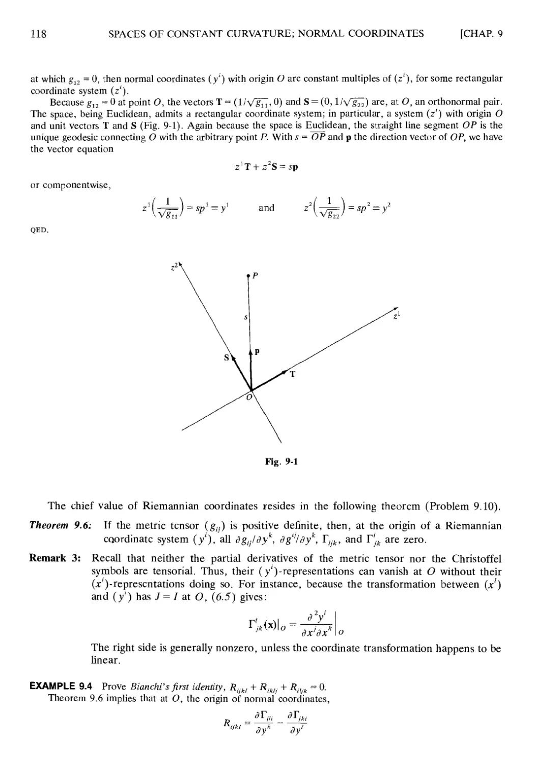
•
I ' I
Coverage of all course fundamentals
Effective problem-solving techniques
300 fully worked problems
with complete solutions
Supplements all standard
texts \* ч
\ ' ч
V Ν4
Use With these COUPSes: S'Tensors if Electromagnetic Theory \£ Theoretical Physics
Lif Aerodynamics j£ FluW* ,ЛШ#

SULU'M'S (Ч"ШХ1-1 OF
THEORY AND PROBLEMS
TENSOR
CALCULUS
UAVIU C> KAY, Ph.D.
Pmfi'sfi···- of Mathematirs
i'tiitrrviiy vf North Ctirnhnn tit AkAi'sm/A1
McGRAW-HILL
.Sn.ii ftrtiictfro \H\^hitigtany If.t.',. Auf.'kianti hogata Caraiias
Ijtmiioit Minimi M-e.xim ί'ίίν AMon Mttntrcal New Dehli
io.4 J milt Нтр.иръге Sydney Ttp'kya Toronto

DAVID C. KAY is currently Professor and Chairman of Mathematics at
the University of North Carolina at Asheville; formerly he taught in the
graduate program at the University of Oklahoma for 17 years. He
received his Ph.D. in geometry at Michigan State University in 1963. He
is the author of more than 30 articles in the areas of distance geometry,
convexity theory, and related functional analysis.
Schaum's Outline of Theory and Problems of
TENSOR CALCULUS
Copyright © 1988 by The McGraw-Hill Companies, Inc. All rights reserved. Printed in the
United States of America. Except as permitted under the Copyright Act of 1976, no part of this
publication may be reproduced or distributed in any form or by any means, or stored in a data base
or retrieval system, without the prior written permission of the publisher.
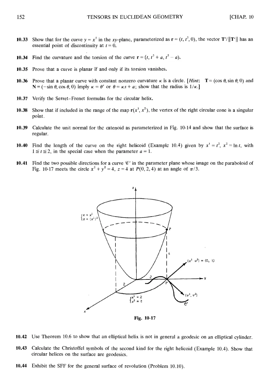
14 15 16 17 18 19 20 CUS CUS 09 08 07 06 05
ISBN D-D7-D33Mfi4-b
Sponsoring Editor, David Beckwith
Production Supervisor, Denise Puryear
Editing Supervisor, Marthe Grice
Library of Congress Cataloging-in-Publication Data
Kay, David С
Schaum's outline of theory and problems of tensor
calculus.
(Schaum's Outline series)
1. Calculus of tensors—Problems, exercises, etc.
I. Title. II. Title: Theory and problems of tensor
calculus.
QA433.K39 1988 515'.63 87-32515
ISBN 0-07-033484-6
McGraw-Hill
Л Division of The McGraw-Hill Companies

Preface
This Outline is designed for use by both undergraduates and graduates who
find they need to master the basic methods and concepts of tensors. The material
is written from both an elementary and applied point of view, in order to provide
a lucid introduction to the subject. The material is of fundamental importance to
theoretical physics (e.g., field and electromagnetic theory) and to certain areas of
engineering (e.g., aerodynamics and fluid mechanics). Whenever a change of
coordinates emerges as a satisfactory way to solve a problem, the subject of
tensors is an immediate requisite. Indeed, many techniques in partial differential
equations are tensor transformations in disguise. While physicists readily
recognize the importance and utility of tensors, many mathematicians do not. It is
hoped that the solved problems of this book will allow all readers to find out what
tensors have to offer them.
Since there are two avenues to tensors and since there is general disagreement
over which is the better approach for beginners, any author has a major decision
to make. After many hours in the classroom it is the author's opinion that the
tensor component approach (replete with subscripts and superscripts) is the
correct one to use for beginners, even though it may require some painful initial
adjustments. Although the more sophisticated, noncomponent approach is
necessary for modern applications of the subject, it is believed that a student will
appreciate and have an immensely deeper understanding of this sophisticated
approach to tensors after a mastery of the component approach. In fact,
noncomponent advocates frequently surrender to the introduction of components
after all; some proofs and important tensor results just do not lend themselves to
a completely component-free treatment. The Outline follows, then, the
traditional component approach, except in the closing Chapter 13, which sketches the
more modern treatment. Material that extends Chapter 13 to a readable
introduction to the geometry of manifolds may be obtained, at cost, by writing to the
author at: University of North Carolina at Asheville, One University Heights,
Asheville, NC 28804-3299.
The author has been strongly influenced over the years by the following major
sources of material on tensors and relativity:
J. Gerretsen, Lectures on Tensor Calculus and Differential Geometry, P.
Noordhoff: Goningen, 1962.
I. S. Sokolnikoff, Tensor Analysis and Its Applications, McGraw-Hill: New
York, 1950.
Synge and Schild, Tensor Calculus, Toronto Press: Toronto, 1949.
W. Pauli, Jr., Theory of Relativity, Pergamon: New York, 1958.
R. D. Sard, Relativistic Mechanics, W. A. Benjamin: New York, 1970.
Bishop and Goldberg, Tensor Analysis on Manifolds, Macmillan: New York,
1968.
Of course, the definitive work from the geometrical point of view is L. P.
Eisenhart, Riemannian Geometry, Princeton University Press: Princeton, N.J.,
1949.
The author would like to acknowledge significant help in ferreting out
typographical errors and other imperfections by the readers: Ronald D. Sand-

PREFACE
strom, Professor of Mathematics at Fort Hays State University, and John K.
Beem, Professor of Mathematics at the University of Missouri. Appreciation is
also extended to the editor, David Beckwith, for many helpful suggestions.
David С Kay

Contents
Chapter 1 THE EINSTEIN SUMMATION CONVENTION 1
1.1 Introduction 1
1.2 Repeated Indices in Sums 1
1.3 Double Sums 2
1.4 Substitutions 2
1.5 Kronecker Delta and Algebraic Manipulations 3
Chapter 2 BASIC LINEAR ALGEBRA FOR TENSORS 8
2.1 Introduction 8
2.2 Tensor Notation for Matrices, Vectors, and Determinants 8
2.3 Inverting a Matrix 10
2.4 Matrix Expressions for Linear Systems and Quadratic Forms 10
2.5 Linear Transformations 11
2.6 General Coordinate Transformations 12
2.7 The Chain Rule for Partial Derivatives 13
Chapter 3 GENERAL TENSORS 23
3.1 Coordinate Transformations 23
3.2 First-Order Tensors 26
3.3 Invariants 28
3.4 Higher-Order Tensors 29
3.5 The Stress Tensor 29
3.6 Cartesian Tensors 31
Chapter 4 TENSOR OPERATIONS: TESTS FOR TENSOR CHARACTER 43
4.1 Fundamental Operations 43
4.2 Tests for Tensor Character 45
4.3 Tensor Equations 45
Chapter 5 THE METRIC TENSOR 51
5.1 Introduction 51
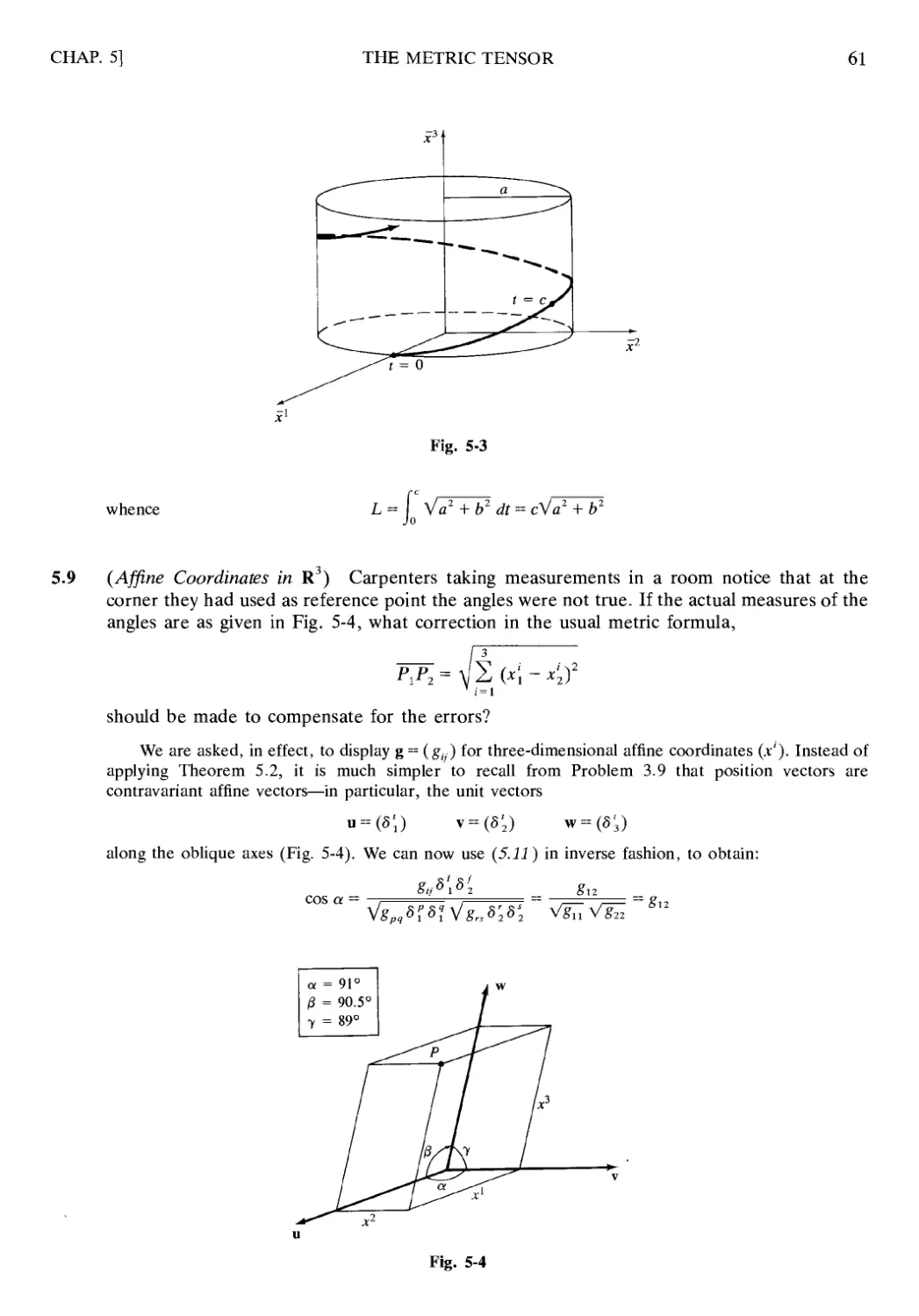
5.2 Arc Length in Euclidean Space 51
5.3 Generalized Metrics; The Metric Tensor 52
5.4 Conjugate Metric Tensor; Raising and Lowering Indices 55
5.5 Generalized Inner-Product Spaces 55
5.6 Concepts of Length and Angle 56

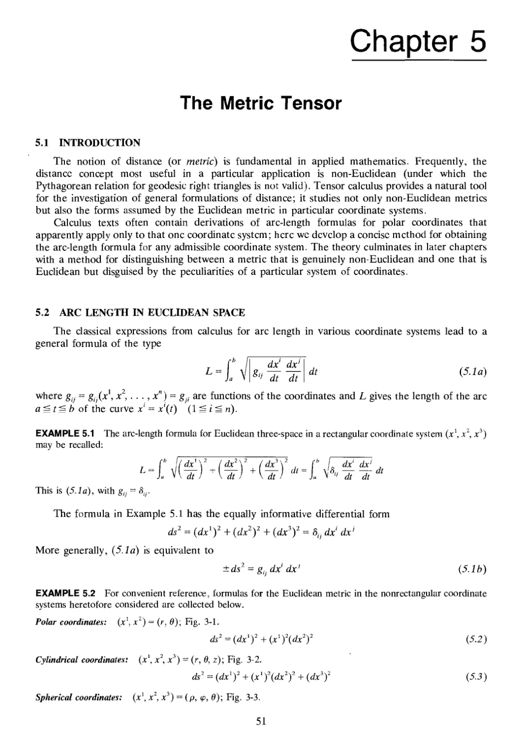
CONTENTS
Chapter 6 THE DERIVATIVE OF A TENSOR 68
6.1 Inadequacy of Ordinary Differentiation 68
6.2 Christoffel Symbols of the First Kind 68
6.3 Christoffel Symbols of the Second Kind 70
6.4 Covariant Differentiation 71
6.5 Absolute Differentiation along a Curve 72
6.6 Rules for Tensor Differentiation 74
Chapter 7 RIEMANNIAN GEOMETRY OF CURVES 83
7.1 Introduction 83
7.2 Length and Angle under an Indefinite Metric 83
7.3 Null Curves 84
7.4 Regular Curves: Unit Tangent Vector 85
7.5 Regular Curves: Unit Principal Normal and Curvature 86
7.6 Geodesies as Shortest Arcs 88
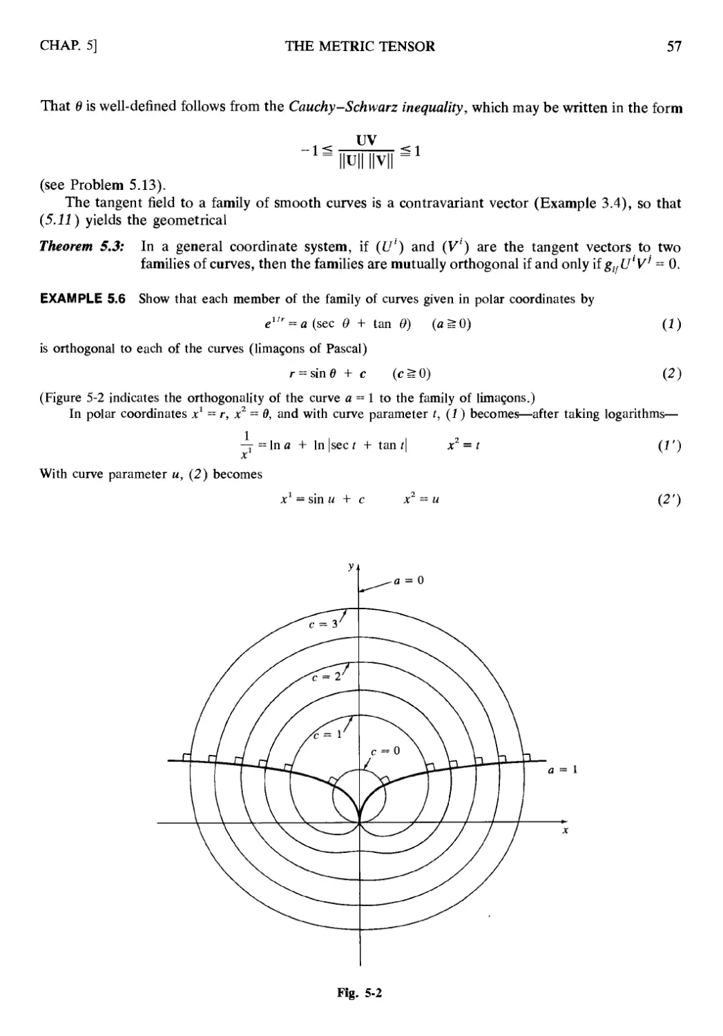
Chapter 8 RIEMANNIAN CURVATURE 101
8.1 The Riemann Tensor 101
8.2 Properties of the Riemann Tensor 101
8.3 Riemannian Curvature 103
8.4 The Ricci Tensor 105
Chapter 9 SPACES OF CONSTANT CURVATURE; NORMAL COORDINATES .... 114
9.1 Zero Curvature and the Euclidean Metric 114
9.2 Flat Riemannian Spaces 116
9.3 Normal Coordinates 117
9.4 Schur's Theorem 119
9.5 The Einstein Tensor 119
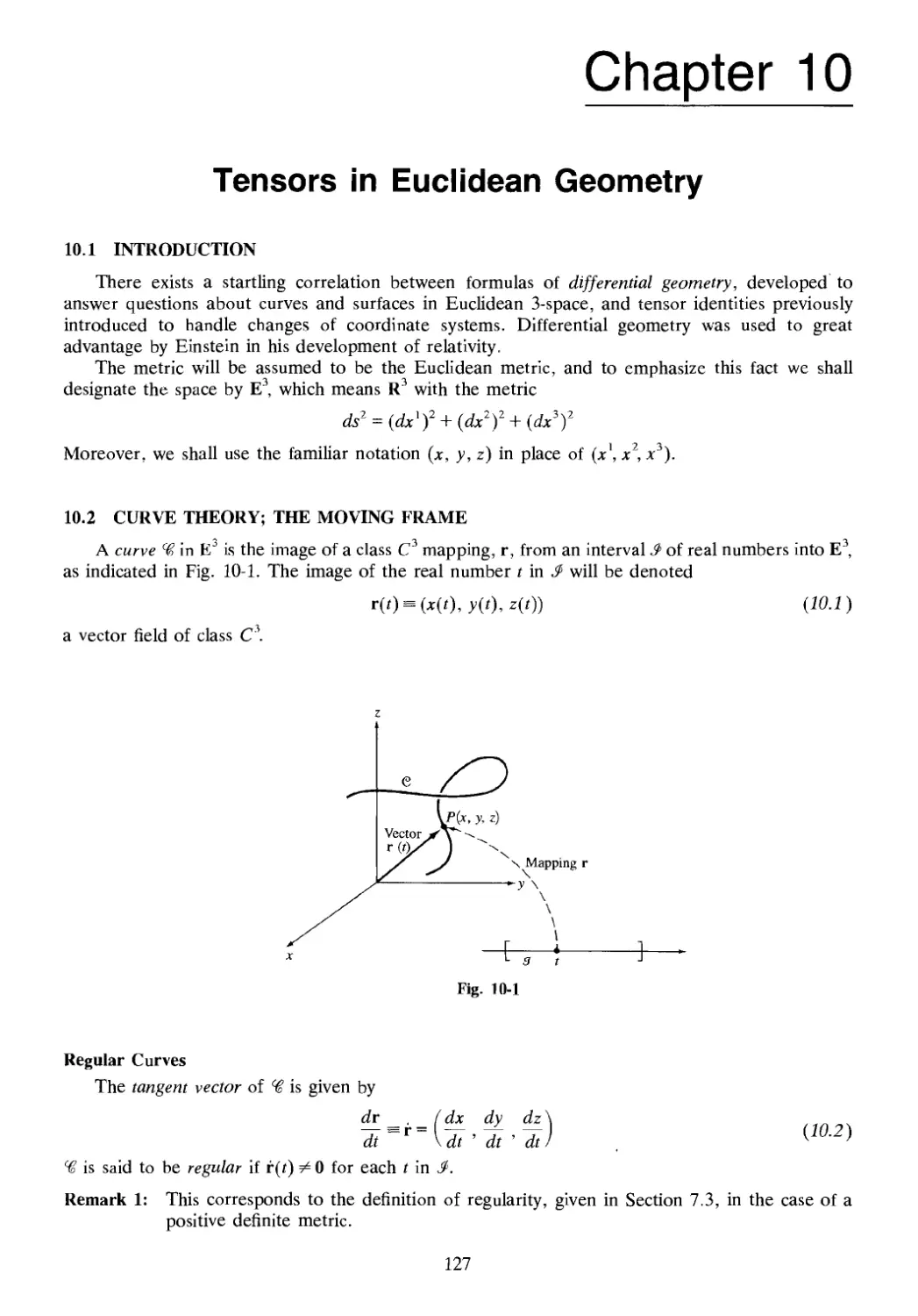
Chapter 10 TENSORS IN EUCLIDEAN GEOMETRY 127
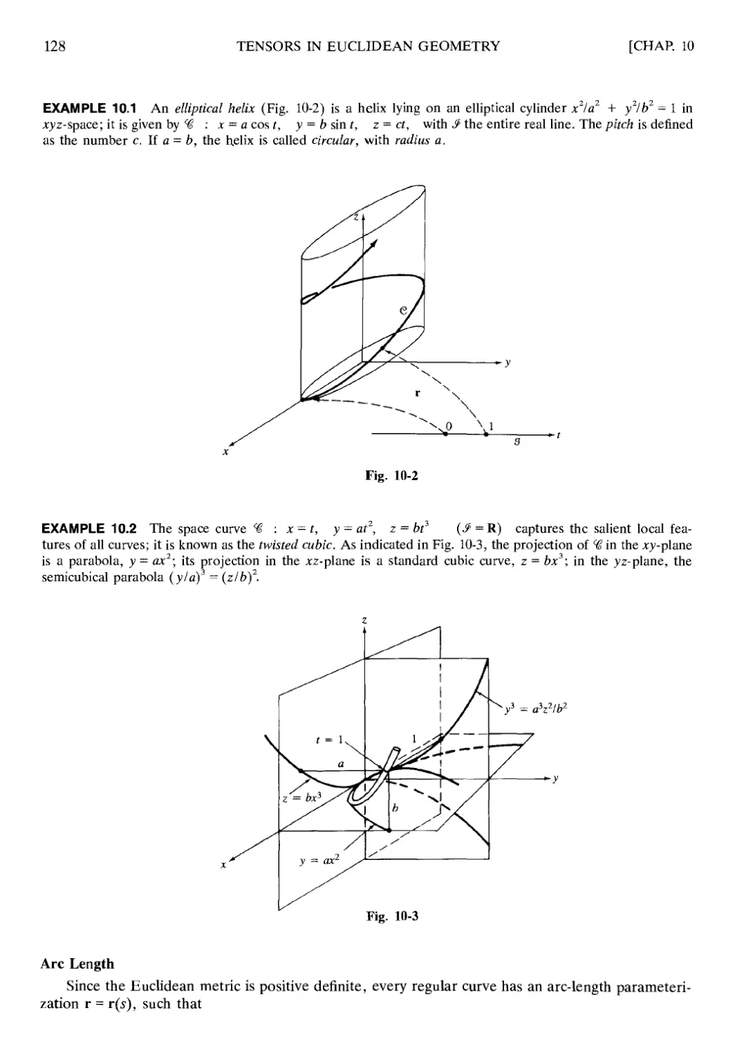
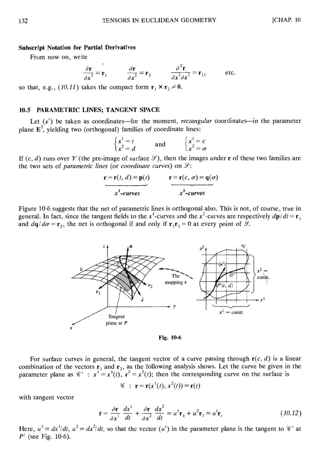
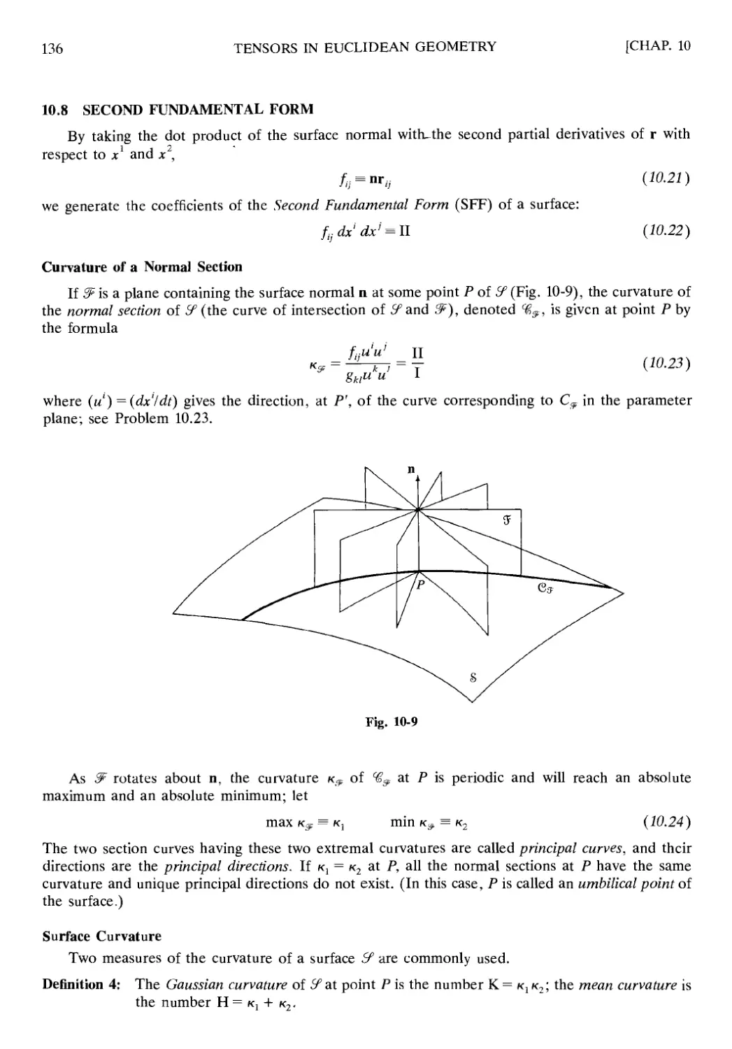
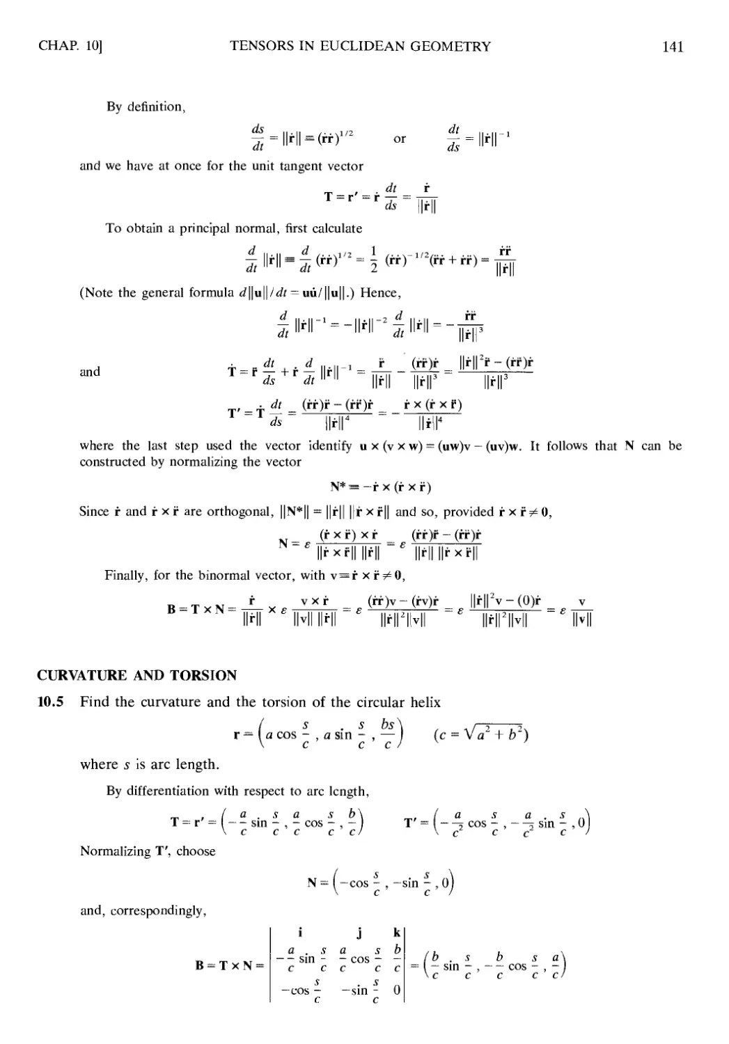
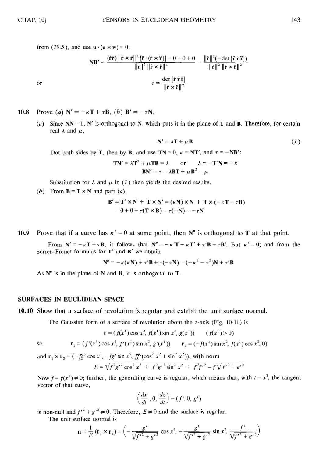
10.1 Introduction 127
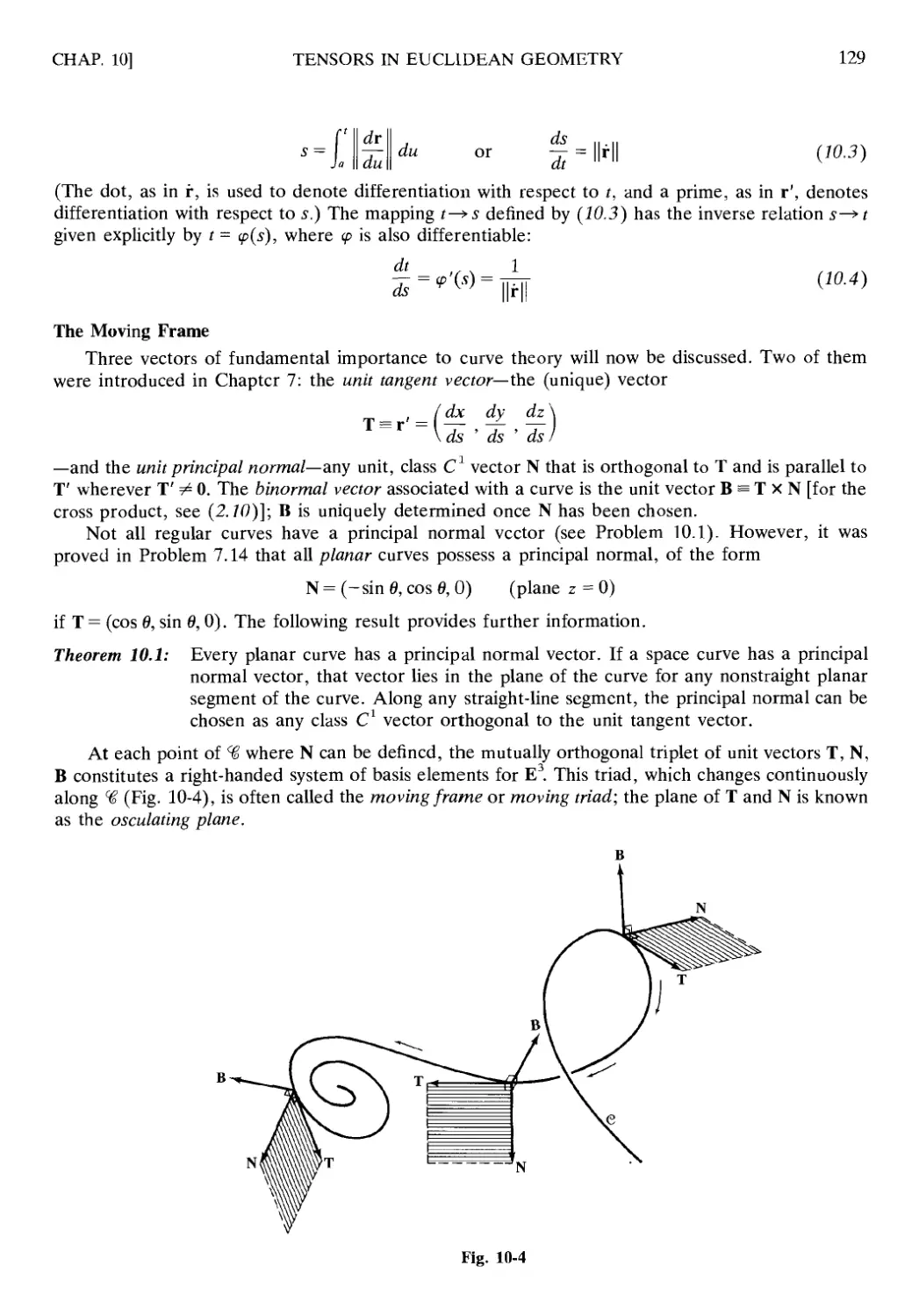
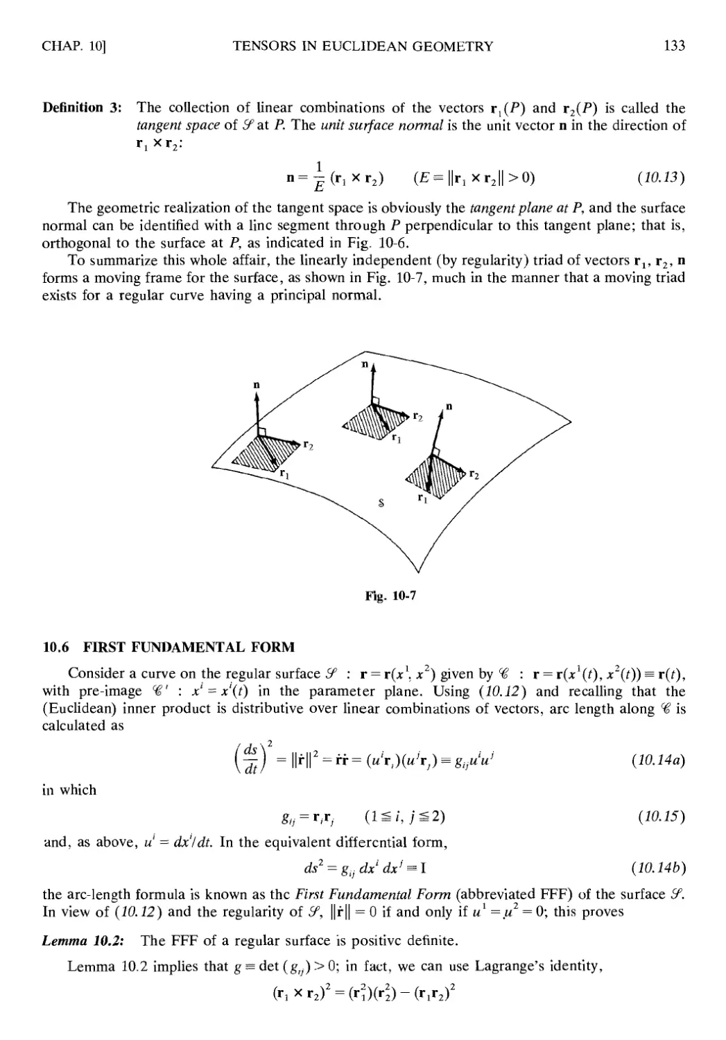
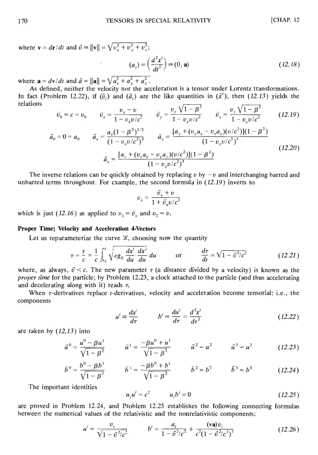
10.2 Curve Theory; The Moving Frame 127
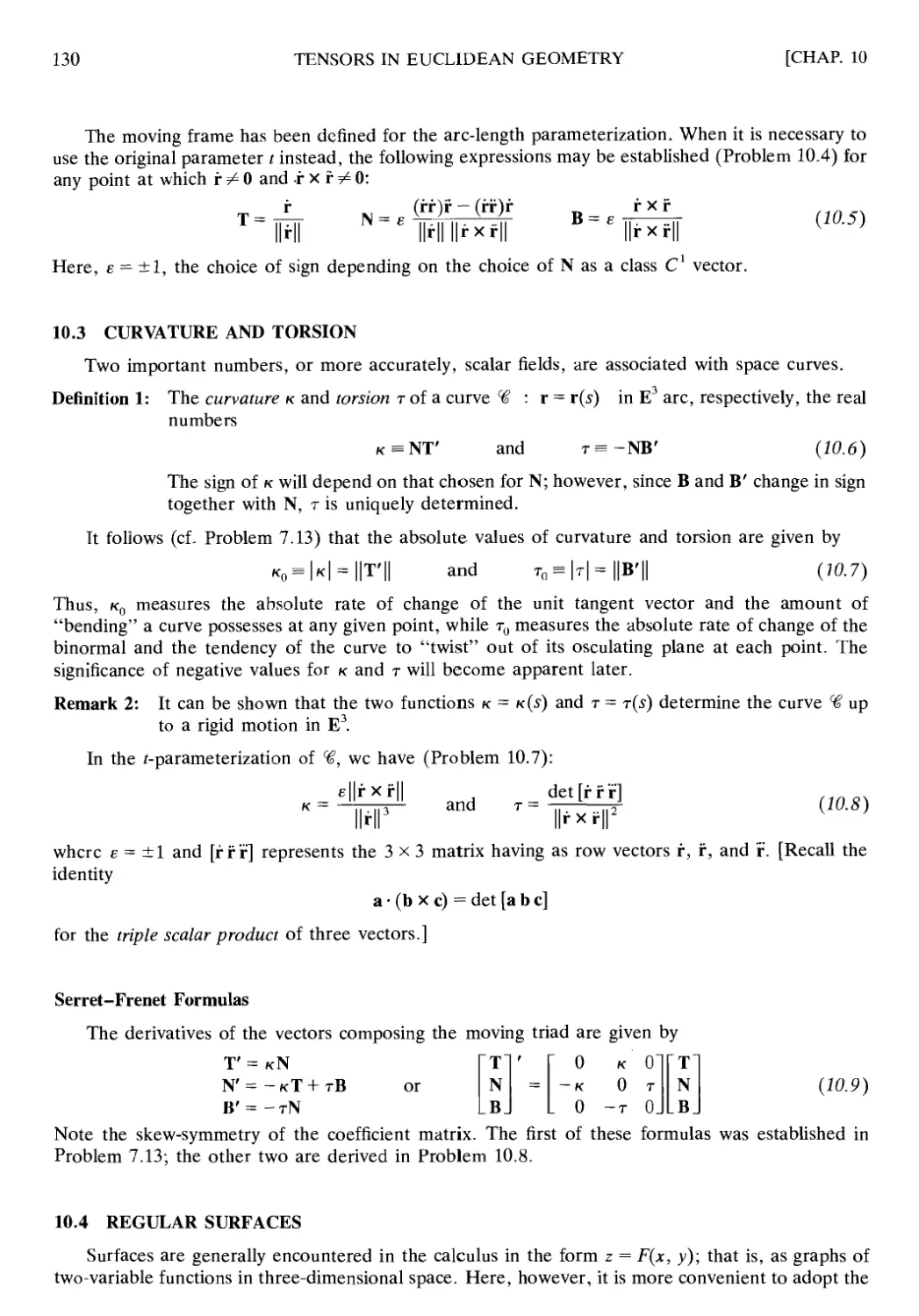
10.3 Curvature and Torsion 130
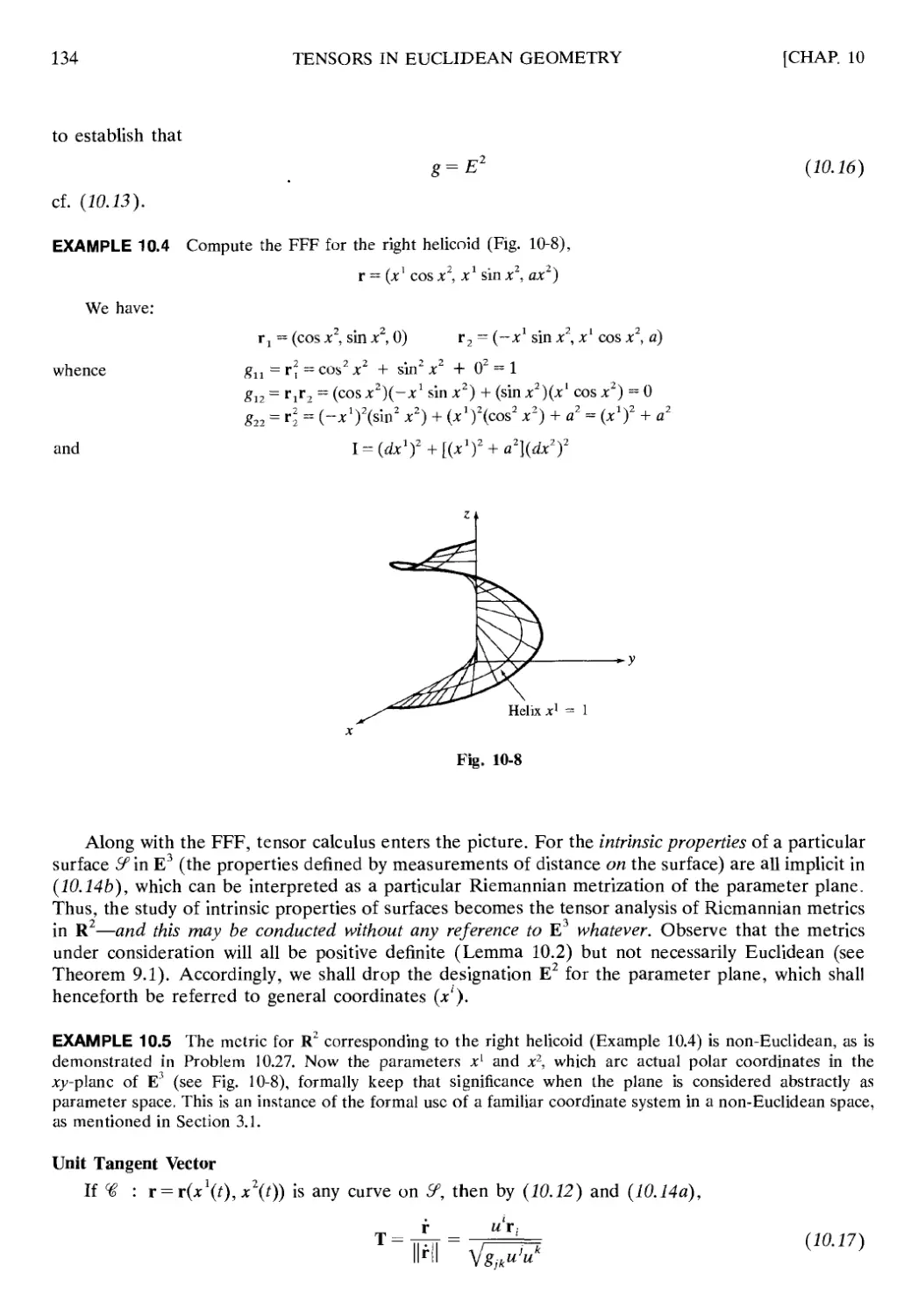
10.4 Regular Surfaces 130
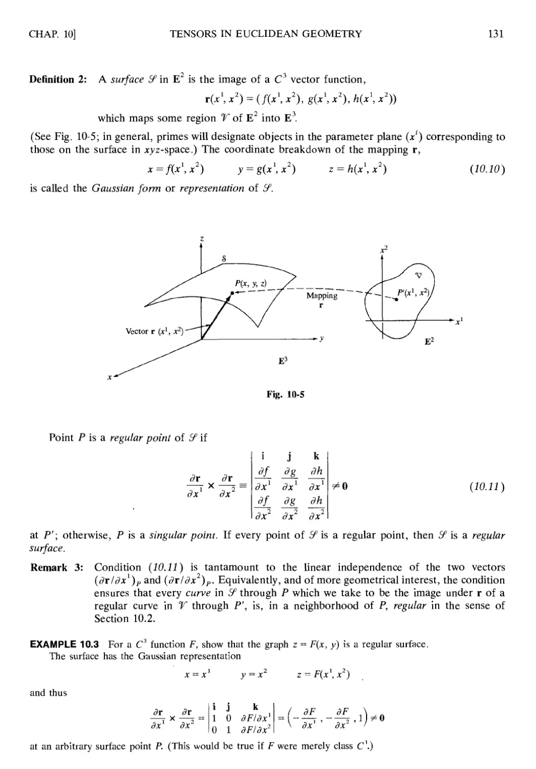
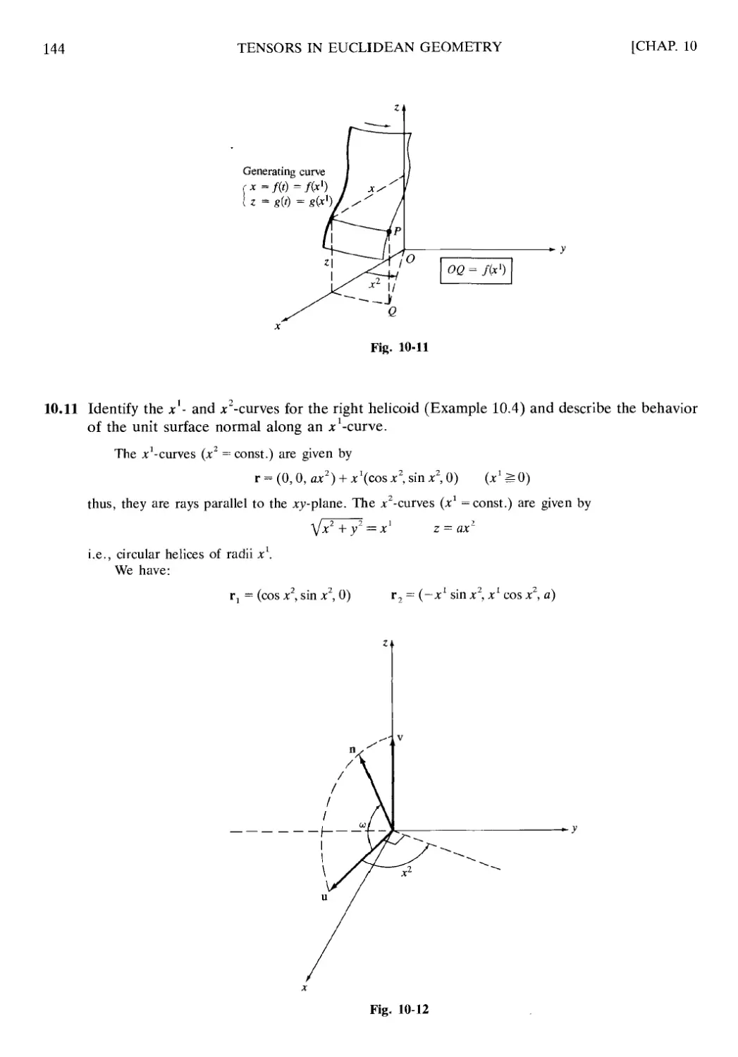
10.5 Parametric Lines; Tangent Space 132
10.6 First Fundamental Form 133
10.7 Geodesies on a Surface 135
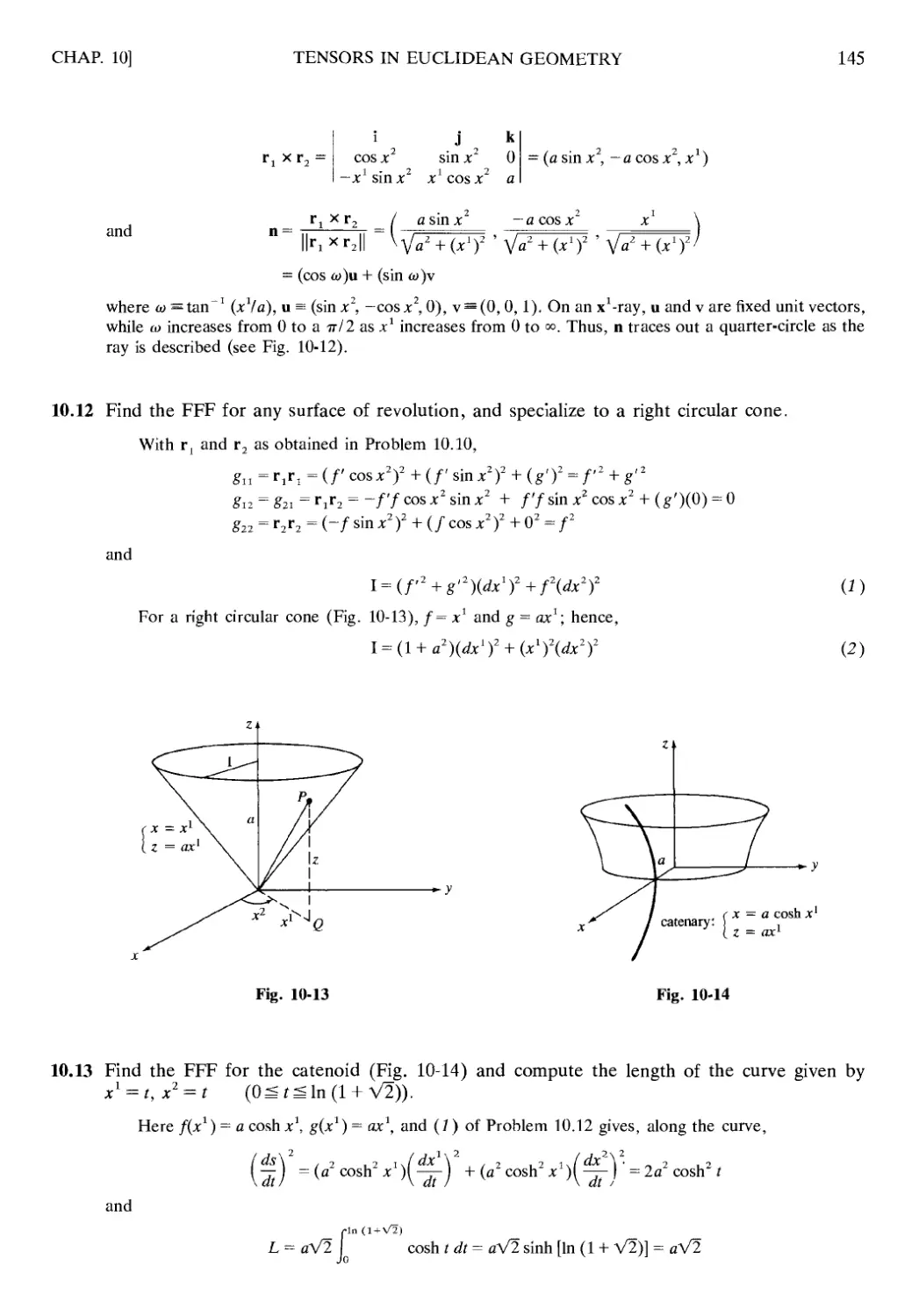
10.8 Second Fundamental Form 136
10.9 Structure Formulas for Surfaces 137
10.10 Isometries 138

CONTENTS
Chapter 11 TENSORS IN CLASSICAL MECHANICS 154
11.1 Introduction 154
11.2 Particle Kinematics in Rectangular Coordinates 154
11.3 Particle Kinematics in Curvilinear Coordinates 155
11.4 Newton's Second Law in Curvilinear Coordinates 156
11.5 Divergence, Laplacian, Curl 157
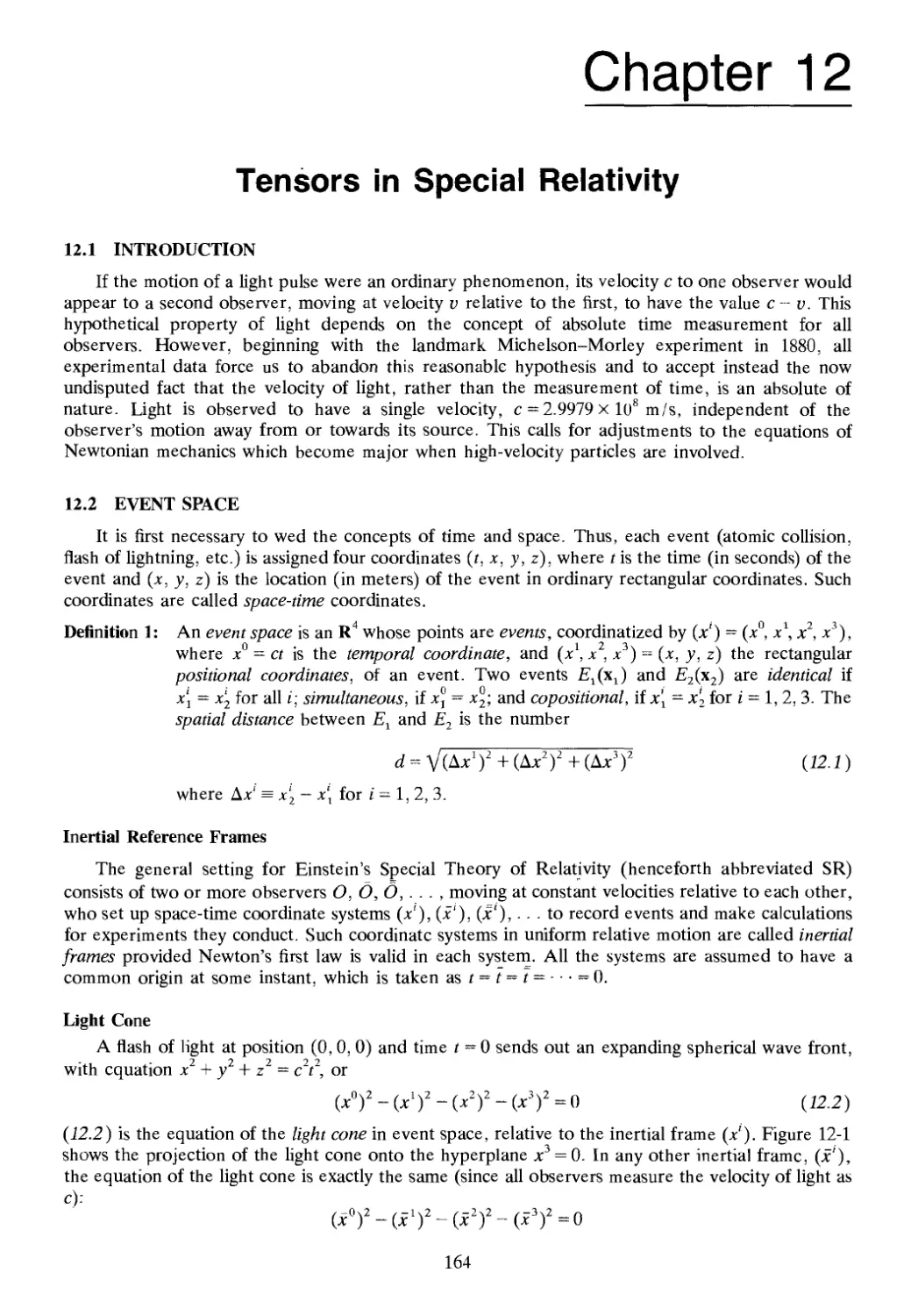
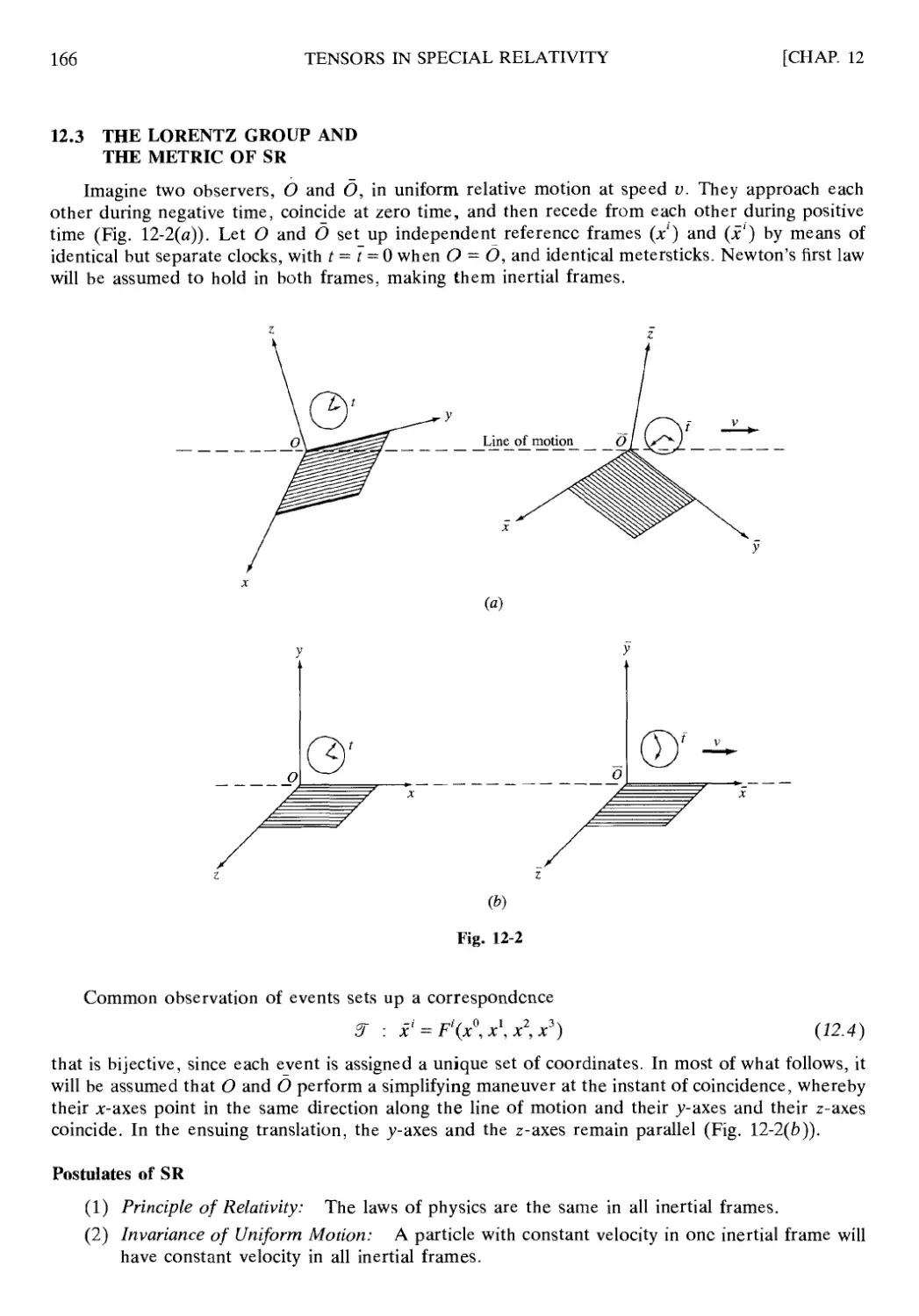
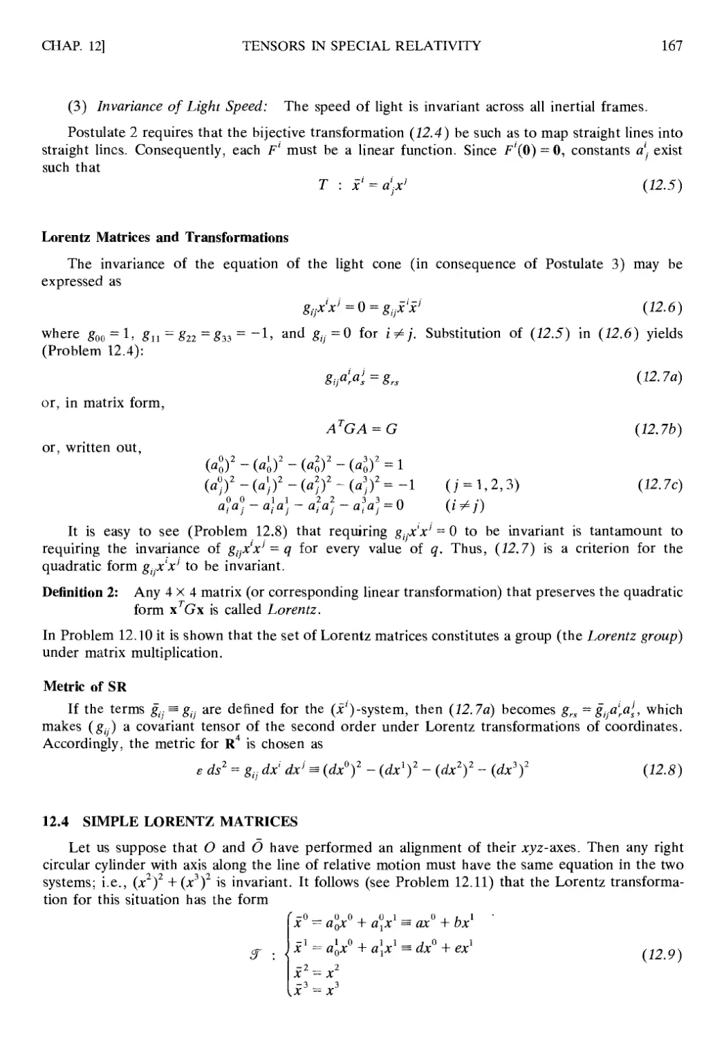
Chapter 12 TENSORS IN SPECIAL RELATIVITY 164
12.1 Introduction 164
12.2 Event Space 164
12.3 The Lorentz Group and the Metric of SR 166
12.4 Simple Lorentz Matrices 167
12.5 Physical Implications of the Simple Lorentz Transformation 169
12.6 Relativistic Kinematics 169
12.7 Relativistic Mass, Force, and Energy 171
12.8 Maxwell's Equations in SR 172
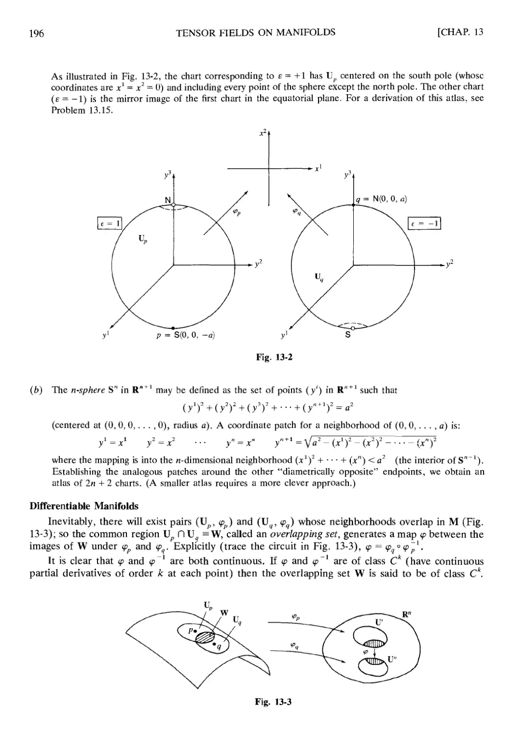
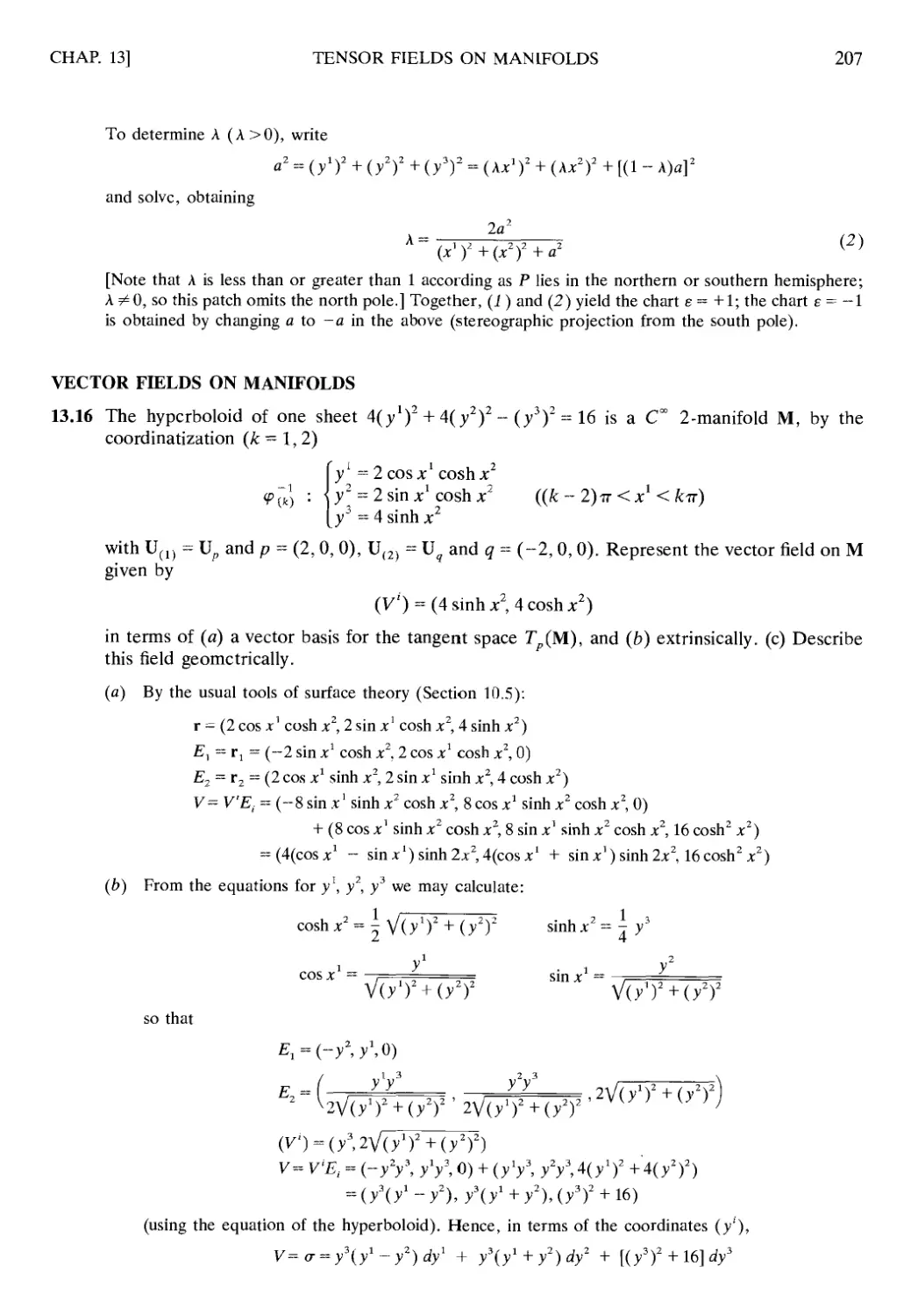
Chapter 13 TENSOR FIELDS ON MANIFOLDS 189
13.1 Introduction 189
13.2 Abstract Vector Spaces and the Group Concept 189
13.3 Important Concepts for Vector Spaces 190
13.4 The Algebraic Dual of a Vector Space 191
13.5 Tensors on Vector Spaces 193
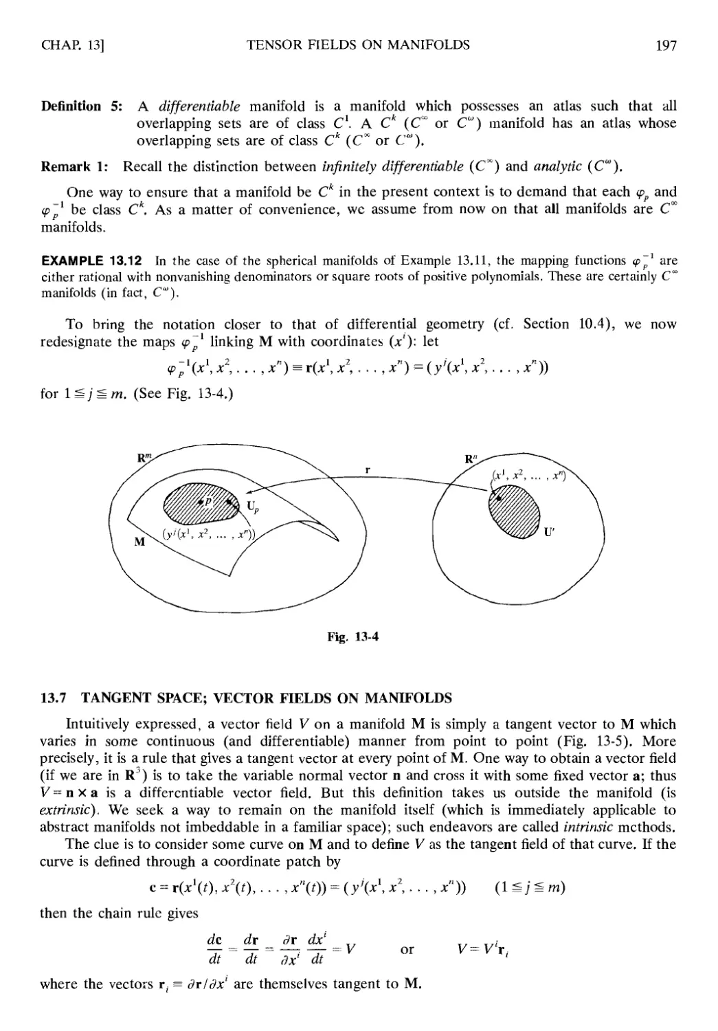
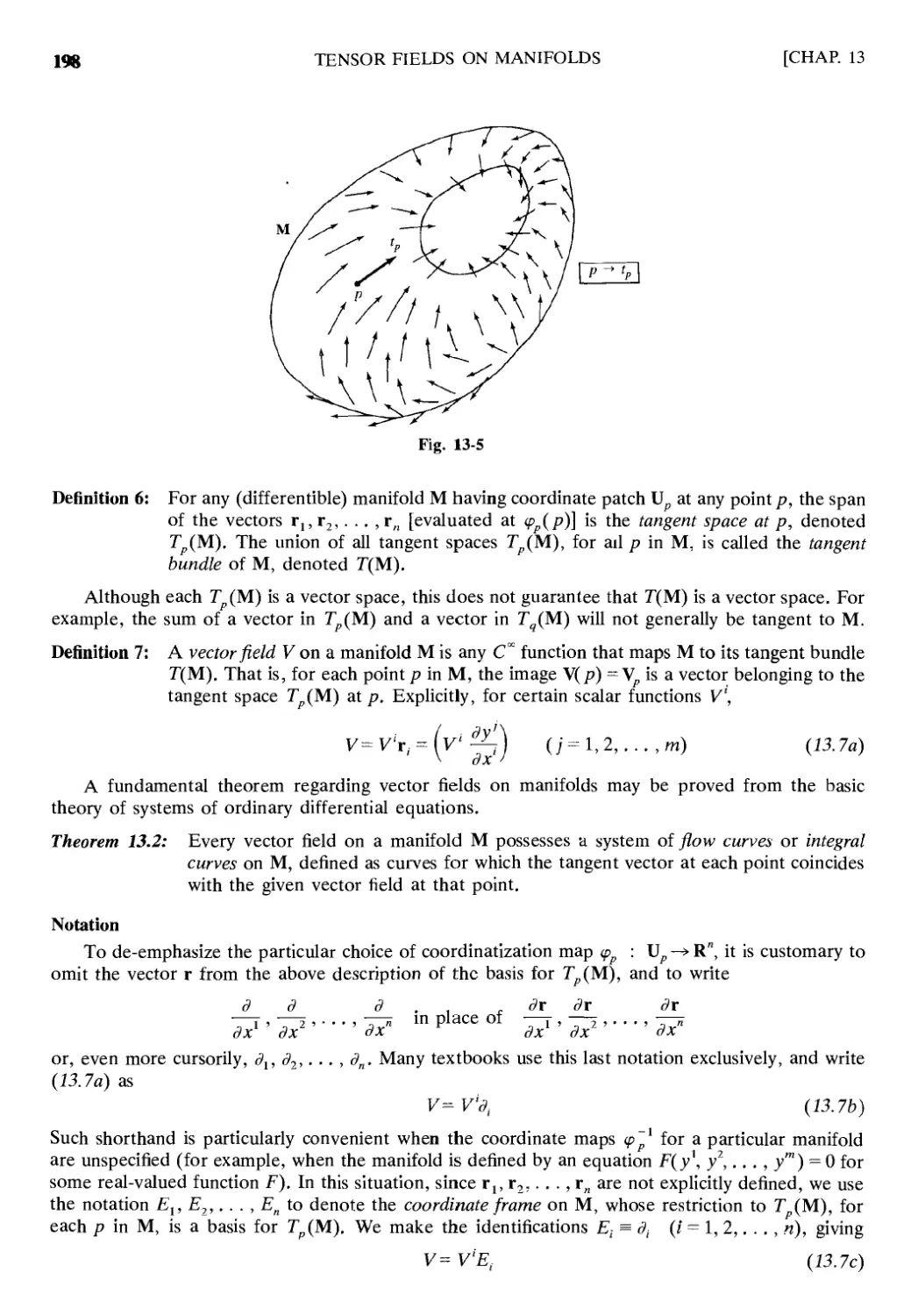
13.6 Theory of Manifolds 194
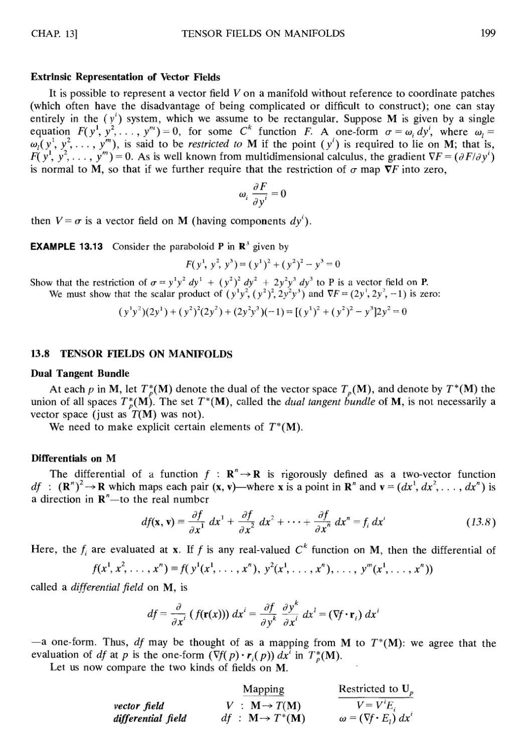
13.7 Tangent Space; Vector Fields on Manifolds 197
13.8 Tensor Fields on Manifolds 199
ANSWERS TO SUPPLEMENTARY PROBLEMS 213
INDEX 223

Chapter 1
The Einstein Summation Convention
1.1 INTRODUCTION
A study of tensor calculus requires a certain amount of background material that may seem
unimportant in itself, but without which one could not proceed very far. Included in that prerequisite
material is the topic of the present chapter, the summation convention. As the reader proceeds to
later chapters he or she will see that it is this convention which makes the results of tensor analysis
survey able.
1.2 REPEATED INDICES IN SUMS
A certain notation introduced by Einstein in his development of the Theory of Relativity
streamlines many common algebraic expressions. Instead of using the traditional sigma for sums, the
strategy is to allow the repeated subscript to become itself the designation for the summation. Thus,
η
axxx + a2x2 + агхъ + ■ ■ ■ + anxn = 2j aixi
/=1
becomes just а{х(, where l^ii/i is adopted as the universal range for summation.
EXAMPLE 1.1 The expression a(jxk does not indicate summation, but both aHxk and ai]xj do so over the
respective ranges l^iSn and 15; 5л. If«=4, then
avSk = βιΑ + a2iXk + a33xk + a44xk
aijXj = β,.,χ, + ai2x2 + 0.3*3 + fl,4*4
Free and Dummy Indices
In Example 1.1, the expression a^Xj involves two sorts of indices. The index of summation, j,
which ranges over the integers 1, 2, 3,. . . , n, cannot be preempted. But at the same time, it is clear
that the use of the particular character/ is inessential; e.g., the expressions airxr and alvxv represent
exactly the same sum as aijxi does. For this reason, j is called a dummy index. The index i, which
may take on any particular value 1,2, 3, . . . , η independently, is called a free index. Note that,
although we call the index i "free" in the expression a^*., that "freedom" is limited in the sense that
generally, unless i = k,
aljXj Φ akixs
EXAMPLE 1.2 If η = 3, write down explicitly the equations represented by the expression yi = airxr.
Holding i fixed and summing over r = 1,2,3 yields
У ι = anx, + ai2x2 + ai3x3
Next, setting the free index ί =1,2,3 leads to three separate equations:
y, = a11x1 + a12x2 + a13x3
y3 = a31x, + a32x2 + a33x,
Einstein Summation Convention
Any expression involving a twice-repeated index (occurring twice as a subscript, twice as a
superscript, or once as a subscript and once as a superscript) shall automatically stand for its sum
1

2
THE EINSTEIN SUMMATION CONVENTION
[CHAP. 1
over the values 1,2,3, . . . , η of the repeated index. Unless explicitly stated otherwise, the single
exception to this rule is the character n, which represents the range of all summations.
Remark 1: Any free index in an expression shall have the same range as summation indices, unless
stated otherwise.
Remark 2: No index may occur more than twice in any given expression.
EXAMPLE 1.3 (a) According to Remark 2, an expression like aiixi is without meaning, (b) The meaningless
expression a'jxtxl might be presumed to represent a^x^f, which is meaningful, (c) An expression of the form
al(xl + yt) is considered well-defined, for it is obtained by composition of the meaningful expressions aizi and
xi + y. = zr In other words, the index i is regarded as occuring once in the term {xi + y.).
1.3 DOUBLE SUMS
An expression can involve more than one summation index. For example, агхьу, indicates a
summation taking place on both i and j simultaneously. If an expression has two summation
(dummy) indices, there will be a total of n2 terms in the sum; if there are three indices, there will be
η terms; and so on. The expansion of aijxiyj can be arrived at logically by first summing over i, then
over j:
аахгУ) = «i^iJ/ + ЧргУ) + <*3]х3У] + ■■■ + ап!.хпУ] [summed over i]
= (я11#1)'1 + al2xly2 + ■ ■ ■ + allJx1yIJ) [summed over j]
+ (a2lx2yl + a22x2y2 + ■■■ + a2nx2yn)
+ О3ЛУ1 + a32x3y2 + ■■■ + a3nx3yn)
+ 0„Λ>Ί + ап2хпУ2 + ■■■ + аппхпуп)
The result is the same if one sums over j first, and then over /.
EXAMPLE 1.4 If η = 2, the expression yt = c'iarsxs stands for the two equations:
yl — c1a11x1 + c1a21x1 + c1a12x2 + c1a22x2
_ ! ι 2 ι ! ι 2
1.4 SUBSTITUTIONS
Suppose it is required to substitute yt = ai]xj in the equation Q = b^y^Xj. Disregard of Remark 2
above would lead to an absurd expression like Q = b^a^xjx-. The correct procedure is first to identify
any dummy indices in the expression to be substituted that coincide with indices occurring in the
main expression. Changing these dummy indices to characters not found in the main expression, one
may then carry out the substitution in the usual fashion.
step 1 <2 = bjjy^j, yt = a(jXj [dummy index j is duplicated]
step 2 yi = airxr [change dummy index from j to r]
step 3 <2 = b^a^x^Xj = airbijxrxJ [substitute and rearrange]
EXAMPLE 1.5 If y. = a^Xj, express the quadratic form Q = g^y^j in terms of the x-variables.
First write: y. = airxt, yf = ajsxs. Then, by substitution,
Q = 8iMirxr)(aisxs) = g,jairajsxrxs
or Q = hrsxrxs, where hrs = gnairajs.

CHAP. 1]
THE EINSTEIN SUMMATION CONVENTION
3
1.5 KRONECKER DELTA AND ALGEBRAIC MANIPULATIONS
A much used symbol in tensor calculus has the effect of annihilating the "off-diagonal" terms in
a double summation.
*<,■=*>-«Hi Wj (^)
Kronecker Delta
Clearly, δ;/ = δ,,, for all ι, j.
EXAMPLE 1.6 Ifn = 3,
δ/jXiXj = lx1X1 + Qx,X2 + 0XjX3 + Qx2xl + \х2хг + Qx2x3 + Qx3xl + 0x3JC2 + \хъХъ
= (x1)2 + (x2f + (x,)2 = xixi
In general, 8lpclxj = xixi and 8r/atrxl = atjxt.
EXAMPLE 1.7 Suppose that V = g'rarsys and yt = birxr. If further, airbrj = d:j, find V in terms of the xr.
First write ys - bs,x,. Then, by substitution,
T = SrarsbsiXi = g'AS, = g'rXr
Algebra and the Summation Convention
Certain routine manipulations in tensor calculus can be easily justified by properties of ordinary
sums. However, some care is warranted. For instance, the identity (1.2) below not only involves the
distributive law for real numbers, a(x + y) = ax + ay, but also requires a rearrangement of terms
utilizing the associative and commutative laws. At least a mental verification of such operations must
be made, if false results are to be avoided.
EXAMPLE 1.8 The following nonidentities should be carefully noted:
Я/А+У/^я^ + Я-Л-
(ail + aji)xiyj^2aijx,yj
Listed below are several valid identities; they, and others like them, will be used repeatedly from
now on.
aiMs + У,) = aijXj + aiiyi (1.2)
aijxiy]^aiiyixi (1.3)
ai.xix] = ajixixj (1.4)
(ai, + ап)х,х} = 2aijXiXj (1.5)
(«v-«,,>/*, =0 (1.6)

4
THE EINSTEIN SUMMATION CONVENTION
[CHAP. 1
Solved Problems
REPEATED INDICES
1.1 Use the summation convention to write the following, and assign the value of η in each case:
(a) allbll + a2lbl2 + a3lbl3 + a4lbl4
(b) anbn + al2b12 + a13b13 + aubu + alsbls + al6bl6
(c) c'n+ 4 + 4 + 4 + 4 + 4 + 4 + 4 (1 =£*=£ 8)
(β) β,A, (n = 4);(b)aublt (n = 6); (с) с), (и = 8).
1.2 Use the summation convention to write each of the following systems, state which indices are
free and which are dummy indices, and fix the value of n:
(a) cllx1 + c12x2 + c13x3 = 2 (b) ajxl + a2x2 + α^χ3 + α*χ4 = bj
21 1 22 2 Ί."\ "\ \/ J /
311 42 2 314
(a) Set d, =2, ίί2 = -3, and d3 = 5. Then one can write the system as ctjx; = d; (n = 3). The free
index is i and the dummy index is /.
(b) Here, the range of the free index does not match that of the dummy index (и = 4), and this fact
must be indicated:
a% = b, (J = 1,2)
The free index is / and the dummy index is i.
1.3 Write out explicitly the summations
Φι + У ι) cixi + скУк
where η = 4 for both, and compare the results.
с,(х, + У,) = ^(*! + У г) + с2(х2 + у2) + с3(х3 + Уз) + с4(*4 + У а)
= СЛ + С1У1 + С2*2 + С2У2 + С3*3 + СзУз + С4*4 + С аУ А
СЛ + С*У* = С1*1 + С2*2 + С3*3 + С4*4 + С1У1 + С2>Ί +/ъУъ + С аУ А
The two summations are identical except for the order in which the terms occur, constituting a special
case of (1.2).
DOUBLE SUMS
1.4 If η = 3, expand Q = ά'χμ,^.
Q = a^XjXy + α2'χ2χ} + a3/x3^
= α χγχγ + α XjX2 + a ~xlx3 + α x2xl + a x2x2 + a x2x3 + a" x3Xj + a" x3x2 + α33χ3χ3
1.5 Use the summation convention to write the following, and state the value of η necessary in
each case:
(θ) at Al + Я2А2 + йзАз + u12^21 + a22^22 + u32^23 + u13^31 + ^23^32 + u33^33
? Ψ) ' g\t + 'g\2 + Ϋ2ι +'gL +'gj, +fc?2 +^221 + '*22

CHAP. 1]
THE EINSTEIN SUMMATION CONVENTION
5
(fl) β,Α,-+ ei2fr2i + fli3fr3i = «Λ« (" = 3)-
(b) Set c, =1 for each i (n = 2). Then the expression may be written
g'llCi + g'l2Ci + #21С/ + S'll^i = (g'n + g'l2 + #21 + g^)^
= (8'jkcic,c)ci=S'ikcicjck
1.6 If и = 2, write out explicitly the triple summation crstxrysz.
Any expansion technique that yields all 23 = 8 terms will do. In this case we shall interpret the
triplet rst as a three-digit integer, and list the terms in increasing order of that integer:
crstxrysz' = с111д:1)'121 + c112x1y1z2 + c121x1y2z1 + cl22x1y2z2
+ c2^x2yxzl + c212x2y1z2 + c-,2lx2y2z'i + c222x2y2z2
1.7 Show that ailxixj = 0 if ац = i - /.
Because, for all ι and j, αί; = —ajt and ж,.*. = хрс,, the "off-diagonal" terms а^х{х} (i <j; no sum)
and tijfXjXi (/>«"; no sum) cancel in pairs, while the "diagonal" terms α,,(χ,)2 are zero to begin with.
Thus the sum is zero.
The result also follows at once from (1.5).
1.8 If the ai; are constants, calculate the partial derivative
3 ( \
JxTk (W,}
Reverting to Σ-notation, we have:
Σ at1xixj = Σ a^xpcj + Σ α,,*,*, + Σ aijxix) + Σ aipcixi
i,j i*k I-k i^k i=k
)*k f^k j = k j=k
= C + (Σ akjx.)xk + [Σ aikXl)xk + akk(xk)2
'j^k ' i^k '
where С is independent of xk. Differentiating with respect to xk,
τ— (Σβ,Λ-^)=0 + Σ akiXj + Σ aikx, + 2akkxk
"лк vi,j ' j¥-k l^k
= Σα„χ, + Σο,Λ-
f ί
or, going back to the Einstein summation convention,
— (ait.xiXj) = ahixt + aikx, = (aik + aki)Xi
SUBSTITUTIONS, KRONECKER DELTA
1.9 Express tf'yjj in terms of x-variables, if у ι — cijxj and b''cik = 8[.
tfy.y. = b'\cirxr)(cjsxs) = (bi]cir)xrcjsxs = 3irx,.cjsxs = *,с,.Л = cijxixl
1.10 Rework Problem 1.8 by use of the product rule for differentiation and the fact that
dxp
~ϊχΖ~8™

6
THE EINSTEIN SUMMATION CONVENTION
[CHAP. 1
= a>j(Xj3ik + x.8jk) = akjXj + aikx,
1.11 If fly = Oji are constants, calculate
(PijXiXj)
dxkdxt
Using Problem 1.8, we have
Э2
dxkdxt
(W/) = ^ [^ (W,)] = ~tk IN + *,>,]
<9*
(2α,Λ.) = 2e/V — (*,.) = 2β,7δΑι. = 2aw
1.12 Consider a system of linear equations of the form у = a''xj and suppose that (btj) is a matrix
of numbers such that for all i and j, bird' = δ ■ [that is, the matrix (ft;.) is the inverse of the
matrix (a1')]. Solve the system for xt in terms of the y'.
Multiply both sides of the /th equation by bki and sum over i:
bkiy' = bkia'ixJ = 8Jkx] = xk
отх, = Ъуу\
1.13 Show that, generally, aijk(xl + y})zk Φ а1]кхьгк + aijkyfzk.
Simply observe that on the left side there are no free indices, but on the right, ;" is free for the first
term and i is free for the second.
1.14 Show that cf/(*,. + y^Zj = cVjxiz] + cijyiz].
Let us prove (1.2); the desired identity will then follow upon setting atj = cJt.
aaxi + аиУ; = Σ aijXj + Σ ацУ} = Σ (a^Xj + а1]У])
i i i
= Еву(^-+)'7)=в,у(-Ку + Уу)
Supplementary Problems
1.15 Write out the expression aibl (n =6) in full.
1.16 Write out the expression R'jki (n = 4) in full. Which are free and which are dummy indices? How many
summations are there?
1.17 Evaluate 3'jxl (n arbitrary).
1.18 For η arbitrary, evaluate (α) δ„, (b) δ δϋ, (с) 8i}8[clk.

CHAP. 1]
THE EINSTEIN SUMMATION CONVENTION
7
1.19 Use the summation convention to indicate a13b13 + a23b23 + a33b3i, and state the value of n.
1.20 Use the summation convention to indicate
αιι(ΛΓι )Z + а\2х\хг + а\ъх\хг + а21х2хг + a22{x2)2 + a23x2x3 + а31хъхг + a32x3x2 + a33(x3)2
1.21 Use the summation convention and free subscripts to indicate the following linear system, stating the
value of n:
У \ C\\X\ C\2X2
y2 C21X1 ' C22-^2
1.22 Find the following partial derivative if the a:j are constants:
_d_
dX
— (anx1 + al2x2 + a13x3) (A: =1,2,3)
к
1.23 Use the Kronecker delta to calculate the partial derivative if the atj are constants:
д ι ^
1.24 Calculate
~ [а„х,(х,У
where the atj are constants such that ац = ajt.
1.25 Calculate
д
д (Vi¥*)
where the a... are constants.
1.26 Solve Problem 1.11 without the symmetry condition on air
1.27 Evaluate: (а) Ъ)у, if yt = T?, (b) a^y,. if y, = b;jXj, (c) aijkyiyjyk if y, = bijXj.
1.28 If ε, = 1 for all i, prove that
(a) (flj + e2 + - ■ ■ + α„)2 s EiElalaj
(b) e,.(l + χ J = aiei + afx(
(c) aiJ(xi +xj)^2aijEjxl if ац = aj;

Chapter 2
Basic Linear Algebra for Tensors
2.1 INTRODUCTION
Familiarity with the topics in this chapter will result in a much greater appreciation for the
geometric aspects of tensor calculus. The main purpose is to reformulate the expressions of linear
algebra and matrix theory using the summation convention.
2.2 TENSOR NOTATION FOR MATRICES, VECTORS, AND DETERMINANTS
In the ordinary matrix notation (a,v), the first subscript, i, tells what row the number ar lies in,
and the second, /, designates the column. A fuller notation is [a,]mn, which exhibits the number of
rows, m, and the number of columns, n. This notation may be extended as follows.
Upper-Index Matrix Notation
KL»:
<
2
«1
«2
2
«2
a3 .
2
a3 .
.a
.a,
[a"
'Ί =
'a11
a11
ml
a
12
a
22
a
ν»2
a
13
a .
23
a .
am\
„1" "
. a
„2b
. a
inn
. a
Note that, for mixed indices (one upper, one lower), it is the upper index that designates the row,
and the lower index, the column. In the case of pure superscripts, the scheme is identical to the
familiar one for subscripts.
EXAMPLE 2.1
\P%
c1 c1 c1
Lj (,2 L3
2 2 2
С С С
с, с2 с3
KJ23 =
άλ d2 d3
dx d2 d3
= [d'jL·
[χΓΑκ = [χ\ χ1ι χ1 *']
[у"4]
у"
у21
у31
Ь41
у12]
у22
f2
42
У .
Vectors
A real «-dimensional vector is any column matrix v= [х^]п1 with real components xt =*n; one
usually writes simply v = (xt). The collection of all real и-dimensional vectors is the n-dimensional
real vector space denoted R".
Vector sums are determined by coordinatewise addition, as are matrix sums: if A = [fliy]m„ and
ДИМ™, then
A + B = [ai; + b ,,]„,„
Scalar multiplication of a vector or matrix is defined by
Basic Formulas
The essential formulas involving matrices, vectors, and determinants are now given in terms of
the summation convention.

CHAP. 2]
BASIC LINEAR ALGEBRA FOR TENSORS
9
Matrix multiplication. If A = [ai}]mn and В = [Ьи]пк, then
AB = [airbr}]mk (2.1а)
Analogously, for mixed or upper indices,
ЛВ = [а)]тп[Ь)]пк = K^,]mfc ЛЯ - Ит(ГЬ'']вк = [a%ri]mk (2.1b)
wherein i and j are not summed on.
Identity matrix. In terms of the Kronecker deltas, the identity matrix of order η is
which has the property IA = AI = A for any square matrix A of order и.
Inverse of a square matrix. A square matrix A = [α^]„„ is invertible if there exists a (unique) matrix
В = [bij\nn, called the inverse of A, such that Л5 = В A = I. In terms of components, the criterion
reads:
airbrj = biA, = δν (2.2a)
or, for mixed or upper indices,
а% = Ъ\аТгЬ\ a'rbrj = b'rari = 8ij (2.2b)
Transpose of a matrix. Transposition of an arbitrary matrix is defined by Ат =[а^]'тп = [а'и]пт,
where a'u = ap for all i, j. If AT = A (that is, ац = α;/ for all i, j), then Л is called symmetric; if
Л = —Л (that is, аг. = — fly-,- for all г, /), then Л is called antisymmetric or skew-symmetric.
Orthogonal matrix. A matrix Л is orthogonal if ЛГ = Л_l (or if ATA = AAT — I).
Permutation symbol. The symbol eljk_ _w (with η subscripts) has the value zero if any pair of
subscripts are identical, and equals (-\)p otherwise, where ρ is the number of subscript
transpositions (interchanges of consecutive subscripts) required to bring (ijk. . . w) to the natural order
(123. . .n).
Determinant of a square matrix. If Л = [fliy]„„ is any square matrix, define the scalar
det Л = e, ι ι , au a,, a3, ■ · · ani (2.3)
Ί'2'З ■ ■ ■ 'n "1 £!2 J,3 nln v '
Other notations are |Л|, \ai}\, and det(a;y). The chief properties of determinants are
|ЛВ| = |Л||5| |ЛГ| = |Л| (2.4)
Laplace expansion of a determinant. For each i and j, let Ml} be the determinant of the square matrix
of order η — 1 obtained from Л = [аи]пп by deleting the ith row and y'th column; Mtj is called the
minor of α · in |Л|. Define the cofactor of atj to be the scalar
Аи = (-1)кМ„ where k = i+j (2.5)
Then the Laplace expansions of \A\ are given by
\Α\ = αυΑν = ανΑν = --· = αη]Αηί [row expansions]
\A\ = anAn = af2Ai2 = · ■ · = ainAjn [column expansions]
Scalar product of vectors. If u = (χέ) and ν = (_y,.), then
uv = u · ν = urv = xjyi (2.7)
If u = v, the notation uu = u" = v" will often be used. Vectors u and ν are orthogonal if uv = 0.
Norm (length) of a vector. If u= (x{), then
||u||=Vu5 = V3cpc: (2.8)

10
BASIC LINEAR ALGEBRA FOR TENSORS
[CHAP. 2
Angle between two vectors. The angle θ between two nonzero vectors, u = (x() and ν = (y,), is
defined by
uv xji
cos θ :
(OS 0^77")
НИ νχ-χ,νηη
It follows that 0 = it/2 if u and ν are nonzero orthogonal vectors.
Vector product in R3. If u = (jt,) and v= (y;), and if the standard basis vectors are designated
i-(Sn) Js(Si2) k-(5i3)
then
(2.9)
uX v =
i
•4
>1
j
x2
Уг
к
л3
>3
—
х2 х3
Уг Уз
ι —
χλ
Ул
х?
Уз
J +
χλ
У,
Хо
У,
(2.10а)
Expressing the second-order determinants by means of (2.3), one can rewrite (2.10a) in terms of
components only:
uXv = (ei]kXjyk) (2.10b)
2.3 INVERTING A MATRIX
There are a number of algorithms for computing the inverse of Α = [αί}]ηη, where |Л| т^О (а
necessary and sufficient condition for A to be invertible). When η is large, the method of elementary
row operations is efficient. For small и, it is practical to apply the explicit formula
1
A" = ш И,]
Thus, for η = 2,
in which |Л| = ana22 - al2a2l; and, for η = 3,
* 'уу \Л ух
1
\А\
1
*22
*12
Ли Л21 А31
■"12 22 -^32
.-^13 ^23 ^33.
in which
ji -i-i d-y-jd-j-i 71 11
^T. ^ -ι I Wi^Mii 1 4 1") /
(2.11a)
(2.11b)
(2.11c)
2.4 MATRIX EXPRESSIONS FOR LINEAR SYSTEMS
AND QUADRATIC FORMS
Because of the product rule for matrices and the rule for matrix equality, one can write a system
of equations such as
Ъх - 4y = 2
-5x + 8y = 7
in the matrix form
3 -4
-5 8
км

CHAP. 2]
BASIC LINEAR ALGEBRA FOR TENSORS
11
In general, any w x η system of equations
aijxi = bi (l^i^m)
can be written in the matrix form
Лх=Ь
(2.12a)
(2.12 b)
where А = [а^]тп, x = (xt), and b = (&,). One advantage in doing this is that, if m = η and A is
invertible, the solution of the system can proceed entirely by matrices: x = А~1Ъ.
Another useful fact for work with tensors is that a quadratic form Q (a homogeneous
second-degree polynomial) in the η variables xx, x2, . . . , xn also has a strictly matrix representation:
Q = α^χ,.χ} = xTAx (2.13)
where the row matrix x' is the transpose of the column matrix χ = (xt) and where A = [а,.]лл.
EXAMPLE 2.2
yx1 x2 x3\
12
22
32
fl13"
fl23
fl33_
~*l~
X2
_*з_
\X j X2 X^\
= k-K*,)] = aiS^
The matrix A that produces a given quadratic form is not unique. In fact, the matrix
В = \(A + AT) may always be substituted for A in (2.13); i.e., the matrix of a quadratic form may
always be assumed symmetric.
EXAMPLE 2.3 Write the quadratic equation
2>x2 + y2- 2z2 - 5xy - 6yz = 10
using a symmetric matrix.
The quadratic form (2.13) is given in terms of the nonsymmetric matrix
"3 -5 (Г
A= 0 1-6
_0 0 -2.
The symmetric equivalent is obtained by replacing each off-diagonal element by one-half the sum of that
element and its mirror image in the main diagonal. Hence, the desired representation is
[x у z\
3
-5/2
0
-5/2
1
-3
0"
-3
-2.
x~
У
-Z.
= 10
2.5 LINEAR TRANSFORMATIONS
Of utmost importance for the study of tensor calculus is a basic knowledge of transformation
theory and changes in coordinate systems. A set of linear equations like
У:
5x — 2y
3x + 2y
(I)
defines a linear transformation (or linear mapping) from each point (x, y) to its corresponding image
(x, y). In matrix form, a,linear transformation may be written χ = Лх; if, as in (/), the mapping is
one-one, then |Л|^0.
There is always an alias-alibi aspect of such transformations: When (x, y) is regarded as
defining new coordinates (a new name) for (x, y), one is dealing with the alias aspect; when (x, y) is
regarded as a new position (place) for (x, y), the alibi aspect emerges. In tensor calculus, one is
generally more interested in the alias aspect: the two coordinate systems related by χ = Лх are
referred to as the unbarred and the barred systems.

12
BASIC LINEAR ALGEBRA FOR TENSORS
[CHAP. 2
EXAMPLE 2.4 In order to find the image of the point (0, -1) under (/), merely set χ = 0 and у
result is
1; the
* = 5(0)-2(-l) = 2
y = 3(0) + 2(-l) = -2
Hence, (0, -1) = (2, -2). Similarly, we find that (2,1) = (8, 8).
If we regard (x, y) merely as a different coordinate system, we would say that two fixed points, Ρ and Q,
have the respective coordinates (0, -1) and (2,1) in the unbarred system, and (2, —2) and (8, 8) in the barred
system.
Distance in a Barred Coordinate System
What is the expression for the (invariant) distance between two points in terms of differing
aliases? Let χ = Ax (| A\ ¥^ 0) define an invertiblc linear transformation between unbarred and barred
coordinates. It is shown in Problem 2.20 that the desired distance formula is
d(x, y) = A/(x - У f G(x - у) = Уg,y Δ*,. Δ*,. (2.14)
where [g,7]„„ = G = (AAT)"г and х-у = (Дх,). If Л is orthogonal (a rotation of the axes), then
Sij = <V and (2.14) reduces to the ordinary form
d(x,y) = \\x-y\\=VM^xi
[cf. (2.8)].
EXAMPLE 2.5 Calculate the distance between points Ρ and Q of Example 2.4 in terms of their barred
coordinates. Verify that the same distance is found in the unbarred coordinate system.
First calculate the matrix G = (AAT)~1 = (A~~l)TA~~l (see Problem 2.13):
and
G =
16
2 2
-3 5
5 -2
3 2
τ
Λ| = 10-(-6) = 16 φ
2 2] 1
-3 5.1 256
"2 -3"
.2 5.
*-'-h
2 2"
.-3 5.
2
2 2"
.-3 5.
1
56
13
.-И
-11"
29.
Hence gu — 13/256, g12 ■
(2.14) gives:
-11/256, and g22= 29/256. Now, with i-y= [2- 8 -2-8]7=[-6 -10]',
d2 = gij Ax, Axj
13 —11 29
= 25б(-6)2+2-Ж(-6)(-10)+25б(-10)2
13(36)-22(60)+29(100) _Q
~ 256 ~8
In the unbarred system, the distance between P(0, -1) and Q(2, 1) is given, in agreement, by the
Pythagorean theorem:
d2 = (0-2)2 + (-l-l)2=8
2.6 GENERAL COORDINATE TRANSFORMATIONS
A general mapping or transformation Τ of R" may be indicated in functional (vector) or in
component form:
ΓΟΟ
or
T,(xux2,. ..,*„)
In the alibi description, any point χ in the domain of Τ (possibly the whole of R") has as its image the
point T(x) in the range of T. Considered as a coordinate transformation (the alias description), Γ sets
up, for each point Ρ in its domain, a correspondence between (χέ) and (*■), the coordinates of Ρ in
two different systems. As explained below, Γ may be interpreted as a coordinate transformation only
if a certain condition is fulfilled.

CHAP. 2]
BASIC LINEAR ALGEBRA FOR TENSORS
13
Bijections, Curvilinear Coordinates
A map Τ is called a bijection or a one-one mapping if it maps each pair of distinct points χ Φ у in
its domain into distinct points T(x) Φ T(y) in its range. Whenever Τ is bijective, we call the image
χ = T(x) a set of admissible coordinates for x, and the aggregate of all such coordinates (alibi: the
range of T), a coordinate system.
Certain coordinate systems are named after the characteristics of the mapping T. For example, if
Τ is linear, the (x^-system is called affine; and if Γ is a rigid motion, (x;) is called rectangular or
cartesian. [It is presumed in making this statement that the original coordinate system (хг) is the
familiar cartesian coordinate system of analytic geometry, or its natural extension to vectors in R".]
Nonaffine coordinate systems are generally called curvilinear coordinates; these include polar
coordinates in two dimensions, and cylindrical and spherical coordinates in three dimensions.
2.7 THE CHAIN RULE FOR PARTIAL DERIVATIVES
In working with curvilinear coordinates, one needs the Jacobian matrix (Chapter 3) and,
therefore, the chain rule of multivariate calculus. The summation convention makes possible a
compact statement of this rule: If w = f{xx, x2, x3,. . . , xn) and xt = xt(u1, u2,. . . , um) (i =
1,2,... , n), where all functions involved have continuous partial derivatives, then
dw df dxt
du-
дХ, ди:
(l^j^m)
(2.15)
Solved Problems
TENSOR NOTATION
2.1 Display explicitly the matrices (а) [Ц]42, (b) [b)]24, (c) [Sij]33.
(a) [b{U =
(b) [b)]
δ11
δ21
δ31
δ12
δ22
δ32
δ13"
δ23
δ3ϊ_
=
"1
0
0
0
1
0
0"
0
1
(с) [δ4]33 =
From (α) and (b) it is evident that merely interchanging the indices i and j in a matrix A = [a,7],„„ does
not necessarily yield the transpose, AT.
2.2 Given
a —a ~a
2b b -b
Ac 2c -2c.
verify that ΑΒΦΒΑ.
AB
2a + fl-3fl 4a + 2α-6α
4b-b-3b 8b-2b-6b
8c-2c-6c 16c-4c-12c
B =
4 -6'
-2 3
6 -9.
-6a — 3a + 9a
126 + 3b + 9b
24c -ι- 6c + 18c_
=
"0 0 0"
0 0 0
.0 0 0_
= o

14
BASIC LINEAR ALGEBRA FOR TENSORS
[CHAP. 2
but
В А
2a + 86 - 24c -2a + \b - 12c -2a - \b + 12c'
-a-46 +12c «-26 +6c a +26 -6c
3a + 126 -36c -3<r + 66-18c -3a-66 +18c.
^O
Thus, the commutative law (AB = ,ΖΜ) fails for matrices. Further, ЛЛ = О does not imply that A = О or
л = о.
2.3 Prove by use of tensor notation and the product rule for matrices that (AB)T = BTAT, for any
two conformable matrices A and B.
Let A s [atf]mi|i Л ^ [bv]nk, AB - [c;7]mi, and, for all i and /,
4 = S &y = Ь„ сц = c„
Hence, Лг = [%■]„„, βΓ= [A-,L,, and (Afi)r = [c',]b. We must show that BTAT= [с'и]кт. By definition
of matrix product, BTAT=:[b'ilalj]hm, and since
Ka'rj = *rt"fr = fl„
the desired result follows.
2.4 Show that any matrix of the form A = BTB is symmetric.
By Problem 2.3 and the involutory nature of the transpose operation,
AT = (BTB)T = BT(BT)T = B'B = A
2.5 From the definition, (2.3), of a determinant of order 3, derive the Laplace expansion by
cofactors of the first row.
In the case п — Ъ, (2.3) becomes
flll fl12 fl13
аП fl22 fl23
fl31 fl32 fl33
Kyi = e„-kaua2ja3k
Since e,yi. = 0 if any two subscripts coincide, we write only terms for which (ijk) is a permutation of
(123):
\aij\ ~ *-123fl11^22fl33 ' ^132flUfl23^32 ' *-213fll 7fl2 I fl33
^231^12^23^31 ^312^13^21^32 ^371^13^22^31
— fl11fl22fl33 — flufl23fl17 — fllzfl21fl3i + fl12fl23fl31 + fl13fl2jfl32 — fl13fl22fl31
= flu(fl22fl33 - fl23fl32) - fl12(fl21fl33 - fl23fl31) + fl]3(fl71fl37 - fl22fl31)
But, for η =2, (2.3) gives
22 fl23 — , Λ — ι _ _
11 12 22"зз ' C2.'t23u3-, fl22fl33 fl2^fl32
52 "33 " " "
and the analogous expansions of — Л12 and + -A13. Hence,
\aij\ = flllAl + ff12^12 + fl13^13 = lljAlj
as in (2.6).
2.6 Evaluate:
(<0
(«)
ь
-2c
6 -
-2c
-2a
Ь
-2a
6
(b)
5 -2 15
-10 0 10
15 0 30
6 - (-2e)(-2c) = 62 - \ac

CHAP. 2]
BASIC LINEAR ALGEBRA FOR TENSORS
15
(h) Because of the zeros in the second column, it is simplest to expand by that column:
5 -2 15
-10 0 10
15 0 30
= -
= 2
(~2)
-10
15
-10
15
10
30
10
30
= 2(
+ 0
5 15
15 30
-0
-1 1
1 2
5 151
-10 101
300(-2 - 1) = -900
2.7 Calculate the angle between the following two vectors in R5:
χ = (1,0,-2,-1,0) and у = (0,0, 2, 2,0)
We have:
xy = (1)(0) + (0)(0) + (-2)(2) + (-1)(2) + (0)(0) = -6
x2 = i2 + o2 + (-2)2 + (-1)2 + 02 = 6
v2 = o2 + 02 + 22 + 22 + 02 = 8
and (2.9) gives
cos θ ■
V6-V8
V3
2
or 0 =
577
2.8 Find three linearly independent vectors in R which are orthogonal to the vector (3, 4,1, -2).
It is useful to choose vectors having as many zero components as possible. The components
(0,1, 0, 2) clearly work, and (1,0, —3, 0) also. Finally, (0, 0, 2, 1) is orthogonal to the given vector, and
seems not to ^e dependent on the first two chosen. To check independence, suppose scalars x, y, and ζ
exist such that
x(Q) + y(l) + z(0) = 0
*(l) + y(0) + z(0) = 0
x(0) + y(-3) + z(2) = 0
x(2) + y(0) +z(l) = 0
This system has the sole solution χ = у = ζ = 0, and the vectors are independent.
0
1
0
bJ
+ У
1
0
-3
L oj
+ ζ
0
0
2
L ι J
=
0
0
0
LoJ
or
2.9 Prove that the vector product in R is anticommutative: xXy = -yXx.
By (2.10b),
x x У = (eijkXjyk) and у x χ = (ецкурск)
But eikj = -eilk, so that
ецкУ'jXk егк1УкХ1 ечкУкХ1 е1/кХ)Ук
INVERTING A MATRIX
2.10 Establish the generalized Laplace expansion theorem: arjAsj= \A\ Srs.
Consider the matrix
A* =
41 "*12
ar, ar
\-a„i a „2
row s

16
BASIC LINEAR ALGEBRA FOR TENSORS
[CHAP. 2
which is obtained from matrix A by replacing its sth row by its rth row (гФ s). By (2.6), applied to row r
oiA*,
det A* = a A*rJ (not summed on r)
Now, because rows r and s are identical, we have for all /,
Л*=(-1)"Л*=(-1)рЛч. (p = r-i)
Therefore, det A* = (—l)parjAbj. But it is easy to see (Problem 2,31) that, with two rows the same,
det A* = 0, We have thus proved that
and this, together with (2.6) for the case r = J, yields the theorem.
2.11 Given a matrix A = [fl,y]„„, with |Л| ^0, use Problem 2.10 to show that
AB = I where В
[Л,]
Since the (t, y')-element of В is Л ,/|у4|
ab = κ,μ,,/μΐ)]™ = -^ [μ|δ,]„„ = j^j [δ,ν]„„ = /
[It follows from basic facts of linear algebra that also В A — I; therefore, Al = B, which establishes
(2.11a).}
2.12 Invert the matrix
~-2 0 1"
A= 3 1 0
.2-2 3.
Use (2.11c). To evaluate |v4|. add twice the third column to the first and then expand by the first
row:
0 0 1
3 1 0
8-2 3
1-
3 1
8 -2
-8=-14
Then, computing cofactors as we go,
1
3
9
8
-2
-8
-4
-r
3
-2.
=
-3/14 1/7 1/14
9/14 4/7 -3/14
4/7 2/7 1/7
2.13 Let A and В be invertible matrices of the same order. Prove that (a) (AT)~l = (A~l)T (i.e.,
the operations of transposition and inversion commute); (ft) (AB)~l = B~Al.
(a) Transpose the equations AA~l = A~lA = /, recalling Problem 2.3, to obtain
(A~l)TAT = AT(A l)T = IT = I
which show Lhat AT is invertible, with inverse (AT)~' =(^4"')7.
(b) By the associative law for matrix multiplication,
(AB)(B~A~') = A(BB^1)A~' = ΑΙΑ"1 = AA"1 = /
and, similarly,
(B~1A~l)(AB) = I
Hence, (AB)"1 = B'A"1.

CHAP. 2]
BASIC LINEAR ALGEBRA FOR TENSORS
17
LINEAR SYSTEMS; QUADRATIC FORMS
2.14 Write the following system of equations in matrix form, then solve by using the inverse matrix
3x-4y = -lH
-5x + 8y = 34
The matrix form of the system is
3 -4
-5
The inverse of the 2x2 coefficient matrix is:
3 -4
-5 8
-18
34
1
Premultiplying (1) by this matrix gives
χ
J
or χ = —2, у = 3.
24-(+20)
2 1
5/4 3/4.
8 4] Г 2 1
.5 з] 1.5/4 3/4.
-18
34
(1)
2.15 If [bij] = [atJ] \ solve the η x η system
for the ху in terms of the yr
Multiply both sides of (7) by bki and sum on I:
Ьк<у^Ък1а^х^Ь)хГхк
Therefore, xf = b''yr
(1)
2.16 Write the quadratic form in R4
Q — lx\ — 4хххг + Ъхххл - x\ + 10x2x4 + x\ — 6x3x4 + Ъх2л
in the matrix form xTAx with A symmetric.
Q = [x1 x2 x3 x4]
7 0 -4 3'
0-1 0 10
0 0 1-6
0 0 0 3.
Ι^Λ-ι Λ·2 л-j *^4_|
7 0-2 3/2
0-105
-2 0 1-3
3/2 5-3 3
LINEAR TRANSFORMATIONS
2.17 Show that under a change of coordinates xt = a^x^, the quadric hypersurface ctjxtx. = 1
transforms to ctjx,jc;- = 1, where
Cn = c„bribsf with (blj) = (avy1
This will be worked using matrices, from which the component form can be easily deduced. The
hypersurface has the equation xTCx = 1 in unbarred coordinates, and x = Ax defines a barred coordinate
system. Substituting x = Bx (B = A"1) into the equation of the quadric, we have
(Bi)TC(Bx) = 1 or iTB TCBx = 1
Thus, in the barred coordinate system, the equation of the quadric is xTCx = 1. where С = BTCB.

18
BASIC LINEAR ALGEBRA FOR TENSORS
[CHAP. 2
DISTANCE IN A BARRED COORDINATE SYSTEM
2.18 Calculate the coefficients gIJ in the distance formula (2.14) for the barred coordinate system in
R2 defined by xi = atjxjy where an = a22 = 1, an = 0, and a2l = 2.
We have merely to calculate G = (AAT) \ where A = (au):
AA1
1 01Γ1 2
2 lJLo 1
1-1+0 1-2 + 0
2-1+0 2-2+1-1
By (2.11b),
Thus, gu=5, g12=g2
1 2
2 5
(лл'Г =
— ~~^> #22 "
1.2 5.
= 1.
_ ι
5-4
5
.-2
-2"
1.
=
5
.-2
-2"
1.
2.19 Test the distance formula obtained in Problem 2.18 by finding the distance between the aliases
of (xt) = (1, -3) and (yt) = (0, -2), which points are a distance V2 apart.
The coordinates for the given points in the barred system are found to be
1 0
2 1
.;]-[.!]
1 0
2 1.
Π
or (*г) = (1, -1) and (y,.) = (0, -2). Using the giy calculated in Problem 2.18,
d(x, y) = \/5(l ~ 0)2 - 2 ■ 2(1 -0)(-l + 2) + 1(-1 + if = V5
2.20 Prove formula (2J4).
In unbarred coordinates, the distance formula has the matrix form
d(x, y) = ||x - y|| = \/(х~у)Г(х~У)
Now, χ = Ax or χ = Bx, where В — A"1; so we have by substitution,
d(x, y) = V(5x - Byf(Bx - By) = У(В(х - y))TB(x - y)
= V(x - y)TBTB(x - y) = V(x - У)г^(х ~ У)
where G = ΰΓθ = (Α~λ)τΑ~λ =(A1)~1A~1 =(AAT)~\ the last two equalities following from Problem
2.13.
RECTANGULAR COORDINATES
2.21 Suppose that (x ) = (x, у, ζ) and (χ') = (χ, у, ζ) (the use of superscripts here anticipates
future notation) denote two rectangular coordinate systems at О and that the direction angles
of the i'-axis relative to the х-, у-, and z-axes are (an β:,γ{), i = 1,2,3. Show that the
correspondence between the coordinate systems is given by x=Ax, where x = (x, y, z),
χ = (x, y, z), and where the matrix
cos аг
cos a2
cos a.
cos β1 cos yx
cos β2 cos γ2
cos j83 cos γ3
is orthogonal.
Let the unit vectors along the x-, y-, and z-axes be i = OP, j = OQ, and к = OR, respectively (see
Fig. 2-1). If χ is the position vector of any point W(x, y, z), then
χ i + у j + ζ к

CHAP. 2]
BASIC LINEAR ALGEBRA FOR TENSORS
19
W(x,y,z)
VIEW OF AXES FOR
BARRED COORDINATES
Fig. 2-1
We know that the (x, y, z)-coordinates of Ρ are (cos a1? cos ft, cos уг). Similar statements hold for the
coordinates of Q and R, respectively. Hence:
i — (cos «j )i + (cos ft )j + (cos γ± )k
j = (cos a2)i + (cos /32)j + (cos y2)k
к = (cos a3)i + (cos ft)j + (cos y3)k
Substituting these into the expression for χ and collecting coefficients of i, j, and k:
x~(x cos «j + у cos a2 + ζ cos a3)i
+ (x cos ft + у cos β2 + ζ cos ft)j
+ (x cos yj + у cos γ2 + ζ cos γ3 )k
Hence, the дг-coordinate of W is the coefficient of i, or
χ — χ cos «j + у cos a2 + ζ cos a3
Similarly,
у = χ cos ft + у cos ft + ζ cos ft
ζ — χ cos 7j + у cos γ2 + f cos γ3
In terms of the matrix A defined above, we can write these three equations in the matrix form
x = ATi (1)
Now, the (i, /)-element of the matrix AAT is
cos at cos a; + cos ft cos ft + cos yt cos γ
for i, /= 1,2, 3. Note that the diagonal elements,
(cos a,)2 + (cos ft)2 + (cosy,)2 (i =1,2,3)
are the three quantities OP· OP, OQ ■ OQ, OR · OR; i.e., they are unity. If ΊΦ], then the
corresponding element oi AAT\ъ either OP· OQ, OP· OR, or OQ· OR, and is therefore zero (since these vectors
are mutually orthogonal). Hence, AAT = / (and also ATA = /), and, from (1),
Ax = AATx = x

20
BASIC LINEAR ALGEBRA FOR TENSORS
[CHAP. 2
CURVILINEAR COORDINATES
2.22 A curvilinear coordinate system (x, y) is defined in terms of rectangular coordinates (x, v) by
χ = x' - xy
y = xy
(1)
Show that in the barred coordinate system the equation of the line у = χ - 1 is у = χ - χ. [In
the alibi interpretation, (i) deforms the straight line into a parabola.]
It helps initially to parameterize the equation of the line as χ = t, у = t — 1. Substitution of χ = t,
у = t— 1 in the change-of-coordinates formula gives the parametric equations of the line in the barred
coordinate system:
x = t -t(t- 1) = t
у = ί(ί- 1) = t1 - t
(2)
Now t may be eliminated from (2) to give у = χ2 — χ.
CHAIN RULE
2.23 Suppose that under a change of coordinates, xt = xi(xl, x2,. . . , xn) (1 S i S ή), the real-
valued vector functions (Γ,) and (T;) are related by the formula
dxr
T, = Tr^ (i)
Find the transformation rule for the partial derivatives of (Γ,)—that is, express the dfjdXj in
terms of the dTrldxs—given that all second-order partial derivatives are zero.
Begin by taking the partial derivative with respect to fj of both sides of (1), using the product rule:
dt, д
Эх
Τ ~^
дх, Эх, I ' Эх
дТг дХг д \дХг
дх, дх, г дХ. У дх.
By assumption, the second term on the right is zero; and, by the chain rule,
dTL_dTr dxs
dXj dXs dXj
Consequently, the desired transformation rule is
<9Г. дТг дх, дхг
дх,
dxs dXj дХ,
Supplementary Problems
2.24 Display the matrices (a) [uiJ],5, (b) [u%5, (c) [u"]53, (d) [δ)]36.
2.25 Carry out the following matrix multiplications:
И
-1 2
1 -1
2 0
(b) [
1 1
2 1

CHAP. 2]
BASIC LINEAR ALGEBRA FOR TENSORS
21
2.26 Prove by the product rule and by use of the summation convention the associative law for matrices:
(AB)C= A(BC)
where A = (a ), В = (btj), and С = (c:j) are arbitrary matrices, but compatible for multiplication.
2.27 Prove: (a) if A and В are symmetric matrices and if А В = ΒΑ = С, then С is symmetric; (b) HA and В
are skew-symmetric and if А В = ~BA = C, then С is skew-symmetric.
2.28 Prove that the product of two orthogonal matrices is orthogonal.
2.29 Evaluate the determinants
И
3 -2
1 5
(b)
2
3
1
1
0
-1
-1
1
2
(c)
-1 1
1 0
0 1
-1 1
1 1
-1 1 0
1 1 1
0 0 0
0 1 1
0 0 0
2.30 In the Laplace expansion of the fourth-order determinant |aj, the six-term summation e2ijkal2a2ia3Ja4k
appears, (a) Write out this sum explicitly, then (b) represent it as a third-order determinant.
2.31 Prove that if a matrix has two rows the same, its determinant is zero. (Hint: First show that
interchanging any two subscripts reverses the sign of the permutation symbol.)
2.32 Calculate the inverse of
о [I \
Ф)
0
1
2
1
-1
1
2
0
-I
2.33 (a) Verify the following formulas for the permutation symbols eif and eijk (for distinct values of the
indices only):
t-ик
(j-i)(k-i)(k-j)
\j — i\ \k - i\ \k - j\
(b) Prove the general formula:
= (i, - i\) (i3 - h) ■ ■ ■ (i„ - h) (i3 - i2) ■ ■ ■ (i„ - i2) ■ ■ ■ (i„ - i„_,) _
Ί'2 ' ■ ■ ln \ i — / / — / · · ■ 7 — 77 — 7 ■·. 7* — 7* · · * \ ί — 7*
'2 ΊΙΙ'^ ΊΙ 1'и ΊΙ гз *2l l'« li\ r« ίη-\\
2.34 Calculate the angle between the R6-vectors χ = (3, -1, 0,1, 2, -3) and у = (-2, 1, 0,
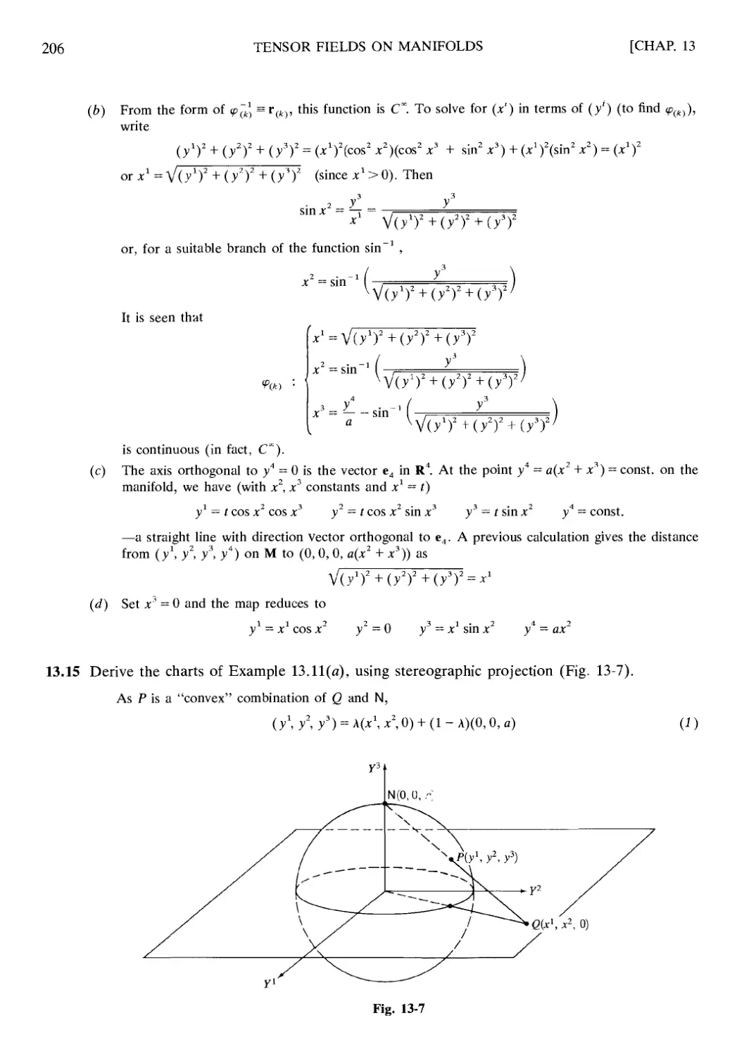
2.35 Find two linearly independent vectors in R1 which are orthogonal to the vector (3, -
2.36 Solve for χ and у by use of matrices:
3x - Ay = -23
5x +- 3y = 10
2.37 Write out the quadratic form in R3 represented by Q =xTAx, where
"1 4 3"
A= 4 2 0
Ъ 0 -lj
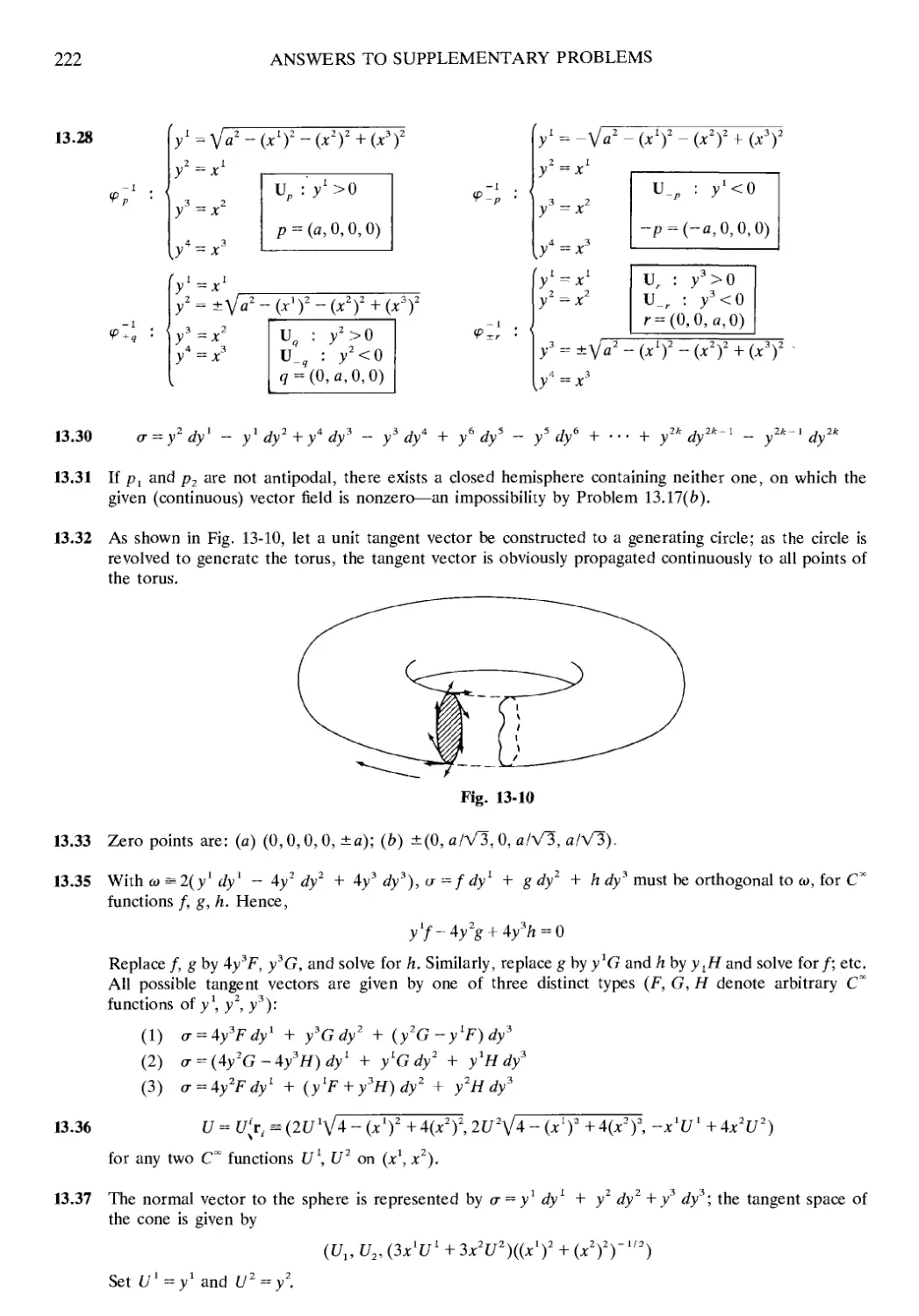
Π l>~1"
1,0,0).
•2,1).
2.38 Represent with a symmetric matrix A the quadratic form in R4
Q = -3*i - x\ + x\ - xvx2 - χγχ3 + 6*!*4

BASIC LINEAR ALGEBRA FOR TENSORS
[CHAP. 2
Given the hyperplane crxr = 1, how do the coefficients c, transform under a change of coordinates
xi = aijX/?
Calculate the glJ for the distance formula (2.14) in a barred coordinate system defined by x = Ax, with
Test the distance formula of Problem 2.40 on the pair of points whose unbarred coordinates are (2, -1)
and (2, -4).
(a) Show that for independent functions xi = xi(xl, x2, ■ ■ ■ , ■*„)>
дх, Эх,
(b) Take the partial derivative with respect to xk of (1) to establish the formula
d2xi dxr _ dzxr dxf dxs
dxkdxr dxj ~ dxsdx dxr dxk ' >

Chapter 3
General Tensors
3.1 COORDINATE TRANSFORMATIONS
At this point the notation for coordinates will be changed to that usual in tensor calculus.
Superscripts for Vector Components
The coordinates of a point (vector) in R" will henceforth be denoted as (x1, x2, x3, . . . , x"). Thus,
the familiar subscripts are now replaced by superscripts, and the upper position is no longer reserved
for exponents alone. It will be clear by context whether a character represents a vector component or
the power of a scalar.
EXAMPLE 3.1 If a power of some vector component is to be indicated, obviously parentheses are necessary;
thus, (x3)2 and (χ"-1)5 represent, respectively, the square of the third component, and the (n - l)st component
raised to the fifth power, of the vector x. If и is introduced as a real number, then u2 and и3 are powers of и and
not vector components. If (c)*7 appears without explanation, the parentheses indicate the use of the superscript к
as an exponent and not as the index of a vector component.
Rectangular Coordinates
Coordinates in R" are called rectangular (also rectangular cartesian or cartesian) if they are
patterned after the usual orthogonal coordinate systems of two- and three-dimensional analytic
geometry. A general definition that is workable in this setting is, in effect, an assertion of the
converse of the Pythagorean theorem.
Definition 1: A coordinate system (x) is rectangular if the distance between two arbitrary points
P(x\ x2, . . . , x") and Q(y\ y2, . . . , y") is given by
pq = VO1 - ylf + (*2 - y'f + ··· + (*"- ynf Ξ \4- Δ*; Δ*7
where Ax = χ' - у'.
Under orthogonal coordinate changes, which are isometric, the above formula for distance is
invariant (cf. Section 2.5). Hence, all coordinate systems (xl) defined by χ = a\x\ where (a'f) is such
that а[аг; = 8if, are rectangular. It can be shown that these are the only rectangular coordinate
systems "whose origin coincides with that of the (x1)-system.
Curvilinear Coordinates
Suppose that in some region of R" two coordinate systems are defined, and that these two
systems are connected by equations of the form
ST : χl = x\x\ x2,. . . , хя) (lgiS/i) (3.1)
where, for each i, the function, or scalar field, x'(x , χ , , . . , x") maps the given region in R" to the
reals and has continuous second-partial derivatives at every point in the region (is class C2). The
transformation ST, if bijective, is called a coordinate transformation, as in Section 2.6. If (x) are
ordinary rectangular coordinates, the (x') are called curvilinear coordinates unless ST is linear, in
which case (xl) are called affine coordinates,
For convenience, the three most common curvilinear-coordinate systems are presented below. In
each case, a "reverse" notation is employed: the two- or three-dimensional curvilinear system {x) is
defined by the mapping ST that takes it into a rectangular system (x') of the same dimension.
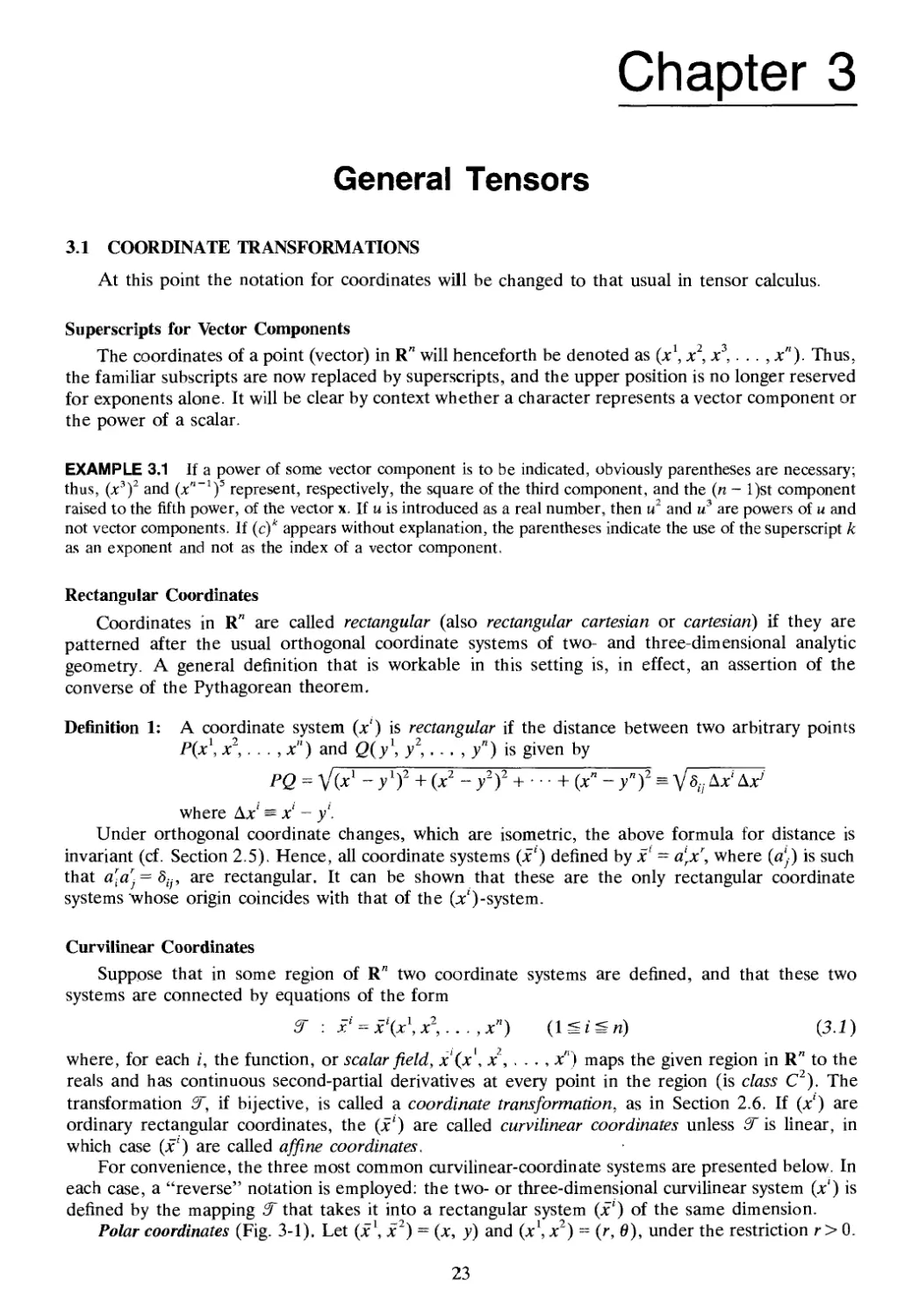
Polar coordinates (Fig. 3-1). Let (χ1, χ2) = (x, y) and (x1, x2) = (r, Θ), under the restriction r> 0.
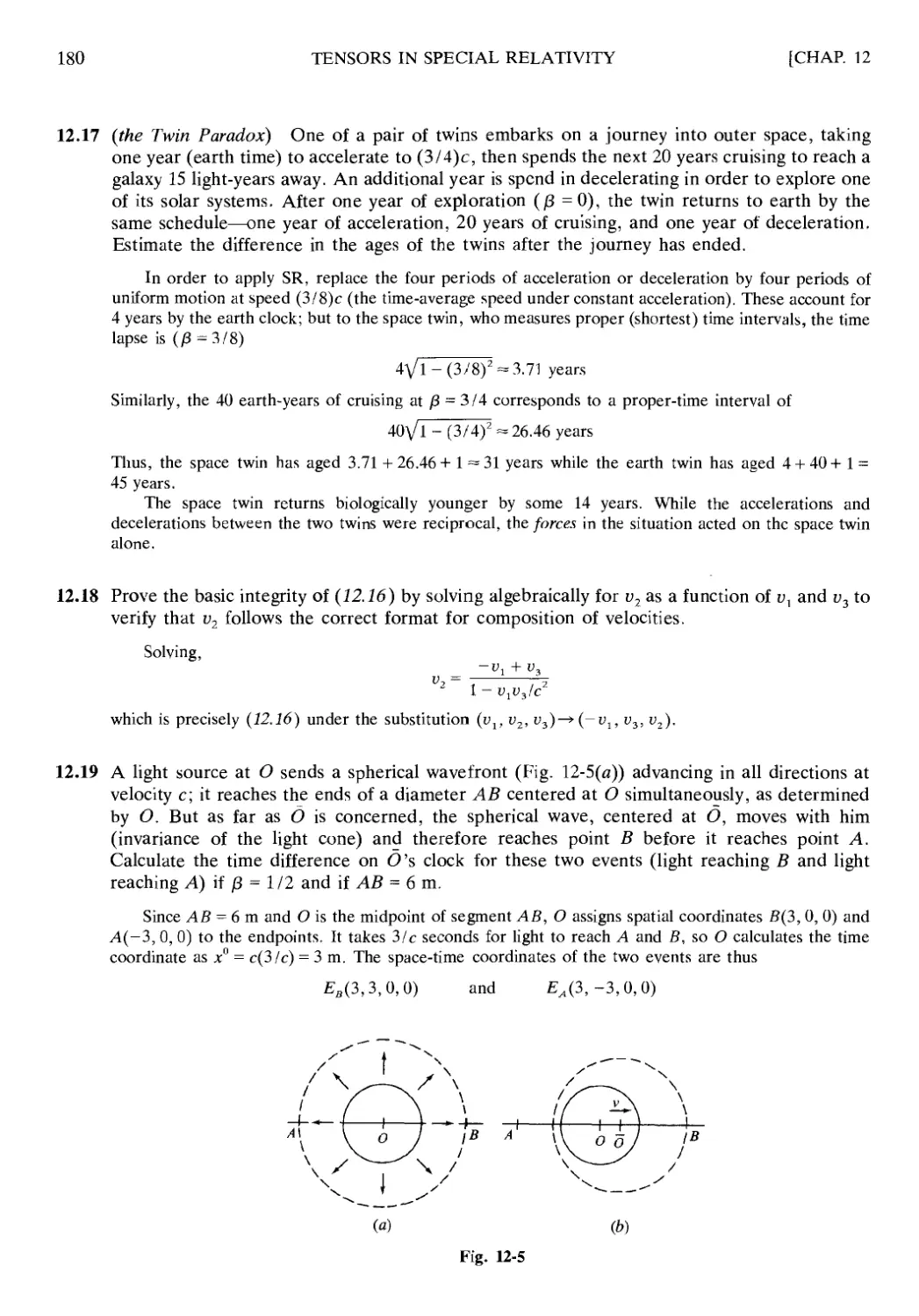
23

24
GENERAL TENSORS
[CHAP. 3
P{r, Θ)
Fig. 3-1
3 :
X = Г COS θ
у = r sin θ
Then,
(-1 1 2
Χ = X COS Χ
-2 1 · 2
χ = χ sin χ
χ' = V(*-1)2 + (*2)2
У = tan"1(f2/f1)
(3.2)
(The inverse given here is, in the equation for x~, valid only in the first and fourth quadrants of the
XjXj-plane; other solutions must be used over the other two quadrants. Likewise for the 0-coordinate
in the cylindrical and spherical systems.)
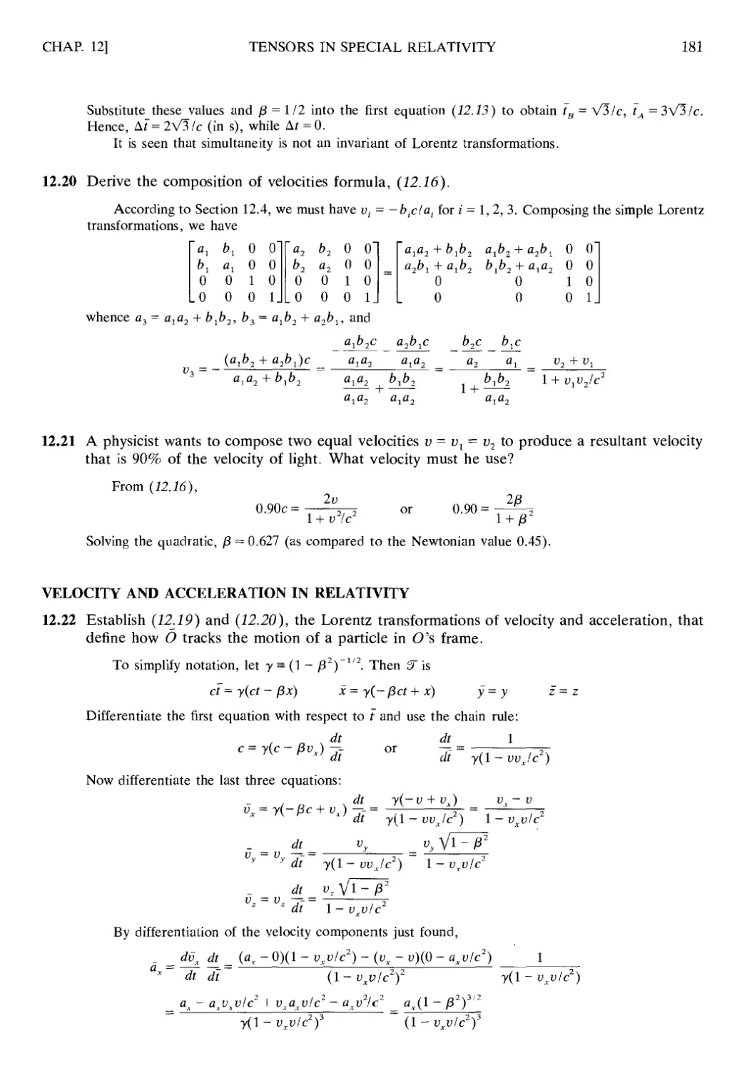
Cylindrical coordinates (Fig. 3-2). If (jc1, χ2, χ ) = (x, y, z) and (jc\ x2, x3) = (r, 0, z), where r > 0,
r -1 1 2
X = X COS X
-2 1 · 2
χ = χ sin χ
-3 _ 3
Э"1
У = V(fx)2 + (*2)2
x2 = tan-1 (i2/*1)
У = *э
(3.3)
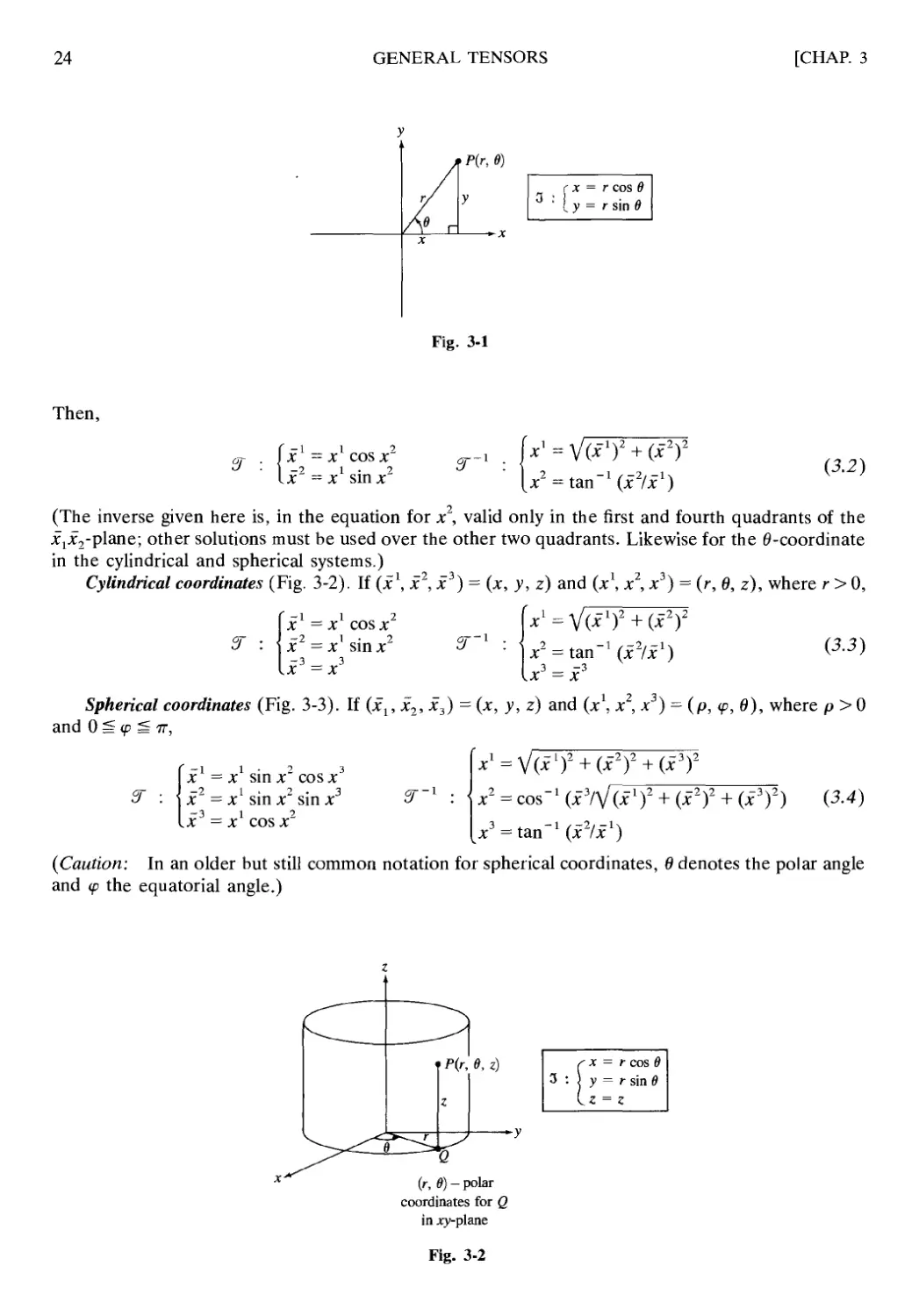
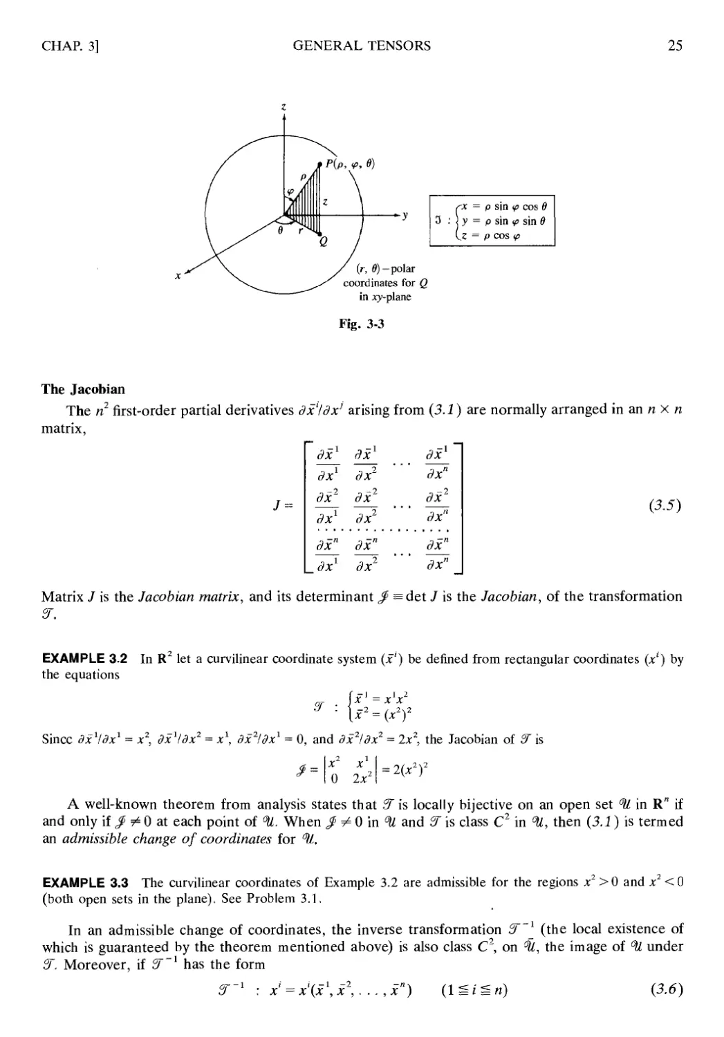
Spherical coordinates (Fig. 3-3). If (jc15 jc2, jc3) = (x, y, z) and (χ , χ , χ ) = (ρ, φ, 0), where ρ > 0
and Ο^φ ё π,
x1 = V(^1)2 + (^2)2 + (^3)2
χ2 = cos-1 (хъ1\[{х1)2 + (χ2)2 + (χ3)2) Ρ·4)
jc^tan-1^2/*1)
(Caution: In an older but still common notation for spherical coordinates, 0 denotes the polar angle
and φ the equatorial angle.)
-1 1-2 3
x = χ sin χ cos χ
-2 1 . 2 . 3
χ = χ sin χ sin χ
-3 1 2
X = X COS X
ST'1 : \
(r, Θ) - polar
coordinates for Q
in jry-plane
3 :
* = r cos 0
у = г sin 0
г = г
Fig. 3-2

CHAP. 3]
GENERAL TENSORS
25
3 .
rx = ρ sin φ cos θ
! у = ρ sin ψ sin θ
Сг = ρ cos φ
(г, 9)—polar
coordinates for Q
in xy-plane
Fig. 3-3
The Jacobian
The n2 first-order partial derivatives dx'ldx1 arising from (3.1) are normally arranged in an η x η
matrix,
(3.5)
dX1
дХ1
дх'
дХ1
дХ
дХ1
дХ
дХ'
дХ'
дХ'
б?*
б?*"
б?*1
б?*"
б?Х"
1 "
дХ
дх"
Matrix / is the Jacobian matrix, and its determinant $ =det / is the Jacobian, of the transformation
ST.
EXAMPLE 3.2 In R2 let a curvilinear coordinate system (*') be defined from rectangular coordinates (xl) by
the equations
or . Ιχ' = χ'χ2
J ■ \x-2 = (xy
Since дх^дх1 = χ2, дхх1дх2 = х\ дх21дхх = 0, and дх21дх2 = 2x2, the Jacobian of ST is
,1
X X'
0 2χΊ
= 2(хГ
A well-known theorem from analysis states that ?T is locally bijective on an open set Ш in R" if
and only if $ Φ 0 at each point of 4. When β Φ 0 in 4 and 2Г is class С2 in %, then (3.1) is termed
an admissible change of coordinates for Ш.
EXAMPLE 3.3 The curvilinear coordinates of Example 3.2 are admissible for the regions x2 > 0 and x2 < 0
(both open sets in the plane). See Problem 3.1.
In an admissible change of coordinates, the inverse transformation 5"1 (the local existence of
which is guaranteed by the theorem mentioned above) is also class C2, on Ш, the image of % under
ST. Moreover, if ST"1 has the form
5"-1 : x' = x'(x\x, , ..,xn) (li(gn)
(3.6)

26
GENERAL TENSORS
[CHAP. 3
on 4, the Jacobian matrix J of ST 1 is the inverse of /. Thus, JJ = JJ = I, or
дхг дх' дх дх' ' У
[cf. Problem 2.42(a)]. It also follows that β = 11β.
General Coordinate Systems
In later developments it will be necessary to adopt coordinate systems that are not tied to
rectangular coordinates in any way [via (3.1)] and to define distance in terms of an arc-length
formula for arbitrary curves, with points represented abstractly by и-tuples (x1, x~, . . . , x"). Each
such distance functional or metric will be invariant under admissible changes of coordinates, and
admissible coordinate systems will exist for each separate metric. Under such metrics, R" will
generally become non-Euclidean; e.g., the angle sum of a triangle will not invariably equal тт.
Although the curvilinear coordinate systems presented above are explicitly associated with the
Euclidean metric (since they are connected via (3.1) with rectangular coordinates and Euclidean
space), those same systems could be formally adopted in a non-Euclidean space if some purpose
were served by doing so. The point to be made is that the space metric and the coordinate system used
to describe that metric are completely independent of each other, except in the single instance of
rectangular coordinates, whose very definition (see Definition 1) involves the Euclidean metric.
Usefulness of Coordinate Changes
A primary concern in studying tensor analysis is the manner in which a change of coordinates
affects the way geometrical objects or physical laws are described. For example, in rectangular
coordinates the equation of a circle of radius a centered at the origin is quadratic,
/-K2 , / -2ч2 _ 2
(x ) + (x ) = a
but in polar coordinates, (3.2), that same circle has the simple linear equation xl = a. The reader is
no doubt familiar with the sometimes dramatic change that takes place in a differential equation
under a change of variables, which is nothing but a change of coordinates. This idea of changing the
description of phenomena by changing coordinate systems lies at the heart of not only what a tensor
means, but how it is used in practice.
3.2 FIRST-ORDER TENSORS
Consider a vector field V=(V) defined on some subset У of R" [that is, for each i, the
component V = V'(x) is a scalar field (real-valued function) as χ varies over У]. In each admissible
coordinate system of a region ^L containing У, let the η components V1, V2, . . . , V" of V be
expressible as η real-valued functions; say, as
Γ1, T~, . . . , T" in the (xl)-system
and
f\ f2, . . . , f" in the (f')-system
where (x) and (x1) are related by (3.1) and (3.6).
Definition 2: The vector field V is a contravariant tensor of order one (or contravariant vector)
provided its components (T') and (T") relative to the respective coordinate systems
(x) and (£') obey the law of transformation
τ — i
contravariant vector T' = Tr ——r (lgi^n) (3-8)

CHAP. 3]
GENERAL TENSORS
27
EXAMPLE 3.4 Let ^ be a curve given parametrically in the (x')-system by
x' = x'{t) (aStSb)
The tangent vector field Τ = (Tl) is defined by the usual differentiation formula
Г' = —
dt
Under a change of coordinates (3.1), the same curve is given in the (f)-system by
Г = x\t) = x\x\t), x\t)> · ■ ■ > *"(0) (aStSb)
and the tangent vector for % in the (i')-system has components
dx'
But, by the chain rule,
T' .
dt
dx dx1 dxr -, dx'
~r = τ~τ —r °r Τ = Τ -—-r
at dx at dx
proving that Τ is a contra variant vector. (Note that because Τ is denned only on the curve "#, we have Sf = <€ for
this particular vector field.) We conclude in general that under a change of coordinates, the tangent vector of a
smooth curve transforms as a contravariant tensor of order one.
Remark 1: In some treatments of the subject, tensors are denned to possess certain weights, with
(3.8) replaced by
π —i
weighted contravariant vector Tl — wTr ——r (l^jgn) (3-9)
for some real-valued function w (the "weight of T")·
In framing the next definition we (arbitrarily) shift to a subscript notation for the components of
the vector field.
Definition 3: The vector field V is a covariant tensor of order one (or covariant vector) provided its
components (Τέ) and (Tt) relative to an arbitrary pair of coordinate systems (x') and
(x'), respectively, obey the law of transformation
π r
covariant vector ft = Tr —— (1 Sr i: ^ n) (3.10)
dX
EXAMPLE 3.5 Let F(x) denote a differentiable scalar field defined in a coordinate system (x') of R". The
gradient of F is defined as the vector field
/^F dF_ £F_
~ W ' dx1 '" ' -' dx'1
In a barred coordinate system, the gradient is given by VF= (dFldx), where F(x) = F°x(x). The chain rule for
partial derivatives, together with the functional relations (3.6), gives
dF _ 3F dxr
dx1 ~ Sxr dx1
which is just (3.10) for Tt = dFldx1, Ti = dP/dx'. Thus, the gradient of an arbitrary differentiable function is a
covariant vector.
Remark 2: Tangent vectors and gradient vectors are really two different kinds of vectors. Tensor
calculus is vitally concerned with the distinction between contravariance and covariance,
and consistently employs upper indices to indicate the one and lower indices to indicate
the other.

28
GENERAL TENSORS
[CHAP. 3
Remark 3: From this point on, we shall frequently refer to first-order tensors, contravariant or
covariant as the case may be, simply as "vectors"; they are, of course, actually vector
fields, defined on R". This usage will coexist with our earlier employment of "vectors"
to denote real и-tuples; i.e., elements of R". There is no conflict here insofar as the
и-tuples make up the vector field corresponding to the identity mapping V'(x) =
xl (i = 1, 2, ... , ή). But the vector (x) does not enjoy the transformation property of
a tensor; so, to emphasize that fact, we shall sometimes refer to it as a position vector.
3.3 INVARIANTS
Objects, functions, equations, or formulas that are independent of the coordinate system used to
express them have intrinsic value and are of fundamental significance; they are called invariants.
Roughly speaking, the product of a contravariant vector and a covariant vector always is an
invariant. The following is a more precise statement of this fact.
Theorem 3.1: Let S' and Ti be the components of a contravariant and covariant vector,
respectively. If the inner product E = SrTr is defined in each coordinate system, then Ε is an
invariant.
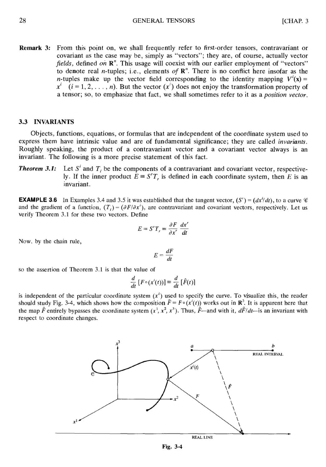
EXAMPLE 3.6 In Examples 3.4 and 3.5 it was established that the tangent vector, (5") = (dx'/dt), to a curve 4i
and the gradient of a function, (Tt~) = (dFldx'), are contravariant and covariant vectors, respectively. Let us
verify Theorem 3.1 for these two vectors. Define
^ „rrr dF dxr
Now, by the chain rule,
dt
so the assertion of Theorem 3.1 is that the value of
dt
И01
is independent of the particular coordinate system (x1) used to specify the curve. To visualize this, the reader
should study Fig. 3-4, which shows how the composition F= F°(x'(t)) works out in R3. It is apparent here that
the map F entirely bypasses the coordinate system (x1, x2, хъ). Thus, F— and with it, dF/dt— is an invariant with
respect to coordinate changes.
REAL LINE
Fig. 3-4

CHAP. 3]
GENERAL TENSORS
29
3.4 HIGHER-ORDER TENSORS
Tensors of arbitrary order may be defined. Although most work does not involve tensors of
order greater than 4, the general definition will be included here for completeness. We begin with the
three types of second-order tensors.
Second-Order Tensors
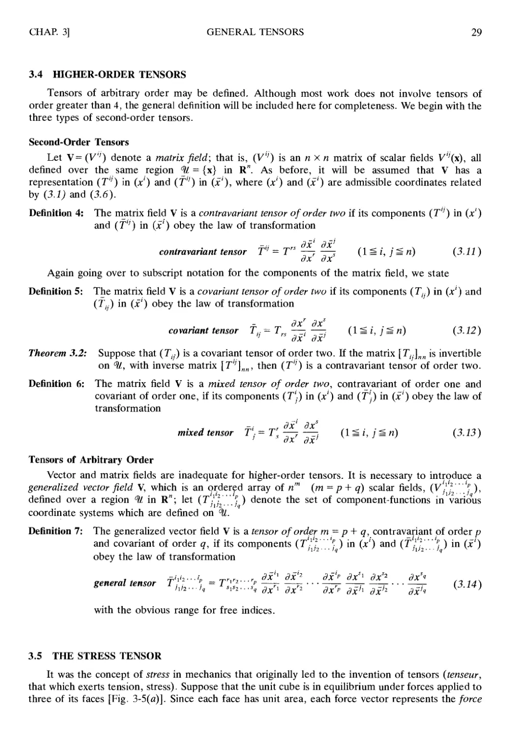
Let V= (V) denote a matrix field; that is, (V) is an η x η matrix of scalar fields V'(x), all
defined over the same region ^ = {x} in R". As before, it will be assumed that V has a
representation (T'!) in (xl) and (V) in (£'), where (xl) and (£') are admissible coordinates related
by (3.1) and (3.6).
Definition 4: The matrix field V is a contravariant tensor of order two if its components (T'1) in (x1)
and (T4) in (xl) obey the law of transformation
contravariant tensor T1' = T" ——r ——s (1 = i, /= η) (3.11)
Again going over to subscript notation for the components of the matrix field, we state
Definition 5: The matrix field V is a covariant tensor of order two if its components (Ttj) in (xl) and
(Ttj) in (xl) obey the law of transformation
covariant tensor Τι;— Τ —— —— (1 = г, / 2= и) (3.12)
' r дх дх'
Theorem 3.2: Suppose that (Tif) is a covariant tensor of order two. If the matrix [Г,.-]ии is invertible
on °и, with inverse matrix [Г';]ии, then (T1') is a contravariant tensor of order two.
Definition 6: The matrix field V is a mixed tensor of order two, contravariant of order one and
covariant of order one, if its components (Т\) in (x!) and (T^) in (x1) obey the law of
transformation
mixed tensor f'; = T's ——r -^ (12= г, / ^ n) (3.13)
OX· CfJC
Tensors of Arbitrary Order
Vector and matrix fields are inadequate for higher-order tensors. It is necessary to introduce a
generalized vector field V, which is an ordered array of nm (m=p + q) scalar fields, (V/^'.'.'J ),
defined over a region % in R"; let (T'^j'"'pj ) denote the set of component-functions in various
coordinate systems which are defined on °U.
Definition 7: The generalized vector field V is a tensor of order m- ρ + q, contravariant of order ρ
and covariant of order q, if its components (T^j'"J ) in (xl) and (f-j'" ^ ) in (x1)
obey the law of transformation
,, τ'Ί'2 ■■·',. Tr,r,...r dXh дх'2 дХ~1Р дх' дХ* dXS* ,„l/f4
general tensor Τ , ρ·. = Τ '/ / —-r у- ■ ■ = : г ■ ■ ■ —г- (3 14)
S hl2...,q slS2...Sq дхг, дхг2 дхгр d-h d-h d-,q \J-it)
with the obvious range for free indices.
3.5 THE STRESS TENSOR
It was the concept of stress in mechanics that originally led to the invention of tensors (tenseur,
that which exerts tension, stress). Suppose that the unit cube is in equilibrium under forces applied to
three of its faces [Fig. 3-5(a)]. Since each face has unit area, each force vector represents the force

30
GENERAL TENSORS
[CHAP. 3
FACE 3
σ31
σ33
FACE V
σ32
σ21
'a12
- FACE 2
(A)
Fig. 3-5
Φ)
per unit area, or stress. Those forces are represented in the component form in Fig. 3-5(b). Using the
standard basis e15 e2, e2, we have
Is
σ e„
2.5
σ e.
σ e.
(stress on face 1)
(stress on face 2)
(stress on face 3)
(3.15)
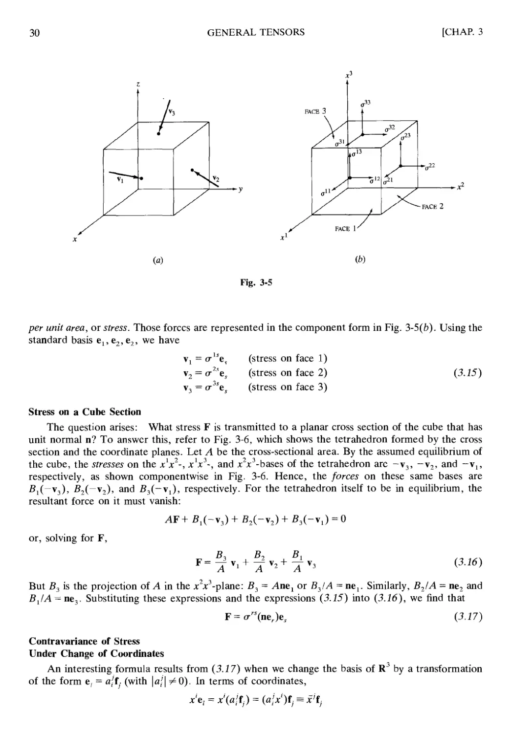
Stress on a Cube Section
The question arises: What stress F is transmitted to a planar cross section of the cube that has
unit normal n? To answer this, refer to Fig. 3-6, which shows the tetrahedron formed by the cross
section and the coordinate planes. Let A be the cross-sectional area. By the assumed equilibrium of
the cube, the stresses on the хгх2-, xV-, and jt2jt3-bases of the tetrahedron are -v3, -v2, and -v15
respectively, as shown componentwise in Fig. 3-6. Hence, the forces on these same bases are
.B^-Vj), Z?2(-v2), and β3(-ν1), respectively. For the tetrahedron itself to be in equilibrium, the
resultant force on it must vanish:
AF + Вг(- v3) + B2(~v2) + β3(-νι)
= 0
or, solving for F,
β,
В,
г=^ + ^+:Ь
(3.16)
But B3 is the projection of A in the x'x3-p\ane: B3 = Лпех or B3/A = nel. Similarly, B2IA = ne2 and
Bl/A-ne3. Substituting these expressions and the expressions (3.15) into (3.16), we find that
F = <r>erK
(3.17)
Contravariance of Stress
Under Change of Coordinates
An interesting formula results from (3.17) when we change the basis of R3 by a transformation
of the form e, = α{ί. (with \a[\ #0). In terms of coordinates,

CHAP. 3]
GENERAL TENSORS
31
Fig. 3-6
That is, we have a new coordinate system (*') that is related to (xl) via
Note that here we have
(3.18)
dx!
dx
Substituting er = a'rfi into (3.17) yields the stress components (σ';) in the new coordinate system, as
follows:
with
F = a»[n(a%)]{a>,ts) = а"а^аЦпЩ - ^(nf,)f;.
дХ дх'
дХГ dXS
A comparison of (3.19) with the transformation law (3.11) leads to the conclusion that the stress
components σ1' define a second-order contravariant tensor, at least for linear coordinate changes.
-it rs ι rt} r,
σ' — σ aras = σ
(3.19)
3.6 CARTESIAN TENSORS
Tensors corresponding to admissible linear coordinate changes, 3~ : χ - а';х' (\а'^0), are
called affine tensors. If (a1.) is orthogonal (and ST is distance-preserving), the corresponding tensors
are cartesian tensors. Now, an object that is a tensor with respect to all one-one linear
transformations is necessarily a tensor with respect to all orthogonal linear transformations, but the converse is
not true. Hence, affine tensors are special cartesian tensors. Likewise, affine invariants are particular
cartesian invariants.
Affine Tensors
A transformation of the form ST : χ = α^χ' (|α'.| τ^Ο) takes a rectangular coordinate system
(xl) into a system (xl) having oblique axes; thus affine tensors are defined on the class of all such

32
GENERAL TENSORS
[CHAP. 3
oblique coordinate systems. Since the Jacobian matrices of ST and ST 1 are
the transformation laws for affine tensors are:
contravariant f' = a'rTr, f'' = a'ra'sT", f''k = a'ra'saktTrs\ ...
covariant f, = b[Tr, f,; = b\ b) Trs, ^ fijk = b- b) b'k Trst, ... (3.21)
mixed T\ = a\b) Ts, T'jk = a'rbsfb'kTrsn . . .
Under the less stringent conditions (3.21), more objects can qualify as tensors than before; for
instance, an ordinary position vector χ = (У) becomes an (affine) tensor (see Problem 3.9), and the
partial derivatives of a tensor define an (affine) tensor (as implied by Problem 2.23).
Cartesian Tensors
When the above linear transformation ST is restricted to be orthogonal, then J'1 = JT, or
b) = ai (l%i,j^n)
so that the transformation laws for cartesian tensors are, from (3.21),
contravariant T' = a\ Tr, f1' = dra's Trs, . . .
covariant tt - a'rTr, Ttj = a\a's Trs, ...
mixed f'j = dra'sTrs,
A striking feature of these forms is that contravariant and covariant behaviors do not distinguish
themselves. Consequently, all cartesian tensors are notated the same way—with subscripts:
(3.22)
Because an orthogonal transformation takes one rectangular coordinate system into another (having
the same origin), cartesian tensors appertain to the rectangular (cartesian) coordinate systems. There
are, of course, even more cartesian tensors than affine tensors.
Note that JJT = / implies /2 = 1, or β = ±1. Objects that obey the tensor laws (3.22) when the
allowable coordinate changes are such that
allowable
coordinate changes
cartesian
tensor laws
xl = aijxj or xi = ajixj
Ti = airTr, Т^ = а1га^Т„,
k,.| = +i
are called direct cartesian tensors.
Solved Problems
CHANGE OF COORDINATES
3.1 For the transformation of Example 3.2, (a) obtain the equations for 3"1; (b) compute /from
(a), and compare with J"1.
(a) Solving χ1 = xlx2, x2 = (x2)2 for x1 and x2, we find that
\xl=xlx2 „__, \x
1---1--2 i^-jcVVF
*2 = (*2)2 σ : U2 = VF {1)

CHAP. 3]
GENERAL TENSORS
33
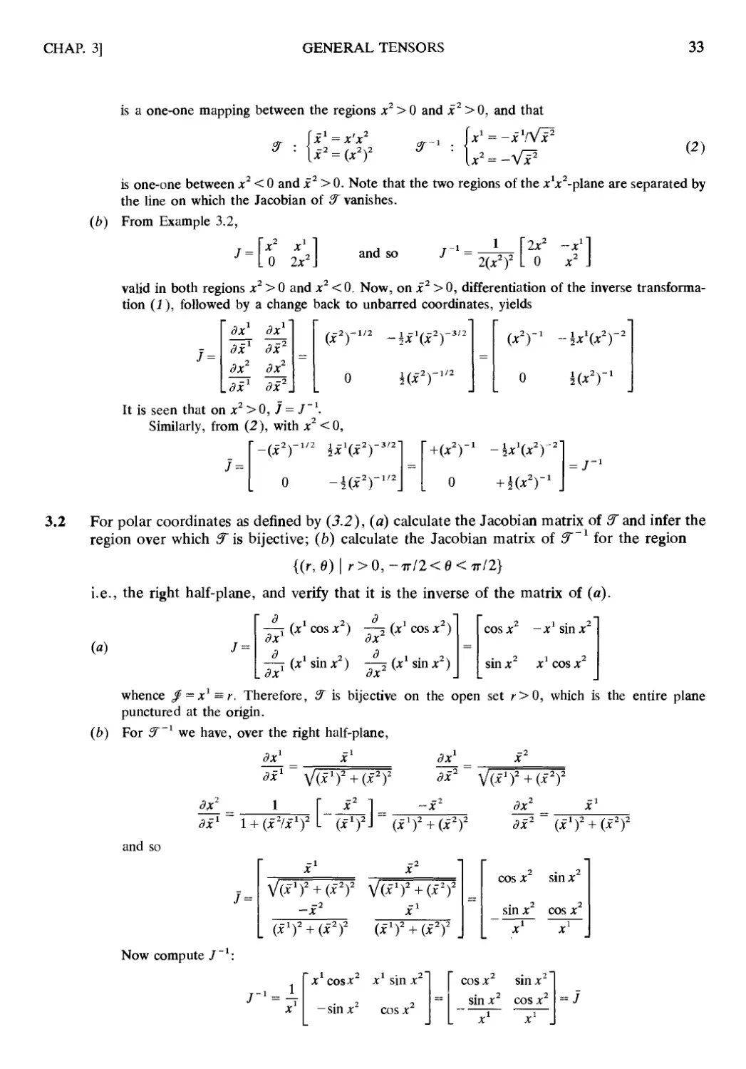
is a one-one mapping between the regions x2 > 0 and x2 > 0, and that
= -хгЫТ
χ1 = x'x2
(χΎ
гг~г :
-VF
(2)
is one-one between x2 < 0 and x2 > 0. Note that the two regions of the j'^-plane are separated by
the line on which the Jacobian of 2F vanishes.
(b) From Example 3.2,
χ2 χ
0 2x
Ά
and so
1
2x2
0
"/]
2(x2)2
valid in both regions x2 > 0 and x2 < 0. Now, on *2 > 0, differentiation of the inverse
transformation (1), followed by a change back to unbarred coordinates, yields
J =
"лс1
dx2
.dx1
Эх1
dx2
dx2
dx2.
=
(x2)-1'2 -,
0
χχ
i(x
,χ2)'3'2
2 ч-1/2
=
(χ2)-1 -
0
seen that on x2 > 0, / = J ' \
Similarly, from (2), with *2 <0,
J=
~-(χ2)
0
-1/2
-К*2)'1'2.
=
-+(x2)-
0
-\x\x2T2'
+ HX2)-1 .
-\x\x2T2
Ηχ2)-1
= j~l
3.2 For polar coordinates as defined by (3.2), (a) calculate the Jacobian matrix of 3~ and infer the
region over which if is bijective; (b) calculate the Jacobian matrix of Э"1 for the region
{(r, 0) | r>0, -я72<0<я72}
i.e., the right half-plane, and verify that it is the inverse of the matrix of (a).
(«)
^ 1 2^1 2
г (χ COS Χ ) 5 (д: COS * )
ί*1 ν дх2У '
д ι 1 · 2ч <? / 1 · 2ч
—7 (х sin д: ) —τ (* sin д: )
L<9* Лс .
COS*2 -XlUnX2
Sin *2 Я1 COS Χ2
whence $-xx = r. Therefore, 2Г is bijective on the open set r>0, which is the entire plane
punctured at the origin.
(b) For ST'1 we have, over the right half-plane,
dx_
1-1
dx1
dX1 V(*')2 + (*2)2 *** V(^)2 + (^2)2
*Г
if1 1 + (i2/*1)2
(*')2J (хГ + (Я2)
dx' x1
dx2 (xlf + (x2)2
and so
V(*-1)2 + (*-2)2 V(*_1)2 + (*2)2
-*2
(хУ + (хУ (хг)2 + {х2Г
cos *2 sin x2
sin X2 COS X2
Now compute J 1:
J-1
χ cos*2 x1 sin x2
- sin χ cos дг
cos χ sin jc
sin x2 cos jc2

34
GENERAL TENSORS
[CHAP. 3
CONTRAVARIANT VECTORS
3.3
If V= (Γ') is a contravariant vector, show that the partial derivatives V- = dT'ldx', defined in
each coordinate system, transform according to the rule
Differentiate both sides of
-,- „.,. дх' dXS m, д х' dXS
Τ = Τ + Τ :
' s дх дх' dxrdxs эх'
дх
with respect to x', using the product rule
if
' die' ■ дх' V дх
дх'
дТ дх
г д (дх'
By the chain rule for partial derivatives, (2.15),
and
dV __ dV dxs __ dxs
дх' ~ dxs дх' ~ s дх'
Substituting these expressions into (1) yields the desired formula.
дх' дХг Ж' \дХг/
д (Sx'\_
die' \dxT)~~
д (дх'Х
дх \дхг).
дх
дх
(1)
3.4 Suppose that (Г!) is a contravariant vector on R" and that (Гг) = (χ', χ1) in the (x')-system.
Calculate (T") in the (x')-system, under the change of coordinates
-2 1 2
x —xx
By definition of contra variance,
дх дх дХ
Note that the top row of the Jacobian matrix J is needed for the case i = 1, and the bottom row is needed
for i =2.
die1
дх
дх
dxi
die1'
dX2
die
~. 2
dX .
"0
2
.X
2x2]
xl .
Thus,
f1 = T1(0)+ 7'2(2jc2) = 2jcV
which, in terms of barred coordinates, are
:Τ=2ί2
f2 = T\x2) + TV) = (x2)2 + (x1)2
iW + Щ-
3.5 Show that a contravariant vector can be constructed the components of which take on a given
set of values (a, b, c, . . .) in some particular coordinate system. (The prescribed values may
be point functions.)
Let (a, b, c, . . .) = (a) be the given values to be assigned in the coordinate system (x). Set V = a
for the values in (У), and for any other admissible coordinate system (f), set V' = a'(dx'ldx). To show
that (V) is a contravariant tensor, let (>'') and (yl) be any two admissible coordinate systems. Then,
у =/'(x1, a2, .... x") and y' = g'(x\ x2, . . . , x"), and, by definition, the values of (V") in (y') and (y')
are, respectively, V = ar(dy'ldxr) and f" = a(dyl!dxr). But, by the chain rule,
Г = а
dxr
dy' dys
ду" дх
df_
df
QED

CHAP. 3]
GENERAL TENSORS
35
COVARIANT VECTORS
3.6 Calculate (T;) in the (*')-system if V= (Γ;) = (*2, χ1 +2x2) is a covariant vector under the
coordinate transformation of Problem 3.4.
To avoid radicals, compute J~l in terms of {x')\
Jl =
-χ ι
2(x2)2 x2
h »
By covariance,
=, „ dX ^ OX ^ dx
τ, = τ, — = т. — + тг —
dx 1 дх г dx'
0' = 1,2)
For Ί = 1, read off the partials from the first column of J \-
f, = Tl(~xll2{x2)2) + T2(l/2x2) = ~хЧ2х2 + xV2x2 + 1 = 1
Similarly, for i = 2, use the second column of /_1:
f2 = Тг(\1х2) + Г2(0) = x\llx2) = 1
Hence, (Г;) = (1,1) at all points in the (F)-system (x1 = 0 excluded).
3.7 Use the fact that V/ is a covariant vector (Example 3.5) to bring the partial differential
equation
df Bf
χ — = у —
dx y dy
into simpler form by the change of variables x = xy, y- {yf; then solve.
Write V/= (df/dx, df/dy)^(T.), (x\ x2) = (x, y), (x\ χ2) = (*, у), and
f-
Again calculating J first, then its inverse, we have
JL = t —
dXl ' dx'
dx1
dx'
= 7"
у χ
0 2y
1 -x
У 2(у)2
о I
2У .
so that
dx
dXr
die1
-L шТ = Τ ζ^— = Τ · - + Τ ·0 =
liL
У dx
1
df _ rf, _ T dxr _ —X
~dj~ г~ г~д?~ Г 2{yf + 2 2y 2(y)2 dx ' 2y iy
χ df + ± d£
But, by (1),
*/
ίνϊ2 V
■*^ + y^-o
0)
<?y 2(y)2 \ <?* ' <9y/
which implies that /= F(x), a function of χ alone; therefore, f—F(xy) is the general solution to (1).

36
GENERAL TENSORS
[CHAP. 3
INVARIANTS
3.8 Prove Theorem 3.1.
We must show that if (5") and (Γ,.) are tensors of the indicated types and order, then the quantity
E^S'Ti is invariant with respect to coordinate changes; that is, Ё = Е, where Ε ~ S'fr But observe
that
S'^S
r Эх'
dXr
and
dx
dx'
so that, in view of (3.7),
3.9 Show that under linear coordinate changes of R", x' = a'jx' (|a^.|#0), the equation of a
hyperplane Atx' = 1 is invariant provided the normal vector (At) is covariant.
In view of Theorem 3.1, it suffices to show that (V) = (x') is a contravariant affine tensor. But this
is immediate:
Γι —j / / ι τ ι
s χ = α,χ= a, I
which is the transformation law (3.21).
SECOND-ORDER CONTRAVARIANT TENSORS
3.10 Suppose that the components of a contravariant tensor Τ of order 2 in a coordinate system
(*') of R2 are Tu = 1, T12 = 1, T21 = -1, and T22 = 2. (a) Find the components fiJ of Τ in the
(*')-system, connected to the (x')-system via
-2 1 2
X = X X
(b) Compute the values of the f'1 at the point which corresponds to i1 = 1, j2
For economy of effort, the problem will be worked using matrices,
(a) Writing
dx
dx'
we have from (2.1b),
t" =-T"—r —s = J1 Tn J'k
Эх Эх ;
That is,
Τ = JTJ'
=
"2*1 0"
2 1
. X X .
" 1 Γ
.-1 2_
"2X1
. 0
(b) At the point (1, -2),
fn=4(l)
f2I=2(l]
2 = 4
(-2) -2
;i)2 =
x2'
x\
=
4(x1)2 2^*2 + 2(*1)2'
_2л:'л:2-2(л:1)2 2(jc')z + (χ2)2 _
= ~6
7'lz=2(l)(~2) + 2(l)z = ~2
f22 = 2(l)2 + (~2)z = 6
-2.
3.11 Show that if (5'') and (Γ'') are contravariant vectors on R", the matrix [U''] = [5,'r/J„„, defined
in this manner for all coordinate systems, represents a contravariant tensor of order 2.

CHAP. 3]
GENERAL TENSORS
37
Multiply
s' = sr
дх'
dXr
and
OX
dXS
to obtain
Эх Эх Эх Эх
which is the tensor law. (The notion of the "outer product" of two tensors will be further developed in
Chapter 4.)
SECOND-ORDER COVARIANT TENSORS
3.12 Show that if Tl are the components of covariant vector T, then Si;. = Г,Т;- T.T, are the
components of a skew-symmetric covariant tensor S.
The skew-symmetry is obvious. From the transformation law for T,
,=,,=, - ,=, „ dxr „ dxs „ dxs „ dxr
T.T. - Τ Τ = Τ : · Τ : - Τ 'Τ :
' дх 5 дх' s дх' ' дх'
„, „, дхг дх" ^ ^ дхг дх" /rr, ^ ^ ^ „ дх' dxs
= Γ Τ : ~ Τ Τ : ;= ΓΓ - Τ Τ ) : :
' s дх дх' s " дх дх' У r s s r) дх дх'
or
S = s — —
"' " дх' dxJ
which establishes the covariant tensor character of S.
3.13 If a symmetric array (Г,-) transforms according to
- _ дх_ дх?_ дх_ дх_
Ц " dXS дх} дХ1 дХк
show that it defines a second-order covariant tensor.
TI; = Τ Л
ι дх' дхк\ дх" дх'
"\дхк дх" I дх1 дх
дх*_ дх!_ _ дх' дх"
" дх' дх' ,s JI' Jx4
\дХ^дХ^__т дх5 дх'
I дх1 дх' ~ " s дх1 дх'
3.14 Let U = ([/,„) be a covariant tensor of order 2. Under the same coordinate change as in
Problem 3.10, (a) calculate the components Όψ if Uu = x2, i/]2 = U2l = 0, U22 = x1; (b) verify
that the quantity T''~UV] = Ε is an invariant, where the T'J and f"' are obtained from Problem
3.10.
(a) In terms of the inverse Jacobian matrix, the covariant transformation law is
Substituting
UiS
дх' dxs
dxl " дх'
2X1 0
Lx2 x1
J'U JS = J"U J"
ι rs j r rs I
2хг
2{x')2
or
U-
U = JTUJ
x1 0
0 xx

38
GENERAL TENSORS
[CHAP. 3
we find
U-
1
2xl
0
x2
2(xlf
1
1
χ
x2
0
0
xx
2xl
1
L 2{хУ x1
xxx2 + (x2f
4{xlf 2{x1)2
V)2
from which the Utj may be read off.
(b) Continuing in the matrix approach, we note that Ε is the trace (sum of diagonal elements) of the
matrix TUr.
TU' =
Ε = χ2 + 2xl
1 1
1 2.
χ2 0
0 x1
and
TUT-
4(У)2 2х1х2 + 2(х1)2
2x1x2~2(x1)2 2(x1f + (x2)2
2 1
X X
_—x2 2x\
x'x' + jx2)2
2
2(хУ
2(x1f
1_
xx
0
1 2
3jc
2л:1
jc2 + 2xl
E = x2 + 2xl = E
3.15 Prove Theorem 3.2.
Observe first of all that if a covariant matrix (second-order tensor) U has inverse V in unbarred
coordinates, then Ό has inverse V in barred coordinates; i.e., (U)'1 = U~l. Now, by Problem 3.14(a),
U = /Γί/7
Inverting both sides of this matrix equation, applying Problem 2.13, and recalling that J J = /, we obtain
W1 = j-'u~\jTy" = juxjt
which is the contravariant law for U~l [see Problem 3.10(a)].
MIXED TENSORS
3.16 Compute the formulas for the tensor components (f'j) in polar coordinates in terms of (7^.) in
rectangular coordinates, if the tensor is symmetric in rectangular coordinates. (In contrast to
Section 3.1, it is now the curvilinear coordinates that are barred.)
The general formula calls for the calculations
f^Tr^-^- = — T —
' s dxr dxj 3xr s Эх1
Using (2.1b), this may be written in matrix form as
where T= [7^]22 and where
; Г cos θ —rsinO
I sin θ r cos θ .
(Τ', = Τ>)
(1)

CHAP. 3]
GENERAL TENSORS
39
is the Jacobian matrix of the transformation from (r, 0) to (x, y). Thus,
cos 0 sin 0
sin 0 cos 0
r r
cos 0 sin 0
sin 0 cos 0
1 1 * 2
Tl Tl
cos θ — r sin θ
sin θ r cos θ
Γ] cos θ + 7^ sin θ ~ϊΤ\ύηθ + rTlcosO'
Tl cos θ + Tl sin θ - КГ' sin0 + КГ2 cos 0
The final matrix multiplication can be carried out routinely, simplifying by means of trigonometric
identities:
T\ cos2 0 + T\ sin 20 + T\ sin2 θ - ^ T\ sin 20 + /T' cos 20 + *- T\ sin 20
, j sin 20 j cos 20
2r
+ T
+ Ti
sin 20
"27"
Γ J sin2 0 - Tl sin 20 + T\ cos2 0
Observe that Τ does not share the symmetry of T: T\ = r 2T\.
3.17 Prove that the determinant of a mixed tensor of order two is invariant.
By (1) of Problem 3.16, we have—whether or not Τ is symmetric—
\Τ\ = \πΓ4 = \ι\\τ\\Γι\=β\τ\β-ι = \τ\
GENERAL TENSORS
3.18 Display the transformation law for a third-order tensor that is contravariant of order two and
covariant of order one.
Take ρ — 2 and q = 1 in Definition 7 and, to avoid unnecessary subscripts, write i, j, k, r, s, t in
place of ι\, i2, jx, rit r2,si. Then (3.14) gives
fy = Trs d* d*' 3x'
k ' дх' дх5 dxk
3.19 Let Τ = (Т'[1т) denote a tensor of the order and type indicated by the indices. Prove that
S = (Tk) = (T'lij) is a covariant vector.
The transformation law (3.14) for Τ is
ТУ
1 Mm
дх1 дх' дх дх" дх"
Jxr эх* Jx7* Ί>¥1 JF
Set I = i, m—j and sum:
дх1 дх"\! дх> дх"\ дх
f = T> -T" — — — — — = Τ
k" '"» дхт dxs дх" Эх1 дх' ,ии\дхт dx')\dxs dxj! дхк
дх
mv°r°s J^K
дх'
дхк
дх'
CARTESIAN TENSORS
3.20 Show that the permutation symbol (et-) defines a direct cartesian tensor over R2. Assume that
etj is defined -the same way for all rectangular coordinate systems.
If the coordinate change is f,- = ai;*,, where (al/)T(akl) = (δρ9) and

40
GENERAL TENSORS
[CHAP. 3
we must establish the cartesian tensor law (3.22):
ё„ = ersairais (n = 2)
We examine separately the four possible cases:
i=j=l ersawau = flnfl12 - β12βη = 0 = ёи
i= 1, j = 2 ersaua2s = a11a22 - a12a21 = 1 = e12
i = 2,j=l e„a2rau = fl2,fl,2- fl22fln = -1 = ё21
i=j = 2 ersa2ra2s = a21a22 - a22a21 = 0 = <F22
3.21 Prove that (a) the coefficients ci;- of the quadratic form c-x'x' = 1 transform as an affine tensor
and (b) the trace cH of (c;/) is a cartesian invariant.
(a) If i' = α'μ' and x' = b^x', where (b1-) = (fl^)-1, the quadratic form goes over into
1 = сц(ЬХ)(Ь',х')1сг,х'х'
with crs = b'rb'sctj. But this formula is just (3.21) for a covariant affine tensor of order two.
(b) Assuming an orthogonal transformation, (b') = (fl,)T, we have
— lis
Hence, c,r = (b>y)ciy = 5^.·
3.22 Establish the identity between the permutation symbol and the Kronecker delta:
eri!erkI - SikSjt - 8u8jk (3.23)
The identity implies η - 3, so that there are potentially 34 - 8f separate cases to consider. However,
this number can be quickly reduced to only 4 cases by the following reasoning: If either i = / or к = I,
then both sides vanish. For example, if i =/', then on the left erij = 0, and on the right,
Hence, we need only consider the cases in which both i¥-j and к Φ I. Upon writing out the sum on the
left, two of the terms drop out, since 1Фу.
eiijeikl """ e2ije2kl """ e3ije3kl ~ eV2'3,ei,kl V ~ ^ > / — ^ )
where (l'2'З') denotes some permutation of (123). Thus, there are left only two cases, each with two
subcases.
Case 1: e1,2,yerkl Φ 0 (with i = 2', / = 3'). Here, either k-2' and 1 = 3' or к = 3' and I = 2'. If the
former, then the left member of (3.23) is +1, while the right member equals
δ2.2'δ3.3. — δ2,3,δ3.2. = 1—0=1
If the latter, then both members equal -1, as can be easily verified.
Case 2: er2,yerkl = 0 (with i = 2', j ~ 3'). Since к Φ /, either к = Г от 1= V. If Л = Г, then the
right member of (3.23) equals
^Z'l'^3'/ ~~ ^2'f^3'l' = 0 — 0 = 0
If / = 1', we have d2.kdyi, - d2i,dyk = 0-0 = 0.
This completes the examination of all cases, and the identity is established.

CHAP. 3]
GENERAL TENSORS
41
Supplementary Problems
3.23 Suppose that the following transformation connects the (x:) and (x:) coordinate systems:
. \xl = exp(x1 +x2)
•J ■ 1 -2 /1 2ч
[x — exp (x - χ )
(a) Calculate the Jacobian matrix J and the Jacobian β. Show that j? Φ 0 over all of R2. (b) Give
equations for 3T~ \ (c) Calculate the Jacobian matrix J of ST 1 and compare with У \
3.24 Prove that if (Г,) defines a covariant vector, and if the components Sif = Γ,Γ. + Γ;Γ, are defined in each
coordinate system, then (S0) is a symmetric covariant tensor. (Compare Problem 3.12.)
3.25 Prove that if (Г;) defines a covariant vector and, in each coordinate system, we define
Эх' όχ' ~ ''
then (Γ ) is a skew-symmetric covariant tensor of the second order. [Hint: Model the proof on
РгоЫеп/з.З.]
3.26 Convert the partial differential equation
to polar form (making use of the fact that
3.27 Show that the quadratic form Q = g^x'x' is an affine invariant provided (g4) is a covariant affine tensor.
[Converse of Problem 3.21(a).]
3.28 Prove that the partial derivatives of a contravariant vector (Tl) define a mixed affine tensor of order
two. [Hint. Compare Problem 2.23.]
3.29 Prove that the Kronecker delta (δ^), uniformly defined in all coordinate systems, is a mixed tensor of
order two.
3.30 Show that the permutation symbol (e;y) of order two, uniformly defined in all coordinate systems, is
not—Problem 3.20 notwithstanding—covariant under arbitrary coordinate changes. [Hint: Use x1 =
xlx2, χ- = χ2, at the point (*'') = (1,2).]
3.31 By use of (3.23), establish the familiar identity for the vector product of three vectors,
u x (v x w) = (uw)v — (uv)w
or, in coordinate form,
eiik^j{ekrsvrws) = (μ,η',-Κ - (и^К
3.32 (α) Show that if (Tj) is a mixed tensor, then (Γ* + T[) is not generally a tensor, (b) Show that a mixed
tensor of order two, symmetric in a given coordinate system, will transform as a symmetric tensor if the
Jacobian matrix is orthogonal.
3.33 Prove: (a) If (T'j) is a mixed tensor of order two, T\ is an invariant; (b) if (S'lk) and (T') are tensors of
the type and order indicated, SrjrT' is an invariant.
df df
дх ду
V/is a covariant vector), and solve for f(x, y).

GENERAL TENSORS
[CHAP. 3
If Тг(Т^) is a tensor, contravariant of order 3 and covariant of order 2, show that S = (T'lk) is a
contravariant vector.
Show that the derivative, dTldt, of the tangent vector T= (Tl) = (dx'/dt) to a curve x'! = x'(t) is a
contravariant affine tensor. Is it a cartesian tensor?
(a) Use the theory of tensors to prove that the scalar product uv = uivi of two vectors u = (и.) and
v= (d;) is a cartesian invariant, (b) Is uv an affine invariant?

Chapter 4
Tensor Operations;
Tests for Tensor Character
4.1 FUNDAMENTAL OPERATIONS
From two given tensors,
S = (^'.''\) Т = (Г^;;;;о (4.1)
certain operations, to be described, will produce a third tensor.
Sums, Linear Combinations
Let p = r and q = s in (4.1). Since the transformation law (3.14) is linear in the tensor
components, it is clear that
S + Ύ ^(SYf1- +Τ\ή· ■■'<) (4.2a)
4 1лП ■ ■ ■ h HH ■ ■ ■ h' x '
is a tensor of the same type and order as the original two tensors. More generally, if T,, T2, . . . , Τμ
are tensors of the same type and order and if λ,, λ2, . . . , λμ are invariant scalars, then
A,T, + A2T2 + · · · + λμΎμ (4.2b)
is a tensor of that same type and order.
Outer Product
The outer product of the tensors S and Τ of (4.1) is the tensor
\sT]^(s';X;;)g-T^-^) (4.3)
which is of order m^p + q + r + s (the sum of the orders of S and T), contravariant of order ρ + r
and covariant of order q + s. Note that [ST] = [TS].
EXAMPLE 4.1 Given two tensors, S = (S)) and Τ = (Tk), the outer product [ST] = (S'fTk) = (Pljk) is a tensor
because
pi „if /„, дХ_ дХ*_\(т дХ?_\ = pr d±_ crf_ d±_
rik *jik V* dxr dx'/V» dxk' s" dxr dx>' dxk
Inner Product
To take the inner product of two tensors, one equates an upper (contravariant) index of one
tensor to a lower (covariant) index of the other, and sums products of components over the repeated
index. In effect, the contravariant and covariant behaviors cancel out, which lowers the total order of
the two tensors.
To state this more formally, set ia = u~ Ιβ in (4.1). Then the inner product corresponding to this
pair of indices is
ST-(^,;/.%?vr^^j {44)
It is seen that there will exist ps + rq inner products ST and TS; in general, all of these will be
distinct. Each will be a tensor of order
m^p+q+r+s-2
43

44 TENSOR OPERATIONS; TESTS FOR TENSOR CHARACTER [CHAP. 4
EXAMPLE 4.2 From the tensors S = (S") and Τ = (Tklm), form the inner product U = (U{m)= (S"'Tkum). We
have:
w„.
•(s"££)(t.
= SrrT.
dx dxq dx
dx" dxr/\'sq' дхк ~дГ дхт
a χ11 dxq\ dx' dxs dx'
s<1,\dxp dx"
=„PrT dx' dx5 dx'
dx' dxk dx"' l'« ' dxr dx" dx"'
_ vprT dx' dxs dx' _ dx' dxs dx'
sp' ~d7 Jx~k ~df^ ~~ st ~d4 Jk~k Jr*
which verifies that U is a tensor of order 3, contravariant of order 1 and covariant of order 2.
EXAMPLE 4.3 With (Гу) and (TiJ) as in Theorem 3.2,
As an inner product, the left side defines a second-order tensor that is contravariant of order one and covariant
of order one. This constitutes a new proof (cf. Problem 3.29) of the tensor nature of the Kronecker delta.
In the special case when S is a contravariant vector and Τ is a covariant vector, the inner product
ST is of the form S'Tt, which is an invariant (Theorem 3.1). Because the tensor ST is of order
m = p + q + r + s-2=1+0 + 0+ 1-2 = 0
an invariant is regarded as a tensor of order zero.
Contraction
Another order-reducing operation, like the inner product but applying to single tensors, is that of
contracting a tensor on a pair of indices. In tensor S of (4.7) set ia = u = jp and sum on u; the
resulting tensor (Problem 4.7),
s' = (<-.::l:;:X) (4.5)
is called a contraction of S, with contraction indices ia and }β. S' is contravariant of order ρ — 1 and
covariant of order q - 1.
Combined Operations
It is clear that one may form new tensors from old in a variety of ways by performing a sequence
of the tensor operations discussed above. For example, one might form the outer product of two
tensors, then take an inner product of this with a third tensor; or contract on one or more pairs of
indices, either before or after taking a product. It is noteworthy that an inner product of two tensors
may be characterized as a contraction of their outer product: ST = [ST]'. See Fig. 4-1.
S = (^), T = (T )-
■ST = (^"T ) = [ST]'
OUTER PRODUCT
[ST] = (^'^)
Fig. 4-1
CONTRACTION

CHAP. 4] TENSOR OPERATIONS; TESTS FOR TENSOR CHARACTER 45
4.2 TESTS FOR TENSOR CHARACTER
It is useful to have an alternative method for verifying tensor character that does not directly
appeal to the tensor transformation laws. Roughly stated, the principle is this: If it can be shown
that the inner product TV is a tensor for all vectors V, then Τ is a tensor. This idea is often referred
to as the Quotient Rule for tensors; the official Quotient Theorem is our Theorem 4.2 below.
The following statements are useful criteria or "tests" for tensor character; they may all be
derived as special cases of the Quotient Theorem.
(1) If Ty' = E is invariant for all contravariant vectors (V), then (Гг) is a covariant vector
(tensor of order 1).
(2) If TtjVl = Uj are components of a covariant vector for all contravariant vectors (V), then
(Г,--) is a covariant tensor of order 2.
(3) If T-U'V = E is invariant for all contravariant vectors (Ul) and (V), then (Гг/) is a
covariant tensor of order 2.
(4) If (Г-) is symmetric and T^V'V = Ε is invariant for all contravariant vectors (V), then
(Γ;-) is a covariant tensor of order 2.
EXAMPLE 4.4 Establishcriterion (1).
Since Ε is invariant, Ε = Ε, or Τ у' = T;V. Substitute in this equation the transformation law for (V1) and
change the dummy index on the right:
flv* —\ = T.V or (T. - T, —)v> = 0
The latter equation must hold when (V) is any of the contravariant vectors represented in (*') by
(δ!,), (δj),. . . ,(δ'η); their existence is guaranteed by Problem 3.5. Thus, for the kth of these vectors
(lS/cSrc),
—f I · 1 = О ОГ Γ = Τ, τ
дхк/ к дхк
(T*-f3h=o or Тк
which is the law of transformation—from (*') to (x')—of a covariant vector.
The method of Example 4.4 may be easily extended to establish the following result, which in
turn implies the Quotient Theorem.
Lemma 4.1: If Т'^ ' / ) U^ U^ ■ ■ ■ U^V'faV'fa · ■ ■ V{qq) = Ε is an invariant for arbitrary
covariant vectors (U\a)) = U{a) (a = 1,2, . . . , p) and arbitrary contravariant
vectors (ν'(ββ))=\{β) (β = 1,2, ... , q), then (TjJ2\\~'Fj ) is a tensor of the type
indicated by its indices.
Theorem 4.2 {Quotient Theorem): If T'lJ "' J kVk = S}^'.'.'Fj are components of a tensor for an
arbitrary contravariant vector (V ), then (T^''' p . ) is a tensor of the type and
order indicated.
4.3 TENSOR EQUATIONS
Much of the importance of tensors in mathematical physics and engineering resides in the fact
that if a tensor equation or identity is true in one coordinate system, then it is true in all coordinate
systems.
EXAMPLE 4.5 Suppose that in some special coordinate system, (У), the covariant tensor Τ = (Τ ) vanishes.
The components of Τ in any other coordinate system, (x'), are given by
=, π dxr dXs ,, ,,
τ„· = Trs — ^7 = ° + ° + · ■ ■ + 0 = О
" " дх дх'
Therefore, Τ = 0 in every coordinate system.

46 TENSOR OPERATIONS; TESTS FOR TENSOR CHARACTER [CHAP. 4
EXAMPLE 4.6 Consider a putative equation
RiJkUk = AWf'MjkI, (1)
connecting six entities that may or may not be tensors. If it can be shown that (i) Τ = (Ttj) = (RtjliUk -
AWf'M^U,) is a tensor, and (ii) a special coordinate system exists in which all Тц are zero, then (1) is valid in
every coordinate system.
EXAMPLE 4.7 A second-order covariant tensor, or a second-order contravariant tensor, that is known to be
symmetric in one coordinate system must be symmetric in every coordinate system. (This statement does not
extend to a second-order mixed tensor; see Problem 3.16.)
Another application of the principle yields (Problem 4.15) a useful fact in tensor analysis, often
taken for granted:
Theorem 4.3: If (Ti;) is a covariant tensor of order two whose determinant vanishes in one
particular coordinate system, then its determinant vanishes in all coordinate systems.
Corollary 4.4: A covariant tensor of order two that is invertible in one coordinate system is
invertible in all coordinate systems.
Solved Problems
TENSOR SUMS
4.1 Show that if λ and μ are invariants and S' and 7" are components of contravariant vectors, the
vector defined in all coordinate systems by (AS' + μΤ') is a contravariant vector.
Since λ = λ and μ — μ,
as desired.
4.2 Prove that (a) the array defined in each coordinate system by (Γ;· - Γ-;), where (T;J) is a given
covariant tensor, is a covariant tensor; (b) the array defined in each coordinate system by
(T'j — T\), where (T'-) is a given mixed tensor, is not generally a tensor, but is a cartesian
tensor.
(a) By (4.2b), the array is a tensor if and only if (7*) = (7y,) is a covariant tensor. But the
transformation law for (7(/) gives
f _T S^_d^_ -* _ « dxs dx
i! ~ " dx' dx1 °r "' sr dx' dxj
" ■ which shows that (7*) is indeed a covariant tensor.
(b) We give a second proof [recall Problem 3.32(a)], based on (4.2b). The question is whether
(U') = (T{) is a tensor. From the transformation law for (7,),
=y dx' dxs -■ dx' dx'
* dx dx' ' r dx dxr
Thus, ({/') does not obey a tensor law, unless, for all p, q,
dx" dx" 1T
i.e., unless the Jacobian matrix is orthogonal—as it is for orthogonal linear transformations
(cartesian tensors).

CHAP. 4] TENSOR OPERATIONS; TESTS FOR TENSOR CHARACTER 47
OUTER PRODUCT
4.3 Show that the outer product of two contravariant vectors is a contravariant tensor of order
two.
™-«£)(τ£)-*τ·££
With (5") and (Γ) as the given vectors,
s't' = (s'^
\ dX ,
which is the correct transformation law for the outer product to be a contravariant tensor of order two,
INNER PRODUCT
4.4 Prove that the inner product (TrUir) is a tensor if (T1) and (£//;) are tensors of the types
indicated.
With Vi = T'Ufi,
*.-(r%){u.%%)-<rvM%-v.%
which is the desired transformation law.
4.5 Prove that if g = (gi]) is a covariant tensor of order two, and U = (£/') and V=(V!) are
contravariant vectors, then the double inner product gUV= g^-U'V is an invariant.
The transformation laws are
дх Эх" -ι , Эх' -j Эх'
Multiply, and sum over i and /':
iuv= gltu'v'- = grsu'v" %%%^ = 8„υ'ν»δ:δ: = gnu'v = guv
CONTRACTION
4.6 Assuming that contraction of a tensor yields a tensor, how many tensors may be created by
repeated contraction of the tensor Τ = (Γ1^)?
Single contraction produces the four mixed tensors
ra (T-jj (о (г-)
and double contraction produces the two zero-order tensors (invariants) Τ""ΰ and T"v"u. Thus there are six
tensors, in general all distinct.
4.7 Show that any contraction of the tensor Τ = {Tljk) results in a covariant vector.
We may contract on either i = /' or i = k. For (Sk) = (T'tk), we have the transformation law
с = τ' τ' дх Зх" дх = τ Rs дх τ' дх - дх
\ -1* 1 „ дхг g-i g-k s,*r д~к ,, аЯЬ \ а-к
and, for(i//)-(r;,),
fj = г = Τ' д-^- **- — = "Г Ά1 — = Tr — = U —
" 3xr дх' Эх' " r Эх1 sr дх' s дх'
In either case, the transformation law is that of a covariant vector.

48 TENSOR OPERATIONS; TESTS FOR TENSOR CHARACTER [CHAP. 4
COMBINED OPERATIONS
4.8 Suppose that S = (S'l) and Τ = (Γ'.) are tensors from which a contravariant vector V= (V) is
to be constructed using a combination of outer/inner products and contractions, (a) Show that
there are six possibilities for V, which can all be distinct, (b) Verify that each possible V is
obtainable as a contraction of an inner product ST.
(a) Writing [ST]=U = (t/|'*), we obtain the contravariant vectors as the double contractions of U:
(u:ik) (U'Zk) (UZ) (ut) (u'Z) (UZ)
(b) The vector (UZk) = (S"u"T*) may be obtained by first taking the inner product (S*Tkv) and then
contracting on i = и = /. Likewise for the other five vectors of (a).
TESTS FOR TENSOR CHARACTER
4.9 Prove criterion (2) of Section 4.2 without invoking the Quotient Theorem.
We are to verify that (Ttj) is a covariant tensor of order two if it is given that for every contravariant
vector (V), TlfV = Uf are components of a covariant vector. Start out with the transformation law for
(Uj) [from (*'') to (f')]:
ϋ, = υ·^ or fi,V' = ТУ ^7
' J dx' " ,s dx'
Now substitute the transformation law for V' [from (x') to (χ*)]:
^ -t π /"- η дх \ Эх"
т. ν = τ Α νρ — —:
11 "V дХР) дХ>
Replace the dummy index i by ρ on the left and by r on the right:
fyp=TV* **-K. or (f . - Τ ^^V=0
" dx' dx' \ " " 3xp dx''
The proof is concluded as in Example 4.4.
4.10 Prove criterion (3) of Section 4.2.
Here we must show that (7\,.) is a covariant tensor, assuming that TtjU'V is invariant. Using
criterion (1), we conclude that (f^U') is a covariant vector. Using criterion (2), it follows that since
(Ul) is arbitrary, (T,) is a covariant tensor of order two, the desired conclusion.
4.11 Prove criterion (4) of Section 4.2.
We wish to show that if (Tr) is a symmetric array such that T^V'V is an invariant for every
contravariant vector (V), then (Γ.) is a (symmetric) covariant tensor of order two.
Let (t/') and (V) denote arbitrary contravariant vectors and let (W) = (V + V). a contravariant
vector by (4.2a). Then,
Ti-W'W = 7V(t/' + V')(U'' + V)
= τ,,.υ'υ' + τ,.ν'ί/'' + τ,,υ'ν' + τ.,ν'ν'
ij i] ij i]
= TlfU'U' + TtfV'V'+2T:jU'V'
where the symmetry of (Tit) has been used in the last step. Now, by hypothesis, the left-hand side and
the first two terms of the right-hand side of the above identity are invariants. Therefore, T^U'V must be
an invariant, and the desired conclusion follows from criterion (3).
4.12 Use Lemma 4.1 to write a proof of the Quotient Theorem, Theorem 4.2.

CHAP. 4] TENSOR OPERATIONS; TESTS FOR TENSOR CHARACTER 49
In the notation of the theorem and lemma, S^'""' · U\l) i/<2) · · ■Ul")V'tiuV'2n ■ ■ ■ v'* is a
tensor of order zero, or an invariant, for arbitrary U<a) and V(iJ); that is,
Thh- 'p n(DfiP)...f|(p)y/i yh ...и'ч yk
is an invariant, with (V*) also arbitrary. It then follows from Lemma 4.1 (with q replaced by q + 1) that
(TV ,2 ? t) is a tensor, contravariant of order ρ and covariant of order q + 1.
From the above method of proof, it is clear that the Quotient Theorem is equally valid when the
"divisor" is an arbitrary covariant vector. This form of the theorem will be used in Problem 4.13.
4.13 Use the Quotient Theorem to prove Theorem 3.2.
If U = (U') is a contravariant vector, the inner product
ν=τυ=(Γ1/ί//)
is a covariant vector. Moreover, because [7V]„„ has an inverse, it follows that as U runs through all
contravariant vectors, V runs through all covariant vectors. Thus,
υ = τ-1ν=(Γ''ν;.)
is a tensor for an arbitrary (V,), making (7"') a contravariant tensor of order two.
TENSOR EQUATIONS
4.14 Prove that if (T'jkl) is a tensor such that, in the (x')-system, T'jki = 3T'ljk, then T'jk, =3T',jk in
all coordinate systems.
We must prove that Т]к1=ЪТ\]к in (*''). But
f" ~-\T = Tp ^— — ^- — - -\Tp ^- — — —
'"*' "'* "' Эх" дх' дхк дх1 "' дх" Эх1 Эх1 дхк
__ ρ дх' дхг Эх" дх' дх' дх' дх' dxs
"' ~д~Р Л> IP ~di' ~ '" ~д~Р ~dF' 'дХ4 ~дХ~к ■
^(ТР ЛТрЛ дЯ' дХ' дХ* дХ' -п
yl"' iltrJ дхр дх'' дхк дх'
as desired.
4.15 Prove Theorem 4.3.
By Problem 3.14(a), the covariant transformation law has the matrix expression
Г=/Г7У whence |7l=i2|7l
Thus, |Г| =0 implies |Г| =0.
4.16 Prove that if a mixed tensor (Г1.) can be expressed as the outer product of contravariant and
covariant vectors (U1) and (V-) in one coordinate system, then (Ггу) is the outer product of
those vectors in general.
We must prove that T"; = U'V- for any admissible coordinate system (x). But, by hypothesis,

50
TENSOR OPERATIONS; TESTS FOR TENSOR CHARACTER [CHAP. 4
Supplementary Problems
4.17 If (V) and (V) are contravariant vectors, verify that (2U' + ЗУ) is also a contravariant vector.
4.18 Verify that the outer product of a contravariant vector and a covariant vector is a mixed tensor of order
two.
4.19 How many potentially different mixed tensors of order two can be defined by taking the outer productof
S = (S'l) and Τ = (T'fk), then contracting twice?
4.20 Show that if T"kl are tensor components, T'/. is an invariant.
4.21 Prove that if T'jklU' = S'kl are components of a tensor for any contravariant vector {U'), then (T'jkl) is a
tensor of the indicated type. [Hint: Apply the Quotient Theorem to (M'klj) = (T'jkl). More generally,
the Quotient Theorem is valid for all choices of the inner product.]
4.22 Prove that if T'jklSkl = U't are tensor components for arbitrary contravariant tensors (Skl), then (T'jkl) is
a tensor of the indicated type. [Hint: Follow Problem 4.9.]
4.23 Prove that if TllklUkU' = V'. are components of a tensor for an arbitrary contravariant vector (U:). and if
(T'jkl) is symmetric in the last two lower indices in all coordinate systems, then <T'kl) is a tensor of the
type indicated.
4.24 Show that Theorem 4.3 and Corollary 4.4 are equivalent.
4.25 Prove the assertion of Example 4.7.
4.26 Prove that if an invariant Ε can be expressed as the inner product of vectors ({/,) and (V) in one
coordinate system, then Ε has that representation in any coordinate system.

Chapter 5
The Metric Tensor
5.1 INTRODUCTION
The notion of distance (or metric) is fundamental in applied mathematics. Frequently, the
distance concept most useful in a particular application is non-Euclidean (under which the
Pythagorean relation for geodesic right triangles is not valid). Tensor calculus provides a natural tool
for the investigation of general formulations of distance; it studies not only non-Euclidean metrics
but also the forms assumed by the Euclidean metric in particular coordinate systems.
Calculus texts often contain derivations of arc-length formulas for polar coordinates that
apparently apply only to that one coordinate system; here we develop a concise method for obtaining
the arc-length formula for any admissible coordinate system. The theory culminates in later chapters
with a method for distinguishing between a metric that is genuinely non-Euclidean and one that is
Euclidean but disguised by the peculiarities of a particular system of coordinates.
5.2 ARC LENGTH IN EUCLIDEAN SPACE
The classical expressions from calculus for arc length in various coordinate systems lead to a
general formula of the type
f
V
dx' dx1
Si' ~dt ~dt
dt (5.1a)
where gtj = gt](xl, χ , . . . , χ") = gjt are functions of the coordinates and L gives the length of the arc
a ^ t^ b of the curve xl = x\t) (lgiSn).
EXAMPLE 5.1 The arc-length formula for Euclidean three-space in a rectangular coordinate system (x\ x2, x3)
may be recalled:
r ( (<Ь\ (<b\ (dx \ ι ( L dx' dx' _,
This is (5.1a), with gtj - S;/.
The formula in Example 5.1 has the equally informative differential form
ds2 = (dx1)2 + (dx2)2 + (dx3)2 = 8tj dx1 dx'
More generally, (5.1a) is equivalent to
± ds2 = gtj dx dx' (5.1 b)
EXAMPLE 5.2 For convenient reference, formulas for the Euclidean metric in the nonrectangular coordinate
systems heretofore considered are collected below.
Polar coordinates: (x1, x2) = (r. Θ); Fig. 3-1.
ds2 = (dx1)2 + (x'fidx2)2 (5.2)
Cylindrical coordinates: (x\ x2, хъ) = (r, Θ, z)\ Fig. 3-2.
ds1 = (dx1)2 + (x1f(dx1f + (ахъ)2 (5.3)
Spherical coordinates: (χ1, χ2, χ3) = (ρ, φ, θ); Fig. 3-3.
51

52
THE METRIC TENSOR
[CHAP. 5
ds2 = (dx1)2 + (x'fidx2)2 + (x1 sin x2f(dx3)2 (5.4)
Affine coordinates: (see Fig. 5-1).
ds2 = (dx1f + (dx2)2 + (dx3)2
+ 2 cos a dx1 dx2 + 2 cos β dx1 dx3 + 2 cos γ dx2 dx3 (5.5)
Formula (5.5) is derived in Problem 5.9. Note that the matrix (gtj) defining the Euclidean metric
is nondiagonal in affine coordinates.
Although formulated for Euclidean space, (5.1) is extended, in the section that follows, to
provide the distance concept for non-Euclidean spaces as well.
ζ
t
—<~y
x2
5.3 GENERALIZED METRICS; THE METRIC TENSOR
Assume that a matrix field g = (gtj) exists satisfying in all (admissible) coordinate systems (x)
and in some (open) region of space:
A. g is of differentiability class C2 (i.e., all second-order partial derivatives of the gtj exist and
are continuous).
B. g is symmetric (i. e., gtj = gjt).
С g is nonsingular (i.e.. \gjj\ 5^0).
D. The differential form (5.1b), and hence the distance concept generated by g, is invariant
with respect to a change of coordinates.
Sometimes, particularly in geometric applications of tensors, a property stt .ger than С above is
assumed:
C. g is positive definite [i.e., g,· i>V > 0 for all nonzero vectors ν = (у1, ν2, . . . , ν")].
Under property С, |giy| and gn, g21, . . . , gnn are all positive. Furthermore, the inverse matrix field
g_1 is also positive definite.

CHAP. 5]
THE METRIC TENSOR
53
For later use we define the arc-length parameter for a curve 4 : χ = x'(t) (a^t^b):
dx dx
du du
(5.6a)
where ε = +1 or -1 according as
ft;
dx' dx'
du du
:0 or
ft/
dx' dx'
du du
<0
The functional ε is called the indicator of the vector (dx'ldu) relative to the metric (&·■). One can, of
course, use absolute value signs instead of the indicator, but the latter notation works better in
algebraic manipulations. In terms of the arc-length parameter, the length of 4 is L = s(b).
Differentiating (5.6a) and squaring yields the equivalent formula
2
ds
dx' dx'
Finally, introducing the differentials
dt/ F'8i< dt dt
dt
(5.6b)
the values of which are independent of the choice of curve parameter, we retrieve (5.1b) as
ε ds2 = gr dx' dx' (5.6c)
EXAMPLE 5.3 Suppose that on R3 a matrix field is given in (x') by
(s,)
(x1)2-! 1 0
1 (χ2)2 0
64
0 0 —
where
[(^)2-ip2)2#l
(a) Show that, if extended to all admissible coordinate systems according to the transformation law for covariant
tensors, this matrix field is a metric; i.e., it satisfies properties A—D above, (b) For this metric, compute the
arc-length parameter and the length of the curve
χ1 =2ί- 1
x2 - It2
(Oeiel)
(a) Property A obtains since gt/ is a polynomial in x1 and x2 for each i, j. Since the matrix (g,.) is symmetric,
property В holds. Since
64 j (л:1)2-! 1
9 ; 1 (x2f
64
{(*2Π(*)2-ι]-ι}^0
property С obtains. Property D follows from Problem 4.5.
(b) It is convenient, here and later, to rewrite (5.6b) as the matrix product
(ds
eYdt
Along the given curve, this becomes
1 ds
dt
[2 4i ЗГ]
dx'\T/ / dx'
(It - l)2 - 1 1 0
1 (2Г2)2 0
64
9.
2
0 0
= 64i6 + 64/4 + 16i2 = (8i3 + 4/)
2
At
3t2
(5.6 d)

54
THE METRIC TENSOR
[CHAP. 5
Hence, ε = 1 and
■ s(t) = f (8ы3 + \ύ) du = [2ил + 2u2]'n = 2/4 + It1
from which L = 2(1)4 + 2(1)2 = 4.
The properties postulated of g make it a tensor, the so-called fundamental or metric tensor. In
fact, property D ensures that
is an invariant for every contravariant vector (V) = (dx'ldt). (By solving an ordinary differential
equation, one can exhibit the curve that possesses a given tangent vector.) Then, in view of property
B, criterion (4) of Section 4.2 implies
Theorem 5.1: The metric g = (g;-) is a covariant tensor of the second order.
In Problem 3.14(a), the matrix equation U = / UJ was found for the transformation of a
second-order covariant tensor U. If (xl) is a rectangular system and U = g is the Euclidean metric
tensor, then in (x), U = G, and in (xl), U = G = /; thus we have proved
Theorem 5.2: If the Jacobian matrix of the transformation from a given coordinate system (x) to a
rectangular system (x1) is /= (дх'/дх1), then the matrix G = (gij) of the Euclidean
metric tensor in the (x)-system is given by
(5.7)
fj
Remark 1: Equation (5.7) illustrates the following well-known result of matrix theory: Any
symmetric, positive definite matrix A has a nonsingular "square root" С such that
A
CTC.
It should be emphasized that only the Euclidean metric admits of a representation of the form
(5.7). For, by very definition, if g is non-Euclidean, there exists no coordinate system (xl) in which
G = /.
EXAMPLE 5.4 Cylindrical coordinates (x') and rectangular coordinates (x') are connected through
: χ cos χ
χ sin χ
Thus
0
0 0 1
and the (Euclidean) metric for cylindrical coordinates is given by
1 · 2 n'
-x sinx 0
COSJC
sin x2 x1 cos x1
G^J'J-
COSJC
sin χ
-x1 sinx2 x1 cosjc2
0
0
1_
cosjc2
sinx2
. 0
~x smx
xx cosx2
0
0
"1 0 0"
0 (x1)2 0
.0 0 1.
or £n = £зз = 1' #22 = (x1)2· and gi,- =0 for i Φ;. These results verify (5.3).
In spite of the apparent restriction to the Euclidean distance concept, in connection with such
results as Theorem 5.2, the reader should keep in mind that one is free to choose as the metric tensor
for R" any g that obeys properties A-D above. For instance, it can be shown by methods to be
developed later that the metric chosen in Example 5.3 is non-Euclidean.

CHAP. 5]
THE METRIC TENSOR
55
5.4 CONJUGATE METRIC TENSOR;
RAISING AND LOWERING INDICES
One of the fundamental concepts of tensor calculus resides in the "raising" or "lowering" of
indices in tensors. If we are given a contravariant vector (T1) and if, for the moment, (g^) represents
any covariant tensor of the second order, then we know (Problem 4.4) that the inner product
(5,) = (g^T1) is a covariant vector. Now, if (gtj) is in fact the metric tensor whereby distance in R" is
defined, it will prove useful in many contexts to consider (St) and (T1) as covariant and contravariant
aspects of a single notion. Thus, we write Γ, instead of 5,:
T^g.fT1
and say that taking the inner product with the metric tensor has lowered a contravariant index to a
covariant index.
Because the matrix (gtj) is invertible (property С of Section 5.3), the above relation is equivalent
to
Г = g'iTj
where (gl') = (&;)"'; now we say that a covariant index has been raised to a contravariant index.
Definition 1: The inverse of the fundamental matrix field (metric tensor),
\g"L· = [gij] nn
is called the conjugate metric tensor.
Both metric tensors are freely applied to create new, more covariant (g) or more contravariant (g )
counterparts to given tensors. Thus, starting with the mixed tensor (T'[),
j.ijk _ ir^jk
1 ik gir1 к
and
Τ = σ Ts = σ σ Tsr
ijk ois ]k oisOjf- к '
5.5 GENERALIZED INNER-PRODUCT SPACES
Suppose that a metric g has been imposed on R" and that U and V are two vectors on the metric
space. It is essential to the definition of a geometrically significant inner product UV that its value
depend only on the vectors U and V, and not on the particular coordinate system used to specify
these vectors. (There are other requirements on an inner product, but they are secondary.) This fact
motivates
Definition 2: To each pair of contravariant vectors U= (f/') and V= (V) is associated the real
number
uv= gyU'v' = υίνι = υ у1 (5.8)
called the (generalized) inner product of U and V.
In similar fashion, the inner product of two covariant vectors is defined as
UV= giiU,Vj = U% = Uy' . (5.9)
consistent with (5.8). We therefore have the rule: To obtain the inner product of two vectors of the
same type, convert one vector to the opposite type and then take the tensor inner product.
Remark 2: It follows from Problem 4.5—or, more fundamentally, from property D of g—that the
inner product (5.8) or (5.9) is an invariant, as required.

56
THE METRIC TENSOR
[CHAP. 5
According to (4.2), the set of all contravariant vectors on R" is a vector space, as is the set of all
covariant vectors on R". With an inner product as defined above, these vector spaces become
(generalized) inner-product spaces.
5.6 CONCEPTS OF LENGTH AND ANGLE
Expressions (2.7) and (2.8) readily extend to a generalized inner-product space, provided the
metric is positive definite. The norm (or length) of an arbitrary vector V= (V) or V= (V^) is the
nonnegative real number
|v||=Vv5 = Vvv^
(5.10)
Remark 3: The norm of a vector—and thus the notion of a normed linear space—can be defined
abstractly (see Problem 5.14), without reference to an inner product.
EXAMPLE 5.5 Show that under the Euclidean metric (5.2) for polar coordinates, the vectors
(!/'') = (3/5,4/5*') and (V1) = (-4/5, 3/5*1)
are orthonormal.
Using matrices, we have:
№= </■!/, = *,!/'!/' = [§ ±]
1 0
0 (x1)2
' 3 "
5
4
1.5x4
3 _4
5 5x
τ]
3 '
5
4xl
25 + 25*1
or ||U|| = 1; likewise, ||V|| = 1. Now we verify that the vectors are orthogonal:
3 4
JTV=gllUlV]-
5 5*1
3 J_
.5 5*1
1 0
0 (x1)2
5
3
1.5x4
_4
5
Зх1
25 + 25*1
Both normality and orthogonality depend, of course, on the metric alone, and not on the (polar) coordinate
system.
The angle θ between two non-null contravariant vectors U and V is defined by
uv gipY'
cos θ
|u||||v|| y/gnU'VyfoxV*
(0 ^ θ S 77)
(5.11)

CHAP. 5]
THE METRIC TENSOR
57
That θ is well-defined follows from the Cauchy-Schwarz inequality, which may be written in the form
UV
1
υ ν
1
(see Problem 5.13).
The tangent field to a family of smooth curves is a contravariant vector (Example 3.4), so that
(5.11) yields the geometrical
Theorem 5.3: In a general coordinate system, if (U1) and (V) are the tangent vectors to two
families of curves, then the families are mutually orthogonal if and only if g^U'V' = 0.
EXAMPLE 5.6 Show that each member of the family of curves given in polar coordinates by
e1/r = a (sec θ + tan θ) (β&Ο)
is orthogonal to each of the curves (limagons of Pascal)
r = sin0 + с (с SO)
(1)
(2)
(Figure 5-2 indicates the orthogonality of the curve a — 1 to the family of limagons.)
In polar coordinates x1 = r, χ2 = Θ, and with curve parameter t, (1) becomes—after taking logarithms-
= lna + In sec t + tan t\
χ = t
With curve parameter u, (2) becomes
χ = sin и + с
(П
(2')
Fig. 5-2

58
THE METRIC TENSOR
[CHAP. 5
Differentiation of (Γ) with respect to t yields
1 dx1 , dx
2
sec t = sec χ —— — 1
(χ1)2 Λ " dt
so that the tangent vector to family (1') is
(U\ U2) = (-(x1fsecx2,1)
Similarly, the tangent vector to family (2') is
(V\ F2) = (cos u, 1) = (cos x\ 1)
Applying Theorem 5.3, with the Euclidean metric tensor in polar coordinates,
g,,i/T' = gnt/V1+g22i/2F2 + 0
- (l)t-(x1)2 sec x2](cos x2) + (хУ(1)(1)
-=-(хУ + (хУ=0
Observe that nonparametric forms of the tangent vectors are used in the orthogonality condition. This is
necessary because the metric tensor at the intersection point (x\ x2) of a curve (1) and a curve (2) depends on
neither the parameter t along (1) nor the parameter и along (2).
Solved Problems
ARC LENGTH
5.1 A curve is given in spherical coordinates (x) by
χ = t χ = arcsin
t
i *3 = v7^T
Find the length of the arc 1^ i^2.
By (5.4),
(l)4£)V>-(£)4w>'(£f
so we first calculate the (dx'/dt)2:
(dx'V
Then
and (5.1a) gives
ux2\2 / -ι/t2 γ ι
\dt) \y/i~(i/tfJ t2(t2-\)
(dt) =1 + '\ν-ΐ)+('·7)·7
(dx"\2 /1 It \2 t2
\ dt 1 \2У/2-1/ t2~\
t2 2Г
2 -1 e -1
L-Ι -π= dt-W-l)]
2
= V6
1
5.2 Find the length of the curve
2 , (l^i^2)
χ = ί
if the metric is that of the hyperbolic plane (x > 0):
1
Si! = #22 = 7^2 #12= #21=0

CHAP. 5]
THE METRIC TENSOR
59
Since (dx'ldi) = (0,1), (5.6d) yields (ε = 1)
and
f ) "Ю И
" 1
ι
0
0
1
t\
0
1
L
-f1
Λ = In 2
GENERALIZED METRICS
5.3 Is the form ώτ + 3 dx dy + 4 φ2 + dz2 positive definite?
It must be determined whether the polynomial Q = (ux)2 + Ъихи2 + 4(н2)2 + (и3)2 is positive unless
η1 = и2 = и3 = 0. By completing the square,
- 2n2 , ' / 2\2 ι / 3\2 .
Q = (uxf + 3uxu2 + -4 (u2f + -4 (и2)2 + (и3)2 = [и1 + \ и2) + -4 (и2)2 + (и3)2
All terms are perfect squares with positive coefficients; hence the form is indeed positive definite.
5.4 Show that the formula (5.1a) for arc length does not depend on the particular
parameterization of the curve.
Given a curve % : x' = x'(t) (a^t^b), suppose that x'= x'(t) (a^l^b) is a different
parameterization, where F= φ(ή, with φ'(ή>0 and a = ф(а), b = ф(Ь). Then, by the chain rule and
substitution rule for integrals,
L
dx' dx'
?ii ~dt It
dt
/.V
dx' dx'
?" ~dt~dJ
-i
С ι
(t)dt = l_ yj
dx^ dx^
"' dt dt
ь ί
(<PV)f
dt
dx' dx'
" ~dt ~dJ
dt = L
TENSOR PROPERTY OF THE METRIC
5.5 Find the Euclidean metric tensor (in matrix form) for spherical coordinates, using Theorem
5.2.
Since spherical coordinates (У) are connected to rectangular coordinates (x1) via
-1 1-2 3 -2-1-2-3 -3
x = x sin χ cos χ χ = χ sin χ sin χ χ
we have
xl cos x2
j'j-
sin χ cos χ sin χ sin χ
xx cos x2 cos x3 xl cosjc2 sin x3
~xx sinx2 sin χ xx sin x2 cos x3
COS X
1 · 2
-x sin χ
0
sin x2 cos χ χ cos χ cos χ
-xx sin x2 sin x3
sin л^ sin x3 xx cos x2 sin χ xx sin x2 cos x3
COS*
-x sin χ
0
Since G = 7r7 is known to be symmetric (see Problem 2.4), we need only compute the elements on or
above the main diagonal:
(sin x2)(l) +cos2 x2 (xx sinx2 cosx2)(l) — xx sin x2 cos x2
g21 ((;c1)2cos2jc2)(l) + (jc1)2sin2jc2
Sj, ι £32
513
?23
1\2 „:_2 2
((xI)2sin2x2)(l)
where
g13 = (x1 sin2 x2)(-sin χ cos x3 + cos x3 sin л: ) = 0
^2з = ((x1)2 sin x2 cos x2)(—cosx3 sinx3 + sin x3 cos x3) = 0

60
THE METRIC TENSOR
[CHAP. 5
Hence
G
1 0 0
0 (xlf 0
0 0 (x1 sin x2)2
5.6 Find the components gtj of the Euclidean metric tensor in the special coordinate system (x)
defined from rectangular coordinates (xl) by χ = χ , χ = exp (χ2 - χ ).
We must compute J1 J, where J is the Jacobian matrix of the transformation x' = x'(x\ x2). Thus, we
solve the above equations for the x':
χ = x
Hence
χ = χ + In χ
1 0
1 (χ2)"1
1 1
0 (χ2)"1
and G
or gu = 2, gl2 = g2l = (x2)"1, g22 = (x2)
1 0 ]_| 2 (x2)
1 (x2)"1]"1 /"2л"1 '--2^2
2r
(хГ1 (χ2)
5.7 (a) Using the metric of Problem 5.6, calculate the length of the curve
« : xl = 3i, x2
(0^ί^2)
(ft) Interpret geometrically,
(a) First calculate the dx'ldt:
dx1
dt
Then
and
= 2'
d£_
dt
dx
dt
2-,-ii dxl\( dx
+ 2(^U)UJ+(^
dx
dt
^2(9)+2e '(3)(e') + e-2'(e2')^25
L
5 dt = 10
(fo) From the transformation equations of Problem 5.6, the curve is described in rectangular
coordinates by x2= 3X1; it is therefore a straight line joining the points which correspond to Z = 0 and
i = 2, or (0,0) and (6,8). The distance from (0,0) to (6,8) is
V62 + 82 = 10
as found in (a).
5.8 Making use of the Euclidean metric for cylindrical coordinates, (5.3), calculate the length of
arc along the circular helix
xl = a cos t χ = aunt x3 = bt
with a and ft positive constants, from i = 0toi=c>0. See Fig. 5-3.
In cylindrical coordinates (x'), where
-11 2 -21-2 -33
x = x cos χ ;t=xsinx x=x
the helical arc is represented by the linear equations
1 2
χ = α χ = t
1 - - -2 ~ - χ3 = bt
(0S(Sc)
[0 1 b]
1
0
0
0
2
α
0
0"
0
1_
"0"
1
_b_
[0 1 6]
0
2 1 /2

CHAP. 5]
THE METRIC TENSOR
61
Fig. 5-3
whence
L = f Va2 + b2 dt = cVa2 + b2
Jo
5.9 (Affine Coordinates in R ) Carpenters taking measurements in a room notice that at the
corner they had used as reference point the angles were not true. If the actual measures of the
angles are as given in Fig. 5-4, what correction in the usual metric formula,
pxp2 = у Σ (*Ί - 4)2
should be made to compensate for the errors?
We are asked, in effect, to display g = (gif) for three-dimensional affine coordinates (У). Instead of
applying Theorem 5.2, it is much simpler to recall from Problem 3.9 that position vectors are
contravariant affine vectors—in particular, the unit vectors
u = (s;) v = (s'2) w = (s'3)
along the oblique axes (Fig. 5-4). We can now use (5.11) in inverse fashion, to obtain:
cos a :
V^sf5?Vs„s^s2 Vg^Vgl
a = 91°
β = 90.5°
γ = 89°
^^P^-
A w
Fig. 5-4

62
THE METRIC TENSOR
[CHAP. 5
since, obviously, gn = g22 = g33 = 1 (±ds = ife1 for motion parallel to u; etc.). Likewise,
cos β = 8гз cos У = en
and the complete symmetric matrix is
1 -0.01745 -0.00873'
G
1 cos a cos β
cos a 1 cos γ
cos β cos γ 1
It follows that the carpenters must use as the corrected distance formula
-0.01745 1 0.01745
-0.00873 0.01745 1
РгРг = Vs*-(*i-*2)W-*D
where the gy have the numerical values given above.
RAISING AND LOWERING INDICES
5.10 Given that (V) is a contravariant vector on RJ, find its associated covariant vector (V,) in
cylindrical coordinates (x') under the Euclidean metric.
Since
ш
1 0 0'
0 (x1)2 0
.0 0 1.
and Vt — girV, we have in matrix form,
1 0
0 (X1)2
0 0
01
0
lj
IVI
V2
lv3\
=
Γ ν1 Ί
(x'fV2
L v3 J
5.11 Show that under orthogonal coordinate changes, starting with any particular system of
rectangular coordinates, the raising and lowering of indices has no effect on tensors, consistent
with the fact (Section 3.6) that there is no distinction between contravariant and covariant
cartesian tensors.
It suffices to show merely that gtj — δ^. = g" for any admissible coordinate system (x'), for then it will
follow that
Τ' = δ"'Τ
r„* = e„7V
Τ'
t'j^Wi
and so on. To that end, simply use formula (5.7), with J — (a'y) an orthogonal matrix. Because JT' — J l,
we have G — J~XJ = I, or gtj — bip as desired. Since G1 = I1 = I, it is also the case that g" — Ъц.
GENERALIZED NORM
5.12 Show that the length of any contravariant vector (V') equals the length of its associated
covariant vector (Vj).
By definition,
||(V')II = igijV'V and 11(^)11 = Vg%V,
But, since V' = girVr and gtj = gM,
s.v'V = gii(girvr)(g'svs) = g^g'Xv, = 8'}g"vrv. = g"vrv,
and the two lengths are equal.

CHAP. 5] THE METRIC TENSOR 63
5.13 Assuming a positive definite metric, show that the basic properties of the cartesian inner
product U ·ν are shared by the generalized inner product UV of contravariant vectors.
(a) UV=VU (commutative property). Follows from symmetry of (g;;).
(b) U(V + W) = UV + UW (distributive property). Follows from (1.2).
(c) (AU)V=U(AV) = A(UV) (associative property). Follows from Ai/,.V" = U^W') = λί/,1Λ
(d) U220 with equality only if U = 0 (positive-definiteness). Follows from the assumed positive-
definiteness of (&,).
(e) (UV)2 S (U2)(V2) (Cauchy-Schwarz inequality). This may be derived from the other properties,
as follows. If U = 0, the inequality clearly holds. If U^fl, property (d) ensures that the quadratic
polynomial
Q( A) = ( AU + V)2 = U2A2 + 2UVA + V2
vanishes for at most one real value of A. Thus, the discriminant of Q cannot be positive:
(UV)2-(U2)(V2)S0
and this is the desired inequality.
5.14 A generalized norm on a vector space is any real-valued functional φ[ ] that satisfies
(i) φ[\] δ 0, with equality only if V= 0;
(ii) ф[\\] = \\\ф[У\;
(iii) φ[\] + V] ^ ф[И] + ф[\] (triangle inequality).
Verify these conditions for <£[V] = ||V||, the inner-product norm under a positive definite
metric.
(i) and (ii) for ||V|| are evident. As for (iii), the Cauchy-Schwarz inequality gives
||U + V||2 = (U + V)2 = U2 + V2 + 2UV
Ш ||U||2 + ||V||2 + 2 ||U|| ||V|| = (Ци|| + ||V||)2
from which (iii) follows at once.
ANGLE BETWEEN CONTRAVARIANT VECTORS
5.15 Show that the angle between contravariant vectors is an invariant under a change of
coordinate systems.
The defining expression (5.1) involves only inner products, which are invariants.
5.16 In R2 the family of curves x2 = xl — с (parameterized as x1 = t, x2 = t — c), has as its system of
tangent vectors the vector field U = (l, 1), constant throughout R2. If (x') represent polar
coordinates, find the family of orthogonal trajectories, and interpret geometrically.
The metric is given by
"1 0
_0 (хУ
so, by Theorem 5.3, the orthogonality condition becomes
or, eliminating the differential du,
dx1 + (x1)2 dx2 = 0

THE METRIC TENSOR
[CHAP. 5
This is a variables-separable differential equation, whose solution is
i_ 1
x2 + d
The given family of curves in the usual polar-coordinate notation is r = θ + с, which is a family of
concentric spirals (solid curves in Fig. 5-5). The orthogonal trajectories,
1
Г~ θ + d
are also spirals, each having an asymptote parallel to the line θ = ~d; these are the dashed curves in Fig.
5-5.
Note: To solve this problem in rectangular coordinates—that is, to find the orthogonal trajectories
of the family
tan
0jx2+y2~c)
under the metric (gy) = (S,-)—would be difficult or impossible. Quite often, the complication of the
metric involved in going over to a specialized curvilinear coordinate system is vastly outweighed by the
degree to which the problem is simplified.
Find the condition for two curves on a sphere of radius a to be orthogonal, if the curves are
represented in spherical coordinates by
% : 0 = /(φ) and % : θ = g{q>)
The two curves can be parameterized in spherical coordinates (x') = (p, φ, θ) by
% : \ Ψ = t % ; \ φ = и
[θ=№ ie=g(")
At an intersection point (α, φ0, θ0) the tangent vectors of %x and ^2 are, respectively,
U = (0,1,/'(%)) and V=(0,l,g'(%))

CHAP. 5]
THE METRIC TENSOR
65
These are orthogonal if and only if guU'V' = 0, or
0 = [0 1 /'(%)]
1 0
0 a2
0
0
0
1
0 0 (α sin <p0)
= 0 + a2 + (a sin <p0)2/'(<p0)g'(<Po) = ("2 «n2 <p0)[csc2 «p0 + /'(%)«'(%)]
Henee, the desired criterion is that/'(<p0)g'(<p0) = —esc2 <p0 at any intersection point (α, φ0, θ0).
5.18 Show that the contravariant vectors U = (0, 1, 2bx2) and V= (0, -2bx2, (*')2) are orthogonal
under the Euclidean metric for cylindrical coordinates. Interpret geometrically along xl = a,
2 . 3 , .2
X = ί, Χ = Οί .
g<,t/V = [0 1 2^2]
1
0
0
0
(χ1)2
0
0]
0
lj
0 Ί
~2bx2
L (χΎ J
[0 1 2bx2]
0
-2ί)χ2(χ')2
(χ1)2 .
= 0 - 2bx2(x1)2 + г^2^1)2 = 0
The geometric interpretation is that x1 = a, x2 = t, χ — bt2, for real t, represents a sort of
variable-pitch helix on the right circular cylinder r- a, having tangent field U. Therefore, any solution of
dxl
du
ν = ο
dx
du
= VZ
-2bx2
dr*
du
(1)
or χ = a
will represent a curve on that cylinder that is orthogonal to this pseudo-helix. See Problem 5.28.
5.19 Show that in any coordinate system (xl) the contravariant vector (recall Problem 3.5)
V= (g'a) is normal to the surface xa = const, (a =1,2, . . . , h).
Being "normal to a surface at the surface point P" means being orthogonal, at P, to the tangent
vector of any curve lying in the surface and passing through P. Now, for the surface x" = const., any such
tangent vector Τ has as its ath component
dt
We then have:
ντ=gilv'r = gi.g'- r = gjigia r = s; r = r = о
and the proof is complete.
5.20 Show that in any coordinate system (xl), the angle θ between the normals to the surfaces
xa = const, and χβ = const, is given by
cos θ -
8
(no sum)
Ц)
yg vr
By Problem 5.19, U = (g'a) and V= (g"3) are the respective normals to xa — const, and χβ = const.
Therefore, by the definition (5.11)
δ~8'β _ 8"β
cos θ
UV
Sijg 8
I^HIH ^8„q8Pa8qa \ΐ8,,8Ύβ VW^V^ Vg^V?
In consequence of (1), orthogonal coordinates are defined as those coordinate systems (x') relative
to which, at all points, giJ = 0 (tV/), or, equivalently, g,t =0 (tVy). Obviously, orthogonal
coordinates need not be rectangular: witness polar, cylindrical, and spherical coordinates.

66
THE METRIC TENSOR
[CHAP. 5
Supplementary Problems
5.21 Using the Euclidean metric for polar coordinates, compute the length of arc for the curve
« : xL=2acost, x2 = t (OSfSir/2)
and interpret geometrically.
5.22 Is the form Q(u, и2, и3) = 8(ί/)2 + (и2)2 - 6м V + (ы3)2 positive definite?
5.23 Using the metric
"12 4 0
G= 4 1 1
_ 0 1 (x1)2
calculate the length of the curve given by x1 — 3 — t, x2 — Ы + 3, x3 = In t, where lSiSe.
5.24 A draftsman calculated several distances between points on his drawing using a set of vertical lines and
his T-square. He obtained the distance from (1,2) to (4,6) the usual way:
V(4-l)2 + (6-2)2 = 5
Then he noticed his T-square was out several degrees, throwing off all measurements. An accurate
reading showed his T-square measured 95.8°. Find, to three decimal places, the error committed in his
calculations for the answer 5 obtained above. [Hint: Use Problem 5.9 in the special case x\ = x\=Q,
with a = 95.8°.]
5.25 In curvilinear coordinates (*'), show that the contravariant vectors
U=(-*7*2,1,0) V=(l/x2,0,0)
are an orthonormal pair, if (x') is related to rectangular coordinates (*') through
ж ж ж ж ж ж ж
where χ2 фЧ).
5.26 Express in (x) the covariant vectors associated with U and V of Problem 5.25.
5.27 Even though (g;.) may define a non-Euclidean metric, prove that the norm (5.10) still obeys the
following "Euclidean" laws: (a) the law of cosines, (b) the Pythagorean theorem.
5.28 (a) Solve system (1) of Problem 5.18. (b) Does the solution found in (a) include all curves orthogonal to
the given pseudo-helix? Explain.
5.29 Find the family of orthogonal trajectories in polar coordinates for the family of spirals x1 = ex2 (c =
const.). [Hint: Parameterize the family as x1 = ce', x2 = e'.]
5.30 Find the condition for two curves, ζ =/(0) and ζ =g(0), on a right circular cylinder of radius a to be
orthogonal.
5.31 Let (x') be any coordinate system and (gv) any positive definite metric tensor realized in that system.
Define the coordinate axes as the curves %a : x' = t8'a (a = 1,2,. . . n). Show that the angle φ
between the coordinate axes 4ia and %β satisfies the relation
cos φ = —^=— (no sum)
Vga„ V ξββ
and is thus distinct, in general, from the angle θ of Problem 5.20.

CHAP. 5]
THE METRIC TENSOR
67
5.32 Refer to Problems 5.20 and 5.31. (a) What property must the metric tensor (g,y) possess in (*') for the
coordinate axis (βα to be normal to the surface xa = const, (in which case θ = φ)? (b) Show that the
property of (a) is equivalent to the mutual orthogonality of the coordinate axes.
5.33 Under the metric
„ _ \ 1 cos 2x
„ -, „ , (2χ /π nonintegral)
coszjc 1 J
compute the norm of the vector V= (dx'/dt) evaluated along the curve x1 = — sin 2t, x2 — t, and use it to
find the arc length between i = 0 and t= π/2.
5.34 Under the Euclidean metric for spherical coordinates, (5.4), determine a particular family of curves that
intersect
x1 = a x1 — bt x3 — t
orthogonally. (Cf. Problem 5.28.)

Chapter 6
The Derivative of a Tensor
6.1 INADEQUACY OF ORDINARY DIFFERENTIATION
Consider a contra variant tensor Τ = (Tl(\(t))) defined on the curve % : χ = x(t). Differentiating
the transformation law
Τ
r dx'
dx'
with respect to t gives
n 2 — i is
д χ αχ
dT_^dT_dx_
dt dt dxT dxsdxr dt
which shows that the ordinary derivative of Τ along the curve is a contravariant tensor when and only
when the x' are linear functions of the xr.
Theorem 6.1: The derivative of a tensor is a tensor if and only if coordinate changes are restricted
to linear transformations.
EXAMPLE 6.1 With T= dx/dt the tangent field along <£ (under the choice t~s = arc length), the classical
formula for the curvature of <£,
dj
dt
will hold in affine coordinates but will fail to define an invariant in curvilinear coordinates, since dT/dt is not a
general tensor. Clearly, to make the curvature of '€ an intrinsic property, we require a more general concept of
tensor differentiation. This will entail the introduction of some complicated, nontensorial objects called
Christoffel symbols.
6.2 CHRISTOFFEL SYMBOLS OF THE FIRST KIND
Definition and Basic Properties
The η functions
■ ijk
(&*)+^(S*')~^(&y)J
(6.1a)
dx' w-"" дх' ч"л" dx"
are the Christoffel symbols of the first kind. In order to simplify the notation here and elsewhere, we
shall adopt the following convention: The partial derivative of a tensor with respect to xk will be
indicated by a final subscript k. Thus,
■ ijk ■
2 {-gijk + g.ki + gkti)
(6.1b)
EXAMPLE 6.2 Compute the Christoffel symbols corresponding to the Euclidean metric for spherical
coordinates:
G
1 0
0 (χ1)2
о о
0
0
(x1)2 sin2;c2
Here, g221 = 2x\ g311 = 2xl sin2 x2, g^2 = 2(x1)2 sin x2 cos x2, and all other gljk are zero. Hence, Г,
unless the triplet ijk includes precisely two 2s (six cases) or precisely two 3s (six cases):
4jk

CHAP. 6]
THE DERIVATIVE OF A TENSOR
*221 9^ &221 &212 &122) X
Γ223 = J (~Sl23 + #232 + #322 ) = 0
*212 2 ^ &212 &122 ^221J X
* 232 О ^~^232 #322 ^223 J ~ ^
Γ122=2(-
i + fei+fe)^'
*322 О ^ &322 &223 &233J ^
and
Г331 = 0 <~&>3i + £313 + Лзз) = -*' sin2 χ2
Г332 = J (~&32 + #323 + #23з) = ~(ΧΎ sil1 X COS X
1
2
Г323 = 2 (_^323 + #233 + £332) = 0 ) Sln X COS *
Γΐ33 = 2 ^"gl33 + &1 + &>") = *' Sin2 ^
Γ233 = 2 (~&33 + #332 + #32з) = (ΧΎ ™ *' COS ^
(The nine nonzero symbols are marked with bullets.)
The two basic properties of the Christoffel symbols of the first kind are:
(i) Tijk - Tjik (symmetry in the first two indices)
(ii) all Tijk vanish if all gtj are constant
A useful formula results from simply permuting the subscripts in (6.1b) and summing:
The converse of property (ii) follows at once from (6.2); thus:
Lemma 6.2: In any particular coordinate system, the Christoffel symbols uniformly vanish if and
only if the metric tensor has constant components in that system.
Transformation Law
The transformation law for the Tijk can be inferred from that for the gtj. By differentiation,
8цк
д ( дх дх \ _ dg^ дх[ дх*_ д2х дх дх_ д2х
дхк дх' дх' + 8rs дхкдх' дх1 + 8rs Jx1 дхкдх'
iik. n — к \ ors n —i n —/'
' дХ V дХ дх'
Use the chain rule on dgrsldxk
dgrs dSrs dXl
дх
n — k Ί„/ n -k orst п —к
дХ дХ дХ дХ
Then rewrite the expression with subscripts permuted cyclically, sum the three expressions (arrows
couple terms which cancel out), and divide by 2:
ι—^
д ~Xr dXS
_ _ дХ дх дХ
дХ дХ дХ V дХ дХ дх
д X дХ_
дхкдх' дх'
о jki &sir
dXS дх' дХГ
дх' дХ дХ
+ 8гг
д X дХ
дХ дх' дХ
+
п 2 г п s
д X дХ
дх1дхк дх'
_ _ дХ дХГ dXS
Skij - g,rs JfkJ^J^] + gs
д"х" дХГ д'ХГ dXS
+ ~—— —
дх'дх дх
дх'дХк дХ
give
- „ дХг дх" дх'
Г = Г + σ
*■ iik *■ rvl _ — i _ — i - — к δ,
д 2Xr dXs
■ ijk -1 rst „ -i
дХ дХ дХ
rs 3ϊ'ίϊ<
дХ дХ дХ
(6.3)

70
THE DERIVATIVE OF A TENSOR
[CHAP. 6
From the form of (6.3) it is clear that the set of Christoffel symbols is a third-order covariant
affine tensor but is not a general tensor. Here again, conventional differentiation—this time, partial
differentiation with respect to a coordinate—fails to produce more than an affine tensor (recall
Problem 2.23).
6.3 CHRISTOFFEL SYMBOLS OF THE SECOND KIND
Definition and Basic Properties
The пъ functions
!> = £%, (6.4)
are the Christoffel symbols of the second kind. It should be noted that formula (6.4) is simply the
result of raising the third subscript of the Christoffel symbol of the first kind, although here we are
not dealing with tensors.
EXAMPLE 6.3 Calculate the Christoffel symbols of the second kind for the Euclidean metric in polar
coordinates.
Since
we have:
G
1 0
0 (x1)2
* 111 _ 3 Sill ~ " 1 121 — I 211 _ 2 \ 8l21 """ #211 """ S\\2) ~ "
1 221 = 2 \ 8221 ~*~ 8212 ~*~ 8122) ~ ~x 1ц2 — Ί \ 8\\2~*~ 8\2\~*~ 821k) ~ "
* * 122 _ * 212 — 2 \ 8l22 "*" &221 "*" 8212) ~ X * 222 — 2 ^222 — "
To continue,
СГ1
1 0
0 (x1)-2
From g12 = ϋ = g21, it follows that T'jk = g'rTjkr = g"Tjkl (no sum). Therefore, when i = 1,
• Y\i = —xl Tljk = Q otherwise
and when i = 2,
• Γ?2 = Γ21 = 11 xx T2jk = 0 otherwise
The basic properties of Yijk carry over to T'-k:
(i) T'jlc = T'kj (symmetry in the lower indices)
(ii) all T'jk vanish if all gtj are constant
Furthermore, by Problem 6.25, Lemma 6.2 holds for both first and second kinds of Christoffel
symbols.
Transformation Law
Starting with

CHAP. 6]
THE DERIVATIVE OF A TENSOR
71
substitute for T-kr from (6.3) to obtain
„ dx' dxr\(r dx11 dx" dxw\ ( st dx1 dxr\l д2хи dxL
Y'ik \gS dx dx4Vuvw dx1 dxk dxr) + \8' dxs axlJ\om dx'dxk dx
stT wdx_dx^dx^_ st dx d2Xu
8 *-uvw"t η s n-/' n-fc "' S guv" t n* „-/„-*
OX dx' dX dX dX dX
st dX dX dX st dX d X
8 i-uvt ~Zj ~7ч T=fc 8 gut
dx' dx' dxK ' ° out dx dx'dxk
Since gs'Tuut = Tsuv and gstgut= 8SU, after changing indices this becomes
Г = Гг — — — + δ2χΓ — (f> <n
ik st dxr dxJ dxk dx'dxk dxr l°"?J
The transformation law (6.5) shows that, like (Tljk), (T'jk) is merely an affine tensor.
An Important Formula
d'x' _-s dXr dXS dx'
JFJF = iy d~r ~ ■« 7F Ή'1 (6-6)
See Problem 6.24. Needless to say, (6.6) holds when barred and unbarred coordinates are
interchanged.
6.4 COVARIANT DIFFERENTIATION
Of a Vector
Partial differentiation of the transformation law
^ π дХГ
T-=T :
ι г п -ι
dX
of a covariant vector Τ = (Γ() yields
df, dTr dxr „ d2xr
+ T,
dxk dxk dx* r dxkdxi
Using the chain rule on the first term on the right, and formula (6.6) on the second, results in the
equations
dtt = дТ\ dx^ d£_ /-, dx_ _ dx^_ dx!_
dXk dXS дх1 дхк Л1 <"* dXS st dX1 dXk
= dTLdS_ irf_ ft f T, T dXr dXS
dxs dx1 dxk lk ' " ' dx' dxk
which rearrange to
*T> t.fJ*L-r'T)**'**
dxk ik ' V dxs " 4 dx1 dxk
which is the defining law of a covariant tensor of order two. In other words, when the components of
dT/dxk are corrected by subtracting certain linear combinations of the components of Τ itself, the
result is a tensor (and not just an affine tensor).
Definition 1: In any coordinate system (x'), the covariant derivative with respect to xk of a covariant
vector Τ = (Tt) is the tensor

72
THE DERIVATIVE OF A TENSOR
[CHAP. 6
Remark 1: The two covariant indices are notated i and ,k to emphasize that the second index arose
from an operation with respect to the kth coordinate.
Remark 2: From Lemma 6.2, the covariant derivative and the partial derivative coincide when the
gtj are constants (as in a rectangular coordinate system).
A similar manipulation (Problem 6.7) of the contravariant vector law leads to
Definition 2: In any coordinate system (*'), the covariant derivative with respect to xk of a
contravariant vector T = (T') is the tensor
τ, = (ή)-(^ + ΓΛΓ'
Of Any Tensor
In the general definition, each covariant index (subscript) gives rise to a linear "correction term"
of the form given in Definition 1, and each contravariant index (superscript) gives rise to a term of
the form given in Definition 2.
Definition 3: In any coordinate system (xl), the covariant derivative with respect to xk of a tensor
Τ = (Thh 'f) is the tensor Τ k = (τ)) ''''' Λ, where
I,I2 . . . lp _ I\l1 ■ ■ ■ Iq „ij i>2 ■ - > ri2 T»l> ■ ■ ■ 'p r'p
i ;.;. ; L· — _ к "τ" l tk L i, /,.../ T l tk 1 i.i-, : "·" "·" 1 ik λ
1'2 ■
ilh--iq-k QXk tk hil--iq tk hh-'-lq '* l\h ■ ■ ■ Iq
_ yt T/j!2 . . . ip _ -pi j,iji2 · ■ ■ 'p _ . . . _ pf T'i'2 · ■ ■ 'p /-j 7-,
1 Л*: 1tJ2---Jq J2k L h' ■■■ iq 1 iqk l hh ■■■' ^ ' >
That Τ k actually is a tensor must, of course, be proved. This can be accomplished basically as in
Problem 6.8, by use of Theorem 4.2 and an induction on the number of indices.
Theorem 6.3: The covariant derivative of an arbitrary tensor is a tensor of which the covariant
order exceeds that of the original tensor by exactly one.
6.5 ABSOLUTE DIFFERENTIATION
ALONG A CURVE
Because (Tl ) is a tensor, the inner product of (Г'у) with another tensor is also a tensor. Suppose
that the other tensor is (dx'/dt), the tangent vector of the curve % : χ = x\t). Then the inner
product
„■ dx_s
>r dt
is a tensor of the same type and order as the original tensor (Γ'). This tensor is known as the
absolute derivative of (T') along <#, with components written as
^)=(^+г»г^) "here r=T'«'» <*8>
(see Problem 6.12). It is clear that, again, in coordinate systems in which the gVl are constant,
absolute differentiation reduces to ordinary differentiation.
The definition (6.8) is not an arbitrary one; in Problem 6.18 is proved
Theorem 6.4 (Uniqueness of the Absolute Derivative): The only tensor derivable from a given
tensor (T') that coincides with the ordinary derivative (dT'ldt) along some curve in a
rectangular coordinate system is the absolute derivative of (T') along that curve.

CHAP. 6]
THE DERIVATIVE OF A TENSOR
73
Remark 3: Theorem 6.4 concerns tensors with a given form in rectangular coordinates. Thus it
presumes the Euclidean metric (see Section 3.1).
Acceleration in General Coordinates
In rectangular coordinates, the acceleration vector of a particle is the time derivative of its
velocity vector, or the second time derivative of its position function χ = (x'(t)):
. ,■ I d dx\ I d χ
The (Euclidean) length of this vector at time t is the instantaneous acceleration of the particle:
a = Vfy*'a;
Since derivatives arc taken along the particle's trajectory, the natural generalization of — ( — I
8_ (d£\_chc_ dx_d^_
1S 8t\dt)~ dt2 " dt dt
Hence, in general coordinates, we take as the acceleration vector and the acceleration
, /rfV , dx dx\
Ά = {α)Λ~ά7 +Τ"^Ίί) (6-9)
a = ^J\gijaiai\ (6.10)
Note that positive-definiteness of the metric is not assumed in (6.10).
Curvature in General Coordinates
In Euclidean geometry an important role is played by the curvature of a curve % : x' = x'(t),
commonly defined as the norm of the second derivative of (x'(s)):
I d2x d2x'
where dsldt = \] 8^(ах11 dt)(dx! I dt) gives the arc-length parameter. The obvious way to extend this
concept as an invariant is again to use absolute differentiation. Writing
_δ_ ώΤ\ /rfV ■ <Ы_ dx"
8s ds )~\ ds2 + pq ds с
where the arc-length parameter s = s(t) is given by (5.6), we have
^U^H^ + r^^) (6-n)
K(s) = i\g~bbI\ (6.12)
Geodesies
An important application of (6.12) in curvilinear coordinates is the following. Suppose that we
seek those curves for which к =0 (that is, the "straight" lines or geodesies). For positive definite
metrics, this condition is equivalent to requiring that
dV dxp dx4
к'4+ГЛ1=» (/ = 1.2......) (6ЛЗ)
The solution of this system of second-order differential equations will define the geodesies x' = x'(s).

74
THE DERIVATIVE OF A TENSOR
[CHAP. 6
EXAMPLE 6.4 In affine coordinates, where all g,.. are constant and all Christoffel symbols vanish, integration
of {6.13) is immediate:
χ' = α'ί + β' (i=l,2,...,n)
where, s being arc length, g^a'a' = 1. Thus, from each point x= β of space there emanates a geodesic ray in
every direction (unit vector) a.
6.6 RULES FOR TENSOR DIFFERENTIATION
Confidence in the preceding differentiation formulas should be considerably improved when it is
learned (see Problem 6.15) that the same basic rules for differentiation from calculus carry over to
covariant and absolute differentiation of tensors. For arbitrary tensors Τ and S, we have:
Rules for Covariant Differentiation
sum (T + S)pfc = Tfc+Sit
outer product [TS] fc = [T kS] + [TS k]
inner product (TS) fc = Τ kS + TS k
Since the absolute derivative along a curve is the inner product of the covariant derivative and
the tangent vector, the above rules for differentiation repeat:
Rules for Absolute Differentiation
δ , _ δΤ 6S
sum — (T + S) = —- + —
δί ν ' δί δί
с
outer product ■— [TS]
δί
δΤ
δί
+
δί
inner product — (TS) = —— S + Τ ——
δί δί δί
Solved Problems
CHRISTOFFEL SYMBOLS OF THE FIRST KIND
6.1 Verify that rfyfc = ryifc.
By definition,
Tijk = \ (-gljk + gjki + gklj) and Tjik = \ (-gjik + glkI + gk!l)
But gijk = gjik, gjki = gkjl, and gkij = gikj, by symmetry of gij, and the result follows.
6.2 Show that if (g;>) is a diagonal matrix, then for all fixed subscripts a and β Φ a in the range
1, 2, . . . ,n,
0) Γααα = \ gaaa (not summed on a)
Φ) ~Γααβ = Γαβα = Γβ*α = 2 8ααβ (not summed on a)
(c) All remaining Christoffel symbols Tijk are zero.

CHAP. 6]
THE DERIVATIVE OF A TENSOR
75
(a) By definition, Taaa = \{-gma + gaaa + gaaa) = \gaaa.
(b) Since α Φ β,
Ταβα = ΓΡαα = i {~8αβα + g„M + gMi,) = Η-0 + 0 + g^) = h gaaft
(c) Let г, j, к be distinct subscripts. Then g;. = 0 and gi>Jt = 0, implying that Tijk = 0.
6.3 Is it true that if all Tijk vanish in some coordinate system, then the metric tensor has constant
components in every coordinate system?
By Lemma 6.2, the conclusion would he valid if the Ttjk vanished in every coordinate system. But
(Г^) is not a tensor, and the conclusion is false. For instance, all fifk = 0 for the Euclidean metric in
rectangular coordinates, but g22 = (xl) in spherical coordinates.
CHRISTOFFEL SYMBOLS OF THE SECOND KIND
6.4 If (g;.) is a diagonal matrix, show that for all fixed indices (no summation) in the range
— (-
1,2, ... ,n,
(«) Π, = r;„ = -^(bn|ga
Φ) r;, = -^gf3f3a (α φ β)
(с) All other Y'jk vanish.
(a) Both (g/y.) and (g,-)-1 = (g") are diagonal, with nonzero diagonal elements. Thus,
J_/i dg\_ а (l
gaa \2 9χβ> 3χβ \2
Κβ = Ε"ταβί = §ααταβα = ^ = -^ (-1„ |ge
1/1
(b) Τ"ββ = 8ααΤββα = —{-2 8PP.
(c) When i, j, к are distinct, T'jk = g"Tjkr = g"TJlcl = 0 (not summed on i).
6.5 Calculate the Christoffel symbols of the second kind for the Euclidean metric in spherical
coordinates, using Problem 6.4.
We have gn = 1, g22 = (я1)2, and g33 = (χ1)2 sin2 x2. Noting that gn is a constant and that all gaa are
independent of x3, we obtain the following nonzero symbols from Problem 6.4(a):
Γ" = Γζ3 = έ (^1η ((χ1 )2 si"2 χ2))= cot *'
Similarly, from Problem 6.4(b),
2(1) Λκ1 ^ J
τ-il jj- " и ls2 · 2 2n 1 ■ 2 2
33 = ~ 2(1) 7? ^X J Sln x ) = ~* sin x
Гзз = , l4? —? ((x1 )2 sin2 x2 ) = — sin x2 cos jc2
33 20k1)2 dx~ vv y ;

THE DERIVATIVE OF A TENSOR
[CHAP. 6
Use (6.6) to find the most general 3-dimensional transformation χ = χ'(χ) of coordinates such
that (У) is rectangular and (*') is any other coordinate system for which the Christoffel
symbols are
fn = 1 f22 = 2 Гз3 = 3 all others = 0
Since T'sl = 0, (6.6) reduces to the system of linear partial differential equations with constant
coefficients:
<?V = pS dX_
дх'дх1 " dx K '
It is simplest first to solve the intermediate, first-order system
^ = i>-; (*: = §) (2)
Since the systems (2) for r= 1,2,3 are the same, temporarily replace u's by us, and xr by a single
variable x; thus,
дй,
4 = г;л (з)
For /' = 1, (3) becomes
Эх
ди1 -j _ -2 -3
—x = ГцМ, + Гпи2 + Гпи3 = ί/j
<?W, - ( _ -2 __ -3 _
-^ = Г21и1 + Г2,и2 + Г2,и3 = 0
—| = Г зХ + Г з!И2 + Г з>3 = 0
Hence uj is a function of if1 alone, and the first differential equation integrates to give
iij = bx exp xx (frj = constant)
In the same way, we find for / = 2 and /' = 3:
u2 = b2 exp2x2 (b2 = constant)
ы3 = Ьъ exp 3i3 (fo3 = constant)
Now we return to the equations dxldx' = ы( with the solutions just found for the ur
dx , -ι dx , „_2 dx , 3
—7 = о.ехрл: -^ч-о7ехр2л: —-τ = о, exp 3jc (4)
dx1 1 F ^jc 2 F Лс 3 F ;
Integration of the first equation (4) yields
x = blexpx1 + <р(х2,хг)
and then the second and third equations give:
дю _2 _2 / -3
^ — b2 exp 2jc or φ = α2 exp 2jc + ψ(χ )
dx
1 -3 -3
b3 exp 3x or ф = α3 exp Здг + а
άΦ _ «. _..._-,-з
This means that, with αχ = £>15
χ = аг exp χ + a2exp2x + а3ехрЗх + α4
so that the general solution of (1) is
хг = а[ехрх1 + a'2exp2x2 + а3ехрЗх3 + a'4 (5)
for r=l, 2, 3.
The constants u\ in (5) are unimportant; they merely allow any point in R3 to serve as the origin of
the rectangular system (xr). The remaining constants may be chosen at will, subject to a single condition
(see Problem 6.27).

CHAP. 6]
THE DERIVATIVE OF A TENSOR
77
COVARIANT DIFFERENTIATION
6.7 Establish the tensor character of Τ k (Definition 2), where Τ is a contravariant vector.
Beginning with the transformation law
πι r^r dx'
Γ = T —-r
дх
take the partial derivative with respect to xk and use the chain rule:
2-i
ST' _ 3 I dic_\ д£_ _ дТ_ дх^_ дх^_ д х1 дх
дхк дх" V дх') дхк дх3 дх* дхк дх*дхг дхк
Now use (6.6), with barred and unbarred systems interchanged:
дТ' дТ' дх' dxs mr/,„ дх' ;=,, дх" дх"\ дх
^к
+ Г Г' —г - Г
дхК дх' дхг дх \ sr дх "" дх' дх 1 дх
Since (дх"/дх')(дхУдхк) = 8"к and Т\дх"1дхг) = Т\ this becomes
дТ_ = дТ^ д^_ дх^ , дх_ дх^ _ -, -„
~ -к *> vs j „г ^ -к * sr * -,ι ~-к l kv *
βχ ϋΧ ϋΧ дх дх дх
or (by factoring and using the symmetry of the Christoffel symbols)
дТ -, -, Ι дТ ~ „λ дх дх -t ^г дх' dxs
6.8 Show that (7%), as defined by (6.7), is a tensor, using the previously proven facts that T'k
and TiJc are tensorial for all tensors (Tl) and (Γ,·).
Let (У.) be any vector and set t/. = TrVT. The covariant derivative of the tensor (£A) is the tensor
(Uj k), where
dU; ■ 3 dTs. dV
,,k gxk ,k r gxk , r) ,k\ τ s) gxk s , dxk ,k r s
But
dVr „, dVr
vrk = -ri- T'rkv, or -ri = vrk + rrkv,
,,k dyk rk s dyk r,k
When the above expression for dVr/dxk is substituted into the preceding equation and the terms
rearranged, the result is:
ддф + ггкт) - rjkr)jvs = uIJc - rfvrik
i.e., Tst kV, = tensor component
It follows at once from the Quotient Theorem (Theorem 4.2) that (T'jk) is a tensor.
6.9 Extend the notion of covariant differentiation so that it will apply to invariants.
First note that the partial derivative of an invariant is a tensor:
ЭЁ _ ЭЕ _ дЕ дх"
дх1 дх' дхг дх'
Now, under any reasonable definition, (£ ■) must (1) be a tensor; (2) coincide with (дЕ/дх') in
rectangular coordinates. The obvious choice is therefore
' ЭЕ\
<*■«> W

78
THE DERIVATIVE OF A TENSOR
[CHAP. 6
6.10 Write the formula for the covariant derivative indicated by T'/.j.
τι^^ + Γ,χί + τι,ή-Γ,χί
6.11 Prove that the metric tensor behaves like a constant under covariant differentiation; i.e.,
Sij,k = 0 for a11 hJ>k-
By definition, since (gtj) is covariant of order 2,
dg..
Sij.k ~ ~7~k ~ ^ ikSrj ~ * jkSir ~ Sijk ~ * ikj ~ * jki ~ "
by (6.2). (In a similar manner, it follows that g''k = 0; see Problem 6.34.)
Because of the above property of the metric tensor and its inverse, the operation of covariant
differentiation commutes with those of raising and lowering indices. For example,
ABSOLUTE DIFFERENTIATION
6.12 Prove that (6.8) is the result of forming the inner product of the covariant derivative (X'y)
with the tangent vector (dx'ldt) of the curve.
■y dt \dx' rf I dt эх' dt r> dt dt " dt
6.13 A particle is in motion along the circular arc given parametrically in spherical coordinates by
x1 = b, x2 = 77/4, χ3 = ωί (t = time). Find its acceleration using the formula (6.10) and
compare with the result a = τω' from elementary mechanics.
From Problem 6.5, we have along the circle
Tl2i= -xx = -b Γ33 = -χ1 sin2 x2 = -fosin2 ^ = --
,,11 , . , ■> . 17 17 1
Г., = Г,, = —г = γ Γ, = - sin χ cos x~ = - sin - cos — = - -
12 21 1 fr 33 4 4 2
X
11 „3 .,4 .2 .17
4
Tf, = Γ*, = — = г Г'3 = Г\2 = cot χ1 = cot ^ = 1
with all other symbols vanishing. The components of acceleration are, from (6.9),
i_d1x1 , _! <fc' dxs _ 1 (dx2\2 ! /ifeV
i/2*2 „·, <iir ife1 „ „„, dx1 dx2 - /ώ"\ „ / 1\, ,, ω2
Λ2 " ώ ί/r 13 ώ ώ 23 ώ ώ
Together with the metric components along the circle,
?11 = 1 g22 = (*' )2 = fr2 g33 = (*' )2 «in2 x2 =
the acceleration components give, via (6.10),
a = \jgijaai = λ] (\)(-bw2llf + (b2)(-a>2!2)2 + 0 = Ьо2/л/2
Upon introducing the radius of the circle, using (3.4) with χ1 = χ = r and хъ = 0,
17 Ь
r = b sin , - /-
4 V2
we obtain α = 7ω"

CHAP. 6]
THE DERIVATIVE OF A TENSOR
79
6.14 Verify that x1 = asecx~ is a geodesic for the EucUdean metric in polar coordinates. [In
rectangular coordinates (x, y), the curve is χ = a, a vertical line.]
First choose a parameterization for the curve; say,
xx = aseci
2= (~ττ!2<ί<ττΙ2) (1)
Parameter t is related to the arc-length parameter s via
ds j dx' dx' lidx1^2
dt Va/' dt dt
-y(—j +(aseci)2( -j-) = Va2 sec2 t tan2 t + a2 sec2 t
(a sec t)\ 1 + tan21= a sec2 Ζ
Λ cos2t
or
so that for any function x(t)
dx _ dx dt cos t dx
ds dt ds a dt
d2x d { cos2 t dx\ dt cos4 t d2x 2 sin t cos3 t dx
ds2 dt\ a dt/ ds a2 dt2 a2 dt
Now, taking the nonzero Christoffel symbols from Example 6.3, we can rewrite the geodesic
equations (6.13) in terms of the independent variable t:
_ d2xx j / dx2\2 _ cos4 t d2x1 2 sin t cos3 t dx1 г cos4 t ί dx2
0=Ί^+ 22\Ί*~) =~a^^F ? ^i + {~x)~^~\^t
d2xl ,„ „ dx" Jdx2\ ,, ...
^--(2tan,) ^--4^) =0 (2)
rfV 2 dx1 dx2 _ cos4/ ЛУ 2 sin/cos3 f rfx2 / 1 \/cos2A2 ^х1 rfx2
°~Ί^ + l2 ds ds ~ a2 dt2 a2 dt 2\xl)\ a ) dt dt
d2x2 ,„ ч dx2 { 2\ dx1 dx2 n
—=- - (2 tan t) — + -r — — = 0 (3)
Л2 v > dt \xll dt dt y '
All that remains is to verify that the functions (1) satisfy the system (2)-(3). Substituting in (2):
a(sec t + 2 sec t tan () - (2 tan ί)(α sec ttan t) - (a sec t)(\) = 0
Substituting in (3):
0- (2tani)(l) + ( )(a sec t tan t)(\) = 0 qed
or
and
or
DIFFERENTIATION RULES
6.15 Prove the rules for covariant differentiation stated in Section 6.6.
(a) The sum rule obviously holds, as (6.7) is linear in the tensor components.
(b) Let Τ = (Г.) and S = (S)) be two mixed tensors of order 2, with outer product U = (T^Sqs). Then,
Kks: + TpTsik
этрг . „_, w „ \ . /as
\ I 3S
^X / \ OX

80
THE DERIVATIVE OF A TENSOR
[CHAP. 6
dx dx I
dUpJldxk
= Upq
u n,k
and this proof of the outer-product rule extends to arbitrary Τ and S.
(c) The inner-product rule follows from the outer-product rule and the following useful result:
Contraction of indices and covariant differentiation commute. To prove this last, let R= (R'l). Then,
/ r)R'' \
Kflk, = {-jj + KK + rX - Κ,ιϊήδ]
r)R'k
= -^- + г;1л*+о = («*),, oed
6.16 Instead of Problem 6.15, why not: "Each rule is a tensor equation that is valid in rectangular
coordinates, where covariant differentiation reduces to partial differentiation. Therefore, each
rule holds in every coordinate system."?
If the space metric is non-Euclidean, there is no way to transform to a rectangular coordinate system
(in which the rules would indeed hold).
6.17 Infer the outer-product rule for absolute differentation from the corresponding rule for
covariant differentiation.
Let χ = x(i) be any curve, and T(x(i)) and S(x(i)) two tensors defined on the curve. Then,
UNIQUENESS OF THE ABSOLUTE DERIVATIVE
6.18 Prove Theorem 6.4.
Denote by ΔΤ/Δί any tensor that satisfies the hypothesis of the theorem. The tensor equation
AT _ δΤ
Δί ~ δί
is valid in rectangular coordinates (*'), since, in (*'), both sides coincide with dT/dt. But then (Section
4.3) the equation holds in every coordinate system; i.e.,
AT _ δΤ
^δ7 = δί
dxk
dt
Γ dxk
Τ . S
L -k dt 1
+
dx'
TS, —
L ·* dt
__
ΓδΤ Ί
-г- S
L δί J
+
Γ 8S1
T^~
L δί J
Supplementary Problems
6.19 Find the general solution of the linear system
a,. = const.
d2x' =
дх'дх" ~ a'k
к
with a'jk symmetric in the two lower subscripts. [Hint: Set y'k = dx'ldx - a'rkxr.]

CHAP. 6]
THE DERIVATIVE OF A TENSOR
81
6.20 A two-dimensional coordinate system (xl) is connected to a rectangular coordinate system (x') through
-1 τ/ 1\2 r 2 -2 1 _r_ -, 2
x ~2(x ) + χ χ ■=■ —x +3x
(a) Exhibit the metric tensor in (*').
(b) Calculate the Christoffel symbols of the first kind for (*') directly from the definition (6.1).
6.21 (a) Derive the formula
__ d2Xr dxr
l'k ~ дх'дх1 дхк
when (χ') is rectangular and (x1) is any other coordinate system. [Hint: Interchange barred and
unbarred coordinate systems in (6.3)]. (b) Derive the analogous formula
__ d2Xr dX
ik ~ дх''дхк ~dF
when (f) is such that all gi; arc constant. [Hint: Interchange barred and unbarred coordinate systems
in {6.5).]
6.22 Let the coordinate system (*') be connected to a system of rectangular coordinates (x') via
x1 = exp (x1 + x2) x2 = exp(x — x~)
Use Problem 6.21(b) to compute the nonzero Christoffel symbols of the second kind for (*').
6.23 If
x1 = — exp άΛχλ + exp d2x2 + exp аъхъ
χ" = 2 exp ί/jjt ~- exp d2x + exp d3x
χ = exp dxx — 2 exp d2x + 3 exp d3x
and if all fjk = 0, find the T)k.
6.24 Derive (6.6) by solving (6.5) for the second derivative and then changing indices.
6.25 Prove that all Г^ vanish only if all g, are constant.
6.26 Calculate the nonzero Christoffel symbols of both kinds for the Euclidean metric in cylindrical
coordinates, (5.3).
6.27 Express the condition that the transformation (5) of Problem 6.6 be bijective (Section 2.6).
6.28 Show that if l)jk are constant, then g . are linear in the variables (x); but that this is not necessarily true
if Vjk are constant. (For a counterexample, use the metric gn — exp 2л:1, g12 = g21 = 0, g22 = 1.)
6.29 What is the most general two-dimensional transformation x' = x'(x) of coordinates such that (x1) are
rectangular and the Christoffel symbols Г'^ in (x') are those for the metric of polar coordinates
(Example 6.3)?
6.30 Is the covariant derivative of a tensor with constant components equal to zero as in ordinary
differentiation? Explain your answer.
6.31 If T'jrs are tensor components, write out the components of the covariant derivative, T'jrs k.
6.32 Show that 8)k = 0 for all i, j, k.
6.33 For any tensor T, verify that (g*T) k = g*T k, where * denotes either an outer or inner product.

82
THE DERIVATIVE OF A TENSOR
[CHAP. 6
6.34 Use Problem 6.32 and gjrg" = 8) to show that the covariant derivative of g"1 is zero.
6.35 Use the recursive method of Problem 6.8 to verify that (Ttj k) is a tensor.
6.36 Using tensor methods in polar coordinates, And the curvature of the circle
x = b χ = t
6.37 If the metric for (x) is
(V)2
οίο 1.
(α) write the differential equations of the geodesies in terms of the dependent variables и = (χ1)2 and
υ = χ2; (b) integrate these equations and eliminate the arc-length parameter from the solution.
6.38 Find the geodesies on the surface of a sphere of radius a by (a) writing the geodesic equations for the
spherical coordinates x2 and x' (the j^-equation is trivial for x1 = a = const, and may be ignored); (b)
exhibiting a particular solution of these two equations; and (c) generalizing on (b). Use Problem 6.5 for
the Christoffel symbols.

Chapter 7
Riemannian Geometry of Curves
7.1 INTRODUCTION
At this point, some new terminology is introduced, which commemorates the general
formulation of и-dimensional geometry by Bernhard Riemann (1826-1866).
Definition 1: A Riemannian space is the space R" coordinatized by (*'), together with a fundamental
form or Riemannian metric, g^dx' dx', where g = (g,:) obeys conditions A-D of
Section 5.3.
Thus, in our preliminary treatment of angles, tangents, normals, and geodesic curves, in Chapters 5
and 6, we already entered Riemannian geometry—though largely restricted to familiar 3-dimensional
coordinate systems and a positive definite (Euclidean) metric. The present chapter focuses on the
theory of curves in a Riemannian space with an indefinite metric. It also takes up geodesies from a
different viewpoint.
7.2 LENGTH AND ANGLE UNDER
AN INDEFINITE METRIC
Formulas (5.10) and (5.11) must be generalized to allow for changes in sign of the fundamental
form.
Definition 2: The norm of an arbitrary (contravariant or covariant) vector V is
\\\\\^VeVi = ^eVyi (e = e(V))
where ε( ) is the indicator function (Section 5.3).
Under this definition, ||V|| ^ 0, but it is possible that ||V|| = 0 for V# 0; such a vector is called a null
vector. Moreover, the triangle inequality is not necessarily obeyed by this norm (see Problem 7.8).
If V(i) is the tangent field to the curve x' = x\t) (a^t^b), then the length formula (5.1a) may
be written as
The angle between non-null contravariant vectors is still defined by (5.11), provided the new
norm is understood:
UV g-U'V'
11411141 yelgpqUpUq Ve2grsV V
where ег = e(U) and ε2 = e(V). Because of the indefiniteness of the metric, we must distinguish two
possibilities in the application of (7.2).
Case 1: |UV|^||U|| ||V|| (the Cauchy Schwarz inequality holds for U and V). Then θ is
uniquely determined as a real number in the interval [0, 77].
Case 2: |UV| > ||U|| ||V|| (the Cauchy-Schwarz does not hold). Then (7.2) takes the form
cosd = к (|fc|>l)
which has an infinite number of solutions for Θ, all of them complex. By convention, we always
choose the solution
83

84
RIEMANNIAN GEOMETRY OF CURVES
[CHAP. 7
f/lnf/c + VV-l) k>\
. {77 + iln(-k + Vk2-l) k<-l
that exhibits the proper limiting behavior as k—> 1+ or k—>-l~.
EXAMPLE 7.1 At the points of intersection, And the angles between the curves (i.e., between their tangents)
% : (*ί) = (ί,0,0, t2) % : (4) = (к, 0,0, 2-и2)
(t, и real), if the Rieiiiannian metric is
ε ds2 = (ώ;1)2 + (<fc2)2 + ((it3)2 - (dx*)2
[This is the metric of Special Relativity, with x4 = (speed of light) x (time).]
The curves meet in the two points P(l, 0, 0,1) and β(-1, 0, 0,1). At P, (where t = и = 1) the two tangent
vectors are
UP = (dx\ldt)p = (1, 0, 0, 2t)p = (1, 0, 0, 2)
Vf = {ах\1аи)г = (1,0, 0, -2u)p = (1, 0, 0, -2)
so that (7.2) gives
cos θ = l(l)(l) + l(0)(0) + l(0)(0)-l(2)(-2)
Vejl(l)2 + Ц0)2 + Ц0)2 ~ 1(2)2] У e2[l(l)2 + 1(0)2 + 1(0)2 - l(-2)2
5
43V+3 3
and θρ = i In [(5/3) + V(5/3)2-l] = i In3.
Similarly we calculate (for —ί = и = 1)
ϋβ = (1,0,0, -2)=\ρ νβ=(1,0,0,2) = υ,
so that θβ = ΘΡ.
7.3 NULL CURVES
If g is not required to be positive definite, a curve can have zero length.
EXAMPLE 7.2 In R4, under the metric of Example 7.1, consider the curve
x1 = 3 cos t x2 = 3 sin t хъ = 4ί χ4 = 5ί
for 0 S ί S 1. Along the curve,
'dx'>
. . (—3 sin t, 3 cos t, 4, 5)
at I
(ds\ dx' dx'
and so the arc length is
L = [ 0<ft = 0
Jo
A curve is null if it or any of its subarcs has zero length. Here, a subarc is understood to be
nontrivial; that is, it consists of more than one point and corresponds to an interval с ^ t^d, where
с < d. A curve is null at a point if for some value of the parameter t the tangent vector is a null
vector; i.e.,
dx dx' n
*'/-л "л =0
The set of ί-values at which the curve is null is known as the null set of the curve.

CHAP. 7]
RTEMANNIAN GEOMETRY OF CURVES
85
Under the above definitions, a curve can be null without having zero length (if there is a subarc
with zero length); but a curve having zero length is necessarily null at every point, and hence a null
curve. Example 7.2 gives such a curve.
EXAMPLE 7.3 Under the Riemannian metric
G-
(χ1)2 -i
-1 0
the curve (x\ χ2) = (ί, |ί3|/6) possesses a null subarc that renders the length of the curve much smaller than
might be expected. In fact, because dx1/dt = 1 and dx2Jdt = δ ί2/2, where δ = ±1 and is positive if 13 0,
^ΊΤΛ -[(x1)^)2^^ ^] = ^(1)-2(1)(8Л2)]=е(г»-80
Since the quantity following the indicator is nonnegative, ε = +1 everywhere. But note that t2 - δ t1 = 0 if
iSO. Hence,
r-999 /*0 /.999 /*0
L=\ У/t2 - δ t2 dt = J V2? dt + 0i/i = V2j (-t)dt
= -V2i2/2|0_j=V2/2« 0.707
The interpretation in rectangular coordinates (x\ x2) is queer: As a particle travels less than a millimeter
along the curve, its "shadow" on the x'-axis travels a meter!
Nonexistence of an Arc-Length Parameter
For a positive definite metric, the arc-length parameter s is well-defined by (5.6) as a strictly
increasing function of the curve parameter t. (Then it is also the case that t is a strictly increasing
function of s.) This fact allowed us freely to convert between the two parameterizations in the Solved
Problems to Chapter 6. However, it is clear that on a null curve, which possesses at least one interval
ij < t< t2 of null points, it is impossible to define arc length s.
Indeed, even isolated points of nullity pose analytical problems. For if s'(t0) = 0, then the chain
rule,
ds dt s'{t) K }
breaks down at s0, the image of i0. When necessary, we get around the difficulty by restricting
attention to curves that are regular.
Definition 3: A curve is regular if it has no null points (i.e., ds/dt>u).
It will be further assumed that all curves are of sufficiently high differentiability class to permit the
theory considered; usually, this will require the assumption that curves are of class C2.
7.4 REGULAR CURVES:
UNIT TANGENT VECTOR
Let a regular curve r£ : x' = x'(s) be given in terms of the arc-length parameter; the tangent
field is T = (dx'lds). By definition of arc length,
= Jj|T(«)||
du
and differentiation gives 1 = ||T(i)||, showing that Τ has unit length at each point of r-€.
When it is inconvenient or impossible to convert to the arc-length parameter, we can, by (7.3),

86
RIEMANNIAN GEOMETRY OF CURVES
[CHAP. 7
obtain Τ by normalizing the tangent vector U = (dx'/dt):
T =
1
U:
1
и
JU|| - s'(t)
In Problem 7.20 is proved the useful
Theorem 7.1: The absolute derivative δΤ/δί of the unit tangent vector Τ is orthogonal to T.
(7.4)
7.5 REGULAR CURVES:
UNIT PRINCIPAL NORMAL AND CURVATURE
Also associated with a regular curve % is a vector orthogonal to the tangent vector. It may be
introduced in two ways: (1) as the normalized δΎ/Ss, if it exists; (2) as any differentiable unit vector
orthogonal to Τ and proportional to 8T/8s when ||δΤ7δί|| ¥=0. The latter definition is global in
nature, and it applies to a larger class of curves than does the former.
Analytical (Local) Approach
At any point of % at which ||δΤ7δί|| #0, define the unit principal normal as the vector
Nft
δΤ
8s ι
8Ύ
8s
The absolute curvature is the scale factor in (7.5):
8Ύ
8s
8T' 8T'
~~ Ve8,1 Ss 8s
(7.5)
(7.6)
This notion of curvature was informally denned in [6.12).
Calling this quantity "curvature" is suggestive of the fact that in rectangular coordinates
||δΤ/δί|| = ||dT7di|| measures the rate of change of the tangent vector with respect to distance, or
how sharply <£ "bends" at each point. Substitution of (7.6) into (7.5) yields one of the Frenet
equations:
ST " K^O) (7.7)
8s
k0N0
While this approach is simple and concise, it does not apply to many curves we want to consider;
for instance, a geodesic—as defined by (6.13)—will not possess a local normal N0 at any point. Even
if there is only one point of zero curvature and the metric is Euclidean, N0 can have an essential
point of discontinuity there.
EXAMPLE 7.4 The simple cubic у = xi has an inflection point at the origin, or s = 0 (by arrangement). As
shown in Fig. 7-1,
lim N„ = (0,-1)
lim No = (0,1)
To verify this analytically, make the parameterization χ = t, y = t, and calculate N0 as a function of t
(j'(0 = Vl + 9f4).
U = (*'(*),/(f)) = (l,3f2)
1 .. 1
s'(t)
ds
Vl + 9i
1 dT 6i
(1.3П
i'(0 dt (1+9Γ)'
(~3i2,1)
ds
(l + 9i4)3'2

CHAP. 7]
RIEMANNIAN GEOMETRY OF CURVES
87
Fig. 7-1
Nn =
1 dT
tl\t\
(--3i2, 1) (i^O)
0 «o ds Vl + 9i4
The scalar factor tl\l\ accounts for the discontinuity in N0 at t — 0 (s = 0).
Geometric (Global) Approach
A unit principal normal to a regular curve % is any contravariant vector N = (N'(s)) such that,
along r£,
A. N' is continuously differentiable (class Cl) for each /;
B. ||N|| = 1;
C. N is orthogonal to the unit tangent vector T, and is a scalar multiple of STISs wherever
ΐΐδτ/δίΐι#ο.
The curvature under this development is defined as
κ Ξ εΝ 17 = ε8ί>Ν' ^f (ε = ε(Ν))
If the metric is positive definite, the Frenet equation
δΤ
!7 = *N
holds unrestrictedly along a regular curve (see Problem 7.13).
(7.8)
(7.9)
EXAMPLE 7.5 For the curve of Example 7.4, conditions A, B, and С allow precisely two possibilities for N:
N =
+ 1
vTTV
(-3t2,1)
N=-7=Li-(-3f2,l)
for —oo<j<oo. Geoinetrically, these amount to reversing the normal arrows in either the left half or the right
half of Fig. 7-1. The corresponding formulas for curvature are (ε = 1)
6t
(\ + 9ty
or
6/
On curves having everywhere a non-null δΤ/δί, either N =N„ (with к - кп) or N = —N„ (with
k = —k0). Thus, the global concept applies to all curves covered by the local concept and, in
addition, to all regular planar curves (see Problem 7.14) and all analytic curves (curves for which the
χ are representable as convergent Taylor series in s).

RIEMANNIAN GEOMETRY OF CURVES [CHAP. 7
7.6 GEODESICS AS SHORTEST ARCS
When the metric is positiye definite, a geodesic may be defined by the zero-curvature conditions
(6.13), or, equivalently, by the condition that for any two of its points sufficiently close together, its
length between the two points is least among all curves joining those points.
The minimum-length development employs a variational argument. We need to assume that all
curves under consideration are class C" (that is, the parametric functions which represent them have
continuous second-order derivatives). Let χ ~ x'(t) represent a shortest curve (geodesic) passing
through A = (x'(a)) and В = (x'(b)), where b - a is as small as necessary. Embed the geodesic in a
one-parameter family of C2 curves passing through A and B:
x' = X(t, u) = x\t) + (t - a)(b - 1)иф\г)
where the multipliers φ'(ί) are arbitrary twice-differentiable functions. The length of a curve in this
family is given by
r. . Г аХ ах> . Г г-—_ А
with ε = 1 for a positive-definite metric. Since X'(t, 0) = x'(t) (i = 1, 2, ... , n), the function L(u)
must have a local minimum at и = 0. Standard calculus techniques yield the following expression of
the necessary condition L'(0) = 0:
rb Г .,„ де,= dxl dx' d ( .,„ dr'Y
(t-a)(b-t)4>\t)dt = 0 (7.10)
dgjj dx' dx' d ( _I/2 dx'
~д7 ~dt' ~dt ~ Jt\ 8ik~dt
in which
, „4 dx' dx'
— w(,,0) = g,^-^ (7.11)
Since (t — a)(b — t)>0 on (a, b) and φ (t) may be chosen arbitrarily, the bracketed expression in
(7.10) must vanish identically over (a, b), for к = 1, 2, . . . , л; this leads to (Problem 7.21)
d x' ^, dx1 dx 1 dw dx1 л „
■7Т+Г*ТТ = ГТТ (i=l,2,...,n) (7J2)
Л2 'k dt dt 2w dt dt v ' y v y
System (7.12), with w defined by (7.11), are the differential equations for the geodesies of
Riemannian space, in terms of the arbitrary curve parameter t. Assuming that these geodesies will be
regular curves, we may choose t = s = arc length. Then
HD'-d)1-^ - £=·
so that (7.12) becomes
d χ „,■ ώ; dxk , ,
which is precisely (6J3).
It must be emphasized that L'(0) = 0 is only a necessary condition for minimum length, so that
the geodesies are found among the solutions of (7.12) or (7.13).
Null Geodesies
Consider the case of indefinite metrics and class <€г curves which may have one or more null
points. Since, at a null point, w = 0 in (7.11) the variational theory breaks down, because L(u) fails

CHAP. 7]
RIEMANNIAN GEOMETRY OF CURVES
89
to be differentiable at such a point. Analogous to the zero-curvature approach, we consider the more
general condition for geodesies
d2x' ,„■ dx' dxk 8Ul ,. Λ „
^ + i^^=¥^° 0 = 1,2,...,«) (7.14)
where U = U' = (dx'ldt) is the tangent vector field. By properties of absolute differentiation,
along a solution curve to (7.14); so w = const, along the curve. Since the curve has at least one point
of nullity, w = 0 at all points, whence the curve is a null curve—called a null geodesic. In summary,
the following system of η + 1 ordinary differential equations in the η unknown functions x'(t) will
determine the null geodesies:
d2x' ■ dx dx
-άΤ+Υ"-ά7Ίΰ = * 0 = 1.2...-,π)
dxr dxs
*»ΊΓΊΓ=0 <7-i5>
EXAMPLE 7.6 If the g;. are constants, (7.15) has the expected general solution
x' = x'0 + a't with gt a'a' = 0
Imagining the χ to be rectangular coordinates, we interpret the null geodesies as a bundle of straight lines
issuing from the arbitrary point x0; each line is in the direction of some null vector a. By elimination of the a'
the equation of the bundle is found to be
gij(xi-xi0)(xi~xi0) = Q
tivity (gn = g22 = g33= -
(S - x\f + (x* - x\f + (x> - xlf = (x* - xlf
In particular, for the space of Special Relativity (gn = g22 = g33 = -g44 = 1, giy = 0 for iV/'), the null geodesies
compose the 45° cone
—see Fig. 7-2.
Y-
/
/
/
I
45 _^
^ -4 _ „4
Fig. 7-2

90
RIEMANNIAN GEOMETRY OF CURVES
[CHAP. 7
Solved Problems
LENGTH IN RIEMANNIAN SPACE
7.1 Determine the indicator of the tangent vector U to the curve
1 ^3
X = t
2 ,2
X = t
X = t
(-co</<co) if the fundamental form is
(a) (dx1)2 + (x2f(dx2)2 + (xlf(dx3)2 - 6 dx1 dx3 + 2xlx2 dx2 dx3
(b) (dx1)2 + 2(dx2)2 + 3(dx3)2
(a) (3t2)2 + t\2tf + t\\f - 6(3ί2)(1) + 2(ί3)(ί2)(2ί)(1) = 9t6 + 9f - 1812 = 9t\t2 + 2)(i2 - 1)
Since t2 + 2 is always positive,
e(U) = ·
(b) e(U) = +1, because the form is positive definite.
+ 1
-1
+ 1
-1
+ 1
cai
0<ί<1
t = 0
■KKO
iS-1
7.2 Show that the following matrix defines a Riemannian metric on R :
G =
2 Γ
1 2
(χ >0, -χ1 < χ < χ )
We must show that conditions A-D of Section 5.3 are satisfied.
A. Since each g.. is linear in the x\ it is differentiable to any order.
B. By observation, the matrix is symmetric.
С \sA = C*2)2 ~ C*1)2 <^ over tne given domain.
D. Extend the matrix to a tensor g by using the tensor transformation laws to define the g;. in
terms of the g;.. This will then make the quadratic form g-y dx' dx1, hence the distance formula,
an invariant.
7.3 Find the null set of the curve % : χ - (χ1) (χ1 >0) under the metric of Problem 7.2.
Let 9? be parameterized by x1 = t, χ1 = ί2 (i>0). Then, along f<?
dx' dx1
''' dt dt
[1 2i\
·: 7]ti]-u *■
-ί + 2ί3
ί2(4ί2 - 3)
which, for positive t, vanishes only at t = V3/2.
7.4 Find the arc length of the curve % in Problem 7.3 from x1 = 0 to xl = 1.
Again using t = x1, observe that
dx' dx'
8i' ~dt ~dt
<0 for 0<i<V3/2
Hence,
3V3 + 1
ώ
-^O-^r
V5/2 -.
о +Т1(4'2"3)3
V5/.
12
0.516

CHAP. 7]
RIEMANNIAN GEOMETRY OF CURVES
91
7.5
7.6
Write g = det G for the determinant of a Riemannian metric. Prove that | g\ is a differentiable
function of the coordinates.
Applying the chain rule to \g\ = Vg , we have
d\g\ _ g dg
dx \g\ Эх'
(1)
Since dgldx1 exists (Property A) and \g\ Φϋ (Property C), the right-hand side of (1) is well-defined.
Show that under the metric ε ds2 = (dx1)2 - (dx2)2 - (dx3)2 - (dx4)2 (another version of the
metric for Special Relativity), the curve
xl = A sinh t x2 = A cosh t x3 = Bt x4 = Ct (0 S ί S 1)
with A2 = В + С2, is null at each of its points.
dx dx'
8ii ~dt ~dl
dx
~dt
dx
It
dx
dt
dx^_
dt
(A cosh tf - (A sinh tf - B2 - C2
/i2(cosh21 - sinh21) - B2 - C2
A2- B2 - C2~Q
7.7 At the point of intersection (0,0), find the angle between the curves
a> . \xl = 2i-2
% ■ U2 = /2-i
«,
4 1
и — 1
.x~ = 25w + 50м-75
if the Riemannian metric is given by ε ds2 = (dx1)2 — 2 dx1 dx2.
At t = 1, Τ = (dx'ldt) = (2, 2); at к = 1, U= (dxlldu) = (4, 100). Hence, using matrices,
TU=[2 2]
4
100
]
-200
e,P 2]
and
ε2[4 100]
cos θ
-ί "ί][ιο4ο]^^Κ-784)^784
-200
V4V784
25
7
This is Case 2 of Section 7.2; we have
о^ + пм24 + Щ)2-1
■π + i\n'
7.8 Verify that the vectors of Problem 7.7 do not obey the triangle inequality.
As calculated, ||T|| + ||U|| = 2 + 28 = 30. But
||Т + и||2=г3[6 Ю2][_| "J][1J2] = e3(-1188) = 1188
whence ||T + U|| « 34.46 > ||T|| + ||U||.
ARC-LENGTH PARAMETER,
UNIT TANGENT VECTOR
7.9 Let r-€ : xl = xl(t) be any non-null curve, (a) Prove that arc length along ^ is defined as a
strictly increasing function of t. (b) Exhibit the arc-length parameterization of <$.

92
RIEMANNIAN GEOMETRY OF CURVES
[CHAP. 7
(a) For tx < t2, the Mean-Value Theorem of calculus gives
4'2) - ί(Ί) = (t2 - Qs'ir) (ί, < τ < t2)
The right-hand side is nonnegative, so that s{t,) Ss(t2). But, in view of the identity
s(t2) - sit,) = [s(Q - s(t3)] + [s(t3) - j(i,)]
where t3 is any point in (tlt t2), the equality s^t^ = с = s(t2) would imply s{t3) = c; i.e., s{t) would
be constant on \tlt t2], making s'(t) = 0 on (ί,, i2) and thus making <£ a null curve. We conclude
that
s{tt) < s(t2) whenever tx < t2
(b) The strictly increasing function s{t) will possess a strictly increasing inverse; denote it as t = 9{s).
Then <€ admits the parameterization x' = x'{6{s)).
7.10 {a) In rectangular coordinates (χ1, χ ) but adopting the metric of Problem 7.7, find the null
points of the parabola % : xl = t, χ - t1 (0 S t S §)■ (b) Show that the arc-length
parameterization of 4Ϊ is differentiable to all orders except at the null points, (c) Find the length of <#.
, ч ί ds\2 I ахг\2 „ dx1 dx
so there is only one null point, at t— IIA.
(b) s= VK1 ~4m) ^m
Thus, for OS ig 1/4,
ί = |o VT^7^ i/M = i [1 - (1 - 4i)3'2]
and, for 1/4S/S1/2,
s=\ V^_г4ΐί/м + Jl;4V4iΓгTί/м=^[l + (4ί-l)3,2]
Inversion of these formulas gives
1
t = 0(ί)ί
[1-(1-6ί) ] 0SiSl/6
I [1 + (6.5 - If'3] l/6iigl/3
(i)
It is evident that θ(ί) is infinitely differentiable except at the null point s=l/6 (the image of
t= 1/4); the same will be true of the functions xl = 9{s), x2 = 92{s).
(c) Set t = 1/2 in the applicable expression for s:
s=\[l + (2-lf'2]=\
7.11 Find the arc length of the same curve 4 as in Problem 7.10, but with the normal Euclidean
metric, ds = {dx ) + {dx2) .
ds \( ахг\2 (dx2'*·2
so that
L4',2V^TI^4^V^TI+iln(^ + V47TI)]1,^V2 + ln(1 + V2) -0,574
Jo L2 4 Jo 4
as compared to L —0.333 in Problem 7.10.

CHAP. 7]
RIEMANNIAN GEOMETRY OF CURVES
93
7.12 Using the arc-length parameterization found for the curve 4Ϊ in Problem 7.10(b), compute the
components T'(s) of the tangent vector and verify that this vector has unit length for all
5^1/6.
We have (T') = (0', 200'), where 0 = 0(s) is the function defined by (1) in Problem 7.10(6). Hence,
||T||2 = ε(θ'2 - 400'2) = ε(\ - 40)0'2
But, by (1) of Problem 7.10(b),
_( (l-6i)2'3 0ei§l/6 я^И1"6·*)-"3 0<s<l/6
(6s-l)2'3 1/6SJ51/3 [(6i-l)"1/3 1/6<ί<1/3
Therefore, ||T||2 = (ε)(±1) = +1, or ||T|| = 1 (s^M6).
UNIT PRINCIPAL NORMAL, CURVATURE
7.13 Prove that the Frenet equation (7.9) holds at each point of a regular curve when the metric is
positive definite.
At a point where ||δΤ/δί|| 5^0, we have (from property С of N),
N = A — (1)
OS
from some real A. Take the inner product with the vector N in (1); with ε — ε(Ν),
εΝ2 = ελΝ —= λκ or l = λκ (2)
OS
Then A = 1/κ, and substitution into (1) yields (7.9).
At a point where ||δΤ/δί|| = 0, both δΊ/ds = 0 (because the metric is positive definite) and к = 0
(by (7.8)); the Frenet equation then holds trivially.
7.14 For any regular two-dimensional curve % : x' = x'(s), define the contravariant vector
n=(Ni)^(-T2/V\i\,Tl/VU[\) (7.16)
where Τ = (Тг) is the unit tangent vector along <в and g = det (&.). Show that N is a global
unit normal for %.
We must show that the three properties of Section 7.5 are possessed by the given vector (except
possibly at null points).
A. Since <£ is regular, the V, and with them the Tt = gtjT', are in C1. The same is true of \g\
(Problem 7.5), which function is strictly positive. Therefore, the N' are also in C1.
B. By (2.11), g" =gjg,g" = g21 = -gl2/g, and g22 = gjg. Hence,
Ml2 = \8u(T22/\g\) + 2g12(-T1T2/\g\) + g22(TV\g\)\
= Y^\gg22Tl+2ggl2TlT2 + gguT\\
Ы
— ' ° ' \ n,}T Τ I \T}T I — II Til2
\g\18 ' /M >]~m
and so ||N|| = ||T|| = 1.
C. N is orthogonal to T:
Τ Τ
N'T, = - -j^= Tl + -j= T2 = 0
Furthermore, when ||δΤ/δί|| 5^0, then N0 is defined and is also a vector orthogonal to Τ (by
Theorem 7.1). In two dimensions this implies N= ±N0 = Α(δΤ/δί).

94
RIEMANNIAN GEOMETRY OF CURVES
[CHAP. 7
7.15 For the curve and metric of Problem 7.10, determine the local normal N0 and, using Problem
7.14, a global normal N. Verify that the two stand in the proper relationship.
We have gll = 1, g12 = g21
δΤ dT
-1> #22 = ϋ (all constants), and T = (0', 200'); therefore, for i^ 1/6,
8s ds
and
Thus,
With g
= (0",20'2+200")
Γ(2(1 - 6s)-413, (1 - 6y)-2'3 + (1 - 6i)-4'3)
[ (-2(6* - 1)"4'\ (6s - IT2'3 - (6* - I)"4'3
δΤ
0<s<l/6
1/6<ί<1/3
Ν -**
*° 8s/
8s
δΤ
2(1 - 6ί)~
2(6ί-1)"
8s
dT_ dV_
Veg" ds ds
((1-6J)"1'3,2(1-б*)1/3 + Н1-б*Г'3)
(-(6s-iruM(6s-iYi3-{(6s-iy"3)
-1, Problem 7.14 gives (s ^ 1/6):
7\ = gyT' =T" -T2 = 0'(1 ~ 2Θ)
T2 = g2jT' = -Tl = ~e'
\(\-6syV3 + \(\-6s)113
\(6s-\yll3-\{6s-\Y'3
(i-fo)'
(6, - 1)
-1/3
-1/3
N _ ,_ T T s _ { ((1 " 6^)-1/3, 2(1 - 6,)"1'3 + 1(1 - 6s)1'3)
It is seen that, as expected, N= +N0 for s<l/6 and N= -N0 for s>l/6. neither N0 nor N is
defined at the null point s = 1/6. For comparison, recall the situation in Examples 7.4 and 7.5: there the
discontinuity in N0 occurred at a regular point (the cubic has no null points under the Euclidean metric),
and N (either choice) was defined everywhere.
7.16 Under the metric of Special Relativity (Example 7.1), a regular curve r£ is given by
7 3S
3 4s
X = 7
4 2
X — S
for OSiSl. (a) Verify that s is arc length for <в, and show that the absolute derivative,
δΤ/δί, of Τ is a null vector at every point of the curve (hence, a local principal normal N0 is
nowhere defined on <β). Construct a global principal normal for c€ in such a manner that the
corresponding curvature function is nonzero. Is more than one curvature function possible?
(a) We have (Γ) = (2s, 3/5, 4/5,2s) and
Ι&,.ΓΤ'Ι = \As2 +- (9/25) + (16/25) - 4s2| = 1
hence, s is an arc-length parameter. Also, since the g are constant, all Christoffcl symbols vanish
and
f = f=ft»·»·2)
δ Τ
8s
У|22 + 02 + 02-22| = 0
for all s.
(b) Any differentiable unit vector orthogonal to Τ will do for N, which then determines the curvature
through (7.8). In the orthonormality conditions
2SN1 + | N2 + | N3 - 2sN4 = 0
1 \2 , /лг2\2 , /лг3ч2 /лг4ч2 , ,
(ЛГ) + (Ν2)2 + (Ν3)1 - (Ν*)
we may successively set N1-^ Ν4 = 0, Ν3 = Ν4 = 0, and Ν2
normals:
Ν = 0 to obtain three candidate

CHAP. 7]
RIEMANNIAN GEOMETRY OF CURVES
95
Νι = (θ,-|, |,θ) Ν
1
V(9/25)+4.y2 V 5
1 / 4
-ί,2л, 0,0
N3= . \—=,0,2s,0
V(16/25) + 4j2 V 5
The constant N, yields к1 = О; but N2 and N3 yield the distinct curvature functions
-1 -1
2 vTTf? 3 Vi^W
Note that the Frenet equation is invalid for all these normals.
7,17 Refer to Problems 7.10 and 7.15. Calculate the curvature functions к0 and к, and discuss the
variability of к0 over the parabolic arcOSiil/3.
Our previous results show that both curvatures are defined everywhere except s = 1/6, with к — к0
on 0Si<l/6 and к = ~к0 on 1/6 <i el/3 (cf. Problem 7.13). By Problem 7.15,
δΤ
\l-6s\
(s Φ 1 /6)
whence
K = T^fa (s^1/6>
It is seen that κ0 has the same value, 2, at s = 0 (the vertex, or point of greatest Euclidean
curvature) and the undistinguished point s=l/3. Moreover, near the ordinary (from the Euclidean
viewpoint) point ί = 1/6, the absolute curvature becomes arbitrarily large.
7.18 (a) For any regular two-dimensional curve, derive the formula for absolute curvature
*ο=νϊΐϊ
,i 8Тг
8T1
8s
8s
(b) Use (7.17) to check Problem 7.17.
(a) By (7.8) and the remarks made following Example 7.5,
δΤ
N.
' 8s
лг δΤ' лг δΤ
N,^— + N,
ds
ds
Choosing the global normal (Nl) established in Problem 7.14, we have:
Ni = g11N1 + g12N2^(gg22)
N2^g2X + g22N2^(~gg12
- y (g1% + g12T2) =
V\g\J
U.
Ш
+ (gg")
VW V\i\
τ,
(g2iT1 + g22T2)-
V\g\
Γ1
~vhV6 Μ,β ί2> m
Substitution of these components in (1) yields (7.17).
(b) For the metric of Problem 7.10,
1 "Ί
■1 OJ
G
(7.17)
(1)
V\i\
g = det G = -1 and absolute derivatives reduce to ordinary derivatives. Thus we can rewrite (7.17)
in terms of the curve parameter t, as follows:
Ti dT2 dt t2 dT1 dt
dt ds dt ds
1
s\t)
dt
dT
dt
(τ1)2
s'(t)
d_ /ту
dt Vr1;

RIEMANNIAN GEOMETRY §F CURVES
[CHAP. 7
Substitution of s'(t) = л/11 — 4ί| (ίΦ 1/4) and the components of the unit tangent vector,
1 dx1 1 , 1 <fe2 It
Τ':
gives:
s'(t) dt s'(t)
2 2
О /„'/,ллЗ
(,'(0)3 |i-4i|
From Problem 7.12,
|1-4ί| = |1-4β(ί)| = |1-6ί
yielding exact agreement with Problem 7.17.
s'(t) dt s'(t)
Ш (ίΦΙ/4)
7.19 Compute the absolute curvature of the logarithmic curve <% : x1 = t, x2 = a In t, for \ ^ t< a,
if the Riemannian metric is
ε ds1 = (dx1)2 - (dx2)2
As the gif are constants (with g = — 1), we can proceed as in Problem 7.18(b). This time, the most
convenient version of (7.17) is
Substituting
Ao = V
s'(t
T2 = ^-
«o = VW
(dx \ (dx \
\~dtl ~\~dt!
dx1 t
) dt yV-i2
dx' a
(τ2)2
j'(0
W
dt\T
2
1--
i2
;)
=
*'(0 л vV-^?
-V7^?(^o)
we find: к0 = at(a — t ) ' .
7.20 Prove Theorem 7.1.
Along a regular curve we have
||Τ||2=εΤΤ=1
or
TT= ε
where the indicator ε is constant, |ε| = 1, on the curve. By the inner-product rule for absolute
differentiation, and the fact that the absolute derivative of an invariant is the ordinary derivative,
δΤ δΤ δΤ d δΤ
T + T —=2T — = —(e) = 0 or T —=0
ds
8s ds
ds
GEODESICS
7.21 Establish (7.12).
Start with the conditions
1/2 ^Sij_ d)c_ (bd_ _ d_ I _1/2 dx_
J7 dt ~di ~ dt\ W 8ik dt
(1)

CHAP. 7]
RIEMANNIAN GEOMETRY OF CURVES
97
By use of the product and chain rules, the expression on the right may be written
3/2 dw I dx'\ -irJd8ik dx'\dx _ll2 d2x
-di\^^)+2w \JffF)fF + 2w 8ikfP
Put this back in (1), multiply both sides by w1'2, and go over to the notation gijk = dg^/dx":
which rearranges to
dx' dx' _j dw dx' dx' dx' d x'
8i>k ~dt ~dt=~w 8ik4i~dt + 8ik> ~dt~dt+ 8ik ~d7
d2x' dx' dx' dx' dx' _ 1 dw dx'
8ik df ~ 8i/k ~dl ~dt + 8ik> ~dt ~dt ~ w 8ik ~dt ~dt
Making use of the symmetry of gij, the third term on the left may be split into two similar terms, yielding
d2xl dx1 dx[ dx[ dxJ_ dx^_ dxJ_ _ j_ dw dx1
8ik df ~ 8i,k It ~dt + s>ki ~dt dt + 8k'i ~dt dt ~ w 8ik ~dt ~dt
Divide by 2, multiply by gpk, and sum on k:
d2x pk dx' dx' _ 1 dw dx' d2xp dx' dxk _ 1 dw dxp
' ~άΨ ~ 8 ijk ~dt ~dl ~ 2w~ ' ~dl ~dt ОГ If + >k ft dT ~ 2w ~dt It
which is (7.12).
7.22 In a Riemannian 2-space with fundamental form (dx1)2 - (x2)~2(dx2)2, determine (a) the
regular geodesies, (b) the null geodesies.
Here gu = 1, g12 = g21 = 0, g22 = ~(x2y2; Problem 6.4 gives
Г
d
dx
as the only nonvanishing Christoffel symbol.
(a) The system (7.13) becomes
\^(x2y2
2
X
d χ „ d χ 1 / dx
0 -гт--^;\-^) =0
ds ds χ
The first equation integrates to x1 = as + x^. In the second, let и = dx2lds:
du 1 2 du dx' 2
и —ι j и = U or — = —γ or и = едг
dx χ их
from which
/ίν2 2 ^2 J 2 2c
cjc or —γ = с ds or jc = x„e
ds
As our notation indicates, an arbitrary point (x0, x2a) is the origin (s = 0) of a family of
geodesies that seems to depend on two parameters, a and c. However, s must represent arc length,
so that
dX \ , 2ч-2( "*
±1 = Ш-^"\Л
Hence, either a2 = c2 + 1 (the fundamental form is positive) or c2 = a2 + 1 (the fundamental form is
negative). Both cases may be accounted for by a single parameter, A, if s is eliminated between the
parametric equations for x1 and x2:
regular geodesies x2 = x\ exp [A(x! - xl0)] (\ A| φ 1)

RIEMANNIAN GEOMETRY OF CURVES
[CHAP. 7
λ = -0.1
Fig. 7-3
(b) System (7.14), in t, becomes
iZ 1
a x
о
dx
~dt
d χ 1 / dx
1 \ 2 /J 2-\2
It is clear that the solution may be found by formally replacing £ by t in part (a) and setting a2 = c2.
Thus, the null geodesies through (x\, x2a) are given by
null geodesies x2 = x\ exp [+(x1 - x\)\ and x2 = x\ cxp \r(xx - x\)\
Note that the null geodesies correspond to the exceptional values A = ±1 in part (a). Figure 7-3 is а
sketch of the geodesies through the point (1, -1) in cartesian coordinates.
7.23 Without converting to arc length, verify that in spherical coordinates, under the Euclidean
metric
ds = (dx ) + (x1 dx2)2 + (x sin χ dx )2
any curve of the form % : x1 = a sec t, x2 = t + b, x3 = с (a, b, с constant) is a geodesic. (It
should be apparent that % is a straight line.)
The equations (7.12) must be verified. The Christoffel symbols l"jk for spherical coordinates are
(Problem 6.5):
i, Л. J. 0-7 л * J. oo
1·22
x sin χ

CHAP. 7]
RIEMANNIAN GEOMETRY OF CURVES
99
I — ί 1 12 — 1 21 — , , 1
sin jc cos χ
• __ ij Τ"1 Ι-1 Ι-1 Τ"1 +
The derivatives of the x'(t) are:
, a sec Ζ tan Z, —=r
Λ:
dt
2 .2 2
1, —~г = 0 and
dt1
(α sec r)(tan2 ί + sec21)
= 0
J 3 ,2 3
ax _ d χ
~dt ~~df
With ε = 1, (7.ίί) gives
and
= (α sec Ζ tan Ζ)2 + (α sec Z)2( 1 f + 0 = a2 sec4 Ζ
1 ί/w _ (4a2_sec3 Z)(sec Ζ tan t)
2a2 sec4 f
2 tan Ζ
2w i/Z
For convenience in the verification of (7.12), let LS denote the left side, and RS the right side, of the
equation in question. We obtain:
= (a sec Z)(tan2 Ζ + sec2 Z) - (a sec Z)(l)2 + 0 = 2a sec Ζ tan2 Ζ
Λ:1
RS = (2 tan Z) — = (2 tan Z)(a sec Ζ tan Z) = 2« sec Ζ tan2 Ζ = LS
i = 2 LS^
—r + 2Γ2 — — + Γ2
Λ Λ dt 3
<fe2
RS = (2 tan Z) — = 2 tan Ζ = LS
"л"
0+ (asecZtanZ)(l) + 0 = 2tanZ
a sec Ζ v /v 7
i = 3 LS ^
,2 3
d χ
~df
13 dt dt 23 dt dt
dx3
RS = (2 tan Z) — = 0 = LS
Supplementary Problems
7.24 Determine the fundamental indicator ε(υ) if (Lri) = (2Z,-2Z, 1) at the point (*') = (Z2, - Ζ2 Ζ). The
Riemannian metric is given by
(8,,)-
Ix1 χ2 Ο
χ 2x 0
(4*V#(*3)2)
0 0 1
7.25 Find the null points of the curve % : χ1 = Ζ, χ2 = Ζ4 (Ζ real), if the metric is
ε ds2 = 8(xl dx1)2 - 2 dx dx
7.26 Find the arc length of the curve in Problem 7.25 if 0^ ζШ2.

100
RIEMANNIAN GEOMETRY OF CURVES
[CHAP. 7
7.27 Find the null points of the curve % : x1 = t3 + 1, x2 = t2, x2 = t, if the metric is
eds2 = (dx1)2 - (dx2)2 - (x2 dx3)2
7.28 Find the arc length of the curve in Problem 7.27 if \ ^ t S 1.
7.29 Find the angle between the curves
|V = 5i |V=m
% : \x2=2 % : \x2 = 2
lx2=3t U3 = 3m2/25
at each of the points of intersection, if the fundamental form is (dx1)2 —(dx ) — (dx3)2.
7.30 If ε ds2 = (dx1 f - (dx2)2, (a) find the length L of the curve 41 : χ1 = \2t2, x2 = 8i3, for 0S t ё 2. (b)
Find an arc-length parameterization, x' = x'(s), for %, with s = 0 corresponding to t = 1. (c) Show that
the x'(s) are differentiable to all orders except at points of nullity.
7.31 Find the arc length of the curve of Problem.7.30, but with the Euclidean metric.
7.32 Compute Τ = (dx'lds) from the arc-length parameterization found in Problem 7.30 and verify that Τ has
unit length at all points except s = 0.
7.33 Calculate the components N' of the unit principal normal of the curve of Problem 7.30, using (7.16)
(Problem 7.14).
7.34 Calculate both the curvature к and the absolute curvature к0 for the curve of Problem 7.30. Discuss the
numerical behavior of к0 along the curve.
7.35 Use the formula of Problem 7.18(b) to confirm the value of к0 found in Problem 7.34.
7.36 Compute к0 under the Euclidean metric for the curve of Problem 7.30; compare with the result obtained
in Problem 7.34. For convenience, let t = 0 correspond to s = 8.
7.37 Without calculating an arc-length parameter, find the vectors Τ and N, and the curvature к, for the
"parabola" x1 = t, x2 = t2 (0 ^ t ^ \) under the Riemannian metric
sds2 = (dx1)2 - 2dxl dx2
7.38 Show that the first-quadrant portion (x' > 0) of the hypocycloid Ж of four cusps
(x')ln + (x2)2/3 = a212 (a>0)
may be parameterized as x1 = a cos31, x2 — a sin3 t, with 0 S t S π 12. Find the arc length under the two
metrics
(a) eds2 = (dx'f-(dx2)2- (b) ds2 = (dx1)2 + (dx2)2
(c) Without computing an arc-length parameter, find Τ and κ0 for Ж under both metrics.
7.39 (a) Determine the Christoffel symbols of the second kind for the Riemannian metric ε ds2 = xl(dx1)2 +
x2(dx2f. (b) Without converting to an arc-length parameter, verify that all curves x1 = t2, x2 =
(at3 + b)2'3, where a and b are arbitrary constants, are geodesies.

Chapter 8
Riemannian Curvature
8.1 THE RIEMANN TENSOR
The Riemann tensor emerges from an analysis of a simple question. Starting with a covariant
vector (V-;) and taking the covariant derivative with respect to x' and then with respect to χ produces
the third-order tensor
(Wbbs(vu)
Does the order of differentiation matter, or does Vl]k = Vikj hold in general?
Standard hypotheses concerning differentiability suffice to guarantee that the partial derivative of
order two is order-independent,
д2У, d2Vt
дх'дхк дхк3х'
but due to the presence of Christoffel symbols, such hypotheses do not extend to covariant
differentiation. The following formula is established in Problem 8.1:
where R)kl = -ф--±+ Г}1Ггк - Г)кГг1 (8.2)
The Quotient Theorem (covariant form) immediately implies
Theorem 8.1: The n" components defined by (8.2) are those of a fourth-order tensor, contravariant
of order one, covariant of order three.
(R'jki) is called the Riemann (or Riemann-Christoffel) tensor of the second kind; lowering the
contravariant index produces
Rtjki = 8i,Rrjki (8.3)
the Riemann tensor of the first kind.
In answer to our original question, we may now say that covariant differentiation is order-
dependent unless the metric is such as to make the Riemann tensor (either kind) vanish.
8.2 PROPERTIES OF THE RIEMANN TENSOR
Two Important Formulas
The Riemann tensor of the first kind can be introduced independently via the following formula
(see Problem 8.4):
From (8.4) there follows
dT,n dT,ki
*№l =-^ --^ + rlfrrv rtt,rr, (8-4)
1 / d2gu , d% d2gik d2gjl
j? — t \ °·ι _l °'K — blk 22L· j_ Г Гг — Г Гг (Я *\
iikl ~ 2 \ дх'дхк + эх1дх> дх'дх' дхдхк J + "Л ik l 'kA 'Ί ^)
EXAMPLE 8.1 Calculate the components Rijkl of the Riemann tensor for the metric of Problem 7.22,
ε ds2 = (dx1)2 - (x2y\dx2)2
101

102
RIEMANNIAN CURVATURE
[CHAP. 8
The nonvanishing Christoffel symbols are Γ22 = -(х2уг and Г222 = £22Г22 = (x2)~2. The partial-derivative
terms in (8.4) vanish unless all indices are 2; but then the two terms cancel. Likewise the Christoffel-symbol
terms either vanish or cancel. We conclude that all sixteen components Rijkl = 0.
Symmetry Properties
Interchange of к and / in (8.2) shows that R'jkI = -R),k, whence Rljkl = -Rljlk. This and two
other symmetry properties are easily established at this point; Bianchi's (first) identity will be
demonstrated in Chapter 9.
first skew symmetry Rljkt = —Rjikl
(8.6)
second skew symmetry Rijkl = —Rii[k
block symmetry Rijkl = Rklij
Bianchi's identity Rijkl + Riklj + Rtljk = 0
Number of Independent Components
We shall count the separate types of potentially nonzero components, using the above symmetry
properties. The first two properties imply that Raacd and Rabcc (not summed on a or c) are zero. In the
following list, we agree not to sum on repeated indices.
(A) Type Rabab, a<b: nA = nC2 = n(n - l)/2
(B) ТуреДв6вс>Ь<с: nB = 3 · „C3 = n(n - l)(n - 2)/2
(C) Type Rabcd or Racbd, a < b < с < d (for type Radbc, use Bianchi's identity): nc = 2 · „C4 =
и(и-1)(и-2)(и-3)/12
In (A) the count is of combinations of η numbers two at a time (for a and b). In (B) one
partitions the index strings into the three groups (with ИС3 in each group) for which
a<b<c b<a<c b<c<a
Either subtype of (C) has as many members as there are combinations of η numbers four at a time
(for a, b, c, and d).
Summing nA, nB, and nc, we prove
Theorem 8.2: There are a total of n2(n2 — 1) /12 components of the Riemann tensor (Rijkl) that are
not identically zero and that are independent from the rest.
Corollary 8.3: In two-dimensional Riemannian space, the only components of the Riemann tensor
not identically zero are R12U = ^2121 = "^1221 = —^2112-
EXAMPLE 8.2 For the metric of spherical coordinates,
ds2 = (dx1)2 + (x1 dx2f + (x1 sin*2 dx2)2
list and calculate the nonzero components Rijkl, if any.
By Theorem 8.2 with n = 3, there are six potentially nonzero components:
(A) Л1212, Л1313, Л2323
(B) п1213, л1232(= a2i23), n1323(— /ί3ι32)
Because Rijkl = guR'lkl (diagonal metric tensor; no summation), we may instead compute the mixed components.
From Problem 6.5,
i = 1 Y\2=-χ1, Γ33 = -χ1 sin χ
i = 2 T22 = Γ21 = — , Γ33 = -sin x~ cos x2

CHAP. 8]
RIEMANNIAN CURVATURE
103
and (8.2) gives:
1 _ 01 22 _ °l 21 „, „I _r _! _ _ -ι _ rl |-.l _ rf pi _ «
Λ212 - 1 -2 """ J 221 rl 1211,2 1 * 221 11 121122 "
■"313 = —; Г ~~Ί \~ * зз^ r\~ ι 3i^ гъ ~ —Sin X + J 33J + J 31J 33 = U
η p2 л p2
лз2з= —Τ ψ + гззГг2 " Гз2Ггз = -cos2jc2 + ГззГ^2 - Гз2Г23 = -cos 2x2 - sin2 χ2 + cos2 x2 =0
Эх Эх
pl ^23 _ ^21 pr pi _ pr pi рЗ pi _ р2 pl ,,
"213 - 1 ι 3 -1 23 Π J 211 ГЗ J 231 31 * 21-1 23 "
σΧ Эх
. _ ό>Γ22 _ £Гзз _r _i _ .г „ι _ „ι „ι _ гз Γι _ п
п232 , 3 - 2 "■" J 221 1-3 х 23J ,2 J 22J 13 J 23* 32 "
Эх Эх
pl _ 33 _ "^ 32 , pr pl _ pr pl _ _ry 1 ■ 2 2 , p2 pl _ p3 pl
^323 — - 2 - 3 ' ■* 33^ r2 * 22* r3 — ^X Sln X COS ■* ' * 331 22 * 32* 33
= -2л:1 sin x2 cos x2 + jc1 sin л:2 cos x2 + (cot х2)(хг sin2 л:2) = О
Therefore, Rijkl = 0 for all i, j, k, I.
8.3 RIEMANNIAN CURVATURE
The Riemannian (or sectional) curvature relative to a given metric (&.) is defined for each pair of
(contravariant) vectors U = (CT), V= (Vf) as
J?,.fc,i/'V;'i/V
K = K(x;U,V)=- f r (G^^g^-g^,.) (S.7)
This sort of curvature depends not only on position, but also on a pair of directions selected at each
point (the vectors U and V). By contrast, the curvature к of a curve depends only on the points along
the curve. Although it would seem desirable for К to depend only on the points of space, to demand
this would impose severe and unrealistic restrictions, as will become apparent in Chapter 9.
EXAMPLE 8.3 The numerator of (8.7) is an invariant, because (RiJkl) is a tensor. As for the denominator, the
identity
GpqrsVPWV\2)V[3)V'W = (V(1)V(3))(V(2)V(4)) - (V(1)V(4))(V(2)V(3)) (8.8)
implies that the denominator is an invariant and proves (Lemma 4.1) that (Gijkl) is also a tensor. It follows that
K(x; U, V) is an invariant, and thus it serves to generalize the Gaussian curvature of a surface to higher
dimensions.
Helpful in the calculation of К is the fact that the Gikl possess exactly the same symmetries as the Rijkl (see
Problem 8.19). Moreover, if g= (gif) is diagonal, all the nonzero Gi/k, will be derivable from the type-Α terms
Gabat = Saagbb (<* < Ъ\ ПО вШППШЮП)
EXAMPLE 8.4 Evaluate the Riemannian curvature at any point (xl) of Riemannian 3-space in the directions
(a) U =(1,0,0) and V= (0,1,1), and (b) U= (0,1,0) and V= (1,1, 0), if the metric is given by
£n= 1 #22 = ^ £зз=2х2 g,y = 0 if i Ф)
From Problem 6.4, the nonzero Christoffel symbols are:
pi _ ._ ι F2 = Г2 = F2 = — F3 = F3 =
1 22 i * 12 J 21 r, 1 * 33 r. 1 * 23 * 32 r. 2
Since η = 3, only six (by Theorem 8.2) components of the Riemann tensor need be considered: Λ1212, Λ1313,
Л2Ч23, Λ1213, Λ2ΐ23 and ^3i32- The metric being diagonal, we compute:

104
RIEMANNIAN CURVATURE
[CHAP. 8
R1
/\212
<9Г„ дТ0
Эх
21 r pi
«9 л:1
/?313 ~ ^ R
which yield the three terms
(A) R1212 = gnR212 = l/2x , R2323=822R
1
4* У
r^r^ = 0-0 + 0
«213=0
Г2 Г1 = —
21 22 2/
«223=0
«132 -
4x1x2
2
323
l/2x2
(B) R2132 = g33R]32 =l/2x1
Theorem 8.2 also applies to the Gikl; but we may take the shortcut indicated in Example 8.3:
(A) *J1212 8ΐ1§22 ^X ' "1313 £п£зЗ ^X > "2323 .
:4jt л:
522633
Let us now give an expanded form of (8.7) in the case that type-C terms are absent. It is convenient to define
the nA functions
of two vectors U = ((/') and V= (V). Observe that the Wijkl possess all the symmetries of the Rijkl (or the Gijkl).
Looking at the numerator of (8.7), we see that a given type-Α coefficient from the basic set generates, via its
skew symmetries, the 4 terms
Rabab(UaVbU"Vb - UbVUaVb - UaVbUbV + VbVVbVa)
R W
nabab " abab
and these precisely exhaust the 2x2 = 4 terms in which the coefficient R;jkl involves the same distinct integers, a
and b, in the first pair of indices as in the second pair. A given type-B coefficient from the basic set will
generate, via its skew symmetries and block symmetry, the 8 terms
"■abac\ ''oboe ~"~ "a cab) ~ ^"-abac" abac
and these exactly correspond to the 22 x 2 = 8 ways of writing Rijkl such that the first and second index-pairs
contain the common integer a but are otherwise composed of distinct integers b and c. Analyzing the
denominator of (8.7) in the same fashion, we obtain as the desired formula:
^-* "ubub^abab + 2 Zj Rabac^abac
}У11Л 4^1 {8J0)
K =
Σ GababWabab + 2 Σ GabacWab
type A type В
It is understood that the summation convention does not operate in (8.10); the indicated summations are over
all the nonzero, independent Rijkl (Gjjkl), according to type. Now to the problem at hand.
(a) For the data, (8.10) becomes
R W + R W +2R W
- _ *v1212 rr 1212 T Jv2323 "2323 τ ^М132 "3132
a w + a w + с w
"1212 1212 T *Ji3i3r,i3i3 ^ "2323 "2З23
K =
For
we have
W =
W,
1 0
0 1
0 1
1 0
Ы1 ° °1
J ίθ 1 L
1 W =
1 "2323
0
1
= 0 w13
13
0 0
1 1
1 0
0 1
and so
K =
(b) For
(\!2xl)(l) + (1 /2x2)(0) + 2(112xl)(0)
(2x1)(l) + (2x2)(l) + (ix1x2)(0)
[sh: 1 si
=0
= 1
1
4x\x1 + x2)

CHAP. 8]
RIEMANNIAN CURVATURE
105
we have
W =
"1212
W =
"3132
0 1
1 1
2
0 Oj
0 1
= 1
0 1
0 1
w =
"2323
whence
K =
;0 W1313 =
(l/2*')(l) + 0 + 0 1
1
1
0
1
0
0
0
0
= 0
= 0
(2jc1)(1) + 0 + 0 \(xf
Observations on the Curvature Formula
I. If η = 2, (8.7) reduces to
K =
"1212 _ "1212
(8.11)
8^1822 812 8
(see Problem 8.7). Thus, at a given point in Riemannian 2-space, the curvature is
determined by the gtj and their derivatives, and is independent of the directions U and V.
II. The extension of (8.10) to include type-C terms is as follows:
K =
Σ Rababwabab + 2 Σ Rahacwahac + 2 Σ RaUwabcd - wadbc) + 2 Σ RachAWachd-wadcb)
type A type В type С type С
Σ GababWabab + 2 Σ GabacWabac + 2 Σ Gahcd(Wabcd-Wadbc) + 2 Σ Gacbd(Wacbd-Wadcb)
type A type В type С type С
(8.12)
(see Problem 8.9).
III. If linearly independent U and V are replaced by independent linear combinations of
themselves, the curvature is unaffected; i.e.,
K(x; AU + vW, μ,υ + ω\) = K(x; U, V)
(8.13)
Therefore, at a given point x, the curvature will have a value, not for each pair of vectors U
and V, but for each 2-flat passing through x.
Isotropic Points
If the Riemannian curvature at χ does not change with the orientation of a 2-flat through x, then
χ is called isotropic. From (8.11), we have
Theorem 8.4: All points of a two-dimensional Riemannian space are isotropic.
It is not immediately clear whether any metric (gtj) could lead to isotropic points in R", η =ёЗ.
But such is the case. Indeed, as is shown in Problem 8.12, R3 under a hyperbolic metric is isotropic at
any point.
8.4 THE RICCI TENSOR
A brief look will be given a tensor that is of importance in Relativity. The Ricci tensor of the first
kind is denned as a contraction of the Riemann tensor of the second kind:
ρ _ ηί i_k_ lJ_ , pr т^к pr j^k
Kij-Kijk~ ϋχϊ dxk + l ikl rj l ijl rk
Raising an index yields the Ricci tensor of the second kind:
(8.14)
(8.15)

106
RIEMANNIAN CURVATURE
[CHAP. 8
By use of the following simple consequence of Laplace's expansion (2.5):
Lemma 8.5: Let A = [atj(x)]nn be a nonsingular matrix of multivariate functions, with inverse
B = [btj(x)]nn.Then
-^(Ш|с1е1Л|)--^г-^(с1е1Л) = ^ да"
dxl v ' u det Л дх' У ' sr дх1
the definition (8.14) may be put into a form (Problem 8.14) that makes evident the symmetry of the
Ru
«Γ ,. η-!. 1
*<>= ТТЛ <1п^ " Т7П ^7 (VH П) + rxy (SJ6)
дхдХ \\g\ "X
Here, as always, g = det G.
Theorem 8.6: The Ricci tensor is symmetric.
After raising a subscript to define the Ricci tensor of the second kind, R' - g'sRsj, and then
contracting on the remaining pair of indices, the important invariant R = R\ results, called the Ricci
(or scalar) curvature. By (8.16),
R-g"
d" ,. n—r, 1 S
дХ дХ
ι (inVfif) - 77r=f jrr ЫШП) + г;л.
VI δ I
(8.17)
Solved Problems
THE RIEMANN TENSOR
8.1 Prove (8.1).
By definition of the covariant derivative,
Substitute
dV
ν:. = —' - tv
in (1), carry out the differentiation, and remove parentheses:
d2V, ЭТ], dV, ,. dV dV. ^
V = V — Г —- - V —- + Г Г V — V —- + Γ ГУ (?\
У'·'" дхкдх> дхк Vs 1 '" дхк 'к дх' ik "s ik дхг +1 '" »V- {J)
Interchanging / and к yields
d2V. dTs dV dV dV
'■k' дх'дхк дх' ' ik дх' u дх" " :ks 1"' dxr +1 k' ,rVs {J)
Subtracting (3) from (2), one sees that the first, third, fourth, sixth, and seventh terms on the right of
(2) cancel with the first, fourth, third, sixth, and seventh terms on the right of (3), leaving
3YS /9FJ
V -V = V + ΓΓ Г1 V + —- V -FT* V

CHAP. 8]
RIEMANNIAN CURVATURE
107
8.2 Show that at any point where the Christoffel symbols vanish,
R'jkl + R'kl, + R'lfk-Q
In this case the expression for R'jkl reduces to just дТ'п1дхк — dT'jkldx'. Therefore,
ST' ЭГ' 3T' дТ' дТ' ЭТ\,
ρ" -i- T> + R = — — -ι — — -ι — -
'*' k" IJk дхк дх' дх1 дх> dxJ дхк
As all the terms cancel, the desired relationship is proved.
8.3 Prove that for an arbitrary second-order covariant tensor (Ttj)
(The general formula,
L ij,kl * ij.lk Rikl * sj + " jkl *■ is
1\xi2 . . . ip,kl Tixh...ip,lk ^RiqklTi1...iq.1siq + 1...ip (8.18)
which is credited to Ricci, is similarly established.)
A direct approach would be quite tedious; instead, first establish that
VtJk-V,M=-R\lkV' (1)
for any contravariant vector (V) (see Problem 8.16). Now observe that (VTiq) is a covariant vector, to
which (8.1) applies. Thus,
(VqTiq)^-(VTiq)Jk = Rsik,V'Tsq (2)
By the inner-product rule for covariant differentiation,
(3)
(VTiq),k, = V%Tiq + VqkTiqJ + VJ^k + ГГ,,И
Interchange к and /:
(VTlq)Jk = VJkTiq + у'Г,,., + V\TiqJ + VTtqJk (4)
Subtraction of (4) from (3) will cancel the middle two terms on the right-hand sides, leaving
KuVqTsq = (VI, - V%)Tiq + (Tiq,kl - TiqJk)V< (5)
Now use (1) in the right member of (5):
KklVqTsq = -RsqklVTiS + (Tiqrk, - TiqM)V
which may be rearranged into
[(T,q,kl ~ TiqJk) - (R°iklTsq + RsqklTis)]V4 = 0
But (V) is arbitrary, so the bracketed expression must vanish. qed
PROPERTIES OF THE RIEMANN TENSOR
8.4 Establish (8.4).
By definition,
R = e Rs = e Ί _ e Ά + ζ TrTs -гГТ
lv/y'JH Sislx jkl Sis - * Sis - I ' Sis1 jl1 rk Sis1 jk1 rl
д(8иГц) _H^Vs _ d(Eis^Sjk) 3g^ _
dxk dxk μ дх1 вх1 ''■*"*"'"''*' 1/*1*

108
RIEMANNIAN CURVATURE
[CHAP. 8
дхк дх' А эх' r") Лдхк irki
T„
Recall from (6.2) that for arbitrary index /,
Hi.
Г = Г
dX
By substitution,
Эх" Эх
ρ — 'Jl '— -ι- Γ V — Γ Гг
8.5 Establish the first skew-symmetry property, Ri]kl = ~Rjikl.
To save writing, let
Gi - \ (-^гЧ + -Φί) and HI - Г, Г„
*' 2 \дхкдх' дхдх'1 ki "r kl
Note the obvious symmetry properties
G'ii = G'kl = G'fk and R''kl = Яkl = Η)*
Also, it is clear that G'kl = G*'; furthermore,
я£ = (g„rt))rkl = r;/ &rrw) = ιχ.Γ41ϊ = я*'
Now, by (8.5),
Rim = Glljk-Gik + H%-H'k
and Rlikl = GH- Gik + НЦ- Hi: = Gik - G!;k + Wk - H% = -R
ijkl
8.6 List the independent, potentially nonzero components of Rijkl for η = 5 and verify the formula
of Theorem 8.2 in this case.
Type
Type
Type
A:
B:
C:
■"1212'
"2323'
"3434'
^4545
^1213'
■"2123'
ρ
Λ3132>
■"4142'
"5152'
"l234'
■"1324'
"l313'
"2424'
"3535
■"1214'
"2124'
■"3134'
■"4143'
■"5153'
■"1235'
■"1325'
■"1414'
"2525
ρ
"l215'
■"2125'
η
"3135'
Λ4145'
Л5154'
ρ
■"1245'
'Μ 425'
■"1515
■"1314'
"2324'
"з234'
■"4243'
"5253'
Л1345>
■"1435'
■"1315'
"2325'
■"3235'
■"4245'
"5254>
"2345
■"2435
"1415
^2425
Я 3435
■"4345
"5354
There are 10 components of types A and С each, and 30 of type B; or 50 altogether. From the formula,
n2(n2-l) = 52(52-l) (25)(24)
12 12 12
RIEMANNIAN CURVATURE
8.7 Prove (8.11).
By Corollary 8.3 and the corresponding result for the Gllkt,
RiJklU'V'UkV> _ R1212[(U>)2(yy - Zt/Wv1 + (U2f(V1)2] _ R1212 _ *1212
K =
G^U'V'irV G1212[(U1)2(V2)2-2U1V2U2V1+(U2)2(V1)2] G1212 gug2,
2
Ϊ12

CHAP. 8]
RIEMANNIAN CURVATURE
109
8.8 Calculate К for the Riemannian metric ε ds = (x ) (dx ) - (x ) (dx ) , using the result of
Problem 8.7.
We have only to calculate /?1212 = guR\12· The nonvanishing Christoffel symbols are, by Problem
6.4,
Consequently,
Γ1 =
1 11
I 1
pi ^ p2 p2 ^_
1 22 1 J 12 J 21 1
pi _ "*Γ22 _ "T21 j _ , _ 1 _n,rlrl - Γ2 Γ1
K212 ~ - 1 ,2 Г J 221 Μ 1211r2_/ 1x2 иТ122Д11 121122
1 1
1
1 \/ 1
1
and
(Χ1)2 Χ1 V X1/ V xV\ χ1/ (χ1)2
τν- _ 8\\"-2\2 _ 4-211 _ \X J _ ι
811822 822 ~\x )
8.9 Derive the form (8.12) of the curvature equation.
We need only establish the summations over the type-C terms in the numerator; the rest of the work
was done in Example 8.4.
First of all, let us verify that all Rijkl with ijkl a permutation of abed, where a<b< c<d are
distinct integers, are generated by the skew and block symmetries of the three components Rabcd, Racbd>
and Radbc. Examination of Table 8-1, which uses an obvious notation for the symmetry operators, shows
that all 4! = 24 permutations are accounted for. Consequently, the type-C part of the numerator of
(8.12) is [cf. the equation preceding (8.10)]
22ZR„
si* W + ? У R W +2У Л Wj
• ^-1 L^abcd y'abcd τ - ^-J ^acbd y4acbd ' ■i *-l Iyadbc '' adbc
(1)
Symmetry
Operator
I
s.
s2
^1^2 2 1
В
BS} = S2B
BS^S^
BSjS2 = SjS2B
Table 8-1
Subscript Chain
abed
abed
bacd
abdc
bade
cdab
cdba
dcab
dcba
acbd
acbd
cabd
aedb
cadb
bdac
bdea
abac
dbca
adbc
adbc
dabc
adcb
dacb
bead
bcda
cbad
cbda
The first summation is over all a < b< с < d that yield a nonzero Rabcd in the basic set; similarly for
the second summation. The third summation does not involve the basic set, but the symmetries of Rijkl
(shared by WjJkl) allow its absorption in the first two summations. Thus, by Bianchi's identity,
2RadbcWadbc = 2(~Rabcd - Racdb)Wadbc = -2RabidWadhr - 2RachdWadcb (2)
and substitution of (2) in (1) produces the expression given in (8.12).

110
RIEMANNIAN CURVATURE
[CHAP. 8
8.10 Prove (8.13).
We have
Wijkl(XU + v\, μυ+ωΥ):
AU' + ν
V
μϋ' + wV
λ ν
μ ω
2
υ'
ν
χυ
i
+ vV
μϋ' + ων'
U'
V
и" и1
Vk V1
XUk + vVk XU' + vV1
μί/* + ων* μυ' + wV'
(λω-νμ)2ΨίιΊζ,(ν,\)
so that the quantity (λω - νμ)2 factors out of all terms in (8.12) for K(x; AU + vY, μ\] + ων), leaving
K(x; U, V).
8.11 Find the isotropic points in the Riemannian space R with metric
«u = l «22 = йз = (*1)2 + 1 &, = ° О'^У)
and calculate the curvature К at those points.
Follow Example 8.4. By Problem 6.4, the nonzero Christoffel symbols are
Г1
Г2 = Г2 =
1 12 J 21 / 1
(хГ + 1
Then:
pi
/\212
dTX
dx
8Y\
ii+f г - Г Г = -1 -
1 ' J 22J 11 J 21J 22 ί
pi ._ 33 , pi τ-Ί _ рЗ pi
nrl 331 11 J 311 33
-Ί T-i2 _
Л323 l ЗЗ1 12
χ1
~ (χΎ + ι
(*Ύ
г3 =г3 =
1 13 1 31
(-*') = "ТТ
(*')2 + ι
1
(-*>
(*Υ+1
1
V)2 + i
ь <У)2 + 1 OO' + l
pi — р2 — Р3 ™ О
п213 Л123 л132 "
which give
(A) #i2i2 = guRZ12 = ~[(Х ) + 1] > ^1313 = #11^313 = "~ [(* ) +1] 7 ^2323 = #22^323 = ~ С* )
The corresponding terms for the denominator of (8.10) are
(A) Gi2i2=gii^22 = (x1)2+1, G1313 = gng33 = (jr1)2 + 1, G2323=g22g33 = [(^)2+1]2
Thus
K =
-[(x1)2 + 1]-'W1212 - [(x1)2 + 1ГЧУ»» - (^)2^23
[(X1)2 + I]^i2i2 + K*1)2 + l]Wi3i3 + [(Χ1)' + 1]2W23
W1212 + Wlm + (x1)2^1)2 + 1]W2323
^1212 + ^1313 + [(^)2 + 1]WM23
-[(^)2+i]-
If К is to be independent of the Wijkl (which vary with Lne direction of the 2-flat), then (x1)2 = 1, or
xx = ±1. Therefore, the isotropic points compose two surfaces, on which the curvature has the value
K= -[1 + 1] 2-1 = -1/4.
8.12 Show that every point of R3 is isotropic for the metric
ds2 = (xl)'2(dxlf + (xly2(dx2)2 + (х1у2(ахъ)2
Problem 6.4 gives as the nonvanishing Christoffel symbols:
Г1 = - — Г1 =— Г1 = —
xx 22 xx ъъ xx
Г2 = Г2 = - —
1 12 J 21 1
Г3
1 13
г3 =
1 31
1

CHAP. 8]
RIEMANNIAN CURVATURE
111
As in earlier problems, we proceed to calculate a basic set of Rijkt, via Rijkl = gitR)kl (no sum).
, __ α ι 22 ^ ci 21 j ^ j ^ 1 _ η 4- Γ1 Γ1 — Γ2 Γ1
С**1 ijC2 22 rl 211 r2 ("r14)2 22 И 121122
1 J_ /_ 1_
(х1)2 + хЛ хх
1 \ 1
1
(хУ
Similarly, R\1,= -I/(x1)2. For the remainder, the partial-derivative terms all drop out, yielding
p2 _ r" r2 _ r" F2 = Γ1 F2 — Π =τ
П323 J 33J r2 * 321 ГЪ J 331 12 " /,.1\2
(*T
pi =p2 =P3 =0
iv213 -"123 Λ132 "
Our basic set is thus
(A) R12l2 ~ "l313 = R-2
■ii(xy
and, by Example 8.3,
(A) G1212=G1313=G232, = 1/U1)4
is a basic set of Gijkl. Formula (8.10) or (8.12) now gives
K _ Ri2l2Wl2l2 + JJ,31iW,il3 + Д232з^232з _ [-(л'ГЧОУ,^ + W„„ + W2323),
G1212W1212 + G1313W1313 + G2323W2323 [(i,)-,](Wm2 + W1313 + lf2ra)
It is seen that this Riemannian space is more than just isotropic; it is a space of constant curvature.
THE RICCI TENSOR
8.13 For the metric of Example 8.4, calculate (a) Rijt (b) Rl}, (c) R.
(a) From R(j = Rkijk = R]n + R2ij2 + R3lj3 and the fact that giy. = 0 for iΦ/', it follows that
Я,7 = £ПЯ1У1+£22Я2<,2 + £33Яз„-з
where gn = 1, g22 = 1 /2.x1, g33 = l/2x2. Now, a basic set of the Rijkt was computed as
1 1
*M221\ _*M212,J — — ~ Γ **2332\ ~~^2323/ — _ r. 2
"З12з(~~ "-21321
and the only other nonzero components of the form Raija generated by these are
R =--L R =-J- Я =-J-
Λ2112 2»-1 Λ3223 ~ 2 П3213 г. \
Hence, the nonzero Rtj may be read off from (1) as
1
А(хУ
1 1
if = σ22ρ
л11 6 П2112
^22 8 *M221 "*" S ^32
1
ρ _ „22p _
n33 5 n2332
/? ™ σ33/? —
л12 5 n3123
\xxx2
1
2л:1 4(x2)2
„ззр __ ρ
6 Л3213 Л21
(b)
(с)
R) = g'*^, = g"Rit- (no summation on г)
R = R\ + R22 + Rl = gn«n + g22«22 + g33«33
2л:1
■A-w
4(xy
2хг
2xl 4(x2)2
2x2
\xxx2
Xх + 2(x2)2
(г*1*2)2
(1)

112
RIEMANNIAN CURVATURE
[CHAP. 8
8.14 Derive (8.16) from (8.14).
Formula (8.14) involves two summations of the form Γ*,. By (6.4) and (6.1b),
1 1 1 1
* is О * isr 9 О I 6(5r osn' oris) ~ 9 о 6sir 9ft Osri 96 ο,τι/
= i „"„ . = i „" ^» = JL (in -JUT)
where Lemma 8.5 was used in the last step. Now substitute in (8.14):
_<92(in^lH) эг a(invTu)
dxldx> 3xs " ri iJ dx"
,^2(lnVTU) / 1 ,/ы^ 4. 1 S(^\g\) \
~ дх'дх' ^Ш дх Ш Зх° "' '
d2(\nj\g\) 1 a Λ/ΓΓ™. , ΓΓΓ,
Supplementary Problems
8.15 The absolute partial derivatives of a tensor Τ = (Τ" ) defined on a 2-manifold Μ : χ' — x'(u, υ) are
defined as
5T=/„,... дх*\ δΤ
8u ~V>- <k Эй) аПй δυ ~V' ■■■■* ^
Since (dx'ldu) and (dx'ldv) are vectors, the inner products produce a pair of tensors of the same type
and order as T; thus the operation of absolute partial differentiation may be repeated indefinitely. Prove
that if (V) is any contravariant vector defined on M,
8u \ δν 1 δυ\ Su J ш Эй ди
[Hint: Expand the left side and use Problem 8.16.]
8.16 Prove that for any vector (V), V'kl - Vllk = ~R'sklVs.
8.17 For an arbitrary second-order contravariant tensor (T"). show that
,kl 1 ,lk - "Kskl1 Kskl1
[Hint: Lower superscripts and use Problem 8.3.]
8.18 For an arbitrary mixed tensor (T'j) show that
1 j.kl 1 j.lk~ ~Kskll i+ Klkl< s
8.19 Verify the symmetry properties (8.6) for the Gi/kl [see (8.7)] and for the Wijkl [see (8.9)].
8.20 Derive (8.5) from (8.4). [Hint: It is helpful to adopt the notation gtjkl for d2gij/3xk3x1.]
8.21 List the independent (nonzero) components of Rijkt when л = 4 and verify Theorem 8.2 for this case.
8.22 Calculate the Riemannian curvature К for the metric ε ds2 = (dx1)2 — 2x1(dx2)2.

CHAP. 8]
RIEMANNIAN CURVATURE
113
8.23 Confirm that K = 0 for the Euclidean metric of polar coordinates,
ds2 = (dx1)2 + (x1 dx2)2
(a) by a calculation; (b) by noting that К is an invariant.
8.24 Rework Example 8.4 for the pairs (a) U(1) = (1, 0,1), V(1) = (1,1,1) and (b) U(2) = (0,1, 0), V(2) =
(2,1,2). (c) Explain why the answers should be the same for (a) and (b).
8.25 Let the surface of the 3-sphere of radius a be metrized by setting x1 = a in spherical coordinates and then
allowing x\ x2 to replace x2, Xs, respectively:
ds2 = a2(dx1)2 + (a sin x)\dx2)2
Determine К for this non-Euclidean R2.
8.26 If the metric for Riemanhian R3 is given by
8n = ί(χ2) Si2 = g(*2) £зз = Kx2)
and git = 0 for iV/, write explicit formulas for (a) K(x2; U, V), (b) R.
8.27 Specialize the results of Problem 8.26 to the case f(x2) = g(x2) = h(x2).
8.28 Find the isotropic points for the Riemannian metric
ds2 = (In χ2)(άχγ)2 + (In x2)(dx2)2 + (In x2)(dx2)2 (x2 > 1)
and find the curvature К at those points. [Hint: Use Problem 8.27.]
8.29 Show that R3 under the metric
has constant Riemannian curvature with all points isotropic, and find that curvature.
8.30 Show that in a Riemannian 2-space [for which (8.11) holds]: (a) Rtl = -giyK, (b) R) = -δ'-Κ, and (c)
R = ~2K.
8.31 Calculate the Ricci tensor Rl} for Problem 8.13 using (8.16), and compare your answers with those
obtained earlier.
8.32 Use Problem 8.30 to calculate the Ricci tensors of both kinds and the curvature invariant for the
spherical metric of Problem 8.25.
8.33 Calculate the Ricci tensors of both kinds and the curvature invariant for the (hyperbolic) metric of
Problem 8.12. [Hint: Problem 8.27 can be used to good advantage here.]
8.34 Prove that for any tensor (T"), symmetric or not, Т'Ц=Т')Г [Hint: Use Problem 8.17 and the
symmetry of the Ricci tensor.]
8.35 Is identical vanishing equivalent for the Riemannian curvature and the Ricci curvature invariant? Can
you And an example where one is zero everywhere but not the other?
8.36 Is constancy in space equivalent for the two curvatures К and R?

Chapter 9
Spaces of Constant Curvature;
Normal Coordinates
9.1 ZERO CURVATURE AND THE EUCLIDEAN METRIC
A fundamental question has run unanswered through preceding chapters: How can one tell
whether a given metrization of R" is Euclidean or not? To be sure that the meaning of "Euclidean" is
clear, let us make the formal
Definition 1: A Riemannian metric g = (&,), specified in a coordinate system (x), is the Euclidean
metric if, under some permissible coordinate transformation (3.1), g = (S;).
Now, a coordinate system (x') in which gi} = 8if is (by Definition 1 of Chapter 3) a rectangular
system. Hence our question amounts to: Does a given Riemannian space admit rectangular
coordinates or does it not?
Suppose that a rectangular system (xl) does exist. Then K=0, since all Christoffel symbols
vanish in (x1). But Riemannian curvature is an invariant, so that K = 0 in the original coordinates
(x) as well. Moreover, by invariance,
Thus, the necessity part of the following theorem is immediate.
Theorem 9.1: A Riemannian metric (&.) is the Euclidean metric if and only if the Riemannian
curvature К is zero at all points and the metric is positive definite.
To prove the sufficiency portion, we set up a system of first-order partial differential equations
for η rectangular coordinates χ as functions of the given coordinates x' (j = 1, 2,. . . , n). The system
that immediately comes to mind (Theorem 5.2) is G = JTJ, or
дхк дхк ,12 „4 ,o ,x
дХ дх'
But (9.1) is generally intractable because of its nonlinearity. Instead, we select the linear system that
results when barred and unbarred coordinates are interchanged in (6.6) and then the T'jk are equated
to zero:
^ I»4| (9.2)
ахах1 чК' ах'
Setting w = xk and ui = dxkldx yields the desired first-order system
dW
: = U-
dX
(9.3)
: = 1 U
дх' " r
EXAMPLE 9.1 It is proved in Problems 9.7 and 9.8 that when К = 0, (9.3) is solvable for a coordinate system
(xk) for which all gf. are constants (i.e., all Г^ = 0); from these coordinates, rectangular coordinates can be
reached, provided (gr) is positive definite. To make these results plausible, consider the two-dimensional metric
#11 = 1 #12 = #21=0 #22 = (X2)2
This metric is obviously positive definite and, because the only nonvanishing Christoffel symbol is Тггг = 11 χ2, it
has Λ1212 = 0 = К. It is possible to solve (9.1) directly for the corresponding cartesian coordinates, and then to
verify that that solution is contained in the general solution to (9.3).
114

CHAP. 9J SPACES OF CONSTANT CURVATURE; NORMAL COORDINATES 115
Introduce the notation
дХ1 „ дХ1
fl dx1 h dx2 h~ dx1 h~ dx2 {1)
whereby [9.1) becomes the algebraic system
Л/2+/з/4 = 0 (2)
System (2) can be solved for three of the ft in terms of the fourth—say, /,:
Now (7) becomes two simple first-order systems in x1 alone and x2 alone:
T: \
dXX
dx1 ^
and 11:
A=*2vwl
{dx
dx1 ν л
The unknown function /j is determined by the requirements that the two equations I and the two equations II
both be compatible:
ψ-г = -A (*2Vwb and -^ (-Vw!) = А (*2/,)
The only function satisfying these two compatibility conditions is
/i = const. = cos φ
and I and II immediately integrate to give
xx = хл cos φ + - (χ2)2 sin φ + с
χ2 = -χ1 sin φ + - (χ2)2 cos φ + d
(4)
We are, of course, free to set φ = с = d = 0 in (4).
Turning to (9.3), we have to solve
._ <9vv <9w
(1) tt="i, Т^ = ы2
du, du, , <9ы, <?M, , И,
(2) —j = 0, -4 = 0 (3) —τ = 0, —§ = ы2Г22 = 4
v ; dx dx ' dx dx χ
Note that these equations include their own compatibility conditions! For instance, the second equation (2) and
the first equation (3) ensure the compatibility of the two equations (1). The fact that system (9.3) is
automatically compatible whenever К = 0 is crucial to the proof of Theorem 9.1. Integrating the above equations
in the order (3)-(2)-(l), we get:
w = fljjc1 + a2(x2)2 + a3 (flj, α2, α3 = const.)
or, replacing the index k,
χ = axx + a2(x )2 + a\ (of = const.) (5)
As announced, (5) includes (4).
For subsequent use, the following compatibility theorem for quasilinear systems [which include
linear systems such as (9.3)] is stated here, without proof:
Theorem 9.2: The quasilinear first-order system
T7 =Fa,(mo> u,;. . . ,um,x\x2, . . . ,x") (A = 0,1, ... ,m; / = 1,2, ... , n)

116 SPACES OF CONSTANT CURVATURE; NORMAL COORDINATES [CHAP. 9
where the functions Fxj are of differentiability class С , has a nontrivial solution for
the wA, bounded over some region of R", if and only if
dFV г л. dF*i dF^ г л. dF^ μ πι ™ 1 <=-·//< л
Ί^^ + Ί^ = Ί^^ + Ί^ (A = o,i,...,i»;is,<^„)
[The v-summations run from 0 to т.]
9.2 FLAT RIEMANNIAN SPACES
A Riemannian space, or the determining metric, is termed flat if there is a transformation of
coordinates χ = x'(x) that puts the metric into the standard form
ε ds2 = ελ(άχ1)2 + ε2(άχ2)2 + ■■■ + εη(άχη)2 (9.4)
where εί = ±1 for each i. This condition generalizes the concept of the Euclidean metric. The
essential distinction between the two concepts revolves about positive-definiteness; the analogue to
Theorem 9.1 with positive-definiteness removed is:
Theorem 9.3: A Riemannian space is flat if and only if K = 0 at all points.
Corollary 9.4: If К = 0, then R = 0.
Proof: If К = 0, then by Theorem 9.3 thespace is flat, and hence the gtj are constant forsome
coordinate system (*''). It follows that all Tijk, T'jk, R)kl, Rtj, and R) vanish. Therefore, R = R\ = 0,
and since Ricci curvature is invariant, R = 0.
Remark 1: Problem 8.35 shows that the converse of Corollary 9.4 does not hold.
EXAMPLE 9.2 Consider the Riemannian metric
eds2 = (dx1 f + 4(x2)2(dx2)2 + 4(x*)2(dx")2 - 4(x*)2(dx<)2
(a) Calculate the Riemannian curvature, (b) Find a solution of system (9.3) from which it may be inferred that
the space is flat.
(a) Using Problem 6.4, we find as the nonvanishing Christoffel symbols
Γ2 = — Γ3 = — Γ4 = —
x2 33 x3 4* x4
Because T'jk = 0 unless i = j = k, the partial-derivative terms drop out of (8.2), leaving
R'j*. = W* ~ ВД, = ВД - ÄÄ = О (not summed)
which in turn implies that Rijkl = 0 and К = 0.
(b) For the above-calculated Christoffel symbols
dux du2 u2 du2 иъ duA uA
~Z Г ^ "^ I 2 ~Z 3 3 "^ 4 ~ ~4
dX dx X dX X dX X
with dutldXj = 0 for i Φ j. Integrating,
£ / 2 3 4ч 2r I 1 3 <4\ 3/· / 1 2 4ч 4r / 1 2 3\
ul ~ h(X ' X ' X ) U2 = X f2(x ,X ,X ) U3 = X f,(X , X , X ) H4 = X f4(x ,Χ,Χ)
for arbitrary functions /-. But the remaining equations (9.3), dwldx' — ы;, give rise to the compatibility
relations
du; _ dUj
dx1 dx'
which are satisfied only if fi = c. = const. Therefore,
w = α,χ1 + a2(x2)2 + a,(x3)2 + α4(χ*)2 + a5

CHAP. 9] SPACES OF CONSTANT CURVATURE; NORMAL COORDINATES 117
and the transformation must be of the general form
-к к \ . к / 2ч2 . k/ Зч2 . k/ 4\2 . к /к * * \
x = fljjc + a2(x ) + аг(х ) + a4(jc ) + a5 (ai constants)
Wc wish to specialize the constants so that the covariant law G = JTGJ will hold, with G
corresponding to (9.4). As a preliminary guess, set
b, 0 0 0 0
0 b2 0 0 0
0 0 b3 0 0
0 0 0 b., 0
so that the covariant law becomes
"1
4(*2)2
4(*3)2
-4(*<)\
By inspection, the choice Ьг -
= b
'b,
2b2x2
2b3x3
2b4x\
- b, = fr4 = 1 will render ε
"ει
ε2
ε3
£4.
1 c2 C3 C4
"bi
2fo2jc2
2fo3jc3
.
= 1.
_
2&„*4_
In connection with (9.4) there is an interesting theorem (Sylvester's law of inertia). Define as the
signature of a flat metric (gi}) the ordered и-tuple
(sgn e,,sgn ε2, . . . , sgn εη)
composed of the signs of the coefficients in the standard form (i.e., the signs of gu, . . . , gnn).
Theorem 9.5: The signature of a flat metric is uniquely determined up to order.
9.3 NORMAL COORDINATES
It is possible to introduce local, quasirectangular coordinates in Riemannian space the use of
which greatly simplifies the proofs of certain complicated tensor identities.
Let О denote an arbitrary point of R", and p = (p') an arbitrary direction (unit vector) at O.
Assuming a positive-definite metric, consider the differential equations for geodesies,
dx' dxk
«г
ία χ
ds
[cf. (7.13)], along with initial conditions
>k ds ds
dx1
ds
(9.6)
Here the arc-length parameter is chosen to make s = 0 at O.
Remark 2: Under an indefinite metric, there could exist directions at О in which arc length could
not be defined; see, e.g., Problem 7.22. There would then be no hope of satisfying (9.6)
with (p') arbitrary.
It can be shown that for a given p, the system (9.5)~(9.6) has a unique solution; moreover, for each
point Ρ in some neighborhood Μ of O, there is a unique choice of direction ρ at О such that the
solution curve xl = x'(s) (a geodesic) passes through P. Accordingly, for each Ρ in Л, take as the
coordinates of Ρ
y'-sp' ■ (9.7)
where s is the distance along the geodesic from О to P. The numbers (/) are called the normal
coordinates (or geodesic or Riemannian coordinates) of P.
EXAMPLE 9.3 Show that if the Riemannian metric ds2 = gtj dx dx' for R2 is Euclidean and there is a point О

118 SPACES OF CONSTANT CURVATURE; NORMAL COORDINATES [CHAP. 9
at which g12 = 0, then normal coordinates (/) with origin О arc constant multiples of (z'), for some rectangular
coordinate system (z').
Because g12 = 0 at point O, the vectors Τ = (HYg^l, 0) and S = (0, HVgTi) aiey at O, an orthonormal pair.
The space, being Euclidean, admits a rectangular coordinate system; in particular, a system (z') with origin О
and unit vectors Τ and S (Fig. 9-1). Again because the space is Euclidean, the straight line segment OP is the
unique geodesic connecting О with the arbitrary point P. With s = OP and ρ the direction vector of OP, we have
the vector equation
or componentwise,
QED.
= sp
ζ'Ύ + ζ S = sp
and
sp =y
Fig. 9-1
The chief value of Riemannian coordinates resides in the following theorem (Problem 9.10).
Theorem 9.6: If the metric tensor (g-) is positive definite, then, at the origin of a Riemannian
coordinate system (/), all dgijldyk, dg'!ldyk, Yijk, and Y'jk are zero.
Remark 3: Recall that neither the partial derivatives of the metric tensor nor the Christoffel
symbols are tensorial. Thus, their (y1)-representations can vanish at О without their
ix')-representations doing so. For instance, because the transformation between (x')
and (y:) has / = / at O, (6.5) gives:
г'*(ж)|0-
-.2 i
д у
дх'дх
The right side is generally nonzero, unless the coordinate transformation happens to be
linear.
EXAMPLE 9.4 Prove Bianchi's first identity, Rijkl + Riklj + Riljk = 0.
Theorem 9.6 implies that at O, the origin of normal coordinates,
R
ЭТт <?Г
jki
ijkl
dyk dyl

CHAP. 9] SPACES OF CONSTANT CURVATURE; NORMAL COORDINATES 119
If we use the notation Tijkt for дУцк1ду\ for arbitrary i, j, k, I, then
R,jkl Z
Rikij -
Rm-
1 /lik
= r
1 kjtt
1 tkij
-Г
1 jkil
1 ktij
-т„*
On summing these three relations and observing the cancellations which take place, we see that the desired
identity holds at О in the coordinates (/). This tensor identity must therefore remain valid at О in the alias
coordinates (*'). But О is any point of R", and the proof is complete.
EXAMPLE 9.5 Prove Bianchi's second identity,
Я,,*,,»+ «,■„»,*+ ««,-Ht.,= 0 (9.8)
Working with the Riemann tensor of the second kind, we have, at the origin О of normal coordinates,
*'■"■" ду" дуи\дук ду' >'' гк '* "
= Г"' — Г"'
1 jlku J jklu
since terms like (dYr]lldyll)Ylrk vanish along with the T'rk at O. From this, permutation of subscripts yields
R'jkl.u + Rjlu.k + R'juk.l =0
at O, and the validity of (9.8) at О follows from the fact that covariant differentiation commutes with the
lowering of a superscript (Problem 6.11). We conclude, as in Example 9.4, that (9.8) holds generally in (*').
A positive definite metric has been tacitly assumed, both here and in Example 9.4. The assumption can be
dropped; see Problem 9.13.
9.4 SCHUR'S THEOREM
From Chapter 8 it is known that although every point of Riemannian two-space is isotropic, the
curvature (= R1212lg) can still vary from one isotropic point to the next. However, Problems 8.11,
8.12, 8.28, and 8.29 suggest that a different situation prevails in R3. To prove the general theorem,
known as Schur's theorem, it is necessary to establish a preliminary result, a generalization of (8.11).
Lemma 9.7: At an isotropic point of R" the Riemannian curvature is given by
τζ „ abed __ abed /q q\
oac&bd oad&bc abed
for any specific subscript string such that Gabcd Φ 0. [If Gabcd = 0, then Rabcd = 0 also.]
For a proof, see Problem 9.8.
Theorem 9.8 (Schur's Theorem): If all points in some neighborhood Л in a Riemannian R" are
isotropic and n^3, then К is constant throughout that neighborhood.
For a proof, see Problem 9.14.
9.5 THE EINSTEIN TENSOR
The Einstein tensor is defined in terms of the Ricci tensor Rif and the curvature invariant R
(Section 8.4):
G'^R'j-^S'jR (9.10)
It is clear that (G';) is in fact a mixed tensor of order two.
As a direct generalization of the notion of the divergence of a vector field V= (V) relative to

120 SPACES OF CONSTANT CURVATURE; NORMAL COORDINATES [CHAP. 9
rectangular coordinates (xl),
dVl dV2 dV dV
-div V= —г + —τ + ■■■ + -τ~ΊΓ ^ ττ
дх1 дх2 дхп дх
we define the divergence of the general tensor T = (Г^'Д'/_''*■''''") with respect to its kth con-
travariant index to be the tensor
άίνΤ-(Γ£?"/ν·Λ) (9.77)
In Problem 9.15 is proved
Theorem 9.9: For any Riemannian metric, the divergence of the Einstein tensor is zero at all
points.
Solved Problems
ZERO CURVATURE AND THE EUCLIDEAN METRIC
9.1 Test the compatibility conditions (Theorem 9.2) for the system
—Τ - "Τ Τ^ - 2* и0 (1)
дХ X дХ
If it is compatible, solve the system.
In the notation of Theorem 9.2, there is only the condition corresponding to λ = 0, / = 1, к = 2 to be
satisfied.
dFm p . dfoi ? dF02 dF02
ди0 Р°2 дх2 ~ ди0 m дх1
д (U0\ г д (иЛ д 2 и0 д 2
_^.2хио+_у1_(2хио)._ + _(2х1|0)
2xzu0 __ 2х2и0
Therefore, the system is compatible. The first equation (1) integrates to u0 = χ1 φ(χ2); the second
equation then gives
хгф' — 2χ2χιφ whence φ = с exp (χ2)2
Hence the solution of (1) is u0 = ex1 exp (x2)2.
9.2 Show that R3 under the metric ds2 = [(x1)2 + (x2)2](dx1)2 + [(x1)2 + (x2)2](dx2)2 + (dx3)2 is
Euclidean.
This metric has g33 = const., and gn and g22 independent of x2. Problem 6.4 then shows that V'jk = 0
whenever i, j, or к equals 3; consequently, of the six independent components of the Riemann tensor,
only Л1212 is possibly nonzero. But (from Problem 6.4), with z = (x1)2 + (x2)2,
11 ζ
v2--x-
ζ
Γ1 =
1 12
Γ2 -
1 12
1 21
-Г2
1 21
=
=
2
X
ζ
1
χ
ζ
Γ1 =
1 22
Γ2 =
1 22
Ζ
2
Χ
ζ

9] SPACES OF CONSTANT CURVATURE; NORMAL COORDINATES 121
so that
r> 1 22 21^ , y-il y-il , jn2 y-il y-il y-il тп2 тп
Λ2Ι2 — - 1 ,2 "*" ■* 22-1 11 "■" * 22-1 21 * 21 * 12 ■* 21-*
2 1-Ί
22
<9л: <9л:
Consequently, Ri2U = 0 = K. As the metric is clearly positive definite, Theorem
9.1 implies that the space is Euclidean.
For the Euclidean space of Problem 9.2, exhibit a transformation from the given coordinate
system (x) to a rectangular system (x').
Using the Christoffel symbols as calculated in Problem 9.2, we obtain from (9.3) the following
system for the «,-:
dxx
1
dux x Mj + χ
дх2 ζ
ди2 —χ иг H-
дх2 ζ
ди,
дх
и2
х2и2
ди.
—ϊ =0
5х3
(1)
(2)
ди2 х ил + χ и2
дх1 ~ ζ
ди, „ „., —,
Н^=0 "4=0 "4=0 (3)
дх1 дх2 дхъ ν ;
Thus ил and u2 are functions of χ1, χ2 alone, and u3 = const. Since the gtj are all polynomials of degree 2
in x1, x2, use the method of undetermined coefficients, assuming polynomial forms
u, = a^x1)2 + b/x2 + ct(x2)2 + d.x1 + e^2 + f, (i =1,2)
The (compatibility) relation дил1дх2 = ди21дх1 implied by the second equation (1) and the first equation
(2) requires
frj =2a2 2c, = fr2 gj = ίί2
Similarly, dujdx1 = — ди21дх2 implies
2flj = ~fo2 frj = —2c2 i/j =■ —e2
Using the first equation (1), or г(Эи1/Эх1) ^jt1^ — х2ы2, we get:
β!=0 α2=0 c1=fo2 2^-c, d^ = -e2 /1=0=-/2
It follows that frj = fr2 = Cj = c, = 0, and therefore (renotating dt and ег)
ы, = αχλ + frjt2 ы2 = bx1 — ax2 и, = с
{Note: This solution of (1 )-(2)-(3) may be obtained by the method of characteristics, without any
prior assumptions.]
The first equations (9.3),
dW 1 . , 2 OW г 2 dW
—r = ax -V bx —2 =bx -ax —τ — с
дх1 Эх дхъ
may now be integrated to give
w = 2 (χ1ΐ + *>χ1χ2 ~ J (χ2Ϋ + cx3 + d
or, replacing χ and corresponding superscripts, and with d =0,
xk = у (χ1)2 + Ь W - у (χ2)2 + c\x2)2

122
SPACES OF CONSTANT CURVATURE; NORMAL COORDINATES [CHAP. 9
It is clear that we may take c1 = c2 = 0 = a3 = b3 and c3 = 1:
-Λ _ 1 1/..1
1
jc = - a (x ) -V ο χ χ — - a (x )
x2 = i a2(x1)2 + b2x'x2 - i fl2(x2)2
-3 3
The Jacobian matrix is
flV + fr1*2 fcV-flV 0
α У + &У b2xl - a2x2 0
0 0 1.
Since JTJ = G, we must have
(a1)2 + (fl2)2=l αΨ + a2b2=Q (b1)2 + (b2)2 = 1
so take a1 =0, a2 = 1, £r =0, bx -\. The transformation is, finally,
-2 A f/ 12 / 2n2t -3 3
FLAT RIEMANNIAN SPACES
9.4 Determine whether the following metric is flat and/or Euclidean:
eds2 = (dxlf-(x2)2(dx2)2 (n=2)
Since the metric is not positive definite, it cannot be Euclidean. To determine flatness, it suffices to
examine R12l2 - guRln- But Problem 6.4 shows that R\12 =0; hence the space is flat.
9.5 Show that if the metric tensor is constant, the space is flat and the coordinate transformation
x = Ax, where Л is a rank-и matrix of eigenvectors of G = (g;i), diagonalizes the metric (i.e.,
gif = 0 if i*j).
Since all partial derivatives of gtj are zero, all Christoffel symbols will vanish and all RIJkl = 0,
making К = 0. Thus, by Theorem 9.3, the space is flat. By Chapters 2 and 3, if χ = Ax, then J = A and
G = JTGJ = A'GA
However, since G is real and symmetric, its eigenvectors form an orthogonal matrix which we now
choose as A, with
AGA~l - AGAT = D (diagonal matrix of eigenvalues of G)
Hence, G-AGAT=D
QED.
9.6 Find the signature of the flat metric
eds2 = 4(dx1)2 + 5(dx2)2 - 2(dx3)2 + 2(dx4)2 - 4 dx2 dx3 - 4 dx2 dxA - 10 dx3 dx4
In view of Problem 9.5, it suffices to find the eigenvalues A of G = (gif). The characteristic equation
is
IG-A/I =
4-A 0 0 0
0 5-A -2 -2
0 -2 -2-A -5
0 -2 -5 2-λ
(4-A)
5 - A -2 -2
-2 -2-A -5
-2 -5 2-A
-(4-A)
5-A 2 0
-2 2 +A -3 + A
-2 5 7-A
= -(4 - A)[(5 - λ)(29 - A2) + 8(5 - A)] = -(4 - A)(5 - A)(37 - A2) = 0

CHAP. 9] SPACES OF CONSTANT CURVATURE; NORMAL COORDINATES 123
from which the eigenvalues are A = +4, +5, + V37, - V37. This means that there is a transformation
which changes the metric into the form
e ds2 = \(dxf + 5(dx2)2 + V3l(dx')2 - VJ7(dx4)2 = (dx1)2 + (dx2)2 + (dx3)2 - (dx'f
with the obvious change of coordinates. Hence, the signature is (+ + Η—), or some permutation thereof
(Theorem 9.5).
9.7 Show that the conditions Rljkl =0 are sufficient for the compatibility of (9.3).
In the notation of Theorem 9.2, (9.3) takes the form (with m= n)
λ>° S = F^"^-(X)
The corresponding compatibility conditions are
λ = 0 8]игТ1к = 8"кигТгч
or urTrfk = игГк., which holds trivially, and
r λ^ s *k r дхк г л* s .ι r dxi
which rearranges to
V dxk dx
j ' * Aj1 чк x xkx sj lur
Thus, RrXkj = 0 forces R\kj = 0 and compatibility.
9.8 Prove Lemma 9.7.
As (Rtjkt) and (G kl) are tensors [see Example 8.3] and К is an invariant,
is a tensor of the same type and order. It must be proved that all TiJkl = 0 at an isotropic point P. Since К
is independent of direction at P, so are the Τ kl; and (8.7) gives
TV, u'v'uW = о (T,jkl = Tijkl(P)) (i)
If we define the second-order tensor (Sik) = (TijklV'Vl), we find that Sik = Ski, and by (1), SikU'Uk = 0
at Ρ for any (U'). It follows that all Sik =0 at P. Now set V =8'a. Then, at F,
0 = Sik = Tijkl8'a8la = T-aka
for arbitrary (fixed) index a. Next set V' = 8'a + 8'b for arbitrary fixed indices a and fr:
о = TiJklvvl = ri>w(«i + δίχβΐ + δ'6) = т1ака + rieti, + г,.6Ао + Tibkb
or ^<a*b + Tlbka = 0. Therefore, since TIJkl obeys the same symmetry laws as Rijkl and Gi/JH,
TlJU-Tm=0 (2)
Tijkl + Tiklj+Tilik = 0 ■ (3)
Adding (2) and (3),
2Γ„., + Γ/Α, = 0 (4)
But, from (2), Γ,^ = Tljkl, so that (4) implies TIJkl = 0, as desired.

124 SPACES OF CONSTANT CURVATURE; NORMAL COORDINATES [CHAP. 9
9.9 Prove Theorems 9.1 and 9.3.
We already know that if the space is either Euclidean or flat, K = 0. Suppose, conversely, that K = 0;
then every point is isotropic, and Lemma 9.7 implies that all Rijkl vanish. It then follows from Problem
9.7 that there exists a coordinate system (i") for which t'jk = 0 or gtj = const. By Problem 9.5. there
exists another coordinate system, (>''), in which the metric takes the form (for real constants a;)
ε ds2 = erfidy1)2 + e2a22(dy2Y + ■■■ + ena2n(dy"Y
The transformation y1 = axyx, y2 = a2y2,..., y" = any" now reduces the metric to
ε ds2 = e^dy1)2 + e2(dy2)2 + ■ ■ ■ + en(dy"f (1)
and the space is flat. This proves Theorem 9.3. If the given metric is positive definite, then in (1), ε, = 1
for each i. In this case the metric is Euclidean, proving Theorem 9.1.
NORMAL COORDINATES
9.10 Prove Theorem 9.6.
If (yl) are normal coordinates, then the geodesic through О and any point Ρ in some neighborhood
Л of О has the parametric form
y'= sp' (p'- const.)
This geodesic thus obeys the differential equations
dy' i , d2y'
~r = P and —-r- = 0
ds r ds
But it must also satisfy (9.5), 3T/3s = 0, in the coordinates (y')\
d2y' r dy' dyk
ds2 >k ds ds
Thus, by substitution, T'kp'p = 0 for all directions (p') at O. But T'jk is symmetric for each i; hence,
r'.fc = 0 at О foi all i, j, k. Also, Tijk = g^ = 0; hence, dgijldyk = Q at O, by (6.2). Finally, since
g''gjr = 8'r, the product rule for differentiation yields dg''ldyk =0 at O.
9.11 Prove that at the origin of a Riemannian coordinate system (y1),
rl Τ ' jFl
—j- = —j (all / and k; summed on i)
dy dy
Since Г'уд. and dg''ldyk all vanish at the origin О of the Riemannian coordinate system,
дГп а , ir„ , ,, а
ι
ι
r)Vk r)Vk lir' & 2vk 9 &jir~T~Sirj'Srji) τ & ^ Sjirk ' 8irjk~*~ Srjik) \* )
at O, with gijkl = d2gijldykdyl. But, since g" = g",
ir /·/ i> ir
о о jirk о о jirk О о jrik О orjik
and (1) becomes
^ 2 δ Sir^ 2 δ Sir*> iy'
9.12 Prove the identity Ri]kKu + Riljk^ = Rikulj + Rikjul.
Covariant differentiation of Bianchi's first identity, (8.6), gives Rijk, u + Rikl u + Ra „ = 0. Then
the second identity, (9.8), yields
^Ijkl.u ' "-iljk.u ~ ~Riklj,u ~ Rikju.l "■" KikulJ

CHAP. 9] SPACES OF CONSTANT CURVATURE; NORMAL COORDINATES 125
9.13 Show that Bianchi's identities remain valid under an indefinite metric.
One can appeal to the topological fact that, at a given point Ρ of R", the directions for which a given
metric (g,7) is indefinite span, at worst, a hyperplane. Hence, normal coordinates are possible along
geodesies whose tangent vectors (p') at Ρ do not lie in the hyperplane; Problem 9.10 gives T'jkp'pk = 0
for these directions. But the T'jk are continuous, and any direction in the hyperplane is the limit of a
sequence of directions not in the hyperplane. It follows that T'jkp'pJ = 0 for all (p'), yielding Theorem
9.6 and the Bianchi identities.
SCHUR'S THEOREM
9.14 Prove Schur's theorem (Theorem 9.8).
By Lemma 9.7, Rijk, = Gijk,K throughout N. Take the covariant derivative of both sides with respect
to x", then permute indices (Gijklu = 0 because gtju = 0 in general):
Rijki.u - GlJklK u Rijiu.k = GljluK k R.jukj - Gtjuk&j
Add the three equations and apply (9.8):
G,.A,Ku + G^K, + G,„,K;=0 (1)
Multiply both sides of (1) by g'kg'1 and sum. Since
gV<V, = g'Yig.kSj, ~ 8n8,k) = Bkk8'- 8f8'k = n2-n
ё'кё'%ы = g'YW,. - gt»g„) = W - Ks\ = 8*u- пьки ^
g'kg"GVuk = gkg'\giugjk - gikgJU) = SkuS[ - 8kk8lu = 8lu - n8lu
that summation yields the relation
0= (n2 - И)К B + (8ku - n8k)Kk + (δ'„ - «δ'„)Κ,,
= (η2 - И)К „ + (1 - л)К „ + (1 - И)К „ = (и - 2)(и - 1)К „
For и S3, К „ = Ж/дх" = 0. Since и was arbitrary, К must be constant over N. qed
THE EINSTEIN TENSOR
9.15 Prove Theorem 9.9.
We must prove that Grir = 0. Multiply both sides of (9.8) by g''g'k and sum:
0 = g'lg'kRijkKu - g''g'kRiju,,k ~ g''g'kRjiuk,i
- o'kRl - o'kRl _ e'lnk = g'kR - g'kR - g"R
= Rk,u ~ Ru.k ~ Ru,l =2\2 R" ~ R"-k)
or, changing и to i and к to r, \8rtR r - R[r = 0. But, by Problem 6.32, 8ritj = 0 for all i, j, r; hence,
[r-,-18-^)^ = 0 or g;„=o
9.16 Show that Gtj, the associated Einstein tensor obtained by lowering the index i in G'y·, is
symmetric.
By definition,
1 _,_\ _ 1
G
4
gikGk = gik[Rk-^8kR) = Ril--gllR
which is obviously symmetric (by symmetry of the Ricci tensor).

126
SPACES OF CONSTANT CURVATURE; NORMAL COORDINATES [CHAP. 9
Supplementary Problems
9.17 Solve, if compatible, the'system dujdx' = FA., with
(a) Fm = х212иа F02 = xll2u0
\L/\ 01 Ι*ηΑ 02 1 11 Μ-ΓΐΛ 19 14-* Λ
9.18 Verify that ώ2 = (dx1)2 + (x1)2^2)2 represents the Euclidean metric (in polar coordinates).
9.19 Consider the metric ε ds2 = (dx1)2 - (x1 dx2)2 - (x1 dx3)2. Show that R1212 = 2 and that, therefore, the
space is not flat.
9.20 Determine whether the following metric is flat and/or Euclidean:
ε ds2 = (dx1)2 - (x'Yidx2)2 (n =2)
9.21 Determine whether the following metric is flat and/or Euclidean:
ds2 = (dx1)2 + (Xy(dx2)2 + (dx1)2
9.22 Find the signature of the metric for R3 given by
eds2 = 2(dx1)2 + 2(dx2)2 + 5(dx3)2 - 8 dx1 dx2 - 4 dx1 dx3 - dx2 dx3
9.23 Prove that R\jk = 0. [Hint: Use the first of (8.6).]
9.24 Use Problem 9.11 to obtain a simplified proof for Problem 8.34.
9.25 Show that the Einstein invariant, G = G\, vanishes if the space is flat. [Hint: Use Corollary 9.4.]
9.26 In the general theory of relativity one encounters the Schwarzschild metric,
eds2 = e^dx1)2 + (x1)2^*2)2 + (sin2 x2)(dx3)2] - e\dx*f
where both φ and ψ are functions of x1 and x" only. Calculate the nonzero components of the Einstein
tensor.

Chapter 10
Tensors in Euclidean Geometry
10.1 INTRODUCTION
There exists a startling correlation between formulas of differential geometry, developed to
answer questions about curves and surfaces in Euclidean 3-space, and tensor identities previously
introduced to handle changes of coordinate systems. Differential geometry was used to great
advantage by Einstein in his development of relativity.
The metric will be assumed to be the Euclidean metric, and to emphasize this fact we shall
designate the space by E3, which means R3 with the metric
ds2 = {dxxf + (dx2)2 + (dx3)2
Moreover, we shall use the familiar notation (x, v, z) in place of (χ , χ , χ ).
10.2 CURVE THEORY; THE MOVING FRAME
A curve ^ in E3 is the image of a class C3 mapping, r, from an interval .9 of real numbers into Ε ,
as indicated in Fig. 10-1. The image of the real number t in 3 will be denoted
r(t) = (x(t),y(t),z(t)) {10.1)
a vector field of class С .
ζ
]—-
Regular Curves
The tangent vector of % is given by
dr_._(dx dy dz\
<€ is said to be regular if r(i) Φ 0 for each t in 3.
Remark 1: This corresponds to the definition of regularity, given in Section 7.3, in the case of a
positive definite metric.
127
■ь-^
Fig. 10-1

128
TENSORS IN EUCLIDEAN GEOMETRY
[CHAP. 10
y2ll
1 in
EXAMPLE 10.1 An elliptical helix (Fig. 10-2) is a helix lying on an elliptical cylinder x2/a2 +
xyz-space; it is given by <ё : χ = a cos t, у = b sin t, z = ct, with $■ the entire real line. The pitch is defined
as the number c. If a = b, the helix is called circular, with radius a.
Fig. 10-2
EXAMPLE 10.2 The space curve % : χ = t, у = at2, ζ = bt3 (^=R) captures the salient local
features of all curves; it is known as the twisted cubic. As indicated in Fig. 10-3, the projection of 41 in the ry-plane
is a parabola, у = ax2; its projection in the xz-plane is a standard cubic curve, ζ :
semicubical parabola (yldf — (z/b) .
bx ; in the у ζ- plane, the
= a\2lb2
Fig. 10-3
Arc Length
Since the Euclidean metric is positive definite, every regular curve has an arc-length
parameterization r = r(s), such that

CHAP. 10]
TENSORS IN EUCLIDEAN GEOMETRY
129
f
dx_
du
du
or
ds
Jt
= r
(10.3)
(The dot, as in r, is used to denote differentiation with respect to t, and a prime, as in r', denotes
differentiation with respect to s.) The mapping t—>s defined by (10.3) has the inverse relation ί—>ί
given explicitly by t = 9(5), where ψ is also differentiable:
dt
ds
<pXs):
1
(10.4)
The Moving Frame
Three vectors of fundamental importance to curve theory will now be discussed. Two of them
were introduced in Chapter 7: the unit tangent vector— the (unique) vector
τ = τ> = (^ί ^l i*i\
\ds ' ds ' ds I
—and the unit principal normal—any unit, class С vector N that is orthogonal to Τ and is parallel to
T' wherever Τ' Φ 0. The binormal vector associated with a curve is the unit vector Β = Τ x N [for the
cross product, see (2.10)]; В is uniquely determined once N has been chosen.
Not all regular curves have a principal normal vector (see Problem 10.1). However, it was
proved in Problem 7.14 that all planar curves possess a principal normal, of the form
N = (- sin Θ, cos Θ, 0) (plane ζ = 0)
if Τ = (cos Θ, sin Θ, 0). The following result provides further information.
Theorem 10.1: Every planar curve has a principal normal vector. If a space curve has a principal
normal vector, that vector lies in the plane of the curve for any nonstraight planar
segment of the curve. Along any straight-line segment, the principal normal can be
chosen as any class C1 vector orthogonal to the unit tangent vector.
At each point of % where N can be defined, the mutually orthogonal triplet of unit vectors Τ, Ν,
В constitutes a right-handed system of basis elements for E3. This triad, which changes continuously
along % (Fig. 10-4), is often called the moving frame or moving triad; the plane of Τ and N is known
as the osculating plane.
Fig. 10-4

130
TENSORS IN EUCLIDEAN GEOMETRY
[CHAP. 10
The moving frame has been defined for the arc-length parameterization. When it is necessary to
use the original parameter t instead, the following expressions may be established (Problem 10.4) for
any point at which rΦ0 and rxf^O:
\\r\\ \\r\\ \\r X r|| ||r X r||
Here, ε — ±1, the choice of sign depending on the choice of N as a class С vector.
10.3 CURVATURE AND TORSION
Two important numbers, or more accurately, scalar fields, are associated with space curves.
Definition 1: The curvature к and torsion τ of a curve r-€ : r = r(s) in Ε arc, respectively, the real
numbers
κ^ΝΤ' and τ^-ΝΒ' (10.6)
The sign of к will depend on that chosen for N; however, since В and B' change in sign
together with Ν, τ is uniquely determined.
It follows (cf. Problem 7.13) that the absolute values of curvature and torsion are given by
κ0 = |κ| = ||Τ'|| and τη = |τ| = ||Β'|| (70.7)
Thus, κ0 measures the absolute rate of change of the unit tangent vector and the amount of
"bending" a curve possesses at any given point, while τ0 measures the absolute rate of change of the
binormal and the tendency of the curve to "twist" out of its osculating plane at each point. The
significance of negative values for к and τ will become apparent later.
Remark 2: It can be shown that the two functions к = k(s) and τ = t(s) determine the curve r-€ up
to a rigid motion in E3.
In the ί-parameterization of <£, wc have (Problem 10.7):
ellrxfll detirf'rl
κ= '' „3 " and τ= „ ,,2 (10.8)
\\r\\ llrXr1l
where ε = ±1 and [rf r] represents the 3 x 3 matrix having as row vectors r, f, and f. [Recall the
identity
a · (b x c) = det [a b c]
for the triple scalar product of three vectors.]
Serret-Frenet Formulas
The derivatives of the vectors composing the moving triad are given by
T' = κΝ ΓΤΊ' Γ 0 κ °ΊΓΤ"
Ν'=-κΤ+τΒ or Ν = -к 0 τ Ν (10.9)
Β'=-τΝ LbJ ί 0 -ι OJLb.
Note the skew-symmetry of the coefficient matrix. The first of these formulas was established in
Problem 7.13; the other two are derived in Problem 10.8.
10.4 REGULAR SURFACES
Surfaces are generally encountered in the calculus in the form ζ = F(x, v); that is, as graphs of
two-variable functions in three-dimensional space. Here, however, it is more convenient to adopt the

CHAP. 10]
TENSORS IN EUCLIDEAN GEOMETRY
131
?2 ·
Definition 2: A surface if in Ε is the image of а С vector function,
r(x\ x2) = (f(x\ x2), g(x\ x1), h(x\ x2))
which maps some region Υ of E2 into E3.
(See Fig. 10-5; in general, primes will designate objects in the parameter plane (У) corresponding to
those on the surface in *>>z-space.) The coordinate breakdown of the mapping r,
x=f{x\x2) y = g(x\x2) z = h(x\x2) (10.10)
is called the Gaussian form or representation of if.
Mapping
r
Point Ρ is a regular point of if if
Г 2
дх дх
Fig. 10-5
i J к
df_ dg_ dh_
дх дх дх
df dg dh
дх дх дх
7^0
(10.11)
at P'\ otherwise, Ρ is a singular point. If every point of if is a regular point, then if is a regular
surface.
Remark 3: Condition (10.11) is tantamount to the linear independence of the two vectors
(drldx1)P and (drldx )P. Equivalently, and of more geometrical interest, the condition
ensures that every curve in if through Ρ which we take to be the image under r of a
regular curve in Ύ through P', is, in a neighborhood of P, regular in the sense of
Section 10.2.
EXAMPLE 10.3 For a C3 function F, show that the graph ζ = F(x, y) is a regular surface.
The surface has the Gaussian representation
and thus
dr dr
Γ Χ 2
дхх дх2
y=-x
i J к
1 0 dFldx1
0 1 dFldx2
ζ — F(xl, χ )
dF
dx'
dF
dx
2 ,lj*0
at an arbitrary surface point P. (This would be true if F were merely class C\)

132
TENSORS IN EUCLIDEAN GEOMETRY
[CHAP. 10
Subscript Notation for Partial Derivatives
From now on, write
dr
dr
= r,
„2
d Г
1 Ί. 1
dx1 ' dx- " dx dx
so that, e.g., (10.11) takes the compact form гг Xr2^0.
etc.
10.5 PARAMETRIC LINES; TANGENT SPACE
Let (*') be taken as coordinates—for the moment, rectangular coordinates—in the parameter
plane Ε , yielding two (orthogonal) families of coordinate lines:
.1 _ - f . ι
χ = t
[x2 = d
and \X2~C
If (c, d) runs over V (the pre-image of surface Sf), then the images under r of these two families are
the two sets of parametric lines (or coordinate curves) on У:
r = r(t, d) = ρ(ί) г = r(c, σ) = q(a)
χ -curves
χ -curves
Figure 10-6 suggests that the net of parametric lines is orthogonal also. This is not, of course, true in
general. In fact, since the tangent fields to the ^-curves and the ^-curves are respectively dp/dt = r1
and dqlda = r2, the net is orthogonal if and only if rjr2 = 0 at every point of У.
Tangent
plane at Ρ
The ^
mapping r
χ — const,
Fig. 10-6
For surface curves in general, the tangent vector of a curve passing through r(c, d) is a linear
combination of the vectors гг and r2, as the following analysis shows. Let the curve be given in the
parameter plane as c€' : xl = xx(t), x2 = x2(t); then the corresponding curve on the surface is
« : r = r(*1(/),*2(i))^r(i)
with tangent vector
дГ dx дГ dx ! 2 i
(10.12)
Here, и = dx Idt, и = dx Idt, so that the vector (u1) in the parameter plane is the tangent to c€' at
P' (see Fig. 10-6).

CHAP. 10]
TENSORS IN EUCLIDEAN GEOMETRY
133
Definition 3: The collection of linear combinations of the vectors r^P) and r2(P) is called the
tangent space of У at P. The unit surface normal is the unit vector η in the direction of
n=|(r1xr2) (£HkiXr2||>0) (10.13)
The geometric realization of the tangent space is obviously the tangent plane at P, and the surface
normal can be identified with a line segment through Ρ perpendicular to this tangent plane; that is,
orthogonal to the surface at P, as indicated in Fig. 10-6.
To summarize this whole affair, the linearly independent (by regularity) triad of vectors r1? r2, η
forms a moving frame for the surface, as shown in Fig. 10-7, much in the manner that a moving triad
exists for a regular curve having a principal normal.
Fig. 10-7
10.6 FIRST FUNDAMENTAL FORM
Consider a curve on the regular surface if : r = r(x1. x2) given by % : r = r(x1(t),x2(t)) = r(t),
with pre-image c€' : x' = x'(t) in the parameter plane. Using (10.12) and recalling that the
(Euclidean) inner product is distributive over linear combinations of vectors, arc length along % is
calculated as
jt) = \\r\\2 = rr=(uir,)(u'rJ)^glJuiui (10.14a)
in which
g„. = r,r,. (lS/,/S2) (10.15)
and, as above, и = dx'ldt. In the equivalent differential form,
ds2 = gijdx'dx' = l (10.14b)
the arc-length formula is known as the First Fundamental Form (abbreviated FFF) of the surface if.
In view of (10.12) and the regularity of if, ||r|| = 0 if and only if ul = u = 0; this proves
Lemma 10.2: The FFF of a regular surface is positive definite.
Lemma 10.2 implies that g = det (gtj) > 0; in fact, we can use Lagrange's identity,
(Γ>ΧΓ2)2 = (ή(Γ22)-(ΓΛ)2

134
TENSORS IN EUCLIDEAN GEOMETRY
[CHAP. 10
to establish that
cf. (10.13).
g=E
(10.16)
EXAMPLE 10.4 Compute the FFF for the right helicoid (Fig. 10-8),
r = (x1 cos x2, x1 sin x2, ax2)
We have:
whence
and
i-j = (cos x2, sin χ , 0) r2 — (—x1 sin x2, xl cos x2, a)
Sn = r2 = con2 x2 + sin2 л:2 + О2 = 1
8i2 = rir2 = (cos x2)(~xl sin jc2) + (sin x2)(xi cos x2) = О
g21 = r2 = (-χ1)2^2 x2) + (x'^cos2 x2) + a2 = (χ1)2 + α2
I = (djc1)2 + [(jc1)2 + a2](iijc2)2
Along with the FFF, tensor calculus enters the picture. For the intrinsic properties of a particular
surface У in E3 (the properties defined by measurements of distance on the surface) are all implicit in
(10.14b), which can be interpreted as a particular Riemannian metrization of the parameter plane.
Thus, the study of intrinsic properties of surfaces becomes the tensor analysis of Riemannian metrics
in R2—and this may be conducted without any reference to E3 whatever. Observe that the metrics
under consideration will all be positive definite (Lemma 10.2) but not necessarily Euclidean (see
Theorem 9.1). Accordingly, we shall drop the designation Ε for the parameter plane, which shall
henceforth be referred to general coordinates (*').
EXAMPLE 10.5 The metric for R' corresponding to the right helicoid (Example 10.4) is non-Euclidean, as is
demonstrated in Problem 10.27. Now the parameters xl and x2, which arc actual polar coordinates in the
лу-planc of Ε (see Fig. 10-8), formally keep that significance when the plane is considered abstractly as
parameter space. This is an instance of the formal use of a familiar coordinate system in a non-Euclidean space,
as mentioned in Section 3.1.
Unit Tangent Vector
If r-€ : r = r(x\t),x\t)) is any curve on У, then by (10.12) and (10.14a),
U Г:
ygjku'uk
(10.17)

CHAP. 10]
TENSORS IN EUCLIDEAN GEOMETRY
135
Angle Between Two Curves
Let c€1 and %2 be two intersecting curves on if that correspond to χ1 = φ'(ί) and χ' = ψ'(σ) (i =
1, 2) in the parameter plane. Writing и = άφ'/dt and v' = άψ'/άσ, we have for the angle θ between Tj
of ^ and T2 of ^2:
их-, υ'τ: gi-.uv'
cosg=T1T7= . ' · , ; = . ; , (10.18)
Compare (5.11).
Theorem 10.3: The angle between the two parametric lines through a surface point is
cosfl= _Ьг (10.19)
Corollary 10.4: The two families of parametric lines form an orthogonal net if and only if g12 = 0 at
every point of if.
10.7 GEODESICS ON A SURFACE
A further link with tensors is provided by the concept of geodesies for regular surfaces. One can
intuitively imagine stretching a string between two points on a surface, and pulling it tight: on a
sphere this would lead to a great circular arc, and on a right circular cylinder, a helical arc. Since
from our point of view the surface is disregarded and (g!;) is taken as a metric for the parameter
plane, the problem has already been worked out (Section 7.6).
Relative to the FFF of if, define the Christoffel symbols through formulas (6.1) and (6.4), η = 2.
[Problem 10.48 gives an equivalent "extrinsic" definition, in terms of the vector г.] Then a geodesic
on if is any curve r = r(x1(t), x2(t)) in the surface whose pre-image in the parameter R satisfies the
system of differential equations (7.11 )—(7.12); if t = s = arc length, the governing system is (7.13).
[Remember that the (non-Euclidean) distance measured by s in R is the Euclidean distance along
the geodesic as a curve in E3.]
Similarly, harking back to Section 6.5, the intrinsic curvature of a curve r£ in if is the function
t(s) = \fg~bb] (10.20)
—cf. (6.12)—where the intrinsic curvature vector (b1) (in R2) is given by (6.11).
Remark 4: Intrinsic curvature can be shown to be the instantaneous rate of change of the angle
between the tangent vector of r£ and another vector in the tangent space that is
"transported parallelly" along the curve. Here, the term "parallel" refers to a certain
generalization of Euclidean parallelism (see Problem 10.22).
Theorem 10.5: A curve on a surface is a geodesic if and only if its intrinsic curvature к is identically
zero.
In contrast to the above intrinsic characterization of geodesies, there is an interesting and useful
extrinsic characterization, proved as Problem 10.18. It adds a visual dimension that often allows the
immediate identification of a geodesic.
Theorem 10.6: A curve on a regular surface is a geodesic if and only if a principal normal N of the
curve can be chosen that coincides with the surface normal η at all points along the
curve.

136
TENSORS IN EUCLIDEAN GEOMETRY
[CHAP. 10
10.8 SECOND FUNDAMENTAL FORM
By taking the dot product of the surface normal wittuthe second partial derivatives of r with
respect to x1 and χ ,
/,-nr, (10.21)
we generate the coefficients of the Second Fundamental Form (SFF) of a surface:
//;. dx dx1 - II (10.22)
Curvature of a Normal Section
If 2F is a plane containing the surface normal n at some point Ρ of У (Fig. 10-9), the curvature of
the normal section of У (the curve of intersection of if and 9<), denoted %9, is given at point Ρ by
the formula
к 1 τ
gklu и 1
(10.23)
where (и1) =(dx'/dt) gives the direction, at P', of the curve corresponding to C9 in the parameter
plane; see Problem 10.23.
~—~~
η
1
p\
5
CiF
Fig. 10-9
As & rotates about n, the curvature κφ of ^ at Ρ is periodic and will reach an absolute
maximum and an absolute minimum: let
max Kcs = κ
min κ,.
(10.24)
The two section curves having these two extremal curvatures are called principal curves, and their
directions are the principal directions. If кг = к2 at Ρ, all the normal sections at Ρ have the same
curvature and unique principal directions do not exist. (In this case, Ρ is called an umbilical point of
the surface.)
Surface Curvature
Two measures of the curvature of a surface Sf are commonly used.
Definition 4: The Gaussian curvature of У at point Ρ is the number K= κ1κ2; the mean curvature is
the number Η = кг + к2.

CHAP. 10]
TENSORS IN EUCLIDEAN GEOMETRY
137
It will be proved in Problem 10.25 that the extreme curvatures Kj and κ2 are the roots of the
following quadratic equation in λ:
(gng22 "gi2)A2 -(/llg22 + /22g„ "2/12gl2)A + (/n/22 -f212) = 0 (10.25)
The relations between the roots and the coefficients of a polynomial equation then give:
i^ _ /ll /22 ~ / 12 τ τ _ JI1822 "*" /2281I ~ ^J 12§12 (1П?6\
811822 ~ 812 811822 ~ 8l2
10.9 STRUCTURE FORMULAS FOR SURFACES
Two fundamental sets of relationships involve the parts of the moving triad of a surface,
0Ί,Γ2,η).
Equations of Weingarten
Since n2 = l, d(j\2)ldx =2nn. = 0 (г = 1,2). Hence, for each г", n; lies in the tangent space:
П; = u]r1 + u2r2, for certain scalars «f. Similarly, from orthogonality,
0 = (nr,.); = η;Γ/ + nr,; or n;r; = -ftj
It follows (Problem 10.28) that
^ = -8%** (10.27a)
for i = 1, 2. From the explicit form of the inverse metric matrix (g''), (10.27a) may be spelled out as
follows:
812/12 ~ 822/n , 812/n ~~ 811/12
ni = ri + r2
8 8
(10.27b)
812/22 — 822/12 . 812/12 ~~ 811/22
n2 = rx + r2
8 8
Equations of Gauss
Since (rl7r2,n) is a basis for E3, we can write r!; = «^Tj + «f;r2 + и3;п. Evaluation of the
coefficients (Problem 10.29) leads to
г;; = Г>,+/,п (10.28)
An Identity Between FFF and SFF
Since rijk =rikj, (10.28) implies (Г>, + fvn)k = (Fikrs + fikn)jt or
(T'ti)kr, + Цггк + fijkn + f,nk = (Г?Дт, + Γ>,. + fikja + /Λη,.
Dot both sides with r, and use the definition r;rs = gls and the relations r;rsfc = Гм (Problem 10.48)
and r;n = 0:
(rjOtg,/ + rijrski + fankri = (ПД&г + Vs/i + fik*jri
Now substitute for the п; from (10.27a) and use rtr, = gti and gs'gti = 8\ to simplify the result:
(J VS ri Г*
~~! ~T~k + ^ iVt^ r/ ~ "I £/-*■ r*
Finally, introducing the Riemann tensor via (8.2) and (8.3), we obtain
Rm=fikfn-fnf,k (Ю-29)

138
TENSORS IN EUCLIDEAN GEOMETRY
[CHAP. 10
The left member of (10.29) depends only on the coefficients of I together with their first and
second derivatives; the right member depends only on the coefficients of II. This essential
compatibility relation between the two fundamental forms must hold at every point of a regular
surface.
The 'Most Excellent Theorem' of Gauss
By (10.26) and (70.29),
K= /11/22-/12 = gm2 {10J0)
811822 812 8
Thus, the numerator of К can be derived entirely from the FFF. Since the denominator is also
obviously from the FFF, we have:
Theorem 10.7 (Theorema Egregium): The Gaussian curvature is an intrinsic property of a surface,
depending only on the First Fundamental Form and its derivatives.
Remark 5: The motive for the definition (8.7) of Riemannian curvature is now apparent.
10.10 ISOMETRIES
The practical question of whether inhabitants of a fog-enshrouded planet could, solely by
measuring distances on the surface of the planet, determine its curvature, is answered in the
affirmative by Theorem 10.7. A further important conclusion can be drawn.
Suppose that two surfaces, У(1) : r(1) =r(1)(x\ x2) and Sf(2) : r(2) = r(2)(x\ x2), are defined
over the same region V of the plane and that the First Fundamental Forms agree on V. This will
obviously set up a correspondence between 5^(1) and 5^(2) in E3 that is bijective between small
patches (induced by the neighborhoods of V over which both r(l) are bijective) of the two surfaces.
This correspondence is called a local isometry between 5^(1) and 5^(2) because the two surfaces are,
patch for patch, metrically identical. But then (Theorem 10.7) the Gaussian curvatures K(1) and K(2)
must be equal at corresponding points.
Theorem 10.8: If two surfaces are locally isometric, their Gaussian curvatures are identical.
In the case of constant Gaussian curvature K, Beltrami's theorem tells us that there is a
parameterization for if for which the FFF takes on the form:
ds2 = a2(dx1)2 + (a2 sinh2 д:1)^*2)2 if K= -1/a2 <0
ds2 = (dx1)2 + (dx2)2 ifK = 0
ds2 = a2(dx1)2 + (a2 sin2 xl)(dx2)2 if K= 1/a2 > 0
EXAMPLE 10.6 The plane and the sphere are surfaces of constant zero curvature and constant positive
curvature, respectively. For a surface of constant negative curvature, see Problem 10.49.
Beltrami's theorem implies a partial converse of Theorem 10.8:
Theorem 10.9 (Minding's Theorem): If two surfaces are of the same constant Gaussian curvature,
they are locally isometric.
Remark 6: A proof of Theorem 10.9 for zero curvature was given in Problem 9.9.

CHAP. 10]
TENSORS IN EUCLIDEAN GEOMETRY
139
Solved Problems
CURVE THEORY; THE MOVING FRAME
10.1 The curve
(i<0)
(ii?0)
lies partly in the xy-plane and partly in the *z-plane (Fig. 10-10). Show that it is regular of
class С , but that it possesses no principal normal vector.
limN
f-++0
Fig. 10-10
10.2
The component functions for r(/) are
*(/) = / y(t) =
When t < 0, y{t) = 4/3. As / -» 0,
,. У(?)-у(0) .. г4
hm -^^—7^ = hm —
f—-о t-Q г—-о /
/<0
z(0;
0
lim
y(0-y(Q)
/-0
/<0
ίίΟ
0
lim - = 0
r^ + 0 /
f<0
/SO
hence, y(t) is differentiable at / = 0. Clearly, y(t) = 0 for / > 0. A similar analysis applies to z(t). Hence:
which are continuous functions. Continuing the analysis up to the third derivatives
(24/ /<0 ·■·/,) =Л° г<0
Ίθ ifeO Z[) 124/ /a0
Я0 :
Hence, x(t) being differentiable to all orders, r(/) is of class C3. Furthermore, because x(t) = 1, f(/) Φ 0
for all / and <£ is regular. However, the principal normal, which exists for the separate parts of <£ (lying
in the xy-plane for / < 0 and in the xz-plane for / > 0), cannot possibly be continuous at / = 0, let alone
differentiable. Hence, % does not possess a principal normal.
(a) Describe the curve r = (cos t, sin t, tan1 i), where 0^ ί and where the principal value of
the arctangent is understood. (£>) Find the arc length between the points r(0) and r(l).

140
TENSORS IN EUCLIDEAN GEOMETRY
[CHAP. 10
(a) This is a form of the circular helix, except that the pitch decreases with increasing /. The curve lies
on the right circular cylinder x2 + y2 = 1; beginning at (1, 0, 0), it winds around the cylinder and
approaches the circle x2 + y2 = 1, ζ = π/2 asymptotically as <—»<».
(*)
r = I -sin /, cos /,
/2 + l
as
It
or — = vsin21 + cos2 t +
1
{t2 + iY
A numerical method of integration is required. Using Simpson's rule on a programmable
calculator, one obtains
f1 V/4+2/2
Jo t2 + 1
+ 2
dt« 1.27797806
10.3 Find the moving frame for the curve
<g
3 - 3i3 4 + 4i3
, 3ί Ι (ί real)
5 ' 5
Show that the binormal vector В is constant, so that the curve is actually planar.
Making the calculations required in (10.5):
-9t2 Ylt2
and
and
,3
/81
144
„.„ \\ — /4+ — i4 + 9 = 3\V+T
5 ' / " " V25 25
(-9Г/5,12г2/5,3) _ (-3t2,4t2,5)
3V/4 + 1
5V/4 + l
18/ 24/
0
r xr
rxr
5 ' 5
i J к
9 2 12 2 „
-- / — / 3
5 5
18/ 24/
5 5
18|/
72/ 54/
ΊΓ '" 5
,0
18/
(4,3,0)
V42 + 32 + 02 = 181/1
/..χ.. /„4 „Ύ 18 24 \ / 162 5 162 216 5 216 ,'
(rr)r=(9/4+9)(-T/,T/,0)^-—/'- — /, —/5 + — /,0
(rr)r =
9-18
25
/J +
24-12
25
/3 + 0
12
ЛЗ
162 5 216 5 cA 3
-=- / , -z- t , 54/3
,..,.. ,...,. , 162 216 rjJ\ 10/ 9 12 .
(rr)r - (rr)r =(-—/, — /, -54/3j = 18/(^- - , -j , -3/·
Ν=ε
-18/(9/5,-12/5, 3/2) __£/ (3,-4,5/2)
(3V/4 + l)(18|/|) ~ I'l 5V7T7
Now choose ε = +1 when /<0 and —1 otherwise, making
N =
(3,-4,5/2)
5V/4 + l
Β=ε
(-18//5)(4,3,0)
18 1/1
st /4 3
-e/ /4
1/1 V5 '
M-»
10.4 Establish the general formulas (10.5) for the moving frame of the curve 4ό : r = r(i), with an
arbitrary parameter t.

CHAP. 10]
TENSORS IN EUCLIDEAN GEOMETRY
141
By definition,
ds
It
Krr)1
or
ώ
ds
and we have at once for the unit tangent vector
„ . ■ dt
T = r' = r -r
ds
To obtain a principal normal, first calculate
dt
^)1,2=^)"1,2^+*)-ш
(Note the general formula </||u||/</< = uu/||u||.) Hence,
and
dt
^ dt . d ,, ..
T = f-+f7 r
ds dt " "
dt IHI3
r (rf)r _ ||г||2У — (rf)r
. A = (rr)r - (rf)r = _ r x (r χ f)
ds ||rir luir
where the last step used the vector identify u χ (v x w) = (uw)v - (uv)w. It follows that N can be
constructed by normalizing the vector
N* = -r x (r x r)
Since r and r χ r are orthogonal, ||N*|| = ||r|| ||r χ f || and so, provided rxf^O,
N=£ (rxr)xr _£ (rr)f-(rr)r
||r χ f || ||r|| ||r|| ||r χ r|
Finally, for the binormal vector, with v=r xr^O,
Г V X Г
B = TxN= -77T77 x ε
m ν llrl
(rr)v - (rv)r _ ||r||2v-(0)r = jv_
llr||2ltvll llrll2llvll llvll
CURVATURE AND TORSION
10.5 Find the curvature and the torsion of the circular helix
S . S bs\ , . l—l Г2ч
r = \ a cos - , asm - , — | (c = Va + b )
с с
where s is arc length.
By differentiation with respect to arc length,
T = r'
Normalizing T', choose
and, correspondingly,
a . s a s b
- - sin - , - cos - , —
с с с ее
Τ'
cos
a . s
— sin - , U
N =
s . s
cos - , —sin - , 0
с с
B = TxN
a . s a so
-sin - - cos - —
с с с ее
s s
-cos - —sin - 0
с с
о . s b s a
— sin - , cos - , -
с с с ее

142
TENSORS IN EUCLIDEAN GEOMETRY
[CHAP. 10
B'
—5 cos - , —* sin
с с с
in»
Then, by (10.6),
1 - . » . ζ - . ni - b 7 s b . , s -, b
κ = -τ cos - + ^sin-+0=-^ τ=-τ cos - + -^ sin - + 0 = -7
С С С С С С С с С С
[If we introduce the "time" parameter t = cs, we then have:
rfz b_ =
dt~c2~T
i.e. the rate at which the helix rises out of the xy-plane (its osculating plane at t = 0) is given by its
(constant) torsion.]
10.6 Find the curvature and torsion of the curve r = (i2 + iV2, t2 - fV2, 2ί3/3) (ί real).
Use the formulas (10.8):
Hence
f = (2/ + V2, It - V2,2r) ||r|| = \j(2t + V2)2 + (It - V2)2 + 4/4 = 2(/2 + 1)
r = (2,2,4i) f=(0,0,4)
rxr
ί J к
2f + V2 2/-V2 2/2
2 2 4/
^ 4(/2 - л/2, -(г2 + r/2), V2)
(r χ f )2 = 16[(/2 - Л/2)2 + (г2 + Л/2)2 + 2] = 32(/2 + l)2
det [r r r] = r · (r χ f) = (0, 0, 4) · 4(/2 - л/2, - г2 - л/2, л/2) = 16V2
_ ε\/32(Γ + l)z _ e 16V2 _ 1
K~ 8(/2 + l)3 ~V2(f2+l)2 T~ 32(/2 + l)2 ~ V2(/2 + l)2
10.7 Prove (iO.S).
Using the results of Problem 10.4, we have
κ.-ΝΤ'-ί.· (*xf>x*V/' гх(гх?)У ||гх(гхг)||
Г ||f||||rxf||/ V ||f||4 1 ||f||5||rxf||
||r||2||rxf||2 sin2 (it/2) _ ||rxr||
||r||5 |r χ r|| ||r||3
The torsion requires the computation of B'. By (10.5),
rxr ν
εΒ
rxr
whence
d I v
r= — I — 1 = — · + A (—\ ν (vv)v_ ||v|| v-(vv)v
εα dt\\M\) ΙΙνίΓ Λ\||ν||/ν llvll llvll3 llvll3
But ν = d(r χ t)ldl = (r χ if) + (f χ F) = r χ r; hence,
εΒ
, εΒ ||r xr||2(r xr')-[(r xr)(r χ r)](r xr)
r rxr
Dot this with
εΝ--
(rr)f-(rf)r
||f II ||f χ f||

CHAP. 10]
TENSORS IN EUCLIDEAN GEOMETRY
143
from (10.5), and use u · (u x w) = 0:
(rr)||rxr||2[f-(rx?)] -0-0 + 0 ||r||2(-det [frif])
NB'
г г χ r llrii г χ г
det [r if if]
T ~ IT- ^M2"
rxr
10.8 Prove (α) Ν' = -кТ + тВ, (b) Β' = -τΝ.
(α) Since NN = 1, Ν' is orthogonal to Ν, which puts it in the plane of Τ and B. Therefore, for certain
real A and μ,
Ν' = λΤ+μΒ (1)
Dot both sides by T, then by B, and use TN = 0, к = NT', and τ = -NB':
TN' = AT2 + μ ΤΒ = λ or λ = -Τ'Ν=-κ
BN' = τ = АВТ + μ.Β2 = μ
Substitution for A and μ in (7) then yields the desired results.
(b) From Β = Τ χ N and part (α),
В' = Τ' x Ν + Τ χ Ν' = (κΝ) Χ Ν + Τ Χ (-κΤ + τΒ)
= 0 + 0 + τ(Τ Χ Β) = τ(-Ν) = -τΝ
10.9 Prove that if a curve has к' = 0 at some point, then N" is orthogonal to Τ at that point.
From N'=-kT + tB, it follows that N" = -κ'Τ - κΤ + τ'Β + тВ'. but к' = 0; and from the
Serret-Frenet formulas for T' and B' we obtain
Ν" = -κ(κΝ) + τ'Β + τ(-τΝ) = (-κ2 - τ2)Ν + τ'Β
As N" is in the plane ol N and B, it is orthogonal to T.
SURFACES IN EUCLIDEAN SPACE
10.10 Show that a surface of revolution is regular and exhibit the unit surface normal.
The Gaussian form of a surface of revolution about the z-axis (Fig. 10-11) is
r = (fix1) cos x2, fix1) sin x\ gix1)) i fix1) > 0)
so Tj = (/'(x1 )cosx2, fix1) sin x2, g'{x1)) r2 = i-fixl)s\nx2, fix1) cos x2, 0)
and r,xr2 = (,—fg' cosx2, —fg' sinx2, ff (cos2 x2 + sin2 x2)), with norm
Γ Λ /ΐ2 ,2 2 2 . 72 J2 ^ 2 2 < 75772 г л I г, 2 , Γ2
E = \f g' cos χ + f g' sm χ + ff =/V/ +g
Now/ = /(jc1)t^0; further, the generating curve is regular, which means that, with / = x1, the tangent
vector of that curve,
(|.*2)-<Λ0.,Ί
is non-null and f'2 + g'2 Φ 0. Therefore, E^Q and the surface is regular.
The unit surface normal is

144
TENSORS IN EUCLIDEAN GEOMETRY
[CHAP. 10
Generating curve
*=/©=/(*')
ζ = g{t) = g(xl)
OQ = Д*1)
Fig. 10-11
10.11 Identify the xl- and *2-curves for the right helicoid (Example 10.4) and describe the behavior
of the unit surface normal along an ^-curve.
The x'-curves (x2 = const.) are given by
r = (0, 0, ax2) + ^(cos x2, sin x2, 0) (ί'έΟ)
thus, they are rays parallel to the xy-plane. The x2-curves (x1 — const.) are given by
i.e., circular helices of radii x1.
We have:
\Jx2 +y2 = x1 z = ax2
гг — (cos x2, sin x2, 0) r2 = (—x1 sin x2, x1 cos x2, a)
*~y
Fig. 10-12

CHAP. 10]
TENSORS IN EUCLIDEAN GEOMETRY
145
cos χ sin jc* 0
~xl sinx2 xl cosx2 a
■ (a sin χ , — flcosx2, x1)
and
a sin χ
- a cos χ
lkixr2|| V Vfl2 + (x1)2 ' V«2 + (л:1)2 ' V«2 + (л:1)2
= (cos ω)ιι + (sin ω)ν
where ω = tan _1 (xVa), u = (sin x2, —cosjc , 0), v = (0, 0,1). On an χ'-ray, u and ν are fixed unit vectors,
while ω increases from 0 to a π/2 as x1 increases from 0 to °°. Thus, η traces out a quarter-circle as the
ray is described (see Fig. 10-12).
10.12 Find the FFF for any surface of revolution, and specialize to a right circular cone.
With i-j and r2 as obtained in Problem 10.10,
g„ = γιΓι = (/' cos*2)2 + (/' sin x2)2 + (g1)2 = f2 + g'2
811 = 821 =r1r2 = -/'/cosx2sinx2 + /'/sinx2cos.x2 + (g')(0) = 0
g22 = r2r2 = (-/ sin x2)2 + (/ cos x2)2 + 02 = f
and
i = (/'2 + ^2)(^)2 + /2(^2)2
For a right circular cone (Fig. 10-13), /= x1 and g = ax1; hence,
1 = (I + a^idx1)2 + (x^Xdx2)2
(1)
(2)
Ζ = ax
z.
1^-
a
P. /
A/
// I*
С
* x^e
- χ = a cosh xx
catenary: j
Fig. 10-13
Fig. 10-14
10.13 Find the FFF for the catenoid (Fig. 10-14) and compute the length of the curve given by
x1 = t,x2 = t (0^i^ln(l + V2)).
Here fix1) = a cosh x1, g(x1)= ax1, and (7 ) of Problem 10.12 gives, along the curve,
ds\
dx'
Jdx2
and
) = (a2 cosh2 x'^^j-) + (a2 cosh2 -Х^^Ч ' = 2α2 cosh2 t
rla (l + x/2)
L = aV2 I cosh t dt = aV2 sinh [In (1 + V2)] = aVl

146
TENSORS IN EUCLIDEAN GEOMETRY
[CHAP. 10
10.14 Let <6l and Чг be two curves on the right circular cone r = (я1 cos x~, x1 sin χ ,2л:1) whose
pre-images in the parameter plane are
σ
At the point of intersection, find the angle between (€1 and <β2, and show that orthogonality in
the xlx -plane does not carry over to the cone.
The intersection point P' of the two pre-image curves is determined by the simultaneous equations
t ,
3 - t = σ and - = σ
which give t — 2, τ = 1, and P' = (1, 1). Thus, the two tangent vectors at P' are:
<"'· ν Λ
-,-<-·»> С)-(г
= (1,2)
Considered in the Euclidean sense, (u) and (υ') are orthogonal.
To express the angle between tangents at the image of P\ we adopt the metric (2) of Problem 10.12
(with я = 2) and apply (10.18) for xl = 1, x2 = 1:
(l + 22)(-l)(l) + (l)2G)(2) -4
cos θ = j; = — ^ о
Therefore, the curves are not orthogonal at the image of P'.
10.15 Prove Theorem 10.3 and verify Corollary 10.4 geometrically for the right helicoid (Example
10.4) and for any surface of revolution (Problem 10.12).
The proof consists merely in taking (и')= (1,0) and (v') = (0,1) in (10.18). (Compare Problem
5.31.)
As is clear from Problem 10.11, the right helicoid is a ruled surface, generated by a half-line (an
x'-curve), pivoted on the z-axis, that rotates parallel to the xy-plane while the pivot point travels up the
z-axis. A given point Ρ of the generator thus describes a helical χ -curve (Fig. 10-8), which is necessarily
everywhere orthogonal to the generator (i.e., to the x'-curves). As for surfaces of revolution, it is clear
that the parameter lines that match the revolved planar curve (xl-curves, or meridians) and the circles
traced by individual points of the planar curve (x2-curves, or parallels of latitude) are mutually
orthogonal. By previous computations, g12 = 0 for both the helicoid and for the general surface of
revolution.
10.16 Show that under a change of coordinates χ =x (x\x~), x~ = x2(xl, x~) in the plane, the
surface metric (gtj) transforms as a second-order covariant tensor.
We have by substitution r^1, χ2) = τ(χ\χι, χ2), χ2(χ\ x2)) = r(x\ x2), the latter being the "new"
parameterization for Sf. To compute the metric under this parameterization, write (by the chain rule for
partial derivatives and the bilinearity of the inner product)
- _-- _дГ дГ ( dt dXP\ ί дГ dXq\_
s,i = Γ,Γ;'= lix7'~дх~1 ~ Vdx^ дгУ\дх" dx'I
дхр дх" _ дх" Эх"
~ГрГ" дх' ~dx4~Spq дх' dl1
which is the correct formula for tensor character.
GEODESICS
ШУ
/ Эх"
\q дх1
10.17 (a) Find the Christoffel symbols of the second kind for the sphere of radius a. (b) Verify that
the great circles passing through the north and south poles (i.e., the ^-curves) are geodesies.

CHAP. 10]
TENSORS IN EUCLIDEAN GEOMETRY
147
(a) The FFF for the sphere of radius a may be calculated from Problem 10.12:
£ll = fl £,2=0= #21
The formulas from Problem 6.4 can be used, since (g;) is diagonal; the nonzero Christoffel
symbols are found to be:
ΓΙ ·1 Ι Γ*2 ι-ι2 . 1
22 = -sin χ cos χ I 12 = 1 21 = cot jc
(b) We want to show that the family of curves x1 = t, x1 = d = const, are integral curves of the
differential system (7.11)-(7.12), which may be conveniently written as
d x' dx' dx 1 dx'
~^tT+'k~dT~dt~ = 2~dT
or, for the given metric,
ά2χΛ . . , ,Jdx2\2 1 dx1
ι = 1 —-, (sin χ cos χ ) -—- I = - -—-
dt V dt I 2 dt
d χ , ,, dx1 dx 1 dx
i-2 —γ- + (2cot χ) — — = - —r-
dt dt dt 2 dt
d I dx' dx
~dt \8>* ~dJ ~dt
ln^( —) +(fl2sin2x1)l
In I
(dx2
dt \ \ dt I v '\ dt
d
dt
Since dxlldt — 1 and dx2/dt = 0, both equations reduce to 0 = 0, and the verification is complete.
10.18 Prove Theorem 10.6: A curve on a regular surface is a geodesic if and only if, by proper
choice of the principal normal, N = n.
Let any curve on the surface be given by % : r = r(x\s), x2(s)), where s = arc length, Then,
dx'
and the first formula (10.9) gives
,T _,, d2x' dx' (dr. dx'\ d2x' dx' dx' .„4
KN = T=^r' + ^te^)^^r' + ^^r'> (i)
Dot both sides of (1) by the vector rk and use the result of Problem 10.48:
d x' , dx' dx' d x' , dx' dx'
kl
ΚΓλΝ= "ТУ rirk + ~5 J" rurk = ~TT Sik + ~1 J" Г,-/А (2)
ds ds ds '' " ds ds ds ,Jk v '
Multiply both sides of (2) by g and sum on k:
"i XT d^x' st' j. dx' dx' *'r ά2χ' , -pi dx' dx'
Now if Я?? is a geodesic, the right side of (3) vanishes, and this implies that κγαΝ = 0 for к = 1,2. If
к Ф0, then r1N = 0 = r2N; so that N is orthogonal to both r: and r2 (thus to the tangent plane).
Therefore, but for orientation, N = n. If к = 0 at some point Ρ and there is a sequence of points along
the curve approaching Ρ for which κ Φ 0, then, by continuity, N = n. Otherwise, к = 0 on an interval and
the curve is a straight line on that interval, in which case its principal normal N can be chosen to agree
with n. Conversely, if the curve has the property that Ν = η at all points, then rAN = rAn = 0 and the left
side of (3) vanishes, showing that the pre-image of <€ satisfies the differential equations for a geodesic.
10.19 Apply Theorem 10.6 to the plane sections of a torus.
In Fig. 10-15 is shown a torus and various examples of plane sections. In (a), an elliptical-shaped
vertical section, the section cannot be a geodesic because the surface normal at Ρ does not lie in the
plane of the curve (which contains the curve normal). In (b), a horizontal section that is a circle, again
the surface normals do not lie in the plane, and this section is not a geodesic. The circles shown in (c)
and (d) are geodesies, since the surface normal will coincide with a correctly chosen principal normal of
the curve.

148
TENSORS IN EUCLIDEAN GEOMETRY
[CHAP. 10
Geodesies
Fig. 10-15
10.20 Demonstrate that the intrinsic curvature к of a curve on a surface can be different from its
curvature к as a curve in E3.
One example is a circle on a sphere of radius a. If the circle also has radius a, it is a great circle and,
hence, a geodesic with zero intrinsic curvature. But its curvature as a (planar) curve in E3 is 1/a.
Another example is the circular helix: its curvature is nonzero as a curve in E3, but as a geodesic on a
circular cylinder its intrinsic curvature is zero.
SECOND FUNDAMENTAL FORM
10.21 (a) Find the SFF for the right circular cone of Problem 10.12. (b) At the point P(l, 0, a),
calculate the curvature of the normal section having the direction j at Ρ (see Fig. 10-16).
ζ
It
/1
1
a. \
X
Fig. 10-16

CHAP. 10]
TENSORS IN EUCLIDEAN GEOMETRY
149
(a) From r = (x1 cos x2, x1 sin χ2, αχΛ) (χ1 > 0), we obtain:
rt = (cos x2, sin x2, a) r2 = (-x1 sin x2, x1 cos x2, 0)
ru = (0,0,0) r12 = r21 = (-sin x2, cosx2,0) r22 = (-хл cos χ2, -χλ sin χ2,0)
and by Problem 10.10, n= (a2 + l)~1/2(-acos x2, -a sin x2,1). The coefficients in II are thus
/n Ξ nrn = °> /,2 = /21 = nr12 = 0, /22 = nr22 = (a2 + iy1,2ax\
(b) The direction j at Ρ corresponds to the direction (и1, и2) at Ρ' = (1,0) in the parameter plane,
j=M1r1(P) + M2r2(P)
(0,1,0) = и'(1,0, α) + κ2(0,1,0)
(0, 1, 0) = (и , и , аи )
Thus, и1 = 0 and и2 = 1. Appropriating I from Problem 10.12, we have
_ IV, u2) _ /22(P)(m2)2 _ Д
Ky i(M>2) (fl2 + i)(M1)2 + (i)V)2 /22^ VZTT
10.22 Develop geometrically a notion of "parallel transport" of a vector along a curve <6 on a
regular surface if.
Imagine $, and with it Sf, as being rolled without slipping onto a fixed plane &, in such fashion that
the point of contact is aways on 4i and the tangent plane to У at the point of contacts always coincides
with W. This maps <€ to a (planar) curve % * in cF that has the same arc-length parameter and the same
tangent vector. Then, any vector in 9 that is attached to the point of contact and that remains parallel to
itself (in the ordinary Euclidean sense) as the contact point describes ζ€* may—under the inverse
mapping сё*—> <£—be considered as undergoing parallel transport along Ш. In general, parallel transport
of a given vector around a closed curve on a surface does not reproduce the initial vector.
10.23 Prove (10.23).
Start with the formula for the unit tangent vector of any curve 'eon У:
и'г; / . dx'
и
ν**,«ν ν dt
Then
T = Л Ь=^)Г' + W=Ti r; = Q *, + 77=1=7 'uu' V )
where Q' is an abbreviation for the scalar coefficient of r,. Now the Frenet formula gives κΝ=Γ =
Ϊ/Vgkluku\ together with (1), this yields:
Q, ^ u'u'
\lgklukul ' gk,uku
Dot both sides of (2) with η (the surface normal) and use the fact that r;n = 0 for each i:
κΝ=77===Γ. + 7Γ7^^ (2)
кnN = —, r,7n = ^ Д. (3 )
If ^ is a normal section Ч& at Ρ, and κ, Ν, and the right side of (3) are all evaluated at P, then к = κ^,
nN = η2 = 1, and (3) becomes the desired expression

150
TENSORS IN EUCLIDEAN GEOMETRY
[CHAP. 10
CURVATURE OF SURFACES
10.24 Show that the maximum and minimum values of the function
a^u'u' uTAu
F(u) = ,, .t ι = ~τ—
bkluu uBu
where A = [а^]22, В = [Ь^]22, u = (и1, и2) Φ (0, 0), with В positive definite, are the two roots
of the quadratic equation in λ
11 _ ^Ьц flX2 — ^Ь12
■y, Ad^, Qti Ко ^^
det (A - λΒ) -
(1)
(hence, eigenvalues of Β ιΑ), and that the extreme values of F occur for vectors u satisfying
(A - xB)u — 0, where χ takes on the two eigenvalues of B~ A (hence, eigenvectors of Β ~lA).
We may assume without loss of generality that A and В are symmetric. Let S be any simple closed
curve in the м1м2-р1апе having the origin in its interior. The Weierstrass theorem guarantees that F(u)
asumes a largest value on S; say, F(w) = M. Because F is constant on rays emanating from the origin
(F(Au) = F(u) for any λ Φ 0), the absolute maximum on <§ is both an absolute and a relative maximum in
the ii'ii2-plane; hence, the gradient of F must vanish at w. We have:
dF(u) (рк1ики1){1аИи') ~ (а,и'и')(2Ьр1и1) 2
~^T~ = 77—ΓΤα = 7—η [apiW - F(u)(b ,u )
or VF(u) = -^— [Au - F(u) Bu]
Therefore, ^4w - Μ 5w = 0, which shows (i) that Μ is an eigenvalue of В'гА and thus is a root of the
characteristic equation (1); (ii) that w is an eigenvector belonging to M.
A like consideration of the minimum value, m, of F on S leads to the other eigenvalue and
associated eigenvector.
10.25 Prove that the extreme normal curvatures κλ, κ2 are the two roots of the quadratic equation
(10.25).
In Problem 10.24, take ац = fv and bkl = gkl; expand (1) to obtain (10.25).
10.26 Prove that the two normal section curves through Ρ on У giving rise to max κ^ = κγ and
min κφ = κ2 are orthogonal when κ, Φ κ2 (that is, when Ρ is not an umbilical point on if).
Let us prove the general result, in the notation of Problem 10.24. We have:
Aw-MBw=0 Ay - m5v = 0
With the inner product of column vectors defined as ρ · q = pT5q, multiply the first equation by v' and
the second by wr, and subtract:
(m - M)v w = 0
Hence, if m φ Μ, ν and w are orthogonal.
10.27 Calculate К and Η for the right helicoid. Show that as xx-^>°°, К tends to zero (the surface
becomes "flatter" as the distance from its axis increases without bound).
From Problem 10.11 and Example 10.4,
1
(a sin x1, -a cos x2, x1)
VOO2 + a
rn = (0,0, 0) r12 = r21 = (-sinx2, cosjc2, 0) r22 = (—x1 cos x2, — x1 sin x2,0)

CHAP. 10]
TENSORS IN EUCLIDEAN GEOMETRY
151
so that
/n = nrn=0 Г12=Г21 = -а/У(х1)г + аг /22 = 0
and
K. Мгг-fn 0~а2/[(хГ + а2} .() ,_!_
511Й22 SI
-g\2 [(x'f+a2] [(x'f + a2]2
n _ Λΐ?22 + /22g„ ~ 2/12g12 _ 0 + 0 - 2(0) _ 0
511622 612
STRUCTURE FORMULAS; ISOMETRIES
10.28 Complete the proof of (10.27a).
The relations n; = щгк and nyr, = -ftj imply
-fa = u)8ki
Multiply both sides by g"' and sum over i, obtaining и, = —g'sfir Hence,
^ = <rk=-gl%rk=-g'%rk
10.29 Prove (10.28).
Let the equation r-; = u]jr1 + и2р2 +- и^-п be rewritten as r;/ = uljrs + и^п. Dot with n, obtaining
ul = f„\ therefore,
«V = <rS + fijn i1 )
Dot (1) with rk and use Problem 10.48:
Solve for u],
Substitute back into (J):
ГЦГк = U\jrsrk + 0 ОГ Г/,* = 4&*
8 rijk=uifg gslc or rij = uii8s=ulj
г^Г^ + Д-п
Supplementary Problems
10.30 (a) Describe geometrically the curve whose parametric vector equation is
r = (cos i, sin i, (l-ί)'1) (0S(<1)
What happens as t—> 1? (b) Use a programmable calculator and Simpson's rule to find the arc length for
0^ t^ 1/2 accurate to 6 places.
10.31 Find the exact length of the space curve r = (i2 + л/2, t2 - л/2, 2ί3/3) (-ISiSI).
10.32 (α) Using the arc-length parameterization of the right circular helix,
r = I a cos - , a sin
с с с
find the coordinate equations of the tangent line to the helix at any point P = r(s). (b) Show that the
tangent line intersects the xy-plane at a point Q = r*(s) such that PQ = s. (c) By thinking of a string
wound along the helix, interpret the result of (b).

152
TENSORS IN EUCLIDEAN GEOMETRY
[CHAP. 10
10.33 Show that for the curve у = χ5 in the xy-plane, parameterized as r = (i, t\ 0), the vector TV||T'|| has an
essential point of discontinuity at t = 0.
10.34 Find the curvature and the torsion of the curve r = (i, t5 + a, t5 - a).
10.35 Prove that a curve is planar if and only if its torsion vanishes.
10.36 Prove that a planar curve with constant nonzero curvature к is a circle. [Hint: T= (cos Θ, sin Θ, 0) and
N = (-sin Θ, cos Θ, 0) imply к = θ' or θ = κ.τ + a; show that the radius is Ι/κ.]
10.37 Verify the Serret-Frenet formulas for the circular helix.
10.38 Show that if included in the range of the map r(x\ x2), the vertex of the right circular cone is a singular
point.
10.39 Calculate the unit normal for the catenoid as parameterized in Fig. 10-14 and show that the surface is
regular.
10.40 Find the length of the curve on the right helicoid (Example 10.4) given by χΛ = t2, χ2 = In t, with
1 S t S 2, in the special case when the parameter a = 1.
10.41 Find the two possible directions for a curve <€' in the parameter plane whose image on the paraboloid of
Fig. 10-17 meets the circle x2 + y2 = 4, ζ =4 at P(0, 2,4) at an angle of π/3.
U= (χ1)
(u1 иг) = (0, 1J
♦-У
Fig. 10-17
10.42 Use Theorem 10.6 to show that an elliptical helix is not in general a geodesic on an elliptical cylinder.
10.43 Calculate the Christoffel symbols of the second kind for the right helicoid (Example 10.4). Show that
circular helices on the surface are geodesies.
10.44 Exhibit the SFF for the general surface of revolution (Problem 10.10).

CHAP. 10]
TENSORS IN EUCLIDEAN GEOMETRY
153
10.45 Establish the formulas below for any surface of revolution, with G = g'lf (see Problems 10.12 and
10.44):
K= GG' and π /G'+g'd + G2)
Use these formulas to verify that a sphere of radius a has Gaussian curvature 1/a2 and mean curvature
-21a.
10.46 (a) Calculate К and Η for two different parameterizations of the paraboloid ζ = a(x2 + y2): (i) as the
surface of revolution for which /= x\ g = a(x1)2; (ii) as the surface r = (x\ x2, а(хг)2 + α(χ2)2). (b)
Interpret the results of (a).
10.47 Infer from Problem 10.45 that Η = 0 for any catenoid. [A surface with Η = 0 at all points is called a
minimal surf ace. Among minimal surfaces are those that solve "soap-bubble" problems, which require a
minimum in surface area.]
10.48 Prove that Гц4 = r#/rt. [Hint: (γ,γ,), = r,,ry + г/Г.,.]
10.49 Surfaces for which the Gaussian curvature is a negative constant are very rare. One such surface can be
constructed as follows, (a) A tractrix is the involute of a catenary (see Problem 10.32(c)). Write the
vector equation for the involute of the catenary r = (a coshx1, 0, ax1) (see Fig. 10-14). (b) Using
Problem 10.45, show that К = —На2 for the tractroid generated by revolving the tractrix of (a) about the
z-axis.
10.50 Prove that the catenoid,
I = (a2 cosh2 x^idx1)2 + (a2 cosh2 x^dx2)2
and the right helicoid,
1 = (dx1)2 + [(x1)2 + a2](dx2)2
are locally isometric.

Chapter 11
Tensors in Classical Mechanics
11.1 INTRODUCTION
Classical mechanics originated with the work of Galileo and was developed extensively by
Newton (it is often called Newtonian mechanics). It deals with the motion of particles in a fixed
frame of reference (rectangular coordinate system). The basic premise of Newtonian mechanics is the
concept of absolute time measurement between two reference frames at constant velocity relative to
each other (called Galilean frames). Within those frames, other coordinate systems may be used so
long as the metric remains Euclidean. This means that some of the theory of tensors can be brought
to bear on this study.
11.2 PARTICLE KINEMATICS IN RECTANGULAR COORDINATES
Let Ρ be a particle whose path in E3 is given by
<*? : x=(*'(i)) (11.1)
where t represents time. The velocity vector of Ρ is defined as
dx (dx1 dx2 dx3] x .2 .3
and the (instantaneous) velocity or speed as the scalar
i^llvll^VCiT + C^ + Ot3)2 Ш-3)
Further, define the acceleration vector as
dv (d2xx d2x2 d2x3\ , „2 ..3
and the acceleration as
а = Ы=У(х^)2 + (х2)2 + (х3)2 (11.5)
If v= (υ1) and a = (a1), the preceding formulas have the component forms
dx , r~r~i ι d χ
V — —~ ν — \ ν ν и — ,τ
dt dt
In terms of the geometry of the curve <# we have v= vT, with ν = dsldt. Hence,
d , ■ . dT ds „ -,
a = — (υΎ) = νΎ + υΎ = υΎ + υ -у- — = υΎ + υ2Τ
dty ' ds dt
But Τ' = κΝ, and so
Via the Pythagorean theorem, (11.7) implies
(11.6)
a=uT+Ki;2N (11.7)
α = λ/ύ2+ kV (11.8)
EXAMPLE 11.1 Formula (11.7) serves to define the tangential and normal accelerations of Ρ as
i2 2
ύ = —rj and κυ2 = — (p = radius of curvature)
dt Ρ
154

CHAP. 11]
TENSORS IN CLASSICAL MECHANICS
155
respectively. For a particle with constant velocity, a = \\κν2Ν\\ = \κ\ ν2; i.e., the acceleration is proportional to
the absolute curvature.
11.3 PARTICLE KINEMATICS IN CURVILINEAR COORDINATES
There emerges the problem of expressing the preceding formulas in nonrectangular coordinate
systems. This is not merely an academic consideration, for there are important situations in which the
differential equations of motion can be solved only in polar or spherical coordinates (cf. Example
11.3), not to mention applications in relativistic mechanics.
Let us start with the definitions of the velocity and acceleration vectors in a barred rectangular
system:
_,- dx' ■ dvl
ν = —r- and a = —r-
dt dt
Because the tangent field of % is a tensor, the velocity components in an arbitrary coordinate system
(xl) are just v' = dx'Idt. However, as we found in Chapter 6, the acceleration components must be
written as absolute derivatives along <# : a = Sv'ISt. Hence, in an arbitrary coordinate system (xl),
with (gf) representing the Euclidean metric, we have:
i dx' i dv' ,-ri rs d2xl dxr dxs
ν = —r- a = -г- + Tv ν = —y + Γ„ — — (НУ)
dt dt " dt dt dt v '
and the speed and acceleration scalars are the invariants
ν = y/gijvV « = Vft^ (11-Ю)
EXAMPLE 11.2 Formulas (ί 1.9) give the contravariant components of velocity and acceleration. These are not
the components used in classical physics and vector analysis. There, the metric for an orthogonal curvilinear
coordinate system is written as
ds2 = h\(dxl)2 + h\(dx2Y + h23(dx3f
and one defines the physical components of the velocity vector as
dxl dx2 dx}
Thus, the physical components are related to the contravariant components via
v(a) = yfg^~ava (a = 1,2,3; no summation) (1)
Likewise for acceleration and force vectors. (See Problem 11.24.)
Let us illustrate the distinction by calculating the components of acceleration in cylindrical coordinates,
(x\ x2, хъ) = (хг,х2,хъ)= (r, θ, ζ), for which gn = 1, g22 = (χ1)2, g33 = 1. By Problem 6.26,
Γ22 = —χ Γ12 = Г21 = I/xl (all others zero)
so that (11.9) gives for the contravariant components
! d2r (άθ\2 2 d26 2 dr άθ , d2z
a = —τ — r\ — I a = —τ + - — —- a = —τ (2)
dt2 \dt/ dt2 r dt dt dt2 V ;
The physical components are then obtained from (ί) as
d2r /de\2 d26 „ dr άθ d2z
Only the 0-component differs between (2) and (3); but the difference is significant. For instance, the coriolis
acceleration of a particle is 2'rh, as in (3).

156
TENSORS IN CLASSICAL MECHANICS
[CHAP. 11
11.4 NEWTON'S SECOND LAW IN CURVILINEAR COORDINATES
The momentum vector of a particle of mass m is defined as Μ = m\. Relative to a rectangular
coordinate system (with the property of being an inertial frame), Newton's second law of motion
effectively defines the force vector acting on a particle as F = dMIdt. Accordingly, in curvilinear
coordinates (x), the law reads:
δΜ δν ,
F= —= w —=wa (11.11)
assuming a constant mass. Therefore, the contravariant components of force are given by
d xl „/ dx dx
' — ma — m\
and the covariant components by
Р = ™' = т\-& + Г"-&-&) <1L12e>
„ ,_,,. ( d xr _, dxr dxs\
*. = ^ = Чй'-^ + Г»<-Л Л") {1112Ь)
By introducing a scalar invariant called the kinetic energy of the particle,
τ 1 2 1 if
T= -mv =2 m8av v
one can (see Problem 11.5) put (11.12b) into the equivalent Lagrangian form
d ( дТ\ дТ
Fi=7 — j (11.13)
1 dt\dv> dx1 y '
The partial derivatives in (11.13) are taken with Τ considered as a function of six independent
variables, the x' (via the g/y) and the v'.
EXAMPLE 11.3 (Motion under a Central Force) (a) Obtain the differential equation for the trajectory of a
particle acted on by a force that is always directed from (or toward) a fixed point O. (b) Solve the equation of
(a) when the central force is gravitational, thus determining the orbit of a satellite.
(a) By Problem 11.18, the motion will be confined to a plane through O. Take О as the origin of polar
coordinates (x1, x2) = (r, Θ) in the plane; the force field then has the form F=(F\ 0). Taking the
acceleration components from (2) of Example 11.2, we have as the equations of motion:
Z7l 1
r = ma
m
dr Idd
dt2 r\ dt
)]
0 = ma2 = m
The 0-cquation has the first integral
d θ 2 dr άθλ = m d_ I 2 dQ
dt2 r dt dt\~r2 dt V dt
2 άθ
r — = q = const.
dt ч
(conservation of angular momentum), which can be used to change the parameter of the trajectory from /
to Θ. Thus, writing и = \lr, we have:
dr άθ du~l , 2ч/ -τ du\ du
d и
dt2 n do2 ^" ' qu de
2 - q~^i(qu ) = -qu 2
and the r-equation becomes
,2
-^ + u = g(u,e) (1)
in which g(u, θ)= -F\u'\ &)!mq2u2

CHAP. 11]
TENSORS IN CLASSICAL MECHANICS
157
(b) For the gravitational field, F1 = -k/r2 = -ku2 (k>0; attractive force), so that g(u, Θ) = Q = const, and
the solution of (1) is и = Ρ cos θ + Q, or
1/Q
1 + e cos θ
which is a conic having eccentricity e= PIQ and focus at O, the classical result.
(2)
11.5 DIVERGENCE, LAPLACIAN, CURL
The divergence of a contravariant vector u = (u) on Ε is defined by (9.11), with use of Problem
8.14:
j- ι du ■ r du r д /л _ ди ,1 д , _
The product rule for partial differentiation yields the compact form
diVU=W^(^H/)
(11.14)
Another notation for the divergence is V-u.
The Laplacian of a scalar field / is given by V/=div(grad /). Since in general coordinates
divergence is defined for contravariant tensors only, while grad / = (dfldx1) is a covariant tensor
(Example 3.5), we first raise the subscript and then find the divergence by (11.14):
vz/=divU
siJL
ι а (
dx'I Vg dxl
[Vgg-
dx'
(11.15)
The Laplacian figures importantly in electromagnetic theory via the scalar wave equation,
(11.16a)
dt1
д f ii
—2 —k V / (k — const. = wave speed)
In cartesian coordinates only, one defines the Laplacian of a vector field as V u = (V u), where
V«' = uxx + и + uzz, and writes the vector wave equation,
dt2
= k2 V2u
(11.16b)
as an abbreviation for three scalar wave equations.
EXAMPLE 11.4 Write the Laplacian for cylindrical coordinates.
Using gu = 1, g22 = llix1)2, g33 = 1, and g= (x1)2 in (11.15),
v2/=
1
Idx' \ dx1/ dx \x dx1' dx V dx
"/ll-"- /rl\2 J22 "*" J3,3, "τ" 1 /l
(^>0)
the last line employing subscript notation for the partial derivatives.
The curl of a vector field u — (u)—symbolized curl u, V x u, or rot u—is given in a rectangular
coordinate system (xl) by
curl u = \e
du
''^Tx1
(11.17a)
where eijk is the permutation symbol (Chapter 3). The definition may be rewritten as a determinantal
operator:

158
TENSORS IN CLASSICAL MECHANICS
[CHAP. 11
curl u;
ei
d
Ϊ7
1
e2
d
дх
2
dx~
(П.17b)
in which (e1,e2,e3) = (i, j, к) is the standard orthonormal basis. Unlike the gradient and the
divergence, the curl cannot be extended to curvilinear coordinate systems by a tensor formula.
Remark 1: Not everything in mathematical physics is a tensor. Problem 11.11 shows that (11.17)
defines a direct cartesian tensor, but that is all. This is not to say that the curl operator
cannot be formulated and used in curvilinear coordinates (see any text in vector
analysis). It is only that the curl in spherical coordinates (say) and the curl in
rectangular coordinates are not related tensorwise.
Nonrelativistic Maxwell's Equations
Let Ε = electric field strength
D = electric displacement
Η = magnetic field strength
В = magnetic induction
J = current density
ρ = charge density
e — dielectric constant
μ = magnetic permeability
с = velocity of light
Then the famous Maxwell's equations may be written as follows:
1 dB
curl Ε + - — = 0
с dt
divB = 0
curl Η
1
(11.18)
div D = ρ
1 JO
С dt С
From standard formulas in electromagnetic theory, D = eE, Β = μΗ, and J = pu, where u denotes
the velocity field of the charge distribution; (11.18) becomes
μ Ж
с dt
e dE
curl Ε =
curl Η
-- + %
С dl С
If the charge distribution is in free space (e = e0
equations into the form
1 iH
curl Ε =
с dt
μ
divH = 0
div Ε = -
μ0), a proper choice of units brings the
div Η = 0
curl Η =
1 дЕ о
+ ί- u
с dt с
(11.19)
div Ε = ρ
Work with Maxwell's equations requires the vector identities listed below (see Problems 11.10
and 11.21).
V-(Vxu) = 0 (for any u) (11.20)
Vx(Vxu)=V(V-u)-V2u (11.21)
— (V-u)=V·
dt v '
o>u
dt
— (V xu) =V x —
dtK ' dt
(11.22)
(11.23)

CHAP. 11]
TENSORS IN CLASSICAL MECHANICS
159
Solved Problems
VELOCITY AND ACCELERATION
11.1 Find the velocity and acceleration vectors and the scalars υ and a for a particle whose equation
of motion (along a twisted cubic) is χ = (ί, ί , г3) (—1 = t = 1)· Determine the extreme values
of ν and a, and where they are assumed.
v=(l,2/,3/2)
a =(0,2, 6/)
and
and
u = Vl +4Г +9t4
a = V4 + 36i2
Hence υ and α have maxima at t = ±1, where ν = Vl4 and a = V40. They have minima at / = 0, where
υ = 1 and α = 2.
PARTICLE DYNAMICS
11.2 A particle travels at constant speed ν on a curve with positive curvature. Show that its
acceleration is greatest where the curvature is greatest.
By (11.8) with ν = 0, a = κυ2 or α/κ = const.
11.3 Compute the contravariant acceleration components in a coordinate system (x) connected to
a rectangular coordinate system (xl) by x1 = (x1)2, x2 = x2, x3 = x3.
Use (5.7):
\2xl 0 0
G = 7r7= 0 10
_ 0 0 1
Hence, the Christoffel symbols are given by
д
Го ι
2x
0
L о
0 0
1 0
0 lj
=
A(xlf 0 1
0 1 0
. 0 0 1.
Г1
and (11.9) gives
- In \(x' )2 = —ϊ (all others zero)
Z, J X
■Xх 1 (dxl\2 , d2x2 3 d2.
NEWTON'S SECOND LAW
11.4 Show that Newton's second law is consistent with Newton's first law: A particle that is not
acted upon by an outside force is at rest or is in motion along a straight line at constant
velocity. Assume a rectangular coordinate system.
F = 0 implies dvidt = 0, or ν = d (constant). Then,
dx
1U = A
or
χ = /d + xn
which is the parametric equation for a point (if d= 0) or for a straight line (if d^0), along which
υ = lldll = const.
11.5 Prove the equivalence of (11.13) and (11.12b).
For simplicity, take m = 1 in (11.13). By the chain rule and the symmetry of (gu),

160
TENSORS IN CLASSICAL MECHANICS
[CHAP. 11
dvr
~dF
2VV) + J7-dFv
',·, dxs r dvr 1
'"' ~di ~ 2
,ν ν + e.v ν
dv \ , s 1 „ , 1
?ir -^ - 2 8rSiv ν + 2 Ss,rv ν + - girsv ν
The final expression is exactly the right-hand side of (11.12b) (for m = 1).
11.6 Solve (1) of Example 11.3 when the force field is of the form
g(u, 0) = Au + h(d)
where Л is a constant and h(6) is periodic of period 2π.
With primes denoting θ-derivatives, we must solve
u" + u = Au + h(e) or m" + (1-v4)m = A(0)
The general solution to the homogeneous equation is
\P cos (VI- Α θ + a)
ιι = \αθ + β
Α<ί
Α=ί
Qexp(VA-10) + Rexpi-VA^Je) A>\
A particular solution of the nonhomogeneous equation may be obtained in the form и = uHw, where uH
is any particular solution of the homogeneous equation. In fact, substitution in the differential equation
yields
2u'Hw' + uHw" = h or (u2Hw')' = uHh
and this last equation can be solved by two quadratures:
W'W= ~4^ L И*(Ф) *(Ф) άφ and w(0) = -η— I ия(ф)Н(ф)
The integrals are easily evaluated when к(ф) is represented as a Fourier series.
άφ
11.7 If /г(0) = О in Problem 11.6, identify the orbits corresponding to (a) A = 0, (b) A = 1, (c)
Λ = 5/4.
(α) The curve l/r= Pcos(0 + α), or rcos(0 + a) = 1/F, is а straight line (Fig. 11-1).
(b) The curve 1/r = αθ + /3 is a hyperbolic spiral that degenerates into a circle for a = 0.
(c) The curve 1/r = 2е"'2 + Re~e/2 is a complex spiral which, in the case Q = Q, R = 1, reduces to the
simple logarithmic spiral r = e"/2.
Fig. 11-1

CHAP. 11]
TENSORS IN CLASSICAL MECHANICS
161
DIFFERENTIAL OPERATORS
11.8 Calculate the Laplacian for spherical coordinates by the tensor formula. (The calculation is
very tedious by other methods.)
We have
G =
..1л4 · 2 2
10 0
0 (χ1)2 0
0 0 (л:1 sin*2)2
С
1 0 0
0 (χ1)'2 0
0 0 (jc^injc2)"
and g = (χ1)4 sin2 x2, so that in (11.15),
«*%-<>·***('·%+<·£+<■%
Therefore,
У df _ /,.1л2/„;„ ,.2λ tf
«,*%-(,'П**%
vj g" Я-, = (^("(sin ,!) -L -ίζ = (sin *!) Д
<2л:'
cU'
3j df . ι ч τ, . ,. 1
Vgg3i fj = (^)2(sin x2) -^
cU (JC SinjC ) cU
.2\2 ,„ч (esc л: ) 3
and so
д
дх1
дх' -I с»*
(xl)2(sinx2)-^
дх
, ■ г df
(sin *) -^j
<9*
дх
(cscx2) —ч
v ' дх3
-2x\smx2) "Й + (^(sin*2) -^ + (cos*2) -^ + (sinx2)-^
OX (dX ) dX {dX )
д f
+ (esc x2) / ^ Зч2
(дх2)2
In writing the final steps we convert to ρ = χ1, φ = χ2, and θ = χ3:
1 Vg дх'
1
ρ2 sin <p
(2ρ sin <ρ) — + (ρ2 Sin <ρ) -4 + (cos φ) -f- + (sin φ) -\ + (CSC <ρ) -^
ν
<9<ρ
<9<ρ'
,202
ύ. + ι g2f { ι g2f + ΙΕ + cot<p */
<9ρ2 ρ2 <9<ρ2 ρ2 sin2 <ρ дв2 ρ dp p2 dip
*(3)e3·
11.9 Calculate the divergence in spherical coordinates (ρ,φ,θ) of (a) a contravariant vector,
u = (и1); (b) a vector specified by its physical components, u = w^ej + w(2)e2 + и( °
(α) We plug into the formula (11.14):
a- Id, du' ,1 <9
div u = -7= —i (л/1»ы ) = —τ + и -η= —; (Vg)
Vg дх v s ' дх' Vg дх' v &J
dU' i 1 ί r, κι . 2i
= -■ + U —т-Ъ 5 7 К* ) Sin Χ Ι
<?*' (χ1)2 sin χ2 дх u ; J
<2ы' , ./ 2 \ 2/cos x2\ 3.,,.
= Τ"? + и ( - ) + и ( -—2 ) + и (0)
с** \Х I ^SinjC /
ди ди ди 2 , ,
Thus divu = -τ- + —— + -— + - u[ + (cot <р)ы
ф <9φ ΰθ ρ

162
TENSORS IN CLASSICAL MECHANICS
[CHAP. 11
(h) By Example 11.2, we apply (11.4) to the contravariant vector having components
u.
"(1)
и = —г- и
1 χ л: sin jc
Hence, from (a),
д д /"(2,\ д ( «(з, \ /2\ ит
= ^М + 1 ίίίίΣ) + 1 *"»> + 2 со^
φ ρ ify? ρ sin .ρ ^ ρ (ρ) ρ "<<ρ)
It is in this last form that "the divergence in spherical coordinates" is generally encountered in
reference books.
11.10 Establish in rectangular coordinates the identity
Vx(VXu)=V(V-u)-V2u (1)
("curl curl equals grad div minus del-square").
Both sides of (1) are (cartesian) vectors; we shall show that they are componentwise equal.
By (11.7), the i'th component of curl u is el]k(dukldx!). Therefore, the /th component of curl (curl u)
is [use (3.23)]:
д
dxr
( duk^
Vs'k dxJ/
' *'"*"* дх'дх' *'**"'*
Я 2 k
-/-(drvu)-W
дх
.,2 к
д и
дх'дх'
д2и'
дх'дх'
„2 /
ό и
дх'дх'
The first term on the right is recognized as the ith component of grad (divu), and the second term is (by
definition) the /th component of the Laplacian of the vector u. qed
11.11 Prove that the array represented in rectangular coordinates (x1) by
Ί к·,
dU
'"iik ~d~x>
is a direct cartesian tensor.
It suffices to show that (el]k) is a direct cartesian tensor, since (du'ldx1) is known to be a (direct)
cartesian tensor. Therefore, given the orthogonal transformation χ' = α\χ\ with |e'.| = +l, define the
33 = 27 quantities
дх' dxs дх' { ■ k
T^e"'Ji^'Jik = e-a'a*a'
We observe that:
(0 Tijk =0 when two subscripts have the same value; e.g.,
T.-22 = ersta'ra2a2 = - e rtsara2sa2 = -ersta'ra2a2 = -ri22
(") ^23 = «„tfl»? = l<!=+l
(n0 Tijk changes sign when any two subscripts are interchanged; e.g.
But these three properties identify Tijk with eijk, and the proof is complete.

CHAP. 11]
TENSORS IN CLASSICAL MECHANICS
163
11.12 Show that in a vacuum with zero charge (p =0), the electric field Ε satisfies the vector wave
equation
dt2
c2 V2E
From Maxwell's equations (11.19), along with the identity (11.23),
1 д ,_ „, 1 /1 д2Е\ 1 д2Е
Vx(VxE) =— — (VxH)- , ,,- 2 2
v ' с dty ' c\c at I с dt2
But V· Ε = 0 and Problem 11.10 imply V χ (V χ Ε) = -V2E, and the wave equation follows.
Supplementary Problems
11.13 Show that if υ is constant, a particle describes equal lengths of arc in equal periods of time.
11.14 (β) Show that a particle whose path is given by χ = (cos t, sin t, cot /), for я74 S t < it 12, has velocity
decreasing to VI as t-+irl2. (b) What is the behavior of the acceleration as ί-»π/2? (с) Find the
extreme values of υ and α for this particle.
11.15 For what kind of motion, if any, is а = dvldtl
11.16 Develop a formula for a for a particle that has constant speed v.
11.17 Calculate the acceleration components (contravariant) in spherical coordinates (ρ, φ, θ).
11.18 Prove that motion under a central force is planar.
11.19 Calculate the Laplacian for cylindrical coordinates (r, Θ, z).
11.20 Show that V2/= g'%r [Hint: Write (11.15) at the origin of Riemannian coordinates.]
11.21 Prove (11.22) and (11.23).
11.22 Prove that curl (grad /) = 0 for any C2 scalar field /.
11.23 Show that in a charge-free vacuum, Η also satisfies the vector wave equation.
11.24 Show that, relative to an orthogonal curvilinear coordinate system (x1, x2, Xs), an arbitrary contravariant
vector v= (υ') has the representation
v=u(1)e1 + u(2)e2 + i>(3)e3
where u(a) is the physical component and ea is the unit normal to the surface x" = const. [Hint: Use
Problems 5.19 and 5.20].

Chapter 12
Tensors in Special Relativity
12.1 INTRODUCTION
If the motion of a light pulse were an ordinary phenomenon, its velocity с to one observer would
appear to a second observer, moving at velocity ν relative to the first, to have the value c— v. This
hypothetical property of light depends on the concept of absolute time measurement for all
observers. However, beginning with the landmark Michelson-Morley experiment in 1880, all
experimental data force us to abandon this reasonable hypothesis and to accept instead the now
undisputed fact that the velocity of light, rather than the measurement of time, is an absolute of
nature. Light is observed to have a single velocity, с = 2.9979 X Ю8 m/s, independent of the
observer's motion away from or towards its source. This calls for adjustments to the equations of
Newtonian mechanics which become major when high-velocity particles are involved.
12.2 EVENT SPACE
It is first necessary to wed the concepts of time and space. Thus, each event (atomic collision,
flash of lightning, etc.) is assigned four coordinates (t, x, y, z), where t is the time (in seconds) of the
event and (x, y, z) is the location (in meters) of the event in ordinary rectangular coordinates. Such
coordinates are called space-time coordinates.
Definition 1: An event space is an R4 whose points are events, coordinated by (x') = (x , x\ x2, x3),
where x° - ct is the temporal coordinate, and (χ1, χ , χ ) = (χ, у, ζ) the rectangular
positional coordinates, of an event. Two events ^(xj and E2(x2) are identical if
x\ = x2 for all i; simultaneous, if xx = x2', and copositional, if x\ — x'2 for i = 1, 2, 3. The
spatial distance between E1 and E2 is the number
d^iiAx1)2 + (Ax2)2 + (Ax')2 {12.1)
where Ax = х'г — x\ for i = 1, 2, 3.
Inertial Reference Frames
The general setting for Einstein's Special Theory of Relativity (henceforth abbreviated SR)
consists of two or more observers Ο,Ο,Ο, . . . , moving at constant velocities relative to each other,
who set up space-time coordinate systems (x), (x), (x'),... to record events and make calculations
for experiments they conduct. Such coordinate systems in uniform relative motion are called inertial
frames provided Newton's first law is valid in each system. All the systems are assumed to have a
common origin at some instant, which is taken as t = t = 1 = ■ · · = 0.
Light Cone
A flash of light at position (0, 0, 0) and time t = 0 sends out an expanding spherical wave front,
with equation x2 + y1 + z2 = cV, or
(^0)2-(^)2-(^2)2-(«3)2 = 0 (12.2)
(12.2) is the equation of the light cone in event space, relative to the inertial frame (x). Figure 12-1
shows the projection of the light cone onto the hyperplane x3 = 0. In any other inertial frame, (x1),
the equation of the light cone is exactly the same (since all observers measure the velocity of light as
(x°)2-(xl)2^(x2f~(x3f=0
164

CHAP. 12]
TENSORS IN SPECIAL RELATIVITY
165
Fig. 12-ί
In Example 7.6 (using slightly different notation), we identified the light cone with the null geodesies
of R under the metric of SR.
Relativistic Length
For an arbitrary event E(x), the quantity (x0)2 - (x1)2 — (x2)2 - (x3)2 may be positive, negative,
or zero. The relativistic distance from E(x) to the origin £Ό(0) is the real number s^O such that
2 .- CK2 .- K2 / 2\2 , Ъ\1 , ,Λ\
ss = (χ ) - (χ ) - (χ ) - (χ ) (ε = ±1)
More generally, the length of interval or relativistic distance between ^(Xj) and E2(x2) is the unique
real number As ^ 0 such that
s(As)2 = (Ax0)2 - (Ax1)2 - (Ax2)2 - (Αχ3)2 (ε = ±1) (12.3)
where Ax' = x2 - x\ for i = 0,1, 2, 3. The chief significance of this length-concept is to be found in
Theorem 12.1: Relativistic distance is an invariant across all inertial frames.
For a proof, see Problem 12.6.
Interval Types
The interval between E^x^ and E2(x2) is
(1) spacelike if (Ax')2 + (Ax2)2 + (Ax3)2 > (Ax0)2 (or ε = -1; predominance of distance over
time);
(2) lightlike if (Ax0)2 = (Ax1)2 + (Ax2)2 + (Ax3)2 (equality of time and distance);
(3) timelike if (Ax°)2>(Ax'f + (Ax2)2 + (Δχ3)2 (or ε = 4-1; predominance of time over
distance).
By Theorem 12.1, the categorization is independent of the particular inertial frame.

166
TENSORS IN SPECIAL RELATIVITY
[CHAP. 12
12.3 THE LORENTZ GROUP AND
THE METRIC OF SR
Imagine two observers, О and O, in uniform relative motion at speed v. They approach each
other during negative time, coincide at zero time, and then recede from each other during positive
time (Fig. 12-2(a)). Let О and О set up independent reference frames (x) and (x) by means of
identical but separate clocks, with t = Ί = 0 when О - O, and identical metersticks. Newton's first law
will be assumed to hold in both frames, making them inertial frames.
Ф)
Fig. 12-2
Common observation of events sets up a correspondence
Э~ : x' = F\x\x\x2,x3) (12.4)
that is bijective, since each event is assigned a unique set of coordinates. In most of what follows, it
will be assumed that О and О perform a simplifying maneuver at the instant of coincidence, whereby
their x-axes point in the same direction along the line of motion and their y-axes and their z-axes
coincide. In the ensuing translation, the y-axes and the z-axes remain parallel (Fig. 12-2(b)).
Postulates of SR
(1) Principle of Relativity: The laws of physics are the same in all inertial frames.
(2) Invariance of Uniform Motion: A particle with constant velocity in one inertial frame will
have constant velocity in all inertial frames.

CHAP. 12]
TENSORS IN SPECIAL RELATIVITY
167
(3) Invariance of Light Speed: The speed of light is invariant across all inertial frames.
Postulate 2 requires that the bijective transformation (12.4) be such as to map straight lines into
straight lines. Consequently, each F' must be a linear function. Since F'(0) = 0, constants a1, exist
such that
Τ : χ' = α)χ> (12.5)
Lorentz Matrices and Transformations
The invariance of the equation of the light cone (in consequence of Postulate 3) may be
expressed as
£,7*ν=0 = £,^ (12.6)
where g00 = l, gn - g22 = g33 = -1, and giJ- = 0 for i^j. Substitution of (12.5) in (12.6) yields
(Problem 12.4):
or, in matrix form,
or, written out.
giM=g„ (12.7a)
ATGA = G (12.7b)
, CK2 , \\2 , 2\2 , 3\2 1
К) ~(flo) ~(flo) ~(ao) =1
(a))2-(a))2-(a2)2-(a))2 =-I (/ = 1,2,3) (12.7c)
0 0 11 2 2 33a ί · _l ·\
aiaj - aia.j - aiaj - aiaj = 0 (i¥=j)
It is easy to see (Problem 12.8) that requiring gifx'x' = 0 to be invariant is tantamount to
requiring the invariance of g^x'x'= q for every value of q. Thus, (12.7) is a criterion for the
quadratic form g^x'x' to be invariant.
Definition 2: Any 4X4 matrix (or corresponding linear transformation) that preserves the quadratic
form χ Gx is called Lorentz.
In Problem 12.10 it is shown that the set of Lorentz matrices constitutes a group (the Lorentz group)
under matrix multiplication.
Metric of SR
If the terms gtj = gtj are denned for the (x')-system, then (12.7a) becomes grs = gifa'ra's, which
makes (gtj) a covariant tensor of the second order under Lorentz transformations of coordinates.
Accordingly, the metric for R4 is chosen as
ε ds2 = gtj dx dx> = (dx0)2 - (dx1)2 - (dx2)2 - (dx3)2 (12.8)
12.4 SIMPLE LORENTZ MATRICES
Let us suppose that О and О have performed an alignment of their ryz-axes. Then any right
circular cylinder with axis along the line of relative motion must have the same equation in the two
systems; i.e., (x1)2 + (x3)2 is invariant. It follows (see Problem 12.11) that the Lorentz
transformation for this situation has the form
f-0 U0. 0 1 _ O.il
χ = α0χ + αλχ = ax + ox
ST
χ — a^x τ д.χ — dx ι ex (to q\
2 2
X — X
-3 _ 3

168
TENSORS IN SPECIAL RELATIVITY
[CHAP. 12
By (12.7),
d2 = l
1
ab - de = 0
(12.10)
By considering the coordinates which О and О would assign to each other's origin (see Problem
12.12), we find that
d = -(vlc)a = - βα and a = e (12.11)
(The notation β = vie is standard in SR.) From (12.10) and the fact that a > 0 (since both clocks can
be assumed to run in the same sense), it follows that
α = (1-β2)χι2 = ε b
Therefore, the coordinate transformation takes on the simplified form
0 „ 1
о x - βχ
ST
or
X = X
-3 3
^X = X
Any 4x4 matrix (linear transformation) of the form
a b 0 0
A
β(\-β2)-ιη = ά
mplified form
\ l ~β "
Vi-j82 Vi-β2
^ г1-, о
VI - j82 VI - j82
0 0 1
L о oo
0
0
0
iJ
b a 0 0
0 0 10
0 0 0 1.
where a - b =1, will be termed simple Lorentz. The relative velocity in the physical situation
modeled by A is recovered as β - —bla.
(12.12)
(12.13)
EXAMPLE 12.1 By Problem 12.9, the inverse of a simple Lorentz matrix is
a ~b 0 0"
-b
0
0
a
0
0
0 0
1 0
0 1
which is itself a simple Lorentz matrix, corresponding to a reversal in sign of β. [If the velocity of О with respect
to О is v, then the velocity of О with respect to О is —v.]
A Decomposition Theorem
The possibility of simplifying an arbitrary Lorentz matrix by a suitable rotation of axes can be
expressed in purely mathematical terms. (See Problems 12.14 and 12.15.)
Theorem 12.2:
An arbitrary Lorentz matrix L = (a'y) has the representation
where L* is a simple Lorentz matrix with parameters a = \аЦ = εαϋ0 and b
-V(flo)2 ~ 1» an^ ^i and R2 are orthogonal Lorentz matrices defined by
R^LR^L*)-1
and
K2 = [e, r'
t'V
(12.14)
Corollary 12.3:
Here, ei = (l,0,0,0), r' = (slb)(0, a\, a°2, a\) = (0, r), s' = (0,s), t'=(0,t), with s
and t chosen to complete a 3 x 3 orthogonal matrix [r s t].
If L = (a'j) connects two inertial frames, then the relative velocity between the
frames is
υ = cVl - (flo)'2 (12.15)

CHAP. 12]
TENSORS IN SPECIAL RELATIVITY
169
12.5 PHYSICAL IMPLICATIONS OF THE
SIMPLE LORENTZ TRANSFORMATION
Length Contraction
For any fixed χ , {12A3) gives
Ax1--F=Ax1 or Αχ1 = λ/ΐ- β2 Axl<Ax'
If the frame О is moving at a uniform velocity υ relative to O, distances in О appear to observer О to
be foreshortened in the direction of the motion by the factor у 1 - β .
Time Dilation
For any fixed x\ (12.13), inverted, gives
Ax°=-r=^=Ax° or Af= . l ;AJ>AJ
Vl-β2 λί^β
If the frame О is moving at a uniform velocity υ relative to O, the clock of observer О appears to
observer О to run slow by the factor у 1 - β2 .
Composition of Velocities
If О has velocity иг relative to О and О has velocity u2 relative to O, then the Newtonian
composition of velocities predicts that О has velocity v3 = vl + v2 relative to O. Although the error
does not show up unless υγ and v2 are substantial fractions of the velocity of light, SR shows the
Newtonian theory to be incorrect. The correct formula (Problem 12.20) is
V, + V-,
υ3= l 2-5 (12.16)
3 1 + vxv2lc2 У '
12.6 RELATIVISTIC KINEMATICS
4-Vectors
We begin with ordinary velocity and acceleration of a particle within a single inertial frame (x ).
By introducing the concept of proper time, we shall be able to obtain velocity and acceleration as
contravariant vectors with respect to Lorentz transformations (to be called 4-vectors from now on).
In general, (V) is a 4-vector if it transforms according to the law V' = ay', where (a') is the
Lorentz matrix of (12.5). It is customary to use the following notation for 4-vectors:
(У) = (У°,У) where V°^Vr and V-(V\ V2, V3) = (Vx, Vy, Vz)
V is referred to as the time component of the vector and (Vx, Vy, Vz) are the usual space
components. All indices are understood to range over the values 0, 1, 2, 3, unless specifically noted
otherwise.
Nonrelativistic Velocity and Acceleration
In the inertial frame (x) = (x, y, z) let a particle describe the class C2 curve
Ж : (х') = (а,г(1))=(с1,х(1),у(1),г(1))'
Then we have the classical formulas
(".-) = (^Η*,ν) 02.17)

170
TENSORS IN SPECIAL RELATIVITY
[CHAP. 12
where v — drldt and v = ||v|| = yu2 + υ2 + υ\\
(«,) = 1^)-(0,а) (12.18)
where a = ay I at and a = ||a|| = у a'x + a2y + a2z .
As denned, neither the velocity nor the acceleration is a tensor under Lorentz transformations.
In fact (Problem 12.22), if (ϋ;) and (at) are the like quantities in (xl), then (12.13) yields the
relations ζ = , ,
- »*-» - »У v1-^ - ^VT^p^
u0 = c=u0 ux=- -5 uv=- -5- ux=- -5- (ί2.ίΡ)
1-ихи/с ' l-vxv!c l-vxv!c
_ _ αχ(1-β2Ϋ'2 - К+(«уах-^ву)(«/с2)](1-)82)
0 * (Ι-ϋ,υ/c2)3 y (l-vxvlc2f
[αζ+(νζαχ-νχαΣ)(ν1ο2)](1-β2)
(l-vxvlc2f
(12.20)
The inverse relations can be quickly obtained by replacing υ by - υ and interchanging barred and
unbarred terms throughout. For example, the second formula in (12.19) inverts to
Vr + V
1 + υ vie2
which is just (12.16) as applied to v1 = vx and v2 = v.
Proper Time; Velocity and Acceleration 4-Vectors
Let us reparameterize the curve Ж, choosing now the quantity
s 1 Γ dx dx' , άτ .г тт. ,..,■. „..ч
τ = - = - Л eg;, -г- 1- du or Τ = V1 - и'/с2 (ί2.2ί )
с с Jf0 ν й1' au du at y '
where, as always, ν <c. The new parameter τ (a distance divided by a velocity) is known as the
proper time for the particle; by Problem 12.23, a clock attached to the particle (and thus accelerating
and decelerating along with it) reads т.
When τ-derivatives replace t-derivatives, velocity and acceleration become tensorial; i.e., the
components
t dx ,: du1 ά2χ' /лп „ч
"=-Г- Ь--Г = -ГТ (12.22)
άτ άτ J- v
are taken by (12.13) into
_0 и - /Зм1 _! -βυ° + U1 -ζ ζ -j /tooi\
κ =—, κ =—, и —и и =и (12.23)
ь« = »^Ж в·-=^4 *2"»' «'"»' <12·2")
у ι-β γι-β2
The important identities
utu' = с2 м;Ь; = О (12.25)
are proved in Problem 12.24, and Problem 12.25 establishes the following connecting formulas
between the numerical values of the relativistic and the nonrelativistic components:
" ,, a; (va)u,
b' = TIT! + г,л U 2Ч2 (12-26)
rfV
άτ2
-2
Μ =
Ρ =
2
= Ь2
-3
и =
б3--
3
= и
= b3
VwV 1 - ν21 с2 с2(1 - tfV)2

CHAP. 12]
TENSORS IN SPECIAL RELATIVITY
171
Instantaneous Rest Frame
At time t= txi the particle moving along Ж has instantaneous position Px =г(^) and
instantaneous speed v(tx). An instantaneous rest frame for the particle is an inertial frame that translates at
speed £(ij) along the tangent to Ж at Ρλ, in such manner that its origin coincides with P1att=t1. See
Fig. 12-3.
Fig. 12-3
We shall say that a particle's motion (with respect to frame O) is uniformly accelerated if its
spatial acceleration relative to an instantaneous rest frame O,
- 1 / -2 ι -2 . ^2
a = a = v^ + fly + fl2
does not vary along the trajectory Ж.
EXAMPLE 12.2 An electron fired at right angles into a uniform magnetic field undergoes uniformly
accelerated motion (in a circle).
12.7 RELATIVISTIC MASS, FORCE, AND ENERGY
The appropriate SR version of Newton's second law depends on the concept of mass to be
adopted.
Rest Mass and Relativistic Mass
The rest mass of a particle is its mass as measured or as inferred from Newtonian mechanics in
any instantaneous rest frame for that particle.
The relativistic mass (in О) of a particle with spatial velocity ν (with respect to О) is
m
m=vr^n {12-27)
VI — и !c
where m is the rest mass of the particle. As is shown in Problem 12.27, (12.27) is a necessary
consequence of conservation of momentum.

172
TENSORS IN SPECIAL RELATIVITY
[CHAP. 12
Relativistic Momentum and Force
The 4-momentum of SR is defined by
(р') = (р°,р) = (ти') = (т>,) (12.28)
and the (nontensorial) Lorentz force (F0, F) is defined as the time derivative of the 4-momentum:
_ dp _ d I mc \ __ d I my
F°- dt dt\y/r^l?) F ^vvwv' {12'29)
Like velocity, force becomes tensorial when proper time is introduced. Thus, the 4-force (Minkowski
force) of SR is defined as
(Лэ(|) (12-30)
From (12.21), we have the connecting formula
K'= 7f7=m (1231)
VI - ν I c
The following identities for the Lorentz and Minkowski forces are proved in Problem 12.29:
Relativistic Energy
According to the classical work-energy theorem, the rate at which work is performed on a
particle, (vF), equals the rate of increase of the particle's kinetic energy. Thus, the last identity
(12.32) suggests the definition for SR
тс л 2
£= /ι ,г,г^тс (12Х)
VI- ν I c
for the energy of a particle moving at speed v. In the limit as v—*0, (12.33) becomes
E = mc2 (12.34)
This is Einstein's famous formula for the rest energy Ε of a particle with rest mass m.
12.8 MAXWELL'S EQUATIONS IN SR
It is helpful to look briefly at the way the metric for Special Relativity affects the formulas for the
divergence and the Laplacian, and to consider a new kind of matrix that will be useful in formulating
Maxwell's equations.
Vector Calculus and Lorentz Transformations
For the metric of SR, all Christoffel symbols vanish, so that
and
div(grad f) = Uf--
divu ;
£('
a2f
(OX )
1 d2f
г dt2"
du
dx
dx1'
a2f
(dx1)2
-v2/
g" d2f
дх'дх'
d2f
(dx2)2
(12.35)
*2f
(dx'f
(12.36)

CHAP. 12]
TENSORS IN SPECIAL RELATIVITY
173
Note that in SR the Laplacian operator is notated D, with V2 reserved for its spatial part. It is
verified in Problem 12.31 that D/is an invariant under Lorentz transformations, which means that
the scalar wave equation has the same form, D/ = 0, in every inertial frame.
If we introduce the differential operator
d'=-
g'
dx'
then we can express the equation of continuity for a vector (w;) = (w0, w) as
(12.38) is equivalent to dwjdt = cdivw.
(12.37)
(12.38)
Maxwell's Equations in Event Space
First, introduce for any two 3-vectors U = (Ul) and V= (V) the two antisymmetric matrices
[Л44 =
0
Vх
V2
V3
-Vх
0
-и3
u2
-V2
и3
0
-и1
-ν
-и
и
0
L /ί / J 44
0
и1
и2
и3
и1
0
-У3
V2
и2
V3
0
-У1
и3'
-V2
V1
0 .
(12.39 а)
The second matrix may be obtained from the first by making the replacements V—» —U and U—»V;
because these replacements constitute an anti-involution—i.e., fv = —f—the two matrices are said
to be dual to each other. In terms of individual components (e denotes the permutation symbol of
order 3):
f'i = — fi' fuq = —Vq fpq
in which i, j ё 0 and p, q Ш 1.
By their concoction, these matrices turn out to be tensors under Lorentz transformations
(provided the row-divergences vanish in all inertial frames); a proof is given in Problem 12.32.
Moreover, these tensors have the properties (Problem 12.33)
(12.39b)
0;
and
a£l afi af[
ox' ' ox' ' ox'
dx>
curl U +
-divV
1 ^V
с dt
ox'
dx'
divU
dx! ' dx'
curlV -
1 SV
с dt
(12.40)
(12.41)
We now show how Maxwell's equations in vacuum, (11.19), may be extended to space-time via dual
tensors of this sort. The equations are:
1 ΟΉ
с dt
1 Ш
с dt
div Η = 0
divE:
curl Ε +
curl Η —
0
Ρ
(12.42)
(12.43)
in the last of which ν is the classical spatial velocity (12.17) of the charge-cloud p. Define per (12.39)
the tensors
&=[F!i]
44 '
0
Иг
я,
я
я,
E3
0
Ε,
-н;
-E2
Ε:
0
£ = [П44-
0
Ег
-Е2
-Еъ
■ Е,
0
-Я3
Я2
Е2
н3
0
~Нг
Е3
-н2
Нг
0
(12.44)
(with U = Ε and V= Η). In view of the first equations (12.40) and (72.47), (12.42) may be written as

174
TENSORS IN SPECIAL RELATIVITY
[CHAP. 12
dF'j
-=0 (12.45 a)
ox'
Similarly, if we make a 4-vector out of ν and ρ by the prescription
(O = (p,^v) (12.46)
(see Problem 12.52), then the remaining Maxwell's equations, (12.43), are rendered tensorial as
OF"
dx>
sl (12.45b)
Equations (12.45) are the relativistic Maxwell's equations, valid in every inertial frame. Because
F is antisymmetric, we have from (12.45b):
dxl dx dx' dx y μ \ dx1) ' '
so that the covariant vector (i.) obeys the equation of continuity (12.38).
Solved Problems
EVENT SPACE
12.1 Calculate ε and /As for the event pairs: (a) £\(5, 1, -2,0) and £2(0,3,1,-3), (b)
ЕД5, 1, 3, 3) and E2(2, -1,1, 1), (c) Ex(l, 2, 4, 4) and £2(4,1, 2, 6), (d) E1 = flash of light in
Chicago at 7 p.m. and E2 = flash of light in St. Louis (400 miles away) at 7.000 000 61 p.m. (e)
Determine the interval type in each case.
(β) ε(Δί)2 = 52 - (-2)2 - (-3)2 - 32 = 25 - 4 - 9 - 9 = 3, or Δί = V3 and ε = 1.
(b) ε(Δί)2 = 9-4-4-4= -3, or Δ* = V3 and ε = -\.
(c) ε(Δί)2 = 9 - 1 - 4 - 4 = 0, or Δϊ = 0 and ε = 1.
(d) With с = 186 300 mi/sec, ε(Δί)2 = (0.002 196cf - (400)2 = 7375 mi2, or As ~ 85.8 mi and ε = 1.
(e) Time like, spacelike, lightlike, and timelike, respectively.
12.2 Show that (a) simultaneous events have a spacelike interval; (b) copositional events have a
timelike interval; (c) the interval between two light flashes is lightlike if they are simultaneous
to an observer who is present at the site of one of the flashes.
(β) ε(Δί)2 = 02 - (Ax1 f - (Ax2 f - (Ax3 f < 0
(b) ε(Δί)ζ = (ΔΛ:ο)2-0>0
(c) Let the observer measure the proximate flash as ЕДО, 0,0,0). The distant flash
E2(c At, Ax1, Ax2, Ax^) will be registered simultaneously, at x° = 0, if
ΥίΔχ1)2 Η (Αχ2)2 + (Ax3)2
At=
с
But then s(As)2 = 0 and the interval is lightlike. (Note that the (negative) time coordinate of E2 is
calculated, not measured.)

CHAP. 12]
TENSORS IN SPECIAL RELATIVITY
175
THE LORENTZ GROUP
12.3 Prove the following lemma involving the metric of SR, gtj, as given by (12.6).
Lemma 12.4: If С = (cfy) is a symmetric 4x4 matrix such that c^x'x1 = 0 for all (x) such that
gijx'x' ~ 0, there exists a fixed real number λ for which c/; = \gtj (C — AG).
Observe that the vector (1, ±1,0,0) satisfies gtjx'x' = 0. Hence, substituting these components into
the equation ctx'x' = 0 yields
cOo±coi±cio + cii=0 or coo + cii=0=coi = Cio
(by symmetry of C). Similarly, using the vectors (1,0, ±1,0) and (1,0,0, ±1), we get
c0o=-cn = -c22=-c33 = A cjy=0 (i=0or/ = 0)
Finally, employing the vectors (V2,1,1, 0), (V2,1, 0,1), and (V2,0,1,1), we obtain c12 = c13 = c23 =
0.
12.4 Establish the transformation (12.7) between inertial frames under the postulates for SR.
From (12.6) and (12.5),
that is,
g^x'x' = 0 = gilx'x' = g,t(aX)(a'sxs) = grsaia'jx'xi
fi'fijXX1 =0 whenever g^x'x1 =0
(1)
Now apply Lemma 12.4 to (2), with grsaria/ = cy, where C= (ctJ) = ATGA is symmetric. We obtain
^Χ< = λ&/ or ATGA = \G (2)
It remains to show that A = l. Since G2=I, multiplication of (2) by the matrix A_1G gives
(С(\~гАт)С)А = I, which shows that the inverse of A is
B= ν GA'G
л
α0/Α —a^l Κ —α01λ —al/λ
-α°/λ. α] /Α α J/Α α^/λ
-α°/Α α2/λ α2/Α α2/Α
-β°/λ β'/λ allk all Κ
"lb%
(3)
In particular, b0 = α^ΙΚ. Now since observers О and О are receding from each other at constant velocity
υ and are using identical measuring devices, it is clear that each views the other in the sam^ way. It
follows that Aq = £>o and A = а°01Ь°0 = 1 (see Problem 12.5).
12.5 With reference to Problem 12.4, give a "thought-experiment" which leads to the conclusion
that αϊ) = b°0.
Consider the motion of О in (7's frame: Transform the point (ct, 0, 0, 0) under 1 to get
-o - о .
χ = ct = anct
7 0.
f = flnf
Thus, 1 second on O's clock is a° seconds on O's; reciprocally, 1 second on O's clock is b°0 seconds on
O's. Thus, a„ = b"0.

176 TENSORS IN SPECIAL RELATIVITY [CHAP. 12
12.6 Prove Theorem 12.1 from (12.7). [Note that Problem 12.4 did not make use of Theorem 12.1,
so the proof will be logically correct.]
By (12.7), (glt) is a covariant tensor under Lorentz transformations, so that gtj Ax' Ax1 is an
invariant (under Lorentz transformations).
12.7 Verify that the following matrix is Lorentz:
'V5 V2
V6
1
1
0
2
V6
2
0
0
1
2
1
2
V2
2
0
1
2
_1
2
V2
2
We verify directly the conditions (12.7c):
(V3)2-l2-l2-02=3-2=l (^)2"(^)2-(^
2 τ ο
-О2 = 2----
2 2
V6\
•'-(г)-H)-(*W- <^-<.,(£)-<.>(£)-.-о
№(„)-(1,(1)-(1)(-1)-,о)(^).о (v,K„,-(^)(l)-(f)(-i)-(o,(ti^„
Ш) ♦(№(£)(£
■°-ϊ-Η-°
12.8 Show that a matrix A which preserves xTGx = 0 necessarily preserves xTG\= q.
This is really Problem 12.6 in another guise. By Problem 12.4, A must satisfy ATGA = G. But then
(Ax)TG(Ax) = xT(ATGA)x = xTGx = q
12.9 (a) Exhibit the inverse, B, of a given Lorentz matrix, A. (b) If we define a matrix A to be
pseudo-orthogonal when there exists a matrix J whose square is the identity and A J A - J,
show that all Lorentz matrices are pseudo-orthogonal.
(a) Set λ = 1 in (3) of Problem 12.4.
(b) If A is a Lorentz matrix, then G clearly fills the role of / in the definition of pseudo-orthogonal
matrix.
12.10 Prove that the Lorentz matrices compose a group under matrix multiplication.
We are required to show that (a) the product of two Lorentz matrices is Lorentz, (b) the inverse of
a Lorentz matrix is Lorentz.
(a) (PQ)TG(PQ) = QT(PTGP)Q = QrGQ = G
(b) Using Problem 12.4 with \ = 1, B = A'1 = GATG, and
BTGB = (GATG)TGB = GAGZB = GAB = G

CHAP. 12]
TENSORS IN SPECIAL RELATIVITY
177
SIMPLE LORENTZ MATRICES
12.11 Derive the simple form (12.9) of the transformation equations for SR by considering how
observers О and О will view events occurring on a circular cylinder about their common
x-axis.
Fig. 12-4
At any time t, let Ex and £2 be two events taking place at the points of space (q, 1,0) and (q, 0,1),
respectively, which lie on a unit cylinder about O's x-axis (Fig. 12-4). Thus, with ρ = ct, we have
space-time coordinates Ег(р, q, 1, 0) and E2(p, q, 0,1). Since the axes of О are not turning with respect
to O's, these two events will be viewed by observer О as E}(p, q, 1,0) and E2(p*, q*, 0,1),
respectively. The transformation equations (12.5) give:
(I)
Observing just the last equation of (I) and the third equation of (II), we may, since ρ and q arc
arbitrary, take ρ = q = 0, then ρ = 1, q = 0, and ρ = 0, q = l. It follows that all six of the coefficients
aj = a\ = 0. Using the third equation of (I) and the last equation of (II), we
хъ. Now to
Ρ
q
1
0
= a0p + aYq + a2
= al„p + a\q + a\
= a-lP + a\q + a\
= alp + a\q + a\
(Π)
p* = a°0p + a\q + a°
q* = flo/> + a\q + a\
0 = alp + afg + 03
1 = alp + a\q + a\
vanish: a0= ax = a3 = a0
find that flj = a\ = 1, It follows that the last two equations of 5" reduce to x2
concentrate on the first two:
x1 = 0, the instant when x1 -
■ хг and xz ■■
p = q = 0 implies ρ * = q * = 0 and a% ■-
If ρ = q = 0, then event Ej is (0, 0,1, 0)—occurring when t = ί = 0 at
0. That is, /?= q =0, with the result a° = a] = 0. Similarly, using £2,
= 0.
12.12 Consider event Ex, a lightning flash at the point (v,0, 0) at time ί = 1 s in O's frame, and
event E2, a lightning flash at (-и, 0,0) at time i= 1 s in O's frame. By determining the
corresponding events in the opposing frames of reference, deduce (12.11).

178
TENSORS IN SPECIAL RELATIVITY
[CHAP. 12
Since at t = 1 observer О has reached the point (v, 0, 0), the lightning strikes O's origin at time t.
Hence, Ex has coordinates (c, v,0, 0) in О and (ci, 0,0, 0) in O. Substituting these into ST we obtain
ci = ac + £>l>
0= dc + ev
The second equation gives d= -ββ.
Since О has progressed backwards to the point (-v,0, 0) in О at the time ί = 1 at which E2 occurs,
this event has coordinates (ci, 0, 0, 0) in О and (c, — υ, 0,0) in O. Substituting these into 5" yields
c= act+ b(0)
which upon division give d = — β a. Hence, a = e.
dct + e(0)
12.13 Show that a 4 x 4 matrix is both Lorentz and orthogonal if and only if it has the form
R
1
0
0
0
0
ri
Г2
гз
0
*1
*2
s3
0
Ί
h
h
(1)
where the 3x3 matrix [r s t] is orthogonal.
A Lorentz matrix A = (a'y) is also orthogonal if and only if its inverse B, as obtained in Problem 12.4
(with A = 1), is equal to AT and is itself orthogonal. This observation immediately yields the form (1).
12.14 Prove Theorem 12.2.
Since \\r\\2 = b~2[(a01)2 + (a02)2 + (al)2] = b-2[(a°0)2-l] = l (using Problem 12.36), the matrix
[r s t] is orthogonal and R2 has the form of the matrix in Problem 12.13, making it Lorentz and
orthogonal. It follows that R2 is orthogonal (and Lorentz), with R~г = R2; hence, L = R1L*R2.
Now, as the product of Lorentz matrices, R1 is Lorentz; to show it is orthogonal, consider
LR^(L*)~\ which may be written as
0
'"l
r-,
0 0
ь о o'
a 0 0
0 1 0
0 0 1.
Ь0гг + c0r2 + d0r3 b0sr + c0s2 + dgSj b0t^ + c0t2 + d0t3
a -b 0 0
-b a 0 0
0 1 0
0 0 1.
[The omitted rows have the form (a„blr1 + ctr2 + dlri,bisx + ср2 + dis3,b!tl + ctt2 + а,1ъ), with
i=l,2,3.] We first concentrate on proving that the top row and first column of this product are
(±1, 0, 0, 0). The 00-element of the product is
a0a + (Ь0гг + c0r2 + d0r3)(-b) = εα20 + | (b20 + c20 + d20)(-b) = ε(α20 - b\ - c20 - d20) = ε
again using the fact that the transpose of a Lorentz matrix is Lorentz. The next element in the top row of
the product is
-a0b + (b0r1 + c0rz + d0r3)a= -a0b + - (r2)εα0 = -a0b + ba0 = 0
For the third and fourth elements,
!>0s1 + c0s2 + d0s3 = - rs = 0
and b
0ij + c0t2 + dgt^ = - rt = 0

CHAP. 12]
TENSORS IN SPECIAL RELATIVITY
179
Now for the first column of the product; its elements, beginning with the second, are (for ί = 1, 2, 3)
α,α + (Ь,г, + ctr2 + d,r3)(- b) = εα,α0 - e{btb0 + c,c0 + d,d0) = 0
Hence, the product matrix becomes
*i =
ε 0 0 0
0
0 R
.0
and the 3 X3 matrix R must be orthogonal, since R1 is Lorentz.
12.15 Apply Theorem 12.2 to the Lorentz matrix of Problem 12.7, and demonstrate the physical
significance of this matrix by computing the velocity υ between the two observers involved.
We proceed to calculate a, b, and the vectors r, s, and t:
a = V3 ε = 1 i>=-V3_rT=-V2
Hence, we may take s = (0,1,0) and t = (0,0,1), yielding
r =
V2
(V2, 0,0) = (-1,0,0)
«! =
=
Corolla
"V3
1
1
. 0
"V3
1
1
. 0
V2
V6/2
V6/2
0
-V2
-V6/2
-V6/2
0
ry 12.3,
0
1/2
-1/2
-V2/2
0
1/2
-1/2
-V2/2
R
о 1"
1/2
-1/2
V2/2J.
0
1/2
-1/2
V2/2
ι
"1 0
0 -1
0 0
.0 0
1 0 0
0-10
0 0 1
0 0 0
TV3 V2
V2 V3
0 0
.L 0 0
0
0
1
0
0"
0
0
1.
0"
0
0
1.
"V3 V2
V2 V3
0 0
. 0 0
0 0"
0 0
1 0
0 1.
=
■Ί
"1
0
0
.0
0 0"
0 0
1 0
0 1.
0
-V2/
-V2/
0
0
2 1/2
2 -1/2
-V2/2
0
1/2
-1/2
V2/2.
LENGTH CONTRACTION, TIME DILATION
12.16 A pole-vaulter runs at the rate (V3/2)c (in m/s) and carries a pole that is 20 m long in his
reference frame [the rest length of the pole is 20 m]. He approaches a barn that is open at both
ends and is 10 m long, as measured by a ground observer. To the ground observer, will the
pole fit inside the barn? What is the pole-vaulter's conclusion?
To the ground observer, the pole undergoes length contraction with the factor yl - β2, where
β = V3/2. Hence, the length of the pole in the frame of the ground observer is
20Vl - (V3/2)2 = 10 m
and so, for her, the pole exactly fits inside the barn (instantaneously). To the runner, however, the barn
is 10(1/2) = 5 m long, so that the 20-m pole does not fit.
This example shows that order relations are not preserved under the Lorentz transformation.

180
TENSORS IN SPECIAL RELATIVITY
[CHAP. 12
12.17 (the Twin Paradox) One of a pair of twins embarks on a journey into outer space, taking
one year (earth time) to accelerate to (3/4)c, then spends the next 20 years cruising to reach a
galaxy 15 light-years away. An additional year is spend in decelerating in order to explore one
of its solar systems. After one year of exploration (β =0), the twin returns to earth by the
same schedule—one year of acceleration, 20 years of cruising, and one year of deceleration.
Estimate the difference in the ages of the twins after the journey has ended.
In order to apply SR, replace the four periods of acceleration or deceleration by four periods of
uniform motion at speed (3/8)c (the time-average speed under constant acceleration). These account for
4 years by the earth clock; but to the space twin, who measures proper (shortest) time intervals, the time
lapse is (β =3/8)
4\/T-(3/8)2 = 3.71 years
Similarly, the 40 earth-years of cruising at β = 3/4 corresponds to a proper-time interval of
40\/l - (3/4)2 « 26.46 years
Thus, the space twin has aged 3.71 + 26.46 +1 = 31 years while the earth twin has aged 4 + 40 + 1 =
45 years.
The space twin returns biologically younger by some 14 years. While the accelerations and
decelerations between the two twins were reciprocal, the forces in the situation acted on the space twin
alone.
12.18 Prove the basic integrity of (12.16) by solving algebraically for v2 as a function of u, and v3 to
verify that v2 follows the correct format for composition of velocities.
Solving,
-υ, + i>3
v-, ~
1 - v1v3/c
which is precisely (12.16) under the substitution (u1; v2, ι>3)—>(-ΐΊ, ι>3, v2).
12.19 A light source at О sends a spherical wavefront (Fig. 12-5(a)) advancing in all directions at
velocity c; it reaches the ends of a diameter AB centered at О simultaneously, as determined
by O. But as far as О is concerned, the spherical wave, centered at O, moves with him
(invariance of the light cone) and therefore reaches point В before it reaches point A.
Calculate the time difference on O's clock for these two events (light reaching В and light
reaching A) if β = 1/2 and if AB = 6 m.
Since AB = 6 m and О is the midpoint of segment AB, О assigns spatial coordinates B(3, 0, 0) and
A(-3, 0, 0) to the endpoints. It takes 3/c seconds for light to reach A and B, so О calculates the time
coordinate as x° = c(3/c) = 3 m. The space-time coordinates of the two events are thus
EB(3,3,0,0) and EA(3, -3, 0, 0)
Fig. 12-5

CHAP. 12]
TENSORS IN SPECIAL RELATIVITY
181
Substitute_ these values and β = 1/2 into the first equation (12.13) to obtain tB = V3/c, tA =3V3/c.
Hence, Δί~= l\fblc (in s), while Δί =0.
It is seen that simultaneity is not an invariant of Lorentz transformations.
12.20 Derive the composition of velocities formula, (12.16).
According to Section 12.4, we must have u; = -biclai for i = 1, 2, 3. Composing the simple Lorentz
transformations, we have
аг Ьг О О
b, a, 0 0
0 0 10
L0 0 0 1.
fl,
b2
0
0
b-,
a2
0
0
0
0
1
0
0]
0
0
lj
=
fljfl2 + b1b2 агЬ^ + a2bl 0 0
a2b1+a1b2 blb2 + a1a2 0 0
0 0 10
0 0 0 1.
whence a3 = ara2 + ЬгЬ2, b3 = агЬ2 + а2Ьг, and
axb2c a2bxc b2c
(a1b2 + a2b1)c ага2 ага2 α.
ν-, = -■
α,αΊ
ЬгЬ2
1 +
1 + υΛυ2Ιε
12.21 A physicist wants to compose two equal velocities υ — υλ = υ2 to produce a resultant velocity
that is 90% of the velocity of light. What velocity must he use?
From (12.16),
0.90c =
2v
1 + v2lc2
or
0.90 =
2β_
1 + β2
Solving the quadratic, β~ 0.627 (as compared to the Newtonian value 0.45).
VELOCITY AND ACCELERATION IN RELATIVITY
12.22 Establish (12J9) and (12.20), the Lorentz transformations of velocity and acceleration, that
define how О tracks the motion of a particle in O's frame.
To simplify notation, let у = (1 - /32)"1'2. Then ST is
ct = y(ct- βχ) χ = γ(-βα + χ) y = y z = z
Differentiate the first equation with respect to Fand use the chain rule:
dt dt 1
c = y(c- βυχ)
dt
or
Now differentiate the last three equations:
vx = y(~fic + vx)
dt y(\ - vvjc )
y(-v + vx) vx-v
dt
dt
dt y(l-vvjc2) l-vxv!c2
= v, Vl ~ β2
dt y(\ - vvjc2) 1 - vrv/c2
ν,λ/1-β2
- - dt_-
υ*~υ* dt~ \-vxvlc2
By differentiation of the velocity components just found,
_ dvx dt _ (ax - 0)(1 - vxv/c2) - (vx - v)(0 - axv/c2)
1
dt dt
(l-vxv/c2)2
y(\ - vxv!c )
axvxv/c2 I vxaxv/c2 - axv2/c2 _ ax(\ - β2)3/2
7(1 - vxvlc2Y
(1 - vxv!c2)3

182
TENSORS IN SPECIAL RELATIVITY
[CHAP. 12
(1 - vxvlczf 1 - i^/c2 (1 - vjc2)3 { ** '
The formula for dz is derived as that for dy, with ζ replacing у throughout.
12.23 Show that if the curve of motion in O's frame is the path of О itself, the clock in O's frame
(the clock moving with the particle) measures proper time.
By (3) of Problem 12.4,
0 0-0 1-1 2-2 3-3
x = a0x — a0x - a0x — a0x
xl = - a°x° + α]χα + a2 x2 + a3x3 (i = 1, 2, 3)
Now the motion of б relative to itself is obviously χΊ = χ2 = χ2 = ϋ. Hence,
U t) 10 2 0 3 0
χ = aucu χ = — fl,ci< χ = — a2cu χ = — аъси
give the trajectory of О in O's frame, with parameter u= t. Therefore, the tangent field to the trajectory
is
"■* 1 / о о о 0ч
— J = (a0c, -a,c, -a2c, - a3c)
so that the proper time parameter for this curve is defined as
r=-cj'o λ/\(α°0α)2 - (a\cf - (a"2c)2 - (а"3с)2\ du = УК^оУ - (a0,)2 - (a°2)2 - (a°3)2\ [ du
Because the inverse transformation is Lorentz, the factor in front of the integral sign equals 1, and so
T = t.
12.24 Derive the identities (12.25).
By (12.21),
i · „ ' У_/ 0ч2 / 1ч2 / 2Ч2 / Зч2
utu = gyU и = (и ) — (и ) — (и ) — (и )
= к-,)2 - (о2 - (vy)2 - (o2i(f )2=[-2 - *2] γ-^
and from this,
0=^-(с2) = 4~(щи') = 2и^
dr dr
12.25 Establish the formulas in (12.26).
dx' dx' dt ν.
dr dt dr Vl - v2/c
du
dr
dr Lift \-Λ/ΐ-β2/ε2>
_ д,(1 - v2lc2f12 - u,-(l/2)(l - v2/c2)-1,2(-2axvx~2ayvy - 2atvz)/c2 dt.
1 - u2/c2 dr
a,(l ~ t;2/c2) + υ,(αχνχ + avvy + azvz)lc2 a. (va)u,
/1 л2, 2Ч2 , ~2/ 2 "*" 2/1 ~2/ 2ч2
(1 - и /с ) 1 - υ 1с с (1 - υ /с )
12.26 Derive the equation for uniformly accelerated motion along the x-axis of an inertial frame:
2 2 2 c
JC - C( = —

CHAP. 12]
TENSORS IN SPECIAL RELATIVITY
183
Let О be an instantaneous rest frame at some point i1; and let О be a given (stationary) frame in
which the motion curve is traced. Since the motion is along the х-axis of O,
u„ = υ, = a = a, = 0
and
υ, = υΎ = αν = αΎ =0
whereby αΛ = a = const, (assuming ax >0). At ί = tr, υ = vt (the constant velocity of О is by definition
equal to the instantaneous velocity of the particle); thus, from (12.20),
2, 243/2
ax(\ - v'lcy~ ax(\ - vxlc~)
(1-^u/c) (l-vx/c) (l-vjc)
Since ij is arbitrary, (1) must hold for all i. Writing i, χ for the derivatives of x(t), we have from (ί):
3·· / 2 ·243/2 /ТЧ
с х- а(с - χ ) (2)
Make the substitution у = χ and (2) becomes
с dy _ Г
^з72 = J α
3 4" /2 2чЗ
с ^- = а(с - у )
or
к
■У )
Л
Р)
Standard techniques of integration yield the first integral
cy
v<
2 2
с -у
= at
(4)
(where wc have taken the initial velocity to be zero). Solving (4) for у (assumed positive for positive i)
and then integrating the equation χ = y(t), we obtain
JC = cVc2 + a2t2/a or x2 - c2t2 = с I a1
(where we also take the initial position as zero). This is the desired equation, which represents a
hyperbola in the xt plane. By contrast, the Newtonian equation is the parabola χ = \at.
RELATIVISTIC MASS, FORCE, AND ENERGY
12.27 Show that the observed mass of a particle with rest mass m, moving at velocity υ, is
m = m(\ - v2lc )~12, by considering the following experiment. Let each observer О and О
carry a ball with rest mass m near his origin and so situated as to collide obliquely at t = t = 0
(when their origins coincide). See Fig. 12-6. Suppose this collision imparts reciprocal velocities
of ε in the positive x-direction and negative x-direction. Calculate the momentum of the
system before and after collision (which is preserved), and what each observer sees based on
the equations of SR; then take the limit as ε^Ο.
The velocity vectors Vj and v2 of balls Bt and B2 before collision are, as seen by O, (0,0,0) = 0 and
(u,0,0) = in. Observer O calculates these vectors as У! = (-и,0,0) and v2 = (0,0,0) (either by
Вг{т)
BiH
у У
(a) Before impact
(b) After impact
Fig. 12-6

184
TENSORS IN SPECIAL RELATIVITY
[CHAP. 12
reciprocity or by use of (12.19). After collision, observer О calculates the velocity of Вг as \г =
(ε, δ, 0) = ε'ι + 5j, assuming Bt has the proper alignment with B2. Reciprocally, observer О calculates
the velocity of B2 as v2 = (-ε, —δ, 0). To find v2, use the inverse of (12.19), with vx = — ε and ϋ = — δ:
.1- ευ/c2/ V Ι-ευ/c2
Thus, observer О calculates the net momentum vector of the system as follows, using the rest mass m of
B1 for m1 and the "perceived mass" m of B2 for m2:
before impact m1v1 + m2v2 = тДО) + m2(vi) = mv'\
v2 = uvi + vj = { ^тт^ ji + \ — _ 2 )j
α/ier impact mlv1 + m2v2 = m(ei + 6j) + m
ε + υ V ί-δ\Ι i-β2
1 - ευ/c / V 1 — ευ/c
l+ ^—Z^T- J
- и - e \. / с л S\/l-/32\
mf + m ^ 7T li + m5 - m -j- j
1 - ευ/c / V 1 - eu/c /
Since ϋ is using the universal laws of physics as they apply to his frame (Postulate 1 of SR), the two
momentum vectors above must be the same. Hence,
mv = me + m 2 and 0 = m - m r
1 — εν/c 1 — εν/c
(after division by δ). Now take the limit as e—>0:
mv = mv and 0 = m - m\ 1 - β2
The right-hand equation is the connection between m and m.
12.28 Show that the Minkowski force is a 4-vector.
We must show that K' = a'-K', if x' = a^x', where (a'y) is any Lorentz matrix. Since τ is invariant and
a'- = const, we may differentiate the coordinate transformation with respect to τ across the equal sign:
d d
dr(x^Jr
(.*')=-jiVj*') or
(proving that (и') is a 4-vector). Multiply both sides by m and differentiate again, using the fact that the
rest mass of a particle is invariant:
K' = — (тй1) = — (тй') = — (a\mu>) = a\ — (mu>) = a K'
12.29 Establish (12.32).
Definition (12.30), К' = d(mu)Idr = mb\ along with the second identity (12.25), gives at once
u.K' = 0.
From кД' = 8ии'К* = u°K° - uqKq = 0 and the first formula (12.26), we have
vaK° vqKq
= 0 or cK° = vK
Vl - v2/c2 Vl - v2lc
By (12.31) and cK° = vK,
1 „ 1
vF = - vK Vl - ν 2/c2 = K° Vl - v2lc2 = Fn
Using the first definition (12.29),
vF = cF° *WwV

CHAP. 12]
TENSORS IN SPECIAL RELATIVITY
185
The result is
12.30 Show that as ΰ—*0, Ё = тс' + \πιΰ2 + 0(v*lc2). Interpret this result.
The expression for relativistic energy, E= mc2(l - u2/c2)-1'2 may be expanded by the binomial
theorem:
(1 +*)" = 1 + ax + ^^—'-x2 + -·- (—1 < л: < 1)
- 2 I -2 Эти"4
Ε = тс + χ mv Η ,—l· · ■ ■
2 8c"
Thus, at low speeds, the total energy of particle is very nearly the sum of its rest energy (which includes
all sorts of potential energy) and its classical kinetic energy.
MAXWELL'S EQUATIONS IN SR
12.31 Prove that □/=□/.
As the git are constants, D/= g"f tj = invariant.
12.32 Prove that if (F'1) is any matrix of functions of the 3-vectors U and V such that dF''/дх' =
0 (i = 0,1, 2, 3) for all inertial frames and Fu(0, 0) = 0 for all i, j, where 0 = (0, 0, 0), then
(F'J) is a second-order contravariant tensor under Lorentz transformations.
Let (m;.) be any constant, covariant vector under Lorentz transformations [hence, (iZ;) = (bkuk) is
also constant]. Define
S' =■ ukFkf S' = ukFki
By the given conditions 3F"/dxJ = 0,
?n - - dH _ η _3S'
dx' ~~ Uk dx1 ~~ ~~ dx'
Suppose that at some point (x'0), S' = ti(S°, S\ S7, S3); then,
dS' „ dht dS' dxk (,t dh'\ dS
dx' 0 = ^^^ or [b'7e)7?=0
for an arbitrary matrix (dS'ldxk) having dS'ldx1 = 0. By a well-known lemma (Problem 12.57), there
exists a real number A= A(5'0, S\ S2, S3) such that
(1)
(2)
b'W = K3'
Now differentiate both sides of (1) with respect to Sl:
k d2h' ЭК k
' dS'dS' dS1 '
which is symmetrical in / and /; therefore,
dS' '' dS'0'
for all /, k, I. Let к = / Φ j in (3):
ЭК дК ЭК
dsk ds> or ds>
Hence A is constant with respect to the 5" and (1) inverts to give
Sh'
= 0
(3)
(4)

186
TENSORS IN SPECTAL RELATIVITY
[CHAP. 12
Integrating (4),
ti = S' = Ka'jS' + Г (5)
For the special assignment U = V= 0, we have (since 0 = 0):
S' = K)(0) + (и2)(0) + (ιι3)(0) + (и4)(0) = 0
S'= (щ)(0) + (й2)(0) + (й3)(0) + (й4)(0) =0
Together, (5) and (6) imply T' = 0 (г = 0,1, 2, 3); consequently,
S' = \aijSi (7)
Similarly, there exists a real number μ such that
Sl = μ^β' (8)
It follows that S' = ka^b'kSk = λμ.5', or λμ. = 1. But we can exploit the reciprocal relationship between
observers О and O, as in Problem 12.4; to show that A = μ. Therefore, A = μ = 1 and (7) or (8)
becomes the transformation law of a (contravariant) 4-vector. Finally, we conclude from the Quotient
Theorem that if Fk'uk = 5" is a tensor for an arbitrary covariant vector (и,.), (Fu) is a second-order
contravariant tensor.
12.33 Prove the relations (12.40) and (12.41).
By (12.39) and the constancy of the gijr
дх'
and, for ρ = 1, 2, 3,
df dfp0 df"
дх' ~ Ί)Ι + дх" ~
df° df
" dx" + dx4
df d
. ттг, dVp dUr (1 d\ , \
The other two formulas arc derived from these by replacing U, V by V, —U.
Supplementary Problems
12.34 Suppose two events consist of light signals, and an observer sends one of the signals himself. Classify the
space-time interval between the events if the observer sees the distant light signal (a) before he sends his
own signal, (b) after he sends his own signal, (c) at the same time he sends his own signal.
12.35 Assuming that any velocity less than с is attainable, suppose that a concert in Los Angeles begins at
8:0508 p.m. and one in New York City, 3000 miles away (consider this the accurate distance), begins at
8:0506 p.m. could a person physically attend both events (opening measures only)? Is the pair of events
timelike or spacelike?
12.36 Show that the transpose of a Lorentz matrix is Lorentz.
12.37 Verify the expressions (12.12).
12.38 An event occurs at O's origin at some time t. (a) How does О view this event? (b) What is the
significance of a° > 0?
12.39 Write out the simple Lorentz transformation connecting inertial frames О and О that move apart at 80%
of the velocity of light.

CHAP. 12]
TENSORS IN SPECIAL RELATIVITY
187
12.40 (a) Confirm that a photon (a particle with the velocity of light in some inertial frame) will be viewed as
having the velocity of light in all other inertial frames, (b) What must be the rest mass of such a particle?
12.41 Show that the following matrix is Lorentz, and use Theorem 12.2 to find the matrices L*, Д1; and R2,
and the velocity υ between the two observers.
5/4 1/2 1/4 -1/2"
-3/4 -5/6 -5/12 5/6
0 2/3 2/15 11/15
. 0 -1/3 14/15 2/15.
12.42 Verify that the following matrix is Lorentz and calculate the velocity between the two observers without
finding the simple Lorentz matrix L*.
"3/V3 1/V3 2/V3 -1/vT
1 1 1 0
^10 1 -1
0 1/V3 -1/V3 -1/V3.
12.43 Show that by definition the proper-time parameter τ is an invariant with respect to all Lorentz
transformations.
12.44 Verify the formula for the composition of velocities by (i) multiplying the two simple Lorentz matrices
below; (ii) calculating from (12.15) the velocities belonging to the two matrices and to their product;
(iii) showing that the three velocities obey (12.16).
17/8 -15/8 0 0"
-15/8 17/8 0 0
0 0 10
.0 0 0 1.
12.45 An electron gun shoots particles in opposite directions at one-half the velocity of light. At what relative
velocity are the particles receding from each other?
12.46 Show that the composition of two velocities less than с is also less than с
12.47 How slow would your watch run relative to a stationary clock if you were moving at 2/3 the velocity of
light?
12.48 At the age of 20, an astronaut left her twin brother on earth to go exploring in outer space. The first two
years the spaceship gradually accelerated to a cruising speed 95 percent of the velocity of light. Traveling
at that speed for 25 years, it reached a distant galaxy (23.75 light years away) and then decelerated for
two years. Two years were spent exploring the galaxy before the journey back home, which followed the
schedule of the trip outward. How old is the astronaut when she rejoins her 80-year-old brother? (Use
an average rate for clock-retardation during the 8 years in acceleration/deceleration.)
12.49 How fast would a pole-vaulter have to run for his 20-foot pole to fit (instantaneously) inside a barn, in
the judgment of a ground observer for whom the barn is 19 feet 11 inches long?
12.50 An alternate definition of uniformly accelerated motion is motion under a constant Lorentz force. Verify
that the two definitions are equivalent for one-dimensional motion.
12.51 Show that ξ"α\α[ = giJ.
12.52 Prove that the array (12.46) is a 4-vector.
"13/12 5/12 0 0"
5/12 13/12 0 0
0 0 10
. 0 0 0 1.

188
TENSORS IN SPECIAL RELATIVITY
[CHAP. 12
12.53 Show that the matrices #and ^of (12.44) are connected via F'!:
the matrix product GFG = P.]
eukiSkrSbF"· Wint: First evaluate
2*ijkl
12.54 Define Faraday's two-form by
Φ = G&G =
0
E,
Ez
Б,
-^
0
-H3
я,
-E2
Я3
0
-я,
-£з
-н2
я,
0
= [Ф,Д
or, inversely, #= G^G. Show that (α) SP is related to Φ through F'J = - \eljkl<&kl; (b) Maxwell's
equations can be written in terms of the single matrix Φ as
ЭФ
дх
дФ
к дх'
дФ
у*
дх'
= 0
дФ
дх1
12.55 The energy flux in an electromagnetic field is specified by the Poynting vector, p=ExH. By direct
matrix multiplication or otherwise, derive the formula
- ψ®- &&)■■
0 0
* 0
* *
* *
0
Ръ
0
*
0
-ρ
Pi
0
(antisymmetric matrix)
12.56 Verify that for simple Lorentz matrices A (hence, no rotation of axes allowed): (a) iF(U, V) =
G&(\, V)G; (b) &(V, V) = BT&(Y,V)B, where B = A~K, and (c) .#(U, V) = A3F(V, V)AT (thereby
proving that (F1') is a contravariant tensor under simple Lorentz transformations).
12.57 Prove that if Λ = [Α,]„
satisfies А^ВЦ
0 for every B—[Blt]n„ that has zero trace (B;/ = 0), then
A = A/, for some real A. [Hint: First take 5 as having all elements zero, except for one off-diagonal
element. Then choose Baa = -Βββ = 1 (α Φ β; no summation), with all other BtJ zero.]

Chapter 13
Tensor Fields on Manifolds
13.1 INTRODUCTION
The modern, noncoordinate approach to tensors will be introduced as an important alternative to
the coordinate-component approach employed exclusively in the previous chapters. This will entail
somewhat more sophisticated mathematics.
13.2 ABSTRACT VECTOR SPACES AND THE GROUP CONCEPT
Linear algebra provides a means of systematically studying the algebraic interplay between real
numbers (scalars) and a wide variety of different types of objects (vectors). Vectors can be matrices,
π-tuples of real numbers, functions, differential operators, etc. In this chapter, we shall adopt the
convention of using uppercase boldface characters for sets (of points, of real numbers, of elements of
a group, etc.), and lowercase boldface for vectors (as in the preceding chapters). However, the latter
will be gradually phased out in favor of light uppercase characters, not only for easier reading, but
also in conformity with notation used in many standard textbooks.
The concept of vector spaces requires a careful distinction between the scalars a,b, c,. . . , and
the objects of study (vectors), u, v, w,. . . . We shall always identify the scalars with the field of real
numbers, although any field could serve for the construction of an abstract vector space.
Algebraic Properties of a Vector Space
In terms of two binary operations, the axioms for a vector space are as follows.
Addition Axioms
1. u + ν is always a vector
2. u + v = v + u
3. (u + v) + w = u + (v + w)
4. There is a vector 0 such
that u + 0 = u.
5. For each u there is a vector
-u such that u + (—u) =0.
Scalar Multiplication Axioms
6. a · u = flu is always a vector
7. fl(u + v) = flu + flv
8. (a + b)u = au + bu
9. (ab)u = a(b\i)
10. lu = u
EXAMPLE 13.1 We give notation for four familiar vector spaces.
(a) R" = the n-tuples of reals under componentwise addition and scalar multiplication.
(b) P" =the polynomials (in a variable t) of degree η or less. If p(t) = a/, q(t) = b(t\ let p(t) + q(t) =
(a,. + bt)tl and r -p{t) = (ra,.)i''.
(c) Cfc(R) = the continuously Λ-times differentiable functions (of i), / : R^-R (mapping the reals into
the reals). To define + and ·, write/(i) + g(t) = (f + g)(t) and r-f(t) = (rf)(t).
(d) M"(R) = the η χ η matrices over R. If A = (aif) and В = (Ь .), addition and scalar multiplication are
defined by A + В = (acj + Ьи) and rA = (ra,y).
189

190
TENSOR FIELDS ON MANIFOLDS
[CHAP. 13
Algebraic Properties of a Group
Axioms 1-5 make a vector space an abelian (commutative) group under addition. In the general
definition of a group, the binary operation is designated as "multiplication" and the commutative
requirement is dropped.
Multiplication Axioms
1. uv belongs to the group.
2. (uv)w = u(vw).
3. There is an identity element e such that eu = ue= u.
4. For each и there is an inverse element u~ such that uu~ = ulu = e.
EXAMPLE 13.2 Some frequently encountered groups follow.
(a) The reals R over ordinary addition; the reals over ordinary multiplication if 0 is removed from the set.
(b) The cube roots of unity, C3 = {1, ω, ω2}, over ordinary multiplication of complex numbers, where
ω = |(—1 + iV3). Groups of this type are called cyclic and are generally denoted by C* (the cyclic
group of order к). С* is necessarily abelian.
(c) The 4-group {e, u, s, b), under the rules u2 = s2 = b2 = e, b=us, and the associative law of
multiplication. The 4-group is abelian, but it is not equivalent to the cyclic group on four elements,
C4.
(d) M"(R), under matrix addition.
(e) GL(n, R) = the real, nonsingular η χ η matrices under matrix multiplication; this is the general linear
group (nonabelian). GL(n, R) contains many very important smaller groups (called subgroups). Some
of these are: SL(n, R) = the real η χ η matrices with determinant +1; SO(rc) — the η x η orthogonal
matrices; and L(n) =the η x η Lorentz matrices [see the definition of L(4) in Section 12.3].
(/) GL(n, C)=the complex, nonsingular nxn matrices under matrix multiplication. An important
subgroup is the unitary group, U(n), consisting of all η χ η Hermitian matrices (such that A'1 = AT,
where the bar denotes complex conjugation).
13.3 IMPORTANT CONCEPTS FOR VECTOR SPACES
Basis
A basis for a vector space is a maximal, linearly independent set of vectors bl7 b2,. . . . If this set
is finite, possessing η elements, the vector space is finite-dimensional, of dimension n. Otherwise, the
space is said to be infinite-dimensional.
EXAMPLE 13.3 (1) It is obvious that a basis for R" is the set of vectors
βι = (1,0,0,...,0), e2=(0,l,0,...,0), ..., e„ = (0,0,...,0,l)
called the standard basis. (2) P" is finite-dimensional, of dimension η + 1; one basis is {t'}, OSiSn. (3) The
vector space of all polynomials is infinite-dimensional, as is the vector space C*(R). See Problem 13.4.
Isomorphisms, Linear Mappings
Two mathematical systems of the same type (such as two vector spaces or two groups) are called
isomorphic if they are structurally identical and differ only in nomenclature. In the case of two vector
spaces, an isomorphism is a one-to-one (bijective) linear mapping φ from one space to the other,
where the term linear refers to the properties (for all vectors u, v, and scalars a):
<p(u + v) = <p(u) + <p(v) and φ(α\ι) = fl<p(u) (13.1)
For groups, an isomorphism would be a bijection ψ with the property ф(ии)= ф(и)ф(и), for all
elements of the group. A more general mapping that is important for groups is a homomorphism,
which merely requires that ф(ии) = ф(и)ф(и) for all и and υ, without necessarily requiring one-to-
oneness.

CHAP. 13]
TENSOR FIELDS ON MANIFOLDS
191
Product of Vector Spaces
If U and V are any two vector spaces, the ordinary cartesian product U x V, the set of ordered
pairs (u, v) with u in U and ν in V, can be made into a vector space by defining addition and scalar
multiplication of pairs via
(p, q) + (r, s) = (p + r, q + s) and a(p, q) = (ap, aq)
Such a product space is denoted U® V; if U =V, write U® V as U2. More generally, the product of
any number of vector spaces \l,\2, . . . ,\k may be easily defined as above; this product is denoted
У!®У2®У3® ·· · ®\k. If \l =V2 = · · · =\k =V, the product space is written V*. (This notation is
also often used for the tensor product of two vector spaces, a concept which will not be treated here.)
13.4 THE ALGEBRAIC DUAL OF A VECTOR SPACE
If a vector space V be mapped linearly into the reals R, satisfying (13.1), the mapping is called a
linear functional, or one-form. As in Example 13.1(c), we can make the set of all linear functional
on V into a vector space itself, with the zero functional as that mapping which takes every vector in V
into 0 in R.
Definition 1: The algebraic dual of a vector space V is the set V* of all linear functional made into a
vector space under ordinary pointwisc addition and scalar multiplication:
(/ + g)(v) = /(v) + g(v) ( A/)(v) = A/(v)
Since any linear functional on R" can be expressed as a linear function of the coordinates,
ν = ν el + v'e2 + ■ ■ ■ + v"en —* f(v) = axv + a2v2 + ■ ■ ■ + αηυ"
where at = /(e,) for each i, the functional is completely determined by the π-tuple (a1, a2, . . . , an).
Differential Notation: One-Forms
Thus, different functional correspond to different π-tuples, as
f±*(a1?a2, .. . ,an) g±*(bl,b2, . . . ,b„)
and it has become customary to represent linear functional by the compact notation of one-forms:
ω = αλάχ + a2dx + · · · + an dx" σ = bl dx + b dx + · · · + bn dx"
But why dx' for the coordinates? The motivation comes from differential geometry. Recall that
any class C1 multivariate function F(x1, x1, . . . , x") on R" has the gradient VF = (dFldx1) and the
directional derivative (in the direction (dx, dx2, . . . , dx"))
dF = —7 dx + —j dx' + ■ ■ ■ + ——^ dx"
dx dx dx
which, at a specific point in space, is a one-form that defines a linear functional on R" (i.e., the set of
all directions). Recall too that, just as in ordinary one-dimensional calculus,
dx = Ax = an unspecified real number
not necessarily small.
EXAMPLE 13.4 (a) In R3, find the image of ν = (1, 3, 5) under the one-forms (linear functionals)
ω = 4<ί*1 - dx2 σ = 2ώ' + 3 dx1 - dx% ω + σ = 6 dx1 + 2 dx2 - dx3
(b) What is the relationship among ω(ν), σ(ν), and (ω + <τ)(ν)?

192
TENSOR FIELDS ON MANIFOLDS
[CHAP. 13
(a) ω(ν) = 4·1-1·3 + 0·5 = 4-3 + 0=1
σ(ν) = 2 · 1 + 3 · 3 - 1 ■ 5 = 2 + 9 - 5 = 6
(ω + σ)(ν) = 6·1 + 2·3-1·5 = 6+6-5 = 7
(b) ω(ν) + €τ(ν) = 1 + 6 = 7 = (ω + σ)(ν)
For vector spaces different from R" we agree to use the procedure of Example 13.4 on the
components of vectors relative to an arbitrary basis. That is, to evaluate the image of ν =
t/bj + v2b2 + · · · + v"bn = t/b,- under the one-form ω = a; dx', simply write
ω(ν) = <о(и*Ъ}) = (at dxl)(v''bj) = α,υ' (13.2)
A dual reading of (13.2) gives a better understanding of the relationship between V and V*
(between vectors and one-forms). If we regard the ai as fixed (tantamount to fixing a basis in V)
while the v' vary—the "normal" situation—then a linear map from V to R is uniquely defined. If, on
the other hand, the vector components v' are held fixed and the coefficients ai are allowed to vary
(this amounts to fixing a basis in V*), a linear map from V* to R is denned (the latter map is actually
an element of the space V**). The expression at ν is bilinear in the two vector variables ν and ω.
Theorem 13.1: If V is a finite-dimensional vector space, then V* is finite-dimensional, of the same
dimension, and is isomorphic to V.
A proof is given in Problem 13.6.
Dual Basis
A basis bj, b2, . . . , b„ for V determines one for the dual space V* in a very natural way. Each ν
in V has a representation ν = v'bj and thus defines a linear functional
<p(v) = υι dx1 + υ2 dx2 + ■■■ + υ" dx" (13.3)
Then the η linear functional (vectors in V*) defined by
<p(b,.) = p; (i = l, 2,..., я) (13.4a)
form a basis for V* (see Problem 13.6); we say that the basis {β1} in V* is the dual of the basis {b;}
in V. The evaluation rule (13.2) provides a simpler characterization of the dual basis:
β'(ν) = (<p(b;))(vJbj) = (0 - dx1 + 0 · dx2 + ■ ■ ■ + 1 · dx' + ■ ■ ■ + 0 · άχη)(υ%;) = ν! (13.4b)
Thus, β' = dx1 is the linear functional that picks out the ith component relative to {bk} of any vector
in V. A special application of (13.4b) gives
β'0>;.) = δ;. (13.5)
for all i, j.
EXAMPLE 13.5 The standard basis e = {βι, e2,.. ., e„} for R" generates the standard basis for (R")*, given in
terms of one-forms as
P\e) = dx1 ft2(e) = dx2 ... βη(έ) = άχ"
Suppose, then, that R3 is referred to the (nonstandard) basis
ft, = (1,1,0) b2 = (1,0,1) ft3 = (0,1,1)
This may be written in terms of the standard basis {ej through a formal matrix multiplication:
V
b2
b3
=
"1 1 0"
1 0 1
.0 1 1.
"еГ
e2
_ез_
Express the dual basis {β'} for (R3)* in terms of its standard basis (dx') as a similar matrix product.

CHAP. 13]
TENSOR FIELDS ON MANIFOLDS
193
Let β' = a'j dxx + a'2 dx2 + a3 ахъ\ we must solve for the components a'.. For i = 1, we have from (13.5):
β'Ο^) = β\ΐ, 1, 0) = flj · 1 + a' · 1 + a\ ■ 0 = a\ + aj = χ + у = 1
β1(^) = β1(1,0, l)=rl + jO+2'l = i + 2 = 0
β'0>3) = β'(0, l,l) = x-0 + y-l + z-l = y + z = 0
(where χ = α\, у = α\, ζ = α\). Solving, χ= \= у, ζ = - j. A similar analysis may be used to determine the a2
and a3. The final result is
β1 = \dxx + \dx2 - \ахъ
β2= \dxx - \dx2 + \dx2
β3= -£<&' + 4й(д:2+ ^(£t3
or
β1
β2
β3
1
2
1
2
1
2
I
_1
2
1
1"
2
1
2
1
2
dxx
dx2
dx\
Observe that the two basis-connecting matrices are formal inverses of each other.
Change of Basis in V and V*
The result of Example 13.5 can be generalized. Let {bj and {bj be two bases for V, and let
{β1} and {β1} be the respective dual bases for V*. Then
Ь; = Л/Ьу -> β; = Α^ with (А') = (А)У1 (13.6)
the arrow denoting implication. (See Problem 13.7.)
13.5 TENSORS ON VECTOR SPACES
The concept of a multilinear functional is needed: If /(v , v2, . . . , v'") represents a mapping of
m vector variables into the reals such that the restricted mapping obtained by holding all but one of
the variables fixed is a linear functional, then /is said to be multilinear in all its variables.
Definition 2:
A type-(q) tensor is any multilinear functional Τ : (V*)/'®V9-
one-forms and q vectors into the reals; the real image is denoted
■R mapping ρ
Τ(ω\ .
ρ ι
,ν*)
EXAMPLE 13.6 Let T represent a linear functional in what follows. A type-(J) tensor takes on real values
Γ(ω) for all one-forms ω as argument. As we shall see later, such a tensor can be identified with a contravariant
vector. A type-(5) tensor takes on real values Γ(ν) for all vectors ν as argument; it can be shown to correspond
to a covariant vector. A type-( [) tensor takes on real values ί/(ω; ν) for all ordered pairs in V* ® V as
argument, with U a bilinear functional.
EXAMPLE 13.7 For л-dimensional vectors, the ordinary scalar product u · ν = uv defines a type-( °) tensor, in
the form G(u, v) = uv, since the elementary properties of the scalar product make G a bilinear mapping of a
vector pair into the reals. More generally, an inner product defined arbitrarily by the quadratic form
G(u, v) = uTE\
where Ε is an η χ η matrix, defines a type-( %) tensor.
Definition 3: A type-^) tensor G(u, v) is (i) symmetric if, for every u and v,
G(u, v) = G(v, u)
(ii) nonsingular if
[G(u, v) = 0, identically in u] —> ν = 0
and (iii) positive definite if, for any nonzero vector u, ·
G(u,u)>0
A type-(2) tensor that is symmetric and nonsingular is called a metric tensor. (A positive definite
tensor is necessarily nonsingular.)

194
TENSOR FIELDS ON MANIFOLDS
[CHAP. 13
EXAMPLE 13.8 Let С = [Cy]„„ be a square matrix and let (a,.) and (V) be the respective components of ω and
ν relative to the standard basis in R" and its dual. Then the matrix product
T(<a; \) = <aCv = a^'jV' (a bilinear form)
defines a type-( \) tensor over the vector space R".
Tensor Components
In the three types of tensors considered in Examples 13.6-13.8, we may define tensor
components in the following manner, which may be generalized to arbitrary tensors in an obvious
way. Let b,, . . . , b„ be a basis for V, and β1, . . . , β" its dual in V*. Then, for each i, write
type (I) f=T(p)
type (l) Г,= Г(Ь;)
type(\) Γ; = ΐχβ'; b7.)
EXAMPLE 13.9 Find the components, relative to the standard basis for V=R", of a type-(J) tensor on V
constructed by the recipe of Example 13.8.
By construction, Γ(ω; ν) = а^С'р', for all ω and v. Substituting ω = βρ = dxp and ν = b = e , we find
r^r(^p;e9) = 5fc;5;=Cp
Thus, the components of Τ are independent of those of the arguments, ω and v, and depend only on the
components of the matrix C.
Effect of Change of Basis on Tensor Components
Under a change of basis, (13.6),
type (I) T= Γ(β') = T(Alrp) = AlrT(p) = TA\
type φ f. = Т(Ъ;) = Т(А[ЪГ) = А]Т(ЪГ) = TrA\
type{\) Г>к = Γ(β', β'; Ък) = T(A'rp, А>#; А\Ъ,) = А\А[А\Т(р, β*; Ь,) = Т\°А\А\Ак
EXAMPLE 13.10 If V is Euclidean R", the change of basis b; - Д'Ьу induces the change of coordinates
χ = Α\χ', for which
J=(*L) = A and so J=J~l = A
\dx'l
The above transformation formulas then reduce to the classical laws for affine tensors—compare (3.21).
13.6 THEORY OF MANIFOLDS
A manifold is the natural extension of a surface to higher dimensions, and also to spaces more
general than R". It is helpful at first to think of a manifold as just a hypersurface in R".
By the term neighborhood of a point we shall understand either the set of all points in R" within
some fixed distance from the given point, or any set containing these points. A neighborhood of ρ
will be denoted U^. If the concept used for distance in Rm is Euclidean, then every neighborhood U
contains a solid, spherical ball (or "hyperball," if η > 3), having some positive radius and centered at
p. A neighborhood of a point ρ in a set is the intersection of a neighborhood U and the set. A set is
open if each of its points has a neighborhood completely composed of points of the set. An open
neighborhood is simply a neighborhood that is also an open set (in the case of a solid-ball
neighborhood, the outer boundary of the ball would have to be removed in order to make it an open
neighborhood).

CHAP. 13]
TENSOR FIELDS ON MANIFOLDS
195
Descriptive Definition of a Manifold
A manifold is a set which has the property that each point can serve as the origin of local
coordinates that are valid in an open neighborhood of the point, which neighborhood is an exact
"copy" of an open neighborhood of a point in R". Though such a definition allows the manifold to lie
in a metric space, topological space, Banach space, or other abstract mathematical system, it is best
that we begin with manifolds in a simpler space, like R"\ Accordingly:
Definition 4: A manifold is any set Μ in Rm which has the property that for each point ρ in the
manifold there exists an open neighborhood U in Μ and a mapping <pp which carries
U into a neighborhood in R". The mapping is required to be a homeomorphism; i.e.
(1) φρ is continuous.
(2) ψ is bijective from \Jp onto its range, φρ(Χ}ρ).
(3) φ~ι is continuous.
See Fig. 13-1.
Fig. 13-1
Coordinate Patches, Atlas
The neighborhoods U for ρ in Μ provide a means for locally ascribing coordinates to Μ which
have the correct dimension (e.g., a plane lying in 3-space is actually 2-dimensional and, as a
manifold, has a coordinatization by pairs of reals instead of triples, as in Section 10.4). For any point
ρ in M, the pair (Vp, φ ) is called a coordinate patch (also chart, or local coordinatization) for M,
while any collection of such pairs for which the neighborhoods U together cover Μ is called an atlas
for M. Since the coordinate patches make Μ и-dimensional at each point, Μ is sometimes referred to
as an n-manifold.
Often a finite number of charts is sufficient for an atlas (Example 13.11). It can be proved that if
a manifold in Rm is closed, and bounded in terms of the distance in Rm, a finite number of charts will
always be sufficient.
EXAMPLE 13.11
(a) The 2-sphere, denoted S2, is the ordinary sphere in 3-dimensional space (y'), centered at (0,0,0) having
radius a. It may be coordinatized by an atlas of only two charts, as follows. [Note that the usual spherical
coordinates (φ, θ) fail to give a one-one mapping at the poles, where θ is indeterminate.]
Τ 2 1
ι _ 2a χ
У ~ (x1)2 + (x2)2 + a2
Τ 2 2
, 2a x
{x ) +{x ) + a
I 1ч2 . / 2Ч2 2
{χ ) + (χ ) - а
&α / 1ч2 / 2ч2 . 2
{χ ) +(χ ) + а
(е=±1)

196
TENSOR FIELDS ON MANIFOLDS
[CHAP. 13
As illustrated in Fig. 13-2, the chart corresponding to ε = +1 has Up centered on the south pole (whose
coordinates are x1 = x2 = 0) and including every point of the sphere except the north pole. The other chart
(ε = -1) is the mirror image of the first chart in the equatorial plane. For a derivation of this atlas, see
Problem 13.15.
У1 Ρ = S(0, 0, -a) y1 S
Fig. 13-2
(b) The η-sphere S" in R"+1 may be defined as the set of points (/) in R" + 1 such that
iff+ (УУ+ {/? + ■■■+ {y'l+1f = a2
(centered at (0, 0, 0,... , 0), radius a). A coordinate patch for a neighborhood of (0, 0,... , a) is:
yl=xx y2 = x2 ■·■ >■" = *" у"+1=^а2-(хУ-(х2)2 (χ"γ
where the mapping is into the и-dimensional neighborhood (дс1)2 + ■ · ■ + (χ") < a2 (the interior of S""1).
Establishing the analogous patches around the other "diametrically opposite" endpoints, we obtain an
atlas of 2л + 2 charts. (A smaller atlas requires a more clever approach.)
Differentiable Manifolds
Inevitably, there will exist pairs (Up, <pp) and (U?, <pq) whose neighborhoods overlap in Μ (Fig.
13-3); so the common region U Π U = W, called an overlapping set, generates a map φ between the
images of W under φρ and (pq. Explicitly (trace the circuit in Fig. 13-3), φ = φ ° φ~ρι.
It is clear that φ and φ'1 are both continuous. If φ and φ~ι are of class Ck (have continuous
partial derivatives of order к at each point) then the overlapping set W is said to be of class Ck.
Fig. 13-3

CHAP. 13]
TENSOR FIELDS ON MANIFOLDS
197
Definition 5: A differentiable manifold is a manifold which possesses an atlas such that all
overlapping sets are of class C1. A Ck (C* or Сш) manifold has an atlas whose
overlapping sets are of class Ck (C°° or C).
Remark 1: Recall the distinction between infinitely differentiable (C°°) and analytic (Сш).
One way to ensure that a manifold be Ck in the present context is to demand that each φ and
φ~ι be class Ck. As a matter of convenience, we assume from now on that all manifolds are C°°
manifolds.
EXAMPLE 13.12 In the case of the spherical manifolds of Example 13.11, the mapping functions φ~* are
cither rational with nonvanishing denominators or square roots of positive polynomials. These are certainly C°°
manifolds (in fact, C°).
To bring the notation closer to that of differential geometry (cf. Section 10.4), we now
redesignate the maps <p~l linking Μ with coordinates (*'): let
— 1/12 n\ /12 n\ ///12 n\\
φρ (X , X , . . . , X ) = x(x , X , . . . , X ) =(y\X , X , . . · , X ))
for l^j^m. (See Fig. 13-4.)
Fig. 13-4
13.7 TANGENT SPACE; VECTOR FIELDS ON MANIFOLDS
Intuitively expressed, a vector field У on a manifold Μ is simply a tangent vector to Μ which
varies in some continuous (and differentiable) manner from point to point (Fig. 13-5). More
precisely, it is a rule that gives a tangent vector at every point of M. One way to obtain a vector field
(if we are in RJ) is to take the variable normal vector η and cross it with some fixed vector a; thus
V=nxa is a differentiable vector field. But this definition takes us outside the manifold (is
extrinsic). We seek a way to remain on the manifold itself (which is immediately applicable to
abstract manifolds not imbeddable in a familiar space); such endeavors are called intrinsic methods.
The clue is to consider some curve on Μ and to define V as the tangent field of that curve. If the
curve is defined through a coordinate patch by
с = r(x\t), x\t), ..., x'\t)) = (y'(x\ x2,..., xn)) (1 Ш] ё m)
then the chain rule gives
dc
~dt
dx __ dx dx'
dt ~ dxi dt
= V
or
ν=νν
where the vectors r; = drldx1 are themselves tangent to M.

198 TENSOR FIELDS ON MANIFOLDS [CHAP. 13
Fig. 13-5
Definition 6: For any (differentible) manifold Μ having coordinate patch Up at any point p, the span
of the vectors rt, r2, . . . , r„ [evaluated at φ (p)] is the tangent space at p, denoted
Γ (Μ). The union of all tangent spaces Γ (Μ), for ail ρ in M, is called the tangent
bundle of M, denoted Γ(Μ).
Although each Tp(M) is a vector space, this does not guarantee that T(M) is a vector space. For
example, the sum of a vector in Tp(M) and a vector in Tq(M) will not generally be tangent to M.
Definition 7: A vector field V on a manifold Μ is any C" function that maps Μ to its tangent bundle
T(M). That is, for each point ρ in M, the image \(p) = V is a vector belonging to the
tangent space Tp(M) at p. Explicitly, for certain scalar functions V,
V= v-r, = (у1^£) U =1,2,..., m) (13.7a)
A fundamental theorem regarding vector fields on manifolds may be proved from the basic
theory of systems of ordinary differential equations.
Theorem 13.2: Every vector field on a manifold Μ possesses a system of flow curves or integral
curves on M, defined as curves for which the tangent vector at each point coincides
with the given vector field at that point.
Notation
To de-emphasize the particular choice of coordinatization map φ : Vp —> R", it is customary to
omit the vector r from the above description of the basis for Tp(M), and to write
д д д . , . дх дх дх
—\ > —г . · · · > -^п ш place of —т , —-г ,. . . , —ц
дХ дХ дХ дХ дХ дХ
or, even more cursorily, дх, д2,. . . , дп. Many textbooks use this last notation exclusively, and write
(13.7a) as
ν=ν% (13.7b)
Such shorthand is particularly convenient when the coordinate maps φ~ι for a particular manifold
are unspecified (for example, when the manifold is defined by an equation F(y\ y2,. . . , ym) = 0 for
some real-valued function F). In this situation, since r1( r2, . . . , xn are not explicitly defined, we use
the notation Ex, E2,. . . , En to denote the coordinate frame on M, whose restriction to Τ (Μ), for
each ρ in M, is a basis for Γρ(Μ). We make the identifications E-t = di (i = 1, 2,. . . , ή), giving
V= ViEi (13.7 c)

CHAP. 13]
TENSOR FIELDS ON MANIFOLDS
199
Extrinsic Representation of Vector Fields
It is possible to represent a vector field У on a manifold without reference to coordinate patches
(which often have the disadvantage of being complicated or difficult to construct); one can stay
entirely in the (y!) system, which we assume to be rectangular. Suppose Μ is given by a single
equation F(yl, y2,. . . , ym) — 0, for some С function F. A one-form σ = ωίάγ, where ω. =
wi(y\ У2, ■ ■ ■ , ym), is said to be restricted to Μ if the point {y) is required to lie on M; that is,
F(yl, y~, . . . , ym) = 0. As is well known from multidimensional calculus, the gradient VF = (dF/dy1)
is normal to M, so that if we further require that the restriction of σ map VF into zero,
ω, —: =0
dyl
then V — σ is a vector field on Μ (having components dy').
EXAMPLE 13.13 Consider the paraboloid Ρ in R3 given by
F(y\y2,/)-(ylY + (y2f~y3-0
Show that the restriction of σ = у1 у2 dy1 + (у2)2 dy2 + 2y2y2 dy2 to Ρ is a vector field on P.
We must show that the scalar product of (y1)/2, (y2)2, 2y2>·3) and VF=(2y', 2y\ -1) is zero:
(уУ)(2у1) + (у2)2(2у2) + (2уУ)(-1) = [(у1)2 + (у2)2-Л2)'2 = 0
13.8 TENSOR FIELDS ON MANIFOLDS
Dual Tangent Bundle
At each ρ in M, let Γ*(Μ) denote the dual of the vector space ГДМ), and denote by Г*(М) the
union of all spaces Г*(М). The set Г*(М), called the dual tangent bundle of M, is not necessarily a
vector space (just as T(M) was not).
We need to make explicit certain elements of Г*(М).
Differentials on Μ
The differential of a function / : R" —> R is rigorously defined as a two-vector function
df : (R") —> R which maps each pair (x, v)—where χ is a point in R" and ν = (dxl, dx2,. . . , dx") is
a direction in R"—to the real number
df(x, v) = -^r dx' + Дг dx2 + · ■ ■ + —n dxn = fi dx (13.8)
дХ дХ дХ
Here, the ft are evaluated at x. If / is any real-valued Ck function on M, then the differential of
Л1 2 ri\ r/ 1/1 n\ 2/1 n\ m / I nw
X , X , . . . , X ) = f(y (X , . . . , X ), у (X , . . . , X ),..., У (Χ , . . . , Χ ))
called a differential field on Μ, is
df=j-i(mx)))dxl = -f-kf1dx' = (yf-rl)dxi
dx dy dx
—a one-form. Thus, df may be thought of as a mapping from Μ to T*(M): we agree that the
evaluation of df at ρ is the one-form (V/(p) · r^p)) dx in T*(M).
Let us now compare the two kinds of fields on M.
Mapping Restricted to U^
vector field V : M-» Г(М) У=У;£1
differential field df : M-» T*(M) <o = (Vf-El)dxi

200
TENSOR FIELDS ON MANIFOLDS
[CHAP. 13
Definition 8: A tensor field of type (Ϊ) on a manifold Μ is a mapping
Τ : [T*(M)]r ® [Γ(Μ)]*-»· Ck(Rm) taking r differential fields and s vector fields on
Μ to real-valued Cfc-functions / on Rm. It is assumed that the evaluation of Γ at a
point ρ on Μ is given by
Τρ{ω\ . . . , ω'; V,, . . . , Vs) = Цс^, . . . , α/ρ; Vlp, . . . , Vsp)^f(p)
and that each map Τ is multilinear.
EXAMPLE 13.14 (a) At each fixed ρ on M, the mapping Tp is a tensor [on the vector space
[T*(M)Y®[T (M)Y, of type (;)], per Definition 2. (b) Any vector field У on Μ can be interpreted as a
type-(o) tensor field via a mapping Γ(ω)= ω(ν); compare Problem 13.20.
Solved Problems
ABSTRACT VECTOR SPACES AND THE GROUP CONCEPT
13.1 (a) Show that the set of polynomials
Pi(0 = l + f Pi(t)=t + t2 p3(t) = t2 + t3 ρ4(ί) = '3-1
is a basis for the vector space P3 (polynomials of degree §3). (b) Find the components of the
polynomial p(t) — t3 relative to this basis.
(a) Since the dimension of P3 is 4 and there are 4 vectors, it suffices to show they are linearly
independent. Suppose that, for all t,
λ\\ + t) + \2{t + t2) + \\t2 + i3) + λV - 1) = 0
or (A1 - A4) · 1 + (A1 + k2)t + ( A2 + λ3)ί2 + (λ3 + Α4)ί3 = 0
Since this is an identity, we must have
0 = A1 - A4 = A1 + A2 = A2 + λ3 = λ3 + λ4
Thus A1 = A4 A1 = —A2 = A3; so the last equation gives A1 + A1 = 0 or A1 = 0, and all A' vanish,
thus proving linear independence.
(b) To find the linear combination yielding p(t) = i3, write
X\l + t) + \2(t + t2) + A3(i2 + i3) + A4(i3 - 1) = i3
i.e. (A1 ~ A4) · 1 + (A1 + A2)i + (A2 + A3)i2 + (A3 + A4 - l)i3 = 0
or A^A4 A1 = -A2 = A3 A1 + A1-1 = 0
Hence, A1 = - A2 = A3 = A4 = 1 /2.
13.2 (a) Model the 4-group by manipulating an ordinary 85 by 11 sheet of paper, in the following
way: Let s be the operation of turning the sheet over sideways (as in a book) and setting it on
its original location; u, the operation of turning the sheet upside down (end-for-end); b, both
operations (s followed by u, resulting in a 180° rotation of the page, face up); and e, doing
nothing (identity). Interpret the group operation (multiplication) as one operation followed by
another (thus, for example, by the above definitions, b = su, reading from left to right), (b)
Show that the 4-group cannot be isomorphic to the cyclic group on four elements, C4.

CHAP. 13]
TENSOR FIELDS ON MANIFOLDS
201
(a) This is one of those problems in mathematics that is best handled without formulas or equations.
By simple observation, the operation us also results in a 180° rotation; hence, b = su = us. It is also
clear that if we apply s twice, or и twice, the sheet is left in its original state; s2 = u2 = e. Next,
observe that the associative law is valid, so long as we keep the order of the operations intact. It
follows that
b2 = (su)(us) = s(u)2s = s2 = e
When we multiply all the group elements by b, we obtain:
be = b bb = e bu = (su)u = su2 = s bs = (su)s = (us)s = и
Hence, the multiplication table for this group may be displayed and may be seen to coincide with
that for the 4-group:
•
e
s
и
b
e
e
s
и
b
s
s
e
b
и
и
и
b
e
s
b
~T~
и
s
e
(b) For the cyclic group, {e, z, z2, z3}, with z4 = e for some z, we could not have z2
characteristic property of all elements of the 4-group.
: e, which is the
13.3 The simple Lorentz group can be studied by compressing the 4 x 4 matrices down to 2 x 2
matrices:
'a b 0 0"
a b~
a b 0 0"
b a 0 0
0 0 10
0 0 0 1.
~*
b a
] (a2-b2 = l)
Show explicitly that all real 2x2 matrices of the above form constitute an abelian group (the
group L(2)) under matrix multiplication, and that L(2) is a subgroup of the following two
larger groups:
GL(2, R) : matrices of the form , , ad¥=bc
SU(2) : matrices of the form
Since for a matrix in L(2),
ad — be = a — ,
dl'
ad — be = 1
1
all such matrices belong to SU(2), which, in turn, is a subgroup of GL(2,R). Now verify the group
properties:
(1) uv belongs to the group for all u, v.
If
then
AB
a
b
A
ЬЛ
a.
=
a
_b
\c d]
Id
ci
b~
a.
B =
с d
.d с
ac + bd ad + be
_ be + ad
bd + a
χ y~
1У x.
and x2 - y2 = det AB = (det A)(det B) = (1)(1) = 1
(2) (uv)w = u(vw). Yes: matrix multiplication is associative.
(3) For some e and all u, eu = ue = u. Yes: the identity matrix has l2 - 02 = 1, so is a member of L(2).
(4) Given и, и~ги = ии~г = e for some и l.
a bV
b aJ
2 1.2
a — b
a -b
-b a
а -ЬЛ
-b a\
which is in L(2).

202
TENSOR FIELDS ON MANIFOLDS
[CHAP. 13
(5) uv = vu (abelian group).
В А
с d
d с
a b'
.b a.
ca + db cb + da
.da + cb db + ca.
χ у
у χ
AB
VECTOR SPACE CONCEPTS
13.4 (a) Show that the space Ρ of all real-valued polynomials in a real variable χ is infinite-
dimensional, (b) Conclude that C*(R) is infinite-dimensional.
13.5
(a) Suppose that Ρ had the finite basis {рг, р2,
exist constants a1,. . . ,an such that
alPl(x) + a2(x) + ■■■ + anPn(x) = p(x)
Write (1) for the η + 1 values хг < x2 < ■ · · < xn + 1 as a matrix equation
pn}. Then, for any real polynomial p(x), there
(1)
Pl(*l)
Pi(x2)
Рл(Хп+л)
+ a.
/>z(*i)
p2(x2)
+ a.
Pn(*l)
Рп(Хг)
Ра(Ха + л)
P(Xl)
p(x2)
P(x„+i)
(2)
The column vectors on the left are elements of R"+1, and as there are η of them, they do not span
R"+1 (see Problem 13.5). To finish the proof, we have only to choose a vector on the right of (2)
that is not in the span of those on the left—say, (zt, z2, . . ., z„ + 1)—and then to exhibit a
polynomial ρ that takes on those values at x1,x2,. . . ,xn+1. The polynomial provided by
Lagrange's interpolation formula does the job.
(b) For any k, the vector space C*(R) contains the infinite-dimensional subspace P; thus, it too is
infinite-dimensional.
The set S of all linear combinations of a fixed set of η vectors, {bj, b2, . . . , b„}, is called the
span of the given vectors; it is obviously a vector space. Prove that this space has dimension
mg n, with equality if and only if the given vectors are linearly independent.
First we show that any n + \ vectors in S are linearly dependent. Suppose, on the contrary, that
{u,,u2,. . . ,un + 1} are linearly independent. Then, because the sequence of vectors
ui bi b2 . . . b„
is necessarily dependent, the well-known exchange lemma tells us that a sequence
ui bi b;-i b/ + i b„
also spans S. Repeating the argument η — 1 times, we arrive at the result that the vectors
span S, making un+1 dependent on them—a contradiction.
If, therefore, {b,} is linearly independent, it constitutes a basis for S, and m= n. On the other
hand, if only m < η of the bf are linearly independent, the above argument shows that any basis consists
of exactly m vectors.
DUAL SPACE
13.6 Prove Theorem 13.1.
It is almost trivial that any two vector spaces of dimension η are isomorphic [if {b,(1)} and {bj2)} are
bases, set up the correspondence ί/b,-1' •w-n'b-2']. Thus it is necessary to prove only that V* is
л-dimensional if V is; in other words, to prove that the set of vectors {β'} defined by (13.4) (i) is
linearly independent and (ii) has V* as its span. (Problem 13.5 will then immediately yield Theorem
13.1.)

CHAP. 13]
TENSOR FIELDS ON MANIFOLDS
203
Proof of (f): By (13.5), for / = 1, 2,. .. , n,
λ,β'(ν) = 0 -> λ,β'(^) = 0 -> Лг5/ = 0 -> λ,=0
Proof of (»): If β(ν) is an arbitrary element of V*, then, by (13.4b),
β(ν)=β(υ>.)=β(Μ«''=β(^)β'(ν)
that is, β is a linear combination of the β'.
13.7 Prove the inverse relation between the matrices A and A of (13.6).
By definition b, = А{ъ, and β; = A'k$k, so look at (13.5): ji;(b,) = δ?. By the algebra of mappings
and the fact that each β; and β*" is linear, we have
δ> = β'(*,.) = (А№)(ЪЛ = А'Ж(Ъ,) = Α№(ΑΧ)
^А{А^к(Ъг)=А'кАгХ = А'^
that is, AA = I.
TENSORS ON VECTOR SPACES
13.8 Which of the following represent linear mappings of (R )* (taking the one-forms on R into
the reals), and so constitute (contravariant) tensors of type (J)?
(a) T(axdx + a2dx + a3 dx )г=ала1аъ (b) T(aidx') = ax — a3
(c) T(aidxL)-\ (d) T(aidx) = 0
(b) and (d)—the only linear mappings.
13.9 Associated with a particular basis {bj of a vector space of dimension n, we are given some set
of numbers {C'k; i, j, к = 1, . . . , η}. Then we define another set of numbers (and assume a
similar definition for all changes of bases), {C'k; i, j, к - 1, . . . , η}, such that
с'к-А\А'Лс;
and call these numbers the components of the "tensor" С on the new basis {bj. Show that
this "tensor" is indeed a tensor per Definition 2.
Wc have only to define the functional
ΓΚ, ω2; ν) = Τ(α,β; bfl'; v%k) = afiftv*
which, by inspection, is a type (i) tensor. We have:
T'i = Γ(β', β'; Ък) = Τ(δ[β\ 8$'; дкЪс) = 8'г8',С78'к= С'[
f'i = Γ(β', β';bk) = ЦА',р, Α'β*; А\Ъ,) = Α',Α{Α[Τ(β\ β°; bt) = Α^Α',σ/ = C\
which show that Τ and С coincide in all coordinate systems.
13.10 In terms of the components gtj of a metric tensor G(u,v), show that:
(a) G is symmetric if and only if gt] - gjt for all i, j.
(b) G is nonsingular if and only if |g,;| Φ 0.
(c) G is positive definite if, for all vectors (u) Φ 0, g^uu' Φ 0 and gu > 0.
By Section 13.5, g,y = G(b,, b,) where {b,} is some basis for V. Then, if u = и'Ь,. and ν = v'bl are any
two vectors in V,
G(u,y)=u'viG(bi,bi) = giju'vi

204
TENSOR FIELDS ON MANIFOLDS
[CHAP. 13
(a) G(u, v) = G(v, u), for all u, v, if and only if
gu^v'= g^v'u'= g^u'v' °r (glt-g,t)u'v' = Q
for all real u, υ', which is true if and only if gtj = gjr
(b) In matrix form, the nonsingularity criterion reads:
[MrGi;=0, for all и] -> υ=0
But uTGv vanishes for all и if and only if Gv is the zero vector. Hence the criterion takes the form
Gv = 0 -> υ = 0
which defines G as a nonsingular matrix (a matrix with nonvanishing determinant).
(c) For each fixed u and a scalar parameter A, we have
g-iu1 + ЛЬ', )(и' + Ab() = glJ(u' + λδ'ΟΚ + \δ[) = G(u, u) + b\ + gllA2 - P( A)
where fr = (giy + gn)u'. If u is not in the span of b1? the quadratic form is, by hypothesis, nonzero.
Hence, the discriminant of F(A) is negative:
b2
b2~4guG(u,u)<0 or G(u,u)>7—SO
It only remains to note that if u = кЪ1 (к^О), then G(u, u) = «2g11, which is again positive.
13.11 Show that positive-definiteness of a type-^) tensor G implies its nonsingularity.
If G(u,v)=0 for all u and some v, then G(v, v)=0; and so, by positive-definiteness, v = 0.
13.12 A covariant tensor A(u, v) is antisymmetric if and only if Л(и, ν) = - Л (ν, u), for all u, v. Show
that a criterion for antisymmetry is:
A(u, u) = 0 (all u)
By bilinearity,
A(u + v, u + v) = A(u, u) + A(u, v) + A(y, u) + A(\, v)
Thus, if v4(u,u) = 0 for all u,
0 = 0+ A(u,y) + A(\,u) + 0 or A(u,\) = -A(y,u)
Conversely, suppose A(u, v) = ~A(\, u), for all u and v. Then, with u = v, we have A(u, u) = ~^4(u, u),
or v4(u, u) = 0.
MANIFOLDS
13.13 (a) Show that the 1-sphere S1 (a circle in R2) can be made into a C°° 1-manifold by
constructing an atlas with two charts, (b) Show that a one-chart atlas does not exist [thus, a
circle is not homeomorphic to a line or interval].
(a) The standard parameterization of the circle,
_l iy1 = flCOS0 ... л „ .
i) : ζ · a (0<θ<2ιτ)
ψ {у = a sin θ ν ;
is insufficient, since the inverse map φ is discontinuous at point ρ (Fig. 13-6). But if we define
_i |y1 = flCosjt:1 ,ι,χ -ι |y1=flCosjt:1 ... ι _ ,
<P„ : 2 . ι (-ir<x <ττ) ψη : у г -ι (Q<x <2ττ)
then (S1 — q, φρ) and (S1 —p, <pq) will constitute an atlas. Since there are no 'singular' points
involved, it is clear that φ , φ4 and their inverses are C°°.

CHAP. 13]
TENSOR FIELDS ON MANIFOLDS
205
Fig. 13-6
(b) Suppose (U, φ) covered S1 (U = S1) and φ mapped S1 to the real line (x1), with both φ and φ'1
continuous. It is not too difficult to see that φ maps the circle to a closed interval I: for continuous
maps take bounded, closed sets to bounded, closed sets, and connected sets to connected sets; and
the only bounded, closed, connected subsets of the real line are closed finite intervals. For any
point Ρ on the circle let P' be its diametrically opposite point. The map g(t) = φ[(φ~\ή)'] takes a
real number t in I, maps it to a unique point Ρ on S1, goes to the (unique) diametrically opposite
point P', and returns to a unique real number t' in I; it is thus a continuous map from I to I. As
such, it must (by a familiar theorem of analysis) have a fixed point:
£('о) = lo f°r some t0 ш I
But this means that φ sends some pair of diametrically opposite points on S1 to the same real
number, denying one-oneness of φ.
13.14 A manifold in R is defined by the charts (k
ι
'(*)
y' = χ' cos χ cos x3
2 1 2.3
у = χ cos χ sin χ
3 1-2
у = χ sin χ
ly4 = a(x2 + x3)
-2,-ί,0,ί,2,--.;χ1>0)
(к~1)~<х3<(к + 1)~
(α) Show that on each coordinate patch, the mapping r(fc) is one-to-one; hence, <p(fc) =
r(k) '■ U(k)~^R3 exists. (£>) Show that both <p(fc) and φ^\ are continuous, (c) Show that the
manifold is generated by a line in R4 moving along an axis orthogonal to it, with the axis, in
turn, orthogonal to the hyperplane y4~0 (use vector geometry in R4). Verify that the
parameter χ measures the distance from a given point on the manifold to the axis, (d) Show
that the parametric section x3 =0 is a right helicoid (Example 10.4), lying in the hyperplane
0 (R coordinatized by у1, у3, у4).
Assume that r(/t)(jt') = r(/t)(ii'); we want to show that (x1, x2, x3) = (и1, и2, и3). Now,
χ cos χ cos χ
χ1 cos χ2 sin x3
и cos и cos и
1 2-3
и cos и sin и
tan x~ = tan u~
But, for U(/t), the argument of the tangent function is restricted to a range of тт units; so x3 = и3. It
follows that
/2. 3\ /2.3ч ^ 2 2
a(x + χ ) = a(u + и ) —> χ = и
Finally, from χ1 sin χ2 = и1 sin и2, we obtain χ1 = и1.

206
TENSOR FIELDS ON MANIFOLDS
[CHAP. 13
(b) From the form of φ^ sr(fc), this function is C". To solve for (У) in terms of (/) (to find <p(/t)),
write
(У1)2 + (У2)2 + (гУ = (^(cos2 x2)(cos2 x3 + sin2 x3) + (^/(sin2 x2) = (x1)2
or x1 = νυΨ+ΪΤΐ+ΪΤ? (since x1 > 0). Then
sin*2 = 7 = V(>Wy2)2 + (y3):
or, for a suitable branch of the function sin-1 ,
3
У
V(/)2 + (y2)2 + (/)2
χ =sin
It is seen that
ί^ = ν(/)2 + (/)2 + (/)2
«"(*) ■■
jc =sin
V(/)2 + (/)2 + (/):
3
jc3 = sin , .
νν(/)2 + (/)2 + (/)2
is continuous (in fact, C).
(c) The axis orthogonal to y4 = 0 is the vector e4 in R4. At the point y4 = a(x2 + x*) = const, on the
manifold, we have (with x2, x3 constants and x1 = t)
y1 = t cos x2 cos x3 у1 = t cos x2 sin jc3 y3 = ί sin x2 y4 = const.
—a straight line with direction vector orthogonal to e4. A previous calculation gives the distance
from (y\ y2, y\ y4) on Μ to (0, 0, 0, a(x2 + x3)) as
V(/)2 + (/)2 + (y3)2 = x1
(d) Set χΊ = 0 and the map reduces to
11 1 2/Λ 31-2 4 1
у = χ cos χ у = 0 у = * sin * у = ax
13.15 Derive the charts of Example 13.11(a), using stereographic projection (Fig. 13-7).
As Ρ is a "convex" combination of Q and N,
(/, Г, /) = λ(*\ χ\ 0) + (1 - A)(0, 0, a)
(1)
Fig. 13-7

CHAP. 13]
TENSOR FIELDS ON MANIFOLDS
207
To determine λ (λ>0), write
я2 = (У1)2 + (уУ + (уУ = (Ах1)2 + (Ах2)2 + [(1 ~ А)я]2
and solve, obtaining
2а2
(2)
(χ Υ + (Ху + а
[Note that A is less than or greater than 1 according as Ρ lies in the northern or southern hemisphere;
λ Φ 0, so this patch omits the north pole.] Together, (1) and (2) yield the chart ε = +1; the chart ε = —1
is obtained by changing α to -a in the above (stereographic projection from the south pole).
VECTOR FIELDS ON MANIFOLDS
13.16 The hypcrboloid of one sheet 4(j/')2 + 4(у2)2 - (y3)2 = 16 is a C°° 2-manifold M, by the
coordinatization (k - 1, 2)
Iyl - 2 cos xl cosh x2
y2 = 2 sin x1 cosh x2 ((fe - 2)77 < x1 < fetr)
y3 = 4 sinh x2
with U(1) - ир and ρ = (2, 0, 0), U(2) = U? and q> = (-2, 0, 0). Represent the vector field on Μ
given by
(V"') = (4 sinh jc2, 4 cosh x2)
in terms of (a) a vector basis for the tangent space Г (М), and (£>) extrinsically. (c) Describe
this field geometrically.
(a) By the usual tools of surface theory (Section 10.5):
r = (2 cos хл cosh x2, 2 sin χ1 cosh x2, 4 sinh x2)
Ел = r-j = (—2 sin x1 cosh jc2, 2 cos x1 cosh χ2, 0)
E2 = r2 = (2 cos χ1 sinh дг, 2 sin χ1 sinh x2, 4 cosh x2)
V= VEi = (—8 sin x1 sinh jc2 cosh jc2, 8 cos x1 sinh x2 cosh x2, 0)
+ (8 cos хл sinh x2 cosh x2, 8 sin x1 sinh x2 cosh x2, 16 cosh2 x2)
= (4(cos*1 — sin x1) sinh 2x24(cosx1 + sinхл) sinh 2x2, 16cosh2 jc2)
(fr) From the equations for y\ у2, у3 we may calculate:
cosh x2 = i VC/V' + C)'2)2 sinh *2 =!/
ι У1 ■ г У2
cos χ = ,——— sinx -
V(?)2 + (/)2 V(/)a + o2)a
so that
£, = (-/,/,0)
,1 .3 2 3
^шттт-'штгт-2^177^'
(V') = (/,2\V)2 + (/)2)
V^V%^(-y2y\yy,0) + (yy,yy,4(y1f+4(y2)2)
-(у\уг~у2),у\уг + y2),(y3f +16)
(using the equation of the hyperboloid). Hence, in terms of the coordinates (y'),
V=^ = y3(y1-/)dy1 + y\yl+f)dy2 + [(y3)2 + l6\dy3

208
TENSOR FIELDS ON MANIFOLDS
[CHAP. 13
(c) See Fig. 13-8 and note that the first component is zero in the plane y1 = y2 Hence, along the curve
of intersection, the field is always parallel to the y2y 3-plane. Similarly, along y1 = -yz, the field is
parallel to the y1y3-plane. On the circle y3 =0 the field is (0,0, 16), or vertical. Since the third
component is S16, there is always a vertical component.
Fig. 13-8
13.17 Show that the restrictions of (a) σ-j = yl dy2 - у dy1 and (b) σ2 = (у -у3) dyl ~ (у1 +
у3) dy2 + (у1 + у2) ауъ to the sphere (у1)2 + (у2)2 + (у3)2 = α2 are vector fields. (See Fig.
13-9 for a graph of selected values of σΡ) By the well-known "Hairy-Ball Theorem" (every
head of hair has a cowlick), every continuous vector field on S2 (and also on S", for all even
integers ή) is zero at some point on the sphere. In fact, the field must vanish at some point of
an arbitrarily selected, open hemisphere, (c) Find the zero points explicitly.
-*r

CHAP. 13]
TENSOR FIELDS ON MANIFOLDS
209
(a) The normal vector to S is ω = 2y dy1 + 2y2 dy2 + 2уъ dy3 and
1
2
σ, · ^ ω = (-/)(/) + (/)(/) + (0)(y3) = 0
1
(ft) σ2· ϊ ω = (/ - y3)( у1) - (/ +y3)(y2) + (у1 + y2)(f)
(с) If ^=0, -у2**/ =0 and 02=02 + (>>3)2 = a2, or у3 = ±α. Thus, the zero points are (0,0, ±a).
For σ2 = 0,
/-уз = у+уз = /+/=0 ^ ^^„y
and (y1)2 +(y2)2 + (У)2 = а2 = 3(У)2, or / = ±a/Vb. Hence, the zero points are ±(аЛ/3,
~fl/V3, -a/V3).
13.18 Consider a manifold whose coordinatization is not easily determined (SO(rc), of Example
13.2(e), is such a manifold in R" ) for which, therefore, base vectors r, = Et for ^(M) are
unavailable. Develop a reasonable definition of ГДМ) in this situation, which possesses the
salient properties of a "tangent space" at point p.
To get an idea of what may be desirable, examine the case when the vectors r15 r2,. . . , rn are
available. Each tangent vector has the form V= V'r,., and when V is the tangent vector of a curve <€ on
Μ—the image of <€' : x' = x'(t) in the coordinate space R"—then
dx' ■ dx
V= -г- r. or V = —r
dt ' dt
Thus (V') is a direction vector. Recall that
r = r(x\ . . . , x")^r(y\x\ . . .,x"), y\x\ . . . ,x"),..., y"\x\ . . .,x"))
dy1 dy2 dy"
whence ., , , , ,,·.., ;
\ Эх Эх дХ
Thus when we write V'r, we are actually indicating the m directional derivatives
y'SsV/'y (!=/ =m)
with each y'(x\ x2, . . . , x") a C°° real-valued function (defined on Μ if we identify the points of Μ with
their coordinates (x') in R"). It is customary to let the directional derivative of a function/ : R"^R in
the direction V be denoted
V(/)»V/-V
Thus, each vector V maps a differentiable, real-valued function f to its directional derivative in the
direction V. The properties of this mapping are immediate: If / and g denote any two differentiable
functions from Μ to R, with fg denoting the ordinary product of two functions, and if a and b are two
scalar constants, then
linearity V(af +bg) = aV(f) + bV(g)
Leibniz' rule V(fg) =V(f)g + fV(g)
With this in mind, and armed with the knowledge that the directional derivatives of all functions on
Μ would be enough information to construct the basis {r,} when r is known, we frame
Definition 9: By C°°(p) will be understood the real-valued C°° functions on U such that any two
functions that agree on some neighborhood of ρ are identified.
Definition 10: The tangent space Tp(M) at ρ is the set of all mappings Vp : C*°(p)^>R that satisfy for
all a, b in R and /, g in C"(p) the two conditions

210
TENSOR FIELDS ON MANIFOLDS
[CHAP. 13
(i) Vp(af+bg) = aVp(f) + bVp(g)
(ϋ) VfUs) = VpU)E + fVp(g)
with the vector-space operations in ГДМ) defined by
(Up+Vp){f)^Up(f) + Vp(f)
(aVp)(f)^aVp(f)
Any У in Γ (Μ) will be called a tangent vector to Μ at p. This definition has the advantage not only
of dispensing with coordinates, but of enabling one to extend naturally a mapping F : M^N (from
one manifold to another) to a mapping F* : Tp(M)^> Tp.(S) at each point ρ in M, where p' = F(p).
Such an extension cannot be accomplished using the more elementary definition.
Remark 2: The vectors of Τ (Μ) as originally defined, if regarded as mappings on C"(p), are members
of the abstract Tp(M) (Definition 10). In more advanced treatments it is shown that the
reverse is true and that dim rp(M) = dimM= n. Hence, the two approaches to tangent
spaces are equivalent.
TENSOR FIELDS
13.19 Show that tensor fields always have the property of being bilinear with respect to scalar
functions (as well as to scalar constants), unlike differential operators.
We must show that for any scalar function / on Μ and any tensor Τ of type (°r),
Г(У,,. . . , fVt, . . . , Vr) =/ Г(У1; . . . , Vn . . . , Vr)
This is true, since it is true at each point ρ of M:
W, . . . , fVn . . . , Vr) = T(Vlp, ..., f(p)Vlp, ..., Vrp) = f(p) T(Vlp, ...,Vtp,..., Vrp)
= /rp(y1,...,y,.,...,yj
13.20 Show how to interpret the tangent vector to a curve on a surface S as a (contravariant) tensor
of type (o).
Let с = c(i) be a given curve on Μ = S, with
C*{) dt эх' dt
Define for any one-form ω = at dz the linear mapping from Γ*(Μ) to R:
dx I dx
T(a>) = at^^a>Kdt
Under the standard basis {dz\ dz2,. . . , dz") of T*(M), and with ω = dz' sjj. dz,
^ „, , 1ч „г dx' dx'
T^T(dZ') = S'- = -
(We saw earlier that the dx'ldt were contravariant components.)
13.21 Show how to interpret the gradient of a function as a tensor of type (?).
Let /have gradient V/= (dfldx'). Define the linear mapping
Г(У) = у<4 (4 fixed
v ' dx' \dxl
Use the basis {£,, E2,. . . , EJ for ГДМ); then with V= £,. = 5f£y,
Г1.= Г(£|) = в; Д = 4
v "; ' dx' dx

CHAP. 13]
TENSOR FIELDS ON MANIFOLDS
211
Supplementary Problems
13.22 The set of all 2 x 2 matrices of the form
Γ±1 0"
L 0 ±1_
where all possible combinations of signs are taken, forms a four-element subset of GL(2, R). Is it a
subgroup?
13.23 Prove that SU(n), the set of all η x η matrices over the complex numbers having determinant +1, is a
subgroup of GL(n, C). [Hint: det AB = (det v4)(det B) holds for complex matrices.]
13.24 Show that the operator L(f) = J^ f(x) dx is a linear functional over the set of continuous, real-valued
functions on [0,1].
13.25 In terms of the standard basis {dx'} of (R3)*, a new basis is defined by
β1 = dx1 - 2 dx3 β2 = 2 dx1 + dx2 β3 = dx1 + dx3
Find the corresponding dual basis {b,.} for R3 in terms of (ег), using (13.6). Check your answer by
making several calculations of the form ω(υ) = ώ(ϋ) (a change of basis does not affect the value a linear
functional assigns to a vector),
13.26 Consider a tensor Γ(ω; ν) over a vector space of dimension η and its dual, with components T'r (a)
Show that the trace τ(Τ) = T\ is invariant under changes of bases, (b) Find τ(Τ) for the tensor defined
by Γ(ω; ν) = ω (ν).
13.27 Show that every metric tensor G induces a one-to-one mapping (which is an isomorphism, since it is
linear) G : V—>V* from a vector space to its dual, under the definition: For each fixed u in V, let G(u)
be the linear functional G(u)(v) = G(u, v), for all ν in V. This proves for vector spaces of arbitrary
dimension:
Theorem 13.3: If V possesses a metric tensor, then V is isomorphic to its dual V*.
13.28 Find a convenient atlas showing that the set in R4 given by the equation
/ 1\2 . / 2x2 ι / 3\2 / 4x2 2
(У ) +(У ) +(У ) ~(y ) =a
can be made into a C°° 3-manifold. [Hint: Use radicals, as in Example 13.11(b); here, 6 charts will
suffice.]
13.29 Show that the restriction of а = уг dy2 - y2 dy1 + y3 dy4 - y* dy3 on R4 to the sphere S3 is a
nonzero vector field on S".
13.30 Extend Problem 13.29 to the sphere S2Ar_1 (fee2).
13.31 Show that if there are only two points, pt andp2, on S2 where a vector field is zero, those points must be
antipodal (endpoints of a diameter).
13.32 Show, by geometric reasoning, that there exists a continuous, nonzero vector field on the torus.
13.33 Show that the restrictions of the following one-forms to S4 (y1)2 + · · · + (>5)2 = 1, are vector fields on
S4, and find the points where they are zero:
(α) σ = >'2 dy1 - y1 dy2 + y4 dy3 — y3 dy4
(b) a^(y2-y3-y4)dyl + (y3-yl)dy2 + (y1 ~ y2 + y5) dy* + /dy4 - y3dy5

212
TENSOR FIELDS ON MANIFOLDS
[CHAP. 13
■3L34 Although no nonvanishing continuous vector field exists on the 2-sphere S2, there are three, mutually
orthogonal, unit vector fields on S3 CR4. These are, in the extrinsic representation of S3,
σλ = -у1 dy1 + у2 dy2 + / dy3 - у3 dyA
3jl 4 j 2 , 1 j 3 , 2 τ 4
σ2=-y dy — у dy + у dy + у dy
σ3 = -у4 dy1 + у3 dy2 - у2 dy3 + у1 dy*
Show this. [Note: Manifolds with such vector-field bases are called parallelizable. The manifolds S\ S3,
S7— and no other n-spheres—and the torus are examples.]
13.35 Without resorting to coordinate patches, express extrinsically the collection of tangent spaces Г(М), if Μ
is the hyperboloid of one sheet (y1)2 - 4(y2)2 + 4(y3)2 =4.
13.36 For the manifold Μ of Problem 13.35, consider the coordinate patch
/=*' y2=x2 / = Vl~(*V2)2+(x2)2
valid for y3 >0. Find an expression for an arbitrary vector in Tp(M).
13.37 One way to show that two surfaces meet at right angles is to show that along the curve of intersection the
normal vector to one lies in the tangent space of the other. Illustrate this idea for the sphere
(У1)2 + (У2)2 + (У3)2 = 16 and the cone (уУ = %У1)2 + %y2f> the latter coordinatized by
11 2 2 3 -,, Г/ 1ч2 , / 2ч2
у =х у =х у =ЗУ(дг ) +(х )

Answers to Supplementary Problems
CHAPTER 1
1.15 Ajfrj + агЬг + a3b3 + a4b4 + a5fr5 + аьЬь
1.16 R\kl + R2jk2 + Rjk3 + Rjki. The index i is a dummy index, while / and к are free indices; there are
summations.
1.17 Xj
1.18 (a) n; (b) δ,,δ,, = δ„ = η; (с) diftI = с„ = cn + с22 + с33 + · · · + с„„
1.19 ai3ba (n=3)
1.20 α,.^,.^. (η = 3)
1.21 у,. = с/Л (η = 2)
1.22 alt (fc = 2,3)
1.23 ±-^ацх^ац^{х^а>Ъ^а1к
1.24 alk[(Xt)2 + 2jcl.jc/t] [not summed on fe]
1.25 (a(j/ + fl,v/ + a,-,-,)*,*,-
1.26 aw + a;/t
1.27 (a) b)T^ (b) atlbjrx,\ (с) ^ААА^Л
1.28 (с) α;/(χ. + Xj) = a,.,(£/x, + ε,χ,.) = β,,.ε,.*, + β,,.ε,.*,. = α,.,ε,.χ, + β,-,ε,·*,. = 2fli/£,.*,.
CHAPTER 2
2.24 (α) and (b)
2.25
11 12 13 14 15
и и и и и
21 22 23 24 25
и и и и и
31 32 33 34 35
(«О
11 12 13
5"
0
5.
(с)
и
21
и
31
и
41
и
51
_и
(Ь)
1
.2
и
22
и
32
Μ
42
Μ
52
Μ
2
2
и
23
ы
33
43
и
53
и
-4"
-2_
(<*)
"10 0 0 0 0
0 10 0 0 0
.001000
2.29 (а) 17; (&) 0; (с·) -1
2.30 (а)
-а12а21а33а44 + а12а21а34а43 + а12а23а31а44 - a12fl23fl34fl41 - fl12fl24a31fl43 + a12fl24fl33fl41
a„ a„ a,,
а12Л12
21 "23 "24
^31 33 fl:<4
«41 fl43 fl44
213

214
ANSWERS TO SUPPLEMENTARY PROBLEMS
2.32
И
(b)
1 3
1 -4
.3 2
2.33 One need verify only that (i) interchanging a pair of consecutive indices changes the sign of a single
factor in the product; (ii)
ΠΡί=Πι = ι
р>я \p-q\
2.34 2тт73
2.35 One pair are (2, 3, 0) and (-3, -2, 5).
2.36
2.37 Q = xx + 2x2 — хъ + 8xlx2 + 6*j*3
-3 -k ~\ 3"
-\ -1 0 0
2.38 Л ^
0
1 0
3 0 0 0.
2.39 c, = crbrl, where (fr„) = (я,)"1.
2.40 g11 = 13/49Jg12 = g21=4/49,g22=5/49
2.41 «/(Ϊ, y) = 3 = d(x, y)
CHAPTER 3
3.23 (a) / = ~2exp(2jc1)<0
\х1 = ±1п(х1х2)
<*> *-1 : l**-Sin(*V) <*·* >0>
(с) / =
1/2*
1/2*
1/2* -1/2* J
exp (χ1 + χ ) exp (x1 + x2)
exp(x* ~ x2) —exp (x1 — x2)
3.26 -1 = 0, so that /(*, у) = Дг) = /(V^+y2) = S(x2 + У*)-
3"29 8^^ = ^iF = 8J = 8>
3.30 The inverse Jacobian matrix at (1,2) is
χ χ
0 1
By Problem 3.14(a), covariance of the matrix
would imply the matrix equation
or
which is patently false.
0 1
1 0
"2
01
.1 1_
0 1"
-1
oJ
" 0 1
.-1 0
" 0 2
_-2 0
2 1
.0 1
■?J]
;]

ANSWERS TO SUPPLEMENTARY PROBLEMS
215
3.32 (a) (7" + T') represents a tensor if and only if
Эх' Эх" Эх' дх> Эх1 дх
K s r) 3xr эх1 5 3xr Эх'' ' дх дх'
which requires that JTJ = J TJT. This last relation, in turn, generally requires that J — JT; i.e., J
must be an orthogonal matrix.
(b) f = JTJ, so that fT = Τ if J = JT.
3.35 As Τ is a tensor (Example 3.4), it is an affine tensor: f' = drTr. Thus,
dT _ , dT
dt ~a' dt
showing dTldt also to be an affine tensor. Any affine tensor is a fortiori a cartesian tensor.
3.36 (a) (7,(7, = (airur)(alsu.s) = airalsurus = drsurus = urur
(b) No, because distance and angles are not preserved under arbitrary linear transformations.
Specifically, consider χl = Зх1, χ2 = χ + χ2. A scalar product in (x') is
uivi = (3hj, «j + u2) · (3i)j, υι + v2) = IOhjUj + u1v2 + u2v1 + u2vz
This clearly will not coincide with u1v1 + u2v2.
CHAPTER 4
4.19 Write [ST] = (U','*m). There are (\) ways of choosing locations for the contraction indices и and υ among
the contravariant indices, and, for each of these, (2) ways of choosing locations among the covariant
indices. A given quartet of locations can be filled in 2 inequivalent ways. Thus, the desired number is
4.23 First, use the device of Problem 4.11 to establish that T'Jk!UkV' are tensor components for all (t/') and
(V); then apply the Quotient Theorem twice.
CHAPTER 5
5.21 L = απ; semicircle of radius a.
5.22 No: Q(1,0, 3) =-1.
5.23 L = 2 + e
5.24 The true distance formula, PlP2 = У/(х\ - x\f + (x\ - x\f - 0.2021125(^5 - x\)(x\ - x\), yields 4.751.
for an error of +0.249.
5.25 G ■■
5.26 (t/,) - (0,1, 0), (V:) = (jc2, jc1, 0)
(x2f xLx2 0
xlx2 1 + (x1)2 0
0 0 1
5.27 (fl) ||U+V||2 = (U + V)2=U2 + V2+2UV= ||U||2 + ||V2|| + 2 ||U|| ||V|| cos θ
(b) Take θ = π/2 in (α).
5.28 (α) χ2 = Cexp (~2bx3/a ) (a one-parameter family of spirals on the cylinder x1 = a)

216
ANSWERS TO SUPPLEMENTARY PROBLEMS
(b) No: the curves of (a) have tangent field V all along their length; but, for orthogonality, it is
necessary only that the tangent at intersections with the pseudo-helix be V. For example, the curve
x2 — x3 on xx - a is also orthogonal to the pseudo-helix at the point x2 — -a2/2b, л3 = a4/4b.
5.29 xl = аещ>(-(х2)212) (d = const.)
5.30 f'(0o)g'(da) = —a2 at intersection points.
5.32 (a) g'a = λ.(α)δ'α, which is tantamount to g'1 = gtj — 0 for i Φ j.
5.33 ||V|| = 1, L=tt/2
5.34 χ =α, x3 — b cot x2 + с (c~ const.)
CHAPTER 6
6.19 x' = - a'rsxrxs + b'X + c' (the b) and c1 constants)
ΙόζΛ:1)2 + 1 4л:1-3'
Ax1 - 3 10
6.20 (a) G
(b) Гш = 16л:1, ГИ2 = 4, all others 0
6.22 The values, in (x'), of the dx'ldx' are easiest found by inverting J'= (dx'ldx1). Final results are:
Г1 =Г1 =Г2 =Г2 =1
1 11 J" 22 J 12 J 21 *
6.23 From Problem 6.21(b), T'jk — 0 for /' Φ к; while, for /' = к — a (no summation on a),
"" дха \дх"1 дх \ " Эх I дх " "
6.26 1 221 — 1 212 — Fi22 ■* > ^ 21 ^ 12 ί 'X , 1 22 Х
ajexpi1 2α1 ехр 2л ЗазехрЗл"
6.27 β= α2ехрл1 2а2. схр 2л За3ехрЗл"
3 -1 ι 3 л -2 -, 3 „ -ь -3
^схрл 2а2ехр2л За3ехрЗл
Hence the condition is det (а'^ФО.
6.29 x' = A'x^inx2 + B'x1 cosx2 + С (ί = 1,2), with
A1 B1
A2 B2
-- [6 ехр (л1 + 2x2 + Зл3)] det (а))Ф0
Φ0
for a bijection.
6.30 No, because of the presence of Christoffel symbols in (6.7).
6.31 Τ
дТ\
jrs.h
дХ
к -1 uA /лг /A wrs rfc ^ ;'i/5 .?/: jru
6.36 κ=1/ί>
6.37 (a)
d и d ν
= 0
(fr) л2 ^^(x1)2 + q (a two-parameter family of "parabolas")

ANSWERS TO SUPPLEMENTARY PROBLEMS
217
6.38 (a) dj2 ,__._2 2Jdx3^
ds2
ι ■ 2 2ч/ ах \
(sinjc cosjc)I-t-I =0
. ± dx2 dx3
+ (2cotx )-t--7-=0
ds2 ds ds
(b) x2 = -s x3=0
a
(c) The solution (b) represents an arc of a particular great circle (x2 + z2 = a2, in the usual cartesian
coordinates) on the sphere. By symmetry of the sphere, all great-circular arcs, and only these, will
be geodesies.
CHAPTER 7
'+1 0<|i|Sl/2
7·24 ε~' -1 M>l/2
7.25 / = 0,1
7.26 L = 8V2/3
7.27 / = V5/3 [z = 0, which makes r = |g,v|=0, is disallowed]
7.28 L = (64 + 11VTT) /216 «0.465
7.29 0 = iln2 at (0,2,0); θ = cos-1 (7/4VTT) at (5,2,3)
7.30 (a) L = 8(1 +3V3)« 49.57
(b) xl = 3(as2'3 + 4), x2 = (σί2/3 + 4)3/2, where
i+1 -8Ss>0
σ~ί-1 0£sS24V3
(c) The null points are Ζ = 0 (s = —8) and / = 1 (s = 0).
7.31 L = 8(5V5-1)« 81.44
7.32 For s 5^0, T = (2|i|"1/3,Vir + 4i-2/3) and ||T||2 = \-σ\ = +1
7.33 Ν1 = Γ2, Λί2 = Τ1
7.34 For s^-8,0,
3s\W,3+4
7-36 Ko = |k|=3|J|(J2'3-4)1'2 (^8)
At the null point (0, 0), both Euclidean and Riemannian absolute curvatures become infinite; but at the
null point (12,8), only the Riemannian curvature becomes infinite.
7.37 T= 1 — 4/| 1/2(1,2/), N=|l-4z|"1/2(l,l-2z), к =2 |1-4z|"3/2
7.38 (a) L = a. (b) L = 3a/2. (c) Riemannian: T= |cos2z|~1/2(-cos Z, sin ζ), κ0 = (2/3a)(csc2z)|cos2z|"3/2;
Euclidean: Τ = (-cos Z, sin Ζ), κ0 = (2/За) esc 2ί
7.39 (a) Tln = \!2x\ Г22 = 1/2*2 others zero

218
ANSWERS TO SUPPLEMENTARY PROBLEMS
CHAPTER 8
8.16 By Problem 6.34 and (8.1),
П, ~ V\lk = g'\Vrkl - VrJk) = girR'rklVs
= 8"(8«R'rn)V = (g"R,rkl)V = -R'MV
8.22 K = 1/4(jc1)2
x'+x1
8.24 (a) and (b) К =
4(*1)V(l+2*2)
(c) ϋ(2) = -ϋ(1)+ν(1),ν(2)=ϋ(1)+ν(1)
8.25 Κ=1/α2
8.26 Basic sets of nonvanishing terms are:
r,2
\S\) K1212 — 4 \^7 r J> «1313 ~ 4 > «2323 _ 4\
/
and
(A) Gi2i2=/g, G1313=/A, G2323=g/i
so that
ρ ту _|_D W _|_D W
/ ч τ/γ 2 |т -уч _ «1212 "1212 τ «1313 " 1313 τ «2323 ''2323
{) **x>v,v)- fgWi2i2 + βψ^ + f AWr23a
, -2(ln|/|)"(W1212 + W„,3)-(ln|/|y2W14„
8.27 (a) K(x2;U,V)= lAiL^izi? 2зму__ ν щ; тз
Τ/(."1212 """ "1313 """ "232з)
(Ь) д= 2/3
8.28 Isotropic points compose the surface χ = е~зп, over which K = 2e3/27.
8.29 К =-1/4
8.32 Rn=-1, K12=K21=0, R22=sin2jc1; «J =-1/a2 = Я2, Я2=0 = Я2; Д =-2
8.33 Дп=Д22 = Д33=2/(х1)2 others 0; «*| = A*2 = Й3 = 2, others 0; A* =6
8.35 gi} = (x1 )\ has Д = 0, К φ 0 (use Problem 8.27).
8.36 No implication either way.
CHAPTER 9
9.17 (a) u0 = ±Vjc'jc2 + α (α = const.); (fr) incompatible
9.20 flat, non-Euclidean
9.21 Euclidean
9.22 (+ + -)

ANSWERS TO SUPPLEMENTARY PROBLEMS
219
9.26 With the notation / = dfldx1, for any function /:
Φ, 1
xx (χ1)2
n2_-v( Фи Φΐ.ΨΐΦΐ,Ψι ΦΛ,-*(<Ρ44,<Ρ4 <РА\ пЪ
1
(χ )
+ e
-J Pi 1
Ix1 (x1)2
G\ = -<pAe->lxl G\ = <pAe-*lxl
CHAPTER 10
10.30 (a) The curve lies on a right circular cylinder of unit radius, beginning at the point (1,0,1) and rising
in helix fashion, approaching °° asymptotic to the vertical line χ = cos 1, у = sin 1, as i—» 1.
(b)
10.31 16/3
L = — Ц— dt« 1.13209039
Jo 1-i)
10.32 (α) Τ = (—(ale) sin (sic), (ale) cos (sic), blc). Hence the tangent line, r(t) = r + iT, has the coordinate
equations
s at . s . s at s bs bt
χ — a cos - — — sin - у = a sin - + — cos - ζ = 1
с с с с с с ее
(b) Q corresponds to t = —s and PQ — || — iT|| = s.
(c) The interpretation is that Q can be thought of as the free end of the taut string as it is unwound
from the helix. [The locus of Q, r* = r(s) — sr'(s), is called an involute of the helix.]
10.33
10.34
tl\t\
τ
||T'|| ~ (1 + 25ί8)
= 20f3V2
K"(l+50i8)3''2
171 (~5 Λ 1,0)
7=0
10.35 Let the curve r = r(s) lie in the plane br = const., where b = const, and ||b|| = 1. Differentiate twice with
respect to s: bT = 0 and bT' = 0; hence, b(«N) = 0 or bN = 0. It follows that b = B, the binormal vector,
so that B' = 0 and τ = -B'N = 0. Conversely, if τ — 0 for a curve r = r(s), then B' = ~rN = 0 and В is a
constant unit vector. Define the function β(^) = Β· (r(i) ~ r(0)); we have
(2' = Br' = BT=0
whence Q — const. = Q(Q) = 0. Therefore, the curve lies in the plane
Br = Br(0) = const.
10.38 £ = |jc1| Va2 + 1=0 atx^O.
1
10.39 £ = a coshx^O, n =
cosh χ
γ (~cos x2, —sin x2, sinh x1)
10.40
f V5i4 + 1 1
9-V6 + ln^ (V6 + 1)

220
ANSWERS TO SUPPLEMENTARY PROBLEMS
10.44 II =ff. f'i (dx1)2 + {g (ώ:2)2
Ю.46 (e) (o K^[1+4flV)2]2, н=[^?Ш
гл „ ^ ,r 4fl[l+2fl2(f')2+2fl2(f2)2]
W K [l+4fl2(f,)2+4a2(f2)2]2' И [l+4fl2(f1)2+4fl2(f2)2]3/2
(b) Consistent with the invariance of К and H, the change of parameters χг = xl cos χ2, χ2 =
χ1 sin jc2—i.e., the transformation from polar to rectangular coordinates in the parameter plane—
takes the forms (i) into the forms (ii).
10.49 (a) r* = (a sech x\ 0, ax1 - a tanh xl)
10.50 The two FFFs correspond under the mapping χί = a sinh xl, x2 = x2.
CHAPTER 11
11.14 (a) D=Vl + csc4i -> V2; (b) a = Vl + 4 esc4 t cot2 t-> 1; (c) maxu=V5, max α = VT7
(no minima)
11.15 Rectilinear motion [use (11.8) to show that к must vanish].
11.16 From (11.7) and (10.9), a= -kVT + kd2N + κτν3Β.
„ ,„ ! d2p . 2 4/d0\2 /ί/<ρ\2 2 ά2ψ 2 dp άφ , . Ύ^\2
11.17 α = —-у - (ρ sm <p) ~r I ~ Pi ~r I . fl = —rr + ;—τ — (sin φ cos <p) — .
dt2 κμ ψ'\άί) H\dt/' dt ρ dt dt v ψ Ύ'\άί/ ■
α3 = —- + - ~ — + (2 cot <ρ) — "τ
ί/ί2 ρ dt dt v ry </ί </ί
11.18 Let the center of force be the origin of rectangular coordinates for E3, with the particle's path given by
r = r(i). By Newton's second law, /r = mi, so that
d / -4 " if
7 ГХГ =ГХГ = ГХ -Г
dty ' \m
and rXr = p = const. It follows that ρ·r = 0.
11.19 vy-^4+4 + ^
<9r r2 8Θ dz2 r dr
CHAPTER 12
12.34 (a) timelike; (b) spacelike; (c) lightlike
12.35 Yes: travel at 4167 mi/sec <s c. Timelike interval.
12.36 Premultiply ATGA = G by AG, and postmultiply by A~lG.
12.38 (a) t = a0t, χ = ~a\ct, χ = ~a20ct, x3 = —a\ci. (b) a°0 > 0 if ί and ί have the same sign; that is, if the
clocks of the two observers are both turning clockwise or both counterclockwise.
!-> in -» 0 1 -1 0 , 3 1 -2 2 -3 3
12.39 χ = - χ ~ - χ χ =-^ χ +- χ χ ~χ χ =x

ANSWERS TO SUPPLEMENTARY PROBLEMS
221
12.40 (b) zero
12.41
5/4
-3/4
0
0
-3/4 0 0'
5/4 0 0
0 1 0
0 0 1.
«1
1
0
0
0
0
1
0
0
0
0
4/5
3/5
0
0
-3/5
4/5
«,
1
0
0
0
0
-2/3
1/3
-2/3
0
-1/3
2/3
2/3
0 "
2/3
2/3
-1/3 J
12.42
12.45
12.47
12.48
12.49
12.50
12.52
12.54
V
d = (3/5)c
1.
d = (4/5)c
Approximately 25% slow.
About 45 years old.
«17 000 mi/sec
For constants F and a = Flm, and with F = (F, 0, 0) and \ = (vx, 0,0), (12.29) becomes identical with
(1) of Problem 12.26.
Since Ss'/Sx' — 0— ds'ldx' (the equation of continuity), (sl) may be identified with the vector (5") of
Problem 12.32.
(a) By analogy with the evaluation oi{ejjklPkl in Problem 12.53,
Hl -H2 -#3
... ^ ^ ,.0 F — F
fig /„φ \1 = " ^03 -*-U2 = V D3 D2 =[M
0
*
*
*
φ
^23
0
*
*
Φ»
-φ03
0
*
~Φΐ2
Φ
^U2
-Φ
0 .
0
*
*
*
~Η,
0
*
*
-Η2
Ε3
0
*
-н3
~Ε2
Я,
0
(b) Let (abed) denote a permutation of (0 1 2 3). Then ФаЬ
eabcdFc (no summation) and
*Ф.
дхс
дФс,
дхь
дФь
дха
dFcd
гаЬЫ дхс
idFc
'"ьы\ дхс
dFbd dFa
Эх"
дха
bcai дх«
dFid
Эх'
■Q
The second set of equations is derivable directly from (12.45b), the definition of Ф, and the fact
that the gtJ are constants.
CHAPTER 13
13.22 Yes; it is isomorphic to the 4-group.
13.26 (a) By (13.6),
t; = T(p, ь,) = τ(Λ'β', А*ък) = А'^цр*, bj=β*η = г;
(b) т(Г) = л
13.27 Suppose that о(и:) = G(u2). Then G(iij, v) = G(u2, v), or by symmetry, G(v, uj = G(v, u2) for all ν
By nonsingularity, Uj = u2.

222
ANSWERS TO SUPPLEMENTARY PROBLEMS
13.28
-1
у^Уа2-(х>)2-(х2)2 + (х3)2
У =x
y-=x
\y -=x
/=*'
Vp:yl>0
p = (fl,0,0,0)
/ = ±ν«2-(^)2-(^)2 + (^)2
у =x
4 3
у = x
u„
u_
<7 =
9 '
= (0
y2>0
>'2<0
a, 0,0)
Ψ±τ
1 л / 2 / К 2 / 2~ч2 , / 3x2
у = -Л/а - (х ) - (* ) + (л )
2 1
1 1
2 2
и,
и_
г =
г
= (0
у3>0
у3<0
Ο,ω,Ο)
>·3 = ±ν«2-(^)2-(^2)2 + (χ3)2
[у
13.30
(7 = /i/y1 - y'^+Zdy3 - у3 dy' + y6dy5 - y5dy6 + ■■■ + y2kdy2k-1 - y2k-1 dy2k
13.31 If p1 and p2 are not antipodal, there exists a closed hemisphere containing neither one, on which the
given (continuous) vector field is nonzero—an impossibility by Problem 13.17(b).
13.32 As shown in Fig. 13-10, let a unit tangent vector be constructed to a generating circle; as the circle is
revolved to generate the torus, the tangent vector is obviously propagated continuously to all points of
the torus.
Fig. 13-10
13.33 Zero points are: (a) (0,0,0, 0, ±a); (b) ±(0, a/V3, 0, a/V3, alVb).
13.35 With ω =2(y1 dyl - \y2 dy2 + Ay3 dy3), σ = f dyl + g dy2 + h dy3 must be orthogonal to ω, for C"
functions /, g, h. Hence,
ylf-*y2g + *y3h=Q
Replace /, g by 4y3F, y3G, and solve for h. Similarly, replace g by y1G and h by у:Н and solve for/; etc.
All possible tangent vectors are given by one of three distinct types (F, G, Η denote arbitrary C"
functions of y\ у2, у3):
(1) a = 4y3Fdy1 + y3G dy2 + (y2G~y1F)dy3
(2) a = (4y2G-4y3H)dyl + ylG dy2 + ylH dy3
(3) v=\y2Fdy' + {ylF+y3H)dy2 + y2Hdy3
13.36 U = СГг, = (2i/V4 - (л:1)2 + 4(x2)2, 2U2\'4 - (x1)2 + Цх2)\ -χ'ϋ1 + 4x2U2)
for any two C°° functions U1, U2 on (x1, x2).
13.37 The normal vector to the sphere is represented by а = уг dy1 + y2 dy2 + y3 dy3; the tangent space of
the cone is given by
Set Ul=yl and U2=y2
(t/,, U2, (З^и1 + 2>x2U2)({xf + (χ2)2)-1'")

Index
Absolute derivative, of a tensor, 72
uniqueness of, 72, 80
partial derivative on 2-manifolds, 112
Acceleration, in curvilinear coordinates, 73
nonrelativistic, 169
in rectangular coordinates, 154
relativistic 4-vector, 170
Admissible change of coordinates, 25
Affine coordinates, 12, 23
Affine invariants, 31
Affine tensors, 31
Angle, between curves on a surface, 135
between vectors, 10, 56
Antisymmetry, 9, 204
Arclcngth, of curves in space, 51, 53, 129
of curves on a surface, 133
Arc-length parameter, 53, 128, 129
Atlas, coordinate patches of, 195
for a sphere, 195, 196
Associated metric {see Conjugate metric tensor)
Associated tensor {see Raising, lowering indices)
Barred, unbarred coordinates, 11
Basis, change of, 30, 193
dual, 192
of R3, 10
standard, 10, 61, 190 (for R")
of a vector space, 190
Beltrami's theorem, 138
Bianchi identities:
first, 102, 108
second, 119
Bijection, 12
Bilinear functional, 193
Binormal vector, 129
Cartesian coordinates (rectangular), 13, 23
Cartesian invariants, 31
Cartesian tensor, 31, 32
Catenoid, 145, 153
Cauchy-Schwarz inequality, 57, 63, 83
Central force, 156
gravitational, 157
Chain rule for partial derivatives, 13
Chart, 195
Christoffel symbols, definition, 68, 70
for cylindrical coordinates, 81
for polar coordinates, 70
for spherical coordinates, 69, 75
transformation laws, 69, 71
Circular helix, 141
Compatibility conditions, for partial differentia
equations, 115, 116
for zero curvature, 123
Components:
of vectors, 23
of tensors, 26
physical, 161, 163
Composition of velocities (relativistic), 169
Cone:
circular, 145
light, 164, 165
Conjugate metric tensor, 55
Constant curvature, 138, 153
{See also Zero curvature)
Continuity equation, 173
Contraction, of indices (tensors), 173
of length (relativity), 169
Contra variant;
tensor, 26, 29
vector, 26, 28
Coordinate axes (general), 66
Coordinate patch (frame), common notation for
198
for a manifold, 195
for a sphere, 195, 196
Coordinate system:
admissible change of, 25
affine, 13, 23
Cartesian (rectangular), 13, 23
curvilinear, 13, 23
cylindrical, 24
general, 26
normal (geodesic), 117
polar, 23
spherical, 24
transformation of, 25
Coordinates {see Coordinate system)
Coriolis force, 155
Co variant, derivative of a tensor, 71, 72
Covariant tensor, 27, 29
Covariant vector, 27, 28
Cubic curve (twisted cubic), 128
Curl, 157, 158
Curvature:
of a curve, 68, 73, 86, 87, 130 (formula)
Gaussian, 136, 137 (formula)
geodesic, 73
intrinsic (for curve on a surface), 135
invariant (Ricci), 106
and isometry, 138
mean, 136, 137 (formula)
of normal section, 136
Riemannian, 103^ 105 (formula)
zero (Riemannian), 114, 116

224
INDEX
Сшгге:
definition, 127
length of, 51, 53, 85
parameterization by arc length, 53, 128, 129
null, 84
planar, 129
regular, 85
space, 27, 28, 51, 127
on a surface, 132, 135, 136
Curvilinear coordinates, 13, 23
axis of, 66
Cylindrical coordinates, 24, 51
Christoffel symbols for, 81
definition, 24
metric tensor, 51
Cyclic group, 190
Derivative:
absolute, 72
absolute partial derivative on 2-manifolds, 112
covariant, 71, 72
of a determinant, 106
of metric tensor, 78
of tensors, 68, 71, 72, 74 (product rule)
Determinant, of metric tensor, 91
of a square matrix, 9
Differentiability class of a function, 23
Differentiable manifold, 197
Differential fields on a manifold, 199
Differential forms (as linear functionals), 191
Differential geometry, 127
Differentiation (see Derivative)
Dilation of time (relativity), 169
Dimension of space, 190
Directional derivatives (manifolds), 199
Distance formula, 12
(See also Metric, Length)
Divergence, in spherical coordinates, 161
of a tensor, 120, 157
Dot product (see Scalar product)
Dual tangent bundle, 199
Dual tensors (see Raising, lowering indices)
Dual of vector space, 191, 192 (basis)
Dummy index, 1
Dynamics (see Kinematics of a particle)
Eigenvalues and eigenvectors, 122, 150
Einstein:
invariant, 126
and Special Relativity, 164
summation convention, 1
tensor, 119, 120
Elliptical helix, 128
Energy:
Einstein's equation for, 172
Newtonian concept, 156
Energy (continued):
relativistic, 185
Equation of continuity, 173
Equations of Gauss, 137
Euclidean space, 54, 114
Event space, 164
Faraday's 2-form, 188
Field (see Matrix field; Vector field)
First curvature (see Curvature)
First Fundamental Form, of catenoid, 145
of general surface, 133
of helicoid, 134
of right circular cone, 145
of surface of revolution, 145
Flat space, 116
Flow curves (manifold), 198
Force:
central, 156, 157
gravitational, 157
Lagrangian formula for, 156
Lorentz (relativistic), 172
Minkowski (relativistic 4-vector), 172
(See also Newton's second law)
Forms, differential, 191
Four-group, 190
Four-vector (relativity), 169
Frame (of reference):
coordinate, of manifolds, 195
Galilean, 154
inertial, 164
moving, of a curve, 129, 130 (formulas)
moving, of a surface, 133
of observer, in relativity, 164, 166
Free indices, 1, 2
Frenet equations, 86, 87, 130
Functional (linear), 191
Fundamental indicator, 53, 83
Fundamental form or tensor, 54, 83
(See also Metric)
Galilean frame, 154
Gauss:
equation (formula) of, 137
theorem of, 138
Gaussian curvature, 136
Gaussian representation of surfaces, 131
General linear group, 190
Geodesic:
as curve of zero curvature, 73
null, 73, 88, 89
as shortest arc, 88
on a surface, 135
Geodesic coordinates (see Normal coordinates)
Geodesic curvature, 73
Gradient, 157

INDEX
225
Group:
cyclic, 190
definition of, 190
four-group, 190
general linear, 190
Lorentz, 166, 176
unitary, 190
Kinematics of a particle, in curvilinear coordinates,
155
in rectangular coordinates, 154
in Special Relativity, 169, 170
Kinetic energy, 156, 172, 185
Kronecker delta, definition, 3
generalized (permutation symbol), 9
Hairy-ball theorem, 208
Helicoid, 134
Helix, 128, 141
Hermitian matrices, 190
Homeomorphism, 190
Hyperbolic motion (relativity), 183
Identity element of group, 190
Identity matrix, 9
Index (indices):
for matrices, 8
notation, 1
range of, 2
tensor notation, 8, 23, 26
Indefinite metric:
Cauchy-Schwarz inequality, 83
definition, 83
indicator of, 53, 83
Indicator, 53, 83
Inertial frames, 164
Inner product, as a contraction, 44
of tensors, 43
of vectors, 55
Inner-product space, 55
Instantaneous rest frame, 171
Intervals in space-time, 165
Integral curves (see Flow curves)
Intrinsic curvature (curves), 135
Intrinsic properties (surfaces), 134
Invariant:
relativistic distance, 165
Ricci curvature, 106
Riemannian curvature, 103
tensor symmetry, 46
zero-order tensor, 44
Inverse, of Jacobian matrix, 26
of a matrix, 9, 10
of a transformation, 25
Involute (of catenary), 153
Isomorphism, 190
Isometry:
between catenoid and helicoid, 153
definition, 138
(See also Curvature)
Isotropic point, 105, 119
Jacobian, 25
Jacobian matrix, 25
Lagrange multiplier method, application of, 150,
175, 185, 188
Lagrange's identity, 133
Lagrangian form of second law of motion, 156
Laplacian:
in cartesian coordinates, 157
in cylindrical coordinates, 163
relativistic, 173
in spherical coordinates, 161
Length:
of a curve, 51, 53, 85
of interval (relativity), 165
of a vector, 9, 56
(See also Arc length; Contraction)
Light cone, 164, 165
Light velocity, 164
Lightlike interval, 165
Linear:
combination (tensors), 43
combination (vectors), 202
functional, 191
group, 190
independence, 15, 190
transformation, 11
Lorentz force, 172
Lorentz group, 166, 176
Lorentz matrix, 167
simple, 168
Lowering, raising indices, 55
Magnitude of vector (see Length)
Manifold, definition of, 194, 195
differentiable, 197
parallelizable, 212
Mass, relativistic, 171
Matrices, basic definitions involving, 9, 10
Matrix field, 29
Maxwell's equations, in Newtonian mechanics, 158
in Special Relativity, 173, 185
Mean curvature, 136, 137
Metric (metric tensor):
for affine coordinates, 52
for cylindrical coordinates, 51
determinant of, 91
Euclidean, 26, 51, 54, 114
general, 26, 52, 54, 193
non-Euclidean, 26, 114
for polar coordinates, 51

226
INDEX
Metric (metric tensor) (continued):
for Riemannian geometry, 83
for Special Relativity, 84, 89, 165
for spherical coordinates, 51
Michelson-Morley experiment, 164
Minding's theorem, 138
Minimal surfaces, 153
Minkowski force (4-vector), 172
Mixed tensor, 29
Momentum:
Newtonian, 156
relativistic, 172
Motion equations (see Kinematics of a particle)
Moving frame (on a curve) 129, 130 (formulas)
Multilinear functional, 193
Natural basis (see Standard basis)
Newtonian mechanics, 154
Newton's second law, in curvilinear coordinates,
156
in Special Relativity, 172
Non-Euclidean metric, 26, 52, 54
Norm of a vector:
Euclidean length, 9
generalized (Riemannian metric), 56, 63
Normal coordinates, 117
Normal vector, principal, 86, 87, 129
Normed linear space, 56
Null:
curve, 84
geodesic, 88, 89
point of curve, 84
vector, 83
One-form, 191
Order, of differentiation, 101
of a tensor, 29
Orthogonal:
coordinates, 65
families of curves, 57
matrix, 9
trajectories, 57
transformation, 31
vectors, 9
Osculating plane, 129
Outer product, 43
Parallel transport, 135, 149
Parallelizable manifolds, 212
Parametric equations, for curves, 127, 128
for surfaces, 131
Parametric lines, 132
Permutation symbol, 9
Perpendicularity (see Orthogonal)
Physical components, 155, 161, 163
Pitch of helix, 128
Planar curve, 129
Polar coordinates, Christoffel symbols for, 70
definition, 23
metric for, 51
Position vector, 28
Positive-definiteness, of bilinear functionals, 193
of inner product, 63
of metric tensor, 52
Principal curvatures, 136
Principal normal (curve), 86, 87, 129
Product:
inner, 43
outer, 43
scalar, 43
of vectors, 10
of vector spaces, 191
Product rule, 74
Proper time, 170
Pseudo-orthogonality (Lorentz matrices), 176
Pythagorean theorem, 66
Quadratic forms, 10
Quotient theorem, 45
Raising, lowering indices, 55
Range of free indices, 2
Rectangular coordinates, 13, 23
Regular curves, 85, 127
Regular surfaces, 131
Relativistic:
acceleration, 170
energy, 172
force, 172
mass, 171
motion, 170
velocity, 170
Relativity, special theory, 164
postulates for, 166
Rest mass, 171
Ricci curvature invariant, 106
Ricci tensor, 106
Riemann, Bernhard, 83
Riemann tensor, 101
Riemann-Christoffel tensor, definition, 101
symmetry properties, 102
Riemannian:
coordinates (see Normal coordinates)
curvature, 103, 105 (formula)
space, 83
Right helicoid, 134
Scalar multiplication, 8, 189
Scalar product (vectors), 9
Schur's theorem, 119
Schwarz inequality (see Cauchy-Schwarz
inequality)

INDEX
227
Schwarzschild metric, 126
Second Fundamental Form, of a cone, 148, 149
definition, 136
of surface of revolution, 152
Second curvature (see Torsion of a curve)
Second law of motion (see Newton's second law)
Serret-Frenet formulas (see Frenet equations)
Signature of flat metric, 117
Singular point (surface), 131
Simultaneity (relativity), 164, 181
Skew-symmetry (see Antisymmetry)
Space:
of constant curvature, 138
event space (relativity), 169
Euclidean, 54, 114
flat, 116
R", 23
Riemannian, 83
Space components (relativity), 169
Space curve, 127
Space-time, 164
Spacelike interval (relativity), 165
Special theory of relativity (see Relativistic;
Relativity)
Sphere, coordinate patches of, 195, 196
Spherical coordinates, Christoffel symbols for,
75
definition, 24
metric for, 51
Standard basis, 10, 18, 30, 61, 190
Stcreographic projection, 206
Stress tensor, 30, 31
Subgroup, 190
Subscripts, superscripts (see Index)
Suffix (see Index)
Sum of tensors, 43
Summation convention, 1, 2, 3
Surface, definition of, 131
Surface of revolution, curvature of, 153
First Fundamental Form for, 145
Gaussian form of, 143, 144
Sylvester's theorem, 117
Symmetry:
of bilinear functionals, 193
of matrices, 9
of tensors, 46
Tangent bundle (manifold), 197, 198, 209
(generalized)
dual, 199
Tangent plane, 133
Tangent vector (curve), 85, 127, 129
as a tensor, 27
Tensor:
cartesian, 31. 32
components of, 26
Tensor (continued):
contravariant, 26, 29
covariant, 27, 29
differentiation of, 68, 71, 74
metric (fundamental), 52, 54
mixed, 29
noncoordinate definition, 193, 200
order of, 29
symmetry of, 106
on vector space, 193
(See also Einstein tensor; Ricci tensor; Riemann
tensor)
Tensor field (manifold), 200
Tests for tensor character, 45
Theorema egregium, 138
Time, absolute, 164
Time component (relativity), 169
Time dilation (relativity), 169
Timelike interval (relativity), 165
Torsion of a curve, 130
Torus, 147
Trace of a matrix, 38
Transformation:
affine, 31
of Christoffel symbols, 69, 71
of coordinates, 23
linear, 11
Lorcntz, 167
orthogonal, 9
Tractrix and tractroid, 153
Transpose of a matrix, 9
Triad (see Moving frame)
Triple scalar product, 130
Triple vector product, 41
Twin paradox (relativity), 180
Twisted cubic, 128
Umbilic point (surface), 136
Uniform acceleration (relativity), 171
Unitary group, 190
Vector:
contravariant, 26, 28
covariant, 27, 28
length of, 9, 56
in R", 8
(See also Position vector)
Vector field, 26
on a manifold, 197, 198
Vector product in R3, 10
Vector space, 8
axioms, 189
Velocity:
composition of two velocities. 169
of light, 164
nonrelativistic, 169

228
INDEX
Velocity (continued): Weingarten's formulas, 137
of a particle, 154 Work-energy equation, 172
relativistic, 170
Wave equation, 157 Zero curvature, 114, 115
Weighted tensor, 27 vanishing Ricci curvature, 116

Master tensor calculus with c ms
the high-performance study guide. It
will help you cut study time, hone
problem-solving skills, and achieve your
personal best on exams!
OVER 30 MILLION SOLD
Students love Schaum's Outlines because they produce results.
Each year, hundreds of thousands of students improve their test
scores and final grades with these indispensable study guides.
Get the edge on your classmates Use Schaum si
If you don't have a lot of time but want to excel In class, this
book helps you:
■ Brush up before tests
• Find answers fast
• Study quickly and more effectively
• Get the big picture without spending hours poring over
lengthy textbooks
Schaum s Outlines give you the information your teachers expect
you to know in a handy and succinct format—without
overwhelming you with unnecessary details You get a complete overview of
the subject Plus, you get plenty of practice exe ctses to test your
ski I Compatible with any classroom text, Schaum's let you study
at your own ace and remind you of all the important facts you
need to remember—last! And Schaum's are so complete, they re
perfect for preparing for graduate о professional exams
inside, you will find:
• Coverage of ail course fundamentals for tensor calculus
• Effective problem-sotving techniques
• 300 fully worked problems with complete solutions
- Hundreds of supplementary ρ oblems
II you want top grades and thorough -understand ng of tensor
calculus in*s powerful study tool Is the best tutor you can have!
Chaplers include: The Einstein Summation Convention · Basic
Unear Algebra for Tensors - General Tensors · Tensor Operations.
Tests for Tensor Character · The Metr* Tensor · The Derivative of
a Tensor · Riemannian Geometry of Curves · Spaces of Constant
Curvatu e Normal Coordinates · Tensors in Euclidean Geometry ·
Tenso s in Classical Mechanics · Tensor in Special Relativity *
Tensor Fields on Manifolds
• <
Э: . ►!
I o- -- ,-. : 1 : -. к. j
*-- -. 1-.
,,ι · i : ^ ·:, . · -
. 1 : —: :
McGraw-Hill
Μ 1||ш* иГЛг-Чилш Hill ι «у tri~
S15 95U.SA.
ISBN 0-07-0334fl4-b
9Г0ПС
fc?
9L 8OO7011
33464