/


Текст
MATHEMATICAL EXPOSITIONS, No. 4
THE VARIATIONAL
PRINCIPLES OF
MECHANICS
by
CORNELIUS LANCZOS
UNIVERSITY OE TORONTO PRESS
TORONTO
THE VARIATIONAL
PRINCIPLES OF MECHANICS
MATHEMATICAL EXPOSITIONS
EDITORIAL BOARD
S.BEATTY, H.
A.ROBINSON,
S.入1.
C.DE
COXETER, B.A. GRIFFITH, G. G,LOREN TZ,
B.R0BINSON(Secretary),}N}. J·WEBBEI,
with the co一operation of
A.A.ALBEIT, G.BInmiOI}-F, R.1311“UE11, R. L.JEFFERY, C·G·LATIMEI3.
E.1.\ICSIIANE,G. TALL, II·P. ROBERTSON, J·L. SYNcE,G. SZEC;O-
A. W. TUCKER, O.ZARISKI
Volumes Already Published
X().I.The FO,,,,Clatio,‘,、of Geo,,,〔t,·:,!一G.DEB.ROBINSON
No,.二. 1"cii-Euclidean Geometry-II. S. M. COXETER
\、)…Th。Theory of Potential anal Splicrical Harm。),‘1 cs
一、V.J.S TERNBERG AND T. L. SMITH
全\’、,‘4.Th〔)Variatioiial Prilicij)lcs o f AIecha,,icy。一CORNLL,Us L、、:·:(、、
No.5.Teiiso'r Calcillti.、一J.L.SYNGE AN-D' A..c(一‘1“一,、
N0. 6. The Theory o f Functions o f a Real Variahlc-R. L. JEFF- Eli Y
I n Press
入 ().丁
N0.8
G。,cra2
Beriisteiii
Topolog y一\VACLAW SIERPINSKI
(Translated by C.CECILIA KMEC;ER
Polynomial、一G. G.Loi,E- Tz
REPRINTED 1952
LONDON:
GIJOFFRE、’CI: `IBERLEGE
OXFORD L NI、一ERSITY PRESS
COPYRIGHT, CANADA, 1949
PRINTED IN CANADA
Was dit e),ej-bt voit deinen厂stern lzast,
五)-Wirb es, it,,:es }u besit,}e,:.
GOETHE
DEDICATED
TO
ALBERT EINSTEIN
PREFACE
F
OR a number of years the author has conducted a two_
semester lecture course on the variational principles of mecha-
nics at the Graduate School of Purdue University.Again and
again he experienced the extraordinary elation of mind which
accompanies a preoccupation with the basic principles and
methods of analytical mechanics.There is hardly an)·other
branch of the mathematical sciences in which abstract mathe-
matical speculation and concrete physical evidence go so beauti-
full, together and complement each other so perfectly. It is no
accident that the principles of mechanics had the greatest fasci-
ration for many of the outstanding figures of mathematics and
physics.Nor is it an accident that the European universities
of earlier days included a course in theoretical mechanics in the
study plan of every prospective mathematician and physicist.
Analytical mechanics is much more than an emcient tool for the
solution of dynamical problems that we encounter in physics
and engineering. However great may be the importance of the
gyroscope as a practical instrument of navigation or engineering,
it is not needed as an excuse to demonstrate the importance of
theoretical mechanics.The very existence of the general prin-
ciples of mechanics is their justification.
The present treatise on the variational principles of mechanics
should not be regarded as competing with the standard textbooks
on advanced mechanics.without questioning the excellent
quality of these primarily technical and formalistic treatments,
the author feels that there is room for monographs which exhibit
the fundamental skeletons of the exact sciences in an elementa:\,
and philosophically oriented fashion.
Man):of the scientific treatises of today are formulated in a
half一mystical language,as though to impress the reader with the
uncomfortable feeling that he is in the permanent presence of a
1X
PREFACE
superman.The present book is conceived in a humble spirit and
is written for humble people.The author灿ows from past ex-
perience that one outstanding weakness of our present system of
college education is the custom of classing certain fundamental
and apparently simple concepts as "elementary,”and of rele-
gating them to an age一level at which the student’s mind is not
mature enough to grasp their true meaning. The fruits of this
error can be observed daily. The student who is thoroughly
acquainted with the smallest details of an atom一smashing appara-
tus often has entirely confused ideas concerning the difference
between mass and weight,or between heavy mass and inertial
mass.In mechanics,which is a fundamental science,the con f u-
sion is particularly conspicuous.
To a philosophically trained mind,the difference between
actual and virtual displacement appears entirely obvious and
needs no further comment.But a student of today is anything
but philosophically minded.To him the difference is not only
not obvious,but he cannot grasp the meaning of a“virtual dis-
placement”without experimenting with the concept for a long
time by applying it to a variety of familiar situations.Hen cc,
the author could think of no better introduction to the applica-
tion of the calculus of variations than letting the student deduce
a number of familiar results of vectorial mechanics from the
principle of virtual work. As a by一product of these exercises,
the student notices how previously unconnected and more or less
axiom atically stated properties of forces and moments all follow
from one single,all一embracing principle.His interest is now
aroused and he would like to go beyond the realm of statics.
Here d'Alembert’s principle comes to his aid,showi;:g him how
the same method of virtual displacements can serve to obtain the
equations of motion of an arbitrarily complicated dynamical
problem.
The author is `yell aware that he could have shortened his
exposition considerably,had he started directly with the Lagran-
gian equations of motion and then proceeded to Hamilton's
theory. This procedure would have been justified had the pur-
pose of this book been primarily to familiarize the student with
PREFACE
x1
a certain formalism and technique in writing down the differential
equations which govern
with certain
a given dynamical problem,together
“recipes”which he might apply in order to solve
them.But this is exactly what the author did not want to do.
There is a tremendous treasure of philosophical
the great theories of Euler and Lagrange,
meaning behind
and of Hamilton and
Jacobi,which
is completely smothered in a
purely formalistic
treatment,
intellectual
although it cannot fail to be a source of the greatest
intellectual enjoyment to every mathematically一minded person.
To give the student a chance to discover for himself the hidden
beauty of these theories was one of the foremost intentions of the
author. For this purpose he had to lead the reader through the
enter
and
e historical devel
felt compelled
opment,starting from the very beginning,
to
student with the new
character,were chosen
involved.
As regards content,
present book is the
include problems which familiarize the
concepts.These problems,of a simple
in order to exhibit the general principles
an important topic not
perturbation theory of
equations·
Mechanics
Yet even
so
Al
had
an originally planned chapter
included in the
the dynamical
on Relativistic
to be omitted,owing to limitations of space.
the material
as it stands can
well form the subject
matter of a
and it may
engineering
tw。一semester graduate course of three hours weekly,
sumce for a student of mathematics or physics or
who does not intend to specialize in mechanics,but
wants to get a
The author
thorough grasp of the underlying principles.
apologizes for
not
giving many specific refer-
ences. This material has grown with him for many years and
consequently he is often unable to tell -"There he got his informa-
tion。He is primarily indebted to Whittaker's Analytical Dyna-
mtics,Nordheim’s article in the uandbuch der Physik,and Prange's
article in the Encyklopaedie der inalhe;nalischen Wissenscliafte二一
all of which are mentioned in the' Bibliography and recommended
for advanced reading.
The author is deeply indebted to Professor J.L.Synge for
the painstaking care with which he reviewed the manuscript and
pointed out many weak points in the author's presentation.In
X11
PREFACE
some instances a divergence of viewpoints was apparent,but in
others an improved formulation could be given,thus enhancing
substantially the readability of the book.The author is also
indebted to Professor G. de B.Robinson and Professor A.F.C.
SteN-enson who revised the entire manuscript,Mrs.Ida Rhodes
of the NTathematical Tables Project,Ne二,York CiteJ,and 1 T r.
G.F. D.Duff of the University of Toronto,who helped read the
proof and prepare the Index.The generous co一operation of all
these friends and colleagues has been a heart一+Tarming experience·
The variational principles of mechanics are firmly rooted in
the soil of that great century of Liberalism which starts with
Descartes and ends with the French Revolution and which has
二,itnessed the lives of Leibniz,Spinoza,Goethe,and Johann Seba-
stian Bach.It is the only period of cosmic thinking in the entire
history of Europe since the time of the Greeks.If the author
has succeeded in conveying an inkling of that cosmic spirit,
his efforts will be amply rewarded.
COR\ ELIUss LA- CZO:
Los Angeles
1 l a}-,1949
CONTENTS
INTRODUCTION
5ECTION
1.The、一ariational approach to mechanics
2.The procedure of Euler and Lagrange
3.Hamilton's procedure
4. The calculus of variations
5.Comparison between the vectorial and the variational
treatments of mechanics
6. Mathematical evaluation of the variational principles
7.Philosophical evaluation of the variational approach
to mechanics·
PAGE
XX111
XV111
X1X
XX
XX11
I.THE BASIC CONCEPTS OF
ANALYTICAL 1IECHAN ICS
,j尹0伪产1连人坷了
,.1刁.上月.土
4
,白
朽了,.人
内乙,J
1.The principal viewpoints of analytical mechanics
2. Generalized coordinates
3. The configuration space
4. flapping of the space on itself
5.Kinetic energy and Riemannian geometry
6. Holonomic and non一holonomic mechanical systems
7.Work function and generalized force
8.Scleronomic and rheonomic systems. The law of the
conservation of energy
臼勺0八︶nU伪乙,jlVOO尹4尹0
,j,j44444工工口to
II.THE CALCULUS OF VARIATIO'TS
1.The general nature of extremum problems}
2.The stationary value of a function
3. The second、一a-riation
4. Stationary value versus extremum value
5.Auxiliary conditions. The Lagrangian A一method
6. Non一holonomic auxiliary conditions
7. The stationary value of a definite integral
8. The fundamental processes of the calculus of variations
9. The commutative properties of the o一process
X111
xlv
CONTENTS
PAGE
脚了︵0伪乙-匀产0
回﹄口了0666
0八︶
6
SECTION
10. The stationary value of a definite integral treated
bti- the calculus of variations
11.The Euler-Lagrange differential equations for n degrees
of freedom
12.Variation with auxiliary conditions
13.Non一holonomic conditions
14. Isoperimetric conditions
1J.The calculus of variations and boundary conditions.
The problem of the elastic bar
4Q八︶90,j6
片了片了片了OQ只UQ曰
III.THE PRINCIPLE OF VIRTUAL WORK
The principle of virtual work for reversible displacements
The equilibrium of a rigid body
,工0‘
3.Equivalence of two systems of forces
with auxiliary conditions
Equilibrium problems’
Physical interpretation
of the Lagrangian multiplier method
Fourier's inequality
41、口沪0
IV. D'ALEXIBERT'S PRINCIPLE
又︶,白4
只︺n夕n7
沪00,j4一0
n丫OOCUlllU
J.上11,1咭.JL
1.The force of inertia
2.The place of d'Alembert's principle in mechanics
3.The conservation of energy as a consequence of
d'Alembert's principle
4. Apparent forces in an accelerated reference system.
Einstein's equivalence hypothesis
5.Apparent forces in a rotating reference system
6. Dynamics of a rigid body. The motion of the centre of mass
7. Dynamics of a rigid body. Euler's equations
8. Gauss' principle of least restraint
V. THE LAGRANGIAN EQU ATIONS OF ?1IOTION
1一之口
,土月.人
,1‘1上
g工JnU
,上八乙邝」
11刁.1月.1
1.Hamilton's principle
2.The Lagrangian equations of motion and their invariance
relative to point transformations
3.The energy theorem as a consequence of Hamilton’s
principle
4. Kinosthenic or ignorable variables and their elimination
5.The forceless mechanics of Hertz
6. The time as kinosthenic variable;Jacobi's principle;
the principle of least action
CONTENTS
xV
PAGE
138
,IJO怜1
444
,土,土,工
SECTION
7. Jacobi's principle and Riemannian geometry
8. Auxiliary conditions;the physical significance of the
Lagran gLagranian X一factor
9. }'o n一holonomic auxiliary conditions and polygenic forces
10. Small vibrations about a state of equilibrium
VI.THE CANONICAL EQUATIONS OF MOTION
1.Legendre's dual transformation
2.Legendre's transformation applied to the
Lagrangian f unction
3. Transformation of the Lagrangian equations of motion
4. The canonical integral
5.The phase space and the space fluid
6. The energy theorem as a consequence of the
canonical equations
7. Liouville's theorem
8. Integral invariants, Helmholtz' circulation theorem
9. The elimination of ignorable variables
10. The parametric form of the canonical equations
161
164
1.66
168
172
户勺片了nU,jllJ
片了朽了只︺00一只︺
,工,.IJ.1,1曰.1工
VII.CANONICAL TRANSFORMATIONS
1.Coordinate transformations as a method of solving
mechanical problems
2.The Lagrangian point transformations
3. "Mathieu’s and Lie's transformations
4. The general canonical transformation
5.The bilinear differential form
6. The bracket expressions of Lagrange and Poisson
7.Infinitesimal canonical transformations
8. The motion of the phase fluid as a continuous succession
of canonical transformations
9. Hamilton’s principal function and the motion of the
phase fluid
193
193",
201
204
207
212
216
Qll︸7自
,.人今自
伪产曰,自
VIII.THE PARTIAL DIFFERENTIAL EQUATION
OF HA1Z I LTO'-JACOBI
n丫,工ny
介乙门j丹j
9曰八乙9~
.The importance of the generating function for the
problem of motion
.Jacobi's transformation theory
Solution of the partial differential equation by separation
伪乙弓0
CONTENTS
SECTION
5462科76
,~,1,1,一
0月.1,j
OC︵弓砂n口
,1,1,j
4.Delaunay’s treatment of separable periodic systems
J.The role of the partial differential equation in the theories
of Hamilton and Jacobi
6. Construction of Hamilton's principal function with the
help of Jacobi’s complete solution
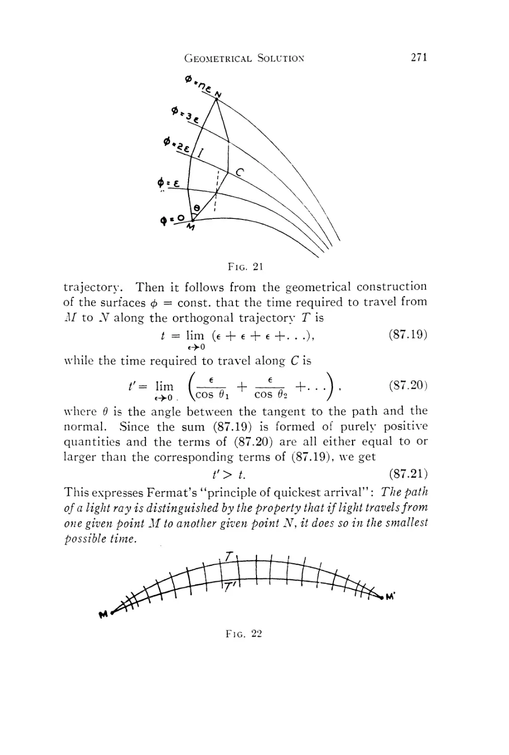
i.Geometrical solution of the partial differential equation.
Hamilton's optico一mechanical analogy
8.The significance of Hamilton's partial differential equation
in the theory of +-a、一e motion
9.The geometrization of dynamics. '-,\-on一Riemannian
geometrics. The metrical significance of Hamilton’s
partial differential equation
PAGE
243
IX。HISTORICAL SURVEY
BIBLIOGRAPHY
INDEX
305
INTRODUCTION
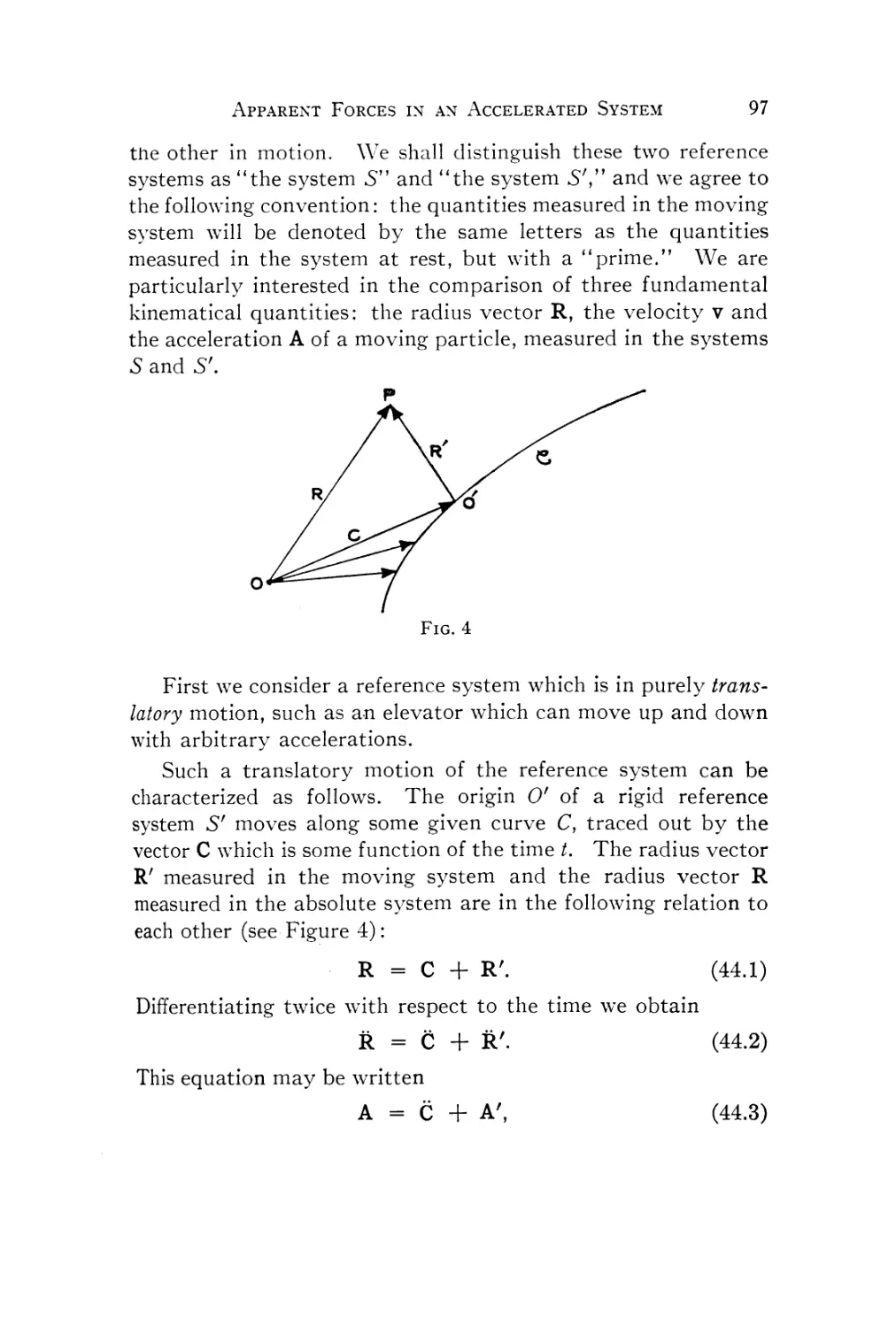
1.The variational approach to mechanics. Ever since New-
ton laid the solid foundation of dynamics by formulating the laws
of motion,the science of mechanics developed along two main
lines.One branch,which we shall call“vectorial mechanics,”‘
starts directly from Newton’s laws of motion.It aims at recog-
nizing all the forces acting on any given particle,its motion being
uniquely determined by the known forces acting on it at every
instant.The analysis and synthesis of forces and moments is
thus the basic concern of vectorial mechanics.
`while in Newton’s mechanics the action of a force is measured
by the momentum produced by that force,the great philosopher
and universalist Leibniz,a contemporary of Newton,advocated
another quantity,the vis viva (living force),as the proper gauge
for the dynamical action of a force.This vis viva of Leibniz
coincides一 apart from the unessential factor 2 -with the quan-
tity we call today“kinetic energy.”Thus Leibniz replaced the
"momentum”of Newton by the“kinetic energy.”At the same
time he replaced the“force”of Newton by the "work of the
force.”This "work of the force”was later replaced by a still
more basic quantity,the "work function.”Leibniz is thus the
originator of that second branch of mechanics,usually called
"analytical mechanics,”止which bases the entire study of equili-
brium and motion on two f undamental scalar quantities,the
“kinetic energy”and the "work function,”the latter frequently
replaceable by the“potential energy.”
Since motion is by its very nature a directed phenomenon,it
seems puzzling that two scalar quantities should be sufficient to
determine the motion.The energy theorem,which states that
the sum of the kinetic and potential energies remains unchanged
'This use of the term does not necessarily imply that vectorial methods
are used.
2See note on terminology at end of chap.T,section 1.
.vii
XV111
INTRODUCTION
during the motion,yields only one equation,while the motion of
a single particle in space requires three equations;in the case of
mechanical systems composed of two or more particles the dis-
crepancy becomes even greater.And yet it is a fact that these
two fundamental scalars contain the complete dynamics of even
the most complicated material system,provided they are used
as the basis of a principle rather than of an equation.
2.The procedure of Euler and Lagrange.In order to see
how this occurs,let us think of a particle which is at a point P,
at a time t,.Let us assume that we know its velocity at that
time.Let us further assume that we know that the particle will
be at a point P2 after a given time has elapsed.Although iwe do
not know the path taken by the particle,it is possible to es-
tablish that path completely by mathematical experimentation,
provided that the kinetic and potential energies of the particle
are given for any possible velocity and any possible position.
Euler and Lagrange,the first discoverers of the exact prin-
ciple of least action,proceed as follows.Let us connect the two
points P, and P2 by any tentative path.In all probability this
path,which can be chosen as an arbitrary continuous curve,will
not coincide with the actual path that nature has chosen for the
motion.However,we can gradually correct our tentative solution
and eventually arrive at a curve which can be designated as the
actual path of motion.
For this purpose we let the particle move along the tentative
path in accordance with the energy principle.The sum of the
kinetic and potential energies is kept constant and always equal
to that value E which the actual motion has revealed at time t1.
This restriction assigns a definite velocity to any point of our
path and thus determines the motion.We can choose our path
freely,but once this is done the conservation of energy deter-
mines the motion uniquely.
In particular,we can calculate the time at which the particle
will pass an arbitrarily given point of our fictitious path and
hence the time一integral of the vis viva i.e.,of double the kinetic
energy,extended over the entire motion from P1 to P-2.This
INTRODUCTION
XiX
time integral is called "action.”It has a definite value for our
tentative path and likewise for any other tentative path,these
paths being always drawn between the same two end一points P1,
P2 and always traversed with the same given energy constant E.
The value of this "action”will vary from path to path.For
some paths it will come out larger,for others smaller. Xlathe-
matically we can imagine that all possible paths have been tried.
There must exist one definite path (at least if P1 and P:are not
too far apart) for which the action assumes a minimum value.
The principle of least action asserts that this particular path is
the one chosen by nature as the actual path of motion。
We have explained the operation of the principle for one single
particle.It can be generalized,however,to any number of par-
ticles and any arbitrarily complicated mechanical system.
3.Hamilton's procedure. We encounter problems of mecha-
nics for which the work function is a function not only of the
position of the particle but also of the time.For such systems
the law of the conservation of energy does not hold,and the
principle of Euler and Lagrange is not applicable,but that of
Hamilton is.
In Hamilton's procedure we again start with the given initial
point P:and the given end一point P2.But now we do not restrict
the trial motion in any way. Not only can the path be chosen
arbitrarily一 save for natural continuity conditions一 but also the
motion in time is at our disposal.All that we require now is that
our tentative motion shall start at the observed time t1 of the
actual motion and end at the observed time 12.(This condition
is not satisfied in the procedure of Euler-Lagrange,because there
the energy theorem restricts the motion,and the time taken to
go from P:to P2 in the tentative motion will generally differ from
the time taken in the actual motion.)
The characteristic quantity that we now use as the measure
of action一 there is unfortunately no standard name adopted for
this quantity一 is the time-integral of the difference between the
kinetic and potential energies. The Hamiltonian formulation of
the principle of least action asserts that the actual motion realized
XX
INTRODUCTION
in nature is that particular motion fo;二hick this action assumes its
smallest value.
One can show that in the case of "conservative”systems,i.e
systems which satisfy the law of the conservation
principle
principle,
of Euler-Lagrange is a consequence
but the latter principle remains valid
of energy,the
of Hamilton’s
even for non-
conservative systems.
4. The calculus of variations.The mathematical problem
of minimizing an integral is dealt with in a special branch of the
calculus.called“calculus of variations.”The mathematical
theory shows that our final results can be established without
taking into account the infinity of tentatively possible paths.
we can restrict our mathematical experiment to such paths as
are i顽nicely二ear to the actual path.A tentative path which
differs from the actual path in an arbitrary but still infinitesimal
degree,is called a“variation”of the actual path,and the calculus
of variations investigates the changes in the value of an integral
caused by such infinitesimal variations of the path.
5.Comparison between the vectorial and the variational
treatments of mechanics.The vectorial and the variational
theories of mechanics are two different mathematical descriptions
of the same realm of natural phenomena.Newton’s theory bases
everything on two fundamental vectors:"momentum”and
“force”;the variational theory,founded by Euler and Lagrange,
bases everything on two scalar quantities:“kinetic energy”and
"work function.”Apart from mathematical expediency,the
question as to the equivalence of these two theories can be raised.
In the case of free particles,i.e.particles whose motion i s not
restricted一by given "constraints,”the two forms of description
lead to equivalent results.But for systems with constraints the
analytical treatment is simpler and more economical.The given
constraints are taken into account in a natural way by letting the
system move along all the tentative paths in harmony with them.
The vectorial treatment has to take account of the forces which
maintain the constraints and has to make definite hypotheses
I N TRODt'CTIO
xxt
concerning them.Newton’s third law of motion,"action equals
reaction,”does not embrace all cases.It sumces only for the
dynamics of rigid bodies.
On the other hand,Newton’s approach does not restrict the
nature of a force,while the variational approach assumes that
the acting forces are derivable from a scalar quantity,the“work
function.”Forces of a frictional nature,which have no work
function,are outside the realm of variational principles,while
the Newtonian scheme has no dimculty in including them.
Such forces originate from inter一molecular phenomena which are neglected in
the macroscopic description of motion.If the macroscopic parameters of a
mechanical system are completed by the addition of microscopic parameters,
forces not derivable from a work function would in all probability not occur.
6. Mathematical evaluation of the variational principles.
Many elementary problems of physics and engineering are sole-
able by vectorial mechanics and do not require the application
of variational methods.But in all more complicated problems
the superiority of the variational treatment becomes conspicuous.
This superiority is due to the complete freedom we have in
choosing the appropriate coordinates for our problem.The prob-
lems which are well suited to the vectorial treatment are essen-
tially those which can be handled with a rectangular frame of
reference,since the decomposition of vectors in curvilinear co-
ordinates is a cumbersome procedure if not guided by the ad-
vanced principles of tensor calculus.Although the fundamental
importance of invariants and covariants for all phenomena of
nature has been discovered only recently and so was not known
in the time of Euler and Lagrange,the variational approach to
mechanics happened to anticipate this development by- satisfying
the principle of invariance automatically. We are allowed sove-
reign freedom in choosing our coordinates,since our processes
and resulting equations remain valid for an arbitrary choice of
coordinates.The mathematical and philosophical value of the
variational method is firmly anchored in this freedom of choice
and the corresponding freedom of arbitrary coordinate trans-
formations.It greatly facilitates the formulation of the differen-
tial equations of motion,and likewise their solution.If we hit
INTRODUCTION
on a certain type of coordinates,called "cyclic”or "ignorable,”
a partial integration of the basic differential equations is at once
accomplished.If all our coordinates are ignorable,our problem
is completely solved.Hence,we can formulate the entire prob-
lem of solving the differential equations of motion as a problem
of coordinate transformation.Instead of trying to integrate the
differential equations of motion directly,we try to produce more
and more ignorable coordinates.In the Euler一Lagrangian form
of mechanics it is more or less accidental if we hit on the right
coordinates,because we have no systematic way- of producing
ignorable coordinates.But the later developments of the theory
by Hamilton and Jacobi broadened the original procedures im-
mensely by introducing the“canonical equations,”with their
much wider transformation properties.Here we are able to
produce a compleille set of ignorable coordinates by solving one
single partial differential equation.
Although the actual solution of this differential equation is
possible only for a restricted class of problems,it so happens that
many important problems of theoretical physics belong pre-
cisely to this class.And thus the most advanced form of analy-
tical mechanics turns out to be not only esthetically and logically
most satisfactory,but at the same time very practical by provid-
ing a tool for the solution of many dynamical problems which
are not accessible to elementary methods.1
7. Philosophical evaluation of the variational approach to
mechanics.Although it is tacitly agreed nowadays that scien-
tific treatises should avoid philosophical discussions,in the case
of the variational principles of mechanics an exception to the
rule may be tolerated,partly because these principles are rooted
in a century which eras philosophically oriented to a very high
degree,and partly because the variational method has often
been the focus of philosophical controversies and misinterpre-
tations.
The present book does not discuss other integration
not based on the transformation theorv.
reader is referred to the advanced text一books
C
oncerning
methods which are
such methods the
mentioned in the Bibliography.
INTRODUCTION
XXlll
Indeed,the idea of enlarging reality by including“tentative"
possibilities and then selecting one of these by the condition that
it minimizes a certain quantity,seems to bring a purpose to the
flow of natural events.This is in contradiction to the usual
causal description of things.Yet we must not be surprised that
for the more universal approach which was current in the 17th
and 18th centuries,the two forms of thinking did not necessarily
appear contradictor-y. The keynote of that entire period was
the seemingly pre-established harmony between“reason”and
"world.”The great discoveries of higher mathematics and their
immediate application to nature imbued the philosophers of those
days with an unbounded confidence in the fundamentally intel-
lectual structure of the world.The“deus intellectualis”was
the basic theme of the philosophy of Leibniz,no less than that
of Spinoza.At the same time Leibniz had strong teleological
tendencies,and his activities had no small influence on the
development of variational methods.' But this is not surprising
if we observe how the purely esthetic and logical interest in
maximum一minimum problems gave one of the strongest impulses
to the development of infinitesimal calculus,and how Fermat’s
derivation of the laws of geometrical optics on the basis of his
“principle of quickest arrival”could not fail to impress the
philosophically一oriented scientists of those days.That the dilet-
tante misuse of these tendencies by Alaupertuis and others for
theological purposes has put the entire trend into disrepute,is
not the fault of the great philosophers.
The sober, practical,matter-of-fact nineteenth century
which carries over into our day一 suspected all speculative and
interpretative tendencies as“metaphysical”and limited its pro-
gramme to the pure description of natural events.In this philo-
sophy mathematics plays the role of a shorthand method,a
conveniently economical language for expressing involved rela-
tions.Hence,it is not surprising,but quite consistent with the
“positivistic”spirit of the nineteenth century,to meet with the
following appraisal of analytical mechanics by one of the leading
'See the attractive historical study of A. Kneser, Das Prinzip der kleinsten
Wirkung von Leibniz bis zur Gegenwart(Leipzig:Teubner, 1928).
XXI、"
INTRODUCTION
figures of that trend,E.人lach,in“The Science of Mechanics”
(Open Court,1893,p.480):“No fundamental light can be ex-
petted from this branch of mechanics.On the contrary,the
discovery of matters of principle must be substantially completed
before we can think of framing analytical mechanics the sole aim
of which is a perfect practical master`- of problems.Whosoever
mistakes this situation will never comprehend Lagrange's great
performance,which here too is essentially of an econ。,;:2cal
character.”(Italics in the original.)According to this philosophy
the variational principles of mechanics are not more than alter-
native mathematical formulations of the fundamental laws of
Newton,without any primary importance.
However,philosophical trends float back and forth and the last
word is never spoken.In our own day we have witnessed at least
one fundamental discovery of unprecedented magnitude,namely
Einstein’s Theory of General Relativity,which was obtained by
mathematical and philosophical speculation of the highest order.
Here was a discovery made b)·a kind of reasoning that a posi-
tivist cannot fail to call“metaphysical.”and yet it provided an
insight into the heart of things that mere experimentation and
sober registration of facts could never have revealed.The Theory
of General Relativity brought once again to the fore the spirit
of the great cosmic theorists of Greece and the eighteenth century.
In the light of the discoveries of relativity,the variational
foundation of mechanics deserves more than purely formalistic
appraisal.Far from being nothin; but an alternative formula-
tion of the Newtonian laws of motion,the following points sug-
gest the supremacy of the variational method:
I.The Principle of Relativity requires that the laws of
nature shall be formulated in an“invariant”fashion,i.e.inde-
pendently- of any, special frame of reference.The methods of
the calculus of、一ariations automatically satisfy- this principle,
because the minimum of a scalar quantity does not depend on
the coordinates in +,-hich that quantity- is measured.while the
Newtonian equations of motion did not satisfy the principle of
relativity-, the principle of least action remained valid, with the
INTRODUCTION
only modification that
brought into harmony w
the basic action quantity
XYV
had to be
ith the requirement of invariance.
2.The Theory of General Relativity has shown that matter
cannot be separated from field and is in fact an outgrowth of the
field.Hence,the basic equations of physics must be formulated
as partial rather than ordinary differential equations.\\一hile
Newton’s particle picture can hardly be brought into harmony
with the field concept,the variational methods are not restricted
to the mechanics of particles but can be extended to the mechanics
of continua.
3.The Principle of General Relativity is automatically satis-
fied if the fundamental“action”of the variational principle is
chosen as an int-,ariant under any coordinate transformation.
Since the differential geometry of Riemann furnishes us such
invariants,we have no dimculty in setting up the required field
equations.Apart from this,our present knowledge of mathe-
matics does not give us any clue to the formulation of a co一variant,
and at the same time consistent,sI·s tern of field equations.Hence,
in the light of relativity the application of the calculus of varia-
tions to the laws of nature assumes more than accidental signi-
ncanoe.
THE VARIATIONAL
PRINC I PLES OF M ECHAXICS
CHAPTER
THE BASIC CONCEPTS OF ANALYTICAL MECHANICS
1.The principal viewpoints of analytical mechanics.The
analytical form of mechanicsI,as introduced by Euler and La-
grange,differs considerably in its method and viewpoint from
vectorial mechanics.The fundamental law of mechanics as
stated by Newton:“mass times acceleration equals moving
force”holds in the first instance for a single particle only. It
NN-as deduced from the motion of a particle in the field of gravity
on the earth and was then applied to the motion of planets under
the action of the sun.In both problems the moving body could be
idealized as a“mass point”or a“particle,”i.e.a single point to
which a mass is attached,and thus the dynamical problem pre-
sented itself in this form:“A particle can move freely in space
and is acted upon by a given force.Describe the motion at any
time.”The lain of Newton gave the differential equation of
motion,and the dynamical problem was reduced to the integ-
ration of that equation.
If the particle is not free but associated with other particles,
as for example in a solid body,or a fluid,the Newtonian equation
is still applicable if the proper precautions are observed·One has
to isolate the particle from all other particles and determine the
force which is exerted on it by the surrounding particles.Each
particle is an independent unit which follows the law of motion
of a f ree particle.
This force-analysis sometimes becomes cumbersome. The
unknown nature of the interaction forces makes it necessary to
introduce additional postulates,and Newton thought that the
principle "action equals reaction,”stated as his third law of
motion,would take care of all dynamical problems.This,how-
ever,is not the case,and even for the dynamics of a rigid body
4
THE BASIC CONCEPTS OF ANALYTICAL MECHANICS
the additional hypothesis that the inner forces of the body are
of the nature of central forces had to be made.In more compli-
cated situations the Newtonian approach fails to give a unique
answer to the problem.
The analytical approach to the problem of motion is quite
different.The particle is no longer an isolated unit but part of
a“system.”A "mechanical system”signifies an assembly of
particles which interact with each other. The single particle has
no significance;it is the system as a whole which counts.For
example,in the planetary problem one may be interested in the
motion of one particular planet.Yet the problem is unsolvable
in this restricted form.The force acting on that planet has its
source principally in the sun,but to a smaller extent also in the
other planets,and cannot be given without knowing the motion
of the other members of the system as well.And thus it is
reasonable to consider the dynamical problem of the entire sys-
tem,without breaking it into parts.
But even more decisive is the advantage of a unified treat-
ment of force一analysis.In the vectorial treatment each point
requires special attention and the force acting has to be deter-
mined independently for each particle.In the analytical treat-
ment it is enough to know one single function,depending on the
positions of the moving particles;this "work function”contains
implicitly all the forces acting on the particles of the system.
They can be obtained from that function by mere differentiation.
Another fundamental difference between the two methods
concerns the matter of "auxiliary conditions.”It frequently
happens that certain kinematical conditions exist between the
particles of a moving system which can be stated a priori. For
example,the particles of a solid body may move as if the body
were“rigid,,’which means that the distance between any two
points cannot change.Such kinematical conditions do not
actually exist on a priori grounds.They are maintained by
strong forces.It is of great advantage,however,that the ana-
lytical treatment does not require the knowledge of these forces,
but can take the given kinematical conditions for granted.We
can develop the dynamical equations of a rigid body without
THE PRINCIPAL VIEWPOINTS OF ANALYTICAL MECHANICS
5
knowing what forces produce the rigidity of the body. Similarly
we need not know in detail what forces act between the particles
of a fluid.It is enough to know the empirical fact that a fluid
opposes by very strong forces any change in its volume,while
the forces which oppose a change in shape of the fluid without
changing the volume are slight.Hence,We can discard the un-
known inner forces of a fluid and replace them by the kinematical
conditions that during the motion of a fluid the volume of any
portion must be preserved.If one considers how much simpler
such an a priori kinematical condition is than a detailed know-
ledge of the forces which are required to maintain that condition,
the great superiority of the analytical treatment over the vecto-
rial treatment becomes apparent.
However,more fundamental than all the previous features is
the un访,i二g principle in which the analytical approach culmi-
nates.The equations of motion of a complicated mechanical
system form a large number一 even an infinite number一 of
separate differential equations.The variational principles of
analytical mechanics discover the unifying basis from which all
these equations follow.There is a principle behind all these
equations which expresses the meaning of the entire set.Given
one fundamental quantity,"action,”the principle that this
action be stationary leads to the entire set of differential equa-
tions.Nl oreover,the statement of this principle is independent
of any special system of coordinates.Hence,the analytical equa-
tions of motion are also invariant with respect to any coordinate
transformations.
Note on terminology. The word "analytical”in the expression "analytical
mechanics" has nothing to do with the philosophical process of analyzing,
but comes from the mathematical term "analysis,”referring to the applica-
tion of the principles of infinitesimal calculus to problems of pure and applied
mathematics.While the French and German literature reserves the term
"analytical mechanics”for the abstract mathematical treatment of mechanical
problems by the methods of Euler, Lagrange,and Hamilton,the English
and particularly the American literature frequently calls even very elementary
applications of the calculus to problems of simple vectorial mechanics by the
same name.The term“mechanics”includes“statics" and“dynamics,”the
first dealing with the equilibrium of particles and systems of particles, the
6
THE BASIC CONCEPTS OF ANALY TICAL 'MECHANICS
second with their motion.(A separate application of mechanics deals with
the "mechanics of continua"-which includes fluid mechanics and elasticit)一
based on partial,rather than ordinary, differential equations.These problems
are not included in the present book.)
Summaryr.These,then,are
viewpo
differ:
1.
ints in which vectorial and
the four principal
analytical mechanics
Vectorial mechanics isolates the particle and
considers it as an individual;anal\一tical mechanics
considers the system as a、、!hole.
2.\-ectorial mechanics constructs a separate
acting force for each moving particle;analytical
mechanics considers one single function:the "-ork
function (or potential energy).This one function
contains all the necessar-\一information concerning forces.
3.If strong forces maintain a definite relation
between the coordinates of a system,and that relation
is empiricall)?given,the vectorial treatment has to
consider the forces necessary to maintain it.The anal\,-
tical treatment takes the given relation for granted,
without requiring knowledge of the forces which main-
tain it.
4.In the analytical method,the entire set of
equations of motion can be developed from one unified
principle which implicitly includes all these equations.
This principle takes the form of minimizing a certain
quantity,the“action.”Since a minimum principle is
independent of an-,,-、pecial reference system,the
equations of analytical mechanics hold for any set of
coordinates.This permits one to adjust the coordi-
nates employed to the specific nature of each problem.
2.Generalized coordinates.In the elementary vectorial
treatment of mechanics the abstract concept of a“coordinate”
does not enter the picture.The method is essentially geo-
metrical in character.
GENERALIZED COORDINATES
7
Vector methods are eminently useful in problems of statics.
HoNN-ever,when it comes to problems of motion,the number of
such problems which can be solved by pure vector methods is
relatively smallJ.For the solution of more involved problems,
the geometrical methods of vectorial mechanics cease to be ade-
quate and have to give way to a more abstract analytical treat-
ment.In this new analytical foundation of mechanics the
coordinate concept in its most general aspect occupies a central
position.
Analytical mechanics is a completely mathematical science.
E、一。rN-thing is done by calculations in the abstract realm of
quantities.The physical world is translated into mathematical
relations.This translation occurs with the help of coordinates.
The coordinates establish a one一to-one correspondence between
the points of physical space and numbers.After establishing
this correspondence,we can operate with the coordinates as
algebraic quantities and forget about their physical meaning.
The end result of our calculations is then finally translated back
into the world of physical realities.
During the century from Fermat and Descartes to Euler and
Lagrange tremendous developments in the methods of higher
mathematics took place.One of the most important of these was
the generalization of the original coordinate idea of Descartes.
If the purpose of coordinates is to establish a one一to-one corres-
pondence between the points of space and numbers,the setting
up of three perpendicular axes and the determination of length,
width,and height relative to those axes is but one way of estab-
lishing that correspondence.Other methods can serve equally
well.For example,the polar coordinates r,0,0 may take the
place of the rectangular coordinates x,y,:.It is one of the
characteristic features of the analytical treatment of mechanics
that +-e do not specify -the nature of the coordinates which trans-
late a given physical situation into an abstract mathematical
situation.
Let us first consider a mechanical system which is composed
of N free particles,“f ree”in the sense that they are not restricted
by any kinematical conditions.The rectangular coordinates
of these particles:
8
TIIE BASIC CONCEPTS OF ANALYTICAL MECHANICS
x、,y、,:、,(ti=1,2,…,N),(12.1)
characterize the position of the mechanical system,and the prob-
lem of motion is obviously solved if x、,争,;,:z are given as func-
tions of the time t.
The same problem is likewise solved,however,if the x、,y 1i):l
are expressed in terms of some other quantities
9l,q?,…,q3二,(12.2)
and then these quantities q、are determined as functions of the
time t.
This indirect procedure of solving the problem of motion
provides great analytical advantages and is in fact the decisive
factor in solving dynamical problems.1Iathematically,we call
it a“coordinate transformation.”It is a generalization of the
transition from rectangular coordinates x,y,:of a single point
in space to polar coordinates r,B,0.The relations
x=r sin 6 cos }),
y=r sin 6 sin ",(12.3)
z=I,cos0,
are generalized so that the new variables are expressed as arbi-
trarv functions of the old variablesr.The number of variables
is not 3 but .3 AT, since the position of the mechanical system
requires 31V coordinates for its characterization.And thus the
general form of such a coordinate transformation appears as
followS:
x1=f , (q l,…,q 3,7V),
(12.4)
z"'-=介二(q1,…,q3j.%T).
We can prescribe these functions, fl,…,f W, in any way we
wish and thus shift the original problem of determining the x;,
多,、,z、as functions of t to the new problem of determining the q,,…,
q3,v as functions of t.认一ith proper skill in choosing the right coordi-
nates,we may solve the new problem more easily than the original
one.The flexibility of the reference system makes it possible
to choose coordinates which are particularly suitable for the
GE\ ERALIZED COORDINATES
9
given problem.For example,in the planetary problem,1.e.a
particle revolving around a fixed attracting centre,polar coordi-
nates are better suited to the problem of motion than rectangular
ones.
The advantage of generalized coordinates is even more obvious
if mechanical systems with given kinematical conditions are con-
sidered.Such conditions find their mathematical expression in
certain functional relations between the coordinates.For exam-
ple,two atoms may form a molecule。the distance between the
bN-o atoms being determined by strong forces which are in equili-
brium at that distance.Dynamically this system can be con-
sidered as composed of two mass points with coordinates x1,y1,
::and x:,〕,2,::which are kept at a constant distance a from one
another. This implies the condition
(x1一x2)2+(y,一:}12)2+(z,一z2) 2 = a2. (12.5)
Because of this condition,the 6 coordinates x1,…,z2 cannot be
prescribed arbitrarily.It suffices to give 5 coordinates;the sixth
coordi“ate is then determined by the auxiliary condition(12.5).
However,it is obviously inappropriate to designate one of the rec-
tangular coordinates as a dependent variable when the relation
(12.J)is symmetrical in all coordinates.It is more natural to pre-
scribe the three rectangular coordinates of the centre of mass of
the system and add two angles which characterize the direction of
the axis of the diatomic molecule.The 6 rectangular coordinates
xl,…,z2 are expressible in terms of these 5 parameters.
As another example,consider the case of a rigid body,which
can be composed of any number of particles.But whatever the
number of particles may be,it is sufficient to give the three co-
ordinates of the centre of mass and three angles which define the
position of the body relative to the centre of mass.These 6 para-
meters determine the position of the rigid body completely. The
coordinates of each of the component particles can be expressed
as functions of these 6 parameters.
In general,if a mechanical system consists of N particles and
there are m independent kinematical conditions imposed,it will
be possible to characterize the configuration of the mechanical
system uniquely by
10
THE B:}sic CONCEPTS OF A\ ALITICAL -IECIIA\ics
”一3 X - vi ( 1,2. 6)
independent parameters
9l,92,…,q、,(12.r
in such a way that the rectangular coordinates of all the particles
are expressible as functions of the -\rariables(12.7):
x1=fl(gl,…,q,:),
(12.8)
z --=关l- (q,…,q,乙).
The number,:is a characteristic constant of the given mechanical
sNrstem which cannot be altered.Less than it parameters are not
enough to determine the position of the systen-i.More than n
parameters are not required and could not be assigned without
satisfying certain conditions.We express the fact that,:para-
meters are necessary and sumcient for a unique characterization
of the configuration of the system by saying that it has“n degrees
of freedom.”Moreover,we call the,:parameters q1,92,…,q、
the“generalized coordinates”of the system.The number X of
particles which compose the mechanical system is immaterial for
the analytical treatment,as are also the coordinates of these
particles.It is the generalized coordinates q1,92,…,q,, and
certain basic functions of them which are of importance. A rigid
body may be composed of an infinity of mass points,yet for the
mechanical treatment it is a sN-stem of not more than G inde-
pendent coordinates.
Examples:
One degree of f reedozn:A piston moving up and down.A
rigid body rotating about a fixed axis.
T-w!o degrees of freedanz:A particle moving on a given surface.
TIz ree degrees of freedom:A particle moving in space.A rigid
body rotating about a fixed point (top).
Four degrees of freedom:Two components of a double star
revolving in the same plane.
Five degrees of f reedonz:Two particles kept at a constant dis-
tance from each other.
(-jE-ERALIZED COORDINATES
11
Sit degrees of f reedo二:Two planets revolving about a fixed
sun.A rigid body moving freely in space.
The generalized coordinates q,,qZ,…,1。may or may not
have a geometrical significance.It is necessary,however,that
the functions(12.8) shall be finite,single valued,continuous and
differentiable,and that the Jacobian of at least one combination
of n functions shall be different from zero.These conditions may
be violated at certain singular points,which have to be excluded
from consideration.For example,the transformation(12.3)from
rectangular to polar coordinates satisfies the general regularity
conditions,but special care is required at the values r=0 and
8=0, for二一hich the Jacobian of the transformation vanishes.
In addition to these restrictions“in the small,”certain con-
ditions "in the large”have to be observed.It is necessary that ar
proper continuous range of the variables ql,92,…,q,z shall
permit a sumciently +-ide range of the original rectangular co-
ordinates,Without restricting them more than the given kine-
matical conditions require.For example,the transformation
(12.3)guarantees the complete,infinite range of the variables
YX,〕,,:if r varies between 0 and co,8 between 0 and二,and 0be-
t`i-een 0 and 2二.However,such conditions in the large seldom
burden our considerations because,even if we cannot cover the
entire range of motion,we may still be able to describe a char-
acteristic portion of it.
It is not always advisable to clin)Iinate all the kinematical
conditions of a problem by introducing suitable generalized co-
ordinates.\\一c sometimes prefer to eliminate only some of the
kinematical conditions,and
restricting conditions.Hence
to leave the others
the general problem
systems with kinematical conditions presents itself
lo}N-ing form.
equations of
We have the equations(12.S) and in
additional
mechanical
in the fol-
addition nn
the form:
,、(q I,92,…,qn)=0,(!’=1
。:)
(12.0)
The numb‘·:。f degrees of freedom is here
12
THE BASIC CONCEPTS OF ANALYTICAL MECHANICS
Sunmmary.Analytical problems of motion require
a generalization of the original coordinate concept of
Descartes.Any set of parameters which can char-
acterize the position of a mechanical system may be
chosen as a suitable set of coordinates.They are called
the "generalized coordinates”of the mechanical
svstem.
3.The configuration space.One of the most imaginative
concepts of the abstract analytical treatment of mechanical prob-
lems is the concept of the configuration space.If we associate with
the three numbers x,y,:a point in a three一dimensional space,
there is no reason why we should not do the same with the n
numbers q1,q2,…,qn,considering these as the rectangular co-
ordinates of a“point”P in an n一dimensional space.Similarlv,
if we can associate with the equations
x=fW,
y=gW,(13.1)
“=h (t),
the idea of a“curve”and the motion of a point along that curve,
there is no reason why we should not do the same with the corres-
ponding equations
q1==q1W,
(13.2)
qn=qn (t).
These equations represent the solution of a dynamical prob-
lem.In the associated geometrical picture,we have a point P
of an n一dimensional space which moves along a given curve of
that space.
This geometrical picture is a great aid to our thinking. No
matter how numerous the particles constituting a given mecha-
nical system may be,or how cornplicated the relations existing
between them,the entire mechanical system is pictured as a
THE CONF1GURATION SPACE
13
single point of a mane,一dimensional space,called the“configura-
tion space.”For example,the position of a rigid body一 with all
the infinity of mass points which form it一 is symbolized as a
single point of a G -一dimensional space. This 6一dimensional space
has,to be sure,nothing to do with the physical reality of the rigid
body. It is merely correlated to the rigid body in the sense of a
one-to-one correspondence. The various positions of the rigid
body are "mapped”as various points of the 6一dimensional space,
and conversely,the various points of a 6一dimensional space can
be physically interpreted as various positions of a rigid body. For
the sake of brevity we shall refer to the point which symbolizes
the position of the mechanical system in the configuration space
as the“C一point,”while the curve traced out by that point during
the motion `rill be referred to as the“C一curve.”
The picture that we have formed here of the configuration
space needs further refinement.+'e based our discussions on the
analytical geometry of a Euclidean space of n dimensions.Ac-
cordingly +7,e have represented the n generalized coordinates of
the mechanical system as rectangular coordinates of that space.
A much more appropriate picture of the geometrical structure of
the configuration space can be obtained if we change from analy-
tical' geometry to differential geometry,as we shall do in section 5
of this chapter. However,even our preliminary picture can serve
some useful purposes.we demonstrate this by the following
example.
The position of a f ree particle in space may be characterized
by the polar coordinates (r,8,")·If these values are taken as
rectangular coordinates of a point,we get a space whose geo-
metrical properties are obviously greatly distorted compared with
the actual space.Straight lines become curves,angles and
distances are changed.Yet certain important properties of
space remained unaltered by this mapping process.A point re-
mains a point,the neighborhood of a point remains the neigh-
borhood of a point,a curve remains a curve,adjacent curves
remain adjacent curves.Continuous and differentiable curves re-
main continuous and differentiable curves.Now for the processes
of the calculus of variations such“topological”properties of
14
THE BASIC CONCEPTS OFA\ALYTICAL MECHANICS
space are the really important things,while the "metrical”pro-
perties of space,such as distances,angles,areas,etc.,are irrele-
vant.For this reason even the simplified picture of a configura-
tion space without a corresponding geometry is still an excellent
aid in visualizing some abstract analytical processes.
Sit”,nzary.The pictorial language of n一dimen-
sional geometry makes it possible to extend the meth-
anics of a single mass一point to arbitrarily complicated
mechanical systems.Such a system may be replaced
b),a single point for the study of its motion.But the
space which carries this point is no longer the ordinary
physical space.It is an abstract space with as many
dimensions as the nature of the problem requires.
4. Mapping of the space on itself.Since the significance of
the}:generalized coordinates
4l,92
q,;
(14.1)
is not sl_)(2cified beyond the requirement that it shall allow a corn-
plete characterization of the system,we may choose another set
of quantities
q1,q?,…,q二
(14.2)
。s (yeneralized coordinates.There must,then,exist a functional
relationship between the two sets of coordinates expres:1}〕I e, i n
the form:
(j:=fl}gl,…,9n),
(/n=,f n(ql,…,q,:)
(14.3)
MAPPING OF TH:, SPACE O\ ITSELF
15
The functions f i,f?,…,f n must satisfy the ordinary regularity
conditions.They must be finite,single valued,continuous and
differentiable functions of the q、,二·ith a Jacobian△which is
different from zero.
Differentiation of the equations(14.3)give:
dql一篡dql+…+塔:dq。
dqn一绘dql+…+毅dqn
(14.4)
These equations show that no matter what functional relations
exist between the two sets of coordinates,their differentials are
aINN-ays linearly dependent.
we can connect a definite geometrical picture with this“trans-
formation of coordinates.”If the qi are plotted as rectangular
coordinates of an n一dimensional space,the same can be done with
the q}. We then think of the points of the q-space, and the points
.!1,1,..,龟
FIG. 1
of the q-space. To a definite point P of the q一space
a definite point P of the石一space.
corresponds
For this reason a transforma-
tion of the form(14.3)is called a“point transformation.”In a
16
THE BASIC CONCEPTS OF ANALYTICAL MECHANICS
certain region the points of the q一space are in a one一to一one corres-
pondence二,ith the points of the q-space. we have a "mapping"
of the n一dimensional space on itself. This mapping satisfies more
than the general requirements of on。一to一one correspondence.Con-
tinuity is preserved.The neighborhood of the point P is mapped
on the neighborhood of于and vice versa.But even more can be
said.A straight line of the q一space is no longer a straight line
of the西一space.However,the relations get more and more regu-
lar as二:e consider smaller and smaller regions. In an infinil esimal
region around P straight lines aye mapped on straight lines and
parallel lines remain parallel lines,although lengths and angles
are not preserved.A small parallelepiped in the neighborhood
of P is mapped on a small parallelepiped in the neighborhood of
P.The functional determinant△is just the determinant of the
linear equations(14.4).Geometrically this determinant repre-
sents the ratio of the volume T of the new parallelepiped to the
volume -r of the original one.The non一vanishing of△takes care
of the condition that the entire neighborhood of P shall be
mapped on the entire neighborhood of P,which is indeed neces-
sary if the one一to-one correspondence between the points of the
two spaces shall be reversible.if△vanishes,an n一dimensional
region around P is mapped into a region of smaller dimension-
alit),around户,二,ith the consequence that some points around
户have no image in the q一space while others have an infinity of
images·
A physical realization of such a mapping of the space on itself
can be found in the。:olion of a fluid.If the fluid particles are
marked and a snapshot is taken at a certain instant,and then
again at a later instant,the corresponding positions of the fluid
particles represent a mapping of the space on itself.If we cut
out a little fluid parallelepiped,the motion of the fluid will distort
the angles and the lengths of the figure but it still remains a paral-
lelepiped.Incidentally,if the fluid is incompressible,the volume
of the parallelepiped will remain unchanged during the motion.
The analytical picture of the motion of such a fluid is a coor-
dinate transformation with a functional determinant which has
everywhere the value I.
KINETIc ENERGY AND RIEMANNIAN GEOMETRY
17
S1,1rt2,,:aril.In view(、f the arbitrariness of co-
ordinates,one set of generalized coordinates can be
changed to another set.This“transformation of co-
ordinates”can be conceived geometrically as a map-
ping of an n一dimensional space on itself.The mapping
does not preserve angles or distances.Straight lines
are bent into curves.Yet in infinitesimal regions,in
the neighborhood of a point,all mappings“straighten
out”:Straight lines are mapped on straight lines,
parallel lines on parallel lines,and the ratio of volumes
is preserved.
5.Kinetic energy and Riemannian geometry.' The use of
arbitrary generalized coordinates in describing the motion of a
mechanical system is one of the principal features of analytical
mechanics.The equations of analytical mechanics are of such
a structure that they can be stated in a form which is inde-
pendent of the coordinates used.This property of the General
equations of motion links up analytical mechanics with one of
the major developments of nineteenth century mathematics:the
theory of invariants and covariants.This theory came to ma-
turity in our own day when Einstein’s theory of relativity showed
how the laws of nature are tied up with the problem of invari-
ance.The principal programme of relativity is precisely that of
formulating the la二:of二ature indepe二dently of any special co-
ordinate system.The mathematical solution of this problem has
shown that the matter is intimately linked with the Riemannian
foundation of geometry.According to Einstein’s general rela-
'The first discoverer of the intimate relation between dynamics and the
geometry of curved spaces is Jacobi(1845)(cf.“Jacobi's principle,”v).
More recent investigations are due to Lipka,Berwald and Frank,Eisenhart,
and others. The most exhaustive investigation of the subject,based on the
systematic use of tensor calculus,is due to J.L.Synge,“4n the geometry of
dynamics"(Philos.Transactio二S(A)226(1927),p.31).
18
THE BASIC CONCEPTS OF ANALYTICAL M ECH A\ ICS
tivity,the true geometry of nature is not of the simple Euclidean,
but of the more general Riemannian,character;this geometry
links space and time together as one unified four一dimensional
manifold.
Descartes’discovery that geometry may be treated analy-
tically、、一as a landmark in the history of that subject.However,
Descartes’geometry assumed the Euclidean structure of space.
In order to establish a rectangular coordinate system,we must
assume a geometry in、、,hick the congruence postulates and the
parallel postulate hold.
A second landmark is the geometry of Riemann,which grew
out of the ingenious investigations ofGauss concerning the in-
trinsic geometry of cur、一。d surfaces.Riemann’s geometry is
based on。Ile single differential quantity called the“line element”
厉.:The significance of thi*quantity is the distance between t2}}o
i?ei hl)ori二9points of space,二pressed in terms oft ile coordinates
a,,}i their differentials. Let us consider for example the infinitesi-
mal distance ds between two points P and P1 with the coordi-
nates x,11,:and x+dx,'1'+心,,:+dz.According to the Pytha-
gorean theorem we have
ds2=dx 2+办2+d -2.(15.1)
This expression is a consequence of the Euclidean postulates and
the definition of the coordinates x,〕,,:.
But let us assume now that we know nothing about any-
postulates,but are willing to accept(15.1)without proof as the
expression for the line element.If we know in addition that the
、、ariab!es x,y,z vary between一co and+①,we can then deduce
all the laws of Euclidean geometry,including the interpretation
of x,〕,,:as rectangular coordinates.Similarly,if the square of
the line element happens to be given in the form
'Here we adopt the custom of denoting non一integrable differentials,
which cannot be considered as the infinitesimal change of something, by
potting a dash above the symbol.Thus dqk or dt means the“d of 9k,”or
the“d of t,”while击for example,has to be conceived as an infinitesimal
expression and not as the“d of s.”Indeed,if击were integrable,it would
})。impossible to find the shortest distance between two points because the
length of any curve between those two points-depending on the initial and
ec1d一positions 0111Y-Would be the same.
NI\ ETIC ENERGY A\ D RIE}IA- \ IA- GEOMETRY 19
存二dX2 + X2 d梦十X 2 sin 2 }idZ2,
} IN here x varies' between O.and oo,y between 0 and二,:between 0
and 2二,the geometry established by this line element is once
more Euclidean,but now the three variables x,Y,:have the
significance of polar coordinates,previously denoted by r,8,0.
All this is contained in the single differential expression(15.2),
augmented by the boundary conditions.
Generally,if the three coordinates of space are denoted by
x1,二2,二3 (instead of二,AI,:),and they represent some arbitrary
“curvilinear”coordinates一curvilinear because the coordinate
lines of the reference system are no longer straight lines as in
Descartes’scheme,but arbitrary curves一then the square of the
line element appears in the following general form:
ds2=(g11dx1+ g12dx2+g13dx3)dxl
+ (g21dx1+ g22dx2+ g23dx3)dx2 (107.3)
+(g31dx1+932d x,.)+g33dx3)dx3.
An expression of this nature is called a“quadratic differential
f orm”in the variables x1,x2,x3.The“coefficients”of this form,
911,…,g 33 are not constants but functions of the three variables
x1,::,x3.The sum(15.3)may be written in the more concise
form:、3
d s2二:gikdxidxk.(15.4)
i, k=1
Since the terms gikdxidx、and g、idx、dx、can be combined into one
single term,the number of independent terms is not 9 but 6.the
can cope with this reduction of terms by imposing the following
condition on the coemcients:
g。=gik(15.5)
In the "absolute calculus,”which develops systematically the
covariants and invariants of Riemannian geometry,the quan-
titles gi、form the components of a“tensor.”The quantity (is'
has an absolute significance because the distance between two
points does not change,no matter what coordinates are em-
ployed.It is an "absolute”or“invariant”quantity which is
1"'e have to add the boundary condition that the two points(二,y,o)
and(x, y, 27r)shall coincide for all二and〕,.
20
THE BASIC CONCEPTS OF AN ALYTICAL MECHANICS
independent of any special reference system.A tensor is defined
by the components of an invariant differential form.For exam-
ple,an invariant differential form of the first order
dw=Fldxl+ F2dx2+. . .+Fndxn, (15.6)
defines a vector. The quantities F1,F2,…,Fn are the“com-
ponents”of the vector;they change with the reference system
employed and are therefore "covariant”quantities.The whole
differential form,however,is an invariant。Here is an abstract,
purely analytical definition of a vector which dispenses entirely
with the customary picture of an "arrow.”A differential form
of the second order defines a tensor of the second order,and so
on。
The special tensor gi、which lies at the foundation of geo-
metry,is called the“metrical tensor.”It allows the development
of a complete geometry not only in three,but in any number of
dimensions.The geometry of an n一dimensional space is deter-
mined by postulating the line element given by
n
ds2=:gi kdxidx k,
(15.7)
i, k二1
with the additional condition
9i、=g二,(15.8)
which makes the metrical tensor a "symmetric tensor.”Einstein
and I'ainkow-ski have shown that the geometry of nature includes
space and time and thus forms a four一dimensional world,the four
variables being x,Y,:,t.
The quantities gi、are generally not constants but functions
of the variables%1,x2,…,x二.They are constants only if rec-
tangular,or more generally“rectilinear,”coordinates (with oblique
instead of rectangular axes) are employed.For curvilinear co-
ordinates the gi、change from point to point.They are compar-
able to the components of a vector,except that they depend on
two indices 1 and k and thus forn-i a manifold of quantities which
can be arranged in a two-dimensional instead of a one-dimen-
sional scheme.
The fact that geometry can be established analytically and
independently of any special reference system is only one of the
merits of Riemannian geometry.Even more fundamental is the
KINETIc ENERGY A-TD RIEMANNIAN GEOMETRY
21
discovery by Riemann that the definition(15.7) of the line ele-
ment gives not onlv a new,but a much more general,basis for
building geometry- than the older basis of Euclidean postulates.
The gi、have to belong to a certain class of functions in order to
yield the Euclidean type of geometry.If the gi、are not thus
restricted,a new type of geometry emerges,characterized by two
fundamental properties:
1.The properties of space change from point to point,but
only in a continuous fashion.
9.Although (Euclidean geometry does not hold in large re-
gions,it holds in 0诉,:itesiinal regions.
Riemann has shown how ewe may obtain by differentiation
a characteristic quantity,the“curvature tensor,”which tests
the nature of the geometry.If all the components of the curva-
ture tensor vanish,the geometry is Euclidean,otherwise not.
When the“special relativity”of Einstein and Alinkowski
combined time with space and showed that the geometry of
nature comprises four rather than three dimensions,that geo-
metry was still of the Euclidean type.But the "general rela-
tivity”of Einstein demonstrated that the line element of con-
stant coefficients has to be replaced by a Riemannian line element
NN-ith ten gi、which are functions of the four coordinates x,Y,z,t.
The mti-sterious force of universal attraction was interpreted as a
purely geometrical phenomenon -a consequence of the Rieman-
nian structure of the space一time world.
The abstractions of Riemannian geometry are utilized not
only in the theory of relativity,but also in analytical mechanics.
The concepts of Riemannian geometry and the methods of the
absolute calculus provide natural tools for dealing with the co-
ordinate transformations encountered in the analytical treatment
of d}-namical problems.
Geometry enters the realm of mechanics in connection with
the inertial quality of mass.This inertial quality is expressed on
the left一hand side of the equation of Newton in the form "mass
times acceleration,”or“rate of change of momentum.”The prin-
ciples of analytical mechanics have shown that the really funda-
mental quantity which characterizes the inertia of mass is not the
22
THE BASIC CONCEPTS OFAN ALYTICAL 1IECHAN ICS
I11omentum but the kinetic energy.This kinetic energy is a
scalar quantity and defined as告,,,v? for a single particle,and as
71
T=1二 Pl iv1?
1=1
(15.9)
for a system of particles;:1s
here the velocity of the particle,
defined by
V"一‘坐丫-
\dt/
dX2+心,?+d -2
dt2
(15.10)
Thus the kinetic energy of a particle involves explicitly the line
element cps and hence depends on the geometry of space.
Now let us define the line element of a 3X-dimensional space
by the equation
-\’
ds2=2Tdt2=二21livildt2(15.11)
1=1
v
=t,二、(dx、。+心,、“+dz沟.
i二1
If we do that,then the total kinetic energy of the mechanical
s}-stem may be written in the form
_,/ds、2
1=1 mf—1
\dt/
(15.12)
\\一ith
m=1.(15.13)
The meaning of this result is that the kinetic energy of the二hole
systei;二ay b。replaced妙the kinetic energy of one single particle
of,,:ass 1.This imaginary particle is a point of that 3-Y-dimen-
sional configuration space which symbolizes the position of the
mechanical system.In this space one point is sumcient to re-
present the mechanical system,and hence we can carry over the
mechanics of a free particle to any mechanical system if we place
that particle in a space of the proper number of dimensions and
proper geometry.
The f orm(15.11)of the line element shows that the 31T-
dimensional configuration space of 1}T free particles has a Eucli-
dean structure,and that the quantities
VM-Xiq N/而、,11nzzi (15.14)
have to be considered as rectangular coordinates of that space.
KINETIC E\ERGY AND RIE}IA\ \ IAAGEOIIETRY
23
If the rectangular coordinates(15.14)are changed to arbitrary
curvilinear coordinates according to the transformation equations
(12.4),the geometry remains Euclidean,although the line ele-
ment is now given by the more general Riemannian form(15.7)
(with n=3 V).
But let us now consider a mechanical system with given kine-
jizatical conditions between the coordinates.\\一e can handle such
a system in two different ways.+'e ma`, consider once more the
previous configuration space of 3-V dimensions but restrict the
free movability of the C一point by the given kinematical condi-
tions which take the form
,f1(X1,…,:一)二0Y
(15.15)
,f .(x1,…,:一)=0.
Geon}etricall),each one of these restricting equations signifies a
curved hyper-surface of the 3入几dimensional space. The inter-
section of these hyper-surfaces determines a subspace of 31V一
”:=n dimensions, in which the C-point is forced to stay. This
subspace is no longer a flat Euclidean but a curved Riemannian
space.
Another wav of attacking the same problem is to express from
the very bejinl-ling the rectangular coordinates of the particles
in terms of,:parameters q1,…,q., as二一e have done in (12.8).
These parameters are now the curvilinear coordinates of an n-
dimensional space whose line element can be obtained by taking
the differentials of each side of the equations(12.8)and substi-
tuting them in the expression(15.11).This results
element of the form
ds
7乙
2=:aikdgidq/:.
in a line
(15.16)
i,k=1
The a;、are here一given functions of the qi.The line element is
now truly Riemannian,not only because the qi are curvilinear
coordinates but because the geometry of the configuration space
does not preserve the Euclidean structure of the original 3X-
dimensional space,except in infinitesimal regions.For example,
the motion of a perfectly balanced top (i.e.a top pivoted about
its centre of gravity)can be conceived as the motion of the C-
24 THE BASIC CONCEPTS OF ANALYTICAL A'TECHANICS
point in a certain curved Riemannian space of 3 dimensions,
tracing out a shortest line of that space。Similarly the motion
of a diatomic molecule can be conceived as the problem of tracing
out a shortest line in a certain five一dimensional Riemannian
space,and so on.The mechanical problem is translated into a
problem了d毋erential geonzetr3,.
Notice that in the first method of attack the n一dimensional configuration
space is considered as imbedded in a Euclidean space of 3.,V dimensions.
in the second method of attack the configuration space stands by itself,
without being considered as imbedded in a higher一dimensional space.
.Summary.The consideration of arbitrary coor-W
dinate systems and the invariance of the mechanical
equations relative to arbitrary coordinate transforma-
tions links analytical mechanics intimately with the
concepts and methods of Riemannian geometry.The
motion of an arbitrary mechanical system can be stu-
died as the motion of a free particle in a certain n-
dimensional space of definite Riemannian structure.
The kinetic energy of the system provides a definite
Riemannian line element for the configuration space.
6.Holonomic and non一holonomic mechanical systems.
Given kinematical conditions do not always show up as equa-
tions between the coordinates of the particles.Occasionally,
conditions of a more general nature occur which can only be
stated in infinitesimal form.A characteristic example is the
rolling of a ball on a table.The ball,moving freely in space,has
six degrees of freedom.Since the ball rests on the surface,the
height of the centre is a given constant,which reduces the number
of degrees of freedom to five.We may characterize the position
of the ball by the two rectangular coordinates x and y of the point
of contact,plus three angles a,0,-y which fix the position of the
ball relative to its centre.If the ball can slide along the surface,
it can make use of all of its five degrees of freedom.However,
if it is confined to rolling, the point of contact has to be momen-
HOLONODIIC AND NON一HOLOx OMIC SYSTEAZS
25
tarily at rest.This requires that the instantaneous axis of rota-
tion has to go through the point of contact.If the instantaneous
axis is confined to some line which has to stay within the surface
of the table,we have“pure rolling,”otherwise "rolling and
pivoting.”Pure rolling cuts down the degrees of freedom to two.
If the path of the point of contact is determined by giving x and y
as functions of the time t,the condition of rolling determines the
position of the ball at any time uniquely. This would suggest
that perhaps the angles a,0,"y can be given as functions of x and
争,.This,ho二:ever,is not possible.The differentials of a,0,ly
are expressible in tern-is of the differentials of二and〕,,but these
differential relations are not integrable.They cannot be changed
into finite relations between the coordinates.Indeed,if the ball
starts from a certain position and rolls along two different paths so
that the final position of the piont of contact is the same in each
case,the two final positions of the ball are rotated relative to
each other. If the angles a,0,-y could be given as functions of
x and y,the final positions of the ball would be the same in both
cases.
Such kinematical conditions,which can be given only as rela-
tions between the differentials of the coordinates and not as finite
relations between the coordinates themselves,were called by
Hertz“non一holonomic”conditions,in contrast to the ordinary
"holonomic”conditions.A kinematical condition of the form
f(ql,…,q二)=0,(16.1)
is holonomic.From this it follows by differentiation that
丝dql+…+丝dq、一0.(16.2)
aq1一aqn
However,if we start with a differential relation of the form
A ldgl+. . . -f- A ndgn = 0, (16.3)
(with coefficients A、
relation is convertible
which
are
given functions
into the form(16.1)only
of the q、)this
if certain inte-
grability conditions are satisfied.The only exception is the case
n=2,because a differential relation between two variables is
always integrable.
It is always possible to decide by mere differentiation
and elim
a given set of differential conditions is holonomic or not
'}二_i} j
THE BASIC CONCEPTS OF ANALYTICAL MECHANICS
石U
、尹︼
procedure for the simplest case of one condition between three variables;
the generalization to more variables and more than one equation follows
automatically.:fit first we rewrite the given condition in the form:
内3二B1向1+B2向2.(16.4)
If there is a finite relation between the variables q1,92, q3 on account of the
given condition,we must have
口B1口BO
aq2 aq1
This relation has to be reinterpreted in view of the fact
B1 and B;,' may depend implicitly or. q3.We thus replace
aB
+下一一二址
dq3 092
日BZ
口q1
U刀 1)U任3
十万一万一
dq3 d q1
aB
口q
(16.5)
that the coemcients
(16.5)by
(16.6)
B一卯
﹄日︸口
the quantities aq3厂0q1:1nd ag3%ag2 are given by(16.4),and we get
aB, aB:_日BI)
;厂一+。一B2=万一-
dq2 dq3 dq1
日B
B1
This relation has to be
it must be an
otherwise not.
ldentlt\:
satisfied for all
If that is the
values of q1 and q2, which
case,the relation(16.4)is
(16.7)
means that
integrable,
However,it may happen that q3 does not drop out from the
resulting equation and can be expressed in terms of q1 and q2。With this
solution for q3 +-e then go back to(16.4)and test whether the partial deriva-
tives of q3 with respect to q1 and q2 agree with B1 and B, or not.If they do,
we have proved that the given differential relation is holonomic and we have
replaced it by a finite relation between the coordinates.In the case of more
than two independent variables all the integrability conditions
(16.8)
a whole system of independent
,片.-人九了.几
不儿一口人
口一叭刁口
二r
-一e
n
弘‘一无n
了上-门以a
叭d一力Ufl
份.二
r
a
.1二
1
n
;人
S
a
、且
:,占
d
e
十L
S
C
‘L
C
b
O
十L
e
V
a
月h
differential relations is given,we first solve them for a suitable set of dependent
differentials and then proceed in a similar way with testing the integrability
conditions.
Probl。),:.Investigate the integrability of the following differential relation:
x da+(y2一二^_一:)dx+(。一y2- xy) dy=0. (16.9)
(This condition is holonomic and can be replaced by the finite relation
:=x'一、Y+y2.)(16.10)
Holonoin is kinematical conditions can be attacked in
ways.If there are,,:equations between n variables,we
t乞口口
can
eliminate nz of these and reduce the problem to
n一”i inde-
pendent variables.Or we can operate
of variables and retain the given relations
with a surplus number
as auxiliary conditions.
WORK FUNCTION A\D GE\ERALIZED FORCE
27
X071一liolononzic conditions necessitate the second form of treat-
ment.A reduction in variables is here not possible and we have
to operate with more variables than the degrees of freedom of the
sN-stem demand.The configuration space is here imbedded in a
higher一dimensional space but without forming a definite subspace
of it,because the kinematical conditions prescribe certain pencils
of directions,but these directions do not envelop any surface.
From the viewpoint of the variational principles of mechanics,holonomic
and non-holonomic conditions display a noticeably different behavior.
Although the equations of motion can be extended to the case of non-holonomic
auxiliary conditions, yet these equations cease to be derivable from the
principle that the variation of a certain quantity is equated to zero.(Chap.
II,section 13.)
Sun2nzary.Kinematical conditions do not always
take the form of definite relations between the coor-
dinates.I f they do,we call them“holonomic condi-
tions.”But occasionall)?the condition can be stated
onl)·as a relation between the differentials of the co-
ordinates with no chance of changing it into a finite
relation.Such kinematical conditions are called“non-
holonomic conditions.”The rolling of a solid body on
a surface is an example.
7. Work function and generalized force.The two sides of
the Newtonian equation of motion correspond to two funda-
mentally different aspects of mechanical problems.on the left
side we have the inertial quality of mass.This is absorbed by
the kinetic energy in the analytical treatment.The right side of
the equation,the“moving force,”describes the dynamical be-
havior of an external field in its action on the particle.Although
`NTe are inclined to believe that force is something primitive and
irreducible,the analytical treatment of mechanics shows that it
is not the force but the -work done by the force which is of primary
importance,;`-hile the force is a secondar`- quantity derived from
the work.
28
THE BASIC CONCEPTS OFANALYTICAL MECHANICS
Let us assume that each particle of mass m、and rect-
angular coordinates xi,y、,:;is acted on by a force Fi with com-
ponents
Xi,Yi,Zi. (17.1)
These forces come either from an external field or from the mutual
interaction of the particles,but they are not to include the forces
which maintain the given kinematical conditions.The analytical
treatment of mechanics does not require a knowledge of the latter
forces.
Let us change the coordinates of each one of the particles by
arbitrary infinitesimal amounts dx;,dy、,dzi. The total work of
all the impressed forces is
刃
d u,,=N,LJ(X idxi+Yi勿、+Zidz刁.(17.2)
z=1
If now the rectangular coordinates are expressed as functions of
the generalized coordinates q1,…,q,z according to equations
(12.8),the differentials dx、d}7、,dz、can be expressed in terms of
the dqi,and the infinitesimal work dw comes out as a linear
differential form of the variables qi:
duj一Fldq 1+F2dg2+…+F,dq,,. (17-3)
This differential form is of prime importance for the analytical
treatment of force.The original force一components are of no
importance,but only the coemcients
F1,F2,…,Fn(17.4)
of the differential form(17.3).They take the place of the com-
ponents(11.1)of the single forces which act on each particle.
The quantities(17.4)determine completely the dynamical action
of all the forces.These quantities form the components of a
vector,but it is a vector of the n一dimensional configuration space
and not one of ordinary space,We call this vector the "genera-
lized force,”and the quantities Fi the“components of the
generalized force.”
Just as the motion of a mechanical system can be symbolized
as the motion of a single particle in an n一dimensional Riemannian
space一the inertia of the entire system being included in the
WORK FUNCTION AND GENERALIZED FORCE
29
kinetic energy of that symbolic particle一 the dynamical action
of all the forces can likewise be represented by a single vector
acting on that particle.This vector has n components,in agree-
ment with the n dimensions of the configuration space.They are
ai,alytically defined as the coemcients of an invariant differential
form of the first order which gives the total work of all the im-
pressed forces for an arbitrary infinitesimal change of the position
of the system.
Now the forces acting on a mechanical system fall auto-
matically into two categories.It is possible that all ewe can say
about the work dw is that it is a differential form of the first order。
But it is also possible that dw turns out to be the true differential
of a certain function.The latter case is the usual one in analy-
tical problems.
Let us assume that the infinitesimal work dw is the true dif-
ferential of a certain function so that the dash above dw may be
omitted.That function is called the“work function”and is
frequently denoted by the letter tT. Hence we put
d二=d U,(17.5)
where
U=U(ql,q2,…,qn).(17.6)
we thus have
____aU,
二P'idq;二1`LJ二-一dgij
dqi
which gives
Fz=
(17.7)
(17.8)
The present practice is to use the negative work function and
call this quantity V:
V二一U.
The advantage of this change of sign
of the conservation of energyUcan be
(17.9)
is that in view of the law
interpreted as the“poten-
e
b
tial energy”of the system.The equation(17.8)
rewritten in the form
Pi。~V ["1"
~一~一一
a(7,
can now
(17.
10)
30
THE BASIC CONCEPTS OF入N :SLY T IC AL MECHANICS
where I' i*a function of the position
(q,,q?,’
coordinates:
.,qn).
(17.11)
Forces of this category- are remarkable for two reasons.
Firstly,they satisfy the lai、一of the conservation of energy;for
this reason such forces are called“conservative forces.”Secondly,
although the generalized force has n components,they can be
calculated from a single scalar f i‘二‘tion, U. The variational
treatment of mechanics takes account of the latter propert),only,
while the requirement that the conservation of energy shall be
satisfied,is irrelevant.
The definition of a、、一ork f UIICtion Oil the basis of the equation
(17.6) is too restricted. We have forces in nature二,hich are
derivable from a tijjie-dependent二,ork function Z一U (q,,q2,…,
g7t,t).Then the equation (1'7.5) still holds,二一ith the understand-
ing that in forming the differential dZ一the time t is considered as
a constant.The equations (17.r)and(17.8) remain、一al id,but
the conservation of energy is lost.The generalized force possesses
a work function zvItIzout being conservative.An electrically
charged particle revolving in a c)一clotron returns to the same
point with increased kinetic energy,so that energy is not con-
served.This is not because the work function does not exist,
but because the Nvork function is time一dependent. On the other
hand,a generalized force may have no work function and still
satisfy the conservation of energy, as for example the force which
maintains rolling.
It seems desirable to have a distinctive name for forces which
are derivable from a scalar quantit)一,irrespective of whether they
are conservative or not.This book adopts the name“monogenic”
(二一hich means "single一generated")as a distinguishing name for
this category of forces,while forces which are not derivable from
a sca!ar function一SUc}l as fric:loll一(can fee called“l oiygenic.”
The work function associated with a monogenic force is in the
most general case a function of the coordinates and the velocities:
Z一二Z+(al,…,91 1; 4l,…,q71约.(1-.12)
For example,the electro一magnetic force of Lorentz,which acts
on a charged particle in the presence of an electric and a mag-
SCLERONOIIIC AND i\HEONO-iIC SYSTE\1S
31
netic field,is derivable from a work function of this kind.Such
forces are still susceptible to the variational treatment.As the
differential equation of Euler-Lagrange shows (see later, chap. II,
section 10),the connection between force and the二,ork function
is now giN-en by the equation
d一dl
FZ
口U
口91
of the
(17.13)
which is a (L-retteralization
L〕
simpler relation (17.8).
SztIVI1I(IrV.The quantity- of prime importance for
the analN-tical treatment of mechanics is not force,but
the 71-iork done by the impressed forces for arbitrary
infinitesimal displacements.Particularly important
for the、一ariational treatment are forces which are de-
rivable from a single scalar quantity,the work func-
tion Z几Such forces may- be called“monogenic.”if
the work function is time一independent,we obtain a
class of forces called“conservative”because they satis-
fv the conservation of enemy-. In the frequent case
where the work function is not only time- but also
velocity一independent,the negative of the work func-
tion can he interpreted as the potential energy,and
the force becomes the negative gradient of the poten-
tial en。rgy.Forces which are not deri、一able f rom a
work function can still be characterized by the work
done in a small displacement,but they do not yield to
the general minimizing procedures of analytical me-
chanlcs.
8. Scleronomic and rheonomic systems.The law of the
conservation of energy. In all our previous considerations Nve
have not taken into account the most characteristic variable of
all dynamica l problems:the time t.The procedures of analytical
mechanic:are decisively influenced by the explicit presence or
32
THE BASIC CONCEPTS OF ANALYTICAL MECHANICS
absence of t in the basic scalars of mechanics.All quantities in
mechanics are functions of the time;the question is,however,
whether the time appears explicitly in the kinetic energy or the
work function.
In our earlier discussion(16) we have assumed that a holo-
nomical kinematical condition takes the form of a given relation
between the coordinates of the mechanical system.It might
happen that this relation changes continuously with the time t,
so that the equation which expresses the kinematical condition
takes the form
.f (q1,…,9n,t)=0.(18.1)
This is,for example,the situation if a mass point moves on a
surface which itself is moving according to a given law. The
equation of that surface takes the form
f (x,〕,,:,t)=0.(18.2)
Or consider a pendulum whose length is being constantly changed
by pulling the thread in a definite manner. This again amounts
to an auxiliary condition which contains the time explicitly.
Boltzmann used the terms“rheonomic”and "scleronomic”
as distinguishing names for kinematical conditions which do or do
not involve the time t.If rheonomic conditions are present among
the given kinematical conditions,the elimination of these condi-
tions by a proper choice of curvilinear coordinates will have the
consequence that the equations(12.8) will contain t explicitly:
x1=f l(91,…,q二,t),
(18.3)
:、- }f 3N (q 17…,qn t t)
A similar situation arises even without time一dependent kine-
matical conditions,if the coordinates chosen belong to a reference
system which is in motion.
Rheonomic systems are within the scope of the analytical
approach,but we lose certain characteristic consequences which
SCLERONOMIC AND RHEONOMIC SYSTEMS
33
hold only for scleronomic systems.In the first place,differen-
tiation of the equations(18.3)with respect to t yields:
x,
1
万1:,万1
月-丁一一yn门-丁二甲
dqn dt
+
1.
。力丫
尹产-口二。
叭d.-口
--
.
......……
:af3N:,,of 3N;上of 31V
zN二-~二~一一今1个…下下甲一一yn丁-下丁
dq1 dqn at
(18.4)
If these expressions are substituted in the definition(15.9)of the
kinetic energy,it will not come out as a purely quadratic form
of the generalized velocities奋、;we obtain additional new terms
which are linear in the velocities,and others which are indepen-
dent of the velocities.The Riemannian geometry of the configura-
tion space ceases to play the role that it has played before.
Again,the time may enter explicitly in the work function U.
Whether the coefficients of the kinetic energy of the work func-
tion containI the time explicitly or not,the analytical conse-
quences are the same and the system becomes rheonomic in both
cases.The essential difference between a scleronomic and a
rheonomic system is that in a scleronomic system一 as we shall
prove later -a fundamental quantity,interpreted as the“total
energy" of the system,remains constant during the motion.
The total energy is equal to the sum of the kinetic and the poten-
tial energy,provided that the potential energy V of the mecha-
nical system is defined as follows:
V一:aU、、-
dQj
U
(1s.5)
In the frequent case where the work function is independent of the
velocities,the potential energy becomes simply the negative work
function,and we can consider the kinetic energy T and the
potential energy V as the two basic scalars of mechanics,dis-
pensing with the work function U. In the general case(1s.5),
however,we have to retain the work function U, but if U is
time一dependent,a reasonable definition of the“potential energy"
34
THE BASIC CO`CEPTS OF A'ALYTICAL 'MECHANICS
as a second form of energy which compensates for the loss or gain
of kinetic energy is no longer possible.
The really fundamental quantity of analytical mechanics is
not the potential energy but the work function,although the
physicist and the engineer are more familiar with the former
concept.In all cases where we mention the potential energy,it
is tacitly assumed that the work function has the special form
(17.6),together with the connection V=一U.
Rheonomic systems do not satisfy any conservation law but
scleronomic systems do.For this reason scleronomic systems
are frequently referred to as“conservative systems.”
Sunznzary.It is possible that the two basic quan-
tities of mechanics,the kinetic energy and the work
function,contain the time t explicitly. This will hap-
pen if some of the given kinematical conditions are
time一dependent.It will also happen if the work func-
tion is an explicit function of the time as well as of the
position coordinates (and perhaps of velocities).If both
the kinetic energy and the work function are sclero-
nomic,i.e.time一independent,the equations of motion
N 'r, ield a fundamental theorem called the law of the con-
servation of energy.If either kinetic energy or work
function or both are rheonomic,i.e.time一dependent,
such a conservation law cannot be found.
CHAPTER II
THE CALCULUS OF VARIATIONS
1.The general nature of extremum problems.Extrernum
problems have aroused the interest and curiosity of all ages.Our
walk in a straight line is the instinctive solution of an extremum
problem:we want to reach the end point of our destination with
as little detour as possible.The proverbial“path of least resist-
ance”is another acknowledgment of our instinctive desire for
minimum solutions.The same desire expresses itself in the
public interest attached to record achievements,to do something
which "cannot be beaten.”
Mathematically we speak of an“extremum problem”when-
ever the largest or smallest possible value of a quantity is in-
volved.For example we may want to find the highest peak of
a mountain or the lowest point of a valley,or the shortest path
between two points,or the largest volume of a container cut out
of a piece of metal,or the smallest possible waste in a problem
of lighting or heating,and many other problems.For the solu-
tion of such problems a special branch of mathematics,called the
"calculus of variations,”has been developed.
From the formal viewpoint the problem of minimizing a definite integral
is considered as the proper domain of the calculus of variations, while the
problem of minimizing a function belongs to ordinary calculus. Historically,
the two problems arose simultaneously and a clear一cut distinction was not
made till the time of Lagrange,who developed the technique of the calculus
of variations. The famous problem of Dido, well known to the ancient
geometers, was a variational problem which involved the minimization of an
integral. Hero of Alexandria derived the law of reflection from the principle
that a light ray which is emitted at the point A and proceeds to a certain
point B after reflection from a mirror, reaches its destination in the shortest
possible time.Fermat extended this principle to derive the law of refraction.
All these problems were solved by employing essentially geometrical methods.
The problem of the "brachistochrone"-the curve of quickest descent--was
proposed by John Bernoulli and solved independently by him,Newton and
35
36
THE CALCULUS OF VARIATIONS
Leibniz.The basic differential equation of variational problems was dis-
covered by Euler and Lagrange.A general method for the solution of varia-
tional problems was introduced by Lagrange in his 111ecanique Analytique
(1788).
Before we proceed to develop the formal tools of the calculus
of variations,we shall consider a simple but typical example
which can well serve to elucidate the general nature of extremum
problems·Let us suppose that we wish to find the highest point
of a mountain.The height of the mountain can be analytically
represented by the equation
“=f (x,y),(21。1)
where f (x,y)will be considered as a continuous and differentiable
function of x and y.
Now the question of a maximum or minimum involves by its
very nature a comparison.If we claim to be on the top of a
molLintain,we have to show that all nearby points are below us.
Here we encounter the first characteristic restriction of an ex-
tremum problem.There may be other peaks still higher in more
distant parts of the mountain.We are satisfied if our own height
is established as a maximum in comparison with the immediate
surroundings,even if it is not established as a maximum in rela-
tion to arbitrarily wide surroundings.`Ve thus speak of a local
maximum (or minimum)in contrast to an absolute maximum (or
minimum).
夕 However,even this search for a relative extremum can be
further restricted by first exploring the i顽nitesimal (i.e.,arbi-
trarily small)neighbourhood of our position.It is obvious that
on the peak of a mountain all points of the infinitesimal neigh-
bourhood must have the same height (to the first order),which
means that the rate of change of the height must be zero in whatever
direction we proceed.Indeed,a positive rate of change in some
direction would mean that there are points in our neighbourhood
whose height exceeds our own.4n the other hand,if the rate of
change is negati、,e in a certain direction,we can proceed in the
opposite direction一pro`-ided that every direction can be reversed
(a very essential condition)一 and thus make the rate of change
positive.
THE GENERAL NATURE OF EXTREINZUM PROBLEMS
37
we see that both positive and negative values of the rate of
change of the function have to be excluded if the relative max-
imum of a function is required at a certain point.This leads to
the important principle that the maximum of a given function
at a certain point requires that the rate of change of the function
in every possible direction from that point must be zero.
However,this condition in itself is not enough to guarantee
a maximum.It is possible that we are at the level point of a
saddle surface,which yields a minimum with respect to some
directions and a maximum with respect to some others.We thus
see that the vanishing of the rate of change in every possible
direction is a necessary but by no means a sufficient condition
for an extremum.Subject to this condition,an additional inves-
tigation is required which will decide whether a maximum or a
minimum is realized or whether we are at a saddle point without
an、:extremum value.
However,even the fact that we are at a point where the rate
of change of the function vanishes in every possible direction is
of interest in itself. Points where this happens are exceptional
points,no matter whether the further condition of a maximum
or minimum is satisfied or not.For this reason a special name
has been coined for such points·We say that a function has a
"stationary value”at a certain point if the rate of change of the func-
tion in every possible direction fr。二that point vanishes.
It so happens that the problems of motion require only the
stationary value of a certain integral.Under these circumstances
there is a noticeable difference between the calculus of variations
as a science of pure mathematics,and the application of that
calculus to problems of mechanics.From the purely mathe-
matical standpoint the problem of a stationary value is of minor
interest.After establishing the criteria for a stationary value,
we go on and seek the additional criteria for a true extremum.
For the variational principles of mechanics,however,this latter
investigation is of interest only if stability problems are involved
-when we look for the actual minimum of the potential energy.
Problems of motion are not influenced by the specific minimum
conditions.
THE CALCL LL'S OFVARIATIO\ S
Sztmmary.The problem of finding the position of
a point at which a function has a relative maximum or
minimum requires the exploration of the infinitesimal
neighbourhood of that point.This exploration must
show that the function has a stationary value at the
point in question.Although this requirement cannot
guarantee an extremum without further conditions,
yet `tie need not go further for the general aims of dy-
namics because problems of motion require merely the
stationary value,and not necessarily the minimumJ,of
a certain definite integral.
2.The stationary value of a function.We consider a func-
tion of an arbitrary number of variables:
F=F(:‘1,:‘2,…,:‘n) (22.1)
These variables can be pictured as the rectangular coordinates
of a point P in a space of,:dimensions.If we plot the value of
the function along one additional dimension,we obtain a surface
in a space of,:+1 dimensions.\\一e assume that F is a continu-
ous and differentiable function of the variables;‘、.
Let us now translate the expression:“the exploration of the
infinitesimal neighbourhood of a point”into exact mathematical
language.It is this process to which the name“variation”is
attached.A“variation”means an infinitesimal change,in
analogy with the d一process of ordinary calculus.However,con-
trary to the ordinary d一process,this infinitesimal change is not
caused by the actual change of an independent variable,but is
imposed by us on a set of variables as a kind of mathenzatical
experiment.Let us consider for example a marble which is at
rest at the lowest point of a bowl.The actual displacement of
the marble is zero.It is our desire,however,to bring the marble
to a neighbouring position in.order to see how the potential
energy changes.A displacement of this nature is called a "vir-
tual displacement.”The term“virtual”indicates that the dis-
placement was intentionally made in any kinematically admis-
THE STATIONARYVGLUE OF A FUNCTION
39
sible manner. Such a virtual and infinitesimal change of position
is called briefly a "variation”of the position.The corresponding
change of the given function F-~一which is in our example the
potential energy of the marble一 is determined by this variation.
\、一e have the variation of the position at our disposal,but the
corresponding change of the function一 called the "variation of
the function"一 is not at our disposal.
It was Lagrange’s ingenious idea to introduce a special symbol
for the process of variation,in order to emphasize its virtual
character. This symbol is 8.The analogy to d brings to mind
that both symbols refer to i7价nitesimal changes.However,d
refers to an actual,5 to a virtual change. Since in problems in-
volving the variation of definite integrals both types of change
have to be considered simultaneously,the distinction is of vital
importance.
In accordance with this notation we write the infinitesimal
virtual changes of our coordinates in the form
5u1,but,…,bun,·(22.2)
The corresponding change of the function F becomes by the rules
of elementary calculus
__aF、.aF_二aF_/___、
5F=二二一6u.-+-二二一5U2+- . .+二二一.bu, (22.3)
d“1 au2 au"
This expression is called the“first variation”of the function F.
In order to operate with finite rather than infinitesimal quan-
tities,+-e put:
5111=Eal,but=。a2,…,bun=。an,(22.4)
denoting by a 1,a2,…,a、the direction cosines of the virtual
direction in which we have proceeded,while E is a parameter
which tends toward zero.
The rate of change of the function Fin the specified direction
now becomes
5F
aF
In order that
to vanish:
au,
F shall
。1+a二a2+…
auZ
have a stationary
(22.5)
this quantity has
40
THE CALCULUS OF VARIATIONS
(22.6)
0.
一一
k
a
,;一,凡
.日一U
口一氏
,上
nV曰=
k
But now the "virtual”nature of our displacement implies that
we may proceed in any direction we like,so that the a、are arbi-
trary and hence
aF
auk
Conversely,if the
=0,(k=1,2,…,n).
(22.7)
equations (22.7) are satisfied,
(22.5) vanishes and thus
equations (22.7)are both
F has a stationarv value。
the quantity
Hence the
necessary and
Notice that the equations(22.7)determine
sumcient.
the position of a stationary
value of a function rather than the stationary value itself. If we have found
,values u1,,2,…,,‘,which satisfy the二equations(22.7)we can substitute
these values in the expression for F and thus obtain the stationary value of
the function.
Summary.The necessary and sufficient condition
that a function F of n variables shall have a stationary
value at a certain point P is that the n partial deriva-
tives of F with respect to all the”variables shall
vanish at that point P.
3.The second variation.Let us once more determine the
infinitesimal change of a function due to a virtual variation of
the coordinates.`NI'riting the variation of the coordinates once
more in the form (22.4),we have to evaluate the quantity
△F=F(u 1+。a1,u2+Eat,…,un+〔an)
一F(u 1,112,…,un).(23.1)
we consider this quantity as a function of the parameter E and
expand it in powers of〔:
aZF
aia、+…(23.2)
亡
,1一2
n习白
亡
一一
F
△
k=1
2万
i, k=
1 alt、口u、
Now if w e are at a point where
first
sum
vanishes and△F starts
F has a stationary value,the
with the second order terms.
THE STATIO\'ARY VALUE OF A FUNCTION
41
If E is chosen sumciently small,we can neglect the terms of order
higher than the second and write
F
Q‘
卜O
1上-2
△F
bZF
(23.3)
where
n
〔2万
i, k==1
aZF
aui口It k
aiak.
(23.4)
This expression is called the "second variation”of F. If it so
happens that 62F is always positive no matter what values we
choose for the direction cosines a2 except that the sum of their
squares has to equal 1一then F is increasing in every possible
direction from P and we have a real minimum at that point.
If 62F is always negative,no matter what values we choose for
the a、,then F is decreasing in every possible direction from P and
we have a real maximum at that point.If 62F is positive in some
directions and negative in others,then we have neither a maxi-
mum nor a minimum.Hence it is the sign of the second variation
which enables us to determine the existence of an extremum
value.N}Te can write down the equation
62F=0,(23.5)
and see whether we can find real values a、which satisfy it.if
this is the case,then S1F can change sign and no extremum exists.
If,on the other hand,the equation (23.5) has no real solution for
the ai,then we have an extremum value because 62F cannot
change sign.(The further decision whether we have a minimum
or maximum is reached by evaluating 62F for an arbitrary set of
a、and recording whether the result is positive or negative.)
we shall deal with the second variation of a function in greater detail
later when we discuss the small vibrations near a state of equilibrium (cf.
chap.v, section 10).We then find more exact criteria for deciding between
a maximum or minimum.I t is worth mentioning, however, that occasionally
the investigation of the second variation is superfluous because the nature of
the problem may be such that the existence of, say, a minimum is a priori
established. If for example a function is to be minimized which is composed
of purely positive terms,we know in advance that this function must have
somewhere a smallest value.Hence,if it so happens that the condition for
42
THE CALCULUS OF VARIATIONS
a stationary value has one
yield a minimum (cf. chap.
definite solution,that solution must automatically
iv, section 8).
Summary.After satisfying the conditions for a
stationary value,the further criterion for an extremum
depends on the sign of the second variation.An ex-
tremum requires that the sign of the second variation
shall remain the same for any possible infinitesimal
virtual displacement一 positive for a minimum,nega-
tive for a maximum.If the sign of the second varia-
tion is positive for some displacements and negative
for others,then the stationary value of a function does
not lead to an extremum.
4. Stationary value versus extremum value.We should
keep well in mind the difference between stationary value and
extremum and the mutual relation of these two problems.A
stationary value requires solely the vanishing of the first varia-
tion,without any restriction on the second variation.An ex-
tremum requires the vanishing of the first variation plus further
conditions on the second variation.T loreover,we have investi-
gated the question of an extremum under the condition that we
are inside the boundaries of the configuration space. A function
which does not assume any extremum inside a certain re彭on may
well assume it on the boundary of that region.On the boundary
of the configuration space the displacements are no longer rever-
sible and hence our argument that the first variation must
vanish一 because otherwise it can be made positive as well as
negative一 no longer holds. For non一reversible displacements a
function may well assume an extremum without having a sta-
tionary value at that point.In that case an extremum exists
+-ithout the vanishing of the first variation.If a ball rolls down
a groove,it will come to equilibrium at the lowest point of the
groove where the tangent to the path is horizontal.But the ball
may be stopped earlier by a peg which prevents its further
descent.The ball is now in its lowest position although the
AUXILIARY CONDITIONS
43
tangent is not zero and the height has no stationary value.
That condition is no longer required because the ball arrived at
the limit of the available configuration space and there the
variation of the position is not reversible.
Sionnzary.The extremum of a function requires
a stationary value only for reversible displacements.
On the boundary of the configuration space,where the
variation of the position is not reversible,an extremum
is possible without a stationary value.
5.Auxiliary conditions.The Lagrangian a一method.The
problem of minimizing a function does not always present itself
in the form considered above.The configuration space in which
the point P can move may be restricted to less than”dimensions
by certain kinematical relations which exist between the coor-
dinates.Such kinematical conditions are called "auxiliary con-
ditions”of the given variation problem.If such conditions do
not exist and the variables“1,…,un can be varied without
restriction,we have. a“free”variation problem,as considered
previously (3ections 1一3).
We shall now investigate the variation of the function
F=F(u 1,“2,…,u二),(25.1)
从-ith the auxiliary condition
f (it,,“2,…,“n)=0二(25.2)
Our first thought would be to eliminate one of the,‘、一for
example u二一from the auxiliary condition,expressing it in terms
of the other:‘、.Then our function would depend on the,:一I
unrestricted variables it,,…,u二一1 and could be handled as a
free variation problem.This method is entirely justified and
sometimes advisable.But frequently the elimination is a rather
cumbersome procedure·A I oreover,the condition (25.2) may be
symmetric in the variables,‘1,…,u二and there would be no
reason why one of the variables should be artificially designated
as dependent,the others as independent variables.
44 THE CALCULUS OF VARIATIONS
Lagrange devised a beautiful method for handling auxiliary
conditions,the“method of the undetermined multiplier,”which
preserves the symmetry of the variables without eliminations,
and still reduces the problem to one of free variation.The method
works quite generally for any number of auxiliary conditions and
is applicable even to non一holonomic conditions which are given
as non一integrable relations between the differentials of the vari-
ables,and not as relations between the variables themselves.
In order to understand the nature of the Lagrangian multi-
plier method,we start with a single auxiliary condition,given in
the form (25.2).Taking the variation of this equation we obtain
the following relation between the bu、:
of。_.__n.
0环1一护··.-仁—0环n牛v;
(25.3)
while the fact that the variation
value,gives
aun
of F has to
vanish at a stationary
__aF_二aF
6r,二—bul十…十—bu。二U.
au, au"
(25.4)
We know from section 3 that the condition (25.4) would lead to
the vanishin;of each竺if the。二、were all independen:of each
duk
other. This,however,is not the case,because of the condition
(25.3).We agree to eliminate bu。in terms of the other varia-
tions-assuming that其is not zero at the point二一and then
aun
consider the other bu、as free variations.But before we do so,
we shall modify the expression (25.4).It is obviously permis-
sible to multiply the left一hand side of (25.3)by some undeter-
mined factor A,which is a function of u 1,…,u。,and add it to
6F. This does not change the value of 6F at all since we have
added zero.
aF
au,
Hence it is still true that:
bul+…
入
+二二一ubn
aun
(竺。。1+二
\dul
)一0·(25·5)
AUXILIARY CONDITIONS
45
This move is not trivial because,although we have added zero,
we have actually added a sum;the individual terms of the sum
are not zero,only the total sum is zero.
NVe write (25.5) in the form
/aF._a厂、_
1—十入一16uk = ()-
I\口uk口uk/
(25.6)
牲习白
We wish to eliminate 6u、.But now we can choose X so that the
factor multiplying bit二shall vanish:
aF.、of
—月一八—=
du、a2‘二
0
This dispenses with the task of eliminating bu。.
sum is reduced to only n一1 terms:
(25.7)
After that our
n-1/aF._of、_
乙I—+入-J】b21 k=0,
k=1、口u、auk/
(25.8)
and
the
since only those bu、remain which can be chosen arbitrarily,
conditions of a free variation problem are
require that- the coefficient of each 5u、shall
applicable.These
vanish:
a V._口厂
二二一+X二 J=0, (k=1, 2,…,”一1). (25.9)
au、auk
The conditions (25.9),combined with the condition (25.7) on A,
lead to the conclusion that each coefficient of the sum (25.6) van-
ishes,just as if all the variations 8u、were free variations.The
result of Lagrange's "method of the undetermined multiplier"
can be formulated thus:instead of considering the vanishing of
3F, consider the vanishing of
6F+X叮,(25.10)
and drop the auxiliary condition,handling the u、as f ree,inde-
pendent variables.
NN"e have一6F+Xaf=b(F+V),(25.11)
since the term弃X vanishes on account of the auxiliary condition
f=0.Hence we can express the result of our deductions in an
even more striking form.Instead of putting the first variation
of F equal to zero,modify the function F to
F=F+V,(25.12)
46
THE CALCULUS OF VARIATIONS
and put its first variation equal to zero,for arbitrary variations
of the,‘、.
NN' e generalize this X一method for the case of an arbitrary
number of auxiliary conditions.Let us assume once more that
the stationary value of F is sought,but under m independent
restricting conditions:
,f 1(“1,u2,…
几(u1,“2,‘”
These auxiliary conditions
tai een the variations bit、:
,:‘n)=0,
(。;<,:).(25.13)
,;、n)=0.
establish the following relations be-
bf 1=
a厂1_
一二二- bul十…
口u1
bun=0,
25.14)
511 ,+…
bun=0
Because of these conditions m
au。
of the bu、can
be designated as
dependent variables and expressed in terms of the others.We
shall consider the last m of the u、as dependent,the first n一m
as independent,variables.
Tow the given variational problem requires the vanishing of
(25.15)
无
U
卜O
、-无
zJ一U
日一叭d
,二
n兮曰=
k
一-
F
八O
for all possible variations au、which satisfy the given auxiliary
conditions.we should express the last,”6u、in terms of the
independent bit、.However,before doing so let us modify the
expression (25.15) by adding the left一hand sides of the equations
(25.14) after multiplying each one by some undetermined X-
factor. We thus get
OF,、叮1
—~寸一八1月一·
auk
au、
二+X m of m、6u、一0. (25.16)
口it无/
/了吸、
d.工
儿Vl=
入几
AUXILIARY CONDITIONS
4
户,
l
Now the elimination of the last m bit、can be accomplished by
the proper choice of the A一factors,so that
竺+入1of 11+
a:‘、au、
This leaves
…+xm丛一。,(k一二一二+-F-1
auk
川.(25.17)
儿一n2
、,
泊.口
k=1
,、of 1,.、
+入:二匕止+…+入m
au;.
0.(25.18)
But all the bit、which remain in (25.18) are free variations.Hence
the coefficient of each 6u、must vanish separately. In the final
analysis we have the equations
aF._a f,
二二一+入1二二土
alt、au、
which can be
principle
afm n,二,__、,。,,。
个…个八m二,=V, lK二l,…,n),又‘。·1y少
dIt k
considered as obtained from the variational
6F+X1叮1+…+X m鲜 m=0,
considering all the u、
result the distinction
ables disappears.
Equation (25.20)
N`-riting it in the form
as independent variables。
(25.20)
Thus in the final
between dependent and independent vari-
can be stated even more strikingly b}
6(F+X1 fl+…+Xm几)=0,(25.21)
and interpreting this equation as follows:Instead of asking for
th。stationary二lue of F, w。二k for the stationary二lue of th。二odi-
万ed户inction
F=F+X f 1十…+Xmfm,(25.22)
dropping the auxiliary conditions and handling this as a free z-ari-
ation problem.This yields n equations.In addition to these
equations we have to satisfy the二auxiliary conditions (25.13).
This gives n+m equations for the n+”:unknowns
:‘1,:‘2,…,:‘、;X1,X2,…,xm.(25.23)
The ingenious multiplier一method of Lagrange changes a
problem of n一m degrees of freedom to a problem of”+in
48
THE CALCULUS OF VARIATIONS
degrees of freedom.If we add to the n variables u、the m quan-
tities Ai as additional variables and ask for the stationary value
of the function F, this variation problem gives the same n equa-
tions as we had before if we vary with respect to the u、,while the
variations of the X、give the in additional conditions
fl=0,…,,f m=0.(25.24)
These are exactly the given auxiliary conditions,but now obtained
a posteriori,on account of the variation problem.
The method of Lagrange permits the use of surplus coordin-
ates一 a great convenience in many considerations of mechanics.
It preserves the full symmetry of all coordinates by making it
unnecessary to distinguish between dependent and independent
variables.
Summary.The Lagrangian一multiplier method re-
duces a variation problem with auxiliary conditions to
a free variation problem without auxiliary conditions.
\\一e modify the given function F, which is to be made
stationary,by adding the left一hand sides of the auxil-
iary conditions,after multiplying each by an undeter-
mined factor X.Then ewe handle the modified problem
as a free variation problem.The resulting conditions,
together with the given auxiliary conditions,determine
the unknowns and the X一factors.
6. Non一holonomic auxiliary conditions. As was pointed
out in chap.I,section 6,the restrictions on the mechanical vari-
ables of a problem may be given in a differential instead of a
finite form.We then have a variation problem with non-
holonomic auxiliary conditions.The equations (25.13)do not
exist in this case,but we have relations analogous to the differ-
entiated forms (25.14) of the auxiliary conditions.The only dif-
ference is that the left一hand sides of these equations are no longer
exact differentials but merely infinitesimal quantities.NVe can
write the non一holonomic conditions in the following form:
THE STATIONARY VALUE OF
鱿;=A 116u:+A,25u2+二
AN INTEGRAL
49
.+A 1Jun=0,
(26.1)
毓、=Amibu1 + Am26u2+…+Amnbu二二0.
Here the A、、are given functions of the u、which cannot be con-
sidered as the partial derivatives of a function f2.
Non一holonomic conditions cannot be handled by the elimin-
ation method,because the equations for eliminating some vari-
ables as dependent variables do not exist.The Lagrangian X-
method,however,is again available.By exactly the same pro-
cedure as before,NAT can obtain an equation analogous to (25.20),
namely:
6F+X1叮1+…+Xm万m二0;(26.2)
and again all the 6u、are handled as free variations.The only
difference lies in the fact that we cannot proceed to the equation
(25.21)and have to be content with the differential formulation
of the procedure.The reduction of a conditioned variation
problem to a free variation problem is once more accomplished.
S2oninary.The Lagrangian A一method is appli-
cable e`-en to non一holonomic conditions.`N'e multiply
the left sides of these conditions by some undetermined
x一factors and add them to the variation of the function
F which is to be made stationary. This whole expres-
sion is put equal to zero,considering all the variations
5u、as free variations.
7. The stationary value of a definite integral. The analy-
tical problems of motion involve a special type of extremum
problem:the stationary value of a definite integral. The branch
of mathematics dealing with problems of this nature is called the
Calculus of Variations.A typical problem of this kind is that
of the brachistochrone (the curve of quickest descent),first
formulated and solved by John Bernoulli(1696);it is one of the
earliest instances of a variational problem.We wish to find a
50
THE CALCULUS OF VARIATION -S
suitable plane curve along which a
shortest possible time,starting from
particle
A and
descends in the
arriving at刀.If
怡
A
仪
色
e
C‘
卜
K
FIG. 2
the unknown curve is
the time which must
definite integral:
analytically characterized by the equation
y=f(x),(27.I)
be minimized,is given by the following
(27.2)
to be determined.
X
d
V1+y,2
丫。一y
Here y is an
Amongst all
unknown function of x which is
possible y=f (x)
we want to find that particular
f (x) which yields the smallest possible value of t.The general
conditions are that y must be a continuous and differentiable
function of x,with a continuous tangent.Moreover,since the
t二,o end points of the unknown curve y=f (x) are given,y has
to satisfy the following boundary conditions:
f (a)=a,f (b)=0.
There is one and only
conditions.
The type of problem
one
function f (x) which satisfies
(27.3)
these
we encounter here
characterized as follows:we
variables:
F=
are
F(}V,
given a
can be more generally
function F of three
Y‘,x)
(2i.4)
THE STATIONARY VALUE OF AN INTEGRAL
51
(in the above example F happens to be independent of二,but it
is unnecessary to make that restriction);and given the definite
integral
F(y,y‘,x) dx;
(27.5)
,口a
广|.J
-一
I
we are given also the boundary conditions
f (a)==a,f (b)=a.
(27.6)
The problem is to find a function
y=f (x)
(27.7)
一restricted by the customary regularity conditions一 which will
make the integral I an extremum,or at least give it a stationary
value.
At first sight this problem appears utterly different from the
previous problem where we dealt with the extremum or stationary
value of a function F(ul,…,u二)of a set of variables.Instead
of a f unctio7z,a definite integral must be minimized.Moreover,
instead of a set of variables:‘1,…,u。we have a certain unkno二n
function y=f(x) at our disposal.Yet closer inspection reveals
that the mathematical nature of this new problem is not sub-
stantially different, from that of the previous problem.
Let us make use of the concept of the“function space,”originated by
Hilbert.The arbitrary function y=f(x)-provided that it satisfies certain
general continuity requirements-can be expanded in an infinite Fourier series
throughout the given range between a and b:
f(x)=la2。+a; cos }+a2
+b:sin奢+b:
cos 2言十…
sin 2言+…
(27.8)
with
,?j l。+b1
屯二万一一- Ix一-一反一一1·
U一a\z/
The coemcients of this expansion are uniquely determined. Then we can
associate a definite一set of coemcients ao, al,…,an;bit…,bn with any func-
tion y=f (X),provided we choose n large enough to make the remainder of
the expansion sufficiently small.We now plot these coefficients as rectangular
coordinates of a point P in a (2n+1)一dimensional space.In this picture an
arbitrary function is mapped as a definite point of a space of many dimensions;
the value of the integral I associated with this f (x) can be plotted perpen-
dicularly as an additional dimension.We thus return to the picture of a
surface in a many-dimensional space. A small change of the function f(x)
52
THE CALCULUS OF VARIATIONS
means a small variation of the position of the point P. The problem of finding
the function f(二)which minimizes the definite integral I is translated into the
problem of finding the coordinates of the deepest point of a surface in a space
of 2n+2 dimensions. This is exactly the problem we have studied in the
previous sections of this chapter.
Euler has shown how the problem can be solved by elemen-
tary means,without resorting to the tools of a specific calculus.
We make use of the fact that a definite integral can be replaced
by a sum of an increasing number of terms.if}7 oreover,the
derivative can be replaced by a difference coefficient.The errors
we commit in this procedure can be made as small as eve wish.
In accordance with the customary procedure of the calculus,
we divide the interval between x=aandx==b into many equal
small intervals,obtaining a set of abscissa values:
x。=a,x1,x2,…,xn,x n-}-1=b,(27.9)
and the corresponding ordinates
y。=a,y1,y2,二。,y。,Y n+:=月,
where
y、=Ax、).
we then replace the derivative f‘(二、)by the difference
z、一‘'AY)-
、Ox/ x=xk
Yk+1一yk
xk+1一xk
(27.10)
(27.11)
coefficient
(27.12)
and the integral (27.5) by the sum
n
S二万F(yk, zk, xk) (xk+1一二k). (27.13)
k=0
This involves a certain error which,however,tends toward zero
as each one of the intervals Ax、=x、+1一x、tends toward zero.
We replace the original integral by the sum (27.13)and ask
for the stationary value of this sum.This new problem is of the
customary type.We have a given function S of the n variables
y1,…,y。which take the place of our earlier u1,…,un.We
know that this problem is solved by setting the partial deri-
vatives of S with respect to y、equal to zero.Then we investigate
what happens to these conditions as Ax、tends toward zero.
Before carrying out this program we alter the expression
(27.13)to an extent which becomes negligible in the limit.Since
THE STATIO-NARY VALUE OF AN INTEGRAL
y、and y、+:are arbitrarily near to each other, it
to change F(y、,:、,x、)to F(y、+1,:、,x、).Hence
we want to minimize is finally defined as follows:
is
53
permissible
the function
n
e,_,i1,二,,、/,,_。_、
0一白1' Uj+11 z力卉j’j钟j十1一西j’/.
J=0
Now,in forming the partial derivative of S' with
say,y、+1,we have to bear in mind that y、+1 appears
(27.14)
respect to,
in the sum
S' in two neighbouring terms,namely,
j二k+1,in
differentiation
as'l
ayk+1
view
of the definition
those for which j=k and
(27.12) of z、+1·Partial
with respect to y、+1 gives therefore
一‘竺、
\ay/x=
(x、+:一x、)+
xk
{塑、一(塑、(27·‘5)
\ay,i,二k \ay'l x=xk+1
Dividing by IAxk=xk+ 1一xk,this equation can be written as fol-
lows:
「aF△/aF、刁_,,_._.、,__._、
}兰二一一止二1泣三,】I=0. (k二0. 1. 2..…n一劝.(27.16)
Lay Ax\ay/」x一xk
Here we have the necessary,and also sufficient conditions for the
sum S' to be stationary. It is important to note that the two
limiting ordinates yo and yn+1 are given quantities and thus remain
unvaried.Should they also be unknown,we would get two
boundary conditions in addition to the equations (27.16).
In the limit,when Ox decreases toward zero,the difference
equation (27.16) becomes a differential equation.Moreover,since
the points xk come arbitrarily near to any point of the interval
(a,b),that differential equation has to hold for the entire in-
terval:
aF
ay
This fundamental eq
Euler and Lag range
兰‘aF、
dx `ay"I
r、/叫之叫之1、
=u,戈a=x二0少·
(27.17)
uation
and is
was discovered independently by
usually called the Euler一Lagrange
differential equation.we notice that this differential equation
is derivable by elementary means,as the condition that the sum
which replaces the integral originally given shall be stationary.
THE CALCULUS OF VARIATIONS
This method of deriving the basic differential equation of the calculus of
variations, essentially due to Euler, is objectionable from the rigorous point
of、一iew since it makes use of a double limit process in a fashion which is not
necessarily admissible.The direct method of Lagrange which we shall discuss
in the next chapter is free from this objection.
Summary.The problem of minimizing a definite
integral which contains an unknown function and its
derivative can be reduced to the elementary problem
of minimizing a function of many variables.For this
purpose the integral is replaced by a sum and the deri-
vative by a difference coefficient。The condition for
the vanishing of the first variation takes the form of a
difference equation which in the limit goes over into
the differential equation of Euler and Lagrange.
8. The fundamental processes of the calculus of variations.
Lagrange realized that the problem of minimizing a definite
integral requires specific tools,different from those of the ordinary,
calculus.With the help of these tools ewe can attack the problem
directly, instead of reverting to the limiting process by which
Euler obtained the solution of the problem.
Consider the function y=f(二)which by hypothesis gives a
*tationary value to the definite integral (27.5).In order to
prove that we do have a stationary value,we have to evaluate
the same integral for a slightly mod价ed function y=f (x) and
show that the rate of change of the integral due to the change in
.m
、11
,土
.
the function becomes zero.
Tow the modified function f(二)can obviously be written
the form
f (x)=f(x)+E0 (x),
(28
where O(x) is some arbitrary new function which satisfies the
same general continuity conditions as f(二).Hence 0(二)has to
be continuous and differentiable.
It is obvious that the selection of the hypothetical function f(x)which
solves our variation problem has to be made from the class of continuous
户口e
.jh
子L
THE FUNDAMENTAL PROCESSES
functions which
integral F(y, y',
can be differentiated at least once.because otherwise
x) would have no meaning. However, we want to restrict
our f(x) by the further condition that even f "(x) exists throughout the range.
(A similar ass、,mption for q(x) is not required.)
flaking use of the variable parameter E we have it in our
power to modify the function f (x) by arbitrarily small amounts.
For that purpose we let E decrease toward zero.
活
{
}
}
l
风个d瓦
FIG.
‘‘~一~一X
0.1
州!wewe]一一!!山X
甘-,.
一。一·!卜。11、11一一一d
} 7,e now compare the values of the modified function f (x)
二·ith the values of the original function f(二)at a certain definite
point x of the independent variable,by forming the difference
between f(二)and f(二).This difference is called the“variation"
of the function f(二)and is denoted by by:
by =f(二)一f (x)=E"(二).(28.2)
The variation of a f unction一 in full analogy with the variation
of the position! of a point,studied before一 is characterized by two
fundamental features.It is an ii价nitesimal change,since the
parameter e decreases toward zero.Moreover,it is a z,irtual
change,that means we make it in any arbitrary manner we
please.Hence O(x) is a function chosen arbitrarily,so long as
the general continuity conditions are satisfied。
Note the fundamental difference between by and dy.Both
are infinitesimal changes of the function y.However the dy
3 '6
T14E CALCULUS OF VARIATIONS
refers to the infinitesimal change of the given function f(二)caused
by the infinitesimal change dx of the independent variable,while
by is all infinitesimal change of y which produces a二ew力tnction
v+b笋
I”is in the nature of the process of variation that only the
dependent function y should be varied while the variation of x
serves no useful purposes.Hence we agree that we shall always
put
b二=0.(28.3)
Moreover,if the two limiting ordinates f (a) and f }o) of the func-
tion f(二)are prescribed,these two ordinates cannot be varied,
which means
[6AX)
15A X)
x二二二a
(28.4)
x=b
=0,
二0.
VA T,+仁八。。*-.
1,r, r。“,,。,:。+:I-,.认., 4----。月-r-。:+。1:一:本。,,
、V C 1.11011。尸Ca入U1OVO11OLIV11口C L W CC11 11011111 LC 111111 L5.
叙mmary.The calculus of variations considers a
virtual infinitesimal change of a function y=Ax).The
variation 5y refers to an arbitrary infinitesimal change
of the value of y,at the point x.The independent vari-
able x does not participate in the process of variation.
9. The commutative properties of the 5-process. The varia-
tion of the function f (x) defines an entirely new function Eo(二).
We can take the derivative of this function.On the other hand,
we can take the derivative of the new function了两and the
derivative of the original function f (x).The difference of these
two derivatives can naturally be called the variation of the
derivative f(二).I n the first case we have“the derivative of the
variation”:
d。一.,、ld
下lI (x)一I (x)」=下E0娜夕=E0‘(x).
axax
(29.1)
y
氏入口
d一dx
I n the second case we have“the variation of the derivative”:
THE STATIONARY VALUE
AN INTEGRAL
57
)F叻
O以
二fI(劝一f (x)二(y‘十
__1,/,二、
=E(P fix)
(29.2)
、;/
X
/1、、
子了
1一X
d一乙
‘一d
卜O
y
乙一X
d一女
汽O
This gives
d
一0-.y
己x
(29.3)
This shows that the derivative of the vari
ation of the derivative.
is equal to the vari-
In a similar way we may be interested in the variation of a
definite integral.This means that we take the definite integral
evaluated for the modified integrand minus the definite integral
evaluated for the original integrand:
广ee!es︺
一一
“{:F(x) dx{
一{
一F(x) dx -{
b
F(x)dx
[F(x)一F(二)] dx
6F(x)dx.
(29.4)
Hence
F(x) dx ={
5F(x)dx.
(29.5)
,Oa
广.1.J
6六口
This shows that the variation of a definite integral is equal to the
definite integral of the variation.
Summary.
istic properties:
(a) Variation
processes.
(b) Variation
cesses.
The 5一process reveals two character-
and differentiation are permutable
and integration are permutable pro-
10. The stationary value of a definite integral treated by
the calculus of variations. We consider once more the problem
of section 7,but this time treated by the direct methods of the
calculus of variations.Given the definite integral (27.5),with
the boundary conditions (27.6),the stationary value of this
integral is to be found.
THE CALCULUS OF VARIATION'S
In order to solve this problem we investigate the rate of
change of the given integral,caused by the variation of the
function y=f(二).We start out with the variation of the inte-
grand F(y,y‘,;)itself, caused by the variation of y (remembering
that F is a given扭nction of the three variables y,y',x and this
functional dependence is not altered by the process of variation):
SF(y, y', x)二F(y+E0, y'+ Eo', x)一F (y, y', x)
/0F.aF,、
=‘【二,-~.0十一0' I.
\dy dyI/
(210.1)
The higher order terms of the Taylor development can be neg-
lected
认了e
since E approaches zero.
are now in a
position to evaluate the variation of the
definite integral (27.r):
b Fd二一。[b (aF q5+a F },、dx.
Jd\ay ay,/
I n order to get the“rate of change”of our integral,
to divide by the infinitesimal parameter。,as we did in
(210.2)
we have
section 2
,口口
广|!︺
6八口
二,hen the stationary value of an ordinary function F(ul,…,。、)
was involved.Hence the quantity which has to vanish for a
stationary value of the integral I is
/OF_.OF八,
{—0十丁一丁训】a从
\ay ay‘/
(210.3)
广|十」
-一
盯一。
This expression is not accessible to further analysis in its
present f orm,because 0(二)and 0'(x) are not independent of each
other,although their relation cannot be formulated in any alge-
braic form.The di伍culty can be removed by an ingenious
application of the method of integration by parts.We can trans-
form the second part of (210.3)as follows:
厂“OF,,「OF平厂“d/OF、
}二一二,q5' dx-=I,一一-} I一}一丁-一1 _一 . I.0dx.
Ja dyl Lay, i;J。dx、a y,/
(210.4)
The first term drops out since we vary between definite limits so
that 0(二)vanishes at the two end-points a and b. Alaking use of
this transformation,equation (210.3)becomes
5I厂b/a. d OF、
—二}气—一=,二】Odx.
。Ja gay dx ay'/
(210.5}
THE STATIONARY kIALUE OF AN INTEGRAL
59
Fo; the sake of brevity
E(x)
we
introduce the following
aF d aF
notation:
即一dx万’
a stationary value
(210.6)
and write the condition for
of I in the form
E(x)o(x)d二二0.
(210.t)
入以a
尸一
N ow it is not difficult to see that this integral can vanish for
arbitrary functions 0(二)only if E(x) vanishes everywhere between
a and b.Indeed,we may arrange that the function 0(二)shall
vanish everywhere with the exception of an arbitrarily small
interval around the point x=右.But within this interval E(x)
is practically constant and can be put in front of the integral sign'
6I_,。_、
_=乃情)
〔
亡+p
O(x)dx.
右一P
The error we have made tends to zero as p tends to zero.
(210.8)
Since
the second integral is at our disposal and need not vanish,the
vanishing of SI/E requires the vanishing of the first factor.The
point x=} may be chosen as any point of the interval between
a and b.Hence we obtain for the entire interval between a and b
the differential equation
aF
ay
二0.
This condition is
hand,it is also
necessary for the vanishing of 81.
(210.9)
On the other
汀一汀
d一dx
sufficient,because,if the integrand of (210.9)
vanishes the integral also vanishes.The differential equation
(210.9) is thus the necessary and sufficient condition that the definite
integral I shall be stationary under the given boundary conditions
(27.的.
Problem. Consider the definite integral
I一丁ba:(,,,,,,,,,:)dx,(210.10)
which contains the first and second derivatives of y. Find the condition for a
stationary value by forming the
method of integration by parts
aF d
dy dx
variation of the integral and applying the
twice.
aF
Derive the differential equation
d2 aF
二二+下一丁下一二=
d y, dxl ay'
0
(210.11)
'We assume that E(x) is a continuozts function of x.
60
THE CALCULUS OF VARIATIONS
and the boundary term
卜[(ay一d a F by + a F Sy}dx ay") ay"」一
(210.12)
which vanishes if y and y' are prescribed at the two end一points.
Suns niary.The necessary and sufficient condition
for the integral
{
to be stationary,with
F(y,y‘,x) dx
the boundary conditions
y (a)=a,贝b)=01
is that the differential equation
aF d aF
ay dx ay'
shall be satisfied.
of Euler一Lagrange
二0.
11.The Euler-Lagrange differential equations for n de-
grees of freedom. In mechanics the problem of variation pre-
sents itself in the following form.Find the stationary value of
a definite integral
:一{一L(ql,一:n; 41,一4n; t)dt,
(211.1)
with the boundary conditions that the 9k are given (and thus their
variation is zero) at the two end一points t:and t2:
!bqk (t)〕‘一。,=0,!6gk(t)」‘一‘2= 0. (211.2)
The q1,…,9n are unknown functions of t,to be determined by
the condition that the actual motion shall make the integral I
stationary:
61=0,(211.3)
for arbitrary independent variations of the qk,subject only to
the boundary conditions (211.2).
NT ow we can obviously select one definite 9k and vary it all by
itself, leaving the other qi unchanged.Hence we can apply the
THE EULER一LAGRANGE EQUATION-S
61
differential equation (210.7)to our present problem,after adapt-
ing it to the present notation.The y corresponds to qk,the y‘
to奋、,the independent variable二is now the time t.The function
F is denoted by L and the limits of integration are t, and t2.
=0,(t1 { t至 t2).
(211.4)
子一无
口一叭d
d一次
一
Hence we get
aL
dqk
These equations
lton.
have to hold for each separate qk,k running from
The variations we have employed so far are but special vari-
ations,and the question arises whether a simultaneous variation
of all the qk would not bring in additional conditions.This is
actually not the case,on account of the superposition principle
of infinitesimal processes.Let us denote by 6k1 the variation of
I produced by varying qk alone。Then the simultaneous vari-
ation of all the qk produces the following resultant variation:
51=611+62I+…+6n-r-(211.5)
Now the differential equation (211.4)guarantees the vanishing
of BkI. If that differential equation holds for all indices k the
sum (211.5) vanishes,and thus 51 is zero for arbitrary variations
of the 9k·
The problem of finding the stationary value of I for arbitrary
variations of the qk between definite limits is thus solved.The
conditions for the stationary value of I come out in the form of
the following syste二of simultaneous differential equations:
=0,(k=1,2,…,n).(211.G)
,一无
了儿一口止
八d一叭d
一
了L一。口丈
叭d-叭d
d一dt
They are called“the differential equations of Euler and La-
grange,”or also,if applied to problems of mechanics,“the
Lagrangian equations of motion.”
With the exception of the singular case in which the function
L depends on some or all the护、in a linear way,the partial deri-
vatives势will contain all the、、,。。that differentiation with
u叮k
respect to t brings in all the second derivatives女、.We can solve
6? THE CALCC LLs OF、一ARI ATION S
the equations for the女k algebraically and thus rewrite the differ-
ential equations (211.6) in the follo二一ing explicit form:
4k==Ok(ql.二,qn,4:,…,In,t).(211.7)
The integration .of such a system of differential equations of the
second order involves 2n constants of integration,so that the
complete solution of the equations(211.r)may be二,ritten as
follows:
4h=9k (A 1,…,A、;B1,…,B、;t).(211.8)
The constants of inte ;ration A、and B、can be adjusted to the
given boundarv conditions.Our variational problem requires
variation bet二?een definite liwits,二,hich means that the coor-
dinates qk are given at t==t:and t=t?.These are 2n boundarv
conditions which can be satisfied by the proper choice of the con-
stants A、and B、.The nature of mechanical problems is such
that more frequently initial conditions take the place of boundary-
conditions.The freedom of 2n constants of integration allows
all the initial position coordinates and velocities to be prescribed
arbitrarily.
Summary.If a definite integral is given which
contains not one but n unknown functions,to be deter-
mined by the condition that the integral be stationary,
we can vary these functions independently of each
other.Thus the Euler一Lagrange differential equation
can be formed for each function separately. This gives
n simultaneous differential equations of the second
order.The solution of these differential equations de-
termines the n unknown functions in terms of the inde-
pendent variable and 2n constants of integration.
12.Variation with auxiliary conditions. We consider once
more the problem of the previous paragraph,with the modi-
fication that the variables q1,…,q二shall not be independent,
but restricted by given auxiliarv conditions.These conditions
will take the form of certain functional relations between the qk:
VARIATION WITHAUXILIARY CO\DITIONS
63
,f 1(q‘,”’
f ?7z (q1,…
q二,t)=0,
(212.1)
.…
q、,t)=0.
It is possible to eliminate )n of the q、in terms of the other vari-
ables and thus reduce the problem to n一m degrees of freedom.
After the reduction the differential equations of Euler一Lagrange
come into play.However,this elimination may be rather cum-
bersome;moreover,the conditions between the variables may
be of a form which makes the distinction between dependent and
independent variables artificial.Here again the method of the
Lagrangian multiplier,studied before in section
adequate solution of the problem.
Variation of the equations (212.1)gives:
叮1一单bql十…+典、。一。
0(71 d q n
.
.…
.
鱿、一}f m。ql+. . --}-5q,+.箕aq、一。
aql dqn
These equations hold at any time t.According to the principle of
the Lagrangian multiplier we multiply each one of these equations
by an undetermined factor X、.Since the auxiliary conditions are
prescribed for every value of the independent variable t,the
1一factors have also to be applied for every value of t,which makes
them f unctions of t.Moreover,the summation over all the
auxiliary conditions一 after multiplication by aZ amounts to an
integration with respect to the time t.Thus the method of the
Lagrangian multiplier appears here in the follo`N-ing form:instead
of putting the、一ariation of the given integral I equal to zero,
modify it in the following fashion:
51 '一。}一Ld t+1z('X l5f 1+…+"xmaf m)dt一0·(212.3)
64 THE CALCULUS OF VARIATIONS
This is obviously permissible since what we have actually added
to the variation of I is zero.Tow in the first term we perform
the standard integration by parts and reduce it to the form
“{一rLd‘一{一。二i(t)bgl+. . .+二。(/)。、。:、,.(212.4)
We now unite the two integrands of (212.3)and collect the terms
which belong to a certain bqk.We should eliminate the last
(n一m) 59k with the help of the equations (212.2),but we can
avoid this step by choosing .the Xi in such a manner that the
coemcients of these 69k shall vanish.The remaining bqi,on the
other hand,can be chosen arbitrarily and hence our previous
conclusion that the coefficients of these bqi must vanish indi-
vidually throughout the range becomes valid again.But then
we see that in the final analysis the coefficient of each individual
bqk vanishes,irrespective of whether a certain qk was designated
as a dependent or an independent variable.The resulting equa-
tions are:
aL d aL._a二_日几
~止二二一二一二二乙+Xl一二三少+…+n跳二 J rrcm=0. (212.5)
aq、dt a奋、aq、一aqk
This is equivalent to the following variational problem.In-
stead of conside一ring the variation of the definite integral
:一fLdt
with the auxiliary conditions
the modified integral
(212.6)
(212.1),consider the variation of
where
I'一f一L'dt,
L‘=L+V1+二。+Xmfm,
(212.7)
(212.8)
and drop the auxiliary conditions.
Here again,as in the general procedure,the Xi have to be
considered as constants relative to the process of variation.But
we can also include them in the variational problem as additional
unknown functions of t.The variation of the Xi gives then the
auxiliary conditions (212.1)a posteriori.
NON一HOLONOMIC CONDITIONS 65
The solution of the differential equations (212.5) has to be
completed by satisfying the二auxiliary conditions (212.1).This
determines the A、as functions of t.In the matter of initial condi-
tions we can choose arbitrarily only n一m position coordinates
and n一。:velocities,because the remaining q? and奋、are deter-
mined by the auxiliary conditions.This is in accord with the
fact that the given system represents a mechanical system of
”一n-z degrees of freedom and the use of surplus coordinates is
merely a matter of mathematical convenience.
13.Non-holonomic conditions.If the auxiliary conditions
of the variational problem
between the variables,but
are not given as algebraic relations
,S
丁.几;人
as differential relations一 cf. chap.
section 6 and chap. II,section 6 -the Lagrangian X-method
still applicable.
only modification
eve again get the equations (212.4) with the
that the兽are replaced by the coefficients
VV无
A、、of the non一holonomic conditions (26.1).A difference exists
in the matter of initial conditions.The coordinates qi are at
present not restricted by any conditions,only their differentials.
Hence the initial values of all the qi can now be prescribed arbi-
trarily.The velocities,however,are restricted on account of the
given conditions,according to the equations
A i,41+…+A、讨。=0,(i二1,…,m).
(213.1)
66
THE CALCULUS OF VARIATIONS
We can thus assign arbitrarily n initial position coordinates and
n一”;initial velocities.
The m equations (213.1)serve not only the purpose of elimi-
nating m of the initial velocities.They have the further func-
tion of determining the a一factors which enter the equations of
motion as undetermined multipliers.
Ton-holonomic auxiliary conditions which are rheonomic, i.e. time-de-
pendent,require particular care.Here it is necessary to know what conditions
exist between the bqk if the variation is not performed instantaneously but
during the infinitesimal time 6t. The auxiliary conditions now take the form
Aiibq,+…+Ainbgn+Bi6t==0,(213.2)
with coemcients A;、and Bi which are in general functions of the gi and the
time t. The quantities Bi do not enter into the equations of motion since the
virtual displacements 6qk are performed without varying the time;but they do
enter into the relations which exist between the velocities:
Ai1q,+…+A in奋n+B;二0. (213.3)
Summary。A variational problem with non一holo-
nomic auxiliary conditions cannot be reduced to a form
where the variation of a certain quantity is put equal
to zero.However,the equations of motion are once
more derivable,with the help of the multiplier method,
in a fashion analogous to the case of holonomic con-
ditions.
14. Isoperimetric conditions.It can happen that an auxil-
iary condition does not appear as an algebraic relation between
the 9k,but in the form of a definite integral which must have a
prescribed value C:
qn,t)dt=C.
(214.1)
ql
了‘、、
2厂︺!
声‘J‘
厂!|J
Auxiliary conditions of this form are called“isoperimetric con-
ditions,”since the first historically recorded extremum problem,
that of finding the maximum area bounded by a perimeter of
given length(Dido'sproblem)prescribes a condition of this nature.
Generally speaking we might have an arbitrary number of
I SOPERENIETRIC CONDITIONS
67
conditions of the form (214.1)prescribed as auxiliary conditions,
but it will suffice to treat the case of a single condition since the
generalization to m conditions is obvious.
The condition (214.1)must hold not only for the actual func-
tions q:,…,q,1 which make the given integral I "of (211.1)sta-
tionary,but also for the varied functions q1,…,虱;hence二,e
can take the variation of (214.1),which gives the follo二,ing
integral relation between the bq1,…,bqn:
{
(of。:1+…+of。:。、、,一
\dq1 dqn/
(214.2)
Hence our present problem is to satisfy the equation
5I一{一{EI(t)bg1+. . . + En(0bgn]“‘一0, (214.3)
Nvith the auxiliary condition (214.2).‘Again,it is allowable to
multiply the left一hand side of the equation (214.2) by some un-
determined constant X and add it to 51. Hence we consider the
equation
「‘’「(:1+、of 1。、1+…+(:。+a of、。:。飞dt一0.(21、.4)
J it L\ aql/一\aqn/一J
Let us now replace -dt by At,and the definite integral by a sum,
making At smaller and smaller and thus approaching the given
definite integral more and more.We can see by similar reason-..
in; as before that during this process the A can always be deter-
mined in such a way that the integral (214.4) shall vanish for
arbitrary variations of the bqk. Since this holds independently
of At,it must hold even in the limit;which gives the principle
that with a proper choice of X we have
占加+Af)“‘一0’
(214.5)
for arbitrary variations of the bqk.But this means that we once
more have succeeded in transforming our conditioned variation
problem into a free variation problem by changing the original L
into
L尹
where X is an undetermined
二L+V $
constant.
(214.6)
68
THE CALCULUS OF VARIATIONS
From here on,the conclusions are the same as in section 12.
We once more arrive at the equations(212.4)with the only
difference that the ai are now constants and not functions of t.
These constants can again be determined by satisfying the given
integral conditions.
The same X一method applies if the isoperimetric condition(214.1)depends
not only on the qk but also on their derivatives with respect to t:
q7 t:q1,…,4n;t)dt=C.
(21.4.7)
ql
/了‘、
了了
01..1
产|J
For a problem of this nature,see the problem of the flexible chain,treated in
chap. III,section 4.
Summary.The Lagrangian X一method can be ex-
tended to the case of auxiliary conditions which are
such that some given definite integrals must not change
their value during the process of variation.The result-
ing equations have the same form as those which hold
for algebraic auxiliary conditions.The only difference
is that now the A一factors are constants and not func-
tions of t.
15.The calculus of variations and boundary conditions.
The problem of the elastic bar.‘In all our previous consider-
ations we were essentially interested in the differential equations
which can be deduced as the solution of the problem that a given
definite integral shall assume a stationary value.The derivation
of these equations by the method of integration by parts revealed
that the variation of a definite integral is composed of two parts,
namely,an integral extended over the given range,plus a boun-
'The credit for the material discussed in this section goes to the various
brief but fundamental references to this subject in Coura二t一Hilbert (see Biblio-
graphy),particularly pp. 206-207 of volume i.The connection between the
calculus of variations and boundary conditions is not only interesting for
its own sake but quite important for many applications, particularly to
stability problems of elasticity.
BOUNDARY CONDITIONS
69
dary term.认'e did not pay much attention to this boundary
term,since we assumed boundary conditions which made this
term vanish.But actually there are situations where this boun-
dary term plays a more active role.We shall see later,in the
Hamiltonian theory of solving the differential equations of
motion by means of a partial differential equation,that in the
advanced mathematical theory of dynamics the previously neg-
lected boundary term is important.Here,however,we wish to
discuss another aspect of the boundary term which has a more
direct physical significance.
+'e know that any problem which involves the solution of
differential equations requires a proper number of boundary con-
ditions in order to make the solution unique.These conditions
might be determined by the given physical circumstances.But
it is also possible that the physical conditions under consider-
atien give no boundary conditions or not enough boundary con-
ditions to make the solution unique.
As. an illustrative example we consider a problem from the
mechanics of continua.We consider a horizontal elastic bar,
loaded by weights and supported at the two ends.The differ-
ential equation which gives the transverse displacement of the
bar is of the fourth order and thus requires the prescription of
four boundary conditions.Indeed,we can clamp the bar at both
ends,which means that not only the displacement,but also its
first derivative,is prescribed as zero at both ends.This gives
four boundary conditions.
However,instead of being clamped,the bar may be merely,
supported at both ends.In this case the physical conditions
prescribe but two boundary conditions,namely,the vanishing of
the displacement at the two ends while the derivative remains
undetermined.From where will the additional two boundary
conditions come?
It is a particularly beautiful feature of variational problems
that they always furnish auto二atically the right nu二ber of bou二dary
conditions.Those boundary conditions which are not imposed
on the system by the given external circumstances,follow from
the nature of the variational problem.The condition for a
70
THE CALCULUS OF VARIATION -S
stationarv value requires these surplus boundary conditions,no
less than it requires the fulfillment of the Euler一Lagrange differ-
ential equations.It is the boundary term of 5I which is respon-
sible for these surplus boundary conditions.“I iii posed”and
“natural”boundary conditions,taken together,provide a unique
solution.
This principle is illustrated by the problem of the loaded
elastic bar already referred to.The equilibrium of the bar is
determined by the condition that its potential energy shall be a
minimum.we are not concerned here with the derivation of the
expression for the elastic energy of a bar,which can be found in
any textbook on elasticity.认''e denote by l the length of the bar
and by x the independent variable which runs from 0 to l,char-
acterizing the position of a point of the bar. The small vertical
displacement caused by the loading of the bar grill be denoted
by y(、),while。(二)denotes the load per unit length.we assume
that the bar has everywhere the same cross一section.Then the
potential energy due to the elastic forces is given by
y“)2dx,
(215.1)
l0
;J
k一2
Ul=
where k is a constant,while the potential energy due to gravity is
:
尸01口
,.人,.工
9曰9一
砂了1、.Zt、
j "0-一‘p1'dx.
J0
2)
Hence the integral which must be minimized is
I一{一(;},1,2 Py) d x.)
3)
The Euler一La;ran}e differential equation of this variational
problem is一 see (210.11):
勿““(劝二P(劝.
(215.4)
If this equation is satisfied,the variation 5I is reduced to a boun-
dary term which in our problem appears as follows一 see (210.12):
5I=k【一y“‘(l) by (l)+y“‘(0)511(0)
+y“(1) 6y‘(l)一y“(0)6YI(o)l
1.Clamped ends. The boundary conditions imposed
bar are here:
(215.5)
on the
BOUNDARY COtiDITIO\S
71
Since the variation of fixed quantities is zero,we
the terms of (215.5)vanish and the only condition
ing of 51 is the differential equation (215.4).All
(215.6)
notice that all
for the vanish-
the boundarv
.
氏o
一-一-
!、、./
、、才/户,碑
rr,‘,才夕
,才奋滋‘
几、‘/‘、
y丫
.,,
n口︶0
一-一一
、、矛/、、刀/
0n
护/.、/r、
y丫
conditions are here provided by the external circumstances of
the problem and no natural boundary conditions have to be
added.
2.Supported ends.The only imposed conditions are now
y(0)=0,y (l)=0.(215.7)
Hence the variations 6y‘(0) and 5y'(1) are arbitrary and the van-
ishing of (215.5) now requires the ti、一o additional boundary
conditions:
y“(0)==0,y“(l)=0,(215.8)
which supplement the“imposed”boundary conditions (215.7).
3.One end clamped,the other fee. Let the bar be clamped
at the point x=0,but free at the other end.The given boun-
dary conditions are thus:
y(0)=0,y‘(0)二0,(215.9)
while y (l) and y'(1) are not prescribed.Hence the variation of
these two quantities is arbitrary and the vanishing of (215.5)
requires the following two conditions:
y‘,(l)二0,y“,(l)=0,(215.10)
as a consequence of the variational problem,supplementing the
imposed conditions (215.9).
4.Both ends free. The natural boundary conditions (215.10)
come into play at both ends:
y"(0)=一0,y“‘(0)=0,,。,,,,、
二.11,r;(_人’二.//f_凡’(215.11)
y"(7)=0,y“‘(l)(=0.
Notice that now all the boundary conditions are furnished by
the variational problem.We have no“imposed”conditions,
but the“natural”boundary conditions are present in sufficient
number.
Yet we feel that this problem must have its own difficulties
72
THE CALCULUS OF VARIATIONS
since obviously the bar cannot be in equilibrium without proper
support from two upward f orces.we shall regard these forces
as a limiting case of forces continuously distributed along the bar,
so that they can be included in p(二),counting an upward force
`with a negative sign.It is shown in the general theory of differen-
tial equations that the right一hand side of (215.4)can be prescribed
arbitrarily only if the corresponding homogeneous differential
equation一i.e.,the differential equation +,,ithout any load dis-
tribution-has no solution except the trivial solution y=0.In
all the previous cases the boundary conditions were such that
the differential equation
y““(x)=0 (215.12)
had no solution under the given boundary conditions.Here,
however,two such independent solutions exist,namely
y=1,(215.13)
and y=x. (215。14)
In such cases our boundary value problem is not solvable unless
P(二)is“orthogonal”to the homogeneous solutions (215.13),
(215。14)一i.e.
丁l0 P(二)dx一0, (215.15)
and丁o p(x)xd二二0. (215.16)
The physical significance of these conditions is that the sum of the
forces and the sum of the moments of the forces acting on the bay aye
zero.These conditions determine the two upward forces which
are necessary to support the bar. They are derivable as the
integrability conditions of the boundary value problem which is
here completely furnished by the calculus of variations.
Problem 1.Investigate the case where the end x=0 is supported(but
not clamped),the end x=l f ree.Show that there is now the single integ-
rability condition "sum of all moments equals zero.”
Problem 2. Consider the case of two bars of different cross一sections
rigidly joined together. Here the constant k of the differential equation
(215.4) makes a sudden jump at the point x==夸where the two bars are joined.
Show that now the boundary term (215.5)yields two continuity conditions at
the point x=若,namely,that ky" and ky"' are continuous at the point x=之.
BOUNDARY CONDITIONS
73
Su}tanaary.The solution of a differential equation
一or a set of differential equations一 is not unique with-
out the addition of the proper number of boundary con-
ditions.Problems arising from finding the stationary
value of a definite integral have always the right num-
ber of boundary conditions.I f the given external
circumstances do not provide the sufficient number
of boundary conditions,the remainder is always made
up by the variational problem itself,because the
boundary term in the expression for 61 furnishes some
“natural”boundary conditions in addition to the
“imposed”boundary conditions.The problem of the
elastic bar with various end一conditions provides an
excellent illustration of this principle.
CHAPTER III
THE PRINCIPLE OF VIRTUAL WORN
1.The principle of virtual work for reversible displace-
ments.The first variational principle Nve encounter in the science
of mechanics is the principle of virtual work.It controls the
equilibrium of a mechanical system and is fundamental for the
later development of analytical mechanic*.
In the Newtonian form of mechanics a particle is in equili-
brium if the resulting force acting on that particle is zero.This
form of mechanics isolates the particle and replaces all constraints
by forces.The inconvenience of this procedure is obvious if
we think of such a simple problem as the equilibrium of a lever.
The lever is composed of an infinity, of particles and an infinity
of inner forces acting between them.The analytical treatment
can dispense with all these forces and take only the external
force-i.e. in this case the force of gravity一 into account. This
is accomplished by’performing onlv such virtual displacements
as are in harmony with the given constraints.I n the case of the
lever,for example,we let the lever rotate around its fulcrum
as a rigid body,thus preserving the mutual distance of any two
particles.By this procedure the inner forces which produce the
constraints need not be considered.
The mechanical behavior of a rigid body is certainly very
different from that of a sandpile.There are strong inner forces
acting between the particles of a rigid body which keep these
particles together and which do not act between the particles of
a sandpile.But how can we prove the presence of these forces?
By trying to break the rigid body,i.e.by trying to move the
particles relative to each other in a manner which is not in har-
mony with the given constraints.I f we merely move a rigid
body or a sandpile by rotation and translation,the mechanical
difference between the two systems disappears,because now the
74
THE PRINCIPLE OF VIRTUAL WORK
75
strong inner forces which characterize the rigid body in contrast
to the sandpile do not come into action.This is the reason why
in the variational treatment of mechanics the“forces of con-
straint”which maintain certain gi-}-en kinematical conditions are
neglected,and only the work of the“impressed forces" needs to be
taken into account.We may eliminate the action of the inner
forces,since the virtual displacements applied to the system are
in harmonv with the given kinematical conditions.The number
of equations obtained by this procedure is smaller than the
number of particles.But it is exactly equal to the number of
degrees of freedom which characterize the system.
Let us use at first the language of vectorial mechanics.Nve
assume that the given external forces F1,F2,…,F,, act at
the points P1,P2,…,Pn of the system.The virtual displace-
ments of these points will be denoted by
5R1,6R2,…,6Rn.(31.1)
These virtual displacements must be in harmony with the given
kinematical constraints,and we shall assume that they are re-
versible,i.e.the given constraints do not prevent us from changing
an arbitrary 6R;into一aRi.
Now the principle of virtual work asserts that the given,,;ech-
anical systeii:will be in equilibriz‘二if, and only if, the total virtual
二ork of all the艺 mpressed forces vanishes:
而=F1.SR1+F2.6R2+…+Fn.6Rn=0.(31.2)
Let us translate this equation into analytical language.For
this purpose we express the rectangular coordinates xi,yi,“‘as
functions of the generalized coordinates q,,q2,…,On,exactly
as Nve have done in chap.I,section 7.The differential form
(31.2)is then transformed into the new differential form
而=Flbq,+F26g2+…+Fn6gn,(31.3)
Where F1,F2,…,Fn are called the components of the general-
ized force.Thev form a vector of the n一dimensional configu-
ration space.
The principle of virtual work requires that
Flbgl+ F2bg2+. . .+Fn8gn = 0. (31.4)
76 THE PRINCIPLE OF VIRTUAL认’ORIL
we can give a striking geometrical interpretation of this equa-
tion.The left一hand side of the equation is nothing but the
“scalar product”of force and virtual displacement.The vanish-
ing of this scalar product means that the force Fi is perpendicular
to any possible virtual displacement。
Let us assume at first that the given mechanical system is
free of any constraints.I n that case the C-point of the con-
figuration space can be displaced in an arbitrary direction.Then
the principle (31.4)requires that the force Fi shall vanish,be-
cause there is no vector which can be perpendicular to all direc-
tions in space.
Let us assume that the C-point has to stay within a certain
(,一二)-dimensional subspace of the configuration space, on
account of m given kinematical constraints.Then the condition
(31.2)no longer requires the vanishing of the force Fi,but only
its perpendicularity to that subspace.This amounts to n一m
equations,in conformity with the n一”;degrees of freedom of
the mechanical system.
We now come to the physical interpretation of the principle
of virtual work.According to Newtonian mechanics,the state
of equilibrium requires that the resultant force acting on any
particle of the system shall vanish.This resultant force is the
sum of the impressed force and the forces which maintain the
given constraints.These latter forces are usually called“forces
of reaction.”Since the principle of equilibrium requires that
“impressed force plus resultant force of reaction equals zero,”
we see that the virtual work of the impressed forces can be re-
placed by the negative virtual work of the forces of reaction.
Hence the principle of virtual work can be formulated in the fol-
lowing form,which we shall call Postulate A:
“The virtual work of the forces of reaction is always
zero for any virtual displacement which is in har-
mony with the given kinematic constraints.”
This postulate is not restricted to the realm of statics.It
applies equally to dynamics,when the principle of virtual work
is suitably generalized by means of d'Alembert’s principle.Since
THE PRINCIPLE OF VIRTUAL WORK
77
all the fundamental variational principles of mechanics,the prin-
ciples of Euler,Lagrange,Jacobi,Hamilton,are but alternative
mathematical formulations of d’Alembert’s principle,Postulate
A is actually the only postulate of analytical mechanics,and is
thus of fundamental importance.’
The principle of least action assumes a special significance in
the particularly important case where the impressed force .Fi is
monogenic,i.e.derivable from a single scalar function,the work
function.in this case the virtual work is equal to the variation
of the work function U(qi,…,q.).Since the work function can
be replaced by the negative of the potential energy, we can say
that the state of equilibrium of a mechanical system is distin-
guished by the stationary value of the potential energy,i.e.by
the condition
5V==0.(31.5)
If the equilibrium is stable,the potential energy must assume its
minimum value一 the minimum understood in the local sense
while in general,equilibrium does not require the minimum,but
only the stationary value,of V.
Summary.The principle of virtual work demands
that for the state of equilibrium the work of the im-
pressed forces is zero for any infinitesimal variation of
the configuration of the system which is in harmony
with the given kinematical constraints.For mono-
genic f orces,this leads to the condition that,for equi-
librium,the potential energy shall be stationary with
respect to all kinematically permissible variations.
The following two sections will be devoted to the application of the prin-
ciple of virtual work to the statics of a rigid body. The results are well known
'Those scientists who claim that analytical mechanics is nothing but a
mathematically different formulation of the laws of Newton must assume that
Postulate A is deducible from the Newtonian laws of motion. The author is
unable to see how this can be done.Certainly the third law of motion,"action
equals reaction,”is not wide enough to replace Postulate A.
I8
THE PRINCIPLE OF VIRTUAL WORK
from elementary
mental principle
vectorial mechanics, but their deduction from one funda-
is a valuable experience.
2.The equilibrium of a rigid body. A rigid body which
can move freely in space has six degrees of freedom:three on
account of translation and three on account of rotation.Making
use of the superposition principle of infinitesimal quantities,`ve
can apply these two types of displacements independently of one
another.
(A) Translation.An infinitesimal translation produces at
each point of the rigid body the same displacement.Let E be
the extent of the infinitesimal displacement,and B a vector of
unit length.we then have for the virtual displacement 5Rk of
the particle Pk 6Rk=EB,(32.1)
and the resultant work becomes
Since the vector B
of (32.2) requires:
6二=2: (Fk·EB)=EB·2;Fk.
can be chosen in any direction,the
0,
of all
(32.2)
vanishing
(32.3)
无
F
万
--
一F
which means that the resultant force F
vanishes.
the impressed forces
A piston may be forced to move tip and down in its tube.The vector B
has then a definite direction,and the vanishing of(32.3)requires only that the
co二ponent of F in the direction of motion shall vanish.
(B)Rotation.Let E be the angle of an infinitesimal rotation,
and } a vector of unit length along the axis of rotation.The
displacement of the point Pk due to the rotation can be written
as follows:6Rk=。。XR、,(32.4)
where Rk denotes the position vector of PI.- with respect to an
origin on the axis of rotation.
The work of the f orce Fk becomes
‘二、=F I,·。。X Rk=〔。·(Rk X Fk)=。2·M、,(32.5)
where ewe have introduced the vector
M、= R、X Fk (32.6)
to denote the“moment of the f orce" about the origin.
EQuIVALE-CE OF Two SY STENIS OF FORCES
79
Hence the total work of all acting forces becomes
8W=2:6S2·M、=。2·IM、.(32.7)
Notice the complete analogy of (32.7) with (32.2),the vector。
taking over the role of the translation vector B and the moment
M the role of the force F.
Since a free body may rotate about any axis,and thus 2 has
an arbitrary direction,the vanishing of (32.7)requires that
M=IM、=0.(32.8)
Die resultant。;oT3zent of all the impressed farces vanishes.
Here we have the second condition for the equilibrium of a
rigid body. Since an arbitrary virtual displacement of a rigid
body can always be produced by the superposition of an infini-
tesimal translation and rotation,the conditions (32.3)and (32.8)
together determine its equilibrium.
Note 1.The body may be filed at the origin 0 and thus its freedom of
translation destroyed. In that case the first condition,"the sum of all forces
vanishes,”no longer holds;but the second condition,the vanishing of the
resultant moment,still holds.The radius vectors Rk are now measured from
the fixed point;hence it is the resulting moment about that point which must
vanish.
Note 2. Not only one point of the body, but a whole axis may be fixed.
In this casenis no longer an arbitrary vector but has the direction of the given
axis. The vanishing of (32.7) requires only
SZ·M=0,(32.9)
which means that only the component of the resultant moment in the direction of
the axis of rotation has to vanish.
Summary.The general kinematica.l possibilities of
a rigid body are translation and rotation.The possi-
bility of translation requires the sum of all forces to
vanish,and-the possibility of rotation requires the sum
of all moments to vanish for equilibrium.
3.Equivalence of two systems of forces. As we shall see
later,the virtual work of the impressed forces determines not
only the equilibrium but also the dynamical behaviour of a mech-
80
THE PRINCIPLE OF VIRTUAL WORK
anical system.Two syste二s of forces which produce the same vir-
tual displacements are dyna二:ically equivalent.
S *nce the N7S 1 -irtual work of an arbitrary system of forces acting
on a rigid body depends solely on two quantities,Viz.the re-
sultant force F and the resultant moment丽,we get at once the
important theorem that t二o systems of forces二hick have the same
resultant force and resultant,二oment are mechanically equivalent.
Problem 1.Show that any given system of forces acting
can be replaced by a single force if, and only if, the resultant
the resultant force F are perpendicular to each other:
r·B度二0.
on a rigid body
moment M and
(33.1)
Problem 2.
only if, the
Problem 3.
Show that two forces can be replaced by a single force if, and
two forces are coplanar.
Show that an arbitrary parallel system of forces
F、二m GZ,
(33.2)
can always be replaced by a single force
F=而G
applied at the point
(33.3)
Ro=
(33.4)
provided that m==艺m is not zero.
Problem 4. Show that an arbitrary
a single force F=IF plus a couple wh
system of forces can be replaced by
ose axis is parallel tor.
4, Equilibrium problems with auxiliary conditions.Occa-
sionally,equilibrium problems occur which involve one or more
auxiliary conditions.In such problems the infinitesimal virtual
work 6w,before being equated to zero,must be augmented by
the variation of the auxiliary conditions,each one multiplied by
an undetermined Lagrangian factor X,according to the general
method discussed in chap.II,sections 5 and 12.As an illus-
tration of the general method we consider here two problems of
statics.One requires the minimizing of an ordinary function,
the other of a definite integral.
I.The problem of jointed bays. Consider a system of uniform rigid bars
of constant cross-section, freely jointed at their end-points. The two free ends
of the chain are suspended. Find the position of equilibrium of the system.
J.1
O己
EQUILIBRIUM PROBLEMS WITH AUXILIARY CONDITIONS
In this problem the impressed force is the force of gravity, which is a
monogenic force.NVe determine the potential energy V of the system which
has to be minimized.Let us denote by xk, yk the rectangular coordinates of
the end points of the bars-the x-axis being chosen horizontally, the y-axis
vertically downwards---while the given lengths of the bar will be denoted by IA;:
1、 1k2=(xk+1一xk)2+(yk+l一YO (34.1)
=(,Axk)2+(AA )2,(k=0, 1,…,,一1).
If o' is the mass per unit length,we obtain the following expression for the
potential energy of the system:
,2一1
万(Y7 '-十A十1)lk.
(34.2)
k二0
塑2
一-
V
This is the potential energy to be minimized, considering the equations (34.1)
as n auxiliary conditions.
According to the general Lagrangian procedure we form the二od价ed potential
energy:
李2一1
(yk+yk+1)lk+
n一1
艺
k=a
Nk f(oxk)2+(Ayk)2]
(34.3)
O
艺片
,‘k
1-2
一一
-V
(omitting the irrelevant constant factor ag in V),and this is the new function
which has to be minimized. The variables of the problem are the xk and yk
(k=1,2,…,n一1),while xo, yo and x, y,, are given as the two points of
suspension.
Variation with respect to the xk yields
X kAx、一Xk-10xk-1= 0. (34.4)
This difference equation is soluble in the form
入k=
Variation with respect to the yk一yields
C
△xk
(34.5)
(lk+ lk-1)一'Xk0y、十Xk-10yk-1=
0, (34.6)
the following differ-
1一2
and if we substitute for Xk its value from(34.5),we obtain
ence equation as the solution of our equilibrium problem:
/Dyk Dyk-1、,、,.,、
‘1口丁一一一一厂一一一1=2、峨卞tk--1)·
、Uxk L1xk-1/
(34.7)
2. The problem of the un伽rm chain (catenary).If the number of jointed
bars increases more and more,while their lengths decrease (irrespective of
whether these lengths are equal or not),the bars approach a smooth,continuous
and differentiable curve. In the limit we get the problem of the uniform chain.
Now the difference
differential equation
equation(34.7)obviously approaches in the limit the
‘刹Ya (ax)一1,
(34.8)
THE PRINCIPLE OF VIRTUAL叭CORK
﹃,1
0入︺
if we denote by ds the line element of the curve.Let us characterize the curve
by the equation y=f(二);then (34.8) may be二,ritten in the form
y’
丫
1+Y/2
Q,
(34.9)
1
where we have put a=
一This equation can be integrated, and we obtain
‘
1
y-一
Q~
(e ax十e-。‘夕
(34.10)
which is the well一known equation of the catenary.
Instead of using this limiting process,let us now apply the direct
of the calculus of variations to our problem,translating the previous
of the jointed bars directly to the problem of the chain.We assume
resulting curve is given in parametric form by
二=x (-r),
y=y(T).
The definite integral to be minimized is now
methods
problem
that the
(34.11)
。一{一v:一+y'dT.
(34.12)
As far as auxiliary conditions are concerned,`ire can follow two different pro-
cedures.If we proceed as in the previous problem,we must keep the length
of any arbitrarily small part of the chain constant during
ation.This amounts to the auxiliary condition
process of vari-
x‘,+y 12=1,
if we agree that our parameter T shall coincide with the
length
actual curve.In this case the method of the Lagrangian multiplier
that we minimize the modified integral
(34.13)
s of the
requires
eC
r
a
V一工一卜X(x‘’十y a”dT.
(34.14)
However, since our chain is perfectly flexible,we can perform our variation in
a different manner. We can allow any arbitrary variations of the curve
(34.11)which will not change the total length of the curve.Here the problem
is to minimize the integral (34.12)with the auxiliary condition
{
丫
x'2十丫_'d7二
Constant.
This problem is of the isoperimetrical type
modified integral here becomes
see chap.
(34.15)
ii, section 14).The
(,+入)1/x'' + y'2 dT.
(34.16)
1了
厂lesJ
-一
一V
,j
O0
PHYSICAL INTERPRETATION OF THE 1`IULTIPLIER
The essential difference between the two treatments is that in the first case一
where the auxiliary condition is of the local type-the Lagrangian factor入will
be a function of T;while in the second case-where the auxiliary condition is
an integral extended over the entire range一入will be a constant.
Problem 1.Apply the Euler一Lagrange differential equations to the in-
tegral(34.14).The first equation (connected with the variable x)is directly
integrable.Eliminating 'X and substituting in the second differential equation
shows that the differential equation (34.8) is obtained. Verify that入comes
out as a function of T.
Problem 2.Apply the Euler一Lagrange differential equation to the in-
tegral(34.16).If we identify r with y, the differential equation for二becomes
directly integrable.Show that the results agree in both problems.In the
second problem X is a constant and entirely different from the入of the first
problem.
5.Physical interpretation of the Lagrangian multiplier
method.Let us assume that we have a mechanical system of,;
degrees of freedom,characterized by the generalized coordinates
Q1,…,Qn,and that there is a kinematical condition given in the
form
f (Q1,…,Qn)=0.(35.1)
No+- the Lagrangian multiplier method requires that
bV+X叮=0.(35.2)
This equation,however,can be expressed in the form
where
6V=0,
V=V+V.
(35.3)
(35.4)
Once more we have the problem of finding the stationary
value of a function,but that function is no longer the original
potental energy V but a modified potential energy V. This,how-
ever,is physically very plausible。I f we do not restrict the varia-
tion of the configuration of the system by the condition (35.1)
but permit arbitrary variations of the qi,then not only the im-
pressed forces will act but also the forces which maintain the
given kinematical condition.They too have a potential energy
which has to be added to the potential energy of the impressed
forces.And thus the modification of the potential energy by
84 THE PRINCIPLE OF VIRTUAL WORK
the additional termVis not merely a matter of mathematical
method but has a very real physical significance.The二od抓-
cation of the potential energy on account of the Lagrangian X一method
represents the potential energy of the forces二hich are responsible for
th。二aintenance of the given auxiliary conditions.
It is entirely in the nature of the problem that we cannot
expect too much information about the mechanism which main-
tains a given kinematical condition if we know nothing but that
condition itself. The termVcontains the factor A,which can
be calculated only for the actual configuration of the mechanical
system.Hence X is known only at a point C of the configuration
space which lies on the surface (35.1).And yet this scanty knowl-
edge about the work function of the force which maintains a
given kinematical condition is quite sufficient to give us this
force.The reason is that in forming the gradient of the addi-
tional potential energy
一
法7一尤
护C-叭d
,入
V一
-一-一
不r一X
d一d
一
we obtain
Fli=
f.
(35.5)
(35.6)
At the point C the second term drops out because it is multiplied
by f which vanishes at C;and thus the“f orce of reaction”Fli is
reduced to
F1、一a丝.
ox‘
(35.7)
We see that the Lagrangian X一term has the remarkable prop-
erty of giving us the force of reaction connected with a given
kinematical constraint.The same holds not only in the state of
equilibrium but also in the state of motion,as we shall see later
(cf. chap.V,section 8).
Problem 1.Let-us assume that the work function of an assembly of free
particles, subject to mutual forces between these particles, depends only on
the "relative coordinates"
}i、二x‘一xk, IM = y‘一yk, }ik = Zi一zk, (35.8)
of any pair of particles Pi and Pk:
U=UMk, 77ik, , ik) - (35.9)
脚气口
0︵︶
PHYSICAL INTERPRETATION OF THE MULTIPLIER
Let the coordinate xi be varied by bxi, thus obtaining the x一component of the
force acting at Pi. Show that the quantity
、,.产、J‘﹄,宁
们Le,1
,工511
:
aU
Xik=石下丫
U};ik
(35
can be interpreted as the x-component of“the force on P,; due to Pk.”we
directly that
Xik=一X ki,
(35
which shows that these forces satisfy Newton’s law of "action equals reaction.”
The forces appear in pairs of equal magnitude but opposite direction and the
sum of all forces is zero.
Problem 2. Assume now more specifically that U depends solely on the com-
bination
2r2、一ik+277ik+iky (35.12)
i.e.on the mutual distance of any two particles. Show that the inner forces are
now of the nature of central forces which act along the straight line between
Pi and Pk. Such forces produce no resultant moments.
‘·Problem 3. Consider a rigid body
by the auxiliary conditions
as an
assembly of free particles, restricted
,、。.,___}} 2
Vi一xk)‘十Ui一yk)‘十lei一Zk )`=Cik·
(35.13)
Show with the help of the Lagrangian multiplier method, and making use of
the results of the previous two problems, that the forces which keep a rigid
body together produce no resultant force F and no resultant moment刃.
If a given kinematical condition is non一holonomic,we can no
Longer modify the function which is to be minimized.But the
A-terms still appear in the conditions of equilibrium.This again
has a direct physical significance.The A一terms augment the
impressed forces by those forces which maintain the given kine-
matical constraints.No work function exists in this case,but
once二ore the f orces of reaction are provided.
Hence the ingenious method of the Lagrangian multiplier
elucidates the nature of holonomic and non一holonomic kinema-
tical conditions,and shows that holonomic conditions and mono.
genic forces are mechanically equivalent;on the other hand,non-
holonomic conditions and polygenic forces are also mechanically
equivalent.A holonomic condition is maintained by monogenic
forces; a non一holonomic condition by polygenic forces.
S6
THE PRINCIPLE OF、一IRTLYAL WORK.
Suininar'y.The Lagrangian multiplier method has
the physical significance that it provides the forces of
reaction which are exerted on account of given kine-
matical constraints.In the case of holonomic co: di-
tions these forces are deducible from a work function,
while in the case of non一holonomic conditions such a
work function does not exist.The forces of reaction
are provided in both cases.
6.Fourier's inequality. All our previous conclusions were
made under the tacit assumption that the virtual displacements
are reversible.This is the case if we are somewhere inside the
configuration space,so that motion can occur in every direction.
The situation is quite different,however,if we reach the boun-
daries of the configuration space.Here a virtual displacement
has to be directed inward and the opposite displacement is not
possible because it would lead out of the region.Consider a ball
hanging on the end of a flexible string.That ball can move
upwards,which merely relaxes the string.But it cannot move
downwards because the string does not permit it.Again,a ball
on the table can move on the surface of the table but it can also
move upwards in any direction we like;however,it cannot move
downwards.The virtual displacement is reversible if the motion
occurs in the horizontal direction,but it is irreversible in all other
directions.
Fourier pointed out that the ordinary formulation of the
principle of、一irtual work
6V=0,(36.I)
is restricted to reversible displacements;for irreversible displace-
ments it has to be replaced by the inequality
6V > 0.(36.2)
Indeed,our final goal is to minimize the potential energy. This
requires for small but finite displacements that V shall always
increase:△T"->0.(36.3)
FOL RIER’S I\EQL'ALITY
87
For infinitesimal displacements this must be replaced by
△V > 0.(36.4)
There is no二·no objection to the“greater than”sign.The only
reason we were able to remove it before `vas that“greater than”
would become“smaller than”if applied to the reversed displace-
Inent,and“smaller than zero”contradicts the hypothesis of a
minimum.For irreversible displacements,however,the argu-
ment is no longer valid,and we have to leave (36.4) in its original
form because there is no objection to positive changes of the
potential energy.Since the change of the potential energy is
the same as the negatiN-e work of the forces,we can express the
inequality(36.4)in the form
6W - 0.(36.r)a
In this form Fourier’s inequality includes even polygenic forces
which have no potential energy.If the work of the forces for any
virtual displace)irent is zero or negative,the system is in egitilibrium.
If the ball at the end of a string is moved upwards, the work of the force of
gravity is negative.For a horizontal (and reversible)displacement it is zero.
Similarly,moving a ball on the horizontal table (reversible displacements) the
work of the force of gravity i:zero, but moving the ball upwards the work
becomes negative.any mechanical system which cannot come to equilibrium
within the configuration space will move to the boundary of that space and find
its equilibrium there.It is easier to satisfy the inequality (36.5)on the
boundary of a region than the equality(36.I)inside the region.Notice that
on the boundary of the configuration space equilibrium does not require a
stationary value of the potential energy.
Sunmzary.The customary formulation of the prin-
ciple of virtual work,“the sum of all virtual works is
equal to zero,”is true for reversible displacements
only.For irreversible displacements which occur on
the boundary of the configuration space,“equal to
zero”has to be replaced by“equal to or less than zero.”
CHAPTER IV
D'ALEMBERT'S PRINCIPLE
Introduction:With d' Alembert's principle we leave the realm of statics
and enter the realm of dynamics. Here the problems are much more compli-
cated and their solution requires more elaborate methods. `While the problems
of statics of systems of a finite number of degrees of freedom lead to algebraic
equation3 which may be solved by eliminations and substitutions,the prob-
lems of dynamics lead to differential equations.The present treatise is
primarily devoted to the formulation and interpretation of the basic differen-
tial equations of motion,rather than to their final integration.D'Alembert's
principle, which we shall discuss in the present chapter, did not contribute
directly to the problem of integration.Yet it is an important landmark in the
history of theoretical mechanics,since it gives an interpretation of the force
of inertia which is fundamental for the later development of variational
methods.
1.The force of inertia. With a stroke of genius the eminent
French mathematician and philosopher d'Alembert(1717一17 83)
succeeded in extending the applicability- of the principle of virtual
work from statics to dynamics.The simple but far一reaching idea
of d'Alembert can be approached as follows.We start with the
fundamental - ewtonian law of motion:“mass times acceleration
equals moving force”:
,二A=F,(41.1)
and rewrite this equation in the form
F一,nA=0.(-11。2)
We now define a vector I by the equation
I=一,7zA.(41.3)
This vector I can be considered as
we call it the“force of inertia.”
of Newton can be formulated as
a force,created by the motion.
With this concept the equation
follows:
F+I=0
88
(41.4)
THE FORCE OF INERTIA
89
Apparently nothing is gained,since the intermediate step (41.3)
gives merely a new name to the negative product of mass times
acceleration.It is exactly this apparent triviality which makes
d' Alembert’s principle such an ingenious invention and at the
same time so open to distortion and misunderstanding.
The importance of the equation (41.4)lies in the fact that it
is nzore than a reformulation of Newton's equation.It is the
expression of a principle. We know that the vanishing of a force
in Newtonian mechanics means equilibrium.Hence the equation
(41.4)says that the addition of the force of inertia to the other
acting forces produces equilibrium.But this means that if we
have any criterion for the equilibrium of a mechanical system,
we can immediately extend that criterion to a system which is in
motion.All we have to do is to add the new“force of inertia”
to the previous forces.By this device即namics is reduced to
statics.
This does not mean that we can actually solve a dynamical
problem by statical methods.The resulting equations are dif-
ferential equations which have to be solved.We have merely
deduced these differential equations by statical considerations.
The addition of the force of inertia I to the acting force F changes
the problem of motion to a problem of equilibrium.
The objection can be raised that since the mass,:is actually
in motion,why should we treat it as if it were in equilibrium?
Two ans二,ers can be given to this objection.Firstly,motion is a
relative phenomenon.`'}'e can introduce a reference system
which moves with the body and +-e can observe the body in that
system.The bod}-r is then actually at rest.Secondly,d'Alem-
bert's principle focuses attention on the forces,not on the moving
body,and the equilibrium of a given system of forces can be
treated without referring to the state of motion of the body on
which they act一The criterion for the equilibrium of an arbi-
trary system of forces is that the total virtual work of all forces
vanishes.This criterion involves virtual,not actual displace-
ments,and is thus equally applicable to masses at rest and to
masses in motion.Since the virtual displacement involves a
possible,but purely mathematical experiment,it can be applied
90
UALElIBERT' S PRIN- CIPLE
at a certain definite time (even if such a displacement would in-
volve physically infinite velocities).At that instant the actual
motion of the bodv does not enter into account.
D'Alembert generalized his equilibrium consideration from a
single particle to any arbitrary mechanical system.His principle
states that any system of forces is in equilibrium,扩二e add to the
impressed forces the forces of inertia.This means that the total
virtual work of the impressed forces,augmented by the inertial forces,
vanishes f or reversible displacements.It seems appropriate to have
a special name for the force which results if we add the force of
inertia Ik; to the given impressed force F、which acts on a particle.
we shall call this force the“effective force”‘and denote it by Fk:
Fk+I、.
(41.5)
一-
e左
F
D'Alembert's principle can now be formulated as follows:The
total virtual二ork of the effective forces is zero for all:二。rsible二:i-
atio。二hich satisfy the given ki二二atical co二ditions:
N艺k=
三
工
乙F e'I'd k·5R、
(F、一MA、)·5R、二0.
(41.6)
无=1
Notice that the impressed forces FIv may act at just a few points,while the
effective forces F吴are present wherever a mass is in accelerated motion.
A given system of impressed forces will generally not be in
equilibrium.This requires the fulfilling of special conditions.
The total virtual work of the impressed forces will usually be
different from zero. In that case the,,;otion of the svstem makes
up for the deficienct}. The body moves in such a way that the
additional inertial forces,produced by the motion,bring the
balance up to zero.in this way d'Alembert's principle gives the
eq二Lions of motion of an arbitrary二echanical system.
In contrast to the impressed forces,which are usually deri-
vable from a single work function by differentiation (monogenic
forces),the forces of inertia are of a polygenic character. While
'Synge and Griffith,The Principles of Mechanics (see Bibliography),and a
few other authors use the name "effective force'’for the product of mass times
acceleration,i.e.,for the negative of the force of inertia.
THE FORCE OF INERTIA 91
the virtual work of the impressed forces can be written as the
complete variation of the work function:
而=占U,(41b U,.7)
the virtual work of the forces of inertia:
bwi=一2:m kAk - O'Rk (41.8)
is merely a differential form,not reducible to the variation of a
scalar function. (We shall see later ho二一this shortcoming can be
remedied by an integration二,ith respect to the time.)
The Newtonian equation (41.I)holds only if the mass is
changes during the motion,the fundamental equation of
written in the form:
a constant.If m
motion has to be
d(MV)一F.
dt
i.e.,"rate of change of momentum equals moving force."
force of inertia I has to be defined as the negative rate of cha
d
I=一一二(MV).
d云
(41.9)
Accordingly,the
nge of momentum:
(41.10)
For the customary case of constant m the general definition can be replaced
by (41.3).
The definition of the force of inertia requires an "absolute reference system"
in which the acceleration is measured.This is an inherent difficulty of New-
tonian mechanics,keenly felt by Newton and his contemporaries.The solution
of this difficulty came in recent times through Einstein's great achievement,
the Theory of General Relativity.
`Ve can ask the question,what is the physical significance of
d'Alembert's principle?From the definition of the“effective
force”by (41.5) it folio二·s that this force is zero in the case of a
free particle,while it is equal to the negative force of reaction if
the particle is subject to constraints.Hence the application of
the principle of virtual work to the effective force Fe is equivalent
to the assumption that“the virtual work of the forces of reaction
is zero for any virtual displacement which is in harmony with the
given constraints.”we thus come back to the same“Postulate
A'’that we have encountered before in chap.III,section 1.
D'Alembert's principle generalizes this postulate from the field
of statics to the field of dynamics,without anv alteration.
92
D'ALEMBERT'S PRINCIPLE
Sit,,,inary.D'Alembert’s principle introduces a
new f orce,the force of inertia,defined as the negative
of the product of mass times acceleration.If this force
is added to the impressed forces we have equilibrium,
which means that the principle of virtual work is satis-
fied.The principle of virtual work is thus extended
from the realm of statics to the realm of dynamics.
2.The place of d'Alembert's principle in mechanics·
D' Alembert's principle gives a complete solution of problems of
mechanics.All the different principles of mechanics are merely
mathematically different formulations of d'Alembert's principle.
The most advanced variational principle of mechanics,Hamil-
ton's principle,can be obtained from d'Alembert's principle by
a mathematical transformation.I t is equivalent to d’Alembert's
principle where both are applicable.In fact,Hamilton's prin-
ciple is restricted to holonomic systems,while d'Alembert's
principle can equally well be applied to holonomic and non-
holonomic systems.
This principle is more elementary than the later variational
principles because it requires no integration with respect to the
time.But the disadvantage of the principle is that the virtual
work of the inertial forces is a polygenic quantity and thus not
reducible to a single scalar function.This makes the principle
unsuited to the use of curvilinear coordinates.However,1n
many elementary problems of dynamics which can be adequately
treated with the help of rectangular coordinates,or by the vector
methods without the use of any coordinates,d'Alembert's prin-
ciple is of great use.
For certain problems d'Alembert's principle is even more
flexible than the more advanced principle of least action.The
differential equations of motion are of the second order,deter-
mining the accelerations of the moving system.These acceler-
ations are the second derivatives互、of the position coordinates
qi or the first derivatives of the velocities qi. Now it may hap-
THE PLACE OF D'ALEMBERT'S PRINCIPLE
93
pen一and such a situation arises particularly in the dynamics of
rigid bodies一that it is more convenient to characterize the
motion with the help of certain velocities which are not the deri-
`-atives of actual position coordinates.Such quantities are called
“kinematical variables.”A good example is the spin of a top
about its axis of symmetry.This spin is the angular velocity of
rotation,。=d"/dt,but the do is here merely an infinitesimal
angle of rotation and not the differential of an angle 0.This
angle exists only if the axis is fixed but not if the axis is changing.
And vet it is convenient to use the spin as one of the quantities
which characterize the motion of a top.In the principle of least
action ewe cannot use kinematical variables,whereas in d'Alem-
bert's principle ewe can.
D'Alembert's principle is fundamental in still another re-
spect:it makes possible the use of moving reference systems,and
is thus a forerunner of Einstein’s revolutionary ideas concerning
the relativity of motion,explaining一 within the scope of New-
tonian physics一 the nature of those“apparent f orces”which are
present in a moving frame of reference.
Summary.D’Alembert's principle requires a poly-
genic quantity in forming the virtual work of the forces
of inertia;hence it cannot provide the same facilities in
the analytical use of curvilinear coordinates as theJ
principle of least action.However,in problems which
involve the use of kinematical variables (non一holo-
nomic velocities) and the transformation to moving re-
ference systems,d'Alembert's principle is eminently
useful.
In the following sections we show the application of d'Alembert's principel
to a number of typical problems,particularly connected with the use of movign
reference systems. The first application concerns the deduction of the law of
the conservation of energy,well known from elementary mechanics. This
deduction is of interest,however,because it shows the limits within which
the law holds.
94
D'ALEMBERT’S PRINCIPLE
3.The conservation of energy as a consequence of d'Alem-
b ert's principle.Although d’Alembert’s principle is generally
of a polvgenic nature,in one special case it becomes monogenic
and integrable.This special case leads to one of the most funda-
mental laws of mechanics,the law of the conservation of energy.
`N'e consider the general formulation of d'Alembert's prin-
ciple,given in equation (=11.G).Let us assume that the impressed
forces are monogenic,derivable from a potential energy function.
Then the work of the impressed forces is equal to the negative
variation of the potential energy,and d' Alembert's principle may
be written as follows:
6l,+}}yz }A、·5R、二0.(43.1)
The second term,the negative work of the forces of inertia,
cannot in general be written as the variation of something.But
now let us dispose of the 5R,.一 which mean arbitrary tentative
variations of the radius vector Rk一 in a special way. Let these
tentative. displacements coincide with the actual displacements as
they occur during the time dt.This means that we replace 6R、
by dR、,which is merely a special application of the variation
principle (-13.1).
For this special variation the virtual change 6v of the potential
energy will coincide with the actual change dv that occurs during
the time dt.人Moreover,the second term too becomes the perfect
differential of a quantity,as can be seen if the acceleration A、
is replaced by the second derivative of the radius vector R、:
_二___二二,d/‘_二。___
}nzkRk dK、二2"'MkRk - x、dt二待};Jl }K})dt二dl’
(i t
(43.2
,-here +-e put
告,:k斌=告;Ir kv<i二T.
T is the kinetic energy of the mechanical system.
Equation (43.1)no二,takes the form
dV+dT=d(I"+T)=0,
which can be integrated to give
T+l"二constant二E.
(43.3)
(43.4)
THE CONSERVATION OF 1-71-NERGY 95
Tl,,e s:‘,,:of the kinetic and potential energies remains unchanged
during the motion.This fundamental theorem is called the“law
of the conservation of energy.”It is a scalar equation and only
oiie of the integrals of the equations of motion.Although in itself
insumcient for the complete solution of the problem of motion,
except in the case of a single degree of freedom,it is one of the
most fundamental and uni、一ersal laws of nature and,properly
modified,holds not onl),for mechanical but for all physical
phenomena.The constant E is called the“energy constant.”
At first sight we might think that it is always permissible to
identify the 6R、with tl:e dR、because the actual displacement must
surely be among the hinematically possible displacements.And
yet this apparently obvious reasoning is not alwa-y's flawless.It
holds in the case of free particles,but not always in the case of
mechanical systems with constraints.It is certainly permissible
to vary the position of the C-point in the configuration space
arbitrarilv,and we can certainl)·let the oqi coincide with the d qi.
This,however,will not always mean that the variations 5Ri of
the positions of the particles coincide with the actual displace-
ments dRi. We have to bear in mind that the variation is ap-
plied suddenly,at a certain instant,which means with infinite
`-elocityJ,while the actual motion occurs with finite velocity. If
ii-e compare the equations (12.8)+; ith the equations (18.3),二·e
notice that in the first case the identification of 6qi with dqi leads
to 6R j=dR、;in the second case,not.Xow equations of the first
tN-pe hold in the“scleronomic”case,where the given kinematical
conditions do not contain the time explicitly,while equations of
the second type hold in the“rheonomic”case,where the kinema-
tical conditions involve the time explicitly.
A similar remark holds with regard to the potential energy IT.
If T' is a function of the qt only,then the choice 5q;=dqi will
lead to b ti'=dT,几But this would no longer be true ifFwere
rheonomic through depending on t explicitly Since T’was defined
as一L', our result implies that the work function U must not
depend on t explicitly if the conser、一ation of energy is to hold.
N`' e see that the law of the conservation of energy has to be
restricted to systems which are scleronomic in both work function
96
D'ALEMBERT'S PRINCIPLE
and kinematical conditions.I loreover
our
deduction assumed
implicitly that the masses m、are constants.
Summary.If the variations of position in d'Alem-
bert's principle are made to coincide with the actual
displacements which occur during the time dt, the re-
sulting equation can be integrated.It yields the lawr
of the conservation of energy, iN-hich states that the
sum of kinetic and potential energies remains constant
during the motion.The conditions for the validity of
this procedure are that the masses of the particles shall
be constant,and that both the work function of the
system and the given kinematical conditions must be
scleronomic,i.e.,independent of the time.
4. Apparent forces in an accelerated reference system.
Einstein's equivalence hypothesis. The fundamental soundness
of d'Alembert's principle can be tested by the most exact physical
experiments.The conclusions from the principle are in agree-
ment with observation.D'Alembert's principle assumes that the
force of inertia is just one more additional force which acts exactly
like all the other forces.Now for the definition of the force of
inertia we have to make use of an“absolute reference system.”
If the reference system in which the accelerations are measured
is in motion relative to the absolute system,the force of inertia
measured in the moving system is no longer the true force of
inertia but has to be corrected by additional terms.According
to d'Alembert's principle,the correction terms which enter the
force of inertia on account of the motion of the reference system
can equally well be interpreted as belonging to the impressed
forces produced by an external field of force.This gives rise to
the phenomenon of“apparent forces”which occur in reference
systems that are in motion.
In the following discussion a comparison between two refer-
ence systems will be necessary, one of which is at“absolute rest,”
APPARENT FORCES IN AN ACCELERATED SYSTEM
97
the other in motion.we shall distinguish these two reference
systems as“the system S" and“the system S',”and we agree to
the following convention:the quantities measured in the moving
system will be denoted by the same letters as the quantities
measured in the system at rest,but with a“prime.”We are
particularly interested in the comparison of three fundamental
kinematical quantities:the radius vector R,the velocity v and
the acceleration A of a moving particle,measured in the systems
S and S'.
FIG. 4
First we consider a reference system which is in purely trans-
latory motion,such as an elevator which can move up and down
with arbitrary accelerations.
Such a translatory motion of the reference system can be
characterized as follows.The origin O' of a rigid reference
system S' moves along some given curve C, traced out by the
vector C which is some function of the time t.The radius vector
R' measured in the moving system and the radius vector R
measured in the absolute system are in the following relation to
each other (seel Figure 4):
R=C+R'
(44.1)
Differentiating twice with respect to the time we obtain
获=C+R‘.
(44.2)
This equation may be written
A=C+A'
(44.3)
98
D' ALEDIBERT'S PRINCIPLE
and multiplication by一”:gives
I=一二C+I'. (44.4)
we see that the force of inertia which,according to d'Alembert’s
principle,has to be added to the impressed forces F,consists of
two parts. The quantity一niC is part of the true force of inertia
and is due to the fact that the reference system in which the
measurements are made is in motion relative to the absolute
system.whenever the motion of the reference system generates
a force which has to be added to the relative force of inertia I',
measured in that system,we call that force an“apparent force.”
The name is well chosen,inasmuch as that force does not exist
in the absolute system and is created solely by the fact that our
reference system moves relative to the absolute system.The
name is misleading,however,if it is interpreted as a force which
is not as“real”as any given physical force.In the moving
reference system the apparent force is a perfectly real force which
is not distinguishable in its nature from any other impressed
f orce.Let us suppose that the observer is not aware of the fact
that his reference system is in accelerated motionI.Then purely
mechanical observations cannot reveal to him that fact.Ac-
cording to d'Alembert’s principle the physical action is deter-
mined by the sum of the impressed force F and the force of
inertia I.There is no way, of separating these two forces in any
fundamental way.If the physicist who is unaware of his own
motion interprets the apparent force一二C as an external force,
he comes into no conflict with the facts.
This is indeed a logical consequence of d'Alembert's principle.
Let us assume that the true force of inertia I and the force of
inertia I‘measured in a moving system are related to each
other as follows:
I=J+I‘.(44.5)
Now the effective force which acts in the moving system is
F“=F+J+I'.(44.6)
Sli1ce it is ,-his effective force alone which determines the mechani-
cal action,it makes no difference whether we interpret F‘as the
sum of F and J+I‘,or as the sum of F+JandI‘.In the first
APPARENT FORCES IN AN ACCELERATED Si STE-M 99
case,we take notice of the fact that our reference system is in
motion,and that that motion creates the force J as part of the
force of inertia.In the second case,we forget about the motion
of our reference system and interpret the force J as an additional
impressed force which acts on the particle.
Let us assume in particular that we are in a closed labora-
tory which is pulled upwards with constant acceleration G,
while at the same time the field of gravity suddenly disappears
(Einstein’s“box一experiment”).Then d'Alembert’s principle im-
plies that no mechanical experiment can detect this change,
because it is impossible to distinguish between the following
two hypotheses:
I.Our reference system is moving upwards with constant
acceleration G;no field of gravity exists.
2.Our reference system is at rest but there is a field of
gravity present which pulls every mass in downwards with the
force nzG.
This“equivalence hypothesis”was introduced by Einstein in
his early attempts to solve the riddle of gravity,before estab-
lishing the general principle of relativity.For purely mechanical
phenomena the equivalence hypothesis is a direct consequence
of d' Alembert's principle.Einstein raised it to a general prin-
ciple of nature.It seems justifiable to call the apparent force
E二一州C,(44.7)III C,
which acts in an accelerated reference system on account of
d'Alembert's principle,the“Einstein force.”Note that all
apparent forces,being generated by the force of inertia一mA,are
proportional to the inertial mass”;.The empirical fact that the
gravitational mass is always proportional to the inertial mass
was the decisive clue which enabled Einstein to establish the
force of gravity as an apparent force.
(a) The pilot of an airplane bailing out from his plane has a peculiar sen-
sation during the first moments of his fall,caused by the fact that he is entirely
weightless.The apparent force generated by his fall compensates the force
of gravity. As his parachute opens,his weight comes gradually back. (b) A
similar sensation of becoming lighter is felt in a lesser degree in the first moments
after an elevator starts downwards. `when the elevator decelerates before it
100
D'ALEMBERT'S PRINCIPLE
stops,our apparent weight increases. (c) +` hen a bus begins to move,we are
pushed backwards,when it decelerates,forwards.(d) The acceleration and
deceleration of a train can be measured by a sensitive spring balance fastened
to a wall which is perpendicular to the tracks一All these phenomena are
illustrations of d'Alembert's principle.
Summary. If a reference system is in accelerated
motion,this motion produces the same effect as if ex-
ternal forces N17 ere present which have to be added to
the impressed forces.These forces are called the“d'Al-
embert forces”or "apparent forces”because they are
generated by the motion of the reference system but are
not present in an absolute system.If the reference
system is in a state of uniformly accelerated translation,
the apparent force generated is that of a uniform
gravitational field.
5.Apparent forces in a rotating reference system. Any
motion of a rigid reference system can be considered as a trans-
lation plus a rotation.After studying a pure translation of the
system we now deal with the case of pure rotation.The general
problem is a superposition of these two special problems.
If the origin O of the reference system is kept fixed,the
radius vectors R and R' in the absolute system S and in the
moving system S' are the same:
R=R'.(45.I)
Nevertheless,the velocities and accelerations measured in both
systems differ from each other because of the fact that rates of
change observed in the two systems are different.If a certain
vector B is constant in S' it rotates with the system and thus,if
observed in S, undergoes in the time dt an infinitesimal change
dB=(。XB)dt (45.2)
(see 32.4),where S., is the angular velocity vector which gives the
rotation of S' with respect to S. Hence
少_。XB,
dt
(45.3)
APPARENTT FORCES IN A ROTATING SYSTEM
101
while at the same time
d'B
—=u.
dt
(45.4)
we have introduced here the notation d'/dt which refers to the
operation of observing the rate of change of a quantity in the
moving system S'.
If,on the other hand,the vector B is not constant in S',so
that d'B/dt X 0,we find,by making use of the superposition
principle of infinitesimal
dB
dt
processes,that
一些+。X B.
dt
(45.5)
Applying this equation to the radius vector R=R
dR d'R'
dt dt
+Q X R'.
we get
(45.6)
This yields the following relation between the velocities v and v':
v=v‘+Q X R'.(45.7)
In order to obtain the relation between the absolute and
relative accelerations A and A',we differentiate the equation
(45.7):
dv一丝+} X R'+。X
dt dt
On the right一hand side,the relation (45.6)
(45.8)
be employed in
.
别、一tn
几这-,口a
.︵日工C
order to express everything in terms of quantities which belong
to S'.The result is:
dv d'v'.__._,._‘.,_二,,、.二、,,,,月,八、
竺=兰二‘+2Q.,X v'X+。X(。X R' )+。X R'.45.9
dt dt
Multiplication by一m gives the relation between the two
forces of inertia I and I‘,
I=I‘一2,二。Xv‘一mQ X(。X R')一*公X R'. (45.10)
From now on,we abandon the comparison between absolute
and rotating systems.We agree to stay consistently in the rotating
system S'.Hence we may omit the primes on the understanding
that all quantities will refer to S'.We notice that the motion
102
D'ALEMBERT’S PRINCIPLE
of the reference system gives rise to three apparent forces of a
different character. The third term on the right一hand side of
(45.10) can be transformed into
C=。;W2 R一,(45.11)
where R二denotes that component of the radius vector R which
is perpendicular to the vector n.This force is of a monogenic
nature,being derivable from the potential energy
汁2。2
中-一厄W,r-L.
It is called the“centrifugal force.”On the earth,which
around its axis,the plumb一line indicates the direction
resultant of the force of gravity and the centrif
D’Alembert’s principle shows that these two forces
separated by any experiment.
Of a different nature is the second term:
B=一2m P X v=2m v X Q,
ugal
(45.12)
rotates
of the
force.
cannot be
which depends on
the velocity of the moving particle.
always perpendicular to
This force is called the
the velocity and thus does no
(40".13)
It is
work.
“Coriolis force.”Its horizontal com-
ponent can be shown to exist by Foucault’s celebrated experi-
ment of the precessing pendulum,一 the first mechanical demon-
stration of the rotation of the earth.
The existence of the vertical component can be demonstrated by the
ingenious experiment of the Hungarian physicist Eotvos who took a chemical
balance and rotated it with constant angular velocity about a vertical axis,
after taking away the two pans of the balance.The beam of the balance
rotates in a horizontal plane,a particle of the right beam and a symmetrically
situated particle of the left beam having equal velocities in opposite directions.
The Coriolis force acts up and down and produces a periodic torque on the
beam which brings the balance into forced vibration (the maximum of the
torque occurs when the beam is parallel to the meridian,while in passing the
east-west direction the torque becomes zero).Although the effect is very
small,it is measurable by resorting to the resonance principle and letting the
period of rotation coincide with the period of oscillation of the free balance.
The last term of (45.10) is present only if the angular velocity
vector changes in either direction or magnitude.It vanishes for
uniform rotation about a fixed axis.This third apparent force
DYN Ati1ICS OF A RIGID BODY
103
has no universally accepted name.The author likes to call it
the'“Euler force,”in view of the outstanding investigations of
Euler in this subject.叭Ie put
K=一”:,XR,(45.14)
and finally obtain for the effective force F“which acts in a rotat-
ing system:
Fe=F+C+B+K+I (45.15)
(impressed force+centrifugal force+Coriolis force+Euler
force+force of inertia)。
Summary.An observer who is attached to a rotating
reference system experiences in his system the centri-
fugal force and the Coriolis force as apparent forces.
If in addition the rotation is not uniform,a third appar-
ent force is generated,the“Euler force.”
6. Dynamics of a rigid body. The motion of the centre of
mass. As a last illustration of the action of apparent forces and
d'Alembert’s principle we consider the dynamics of a rigid bodv
W " ich can move freely in spaceti.NN }e assume an observer who
makes his measurements in a reference system attached to the
moving body.In this reference system the body is at rest and
is thus in equilibrium.
Now we have seen in chap.III,section 2 that the equilibrium
of a rigid body requires two vector conditions:the sum of all
forces and the sum of all moments must vanish.In the present
section we consider the first condition only.
In forming the resultant force F“we have to keep in mind
that in addition to the impressed forces F +-e have the apparent
forces acting in our system.X`-e have firstly the“Einstein force"
(44.7),resulting from the translatory motion of the rigid body.
Then we have the centrifugal force (45.11)and the“Euler force”
(45.14) on account of the rotatorv motion of the rigid body (the
Coriolis force B and the force of inertia I drop out since there
are no velocities and accelerations in our reference system).NVe
104
D'ALEMBERT' S PRINCIPLE
sha11 assume that the origin 0' of our reference system coincides
with the centre of mass of the rigid body. This means
2;mR=0·(46。1)
Problem 1.Show that
fugal forces vanishes.
Problem 2.Show that
forces vanishes.
in our reference system the vector sum of the centri-
in our reference system the vector sum of the Euler
Since the resultant centrifugal force and the resultant Euler
force vanish in our reference system,we
between the impressed forces and the
gives the condition
F一2;mc=0,
or
must have equilibrium
Einstein forces.This
(46.2)
where we have put
InC=F,
In二2;m.
(46.3)
(46.4)
If we keep in mind thatCis the acceleration of the centre of
mass,we see that the equation (46.3)expresses the well一known
theorem of the centre of mass:the centre of mass of a rigid bo办
。ones like a particle in which the total mass of the bo办is concen-
trated and on which the resultant of all the forces impressed on the
rigid body acts.
Summary.The law which governs the motion of the
centre of mass of a rigid body can be conceived as a
consequence of the fact that the impressed forces and
the Einstein forces which act in a reference system
attached to the rigid body are in equilibrium.
7. Dynamics of a rigid body. Euler's equations. We come
now to the second condition for the equilibrium of a rigid body,
freely movable in space:the sum of all moments must vanish.
Problem 1.Show that the resultant moment of the Einstein forces vanishes
in our reference system.
DYNAMICS OF A RIGID BODY
105
Since the Einstein forces have no resultant moment,the sum
of the moments of the following three forces must vanish:the
impressed forces,the centrifugal forces and the Euler forces.
We set up a rectangular system of axes x,y, z, with origin at
the centre of mass.We shall assume that these axes are rigidly
connected with the moving body,and coincide with the "prin-
cipal axes.”This means that in our reference system the
“products of inertia”are zero:
Inayz=2;mzx二2;mxy=0. (47.1)
Moreover, we introduce the customary notations:
Im (y2+22)=A,
2;m (z2十x2)“B,
2;m (x2+y2)==C. (47.2)
Problem 2. Show that the resultant moment of the centrifugal forces (45.11)
has components
(B一C)wywzp (C一A)wzwz, (A一B)wxwy. (47.3)
Problem 3. Show that the resultant moment of the Euler forces (45.14) has
components
一Awz,一Bc!,)y,一CW z" (47.4)
Let us denote the components of the resultant moment
万==2;(R X F) of the impressed forces by
刃二,万,,万:.(47.5)
The vanishing of the resultant of the moments (47.3),(47.4),
and (47.5) gives Euler's equations:
A c}二一(B一C)wyw:二Mx,
BW:一(C一A)w,。二=my, (47.fi)
Cc}:一(A一B)wzwy=MZ.
These famous equations describe how the instantaneous axis of rotation
9 changes with the time relative to a body一centered reference system. They
give a partial solution of the dynamical problem of a freely rotating rigid body,
but they have to be completed by filing the position of the body一centered
reference system relative to a space一centered system. This problem,and many
others in the dynamics of rigid bodies,is outside the scope of the present book,
which is devoted to the general principles of mechanics and deals with appli-
cations only as illustrations of the operation of the general principles.For
further developments the reader is referred to the textbooks given in the
Bibliography.
106
D'ALEMBERT’S PRINCIPLE
Summary.Euler’s equations,which describe the
rate of change of the instantane-ous axis of rotation of
a rigid body relative to the body一centered reference sys-
tem of the principal axes,can be interpreted as the
conditions for the vanishing of the resultant of three
moments:those of the Euler forces,the centrifugal
forces,and the external forces.
8. Gauss’principle of least constraint. D'Alembert's prin-
ciple is not a minimum principle.It makes use of an infinitesimal
quantity一 the virtual work of the impressed forces,augmented
by the virtual work of the forces of inertia一 but the latter quan-
tity is not the variation of some function.Gauss(1777一1855)
gave an ingenious reinterpretation of d'Alembert's principle
which changes it into a minimum principle. The procedure of
Gauss can be described as follows.
The differential equations of motion determine the accelera-
dons of the position coordinates q, -.Let us suppose that we are
confronted with the following problem.At a certain time t the
position and velocity of all the particles of a mechanical system
are given.However,we may dispose of the accelerations at will,
though subject to the given constraints.If the actual accelera-
tion of a particle at time t is A(/),the change of that acceleration
to A+5A has the following effect.The position of the particle
at time t+-r is given by Taylor's theorem:
R (t+:)=R (t)+v(t):+告A (t) -r2+…(48.1)
Now the variation of the acceleration will cause a deviation in
the path of the particle.The variation of the first two terms of
the right一hand side of (48.1)is zero,in accordance with our con-
vention that we shall not change the initial position and velocity
of the system.Hence,if we consider:as an arbitrarily small
time interval and thus neglect terms of higher order,we obtain
SR(t+:)=2 6A (t)·T2. (48.2)
This consideration is entirely independent of any constraints;
they enter only in the choice of the 5A(t).
GAL SS' PRINCIPLE OF LEAST CONSTRAINT
107
NTow we know that d'Alembert’s principle requires that
v
万(F、一二、Ai)·6Ri==0,
=1
(48.3)
NN-here the 6R、may be identified with any virtual displacements
+-hich are in accord with the given constraints.we can apply
this principle at time t+:,choosing our aR、(t+:)according to
(48.2).This gives
v
IV (F、一。;iA、)·SA、=0.
(48.4)
Since the impressed forces
the condition (48。4)may be
F
Z
are
given and cannot be varied,
rewritten as follows:
v(F_., (;一,二、A)·。( Fi - miAj、一。,
二I\刀亿i/
(48.5)
at刃万1=
th、0
but this means
1,_。、。八
—丈r- i一”Z IA 1)‘二认
2”2、
(48.6)
Gauss defined the quantity
as the“constraint”
(48.6) in the form
of the
of the
actual motion occurring in
1,_。、。,』n,、
丁二(F、一、jAZ)2 (48.7)
2m;’
motion and expressed the equation
“principle of least constraint”:the
nature is such that under the given
.\’万
一一
Z
kinematical conditions the constraint becomes as small as pos-
sible. If the particles are free from constraints,Z can assume its
absolute minimum,which is zero.NVe get then
。:iA;=F;(48.8)
which expresses Newton’s law of motion.I f constraints prevent
the free choice of the A_,we can still minimize Z under the given
auxiliary conditions.The solution obtained yields the actual
motion of the system realized in nature.
Example: A particle is forced to sta,,· on the surface
:=f (x,Y),(48.9)
and is acted upon by the force F. Find the equations of motion.We now have
艺二f x.} + f yy + fzxx2十.…(48.10)
108
D'ALEMBERT'S PRINCIPLE
The quantity to be minimized is
(Fl一Mx) 2+(F2一。夕),+(F3一mz)2, (48.11)
where z is given by (48.10).The independent variables are x,乡.This yields:
F1一。x+(F3一。2)fx=0,
F1一柳..my十(F3一、2肠=0, (48.12)
and these are the equations of motion。
Gauss `vas much attached to this principle because it repre-
sented a perfect physical analogy to the "method of least squares”
(discovered by him and independently by Legendre),in the ad-
justment of errors.If a functional relation involves certain
parameters which have to be determined by observations,the
calculation is straight一forward so long as the number of observa-
tions agrees with the number of unknown parameters. But
if the number of observations exceeds the number of parameters,
the equations become contradictory on account of the errors of
observation.The hypothetical value of the function minus the
observed value is the "error.”The sum of the squares of all
the individual errors is now formed,and the parameters of the
problem are determined by the principle that this sum shall be
a minimum.
The principle of minimizing the quantity Z is completely
analogous to the procedure sketched above. The 3 N terms of
the sum (48.7) correspond to 3 N observations.This number
is in excess of the number of unknowns互;,on account of the。
given kinematical conditions.The“error" is represented by the
deviation of the impressed force from the force of inertia "mass
times acceleration.”Even the factor 1/、、in the expression for
Z can be interpreted as a "weight factor,”in analogy with the
case of observations of different quality which are weighted
according to their estimated reliability.
Although the condition (48.6) establishes at first only the
stationary value of Z, we can easily prove that in the present
case the stationary value leads automatically to a minimum,
without any further conditions.This follows from the fact that
Z -being a sum of essentially positive terms一 must have a mini-
mum somewhere.Hence,if the condition for the stationary
GAUSS' PRINCIPLE OF LEAST CONSTRAINT
109
value gives a unique solution,that solution must give the mini-
mum of Z. Now the uniqueness of the solution provided by the
Gaussian principle can be established as follows. We have seen
in the above example that z came out as a linear function of X
and夕.Generally, no matter what the given kinematical condi-
tions are,differentiating twice we always get linear relations
between the accelerations.If we eliminate the surplus accelera-
tions from these conditions,the resulting expression for Z will
again be a quadratic function of the remaining accelerations
which can now be varied freely. Hence we get a system of linear
equations which has a unique solution.
The Gaussian principle of least constraint is thus a true mini-
mum principle,comparable with the principle of least action,
but simpler in not requiring an integration with respect to the
time. However,this advantage is more than offset by the disad-
vantage that the accelerations are required,while the principle of
least action needs the velocities only. This puts the principle of
Gauss in a notably inferior position.On the other hand,it can
be used for non-holonomic forces no less than for holonomic ones,
without losing its minimum character, while the principle of
least action cannot be formulated as a minimum principle if the
forces or the auxiliary·conditions are non一holonomic.
Hertz' gave a striking geometrical interpretation of the
Gaussian principle for the special case where the impressed forces
vanish.He showed that in this case the constraint Z can be in-
terpreted as the "geodesic curvature”of the C-point which
represents the position of the mechanical system in a 3 N-dimen-
sional Euclidean
-VM-i Y;,斌m 2:‘
space with the rectangular coordinates
(cf. chap.I,sections 4 and 5).Our
Vinj xi,
point is
bound to stay within a certain subspace of that 3 N-dimensional
space, owing to the given constraints.The principle that Z has
to become a minimum can now be formulated as the principle
that the moving C-point tries to reduce the curvature of its path
at any point to the smallest value compatible with the given
constraints.This means that the path of the C-point tends to be
as stra奄ht as possible. This Hertzian“principle of the straightest
'Cf. H.Hertz,Principles of Mechanics (London,ATacmillan,1900)。
D’ ALEAIBERT'S PRINCIPLE
path”brings the Gaussian principle into close relation with
Jacobi’s principle which achieves the same aim much more dire; t-
ly,by minimizing the arc length of the configuration space.The
Hertzian“paths of least curvature”can be interpreted as the
geodesic lines of that curz,ed co硕guration space which aye imbedded
i n the flat 3 j.'-dimensional space of IIertz. (cf. chap.I,section 5).
Appelll gave a modified formulation of the Gaussian principle
which made it particularly suitable for the derivation of the
equations of motion in the case of non一holonomic conditions and
in cases where it is desirable to employ kinematical variables of
the type considered in section 2.
Szonnzary.By a special form of variation Gauss suc-
ceeded in changing d'Alembert’s principle into a genuine
minimum principle in which a scalar quantity一 called
by Gauss the“constraint"一 is minimized,considering
the accelerations as the variables of the minimum prob-
lem.As a minimum principle,the principle of least con-
straint parallels the principle of least action.It is
simpler than the latter principle in not requiring the
calculus of, variations because no definite integral,but
an ordinary function,has to be minimized.However,
the great disadvantage of the principle is that it re-
quires the evaluation of the accelerations;this,in
general,involves rather cumbersome and elaborate cal-
culations,while in the principle of least action every-
thing is deduced from a scalar function which contains
no derivatives higher than the first.
‘P.E.Appell,“Sur,‘,,e forme generale des equations de la d ynamique"
(1Zemorial des sciences mathem.,tasc.1,Paris,Gauthier-Villars,1920).
CHAPTER V
THE LAGRANGIAN EQUATIONS OF MOTION
Introduction. We now arrive at the typical "variational principles,”
namely, those principles which operate with the minimum-or more generally
the stationary value-of a definite integral.The polygenic character of the
force of inertia can be overcome if we integrate with respect to the time. By
this procedure the problem of dynamics is reduced to the investigation of a
scalar integral.The condition for the stationary、一alue of this integral gives
all the equations of motion.
In spite of the various names connected with these principles-Euler,
Lagrange, Jacobi, Hamilton-they are all closely related to each other, and
the name“principle of least action,”if taken in the broader sense, applies to
them all.
I n our exposition of these principles we shall not follow the historical develop-
ment, but shall start with“Hamilton's principle,”which is the most direct and
most natural transformation of d' Alembert's into a minimum principle.From
this we can obtain by specialization the older form of the principle used by
Euler and Lagrange, and likewise Jacobi's principle.
1.Hamilton's principle.D'Alembert's principle operates
with a non一integrable differential.A certain infinitesimal quan-
tits- 6W“一the total virtual work done by impressed and inertial
forces一 is equated to zero.The two parts of the work done are
very different in their nature.叭一hile the virtual work of the
impressed forces is a monogenic differential,deducible from a
single function,the work function,the virtual work of the inertial
forces cannot be deduced from a single function but has to be
formed for each particle separately.This puts the inertial
forces at a great disadvantage compared with the impressed
forces. It is of the‘ greatest theoretical and practical importance
that this situation can be remedied by a transformation which
brings d'Alembert’s principle into a monogenic form.Although
implicitly used by Euler and Lagrange,it was Hamilton who first
transformed d'Alembert's principle,showing that an integration
with respect to the time brings the work done b)?the inertial forces
into a monogenic form.
111
112
THE LAGRANGIAN EQUATIONS OF MOTION
Let us multiply bwe by dt and integrate between the limits
t=t1 and t=t2:
厂Ewe dt·介CF
d
一又(二‘Vi)
住ll
(51.1)
名.夕
d
.月‘
R
卜八口
门lsese曰
We separate the right一hand side into two parts.The first part
can be written
价Fi - 6Ri dt一12b V dt11一。{
V dt.
(51.2)
(We assume that the work function is independent of the velo-
cities and we put V=一U).In the second part an integration
by parts can be performed:
介d,_,、__,_介d,____
一j,;dt }m i v‘,6Ki“‘一」,:dt (miv i’6K i)“‘
+12-}- m11从·d (6Rdt。“·
(51.3)
The first part of this sum is integrable and we get a boundary
term:
一Len iv、·SR、〕{:,(51.4
while the secondpart,making use of the interchangeable nature
of variation and differentiation (see eq.(29.4)),may be written
如V‘·d 5Ri dtdt一12mV ih
一‘l2mti‘“(vi·V j) d‘一、。l2ti
6V‘
nziv公
dt
2 dt. (51.5)
Summing over all particles we finally get:
12Swe“一“122艺 M,V'i2 dt1140一12V dt
一LEntiVi·SR、」会.
We introduce the kinetic energy T of the mechanical
according to the definition(15.9) and we furthermore set
L=T一V.
(51.6)
system
(51.7)
HAMILTON'S PRINCIPLE
113
This function L,defined as the excess of kinetic energy over
potential energy,is the most fundamental quantity in the mathe-
matical analysis of mechanical problems.It is frequently referred
to as the "Lagrangian function.”
With these definitions we can write (51.6) in the form:
12bwe dtti一。t2:dt一。:miVi·6 j 12R 11.(51-8)
So far the variations 6R‘are arbitrary virtual changes of the
radius vectors R;.We now require that the 8R、shall vanish at
the two limits t1 and t2:
6R
5R
(ti)
(t2)
二0,
二0.
(51.9)
This means that the position of the mechanical system is sup-
posed to be given for t=ti and;=t2,and no variations are
allowed at these limits.We say that we "vary between definite
limits",because the limiting positions of the system are pre-
cribed.In that case the boundary term on the right一hand side
of(51.8) vanishes and the integral with respect to the time of the
virtual work done by the effective forces becomes the variation of a
d娇nite integral:
wt25w, dt一。介dt一SA
(51.10)
with
、一'12‘dt.
Since d'Alembert's principle requires the vanishing of
any time, the left-hand side of (51.10) vanishes also.
d'Alembert's principle can be reformulated as follows:
(51.11)
ewe at
Hence
8A=0.(51.12)
This is“Hamilton's principle" which states that the motion of
an arbitrary mechanical system occurs in such a way that the
definite integral A bec。二es stati。二ary for arbitrary possible vari-
ations of the co叨guration of the syste二,provided the initial and
万nal co顽gurations of the system are prescribed.
114
THE LAGRANGIAV EQUATIONS OF NOTION
Hamilton gave an improved mathematical formulation of a principle which
was well established by the fundamental investigations of Euler and Lagrange;
the integration process employed by him was likewise known to Lagrange.
The naare“Hamilton's principle,”coined by Jacobi,was not adopted by the
scientists of the last century. It came into use, however, through the text-
books of more recent date.
Our reasoning which led to Hamilton’s principle can be pur-
sued in the opposite order. `v e can start out with the postulate
that 5A vanishes for arbitrary variations of position,transform
5A to the left一hand side of(51.10)and deduce the vanishing of
6W,,which is d'Alembert’s principle.This shows that Hamilton’s
pri}lciple and d'Alembert’s principle are mathematically equival-
ent and their scopes are the same as long as the impressed forces
which act on the mechanical system are monogenic.For poly-
genic forces the transformation of d'Alembert’s principle into a
minimum一 or strictly speaking stationary value一 principle is not
possible.Since holonomic kinematical conditions are mechanic-
ally equivalent to monogenic forces,non一holonomic conditions
to polygenic forces,we can say that Hamilton's pri二ciple holds for
arbitrary mechanical systems u)hich are characterized by mono-
genic forces and holonomic auxiliary co,:ditions.The conservative
nature of these forces and auxiliary conditions一 i.e. their inde-
pendence of the time一 is not required.
While d'Alembert’s principle makes an independent state-
Inent at each instant of time during the motion,Hamilton’s
principle includes all these in one single statement.The motion
is taken as a whole.
The unifying quality of a variational principle is truly remark-
able.Although the modern development of physics deviates
essentially from the older course on account of relativity and
quantum theory,yet the idea of deriving the basic equations
of nature from a variational principle has never been abandoned,
and both the equations of relativity and the equations of wave
mechanics share with the older equations of physics the common
feature that they are derivable from a“principle of least action.”
It is only the Lagrangian function L which has to be defined in
a different manner.
TiiE LAGRANGIAr EQUATIONS OF MOTION
115
Summary.By an integration with respect to the
time the virtual work done by the force of inertia can
be transformed into a true variation.D'Alembert’s
principle can thus be mathematically reformulated as
Hamilton’s principle,which requires that a definite in-
tegral shall be stationary,namely the time一integral of
the Lagrangian function L,where L is the difference
between the kinetic and potential energies.The vari-
ation has to occur between definite end一positions.
2.The Lagrangian equations of motion and their invariance
relative to point transformations.In the derivation of the prin-
ciple of least action rectangular coordinates are used.However,
the mechanical system may be subject to kinematical conditions;
if these conditions are holonomic,the 3 N rectangular position
coordinates of the system will be expressible in terms of n gener-
alized coordinates q1,…,q二,as in(12.8) and(18.3).Then
both the potential and kinetic energies are functions of the gen-
eralized coordinates and the generalized velocities奋1,…,梦二.
The motion of‘the system can now be pictured as that of the
single C-point in the n-dimensional configuration space of the
q、.However,we can go one step further in the geometrization
of dynamics by plotting the time t as one more additional dimen-
sion and thus operate with an n+1一dimensional "extended
configuration space”which comprises the generalized coordinates
and the tinze t as independent variables.‘In this space the suc-
cessive phases of the motion show up as successive points of a
curve. This curve, the "world-line" of the C-point, contains in
geometrical form the entire physical history of the mechanical
system.
Now in this picture the variation of the position of the system
at any time between t1 and t2 becomes a variation of the curve C
'The idea of adding the time t as an additional dimension for the geometri-
zation of mechanics was first introduced by Lagrange in his Mecanique Analy-
tique (1788).
116
THE LAGRANGIAN EQUATIONS OF MOTION
1.e. of the world-line of the mechanical system.Since the two
end一pos itions of the system at the times tj and t2 are givenosi,the
variation occurs between definite limits,which means that the
varied curve C' has the same end-points A and B一The time t
does not play any special role in this representation and need not
be considered even as the independent variable.One could
characterize the curve C in parametric form equally well,giving
all the q;and the time t as functions of a parameter T.
t
O
{,‘
!/
I,/
犷
to
FIG. 5
The necessary and sufficient conditions for the action integral
(51.11)to be stationary are (see chap·II):
=0,(i=1,…
,)
(52.1)
aL一oqi
一
7上-。口孟
a一叭d
d一dt
It is a- remarkable fact that the problem of minimizing a
definite integral is quite independent of any special reference
system.Let us assume that the original set of coordinates qj
is changed to a new set of coordinates by a point-transformation
(14.3).This point一transformation can be pictured as a mapping
of the二一dimensional q-space on itself: (cf. chap. I, section 4).
In the (q,t)-space the curve C is transformed into some new curve
THE LAGRANGIAN EQUATIONS OF MOTION
117
C. The varied curve C' is transformed into a corresponding
variation万‘of C. Variation between definite limits in the (q,t)-
space means variation between definite limits in the (q,t)一space;
(cf.Fig.5).The vanishing of. the variation of the integral A re-
quires the vanishing of this variation when expressed in terms of
the new coordinates.Hence the differential equations of Euler-
Lagrange remain valid in the new refere二‘e system.The Lagran-
gian function L and the action integral A are invariants of the
transformation.We merely substitute for q、the functions which
express them in terms of the new variables q、.The form of L in
the new’ variables is quite different from what it was before,but
its value remains the same. Similarly,the value of the action
integral A,taken along the curve C, and then along the curve乙,
remains the same.The Lagrangian equations of motion,if
taken seperately for a certain index i,are not transformed into
the corresponding equations in the new reference system.But
the complete set of equations is transformed into the corresponding
set in the new coordinate system,’because the complete set of
Lagrangian equations expresses the vanishing of the variation
of the action integral A,and this statement is independent of
any special system of coordinates.
Since t is merely 'one more additional variable, these considerations
remain valid even if the relations between the old and the new qi depend on the
time ti (see chap. I,section 8).This is the case if the mechanical phenomena
are described in a reference system which is in motion. The Lagrangian equa-
tions of motion remain valid even in arbitrarily moving reference systems.
The remarkable invariance of the Lagrangian equations with
respect to arbitrary point-transformations gives these equations a
unique position in the development of mathematical thought.
These equations stand out as the first example of that“principle
of invariance"‘ which was one of the leading ideas of 19th century
mathematics,and which has become of dominant importance in
contemporary physics.
The invariance of the Lagrangian equations of motion is one
of their most important features.It makes it possible to adjust
'For this reason we use the word "covariant'’rather than "invariant'’if
a whole system of equations is involved.
tts
THE LAGRANGIAN EQUATIONS OF 'MOTION
the type of coordinates employed to the nature of the problem.
There is no general method known by which the Lagrangian
equations can be solved.The best that we can do is to try to
find a system of coordinates in which the equations are at least
partially integrable.
Another great advantage of the principle of least action,com-
pared with d'Alembert’s principle,is the use of the single scalar
户‘nction L.It is no longer necessary to find the acceleration of
each particle and the virtual work done by all the inertial forces.
The scalar function L=T一1% determines the entire dy二amics
of the given s},,stem.
Problent I.Characterize the position of a compound pendulum by the
angle which the plane passing through the axis of suspension and the centre of
mass makes with the、一ertical.Show that
T二告162,
where I is the moment of inertia about the axis of suspension,and
V二lug l (1一cos 9)
where 1I is thel mass of the pendulum and l the distance of the centre of mass
from the axis of suspension.
Form the Lagrangian equation of motion and integrate it assuming 8 to
be small.
OYnk7niv, 9 (1i,。,。r` f- or:二。+卜八。八。:+:八。。f。TI。.,o+ I-,,% , *-T-% o rNr-, I。,nrlnrAi"1-1+。。
1,VC/DC. /ID-·t-. 1 1以1以卜U%-1 1乙%- 1111.F口。1 L ilJI lU1“尸1U11L L曰岁L11%-FU1以1 %_kjkJ1 \1111以LL。
r, o. Show that:
_刀·三
T一万(r2+r2 d2
I /-
f nil
,
r
assuming the sun fixed at the origin.
Form the Lagrangian equations of motion.
Problem 3.Characterize the position of a spherical pendulum of length l
by spherical polar coordinates r, 8,中and obtain:
:一誉12 (02+sin2o币2),
石
V=mgl (1一COs o)
Form the Lagrangian equations of motion.
The two basic functions T and V
of the Newtonian equation:“NTass
correspond to the two sides
times acceleration equals
THE E\ ERGY THEOREM
119
force”.This equation can be interpreted as the balance between
the force of inertia and the moving force.A similar balance
can be established in the analytical treatment by separating the
t`N-o basic scalars of analytical mechanics:the kinetic energy T
e
b
and the work function
NA-ritten
d aT
dt a叭
The,:quantities
L'. The Lagrangian equations
can
(52
2)
.
了仁一口︷
六d一扒d
+
︸.乞
砚一叼
d一击
一
--
盯一你
(52.3)
盯一娜
一
,工一.口三
口-d
d一dt
represent the n components of the force of inertia in the configur-
ation space. The n quantities
d aU_au
一丁丁下+丁一
“t dq;dq、
(52.4)
similarly represent the,:components of the moving force.
Ordinarily,the first term of(52.4) is omitted on the ground
that L' is a function of the q;alone.人」」loreover,U is replaced
by一V. However,there is no inherent reason for excluding the
possibility that the work function may depend on the velocities
爹;.In the relativistic form of mechanics this is actually the case;
the electromagnetic force which acts on a charged particle can
be derived from a work function dependent on velocity.
Summary.Hamilton's principle leads to a system
of simultaneous differential equations of the second
order,the Lagrangian equations of motion.These
equations have the remarkable property of remaining
invariant with respect to arbitrary transformations of
the coordinates.
3. The energy theorem as a consequence of Hamilton's
principle. The fundamental law of the conservation of energy,
derived previously as a consequence of d'Alembert's principle (cf.
120
THE LAGRANGIAN EQUATIONS OF MOTION
chap.IV,section 3),can now be established as a consequence of
Hamilton's principle.This new derivation will bring into evidence
the general relation which exists between the total energy of a
mechanical system and the Lagrangian function L.
For this purpose we use once more that special variational
process which we considered before when we related d'Alembert's
principle to the energy theorem.We let the virtual displace-
ment bq、at each instant coincide with the actual displacement
dq、which takes place during the infinitesimal time dt==。.This
means that we put
6q、=dqi=E4j. (53.1)
Problem 1.Make a graph of this variation in the q, t diagram and show
that it amounts to a horizontal sh价of the actual curve to the left by the amount
。.Do not forget that the time t is not varied, in accordance with our general
convention;(cf. chap.ii, section 8).
This variation alters the coordinates q、(t) even at the two
end points t1 and t2 and thus we cannot speak of a "variation
between definite limits.”We know that the equations of motion.
were derived from the principle
。{一L“‘一0,
provided that the q、are not varied at the two end一points.
(53.2)
But
now we wish to see what happens to the variation of the action-
integral if we do not adhere to the condition of varying between
definite limits,but vary the position even at the limits.The
method of integrating by parts in transforming the variation of
a definite integral [cf. (210.4)}shows that the variation at the
limits causes the appearance of a boundary term.We obtain:
r12__厂”aL
6 1,;Ldt一L、 2;j=1 (9qj
Before we continue our deductions,
〕
(53.3)
shall introduce a nota-
卜叻.e
口山八
卜八U幼
tion of fundamental importance. The partial derivations of the
Lagrangian function with respect to the velocities play such a
fundamental role in all considerations of analytical mechanics
that a special name and notation has been created for them.
We put
THE ENERGY THEOREM
121
aL
pa二石
vq‘
(53.4)
and call these p;the components of the "generalized momentum,”
because if we deal with a single free particle and use rectangular
coordinates,the three quantities p 1,p2,p3 become identical with
the rectangular components of the momentum mv. In the
general case,the quantities p、do not even resemble the elemen-
tary definition and have to be considered as the components of a
vector in the configuration space.The fundamental importance
of the p、as a new set of independent variables was recognized
by Hamilton,who developed his entire theory from the realiza-
tion that the momenta can be handled as a new set of mechanical
variables.But even the Lagrangian equations gain in simplicity
if we introduce the p、as a set of intermediate variables and write
the equations of motion in the form
aL
p、=互丁。
Dy1
(53.5)
With these momenta,the equation (53.3)becomes
门lwesel
b「‘’:d‘一「
J11七公
2; p、bq‘
(53.6)
Now for the special variation (53.1)of the q‘we can establish
a certain relation between the variation of L and the actual
infinitesimal change of L as it occurs during the interval dt. Let
us assume that our system is scleronomic, i.e. L does not contain
the time explicitly (cf. chap.r,section 8):
L=L (q1,…,9n;41,…,4n).(53.7)
Then we see at once that the condition (53.1)leads to a corres-
ponding equation for the variation of L:
6L=dL=EL,(53.8)
and we obtain
“卫Ld‘一办Ldt一仆Ld‘一[[L]}1,(53.9)
while the right一hand side of (53.6) becomes
(53.10)
J‘j..
﹁1曰
.八‘
。口止
扩‘
P
”万
122 THE LAGRANGIAN EQUATIONS OF 'MOT TON
The equation (53.6) thus yields
n-
万piq、一L
=1
0
(53.11)
This means that the quantity 2;p‘、一L has the same value at
the time t=t, as at the time t=t2.Since,however,the limits
t1 and t2 do not enter into the equations of motion and t2 may be
chosen arbitrarily,we obtain
7Z
2;P P4、一L二
const.
i=1
This fundamental theorem does not
(53.12)
assume any specific form
for L,except its independence of the time t.Now in the mecha-
nical applications of the calculus of variations the function L has
usually the form T一V and both T and V are functions of a
definite character.T is a quadratic form in the veloci
[cf.(15.16)」:
T=2 I ai、4、4k,
(53
k=1
.
s QZ
.13)
一the a i k being functions of the g;一while V is ordinarily inde-
pendent of the velocities.Under these circumstances we have
aT
夕‘一aya一、三aikgk,=1
(53.14)
and thus
_V
-L1
i, k=
a、、么护、二2 T.
(53.15)
·外
;‘
P
儿万
Equation (53.12) now assumes
2T一(T一T,/-)
This is the well known law
1
the form
T+V=const.=E.
(53.16)
of the conservation of energy·
Our deduction shows that the customary form of the energy
theorem:“The sum of kinetic and potential energies is constant
during the motion,”holds only under definite restricting condi-
tions.It is not enough that the system shall be scleronomic.It
is further necessary that the kinetic energy shall be a quadratic
form in the velocities while the potential energy shall not con-
tain the velocities.We encounter mechanical systems with
"gyroscopic terms”which are linear and not quadratic in the
THE EN ERGY THEOREM
123
velocities.T Ioreover,in relativistic mechanics the kinetic part
of the Lagrangian function depends on the velocities in a more
complicated way than in Newtonian mechanics.Such systems,
if they are scleronomic,still satisfy y a conservation la二.But that
law takes the more general form (53.12) which holds for any
form of the Lagrangian function.
Notice that in the case of mechanical systems of one degree
of freedom the energy theorem (53.12) leads to a co二plete in-
tegration of the problem.The equation (53.12) is then of the
form
f (q,4)=E,(53.1r)
from which奋can be found:
4=沪(E,q)·(53.18)
We then have
厂dq
t=!/ T一 1十丁,
J (P}乃,q)
(53.19)
which gives t as a function of q. The inverse function gives q as
a function of t,with the two constants of integration E and:.
Problem 1.Solve the problem of the linear oscillator:
0一
X
,左
112
一一
V
T=告mx2
with the help of the energy theorem.
Problem 2.Do the same for the problem of the compound pendulum,
treated
integral
Problem 1 of section 2.(Here the quadrature leads to an
elliptic
n)
…几.
we can interpret the quantity:
11=464M‘一五
as the“total energy" of the mechanical system.
(53.20)
It is,together
with the Lagrangian function L,the most important scalar
associated with a mechanical system.In fact,we shall see later
that in the Hamiltonian form of dynamics this function .A takes
precedence over the Lagrangian function L,and,expressed in the
proper variables,becomes the“Hamiltonian function”11 of the
mechanical system which completely replaces the original Lagran-
gian function L.
124 THE LAGRANGIAN EQUATIONS OF MOTION
It is of interest to see what happens to the total energy A if
the system is rheonomic,i.e. if L depends on the time t explicitly:
L=L (q1,…,9n;4l,…,4n;t).(53.21)
In that case 5L
SL occurs at a
the interval dt.
relation
and dL are no longer equal because the variation
d抓nite time,while the change dL occurs
Instead of(53.8) we now
aL_/。
SL = dL一万-dt=E(L一
dt\
get the more
些、.
口t/’
during
general
(53.22)
and our previous equation (53.11)has now to be generalized as
follows:
aL
(53.23)
厂J
一
一一
介!!!一
2; P Zq、一L
=1
尸1﹂
This shows that the total energy A is no longer a constant,but
changes according to the following law:
。A一且aL dt.at
(53.24)
Problem 3.A simple pendulum hangs from a filed pulley. The other end
of the string is in the hand of an observer who pulls up the string slowly, thus
shortening the length of the pendulum with uniform velocity. (Ehrenfest's
pendulum.)Show that, neglecting friction,the amplitude of the oscillations
increases in the following manner. The change of the total energy from the
position 8=0 to the next position 8==0 is given by
,△2
AE=一告—E.
l
where E is the energy constant of the undisturbed oscillations.
Summary.For scleronomic systems the Lagrangian
equations of motion yield a first integral in the form
Ipiq、一L=E,which can be interpreted as the law
of the conservation of energy if we define the left-hand
side of the equation as the total energy of the system.
For the customary problems of classical mechanics the
sum Ip、爹、is equal to twice the kinetic energy, in which
case the energy theorem assumes the form T+V=E.
KINOSTHENIC VARIABLES
125
4. Kinosthenic or ignorable variables and their elimination.
NN'e have mentioned before that a general method of integration
of the Lagrangian equations cannot be given.It is possible,
however,that under special circumstances at least a partial
integration can be accomplished.A particularly important ex-
ample of such a situation is the case of "ignorable" or“kinos-
thenic”variables.
The Lagrangian function L is generally a function of all the
position coordinates q、and the velocities奋、.Now it may happen
that a certain variable q、does not appear in the Lagrangian
function,although梦、is present.The fundamental importance
of these variables for the integration of the Lagrangian equations
was first recognized by Routh' and somewhat later by Helmholtz.“
Routh called these variables "absent coordinates" while J.J.
Thomson refers to them as“kinosthenic" or "speed coordinates.”
Helmholtz calls the same coordinates“cyclic variables,’
while the textbook of Whittaker (cf.Bibliography) uses the
name“ignorable variables.”The present book adopts the latter
expression,but in a few instances the name "kinosthenic”seems
more appropriate.
We have seen that,after introducing the "momenta”P、
according to the definition (53.4),we can write the Lagrangian
equations of motion in the following form:
aL
,p k一aqk’
(54.1)
Now,if q、is an ignorable variable,
aL
dq、
and (54.1)can.be integrated at
0,
(54.2)
.
once to give
P、=const.==c、.(54.3)
The momentum connected with an ignorable variable is a constant
during the motion.This important theorem has many physical
applications.
1E. J.Routh,Dynamics of Rigid Bodies(Macmillan,1877).
2H, V. Helmholtz, Journal of Math,,97 (1884),p, 111.
126
THE LAGRA\GIANN EQUATIONS OF 'MOTION
Problem I.Consider the problem of planetary motion,treated before in
Problem 2 of section 2. Show that the constancy of the kinosthenic momentum
pe expresses Kepler's law of areas.
Problem 2. Examine in a similar way the problem of the spherical pen-
dulum considered in Problem 3, section 2, interpreting the constancy of the
kinosthenic momentum.
Since q、is not present in the partial derivative P、二。L/a4、,
but q、is present,we can obtain奋、from (54.3)as a function of the
non一ignorable variables and velocities.For the sake of simpler
formalism we restrict our considerations to one single ignorable
coordinate,the generalization to any number being obvious.
we assume that we have arranged the subscripts of the coordi-
nates q;in such a manner that the last coordinate q,z is the ignor-
able coordinate,so that
aL
,一丁二‘n
dq,‘
(54.4)
and hence
qn = f (ql,…,qn-1 , 411…,qn-1 , Cn , t) . (54. 55)
\\’henever二,e encounter奋、in the Lagrangian equations (q,, itself
is not present),we can replace it by the right一hand side of (54.5).
Hence the problem of integration of the Lagrangian equations
can be reduced to one involving the non一ignorable variables
alone. After obtaining the solution of the reduced problem,we
finally put the qi and q2 which are now given functions of t
in the relation (54.5) and obtain q二by a quadrature.
If this reduction process can be carried through after writing
down the Lagrangian equations of motion,the question can be
raised whether we could not eliminate the ignorable variables
before writing down these equations,i.e. in the formulation of
the variation problem itself. We know that the first variation
of the integral
A=丁{:L(q1,…,qn-1, 41,…,4'n-1, qn ;,)dt (54.6)
vanishes for arbitrary variations of the q、between definite limits.
If we eliminate奋。by means of the equation (54.5),our problem
is reduced f ram n to n一1 degrees of freedom from the start.
Hence we can actually simplify the given variation problem by
KIN OSTHEN IC VARIABLES
127
eliminating in advance all of the kinosthenic coordinates.How-
ever,we have to keep in mind that the relation (54.5) makes q,,
a function of the non一ignorable variables in the sense that
+-e assume the relation (54.4) to hold not only for the actual
motion but for the varied motion as well.Now there is no
objection to this restriction of the variation of q,,,since the
variation of A vanishes for arbitrary variations of all the q、.
However,the condition that the variation of q。must vanish at
the two end一points of the range is violated because q,, is obtained
from (54.5) by a quadrature.Hence,from equation(53.3)we
now have
门‘,上
尹‘声‘
门!|IJ
几
口孟
卜六口
几
P
尸.lweJ
L dt=
比ll
月一
卜八口
But p。,the kinosthenic
along the C-curve.Hence
momentum,is
(54.7)
constant everywhere
we can write
Yn
么dt=
pnq二dt,
(54.8)
一J
卜O
尸|!!︺
妙八︺
月山.月一
﹁.llJ
n
口孟
汽入口
n
P
︻﹄||.﹄
so that (54.7) becomes
一pngn) dt=0.
(54.9)
L
2才、、
一J
八入U
Let us put
L一Cn4n=L,(54.10)
and call L the“modified Lagrangian function.”The result of
our deduction can now be stated as follows:The minimizing of
the action integral A with the ignorable variable q,, can be reduced
to the minimizing of the modified action integral
L dt
(54.11)
llJ
-一
一A
二,itjrout the ignorabl.e variable q,,after eliminating梦。with the
help of the momentum integral p、=Cn.
The process of eliminating
divided into three steps.
1.write down the equation
aL
an
for
ignorable variable may be
the kinosthenic momentum
口4二
Cn
(a)
128
THE LAGRANGIAN EQUATIONS OF MOTION
2.Modify the given Lagrangian function to
L二L一‘nqn" (0)
3.Eliminate the ignorable velocity梦。by solving the
equation (a)for奋。and substituting in (0).Then the new
Lagrangian function L does not depend on the ignorable variable,
and the original variation problem of”degrees of freedom is
reduced to a new variation problem of n一1 degrees of freedom.
This reduction process remains the same if the given problem
contains more than one
Lagrangian function has
ignorable coordinate.The modified
now to be defined by
L=L一2; c讨、,(54.12)
the summation in the second term being extended over all the
ignorable coordinates.
Problem 1.Apply the general reduction process to the problem of planetary
motion studied before (cf. Problem 2 of section 2),eliminating B. The reduced
problem has but one degree of freedom and can be integrated by the energy
theorem.
Problem 2.Treat in the same way the problem of the spherical pendulum
(cf. Problem 3 of section 2).
Problem 3. Again, consider those ignorable coordinates which are present
themselves but whose velocities do not appear in the Lagrangian function.
Show that a variable of this nature can be eliminated algebraically with the
help of the equation
'a!ithout modifying the Lagrangian function L.
The elimination of an ignorable variable has interesting con-
sequences for the reduced problem.The kinetic energy T of the
originall system may be
T=工
占—2
written
n一1
aik4iq、+万
as follows [cf. (53.13)]:
aingign+2 ann奋n2.(54.13)
We have
velocities.
separated here the kinosthenic velocity from the other
Now the kinosthenic momentum becomes
ain夕、+a。二梦。==Gn,
(54.14)
一一
气-儿
厂JJ-。口孟
口-d
一一
儿
P
KINOSTHENIC VARIABLES
129
and we obtain for the modified Lagrangian function
L二L一‘n4。二告
n一1
艺
aikgiq、一1an ' 22 anngn一V. (54.15)
i,k二1
The reduction process is not yet accomplished since
eliminate奋,with the help of (54.14).We obtain one
we have to
term in:
,2
,L们
—生~二二-
2
an儿
which is independent of any velocities.
(54.16)
We further obtain”一1
terms which are linear in the non一kinosthenic velocities.
The term (54.16)behaves like an apparent potential energy
and can be combined with V to give
V一V+2卫.(54.17)
已nn
The remaining terms,however,are of an unusual nature.They
can be considered as part of the kinetic energy T, but instead
of being quadratic they are linear in the velocities.Such expres-
sions in the Lagrangian function are called "gyroscopic terms”
because they are responsible for the paradoxical behavior of a
gyroscope.The Coriolis一force in a rotating reference system and
the magnetic force due to electric currents are further examples
of the effect of gyroscopic terms in the Lagrangian function.
Whether or not we get gyroscopic terms depends on the
ain-coefficients (i /- n) between ignorable and non-ignorable
velocities.We say that there is a“kinetic coupling" between
ignorable and non一ignorable velocities if the a、、do not all vanish.
If these coefficients vanish,there is no coupling and the reduced
problem is free from gyroscopic terms.
Example. In the Kepler problem the elimination of 6 yields an apparent
potential energy of the form c2/r2. This means an apparent repulsive force
which is proportional to 1,/r3 while the attractive force is proportional to 1/r2.
These two forces balance each other at a certain point, which is a point of
stable equilibrium.The oscillation of r around that point explains the pulsa-
tion of the radius vector between perihelion and aphelion.If the attractive
force decreased as 1/r3 or any higher inverse power of /r, no stable equilibrium
of the two forces would exist and the radius vector could not oscillate between
finite limits.The paths of the planets would be either of a hyperbolic type,
or of the nature of spirals approaching the sun-depending on the magnitude
of the angular momentum constant. (The kinetic coupling is here zero.)
130
THE LAGRAN GIA\ EQUATIONS OF MOTION
SuTimiary.If a variable is not present explicitly in
the Lagrangian function,but only its velocity,that vari-
able is called kinosthenic or ignorable.The momentum
connected with an ignorable variable is a constant dur-
ing the motion.Ignorable variables can be eliminated
from the Lagrangian function by suitable- modifying
it.The elimination produces an apparent potential
energy;in addition,we may get an apparent kinetic
energy which is not quadratic but linear in the velocities.
5.The forceless mechanics of Hertz.The properties of
ignorable variables formed the basis of an ingenious theory of
Hertz designed to explain the deeper significance of the potential
energy.A mechanical system is characterized by a definite
number of position coordinates,but it is not certain that all
these coordinates are observable.A mechanical systen may
contain“microscopic parameters”which are not directly evident.
On account of these“microscopic parameters" the number of
degrees of freedom of a mechanical system may seem much
smaller than it actually is.For example,a solid body is approxi-
mately rigid;but actually the molecules of the solid body oscillate
about their average positions.The six degrees of freedom of a
rigid body describe the mechanical behaviour of a solid only
iizacroscopically.
Now these microscopic motions inside a mechanical system
can be put into two categories:those expressible by kinosthenic
and those expressible by non一kinosthenic variables。The motions
associated with non一kinosthenic variables produce apparently
polygenic forces in the macroscopic motion.A good example is
the force of friction which acts macroscopically like a polygenic
force,but is actually merely a substitute for the non一observable
microscopic motion of the molecules.
Quite different in nature are those microscopic motions
which are associated with kinosthenic variables.These can be
eliminated,and it is possible to have a mechanical system with
THE. 1~ ORCELESS 1TECHANICS OF HERTZ
131
hidden motions which are not brought into evidence by any
non一holonomic behavior.The reduced system is entirely holo-
nomic and satisfies the principle of least action.The presence
of hidden motions cannot be detected.
Now if there is a kinetic coupling between the macroscopic
and the hidden ignorable coordinates,the Lagrangian function
of the macroscopic system will contain gyroscopic terms which
are linear in the observable velocities.if,however,this coupling
is lacking,the presence of hidden motions will show up only in
the form of an additional apparent potential energy of the
macroscopic variables.
This consideration led Hertz' to the speculation that possibly
the whole potential energy of the impressed forces may be caused
by hidden motions expressible by kinosthenic variables.The
dualism of kinetic and potential energy is a puzzling problem to
philosophical thinking.XVe have on the one hand the inertial
property of matter,on the other the force.The inertial property
of matter is something derivable from the mere existence of mass.
Pure inertia causes matter to move along a straight line,and the
same holds true in the Riemannian space which pictures even
the most complicated dynamical motion as the motion of a
single point.One gets the impression that inertia is an inborn
quality of matter which can hardly be reduced to something still
simpler. Hence,from the philosophical point of view,we can
be reconciled to the expression of the inertial property of matter
by means of the kinetic energy.But no similar explanation can
be offered for the“force.”If the kinetic energy is the ultimate
moving power of mechanics,could we not dispense somehow
with the potential energy and thus eliminate the inexplicable
dualism which creeps into mechanics on account of the two
widely different forms of energy,kinetic and potential.Hertz
thought to explain the potential energy as actually of kinetic
origin,caused by the hidden motions of ignorable variables.The
}kinematical conditions which are imposed on the motion of the
1H.Hertz,Die Prinzipien der 111echanik (Barth,1894),P.256;cf.also
i.J.Thomson, Applications of dynamics to Physics a二d Chemistry (Macmillan,
“1888),P.11.
THE LAGRANGIAN EQUATIONS OF ]NIOTION
microscopic parameters take the place of the force in the force-
less mechanics of Hertz.
This ingenious hypothesis,although not developed beyond its
sketchy beginnings,had nevertheless a prophetic significance.
The theory of relativity,starting from entirely different consider-
ations,and developing along different lines,provided an impres-
sive example of the forceless mechanics of Hertz.Planetary
motion around the sun was explained as caused by pure inertia,
without any acting force.The planets trace out shortest lines
in a Riemannian space,just as Hertz imagined for mechanical
systems which are free from potential energy. The only differ-
ence is that in Hertz’system the Riemannian curvature of the
configuration space was caused by kinematical conditions im-
posed on the hidden motions of the system,while in Einstein's
theory the Riemannian structure of the physical space一time
manifold is an inherent property of the geometry of the world.
Summary.If a mechanical system contains hidden
microscopic motions expressible by ignorable variables
these motions do not disturb the holonomic character
of the macroscopic system,nor the validity of Hamil-
ton's principle.They are "ignorable”because they
can be eliminated.They cause an apparent potential
energy which can be interpreted as the potential energy
of impressed forces.This phenomenon led to the spec-
ulation of Hertz that the potential energy of any me-
chanical system may have its origin in hidden motions
of a kinosthenic nature.
6. The time as kinosthenic variable;Jacobi’s principle;the
principle of least action. We consider a scleronomic or "conser-
vative”mechanical system whose Lagrangian function does not
contain the time explicitly. Let us imagine that we do not use the
time t as the independent variable,but that all the”+1 vari-
ables q1,…,q,, and t are given as functions of some parameter r.
JACOBI'S PRINCIPLE
133
The system has now”+1 degrees of freedom.Denoting deri-
vatives with respect to T by a prime,the action integral appears
in the following form:
(56.1)
丁
d
名口夕
、、夕/
儿一7r
口孟一2
夕口.
,几~夕了
,JrJ工夕f奋
儿
介甘一
,占
口孟
/才飞\
L
T丁
lJ
-一
A
The time is now a kinosthenic variable since only t' appears in
the integrand but not t itself.
We can make use of the theorem that the momentum con-
nected with a kinosthenic variable is a constant of the motion.
For this purpose let us form p。,the momentum which is associated
with the time t:
P‘=
a(Lt"
at尸
a
)
二L一
n竺
‘一1 a4、
.乞
。口孟
.月奋
P
n万
=L一
=1
n*、、、一L).
“I/
(56.2)
The expression in
last parenthesis is exactly that which we
/才、、he
一t
encountered before when dealing with the law of the conser-
vation of energy (cf. section 3).We called it the "total energy"
and denoted it by A.For the usual mechanical systems A is the
sum of the kinetic and potential energies,T+V. We then
have the important theorem一 which holds whether the system is
conservative or not一 that the momentum associated with the time
t is the negative of the total energy.If t is kinosthenic,i.e. if our
system is conservative,we get at once
Pt=一A=const.=一E, (56.3)
which gives a new derivation of the energy theorem.
However, more than this can be done. We know that a
kinosthenic variable can be eliminated,reducing the original
variational problem by one degree of freedom.In the present
case we can eliminate t from the variational problem and obtain
a new variational problem which determines the motion in space
but says nothing as to how the path is described with respect to
the time t.
THE LAGRANGIAN EQUATIONS OF MOTION
According to the general reduction process
从,e
first modify
Lagrangian function.In the present case we have
to put
(56.4)
工人e
,jh
11手L
,户杏
;‘
。口乙
;‘
P
书.占
n兮曰=
L
-一
一石
and thus our new
一p t}t=(L一P t)t,=
Z
action integral becomes
it
万p、梦、t' d二,
二1
(56.5)
T7
厂!|J
一-
一A
which,in view
of (53.15),
A=
we can write
2介““子
In the literature of the eighteenth century
(56.6)
this integral frequent-
(56.r
unsatisfactory because the
子.奋
d
T
尸||︺
2
ly appeared in the form
A=
but Jacobi pointed out that this is
time t cannot be used as an independent variable in the varia-
tional problem.Indeed,our process of reduction is not finished
yet.we have to eliminate the kinosthenic variable t from the
momentum equation (56.3)and this makes t a dependent variable.
without this elimination the variational principle (56.6) or
(56.7) cannot be used·
N}' e now make use of the symbolic C-point which represents
the mechanical system in the configuration space.NN'e know
that the kinetic energy of the system can be written as the kinetic
energy of a single particle of mass 1:
。,/ ds、“
‘一亩Ut )
where ds is the line一element of the confi
chap.I,section 5).Since our independent
t but T,we must write
(56.S)
guration space (see
variable is no longer
T=‘骨/t'?
工J--。。4-1-,,,:_:_~4-:,_~r it f--____.L-1-__________4,_____
11C11UC 1,110 Clllllll1ULIUll Ul‘1FUI11 We ellergy Lneorem
t‘=
1 ds
V2(E一V)弄
(56.9)
(56.3)gives
(56.10)
J ACOBI’S PRINCIPLE
135
Moreover,in the integrand of(56.6) we can put
T=E一I
(56.11)
and (56.6)finally becomes
A
‘/八,二。””,,、ds,
vL (}L一「/夕下d丁
aT
︸·了
产lwellJ
-一
一且1/2 (E - l/') ds·
(56.12)
We have now completed the elimination process and have ob-
rained the action integral of the reduced system.The time t
does not appear in A,which is moreover independent of the
parameter T. However, ds is not a complete differential and it
would be quite wrong to believe that the integrand of万is
1/2 (E -而;ds corresponds to the differential of the indepen-
dent variable.In order to prevent this misunderstanding,`ire put
a dash above ds.Some parameter r must be chosen as independent
variable.In particular,we may take -r to be one of the q、,for
example qn,giving all the other q、as functions of 9n.This at
once reduces the variational problem from n to n一1 degrees
of freedom.
The principle of minimizing the integral (56.12) in order to
find the path of the mechanical system is called "Jacobi’s
principle.”The time does not appear in its formulation.It
determines the path of the C-point in the configuration space,
not the motion in time.Yet this last part of the problem can
easily be solved by integrating the equation (56.10) which will
give t as a function of:.This last equation is the expression of
the energy theorem and no part of the variation problem.How-
ever,it completes the variation problem by determining how the
motion occurs in time‘
Jacobi's principle is a fundamental principle of mechanics.
If we restrict ourselves to the case of a single particle,the line
element ds becomes identical with the line一element of ordinary
three一dimensional space in arbitrary curvilinear coordinates.
Jacobi's principle then presents a remarkable analogy with Fer-
mat's principle of least time in optics which determines the optical
path by minimizing the integral
136
THE LAGRANGIAN EQUATIONS OF MOTION
,一{了’n二,
曰丁1
(56.13)
where”is the
to point,thus
\/z(E一V).
refractive index,which may change from point
behaving in a manner similar to the quantity
Maupertuis claimed that the phenomena of nature
can be derived by minimizing a certain quantity which he called
“action" -a quantity which,if suitably formulated,coincides
with Tacobi’s integral (56.12)一 and he tried to show that the
law of the refraction of light is deducible trom the principle of
least action as well as from Fermat’s principle of least time.He
thus pointed to that remarkable analogy between
optical and
mechanical phenomena which
John Bernoulli and which was
was observed much
later fully developed
earlier by
in Hamil-
ton’s ingenious optico一mechanical theory.
This analogy played
a fundamental role in the development of modern wave一mechanics.
The link in this analogy is Jacobi’s principle on the one hand
and Fermat's principle on the other. The analogy does not go
beyond the path described by a moving point in mechanics and
by a light ray in optics.How the motion occurs in time is entirely
different in the mechanical and in the optical case (cf. chap.
VIII,section 5)二
Jacobi criticized Lagrange's
least action,”pointing out the
definite limits,which
independent variable.
is not po
treatment
importance
ssible if the
of the“principle of
of varying between
time is used as the
In that case the upper limit of the action
integral has to be varied in a definite manner,in order to satisfy
the conservation of energy throughout the actual and the varied
path.Nevertheless,the procedure of Euler and Lagrange in
their formulation of the principle of least action is,when properly
understood,‘entirely correct,and their principle is only formally
different from Jacobi's principle.Jacobi's principle,as we have
seen above,can be conceived as the result of the following steps。
1.In the kinetic energy replace differentiation with respect
to t by differentiation with respect to the parameter r:
T'=蚤2; a‘kq 1'q、‘=Tt'2.(56.14)
JACOBI'S PRINCIPLE
137
2.Minimize the action integral
万_,f 72 T'、,
--一}_t尹一”
JT1-
(56.15)
。It-~一,1:_竺_,孟竺___1tt_________r L I-_____________I_、全__
a1 LCl C11111111U l,lllg c uy llleall5 u1 Me e11ergy reld LIU11
T'.___
下二+厂=E.
L'‘
(56.16)
Now the "action”used by Euler and Lagrange was the same
integral which serves as the basis for Jacobi’s principle except
for the use of the parameter -r. Moreover, Euler and Lagrange
used (56.16) as an auxiliary condition which is equivalent to
eliminating t' from that relation.we know that an auxiliary
condition can be treated by elimination,but it can likewise be
treated by the X一method.The first method corresponds to
Jacobi's procedure,the second to the procedure of Lagrange.
The latter method leads to the following new form of the action
integral:
A一72 2 T',T1 t+入(T't/2+V'J dr.i
(56.17)
It so happens that in the present problem the undetermined
multiplier A can easily be evaluated.Since t' is one of our vari-
ables,we obtain by minimizing with respect to t'
2 T'
t/2
2XT
t/3
0,
(56.18)
which gives
入=一t'.
Hence the resulting integral becomes:
(56.19)
A一-T2( T'Tl t'2一恤一户T一V) t'dT.
(56.20)
Since,however, the new variational problem is a free problem,
without any auxiliary conditions,there is now no reason why we
should not use the time;as independent variable. This gives
the action integral
A一户T一V)“一‘,
(56.21)
138
THE LAGRA\ GIA'_V EQL ATIO\ S OF ' I OTION
NN-hich leads back to I1amilton's principle.This deduction ex-
plains how Lagrange arrives at the Lagrangian equations of
motion一 `N,hich are actually direct consequences of Hamilton’s
principle一 although starting from an entirely different principle,
the“principle of least action.”
Summary.In the parametric representation of
motion the time is an additional position coordinate
which can participate in the process of variation.The
momentum associated with the time is the negative of
the total energy. For scleronomic systems the time
becomes a kinosthenic variable and the corresponding
momentum a constant.This yields the energy theorem
of conservative systems.The elimination of the time as
an ignorable coordinate gives a new principle which
determines only the path of the mechanical system,not
the motion in time.This is Jacobi’s principle which is
analogous to Fermat’s principle in optics.The same
principle can be formulated as the“principle of least
action.”In the latter,the time一integral of double the
kinetic energy is minimized with the auxiliary condi-
tion that both actual and varied motions shall satisfy
the energy theorem during the motion.If this prin-
ciple is treated by the A一method,the resulting equations
are the Lagrangian equations of motion.
7. Jacobi's principle and Riemannian geometry. As pointed
out in chapter 1,section 5,the geometrical structure of the con-
figuration of, space is not in general Euclidean,but Riemannian.
If a mechanical system consists of N free particles,then the
configuration space is Euclidean of 3 N dimensions.But if there
are any constraints between these particles,then the configura-
tion space is a curved subspace of less than 3 AT dimensions,
the geometry of which can be characterized by a Riemannian
line element.This line element is defined by the kinetic energy
of the mechanical system,expressed in curvilinear coordinates q、:
JACOBI’S PRI\ CIPLE A- ND RIEaIAti \ IAV GEOMETRY
139
ds?一2 Tdt}一万叭洲外匆、.r P.rI aik,gidgk. (o! .1)
Jacobi’s principle brings out vividly the intimate relationship
which exists between the motion of conservative holonomic sys-
tems and the geometry of curved spaces.We introduce,in
addition to the line element瓜of the configuration space,
another Riemannian line element丽defined by
d U2=(E一Z') ds2.(57.2)
According to (56.12),Jacobi's
of the definite integral
A=
principle requires the minimizing
(57.3)
-a
一d
了了
广!eeJ
This is the same as finding the shortest path between two d动nite
end-points in a certain Riemannian space. We can associate with
the motion of a mechanical system under the action of the poten-
tial energy V the motion of a point along some geodesic of a given
Riemannian space. The problem of finding the solution of a given
dynamical problem is mathematically equivalent to the problem
of finding these geodesics.
In particular,let us restrict ourselves to the case where the
potential energy V vanishes,i.e.where the motion occurs in the
absence of any impress己d forces.In that case we can dispense
with the introduction of the additional line element而and can
operate directly with the line element而of the configuration
space.Since V=0,Jacobi's principle now requires:
0
(57.4)
-S
一d
仆山,盖
T1
产1.1..J
入入口
This means that the C-point of the mechanical system二owes along
。shortest line or geodesic of the co顽guration space. Moreover,
the energy theorem gives
E,
(57.5)
9曰
、、,/户
八J一.护‘
d-d
11于工Q曰
Nvhich shows
Here we
that the C-point moves -z,}ith constant velocity.
have a truly beautiful generalization of the law of
inertia,asserted by Leonardo da Vinci and Galileo:"A particle
moves under its own inertia in a straight line,with constant
THE LAGRANGIAN EQUATIONS OF MOTION
velocity.”This law still holds even for the most
mechanical systems subjected to arbitrary
However,the“particle" which represents
holonomic
complicated
constraints.
that system does not
move in the ordinary three一dimensional space but in an n一dimen-
sional Riemannian manifold.
Example. A particle is forced to stay on a curved surface;no impressed
force is present. The Riemannian space is now two-dimensional and its
geometry identical with the intrinsic geometry of the given surface. The mov-
ing particle traces out a goedesic line of that surface.
Problem. Show the same by using Hamilton's principle.
Notice the close relation of this geodesic principle to the
dynamical principle of Einstein's theory. There,too,the problem
of motion is equivalent to the finding of the geodesics of a Rieman-
nian space.That Riemannian space has four dimensions,since
space and time together form one unified manifold of four dimen-
sions.The law of inertia gives the motion of the planets without
the introduction of any specific force of gravity. Jacobi’s prin-
ciple holds for the relativistic mechanics of a particle.The only
difference is that now the Riemannian structure of the space-
time manifold一is an innate property of the world and not a con-
sequence of kinematical constraints.
Summary.Jacobi's principle links up the motion
of holonomic conservative systems with Riemannian
geometry.In particular,if the system moves under its
own inertia without impressed forces,the representative
C-point describes a geodesic or shortest path of the con-
figuration space,which is an n-dimensional Rieman-
nian space.The energy theorem adds that the motion
occurs with constant velocity. This is a natural gener-
alization of the ordinary law of inertia which states
that a particle under the action of its own inertia moves
in a straight line with uniform velocity.
AUXILIARY CONDITIONS 141
8. Auxiliary conditions;the physical significance of the
Lagrangian X-factor. In the general treatment of the Calculus
of Variations we have discussed in detail how mechanical sys-
tems with kinematical constraints can be handled (cf. chap.II,
section 12).If these constraints are holonomic and appear in
the form of algebraic relations between the variables:
f i (q1,…,qn,t)=0,(艺=1,…,m),(58.1)
we can proceed in two different ways. We may eliminate m
coordinates q、with the help of the auxiliary conditions,thus
reducing our system to a free system without kinematical con-
straints.Or we may dispense with eliminations and utilize the
Lagrangian X一method.In this method the integrand L of the
given variational problem is modified to L by adding the left-
hand sides of the equations (58.1),after multiplying each equa-
tion by some undetermined factor X‘(t).‘Then the problem is
again handled as a free problem,discarding the given auxiliary
conditions.
Since the A;are undetermined factors,we can use一X‘as
factors equally well and write L in the form
L二L一(Xif1+…+am fm) . (58.2)
Moreover,in ordinary problems of classical mechanics L appears
in the form T一V. We can combine the modification of L with
the potential energy V by saying that V has been changed to V
’defined as follows:
下=V+X1 f l+…+A,fine( 58.3)
This elegant mathematical method has a striking and impres-
sive physical counterpart.The fact that we make the variation
problem free after modifying the Lagrangian function L means
that we drop the given kinematical conditions and consider the
mechanical system as without constraints.But then the modi-
fication of V to V means that we add to the potential energy of
the impressed forces the potential energy of the forces which maintain
the given kinematical constraints. These forces are given by:
1The X-method remains valid even if the auxiliary conditions contain not
only the q,; but the互;.We encountered such a situation in section 6 where the
energy equation was an auxiliary condition of the variation.
142
THE LAGRA\ GIAN EQUATIONS OF }A'IOTIONT
a
K、二一-, __ (X l fl+.
ax ,;
+入m f m)
+…+入二
(58.4)
入
J/‘、\
We see that the same conditions that we encountered before
in statics (cf. chap.III,section 5) prevail in an exactly similar
manner in dynamics.Once more the Lagrangian a一method pro-
vides the f orces of reaction which二aintain kinematical constraints.
However,the following point requires special attention.Let
us assume that the given kinematical conditions (58.1)and the
potential energy V are independent of the time t. Then the system
is conservative,as we can see at once if we use the elimination
method of surplus variables in treating auxiliary conditions.But
then the forces which maintain the given constraints must like-
wise be conservative,which means that their potential energy
cannot depend on t.On the other hand,the 'Xi are functions of t,
which gives the impression that the potential energy of the forces
of reaction
Vo='X1 f1+…+am f m (58.5)
is also a function of t.
This apparent contradiction comes from the fact that we
know the potential energy of the forces of reaction only along the
C-curve.A more detailed analysis removes the contradiction
and brings about an interesting physical interpretation of the
factors、.
It will be sufficient to consider a single auxiliary condition
f (gi,…,9n)=0,(58.6)
since the results can easily be extended to an arbitrary number of
such conditions.We shall assume that the potential energy V1
of the forces which maintain the condition (58,6) has the form
V1=0了).(ss.7)
[This assumption needs revision.It is obvious that (58.6) has no
invariant significance since the same condition could have been
given in the more general form
gf=0,(58.8)
AUXILIARY CONDITIONS
14,E
二’here g (q,,…,q,) is any other function of the coordinates which
does not vanish along the surface f==0.Hence the argument of
0 in(58.7) should actually be changed to好,where g is some
function of the q、.See Problem 4 at the end of this section.」
We know that the constraint (58.6) is maintained by strong
forces,so that the equation (58.6) cannot be greatly violated.
Hence二一e need the potential Vl only for small values of f. Hence,
we can expand the function 0 in a Taylor series in the neighbour-
hood of f=0.Since a constant has no significance in the poten-
tial energy,we can write
Vl=01(0) f+2 `l'“(0)J,(58.9)
neglecting terms of higher order than the second.
Now we know that the forces of reaction are dormant as long
as the constraint (58.6) is exactly fulfilled.This means that f=0
must be a state of equilibrium of these forces,and we can further
assert that the given constraint could not be maintained if it
+-ere not a state of stable equilibrium.Hence Vi must have a
nii nimu二at f=0,which means that
0‘(0)=0,(58.10)
and that 0"(0) must be positive. `Ve put
0" (o)=1/。,(58.11)
where E is a small positive constant.The smallness of E expresses
the fact that the constraint (58.6) is maintained by strong forces.
The permanent exact fulfillment of the condition (58.6) would
require i顽nitely strong forces,i.e一==0.
Since actually〔is a small but万nite constant,the constraint
(58.6) will not be exactly fulfilled during the motion.The actual
motion will occur according to the law
f-(ql,…,qn)=EP(t),
(58.12)
where p(t) is some function of the time.In view of the smallness
of〔二·e can say that the condition f=0 will be::a crosco pi call y
but not microscopically fulfilled.+V'e can call the right一hand side
of (58.12) the“microscopic error" of the given constraint f=0.
This error changes with the time t.
144
THE LAGRANGIAN EQUATIONS OF MOTION
Now,due to the potential energy
1—
(58.13)
the force
(58.14)
丝帆
fz,于
1一入一
Ki=
while by the Lagrangian X一method
K、一入of.
dx‘
(58.15)
The comparison of (58.14) and (58.15) yields
and in view of (58.12)
入=p(t).
(58.16)
(58.17)
尹Jle
一-
入
This relation shows that the Lagrangian A一ctor is a二easure of
the microscopic violation of the equation of constraint f=0.The
right-hand side of that equation is actually not zero,but E times
X,where E is a small positive constant which tends towards zero
as the force which maintains the constraint increases toward
infinity.
Here we have the explanation of why the potential energy Vl
of the force of reaction depends apparently on the time t,although
actually the force is a conservative force.
We have once more established the result一 as done before
for systems in equilibrium一 that holonomic auxiliary conditions
are mechanically equivalent to二onogenic forces. We can add that
scleronomic holonomic conditions are equivalent to conservative mono-
genic forces.
Problem 1.Consider a diatomic molecule of the following structure. The
inner forces have a potential energy of the form
A/八
V1=二【r2+下!,
2、’r2/‘
where r is the mutual distance of the two atoms;A is a large constant. Show
that the motion of the system under the action of impressed forces of potential
energy V is macroscopically equivalent to the motion of a diatomic molecule
without any Vi but with the auxiliary condition r=1.
Problem 2.Show that in the same
Lagrangian factor A is
equal to the microscopic violation of the
problem the
condition r
==1,multiplied by 4A.
AUXILIARY CONDITIONS 145
Problem 3.Consider a heavy particle of mass m which is constrained to
stay on the sphere_ r=1.
Show that the Lagrangian入is here proportional to the microscopic elastic
penetration of the sphere, caused by the pressure on the surface;the factor入,
and with it the force of reaction,becomes zero at the point where the mass
leaves the sphere and continues its motion by falling freely.
Problem 4.Consider the more general problem which arises owing to
the fact that the equation f=0 has no invariant significance, on account of
which the simple relation (58.7) should be replaced by the more general assump-
tionV1==0 (fg),(58.18)
where a is an unknown function of the coordinates. In order to eliminate
this unknown function,+-e need additional information not contained in the
equation of constraint f=0.We know that the surface f=0 will be an
equipotential surface of the forces of reaction.Let us assume that we know
in the configuration space a second neighbouring equipotential surface.This
surface can be characterized by giving at each point of the surface f=0 the
i顽nitesimal distance v between the two equipotential surfaces功=0 and 0=P,
where p is a positive infinitesimal constant. Then the following relation can
be established for入:
2p
八=二厂一一一厂丁二J·
VA。grad J一‘
(58.19)
Once more X is proportional to f一i.e.to the microscopic violation of the con-
straint f=0一but the factor of proportionality is generally no longer constant,
although it is still necessarily a positive quantity.
This additional information is required only for the interpretation of the
factor入.The force of reaction does not depend on the unknown function g
and is always furnished by the Lagrangian入一method.'
Summary.The Lagrangian X一method in dealing
with auxiliary conditions has the physical significance
that we replace the given kinematical constraints by
forces which maintain those constraints.The A一method
furnishes the forces of reaction associated with a given
constraint.These forces are exerted through a micro-
scopic violation' of the constraints,and the factor A can
be interpreted as a measure of this violation.This
violation changes during the motion,thus making the
X、functions of the time t,in spite of the conservative
nature of the forces which maintain the given constraints.
'The author is not aware of a similar
cance of the入一factor in the literature.
discussion on
the physical signifi-
146
THE LAGRA\ GIAN EQt; ATION S OF 'MOTION
9. Non-holonomic auxiliary conditions and polygenic forces.
If the kinematical conditions do not appear in the form of alge-
braic relations between the coordinates but as non一integrable
differential relations of the form(26.1),we can no longer reduce
the number of degrees of freedom by eliminating the surplus
variables.The Lagrangian X一method,however,continues to hold.
From (26.1)we now have,in fact,for the Lagrangian equations:
X1 A 1、+X2 A 2、+…+XmA mk).(59.1)
一
--
,-无
了上-口一
几d一扒d
-
产一k
了占-。口二
叭d-八d
d一dt
The A、、are given functions of the q;.They take the place of
the叮、’ax、which occur when the conditions are holonomic.
This can be interpreted physically by observing that the
work function of the forces which maintain the given non一lzolo-
nomic conditions does not now exist,but the forces themselUes
are once二ore furnished by the A一二ethod. Let us put
K;二一(X1 Ali+…+Xm Am刁.(59.2)
These K、can be interpreted physically as the components of
the force which acts on the mechanical system in order to main-
tain the given non一holonomic conditions.This force is now of a
polygenic nature.Once more we see that non一holonomic auxiliary
conditions aye mechanically equivalent to polygenic forces.
In view of this equivalence,we conclude that,when properly
modified,the Lagrangian equations of motion are applicable even
to the case of polygenic forces.This is indeed the case.We
can characterize a polygenic system of forces by means of the
virtual work of these forces.Let that work be
6w=P1 bqi+p:3P2 aq2+…+P、5qn.(59.3)
The only difference compared with a monogenic force is that
this work can no longer be expressed as the variation of a scalar
function.Let -us assume that all the impressed forces of mono-
genic type are absorbed in the usual way into the Lagrangian
f unction L,while the polygenic forces are given by their virtual
work(59.3).Then we obtain the
form d aL aL
一一...一
dt a梦‘aq‘
equations of motion in the
Pi
(59.4)
S-MALL VIBRATIONS
147
Here
hand
again,as in(59.1),the polygenic force produces a“right-
side”of the Lagrangian equations.
Summary.The method of the Lagrangian multiplier
remains valid even in the case of non-holonomic auxili-
arv conditions.The forces exerted on account of these
conditions are once more furnished.These forces are
of a polygenic nature.Non一holonomic auxiliary con-
ditions and polygenic forces have the same effect in the
Lagrangian equations of motion:they produce a "right-
hand side”of these equations.
10.Small vibrations about a state of equilibrium. One of
the most beautiful examples of the power of the analytical
method is the application of the Lagrangian equations to the
theory of small vibrations about a state of stable equilibrium.
This theory is of basic importance for the elastic behaviour of
solids,for the vibrations of structures,for the theory of specific
heat and other fundamental problems.The most impressive
feature of this theory is its great generality.No matter how
simple or how complicated·a mechanical system is,its motion
near a state of equilibrium is always describable in the same
terms.The actual calculation gets complicated if the number of
degrees of freedom is large.But the theoretical aspects of the
problem remain unchanged.
The simplifications which occur in this problem are due to
the fact that the vibrations are small.`N'e know that the geometry
of the configuration space is not Euclidean but Riemannian.
But we also know that the curved Riemannian space flattens
out more and more if ewe restrict ourselves to smaller and smaller
regions.This behaviour of the Riemannian space finds its ana-
lytical expression in the fact that the line element
帷
d5?二2; a,k dq、
i,k
where the a、、are functions
of the q j,
dq、,(510.1)
can be replaced by a separ-
ate line element with constant coefficients if we do not leave the
148
THE LAGRANGIAN EQUATIONS OF MOTION
immediate neighbourhood of the point P. The a、、change so
little in that neighbourhood that we can replace them by their
values at the point P.
Let the point P,which is the C-point representing the state
of the mechanical system in the configuration space,be a point
of equilibrium.For the sake of simplicity,let us agree that the
point P shall be at the origin of our reference system,which
means that its coordinates are qi=0.We now consider the line
element (510.1),with the a、、constant,as applicable to the二,hole
of space.The new space is Euclidean,but the error we thus
commit tends towards zero as we approach the point P.
In the new space the q‘are no longer curvilinear, but recti-
linear,coordinates,and we have to know a few basic facts about
the analytical nature of such coordinates. In the first place,in
our flat space not only the differential form (510.1),but also the
finite form
S2=2; a、、q、q、(510.2)
i, k二1
has a simple geometrical significance.It gives the distance s of
the point Q二(q1,…,qn) from the origin P=(0,…,0).
Now let us assume that we are in an n一dimensional Euclidean
space and that we choose n basic vectors
u1,u2,…,un,(510.3)
which may be of arbitrary length and orientation so long as they
are linearly independent of each other i.e.no u k is equal to a
linear combination of the other basic vectors.Then we can ex-
press the radius vector R in that space in the form
R=9l u1+92 u2+…+9n un. (510.4)
If we form the "dot一product "of R with itself, we obtain
摊
R2=S2=Ir (u、·u、)q、q、·
‘,k=1
Co
Iparlson
element
with (510.2) shows that the coefficients
have the following significance:
(510.5)
a、、of the
line
aik=aki二ui
In the special case of rectangular
u、.(510.6)
coordinates the u‘are chosen
SMALL VIBRATIONS
149
as mutually perpendicular vectors of unit length.Then we have
u‘’uk=0,(i 5;!} k)
ui ?==1,(510.7)
and the square of the distance s assumes the customary Pytha-
gorean form
S2=q12+qty+·…+qn2. (510.8)
However,we intentionally do not specialize our unit vectors,and
operate with an arbitrary rectilinear reference system.We do
require,however,that our Euclidean space shall be a "real”
space in which the distance between P and Q cannot be zero
unless P and Q coincide.This implies that the quadratic
form (510.5) is a“positive definite”form which will always give
a positive S2 no matter what values we assign to the q‘except
the trivial values q、=0 when s becomes zero.
In the configuration space this condition is actually fulfilled
because the kinetic energy which determines the line element
(510.1),and with it the distance (510.2),can never become
negative,and even the value zero is only possible if all dq j vanish.
This guarantees the positive definite character of the expression
(510.2).
Let us now consider two different points Q and Q',belonging
to the two vectors
PQ=R=glul+…+gnun,(510.9)
and
而‘=R'=q1 ' u1+…+:‘。Un.(510.10)
we form the dot一product of these two vectors and obtain
R·R'=2; (u、·u、)q‘q'、
i, k=1
=2; a、、q、q'、.(510.11)
i, k==1
We notice that the vanishing of the sum (510.11)means that the
two vectors R and R' are orthogonal to each other.
After making these general observations which apply to the
analytical geometry of a Euclidean space of n dimensions,we now
come to the study of the potential energy V (q,,…,q,,) of the
150
THE LAGRANGIAN EQUATIONS OF MOTION
mechanical system.\\一e can expand this function in the neigh-
bourhood of the origin,q、=0,in a Taylor series:
n/a 11A_71/a? V、
V二V。十v【厂)qi+合LJ【;二不万)gigk+.…(510.12)
‘’‘一1\dgi/o““i,&--=l \agiagkl。‘以“””’、--一,
Now we have assumed that the origin P of our reference sys-
tem. is a point of equilibrium.Hence,V must have a stationary
value at that point (cf. chap.II,section 2 and chap.III,
section 1)and thus the linear terms of the expansion (510.12)
drop out.Since an additive constant in the potential energy is
always irrelevant,the expansion starts with the second order
terms.we need not go beyond these terms because terms of the
third order become negligible if the q‘remain sufficiently small.
Hence we can write
s多
V=告:bi、9、9k,
2。k=1
(510.13)
where
/a21尸\
b认一bk‘一气agiagk夕 o·
(510.14)
Let us no二,consider the equation V=告,or
Ib、、g、g、=1.(510.15)
GeometricallyJ,this equation represents a surface of the n一dimen-
sional space,and we can say more specifically that it represents
a surface of the second order in that space.We may think of an
ellipsoid or a hyperboloid of our ordinary space,only the number
of dimensions is increased from 3 to n.It is remarkable that the
analytical geometry of surfaces of the second order can be de-
veloped equally well in any number of dimensions.The theory
of these surfaces is of great importance in almost all branches of
mathematical physics.The entire mathematical background of
elasticity,acoustics and wave mechanics can be formulated in
terms of an analytical geometry of such surfaces in a space of
infinitely many dimensions.
In mechanics +-e encounter this theory in connection with the
oscillations of a mechanical system about a state of equilibrium.
N'e'e know from ordinary solid analytic geometry that the study
;MALL VIBRATIONS
151
of surfaces of the second order is greatly facilitated if we let the
axes of our reference system coincide with certain axes of sym-
metre,e.g.an ellipsoid or hyperboloid has three“principal axes”
+-hich are mutually perpendicular.
I f the equation of the surface is not given with reference to
these principal axes,these must be found and the reference sys-
tem rotated into the new position.In problems of physics this
“transformation to principal axes”is of the greatest importance
because the major part of the analytical problem is usually
Sol、一ed when this transformation has been effected.
We shall now show how the problem of small oscillations of
a mechanical system about a state of equilibrium is intimately
linked up with that of determining the principal axes of the
potential energy T'. The principal axes of a surface of the second
order have certain extremum properties.They can be found by
looking for those points of the surface whose distances from the
origin have stationary values.Thus our problem is to find the
stationary value of‘
(510.16)
nV曰
一一
S
i,k二
under the auxiliary condition
aik Qi ql,-,
1
that,kN-e move on the surface
n
I bik;1、二1.
(510.1l)
k二1
This is an ordinary algebraic extremum problem with
auxiliary
drop the
condition,which can be handled by the X一method。
auxiliary condition(510.17) and minimize the function
:一q2 qk一畏:bik:‘9k-
(510.18)
Since X is an undetermined factor,it is permissible to replace it
b},一1/A,which will be more suitable for our present purpose.
But then we see that instead of minimizing(510.18) we can
equally well minimize the function
F幢1,…,qn)=2;b;kgzq、一KIa、kq 2q、.(510.19)
This gives the following interpretation of our extremum problem:
find the stationary values of the function
2V=lb、kgiq、,(510.20)
152 THE LAGRANGIAN EQUATIONS OF MOTION
under the auxiliary condition
2;a、kgiq、=1.(510.21)
The auxiliary condition (510.21)means that we stay on a sphere
of radius 1.At each point of this sphere the potential energy V
has a certain value.We wish to find those special points Q‘of the
unit sphere for which V becomes stationary.
The conditions for the stationary value of the function F
give us the following linear equations:
b11 q1+。二+bin qn=X (allgl+…+aln qn),
(510.22)
bnlgl+…+bnngn=X(anl 91+…+an二qn).
These are homogeneous linear equations for the q、which have a
non-zero solution provided that the determinant of the system
is zero.We thus get the following fundamental determinant
condition,called the "characteristic equation,”from which the
"characteristic values”X、can be determined:
bil一nail,…,bl。一Xain
二0.
(510.23)
..…
bnl一X anl,…
bnn一Xann
This is an algebraic equation of the nth order for A which must
have n (possibly complex) roots.}N,, e denote these roots by
X1,X2,…,Xn.(510.24)
It is possible that some of the roots are multiple roots.We con-
sider such a case a "degenerate" case,and remove the degeneracy
by modifying' the coefficients a、*or b‘、by arbitrarily small
amounts.This separates the multiple roots,and thereafter we
perform a limiting process.Hence it is justifiable to exclude
multiple roots and assume that all the X、are different from one
another.
To each X、we can find a corresponding solution of the linear
equations (510.19).This solution leaves a common factor of all
SMALL VIBRATIONS
153
the q、arbitrary,but this factor is uniquely determined (except
for the sign士)by satisfying the auxiliary condition (510.21).
The values q1,…,qn which belong to a certain X、,can be
considered as the components of a vector p;of unit length.This
vector will be called the ith“principal axis”of the surface (510.17)
We have n such principal axes
P1,P2,…,Pn,(510.25)
corresponding to the n characteristic values (510.24).
These principal axes have a number of remarkable properties
that we shall mention briefly:
1.The Xrroots of th。characteristic equation are invaria二is with
respect to arbitrary linear transformati。二s of the coordinates q、.If we
multiply the equation (510.22) in succession by q1,…,q,, and
form the sum,we obtain on the right一hand side X·1 in view of
the auxiliary conditions (510.21),while the left-hand side becomes
2 l% . This gives the relation
A=2 V. (510.26)
Hence any linear transformation of the coordinates q;which
leaves the value of V unchanged also leaves the X、unchanged。
While the n principal axes p‘give the directions in which the
potential energy V assumes its stationary values,the roots X、
give those stationary values V,; themselves,according to the
relation
V,;=az/2.(510.27)
2.The X一roots are all real,and thus the principal axes are”
-real vectors of the二一dimensional Euclidean space. The roots a‘of
an algebraic equation of the nth degree are in general complex;
that they are real in the case of the characteristic equation (510.23)
is due to the symmetry of the elements a、、and b、、of the deter-
minant:
a、、=a*、,b、、=b、‘.(510.28)
In order to prove this important theorem,we proceed as f of-
lows.Let us assume that a certain X、is complex and let us solve
the linear equations (510.22) associated with this complex X.
The q、are now complex numbers and we know that any algebraic
THE LAGR ANGIAN EQUATIONS OF MOTION
relation between complex numbers remains true if i is changed to
一i.Hence we can write down the equations (510.22) once more,
changing q、to qi*and X to X*,where the "star”denotes the com-
plex conjugate.Now we multiply the first set of equations in
succession by q1*,…,qn*,and the second set of equations by
9l,…,q,z and form the sum in each case.On the left-hand
sides we get the same sum in both cases and thus comparison of
the right一hand sides gives the relation
称
(A一X*)2; aikgiq、*=0.
(510.29)
k=1
If we replace q、by a、+io*,where a、and 0、are real,(510.29)
becomes,in view of (510.28),
怀一X*)(s1 2+S22)=0,(510.30)
where s1 and s2 are real distances of the n一dimensional Euclidean
space.Hence
X=n*,(510.31)
which means that X must be real.
3.The principal axes p、ar。二utual妙perpendicular and thus
form an orthogonal reference system for the二一dim ensi。二al space.
This fundamental property of the principal axes of a surface of
the second order can be proved with the help of the same relation
(510.29) that we used before in proving the reality of the X、.We
merely interpret this equation in a new way. Let us assume now
that X and X*are two different characteristic roots and that q‘
and q;*,respectively define the two principal axes associated with
these two X、.In the present case the first factor of (510.29) can-
not vanish because X and X*are different.Hence the second
factor must vanish,which gives
n
万aikgiq、*二0.
(510.32)
i,k=1
According to (510.11),the significance of this equation,if written
in vector form,is
P·P,*(510.33)
which means that the two principal axes p and p*一which can
be identified with any pair of axes p;and pk一 are orthogonal.
SMALL VIBRATIONS 155
with the help of these fundamental properties,we can now
take these n principal axes as the axes of a new reference system
which is rectangular. Analytically,this transformation is per-
formed according to the following scheme.Let us denote the
solution qi,…,qn obtained by solving the principal axis problem
for a certain A、,by
e1i,以2i,…,反ni·
We arrange these solutions in successive
the following scheme:
(510.34)
colunins,according to
P1,P2,…,Pn
反11,
e几1,
仪12,…,反In
Then we apply the linear
qI=
Qn2,…,en,‘
transformation:
all it:+…+al、:‘,‘,
and U1+…+a,、un.
(510.35)
qn=
The u1,…,un are the rectangular coordinates of a certain point
口which in the old system had the rectilinear coordinates q,,…,q。.
The simplification that this transformation accomplishes is
quite remarkable. In the first place,the distance s`' of a point Q
from the origin appears now in the Pythagorean form
s}=u11)+u22+…+un 2,(510.36)
because we operate with ordinary Cartesian coordinates.Hence
the general quadratic form (510.2) is transformed to a purely
diagonal form.
Now let us see what happens to the potential energy 1' in
consequence of this transformation.At first we know only that
I' must be some quadratic form of the new coordinates u、with
new coe伍cients b'、、:
V二
2
i, k=
b‘、、it、“、
(0 '10.37)
156
But
THE LAGRANGIAN EQUATIONS OF MOTION
now we can set up the problem of the principal axes once
more in our new reference system.
We now get the equations
竹
2; b、。U t%=/\u、,
(510.38)
a=1
together with the auxiliary condition
u12+…+u。“=1.
We know that the a of the equation (510.38) can
successively with the n previous values A1,…,N二,
(510.39)
be identified
since
are invariants of transformation.Furthermore,in the new
the X、
refer-
ence system the solution to the problem of the principal axes is
known explicitly,seeing that the principal axes coincide with the
coordinate axes.Hence the solution which belongs to a given X;
must be
,‘;=1,all other,‘、=0.
If we put these values into the equations (510.38)
(510.40)
we have
b'、;=
b‘、k=
入
乞,
0,(i厂 k).
This shows that the potential energy V assumes
ence system the form
(510.41)
in the new refer-
、_,,_2目」一、_,,_2.」一曰」-、,,2、
/"1"1一I i%ztIvZ I··.一1 I%nwn/,
(510.42)
112
一-
厂
了卜
and we obtain the remarkable result that not only the square of
the distance,s2,but also the potential energy V, assumes in the
new reference system a diagonal form.By one linear transfor-
mation of the coordinates two general quadratic forms can be
reduced simultaneously to diagonal form.
For our mechanical problem this transformation accomplishes
a great simplification of both kinetic and potential energies.
The kinetic energy in the new reference system becomes
/14。、2
T一1 2 at)一12 (u12+.二+un2) 2
(510.43)
while the potential energy becomes
V二告(x1 u12+…+Xn un2).
(510.44)
SMALLVIBRATIOI,TS
157
The Lagrangian equations of motion are now:
u;+A1 u1=0,
7} n+Xn u、二0.
(510.45)
These口 differential equations are completely separated and easily
integrable.They are the differential equations of simple har-
monic motion,giving
;,、==A;cos斌双t+B;sin-\/众t,(51o.4s)
where A;and B、are arbitrary constants of integration.
Problem: Consider a double pendulum,composed of two single pendulums
of the same length and mass, the second being suspended from the bob of the
first. Use as position coordinates the two infinitesimal angles 01 and 02 between
thread and plumb line.
1.Form the kinetic energy and the potential energy of the system.
2.Show from the form of the line element that the two axes Ql and Q2 of
the oblique reference system are at an angle of 450 to each other.
3.Show that the two principal axes p, and p2 bisect the angle between
Q1 and Q2 and its supplementary angle.
4.Show that the frequencies connected with the two principal axes are
;:一1/2一丫2;,
,2=斌2+币,,
where v is the natural frequency of each of the simple pendulums.
We now have to distinguish between two fundamentally dif-
ferent possibilities.We know that the A‘are always real numbers·
But we cannot guarantee that they are always positive. In the
general case some of the X;may be positive and some negative。
Let us assume that all a、are positive. In this case the solution
(510.46) shows that the C-point oscillates around the point of
equilibrium P. The motion consists of a superposition of mono-
chromatic vibrations of frequency
v‘=V双,
(510.47)
with small but constant amplitudes and arbitrary phases.These
vibrations occur in the direction of the n mutually orthogonal
principal axes p、.The superposition of all these vibrations gives
158
THE LAGRANGIAN EQUATIONS OF 'MOTION
“Lissajous figures”in the it-dimensional configuration space.
These vibrations are called "normal vibrations”on account of
their mutual orthogonality. Their number is always equal to the
number of degrees of freedom of the mechanical system.The
f requencies;;change from one principal axis to the other,and
thus we speak of the "spectrum”of the normal vibrations.
A beautiful example is the case of a solid body,the molecules of which
are near a state of equilibrium but in permanent irregular vibrations on account
of the thermal motion.All these vibrations can be analytically represented
by one single C-point which is placed in a Euclidean space of 3N dimensions,
if N is the number of molecules constituting the solid body. The motion of the
C-point can be pictured as harmonic vibrations of definite frequencies along
definite mutually perpendicular axes.Each degree of freedom is connected
with one axis.The spectrum of these vibrations extends from the very low
elastic and acoustic vibrations up to the very high infra一red vibrations.The
distribution of the amplitudes and phases is governed by statistical laws and
is a function of the absolute temperature T.
Let us now assume that at least one of the characteristic roots
a、一for example X二一is negative. In this case we put
丫-Xn=。n,(510·48)
and obtain as the solution of the last Lagrangian equation of
motion
;‘。=Anevilt+B,乙e_vB,te,“.(510.49)
This solution is no longer periodic,but exponential.The smallest
impulse along the p,, axis is sufficient to bring the C-point into
a motion which is no longer oscillatory but which recedes from
the point P of equilibrium more and more·
We see the study of the small vibrations about a state of
equilibrium leads to the conclusion that we have to distinguish
between two types of equilibrium which are widely different in
their physical behaviour.The first case is realized if all the roots
of the characteristic equation are positive.In this case we call
the equilibrium "stable,”because small disturbances will not
throw the system out of its state of equilibrium,but merely pro-
duce vibrations about that state.The second state is realized if
at least one of the characteristic roots is negative.In that case
the smallest disturbance suffices to bring the system away from
S-MALL VIBRATIONS
159
the original state of equilibrium,which means that the equilibri-
um,even if it exists at a partic‘小·r in”‘“nt,cannot be maintained.
An equilibrium of this nature is called“unstable.”In the limit-
ing case where none of the X;are negative but one or more are
zero,we speak of a "neutral”equilibrium.
we have to bring the discussions of this section,which explore the mechan-
ical events in the neighbourhood of a state of equilibrium, into relation with
the macroscopic picture of the configuration space.Our coordinates with which
we operated have the significance of local coordinates;they represent small
local variations Sqi of the coordinates qi0 from the point of equilibrium P.
The potential energy V that we have considered represents likewise the local
z,}Iriation of the potential energy V in the neighbourhood of the point P,
obtained by expanding V in a Taylor series.The linear terms drop out since
+-e expand about a point of equilibrium.The expansion starts with the second
order terms and gives what we called in our general discussions (cf.chap.Ii,
section 3) the“second variation'’of V. We now see that the same second
variation which was decisive for the minimum properties of a stationary value
is decisive for the stability or instability of a state of equilibrium.I f all Ai
are positive, then the second variation is a positive definite form which means
that the potential energy increases in every direction from P. Hence V has a
in‘一(Zl minimzc”:at P.Stability of an equilibrium position and the minimum
of the potential energy are equivalent statements. If at least one of the入;is
negative, the second variation changes its sign and the stationary value of the
potential energy no longer leads to a true extremum.At the same time the
corresponding equilibrium is unstable.
Stabilitv questions are of the greatest importance for certain problems of
。la:ticity.Athin elastic structure suddenly collapses if the load gets too large.
This collapse does not occur by a breakdown of the elastic forces but by
“buckling.”The phenomenon of buckling has the significance that at a
certain load the elastic structure changes its state of stable equilibrium to
one of unstable equilibrium.The analytical problem of buckling leads
automatically to an investigation of the second variation 62V of the potential
energy at a point where b V is zero.I f the characteristic values of 62 V can
be found, then the signs of the入;decide at once whether the equilibrium is
stable or not.As long as the smallest Xi is positive, the structure is stable;if
the smallest入i is negative, the structure is unstable.The critical load is
reached at the moment when the smallest入、vanishes.
It is frequently very dimcult to find the characteristic spectrum of the
second variation and another approach to the problem is more accessible.N IN, e
minimize the second、一ariation and investigate whether the minimum is posi-
tive or negative.In the first case, the equilibrium is stable;in the second
case, unstable.The condition for buckling is obtained by setting the minimum
value of 62 V equal to zero.
160
THE LAGRANGIAN EQUATIONS OF MOTION
Summary. The motion of any mechanical system
near a state of stable equilibrium can conveniently be
studied in the configuration space. This space is now
Euclidean and the gZ-variables are rectilinear coordi-
nates of that space.The principal axes of the potential
energy designate”mutually perpendicular directions
in the configuration space which can be chosen as the
axes of a natural reference system.The C-point per-
forms harmonic vibrations in these directions,with de-
finite frequencies which change from axis to axis.The
amplitudes and phases of these vibrations,called
"normal vibrations,”are arbitrary,depending on the
initial conditions. The general motion of the system
is a superposition of the,normal vibrations,resulting
in Lissajous figures described by the C-point in the con-
figuration space.The stability of the equilibrium re-
quires‘ that all the roots of the characteristic equation
be positive,since otherwise the oscillatory character of
the motion is destroyed.
CHAPTER VI
THE CANONICAL EQUATIONS OF MOTION
"Was it a God who wrote these signs
Which soothe the inner tumult’s raging,
Which fill the lonely heart with joy
And,with mysteriously hidden might,
Unriddle Nature’s forces all around?”
GOETHE
(Faust gazing at the sign of
the 1Vlacrocosmos, Faust,
Part i, Scene 1.)
Introduction. The principle of least action and its generalization by
Hamilton transfer the’ problems of mechanics into the realm of the calculus
of variations. The Lagrangian equations of motion,which follow from the
fact that a definite integral is stationary, are the basic differential equations
of theoretical mechanics. Yet we are not at the end of the road. The Lao-ran-11_1>
gianfunction is quadratic in the velocities. Hamilton discovered a remarkable
transformation which renders the Lagrangian function linear in the veloci-
ties, at the same time doubling the number of mechanical variables. This
transformation is not limited to the particular Lagrangian function which
occurs in mechanics. Hamilton's transformation reduces all Lagrangian
problems to a specially simple form,called by Jacobi the "canonical”form.
The dynamical equations associated with this new Lagrangian problem,the
"canonical equations,”replace the”original Lagrangian differential equations
of the second order by 2n new differential equations of the first order, remark-
able for their simple and symmetrical structure.The discovery of these
differential equations started a new era in the development of theoretical
mechanics.
1.Legendre’s dual transformation. The French mathe-
matician Legendre(1752一1833)discovered an important trans-
formation in his studies connected with the solution of differen-
tial equations.This transformation has remarkable properties
and is well adapted to many problems of analysis.In mechanics
16?
THE CANONICAL EQUATIONS OF MOTION
it brings about a new form of the Lagrangian equations which is
well suited to f urther mathematical research,Before applying
this transformation to the Lagrangian equations,we discuss its
general mathematical properties.
Let us start with a given function of”variables u1,…,u二,
F=F(ul,…,u二).(61.1)
We introduce a new set of variables v1,二,,:,二,by means of the
following transformation:
(61.2)
,户人一U
杭d︸1叭d
--
-月‘
公
The so-called "Hessian"一 i.e.,the determinant formed by the
second partial derivatives of F‘一we assume to be different from
zero,guaranteeing the independence of the”variables vi. In
that case the equations (61.2) are solvable for the ui as functions
of the vi.
认'e now define a new function G as follows:
F
一
;创
V
厂不
U
”甲曰
一-
G
we express the ui
The function G can
ables vi alone:
in terms
then be
:l
of the vi,and substitute
expressed in terms of the
(61.3)
in (61.3).
new vari-
G=G (v l,…,vn).(61.4)
we now consider the infinitesimal variation of G produced by
arbitrary infinitesimal variations of the。、.The combination of
(61.4) and (61.3)gives
6G二
aG
avz 621i
竹勺1
(:‘i5V;+vz6:‘、)一6F
1==”万
一一
(61.5)
﹁.|J
.月卜
U
八O
V
刃/了t、、
+
公
卜O
U
广!IIJ
件”万
--
万二1
Since G is a function
functions of the vi.
of the v2 alone,`ve should express the“、as
This expresses the variations of the#‘in
terms of the variations of the:、.Ho二一ever, examination of (61.5)
LEGENDRE’s DUAL TRAM SF0RIIATIOti
163
shows that this elimination:is rendered unnecessary- by the fact
that the co项cient of 5ui
fined the vi according to
is automatically zero,since we have de-
(61.2).But then
a‘
ui一avi
(61.5)gives at once
(61.6)
This result expresses a remarkable duality of Legendre’s trans-
formation from which it has received the name“dual trans-
formation.”The following scheme brings out this duality:
Old system Nen} system
Variables:,‘1,…,:‘、;V'1,.。.,vn·
Function:F=F(u1,…,un);G=G(::,…,。,‘).
Transformatio二
aF
Z}i二aui’
G二24 u iv、一F,
G=G (v 1,…,。n).
a‘
ui一瓦,
F=luiv;一‘,
F=F(ul,…,;‘,‘
t叹 t脚\
\U1·‘)
、.J/、、.夕/
a︵汀‘
2才、、/才..、
(T)
Just as the new variables are_the partial derivatives of the old function
with respect to the old variables,so the old variables are the partial
derivatives of the二ew function with respect to the ne二:ariables.
The transformation given by (61.7) is entirely symmetrical.
“Old system”and“new system”refer to the fact that we start
oil the left and go to the right.But actually we can equally well
start from the right and go to the left.“Old”and“new”systems
are entirely equivalent for this transformation.
we enlarge our transformation in one further respect.Let
us assume that F is actually a function of two sets of variables:
,‘1,…,“二,and w1,…,wm:
F=F(wl,…,二、;u:,…,:‘。).(61.8)
The -zvi are independent of the u、.They- occur in F as mere
parameters
perf ormed
but do not participate in the
exactly as before.The new
transformation,`'Which is
function G will likewise
164
THE CANONICAL EQUATIONS OF AlOTION
contain them.We call the ui the active,the wi the passive vari-
ables of the transformation.
We now go back to the equation (61.5),and find the complete
variation of G,letting all the vi and wi vary arbitrarily. We then
get an additional relation which we did not have before.The
relation (61.2) remains unchanged;but
aF aG
aw‘口w、
we now have in addition
(61.9)
Summary.Legendre’s transformation changes a
given function of a given set of variables into a new
function of a new set of variables.The old and the
new variables are related to each other by a point
transformation.This transformation has the remark-
able property that it is entirely symmetrical in both
systems,and the same transformation that leads from
the old to the new system leads back from the new to
the old system.
2.Legendre’s’transformation applied to the Lagrangian
function. The Lagrangian function L of a variation problem is
generally some function of the”position coordinates qi,the n
velocities奋、,and the time t:
L=L (q 1,…,qn;q,,…,qn;t).(62.1)
For the present we do not think of the梦、as velocities in the actual
motion.For our discussion they are merely n variables,entirely
independent of the qi.
We now apply Legendre’s transformation,considering the
奋1,…,夕。as active variables and all the others as passive vari-
ables.Hence the奋;correspond to the ui, and the q;,…,q.,, and
t to the wi of the general scheme.Thus the number m of passive
variables is n+1 in the present problem.
Following the general scheme of Legendre’s transformation,
we proceed in three steps.
LEGENDRE's TRANSFORMATION OF THE LAGRANGIAN
165
1.We introduce the“new variables,”which are now called
“momenta,”and are denoted by pi:
L一
叭d一
一一
Pi
2.We introduce the
H and called the“total
new
aqi’
function
(62.2)
which is now denoted by
energy”:
H=艺Piq、一L.(62.3)
i=1
3.We express the new function H in terms of the new vari-
ables p;by solving the equations (62.2) for the梦、,and substituting
in (62.3).We thus obtain
H==H(ql,…,qn;Pi,…,t' n;t),(62.4)
H being now called the“Hamiltonian function.”The basic fea-
tures of the transformation are as follows:
Old system New system
Function:Lagrangian function L,Hamiltonian function H.
Variables:velocities,momenta.
Passi ve variables:position coordinates,time.
The dual nature of the transformation is expressed in the follow-
ing scheme:
aL.aH
一舔’qj一api,
二I piq、一L, L二xpiq、一H,
==H (q1,…,qn;pi,…,p。;t),L=L(ql,…,qn;梦1,。.
(62.5)
·,qn;
and
t)
勿HH
Just as we started from the Lagrangian function L
structed in three steps the Hamiltonian function H,
con一
so we can
start from the Hamiltonian function H and
steps the Lagrangian function L.
The equation (61.9) of our general scheme
construct in three
now takes the form
(62.6)
7才-口孟下去︸-名夕F
d下d八口-d
--
一一--
7工一口一了志-孟‘‘
a丁d日-d
166
THE CA\ Oti ICAL EQUATIONS OF -MOTION
Sztjlzznar.Legendre’s transformation can be ap-
plied to the Lagrangian function L,considering the
velocities奋;as active variables of the transformation
and the position coordinates qi and the time t as pas-
sive variables.The velocities are transformed into
the momenta:the Lagrangian function is transformed
into the Hamiltonian function.
3.Transformation of the Lagrangian equations of motion.
The Langrangian equations of motion are differential equations
of the second order in the position coordinates qi. However,thev
can be written as differential equations of the first
introduce as intermediate quantities the momenta pi,
order if we
pi=
The Lagrangian equations can
Pi二
aL
a4‘
then
aL
aqz
defined by
(63.1)
be written in the form
(63.2)
we have merel)·called a certain set of quantities“momenta”in
order to simplify‘the writing of the Lagrangian equations.Yet
the introduction of the p;has the effect of replacing the original
system of n differential equations of the second order by a system
of 2n differential equations of the first order,namely the equa-
tions (63.1)and (63.2).The introduction of the p、has the effect
that no derivatives of an order higher than the first are required
in forming the equations of motion.The procedure is analogous
to expressing“mass times acceleration”as“rate of change of
momentum,”after defining momentum as“mass times velocit1-”
in vectorial mechanics.
We now apple Legendre’s transformation as in the preceding
section.Equation (63.1)can be written
aH
q,L二下了
ap;’
because of the duality- of the transformation.
(63.3)
The equations
TRA\ SFOR}IATIO\ OF THE LAGRAN-GIAN EQUATIONS
167
(63.1)and (63.3)are equivalent to each other.Notice that these
equations do not express any physical law.The equations(63.1)
nlerely define the momenta,and the equations (63.3)rewrite these
equations by expressing the velocities in terms of the momenta,
instead of the momenta in terms of the velocities.
The Lagrangian eq
Applying Legendre’s
[cf. (62.6)」
uations of motion
transformation,
aH
are contained in (63.2).
these
Pi
口qi
Thus,finally,the Lagrangian equations of
replaced by a new set of differential equations,
ical equations of Hamilton”:
aH.aH
can be written
(63.4)
motion have been
called the“canon-
4i=}-kl
up
P‘=一
瓦
(63.5)
These equations are entirely equivalent to the original Lagran-
gian equations and are merely a mathematically new form.Yet
the new equations. are vastly superior to the originals.For
derivatives with respect to t appear only on the left一hand sides
of the equations,since the Hamiltonian function does not contain
anv derivatives of qi or pi with respect to t.
This -)utstanding system of equations appears for the first time in one of
Lagrange’s papers(1809) which deals with the perturbation theory of mech-
anical systems. Lagrange did not recognize the basic connection of these
equations with the equations of motion.I t was Cauchy who(in an unpublished
memoir of 1831)first gave these equations their true significance.Hamilton
made the same equations the foundation of his admirable, mechanical investi-
gations. The reference to“Hamilton’s canonical equations" is thus fully
justified, although Hamilton’s paper appeared in 1835.
Summary. The Lagrangian equations of motion
are differential equations of the second order. The ap-
plication of Legendre’s transformation produces a re-
markable separation between differentiation with re-
spect to time and algebraic processes.The new equa-
tions form a simultaneous system of 2n differential
equations of the first order.Thev are called the
“canonical equations.”
168
THE CANONICAL EQUATIONS OF MOTION
4. The canonical integral. The equations (63.5) have a
double origin.The first set of equations holds on account of
Legendre's transformation and can be considered as an implicit
definition of the momenta Pi. The second set of equations is a
consequence of the variational principle.Yet the conspicuous
symmetry of the complete set of equations suggests that they
must be deducible from one single principle.This is actually the
case。
Because of the duality of Legendre's transformation,we can
start with the Hamiltonian function Hand construct the Lagran-
gian function L.We obtain L by means of the relation
L=2; Pi奋、一H.
(64.1)
We then have to eliminate the p;by expressing them as functions
of the q? and奋、.Closer inspection shows,however,that this
elimination need not be performed.
Let us investigate how the variation of the Pi influences the
variation of the action integral.The variation of (64.1)with
respect to the p;gives
8L二
(64.2)
·外
//‘、\
,万=1
but the coemcient of by、is zero on account of Legendre’s trans-
f ormation.This shows that an arbitrary二riation of the p、has
二o influence on the variation of L.But then it has no influence
either on the integral of L with respect to the time.This gives
the following important result.Originally we required the van-
ishing of the first variation of the action integral L,with the
restriction that the p;are not free variables but certain given
functions of the qi and奋;.The variation of p;is thus determined
by the variation of qi. However,since the variation of pi has no
influence on the variation of the action integral,we can enlarge
the validity of the original variational principle and state that the
action integral assumes a stationary value even扩the p、are varied
arbitrarily,which means even扩the p;are considered as a second
set of independent variables.
THE CANONICAL INTEGRAL
169
Hence it is not necessary to change anything in the Lagrangian
f unction (64.1).We can form the action
、一{一!“piq‘一IH(gl,一9n;”‘,’
integral
二,L' n;t)」dt,(64.3)
and require that it assume a stationary value for arbitrary varia-
tions of the q? and the pi. This new variation problem has 2n
variables and the Euler一Lagrange differential equations can be
formed with respect to all the q? and the Pi.If we do that,we get
the following 2n differential equations:
aL d丸.aH
一下一一三一万厂十百一一=认
Uqi aL oqi
aL aH
一丁厂三0一奋;+丁万一=0.
ap、一z‘’api
(64,4)
了上-。口上,又-.矛户
六d一六da一扒d.
d一介d一介
(一d‘一d
These are exactly the canonical equations (63.5),二ow conceived as
au,:ified system of 2n differential equations,derived from the action
integral (64.3).We no longer need the original Lagrangian func-
tion and the Legendre transformation by which H was obtained.
We have a new variational principle which is equivalent to the
original principle,yet superior on account of the simpler struc-
ture of the resulting differential equations.These equations are
no longer of the second oeder,but of the first. The derivatives
are all separated and not intermingled with algebraic operations.
This remarkable simplification is achieved on account of the
simple form of the new action integral (64.3).We call this form
the“canonical integral.”The integrand has again the form,
“kinetic energy minus potential energy,”since the second term
of the integrand is a mere function of the position coordinates
which are now the qi and the pZ while the first term depends on
the velocities.It is .the kinetic part of the canonical integral
which accounts for its remarkable properties.The“kinetic
energy”is now a simple linear function of the velocities 4i,’namely:
Pl奋 P141十P242+…+PnQn.(64.5)
'In classical mechanics the kinetic energy happens to be a quadratic func-
tion of the velocities. This, however, is by no means necessary. The trans-
formation to the canonical form can be performed for arbitrary Lagrangian
functions, however complicated.
170 THE CANONICAL EQUATIONS OF -MOTION
we notice that each q、is associated with its own p、.For this
reason the p、are called the“conjugate monlenta”and the vari-
ables of the variational problem can appropriately be arranged
in pairs:
\、,刀了/
几九
口孟P
//亨‘、\
(:一),!:一)
(64.6)
Hamilton’s ingenious transformation of the Lagrangian equa-
tions amounts to the realization that an arbitrarN- variational
problem,however complicated,can be changed into an equi-
valent problem with twice the number of variables,which in its
kinetic part is normalized to a simple form.This transformation
does not require any integration,but only differentiations and
eliminations.
The ordinary problems of mechanics lead to Lagrangian
functions which do not contain derivatives higher than the first.
In the general case of a variational problem derivatives up to
any order m may occur in the integrand.Even these problems
can be normalized by the canonical integral,so that the canonical
equations of Hamilton can be considered as the二ormal form into
which any set of differential equations arising fro二a variational
proble二can be transformed;the transformation once more re-
quired nothing but differentiations and eliminations.I
Problem. Consider the problem of the loaded elastic bar, treated in chapter
II,section 15,particularly the integral (215.3).Introduce the preliminary
“momentum,’u by the definition
a五
and transform the given integral
:二二一,
ay’
according to the Hamiltonian method into
{一[uy一0(y, y)“”“‘’
An integration by parts changes the first term of the integrand into一u夕,and
now we have a regular Lagrangian problem in y and u which can be transformed
'This was first recognized by the Russian mathematician IM.Ostrogradsky:
“Memoire sur les equations differentielles relative au probleme des Isoperi-
mitres”(Mm. de I'Acad. de St. Petersb.,1850, vol.VI,p. 385).Quoted after
Cayley's first Report, p. 186;see Bibliography.
THE CANONICAL INTEGRAL
t7t
into the Hamiltonian form,giv ing two pairs of canonical equations for the four
variables y, u, pi, p2;these take the place of the original single differential
equation of the fourth order for y. Show the equivalence of the canonical
system with the original differential equation.This method is obviously
applicable to any number of variables, reducing the second derivatives to first
derivatives. In the general case of mth derivatives we start with the highest
derivatives, reducing them to derivatives of the(m一1)th order;then we
repeat the process, until finally only first derivatives remain in the integrand.
Then the Hamiltonian transformation brings the integrand into the canonical
form.
Notice that an arbitrary system of differential equations can
be transformed into the form
q1=f i (q:,…,qn,t),(64.7)
by introducing suitable independent variables q1,…,qn.How-
ever,differential equations arising from a variational principle
have the outstanding property that the right一hand sides are
derivable from a single function H by differentiation.The function
II characterizes the entire set of equations.
A peculiar feature of the canonical equations is their appearance in pairs.
If, however, the conjugate variables qk, pk are replaced by the complex
variables
qk+ZPk
丫2
Qk一2pk
U k,
(64.8)
一二二二
..曰........
V2
釜
Uk
then the double set of canonical equations(63.5) can be replaced by the fol-
lowing single set of complex equations:
(64.9)
︸了‘一关k
由-面
一
一-
L几一!
况一,.压
,以一.2
Because of the_ duality of Legendre’s transformation,every
万。fniltonian problem can be associated with a corresponding
Lagrangian problem.For this purpose we express the p、
of q‘and梦、,making use of the implicit equations
aH
in terms
Qi“一
f9石.
(64.10)
172
THE CANONICAL EQUATIONS OF MOTION
and substitute these p;in the integrand.This gives the Lagran-
gian function L,which depends only on the qi and夕;.
5.The phase space and the phase fluid. The variables of
the canonical integral are the qi and the pi. Hence the new var-
iational problem has 2n degrees of freedom.Accordingly,if we
wish to picture the new situation geometrically,we have to use
a space of 2n dimensions·The“position”of the mechanical
system now includes the original position coordinates of Lagran-
gian mechanics along with the momenta·The great American
physicist Gibbs called this q一p space,in which a single point C
represents the extended“position”of the mechanical system,the
“phase space.”In Lagrangian mechanics we spoke of the“con-
figuration space”which included the variables qi alone.In
Hamiltonian mechanics we speak of the“phase space”which
includes the q; and the pi as a set of 2n variables.
While we found it advantageous to establish a definite kind
of geometry in the configuration space,and that geometry
turned out to be of the Riemannian type,the situation is different
in the new phase space. The phase space has no definite metrical
structure,and merely for convenience we shall assume that the
qi and pi are plotted as rectangular coordinates of a 2n一dimen-
sional Euclidean space.The Euclidean geometry is as good as
any other geometry since there is no inherent reason for intro-
ducing a metric in the phase space.
THE PHASE SPACE AND PHASE FLUID
The doubling of dimensions which characterizes the phase
space seems at first sight an unnecessary complication.Yet for
the theoretical investigation of problems of motion the new pro-
cedure has great advantages.One of the most conspicuous
advantages comes into evidence if we consider the geometrical
representation of the totality of paths,pictured at first in the
Lagrangian configuration space and then in the Hamiltonian
phase space.As long as it is a question of a single path,the
moving C-point traces out a curve in both cases.However,many
theoretical investigations would be hampered if we were to single
out one particular path from the totality of all possible paths.
Many questions in mechanics cannot be answered satisfactorily
if we single out one particular solution of the equations of motion
corresponding to a given special choice of initial conditions.The
complete solution has to be obtained,which is adjusted to arbi-
trarv initial conditions.
Now in the Lagrangian configuration space we get a hopeless
cross一cross of lines if we try to picture the totality of paths.
1\Zotion can start from every point of the configuration space in
every direction and with arbitrary initial velocity.I t is impos-
sible to get any well一ordered representation of all these lines.
But let us consider the phase space of the Hamiltonian equations.
These equations are not of the second but of the first order.They
determine the velocity of the moving C-point if its position is
given.The motion may start from any point of the phase space,
but after giving one point P the motion is uniquely determined.In
analytical language we can say that a complete solution of the
canonical equations (63.5)is obtained if the qi and pi are given
as functions of the time t and 2n constants of integration which
may be identified as the 2n position coordinates at time t=0:
=fi (q l0
=9;(q10
qn 0;Y10
qn0;P10
Pn0;t),
P n,;t).
qP
This
pictured
complete solution of the canonical equations
(65.1)
can be
in a well一ordered way,without any overlapping,if the
2n coordinates qi,pi are considered as different dimensions of the
phase space.In fact,the geometrical picture is even more com-
THE CANONICAL EQUATIONS OF NOTION
plete if we add one more dimension by introducing the time t as
a (2n+1)th coordinate.Cartan‘called this (2n+1)一dimensional
space the“state space”(espace des etats).In the state space the
problem of motion is completely geometrized,and the complete
solution of the canonical equations is pictured as an infinite
manifold of curves which fill a (2n+1)一dimensional space.
These curves never cross each other. Indeed,such crossing
would mean that two tangents are possible at the same point of
the state space,but that is excluded because of the canonical
equations which give a unique tangent at any, point of the space.
The geometrical and analytical picture we get here is in com-
plete analogy, with the motion of a fluid.Let us imagine the
motion of an ordinarv three一dimensional fluid as we encounter
it in hvdrodN7namics.The motion of that fluid can be described
in two ways:we can use the“particle description”or we can use
the“field description.”
In the first case we follow the individual fluid particle and
give its position as it changes `with the time t,starting from a
certain initial position xo,yo,:0:
t)
(65.2)
.尸.
、.12、、/
子.杏事右
On the
exists at a
other hand,we
f(二。,y。,:。,2
g(、。,yo,:。,
h (x。,yo,:。,
can consider
戈y名
the“velocity field”as it
certain time t,
ah
z二—.
at
(65.3)
丫"口6-浮去
b口一d
n二
e二
V.7
。户·丫时
g
叮一御
一一
。丫
+X'e now solve the equations (65.3) for the二。,yo) zo, expressing
them as functions of x,y,:,t.If we substitute these expressions
in (65.3),we obtain,夕,r,expressed as functions of x,y,:and t:
x=u(二,y,:,t),
夕=v(二,y,:,t),(65.4)
z二'1,21(二,y, z, t).
This is the field description of the fluid motion which determines
the velocity vector at any point of space,at any time.If the par-
'Cartan,Invariants integraux, p. 4;see bibliography.
THE ENERGY THEORENT
4片少
110
title description is given,we can obtain the field description by
differentiations and eliminations.On the other hand,if the field
description is given,we can obtain the particle description by
integrating the equations (65.-I).The two descriptions are
equivalent.
This hvdrodynamical picture carries over completely into the
phase一space.The only difference is that instead of the 3 coor-
dinates x,〕,,:we have the 2n coordinates q1,…,qn:P1,…,E' n·
The field description corresponds to the integrated form of these
equations.The behaviour of the 2n一dimensional phase fluid is
similar to that of an ordinary fluid.
Summary. The configuration space of the canonical
equations comprises 2n dimensions,viz.the,:position
coordinates q,: and the n momenta pi,which are the in-
dependent variables of the variational problem.This
21:一dimensional space is called the“phase space.”If the
time is considered as an additional variable the (2n+I)-
dimensional space is called the“state space.”Geometri-
cally,the motion can be pictured as that of a 2n一dimen-
sional fluid,called the“phase fluid.”Each individual
stream一line of the moving fluid represents the motion of
the mechanical system under specified initial conditions;
the fluid as a whole represents the complete solution,for
arbitrary initial condition;.
6. The energy theorem as a consequence of the canonical
equations.
The canonical equations
qk=
aH
口p、’
(66.1)
Pk
口H
a (q、
176
THE CANONICAL EQUATIONS OF MOTION
assume a new significance,if interpreted hydrodynamically,in
connection with the motion of the phase fluid.They determine
the velocity of a fluid particle at a certain point of the phase
space at a certain time.Now it so happens that certain types
of fluid motion which are of special interest in ordinary hydro-
dynamics are also of interest in the motion of the phase fluid.
One such type is the steady motion of a fluid.In this the
velocity field is independent of the time t.Although the fluid
is in motion and the particles constantly change position,yet
the velocity at a d颐nite point of space is constant. This means,
for the field description (65.4),that the right一hand sides of the
equations are independent of t.
The same situation arises for the phase fluid in the case of a
conservative (scleronomic) system.Here the Lagrangian func-
tion L does not depend on t,and consequently the Hamiltonian
function His likewise independent of t:
H==H(ql,…,qn;pi,…,p二).(66.2)
But then the right一hand sides of the equations (66.1)are indepen-
dent of the time,which shows at once that the phase刀uid associated
with a conservative system is in a state of steady motion.
A second fundamental theorem can be derived for such sys-
tems,and that is the energy theorem.Differentiation of (66.2)
gives
dH竺
—二石
dt‘=1
4i+a piapi
aH
(66.3)
The canonical equations (66.1)show at once that
(66.4)
and thus
H二const.=E.
This theorem gives H the physical significance
equal to T一V and T is a quadratic form in the
pendent of the velocities, then
H=T+V.
(66.5)
of "total energy.”If L is
velocities, while V is inde-
(66.6)
LIOUVILLE's THEOREM
177
In relativistic mechanics both conditions are violated.
theorem(66.5) remains true,but for an H which is defined
general law(62.3):
Yet the energy
according to the
4;一L.
了儿一。口孟
八d二d
,上
帷万二
--
H
The energy theorem (66.5)has an
(66.7)
interesting geometrical
interpretation in connection with the moving phase fluid.The
equation
H (q1,…,qn;Y1,…,P。)==E (66.8)
represents a surface of the 2n一dimensional phase space.1 f the
constant E assumes arbitrarv values we obtain an infinite family
of surfaces which fill the phase space.The meaning of the energy
theorem is that a fluid particle which starts its motion on a d幼nite
energy surface remains constantly on that surface,no matter how
long二。f oil ow it:二otion.
Summary. I f the Hamil tonian function His indepen-
dent of the time t,we have a conservative mechanical
system.Such systems are distinguished by two special
properties of the associated phase fluid:
1.The motion of the phase fluid is steady.
2。Each fluid particle remains permanently on the
“energy surface”H=E.
7. Liouville’s theorem. A physical fluid sometimes resists
changes of volume by strong forces.We speak of an“incompres-
sible fluid”if an arbitrary volume of the fluid is carried along
unchanged during the motion.Analytically the incompressibility
of a fluid shows up in two ways·I n the particle description (65.2),
the condition of incompressibility is that the“functional deter-
minant" of the x,y,:with respect to the xo,yo,zo is everywhere
equal to 1.In the field description (65.4),the condition of in-
compressibility is that
au.av.aw
div v十下十百一=U
ax ay 0 z
(67.1)
178
THE CANONICAL EQUATIONS OF MOTION
The phase fluid associated with the canonical equations has the
interesting property that it imitates the behaviour of an incompres-
sible fluid. This fluid is now 2n一dimensional and thus the natural
generalization of eq
.
uation
摊
div v三万
Z二二
0
The canonical equations (66.1)show directly
(67.2)
that this relation
is fulfilled,and not only for conservative systems but for any
systems.Now Green’s theorem which transforms the volume
integral of the divergence into a surface integral of the flux,
holds in n dimensions no less than in three dimensions.I n view
of this transformation,the divergence equation (67.2)can be
changed into the statement that the total flux of the phase .fluid,
taken for any closed surface of the phase space,is always zero.
But this means that the phase .fluid moves like an incompressible
fluid.This theorem was first discovered by Liouville(1838) and
is thus called“Liouville’s theorem.”
Liouville’s theorem permits us to add a new conservation law
to the previous energy theorem.we may cut out an arbitrary
271一dimensional region of the phase space of volume
口孟
d
一J
叮=
dq二,’dpi,…,dp。,
(67.3)
and investigate what happens as the points of this region move
with the phase fluid.Although the region may become distorted,
vet its volume remains unchanged during the motion:
。=const.(67.4)
Exa fit ple:If the mechanical system has but one degree of freedom,the
phase space becomes two-dimensional and the state space three一dimensional.
Henc0 for this simple case the behaviour of the phase fluid can be completely
visualized in our ordinary space.The "energy surfaces" are here reduced to
curves and these curves give directly the streamlines of the two一dimensional
phase fluid. Moreover, although the picture of the streamlines is static and
does not contain the velocity with which the fluid particles travel along the
streamlines,this velocity is deducible from the distance between neighbouring
streamlines, in view of the incompressibility of the phase fluid.
Problenz.The two figures below belong to the following two problems:
1.Linear oscillator:
L=告m42一告k2 q2.(67.5)
LIOUVILLE's THEOREM
179
2.Elastic reflection of a particle between two rigid walls.
t
、-,一、E-
-…七.......‘
、七‘
一’“、<
...,.巨....肠..
、一,‘‘
,声尹一一
、、、_
一~二之士、
,.
宁
FIG.6
Linear oscillator.
(A)Phase space·
(B)State space·
于
%
FIG.7
Elastic reflection.
(A)Phase space·
(B)State space.
180
Give an
THE CANONICAL EQUATIONS OF MOTION
analvsis
are concentric
ellipses, of the
of Figs.
6 and 7.
second
The streamlines of the first problem
problem rectangles.
Assume the law
where
bulge
angles
m varies from 1 to
V=
infinity.
晋k2g2m (67.6)
Show that the ellipses of the oscillator
out snore and more, as m increases, and come nearer and nearer to rect-
For m=co we get the streamline distribution of the elastic reflection.
The helix of Fig. 6(B)is then deformed to the broken line of Fig. 7(B).The
"wall s”are at the points q=士1.
Summary. The phase fluid of the 2n一dimensional phase
space behaves like an incompressible fluid.An arbitrary
region,cut out of the fluid and carried along by the fluid
particles,changes its shape during the motion but re-
mains of constant volume.
8. Integral invariants,Helmholtz’circulation theorem. The
French mathematician Poincare(1859一1912) called any integral
associated with the phase fluid which has the property of remain-
ing unchanged during the motion an“integral invariant.”The
volume o- of the phase fluid,considered in the last paragraph,is
one example of such an integral invariant. Another important
example is a quantity introduced by Helmholtz and called the
“circulation.”
We return to an earlier theorem,considered in Chapter v,
section 3 [cf. (53.3)] which gives the variation of the action in-
tegral for arbitrary variations of the qi,even though they may
not vanish at the two end一points:
。、一r_n*;。、;1t2.(68.1)
Li二1Jti
This important theorem holds for the Hamiltonian form of
mechanics without any modification,since the variation of the
pi has no influence on 5A.Hence (68.1)holds for arbitrary
variations of the qi and the pi.
We make the following use of this theorem.Let us draw an
arbitrary closed curve L in the phase space at a certain time t1.
INTEGRAL INVARIANTS
181
This is to be a“material line,”i.e.its points are rigidly attached
to fluid particles which carry the line with them.Hence we
shall find the line L at another time t2 somewhere else in the
phase space.It will again be a closed
Pa你冲
the curve at time t1 is given in the
curve.Let us assume that
rameter form
=fi(
=g
2
(丁
(68.2)
.乞多
qP
we can now form the following line integral,extended along the
closed curve L:
3)
4)
只︶0︵︶
乃勺no
/‘、、2.、
铭
2; Piqi dT.
=1
月10...︺
一一
r一事_兰PZdgi
Ji=1
This quantity is an in二giant of the motion
r==const.
..-I
FIG. 8
Fig.8 illustrates the situation.The phase space at the times
t 1 and t2 is pictured as two cross-sections of the (2n+1)-dimen-
sional state space.The point M1 is carried over into the point
1112 by the moving fluid,and the neighbouring point N1 into N2.
The line 11111112 is the world line of a fluid particle,and so is the
line N,N2.The action integral has the value A between M1 and
1112,and the value A+dA between N1 and N2.Since the line
182
THE CANONICAL EQ- ATIO\ S OF -MOTION
N,N2 can be considered as a variation of the line 1111112,we can
appIN一the theorem (68.1)and obtain
dA一[、ni=1*idgi
(68.5)
If we integrate this equation between two points:1 and T2 of the
curve刃,we obtain
However,if we go completely round L,so that the
and the initial point coincide,then AA vanishes.This
「厂”_1z-
}宁_v,pidgi},一U,
L.JZ=工.J11
(68.6)
end一point
gives
(68.n)
一|lweJ
广,‘
口孟
d
。,︺
P
,土
”习曰=
月|!J
广!1|L
一-
A
△
and, since t1 and t2 are arbitrary, the theorem (68.4) follo二一S.
Helmholtz made an interesting application of this“circula-
tion theorem.”Let us think of the motion of a particle in a field
of force of potential energy V. The associated phase space here
is six-dimensional. Yet we do not need this six-dimensional
space in order to visualize the theorem (68.4).Instead of con-
sidering P1,P2,P3,as three additional coordinates,we can draw
a vector with components P1,p2,P3 at points q1,q2,q3 of the con-
figuration space.、Let us choose as q一coordinates the ordinary
rectangular coordinates x,y,:.we then have a closed curve in
ordinary three一dimensional space,and along that curve a con-
tinuous vector field with components p1,P2,P3.But the momen-
tum vector P is merely my,where v is the velocity. Hence the
circulation becomes
r
·ds,
(68.8)
xN-here ds is the directed element of length along the closed curve.
This picture dispenses with the six一dimensional phase space and
replaces it by the three一dimensional configuration space.
The configuration space generally has no relation to the
actual physical space.However,the configuration space of a
single particle coincides with the physical space.The various
paths drawn in this space represent the paths of the particle,
described under various initial conditions.Tow these paths can
THE ELI-IINATION OF IGNOR ABLE VARIABLES
183
also be considered as the streamlines of a so一called“ideal fluid,”
i.e.a physical fluid (not necessarily incompressible)which is fric-
tionless and the temperature of which is constant.I t is true
that the fluid particles are acted upon by forces which originate
from the surrounding particles,but Euler’s hydrodynamical
equations of motion show that these forces have a potential and
are thus equivalent to an external monogenic force.Hence the
conditions for the validity of Hamilton’s principle are satisfied
and the streamlines of the moving fluid are the same as the
streamlines of the configuration space,to which the circulation
theorem can be applied.we thus get the circulation theorem of
Helmholtz which states that
王二ds = const.
the integral being taken round any closed
fluid and carried along by the fluid particles.
(68.9)
curve in the ideal
Hence.if the circu-
lation round everv closed curve is zero at t=0,then the same
propert-\
initiall、·
holds permanently.This means that a fluid which is
free from
cannot be created
vortices remains so permanently一 i.e.vortices
or destroyed.
Summary. The“circulation”is an invariant of
the motion of the phase fluid.This is the quantity
"St'idg;,integrated along an arbitrary closed curve of
the phase space.The invariance of the circulation
has the same significance for the phase fluid that the
theorem of Helmholtz has for an ideal physical fluid,
asserting the indestructible character of vortices.
9. The elimination of ignorable variables.Although the
canonical equations have a much simpler structure than the
original Lagrangian equations,we do not possess any general
method for the integration of these equations.The ignorable
variables again play a particularly important role in the integ-
184
THE LAGRANGIAN EQUATIONS OF MOTION
ration of the equations of motion.Whenever a variable is ignor-
able,a partial integration and reduction of the given mechanical
problem becomes possible.The process of reduction,however,
is much simpler in the Hamiltonian than in the Lagrangian form
of mechanics.
If the Lagrangian function L does not contain a certain q、一
let us say q二一the Hamiltonian function H will not contain it
either.The last of the canonical equations then gives
乡、=0,(69.1)
from which
Yn=const一Cn·(69.2)
The constancy of a kinosthenic momentum is thus once more
established.
Since the p;are now independent variables,there can be no
objection to using the condition (69.1)during the process of
variation.The principle of varying between definite limits is
not violated since Pn is not varied at all.
If P、is kept constant,it can be replaced in the Hamiltonian
function by Cn.Moreover,in the kinetic part of the action
integral we get
s2pngndt一C71 J
This is a pure boundary term which is a constant as
iation goes and can be dropped.Hence,the action
reduced to
(69.3)
far as vari-
integral is
二_)丫n-1s*.、.
介一}、.~_rzY2
JII\z=1
(69.4)
The same procedure holds for any number of ignorable vari-
ables.
Problem.Since every Hamiltonian problem is associated with a Lagran-
gian problem,show that the dropping of ignorable variables in the Hamiltonian
treatment amounts in the Lagrangian treatment to the Routhian reduction
process, studied before in chapter v, section 4.
After solving the reduced mechanical problem,the ignorable
variables are finally obtained as functions of t by straight integ-
THE PARAMETRIC FORM OF THE CANONICAL EQUATIONS 185
rations,since the right一hand sides of the corresponding canonical
equations
4。二
of t.
(69.5)
are then explicit functions
Summary. The elimination of ignorable variables
in the Hamiltonian form of mechanics is a very simple
process.We drop the contribution of the ignorable
variables to the kinetic part of the canonical integral,
while in the Hamiltonian function the ignorable mo-
menta are replaced by constants.
10. The parametric form of the canonical equations. We
have seen how the concept of the“state space”completely
geometrizes the problem of motion associated with the canonical
equations.The totality of solutions of the canonical equations
can be pictured as an infinite family of non一intersecting curves
which fill the state space,
The strange一feature about the state space is that it comprises
an odd number of dimensions.While all the position coordinates
qi are associated with their momenta p;,the time t is singled out
as a variable which is not associated with its momentum.The
reason is that the time is not considered as a mechanical variable
but it plays the role of the independent variable.
Great advantage sometimes accrues through letting the time
t become one of the mechanical variables.Instead of considering
the position coordinates qi as functions of the time t,we consider
the position coordinates q? and the time t as mechanical variables,
giving them as functions of some unspecified parameter:.
Lagrange observed that in this case the configuration space of a
single particle becomes a space of four rather than three dimen-
sions.In relativistic mechanics this procedure is an absolute
necessity since space and time are united into the four-dimen-
sional world of Einstein and MinkoArski.
186
THE CA\'ON ICAL EQL'AT10N S OF MOTION
The next problem is how to formulate the Hamiltonian
canonical equations of motion.The original Lagrangian problem
is now one of finding q1,…,q二and t as functions of an inde-
pendent variable:.Hence the Lagrangian configuration space
has n+1 dimensions,and we can add t to the position coor-
dinates qi by putting
t=qn+l
But then the corresponding
dimensions,corresponding
variables,
phase space must comprise
(610.1)
2n+2
to the n+1
,{q“
\pn
pairs of canonical
(:一),(:一)
where t and pt are merely alternative notations for qn+1 and
p、+1.The momentum p。associated with the time t -which has
as its physical interpretation the negative of the total energy A
[cf. chapter v,section 6,(56.2)」一has joined the other variables
as an additional independent variable and thus adds one more
dimension to the previously conceived“state space.”We shall
call this new space the“extended phase space.”The original
Lagrangian integral,in parametric form,becomes [cf . chap.v,
section 6,(56.1)},
qn,qn+ 1,
轰」9n+1“二(6‘0.2)
11曰.占
口止一,月
-口人
we can see in advance that the ordinary routine procedure will
not cover the parametric case,because the canonical equations
of motion determine the variables qi and p;as definite functions
of the independent variable一 which in our case is -r-while
actually T is an unspecified variable,and the freedom of iden-
of ring:with any suitable variable must show up in the solution.
Indeed,the Hamiltonian function H1 of the extended problem
vanishes identically.we can see this by examining the Lagran-
gian function
L1一L(q1,…
qn} q二十1;
q1‘
q}n+1
先):,一(6‘0·3,
THE PAR AMETRIC FORM OF THE C ANTO- ICAL EQUATION -S
'I`he function L1 is a homogeneous form of the first order in
”+1 variables q 1‘,…,q/、+1.Hence,by Euler's theorem
homogeneous functions,
18
the
on
儿十I
万
aLl
-, -,q i.=
I vgi‘
五I
(610.4)
which shows that
71一I
IH:二I pigi,一L:二0
(610.5)
Hence,the canonical integral is reduced to the completely sym-
metrical for二
A=
”十1
I pigi dT,
i二1
(610.6)
仰n
广|J
}zvithout any Ilanziltonian介cnction.Yet obviously something has
to take the place of the function Hl,since in the absence of a
Hamiltonian function all the qi and p;would become constants,
which is obviously, impossible.
Actually there is something which takes the place of the
Hamiltonian function,namelv,an auxiliarv condition which must
hold between the qz and the p、The equations
can obviously not be solvable for the qi',otherwise we
(610.7
would get
a definite set of qi‘associated with a definite set of pi,but actually
the p:remain unchanged if all the qi' are multiplied by the same
factor a.Now,if the equations (610.7) are not solvable,this
must mean that they are not independent of each other,which
again means that there must (*,,Fist an identity between the p;(this
identity contains the qi as passive variables,and is thus actually
a relation between the qi and pi.
Indeed,if we single out the last variable q二+:=t,we obtain
for the momentum associated with this variable
pn+l=一H (q,,…,qn+l;Pi,…,pn),(610.8)
and thus our variation problem assumes the following form一the
integral
(p:q、‘+…+夕。rl了,:、l)d T
(610.9)
了宁
尸1‘|J
A
188
THE CANONICAL EQUATIONS OF MOTION
is to be stationary under the auxiliary- condition:
pn+1+.H=0.
If,in the integral (610.9),we substitute
(610.10)
for p二+:its value一H,
we obtain the standard form of the canonical integral
“一价141+…+pnq一H) dt,
provided that ewe return from the parameter二to qn+:=
(610.11)
t as inde-
pendent variable.
However,we need not single out the variable qn+1,and it is
preferable to write down the identity which must exist between
the qi and pi in the more general form
K(q1,…,qn+1;p1,…,pn+1)==0.(610.12)
This form preserves the symmetry of the 2n+2 canonical
variables,without giving preference to any of them.
Problem 1.Consider the action integral of Jacobi's principle
,{一-\IYVE二V丫‘一‘“,,“了·
Show that the p1 associated with this integrand satisfy the following identity:
2; bik pi pk
2 (E一V)
=1,
where the bik are the coemcients of the matrix which is the reciprocal of the
original matrix a,k.
Hence the Hamiltonian problem associated with a parametric
Lagrangian problem
assumes finally the following form.
canonical integral (610.9)is
auxiliary condition (610.12).
to be made stationary under
NVe can treat the auxiliary
The
the
con-
dition (610.12)bN, means of the Langrangian A一method,modi-
fying the given integral as follows:
一厂“/”+1、
A一}(_2; Pzq2'一XK ) dT.
JT1\,=1/
(610.13)
Here X is some arbitrary function of -r,in complete harmony with
its unspecified nati-tre.In the present problem the“undeter-
mined Lagrangian factor”actually remains an undetermined
factor.I f we wish,we can put X equal to 1 by proper choice of
the variable -r.Then we obtain the variational integral
n丫、、矛/
8连」
,上,1
THE PARAMETRIc FORM OF THE CANONICAL EQUATIONS
/n+ 1、
(_万P1厂一K)dT,
\i=1/
(610
仰n
月l
一一
一A
which is precisely of the canonical form,except that our“ex-
tended”problem has 2n+2 instead of 2n canonical variables.
The function K -the left-hand side of the auxiliary condition
(610.12)一takes the place of the Hamiltonian function H;hence
we shall call K the“extended Hamiltonian function.”
The parametric formulation of the canonical equations thus
becomes
qk I=
aK
(9pk
{(k一
n+1).
(610.15)
Pk
aK
口qk
For the special
K
二二二一
choice
二P n+ 1+H,
(610.16)
we have
qk
aH
apk
n),
(610.17)
九‘二
qn, +1=
Pn, +1二
aH
aqk
1,
Equatil:n (610.18)
becomes equal to
aH
aq二+1
shows
(610.18)
(610.19)
that our normalized parameter r now
qn+l,which is the time
(610.17)are the regular canonical equations·
t. The equations
The last equation
of the set,(610.19),gives the law according to which the nega-
tive of the total energy,P二+:,changes with the time t (cf. chap.
v,section 3).This equation is now included in the parametric
set of equations as an independent equation,since p。+:is one
of the independent variables.
The general parametric formulation of the canonical equa-
tions in the form (610.15) has great theoretical advantages and
190 THE CAxO'NICAL EQUATIONS OF 'MOTION
can be considered as the most advanced form of the canonical
equations.It shows the role of conservative svstems in a new
light.we notice that after adding the time t to the mechanical
variables,every system becomes conservative.The“extended
Hamiltonian function”K does not depend on the independent
variable T,and thus our system is a conservative system of the
extended phase space.The motion of the phase fluid is steady
and ever`- fluid particle remains permanently on a definite
surface:
K=const.(610.20)
Thus the auxiliary condition K=0 is permanently satisfied if
only the initial values of the qi and pi at the二一value T1 are chosen
in agreement with the condition K=0.
The formulation of the principle of least action b`- Euler and
Lagrange for the case of conservative systems assumes new signi-
ficance in the light of parametric systems.NN'e remember that
that principle required the minimizing of the integral 2 T with
respect to the time,provided that the moving point satisfied the
energy equation T+T'=E.If we change from configuration
space to phase space,the principle of Euler一Lagrange appears in
the follm、一ing form.The integral
、一介,1:1'+…+户、‘,d·
(610.21)
is to be made stationary,under
万一E
The principle expressed by the
requires the intezral
the auxiliary condition
=0.(610.22)
parametric canonical equations
、一{:(P Iq I,+二
.+PA,“十P7‘二1q n -f-1) d T
(610.23)
to be stationary,underxhe auxiliar、一condition
Notice that this principle
principle of Euler-Lagrange
K=0.(610.24)
changes over immediately into the
if our system is conservative
is given in the form H+P。+1.Since
now ignorable,the momentum p。+:
the last variable t
and if
=qn十1
can
be replaced by the
﹃、5
.J又;.几
11n、、.1尸
19Ca:21
THE PARAIIETRIC FORM OF THE CAN O\ ICAL EQUATIONS
constant一E and the last term of the integrand in (610.23)
be dropped.This is exactly the principle enunciated in (610
and (610.22).
The parametric form of the canonical equations gives us also
a deeper insight into the mutual relations of the various minimum
principles of mechanics.If the canonical integral is normalized
to the form
、一{:p } q2'd T,
(610.25)
the difference between the various minimum principles corres-
ponds to different interpretations of the auxiliary condition
h=0.(610.26)
As was stated in Problem 1 of this section,the auxiliary
condition of Jacobi’s principle assumes the form
n
万blkpip、
i,k=1
E一V
二1.
(610.27)
1土191
This same auxiliary condition can obviously be given also in the
form
告I b i kP ZP、十V二E, (610.28)
which is the auxiliary condition of the Euler一Lagrange principle.
The equivalence of these two principles is thus directly estab-
lished.Moreover,if二:e treat the auxiliary condition (610.28)
b-\- the一method and go back from the phase space to the con-
figuration space,we obtain Hamilton’s principle.This shows
the eq击valence of all three principles for conservative svs-
tems.The time t which plays simply the role of a parameter,
is interpreted as that particular variable:for which the unde-
*ermined factor X becomes I.
I t is of interest to see what happens if we leave the auxiliary
condition in the form(G10.2 7)and now apple- the X一method.
I f +-e change back from phase space to configuration space,we
obtain the principle that the integral
,1
一U)万a Z}.} qi勺,k'd -r
(610.29)
k=1
192
THE CANONICAL EQUATIONS OF MOTION
is stationary.This is Jacobi’s principle,but without the custom-
ary square root.The mechanical paths following from this
principle are nevertheless the same as those which follow from
Jacobi’s principle.The difference lies only in the normalization
of the independent variable T. The:of the customary form of
Jacobi’s principle is an unspecified parameter. The -r of the
principle (610.29),however,is normalized in a definite manner·
Problem 2.The principle(610.29) leads to the following interesting
equivalence theorem.Consider the motion of a particle whose mass m is not
constant,but changes according to the law
m=m。(1一a V)
where a is a constant.This variable mass describes, under its own inertia,
without any external field of force,exactly the same path as the constant
mass m。under the action of the potential energy矶provided that the constant
mass mo starts its motion in the initial direction of the mass m and moves with
the total energy E=I /a. Show the truth of this theorem by writing down
the Lagrangian equations of motion.The equivalence holds for the paths
only, not for the motion with respect to time.
Summary.If the time t is added to the other
mechanical variables as an (n+1)th position coor-
dinate,a remarkable symmetrization of the canonical
integral takes place.The canonical integral is now
厂“n +I
}.万,pigi/dT ,
JT1 z,1
which must be made stationary under the auxiliary
condition
K(qi,Pi)=0.
The phase space has now 2n+2 dimensions and the
motion of the phase fluid is always steady,while the
mechanical system is always conservative.The par-
ticular properties of conservative systems are thus
generalized to arbitrary systems.This parametric
formulation of the canonical equations has many
theoretical advantages.
CHAPTER VII
CANONICAL TRANSFORMATIONS
Introduction. We have brought the differential equations of motion into
a particularly desirable form,the "canonical form.”But our ultimate goal
will be reached only if we can solve these equations.No direct integration
method is known,and we have to follow a more indirect course. One such is
the method of coordinate transformations. We try to find coordinates in
which the Hamiltonian function of the canonical equations is so highly simpli-
fied that in the new coordinates the equations of motion are directly integrable.
From this point of view- it is obviously desirable to investigate the entire group
of coordinate transformations which are associated with the canonical equa-
tions.The study of these“canonical transformations" is thus a valuable aid in
the integration problem of mechanics.This theory is essentially due to Jacobi.
Although he may not have possessed the imaginative capacities of Hamilton
and his efforts were too much bent on the integration problem,vet the dis-
covery of the canonical transformations is a great achievement.The resulting
integration theory played an important part in the modern development of
atomic physics. In Hamilton's far-reaching investigations,the integration
problem assumed a more incidental importance.
1.Coordinate transformations as a method of solving
mechanical problems. We have already found in the Lagrangian
form of mechanics that a proper choice of coordinates can greatly
facilitate the problem of solving the differential equations of
motio*1.we may find a first integral of the Lagrangian equa-
tions whenever one of our variables happens to be kinosthenic
or ignorable.Hence we try, to produce ignorable variables by
transforming the original set of coordinates.
In the Hamiltonian form of dynamics the situation is quite
similar.Once more we have no direct method for the inte-
gration of the canonical equations and the most effective tool
we possess is the method of coordinate transformations.In this
procedure the Hamiltonian equations show a number of advan-
193
194
CA\ O\ ICAL TRA\ SFOR-iATION S
tages compared with the Lagrangian equations.In Lagrangian
mechanics the significant function is the Lagrangian function L,
and this function is the difference between the kinetic energy
and the potential energy. If we try to simplify the potential
energy the kinetic energy may get too complicated,and vice
versa.It is rather difficult to simplify simultaneously the
potential and the kinetic energy.In Hamiltonian mechanics the
situation is much more favourable because the significant func-
tion,the Hamiltonian H, does not contain any derivatives,but
only the variables themselves.Hence,it is comparable with the
potential energy of the Lagrangian problem.The kinetic energy
is normalized to the form 2;pi梦;and does not participate in the
transformation problem.It does determine the general class of
transformations which can be employed,but staying within that
class we can focus our attention entirely on the Hamiltonian
function H.
A further reason why the Hamiltonian equations are superior
to the Lagrangian equations in their transformation properties
is that the number of variables is doubled.If at first sight this
increase seems more of a loss than a gain,the procedure of co-
ordinate transformations turns the liability into an asset. It is
of great advantage that we can widen the realm of possible
transformations by having a larger number of variables at our
disposal.
FinallyJ,in Lagrangian mechanics we do not possess any
systematic method for the simplification of the Lagrangian
function.We may hit on ignorable variables by lucky guesses,
but there is no systematic way of producing them.In Hamiltonian
mechanics a definite method can be devised for the systematic
production of ignorable variables and the simplification of the
Hamiltonian function.This method,which reduces the entire
integration problem to the finding of one fundamental function,
the generating function of a certain transformation,plays a
central role in the theory of canonical equations and opens wide
perspectives,as the next chapter will show.
The method of coordinate transformations employs a point of
、,ie+- entirely different from that of the direct integration prob-
THE LAGRA--,,-GIAN-- POINTTR X\ SFORM ATIO\ S
195
lem.`N'e do not think of the q、and pi as functions of the time t.
We forget completely about the equations of motion and consider
the qi,P;merelN, as variables.They are the coordinates of a point
of the phase space and nothing else.The specific problem of
motion is entirely eliminated.However,it is important that our
transformation shall preserve the canonical equations.This
involves the differential form which appears in the canonical
integral.I f this differential form is preserved,the ,,,-hole set of
canonical equations is preserved.And hence we have a trans-
formation problem which is characterized by the invariance of
a certain differential form.
We call transformations which preserve the canonical equa-
tions“canonical transformations.”The general theory of these
transformations is the achievement of Jacobi.
Summary.The most effective tool in the investi-
gation and solution of the canonical equations is the
transformation of coordinates.Instead of trying to
integrate the equations directly,we try to introduce
a new coordinate system which is better adapted to
the solution of the problem than the original one.
There is an extended class of transformations at our
disposal in this procedure.They are called“canonical
transformations.”
2.扮he Lagrangian point transformations. The position
coordinates of Lagrangian mechanics are the quantities qj. The
Lagrangian equations of motion remain invariant with respect
to arbitrary point transformations of these coordinates.In
Hamiltonian mechanics we again have a Lagrangian problem,
but now in the 2n variables qi and p、.The configuration space
of Hamiltonian mechanics is the 2n一dimensional phase space.
Hence at first sight we might think that arbitrary point trans-
formations of the phase space are now at our disposal.This
would mean that the 2n coordinates qi and p;can be transformed
196
CANONICAL TRANSFORMATIONS
into some new
This,however,
互;and p;by any functional relations
、Ve
please·
is not the case.
The canonical equations
aH
,
ap、(72.1)
--
.冬
。口孟
aH
Pi二一二一
d9i
are the result of a very special Lagrangian problem,namely a
Lagrangian problem
the canonical form
whose Lagrangian function is normalized to
n
2; p、护、一H.
(72.2)
An arbitrary point transformation of the qi and p;into歹、and p‘
would destro`- the normal form of the canonical integral,and
with it the canonical equations.认'e thus restrict ourselves to
transformations `}-hich preserve the canonical form of these
equations,`IN-hich is guaranteed if the variational integrand has
the form (72.2).Any tra二sf ormation which leaves the canonical
i7产i tegrand (72.2)invariant,leaves also the canonical equations
(72.1) in二riant.
Before we investigate the most general group of canonical
transformations,we study some special types.The Lagrangian
point transformations form a very special case of the much more
extended group of canonical transformations.
In all our further discussions concerning transformations,we
shall adhere to a convenient custom inaugurated by Whittaker
in his Analytical Dyna二ics (see bibliography).The transformed
var事bles二·ill be denoted b`T corresponding capital letters Qi, Pi.‘
Since the variables of Lagrangian mechanics are the qi alone,
a point transformation of Lagrangian mechanics is of the form:
q1=,fl(Q1,…,Qn),
(72.3)
qn=,f n(Q1,…,Qn).
'If the time t enters into the transformation,however, we shall denote its
transform by t rather than T, so as to avoid confusion with the kinetic
energy T.
THE LAGRANGIAN POINT TRANSFORMATIONS
197
we see from the form (72.2)of the canonical integrand that the
canonical equations will certainly be preserved if we transform
the pi by requiring the invariance of the differential form
2; Pi bgi=
2; Pi5Qi.
=1
fpiagi:
(72.4)
If this principle holds for arbitrary infinitesimal changes of the
9i,we can replace the canonical integral
2; p;dqi
(72.5)
JZ‘、\
广1|.J
-一
A
by the corresponding integral
A
2; Pi dQi.
一Hdl
一Hdt 1
(72.6)
尸/才飞、,
广l
-一
which shows at once that the canonical equations are preserved
and that the Hamiltonian function H' of the new coordinate
system is the same as the H we had before,after expressing the
old variables q. p;in terms of the new variables Qi,Pi.} 'e can
say that tj.,.e H。二ilto二ian function H is an invaria二t of the point
transf orinalion' (72.3).
We shall see later that the invariance of the differential form
(72.4)is no inherent attribute of an arbitrary canonical trans-
formation.The transformations which satisfy this condition
are merel)一a subgroup of the general group of canonical trans-
formations.Even within this subgroup the transformation for-
mulae(72.3)characterize a very restricted group of transforma-
tions,distinguished by the property that the relations between
the q、and the Qi do not involve the pi,Pi at all.The correlated
tra呀formation of the p;follows from the invariance principle
(72.4).From the formulae (72.3)we have
:___of i。。。.of、。。
。1i=丁反一。tZ1宁…卞丁二万-。叼n
d心1 d心n
(72.7)
and,introducing these expressions in (72.4),we obtain the trans-
formation of the pi implicitly一 in the form of n linear equa-
tions-by equating the coefficients of SQi on both sides of the
equation.These equations can be solved for the p、,provided
that the functional determinant of the transformation (72.3)is
different from zero.
19S
C A\ ON IC AL TR AN 5FORMATIO\ S
we have to show that this transformation of the q‘and p、is
actuall)一equivalent to a Lagrangian point transformation.The
formulae (72.3)establish such a transformation as far as the
q一variables are concerned,but we have to show that the trans-
formation of the momen to,based on the invariance principle
(1 2.4),is likewise in agreement二,ith the corresponding trans-
formation of Lagrangian mechanics.
we know that the momenta p、of Hamiltonian mechanics are
introduced b、一the definition
p、
aL
d4。
Correspondin(,)-l、一,if we introduce the
几、~钾.甲
(72.8)
ne、、一coordinates Q‘in the
Lay ran, ian function,we have to define the new momenta P、b、,
‘一J、eeU-
_aL
F‘二一·
aQi
(72.9
The Lagrangian function L is an invariant of this transformation,
but the p、and Pi are“covariant”quantities,connected with
each other b\:a definite rule.Let us consider L as a function of
the q:alone,forgetting for the moment the presence of the vari-
ables qi and t,which will be kept constant.Then the principle
of invariance gives,for arbitrarN- variations of the q,and corres-
ponding variations of the口1
6五=
'Z OL
』:aqL
oq。
aL
育只一U QZ
aUi
(72.10)
井勺白
11了.
冬介J.。
.‘奋.、/1、、
This\一ields
乒
梦乙
互pi 5 qt
二1
71
?P.
‘“孟1
=1
But no+-,differentiation of the equations
(72.11)
3)。·ith respect to t,
aft、,.aft。
ql牛下二二Q)i十二‘十百., (,2n f
d(21d叼n
shows that the transformation from the奋: to the Qj is
transformation,and exactly the same as (72.7)which
the 5q2 and the 6Q、.For this reason the invariance
(72.12)
a linear
connects
principle
(72.11) remains true if二一e replace the bpi and 6Qi by the“:‘and
6Q、:
THE LAGRANGIAN POINT TRANSFORMATIONS
万P;bqi
=1
sZ
`} Pi b Q、
=1
199
(r2(~.13)
'I,llls,ho二·ever, is the invariance principle (72.4) from二,hick二,e
started.We have thus established that the transformation of
the momenta,associated with a Lagrangian point transforma-
tion,can be obtained from the invariance principle (72.4).
Problem 1.Express the kinetic energy of a particle in rectangular ce-
ordinate:二,夕,:and again in polar coordinates r, 8, 0.Introduce the conjugate
illo.nenta p二,py, pz and pr, p8,p" on the Lagrangian basis and determine their
mutual relations. Then show that the same relations are obtainable from
the invariance principle
px5二+py5y+pzaz=prbr+P050+p"孙.
The point transformation (72.3)was“scleronomic,”i.e.it did
not involve the time t.In order to extend our discussion to the
rheonomic case,the most natural procedure is to add the time
t to the mechanical variables and consider our problem in the
(2,:+2)一(limensional“extended phase space”which belongs to
the parametric form of the canonical equations (cf. chap.VI,
section 10).In this space the point transformation (72.3)auto-
matically includes the time t,since we now have a point trans-
formation from the old variables q1,…,qn,t to the new ones
Q1,…,Q二,t. The invariance principle (72.4)now takes the
form
2; Pi匆;+Pt 6t二2; PZ 6Q;十p t bt.
(72.14)
'Moreover,it is no longer the Hamiltonian function H, but the
extended Hamiltonian户inction K,二,hich is an invariant of the
transformation.This function一 as we have seen in chapter vi,
section 10一 stands in the following relation to the ordinar`,
Hamiltonian function H:
K=P‘+H, (72.15)
and thus the invariance of K leads to the relation
P‘+H二Pt+H
(72.16)
200
CANONICAL TRANSFORMATIONS
if H' denotes the Hamiltonian function of the transformed
system.Hence we have
H‘=H+P‘一Pt, (72.17)
which shows that in the case of a general rheonomic transforma-
tion the Hamiltonian function is no longer an invariant of the
transformation.
Usually we are interested in rheonomic transformations which
intro(.-Ii.ice a moving frame of reference,without,however,trans-
forming the time itself. A transformation of this type is char-
acterized by the equations
ql==,f1(Q1,…,Q二,t):
..........……
..........……
..........……
qn=,f n(Q1,…,Qn,t)
(72.1s)
-子‘
--
Let
(72
us introduce these relations in the invariance principle
14),varying the time alone,without the Q、;we find
n140 L a fi
P‘一Pt=一‘Pi
玄=1d石
(72.19)
and thus
H产一H一n、、z2; Z .a
i=1 dt
(72.20)
Since万‘has to be expressed in terms of the new variables QZ and
Pi,we have to eliminate the p、from the second term on the right-
hand side of (72.20),expressing them as functions of the Pi.
Notice that this term is linear in the momenta,and thus gives
rise to“gyroscopic terms" in H'.
Problem 2. Consider the
rectangular coordinates x, y,
x=
y=
motion of a single particle, transforming the
:to a rotating reference system:
cos wt一y' sin wt,
sin wt十y' cos list,
x’了扩
Show that the modification of the Hamiltonian function gives rise
apparent Coriolis force and centrifugal force in the rotating reference
to the
system.
MATHIEU AND LIE TRANSFORMATIONS
201
Summary. A Lagrangian point transformation
leaves the canonical equations invariant.The trans-
formation of the momenta takes place on the basis of
the invariance of the differential form 2;pibgi. The
Hamiltonian function is an invariant of the trans-
formation if the new coordinate system is at rest rela-
tive to the old system.Otherwise the Hamiltonian
function has to be modified by gyroscopic terms.
3.Mathieu's and Lie’s transformations. The previous
section has shown that the invariance of the differential form
(72.4)leads to the invariance of the canonical equations.we
can,however,achieve the invariance of the differential form
(72.4)zeitllout restricting the transformation so that (72.3) holds.
Such more general transformations一 known already to Jacobi一
were studied b、:the French mathematician Mathieu (in 1874)
and are sometimes referred to as“N-7athieu transformations.”1
Sophus Lie made extended use of the same transformations in
his gevinetrical methods of solving differential equations.
called them“contact transformations.”
Lie defied a contact transformation by requiring the differential
摊
dz一2; pidgi
i=1
to be proportional to the transformed differential form
dZ一
If z is introduced as
in the homogeneous
an (n+1)th
f orm
i==1
variable
dQi.
q,,+1, the
P
”万
condition may be written
”+1
艺
Pi d么,
公二二
and becomes equivalent to
pi dgi=
入lathieu
=1
transformation
(73.3)
of n+1 dimensions.
Instead of a point transformation which connects the qi and
Qi without involving the pi,we widen the functional relation be-
'Cf. E.T. Whittaker, Analytical Dynamics (see bibliography),p. 301.
202
CA\ O\ ICAL TRA\ SFORIIATIO\ S
tween the coordinates by lettin( the momenta participate in the
transformation of the position coordinates.Our only- condition
is the invariance principle
IV pLJ;6q、
=1
i3.封
Closer inspection of this principle reveals that the q、and the
Qi cannot be totally independent of each other.Other二?ise the
absurd result would follow that all p;and P;must vanish.There
must exist at least one functional relation
.f(q l,…,q,;,Q1,…,Qn)=0 (i3.5)
between the qi and Qi alone,二一ithout involving the pi and Pi. In
the case of a point transformation n such relations exist.NN -e can
classify the general ATathieu transformations according to the
number m of independent relations which exist between the
q一coordinates alone.The smallest number is 1,the largest is n.
These礴lations
transformations
iar、一(;onditions
Q1
can
are
be prescribed at will,and thus the Mathieu
characterized by the following set of auxil-
二:hich have to be added to the principle (13.4):
q1,…,q二;Q1,…,Q。)=0,
了7只n、
、.口.口/
..................……
Qm(g1,…,q。;Q,,…,Qn)=0.
The number m is <-,:.If the maximal number,:is reached,we
get the most restricted form of -Tathieii transformations.We
then return to the previously considered case of point transfor-
mations,because now we can eliminate all the qj in terms of the
Q、,and obtain the relations (12.3).
In order to get the actual transformation between the old
and clew coordinates,we might eliminate m of the qi as functions
of the remaining qk and the Q:,and then substitute the variations
of these qi in the invariance principle (73.4).It is preferable,
however,not to disturb the symmetry of the relations (73.6) but
to apply the Lagrangian X一method,considering the equations
(73.6)as given auxiliary conditions of the variation.This yields
the principle
1 I ATHIFU AND LIE TRAM SFORMATIONS
203
IZ
:(P拍q、一Pi 6Qi)=A1 691+…+入。5 Qmf (73.7)
i==1
and now we can vary- all the qi and Q;arbitrarily.We thus obtain
the generating formulae of an arbitrary }Iathieu transformation
in the following form:
Pi=
入1ail1十…+入爪
(73.8)
Pi二一
生兰干
OQ,
力(、
1,乙二
+入m
for:=1,2,…/v.These equations,together with the given auxil-
iaryconditions(73.6),determine the transformation completely,
although in an implicit form.We may eliminate the A‘fromthe
equations (73.8),obtaining 2n一m relations between the old and
the new variables.These,together with the m auxiliary
tions(73.6),complete the transformation.By proper
tionsthe old qi,pi can finally be expressed in terms of the new
口:,P:,or vice versa·
From here on,our conclusions run parallel to those of the
previous section.The invariance of the differential form lpibq‘
guarantees the invariance of the canonical equations,and once
more the Hamilton.ian function 1-1 is an invariant of the trans-
formation.NZoreover,we can once more include the time amongst
the variables by changing over to the parametric form of the
canonical equations in which the time t joins the position co-
ordinates q1,…,q,, as a surplus variable.we then get the
rheonomic form of the 1Zathieu transformations,characterized
by the invariance of the differential form
NI p、Sqi+p。St=Vpi姆;+Y1 St,
(73.9)
together with the auxiliary conditions
见、(q I,…,q,;,Q1,…,Qn,t)=0,(k=1,…
t=t.
m) (73.10)
Tile equations(73.8)are no二,completed by one further equation
户。一t't=
入1and1+二,+入,
at
a 91m
口t
(73.11)
204
We are once
CANONICAL TRANSFORMATIONS
more in
the extended
function K is
phase space in which the
extended Hamiltonian
an
invariant of the trans-
formation.This involves the relation
P。+IH二勿+H
(73.12)
f rom which
H‘二H+P,一pt,
H+入:aQl+…+入、aQm.
at at
(73.13)
we see once more that the invariance of the Hamiltonian func-
tion holds only for scleronomic transformations,while the rheo-
nomic case requires additional correction terms.
Problem.Assume、==n, and let the auxiliary conditions (73.6) be given
in the explicit form (72.18).Show that the transformation of the Hamiltonian
function according to (73.13) agrees with the result (72.20) of the previous
section.
Summary. Mathieu’s transformations are charac-
terized by the requirement that the differential form
万P;占q、shall be an invariant of the transformation.
This requires that there shall exist at least one condi-
tion bet二·een the qti and Qi alone not involving the pi.
Mathieu’s transformations can be classified according
to the number of conditions which exist between the qi
and Qi alone,and which can be given a priori. The
minimum is 1,the maximum is”.The latter case cor-
responds to the point transformations previously con-
sidered,which are thus a special sub一group ofMathieu
transformations.
4. The general canonical transformation. In order to
preserve the canonical equations,the invariance of the differ-
ential form (72.13)is not absolutely necessary.There is a more
extended group of transformations which leaves the canonical
equations invariant.Let us assume that the differential form
THE GENERAL CANONICAL TRANSFORMATION
205
(72.13)transforms according to the following law:
lptiaq‘=l piaQi+as, (74.1)
where 5S is the complete differential of a certain function S which
is given as a function of the qi and Q‘.The canonical integral
now becom-es
(74.2)
/了.、、J/才、\
门|如厂1妇
A=
n‘dqi一Hd今
n1Pi dQ=1‘一Hdt )+加·
The last term gives a pure boundary term with no influence on
the variation,which is between definite limits.Hence,although
we have modified the canonical integral,the modification
amounts to the addition of a constant.And thus the vanishing
of the variation of the canonical integral in the original variables
guarantees the vanishing of the variation of the canonical in-
tegral in the new variables.This means that the canonical equa-
tions of motio二:emain invari二:t under the transformation (74.1).
Here we have the most general condition for a canonical
transformation.Instead of requiring the invariance of the dif-
ferential form 2%pibgi,we stipulate that
44
片了片了
了了吸、/吸、
刀
,2; (Piaq;一Pi 5Qi)二
多=
where S is given as
S=
a function of the qi
S(ql,…,9。;Q1,.
b s,
and Q;
二,Qn).
3)
4)
The function S is called the“generating f unction”of the ca-
nonical transformation.The variation of S becomes
二一昼(as bqi+as 6r, Q i.
‘=i \dqi d心、/
(74.5)
Let us substitute this expression in (74.3),assuming that no
auxiliary conditions connect the qi and口、,so that all the bqi and
6Qi are free variations.This gives
践一oqi昭一。
P;今
(74.6)
Pi
206
CAxOti ICAL TRA\ SFORAIATIONTS
The equations(74.6)are the fundamental equations of a
general canonical transformation which is free from conditions
given a priori. It is in the nature of a canonical transformation
that we cannot obtain explicitly- the old variables in terms of the
new variables or vice versa without eliminations.We have a
mixed representation in which the old and the new momenta are
expressed as functions of the old and new position coordinates.
For an explicit representation we have to solve either the first
or the second set of equations for the position coordinates.
The most general form of canonical transformation arises if
the transformation possesses a generating function S and in
addition there are auxiliary relations given between the q、and
口‘as in the case of the 1Zathieu transformations.The application
of the Lagrangian X一method shows that the transformation
equations now have the form
p‘=
as
—,
aq、
as
........一.一一
(74.7)
P、二
aQ‘
二,here the“mod‘ified generating function”序is defined as follows:
s二s+X12,十…十-XM QM. (74.8)
So far we have considered only scleronomic transformations.
But the rheonomic case can be included at once if we treat the
problem again in the extended phase space in which the time is
an additional position coordinate.The generating function S
has now the form
s=s(q1,…,9,、;Q1,…,Q二;t),
with the auxiliarv condition
(74.9)
(74.10)
extended diff er-
一又不夕
一-
The definition of the function S by means of the
ential form
万pi匆、+p,at一
=1
==as,(74.11)
THE BILINEAR DIFFERENTIAL FOR-1I
sho二,s that we obtain once more the equations (74.6)which
207
are
characteristic of a canonical transformation;but they are aug-
mented by one further equation:
as
P。一Pt二-丁,·
dt
(74.12)
Finally,the invariance of the extended Hamiltonian function
h'=P‘+H leads to the following transformation law for the
ordinary Hamiltonian function H
H'二
H+P。一Pr
__.口s
11+—·
Proolern. Give the proof of the
diff--rent way.Leave the time t as
canonical transformation in which the
at
equation
(74
(74.13)
proceeding in a
independent
.13) by
variable
time appears as a
pa
and consider a
rameter.Then
obtain the relation (74.13) by distinguishing between dS in the canonical
integral and the bS in the definition of a canonical transformation.In the
first case the time is varied,in the second case not.
Summary. The general form of a canonical trans-
formation involves a generating function which con-
trols the transformation.An)·function of the qi and Qt
may be chosen as the generating function of a canon-
ical transformation.In addition to this function cer-
tain relations may be given a priori between the qi and
the口、.we then have a“conditioned”canonical trans-
formation.The number of prescribed conditions may-
vary from one to,:.The formulae of a canonical trans-
formation have the peculiarity that they do not give
the transformation in explicit form.Instead of deter-
mining the new variables in terms of the old ones or
vice versa,we get a mixed representation.The old and
new momenta are expressed in terms of the old and
new position coordinates.
5.The bilinear differential form. In every transformation
theory we have certain basic quantities which do not change with
208 CANONICAL TRANSFORMATIONS
the transformation.Thev are the basic invariants which deter-
mine the nature of the transformation.when we began the
study of canonical transformations,ewe established the invariance
of the differential form }pibgi to insure the invariance of the
canonical equations.But later we saw that the invariance of the
canonical equations holds under even more‘general conditions.
The necessary and sufficient condition for a canonical trans-
formation was given in the form that the difference of two differ-
ential forms has to be a complete differential SS of a certain
function S. Under these circumstances the question arises as to
what is actually the basic invariant of the canonical transfor-
mations.
This problem is closely related to the problem of the geo-
metrical structure of the phase space.We have seen how much
the theory of dynamics benefited by assigning a definite geo-
metrical structure to the Lagrangian configuration space.There
we were given a Riemannian line element ds,whose square was
prescribed as a quadratic differential form in the variables qi.
This ds2 was the basic invariant of the Lagrangian point trans-
formation and it was this infinitesimal distance which一if aug-
mented by the proper boundary conditions一 determined the
geometrical structure of the configuration space.
Do we have something similar in Hamiltonian phase space?
Is there any invariant differential form which could take over
the role of the ds? of configuration space?Actually there exists
a fundamental differential form associated with the canonical
transformations which is an invariant of these transformations,
although it is widely different from the Riemannian ds'.It is
also quadratic in the differentials but it is associated with two
displacements and thus does not resemble a distance.The geo-
metry of the phase space is thus not of the ordinary metrical
kind.It resembles more a geometry in which areas can be
measured but not distances.Since the fundamental differential
invariant of canonical transformations is linear in both infini-
tesimal displacements,we call it the“bilinear differential form.”
The entire theory of canonical transformations can be based on
this invariant differential form.
THE BILINEAR DIFFERENTIAL FORM
The differential quantity
n
2; p;dqi一
IVv尸、
=1
=dS
reminds us of the work of a monogenic force.
(75.1)
That work was
Q
d
the complete differential of a definite function from which the
force itself could be derived.If we seek to test whether a given
force is monogenic or not,we let that force act on a particle,
carrying it round an arbitrary path back to the origin.If the
total work of the force is zero for any closed path,the f orce is
monogenic,otherwise not.
A similar criterion can be applied to the differential form
(75.1).Let us integrate (75.1)round any closed curve L of the
phase space.Then we obtain two line integrals on the left一hand
FIG. 9
side,since everyp,q point is connected with a corresponding
P,Q point by the transformation.The integral on the right一hand
side vanishes.Hence we get an invariance principle in which
the undetermined function S is no longer present:
户‘..01.‘
--
.月‘
口工
d
.月‘
P
曰.上
”V白=
尸!.0恤eeJ
一-
r
For any closed curve of the phase space,
tion,”can be formed and is invariant
2; P;, dQi. (75.2)
=1
the quantity F,the“circula-
with respect to an arbitrary
canonical transformation.
Now,instead of thinking of the 2n一dimensional phase space,
we can visualize our procedure by staying in the space of the
q一variables alone,plotting at every point q? the quantities pi as
CA\ O\ ICAL TRAN SFOR}IATI0\ S
vector components.An arbitrary closed curve L of the phase
space means in this picture a closed curve L of the q一space,
associated with an arbitrary continuous pencil of vectors along
that curve (see Fig.9).
The equation (75.2) characterizes a canonical transformation
with the help of an integral invariant.We now wish to show
how this integral invariant can be changed into a differential
invariant.For this purpose we consider the given closed curve L
as the contour of a certain two一dimensional region K. We assume
the vector p;to be given at every point of this region,which we
CONSt
FIG.10
characterize analytically by two“Gaussian curvilinear coordin-
ates”is and v:
乙,‘
/了‘、/1、
qZ=
Pi=
q公
Pi
2乙
。),
:).
(75.3)
The parametric lines“=const.and。=const.form a dense
network of lines.Instead of going round the smooth contour L,
we follow the zig一zag line L‘which is formed of infinitesimal
portions of parametric lines.In the limit,as the parametric lines
become arbitrarily dense,the circulation T taken along the zig-
zag line L' approaches indefinitely the circulation taken along
the smooth contour L.
We notice that we can evaluate the circulation I' in two ways.
we can go along the contour,as we have done before.But we
can also go round all the numerous little parallelograms,formed
by the two families of parametric lines u=const.and v=const·
The final result is the same since all contributions +-hich come
THE BILI\ EAR DIFFERE\ TIAL FORM
211
from the interior cancel out,due to the fact that each interior
line is described once in each direction.The contribution from
the border,on the other hand,remains unaltered.This leads
to a transformation of a line integral into a surface integral.
Let us assume that f (u,v) is an arbitrary function of the
region K and let d'f denote the change of f due to the change of
v alone,keeping;‘constant:
V
d
沪了了了一公
力U一么d
--
,f
d
Similar]),let d‘了denote the change of f due
alone,keeping v constant:
(75.4)
to the change of“
d "f一些du.
au
(75.5)
Now the circulation round an infinitesimal parallelogram formed
by parametric lines can be written as follows:
少Z
万[d'(p、d"gi)一d“(p、dl qi)}
,1
二万(d'pi
i=1
竺/日。、
=·万叹长£
i=1\口u
一d"pi d'qi)
api aq八二_.二一
一——I。环UV,
口“av/
(75.6)
户奋
灼些彻
and we obtain the following fundamental transformation of a line
integral into a surface integral:
pi dq;一「n(a., a p,一ape aqz du dv.(75.7)
1 JK i=1 \du dv du dv/
nV工
L
产|0·J
Problem.Investigate the theorem (75.7) for the three一dimensional case
11=3 and show that it reduces to the integral transformation known as
“Stokes'
theorem
theorem.”The integral transformation (75.7) generalizes Stokes'
to anv
number of dimensions.Notice that this theorem does not
depend oil any specific metrical
with the help of this
circulation I' can be stated
properties of space.
transformation the invariance of the
in a new form.That circulation can
now be written as a
Since this region is entirely arbitrary,the
the invariance of the integrand
lded over the region K.
invariance of I' involves
surface integral,exte
212
CANONICAL TRANSFORMATIONS
n140 Oqi api ap、aqti}_
‘吃——一——J’
=1\a“dv au av/
(75.S)
This again is equivalent to the invariance of the differential form
铭
2; (d'p、d" q、一d"p、d'gi),
(75.9)
which can be
i=1
associated w
ith any two independent infinitesimal
displacements d'qi, d‘pi,and d"qi, d"p;of the phase space.
is the“bilinear differential form,”the
二ecessary and sufficient condition for a
Znvar2ance
canonical
of which
Th衍
ss a
transformation.
The generating一
fact,the definiti
In
on of the canonical transformation with the help
of the S-function can be considered as the integrated f orm of the
statement that the bilinear differential form is the determining
invariant of a canonical transformation.
Summary. The condition that a transformation
be canonical can be formulated without the use of the
generating function S. The invariance of the circula-
tion round any closed curve of the phase space is a
characteristic property of canonical transformations.
The same property can be expressed in differential
form.we obtain a definite differential expression,the
“bilinear differential form,”which is an invariant of
canonical transformations.The bilinear differential
form parallels the i s2 of metrical geometry.However,
while the distance element is assigned to one infinitesim-
al displacement,the bilinear differential is assigned to
two infinitesimal displacements.Hence it resembles an
area一element rather than a distance一element.
6.The bracket expressions of Lagrange and Poisson.
Lagrange anticipated many of the results which are more sys-
tematically deducible from the theory of canonical transfor-
mations.1 He noticed that a certain expression is of prime im-
Lagrange, Oeuvres, vol.vi, p.713.The original paper came out in 1808.
THE LAGRANGE AND POISSON BRACKETS
213
portance for the theory of perturbations.Let us consider two
sets of variables,gi and pi,which are given as functions of the
two parameters u and v.Then we form the“Lagrange bracket"
执一彻
垫奴
!。,。〕一‘n(
(76.I)
I t is obviously anti一symmetric with respect to a change of the
variables u,v:
【“,v」=一【:,u〕.(76.2)
This bracket expression is closely connected with the theory of
canonical transformations.
we notice that this is exactly the quantity encountered in the
last section when we transformed the circulation expressed as a
line integral to a surface integral.I n the new notation we can
write
n。‘dqi一{二[[it, v,du dv.
(76.3)
L
尸.!0.ee︺
Since the invariance of the circulation,taken round any closed
curve L,is a characteristic property of a canonical transforma-
tion,we see that the same property can also be expressed as the
invariance of the Lagrange bracket【。,v]:The canonical trans-
formations aye those transformations of the variables qi,pi to Qi,Pi
which leave the Lagrange bracket invariant,no matter how the
qi,pi depend on:‘and v. The meaning of this invariance is that
if we change our coordinates qi,P;to new coordinates Q、,P‘by
a canonical transformation,and then form the Lagrange bracket
in the new system of coordinates,we get the same value for it
that we had before.
We have seen that the characterization of a canonical trans-
formation by the generating S-function does not lead to explicit
transformation equations.We get the transformation in implicit
form and obtain the final equations by elimination.The question
is obviously of interest:how can we decide whether a given
explicit transformation is canonical or not?We have no way of
producing explicit canonical transformations but we can actually
test a given transformation as to its canonical nature.We can
CANONICAL TRA\ SFOR-IATION S
characterize a canonical transformation by a system of differ-
ential relations.If these relations are satisfied,our transfor-
mation is canonical,and conversely,if our transformation is
canonical,these relations must be satisfied.
These differential relations follow at once from the fact that
an arbitrary Lagrange bracket does not change with the canonical
transformation.Let us assume that we are given the trans-
formation from the old to the new coordinates in explicit form:
q‘=fl(Q:,…,Q。;P1,…,Pn),
bi = gi(Q1,…,Qn, P1,…,Pn). (76.-x)
N}' e can now pick out any pair of variables Q‘and Qk or Q? and
Pk or P、and Pk,and consider them as the two parameters u,v
for which the Lagrange bracket is to be formed,considering the
other variables as constants.we then do the same in the new
coordinate system.In the new system,all the Qi and Pi are
independent of each other,and we obtain directly from the
definition of the Lagrange bracket:
[Qi,Qk]=0,[P、,Pk ]=0,!Qi,Pk』=b、、,(76.rt7)
where the“Iironecker delta,”b、、=1 or 0 according as i=k
or i5z} k.
Problem 1.Making use of the law of implicit differentiation show that,
for any transformation of the coordinates qi, pi to Qi, Pi which satisfies the
conditions (76.6),an arbitrary Lagrange bracket【:‘,:」is invariant. This
shows that the conditions (76.6) are not only necessary, but also sufficient, to
guarantee ,he canonical nature of a transformation.
Problem 2. Show that the bilinear differential form
、、J,1
.八否
口孟
d
少~‘
P
d
一
.舟石
门甘一
d
。丹‘
P
d
产‘、
nV白
i=1
is likewise an invariant of the transformation if the conditions
Soon after Lagrange’s investigation,Poisson (in
duced another type of bracket expression which is
counterpart of the Lagrange bracket.
(76.6) hold.
1809)intro-
the natural
considering
the q: and p、
ables 1t and v
as functions of u and v,we
Instead of
consider a
pa
as given functions of the
u=:‘(q1,…,q、;Pi,
v=z'(ql,…,q。;P,,
coordinates qi,
…,pn),
「二,pn).
it of vari-
p‘:
(76.6)
THE LAGRA\GE AND PoIssoN BRACKETS
Then the following quantity is known as a“Poisson bracket'’:
加一娜
一
it,L})=
(76.7)
These brackets have likewise the property of anti一symmetry:
(;‘,:)==一(:,;‘).(76.8)
They are closely related to the Lagrange brackets.Let us assume
that we have 2n variables;‘1,…,“2、which are given functions
of the q:,p;.Alternatively,we may regard the q、,P;as functions
of the it,,…,112、.‘For the first type of relations the Poisson
brackets can be formed,for the second type the Lagrange
brackets.One kind of bracket determines the other. Hence,if
the Lagrange brackets are invariants of a canonical transforma-
tion,so are the Poisson brackets.This gives an alternative
formulation of the conditions for a canonical transformation.
Th。cano二ical transformations are those transformations which leave
the Poisson bracket(,‘,v) invariant,no matter ho二the functions
u and v depend on the coordinates qi,pi.
we now apply this invariance principle to the inverse form
of the canonical transformation (76.5),expressing the new co-
ordinates in terms of the old:
Q;==
尸i=
+'e identify it and
Qi(ql,…,q、;P1,…
P、(q1,…,q。;P1,…
:with any two of the
the new and likewise
p。)
P。)
(76.9)
Qi,Pi,and form the
Poisson brackets
system.For the
in
in the old
they can be directly
coordinate
evaluated,
invariance gives
0,(Qi,P})=b、、.(76.10)
.工Ti一-
O:
as before.Hence
(Qi,Qk)
latter system
the property
=0,(Pi,Pk)
These conditions are equivalent to the original conditions (76.6).
Proble,,:.Consider:‘,,…,;‘2n as given functions of the qi, pi,
these relations for the qi, pi;
between th、:Lagrange and the
2摊
IVrd【,‘
establish the following reciprocity
Poisson brackets:
and solve
relations
、,/八n︶
Q片了
了F了!
刁‘
f,;‘二1 (11k,
Because of these relations,
of the conditions (76.5).
=1
the conditions
=5ik.(76.11)
10) are immediate consequences
CANONICAL TRANSFORMATIONS
Summary.A given generating function defines a
canonical transformation in implicit form.Although
explicit canonical transformations cannot be given by
any formulaJ,a particular transformation can be
tested as to its canonical or non一canonical character.
For this purpose the Lagrange or the Poisson bracket
expressions can be employed.These brackets are
closely related to canonical transformations,which
can be defined as those transformations of the con-
j ugate variables which leave an arbitrary Lagrange
or Poisson bracket invariant.
7. Infinitesimal canonical transformations. Let us perform
arbitrary canonical transformation,defined by the condition
161-es.ee.we.sel..wees...n
,白a
竹
艺(pi l}q、一Pi 5Qi)=SS.
(77.1)
Now let the variables Qi,Pi be transformed into other variables
J、,万、,by a second canonical transformationJ:
称
2; (Pi 5Q;一P、bqi)=5S '.(77.2)
云=1
Then the sum of these two equations gives:
n
2; (pi 5q、一pi 59i)二5(S+S'), (77.3)
which shows that the direct transition from the q;,pi to the final
歹、,万、is in itself a canonical transformation.This means that
the product of two canonical transformations is once二ore a canonical
transf or二anon.eve sa}r that the canonical transformations“have
the group property,”which plays a fundamental role in Lie’s
theory of differential equations.There the complete solution of
a set of differential equations is reduced to the study of a con-
tinuous group of transformations.The canonical equations of
motion are in the closest relation to such continuous transfor-
mations,as the following developments will show.
INFINITESIMAL CANONICAL TRANSFORMATIONS
We consider
meter t:
S
a generating function S which contains a para-
=S(ql,…,qn;Q1,…,Qn;t).
(77.4)
This t will later be identified with the time;at present,however,
it is merely a variable parameter.
A generating function of the form (77.4) gives rise to an
infinite of canonical transformations since to each value of t there
corresponds a definite canonical transformation.We now con-
sider the transformation which belongs to a definite value t,and
another neighbouring transformation which belongs to the value
t+,t.We can think of the transformation as a mapping of
the space on itself.The transformation I maps a point P of the
phase space into some point Q,while the transformation II maps
the same point P into some other point Q'.Since S is a con-
ti,:uous function of t,the two points Q and Q' are near to each
other.Because of the group property of canonical transfor-
mations,the transition from Q to Q' is in itself a canonical trans-
formation.We have here a special type of transformation in
which each point of the phase space is transformed into a neigh-
bouring point.Thus we can put
Qk=qk+Oqk,
Pk=pk+Opk,
(77.5)
where Aqk and op、are small quantities,whose product and
squares are negligible.
Such a transformation is called an“infinitesimal canonical
transformation.”It has the outstanding property that,while an
arbitrary canonical transformation does not permit an explicit
representation,an infinitesimal canonical transformation can be
obtained in explicit f o:二.
For our present purpose it will be more convenient to denote
the original variables from which we start by capital letters Qi,
Pi.The new variables will be denoted by qi,p;if the parameter
assumes the value t,and by q?+△qi,p、+op;,if the parameter
assumes the value t+"At.We now have:
218
C... AN Oti ICAL TRAti SFOR}IATIO\ S
乙(pi aq、一Pi 6Q、)=as,
(77.6)
万L (p i+△pi)a(gi+-}qi)一Pi 5QiJ二5s
=1
where
S'=S(ql+△q1,…,(7、+△q二;Q,,…,Qn;t+△t)
,口S._
十—△t
at
qi
么
‘枯-口二
叭d一八d
,工
n兮曰=
+
S
。.兰.。.as.
J十r "' Pi -19i十二一fit.
i=1 }t
(77.7)
Forminc the difference of the two equations(77.6),we obtain
the following remarkable relation:
n
万(Ap、6q;一△qi api)=
。as△,.
口t
(77.8)
In order to draw further conclusions,we construct a new
f unction.The original function S has the form (77.4),and its
partial derivative with respect to t has a similar form.We now
introduce the p;bv means of the determining equations of a
canonical transformation:
(77.9)
‘气一口子
叭d-叭d
-一
丸
From these equations we obtain the Q、as functions of the qi and
pi. Then we substitute‘。·Qi‘·芸and二,,the resulting‘一
tion一B:
as_,
二丁=一刀}ql7…,qn, pli…,Pn;t) .
dL
(77.10)
This is the function to be constructed.
If we make use of this new function on the right一hand side
of(77.8),we obtain
(Api 5q、一△9i api)=
一;n1( aB=i aqi“q‘+
aBapi“*‘)一(77·“’
刀夕
THE MOTION OF THE PHASE FLUID
219
Comparison of the two sides of this equation yields
dB‘
二—LA t
apz (77.12)
一塑△,.
aq、
of a,:infinitesimal canonical tra二s-
.二奋
口工·1
△乡‘
△
the explicit equations
These aye
formation.
Ap;of the
Instead of the“absolute
new reference svstem,the
△pi can be used.
terms of a single
mation,and can
ables qi and p;·
These coordinates
coordinates”q;+△qi,P;+
“relative coordinates"△qi,
are explicitly expressed in
function B which characterizes the transfor-
be chosen as an arbitrary function of the vari-
Summary.In an infinitesimal canonical transfor-
mation the points of the phase space are displaced by
infinitesimal amounts.The formulae of such a trans-
formation can be given in explicit form.The transfor-
mation is characterized b-- an arbitrarily chosen
function of the variables qi,pi.
8. The motion of the phase fluid as a continuous succession
of canonical transformations. The result of the last section
throws new light on the nature of the dynamical equations.if
we let .fit tend towards zero after dividing both sides of the equa-
了丈-口工
,叭d-八d
五一P一
叭d-叭d
-一一一
(77.12) by ,t,二·e obtain
dq、
dt
dpi
dt
in the limit the differential equa-
SS
nn
0O
;.占;.几
十L十L
(78.1)
These are nothing but the ca,:onical equations of moti。二,if the
variable parameter t is identified +-ith the time and the function
B is identified with the Hamiltonian function H. For the full
understanding of this result,let us assume that Nve watch the
220
CANONICAL TRANSFORMATIONS
motion of the phase fluid during a certain time interval At.Let
us assume that the fluid particles are marked so that the position
of each particle is recognizable.At a certain instant t a snapshot
is taken of the moving fluid;then at the instant t+At another
snapshot。All the fluid particles have moved away from their
original positions but their displacements are infinitesimal.These
infinitesimal displacements repres。二t a canonical transformation of
the phase fluid.The process can be repeated any number of
times.The whole motion of the phase fluid is二othing but a con-
tinuous succession of canonical transfor二ations.
This amazing result一 first conceived by Hamilton,although
with a slightly different interpretation一reveals the role of canon-
ical transformations in the study of the phenomena of motion
from a new angle.The entire motion of the mecha二ical system can
be considered as a transformation problem.The successive states
of the phase fluid represent a continuously changing mapping of
the space on itself.This mapping is constantly canonical.
But even more can be said.The successive transformations
of the phase fluid are connected with each other.At the end of
the previous paragraph we constructed the Hamiltonian function
B==H by starting from an aribtrary generating function S which
contains a parameter t.But now we can proceed in the opposite
direction.
tonian H
A given problem of motion presents us with the Hamil-
as a function of the qi,
as
the p‘by万一 and try
dq‘
the equation
to find the
P;and (possibly) t. We replace
original function S from which
as
—=一月
at
arose.This means an integration problem.
(78.2)
The first procedure
was simpler because it required nothing but differentiation
elimination.The
studied in greater
new problem
is more
difficult and will
and
be
detail in the next chapter. One can show
for any given H a corresponding S-function can be found;in
that
fact,
even an infinity of possible S-functions.After constructing this
S-function we have arrived at a function
S=S(ql,…,qn;Q1,…,Qn;t)
(78.3)
THE 1\'TOTION OF THE PHASE FLUID
which generates an infinite family of canonical transformations.
A point Q?,Pi is transformed into a point qti,pi,the position of
which changes continuously with the time t,and this motion
represents exactly the motion of the mechanical system if we let
t change while the Qi,Pi are kept constant.The motion of the
entire phase fluid is nothing but the successive evolution U-f。time-
depende二t canonical transformation.
This new viewpoint shows also the invariants of the motion
in a new light.These invariants are actually invariants of any
canonical transformation.The invariance of the circulation,dis-
cussed in chapter vi,section 8,is a characteristic feature of
canonical transformations:in fact it defines these transforma-
tions.Liouville’s theorem [cf.chapter vi,section 7] brought the
invariance of the volume into evidence,based on the incompres-
sibility of the phase fluid.This theorem may be expressed in the
form that the value of the functional determinant of the trans-
formation which connects any two states of motion with each
other is always equal to 1.This,too,is a general property of
canonical transformations.The value of the functional deter-
minant of any canonical transformation is equal to 1.
Problem. Write down the functional determinant△of a canonical trans-
formation and multiply it by itself. Show that A2==1.The exclusion of the
possibility△=一1 requires further consideration,but for the motion of the
phase fluid the choice+1 follows from the continuity of motion.
Summary. A time一dependent function generates
an infinite family of canonical transformations.The
successive phases of this transformation can be con-
ceived as a continuously changing mapping of the
space on itself,and that again means the motion of a
fluid.This motion satisfies the canonical equations.
认Te thus get an entirely new conception of the canoni-
cal equations.The motion of the phase fluid can be
conceived as the successive stages of an infinite
family of continuous canonical transformations.
CA\ O\ ICAL TRAM SFOR-NIAT10NS
9. Hamilton's principal function and the motion of the phase
fluid.The results of our discussion have obviously a bearing
on the integration problem of the d)一namical equations.从,e
know that the relation between the generating function S and
the given Hamiltonian function H [cf.equation (78.2)}is
as+H一0,
at
always understanding that the pi
(79.1)
of the Hamiltonian function H
are replaced by aS,I aqi. Let us assume that we are able to find
a generating function S which satisfies this partial differential
equation.Then we have succeeded in obtaining the motion of
the phase fluid as the successive phases of a time一dependent
canonical transformation,with a given generating function S.
After appropriate differentiations and eliminations this trans-
formation can be found in explicit form.The transformation
equations take the form
q、=f i(Q1,二
p;二gi(Q1,二
Q r2;P1,…,P二;
Q、;P1,…,P二;
(79.2)
、、卫尹/、、,/
子.奋不矛‘
This,however,amounts to a complete integration of the dynamical
problem because all the mechanical variables are expressed as
explicit functions of the time t and 2n constants Q1,…,Q。;
P19…,P,z which can be adjusted to arbitrary initial conditions.
Actually these constants are the coordinates of that fixed point
Q、,P‘二,hich is transformed into the variable point q、,P、.This
latter point changes its position with the time t in view of the
fact that our transformation depends on t.But the fact remains
that the entire motion of the phase fluid is described in explicit
form.In this description the coordinates QZ,Pi play- the role of
arbitrary constants of integration.
Hence the problem of integration is shifted to the problem of
finding the generating function of a given continuous sequence
of infinitesimal canonical transformations.If this task is accom-
plished,the rest is plain differentiation and elimination.
It was Hamilton who first hit on the idea of findincy a funda-1 *75
mental function which can yield all the equations of motion b-\-
simple differentiations and eliminations,without any integration.
HAMILTON’S PRINCIPAL FL'\CTIO\
223
He first proved the existence of such a function in geometrical
optics,where he called it the“characteristic function”;this func-
tion was of great advantage for mane involved problems.Later,
in his dvnamical researches,Hamilton encountered the same
function again and this time he called it the“principal function.”
In view of the common variational background of optics and
mechanics the two concepts are equivalent,since Hamilton’s
discovery belongs actually to the calculus of variations and the
special form of the variational integral一 which is the time in
Fermat’s optical principle and the action in Lagrange’s mech-
、,nical principle一has no bearing on the problem.
Hamilton did not have available the theory of canonical
transformations and made his discovery from an entirely dif-
ferent starting point.The principal function of Hamilton is not
a speculative mathematical device for producing a transfor-
mation of a definite kind,but has a very definite physical signi-
ficance.In order to explain Hamilton’s procedure,let us start
with a conservative s)一stem whose Lagrangian function L and
Hamiltonian function H do not contain the time explicitly.
This is the situation in optics and this was Hamilton’s starting
point in both optics and mechanics.The generalization to non-
conservative systems can be made by a very simple device:we
reduce the problem to the conservative case by adding the time
t to the mechanical variables.
we consider the principle of least action in Lagrange’s formu-
lation,but change over from configuration space to phase space
(cf.chapter v,section 10).Find the stationary value of the
,目
弓
,‘
T
“action”
了?,;
}P-} i梦、dt
N,P`/;dqi,
(79.3)
T1 2=1
一,︺
-一
T1 Z=1
;︺
9曰
一-
A
under the auliliarV condition that the C-point of the phase space
stars on the energN.- surface
H(ql,…,qn,P1,…,pn)一E=0.(79.-1)
We know that the same principle is expressible in Jacobi’s form.
Minimize th。:integral
,一、/2一了’-\/ E - V TS
J二
(79.5)
224
CANONICAL TRANSFORMATIONS
without any auxiliary condition.As we have seen,we can intro-
duce the Riemannian line一element
do-二-V2(E一V) ds, (79.6)
in which case Jacobi’s principle assumes a purely geometrical
significance:determine the shortest lines or geodesics of a given
Riemannian manifold.Let us assume that we have found these
geodesics and that we evaluate the integral (79·6) along these
geodesics.What we get is the arc length of a geodesic between
two points M and N or,in simpler language,the“distance'’
between the two points M and N. This distance will obviously
be a function of the coordinates q;, of the two end一points 111 and
N. This distance,expressed in the coordinates of the two end-points,
Hamilton’s principal function.Obviously any two points
in
…,互。,and q1,…,q,z of the configuration space
a sufficiently limited region)can be connected by a
(at least
geodesic,
5.勺.
。衣一口一。
and thus Hamilton’s principal function can be formed for any
pair of points q j and qi. I f we denote this principal function by
评,then
Now
tion of
between
of A can
W==W(ql,…,q。;q1,…,qn).(79.7)
we know from our previous discussions that the varia-
any integral A is zero whenever the variation occurs
definite limits,while if we vary the limits the variation
be expressed in the form of a boundary term (cf.chapter
VI,section 8):「1一
8A一L2; Pi5qi JT1-
v;Sq;一
怜
2; A 5qi·
(79.8)
On the other hand,the function W is by definition nothing but
the definite integral A,expressed in terms of the qi and互;between
which the integral has been taken.This gives
5A=bW=艺
公二
1aWsaqi:;+aWaqi朴
(79.9)
Comparison
tions:
of the last two equations yields the following rela-
P‘=
aW
aqi
aW
口q‘
(79.10)
p
HAMILTON'S PRINCIPAL FUNCTION
225
These equ
ations show once more that two positions of the moving
phase fluid
are connected with each- other by二eans of a canonical
transformation.But now we can say more
equations (79.10)shows
that Hamilton’s
;the role of W in the
principal function is
the generating function of that
canonical transformation which
converts one state of the moving
phase fluid into a later state.
Notice that the generating function S of
transformation
time一dependent
is more general than Hamilton's
a time一dependent canonical
W-f unction,because a general
canonical transformation transforms an
arbitrary point Qi, Pi
of the phase space
transforms the ini
into the moving point qi, pi while Hamilton's transformation
tia l position互、,矛、of the moving fluid particle into some later
position gi, p
In our
whole construction the coordinates gi,p;have never
left the energy surface H
==E.Our variables form actually a
(2n一1卜dimensional manifold for
which the phase space outside
the energy surface does not exist.(Remember that the equation
(610.29),associated with Jacobi’s principle,came out as an iden-
tity satisfied by the variables qi,Pi.)For this reason the function
TV satisfies automatically the partial differential equation
qn;
一E==0.(79.11)
1J.
口二
/了、\
H
But the
point NNT
same can b6said of the coordinates qi,P
hich belongs to the same manifold.Hence
of the initial
the f unction
TV satisfies also a
by replacing p;by
second partial differential equation,obtained
aW
一aqi
一aw
q ti;一a
,…
Uq1
一E=
一咖
/了、\
H
Hamilton’s principal function
partial differential equations·
is thus restricted by
0.(79.12)
a pair of
Since the explicit equations of a
canonical transformation
can be obtained by simple differentiations
and eliminations if the
generating function
is given,we see that we
the coordinates qi,Pi
obtain explicitly the
in terms of the qi, p;,
can express explicitly
which means that we
path of the C-point which starts
given position in
the configuration space.This is
from some
Hamilton’s
?6
CANON ICAL TRA\ SF0R1IAT10-NS
outstanding discovery. If the principal function W is given,the
entire dynamical problem is reduced to differentiations and
eliminations.
We now proceed to the time一dependent case,which holds for
conservative and non一conservative systems alike. Our procedure
is exactly the same as that for conservative systems:we merely
add the time t to the position coordinates and thus consider the
“extended act;on”
n
I pidgi+p tdt
=1
(79.13)
丁T
产|︺
TT
户|1!卜︺
-一
A
under the auxiliary condition
Ii (q 1,…,qn,t;Pi,…,p。,p,)
Once more we can define a line element du
figuration space q1,…,q、,t by putting
=0. (79.14)
for the extended con-
da二Ldt=Lt'd:,(79.15)
although the geometry established by this line element will no
longer be of the Riemannian type.Again we can connect two
points 4l,…,qn, t and q1,…,qn, t of the(,+1)-dimensional
space by a shortest line and measure the arc length
A二
(79.16)
丁
d
J了夕
L
TT
户|!IJ
-a
一d
T了
月||.J
along this line.Furthermore,we get a definite“distance”asso-
ciated with the position of two points of space and that distance
will again be a function of the coordinates of the two end一points:
TV=TV(g1,…,qn,ti石1,…,亏。,t).(79.17)
Hence we have constructed Hamilton’s principal function.
Varying again between arbitrary limits
aW
P;二二二,
(Jqi
a详
Pt=兰01 r
we establish the relations
a干V
。互;’
(79
which show the canonical nature of the transformation.
partial differential equation now takes the form
.18)
The
一-一-
一Pi丸
勺了、,J/
夕工OU
八乙,土
H A--} IILTO\’5 PRIZ CIPAL FL \ CTION
a于于厂
dqn
aTV、
dt/
=0,(79.
了卜-口工
口丁d
子口杏
n
口孟
心.工
口孟
/了厅、\
兀
or,expressing K in terms of the Hamiltonian function K=p‘+H,
a丁丁厂
at
H
a于F
aqn
a于于,
a互。
0,
a仆厂,口
_兰~答十n
Ot
-r1,Pge are the
(79.20)
0.
\、刀/诊、、.少/
子口‘J了‘
叮-‘勺H-.q]
叭d一口,--八
.(1.(口-几口
-
外‘
,-口占
1人.
门︺一b
o partial differential equations which hold for 1,17.
(八︾抓
we notice that in view of these two conditions for tih the last
two equations of the transformation (19.18) follow from the
previous equations and can be dropped.In the remaining equa-
tions we obtain女;from the second set and substitute for them
in the first set.This gives the transformation equations:
9i=二(q1,二
P;=9‘(q 1,二
q二;t,t)
q、;t,t)
(79.21)
which solve the problem of motion in explicit form by giving the
coordinates qi,P;of the moving point at any time t if the initial
position at the time t is given.
This integration scheme of Hamilton was simplified and im-
proved by Jacobi.The principal function of Hamilton is very
restricted and has to satisfy two simultaneous partial differential
equations.The solution of this problem would be practically
impossible without the broader integration scheme of Jacobi.The
generating function S of a time一dependent canonical transfor-
mation generates the entire motion of the phase fluid,subject
only, to the partial differential equation
as.__Zas as、
币+H(q1,…,q。法于,…八斗;t)=0.(79.22)
at’一\“’一’‘,&Y a q,’一”aqn’一/一’、’一’一‘
A second differential equation is no longer necessary,since the
point Q1,…,Qn need not lie on the extended energy surface
K=0.Moreover,S is a function of q 1,,二,qn;Q1,…,Qn;t
onl)一,while Hamilton’s principal function contains in addition
to these variables the surplus variable了.
“the
The literature frequently refers to the differential equation (79.22) as
partial differential equation of Hamilton一Jacobi.”The name is well
228
CANONICAL TRANSFORMATIONS
justified because, in spite of the fundamental importance of Hamilton's dis·
tance function, his original scheme was impractical for actual integration pur-
poses.Hamilton's great discovery gave Jacobi the clue to the canonical
transf ormations which put Hamilton's own method in a broader framework.
" I"ith the help of Jacobi's much less restricted S-function,even Hamilton's
ti-V function can be obtained.But it would be practically impossible to find
the IV function directly by solving two simultaneous partial differential equa-
Lions.The relation between the two theories will be discussed in greater
detail in the next chapter.
Summary. While the generating function of a
canonical transformation is a purely mathematical
quantity,Hamilton introduced a principal function
which is closely related to the variational integral.In
its geometrical interpretation this function has a strik-
ing significance.I t gives the distance between two
points in a properly defined metrical geometry,ex-
pressed as a function of the coordinates of the two end-
points.Hamilton’s principal function is the gener-
ating function of that particular canonical transfor-
mation which connects two states of the phase fluid,
belonging to two different times,directly with each
other,without the help of an intermediary outside
point.
CHAPTER VIII
THE PARTIAL DIFFERENTIAL EQUATION OF
HAMILTON一JACOBI
Put off thy shoes from off thy feet,for the place whereon
thou standest is holy ground.
EXODUS III, 5
Introduction. We have done considerable mountain climbing. Now we
are in the rarefied atmosphere of theories of excessive beauty and we are
nearing a high plateau on which geometry,optics,mechanics, and wave mech-
anics meet on common ground.Only concentrated thinking, and a consider-
able amount of re一creation,will reveal the full beauty of our subject in which
the last word has not yet been spoken. We start with the integration theory
of Jacobi and continue with Hamilton's own investigations in the realm of
geometrical optics and mechanics. The combination of these two approaches
leads to de Bro, lie's and Schroedinger's great discoveries, and we come to the
end of our journey.
I.The importance of the generating function for the prob-
lem of motion. In the theory of canonical transformations
no other theorem is of such importance as that a canonical trans-
formation is completely characterized by knowing one single
function S, the generating function of the transformation.This
parallels the fact that the canonical equations are likewise char-
acterized by one single function,the Hamiltonian function H.
These t`}-o fundamental functions can be linked together by a
definite relation.In order to solve the problem of motion it
suffices to consider the Hamiltonian function and try to simplify
it to a form in which the canonical equations become directly
integrable.For this purpose a suitable canonical transforma-
229
230
THE H AMILTO\一J ACOBi EQU ATION
tion can be emplo-\一ed.But this transformation depends on one
single function.And thus the problem of
canonical set can be replaced by the problem
This equation happens to be a
solving the entire
of solving a single
partial differential
nn
OO
…几…孟
十L十L
aa
UU
qq
ee
From the practical viewpoint not much is gained.The sol u-
tion of a partial differential equation一 even one equation一 is no
easN- task,and in most cases is not simpler than the original
integration problem.Those problems which can be solved ex-
illicitly by means of the partial differential equation are,in the
majority of cases, the same problems二一hich can be solved also
by other means.For this reason the Hamiltonian methods were
long considered as of purely mathematical interest and of little
practical importance.The philosophical value of these methods,
the entirely new understanding they furnished for the deeper
problems of mechanics,remained unnoticed except by a few
scientists who were impressed by the extraordinary beauty of
the Hamiltonian developments.Among these we may mention
especially Jacobi;while later there二一ere Helmholtz,Lie,Poincare,
and,in our day,de Broglie and Schroedinger. In contemporary
ph-\一slcs,the Hamiltonian methods gained recognition because of
the optico一mechanical analog- which was made clear by Hamil-
ton’s partial differential equation.Since the advent of Schroe-
dinger’s wave mechanics,which is based essentially on Hamilton’s
researches,the leading ideas of Hamiltonian mechanics have
found their way into the textbooks of theoretical physics.Yet
even so,the technical side of the theory is primarily stressed,at
the cost of the philosophical side.
From the point of view adopted here,the purely technical
side of the subject is of minor importance.The principal interest
is focused on -the basic significance of the theory and the inter-
relation of its various aspects.We shall thus discuss in succes-
sion the Jacobian and the Hamiltonian theories and exhibit the
central role which the partial differential equation of Hamilton-
Jacobi plays in these developments·
JACOBI’S TRA\ SFOR-i ATIO\ THEORY
231
Summary. Canonical transformations are char-
acterized bNl one single function,the generating func-
tion.The problem of finding a proper canonical trans-
formation which simplifies the Hamiltonian function
to a form in which the equations are directly integ-
rable is thus equivalent to the problem of constructing
one single function.This function is determined bv a
single partial differential equation.The problem of
solving the entire svstem of canonical equations can
be replaced by the problem of solving this one equation.
2.Jacobi,s transformation theory. Let us consider a
conservative mechanical system with a given Hamiltonian func-
tion H which does not depend on the time t. We wish to trans-
form the mechanical variables q,,…,q。;p1,…,P、into a new
set of variables口1,…,口二;P:,…,P、by a canonical trans-
formation.we do not specify this canonical transformation,
except for a single condition,namely,that the Hamiltonian
function H shall be one of the new variables,say Qn:
口。=H(q 1,…,qn;p1,…,t' n).(82.1)
The other 2n一1 equations of the transformation are arbitrary
except for the requirement that the transformation shall be
canonical.
Let us assume that we have succeeded in finding such a trans-
formation.Then it is easy to integrate the canonical equations
in the new system of coordinates.Since the Hamiltonian func-
tion H is an invariant of a canonical transformation,the Hamil-
tonian function H' of the new system is equal to Q,,.But this
means that in the new system all variables aye ignorable and we
can obtain a complete integration of the equations of motion.
The first set of equations
些叭
一一
·口
gives at once
Qi=const.=a、,(i=1,2,…,n一1).
(82.2)
?3?
THE HA-MILTO-一JACOBI EQUATION
认Ie wish to separate the last subscript n because the constant
associated with Qn has a special significance;it is nothing but the
energy constant E:
Qn=const一E.
82.3)
Now the second set of equations
树一峪
-
-一
·P
yields
Pi=const.
while the last equation
=一oi, (i=1,…,n一1),
gives
尸n=T一t.
(82.4)
(82.5)
we can interpret this solution of the canonical equations in
geometrical language as follows.The original world lines of the
moving phase fluid fill the state space with an infinite family of
curves.By a canonical transformation a mapping of the space
on itself is produced which straightens out these world lines to an
i叻nite bundle of parallel straight lines,inclined at an angle of 450
to the time axis.
FIG. 11
T ACOBI's TRANSFORMATION THEORY
233
The remarkable feature of this transformation is the fact that
by merely flattening out the cylindrical surfaces H=E into the
parallel planes Q,z=E we ensure automatically that all the pre-
viously curved world lines of the phase fluid are now straightened
out to parallel straight lines.
NX'e see that the original integration problem has been reduced
to that of finding a canonical transformation which satisfies the
single condition (82.I).This condition requires that if we express
the given Hamiltonian function in the new variables Qi,Pi,it
becomes Q二.
Now we cannot solve this problem explicitly since we have
no means of obtaining a canonical transformation expressing the
q;,p;in terms of the Qi,Pi. We interject an intermediate step,
Instead of introducing the new variables Qi and Pi at once,we
first introduce the Qi only,keeping the old qi but eliminating the
p、.After that we eliminate also the q、.
The first step can be accomplished explicitly since we have
the formula
which expresses the pi in terms of the qi and Qi.
(82,6)
If we put these
expressions in H, the Hamiltonian function becomes a function
of the qi and Qi·
Now let
Hamiltonian
us assume that as a result of this elimination the
f unction
becomes
as
一qn;下丁
_,二!·’aqi
simply Q
,:
=Qn.
(82.7)
‘.上
口山
/奋、\
H
Here the qi are not present at all.万ence the second step,the elim-
ination of the qi,can be omitted and our task is completed.
The equation (82.7)is a partial differential equation for the
function S. It is not enough to find some solution of this differ-
ential equation.In order that S shall serve as a generating
f unction,it must have the form
S=S(ql,…,qn;Q1,…,Qn).(82.8)
\Tow the Qi,except for Qn,do not appear explicitly in the differ-
ential equation;they occur merely as parameters.From the point
THE HA'iILTON一f ACOBI EQUATION
of vie+- ()f integrating (82.7),the first,:一1 of the口、play the
role of integration constants.
I n the general theorv-,any solution of a partial differential
equation of the first order which contains as many constants of
integration as there are variables is called a“complete solution.”
Although in the present case the number of variables is n,and
thus a complete solution should contain n constants of integ-
g ration,actually one of tdie constants is irrelevant.
Since S itself is not present in the differential equation,but
only the partial derivatives of S, a solution is determined only
to an additive constant.This constant,however,is irrelevant for
the canonical transformation and can be omitted.The remaining
,:一1 constants of integration in the complete solution are iden-
tified with Q1,…,Qn-1"
Hence we can describe the process of constructing the func-
tion S as follows.Find a complete solution of the differential
equation (82.7)二·ith二一1 essential constants of integration
al,
反n一1
S=S(q1,…,q。;al,…,an一1;Qn).
Then replace these constants by the variables Q1,.
Wheir this-
the canonical e
is done
ewe
have found the complete
(82.9)
二,Qn-1"
solution of
quations of motion.The equations
P;=
尸;二
(82.10)
,昭一吃
昭一娜一
contain implicitly the transformation of the qi,p、into the Q;,P、.
After the proper eliminations the qi,P;can be expressed as func-
tions of the Qj,Pi:
qi - f i(Qi,…,Qn;一P1,…,一Pn),
P;二gi(Qi,…,Qn;一P1,…,一Pn).
(82.11)
But the values of the new coordinates are all known,as the solu-
tion (82.2一5)shows.If we substitute these expressions in (82.11),
the q? and p、are determined as explicit functions of the time t and
2n constants of integration all…,a。一1, E, Oil…,On-1,::
JACOBI’s TRA\ SFORJiATION THEORY
qi=f i (a 1,…,an-1, E, 017…,On-1} t一T),
pi = 'i(al,…,an-1i E, 019…,On-1, t一:).
235
(82.12)
Problem.In the case of one single degree of freedom the partial differen-
tial equation (82.7) reduces to an ordinary differential equation and is solvable
by quadratures. Consider the
V
problem of the linear oscillator
二1 nik'x?.
Solve the Hamilton一Jacobi differential eq
onical transformation
uation
(82.13)
obtaining the following can-
p=丫2mQ sin
cos kP,
k尸.
The ellipses H=E of the original coordinate system are transformed into the
straight lines Q=E of the new coordinate system.Now a canonical trans-
formation of one pair of variables preserves the area.
How can an ellipse
公.Eli
I
FIG.12
which encloses a definite area be transformed into a straight line? The solution
of this apparent contradiction is provided by the non-single-valued nature of
the transformation. In order to make the transformation single-valued,we
restrict P to the range 0 to 27r/k and we“cut" the x, P plane along the x-axis.
But then the ellipse cannot be closed except by the method shown in Fig. 12.
The corresponding figure in the transformed reference system is the shaded
rectangle which has actually the same area as the original ellipse.
If ewe review the procedure from the standpoint of sowing the
canonical(:quations,N IN-e notice that it is not necessary to change
the constants of integration to the variables Qi and then the Q;,
back to constants again.Similarly,the variable Q, can be iden-
tified in advance with the energy constant E.Hence the fol-
lowing“recipe”contains the entire procedure in the technical
sense:
236
THE HAMILTON7一JACOBI EQL ATIO\T
1.write down the energy equation
H(ql,…,q 7I,Pi,…,Pn)=
2.Replace the p;by the partial derivatives
(a)
some function
S with respect to qi,as
=E
(0)
昭一aql
儿
口山
,上
口孟
廿/‘、\,
H
3.Find a complete solution of this equation with n一1 non-
trivial constants of integration:
S=S(ql,…,q。;al,…,an一1:E)·
4.Form the equations
('Y)
}i,
t一丁
(8)
‘匀-a‘k一了上
叭d-叭刁口叭d-叭d
5.Solve these equations for the qi,obtaining
qi = f i(a1}…,an-17 E, 017…,on-1} t一T).(。)
This completes the solution.
we now come to the general case of a rheonomic system
NN rhich does not satisfy the law of the conservation of energy.
according to the method followed in earlier sections we can
always generalize the conclusions drawn for conservative systems
bN- merely adding the time t to the position coordinates q.,. and
formulating our problem as a
tended phase space.We have
conservative problem in the
the canonical integral
A
f+。tt,)“一
(82.
eX一
14)
which must be made stationary under the auxiliary condition
K(qi,…,qn, t ; P1,…,Pn, Pt)=0. (82.15)
Let us assume that we apply a canonical transformation
Which is arbitrary except for the condition that one of the equa-
dons of the transformation assumes the form
t=K(ql,…,qn,t;P1,…,t' n,P。).(82.1G)
JACOBI's TRA\ SFOR`IATIO\ THEORY
237
Then in the new coordinate system
becomes
t=0,
the auxiliary condition
(82.17)
and the canonical integral is reduced to the form
Pi Qi击
n勺曰
t1hout
叨2刁
aZZ
an、,
、一「丁’
以T1
further auxiliarv
i=1
condition.
(82.18)
But this implies that
Q、and P、aye consta二is:
Qi=a‘,
尸、二Oi.
(82.19)
Once more
the solution of the canonical equations in the
new
s}-stem of coordinates is very easily obtained,
even more symmetrical than before,because all
on an equal footing.
and the result is
variables are now
The condition (86.16)is equivalent to the solution of the
partial differential equation
qn,
as
t;—
as a s\
—,—刀=t
ag71 at/
(82.20)
曰.工
口孟
2了几、、
K
and once more a“complete
aql
solution”
is required which contains
,:constants of integration a 1,…,a二,to be identified with the
,:variables Q1,…,Qn.Moreover,in view of the auxiliary con-
dition (82.17),the variable t remains permanently zero for the
actual motion and we can introduce this value for t in advance.
If +-e remember that the connection between K and the ordinary
Hamiltonian function H was K=p‘+H, +-e obtain the partial
differential equation
as.__/_as a s、
下+H【q1,…,qn;t;拼,…,拼}=0,(82.21)
dt\-一aql aqn/
which is the partial differential equation of Hamilton一Jacobi,
now formulated for arbitrary rheonomic s-\-stems.
The remarkable feature of this transformation method is
that merely finding a canonical transformation which flattens
out the“energy surface”K=0 into the plane t=0 is sufficient
to transform all the strea二lines of the。;oving phase fluid into par-
allel straight lines.
THE HAMILTON一JACOBI EQUATION
认'e have followed a line of reasoning which has carried over
properties of conservative systems to the general rheonomic
0八︶e
,j‘h
,白十L
case, bv, merely adding two more dimensions -t and pt一 to the
phase space.But we can follow an alternative method which
retains the t as the independent variable while remaining within
the ordinar)一phase space.we can consider a canonical trans-
formation of the qi,p、into the Q?,Pi,without adding the time t
to the active variables of the transformation.The time is pre-
sent in the transformation merely as a parameter,i.e.the equa-
tions of the transformation between the old and new variables
are constantl),changing.Under such a time一dependent canonical
transformation the Hamiltonian function H is not an invariant.
As the equation(74.13)has shown,the Hamiltonian function H'
of the new system of coordinates has the value
H,一些+H.
at
(82.22)
we can now require that
H'=0.(82.23)
This gives exactly the condition (82.21),i.e.the partial differ-
ential equation of Hamilton一Jacobi,now interpreted as the con-
dition that the Hamiltonian function be transformed into zero
b)一a time-dependent canonical transformation. If the Hamil-
tonian function of the new coordinate system is zero,then the
canonical equations give at once that all the Qi and P‘are con-
stants during the motion.we thus come back to our previous
integration method,now derived from a somewhat different point
of、·i e ,}- .
Here again we can formulate the results of the transformation
theor,,一in the form of a“recipe”which contains the procedure
of integration in the technical sense (and there are happy souls
二,ho think that they understand the entire Hamilton-Jacobi
theory ii they understand this recipe).
1.Obtain an arbitrary complete solution of the partial differ-
eiltial equation (82.21),i.e.a solution二·hich contains,:essential
constants of integration al,…,a、:
S=S(ql,…,qn,t1,al,…,an).(82.24)
SOLUTION BY SEPARATION
2.Set the partial derivatives of S with respect to the n
239
con·
stants of integration equal to n
as
aai
new constants:
3.Solve these equations for
obtaining them in the form
0:·(82.25)
the n position coordinates qi,
q、=f i(a1,…,a rt,01,…,On,t).(82.26)
This procedure amounts to a complete solution of the integration
problem,since the mechanical variables are expressed as explicit
functions of the time t and 2n constants of integration which can
be adjusted to arbitrarv initial conditions.
Problem.Assume H to be independent of t and put
S==一Et+S1(gl,…,q,; a,,…,an-,; E).
Show that the general procedure applied to this form for S leads back to the
integration method discussed first, which was valid for conservative systems.
Summary.Instead of trying to integrate the
canonical equations directly,we adopt a transforma-
tion procedure.If the system is conservative,we look
for a canonical transformation which transforms the
Hamiltonian function H into one of the new variables.
If the system is rheonomic,we look for a time一depen-
dent canonical transformation which transforms H
into zero.In both cases the transformation solves the
problem of motion since in the new system of coordi-
nates the canonical equations can be directly integ-
rated.The desired transformation is accomplished if
we can find a complete solution of the partial differ-
ential equation of Hamilton一Jacobi.
3.Solution of the partial differential equation by separation.
We do not possess any general method for the solution of a
partial differential equation.Yet under certain special condi-
tions a complete solution of the Hamilton一Jacobi equation is
possible.This special class of problems turned out to be of great
?40
THE HAMILTON一JACOBI EQUATION
importance in the development of theoretical physics,because
some of the fundamental problems of Bohr's atomic theory be-
longed to this class.In such problems the one partial differential
equation in n variables can be replaced by n ordinary differential
equations in a single variable.These equations are completely
integrable.Such problems are called“separable problems.”
The method of separation consists in the following procedure.
+'e try to solve the given differential equation by setting S equal
to a sum of functions,each of which depends on a single variable
onlN-:
S=Si(D)+S2 (q2)+…+Sn (qn).(83.1)
Whether or not we shall succeed under such a special assumption
cannot be seen in advance.The purely algebraic form of the
Hamiltonian function does not reveal its separable or non一separ-
able character.Levi一Civital has shown how to test a given
Hamiltonian function as to its separability,but in a given case
it is simpler to assume S to be of the form (83.1)and test this
assumption in the partial differential equation.
The characteristic feature of a solution of the form (83.1)is
that now the momentum
aSk (qk)
aq、
(83.2)
一-
,.一k
‘忆-门甘一
叭dl叭d
-一
无
P
beco;,:es a function of qk alone.Let us write do二:n the equation
H(ql,…,qng P1,…,Pn)一E=0, (83.3)
and solve it for p、.I n view of (83.2) this must yield p、as a func-
tion of q、alone,while the actual elimination will give it as a
function of all the other qi and pi too.The contradiction can
onl),be removed if certain combinations of the other variables
reduce to mere constants.Hence we can see in advance that a
separation is possible only if the equation (83.3)can be considered
as a consequence of n relations of the form
P、=fk (9k,al,…,an一1,E),(83.4)
where a,,…,a。一1 are arbitrary constants, obtained by the pro-
cess of separation.Usually not all the a;will enter into each of
1T. Levi一Civita, ?l1athematische Annalen (1904),Lzx, 383.
SOLUTION BY SEPARATION
241
the equations (83.4).Frequently- the separation in a properly
chosen first variable brings in one constant,then the separation
in the next variable one additional constant,and so on,until we
have finally n constants of separation al,…,a二,and the energy
constant E is some function of these constants:
E=}(al,…,an).(83.5)
Now %z-e can eliminate a。from this relation,expressing it as a
function of al,…,a,卜:and E.The general equations (83.4)are
thus wide enough to include all separable systems and,on the
other hand,if our sx-stem is separable,n equations of the general
form (83.4)must hold.
I f we replace pk by dSk/dgk,according to (83.2),we obtain,
by a straightforward quadrature,
Sk一{,f k (9k, a,,··一E)dgk+ Ck.
(83.6)
The additive constants Ck add up to an additive constant of the
resulting function S, which is of no interest.The“constants of
integration”are obtained by the technique of separation;the
actual integration does not add any new constants.
As a typical example,consider the Kepler problem of plan-
etarv motion.If we use polar coordinates r,8,0,the line-
element becomes:
ds-二dr2+r2d02+r2 sin 2 8dO2,(83.7)
and the Hamiltonian function becomes:
尸一r
一
、、,/夕
二一l lJ-。,p02.
11一二,一I Pr-个一气,十
2”么\r:}
朽2
r叻
r2 sin 2 B
(83.8)
The equation H=E can be separated as follows:
叻
P
石2-上
厂
=const.=a,
Q
a一
sin20
=const·=尽
(83.9)
2m
/(q?、
三石2~耘二1二、_
tvr I—一I
\一r2/
k2_
一=五.
Tlle tecl nique of separation
of constants.The actual
constants.
brings in automatically the right number
integration does not produce any new
242
THE HA-iILTONT一JACOBI EQUATION
Problem 1.Separate the problem of motion in a homogeneous field of
gravity, V=ma z, in rectangular coordinates.
Problem 2. Separate the problem of the "anisotropic oscillator"
V=告M(ki 2X2+k2 2 Y 2+k3 2,,2)3 4.0,
in rectangular coordinates.
Problf,m 3. Separate the problem of the Stark-effect
V=一k2/r+Ez
(E=electric field strength acting in the:一direction),in parabolic coordinates
(Epstein, 1916):x==创:‘。cos 0,
y=丫;‘。sin }),
:=2 (ac一v).
Sometimes a separation is possible in more than one kind of coordinates. The
older quantum theory called such systems "degenerate systems.”For example,
the Kepler-problem is separable in polar coordinates, but it is also separable
in parabolic coordinates.
The equation (83.6)shows that separable systems allow a
complete solution of the Hamilton一Jacobi partial differential
equation by quadratures.We have the unusual situation that
the conjugate variables qk,P、of each pair interact strictly with
one another,without any interference from the other variables.
The mechanical system of n degrees of freedom can be considered
as a superposition of n systems of one degree of freedom.How-
ever,the actual equations of motion are contained in the equa-
tlolls
0‘,
t一丁,
(83.10)
‘心-a‘火二声儿
叭d-八口叭d一八口
and these equations are not separated since generally a certain
a i一 and also E-will be present in二ore than one of the Si.
Problem 4.Obtain the function S and the complete solution of the
Kepler problem (cf. example above).
Problem 5. Do the same for the problem of the homogeneous field of
gravity, considered in Problem 1.
DELAUN AY’S TREATMENT OF PERIODIC SYSTEMS
243
The separable nature of a problem constitutes no inherent
feature of the physical properties of a mechanical system,but is
entirely- a matter of the right system of coordinates.A problem
which is riot separable in a given system of coordinates might
become separable after a proper point transformation.Unfor-
tunately,the finding of the right system of coordinates is to some
extent a matter of chance,since we do not possess any systematic
method of procedure.
Burgers' has shown that the problem of combined Stark-effect and
Zeeman一effect (electron revolving around the nucleus, disturbed by external
electric and magnetic fields) is not separable in any coordinates, but becomes
separable after a proper canonical transformation.
Summary.Under favourable circumstances the
differential equation of Hamilton一Jacobi is completely
integrable by straight quadratures.This is the case if
the energy equation can be separated into n equations,
each containing just one pair of conjugate variables
q、,P、.In that case the function S can be expressed
as a sum of n functions,each containing but a single
variable qk,The. constants of integration appear during
the process of separation.
4. D elaunay’s treatment of separable periodic systems. The
method of separation一 if it is applicable一 provides us with the
complete solution of the Hamilton一Jacobi equation which is
required in Jacobi’s integration theory.Now a“complete solu-
tion”of a partial differential equation of the first order can
appear in plan)·different forms.Let us assume that we have a
certain complete solution
s二
Let us apply an
of integration:
S(ql,…,qn;al,…,an一1,E).(84.1)
arbitrary point transformation to the constants
J.N7.Burgers,Het Atoommodel van Rutherford-Bohr (Leyden, 1918).
?44
THE HA}IILTO}i一JACOBI EQUATION
al=,f l (-Y1,…,T' 71),
(84.2)
a it-:=fn一1行I,…,7,、),
E=.fn (-Y I,…,
'i,小
If we introduce these relations in the function (84.1),二一e obtain
S in the form
S=S(ql,…,4' n;'Y I,…,ly。).(84.3)
This S is likewise a complete solution of the Hamilton一Jacobi
equation,provided that we add to our solution the equation
E=几('Y I,…,'Yn)(84.4)
as an auxiliary condition.
just as we considered the separation constants al,…,a。一I,E
as the transformed variables QI,…,Qn,so also can we con-
sider the new constants 'Y I,…,7二.Then we obtain a canonical
transformation from the qi,pi to the Q、,Pi,which transforms
the Hamiltonian function H into
H'=,fn (Q1,…,Qn).(84.5)
Although this form of the Hamiltonian function is more com-
plicated than the simpler form H'=Qn,nevertheless the can-
onical equations are still explicitly integrable in the new coor-
dinates.For,since H' depends on only one set of variables,
without: involving the Pi at all,the variables of our problem are
still all“ignorable.”We have
which gives
while the second set of
OH'n
兰兰二0,
0尸i
const.= 'Yi
(84.6)
(84.7)
.内乙
·必Q
一尸
乞
canonical equations gives
口万‘
=—=const.=vi.
aQ、
(84.8)
The constancy of the right一hand side follows from the fact that
all the Qi are constants,so that we get
一Pi=;it+“;,(84.9)
and the canonical equations are completely integrated.
DELAUN AY'S TREATMENT OF PERIODIC SYSTEMS
245
The advantage of this more general form of the solution of a
separable system is as follows.It is possible that the original
constants al,…,a、一I,which appear as the result of the separ-
ation process,have no direct physical significance,while the new
constants 71,…,7二may, be adjusted to the nature of the
physical problem and thus may- be much better suited for theo-
retical conclusions than the original set of constants.
This is the leading idea of a remarkable method invented by
the French astronomer Delaunay1 (1816一1872) for the treatment
of a certain class of separable problems.At first sight Delaunay’s
tlieor,\- seems rather technical and involved.Yet it was this
procedure,originally developed for purely astronomical purposes,
which opened the eyes of physicists to the power of the Hamil-
Ionian methods.
In view of the separation,we know that the conjugate vari-
ables in each pair interact with each other,without any inter-
ference on the part of the other variables.Hence we can draw
the stream lines in the qk,P、plane,on the basis of the equation
(83.4),considering the a、as constants.In the classical problems
of mechanics H is a quadratic function of the p、,and thus the
solution of the equation H=E for a certain p、must lead to the
solution of a quadratic equation.This gives generally two solu-
tions,so that to the same qk two different p、can be found.We
assume that the discriminant of the solution is positive only for
a definite finite range of qk.In this case 9k must oscillate between
two definite limits a、and bk,and the stream lines of the associated
two一dimensional phase一fluid must be closed.
There is still another possibility for stream lines to be closed,
without a double一valued relation between p、and q、.I t is pos-
sible that a certain variable 9k has a definite range from ak to b、
on account of the geometrical connectivity of space.For example,
if the coordinate is an angle 0 limited to the interval 0 to 2r,an
apparently open stream line,as in Fig.14,is actually closed
because the two end points a、and b、coincide.We could illus-
trate this by bending the plane of the figure into a cylinder and
'Ch. E. Delaunay, Sur une nouvelle theorie analytique du mouaenzent de la
lune (18.16).
?46
THE HAMILTON-JACOBI EQUATION
glueing the two end-ordinates together. The moving C-point
jumps Wick from 1-1" to 31' and continues its motion along the
same stream line.
No matter whether for the first or for the second reason,we
assume that the stream lines in all the qk,P、planes are closed.
FIG. 13
ITK
M
MN
二
以阮
.LYf,一分‘
~K
FIG. 14
In that case the moving fluid particle returns to the same point
and repeats its motion in identical fashion.Hence we have a
periodic motion.This,however,holds only for the path of the
moving point when projected on the qk,p、planes.It does not
hold for -t-he motion in time.The velocity with which the point
starts its second revolution is not identical with the original
velocity- because 4k,乡、will in general depend on all the qi,p;,and
thus the return of one pair of variables qk,p、to their initial
DELA Ut AY’S TREATMENT OF PERIODIC SYSTEMS
?47
、一alues is not a sumcient condition for the motion to be periodic.
However,the motion does contain n independent periodicities,
but these are spread over all the variables in a non一separable
manner.It is the virtue of Delaunav’s method that it shows how
the frequencies of the motion can be obtained by studying the
properties of the two basic functions:the Hamiltonian function
H and the generating function S. A proper transformation ex-
hibits the multiply-periodic nature of the given separable system
and determines its frequencies explicitly. The process requires
nothing but quadratures and eliminations.
we know that the constants of separation ai and the energy
constant }: are the ne二,position coordinates Q? of a canonical
transformation.we shall now change these variables into a new
set of variables Ji,called“action variables,”since they- have the
dimensions of“action”一i.e.of p times q.
N iVe start二·ith the equations (83.4)二,hick, according to our
assumption,give closed lines in the 9k,P、planes.we evaluate
the following definite integrals,extended over a complete stream
line:
J'}-一{Phd。一rWJ、(qk,一、9k-
(84.10)
This line integral is equal to the area enclosed by the stream line.
This area is a function of the ai and E,which occur as parameters
during the process of integration:
J'-,=Jk(a1,…,an一1,E).(84.11)
From these equations we can eliminate the a、and E,expressing
them in terms of the Ji:
、刁以、飞J/
a、=ai(J1,…
E=E(J1,…
in
in
(84.12)
(84.13)
On account of these relations we can introduce the new“action”
variables in the generating function S, and obtain S as a function
of the 2L and the Ji:
S=S(q1,…,q二,J1,…,in).(84.14)
Our transformation is now determined.The two basic functions
of the new system of variables are the functions E and S. The
248
THE H A-IILTOti一J ACOBI EQL _1TIO
f unction五is
system.
The action
new reference
angle variables.
actually the Hamiltonian function H of the
neiv
variables人are the position coordinates Qi of the
system.The conjugate momenta Pi are called
They are pure numbers without physical dimen-
sions.
", Te prefer to use
the negative Pi
selves and denote them by w 1,二
transformation scheme we have
·instead of the Pi them-
According to the general
一尸、二“、=
·,ce Y6.
己S
口J71-
We shall investigate these equations somewhat more
We are interested in the functional relation between the
(84.15)
closel、一
original
qi and the new。、,keeping the大as constants.We can then
speak of the mapping of the n-dimensional q-space on the n-
dimensional二一space, and vice versa. The relations (8-1.]5),
which express the。、in terms of the大,are not single一valued.At
first we notice that the configuration space of the qi in which the
motion takes place is a limited portion of the”一dimensional
space.The coordinate qk varies between a certain minimum and
a certain maximum.Therefore,if the qi are plotted as rec-
tangular coordinates of an n一dimensional space,the entire motion
must be restricted‘to a certain“rectangular box”of that space,on
account of the separation.For example,in the Kepler problem
the separation equations (83.9) show that (} varies bet二一een 0 and
2r,8 between a certain minimum value Bo and a maximum 7r一0o,
and/bet二,een a certain minimum r1 (perihelion)and a certain
maximum r:(aphelion).This means,for the physical space,
that the motion is restricted to a region limited by a double cone
and two concentric spheres.
We now pick out one stream line of the q、,pk plane and follow
it for a complete revolution;qk then changes from its minimum
to its maximum and back to its minimum,while all the other qi
remain fixed.Let us see what happens to the associated wi
(i、,ring this process.The equations (84.15)give
厂,厂a2s
'Aa"i=?dwi二?丁丁丁丁-dqk.
JJVJ iV吵
(84.1G)
DELAti 1 AY’S TREATMENT OF PERIODIC SYSTEMS
249
Now the大are mere parameters during the process of integ-
ration.It is hence permissible to bring the operation of differ-
entiation with respect to几outside the integral sign,making use
of the rule for differentiating with respect to a parameter.This
9Ives
(84.17)
厂01︺厂OJ
口_Ti
The last integral is by definition
equal to Jk.Therefore
口Jz-
Z_} cc)=二一二甲二b;‘二
dii
(84.18)
where 6i、is ILronecker’s sN-mbol.
ewe see that the passage of qk through a complete cycle causes
iio change in the。:,e二cept for the variable w、which, changes by one.
。卜一:一叫
FIG. 15
This result gives a definite clue as to the relationship between the
w- and the q-variables. The w-space has the character of a
"mirror-cabinet." Let us imagine a cube of the n-dimensional
space with an edge of length one in every direction.The walls
of this cube are reflecting mirrors.We consider an arbitrary
point inside the cube.An infinite number of images is formed
in everv direction perpendicular to the reflecting walls.The unit
cube is repeated an infinite number of times.But all the images
of a point P inside the unit cube belong to one and the same
point Q of the q-space·
250
THE HA__N1ILTON一JACOBI EQUATION
This geometrical picture has a corresponding analytical
counterpart.Let us reverse the relationship between the。一and
the q一spaces by expressing the qi as functions of the wi.The fact
that the change of an arbitrary- wi b,\一one does not change the
values of the qi means that the qi are periodic扭nctions of all the
angle variables、1,…,。、with the period one.This again means
that the qi can be expressed as multiple Fourier series,i.e.as
infinite series of sines and cosines with the arguments
2二(kiwi+k2w2+…+k nW n),(84.19)
where k:,k:,…,k、are arbitrarv integers。The amplitudes of
these terms are constants.
Fig. 15 shows that the transformation from the q-space to the w-space is
double-valued (one q-point is transformed into two w-points),in accordance
with the back-and-forth oscillation of 9k between two limits, as represented
by Fig. 13.If the conditions of Fig. 14 hold,then the transformation from
the q-space to the w-space is single-valued, because the original qk is already
an angle-variable. The transformation from the w-space to the q-space is
always single-valued (one w一point is transformed into one q-point).
This definite information about the relation between the q-
and。一variables helps us to get a rather concrete picture con-
cerning the complete integration of the problem of motion.So
far we have not taken into account the canonical equations;we
have merely investigated a certain canonical transformation.
But now we solve the canonical equations in the new coordinate
system of the人,。;variables.we know that the人correspond
to the Qi,the一。;to the Pi.The Hamiltonian function is
E (J1,…,in).The first set of canonical equations vields
[cf. (84.6)I
ii
OE
which gives
The constancy
siderations.
The second
ac", i
ii=collst.
0,
of Ji was al read):assumed
(84.20)
(84.21)
in our previous con-
set of equations gives [cf.(84.7)J
aE
Wi
const.=vi,
and hence
Wi=Pit十6i·
(84.22)
(s4.23)
--
-J
-叭d
L>ELAU\ Ax's TREATMENT OF PERIODIC SYSTEMS 251
If these values of。、are introduced in the arguments (84.19)of
the multiple Fourier series,we notice that the entire motion is
analvticall-N- represented as a superposition of simple harmonic
二otions,with the fundamental frequencies;;.Thus the frequencies
of the motion are obtained from the total energy,expressed in
terms of the action variables.The partial derivatives of E With
respect to the大give directly- the frequencies of the system.
Proble7n. Consider the problem of the anharmonic oscillator, already
treated in Problem 2 of section 3. Applying Delaunav's method, show that
1
E===(k,Ji+k2J2+k3J3),
27r’
二,hich gives the three frequencies vl=k i% 27r.
Howeve:,our anaIN-sis can be pursued still further.We can
follow the path of the moving point in the w一space.The equations
(84.23)sho二:that the path becomes a straight line,traversed
with uniform velocity. The corresponding curve in the q-space
mad- be a very complicated Lissajou一figure.
Let us make use of the fact that the w一space is reduced to a
cube whose edges are of unit length.If the straight line reaches
the right一hand wall of the unit cube,it jumps back to the corres-
ponding point of the.left一hand wall and continues in the san-le
direction.This jumping back and forth occurs again anal again,
as is illustrated (in t+-o-dimensional projection) in Fig. 16.
A
FIG. 16
Eventuallv the line mad- close,but it mad- equall):well happen
that it never returns to its starting point.The criterion is
、、,hether or not we can find some linear relations of the form
k1。:十k2:,:+…+k,‘。,*=0,(84.24)
252
THE HAMILTON一JACOBI EQUATION
with integral values of the k2.If n一I relations of this nature
exist,then the line does return after a finite time to its starting
point and so the motion is strictly periodic.If no relation of the
form (8-.1.24) exists,then the line fills the entire unit-cube, coming
eventually arbitrarily near to every point of the cube.I f in con-
ditions of the form (84.24)exist,the moving point will stay on a
definite (n一,n卜dimensional plane of the cube and come arbi-
trari 1y near to an),point of that subspace.These results can be
directly transferred to the original configuration space of the
variables qi,although straight lines are changed into curves and
a plane subspace into a curved subspace of the same number of
dimensions.
Delaunav’s method throws a new light on the“degenerate
systems”of the older quantum theory.I f the motion completely
fills the permissible portion of the configuration space,the
s-\-stem is non一degenerate and the separation can occur in co-
ordinates of ornly one hind.This corresponds to the case of no
integral relations between the frequencies.If one or more con-
ditions of the form (84.24)exist,the motion fills only parts of the
configuration space.The system is then simply or multiply
degenerate.
For example,i-n t h e
form
case of the Kepler ellipses,
2沪m解
E takes the
E
(J1+J2+J3)“
Here v1=v=L' 3,
and the motion continues along the same ellipse.
duction of a二,eak magnetic field (Zeeman effect)
degeneracy- by letting the plane of the ellipse precess
the polar axis.The second degeneracy could be
(84.25)
(84.26)
The intro-
removes one
slowl、:about
removed by
assuming that.the attracting force varies inversely as a p:-)wer
of the distance,which power differs slightly from 2.Actually
this degeneracy is removed by the fact that the motion occurs
accordillg to relativistic instead of classical mechanics.This
causes the perihelion of the ellipse to precess slowly in its own
plane."These effects together give a motion which fills the per-
missible portion of the configuration space completely.
DELAL \ AY’S TREATMENT OF PERIODIC SYSTEMS 253
Delaun.+-’s method originated from astronomical pertur-
bation problems.Yet it was eminently adapted to the problems
of the earlier quantum theory. The quantum theory of Bohr
assumed that only certain orbits were allowed for the revolving
electron.These orbits were entirely free from energy losses,so
that the mo)tion in them occurred according to the ordinary laws
of mechanics.Hence the quantum theory accepted the prin-
ciples of mechanics一 and thus also the canonical equations
without modification.It merel`- added certain additional re-
strictions to the initial conditions.The 2n constants of integ-
ration were no longer arbitrary quantities,but were“quantized”
according -o certain rules.For these“quantum conditions”
Delaunay’s treatment of multipl)一periodic systems was emin-
en t1、一suitable. The second set of constants, the "phase一angles"
5i which enter when integrating the second set of canonical equa-
tions in Delaunav’s transformation [cf.(84.23)}二·ere left arbi-
trary.However,the first set of constants,the action variables,
were quantized.The quantum conditions require that the action
variables of Delaunay shall be equal to integral multiples of
Planck’s fundamental constant h:
Jk=11kh.(84.27)
(The integers二、ar己called“quantum numbers.”)And thus
Delaunav’s method,originally conceived for planetary per-
turbation problems,found its most important applications in
the realm of atomic physics.
The conditions (54.27) are called the“Sommerfeld一Wilson quantum con-
ditions"(1915).Thev did not answer the question as to what would happen
in the case of non一separable systems. Moreover, the quantization depended
on the coordinates employed,and led to entirely different mechanical paths
if the separarion coordinates were changed.Einstein (in the year 1917) gave
an astonishingly imaginative new
quantum conditions 'by abandoning
operating with the S-function itself.
interpretation of the Sommerfeld-Wilson
the stream lines of the qk, Pk planes and
Notice that the‘’phase一integrals" (84.10)
can be replaced by ASk-i.e. the change of Sk in a complete revolution-on
account of she relation (83.2).Hence the quantum conditions enunciate
something about the multiple-valued nature of又.Einstein now took the
su7n of all the quantum conditions:
万1。= }OS、二△S=n71, (84.28)
1);二
THE H AMILTO`一JACOBI EQUATION
where”=2ank is again an integer. This one equation cannot replace,of
course, the original set of equations.But Einstein handled this equation as
a principle rather than an equation, by requiring that the multiple-valuedness
of S shall be such that for any closed curve of the configuration space the
change in S for a complete revolution shall be a multiple of h. Taking these
curves to be qk=const. in the case of separable systems,the quantum con-
ditions (84.27) are immediate consequences of Einstein's principle. Einstein's
invariant formulation of the quantum conditions led de Broglie (in 1924) to
his fundamental discovery of matter waves.
Sumniarv.Delaunav invented a beautiful method
f or treating separable s)一stems which satisfy the addi-
tional condition that the stream lines of the separated
phase planes (qk,p、)are closed lines.He considers a
canonical transformation whose position coordinates
are the“action variables”.Tk defined by the areas en-
closed by the stream lines.The Jk are constants for
the actual motion二,hile the negatives of the conjugate
momenta,the“angle variables”。、,change linearl-\-
with the time t.The partial derivatives of五with
respect to the人give n new constants which are the
frequencies。、of the motion.Each qk can be written
as a multiple Fourier series containing all the frequen-
ties。;and their overtones.For this reason the s,\-stem
is called multiple,一periodic.
5.The role of the partial differential equation in the
theories of Hamilton and Jacobi. We ha、一e pointed out in
the last chapter (chapter vii, section 9) that it二一as Hamilton
who discovered the fundamental partial differential equation of
analytical mechanics.It was likewise he who first conceived the
idea of a fundamental function which can provide all the meth-
anical paths by mere differentiations and eliminations.Yet
Hamilton’s original scheme `vas practically unworkable.And,
moreove:,Hamilton’s principal function satisfies two partial
differential equations.This second differential equation is an
unnecessary complication from the standpoint of integration.
THE ROLE OF THE PARTIAL DIFFERENTIAL EQUATION
755
theor,\-.On the other hand,Jacobi’s theory requires a complete
solution of the basic differential equation and nothing more.In
the case of separable systems such a solution can actually be
obtained.'Thus,superficially,we get the impression that Jacobi
freed the Hamiltonian theory from unnecessary complication and
converted it into a practicable scheme.
This is actually true if we presume that the principal goal of
mechanics is nothing more than an integration of the equations
of motion.But this very limited viewpoint would not do justice
to the far一sighted investigations of Hamilton.Granted that we
cannot obtain the principal function of Hamilton directly,but
have to make use of Jacobi’s approach,yet the principal function
remains all important and interesting function which serves
much more fundamental purposes than the mere integration of
the canonical equations.Thus the problem of comparing
Hamilton's TV-function with Jacobi's S-function deserves more
than passing attention.If +-e perceive all the implications of
Hamilton’s theory-,"-e come to the conclusion that the two par-
tial differential equations in Hamilton’s theory are logically just
as necessary and natural as the one partial differential equation
in Jacobi’s theory.
Let us first concentrate on the problem of a conservative
mechanical system.This is actually the general case because,if
+-e add the time t to the mechanical variables by defining the
configuration space as the q一t space and change the phrase“in-
dependent of the time t”to“independent of the parameter:,”
everv mechanical system can be made conservative.Now we
connect the point q1,…,qn with the point q1,…,qn by a path
which makes the认tegral
A二
万pkdgk
(85.1)
k
TT
广1|!J
statiol:ar,\-,under the auxiliary- condition that the path
is re-
stricted to lie on the
11 (q1,二
energy surface
qn) P1i…,Pn)一E
Then +-e express the value of the integral A
=0.(85.2)
taken for the sta-
256
THE HAMILTON一JACOBI EQUATION
tionar,一path,as a function of the coordinates qi and矶,obtaining
Hamilton’s principal function TV:
If'=IY(g1,…,q11,q1,…,q,1).(85.3)
Hamilton shows that this function TI' satisfies the partial differ-
ential equation
q;:,
E
0
(85.4)
,工
口工
/了气、,
H
So far the analog- to Jacobi’s S-function,which satisfies the
same differential equation.seems to be perfect.Both functions
depend on 2n variables,and each can be considered as the gener-
ating function of a canonical transformation.From the stand-
point of integrating the partial differential (85.4),both functions
contain n constants of integration.
And vet we need not bring in the second partial differential
equation to discover a fundamental difference between the two
functions.In Jacobi’s theory the energy constant E was one of
the ne二variables Q。.aside from the energy constant E,the
solution contained but n一1 constants of integration.In Hamil-
ton’s theorN- all variables are on an equal_ footing and the energy
constant E plays the role of a given constant and not the role of
a variable.Hamilton’s solution of the partial differential equa-
tion is thus not a complete but an over一complete solution which
contains one more constant of integration than a complete solu-
tion.This homogeneity in all the n variables is the characteristic
property which differentiates Hamilton’s IV-function from
Jacobi's S-function.I t endo二,s the TV-function with transfor-
mation properties which are completel-- different from those of
the S-function.
Jacobi’s S-function accomplishes the transformation of the
energy surfaces H=E into the planes Q。=E.The significance
of the partial differential equation is here that the Hamiltonian
function is transformed into one of the ne二,variables Q,z.In the
Hamiltonian case the situation is entirely different.Far from
transforming the energy surface into a plane,the entire Hamil-
tonian construction is strictly limited to the energ,,- surface H=E
and never leaves that surface.In the Tacobian case we have a
THE ROLE OF THE PARTIAL DIFFERENTIAL EQUATION
257
regular transformation which is solvable for both the qk,Y、and
the Qk,Pk.No identity exists here between the coordinatesr
because the partial differential equation establishes a relation
between the qk, pk and Q,z, and not one between the qk, pk alone.
In the Hamiltonian case the transformation cannot be regular
because the space qk,p、is mapped on to a surface.
The equations
(85.5)
are not solvable for the qi,because the canonical transformation
二·hich transforms the qi,pi into the歹、,pi exists only if the point
qL,pi of the phase space is chosen somewhere on the energy
surface H=E. This shows that the functional determinant of
the equations (85.5)with respect to the q; must be zero,which
gives the following determinantal condition for the function W:
(85.G)
This is a characteristic property of the TV fitnction which ha:二。
analogue in Jacobi’s theory.The partial differential equation
of Hamilton brings about an identity between the qk,p、which
forces them to remain oil a definite surface of the phase space.
we illustrate the s里tuation b),the example of a linear trans-
formation which maps the ordinary three一dimensional space on
itself.The coordinates x,y,:belong,say,to Space I;the co-
ordinates X,Y, Z,to Space II.If the determinant of the trans-
formation is different from zero,we have an ordinary point一to-
point transformation.But now let us assume that the deter-
minant of the transformation vanishes.Then the coordinates
x,y,:Which are expressed as linear functions of the X,Y, Z,
satisfy- an identitv of the form
A;+By+Cz二0,(85.7)
which means that the point x,y,:is confined to a plane.We wish
to rotate our axes and normalize this plane to:=0.Hence we
set tip our singular transformation in the following form:
(85.8)
,.,r
ZZ
Q闷尸
++
Xr
-一-一
0
尤y名
258
THE HA-MILTON一JACOBI EQUATION
The transformation (85.8)has the property, that Space I is re-
duced to the plane:=0,which is transformed into the entire
Space II.Consequently,the transformation cannot be a point-
to一point correspondence.Going from Space II to Space I,we
have a point-to一,oint transformation. But going from Space I
to Space II we have a point-to一line transformation. The point
p at the foot of the straight line L is transformed into the entire
!:一
一--一,
/
/
,
夕护/
‘‘‘/
,
了~_一一~_一
FIG. 17
is point一to一line transformation is chracteristic of a singular
transformation,and explains why, the transformation generated
by the principal function must be singular.Somehow the motion
has to come in,i.e.the transformation of the point瓜,风into all
its later positions qk, pk ; but this means a point-to-line trans-
formation.
In the Jacobian theory the point一to一line transformation arises
in an entirely different manner一There the variable Qn, is dis-
tinguished from the other variables.The point Qi,Pi is fixed,
except that the coordinate Pn is”of constant.Hence we need to
solve the n一1 equations:
_as/,
Fk二一,二-仁总二1
口臼、
,:一1)
(85.9)
THE ROLE OF THE PARTIAL DIFFERENTIAL EQUATION
259
for the qi, obtaining n一1 equations between the,:variables q,,;
this is a line. In the Hamiltonian case all the Pk,including Pn,
are constants,and the point一to一line transformation is generated
by the singularity of the transformation.
But now we can go one step further and see that the sin-
gularity of the transformation in one direction cannot suffice.
Since the motion occurs on the surface H=E,it would not help
to transform the points of that surface into the surrounding
space.That transformation would have nothing to do with the
problem of motion.Hence in our illustrative example NN-e assume
that the angle of inclination of the parallel straight lines L to the
:一plane becomes smaller and smaller until eventually the lines L
lie in the plane:=0.The transformation is now singular in
FIG. 13
both directions.Space I is reduced to the surface:=0,but so
also is Space II. The point-to-line transformation now holds
quite symmetrically,going from Space I to Space II and also
from Space I I to Space I.
This is the picture of the transformation generated by Hamilton’s
principal扭nction.The surface H=E is transformed into itself
because the points qk,Pi: are transformed into lines which lie on
that surface.This means that not only the point qk,p、,but also
the point二,风,lies on the surface H=E -which is exactly the
statement of the second partial differential equation of Hamilton.
?60
Just as
THE HA-MILTON一JACOBI EQUATION
the equations (85.4) cannot be solved for the Q; because
J‘、产一Lr
the functional determinant
Pi
vanishes,
a IV
age
so also the equations
(85.10)
cannot be solved for the q2 because here too the functional deter-
minant vanishes.Indeed,this functional determinant is iden-
tical with the previous functional determinant (85.6)in view of
the svmmetry of the expression in qi and互、.Thus we see that
the singularity of the transformation in one direction involves
already the singularity of the transformation in the other direc-
tion.The one partial differential equation cannot exist without
the other,the common tie between the two being provided by
the determinantal condition (85.6).
we now proceed to the general rheonomic case.I n view of
the similarity of the situation we can restrict ourselves to a brief
exposition.we add the time t to the mechanical variables and
require that the“extended action”
A
”+1
夕
曰
P‘公dt一
兰*‘::‘+*‘:,、(85.11)
=1/
/了.、\
了T
广|J
丁了
厂!
be stationary,under the auxiliary condition that the C-point of
the extended phase space remains on the“extended energy
surface”P‘+H(ql,…,:n,t,P1,…,Yn)一0·(85·12)
Again we evaluate the integral (85.11)taken between the two
points互1,…,虱,t and q1,…,q二,t of the extended configura-
tion space,expressing it as a function of these two sets of co-
ordinates:TV一;V(q1,…,、、,t;q1,…,qn,t)·(85·13)
Problem 1.Show that this definition of Hamilton's principal function
is equivalent to the following procedure:
i.Obtain a complete solution of the Lagrangian equations in the form
q2==,f i (a l,…,a2n,t).
ii.Evaluate the definite integral
A
Ldt
for this solution,obtaining A as a function of t, t and the 2n constants of
integration ai.
THE R\OLE OF THE PARTIAL DIFFERENTIAL EQUATION
261
iii.Eliminate the constants of integ
Qz=f2(ai,…
qi=fz (a i,…
ration
aZ几,
Q2 7L,
by solving the 2n equations:
t),
t),
for the a z .
iv. Substitute these solutions for the a2 in A.The function so constructed
gives Hamilton's principal functionW.
尸roblein 2. Consider the dynamical problem of a uniform gravitational
field,V==nags,, using rectangular coordinates. Here the Lagrangian equa-
tions are integrable by elementary means。Construct Hamilton's W-function
on the basis of the previous procedure, obtaining
III F (x一.0Z+(y-V)l+(:一:)?,,一、,,二、1。/,:、,〕
If'二二!‘一—一g(:十习(t一t)--g''(t一t)j I’
2L‘一f“‘’‘’‘12一“」
Once more the transformation equations hold;
乡
OW
q2
(85.14)
P,二一
力 s
口IV
口t
一-
一Pt
The auxiliary condition (85.12),written do二?n for both points
(qi,t,pi,p。)and(互;,t, pi,p‘),yields the two partial differential
equations that the W-function satisfies [cf.(79.20) ].
Here again the functional determinant of the transformation
vanishes,which makes the transformation singular.We cannot
express the gi,t,P、,p:in terms of the qi,t,多;,肠。,or vice versa.
HoN,%-ever,if we agree to choose the first and second sets of co-
ordinates in harmony with the condition (85.12),sue can omit
ripe last members of the two sets of equations (85.14),because
they are consequences of the previous equations.The remaining
equations
工f-一口工
叭d一叭d
-
Pi
口1下
,
口qi
and pi
Pi
(85.15)
are solvable for the gi
the folio+-ing form:
and we obtain a transformation of
=二(t,互1,二
二gi (t,互1,.
户。,户1,…,互二,t),
(85.16)
夕,‘,户1,…,夕、,t
·乙.2
门呀﹃‘夕左
262
THE HAMILTON一,J 3COBI EQUATION
丁his gives }es the complete solution of the problem of motion,ad-
justable to arbitrary- initial conditions. Compared二一ith Jacobi's
solution,the number of integration constants is not 2n but
2n+1,in agreement with the over-completeness of the II%-
f unction.
Summary.While Jacobi’s transformation theory
flattens out the energy surfaces to planes and the
curves of motion to straight lines,the transformation
estAlished by Hamilton’s principal function is of an
entirely different nature.The transformation is lim-
ited to the energy surface H=五and has thus a sin-
gular character.The motion is here a consequence of
the point一to一line nature of the transformation,caused
by the vanishing of the functional determinant.
6.Construction of Hamilton’s principal function with the
help of Jacobi’s complete solution. In spite of the different
viewpoints二·hick characterize Hamilton’s and Jacobi’s integ-
ration theories,there is a definite relationship between the TV-
function and the S-function.Jacobi’s integration theory in-
eludes the over一determined IT/'-function in an indirect way.if
,}t护‘
户
‘
FIG.19
二,e know Jacobi's S-function,sire can construct Hamilton's prin-
cipal function by differentiation and elimination.
in order to show this we go back to the theory- of infinitesimal
canonical transformations,developed before (cf. chapter vii,
section 7).we consider Jacobi’s S-function as the generating
THE CONSTRUCTION OF HAMILTON'S PRINCIPAL FUNCTio- 263
function of an infinite succession of continuously changing
canonical transformations,physically realized by the motion of
the phase fluid.An arbitrary fixed point Qi,Pi
of the
ha
space is transformed into the point q?,Pi which moves
lepfla se
with the
time t.
the time
we find the transformed point in the position亏、,万
at
t,and in the position qi,pi at the time t.
if'-function on the other hand can be conceived as the
Hamilton’s
generating
function of a canonical transformation which eliminates the
point Qi,P:and transforms the point玉,万、directly into qi,Pi.
we now make use of the group property of canonical trans-
formations (cf. chapter vii,section 7).The transformation from
qi,pi to Qi,Pi,and then from Qi,Pi to qi,p‘are both canonical,
and thus the resulting transformation from虱,万、to q?,pi is
likewise canonical.The generating function of the resulting
transformation is equal to the difference bet二,een the t二一o gener-
ating functions which are employed in the two separate trans-
formations [cf. (77.3){.Thus the following remarkable relation
holds:
iw=△s=S(ql,…,qn,Ql,…,Qn,t)
一S(ql,…,qnq Qii…,Qn 7 t) (86.1)
However, our construction is not finished,since we have to con-
sider the equations
Pi=
as(q,Q,t)
aQi
P;二
as(q,Q,t)
a Qi
(86.2)
as auxiliary conditions.If we subtract these two equations,we
obtain the n conditions
口△S
dQi
0
These n conditions can be used to eliminate the Qi,so
(86.3)
that finally
TV appears as a function of the qi,t and y?,t alone。
Hence NN-e arrive at the following procedure which allows us
to obtain Hamilton’s principal function from a complete solution
S(ql,…,qn,t,al,…,a。)of the Hamilton一Jacobi partial dif-
ferential equation:
1.Take the difference
As=s(ql,二,qn, t, al,…,an)一scl,…,歹。,t, a l,…,an)
264
THE HAMILTON一JACOBI EQUATION
2.Solve the equations
aAS
dai
二0
for the ai.
3.Substitute these ai in△S, thus obtainingw=△S as a
function of q1,…,qn,t and q1,…,qn,t. This gives Hamilton,s
principal介nction W.
Problem 1.Solve the partial differential equation of Hamilton-Jacobi by
separation for the case of a uniform gravitational field (cf. Problem 2, section 5).
Obtain from this solution Hamilton's W-function, and show that the result
agrees with that earlier result where the W-function was constructed on the
basis of a preliminary complete solution of the equations of motion.
Problem 2. Assume a conservative system and suppose that the time
independent W-function between two points of the phase space:
W=W(ql,…,qn,q1,…,qn, E)
is known. Show that the time一dependent W-function can now be obtained
as follows: Wl=一E (t一t)+W,
provided that we eliminate the energy constant E with the help of the equation
aW
丽=t一t.
Summary.Although Hamilton’s
tion is over一determined,complete
equation of Jacobi’s integration
principal f unc-
solution of the
theory provides
Hamilton’s principal function by mere differentiation
and elimination.
7. Geometrical solution of the partial differential equation.
Hamilton’s optico-mechanical analogy. I n our previous con-
siderations we have assumed that we possess a complete solution
of the partial differential equation. of Hamilton一J acobi.We now
assume much less.We are satisfied if we have a particular solu-
tion of the given pa
rtial differential
aS
equation
qn,.五二一
v燮1
E,
(87.I)
,工
口人
夕/‘、、
H
without any constants of integration.
GEOMETRICAL SOLUTION
265
Analytically, such a particular solution can be
one half of the complete set of canonical equations.
terms of the q2 by means of the equations
as
exploited for integrating
We can express the pi in
Pi、、
an。.
(87.2)
If we introduce these pi
in the first set of canonical equations
dH
qi=api
(87.3)
our task is reduced to the solution of these”differential equations of the first
order, instead of the original set of 2n equations. In the following treatment
we pursue a geometrical,rather than an analytical,method of solution.
We can construct a particular solution of the partial differ-
ential equation (87.1)by geometrical means.The physical inter-
pretation of this construction leads to a new insight into the
nature of mechanical problems and elucidates one of Hamilton’s
most startling discoveries,the analogy between optical rays and
mechanical paths.Through present theories of wave一mechanics
this analogy has become one of the leading ideas of modern
atomic research.
In the following discussion we assume that we are dealing
with the motion of一 a particle in a field of potential energy h. As
coordinates we employ the ordinary rectangular coordinates
L,〕,,:.However,the next section will show that all our con-
elusions are
sN-stems.
The ener
1
2m
applicable to the motion of arbitrary mechanical
gy一equation of our present problem takes the form
(,x,12+P22+P32)+V (x,y,:)=E. (87.4)
This leads to the following partial differential equation for the
function S:
(as )8x2+(ay )2+(az )-
2m(E一码.
(87.5)
`ire consider S as a function of x,y,:without any constants of
integration:
S=S(x,Y,:).(87.6)
266
THE HAMILTON一JACOBI EQUATION
This means that we assume a particular solution of the differ-
ential equation (87.5) instead of the complete solution二一hich
would contain two arbitrarN- constants of integration a1 and a.
Such a particular solution of the equation (87.5)permits a simple
geometrical interpretation.
+'e know that the gradient of a function S has the direction
of the normal to the surface
S(:,y,:)=const.(87.7)
+'e now consider two neighbouring surfaces S=C and S=C+。.
3.c+乙
FIG. 20
From ail arbitrary point P of the first surface we arrive at the
point P' of the s已cond surface by proceeding along the normal,
i.e.along the gradient of S. Now the absolute value of grad S
can be defined as the directional derivative of S:
grad S二
(87.8)
taken in the direction of the normal.
write
as
av
Relative
to Fig.20 we can
grad S一EU
(87.9)
But then equation (87.5)can be rewritten as follows:
0'一-*,/2m(E一 - V)’
This
S=
equation gives a method of constructing
(s7.10)
the surface
C+〔if the surface S=C is given.For this purpose %N-e
GEOMETRICAL SOLUTION
26 7
lay off the infinitesimal distance,,evaluated from (87.10),per-
pendicular to the given surface,at every point of the surface.
This construction provides a successive infinitesimal pro-
cedure by which a particular solution of the Hamilton一Jacobi
partial differential equation can be obtained.We start out with
an),giNTen basic surface of the three一dimensional space,We attach
to this surface the value S=0.We now construct the neigh-
bouring surface S=〔,from this the surface S=2E,then the
surface S=3。,and so on.Eventually a certain finite portion
of the three一dimensional space `rill be filled by surfaces S=con st.,
one passing through each point of space.This means that we
have a function S in a certain region which satisfies the partial
differential equation (87.5).
The surfaces S=const.stand in a remarkable relation to
the problem of motion.To solve the canonical equations of
motion with the help of the generating function S is not possible
in the manner of Jacobi’s integration theory,because we do not
know ho二·the function S depends on the variables Qi.However,
instead of malting use of the second set of transformation equa-
tions,二,e can now utilize the first set
as
pi
This relation can be written
P
aqi’
in the form
=grad S,
(87.11)
of the vector equation
(87.
and since the momentum P=my has the direction of the tang
12)
ent
to the path,二,e obtain the theorem that the mechanical path of the
,,:oz}irzg point is perpendicular to the surfaces S=const. We obtain
a family of possible mechanical paths by constructing the ortho-
go;zal trajectories of the surfaces S=const.
This theorem has the following significance.Let us consider
1} family of mechanical paths which all have the same total energy
E and which all start perpendicular to a given surface S==0.
The,:these paths have the property that one can find an i可mite
‘fa)izily of surfaces S二‘onst.to which they remain perpendicula:.
we say that these mechanical paths“have the ray property,”
because they behave exactly like the light rays of optics.These
268
THE HAMILTON一J ACOB I EQUATION
light rays are characterized by the fact that they are the ortho-
gonal trajectories of the wave surfaces.The same holds now for
the mechanical paths of a conservative system.They can be
considered as the orthogonal trajectories of the surfaces S=
const.
The orthogonality of the light rays to the wave surfaces does not hold in
crystal optics. Nor is a mechanical path always perpendicular to the surfaces
S=const. An electron moving in a magnetic field does not cross the surfaces
S=const.perpendicularly. In all these cases, however, the orthogonality
is restored if we think not in Euclidean terms but in terms of a geometry which
is intrinsically connected with the dynamical structure of the configuration
space, as Section 9 of the present chapter will show. We shall see that in the
case of a line-element of the Jacobian form da=斌E-二一V ds the difference
remains latent, because here the intrinsic orthogonality leads to orthogonality
in the ordinary sense. In other cases, however, the orthogonality of rays
and wave surfaces, taken in the intrinsic sense, does not involve orthogonality
in the ordinary Euclidean sense.
The“ray property”of a selected family of mechanical paths
is by no means trivial.An arbitrarv continuous family of curves
in a space of more than two dimensions cannot be considered as
orthogonal trajectories of a family of surfaces.The ray property
of mechanical paths holds only because they are derivable from
a variational principle.'without the principle of least action,
the ray property of mechanical paths could not be established.
It is important to emphasize the condition under which the ray property
of mechanical paths holds, since we made a definite selection amongst all
possible mechanical paths. The light rays of a given optical field form a two-
dimensional manifold of curves, while the totality of mechanical paths in a
given mechanical field form a five一dimensional manifold. The paths could
start from a given basic surface with arbitrary initial velocities. We select
those paths which start with the same total energy and are perpendicular to the
given surface. The ray property is established for these paths. Mechanical
paths are isolated lines which do not intersect with one another. If we single
out artificially a family of mechanical paths through a certain condition,there
is no reason why we could not add a "stray" path which does not belong to that
family. An optical ray,however, cannot exist as an isolated unit but is always
part of a field.
I n the "electron microscope,”moving electrons produce the optical image.
All the electrons leave the heated cathode with practically the same total
energy because the temperature of the cathode is everywhere the same.
GEOMETRICAL SOLUTION
269
The ray property of mechanical paths
picture in the close analogy between optics
is only part of the
and mechanics.The
wave一surfaces on the basis
mechanical counterpart.
of Huygens' prin-
In fact,the infini-
t蕊imal formulation of Huygens' principle coincides with Hamil-
ton’s partial differential equation for the realm of optics.
Huygens' principle,if restricted to infinitesimal distances,
can be formulated as follows.We start with an arbitrary surface
on which there is a light disturbance at a certain time t=0.We
then construct the neighbouring surface at a time t=。by using
the value
surface t
Fig.19.
of the velocity of light at every point of the basic
0.The construction is entirely similar to that of
v is the velocity of light at the point P,we
J二vE.
have
(87.13)
We assume that our medium is optically, heterogeneous so that
the velocity of light changes from point to point.We then have
v=
‘
,(二,y,:)
where n is the“refractive index'’of the medium
of light in vacuo.I f n is given everywhere,we
infinitesimal distance
(87.14)
and c the velocity
can construct the
(87.15)
仁
‘一n
一一
叮
at every point of the basic surface,and then continue this infini-
tesimal construction further and further. Eventually a certain
portion of space will be filled by surfaces which may be denoted
by
0 (x,y,:)=C. (87.16)
This 0-function corresponds to our previous S-function. The
significance of " is that it is equal to the time that light requires
to travel from the basic surface 0=0 to the given point x,y,z.
2J O THE HA-MILTON一JACOBI EQUATION
In view of the relation which exists between the infinitesimal
distance a separating two neighbouring surfaces 0 = const.and
the gradient of 0 [cf. equ.(87.9)〕,二·e obtain for 0 the partial
differential equation
Ca a)=+(2(ay)+C a} )=一n-C2 '
This basic differential equation of geometrical
expresses Huygens’principle in infinitesimal form,
(87.17)
optics,which
was discovered
by Hamilton in his fundamental researches in the realm of geo-
metrical optics.
In mechanical problems we have encountered the partial
differential equation (87.17)in the form (87.5).This differential
equation can now be considered as an analogue of Huygens'
principle.Comparing the right一hand sides of the equations
(87。5)and (87.17),we can correlate a definite optical problem
to a given mechanical problem by defining the refractive index
of a hypothetical optical medium according to the law
71/。/二1,、
一二a丫Zm l-r,一,/)
(87.18)
\N-here a is an arbitrar,\- constant.
I t is historically a startling fact that,at the early dawn of the physical
sciences, %N-hen the methods of higher mathematics were barely established,
John Bernoulli treated the
optical problem,assuming a
motion of a particle in the field of gravity as an
fictitious refractive index proportional to丫万丁获
In this discussion we have emphasized the wave一surfaces,in
both optics and mechanics,and considered both optical and
mechanical paths as the orthogonal trajectories of these surfaces.
But now we wish to show how the minimum principle,by which
the paths can be defined,is obtainable from the partial differ-
ential equation一which determines the wave surfaces.
In Ficy.21 we consider light travelling along the orthogonal
trajectory- T which originates in the point H of the wave surface
0=0 and terminates in the point N of the wave surface 0=nE.
Together with this path we consider another path,C, termin-
ating in the same end points -11 and N, which is not an orthogonal
GEOMETRICAL SOLUTION
271
FIG. 21
trajectory.Then it follows from the geometrical construction
of the surfaces 0=const.that the time required to travel from
},1I to N along the orthogonal trajectory T is
t=lim(。+〔+〔+…),(87.19)
。争0
while the time required to travel along C is
where 8
normal.
t‘二
is the
lim
(
〔
cos
_干
日,
cos 62
+
)
(87.20)
。争0
ang
le between the tangent to the path and the
Since the sum
(87
quantities and the terms of
.19)is
(87.20)
formed of purely positive
are all either equal to or
larger than the corresponding terms of (87.19),二,e get
t‘>t.(87.21)
This expresses Fermat’s“principle of quickest arrival”:The path
of a light ray is distinguished妙the property that if light travels from
one given point -1l to another given point A', it does so in the smallest
possible time.
FIG.2`}
272
THE HA-MILTON一JACOBI EQUATION
Our conclusion seems to indicate that Fermat's principle is a true minimum
principle (and not merely a stationary value principle) if we make comparisons
in the local sense, i.e. between the actual path and other paths arbitrarily
near to it. However, our deduction requires that, all along the trajectory T,
the wave surfaces shall be well defined,single一valued surfaces with definite
normals. Now the following situation might arise (see Fig. 22).We consider
the bundle of rays starting from the point M. These rays diverge in the
beginning, but later on they may converge, and it is possible that the two
neighbouring trajectories T and T' actually intersect at a certain point M'.
In that case, the wave surface to which the point M' belongs degenerates into
a line or a point.(I n optical instruments to every point source M, of optical
waves there should correspond an "image”31" at which the wave surface
degenerates into a point.)Our conclusion of a true local minimum holds only
up to the point M' but cannot be extended beyond,because then our neigh-
bouring path goes through a region in which it does not intersect any wave
surfaces. Consequently the angle 8 ceases to be real,and the conclusion
t'> t becomes illusory. In the corresponding mechanical situation M' is
called the "kinetic focus'’associated with M along the trajectory T. The
principle of least action loses its“least'’feature if we pass the kinetic focus.
Problem 1.Discuss the motion of a particle on a sphere, in the absence
of external forces.Show that the action ceases to be a minimum if the moving
point passes the "kinetic focus,”which is here the antipole of M.
Problem 2. Find the kinetic focus in the field of gravity of the earth for
particles which leave a certain point -A1 in various directions with the same
total energy E. Investigate the“least" feature of the principle of least action,
in its relation to the kinetic focus.
Minimizing the time t means minimizing the integral
I二
n3,
—as。
C
(87.22)
了了
一︺
15-,
一汰-公
了丁
厂IJ
Hence we have two principles by which optical phenomena can
be described.We can use the principle of the wave一surfaces
determining the function 0 from the partial differential equation
(87.17) and then constructing the orthogonal trajectories of these
surfaces.Or we can use Fermat's principle,minimizing the
integral (87.22).These two principles are entirely equivalent.
The same dualism appears in the phenomena of mechanics.
We can define the mechanical paths as the orthogonal trajec-
tories of the wave一surfaces S==const.,determining S by solving
the partial differential equation (87.5).Or we can use a minimum
GEOMETRICAL SOLUTION 273
principle二:hich corresponds to Fermat's principle (87.22).In
view of the correlation (87.18),this principle must take the form
of minimizing the definite integral
、一分2m(“一’V) ds.
(87。23)
This is nothing but Jacobi’s principle (cf. chapter v,section 6),
which again is equivalent to the principle of least action.If one
assumes Jacobi’s principle in mechanics and Fermat’s principle
in optics,the parallelism of mechanical and optical phenomena
can be predicted.Jacobi’s principle invites an optical interpre-
tation through associating with a conservative mechanical system
an optical medium whose refractive index changes proportionally
to斌E - v.The analogy can be exploited in both ways.On
the one hand the canonical equations of Hamilton become avail-
able for optical problems.On the other hand,Huygens’con-
struction of the wave surfaces can be transferred from optics
to the realm of mechanics.
This gives a new significance to the function S, defined as an
arbitrary particular solution of the partial differential equation
of Hamilton一Jacobi.A complete solution of that differential
equation was interpreted in abstract mathematical terms.It
represented the generating function of a certain canonical trans-
formation.But the S-function in the sense of a particular solu-
tion has a much more direct physical significance,The function
S is optically paralleled by the function 0,which represents the
time taken by light in passing from one wave surface to another.
It can be defined by the integral (87.22),taken along the ortho-
gonal trajectories of the wave surfaces.The corresponding in-
tegral in mechanics is the action (87.23),taken f rom a given
basic surface along the actual mechanical paths which start
perpendicularly, from that surface with the same total energy E.
If this action is expressed as a function of the end一point x,y,:
of the path,the function S is obtained.The surfaces S=const.
are thus surfaces of equal action,the action being measured from
an arbitrary basic surface which is designated as the surface
S二0.
274
THE HAMILTON-一JACOBI EQLTATIONT
This interpretation of the S-function is strongly reminiscent
of Hamilton’s principal function W, the only difference being
that in the case of the W-function we start from a point and not
from a surface.Proceeding along an arbitrary mechanical path
which starts from the point x,Y,z,the action is taken up to the
point x,y,:.In the case of the previously considered S-function
we can start from an arbitrary basic surface and then proceed
along an arbitrary orthogonal trajectory to that surface.
One more feature of the optico一mechanical analogy deserves attention.
An optical field can include at the same point (x, y,:)of space light vibrations
of various frequencies. It can happen that the refractive index”is a function
of the frequency. This is the phenomenon of“dispersion.”The original
wave一surface q5=0 is propagated in various ways for the different frequencies,
and in the design of optical instruments we speak of a "chromatic aberration.”
Here too we can establish a corresponding mechanical analogy. The mecha-
nical paths starting perpendicularly from a basic surface S=0 might be slightly
inhomogeneous with respect to the total energy E. Such is the case, e.g.,in
the electron microscope where the thermal motion of the electrons causes slight
variations in their total initial energy E. Accordingly we get dispersion, and
a slight chromatic aberration in the picture produced by the electron micro-
scope.
I n the optico一mechanical analogy,the time of light propa-
gation and the action are parallel quantities.Starting from a
given initial surface,we can determine the infinite family of
surfaces to which light pulses are propagated during successive
small intervals of time.The corresponding surfaces in mech-
ani; s are the surfaces of equal acti。二.It is of great importance
that the optico一mechanical analogy holds only between the
mechanical paths and light rays.The motion in time occurs
according to entirely different laws.Particles starting in direr-
tions normal to a certain basic surface with the same total energy
do not remain.on the surfaces of equal action.This would be the
case if the relation (87.13)between neighbouring wave surfaces
were to hold.However,the quantity丫.dm’ (E - V) is equal to
the momentum my.In view of the partial differential equation
of Hamilton一Jacobi,the relation (87.13)has,therefore,to be
written in mechanics as follows:
J二二:—
少nv
(87.?4)
GEOMETRICAL SOLUTION
The
faces
clt、一
infinitesimal distance between two
is thus not directIN-,but inversely,
neighbouring wave
proportional to the
Hence the surfaces of simultaneous position of the moving
particles are entirely different from the surfaces of equal action.
The decision as between the emission theory and the undulatory theory
of light can not be made simply by observing the paths of optical rays. The
laws of reflection and refraction can be explained on purely mechanical grounds.
However, while the emission theory gives the law of refraction in the form
sin s
sin r
v2
=const.=—
vi
(87.25)
the corresponding law for the wave theory is
sin s
v1
==const.=一
v2
(87.26)
sin r
The decision between the two theories came through Foucault's famous ex-
periment (in 1850) which showed that light travels in water more slowly than
in air, while the emission theory demanded the opposite.
Problem 3. In the optico一mechanical analogy, normalize the mass of
the moving particle to 1,and the velocity of light likewise to 1.Equation
(86.18) then gives”=。.A sudden change in the refractive index between
two optical inedia corresponds to a sudden change of the associated potential
energy V. Replacing this discontinuity by a steep but continuous change
of V in the boundary layer, explain the mechanical significance of the laws of
reflection and refraction.
Problem不.Assume a continuous change in the refractive index n from
point to point, corresponding to a continuous field of force, of potential energy
V(X,:).Interpret the infinitesimal formulation of the law of refraction
and show that it determines
mechanical law
刀1 sin t=n2 sin r,
the curvature of the optical ray according to the
mv2/p=Fn,
where兀‘is the component of the force along the principal normal and p is the
radius of curvature of the path.
276
THE HAMILTON一JACOBI EQUATION
Summary.The mechanical paths connected with
a conservative sN-stem may be obtained by finding a
particular solution of the partial differential equation
of Hamilton一Jacobi and then constructing the ortho-
gonal trajectories of the surfaces S=const.This
construction is parallel to that of the wave surfaces in
geometrical optics.The surfaces of equal time in
optics are paralleled by the surfaces of equal action in
mechanics.Fermat’s principle of least time is paralle,-
ed by the principle of least action,or Jacobi’s principle.
Both optical and mechanical phenomena can be de-
scribed in wave terms as well as in particle terms.In
wave terms we have an infinite family of surfaces,con-
trolled by HamiltonJ’s partial differential equation.In
particle terms ewe have the orthogonal trajectories of
these surfaces,controlled by Fermat’s and Jacobi’s
principles.The parallelism extends to the paths of
mechanical particles only, and does not include the
manner in which the motion occurs in time.Moreover,
this analogy selects amongst all possible mechanical
paths those which start the motion normal to a given
surface.
8. The significance of Hamilton’s partial differential equa-
tion in the theory of wave motion. We have pointed out
that Hamilton’s partial differential equation (87.17)in optics
expresses Huygens’principle in infinitesimal form.Although
Huygens’principle is based on undulatory assumptions,never-
theless the construction of the successive `nave一fronts with the
help of this principle is a method of geometrical,and not of
physical,optics.In order to examine more deeply the relation
of Hamilton’s partial differential equation to the principles of
physical optics,we modify somewhat the definition of wave
surfaces.we considered these surfaces in connection with the
propagation of elementary light waves in geometrical optics.
THE SIGNIFICANCE OF HA3iILTON's EQUATION
However
with the
these surfaces have no less significance in connection
propagation of a light `Nave of a definite frequency in
physical optics.The wave surfaces can then be defined as sur-
faces of equal phase, and the velocitN一二-ith which light is
pagated is also the velocity二:ith二·hich the phase angle,石
is propagated,normal to the wave surfaces.
pro-
say,
The propagation of a wave
described 1)-%. means
of definite frequency may be
of the equation
u=Aei 27r [v1一0 (X,,,。)I
(88.1)
where u represents the disturbance,A is the amplitude,;
frequency and 0 the phase angle.I n this picture the wave
faces are characterized by the equation
丈/…。~、
wkx,.v。若{
.、,产,,
The propagation of a definite
心t一dq5
0r
=const·(88.2)
phase requires the relation
=0,(88.3)
而=vdt.(88.4)
This relation shows that the time taken for light to pass between
neighbouring surfaces不=const.is d不/,,whereas the corres-
ponding time for the surfaces 0一const·of the previous section
[cf. (87.16)}is do.Hence the differential equation satisfied by 0
is derived from (87.17) by putting
0=“0,(88.5)
and the partial differential equation of Hamilton becomes
。grad 0一2一;2n2/c2一1/X2,(88.6)
if X denotes the wave一length.
The interpretation of (p as a phase function gave
fundamental discovery of matter waves.
truth in the optico一mechanical analogy
rise to de Broglie's
Let us assume that there is physical
notwithstanding the obvious dis-
crepancy which
of light
only the
exists
Let
between the propagation of matter and the propagation
waves.
us forget about the electron as a particle and consider
path of the moving electron as a kind of light ray.
closed
closed
point,
phase
orbit around the nucleus. Now if there exists a
path, then this vibration,coming back again and
This path is a
vibration along a
again to the
`vill add up
angle of the
to a resultant amplitude. This amplitude
is zero
same
if the
returning vibration is not in resonance with the original
278
THE HAMILTON一JACOBI EQUATION
phase angle. On the other hand,the amplitude can become arbitrarily large
if the new phase angle differs from the original one by 27r or a multiple of 27r.
In view of the fact that the phase angle is 27r(p, we obtain the following selection
principle for those paths which are not blotted out by interference:
△石=n, (88.7)
where n is an integer. On the other hand,Einstein's invariant formulation
of the quantum conditions [cf. (8-1.28)』gives
△S=二h. (88.8)
In the optico一mechanical analogy the phase angle西and the action S are cor-
responding quantities. The resonance condition (88.7) shows that we can
obtain a natural and adequate interpretation of Einstein's quantum condition
if二,e conceive the action function S as a phase function币,in accordance with
the correlation:
币二S/la. (88.9)
Now, i月we compare the partial differential equations (87.5) and (88.6) which
determine,he functions S and -, respectively,we obtain the result that the
moving electron is associated with a definite wave一length according to the law
1
入2
This gives the celebrated
2 rya (E一V)
112
(88.10)
“de Broglie wave一length,”
x二h/mv,
which has influenced so decisively the course of contemporary atomic
(88.11)
physics.
Hamilton’s partial differential equation in optics is equi-
valent to Can infini }esimal formulation of Huygens’principle.But
Huygens’principle is only an approximate consequence of the
true principles of ph)一sisal optics.Light is a vectorial pheno-
menon and the adequate description of optical phenomena pro-
seeds on the basis of IWax+ ell’s electromagnetic field equations.
'Y'et man-\l optical phenomena are explainable on the basis of the
simpler scalar theory of Fresnel.Here `tire consider a field func-
tion"(二,〕,,:,t)which satisfies Fresnel's wave equation:
a20 a20 a20 it 2 a20
下甲二十二厂一又+气二一下-下万二=0. (88.12)
ax“一’ay}’az}} C2 at
This +-ave equation is a linear differential equation of the second
order in contrast to Hamilton’s partial differential equation
(88.6)which is of the first order but of the second degree.The
connection between these two basic equations can be found as
follows·
THE SIGNIFICANCE OF HAAIILTON}s EQUATION
279
Let us .-assume
that the optical vibration occurs with a de-
finite frequency v.Then a sep
becomes possible b-\一writing
aration with
in the form
respect to the time
叻=。“}rivt(二,y,习.
(88.13)
沪Is
tlon
called the“amplitude一function,”and the differential equa-
which determines it is the“amplitude equation”
口2}.己2诱
廿六,+七六+
aX2‘口yZ
The comparison of (88.13)二,
following connection between
function 0:
aZ沪
47r `_
+万了T=U。(88.14)
八“
(88.1)sho二,s that we have the
wave function V and the phase
沪=e-2 ,r‘0
(88.15)
If二,e substitute the expression (88.15)in the amplitude equation
(88.14),we obtain the following differential equation for币:
一中
O自
叭d
,一‘、/1、2 2/。布.a2石
gray 0‘一琢夕一27r火aX2十aye十
八_0
0名-
)·(88·‘6,
The last term of this differential equation becomes negligible as A
tends to zero.Hence the interesting conclusion can be drawn
that Hamilton’s partial differential equation in optics is equi-
valent to Fresnel’s wave equation for the case of infinitely small
wave lengths of infinitely large frequencies.For small but finite
wave lengths,Hamilton’s partial differential equation is only- an
approximation and should be replaced by the correct equation
(88.16),or better still by the amplitude equation for the func-
tion沪·
Schroedinger had in 1927 the original idea of going beyond the analogy
between geometrical optics and mechanics, established by Hamilton's partial
differential equation,and changing over from the phase function 0 to the
wave function沪.I f . we introduce de Broglie's wave一length (88.10) into the
amplitude equation (88.14),we obtain Schroedinger's famous differential
equation
a2>L a2} a2j,} 87r 2n,/___、
二汽十二决~十二-分+一二万一/E一V】诊=0,
dxl}dy山‘h`、/’
(88.17)
which is the basis of modern wave mechanics. The great development from
classical mechanics to wave mechanics is thus characterized by the following
landmarks:Delauna}7's treatment of separable multiply一periodic mechanical
280
THE HAMILTON一JACOBI EQUATION
systems;the
formulation
of Einstein'
of the quantum
ilson quantum conditions;七instein's invariant
conditions;de Broglie's resonance interpretation
s quantum
from the phase function
condition;Schroedinger's logarithmic transformation
S to the wave function梦.
Summary. The wave surfaces of light propaga-
tion can be defined as surfaces of equal phase.Hamil-
ton’s partial differential equation in optics then deter-
mines the space distribution of the phase angle in a
stationar,\一optical field.This differential equation is
closely related to Fresnel’s
wave
approximate
comes exact
consequence of that
equation.It is an
equation which be-
for the case
of infinitely small wave-
lengths or infinitely large frequencies.
9. The geometrization of dynamics. Non-Riemannian geo-
metries. The metrical significance of Hamilton’s partial differ-
ential equation. Again and again we have found how much
the pictorial language of geometry helps in the deeper under-
standing of the problems of mechanics.The configuration space
with its Riemannian metric made it possible for us to picture a
mechanical system,however complicated,as a single point of a
properly defined many一dimensional space.The principles which
govern the motion of a single particle could be extended to the
motion of arbitrary mechanical systemsJ.
The advantage of a geometrical language is particularl)?con-
spicuous if the mechanical system is not subject to external
forces.In that case the mechanical path of the system can be
conceived as a geodesic of the configuration space (Hertz’s prin-
ciple of the straightest path).Furthermore,if the potential
energy does not depend on the time t,we can introduce an
auxiliary line element
do-=侧E - h ds,(89.1)
where ds is the line element of the original configuration space,
and once more obtain all the mechanical paths which belong to
the same total energy E as the geodesics of this manifold.
THE GEOMETRIZATION OF DYNAMICS
However,not all mechanical sN-stems are conservative.Nor
is it always true that the work function of the external forces is
a function of the coordinates alone.The work function of the
forces which act on an electron in the presence of an external
electromagnetic field depends on the velocities梦;and may also
depend on the time t.Hence the ordinary conditions of a work
function independent of time and velocity do not hold here.
1loreover,if we change from classical to relativistic mechanics,
the ordinary form of the kinetic energy responsible for the
Riemannian structure of the line element can no longer be
retained.
The close relation of dynamics to geometry, continues to hold
even under these more general conditions.The Riemannian
geometry is not the only possible form of metrical geometry.
Riemann’s geometry is distinguished by the unique feature that
space flattens out in the neighbourhood of an arbitrary point of
the manifold,and thus the customary Euclidean geometry holds
at least in infinitesimal regions.But the constructions of geo-
metry,based on straight lines and angles,do not require this
restriction.In view of the general problems of dynamics a more
general form of geometry deserves attention,in which the line
element ds is defined in a more general manner than the Rie-
mannian line element.
For the following discussion the time t must abandon the
preferred position which it occupies in the customary problems
of mechanics.We add the time t to the position coordinates qi
by putting
t=qn+1,(89.2)
and we consider all the variables qa on an equal footing.The
subscript i,if not stated otherwise,will always run from 1 to
,:+1.The configuration space has thus”+1,instead of n,
dimensions.We introduce a line element砚in this space by
the definition
ds=F(ql,…,qn+1,dql,…,dqn+l).(89.3)
The function F is here an arbitrary function of the 2n+2 vari-
ables qZ and dqi,except for the natural restriction that it is
282
THE HAMILTON-JACOBI EQUATION
supposed to be a homogeneous differential form of the first order
in the variables dqi.This means that
F(q1,…,q,,十:,adq l,…,adgn--+1)=
aF(gl,…,9n+1,dq l,…,dq,:+1).(89.4)
Let Lis consider an arbitrary curve of this manifold,given in
parametric form
g2=二(:).(89.5)
Due to the condition (89.4)the line element of this curve can be
written
ds=F(q I,…,qn+1,q‘1,…,q‘ n+l)d 'r.(89.6)
Hence the problem of the geodesic lines,i.e.the problem of
minimizing the length of a curve between two points -r1 and T2,
leads to the variational problem of minimizing the definite
integra!
A二
F(ql,…,q二+1,空‘1q/,…,g'n+I)d:.
(89.7)
The same problem,however,can be stated in a slightly dif-
ferent form by choosing the last variable qn+1=t as the para-
meter:.Then the equations of the geodesic appear in the form
9i=二(t),(89.8)
and the functions介(t) are found by minimizing the integral
A=
F(q1,…,q二,t,41,…,4n,1)dt.
产一
Here we recognize the standard problem of Lagrangian
an ics,namely that of finding the motion of a mechanical
(89.9)
meth-
system
b}- minimizing the time一integral of the Lagrangian function L.
The扭nction F can thus be interpreted mechanically as the Lagran-
gian扭nction L一of analytical mechanics.
Conversely,if we start with a mechanical problem,charac-
terized b\- a given Lagrangian function L,
L==L (q1,…,qn,t,41,…,4n),(89.10)
we can define the line element ds of an (n+1)一dimensional space
by writing
THE GEOMETRIZATIO\ OF
283
dql
q11+’dgn+l”
DYti A`IIC-
dq二\,
二,丁丁一一I aqn十1
a互n+1/
=F(q1,…,qn-}- 1,dq 1,…,dqn+1),(89.11)
and transform the problem of motion to the problem of finding
the geodesics of this (n+1)一dimensional manifold.Hence we
see that the problem of solving the equations of dynamics and the
problem of finding the geodesics of a certain-in general non一Rie-
mannian一 manifold are equivalent.
In this geometrical interpretation of dynamics,the“principal
f unction”of Hamilton is particularly significant.Since the
“action”is now geometrically interpreted as“arc length,”and
“least action”means“least length,”Hamilton’s W-function
simply, means the distance between the two points q1,…,qn+l
and q1,…,qn+1 of the manifold.1
In the light of this interpretation we can see directly, why
Hamilton’s principal function must be conditioned by some kind
of differential equation.we cannot expect that an arbitrary
function of the coordinates of two points of a manifold could be
prescribed as the“distance”between these two points.“Dis-
tance”actually meansJ“least distance,”and the word“least”
would not be applicable to an arbitrary definition of distance.
Obviously we can expect some fundamental geometrical sig-
nificance to be attached to Hamilton’s partial differential equa-
tion if we attack the problem from the geometrical angle.In
order to derive this new interpretation,we start out by trans-
forming the variational problem (89.7)into the canonical form.
we introduce the momenta
aF
Pi=丽一
./ Y z
X89.12)
'In view of this interpretation,Hamilton's notation S for his principal
function assumes a prophetic significance. The reason why the present treatise
did not adhere to Hamilton's notation is that the contemporary literature uses
the S-function in the sense of Jacobi's integration theory, i.e. as a generating
function of a general canonical transformation. Considering the deep一seated
differences which exist between the theories of Hamilton and Jacobi (cf. section
5),a distinctive notation for Hamilton's principal function seemed justified.
284
THE HAMILTON一JACOBI EQUATION
and proceed to the construction of the Hamiltonian function H.
However,since F is a homogeneous function of the first order in
the variables q
、,we have
”+1
H=万
i=1
aF._
,, _/ qFi一P,=U.
oq i
(89.13)
eve know that the vanishing of the Hamiltonian function is
always compensated for by the existence of an identity betweenJ
the qi,Pi:
K(ql,…,qn+1,P1,…,Pn+1)=0.(89.14)
This identity has to be considered as an auxiliary condition of
the variational problem which requires the stationary value of
A=
”+1
艺
i二1
pidgi.
(89.15)
Problem 1.Show that in the
ds=丫
the pi are the "direction cosines"
(89.14) now takes the form
of a Euclidean line-element
21e
了了5
产leeraeeesla
.C
dx2+d尹+dz2,
a‘of an arbitrary direction. The identity
万a产=1.
Hence we can conceive of the "momenta" pi, associated with an arbitrary
metrical manifold,as the "generalized direction cosines" of that manifold.
These direction cosines are not independent of one another, but are connected
by the identity (89.14).
We now consider an arbitrary surface
f(ql,…,9n+1)=0 (89.16)
of our manifold.Our aim is to find the normal to this surface.
For this purpose,we drop a perpendicular on the surface from
a point q1,…,qn+:outside.We then have the problem of
finding the shortest distance of the point qi from an arbitrary
point of the surface.Hence we have to minimize the function
W (qi,qi) under the auxiliary condition (89.16).The solution of
this minimum problem is given by the equations
(89.17)
0.
一一
盯一姆
入
一
厂.
了F-口孟
六d-叭d
flaking use of the fundamental properties of Hamilton’s prin-
cipal function we get
THE GEOMETRIZATION OF DYNAMICS
p‘一入of.
v cq j
285
(89.18)
This equation expresses the direction cosines of the normal in
terms of the gradient of f. The factor X has the following signi-
ficance.We can write equation (89.13)in the form
2;pidgi二ds,
and thus obtain
ds一A:彩dq‘一adf,
vqi
(89.19)
(89.20)
from which
1
of
王=一grad f-}·
as
(89.21)
一一
一入
Hence 1/X
the normal,
is equal to the directional derivative of f, taken along
二
given point.
or is the steepest rate of cha二ge of the function f at the
The equation (89.18)of the normal now becomes
pi=
1
grad f
of
aqi’
(89.22)
In order to evaluate X,we substitute the expression (89.18)
for P、in our identity (89.14),obtaining
:一‘ofaql,一X ofagn+1)一0. (89.23)
1人
口一
2了1、、
K
From this condition the undetermined factor A can
Problem 2. Assume a Riemannian line element
and obtain for the steepest rate
此aikdxid琳
of change of a function f (xi) the
be found.
law
洲
一ds
}grad f=
where the b ik are the elements of a matrix which is the reciprocal of the matrix
aik"
We notice that this procedure for determining the factor A,
and with it the steepest rate of change of f, reminds us of the
partial differential equation of Hamilton.There we replaced pi
by a侧agi and obtained a condition on the function W. In the
present problem the function f can be an arbitrary function,and
286 THE HAMILTON一JACOBi EQUATION
the condition (89.23)serves to obtain the steepest rate of change
of f. Hamilton’s partial differential equation is thus equivalent
to the condition
入二1
(89.2-1)
which means
grad W’一(韵
This property, of the principal
(89.25)
max
function has a very plausible
geometrical significance.The surfaces TV=const.are by defi-
nition concentric spheres with the common centre互、.The radius
vector R is everywhere perpendicular to the surface of the sphere.
Hence,to proceed in the direction of the radius vector means to
proceed in the direction of the normal一and,by the definition
of f V as the length of the radius vector R:
grad二{一粤、一dr一1.(89.26)
\as/max ar
We notice that the perpendicularity of the radius vector to the
surface of a sphere is not a characteristic property of Euclidean
geometry- alone.It is an invariant property of any kind of metrical
geometry.
The condition (89.26)is equivalent to Hamilton’s partial
ainerential equation
、。+1,翼,…,龚兰、一0.(89.27)
一’aq1 dqn-+/
,上
口孟
‘/‘、\
K
This differential equation is sufficient to determine Hamilton’s
principal function W if we add the proper boundary conditions.
These boundary conditions follow from the definition of TV as
the distance between the two points -i and qi of our manifold.
Let us assume that the two points come arbitrarily near to one
another,i.e.
qa
The distance between two
=互、+dqi·
(89.28)
neighbouring points is simply the line
element ds which
the condition
was given in the form (89.3).
Hence we obtain
l'f/'(q l,…
qn+1) 91一dql,…,qn+l一dqn+1)
=F(ql,二,qn十1" dql,…,dqn+1). (89.29)
THE GEOMETRIZATIO- OF DYtiA}IICS
287
The differential equation (89.27),together with the boundary
condition (89.29),determines Hamilton’s principal function
uniquel),.
The boundary condition (89.29) permits us to obtain an explicit expression
for the distance一function IV in the form:
TV=F(qi,…,qn+l ; q:一qj,…,9n+1一qn+l), (89.30)
provided that the point母、is near to the point q、.A complete integration be-
comes possible in the special case where F depends on the dqi alone, without
involving the qi:
不=F(dq i,…,dqn+i).(89.31)
The problem of the geodesics is then completely integrable because all the qi
are now ignorable variables. The result is
W=F(qi一q1,…,qn+ l一qn+1) . (89.32)
which gives the distance between tiny two points of the manifold by mere
substitution, without any integration.I n this geometry, space is homo-
geneous, i.e. the properties of space around every point are the same. At the
same time, space is not isotropic,i.e. the properties of space depend on the
direction. Figures can be freely translated,but generally not rotated,in this
geometry.
Problem 3. Obtain the distance between two points in Euclidean geo-
metry from the line element ds=V丽蔽on the basis of the principle (89.32)·
Problem -'.Obtain by the same method
particle of mass m which moves in the absence
the result agrees Nvith the expression obtained
put g=0.
the principal function of a free
of external forces. Show that
in Problem 2, section 5, if we
Problem ;.Show that the determinantal relation (85.6) is satisfied for
this geometry.
In Section 7 we dealt with the remarkable analogy between
optical and mechanical phenomena.We constructed the wave
surfaces S=const.,0=const.,and we saw that the orthogonal
trajectories of these二,ave surfaces are,respectively,the mech-
anical paths and the optical rays.Our considerations were
restricted to the case of a single particle acted upon by a con-
servative external force which did not depend on the velocity
of the particle.We now abandon this restriction and show that
our results remain valid for arbitrary mechanical systems pro-
288
THE HAMILTON一JACOBI EQUATION
vided that we associate each system with its own natural geometry.
The fundamental differential equation which the function S
has to satisfy can be formulated geometrically,in the light of
(89.24) and (89.25),as follows:
l grad S一I.(89.33)
This equation has a striking geometrical significance.The
surface S=const.has everywhere the same constant distance f rom
a basic surface S=0.Hence the surfaces S=const.represent
a family of parallel surfaces.The wave surfaces,which before
were“surfaces of equal action,”now become“surfaces of equal
distance,”i.e.parallel surfaces.
The orthogonality of the wave surfaces S=const.to the
mechanical (or optical)paths can once more be established.In
Section 7 of this chapter we obtained the mechanical paths from
the wave surfaces by solving the first set of transformation
equations
Pi
as
dqi’
the form
(89.34)
I f we write these equations in
I as
pi=一}_____」。.又万,
厂‘一grad S一agi’
which is permissible in view of (89.33),we see that
(89.35)
we are con一
cerned here with the equations of the normals to the surfaces
S=const.Thus we can establish once more the fact that the
mechanical paths are orthogonal trajectories of the wave surfaces.
This theorem applies now in a much more general sense than
before.In our earlier treatment the orthogonality of path and
wave surface was understood in the sense of ordinary Euclidean
geometry. Actually the theorem belongs to the non一Euclidean
and in general even non一Riemannian一 geometry which is intrin-
sically associated with the given mechanical problem.That our
earlier treatment sufficed is due to the somewhat accidental fact
that the line element of the intrinsic geometry was proportional
to the Euclidean line element [cf. (89.I)」.
Problem 6. Show that the
with respect to a multiplication
ofthf
normal
equation ottlienote
of ds by some factor
remains invariant
a(ql,…,qn+l).
THE GEOMETRIZATION OF DYNAMICS 289
In more general cases一 such as the motion of an electron in
a magnetic field,non一conservative systems,relativistic mech-
anics,optical rays within a crystal一 the proportionality of the
intrinsic厨and the ordinary石is no longer true,The ortho-
gonality of paths and wave surfaces then still holds in the intrinsic
sense,although it ceases to hold in the ordinary sense.
The relation of the wave surfaces to the mechanical paths is
more significant if we regard the problem from the point of view
of its own intrinsic geometry.we then have,quite generally,
the same situation that we encounter in optics when light is
propagated in an optically homogeneous medium.The light rays
are then straight lines,i.e.shortest lines or geodesics.The ele-
mentary waves in Huygens' construction are spheres,not only
in infinitesimal,but even in finite regions.The envelopes of
these spheres,i.e.the wave surfaces,are parallel surfaces,and the
optical rays一 or mechanical paths一 are orthogonal trajectories of
this family of parallel surfaces.All this remains true for arbi-
trary optical and mechanical systems,provided that we operate
in a properly defined metrical space.
It was Gauss who,in his immortal“general investigations of
curved surfaces”(Disquisitiones generales circa superficies curvas,
1827),first discovered·that the orthogonal trajectories of an arbi-
trary fa二ily of parallel surfaces are always geodesics.His investi-
gations were naturally restricted to the Riemannian form of
metric.But actually we have here a theorem which holds equally
in any kind of metrical geometry.
An amazing form of non一Riemannian geometry is realized in nature in
the optical phenomena associated with crystals. In this geometry the line
element is defined as follows:
(89.36)
where v--the velocity of light-is
dx2
obtained by solving "Fresnel's equation"
dye
v2一v12
't
十一一二一
2_.一
dz2
+n,2二4,_2=
v—c/吕
0
(89.37)
The constants。:,v2, V3 are called the“principal velocities.”Since this equation
leads to a quadratic equation for v, we have here a double-valued metric, i.e. the
coexistence of two different kinds of geometries in the same problem. As a
290
THE HAMILTON-一JACOBI EQUATION
consequence, a light wave striking the crystal separates into two (differently
polarized)waves and we obtain the phenomenon of "double refraction.”The
elementary `nave surfaces of Huygens' theory form a double family of com-
plicated surfaces of the fourth order, although in the proper geometrical setting
they remain spheres.
Proble”:7. I n Fresnel’s equation, put V1=v2. we then have rotational
symmetry around the:一axis and the crystal becomes“uniaxial”instead of
“biaxial.”Show that now one form of metric degenerates into the Euclidean
type, so that wave surfaces of one kind become spheres in the Euclidean sense
(` `ordinary ray").
(which belongs to
T1犷
The distance-expression for the other kind of geometry
the "extraordinary ray")becomes
(x一x), -i- (y一J)2 +(:一2)2
一丫v32I(:1C’‘ X)2+ (y - y)2] + 7112(2 - Z)2’
Summary. The problems of dynamics can be for-
mulcted in completely geometrical language if we
associate the given dynamical problem with the
proper form of metrical geometry.This geometry is
generally not of the Riemannian type.The configura-
Lion space includes now the time with the other vari-
ables on an equal footing.The mechanical paths are
shortest lines or geodesics of this manifold while the
wave surfaces become parallel surfaces.The geodesics
can be constructed as the orthogonal trajectories of
the wave surfaces.The dvnamical phenomena corres-
pond to the propagation of light in an opticall):homo-
geneous medium.
CHAP丁E I` 1X
HISTORICAL SURVEY
A truly satisfactory and adequate historN一of the anal,\-tical
principles of mechanics has never been written.The book by
Dtihring,’1xhich claims to deal with this subject,contains little
pertinent history.Mach’sc!assical book on the development of
mechanics' is primarily devoted to the physical principles of
mechanics and is inadequate in its analytical aspects.Mach had
so little sympathy iNTith anything that smacked of a priori and
rationalistic thinking that he could never reach a proper evalu-
ation of the analytical method in its relation to the phN一sical
sciences.The predominant influence of the positivistic type of
phslosophy on the scientific thinking of the past fifty, years has
much to do with the fact that the development of the variational
principles一 this magnificent chapter in the evolution of human
thought一never aroused the enthusiasm of scientific circles,but
was merely tolerated as an emcient too] in d`-scribing mechanical
phenomena.Hence it is understandable that no systematic his-
torical account of this branch of mathematical physics follows
the development up to our own day.The short essav of A.
Mayer3 covers only the Maupertuis一Euler一Lagrange episode and
omits the Hamilton一Jacobi development.For this phase of
the theory,which is essentially a creation of the nineteenth
century,the occasional footnotes in the Encyklopadie der
matheniatischen Mssenschafte,z4二一ere consulted by the author.
1E. E. Duhring, Kritische Geschichte der allgemeinen Principien der 1llechanik
(Leipzig, 1877).
2E. Mach, The Science of Hechanics (Chicago:Open Court Publishing
Company, 1919).
3A. Mayer, Geschichte des Princips der kleinsten Aktion (Leipzig, 1877).
4Encyklopddie der mathernatischen Wissenschaften, iv, .Ilechanik (Leipzig,
1904-1935),articles 12 and 13 by G. Prange.
292
HISTORICAL SURVEY
The excellent articles in the Handbuch der Physikl of Geiger-
Scheel were likewise of help.The present historical survey gives
merely an outline of the principal developments of thought.For
this reason it seems advisable to group the material around the
leading individuals who played a critical part in these develop-
ments.
A ristotle (384一322 B.C.).The first veiled formulation of the
principle of virtual work is contained in the Physics of Aristotle.
He derives the law of the lever from the principle that“forces
balance each other if they are inversely proportional to the
velocities.”Since it is the equilibrium of the lever which is in
question,and yet the argument is based on velocities,the idea
of a virtual displacement,brought about by a small disturbing
force,is already clearly present.The name“virtual velocities"
instead of“virtual displacements,”widely used up to the 19th
century,originates from Aristotle’s formulation of the principle.
The same principle一 but in the new formulation:“What is gained
in force is lost in velocity"一 was used by Stevinus (1598-1620)
for deducing the equilibrium of pulleys.
Galileo(1564一1642).The fundamental contributions of
Galileo to mechanics are universally known.However,in paying
exaggerated tribute to the empiricist Galileo as the father of the
experimental method,one is frequently prone to overlook his
great achievements as a theoretical physicist.He contributed
essentially to theoretical mechc-_nics by an improved formulation
of Aristotle's principle.Galileo recognized the important fact
that in formulating the principle of virtual velocities it is not the
velocity,but only the velocity in the direction of the f orce which
counts.His method amounts to the recognition of the“work'’
as the“product of the force and the displacement in the direction
of the force.”He applies the principal of virtual work to the
equilibrium of a body on an inclined plane,and shows how his
principle gives the same result that Stevinus found on the basis
of the energy principle.He shows the validity of the same prin-
1Handbuch der Physik (Berlin, 1927),v, Mechanics of Points and Rigid
Bodies: Chapter 1,"The Axioms of Mechanics,”by G. Hamel, and Chapter 2
“The Principles of Mechanics,”by L. Nordheim.
BERNOULLI, NEWTON
293
ciple in hydrostatics where he deduces with its help the laws of
hydrostatic pressure,established before by Archimedes through
considerations based on the concept of the centre of mass.
John Bernoulli(1667一1748).In previous applications of the
principle two forces were always engaged,the“moving force”
and the“load.”In these instances the law could be expressed
by means of a proportion.John Bernoulli was the first to recog-
nize the principle of virtual work as a general principle of statics
with which all problems of equilibrium could be solved.He omits
the use of proportions,and introduces the product of the force and
the virtual velocity in the direction of the force,taken with a positive
or negative sign according to the acute or obtuse angle between
force and velocity. In a letter written in 1717 to Varignon,
Bernoulli announced the general principle that for all possible
infinitesimal displacements the sum of all these products must
vanish if the forces balance each other.The principle now holds
for anv forces and under any mechanical conditions.
Remarkably ingenious also is another observation of Ber-
noulli.He compares the motion of a particle in a given field of
force with the propagation of light in an optically heterogenous
medium,and tries to give a mechanical theory of the refractive
index on this basis.Bernoulli is thus the forerunner of that great
theory of Hamilton which has shown that the principle of least
action in mechanics and Fermat's principle of shortest time are
strikingly analogous in their consequences,permitting the inter-
pretation of optical phenomena in mechanical terms,and vice
versa.
Newton (1642一1727).The fundamental equations of motion
were formulated by Newton,based on previous researches of
Leonardo and Galileo.The fundamental quantities of motion
were established as the momentum and the acting force.The
Newtonian law of motion solved the problem of motion of an
isolated particle.It could be considered as the general solution
of the problem of motion if one agreed to break up every assembly
of masses into isolated particles.The difficulty arose,however,
that the acting forces were not always known.The difficulty was
partly overcome by the Third Law of Motion which announced
294
HISTORICAL SURVEY
the principle of action and reaction.This eliminated the un-
known forces in the case of the motion of a rigid body-,but the
motion of mechanical systems with more complicated kinematical
conditions was not always susceptible to theNewtonian
analysis.The followers of Newton envisaged the Newtonian
laws as absolute and universal laws of nature,interpreting them
with a dogmatism to which their originator would never have
subscribed.This dogmatic reverence of Newtonian particle
mechanics prevented the physicists from an unprejudiced appre-
ciation of the analytical principles which came into use during
the 18th century,developed by the leading French mathema-
ticians of that period.Even Hamilton’s great contributions to
mechanics were not recognized by his contemporaries on account
of the prevalence of the Newtonian form of mechanics.
Leib niz(16-16一1716).While Newton proposed to measure
motion by the time rate of change of momentum,Leibniz argued
for another quantity,the“vis viva,”which一 except for the factor
1/2一 is identical with our“kinetic energy.”Leibniz replaced
theNewtonian equation by the equation that“the change of the
kinetic energy is equal to the work done by the force.”The ideas
of Leibniz were in harmony with the later analytical develop-
ments.Both the kinetic energy and the work of the acting forces
could easily be generalized from one single particle to an arbi-
trarv system of particles,without the necessity of isolating the
individual particles.The work of the forces could be replaced
by another more fundamental quantity,the negative of the
“potential energy”一a term coined by J.Rankine about the close
of the 19th century.Both kinetic and potential energies were
quantities which could characterize a system as a whole. This
was one of their great advantages for an organic treatment of the
dynamics of an interlocked system of particles.The other was
that in spite of their scalar nature they were sufficient to include
all the forces acting on the system,no matter how elaborate and
numerous those forces were·This became possible by applying
the principle of variation to the kinetic and the potential energies.
The controversy between Newton and Leibniz concerning force
is thus essentially a question of method.While the Newtonian
D'ALEMBERT, MAUPERTUIS
295
definition may have been better suited to the vectorial treatment
of mechanics,the concepts of Leibniz became the cornerstones
of the analytical treatment.
D'Alembert(1717一1785).An important advance in the
analytical treatment of mechanical systems was accomplished by
d’Alembert,who reduced any problem of motion to a problem of
equilibrium by the device of adding to the given acting forces a
new force,namely,that created by the motion.This new force,
the force of inertia,together with the other forces,produces equi-
librium,which means that the principle of virtual work is appli-
cable to any system in motion.All the equations of motion of
an arbitrary mechanical system are thus comprised in one single
variational principle.
Maupertuis(1698一1759).Maupertuis conceived the universal
hypothesis that in all events of nature there is a certain quantity,
called“action,”which is a minimum.The bold universality of
this assumption is admirable and well in line with the cosmic
spirit of the 18th century.However,the mathematical powers
of Maupertuis were far behind the high standards of his period.
}'laupertuis could not establish satisfactorily the quantity to be
minimized.He applied the principle to the derivation of the
laws of elastic collision.“This phenomenon is very intricate if
treated as a minimum problem and requires great skill in hand-
ling.Maupertuis obtained the correct result by an entirely
incorrect method.More satisfactory is his treatment of the law
of refraction,in which he shows how Fermat's principle of least
time can be replaced by the principle of least action.This result
NN-as earlier recognized by John Bernoulli.
Of great interest is the Maupertuis一Euler episode,told by
ATaver in his afore一mentioned paper. The priority of Maupertuis’
discovery was assailed by Koenig,who claimed that Leibniz
expressed the same idea in a private letter. This letter was never
produced.In the ensuing controversy,Euler defended most
emphatically the priority rights of Maupertuis.The peculiar
thing in this defense is that Euler himself had discovered the prin-
ciple at least one year before Maupertuis,and in an entirely
correct form.In particular,Euler knew that both the actual and
296
HISTORICAL SURVEY
the varied motion have to satisfy the law of the conservation of
energy.Without this auxiliary condition the action quantity
of Maupertuis一 even if corrected from a sum,the form in which
Maupertuis used it,to an integral一loses all significance.Al-
though Euler must have seen the weakness of Maupertuis’argu-
ment,he refrained from any criticism,and refrained from so
much as mentioning his own achievements in this field,putting
all his authority in favour of proclaiming Maupertuis as the
inventor of the principle of least action.Even knowing Euler's
extraordinarily generous and appreciative character,this self-
effacing and self-denying modesty has no parallel in the entire
history of science,which abounds in examples to the contrary.
Euler(1707一1783).Euler contributed very essentially to the
development of theoretical mechanics.His treatment of the
rotating rigid body makes the first use of kinematical variables
by using the three components of angular velocity as auxiliary
variables.In the variational treatment of mechanics Euler's
pioneering work is of the highest quality. Euler started the
systematic investigation of variational problems,sometimes
called“isoperimetric problems.”These maximum一minimum
problems attracted the interest of the best minds一 such as
Newton,Leibnia,James and John Bernoulli一 from the verv
start of the infinitesimal calculus. Euler found a differential
equation which gave the implicit solution of an extended class
of such problems.Although Euler did not express the principle
of least action in the exact form in which it was first given by
Lagrange,his application of the principle to mechanical phen-
omena is equivalent to Lagrange’s explicit formulation.
Lagrange(1736一1813).The achievements of Lagrange,the
greatest mathematician of the 18th century,parallel Euler's work
in many respects.Lagrange gave the solution of isoperimetric
problems quite independently of Euler,and with entirely new
methods.He developed for this purpose a new calculus,the
calculus of variations. He also recognized the superiority of
variational principles on account of the freedom we have in
characterizing the position of a mechanical system by any set of
parameters we may choose (the“generalized coordinates”).if
HAMILTON
297
the chief advantage of the principle of virtual work and d’Alem-
bert’s principle has been that the mechanical system could be
handled as an organic unity,without breaking it into isolated
particles,the Lagrangian equations added a new feature of
supreme importance:the invariance with respect to arbitrary
coordinate transformations.This meant the freedom to choose
and- system()f coordinates well suited to the nature of the prob-
lem.In his Mecanique Analytique(1788) Lagrange created a
new and immensely powerful weapon which could solve any
mechanical problem on the basis of pure calculation,without any
reference to physical or geometrical considerations,provided that
the kinetic energy and the potential energy of the system were
given in abstract analytical form.He refers to this extraordinary
achievement with his usual modesty when he says in the preface
of his book:“The reader will find no figures in the work.The
methods which I set forth do not require either constructions or
geometrical or mechanical reasonings:but only algebraic opera-
tions,subject to a regular and uniform rule of procedure.”
Lagrange thus gave the program and foundation of analytical
mechanics.
The method of treating auxiliary conditions with the help of
the undetermined multiplier is another of Lagrange’s immortal
discoveries which plays a vital part in problems of theoretical
mechanics.Hamilton,himself one of the most outstanding fig-
ures of analytical research,called Lagrange the "Shakespeare of
mathematics,”on account of the extraordinary beauty,elegance,
and depth ()f the Lagrangian methods.
Hamilton(1805一1865).An entirely new world beyond the
discoveries of Lagrange was opened by the investigations of Sir
William Rowan Hamilton.The equations of Lagrange were
rather complicated_differential equations of the second order.
Hamilton succeeded in transforming them into a set of differ-
ential equations of the first order with twice as many variables,
considering the position coordinates and the momenta as inde-
pendent variables.The differential equations of Hamilton are
linear and separated in the derivatives.They represent the
simplest and most desirable form into which the differential
298 HISTORICAL SURVEY
equations of a variational problem can be brought.Hence the
name“canonical equations”by which Jacobi designated them.
It was likewise Hamilton who,by a transformation of
d’Alembert’s principle,gave the first exact formulation of the
principle of least action.The form in which Euler and Lagrange
employed the principle holds only for the conservative (sclero-
nomic)case.
One of the most significant discoveries of Hamilton is his
realization that problems of mechanics and of geometrical optics
can be handled from a unified viewpoint.He operates with a
“characteristic”or“principal”function in both optics and me-
chanics.This function has the property that by mere differen-
tiation the path of a moving point,as well as the path of an
optical ray,can be determined.Moreover,in both optics and
mechanics,the characteristic function satisfies the same partial
differential equation.The solution of this partial differential
equation under the proper boundary conditions is equivalent to
the solution of the equations of motion.
Jacobi(1804一1851).Jacobi was one of the few mathema-
ticians who at once recognized the extraordinary importance and
brilliance of the Hamiltonian methods.Jacobi developed the
transformation theory of the canonical equations,the theory of
“canonical transformations.”He interpreted the characteristic
function on the basis of the transformation theory,and showed
that the function used by Hamilton is only one special case of a
function which generates a suitable canonical transformation.
He thus greatly extended the usefulness of Hamilton’s partial
differential equation by proving that any complete solution of
that differential equation,without the specific boundary condi-
tions required by Hamilton,is sufficient for the complete integ-
ration of the problem of motion.
Jacobi gave also a new formulation of the principle of least
action for the time一independent case with which Euler and
Lagrange were dealing. He criticized the formulation of Euler
and Lagrange because the range of their integral did not satisfy
the condition of varying between fixed limits.Although Euler
and Lagrange applied their principle quite correctl-\,,,- Iyet JacobiI’s
GAUSS 299
elimination of the time from the variational integral led to a new
principle which determined the path of the moving point without
saying anything about how the motion occurs in time.The
analogy of this principle to Fermat's principle of least time,by
which the path of an optical ray could be determined,established
directly the analogy between optical and mechanical phenomena.
Gauss(1777一1855).Somewhat aside from the main path lies
the“principle of least constraint,”established by the eminent
mathematician Gauss.This principle does not use a time-
integral as the function to be minimized,but sets up,at any time,
a certain positive quantity defined as the“constraint,”and,
considering position and velocity as given at that time,deter-
mines the accelerations by minimizing this quantity.The prin-
ciple of Gauss has the virtue of being a genuine minimum一and
not merely stationary value一 principle.However,it has not
the analvtical advantages of the other principles,since his“con-
straint”involves the accelerations in addition to the position
coordinates and velocities.Hertz gave a geometrical interpre-
tation of the“constraint”of Gauss,conceiving it as the geodesic
curvature of a space of 3N dimensions,the“configuration space.”
In this space the .principle of Gauss can be interpreted as the
“principle of the strai宫htest path.”This interpretation brings
the Gaussian principle into close relationship with Jacobi’s
principle.
The later development of analytical mecha二ics.We have
sketched the historical development of the variational principles
of mechanics and thus our task,as far as the main topics of this
book are concerned,is finished.However,many more scientists
added their share in erecting the edifice,by furnishing the analy-
tical tools and adding valuable details to the main theory,besides
appl),ing it to special cases.The following list enumerates the
highlights of these contributions.
Poisson,together with Lagrange,introduced the bracket-
symbols in the theory of perturbations,coming near to the
general theory of canonical transformations.
Delazznay developed the analytical theory of multiply一periodic
separable systems一a method +-hich became later of basic im-
portance in f3ohr's atomic theory.
300
HISTORICAL SURVEY
E.J. Ro uth,and independently H. Helmlioltz,discovered the
particular importance of the“speed variables”or“cyclic vari-
ables”一later called "kinosthenic" or "ignorable variables”一
and the general process for their elimination.
J. J. Thomson thought of the possibility of a mechanics with-
out forces,assuming the presence of kinosthenic coordinates
which are“ignorable”because they can be eliminated.
H. Hertz developed this idea more systematically,conceiving
the potential energy as the kinetic energy of hidden motions.it
was likewise Hertz who conceived the geometrical aspects of
mechanics by picturing the motion of a arbitrary mechanical
system as the motion of a single particle in a space of many
dimensions,the“configuration space.”
S. Lie introduced the group viewpoint into the theory of
canonical transformations,paying particular attention to the
group of infinitesimal transformations.
万.Poincare studied the“integral invariants" of the canonical
equations.He added valuable contributions to the pertubation
theory of astronomy,especially the three一body problem.Prob-
lems of the geometry of the configuration space“in the large”
aroused Poincare's interest and led hire to fundamental topo-
logical investigations.
G.Appell studied the analytical implications of non一holo-
nomic svstems.
The contributions of many contemporary scientists to vari-
ous advanced chapters of analytical mechanics are outside the
scope of the present treatise,which is devoted to the fundamental
principles onlN7.
Analytical mechanics in its relation to contemporary physics.
The two great achievements of contemporary physics,the theory
of relativitv and the quantum theory,are both closely allied to
analytical mechanics.Einstein’s theory of relativity revolution-
ized all branches of physics.It has shown that Newtonian mech-
anics has only an approximate validity for velocities which are
small compared with the velocity of light.The analytical treat-
ment on the basis of the principle of least action,however,re-
mained intact.It was only the Lagrangian function which had
RELATION TO CONTEMPORARY PHYSICS
301
to be modified,but the fact that the differential equations of
motion can be derived from a minimum principle continues to
hold.In fact,the complete independence of a variational prin-
ciple from any special reference system made it particularly valu-
able for the formulation of equations which satisfy the principle
of general relativity。This principle demands that the basic field
equations of nature must remain invariant with respect to arbi-
trary coordinate transformations.
The other revolution in modern theoretical physics,the
quantum theor)一,is likewise closely related to analytical mech-
anics,particularly in its Hamiltonian form.Bohr's theory of
electronic orbits made excellent use of the Hamiltonian methods
+I-hen the importance of separable systems for the formulation of
quantum conditions was discovered.While in earlier days the
study of the Hamiltonian methods was left to the astronomer,
the formulation of the quantum conditions by Sommerfeld and
Wilson in 1916,and the calculation of the Stark一effect in the
same year by Epstein,emphatically demonstrated the impor-
tance of the Hamiltonian concepts for the structure of the atom.
The reinterpretation of the laws of nature in terms of the
wave一mechanical theories of Schroedinger,Heisenberg and Dirac
also grew out of Hamiltonian methods.Conjugate variables and
canonical transformations are part of the foundation of the new
theor)二As a new feature, the matrix character of the q- and p-
variables has been added to the theory of Heisenberg,Born and
Jordan;while Dirac’s theory considers conjugate variables as
non一commutative quantities.Schroedinger,on the other hand,
introduced the operational viewpoint and reinterpreted the par-
tial differential equation of Hamilton一Jacobi as a wave equation.
His starting point is the optico一mechanical analogy of Hamilton.
In spite of the radical departure of the new concepts from
those of the older physics,the basic feature of the differential
equations of grave一mechanics is their self-adjoint character,which
means that they are derivable from a variational principle.
Hence,in spite of all differences in the interpretation,the varia-
tional principles of mechanics continue to hold their ground in
the description of all the phenomena of nature.
BIBLIOGRAPHY
THERE are many text一books on Analytical Mechanics;the
following selection,in the author's opinion,may be consulted
beneficially for collateral reading.
Ames,J.S.,and Murnaghan,F. D.,Theoretical Mechanics (Ginn
&Co.,1929).
Coe,C.J。,Theoretical Mechanics: A Vectoral Treatment (Mac-
millan,1938),
Courant,R.and Hilbert,D.,Methoden der mathematischen
Physik (Springer,Vol.I,1931;vol.II,1937).
1lacN'lillan,W. D.,Statics and Dynamics of a Particle(McGraw-
Hill,1927).
Phillips,H.B.,Vector Analysis (Wiley,1933).
Synge,J.L.and Griffith,B.A.,Principles of Mechanics(ltd c-
Graw一Hill,1942).
NN'intner,Aurel.The Analytical Foundations of Celestial 1'llechanics
(Princeton,1941).
For advanced reading:
Appell,P.E.,Traite de mecanique rationelle,VOIS.i and ii (Gau-
thier一Villars,1909).
Birkhoff,G.D.,D yna二ical匆stems (American Math.Soc.,1927).
Cartan,E.,Lqons sur les invariants integrau二(Hermann,1922).
Nordheim,L.,“Die Prinzipe der Dynamik'’(Handbuch der
Physik,vol.v,PP.43一90).
Tordheim,L。and Fues,E.,“Die Hamilton-Jacobische Theorie
der Dynamik" (Handbuch der Physik,Vol.v,pp.91一130).
Prange,G.,“Die allgemeinen Integrationsmethoden der ana-
lvtischen Mechanik" (Encyklopadie der mathematische二
Wissenschaften,Vol.IV,no.2,issue 4).
Whittaker,E.T.,A Treatise on the Analytical Dynamics of Par-
ticles and Rigid Bodies(Cambridge,1917).
303
304
BIBLIOGRAPHY
A n excellent historical review of the older literature on theoretical
dy二amics up to 1860 can be found in:
Ca}}le}-,A.,Collected..11-athematical Papers(Cambridge,1890).
“Report on the Recent Progress of Theoretical Dynamics,”
Vol.III,PP.156一20-1,and a second report on special prob-
lems,vol Iv,PP.513一93.
INDEX
Action, 5;variables, 247;least,
l l 1f., 132
D'ALEMBERT, 76, 88f., lllf.,295;
principle oz, 88f., 92
APPELL, 110, 300
ARCHIMEDES,293
ARISTOTLE,2c>}
Auxiliary conditions, 43, 48, 62,
141,146
Degree of freedom, 10, 126
DELAUNAY, 243f.,279
DESCARTES,7, 17
DIDO, 35,66
Differential, bilinear, 212
DIRAC, 301
Displacement, reversible, 74;vir-
tual, 38
DiJHRING, 291
Dynamics, 92
Bar, clamped, 70;j ointed, 80
13ERNOULL工,35,99, 136, 270 293
Body, rigid, 103
ROHR, 2-10, 301
BOLTZMANN, 32
BORN, 301
Boundary condition, 68f.;term, 120
Brachistochrone, 35
BROGLIE, DE, 229, 240, 254, 277, 280
BURGERS,243
Canonical equations, 161;integral,
168, 192;transformations, 193f.
CARTAN, 174
Catenary, 81
CAUCHY, 167
CAYLEY, 170
Centre of mass, 103
Circulation, 209
Configuration space,.12, 138
Conservation of energy, 31,94,
120f.
Conservative forces, 30
COURANT, 68
Curvilinear coordinates, 19, 93
Effective force, 90
EINSTEIN, 17, 20, 21,91,96, 99,
103, 132, 185,253, 280
Electron microscope, 268
Energy theorem, 119
E6TV65, 102
EPSTEIN, 301
Equilibrium, 78;stability of, 158
EULER, 3, 6, 36, 53f., 103, 111,136,
190, 289, 296;equations of, 104
EULER一LAGRANGE, diff erential equa-
tion of, 59, 70, 77, 117;principle,
190
Extremum, 42
FERMAT, 7, 35;principle of, 135,
271
Force, generalized, 27;of inertia,
88;apparent, 96
FOUCAULT, 102, 275
FOURIER, 51,86
FRESNEL, 278, 289
Degeneracy, 152
GALILEO, 139, 292
GAUSS, 18, 106f., 289, 299
GEIGER一SCHEEL, 292
305
306
INDEX
Generalized coordinates, 6, 60, 116
Generating function, 205, 228, 231
Geodesic, 109
Geometrical solution, 264, 280f.
GIBBS, 172
GRIFFITH,90
Gyroscopic, 122, 200
HA \IEL, 292
HARiILTON, 6, 77, 111,167, 170, 193,
220, 2221.,229, 255, 277, 291,297
HA、,I LTO N一JACOBI, differential
equation of, 224f., 276
HEISENBERG, 301
HELIiHOLTZ, 180, 230, 300
HERO, 35
HERTZ, 25, 109, 130f., 299, 300
HILBERT, 51,68
Holonomic, 24, 85, 92
HUYGENS, principle of, 269, 278,
289
Least action, 92, 132
LEGENDRE, 108, 161
LEIBNIZ, 36, 294
LEvi-CIVITA, 240
LIE, 201,216, 230, 300
LIOUVILLE, 178;theorem of, 177
LISSAJOUS figures, 158, 251
LORENTZ, 30
AIACH, 291
MATHIEU, 201f.
MAUPERTUIS, 136, 289, 295
MAX WELL, 278
MAYER, 291
-MINKOWSKI, 20, 21,185
Moment, 72
?Momentum, 91,121
Multiplier, 44, 48, 62, 141
}Tonogenic, 30, 85
Ignorable variable, 125
Inertia, 88
Integral invariant, 210
Invariance, 19, 115, 1972 201
Invariant, 208, 221
Isoperimetric, 66
NEWTON, 3, 21,35, 77, 89, 91,92,
107, 293
Non-holonomic, 24, 48, 65, 85, 146
NORDHEIM, 291
OSTROGRADSKI, 170
Phase space, 172, 186;fluid, 172
JACOB工,77, 111,136, 193,
255,291,296;principle
138f.
JORDAN, 301
KEPLER problem, 242, 248
Kinematical condition, 11,
Kinetic energy, 17, 21,33,
Kinosthenic variable, 125
KOENIG, 295
227, 229
of, 135
POINCARE
POISSON,
180, 230, 300
22, 299;bracket, 215
房峥
声0夕︼夕1
月份夕一Q廿
,.人
Polygenic,
Potential
Principal
Principle
Principle
30, 85, 92;forces,
energy, 33, 94
axes, 151;function
Of D'ALEbIBERT, 88f.,
of
constraint,
least action, lllf.;
106
LAGRANGE, 3, 6, 35, 53f., 111, 116,
136, 167, 185,190, 212, 289, 296;
equations of, 111;bracket, 213
Lambda一method, 43, 49, 68, 83, 144,
188
RANKINE, 294
Ray, 268
Reaction, 85
Resultant, 79
Rheonomic, 32, 95, 124
RIE3ZANN, 20
Riemannian geometry,
200, 206
17, 138f.
脚了;
n曰︶2
内jo了
弓.人
INDEX
Rotation, 78
ROUTH, 300
Saddle point, 37
SCHROED工N GER, 229, 230, 279, 280,
301
Scleronomic, 31,95,121,200, 206
Separable, 240f.
SOMMERFELD, 253, 280, 300
STARK一effect, 243, 301
Statics, 92
Stationary value, 38
STEVINUS, 292
STOKES theorem, 209
SYNGE, 90
System, reference, 96;rotating,
100
Top, 92
Transformation,
coordinate, 194
Translation, 78
canonical,
;point, 195
Variables, kinematic, 92;passive,
165
Variation, first, 39;second, 40
Variations, calculus of, 35f.
VARIGNON, 293
Victorial mechanics, 5f.
Vibrations,‘147
VINCI, DA, 139
Virtual displacement, 38;work,
74, 87, 89
HITTAKER, 196, 201
Tensor, 19
THOMsON, 131,300
ILSON, 253, 280,
ork function, 27
ZEE-MAN一effect, 243
301
,252
WWW