ENCYCLOPEDIA OF MATHEMATICS AND ITS APPLICATIONS
EDITED BY G.-C. ROTA
Volume 27
Regular variation

A-
ENCYCLOPEDIA OF MATHEMATICS AND ITS APPLICATIONS
Regular variation
N.H.BINGHAM
Royal Holloway and Bedford New College
University of London
C.M.GOLDIE
University of Sussex
J.L.TEUGELS
Katholieke Universiteit Leuven
If
* *
If
i.i
*
* i
i
1 i
H
V;*
The right of the
University of Cambridge
to print and sell
all manner of books
was granted by
Henry VIII in 1534.
The University has printed
and published continuously
since 1584.
CAMBRIDGE UNIVERSITY PRESS
Cambridge
New York New Rochelle
Melbourne Sydney
gyj.4

Published by the Press Syndicate of the University of Cambridge
The Pitt Building, Trumpington Street, Cambridge CB2 1RP
32 East 57th Street, New York, NY 10022, USA
10 Stamford Road, Oakleigh, Melbourne 3166, Australia
CO Cambridge University Press 1987
First published 1987
First paperback edition (with additions) 1989
Printed in Great Britain at the University Press, Cambridge
British Library cataloguing in publication data
Bingham N. H.
Regular variation. - (Encyclopedia of
mathematics and its applications; 27)
1. Calculus 2. Functions of real variables
I. Title II. Goldie, C. M. III. Teugels,
J. L. IV. Series
515.8 QA331.5
Library of Congress cataloguing in publication data
Bingham, N. H.
Regular variation.
(Encyclopedia of mathematics and its applications
v. 27)
Bibliography
Includes indexes.
1. Functions and real variables. 2. Calculus.
I. Goldie, C. M. II. Teugels, J. L. III. Title.
IV. Series.
QA331.5.B54 1987 515.8 86-28422
ISBN 0 521 30787 2 hard covers
ISBN 0 521 37943 1 paperback
MC

To
Cecilie
Brenda
and
Rita

CONTENTS
Preface xvii
Preface to the paperback edition xix
1 Karamata Theory 1
1.0 Introduction 1
1.1 Steinhaus Theory and additive functions 1
/././ Additive functions 1
1.1.2 Steinhaus Theory 2
1.1.3 The Cauchy functional equation 4
1.1.4 Pathological solutions 5
1.1.5 Multiplicative notation 6
1.2 The Uniform Convergence Theorem 6
1.2.1 The Theorem 6
1.2.2 Direct proofs 6
1.2.3 Indirect proofs 7
1.2.4 Pathology 10
1.2.5 Remarks 11
1.3 The Representation Theorem 12
1.3.1 The Theorem 12
1.3.2 Variants 14
/ .3.3 Examples and properties 16
1.4 The Characterisation Theorem 16
1.4.1 The limit function 16
1.4.2 Regular variation 17
1.4.3 Other characterisation theorems 18
1.4.4 Weak regular variation 19
1.4.5 Discussion 20
1.5 Functions of regular variation 21
1.5.1 Uniform convergence and representation 21
1.5.2 Monotone equivalents 23
1.5.3 The Zygmund class 24
1.5.4 Potter bounds 25
1.5.5 Properties 25
1.5.6 Karamata's Theorem (direct half) 26
1.5.7 Asymptotic inversion and conjugacy 28

viii Contents
1.6
1.6.1
1.6.2
1.6.3
1.6.4
1.7-
1.7.1
1.7.2
1.7.3
1.7.4
1.7.5
1.7.6
1.8
1.8.1
1.8.2
1S3
1.8.4
1.9
1.10
1.11
2
2.0
2.0.1
2.0.2
2.1
2.1.1
2.1.2
2.2
2.2.1
2.2.2
2.2.3
2.3
2.3.1
2.3.2
2.3.3
23.4
2.4
2.4.1
2.4.2
2.4.3
2.4.4
2.5
2.6
2.6.1
2.6.2
2.6.3
2.7
2.7.1
Karamata s Theorem
Converse half
The Aljancic-Karamata Theorem
Stieltjes integral forms
Frullani integrals
Tauberian Theorems
LS transforms
Karamata's Tauberian Theorem
Monotone Density Theorem
Power series
Stieltjes transforms
Slow decrease
Smooth variation
The Smooth Variation Theorem
Properties
The group SR +
de Bruijn and Young conjugates
Sequences
Monotonicity
Exercises and complements
Further Karamata Theory
Extensions: RczERcOR
Uniformity theorems
Extensions of regular variation
Karamata and Matuszewska indices
Karamata indices
Matuszewska indices
Further properties of ER and OR
Almost increasing and almost decreasing functions
Orders
Representations
Rates of convergence and growth
Rates of slow variation
de Bruijn conjugates
Rates of growth
Approximation by a regularly varying function
Rapid variation
Function classes
Uniform Convergence Theorem
Characterisations and representations
Maximum and inverse
Polya peaks
'Karamata's Theorem' for one-sided indices
Ratio of function and integral
Stieltjes versions
Rapid variation
Quasi- and near-monotonicity
Definitions
30
30
31
33
35
36
37
37
38
40
40
41
44
44
44
46
47
49
54
57
61
61
61
65
66
66
68
71
72
73
74
76
76
78
79
81
83
83
84
85
87
88
94
94
97
103
104
104

2.7.2
2.7.3
2.8
2.9
2.10
2.10.1
2.10.2
2.10.3
2.11
2.12
3
3.1
3.1
3.1.1
3.1.2
3.1.3
3.1.4
3.1.5
3.1.6
3.1.7
3.1.8
3.2
3.2.1
3.2.2
3.3
3.4
3.5
3.6
3.6.1
3.6.2
3.6.3
3.6.4
3.6.5
3.7
3.7.1
3.7.2
3.7.3
3.8
3.8.1
3.8.2
3.8.3
3.9
3.10
3.10.1
3.10.2
3.10.3
3.10.4
3.11
Representations
Examples
Gauge functions
Exceptional sets
Tauberian theorems
Ratio Tauberian Theorem
A Tauberian theorem for dominated variation
O-version of Monotone Density Theorem
Beurling slow variation and its relatives
Exercises and complements
de Haan Theory
Introduction, definitions, notation
Uniformity
Upper bounds
Bounds
Both sides of 1
Function classes
Bounded decrease of auxiliary function
Positive increase and decrease of auxiliary function
Specified right-hand side
Rapid variation
Limits
Limits under measurability
Limits without measurability off
Local indices and ETlg
Global indices and OTlg
The indices transform
Representations
The classes OTlg, oTlg
The class ETlg
Canonical representations
The class Tlg
Monotone-density versions
de Haan's Theorem
de Haan's Theorem
O-versions
Smooth variation
One-sided representations
Local indices
O-version
Global bounds
Tauberian Theorems
The class F
Definition and first properties
Inverses
Representation
Further properties
Asymptotic balance
Contents jx
106
109
110
113
116
116
118
119
120
122
127
127
130
130
131
132
133
133
134
137
139
139
140
143
145
148
150
152
152
154
154
158
159
160
160
164
165
167
167
170
171
172
174
174
175
178
180
180

x Contents
3.11.1 Definitions 180
3.11.2 Uniform Convergence Theorem 182
3.11.3 Representations 183
3.11.4 Remarks 184
3.12 Slow variation with rate 185
3.12.1 Slow variation with remainder 185
3.12.2 Super-slow variation 186
3.13 Exercises and complements 188
3.14 Addendum 192
4 Abelian and Tauberian Theorems 193
4.0 Preliminaries 193
4.0.1 Mellin transforms and convolutions, and notational conventions 194
4.0.2 Sequences 194
4.0.3 Radiality 195
4.0.4 Permanence 197
4.0.5 Tauberian conditions on sequences 197
4.0.6 Tauberian conditions on functions 198
4.1 Abelian Theorems 198
4.1.1 Integral averages 198
4.1.2 Improper integrals 200
4.1.3 Mellin convolutions 201
4.1.4 Improper Mellin convolutions 202
4.2 Radial matrices 203
4.3 Fourier series and integrals 206
4.4 Mellin-Stieltjes convolutions 209
4.5 Converse Abelian Theorems 212
4.5.1 Integral averages and Mellin convolutions 213
4.5.2 Radial matrices 214
4.5.3 Improper integrals 216
4.6 Elementary Tauberian Theorems 217
4.6.1 Matrix transforms 217
4.6.2 One-sided Tauberian condition 219
4.6.3 O-version 221
4.6.4 Convolutions 221
4.7 Matrices and convolutions 222
4.7.1 Matrix transforms as approximate convolutions 222
4.7.2 Asymptotic commutativity 224
4.7.3 Non-negative matrix 225
4.8 Wiener Tauberian Theorems 227
4.8.1 Matrix transforms 227
482 The Vuilleumier-Baumann Theory 228
4.8.3 Convolutions 229
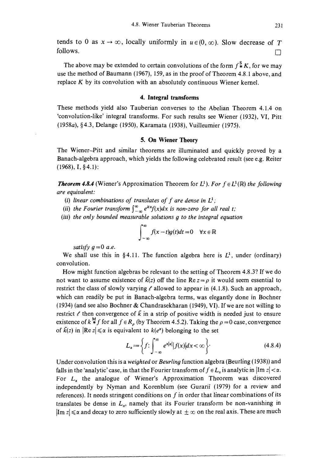
4.8.4 Integral transforms 230
4.8.5 On Wiener Theory 231
4.8.6 Sine series 232
4J8.7 Lambert summability 232
4.8.8 Laplace-Stieltjes transform 233
4.9 Tauberian Theorems for Mellin-Stieltjes convolutions 234
4.9.1 The Theorems 234

Contents xi
4.9.2 Variants
4.9.3 Alternatives
4.10 Tauberian Theorems for Fourier series and integrals
4.10.1 Conditionally convergent trigonometric series
4.10.2 Monotonicity
4.10.3 Integrability theorems
4.11 Tauberian Theorems for differences
4.11.1 Abelian matters
4.11.2 A Tauberian theorem
4.11.3 Non-negative kernel
4.11.4 Particular kernels
4.11.5 Remainder formulations
4.12 Theorems of exponential type for Laplace transforms
4.12.1 Kohlbecker's Tauberian Theorem
4.12.2 Limits of oscillation
4.12.3 Re-statements
4.12.4 Kasahara's Tauberian Theorem
4.12.5 de Bruijns Tauberian Theorem
4.12.6 Absolutely continuous measure
4.12.7 Boundary cases
4.12.8 Laplace's method
4.12.9 Applications
4.13 Addendum: special summability methods
5 Mercerian Theorems
5.0 Preliminaries
5.1 Mercerian Theorems for differences
5././ The Theorem
5.1.2 The integral equation
5.1.3 Alternative conditions
5.1.4 Particular kernels
5.1.5 Connection with the Aljancic-Karamata Theorem
5.2 The Drasin-Shea Theorem
5.2.1 The Theorem
5.2.2 Pblyds Lemma
5.2.3 Proof of the Drasin—Shea Theorem
5.2.4 More variations on the assumptions
5.2.5 LaplaceStieltjes transforms
5.2.6 Extensions
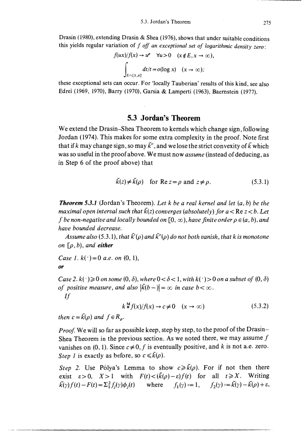
5.3 Jordan's Theorem
5.4 Laplace and Kohlbecker transforms
5.4.1 Embrechts's Theorem
5.4.2 Converse to Theorem 3.9.1
5.4.3 Example
5.4.4 Kohlbecker-transform and slow-variation-with-remainder formulations
5.4.5 Another example
5.4.6 Further results
6 Applications to Analytic Number Theory
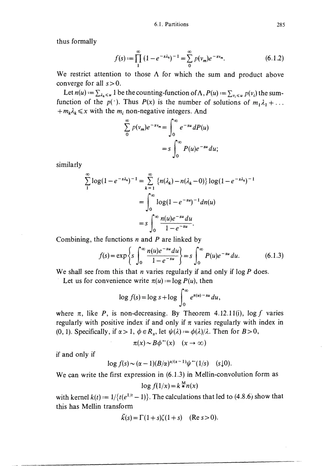
6.1 Partitions
6.2 The Prime Number Theorem
236
237
237
237
240
241
242
242
243
245
246
247
247
247
252
252
253
254
254
257
257
258
258
259
259
260
260
261
262
263
263
264
264
266
267
273
274
274
275
278
278
280
281
281
282
282
284
284
287

xii Contents
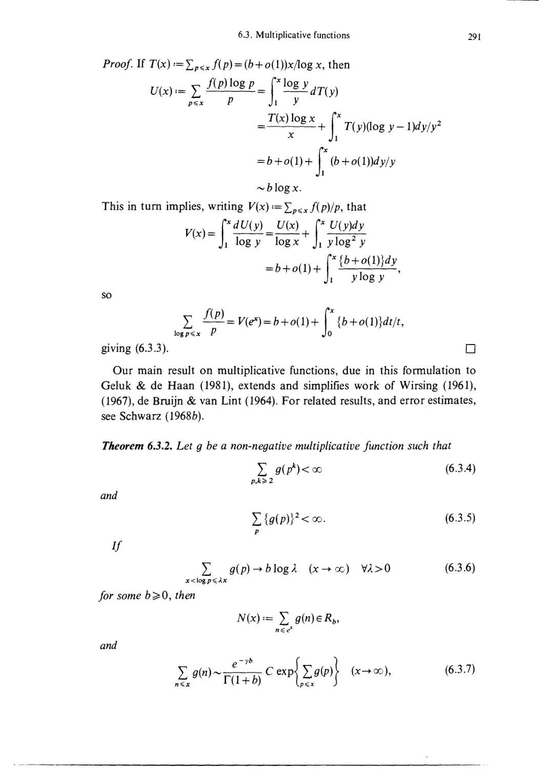
6.3 Multiplicative functions 290
6.4 Exercises and complements 295
7 Applications to complex analysis 298
7.1 Entire functions 298
7.2 Entire functions with negative zeros 301
7.2.1 Formulae 301
7.2.2 Non-integer order 302
7.2.3 Extremal properties 305
7.2.4 Meromorphic functions 306
7.2.5 Integer order 306
7.2.5a Order p, genus p 306
7.2.5b Order p + 1, genus p 308
7.3 Entire functions with real zeros 308
7.4 Proximate orders 310
7.4.1 Proximate orders and regular variation 310
7.4.2 Embedding 312
7.4.3 Type 313
7.5 Indicators 313
7.5.1 Definition and properties 313
7.5.2 Examples 315
7.5.3 Order p=l 315
7.6 Completely regular growth 316
7.6.1 Definitions 316
7.6.2 Non-integer order 317
7.6.3 Remarks 318
7.6.4 Integer order 319
7.6.5 Integer and non-integer order 320
7.6.6 Examples 321
7.7 The minimum modulus 321
7.8 Exercises and complements 324
8 Applications to probability theory 326
8.0 Preliminaries 326
8.0.0 Laws and transforms 326
8.0.1 Convergence in distribution 327
8.0.2 Type 327
8.0.3 Narrow convergence 328
8.0.4 Method of moments 329
8.0.5 Mittag-Leffler laws 329
8.1 Tail-behaviour and transforms 330
8.1.1 Tail-sum and truncated variance 330
8.1.2 Truncated moments 330
8.1.3 Transforms: laws on a half-line 333
8.1.4 Transforms: laws on the line 336
8.1.5 Exponentially small tails 337
8.2 Infinite divisibility 337
8.2.1 Compound Poisson limits 338
8.2.2 Triangular arrays 339

Contents xiii
8.2.3 Levy-Hincin formula 339
8.2.4 Convergence 339
8.2.5 Non-negativity 340
8.2.6 Levy processes 340
8.2.7 Asymptotic properties 341
8.2.8 Rates of tail decay 342
8.2.9 Spectral positivity and negativity 342
8.2.10 Laws on the positive integers 342
8.3 Stability and domains of attraction 343
8.3.1 Stable laws 343
8.3.2 Domains of attraction 344
8.3.3 Stable characteristic functions 347
8.3.4 Spectral positivity 348
8.3.5 Positive stable laws 349
8.3.6 Partial attraction 349
8.3.7 Index tx = 0 349
8.3.8 The case «= /: lines and half-lines 350
8.4 Further Central Limit Theory 350
8.4.1 Local limit theorems 350
8.4.2 Rates of convergence 353
8.4.3 Other summation methods 353
8.4.4 Large deviations 354
8.5 Self-similarity 354
8.5.1 The group Aff 354
8.5.2 Self-similar processes 354
8.5.3 Limit processes 356
8.5.4 Sequential convergence 357
8.5.5 Generalities 358
8.6 Renewal Theory 359
8.6.1 The Renewal Theorem 359
8.6.2 Infinite mean lifetime 360
8.6.3 The Dynkin-Lamperti condition 364
8.6.4 Key renewal theorems 367
8.6.5 Convergence rates 367
8.6.6 Generalisations 368
8.6.7 Transient renewal theory 368
8.6.8 The renewal process 368
8.7 Regenerative phenomena 369
8.7.1 Discrete-time renewal theory 369
8.7.2 Multiplication 371
8.7.3 Continuous time 372
8.8 Relative stability " 372
8.8.1 Definition 372
8.8.2 Laws on [0, x) 372
8.8.3 Laws on U 374
8.8.4 Stochastic compactness 375
8.9 Fluctuation theory 375
8.9.1 Random walk 375
8.9.2 Spitzer's condition: ladder epoch 379

xiv Contents
8.9.3
8.9.4
8.9.5
8.10
8.10.1
8.10.2
8.10.3
8.10.4
8.11
8.11.1
8.11.2
8.11.3
8.12
8.12.1
8.12.2
8.12.3
8.12.4
8.12.5
8.12.6
8.12.7
8.12.8
8.12.9
8.12.10
8.13
8.13.1
8.13.2
8.13.3
8.13.4
8.13.5
8.13.6
8.13.7
8.13.8
8.13.9
8.13.10
8.13.11
8.13.12
8.14
8.15
8.16
8.16.1
8.16.2
8.16.3
8.16.4
1
Al.l
A1.2
A1.3
A1.4
A1.5
Left-continuous random walk
SinaCs condition: ladder height
Continuous time
Queues
GI/G/1
M/G/l
Dams
Insurance
Occupation times
Darling-Kac Theory
Variants and extensions
The converse problem
Branching processes
Classification
Subcritical case
Critical case
Supercritical case
Infinite-mean case
Immigration
Continuous time
Continuous state
Age-dependent processes
Multitype processes
Extremes
Extremal types
Domains of attraction
von Mises' conditions
Local limit theorems
Large deviations
Rates of convergence
Statistical estimation of tails
Extremal processes
Generalisations
Laws of large numbers
Other order-statistics
Stochastic compactness
Records
Maxima and sums
Other limit theorems
Strong convergence
Central limit theory under weak dependence
Tail-behaviour under random stopping
Sojourns of Gaussian processes
Appendices
Regular variation in more general settings
Topological groups
Complex values
Complex variable
Higher dimensions
Multivariate extremes
383
384
385
385
385
387
389
389
389
389
394
395
397
397
398
399
403
406
406
407
407
407
407
408
408
409
411
413
413
413
414
414
414
414
415
415
415
419
420
420
420
421
422
423
423
423
424
426
426

Contents xv
2 Differential equations 427
3 Functional equations 428
429
429
430
431
432
433
433
433
433
434
436
436
437
438
438
439
443
443
445
466
470
472
479
4
A4.1
A4.2
A4.3
A4.4
5
A5.1
A5.2
A5.3
A5.4
6
A6.1
A6.2
A6.3
A6.4
A6.5
A6.6
A6.7
Subexponentiality
Theory
Applications
Extensions
Addendum
Calculating the de Bruijn conjugate
The problem
Bekessy's criterion
Lagrange inversion
Truncated Lagrange inversion
Bounded variation
Variation measures
Integration by parts
Composition
The space NBV{0, oo)
Narrow convergence
The monotone case
Mellin-Stieltjes convolution
References
Additional references
Index of named theorems
Index of notation
General index

PREFACE
The subject of regular variation as we use the term today was initiated by
Jovan Karamata in a famous paper of 1930, though preliminary or partial
treatments may be found in earlier work of Landau in 1911, Valiron in 1913,
Polya in 1917, and others. Karamata made striking use of his new theory in
Tauberian theorems (the 'Hardy-Littlewood-Karamata Theorem' dates
from this period), and his ideas were developed by Karamata himself and the
'Yugoslav School' of his collaborators and pupils (Aljancic, Bojanic, Tomic
and others), intermittently between 1930 and the 1960s. The great potential of
regular variation for probability theory and its applications was realised by
William Feller, whose book (in its 1968 and 1971 editions) did much to
stimulate interest in the subject. Another major stimulus - again from a
probabilistic viewpoint - was provided by Laurens de Haan in his 1970 thesis,
while Eugene Seneta gave a treatment of the basic theory of the subject in his
monograph of 1976.
In its basic form, regular variation may be viewed as the study of relations
such as
f(Xx)/f(x)^g(X)e@,oo) (x-oo) n>0,
together with its numerous ramifications. We will refer to this study for
convenience as 'Karamata Theory'. In Chapter 1 we set out the essential
ingredients - what the 'mathematician in the street' ought to know about
regular variation, as it were, following this in Chapter 2 with some
refinements. More general than the relation above is
f{Xx)-f{x) ^ gu (^ n>Q
The study of relations of this kind we refer to as 'de Haan Theory', a topic
treated in Chapter 3. An extensive treatment of those Abelian, Tauberian and
Mercerian Theorems relevant to regular variation follows in Chapters 4 and 5,

xviii Preface
completing the first part of the book, on theory. In the remaining three
chapters we deal with applications, to analytic number theory (Chapter 6),
complex analysis (Chapter 7) and probability (Chapter 8). Some scattered
topics are dealt with in Appendices.
The formal prerequisites for the book amount to a good background in
analysis at, say, the first-year graduate level, including in particular a
knowledge of measure theory. A few results from functional, Fourier, complex
or convex analysis and general topology are needed, references to standard
texts being provided. However, as usual, the real prerequisites (apart from the
persistence needed to absorb a certain amount of unfamiliar notation and
terminology) are intangibles concerned with maturity, motivation and the
like. The book is intended for those with a taste for classical analysis
(particularly questions involving limits), or a pre-existing interest in one of the
major fields of applications covered (or, like us, both).
Mathematically, regular variation is essentially a chapter in classical real-
variable theory, together with its applications in the fields mentioned above
and elsewhere. In the half-century or more of the subject's history, the
literature has been widely scattered in time and place, while essential parts of
the theory are comparatively recent. It seems that the time is now ripe for a
full-length treatment of the theory and its major applications. Our unified
approach has led to new, corrected or extended results in a number of cases.
Our style of treatment has varied as between theory and applications. In the
first five chapters our treatment of the theory is essentially complete, and full
proofs almost always are given. However, we have not attempted a complete
treatment in the remaining three chapters on applications. Our aim here has
been to formulate and discuss the results, and above all to put them in
context: key proofs are given, and those that are essential to understanding,
but otherwise the reader is referred to the literature.
Each chapter is divided into sections (§ n.p, etc.) within which the results are
numbered decimally (Theorem n.q.p) as are formulae ((n.p.q)).
Independently, many of the sections have been divided into named and
numbered subsections (§n.r.s), where it seemed appropriate; the subsection
numbers do not relate to those of results or formulae. Some chapters have a
final section of exercises and complements, referred to from elsewhere in the
text as individual subsections.
References and historical remarks are in the text proper rather than a 'notes'
section at the end. Many important theorems are named, and referred to by
name rather than by number. An index of named theorems is provided.
Instead of, and we believe more helpfully than, an author index, our list of
references gives the page numbers where each cited item is referred to. Names
not attached to references are listed in the general index.
We use iff for 'if and only if, «= for 'is defined by' and ? for the end of a

Preface xix
proof. Notation is collected together in the Index of Notation, but we bring a
few matters now to the reader's attention. Functions are generally denoted by
lower-case letters (/, g,...), the exception being the generic slowly varying
function which is / (not the usual L). Classes of functions are denoted by
upper-case letters (e.g. S for the subexponential class, in Appendix 4).
Sequences are (an), (bn), etc. We use Landau's O,o, ~ symbols (defined in the
Index of Notation) with a slight and very convenient extension to the latter: in
writing
Ax)~cg(x) (x-x), @.1)
or just /~ eg, the function g( •) is positive (>0) in a neighbourhood of infinity,
but the constant c is allowed to be zero. When c = 0, @.1) is interpreted as
f(x) = o(g(x)).
Integrals are always Lebesgue or Lebesgue-Stieltjes integrals unless noted
otherwise, and 'measurable', 'a.e.' (almost everywhere) refer to Lebesgue
measure. Measures take non-negative values. We allow ourselves to write dt/t
as shorthand for — or t~ldt.
t
We are indebted to a number of people for general advice or specific
suggestions. We thank in particular J. Milne Anderson, Julien Cuypers,
David Drasin, Paul Embrechts, Laurens de Haan, G. Sam Jordan, Edward
Omey, Sid Resnick, Richard Smith and Wim Vervaat.
We are also most grateful to Sandra Place for her patient and skilful typing
of the text, to Phyllis Smith for undertaking a huge author-generated revision,
and to Sue Bullock and Sheila Collier for their help with the latter task.
N. H. Bingham, C. M. Goldie, J. L. Teugels
Preface to the paperback edition
We take the opportunity to correct such mathematical or typographical
errors as we have noticed, and to add at the ends of Chapters 3, 4 and
Appendices 1,4 a few brief addenda. We also include a supplementary
bibliography, annotated with the relevant section number in the text. The
list is made up of references previously omitted and of recent or forthcoming
works; these last give a fair impression of recent progress in the field. We
note in particular R. Trautner's recent covering principle (p. 10), providing
a natural way to prove the Uniform Convergence Theorem by using Lusin's
and Egorov's theorems. We thank also Karl-Goswin Grosse-Erdmann and
Makoto Maejima for their comments.
N. H. Bingham, C. M. Goldie, J. L. Teugels

Karamata Theory
1.0 Introduction
Suppose that /(•) is a positive function, defined on some neighbourhood
[X, oo) of infinity and satisfying
f{Xx)/f{x)^g{X) (x-oo) VA>0, A.0.1)
for some function g. If / has some minimal smoothness property - for
instance, measurability - the convergence above is uniform on compact
subsets of @, oo), the function g(X) is restricted to be a power Xp, and the
convergence need only be demanded for some, rather than all, X > 0. The study
of these and other properties of relations such as A.0.1), together with their
wide-ranging applications, constitutes the theory of regular variation,
instituted by Karamata A930) and subsequently developed by him and many
others.
We begin in § 1.1 with some preliminaries on lemmas of Steinhaus type and
solutions of the Cauchy functional equation. The basic uniformity property is
studied in § 1.2, followed by representation theorems for the possible functions
/ in § 1.3 and characterisation of the possible limit-functions g in § 1.4.
Properties of regularly varying functions follow in § 1.5. Karamata's main
theorem is proved in § 1.6, and the principal Tauberian theorems in § 1.7. The
extent to which one may restrict attention to C°°-functions /is studied in § 1.8.
In § 1.9 sequential rather than continuous limits are taken; in § 1.10 monotone
functions / are considered.
1.1 Steinhaus Theory and additive functions
1. Additive functions
We shall be concerned initially with certain properties related to the addition
structure of sets on the real line with pleasant properties from either a
measure-theoretic or a topological viewpoint.

2 1. Karamata Theory
Recall that a set in U is meagre (of first Baire category) if it is expressible as a
countable union of nowhere dense sets, non-meagre (of second Baire category)
otherwise. A set A has the Baire property if there is an open set G with the
symmetric difference AAG meagre; a function / has the Baire property if for
every open set G the set /-1(G) has the Baire property. We will use the
adjective 'Baire' to mean 'with the Baire property' (not 'Baire-measurable').
See Kuratowski A966), §§11,32 for results on the Baire property.
We will suppose that the functions / in A.0.1) are either (Lebesgue)
measurable, or Baire. There are many analogies between the theories of
measure and Baire category, the analogue of a null-set [set of positive
measure] being a meagre set [a non-meagre set]; see Oxtoby A980) for a full
treatment.
A function k(') is said to be additive if it satisfies the Cauchy functional
equation
k(x + y) = k(x) + k(y) Vx, yeU.
Obvious examples are k(x) = cx (ceU). Pathological examples of additive
functions not of this form exist (at least, granted the axiom of choice). But
subject to smoothness restrictions - measurability or the Baire property -
additive functions are of the form ex, as will be proved below.
2. Steinhaus Theory
This section takes its name from the following result due to Steinhaus A920)
for measurable A, and to Piccard A939) (see also McShane A950), Pettis
A950), A951)) for Baire A. Our proof is from Oxtoby A980). By the phrase
'open interval', we always mean a non-empty open interval.
Theorem 1.1.1. If AczU is measurable of positive measure [is a non-meagre
Baire set] then its difference-set {a —a': a,a'eA] contains an open interval
containing the origin.
Proof Throughout this and the ensuing proofs, let x + S ¦¦= {x + s:xeS} for
any xeU, SczM.
First suppose A is measurable, with Lebesgue measure |.4|>0. If \A\ = oo
then we replace A by a subset of positive measure, and so shall assume that
0 < \A\ < oo. Enclose A in an open set G with \A\ > f |G|. Now G is the union of a
sequence of disjoint open intervals, and there must exist one of these, /, such
that |^n/|>||/|. Set <5-=i|/|. If xe(-d,S) then (x + J)uJ is an interval of
length less than f |/| that contains both A nl and x + (A nl). These sets must
intersect, because |x + (Anl)\ = \A nl\ > ||/|. Thus there exist a,a'eAnI such
that a = x + a', and so x belongs to the difference set, as required.
When A is a non-meagre Baire set it can be represented as the symmetric difference
of an open set and a meagre set (Oxtoby A980), Theorem 4.6), and because A is non-

1.1. Steinhaus Theory and additive functions 3
meagre, the open set is non-empty, so contains an open interval /. Thus A=>I\P where
P is meagre. For any x,
If |x| < S •¦= |/| the last line constitutes an open interval minus a meagre set; it is therefore
non-empty. Thus (x + A)nA^0, hence x belongs to the difference set. ?
The following extension is also due, under its two alternative assumptions,
to Steinhaus and Pettis respectively. See also Kuczma & Kuczma A971) for an
alternative proof in the measurable case.
Theorem 1.1.2. Let A and B be measurable and both of positive measure [both
non-meagre Baire sets in U~\. Then the difference set D ¦¦= {a — b:a e A, b eB]
contains an open interval.
Proof (measurable case). As in the previous proof we may find a bounded
open interval / such that \A n/| >||/|, and likewise a bounded open interval J
such that |Bn J|> || J\. To proceed we need to alter / and J until their lengths
are not too different. If we divide J into n subintervals of equal length, by
removing n — 1 points from it, then one of these intervals, J', must retain the
defining property of J, in that |BnJ'j>||J'j. Likewise, on dividing / into m
subintervals of equal length, we may find one of them, /', such that \A n/'| >
||/'|. By suitable choice of m and n we may ensure also that -j|/'| ^ |J'| < |/'|, and
because of the latter inequality there exists an open interval A of length
|/'|-|J'|>0 such that x + J'czf for all xeA, upon which
x + (Bn/)c/' (all xeA).
Pick any xeA, then
so that Anl' and x + (BnJ') are both contained in /' and the sum of their
measures exceeds f|/'|, which implies that they intersect. Thus there exist
aeAnl', beBnJ' such that a = x + b, whence x = a—beD.
(Baire case). As in the proof of the previous theorem, A=>I\P, and similarly B=>J\Q,
where /, J are open intervals and P, Q are meagre. There exists an open interval A such
that for all xeA the set In(x + J) is a (non-empty) open interval. But then for each
xeA,
/I n (x + 5) z> / n (x + J)\(P u (x + ?>)),
and this is non-meagre because Pu(x + Q) is meagre. So An{x + B) is non-empty,
whence xeD as before. ?
Corollary 1.1.3. If SczM contains a set of positive measure [a non-meagre Baire
set~\ then the set S + S ¦¦= {s + s':s,s' eS} contains an open interval.
Proof Immediate, on taking A to be the set mentioned and B-={—a:aeA},

4 1. Karamata Theory
and applying Theorem 1.1.2. ?
See Rudin A974). p. 189 for alternative proofs of this corollary, hence of the previous
two theorems. We note in passing that if S has measure zero S + S may be non-
measurable (cf. Rubel A963), and § 1.11.0).
Corollary 1.1.4. If S is an additive subgroup ofU, and S contains a set of positive
measure [a non-meagre Baire set], then S=U.IfT is a multiplicative subgroup
of@, x) containing a set of positive measure [a non-meagre Baire set] then
T=@, x).
Proof. By Theorem 1.1.1,5 contains ( — 3,3) for some <5>0. Being an additive
group, S thus contains (— n3,n3) for n= 1,2,..., and so S=U. ?
Corollary 1.1.5 (Hille & Phillips, 1957 (measurable case); Bingham & Goldie,
1982a (Baire case)). If Scz@,co) is an additive semi-group, and S contains a set
of positive measure [a non-meagre Baire set], then for some be@,oo) S
contains the interval (b,oc).
Proof. S + S contains some interval (a, /?), with 0< a < /?, and so the semigroup
5 contains all the intervals (ncc,nC), ri=\,2, Fix a positive integer k such
that l+k <P/cc, then for n = k,k + 1,... each set (noc,nf3) overlaps the next,
hence (J"=fc {noc, nf3) = {koc, oo), and this is contained in S. Q
3. The Cauchy functional equation
First, a preliminary result.
Lemma 1.1.6. If k(w) is additive, and bounded above on a set A of positive
measure [a non-meagre Baire set], then k{ •) is bounded on some neighbourhood
of the origin.
Proof. Suppose k(x)^M<oo for xeA. By Theorem 1.1.3, A + A contains
some interval (y — 3,y + 3) with <5>0. So if \t\<3 we have t+y = a + a' with
a,a' eA, so
Thus k is bounded above on (-3,3). Since k{t)= -k{-t), k is also bounded
below on (-3,3), as required. ?
Next is the main result, due in the measurable case to Ostrowski A929) (see
also Kestelman A947)), in the Baire case to Mehdi A964).
Theorem 1.1.7. If k() is an additive function, bounded above (or below) on a set
A of positive measure [a non-meagre Baire set], then k{x) is of the form ex for
some constant c.

1.1. Steinhaus Theory and additive functions 5
Proof. By additivity of k, k(nx) = nk(x), k(x/m) = k(x)/m for m, n= 1,2,...,
whence k(rx) = rk(x) for rational r.
By Lemma 1.1.6, there are M, <5>0 with \k(x)\ <M for |x| <S. By additivity,
\k(x)\^M/n for |x|<<5/rc (n= 1,2,...). For any xeR and «= 1,2,... we can
find rational r with \r — x\<S/n. Then, since &(r) = r&(l) for rational r,
\k(x)-xk(l)\ = \k(x-r) + (r-x)k(l)\
Letting n -> oo, k(x) = xk(l), as required. ?
This result is usually stated in a slightly weaker form.
Theorem 1.1.8. If k is additive, and measurable [Baire], then k(x) = cx for some c.
Proof. For n= 1,2,..., the sets An ~{x:f(x)^n} are measurable [Baire], and AJU as
«-> oo.In the measurable case, |/ln||oo,so some|/ln|>0; in the Baire case, some An is
non-meagre by Baire's Theorem. The result follows by Theorem 1.1.7. ?
4. Pathological solutions
We turn now to additive functions not of the form ex. Consider the set U of
reals as a vector space over the rational field Q. By a well-known argument
involving Zorn's Lemma (see e.g. Greub A975)), U has a basis over Q, B say
(called a Hamel basis). That is, every real x may be written uniquely as a finite
linear combination
r=l
For any boeB, we can define a function k on B by k(bo)—bo, k(b)—O
(beB,b^b0). If we extend k from B to R by
r=l 1
k is additive but not of the form k(x) = cx for any c.
It follows from Theorem 1.1.7 that k(x) must be unbounded above and
below on every set of positive measure and every non-meagre Baire set, in
particular on every interval. Thus an additive function is either of the form ex
or highly pathological. We will refer to such pathological solutions of the
Cauchy functional equation as the Hamel solutions.
Note also that an additive function is, in particular, subadditive (Hille & Phillips
A957)) and convex (Hardy et al. A952)). The theory of subadditivity and convexity,
like that of additivity above, is complicated by the existence of the 'Hamel pathologies':
the main theorems of all three subjects require smoothness conditions such as
measurability or the Baire property to exclude them.

6 1. Karamata Theory
5. Multiplicative notation
A function g:(Q, x )-*¦((), oc) is said to be multiplicative if
gtt)giii)=g(i.ii) v;.,Ju>o.
If k(x) = logg(ex), then k is additive iff g is multiplicative, so Theorem 1.1.8
becomes
Theorem 1.1.9. If g is multiplicative, and measurable [Baire\, then g{X) = Xc
(X>0) for some real c.
1.2 The Uniform Convergence Theorem
1. The Theorem
Definition. Let if be a positive measurable function, defined on some
neighbourhood [X, oo) of infinity, and satisfying
/(/bc)//(x)-> 1 (x->oo) \fX>0; A.2.1)
then { is said to be slowly varying (in Karamata's sense).
These functions were introduced and studied by Karamata A930) in a pioneering
paper, with continuity in place of measurability.
The neighbourhood [X, oo) is of little importance; we may (and often shall)
suppose / defined on @, oo) - for instance, by taking ^(x)=^(X) on @,X).
The basic Uniform Convergence Theorem — the most important theorem in
the subject - was given by Karamata A930) in the continuous case, Korevaar
et al. A949) in the measurable case. Because of its importance, we give several
proofs.
Theorem 1.2.1 (Uniform Convergence Theorem, or UCT). // / is slowly
varying then
f{Xx)/t{x) -*¦ 1 (x -> oo), uniformly on each compact X-set in @, oo). A.2.2)
It is actually local uniformity that is being proved - uniformity in each compact subset
of the set of X.
2. Direct proofs
First proof (Delange A955a)). Write h(x) — log /(e*); our assumption is
h(x + u)-h(x)-^0 (x->oo) WeU, A.2.3)
and we are to prove uniform convergence on compact w-sets in U. It suffices to
prove uniformity on each [0, A] (for by translation this gives uniformity on
each closed interval, hence on each compact by inclusion).

1.2. The Uniform Convergence Theorem
Choose ?e@, A). For x>0, let
Ex:={telx:\h(t)-h(x)\^e},
E* :={telO,2A]:\h(x + t)-h(
Then Ex, E* are measurable, as / is, and 1^1 = |?*| (where | • | denotes
Lebesgue measure). By A.2.3), the indicator-function of E* tends pointwise to
zero as x-»¦ oo. So by dominated convergence, its integral \E*\ -> 0. Thus
\ex\ <ie f°r x^*o> say-
Now for ce[0,A], Ix+cnIx = [x + c,x + 2A] has length 2A-c^A, while
for
|?,u?,+c <EX + Ex+c\ = \E*\ + \E*+c\<e<A.
So force[0,4],x>x0>
(IxnIx+e)\(E*vEx+e)
has positive measure, so is non-empty. Let t be a point of it: then
\h(t)-h(x)\<y,
\h(t)-h(x + c)\<±e.
So for all ce[0,A],
proving the desired uniformity on [0, A], which suffices as above. ?
The proof above uses 'quantitative' aspects of measure theory. The next proof uses
only 'qualitative' aspects, in which we are concerned with measures of sets only
through observing whether they are zero or positive.
Second proof. Assuming A.2.3) we first show that for any sequence xn -> oo and any
bounded sequence un,
h(xn + un)-h(xn)-+0 (n-oo). A.2.4)
Choose ?>0. Let B~ l + sup|un|<oo. For each ue[-B,B], n^l, let Anu~
[-B, 5] n {v: V/c ^ n, \h(xk + u + v)-h(xk + u)| ^\e, \h(xk + uk + v)-h(xk + uk)\ <^}. Fix
ue\_-B,B]. The sets Anu are measurable and (J*=1 Anu = [-5,5]. So there exists
N(u) such that AN(uhu has positive measure. By Theorem 1.1.1 the difference set
{v1-v2:vieANiu)J
contains an interval (— V(u), V{u)) for some V(u) > 0. Then for any n such that n ^ N(u)
and \un — u\< V{u) we may find v',v"eAN(uhu such that u + v' = un + v". Hence
\h(xn + un)-h(xn
^ \h(xH + u + v')- h(xn + un)\ + \h(xn + u + v')-h(xn + u)\
= \h(xn + un + v")'-h(xn + un)\ + \h(xn + u + v')- h(xn + u)\
^i? + i? = |?. A.2.5)
The intervals (u-V(u),u+V{u)) form an open cover of [-5,5], so we may select

8 1. Karamata Theory
a finite cover (uj-V(uj),uj+V(uJ)), for some finite set {u1,..., ur} <=[-?, B~\. Let
N ==max(iV(w1),.. .,N(ur)) and then increase N so that also
\ J=l,...,r). A.2.6)
For any n^/V the point un satisfies \un — uJ\< V(u}) for some j, and n^N{uj) so that
\h(xn + un)-h(x,, + uJ)\^e. by A.2.5). Combining with A.2.6) we find
\h(xn + un) — h(xn)\<e, whence A.2.4).
Instead of concluding with a quick reductio ad absurdum we choose to continue
directly. Take any compact interval [a, b] in R. For each n we may find un e [a, b~] such
that
\h(n + un) — h(n)\>min(n, sup \h(n + u)— h(n)\— n).
UE[a,f>]
By A.2.4), h(n + un) — /i(n)-> 0 as «->oo, from which it follows that the above
supremum is finite for all large n and indeed tends to zero. Thus h(n + u)—h(n) -> 0 as
n -> go, locally uniformly in u.
Lastly, writing [] for integer part,
sup \h(x + u) -h(x)\
UE[a,h]
< sup \h(
sup |MM + «)-MM)|+ sup
[a,h+l] ue[0,l]
as [x] -> oo, by the above. ?
We note at this point that measurability may be replaced by the Baire
property. Here and elsewhere we denote the 'Baire' analogue of a
'measurability' theorem by the suffix B.
Theorem 1.2.1B. If / is Baire, then A.2.1) implies A.2.2).
Proof. Use the second proof of Theorem 1.2.1 above, replacing the terms 'measurable'
and 'of positive measure' by 'Baire' and 'non-meagre', and using the Baire version of
Theorem 1.1.1. ?
It is traditional, and (for reasons which will appear below) convenient, to
retain measurability as part of the definition of slow variation; we shall thus
refer to Baire functions satisfying A.2.1) as being 'Baire slowly varying'.
3. Indirect proofs
There are several other interesting proofs of Theorem 1.2.1, which are indirect (by
contradiction) but handle the measurable and Baire cases together and so,
incidentally, provide further proofs of Theorem 1.2.IB.
Third proof (Matuszewska A965)). Assume A.2.3) but suppose that local uniformity
fails, so that there exist e>0, xn -> go and a bounded sequence un with

1.2. The Uniform Convergence Theorem 9
\h(xn + un)-h(xn)\>2e for n=l,2,... . Passing to a subsequence, we may take un
convergent - to u0, say. Since \h(xn + u0)-h(xn)\^e for all large n, it follows that
\h(xn + un) — h(xn + uo)\>e for all large n. Now define
The sets An are measurable [Baire] and {J™=1 /!„ = U. So there exists iV such that AN
has positive measure [is non-meagre], whence again by Theorem 1.1.1 the difference
set of AN contains an interval (—V,V) for some V>0. Pick K^N such that
|M*~Mo|<^ f°r a^ k^K, then for each such k there exist i/.i/'e.^ such that
u0 + v' = uk + y". Hence
a contradiction. ?
Fourth proof (after Csiszar & Erdos A964)). Assume A.2.3) but suppose that local
uniformity fails, so that there exist e>0, xn-> oo and a bounded sequence un with
\h(xn + un) — h(xn)\> 2e for n= 1,2,... .Passing to a suitable subsequence, we may take
it that un converges to some u0 and that \un — mo| < 1 for all n. For every y we know that
\h(xn + y)—h(xn)\ ^e for all large n, hence \h(xn + un) —h(xn + y)\ >e for all large n.Thus
Each Ik is measurable [Baire], so there exists K such that IK has positive measure [is
non-meagre]. Let
Zn-=un-IK={un-y:yeIK} («=1,2,...),
and let Z — f]f=i (J™=jZn.In the measurable case, all theZn have measure \IK\, and as
they are subsets of the fixed bounded interval [u0 —2, u0 + 2], Z is a subset of the same
interval having measure
./-co
So Z is non-empty.
In the Baire case IK contains some set I\M, where / is an open interval of length 5 > 0,
and M is meagre. So each Zn contains I"\M", where I" ==«„—/ is an open interval of
length S, and M" •=un — M is meagre. Choosing J so large that |u, — uj < S for all i,j^J,
the intervals IJ,IJ + 1,... all overlap each other, and so {J™=JI" is an open interval for
all j^J. But then the sequence of sets (J*=7/n, for j = J,J+ 1,..., is a decreasing
sequence of intervals, all of length ^ 5 and all contained in the interval [u0 —2, u0 + 2];
hence 7° ••= f]f= x U™=;/" is an interval of length ^ 5. Since Z contains /°\IJ^= x M", it
follows that Z is non-meagre, so non-empty.
In either case there exists z belonging to infinitely many of the Zn. Hence
for infinitely many n, contradicting A.2.3). ?

10 1. Karamata Theory
We shall use the idea of the fourth proof repeatedly in proving uniform
boundedness assertions in Chapter 3.
Our fifth and final proof (but see Appendix 1 for slow variation in other settings) is
included as apparently the first successful useof Egorov's theorem to this end. Previous
attempts to use this 'apparently natural tool' met with measure-theoretic difficulties
(see Seneta A976), p. 44 for details)*.
Fifth proof (Elliott A979-80), Lemma 1.3). Suppose A.2.1) fails to hold uniformly in
ke\_e~l,e\. So there exist xn->oo and wne[—1,1] such that f{xnew")/t(xn) ++1 as
n-* co.
The functions /„: [- 1,1] -»¦IR defined by fn(y) — t(xne?)/t{xn) are measurable and
tend pointwise to 1 as n -> oo. By Egorov's Theorem there is a subset E of [— 1,1], of
measure at least \, such that
t{xne*)/t{xn) -> 1 (n ->¦ oo), uniformly for yeE.
Similarly there is a subset F of [— 1,1], of measure at least I, such that
/(xnew" + z)//(xnew") -» 1 (n -» oo), uniformly for zeF.
For each n the sets wn + F and E must contain a common point. Otherwise if, for
example, wn^0 then they are both contained in the interval [— 1,1 + wJ, so that
which is impossible. Similarly if wn<0.
Let wn + zn = yn, with zneF, yneE. Then
t(xn) /(xn^- + z») t(xn)
1,
contradicting our original assumption.
Thus A.2.1) holds uniformly in X e [e~l, e], and it is easy to iterate to get uniformity
in [e~m,eTr\ for each positive integer m. ?
4. Pathology
It is an important fact, due to Korevaar et al. A949), that the UCT is false if no
good-behaviour condition such as measurability or the Baire property is
imposed on /. We give the relatively simple counterexample - 'relatively
simple' because there is no way to avoid Zorn's Lemma — due to Ash et al.
A974).
Theorem 1.2.2 (Korevaar et al. A949); Ash et al. A974)). There exists a real
function h(x), defined for x^O, which satisfies the relation
h(x + t)-h(x)^0 (x->oo) A.2.7)
for every real t, without satisfying it uniformly on any interval a^t^b, where
a<b. Further, h may (if desired) be taken uniformly bounded on U.
Proof Let B be a Hamel basis for U as a vector space over Q (see §1.1). For
* Another proof of this kind has recently been given by Trautner A987): see the additional
bibliography.

1.2. The Uniform Convergence Theorem 11
each real x let n = n(x) be the number of summands in the unique expression of
x as a linear combination of basis elements:
rtbif r,eQ\{0} (bteB).
r=l
Evidently, \n(x + t)-n(x)\^n(t). Let h(x)--=\og(x + n(x)) for x>0, and
h(x)>=0 for x^O. Then for x,?>0,
\h(x + t)-h(x)\ =
n(x+t)
du/u
n(x)
which, for t fixed, tends to zero as x -> oo. But uniformity is far from present;
indeed
limsup sup \h{x + t) — h(x)\ = ao.
b
For if x is fixed > — a, we can find f e [a, b] so that /z(x +1) is as large as we
please. This follows because for fixed neN and blf. ..,bneB, the numbers
rtbt (r,eQ\{0})
r=l
are dense.
The above h is unbounded in every interval. Taking h1 —sino/* we find
|/z1(x + O-/iiU)|<|^(^ + O-^U)| so /ij satisfies A.2.7). Yet for x fixed > -a
we can find te[a,b~\ so that j/ij(x +1) — h1(x)\>^, so the convergence is non-
uniform. ?
5. Remarks
The UCT is the basic result of the subject, and we will avoid failure of its
conclusion as in Theorem 1.2.2 above by imposing measurability or the Baire
property (it is an interesting open question as to what other properties suffice).
Often we will need to integrate the slowly varying function in question, and
then measurability is appropriate.
One may also study 'very slow variation', in which the convergence in A.1.1) takes
place at least at a certain rate. Ash et al. A974) obtain results in which, from pointwise
convergence
{h{x + u)-h(x)}/g(x)-+0 (x-»x) VueR,
uniformity on compact u-sets is obtained. We will give a full treatment of questions of
this sort in Chapter 3. As a foretaste, if g > 0 is non-increasing and satisfies the stringent
condition
CO
? g(x + n)/g(x) < B < x Vx ^ 0
n = 0
(such as, for instance, g(x) = e~"x with <x>0), pointwise convergence implies locally
uniform convergence without the assumption that h be measurable or Baire (Ash et al.

12 1. Karamata Theory
A974), Th. 3). Results in which pointwise O-statements such as
{h(x + u)-h(x)}/g(x) = O(l) (x-+x) \/ueR
imply local uniformity have been obtained by Aljancic & Arandelovic A977), Bingham
& Goldie A982a); see §3.1 for these, and for local uniformity in
{h(x + u)-h{x)}/g{x) -> x (x -> x) Vw e R
(Heiberg A971ft); Bingham & Goldie A982a), §5). For uniformity in the alternative
formulation of 'slow variation with remainder' see §3.12.
1.3 The Representation Theorem
1. The Theorem
We turn now to the question of exactly which functions / can satisfy A.2.1).
The basic representation below is due to Karamata A930) in the continuous
case, Korevaar et al. A949) in the measurable case. We give the proof from the
latter reference, as it is still the simplest known construction. Following it, we
give two further results, in which components of the representations used have
many extra properties. We will be concerned with the measurable case except
where indicated.
Theorem 1.3.1 (Representation Theorem). The function / is slowly varying if
and only if it may be written in the form
e(u)du/ul (x^a) A.3.1)
for some a>0, where c() is measurable and c(x) -*¦ ce@, oo), s(x)-^0 as
x -> oo.
Since /, c, e may be altered at will on finite intervals, the value of a is unimportant
(one may choose to take a = 1, or a = 0 on taking ? = 0ona neighbourhood of 0 to avoid
divergence of the integral at the origin), and one may also take c eventually bounded.
We may re-write A.3.1) as
/(x) = exp|c1(x)+ I e(u)du/u\ A.3.1')
where cl(x), e(x) are bounded and measurable, cx(x) -> de R, e(x) -+0asx->oo.
As in § 1.2 we will write h(x) ¦¦= log /(e*); thus we are to prove that h satisfies
A.2.3) if and only if h may be written
h(x) = d(x)+ e(v)dv (x^b) A.3.2)
on writing b = \oga, d(x) = c1(ex), e(x) = e(ex), with d(x)-^deU, e(x)-^0 as
x -> oo. By '?-function', 'e-function' below, we shall understand functions e(x),
e(x) as in the representations A.3.1), A.3.2).

1.3. The Representation Theorem 1?
The 'if part of the theorem is easy: if A.3.1) holds,
/(/U)//(x) = {c(Xx)/c(x)} exp | s(u)du/u 1.
Choose any interval [a,b~\ with 0<a<b<oo, and any ?>0. Then for all
x^x0, say, and all Xe[a, b], the right-hand side lies between
A +?) exp{ ±? max(|log a\, |log b\)},
from which A.2.1) follows. Indeed, A.2.2) follows; this shows that the
Representation Theorem 1.2.1 implies the UCT, Theorem 1.2.1, as well as
being implied by it (see the 'only if proofs below); the two are thus equivalent.
Before proving the theorem we note an important property of functions
satisfying A.2.1).
Lemma 1.3.2 (Seneta A973)). // / is positive, measurable, defined on some
[A, oo), and
/(/bc)//(x) -> 1 (x->oo) VA>0,
then / is bounded on all finite intervals far enough to the right. If
h(x) — log /(e*), h is also bounded on finite intervals far enough to the right.
Proof. By the UCT we can find X so large that
\h(x + u)-h(x)\<l for x>X («e[0,1]),
whence \h(x)\ < 1 + \h(X)\ on [X, X + 1], and by induction \h(x)\ ^n + \h(X)\ on
[X,X + ri] for n=l,2,..., whence the conclusion for h, from which the
conclusion for /(x) = exp /z(log x) follows. ?
We shall call a function locally bounded in some set A if it is bounded in each
compact subset of A. Thus the above lemma concludes that there exists X > 0
such that /is locally bounded in [X, oo). Since /is measurable, it is also locally
integrable in [X, oo), /eL^X, oo).
Proof of Theorem 1.3.1 (Korevaar et al. A949)). By Lemma 1.3.2, h is
integrable on finite intervals far enough to the right, being bounded and
measurable thereon. For large enough X, we may thus write
h(x)=\ {h(x)-h(t)}dt+\ {h(t+l)-h(t)}dt
X + l
+ h(t)dt (x^X). A.3.3)
The last term on the right is a constant, c say. If e(x) ••= h(x + 1) — h{x), e(x) -> 0
as x ->-oo by A.2.3). The first term on the right is JJ, {h(x) -h(x + u)}du, which
tends to zero as x -*¦ oo by the UCT. Thus A.3.2) follows with
d(x) = c + f o {h(x) - h(x + u)}du. ?

14 1. Karamata Theory
2. Variants
Given a representation A.3.2), we can add any integrable, o(l) function to e(-),
and adjust d( •) accordingly, and hence obtain another representation with the
required properties. Thus the Karamata representation A.3.1) is essentially
non-unique: within limits, one may always adjust one of c( ), ?( ), making a
compensating adjustment to the other. It turns out that the ?-function may be
arbitrarily smooth, but the smoothness properties attainable for c() are
limited by those present in /(•). However, replacing c(x) by its limit c e @, oc),
we obtain a slowly varying function <?1(x) = cexp{$*s(u)du/u} with /(x)~/j(x)
as x -> oo. Thus any slowly varying function is asymptotic to another with
much enhanced properties. Our first result of this sort shows f1 may be taken
'smoothly slowly varying' (for more on which, see § 1.8):
Theorem 133 (cf. de Bruijn A959)). Let / be slowly varying. Then /(x) ~ ex (x)
where {x eC^la, oo), and /zj(x) —log ^1{ex) has for n= 1,2,... the property
h^(x) -> 0 (x -> oo).
(So /j is slowly varying with representation /j (x) = exp(cj + j* ?j (t)dt/t) in which
c1=h1 (log a) and ?j (t) = h\ (log t).)
Proof. Let p(-) be a C00 probability density on U, with support [0,1]. For
example, set q(x) ¦¦= exp( — x'1 — A — x)~1) for 0<x< 1, ^(x) = 0 for x<0 and
1, and let p(x) *=g(x)/JJ q(t)dt for all x.
With h(x) = log /(^), let
for n large enough for [n, oo) to lie in the domain of definition of h, say, n^B
(integer). Then e( •) is C00 in each interval (n, n + 1), and also at the endpoints
because p and all its derivatives are zero at 0 and 1. For k = 0, 1,... write
Mk ==sup;c|p('c)(x)|, where p@) = p. All Mk are finite so
|g»>(x)| = |/z(H + 1)-MM)||p«4)(x-[x])|<|MM + 1)-h([x])\Mk - 0
as x -> oo. Set /zj(x) ~/z(B) + fge(f)^f then we have shown /ij eC00 and all its
derivatives are o(l) as x -> oo. Finally, for
- I e(t)dt
-»-0 (x->oo)
by the UCT. Thus /(x) ~ /j(x) == exp /ij(log x). ?

1.3. The Representation Theorem 15
Observe that the latter proof holds equally well for Baire slowly varying functions.
Thus they have the same representation A.3.1), in which c(x) -»¦ ce@, oo) and c() is
Baire (as the quotient of a Baire function by a positive continuous function), while
e(x)->0and e() is Ccc[a,cx)).
As our next variant we show how a C00 slowly varying function tf0 may be chosen to
interpolate tf at will. In turn, tf0 may be represented by the means given in Theorems
1.3.1 or 1.3.3.
Proposition 1.3.4 (cf. Adamovic A966)). Let tf be slowly varying and let (xn) be any
sequence increasing to oo. Then there exists a C00 function tf0 such that tfo(x)~tf(x)
(x -> oo) and tfo(xn) = tf(xn) for all large n. If tf is eventually monotone, so is tf0.
Proof. Let tf be defined on [a, oo) where a > 0. By removing from the sequence all xn <a,
and adjoining to it all points ae" for integer n ^ 0, we may assume that x0 = a, xj oo and
xn+Jxn^e for all n. Also remove all repetitions, so xn strictly increases. Clearly it
suffices to prove the result for the sequence thus modified. For n = 0,1,... and
xn^x<xn+l define
^(x):=tf(Xn)+{tf(Xn+l)-tf(Xn)} P(t)dt
Jo
where p( ) is as in the previous proof. This makes tf1 e C00 [a, oo) and tf1 is monotone on
each interval [xn,xn+1] and agrees with tf at each xn. Since by the UCT
/f(x)//f(xn) -> 1 (n -> oo) uniformly in x e [xn,xn + x],
it follows that ^(xHAx) (x -+ oo). ?
From some points of view (for instance, the measuring of scales of growth)
slowly varying functions are of interest only to within asymptotic equivalence.
We then lose nothing by restricting attention to the case of constant c-function
in A.3.1), i.e. to slowly varying functions of the form
/(x) = cexp| e(u)du/ul (x^a) A.3.4)
@<c< oo, e(x) -> 0), called normalised slowly varying functions (Kohlbecker
A958)). For these,
?(*) = */'(*)//(*) a.e.
Conversely, given a function / with e(x) —xtf'(x)/f(x) continuous and o(l) at
infinity, we may integrate to obtain A.3.4), showing / to be normalised slowly
varying.
It is sometimes desirable to be able to find representations in which particular
properties of / are reflected in properties of e( ), though not necessarily in c( ) as well.
For instance, the proofs of the Representation Theorem given above show that non-
decreasing / may be represented with non-negative e():
Corollary 1.3.5. If tf is eventually non-decreasing (non-increasing), e()in A.3.1) may be
taken eventually non-negative (non-positive).

16 1. Karamata Theory
We will show in Proposition 1.10.8 below that monotonicity of/does not, however,
imply that of c() in A.3.1).
3. Examples and properties
Using the Representation Theorem, specific examples of slowly varying
functions may be constructed at will. Trivially, (positive, measurable)
functions with positive limits at infinity (in particular, positive constants) are
slowly varying. Of course, the simplest non-trivial example is /(x) = logx
(c(x) = l,e(x) = I/log x). The iterates loglogx ( = log2x), logkx
( = loglogk_1 x) are also slowly varying as are powers of logkx, rational
functions with positive coefficients formed from the logkx, etc. Non-
logarithmic examples are given by
/(x) = exp{(logx)a'(log2xr ... (logkx)*'} @<a;< 1),
and
/(x) = exp{(log x)/loglog x}.
Note that a slowly varying function ( may have
liminf/(x) = 0, lim sup /(x) = oo
x-+ oo x-* oo
(that is, may exhibit 'infinite oscillation'), an example being
/(x) = exp{(log x)* cos((log x)*)}
(see §1.11.3).
Finally, we note some elementary properties of slowly varying functions, whose
proofs may be left to the reader.
Proposition 1.3.6
(i) If <? varies slowly, (log tf (x))/log x -> 0 as x -> oo.
(ii) If tf varies slowly, so does (/f(x))a for every oceR.
(Hi) Iftfl,tf2varyslowly,sodo/!'1(xy2(x),/fi(x) + /!'2(x)^at^(if^2(x)-^ cc asx-+ oo)
( iv) If ffl,.. .,/k vary slowly and r{xx,.. .,xk) is a rational function with positive
coefficients, r(/f1 (x),..., /k(x)) varies slowly,
(v) If /? varies slowly and <x>0,
xV(x)-»oo, x"V(x)-»0 (x-»oo).
1.4 The Characterisation Theorem
1. The limit function
Suppose now that /(•) is a positive function, defined on [X, oo) for some X > 0
(taking /(x) =f(X) on @, X) we can extend the domain of definition of / to
@, oo) if desired), and let S be the set of all A>0 such that

1.4. The Characterisation Theorem 17
flXx)/flx)^g(X)e@,oo) (x-oo). A.4.1)
If X,neS then
) flux)
fix) fljxx) fix)
so XfieS and
From A.4.1) we find that if XeS then 1/AeS and #(l//) = l/#(/l). Thus S is
a multiplicative subgroup of @, oo).
As usual, we will change to additive notation for the proofs below. Write
hix) ¦¦= log fle'), k(u) ¦¦= log gie% T ¦¦= {log X: X e 5}. Then in
li(x + u)-/i(x)->fc(u)eR (x->oo) VweTcrR, A.4.1')
T is an additive subgroup of R, and
A:(« + i?) = /fc(«) + /fc(y) («,ce7). A.4.2)
We now show that if/ is not too pathological and S is known not to be too
small, A.4.1) holds for all X e@, oo) with giX) = Xp for some real p. Such a result
characterises the possible limits g. The result below is given in Karamata
A933), though with an incorrect proof. Use of the Cauchy functional equation
in this context is due to Feller A971); see also de Haan A970) (compare Petrini
A916) for an early attempt in this direction).
Theorem 1.4.1 (Characterisation Theorem). /// > 0 is measurable [Baire], and
A.4.1) holds for all X in a set of positive measure [a non-meagre Baire set], then
(i) A.4.1) holds for all X >0,
(li) there exists a real number p with giX) = Xp VA>0,
(iii) fix) = xpt?ix) with ( slowly varying [Baire slowly varying].
Proof. In additive notation, A.4.1') holds with Tan additive subgroup of U, of
positive measure [a non-meagre Baire set]; by Corollary 1.1.4, T= U, proving
(i).
Taking the limits in A.4.1), A.4.1') sequentially, #,& are pointwise limits of
sequences of measurable [Baire] functions, and are thus measurable [Baire].
But since T= U, A.4.2) shows that k is additive (gr is multiplicative), and then
Theorem 1.1.8 shows that for some peU we have kiu) = pu, giX) = Xp,
proving (ii).
Now if /(x) —fix)/xp, we have
?(kx)/?(x) -> 1 (x -> oc) V/l > 0,
proving (ii). ?
2. Regular variation
In the situation of Theorem 1.4.1, we thus have

18 1. Karamata Theory
)-^Xp (x->oo) VA>0. A.4.3)
Definition. A measurable [Baire] function />0 satisfying A.4.3) is called
regularly varying {Baire regularly varying] of index p; we write feRp
We write
peU
for the class of all regularly varying functions; BR is defined similarly. R0[BR0]
is the class of slowly varying [Baire slowly varying] functions considered
earlier.
Part (iii) of the Characterisation Theorem, with Lemma 1.3.2, gives the
valuable
Corollary 1.4.2. If feR then there exists X^O such that f and \jf are locally
bounded and locally integrable on [_X, oo).
The definition and principal properties of regularly varying functions are due to
Karamata A930) in the case of continuous functions, Korevaar et al. A949) for
measurable functions; use of the Baire property in this context is due to Matuszewska
A965). Various earlier attempts in similar directions had been made; for instance,
Schmidt A925) defined radial sequences (gestrahlte Folgen) which are related to
regular variation. Polya A917) and Landau A911) obtained results under
monotonicity restrictions, and the work of Petrini A916), Faber A917), and Schur
A930) is also relevant.
It is sometimes convenient to transfer attention from infinity to the origin;
thus if / is positive,
and, for instance, / is measurable, we say / is regularly varying {on the right) at
the origin with index p, feRp{0 + ). This is equivalent to saying f{\/x)eR_p.
3. Other characterisation theorems
We turn now to a different type of result in which, at the cost of imposing a
side-condition on /, it suffices to assume the existence of the limit in A.4.1) on
an even smaller set, and we do not need to assume / measurable or Baire.
Theorem 1.4.3. Write
g*{X):=hmsupMx)/f{x)
and assume that
*(,l)<l. A.4.4)

1.4. The Characterisation Theorem 19
Then the following are equivalent (for a positive function f):
(i) there exists peU such that
f(Xx)/f(x)-^ X" (x-oo) VA>0,
(ii) g(X)-=\imx^o0f(Xx)/f(x) exists, finite, for all X in a set of positive
measure [a non-meagre Baire set],
(Hi) g(X) exists, finite, for all X in a dense subset of @, oo),
(iv) g(X) exists, finite, for X = X1, X2 with (log Xx )/log X2 finite and irrational.
Theorem 1.4.3 contains results of Seneta A973), Theorem 2, Heiberg
A971a). We prove it in a more general setting in Theorem 3.2.5: the proof of
the special case here is no easier.
Inequality A.4.4), a condition of 'lim sup lim sup' type, resembles but (we shall see) is
strictly weaker than the corresponding 'limlimsupsup' condition of 'slow increase'
type in the classical sense of R. Schmidt A925). Slow increase (and the corresponding
slow decrease) conditions play the role of Tauberian conditions in many Tauberian
theorems; see § 1.7.6 below. Note also that, when (i) holds, g*(X)=g(X)=X" trivially
satisfies A.4.4). Thus if we assume any of (ii)—(iv), A.4.4) is necessary, as well as
sufficient, for (i) to hold.
Alternatively, one could use 1// in the theorem in place of/; then A.4.4)
becomes
lim inf lim inf f(Xx)/f(x) > 1.
All x-»oo
Thus, for Theorem 1.4.3, one needs a one-sided condition on /, restricting /
'above' or 'below'. We may without loss agree to restrict 'above' as in A.4.4);
we may always pass to this case by considering 1// for / if need be. The
prototype of this situation is in Tauberian theory, when a one-sided condition
suffices. Suppose (as is conventional) we work with restrictions below. Then
slow decrease is necessary and sufficient for the implication from Cesaro
convergence to ordinary convergence (Hardy A949), Theorem 68).
4. Weak regular variation
There is an alternative approach in which, as in Theorem 1.4.3, the Cauchy functional
equation and the assumption of measurability or the Baire property are avoided, but a
different side-condition is imposed on /.
Theorem 1.4.4 (Seneta A973)). /// is positive, f and 1// are bounded on finite intervals
far enough to the right, and
f(kx)/f(x) - g(k) 6@, oo) (x - x)
for all A in a set of positive measure or non-meagre Baire set (in particular, in an interval),
then there exists peU with
f(Xx)/f(x)-+Xp (jc-+oo)
The proof depends on the following:

20 1. Karamata Theory
Lemma 1.4.5 (Seneta A973)). // h is defined (real, finite) on some [X,oo), and
h(x+l)-h(x)->ceM (x-»oo),
then h{x)/x -> c (x -> x) if and only if h is bounded on finite intervals far enough to the
right.
Proof. For necessity: choose e > 0; then h(x) lies between x(c ± e) for x ^ X(e) say, so h is
bounded on finite subintervals of [X(e), x).
For sufficiency: by replacing h(x) by h(x)—ex we may assume c = 0. Choose e > 0 and
find X so large that \h\ is bounded (by M, say) on [X,X+l], and so that
\h(x+ l)-h(x)\<\e for all x^X. Write n, 5 ( = n(x),S(x)) for the integer and fractional
parts of x — X. Then for x> X+ 1,
\h(x)\/x = \h(X + n + d)\/(X +
which is less than e for x sufficiently large. ?
Proof of Theorem 1.4.4. Let S be the subset of X e @, x>) for which the limit as x -> x> of
f(Xx)/f(x) exists. As before, 5 is a multiplicative subgroup of @, x>). As in the proof of
Theorem 1.4.1, 5 = @, x>), and g(X) ^lim^^ f[Xx)/f{x) exists for all X>Q.
Changing to additive notation as before, we thus have
h{x + u)-h{x)-+k{u) {x-+co) VuelR.
First, take u>0. If y~x/u,
h(u(y+l))-h(uy)-+k(u) (y->x)).
Since / is bounded on finite intervals far enough to the right, so is xt-+h(ux). Then
using the lemma,
h{uy)/y -+ k{u) (y-+co),
or
h(x)/x -> k(u)/u (x ->¦ x>).
This holds for each u > 0, so the limit is independent of u > 0. That is, for some constant
p we have k(u)=pu for u>0. For u<0 we have
h(x + \u\)-h{x)-+ -k(u) (x-+x) Vu<0
and by above the left tends to p\u\ = —pu. So k{u) = pu for all non-zero u, and trivially
for u = 0 also. Thus k(u) = pu, g(X) = X", as required. ?
The method of proof above is based on that of Karamata A933). However,
Karamata passed from h{x,+ 1) — h(x) -> c to h{x)/x -> c without conditions. While for
a discrete variable this is merely the regularity of Cesaro summability, Lemma 1.4.5
shows that further conditions are needed for a continuous variable, as was recognised
by e.g. deHaan A970), p. 3.
5. Discussion
For the function hx constructed in the proof of Theorem 1.2.2, plainly f^x) •¦=
)) satisfies the conditions of Theorem 1.4.4. Thus Theorem 1.4.4

1.5. Functions of regular variation 21
provides a non-trivial context in which the Characterisation Theorem holds
but the Uniform Convergence and Representation Theorems do not. On the
other hand, the Hamel pathology of § 1.1 provides multiplicative functions
fix) not of the form x"; for these, f(Ax)/f(x) =f(X), so the UCT holds trivially,
but the Characterisation Theorem does not.
To recapitulate: of the basic Uniform Convergence, Representation and
Characterisation Theorems:
(i) in the measurable and Baire cases all three hold,
(ii) in the case of boundedness on finite intervals far enough to the right, only the
third holds (the term 'weak regular variation' is sometimes used here), and so we
cannot develop this case further.
Of the Baire and measurable cases, the latter is the usual one (and appears in the
definition of slowly varying function), as the relevant slowly varying function has often
to appear as an integrand.
Observe also that if f(x)~g(x) as x-> oo and the conclusion of one of the three
theorems above holds for /, it holds for g. This gives a rather trite extension of these
theorems in the measurable and Baire cases (though not in the case of boundedness on
finite intervals far enough to the right), and we will not pursue this here (but see § 3.2
below).
Regular variation can be developed in more general settings than IR - see Appendix 1
for a survey -but the strength of the theory in the real-line case relies on its identification
and deployment of the single real-valued index p of a regularly varying function, not
present in such a simple form in most other settings. It is because of this that we have
restricted attention to the real-line setting.
1.5 Functions of regular variation
1. Uniform convergence and representation
Now that we have not only slow but also regular variation at our disposal, we
return to the Uniform Convergence and Representation Theorems and re-
examine them in this setting.
If / varies regularly with index p, feRp, we have
= x"c(x)exp| s(u)du/ui (x>a) A.5.1)
for some a>0, where c(x) -»-ce@, oo), e(x) -> 0 as x -> oo. Thus
[p + o(l)]du/ul @<c<x) A.5.2)
(re-defining / on some compact subset of @, oo) if necessary) gives a
representation of the general / e Rp. The representation of the function h(x) ¦¦=
log fie") corresponding to it as in § 1.4 is, writing d — log c,

22 1. Karamata Theory
h(x) = d + o(l)+ {p + o(l)}dy (deR). A.5.2b
J
o
One simple but useful consequence follows immediately from A.5.2b) or
Proposition 1.3.5(i).
Proposition 1.5.1. If f varies regularly with index p^O, then as x -> x
fee ifp>0
/(x)-> ifP<o-
In the UCT for slowly varying functions, we obtain uniformity in X e la, b~].
0<a^b<co. For regularly varying functions of index p<0, we may take
b=co; for p>0 we may take a = 0 (in this last case, we are involved with fix)
for arguments y right down to the origin. To obtain our conclusion we may
have to modify f(x) on some interval @, X), but this is barely a restriction as
such modification does not alter regular variation). The result is due to
Karamata A930) in the continuous case; for the measurable case see Berman
A973).
Theorem 1.5.2 (Uniform Convergence Theorem for R). If f varies regularly
with index p, then (in the case p>0, assuming f bounded on each interval
f(Xx)/f(x) -*¦ Xp (x -*¦ oo) uniformly in X
on each [a,b~\ @<a^b<co) ifp = O,
on each @, ft] @<b<co) ifp>0,
on each [a, oo) @<a<oo) ifp<0.
Proof The case p = 0 is Theorem 1.2.1. We prove only the case p > 0, the case
p<0 being handled similarly. In view of Theorem 1.2.1 we may confine
attention to Xe@,1].
Choose ee@, 1), set A:=(ieI/p, then
0<Xp<\e, 0<4Xp + 1^y @<A^A). A.5.3)
We may find X1 so that the functions in A.5.1) satisfy
ic^c(xK2c, e(x)^l (x^X,). A.5.4)
ThusforO</l^A and x^XJk, A.5.4) is satisfied both at x and Xx, whence
f(Xx)lf(x)^AXp + \ and then A.5.3) gives
\f(Xx)lf(x)-Xp\<& @<X^A,x>XJX). A.5.5)
Set M •¦= supo<t^Xi f(t)< oo, then we may find X2 so that M/f(x)<\e for all
. Hence, again using A.5.3),
\f(Xx)/f(x)-Xp\<e @<X^A,X2^x^XJX). A.5.6)

1.5. Functions of regular variation 23
For the slowly varying /(x) —f(x)/xp we may by Theorem 1.2.1 find X3 such
that
Then
\f{Xx)/f{x) -
On combining this with A.5.5) and A.5.6),
\f(kx)/f(x)-Xp\^2e @<X^l
yielding the desired uniformity. ' ?
2. Monotone equivalents
The next result gives a useful property of regular variation which follows
easily: see Matuszewska A962), Karamata A930), pp. 45-6.
Theorem 1.5.3. Let feRp, and choose a^O so that f is locally bounded on
[a, oo). If p>0 then
(i) f(x)-.= sup{f(t):a^t*:x}~f(x) (x - oo),
(ii) f(x) i=inf{f(t):t>x}~f(x) (x - oo).
If p<0 then
sup{f(t):t>x}~f(x) (x-^oo),
f(x) (x-^oo).
Proof. We prove only the p>0 case, the p<0 case being similar.
After suitable alteration of / on a finite interval (which does not affect
regular variation of/, nor the desired conclusion), Theorem 1.5.2 gives
uniformity on @,1], whence
sup f{Xx)/f(x) -> sup Xp (x -> oo),
/U@,l] Ae@,l]
that is, /(x)~/(x), giving (i); (ii) follows similarly. ?
By Theorem 1.5.3, any function / varying regularly with non-zero exponent
is asymptotic to a monotone function. In particular, if / is slowly varying and
a>0, xY(x) is asymptotic to a non-decreasing function, x~Y(x) to a non-
increasing one. Conversely, if ( has this property for every a>0, it must be
slowly varying (Matuszewska A962)):
Theorem 1.5.4. A (positive, measurable) function f is slowly varying if and only
if, for every a > 0, there exists a non-decreasing function </> and a non-increasing
function if/ with
xY(x)~</>(x), x-Y(x)~i/>(x) (x->oo). A.5.7)

24 1. Karamata Theory
Proof. The 'only if part was proved above. For the 'if part, for each a >0 and
<f>, if/ as in A.5.7), there exist functions cl(x),c2(x) -*¦ 1 as x -*¦ oo with
f{x) = Cl (x)x ~ *<f>(x) = c2(x)xai/>(x).
^V(x) ./>(*) c2(x)
Let x -> oo:
•
X 'a ^ lim inf /(Ax)//(x) ^ lim sup «f (Ax)/«f (x)
Now let a -> 0+ : /(Ax)//(x) -> 1, and / is slowly varying as required. ?
3. The Zygmund class
The following definition is sometimes useful in applications.
Definition (after Zygmund A968)). A (positive, measurable) function f belongs to the
Zygmund class Z if, for every <x>0, xaj{x) is ultimately increasing and x~xJ\x) is
ultimately decreasing.
Theorem 1.5.5 (Bojanic & Karamata A963a)). The Zygmund class coincides with that of
the normalised slowly varying functions.
Proof. Consider / in the Zygmund class. For each a > 0 let Xa be such that xaf(xI and
x~xj{x)l on [A^, oo). Let h(x) ••= log fie'), and r.—logA',,, then h(x) + ax is non-
decreasing, and h(x) — ux non-increasing, on [Ta, oo).
For
hence h is absolutely continuous on [7\, oo), in the usual sense:
t
k=l
for every finite family of disjoint subintervals {(xk,yk)} with ?" (yk — xk)<d(e).
Therefore
h(x) = h(T1)+\ e(t)dt (T1^x<oo)
for some measurable function e{), and e=h' almost everywhere in [T], cc). We may
re-define e(x) ••= 0 where h'(x) does not exist. The defining property of Ta implies that
for every x> Ta at which h'(x) exists. Thus e(x) -> 0 as x -> oo. So
jr e(logu)du/u\

1.5. Functions of regular variation 25
which expresses / as normalised slowly varying.
Conversely, it is easy to see that every normalised slowly varying function is in the
Zygmund class. n
4. Potter bounds
Theorem 1.5.3 has other useful consequences. The next result (which is
actually equivalent to Theorem 1.5.3) concerns global bounds for f(y)/f(x),
extending Potter A942):
Theorem 1.5.6 (Potter's Theorem)
(i) // / is slowly varying then for any chosen constants A> 1, <5>0 there
exists X = X(A, 5) such that
(ii) If, further, / is bounded away from 0 and oo on every compact subset of
[0, oo), then for every <5>0 there exists A' = A'E)> 1 such that
/(y)//(xK/l'max{(y/x)<5,(y/x)-<5} (x>0,y>0).
(iii) // / is regularly varying of index p then for any chosen A > 1, d > 0 there
exists X = X(A, 5) such that
f(y)/f(x)^Am<ix{(y/xy+s,(y/xy-s}
Proof.
(i) This follows at once from the Representation Theorem or Theorem
1.5.3.
(ii) Pick A> 1, <5>0, and let X be such that (i) holds. By local boundedness
there exists A* ^ 1 such that
Then for
ax) ax) a*)
and similarly for 0<y^X<x,
Combining, (ii) follows with A' ¦¦= AA*.
(iii) Immediate from (i).
5. Properties
Regularly varying functions possess a number of closure properties, along the lines of
those in Proposition 1.3.5. The reader may readily prove

26 1. Karamata Theory
Proposition 1.5.7
(i) IfAx)eRp,thenfix)'eRap.
(ii) If feRp (i= 1,2), /2(x) -> x as x ^ oc, t/ie« /,(/2(x))e/?Pi/,,.
( 7/ /) e/?Pt (i = 1,2), tftcn /, +/2 e/?„ w/i<?r<? p = max(p,, p2).
(iv) If fi^Rp, 0=1 to k) and r(xj,. . .,x*) is a rational function with positive
coefficients then r(/,(x),.. .,/*(x
6. Karamata's Theorem (direct half)
The asymptotic behaviour of integrals of regularly varying functions will be of
importance later.
Proposition 1.5.8. If f is slowly varying, X is so large that /(x) is locally bounded
in [X, go), and a> - 1, then
[X * « + i
J* X X X ^ GC .
Proof. Choose <5e@,a+l). With XB,3) as in Potter's Theorem, (i), take
X' ¦¦= max(X, XB,3)). Write
Jx' Jo tyx)
then the integrand on the right tends pointwise to ua, and by Potter's Theorem
is dominated by 2ux~d. By dominated convergence, the integral converges to
\yQuadu= l/(a + l). We thus have the result, apart from X having been
increased to X'. Since, in the result, the right-hand side tends to oo, we may
alter X' to X in the left. ?
The result remains true for <x= — 1 in the sense that then
i
f
S(x) Jx
but what is more important here is that the integral is now slowly, rather than
regularly, varying. (We shall see in Chapter 3 that actually the integral is, more
precisely, a de Haan function, to be defined in that chapter).
Proposition 1.5.9a. Let ? be slowly varying and choose X so that ?eL{0C[X, oo). Then
\xx?{t)dtlt is slowly varying and A.5.8) holds.
Proof. We first prove A.5.8). Choose ee@,1) arbitrarily; then
Jx
Cx
^ ?(t)dt/t for large enough x
Jxc
= f ?(xt)dt/t
~{{x) [dt/t

1.5. Functions of regular variation 27
by the UCT. Thus
and as c is arbitrarily small, 7(x)//(x) -»• x follows.
Next, by Lemma 1.3.2 we can find Y^ X so that /, hence also 7, is locally bounded
away from 0 on [Y, oc). Write e(x) — /(x)//(x); then e(x) -»• 0 as x -»• oc, and
/'(x) = /(x)/x = e(x)/(x)/x a.e. on [Y, oo).
So /'(x)//(x) = e(x)/x a.e. Now /is (locally) absolutely continuous, hence so is log A
Integrate :
giving slow variation of/by the Representation Theorem. ?
With / slowly varying, j00 if(t)dt/t may or may not converge. In the case of
convergence, slow variation of jxx f(t)dt/t is trivial; a more interesting result is
Proposition 1.5.9b. If f is slowly varying and j°V(t)dt/t< x, then J™^(t)dtjt is slowly
varying, and
^ I oo (x-oc). A.5.9)
This may be proved by an argument analogous to that above; cf. Potter A942),
Feller A971), Chapter VIII, §9, Bingham & Doney A974), §2.
There is also an analogue of Proposition 1.5.8 in which we integrate up to
infinity:
Proposition 1.5.10. If / is slowly varying and a < — 1 then J00 ta/f(t)dt converges
and
Proof. Let p ==^(a+ l)<0, then f(x):=x>(a + 1V(x)eRp. Now
a+1 J, \f(x) J
On the right, as x -* x the bracketed term tends to zero uniformly in u, by
Theorem 1.5.2. Since up~1 is integrable over (l,x), the integral tends to
0. ?
The way to remember Proposition 1.5.8 is that /(t) can be taken out of the integral as
if it were /(x): thus
tV(t)dt~/(x) txdt (x->x);
similarly for Proposition 1.5.10.
For later use, it is convenient to summarise Propositions 1.5.8-10 in slightly
different form.

28 1. Karamata Theory
Theorem 1.5.11 (Karamata's Theorem; direct half). Let f vary regularly with
index p, and be locally bounded in [X, oo). Then
(i) for any
(«) for any a<-(p+l) (and for o = -(p + 1) if Jro t"(" +1 >/(f )</f< x)
xa + 1f(x) T ff{t)dt^ -(a + p+l) (x -> x).
7. Asymptotic inversion and conjugacy
If / is defined and locally bounded on [X, oo), and tends to cc as x -> oo, the
generalised inverse
/-(x):=inf{yG[X,oo):/(y)>x} A.5.10)
is defined on \_f{X), oo) and is monotone increasing to oo.
Theorem 1.5.12. If feRa with a>0, there exists geRl/x with
fig(x))~g(Ax))~x (x-+oo). A.5.11)
Here g (an 'asymptotic inverse' off) is determined uniquely to within asymptotic
equivalence, and one version of g isf".
Proof By A.5.1), /(x)~/i(x) == xV:(x) where ^ is as in Theorem 1.3.3. Thus
/j^ — log/i^has/i'tx)-* a>0asx-> oo.So/ion some [X,oc) has inverse
h*~, with /j"'(x) -* I/a as x -+ cc. Define g(x) ==exp/j"(log x) (on [efc(Jf), oo)),
then geRllx and
for large x. From this, f{g(x))~x immediately, and #(/(x))~x by the UCT,
yielding A.5.11). If g0 is another function with g0(x)->GO and/(#0(.x))~x then
9(f(9o(x)))~g(x) since d^Ri/^ hence go~g by A.5.11). Thus g is
asymptotically unique.
To see that /*" may be used for g it suffices by the last remarks above to
Choose A> 1, A> 1, <5e@, oo), then by Potter's Theorem there exists u0
such that
A-1*-*-*/^) ^f(u) ^ AXa+6f{v) Vi? 6 [A~ 1u, Xu], u^ u0.
Choose x so large that f*~{x)^u0, then by definition of /*" there exists
y e[/^(x), A/*-(x)] such that/(y)> x, and there exists / 6 [A-y*-(x),/^(x)]
such that f{y') ^x. Taking u above to be f*~(x), and v to be y and then y', we
get

1.5. Functions of regular variation 29
So the limsup and liminf as x -* oo of Jlf*~(x))/x lie between AX*+d and its
reciprocal. Let A, X{\, hence j\f*~{x))/x -+ 1. ?
Theorem 1.5.13 (de Bruijn A959)). // ( varies slowly, there exists a slowly
varying function f*, unique up to asymptotic equivalence, with
+l (x-*oo); A.5.12)
Proof. Existence and asymptotic uniqueness of (* follow from Theorem
1.5.12 on taking a= 1, /(x) = x/(x), #(x) = x/#(x). That ?* * ~? follows by the
symmetry between / and g. ?
The slowly varying function t* is the de Bruijn conjugate of ?; (/, ?#) is a
conjugate pair. Such pairs are of common occurrence in problems connected
with asymptotic inversion. Two typical areas of application, considered later,
involve Laplace's method for the asymptotics of Laplace transforms, and
domain-of-attraction problems in probability theory.
The reader may readily verify the following
Proposition 1.5.14. If (/, / *) is a pair of conjugate slowly varying functions, A,
B, a>0, each of the following is also such a pair:
We have seen above that the conjugacy relation between / and t* is
essentially what is involved in the asymptotic inversion of functions in Rx. The
analogous result for an arbitrary positive index is:
Proposition 1.5.15. Let a,b>0,let f(x)~ xaVa(xb) wherei is slowly varying,and
let g be an asymptotic inverse of f as in Theorem 1.5.12. Then
Note. The converse also holds, by the symmetry of asymptotic inversion and
conjugacy.
Proof. If F has asymptotic inverse G as in Theorem 1.5.12 then immediately
Fa(-b) has asymptotic inverse (G1/b(-1/a). Take F(x) = x/(x),
G(x) = x/#(x). ?
Methods of calculating ?* are in §5.2 and Appendix 5.

30 1. Karamata Theory
1.6 Karamata's Theorem
1. Converse half
Theorem 1.5.11 tells us in detail how slowly varying functions behave when
multiplied by powers and integrated. It is a remarkable fact that such
behaviour can only arise in the case of regular variation - that is, in the context
of Theorem 1.5.11. This is of fundamental importance; the continuous case is
due to Karamata A930), the measurable case to de Haan A970).
Theorem 1.6.1 (Karamata's Theorem; converse half). Let f be positive and
locally integrable in [X,rx,).
(i) If for some a > — (p + 1),
j[\ (X-+OO),
then f varies regularly with index p.
(ii) If for some a < — (p + 1)
*a + 7W / f °° taf(t)dt -+ - (a + p + 1) (x -+ oo),
then again f varies regularly with index p.
Proof
(i) Write g{x)--=xa + 1f{x)l\xx ff{t)dt. Pick Y >X, then
g(t)dt/t = \ogU ff{t)dt/C\ (x>7),
where C == \YX taf{i)dt. This is from both sides being absolutely continuous,
with the same derivative. Then
fx
Jlx) = x~a-Ig{x) fj{t)dt
u
g(t)dt/t \
Y \
1 r J
[X\jg(t)-a-lldt/t\.
But we are given g(x) — a— 1 ->p, so regular variation of / with index p
follows by the Representation Theorem; see A.5.2).
(ii) Defining g(x)-.= xa + 1f(x)/^ taf(t)dt this time, we find for x>X that
[Xg(t)dt/t = log| T t°f{t)dtl T ff{t)dt\
whence, by an argument like that above,

1.6. Karamata's Theorem 31
f
f t°f(t)dt\g(x)exp\- P lg(t) + a+ l]dt/t\,
x J I Jx J
giving regular variation of / of index p, as g(x) + a + 1 -* — p. ?
Suppose now that in case (i) of the Theorem, / is extended to be defined on
@,X) also in such a way that \xQff{t)dt converges. Then case (i) of the
Theorem, and Theorem 1.5.11, asserts that for o-
[ t°{f{xt)lf{x)}dt-+ f t°.t»dt=l/(<T + p+l) (X-X),
Jo Jo
if and only if
f(xt)lf{x)->f (x-oc) We @,1),
while case (ii) asserts that when on the other hand a + p + 1 < 0 this last holds if
and only if
I f{f(xt)/f(x)}dt-*\ r.fdt=-l/(a + p + l) (x-x).
This formulation brings out very clearly how Karamata's theorem characterises
regular variation in terms of behaviour when integrating against powers.
2. The Aljancic-Karamata Theorem
It is interesting to compare the above with the following result, due to Aljancic
& Karamata A956); cf. Seneta A976), Theorem 2.2, de Haan A970), Theorem
1.3.3, Bingham & Goldie A9826), Corollary 4.2.
Theorem 1.6.2 (Aljancic-Karamata Theorem). Fix a>0. The following are
equivalent, for f such that log Lloc[X, co):
(/) / varies regularly with index p,
{ii) after altering f on @,X) so that ^u"'1 log f{u)du converges,
= -p/o (x -+ oo),
(hi) f f log{ f(x/t)/f(x)}dt/t - f1 f log(f ~p)dt/t
Jo Jo
= p/a2 (x-*x).
Karamata's Theorem and the Aljancic-Karamata Theorem are the prototypes of
much more general results, of a 'Mercerian' nature. For these, see § 5.2 - the Drasin-
Shea Theorem - and § 5.1 respectively.
Proof (ii) => (i). We have
X
logf(x)-ax~a \ y"\ogf(y)dy/y = pa~1+ae(x), A.6.1)
Jo

32 1. Karamata Theory
where ?(x) -* 0 as x -* go, and by assumption ?( •) is locally integrable. Divide
through A.6.1) by x and integrate over (l,x):
x~" y" ~Y log f(y)dy= (p/a) log x +a \ e(t)dt/t + const.
so exp{x~"\xoy"~1f{y)dy) is regularly varying with index p/a, by the
Representation Theorem. But from A.6.1),
^x~ff y" log f(y)dy/y\exp{pa~1+ae(x)}
I Jo J
<ax a \ y"logf(y)dy/y\,
L Jo J
which is regularly varying with index p.
(i) => (ii). The Representation Theorem gives
{ - e(u)du/u
Jxt
where rj(x)-+ceM, ?(x)->0 as x-+oo; we may suppose ?(x) bounded and
vanishing near the origin. Now
flog tdt/t= -I/a2,
Jo
G-1\x~a rj(vll<J)dv-r](x){
0 (x-
ta~ldt\ s(u)du/u= f~ldt\ e{xv)dv/v
0 Jxt Jo Jt
by dominated convergence, yielding (ii).
The proof of the equivalence of (i) and (iii) is analogous. ?
In terms of <j) ••= log / the Aljancic-Karamata Theorem can be reformulated
as follows; this will turn out to be a special case of de Haan's Theorem (§3.7).
Corollary 1.6.3. Fix a>0.The following are equivalent, for (j) locally integrable
on [X, oo):
(ii) After suitably altering <j) on @, X) if necessary,
f*
<b(x) — ax a ua(j)(u)du/u—> p/a (x—>cc),
Jo
(iii) ax" \y-°<t>(u)du/u - <j)(x) -* p/a (x -* oo).

1.6. Karamata's Theorem 33
3. Stieltjes-integral forms
The general regularly varying function / need not be locally of bounded variation,
because the function c( •) in the Representation Theorem need not be. But if / is locally
of bounded variation (at least, far enough to the right) we may use it as a Lebesgue-
Stieltjes integrator, which enables us to re-write the Karamata and Aljancic-Karamata
Theorems in an alternative and perhaps simpler form.
See Appendix 6 for details about bounded variation. In the notation given there, we
assume fsBVloc[X, co) for some X^O. In particular, / is right-continuous. It is
convenient to assume further that intervals of integration include (finite) right end
points and exclude left end points. Then for integrating against powers the integration-
by-parts formula becomes simply
I fdf(t) = y°f{y) - x"f{x) - a T t°f{t)dtlt, A.6.2)
for every finite interval on which / has bounded variation.
Theorem 1.6.4. Let f be positive, and f e BVloc[X, <x>). If f is regularly varying of index
p, and cr + p>0, then
(x->oo). A.6.3)
jx
Conversely, if A.6.3) holds, with a + p>0, and if either (i) a>0, or (ii) a<0 arid
xaj\x) -*¦ co, then f varies regularly with index p.
Proof. A.6.3) is equivalent to
Xaf[X) + G\xtaf{t)dtlt a
—^- >—— (x->co). A.6.4)
x"f{x) a + p
If fsRpthenx"f(x) -»• co,and A.6.4) follows on applying the direct half of Karamata's
Theorem. Conversely if cr#O and x^x) -»• oo then A.6.3), via A.6.4), implies
$xtaf(t)dt/t~xaf(x)/(<r+p), whence fsRp by the converse half of Karamata's
Theorem. It remains to show that in case (i) of the converse we can dispense with the
condition x"f{x) -*¦ co. For in that case, a being positive, if the integral in A.6.4)
converges as x -»• co then x"f{x) tends to some c e @, co). But then jj t"f(t)dt/t ~ c log x,
a contradiction. So the integral tends to infinity, whence so does x"f{x), by A.6.4). ?
There is, as one expects, an analogous result for integrals up to infinity. But here one
hits trouble, in that the relevant integral \™fdf(t) need not exist, even though / is
regularly varying of index p< —a, and locally of bounded variation on [X, co). For an
easy example let /(x) be positive, converge to 1 as x-»• oo, and such that its total
variation on each interval [n,n + 1], n= 1,2,..., is n. (Use a zigzag!) This / is slowly
varying, but
i + 1 fn + 1
\djlt)\/n =
so j"r l\df(t)\ = co and $"rldj[t) does not exist.
By contrast the improper integral

34 I- Karamata Theory
fdj{t) ¦¦= lim
is, when fsRp with p < - o\ finite for x ^ X, for the right-hand side of A.6.2) converges
as y -»• x . So the next theorem is couched in terms of improper integrals. In particular
applications there may well be extra information, for instance monotonicity of/, which
forces the proper and improper integrals to coincide, and then the results below carry
over from one to the other.
Theorem 1.6.5. Let f be positive, and fsBVloc[X, x). /// is regularly varying of index
p, and <j + p<0, then
f t"df(t)/{xaf(x)}^-p/(G + p) (x-x). A.6.5)
Conversely if cr#O, and A.6.5) holds for some (finite) p with cr + p<0, then f varies
regularly with index p.
Proof. If feRp and a + p<0 then y"f[y) -*•() as y-> oo, so from A.6.2) there exists
ff{t)dt/t (x>X), A.6.6)
where the integral on the right coincides with the corresponding improper integral. On
dividing by x"f{x) and applying the direct half of Karamata's Theorem, A.6.5) follows.
Conversely, assume A.6.5), which says in part that the improper integral is finite. We
must prove A.6.6). If p#0 then A.6.5) implies x"f{x) -»• 0 as x -»• oo, whence on fixing x
in A.6.2) we find that lim^^ ? taf(t)dt/t isfinite,so j" ff(t)dt/t < oo. If p = 0 then <t<0,
by assumption, and from A.6.2),
o < - a r fmdt/t < x"f(X) + r fdfit) - x°f(x) +
Since J? t"f(t)dt/t is monotone in y, it follows that it converges as y -»• oo, so
$™t"j\t)dt/t< oc. Then from A.6.2), y"f(y) converges to c, say, as y -»• oc. If c>0 then
Jx taf(t)dt/t~clog y as y -»• oo, a contradicton. So /'/(y) -»• 0.
Thus in both cases p#0 and p = 0, A.6.6) holds. On dividing by x"f{x) and applying
A.6.5), the converse half of Karamata's Theorem gives regular variation of / with
index p. ?
From Karamata's Theorem or the latter two variants it is easy to obtain
regular variation of the indefinite integrals from that of /. For instance,
Proposition 1.5.8 gives regular variation of J* tat{t)dt, while if/(x) ~ J* t"df{t)
is positive, Theorem 1.6.4 gives / eRp + a provided p>0. In the latter case it is
worth noting that the converse is straightforward, for we have f(x)=f(X) +
J*, t~"'dj{t), and Theorem 1.6.4 applies to give regular variation of/from that
of /. Similar remarks apply in the setting of Theorem 1.6.5. For integrals
^txf{t)dt, though, such converses are less immediate; they are dealt with en
passant in Theorem 1.7.2, and in the general setting of integrals of the form

1.6. Karamata's Theorem 35
% k(x/t)i]/(t)dt and J^ k{xlt)<F?(t), in Chapter 4. (Observe that on taking
k{x) — x~a\[04](x), or k{x)-=x~"l[1 jQ0)(x), one obtains all forms of integral
considered above.)
4. Frullani integrals
The Aljancic-Karamata Theorem (in the form of Corollary 1.6.3) and Theorem 1.4.2
may be usefully combined in the context of Frullani integrals. If ip is locally integrable
in @, oc), and a,b>0, the Frullani integral I = I(\p;a,b) of \p is the improper integral
f {t(at)-iP(bt)}dt/t= lim f {ilt(at)-ilt(bt)}dt/t,
JO+ ?|0,A"Too JE
when the (finite) limit exists. Writing bt = u, we see that I(ip;a,b) = I(tp;a/b,l) =
I(\p;a/b) say; we may thus restrict attention to
Jo +
Now
{\P(Xt)-\p(t)}dt/t= 4i(t)dt/t- \p(t)dt/t @<e<X). A.6.7)
So / exists if and only if the first term converges as X -»• oo, the second as e -»• 0. We
shall deal with the two terms separately. For the first, keep X > 1; we may then suppose
\p = 0on @,1). For the second, keep e<l; we may then suppose ip=0 on (l,oo),and
proceed analogously.
Theorem 1.6.6 (Bingham & Goldie A982&), § 6). For \p integrable on compact subsets of
@, oo), I(ip', X) its Frullani integral, the following are equivalent:
(i) I(ip,X) exists for all X>0;
(ii) I(\p; X) exists for X in a set of positive measure;
(Hi) I(\p;X) exists for X in a dense set in @, x) (or, for Xl,X2 with (log A1)/log/i.2
irrational), and
ri.x
liminfliminf \p(t)dt/t^Q,
Ail x->ao Jx
r-xx
liminfliminf \p(\/t)dt/t>0.
Ail x->ao Jx
Each of (i)-(iii) holds if and only if both the following finite limits exist for some (all)
cr>0:
fx
M = M(ip) •= lim ax " u"\p(u)du/u, A.6.8)
X-X30 Jl
m = m(\p):= lim ax~" f u"\P(\/u)du/u. A.6.9)
*-*<*> Ji
Then
(X>0).

36 1 • Karamata Theory
Corollary 1.6.7. A.6.8,9) may be replaced by existence of
poo
ax" \ u~"ip(u)du/u, A.6.8')
fao
*= lim ax" \ u~"ij/(l/u)du/u. A.6.9')
J
Proof. The equivalence of (i)-(iii) follows from the remarks above on applying
Theorem 1.4.2 to the functions exp{Jj i(/(u)du/u}, exp{j* \j/{\/u)du/u} in turn. Then
,X) is some multiple of log A. Write
4>(x)-.= \j/{u)du/u if x>l, 0 if 0<x<l;
then for fixed a>0,
4>{x)-ax~a\ ua(f)(u)du/u = x~'7 u"<p(u)du/u (x> 1).
By Corollary 1.6.3,
'4>{kx)-(t>{x)= [ <P(t)dt/t
Jx
(x->oc) V
if and only if
crx"" uai(/(u)du/u^> p (x->oc),
Ji
or alternatively if and only if
poo poo
ax" u~a\j/(u)du/u = a2xa u~"(f)(u)du/u-a(f)(x) -»• p (x-»oo).
Jx
Write M for p, and proceed similarly for the other term on the right of A.6.2); the result
follows. ?
The equivalence of integral means such as A.6.8), A.6.8') is due to Hardy &
Littlewood A924).
For other extensions of Frullani's integral, due to Ramanujan and to Hardy, see
Berndt A984), pp. 466-7.
1.7 Tauberian Theorems
We now turn aside from the development so far, which has largely centred
around properties characterising regular variation, to prove some classical
theorems in which regular variation plays a role. The first of these is
Karamata's Tauberian Theorem for Laplace—Stieltjes transforms (Karamata
A931a); Feller A971), XIII §5).

1.7. Tauberian Theorems 37
1. LS transforms
If U:M->M has locally bounded variation (see Appendix 6), is right-
continuous, and vanishes on ( — oo,0), we define its Laplace-Stieltjes
transform (LS transform)
/•« r
U(s):=\ e-'xdU(x)=\ e~sxdU(x), A.7.0a)
J-oo J[0,oo)
where the integral converges absolutely for s>a (where a may be + oo) or
more generally for all complex s with Res>a (see e.g. Widder A941)). The
most important case is when U is non-decreasing on U, with G = 0 on
( — oo,0). For such U, statements about U below are to be considered to
include the assertion that it is finite for the arguments in question.
If/: U -*¦ U. is locally integrable, and vanishes on (— oo, 0), it is convenient to
define its 'Laplace-Stieltjes transform'
e-sxf(x)dx = s \ e-sxf(x)dx, A.7.0b)
J
again for all s (a half-line or half-plane) for which the integral converges
absolutely. When / has locally bounded variation, f(x) = J[0)X] df(t) for x^0,
Fubini's Theorem shows that the two definitions coincide.
2. Karamata's Tauberian Theorem
Theorem 1.7.1 (Karamata Tauberian Theorem). Let U be a non-decreasing
right-continuous function on U with U(x) = 0 for allx<0.If ( varies slowly and
c^0, p^0, the following are equivalent:
U(x)~cxpf(x)/r(l+p) (x-kx>), A.7.1)
U(s) ~cs~p{{ 1/5) (S-+0 + ). A.7.2)
When c = 0, A.7.1) is to be interpreted as U(x) = o(xpt?(x)); similarly for
A.7.2).
Proof. Assume A.7.1). We have
for large x. By Potter's Theorem, (iii), for large x this is at most
I i J
so U(l/x)/{xpt?(x)} remains bounded as x -* oo.

38 1. Karamata Theory
Now for fixed x, U(yx) has LS transform U(s/x), so U(yx)/{xp/(x)} has
transform U(s/x)/{x'7(x)}. But A.7.1)and slow variation of/give, for each v,
O'(r.v)/{.x"/(.x)}^cy7ni+p) (x^x), A.7.1a)
and this has transform
[O,oc)
This holds even when p = 0, in that for fixed r^O, the left of A.7.1a) tends to
cI[o,oo)(>')' w'tn transform c.
The boundedness of 0{\/x)/{xpt?{x)} now enables the continuity theorem
for LS transforms of (not necessarily bounded) positive measures to be
applied (see e.g. Feller A971), XIII 1, Theorem 2a), giving
il{sjx)l{xp/{x)} -+ c/sp (x -» x) A.7.2a)
for each s> 1. Taking s — 2 and then writing 2/s for x, we obtain A.7.2).
Conversely, if A.7.2) holds, slow variation gives A.7.2a) for each s > 0. Now
the left is the transform of U{yx)/{xp/{x)}, the right is the transform of
cyp/F(l+p), and the left is bounded for s= 1; the continuity theorem then
yields A.7.1a). Taking y-= 1, this is A.7.1). ?
Note that either of A.7.1), A.7.2) yield, when c =
C/(x)/tf(l/x)->l/T(l+p) (x-x). A.7.3)
This itself implies A.7.1-2) (a result of Drasin: see Theorem 5.2.4).
The method of proof above is due to Konig A960) and Feller A963). The
passage from A.7.1) to A.7.2) is Abelian, in a sense which will be explained in
Chapter 4, the converse is Tauberian. The continuity theorem for Laplace-
Stieltjes transforms used above depends on the uniqueness theorem for such
transforms, and it is in fact in the uniqueness theorem that the Tauberian
properties are contained; see Chapter 4 below.
We point out that the same method of proof yields a version of Theorem 1.7.1 with
x -»• 0 + , s -> x :
Theorem 1.7.1' (Feller A971), XIII, § 5). Let U be non-decreasing on R, U(x) = 0 for all
x<0, and such that U(s)< x for all large s. Let /sRo,c^0, p^O. The following are
equivalent:
C/(x)~.cxV(l/x)/r(l+p) (x-»0 + ), A.7.1')
0(s)~~cs~p/(s) (s-*x). A.7.2')
Monotonicity of U plays the role of a Tauberian condition in Theorem 1.7.1. It may
be weakened considerably; see Theorems 1.7.6 and 4.8.7 below.
3. Monotone Density Theorem
Suppose now that U is absolutely continuous, with density u, say:

1.7. Tauberian Theorems 39
U(x)= [X u{y)dy.
Jo
The question arises of passing from A.7.1) to a statement on u. If, for instance,
p>0 and
then Proposition 1.5.8 on 'integrating asymptotic relations' yields A.7.1). In
this direction the argument is Abelian; the converse, on 'differentiating
asymptotic relations', is Tauberian, and needs a Tauberian condition on u.
Questions of this sort will be considered in Chapter 4; we give here only the
simplest Tauberian theorems to show the flavour of the arguments.
Theorem 1.7.2 (Monotone Density Theorem). Let U{x) = \xQu{y)dy. If
U(x)~cxptf(x) (x-*oo), where ceU, peU, t?eR0, and if u is ultimately
monotone, then
A.7.4)
Note. If c> 0 our assumptions say in part that UeRp. However, A.7.4) does not imply
regular variation of u unless cp>0.
Proof Suppose first that u is eventually non-decreasing. IfO<a<6<oo,
"bx
U{bx) - U(ax) = u(y)dy
Jax
so, for x large enough,
{b-a)xu(ax) U(bx)-U(ax) (b-a)xu(bx)
) ^ xpt{x)
The centre member is
U(bx) f{bx) U(ax) /{ax)
b -JT-,— /, w,,/ ,ap——-^c{bp-ap) (x -> go),
(bx)pf(bx) /(x) {ax)pt{ax) /(x)
so the left inequality of A.7.5) yields
lim sup u(ax)/{xp ~1 /(x)} < c(bp - ap)/(b - a);
taking a ••= 1 and letting b[\ gives
lim sup u{x)/{xp~1if(x)}
By a similar treatment of the right inequality with b •¦= 1 and a] I we find that
the liminf is at least cp, and the conclusion follows.
The argument when u is non-increasing is similar. ?
Variants of the Monotone Density Theorem involving integrals j^° u{y)dy as x -»• go ,
or J* u(y) as x|0, have almost exactly the same proof. We shall need the latter case:
Theorem 1.7.2b. Let U be given on @,X] by U{x) = \xou{y)dy for some uel}[0,X']. If

40 1 • Karamata Theory
?/(x)~cxV(x) (xj.0), where cs R, p^O, SeRo@ + ), and if u is monotone in some right
neighbourhood of 0, then
u{x)~cpxp~x/{x) (xjO). A.7.4b)
4. Power series
One may specialise Theorem 1.7.1 to Dirichlet series Y,™=oane~x"s- The case
?,n = n is particularly important; writing s in place of e~s one studies the power-
series A(s) —Y.'o ans"- The results above yield:
Corollary 1.7.3 (Karamata's Tauberian Theorem for Power Series). If an
and the power-series A(s) = ?" ans" converges for s e [0,1), then for c,p^0 and
? slowly varying,
(«->x) A.7.6)
k = 0
if and only if
Ifcp>0 and an is ultimately monotone, both are eqivalent to
an^cnp-^(n)/r(p) (n-> oo). A.7.7)
Proof. Defining U(x) ¦=Y! = oak f°r n^x<n+ 1, A.7.6) is equivalent to
U(x) ~cx?/(x)/T(l +p) (x -> oo)
because /(x) ~ /(«) for n < x < n + 1, by the UCT. Likewise A.7.7) is equivalent
to u(x)~cxp~1tf(x)/r(p), where u(x)~an for n^x<n+l. The result now
follows from Theorem 1.7.2. ?
5. Stieltjes transforms
The Stieltjes transform S(f;s)>=^ f(t)dt/(t + s) arises by two applications of the
Laplace transform: S(f;s) ~^e'stg(t)dt, where g{t) ~^e~ty f[y)dy. One may thus
expect Karamata's 'Laplace-Tauber' Theorem 1.7.2 to be related to a 'Stieltjes—
Tauber' theorem, as is indeed the case. The following result is due to Karamata
A931a); cf. Titchmarsh A927), Valiron A913), Seneta A976), Theorem 2.5. The case
/= 1 is a classical result of Hardy & Littlewood A914).
Theorem 1.7.4. If U is non-decreasing, G@ — ) = 0 and p>0, let SP(U; )be the Stieltjes
transform of order p:
Sp(U;x)-= f dU(y)/(x
J[0.°o)
Then if 0<cr^p, c^O and / is slowly varying,
if and only if
U(x)~ ^r(P) J_n^-V(x) (x^oo) A.7.8)

1.7. Tauberian Theorems 41
Sp(t/;x)~x~V(x) (x->oo). A.7.9)
Proof. We proceed by reduction to the 'Laplace-Tauber' case, using
Thus
where
J[0,oo)
Suppose first that A.7.9) holds. The Karamata Tauberian Theorem gives
Sp(U;x)= f e-xlV(t)dt,
Jo
(x->0 + ),
Jo
or
U{t)d{tp)/T{\+p)~cxa{{\/x)/r{\ + o) (x->0 + ).
Jo
Now ?/ is monotone; changing variables to v ~tp and using Theorem 1.7.2b (clearly
/(x~1/p) varies slowly at 0 + ) we obtain
U(x)~ (r(p)/r(G)) • ex*"M 1/x) (x - 0 +).
By the Karamata Tauberian Theorem again,
U(x)~ .J^iP) x^-V(x) (x-oo),
r((x)r(p7+i)
completing the Tauberian implication. The Abelian implication is similar but
simpler. ?
6. Slow decrease
To conclude this section we return to the Monotone Density and Karamata
Tauberian Theorems and weaken their monotonicity assumptions, indeed in
a 'best-possible' way (see the remarks below).
Definition. The function f: [X, cc) -*¦ Uis called slowly oscillating (in the sense
of R. Schmidt A925)) if
limlimsup sup \f(tx)-f(x)\ = 0,
All a:-oo fe[l,A]
slowing decreasing if
limliminf inf {f(tx)-f(x)}^0 (hence = O),
slowly increasing if —f is slowly decreasing.
Obviously, slow oscillation is the same as slow increase and decrease together.

42 1. Karamata Theory
Note that a slowly decreasing function can increase as fast as maybe. The
point is that its decrease, if any, can be no more than slow.
Theorem 1.7.5. Let peU, ceU, SeR0, l/eL/oc[0, x) and either
limliminf inf ^^-^O A.7.10)
/.[i a:-oo f€[i,;.] xp/{x)
or
U{x)l{xp/\x)} is slowly decreasing, A.7.10')
or
U is eventually positive and log U is slowly decreasing. A.7.10")
Then
I
Jo
implies
U(x)~c(p + l)xpf(x) (x->oo). A.7.11)
Proof. Assume first A.7.10). Then for each e>0 there exist X = X(e),
X = X(e) > 1 such that
U(y)-U{x)^-exp<?{x) (y^x^X, y/x^X). A.7.12)
Forbe(l,Xl
U(y)dy~(bp + 1 - l)cxp
But the left-hand side is at least (bx — x)(U(x) — expt?(x)) for large x. So
lim sup U{x)l{x?S{x)
Let bll and e|0, hence the lim sup is at most c(p + 1).
On the other hand, for be[l/A, 1),
I
Jby
and the left side is for large y at most
f {U(y) + expS(x)}dx = (l-b)yU(y) + e(l + o(l))yp + 1f(y) \ tpdt.
Jby Jb
Thus
l-b
Let 6|1, then g|0, hence the lim inf is at least c(p+ 1).
Under A.7.10') we use

1.7. Tauberian Theorems 43
instead of A.7.12), and the conclusion follows similarly.
Finally, under A.7.10") we may choose 5 e@,1) and find X > 1, X such that
U(y)>SU(x)>0
Again, we can use this instead of A.7.12) in the integrals $bxxU{y)dy, \yby U(x)dx,
and finally let b, 5 -* 1. ?
The above is a prototype and typical 'Tauberian Theorem' with several
possible 'Tauberian conditions' A.7.10-10"). Obviously, A.7.10) can be
replaced by the same condition on — U, and A.7.10', 10") by slow increase;
further valid conditions are in §1.11.14. Individually, no two of these
conditions are comparable. However, each of them is necessary for the
implication of the theorem in that (it is easy to see) each is a consequence of the
final assertion A.7.11). Thus each condition is non-restrictive: it does not
restrict the class of functions U that the theorem covers, and all U to which the
final assertion applies are so covered.
'Slow increase' can often be used as a Tauberian condition just as well as 'slow
decrease'. We shall in what follows not feel obliged to point the fact out.
Now for Karamata's A9316) Tauberian Theorem:
Theorem 1.7.6 (Karamata's Tauberian Theorem; extended form). Assume
L/(-)^0, c^0, p>-l, U(s)--=s^e~sxU(x)dx convergent for s>0, and
SeR0. Then
U(x)~cxpf(x)/r(l+p) (x-»oo) A.7.13)
implies
U(s)~cs-pf(l/s) (sjO). A.7.14)
Conversely, A.7.14) implies A.7.13) if and only if U satisfies one of the
Tauberian conditions A.7.10,10', 10").
Proof. Write V(x) ••=]"* U(y)dy, then V is non-decreasing and
V(s)-.= e~sxdV{x) = U{s)js.
Jo
Thus A.7.14) is equivalent to F(s)~cs~(p + 1)/(l/s), which by the 'monotone'
form of Karamata's Tauberian Theorem is equivalent to
By Proposition 1.5.8, A.7.13) implies A.7.15), and if A.7.10) holds we can go
the other way, by the result above. Again, A.7.10) is necessary for the latter
implication, because A.7.13) implies A.7.10) as remarked earlier. Similarly
with A.7.10', 10"). ?

44 1. Karamata Theory
Karamata's Tauberian Theorem in either of its forms is frequently called the Hardy-
Littlewood-Karamata Theorem. In Chapter 4 we shall make systematic use of 'best-
possible' Tauberian conditions, one-sided (such as A.7.10)) or two-sided as the case
may be. In fact in Theorem 4.8.7 we shall obtain a third form of Karamata's Tauberian
Theorem, replacing non-negativity of U by local boundedness.
1.8 Smooth variation
1. The Smooth Variation Theorem
We return to properties of the type treated in Theorem 1.3.3, following
Balkema et al. A979), §7, de Haan A977).
Definition. A positive function f defined on some neighbourhood of infinity
varies smoothly with index <xeM, feSRa, if h(x) ==log/(e*) is C°°, and
h'ix)->u, h(n)(x)->0 (n=2,3,...) (x -> oo). A.8.1)
If feSRa, xf'(x)/f(x) = h'(logx)-*tx and is continuous, whence / is
normalised regularly varying (can be written in the form A.5.1) with c(x)
constant); in particular, SRacRa. One may check that A.8.1) is equivalent to
x"/(B)(x)//(x)->a(a-l)...(a-« + l) (x->oo) (n = 1,2,.. .).A.8.1')
Smooth variation is well-adapted to the processes of integration and
differentiation.
Proposition 1.8.1.
(i) If feSRa, a*0, then^eSR^.
(ii) If feSRa, then for a> -1, J* f(t)dt eSRa +1 for X large enough; for
Proof
(i) Write F—f, then for each «=1,2,..., as x-* oo,
) xn + 1fn + 1)(x) fix) , u , x l
•>a(al)(a«)
—r——= ^-r -->a(a-l)...(a-«) —= (a-l)...(a«).
F(x) f{x) xf (x) a
If a>0 then F(x)~af(x)/x>0 for all large x and so Fe&Ra_j. If a<0 then
-F{x)>0 for all large x and we have shown xn{-F){n)(x)/(-F(x))->
(a —1)... (a— n) for each n, so —FeSRa_1.
(ii) For a>-l, F{x)-=\xxf{t)dt exists for large enough X, and
xF'(x)/F(x)->a+l by Theorem 1.5.11. For n = 2, 3,...,
x"F^(x) xF'jx) xr-if-Vjx)
——— = -——• — >(a+l)-a(a-l)...(a-«+2)
F(x) Fix) fix)
as x -* oo. Thus FeSRa_1. The proof when a< — 1 is similar. ?

1.8. Smooth variation 45
Extending Theorem 1.3.3, the following result shows that for many
purposes it suffices to restrict attention to the smoothly varying case. (And see
also Theorem 7.4.3 below.)
Theorem 1.8.2 (Smooth Variation Theorem). // feRa, then there exist fx,
f2eSRa with fi~f2 and f1^f^f2 on some neighbourhood of infinity. In
particular, if f sRa there exists geSRa with g~f.
Proof. Set h(x) ~logf(ex) -ax; thus h is locally bounded on IX -1, oo), say,
and satisfies
— h(x)-+0 (x-+ oo) locally uniformly in XeR.
We can take X to be an integer. Set H(x) ¦¦= supts[jc _lx + ^h(t), let p be as in the
proof of Theorem 1.3.3 and define
e(x):={H(n+l)-H(n)}p(x-n) (xe[n,n+ l),n = X,X+ 1,...).
Take/i2(x) -.= H(X) + {* e(t)dt, then h2eCco(X, oo)and h2n){x) ^ 0 (x ^ oo) for
each n^l. We get h2(x)—H(x) -*¦ 0 (x -*¦ oo) by re-working the calculation in
the proof of Theorem 1.3.3. Since also H(x) — h(x) -*0 we conclude
h2(x)-h(x)-*0. And /i2(x)^min(H([x]),H([x] + l))>h(x) for x^X. Now
define/2(x) «= xa exp h2(log x), then /2 eSRa,f2(x)~j\x)and /(x) ^/2(x). The
construction of fx is analogous. ?
If/e5/?aanda^{0,1,2,...}, each derivative/ will ultimately have constant sign,
so |/(n)| eSRa-n. In particular, for a> 1 the first [a] — 1 derivatives will be ultimately
convex and the ?a]th derivative ultimately concave. A related result is the following (de
Haan A977)):
Theorem 1.8.3. If fe Ra, a $ {0, 1,2,...}, then there exists a C™-function g, all of whose
derivatives are monotone, with f~g.
Proof. We may assume / is defined, locally bounded and positive on [0, oo). If a <0, let
g(x)-.= P' e-x>f{\/y)dy/{yr{-oi)}.
Jo
By (the Abelian half of) Karamata's Tauberian Theorem (with 0+ and oo reversed),
g(x)~f(x) as x -*¦ oo. As the ordinary Laplace transform of a positive function, g( ) is
completely monotone by (the easy half of) Bernstein's Theorem (Widder A941),
p. 160), so all derivatives exist and are monotone.
If «-l<a<« («=1,2,...), let
\
Jo
the same argument yields go{x)~f{x)/xn and complete monotonicity of g0. Now put
9m(x)~\ gm-i(y)dy, m=l,2,...;
Jo
then by Proposition 1.5.8,

46 1. Karamata Theory
gn(x)~xngo(x)/{«(«- 1)... (a-n+l)},
thus g(x) i=a(a — 1)... (a — n + l)gn(x) has the required properties. ?
2. Properties
Proposition 1.8.4. If fsSRx, geSRp, let
then f-geSRa+fl and if g(x) -* oo (x -* oo) then fogeSRap.
Proof If F(x) ••= log f(ex) and G,H,K are defined analogously for g,fo g,fg,
then
H(x) = F(G(x)), K(x) = F(x) + G(x).
The desired properties then follow from the definition of smooth variation. ?
Theorem 1.8.5. If feSRa with a>0, then on some neighbourhood of infinity f
possesses an inverse function geSR1/a with f(g(x)) = g(f(x)) = x.
Proof. As f'(x) -*¦ a > 0, we can find X so large that /' > 0 on [X, oo). Then it is
standard that / on (X, oo) has an inverse g:(f(X), oo) -> (X, oo) such that
g(f(x)) = x (x>X); f(g(x)) = x (x>f(X)).
Let h(x) •= log f(ex), k(x) ••= log g(ex), then k(h(x)) = x on (Y, oo). By induction,
), °o), fc'W-* I/a and kM(x) -* 0 for each «>2, as x^ oo. Thus
n
Theorem 1.8.5 provides a substitute (in many ways a more convenient one)
for the existence part of Theorem 1.5.12 on asymptotic inversion; see below.
3. The group SR +
Write R+ ¦¦= IJa>0 Ra for the class of functions varying regularly with positive index,
and define SR+ ¦¦= IJa>0 SRa similarly.
More precisely, let us consider fe C°°(X, oo) and g e C°(Y, oo) as equivalent if their
restrictions to (max(X, Y), oo) coincide; then SR + is to be the set of equivalence classes
(of smoothly varying functions of positive index) under this relation. However we shall
continue to refer to these classes by suitable representatives.
Write e(f) for the index of regular variation of feR + . The next result now follows
immediately from the last two.
Theorem 1.8.6. SR+ forms a group with respect to the operation o of functional
composition, and a semigroup with respect to pointwise multiplication. For f, geSR + ,
the indices satisfy
e(fog) = e(f)e(g), e(fg) = e(f) + e(g).
The relation f~g of asymptotic equality is an equivalence relation; write
3?+ ¦= R +/~ for the quotient space of equivalence classes, [/] for the equivalence class
of/. We can extend e from R+ to J>+ by writing e([/]) ~e{f).

1.8. Smooth variation 47
Theorem 1.8.7. .^?+ :=/? + /~ forms a group under composition and a semigroup under
multiplication, defined by
the indices satisfy
Proof. If J\~f, gx~g, then (fx gx){x)~{f-g){x), and the UCT gives
(/i ogi){x)~{fog)(x). The assertions of the theorem are thus independent of the
choice of representatives / and g, and the result follows as in Theorem 1.8.6. ?
Theorem 1.8.2 tells us that every equivalence class FeR+ contains representatives
feSR + . This enables us to define the operations of calculus on @+, indeed in a purely
algebraic form. If F e @+, we can choose a representative feSR + , and ensure further
that / is locally integrable on [ 1, oo). We may thus form J* f(t)dt/t eSR + , and consider
its equivalence class, which we write I(F). By an abuse of notation, we summarise this
by writing
Similarly, with Fef+ and / a representative of F in SR+ we can form xf'(x), and
consider its equivalence class which we write as D(F). Again, we summarise this by
abuse of notation as
?>([/]) = [*/'(*)]•
With this understanding of the choice of representatives / in the notations /([/]),
)> we have immediately
Theorem 1.8.8. The operators I, D on ?%+ are inverse to each other, and
Proof. Choose the representation / so that /(l)=0, and put
/(/)(*) '= f Mdt/t, D(f)(x) :=xf'(x).
Then (IoD)(f) = (Dol)(f)=f, and the result follows on taking equivalence
classes. ?
4. de Bruijn and Young conjugates
The proof of de Bruijn's Theorem 1.5.13 yields
Theorem 1.8.9. If SeSR0, there exists f* eSR0 with
t(x)f * (xf(x)) = (* {x)f{xf * (x)) = 1
for all large enough x, and f* * = / ultimately. Any two such f* agree on some
neighbourhood of infinity.
Suppose now that /:@, oo) -> @, oo), and define f° by

48 1. Karamata Theory
f°(x):=sup{xy-f(y):y>0} (x>0). A.8.3)
One can show that /00 is the greatest lower semi-continuous convex function
majorised by / (see e.g. Rockafellar A970), §§5,7,12). In particular, if/ is
lower semi-continuous and convex, foo=f (Fenchel's Duality Theorem;
Rockafellar A970), 110). For convex /, f° is called the (Young) conjugate off;
see e.g. Krasnoselskii & Rutickii A961), §2.
The operation A.8.3) has many uses for convex /, but is also particularly
convenient when applied to functions / e (J SRa: here lower semicontinuity is
<X>1
automatic, and since by Proposition 1.8.l(i)
xf"(x)/f'(x) ^ a - 1 > 0 (x^oo)
we have in particular f"(x) >0 for large xx so / is ultimately convex. Altering
/ on some finite interval, we may suppose with little loss that / is convex, and
then /=/00.
We proceed to relate regular variation of/ to that of/0. In this connection,
for a> 1 let /?> 1 be the conjugate index to a defined by
- + ~=1. A-8.4)
a p
Theorem 1.8.10 (Bingham & Teugels A975); cf. Matuszewska A962), § 3). If a,
/?> 1 are conjugate indices, / and {!* are conjugate slowly varying functions,
then
f(x)~-xa{S(xa)ya-1)la (x^oo) A.8.5)
implies
f°(x)~~x<3{f*(x<})y<}-1v<} (x-oo). A.8.6)
Proof (after Seneta A976)). Suppose first that feSRa, and write g=f; by
Proposition 1.8.1, geSRa^1. By Theorem 1.8.5, g has a C00 inverse g" on
some neighbourhood of infinity.
The supremum in
f°(x):=sup{xy-f(y):y>0}
is attained where x =f'{y) = g(y), so ultimately where y = g*~(x). Thus for large
x,
g(u)du
x
= xg-(x)-f(X)- j vdg"{v)
= Xg(X)-f(X)+ f g-{v)dv.
Jg(X)

1.9. Sequences 49
But A.8.5) and feSRa give
g(x)^xa-
this and Proposition 1.5.15 give
g~(x)~xll{a-
whence
which is A.8.6) as required.
In the general case, the Smooth Variation Theorem yields fx, f2eSRa with
/1 </</2> /1 ~/~/2- So /5</°</?, while by the case above
/pM-/?*^*^)}^1^ (x-00) 0=1,2),
yielding A.8.6) for /°. ?
Corollary 1.8.11. If f in Theorem 1.8.10 is lower semicontinuous and convex, or
is regularly varying with index p> 1, then A.8.5) and A.8.6) are equivalent.
Proof. In the first case, /=/00. Using the symmetry in a, p and /, /* in A.8.5)
and A.8.6), A.8.5) follows from A.8.6) by applying the theorem to f° in place
of /. In the second case, by the Smooth Variation Theorem we may find
convex flt f2eSRp with /, </</2, fx~f~U Then f?°=fh so /?°~/.
But /°° </00 </5°, so /~/00 and as above we obtain A.8.5) from A.8.6) by
applying Theorem 1.8.9 to f°. ?
The implication from A.8.5) to A.8.6) has an Abelian character, the converse, which
requires extra conditions, a Tauberian one. For further Abelian and Tauberian results
linking / and f°, see the Balkema et al. A979), §4. For results linking f° with the
Kohlbecker transform (Kohlbecker A958); see Chapters 4, 5 below)
K(f;x) -log jx P° efWdyl (x>0),
see Balkema et al. A979), §5.
1.9 Sequences
All the results so far have been with respect to a continuous variable.
However, under suitable restrictions a discrete variable may be used - that is,
one may pass to the limit along some suitable sequence.
We begin with a 'Croftian' result, due to Kendall A968), Kingman A964),
extending Croft A957).

50 1. Karamata Theory
Theorem 1.9.1. Suppose
limsupcn = co, limsup(cn + 1 -cJ=0.
n-* oo n-» oo
(i) // G cz IR is ope/7 afld unbounded above, then for every open interval I there
exists xel with cn + xeG infinitely often.
(ii) Iff: R -*¦ R is continuous and limn^00 f(cn + x) exists for all x in some open
interval I, then limx^o0 f(x) exists.
Proof.
(i) Let / ~(a,b) (a<b). There exists n0 such that cn + 1 —cn<b—a for all
n^n0. Fix N^nQ. We may find xeG such that x>cN + a. Now cn + 1 +a^x
for some n^N: let n(x) be the least such n, then cn(x) + a<x^cn(JC) + l+a but
cn(*) + i-c«(*)<^-a' so x-cB(JC)e(a,fc) = /. Thus the set GN ¦¦= [J™(G -cn)
intersects /. Indeed, this holds for every N, because GN decreases in N. Thus
each GN meets every open interval, so is dense. Also GN is open. By Baire's
Theorem (see e.g. Oxtoby A980), Theorem 1.3), H--=f]^=1GN =
(~]n=i [J?=n (G —cn) is dense. So every open interval contains points x lying
in infinitely many G—cn, proving (i).
For (ii), let /„ be the continuous function defined by /„(*) =f{cn + x); then /„
converges (to g, say) throughout the open interval /. Hence (Kuratowski
A966), § 31, IX, X Theorem 1) g has a continuity point xQ e I. So for each e > 0,
\g(x)—g(xo)\<e for all x in some open sub-interval of/, Jt say.
We prove that f(x) -*¦ g(x0) as x -*¦ oo. For if not, for some e> 0 the open set
GE ~ {x: \f(x) — g(xQ)\ > e} is unbounded above. By (i), there is some xeJE with
cn + xeGE infinitely often, that is, with \f(cn + x) -g(xo)\ > e for infinitely many
n. But then \g{x)— g(xo)\^e, a contradiction, proving (ii). ?
As a consequence, we have the following result of Kendall A968), Theorem
16.
Theorem 1.9.2. If
limsupxM=oo, limsupxn + 1/A:n= 1 A-9.1)
and for some continuous positive functions f and g and 0<a<b<cc, and some
sequence (an),
anf(Xxn)^g(X)e@,oo) (n^oo) ne(a,b),
then f varies regularly.
Proof. Write h(x) ••= log f{e*), cn ~ log xn, etc.; thus cn satisfies the condition of
Theorem 1.9.1, and
h(cn + u) + log an-+k(u) (n -> oo) Vue(a,a
where <5>0. Then for ve(O,S) and ue(oc,oc

1.9. Sequences 51
h(cn + u + v) -h(cn + u) -> k(u + v) - k{u).
By Theorem 1.9.1, the set of v for which lim^ ^{hix + v)-h(x)} exists contains
the open interval @,<5). The result follows by the Characterisation
Theorem. q
Theorem 1.9.2 is false without the condition Iimsupxn+1/xn = 1, as is shown by the
following counter-example, due to G. E. H. Reuter (Seneta A971a), 566). Let xn = e",
/(x) = x<s{l+asinB7tlogx)}, where |a|<l. Then J\Xxn)/J\xn)=f{X), so f(Xxn)/J{xn)
trivially converges, but not to a function of the required form X". To obviate this
difficulty, the limit must be assumed to be of the required form.
Proposition 1.9.3 (Seneta A971a)). // / is a positive function, limsupxn = oo,
xn + 1/xn^C where \<C< oo, and for some p, (an),
anj\Xxn) -» X" (n -» oo) uniformly on compact X-sets in @, oo),
then
Mx)/f(x) -> k" (x^oo)
so f eRpUBRp] if measurable [Baire~\.
Proof. For t^-xl, let n{t) be the smallest positive integer n with r<xn + 1, so
xn@+1. Pick X>\. The ratios Xt/xn{t) and t/xni0 fall in the interval [1,AC], so the
uniform convergence gives, as t and therefore n(t) and xn@ tend to oo,
M amf{t) (t/xm
In the right-hand term the numerator and denominator are asymptotic to (Xt/xnMY
and {t/xm)p respectively. Thus f(Xt)/f(t) ^ X". Q
The next result is intermediate between the last two, combining parts of the
assumptions of each.
Proposition 1.9.4. If f is positive and measurable [Baire], (xn) satisfies A.9.1), and for
some A> 1, (an),
anf(Xxn) ->g(X)e@,oo) (« -> oo) uniformly for 1 ^X ^ A,
where g is continuous on [1, A], then f is regularly varying [Baire regularly varying^-
Proof. Let n(t) be as in the previous proof. Pick /le(l,A).Sincef/xn(t)^A for all large t
we have this time
Since t/xm -» 1 and g is continuous with #A)^0, the right-hand side tends to g{X)/g(\).
The conclusion now follows by the Characterisation Theorem. ?
For variants in which continuity of/ is replaced by monotonicity here, see § 1.10
below.
We turn now to a somewhat different topic, the theory of regularly varying
sequences.

52 1. Karamata Theory
Definition (Bojanic & Seneta A973)). A sequence (cn)®=0 of positive numbers is
regularly varying if
Theorem 1.9.5 (Bojanic & Seneta A973)). // (cn) is regularly varying,
(i) the above limit function i{/(X) is of the form Xp for some peU,
(ii) the function f(x) !=cw varies regularly with index p.
Thus every regularly varying sequence is embeddable, as in (ii), as the integer
values of a regularly varying function. We may call p in (i) the index of (cj, and
write (cn)eRp.
The simple proof which follows is due to Weissman A976).
Lemma 1.9.6. If (cn) varies regularly, cn^l/cn-^ 1 as n-> oo.
Proof Write \j/n{X) --=cliHl/cn, Sn(X) ==c[Un]M]/cn. Then
Cn
So as n -> oo, Sn(X) -> \j/(X)-\l/(l/X)e(O, oo), for all /l>0. In particular,
converges. But if n is even, En(j)= 1, while if n is odd <5n(j) = cn_ Jcn*
Proof of Theorem 1.9.5. We have
Cn C[Xn]
But 0 ^ [Xfin] — [/i[Afl]] ^fi +1; using the lemma at most [/*] + 1 times, we find
C[Wcma«]] "* L LettinS "^°° this gives ^(A)^(At) = ^(A|x). But xj/n,
being a step-function, is measurable, so ^ = lim^n is measurable. As
it is also multiplicative, if/(X)^Xp for some p, proving (i).
Next, if f(x)--=cM,
C[x]
= .
Since 0^ [Ax] — [/l[x]] ^/l+ 1, repeated application of the lemma as above
gives cUx]/cU[x]] -¦ 1, so f\Xx)/f{x) -* il/(X) = Xp, proving (ii). D
Theorem 1.9.7 (Representation Theorem for Sequences; Bojanic & Seneta
A973)). (cn)eRp if and only if cn may be written
Cn->Ce@, oo), <5n->0 asn-> oo.
Proof That such a sequence is regularly varying is easily checked (as in the
* This shows only that cn_ /c -+ 1 as n tends to infinity through odd integers. But when X> 1
is irrational, 5n(l) = cn "_Jc Tor all n. Thus cn_Jcn converges. We thank L. F. M. de Haan
and A. A. Balkema for this correction.

1.9. Sequences 53
proof of the corresponding part of the Representation Theorem). Conversely,
if f(x) ~cM is represented as in A.5.1), write Sn~n^nn_l e(y)dy/y; then
yielding a representation of cn of the desired form. ?
The following result shows that the definition of regularly varying sequence used
above is equivalent to the one used by Galambos & Seneta A973).
Theorem 1.9.8 (Bojanic & Seneta A973)). (cn)eRp if and only if cn~bn where
(n->oo). A.9.2)
Proof. First, if (cn)eRp, then using the representation of Theorem 1.9.7,
= bn, say, and
bn \ n) n n \n )
giving A.9.2).
Conversely,if cn~bn with 6, satisfying A.9.2), writepn + 1 :=(n+l)(bn + 1/bn-l)^ p.
By altering bo,b1,. ..,bN for some suitable N, for instance by re-defining all these
elements to equal bN+1, we ensure that |p,,/n|< 1 for all n. Then bn = b0W1(
whence
Since pn -* p, pn is bounded, whence the first sum converges as n -* oo. The second sum
is p{log« + y + o(l)}, y being Euler's constant. Exponentiating, we obtain a
representation for bn of the type in Theorem 1.9.7, so bneRp, whence also cneRp. ?
Condition A.9.2) is the sequence analogue of the condition xf'(x)/f(x) -*¦ p for / to
be a normalised regularly varying function. Thus the theorem above shows that the
distinction between ordinary and normalised (or Zygmund) regular variation
disappears on passing from functions to sequences.
We note that if the continuous variable X in the definition of a regularly
varying sequence is restricted to integer values k, all the results above fail.
Thus, there exist sequences cn with
cjcn-*l (n-+co) (fc=l,2,...),
For instance, if co(n) is the number of prime divisors of n, cn=co(n) +
^/loglogH will do; see Galambos & Seneta A973), 112. However, for
monotone cn such an approach is possible (de Haan A970), Theorem 1.1.2; see
§1.10 below).
Since we may without loss regard a regularly varying sequence as a
regularly varying function, we will usually not need to comment on sequence
aspects in what follows.

54 1. Karamata Theory
1.10 Monotonicity
Various aspects of the theory of regular variation are simplified if the functions
in question are assumed monotone.
Proposition 1.10.1 (Landau A911)). // tf(x) is defined, positive and monotone on
\_X, oo), and there exists a positive c^\ with
«f(cx)/«f(x)-* 1 (x-*oo),
then { is slowly varying.
Proof. Suppose c>\. If / is n on-decreasing,
1 ^ «f (Ax)/«f (x) ^ / (cx)/«f (x) -¦ 1 (x -* oo) VA 6 [1, c],
with the reversed inequalities but the same convergence if / is non-increasing.
The A-set on which f(Xx)/f(x)-+ 1 is thus a multiplicative subgroup
containing [l,c], and so must be @, oo) by Corollary 1.1.4; similarly if
c<\. D
The same argument shows that, with / positive and monotone, if
for some positive c^\, then the same is true for all positive c. This motivates
the following.
Definition (Feller A969)). A positive monotone function f is of dominated
variation if
(i) / is non-decreasing and fBx)/f(x) = O(\) (x -*¦ oo),
or
(ii) f is non-increasing and /Bx)//(x) = 0(l) (x -+ oo).
This class will be subsumed in the class OR of 'O-regularly varying
functions' of §2.1 below.
Theorem 1.10.2 (after Karamata A933)). // / is positive and monotone on some
neighbourhood of infinity, and
f(Xx)/f(x)-*g(X)e(O,<x>) (x^ oo)
for all X in some dense subset A of @, oo), or just for X=XX,X2
/logAj finite and irrational, then f is regularly varying.
Proof. Under the latter assumption the set S ¦¦= {X™X: m, n integers} is dense in
@, oo) by Kronecker's Theorem (Hardy & Wright A979), XXIII, Theorem
438). The set A of X for which f(Xx)/f(x) converges (to a positive finite limit)
contains S, so is also dense.
Thus under either assumption g(X) ¦=limx_aof(Xx)/f(x) is a monotone
function defined on a dense set A, so there exists a monotone function gx,

1.10. Monotonicity 55
defined on @, cc), whose restriction to A is g. Now gx has at most countably
many discontinuities, and at every X at which gl is continuous it is easy to use
monotonicity of/ to show f{Xx)/f(x) -> gx{X). So / is regularly varying by the
Characterisation Theorem. ?
One may also let x -> oo through a suitable sequence, as in § 1.9.
Theorem 1.10.3 (Feller A971), VIII.8, Lemma 3). // / is positive and monotone
on some neighbourhood of infinity, ajan + 1 -> 1, xn -> oo and
anf(Xxn)^g(X)e@,oo) (n^oo) VXeA,
for some dense subset A of @, oo), then f varies regularly.
Proof. We may assume 1 eA: for if ceA is chosen arbitrarily, we need only
replace xn by cxn.
For x^xx, let r = r(x) be the largest integer with xr^x. If / is non-
decreasing,
f{Xxr)/f{xr +1) ^f(Xx)/f(x) ^f(Xxr +, )/f[xr). A.10.1)
But the left is {arf(Xxr)}(ar + 1/ar)/{ar + 1f(xr + 1)} which tends to g{X)/g(l), for
each XeA. Similarly for the right. Now use Theorem 1.10.2. Similarly if/is
non-increasing. ?
We can drop the condition on (an) in the above by assuming extra properties
elsewhere (and see § 1.11.23).
Proposition 1.10.4 (Rubin & Vere-Jones A968)). // limsupxn= oo, xn + 1/xn<C< oo,
and f is a positive monotone function such that for some p, (an),
anf{Xxn)^X" (n^oo)
for all X in some dense subset A of @, oo), then f varies regularly.
Proof. Monotonicity of / and continuity of the limit allow us to extend the
convergence-set to all Xe@, oo). Since fn(X) ¦=anf(Xxn) are monotone functions
converging pointwise to a continuous limit X", the convergence is locally uniform, by an
extension of Dini's theorem due to Polya (see Polya & Szego A972-76), Part II,
Problem 127). Now use Proposition 1.9.3. ?
Alternatively we can in suitable cases reduce the A-set in Feller's Theorem 1.10.3:
Proposition 1.10.5. If f is positive and monotone on some neighbourhood of infinity,
xn -» go, /(xj//(xn + 1) -» 1 and
f(XiXn)/f(xn) -> d, € @, oc) (n -> oo, i = 1,2)
where (logA1)/logA2 I5 finite and irrational, then f varies regularly.
Proof. Let r=r(x) be as in the proof of Theorem 1.10.3, then for f] we have A.10.1) for
X=X,,X2. Its left-hand side is {/(A,xr)//(xr)}{/(xr)//(xr+ J} which tends to dv Similarly
for the right, and we can again use Theorem 1.10.2. ?

56 1. Karamata Theory
For monotone regularly varying sequences cn, one may confine attention to
integer variables throughout (not possible in general, as the example at the
end of § 1.9 shows). We give two results.
Proposition 1.10.6 (after Slack A972)). Let cn be positive and monotone,
cn + \/cn^ 1' and suppose that
cmijcn -»¦ d{ e @, oo) (n -> oo, i = 1,2)
where m1,m2 are positive integers with (Iogm1)/logm2 finite and irrational.
Then cn varies regularly.
Proof. Apply Proposition 1.10.5 with xn = n, f(x)--=clxl. ?
Theorem 1.10.7 (de Haan A970), Theorem 1.1.2). A positive monotone
sequence cn [function f{x)~] varies regularly if there exist positive integers
ml,m2 with (Iogm1)/logm2 irrational such that
cmJcn "> mP [f(mn)/f(n) -> mp] (n integer -> oo)
for m = m1,m2.
Proof. Consider the function case, from which that for sequences follows on
defining f(x) ••= cw. We may assume/1 (so p ^ 0), as the other case is similar.
Note first that on iterating the given limit relation for / we have
limn_>00 f(mfn)/f(n) = mfp for i= 1,2 and any non-negative integer p.
Choose k> 1. If p>0, Kronecker's Theorem allows us to find integers p, p'
such that \<m[mp2<kllp. One of/?, //, say p, must be positive, the other not;
set q-.= —p. Thus
m{>m\, m{p/mq2p<L
When p = 0 we set p •¦= 1, q --=0 and again obtain the displayed inequalities.
Now for each n let r = r(n) •¦= [rc/m^], then rm\ ^ n and n + 1 ^ (r + l)mq2, and for
all large n the latter quantity will not exceed rm[. Then
An + l) ^{rmD J{rm{)/f{r) mf
^ Jin) ^f(rm\) f{rm\)/f{r)"mf
as n -*¦ oo. The limit is less than X. Since X was arbitrary, limn_> K f(n + l)/f(n) = 1.
Now use Proposition 1.10.5, with xn = n, A, = m,-. ?
Having considered variants of the Uniform Convergence and Characterisation
Theorems in the light of monotonicity, we turn now to representations. In the
representation /f(x) = c(x)exp{$xae(u)du/u}, with 0<c(x)-> ce(O, oo), e(w)->0, we
know from Corollary 1.3.4 that if / is eventually non-decreasing then we may take e( •)
non-negative. But we now show that it may be impossible to take c( •) non-decreasing.
Consequently the class of monotone slowly varying functions is not one that is
identifiable by particular individual properties of c(),e() in the representations.

1.11. Exercises and complements 57
Proposition 1.10.8. For every p^O there exists a non-decreasing fsRp such that in the
representations
/(x) = xpc(x)expi e{u)du/u\,
U" J
0 <c(xH ce@,oo), e(w)^0,
it is not possible to take c(') non-decreasing.
Proof. It suffices to assume p = 0, for an example constructed for that case may then be
multiplied by x" to give an example for any chosen p>0. We work with
h(x) •¦=logf(ex), for which the representation becomes
r
h(x) = ri(x)+ ?(t)dt, q(x)->d, ?(t) -> 0.
Jb
One example is
/i(x)==^A:-1 (x^O),
[] denoting integer part. This satisfies h(x + t)-h(x) -> 0, so / is slowly varying.
Suppose h has a representation with r\ non-decreasing. For 0<e< 1, n> [b] + 1,
f"
n =h{n)-h(n-?) = r\{n)-r)(n-e)+ e(t)dt
Jn — f.
-yt](n) — r](n — 0) (ej.0).
So rj(n) —r](n—0) = n~1; consequently
M
2_, {rj(n) — ri(n — 0)}
n = [6] + 2
W
n = [6] + 2
This tends to oo with x, contradicting the requirement ^(x) -+d. ?
1.11 Exercises and complements
0. There exists a Borel subset of IR whose difference set is not Borel (Rogers A970)).
There exist a compact A and a G^-set B with A + B not Borel (Erdos & Stone
A970)).
There exists XcrlR such that A + A is Lebesgue-null but X — A contains an
interval (Piccard A939); cf. Haight A984)).
1. (a) Let H be a Hamel basis for IR and let H* be the additive group generated by it.
Let A be a set of positive measure or a non-meagre Baire-set. If k: M. -*¦ IR is
additive and is bounded above on A r>H* then k is continuous (Kuczma A984)).
(b) If /:IR->IR is measurable, #:IR4->IR is continuous and f(x+y) =
g(f(x),f(y),x,y) identically, then /is continuous (Raskovic A983)).
2. For any a>\, a slowly varying / has a representation with e-function
log{/(xa)//(x)}/log a (Bojanic & Seneta A971)). [By extension of the first proof
of the Representation Theorem.]

58 1. Karamata Theory
3. Let /(x) == exp{(log xf cos((log xf)}. Show that / is slowly varying but neither /
nor l//is bounded. [h(x) = xicosx^; show /?'(x)->().]
4. If f is slowly varying and X is large enough, /,(x) — supfA-_x) {{ ) is slowly
varying.
5. If / in Proposition 1.3.4 is eventually convex then /0 can be taken eventually
convex (cf. Adamovic A966)).
6. In the p >0 case of the Uniform Convergence Theorem for R, the need to alter /
on some (Q,X) cannot be suppressed: consider
fx
J(X)' jl/x
7. f, measurable, is slowly varying iff, for every a>0,
sup {//(y)}~xY(x),
(Bojanic & Karamata A963a)).
8. Let D + ,D+ denote the upper and lower right-hand Dini derivatives. Show that
measurable / is in the Zygmund class Z iff for large enough X,
-oo<Z)+/(xKZ)V(x)<oo
(Bojanic & Karamata A963a)).
9. If / is of normalised regular variation (the Zygmund class) of index a>0, then
f{x + yx/flx)) -fix) ^ocy (x -» oo) Vy e U
(Chow & Cuzick A979)).
10. Let /be non-decreasing and right-continuous on [0, oo),with/@)=0.Leta>0,
, and define
J(x)-= {x-tfdf{t)IT{a+\)
Jo
Then feRfi iff afeRa+p, and each implies
J(x)/{x°f(x)} -+ T(p+ l)/r(a + j?+ 1) (x -+ oo)
(Geluk A9816)).
11. If / is non-decreasing with /@ + ) = 0, a,/?>0, the following are equivalent:
(a) feRp,
(b) f.
Jo
(c) r
Jo
(d) r.
Jo

1.11. Exercises and complements 59
(e) If \}
Uo J
(de Haan A977)).
12. If fl is non-decreasing, f2 strictly increasing and continuous with /2@ + ) = 0,
a,/?>0,any two of the following imply the others.
(a) /i eRa
(b)f2eRp
(c) f
Jo
rx
(d) /i<
Jo
generalising the above (de Haan A977)).
13. Let /(x) ->¦ oo for x -» oo,/ be continuously differentiable in (X, oo). If
x/'(x)//M-P (x^oo) A.11.1)
then feRp. Conversely if fsRp and /'(x) is monotone for large enough x, then
A.11.1) holds (Lamperti (\95%a,b)). [From Karamata's Theorem and the
Monotone Density Theorem.]
14. Show that, whatever asU, the following condition can be used in place of
A.7.10) in Theorems 1.7.5,6:
lim lim inf inf
yli.1 JC-»OO }>e[jC,/ljc]
Cbx TTt ..\ j.. Cbx i.-,
[Write Jf U(y)dy = lbxx{y-aU(y))yady, and replace y-"U(y) by its lower
bound.]
15. If/(x)^c (CJ, that is,
1 r*
- f(y)dy^c (x-» go),
x Jo
then /(x) -» c as x -» oo iff / is slowly decreasing or slowly increasing (Hardy
A949), Theorem 68). Agreeing to impose one-sided Tauberian conditions
'below' rather than 'above', slow decrease is thus what is needed to pass from
Cesaro to ordinary convergence.
16. If O is continuous and strictly increasing to oo, and
®(x) Jo
then s(x) -»c as x -» oo iff the Tauberian condition
limliminf inf {s(y)—s(x)}^0
HI x-ao ue[x,<t>~U<t>(x))]
holds (Karamata A937), Theorem V, p. 36).
17. If/()^c (CJ and for some M>0 and d with (M-l)c^d
limliminf inf {/(xw)-M/(x)}^ -d
3J.0 jc-»oo ue[l,l+3]

60 1. Karamata Theory
then
c + d
Me — d ^ lim inf/(x) ^ lim sup /(x) ^
M
• 00 X-* 00
(Parameswaran & Rajagopal A962)).
18. Show that A.8.1) and A.8.1') are equivalent. [Induction, as in Balkema et al.
A979), or Faa di Bruno's formula - see e.g. Roman A980).]
19. Write f~g if there exist positive constants X, at, bt (i= 1,2) with
Show that ? is an equivalence relation. For strictly increasing continuous/#
vanishing at 0+ and unbounded at oo, show that f^g implies/^^g^, but that
/~g need not imply f~ ~g*~ (take /(x) = log(l + x))(Matuszewska A962), §2.4;
cf. §3.7 below).
20. If cn is a regularly varying sequence, an[0, A/cJ X,,^*^,, ak converges as n -> oo
for all X> 1 iff najcn converges (Higgins A979), Drasin A970)).
21. Let (cn) be a bounded sequence, C(x) ¦¦=e~xYJ^ocnx"/n\
(i) If cneR.p (P>0), then C(x)~cMeR.,.
(ii) Conversely, if (cn) is asymptotic to a non-decreasing sequence, C
implies
(Bingham & Hawkes A983), extending Teugels A977)).
22. Prove the theorem of Polya used in proving Proposition 1.10.4: if for some real
a<b the monotone functions fn'[_a,b~\ -* U converge pointwise on [a,b] to a
continuous limit, then the convergence is uniform.
23. If / is positive and monotone, (xj satisfies A.9.1), and if for some A> 1, (an)
where g(') is continuous on [1,A], then / varies regularly. [Use the previous
exercise and Proposition 1.9.4.]
24. If, on some interval [X, oo), /is positive, non-decreasing, O((log xJ) as x -» oo,
and f(ex) is convex, then / is slowly varying (Drasin & Shea A976)).

Further Karamata Theory
2.0 Extensions: RczERczOR
The main limitation of the theory so far developed is the need to assume the
existence of the limits limx^aof(Ax)/f{x), lim^^, h(x + u) — h(x) (as before, we
write h{x) — log/(e*)). We may instead consider the corresponding limsup,
which always exist (but, however, need not be measurable or Baire, even if/, h
are). Write
/•(A) -li
h*(u)--=limsup{h{x
x-»oo
hm(u)*=timinf{h(x + u)-h(x)} (ueU),
x—'ao
so that /,(A)sl//*(l/A), hm(u)= -h*(-u);
):= limsup sup fbix)/f(x),
Results not specifically attributed are from Bingham & Goldie A982a,6).
1. Uniformity theorems
The first result extends Delange A954), Csiszar & Erdos A964).
Theorem 2.0.1. Let f be positive, and measurable [Baire], with /*(A) < co on a
X-set in [1, oo) of positive measure [a non-meagre Baire set]. Then there exists
ao^l with f*(X)<oo for k^a0, and for every a,b with a%<a<b,
limsup sup f(lx)/f{x)<co. B.0.1)
x->ao Ae[a,ft]
Also for a>a\ there exists xx =x1(a) and a constant K with

62 2. Further Karamata Theory
l) B.0.2)
and f is bounded away from 0 and oo on finite intervals sufficiently far to the
right.
Proof. From
h(x + u + v) - h(x) = h(u + v + x) - h(v + x) + h(v + x) - h(x)
we obtain
h*(u + v)^h*(u) + h*(v) (u,vgU). B.0.3)
Hence the set on which h* < oo is closed under addition. As it contains a set of
positive measure [a non-meagre Baire set] in [0, oo), Corollary 1.1.5 shows
that it contains an interval Qog a0, oo) for some ao^.\. All of this is true even
when h* takes value — oo.
To prove B.0.1) write y40—loga0, A ==loga, B~\ogb; the measurable
[Baire] function h has h*{u)< oo for u^A0, and we must prove
limsup sup {h(x + u)-h(x)}<aD. B.0.1')
x-»oo ue[A,B]
Suppose the contrary. Then there exist xn -> oo and une\_A,B~] such that
h{xn + un)—h(xn) > n for n = 1,2,.... Passing to a subsequence, we may take it
that un -*¦ u e [A, B~\. Since A>2A0, the interval I ••= \_A0, u — Ao~] has positive
length. For every y el we know that h(xn + y) — h(xn) ^n for all large n, hence
h{xn + un)—h{xn + y)>jn for large n. Thus I=\J™Ik, where
Consider first the case that h is Baire. Then each Ik is a Baire set, being the
inverse image under h of a G^-set. There must be a non-meagre Ik, say IK, and
so there is some interval J, of positive length, and some meagre set P, such that
J\P<=IK. Write J= (a -2c, a + 2c), and pick N^X such that |un -u| <c for all
n^N. Let Zn == {un — y: yeJ\P}. ThusZn = (un — a — 2c, un — a + 2c)\Pn, where
Pn-=un—P. The intervals (un—ct — 2c,un — tx. + 2c) for n^N all contain
(u-a-c,u-a + c). So fj^Zn^(u-a-c,u-a + c)\Q, where Q ••= (j? Pn is
meagre. So P)" Zn is non-empty: let z be some point in it. Then z^A0 and
h(xn + un) — h(xn + un — z)>\n for all n^N, contradicting h*(z)<oo.
On the other hand if h is measurable then each Ik is measurable, so there
exists K such that |/K|>0, | -| denoting Lebesgue measure. Let Zn -.= un—IK,
then \Zn\ = \IK\ > 0 for all n. Since all the Zn are subsets of the bounded interval
[_A-B + A0,B-A0~\, the set f)JL1 {J?=jZn is a subset of the same interval
and has measure equal to limj^^jlJ^Zn ^\IK\, and so is non-empty. Thus
there exists z belonging to infinitely many Zn. Hence
h(xn + un)-h(xn + un-z)>jn for an infinite set of n, again contradicting
h*(z)< oo. Thus B.0.1) is proved in both cases.
For B.0.2), fix a>a\, then we may find xx and C^ 1 such that

2.0. Extensions: RcERcOR
63
Choose X^a, then am^X<am + 1 for some m> 1, so for
f{Xx) f(Xx) -1 JVx)
where K — (log C)/loga. This is B.0.2). For any interval [u,y] with
a*! ^u<y<oo it gives
(av/t) ~ Kf(av) ^f(t) ^ (t/Xl )Kf(Xl) (u^t^v),
whence the local-boundedness assertion. ?
The next result shows that we cannot in general take a= 1 in B.0.1), A = 0 in B.0.1') -
that is, *F(A) may be identically +oo.
Proposition 2.0.2a (Delange A954)). There exists a function h, continuous and piecewise
linear, with
h*(u) <oo Vm>0, B.0.4a)
limsup sup h(x + u)-h(x)= +oo Ve>0. B.0.4b)
jc-»oo ue[0,?]
Proof. Take h(n2) = h(n2+2/Cn))= -(n- IJ, h(n2 + l/Cn)) = h(n2 + \/n)= -n2
(n= 1,2,...) and complete h so as to be continuous and piecewise linear (see Fig. 1).
Choose u> 0. When n is so large that l/Bn) < u, for all x ^ n2 we find /i(x + u) —h(x)
So /j*(w)^0 (in fact =0). But when n is so large that l/Cn) <e we have
sup h(n2+--
ue[o,?] V 3"
hence B.0.4b).
?
Proposition 2.0.2b (Csiszar & Erdos A964)). One may have B.0.4a)/or a continuous h but
Proof. Take h(Q)=-2, hBn- \) = h{2n)= -2n + 1 (n=l,2,...), hBn- 1 +2~*) =
= -2n+1+2* (k=l,...,n), hBn-l-2-") = hBn-l + 2-")= -2", and
-(n-D2
— n
Fig. 1

64 2. Further Karamata Theory
complete h so as to be continuous and piecewise linear. One may check that
h*{2~n) = 2n, h*(u)^2" for u>2~". Thus B.0.4a) holds but h*@ + )= oo. ?
That the cases a0 = 1, a0 > 1 in Theorem 2.0.1 are genuinely different is shown by the
following result.
Proposition 2.0.2c. For a continuous h, one may have h*(u) < co on (U, oo) but h*(u) = oo
on @, U), for some U>0.
Proof.TsikehCn) = hCn + 2)= -(n-lJ,hCn+l)= -n2.Then h*(u)= + oo on @,2),
or u^2. ?
So far as the role of measurability or the Baire property is concerned, note
that an additive h satisfies h*(u) = h(u). The Hamel additive functions of § 1.1
thus have h* finite everywhere but unbounded on every interval, violating
B.0.1').
We now seek a minimal condition under which a0 in Theorem 2.0.1 can be
taken to be 1. First we show ? and ?_ are submultiplicative.
Lemma 2.0.3. If Al5A2^l, ^(AjA^^^AJ^A^. Further, if
IP(A)< oo (= 1) for some A> 1 then IP(A)< oo (= 1) for all A> 1. The same
conclusions hold for *? _.
Proof. Pick r\ > 1 and find X such that
sup /(Ax)//(x)
Ae[l,AJ
Then for x^X,
f{Xx)
sup -x-r-= sup
Hence IP(A1A2)^^II'(A1)II'(A2), whence submultiplicativity. Now if AO>1
and ^(Aq) < oo then for any A > 1 we can find n with A < Aq, hence ^(A) ^
IP(AO)"< oo. Similarly, *? is 1 identically in A, oo), or never. Since *?_(/) =
), the conclusions carry over. ?
A consequence of this is that we may speak unambiguously of the cases
= l,'P<oo,'P=oo,and similarly for »P_.
Theorem 2.0.4. If in Theorem 2.0.1 /#(A0)>0 far some ko>al, then for all
/)<oo, V_(A,/)<oo. B.0.5)
Proof. Fix a ?(ao,Ao) and set Ao ~A0/a> 1. From B.0.1) we may find x0 and
C such that f{Xx)/f{x) < C whenever Ae[Ao/Ao,>lo] and x^x0. Then for
Ae[l, Ao] and x^x0 we have A0/A0^A0/A<A0 and

2.0. Extensions: R<=ER<=OR 65
f{Xx)/f{x) = {f(Xox)/f(x)}/{f((Xo/X)Xx)/f(Xx)}
>C-'f{Xox)/f{x),
hence
inf f(Xx)/f(x)>C-%(XQ)>0.
By Lemma 2.0.3, Y_(A,/)<oo for all A^l. But now 1// satisfies the
conditions of the present theorem. So Y_(A, 1//) < oo for all A ^ 1, that is,
In additive notation this is
limsup sup |/z(x + w)-/z(x)|<oo Vt/>0. B.0.5')
x-"oo ue[0,U]
In particular, /i* is bounded on every compact set (recall hju) = -h*(u)),
extending Csiszar & Erdo's A964), Theorem a.
2. Extensions of regular variation
The results above suggest the following extensions of the class R of regularly
varying functions, using limsup, liminf instead of limit.
Definition. The class ER of extended regularly varying functions is the set of
positive measurable f with
^</*UK/*DKAc Vtel, B.0.6)
for some constants c, d.
The class OR of O-regularly varying functions is the set of positive
measurable f with
0<MX)^f*(X)<oD VX^l. B.0.7)
The classes BER, BOR are defined analogously with the Baire property in
place of measurability.
The class OR was defined and studied by Avakumovic A936), Karamata A936); see
also Matuszewska A965), Feller A969), Seneta A976), Aljancic & Arandelovic A977),
Mailer A977). The class ER is implicit in the work of Matuszewska A965).
The next two corollaries, both immediate, show that feOR under the hypotheses of
Theorem 2.0.4.
Corollary 2.0.5. In Theorem 2.0.1, /* is bounded away from 0 and oo on finite intervals
far enough to the right. If also /*(Ao)>0 for some X0>al then feOR and
Xd/C <Mx)/f(x) < CXC {X>\,x> x0)
for some constants C> 1, c, d, xQ.
Corollary 2.0.6 (Feller A969)). // (positive) f is non-decreasing [non-increasing],
finiteness of f*(X0) [positivity of /*(A0)] at one point XQ>1 implies feOR.

66 2. Further Karamata Theory
The classes ER, OR possess important uniformity properties:
Theorem 2.0.7 (Uniform Convergence Theorem for ER). IffeER [feBER~],
then B.0.6) holds locally uniformly in [1, oc): for all A> 1,
{l+o(l)}kd^f(kx)/f(x)^{l+o(l)}?f (*- oc),
uniformly in k e [ 1, A]. B.0.8)
Proof. A special case of Theorem 3.1.14, below. In C.1.18), take # = 1 and
exponentiate. ?
Theorem 2.0.8 (Uniform Convergence Theorem for OR; Aljancic &
Arandelovic A977)). // feOR ifeBOR'] then, for every A> 1, B.0.7) holds
uniformly in ke[l, A]: 0< l/vF_(A,/)<lP(A,/)< oc for all A> 1.
Proof. Immediate from Theorem 2.0.4. ?
2.1 Karamata and Matuszewska indices
The uniformity properties of the previous section allow us to define one-sided
analogues of the index of regular variation. These are of two kinds: the
Karamata indices (local, pertaining to the class ER), and the Matuszewska
indices (global, pertaining to OR). Our results about them are special cases of
certain theorems in Chapter 3, and we could, therefore, replace the proofs in
this section by forward references. But there are good reasons against wholly
following this approach, so we shall compromise by treating one pair of
indices, the Matuszewskas, fully, and reserve forward reference for the others.
In fact we have started this approach with Theorem 2.0.7.
For connections with indices of Orlicz spaces see e.g. Boyd A971), Maligranda A985).
1. Karamata indices
Definition. Let f()be positive. Its upper Karamata index c(f) is the infimum of
those c for which for every A> 1,
f(kx)/f(x)^{l+o(l)}kc (x -> oo), uniformly in Ae[l, A]. B.1.1a)
Its lower Karamata index d(f) is the supremum of those d for which for every
A>1
f(kx)/f(x) > {1+ o( 1)}kd (x -> oo), uniformly in k e [ 1, A] B.1.1b)
(here inf 0 — + oo, sup 0 ••= — oo).
The terminology here is that of Bingham & Goldie A9826). Matuszewska A964)
introduced indices reducing to c(f),d(f) when both are finite.
Note that if c(f) is finite, B.1.1a) holds with c = c(f). For, given A > 1, ?>0
we may choose 77>0 so small that A'7< l+?. Then choosing c^c(f) + rj in
B.0.8) and X = X(A,e) large enough, we have for all Ae[l,A],

2.1. Karamata and Matuszewska indices 67
f(Xx)/f(x)^(l+e)Xc
yielding B.1.1a) with c(f) in place of c. Similarly, if d(f) is finite, B.1.1b) holds
with d = d(f).
We may re-state Theorem 2.0.7 as follows:
Theorem 2.1.1 (Karamata Indices Theorem). For f positive and measurable,
feER if and only if its Karamata indices c(f),d(f) are both finite. In
particular, feRif and only ifc(f) = d(f), finite, their common value p being the
index of regular variation of f
The examples of Proposition 2.0.2a,b,c show that one cannot characterise
c(f) in terms of/* alone. To incorporate the local uniformity implicit in the
definition of c(f), one needs the functions *?, *? _ defined above.
Theorem 2.1.2. For /(•) positive, there exists
-1) = lim(log
and the common value is c{f)+ — max(c(/),0).
// ?A + )>1 then c(/)=+oo. // ?A + )=1 or ?_A + )=1 then there
exists
= sup(log f*{X))/\ogX e[- co, co],
andc{f)=f*'{\).
Proof. The special case of Theorems 3.3.2-3, below, in which the function g
there is identically 1. ?
For / monotone this result is due to Matuszewska A964). Note that the condition
*FA+)=1 says that log/ is slowly increasing, while *F_A + )=1 is log/ slowly
decreasing; see §1.7.6. Note also that the objects named *F'A),/*'A) are only right-
hand derivatives.
From Theorem 2.1.2 we see that if B.1.1a) holds for one A > 1, it holds for
all. Thus c(f) has indeed a local character: knowledge of the limiting
behaviour of f(Xx)/f(x) for X restricted to any interval [1, A] of positive length
is enough, and similarly, by the next result, for d(f).
We can read off the corresponding result for d(f) by applying the last
theorem to 1//. Recalling that f^X)= l/{{l/f)*(X)}, Y
c{\/f)=-d{f) we obtain

68 2. Further Karamata Theory
Corollary 2.13. For /(•) positive, there exists
= sup(log'F_(A))/logAe[0,oo],
and the common value is d(f)~ ¦¦= — min(d(f),0).
7/*F_(l+)>l thend(f)= -oo. 7/«F(l + )=l or «F_A+)=1 r/ie« there exists
41 41
= inf (log /^(A))/log X e [ - 00, 00],
dd(/)=/;(l).
One may also characterise c(f) in terms of monotonicity:
Theorem 2.1.4. For c^c(f), f (positive, measurable) may be represented as
/(*) =/i ix)f2{x), fi e Rc, f2 > 0 non-increasing.
For c < c(f) such representations are not possible.
Here of course the constant c is assumed finite; thus the first statement is
vacuous if c(/)= + 00, the second if c(f)= — 00. Similar results hold also for
d(f). For proof, specialise Theorem 3.8.1, below, by setting g=l.
2. Matuszewska indices
Definition (after Matuszewska A964)). Let /(•) be positive. Its upper
Matuszewska index <x{f) is the infimum of those a for which there exists a
constant C = C(a) such that for each A> 1,
f(Xx)/f(x) <C{ 1+ o{l)}X* (x -> 00) uniformly in X e [1, A]; B.1.2a)
its lower Matuszewska index /?(/) is the supremum of those ft for which ,for some
D = D(p)>QandallA>l,
f{Xx)/f(x)^D{l + o(l)}Xp (x-> 00) uniformly in Ae[l,A]. B.1.2b)
Unlike c(f),d(f), the indices a(/) and /?(/) have an essentially global
character. The two pairs of indices are, however, linked, in that B.1.1a,b)
imply B.1.2a,b) respectively, whence
-oo<d(/Kj3(/Ka(/Kc(/K + oo. B.1.3)
The index a(/) may be partly characterised in terms of ? by the following
result; assuming a slow-increase or slow-decrease condition its value may be
calculated in terms of /*.
Theorem 2.1.5. For /() positive, there exists
l= inf(log?(/l))/log/l6[0, 00];

2.1. Karamata and Matuszewska indices 69
their common value is a(/)+ — max(a(/), 0).
If m < co or *F _ < oo, there exists
lim (log f*(X))/\og X = inf (log f*{X))j\og X e [ - oo, oo];
A-ao
their common value is <x(f).
Proof Use additive arguments: h,h* as before, and now also
M(M,y)--=limsup sup {h(x + w) — h(x)} (i
and JV(u) .= M@, w) = log ?(<?"), N_(v) == log ?_(<?"). By definition, <x(/) is the
infimum of those a for which there exists K = K(a.)< oo such that for each
t/>0,
/z(x + m) — h{x)^K + (xu + o{l) (x-* oo), uniformly in «e[0, ?/].
We are to prove first that there exists
lim N(u)/u= inf N(u)/ue [0, oo], B.1.4)
u-»oo u>0
and that ifN<oo orN_<oo (for one iff all arguments) then there exists
lim/z*(u)/u= inf/z*(u)/mg[-oo,oo]. B.1.5)
u~* oo u>0
Then letting ^ denote the common value in B.1.4), and
f + oo (N=oo)
j
we are to show
lim h*{u)/u= inf h*(u)/u (N< oo),
u—>oo u>0
(ii) if N<oo then a(/) = cr;
(iii) ifN_<oo,N=oo then a(/) = infu>o/i*(M)/M.
First, by Lemma 2.0.3 iV is subadditive, and, as it is non-negative and non-
decreasing, standard theory (cf. §2.12.4) gives B.1.4). Now if N_ <oo then
either h*(u)= -f oo for all m>0, when B.1.5) is trivial, or h*(uo)< oo for some
u0 >0, in which case Theorem 2.0.4 applies to 1//, whence N < oo. So we may
proveB.1.5) assuming N<co. But then h* is locally bounded above on [0, oo),
so the subadditivity proved in B.0.3) implies B.1.5).
Now, of (i)—(iii), we have (iii) at once, for we have just seen that N _ < oo = N
implies h*(u) = -f oo for all u > 0, whence obviously a(/) = oo. So instead of (i)-
(iii) we may prove (i) and
(ii)' a(/) = <7.
In fact we shall prove (ii)' and
(i)' <r+=?,
for these together imply (i) and (ii)'.

70 2. Further Karamata Theory
First, (i)'. This is trivial when <^= oo and easy when ? = 0, so we assume
0<?<oo. Fix Ee@,1), then
Since N(u) = N(Su)v M(Su,u) and ? = \imu^^ N(u)/u it follows that
lim,,.,.^ M(Su,u) = ?. One easily obtains
M(u,v)^h*(u) + N(v-u) (v^u^O), B.1.6)
so
Sh*(Su)/(Su) = h*{Su)/u
^ M(Su, u)/u -N{{\- 5)u)/u
That is, a = ?>0, which proves (i)'.
As for (ii)', that cr<a(/) is easy; we prove ocf <cr. The case with content is
when cr<oo, hence N<co. Pick s>a. By B.1.6),
M(u, u+ l)/u^h*(u)/u + N(l)/u ^g (M -> oo),
so we have M(u,u+ l)^su for all u^U, say. Hence
M(u,u+l)^K + su (m^O) B.1.7)
where K-.= N{U+l) + {-s) + U. So
A(x + «)-/iW<X + sm + oA) (x->oo) Vm^O. B.1.8)
Suppose this fails to hold locally uniformly, so there exist B>0, e>0,
xn -* oo, un e [0, B] such that
Passing to a subsequence, we may take un -* m0 g [0,B]. Choose «l5 m2 with
0<m1<m0<m2 (if m>0; if not take m1=m0=1<m2) and u2^u1-\-l. We may
take u2 so close to ut that infue(-UijUj su^su^ — -je. For large n, «„ e [«l5 m2], and
then
whence M(u1,u1 + l^K + su^ +je, contradicting B.1.7). Thus B.1.8) holds
locally uniformly, so a(/)<s, whence a(/)<cr as required. ?
Again we can read off the corresponding result for /?(/) by applying this result to 1//.
Since p( \/f) = - <t(f) we obtain
Corollary 2.1.6. For /() positive, there exists
lim logOF _ (A))/log X = inf (log *F _ (A))/log X € [0, oo];
r common value is P(f)~ := — min(/5(/),0).
//lF<co orlF_<oo,

2.2. Further properties of ER and OR 71
lim (log /„(A))/log A = supflog /*(A))/log A € [ - oc, 00];
common value is /?(/).
Theorem 2.1.7 (Matuszewska Indices Theorem). For f positive and measurable,
@ a(/)< 00 iff ?(/)< 00; ?(/)> - 00 iff ?_(/)< 00,
(ii) feOR iff its Matuszewska indices a(/), /?(/) are for/z
Proo/.
(i) That a(/) < 00 implies *? < 00 follows by the definition of a(/), the
converse by Theorem 2.1.5; similarly for /?(/).
(ii) By Theorem 2.0.8, fsOR implies *F<oo and *F_<oo; the converse
follows from the definition of OR. ?
Theorem 2.1.8. The indices are linked by B.1.3), the classes by
RczERczOR.
For feOR,
/*W<^(/)^a(/)</*U) VA^l, B.1.9)
while for feER,
1. B.1.10)
Proof. B.1.9) follows from the facts that a(/) is the infimum of
(l°g/*(^))/l°g^ and /?(/) the supremum of (log/^^/logX, for X>\
(Theorem 2.1.5 and Corollary 2.1.6). Interchanging sup and inf one obtains
c(f) and d(f) respectively (Theorem 2.1.2 and Corollary 2.1.3), whence
B.1.10). D
It is useful to name the classes of functions having Matuszewska indices in
certain ranges. The terminology is from de Haan & Resnick A983), with
monotonicity assumptions removed:
Definition. The positive function f has bounded increase, or fe BI, if a(/) < co
(equivalently *F(/)< 00);
has bounded decrease, or feBD, if /?(/)> — 00 (equivalently
has positive increase, or fe PI, if /?(/)>0;
has positive decrease, or fePD, if a(/)<0.
2.2 Further properties of ER and OR
If f=O{g) and g = O{f), we will write

72 2. Further Karamata Theory
1. Almost increasing and almost decreasing functions
Following Aljancic & Arandelovic A977) we shall call a positive function /
almost increasing on [X, oo) if for some constant m>0,
f(y)>mf(x) (y^x^X).
Leaving X unspecified, this may be written f(x) = O(infy>x f(y)) as x -* oo, or
even f(x)^infy>xf(y). Define almost decreasing similarly, as
f(x))*{supy>xf(y). The indices <*(/),/?(/) have a concise characterisation in
terms of the almost increasing and decreasing properties, which will follow
easily from the following useful result, analogous to the Potter-type bounds of
Theorem 1.5.6.
Proposition 2.2.1. Let /( ) be positive. If feBI then for every a>a(/) there
exist positive constants C, X such that
Ry)lf{x)^C{y/xY (y^x^X). B.2.1)
If fs BD then for every f$ < /?(/) there exist positive constants C, X' such that
f{y)lf{x)^C{ylxf {y^x^X'). B.2.1')
// feBIvBD then f is bounded away from 0 and oo on all finite intervals
sufficiently far to the right.
Proof Suppose feBI, so that ? = ?(/,)< oo. By Theorem 2.1.12,
a(/) = inf1>1(log/*(A))/logA, so that there exists X>\ such that f*{X)<Xa.
Hence there exists X such that f{Xx)^X*f{x) for allx^X. Choose
then X"^y/x<X" + 1 for some integer n^O, and
Ay)/Ax)=j fl f(Xkx)/f(Xk ~ 1x)l
U=i J
If a^O then X"a^(y/x)a, while if a<0 then X(n + 1)a<(y/x)a. Thus
giving the first conclusion. The result involving /?(/) may be deduced using
/?(/)= — a(l//), etc. The boundedness remark follows. ?
Theorem 2.2.2 (Almost-Monotonicity Theorem). For positive f,
tx(f) = inf{a eIR:x~af{x) is almost decreasing],
= sup{fieU:x~pf{x) is almost increasing}.
Proof If a(/)<oo then for every cr>a(/) Proposition 2.2.1 gives x~af(x)
almost decreasing. Conversely if x~af(x) is almost decreasing then B.2.1)
holds for some C, X, hence a(/) <a by definition of a(/). The result for /?(/) is
similar. ?

2.2. Further properties of ER and OR 73
Note that this result characterises the finiteness of a(/) and /?(/), as well as
their values, in terms of the almost increasing and decreasing properties, and
hence gives a characterisation of membership of OR (cf. Theorems 1.5.3,
1.5.4). This characterisation is due to Aljancic & Arandelovic A977).
There are close analogues of the above for the Karamata Indices. Thus, first, a one-
onesided version of the Potter-type bounds of Theorem 1.5.6:
Proposition 2.2.3. Let f be positive. If c(f)< oo then for every c>c(f) and A> 1 there
exists X = X(A,c) such that
If d(f) > — oo then for every d<d{f) and A e @,1) there exists X = X(A, d) such that
f{y)/f{x)>A{y/xY
Proof. Choose c' e(c(/), c) and set A ;= 41/(c~c'). By definition of c(f) we may find X so
that f{Xx)/f{x) ^ AXC> whenever 1 <k < A, x ^ X. For y^x^Xletnbe the integer such
that A"x^y<kn+1x, then
f(y)/f(x)^{f(y)/f(Anx)} f
Here the exponent n +1 is at most 1 + (\og(y/x))/log A, whence the first conclusion on
employing the defining formula for A. Similarly for the second conclusion. ?
Theorem 2.2.4. For positive f,
= mf{ceM:x~cf(x)~(j)(x) for some non-increasing (/>},
= sup{deU:x~df(x)~(t)(x) for some non-decreasing <p).
Proof. If c(/)<oo, Proposition 2.2.3 yields x~cf{x)~supy>x y~cf{y). Conversely if
x~cf(x)~<f>(x)l tnen it is easy to see suplsU5-AA~7U*)//(xX l+o(l), and the
conclusion for c(f) follows. That for d(f) is similar. ?
Note that in the above characterisation of c(f) the inf need not be attained (consider
/=log). In Theorem 2.1.4, by contrast, the important point is that c(f) is attained as
the inf of those c for which f=fif2-
Again, Theorem 2.2.4 characterises finiteness of c(f),d(f), so in particular / e ER if
and only if there exist finite c, d and non-decreasing positive functions (f>x, cf>2, such that
x~cf(x)~l/(t>1(x) and x~d/(x)~(/>2(x). This characterisation generalises and contains
that of slow variation given in Theorem 1.5.4.
2. Orders
The upper order (often shorted to 'order') p{f) and lower order //(/) of a
positive function / are often useful. They are defined by
log* ' 'yj' T-T log*

74 2. Further Karamata Theory
If a(/)<oo and a>a(/), we see taking .x = Z in Proposition 2.2.1 that
g y^tx. Thus />(/)< a, for all a>a(/):
Proposition 2.2.5. The orders and Matuszewska indices of f are related by
3. Representations
Versions of the Representation Theorem hold for ER and OR, and the indices
may be related to the representations.
Theorem 2.2.6 (Representation Theorem for ER). feER if and only if
I Ji J
with C constant, n(x) -* 0 as x -* oo, t, bounded and ?, n both measurable. The
Karamata indices are given by
[Ax
= limlimsup(A-l)-1 ?(t)dt/t,
Ml x-ao Jx
and satisfy
liminf^x) ^d(f), c(/Klimsupf(x). B.2.2)
x-><x x-»ao
Proof. Use the proof of Theorem 3.6.3, below, taking g=l. D
The above expressions for c(f), d(f) are equivalent to certain Polya-type means
considered by Rubel A960): see §3.6 for details. Representations (called canonical
ones) exist with equality in both parts of B.2.2) and the canonical ones can be
characterised; again see §3.6.
A less complete representation of ER is given in §§ 4.3.1-3 of Matuszewska & Orlicz
A965). Note how, when c(f)=d(f) = p, finite, we recover the Representation Theorem
of §1.3 for feRp.
Theorem 2.2.7 (Representation Theorem for OR; Karamata A936), Aljancic &
Arandelovic A977)). feOR if and only if
Jlx) = apL(x)+j*Z(t)dt/t\ (x>l) B.2.3)
where n, ?, are bounded on some [X, oo), and measurable.
For every a, ft satisfying /?</?(/)^a(/)<a, representations exist with the
function ?, in the integrand taking values only in [jS,a]. Such a representation,
with ?, bounded by a and /?, is not possible unless /?</?(/) and a^a(

2.2. Further properties of ER and OR 75
Proof. B.2.3) implies 0<f^{X)^f*{X)<oo for every X>\, that is, feOR.
Indeed, if ?, is bounded above by a, and C--=sup|^()|, B.2.3) yields
so a(/)<a by the second part of Corollary 2.1.6.
For the converse, assume feOR and choose (finite) /?< /?(/) and a>a(/).
By Corollary 2.1.6 there exists A> 1 with
hence there exists X with
where H(-) = log/(-). We may also make X so large that the bounds of
Proposition 2.2.1 operate. Write
_j{H(Ax)-H(x)}/logA
so that a<<^(x)<j5 for x^l, while by Proposition 2.2.1, n is bounded on
IX, oo). Now
With ^( •) ~ C + n( •), we have represented / as required, at least for x ^ X. By
defining ;/(¦) suitably on [_l,X), we force the representation to extend
there. ?
Thus, in B.2.3), a(/) is the infimum of the upper bounds of all the functions ?, (}(f)
the supremum of the lower bounds. Neither cc(f) nor fi{f) is in general attainable, as is
shown by the following result.
Proposition 2.2.8. There exists feOR with <x(f) = /?(/) = 0, not expressible as f(x) =
e\p{ri(x) + ^(t)dt/t} with ?(x) -»• 0 as x -> oo and rj{x) bounded.
Proof. Take /i(x)=0 on [0,1], and for each interval [2J,2J + 1],;=0,l,..., take
h{x)=h{2i) + {x-Vf B}^x^2j+1);
take f(x) ¦¦= exp(/i(log x)).
Choose u > 0. For all ; with 2J> u, the difference /i(x + u) -h(x) is decreasing in x for
xe[2;,2J + 1-u], so is maximised there by taking x=2;. For xe[2J + 1-u,2J + 1],
/i(x + u)-/i(x) = 2i/-(x-2-')i + (x + u-2-' + 1)s which has non-negative derivative, and
so is maximised by taking x=2J+l. Thus relative maxima of h(x + u) —h(x) occur only
when x = 2j,2J + 1,..., and at each such point h{x + u)-h{x) = ui. So h*{u) = ui,f*{X) =
exp{(log kf). Since h, f are non-decreasing, f^)> 1. So feOR, and Theorem 2.1.12
yields a(/) = lim^0O(log/*(A))/logA = 0; similarly B.1.12) yields )S(/)^O. So

76 2. Further Karamata Theory
«(/) = ?(/)=0. But if / had a representation /(x) = exp{;/(x) + J* ?(t)dt/t} with rj
bounded and ?(x) -> 0, |?/(x)|^C say, then for
I
<exp<2C+log/l sup ?()>
-» e2C (x -» oo),
so f*(X)-^e2c for all X^ 1, contradicting /*(A) = exp{(log A)*}. ?
2.3 Rates of convergence and growth
1. Rates of slow variation
A slowly varying ? has S{Xx)/?{x) -1 -* 0 (x -* oo). In imposing a
strengthened form of this convergence one can do so 'externally':
{?{kx)l?{x) - \}t(x) -> 0 (x -> oo) B.3.0a)
or 'internally':
^(m(x)x)/Ax) -> 1 (x -> oo), B.3.0b)
for some t(x), u{x) -* oo. (The terminology is due to C. W. Anderson.) Classes
of functions { satisfying either of these relations have their own versions of
uniform convergence and representation theorems, which we discuss in § 3.12.
These results depend on what asymptotic behaviour is given for the rate
functions t, u. Where this behaviour is not given, but t, u are defined in terms of
t itself, different uniformity and representation issues arise: one obtains
'Beurling slowly varying' or 'self-neglecting' functions (see §2.11).
For the present we shall discuss connections between B.3.0a) and B.3.0b),
and implications for the de Bruijn conjugate. We can be a little more general
than above, in not always assuming t{x) or m(x) tends to oo.
Theorem 2.3.1 (Bojanic & Seneta A971); van der Steen A972)). // the slowly
varying function / satisfies
(x^oo) B.3.1)
for some Xo>\, /(x)>0, then for y>0
(i) if xy/(x) is eventually non-decreasing,
t(xf(x))lt(x) -* 1 (x -* oo),
uniformly in 5 e [0, A] for 0< A < 1/y,
(ii) if x~y/(x) is eventually non-increasing,
t?(xf~d{x))/tf{x) -* 1 (x -* oo)
uniformly in S e [0, A] for 0 < A < 1/y.

2.3. Rates of convergence and growth 77
Proof. We prove only case (i); case (ii) is similar. Change to additive notation
by writing h{x) = \og^{ex), g{x) = \ogf{ex), «0 = logA0, C = logX:
h{x + u0)-h{x) = o{l/g{x)) (x->oo),
yx+g{x) increases on [C, oo).
Since yS<l it follows that x + Sg{x)^> oo. Write nx~[S\g(x)\/u0],
sx = sgng{x); then
h(x + Sg(x))-h{x)=
Since the arguments in the second term on the right differ by at most u0, and
x + Sg{x)^> oo, the second term on the right tends to zero by the Uniform
Convergence Theorem (indeed, uniformly for S e [0, A] for each A e @,1/y)).
Choose ?>0; then for x^X{e), say,
[e/\g{x-kuo)\ {g{
Since yx + g{x) increases on [C, oo), there is some D such that for x ^ D, k
) if g(x)^0,
) ifg(x)<0.
So for x^max@, X{e)) the sum above has modulus at most
enj{(l -yA)\g(x)\} ^sA/{uo(l -yA)},
giving h{x + Sg{x))-h{x)^0, <f{xfd{x))/<f{x)^l, uniformly in S. D
Next, a simple sufficient condition for B.3.1) to hold.
Proposition 2.3.2. If f is non-decreasing, f{x)>l, and { is continuously
differentiable, then
xf{x)lt{x) = o{l/\ogf{x)) B.3.2)
implies B.3.1).
Proof. For X> 1, B.3.2) gives
= o{[X dtl{t\ogf{t)]\
= o(-\- ['dill)
Vlog/(x)Jx )
= o( I/log /(*)),
giving B.3.1) for every XQ> 1 on exponentiating. D

78 2. Further Karamata Theory
Now we take / in B.3.1) to be {\
Theorem 2.3.3 (Bojanic & Seneta A971)). If f varies slowly and for some
{^}(x)-0 (x-x), B.3.3)
then
/(x/a(x))//(x)-> 1 (x-> oo) /oca//^ uniformly in aelR. B.3.4)
Proof. Let /(x) = c(x)exp{f* e{u)du/u} as in the Representation Theorem,
<?1{x) = cexp{$xe{u)du/u} where c = limc(x)e@, oo). Then B.3.3) and slow
variation of tf give
But since e(x)->0, for any y>0 we have xVx(x) eventually increasing,
x~Vi(x) eventually decreasing. The result follows by Theorem 2.3.1. ?
Notice that not every slowly varying /can satisfy B.3.3). Thus if /(x) = exp{(log x/},
0 i
.oo if a>0 and \<fi< 1
(Bojanic & Seneta A971)).
2. de Bruijn conjugates
One use of Theorem 2.3.3 is in the context of de Bruijn's Theorem 1.5.13.
Writing m(x) for the slowly varying function t?a{x), B.3.4) is m(xm(x))~m(x). If
m* is the conjugate of m, the asymptotic uniqueness assertion in Theorem
1.5.13 gives m* ~l/m:
Corollary 2.3.4. If B.3.4) holds for some a^O then {{*)* ~l/r, and if
x1'Y{x) = y then x~//^(/) {x,y^ oo).
Another sufficient condition enabling one to find asymptotic inverses in
similar fashion is
Proposition 2.3.5. (Bekessy A957)). // if is slowly varying, define ^2(x) —
tW{x)), ...,tn + l{x) = f(x/fH{x)) {n = 2,3,...). Then each <?„ is slowly varying.
If ^n + 1(x)~^n(x) as x ^ oo for some n, then ^#(x)
Proof. ?2{Xx) = t(kxlt(Xx)) = S(kc{ 1 + o{ l)}/^(x)) ~ t{x/t{x)) = <f2{x) (using
slow variation of tf and the Uniform Convergence Theorem), so {2 varies

2.3. Rates of convergence and growth 79
slowly; one may show similarly by induction that /„ varies slowly. If now
TTxT \77x7/ l (x~*°°)-
But also
+ 1 (x -* oo)
by Theorem 1.5.13, whence {* ~ 1/^ by asymptotic uniqueness of /#. ?
See Appendix 5 for further methods of calculating the de Bruijn conjugate.
3. Rates of growth
Next, some results relating the rates of growth of slowly varying functions and
powers. Compare Hardy A924), Chapter 1.
Theorem 2.3.6 (Vuilleumier A963)). // f{x)/xa -* 0 as x -* oo for every a>0,
then f{x)/f{x) -* 0 for some slowly varying function ?.
Proof. We may replace /(") by max(|/( • )|, 1), for the condition on / implies the
same condition on its replacement, while the conclusion for the replacement
implies the conclusion for /. Thus from now on, /(x)^ 1 for all x.
For every k= 1,2,.. .,xllk/f{x) -* go as x -* oo. So we can find ak so that
xllk^kf{x)forx^ak. Put ao= 1. Increasing a l5a2,... successively if need be,
we can ensure that {ak) is strictly increasing to oo. Set
F(x).= il (*
V ]' \l/k (xk 1
Then e(x)^0, so that tf{x)--=exp{jx1e(y)dy/y} defines a slowly varying
function.
Fix m and take x~^am. If n is the integer with xe[an,an + 1) then
X
)
{e is non-increasing)
^ nf(x) (by definition of an)
^mf(x).
Thus /(x)^m/(x) for x^am, whence /(x)//(x) -* oo. D
There is an integrability version of this result. Integrals, as throughout, are Lebesgue
integrals.
Proposition 2.3.7. If f is measurable, and $™f(x)dx/x" is finite for every a>0, then
§™f(x)dx/<f(x) is finite for some slowly varying /.

80 2. Further Karamata Theory
Proof. The assumption is equivalent to J"|/(x)|dx/xa<oo. Pick ao= I,a1,a2,...,
successively such that ak^ak_1 + 1 and J^ \f{x)\dx/xllk<2~k, k = l,2,.... Set
Then for xe[an,an + 1), n^l, we have {{x):=exv\\?{y)dy/y^xlln as in the proof
above, and / is slowly varying. Further,
whence the result, on adding. ?
Theorem 2.3.8 (Vuilleumier A963)). // / is such that /(xK(x) = 0A) as x -+ oo
for every non-decreasing slowly varying /, then
xaf(x) = O{l) (x^oo)
for some a>0.
Proof. We show that if limsup^^ xa|/(x)| = oo for each a>0, then also
\imsupx^aot?{x)\f{x)\ = co for some non-decreasing feR0. Set ao=l. Since
limsupx17*!/^)^ oo foreach&= 1,2 ,.. .,wemay successively find a1,a2, ¦ ¦ ¦
such that ak ^afc _ x -f 1 and afc1/fc|/K)| ^ A:, A: = 1,2,.... Then define e(afc) as l/k,
and complete e(x) so as to be continuous and piecewise linear. Then e(x)|0 as
x -* oo, while lim sup^^ x?(:<:)|/(x)| = oo. If <?{x) ¦¦= exp J^ e{y)dy/y, if is slowly
varying, and
is unbounded as x -* oo. ?
Again, there is an integrability version:
Proposition 2.3.9. Let /eL^l, oo). Suppose that ^tf(x)f(x)dx is finite for every slowly
varying /f locally bounded on [1, oo). Then §™xaf(x)dx is finite for some a>0.
Proof. We show that if Jt°V|/(x)|dx = oo for every a >0, ? > 1, then there exists a locally
bounded /e/?0 such that j"/(x)|/(x)|dx=oo.
Set ao~ 1. Make
1 and such that x1/n\f(x)\dx^ 1.
Then set
, v=|l (
|l/ (
so that e(x)|0 and /(x) ==exp Jj e(y)dy/y is slowly varying. Also (as before)
for an ^x<an + j, n = 1,2,..., so that

2.3. Rates of convergence and growth 81
I" t(x)\j{x)\dx> f P"x1/n|/(x)Mx=oo. D
Jl n=l Jo,
The Laplace-transform version is immediate. If /feR0 then L(x) •¦= f(e*) is an
'additive-argument slowly varying function': positive, measurable, with
^ L(x + u)/L(x)= 1 for every real u.
Corollary 2.3.10. Let /eL^O, oo). Suppose that \™L{x)f{x)dx is finite for every
additive-argument slowly varying L locally bounded on [0, oo). Then \™exxf{x)dx is finite
for some a>0.
4. Approximation by a regularly varying function
We end with a result that will be important in the complex analysis of Chapter
7. Recall the notion of (upper) order (§2.2.2).
Theorem 2.3.11. Let gbea positive function of finite order p. Then there exists
fsRp such that
\imsupf{x)/g{x)=l.
x-* oo
Remarks. Note that the function g is not even assumed measurable. The
constructed / has extra properties, namely
(i) f{x)^g{x) for all large x,
(ii) 3xn -* oo such that each point (xn,/(xj) is at zero distance in R2 from
the graph of g.
Compare e.g. Levin A964), pp. 35-9 (where there are unstated continuity
assumptions).
Proof. By considering x~pg{x),x~pf(x) we see that a proof for the case p = 0
suffices, so we restrict ourselves to that case. Write G{t) == log */(?*),
F{t) == log/(?*), then we start with G: U-* R with the property
(iii) limsupG(r)/r = O
and must find (measurable) F: R -* R such that
(iv) Vw e R, lim {F{t + u)- F{t)} = 0
and
(v) limsup{G(r)-F(r)}=0.
Let ^ denote the graph of G in R2. The distance of t e R2 from this set is
$) — 'mfgey\t— #|where || is Euclidean norm.
Let u0 -=0. By (iii) we may find ux ^ 1 such that G{t)^t for all t^ut. So
¦¦='mft>Ui{t — G{t)) is non-negative and finite. Let

2. Further Karamata Theory
on [m19 go), but there exists s^u^ such that d({s1, F^)),
82
then Vl
Now for n = 2,3,... we seek constants un and functions Vn: [wn, oo) -> 0?
such that
(Vl) tt^M^ + l,
(vii) Fn(r)^G@(^«n),
(viii) 3sn^un such that d((sB, FB(sB)),#) = 0,
(ix) 3tn^un such that C/B@-^B) = (t-g/« (t^tn).
We have done this for n = 1 (with tt := mJ. So suppose V1,...,Vn_1 have been
defined. Let rn «= max(un _ t + 1, sn _ t, rn _ t) and
If zn ^ 0 we define
TO '= PB -1 («„) + (t - «„)/« (t ^ «„)
where by taking «„ e [rn, co) sufficiently large we can by (iii) ensure that (vii) is
satisfied, and by taking un to be the infimum of such values we ensure (viii)
also. In this case (ix) holds with tn ~un. See Fig. 2.
In the other case, when zn<0, set un ••=/•„ and define
Vn{t)-.= Vn^{un)-{tn-un)/n + \t-tn\ln (t>un)
with tn yet to be chosen. Here, when 0 ^ tn - un ^ -\nzn we will have (vii). But if
tn is sufficiently large, (iii) forces Vn as defined to fail (vii). Thus let tn be the
supremum of the values for which (vii) holds. Then (viii) holds also. The
induction step is complete.
Having constructed V1,V2,... we set
so that F{t)^G{t) for t^u, and d{{sH,F{sH)),&) = 0 for all n. This ensures (v),
and (iv) is immediate because F is continuous and made of a sequence of line
segments whose slopes tend to 0. ?
' *n-l
Case.
Case zn < 0
Fig. 2. The lower dotted line is Fn_1(rn) + (f —rn)/«

2.4. Rapid variation 83
Note, (ii) is equivalent to (ix) because under the mapping between @, ooJ and U2 given
by (t, t') -> (log t, log t'), Euclidean metric on one space induces a metric equivalent to
Euclidean metric on the other space.
1 {X=\) asx^oo, B.4.1)
2.4 Rapid variation
1. Function classes
Following de Haan A970) we say that a measurable function
/: @, oo) -* @, oo) is rapidly varying of index oo, notation feR^,, if
0
f{Xx)/f{x) |
and is rapidly varying of index — oo, notation f eR-^, if
' oo (O<A<1)
/Ux)//(x)-> I 1 (A=l) asx^oo. B.4.2)
0 (A>1)
Together the functions in these clases are called rapidly varying. {'Regular
variation' will always mean of finite index.) Substituting the Baire property for
measurability there are the analogous classes BR^, BR _ ^. The right of B.4.1)
is the limit of X" as p -* oo; it may thus be written conventionally as X°°, and
likewise the right of B.4.2) may be written X~°°. To establish B.4.1), only
f(Xx)/f{x) -* oo for X> 1 has to be proved.
Some of the standard theorems for regularly varying functions have partial
analogues for rapid variation. Thus an attenuated UCT holds, due to Heiberg
A9716), but it is not strong enough to imply that the Matuszewska indices are
both infinite. This is in contrast to regular variation, which does imply
finiteness of Matuszewska indices, viz: RczOR. To emphasise the contrast we
shall denote the class of measurable / whose Matuszewska indices <x{f) and
/?(/) are both + oo by MR^ rather than OR^. Likewise we denote the class of
measurable / whose Karamata indices c{f) and d{f) are both +co by
KR^. If ever needed, MR^^ and KR^^ have their obvious meanings. One
has the inclusion
KR^czMR^czR^, B.4.3)
to be contrasted with B.0.8). The left-hand inclusion of B.4.3) is a
consequence of B.1.3), and the right-hand inclusion follows from the
definition of /?(/), or more easily from Proposition 2.4.4 below. Both
inclusions are strict: see Proposition 2.4.4. Both MR^ and, in a stronger
sense, KR^, may be considered as classes of 'uniform' rapid variation.

84 2. Further Karamata Theory
2. Uniform Convergence Theorem
Here is Heiberg's result, slightly extended. For the same in a more general
setting see Theorem 3.1.17.
Theorem 2.4.1 (Uniform Convergence Theorem for R^). Let f be measurable
[Baire~\ and positive, and assume that for some Ao> 1,
lim /(Xx)/f(x) =oo (A > A 0) • B.4.4)
Then B.4.4) holds uniformly in X over every interval [A, oo), where A>Aq-
Further, f is bounded away from 0 and oo on every finite interval sufficiently far
to the right.
Proof. (A variation of the fourth proof of Theorem 1.2.1.). We prove uniformity
initially over an interval [A,A2], where A>Aq. Equivalently, in terms of
h(x)=logf(ex), we are given that
lim{/i(x + u)-/i(x)} = oo (u^U0), B.4.5)
and must prove this holds uniformly over \_U,2U], where U>2U0>0. Supposing this
fails, there exist K<oo, xn->oo, une[U,2U] such that h(xn + un)—h(xn)^K for
n= 1,2, Passing to a subsequence, we may take it that un -» ue\_U,2U~\. Let /
denote the interval \_U0, u —t/0], which therefore has positive length. For each y el we
know h(xn + y) — h(xn)-> co, so that h(xn + un) — h(xn + y)^O for all large n. Thus
/ = U"=iJk> where
We may now argue exactly as in the fourth proof of Theorem 1.2.1 that there exists K
such that IK has positive measure [is non-meagre], and then that there exists a point z
belonging to infinitely many of the sets un—IK, n= 1,2, So for some sequence of
integers «' -> oo, z=un,—yn., yn-el. Therefore z$sliminfun. — (u — Uo)= Uo, and we
have
contradicting B.4.5).
To deduce uniformity over [A, oo) choose K^l, then there exists x0 such that
f(Xx)/f(x)>K (x^xo,A^A^A2). B.4.6)
Pick n ^ A, then for some n = 0,1,... we have n = A"/l where A ^ X ^ A2. So for x ^ x0:
f(fix)/f(x)={f(Xx)/f(x)} f
by B.4.6). So B.4.6) holds for all Ae[A, oo), giving the desired uniformity.
To prove /locally bounded, the above gives the existence of Xj such that f(Xx)~^f(x)
for all A^A, x^Xj. Thus / is bounded below on [Axl5 oo), and on the other hand
given b > a ^ Xj we get /(x) ^/(Afe) for x € [a, fe]. ?

2.4. Rapid variation 85
Corollary 2.4.2. If feR^ [BR^ then B.4.1) holds uniformly in X over all
intervals @,A-1) and (A, oo), for every A>1. Further, f is bounded and
bounded away from 0 on every finite interval sujfidently far to the right.
3. Characterisations and representations
We characterise the classes MR^, KR^. The two parts of the following are immediate
from Propositions 2.2.1 and 2.2.3 respectively.
Proposition 2.4.3. Let f be measurable.
(i) fsMR^ if and only if for every fleU,
liminfinf-^>0. B.4.7)
X"f(x)
(ii) feKR^ if and only if for every deU,
lim inf inf {—-.> 1 (and so = 1). B.4.8)
XJ(X)
The next result shows that (and the proof is instructive as to how) the classes R^,
, KR^ differ, and gives simple criteria for membership of the latter two. The
condition XF_A + ) = O in (iv) is equivalent to slow decrease of log/: see §§ 1.7.6,2.1.1.
Proposition 2.4.4.
(i) There exists
(ii) There exists
(Hi) fsMR^ if and only if
(iv) fsKR^ if and only if xF_(l + ,/)=l and fsR^ (in particular if f is non-
decreasing and
Proof.
(i) We work with h(x)--=\ogf(ex). Take h(x)>=x3, except that on each interval
(n — l/n,ri],h(x) is to equal x3—n (« = 1,2,...). Then for fixed te@,1), the value of
h(x + t) — h(x), for xe(n —1,«], is everywhere at least
(x +1K - x3 -n - 1 = 3tx2 + 3t2x + t3-n-l
So feR^- Yet for any f >0,
inf h(n — n~l + r)—h(n—n~l)=—n,
re[O,f]
so liminf,..^ m(re^0^{h(x + r)—h(x)}= —oo, and, for X> 1,
xF_(/l,/)=l/{liminf inf f(/ix)/f(x) 1 = + oo.
/ ( J
Thus /?(/)= -oo by Corollary 2.1.6, and so
(iii) The assumption fsBD is equivalent to finiteness of *F_, using Corollary 2.1.6.
When this is so, j?(/) = supA>1(log/1|1(A))/logA, and so when /e/?^ it follows that
(iv) When ? _ A +) = 1 we have d(f)=limAi t (log /„ (A))/log X by Corollary 2.1.3. Thus

86 2. Further Karamata Theory
d(f)= +00 when also feR^. Conversely, the same corollary says d{f)= -oo when
XF_A + )^1.
(ii) For n — l<x^n set h(x) -=x3 —n. Then for 0<f < 1,
sofeR^. Further,
liminf inf {h(x + t)-h(x)}= -1 @<f<l)
x->oo re[O,f]
SO
liminf inf f(dx)/f(x) = e-1
whence xF_(/l,/) = e for \<X<e. By (iii), fsMR^,but since x?(l + )?= 1, <*(/) = -oo
and ftKR*. ?
We now give a representation theorem for KR^. As usual, we assume the domain of
/ includes [1, oo), by making an arbitrary definition on a bounded interval, if
necessary.
Theorem 2.4.5. feKR^ if and only if
U f l , B.4.9)
f
( Ji r J
w/iere the measurable functions z, rj, ? are suc/i r/iar z( •) is non-decreasing, rj(x) -+ 0 and
<^(x)-+ oo as x-+ co.
Proof. Proposition 2.4.4(iv) may be used to show / given by B.4.9) is in
Conversely, assume d(f)=+oo, then for every real d, Proposition 2.2.3 yields
x~"f(x)~<j)d(x) where <j)d(x) «=infy>Jt y~df{y)t Write h(x) :=log/(^) as usual, and set
Ux) ¦¦= log 4>t(^). Then
h(x) = ?d(x) + r,d(x) + dx (x>0) B.4.10)
where ?d is non-decreasing and rjd(x)-+O as x-+oo.
Set x0 ==0. For each n= 1,2,..., find xB>x11_1 + 1 such that |>/n(x)| ^2~" for all
n. Then C ==>7o@) + In00=o fon(*n +1)->/„(*„)) is finite. For fc=0,1,... we define
C(X):=CO(O)+ X I
j=o
ri(x):=r,o(O)+ Z
Then C is non-decreasing and t](x) -* 0, <^(x) -+ oo, as x -+ oo. And for k = 0,1,...,
Xk ^ X < Xk + j ,
Z (Mx,-+1)-M
j=o
+ [\{t)dt
J
[
Jo
by B.4.10). The representation for / follows. ?

2.4. Rapid variation 87
4. Maximum and inverse
We turn now to connections between a slowly or rapidly varying /, its
cumulative maximum function
and, as in A.5.10), its (generalised) inverse
f-(x):=mi{y:f(y)>x}.
In order that / be well defined it is necessary that / be locally bounded on
[0, oo): since this is implied for finite intervals far to the right by slow or rapid
variation it is no real loss to assume it in general. In order that f*~ be well-
defined it is necessary that / be unbounded on [0, oo).
While we shall discuss only /and /*", similar results hold, under assumptions as
above on 1//, for variants of these functions such as
inf{/(>>):(K>^x}. sup{ f(y):y>x}, mf{y:f(y)<x}.
First a result for /, to be compared with Theorem 1.5.3 and § 1.11.4.
Proposition 2.4.6. Let f be locally bounded on [0, oo). // feR^ then feKR^. If
(but not in general) then f~f.
Proof. Assume first feR^. Pick X > 1, A > 1. By Theorem 2.4.1 there exists X such that
f(v)/f(u)>A (v/u^X,u^X). B.4.11)
Again by Theorem 2.4.1, f(x) -+ oo as x -* oo. Since also / is locally bounded we may
find X'^X such that
f(Xx)>Asupf(y) (x^X').
By B.4.11),
f(Xx)> A sup f(y) (x>X).
Combining, we find that f(Xx) > Af(x) for all x Js X', and so f(Xx) Js Af(x) for all x > X',
whence fsR^. Since / is non-decreasing, Proposition 2.4.4(iv) gives fsKR^.
Now suppose feKR^. Choose ee@,1), then by B.4.8), with d= 1, there exists X
such that
Again, there exists X'JsX such that
f(y)> sup f(z)
and combining these inequalities yields f(y) > A - e)f(y) for all y>X'. Since f(y)
it follows that /~/. This cannot be so for general feMR^, for it would imply
MR^^KR^, contradicting Theorem 2.4.4(ii). ?
Now for the relationship between / and /".
Theorem 2.4.7 (extending de Haan A970), p. 22, Seneta A976) Theorem 1.11).
Let f be positive, locally bounded, and (globally) unbounded on [0, oo).

88 2. Further Karamata Theory
@
iii) IffeRn thenf-eRQ.
Proof.
(i) Pick n>\, A>\, then by Theorem 1.2.1 there exists X such that
JWy)/Ay)<n {M<2A,y>x). B.4.12)
Since /*" increases to oo we may find X' such that f"(x)^2X for all
For such an x, set t s=\f~(x), then by definition of /*",
and by B.4.12),
These together give f(z)^fj.x for all z^2At, whence
Thus f~{pLx)lf~{x) -> oo as x-»oo, so f~ eR^. Finally /", being non-
decreasing, is in KRX, by Theorem 2.4.4(iv).
(ii) Pick n>l, 5>l, then by Theorem 2.4.1 there exists X such that
M/M>H (v/u>SKu>X). B.4.13)
Since /*~(x)-+oo there exists X' such that f~(x)>X for all x^X'. By
definition of/", there must exist te[j'~(x),5*f'~(x)'] such that f{t)>x. By
B.4.13),
so
Sr(x
Since <5>1 was arbitrary, and /*" is non-decreasing, it follows that
/<"(/xx)//<"(x) -> 1 as x -> oo, whence f~eR0. D
An important subclass of KR^ is the class F of de Haan: see § 3.10 below.
2.5 Polya peaks
This section is devoted to the theorem of Drasin & Shea A972) which links
Polya peaks, a concept originating in complex variable theory, to the
Matuszewska indices of a positive function. Using the method of Drasin &
Shea we give a re-worked proof which exhibits the simple pictorial idea lying
behind it and avoids the detour via continuous functions that appears in the
original. An extension to one-sided Polya peaks is also made, these simpler
entities being useful elsewhere in the present book in cases where Polya peaks
themselves do not exist.
Definition (Edrei A964), A965), Shea A966), after Polya A923)). For f
positive on [X, oo), sequences rn,sn-> oo such that

2.5. Polya peaks 89
f(lsn)/f(sn)>X*{\-&„) (an~* ^I^an)
hold for some an -> oo, Sn -> 0 are called Polya peaks of order p, of the first and
second kinds respectively, for f.
Definition. For f positive on [X, oo), sequences rn,r'n, sn, s'n, all tending to oo,
such that
f(K)/Arn)^V{ 1 + Sn) (an~* <K 1),
III f(lsn)/f(sn)>l»(l-5n)
IV f(K)/As'n)>V(l-Sn)
/joW ^br some an -> oo, <>„ -> 0 are called one-sided peaks of order p, of Types
I—IV respectively, for f.
We can now state the existence theorems for the peaks. Both use the weak
Tauberian condition of Theorem 2.1.12: that not both of x? = x?{f,X) and
?_ =x?_(f,X) are infinite, or equivalently that / has either /?(/)> — oo or
a(/)<oo (or both).
Theorem 2.5.1. Let f be positive, and feBI^jBD. Then for every finite
p>P{f), and for no other p, there exist one-sided peaks of order p of Types II
and III, while for every finite p^cc(f),and for no other p, there exist one-sided
peaks of order p of Types I and IV.
Theorem 2.5.2 (Polya Peak Theorem). Let f be positive, and feBI\j BD. Then
for every finite p satisfying /?(/) ^p^cc(f) there exist Polya peaks of order p of
the first and second kinds, while for other p there exist Polya peaks of neither
kind.
Both theorems depend wholly on the following lemma.
Lemma 2.5.3. Let h be real on [X, oo) and such that
h(y)-h(x)>A(y-x)-B {y^x^X) B.5.1)
holds for some finite A, B. Let xn -»• oo, un -> oo be given, and define pn by
h(xn + un)-h(xn) = Pnun (n>l). B.5.2)
Then there exist sequences rn, r'n, sn, s'n, an, all tending to oo, and sn-+O,Sn-+O
such that
(a) h(rn-u)-h(rn)^5n-pn(l-en)u
(b)
> @^w^a_,n= 1,2,. ..). B.5.3)
(c) h(sn-u)-h(sn)>-5n-pn(l + en)u
(d) h(s'n + u)-h(s'n)>-Sn + Pn(l-e>

90
2. Further Karamata Theory
B.5.1')
Proof. Assume first that B.5.1) holds with A=\:
Hy)-\i{x)>y-x-B {y>x>X),
so that liminf,,-^ p,,^l.
Choose E,,j0. Choose eB<l, en|0 so slowly that eBun->oo. Because
lim inf pn ^ 1 we have for all large n that pn > 0 and en pnun > B. Fixing such an n,
let S denote the straight line
S(x) ¦¦= h(xn + un) + p,,{ 1 - en)(x -xn-un) {xeU),
and define
2 == inf{x e [xn,xn + kJ : h(x) ^ S(x)}.
A glance at Fig. 3 may help. Now h(x) - S(x) is non-negative at some point in
[z, z+ 1], and by virtue of B.5.1') is bounded above on that interval, hence we
may choose rn in the interval such that
jo, sup (h(x) - S(x)) - Sn).
This and the definition of z give straightforwardly
= Sn + pn(l-en)(x-rn) {xn^x^rn). B.5.4)
From B.5.2), S(xn) lies at height enpnun above h(xn). To the left of xn, the effect
of B.5.1') is that h is nowhere above the straight line T defined by
T(x)*=h(xn) + B + x-xn (xeU).
If the slope pn{ 1 — en) of S is not greater than 1, S and T never meet to the left of
xn, while if pn(\-en)> 1 then the straight lines meet at t-=xn-{enpnun-B)/
(pn(l-en)-i). Define
Fig. 3. The jagged line is h.

2.5. Polya peaks 91
a .K-* ifPn(i-ej^i
a"' \mm(rn-t,rn-X) ifpn(l-ej> 1,
then T(x) is nowhere above S(x) on the interval [rn-an,xn~], and so
that is,
h(x)-h(rn)^pn(].-en){x-rn) {rn
which with B.5.4) gives B.5.3a). Additionally, rn—X->ao, while if
pn(l-en)>l then
rn-t>xn-t={enPnun-B)/{pn{\-&n)-\)
>(enPnun-B)/(pn(l-en))
= (snun-B/pn)/(l-sn)
and the latter tends to oo because enun -> oo, B/pn^B + o{\) (note B^O), and
1—?„-> 1. Thus an -> oo.
The proof of B.5.3b) is easier. We use some of the same notation as above,
with altered values. With en, Sn chosen as before, the straight line S is to be
given by
S(x):=h(xn) + pn(].+en){x-xn)
and
z ¦¦= sup{x e [>„, xn + uj: h(x) > S(x)}.
Again, h{x) — S{x) is bounded above in [z—\,z~], and non-negative
somewhere there, hence we may choose r'ne\_z—l,z] such that
h(r'n)-S(r'n)>m2ix\o, sup (h(x)- X
With the defining property of z this gives
en)(x-r'n) (r
Defining an (anew) to be xn + un we have B.5.3b) provided we can show
xn + un - r'n -»• oo. Now
-B^h(xn + un)-h(r'n) (by 2.5.1')
= S(xn + un) - en pnun - h{r'n)
^S(xn + un)-enPnun-S(r'n)
= Pn( 1 + ej(xn + un - r'n) - enpnun,
so that
xn + un-r'n>enun/(l + en)-B/{pn(l + en)} -* co (n -* oo),
completing B.5.3b).
The proof of B.5.3d) is similar to that of B.5.3a), the line S now being

92 2. Further Karamata Theory
S(x)>=h(xn) + pn(l-en)(x-xn) (xeU),
and
so that we can choose s'n e [z — 1, z] such that
h(s'n) - S(s'n) <min jo, inf (/i(x) - S(x)) + Sn
I *e[z-l,z] J
and continue similarly to the proof of B.5.3a).
Finally, with
we can choose sn e [z, z + 1] such that
lo, inf
and B.5.3c) can be obtained in the same manner as B.5.3b).
When h satisfies B.5.1) but not B.5.1'), define H(x) ¦•= h{x) + A - A)x. Then
H satisfies B.5.1'), and B.5.2) with pn replaced by pn + I —A, hence by the
above proof there exist the rn, etc., sequences with the right properties, such
that
H(rn-u)-H(rn)^Sn-(Pn+l-A)(l-en)u @^u^an,n= 1,2,...) B.5.3a')
and similarly for the other three parts of B.5.3). Decreasing the an if necessary
to force limn_>0Oenan = 0, B.5.3a') gives
whence B.5.3a) with Sn replaced by Sn + A — A)enan -> 0. Similarly for the other
parts of B.5.3). ?
Proof of Theorem 2.5.1. If IV holds then /*(A):
for all A^ 1, hence by Theorem 2.1.5, a(/)^ p. Likewise if I holds then for any
0>l, \\msapn^aDfirn)/f{e-1rn)^ep (setting A=l/0), hence f*@)>0> and
again a(/)^p. Similarly statements II and III each imply /3{f)^p, using
Corollary 2.1.6.
For the converse, we shall first demonstrate the existence of one-sided peaks
under the assumption feBD. For then by the second part of Proposition
2.2.1, h(x) = log fie") satisfies B.5.1), and we can apply Lemma 2.5.3. Choose
p (finite) with p^a(/). Choose any sequence 0<Xn -> oo, and set un —log Xn.
If a(/) is finite then by Theorem 2.1.5, log/*(AJ~a(/)log ln so log/*(AJ =
cc(f)9n log ln where 8n -> 1. In terms of h this becomes
lim sup {/i(x + "J -h(x)} = oc{f)9nun.

2.5. Polya peaks 93
We can choose xn -> oo so that
n
and then pn defined by B.5.2) will satisfy pn -> a(/). The other possibility is
that a(/)=+co, in which case f*(Xn)=+ao for all n, so
limsupJC_>00{/j(x + Mn)-/j(x)} = oo for every n, and we choose xn so that
h(xn + un)-h{xn)^nun. Then again, pn defined by B.5.2) will satisfy
pn-> oo=a(/). So in both cases there exist ^jO such that p — rjn<pn. By
B.5.3a),
n,n= 1,2,...).
Decreasing an if necessary so that rjn(l — en)an -> 0,
where <5* -> 0. Setting A = e~u this is equivalent to
whence I after suitable notation changes. The establishment of IV is similar,
from B.5.3d).
Similarly, if /?(/) is finite (there being nothing to prove in cases II, III if
/?(/) = + oo) we can choose finite p>/3{f), and then for any sequence un -> oo
and a suitable sequence xn -> oo, the pn defined by B.5.2) will satisfy pn -*¦ /?(/).
So p + r\n > pn for some sequence r\n\§, and the existence of one-sided peaks of
order p of Types II and III follows on applying B.5.3b and c) as above.
Finally, suppose that the Tauberian condition is *F = *F(/) < oo rather than *F_ < oo.
In that case ^.(l//) = ?(/) < oo, so the above proof gives one-sided peaks for 1//, of
every order p Js /?A//) for Types II and III, and of every order p s$a(l//) for Types I and
IV. It is immediate that a one-sided peak for 1// of order p of Type I [respectively II,
III, IV] is a one-sided peak for / of order — p of Type III [IV, I, II]. Also
0A//)= —<*(/)> «(!//)= —/?(/)» hence the four one-sided peaks exist for /, of all
appropriate orders. ?
Proof of Theorem 2.5.2. Choose finite p, if possible, satisfying /?(/)
By Theorem 2.5.1 there exist one-sided peaks of order p, namely (rn), {r'n), (sn),
(s'n), of Types I-IV respectively. From (rn) and (r'n) we construct (Rn), a Polya-
peak sequence of the first kind of order p. First, by replacing r'n by a
subsequence if necessary, we may assume rn < r'n, and by adjusting an and 5n we
still have I and II, for all n. The condition 'xF<ooorxF_<oo' forces / to be
eventually locally bounded, by Proposition 2.2.1, so we may pick Rn e [rn, r'^\
such that
n) = 6;1 sup x
where 6n[l. Then
f(x)/f(Rn)^6n(x/Rn)» (rn
while for a ~x rn < x ^ rn,

94 2. Further Karamata Theory
fix) Ax)
and similarly for r'n^x^anr'n. Combining,
f(x)/f(Rn) ^ (x/Rny(l + A.) (a; X
where 1 + An ==max(^,(l + ^n) - 1.
So (#„) is a sequence of Polya peaks of the first kind, and Polya peaks of the
second kind may similarly be constructed from (sn) and (s'n). ?
2.6 'Karamata's Theorem' for one-sided indices
We now extend the ideas of § 1.5,1.6 ('Karamata's Theorem') to wider classes
of functions than regularly varying. The Karamata and Matuszewska indices
provide a natural tool, allowing clarification and extension of previously
known results.
For previous accounts of aspects of the present topic see Aljancic & Arandelovic
A977), de Haan & Ridder A979), Mailer A977), Matuszewska & Orlicz A965),
Simons & Stout A978), together with further references mentioned below.
1. Ratio of function and integral
Theorem 2.6.1 Let f be positive and locally integrable on [X, oo). Let
(a) IffeBI then limsupJt^00/(x)//(x)<oo.
(b) IffePI then lim inf^ ro /(x)//(x) > 0.
(c) cG)^limsupJC_>00/(x)//(x) {so that if the lim sup is finite then
(d) liminfx^./(x)/ftcK</(/) «oo).
(e) IffePI then a(/XlimsupJt..0O/(x)//(x) (<oo).
Before the proof let us comment on the result. The condition for (/) is the weak
Tauberian condition often used above, equivalent to '4/<oo or *F_ <oo\ If it holds
one may combine (b) and (f) to obtain that /?(/) and liminf/// are positive, or not,
together. For fePI one may combine (a) and (e) to obtain that a(/) and lim sup///
are finite or infinite together. Many other combinations of parts of the theorem can be
made, yielding results about OR (see Corollary 2.6.2 and §2.12.15).
Previous expositions of the relation between / and / have involved integrands
f(t) = t6F(t) for some fixed 6 and function F. These are included in our formulation
because a(/) and /?(/) are just 6 + a(F) and 6 + fi{F) respectively. In other expositions
the function F is often assumed monotone, but this again is a special case, for if F is
non-increasing then / has c(f) < oo and so a(/) < oo, while if F is non-decreasing and
0>O then <*(/)>0 and so /?(/)>0.

2.6. Karamata's Theorem for one-sided indices 95
The side-conditions imposed in (e) and (f) cannot be significantly weakened. For
instance, to assume / non-decreasing in (e) is not enough, as is shown by the following.
Example. We construct a non-decreasing / for which a(/) = oo but f(x)/J(x) -+ 0. In
terms of F(x) :=/(e*), and taking X=l, we need F non-decreasing,
lim sup^ „ F(x + 1)/F(x) = oo, but F(x)/J* F(t)dt -+ 0. If (an) is any strictly increasing
sequence the first two properties are achieved by setting F(x) ¦¦= 1 for aQ = 0^x<a1,
letting F be constant except at the points an, and making F{an) ~nF(an — ). Then for
I Jo I Jo
= n\jt (ak-ak-i)(fc-l)!,
/ Jt= 1
and this will tend to 0 if «„ — «„_! is made sufficiently large.
Proof of Theorem 2.6.1.
(a) Choose a>max(a(/),0) and apply Proposition 2.2.1:
it C'l/tYdt x*-X* 1
as x -^ oo. Hence lim sup///^Ca.
(b) Choose /? satisfying 0<jS<jS(/) and apply the second result of
Proposition 2.2.1.
(c) Set y :=limsupJC_>00/(x)//(x). If y = oo there is nothing to prove, so
assume otherwise. Given e > 0 there exists Xo such that /(x)//(x) < y + e for all
x^X0. Now/is absolutely continuous and/'(x)=/(x)/x a.e.; we have just
remarked that /'(x)/7(x)^(y + e)/x for almost all x>X0. Integrating,
log /(Ax) - log /(x) < (y + e)(log Ax - log x),
Therefore c(/)^y + e. Since e>0 was arbitrary,
(d) Similar to (c).
(e) Choose a finite p satisfying 0<p^a(/). Since /?(/)> — oo, by Theorem
2.5.1 / has a one-sided peak of order p of Type I,
where rn, an -> oo, Sn -> 0. We may reduce an in order that rn/an -»• oo. Then
(t/rny(l + Sn)f(rn
>rjan
B.6.1)

96 2. Further Karamata Theory
Now for any fixed k> 1, because / is non-decreasing
lim inf J{rn)lJ{rJan) > lim inf J(Xx)lJ(x) > ld{J).
n-»oo jc-»oo
Because j8(/)>0, parts (b) and (d) give </(/)> 0. Thus J{rn)/J{rjan) -> oo.
Hence, from B.6.1),
and thus lim sup^^ f(rn)/J(rn)^p. Since p may be taken to be a(/) (if finite),
or arbitrarily large (if a(/)= oo), part (e) is complete.
(f) If /?(/)= + oo there is nothing to prove, so assume otherwise and pick p
satisfying max(/?(/),0)<p< oo. Theorem 2.6.1 gives a one-sided peak (sn) of
order p of Type III, and then
I(sn)> f" f(t)dt/t
J
Hence lim inf,..^ f(x)/f(x) <p, and the result follows. ?
Corollary 2.6.2. Let f be positive and locally integrable on [X, oo), and set
J{x) -.= \xxf{t)dtlt. Then /(x)X/W if and only iffeOR and ?(/)>0 (that is,
feBInPI). In that case, JeER and
lim inf /(*)//(*) < d{J) ^ P(J) = fiif) < a(/)
/ B.6.2)
Proof. If feOR and j8(/)>0 then fftf from parts (a) and (b) above.
Conversely if /X/ tnen
0 < lim inf///< d(/) < c(/) ^ lim sup ///< oo
by parts (c) and (d). The inequality ^G)<jSG)<aG)^cG) is always true,
and since the relation X preserves Matuszewska indices we have (if /X7) that
0G) = /*(/) and a(/) = a(/). Q
There are close analogues of the above for integrals \^f{t)dt/t. Proofs are similar,
and we omit them.
Theorem 2.6.3. Let f be positive and measurable, and set J(x) ¦= ^
(a) If fsPD then /(x)<oo for all large x, and liminft_>oo/(x)/7(x)>0.
(b) If fsBD then lim sup^ „ /(x)//(x) < oo.
(c) If J(x)<oo for all large x then -»<-limsup^./M/jfr)<<*(/)<c(
-liminfJc^oo/(x)//(x)^0, (so that if the lim sup is finite then JeER).
(d) If feBIuBD then liming/(x)//(xKmax(-a(/),0).
(e) IffePD then limsup^/M/Ttx):* -/?(/).

2.6. Karamata's Theorem for one-sided indices 97
Again, if the condition of (d) holds then one may combine (a) and (d) to obtain that
liminf,..^ ///and -a(/) are positive, or not, together; likewise if fePD then (b) and
(e) give that limsup^^Z/Zand -/?(/) are finite or +00 together.
Corollary 2.6.4. Let f be positive and measurable, and set fix)--=\™ f(t)dt/t. Then
/Wn/W if a"d °nly iffeOR and «(/) <0 (that isJeBDnPD). In, that caseJeER
and
-lim sup f(x)/fix) ^d(f) </?(/) = /?(/) ^tx(f)=«(/) ^c(J) ^ -lim inf/(x)//(x).
A straightforward consequence of the above two corollaries is the following (cf.
Seneta A976), Theorems A2(b), A3; Bingham & Goldie A9826), Proposition 4.7). For
related index calculations see §2.12.16.
Theorem 2.6.5 ('Karamata's Theorem' for OR). Let f be positive and locally integrable
on [X, 00). The following are equivalent:
(iifeOR;
(ii) there exists x such that J* uzf(u)du/u)^xzf(x) (x -* 00);
(Hi) there exists x such that §™u~*f(u)du/u)^x~xf(x) (x -* 00).
2. Stieltjes versions
So far in the present section we have avoided assuming monotonicity because
conditions on the Matuszewska indices have sufficed, these imposing no
restrictions on the local behaviour of /. But when using / as a Stieltjes
integrator, imposing monotonicity makes df or — df a measure instead of a
signed measure, and leads to some surprisingly complete results.
Let v be a Borel measure (measure that assigns finite mass to every compact
set) on [0, 00). We want to study the asymptotic behaviour of indefinite
integrals §tadv(t), and to avoid complications at the origin we assume
v[0,^) = 0, whereas to avoid the trivialities of division by zero we assume
v@,x]>0 and 0<v(x, oo)^oo for every x^l. As in §1.6, intervals of
integration include (finite) right end-points and exclude left end-points.
Define sets
70'=|ff6R: fdv(t) <aol, 71«=R\/0,
so that 70 and Ix are disjoint intervals, with 70 to the left of 7X. Either of 70 or 7X
may be empty but their union is R. Define
\ fdv(t) (oeh,x>\),
fdv(t) (celo,x>\).
We shall compare Ka with Kx, where a -z = p >0. Note that Ka can stand for
any positive function / that either increases to 00 or decreases to 0, and then

^S 2. Further Karamata Theory
K. stands for fot~pdf(t) or, as appropriate, §™t~p\df{t)\. Alternatively Kr can
be thought of as the basic monotone function /, in which case Ka stands for
whichever is appropriate of $xotp\df(t)\ and ^tp\df(t)\ and $™tp\df{t)\-
Three cases arise:
I ff.Te/j,
II o,xel0,
III oeI^teIq.
Cases I and II are similar and we omit most of the proof of Theorem 2.6.7
which pertains to Case II. Case III is the one considered by Feller A967),
11969), A971, p. 289), but our results go much further, and some of the
formulations in the latter two references need correction, as will be shown. A
precursor of some of the Case II results is Goldie A977), § 3.2.
Case I. ct,t e/lt Here Ka and Kz are non-decreasing to oo, and
similarly for Ka. Basic relationships are
Ka(x)= \tpdKz(t) = xpKx(t)-p \ tpKz(t)dt/t, B.6.3a)
Jo Jo
Kz(x)= I rpdKa(t) = x-pKa(x)+p \ rpKa(t)dt/t. B.6.3b)
Jo Jo
Note also
Ka(x)<xpKx(x) (x>i). B.6.4)
Theorem 2.6.6. In Case I,
(b) a(Kz)^a(Ka)-p, with equality if P(Kx)>0;
(c) P(Kx)>0 if and only if \imsupxxpKz(x)/Ka(x)< oo;
(d) a.(Kr)<<X) if and only if limingxpKz(x)/Ka(x)> 1;
(e) lim sup, xpKx(x)/Ka(x) > 1 + p/P(Kx);
if) lim inf, xpKr(x)/Ka(x) < 1 + p/a(Kx).
'Note that infinitary cases are included.)
Proof
(a) Pick p< P(Ka), then there exists c> 0 such that Ka(kx)/Ka{x)^ cXp for all
x-prpKa{h)dt/t
frpKa(t)dt/t} +
Jo J
B.6.5)

2.6. Karamata's Theorem for one-sided indices 99
hence P(Kx)>p-p, and so P(Kx)^(P(Ka)-p) +.
To prove the reverse inequality we can restrict matters to the case P(KX) > 0.
Choose (finite) /? satisfying 0<p<p{Kx). Then for a large enough A,
Kx(Ax)/Kx(x)^Ap for all x^xo(A). Hence for A"
tpdKx(t)
<"" 1)pxp{Kx(A"x) - KX(A" ~ xx)
("" 1)pxp{ 1 - A -
^A-2p-/»A_A
Thus for A fixed,
hence p(Ka)^p + p. Thus (p(Ka)-p) + ^p{Kr), and (a) is complete,
(c) By applying Theorem 2.6. l(b), (f), we find
lim sup ..',, < go B.6.6)
if and only if fi(x~pKa(x)) > 0. But this index equals P(Ka) —p, which by (a) is
positive if and only if P(Kx)>0. On using B.6.6) in B.6.3b) we conclude (c).
(d) Similar to (c), on dividing B.6.3a) by xpKx(x) and applying parts (a) and
(e) of Theorem 2.6.1.
(e),(f) These are most easily got by dividing B.6.3a) by xpKx{x) and applying
Theorem 2.6.1@, (e).
(b) To prove first a(Kx)^a(Ka)—p, we may assume a(Ka)<co, pick
a > a(Ka), find C such that Ka{Xx)/Ka{x) ^ CX* for alU, x ^ 1, and employ this
inequality in B.6.5) exactly as in the proof of (a).
Now assume P{Kx)>0. By B.6.4) and (c), Ka{x)XxpKx(x), so a{Ka) =
. ?
Example. This demonstrates that equality can be violated in (b). Take v to be atomic,
with an atom of mass l/« at the point e («= 1,2,...). With t = 0 we have
Kr(*) = Ii k~l for e^x<e{n+i)\ so Kx^ oo and a(Kt) = 0. Taking «r= 1 we have
Ka(x) = XI ^/k for e ^x < ein+1J, and it is easily seen that Ka{<?2)/Ka{<?2 ~l) -* oo, so
«(?„) = oo.
See § 2.12.18 for an example in which P(Ka) < p, showing that the + operator in (a) is
needed.
Case II. a,xsl0. Here Kg and Kz are non-increasing and tend to 0, and

100 2. Further Karamata Theory
similarly for Kx. Basic relations are
KJx) = f t»\dKx{t)\ = x»Kx{x) + P r?Kt(t)dt/t, B.6.7a)
JX
Kx(x)= r"\dKJt)\ = x^Ka(x)-p r»Ka(t)dt/t, B.6.7b)
and now
K,(x)>xfKx(x) (x>\). B.6.8)
Theorem 2.6.7. In Case II,
(a) <z(Ka) = mm(oL(Kx) + p,0);
(b) p(Ko)>p(Kr) + P, with equality if <x(Ka)<0;
(c) a(Ka) <0if and only if lim sup* x-"Ko(x)/Kx(x) < oo;
(d) p(K.)>- oo if and only if liminfJtx-"IC(T(x)/Xr(x)> 1;
(e) lim sup, x-"Ko(x)/Kr(x) > 1 -p/a(Ko);
Proof. Apart from half of the proof of (a), an exact analogy of the previous proof can be
used. We therefore give only the proof that oc(Ka)^min(a(Kx) + p,O). It suffices to
restrict matters to the case o^KJ < 0. Choose a satisfying o^KJ < a < 0. Then for a large
enough A, Ka(Ax)/Ka(x)^A' for all x^xo(A). Hence for An^A<An+1,
fAx
tp\dKz{t)\
Hence, as for part (a) of the previous theorem, a(Xr)^a — p, whence a(Ka)^
min(a(KT) + p,0), as asserted. D
As in Case I, an example can be given with strict inequality in (b) (see §2.12.19).
Case HI. asl^, x elo. Here Kg is non-decreasing to oo, Kz non-increasing to 0, and
- oo ^ p(KT) ^ a(KT) ^ 0 ^ p(Ko) ^ <x{Ka) ^ oo.
The integration-by-parts relations now are
Ka{x)= [ tp\dK,(t)\=-xpK,(x) + p f tpKx(t)dt/t, B.6.9a)
Jo Jo
Kt(x)= T rpdKa(t)= -x-»Ka{x) + p T rpKa(t)dt/t. B.6.9b)
There is no analogue of B.6.4) or B.6.8).

2.6. Karamata^ Theorem for one-sided indices 101
Theorem 2.6.8. In Case III,
(a) a(Kz)^min(a(Ka)-p,0), with equality if fi(Kx)> -p;
(b) p(K9)^max{p(Kr) + p,0), with equality if a(KJ<p;
(c) a.{Ka)<p if and only if lim inf, x-pKa(x)/Kx(x)>0;
(d) p{Kz)>-p if and only if liminfJcx"XT(x)/X(T(x)>0;
(e) limmfxx-pKa(x)/Kz(x)^(p/a(K<,)-l) + ;
(/) lim inf, x»Kz{x)IKa{x) ^ (- p/P(KT) - 1)+.
Proof, (c), (e). From Theorem 2.6.3(a), (d) we find that
liminf x~»Ka(x) /{ f t~"Ka(t)dt/t\
is positive if and only if a(Ka)<p, and in that case its value is at most — a(Ka) + p.
Putting these results into B.6.9b) we obtain (c), and also (e) for the case a(Ka)<p. But
the other case of (e) is merely a re-statement of part of (c).
(d), (f). Similar to the above, on applying Theorem 2.6.l(b), (f) to
lim inf x"Kz(x) \ f t"Kz(t)dt/t 1,
* / (Jo J
and then using B.6.9a).
(a). First the inequality. Assume a(Kz)<0, the only case with content. Pick a
satisfying a(Kz)<a<0, then for sufficiently large A we have K,(Ax)^AaKz(x) for all
). Hence for such x, and for A"^A^An + 1,
x)+ t f X t"\dK,{t)\
k = 0 JAkx
n
x)+ ^ Aik + l)pxfKT(Akx)
k = 0
^a(x) + x"Kz(x) f A{k+1)pAka.
t = 0
If a(Kx) < — p then the above a may be taken less than — p, and the right-hand side will
remain bounded as X -+ oo (for x fixed), which contradicts the assumptions of Case III.
So a.{Kz)^ —p, hence a + p>0, and the bound becomes
Ka{Xx) ^Ka(x) + A'(A' + a - 1)- 1A(n+ iHp + a)xpKx(x).
Now for xJsAx0,
(A~a - l)x»Kz(x) ^xp{Kz(A- lx) -KT(x)}
so
Keeping A fixed we find
log jlim sup Ka(Xx)/Ka(x)\ ^ (p + a) log X + o{ 1)
(. x J
as k-+ oo. Thus a(Ka)^p + a, and so a(KT)^min(a(Ka)-p,O), as required.

102 2. Further Karamata Theory
Now, assuming (i(Kx)>-p, we must prove a(Kt)^min(a(Ka)-p,0). This is
immediate if a(Ka)^p, while if a.{Ka)<p then Ka{x))^xpKx(x) by (c) and (d), so
(b) To prove the inequality, we need consider only the case P(Ka) > 0. Choose /? such
that 0<p<p(Ka), then for large A we have Ka(Ax)^ApKJx) for all x^xo(A). Hence
for A"^A<An + 1,
00 /t\"*k*lX
¦¦ ? t~ "dK.it)
00
Jt=l
t = i
oo
f *
A-2"{XT(A"-1x)-Xr(A'Ix)}
Therefore p(Kx)^p-p, and so p(Ko)^(fi(Kx) + p)+, as claimed.
When a{Kg)<p we have equality, for this is immediate if P(Kz) + p^0, while
otherwise (c) and (d) both hold, so Ka(x)Xx"Kz(x) and p(Ka) = p(Kx) + p. \J
Example. This will exhibit strict inequality in (a). (A similar example can be
constructed for (b): see §2.12.20.) With <r = 0, define
O ((Kx<l),
= v@,x] ¦¦= \ xn\/an (an^x^(n+ IK),
l
for some sequence an with al = l and an+l^-(n+ lJan. So a el l and a^KJ = 1. Taking
p = 2 we find
rn-l /•(* + 1 )at
r"dKo(t)= ^ r2(k\/ak)dt
k=l Jak
k= 1
which converges if, say, ak = (klJ. So te/0. The existence of intervals of constancy of
unbounded log-length implies a(Kx) = 0, yet min(a(X(T) —p,0)= — 1.
In Feller A969), A971, p. 289) it is claimed that in Case III the statement
liminfx-"X(T(x)/Xr(x)>0
JC-»O0
is equivalent to dominated variation of Kg, that is, a(X(T)<oo. However Theorem

2.6. Karamata's Theorem for one-sided indices 103
2.6.8(c) shows that the proper equivalent is a{Kg)<p. In the proof of Feller A969),
Theorem 1, and in the earlier paper Feller A967), only this more limited equivalent is
considered. However it is possible, within Case III, to have p^<x{Ka) < oo, as the next
example will show. So Feller's conclusions have to be amended. Similar remarks apply
to the statement \imMxxpKz(x)/Ka{x)>Q, which is equivalent to fi{Kx)> -p rather
than to the whole of dominated variation of Kx.
Example. Start with Kg as in the last example above, so that 0 = ae/1 and a(Ka)= 1.
Taking p=\,
rn n - 1 rtk + 1 )ak
t-"dKa{t)= ? r\k\/ak)dt
*=1 Jak
n-1
and this converges if, say, ak = k*(klJ. Thus we are in Case III, yet p<a(Ka)<cc.
The results for Case III are analogous to, and substantially as strong as, those for the
other cases, despite the absence of a version of the simple relations B.6.4), B.6.8).
Taken together, the theorems for the three cases are a definitive formulation of
'Karamata's theorem' for one-sided relationships between a monotone / and its
integrals J tedf(t) for all 9*0.
Having reached this formulation we can discern the 'symmetry' between bounds on
f{Xx)/f{x) and on J rpdf{t)/{x-pf{x)} that Feller A967), A969) commented was
lacking. Thus considering Case III, with /(x)foo and J" t ~"df{t)\,Q, if we define a(X) for
limsupf(Xx)/f(x) = Xa«\
then a(f)^a(X), and indeed we can ensure a(X) ^a(f) + e by taking X sufficiently large.
If a(X)<p + e, Theorem 2.6.8(e) gives
C-=limsup f t-"df(t)/{x-"f(x)}>a(f)/(p-a(f))
* Jx
>(a(X)-e)/(p-a(X) + e).
Conversely, given this limsup has value c< oo it follows that a(f)^pc/(c+ 1), hence
for sufficiently large X,
lim sup f(Xx)/f(x) ^ Xc+pc'{c +1),
X
and so a(X)^e + pc/(c+1). This is equivalent to the inequality
c^(a(X)—e)/(p—a(X) + e) obtained above.
3. Rapid variation
de Haan A970) has extended Karamata's theorem to monotone rapidly varying
functions multiplied by powers. We extend his results to the classes MR^, MR- o0, and
this is the most one can do, for one may show by example that the corresponding
assertions for R^ and /?_„ fail (see §2.12.22).
Proposition 2.6.9. Let f be positive and measurable and fsBD, consequently being

104 2. Further Karamata Theory
locally bounded on IX, oo), say. Then fsMR^ if and only if /(x)/{J* f(t)dt/t} .-+ oo as
x -+ oo.
Proo/. Let /(x) denote the integral. If /(x)//(x) -+ oo then /?(/) = + oo by Theorem
2.6.1(f), that is, feMR^.
Conversely if fsMR^ then by Proposition 2.4.3 there exists c>0 such that
f{Xx)lf{x)^cX for all A^ 1, x^X, hence the integrand in
I(x) fxlx f(x/t) dt
7W=Ji J\xT~t~
is bounded by c~ lt~ 2. By dominated convergence, since the integrand tends pointwise
to 0, so does /(x)//(x). ?
Proposition 2.6.10. Let f be positive and measurable and have a(/)<oo. Then
feMR-n if and only if f(x)/{$™f(t)dt/t} -+ oo as x -+ oo.
Proof. Omitted.
2.7 Quasi- and near-monotonicity
1. Definitions
We have already seen a characterisation of slow variation involving
monotonicity (Theorem 1.5.4), and the use of monotonicity in Tauberian
conditions involving regular variation (§ 1.7); we turn now to other aspects
involving monotonicity.
We shall be concerned with slowly varying functions that are locally of
bounded variation on [0, oo). The general slowly varying *f does not have this
property, as the function c( ) in the Representation Theorem need not. So this
condition imposes a smoothness requirement on the component c( •) in the
representation of zf. This is hardly restrictive: replacing c(") by its limit
c e @, oo) to obtain the corresponding normalised slowly varying function, we
certainly obtain local bounded variation (after altering ? in some [0, X~\ if
necessary).
We shall make use of the notation and results of Appendix 6.1.
Definition. Let feBV]oc[0, oo) be positive; f is quasi-monotone if for some
<5>0,
|| O(xy(x)) (x-oo),
Jo
near-monotone if for some 5>0,
[
Jo
These definitions are due to Bojanic & Karamata A963a) (who used the

2.7. Quasi- and near-monotonicity 105
term 'pure quasi-monotone' for our 'near-monotone'); they also gave the
representation to be found in the next two theorems below (but our proofs are
different).
A word first about the terminology and its use of the word 'monotone'. If/
is non-decreasing then
o< [t\dM\ =
Jo Jo
thus / is quasi-monotone. But if / is non-increasing then on integrating by
parts,
p= I*tdd(-f(t))= -xdf(x) + S [*t*-lf(t)dt, B.7.1)
Jo Jo
or
writing g(x) for x^/(x), g(x) for J* g(t)dt/t as in § 2.6; thus g = O(g). Corollary
2.6.2. tells us that g = O(g) (so g)*{g) iff j8(#)>0. That is, the right of B.7.1) is
0(xff/(x)) iff /?(/) > — S. Thus functions which decrease 'too fast' are not quasi-
monotone. Similar remarks apply a fortiori to near-monotonicity. However,
for slowly varying functions, which is the context we shall always be in,
monotonicity does imply near- (and hence quasi-) monotonicity. Indeed we
have
Lemma 2.7.1. If f is near-monotone then it is slowly varying. If f is monotone
and slowly varying then it is near-monotone.
Proof. Suppose / is near-monotone, then
?{df+(t)-df-(t)}
\ = o(x*f(x)).
Jo
So
fx
B.7.2)
and this implies slow variation by Theorem 1.6.4. On the other hand if/ is
monotone then J* t6df{t) exists, and \df(t)\ is either df(t) (if /|), or - df(t) (if/I);
if / is also slowly varying then Theorem 1.6.4 gives B.7.2), and near-
monotonicity follows. ?

106 2. Further Karamata Theory
Clearly there are quasi-monotone functions that are not near-monotone:
any non-decreasing no t-slowly-varying function will serve. Of more relevance
is whether there exist slowly varying functions of locally bounded variation
that are not quasi-monotone, and whether there exist slowly varying quasi-
monotone functions that are not near-monotone. The answer to both
questions is yes, and instances will be given below.
2. Representation
Theorem 2.7.2 (Quasi-Monotonicity Theorem). Let<feR0 nBVloc[0, oo). Then
/ is quasi-monotone if and only if there exist two positive non-decreasing
functions </>1,</>2 with
(that is, two <f>t of dominated variation) such that
B.7.3)
Proof. / being slowly varying, we may find X^ 1 such that / is bounded away
from 0 and oo on all finite subintervals of [X, oo). Set 7(x) ••= /(max(x, X)),
then /is slowly varying, and it is clear that / satisfies B.7.3) if and only if 7
satisfies it (for altered </>,). Again, for x^X, 5>0,
- [td\d7{t)\= [Xt*\df(t)\
Jo Jo
and thus is o(xV(x)) because xV(x) -> oo by Proposition 1.3.6(v). Thus / is
quasi-monotone if and only if 7 is. Consider 7 from now on - but omit the
tilde.
Set L~log/ and apply Proposition A6.2 with /(x)==L(x), m(x)-=ex,
g(x) -.= x2d, h(x) ~min(x~^, 1), for all x^O. Since / is constant on [0,1],
= rdt2d\dexpoL(t)\
^ inf {fV(t)}- |%M|dL(O|
= inf (rV(t)} • I t2d\dL(t)\
Jo
t2d\dL(t)\,

2.7. Quasi-and near-monotonicity 107
using Theorem 1.5.3 for the last line. Similarly
f td\df(t)\ = r t* • tl>d\dexp o L(t)\
Jo Ji
^ sup {t»f(t)} T t
] J
o
Thus
-¦>* f* 1 Cx
limsupx 2d | t2d\dL(t)\^limsup dj>{ ^\d/\t)\
t*\dL(t)\. B.7.4)
Px
First, suppose / is quasi-monotone, then the left-hand side of B.7.4) is finite.
The function L is of locally bounded variation (as shown for m o ^ in general);
so has Jordan decomposition L = L+—L...
Set $! =L + , O2=L_, so that the O, are non-decreasing, L = Oj -O2, and
the measure \dL\ is the sum of the measures rfOj and rfO2. For i= 1,2 it follows
that
x-2<5 I f2^o(f)<x-2<5 I t2d\dL(t)\^M<oo B.7.5)
Jo Jo
for x^x0, say. But
<D,.Bx)-<D,.(x)=j
so that </>, — exp O, satisfy
x) < expB2<5M) < oo (x ^ x0),
and /=</I/02, giving a representation of the required form.
Conversely, suppose / = </>i/</>2 is such a representation, then L = Oj —O2
where L — log /, O, —log </>,. This decomposition of L is not necessarily its
Jordan decomposition, so from (A6.2) we have \dL(t)\ ^d<&1(t) + d<&2(t) rather
than equality as above. Since the O, are non-decreasing, dominated variation
of (f>i gives
0<O,Bx)-O,(x)<M<oo (x^O). B.7.6)
Then for 2k^x<2k + 1,
= o
k

108 2. Further Karamata Theory
< O,( 1) + M 2<5xi7Bi<5 - 1) = 0(xid).
Hence J* ^|dL(f)| = 0(xi<5), and by the right-hand inequality of B.7.4), / is
quasi-monotone. ?
Theorem 2.7.3 (Near-Monotonicity Theorem). <feBVloc[0, oo) is near-
monotone if and only if there exist non-decreasing slowly varying functions
/l5/2, with / = /j//2.
Proof. First, modify /as in the previous proof. Again, / = /j//2 if and only if 7
has a decomposition of the same form, and /is near-monotone if and only if 7
is. So we may undertake the proof on the assumption that / is constant on
[0,1], as before.
First, assume / near-monotone, so that the middle term, hence the left, of
B.7.4) are zero. Defining Ol5O2 as before, we find instead of B.7.5) that
x'26 t^dQ-Xt) ^ 0 (x ^ oo) (i= 1,2).
Jo
So
r2x
O,Bx)-O,(x)<x-2<5 fMd<D,(f)-> 0,
and </>, ~ exp O, satisfy
) -> 1 (x-»oo) (f=l,2).
Since </>,- is non-decreasing, Proposition 1.10.1 gives </>,• slowly varying, and we
obtain the desired representation with /, = </>,•.
Conversely, if /=</>1/02 with </>,- non-decreasing and slowly varying, then
with M replaced by an arbitrary e>0, B.7.6) holds for x sufficiently large,
whence
I tidd<t>i(t) = o(xid) (x^oo)
Jo
by an obvious modification of the argument after B.7.6). So
|| (x-oo),
Jo
and the right-hand inequality of B.7.4) gives / near monotone. ?
Note that the characterisations of the above two theorems do not depend on S.
Hence for quasi-monotone slowly varying functions, and for all nearly-monotone
functions, the phrase 'for some <5>0' may be replaced by 'for all <5>0'.
By combining the last two theorems with the Representation Theorem for slowly
varying functions we obtain somewhat more.

2.7. Quasi- and near-monotonicity 109
Corollary 2.7.4.
(a) A function f is quasi-monotone slowly varying if and only if
^| B.7.7)
where n( )isa normalised slowly varying function and i/^, \j/2 are non-decreasing positive
functions of dominated cariation with the property that
<Ai(x)/iA2(x)^c€@,oo) (x^oo).
(b) A function f is near-monotone if and only if it is represented as in (a) but with the
words 'dominated variation' replaced by 'slow variation'.
(c) In particular, all normalised slowly varying functions are near-monotone.
Proof.
(c) Let n(x) = exp{^e(t)dt/t}, then exp{J* e(t)+dt/t} and exp{$xoe(t)~dt/t} are non-
decreasing slowly varying functions and n( ) is their quotient, so is near-monotone by
Theorem 2.7.3.
(a) If / satisfies B.7.7) then n() is near-monotone by (c), so n = /1//2 where /,- are
non-decreasing slowly varying, and then f=(*l/1<f1)/(il/2if2), the quotient of non-
decreasing dominated-variation functions. Obviously / is slowly varying, so / is quasi-
monotone by Theorem 2.7.2.
Conversely, if / is slowly varying and quasi-monotone then there exist 4>i, 4>2 as m
Theorem 2.7.2, and c(x) -* c, n(x) normalised slowly varying, such that
(t>l{x)/(t>2{x)=f{x) = c{x)n{x) (x^O),
and by (c), n( •) = /x (• )//2(") where /x, /2 are non-decreasing slowly varying functions.
Setting i/f j = (^ • /2, i/f 2 = $2 • /x, we find i/^, \\J non-decreasing of dominated variation,
and
c(x) = il/1(x)/il/2(x)^c,
whence B.7.7).
(b) As for (a), with 'dominated variation' replaced by 'slow variation'
throughout. ?
3. Examples
We finally must demonstrate that the classes discussed above do not coincide.
Proposition 2.7.5.
(a) There exist if, slowly varying and locally of bounded variation, but not quasi-
monotone.
(b) There exist functions / that are quasi-monotone but not near monotone.
Proof.
(a) We construct h(x) (= log /(<?*)). Let
h(x)..= n-i (n + Bk-l)/Bn2)<x^n + k/n2) (k=l,2,...,n2;n=l,2,...),
and let h be zero elsewhere. Then for 0<t< 1,
-Mx)|^l/[x]^0, B-7.8)

110 2. Further Karamata Theory
so fe Ro. Also h, hence /, is flat except for finite jumps, and there are only finitely many
jumps in any finite interval, hence h and / have locally bounded variation. But if
h = h1—h2 where ht are both non-decreasing, then
so
n1(n+ Ij — n^rtf^n - = «-+ oo.
Hence if f=4>1/4>2 where the $,- are non-decreasing, identifying /i,(x) = log <pi(ex) we
find (friie'^y^iie?) -* oo, so ^ is not of dominated variation, and / is not quasi-
monotone.
(b) The construction is similar. Let
h(x)-=n~1 (n + Bk — l)/Bn)<x^n + k/n; k= 1,2, ...,«;«= 1,2,...),
and zero elsewhere. If h = h1 —h2 where ht are non-decreasing then by the method
above we find h1(n+ 1) — h^x)^ 1. Thus if f=4>il4>2 with 0, non-decreasing then
4>i{e¦?")/$!(e")^e, so (/>! is not slowly varying, and / is not near-monotone.
However B.7.8) remains in force, so feR0, and there is a particular choice of h1,h2,
namely, hx is the cumulative sum of the upward jumps of hx and h2 the cumulative sum
of the downward jumps, for which
/j;(x+1)—/j,(x)^ 1 (xeJJ, i= 1,2).
The corresponding $,- satisfy (^(exy^x) ^ e for all x ^ 0, whence dominated variation,
and so / is quasi-monotone. ?
The classes of quasi- and near-monotone slowly varying functions are exactly the
classes needed in certain important Abelian theorems for integral transforms, to be
considered in §§4.1, 4.4.
2.8 Gauge-functions
For some purposes, the class of slowly varying functions Ro is too large, and
one needs to single out subclasses with suitable asymptotic properties. The
quasi- and near-monotonicity properties of §2.7 are well suited to this
purpose. We continue our study of them, with a view to applications in
Chapter 4; we follow Bojanic & Karamata A963a). We restrict attention
throughout to feR0; since we shall require at least quasi-monotonicity we
also assume throughout that /ei?Floc[0, oo), without further comment.
The definitions of quasi- and near-monotonicity involve E>0, but the
characterisations of the Quasi-Monotonicity and Near-Monotonicity
Theorems do not. We study the dependence on S. This will, in particular,
allow us to replace all integrals Jq by suitable integrals j"".

2.8. Gauge functions 111
First, Karamata's Theorem tells us that slow variation of ? is equivalent to
fd?(t) = o(xV(x)) (x->oo) for some (all) rj>0, B.8.1)
Jo
or to
/•co-
= o(x"V(x)) (x -> oo) for some (all) n>0, B.8.2)
using the variant Theorems 1.6.4,5. We consider now the effect of replacing d?
by \df\ here.
Definition. The left and right gauge-functions k{r\) = k{r\, /), K(Q = K(C, /) of
0 are defined by
k(n) -= lim sup —!— f f\dt{t)\ (ij > 0),
x->oo X V\X) Jq
Thus / is quasi-monotone iff k{r\) < oo for some (all) r\ > 0 (briefly, /c( •) < oo),
near-monotone iff k( ¦) = 0. That the same is true with k replaced by K follows
from the next result:
Theorem 2.8.1. For SeR0,
(i) k{r\) is non-increasing, rjk(rj) non-decreasing in rj,
K(C) is non-increasing, C-K(C) non-decreasing in ?.
(ii) Forn,C>0,
In particular, we have
Corollary 2.8.2
(i) ?eR0 is quasi-monotone iff one (and then both) its gauge-functions is
finite-valued,
(ii) iCeRq is near-monotone iff one (and then both) its gauge-functions vanishes
identically.
Proof.
(i) The function

112 2. Further Karamata Theory
may be checked to be non-increasing in r\; hence so is its limsup on
x,k(rj).
Integrating by parts, for rj,rj'>0
rx rx /ft \
f'\dat)\= t"'-"d[ i
Jo Jo VJo
That is,
Fix 0 < ri' < ri, split the integral into JJ and ?, and take lim sup on x to obtain
xoo X C[X) Jo
By Karamata's Theorem, the limsup on the right (which may be replaced by
limit) is \/r\'. This yields
and r\k(r\) is non-decreasing. The assertions for K are proved similarly
using
(ii) From (i), if k{r\)< oo for some rj>0, k(rj)< oo for all rj>0, so we may
speak unambiguously of '/c()<oo', and similarly for K()<co.
The required upper bound on K( •) is vacuous unless /e( •) < oo, so suppose
that is the case. Integrating by parts, we have for ?,
x^
Jo *
(the integrated term vanishes at infinity as k(rj)<oo, C>0, tfeR0). But by
Karamata's Theorem
Taking lim sup on x, we thus find

2.9. Exceptional sets 113
giving the first part. For the second, proceed analogously with
[X ?-^{t)Kx{t)dt. ?
2.9 Exceptional sets
We know from § 1.5 that for p>0, /eK0, /(x)~x*/(x) implies
xp/(x)/p. One interprets this as saying that the asymptotic relation
/(x) ~ xp/(x) may be integrated (in effect treated as if ? were constant). It is not
in general possible to reverse the implication: asymptotic relations may not in
general be differentiated. But a partial result of this nature may be obtained, in
which a certain exceptional set is excluded from the limit.
Let ?cz@, oo) be measurable. We say it has relative measure or linear
density m*(E) if
?n[0,x]|/x->m*(?) (x->oo).
When it exists, the relative measure satisfies 0<m*(?)< 1. If a limit relation
holds as x tends to infinity avoiding a set E of relative measure zero, we indicate
this by the notation 'lim*'. Thus 'lim*.^' means 'lim^^, xiE for some set E of
relative measure zero'.
Theorem 2.9.1 (Levin A964), III.2). If p>0, SeR0, /eLjK![l, oo),
lim sup /(x)/{x"/(x)} =c < oo B.9.0)
and
\Xf(t)dt/t~cxp<?(x)/p (x-oo), B.9.1)
then
lim*/(x)/{x"/(x)}=c. B.9.2)
x->oo
Under the same hypotheses but with liminf replacing lim sup in B.9.0), the
conclusion continues to hold.
The proof needs the following lemma. It will be convenient to abbreviate
?n[0,x] to EX.
Lemma 2.9.2.
lim*/(x) = c
x-* oo
if and only if for each e>0 there exists E(e) of relative measure 0 with
(xtE(e)).

114 2. Further Karamata Theory
Proof. The condition is clearly necessary. To prove sufficiency note that the
condition shows us that for each i= 1,2,... we can find sets M, of relative
measure 1 with \f(x) — c\<\/i (xeM,). As the finite intersection of sets of
relative measure 1 has relative measure 1, we may (by an induction argument)
take M1=>M2=> — Write m^r) for |M,n@,r)|: then we can find 0<rx <
r2 < ¦ ¦ ¦, rn -> oo with
Set Mf ==M,.n@,r,. + 1], M.-=(J,Mf, m(r) ==|Mn@,r)|. For ri<
m(r)^m,(r)>(l — \/i)r, whence M has density 1. If xeM and r,<x<rI + 1, x
belongs to at least one M}n @, rj + 1], where j^i; then Mi c= Mh so x eM{, and
so |/(x) — c\< l/i. Consequently, /(x) -> c as x-*oo, xeM, and
lim*/(x) = c. D
Proof of Theorem 2.9.1. By considering instead /(x) —cxV(x), we may
suppose c = 0. Choose e>0. Let ? be the set of x>0 with /(x)< — exptf(x).
Now for r^ 1,
ir
where c= 1/2"-1 if p$s 1, 1 if p < 1. Since /(x)< -exV(x) on ?,
For each rj >0, there exists X = X(rj) with /(x) <^x"/(x) for x^X. Writing F
for the complement of E and C for ff IF(t)f(t)dt/t,
) (r-oo).
By hypothesis,
Thus
Divide by rp/(r) and let r -> oo: we must thus have
-0 (r-oo).

2.9. Exceptional sets 115
Then
lim sup|?r|/r= lim(|?r| -|?'r|)/r + lim sup|?'r|/r
r-*co r->oo r-> oo
=|limsup|?r|/r,
so both sides (being finite) are zero, and the relative measure of ? is zero. Since
lim sup/(x)/{xp/(x)} = 0 by assumption, we thus have that |/(x)/{xp/(x)}| <e
except on a set of relative measure zero. By the lemma, lim*/(x)/{xp/(x)} = 0
follows.
The case with liminf in place of lim sup in B.9.0) is immediate on
considering —/. ?
One cannot in general pass in the reverse direction from B.9.2) to B.9.1): for
instance, consider
[x forn-l^x<nl/v/n ...
/M:H 2 f ,/ / (n=l,2,...).
[-x2 for n-\/Jn<x<n
By a suitable smooth approximation in the neighbourhood of the discontinuities, one
may construct similar examples in which/(x) is C°°. Matters are, however, quite
different in a complex-variable setting. We quote the following result from complex
function theory.
Theorem 2.9.3 (Levin A964), III.2). If p>0, tfeR0, f(z) is holomorphic, and
limsup/(x)/{xV(x)}=c,
then
implies
I f(t)dt/t~cxp<f(x)/p (x^oo).
As well as linear density of a measurable set E c @, oo) we shall occasionally
need the logarithmic density, defined as
1 f dt
log dens E~ lim
if the limit exists.
If E has linear density m then it has log density m. In partial converse, if
log dens E= 1 then
|?n@,x]|~x
as x -> oo outside a set F of log density 0. For this and other relationships
between linear and logarithmic densities see Drasin & Shea A976), §2.

116 2. Further Karamata Theory
2.10 Tauberian Theorems
1. Ratio Tauberian Theorem
This is a useful extension of Karamata's Tauberian Theorem in which regular
variation of the ratio of two functions is linked to regular variation of the ratio
of their LS transforms (see § 1.7), without the functions themselves having to
be regularly varying.
Theorem 2.10.1 (Ratio Tauberian Theorem). Let U be non-decreasing, vanish
on ( — oo,0) and belong to OR, so
U*(X)'=\imsup U(Xx)/U(x)<oo (X> 1).
x-»oo
Let V: U -> [0, oo) be non-decreasing and vanish on (— oo,0); let / be slowly
varying and c^0.
@ //
V(x)~cS(x)U(x) (x^oo) B.10.1)
then
V(s)~cS(l/sH(s) (s->0 + )- B.10.2)
(ii) If U*(l + )=l then B.10.2) implies B.10.1).
(Hi) The Tauberian condition is necessary in (ii), in that if U is as specified at the
beginning of the theorem but has U*(! + )>! then there exist VJ,c
satisfying B.10.2) but not B.10.1).
Remarks
(i) in the form given here is due to Feller A963).
(ii) for the case / = 1 is due to Korenblum A955). A new proof was given by
Stadtmuller & Trautner A979), and we have adapted it to the general case.
(iii) is due to the latter authors.
For multidimensional, and non-monotone, generalisations see Stadtmuller &
Trautner A981,1985). General-kernel versions were given by Korenblum A953,1958).
Proof We may assume U(xo)>0 for some xo.
(i) Since UeOR, the functions yv-* U(xy)/U(x) are uniformly bounded on
compact y-sets. By the selection principle (applied on, say, [0,/c] for
k= 1,2,..., followed by a diagonalisation), from any sequence x'n -> oo we
may find a subsequence xn -> oo such that the functions Un(y) •¦= U(yxn)/U(xn)
converge to some (finite non-decreasing) limit-function U0(y) at each j; at
which the limit is continuous. By the continuity theorem for LS transforms,
Un(s) -*¦ U0(s) pointwise, that is,
U(s/xn)/U(xn)^U0(s) (n^oo) Vs>0. B.10.3)
Define Vn(y)-.= V(yxn)/{f(xn)U(xn)}; then B.10.1) shows that Vn(y)~cUn(y)
for each y, so Vn converges to Uo at each continuity point of the limit. By the

2.10. Tauberian theorems 117
continuity theorem again, Vn(s) -> cU0(s), that is,
(n^oo) Vs>0.
Since G0A)^0, we conclude that V(l/xn)/f(xn)~c0(l/xn). Because every
sequence x'n -> oo has a subsequence with this property, it follows that
F(l/x)//(x)~cG(l/x) as x -^ oo, which is B.10.2).
(ii) We can start as in (i): take x'n, xn, Un and Vn as before, and show B.10.3).
The assumption G*A +)= 1 implies easily that C/0(l +)= 1, and also, since
lim inf U(Xx)/U(x) = l/U*(l/X) @ < X < 1),
x->oo
that U0(l-)=l.
Now B.10.2) and slow variation of / yield that for each fixed s>0,
Ks/xJ ~ a(xn) U(s/xn) as n -> co, so
Fn(s)~ci7nE)^ci70(s) (n-oo).
The continuity theorem for LS transforms now implies Vn -* cU0 pointwise at
each continuity point of the limit. Since 1 is such a point we conclude
Vn(l)-*c, that is, V(xn)~cS(xH)U(xH), and the conclusion B.10.1) follows.
(iii) Assume U*(l +)> 1; then we can find sequences a'n, b'n -*¦ oo such that
1 < b'Ja'n -> 1 but U(b'n)/U(a'n) -> p > 1. Note that p is finite because 17 6 OK. We
can then select a sequence of integers nfc-*oo such that ak ==a^ and bk —b'nt
satisfy
C/(fct)/C/(aik)<2p, ak + 1/ak>k, bk<ak + 1 (k= 1,2,.. .).B.10.4)
Define
otherwise;
then F(x)/G(x) -/¦ 1 as x -> oo.
Let G(x)== F(x)-C/(x) and Gx(y) == G(xy)/U(x). Since F(x)<2pt/(x) we
have Gx(y)^2pU(yx)/U(x), and then since U is non-decreasing and in OR
there must exist C, p < oo such that
0<GxC>)<2pC(l+/), (y>0,x^X). B.10.5)
We shall show that as x -> oo, Gx( ) converges in measure to 0 on every fixed
interval @, T). Since, by B.10.5), we can choose T to make the integrals
\^e~yGx{y)dy uniformly small, it will follow that
I e-yGx(y)dy^0 (x^oo). B.10.6)
Jo
Choose 0<s< T, and let k = k(x) be the smallest integer such that e^ak/x.
Then by B.10.4),
ak + i/x = (ak/x)(ak + Jak) ^ ek,
which exceeds T for sufficiently large x, since k(x) -> oo. Applying the same
argument on bk one finds that for sufficiently large x there exists at most one

118 2. Further Karamata Theory
index k such that ak or bk is within the interval [x,xT]. Thus the subset of
@, T) where Gx{ ) is positive has measure less than
s + (bk — ak)/x = e + akek/x ^e + Tek,
where bk = ak(l + ek) and ek = o(l). This confirms that Gx converges to zero in
measure on @, T).
We now have B.10.6), which says that
e-t/xG(t)dt = o(xU(x)) (x->oo).
Jo
Since
e't/xU(t)dt>U(x) I e-t/xdt = e-1xU(x),
Jo Jx
the first of these Laplace transforms is asymptotically negligible compared to
the second, so that
I e~tlxV{t)dt= I e-t/x(U(t) + G(t))dt
Jo Jo
~ I e~tlxU{t)dt,
Jo
or F(l/x)~ U(l/x), as required. ?
2. A Tauberian theorem for dominated variation
The result following is due to de Haan & Stadtmuller A985), and substitutes
dominated for regular variation in the Karamata Tauberian Theorem.
Theorem 2.10.2 (de Haan-Stadtmiiller Theorem). Let U be non-decreasing, and
vanish on ( — oo,0). The following are equivalent:
(i) UeOR;
(ii) U(l/)eOR;
(iii) O(l/t)XU(t) (t-+co).
Proof. First,
f00
U(s)= e-yU(y/s)dy B.10.7)
Jo
and the right-hand side is at least U(x/s)jx°e~ydy, so
U(t) ^e* U(x/t) (t, x >0). B.10.8)
(i) => (iii). Since U(xt)/U(t)^Cxa for x^ 1, t^ T (Proposition 2.2.1), we find
U(l/t)/U(t)= ^ e-x{U(xt)/U(t)}dx
Jo
< e~xdx + C e~xxadx
and by B.10.8), U{i/t)IU{t)^e-1.

2.10. Tauberian theorems 119
(n) => (i). By Proposition 2.2.1, U(l/(lx))/U(l/x)^C^' for A^ 1, x^X. Pick
, then by B.10.7),
U(s)^ U(a/s) e~ydy + e e~y U(s/y)dy
e-yC'ya'dy (if s^l/X).
Ja
We may make a so large that e §™e~yC'ya'dy^\. Thus
Combine this with B.10.8), with x ==2:
UBt)/U(t)^2e2U(l/t)/U(a/t)
so U (non-decreasing) is in OR.
(Hi) =>(})¦ By B.10.8),
UBt)/U(t)^e2U(l/t)/U(t)
which by assumption is bounded, hence (i).
Finally, (i) plus (iii) imply (ii) which completes the proof. ?
It is notable how easy the converse assertion ((iii) implies (i) and (ii)) is here, in
contrast to the situation for regular variation (see Theorem 5.2.4). For the extent to
which monotonicity of U can be weakened, see de Haan & Stadtmiiller A985); slow
decrease is not enough as Theorem 1.7.6 would suggest.
3. O-version of Monotone Density Theorem
As we saw in § 1.7, the Monotone Density Theorem has an essentially Tauberian
character. Of various possible O-formulations, the following is one that will be needed
in Chapter 5. For another, see §2.12.26.
Proposition 2.10.3. Let U(x) = $™u(t)dt (x>0), where u() is eventually positive and
satisfies the weak Tauberian condition ueBIkjBD. If U eBI r\PI then
/x (x^oo).
Proof. We assume u e BD, as the case ueBIis similar. Choose a, B with 0 < p < p( U) ^
a(t/)<a<oo. Applying Proposition 2.2.1 to U, and taking X>\ so large that
A'--=C'XP>\, we find
Since ueBD we may choose finite b<fi(u), and then by Proposition 2.2.1 there exist
positive constants c, x0 such that
u(y)/u(x)>c(y/x)b
Thus for large y,
Yyu{y) x"dx^ u(x)dx
JiM jyli-

120 2. Further Karamata Theory
so that liminfy_>0O_vu(_v)/[/(_v)>0. A similar calculation on j^u(x)dx shows that the
corresponding lim sup is finite. ?
2.11 Beurling slow variation and its relatives
Let (f>:U -> @, oo) be measurable. It is called Beurling slowly varying if
0(x) = o(x) (x -> oo) and
VfeR, 0(x + f0(x))/0(x)-> 1 (x->oo). B.11.1)
Such functions were employed by Beurling in an extension of Wiener's
Tauberian theorem (see Bloom A976) and its references). For some purposes,
Vf>0, (f)(x + t(j)(x))/(j)(x)^l (x^oo) B.11.1a)
will suffice instead of Beurling slow variation, as we shall see. However, for
probability applications a uniform version is often needed:
(j>(x + t(j)(x))/(j)(x) -* 1 (x -> oo) locally uniformly in teU. B.11.2)
When (j> (positive, measurable) satisfies B.11.2) we shall call it self-neglecting.
As in regular variation, local uniformity is obtainable from the pointwise form
when a smoothness condition operates:
Theorem 2.11.1 (Uniform Convergence Theorem for Beurling Slow Variation)
(after Bloom A976)). // (j>: R -> @, oo) is continuous, o(x) as x -> oo and
satisfies B.11.1a) then it is self-neglecting.
Proof. We are extending Bloom's proof slightly by assuming only B.11.1a).
Thus pick T> 0 and suppose the convergence is not uniform in t e [ — T, 0]. So
there exists ee@,1) and xn->oo, tne\_— T,0) such that
\(j)(xn + tn(j)(xn))/(j)(xn) -1| ^s for all n. Since fn{t) ••= <j>(xn + t<j>(xn))/(j)(xn) -1 is
continuous, and is zero at t = 0, there must exist Ane[ — T,0) such that
\4>{yn)l4>{Xn)- l| = e for all n, where yn ==xn + An0(xn). Then yn -> oo (n -> oo),
because <j>(x) = o(x). Write T ¦¦= T/(l -e) and set
W'n:={An+fi<f>(yn)/<j>(xn):tieWn}.
The Wn are measurable, and on applying dominated convergence to their
indicator functions we find \Wn\ -> 1. Therefore liminfn_00| Wn\^ 1 -e. Now all
the VF; are subsets of the interval [0, (T+ l)(l+a)], and since
^-= D?-i U?- ^ has measure
it must be non-empty. Thus there exists X belonging to an infinite sequence of

2.11. Beurling slow variation
121
W'n, and for those n, setting nn ¦¦= {X-XnL>{xn)l4>{yn) e Wn,
4>{xn
<f>(xn)
W-I
4>{yn
n)) -t
-l
4>{yn)
<t>(Xn)
4>{yn)
-1
contradicting B.11.1a). Thus we have uniform convergence on [ — T,0], and
the proof for subintervals of U+ is similar. ?
For the representation theorem we need first
Lemma 2.11.2 (Bloom A976)). Let (j> be self-neglecting. For x0 sufficiently
large, the sequence (xn) defined by xn ¦=xn_1 +(j>(xn_1) (n^ 1) tends to +oo.
Proof. Choose x0 so large that
4>{x + t(j>{x))>\(j>{x) (-l^<l,x^x0). B.11.3)
Suppose xn -/*• +oo. Thus xn, being increasing, converges to p, say, and
x0<p<oo. By B.11.3),
JJ = 1 (j>(xk_1) so
?
So (j>(xn)^j(j)(p) for all sufficiently large n. But xn = x0
<j>(xn) -> 0, a contradiction.
Theorem 2.11.3 (Representation Theorem for self-neglecting functions). (j> is
self-neglecting if and only if it is positive and there exist e(')eC°°(U), c()
measurable, with e(x) -> 0, c(x) -> c 6 @, oo) as x -*¦ oo, such that
<p(x) = c(x) &{u)du (xel
Jo
B.11.4)
Proof (Bloom A976)). Let (xn) be as in the lemma. Let p( ¦) be as in the proof of
Theorem 1.3.3 and set
.(»),««-»¦>-«*¦¦> ,1
Xn +1 Xn
x~xn
'n A- 1 ^m
1,n = 0,1,...).
On (— oo, x0] we may define e( ¦) e C00 so that e( •) and all its derivatives are
zero at x0, jx_ooe(u)du>0 for all x<xo, and jx°o0e(u)du = (j)(x0). Thus
2(-)eC°°([R), and f(x) ¦¦= \x_x &{u)du coincides with (j> at each point x = xn.
Since / is monotone on each [xn, xn + 1], it is never zero. For x^x0 write n(x)
for the integer such that xn^x^xn + 1, then <p(x)l<j){xn(x)) -> 1 (x -> oo) by
B.11.2). Hence c(x) == 0(x)//(x) -> 1. Lastly, if m==supx|p(x)|,

122 2. Further Karamata Theory
since (j> is self-neglecting. This establishes B.11.4). The converse is straight-
straightforward (see Lemma 8.13.8 below). ?
The properties of c(") and e( •) do not themselves ensure that <f>{ ¦) given by B.11.4) is
positive. Thus there is a hidden condition on c() and e() to that effect. This slightly
unsatisfactory feature of the representation is not present in other representations in
this book, for instance Karamata's for slowly varying functions.
We should note that the latter proof uses only the result of Lemma 2.11.2 together
with a weaker form of B.11.2):
4>{x + t<t>{x))l<t>{x) -+ 1 (x -+ oo) uniformly in te [0,1]. B.11.2a)
In turn, a sufficient condition for the conclusion of Lemma 2.11.2 is that for some
AT>0,
VxSsJT, liminf(?(.y)>0. B.11.5)
These considerations led Goldie & Smith A987) to define an 0-analogue of the above
as follows:
Definition. 4>: @, oo) -* @, oo) is called self-controlled if it is measurable and, for some
A>0,
. ,..,., <l>(x + 54>(x)).. <t>(x + S<t>(x))
0<hminf inf — ^limsup sup —— <oo.
<X) 4>(X)
Theorem 2.11.4. Let (f>:@, oo) -»• @, oo) be positive: it is self-controlled and satisfies
B.11.5) if and only if it may be written
.-.wf
Jo
e(u)du (x>0)
where a()>0is measurable, log a{ •) is bounded on some \X, oo), and e( ¦) is continuous
and bounded on @, oo).
Proof (Goldie & Smith A987)). Omitted.
As noted above, Beurling slowly varying functions originated in an extension of
Wiener's Tauberian theorem. See e.g. Bingham A981), Bingham & Goldie A983) for
other applications in analysis. Self-neglecting functions are important in probability, in
particular extreme-value theory: see §8.13. Another such use is in Meilijson A972).
2.12 Exercises and complements
1. There exists a measurable / with
/*W==limsup/(Ax)//(x)
not measurable (after Rubel A963)).
2. It could be the case in Theorem 2.0.1 that f*(X)=0 for every X> 1. In that case
^n (see § 2.4) and Theorem 2.4.1 applies. If on the other hand f*(X0) > 0 at

2.12. Exercises and complements 123
one point X0>al in Theorem 2.0.1, more can be said. Prove that then
limsup inf f(Xx)/f(x)>0 (l^b<X0/al);
x-xa >U[1,6]
and that /* is bounded away from zero on [1,6] for each such 6.
3. If fe OR, then
VA > 0, lim sup f(Xx)/f(x) > max(Aa(/), Xfiif)).
If feER, then also
VA > 0, lim sup f(Xx)/f(x) ^ max(Ac(/), Xd(f)).
[Use Theorem 2.1.8.]
4. (a) A real-valued function / defined on @, oo) is subadditive if
If / is measurable, show that
3 1im/(x)/x=inf/(x)/x
(Hille & Phillips A957)). Does this result hold for / Baire? Show that
measurability may be replaced by boundedness above on compact subsets of
@, oo) (Aljancic & Arandelovic A977)).
(b) Let /: [1, oo) -> @, oo) be such that h{X) ¦•= sup.^x f(Xx)/f(x) is finite for all
X>\. Then
sup{ - log h{X)}l\o% X = sup{ -log f*(X)}/log X
X>1 X>1
(=-«(/))•
(Boyd A971)).
5. Let us extend the Zygmund class and the class of normalised slowly varying
functions. For — oo < a ^ 6 < oo, let Y [a, 6] denote the class of positive functions
/ on @, oo) such that /(x)/xa is non-decreasing and /(x)/xb is non-increasing.
Show that this coincides with the class of functions expressible as /(x) =
cexp{Jj ?(t)dt/t} where c>0 and ? is measurable with a^^(-)^6.
Now for fixed a, b let the extended Zygmund class be those positive functions
/ such that for every e>0, f(x)/xa~e is eventually non-decreasing and f(x)/xb+e
is eventually non-increasing. Let the normalised extended-regularly-varying
functions be those / expressible as /(x) = c exp{J* ?(t)dt/t} Jorx^X, where ?( •)
is bounded on \X, oo) and a ^ lim inf ?^ lim sup ?^6. Show that these classes
coincide. How can one define exact indices and identify them from the
representation?
[For a characterisation of Y[a, 6] by Dini derivates see Chan A978).]
6.
(a) If / is almost increasing, / is bounded away from 0 at infinity and locally
bounded above.
(b) If / is almost increasing, /(x) ->oo asx->oo or / is bounded above.
(c) If /JxJ g with g increasing, / is almost increasing.

124 2. Further Karamata Theory
7. For positive /, if a(/)< oo or /?(/)> — oo then
a(/)= sup j/Klimsup r>>f(lx)/f(x)= oo},
{ J
(These are the definitions of the indices a(/), /?(/) used by Drasin & Shea A972);
cf. Bingham & Goldie A9826), §2.]
8. Let /: @, oo) -»• IR be non-decreasing and unbounded above, with inverse /*" as
in A.5.10). Then feBI if and only if /~ ePI, and /?(/-) = l/a(/) (de Haan &
Resnick A983)).
9. Show that expfOogx)"}, 0</J< 1, has the property specified below Theorem
2.3.3 (Bojanic & Seneta A971)).
10. If the Laplace transform §™ e~sx f(x)dx off is finite for every s > 0, there exists an
additive-argument slowly varying L (a positive L with L(x + t)/L(t) -> 1 as
x -»• oo, for all real t) such that J™ L(x)f(x)dx is finite.
11. If 0</(x)->oo (x->oo) then there exists tfeR0 such that /(x)->oo and
/(x) = o(/(x)) (Bojanic & Karamata A963a)).
12. For /(x)|oo (x -»• oo), the following are equivalent:
(ii) Jj°exp{r/(<5x)— f(x)}df(x)< oo for every <5e@,1) and some (every) r> 1;
(iii) limx_>00{/(x) — rfEx)}= + oo for every <5e@, 1) and some r< 1
(Tomkins 1986)).
13. Whatever feR^ one chooses, it is impossible to obtain uniformity over all of
A, oo) in Corollary 2.4.2:
lim /(>foc)//(x)= oo uniformly in Ae(l, oo),
for this would contradict finiteness of /.
[Suppose this result holds, then 3X such that
But then
fBX)=f(X)f^
for all n.]
14. Let / be locally bounded on [0, oo) but unbounded above. With /,/*" as in
§2.4.4: (a) /*" is right-continuous, (b) if / is non-decreasing and right-
continuous then /(/~(x)) = x=/~(/(x)) for all x; (c) /- = (/)*"• [(c) V<5>0
3ye[f~(x),f*~(x) + 5) such that f(y)>x. For this y, f(y)>x. Secondly,
Vy</*"(x), f(y) ^ x, so J{y) <, x. Thus f"(x) is the infimum of those y for which
f(y)>x.l
15. Let / be positive, feBI nL^JX oo). Then feOR iff for some real 9,
lim inf xe/(x) / | f ~ lf(t)dt > 0
x-<*> I JX
(extending Seneta A976), Theorem A.5).

2.12. Exercises and complements 125
16. Let feOR and be locally integrable on [X, oo). Then
-°Jlx) asx^ool,
'00
a(f) = in« aeU: i t~ af(t)dt/t X x " af{x) as x -» oo I
I J* J
(Aljancic & Arandelovic A977)).
17. In the notation of Theorem 2.6.1, show that
(a) lim supx_ „ /(x)//(x) < oo iff there exist A, x0 < oo, and a non-increasing g{),
such that /(x) = x'4g'(x) for all x^x0;
(b) lim inf^ „ /(x)//(x) > 0 iff there exist a > 0, x0 < oo and a non-decreasing #( ¦),
such that 7(x) = xflg'(x) for all x^x0.
(c) Formulate and prove similar results for the content of Theorem 2.6.3
[cf. Simons & Stout A978). The lim sup in (a) is finite iff there exist A, xo< oo
such that x" 1/(x)//(x) — A/x^O for all x$sx0. Now integrate.]
18. In Case I of Theorem 2.6.6, construct an example with p(Ka)<p. [Let p = 1 and
let dKa{t) = tdt except on intervals [an,naj, where dKa(t) = O. Then /?(KJ = 0,
yet if an -> oo fast enough, Kz(x) = J* t~1dKa(t) -* oo.]
19. Construct an example with strict inequality in Theorem 2.6.7F). [Take v atomic,
with mass 1/n2 at each point e (n= 1,2,...). With er = O, Ka{x) = v(x, co)< co
and /?(?„)=0. With p= -1, /?(Kt)= -oo.]
20. Construct an example with strict inequality in Theorem 2.6.8(b).
21. Prove Proposition 2.6.10.
22. Show that feR^ does not imply /(x)/{J* f(t)dt/t} -+ oo. [Consider, e.g. /(x) =
exp{(logxK} except at points e", where f(e") = e~". Then feR^ (cf. Theorem
2.4.4(i)). But /(e") is small compared to the integral of / over (e"~n \e").]
23. If un^0, YH uk~cnV(n), SeRQ and
then
(Garsia & Lamperti A963)).
24. If / is positive and non-decreasing on [X, oo), and of order p(f) = 0, then there
exists a set
00
G=1 \n . h I fo —> oo. b Ici- —> oc)
n = 1
of log density 1, such that
)=1 @<A<x)
xeG
(Drasin & Shea A976), Lemma 8.2).

126 2. Further Karamata Theory
25. For i=l,2 let /, be continuous non-decreasing on R, limJC_>_ao/i(x) = 0,
+ „ f,(x) = 1, /((x) < 1 for all x < oo. Then
lim (l-/1(x))/(l-/2(x)) = ce[0,oo)
x-*oo
iff
lim T f[(x)df(x)=\/(\ + c)
n->-oo J - oo
iff
poo
limn f-1(x)df2(x) = c
n-»oo J-oo
(Resnick A971); cf. Mailer & Resnick A984)).
26. Let C/(x) = j"* u{y)dy where u is eventually positive and non-decreasing. Show
that if UeBI then xu(x)#U(x) and ueBI. [U(x)^xu(x)^$2xxu(y)dy^UBx)^
Ct/(x)]. (de Haan & Resnick A983).)
27. Let U be non-decreasing on R, zero in (— oo, 0), and such that U(s) converges for
all s>0. If UeR^ or 0A/^eR^ then U(t)/O(l/t)-*0 as t-^oo
(Feller A971), XIII.5).
28. Let 4> be self-neglecting, and suppose for some sequence xA]ao we know for all
n=l,2,... that xn + 1—xn^M<oo and (/>(xn)><5>0. Then (/>(logx) is slowly
varying (Bloom A976)).
29. Suppose (/> (positive, measurable) is such that O(x) ••= J* dt/<j>(t) is finite for each
x> 1, and define ^(x) ••= (j)(<S>^(log x)). Then (j> is self-neglecting if and only if g is
slowly varying (Bingham & Goldie A983)).

de Haan Theory
(x-oo),
3.0 Introduction, definitions, notation
The Karamata theory considered so far concerns asymptotic relations such as
(j)(Xx)/(j)(x) -*¦ \j/{X) (x -*¦ oo). Writing /=log 4>, k = \og \j/ this becomes
f(Xx)-f(x)->k(X) (x-oo).
We now consider more general asymptotic relations:
' = 0A)
{f(Xx)-f(x)}/g(x) ->k(X)
= o(l)
where g: @, oo) -* @, oo) is called the auxiliary function of /.
First, note one context in which such relations naturally arise, namely the
'limiting cases' in Karamata's Theorem. Here the converse half yields no
assertion, while the direct half tells us that if if varies slowly and m(x) ==
§xxf(t)dt/t then m(x)/V(x) -*¦ oo. Much more precise links between / and m
exist, however, involving differencing, as the UCT yields
m(Xx) - m(x) _ Cx axu) du Cx du
7(x) ~ , Ax) ~u~~* , ~u~'
C.0.1a)
C.0.1b)
C.0.1c)
(X -*¦ OO).
The denominator g in C.0.1b) needs in general to be taken regularly
varying. For suppose C.0.1b) holds (with k{) finite) for all X>0. From
f{Xlix)-f{x)J{Xlix)-f{}ix)g{lix)
g(x) ginx) g{x) g{x)
we see that if k(X)^O,
g(pLx)/g(x) - {k{Xix)-k{p)}lk{X). C.0.3)
If further we can choose X so that k(X^i) — k{p.)^0 for all /z (or for /z in a set of
positive measure), g is thus regularly varying, if measurable.
Thus one may regard C.0.1) as a way to examine the 'gaps' in the Karamata

128 3. de Haan Theory
Theory of Chapters 1,2: the term 'second-order theory' is sometimes used for
this study. In handling the denominator g the theory of regular variation of
Chapter 1 may be used when geRp, since that Chapter is self-contained apart
from Theorem 1.4.3 which we shall not use. When g is not necessarily
regularly varying it will be appropriate to place conditions on one or both of
its Matuszewska (global) indices a(g),fi(g). Here we may rely on Chapter 2,
for (it is important to note) the theory of those indices and of the class OR in
that Chapter is self-contained; the forward references involved only the
Karamata (local) indices and the class ER, which we shall not here employ.
In fact the present chapter implies the core theory of Chapters 1-2, for in
C.0.1) we may set g=l (the 'Karamata case') and define cj)(x) — exp/(x);
then C.0.1a~c) say that (j>€OR, R, Ro respectively.
In a logically correct but unusual sense, the present chapter is even itself self-
contained : for one may read it with g = 1 and extract all that is needed about
the Karamata case, and then read it again as it is, using the conclusions just
gained about the denominator g (see §3.13.1).
We now list the notation to be employed throughout the chapter. If g e Rp it
will turn out that k(X), if it exists (finite) for all X, has to be of the form ch{X) for
some c, where
For g € Rp [g e BRp~\ the class Ylg [_BYlg~\ is the class of measurable [Baire] /
satisfying
VA^l, lim {f(Xx)-f(x)}/g(x) = chp(X) C.0.4)
x-»oo
for some constant c called the g-index off. It is immediate that then the limit in
C.0.4) continues to hold for 0<X< 1. When p = 0 we write # as *?.
The de Haan class II is the set of / for which there exists € eR0 such that
/ell, with non-zero Aindex. Its subclass 11+ [II _] consists of those /with
positive [negative] Aindex. We shall see below that n is a proper subclass of
the class Ro of slowly varying functions.
Let
/ 1^1 *^^ 11X11 OvAL* y -v ? •/ S|C V / /71 V*l
7 x-oo ^W *^» ^W
(not the same as in Chapter 2). When g e K, [BU J we define ?n, [B?n,] as
the class of measurable [Baire] / such that for some constants c,d,
X). C-0.5)
For g of bounded increase, the class OYlg is the class of measurable / that

3.0. Introduction, definitions, notation j29
satisfy
VA>1, f(Xx)-f(x) = O(g(x)) (x-oo), C.0.6)
and ollg is the class of measurable / that satisfy
VA>1, /(Ax)-/(x) = o(a(x)) (x-»oo). C.0.7)
(Here OTlg is more widely defined than in Bingham & Goldie A982a).) While
we may in the class Ug set the o-index to be 0, there are other classes ollg than
those so obtained, since g need not be regularly varying in the latter. The
classes BOTlg, BoTlg are defined similarly to OYlg, oYlg, for / Baire.
Writing F(x) —f(ex), G(x) ¦•= g{e*), and generally an upper-case in place of a
lower case roman letter for the relevant function composed with exp, we
obtain additive-argument versions of the asymptotic relations considered; e.g.
C.0.1b) becomes
{F{x + u)-F{x)}/G(x)-+K(u) (x-oo).
If a(a)<oo then on choosing t>a(a) we have from Proposition 2.2.1 that
g(Xx)/g(x)^CV (A^l,x$sx0) C.0.8)
for some C, x0. The assumption a(o) < oo (bounded increase of a) will often be
employed, and is equivalent to the existence of C, x0, x such that C.0.8) holds.
It is implied by geRp for any p, or even by geMR^^.
Throughout this chapter, Q( = Q(,/)) will denote the function
Q(A)-=limsup sup
Similarly, we will write Q_ ( = Q_(-,/)) for
Q_(A):=limsup sup
Here is an analogue for Q of Lemma 2.0.3. Its proof makes use of
0(A,/z):=limsup sup {f(dx)-f(x)}/g(x) (/^A^l), C.0.9)
x-»oo ee[A,fi]
which will also be needed later.
Proposition 3.0A. Assume g has bounded increase. If Q(A) < oo [ = 0] for some
A> 1, then Q(A)<oo [ = 0] for all A> 1.
Proof For A,^ 1,
g(fix) fjdfix) fii)
5.
Since the supremum on the right is non-negative we may apply C.0.8), whence
C010)

130 3. de Haan Theory
Since Q(A/z) = max(Q(/z),@(/z,/l/z)) we conclude
Q(X^) ^ C^Q(X) + Q(m). C.0.11)
This, with monotonicity, gives the results. Q
The above enables us to refer unambiguously to the cases 'Q = oo', 'Q < oo\
'Q = 0\ and similarly for Q_.
3.1 Uniformity
1. Upper bounds
We first consider the extent to which a statement such as /*(A)<oo
(/*W :=limsupx^00{/(Ax)-/(x)}/^(x)) is implicitly uniform in X. The result
below shows that some local uniformity is present if/ is measurable or Baire,
and the set of X for which f*(X) < oo is assumed is not too small. We omit the
proof, which is an extension of that of Theorem 2.0.1, above, and is given in
full in Bingham & Goldie A982a), Theorem 3.1.
Theorem 3.1.1. Assume geBI. Let f be measurable [Baire], and assume
f*(X)<oo on a X-set in [1, oo) of positive measure [a non-meagre Baire set].
Then there exists ao^l such that f*(X)< oo for X^a0,, and for every a, b with
a\<a<b,
limsup sup {f(Xx)-f(x)}/g(x)<co. C.1.1)
x-»oo Ae[a,fc]
Corollary 3.1.2. In Theorem 3.1.1, for any a>a\ and r>a(g) there exist x^K,
depending on a,x, such that, with a ==t vO,
{f(Xx)-f(x)}/g(x)^KX" (tea,x>Xl). C.1.2)
If gePD then limsupJC_>a0/(x)< oo. In every case, f is bounded on finite intervals
sufficiently far to the right.
Proof. We may avoid ever taking t = 0, for when a(#) < 0 we can take r <0 and obtain
the bound K by the proof for that case. We use C.0.8).
Fix a>al; then we may find x^x0 and Co$s0 such that
{f(Xx)-f(x)}/g(x)^CQ 2
Choose X^a, then am^X<am + 1 for some m^l,and so for
f(Xx)-Ax)m1
i
g(x) kh g(<t-lx) g(x) giff^x) g(x)
i)x C.1.3)
— \j — --
k=l
since C

3.1. Uniformity 131
If t<0 this is a partial sum of a convergent series, hence the bound K. If t>0 the
bound becomes CQC(a"" - \)/{az -1), hence the bound KXZ since m ^ (log A)/log a. The
conclusion limsupJC_>a0/(x)< oo is immediate when t<0.
Finally, C.1.2) implies that / is bounded above on all finite intervals sufficiently far
to the right. For local boundedness below, let a and x1 be as in C.1.2), then for
x1^x^x2<co we have f(ax2)-f(x)^(ax2/xfg{x). Since g is bounded above on
[xj,x2], it follows that / is bounded below on that interval. Q
2. Bounds
We proceed to two-sided versions of the asymptotic bounds hitherto
considered. It is remarkable that finiteness of f^(X) at but one point is needed in
addition to the assumptions of Theorem 3.1.1 to get a full two-sided
conclusion with local uniformity in [1, oo):
Theorem 3.1.3. Suppose that f and g satisfy the conditions of Theorem 3.1.1 and
that additionally there exists X0>a% such that f^{X0)> — oo. Then for every
limsup sup \f(Xx)-f(x)\/g(x)<co, C.1.4)
A[lA]
and for any choice of x > a( g) there exist constants xx, K such that
\f(Xx)-f(x)\/g(x)^KXa (X>l,x>Xl), C.1.5)
where a — t vO.
Proof. The proof of C.1.4) is an extension of the proof of Theorem 2.0.4,
above; see Bingham & Goldie A982a), Theorem 3.3. The bound C.1.5)
follows similarly to Corollary 3.1.2. ?
The requirement on Xo in Theorem 3.1.3 that X0>al is sometimes awkward, since
the constant a0 comes from the conclusion of Theorem 3.1.1 rather than our a priori
knowledge of /. The following re-formulation avoids the difficulty.
Theorem 3.1.4. If f is measurable [Baire], g has bounded increase, and
limsupx^J/(/lx)-/(x)|/0(x)<oo on a X-set of positive measure [a non-meagre Baire
set] in [1, oo), the the conclusions of Theorem 3.1.3 hold.
Proof. Define
f limsup|/(Ax)-/(x)|Mx) (UA< co),
f°W=\ x~~
[ lim sup|/(Ax) -/(x)|/0(Ax) @ < X ^ 1).
JC->00
Then it is easy to prove the following inequalities:
Cfif°(X)+f°(n) (

132 3. de Haan Theory
For instance, in the third case, use
\ |
\f{Xtxx)-f(kx)\g{Xnx)
g(x) ^ g(x) g(Xnx) g(x)
Let A--={Ae@,Go):f°(A)<co}; then the above inequalities imply that X\xsA
whenever both X e A and // e A. Also A contains its reciprocals since f°( I/A) =f°(X). So
A is a multiplicative group, so by Corollary 1.1.4 A = @, cc). Theorem 3.1.1 now
applies with ao= 1, and then Theorem 3.1.3, whence the result. Q
3. Both sides of 1
So far a one-sided restriction on g has sufficed, but conclusions for
{f(Xx)-f(x)}/g(x) have been restricted to X^ 1. To accommodate values of X
on both sides of 1 we must assume more of g (as in Theorem 3.1.5 below) or of
/ (as in Theorem 3.1.6 below).
Theorem 3.1.5. Let f be measurable {Baire], and g have bounded increase and
decrease.If \imsupx^00\f(Xx)—f(x)\/g(x)<co on a X-set of positive measure [a
non-meagre Baire set] in @, oo), then for every A^ 1,
limsup sup \f(Xx)-f(x)\/g(x)<co. C.1.6)
[l/AA]
Proof If lim supx^x\f(Xx)—f(x)\/g(x)< oo for some Xe@,1), then the same
holds with X replaced by I/A, on using the fact that g e BI. So the conditions of
Theorem 3.1.4 are satisfied, hence C.1.4) and C.1.5) hold. Fixing A> 1 and
taking x'^Axt and X'€{A~1,1], it follows from C.1.5) by setting X=l/X',
x = X'x' that
\f(x')-f(X'x')\/g(x')^KXag(x)/g(Xx).
Since geBD,
limsup sup \f(Xx)-f(x)\/g(x)<oo, C.1.6')
which with C.1.4) gives C.1.6). ?
Theorem 3.1.6. Let f be measurable {Baire'], g have bounded increase. If
limsup^ J/(Ax)-/(x)|Mx)< oo for all Xe@,1), then C.1.6) holds.
Proof. Taking X'= I/A, where X> 1, write
where x' = Ax. Using the assumption of the theorem it follows that
limsupx^J/(/lx)-/(x)|/0(x)<oo for all X>1. By Theorem 3.1.4 we have C.1.4).
Fix A>1. By assumption, there exist positive constants A, X such that
\f(A~1x)-f(x)\/g(x)^A for all x^X. For AeCA,1] and x^X,
\f(Xx) -f(x)\/g(x) < {|/(A -x ¦ AAx) -f(XAx)\/g(XAx)}g(XAx)/g(x)
+ \f(XAx)-f(x)\/g(x)
^ Ag(XAx)/g(x) + |/(AAx) -/(x)|/^(x).
Use of a{g)< oo and C.1.4) yields C.1.6'), which with C.1.4) gives C.1.6). ?

3.1. Uniformity 133
4. Function classes
The following special cases of Theorems 3.1.4-5 are particularly important.
Theorem 3.1.7a (Uniform Convergence Theorem for OYlg; extending Bojanic
& Karamata A963/)), Seneta A976), Theorem 2.12). If feOYlg [BOIIJ then
for every A> l,•
/(Ax)-/(x)=O@(x)) (x -» 00) uniformly in Ae[l,A].
Corollary 3.1.8a. If g has bounded increase and decrease and f e OYlg \BOYlg~\
then for every A> 1,
f{Xx)-f{x) = O{g{x)) (x -* 00) uniformly in Ae[l/A,A].
There are o-analogues of all the results so far in this section, with closely similar
proofs. We forbear listing these, and merely quote, for reference,
Theorem 3.1.7c (Uniform Convergence Theorem for oUg; Goldie & Smith A987)). //
/ €oTlg [BoTig] then for every A > 1,
/(Ax)-f(x) = o(g(x)) (x -> 00) uniformly mle[l,A].
Corollary 3.1.8c (Elliott A979-80), I, Lemma 5).Ifg has bounded increase and decrease
andfeollg [BoTIg] then for every A> 1,
f{Xx)-f(x)=o(f(x)) (x-»00) uniformly in Ae[l/A,A].
Finally we note that in terms of the functions Q, Q_ of § 3.0, for g eBI and /
measurable we have
feOYlg iff Q<oo and Q_<oo; C.1.7a)
iffQ=0 andQ_=0. C.1.7c)
5. Bounded decrease of auxiliary function
Up to now we have assumed of g always at least bounded increase. A completely
analogous theory is derivable if we assume instead bounded decrease, and concentrate
on 0 < X < 1 rather than on 1 < X < 00. It would be repetitive to give full details, but the
fact that the two Tauberian conditions are thus symmetric is worth having. To give the
flavour we state and sketch the proof of the analogue of Theorem 3.1.1. It yields local
boundedness of /, which we shall actually need.
Theorem 3.1.9. Assume g e BD. Let f be measurable [Baire~], and assume f*(X) < co on a
X-set in @,1] of positive measure [a non-meagre Baire set}. Then there exists aoe@,1]
such that f*(X)<oo forO<X^a0, and for every a,b with 0<b<a<al,
limsup sup {f(Xx)-f(x)}/g(x)<rc.
Proof Pick t </?(#) and use Proposition 2.2.1: hence

134 3. de Haan Theory
So the set on which /*<oo is closed under multiplication. Apply Corollary 1.1.5,
hence f*{X) < co on @, a0]. Pass to additive arguments, write Ao •= log ao,A— log a,
B-=\ogb. By Proposition 2.2.1,
oo
and F is measurable [Baire] with F*(u)< oo for u^/l0. To prove
limsup sup {F(x + u)-F(x)}/G(x)< oc
x-»oo ue[B,/l]
we suppose the contrary, then there exist xn -> oo and une[B,/l] such that
{F(xn + un)-F(xn)}/G(xn)>n for n=l,2,.... Passing to a subsequence,
«„ ->ue[5, A]. The interval /== [u —/lo,/lo] has positive length, and, for each yel,
by considering F(xn + y)-F(xn) we find that F(xn + un)-F(xn + >;)>inG(xn) for all
large n. By the method of Csiszar & Erdos, as in the fourth proof of Theorem 1.2.1
(and elsewhere), in both measurable and Baire cases we find a point z such that
un-zel and F{xn + un)-F{xn + un-z)>\nG{xn) for infinitely many n. Thus
r^limsup un—infI = A0, and, for an infinite set of n,
{F(xn + un) - F(xn + un- z)}/G(xn + Un-z)>\n G(xn)/G(xn + un-z) >
This contradicts F*(z)< oo, so we have the desired result. ?
6. Positive increase and decrease of auxiliary function
When the (finite or infinite) interval [/?(#), <x(gj] does not include the origin, in
particular when geRp, p^O, the results above, and more, are available
without 'smoothness' properties (measurability, Baire property) of/. First we
take the case cc{g) < 0 (positive decrease of g). It is equivalent to the existence of
t<0, C such that C.0.8) holds, and is implied by geRp, p<0.
Theorem 3.1.10a,c (extending Ash etal. A974)). Assume g has positive decrease.
If f satisfies
C.1.8c)
then it does so uniformly in X^l; further C = limx^00/(x) exists, finite,
and
(The 'b' case, concerning C.0.1b), will appear in the next section.)
Proof. Take the '0' case. By Proposition 2.2.1 we may find A > 1,x0 such that
g(Ax)/g(x)^S<l and g(y)/g{x)^B<oo for y^x^x0. And there exists
0 such that |/(Ax)-/(x)|/<?(xK,4< co for x^X. Fix y^x>X, then for

3.1. Uniformity 135
any neN,
-/(*)! ^(y) y \f(Aky)-f(Ak-1y)\g(Ak-1y)
g(x) "^(x)A sr(Afc-V) g(y)
\f(A"y)-f(A"x)\g(A"x)
(A") ()
g(A"x) g(x) ? giA'-'x) g(x)
The last term tends to 0 as n -> oo. Thus
|/(}0-/W|/<7(*K(B+lM/(l-<5), C.1.10)
which is the required uniformity in C.1.8a). Since g(x) -> 0 as x -> oo,/ is
Cauchy, so convergent to C, say. Let y -> oo in C.1.10), then C.1.9a) follows.
The o-case is the same, with A>0 chosen arbitrarily. ?
An example of Ash et al. A974) shows that, for g non-increasing, the condition
gePD is necessary for uniformity in the above:
Proposition 3.1.11. Let g be non-increasing but not of positive decrease. Then there exists
f satisfying C.1.8c) but with
lim sup sup {f{Xx) -f(x)}/g(x) = oo. C.1.11)
Proof Since a(g)=0, Theorem 2.6.3(d) shows that li
The additive-argument version is limsupJ"G(f)^/G(x) = oo. We may construct a
function \J/[0 such that also
lim sup il/(t)G{t)dt/G(x) = oo.
J
x
Let n( ) be as in the proof of Theorem 1.2.2 and set
f*x + n(x) - 1
F(x)-= \(/(t)G(t)dt (xeU).
J
Fix u>0, then since \j/Gl,
x + u + n(x + u) - 1
-F(x)\/G(x) =
iP(t)G(t)dt\/G(x)
il/(x)G(x)\u + n(x + u) -n(x)\/G(x)
(recalling \n(x + u)-n(x)\^n(u)). This is o(l) as x -¦ oo, so /=Folog satisfies C.1.8c).
To show C.1.11), fix M>0 and pick xo>M such that J^ \l/(t)G(t)dt/G(xo)>M. Since
the numbers x with n(x)= 1 are dense we may pick xl >x0 such that n(xl)= 1 and so
close to x0 that J" \J/(t)G(t)dt/G(xl)>M. Finally, pick ue[0,1] so that n(xt+u) is so
big that
also exceeds M. This establishes C.1.11).

136 3. de Haan Theory
The obverse condition on g is /?(#)> 0 (positive increase). By Proposition
2.2.1 it is equivalent to the existence of positive constants t, C, X' such that
g(y)/g(x)>C'(y/xy (y>x>x% C.1.12)
and is implied by geRp, p>0.
Theorem 3.1.12a,c (extending Bojanic & Karamata A9636); cf. Seneta A976),
§2.4). Assume g has positive increase, and that f is locally bounded in some
[X, oo), or measurable, or Baire. If f satisfies C.1.8{"}) then it does so locally
uniformly in A>0; further,
,, . fOte(x))l C.1.13a)
/(x) = Um)J (X" C°) {respectwely)- C.1.13c)
Proof Assume first that / is locally bounded on [X, oo). Take the '0' case.
Pick A>1, then find X^XvX' such that \f(Ax)-f(x)\/g(x)^A<ao for
x^Xx. Let ? —sup{/(x):*!<*<A2^}. For x^Xx we have KnX^
x<A" + 1X1 for some non-negative integer n, and then, for
fcx) |
)
Since g{x) -> oo we have shown C.1.8a) holds uniformly in ie [1, A]. By the
argument that gave C.1.6'), uniformity in [A,1] is a consequence. Thus
C.1.8a) holds locally uniformly in A>0. To obtain C.1.13a), simply delete
from the display above all terms involving X: thus
\f(x)\/g(x) < (A/C)A - V( 1 - A -T) + B/g(x) = 0A).
The V case is exactly the same, starting with an arbitrary A>0.
Finally, suppose we start with / measurable or Baire. Just as with C.1.6'),
the assumption g e BD makes C.1.8a) imply the corresponding statement with
0<A< 1. Then Theorem 3.1.9 applies, and its conclusion yields boundediiess
of/on finite intervals sufficiently far to the right, similarly to Corollary 3.1.2.
The above proof now applies, in both the O and o cases. ?
In the above result / either starts locally bounded on [X, oo) or is concluded to be
so. Thus by altering / on [0, X) we may make it locally bounded on [0, oo). This does
not affect the premiss C.1.8a,c), nor the conclusions, of Theorem 3.1.12. With the
alteration made, it is easy to extend the uniformity conclusion to that of local
uniformity in Xe [0, oo). We leave the details to the reader. The extended versions of
uniformity obtained in Theorems 3.1.10,12 are analogous to those obtained for
regularly varying functions of non-zero index in Theorem 1.5.2.

3.1. Uniformity 137
7. Specified right-hand side
We turn now to uniformity in C.0.5) rather than C.0.6), which will yield the
Uniform Convergence Theorems for ETlg, ER. First, a one-sided result.
Theorem 3.1.13. Let f be measurable [Baire], gsRp[BRp]. Let k be a
measurable [Baire] function on [a'o, 00), where a'o^ 1, such that for k,fi^a'o,
k(kpi)>pipk(k) + k(n). C.1.14)
If f*(k)^k(k) on a k-set of positive measure [a non-meagre Baire set] in
[a'o, 00), then there exists ao^a'o such that for all k^a0,
{A*x)-Ax)}/g(x)^k(k) + o(l) (x-00). C.1.15)
Further, for every a,b with b>a>a\, C.1.15) holds uniformly for ke[a,b].
Proof. As geRp, C.0.2) yields
/*(^K^/*W+/*(/*), C.1.16)
which together with C.1.14) ensures that the set of k on which f*(k)^k{k) is
closed under multiplication. Hence C.1.15) by Corollary 1.1.5.
Passing to additive arguments, the remainder of the proof is similar to the
fourth proof of Theorem 1.2.1. Equations C.1.14) and C.1.15) become
{v) (u,v^A'o), C.1.14')
(x -> 00) \/u^Ao^A'o. C.1.15')
Suppose that uniformity fails in C.1.15') over some interval \_A,B],
B>A>2A0. Then there exist ?>0, xn-> 00, une\_A,B] such that
{F(xn + un)-F(xn)}/G(xn)>K(un) + e (n=l,2,...). C.1.17)
Passing to a subsequence, we may take un-> ue[A,B], and define / =
[A0,u-A0]. For every yel we know that {F(xn + y)-F(xn)}/G(xn)^
K(y)+\e for all large n. Since the right of C.1.17) is at least
K(y) + epyK(un-y) + e it follows that
{F(xn + un) - F{xn + y)}/G{xn) > e»>K(un -y) + $e
for all large n. As in the fourth proof, using the measurability [Baire property]
of K in addition to that of F, we find that there exists z ^ Ao with
for infinitely many n. But then for all these n,
{F(xn + un) - F(xn + un- z)}/G(xn + un-z)>
{K(z) + \emin(e-pA\e-pB)} ep(u"-z) G(xn)/G(xn + un-z).
The right-hand side converges to K(z)+\Emin(e'pA°,e~pB), by the UCT,
giving the required contradiction. ?
Theorem 3.1.14 (Uniform Convergence Theorem for EHg). If gsRp, f eEUg
[geBRp, feBEUg], then C.0.5) holds locally uniformly in [1, 00), that is, for

138 3. de Haan Theory
all A > 1,
p p (x^ oo)
uniformly in Ae[l,A]. C.1.18)
Proof. Suppose C.1.18) fails, i.e. uniformity fails in either the left-hand or
right-hand inequality. Assume the latter (if the fonner, consider /= —/, etc.).
Then in additive arguments, for some C/ = logA there exist ?>0, xn-> oo,
"„ e [0, U] such that
{F(xn + un)-F(xn)}/G(xn)>cH(un) + 5e (n= 1,2,...). C.1.19)
Now by Theorem 3.1.13 both inequalities in C.0.5) hold locally uniformly in
(l,oo), that is, for every A,B with B>A>0
dH(u) + o(l)^{F(x + u)-F(x)}/G(x)^cH(u) + o(l) (x-> oo), C.1.20)
uniformly in ue\_A,B~]. So in C.1.19), un -> 0. We may choose <5>0 so that
HC6)^e/y, where y= l + max(|c|,|</|). Taking [2<5,3<5] for [A,B\ in C.1.20),
we may find n0 such that for all n^no,un^S and
With C.1.19) this yields that for all
< -2fi.
For each n^n0 set y = un + 2<5e[2<5,3E]. Then
{F(xn + un+2S)- F(xn + un)}/G(xn + un)
which contradicts C.0.5). ?
The Karamata case gives the Uniform Convergence Theorem for ER.
From Proposition 2.0.2 we know that one cannot obtain local uniformity over
[1, oo) merely from a one-sided statement of the form f*(X)^ch(X), X> 1. One must
either have a two-sided condition, as in the last result, or uniformity 'built-in' as in the
next. Recall that the function Q was defined in §3.0.
Proposition 3.1.15. Let f be measurable, geRp [/ be Baire, geBRp2- Assume that for

3.2. Limits 139
some c,
VX>\,{f{Xx)-f(x)}lg(x)^ch{X) + o{\) (x-oo). C.1.21)
Then C.1.21) holds locally uniformly in [1, oo) if and only if
Proof. By Theorem 3.1.13, C.1.21) holds locally uniformly in A, oo), so the only way
local uniformity in [1, oo) can fail on a sequence (Xn) is if that sequence has 1 as a limit
point, and so one can take it that Xn[l. The rest is elementary, using the fact that
Mi + )=o. ?
Theorem 3.1.16 (Uniform Convergence Theorem for IIg; Balkema A973),
Proposition 9.3). If g eRp, f sllg [geBRp,fGEYlg~\ and fhas g-index c, then
for every A > 1
{f(Xx) -f(x)}/g(x) -> chp(X) (x -> oo), C.1.22)
uniformly in X e [A ~ *, A].
Proof. Take c = d in the Uniform Convergence Theorem for ETlg, hence
C.1.22) holds uniformly in [1, A]. Set y —Xx, // ••= l/X, and employ on g the
Uniform Convergence Theorem for Rp:
s(x) g{k<) "
uniformly in fie[A~1,1]. The right-hand side is —chp{pi). So C.1.22) also
holds uniformly in X e [A"~1, 1]. ?
8. Rapid variation
The analogue of rapid variation in the de Haan setting is when c in Theorem 3.1.16 is
formally replaced by + oo. The following result extends Heiberg A9716); see Bingham
& Goldie A9826), § 5b for the proof. The Karamata case is Theorem 2.4.1.
Theorem 3.1.17. Let f be measurable [Baire]. Assume that {f(Xx)—f(x)}/g(x) -* +oo on
a X-set of positive measure [a non-meagre Baire set] in A, oo). Then there exists a0 ^ 1
such that
lim{f(Xx)-f(x)}/g(x)=+oo (X>a0),
uniformly in X over every interval (a, oo), where a>a%. Further, f is bounded on every
finite interval sufficiently far to the right. If g(x)-^O as x->oo, then
3.2 Limits
Consider now the relation
{f(Xx)-f(x)}/g(x)^k(X)<=M (x^oo) VA>0. C.2.1)
We study the form of the limit k and the extent to which the quantifier in

140 3. de Haan Theory
C.2.1) can be weakened. Naturally, the bigger the A-set on which we assume
convergence the less we need to assume about the limit, and vice-versa.
1. Limits under measurability
Lemma 3.2.1. Assume limx_aog(Xx)/g(x) = Xp for all A>0. The set Scz@,cc)on
which k(X) = limx^(X1{f(Xx)—f(x)}/g(x) exists,finite, is a multiplicative group.
IfS contains a set of positive measure [a non-meagre Baire set], then S = @, oo).
IfS = @,oo) and p^O then k{X) = chp{X) for some constant c. The same holds
when p = 0 provided f is measurable [Baire].
Proof. From C.0.2) we see that if A eS, // eS then X^eS, and (taking //=
that if XeS, 1/AeS. Thus 5 is a group, so S = @, oo) by Corollary 1.1.4. From
C.0.2) we also find
k(W=/fk(X) + k(ii) (X,neS). C.2.2)
When p = 0 this says that k{ex) is additive. Now taking the limit in C.2.1)
sequentially, k{X), k(ex) are measurable [Baire] if/ is. Then k(ex) is of the form
cX for some c; that is, k{X) = c log X = cho(X), as required. If p ^ 0, C.2.2) shows
that for all A,//^l
Hpk{X) + k{jx) = k{kii) = Xpk(p) + k(X).
So
k(X)/(Xp - 1) = k(p)/(p.p - 1) = constant = c/p
say, giving k(X) = chp(X) as required (cf. de Haan A970), 32). ?
The next two results show that if we assume suitable properties of k we can
deduce existence of the limit in C.2.1) from seemingly much weaker one-sided
statements. Recall
f*{X) ¦¦= lim sup{/Ux) -f(x)}/g(x).
x-*oo
Theorem 3.2.2. Let f be measurable, gsRp [fbe Baire, geBRp]. Let k satisfy
C.1.4) for allX,n^\. Suppose that f*(X)^ k(X) for allX^l and that there exists
Xo>\ such that f*(X0)>k(X0), that is, limx^aa{f(Xox)-f(x)}/g(x) =
ThenfeUg[feBUg].
Proof. For 1 ^A<Xo, take liminf as x -> oo in
/(Ax) -f{x) _ f(Xox) -f{x) f((X0/X)Xx) -f{Xx) g{Xx)
g(x) g(x) g(Xx) g(x)
to obtain
UX) = k(X0)-f*(X0/X)Xp
Thus limx_oo{f(Xx)-f(x)}/g(x) = k(X) for 1<A<AO. The result follows by
Lemma 3.2.1. D

3.2. Limits 141
Theorem 3.2.3. Assume f measurable, geRp[f Baire, g e BKp] and f*(A) ^ k(/L) for all
X>0, where k satisfies C.1.14) for all X,n>0. Then f eUg [/eSnj.
Proof. Setting n = I/A and using g e Rp [S#p] we find fjji) = -npf*{ 1/fi) > -n"k( 1/pi).
Thus
V/*>0, -fipk(lM^Ufi)^f*{pi)^k(fi). C.2.3)
Setting n = 1 in C.1.14) we find k( 1) <0. Then setting X = lfr we find 0 ^ n"k( 1/n) + k(/j).
With C.2.3) this gives /**/c(l//*) + /c(/i) = O. But then from C.2.3) lim,^ „{/(/«) -/(x)}/
g(x) = k(n) for all /z>0. The result follows by Lemma 3.2.1. ?
In both these last results, note that we in fact obtain the conclusion C.0.4)
without measurability (or the Baire property) of g, and without that of/ when
A different approach is to assume no properties of k, such as C.1.14) above,
but to assume the existence of the limit in C.2.1), on a large A-set. The next
result follows immediately from Lemma 3.2.1.
Theorem 3.2.4 (Characterisation Theorem for ng; Seneta A976), Theorem
2.10). Let g satisfy lim^^^ g(Xx)/g(x) = Xp for all X > 0, and suppose that k(X) =
limx^ao{f(Xx) —f{x)}lg{x) exists, finite, on a X-set of positive measure [a non-
meagre Baire set]. If p^O, C.0.4) holds. If p = 0 then provided f is assumed
measurable [Baire], again C.0.4) holds.
Next, it suffices to assume existence of the limit on a smaller set, provided a
side-condition such as
C.2.4)
is imposed. Note that C.2.4) is weaker than a slow-increase type of condition,
which would impose uniformity in X. The following theorem extends Seneta
A973) Lemma 4 (see also Heiberg A971a)). The nub of the proof is that C.2.4)
and (c) together imply (a).
Theorem 3.2.5. Let g satisfy lim^^^ g(Xx)/g(x) = Xp for all X > 0. Assume C.2.4),
and write k{X) = \\mx^aa{f{Xx)-f{x)}lg{x) for those X>0 for which the limit
exists. The following are equivalent:
(a) k(X) exists, finite, for all X>0, and k(X) = chp(X) for some c,
(b) k(X) exists, finite, for all X in a set of positive measure [a non-meagre Baire
set],
(c) k(X) exists, finite, for all X in a dense subset of @, oo),
(d) k(X) exists, finite, for X = XX,X2 with (log A^/log X2 finite and
irrational.
Note that by the Characterisation Theorem for ng above, (b) implies C.2.4)
when p^0. This is not so for p=0, as is shown (for g= 1) by Theorem 1.2.2.
Note also that the Karamata case of the theorem gives the long-postponed
proof of Theorem 1.4.3.

142 3. de Haan Theory
Proof. As before, (b) implies S = @, oo). As for (d), if Xx ,A2eS then W?S for
all integers m, n as S is a group. If (log AJ/log A2 is irrational, {A^.'m, n
integers} is dense in @,oo) by Kronecker's theorem; thus (c), (d) are
equivalent.
It remains to prove that (c) implies (a). Changing to additive arguments, let
50 be the set of ueU for which K(u) = limx_ao{F(x + u)-F(x)}/G(x) exists,
finite. Then C.1.16) becomes
F*(u + v)^epvF*(u) + F*(v), u,veU. C.2.5)
We do not yet know F* to be measurable [Baire], but C.2.5) and the other
information will enable us to show that F* has the right functional form. First
we verify finiteness. By assumption,
limsupF*(u)<0 C.2.6)
ujO
and, in particular, F*(u)< oo in some interval to the right of the origin. By
C.2.5), F*(u) < oo for all u > 0. When u < 0 we may choose v < u, v e So, since 50
is dense in U, and then from C.2.5),
So F*(u) < oo everywhere. On the other hand, given u e IR we may find v such
that u + v e So, and then the left-hand side of C.2.5) is finite. Since neither term
on the right can be + oo, both must be > — oo. Thus F*(u) > — oo, and so F* is
finite everywhere.
Suppose there exists a sequence yn|0 such that F*(vn) -> a, where a is non-
nonzero but can be infinite. By C.2.6), — oo<a<0. Replacing (vn) by a
subsequence if need be, we may assume w == ?J° yn < oo. Let vvn = ?"=1Uj,
wo = 0, then F*(wo) = 0,
<?»>->F*(wj-wj_1)=
However,
ep{w-w-)F*(wn)>F*(w)-F*(w-wn) (by C.2.5))
>F*(w)-o(l) (by C.2.6)).
This contradictory information about F*(wn) means that the assumption a ^ 0
is untenable. Thus F*@ + ) = 0, that is, F* is right-continuous at zero.
If ueS0, then for any v,
F(x + u + v)-F(x)F(u + v + x)-F(v + x) G(v + x) F(v + x)-F(x)
+
G(x) G(v + x) G(x) + G(x)

3.2. Limits 143
SO
= epvK(u) + F*(v) (ueS0,v<=M). C.2.7)
Hence F* is right-continuous at u eS0. For general u, C.2.5) and C.2.6) give
. C.2.8)
y|0
Fix u0>0 in 50 and define c = K(uo)/Hp(uo). Fix ueU and take S>0 in S'o.
Let i = i(<5) = min{neZ:nE>u},;=;(E) = min{neZ:nE>u0}. Now
F*(iS)= t {F*(m<5)-F*((m-1)<5)}
m = l
= X ep(m~1)dK{5)
m = l
by C.2.7). The same holds with i replaced by ;'. Thus
F*(iS) = < X ep{m-1)d ? ef>{m-1)d\F*(jS). C.2.9)
( / J
As <5jO through 50, F*(jS) -> F*(uo) = cHp(uo), since F* is right-continuous at
u0. If p = 0 the quotient in C.2.9) is i//-> u/u0, while if p^O the quotient is
(e^B-1)/(^'- 1)-»(^B-1)/(^-1). In both cases the limit is Hp(u)/Hp(u0).
Thus F*(iS) -> cHp(u) as <5|0 through 50. But by C.2.8),
p
diO,deSo
If, in particular, ueS0, then since F* is right-continuous at u the inequalities
here become equalities and we have K(u) = F*(u) = cHp(u). But then for any
ueU and v<u, veS0,
cHp(u) < F* (u) = K (v)^" ~v) + F*(u-v)
= cHp(v)ep{u-v)
as v\u. Thus F*(u) = cHp(u) for all ugR. But
F%(«)= -F*(-u)-^"= -cHp{-u)-epu = p
so lim;c^00{F(x + u)-F(x)}/G(x) = c/fp(u)J and the proof is concluded. ?
2. Limits without measurability of/
We saw in §3.0 that if k{l) in C.0.1b) is non-zero for A^O then g has to be
regularly varying, if measurable. And results above show that then under
weak assumptions fe(') will be of the form chp{). In view of this, it is
appropriate to study C.0.1b) in the form
-Ax)}/g(x) -> chp{X) (x^oo) n>0, C.2.10)

144 3. de Haan Theory
where we assume regular variation, of index p,ofg, but not even measurability
of/.
First, we may always ensure that c = 0 in C.2.10), if desired. For, if p ^ 0 let
?(x):=f(x)-cg(x)/p; C.2.11a)
then
{J(Xx)-J(x)}/g(x)^chp(X)-c(Xp-l)/p = O (x ^ oo),
while if p = 0, let
/(x).=/(x)-c \Xg{t)dtlt; C.2.11b)
then
{J(Xx)-J(x)}/g(x) = {f(Xx)-f(x)}/g(x)-c P {g(xu)/g(x)}du/u
-+cho(X)-c log X = 0 (x->oo),
using the UCT on the integrand. Thus
{?(Ax)-?(x)}/g(x)^0 (x^oo) VA>0, C.2.10')
and so if p^O we have a special case of one of Theorems 3.1.10c, 3.1.12c. The
case p = 0 is distinct, and will be considered in § 3.6. When p ^0 we have the
following two results.
Theorem 3.2.6. Assume g e Rp, p < 0. Then f satisfies C.2.10) if and only if there
exists (finite) C such that
{C-f(x)}/g(x)^c/(-p) (x^oo). C.2.12)
In that case f(x) -> C(x-> co), and C.2.10) holds uniformly in every [A, co),for
A>0.
Prao/. C.2.10) implies C.2.10'), and then Theorem 3.1.10c gives {C-/(x)}/
g(x) -> 0, whence C.2.12). Conversely, C.2.12) implies
{C -/Ux)}/0(x) - (-clp)g{Xx)lg{x) -> (-c/pM"
hence C.2.10) on subtracting. For uniformity, observe that /=/+ (c/p)gr, that
/ satisfies C.2.10') uniformly in [A, oo) by Theorem 3.1.10c and Corollary
3.1.8c, and that /:= (c/p)g satisfies C.2.10) uniformly in [A, oo), by Theorem
1.5.2. D
Theorem 3.2.7. Assume gsRp, p>0, and that f is locally bounded in some
[X, oo), or measurable, or Baire. Then f satisfies C.2.10) if and only if
f(x)/g(x)^c/p (x->oo). C.2.13)
In that case C.2.10) holds locally uniformly in @, oo).
The proof is similar to that of Theorem 3.2.6, using instead Theorem 3.1.12c, and is

3.3. Local indices and Ell. 145
9
omitted. As with Theorem 3.1.12, this result gives / locally bounded on some [X, oo)
whether or not that was assumed to begin with, and so on altering / suitably on [0, X)
we can conclude C.2.10) holds uniformly in every [0,A].
In the uniformity statements the measurability [Baire] assumption of
Theorem 3.1.12 is removed or weakened. However, it is 'almost' present in
disguised form. For f(x)-C~cg(x)/p (taking C = 0 when p>0), where
gsRp [BRp] is measurable or Baire. The situation is that discussed at the end
of § 1.4: if we know that fx obeys the UCT and f2 ~f^, then f2 obeys the UCT.
Here is a case in point, with fx=g measurable [Baire], but f2=f-C not
necessarily so.
One may interpret Theorems 3.2.6 and 7 together as saying that study of the
asymptotic relation C.2.10) with p non-zero essentially reduces to study of the
Karamata Theory of Chapter 1. Accordingly, in what follows we shall usually
study C.2.10) withp=0:
{f{Xx)-f{x)}/t{x)^c\ogX (x-oo) VA>0, where SeR0. C.2.13)
This study was initiated by Bojanic & Karamata A963b) (cf. Seneta A976),
§2.4), and independently by de Haan A970 and subsequently). It is from de
Haan's far-reaching contributions that the present chapter takes its name.
3.3 Local indices and EHg
Throughout this section we assume geRp.
Recall the Karamata indices of §2.1, which had a local character, and the
Matuszewska indices, of global character. In this and the next section we
define two more pairs of indices, generalising these. Here as before indices may
be infinite; all other constants are finite; sup0—— oo, inf0—+oo;
Definition. The upper local g-index off, denoted cf, is the infimum of those c for
which, for every A > 1,
{f(Xx)-f(x)}/g(x)^chp(X)+o(l) (x-oo), C.3.1a)
uniformly in X e [ 1, A].
The lower local g-index of f, denoted df, is the supremum of those d for which,
for every A> 1,
{f(Xx)-f(x)}/g(x)>dhp(X)+o(l) (x-oo), C.3.1b)
uniformly in Ae[l,A].
Thus df= — C-f.
It is easy to see that if cf is finite we can put c = cf in C.3.1a); similarly for df
in C.3.1b).
The Uniform Convergence Theorem for ETlg gives immediately:

146 3. de Haan Theory
Theorem 3.3.1 (Local Indices Theorem). / e EUg if and only if it is measurable
and its local g-indices cf and df are both finite.
(There is a similar formulation for geBRp, feBETlg.)
We turn now to expressions for cf in terms of the functions /* and Q defined
in § 3.0. We know from Proposition 2.0.2 that even when g = 1 (the Karamata
case) we cannot characterise cf in terms of /* alone. We will need to use the
function Q, with its built-in local uniformity, through the condition Q( 1 +) = 0
of 'slow-increase' type.
As in Theorem 2.1.5 the equality of limits and supremum below suggests
classical subadditivity theory. When p = 0, f*{ex) is indeed subadditive, but
not all the classical theory applies because even if / is measurable, we do not
know /* is.
Theorem 3.3.2. If Cl(l + )>0 then cf= + oo. // Cl(l + ) = 0 or if Q_A+) = O
then there exists
/•'(l).= lim/*(A)/(A-l) = lii
= supf*(X)/h(X)e[- 00,00], C.3.2)
am/C/=/*'(l).
Proof Clearly cf= oo if fi(l + )>0. We prove C.3.2). Since the two limits in it
are equal, finite or infinite, if either of them exists, it suffices to prove that
limAil f*(X)/h{X) exists and equals the supremum. Define ^ = limMil f*(u). The
proof proceeds by showing that apart from infinilary cases, ft_(l + ) = 0
implies ft(l + ) = 0 implies C.3.2) with finite cf.
First, assume ft_(l+) = 0, so that ^>0. If ^>0 then C.3.2) is trivial, with
everything infinite. Otherwise, ? = 0, and we need
), C.3.3)
which is proved by writing
f{ex)-f{x)J{Xx)-f{x) | ^ gjQx) -f(Xx)+fFx)
g(x) g(x)
g(x) g(x) esiu]9(x) g@x)
[
^ [ sup gup
and taking limsup as x -*¦ oo. For a suitable sequence AnJ,l, f*{Xn) -*¦ ?, so
C.3.3) gives limsup^oofi(/ln)<limn/*(/ln) + fi-(l + ) = 0, whence fl(l + ) = O
because Q() is non-negative and non-decreasing.
We therefore begin again our consideration of /*, starting from the
assumption ft(l + ) = 0. From C.1.16), for l^/^A we have

3.3. Local indices and EUg 147
and so ? = - oo implies /*(A) = — oo for all A> 1. In that case C.3.2) is trivially
true, so we assume ?:> -oo. From C.1.16), f*{X2)<(Ap + 1)/*(A). Letting A
run through the sequence An we find ^2^, so ? >0. But ft bounds /* above,
and fl(l+) = 0, so /*(l + ) = 0.
Choose 1 <\i ^A, then for an integer n> 1 we have A = Q\in where 0 e [1, //],
so, using C.1.16) (cf. Bojanic & Karamata A963b)),
" V -/V)} +/W) -/*V)
(p=0).
So
1 * ¦ J
When /41 keeping A fixed, /•(»)-> 0 and pi" -> A. Hence
limin^ij f*(jJ.)/h(jj.). The left-hand side can be made as close as desired to
supA>1 /*(A)/7i(A), finite orinfinite, and so the equality of limit and supremum
in C.3.2) follows.
Consider Cy. We proved above that Q _A +) = 0 implies ^>0, and that ? =0
implies ft(l + ) = 0. But when ?>0 the equality Cy= oo=/*'(l) is obvious, so
we are left with the case Q(l +) = 0. We remarked that cf is attainable if finite,
hence f*(X)^cfh{X) for all A> 1, whether cf is finite or not. So /*'(l)^e/.
Conversely, by Proposition 3.1.15 if /*(A) <di(A) for all A> 1, then cf^c; that
is, /*'(l)^c implies cf^c, so Cy</*'A), which completes the proof. ?
Remark. The above proof shows that the one-sided 'Tauberian' condition Q^ <oo
implies the corresponding two-sided 'Tauberian' condition Q and Q_ < oo, apart from
infinitary cases which appear as degeneracies from the viewpoint adopted here. This
suggests that some of the two-sided results proved later have one-sided analogues. This
is indeed the case; cf. §3.8.
The following alternative to Theorem 3.3.2 will be useful below. Recall that 0( •, )
was defined in C.0.9).
Theorem 3.3.3. There exists
Q'( 1) == lim QU)/(A - 1) = lim
= sup Q{k)/h{k) e [0, oo], C.3.5)

148 3. de Haan Theory
// Q'(l) = 0 then f*{X) = @{X,n) for n^X^l, whence
cf = lim ®{X, e)/(X - 1) = lim ©(A, e)/h{X)
All All
= sup e(X,e)/h(XN[-oc,0~]. C.3.6)
Proo/. One easily obtains
). C.3.7)
We use this to prove that if Q(l+) = 0 then for any X> 1, e>0, there exists
fj. = n(X, e)e[l,/l] such that
/*0x)>Qa)-e. C.3.8)
If Q(A) — e ^0 then it suffices to take n = 1. Otherwise, find 6n e [ 1, X~\ and xn -»• oo such
that {/(#„*„)—/(*„) }/#(*„) -»• Q(A)>0. By changing to a suitable subsequence we may
assume 6n -*¦ 0e[l,A]; further, 0 cannot be 1 as if it were our assumption Q(l+) = O
would yield {/(#„*„)-f(xn)}/g(xn) -> 0. So d> 1. Choose 5>0 so small that 0-<5> 1
and @-<5)"-Q(@ + <5)/@-<5))^i?. For all large n we will have both |0B-0|^<5 and
-ie. Then e(e-S,e + S)>Q(X)-\e. But then by C.3.7),
which proves C.3.8).
We prove C.3.5) and that c/ = Q'( 1). If Q( 1 +) > 0 thenC.3.5) is immediate, and cf =
oo = Q'(l). So we may assume ft(l + ) = 0. Set z = supA>1 Q(A)/h(A)e[0, oo]. If z = 0
then Q(A) = 0, so that C.3.5) holds and cf = supA> X f*{k)/h{k) ^0 = z, whence c} = z, as
required. We continue under the assumption 0<z^ oo, under which it is possible to
choose a constant Ke@,z), and then X> 1 such that Q.{k)>Kh{k). By C.3.8) there
exists fj. e [ 1, X] such that f*(pi)^ Kh{X). The latter is positive, so fj. ^ 1 and we conclude
/*'( 1) = supf*(d)/h(d) >f*fr)/h(n)
0>1
>Kh(JL)/h(/i)>K.
Thus /*'( 1) ^ z. But the reverse inequality is automatic, so /*'( 1) = z. Then for all X > 1,
>z as
so that z = limA11 D.{X)/h{X), and C.3.5) is proved. Also c/ = z=Q'(l)>0.
Finally,ifQ'(l) = 0 then QsO by C3.5)and so/*(A) = 0(A,/x)for alU</x by C.3.7),
whence C.3.6), completing the proof. ?
3.4 Global indices and OTlg
We turn now to global indices, complementing the local ones of §3.3. We
assume throughout this section that g = f is slowly varying, that is, p = 0 and
fc(A) = logA in §3.3. (Recall that the interest of the cases geRp, p^O is
substantially exhausted by Theorems 3.1.10-12.) As before, Baire analogues
are possible, but left to the reader.

3.4. Global indices and OUa 149
9
Definition. The upper global (-index of f, denoted <xf, is the infimum of those a
for which there exists a constant C = C(a) such that, for every A> 1,
{J\Xx)-f(x)}/>f{x)^C + <x\ogX+o(l) (x->oo), C.4.1a)
uniformly in X e [ 1, A].
The lower global (-index of f, denoted fif, is the supremum of those /? for
which there exists a constant D = D(/1) such that, for every A> 1,
{J{Xx)-f(x)}/S(x)>D + p\ogX+o(l) (x-oo), C.4.1b)
uniformly in Ae[l,A].
Thus Pf= — a_y.
Unlike the local indices of § 3.3, the global indices are defined only for p = 0.
The reason for defining them in the above lengthy way is that the definitions
chosen are essentially one-sided. However for calculating the indices it is
desirable to have expressions in terms of the functions Q and /*, as we found
for the local indices, under suitable side conditions. First, the behaviour of
these functions for large arguments:
Proposition 3.4.1. There exists
lim fi(A)/log X = inf fi(A)/log X e [0, oo].
// Q< oo or Q_<oo then there exists
lim /*(A)/log X = inf f*(X)/\og X e [ - oo, oo].
Now for calculating af we use the following.
Theorem 3.4.2. (a) If Q< oo or if Q_ < oo then
af= lim /*(A)/logX= inf /*(A)/log A.
(b) oc} =1^^^ fi(A)/logA = inf/l>1 Q(X)/log X, and if Q<<x> or ifQ._ <oo then
<xf= lim 0(A, eA)/log A= inf &(X, eX)f\og X.
The proofs of the two results above are extensions of that of Theorem 2.1.5 and are
omitted; they appear in full in Bingham & Goldie A9826), Proposition 2.6, Theorem
2.7.
We may now link our global indices with the class OTlg:
Theorem 3.4.3 (Global Indices Theorem). Let /feR0, f be measurable. Then
feOHf if and only if its global indices af and fif are both finite.
Proof. If ay and J3f are finite then / e Oil, by definition. Conversely, Corollary
3.1.8a gives Q < oo and Q _ < oo. By Theorem 3.4.2(b), Q < oo implies ay < oo.
By the same result applied to —/, fi_ < oo implies Pf> — oo. D

150 3. de Haan Theory
3.5 The indices transform
Before our next main topic, that of representations, we introduce a technique
that will be useful later. Fix g:@, oo) -> @, oo) and ere R and define
g(x):=x°g(x) (x>0), C.5.1)
so that if geRp then geRz where x —p + a. Take /, locally integrable on
[X, oo), where A'>0 and define
f(x):=f(X) + x"f(x)-X"f(X)-a Pu"f(u)du/u (x>X). C.5.2)
Jx
Note that if / is locally of bounded variation, we may use it as a Lebesgue-
Stieltjes integrator, and then (if right-continuous)
f(x)=f(X)+ f u°df(u); C.5.2')
J(X,x]
in this form, / was defined by Bojanic & Karamata A9636). Now f(X) =f{X),
f is locally integrable on [X, oo) and one may verify that
f u-J(u)du/u (x>X). C.5.3)
Jx
We call/ the indices transform off. Thus, setting &•¦= —a, the map {fo,g)t-+
(f,cr,g) is its own inverse.
Recall the function Q = Q( •, /) of § 3.0, whose definition involves g as well
as /. We relate this now to Q = Q( ¦, /) defined by
n(/l):=limsup sup {f(vx)-f(x)}/g(x)
If <x(g)<co, Proposition 3.0.1 shows that Q is either finite and positive in
A, oo), or identically 0 or oo. Since a(g) = <j + <x{g) we have the same behaviour
for Q. Now we relate the two.
Theorem 3.5.1. Assume geBI and that f is locally integrable on [X, oo). Then
Q< oo if and only if Q< oo, and Q = 0 if and only if fi = 0.
Proof Assume fi<oo. Fix A>1 and K>Q(A), then there exists Xj with
f(hc)-f(x)^Kg(x) for Ae[l,A] and x>xx. ForAe[l,A] we write
ua{f{Xx)-f{ux)}du/u C.5.4)
-f{x) = {Xx)°{f{Xx)-f{x)}-GX° \ u°{f(ux)-f(x)}du/u C.5.5)
if <7>0, or

3.5. The indices transform 151
if cr<0. Thus if g is measurable,
x)-
g(x)
f(Xx)-f{x) \K + Kg fi W{g(ux)/g(x)}du/u
where we have chosen <x><x(g) and employed Proposition 2.2.1 on g. This
remains true even without measurability of g, for we still have the bounds on
the integrand in C.5.4/5). Thus Q < oo. The converse follows on employing the
inverse transformation C.5.3). The ft = 0 assertion is similar, starting with
arbitrary K>0. ?
By C.1.7) we deduce
Corollary 3.5.2. fsOUg [oil,] if and only if f eOUd [oil,].
Next, assuming geRp, we relate cf, the upper local g-index off to cj, the
upper local g-index of /.
Theorem 3.5.3. Assume gsRp and that f is locally integrable in[X,cc). Assume
cf<oo. Then cf — c/, finite or infinite.
Proof Let /f(x) ¦•= x~pg{x) e Ro. Assume cf<oo. Choose finite c^cf and A > 1,
then there exists S(x) = S(x,A) -*¦ 0 as x -*¦ oo, with
{f{Xx) -f(x)}/g(x) ^ chp{X) + S(x) (A e [1, A], x > X).
We may take it that S is non-increasing (replacing S(x) by sup[jC@0)<5(-)). If
we have from C.5.4) that, for
{f(Xx) -f(x)}/g(x) ^chp(A) + S(x) + a f u°{chp{X/u) + S(ux)} ^ -
Ji 9\x) u
c/ J, fA J(ux)du) f, /1X fA , /A\/(wx)^l
I Ji A*) "j I Ji \"/ A*) «J
The term involving S(x) is not decreased by replacing A by A, and the
coefficient of S(x) then tends to 1 + a J^ uzdu/u. So the first term on the right
tends to 0 as x -*¦ oo, uniformly in Xe [1, A]. The second term also converges
uniformly in Ae[l,A], to chp(X) + co\\uzhp(X/u)du/u. Elementary
calculations reduce this to chz(X). We have shown
{f(Xx)-f(x)}/g(x)^chz(X) + o(l) (x -> oo), uniformly in Xe[l, A]. C.5.6)
If cr<0 we can again obtain C.5.6), starting instead from C.5.5). And C.5.6)
shows that c-f^c. So cj^cf, this being the case trivially if cf=+co. The
reverse inequality comes from using inverse transformation C.5.3). ?

152 3. de Haan Theory
3.6 Representations
1. The classes OYlg,oY\g
We first give the basic representations for the classes OTlg, oTlg, and then show
how they simplify under particular assumptions on g.
Theorem 3.6.1 (Representation Theorem for onff[ollff]; Goldie & Smith
A987), extending Aljancic et al. A974), Theorem 2.2). Assume g is measurable
and of bounded increase. Then feOTlg [pTlg] if and only if
)g(x)+\ ?(t)g(t)dt/t (x>X) C.6.1)
J X
where C, X are constants and the measurable functions n, ? are bounded [o(l)J.
Proof. If / is given by C.6.1) then on setting 5{x) ••= (sup[x>00) n) v (sup[x>oo) ?)
we find that for X> 1,
\fttx)-f(x)\/g(xHS(x)h+g(lx)/g(x)+ T (g(ux)/g(x))dt/t\
and on using C.0.8) we see this is bounded [tends to 0] as x -*¦ oo, so
feOng [pUg]. For the converse write, for large enough X,
|X + \g^' ,3,,,
Jx t Jx g(x) t Jx g(t) t
By the Uniform Convergence Theorem for onff[ollff], the term {f(x) —f(t)}/
g(x) in the second integral is uniformly bounded for large x [tends uniformly to
0 as x -> oo], so the middle term on the right is 0{g{x)) [p(g(x))}. In the third
integral the term {f(et)-f(t)}/g(t) is 0A) [o(l)]. And the first term on the
right is constant. ?
(Measurability of g is only a convenience here. If g is not measurable, replace ?(t)g(t)
in C.6.1) by ij/(t) where ij/ is measurable and O(g) [o(^)]. Then the representation still is
valid.)
The first simplification is when <x(g)<0, for example geRp, p<0. But
measurability is not needed:
Theorem 3.6.1 ~. Assume g has positive decrease. Then C.1.8a [c]) holds if and
only if for some constant C,
(x - oo). C.6.3~)
Proof. Take x>a{g) and use C,0.8): thus C.6.3~) implies C.1.8a [c]). The
converse is Theorem 3.1.10. D
It is tempting to suppose that in the positive-increase case, C.1.13) similarly provides
representations. But unless also a{g) is finite, C.1.13) is not sufficient for C.1.8), only

3.6. Representations 153
necessary as in Theorem 3.1.12. In fact, when ($(g)>0, C.1.13) is the representation for
the class of / satisfying
Alx)-f(x) = O(g(x))lo(g(x))-] (x - oo) We@,1]
(so the symmetry between the positive increase and decrease cases noted in § 3.1 exists
here too). For the present we record
Theorem 3.6.1+. Assume g has positive and bounded increase @ < /3(g) ^ oc(g) < oo). Then
C.1.8a [c]) holds if and only if
f(x) = O(g(x))[o(g(x)j] (x - oo). C.6.3+)
Proof. Again, because <x(g) < oo, C.6.3 +) implies C.1.8a [c]). The converse is Theorem
3.1.12. ?
In the case of Oil, the global indices <xf, Pf are both defined (and both finite,
by Theorem 3.4.3). For this case, the representation may be related to the
indices:
Theorem 3.6.2. If feOUg with geR0 then for every a,jS satisfying
<(x,f has a representation C.6.1) where rj() is bounded and
for all x^X. Such representations are not possible unless jS^jSy
and oc
Proof By Theorem 3.4.2, if P<fif and oc>(xf there exists X> 1 with
(recall h0=log); hence there exists X with
?(x) - {f{Xx)-f{x)}/{g{x)log X) g [a, ft (x>X).
Now C.6.2) remains true if e is replaced by X and the right-hand side divided by
log A. It thus gives C.6.1), with the ? just defined and suitable n, C.
Finally, if C.6.1) holds with
{g(xu)/g(x)}du/u
= 0A) +(a+o(l)) log A,
and so <xf^oc by Theorem 3.4.2a; similarly j8r>j8. D
By Theorem 3.6.2, ctf is the infimum of the upper bounds of all possible ?-
functions and jlf the supremum of the lower bounds. These bounds are not in
general attainable, however, even if g = l, as Proposition 2.2.8 shows.

154 3. de Haan Theory
2. The class EUg
Theorem 3.6.3 (Representation Theorem for EUg). Let geRp. Then f e EUg if
and only if
f(x) = C+r,(x)g(x) + \ ?(t)g(t)dt/t (x>X), C.6.4)
Jx
where C, X are constant, n(x) -> 0 as x -> oo, ? is bounded, and both n and ? are
measurable. The local indices of f are given by
c/ = limlimsup(A-l)-1 Z(t)dt/t, C.6.5)
All x-oo Jx
.-I) Z(t)dt/t, C.6.6)
A|l x-»co Jx
and satisfy
dy^liminf ?(t), Cy^limsup?(r). C.6.7)
t ~* 00 t ~~* 00
Proof. We shall show in the next proof that if / e ETlg we can construct for it a
representation satisfying C.6.5-6) and more. For the converse, assume that /
has a representation C.6.4-6); then
{f(Xx)— f(x)}/g{x) = n{Xx)g{Xx)/g{x) — n{x)+ ?(t){g(t)/g(x)}dt/t. C.6.8)
Letting K > 0 be an upper bound for t; we find, since g(t)/g(x) ~ (t/x)p as x -*¦ oo
uniformly in re[x,Ax], that Q(A)^Kh(A). So cf<oo by Theorem 3.3.3.
Similarly df>-co; thus feEUg. Defining ^*(A) = limsupx_00 Jxx^(O^A,
C.6.8) gives
By Theorem 3.3.2, cf = \imHl f*(X)/(X- 1), and it follows that the right-hand
side of C.6.5) exists and equals cf. The proof of C.6.6) is similar, and C.6.7)
follows by Fatou's Lemma. ?
It is easy to show that the following are equivalent to C.6.5-6):
C/= lim lim sup(x — Ax)'1 ?(t)dt, C.6.5a)
1 ?{t)dt. C.6.6a)
Afl x-oo Jax
(For the right-hand side of C.6.5) equals limA11 lim supx^x{Xx — x)'1 ^{fjdt, whence
C.6.5a).) Formulae C.6.5a-6a) express cf and df as the Polya maximal upper and lower
means of ? (see Rubel (I960)).
3. Canonical representations
We call representations with equality in both parts of C.6.7) canonical.
Representations with this desirable property always exist; their construction,
incidentally, completes the proof of Theorem 3.6.3 above.

3.6. Representations 155
Theorem 3.6.4. Every feETlg has a canonical representation.
Proof.
Case 1. p>0. Since g is locally bounded on some [X, oo) we may reset
g(x) ¦•=g{X) for l^x^X. This does not alter the premiss feEUg nor the
conclusion C.6.4). In terms of the altered g we construct a canonical
representation valid for x> 1. Use additive arguments: G(x + t)/G(x) -*¦ ept as
x -*¦ oo, locally uniformly in t, and we are given
fH(u) + o(l) (x-oo), C.6.9)
uniformly in we[0,1/], where H{u) = {epu—l)/p. We wish to construct
N(x) -*¦ 0 and E(x) satisfying
df <lim inf E(x) <lim sup E(x)^cf, C.6.10)
x->oo x->oo
such that
F{x) = C + N(x)G{x)+ E{t)G{t)dt. C.6.11)
Jo
We first construct a sequence wnj0 such that wn/wn_x -> 1 and
uMG{x)
where [] denotes integer part. To do this, define
.= sup sup
C.6.12)
then 5(x) JO as x -> oo. Clearly we can construct (wj, with w0 ~ 1, decreasing to
0 so slowly that S(x) = o(uM) and unjun_^ -> 1. Then
{F(x + mw)-F(x)}/{mwG(x)} ^^(wmVwm + ^W/wm -> Cf,
and similarly for the lower bound.
Now define
E(x):={F(x + uM)-F(x)}/{uMG(x)}-aM (x>0), C.6.13)
where «„, yet to be chosen, will satisfy an -> 0. Thus defined, E satisfies C.6.10).
Let ao = 0 and
(i r»+«.-i i Cn+U"\
— -- )F{t)dt
"n<= U"~lJn fn + 1 U"J" } (n=l,2,...). C.6.14)
G{t)dt

156
3. de Haan Theory
We must check that an -* 0. By the Uniform Convergence Theorem for R,
eptdt = H{\).
C.6.15)
By C.6.3+ ), f(x) = O(g(x)), so for large x, \F(x)\/G{x)^K, say. Also, for large
x, supt6[01] G(x + t)/G{x)^2ep. Then with « = [x],
nF{t)dt/{unG{n)}^K f ""G(t)dt/{unG(n)}
and
Combining these bounds with C.6.15) and C.6.14) we find
a,
Cr-K1
F(t)dt
Now for the representation C.6.11). For n^x<n+ 1,
n-i rj+i F(t + u-)—F(t)
E(t)G(t)dt=Z \ -^^ ~dt
j=Uj
Jn ™n
1 n+uo
"
dt- Y aj\ G(t)dt-an
^ i rj+u-> i
o
UJ
U
c + un n p + 1 pn + 1
F@^~ E flj G(t)dt + an G(t)dt
n Jx j=l Jj Jx
F(t)dt + F(x)+ m^)-^)}^
G{t)dt.
C.6.16)
The first term in this last expression is constant and the last is obviously
o(G(x)). So we have C.6.11) with the correct property of N if we can show that
(x->ao).
C.6.17)
But the absolute value of the left-hand side is at most
{max(\cf\,\df\)-H(u)
which is indeed o{G(x)), since H(u) = o(l) and uM -+0. Case 1 is complete.

3.6. Representations 157
Case 2. p^O. Since feEJJg, it is locally bounded on some [X, oo). With this
X (>l) use the indices transform, taking t-=1, g(x) —x1~pg(x)eR1. By
applying Theorem 3.5.3 to / and -/we find feEUg, with cf=cf, df=df.
Now use Case 1, just proved, on f,g giving
Ax) = C + r,(x)g(x) + T Z(t)$(t)dt/t (x > 1)
where r](x) -> 0 and dy^lim inf,^ ?@<lim sup,^ ?(t)^cf. Since
f(X)=f(X),
(x)g(x)-r,(X)g(X)+ \\{t)g{t)dt/t
Jx
Substituting into C.5.3), routine calculations reveal that
(x)g(x)-r,(X)g(X)+ P
Jx
Since ?(t) + A — p)rj(t) has the same lim sup and lim inf as ?, this is precisely the
representation required. This completes the proof of Theorem 3.6.4 and with
it of Theorem 3.6.3. ?
The Karamata case of the last two results yields a canonical version for the
Representation Theorem for ER, Theorem 2.2.6.
The next result gives a criterion for a representation to be canonical.
Proposition 3.6.5. A representation of fe ETlg is canonical if and only if E(t) = ?(e') has
the property that for every c<limsupJC_Q0 E(t) and every ^>liminfJC_Q0 E(f),
|{ |= 1 C.6.18a)
elO x-> oo
and
| e,E(>')<^}|= 1, C.6.18b)
?10 X—00
where | ¦ | denotes Lebesgue measure.
Proof. First re-write C.6.5) as
pC+?
¦ = lim lim sup e | E(t)dt. C.6.19)
?10 JC — 00
We set C^limsup^^ <^(x). Fix c<C and define SXtE = {y:
Given c'>C we have E(x)^c' for all large x, and then
,-1
Take lim?l0 limsup^^^, whence if C.6.18a) holds we have, using C.6.19), c
hence cf = C.
Conversely, by splitting the interval (x,x + e) into Sxc and its complement,

158 3. de Haan Theory
so that
limsupe E(t)dt^c + (c'-c)limsup
J
Jx
Assuming cf = C, let ejO and then c'[C, and use C.6.19); hence C = c + (C—c)x
lim?iOlimsupJC_ooe~1|SJCJ, and C.6.18a) follows.
The equivalence of C.6.18b) with the statement rf/ = liminft_00 ?(t) is similar. D
4. The class Tlg
When cf = df, the canonical representations become easy to identify because
they are the only ones whose <!;-functions converge. So the (canonical)
representation for fsUg is C.6.4) with the extra property lim^^ ?(x) = c.
Now for p^O, the direct half of Karamata's Theorem shows that for g eRp
g(t)dt/t~g(x)/p+const. (x^oo);
Jx
thus f(x) = C + cp~^g{x) + o(g(x)). Conversely, such / are easily seen to satisfy
C.0.4); that is, /ellff with g-index c. This yields the following result; because
of its importance, however, we include a direct proof.
Theorem 3.6.6 (Representation Theorem for Ug; Bojanic & Karamata A9636),
Seneta A976)). feTlg with g-index c if and only if for some constants C,X,
where the o() functions are measurable.
Proof. That C.6.20) implies C.0.4) is easy (use the UCT when p = 0), giving sufficiency.
We prove necessity in the case p = 0; the cases p> 0, p <0 may be deduced from this via
the indices transform.
Assume / e II,. We may find X such that / and / are locally bounded on [X, oo). We
first show that
S(x)=C + o(S(x))+ f o{\y{u)du/u C.6.21)
Jx
for some constant C. For the Representation Theorem for Ro gives /(x) = a(x)m(x)
where a(x) ->ae@, oo) and m(x) = exp{§xe(u)du/u} with e(x)-»-0. Then since
xm'(x)/m(x) = e(x) a.e.,
m(x) = m(X)+ e(u)m(u)du/u
Jx
= m(X)+ I {e(u)/a(u)}ff(u)du/u
Jx
and m(x) = /(x)/a(x) = a"V(x)(l+o(l)). So
S(x) + o(t(x))=am(X)+ f {ae(u)/a(u)}S(u)du/u
Jx
which gives C.6.21).

3.6. Representations 159
Now assume f elln and write
The last term on the right is constant and the second is J* (c + o(l))/f(t)dt/t. In the first
term, the integrand converges uniformly to ct~l log t by the Uniform Convergence
Theorem for Tlg, so the first term is -^c/(x) + o (/(*)). However, by C.6.21) we may
absorb the -^af(x), suitably adjusting the constant, in the o(/(x)) and J* o(\y{t)dt/t
terms. So C.6.20) follows with / as g. ?
Taking p ~0, g ==/ in C.6.20) we obtain from the c>0, <0 cases
Corollary 3.6.7 (de Haan & Resnick A9796)). 7//eII + [II_] with auxiliary
function / then there exists a non-decreasing lnon-increasing~] f0 with
5. Monotone-density versions
We end with a 'monotone density' representation for II,, which will be needed later.
Theorem 3.6.8 (after de Haan A976a)). Let U(x) = U(X) + J* u(t)dt, where u is monotone
on some neighbourhood of infinity, and let <?eR0. Then U e 11, with /f-index c if and only
if
u(x)~cx"V(x) (x->oo). C.6.22)
Proof
U(Xx) - U(x) fA xtu(xt) <7(xt) dt
x f{xt) ff(x) t
Under C.6.22) the integrand on the right tends to c/t uniformly in [1, X], so the left-
hand side tends to c log X.
Conversely, suppose U eTie with /-index c. We may assume u eventually non-
increasing (otherwise, consider —U, —c). Then for X> 1,
r'i.x
U(Ax)-U(x)= u(t)dt^ u{x)dt = {X-\)xu{x),
so
lim inf x u(x)/S(x) > c(log X)/{X -1),
JC-* 00
and, letting X[l, the lim inf is at least c. Similarly, taking X<\ and letting X\\ the
lim sup is at most c, whence C.6.22). ?
The c>0 case is:
Corollary 3.6.9. Let U{x)=U{X) + \xxu{t)dt, where u is monotone on some
neighbourhood of infinity. Then UeTl+ if and only if ueR^lf and in that case
U(ex) - U(x) ~ x u(x) (x -> oo).
As in § 1.7, monotonicity here may be weakened considerably. An instance, part of
which will be needed later, is as follows.

3.6. Representations '59
Now assume / e U.,, and write
The last term on the right is constant and the second is J* (c + o(l)y(t)dt/t. In the first
term, the integrand converges uniformly to ct'1 log t by the Uniform Convergence
Theorem for Ug, so the first term is -^c/(x) + o(/(x)). However, by C.6.21) we may
absorb the -^ctf(x), suitably adjusting the constant, in the o(/(x)) and J^. o(iy(t)dt/t
terms. So C.6.20) follows with / as g. ?
Taking p ~0, g — / in C.6.20) we obtain from the c>0, <0 cases
Corollary 3.6.7 (de Haan & Resnick A9796)). ///ell + [ll_] with auxiliary
function / then there exists a non-decreasing [non-increasing] f0 with
5. Monotone-density versions
We end with a 'monotone density' representation for U(, which will be needed later.
Theorem 3.6.8 (after de Haan A976a)). Let U(x)= U(X) + J* u(t)dt, where u is monotone
on some neighbourhood of infinity, and let /?eR0. Then U e Tl^ with /f-index c if and only
if
u(x)~cx"V(x) (x->oo). C.6.22)
Proof
U(Xx) - U(x) Cx xtu(xt) t(xt) dt
H
f(x) Jx ff(xt) /(x) t'
Under C.6.22) the integrand on the right tends to c/t uniformly in [1, X], so the left-
hand side tends to c log X.
Conversely, suppose Uell, with /-index c. We may assume u eventually non-
increasing (otherwise, consider —U, —c). Then for X> 1,
r'i.x
U(Xx)-U(x)=\ u(t)dt^\ u(x)dt = (A-l)xu(x),
so
liminf xu(x)/t(x)>c(\og A)/(A — 1),
and, letting X{\, the liminf is at least c. Similarly, taking X< 1 and letting X\l the
limsup is at most c, whence C.6.22). ?
The c>0 case is:
Corollary 3.6.9. Let U(x)=U(X) + $xxu(t)dt, where u is monotone on some
neighbourhood of infinity. Then l/ell+ if and only if ueR^lf and in that case
U(ex) - U(x) ~ x u(x) (x -> oo).
As in § 1.7, monotonicity here may be weakened considerably. An instance, part of
which will be needed later, is as follows.

160
3. de Haan Theory
Theorem 3.6.10. In Theorem 3.6.8 and Corollary 3.6.9, monotonicity of u may be
replaced by: u is eventually positive, and log u is slowly decreasing.
Proof. Only the converse half of the proof of the first result is altered. By slow decrease,
u(t)^u(xN(X) (X^x
where 0( 1 +) = 1. Then for X e @, 1) and x > XX,
U(x)-U(Xx)=\ ^
If U e Ylf with Aindex c then this yields a lower bound on lim infx^ ^ x u(x)/<f(x), which
bound tends to c as X]l. The upper bound is obtained similarly, on considering
X1
3.7 de Haan's Theorem
1. de Haan's Theorem
We turn now to a further study of the class II,,, in particular of II, and of OYlg.
When c = 0, (f> ~ c( is to be read as 0 = o{i). Throughout, / is measurable, and
Theorem 3.7.1. Fix t>0. The following are equivalent:
@ / e II, with (-index c;
(ii) for some
f / V- I XV I 1J J iU in 1J III s>s CT / I Y) I Y —
(ifi) tx1 u rf(u)du/u-f{x)~CT V(x) (x->oo).
Jx
iVofe. Assertion (ii) includes implicitly the statement that the integral exists; similarly
for (iii) and for other like assertions later in the section.
Proof. To prove (i) o (ii) use the indices transform with # = /, p = 0, ct = t, and
/ as in C.5.2). By Theorem 3.5.3, (i) is equivalent to feU§ with ?-index c,
which by C.6.20) is in turn equivalent to f(x)^cx~1§(x). But f(x)x":=f(x)-
TX'Z J* uxf(u)du/u + oV(x)), hence (ii).
Denote the left-hand side of (iii) by k(x). If (i) holds then C.1.5) gives
\fnx)-f(x)\/t{x)^KXxl2 for A^l, x^xl5 so that k exists for x^xl5 and
dominated convergence justifies the limit calculation in the following:
S(x)
v~x~1c log v dv = c/t ,
which is (iii). Conversely, suppose (iii) holds, k being well-defined for x>X,

162 3. de Haan Theory
Lemma 3.7.2. If either C.7.3) or C.7.4) holds then f(ex)—f(x) is eventually of
one sign, and the same is true of f(x) — x~1 \xxf(t)dt.
Proof. C.7.4) implies C.7.3) on division, so let us assume the latter, and set
cf)(x)=f(ex)—f(x). For C.7.3) to make sense, <f>(x) must be non-zero for all
large x. As in C.0.3) we find
fy>0, lim (j)iMx)/cj>(x)=l. C.7.5)
X-+ 00
Hence for each pi>0, sgncf)(jix) = sgn(f)(x) for all large x. Define x(x) =
exp(sgn 0(x)), then x is positive and measurable, and, from the above, is slowly
varying. Now for large arguments x is restricted to the values e and l/e. The
UCT applied to x now shows that x(x) equals e for all large x, or equals l/e for
all large x. So cf) is eventually of one sign.
To complete the proof suppose first that <p(x) >0 for all large x. Then C.7.5)
shows that (f)eR0, and then C.7.3) says that /ell^ with <?-index 1. By
Theorem 3.7.1, f(x)-x~l $xxf(t)dt~cj)(x), so the left is eventually positive. In
the other case when cf) is eventually negative, repeat the latter argument with
— 0, —/ instead. ?
Lemma 3.7.2 ensures that we may take f(ex)—f(x) eventually positive in
C.7.3), first replacing / by —/ if necessary. A similar remark applies to
/(x)-* \xxf{t)dt. Likewise, if fell, that is, c^O in Theorem 3.7.1, then /
belongs to 11+ or n_ (as defined in §3.0). To within sign, it suffices to study
Il + ; absorbing a positive constant into / it suffices to consider /-index 1.
We are led to the following result, due for non-decreasing / to de Haan
A970), Theorem 1.4, A971), A977).
Theorem 3.7.3 (de Haan's Theorem). The following are equivalent, for
measurable f:
0 such that VA>0, lim {f{Xx)-f{x)}/f{x) = \ogX, C.7.6)
that is, such that fsllf with {-index 1;
a^eflo, x^sU such that Vx>xx, fi^-x'1 f{t)dt = f1{x); C.7.7)
Mi
Cx
3t2eR0, x2,CeUsuch that Vx>x2, f(x) = C + S2(x)+ /2{t)dt/t; C.7.8)
Jx2
f00
3/3efl0, x3eUsuch that Vx^x3, x f(t)dt/t2-f(x) = t3(x); C.7.9)

3.7. de Haan's Theorem 163
f(ex) —f(x) is eventually positive, and
V/b>0, hm{f(Ax)-f(x)}/{f(ex)-f(x)}=\ogX; C.7.10)
X~* 00
f(ex)—f(x) is eventually positive, and VA, n>0, fj.^1,
lim {f^x)-f{x)}/{f{pLx)-f{x)} =Oog^)/logAi; C.7.11)
f
for some X^-0,f(x) — x * f(t)dt is eventually positive, and
Jx
n>0, lim {/(/be)-/(*)} \f{x)-x-1 I /{O^LlogA. C.7.12)
x-»oo
77ien ffce slowly varying functions /,/,- (?=1,2,3) are asymptotically
equivalent, and
rx
-x-1 \ f(t)dt (x-oo). C.7.13)
Proof We establish a circle of implications that will include all of C.7.6)
to C.7.12) inclusive. Thus C.7.12) implies C.7.11) on division, which
implies C.7.10). As in the immediately preceding proof, C.7.10) implies
f(ex)-f(x) = tf(x) for x>x0, where ifeR0, and this with C.7.10) implies
C.7.6). By Theorem 3.7.1, C.7.6) implies x \™ f{t)dt/t2-f{x)~S{x), and so
S3(x) :=x^f(t)dt/t2-f(x)>0 for x^x3, say, whence C.7.9) and /3~A By
Theorem 3.7.1, C.7.9) implies C.7.7). From C.7.7),
[* /1{t)dt/t=f{x)-Si{x) (x>Xl),
which is C.7.8) with /2 = A> x2 = x1. Assuming C.7.8) we calculate for
(~x2,
/(/be) -f(x) = ?2{Xx) - ?2{x) + J S2(t)dt/t
whence f{x)-x~1 \xxf{t)dt is eventually positive, and the rest of C.7.12)
follows on dividing and applying the UCT. Thus C.7.6) through to C.7.12) are
proved equivalent, and the argument above yields C.7.13) also. ?
Generalisations of this result are possible. For instance, the quantifier VA > 0 may be
weakened as in §§ 3.1, 3.2. Also, the integrals that appear correspond to setting t = 1 in
Theorem 3.7.1; other values oft could equally well be used.

164 3. de Haan Theory
In the Representation Theorem for Tlg, the case c#0, g = S, p = 0 of C.6.20) is a
representation for the general fell. A different representation for /, namely
(both o(l)-functions being measurable, C constant) follows from C.7.8). That the two
forms are compatible is shown by C.6.21); we may refer to either as the Representation
Theorem for U.
We pause to discuss the behaviour as x -*¦ oo of / satisfying C.7.8). If the
integral tends to oo, since Proposition 1.5.9a shows that /2 is negligible in
comparison to it we have f{x)~\xxJ2(t)dt/t. Otherwise, write C = C —
J S2(t)dt/t, and C.7.8) becomes
M = C' + S2{x)-y S2(t)dt/t (x>x2). C.7.14)
In this case S2(x) = o{j™ S2(t)dt/t) by Proposition 1.5.96, and so if
f(x) -> C, while if C = 0, f(x) ~ - J" S2(t)dt/t and so f(x)<0 for large x. In all
cases,/is eventually of one sign, is asymptotic to a non-decreasing function,
and j/j eR0. Since not all slowly functions are asymptotically monotone, the
class of functions / in de Haan's Theorem is, after taking absolute values, a
proper subclass of the Karamata class Ro. Inserting a non-zero constant
multiplier c, the same is true of the class II. By contrast, every tfeR0 may
appear in C.7.6) because §xx/f(t)dt/t may be used for /. To sum up:
Theorem 3.7.4. If fell, \f\ eR0, but not every member of Ro can arise in this
way. However, every tfeR0 can be the auxiliary function of an feU. If fell
has auxiliary function /fe.R0, \f(x)\/?(x) -*¦ oo as x -*¦ oo.
2. O-versions
There is an analogue of Theorem 3.7.1 for the classes OUg, oUg, for certain g.
Theorem 3.7.5a [c]. Let geOR, and choose T>max@,a(g), — ft(g)). The
following are equivalent:
(x -> oo);
(x -> oo).
Proof Take the 0 case, as the other is similar. Equivalence of (i) and (ii) is
proved as in Theorem 3.7.1: use Corollary 3.5.2, Theorem 3.6.1 and the fact
that x~l = o(g(x)). If (i) holds then on choosing positive e so small that
T-e>a(#) + , C.1.5) gives \f(Xx)-J\x)\/g(x)^KXx~e for A> 1, x^x^ and we

3.7. de Haan's Theorem 165
deduce (iii) similarly to our proof of the corresponding deduction in Theorem
3.7.1.
It remains to show (iii) => (ii), and again we set X >0 so that the left of (iii)
exists for x^X, then redefine / to be zero on [0, X), so that (iii) remains in
force, and let k(x) denote its left-hand side. Again, C.7.0) holds. Our
assumption, (iii), is that k(x) = a(x)g(x) where \a(x)\ ^A< oo for all x. There
exists X' such that g is locally bounded on [X',<x>). The left-hand side of
C.7.0) is bounded in absolute value by
-X'
uzk(u)du/u
;o
+ A uzg{u)dulu+%z~l Axzg(x). C.7.15)
The first term is o(xzg(x)), and by Theorem 2.6.l(b) the middle term is
O(xzg(x)). Thus the left-hand side of C.7.0) is 0(xzg(x)), whence (ii). ?
The Karamata case yields an O-analogue of the Aljancic-Karamata Theorem:
Corollary 3.7.6. Fix x>0. Let f be such that log/eL{OC\_X', oo). The following are
equivalent:
(i)feOR;
(ii) after altering f on @,X) so that j$u*~1logf{u)du converges,
I Xzlog{f(Xx)/f{x)}dX/X = O(l) (x^oo);
Jo
(iii) f X'log{f(x/X)/f(x)}dX/X = O(l) (x^oo).
Jo
Compare also the O-analogue of Karamata's Theorem (Theorem 2.6.5).
3. Smooth variation
The theory of smooth variation of § 1.8 may be extended to n (Balkema et
a/.A979), §7; de Haan A977)).
Definition. The class SYl is the class of those f that are C00, with f
Theorem 3.7.7 (Smooth Fl-variation Theorem). // feYl+ with auxiliary
function /g/?0, there exist f1J2eSU with f^f^f2 and
Proof We may assume / has /-index 1. We construct /2, the construction for fx being
similar. With F(x) --=f(ex), L(x) ==/(e*), F2{x) ¦¦=f2{ex) we have
{F{x + u)-F(x))/L(x)^u (x^oo), C.7.16)
L(x + u)/L(x) ^1 (x ~+ 00), C.7.17)
both locally uniformly in u e U, and F2 is to be C™ on some half-line (C, go) and have

166 3. de Haan Theory
2, F2-F = o{L). By A.8.1), to get f'2eSR_1 we need all derivatives of
H{x) -—log F'2(x) to tend to 0 as x -» oo. We shall show
F2(x)~L(x), F?(x) = o(Ux)) (k = 2,3,...) (x -» oo), C.7.18)
from which, as //w is a polynomial in F2/F2,.. .,F(^+1)/F'2, the conclusion follows.
We may assume F, L locally bounded on [0, oo). Let F3 agree with F at the non-
negative integers and be linear in between. Then by C.7.16),
F3(x) - F(x) = (x- [x])(F([x] + 1)" F(x)) + A + [x] - x)(F([x]) - F(x))
By C.7.17) (again using local uniformity), dn >= sup^^j(F(n + u) — F3(n + u)) is o(L(x)).
Thus if we define F4 by FA{n) *=F{n) + dn, and F4 linear in each [n,n+ 1], we have
Now define
F5(n) ==F» + max@, -iF4
-iF4(n -2) + F4(n -1) ~iF4(n)), C.7.19)
then F5(n)^F4(n) and F5(«)-F4(«) = o(L(«)) by C.7.16-17). Defining F5 linear on
each [«,«+l] we obtain F5^F4,and F5-F4 = o(L) by C.7.17). Further,C.7.19) gives
C.7.20)
which we use to show
C.7.21)
For the points x — t, x + t lie in [n —1,«+1] for some integer n, and
±(Fs(x + t) + F5(x-t)) is by linearity a convex combination of (two or three of) the
values of F5 at n — l,«and «+l. So the point (x,i(F5(x + r) + F5(x — r))) lies inside or
on the triangle A with vertices (r, F5(r)), r = n- 1,«, « + 1. But by F4<F5 and C.7.20)
the point (x,F4(x)) lies below or on A, giving C.7.21).
Let p be a symmetric C00 probability density on R, with support [—i> i]> a°d let
F2{x) •¦= (Fs*p)(x) = $Fs(x -t)p(t)dt. By C.7.21), F2>FA,and recall F^F. Secondly,
F5 — F = o(L), so F5 satisfies C.7.16) locally uniformly in u, hence
F2(x) = (Vs (x) -(t- o{\))}L{x)p{t)dt = (F5(x) + o(l))L(x)
since p is symmetric. Thus F2 — F = o(L), and only C.7.18) remains to be proved. Now
F2(x) = JFs(u)p(x-u)du, so for k =1,2,.. ,
= (F5(x-t)p<k>(t)dt
= {{F5(x)-(t + o(l))}L(x)p(k\t)dt

3.8. One-sided representations 167
whence C.7.18) since
>M*-o. J»«M*-{J lilt_ , D
?
Corollary 3.7.8. If fell + , there exists a (strictly decreasing) seSR^x with
/(x) = I s(t)dt + o(xs(x)) C.7.22)
Jo
f/'limsup;c_ooy(x)=oo,
f00
f(x) = C- s(t)dt + o(xs(x)) C.7.23)
*/ C'=limsupx_00/(x)<co. Then xs(x)eSR0 is an auxiliary function for f
Proof. If / is an auxiliary function for /, the theorem gives /(x)=o(/(x)) +/J (x); thus /x
also has auxiliary function /. We may alter f\ on some compact set so that it is strictly
decreasing on [0, oo) and remains in 5i?_j. By Theorem 3.6.8, the auxiliary function (
may be replaced by x/i(x) so
f(x) = K+ F AMt + oixf'Jx)) C.7.24)
for some constant K. If limsup/<oo, then since by Karamata's Theorem
xf'iW = °(Jo/i)' *ne integral must converge as x-»oo. Setting s=f[ we obtain
C.7.23). If lim sup /= oo then (for the same reason) the integral in C.7.24) must tend to
oo, hence there exists X such that J*/; > Xf\(X) + \K\. Therefore we may find s eSR _ x
such that s agrees with f\ on [X,qo), is strictly decreasing on [0,oo), and has
\ls = K + Hf\. The conclusion C.7.22) follows. ?
3.8 One-sided representations
The classes EHg and OTlg are essentially two-sided: membership of each is
characterised by finiteness of a pair of indices local and global respectively. It
is sometimes important to know what is required for finiteness of just one of
these indices. The results of this section originate in the work of Erdos &
Karamata A956) on 'majorisability' of sequences, and Bojanic & Karamata
A963ft), following VuiUeumier. Applications include recent work on one-sided
Tauberian conditions of Bingham & Goldie A983), Bingham A984).
Throughout the section, / is measurable and geRp.
1. Local indices
Theorem 3.8.1. For every c^cf there is a representation of f:
f=fx —f2, where j\ eFI9, of g-index c, and f2 is non-decreasing. C.8.1)
For c<cf, representations C.8.1) are not possible.

168 3. de Haan Theory
Here c is assumed finite, so that if cf= go the first statement is vacuous,
while if cf= — go the second statement is vacuous and c in C.8.1) cannot
attain the value cf.
The main tool for the proof is the following lemma, extending Lemma 4 of Bojanic &
Karamata A963ft). In it, v/e are implicitly allowing ourselves first to alter /and g to be
locally bounded on [0, oo); under the assumptions of the lemma they are in any case
locally bounded in some [X, oo).
Lemma 3.8.2. Assume p>0 and cf<cc. Fix c^cf and define /i(x)=/(x) +
1 g(t)-f(t)}. Then /i(x)~cp~!0(x) as x-+ go.
Proof. Clearly, fl(x)^cp~lg(x), and we need prove only
limsup f1(x)/g(x)^cp-1. C.8.2)
Case 1. c^0. Fix c'>c, X> 1, and p' satisfying 0<p'<p. By Theorem 3.3.3,
'(l) = supe>1 QF)/hF), so Q(X)^ch(X). Hence there exists x0 such that
f(ex)-f(x)^c'h(X)g(x) (l
Choose p' with 0<p' <p, and define
By Theorem 1.5.3, g(x)~g(x)/xp'. Take y >x^-x0 and let n be the integer with
A"x^3;</l'I + 1x;then
cp-1g(x)-f(x)
f {VxY'
j=o
'- 1)}
From this inequality, firstly
f{y)+ sup {cp-lg{x)-f{x)
xelxo,y]
Secondly, since g{y) -*¦ go,
f(y)+ sup {cp~!0(x)-/(x)}
~1g(x0)-f(x0)+o(g(y))

3.8. One-sided representations 169
But fi(y) is the maximum of the last two left-hand sides. Hence, using
g(y)~g(y)/yfi',
lim suph{y)lg{y)<c'p~1XP'(XP- 1)/(XP'- 1).
y-*ao
Let p']p, c'ic, and then A|l, and C.8.2) follows.
Case 2. c<0. This case arises only if cf<0, and then by Theorem 3.3.3
fi'(l) = 0 and C.3.6) holds. Fix Ae[l,e*], p'>p, and c'e(c,O]. By C.3.6)
&(X,X2)^ch(X), so there exists xo such that
This time define g(x) ¦¦= inf{g(y)fyp': l^y^x}; again by Theorem 1.5.3,
g(x)~g(x)/xp'. For xo^x^y/X, let n^l be the integer such that
; then
'l
j=o
(X)Y g{Xjx)
lxp'g(y) + c'h{X)\ (Xjx)p'g(y)
c'p-lxp'g{y){\-{Xp- \)/{Xp'- 1) + Xnp\Xp- 1)/(XP'- 1)}
c'p- lxp'g{y)Xnp\Xp -
Just as in Case 1 we deduce
f(y)+ sup {cp-lg(x)-f(x)}
' C.8.3)
Now for x g [y/X, y],
f(y) + cp-1g(x)-f(x)^cp-ixp'g(y)+f(y)-f(x)
^cp-lxp'g(y)+g(y)-{g(x)/g(y)}
sup {fFx)-f(x)}/g(x).
Hence, since Q(A) = 0 (using C.3.5) for the second term on the right)
f(y)+ sup {cp-1g(x)-f(x)}^cp~l(y/X)p'g(y) + o(g(y)). C.8.4)
Since fx(y) is the greater of the left-hand sides of C.8.3) and C.8.4), and both
are bounded above by the right-hand side of C.8.3), we find
limsupf1(y)/g(y)^c'p-lX-p\Xp-l)/(Xp'-l)
y~* oo
and then C.8.2) follows as in Case 1. ?

170 3. de Haan Theory
Proof of Theorem 3.8.1. If / has a representation C.8.1) then f(Xx)-f(x)^
fi(Xx)—fl(x) for X^l, and hence cf^cfi = c. This justifies the second
statement of the theorem. For the first statement, there is nothing to do if
cf=cc, so assume c/<oc. When p>0 the representation C.8.1) has been
constructed in Lemma 3.8.2, so from now on we assume p <0. Using Theorem
3.5.3 with t — 1, we find cj- = cf<co, so Lemma 3.8.2 gives a construction
f=fi—f2 where f2 is non-decreasing and /1(x)~c^)- Define f2(x) ¦¦=
xp-1f2(x) + (l-p)ixxt')-2f2(t)dt, so that f2(x) = Sxxt»-1df2(t) + X<}
which is non-decreasing. Setting /j :=f+f2, we find by C.5.3) that
So
j
gf(x) J, gf(ux) #(x) u
This completes the construction, and the proof. ?
The Karamata case gives a characterisation of the upper Karamata index,
Theorem 2.1.4.
An alternative way of regarding the decomposition C.8.1) is provided by the
following result:
Theorem 3.8.4 (Bojanic & Karamata A9636)).
liminf—^<oo C.8.6)
aii a — i
if and only if/=/i —f2 where fellg and/2 is non-decreasing.
Proof. By Theorem 3.3.3, C.8.6) is equivalent to cf<cc; the result now follows as the
case c=cf of Theorem 3.8.1. ?
2. O-version
There is also an O-analogue of Theorem 3.8.1. Recall that we assume geRp.
Theorem 3.8.5. Q < oo if and only if f has a representation
/=/i —fi, where fx sOHg and f2 is non-decreasing. C.8.7)
If p = 0, all representations C.8.7) have the property a.fi^-a.f.
Proof. If / has a representation C.8.7) then f{Xx) —f{x) ^/j {Xx) — fx (x) for X ^ 1, hence
Q<oo and, if p = 0, af^(xfi. So, assuming Q<oo, our task is to construct a
representation C.8.7) for /. We adapt the proofs of Lemma 3.8.2 and Theorem 3.8.1.

3.8. One-sided representations 171
(a) Assume p>0. Define /1W=/(x) + supIe[0^]{-/(r)}, then if we can show
fl{x) = O(g{x)) it will follow that /, eOTlg, and / is represented in the required way.
Since fx(x)>0 it suffices to show limsupx^aof1(x)/g(x)<co. Fix X> 1 and C>C1(X),
then there exists x0 such that
fFx)-f(x)^Cg(x) (
Fix p' e @,p),and as before put g(x) = sup{g(y)/y"' :0 ^y <x}. Take y^x^xo and let n
be the integer such that X"x^y<X" + 1x, then
Ay) -Ax) = "l
<C ? (Vxf'fty)
1 = 0
Thus
f(y)+ sup {-
and since g(y) -» oo,
I)+ sup {-/
and so limsupy^00/1(j/)/g(>')<oo, as required.
(b) Assume p^O. Use Theorem 3.5.1 with x = l, so that Q/<oo implies Qy<oo,
and the representation f=fx —f2 is constructed from f=f1 —f2 exactly as in
the proof of Theorem 3.8.1. We have fi{x) = O(g(x)), and this together with locally
uniform convergence of g(Xx)/g{x) may be inserted into C.8.5) to give
/i{h<) -/i(x) = O(g(x)), as required. ?
Note that Theorems 3.8.4, 3.8.5 give similar characterisations, in terms of suitable
decompositions f=f1 — f2, of the statements Q'(l)< oo and Q< oo. It is interesting to
note that there is no characterisation of this type for the intermediate statement
Q(l + ) = 0; see Goldie & Trustrum A980).
3. Global bounds
These extend the Potter-type bounds of Theorem 1.5.6 to the present setting.
Theorem 3.8.6. Fix d>0 arbitrarily, with 5^ —p, where gsRp.
{a) If Q<oo then there exist constants A2> 1, x2>0 such that
{f(Xx)~Ax)}/g(x)<A2max(X<>+d,l) VX>\,x>x2. C.8.8)
//, further, f,g and l/g are locally bounded on [0, oo) then C.8.8) holds with x2 ==0.

172 3. de Haan Theory
(b) If feOTl, where feR0 then there exist A3> 1, *3>0 such that
\f(y)-f(x)\/t(xHA3 max{(y/x)d, (y/x)-*} Vx>x3, y>x3. C.8.9)
If, further, f, f and 1/f are locally bounded on [0,x) then there exists A4 such that
C.8.10)
Proof
(a) If feOUg, C.8.8) is easy to prove from the representation C.6.1). Then C.8.7)
extends it to the case where we have only Q < oo. Now suppose also that /, g and \/g
are locally bounded. We need consider only the case 0^x<x2^Xx, and write
f(Xx)-f(x) = f(Xx)-f(x2) g(x2) ^ f(x2)
g(x) g{x2) g(x) g(x)
^AA2max{{X/x2)p+d, 1} + A'
by the case of C.8.8) already proved, and local boundedness. When p + 3^0 the right-
hand side is bounded, so can be accommodated in C.8.8) by raising A2. When p + S > 0
the right-hand side is
which again can be accommodated in C.8.8).
(b) Applying (a), with d replaced by \d, to / and to —/ we find, for suitable A'2, x'2,
\Ay)-Ax)]/nx)<A'2(y/x)* (y>x>x'2). C.8.11)
Using Theorem 1.5.6 with E replaced by \5 we deduce, for x3 •=x1 vx'2,
\f(y) -Ax)W(x) = {\f(x) -
= A'2A(y/x)-'.
With C.8.11) this gives C.8.9).
Under local boundedness the same method works on the extended version (with
x2 = 0) of C.8.8), hence C.8.10). Q
3.9 Tauberian theorems
As in § 1.7, we take a function U, non-decreasing and right-continuous on U
with U(x) = 0 for all x<0, and consider its LS transform
Theorem 3.9.1 (after de Haan A976a), Geluk & de Haan A981)). // ? is slowly
varying, c^O, the following are equivalent:
{U(JLx)-U(x)}/?(x)-*clogl (x-*od) VA>0, C.9.1)
{0(l/(JLx))-0(l/x)}/?(x)->clogA (x->oo) VA>0. C.9.2)
Both imply
{U(x)-U(lfx)}f?(x)-*cy (x-*oo). C.9.3)

3.9. Tauberian theorems 173
Proof. Integrating by parts, U(s) = s^e~xsU(x)dx. Write
Q(x) .= I ydU(y) = xU(x)- P U(y)dy.
J[0,*] Jo
By Theorem 3.7.1(ii) with ^-=0 and t--=1, C.9.1) is equivalent to
()(x)~cx/(x) as x-t-Go. Since Q is monotone, Karamata's Tauberian
Theorem shows that the latter is equivalent to E(l/x)~cx/(x) as x-»¦ oo,
where
Q(s)= I e-xsdQ(x)= I e-xsxdU(x).
J[O,oo) J[O,oo)
But U'(s)= -Q(s), hence U(l/x) = J* Q(l/t)t~2dt. Since Q(l/t) is positive and
non-decreasing, log(Q(l/t)t~2) is clearly slowly decreasing. Theorem 3.6.10
then shows that Q{\lt)r2~a?{t)rl if and only if C.9.2) holds. Thus C.9.1-2)
are equivalent.
Supposing C.9.1) holds, we may without impairing C.9.1) or C.9.3) alter /
so that it and 1// are locally bounded on [0, oo). Now
)U(x)
nx) Jo /(x) e
and by C.8.10) the quotient on the right is dominated by /l4max(A<5,A~<5),
where we can take <5e@,1). Since max(Xd,X~d)e~x is integrable we have
dominated convergence as x -*¦ oo, and the integral converges to
i.e. C.9.3). ?
In fact monotonicity of U is not needed for the Abelian assertions (C.9.1) implies
C.9.2-3)), and can be v/eakened for the remaining, Tauberian, assertion. See §4.11,
where general-kernel versions are considered.
There is a variant of Theorem 3.9.1 in which explicit mention of a particular
slowly varying function / is avoided.
Theorem 3.9.2 (de Haan A976a)). The following are equivalent:
U(Xx)-U(x)
U(ex) - U(x)
U(Wx))-U(l/x)
Both imply
log A (x->ao) VA>0, C.9.4)
log A (x->oo) VA>0. C.9.5)
{U(x)-U(l/x)} Rx-1 ydU(y)\-+y (x - oo). C.9.6)
/ I JlO.x) J

174 3. de Haan Theory
Proof. As U is non-decreasing, C.9.4) with Lemma 3.7.2 implies
U{ex)-U{x)>0 for all large x, so UeU + . Similarly C.9.5) implies
1/A/) en + . So we can use the c= 1 case of Theorem 3.9.1 together with de
Haan's Theorem. ?
By taking /=1 in Theorem 3.9.1, we obtain the following interesting
complement to Karamata's Tauberian Theorem:
Theorem 3.9.3 (de Haan's Tauberian Theorem). If p^O, the following are
equivalent:
exp UeRp,
exp GA/ )eRp.
Both imply
U(x)-U(l/x)-+yp (x->oo).
In § 4.12 we shall link log U with log U just as the Tauberian theorems of Karamata
and de Haan link U with U and exp U with exp U. Results converse to the above will be
given in § 5.4.
Just as most results earlier in this chapter about Ug have versions for OUg and ollg,
we have the following O-o version of Theorem 3.9.1, extending Theorem 2.10.2:
Theorem 3.9.4 (de Haan & Stadtmuller A985); Omey A985)). Let geOR with
/?(#)>-1, and let U: [0, oo) -» [0, oo) be non-decreasing and l/@ + ) = 0. Then
UeOng [ong~] if and only if U(l/)eOUg [oIL,], and these imply
Proof. Omitted.
3.10 The class Y
In this section we consider right-continuous non-decreasing functions /
unbounded above. The results are due to de Haan A970), A974). For
application, see §8.13.
1. Definition and first properties
The class of such functions that are also in II + is, from C.7.8), those of the
form
with /ei?0; by Theorem 3.7.4 such / form a proper subclass of Ro.
Linked with this proper subclass of the slowly varying functions is a proper
subclass of the rapidly varying functions.

3.10. The class I" 175
Definition. The class T consists of those functions f:U-* @, oo), non-
decreasing and right-continuous, for which there exists a measurable function
g:U-*@, oo), the auxiliary function of f, such that
/(x + t^(x))//(x)-*eu (x-*oo) VueU. C.10.1)
We note first that auxiliary functions cannot grow too fast:
Lemma 3.10.1. In C.10.1), g(x)/x-*0 as x -* oo.
Proof. Since eu is unbounded above C.10.1) implies in particular that / is
unbounded above: /(x) -> oo as x-»oo. But then C.10.1) implies that
/(x + ug(x)) -*¦ oo as x -*¦ oo for all ueU, whence x + ug(x) -* oo as x -* oo for
all ueU. The conclusion is now straightforward. ?
Next, we have uniformity in C.10.1):
Proposition 3.10.2. Let feT with auxiliary function g. If u(') is any real
function with limx.+ 00 u(x) = ue[ — oo, oo] and limx^oo(x + u(x)g(x)) = + oo
then
f(x + u(x)g(x))/f(x)-+eu (x -> oo). C.10.1a)
Proof. If u is finite this is a consequence of Polya's extension of Dini's Theorem
(§1.11.22).Ifu= +oo then, forfixed.4, the left of C.10.1a)is eventually atleast
f(x+Ag(x))/f(x) which tends to eA; hence C.10.1a) for this case, and
similarly if u = — oo. ?
Proposition 3.10.3. If f eT then
oo (A>1)
/(Ax)//(x) -> 1 (A= 1) as x -* oo.
i
Proof. For A> 1, u(x) := (A- l)x/g(x) -* oo by Lemma 3.10.1. Now use
C.10.1a). Similarly for A < 1. ?
Referring to B.4.1), fe V is rapidly varying, except that the domains of definition of
functions in F are R, while those of functions in Rx are @, oo). As our interest is in
behaviour at oo, and we are assuming / monotone, the distinction is unimportant;
with a slight abuse of notation we may write FaR^ and regard F as a subclass of the
rapidly varying functions. As the members of F are non-decreasing, Theorem 2.4.4
gives r^KR^^R^.
2. Inverses
We define /*" by A.5.10) as usual; then /^:@,oo) -> [-00,00) is non-
decreasing and right-continuous with /<"(oo)=oo.

176 3. de Haan Theory
Theorem 3.10.4. If feT with auxiliary function g then
C.10.2)
whence gof^eR0, and f*~ell + . Conversely C.10.2) implies feT with
auxiliary function g = gof*~ of-
Proof Suppose /el". Choose A>0 and ux <log/<w2. For all large x,
fix + uxg(x)) < kf(x) <f(x + u2g{x)).
The right-hand inequality gives f"(kf(x))^x + u2g{x); the left (by
monotonicity of/) that /"(A/fc^x + w^x). Hence (via limsup, liminf)
{/*-(A/(x))-x}/0(x)->logA (x-oo) VA>0. C.10.3)
Considering small w<0 in C.10.1), we find /(x—0)//(x) -»• lasx-» oo.Now
/(/*"W-O)^^/(/*0), so fof{t)~t as t-> qo. Choose 0<Aj<A<A2.
For large t, At lies between kjofit) (i= 1,2), so {/^(At)—/^(t)}/flr o/"@ is
sandwiched between {/*"(A,/o/*"@)-/*"W}/^o/*"(t). By C.10.3), these
converge to log A; (i= 1,2), whence C.10.2). Lastly, the argument of C.0.3)
shows gof^ eR0.
For the converse, assume C.10.2), so that /*~en + , gof^eR0 and
{r~Mx))-r~of{x)yg{x)-+\ogx (X->^) va>o. C.10.4)
Since x^f-of{x)t
VA>0. C.10.5)
Pick 0<A<A', then C.10.2) implies that for all large t, /
f*~{{k/k'ft). Setting t-=f(x) we find that for all large x there exists y = y{x)
such that
(k/k')f(x)<f(y)<(k/k'Mx).
Since f{y)<f{x) we get /*" of(y)<x, so
{r(?(x))-x}/g(y)^{r(k'f(y))-rof(y))}/g(y).
By C.10.4),
limsnp{r(kf(x))-x}/g(y)^logk'.
x-»oo
Here we can replace g(y) by ^(x), because gro/*" is slowly varying and
/OOX/M- Having made the replacement, let k'lk and conclude with C.10.5)
that
lim{/*-(A/(x))-x}/^(x) = logA VA>0. C.10.6)
a:-»oo
There is a very similar reverse argument to that used to obtain C.10.3) from
C.10.1). Using it,C.10.6) implies limx^oof{x + ug(x))/f{x) = eu for all real u,
that is, feT with auxiliary function g. ?

3.10. The class F 177
We note that the arguments of g in C.10.2) belong to the range of/", hence if that
range has (interval-) gaps, the values of g there are unrestricted by C.10.2), and we
cannot hope to deduce that g itself can be employed as the auxiliary function of /e F.
In fact g agrees with g except on intervals of constancy of/; on such an interval, [a, b)
say, g has constant value g{b). Thus g=g if and only if / is strictly increasing.
Let lit denote the set of /eFI such that /, defined and finite on some (X, 00), where
X^O, is non-decreasing and right-continuous there, with f(X + )= -00,
/(oo—)= +00.
By Theorems 2.4.4 (iv) and 2.4.7, for non-decreasing right-continuous /, fsR0
[respectively R^] if and only if f^sR^ [respectively /?„]. Theorem 3.10.3 thus
identifies the proper subclass F of Rx as corresponding to the proper subclass II | of Ro
under the operation of functional inversion.
Corollary 3.10.5. (a) If fell] with auxiliary function if s Ro then f e F with auxiliary
function g~tfof*~. The auxiliary function of fsU. is unique to within asymptotic
equivalence, and can be taken as x J(A.+ ydf^(y).
{b) If /eF with auxiliary function g then f^sH] with auxiliary function
g of~<=R0. The auxiliary function of f sT is unique to within asymptotic equivalence,
and can be taken as fof(y)dy/f(x).
Proof
(a) The first statement follows from the converse half of the theorem above, noting
that for the functions / in use here, if")" =/. De Haan's Theorem gives asymptotic
uniqueness for the auxiliary function / of /ellf, and that one form for it is /(x) —
xi f*+i /W^'wnere we have altered the lower limit of integration, as entitled. Since
/t, this equals x JU + 1>J[] ydf~(y).
(b) Again, the first statement is part of the preceding theorem. For uniqueness of the
auxiliary function let gx be another auxiliary function, then every sequence x'n -* 00 has
a subsequence xn such that gi{xn)/g{xn) -* c e [0,00], and
e - f(xn + 9l (xn))//(xn) =/(xn + {g, (xn)/g(xn)}g(xn))/f(xn) -> ec.
Soc= 1; thuso1(x)~fif(x) (x -* 00). Indeed, by another use of C.10.1a) we see that not
only is gx ~g necessary for gx to be an alternative auxiliary function in C.10.1), but
sufficient as well.
If /eF, the auxiliary function / of f^ell] may by (a) be taken as t?(x)~
x1 J(*+i x-] ydf(y)' and then the auxiliary function of /eF may be taken as
g :=/o/, by (a) with f for / So we may take
9(x)= f ydr(y)/f(x)
J(X+l,f(x)]
f(z)dz/f(x),
where Y -.=f~(X+ 1). Define^,(x) :=$xYf(z)dz/f(x).Since f~(f(x)-0)<x**f~oj{x),
we have /(/(x)-0)^sf1(x)^/(/(x)). But the UCT for feRo implies t(t-O)~f(t) as
t -* 00, so 0! (x) ~ / o f(x) = g(x), and thus g1 may be used as an auxiliary function for /.
Finally we can replace Y by zero, obtaining g2(x) ¦¦= \xof{z)dz/f{x)~g1{x) as auxiliary
function. D

178 3. de Haan Theory
3. Representation
The next two results are of value in their own right, though placed here as
Lemmas for the representation theorem.
Proposition 3.10.6. If g is an auxiliary function offeT then g is self-neglecting
(see §2.11).
Proof Let l{-) be any real function with lim^^ k(x) = XeU. We prove
g{x + X{x)g{x))lg{x) -+ 1 (x -+ oo), C.10.7)
which suffices. Now x + l(x)g{x) -*¦ oo, by Lemma 3.10.1, so
f(x + Hx)g(x)+g(x + l{x)g{x)))/f{x + Hx)g(x)) -* e (x -+ oo).
By C.10.1a), f(x + X(x)g(x))~e*f(x), so
fix + u(x)g(x))/f(x) ^e* + 1 (x ^ oo)
where u(x) — A(x) +g(x + X{x)g{x))lg{x). In any sequence x^oowe may find
a subsequence xn such that u{xn) -+ue\_X, oo]. By Proposition 3.10.2,
Thus u = X+l; hence m(x)-*A+1 and C.10.7). ?
Corollary 3.10.7. Let f eF and let f(x) »= Jjv\f(y)dy (x e R). Then JeT, with
the same auxiliary function as f.
Proof. We may take it that / has auxiliary function #(x) = $xof(y)dy/f(x). Fix
ueU. Proposition 3.10.6 gives 0(x + u0(x))~0(x) as x -*¦ oo, that is
'fiy)dyl[Xfiy)dy~fix-
Jo I Jo
The right-hand side tends to eu, precisely what is needed. ?
Theorem 3.10.8 (Representation Theorem for F). The following are equivalent:
(a) /eF,
ib) fix) f* dy [ fiz)dzl\ [ fiy)dy\ - 1 (x - oo),
Jo Jo / (Jo J
f f*fl(f) "I
(c) /(x) = exp<f?(x) + TTT^f' w/iere ?y(x)-><i€lR, a(x)-> 1 as x->oo, o(-)
positive and absolutely continuous with fc'(x)—»0 as x—> oo;
(^) /(x) = exp<^(x) + dt/0(t) \, where nix) ->deRasx-> cc,and(f)is self-
l Jo J
negr/ecfmgr.
Proo/ (a) => (b). By Corollary 3.10.5b, we can take the auxiliary function of/
as \xofiy)dy/fix). By Corollary 3.10.7, we may apply the same result to

3.10. The class r 179
\*of(y)dy, which thus belongs to T with auxiliary function $xody$yof(z)dz/
Jo f(yWy- But Corollary 3.10.7 also gives the asymptotic equivalence of these
two auxiliary functions, yielding (b).
(b)=>(c). Define
Now e(x) is the (a.e.) derivative of 0(x) ¦•=\xody\yof{z)dzl\xof{y)dy, so <f>(x) =
Cj + J* e(y)dy for some cx, and 0' -*¦ 0. Then
as the two sides have the same derivative, whence
I dy [f(z)dz = Cexp\[dt/<j>(t)\ C.10.8)
Jo Jo (Ji J
for some C. On the other hand,
Cx p
dy f(z)dz = (tJix)f(x)/(l-six)), C.10.9)
Jo Jo
as one may verify by inserting the definitions of s( ) and 0( •) into the right-
hand side. From C.10.8-9),
fix) = C(l -e(x)) expj [dt/<Pit)\/<P2(x).
But since <p'(x) = e(x),
f Cx )
<jJ(x) = c3exp<2 e(t)dt/(t)it)>,
I Ji J
and so
fix) = c4(l -C(jc)) expj f {1 -2?(O}^/0(r) j isix) - 0, 0'(x) - 0),
Ui J
giving a representation of the required type.
(c) => (d). Part of the Representation Theorem for self-neglecting functions.
(d)=>(a). Fix ueU. By the Representation Theorem (Theorem 2.11.3),
(f)ix) = o(x), so x + u(j>ix) -*¦ oo as x -*¦ oo. Then (d) gives
^ dt/<l>{t)\ (x-+co)-
Ux J
The integrand is ~ l/4>(x), uniformly over the range of integration, by the self-
neglecting property. So the integral tends to u, and /el". ?
In an extension of representation (c), Balkema & de Haan A972) showed that the
function a{) can be replaced by 1.

180 3. de Haan Theory
Corollary 3.10.9. The auxiliary function of feT may be taken as the
denominator b in the representation (c), or the denominator 4> in the
representation {d).
Corollary 3.10.10. If g is self-neglecting, then
{pl C.10.10)
(Jo J
is in F, with auxiliary function g.
4. Further properties
The Representation Theorem for T yields a partial converse to Corollary 3.10.7.
Theorem 3.10.11. If f eT has non-decreasing positive derivative /', then f sT.
Proof. We can take the auxiliary function as gr(x) ~ J* fiy)dy/fix). Now
fix + ugix))-fix + vgix)) g(x) f"
/(x + vv0(x))dw
y(x) /(x) j0
f'ix)&fiy)dy
{fix)}2 I fix)
As x -^ oo, the left tends to eu - ev. If 0 < v < u, the integral on the right is at least u-v,
whence
limsup{/'(x)
*-°o Jo
so letting u[v the limsup is at most 1. Similarly, taking y<u<0 and letting u[v, the
liminf is at least 1. Hence by Theorem 3.10.8b, f'eT. ?
The next result gives a closure property of F; for others, see the exercises.
Proposition 3.10.12. If ft eRp is positive on U, p>0 and /2eF, thenf^ of2sT.
Proof. If g is the auxiliary function to f2,
f2(x + ug(x)/p)/f2(x) -+ e«i» (x - oo).
As /, sRp,
fx ifiix + ug(x)/p)) -/, ieulpf2ix)) ~ e% (/2(x)),
showing /i o/2 e T with auxiliary function gix)/p. ?
3.11 Asymptotic balance
1. Definitions
In defining the class OUg we assumed that, for each X> 1, {f{Xx) —fix)}/gix)
was bounded for all large x. Now we consider the further assumption that it is

3.11. Asymptotic balance 181
bounded away from zero. The class of asymptotically balanced functions,
created for monotone cases by de Haan & Resnick A9846), will here be
developed more generally.
Throughout this section /: @, oo) -»• U and g:{0, oo) -»• @, oo) are
measurable. Monotone functions will be taken right-continuous. If / is
monotone and we take any sequence x'n -* oo, Helly's Selection Principle tells
us there is a subsequence xn such that
{f{Xxn) -f{xn)}/g{xn) -> k{X) e [ - oo, oo] (n -> oo)
vaguely, i.e. for every X>0 at which k is continuous. Here k, which is mono-
monotone and depends on the initial sequence, is called a partial limit (of
{f(Xx)-f(x)}/g(x)).
Definition, f is non-decreasing asymptotically balanced with auxiliary function
g {notation f e \AB or f e \ABg) if f is non-decreasing and every partial limit of
{f{Xx) — f{x)}/g{x) is finite everywhere and not identically zero.
Lemma 3.11.1 (de Haan & Resnick A9846)). If fe\AB then its auxiliary
function geOR.
Proof First, for every // > 0 we must have {f(p.x) —f(x)}/g(x) = 0A) {x -* oo).
Pick X>0 and take any sequence xn-* oo. There must exist A>0, and a
subsequence x'n, such that {f{Ax'n) —f{x'n)}/g{x'n) -* c^O. Now, with y >=Xx,
f(Ax)-f(x)
) g{y) g{y)
So
We have shown that every sequence xn -*¦ oo has a subsequence along which
g(x)/g{Xx) remains bounded. Hence g(x)/g{kx) = O{l) {x -*¦ oo), and
geOR. D
For g g OR and / non-decreasing it is easy to see that / e \AB if and only if
{f(kx) —f(x)}/g{x) is 0A) as x -* oo for each X > 0, and not convergent to zero
for some X> 1. This suggests the following
Definition. Let geOR. We say f is asymptotically balanced with auxiliary
function g {notation feAB or feABg) if there exists A^ 1 such that
0</JA)</*a)<oo (X>A), C.11.1)
where
UX) :=lim inf{/Ux) -f(x)}/g(x), f*(X) «lim sup{f(Xx) -f(

182 3. de Haan Theory
2. Uniform Convergence Theorem
As with other function classes, under measurability of / this definition is
equivalent both to a seemingly much weaker statement and to a seemingly
much stronger:
Theorem 3.11.2 (Uniform Convergence Theorem for AB). Let geOR, with
{finite) Matuszewska indices a(g),C(g). For f measurable, the following are
equivalent:
@ feAB,;
{ii) there exist sets So, S^ cr A, oo), both of positive Lebesgue measure, such
that /„(*)><> (XeS0) and f*(X)<oo (XeSJ;
{Hi) for any a, ft satisfying — oo < /? < p{g) <<x.{g) < a < oo there exist A ^ 1 and
positive constants X, cl9 c2, depending on a,/?, such that
|/ax)-/(x)|/^(x)<cirax(a-°) (tel,x>X), C.11.2)
{f(Xx)-f(x)}/g(x)^c2Xmax^ (A>A,x>X). C.11.3)
Proof. We are to show (ii.) => (iii). First, from C.0.2) we see that if A and \i are in
So then /*(A//)^/*(^)>0 so X/j. eS0, and So is closed under multiplication. By
Corollary 1.1.5, /*(A)>0 for X^a0 where ao^l. With this, we have the
conditions of Theorem 3.1.3. In it, take t *=a if a^O, and take t to satisfy
a(^)<r<0 if a = 0, then the theorem gives C.11.2). To prove C.11.3), first
adapt the proof of Bingham & Goldie A982a) Theorem 3.1 to show that for
every a, b with a\ <a < b,
liminf inf {f{Xx)-f(x)}/g(x)>0. C.11.4)
To do this, let F(x) ==/(<?*), G(x) == #(<?*), Ao -.= log a0, A -^log a, B -^
since g e OR we have
instead of C.10) in the quoted proof. Now take the rest of the proof
(measurable case), reversing every inequality involving F, and replacing n by
n~\%n by 2m, and obtain C.11.4).
We may fix a>a\ so large that g{ax)/g{x)^ap for all x^X2. By C.11.4),
with b~a2, there exists X3^X2 such that
{f(Xx)-f(x)}/g(x)>c>0 (a^X^a2,x>X3). C.11.5)
For l^awe have an^X<an + 1 for some integer n^-1, and then for x^X3,
f(Xx)-f(x)>f(Xx)-f(an-1x) gja^x) y f(akx)-f(ak-1x)g(ak-1x)
g(x) ' g{an~lx) g(x) & giaf^x) g(x)
k l
This gives C.11.3) when 0^0, with c2 ~c and X3 in place of AT. When

3.11. Asymptotic balance 183
the lower bound is
c{an'3 - l)/(o" - 1)? c{{k/af - l}/(a' - 1)
which exceeds cXp/a2p when X>a2, hence again a bound of form C.11.3),
onx^I4 say. Finally, in both C.11.2) and C.11.3), take the largest of the AT,
encountered. ?
Corollary 3.11.3. Let f be non-decreasing, geOR. The following are then
equivalent:
(i) fsUBg,
(ii) fsABg,
{Hi) there exist X1>1,X2>1 such that f*{X1)>0, f*(X2)<oo.
Proof
(j)=>{iii). We must have f*(X)<oo for all X> 1 in order that partial limits
be <oo for X>1. If we cannot find X>1 such that f*{X1)>0 then
\imx^OD{f{Xx)-f{x)]/g{x) = 0 for all X> 1, hence also for all X<={0,1) since
g{Xx))*{g{x), and so all partial limits are identically zero.
{Hi) =>{ii). Monotonicity implies f^{X)>0 for all X^XX, and f*{X)<oo for
all Ae[l,A2], so feABg by Theorem 3.11.2.
{ii) => (!")• Immediate by C.11.2-3). D
3. Representations
We have found representations for feABg only when geOR has positive increase or
decrease (which includes regular variation with non-zero index):
Theorem 3.11.4 Let f be measurable.
@ If ge Bin PI then f<=ABg if and only if f%g.
(ii) If geBDnPD then fsABg if and only if C-f(x)^g(x), for some constant C.
Proof
@ g is almost increasing, by Theorem 2.22, so there exists non-decreasing g)ig,and
the premiss and conclusion of (i) are unaltered by replacing g by g. So without loss of
generality we may assume g non-decreasing. Assume first that / € ABg, then / € OUg so
f(x) = O(g(x)) by Theorem 3.6.1 + . By C.11.3) we can find A>1 and X such that
{f(Ax)-f(x)}/g(x)>c>0 for x>X, and by C.11.2) we can find a positive integer N
such that AN>X and |/(x)|^M<oo for AN^x^AN + 1. For x>AN let n(x) be the
integer such that AN+n$:x<AN+n + 1, then
n-l
fc = 0
\ g(x/Ak +

184 3. de Haan Theory
^ -M + (c/logA) Y
and this is %g(x), by Corollary 2.6.2.
Conversely if /^gr then since gs OR it is immediate that f*(X) < oo for all X^ 1. Let
,4 «= lim infx_ 00/(x)/5(x), B ¦¦= lim supx_ „ f(x)/g(x), then 0 < /I ^ B < oc, and
fJX)^Alimmfg(Xx)/g(x)-B (X> 1).
By Proposition 2.2.1, since /?(#)> 0, there exists A such that
f,.^ g(Xx)/g(x)>B/A for all X^A. Thus /J|t(A)>0 for all X^A, and fsABg.
(ii) Similar, using Theorem 3.6.1". ?
There is, however, a complete representation for the class ]ABg:
Theorem 3.11.5 (de Haan & Stadtmuller A985)). Let cr>max@, -/?(#)). ThenfeiABg
if and only if /(x)=/(l) + JA , t~"df(t) (x>l), where f is non-decreasing and
f(x)%xag(x).
Proof f is simply the indices transform of /, as in C.5.2'), with X — 1. Define g by
C.5.1). Assume /e ]ABg, then all that has to be proved is fyg. In C.5.4) the integrand
is non-negative, hence
limmf{f(Xx)-f(x)}/g(x)>f*(X) (X^ 1)
and the right-hand side is positive for all large X. On the other hand the lim sup is finite
for all X^ 1, by Theorem 3.5.1. Thus feABg, and so f)={g by Theorem 3.11.4.
Conversely if /pj0 tnen feABs, again by Theorem 3.11.4, and since
- - c*
f(Xx)—f(x) = (Xx) a{f(Xx)—f(x)}+(TX " u~a{f(ux)—f(x)}du/u,
Ji
with the integrand non-negative, we obtain
3 lim {f(Xx) -J{x)}/g(x) (X ^ 1).
The right-hand side is positive for all large X. Also f*(X) < oo for all X^ 1, by Theorem
3.5.1. Thus feABg. D
4. Remarks
Asymptotic balance plays a key role in stochastic compactness of sample
extremes (cf. § 8.13.11) and has also begun to be used in Tauberian theorems
(cf. Geluk et al. A986), Geluk A985)).

3.12. Slow variation with rate 185
3.12 Slow variation with rate
1. Slow variation with remainder
Let / be slowly varying. As in B.3.0) we impose a rate on the convergence
/(ix)//(x) -> 1. The material in this section is taken from Goldie & Smith
A987); see also Aljancic era/. A974). Let #:((), oo) -* @, oo) be measurable and
g(x) -*¦ 0 as x -*¦ co, then / is called slowly varying with remainder if it satisfies
one of
SRI VA>1, S{Ax)/S(x)-l = O(g{x)) (x -> oo);
SR2 n>l, {(Xx)j{(x) - l~k(X)g(x) {x -> oo);
SR3 VA>1, f(l.x)/f(x)-l = o(g(x)) (x-*oo).
Setting f(x) -=log f(x) we have for each fixed X>0 that f(Xx) -f(x) -»• 0, so
f(hc)/f(x)-l = efiXx>-fix>~f(Ax)-f(x) (jc->oo). C.12.1)
Thus SR1-3 correspond respectively to / belonging to OJJg, II9 and oJJg, and
the theory of these classes developed in the present chapter largely carries
over, with specialisations here and there following from our standing
assumption that now g(x) -> 0 as x -*¦ oo.
First, as in §3.0, if SR2 holds and there exists X such that k(X)^Q and
k(Xn)y?k(ji) for all n, then g eRp for some p ^0, and in that case k(X) = chp(X)
where c is constant. For SR2 we shall assume this to be so.
But g in SR3 need not be regularly varying, so SR3 is more than just the c=0 case of
SR2.
The Uniform Convergence Theorems for OTIg, TIg and ollg yield:
Theorem 3.12.1. Assume geBI (and f,g measurable, g(x) -* 0). Then each of
SR1-3 implies that the same statement holds locally uniformly in [1, oo). (In the
case of SR2, geBI is a consequence of geRp.)
The Representation Theorems for OTIg, TIg and ollg now give:
Theorem 3.12.2. Let g have bounded increase (and /, g measurable, g(x) -*¦ 0).
Then / satisfies SRI, SR2, SR3, respectively, if and only if for some X,
O(g(t))dt/t\ {x>X), C.12.2a)
f
\ g)) f (c + o(l))g(t)dt/t\ (x>X), C.12.2b)
I Jx )
\ g)) \ o(g(t))dt/t\ (x>X). C.12.2c)
I Jx )
Here C is constant, the O, o functions are measurable and, for SR2, geRp and
k() = chp().
When g has positive decrease (which in the SR2 case necessitates geRp,
p<0), the representations simplify:

186 3. de Haan Theory
Corollary 3.12.3. In Theorem 3.12.2 let g ePD, then the representations become
SRI ~S(x)-C{l + O(g(x))} (x-x),
SR2<>nx) = C{l+cp-1g{x) + o{g{x))} (x-x),
SR3 <>ax) = C{l + o{g{x))} (x - x),
where OO.
Proo/. Since #(x) -> 0 the claimed representations are equivalent respectively
to
/(x) =
log C + o(g(x)).
By Theorems 3.6.1" and 3.6.6, these are equivalent to C.12.2a,b,c). D
2. Super-slow variation
In Theorem 2.3.1 we showed how slow variation with remainder, as above,
can imply slow variation with 'internal' rate. We now discuss the latter topic.
The notions of self-neglecting and self-controlled functions (§2.11) will be
needed.
For the rest of this section we consider measurable functions
/: @, oo) -*¦@, oo) and <*: @, oo) -»A, oo). Extending C. W. Anderson A978)
we have the following.
Definition. / is called super-slowly varying, with auxiliary function ?, if for some
A>0,
/(x<f (x))//(x) -» 1 (x -» oo) uniformly forO^S^A. C.12.3)
If ?(x) -* co (which we shall not always assume) this implies / is slowly varying.
A natural condition on ? turns out to be
clog ?(x)<log ?(x<f(x)) <C log ?(x) @<<5<A,x^X), C.12.4)
where C, c, X are positive constants. Writing <f>(t) —log ?(e') this becomes
c^(f)<0(f + 50(f))^C0(f) (O^S^A,t^T), C.12.4')
that is, (f> is self-controlled (with respect to A). And writing h(t) — log/(e'),
C.12.3) becomes
h(t + S(f)(t))-h(t)-*O (t-> oo) uniformly for 0<5<A. C.12.3')
We note that when ? is non-decreasing it is straightforward to iterate C.12.3'),
hence C.12.3) becomes valid for every A>0. But this is not so in general.
With ^ self-controlled we obtain uniform convergence and representation
theorems:

3.12. Slow variation with rate 187
Theorem 3.12.4 (Uniform Convergence Theorem for Super-Slow Variation).
Suppose that for each <5>0 sufficiently small,
f(xZ6(x)W(x) - 1 (x-oo) C.12.5)
and that 4>(t) ¦= log ?(<?*) is self-controlled. Then t {measurable) is super-slowly
varying, with auxiliary function ?.
Proof. Take A so small that <? satisfies C.12.4') for some c, C, and C.12.5) holds for
0<<5^A. Pick A'6@, A) and suppose /(x<f(x))//(x) fails to tend to 1 uniformly in
<5e[0, A']. Then there exist T^tn-> oo, e>0 and Sne@, A') such that \h(un)-h(tn)\>e
for all n, where un •¦=tn + 5n<l>{tn). Set A >=(A'-A)/C and
Wn •¦= {n e [0, A]: \h(un -ii<Hun)) -h(un)\ <{e},
Then | Wn\ -*¦ A (apply dominated convergence to the indicator function of Wn), so
liminf^JW^c^. All the W'n are subsets of [0,A], and since W.= f)"=i U"=» W'k
has measure
it must be non-empty. Thus there exists X belonging to an infinite sequence of W'n and,
for those n,
\h(tn + X<j>{tn))-h{tn)\ = \h{un +/^(tO) -h(tn)\
> \h{un) -h{tn)\ -\h(un + ii<t>{un)) -h(un)\ >\e,
contradicting C.12.5). Q
Theorem 3.12.5 (Representation Theorem for Super-Slow Variation: extends
Anderson A978).) Let ? be such that <j){t) i=\o%?,(<?) is self-controlled and l/<f)
is locally integrable on [T, oo). Then / is super-slowly varying with auxiliary'
function ? if and only if
s(u)du/u
for some X>0, where a(x) -*¦ a e @, oo), e(x) = o{ I/log <^(x)) as x -* oo.
Proof. We may assume 0 satisfies C.12.4'). We are to show that C.12.3') is equivalent
to
h(t) = b(t) + f e(u)du (t >T) C.12.6)
where b(t)->b and e(t) = o(l/(t>(t)) as t->oo. Assume the latter, and set r{t)~
supu>t|e(i#(u)|, then for 0^<5^A and v& T,
\e(u)\du

188 3. de Haan Theory
r(tM<l>(t){W<Ht))}
<o{l) +Ac-hit)->0.
Conversely, assume C.12.3') and define x(t) ¦¦= fT(\/<j)(u))du, for r^ T. By assumption
x(r) is finite. Also % is continuous and strictly increasing and, for ?^= T,
x{t + 5<l>(t))-T(t)=
so that in particular, by iteration, x{t) -» oc as t -» oo. Thus the inverse function t*~ is
well-defined and finite on [0, oo), continuous and strictly increasing to oc. The above
calculation shows
This and C.12.3') give
h(T~{z + 8/C))-h{x~(z))^0 (z-> oo) uniformly in
so Aor*~ is log /j (e*) for some slowly-varying function ?x, and thus has a representation
Jo
with fej(z) -» b and e1(_y) = o(l). Setting z~t@ yields
h{t) = b, it it)) + f (ex (x(«))/^(«))d« (t ^ T)
which is C.12.6). ?
A sufficient condition for 1/0 to be locally integrable, as the above theorem requires,
is that the sequence
tends to oo, for then we can use C.12.4') iteratively to bound 0 below on every compact
interval in [T, oo). In turn B.11.5) suffices for this.
C. W. Anderson A984) has (different) representations for super-slowly varying /in
cases when the auxiliary function ? grows faster than allowed by C.12.4).
3.13 Exercises and complements
1. Verify that this chapter may be made self-contained by a 'double-sweep' reading,
first extracting the Karamata case by taking g=l, then re-reading the general
case.
2. Suppose geRp where p^O, / is measurable and
{fiXx)-tiX)fix)}lgix)-*kiX) (x^oo) VA>0.
Then either (i) there exist constants A?=0, /z>p, C such that
or (ii) there exists C such that f(x)~Cg(x), kiX) = CiXd-tiX)),

3.13. Exercises and complements 189
or (iii) x-df(x)eUg where g(x)-=x-dg(x)eR0 (Elliott A978); cf. Balkema
A973)).
3. If gr is non-increasing, or more generally if C.0.8) holds with t = 0, then the
bound in C.1.2) can be replaced by KlogX, and the bound in C.1.5) by
K + K'logX (Bingham & Goldie A982a)).
4. In Theorems3.1.5,6,if/andlogaare locally boundedon [0, x) then there exist
constants K,o such that
\f(Xx)-f(x)\/g(x)^Kmax(Xa,X-")
Further, by Proposition 2.2.1 we have
and then for 0<A<l the above bound may be replaced by KX~maMll-0)
(Biingham & Goldie A982a)).
5. Formulate and prove the o-analogues of Theorems 3.1.1-6.
6. If p>0, X> 1, tfeR0, show that
^fr'') (x->oo),
j [<logx)/(logA)]
/ j A CyX/A. J ^ 1/A A J ^.X ^ GO}
S(x) n = o
(Bojanic & Karamata A9636)).
7. Show that measurable/: (R+-*1R+ is in FI if and only if for some X,
jx [X f{y)dy-2 f dy {" f(z)dz\ Iix2f(x) -x t'f{y)dy\->± (x - oo)
(de Haan A970); the restriction to monotone / is removable).
8. Let U be non-decreasing, 1/@+ ) = 0, and let a>0. Then Gen+ iff
$xotadU(t)eRa iff $™radU(t)eR_a (de Haan A977)).
9. /ell if and only if/orell for every reJRj. Let / have auxiliary function g. The
auxiliary function of for is o or (de Haan & Resnick A979a)).
10. / e n + if and only if 1// € n _. The auxiliary function of 1// is g/f2 (de Haan &
Resnick A979a)).
11. If /ell with auxiliary function /, and /oeRo, then tfofeTl if and only if
U0(Xx) ) f{x)
and then /0/ has auxiliary function /0/ (de Haan & Resnick A979a); cf. § 3.12).
12. Formulate a notion of conjugacy in n +, n _, reducing in the Karamata case to
the de Bruijn conjugacy in Ro of § 1.5 (de Haan & Resnick A979a)).
13. If a:@, oo)-»@, oo) and b:@, oo)->!R are such that
{fiXx)-bix)}/aix) -»log X (x -» oo) VA>0
then /en + , assuming a and / are measurable (de Haan A977)).

190 3. de Haan Theory
14. Functions /, g on @, oo) are inversely asymptotic (at oo), written f~g, if for each
k> 1 there exists X{k) with
folk) ^g(x) ^f(kx) Vx > X{k).
(i) Let /ell, with positive Aindex. Then f&g iff f(x)=g(x) + o(<?(x))
(x -> oc).
(ii) For f,g non-decreasing and unbounded above, f^g iff f~~g~-
(iii) Let feRp with p>0. Then f*g iff f^g (Balkema et al. A979)).
15. If fl(l+)=0 or if fi_(l+)=0 then cf=lirnH1 cf(X), where cf{X) =
fMj/llgiWt/t, X> 1. If geRp, p#0, then
*f(X)~limsup p{f(y)-f(x)}l{g(y)-g(x)} (A>1)
may be used instead of cf{X) (Bingham & Goldie A9826)).
16. Assume fl(l + )=0. Then cf<oo if and only if there exists a constant
a function y(-) satisfying y(x)~^x + 1 Vx, lim^^^ y(x)/x= 1, such that
/
Vx, {/(Kx))-^)}/ g(t)dt/t^K.
If geRp, p#0, this may be replaced by
Vx, ^
(Bingham & Goldie A9826)).
17. Let (an) be a real sequence. There exist (An), A with
if and only if lim inf40 W(e)/e< oo, where
^lim sup max n
n-'oo n^n'^d+?)n
n'
'1 ^
In that case the least value of A is
A*=lim w(e)/e = sup w(e)/?,
?J0 ?>0
where
 ^ a,- (e>0),
n->ao i' = n + l
and ^* is attainable (Erdos & Karamata A956)).
18. Assume cf<co. Set c = cf if cf> —oo, and otherwise take arbitrary finite c.
Given e>0, <5>0 there exists x0 such that for all x^x0, k^ 1,
(Bingham & Goldie A9826)).
19. If ^> is continuous and self-neglecting, the following are equivalent:

3.13, Exercises and complements 191
(i) U(x) = B(x) + C(x) with B non-decreasing and for some u,
{C(x + t(j>{x))-C{x)}l4>{x) -*ut (x -» oc) W e R,
(ii) ,. ,. . . . . U(x + u(f>(x))-U(x)
limhminf inf - >-x
hlO x-oo ue[_O.h] h(p(x)
(the case <p(x) = ^/x is particularly important). These are one-sided Tauberian
conditions; for their equivalence, and the corresponding Tauberian theorems,
see Bingham & Goldie A983).
20. Let / be non-decreasing on @, oo), with /@ + )=0. Fix fi^Q and define
G(x)==x^/(x)on@,oo),Oon(-oo,0].Thenx-/JG(x)€n+iffx-/'G(l/x)€n + ,
and they imply
(Geluk A9816)).
21. A non-decreasing function / is in TkjR if and only if
/(*) f dy f Rz)dzl\ f f{y)dy\ -> c (x -> oo).
Here ce[i 1]; c=l if feT, while ce[i 1) if/e/?1/A_c)_2 (de Haan A970)).
22. Let ra(x) .= ? {/(Oj^/fL/itx)]"-1 Jo/Cy)^} for x, a>0.
(a) If /eF, ;-a(x) -> I/a as x -> oo.
(b) If conversely ra(x) -> I/a for /()>0 non-decreasing and a#l, feT
(de Haan A970)).
23. If A eT, /'2eJ?p (- l<p<oo), then /j o/2er (de Haan A970)).
24. If fx e T, f2 e T, /j o/2 € T (de Haan A970)).
25. If fi,f2 e T have the same auxiliary function g, we call fx and f2 g-equivalent.
The equivalence class of feT corresponding to g contains the y(-) defined by
C.10.10). Show that it consists of the functions m(y(x)) with meRl monotone (de
Haan A974)).
26. If fi,f2eT, f1(x)/f2(x)-*ce@,oo) as x->oo if and only if there exists
a(-):U+ -*U+ such that
(x-00)
a(x)
(Resnick A971)).
27. If fe\ABg then there exists a twice-differentiable h with h(x)>f{x),
h(x)-f{x))={g(x) and he^ABg. Further, if we take 5>0 sufficiently small and
set H(x) -.^Hx6) then -xH"{x))^H'{x)eBDr>PD (de Haan & Resnick A9846)).
28. Let /: IR -* U be non-decreasing and /(oc—) = x. Then / € ]AB if and only if for
some T,
()^c()Xl andb()>0,b'() bounded on [T, oc) (de Haan & Resnick
A9846)). (Compare the Representation Theorem for T, also Theorem 2.11.4.)

192 3. de Haan Theory
29. In Theorem 3.9.4, further, Ue]ABg if and only if U(l/-)e^ABg (de Haan &
Stadtmuller A985)).
30. If f satisfies SRI (see § 3.12) then we would expect that for well-behaved v( ),
Jl Jl
This is so if J* yle|y(-l)|rfA< oo for some e^O, and a(#)<e. A similar result holds
for SR2 (Aljancic et al. A974); Goldie & Smith A987)).
31. If e satisfies SR2 (see § 3.12) then / := log f e U. If / g n + then either exp / or
exp(- 1//) satisfies SR2 (Goldie & Smith A987)).
3.14 Addendum
A classical instance of Theorem 3.7.1 (c = 0, t = 1, /=1) is worth noting
explicitly. Given a sequence (an), take V—Zo ak, and f(x)~sM. Then, by
uniformity,
_1
n
iff
k
co(A)~\im sup max ^ar =0.
n-»oo n$fc$(l+A)n n
This result is due to Karamata A935'); for its use in Tauberian theory see
e.g. Bingham A9786). Here the 'Kronecker condition' con -*0 is
1 f* 1
- ydf(y) = f(x) —
X Jo X Jo
which is clearly necessary and sufficient for Cesaro convergence of/ to imply
ordinary convergence to the same limit (cf. Hardy A949), §§7.1-3). Note
also that the Tauberian condition an = 0L(l/n), that is, nan> —K for some
K, says that ?" (kak + K) = ncon + nK is increasing, allowing the use (following
Landau) of 'monotone density' arguments in such contexts; see e.g. Zeller
& Beekmann A970), p. 87 (new references are in the additional bibliography).

Abelian and Tauberian Theorems
4.0 Preliminaries
We have seen in Karamata's Tauberian Theorem that the asymptotics of a
function U and its Laplace-Stieltjes transform U are closely linked: subject to
suitable Tauberian conditions on U, UeR iff U(l/-)eR. In a similar way, de
Haan's Tauberian Theorem tells us that U e II iff U{ 1/ •) e II. It turns out that
this type of behaviour is by no means specific to Laplace transforms but is
present much more generally in integral transforms of convolution type.
Similar behaviour arises with matrix transforms which are, in a certain sense,
asymptotically equivalent to convolutions. Particularly important are the
classical cases of Fourier series and integrals.
Results in which we pass from a function to its transform are called Abelian.
Results in.the converse - Tauberian - direction are typically much harder and
need extra conditions, known as Tauberian conditions. Sometimes our
hypothesis concerns the function and transform together, with no side-
conditions; such results are of Mercerian type (Chapter 5). Our task in the
present chapter is to give an integrated account of the circle of Abel-Tauber
theorems in which regular variation plays a key role.
The Abelian part of the theory substantially originates in Aljancic, Bojanic
& Tomic A954) and important unpublished work of Karamata A962),
Bojanic & Karamata (I963a,b), and was completed by Vuilleumier A967). Its
Tauberian counterpart, developed by Delange A950) and Baumann A967), is
based on the Wiener Tauberian theory, and stems from classical work of
Bochner and others. Our account consolidates and extends the work of these
authors.
As well as Abel-Tauber theorems for integral convolutions and matrix
transforms we shall consider Mellin-Stieltjes convolutions (§§4.4, 4.9), and
second-order results involving differencing (§4.11). Finally, theorems of

194 4. Abelian and Tauberian Theorems
'exponential type' (§4.12) link the asymptotics of, for instance, log U and
log 0A/-).
1. Mellin transforms and convolutions, and notation conventions
Integrals are over @, oc) where not specified. Given a (measurable) kernel
MO, x)->R, let
k\z) ••= rzk(t)dt/t = uzk(l/u)du/u D.0.1)
be its Mellin transform, for zeC such that the integral converges. Since the
convergence of J* t~zk(t)dt/t [_\™t~zk(t)dt/t]for z = a0 e U implies convergence
for Re z < a0 [Re z > <r0], it follows that k~(z) in general exists in a strip (which
may be empty) a1<Rez<a2- It is convenient to think of dt/t as the
integrator, as it is the Haar measure of the multiplicative group @, oo) over
which we integrate.
For suitable functions /, g: @, go) -+ IR the Mellin convolution is the function
fig given by
f^g(x):=\f(x/t)g(t)dt/t D.0.2)
for those x>0 for which the integral converges. We shall also consider the
Mellin-Stieltjes convolution cc % C defined by
a * p(x) -¦= oc{x/t)dp{t) (x>0) D.0.3)
for PeBVioc@, oo) (see Appendix 6) and suitable a. Proposition A6.10 gives
certain of its properties.
In D.0.2) / will often be regularly varying, so the appropriate class of
regularly varying / to use in D.0.2) is R*, the class of feRp that are defined
and locally bounded on @, oo), and O{xp) as x -* 0 +.
One of our concerns will be the relation between / and k */ where k is a
fixed kernel; specifically, the relation between regular variation (of index p) of
/and that of k */. Heuristically, since (&*/)"=?¦/, we expect to be able to
argue from / to k */ without trouble, but to find out / from knowledge of
k */ we expect to need ^BO^0 for relevant values of z, and this is indeed the
case. In fact it is those z with Re z = p that are relevant, and we arrive at the
'Wiener condition' to be imposed in one or other form in §4.8 et seq.
2. Sequences
Given a real sequence (sJJ° we write sx for sw without comment, [ ] being
integer part. This is to be distinguished from s( ¦) which will denote any chosen
interpolantof (sn), that is, a function on @, 00) whose values on each [n—l,ri]
lie between sn_t and sn, and has s(n) ~sn for n e N, and s@) — 1 (say). One

4.0. Preliminaries 195
such interpolant is sx, but applications may call instead for a continuous
interpolant, and our formulation covers both.
When s = (sX=i is a real sequence and a = (anJ)™J=1 a real matrix, write
oo
V=I Vj D.0.4a)
for each n for which the series converges, and if they all converge, write r = as
for the sequence (rn)f so defined. We shall be interested in the relation between
the assertions sn~cn"Sn and rn~c'nptn, where c,c',peU and SeR0. When
c = 0 we interpret ~ cnptfn as o(nptfn). These assertions can always be reduced to
the p=0 case by setting
Sn:=sjn», Rn<=rjn», AnJ>=anJ(j/n)p D.0.5)
upon which D.0.4a) becomes
Rr, -= t KjSp D.0.4b)
J = l
or, in terms of R = (/?„), 5 = (Sn), A = (An J, simply i? = A5. We define a.{np)( •) by
[«] C«]
«ip)@'= Z anJ(j/ny= S ^ (r>0), D.0.6)
whence two more versions of D.0.4):
rn=f5mr-^a^(r), D.0.4c)
Rn=(snM»\t). D.0.4d)
Here we are considering the aj,p) as functions of bounded variation, and the
Abelian and Tauberian theory will hinge on the 'narrow' convergence of such
functions developed in Appendix 6.5. The following quantity will be
important. For aeU, set
A^-limsup Ufe^hlimsup J \aj(j/ny, D.0.7a)
n-»oo J n-*ao j — l
and note that
\f-p\daip)(t)\. D.0.7b)
3. Radiality
We say that a = (anJ) is p-radial (German: gestrahlt) if for some N,
a.(np)eNBV@, oo) for n>N, and the sequence (a.(p))n>N satisfies a(p) ^a(p) for
some oc{p)eNBV(O, oo) which is then called the p-limit function
(Gestrahlungsfunktion) of a. By Corollary A6.6 and remarks following, a is p-
radial with given p-limit function a(p) 6 NBV@, oo) if and only if the following

196 4. Abelian and Tauberian Theorems
hold:
Mp<oo; D.0.8)
limlimsupM + )|rfaJ,p)| = O; D.0.9a)
<5J0 n-co \Jo Jl/dJ
oc(p)(t)= lim oc{p)(t) for a dense set of t s@, oc). D.0.10)
»|-»0O
Here D.0.9a) is equivalent to
limlimsupf X + I )\anJ\(j/ny = 0. D.0.9b)
dlO n-*oo \j^nd j>n/d/
Where we have no specific limit function in view, Corollary A6.7 says that a
is p-radial if and only if we have D.0.8,9) and
lim oc{p)(t) exists for a.e. ts@, oo). D.0.11)
n~* co
Next, we call a quasi-p-radial if, for some r]>0,
Ma<cc V(TG[p-^,p + ^] D.0.12a)
and
Kp ¦¦= lim da{np) exists D.0.13a)
n-oo
J=l
oo
(the limit necessarily being finite, under D.0.12a)). Clearly, D.0.12a,13a) are
respectively equivalent to
(«->oo), D.0.12b)
ATP := lim X anJ{jln)p exists. D.0.13b)
Quasi-radiality is appropriate for certain Abelian results (in §4.2) and
'elementary' Tauberian theorems (§ 4.6). We show in § 4.5 that it is the correct
class, rather than merely sufficient, for the Abel-Tauber results in question.
For 'comparison' results, in §4.7, it will be appropriate to assume only that
a is p-preradial: that D.0.8,9) hold, or equivalently (a.{np))n>N is equitight. By
Theorem A6.4, a is p-preradial if and only if every subsequence (ufi), with
ri -> go, has a narrowly convergent (i.e. radial) subsubsequence.
Connections between the above varieties of radiality are as follows.
Proposition 4.0.1
p-radial <^ quasi-p-radial
p-preradial

4.0. Preliminaries 197
Proof. Comparing D.0.8-10) with D.0.12-13) it is clear that (we can construct
examples to demonstrate) neither of p-radiality, quasi-p-radiality implies the
other. Thus we need show only that quasi-p-radial implies p-preradial. But
l + I )kJ0>)PWl Kj\(j/nr-"+ X \aJU/nY+"\
d j/d/ \jd jd J
so D.0.12b) implies D.0.8). ?
For — go < (Tj < cr2 < go fixed, we say that a is (at, a2)-radial if it is <r-radial
for every a e [al, a2). If a is {al, <72)-radial it is easy to see it is quasi-p-radial for
every pe(a1,a2). (To show D.0.13a), note that J hdoc(p) -> J hdoc(p) for all
h 6 Cb{0, go); take h = 1.) It is a non-trivial result that the converse also holds:
Theorem 4.2.2.
4. Permanence
If y is a class of sequences, call the matrix a ^-permanent if whenever seSf,
the series rn ¦¦= ?j°= l anJSj are convergent for all large n, and limn_> ^ rjsn exists,
finite.
5. Tauberian conditions on sequences
Tauberian conditions on s = (sn) will be based on the functions
vv(") — w(s,/,p, •), W(') = W(s,f,p, ¦), defined in terms of some SeR0, peU
by
w(A):= -liminf min (m-psm-n-psn)/<fn (A>1), D.0.14)
max \m~psm-n-psn\/<fn (A>1). D.0.15)
Thus when /= 1, w(l + )=0 is slow decrease of Sn ^sjn", W(l + ) = 0 is slow
oscillation. (Slow oscillation and decrease were defined in § 1.7.) As for the
stronger condition
W(sJ,p,2.) = 0 VA>1, D.0.16a)
to be imposed in §4.6, we note that by Theorem 3.1.7c it is equivalent to
SsoII,,, that is, to
SXn-Sn = 0(O (n->oo) W>1. D.0.16b)
The / = 1 cases of the above conditions will be important and it will often be
appropriate to incorporate a boundedness condition. For p e U fixed, the class
BSO(p) is that of all real sequences (sjf such that Sn ¦¦= sjnp is bounded and
slowly oscillating:
limlimsup sup \Sm— Sn\=0.
The class BSDip) is that of all real sequences {sn) such that sn~sjrf is bounded

198 4. Abelian and Tauberian Theorems
and slowly decreasing:
limliminf inf (Sm-Sn)^0 (hence =0).
All n~»oo
6. Tauberian conditions on functions
Analogously, for /:@, oc) -+ IR our Tauberian conditions will be based on
w(-) = w(fj,p, )and W{-)~W{fJ,p, ¦) defined by
inf (y-pf(y)-x-pf(x)W(x) W>1), D.0.17)
x-»oo x^y^Xx
VFU):=limsup sup \y-"f(y)-x-pf(x)\/<f(x) (X>1). D.0.18)
x-»oo x^y^Xx
The same remarks apply as for w, W defined above for sequences.
4.1 Abelian Theorems
1. Integral averages
Regular variation is preserved when we form certain averages. First, if k( •) is
integrable on [a,b], 0<a^b<cc (keL1[a,b]), the UCT shows that for
k(ty(xt)dt~<f{x)l k{t)dt {x-^co), D.1.1)
Ja Ja
where if J*fc = 0 we interpret ~/(x) jbak as o(tf(x)). Our first task must be to
extend D.1.1) to a = 0, b~ go. Conditions must be imposed on k:
Lemma 4.1.1.
(a) The following are equivalent:
(i) there exists <5>0 with J1°°^|fc(r)|rfr<oo,
(ii) there exists n>0 with ]™\k{t)\dt = O{x~") {x-> oo).
(b) The following are equivalent:
@ there exists <5>0 with JJ t~s\k(t)\dt<oo,
{ii) there exists n>0 with ]x0\k(t)\dt = O(x") (x-
Proof. We prove only (a); (b) is similar. If (i) holds,
xd r\k(t)\dt^ j°V|*@|df->0,
giving (ii) with n as 3 (and o for O). Conversely, if (ii) holds,

4.1. Abelian Theorems
199
td\k{t)\dt= - t6dl{t)
= 0A) (x->oo)
for d<r], giving (i) for all de(O,ri).
D
Proposition 4.1.2. Let a,de @, oo) be fixed.
(a) If Jo rd\k(t)\dt< oo, if teR0 and xd<f{x) is locally bounded on [0, oo),
then
k(ty(xt)dt~S{x)\ k{t)dt (x->oo).
Jo Jo
(b) If Ja°° t*\k(t)\dt<n and SeR0 then
^00 /»0O
k{t)<f(xt)dt~S(x) k(t)dt (x->oo).
. Set /(x)«=xV(x), then
>a U(xt)
-1 >k(t)dt
This gives (a) because f(xt)/ (x) -> f3 (x -> oo) uniformly in re@,a), by the
UCT for R (Theorem 1.5.2). The proof of (b) is similar. ?
Combining (and specialising a little), we have a simple but important
Abelian result:
Theorem 4.1.3 (Aljancic et al. A954); Bojanic& Karamata A963a)). //<5>0,
\ta\k{t)\dt is convergent for -<5<<r^<5, and SeR$, then
k(ty(xt)dt~S(x) k(t)dt (x -> oo).
By Lemma 4.1.1 the condition on k here may be written
3>7>Owith \k(t)\dt = O(x") (x->0 + ),
Jo
\k(t)\dt = O(x-«) (x->x);
we will see in §4.4 below that this cannot be weakened.
D.1.2)
D.1.3)

200 4. Abelian and Tauberian Theorems
We can write D.1.2) as
k{t/xY(t)dt/x ~ <f(jc) \k(t)dt (x -* oo).
It is sometimes useful to have results of the same kind in which k(t/x) is replaced by a
more general function of t and x. Consider j f(x,ty(t)dt; this reduces to the above
when xf{x,xt)= :k(t) is independent of x.
Theorem 4.1.4 (Vuilleumier A963)). //, for some d>0,
\f(x,t)dt->ceR
f trd\f{x,t)\dt=O{x-d) ) (x-oo),
Jo
td\f(x,t)\dt = O{xd)
and tfeR*, tnen
[f{x,ty{t)dt~cf{x) (x->oo). D.1.4)
This is the function version of Theorem 4.2.1, below, and may be similarly proved.
2. Improper integrals
Now for a related result, in which integrals over @, oo) need not exist in the
Lebesgue sense but merely as improper integrals. The class of slowly varying rf
must be restricted to compensate. We write Jo + , J00"", J"+~to denote improper
integrals obtained from J* on letting ajO, 6foo or both respectively.
Theorem 4.1.5 (Bojanic & Karamata A963a)). // k is locally integrable on
@, oo) and there exists r]>0 with
I k(t)dt=O(x") (x->0 + ), D.1.5a)
Jo +
foo-
k(t)dt=O(x~") (x->oo), D.1.5b)
then for every quasi-monotone slowly varying if,
k(ty(xt)dt~if(x)\ k(t)dt (x->oo). D.1.6)
Jo+ Jo+
Note that the existence of r\ >0 such that D.1.4a.b) hold is equivalent to the existence
of the improper integrals
I t~dk(t)dt, I ?k{t)dt
for some ^>0. This may be shown by a straightforward integration-by-parts
argument; cf. Lemma 4.1.1.

4.1. Abelian Theorems
201
Proof. Put K2(x) ••=? k(t)dt. For 0 < x < y,
k(ty(t)dt
K2(xViX)-K2(yY(y)+\ K2(t)df(t)
By D.1.4) the supremum is bounded as x, y-* oo; x Y(x), y n/f(y) ->0 by
slow variation of rf; the integral on the right tends to 0 by Corollary 2.8.2, as tf
is quasi-monotone. Thus ^ ~ k(ty(t)dt exists, finite, as similarly does
Jo+ k(ty(t)dt. Combining, \™+k{ty(t)dt exists, finite; likewise, so does
]™;k(ty{xt)dt for each x>0.
As before, D.1.1) holds; it remains to consider §aQ+, J"~. For the first, let
Ki(*)«=f;+*(*>/*, then
k(ty{xt)dt
10 +
lo +
t"\dAxt)\.
By Corollary 2.8.2,
t"\d/(xt)\ = x-"
Jo Jo
for some M; by D.1.3) the supremum on the right is finite, and K1(a) = 0(an)
as a -> 0 +. So
Jim sup
;o +
Similarly,
K2(t)d/(xt)
and a similar argument gives
foe
limsup
x-» oo Jb
The result follows on letting a[0, b^cc.
3. Mellin convolutions
Essentially the same results can be given in Mellin-convolution terms:
?
Theorem 4.1.6 (Arandelovic A976)). Let the Mellin transform k of k converge at
least in the strip cr^Rez^r, where -co<ct<t<go. Let pe(a,z), ifsR0,

202 4. Abelian and Tauberian Theorems
ceU. If f is measurable, f{x)/xa is bounded on every interval @,a], and
f{x)~cxpt{x) (x-^oo), D.1.7)
then
k*f(x) ~ ck(p)xY(x) (x -> oo). D.1.8)
Proof. Choose e> 0, then there exists X such that |/(x) -cxptf{x)\ < exV(x) for
all x^X, and such that / is locally bounded on [X, oo). Set
M-=sup\f(x)\/xa,
@,X)
then \f— cg\^eg + h everywhere, so
\k tf(x) -ckt g(x)\ ^ |*| ? (eg + h)(x) Vx.
Replacing k(t) by rp~JA:(l/r) in Theorem 4.1.3 we find k**g(x)~k(p)g(x) as
x -> co. Similarly, |fc| * # ~ |/c| "(/%. So to show k */~ck~(p)g it suffices to check
that |A:|*/z = o@). But
\k\Vh(x) = M r(x/uy\k(u)\du/u, D.1.9)
which is o(xa) since ?(<r) converges, so is o(g(x)). D
In the above result, the wider the convergence-strip extends to the left, the weaker
the bound needed on / at 0 +. With an exceptionally amenable kernel, such as the
Laplace-Stieltjes transform's, the bound can even be replaced by an L1 condition. See
Theorem 4.8.7, below.
4. Improper Mellin convolutions
The 'improper Mellin transform'
r»- r°°-
k(z)-.= t~zk(t)dt/t= uzk(l/u)du/u
Jo+ Jo+
exists in some strip ax <Rez <a2 (which may be empty). By the remark after D.1.6),
existence in some open strip containing Rez=p is equivalent to
I t"k( l/t)dt/t = O(x") (x ^ 0 +),
I tpk(l/t)dt/t = O(x-") (x ^ oo)
for some ?7>0. So we can apply Theorem 4.1.5, with t"~lk(\lt) replacing k(t):
Theorem 4.1.7. Assume that the improper Mellin transform kof k converges in some open
strip containing Re z = p. If f eRp and x~pf(x) is quasi-monotone then for the 'improper

4.2. Radial matrices 203
Mellin convolution' we have
^ k(x/t)f(t)dt/t~K(p)f(x) (x->oo).
The above results and certain others were obtained for monotone / by Soni & Soni
A975), I.
4.2 Radial matrices
The results of this section extend, and slightly correct, Vuilleumier A967),
following the classical work of R. Schmidt A925).
The relevance of convolutions results from the fact that when the argument
of a function in D.1.1,2,6) involves both x and t, it does so only through x/t or
xt. Also important are operations in which two arguments occur, but not in
quite such a simply related way. One classically important context is that of
matrix transformations, as defined in §4.0. Of course these, like the
convolutions of the previous section, are special cases of the setting of
Theorem 4.1.4 (take f(x,r)==aww). However, the matrix and convolution
cases classically are considered separately.
Theorem 4.2.1 Let a be quasi-p-radial. If sn~cnptfn where (tfn)eR0 and ceU
then rn exists for all large n and rn ~ cKpnptfn. In particular, if also Kp>0 then a
is Rp-permanent.
Proof Since sn = O(n'1), D.0.12b) shows rn exists for large n. In terms of the
quantities in D.0.5) we have rJ(npifn) = RJifn, and in view of D.0.4d, 13a) we
need to prove J {€J?n - l)da.(p\t) -> 0, that is, ?, AnJ(fj/fn -1) -> 0. Actually
we prove more;
? \Aj\tj/tH-l\->0 (h-oo). D.2.1)
j = i
Write
Theorem 1.5.3 gives fn~rn~tn.If0<u<l,
By D.0.12b) the bracketed term on the right is O(n "), and tjen ~ /„„//„ -»• 1.
So the right is ^0A), which can be made arbitrarily small by choice of u.
Similarly, if v> 1,
j>vn

204 4. Abelian and Tauberian Theorems
which can be made arbitrarily small by choice of v. Also ?j |/4nJ| = O(l), by
D.0.12a) with o—p, whence by uniform convergence
Z
Combining, we obtain D.2.1). ?
We now characterise 'interval radiality'.
Theorem 4.2.2. For — oc <o^ <p < <72 < oo fixed, suppose that
Ma<cc Vg6(g1,g2). D.2.2a)
Thusoc{np)eNBV(O, oc) forn>N, say. Then (tx{np))n>N converges narrowly if and
only if
lim Ida™ exists \/ae{aua2). D.2.3a)
n~>oo J
In that case the p-limit function a(p) satisfies
\t°-p\doc{p)(t)\^Ma; D.2.4)
a is then (a1,a2)-radial, and the respective o-limit functions a(<T) satisfy
a(ff)@= ua-pd(x.(p\u) @<r<oo) {ae{a1,a2)). D.2.5)
Jo
Proof Recalling the proof of Proposition 4.0.1, we see that D.2.2a) alone
implies a is p-preradial, so the set {oc{np))n>N is equitight, and by Theorem A6.4
any subsequence (/„) of (oc{np))n>N has a further subsequence (gn), say,
converging narrowly to some geNBV@, go). The subsequential (or 'partial')
limit g then has
[f-p\dg{t)\^Ma (<T6(<Tllff2)) D.2.6)
by Proposition A6.7. Also, as we now show,
[f-pdgn{t)->\t°-pdg{t) (n->oo) Vff6(ffll4 D.2.7)
For choose a,rj with oY<o — Y\<o-\-r\<o2. Given e>0, we may find w>0
sufficiently small and v>u sufficiently large that
u"M, _,<e/24, v-"Ma + n<e/24. D.2.8)
Let heCb@, oo) be such that O^h(t)^ta~p everywhere and h{t) = ta~p on
(u,v). Writing Gn for gn-g,
[f ~pdGn{t) = [h(t)dGn{t) + ({" + r\ta~P ~ W)dGn(t).

4.2. Radial matrices 205
On the right the first integral tends to 0 since Gn -^ 0. For the second,
{t°~p-h{t))dGn{t)
t°-»{\dgn{t)\
, (n-oo)
by D.2.2a,6). By D.2.8) this is less than e/3, for large n. Similarly for the third
integral. This establishes D.2.7).
Suppose D.2.3a) holds. Ifg,geNBV@, oo) are subsequential narrow limits
of (aj then by D.2.7),
\f-pda(np\t)
,). D.2.9)
Since also #@ + ) = 0 = 0@ + ), the uniqueness theorem for bilateral Laplace-
Stieltjes transforms (Widder A941), VI §6) gives g = g. Thus the narrow
subsequential limit is unique. By Proposition A6.8, a(np) is narrowly
convergent.
Conversely, if a(p) -*> a(p) then the proof of D.2.6-7), applied to oc(p) and a(p),
shows that D.2.3a,4) hold. The latter inequality shows that a(<7), defined by
D.2.5), is in NBV{0, oo). Now we can prove
\h{t)ta-pda(p\t) -+ \h{i)t°-pda(p\t) (n -^ oo) V/z g Cb{0, oo)
in the same way as for D.2.7). But this says ^hdoc^} -*\hd(x(a), so shows that
We note that D.2.9) cannot ensure g = g until the possibility # = <7 + constant has
been ruled out. The condition /n(l)=0 in Vuilleumier A967) Theorem 2 is not enough
to ensure this, and we have corrected the result in re-working it above.
When a is (crj,cr2)-radial we can define
a(z):= tixdocM{t) (a=Reze(a1,a2),r = ImzeR) D.2.10a)
Jo
whence, by D.2.5),
a(z)= \tz-pda(p){t) (Reze(a1,a2)). D.2.10b)
When {a1,a2) includes the origin we thus have a(z) = J tzdociO){t), a form of
Mellin-Stieltjes transform of a@). Condition D.2.3a) can then be interpreted
as pointwise convergence of ocn(z) ¦= J tzdoc{n0)(t), the corresponding transform
of aj,o). We can rephrase the results of the two theorems above as

206 4. Abelian and Tauberian Theorems
Corollary 4.2.3. Fix — oo < a1 < p < a2 < oo. Then a is (at, a2)-radial if and
only if it is quasi-a-radial for all ae(a1,a2), that is,
OO
Ma ¦¦= limsup X KJU/nf <oc (<r e (<r,,c2)) D.2.2b)
n -> oo j = 1
lim ? anJ(j/n)a exists (ae(al,a2)). D.2.3b)
n-oo j=l
/n that case the latter limit is oc(a), for all ae(a1, a2), and further, if sn ~ cna/n
with cgU, {tfn) g Ro and aeiai^^, then rn ••= ^y anJSj exists for all large n and
rn ~ c<x{a)n"?n. In particular, if a is {ax, o2)-radial then it is Ra-permanent for all
cre(c^,cr2) for which oc(a)>O.
We will prove converses to these results in §4.5. And in §4.7 we shall see that under
radiality, a is asymptotically equivalent to a (Mellin-Stieltjes) convolution.
For a 'remainder' formulation of permanence for radial matrices see Aljancic A977).
4.3 Fourier series and integrals
We illustrate these results by an important example from Fourier series.
Consider the case anj — sin(j/n)/j. If 0< v< 1,
S kiTv
combining, we obtain D.2.4) for all a (:= — v) in ( — 1,0). Take p •¦= —\ in
D.0.6), then for? >0,
*r(o=- s (J~YJ
-> u~* sin udu =
Jo
For 0<v<l,
rv+Wp)@= \t~l~vsin tdt
nv}, D.3.0)
where we have employed the first of the formulae
foo-
| r11 sin tdt=^n/{r(fi)sin^} @<//<2), D.3.1a)
r^ cos tdt=±n/{T(n) cosfan} @<fi<l) D.3.1b)
o +

4.3. Fourier series and integrals 207
(Whittaker & Watson A927), p. 260). (The improper integral in D.3.1a)
reduces to a Lebesgue integral when l</z<2.) The conditions of Corollary
4.2.3 are thus satisfied, with a e (- 1,0). We may replace \jn by 0, and let 0jO
through continuous values (proofs as above). We obtain
Proposition 4.3.1a (Vuilleumier A963), extending Aljancic et al. A956),
Heywood A954)). Let 0<v< 1, f<=R0 and ceU.If
sn~a(n)/nv (n-*oo) D.3.2)
then the Fourier sine-transform
f(9)-.= t sjsinum D.3.3)
j = i
(is absolutely convergent and) satisfies
F-+0 + ). D.3.4)
This (like all Fourier series results of this type) is capable of great generalisation; see
e.g. Bingham A978a) for extensions to Jacobi series. More delicate results, with
conditional convergence and quasi-monotone /, are considered below. We note in
passing the Fourier sine-transform analogue, obtainable as in Theorem 4.1.6:
Proposition 4.3.1b. Let 0<v<l and let s() be locally bounded on [0,oo) and have
s(x)~c/(x) as x—> oo, where /e/?0. Then the Fourier sine transform fF)'=
J s(t) sinFt)dt/ti+v satisfies
/@)~c0Y(l/0) i7r/{r(l + v) cos^Trv} @ -> 0 + ).
Next the conditionally convergent case, where sine and cosine transforms
behave similarly:
Theorem 4.3.2 (Bojanic & Karamata A963a), extending Zygmund A968), V,
B.6), Hardy & Rogosinski A945)). // {is quasi-monotone slowly varying then
the following series are conditionally convergent for all 9>0, and
00
? tf(n) sin nO/n*1 ~^c0"- V(l/0)/{r(//) sin \n^}
@-+0 + ) @<//^l), D.3.5a)
t{n) cos n6/nli~\n6'i~ V(l/0)/{r(//) cos
{0-+0 + ) @<//<l), D.3.5b)
[0-+0 + ) @<fi<l). D.3.5c)
Here, D.3.5c) follows from the other two conclusions because r(p.)F(l — fj) =
n/sin Kfi. To prove the theorem we first note that it holds for tf(n)= 1:

208
4. Abelian and Tauberian Theorems
Lemma 4.3.2'. The following series converges for all 6>0, and
); D.3.6)
Fl=l
similarly for the cosine case.
Proof. See Zygmund A968), pp. 69-70 for the cases 0<^< 1, and for n= 1 observe
that X" n~i sin n0 is the Fourier series of the function g that has period 2n and is
defined on [0,2n) by g(x) ~{(n-x) @<x<2n), g@) — 0. Q
Proo/ o/ ?/ze theorem. We deal only with the sine series. Write tfn for /(n) and
set ?/„(*) ••= ?"=„ sin /cx//c", convergent for x>0 as noted above. Indeed, since
sin kx = sin\{m + n)x • sin j(m — n+ l)x/sin
it is easy to see that
n
sin kx
with c--=nljl\ then \Un{x)\^c/(nlix) by Abel's inequality (Whittaker &
Watson A927), §2.301).
We have on summing by parts that for fixed x e@,-j7i),
n+l
n+l
t~"\dff(t)\
c
~x
,c
' x
c
since ^ has finite right gauge-function, being quasi-monotone. Letting
m,n -*¦ oo we obtain the (conditional) convergence of ?J° »~"^n sin nx. (Quasi-
monotonicity of tf may not be dispensed with here: for general slowly varying
tf, the series need not converge.)
By D.3.6), it suffices to show that
S(x) «=
sin nx
Choose 0^a^l^6<co, and split the sum defining 5(x) into the sums over
n^a/x, over a/x<n^b/x, and over n>b/x, denoted 5j(x), 52(x), 53(x)
respectively. By the UCT, 52(x) = o(x"~ V(l/x)). Summing by parts, and

4.4. Mellin-Stieltjes convolutions
209
writing q~[b/x],
\S3(x)\=
r»\df(t)\
b/x
Since ? has finite right gauge-function we can find M = M(jx), X = X(pi) with
Then for x<b/X,
\S3(x)\ ^ (c/W! {MS{b/x) + \f([b/x] +1)
Choose e>0, then b so large that (M +2)c/b"<e; then let x -*¦ oo and use
uniform convergence to conclude S3{x) = o{x'x~ V(l/x)). The same estimate for
5j(x) is proved similarly. ?
Note that the sine case of the theorem combines with Proposition 4.3.1a: one
obtains D.3.5a) for 0<^<2, with/general for 1 <^< 2, quasi-monotone for 0 <n ^ 1.
With further restrictions on / there is even an extension to —1<^<0, where
convergence of the sine series is replaced by Abel summability; see Bingham A978a).
The analogue for Fourier integrals,
D.3.7)
o +
for 0<^< 1, / quasi-monotone slowly varying, is a special case of Theorem 4.1.5.
Under suitable conditions one may integrate by parts to obtain Fourier-Stieltjes
integrals; in this context the result is due to Pitman A968). Similarly,
(jc-kx)).
D.3.8)
o +
For converses to some of the results of this section see Proposition 4.8.5 and §4.10.
4.4 Mellin-Stieltjes convolutions
It is often useful to have results for convolutions where, instead of the
Lebesgue integrals of D.0.2), one has Lebesgue-Stieltjes integrals. For
UeBVloc{0, oo) (see Appendix 6) we consider k % U, as in D.0.3), for suitable
kernels k. The conditions we will impose on k and U turn out to ensure k * U
exists on @, oo).
Supposing the latter to be the case, and that U is absolutely continuous, let
u be such that U(x) = J* u{t)dt/t, then k*U reduces to k *u. If U(x)~cxV(x)
where p>0, and some form of the Monotone Density Theorem applies,
«(x)~(c/p)xY(x) and we can apply Theorem 4.1.6 to k *«.
On the other hand when k is absolutely continuous on each [0, a], writing

4. Abelian and Tauberian Theorems
k(.x)-jxoh(t)dt/t and using Fubini's theorem we see that klUsh^U. (We
used (his identity for the Laplace-Stieltjes transform in § 1.7.) Again, Theorem
4.1.6 can be applied to the latter convolution.
When the conditions needed for these methods fail there are still at least two
alternatives. For both results below we need stronger boundedness/
integrability conditions on k than Theorem 4.1.6's.
Theorem 4.4.1 (Bingham & Teugels A979)). // /c() is measurable, locally
bounded on @, go), if for some p>0 and d>0,
and if U{x)/xp = t?(x) with ( {slowly varying and) near-monotone, then
Proof
k*U(x)~plc(p)U{x) {x -* oo). D.4.2)
klU(x)=\k(l/t)dt{U(xt)/U(x)}
= \k(l/t)dt{t»<?(xt)/t?(x)}
= p tk(l/t)f{S(xt)/f(x)}dt/t+
By Theorem 4.1.6, the first term on the right converges to pk{p) as x -* oo. By
D.4.1) the second is
= o(l) (x-+ oo)
as both gauge-functions of ? vanish identically. ?
Alternatively, one can keep to a monotone U (if cp^O, any U satisfying
D.4.4) below is asymptotic to a monotone function), and then on the kernel an
intermediate size-condition is appropriate, weaker than the pointwise bounds
D.4.1) Hut stronger than convergence of the Mellin transform on a strip. Thus
for any /: @, oo) -+ U and finite constants a<r, let
,,-= S maxfe-'V-™) sup |/(x)|. D.4.3)
-oo<n<oo
We shall assume 1^11^ < oo. For remarks and context about this condition see
§4.9bdnw.

4.4. Mellin—Stieltjes convolutions 211
Theorem 4.4.2 (after Bingham & Teugels A979), Polya A917, 1923)). Let k be
a.e. continuous on @, oo) and such that ||/c||CTI<oo for some finite constants
a<x. Let U be monotone on @, oo), right-continuous, and 0{xa) atO + .If
U{x) ~ cxV (x) (x -¦ oo) D.4.4)
for some ceR, fsR0, and pe(a,r), then
ks*U(x)~cpk~(p)xpt?(x) (x-*oo). D.4.5)
Proof. Let
kn--= supjk(x)\, D.4.6)
rwkn {N<0)
En != J "^N D.4.7)
-°nkn {N>0)
thus eN-*0 as N-> ±oo. Letting U(x) •¦= U(x a 1), we first show that
klU{x) = o{xa?{x)) (x-*oo). D.4.8)
For monotonicity and the bound on U at 0+ give \U(x)/x"\^M<oo for
, and so
n = [logx]
kn\U(x/e")-U(x/e" + l
k{x/t)dU{t)
n = [logx]
^M{l+ef)xae([logx']) (x>l)
= o(x<T) (x-*oo),
whence D.4.8).
The effect of D.4.8) is that D.4.5) is equivalent to the corresponding
assertion about U(- v 1). Trivially, this is so for D.4.4) also. Thus we
may without loss assume U to be constant on @,1]. We may also, without
impairing D.4.4-5), assume log ^f is bounded on every interval @, a]. It follows
then that
\U(ex) - C/(x)|/{xV(x)} ^M'< oo (x>0),
for the numerator vanishes on @, l/e], while the quotient is bounded on every
(l/e,a], and by D.4.4) tends to c{ep -1) as x -> oo.
We first prove the result for k of compact support: suppose k vanishes
outside [e~N, e*], for some N e N. By the norm-condition, k is then bounded,
and, being a.e. continuous, xp~lk{l/x) is then Riemann-integrable: for any
e>0 we can find step-functions f,g with f^k^g and g(p)—J{p)<e- Now if
h I U{x)l{x?S{x)} = {U(x/a) - U{x/b)}/{x'f(x)}
(x-*oo),

212
4. Abelian and Tauberian Theorems
giving D.4.5) with h in place of k. This extends to step-functions by linearity.
Applying the result to the step-functions /, g above, we obtain the result for k,
since U monotone implies k* U(') lies between f*U{) and g*U{).
For the general k we have, for N>0,
k[j\dU(t)
kn\U(x/e")~U(x/en
where for the last step we used Potter's Theorem, part (ii), with S~p~a.
Similarly, for N>0,
k[~\dU{t)
Thirdly, writing p(x)~k(x)I^-N ^(x), we find
k{x/t)dU(t)=plU(x)
~cpp(p)xV(x)
t~pk{t)dt/t
by the compact-support case. Now
O,x/eN)
k(x/t)dU(t).
Divide by xptf(x), let x -* oo and then N -*¦ oo; the result follows.
4.5 Converse Abelian Theorems
The results of §4.1 state that, under certain conditions on the relevant
kernels, if / behaves in a certain way, so does some average (e.g. convolution)
of/. To pass from this average back to / is a Tauberian, rather than Abelian,
problem, and needs 'Tauberian conditions'; see below. The Tauberian
theorems in question are then 'corrected converses' of the Abelian theorems.
This section concerns results converse in a different sense. We show, for
instance, that if D.1.2) holds for all teR*, then k necessarily satisfies the
conditions of Theorem 4.1.3. This theorem, despite its near-triviality, is thus
best-possible, and the same is true of several of the other results of §4.1.

4.5. Converse Abelian theorems 213
1. Integral averages and Mellin convolutions
Theorem 4.5.1 (Bojanic & Karamata A963a)). Let k e L1 @, oo). // D.1.2) holds
for every tfeR* then there exists <5>0 with J \tzk{i)\dt < oo for |Re z| <<5.
We prove more. First, it is convenient to consider regular rather than slow
variation. Second, one need demand integrability only for some, rather than
all,x>0.
Theorem 4.5.2 (Arandelovic A976)).
(a) The following are equivalent:
(i) for each feR*, there is some x>0 with J k(t)f(x/t)dt/t convergent;
(ii) for each feR* and each x>0, J k{t)f{x/t)dt/t converges;
{Hi) there exists S > 0 with k(z) (absolutely) convergent inp^Rez^p + S:
\\t~'k(t)\dt/t< oo (p^Rez^p
(b) The following are equivalent:
(iv) jk(t)f(x/t)dt/t=O(f(x)) (x - oo) V/etf*;
(v) there exists <5>0 with k(z) (absolutely) convergent in p —
Proof
(a) Clearly (ii)=>(i), and (iii)=>(ii) is straightforward since x~pf(x) is
bounded on every @,X~\, and O(xd) as x -*¦ oo.
To prove (i)=>(iii), take first f(x)=xp in (i), hence ^\k(t)\t~pdt/t<oo. It
remains to prove
\k(t)\rp-ddt/t<oo for some <5>0. D.5.1)
Jo
Choose «T6/?g, then we may set f(x) ¦¦= xpf(x) in (i); thus J \k(l/u)\f(ux)du/u < oo
for some x. Since / eRp we may find A such that f(u) <2x ~pf(ux) for allu^A.
Thus j^ \k(l/u)\uptf(u)du/u<oo. By Proposition 2.3.9, J^ \k(l/u)\up+ddu/u< oo
for some <5>0, whence D.5.1).
(b) By Theorem 4.1.6, (v) => (iv). Suppose conversely that (iv) holds; then in
particular we have (i), whence (iii). It remains to show that
foo
\k(t)\t~p+ddt/t<oo for some <5>0. D.5.2)
Let E be the linear space of bounded measurable functions h:@, oo) -+ U,
vanishing on [1, oo); E is a Banach space under the supremum norm. With
J'gR* fixed, choose hzE and write /,(x)«=(l + \\h\\ +h(x))f(x), then /, is in
R* and so satisfies (iv). Subtracting, we find
\ k(t)f(x/t)h(x/t)dt/t = O(f(x)) (x-oo). D.5.3)

214 4. Abelian and Tauberian Theorems
Write
u*W:=J-j\ k(t)f(x/t)h(x/t)dt/t;
thus ux(h) = 0A) as x -> oo. Since feRp we may find X such that l//is locally
bounded on IX, go). The left-hand side of D.5.3) is locally bounded in x
because the integrand is bounded in modulus by \k{t)\C{xltft~l for some
constant C. Hence ux(h) is locally bounded in xe[I, oo), and so
sup{ux(h):x^X}<oo VheE.
But {ux)x>x are continuous linear functionals on the Banach space E. By the
Principle of Uniform Boundedness, sup{||«x|| :x^X}< oo. Now
\k{t)\f{xlt)dt/t,
as may be seen by first noting the right-hand side is an upper bound for || ux ||,
then considering h{t) -=sgn k(x/t) {0<t< 1). Thus
limsup-^- r \k(t)\f(x/t)dt/t<oo V/etf*.
x-»oo J\x) Jx
Take any tfeR0, let A^lbe so large that 1/7 is locally bounded on \_A, oo),
and redefine ^ to be 1 on @, A]. With /(x) :=xp/{{x) we find
limsup^(x)
x-+ao Jx
Theorem 2.3.8 gives
f00
limsupx" \k(t)\t p~1dt<oo
for some n>0, and finally D.5.2) follows by Proposition 4.1.1a. ?
M
Thus Theorems 4.1.3, 4.1.6 are essentially best-possible: limx_00k */(*)/
f(x) = k(p) for all feR* if and only if the Mellin transform k(z) is absolutely
convergent in some open strip containing Re z = p.
2. Radial matrices
The Abelian results in §4.2 are also essentially best possible (Theorem 4.5.5
below). The proof needs the following two lemmas, the first of which is from
the classical Toeplitz-Schur theory of regular methods of summation, the
second a less-known complement. Both are best proved by the Uniform
Boundedness Principle as used above, or by one of the variants known as the
Banach-Steinhaus theorem. As usual,a = (anJ)™J= x is a real matrix,5 = (sn)™= j
a real sequence. If sn -*¦ 0 we call 5 null.
Lemma 4.5.3. If, for every null sequence s, rn !=Xj°=i anjsj is convergent for
each n, and supn>1|rj<a), then sup^j X]°=i Kj|<c»-

4.5. Converse Abelian theorems 215
Proof. The linear space c0, of all null sequences, is a Banach space under the supremum
norm. For each n define a linear functional Tn by 7>'=?y°=1 anJSj. Then
c0 f°r eacn sec0, so by the Uniform Boundedness Principle,
;|| < co. But clearly || Tn\\ = tfLl \aj. Q
Lemma 4.5.4 (Agnew A939); Rogers A946a,6)). Suppose that for every null
sequence s there exists N = N(s) such that Xj^i anjsj 's convergent for each
n^N. Then there exists n0 such that ?jii |anj<oo for all n>n0.
Proof. On c0 define linear functionals Tnm, for n,m= 1,2,..., by Tnims*=YJ=i anjsj-
Then || Tn>m|| =Yj=i \anj\- Suppose the conclusion fails, then there exists a sequence of
integers ri -» co such that
lim sup 17V>m|| = oo for all ri.
m-* oo
By the Banach-Steinhaus theorem (in the form given by e.g. Rudin A974)), for each ri
there exists a meagre set Sn.ac0 such that
sup|7;.jms| = co for all s4Sn..
m^ 1
But co\(J,,. Sn' is non-empty, hence a contradiction of the hypothesis of the lemma. Q
Theorem 4.5.5 (extending Vuilleumier A967)). For Rp-permanence it is
necessary that a be quasi-p-radial. For a to be Ra-permanent for all ae{al, a2)
it is necessary that it be (al, a2)-radial.
Proof. Supposing a is /^-permanent, D.0.13b) is immediate on letting sn=np.
We prove D.0.12b). Thus the matrix A = (AnJ) of D.0.5) is /?0-permanent and
we are to show
@
y (n-oo),
for some rj>0. Let / = (/„) be slowly varying and let s be a null sequence.
Similarly to the derivation of D.5.3), we see that
Z4,.M = 0(O (n-oo). D.5.4)
In particular, for each large n the series on the left is convergent, so by Lemma
4.5.4 there exists n0 such that Xj°=i \AnJ\/fj<oo for n>n0. Write
Cn,j:= ^n+no,fj/^n+no \n'J= 1j^» • • •/•
If s is any null sequence then each series rn :=XJ°=i cnjsj ("^ 1) ^s convergent,
and by D.5.4) we find supn<i|rn)< oo. By Lemma 4.5.3,
? \AjSj/SH«x>. D.5.5)
">"o j=l
Here n0 depends on /.

216 4. Abelian and Tauberian Theorems
Now suppose (i) fails for every r\ > 0. Then we can find sequences (m(i))%> and
(n(i))$ such that n@):= 1, n(i-l)<m(i-l)<w(i) (i= 1,2,...), and
Z K,J(;M0I/(' + 1)>/ (i=l,2,...). D.5.6)
j = n(i)
Set
Vi (l,i=l,2,...), D.5.7)
so that <?„ is slowly varying. Because XJ=V l/j>log(m/n) whenever m>n, we
find that for n(i)^«<n(i+ 1),
So from D.5.6),
which contradicts D.5.5).
Similarly, if (ii) fails then we can find n{i) -*¦ oo such that
Z M.(OjK^@)-1/(l+1)>i 0=1,2,...),
and then on defining ?„ by D.5.7) and (n — exp( — ?"rI Ej/j) we again arrive at
a contradiction of D.5.5). Thus a is p-radial.
Finally, if a is /^-permanent for each <je(<j1,<j2) then by the above it is
quasi-cr-radial for every such a, so is (ax, cr2)-radial by Corollary 4.2.3. ?
Just as for convolutions and for radial matrices, Vuilleumier's Theorem 4.1.4 for
integral transforms may be shown similarly to be essentially best-possible. See also
MarticA981).
3. Improper integrals
The condition in Theorem 4.1.5 is also necessary as well as sufficient, and this is easier
to prove than in the results above:
Theorem 4.5.6 (Bojanic & Karamata A963a)). // §™~k(t)dt exists and is finite, and
D.1.6) holds for every quasi-monotone slowly varying /, then for some r]>0, D.1.5)
holds.
Proof. Write

4.6. Elementary Tauberian Theorems 217
By D.1.6),
k(t)dt+
|'1/JC ^
2 k(t)dt+ k(tY(xt)dt~f(x) k(t)dt.
J0+ Jl/Jt J0 +
Subtract: J^* /c = o(/(x)) as x -* oo for every quasi-monotone slowly varying /, in
particular for all non-increasing slowly varying /. By Theorem 2.3.8, J^* k = 0(x~n) as
x -* oo, for some rj > 0.
Next, let / be any non-decreasing unbounded slowly varying function, and fix x so
large that the left-hand side of D.1.6) exists. W rite g(u)~l™~k(ty(xt)dt, then g(u) = o(l)
as u—>oo so there exists
)) (m-»oo).
But, integrating by parts,
p g(t)dt(Wxt))=-g(u)lt{xu)+ f"
and so
/•oo-
k(t)dt=o(W(xu)) (m-»oo).
J«
Slow variation allows us to replace this bound by o( l//(u)). Finally, D.1.5b) follows by
Theorem 2.3.8 again. ?
4.6 Elementary Tauberian Theorems
We restrict attention here to transforms (whether of matrix or convolution
type) that are absolutely, rather than merely conditionally, convergent. We
take the matrix case first, for which the theory in this and the next two sections
is based on Baumann A967).
1. Matrix transforms
a = (anj) will be quasi-p-radial (see § 4.0). Theorem 4.2.1 then gives (rn) eRp if
Kp>0 and (sn)eRp. The converse is not in general true, but is true under
suitable 'Tauberian conditions' on (sj.
First, we clearly need Kp^0. If a is p-radial as well as quasi-p-radial then
Corollary 4.2.3 shows Kp = oc(p) (defined in D.2.10)). If we are willing to
impose the 'complex' condition a(r)^0 for all z with Rez = p then
comparatively mild Tauberian conditions on (sn) suffice. We defer these
matters to §4.8, contenting ourselves here with Kp^0 only.
It will be seen that when the matrix a is non-negative {anJ ^ 0 for all n, j) - or,
in the convolution case, the kernel k is non-negative - one-sided Tauberian

.218 4. Abelian and Tauberian Theorems
conditions (slow decrease, slow increase and the like) suffice; in the general
case, two-sided Tauberian conditions (slow oscillation, etc.) typically are
needed. (For cases where one-sided Tauberian conditions do suffice for
kernels or matrices which change sign see Diamond & Essen A978).)
Theorem 4.6.1. Let a be quasi-p-radial with Kp^0,let / eRQ,ceU and suppose
(sn) satisfies the two-sided Tauberian condition D.0.16). Then rn~cKpnpfn if
and only if sn ~ cnpfn.
Proof. The infinite series in D.0.12b) is finite for n>N say. Since n — N~n as
n -> oo, D.0.12b) remains true if we replace n by n —N throughout. Then on re-
indexing, the series in D.0.12b) becomes finite for all rc^l, and D.0.12a)
becomes
Ma ¦¦= sup Hda^l<oo V<re[p-ri,p+ri]. D.6.1)
J
Since §dot{np) converges to Kp^0, again by re-indexing we may assume it is
always non-zero with the same sign as Kp. Set a'nJ •¦= anj\ doc{p), r'n •¦= ?y a'nJ Sj,
then we see that rn~cKpnpin if and only if r'n~cnpin. Thus, dropping the
primes, we may in effect assume J da{p) =l = Kp for all n. We are to prove that
rn~cnp(n implies sn~cnptn, Theorem 4.2.1 having covered the converse
assertion.
Choose ?>0, then for all n,
Jo
<? D.6.2)
for a sufficiently small B~B{e)< 1. Similarly we can find C = C(e)> 1 so that
1 <? Vn. D.6.3)
We noted (see D.0.16b) that (Sn) = (sjnp)eoT\(, so by C.8.10) there is a
constant K such that
D.6.4)
Now
\rnsn\/(nPO =
4^+ Z + Z )Kj\u/ny\Sj-sn\/fn.
\j^Bn Bn<j*SCn j>Cn/
By D.6.2-4) the first and third terms are each at most eK. The middle term
tends to 0 since by Corollary 3.1.8c,
\Sj-Sn\/SH ->0 (n -> oo) uniformly in j/ne[?,C],
and lj\anj\U/n)p^M(p). ?

4.6. Elementary Tauberian Theorems 219
2. One-sided Tauberian condition
The one-sided result is harder. It hinges on the method of monotone
minorants, due to Vijayaraghavan A926, 1928); cf. Hardy A949), §§ 12-14,
Delange A950), I, Theorem 9, Karamata A932).
Theorem 4.6.2. Let a be non-negative and quasi-p-radial, with Kp^0, let
{?n)eR0, ceM and suppose (sn) satisfies the one-sided Tauberian condition (see
D.0.14))
Then rn~cKpnptn if and only if sn~cnp(n.
Proof. As before, we may assume D.6.1) and that $da{np)= 1 = Kp, without impairing
non-negativity of a. In terms of the quantities of D.0.5), in view of Theorem 4.2.1 it
remains to show i?n~-c/n implies Sn~c/n where /?n=?/Li AnJSj. Here is the toolkit.
Take d--=rj/4 and e>0, then as with D.6.2-3) there exist B(e)< 1, C(e)> 1 such that
? (j/nKdAnJ<E, ? U/n)-3dAnJ<e, VO1. D.6.5)
j>Cn
Since ?,• AnJ = 1 these with non-negativity give
? ). D.6.6)
Bn<jiCn
The Tauberian condition gives that for each e>0, X> 1 there exists N^e, X) such that
(Sj-SJ/Sn>-e (n^^n^NJ. D.6.7)
Also it makes f(x) •¦= —S^ satisfy Theorem 3.8.6(a) (with p = 0), so there exist K, N2
such that
(Sj-Sn)/fn>-K(j/n)d (j>n>N2). D.6.8)
Finally, by Theorem 1.5.6(ii) there exists K'> 1 such that
W.^K'maxar/sYAr/s)-') (r,s= 1,2,...). D.6.9)
Write Tn--=SJSn, and
7V=-min@,7;,...,7;)
for its monotone minorant. As usual, we abbreviate Sw as Sx, etc. Now
RJ'n= I AnjT/jVn + CJO I AnJSjSBn)//Bn
Bn<jiCn
M I AnJ(Sj-SBn)/fBn
j>Cn
AnJ
j>Bn
j>Cn
Bn<j*lCn
AHJj/nf + (/Bn//n)min((l - e)TBn, TBn)

220 4. Abelian and Tauberian Theorems
for large n. Since RJ?n -*¦ c we find for large n that
Hence for each e>0 there exists N = N(e) with
D.6.10)
The key step will be to use this upper bound on Tn to obtain a lower bound. First we
show that for
jj/nJs + K'(j/nf\TCn\ (j^Cn). D.6.11)
From the definition of Tn one may check that for i ^j,
Tj-Ti^ -min{Tk-T,:i^k^j}. D.6.12)
And for k^i^N2,
Tk - 7> (/,-/4)(St -S,.)//,. + (/,//, - 1O;-
'ik/ifTi, - Tt),
hence D.6.11), on applying D.6.12) and noting that C~6< 1.
For the lower bound, choose e>0, take N as in D.6.10) and write
N<jiBn
+ I A,jT/j/tn+TcnVcM I Ki
j>Cn Bn<j<Cn
In ^5, j^Cn<Cj/B, so D.6.7) gives (SCn-S7)//;^ -e for large n. Then the uniform
convergence of ///„ to 1, and D.6.6), give -?5 ^2e for large n. The latter argument
also shows that ?4 lies between A ± 3e)TCn for all large n. Next, by D.6.9) and D.6.5),
In ?2, by D.6.10) all the 7} are bounded above by c + e + eTCn, and then, arguing as
above, we obtain
say. Finally, by D.6.10) and D.6.9), for large n,
j>Cn
whence by D.6.11) and D.6.5),
Combining all these estimates and /?„//„ ^ c - e we find that for constants K(i) and large

4.6. Elementary Tauberian Theorems 221
enough n,
That is, for large enough n,
Tn^c-e-eTn-e\Tn\. D.6.13)
With D.6.10) and D.6.13), the rest is easy. First we prove (Sn) bounded below. For if
not there is a sequence («') with rn = min{0,r1,...,rn}= -Tn-> -oo, and D.6.13) gives
a contradiction (if we take e<-|).
Since (Tn) is bounded below, (Tn) is bounded above. This and D.6.10) give (Tn)
bounded above. So |Tj^Af, say, whence Tn^M also. Now D.6.10) and D.6.13) give
c — e —2Me ^Tn^c + e + eM
for large enough n. Thus Tn -* c Q
3. O-version
We note for later use that non-trivial conclusions still result if the Tauberian
conditions w(X) = 0 or W(X) = 0 are weakened to w{X) < oo, W(X) < oo for some
(hence all) k>\.
Theorem 4.6.3. Let a be quasi-p-radial, with Kp^0, and let (?n)eRQ. If (i)
W(')<oo, or (ii) a is non-negative and w()<oo, then rn = O{nptn) implies
Proof. For (i) just use Corollary 3.1.8a instead of 3.1.8c in the proof of Theorem 4.6.1.
For (ii) we follow the proof of Theorem 4.6.2, replacing every use of D.6.7) by that of
D.6.8), which still holds. We find that D.6.10) and D.6.13) are replaced by
Tn^K{0) + eTn (n^N), D.6.10')
Tn> -K{l>-eTn-e\Tn\ (n>N')t D.6.13')
for some K{0), K{1), N, N' depending on e. We fix e<^. Again, if (Tn) is unbounded
below then D.6.13') leads to a contradiction. The rest of the proof is
straightforward. ?
4. Convolutions
In place of the matrix transform rn = ?7 anJSj one may consider the analogous
convolutions J s(xt)doc(t) or \s{xt)a'{t)dt. The latter we can write as s */c(x)
where k(t) ~oc'(l/t)/t. Functions sx interpolated from sequences as above are
automatically well-behaved at 0+, but in what follows we have to impose
such behaviour explicitly.
Tauberian conditions are in terms of the functions W, w of D.0.17,18).

222
4. Abelian and Tauberian Theorems
Theorem 4.6.4 (Delange A950), I, Theorem 2,7). Let -oo<a<p<T<co,let
k{z) converge at least in a^Rez^x, and assume k{p)^0. Let /e/?0. Let
f: @, oc)-*Mbe measurable and such that x~"f(x) is bounded on every interval
@,a]. Suppose either (i) W(f,/,p; ) = 0, or (ii) k is non-negative and
w(f,f,p; ) = 0. Then D.1.8) implies D.1.7).
The proof is similar to those of Theorems 4.6.1-2 above, and for case (ii) we refer to
the reference cited. In case (i) the proof is rapid and we give it:
Proof of case (i). We showed in calculating D.1.9) that k * (/I@,i))W = o(xp/(x)) as
x -> oo. So each of D.1.7-8) and (i)/(ii) is equivalent to the corresponding statement
with / replaced by /I[iH0)- We may thus assume / vanishes on @,1). We may also,
without affecting D.1.7-8) or (i)/(ii), alter { so that it and 1// are locally bounded on
[0, oo). Choose e>0, then there exist 0<a<b with
\ \k(l/u)\ifdu/u<e,
Jo
j \k(l/u)\uTdu/u<e.
Now (i) says that x~pf(x) eoTJr By Theorem 3.8.6b and Corollary 3.1.8c, and because
x~pf(x), { and 1// are now bounded on every @,x0), there exist M, X with
(ux)-pf(ux)-xrpf(x)
/(*)
(Mmax(un,u n) (u,x>0)
Then for
\k?f(x)-k(p)f(x)\
xY{x)
up\k(l/u)\du/u-
a
up\k(l/u)\du/u\s.
So the left-hand side tends to 0.
Again, there is an 0-version under a weaker Tauberian condition:
?
Theorem4.6.5 (Delange A950), I, Theorem 9). In Theorem 4.6 A alter (i) and (ii) to read:
(i) W(f,f,p, )<oo, or (ii) k is non-negative and w(f,S,p, -)<oo. Then k*f(x) =
0(xpf(x)) implies f(x) = 0(xpl(x)) (x-» oo).
4.7 Matrices and convolutions
1. Matrix transforms as approximate convolutions
We compare the transform by a matrix a with the integral transform with

4.7. Matrices and convolutions
223
respect to a(p), the putative p-limit function of a. For the integrand of the
integral transform we need a function on @, oc) that interpolates (sn). Given a
sequence (sn) we shall take s( ¦) to be a fixed interpolant as specified in § 4.0, for
instance the function that is linear on each \n-l,n\ and agrees with sn at
integer arguments (the linear interpolant). If Sn ~sjnp then S(x) ~s(x)/xp is
an interpolant of (Sn).
In view of the expression D.0.4c) for the matrix transform we shall consider
the difference
An = An(s) ¦¦= I anjSj- j s(nt)r»doc(p)(t). D.7.1)
This looks better in terms of S( •) as above, for since the signed measure docip) is
supported by the set {j/n:jeN}, on which S(n-) and sn./-p agree, we obtain
AJnp=
D.7.2)
The results of this section, based on Baumann A967), will be used in the
Wiener Tauberian Theory below. Recall the classes BSO(p), BSD(p) defined
in §4.0.
Theorem 4.7.1. Fix peUJetabe p-preradial and let oc(p) e NB V@, oc). Then a is
p-radial with p-limit function oc(p) if and only if
An(s) = o(np) (n-oo) Vs = (sn)eBSO(p). D.7.3)
Proof. We write ocn, oc for a(p), oc(p), throughout the proof. Now ocn eNBV@, oo)
for n > N, say. Altering the first N rows of a makes no difference to premiss or
conclusion, so we can assume without loss that ocn eNBV@, oo) for all n. By
preradiality, (a,,),,^ is equitight, hence so is (Pn)n>1 where /?„ ~ocn —oc, that is,
M--=sup \dfin\< oo,
i^i J
limsup(T+ P°W|=0.
510 n>\ \Jo Jl/d/
Suppose ocn^oc, so ^^0. Take (sn)eBSO(p), then K :=supn|5n|< oc.
Choose ?>0 then there exists S>0 such that (JJ +ff/a)\dPn\<\e/K for all n.
Then
sup
r+r
JO Jl/d.
)S(nt)dPn(t)
So to show J S(nt)d(l,,(t) —> 0 it remains to prove just
lim sup
Since (sn)eBSO{p) we may find
\S(u)-S(t)\<
¦1/.5
D.7.4)
D.7.5)
1 and T such that
[t, Xt]).

224 4. Abelian and Tauberian Theorems
For a large enough integer r we can find points S = to<t1< .. .<tr=l/S with
all tjti_x<k and with limn /?„(?,) = 0 for each i. Then for n>T/S,
S(nt)dpn(t)
j=l
tj-l
as required.
For the converse, by Theorem A6.4, from any subsequence (<xn-) we may find
a further subsequence (an) converging narrowly to a, say. Take h, continuous
on @, oo) and of support contained in some compact interval [u,v~\. By
selection, ensure nn + l/rij tends to infinity as j -*¦ oo, and exceeds v/u for all j.
Let
_(h(n/nj) (n eN, wij<n^vnj,j= 1,2,...)
"'~\o (other neN).
Then (sn) = (npSn)eBSO(p) by uniform continuity of h. With S{) as
continuous interpolant, the first part of the proof shows
- [s(njt)d?(t) -> 0 (/ - «).
But S(tij )-*h(-) pointwise, and since 6ceNBV@, oo), dominated
convergence makes the last integral converge to j hdoc. Thus
The latter argument applied to D.7.3) shows J S{nt)dotn(t) -»j hdoc. Thus
j hdoc = J Wa. By an easy approximation argument we can extend this from the
general continuous h of compact support to the general heCb@, oo). Then by
Lemma A6.3, 6c = oc. So all subsequential limits of (ocn) are a, and ocn -*> oc by
Proposition A6.8. ?
2. Asymptotic commutativity
The next result shows that p-preradial matrices are asymptotically
commutative in their effect.
Theorem 4.7.2 Let a = {anj) and b = (bnj) be p-preradial, define c = (cnj) and
d= (dnJ) by c ••= ab, d ¦¦= ba, and define ^np)( •), y(np)( ¦), S(np){ ¦) by the versions of
D.0.6) for b, c, d respectively. If oc(p) ^ oc(p) and p(p) U (?p) then y(p) ¦*> yip) and

#
4.7. Matrices and convolutions 225
*, y(P) Where y(P) = a(p) % pp) = pp) % a(p) A[so
cnj-dnJ)Sj-+O (n-oo) V(sn)e?SO(p). D.7.6)
Proof. The matrix /I of D.0.5) is O-preradial. We define B, C, D analogously and note
that C = AB, D = BA, and that a.{np) is given in terms of A by a.(np){t) ¦¦= X,<Bf i4Bj; similarly
for ffi\ etc. The effect of using these matrices is to reduce the problem again to the p = 0
case. So we now assume this is done, i.e. that a and b are O-preradial. Also we omit the
superscript @) from aj,0'^'0', etc.
One may check that c is O-preradial; to prove D.0.9b) with c replacing a, observe that
Z an,il>ij
il Z I*J+ Z kil Z K\-
i>«5n
Also y —u*beNBV@,oo) by Proposition A6.10.
If (sn)eBSO@), Theorem 4.7.1 gives
°k -= Z bk,jsj - [s(kt)dm -> 0 (* -> oo).
From ak -* 0 follows X* «n,fc^ -> 0, that is,
Write Ik for the integral. One may check that (Ik)eBSO@); then Theorem 4.7.1 gives,
in terms of the linear interpolant /( ) of (Ik),
Z a» A - [l(nx)da(x) -> 0 (« -> oo).
Let /(x)— § s(xt)djl(t). Since s() is slowly oscillating we have for each fixed r that
lim;c_fa0(s(xr)—s([x]r))=0 and likewise for s(xt)—s(([x] + l)r); dominated convergence
then gives I(x) — T(x) -*¦ 0. By a further use of dominated convergence we obtain
\I(nx)da(x) - T(nx)da(x) -> 0.
The last integral is §s(nt)dy(t), by Proposition A6.10. Thus
X | > 0 V(sn)
and the conclusion yn ^ y follows from the converse part of Theorem 4.7.1.
Since y = /?$a (Proposition A6.10) we find similarly that 6n**y. For the last
assertion consider c—d, which has limit function y — y = 0. ?
3. Non-negative matrix
For non-negative matrices, again a one-sided Tauberian condition suffices, at
least when the putative limit-function is absolutely continuous.

226 4. Abelian and Tauberian Theorems
Theorem 4.73. Let a be non-negative and p-preradial, and let cc(p) eNBV@, cc)
be absolutely continuous. Then a is p-radial with p-limit function cc(p) if and only
if (for A,, given by D.7.1) or equivalently D.7.2))
(n-x) Vs=(sn)eBSD(p). D.7.7)
Proof. Again we write an, a for a{np\ a(p>. Now D.7.7) implies D.7.3), so the 'if statement
is covered by Theorem 4.7.1. Thus assume a,, -^ a, so that /?„—an — a-^0. As in
Theorem 4.7.1 there is no harm in assuming cnneNBV@, cc) for all n. We set M ¦¦=
\ da + supn \d<xn (whereat since all an|). On choosing (sn)eBSD(p),e>0, we may again
find d>0 so that D.7.4) holds, so it suffices to show D.7.5). We again let
K ••= supn|Sn| < oo. It is easy to see that S( •) is slowly decreasing: thus we may find X > 1
and T such that
S(u) — S(t)> — \e/M (t^-T,us[t,Xt]).
Because each an is non-decreasing, narrow convergence of an implies pointwise
convergence at each continuity-point of the limit (not so in general). As a(p) is assumed
continuous we have pointwise convergence everywhere.
We show later that for some r we can find points S = to<t1< .. .<tr=l/S with all
such that for all n,
ft,
{S(nt)—S(nt_ )} du(t)\<-?. D./.8J
1 = 1 J'/~i
To prove D.7.5), denote the integral in it by /„, then firstly
(S(nt)-S(ntl_1))d*H(t)+ f' (S(ntd-S(nt))da(t)\
rfa(f).
In the first sum, the integrands S(nt) — S(«r,_ J and S(«r,) — S(«r) both exceed — \e/M, if
«E^ T, so the first sum is at least — \e. The second sum tends to 0 as n -> oo, by
pointwise convergence of /?„ to 0, and for the third sum we have D.7.8). Thus
liminf/n> — \e.
Secondly,
¦•=i
and the same arguments yield limsup/n<^e, whence D.7.5).
Finally we establish D.7.8). By hypothesis, da(t) = a(t)dt where a( )>0. On E,1/E]

4.8. Wiener Tauberian Theorems
227
we can find a simple function (j) with
z-fee/K; D.7.9)
Jd
specifically, </>() = Z* =1 </>mIWm_1)tX(m)]() where S = x(O)<x(l)< ... <x(k)= 1/3.
Now for each m= l,...,k we take equidistant points x(m —l) = xm0<xm>1 < ... <
xm>/7(m) = x(m) such that all xmjxm^^y <X and
"
Arrange the points xmJ into a strictly increasing finite sequence (r,),- = 0. The left-hand
side of D.7.8) is at most
plus
(a(t)-<j>(t))dt
4>(t)dt
For ?2, recall that the integrals arising from the same interval coincide; the sum in
then partially telescopes to give
12 =
s(nx(m))
cf>(t)dt-S(nx(m-l))
while Xi <h by D.7.9). This proves D.7.5).
?
4.8 Wiener Tauberian Theorems
1. Matrix transforms
Now we weaken the Tauberian conditions on (sn) at the cost of strengthening
the conditions on the matrix a. Our key tool will be Wiener Tauberian theory,
specifically Wiener's Theorem in Pitt's form (Widder A941), V.10) for the
ordinary Mellin convolution.
Theorem 4.8.0 (Wiener-Pitt Theorem). Let k(z)~\rzk{t)dt/t exist and be
non-zero for Rez = 0. /// is bounded, measurable and slowly decreasing,
k1tf(x)-^ck@) (x-+oc)
implies
/(x)-^c (x-+co).
In what follows the matrix a will at least be p-radial for some p, so we can
define a by D.2.10) for Rez = p. As usual, rn = Y.jan,jsj-

228 4. Abelian and Tauberian Theorems
Theorem 4.8.1. Let a be p-radial with p-limit function cc(p) satisfying the Wiener
condition
a(z)^0 (Rez = p). D.8.1)
Suppose that either (i) (sn)eBSO(p), or (ii) a is non-negative and {sn)eBSD(p).
Let ceU. Then rn~cnp if and only if sn~cnp/<x(p).
Proof. The transformation D.0.5) reduces everything to the p = 0 case, so we
assume it done, and thus that p = 0. Again, we omit the superscript @) from
cc[0), etc. Now the Abelian assertion (which asserts convergence ofrn from that
of sn, and does not need the Tauberian conditions) may be proved as in § 2.2 by
splitting the sum ?, anjSj into IKn<5 +I;>n/E and Y*<jin<iia\ alternatively, note
that a is a regular summability matrix and employ Toeplitz's Theorem (Hardy
A949), 43).
Suppose conversely that rn-> c. Take b a non-negative 0-radial matrix
with absolutely continuous 0-limit function /?, where j?@)=l and /?(z) =
[tzdP{t)^O for Rez = 0. For example bnJ:=e-jln/n, J3{x) = ^xoe'udu,
fi(z) = r(l+z). The Abelian assertion dealt with above yields qn-=
Xj bnjrj ~+ c- Now qn = Y,j cnJSj where c = (cnj) = ab; here c is non-negative if a
is, and c is 0-radial with 0-limit function y = a|/?. Since C is absolutely
o o ° o
continuous, so is y. By (A6.10), y(z) = a(z)/?(z), so y is non-zero on Rez = 0.
Relabelling c as a, we may suppose a is absolutely continuous, and thus use
Theorem 4.7.3 in the non-negative case.
Write r(x) ••= J s(xt)dcc(t), then by Theorem 4.7.1 [Theorem 4.7.3 in the non-
negative case], since (sn)eBSO@) [or 5SD@)], we obtain rn — r(n)-+0 as
integer n-+ go, so r(n) -+ c. In the general case, since s( ) is slowly oscillating it
is easy to deduce r{x) -+casx-+oo through all real values. In the non-
negative case,
r(x)-r([x])=\{s(xt)-s(lx]t)}Mt),
and since dec is a measure (not signed measure) and s( •) is bounded and slowly
decreasing, Fatou's lemma gives liminfJc^oo(r(x) —r([x]))^0. From
l)t)-s(xt)}da(t)
we similarly verify that liminf(r([x] + 1) —f(x))^0. Thus again r(x) -* c.
Since a is absolutely continuous we can rewrite f(x) as fc*s(x) where
k(t):=u'(l/t)/t. Now
k(z)= \rza'(\/i)dt/t2= \uza'(u)du = a(z),
non-zero on Rez = 0, by hypothesis. So the Wiener-Pitt Theorem gives
sH = s(n)-*c/a@). D

4.8. Wiener Tailberian Theorems 229
We move on to the Wiener analogues of Theorems 4.6.1,2, making use of
the Tauberian functions' w(), W(-) of D.0.14,15) and the transform a of
D.2.10a).
Theorem 4.8.2. Let G^<p< o2, let <feR0 and ceU. Let a be (a1, o2)-radial with
cc satisfying the Wiener condition D.8.1). Suppose either
(i) (sn) satisfies the two-sided Tauberian condition W(s,f,p; l + ) = 0,
or
(ii) a is non-negative and (sn) satisfies the one-sided Tauberian condition
w(s,S,p; l + ) = 0.
Then rn~cnp/?n if and only if sn~cnp?Ja(p).
Proof 'If is part of Corollary 4.2.3. Conversely, suppose rn ~ cnp/fn, or Rn ~ c/n
if we use the notation of D.0.5). Set Tn *=SJtn. By Theorem 4.6.3, (Tn) is
bounded. Now a is quasi-p-radial, so D.2.1) holds, hence
^^}0 (n-oo).
But l,jAHtJVj/OTj = RJ/H -+ c, so we deduce that
(n-oo). D.8.2)
Now the matrix A is 0-radial, with 0-limit function ^, say, whose ° transform
is given by ^(z) = a(z — p). So A satisfies the conditions of Theorem 4.8.1
[including non-negativity in case (ii)]. To check that (Tn) eBSO@) [5SZ)@)],
write
use the Tauberian condition on the first term on the right, and boundedness of
(Tm) and the UCT on the second. Thus (Tn) is as we need for Theorem 4.8.1,
which, applied to D.8.2), yields Tn~c/&@), hence 5n~c/n/a(p) as required.
?
2. The Vuilleumier-Baumann Theory
Theorems 4.6.1-2 and 4.8.2, with the results of § 4.2, form a complete circle of
Abel-Tauber theorems for radial matrices. Note the two-fold dichotomy
between one- and two-sided results (depending on whether or not a is non-
negative), and between elementary and Wiener settings. The Vuilleumier-
Baumann Theory is best-possible in two ways:
(i) the radiality condition on a is necessary, as well as sufficient, by
Theorem 4.5.5;
(ii) the Tauberian conditions W{l + )=0, w(l+) = 0, W() = 0, w(-)=0
imposed on (sn) are each implied by the conclusion sn~cnp?n of the
relevant Tauberian theorem, and thus do not narrow the scope of the
results: all sequences satisfying the conclusions are covered.

230 4. Abelian and Tauberian Theorems
For developments of the Vuilleumier-Baumann Theory, including 0-versions,
when the matrix a is triangular, see Zimering A973).
3. Convolutions
Wiener Tauberian theory for the Mellin convolution k */ is simpler in that
§ 4.7, which essentially reduces radial-matrix transforms to convolutions, is no
longer needed. With the Wiener condition
k(z)^0 (Rez=p), D.8.3)
on the kernel, we can weaken the Tauberian condition (i)/(ii) of Theorem 4.6.4
on /:
Theorem 4.8.3 (afterBingham&TeugelsA979),§4).Lef — co<G<p<t<co,
let k converge at least in cr^Re z^r, and satisfy D.8.3). Let /:@, go) -> R be
measurable and such that x~af(x) is bounded on every interval @,a\. Assume
either (i) W(f,/f,p; l + ) = 0, or (ii) k is non-negative and w(f,/f,p; l+) = 0.
Then D.1.8) implies D.1.7).
Proof. As in the proof of Theorem 4.6.4, we may take /to be zero on @,1), and
t and 1// to be bounded on every @,X]. Let T(x)--=f(x)/{xpt?(x)}. By
Theorem 4.6.5, T(x) = O(l) as x-+ oo. Putting these facts together, T() is
bounded on @, oo). The proof is now essentially the same as for Theorem
4.8.2. Thus D.1.8) says
\k(l/«y —^ T(ux) — - ckifi) (x - oo).
J f\X) u
But
J (/() J
for the integrand tends to 0 pointwise, and by Potter's Theorem, (ii), is
dominated by \k(l/u)\up~1{A'(ud v u~s)+ 1} sup T, which is integrableif p±3
are within the convergence-strip. Thus
k(l/u)upT(ux)du/u= k(t)t'pT(x/t)dt/t -* ck(p).
Provided T is slowly decreasing we can apply the Wiener-Pitt Theorem to
this, with k{t)t~p replacing k(t) and T() replacing /( ), to conclude T(x) -+ c,
as required.
For slow decrease (defined in § 1.7), write
Use boundedness of T and the UCT to show that the second term on the right

4.8. Wiener Tauberian Theorems 231
tends to 0 as x -* oo, locally uniformly in ue@, oo). Slow decrease of T
follows. q
The above may be extended to certain convolutions of the form /* K, for we may
use the method of Baumann A967), 159, as in the proof of Theorem 4.8.1 above, and
replace K by its convolution with an absolutely continuous Wiener kernel.
4. Integra] transforms
These methods yield also Tauberian converses to the Abelian Theorem 4.1.4 on
'convolution-like' integral transforms. For such results see Wiener A932), VI, Pitt
A958a), §4.3, Delange A950), Karamata A938), Vuilleumier A975).
5. On Wiener Theory
The Wiener-Pitt and similar theorems are illuminated and quickly proved by a
Banach-algebra approach, which yields the following celebrated result (see e.g. Reiter
A968), I, §4.1):
Theorem 4.8.4 (Wiener's Approximation Theorem for L1). For f el)(U) the following
are equivalent:
(i) linear combinations of translates of f are dense in L1;
(ii) the Fourier transform J"^ eUxf(x)dx is non-zero for all real t;
(Hi) the only bounded measurable solutions g to the integral equation
f(x-t)g(t)dt = O VxeR
J-oo
satisfy g = 0 a.e.
We shall use this in §4.11. The function algebra here is L1, under (ordinary)
convolution.
How might function algebras be relevant to the setting of Theorem 4.8.3? If we do
not want to assume existence of k'(z) off the line Rez = p it would seem essential to
restrict the class of slowly varying / allowed to appear in D.1.8). Such an approach,
which can readily be put in Banach-algebra terms, was elegantly done in Bochner
A934) (and see also Bochner & Chandrasekharan A949), VI). If we are not willing to
restrict / then convergence of k~ in a strip of positive width is needed just to ensure
existence of k *f for all f sRp (by Theorem 4.5.2). Taking the p = 0 case, convergence
of k'(z) in |Rez|^a is equivalent to k(e*) belonging to the set
Lx:=\f:\ e^\f(x)\dx<ooi- D.8.4)
Under convolution this is a weighted or Beurling function algebra (Beurling A938)) and
falls in the 'analytic' case, in that the Fourier transform of feLx is analytic in |Im z\ < a.
For La the analogue of Wiener's Approximation Theorem was discovered
independently by Nyman and Korenblum (see Gurarii A979) for a review and
references). It needs stringent conditions on / in order that linear combinations of its
translates be dense in La, namely that its Fourier transform be non-vanishing in
llm zl^a and decay to zero sufficiently slowly at ± oo on the real axis. These are much

232 4. Abelian and Tauberian Theorems
stronger than what we need for k in Theorem 4.8.3, and correspondingly the
conclusions of resulting Tauberian theorems are much stronger and involve
dominated rather than regular variation (Korenblum A958), Theorems 5,6). It thus
appears that Theorem 4.8.3 is properly intermediate in strength between the L1 and L%
settings.
We give three important applications of the theorems of this section.
6. Sine series
The case anj-=sm(j/n)/j of Theorem 4.8.2 yields a Tauberian converse to
Proposition 4.3. la. The Wiener condition holds because the right-hand side of
D.3.0) is clearly non-zero for 0 < Re v < 1, the gamma function having no poles
to the right of the imaginary axis.
Proposition 4.8.5. Let 0<v<l, tfeR0, ceU and suppose (sn) satisfies the
Tauberian condition
limlimsup max \jvSj — nvsn\/tf(n) = 0.
All jX
If the series D.3.3) defining f is convergent for all small 6>0, and f satisfies
D.3.4), then D.3.3) holds.
1. Lambert summability
We shall need this in connection with the Prime Number Theorem.
Definition. If sn = YJaj (n= 1,2,...), we write
>n = c (L), sn-+c (L),
i
and say Ypn converges to c under the Lambert summability methodi^is Lambert-
convergent to c) if
? nan(l-x)x"/(l-xn)-+c (x|l). D.8.5)
n = l
This implicitly says the series in D.8.5) converges, perhaps conditionally,
when x(< 1) is close to 1. But then an = 0(l/(nx")) as n -+ oo, for each such x,
and so for all xe@,1), and the series in D.8.5) is absolutely convergent.
Essentially it is a power series.
Replacing x by e~1/x, and noting that 1 — e~1/x~ 1/x as x-+ oo, D.8.5)
becomes
Write s0 ~0, s, «=s[f] as usual, and K(u) ¦= l/{u(e1/u- 1)}, then
f00
T(x)= K(x/t)ds(t)
Jo

4.8. Wiener Tauberian Theorems 233
The above bound on an shows this exists as a Lebesgue-Stieltjes integral and,
writing K(u) = §"ok{v)dv/v, allows use of Fubini's Theorem to obtain
T(x)=\ ds(t)k(v)dv/v = s^k(x).
Jo Jo
Thus sn-+c (L) is equivalent to k *s(x) -+casx-+oo. The kernel is readily
seen to be non-negative, and k(z) exists in Rez> —1. For Rez>0,
r
k(z) = z t z ^K^dt (integrating by parts)
J
o
= z ^ {u*/(e"-l)}du
Jo
D.8.6)
the last step by a classical formula of Riemann for his zeta-function ?. We can
continue this relation analytically to the whole complex plane. Now F has no
zeros, since 1/F is entire, and ?(s) has no zeros on Res= 1 (see e.g. Widder
A941), V, Theorem 16.5). So k(z) is non-zero on Rez = 0. At the origin, a
removable singularity, k@) = 1. We may employ Theorem 4.8.3, case (ii), with
p = 0, t=\, hence
Theorem 4.8.6 (Lambert Tauberian Theorem). If sn->c (L), and sn is slowly
decreasing, then sn-+ c.
8. Laplace-Stieltjes transform
The (generalised) LS transform of A.7.0b) can be written f(l/x) = k */(x),
where
k(l/x)--=xe'x (x>0). D.8.7)
Here ?(z) = F(l + z) which is never zero.
Theorem 4.8.7 (Karamata Tauberian Theorem: third form). Let p> — 1,
/feR0, ceU. Let UeLloc\0, oo) and define U by A.7.0b), where convergent.
Then A.7.1) implies A.7.2). Conversely, suppose for some ae( — l,p) that
x~aU(x) is bounded on every @, a]. Then A.7.2) implies A.7.1) if and only if one
of the Tauberian conditions A.7.10,10') holds.
Proof. A.7.1) implies U is locally bounded on some [X, oo). But
, P
-1 e~"xU{t)dt

234 4. Abelian and Tauberian Theorems
so it suffices for the forward assertion to prove it for UI^X^_}, and Theorem
4.1.6 does so.
A.7.10) is w(U,/,p; 1 + )=0 so we have the converse assertion by Theorem
4.8.3(ii). And at the end of the proof of that result we showed in effect that
A.7.10,10') are equivalent under the other conditions. So we have the converse
assertion under A.7.10') also. We noted at the end of § 1.7 that the Tauberian
condition in use is necessary. ?
4.9 Tauberian Theorems for Mellin-Stieltjes convolutions
1. The Theorems
We seek Tauberian converses of the Abelian results of §4.4. The requirement
of recent sections, that k~ exist in an open strip, is strengthened by requiring
that 11^11^, defined in D.3.3), be finite for some o<x.
The norm || \a>T is an amalgam of the L1 norm and a weighted norm on Z1.
For amalgams generally see e.g. Fournier & Stewart A985). We do not know of,
nor shall we need, any general study of the function-space corresponding to
our norm. Putting, formally, a = t=0 and logarithmically transforming the
variable, we obtain the norm X!-oo<n<oo suP[n,n + i]|/(')|- This is Wiener's
classical amalgam-norm which he created in order to prove his 'second
Tauberian Theorem' (see e.g. Widder A941), V, § 12). The latter theorem is
equivalent to the /= 1 case of Theorem 4.9.2 below. However our aim now is
to prove
Theorem 4.9.1. Let — co<a<p<x<co; let ceU and /feR0. Let k be
continuous and non-negative on @, oo), have \\k\\afX<co,and satisfy the Wiener
condition D.8.3). Let U be monotone on @, oo) and O{x") atO + . Then D.4.5)
implies D.4.4).
This result appears here for the first time. (An earlier version in Bingham & Teugels
A979) has a gap in the proof.) Most of the proof is concerned with the following
'general Tauberian theorem'. We use a double-convolution idea of Pitt A938),
Theorem B, similar to that in the proof of (Baumann's) Theorem 4.8.1 above.
Theorem4.9.2.Letk, V',t\c,a,p,x beasin Theorem4.9.l. Then (AA.5)implies
h % U{x)~cph~(p)xpf(x) (x -* oo) D.9.1)
for every continuous real-valued h with \\h\\a-fX-< oo for some a' <p<x'.
Proof. With p fixed, we may replace a by aver' and x by x a t', and thus may
assume g' = (j, x' = x. We re-use the notation of D.4.6), defining hn on /z(-)
similarly.

4.9. Tauberian Theorems-Mellin-Stieltjes convolutions 235
The proof of D.4.8) holds good, and similarly with h replacing k. Thus
without impairing D.4.5) or D.9.1) we may again assume U constant on @,1].
And as usual we alter / so that it and 1// are bounded on every @,a]. With
these properties and D.4.5) let us show that for some M,
\U(ex)-U(x)\^Mx'S(x) (x>0). D.9.2)
This is easiest to do if U is non-decreasing. We may assume so, because
otherwise we could consider —U,—c. Now since k(p)^0, k is not identically
zero, so by continuity is bounded away from 0 on some interval: we can find a
positive integer n, real a ande>0 with k()^son [_e/a,ea + 1/"~\. By D.4.5) there
exist C, X with
In the left-hand side we throw away most of the integral:
e{ U(x/ef) - U{x/<f + 1/n)} < CxV(x) (x ^ X).
Thus
U(e1/nx)-U(x)^C'xp/?(ea + 1/nx) (x>X').
In this we replace x successively by e1/nx,.. .,e(n~1)/nx, add, and use slow
variation of / to deduce D.9.2) for x > X", say. The properties found for U and
/ at 0+ then allow us, by increasing M, to extend to all x>0.
Take h as specified and set q ¦=h%U. Then, with d ¦•=min(r — p,p —a),
\h(x/t)\\dU(t)\
— oo <n< oo
< Mx"/(x) X e ~(n +1 )ph/(x/e"
by Potter's Theorem, (ii). Thus ^(x)/{xp/(x)} is bounded on @, go), and in
particular q(x)/xp is bounded on every @,a] since / is.
We are going to use Theorem 4.8.3 with q replacing /. Let us check the
Tauberian condition on q. For Uu^ewe have
\q(ux) -q(x)\ ^ [\h{ux/t) -h{x/t)\ \dU(t)\
SUP \h{uv)-h{v)\-\U{x/(?-l)-U{xler)\,
— 00<«< 00
e""'<t;$en

236 4. Abelian and Tauberian Theorems
whence by D.9.2) and Potter's Theorem again,
sup \h(uv)-h(v)\.
xV(x)
As h is continuous each summand tends to 0 as u[\, x -+ oo, and the nth
summand is dominated by e~np + ^dBhn^l +hn) which is summable. So by
dominated convergence the right-hand side tends to 0, and W{q/,p; 1 +) = 0
as we want.
Because q(x)/xp is bounded on @,1], q(x)/xp+d bounded on [1, oo), and
t< oc, the integral k **q{x) converges absolutely. And
KM — I \k[ — I dU(w)— (new variables v-= —, w — u)
J WJ W v t
= KM —
J W
We have k* U(x) = 0(xp) as xJO exactly as for q. Theorem 4.1.6, applied to
D.4.5), gives
h * (k % U)(x) ~cph{p)k{p)xpt{x) (x -» oo).
We have just seen the left-hand side is k **q(x). Thus, applying Theorem 4.8.3,
we obtain q(x)~cph(p)xptf(x), which is D.9.1). ?
Proof of Theorem 4.9.1. Our desired conclusion follows formally on taking
^ = I[i,oo)> but since this h is discontinuous an approximation argument is
needed. Choose e>0 and let
on @,1]
on [1+e, oo).
Let h2(x)-=h1(x— e). Then ht,h2 are continuous, and bound h = I^>00) above
and below. As noted in proving D.9.2), we may assume U non-decreasing. So
*
U(x)= U(x)^h2 % U(x),
and
cph\ ifi) < lim inf —^- < lim sup —^- < cph2 (p).
X t\X) x-> oo X (\X)
x-* oo
Letting e|0 we obtain L/(x)/{x"/(x)} -+ cph\p) = c. ?
2. Variants
The assumption that k is non-negative in Theorem 4.9.1 is needed only to establish
D.9.2). Hence

4.10. Tauberian Theorems-Fourier series 237
Corollary 4.9.3. In Theorems 4.9.1-2 the assumption that k be non-negative can be
replaced by
U(ex)-U(x) = O(x»ax)) (x->oo). D.9.3)
We note that the Tauberian condition D.9.3) is implied by the conclusion D.4.4), and
thus when D.4.5) holds is necessary and sufficient for D.4.4).
If we no longer assume U monotone then for Theorem 4.9.2 it suffices to assume
Iex
\dU{t)\^Mxpt{x) Vx>0
in place of D.9.3), as examination of the proof shows. However for the approximation
argument in the proof of Theorem 4.9.1 this needs to be strengthened to
limlimsup—i— f \dU(t)\ = 0.
These conditions on \dU\ are no longer necessary for the conclusion D.4.4).
As for continuity of k, there does not seem to be a clear general way to dispense with
it. See Benes A961) for the e= 1 case.
3. Alternatives
If U or k is absolutely continuous, one can try one of the two methods described at the
o
beginning of §4.4, of reducing k* U to an ordinary Mellin convolution, to which
Theorem 4.8.3 can be applied. Where this works -e.g. for the LS transform (Theorem
4.8.7) - it can yield a better Tauberian theorem than Theorem 4.9.1. But this is to be
expected, as more information has been used about the kernel.
For the LS transform we recall the short Konig-Feller proof of the Karamata
Tauberian Theorem which we gave in § 1.7. It depends on the uniqueness theorem for
LS transforms. To create a corresponding proof for a general kernel we would need a
corresponding uniqueness theorem, in fact the analogue of Theorem 4.8.4(iii) for the
function-algebra La of D.8.4). As we mentioned in §4.8.5, such a result exists, under
stringent conditions on /, that is, on the kernel k. The kernel for the LS transform
satisfies these conditions. We shall not pursue the general case further.
4.10 Tauberian Theorems for Fourier series and integrals
1. Conditionally convergent trigonometric series
Abelian and Tauberian results for absolutely convergent sine series are given
by Propositions 4.3.1a, 4.8.5; these are merely special cases of the
Vuilleumier-Baumann results for radial matrices. In the conditionally
convergent case, Theorem 4.3.2 gives an Abelian result; we turn now to its
Tauberian converse. The Wiener Tauberian theory is no longer available;
instead we use an Abel-limit argument and Karamata's Tauberian Theorem.
The result below and its proof extend to Gegenbauer (ultraspherical) and
Jacobi series; see Bingham A978a).

238 4. Abelian and Tauberian Theorems
Theorem 4.10.1 (Bingham A978a), extending Aljancic et al. A956), Yong
A969)). Let / be slowly varying, 0<a< 1, ck^0 for large k.
(a) If feL1 [0,7r] satisfies
CO
/@):=?c*cos/c0~-^-r(l-a)sin^ra @-*O + ), D.10.1)
then
(b)If geL1 [0, n\ satisfies
? am
g(9) •¦= 2^ dk sin k9~——'1A—a) cos jnct @-+O + ), D.10.2)
i 91 a
then
-a) (n-x).
(c) //, m (a), cnna/?(n) is slowly decreasing or if
limliminf min (cm-cn)/(n~Y(n))^0, D.10.3)
All n-*oo
then
cn~/(n)/na (n-*oo); D.10.4)
similarly if, in (b), dn satisfies one of these same Tauberian conditions then
dn~an)/n" (n-+ao). D.10.5)
Proof. Individual terms ckcosk6 are o(f(9)) in D.10.1), so we may assume
c^Oforall k. Set
7(l/w) :=/B arc sin u)BuI ~7{r(l -a) sin \ntx} @ < u < 1),
then since /B arc sin u) ~ 2X ~ lf{u) as u -* 0 +, we find /(\/u) ~ /A/w). We shall
prove the conclusions with /replacing /, from which the desired conclusions
follow. Thus, omitting the tilde, we may assume
f(9) = 2x- T(l -a) sin%na Y(l/sin^
without altering /.
For re@,1),
00
1 + 2 X r" cos n0 = A -r2)/(l -2r cos 9 + r2)
Since feL1 we may multiply this by /@) and integrate term-wise on [0, n\ by
Fubini's Theorem. Since the ck are the Fourier cosine coefficients of /, we

4.10. Tauberian Theorems-Fourier series
239
obtain
00 / 00
)
/
sin3
-. D.10.6)
The integral on the right is
00 / 00
Let X> 1 be chosen so that / is locally bounded on [X*, 00). The function
satisfies the conditions of Theorem 4.1.4 with c= 1, so
nyn*" (n-*oo). D.10.7)
Denote the corresponding integral from 1 to X by /„, then
/J= const.
cos2" \0-f{6)d9
^const.cos2"(arcsinA'-i)- \f{9)\d9
J
since feL1. Thus we can replace X in D.10.7) by 1.
Now write 5 == 4r/( 1 + rJ :
l-5 = (l-rJ/(l + rJ~(l-rJ/4 (
But by the Abelian part of Corollary 1.7.3,
sin \nCL A — rJ * \ 1 — r
Referring back to D.10.6), this gives

240 4. Abelian and Tauberian Theorems
By the Tauberian part of Corollary 1.7.3, cn^0 gives
f^-n'-VlnVU-a) (n-x),
i
giving the first part. The analogue for sine series is handled similarly, using
(n + l)r" sin(n+ 1H= {A -r2) sin 9}/(I -2r cos 0 + r2J.
o
Finally, the two Tauberian conditions in (c) correspond to A.7.10',10)
respectively, so, under either of them, Theorem 1.7.5 gives D.10.4); similarly
for dn. D
For other ranges of the parameter a the asymptotic relations D.10.1-2) cannot hold,
but one can consider 'corrected' forms of the sine and cosine series instead: see Yong
A971-72).
2. Monotonicity
If tf(n)/n* =cn with cn[, then it is immediate that cjc2n is bounded for large n.
Thus /(n) is the quotient of two non-decreasing dominated-variation
functions (na and l/cn), so is quasi-monotone by the Quasi-Monotonicity
Theorem. Combining Theorem 4.3.2 with this special case of Theorem 4.10.1
we obtain
Corollary 4.10.2 (Aljancic et al. A956); Yong A969)).
(a) If cn[, D.10.1) and D.10.4) are equivalent.
(b) Ifdni, D.10.2) and D.10.5) are equivalent.
The analogue for Fourier integrals is
Theorem 4.103 (Pitman A968); Soni&Soni A975), II). If 0<a< I,,CeR0,f finite and
non-increasing on [0, oo), limx_oo/(x) = 0, the following are equivalent:
(a)f(t)~nt)/t* (f-oo),
(b) cos tu f(u) du ~ t*~ VAA)TA -a) sin %na (f->0 + ),
Jo
f'cc —
(c) sin tu f(u)du~f~H'A/'t\X\\ -a)cos|rox (f
Proof. That (a) implies (b) and (c) follows by D.3.7). We prove (b) implies (a), the
implication (c) => (a) being similar. Write F(t) for the left-hand side of (b). Fix x and let
g(-) -.= I[0^, G(t) ¦¦= ^ cos tu g(u) du = t~1 sin tx, then Titchmarsh A948) Theorem 38
(with f,g interchanged) gives the Parseval-type identity j™f-g = B/n) f°+"FG, or
f(t)dt=B/n) sin txF(t)dt/t @<x<oo). D.10.8)
Jo Jo +

4.10. Tauberian Theorems-Fourier series 241
By (b), this is actually a proper integral at 0 +, and the same is so at oo — because
tF{t) is bounded on @, oo), D.10.9)
as we now show. For by the 'second mean-value theorem' for integrals (Titchmarsh
A939)),
P
F(t) = lim cos tu f(u)du
l/-oo Jo
= lim /@ +) cos tu du
t/—oo Jo
for some <^ e@, U), and D.10.9) follows.
Choose 5 > 0 so small that 1 — a ± 5 e @,1). By (b) and Potter's Theorem we can find
C, X such that
Then on writing D.10.8) as
\xof{t)dtj. [x/x F(t/x)dt 2 filx sin uxF(u)du/u
F(l/x) n Jo }F(l/x) t n F(l/x)
we have dominated convergence, as x ->• oo, in the first term on the right, so by (b) it
converges to
B/tc) I sin tf
Jo
= l/{rB-a)sini7rB-a)} (see D.3.1))
= l/{(l-a)r(l-a)sini7ta}.
In the second term on the right, F{u)/uel}\_l/X, oo) so the integral tends to 0 by the
Riemann-Lebesgue Lemma, hence the term itself is o(l). Thus
I f(t)dt~F(l/x)/{(l -a)T(l -a) sm{na}
Jo
-a) (x-^oo),
whence (a) by the Monotone Density Theorem. ?
This last result is capable of considerable generalisation. The method hinges on use
of the Fourier inversion formula D.10.8) to reduce the Tauberian part of the proof to
an Abelian argument (of course, the Tauberian condition /|0 is used in the appeal to
the inversion formulae). Other 'Fourier kernels' possess analogous inversion formulae,
notably the Bessel-function kernel giving rise to Hankel transforms. For the theory of
such Fourier kernels, see Titchmarsh A948), VIII; for the corresponding analogues of
the result above, see Soni & Soni A975), II, Bingham A972a) (and for applications,
including results for Fourier series as above, Soni & Soni A975), III).
3. Integrability theorems
Analogous to the results above and those of § 4.3 are integrability theorems for sine and

242 4. Abelian and Tauberian Theorems
cosine series
00
f(x) = io0 + Z ancos nx,
#(*) = ]>>„ sin tjx.
1
A specimen result: if 0<a< 1, / eR0 and an[Q, x~V(l/x)f{x)eL1[O,n'] if and only if
Y,n*~ 1/(n)an< cc ; see Aljancic et al. A955). Monograph treatments are given by Boas
A967) (for the case /= 1), Yong A974). For extensions to Jacobi series see Bingham
A979); for related theorems for integral transforms see Soni & Soni A973), Bingham
A9786).
4.11 Tauberian Theorems for differences
1. Abelian matters
The results of §§4.1-10 relate to the Karamata theory of Chapter 1. We turn
now to analogous results for the de Haan theory of Chapter 3.
Let k:@,co)-+U have Mellin transform k{z) = \t~zk(t)dt/t convergent
(absolutely) in some strip — S^Rez^S, where S>0. Thus
\k(l/u)\(u6 wu~d)du/u< oo. D.11.0)
Suppose /, / and 1// are locally bounded on [0, oo). If fell, with /-index c:
{/Bx)-/(x)}//(x)-+clog2 (x-*oo) V2>0, D.11.1)
then in particular, by C.8.10), there exists C = CF) such that
|/Bx)-/(x)|//(x)^Cmax(^,2-<5) B>0,x^0). D.11.2)
Now
k ?/(x)-?@)/(x) _ (Jl\ f(xu)-f(x) du
7w -}%) /(x) 7 D-1L3)
and so under D.11.1) we have dominated convergence:
{k */(x) -/c@)/(x)}//(x) -+ ck(l/u) log u du/u = ck'@) (x -+ oo).
D.11.4a)
Since teeRQ, this gives
{k */Bx) -/c@)/Bx)}//(x) -+ ck'@) (x -^ oo). D.11.4b)
Subtract and use D.11.1):
{klif(Xx)-k*f(x)}/t{x)-+c?{0)\ogX (x-oo) V2>0, D.11.5)
so k */ is also in IT,,, with /-index ck@).
Generalising these Abelian results, one could also consider Mellin-Stieltjes

4.11. Tauberian Theorems for differences 243
convolutions, as in § 4.4, or conditionally convergent convolutions as in § 4.3. This has
not been done, though particular cases are in Pitman A968), Theorem 7(iii).
2. A Tauberian theorem
The converse implications D.11.5) => D.11.1), D.11.4) => D.11.1) are more
difficult, the first, which we now consider, being Tauberian. In the notation of
Chapter 3, taking g as /, recall Q = Q(f), Q_=Q_(f) are given by
sup
Recall that feOn, iff Q< oo and Q_ < oo.
Theorem 4.11.1 (Bingham & Teugels A980), extending Delange A950), II,
Theorem 9). Let t?eR0. Let f: [0, oo) -> R be measurable and locally bounded in
[0, oo). Let k be such that k(z) converges (absolutely) in |Re z\ ^3, where S>0,
and
k(z)^0 (Rez=0).
Assume f satisfies the Tauberian conditions /eOIT^ and Q_(l + ) = 0. Then
D.11.5) implies D.11.1).
Note. Of course, Q(l + )=0 can replace the condition Q_(l + ) = 0.
Proof. Without impairing D.11.1,5) or the Tauberian conditions, we alter / so
that it and 1// are locally bounded on [0, oc). Write
m{x)--=xd vx~d
fi(')'= m(x)dx
and set
gx{u) -= {fixu) -f{x)}/{ax)m{u)} (u, x>0).
Since feOTI,, C.8.10) gives
\gx(u)\^C (u,x>0)
so the gx form a bounded subset of L°°(@, oo), fi). Since this space is the dual of
the separable Banach space ?(@,00),^), by the Banach-Alaoglu Theorem
in the form, e.g., Rudin A973) Theorem 3.17, we may from any sequence of
values .x -> oc extract a subsequence xn with gXn weak*-convergent, to
geU°(@,cc),ii), say:
gXnhdii-+\ghdn (n-oc) V/zeL1^, xMJa). D.11.6)

244 4. Abelian and Tauberian Theorems
Write
y(u)--=g(u)m(u)
Because feOU,, the quantity
S(X) ¦¦= lim sup|/(Ax) -f{x)\//{x) (X > 0)
X — 00
is finite. We show that for each fixed X > 0 and for almost all u > 0 (the null-set
depending on X),
\y(Xu)-y(u)\^S(X). D.11.7)
For take heLl(@, oo),n) and set hx{v) :=h(v/X)/X, then
y{Xu)h{u)du = ghxdn
= \im i^-^hWu. D.11.8)
Take X ••= 1 and subtract:
-—-— h(u)du.
If/z has compact support then we can replace /(xn) here by /(tocj, and obtain
(y(Xu)-y(u))h(u)du
^S(X) \h(u)\du
whence D.11.7).
Next, set G(t)--=^oy(u)du (t>0), finite because y = gm, where g is
essentially bounded. We show that
-Q(Q (f>l)
Thus for t< 1, taking 2~ 1, h--=\ul^ in D.11.8),
f
t-\ , 1-rJ,
and the integrand is, uniformly in ue[t, 1],
o(l))limsup sup
so the t < 1 case follows. The f > 1 case is similar.
Fix t>0. Since ?(z) converges in Rezl^c), we can put h(u)--=k(t/u)/u in

4.11. Tauberian Theorems for differences 245
D.11.6), whence after some manipulation
{k yf(txn) -?@)/(xn)}//(x,,) - fy(u)k(t/u)du/u. D.11.10)
Fix X>0, replace t by Xt and subtract:
{k^f(Mxn)-k^f(txn)}/nxn)- L(t/u){y(Xu)-y(u)}du/u.
By D.11.5), the left converges to ck@)\ogX = c$ k{t/u){\ogX)du/u. Thus
k(t/u){y(Xu)-y{u)-clogX]du/u = 0 W>0.
But D.11.7) shows the { } term is essentially bounded in u. Since k is a Wiener
kernel, we obtain
y(Xu) — y(u) — c\ogX = 0 a.e. in «>O
by Wiener's Approximation Theorem for L1, Theorem 4.8.5. Integrating,
X-lG{X)-G{\)= {y{Xu)-y{u)}du = c log X.
Jo
In particular, G'(l) exists and is G(l) + c. But D.11.9) and the remaining
Tauberian condition Q_(l + ) = 0 show G'(l) = 0. Thus G(l)=-c,
G(i)-c/l(log/l-l),and so y{X) = c\ogX a.e. Thus the right of D.11.10) with
t= 1 is ck'{0). So we have shown that every sequence of values x -*¦ oo contains
a subsequence xn with
{kyf(xn)-k@)f(Xn)}/t(xn) - ck'@) (n -. oo).
The limit being independent of the sequence, we obtain D.11.4a). D.11.4b)
follows, and subtracting it from D.11.5) yields D.11.1) as required. ?
3. Non-negative kernel
While the Tauberian condition Q _ A +) = 0 is one-sided, / e OH, is two-sided.
When the kernel k is non-negative, a one-sided Tauberian condition suffices,
as before:
Theorem 4.11.2 (extending Delange A950), II, Theorem 11, Karamata A935)).
// k{ ¦) ^0 in Theorem 4.11.1, the Tauberian condition f e Oil, may be dropped.
Proof. Again alter i so that it and 1// are locally bounded on [0, oc). Since Q_ < oc,
Theorem 3.8.6a applied to —/ yields the existence of B>0 such that
{f(y)~f(x)W(x)> -B(y/xf \/y>x>0.
And Theorem 1.5.6 gives the existence of A such that
ny)/S(x)^Am(y/x) (x,y>0)
where m( ¦) is as in the previous proof.

246 4. Abelian and Tauberian Theorems
We may choose a> 1 so that a ~\\lxk(\/u)du/u>Q. For x,u>0,
{fBocxu)-f{xu/a)}/ax)> ~BBoc2)dAm(u/oc)
so that, writing K for §m(u/oc)k(l/u)du/u (< oc),
**
( + ^J
J { /(x) \ocjj \uj u
Since k* fell, (i.e. D.11.5)) and feR0, the left-hand side converges as x -> oo, so is
bounded above by M, say, on some [A', oo). On the right the integrand is non-negative
so we do not increase the right-hand side by integrating instead over (I/a, a). Thus for
x>X,
"Ji/« A*) W
Now for u e(I/a,a),
^ -B(oc/u)dAm(u/ot)^ -ABot™.
Write M' ==/15(Ba2)<s+a'M), then, combining,
Ji/«
Thus for all
{fBx) -f(x)}/S(x) < (M + M'a)/a < oo,
and so /*B) •=limsupJC_00{/Bx)-/(x)}//(x)<oo. With Q_<oo, this by Theorem
3.1.3 (applied to — /,/ replacing f,g) forces feOYl,, as required. Q
4. Particular kernels
Here are some non-negative kernels to which the above applies:
LaplaceStieltjes transform. We gave the kernel in D.8.7) and noted the Mellin
transform does not vanish in its domain of definition. Applied to this kernel,
the Abelian implication D.11.1) => D.11.4,5) together with the Tauberian
Theorem 4.11.2, extend Theorem 3.9.1 to non-monotone functions.
Cesaro means. Here, for a>0,
*$?/(*) = (CJ)(x) -= —1— f (x - tf - lf{t)dt;
i (ape j0
It is easy to see that ? is non-zero in Re z> — 1 (consider e.g. the Euler product
for the entire function l/r(z + a+l); see E.4.3) below). Compare also
§1.11.10.

4.12. Theorems of exponential type 247
Holder means. For a>0,
^ P {log(x/t)y-lf(t)dt;
o
Lambert transforms. Here k{l/x)= — x{d/dx){x/(ex — l))>0 and ? is given by
D.8.6), non-zero on Rez = 0. As in §4.8, there are applications to Lambert
series ?J° nan{\ -x)x"/{l -x").
5. Remainder formulations
Tauberian remainder theorems typically deduce f(x) = c + O(p1(x)) (x—>oo) from
k1*f(x) = c~k@) + O(p2(x)), under Tauberian conditions. Here the p{ are specified
o(l) functions. See Ganelius A971), Lyttkens A974). Using Tauberian-remainder
methods Aljancic et al. A974) deduced for the LS transform that U(x) =
x*t(x)(c + O(p1(x)))/r(oc + l) from U(l/x) = x*t(x)/(c+O(p2(x))). These results are
not related to Theorems 4.11.1-2 above.
The theorems of this section do, however, relate to 'slow variation with rate' as in
§3.12. Thus taking L ==exp/, L :=exp(kWf), D.11.1,5) say that L, L satisfy SR2. The
Laplace-Kohlbecker case is that usually considered: see Goldie & Smith A987) and
§5.4, below.
Omey A985) has a Tauberian remainder theorem relating to the O- and ratio-
Tauberian theorems of §2.10.
4.12 Theorems of exponential type for Laplace transforms
1. Kohlbecker's Tauberian theorem
We now consider Abelian and Tauberian theorems of exponential type for
Laplace transforms, complementing the Tauberian theorems of Karamata
and de Haan. We distinguish three cases. The first is essentially due to
Kohlbecker A958):
Theorem 4.12.1 (Kohlbecker's Tauberian Theorem). Let pi be a measure on U,
supported by [0, oc) and finite on compact sets. Let
) U>0).
J[0,oo)
Let <x>l,B>0,4>eRx, and put iJ/(X) •¦=4>(X)/AeRa_1. Then
if and only if
a/(a-1V"W (A-> oo).

248 4. Abelian and Tauberian Theorems
Proof (cf. Kasahara A978)). Set kQ*={Bla)ll{*-l\
/(a-lKx/a)^-1' (x>0)
Mx)ll
The relevance of these is that Ba — ?,x is strictly concave on @, x), attaining its
unique maximum h(B) at A = A0.
Now for
writing fi(x) for //[0,x]. Thus, as <f>eRx,
lim sup - log M(\J/(X)) ^- —?a + ? lim sup — log fi{<j>(x)),
A-* oo ^ jc-» oo X
and similarly with lim inf. Taking suprema on <!;,
lim sup - log M(\J/(X)) ^ hi lim sup - log M<?(x))), D.12.1)
A-»oo ^ \ x-» oo X J
lim inf- log M{\j/{X)) ^ /i( lim inf- log M<?(x))). D.12.1')
A-»oo A \ x-» oo X J
Lemma 4.12.2. If
limsup-log//(</>(x)K? D.12.2)
x-* oo X
then
(i) lim sup j log f" e-xM»dii(x)**BZ-?
A-oo ^ J0
1
(«) limsup-log
o/ t/ze Lemma. Fix ^e@,io), then a^ <B and so by choosing a'
exceeding a and sufficiently close we may ensure that
Choose also a"e(l,a) and set m(x) ••= xa' axa" (x>0). Choose B'>B and
<5e@,1). Then for x, y^X, say, we have
by hypothesis, and
4>(y)/4>(x)>Sm(y/x)
by Potter's theorem applied to

4.12. Theorems of exponential type 249
We can write m(x) = J* n{t)dt where n{t) ¦¦= oc'ta' ~1 @ < f ^ 1), a"t*" ~1 (t > 1).
Note that n{t) ^a'f' ~1 for all t. Define p{x) ¦¦= B'x -3m(x), then for 0 <x <?
we find
{p(O-p(
J
r*
>B- i
Choose ?>0 and put ?k «=^-Ace (A: = 0,1,2,.. .)• Take integer K so large
that 0<^^e. We may take X so large that X^X, ?KX^X, and
) for each A: = 0,1,.. .,K- 1. For such X and A:,
Summing,
Again, for such X,
and since p(<^)>0 this bound is asymptotically negligible compared to the
previous one. Thus
SO
1
limsup-log
A-»oo X
Let B'[B, a'[a, a"|a, fij.0, <5|l, and (ii) follows. The proof of (i) is similar. ?
Lemma 4.12.3. If D.12.2) holds then
upilogM(i/^)KMfl). D.12.3)
A-oo X

250 4. Abelian and Tauberian Theorems
Proof. With Xo as above, choose 0<Xx <X0<X2<x. Then
lim sup - log exp{ — Xx/(f>{X)}dpi{x)
T
^ D.12.4)
as (p€Ra. By the previous lemma,
limsup-log
A-»oo ^
i
limsup-log
So for each e>0 and all large enough A,
The left-hand side is M(^/(X)). Thus
lim sup - log M(\j/(X)) ^BX2 - X\ + e.
A-»oo X
Let XX]XO, X2IXO, ?J0, then the bound becomes BX0 — Xa0 = h{B).
Lemma 4.12.4. If D.12.2) holds, but
lim inf T log M(ij/(X))^ C> 0,
A-oo ~A
then
where Xx ^X2 are the roots in @, cc) of BX — Xa = C.
Proof. Using Lemma 4.12.3 we have C^h{B) = sup{BX—Xx), so there are two
roots XX,X2, which coincide if and only if C=h(B). Choose >/;
0<//, <XX ^X2<ri2<cc. By Lemma 4.12.3,
limsup-rlog \
* J
i
limsup-log
Choose e>0, small enough; then for all large enough X,

4.12. Theorems of exponential type 251
while by hypothesis j^^^e^'. So
whence
"X) C Xx
1
liminfTlog
But (as in D.12.4) but with liminf in place of limsup)
Combining,
1 i
liminf-log ^rj 2 liminf-log fj.(<j>(x))~ rj\.
A x->oo X
liminf-
liminf-
Proof of the theorem (continued). Lemma 4.12.3 shows that D.12.2) implies
D.12.3). Conversely, if D.12.3) holds, D.12.1) gives
h (limsup- log nD>(x)))^h(B).
But h is non-decreasing, and strictly increasing at B, so this gives D.12.2); thus
D.12.2-3) are equivalent.
Next, by D.12.1'), if
-log//(</>(*))->? (x->oo) D.12.5)
x
then /i(B)^liminf (I/A)logM(^(A)), while also D.12.3) holds. Combining,
jlog M(}jf(X))^h(B) (x-x). D.12.6)
Conversely, if D.12.6) holds, D.12.1)gives D.12.2) as h{ ) is increasing. But
Lemma 4.12.4 with C = h{B), Xx =X2( = X0) gives
liminf- log n(<j>(x))>B.
x-»oo X
Combining, D.12.5) holds. Thus D.12.5), D.12.6) are equivalent. The result
follows via Theorem 1.5.12 and Proposition 1.5.7(ii). ?

252 4. Abelian and Tauberian Theorems
2. Limits of oscillation
Corollary 4.12.5 (cf. Davies A976); Kasahara A978)).
f-log/4(?(*))
x->oo X
^lim sup - log n(<p(x))^B2 < oc
x->oo X
implies
h(Bx) ^ lim inf - log M(ijf(X))
4
which in turn implies
^ lim sup - log n{(j){x)) ^ 52,
x->oo X
where Xx ^A2 are the roots of B2^~Xa
3. Re-statements
Kohlbecker's Theorem (and similarly the others below) can alternatively be expressed
in terms of one function inverse rather than two, thence in terms of de Bruijn
conjugates (§ 1.5):
Corollary 4.12.6. With /z, M, a as in Theorem 4.12.1, let xeR^^^, then
log /z[0, x] ~ax/x*~(x) (x -> co)
if and only if
logM(A)~(a-l)x(A)/A (A -> co).
Equivalently, let t?eR0, then
Iog/z(x)~ax1/a{/#(x)}-(a-1)/a (*-> oo)
if and on/y //"
1/AV/(a~1)) (A-» oo).
Proo/. With 4>, \p as in the Theorem, and B ~oc, set xW '•= Ai//*"(A), then, Rising the UCT
where appropriate,
Thus log/i(x)~a(j!>"(x) is equivalent to log/i(x)~ax/x"(x), whereas the asymptotic
expressions for logM(A) are by definition equivalent.

4.12. Theorems of exponential type 253
On employing Proposition 1.5.15 it is straightforward to re-express the above in
terms of/ and {*. q
The Tauberian theorems of Karamata, de Haan and Kohlbecker combine
in a striking way. If U is a non-decreasing function on U with U(x) = 0 for x <0
and LS transform U, these show respectively that:
UeR iff U{l/)eR,
expUeR iff exp U{l/)eR,
log UeR iff logU(l/)eR.
4. Kasahara's Tauberian theorem
We turn now to the second of our three cases due to Kasahara A978) (see also
Rossberg A966, 1967)).
Theorem 4.12.7 (Kasahara's Tauberian Theorem). Let fibea measure on @, oo)
such that
Jo
for all A>0. If 0<a<l, 4>eRa, put ^(A)«=A/0(A)e/?,_a; then for B>0,
— logfi(x, oo)
if and only if
Proof. One considers the function A" — 5A, which is strictly concave on @, x), attaining
its unique maximum h(B) ~(l -ot)(a/B)*/{1~3) at A0 = (a/5I/A ~*'. One then treats
M(i//(A))= I e**1*™ dn(x)
Jo
by a procedure analogous to that in the theorem above. ?
Again, one obtains results on limits of oscillation:
Corollary 4.12.8 (Davies A976); Kasahara A978)).
0<5, ^liminf — log //(</>(*), oo)
jc-»oo %
l@() )B x>
^limsup -log

254 4. Abelian and Tauberian Theorems
which in turn implies
Bx ^liminf — log n(<j)(x), oo)
x — oc %
^limsup ~-\og[i(<j)(x), o
x ~* oc X
where /., ^/.2 are the roots in @, oo) of Aa — B1X =
5. de Bruijn's Tauberian Theorem
We name the third case after de Bruijn A959) (who, in fact, considered all
three cases). Note first that if 0 e Ra@ +) (a <0), ij/(X) ¦¦= <t>(A)/A, then as X -+ 0,
4>U), \j/{X)-+oz, while as i-^oo, <p~{X), ij/~tt)-+0. (Here, <j>~{X)-.=
sup{t:<f>(t)>X}, and similarly for i^.)
Theorem 4.12.9 (de Bruijn's Tauberian Theorem). Let fibea measure on @, oo)
whose Laplace transform
M(X)-.= e~X
Jo
converges for all X>0. //a<0, 4>eRa@ + ), put \f/(X) ••=4>(X)/XeR0[_1@ + ); then
for B>0,
// and only if
Proof. The function — Xx — BX is strictly concave on @, oo), attaining its unique
maximum h(B) ¦¦= ~(l -ct)(BI-afl{"-l) at Ao *=(B/-a)i/l"-1). Now for
Jo
whence
lim sup X log M(\p(X)) ^ -?" + ? lim sup x log /z@,
and the result may be proved by a method closely analogous to that used aboveQ
In all three Tauberian theorems above, generalisations are possible to transforms of
the form J* exp{ ±f(xs)}dfi(x) for suitable f; see Kasahara A978) for further details.
6. Absolutely continuous measure
Suppose now that \i is absolutely continuous, with density e~f{x) or ef(x).

4.12. Theorems of exponential type 255
Under suitable Tauberian conditions on /, one can link the asymptotic
behaviour of / itself with that of the transforms above. Recall (§2.1) that
?_(/; 1+)=1 is a 'slow-decrease' condition on /: for all e>0 there exist
<5 = <5(e)>0, X = X(s) such that for x^X, l^u<l + S, f(ux)/f(x)> 1 -e;
similarly for the 'slow-increase' condition *?(/, 1+) = 1. Where appropriate
(e.g. (ii) of the next theorem) we assume ef or e~f is locally integrable on
[0, oo).
Theorem 4.12.10.
(i)IffeRa,a>O,then
-log e~f(y)dy~f(x) (x->x).
Jx
Conversely, if
-log e 1{y)dy~g(x) (x->x), geRx
and f satisfies the Tauberian condition *P _¦(/, 1 +) = 1 (in particular, iff is non-
decreasing), then
f(x)~g(x) (x-»oc).
(ii) If feRx, a>0, then
log ef(y)dy~f(x) (x-+oo).
Jo
Conversely, if *P _ (/, 1 +) = 1 and
log ef{y)~g(x) (x->oo), geRa,
Jo
then f~g.
(Hi) IffeRa@ + ), a<0 (/(l/x)e/?_,), then
-log e-f(y)dy~f(x) (x-
Jo
Conversely, i/»F(/(l/-),l+)=l anJ
-log I e-/w^~^(x) (x->0 + ), geRx@ + ),
J
Proof, (i) We first prove the direct statement forfeSR^. First, g >=f~eSRl/x, and
/•oo
I(x)-.= e-f(v)dy
f e-'g'(t)dt.
J/M

256 4. Abelian and Tauberian Theorems
Now
f e-'g'(x)+ f e-<g"(t)dt.
Since ^'6Si?1/3_! while #"eSi?1/3_2, the integral on the right is negligible compared to
that on the left, so
But g' ofeSR, so log(g' of) = o(f), and
as required.
In the general case, we can find f^SR^, fx ^/^/2, //~/- Then
/*00 /*00 /»00
-log e"/'^-log e^^-log e~fl,
Jx Jx Jx
and both extremes ~/.
For the converse, for each ?>0 we can find k>l,X with f(y)/f(x)^l—e for
X^x^y^Xx. But then also X^y^Ax^Ay, so /(Ax)//(y)> 1 —e. Decreasing A> 1 if
necessary, we can ensure 1 < Aa< 1 +e. Now
f e-fo»dy=exp{-g(x)(l+o(l))} (x -» oo),
so
f
But
x(A-l)exp{-/(Ax)/(l-?)}^ f
Jx
Thus
—?
The left inequality yields lim sup(f/g) ^ 1. The right inequality yields limi
A -?)/A">(l — e)/(l +?), whence > 1, completing the proof of (i).
The same method applies also to (ii) and (iii). ?
Combining the results above, one obtains pointwise results, concerning the
Kohlbecker transform of § 1.8, and its analogues.

4.12. Theorems of exponential type 257
Theorem 4.12.11
(i) Let g(s):=log^eJ'^-xsdx. If a>l, (f>eRx, let ^(X):=(j){X)IX. If
(x) (x->oo)
«) Lef
W (x-+oc)
//" and only if
g(s)~(l-(x)(<x/B)a/A-a)\l/~(s) (s->ac)
(in) Let g(s)-.=-log!™ e-x*-S"dx. If <x<0, (f><=Ra(O + ),
= 1, B>0,
if and only if
g(s)~(l-a){B/-a)*/la-1)/il,-(s) (s->oo).
The terms above vary regularly with non-zero exponent, and logarithms are in
comparison negligible. The theorem may thus be applied to h(s) — log{s J^3 ^"^"dx}
in place of g(s) ••= log J^3 ef(x)~xsdx, etc. This is the form obtainable from the earlier
results by partial integration, rather than by specialisation to an absolutely continuous
measure.
7. Boundary cases
Each of the three cases ae(l,oo), ae@,1), ae( — oo,0) has two boundary cases
corresponding to the ends of the interval. First, the case a = 00:
Theorem 4.12.12 (Parameswaran A961)). Let f have Kohlbecker transform K(f;s) =
log{s J^3 e^*'"" dx); let t,t* be conjugate slowly varying functions. Then
7(x)~ l/((x) (x -* 00)
implies
K(f;s)~S*(l/s) (s->0 + ),
and conversely if f is non-decreasing.
We will not give the proof, beyond noting that the result is immediate if /(x) ->
ce@, 00) (/#(x) -» l/c) as x -» 00. For then efix) -* e1/c implies sj™ e~sx+fMdx -* el>c
by Abelian methods, so K(f, s) -* l/c, and conversely by a monotone density argument
if/ is non-decreasing. Refinements are possible if feR0 is specialised to /efl; see
§5.4. For both boundary cases of a 6@,1), see Wagner A968).
8. Laplace's method
The 'pointwise' result, Theorem 4.12.11, may be proved by finding the point xs at

258 4. Abelian and Tauberian Theorems
which the integrand in J* exp{±xs±f(x)}dx has its maximum, and restricting
attention to a neighbourhood of this point (Kohlbecker A958); de Bruijn A959)). This
is in effect a form of Laplace's method for the asymptotic estimation of Laplace
integrals (de Bruijn A958), Chapter 4). Under stronger conditions, Laplace's method
yields estimates of J*' exp{ ± xs±f(x)}dx itself rather than its logarithm ('strong' rather
than 'weak' estimates; see e.g. Wagner A968), Balkema et al. A979), §6).
9. Applications
The Tauberian theorems above will be useful later, Kohlbecker's in the context of
partitions in analytic number theory (§6.1), Kasahara's and de Bruijn's in probability
theory (Chapter 8). Kasahara A978) has references to further applications. See also
Dewess A977, 1978), Dewess & Riedel A977), who extend Rossberg's version of
Theorem 4.12.7 to OR and ER functions.
4.13 Addendum: special summability methods
With (sn) and (rn) as in D.0.4a), links between regular variation of sn and tn,
regarded as properties of the summability method a = (an), have been obtained
for a variety of methods. See for instance Knopp A943) for Abel and Cesaro
methods, Karamata A935") for Borel and 'Karamata-Stirling' methods
(cf. Bingham & Hawkes A983)), Jakimovski & Tietz A980), Jakimovski,
Meyer-Konig & Zeller A981) for power-series methods (new references are
in the additional bibliography).

Mercerian Theorems
5.0 Preliminaries
From the Karamata Tauberian Theorem (Theorem 1.7.1) it is evident that
either assertion A.7.1,2) implies, when c^O, that U(l/x)/U(x) -*¦ r(l + p) as
x -*¦ oo. That the latter assertion implies regular variation of U and U is a
Mercerian assertion, of which we shall consider general-kernel versions
below. In fact the Mercerian theorems may be regarded as general-kernel
versions of Karamata's Theorem and the Aljancic-Karamata Theorem. For
the first, we assume convergence of the ratio of a function and its transform,
obtaining as our conclusion regular variation of both. This, the 'general-
kernel Mercerian Theorem for Karamata Theory', is the Drasin-Shea
Theorem of § 5.2 (generalised further in § 5.3 to Jordan's Theorem). For the
second, our convergence condition involves the difference of the function and
its transform, and our conclusion Pi-variation of both. This, the 'general-
kernel Mercerian Theorem for de Haan Theory', due to Arandelovic A976),
Bingham & Teugels A980), is treated in § 5.1. In § 5.4 we consider Laplace and
Kohlbecker transforms in more detail.
The importance of these Mercerian theorems is crucial, since they tell us
that the type of behaviour seen in the Abelian and Tauberian theorems
mentioned above characterises regular variation, under weak conditions.
Thus, so far from being imposed merely as a convenient sufficient condition,
regular variation is necessary as well as sufficient for comparability of function
and transform.
Notation needed will be little more than the Mellin-transform k and Mellin
convolution k*f as defined as §4.0, and of course the Laplace-Stieltjes
transform U already mentioned above.

260 5. Mercerian Theorems
5.1 Mercerian Theorems for differences
1. The Theorem
In § 4.11.1 we gave conditions for, and a simple proof of, the Abelian assertion
that D.11.1) implies D.11.4a). Our task now is to prove the converse. As usual,
k: @, x) ->• U has Mellin transform ?(z) •¦= J^ t' :k{t)dt/t, for all z for which the
integral converges absolutely.
Theorem 5.1.1 (after Bingham & Teugels A980)). Let S<=R0, e>0, <5e@,1).
Suppose f: @, oo) ->• U is measurable and locally bounded, and
(i) f(x) = O(x'd)(x-^0 + );
(ii) g(x) :=/(*)-*-1 l%f(y)dy is O(x?) as x-+ oo;
(Hi) k(z) exists for —S^R
(iv) ?@)*0,?'@)*0;
(v) l((z) takes the value k@) only once in some strip —S'
where S'>0.
Then D.11.4a) implies D.11.1).
Proof. Write /*=IA>0O) •/; then since
= o(x~a) (x-»oo)
= o(tf(x)) (x-* oo).
So if /satisfies D.11.4a), so does J. Also (ii) remains in force with / replacing /
We shall show that then /satisfies D.11.1), from which it is immediate that so
does / Thus, omitting the tilde, we may assume /=0 on @,1].
Integrating g with respect to dx/x, Fubini's theorem yields fix) = gix) +
\xog(y)dy/y=g(x) + G(x), say (note # = 0 on @,1]). We show g(x)~ct?(x),
which by Theorem 3.7.1 yields D.11.1).
Write K(x) ¦¦= J* k(u)du/u. Now k */ exists by assumption, and k *# exists
because g is locally bounded on [0, oo)and O(xE) at oo. So k1*G = k}*f—k*g
exists (finite). By Fubini's Theorem,
k^G(x) = [[ k(t)g(u)-- = K^g(x). E.1.1)
JJut^x t U
Thus
k * f(x) - ?@)/(x) = k * gix) + K * gix) - ?@)G(x) - ^@)^(x)
where ky --=k + K —^@)I:i>0O). Thus D.11.4a) becomes
t
k1t*g(x)-k^@)g(x)^ck^@y(x) (x-^oo). E.1.2)

5.1. Mercerian theorems for differences 261
One may check that the Mellin transform of k^ exists where that of A: exists,
and is given by
We may assume 0<<5'<l. By (iv) and (v), ?,(z)-?@) is non-zero for
-S'^Rez^e. And g(x) is O^"') as x-+0+ (trivially), O(x?) as x-+oo.
By Banach-algebra theory (see below), we may thus solve
kiyg(x)-?@)g(x) = h(x) E.1.3)
to obtain
g(x) = bh(x) + k2*h(x) E.1.4)
for some constant b and kernel k2 with Mellin transform Jc2(z) convergent in
-S'^Rez^e. Now by E.1.2), h(x)~cic'@)t(x). Since g is 0 on @,1), locally
bounded, and O(x?) as x->oo, it is easy to see that k^g is bounded on every
@, a], hence so is h. Thus Theorem 4.1.6 gives
k2*h{x)~k2{0)-ck~'@)S(x) (x->oo).
Then by E.1.4),
g(x)~(b + k~2@))ck~'@y(x).
When c = 0 this suffices. When c^O, similarly
iki • g(x)-^@)flf(x) ^ ^
Substituting these into E.1.2) we find, since
k'@)(b + k2@))=l;
thus g~af as required. ?
2. The integral equation
To solve the integral equation E.1.3) we follow Gelfand et al. A964) § 18. Thus
a: R -*¦ @, oo) is a fixed continuous function satisfying oc(s + t) ^tx(s)tx(t) for all
s,t, so that subadditivity theory (cf. Hille & Phillips A957), Theorem 7.6.2)
gives
Tl := -inf t~l loga(f)= -lim t~l loga(f),
r>0 r-»oo
rMoga(f)= - lim f~
:= -suprMoga(f)= - lim f~Moga(f),
r<0 t-* -oo
— OO <Ty <T2< OO.
L[a] is defined as the linear space of all measurable xilR-^C for which
x|| •=]°lao \x(t)\(x{t)dt< od . Under convolution
x*y(t)~ x(t - s)y(s)ds
J-oo
as multiplication it forms a Banach algebra without unit. K[a] is defined as the

262 5. Mercerian Theorems
Banach algebra obtained by formally adjoining a unit e. Thus F[a] is the
set of all objects Xe + x, where XeC, xeL[u~\, with operations defined
appropriately. (Or more concretely, L[a] can be considered as the space of
complex measures x(t)dt to which we adjoin e, the Dirac measure at the
origin.) Now for each rgCwithij s$Im 2^ t2 the function /.: V[a] -»¦ C given
by
X-_(Xe + x) = X + x{t)ei:t dt (all Xe + x e F[a])
J -00
is well-defined. The ?_ are the 'characters' of F[a]. The analogue of Corollary
1 of Gelfand et al. A964) § 17, which the authors leave to the reader, is
Proposition 5.1.2. The element Xe + x e V[a] has an inverse in V[a] if and only if
x{t)eiztdt\^0 (T1^Imz^i2). E.1.5)
0 /
From this it is easy to deduce the analogue of ibid. § 17.6:
Proposition 5.1.3. Let (f>:M-*C be measurable and such that
cf)(t)/max(e~z'',e~Z2') is bounded. If Ae + xeF[a] satisfies E.1.5) then the
integral equation
x{t-s)cf)(s)ds=\l/(t) (te
J - QO
has solution
f
y(t-s)ij/(s)ds (ten)
J -00
where fie + ye V[cc] is the inverse of Xe + x.
To apply this to solving E.1.3), take cc(t) ¦¦=max(eEt,e~dt),so that tx = —e,
t2 = S', and we have the result on translating into multiplicative-argument
terms.
3. Alternative conditions
Regarding the conditions of Theorem 5.1.1, increasing ^ or e has the effect of
weakening the side-conditions on / at the cost of strengthening the conditions on k.
For condition (ii) it suffices that
,(ii') f(x) = O(xc) asx^oo.
Either way this is merely a mild growth-condition on /; no Tauberian condition of the
type needed in §4.11 is needed. The situation is reminiscent of that in Mercer's classical
theorem for the Cesaro means an :=(l/n)YJ"sk of a sequence (sn):sn->c implies on-*c; the
converse holds under the Tauberian condition of slow decrease (or slow increase) of
(sj. But \{an + sn)-*c implies sn-*c with no condition on (sj; cf. Hardy A949), Theorem
51.

5.1. Mercerian theorems for differences 263
Instead of (v) we usually can check
(v)' k is non-negative, and e is chosen sufficiently small,
which suffices for (v) as we now show. For k@) is assumed positive, so k is not a.e. zero,
so for real t=?0,
Re{k@)-k(it)}= \k(u){l -cos(tlogu)}du/u>0. E.1.6)
Thus k(z) takes the value ?@) # 0 only once on Re z = 0. Now k is analytic in the interior
of its convergence-strip, and by the Riemann-Lebesgue Lemma k~(z) ->0 as
|Im z\ -> oc, uniformly in any closed substrip. Thus ?can attain the non-zero value/c@)
at most finitely many times in any closed substrip. So by taking e, S' sufficiently small
(which may strengthen (ii)), we arrive at (v).
4. Particular kernels
The non-negative kernels listed in §4.11.4 clearly satisfy (iii) and (v)' for
suitable e,S', and have ?@)^0. Let us check ?'@).
Laplace-Stieltjes transform. ?'@)= —y. This case is covered in detail in § 5.4
below.
Cesaro means
^^dt
o l-e
(see e.g. Bingham & Teugels A980)), so ?'@)<0.
Holder means. k'@) = — a<0.
Lambert transform. The Riemann zeta-function has a simple pole at 1 with
residue 1, so in a neighbourhood of 1 we have
z—i 0
where ao = y (Whittaker & Watson A927), §13.21, Corollary). Hence the
function rj(z)-=zC(l + z) has rj'@) = ao = y. Now U{z) = n(z)T{l + z), so
the Lambert kernel violates (iv).
5. Connection with the Aljancic-Karamata Theorem
Theorem 5.1.1 includes a general-kernel version of the Aljancic-Karamata
Theorem. For let k(x) :=x~ffI|-1>0O)(x), where a>0, then k satisfies the relevant
conditions of Theorem 5.1.1, and
dtlx\
Thus Theorem 5.1.1, for this kernel, is the implication (ii)=>(i) of Corollary
1.6.3 (with a few extra growth conditions on /). Similarly the kernel
k(x) —x^o.ilM' where a>0, gives the implication (iii) =>(i).

264 5. Mercerian Theorems
5.2 The Drasin-Shea Theorem
1. The Theorem
Consider now the converse half of Karamata's Theorem, supposing for
convenience that /=0 in a neighbourhood of zero: if
-±- [ it/xyfit)dt/t - l/(a + p) >0 ix - x),
7W Jo
then feRp. Take/c(x) «x"ffI[li(O)(x): then ?(z) = l/(a + z)for Rez> -a, and
Karamata's Theorem becomes
**/(x)//(x)->?(p) (x-oo) implies /e/?p.
It turns out that versions of this result hold for much more general kernels k.
Of course, the c^O cases of Abelian results like Theorem 4.1.6 (where we
assume regular variation of /), and their Tauberian counterparts like
Theorems 4.8.3-4 (where we assume regular variation of k */) imply in
particular that k */(x)//(x) ->• (c(p). The great importance of the results of this
section is that they show that, under weak conditions, such behaviour
characterises regular variation: one has k */(x)//(x) ->• k(p) if and only iff (so
also k */) is in Rp. Matters are simplest when both k and / are non-negative.
First, some properties of kernels k (not a.e. zero). We assume that ?(z)
converges on the open strip a<Re z<b, where a is taken as small, and b as
large, as possible, and either or both of a, b may be infinite. Ub, say, is finite, the
Vivanti-Pringsheim theorem tells us that for non-negative k,z = b is a
singularity of (the analytic continuation of) ? (Doetsch A937), Chapter 4, § 5).
Of course if the singularity is a pole, k~(z) -*¦ oo as z\b: lc(b — )= oo. Otherwise
the singularity is of some more complicated kind, such as a branch-point. If
lc(b — )=<X),b may or may not be a pole, as examples readily show.
Next,
k"(z)= u-z(loguJk(u)du/u.
Jo
Considering real z and assuming k non-negative, we find 0<?"(z)<co for
a<z<b, so (c is strictly convex. Thus k~ can have at most one extremum (a
minimum), and equations of the form fc(z)=c (c real) can have at most double
real roots. (It follows that if real z satisfies K(z) = c then z is of multiplicity at
most 2 as a complex root.) Typical examples are
k(x) = x-aI[UaD){x), k(z)=l/(a + z), a=-co,b=co,
with ? decreasing (in real arguments), and
here fc(a + ) = k(b — )=<x), and ? has a unique minimum (at m, say) with k
decreasing on (a,m) and increasing on im,b).

5.2. The Drasin-Shea Theorem 265
We have some choice in formulating the main theorem of this section as
between conditions on k and /. Consider first the following condition on the
(non-negative) kernel :
for somea>0, k{Xx)^sk(x) for all x>0 and Ae[l,2]; E.2.1)
this may easily be seen to be equivalent to the same condition with [1,2]
replaced by [1, A] for any A > 1. This condition does indeed hold for the two
kernels mentioned above, in particular for that giving Karamata's theorem,
the result we wish to generalise. Under E.2.1), we have for >ie[l,2],
= I k(lx/t)f(t)dt/t
k{x/t)f{t)dt/t = sk*f{x).
lo
If now E.2.2) holds (see below: this is the key condition in the Drasin-Shea
Theorem) we find that for >ie[l,2] and x^X, say,
Thus / has bounded decrease (feBD: see §2.1).
In the result below it is a matter of choice whether to impose E.2.1) on k or
bounded decrease on /. By the above, the second is more general, but the first
makes the result's role as a generalisation of Karamata's Theorem more
apparent. Also, feBD plays the role of a Tauberian condition in the proof
below, and, as we have seen, we do not need to assume it under E.2.1) as it
then follows from the other assumptions. That is, under E.2.1) the result has
no Tauberian character, but rather a 'Mercerian' one; cf. §5.1.
Theorem 5.2.1 (Drasin-Shea Theorem). Let kbea non-negative kernel and let
(a, b) be the maximal open interval such that the Mellin transform k{z) converges
(absolutely)for a<Re z<b. Let f be a non-negative function, locally bounded
on [0, oo), vanishing near zero and of finite order
p — lim sup(log /(x))/log x e (a, b).
x-»oo
Assume also E.2.1), or that feBD. If
k**f{x)/f{x)-+c>0 (x->oo), E.2.2)
then c = k{p) and feRp.
Notes. We have exercised another choice in making / vanish near zero. After all, it is
the behaviour of / near cc that is of interest. We could remove this assumption if we
insisted that a<0<b; the proof would need some changes. Apart from this, our
theorem is as stated in Jordan A974), Theorem A, and our arguments are a selection of
those in Jordan A974) and in Drasin A968). The result takes its name from Drasin &
Shea A976), Theorem 6.2; for an early special case, see Shea A969).

266 5. Mercerian Theorems
2. Polya's Lemma
The proof needs first the following lemma of Polya A926), a powerful
generalisation of the Vivanti-Pringsheim Theorem mentioned above (which
is its n= 1 case). Use of Polya's Lemma in contexts like the present was
initiated by Hellerstein & Shea A968).
Lemma 5.2.2 (Polya's Lemma). Let $,¦(•) (j= 1,2,...,«) be non-negative
measurable functions on {X,oo), where X^O, such that j?e~~"c(j)>j(x)dx all
converge for Rez>cr, but are not all convergent whenever Rez<cr. For
j=l,...,n let fj(z) be holomorphic in some neighbourhood of z=a, take real
values for real values ofz, and have fj(a)>0. Then
<D(Z)==? fj(z)
has a singularity at z = a.
Proof Let D denote differentiation. For polynomials P, Leibniz's rule gives
formally
P(D){<f'F{z)) = (f*P(c + D)F{z).
Thus if F is real and m-times differentiate and h, Xe@, oo) then, for real z,
m
Returning now to our problem, we can find S>0,M,Ml with \fj(z)\ < M for
\z — a\<26 and fj(x)^Mx >0 for a — S^x^a + S. Cauchy's inequality gives
\ff{z)\/k\^M/6k (\z-a\^S,j=l,...,n, /c=l,2,...).
So we can find a < o < P so close that
Were z=a not a singularity of O(z), we could find a, j? close enough to a to
have ?? (u-p)k®ik)(p)/k\ absolutely convergent. Write

5.2. The Drasin-Shea Theorem
267
Then
(X — B\m f00
—f-D)
Z)
t <P
m -I
I
/? —ry
using the estimates above. But
O(z)
m
so the last integral above is at most 2C. As the integrand is non-negative,
Y "
-tx
m
Let m -> oo, then Y-+ oo, hence
our assumption that not all
ffl'^dx is finite, contradicting
converge. Q
3. Proof of the Drasin-Shea Theorem
We may assume feBD, as noted earlier. By re-scaling the x-axis, we may
assume / vanishes on @,1). Since 0 < c < oc, / is eventually positive, and k is
not a.e. zero.
Step 1. We prove c^k{p). Now J^ f(u)du/u1+y converges for Rey>p, and
J^ k{v)dvlvl +y converges for a < Re y < b. Thus for p < Re y < b the product of
these integrals is, by Fubini,
rl-ydt\ k{t/u)f(u)du/u= I F{t)dt/t1+\
Jo Jo Jo
where F = k*f. Thus
f00
{F(t)-?(y)f(t)}dt/t1+? = O (p<Rcy<b).
Jo
If c>k{p) then by E.2.2) there exist e>0 and X> 1 with
F(t)>(k(p) + s)f(t) (t>X).
E.2.3)

268 5. Mercerian Theorems
By E.2.3), for p<y<b one has
I(y)-=-\ {F(t)-k(y)f(t)}dt/t1+y
Jo
= f°° {F(t)-k(y)f(t)}dt/t1+y
Jx
= rtfj(y)<l>j(t)dt/t1+v E.2.4)
Jx i
where My)~l, f2(y) ~k{p) + ?-%), 0,(t) ==F(r)-(/c(p) + a)/(t),
02@ :=/@- Here, the /y are holomorphic in a neighbourhood of y = p, are real
for real y there, and are positive at y = p. Also the 4>j are positive for t ^ X with
I" ^M^t/t1 +y convergent for Rey>p. However, as we now show,
I 4>2{t)dt/tl+->=oz (y<p). E.2.5)
Jx
For since/( = 02) has order p, there exist tn-*oc, with tn + l^2tn, such that
f{tn)^tyn for all n. Then on choosing /? < /?(/) we have by Proposition 2.2.1 that
for large n,
I " f{t)dt/tl
hence E.2.5).
So we may apply Polya's Lemma (with a logarithmic change of variable),
and I(y) has a singularity at y=p.
But consider I{y) directly from its definition. It is easy to see that
F{t) = O(tb-?) (r|0) V?>0. E.2.6)
(For since/ vanishes on @,1),choosing e with b—e>p weknow/(.xX.4.x:ft~?
for all x. Then F{t) = $'of{t/u)k{u)du/u^Atb-? ^ u~ib~e)k(u)du/u.) Thus
Jq F{t)dt/tl +y is regular in a neighbourhood of y = p, as are the other terms in
E.2.4). Thus I{y) has no singularity at y = p, contradicting our conclusion
above. So
Step 2. We prove c = k(p). By the Polya Peaks Theorem / has a sequence (sn) of
Polya peaks of the second kind, of order p. Using the notation of the definition
of the peaks (§2.5),
f(sjt)k(t)dt/t

1+*
5.2. The Drasin-Shea Theorem 269
hence k(p)^c. With Step 1, k{p) = c. (We could alternatively have re-used
Polya's Lemma here: see Step 2 in the next section.)
Step 3. Pick Xe(a,p). Write
g(x)-= I f(t)dt/t
Jo
Then g is finite, non-decreasing and vanishes on [0,1]. By E.2.5),g(x) -> oo as
x -> oo.
By E.2.6), the integral JjF(f)<fc/t1+* converges. Since #(x)-> oo, E.2.2)
gives
I F(t)dt/t1+x~cg(x) (x->oo).
Jo
By Fubini's Theorem the left-hand side is K ™ g{x), where K(u)~k{u)/u*.
Thus
) (x->oo). E.2.2')
4. Assuming k'(p)^-O, we show that g has Matuszewska indices
E.2.7)
For choose finite pe [/?(#), a (#)]. Since # is monotone the Polya Peaks
Theorem applies to it, so g has peaks of the second kind, of order p. Arguing as
in Step 2, on E.2.2') instead of E.2.2), we find K(p)^c ( = K(p-X)). If
K'(p — X) = 0, that is, ?'(p) = 0, strict concavity of K forces p to equal p — X, so
E.2.7) holds. Otherwise we have K'(p — X) = k'(p)>0, so p^p — X, whence
ot.{g)^:p — X. So to prove E.2.7) we need to show P(g)^p—X.
Suppose not, then by the Polya Peaks Theorem we can take p<p—X,
rn -> oo, an -> oo, Sn -> 0 such that for all n,
Choose txe(p—X,b—X); then by Proposition 2.2.1,
g(y)/g(x)<C(y/xy>
Then
~ff+ I + f )g(rJt)K(t)dt/t
\Jo Jl/an Jan /
^g(rn)\c\ "r*K(t)dt/t+\° r»K(t)dt/t+\ K(t)dt/t\
I J 0 J l/fl, J a, )
(using monotonicity of g in the third integral). The latter three integrals
converge, since a, p and 0 all lie in the convergence-strip of K. Letting n -> oo
we find c<?(p). Thus K(p)^K(p-X), and taking p close to p-X from
below, this contradicts K'{p— X)>0.

270 5. Mercerian Theorems
Step 5. Now consider the other case, /T'(p)<0. Choose le{p,b) and write
f00
g(x):=\ f{t)dt/tl+X (X>O), K(u):=k(u)/U\
By E.2.2), F, like/, has order p. So $™F(t)dt/t1+l is finite and is ~cg(x) as
x—*oo. Hence
G{x)-=K *g(x)~cg{x) (x-+cc). E.2.2")
We can now show
a{g) = p — A = p(g) E.2.7)
similarly to Step 4. Considering peaks of the second kind we get jl(g)^p —X.
This with the fact that g is non-increasing gives, via peaks of the first kind, that
tx{g)^p—X, whence E.2.7').
To E.2.7') we can apply Theorem 2.6.8 ((a) then (b)) to obtain E.2.7). We
have thus proved E.2.7) in all cases.
Step 6. Here we show that in fact g e Rp _x. By E.2.7) and Proposition 2.2.1, for
any e>0 there exists C = C(s), X = X(e) with
g(y)/g(x)^Cmsix((y/xy-x±e) (x, y^X).
Since g vanishes on [0,1] and is locally bounded we can by increasing C
extend this to
Fix s so that p + s e (X, b). Choose any sequence xn1 oo, with xx^-X. Consider
hn(u) •¦= g{uxn)/g(xn). The hn:[0, oo)-»[0, oo) are n on-decreasing and by E.2.8)
satisfy /in(u)<Cmax(Mp^±?) for all u^O, n^l. In particular they are
uniformly bounded on each interval [0,N]. By Helly selection (on each
[0, N], then diagonalising) we can find a sequence of integers n' -> oo such that
hn, converges pointwise on [0, oo), to h, say. Then h is non-decreasing, h(l)= 1
and
h{u) = O{up~x+?) at oo, O{up~x~E) at 0+. E.2.9)
Now for r>0,
G{rxn) g{rxn.) ^ f g(uxn.) fr\du
g{rxn.) g(xn.) Jo g(xn.) \u) u '
As ri -> oo the left tends to ch{r). On the right, E.2.8) gives dominated
convergence, hence
ch{r)= I h(u)K{r/u)du/u (r>0). E.2.10)
Jo
We show that this implies h{r) = rp~x.
First note that the subsequential limit h does not depend on the s in use
above, so satisfies E.2.9) for all e>0. Since k^O, and k>0 on a set of positive

5.2. The Drasin-Shea Theorem 271
measure, we have as in the previous section (see E.1.6)) that in some
sufficiently narrow strip p — 2s^Re z^p + 2s,k(z) (exists, and) attains the
value k{p) = c>0 only at the point z=p. Setting ko(u)~k(u)/up,
ho{r)-.= h{r)/rp~\ E.2.10) becomes
cho{r)= ho(u)ko(r/u)du/u (r>0)
Jo
where kQ{z) = k{p + z) converges in JRe z\^2s and takes the value c there only
at z = 0, while ho(r) is 0{rE) at oo, O(r~E) at 0.
It follows from a classical result of Fourier analysis (Titchmarsh A948),
§ 11.2; recall that z = 0 is at most a double root of the equation ko(z) = c) that
h0 is of the form
Since h0 is non-negative, 5 = 0; since /to(l)=l, A=l. Thus ho{r)=l,
h{r) = rp~x as claimed. But now the partial limit up~x of g{uxn)/g(xn) does not
depend on the sequence (xn) chosen. Thus g(ux)/g(x) -> up~x as x -» oo, for
each u.
Step 7. Now that g has been proved regularly varying, the main task needed to
finish the proof is to show ?(/, 1 +) = 1. This will be done in Step 9, after some
preliminaries about /, here, and about k, in Step 8. We shall put in some
superfluous modulus signs, in order to re-use the proofs in the following
section.
Setting q{x) — x^gix) we show first that there exist M>0, Y such that
M~l ^f{x)/q{x)^M (x^Y). E.2.11)
Indeed, this conclusion is given by Proposition 2.10.3, with u{x) ~f{x)/x1 +x.
As a consequence, feOR.
Next, for any fixed B> 1,
f{u)k{x/u)du/u = o(q{x)) (x-»oo). E.2.12)
Jo
For the integral is in fact over A,5). Choose ae{a,p), then the integral is in
modulus at most
() tf\k(x/u)\du/u = const- (x/v)a\k{v)\dv/v
\zun / ji Jx/B
= o(x°)
= o(q(x)).
Finally we show that for any e>0 there exist A{s), X^e) with
+ )f(u)k(x/u)du/u
J0 JAx/
<sf{x) {x^X,). E.2.13)
Take Y as in E.2.11). By Proposition 4.1.2, since qeRp, there exist A,XX

272
5. Mercerian Theorems
with
)q(u)k(x/u)du/u
<sM-2q{x)
)
JY jAx/
By E.2.11) we can replace q by / and sM ~ 2 by e here, and then E.2.13) follows
when we use E.2.12).
Step 8. We show that for any compact [u,v~\ o@, x),
I \k(t)-k(t/a)\dt/t-+O (ff-*l+)
E.2.14)
Setting K{x)-=k{ex), we have KeL{oc(W) and must show that for any
— cc<a<b< oo,
\K(x)-K(x-u)\dx-*0 (h|0). E.2.14')
Ja
But K{ -)I[at6](')eL^R), and translation is continuous in Z^-norm (a result of
Lebesgue: see e.g. Reiter A968), I, 2.1). From these facts it is easy to deduce
E.2.14').
Step 9. We prove ?(/, 1 + ) = 1. Choose e>0 and take A as in E.2.13). Since
feOR we can find K,X2 such that
Fix G6A,2) so small that K{^(Aa)-^/A)\k(u)\du/u<e and, by Step 8,
Kffi{Aa)\k{au)-k(u)\du/u<e. Then for all x^X2,
*Aax PAx
f(t)k(ax/t)dt/t- f(t)k(x/t)dt/t\/f(x)
jax/A
x/A
hl(A<r)
<2e.
u
We can find Z3 so that |F(x)|>(|c|-a)/"(x) for all x^Xz. Then for
^ 1 ? ¦^ 2? "^^ 3/?
:| + 2?)/((tx)>|F(Gx)|+?/(Gx)
f(t)k(ax/t)dt/t
I OX IA
t*Ax
f(t)k(x/t)dt/t
-2ef(x)
>\F(x)\-3sf(x)>(\c\-4s)f(x).
We have shown that there exists ao> 1 such that (|c| + 2a)/"(Gx)> (|c| -4s)f{x)
for all o-gA,o-0] and x^X4. Since s was arbitrary, this gives ?(/,! + )= 1.

5.2. The Drasin-Shea Theorem 273
Step 10. Taking U(x) :=f(x)/x* + 1, Theorem 1.7.5 now gives the regular
variation of/from that of g. For the result of Step 9 is slow decrease of log/,
from which condition A.7.10") follows easily. q
4. More variations on the assumptions
As remarked above, the condition that / vanishes near 0 can be omitted under a mild
condition on k, and the same holds for the condition on the order of /:
Theorem 5.2.3. Let k be a non-negative kernel whose Mellin transform k has maximal
convergence strip a< Re z < b, where a <0. If a is finite, assume k~(a +) = oo; if b is finite,
assume k~(b —) = oo. Let f be a non-negative function, locally bounded on [0, oo). Assume
E.2.1), or that feBD. If E.2.2) holds, then c = k~(p) for some pe(a,b), and feRp.
Proof. As in the previous proof, we may assume feBD, so the Polya Peaks Theorem
applies to /. Considering peaks of the second kind, similarly to Step 2 of the previous
proof, we obtain
f r"k(t)dt/t^c (p finite, j3(/Kp^a(/)). E.2.15)
Jo
If a is finite, this integral is necessarily + oo for p<a, and by assumption it approaches
+ oo as p[a. If a= — oo then /?(/)> a trivially, as / has bounded decrease.
Because /?(/)> a we may choose /? so that a</?<min(/?(/),0,6). Then by
Proposition 2.2.1, for suitable C,X>0,
f(y)lf(x)>C(ylxf (y>x>X). E.2.16)
So, writing A ¦¦= sup[-0,A-] /< °° >
f f(u)k(x/u)du/u^A I k(t)dt/t
J J
\ (tX/xrpk(t)dt/t (as -/?>0)
Jx/X
= o(xp) (x->oo) (as ?(/?)< oo)
= o{f{x)) (x-oo) E.2.17)
where we use the fact that the lower order of / is at least /?(/).
Consider now the upper index, a(/). If b is finite then E.2.15) forces oc(f)<b as
above. If b= oo and k is not a.e. zero on @,1) then for real z,
k(z)^ f rzk{t)dt/t-* oo (z|oo)
Jo
so again E.2.15) gives oc(f)<b. When k is a.e. zero on @,1), necessarily b = go, and
?(z)|0 as z -*¦ + oo. For this case, choose pe(/?(/),<*(/)) and let (rn) be a sequence of
Polya peaks of the first kind, then
cf{rn)~F(rn)= ^ f(rjt)k(t)dt/t
rJX
r<>k(t)dt/t + o(f(

274 5. Mercerian Theorems
by the Polya peaks definition, E.2.16) and E.2.17). Since ?(/?)< oo, the right-hand side
is f(rn)(ic(p) + o(l)), so k~(p)^c. Since ?(oo — ) = 0, this forces oc(f)<b again.
Since the order of/falls within the interval [/?(/), a(/)], we now have the condition
of Theorem 5.2.1, that it lies in the interval (a,b). Finally, set fx —f'ln<a0), then
k*f(x)-k*f1(x) = o(f(x)) by E.2.17), so /, also satisfies E.2.2) and Theorem 5.2.1
may be applied to it. ?
As a final variant of both forms of the Drasin-Shea Theorem, Theorems 5.2.1,3, the
assumption feBD can be replaced, where used, by feBI. This needs a little more
thought than in the Tauberian theorems of Chapter 4, where we could just replace / by
—/. Here we must re-work the proofs, as / must be kept non-negative. However, in the
proof of Theorem 5.2.1, feBD was used only in proving E.2.5), and in Step 7 where
Proposition 2.10.3 was referred to. The latter proposition expressly allows bounded
increase instead. And in proving E.2.5), when f eBI a similar argument involving the
integral from \tn to tn works instead. The proof of Therorem 5.2.3 may be similarly
altered.
5. Laplace-Stidtjes transforms
The case of the LS transform is worth noting explicitly. As usual, / as in
A.7.0b) may be written /(l/x) = /c*/(.x) where k is given by D.8.7). Here
?(s) = F(l+s) has convergence-strip — l<Res< oo and — 1 is a pole. Since
E.2.1) is satisfied we need no Tauberian condition on /.
Theorem 5.2.4 (Comparison Theorem for Laplace-Stieltjes Transforms). Let f
be non-negative, locally bounded on [0, oo) (and, implied by what follows,
measurable, eventually positive, and with ?{s)< cc for all s>0). If
f{l/x)/f(x)-*c>0 (x->oo)
then c = F(l+p) for some p> — 1, and fsRp.
Thus for a n on-decreasing function U, the following are equivalent (p^O,
real arguments):
UeRp,
U(l/-)eRp,
U(l/x)/U(x) -> c, and c = r(l + p)
in the sense that the first two are equivalent; either implies the third; and given
the third, the first two hold for an appropriate root p > 0 of c = F( 1 + p). There
will be a unique root if c> 1, but two (possibly coincident) roots, ornone, if
0 < c < 1. For instance, if c = 1 we conclude that U is either slowly varying, or
regularly varying with index 1.
The O-version of the latter result is the de Haan-Stadtmuller Theorem of §2.10.
6. Extensions
Ideas related to those above arise in the study of convolution inequalities, such as
f(x)^(k(p) + o(l))f(x) (x-oo).

5.3. Jordan's Theorem 275
Drasin A980), extending Drasin & Shea A976), shows that under suitable conditions
this yields regular variation of / off an exceptional set of logarithmic density zero:
f{ux)/f{x) -> uf V«>0 (x??,x->oo),
dt/t = o{\ogx) (x->oo);
these exceptional sets can occur. For 'locally Tauberian' results of this kind, see also
Edrei A969, 1970), Barry A970), Garsia & Lamperti A963), Baernstein A977).
5.3 Jordan's Theorem
We extend the Drasin-Shea Theorem to kernels which change sign, following
Jordan A974). This makes for some extra complexity in the proof. Note first
that if k may change sign, so may k", and we lose the strict convexity of k which
was so useful in the proof above. We must now assume (instead of deducing, as
in Step 6 of the proof above) that
k{z)^k(p) for Rez = p and z^p. E.3.1)
Theorem 5.3.1 (Jordan's Theorem). Let k be a real kernel and let {a, b) be the
maximal open interval such that k(z) converges {absolutely) for a<Rez<b. Let
f be non-negative and locally bounded on [0, oo), have finite order pe(a, b), and
have bounded decrease.
Assume also E.3.1), that k'{p) and k"(p) do not both vanish, that k is monotone
on [p,b), and either
Case l.k(-) = 0a.e.on @,1),
or
Case 2.k()^0on some @, S), where0<S<l, with k(')>0ona subset of @, S)
of positive measure, and also \k(b — )| = oo in case b<co.
If
k?f{x)/f{x)-+c*0 (x->oo) E.3.2)
then c = k(p) and feRp.
Proof We will so far as possible keep, step by step, to the proof of the Drasin-
Shea Theorem in the previous section. As we noted there, we may assume /
vanishes on @,1). Since c^0,f is eventually positive, and k is not a.e. zero.
Step 1 is exactly as before, so c^k{p).
Step 2. Use Polya's Lemma to show c>k(p). For if not then there
exist e>0, X>\ with F(t)<{k(p)-e)f{t) for all t^X. Writing
-F(t) = I121fj(y)(j>j(t) where My) .= 1, f2(y) :=k(y)-k~(p) + e,

276 5. Mercerian Theorems
(jI(t)--={k{p)-s)f{t)-F{t), 4>2{t)--=f{t), the proof is as before (use \k\ in
calculating the estimate E.2.6) for F).
Steps 1-2 give c = k\p). Step 3 is as before. It holds whatever the value of
Xe{a,p). We shall later have to make X suitably close to p.
Step 4. We prove geOR. As g is non-decreasing, it suffices to show
lim sup g (ax)/g{x)<aj E.3.3)
x~> oo
for some o> 1. We distinguish between the two cases in the theorem.
In Case 1 (k=0 on @,1)), take X close enough to p so that
\k{X)\ =
K{t)dt/t
>i\k(p)\. E.3.4)
If k(p)>0, choose a> 1 so small that
Then for large enough x we have by E.2.2') that
±k{p)g(ox)<G{ax) = { + )g(t)K{ax/t)dt/t
VJo Jx J
foo p<r
^g(x) K + (t)dt/t+g(ax) K + (t)dt/t (since #|)
J<r Jl
poo
<^(x) K + (t)dt/t+\k(p)g(ax),
Jo
yielding E.3.3). If ?(p)<0, write E.2.2') as (-K)?g(x)~(-k(p))g(x) and use
the same argument.
In Case 2 (/c^O on @,^), etc.) we may by assumption find a>\ with
ft" K(t)dt/t>0. Then
G(<5x) = f T+ P ^(O^(^A)^A
VJo Jx /
>-g(x)\ K-(t)dt/t + g(ax)\ K(t)dt/t.
Jd Jo
If ^(p)>0 then G{Sx)={k{p) + o{l)}g{Sx)^Cg(x) for large x and suitable C.
Combining,
oo
g(ax) K(t)dt/t^\C+ K-(t)dt/t\g(x)
Jo (. Js J
for large x. But if ?(p)<0, G{Sx)<0 for large x, and we obtain the same
inequality with C replaced by 0. In either case we obtain E.3.3).
Step 5. We prove that the upper Matuszewska index of g satisfies a{g)<b —X.
We know this already from Step 4 when b= oo, which case includes Case 1. So

5.3. Jordan's Theorem 277
consider Case 2 with b<co, when by assumption \k{b-)\ = oo. Now
\™t~zk{t)dt/t is absolutely convergent and bounded for z in a neighbourhood
of b, so it must happen that \js0 t~zk{t)dt/t\ -> oo as real z\b. So, as k^O in
@, S), Jq t~zk{t)dt/t must be + oo for z = fr, and the same is of course true when
z>b:
t~zK(t)dt/t= + oo {z^b-X). E.3.5)
Jo
Since -cc«x{g)< oo, the Polya Peak Theorem yields peaks (sj of the
second kind, of order p = a{g). With notation as in the definition of the peaks
(see §2.5), since fc(-)^0on {0,6) we have for large n that
G(sn)> g(sn/t)K(t)dt/t- I g(sJt)K-(t)dt/t
>g(sn)(l-Sn) I r^K(t)dt/t-g(sJS) [" K~(t)dt/t
Ji/fl. J<5
as g is non-decreasing. But G(sJ = 0{g(sn)) by E.2.2'), and g(sJS) = O(g(sn)) as
# g 0/?. Divide by g(sn) and let« -* oo, hence f0 t~ai9)K{t)dt/t < oo. With E.3.5)
this gives a{g)<b — X.
Step 6. We prove that geRp_x. Choose a e{a{g),b — X), then by Proposition
2.2.1 and monotonicity,
g{ux)/g(x)^CmsLx{l,u*) {u^0,x>X). E.3.6)
Choose xn -> oo, then, as in Step 6 of the previous proof, the functions hn{ •) ••=
g( xn)/g(xn) are non-decreasing and uniformly bounded on each compact set,
hence there exist hn-, converging pointwise to h, say, which is non-decreasing,
non-negative, /i(l)=l and, by E.3.6), has order p{h)^oc<b— X. Further, h
satisfies E.2.10) as before.
In all this, X e (a, p) may be as close to p as we please, with no conflict with
E.3.4). By the key hypothesis E.3.1) and a Riemann-Lebesgue lemma
argument as in § 5.1, we can find some sufficiently narrow strip p — 2r\ < Re z <
p + 2r\ in which k{z) exists and attains the value k(p) = c only at z = p. Fix i
satisfying p—r\<X<p, then the strip |Rez\<r\ contains the point p — X, and,
within the strip, K exists, taking the value c only at z = p—X.
We can now determine p(/i). As noted, it lies within [0, b—X), hence within
the convergence-strip (a —X, b — X) of K. If we let h~ h 'I[i>00), then p(fi) = p(h),
and the relation between H-=K™h and H=K*h is

278 5. Mercerian Theorems
Thus, from E.2.10), H{x)~cfi{x) as x -> oo. And from H = K™fi we obtain,
like E.2.3), that
f00
{ff(t)-K(y)R(t)}dt/t1+y = O (p(K)<Rey<b-X).
Jo
By Polya's Lemma, as used above, we deduce K(p(h)) = c. But we have seen
that for real z, K(z) takes the value c only at p — X on [0, r\\, and at no other
point in [p — X, b — X~] by the monotonicity assumption on fc. So p(h) = p — X.
Thus /i(m) = 0A^) at oo, O{ 1) at 0, and K{z) exists in an open strip containing
|Re z\ ^n, and takes value c there only at p —X. Since k'(p) and ?"(p) do not
both vanish, k(z) — c has at most a double zero at z=p — X. We may thus solve
E.2.10) as before to get /i(r) = r"~A.
Steps 7-10 are proved as before. ?
The key hypothesis in the theorem of this section is of course E.3.1); that the result
may fail without it is shown by example in Jordan A974).
An earlier result for kernels which may change sign is in Ganelius A970); it puts
stringent requirements on k.
If we assume k*f(x)/f(x) converges at a specified rate, more can be said: see Jordan
A976).
5.4 Laplace and Kohl beeker transforms
1. Embrechts's Theorem
We now show that the Tauberian results of §3.9 have Mercerian or
'comparison' converses. The first theorem illustrates the use of Jordan's
Theorem, the Drasin-Shea Theorem not being applicable.
Theorem 5.4.1 (Embrechts A978)). Let U be non-decreasing and right-
continuous on U, with U(x) = 0 for x<0. If
U(x)-U(l/x)
1 f*
- tdU(t)
x Jo
y (x-»oo) E.4.1)
then U() and U(l/)eTI. That is, C.9.4,5,6) are equivalent.
Proof We first prove the result assuming U = 0 on @,1). Set
1 fx
G(x)-.= - tdU(t) (x>0),
x Jo
so that dU(t) = (l/t)d(tG(t)), from which it is easy to show (all integrals
automatically convergent at 0 +) that
U(x)-U(l/x) = G(x)-k*G(x)

5.4. Laplace and Kohlbecker transforms 279
where
So our hypothesis is
k*G(x)/G(x)-*l-y (x->oc). E.4.2)
Now for Rez>0,
This extends by analytic continuation to Re z> —2, which is the convergence-
strip of /T. Now
k(z)= xz-1{(l+x)e"x-l}dx+ xz-1(l+x)e~xdx,
Jo Ji
k'(z)= xz-1Qogx){(l+x)e~x-l}dx+ xz~1(logx)(l+x)e-xdx.
Jo Ji
Thus for real z> — 2, k'(z)>0, whence k(") is strictly increasing from — oo at
— 2 to + oo at oo. Note also that
P f00
fc(O) = {(l + x)e~x-lWx/x+ (l + x)e~x^/x
Jo Ji
= l-<^ (l-e-x)^/x- e~
Uo Ji
(Whittaker & Watson A927), 236), while by monotonicity ? takes the value
1 — y for real arguments only at the origin.
We now show that k satisfies the conditions of Jordan's Theorem, Case 2.
We show that k(z)= (F(z + 2) — l}/z attains the value 1 — y on the imaginary
axis only at the origin. By the product representation of F,
r(z)
(Copson A935) §9.41),
Thus for real
°° / IT ^ , // T2V
irB+/T)i=ni/i+-=ni/ 1+-2 <i>
2 / 2 / \ " /
whence
Im ?(it) = A - Re TB + it))/t ^0 (t non-zero, real),
as required.

280 5. Mercerian Theorems
To apply Jordan's Theorem to G we need to know it has finite order. If not,
U^G fails to be in OR, so Theorem 2.10.2(iii) fails to hold, whence
U(l/x)/U(x) fails to be eventually bounded, its reciprocal being bounded
anyway by B.10.8). And this last failure contradicts E.4.1).
By Jordan's Theorem, GeR0. Since G(x) = U(x) - A/x) J* U(t)dt,de Haan's
Theorem now gives Uell.
Now we remove the assumption that U vanishes on @,1). Consider a
general U, satisfying the conditions. First we check that
f00
tdU(t)=co. E.4.4)
Jo
For suppose not, then U(oo) < oo and x(U(cc) — U(x))^$™ tdU(t)-+0 as
x -> oo, so
f00
xU(x)-xU(l/x) = e-tlx{U(oo)-U(t)}dt-x{U(oo)-U(x)}
o
- {U(oo)-U(t)}dt= tdU(t),
Jo Jo
and the limit in E.4.1) is 1, not y.
Let U^ ¦¦= U • I[i>00), then for x> 1,
1 f1
=t/1(x)-t/1(l/x)— e-t/xU(t)dt
x Jo
The 0-term is o((l/x)J*^t/(t)), by E.4.4), hence E.4.1) implies the
corresponding statement about U^, and the proof above gives U1eTI, whence
UeTI. ?
Converses to the more general forms of E.4.1) given in § 3.13.20 are proved by Geluk
A9816), in cases where the Drasin-Shea Theorem applies.
2. Converse to Theorem 3.9.1
This has a proof quite different from that of the converse to Theorem 3.9.2,
above.
Theorem 5.4.2. Let U be non-decreasing and right-continuous on U, and vanish
on (-oo,0). For t?eR0, C.9.3) implies (so is equivalent to) C.9.1), C.9.2) if
@ for some s with 0 < s < 1, U(x) (or even U(x) - A/x) J^ U(y)dy) is O(xE) as
x -> oo, or
(ii) S(x)/U(x)-*0 (x-+oo)and U^R^
Proof U(x)-U(l/x)=U(x)-k*U(x)
where the kernel is k(x)--=x~1e-1/x, for which ?(z) = r(l + z), ?@)=l,
?'@)= —y. We saw in §5.1 that k takes the value 1 only once (at 0) in some

5.4. Laplace and Kohlbecker transforms 281
open strip about the imaginary axis. Further, k(z)^ 1 for a ¦¦= Re ze@, l],for
the product representation E.4.3) gives
n
In case (i) our conclusion thus follows from the Mercerian result Theorem
5.1.1.
In case (ii), since t? = o(U) we have in particular that U(\/x) ~ U(x), and so
UgR0 or R^ by the Comparison Theorem for Laplace transforms, since
F(l+p)= 1 for real p only at 0,1. The second alternative is excluded by
hypothesis, so U gR0 and case (i) applies. ?
3. Example
This will show that restrictions such as (i) or (ii) are needed in the above theorem. For
let U(x)'=x + Ui(x) where Ut satisfies C.9.1). So U(x)~xeRlt yet 0(l/x) =
and so U satisfies C.9.3) because U1 does so.
4. Kohlbecker-transform and slow-variation-with-remainder formulations
Suppose now that E.4.1) holds; thus Uell+ and so by de Haan's Theorem
S(x)>=- I ydU(y)=U(x)-- | U(t)dt
x Jo x Jo
is in Ro and may be used as auxiliary function for U. Set g(x) •¦= t?(x)/U(x), then
Theorem 3.7.4 gives geR0 and g(x) -> 0 as x -> oo. Thus E.4.1) is equivalent
to
U(Ax)/U(x)-l~g(x)\ogA (x->oo) VA>1, E.4.5)
a form of slow variation with remainder (§3.12). We shall see that E.4.5) is
equivalent to the corresponding assertion about U,
U(l/B.x))/0(l/x)-l~g(x)\ogA (x -* oo) VA>1, E.4.6)
and, if U$Rlt to
C/(l/x)/J7(x)-l~-M(x) (x->oo). E.4.7)
Writing / — log G we see that log U(s) = K(f; s), the Kohlbecker transform of
/(§ 1.8). Via C.12.1) the latter equivalences may be rephrased as the following
'Abel-Mercer-Tauber' Theorem, refining Parameswaran's Theorem 4.12.12.
Theorem 5.4.3. Let f: @, oo) -> [ — oo, oo) be non-decreasing and let geR0 with
g(x)=o(l) as x -> oo. 77ze following are equivalent:
@ /(Ax)-/(x)-^(x)logA (x-> oo)
imply
(in) K(f; l/x)-/(x)~ -y^(x) (x->co),
conversely (Hi) implies (i) and (ii) provided ef(m)

282 5. Mercerian Theorems
Proof. We can work with E.4.5-7). E.4.5) implies UeR0, then that Uell,
where /••= Ug. Theorem 3.9.1 gives 0A/) ell,, and Karamata's Tauberian
Theorem that 0A/ ¦) ~ U( ¦), hence E.4.6). That E.4.6) implies E.4.5) follows
by the same reasoning. Theorem 3.9.1 also gives the implication from E.4.5)
to E.4.7). Assume E.4.7), then O(l/x) ~ U(x) so the Comparison Theorem for
Laplace transforms says U is in Ro or /?j. The latter being excluded, we get
C.9.3) with /••= UgeR0, and Theorem 5.4.2(ii) applies, hence U ell,. ?
5. Another example
We show that the condition ef $RX is needed for the converse implication in the result
above. For let
_fl @<x<e)
(I/log x
and U(x) ¦¦=x/(x)sR1. Then for x>e,
U(l/x)/U(x)-l= f e-
Jo
-^dt-l e~'t(logt)dt/logxt.
Jo J e/x
The first term is 0(x~2logx). Writing ^i'=^'\e<K>), the second integral is
$™ f^xtje-'tlog tdt, which by Theorem 4.1.3 is (l+o^Y^x) ^ e~1 tlogtdt. This
last integral is FB)= 1 —y>0. So the left-hand side is ~ -(l-y)/logx, and E.4.7)
holds with g(x) ¦¦= A -y)/(y logx)sRo, while E.4.5) fails as
6. Further results
Theorem 5.4.3 applies to functions fe 11+ whose auxiliary functions /(x) -> 0
as x -> oo. We turn now to a complementary result for functions fell+ whose
auxiliary functions /(x) -> oo as x -> oo. Recall from Corollary 3.7.9 that in
this case we can always find a strictly decreasing s^eR^^ (even in 5/?_a)
with xs(x) ~ t?(x) -> oo such that
f(x)= \ s(t)dt + o(xs(x)) (x->oo).
Jo
Conversely, each such / is in IT with auxiliary function xs(x) -> oo.
Theorem 5.4.4 (Balkema et al. A979), Theorem 1, '4= oo'). Let f be non-
decreasing. Then
f(Xt)-f(t)~a(t)\ogX (r-»oo)

5.4. Laplace and Kohlbecker transforms 283
with a(t) -> oo as t -> oo iff
K(fls)-K(fs)~b(s)logX (s-*0 + ) Vi>0
with b(s) -> oo as s -> 0 +.
TTzen t/iere exists a strictly decreasing s(t)G5/?_1 mapping @, oo) onto
@, oo), wit/i inverse t(s) with the same properties, and
a(t)~ts(t)-* oo (t-*oo),
fc(s)~sf(s)-> oo (s-»0).
Corollary 5.4.5 (Balkema et al. A979), §6). If further
a{Xt) ~ a(t) (t -> oo) uniformly in X e [ 1, a(t)],
t/ien
K(/;l/*)-/to~aMloga(x) (x-oo).
Note that Theorem 2.3.3 gives a convenient sufficient condition for this corollary.
We omit the proofs, which rest on §3.13.14 and connections with the Young
conjugate (§1.8). Extensions, involving asymptotically balanced functions (§3.11), are
in Geluk et al. A986).
With fell with auxiliary function «f, the case /-> 0 is covered by Theorem 5.4.3,
«f -* oo by Theorem 5.4.4. If ( -> c s@, oo), then e* eRc, and this case is covered by
Karamata's Tauberian Theorem. The three cases are subsumed together by Balkema
et al. A979).

Applications to analytic number theory
Much of the theory developed above can be applied to analytic number
theory. We confine ourselves here to three topics: partitions, the prime
number theorem, and multiplicative functions.
6.1 Partitions
For a positive integer n, let p(n) be the number of unrestricted partitions of n
(the number of ways of writing n as a sum of positive integers, repetitions being
allowed), q(n) be the number of restricted partitions (when repetitions are not
allowed). The estimation of p(n) and q(n) for large n is a classical problem of
analytic number theory. It was shown by Hardy & Ramanujan A917) that
p(n)^}
Anj3
i F.1.1)
and remarkable exact formulae were obtained by Rademacher A937) (see also
Andrews A976)).
We turn now to a related question which yields cruder information
(estimates of log ^n^x p(n) rather than of p(n)) but in much greater generality.
Let A be a countable set of distinct positive numbers k1<X2- • ¦ with Xn -> oo;
let 0 = v0 < v2 < ... be the elements of the additive semigroup generated by A.
Let p(vt) be the number of ways of expressing v? in the form m^ + ... +mkXk
for positive integers m} and XjeA (when A is the set of positive integers, so
v, = z, this is the partition-number p(i) defined above). If we formally expand
the infinite product HT V(l ~e~sXk), the coefficient of e~SVm is the number of
ways of expressing vm in a sum of positive-integer multiples of elements of A;

6.1. Partitions 285
thus formally
f(s) ==n A -e~sXrl=I,p(vm)e-sv". F.1.2)
1 o
We restrict attention to those A for which the sum and product above
converge for all s>0.
Let n{u) -=Za^u 1 be the counting-function of A, P{u) :=Xv,$u p(v,) the sum-
function of the p(-). Thus P{x) is the number of solutions of mikl + ...
+ mkXk^x with the m: non-negative integers. And
00 /*00
Sp(vM)e~5v"= e~sudP(u)
o Jo
f00
= 5 P{u)e-sudu;
Jo
similarly
= s
Jo
l-e~su
Combining, the functions n and P are linked by
« / -,„ > = s P(u)e-°udu. F.1.3)
We shall see from this that n varies regularly if and only if log P does.
Let us for convenience write n(u) ==logP(w), then
= log5+log en{u)~sudu,
Jo
where n, like P, is non-decreasing. By Theorem 4.12.1 l(i), log/ varies
regularly with positive index if and only if n varies regularly with index in
@,1). Specifically, if a> 1, </>eRx, let \ji{X) ¦•= 4>{X)/X. Then for B>0,
7i(x)~B(f>*-{x) (x-+oo)
if and only if
We can write the first expression in F.1.3) in Mellin-convolution form as
with kernel k(t) ¦¦= ll{t{ellt - 1)}. The calculations that led to D.8.6) show that
this has Mellin transform
(Re5>0).

286 6. Applications to analytic number theory
It is easy to see this is non-zero in Res>0. For 1/F is entire, and the Euler
product for ? (see F.2.1) below) shows that ((s) has no zeros in Res> 1.
Now (// *¦ e R j /ix _ j}. Since k is non-negative, and n(•) vanishes near 0 and is
non-decreasing, Theorem 4.8.3 applies and says n(x)~C\l/*~(x) as x-+ co if
and only if
(x-+ oo).
We thus obtain (Kohlbecker A958)):
Theorem 6.1.1 (Kohlbecker's Theorem). Let the partition-numbers p(vm) of the
additive semigroup generated by the Xk be defined by F.1.2); let n(u) —'Zx^u 1>
P(u) :=Zv,$u P(vd- Let a>l, (j)eRa, i//(x) ••= (?(x)/x, and let the positive
constants B, C be linked by
Then
\ogP{x)~B(j)*-{x) (x^oo)
if and only if
n(x)~C\l/-(x) (x-+oo).
In the classical case where A = {1,2,...} and n(x)=[x], C=l, ij/{x) = x,
(f){x) = x2, a = 2, and as ({2) = n2/6, B= =71^/1, we obtain
log J] p(n)~wN/(?x) (x-+oo).
For the restricted partition-number q(v;), the number of ways of
representing v, in the form Xx + ... +Xk with all the Xj distinct, one has the
generating-function relation
00
\ + e~sXk) = ^?jq{vm)e~SVm (s>0). F.1.4)
1 0
But g(s)=f(s)/fBs), and if Q(x)-=lVm^q(vm), g{s) = s^ Q{x)e~sxdx.
Reasoning as above, if either statement in the theorem holds, then
and hence
The limiting case a -+ oo in Kohlbecker's Theorem is also of interest. For this we
need to be able to handle 'Lambert transforms' (Mellin convolutions with the above
kernel) in the limiting case. Geluk A979) has studied this question, using de Haan
theory and the Mobius inversion formula; his results refine work of Parameswaran
A961). For the resulting theorem on partitions, see Geluk A981a).

6.2. The Prime Number Theorem 287
It will be seen from F.1.1) that the rates of growth relevant to partitions lie between
powers (when Karamata's Tauberian Theorem applies) and exponentials (when
Kohlbecker's Tauberian Theorem applies). The relevant Tauberian theorem here is
due to Ingham A941); cf. Wagner A968). For applications to partitions extending
those above, see Schwartz (I965a,b), A967), A968a), A969), Pennington A953),
Meinardus A954).
6.2 The Prime Number Theorem
Write
7Z(X) :=
for the number of primes p which are at most x:
Theorem 6.2.1 (Prime Number Theorem, PNT).
There are many known proofs of this important and classical result, which
fall broadly into three categories.
First, one may use complex analysis. The Riemann zeta-function, defined by
(for Res> 1 and then by analytic continuation) possesses the Euler product
= Y\ 1/A-p-») (Res>l) F.2.1)
p
(see e.g. Hardy & Wright A979), Theorem 280; here and below ?p, \\p denote
sums and products over primes p), from which the relevance of C(s) to prime
number theory is immediately clear. The zeta-function is regular except for a
simple pole at s = 1 of residue 1; it never vanishes on the line Re s = 1 (see e.g.
Widder A941), V, Theorem 16.5). The classical method of proof, originating
with Hadamard & de la Vallee Poussin in 1896, is to show C(s) non-zero in a
suitable region to the left of Re s= 1, and apply Cauchy's Theorem. One may
obtain PNT in this way, with an error term. Write li(x) for the logarithmic
integral:
li(x) := dt/log t.
Then
n(x) -li(x) = O(x exp{ - c(log xI'1 °}) F.2.2)
for some constant c>0 (Ayoub A963), II §2). For a strikingly simple proof
of this kind (without error term) see Newman A980); for the better error-term
O[(x/logx)exp{-c(logxK/5/(loglogxI/5}] see Chandrasekharan A970).

288 6. Applications to analytic number theory
Secondly, one may use elementary methods (that is, avoiding complex or
Fourier analysis). This was first done by Selberg and Erdbs in the late 1940s.
Elementary methods, naturally, yield weaker error estimates; for the error-
term O(xexp{-(logxI/7/(loglogxJ}) see Diamond & Steinig A970).
Tauberian theorems related to elementary proofs of PNT are due to Erdbs
A949), Karamata A957), Pitt A9586), Shapiro A959) and others. Elementary
methods in prime number theory have recently been surveyed by Diamond
A982); cf. also Daboussi A984).
We shall confine ourselves here to methods of the third type, using Fourier
methods, that is, the Wiener Tauberian Theory in one of its formulations.
Further, we shall not pursue the question of error estimates. It will be seen that
the only transcendental information now required on the zeta-function is its
non-vanishing on the line Re 5= 1.
Again, the methods fall into three broad categories. First, one may use a
complex Tauberian theorem, such as the Wiener-Ikehara Theorem; see e.g.
Widder A941), V § 17. Second, one may use Ingham's method. This uses the
kernel g, where
9o(t) = [1 A], 9(t) = 2go{t) - ago{at) - bgo(bt)
(here [ ] denotes integer part and (log b)/log a is irrational), and the Wiener-
Pitt Theorem. For this, see Ingham A945), Hardy A949), § 12.11. Thirdly, one
may use Lambert series. We shall give two such proofs. The first, due to
Delange, is an easy application of the work of § 4.11. The second, for which see
Widder A941), V, § 16, is more classical but less well adapted to our methods,
and we shall merely sketch it.
Define the von Mangoldt function A by
flog p if n = pk with p prime and k=l,2,...
[0 otherwise
and its sum-function by
,/,(*) ••=?>(")= ? log p.
n < x pk < x
It may easily be shown by elementary methods that the Prime Number
Theorem is equivalent to
i//(x)~x (x-* oo)
(see e.g. Hardy & Wright A979), Theorem 420), and we shall prove it in this
form.
First proof (Delange A9556)). Consider the Lambert series ?i°° A(n)(l -x)x"/

6.2. The Prime Number Theorem 289
A-x"), or ?f {A(n)/n} ¦rt(l-x)x7(l-xn) (cf. §4.8). We have
m = l (_n|m
= ?(logm)xm
i
m
>xm
-\-x~\\-x) l-x' \l-xj'
thus
Now the left-hand side is, after replacing x by e~1/JC, /c*#(x) with g(x)
(# and ?(s) = sr(l+s)C(l+s) (cf. §4.8). So
fc*
whence
also k@)= 1 and /c is non-negative, as we showed in §§4.8, 4.11, and g is non-
decreasing. By Theorem 4.11.2 we thus have
and hence by D.11.4)
#(x) = logx-y-?'(()) +o(l) (x->oo).
Then by Euler's summation formula
)- [ g{t)dt
Jl
(see e.g. Hardy & Wright A979), Theorem 421), whence easily
l//(x)~X (X -»¦ GC). D
Second proof. Consider the Lambert series
where

290 6. Applications to analytic number theory
Integrating by parts, as in the Lambert calculations in §4.8,
f(l/x)/x = h%k(x)
with k as above. Now h is easily checked to be slowly decreasing, while k is non-
negative Wiener. One may show by elementary methods (cf. Widder A941), V,
Theorem 16.6) that
f(l/x)/x-*-2y (x->oo).
The Lambert Tauberian Theorem then yields /i(oc)= — 2y, or
Write H(x) == J* udh(u): then
H(x) = xh(x)- I
Jo
so from h(x) -+ — 2y as x -+ oo we see that #(x) = o(x), which states that i//(x)~x. ?
For an interesting discussion of PNT and its link with Lambert and Ingham
summability, we refer to Hardy A949), Appendix IV. A survey of summability methods
in number theory is given by Karamata A958).
Despite its apparently extremely specific nature, the Prime Number Theorem is
capable of generalisation to much wider settings. For Beurling's generalised primes,
see §6.4.2; for other aspects see Knopfmacher A975).
6.3 Multiplicative functions
We work throughout this section with a real-valued arithmetic function /
(that is, / is defined on the positive integers), with / non-negative, and
multiplicative:
f(mn)=f(m)f(n) for m,n coprime.
We shall need to impose certain asymptotic regularity properties on sums
involving /. The result below shows the relationship between the conditions
we shall use. Sums over p will be over primes, sums over n,k will be over
positive integers.
Proposition 6.3.1. For
X /(p)~i (x ~*¦ °°) F.3.1)
imp/ies
(x-+oo), F.3.2)
P
which in turn implies
F.3.3)

6.3. Multiplicative functions 291
Proof If T{x)--=Yjp<xf{p) = {b + o{\))xl\ogx, then
This in turn implies, writing V{x)--=Y,p<xf(p)/p, that
i logj logx J, .ylog2.y
=b+oW+ [
J
Ji
so
logp«x P
giving F.3.3). ?
Our main result on multiplicative functions, due in this formulation to
Geluk & de Haan A981), extends and simplifies work of Wirsing A961),
A967), de Bruijn & van Lint A964). For related results, and error estimates,
see Schwarz A9686).
Theorem 6.3.2. Let g be a non-negative multiplicative function such that
Y q(pk)<cc F.3.4)
and
/ \Q\P)\ <oo. oj.j)
p
If
X g(p)-+ b log X (x^oo) VA>0 F.3.6)
for some 6^0, then
N(x)--= Zxg(n)eRb,
and
F.3.7)

292 6. Applications to analytic number theory
where y is Eulefs constant and
p
the infinite product converging.
Proof. Write P{x) :='Zp<e*9(P)> an<^ ^orm tne Dirichlet series
p P n M
Then P, N are the LS transforms of P, N.
Since g is multiplicative, we have the Euler product
(cf. Hardy & Wright A979), Theorems 285, 286). Write
( \
v
l jet;
= 1 p
then
We write this as
.og^) = I9(,,S)-I9(,,^{;T7^p. F.3.8)
For the first term on the right, by F.3.4),
IJ9(p,s) = lJg(p)/ps+ I g(pk) + o(l) (sjO). F.3.9)
P P k2
For the second term on the right,
9(P,sJ ^
Jo
I 9(Pk)}
k>2
which by F.3.5) and F.3.4) is summable in p. So by dominated convergence
the second term on the right of F.3.8) converges, as s|0 to
Combining this with F.3.9),
log N(s) = S^ + c + o(l) = P(s) + c + o(
P

6.3. Multiplicative functions 293
where
p,k>2 p
Thus
JVE) = (l + o(l)Kexp{PE)} (sjO), F.3.10)
where
p
Now F.3.6) says that expPei?fc. By de Haan's Tauberian Theorem
P(x)-P(l/x)-*yb (x->oo).
Thus
exp{P(l/x)}'-e-''*exp{P(x)}e/?l, (xeoo).
Using F.3.10) we find JV( 1/ •) e i?fc, and so by Karamata's Tauberian Theorem
N(x)~N(l/x)/r(l + b)eRb (x->oo).
Finally,
which is F.3.7). ?
Corollary 6.3.3. Under the conditions of the theorem,
e-yb
I 9in)^ El (l+g(p) + g(p2)+..-) (x-+oo).
Proof
¦exp< x g{p)\- D
One can use Theorem 5.4.2 to reverse the implication in the theorem above, granted
suitable auxiliary information on g.
The case f{n) = 1, g{n) = l/n is particularly important. By the Prime Number
Theorem, F.3.1), hence F.3.2-3), hold with b=l, and then Theorem 6.3.2
yields

294 6. Applications to analytic number theory
where
Additionally, the corollary gives
Both are classical results due to Mertens; see Hardy & Wright A979), §22.8.
One also has the Euler product
so
combining with the above, we find
6^1ogx
12 (X-+00).
71
12
p<*\ P/ 71
These formulae may also be derived more directly by considering the
Riemann zeta-function. One has
+s = N(s), N(x)-.= ? l/p.
P
But if
(the infinite product converging for Re5>^), by F.2.1)
(sjO),
or
Xl/p1+S = l0g(l/5) + l0g/I(l)+0(l) EJ0).
p
De Haan's Tauberian Theorem now gives
(x-+oo)
and the Mertens formulae follow as before (Delange A9556).
It is possible also to make comparisons between two multiplicative functions. Recall
that all three conditions in Proposition 6.3.1 hold with b= 1 for /= 1, by the Prime
Number Theorem. It was shown by Wirsing A967), Satz 1.2.2, that if fx is real-valued
and multiplicative, with l/J^/2, where the multiplicative function f2 satisfies F.3.1)

6.4. Exercises and complements 295
and g(n) :=f2(n)/n satisfies F.3.5,6), then the 'mean value of/, relative to /2' always
exists, and is given by
where the right-hand side is to be taken as zero if the infinite product diverges. Taking
f2 = 1, one thus sees that if the multiplicative function / is real-valued and |/( )| < 1,
then its mean-value always exists and is equal to
For further discussion of this and related mean-value theorems for multiplicative
functions, see Elliott A979-80), Chapters 6,9,10,19, and references therein, and more
recently e.g. Daboussi & Delange A982), Delange A983), Hildebrand A984). Note,
however, that with / the Mobius function n (Hardy & Wright A979), § 16.3) the mean-
value theorem above is equivalent to PNT; see e.g. Hardy A949), A2.11.4).
For related work on additive functions, see Delange A974).
6.4 Exercises and complements
1. Error terms in PNT. Write 0 for the upper bound of the real parts of the zeros of
C('). Then (Ingham A932), Theorem 30)
7r(x)-li(x) = 0(x0logx), iA(x)-x = O(x0log2x) (x->oo)
(cf. F.2.2)). Under the Riemann hypothesis (that all non-real zeros lie on
Re s =|), 0 =^. Conditional on this, the above bounds are almost best-possible.
For it is known (Littlewood A914)) that both the quotients
Gr(x) - li(x))(log x)/(x* log log log x), (ij/(x) - x)/(xi log log log x)
have lim sup + oo and lim inf 0, as x -+ oo.
For some recent results involving the parameter 0, see Chen A981).
2. Generalised primes. We could, following Beurling, take any countable sequence
of positive numbers (pn)J° with pn strictly increasing to oo, and call the pn the
generalised primes and the elements of the multiplicative semigroup they
generate the generalised integers. Versions of the Prime Number Theorem apply
in this context also (Bateman & Diamond A969); Diamond A969)).
3. Renyi's Theorem. Let Q(n), co(n) be the number of prime factors of n, with and
without repetitions, Bk(x) the number of integers ^x with Q(n) — co{n) = k. Then
Bk(x)/x -+ pk (x->cc),
where
This generalises to the context of Beurling's generalised primes if the counting-
function of the generalised integers is regularly varying (Bateman & Diamond
A969)).

296 6. Applications to analytic number theory
4. If / is Riemann integrable on [0,1],
log
r1
I Ap/x)-* AW (x->x).
^x J0
X
More generally, if 0<qi ^q2^ ¦ ¦ ¦, qn -* oo, Q(x) is the number of q^x, and
B(x)~x/^(x) with /ei?0, then
ax) ri
i -> f(t)dt
X q^x JO
Hence show that
X l-> 1 (x-+oo),
logx
(use
'?_[?])
VP IP /
\ I— -J/
1 —y (x -+ oo)
(Polya A917)).
5. If / is a real or complex-valued multiplicative function with |/( )| ^ 1, and
_ (x -+ oo),
then
(Delange A9616)). Remainder versions are possible: see Tull A965), Delange
A967).
6. A remainder form of Mertens' theorem: for some constant a,
FI ^-~V|^[l+O(exp{-u(logxK/5})]
(Vinogradov A963)).
7. Uniform distribution. Let U be non-decreasing with LS transform t/, ro#0 be
real and fixed,
U*(x) ¦¦= I e-"°ydU(y).
JlO.x]
If
U*(x)/U(x)-*0 (x->oo)
then
U(a + ito)/U(a)-*0 (<r->0 +
and conversely if U(l/)eR (Vaaler A977)).

6.4. Exercises and complements 297
8. Uniform distribution, continued. Given a positive sequence (an), let
Call (xj an-uniformly distributed mod 1 if, for all 0 ^ u < v ^ 1,
-j- Z ak-+v-u (n-+oo)
(here { } denotes the fractional part). The case an = \ is the classical case of
uniform distribution mod 1; see e.g. Kuipers & Niederreiter A974).
If
i
converges for Re s > 0, and /A/ •) eR, then for a >0 the following are equivalent:
(i) (axj is an-uniformly distributed mod 1,
(ii) for each integer fc#0,
J\ff + 2niak)lf(a) -* 0 (a -* 0 +).
Hence, if pn is the nth prime and a is irrational, (apj is 1-uniformly distributed
mod 1 (Vaaler A977)).

Applications to complex analysis
7.1 Entire functions
We shall be concerned through most of this chapter with entire functions of
finite order. We begin by summarising some standard and classical facts,
for which see e.g. Titchmarsh A939), Chapter 8, Levin A964), Chapter 1,
Cartwright A956), Chapter 2.
A function / is entire if it is holomorphic throughout the complex plane;
alternatively, if its Cauchy-Taylor expansion
anz" G.1.1)
o
has infinite radius of convergence. We write
M(r) orM(r,/):=sup{|/(z)|:|z|<r}; G.1.2)
then M is non-decreasing, and the maximum-modulus theorem gives
M(r) = sup{|/(z)|:|z| = r}. G.1.3)
By Cauchy's inequality, we have for each n that \an\r"^M(r). Thus if
A(r):=sup{|flB|r":n = O,l,...}
denotes the maximal term, we have
We write also
v(r) ~ max{n: \an\r* = A(r)}
for the index (necessarily finite) of the maximal term.
The order of / is
p orM/)-limsupIOg'OgM(r). G.1.4)
r^oo logr

7.1. Entire functions 299'
Thus / is of finite order if and only if
|/(z)| = O(exp(rc)) (|z| = r-+oo),
for some c, and the order p is the infimum of those c which can occur.
We introduce also the lower order
„ orM/^liminf'08'08^; G.1.5)
logr
thus O^n^p^cc. We shall confine attention, unless stated otherwise, to the
case of finite order p.
We shall keep to these notions of order and lower order throughout the present
chapter, so there should be no confusion with the similarly named concepts in §2.2.
Note first that M{r) may be replaced by X{r) in the definition of order (Polya
& Szego A972-76), IV, Problems 51, 54).
Theorem 7.1.1
(i) For all entire functions f,
loglog/l(r) 1 og log M(r)
lim sup —; = lim sup , .
logr r^m logr
(ii) For entire functions f of finite order,
log M(r) ~log X(r) (r -*¦ oo).
More detailed information on the growth-rate of an entire function / of finite order p
is contained in the type a:
log M(r)
G—lim sup —-—— = inf{c:M(r) = O(exp{cr"})}.
r-»oo '
In terms of the Taylor series, we have
Theorem 7.1.2. The order p and type a are given by
nlogn
p = lim sup
= lim sup n'
n-»oo
The function / is said to be of minimal, mean or maximal type ifcr = 0,0<<r<oo or
0-=oo;/is of exponential type if p< l,orp= 1 and cr <oo. For functions of minimal or
maximal type, the concept of order used above is insufficiently detailed, and one needs
the so-called refined or proximate order of § 7.4 below, with respect to which / has
mean type.
Let the zeros of /, counting multiplicities, and other than the origin, be
zx,z2,... with 0<|z,|<|z2|< ...; then if there are infinitely many zeros,
zn -*¦ oo as n -* oo except in the trivial case f=0, which we exclude without
further comment. The zero-counting function of / is
n(r) = n(r,f)-.= ?l{|zj<r} @<r<cc),
the number of zeros in \z

300 7. Applications to complex analysis
We shall be closely concerned with the connection between the zero-
distribution and growth-rate of / To this end, we define the Weierstrass
primary factors E(z, p), p = 0,1,2,... by
If / has finite order, then the infinite product
f[E(z/zn,p)
i
is convergent for some integer p. We always choose the least possible p; then
the product is called the canonical product formed from the zeros zn of/, and p
is its genus. If zn = rneie", the convergence-exponent px of (zn) is
px :=inf{c>0:?>~c converges}.
Then if px is not an integer, p is its integer part [j){], while if px is an integer p is
px or px — 1 according as Y,rnPi diverges or converges. Always,
(If/ has no zeros, p and pl are 0, while the canonical product is 1.)
Theorem 7.1.3 (Hadamard Factorisation Theorem). An entire function f of
finite order p may be written
f(z) = 2mP(z)exp{Q(z)},
where m is the order of z = 0 as a zero of /,
P(z) = f[E(z/zn,p)
i
is the canonical product formed from the zeros of f and Q is a polynomial of
degree q^p.
The theorem reveals striking differences between the properties of entire
functions of non-integer and integer orders p. In the first case, which is
'typical' and simpler, it may be shown that the order p and convergence-
exponent px are equal. In particular, an entire function of non-integer order
must have infinitely many zeros. Further, the growth of /(z) as r= \z\ -* oo is
dominated by that of the canonical product P(z). Neither statement is true for
integer order p. Here there may be no zeros at all (as for instance with /(z) = e*,
p = l), and the growth-rates of P and expQ may be comparable. However,
since P has order px and exp Q has order q, we have
p = max(q,p1).
The genus of / is defined as max(p,q), and is thus an integer. Note in
particular that for genus zero,
(finite or infinite product).

7.2. Entire functions with negative zeros 301
We shall see in the sequel that the Karamata Theory of Chapter 1 is readily
applicable to the case of non-integer order, whereas for integer order it is the
de Haan Theory of Chapter 3 which is required.
7.2 Entire functions with negative zeros
1. Formulae
Let / be an entire function, with infinitely many negative zeros — an
@<al^a2^ ¦¦¦) and no others; thus /@) is non-zero, and absorbing a
constant we may suppose /@) = 1. Suppose first that / is a canonical product;
let p be its genus. Then we have
f(z) = f\E(-z/an,p)
i
and
In particular, for genus p = 0 we have
f(z) = f\(l+z/an) (an>0)
i
and so f{r) = M{r) for r>0.
We first note an important relation between / and its zero-counting
function n(), due to Valiron A913).
Theorem 7.2.1. Let f be a canonical product of genus p with negative zeros and
zero-counting function n(); then
f00 (z/t)p + 1 dt
iog/(z)=(-H -rrirn®T' argz^
Jo L-rZ/t I
(taking the branch of log / that is real on the positive real axis).
Proof For b>0, J^ dn(t)/tb = Y,o l/abn^oo. Since both are finite for b = p+ 1 as
the genus is p, for each e>0 we can find R = R(e) with l™dn(t)ltl +p<e. But
then for r>R
{n{r)-n(R)}/r1+p^\ dn(t)/tl+p<e,
whence

302 7. Applications to complex analysis
But
= fj\ogE(-z/an,p)
1
= I log E(-z/t,p)dn{t). G.2.1)
Now (even if p = 0),
log?(z,p) = log(l-z)+ X z*/fc,
hence
Iog?(r/t,p).
Since n(f) vanishes for t near 0 and ?(z/r, p) = O(l/t1 +p) as ?-»¦ oo, on
integrating G.2.1) by parts the integrated terms vanish, giving, for Re z>0,
log/(z)= - p n(t) j-t\og E(-z/t, p)dt
The result extends to |arg z\<n by analytic continuation. ?
Write z=reie, \9\<n: then
The integral on the right is the Mellin convolution ke * n(r), where ke(') is the
complex-valued kernel
+ xei6'
Now (Titchmarsh A939), §3.123)
f00 xs dx n
@<Res<l).
Jo 1 + x x sin ns
Using Cauchy's Theorem to rotate the line of integration,
f00 xs dx ne~Ws
Jo l+xe'e x sin7T5
So with /ce as above,
7reWs
sin ns
2. Non-integer order
Suppose now that for p<p<p+ 1, /e/?0, c^O,
n(r)~crV(r) (r->oo). G.2.2)

7.2. Entire functions with negative zeros 303
By Theorem 4.1.6 we find, taking the real and imaginary parts of ke(-)
separately, that for all 9 with —n<9<n,
cnei6p
log f(reie)—: rV(r) {r -> oo). G.2.3)
smnp
There is also a Tauberian counterpart. The following result is due to Valiron
A913), Titchmarsh A927), Bowen & Macintyre A951), Bowen A962),
Delange A952).
Theorem 7.2.2 (Valiron-Titchmarsh Theorem). Let fbea canonical product of
genus p with negative zeros and zero-counting function n("). Let p e(p, p+ 1)
and /(-)e/?0. Then G.2.2) implies that G.2.3) holds for all 9e(-n,n).
Conversely if G.2.3) holds for a single 9e( — n,n), then it holds for all, and
{122) holds.
Proof. All that is left is to show that G.2.3) for a single 9 implies G.2.2). If 9 = 0
this is easy: as noted above, ( —)p log f(r) = ko?n{r), and we can apply
Theorem 4.8.3, as k0 is non-negative, k~0(s) is non-zero inp<Res<p+l, and
n vanishes near 0 and is non-decreasing (so trivially satisfies
w(n/,p, l + ) = 0).
Pick 9, non-zero with —n<9<n. Let ge(x) and he{x) be the real and
imaginary parts of ke(x) (x real). Thus
he(x) = -(ke(x)-k.e(x))=-xp+2(sin9)/(l + 2xcos9 + x2),
- k~0(s)-k~_e(s)_(-)p+1Ksin 9{p+l-s)
6 2i sin ns
and we see fi0(s) does not vanish inp<Res<p+l. Now G.2.3) says ke * n(r) ~
cke{p)rp?(r), whence
ge*n(r) .ho*n{r)
and so he * n(r) ~c/ze(p)rp/(r). If — n < 9< 0, he is a non-negative kernel while if
0<9<n, —he is, so G.2.1) follows again in both cases by Theorem 4.8.3. ?
Rather more is true: under suitable conditions, even the real and imaginary parts of
G.2.3) separately for a single 8 suffice. For these and related results see Bowen &
Macintyre A951), Bowen A962), Delange A952), J. M. Anderson A965a), Drasin &
Shea A970).
The restriction to canonical products may be removed:
Theorem 7.2.3. Let f be entire, with negative zeros and non-integer order p; let
n()be its zero-counting function and / e Ro. Then the conclusions of Theorem
7.2.2 hold.

304 7. Applications to complex analysis
Proof. Since /@)= 1, the Hadamard factorisation of / may be written f(z) =
exp{P(z)}fx(z), where P is a polynomial of degree degP<[p] and fx the
canonical product of /. Since log/(z) and log fx(z) differ only by P{z) =
O(\z\M) = o(\z\p), G.2.3) for / and fx are equivalent and fx has the same order p
as /. The genus of the canonical product fx is thus [p]. Since exp{P(z)} is never
zero, the zeros of/ and fx are the same, so G.2.2) for / and fx are equivalent.
Now apply the result above to fx. ?
Various other extensions are possible (Bowen A948)):
(i) negative zeros may be replaced by 'oriented' zeros an with argan -* n,
(ii) one may obtain uniformity on compact 0-sets in ( — it, n),
(iii) in place of limits along a ray as in G.2.3), one may use limits along a sequence zn
with jzn|Too and zn + l/zn-+ 1.
On the negative real axis, one cannot have G.2.3) with 9 = n because of the
behaviour of log / in the neighbourhoods of the zeros. But a similar statement
can be made, if an exceptional set is excluded from the limit. Recall (§2.9) that
lim* denotes a limit in which an exceptional set of density zero is excluded.
Theorem 7.2.4. Let f be entire, with negative zeros and non-integer order p, and
suppose n(r)~crp/(r) where c^O and ifeR0. Then
p. G.2.4)
This is due to Titchmarsh A927) for 0<p< 1; the other cases will follow
from our study of G.2.2-^4) in the much more general setting of completely
regular growth (§7.6).
Comparison statements are also possible:
Theorem 7.2.5 (Jordan A974)). Let f be a canonical product of non-integer
order p and negative zeros. If for some 9e( — n,n),
n{r)
then a = n(cos 0p)/sin np, and G.2.2-^4) hold for c=l and some /e/?o.
Here the relevant kernel changes sign, and it is this which motivates
Jordan's Theorem as an extension of the Drasin-Shea Theorem. The case
p e @,1), 9 = 0 is due to Edrei & Fuchs A966), Drasin A968), and Shea A969),
and follows from Theorem 5.2.3. See also Drasin & Shea A970).
In the case of genus zero, f(r) = M(r) for r>0, but this need not hold for genus q^ 1.
For the maximum-modulus analogue of the Valiron-Titchmarsh Theorem in this case,
see Wheeler A973). There are also analogues with log/(r) (or log M{r)) replaced by
T(r)= T(r,f), the Nevanlinna characteristic of /. (For definition see e.g. Titchmarsh
A939), p. 284c.)

7.2. Entire functions with negative zeros 305
Theorem 7.2.6. Define C(p) by
1p~1(<?+ l)/jsin7rp| (q+
(q = 0,1,...). For p non-integer and SeRQ, G.2.2) holds if and only if
T(r)~C(p)rV(r) (r-+oo). G.2.5)
//, conversely, p>\ and
T(r)/n(r)-+C*0 (r-*oo), G.2.6)
then C = C(p) and G.2.2), G.2.5) hold for some feR0. However, G.2.6) does not imply
G.2.2) for p^{.
This result depends on an approximate integral representation for T, in terms of
N(r) ¦¦= f0 n(t)dt/t, of the form
T(r) = f N(rt)dKq(^(r),.. .Jq + I(r),t) + O(r«)
Jo
for some kernel Kq, and functions /?; depending on N. The Abelian and comparison
assertions are due to Edrei & Fuchs A966), Shea A966), Hellerstein & Williamson
A969), Hellerstein et al. A970), the Tauberian assertion to Baernstein A969) (cf. Edrei
& Fuchs (I960)).
3. Extremal properties
We quote
Theorem 7.2.7 (Ostrovskii A961)). If f is a canonical product of order p and
genus p (p<p<p+l), then
n(r) smnp r^oo n(r)
arg f(reie) k sin pO . arg f{reie)
limsup ——>—: ^liminf- x—
r^oo n{r) smnp r-.^ n{r)
We know from the Valiron—Titchmarsh Theorem that for functions /
satisfying G.2.2-3) with c>0, equality holds here. Call such / of Valiron-
Titchmarsh type. Then the result above may be interpreted as giving an
extremal property of functions of Valiron-Titchmarsh type. Such extremal
properties have been extensively studied; see, for instance, J. Williamson
A970) and the references cited above. A further extremal property is provided
by the following result, valid for all entire / of order p:
(Valiron A935), Goldberg A963), Govorov A969)). That functions of
Valiron-Titchmarsh type are extremal here also follows from the results
above.

306 7. Applications to complex analysis
4. Meromorphic functions
Many of the results above may be extended to meromorphic functions with negative
zeros and positive poles (Edrei & Fuchs A966)); see also J. M. Anderson A979).
5. Integer order
The factor sin np in the denominators above shows that the results must be
reformulated for integer order p. We consider separately the cases of genus p
and p — 1, extending Bowen A962). The case when / is a polynomial is
trivially included in the first of these.
5a. Order p, genus p
Here it is appropriate to define
J(r)-= f n(t)dt/t1+p; G.2.7)
Jo
then n(r)~rV(r), where f<=R0, yields JeR0 and J(r)/t(r) -> oo, by
Proposition 1.5.9a. We may rewrite the integral representation of Theorem
7.2.1 as
On integrating by parts, the integrated terms vanish, giving
log /(re-) = (-) V<> +' V
Thus
ie) = kg*J(r) G.2.8)
where now we redefine
kd{x)-.= x/{l+xeieJ. G.2.9)
This kernel has ke(s) = ems~1)ns/sin ns, which exists and is non-zero in
— l<Res< 1. Hence, using Theorem 4.1.6 for the Abelian assertions, and
Theorem 4.8.3 on the non-negative kernel kQ for the Tauberian assertion
G.2.12)=* G.2.10), we obtain
Theorem 7.2.8. Let fbea canonical product of integer order p and genus p, with
negative zeros only. For /x gR0, c^O, the following are equivalent (as r -* oo):
JW-ct^r), G.2.10)
log f{reie)^c{-reieY^{r) We(-n,n), G.2.11)
log/W-ct-r)^). G.2.12)
If our initial hypothesis is n(r) ~crp{{r), this result is not best-possible, for by
the Representation Theorem for IT9 we have the more detailed information
that Jell, with /-index c. We are led to

7.2. Entire functions with negative zeros 307
Theorem 7.2.9. With F,J as in G.2.7,8), feR0, c^O, the following are
equivalent:
n(r)~crV(r) (r->oo), G.2.13)
J(Ar)-J(r)~a(r)\ogA (r-oo) VA>0, G.2.14)
F(Ar,0)-F(r,0)~ce-ief(r)\ogJL (r->oo) VA>0 V0#w, G.2.15)
F(Ar,0)-F(r,0)~c/(r)log,i (r-oo) VA>0. G.2.16)
?ac/i implies
F{r,9)-e-wJ{r)~ci9e-iet(r) (r->oo). G.2.17)
Prao/. G.2.13-14) are equivalent, by Theorem 3.6.10. That G.2.14) implies
G.2.15) follows by the Abelian argument of §4.11.1 (considering real and
imaginary parts of the kernel separately), and G.2.15) includes G.2.16). Now
the kernel k0 satisfies the conditions of Theorem 4.11.2; also J satisfies the
Tauberian condition there as it is non-decreasing. So G.2.16) implies G.2.14),
which implies G.2.17) as in §4.11.1; note that k'e@) = i6e~ie. There is no
converse (Mercerian assertion), as kd{s) takes the value kd{0) = e~l8 twice on
the imaginary axis. ?
The case p= l,/() constant is particularly important:
Corollary 7.2.10 (Offner A980)). /// is a canonical product with negative zeros,
order 1 and genus 1, c^O, deU, the following are equivalent:
l r
eWe-^'e (r->oo)
»> -d (r->oo).
Proof J(r) = $ron(t)dt/t2, so the first statement is
J{r)-clogr->d. G.2.18)
The theorem above applies with /()=1. By G.2.17-18),
r log/(re'e) + ce'elog r + de18 -> -icOe18,
giving the second assertion, which includes the third. The third assertion
implies G.2.16), whence, by the theorem, G.2.17), which with the third
assertion gives G.2.18). ?
These results are well illustrated by the function 1/F: take (via E.4.3))
(y is Euler's constant). Corollary 7.2.10 applies with c= 1, d=y — 1, and yields
log T(z) = zlogz-z + o(\z\) (\z\ -»¦ oo,argz = const.e(-n,n)),

308 7. Applications to complex analysis
a weak form of Stirling's formula. Theorem 7.2.9 applies with /\ ) = 1, and Theorem
7.2.8 with /r1(r) = logr.
5b. Order p+1, genus p
Here we work with
f00
J(r):= n(t)dt/tp + 2; G.2.19)
then n(r)~r"/(r), where SeR0, yields JeR0 and J{r)//\r) -> go. The integral
representation may now be written
J (
hence on redefining F as follows we find
F(r,0):=(-)pe-'^ + 2»er-^ + 1»log/(re'e) = ^*J(r), G.2.20)
with ke again given by G.2.9).
Arguing as before, we obtain
Theorem 7.2.11. Let fbea canonical product of integer order p+1 and genus p,
with negative zeros only. For {x eR0, c^O, the following are equivalent (as
r-> oo):
\ogf{r)^{-)PrP + i^(r).
There is a refinement corresponding to Theorem 7.2.9:
Theorem 7.2.12. For SeR0,c^O and F,J as in G.2.19-20), the following are
equivalent:
n(r)~crp+1f(r),
J(Xr) - J(r) ~ - c{{r) log X VA > 0,
F(JLr,6)-F(r,6)~ -ce-'af
F{Xr, 0) - F(r, 0) ~ - ct(r) log X
Each implies
F{r,d)-e-wJ{r)~-cit
7.3 Entire functions with real zeros
We consider now the case when the zeros of the entire function f(z) lie, not on
a half-line as above, but on a line, which we take to be the real axis. As we are

7.3. Entire functions with real zeros 309
concerned with orders at oo, it is no loss to remove any factor zm, and indeed,
by normalising, to assume /@) = l.
Consider first the case of order p< 1: then / is a canonical product. Let
fx,f2 be the products extended over the negative and positive zeros
respectively, n1,n2 be the corresponding counting functions. Theorem 7.2.1
gives
, ,,. , . P° nx{t)dt
log/t (ix) = ix . . ,
Jo t(t + ix)
and similarly
log/2(»x)=-ix ; .
Jo f(t-ix)
Summing and taking real parts, we obtain
We may restrict to x>0 as the right-hand side is even; then
\og\f(ix)\ = k%n(x), where k(x)= 1/A+*J. Here
}0 TTvT
^ @<Re5<2),
sin jns
and k is a non-negative Wiener kernel. By Theorems 4.1.6, 4.8.3 and the
Drasin-Shea Theorem, we obtain the following result, extending Noble
A951):
Theorem 7.3.1. Let f be an entire function of order p e @,1) with real zeros, n(r)
the number of zeros in \z\ ^r, feR0, c^O. The following are equivalent:
^cx'Yfx) (x-oo), G.3.2)
sm-jjzp
n{x)~cxpt{x) (x->oo). G-3.3)
//, conversely,
Oog|/(ix)|)/n(x)-ae@,c») (x - go), G.3.4)
then a = %n/sin%np, and G.3.2) and G.3.3) hold for c= 1 and some SeR0.
This result extends from real zeros an to zeros an clustering around the real axis in the
sense that
|Iman|=o(|an|) (n-» oc)
(Noble A951)).
The integral representation G.3.1) extends from canonical products of order p < 1 to

310 7. Applications to complex analysis
order 1 and genus 1 (Noble A951)). Since p = 1 still lies inside the convergence-strip of
k, we again obtain the equivalence of
and
n(x)~cx/(x) (x-+cc)
and of either, when c= 1, with G.3.4); then a = \% (extending Noble A951), Theorem
D). When /= 1, both asymptotic statements above are equivalent to
For this, and many related results, we refer to Boas A954), Chapter 8, Boas A953),
Paley & Wiener A934), Chapter V, Pfluger A943^4), Bowen A962-63). A typical
example, with c = 2, is given by
Results for general non-integer order p, and for integer order p and genus p and p — 1,
have been given by Bowen A962), §8.
More detailed questions, analogous to those treated at the end of the last section,
have recently been considered by Offner A980), §§5-6. There is an interesting
application to random signs. If in ?J° ±cntne signs are chosen independently with +
and — taking probability \ in each case, then it follows from Kolmogorov's Three-
Series Theorem that ?±cn converges with probability one or diverges with probability
one according as ? c2 converges or diverges. When cn = l/n, write p( •) for the density of
the random variable X •¦= ?|° + l/n. Offner's results show that for some a, b > 0 we have
p(x)^a exp{ —be\x\).This complements the result of Kahane & Kwapieh (cf. Kahane
A985), §2.7) that Eexp (aX2)< oo for all a>0.
7.4 Proximate orders
1. Proximate orders and regular variation
Let / be an entire function of finite order p, M(r) :=sup{|/(z)|:|z| = r} (or
sup{|/(z)|: \z\ ^ r}). One needs an analogue of G.1.4) in which log M(r) appears
rather than its logarithm, and for this purpose a scale of growth more detailed
than the powers r" is needed.
Definition (Valiron A913)). A positive absolutely continuous function p(') is
called a proximate order (or proximate p-order) if for some peU,
(i) p(')is differentiable except at isolated points at which it has left and right
derivatives,
(ii) p(r) -*¦ p as r -*¦ oo,
(ill) rp'(r) log r -> 0 as r -*¦ oo.
r"(r) is just a regularly varying function, with some smoothness conditions.
We set out the connections:

7.4. Proximate orders 311
Proposition 7.4.1. A measurable g is in Rp iff g(x) ~ xp(x) (x -> oo) where p()isa
proximate p-order.
Proof. Let p() be a proximate p-order and set <?(x)--=xp(x)~p, then { is
absolutely continuous and
e(x) ¦= xt'{x)/S{x) = p{x) -p + xp'(x) log x a.e.
-* 0 (r -> oo) by (i) and (ii).
So /(*) = {{c) exp{$x e{u)du/u} (for c chosen large enough) is slowly varying.
Thus if g{x)~xp{x) then geRp.
Conversely, if geRp then g~heSRp by the Smooth Variation Theorem,
and it suffices to show that p( •) defined by h(x) = xp{x) is a proximate p-order.
Now p(x) = (log/j(x))/logx ->p by Proposition 1.3.6(i), and
xp'(x) log x = xh'(x)/h(x) - (log h(x))/\og x^O
by definition of smooth variation. ?
This shows that up to asymptotic equivalence (cf. Theorem 1.8.7) the
class Rp is in correspondence with the set of proximate p-orders. Condition (i)
of the definition of proximate order is imposed for reasons of history and
convenience. Up to asymptotic equivalence, stronger smoothness conditions
can be assumed.
Combining the above with Theorem 2.3.11 we obtain
Theorem 7.4.2 (Proximate Order Theorem; Valiron A913). /// is an entire
function of finite order p then there exists <?eSR0, equivalently a proximate p-
order p("), with
log M{r) logM(r)
limsup =l = limsup . G.4.1)
I—> 00 ' I \>) I—> 00 '
The fact that we have derived this from two real-variable results brings out its real-
variable nature clearly. We note also that from the Smooth Variation Theorem and
Theorem 2.3.11 a little more is available, e.g. that we can make rpf(r) ^ log M(r) for all
r. Another construction involving more-than-regularly-varying comparison functions
is due to Earl A968). Local comparators, based on Polya-Peak Theory and replacing
proximate orders for certain purposes, are considered by Edrei A970), Drasin A974),
Drasin & Shea A976); cf. Theorem 7.7.4 below.
The Proximate Order Theorem shows that there is a regularly varying function
naturally associated with any entire function of finite order. Further, it is a matter of
indifference whether one uses the language of regular variation or of proximate orders.
Incidentally, from an historical point of view it seems that Valiron may well be credited
with initiating the subject of regular variation.
The connection between entire functions and regular variation is particularly close
for those for which the limsup in G.4.1) may be replaced by lim (or more generally,
lim*). Large classes of such functions will be considered below.

312 7. Applications to complex analysis
Functions of Valiron-Titchmarsh type provide important examples. Here for
p e@,1) we may take rpir) = nrp/(r)/sm np in the notation of the Valiron-Titchmarsh
Theorem. Then
log f(rew) ~ eip»- log f(r) (r -* x, 0 * tt)
lim °'^r) /]=cospO
r— oo '*
while for the ray 8 = n containing the zeros we have
2. Embedding
We can use the functions of Valiron-Titchmarsh type to embed, up to
asymptotic equivalence, regularly varying functions as the restrictions to the
positive real axis of the regularly varying functions of a complex variable
defined in Appendix 1.3. We refer to that appendix for definition of the classes
HR{p,ro,a).
Theorem 7.4.3. Let p e R, f eRp. Then there exists geHR(p,0,K) such thatg is
real on @, oo) and
f(r)~g(r) @<r-oo).
Proof. Let /,(/•) :=ri~2'/(r2), then /, eRi. It suffices to find gx eHR$,0,%k), real on
@, oo),such that /1(r)~0i('') asO<r-+ oo,for we can then take g(z) —.^"^(z^the
principal branches of zp~^ and z1 being used.
As /j eRi, we may replace fx by the non-decreasing function to which it is
asymptotic. We may also alter ft near 0 + , preserving monotonicity, so that
/j@ + ) = 0. Then if we set n(r)--=[_f1(r)'], clearly we can write down
0> — r^ — r2> ... such that n(r) = Y,r.*ir 1. So n()eR±. Let G be the canonical
product of genus 0 that has its zeros at —r1,—r2,..., and set g(z) ¦¦=
(log G(z))(sin^7r)/7r = A/tt) log G(z), taking the branch that is real when z>0. Then g is
holomorphic in the sector SQ(^n), and non-zero there because G(z) is a product of terms
l + z/rn of modulus exceeding 1. The Valiron-Titchmarsh Theorem gives
g(rew)~e'wg(r) @<r -* oo, -n<6<n).
As indicated in § 7.2, the latter assertion may be proved locally uniform in 9 (e.g. by
considering the relevant kernels ke simultaneously and reworking the proof of
Theorem 4.1.6). Since fx eR± the two assertions together give that for each fixed A>0,
g{Xrew) ~ tig(rew) @ < r -* co, loc. unif. in 6 e (- n, tt)),
whence g eHR(p,0,^n). D

7.5. Indicators 313
This result gives an alternative proof of the last assertion of the Smooth Variation
Theorem, that for feRpwe can find geSRp asymptotic to /.
Combining the above with Theorem 2.3.11 we obtain
Corollary 7.4.4 (after Valiron A923)). Let f be entire of finite order p. Then
there exists VeHR(p,0,ii) such that
limsup(logM(r))/F(r)=l.
3. Type
When working with respect to a proximate order p( •), the type a with respect to this
proximate order is now defined by
r->oo '
We quote that when 0<p< go the type is now given from the Taylor series G.1.1) by
(Levin A964), 1.13)
n)|a11|1/", G.4.2)
where 0(r) is determined for large t as the solution of t = r"{r). We may, of course, always
take the type.to be 1. Neither proximate order p{r) nor type a are uniquely determined,
however: we may always add (log c)/log r to p(r), which multiplies a by c. The point is
that the introduction of a proximate order makes the function of mean (rather than
maximal or minimal) type with respect to it.
For analogues of G.4.2) for p = 0, using logarithmic orders, see Srivastava & Vaish
A980).
7.5 Indicators
1. Definition and properties
Here we are concerned with / entire or, more generally, holomorphic in some
sector 0^argz^0' (analytic in the interior, continuous at boundary
points not the origin). We define order and proximate order of / based on its
restriction to the sector, and assume the order is finite, so the proximate order
exists.
The (generalised, Phragmen—Lindelof) indicator of /, with respect to
proximate order p(), is defined for 0^#^0' by
/i^or/i^^limsup °'-;;r) 7| G.5.1)
if / has proximate order p( ).
Let us call a function /i trigonometrically convex (with respect to p, or

314
7. Applications to complex analysis
trigonometrically p-convex) if
0i) H02)
sin pQx sin p#2 sm P$3
cos pQx cospO2 cospO3
for
l +n/p.
Theorem 7.5.1 (Indicator Theorem). // / is holomorphic in a sector, and of
finite, positive order p, then its indicator h is finite and trigonometrically p-
convex in that sector. Conversely, every trigonometrically p-convex function
can arise in this way.
For the proof, which depends on the Phragmen—Lindelof principle, see
Levin A964), I, Cartwright A956), III. We refer to these sources also for the
proofs of the following properties of indicators, assuming / has finite positive
order:
1. Continuity: h is continuous.
2. Uniformity: given e>0 there exists rc with
log\ f(reie)\ < (h@) + e)r«« (r > r,, 9 e [0,0']).
3. Type: af = supeh(9).
4. Differentiability: h is differentiate except possibly on a countable set,
where it has a right derivative h'+ and a left-derivative /i'_. Then
h'+^hL,h'+ is right-continuous and h'_ is left-continuous.
5. Characterisation of trigonometric convexity: trigonometrical p-
convexity of h on some ^-interval is equivalent to
re
s{6)-.= h'{6) + p2 h{4>)d4> G.5.2)
being non-decreasing on that interval.
6. Sinusoidal indicators: Call h sinusoidal if hF) is of the form
A cos p6 + B sin p9. For general /i,
h'_(P)-h'+(ai)+p2
with equality if and only if h is sinusoidal, or equivalently, s() is
constant.
7. Inversion: Clearly h is periodic with period 2k. So from G.5.2),
dsF—2K) = dsF). Then /i may be recovered from s by
h(9) =
hF) =
2p SIT!
cos p(9 —\jj + K)ds(\jj) {p non-integer),
H-2n
2k p
H-2n
F-{//) sin pF-\l/)ds(\l/) +A cos pO + B sin p6
{p integer).
G.5.3)

7.5. Indicators
315
2. Examples
(a) Functions with negative zeros. If / is as in Theorem 7.2.3 with order
pe@,l),
h(9) = cosp6.
(b) Mittag—Leffler functions. The function
Ea(z)-= f; z"/T(l+na) (a>0)
n = 0
defines an entire function of order p = I/a, the Mittag-Leffler function with
parameter a. Take for simplicity 0<a< 1; then one obtains
?a(z)~exp(z1/a)/a (\z\ -> go, |arg z| <^a),
and ?a(z) is of smaller order of magnitude elsewhere. Thus we may use as
proximate order p(r) = p, and
h(9) = cosp9 (\0\^^Tta=^n/p), 0 elsewhere
(Cartwright A956), §3.62).
3. Order p= 1
The case p = 1 allows a geometrical interpretation of the indicator h. If G is a
compact convex set in the plane, define
k(9) •¦= sup (x cos
(x,y)eG
in 9).
The supremum is attained at some point (x, y) of G. The line Le in the direction
6 with equation
x cos 9 + y sin d-k{9) = 0
is called a supporting line ofG, while fc( •) is called the supporting function of G;
the point of intersection of Le with G is the supporting point of Le (see Fig. 4).
We quote (Levin A964), I, § 19):
y"
Fig. 4

316 7. Applications to complex analysis
Theorem 7.5.2. A periodic function k with period 2k is the supporting function
of a compact convex set G if and only if it is trigonometrically l-convex.
When k is the indicator h of an entire function / of order 1, the compact convex set G
is called the indicator diagram of /. Then the function s( ), determined to within an
additive constant by G.5.2), is the length of the boundary of G from some fixed point to
the supporting point of the line Lo.
In view of the above identification, we can refer to the function s associated with the
indicator h by G.5.2-3) as the arc-function (German: Bogenfunktion). For further
geometrical background, and for applications, we refer to Pfluger A939^40), Boas
A954), Chapter 5.
7.6 Completely regular growth
1. Definitions
Proximate orders and indicators together provide us with the tools needed to
study rates of growth of entire functions on rays. It turns out that, for a large
and important class of entire functions, growth properties on rays may be
accurately linked to distribution of zeros.
If AT is a countable set {z,} in C, write n(r, 0X, 92) for the number of Zj with
Zj\^r, #! ^argZj^92. Then N is said to have angular density A(\ ¦) with
respect to the proximate order p(-) if for all but at most countably many 0X, 92
there exists the limit
limn(r,01,02)/r'('> =
r->ao
For fixed </>, then,
determines, to within an additive constant, a non-decreasing function A( •) on
[61,62], and A@) is defined except possibly for countably many 0-values,
where A has a jump discontinuity. We may without loss speak of A(-) itself as
the regular density of the set N.
We shall be interested in the case when N is the zero-set {zj} of an entire
function /, of proximate order p( •) and indicator h as above. We say that the
zeros of / have angular density A( ) if
lim n(r,01,02)/^ = A@2)-A@1) G.6.1)
except for at most countably many 0l902.
The functions for which the lim sup in the definition of the indicator h can be
replaced by lim* are of particular importance (recall that lim* is used to
denote limits as r-*¦ oo avoiding an exceptional set of density zero):

7. 6. Completely regular growth 317
Definition. The function f holomorphic {in the plane, or a sector), is said to be of
completely regular growth {in the plane, or sector),with respect to the proximate
order p{), if
for all 9, or 9 in this sector.
We define a function Jfr{'), or simply Jr{~), by
Jr{9)-= [ log\ f{teie)\dt/t.
For p>0, the results of §2.9 show that / has completely regular growth on
arg z = 9 if and only if
Jr{9)/r»"^h{9)/p (r-oo). G.6.2)
2. Non-integer order
Consider first / entire of non-integer order p. Suppose that the zero-set {zj} of
/ has angular density A(); it may be shown that / has completely regular
growth. Since p is not an integer and ^(r) = r*Y(r) eRp, the exponential factor
exp{P(z)}, degP^[p] in the Hadamard Factorisation Theorem has a
logarithm P{z) = P{re'e) negligible with respect to rp(r). Similarly for any factor
z. It remains to consider the canonical product. So for this step we may
without loss suppose that / is itself a canonical product.
Suppose first that the zeros are restricted to lie on a single ray arg z= \p. By a
preliminary rotation, we may take \p = n; then the zeros are real and negative.
To say that the zeros have angular density A( ¦) means in this context that
n{r)~ArV(r) for some constant A^O. Then by Theorems 7.2.2,4 we have
G.2.3) for all 9^n, and G.2.4) for 9 = n, both with c = A. Taking the rotation
through n — \\i into account, we thus obtain
_
,._«, r"(r) smnp
and similarly for 9=\p with lim* in place of lim.
Next, suppose the zeros are restricted to lie on finitely many rays 9 = ij/j
(y=l to m). We break the canonical product up into m partial products
formed with zeros lying on each ray in turn. As the zeros have an angular
density, the zero-counting function on the yth ray satisfies n}{r)~ A/V(r) for
some constant Aj. Proceeding as above, we obtain
and similarly for O = \J/j with lim* in place of lim.
In the general case, the angular density A( •) determines a Stieltjes measure,

318 7. Applications to complex analysis
which may be approximated by finite collections of point masses. For each
such approximating angular density, a result such as the one above holds.
This suggests that in the general case one has
logl/We)l n Ce
lim* 'pI) = ^^ cos{pF + n-t)}dAW),
where lim* may be replaced by lim in sectors free from zeros. This is indeed the
case, though as the proof involves ideas from complex analysis rather than
regular variation we omit it. Thus / is of completely regular growth, and
comparing the formula above for h(9) with G.5.3) we find that
dA(\J/) = ds{\J/)/{2izp). To summarise, we have (Pfluger A938), Satz 3; Levin
A964), II, §1):
Theorem 7.6.1. Let f be entire, with non-integer order p, proximate order p( ¦),
indicator h( •) and arc-function s('). If the zeros off have angular density A( )
with respect to p('), then dAF) = ds(9)/Bnp), and f has completely regular
growth with respect to p('):
lim* log\ f(rem)\/rp(r) = h(9), G.6.3)
and lim* may be replaced by lim in sectors free from zeros.
It is a remarkable fact that this result has a converse. For the proof, which
involves a generalisation of Jensen's formula and G.6.2) above, see Levin
A964), III, §3:
Theorem 7.6.2. If f has non-integer order p and completely regular growth with
respect to p('), then the number n(r, 01,62) of its zeros in \z\ ^r,61^ arg z ^ 92
satisfies
where
sF1,62) = h'(d2)-h'F1
Je,
except possibly for countably many points 6^, 92 where h! has a jump
discontinuity. That is, the zeros of f have angular density A(), where
= ds{d)/Bnp).
3. Remarks
1. The two results above, taken together, may be regarded as a generalisation of
the Valiron-Titchmarsh Theorem in which the severe geometrical restriction
that the zeros lie on a single ray is weakened as far as possible.
2. Some restriction on the angular distribution of the zeros must be made if
results of this nature are to be obtained. For instance, regular variation of «(•)

7.6. Completely regular growth 319
above does not imply that of M( ¦), nor does regular variation of M( ¦) imply that
ofn(-) (Shah A939)).
3. Using dA(9) = ds(9)/Bnp) and Property 6 of indicators, we see that h is
sinusoidal in a sector if and only if A() is constant there.
4. Integer order
We turn now to the case of positive integer p. The Hadamard Factorisation
Theorem shows that we may write / in the form
f(z) = zm exp{Pp _, (z)} exp{z"<5(r)}/r(z),
where Pp-r is a polynomial of degree at most p — 1,
/r(z)-= n ?(^p-!) n E(z/zj,P)
M<r |2j-|>r
and
3(r):=cp+- ? 1/z?;
P \*j\<r
here cp is the coefficient of zp in the polynomial P(z) in the Hadamard
factorisation. Let rp(r) = rp?(r) as before. Now as r-*¦ oo,
,(re») , flr) r7fi,.
Thus study of completely regular growth of / reduces to that of fr, which is
significantly easier to handle, if and only if the following condition (which we
call Condition LP after Levin & Pfluger) holds:
<5(r)//(r) converges as r -* oo. (LP)
We saw in Theorem 7.6.2 that for non-integer order, completely regular
growth implies that the zeros have an angular density. In the integer-order
case, more is true:
Theorem 7.6.3. If f has integer order p>0, and completely regular growth with
respect to proximate order p('), then
(/) the zeros of f have an angular density A() with respect to p('), and
dA(9) = ds(9)/Bnp) as before,
(ii) Condition LP holds,
(iii) JJ*e""</A@) = O.
For the proof, which is analogous to that of Theorem 7.6.2, see Levin A964), III, § 3,
or Pfluger A946). Note that (iii) merely expresses the simple geometrical fact that the
indicator diagram of / forms a closed curve.
In the other direction, matters are a little more complicated than in the
analogous result, Theorem 7.6.1:

320 7. Applications to complex analysis
Theorem 7.6.4. Iff has integer order p > 0, its zeros have an angular density with
respect to proximate order p( •), and Condition LP holds, then f has completely
regular growth with respect to p(').
For the proof, which is analogous to that of Theorem 7.6.1 sketched above, we refer
to Levin A964), II, § 3. It is important to note that the result is false if Condition LP
does not hold. For an extensive discussion of what can be said in that case, we refer to
Pfluger A946), Cartwright A932).
The conclusions for the integer-order case differ from the non-integer case in the
following way, among others. The proximate order of / is always chosen so that / has
mean type with respect to it: 0<<r< oo. By Property 3 of proximate order, h is not
identically zero. When p is not an integer, the inversion formula G.5.3) shows that the
measure ds ( = dA) must have a point of increase - possibly only one. Thus by G.6.1),
n(r) = n(r,0,2n)~ crpir), 0<c<oo,
and so n( •) is regularly varying. However when p is an integer, G.5.3) is consistent with
ds = 0 while h is not identically zero. In such a case h is sinusoidal and G.6.1) tells us
only that n(r) = o(rpir)). A case in point is the reciprocal of the gamma function - see
below - or more generally the functions of integer order and negative zeros of § 7.2.5.
5. Integer and non-integer order
In order to combine the four results above, it is appropriate to introduce one
further piece of terminology.
Definition. An entire function f is said to have regularly distributed zeros with
respect to proximate order p(')if its zeros have an angular density, and also, in
case the order p is an integer, Condition LP holds (with respect to p(-) and /(¦)).
The main result is now
Theorem 7.6.5 (Levin-Pfluger Theorem). An entire function f of finite positive
order is of completely regular growth with respect to proximate order p{')if and
only if it has regularly distributed zeros with respect to p(').
Corollary 7.6.6. The lim* in G.6.3) may be replaced by lim in zero-free sectors.
The indicator h is sinusoidal in a sector if and only if the density of zeros in that
sector is zero.
Functions of completely regular growth have many important properties;
we refer to Levin A964) for a full treatment. We mention one further result:
Theorem 7.6.6 (Levin A964), IV, Theorem 3). The zeros of any entire function
f of finite positive order p, proximate order p() and indicator h(') satisfy
liminfn(r)/r*(r)^^- hF)d6. G.6.5)
Equality holds if and only if f has completely regular growth.

7.7. The minimum modulus 321
Thus functions of completely regular growth are extremal in having, for
given proximate order and indicator, the greatest possible density of zeros.
6. Examples
1. The exponential function. Since f(z) = e: has maximal growth along the positive
real axis, M{r) = er, so p = 1, p(r)=l. The indicator is
h{9) = cos 9,
so \lKhF)d6 = Q, while n(r) = 0 as there are no zeros; cf. G.6.5).
2. Trigonometric functions. For /(z) == sin nz, there is maximal growth along the
imaginary axis, when M(r)~jenr, so p — 1, p(r)= 1, and
h(9) = n\sin9\.
The zeros are at the integers, so n(r)~2r, again agreeing with G.6.5) as \lnh(9)d9 = An.
The cosine case may be handled similarly.
3. Mittag-Leffler functions. For order p > 1 we have, as noted in § 7.5, p(r) = p and
h(9) = cosp9 (\9\^n/p), 0 elsewhere.
The indicator is sinusoidal in the two sectors bounded by the rays 9= ±\n/p. In fact
the zeros tend to these rays, and
n(r)~rp/n
(Wiman A905)), again agreeing with G.6.5) as $2onh(9)d9 = 2/p.
4. The Gamma function. The function /(z)=l/F(z) is entire, with zeros at
z = 0, — 1, —2,..., so n(r)~r. By Stirling's formula,
log] l/r(ref0)| ~ -r(log r) cos 9 (r -> oo, 0#tt).
The order p=l, the proximate order p(r) — 1 + (loglog r)/log r, and the indicator
h(9)= —cos 9. Here G.6.5) merely expresses the fact that n(r) = o(r log r).
It is instructive to compare the two examples sin nz and 1/F(z). Their rates of growth
differ, as above; their zeros differ not so much in their density as in their geometry. An
extensive study of the integer-order case has been given by Pfluger A946), motivated by
the contrast between these two examples.
7.7 The minimum modulus
With / an entire function, the maximum modulus M(r) or M(r,f) is given by
G.1.2-3).
The minimum modulus
is also of interest. Of course, m{r) = 0 if r = rn, where the zeros of/ are zn = rnel0\
It is the large values of m(r) which are more informative; the
classical result is the following.
Theorem 7.7.1 (Cos np Theorem). /// is an entire function of order p e [0,1),

322 7. Applications to complex analysis
then
log m(r)
lim sup, —^^cos7rp.
r^oo logM(r)
This result is due to Wiman and Valiron; see e.g. Boas A954), §3.2,
Cartwright A956), §4.41, Levin A964), I, § 18.
Recall the lower order /j. of /, as in G.1.5). The result above may be
strengthened by replacing p by /j. (since /z^p, cosnfx^cosnp). Further, the
result is now applicable to functions with infinite upper order p. We have
(Kjellberg (I960)):
Theorem 7.7.2 (Cos n/j. Theorem). Iffis an entire function of lower order
/ze@, 1), then
log m(r)
lim sup- ^ cosnu.
r^oo log M(r)
Recall from Proposition 2.2.5 that the Matuszewska indices a, jS of log M
and the upper and lower orders p,/z are related by /2^/^p^a; thus
cos nfl ^ cos k/j. if j8 e @,1) as above. The result may be further refined to give
(Drasin & Shea A972)):
Theorem 7.7.3 (Cos n$ Theorem). Let f be an entire function, g(r) ==log M(r).
If g has lower Matuszewska index jS< 1, then
logm(r)
lim sup —— ^ cos np.
rlogA/(r)
Proof. Choose <T6(jS, 1). As 0<<r< 1, there exist k = k{c), C = C(a)>0 with
@<r<R)
(Kjellberg A960), 193-6; cf. Drasin & Shea A972), 405). By the Polya Peak
Theorem, g = log M has Polya peaks of the first kind of order /?: there exist
rn,an-> cc,dn->0 with
Then
>0
for arbitrarily large rn and X. Hence, if lim sup log m(r)/log M(r)<cos^jS,
we could choose ?>0 and X = X(e) so that for all t^X, logm(r)^
(cos7r/?— fi)logM(r). Then choosing o so close to jS that
cosnfi—E— cosna<0, the integrand on the left above would be ^0 for all

7.7. The minimum modulus 323
. This contradicts our conclusion above, and the result
follows.
Particular interest attaches to functions extremal for the Cos np Theorem,
in the sense that they have order p < 1 and satisfy
logm(r)^{cos7rp + o(l)}logM(r) (r->oo). G.7.1)
By an inequality of Kjellberg A963), § 3, as p< 1 we have
-2 f °° {log m(t) +log M{t)}{r/t)l°*{r/t) -
n Jo (r/t) — 1 t
We have here the non-negative kernel
KM2 xl°gX
-2 f {log m(t) +log M{t)}{r/t)l°*{r/t) - @<r<oo).G.7.2)
n J (r/t) 1 t
whose Mellin transform K(s) has convergence-strip — 1 <Res< 1. As / has
order p < 1, we can choose ?>0 with p +e < 1, and then log M(t) = O{tp+E) for
large t. Now G.7.1) is unaffected if any zero that / may have at the origin is
discarded. We may thus suppose /@) non-zero (= 1 say), and then log M(t) is
bounded on each [0, T]. The methods of §4.1 now show that
o{l)log M{t)K(r/t)dt/t = o(\ log M{t)K(r/t)dt/t) (r->oo).
So, substituting G.7.1) in G.7.2), we obtain
f00
log M(t)K{r/t)dt/t (r-
Jo
Convolution inequalities of this type have been extensively studied, as we
noted in §5.2. Recall the notion of logarithmic density (§2.9). We have
(Drasin & Shea A976) Theorem 8.1):
Theorem 7.7.4 Let f be entire of order pe[0,1), external for the Cosnp
Theorem in that G.7.1) holds. Then there exists a set E of logarithmic density 0,
and a function { varying slowly on E in the sense that
-> oo)
with
The exceptional set E here may actually occur.
More can be said about the behaviour on the exceptional set. Let
?= (Jj° \an, fcj with an + 1/bn -> oo and E of logarithmic density zero. Let a be
any number with p<o< 1. Then there exists an entire /of order p, extremal
for the Cos np Theorem, with
log M(Ar)/log M(r) -> X" (r e E, r -> oo),

324 7. Applications to complex analysis
while as above
log M{Xr)f\og M{r) -> A' {r$E,r-> oo)
(Drasin A974)). Thus Theorem 7.7.4 is best-possible.
Other results on the minimum modulus are known, unlike those above in that they
do not involve exceptional sets. For instance, if Q<X<\, either logm(r)^
cos nk log M(r) for all large enough r, or there exists lim^^ r~x log M(r) e @, x]. For
results of this type, see Kjellberg A960), A963), J. M. Anderson A9656), Essen A975).
For entire functions of order p = 0, the extremal property G.7.1) is no restriction, one
has
log m(r)
limsup- 777T=1,
r^oo log M(r)
and the conclusions of Theorem 7.7.4 hold. More detailed results are known. For
/ei?0, write
Si(r) ¦¦= f S(t)dt/t (eR0), f2{r) ¦¦= f ^(t)dt/t (eR0);
then /'(r)//2(r) ->0. Barry A962) has shown that if
then for each e>0,
on some sequence rn -»• oo, and this inequality is sharp.
7.8 Exercises and complements
1. For / of finite order p,
v(r) . v(r)
If further either v(r) or logA(r) is regularly varying, the index is p and
(Polya & Szego A972-76), IV, Problems 59, 60).
2. Let / be entire. If the convergence-exponent of the zeros is pj < oo, then
hminf-
l
777r
logAf(r)
For a canonical product of genus 0, having negative zeros only, with exponent of
convergence p1,
n(r)
hmsup- 777-r^
r^ oo log M(r) n
(Polya & Szego A972-76), IV, Problems 62, 63).

7.8. Exercises and complements 325
logv(r) log log X{r)
3. limsup = hmsup ,
r^oo logr ,_„ logr
log n(r) log log M{r)
lim sup ^ lim sup
r-co logr r_oo logr
(Polya & Szego A972-76), IV, Problems 35, 36).
4. For order 0<p< oo and s?eR0,
logM(r)~rV(r),
log A(r)~rV(r),
are equivalent (Shah A952)). The case ( constant is Polya & Szego A972-76),
IV, Problem 68.
5. If / is entire of order p e@,1) with negative zeros, c>0, 0<p'<p, then
sin np
implies
n{t) = ct" + 0{t"'/log t)
(Tjan A963)).
6. The Mittag-Leffler function ?" z"/r(l +n/p) @<p< oo) of order p is extremal
for Theorem 7.2.6 (Goldberg & Ostrovskii A970), §2.5).
7. Put k(a) ¦¦= (sin na)/(na) @<a<l), = 1 (a = 0). Let N{r,f)--=\ron{t)dt/t and
similarly for ^r. If/ # are entire with order p < 1 and lower order fi, and g has only
negative zeros,
liminf- </c(/i)</c(p)^limsup ——.
,-.„ logM(r,^r) ,-.oo log M(r,/)
In particular, if
N(r,g)/logM(r,g)->c (r-»oo),
then p = fi and c = A:(p) (J. Williamson A970)).
8. There are functions (j) and O characterised by the following property: for any
entire function / of order p,
n(r) ,
liminfi nr) ^0(p)^O(p)^limsup ...)
r^oc log M(r) ^ log M(r
There exists /t for which the left inequality is an equality, and another for which
the right is. Further
p I Wp(u)du/u1+l)
where p ¦¦= [p] and Wp(r) == sup{?(z, p): \z\ = r} (Polya A923), Wahlund A929)).

8
Applications to probability theory
8.0 Preliminaries
0. Laws and transforms
The distribution function (d.f.) of a real random variable (r.v.) X is
F(x) ¦¦= P(X^x) (xeR). The induced law of X on U is the Lebesgue-Stieltjes
measure dF(x) = P(X edx). We shall identify the law with F. When F is
absolutely continuous, F(x) = jl „ f(t)dt Vx, then /is the (probability) density
of F and of X. When X is integer-valued its 'discrete law' is the sequence
O,Lz where/ -=P(X = n).
When X, Y are independent r.v.s with laws F, G their sum Z-=X + Y has
law #(z);={RF(z->/)dG(.y) (zgR), the Lebesgue-Stieltjes convolution of F
and G. We write H = F* G in accordance with probability convention; note
that if F, G have densities f,g then if has density h(z) •¦= j™x f(z — y)g(y)dy,
the ordinary Lebesgue convolution of the functions / and g which in other
chapters we have denoted f*g.UX and Y are integer-valued with discrete
laws (/„), (gn), then Z has discrete law (hn) with hn •¦= ?meZ fn-mgm (n e Z), and
we write h=f*g.
The convolution powers F"* are defined for neN by F1*-=F and
F1* ,_/¦ <»-!)• ¦/¦, By convention, F°* is the law of the r.v. degenerate at 0;
thus F°* is the indicator function I[0@o)- Convolution-powers of sequences
representing laws on Z are similarly defined.
For a law F (of an r.v. X) the natural tool for many calculations is the
Fourier-Stieltjes transform or characteristic function (c.f.) (of F, and of X),
(}){t):=EeitX= I" eitxdF{x) (ten).
J - oo
For F supported by [0, oo), i.e. X non-negative, we generally use instead the

8.0. Preliminaries 327
LS transform (cf. § 1.7)
F(s)-=Ee~sX = e~sxdF(x) (s^O).
J[0,oo)
When X is integer-valued we define the probability generating function (p.g.f.)
where convergent. If X is (with probability 1) non-negative then this
converges in \s\ ^1.
When X,Y are independent with c.f.s <j),ij/ the cf. of Z—X + Y is the
product 4>{-)\l/( ). The LS transform and p.g.f. have the same property.
If X and Y are independent positive r.v.s with laws F, G then the law H of
Z = XY is the Mellin-Stieltjes convolution
r°°
H(z)-.= F%G(z)= F(z/y)dG(y) @<z<oo)
Jo
as in Appendix 6.7. The role of the cf. in this context is taken by the Mellin-
Stieltjes transform
f00
EXlt=\ xltdF{x) {ten).
Jo
Obviously this is the cf. of log X whose d.f. is F(e*).
Finally, we use two standard abbreviations of probability theory: a.s. (almost surely)
and i.i.d. (independent and identically distributed).
1. Convergence in distribution
If Fn, F are probability distribution functions, of random variables Xn, X say,
one says that Xn (or Fn) converges in distribution (or in law) to X (or F) if
Fn{x) -> F{x) {n -> oo) at all continuity points x of F.
One writes this more briefly as
Fn=>F, oxXn=>X.
We refer for a treatment of convergence in distribution (including criteria for it
in terms of c.f.s, LS transforms and the like) to, e.g., Breiman A968), Chapter
8, Chung A974), Chapter 4.
2. Type
In limit theorems in probability, one is often concerned with sequences (Xn) of
random variables which converge in law after a change of location and
scale. That is, there exist centring constants bn and norming constants an>0
with
(Xn-bn)/an=>X, (8.0.1)

328 8. Applications to probability theory
or in terms of distribution functions
Fn(an+bn)=>F(). (8.0.1')
We write
L
X = Y
when the r.v.s X, Y have the same law. Two r.v.s X, Y, hence also their laws,
are said to belong to the same type if they have the same law after change of
location and scale, i.e. if
X=aY+b
for some a>0, be U. The following result shows that, to within type, (8.0.1)
cannot hold in two different ways. For proof see e.g. Gnedenko &
Kolmogorov A954).
Lemma 8.0.1 (Convergence of Types Lemma). Suppose (8.0.1) holds, with X
non-degenerate. Let Y be a r.v. and let an>0, j3neR be constants. Then
H) {Xn-Pn)/an=>Y
if and only if
(ii) a>n^aG[0,co), (bn-Pn)/ocn^PeU (n^co).
L
In that case Y=ccX + (l and a, /? are the unique constants for which this holds.
When (i) (or (ii)) holds, Y is non-degenerate if and only if a>0, and then X
and Y belong to the same type.
3. Narrow convergence
The concept of convergence in law above applies to real-valued random variables; it
may be extended to ^-dimensional random vectors with little more than notational
changes.
Matters are different when we consider, instead of random variables or vectors,
stochastic processes, X = (X(t):t^0) say (here and below, we will pass at will between
notations such as X(t) and Xt), which are infinite-dimensional entities. One mode of
convergence of a sequence of stochastic processes Xn to a limit process X is that their
finite-dimensional laws should converge: that is, that for every finite set of time-points
h> ¦ ¦ ¦> tk>
(Xn(tl),...,Xn(tk))^(X(tl),...,X(tk)).
On the other hand, if a stochastic process is realisable on a particular function space E
(such as C[0, oo), the space of continuous functions on [0, oo)), the process induces a
probability measure on the Borel sets of E. We assume that E with its topology T is
separable. If fin, fi are the measures induced by Xn, X, one says that Xn converges to X

8.0. Preliminaries 329
narrowly with respect to the topology T,
if
for all bounded T-continuous real functions /. Observe that this coincides with the
notion of narrow convergence introduced in Appendix 6.4, and used extensively in
Chapter 4. For an account of narrow convergence in probability theory (and in
particular, for what is needed to strengthen convergence of finite-dimensional laws to
narrow convergence), we refer to Billingsley A968), Pollard A984).
In this chapter we shall see that regular-variation conditions are necessary and
sufficient for narrow convergence of many different stochastic-process laws. In proving
sufficiency we shall be content with 1-dimensional (marginal) laws. Function-space
convergence usually holds under the same conditions and may or may not be harder to
prove, but always needs technical apparatus which it would distract from our main
theme to provide. For necessity the convergence of marginal laws is in any case enough.
4. Method of moments
A probability law F with moments
f00
J-oo
is uniquely determined by its moments if
oo; (8.0.3)
see e.g. Shohat & Tamarkin A943), 20. If F is determined by its moments,
and if for each k the /cth moment of Fn converges to that of F, then Fn=>F (see
e.g. Chung A974), Theorem 4.5.5). We shall refer to this way of checking
convergence in law as the 'method of moments'. It is often useful; see e.g. § 8.6.
5. Mittag-Leffler laws
It is known (see e.g. Pollard A948)) that ?"= 0 (-s)"/r( 1 + np) is the LS
transform of a probability law on @, oo) for p e [0, 1] but not otherwise. Write
Mp(s) ••= ^ esxdF{x) = ? s"/r( 1 + np).
Jo o
Then Mp is the Mittag-Leffler function with parameter p (§ 7.5), and for p >0
Mp(s)~exp(sllP)/p (s-*oo). (8.0.4)
Note that the limiting cases p = 0, 1 give respectively the exponential law with
parameter 1 and the degenerate law with unit mass at 1. These laws have
important applications in limit theorems; see §8.11.

330 8. Applications to probability theory
8.1 Tail-behaviour and transforms
1. Tail-sum and truncated variance
Many of the limit theorems we shall encounter in this chapter involve
conditions on the tail of the probability law in question. That is, if X is a
random variable with law F, we shall need to study the behaviour of F(x) as
x -> + go or — oo, in terms of transforms of some kind. First however we link
the behaviour of the tail-sum of F with the truncated variance; this will be
important in §8.3. For x^O write
for the tail-sum,
F(x)-= P y2dF(y) (8.1.0)
for the truncated variance. The convention continues that intervals of
integration exclude left end-points and include (finite) right end-points. We
have (Feller A971), VIII.9):
Theorem 8.1.1. The following are equivalent:
0) VgR0,
(ii) x2T(x)/V(x)^0 (x^oo).
Proof. Passing over the trivial case of F having bounded support, we let
T(x)-=jxc(dF(y) + \dF(-y)\) and F(x)—{* y2(dF(y) + \dF(-y)\), and
observe that (i) is equivalent to
(i)' Ve Ro
by monotonicity of V, while (ii) is equivalent to
(ii)' T(x)/{x~2V(x)}^0 (x^oo)
by monotonicity of T(x)/V(x). Then (i)' and (ii)' are equivalent by Theorem
1.6.5, since T(x) = jxcy-2dV(y). ?
2. Truncated moments
Results with powers other than the second are also useful; for simplicity we
confine attention to laws F on (A, oo) for some finite A. For such F write
Ta{x) ¦¦= P fdF(y), Va(x) == I* fdF(y).
Jx JA
We consider Ta or Va according as ^y"dF{y) is finite or infinite: thus Va{x)
will always tend to oo as x->oo, and consequently Va{x) ~ Va(x) •¦=
\xoydF{y). We compare Ta or Va, and Tp or Vp, for oc<[i, assuming for non-

8.1. Tail-behaviour and transforms 331
triviality that F has support unbounded above. Three cases arise, as in §2.5:
I: I fdF(y)= cc,
JA
f°°
II: /dF(y) <oo,
JA
foo /*oo
III: fdF(y)<oo, /dF(y)= oo.
JA JA
In case III we have /?>0 and:
Theorem 8.1.2 (Feller A971), VIII.9). In case III, if TaeRor V0eR then there
-——=ye[0, oo], (8.1.1)
exists
and if, additionally, a<0, then ye[0,/?/( — a)].
Conversely, if (8.1.1) holds then on defining pe[a, /?] by
y =—,
(so that p = a iff y = oo), there exists tfeR0 with
(8.1.2)
"-" ix-^ (8-U)
Thus p^max(a,0), and if p>cc (y < oo) r/zen VpeRp_p, w/u7e if p< fi (y >0)
Proof Connections between Ta and F^ are
Ta(x)= {" f'dfyy), (8.1.4a)
Jo
and the integration-by-parts formulae
Vp(x)= -xp-aTa{x) + {p-a) ?/-'-lTt{y)dyt (8.1.5a)
p t (8.1.5b)
(The latter is most easily proved by applying the Fubini-Tonelli Theorem to
the repeated integral .CV^ ^ot"-x\dTa(t)\dy.)
If Vp, equivalently Vfi, is regularly varying, then as Vfi(oc)=oc its index is
non-negative; call it P—p. Thus p </?, and as the integral in (8.1.5b) is finite,
also p^oc. If p>oc then Theorem 1.6.5 applied to /— Vp gives (8.1.1) and

332 8. Applications to probability theory
(8.1.2), while if p = a we may divide (8.1.5b) by xa~fiVfi(x) and apply the direct
half of Karamata's Theorem to give (8.1.1) with y = oo. On the other hand, if
the non-increasing function TaeR, its index is non-positive; call it a —p. We
then argue as above, with (8.1.5a) and Theorem 1.6.4 replacing (8.1.5b) and
Theorem 1.6.5.
Conversely, assume (8.1.1). If y is finite then the converse half of Theorem
1.6.5, with f-= Vp, gives the first statement in (8.1.3), whence the second also
by (8.1.1). If y is infinite then the converse half of Theorem 1.6.4, with /••= Ta,
gives TaeR0.
Finally, if a<0 the further restrictions on the values of p and y come from
the following considerations: the case p = a is excluded because it implies
TaeR0, inconsistent with the fact that T"a(x)^xa; then because p>a we have
V/jeR/j_p, and since F^(x)^x^ this implies /?-/?=<$/?. So p^O, whence
*)- ?
The other cases are similar variations on Karamata's Theorem and we omit their
proofs.
Theorem 8.1.3. In case I we have 0<a<P, and if Va eR or Vp eR then there exists
xp~"V (x)
lim / =yie[0,oo], (8.1.6)
and y1 then satisfies jS/a^yi ^ oo.
Conversely if (8.1.6) holds we define p by
P-p
y =
a-p
and then there exists if1 eR0 with
W VJjx)
Thus (8.1.6) implies VxeRx_p in all cases, and also VpeRp_p when p#a (y
Theorem 8.1.4. In case II, if TaeRvR_ao or T^ei?ui?_00 then there exists
p~xT (x)
g; J 6[0]
; 26[0,oo], (8.1.7)
and y2 then further satisfies
Conversely, if (8.1.7) holds we define p by
P-P
?2= ;
p-a.
then if y2 = 1 (p = oc), Ta and Tp are in /?_ OT, while ify2 # 1 then there exists /2 ei?0
that

8.1. Tail-behaviour and transforms 333
Thus p e[max(/J,0), go] and Tp eRp_p in all cases, while if p>P then also Ta eRx_p.
Note. The rapid-variation cases above are dealt with by employing de Haan's
'Karamata Theorem' for /?_„: see Proposition 2.6.10.
For later results we need the following expression for moments:
Lemma 8.1.5. For any law F on [0, oo), and any a>0,
x*dF{x) = a xa-x{l-F{x)}dx (^oo). (8.1.8)
J[0,oo) JO
Proof. Apply the Fubini-Tonelli Theorem to J" xa~1 J" dF{y)dx. Q
3. Transforms: laws on a half-line
We turn now to transforms. Matters are simplest for laws F on [0, oo) (as here
there is only one tail to consider). We use the LS transform F. Write
= I x"dF(x) (n = 0,l,...)
J[0,oo)
for the nth moment. When fin<cc, F{s) may be expanded in a Taylor series as
far as the s" term:
F(s) = ?nr(-sy/r\ + o(sn) (sjO)
o
(see e.g. Kingman & Taylor A966), Theorem 12.6, or below). To compare the
tail-behaviour of F with the behaviour of F at the origin, one needs to
eliminate the 'Taylor polynomial' YJo^X— s)r/rl. This may be done by
subtraction or repeated differentiation. Write
gn(s) ¦¦= d"fn(s)/ds" = /!,-(- YF<"\s);
thus
fo(s) = go(s)=l-F(s).
Theorem 8.1.6 (Bingham & Doney A974)). For SeR0, /*„< oo where neZ + ,
and a = n + P with 0</?< 1, the following are equivalent:
/„(*)-sY(l/s) (sjO), (8.1.9)
« ( rt\
r(K
•oo
tndF{t)~nU
X
sV(
\x) {x-
W (slO),
+ oo) w/zen P = 0,
(8.
(8.1
1.10)
.lla)

334 8. Applications to probability theory
l-F(x)~{(-)"/r(l-a)}x-y(x) (x^oo) when O<0<1, (8.1.11b)
t" + 1dF(t)~(n+iyAx) (x-> oo) when 0 = 1. (8.1.11c)
J[0,x]
When 0>O, (8.1.9-11) are also equivalent to
(-)" + 1F(" + 1)(s)~{r(a+l)/r(i3)}/-V(l/s) (sjO). (8.1.12)
In view of the importance of tail-conditions such as (8.1.1 lb), we will use the
shorthand notation
F(x).= 1 — Fix)
Proof. Since gn(s)i0 as sjO and fn(s) is its n-fold integral, the equivalence of
(8.1.9) and (8.1.10) follows by n applications of the monotone density
argument. For 0 > 1, the equivalence of both with (8.1.12) follows similarly. As
(-)" + 1F(n + 1)() is the LS transform of j[0 ^ tn + 1dF(t), the equivalence of
(8.1.11c) with (8.1.12,9) for 0= 1 follows.
Next, s~1gn(s) is the LS transform of the function fadt§™y"dF(y), so by
Karamata's Tauberian Theorem, (8.1.10) is equivalent to
fx poo r(~ i i\
\ d,\ y
Jo Jt
For 0< 1, this is equivalent to
Tn(x) - f"
by a monotone density argument. When /?=0, this is (8.1.11a) as required.
There remains the case 0 < 0 < 1. As fin < oo, J" f" ~J F@^f converges by the
lemma. Integrating by parts,
P [ f-lF(y)dy.
Jx Jx
Hence (8.1.11b) implies (8.1.13) by Karamata's Theorem (note that
-a) = r(a)/{rW*(l-0)}). But also
whence by Karamata's Theorem again, (8.1.13) implies (8.1.11). ?
The case n = 0 deserves special mention:
Corollary 8.1.7. For O^a^ 1, tfeR0, the following are equivalent:
D0),

8.1. Tail-behaviour and transforms 335
tdF(t)~S(x) (x^oo) (a=l),
J[O,x]
{\-F(t)}dt~S(x) (x^oo) (a=l).
Jo
Proof. For the second assertion in the case a= 1, note that \xQF{t)dt has LS
transform A —F{s))/s and use Karamata's Tauberian Theorem; the rest is the
n = 0 case of the theorem. ?
Let us remark that the missing assertion here, namely 1 — F(x)~/(x)/x, is stronger
than the a= 1 cases of the other assertions, and is equivalent to each of
{1 - F{t)}dt e n,, with /-index 1,
Jo
x{l-F(l/x)}eII, with/-index 1,
by Theorems 3.6.8 and 3.9.1.
Existence of 'regularly varying moments' is also of interest. With fn,gn as
above, we have
Theorem 8.1.8 (Bingham & Doney A974)). Let ? be locally bounded on [0, oo)
and slowly varying. LetneZ+ and assume jxn < oo. For a = n + P with 0 <P< 1,
the following are equivalent:
[ gn(s)S(l/s)s-il+fi)ds<oo,
o
@ ),
E(XY(X))<ao @<P<l),
I f(t)dt/t)< ao (P=l).
The proof uses ideas similar to but simpler than those above, and is
omitted. Again, one special case deserves mention.
Corollary 8.1.9. The following are equivalent:
E(Xlog+ X)<oo,
{F(s)-l+ins}ds/s2<oo,
Jo
{log F(s) + niS}ds/s2< oo,
Jo

336 8. Applications to probability theory
f1 -
{F(s) — exp( — fils)}ds/s2< oo.
Jo
This is essentially the special case n = 1, /? = 0, / = 1. It is of importance in the theo ry
of branching processes (§8.12 below); see Athreya & Ney A972), p. 25, Lemma 1.
The two theorems above may be restated and proved, indeed extended, by using the
machinery of fractional integration, but as we shall make no use of this we do not
pursue it.
4. Transforms: laws on the line
Let cj) be the c.f. of the law F. In addition to the tail-sum
T(x) — 1 — F(x) + F( — x) defined earlier, we use now the tail-difference
Now taking real and imaginary parts, 0= U + iVwhere
/*oo /*oo
U(t)= cos txdF(x), V(t) = sin txdF(x);
J — oo J — oo
also
/•O /*oo
<f){t) = eitxdF(x) - eitxd{ 1 - F(x)}.
J-oo JO
Hence
/•oo-
{l-U(t)}/t= T(x) sin txdx,
J
(
V(t)/t= D(x) cos txdx.
Jo
One has the inversion formulae, valid for continuity-points of T and D,
2 r»- \-u(t) .
T(x) = - — sin txdt,
n Jo t
2 f°°~ V(t)
D(x)=- —cos txdt.
n Jo+ t
(These are obtainable from the inversion formula for <j> of Gil-Pelaez A951).)
However, because the integrals are improper, they are difficult to use to obtain
properties of T, D from U, V.
The basic Abel-Tauber Theorem linking U and T is
Theorem 8.1.10 (Pitman A968); Soni & Soni A975), II). For SeR0,0<a<2,
the following are equivalent:
T(x)~f(x)/x« (x-oo),
1 - U(t) ~ rV(l/r)i7r/{r(a) sin %na} (r|0).
The constant on the right of the latter assertion is the integral evaluated in
D.3.1a). For 0 <a < 1, Theorem 8.1.10 is part of Theorem 4.10.3 (and may be

8.2. Infinite divisibility 337
proved similarly to the part we proved). For a proof for the complete range
0 < a < 2, see Pitman A968).
Turning to D and V, as D need not be monotone, side conditons are needed.
Theorem 8.1.11 (after Pitman A968), Soni & Soni A975), II, III). Let /ei?0, 0<a< 1.
// D is quasi-monotone, or if, for large x, F(—x)<c(l —F{x)), where 0<c< 1, then
Z)(x)~/(x)/x* (x^oo) (8.1.14)
implies
F(r)~rY(l/r^/{r(a)cos^a} (rjO). (8.1.15)
Conversely, (8.1.15) implies
I -a) (x^oo), (8.1.16)
Jo
hence if D satisfies any of the conditions of the Monotone Density Theorem (e.g. is
monotone) then (8.1.14) follows.
The Abelian assertion here follows from D.3.7) (real part) under quasi-
monotonicity, and from Pitman A968), Theorem 7 under the other condition. For the
Tauberian assertion, the proof of Theorem 4.10.3 may be used up to (8.1.16), as it does
not need monotonicity until then. Finish with the Monotone Density Theorem.
For the limiting cases a=0,1,2, and higher values of a, we refer to Pitman A968).
5. Exponentially small tails
Suppose now that the c.f. of X is entire. We may then without loss transfer
attention to the moment-generating function
M{s)-.= EesX.
Kasahara's Tauberian Theorem (§4.12) is applicable, and links regular
variation of log M(s) as s -> oo with that of — log(l —F(x)) as x -> oo. (As
stated, the theorem applies to laws on @, oo), but easily extends to laws on U,
for the contribution of J0.^ eXxdF(x) as X -> oo is negligible.)
As an illustration, consider the Mittag-Leffler law of §8.0.5 with parameter
p e@,1). Recalling (8.0.4) and taking ^(s) •¦=sp in Kasahara's Tauberian Theorem, we
obtain
Theorem 8.1.12. The tail of the Mittag-Leffler law F with parameter p e@,1) satisfies
-p)pPlA -p}x1/a ~p) (x -> oo).
8.2 Infinite divisibility
We begin with a brief discussion of infinite divisibility. For background we
refer to, e.g., Breiman A968), Chapter 9, Feller A971), Chapter XVII.
Definition. A distribution function F is infinitely divisible (i.d.) if for each

338 8. Applications to probability theory
n = 1,2,... there is a d.f. Fn whose n-fold convolution Fjf isF.A c.f. (j> is i.d. if its
d.f. is, that is, if for for each n there is a c.f (j>n with 4>=4>%.
An arbitrary c.f. <j) has an interval (- T, T), with 0 < T< oo, within which it is never
zero. As <j) is continuous it follows that on every bounded closed subinterval
[ — 7", 7""], <j) avoids some open disc containing the origin in the complex plane. Hence
one may set up a continuous version of arg <j> on (— T, T), such that arg 0@) = 0, and
thence immediately a continuous version of log <j)(t) = log\(f)(t)\ + i arg <f>(t) on( — T, T),
such that log <?@)=0. These versions we always use. An i.d. c.f. <j)(t) may be shown
never to vanish (for real t: see e.g. Chung A974), Theorem 7.6.1), so for such 0, log <$> is
continuous on IR.
1. Compound Poisson limits
A c.f. 4> is i.d. iff there exists a sequence </>„ of cf.s with
(j>"n(t) - cj>{t) (n^oo) (8.2.1)
for allteU (see e.g. Breiman A968), Proposition 9.9); that is, if for each n there
are independent identically distributed r.v.s Xnl,..., Xnn with the law of
Xnl + ...+X^ converging to the law F of 0. Analysis of (8.2.1) lies behind all
that is discussed in the present section, and starts from the following
reformulation.
Lemma 8.2.0. For an i.d. c.f. 0, and any c.fs </>„, (8.2.1) is equivalent to
n{0n(O-l}-log0(r) (n-^oo) (8.2.2)
for all t e U.
Proof Suppose (8.2.1). Convergence of cf.s to a c.f. is locally uniform (see e.g.
Breiman A968), Proposition 8.31). On any finite interval [ — U, If], 4> avoids
some open disc containing the origin, hence 4>n is zero-free on [ — U, U] for all
large n. From Chung A974), Theorem 7.6.3 it follows that
nlog0n(r)^log0(O (n^oo), (8.2.2')
uniformly on f e[ — U, U]. Consequently 0n = exp(log </>„)-> 1, uniformly on
[—?/,?/]• Hence for all sufficiently large n we have \4>n(t) — l\<% for all
te [— U, LT\. But for such n and t, log 4>n(t) must coincide with LD>n(t)) where
L(z) ••= - ?fc°= i A - z)k/k is the principal value of the complex logarithm on the
disc \z— l|<i, for which we have the expansion
L(z) = z-l+6(z)(z-lJ (|z-l|<i),
where |0(z)|< 1. Applying this to (8.2.2') gives
nF,(f) - 1)A + 9((j>n(t))(<i>n(t) ~ 1)) - log 0@ (n - oo)
for tel-U, IT], and the left-hand side is n(<f>n(t)-1)A +o(l)), hence (8.2.2).
Conversely, (8.2.2) says <f>n(t)=l + (o(l)+log<l)(t))/n, and (8.2.1) follows
easily. ?

8.2. Infinite divisibility 339
On exponentiating (8.22) we see that it reformulates (8.2.1) in terms of narrow
convergence of a certain sequence of compound Poisson laws to <j). These compound
Poisson laws are themselves i.d., so that (8.2.2) has put (8.2.1) entirely in terms of i.d.
laws, for which as we shall see below there are convenient representations.
2. Triangular arrays
Consider an array of random variables (Xnk: l^k^kn,n= 1,2,...) where
kn -*¦ oo with n (we may without essential loss take kn = n). For each fixed n we
suppose the Xnk are mutually independent. The array is called infinitesimal (or
asymptotically negligible) if
maxP(|ABJ>g)-+0 (n -> oo) Ve>0.
k
Then F is i.d. iff it can arise as limit in distribution of laws Fn or row sums
Xnl + ... +Xnkn of an infinitesimal array (Breiman A968), Theorem 9.19).
V
3. Levy-Hincin formula
A c.f. is i.d. iff it is of the form
^+ | ed(x)l (8.2.3)
where v is a measure assigning no mass to the origin and such that
J"^ x2(l+x2)~1dv(x)<oo.So v assigns finite mass to the intervals ( —oo, — 1)
and A, oo) but can assign infinite mass to the interval [—1,1]. Alternatively,
one may write the i.d. c.f. as
I"" (^^\\ (8.2.4)
where the measure M is finite on compact sets and J" dM(x)/x2,
Jl1^ dM(x)/x2 both converge. Here, the integrand {eitx - 1 - itx/( 1 + x2)}/x2 is
interpreted as — \t2 when x =0, making it a continuous function of x e U. This
has allowed the absorption of the — \o2t2 term in (8.2.3) by taking M{0} — a2.
We see that <j) is normal iff v vanishes (M concentrated at 0). The contributions to the
integral in (8.2.3) or (8.2.4) of the terms (eitx-1) and -itx/(l +x2) may or may not
converge separately. But if they do, the second gives a constant multiple of t,
conventionally absorbed in the term ibt, and one uses the simpler integrand (e"x — 1) in
(8.2.3). The factor of <j) that it gives is known as a c.f. of 'compound Poisson type', by
extension from the v-finite case when it is actually the c.f. of a compound Poisson law.
4. Convergence
Let F be an i.d. law with c.f. 4> represented as above by constants b, o2 and a
measure v (or by b and Af); for each n= 1,2,... let Fn, </>„, bn, a2, vn (or bn, Mn)
be defined similarly. A 'continuity interval' for M is one whose end points are
'continuity points', i.e. not atoms, of M. Then Fn converges in law to F if and

340 8. Applications to probability theory
only if bn -> b and Mn(I) -> M(/),
f dMn(y)/y2 - T
- dM(y)/y2,
Jx Jx
for continuity intervals / and continuity points x of M. The equivalent
conditions for the other representation are bn -* b, vn(I) -*¦ v(/) for all
continuity intervals / = (x, x') of v such that -oo<x<x'<0or0<x<x'<oo,
and
for all continuity points x,x' of v such that x<0<x'.
5. Non-negativity
An i.d. random variable is non-negative iff its c.f. is of the form
= exp\ibt+ \ (eitx-l)dv(x)
(.Jo J
where b^O and v is a measure on @, oo) such that j10xdv(x)<oo and
v(l,oo)<oo, that is, J" min(l,x)dv(x)< oo. Alternatively, one may work
instead with the LS transform: the general i.d. law F on [0, oo) has the
representation
F(x):= <T"tfF(x) = exp<-fo- (l-e"-sx)dv(xU (s^O), (8.2.5)
JtO.oo) I JO j
with v as above. Writing
P(X):-{O (X<0)
n) ~\b + Sxotdv(t) (x>0),
this becomes
F(s) = e-"'is), \jf(s)-= -^—dP(x), (8.2.5')
J[0,oo) "^
the integrand being interpreted by continuity at 0.
6. Levy processes
The i.d. laws are just the laws of X(l), where X()=(X(t):t^0) is a stochastic process
with stationary independent increments. This process may without loss of generality be
taken stochastically continuous, to have right-continuous paths with left limits, to be
strong Markov, etc. (indeed, to be a Hunt process). Further, the constants b, a and the
Levy measure v appearing in (8.2.3) correspond to drift, Brownian and jump
components of the process X. That is, X{ ) is the sum of independent processes Xt{ )
and X2(), Xx being a Wiener process or Brownian motion with drift and variance

8.2. Infinite divisibility 341
rates b, a2, while X2 is built from centred jumps. The most illuminating view of X2 is
through its ltd representation. Here one first sets up the 'time-space' point process, a
Poisson process whose points form a random countable subset S of the Cartesian
product space @, oo) x R. The intensity measure of the Poisson process is X x v, where X
is Lebesgue measure. Since X x v is a continuous measure whether or not v is, the
Poisson process has only single points and may be identified with S. In fact S represents
a plot of the heights of the jumps of X2 as they occur in time; the generic point (t, x) of S
gives rise to a jump of X2 of height x at time t. Construction of the path of X2 from the
realisation of S is a deterministic procedure involving adding up the jumps and
centring:
See Ito A969), A972).
A large subset of functional central limit theory -by which we mean convergence to
Levy processes - can be based on convergence of underlying time-space point
processes to the above Poisson process. See Resnick A986a), Kasahara A984a),
Kasahara & Watanabe A986).
7. Asymptotic properties
The interpretation of the Levy measure in terms of the sizes of the jumps
suggests that the right tail of F (large values of the random variable X) is
governed by the right tail of the measure v (or M), and similarly for the left tails
and small values. Matters are simplest when the law is one-sided, when we use
(8.2.5).
Theorem 8.2.1. Write F(x)~l-F(x), v(x) ••= v(x, oo). For a^O, veRa iff
FeRa, and then
F(x)~v(x) (x->oo). (8.2.6)
For the proof, and related results, we refer to Embrechts & Goldie A981);
cf. Feller A969), Feller A971), XVII.4. The result reveals less than the full
truth, however; the necessary and sufficient condition for (8.2.6) is not regular
variation but subexponentiality (Embrechts et ah A979); see Appendix 4).
For the other tail, we have:
Theorem8.2.2 (Bingham & Teugels A975)). In (8.2.5'), ifO<p< 1 and SeR0,
iff
-logF(x)~(l-p)pp/A-pV*(l/x1/A-"))/x"/A-") (x-0 + ). (8.2.8)
Proof. By Theorem 1.7.1', the version of Karamata's Tauberian Theorem with
xJ,0 in place of x -> oo, (8.2.7) is equivalent to P(s)~psp~1/^1 ~p(s) (s -> oo).

342 8. Applications to probability theory
Since \f/' = P, this is by the Monotone Density Theorem equivalent to
\j/(s) -s"//1 -p(s) (s -> oo). (8.2.9)
Since \j/(s)= -log{$%e~sxdF(x)}, this is equivalent to (8.2.8), by de Bruijn's
Tauberian Theorem (Theorem 4.12.8) and the method of Corollary
4.12.6. ?
8. Rates of tail decay
The support of the Levy or spectral measure v of the i.d. law F substantially determines
the rate of decay of the tails 1 - F(x) and F{ -x) as x -> oo. Thus, let A be the smallest
non-negative number (possibly +oo) such that the support of v is contained in
(— oo, A], and let B be the smallest non-negative number (possibly + oo) such that the
support of v is contained in [ — B, oo).
Theorem 8.2.3 (Sato A973)). For every positive <x<l/A,
{l-F(x)}/e-"clogx-»0 (x-»oo),
whereas for every a> I/A,
{l-F(x)}/e-<xlogx-+oo (x->oo).
For every positive fi< 1/B,
F{-x)/e~px{ogx-*Q (x->oo),
whereas for every fi> 1/B,
F(-x)/e-fixlogx-*oo (x->oo).
Taking the upper tail, if ^4 = 0 only the first conclusion has content, and says that
1 — F(x) = o(e~axlogx) as x -¦ oo, for every <*>0. If A = oo only the second conclusion
has content, and says that 1— F cannot decay as fast as e-<«lo8*5 whatever <z>0.
Similarly for the lower tail of F. Taking both tails together we conclude (Kruglov
A970); Steutel A974)) that the tail-sum cannot decay too fast:
l-F(x)+F(-x) = e-°(xlogx) (x-*ao),
unless v has empty support, i.e. F is normal or degenerate.
9. Spectral positivity and negativity
When v (or M) gives no mass to @, oo) - that is, when the corresponding Levy process
has no positive jumps — F is called spectrally negative; F is spectrally positive if the Levy
measure vanishes on (— oo,0). For F to be spectrally positive, it is of course sufficient
(but by no means necessary) for F to be positive -concentrated on [0, oo), as in (8.2.5).
Even though a spectrally positive F may have a left tail, it will be negligible compared
to the right tail, as Theorem 82.3 shows.
10. Laws on the positive integers
If (pn)n3,Q is an infinitely divisible law on the non-negative integers, it may be

8.3. Stability and domains of attraction 343
represented in compound-Poisson form as
where
is the p.g.f. of a law (/„)„;,i on the positive integers and A>0 {A is the rate of the
associated compound-Poisson process, (/„) its jump-distribution). Comparison of the
asymptotic behaviour of (pn) and (/„) is of interest. It was shown by Embrechts &
Hawkes A982) that the following are equivalent:
(ii) p2*~2pnand pn + 1~pn,
(iii) pn~Afn and fn + 1~fn
(here f\* denotes the second convolution power). This result is related to discrete
subexponentiality, for which see Appendix 4.
8.3 Stability and domains of attraction
1. Stable laws
Recall the notion of type of r.v.s and laws, defined in §8.0.2.
Definition. A non-degenerate law F is stable if, whenever Xx, X2 have the same
type as F with Xx and X2 independent, X1 +X2 has the same type as F.
We see by induction that F is stable iff, whenever X1,...,Xn are
independent with law F,X1 + .. .+Xn has the same type as F: that is, there
exist an >0, bn such that Xt + .. ,+Xn has the same law as anX + bn, where X
has law F. If we can take bn = 0, so that X and (X^ + ... + Xn)/an have the same
law F for each n,F is called strictly stable or is said to have the scaling
property.
It is easy to prove the important fact that Y is stable iff it is a limit in
distribution of a normed and centred random walk: that is, iff there is a law F
such that, with (Xn)f, independent with law F and Sn :=?" Xk, there exist
an>0 and bn with
SJan-bn=>Y; (8.3.1)
see e.g. Breiman A968), §9.8.
Write /, (f) for the c.f.s of F and the limiting stable law, G say. Then (8.3.1)
is
e~itbif(t/an)}" - <(>(t)- (8-3-2)
First note that this may be written fnn ->• 0, where /„ is the c.f. of XJan — bnjn.

344 8. Applications to probability theory
As noted in §8.2 above, this shows in particular that </> is i.d.: stable laws are
infinitely divisible.
We say that an F or Sn that can arise in (8.3.1) belongs to the domain of
attraction of the limiting stable law G or is attracted to G. Note that by
definition of stability, G lies in its own domain of attraction: F = G satisfies
(8.3.1) with equality, rather than mere convergence of laws.
Our task here is to find all stable laws, and to find their domains of
attraction. In fact, we shall do the first in the course of doing the second. So far
as the first is concerned, we shall find the cf.s and Levy-Hincin
representations of the stable laws explicitly. (Stable densities exist, but in
general can be found only in series form.)
2. Domains of attraction
First, (8.3.2) gives
\f(t/anf" - |0(r)|2. (8.3.3)
Since the i.d. c.f. </> never vanishes, this shows in particular that
But the left is the law of (Xl —X2)/an, with Xl,X2 independently sampled
from F, so (A^ — X2)/an tends to 0 in law. This forces an -*¦ oo. In particular,
since we are dealing with f{t/an), it is the behaviour of the c.f. / in the
neighbourhood of the origin which counts.
Next, write Xsn for the difference of two independent copies of Xn
(symmetrisation of Xn), Gs for the corresponding symmetrisation of G. Then
(8.3.3) says that
Replace n by n+ 1 and use an + 1 -*¦ oo to neglect the last term:
(X\ + ...+Xsn)/an + 1=>Gs.
By the Convergence of Types Lemma, an + 1/an -*¦ 1: thus
an^co, an + l/an-+l. (8.3.4)
We pause to dispose of one easy case. If F has mean \i and finite variance a2,
the Central Limit Theorem (CLT) tells us that
the standard normal law. Thus (8.3.1) holds with an = ojn, bn = \ijnjo, and 0
is stable. Since from its definition stability is a property of types, and all
normal laws have the same type, all normal laws are stable. Further, we may
confine attention in what follows to laws F with infinite variance.
We next consider briefly another simplifying assumption, that F is
symmetric. Then / is real, and by symmetry we may take bn = 0. We have
{f(t/an)}"

8.3. Stability and domains of attraction 345
or
n{ -log f{t/an)) -> -log <f>{t) (n -> x). (8.3.5)
Now a c.f. / is either identically one (if its law is degenerate at the origin),
takes the value 1 only at points of an arithmetic progression and has \f(t)\ < 1
elsewhere (the lattice case), or has |/(f)|< 1 for all t ^0. Thus, excluding the
trivial case of F degenerate at zero, — log/(r) is positive for all small enough
positive ti and is continuous as is —log 0(r) by the same token. In view of
(8.3.4,5), we may apply Theorem 1.9.2. We find that for some c>0 and a,
-log $(t) = cta for r>0, and -log/(l/-)e/?_a (recall geRp ]ffg{l/-)eR_fi{0)).
Since 0 is symmetric, we thus have
0(r) = exp(-c|ra).
But a c.f. is positive definite, and exp( — c\t\a) is so only for 0<a^2. We
conclude that, in the symmetric case,
Putting t= 1 in (8.3.5), we have, writing g for — log/(I/ ),
9(an)~c/n.
Since geR_x, this gives aneR1/a, by asymptotic inversion (§ 1.6).
We turn now to the general case. With fn(t) •¦=f(t/an)e~i'hJn as above, we
have n(fn — l)->log 0 (see §8.2 above). Thus the (infinitely divisible)
compound Poisson c.f.s exp{n\_fn{t)— 1]} converge to 0(r). If Mn,M denote
the corresponding measures as in (8.2.4), Mn converges to M in the sense of
§8.2.4. But dMn(x)/x2 = ndFn(x), where Fn is the law of/„:
Thus
n{l-F(an(x + bJn))}= \™ dMn(y)/y2 -> P dM(y)/y2 = :v + (x),
J J
for x>0. Now from (8.3.2),
e-itb
and since an-*cc,f(t/an)-*l, so bn/n-*0. Thus
( v (x)
Now 1-F is monotone, so Theorem 1.10.3 gives v + (x) = c1/xa (cx ^0,a^0 as
v+ decreases, and indeed a>0 as v + (og) = 0),and 1 -F()e/?_aunlessc! =0-
that is, unless M gives no mass to @, oc). Arguing in the same way for v~,

346 8. Applications to probability theory
v~(x) = c2/x/?forc2^0and p>0, andF(- )e/?_/? unless c2=0 and M gives
no mass to (—oc,0). The same argument for v+ + v~ gives v + (x) + v~(.x);=
c3/xv (c3^0,y>0), and the tail-sum 1 -F{x) + F(-x)eR_y unless c3 = 0 and
M is concentrated at the origin - that is, the limit law is normal (see (8.2.4)). In
the non-normal case, we find on comparing that <x = fi = y>0, and
F(-x) 1-F{x)
? r^P (*-°c) (p+q=i).
l-F(x) + F(-x) i-F( )
(8.3.6)
That is, either the limit law is normal, or the tail-sum is regularly varying and
the tails are balanced in the sense of (8.3.6). Note that we can write the density
of M as Cpocx1'" on @, oc), Cqa\x\x~a on ( —cc,0), where a>0, p + q= 1,
C ^ 0, and C > 0 in the non-normal case. In the non-normal case, we thus have
2-a
(a<2 since M gives finite mass to finite intervals). In the normal case, M is
concentrated at 0, M[ — x,x] is constant for x>0, and we take a = 2.
Also implied by Mn -» M is MnG) -» MG) for each interval I (see §8.2.4;
each I is a continuity interval as M is continuous). Take I •¦= (— x,x]:
-x,x] = f* ^2^F(a,,(^ + 6»)
r2rfF(r).
Introduce the truncated variance V of (8.1.0): then
(n/a2n)V(anx)->M(-x,xl = cx2-« (ii->oo) Vx>0, (8.3.7)
for some constant c > 0 and 0 < a <2. Using (8.3.4) and the monotonicity of V,
we conclude by Theorem 1.10.3 that VeR2-a. This, by Theorems 8.1.1-2, is
equivalent to
x2{l-F(x) + F(-x)} 2-a /
—— > (x->co).
V(x) oc
We have (cf. Feller A971), XVII.5, IX.8):
Theorem 8.3.1 (Domain of Attraction Theorem).
(i) F is attracted to a normal law (a = 2) iff the truncated variance
V(x) = \x_xt2dF{t) is slowly varying, or equivalently iff
x2i\ — F(x) + F( — x))/V(x) ->0 (x-*oo)
(ii) F is attracted to a non-normal stable law @<a<2) iff the tail-sum
l-F() + F(- )e/?_a, and the tail-balance condition (8.3.6) holds.
Note that the finite-variance case dealt with above is included as the case
V(x) -+ a2 e @, oo) in (i). The norming constants should be chosen to satisfy (8.3.7) with

8.3. Stability and domains of attraction 347
x = 1: this is necessary and sufficient for a sequence (an) to be a suitable norming
sequence. For the centring constants bn, assume the limiting stable c.f. (f> has b = 0
in its representation (8.2.4); then a further consideration of the basic convergence
exp{«[/n(f) — 1]} ~* $W shows that bn can and must be any sequence such that
l + o(l) . (n-+ oo)
(Loeve A977), I, p. 364). It may thus be shown that iff has finite mean p, the natural
centring bn=nn/an suffices, so that (8.3.1) becomes
(Sn-nM)/an=>Y.
Now the mean is finite if a> 1, the tail-sum, being in /?_a. If a < 1, no centring is in fact
needed - nor indeed if a = 1 if F is symmetric.
3. Stable characteristic functions
The work above gives a complete description of the Levy-Hincin
representation of the general stable law. Finding the c.f. is thus merely a
matter of evaluating the integrals in (8.2.4); see e.g. Breiman A968), §9.10. We
obtain (cf. Hall A9816)):
Theorem 8.3.2 (Stability Theorem). The general stable law is given, to within
type, by a c.f. of one of the following forms:
(i) 4>(t) = exp{— t2} (normal case, a = 2),
(ii) 0(f) = exp{ — |?|a(l — *'/?(sgnf)tan 27ra)} @<a<lor
(Hi)
The parameter ae@,2] is called the index of the stable law, while
fi e [ — 1,1] is called the skewness parameter (of course, form (ii) applies also to
a = 2, but then ft drops out). The value of /? is determined in the non-normal
case from the tail-balance condition (8.3.6) by
P = p-q. (8.3.8)
The stable laws with a = 1 are called Cauchy laws, symmetric if /? = 0 and asymmetric
otherwise. If X1, X2,.. . are independently sampled from one of the laws (i), (ii), (iii)
and Sn--=?" Xk, we see from the Stability Theorem that SJn1/x has the same law as
Xi, except in the asymmetric Cauchy case when SJn has the same law as
Xi + ln'1^ log n. That is, when reduced to the type-representatives above, all stable
laws are strictly stable except the asymmetric Cauchy laws. Further, we know that
to within type we can take an as n1/x when F is itself stable. Referring to (8.3.7), we
find that for F stable,
2 „
V(x)~cx2-*, l~F(x) + F(-x) -c/x',
a
while for F in a domain of attraction,
2-a
V(x)~cx2~V(x), l~F(x) + F(~x) -ct(x)lx*

348 8. Applications to probability theory
for some feR0 (both right-hand statements are just 'o-assertions' for a = 2). In the non-
normal case, this shows that the tail-behaviour of a law in a domain of attraction
closely resembles that of the corresponding stable law. But in the normal case, there
need be no such resemblance in tail-behaviour: the tail-sum may decrease like a power
> 2, or exponentially, or ultimately vanish if the law has compact support; while, as we
know, the standard normal law has tail-sum ~y/B/n)e~^x''/x.
The term 'domain of normal attraction' is used when the slowly varying functions in
the truncated variance (e/?2_J, norming sequence (eRllx) and -when a<2 -the tail-
sum (eR _ J can be replaced by constants. Thus a stable law belongs to its own domain
of normal attraction. In particular, the domain of normal attraction of the normal law
consists of the laws with finite variance.
4. Spectral positivity
We consider now the case of a spectrally positive stable law (/J= + 1, p= 1 in
(8.3.8)); for simplicity we restrict attention to the case a# 1. For some scale-
factor c>0, we have for r>0,
(f)(t)--=Ee~itX
= exp{ - cta( 1 +1 tan \itaj)
= exp{ — (c/cos %Ka)ta(cos \%<x + i sin \na)}
= exp{ — (c/cos \na){itf}.
Suppose first that 0<a<l. Then C ¦= c/cos jkoc>O. We may continue
analytically from t real to s —it positive:
Ee-sX = exp(-Csa) (s>0)
(the c.f. of any spectrally one-sided i.d. law may always be continued in this
way from the real line to a half-plane; see e.g. Zolotarev A964)). Here X>0
a.s.The corresponding stable process (Xt:t^0) has positive increments (non-
decreasing paths- these are a.s. pure jump functions), and LS transform given
by
Eexp(-sXt) = exp(-tsa) (t,s>0),
absorbing the scale-factor C>0. This process is called the stable subordinator
of index ae@,1).
For l<a<2, c/cos jmx<0. Proceeding as above, we obtain
il/(s):=Ees{-X) = exp(Csa) (s>0)
for some scale-factor C > 0. For the case 0 < a < 1 above, X > 0 a.s., so —X has
no probability mass on @, oo). Here P( - X > 0) > 0, but the right tail of - X is
very thin. We can say how thin by using Kasahara's Tauberian Theorem.
Trivially
E(e~sXl{X <0}) (s->oo).

8.3. Stability and domains of attraction 349
Since log \f/{s) = Cs*, we obtain
1) (x-k») (8.3.9)
where
5 = (l-a-1)/(aCI/(a~1).
In fact, for x>0, P(-X>x)/P{-X>0) is a Mittag-Leffler law (Zolotarev
A957a)), and the estimate above is that of Theorem 8.1.12.
Thus the right tail of -X is exponentially small, its rate of decay being as in (8.3.9).
Note that for a = 2 we obtain the familiar rate of decay of a normal tail. Of course, for
1 <a <2 the left tail decreases like a power x~a since the tail-sum does (we are in a
domain of normal attraction).
5. Positive stable laws
The stable laws with LS transform exp( — sa), 0 < a < 1, are (to within scale) the
only ones concentrated on [0, oo). We consider again their domains of
attraction. First, recall that no centring is needed. We thus consider laws F on
[0, oo), generating random walks (?„), for which SJan converges in law to the
above limit. This gives
{F(s/an)}n ->.//(*) (n-oo) Vs^O (8.3.10)
(with i//(s) = exp(-sa)): that is
n{l-F(s/an)}~ -nlogF(s/an)-> -log Ms).
By Theorem 1.9.2, -logi//(s) = sa (recovering the form of (//), and
l-F(s)~sY(l/s) (sjO) for some SeR0. (8.3.11)
By Corollary 8.1.7, this is
l-F{x)~t{x)/{xT{l-a)} (x->oo) (SeR0). (8.3.12)
The norming function aneR1/a is determined from
n/K)K-W, (8.3.13)
that is,
6. Partial attraction
The theory above may be broadened by requiring convergence in law only along some
subsequence, rather than the whole sequence. For the resulting theory of partial
attraction (related to stochastic compactness; see §8.8 below) see Feller A971), XVII.9.
For recent results, see Simons & Stout A978), Jain & Orey A980), Mailer A980),
Goldie & Seneta A982).
7. Index a = 0
Suppose we formally take a = 0 in the domain-of-attraction condition, so that the tails
are slowly varying and balanced. In this case ?|Z|P= oo for all p > 0, and the law F has

350 8. Applications to probability theory
no moments of positive order. Here no norming SJbn can have a non-degenerate limit
law, but non-linear 'normings' fn(Sn) may. Some results of this type were given by
Darling A952), §4; cf. Teicher A979), Watanabe A980), Kasahara A986).
8. The case a = 1: lines and half-lines
We know from Corollary 8.1.7 that for a = 1, (8.3.11) above is equivalent to either of
tdF(t)~f(x), (8.3.14a)
Jo
{l-F(t)}dt~S(x) (8.3.14b)
Jo
in place of (8.3.12). Now e~s is the LS transform of the degenerate law with unit mass at
1. So by the above, (8.3.11) with <x= 1 is equivalent, for random walks on [0, oo), to
Sn/an=>l. (8.3.15)
We shall return to this in § 8.8 in the context of relative stability. In the meantime, let us
note the contrast between (8.3.15) and the case a= 1 of the Stability and Domain of
Attraction Theorems. The first case is relevant to laws on the half-line [0, oo): one uses
LS transforms; the limit law, being degenerate, does not count as stable. The second
case is relevant to laws on the line; one uses c.f.s; the limit laws are Cauchy laws (stable
with index 1).
8.4 Further central limit theory
In the previous section we saw that conditions involving regular variation of
truncated moments characterise the central limit behaviour of sums
Sn = Xt+ ... +XBofi.i.d. random variables. The same conditions turnout to
yield further conclusions: functional central limit theorems, and local limit
theory. We pass over the former, but turn next to the latter. After that we
return to (global) central limit theory, and briefly discuss the question of
stronger results (rates of convergence, large deviations) under stronger
conditions.
1. Local limit theorems
From the Stability Theorem, every stable cf. is integrable, and so the
corresponding stable law G possesses a bounded continuous density g (see e.g.
Feller A971), XV.3). Indeed, g is unimodal (non-decreasing to the left of some
point m, and non-increasing to its right: see Ibragimov & Linnik A971),
Theorem 2.5.3). We shall need to distinguish two cases. In the first, F is
supported by some lattice (arithmetic progression) {a + hk: k e Z}. In that case
we can choose h maximal; it then is the span of the lattice or arithmetic d.f. F. In
the other case F is non-lattice. In what follows, (Sn) is a random walk generated
by F, and G is any stable law, its density being g.

8.4. Further Central Limit Theory 351
Theorem 8.4.1 (Gnedenko's Local Limit Theorem). // F is supported on
{a + hk,kel} then
lim sup
n-»oo keZ
= 0, (8.4.1)
h
for some chosen an, bn, iff
(i) F is in the domain of attraction of G, and
(ii) h is maximal.
For the (Fourier-analysis) proof see Ibragimov & Linnik A971), Theorem
4.2.1. The non-lattice equivalent is:
Theorem 8.4.2 (Stone's Local Limit Theorem). Let F be non-lattice. In order
that there exist an, bn such that
aHP(SHe[x-ty,x+\h]) = hg( — -bn\ + o{l) («->x) (8.4.1')
\ n /
uniformly for h in compact sets in U.+ and xeU,it is necessary and sufficient that
F be in the domain of attraction of G.
For proof of sufficiency we refer to Stone A967) (cf. Feller A967)). The
necessity will be proved after Corollary 8.4.3.
The above local limit results may be extended into an L1 version.
Corollary8.4.3.SupposeSJan — bn=>G.IfFissupportedon{a + kh:keZ] with
span h then
0 (n->oo), (8.4.2)
whereas if F is non-lattice then
h fx + kh
,_^ALL^1_A, ->0(n->oo), (8.4.2')
i a \ a I
for every x eIR and h>0.
This is due to Gnedenko in the lattice case (see Ibragimov & Linnik A971),
Theorem 4.2.2). We shall establish both cases by a new easy proof based on
unimodality of g and
Scheffe's Lemma (see e.g. Billingsley( 1979), Theorem \6A\).Let fQ,fl,f2,...
be probability densities such that fn -> f0 pointwise. Then ||/B— /0||i -*0 as
n -*¦ oo.
Proof of Corollary 8.4.3. Take the non-lattice case. Uniformity in (8.4.1') implies that
anP(Sn = x) = o(l) (n -* oc) uniformly in xeU, hence we may alter (8.4.1') to
(n-*oo) (8.4.1")

352 8. Applications to probability theory
uniformly in xeU. Now fix xeU and h>0, let Ink denote the interval
{a;l(x + (k-\)h)-bn, a;J(x + (k + \)h)-6 J, and define
f„(()¦¦= (aJh)P(x + (k~\)h<Sn^x + (k + {)h) (tel^keZ),
fx + kh \
Then (8.4.1") says that fn(t) ~gn(t) -+0(n-+ x) for each t. Further,
gn(t) = g(t + En(t)) where \en(t)\^h/aa, (8.4.3)
and since an -+ oo this with continuity of g implies gn{t) -+ g{t). Thus fn-*g pointwise,
and as g and /„ are probability densities, Scheffe's Lemma yields ||/«-^||i -+ 0. The
conclusion to be proved, (8.4.2'), asserts that \\fn— gn\\i -+0, so it suffices to show
II0i>~0Hi ~* 0- The integrand converges pointwise to 0 so we seek to apply dominated
convergence. Of course \gn —g\ ^gn + g and g is integrable; for gn we let m be a mode of
g, take n so large that jh/an^ 1, and observe that by (8.4.3) and unimodality of g,
g(t + l) (t^m-1)
g(t~l)
and this bound is integrable. The non-lattice case is complete.
The lattice case has exactly the same proof in terms of redefined
I^-ia^ina + ik-^-b^a^ina + ik + m -/?„],
== (aJh)P(Sn = na + hk) {teInk,keZ),
(n) (telnk,kel). Q
V a /
Proof of Theorem 8.4.2 - necessity. Assume F non-lattice and that (8.4.1')
holds. First we check that an -> oo. (A similar check is needed in the lattice
case, though not done in the reference cited.) Taking x = anbn in (8.4.1') we see
that P(\Sn-anbn\^h) = hg@)(l+o(l))/an. If an-+* oo then this formula keeps
an bounded away from 0. So an- -> ae@, oo) along some sub-sequence,
P(\Sn--an-bn-\^h) -*hg@)/a, and on taking h large enough the right-hand
side exceeds 1, a contradiction.
Now (8.4.2') was derived from (8.4.1') assuming only an -> oo which we now
know to be the case. Take x = 0, h = 1, pick yeU and let k(n) be the integer part
of an(bn + y)-i Then
? P(k-±<Sn^k+±)^P(Sn
k= -oo
k(n) +
< Z
fc= -oo
In the notation of the proof of Corollary 8.4.3, the left-hand side is
$ikJi+i)/a"-h"fn(t)dt, the right-hand side is ^{i+3/2)/a"-h"fn(t)dt, and both converge
to j^^gi^dt. Thus SJan-bn=>G, and the necessity is proved. D

8.4. Further Central Limit Theory 353
The point to remark about the above 'local' central limit theorems is that
they cover all cases of F to which the 'global' central limit theory of §8.3
applies, with no further restrictions than domain of attraction. As is apparent
from the last proof, and similarly in the lattice case, the constants an and bn for
Theorems 8.4.1-2 and Corollary 8.4.3 can and must be any sequences such
that SJan-bn=>G.
The lattice half of Corollary 8.4.3 is easy to reformulate in variation-norm terms.
Consider probability measures on U, and differences between them, as signed measures
on (R(see Appendix 6). The variation norm of a signed measure m is ||»i||var := j? \dm\.
Then (8.4.2) says
Il^-Gjvar-O (»->0C)
where Fn is the probability measure (law) induced on U by Sn, and Gn is the discrete
probability measure on (R having mass ha~lg((na + hk)a~l — bn) at the point na + hk
(keZ).
The non-lattice half of Corollary 8.4.3 can be similarly reformulated, but it gives the
variation distance between discretised versions of the law of Sn and g. For a true
variation-norm result the non-lattice case needs an extra hypothesis:
Theorem 8.4.4 (Prohorov's Local Limit Theorem). Let Fn denote the law of SJan — bn,
and G some stable law. Then \\Fn — G || var -* 0 iff for some k the kth convolution-power Fk'
has a non-zero absolutely continuous component, and Fn => G.
For proof see Ibragimov & Linnik A971), Theorem 4.4.1.(Note that if pn denotes the
a.e. derivative of the absolutely continuous component of Fn, and Fsn the singular
component, then since G is absolutely continuous,
\\Fn-G\\w= f \pn(x)-g(x)\dx + FsnM
J-oc
Either of \\Fn — G||var -*0 or the existence of a non-zero absolutely continuous
component of some Fk', implies Fsn(oc) -» 0.)
2. Rates of convergence
Under strengthenings of its conditions, rates of convergence in the CLT may be
obtained. The classical results giving Berry-Esseen bounds and Edgeworth expansions
have recently been revived by the leading-term approach of P. Hall A982), A984).
Under regular variation of tails and tail-balance, some precise evaluations are possible
(Hoglund A970); Hall A979a), A982)).
3. Other summation methods
Instead of forming Cesaro sums Sn-=Y.1 X-Jn one can consider other summation
methods-Abel, Borel, Euler, etc.-falling under the rubric of weighted sums ^c^U).^
with weights parametrised by X>Q or XeN. Central limit theorems, including
functional versions and versions with rates, have been found under domain-of-
attraction conditions and conditions on the weights. See Maejima A987) for a recent
overview.

354 8. Applications to probability theory
4. Large deviations
The Central Limit Theory deals with Fn(x) for fixed x and n -> oc. It is often important
to be able to take x = xn -*¦ oc also. Many such large-deviation results are known, under
strong conditions on the c.f. such as Cramer's condition; see e.g. Ibragimov & Linnik
A971), Chapters 6-14. For specific results involving regularly varying tails see Heyde
A967a,c), Nagaev A979) and references cited there.
8.5 Self-similarity
1. The group Aff
We start with an algebraic reformulation of the notion of 'type' of §8.0.2,
following Balkema A973), Weissman A9756), Vervaat A981). Let Aff denote
the set of positive affine maps y: U -» U. Thus
yx = ax + b (xeU)
for some a>0, beU, and we write y = a- + b to summarise the connection
between y and its defining constants. Define multiplication in Aff by
composition:
ViVi ••=y2oyl=a2{al- + bl) + b2, if y, = a,- + 2>i-
This makes Aff a non-Abelian group. The identity is i= 1- + 0 and y = a- + b
has inverse y~x = (l/a)- — b/a. For r.v.s X, Y to belong to the same type it is
necessary and sufficient that Y = yX for some y eAff.
Let Aff be Aff together with the degenerate (constant) maps 5 = 0-+ c, for
ceU. The extra elements have no inverses, so Aff is a semigroup but not a
group. Let yn = an- + bneAff for all n^l, and y = a- + beAff , then we say
yn -» y as n -» oo if an -*a,bn-> b. In particular, this defines convergence in Aff.
Convergence of Types now becomes
Lemma 8.0.1' (Convergence of Types Lemma). Suppose Xn,X are r.v.s,
yneAff, and that ynXn => X with X non-degenerate. Let Y be a r.v. and 6n
Then
if and only if, for some S e Aff
O^'^S (ii->oo).
In that case, Y = SX, and S is the unique element of Aff for which this holds.
Finally, Y is non-degenerate iff SeAff.
2. Self-similar processes
The idea of the present section is to extend notions of type and convergence of
types to stochastic processes. However we deal only with finite-dimensional
laws: thus a 'process' X = (X,)t>0 is a random element of the product space

8.5. Self-similarity 355
>00). No path properties are expressible within this framework. For more on
this point of view see e.g. Kingman & Taylor A966), §§6.6, 15.2.
In fact we shall be mostly concerned with marginal (one-dimensional) laws.
We say that two processes X and Y are of the same marginal type if there exist
constants a>0, beR such that
Yt = aXt + b to>0. (8.5.1)
Definition (Lamperti A962a); Vervaat A981)). A process Y is marginally self-
similar (m.s.s.) if, for each u>0, (Yt)t>0 and (Yut)t>0 are of the same marginal
type, that is, if there exist Su = au- + bueAJf such that
Yut = SuYt=auYt + bu Vu>0,r>0. (8.5.2)
Lamperti used the term semi-stable, the present terminology being due to
Mandelbrot A977).
Theorem 8.5.1 (Self-similarity Characterisation Theorem). Let Y = (Yt)t>0
(a) be m.s.s.;
(b) be right-continuous in law, i.e. for each to>0, Yt=*>Yta as t[t0;
(c) have Yx non-degenerate.
Then either
ii) there exists beU such that Yt = Y1 + blog t to>0,
or
(ii) there exist p^0,ceU such that. Yt = tp(Y1 -c) + c to>0.
Remarks
1. In case (ii), p is called the index of the m.s.s. process Y. In case (i) the
index p is defined to be 0. Rewriting the formula in (ii) as
fYi +b(tp-l)/p, we formally obtain (i) on letting p -> 0.
2. For p t*0 we say that Yisp-m.s.s. if 7, = ^ for all t>0. Thus case (ii) of
the result says that the process (Zt)={Yt— c) is p-m.s.s.
3. The result identifies the family (<5U) in (8.5.2) as given by either
(i) Su= +b\ogu Vu>0
or
(ii) Su = up{--c) + c Vu>0.
In fact the family (<5U) can be identified as the general form of a
continuous homomorphism from (IR, +) into (Aff, ).
4. The original version of the result (Lamperti A962a)) had time-set [0, oc) instead
of @, oo). Fitting t = 0 into the conclusion forces p to be positive; then (ii) gives
Y0=c a.s. Later it was realised that this is unduly restrictive, and the result in its
present form is present or implicit in most subsequent work.
5. Assumption (b), of right-continuity in law, is very non-restrictive, being implied
by right-continuous paths, for instance, and by continuity in probability. Given
a suitable cr-algebra on the space of probability laws, it can even be weakened

356 8. Applications to probability theory
further to measurability in law: the map n-»law of Yt is measurable (also in
Theorem 8.5.2 below). See Vervaat A981).
Proof of Theorem 8.5.1. A consequence of the Convergence of Types Lemma
8.0. V is that if X has a known non-degenerate law, and we know the law of 6X
where 9 e Aff , then 9 is uniquely determined. (Take all Xn = X,yn = i,9n = 9 in
Lemma 8.0.1'.) From (8.5.2), SuStY1 = Yut=SutY1, and the uniqueness gives
^u^t=^ut- Thus
aut = auat, but = aubt + bu (u,t>0). (8.5.3)
Now the functions a and b are right-continuous, for as u|z;>0,
and the Convergence of Types Lemma applies since Y1 is non-degenerate. So
(8.5.3) yields, via Theorem 1.1.9, that au=up for some p. Putting this into the
second formula of (8.5.3) we find, as in the proof of Lemma 3.2.1, that
bt = blogtif p = 0, c(l-r")ifp#0. ?
With very little effort, our considerations above extend to finite-
dimensional laws. We write X=Y if the processes X and Y have the same
finite-dimensional laws.
Definition. A process Y = (Yt)t>0 is self-similar (s.s.) if for each u > 0 there exists
du — au' +bue Aff such that
(Yut)t>o = ftU>o = (auYt + bu)t
)t>0.
For a s.s. process satisfying conditions (b) and (c) of Theorem 8.5.1, the
theorem applies a fortiori to give the formulae in Remark 3 for (<5U).
3. Limit processes
S.s. processes are exactly those that arise as limits when a process is centred
and normed. Let us write => for convergence of finite-dimensional laws.
Theorem 8.5.2 (Self-Similarity Theorem: Lamperti A962a), Vervaat A981)).
Let yu = cu- + dueAff (w>0) and suppose that X = (Xt) is such that
for some process Y = (Yt) that is right-continuous in law and has Yx non-
degenerate. Then Y is s.s. and satisfies Theorem 8.5.1, and all such processes can
arise in this way.
Let Y have index p. Then the norming function c is, if measurable, regularly
varying with index —p.
Proof (Vervaat A981)). That 'all such processes' Y arise as finite-dimensional
limits in (8.5.4) is immediate, as we may take X to be Y.

8.5. Self-similarity 357
Suppose (8.5.4) holds. Fix t>0, then
yut^ut=>Y1 (w->oo),
yuXut=>Yt (w->oo),
so by Lemma 8.0.1' (in §8.5.1), since Yx is non-degenerate,
luiust lulus lusiust '
Now
and, since multiplication is continuous with respect to the limit operation in
Aff , we find
Sst = SsSt (s,t>0). .
Thus SsS1/s = i, so ds e Aff for all s>0. We can now use the proof of Theorem
8.5.1, from (8.5.3) onwards, to show Y satisfies the conclusions of that
theorem, hence is m.s.s. Indeed, Y is s.s. since the above distributional
convergences hold finite-dimensionally.
Finally, writing St = at • + bt, we have at = tp, and since lim,,^ cjcut = at, it
follows that c eR_p. ?
For us the most important conclusion is the last, as it shows that regular
variation is intrinsically present, via the norming functions, in a huge class of
distributional limit theorems. (The centring functions d can also be
characterised.) If we re-write the norming function as a divisor:
jr-r— =>(>U>o («->oo) (8.5.4)
\ /(") Jt>o
then / is regularly varying with index the same as that of the limiting s.s.
process.
4. Sequential convergence
The following variant of Theorem 8.5.2 will be useful in §8.13.
Theorem 8.5.3 (Weissman A9756); cf. Durrett & Resnick A977)). For
n = 1,2,... let Xn be r.v.s and yn = cn~ +dne Aff, and suppose that for each t>0,
y»*[»0 = c*xw + dn=>Yt (n^co)
where Y = (Yt)t>0 is some process with Yt non-degenerate. Then Y is m.s.s.,
satisfies Theorem 8.5.1, with index p, say, and the norming sequence (cn) is
regularly varying with index —p.
Proof. Let Sn(t) --=yny[nt\. For fixed t>0,
ywXint] => Yt (n -> go),
VnXw =>Yt (n -> oo),

358 8. Applications to probability theory
so by Lemma 8.0.1',
6n(t)-+S(t)eAff (n-oo), (8.5.5)
Yt±&{t)Yx. (8.5.6)
We must show that S{t)eAff. Let T be the set of t>0 for which that is so.
Set
By (8.5.5),
?„(*)-^W1) (n-oo).
If t is rational then en(t) = i whenever nt\s an integer, so 8{t)d{t~1) = ia.n6. it
follows that both t and t ~1 are in T.
Choose t>l irrational, then en(t) = yny~}1 for each n. When n is odd,
?„(!) = yjn~-i» but ?„(?)->¦ i by the rational case just considered. Thus again
<5(r)E(r~1) = iandsobothrandr~1 are in T. We have shown that T=@, oo)as
claimed. The latter argument has also shown that yny^}1 -> i, from which, by
inversion and induction,
VnVn+k ~ (rc -> oo) for each fixed integer k. (8.5.7)
For 0<t, u<oo,
Since 0 < \ntu~] - [[nt]u] < u + 1 for all n, (8.5.7) implies that the product of the
last two terms tends to i. Thus S(tu) = S(t)S(u). Writing S(t) = at- +bt, we see
that the functions at,bt satisfy (8.5.3), and they are measurable as the
pointwise limits of measurable functions. The conclusions for Y follow, as in
the previous proof.
Finally a^lim^^ cjcinq, and at = t", so (cn)eR_p. ?
5. Generalities
In (8.5.4'), the role of using Xut (u large) rather than Xt is to contract the time-scale; the
role of dividing by f(u) -*¦ oo is to contract the space-scale. Thus the s.s. processes
are those which can arise as limits when the time and space scales are contracted
simultaneously. It is well-known that Brownian motion can arise in this way from
simple random walks (see e.g. Breiman A968), Chapter 12). All the processes obtained
as limits in the distributional limit theorems commonly considered may also arise, and
are thus self-similar. The class of self-similar processes is thus of central importance,
but for deeper properties additional structure such as the Markov property needs to be
imposed; see e.g. Lamperti A972), Wendel A964), and the work of Vervaat and others
summarised in Vervaat A986).
The point to stress again in connection with regular variation is that the norming
functions which can appear in distributional limit theorems of this type are necessarily
regularly varying. It is this fact that accounts for the importance of regular variation in
probability limit theorems.

8.6. Renewal theory 359
As noted above, when the time-set is [0, oo) the s.s. process has positive index and an
a.s.-constant starting value Y0 = y0. Often yo = 0 from context, and then in (8.5.4')
the centring function g is o(f) and so may be omitted. A case in point is the theory of
stable processes. Recall that the stable laws other than the asymmetric Cauchy ones are
strictly stable. For a strictly stable process Y of index a, one sees from the Stability
Theorem that (Yat) and (al/xYt) have the same one-dimensional laws, hence the same
finite-dimensional laws by independence of the increments. That is, the strictly stable
processes are self-similar: self-similarity extends to much more general contexts
the classical Central Limit Theory of §8.3.
8.6 Renewal Theory
1. The Renewal Theorem
Suppose that at t = 0 a new lightbulb is installed. Its lifetime is finite and
positive. When the bulb fails, it is immediately replaced by a new one, and so
on. To model this, let F be a probability law on [0, oo), with mean y. e@, oo],
(Xn) be independently sampled from F, Sn'-=Yl"Xi. The points
50 ••=0,Si,S2, • •. are called renewal epochs. Let
be the number of failures up to and including time t; then N ==(iVr:r^0) is
called the renewal process. We have
SNi < t < SNi + x;
call
Yt-'=t—SNt, Zt~SN+1—t
the spent and residual lifetimes, Tt ¦•= Yt + Zt the lifetime. Now
The lightbulb in use at time t is the (Nt+ l)th. The renewal function is the
expected value of this r.v.:
l)= ? (n+l)P(Nt = n)
= I F*(t)
by partial summation. Here, as usual, F°*(t) is equal to 1 for all non-negative t,
and zero for negative t. It is easily seen that U(t)<oo.
By renewal theory (on [0, oo)) we shall mean the study of the function U and
the processes (JV,), (Yt), (Zt), (Tt).

360 8. Applications to probability theory
We shall need to discriminate between F lattice (concentrated on some set
{c,2c, 3c,...} with c>0 maximal; then c is the span ofF) and non-lattice. The
basic result is the following
Theorem 8.6.1 (Renewal Theorem; Blackwell A953)). For non-lattice F,
U{t + h)-U{t)->h/n (f->oc) Wz>0,
and similarly for lattice F if h is a multiple of the span c.
Corollary 8.6.2 (Elementary Renewal Theorem). U(t)/t -> l/pi (t -> oo).
There are many proofs; we refer to e.g. Feller A971), XI.1.
Delayed renewal processes - in which at t = 0, instead of being replaced, the
lightbulb has residual lifetime with law Fo, say - are also useful. In the case pi< oo,
J™ {1-F(x)}dx = n, so one choice for F0(x) is// J* {1 -F(y)}dy. With this initial law
for residual lifetime, it may be shown that the 'renewal rate' is constant: one has
U(t) = t/n, rather than just U(t)~t/pi for t -> oo, as above (Feller A971), XI.4). Further,
in an ordinary renewal process the spent lifetime law converges to this law as t -> oo.
Indeed, one has (Dynkin A961)):
P(Yt>x),P{Zt>x)^n~i r {1-F(y)}dy,
t>v)^n-ir {1-F(y)}dy,
u + v
^-H ydF(y) (r - oo),
in the non-lattice case, with similar lattice analogues.
Refinements are also possible: if F has finite variance, U(t) — t/pi converges as t -> oo
(Feller A971), XI.3). Also
l-F(x)~/(x)/xa (
iff
(Teugels A968); Mohan A976); Anderson & Athreya A987)).
2. Infinite mean lifetime
When the mean pi is infinite, however, results of this type either do not apply or
are much less informative; we turn now to the case pi = oo. Instead of limit laws
for Yt,Zt as t-> oo, it is now appropriate to consider YJt,ZJt as t-> oo.
Indeed, Dynkin A961) showed that no norming functions c(t) can lead to non-
degenerate limit laws unless c(t) ~ ct. The limit theorems in this case are due to
Dynkin A961), Lamperti A9626); cf. Feller A971), XIV.3. First, some
notation and terminology. For 0<a< 1, the function
x-.(i_xri (8.6.0)
n

8.6. Renewal theory 361
gives a probability density on [0,1] (use the beta-integral and the formula
T(z)r(l - z) = n/sin nz). The corresponding law is called the {generalised) arc-
sine law with parameter a (since a = Ogives 2n~1 arcsin yjx. This law arises in
fluctuation problems for coin-tossing, etc.; see e.g. Feller A968), III). Akin to
qa is the density
. , sinrca 1
pa(x) ¦¦= • (x > 0
n xa(l+x)
(obtainable from qa via the change of variable x = y/(l —y)).
We now recall the equivalent conditions of Corollary 8.1.7, and their
relevance to domains of attraction of positive stable laws (cf. (8.3.10-13)). For
0<a< 1, a law F on [0, oo) satisfies
l-F(x)~S(x)/{x"r(l-a)} (x->ao,feRo), (8.6.1)
iff its LS transform satisfies
l-F(s)~sY(l/s) (sjO). (8.6.2)
Since ?/ = ?<? Fn* has LS transform ?%> F"= 1/A -F), Karamata's Tauberian
Theorem shows that this is equivalent to
xa
u{x)~nx)ra+oc) (x^°°^ (8-6J)
in which case
{l-F(x)}U(x)^>— 1— - = ^-^ (x->oo). (8.6.4)
i(l — a)F(l + a) net
It turns out that the first three of these are equivalent forms of the condition for
YJt,ZJt to have non-degenerate limit laws, jointly or separately.
Theorem 8.6.3 (Dynkin-Lamperti Theorem). Condition (8.6.1-3) for ae@,1)
is necessary and sufficient for existence of a non-degenerate limit law as t —*¦ oo
for each of YJt, ZJt, (Yt/t,Zt/t). The corresponding limit laws have densities
qa(x) @<x<l), pa(x) (x>0)
and
ra(u,v) @<u<l,v>0)
where
et sin net 1
ra(u,v)-=-
n
Before proceeding to the proof, we will need information on the distributions
of Yt and Zt:

362 8. Applications to probability theory
Proposition 8.6.4
(i) For Yt, we have
Eexp(-sYt)= I e-si'-x)F(t-x)dU(x),
J[O,t]
e~XtEexp(-sYt)dt =
r A l-ffl)'
(h) For Zr, we
Prao/
@
(by conditioning on Sn. Recall that F( ) ••= 1 -F( ).)
= X f e-si'-x)F(t-x)dF"\x)
n = 0 J[O,t]
J[O,r]
giving the first statement. For the second, we obtain by the Fubini-Tonelli Theorem
I e~XtEexp(-sYt)dt= I I e~Xte-si'-x)F(t-x)dtdU(x)
Jo J[0,oo) Jx
[0,oo)
(
[0.»)
Differentiating with respect to 5 and letting 5J0,
whence the third statement.
(ii) One may proceed analogously for Zt, or refer to Dynkin A961). ?

8.6. Renewal theory 363
Proof of Theorem 8.6.3. First sufficiency. We have at^Yt<bt iff for some n
and some y with 1 -b<y^ 1 -a we have Sn = ty and Xn + 1 >t(l -y).
Summing on n and y,
P(at^Yt<bt) = {l-F(t(l-y))}U(tdy).
Ji -ft
By<861)'
The integrand tends to (l-y) a as r->oo, uniformly in the range of
integration. The right thus tends to
sinrac f1""
{l)-a«ld
™ Ji-ft
(For U(ty)/U(t) -> /, so U(tdy)/U(t) tends narrowly to the measure with
density ay01.) This gives the result for YJt. Similarly,
t)\ (yyfy,
net Jo
whence the result for ZJt, and the joint density may be handled in the same
way.
It remains to show necessity in each case. Consider first YJt. If YJt
converges in law to H(x), then for each z;>0, YJt converges in law to H(x/v),
or
Eexp(-sYJt)^ I e-sxH(dx/v) (s>0),
J[0,oo)
whence by dominated convergence
o J[0,oo)
) say (/l>0).
By Proposition 8.6.4(i), this is
{1 -F{{X + s)lt)}l{\-F{X/t)} - (X + s)F(X,s) (t - oo).
This says that l-Fe Rx@ +) for some a(^O,asO<F<l). Then the left tends
to {X + sf/X*, and
F(x,s)=(x+sy-1/x\
Now
which with the above gives a < 1. But for a = 0, F(X, s) = l/(X + s), which shows
by uniqueness of Laplace transforms that the limit law H is degenerate with

364 8. Applications to probability theory
unit mass at 1, and so is excluded. Similarly, a = 1 gives F(A.,s) = I/A and H
degenerate with unit mass at 0, again excluded. So a e @,1), and the argument
above (or direct calculation and uniqueness of Laplace transforms) shows that
H is the arc-sine law with parameter a.
This gives necessity for Yt/t; that for Z,/t may be handled similarly, and that
for (Yt/t,Zt/t) follows a fortiori. ?
The proof above shows that one may regard the laws with unit mass at 0,1
as arc-sine laws with parameters 1,0 respectively. We may thus speak of the
arc-sine laws with parameter a 6 [0,1]. We then have
Theorem 8.6.5 (Arc-Sine Law for Renewal Theory). For O^oc^l,the following
are equivalent:
(i) YJt converges in law as t -* oo to the arc-sine law with parameter a,
(ii) EYJt^l-a,
(Hi) E(YJt)k - (k ~a\=(-f(a ~ l) far eachk =
Proof. Evaluating a beta-integral, the limit in (iii) is the kth moment of the arc-
sine law with parameter a. This law is uniquely determined by its moments, by
the criterion (8.0.3), so the method of moments shows that (iii) implies (i).
Conversely, since YJte [0,1], (i) implies (iii) by narrow convergence.
In particular, (i) (or (iii)) implies (ii). For the converse, (ii) is EYt~ A -oc)t as
t -> oo, or by Karamata's Tauberian Theorem
I e-XtdEYt~{\-*)/A D0).
JCO.oo)
This and Proposition 8.6.4 give
AF'{A)/{\-F{A)}^-<x D0),
whence 1 — FeRx@ + ). When 0<a< 1, (i) follows by the Dynkin-Lamperti
Theorem. In its proof we dealt also with the degenerate cases a = 0,1. ?
3. The Dynkin-Lamperti condition
Write
m(x)-.= [X {l-F(y)}dy
Jo
for the integrated tail of F. Then
)) 0) (8.6.5)
is equivalent to (8.6.2) for ae [0,1]. Indeed, for 0<a< 1 the equivalence of
(8.6.1) and (8.6.5) follows from a monotone density argument, while fora = 1
we may use Corollary 8.1.7. Thus (8.6.2,3,5) are equivalent for a 6 [0,1], and

8.6. Renewal theory 365
we may refer to any or all of them as the Dynkin-Lamperti condition.
The condition impies (8.6.4) even in the a = 0, 1 cases, and also
m(x)U(x)/x^ I -= **** (x-oo). (8.6.6)
r(l + a)rB— a) 7ra(l—a)
In view of this, one may ask whether
{l-F(x)}U(x)->c (x-*oo) (8.6.7)
or
m{x)U{x)/x-+d (x-*oo) (8.6.8)
implies the Dynkin-Lamperti condition. This Dynkin-Lamperti problem
remains (surprisingly) open. We must however have ce[0,1] as
and de[l,2] as
(Erickson A973), Lemma 1).
In this connection, note that (without any assumptions) for
hence the integrated tail m is in ER; its Karamata and Matuszewska indices satisfy
0 ^ d(m) ^ P(m) ^ tx(m) ^ c(m) < 1. Then since U(x) J^J x/m(x) it follows that any renewal
function U is in OR, with Matuszewska indices P(U) = l —a(m), a(U)= 1 —P(m), both
in [0,1].
If F has finite mean /i, the Renewal Theorem 8.6.1 applies, and of course the
Dynkin-Lamperti condition holds in the form (8.6.5) with a = 1, /(•) = /i. The
next result shows that the Dynkin-Lamperti condition may be used to obtain
versions of the Renewal Theorem when the mean is infinite:
Theorem 8.6.6 (Erickson A970)). // the Dynkin-Lamperti condition holds with
0<a^ 1, and F is non-lattice, then with m() as above and h>0,
liminf m(t){U(t + h)-U(t)} =h/{T(a)rB-a)}. (8.6.9)
r-»oo
Here lim inf may be replaced by lim*, and by lim if \<ol < 1.
Proof U(t + h)-U(t) = % {F"'{t + h)~F"\t)}
o
(for each 0<&<r<oo).

366 8. Applications to probability theory
FixO<a< l,/i>0, and take a,, to satisfy (8.3.13). Since SJan converges in law
to the limiting stable law Gx with LS transform exp( — sa), Stone's Local Limit
Theorem gives
= hgx(t/an) + o{l) («-*x), (8.6.10)
the o(l) term being uniform in t; here gx is the density of Gx.
By (8.3.13), a,, is an asymptotic inverse of 11-> t*//(t). Choose 0<A<B<cc,
k(t):=iAfl/\t)-], r(t)-.= [Bt*/at)l. Writing xn for n/{t)/f (k(t)^n^r(t)), we
have for the relevant values of n,?-+oo that nftt'//^), so t)>{an, so
/{a,) by slow variation of /. Since S(an) ~ a^/n, <fn ~ n/(t), whence x ~1 '* =
*-tlan. Also xn + 1 -xn = />(t)/t*. Thus
an an
I
Ja
Similarly, for the uniform error-term in (8.6.10),
Combining,
Since yl may be arbitrarily small, B arbitrarily large, the left is at least
h I"" x-1/xga(x-1/x)dx = hoc \" y-'
o
(Zolotarev A957a)).
With (8.6.5), this gives
h)-U{t)}^hl{Y{a)YB -a)},
t-* oo
for 0<a< 1. The a= 1 case is similar, with the requisite centring for Stone's
Local Limit Theorem entering into the definitions of k(t), r(t).
Now, taking all cases 0 < a ^ 1 together, the only way remaining for (8.6.9)
to fail is if the lim inf is (/i + e)/{r(a)rB-a)} for some ?>0. In that case, by
(8.6.6),

8.6. Renewal theory 367
hence, since UeRx,
v(x)dx^{l + o{l)){h + s)U(t) (t->ac). (8.6.11)
Jo
But
n / rt+h rh\ /v+a
v(x)dx = i - W(x)dx~ U{x)dx.
The latter integral lies between hU{t) and hll(t + h), so is ~hU(t),
contradicting (8.6.11).
This establishes (8.6.9), and also, by (8.6.3), that
\ v(x)dx~{h/r(a)}t*/{at(t)}.
Jo
By (8.6.5), (8.6.9) is
\immftv(t)/{f/t{t)}=h/r{a).
r-»oo
The liminf form of Theorem 2.9.1 shows that we may replace liminf by lim*
here, and so also in (8.6.9).
It may be shown by Fourier methods that the exceptional set implied in the
lim* is redundant if^<a<l, but not in general forO<a^. For details, see
Erickson A970), Garsia & Lamperti A963), J. A. Williamson A968). ?
4. Key renewal theorems
Since C/ = ?*.Fn* we have, in terms of Lebesgue-Stieltjes convolution,
U(x) = l+F*U(x) (x>0),
sometimes called the renewal equation. Also called the renewal equation is the
somewhat more general
V(x) = v(x) + F*V(x) (x>0)
(here v( ) is a bounded function), regarded as an integral equation to be solved for V.
For suitable ('directly Riemann integrable') v, the solution V satisfies
/»00
V(x)^/i~l v(y)dy (x -> oo)
Jo
(in the non-lattice case, with a discrete analogue for F lattice). This so-called 'key'
renewal theorem is equivalent to the Renewal Theorem stated above; cf. Feller A971),
XI. 1. WhenjU = x, analogues of the key renewal theorem also may be given under the
Dynkin-Lamperti condition; see Erickson A970), Teugels A968).
5. Convergence rates
Under suitable conditions, rates can be given for the approach to the limit in the
Renewal and Elementary Renewal Theorems. We gave a simple instance at the end of
§8.6.1. Much recent interest has focussed on obtaining such rates, using Banach

368 8. Applications to probability theory
algebra methods and, often, characterisations related to subexponentiality (Appendix
4); see e.g. Ney A981), Griibel A9836,1984), Frenk A987), Embrechts & Omey A985).
6. Generalisations
Where the random walk can take leftwards steps we have 'renewal theory on the line'.
We discuss such random walks under fluctuation theory (§8.9) and occupation times
(§8.11).
In Markov renewal processes the successive lifetime distributions are controlled by
the state of a discrete-time Markov chain. For some regular-variation aspects see
Teugels A970).
In generalised or (better) weighted renewal theory the renewal function is redefined,
for some fixed sequence (an), as
I/@'=Ifl»F"*@ = -Elfl»I(-..,](S»). (8-6.12)
o o
The latter expression exhibits U(t) as the expectation of a 'discounted occupation time'
in the interval ( — co,t] by the random walk (Sn). The case an= 1 is ordinary renewal
theory, an = l/n is harmonic renewal theory which is of relevance to fluctuation theory
(see §8.9.4), and an = c" where ce@,1) gives transient renewal theory as discussed
immediately below. If (an) is a probability law on Z+ then, letting M have law (an) and
be independent of (Sn), U is the d.f. of the subordinated r.v. SM. For the latter topic in a
renewal context see e.g. Griibel A987), Omey & Willekens A986), also § 8.16.3 below.
Under assumptions such as regular variation of (an) the asymptotic behaviour of U
in (8.6.12) may be found; see Embrechts et al. A984, 1985),Maejima & Omey A984),
Anderson & Athreya A985).
7. Transient Renewal Theory
In the work above, F is concentrated on [0, go). If however F is defective:
F(oo)=lim F(x)<l
x—ao
(that is, F has an atom of positive mass 1 — F(oo) at go,so each lightbulb has a positive
chance of lasting forever), then the renewal function U is bounded. Indeed,
?/(*)-> I/(oo)= 1/A-F(oo)) (x->oo).
In this case one compares the convergence-rate of F(co)— F(x) with that of
U(oo) — U(x). In terms of the subexponential class S of Appendix 4, which includes
regular variation:
Theorem 8.6.7 (Teugels A975); Pakes A975)). For F(oo) = y<l the following are
equivalent:
@ U(x)/U(ao)eS,
(ii) F(x)/F(ao)eS,
(Hi) {F(ao)-F(x)}/{U(ao)-U(x)}^y(l-y) (x -> go).
8. The renewal process
Af is the path wise inverse of the cumulative-sum process t^-*St = Sm. Feller showed

8.7. Regenerative phenomena 369
that Nt, centred and scaled, has a proper limit law iff F belongs to some domain of
attraction. See Feller A971), XI, Bingham A9726,19736), de Haan & Resnick A9796).
8.7 Regenerative phenomena
1. Discrete-time renewal theory
We now specialise the renewal theory above to the case where the law F is
concentrated on the positive integers. Write /„ for the mass F gives to
n = 1,2,...; then /„ ^ 0, ?f /„ = 1. Instead of LS transforms, it is convenient to
use p.g.f.s. With
i
the renewal function U ••= ? % Fn* has generating function
u(s) = J iv" =1/A-/E)). (8.7.1)
If An is the event that a renewal occurs at time n (that is, that the set
{So = 0,S1,S2, ¦ ¦ •} includes n), the mass the renewal function gives to
{0,1,...,«} is ??oI(Afc) or Y!op(Ak)> since renewals take place only at
integers. But this is also ?q uk (above), so
wo=l, «„ = P(renewal at time n) {n = 0,1,...).
It is this direct identification of un, the mass U gives to {«}, as a probability
which gives the discrete theory such importance. The sequences (un)™=0 are
called renewal sequences; their characteristic property is that, with f(s) defined
as in (8.7.1),/(s) = ?f/ns" with (/n)f a probability distribution.
There is an apparently quite different viewpoint which leads to the same
thing. Suppose that O = (On:n = 0,1,2,...) is a stochastic process in discrete
time, taking values 0 and 1 only, such that for all integers to,...,tn with
= to<t1<...<tn,
for some sequence (un)™. Such a O is called a (discrete time) regenerative
phenomenon (or 'recurrent event'). It may be shown that the sequences (un)
which can arise in this way are exactly the renewal sequences. For these two
viewpoints, and the identity between them, see Kingman A972), I, Feller
A968), XIII.
A renewal sequence is periodic with period d > 1 if un = 0 unless n is an integer
multiple of d, and d is the largest integer with this property. Then (Of is
aperiodic. We thus lose little by restricting attention to the aperiodic case.

370 8. Applications to probability theory
We will as before write
for the mean lifetime. The basic result - the discrete analogue of the Renewal
Theorem - is (Erdos et al. A949); Feller A968), XIII):
Theorem 8.7.1 (Erdos-Feller-Pollard Theorem). As n -» x
un -*• 1/'//
in the aperiodic case. With period d,
und -¦ d/n.
As before, we define
Yn:=n-max{Sk:Sk^n}
as the spent lifetime (time-lapse since the last renewal), then Y={Yn) is a
Markov chain with stationary transition probabilities. There is an important
link between this chain and the renewal sequence («„); see Port A963):
Theorem 8.7.2 (Dwass Representation)
where
Y(s):=fj(l~E(Yn~Yn_1))s"/n.
i
The following result, due to Port A963) (cf. Heyde A969b); Bingham
A973b)) follows by specialisation of Theorem 8.6.5 to laws on the non-
negative integers. We give an alternative proof by the Dwass Representation.
Theorem 8.7.3. For 0<a< 1, /eR0,
SA~^)/{«ar(l-a)} (8.7.2)
n
iff
? (8.7.3)
o
Both imply
EYJn-+l-ot (/i-*oo). (8.7.4)
Conversely, (8.7.4) implies (8.7.2,3) for some leeR0.
Proof. Write an--=l-E(Yn-Yn_1). The Dwass Representation and (8.7.1)

8.7. Regenerative phenomena 371
give
so
Now (8.7.4) is ?" ak~otn, equivalent by Corollary 1.7.3 to
in turn equivalent, by a monotone density argument (since /' is monotone), to
1 -/(s) = (l -s)Y(l/(l -5)) for some teR0.
Replacing s by e~s, this is (8.6.2). ?
We turn now to the analogue of Erickson's Theorem 8.6.6 in the lattice case
- say, for aperiodic laws on the positive integers, i.e. span 1. First, the case
Theorem8.7.4 (Garsia & Lamperti A963)). For (un) aperiodic, 0 <a < 1, (8.7.3)
implies
liminfn1-"/(«)«„ =l/r(a);
similarly with lim*, and with lim if j<oc< 1.
For the case a= 1, letting
n /oo \
»V=I lift),
the assumption ?"=„/*?/?_! is stronger than that mneR0, indeed is
equivalent to mnell + . We quote:
Theorem 8.7.5 (Frenk A982), extending Erickson A970), §2(ii)). For an
aperiodic law (/„) on the positive integers, with renewal sequence («„), the
following are equivalent:
k=n
and both imply
mnun — l=i
2. Multiplication
The time-epochs at which a renewal occurs form a random set, S say; the «th term un of
the renewal sequence is then P(neS). The intersection of two independent such sets

372 8. Applications to probability theory
(with renewal sequences (un),(vn) say) is easily seen to be again 'regenerative'; its
renewal sequence is given by the termwise product (unvn).
The multiplicative semigroup of renewal sequences has an interesting arithmetical
structure, somewhat akin to that of the semigroup of probability laws on the line under
convolution. In particular, infinite divisibility, stability, and domains of attraction may
be defined and characterised. As before, regular variation is needed to describe the
domains of attraction. For this, see Kendall A968), A973).
Theorems analogous to these occur in the Urbanik theory of generalised
convolutions; see e.g. Urbanik A964), Bingham A9716), Klosowska A977).
3. Continuous time
Regenerative phenomena may also be studied in continuous time, the role of the
renewal sequence un being played by the p-function of Kingman A972). The regular
variation aspects are much as above, so we shall not pursue them here; see e.g.
Bingham A9726), A973a), A973c). However, the continuous-time regenerative theory
is closely linked with Markov chain theory. Here many interesting 'solidarity
theorems' are known, in which a property of a state is shared by all states which inter-
intercommunicate with it. Instances relevant to regular variation are in Bingham A973a),
Teugels A970).
8.8 Relative stability
1. Definition
The work above on stability and domains of attraction is concerned with
convergence of SJan to a non-degenerate limit law (centring at means when
means exist, and leaving to one side the Cauchy laws requiring non-trivial
centring). What happens if degenerate limit laws are allowed? First, recall that
for a constant (non-random) limit, convergence in law is the same as
convergence in probability. Next, convergence to limit 0 may not be of
particular interest (it may merely reflect choice of an inappropriately large
norming function). So we take the limit non-zero. To within sign we may take
the limit positive and to within scale we may take the limit 1. This motivates
the following:
Definition. A law F, or the random walk (Sn) it generates, is relatively stable if
there exist norming constants an with SJan -*¦ 1 in probability.
2. Laws on [0, oo)
A classically important and interesting example is the 'Peter and Paul'
distribution, arising in the so-called 'St Petersburg paradox', for which see
Feller A968), X.4, A971), VII.7. In a single play of the 'St Petersburg game', a
player tosses a fair coin till it falls heads, receiving a gain of 2k (pounds, etc.) if

8.8. Relative stability 373
this occurs at trial k. Then Sn represents the accumulated gain in n
independent repetitions, and one may show that
5n/{n(log n)/log 2} -» 1 in probability
(of course F has infinite mean, so the strong law of large numbers does not
apply). Write
F(x)-=l~F(x)= ? 2-
2">x
for the tail of F. Here F halves its value at every jump, so cannot be regularly
varying. However, the integrated tail
is slowly varying. It turns out that the latter property is characteristic of
relative stability. Recall the spent and residual lifetimes Yt,Zt of §8.6. As
before, our notation is that Xn are sampled independently from the law F,
Sn = YH Xk (So = 0) is the generated random walk.
Theorem 8.8.1 (Relative Stability Theorem: Rogozin A971)). If F is a law on
[0, oo) with renewal function U, the following are equivalent:
(i) ydF{y)~tf{x) (x -» oo) for some *feR0,
J[0,x]
(k) {1-F(y)}dy~t(x) (x -* oo) for some /eR0,
Jo
(Hi) l-F(s)~st(l/s) (s|0) for some feR0,
(iv) t/(x)~x//(x) (x -> oo) for some tfeR0,
(v) (Sn) is relatively stable,
(vi) YJt -» 0 {t-> oo) in probability,
(vii) ZJt -> 0 (t -> oo) in probability.
Proof. The equivalence of (i)—(iii) is thecase a= 1 of Corollary 8.1.7. As U has
LS transform 1/A -F), the equivalence of (iii) and (iv) follows by Karamata's
Tauberian Theorem.
If (iii) holds, define an e-Rj as the asymptotic inverse of l/(l-F(l/))e^1.
Then
l-F(l/aH)~t(a*)/an~Vn, (8.8.1)
and by slow variation of /,
l-F(s/an)~s/n.
So since 1-F(s)~ -logF(s),
-nlogF(s/an)~n{l-F(s/an)}->s, (8.8.2)

374 8. Applications to probability theory
or
,-s.
Ecxp(~sSn/an)={F(s/an)}"-^e-
thus SJan -*¦ 1 in probability, and E,,) is relatively stable.
Conversely, relative stability is (8.8.2), which gives l—F{l/-)eR-i, by
Theorem 1.10.3; thus (i)-(v) are equivalent.
The equivalence of (i)-(v) and (vi) is the case a = 1 of the Arc-Sine Law of
Renewal Theory, Theorem 8.6.5. This rests on Proposition 8.6.4(i), and (vii) is
similarly handled using Proposition 8.6.4(ii). ?
One further condition equivalent to those of the theorem is worth remarking:
(viii) x{l-F(x)}/f ydF(y)^0 (x-oc).
/ J[0.x]
For when the mean fj. of the law F is finite, (i) and (viii) both hold, whereas when fj. = oc
they are equivalent by Theorem 8.1.2 (take a=0, /? = p = l).
Conditions (i)-(viii) do not imply 1—F-»/?_x, the Peter-and-Paul law being a
counter-example.
Condition (viii) has been shown by various authors to characterise diverse forms of
'stability' for independent r.v.s with law F on @, oo); for instance E(Ya Xf/Stt) -> 0
(McLeish & O'Brien A982)), or TJSn ^ 1 for certain weighted sums Tn (Cohn & Hall
A982)).
Similarly to the above theorem one may prove
Theorem 8.8.2 (Rogozin A971); cf. Resnick A986a), §5). The following are
equivalent:
(i) l-F(x)~/(x)(x-oo),
(ii) l-F(s)~/(l/s)
{Hi) U{x)~l/t(x) (x
(iv) YJt -> 1 (t -> oo) in probability,
(y) ZJt-* oc (t-> oo) in probability.
Of course, here F(x)~/(x) is equivalent to $xQF(y)dt~x/(x), by the Monotone
Density Theorem. For equivalences of the stronger assertion Fell see Resnick A986a),
§5.
3. Laws on U
For F not necessarily concentrated on [0, oc), let X have law F; then relative
stability is equivalent to
xP{\X\>x)j\ ydF{y)-+0 (x-»oo)
(Rogozin A976); Mailer A978)). Mailer A979) gives alternative criteria for
relative stability, namely
y2dF(y) \x
' X

8.9. Fluctuation theory 375
or
{1 - Re 0(f )}/Im <\>(t) -* 1 (t -* 0) and |Im </>( 1/ • )| e R _ j
@ is the characteristic function of F).
4. Stochastic compactness
Instead of requiring SJa—bn convergent in law one may ask merely that any
subsequence contains a further subsequence convergent in law. This condition of
stochastic compactness has been studied by Feller A967), Mailer A979, 1980-81), de
Haan & Resnick A984a), who obtain criteria for it in terms of the Matuszewska indices
of the truncated variance V of (8.1.0).
8.9 Fluctuation Theory
1. Random walk
There are two main areas where arc-sine laws arise in probability theory. One
is renewal theory - the Dynkin-Lamperti Theorem and the 'arc-sine law for
renewal theory'. The other is in random walks, dealing with the fraction of
time spent in the right half-line (Spitzer's 'arc-sine law for random walks',
derived below). The link between the two is provided by regenerative
phenomena of 'ladder' type, and the classical fluctuation theory for random
walks due to Spitzer, Sparre Andersen and others, to which we now turn.
Let F be a probability law on the line, (Xn) independent with law F,
Sn~Ii Xk (So = 0) the generated random walk. Define
Mn ¦¦= max{0, Sx,..., Sn}, mn.= min{0, Slt...,Sn}.
One calls n a strict ascending ladder epoch i(Sn > Mn _ x, a weak ascending latter
epoch ifSn>Mn^1, and similarly for descending ladder epochs. One easily sees
that occurrence of each of these four types of ladder epoch gives a (discrete-
time) regenerative phenomenon. Indeed, we can find their '/-sequences' and
renewal sequences as follows. For the strict ascending case, we consider the
first positive partial sum, Z say, and its index, T say (T=n if Z = Sn,
n = 1,2,...); T, Z are the first strict ascending ladder epoch and ladder height
(time and place of first passage of the random walk to @, 00)). Weak ascending
ladder variables are similarly defined by considering the first non-negative
partial sum Sn with n^\ (recall 50 = 0 by definition!), and similarly for
descending ladder variables of both types. Subsequent ladder epochs and
heights may be defined by starting the process afresh at the first ladder epoch.
The gaps between successive ladder heights will be called ladder steps.
The ladder epoch T may well be defective - taking the value + x with
positive probability. If T= + x, we make the convention that Z= + x.
Otherwise, Z is finite, and similarly for the other types of ladder height and
epoch.

376 8. Applications to probability theory
To proceed, we need to classify random walks (Sn) according to their
behaviour as n -» oo. If the trivial case of F concentrated at zero is excluded,
without further comment, we have (see e.g. Feller A971), XII, XVIII) exactly
one of the following three alternatives:
(i) drift to + oo: Sa-* + oo a.s. (so m~min{Sn:n^0}> — oo a.s.),
(ii) drift to -co: Sn-* -oo a.s. (so M ~max{Sn:n^0] < +oo a.s.),
(in) oscillation: limsup Sn= + oo, Iiminf5n= —oo a.s. (so m=—oc,
n n
M= +oo a.s.).
Define
(n) f;
the walk drifts to +oo if B<co, A=co, drifts to — oo if A<co, B=co and
oscillates if A = B= go (in fact, ?J° (l/n)P(Sn = 0) always converges, so we may
replace the strict inequality in P(Sa>0), P(Sn<0) by weak inequality here).
The ascending ladder epochs (weak or strict) are proper (non-defective) iff the
walk does not drift to — oo.
In addition to Mn and mn defined above, we will also use the following
random variables:
the number of positive partial sums up to time n,
Ln~mm{k:k = Q, 1,.. .,n:Sk = Mn},
the first time up to time n that the maximum is attained, and
L'n ••= ma.x{k:k = 0,1,..., n: Sk = mn],
the last time that the minimum is attained. One sees that Ln is the last
occurrence up to time n of a strict ascending ladder-point; dually, L'n is the last
occurrence of a weak descending ladder-point. Recall that T, Z are the strict
ascending ladder epoch and height; write T', Z' for the weak descending ones.
Theorem 8.9.1
(i) For re@,1), Re

8.9. Fluctuation theory 377
(«) For re@,1), R
= ? r"
o
For proof, see e.g. Chung A974), Chapter 8, or Port A963).
Write cor+(A) for the expressions in (i), a)~(n) for those in (ii). Then taking
X = fj. purely imaginary, we have in particular, tif{X)-=EeXXl{ReX = Q) denotes
the 'characteristic function' of X1,
= exp{?(r/U)O»
(re@,l),ReA = 0), (8.9.1)
(of course, the c.f. is usually defined for t real as E(eitXl), but if we intend to
stray off the real line the T is merely a nuisance). The functions cor+ ,a>~ are
called the right and left Wiener-Hopf factors of the random walk, (8.9.1) the
Wiener-Hopf factorisation.
The Wiener-Hopf factors are basic for the fluctuation theory of random
walks. We have
Theorem 8.9.2 (Port A963); cf. Wendel (I960))
? r"E(exp{XMn
o
@<r, rx<l, Re
Successively specialising this trivariate result, we obtain two classical
results due to Spitzer A956); see Chung A974), Chapter 8.
Theorem 8.9.3 (Factorisation Identity)
r»E {};
Theorem 8.9.4 (Spitzer's Identity). For 0<r< 1, Re^O,

378 8. Applications to probability theory
oo ;.;i
or
0 I 1 " J|Sn>OJ J
We shall need one further classical result, for which we refer also to Chung
A974), Chapter 8:
Theorem 8.9.5 (Sparre Andersen's Equivalence Principle). For each n
(separately), the laws of (Nn,Sn), (Ln,Sn) and (n—L'n,Sn) coincide.
One easily finds, from the Markov property of the random walk, that
so from the theorem we have (Port A963); Heyde A9696)):
Theorem 8.9.6 (Extremal Factorisation)
There is a further important corollary in terms of the regenerative
phenomena 0,0' of strict ascending and weak descending ladder epochs; let
Yn, Y'n be the time-lapses at time n since last occurrence of 0,<?'.
Corollary 8.9.7. The laws of Nn, n — Yn and Y'n coincide.
Proof. Ln = n - Yn and L'n = n - Y'n. D
Next, let the renewal sequence and /-sequence of $ be («„),(/„) with
generating functions u{'),/('). Similarly, let <?>' have renewal sequence and /-
sequence (u'n),{f'n) with generating functions u{'\f{'\ (The latter primes are
parenthesised to avoid the obvious ambiguity.)
Proposition 8.9.8
Proof. P{T= n) =/„, so f(s) = EsT; since u( ¦) = l/( 1 -/(•)) we get the first part
by taking x = 0 in Theorem 8.9.1(i), and similarly the second follows from
Theorem 8.9.1(ii). ?
We may now translate the arc-sine law from the language of renewal theory
to that of random walks. We have (Spitzer A956)):
Theorem 8.9.9 (Spitzer's Arc-Sine Law). For 0 ^ p ^ 1, NJn converges in law to

8.9. Fluctuation theory 379
the arc-sine law F1_ iff
-fJP(Sk>0)-+p (/1-00); (8.9.2)
n 1
these are the only possible limit laws.
Proof. By Corollary 8.9.7,
1 1
so (8.9.2) coincides with (8.7.4) with a = p, which by Theorem 8.6.5 is the
condition for YJn to tend in law to Fp, that is, 1 — YJn to converge to
Fi-p- ?
Both Mn and Nn tend to 00 with n unless the walk drifts to — 00, when both
have a.s. finite limits M and N. Their distributions may be read off, using Abel
summation, from the results above giving the distributions of Mn,Nn. We
have (Spitzer A956)):
Theorem 8.9.10. When the walk drifts to -co,
Eeim = exp j ? - {Eeits: - 1) [>
(thus the law of M is infinitely divisible), and
(also infinitely divisible - indeed, compound Poisson).
Suppose that the random walk (Sn) is attracted to a limiting stable process X. Using
weak convergence theory, one may link the asymptotic behaviour of the maximum Mn
with the supremum functional of X, and similarly for the 'reflection' Mn —Sn and other
functionals; see Heyde A961b), A969a), Bingham A973/7).
In the case of drift to —00, the rate of convergence of Mn to M is of interest
(particularly for queueing applications; see § 8.10 below). For regular variation (in n) of
P(Mn^x)-P(M^x) see Veraverbeke & Teugels A974); for exponentially fast
convergence see Veraverbeke & Teugels A975).
2. Spitzer's condition: ladder epoch
We refer to (8.9.2), which is of key importance in fluctuation theory, as
Spitzer's condition.
Note first that since ?J° (l//i)P(Sn = 0) always converges (Feller A971), XII),
(l//t)?i PEfc = 0)-*0 by Kronecker's Lemma, so we may use P(Sk^0) or
P(Sk>0) indifferently.
We turn now to the connection with domains of attraction. Suppose that
the random walk Sn is attracted without centring to a stable law G:

380 8. Applications to probability theory
P(SJan^x)-*G{x) (/i-oo)
(pointwise convergence since G is continuous). In particular, P(Sn ^ 0) -» G@),
so Spitzer's condition holds with
p=l-G@) = P(y>0)
(here 7 has the limiting stable law). In terms of the index a and skewness-
parameter /? of Y,
p = i +—arctan(Ntani7ra) (8.9.3)
TtCC
(Zolotarev A957a)).
It is natural to ask whether or not the argument can be reversed. In general
this is not so: if for instance F is continuous and symmetric, P(Sn > 0) = ^ for
each n, so Spitzer's condition holds with p = \. But F need not be in a domain
of attraction if the tails are irregular. More generally, it has been shown by
Doney A980a) that Spitzer's condition does not imply a domain of attraction
'close to symmetry'. On the other hand, it does 'far from symmetry' (if one tail
is negligible with respect to the other); see Emery A975), Doney A977).
Returning to (8.9.3), one may verify that ap^l, with ap= 1 iff a = 2 (the
Brownian case), or 1 <a <2 and /?= — 1 (the spectrally negative case). It was
shown by Rogozin A971) that if (Sn) is attracted without centring to a stable
law of index a such that 0 <ap < 1, then the ladder height Z is attracted to a
(one-sided) stable law with index ap. Indeed, as will follow as a special case of
our next theorem, the ladder epoch T is then also attracted to a stable law.
Greenwood et al. A982/?) have further shown that, apart from the asymmetric
Cauchy case, (T, Z) lies in a bivariate domain of attraction. For further study
of the asymptotics of ladder epochs and heights, see also Doney A980/?),
A982a), A982/?).
The next theorem will exhibit the importance of Spitzer's condition for the
asymptotic behaviour of Mn and the tail behaviour of T. It needs first:
Lemma 8.9.11. If the strict ascending ladder-height Z has law H and renewal
function V=Y,oHn\then
(including the Z-defective case).
Proof. V{x) — 1 is the expected number of successive partial sums of (strict
ascending) ladder epochs that fall in the interval @,x], so
{n is a ladder epoch,5ne@,x]},
i
whence the result on interchanging E and ?. ?

8.9. Fluctuation theory 381
Theorem 8.9.12 (Rogozin A971); Emery A972); cf. Bingham A973c),
Veraverbeke & Teugels A975)). For 0<p< 1, the following are equivalent:
(i) Spitzer's condition (8.9.2) holds;
(ii) the ladder epoch T (is non-defective and) is attracted to a one-sided stable
law with index p;
(Hi) P(Mn ^x)~ V(x)/(np/(n)T( 1 - p)) (n -+ oo) for some x>0, where V(x) > 0
and tfeR0.
Then with V() the renewal function of Z, (Hi) can be taken to hold at all
continuity-points of V.
Proof. Differentiating the result of Proposition 8.9.8 logarithmically
By Karamata's Tauberian Theorem for power series, Spitzer's condition is
then equivalent to
or to
which is equivalent to
u(s)~f A/A-s))/(l-s)p (s|l) for some/eR0, (8.9.4)
by Lamperti's result, § 1.11.13, as u' is monotone.
By Spitzer's identity and Theorem 8.9.1,
\0 J{Lm = m} )
hence
0 J{Lm = m} / 1 n
0 0 (. 1 n
So by the lemma,
or
7«
= V(x)/u(s).

382 8. Applications to probability theory
Thus Spitzer's condition is equivalent to
ft?P(Mn^x)~V(x)/{(l-sI-f'/(l/(l-s))} for some SeR0,
o
or by Karamata's Tauberian Theorem for power series to
fjP(Mk^x)~n1-pV(x)/{TB-py(n)} (n - oo).
o
As P(Mn ^x) is monotone in n, this is equivalent to (iii); thus (i) and (iii) are
equivalent. (The same SeRq is in use for all x.)
As for (ii), (8.9.4) is
1-/E)= l-?5r~(l -5O/A/A S)) E|1),
or
l-Ee-sT~sp/f(l/s) EJ0);
thus defective T are excluded, and by (8.3.11) this is the condition for T to be
attracted to a positive stable law of index p. ?
Let tx be the first-passage time to [x, oo):
Note that ix>n iff Mn<x, so that (iii) is
P(Tx>n)~V(x-)/{nPf(n)T(l -p)} (n -> oo),
which says that tx is attracted to a one-sided stable law of index p.
We see that the function ffsR0 satisfies
We may thus take / constant (Z in the domain of normal attraction of the limiting stable
law) iff
00 1
?-{P(Sn>0)-p} converges.
1 n
The case p=\ here is particularly important because of the following result:
Theorem 8.9.13 (Spitzer-Rosen Theorem). // the law F of the random walk has mean 0
and finite variance,
00 J
Y- {P(Sn>0)—\} is absolutely convergent.
i n
See Spitzer A960) or Feller A971), XII for the convergence, Rosen A961) for
absolute convergence, Hall A981a) for rate of convergence.
There is a complement to Theorem 8.9.12 on conditions for T to be attracted to a
stable law of index p e A,2):

8.9. Fluctuation theory 383
Theorem 8.9.14 (Embrechts & Hawkes A982)). For random walks drifting to + x and
l<p<2, the following are equivalent:
(i) the ladder-epoch T belongs to the domain of attraction of a spectrally positive
stable law of index p,
(ii) P(Sn^0)sR^p,
(Hi) the total time N _ spent by the random walk in the negative half-line is in the domain
of attraction of a spectrally positive stable law of index p — \.
3. Left-continuous random walk
In the following special case, Spitzer's condition will turn out to be equivalent
to a domain-of-attraction condition on the random walk itself.
Consider a random walk (Sn) on the integers, and suppose that the law F of
the step-lengths is concentrated on {—1,0,1,2,...}, with positive mass on
{— 1}. Then the walk can move to the left, but only one step at a time; thus if
50 = 0and5n= —k (k> 0), for each r= 1,2,.. .,k we must have Sm = r for some
me{l,...,«}. Because of this, the walk is called left-continuous or skip-free to
the left (or, a walk with continuous minimum). Further, if Tk is the first-passage
time from 0 to —k, we see that Tk has the same law as that of the kth
convolution-power of 7^, the strict decreasing ladder epoch.
The basic result for left-continuous walks is due to Kemperman A961); for
the proof see Wendel A975).
Theorem 8.9.15. For left-continuous random walks,
P(Tk = n) = (k/n)P(Sn=-k).
Note that the left is the probability of being at — k at time n for the first time.
We re-state Kemperman's result in transform language. Define
for s>0. Then sP(g(s))= 1 (Wendel A975)), or
Suppose now that the walk has zero mean, and consider its attraction to a
stable law of index ae(l,2]. As the walk has zero mean, the remark after
Theorem 8.3.1 shows that the limit law of SJan (not centred) has b = 0 in its
Levy-Hincin representation. This law is necessarily spectrally positive, so has
LS transform exp(Cs*), where C>0 (cf. §8.3.4). By scaling the an, we ensure
C= 1. Thus let Y have LS transform exp(s*), then convergence ofSJa,, in law
to Y is equivalent to
or
mj/(s/an) -* s\

384 8. Applications to probability theory
Since if/ is continuous and (an)eR, by Theorem 1.9.2 this holds iff
iAe/UO + ),orbytheaboveiffGeR1/a@ + ). But G(s) ~ 1 - 4>(s) as s-+0 +, so
this is 1 -<p e R1/a@ + ), which is the condition for 7\ to be attracted to a one-
onesided stable law of index p ••= I/a e [i, 1). By Theorem 8.9.12, applied to the
walk (— Sn), this is equivalent to Spitzer's condition for that walk, namely
We thus have
Proposition 8.9.16. A left-continuous zero-mean random walk (Sn) is attracted to
a {spectrally positive) stable law of index ae(l,2] iff
1A
n\
4. Sinai's condition: ladder height
The condition is (Sinai A957))
(n)^g () . (8.9.5)
i n
Greenwood et al. A982a) have shown that it plays the same role for the ladder
height Z = ST as does Spitzer's condition for the ladder epoch, T:
Theorem 8.9.17. Let 0 ^ /} < 1 and assume Z is proper {i.e. ? (l/n)P{Sn > 0) = oo).
Then Sinai's condition holds iff P{Z> )eR-p.
The proof needs the following lemma for harmonic renewal functions (cf.
§8.6.6):
Lemma 8.9.18. Let C be a {proper) probability law on [0, oo) and
G :=Ya (Vw)C* the corresponding harmonic renewal function. Let 0<)8< 1.
Then \-C{)eR_pffi eG() eRp. If so,
A -C{x))eGM -¦ efi*/T(l-P) (x -+ oo).
Proof Propriety of C is equivalent to G(oo)=oo. The LS transforms are
connected by
1-C{s) = e-Gis) (sSsO). (8.9.6)
Now eGeRp iff G{Xx)-G{x) -*¦ 0logX {x -*• oo), and by Theorem 3.9.1 this is
equivalent to G{l/{Xx))-G{l/x) -+ piogl (x-»oo). By (8.9.6) this is
1 — C{ 1/') eR_p, and Theorem 8.1.6 says this is equivalent to 1 — CeR-p, and
then that
l-e(l/x)~r(l-/?)(l-C(;c)) (x-oo).
With C.9.3) this gives the final conclusion. ?

8.10. Queues 385
Proof of Theorem 8.9.17. From Theorem 8.9.1(i) we find
l-Ee~sZ = exp( - fre
Comparison with (8.9.6) shows that the law of Z has harmonic renewal
function G(x)«=?J° (l/n)P@<Sn^x) (x>0). The result now follows by the
lemma. ?
The relation between the tail 1-F of the step-distribution, and the tail
P(Z > ¦) of the ladder-height, is also of interest. When C == Xi°° n ~ JPEn ^0) is
finite, Grubel A985) has characterised the complete class in which these tails
are comparable:
l-F(logx)eR0iff P(Z>logx)eRo iff P(Z>x)~(I-F(x))ec (x->oo).
5. Continuous time
Instead of working in discrete time with a random walk Sn and its maximum Mn, one
may work in continuous time with a Levy process and its supremum. For a survey of
the continuous-time theory see Bingham A975); we shall return to continuous time in
§8.10 below in connection with queues and dams.
8.10 Queues
1. GI/G/1
We pause to show that the fluctuation theory just treated may be interpreted
and applied in queueing theory. We follow Feller A971), VI.9.
In the classical model of a single-server queue, customers (labelled 0,1,...)
arrive at a queue for service at epochs 0, AX,AX +A2,... (so the An are the
successive inter-arrival times). The server is supposed free at time 0 so the Oth
customer begins his service immediately. Thereafter, if the nth customer finds
the server free on his arrival, he too begins his service immediately; otherwise
he joins the queue and waits a time Wn, his waiting-time, for the queue to clear
and his service to begin (so VFo = 0). Let Bn + 1 be the service-time of the nth
customer. To apply random walk theory to the full, we assume
(i) the An are i.i.d. (with law A(), say),
(ii) the Bn are i.i.d. (with law B( ), say),
(iii) the An and Bn are mutually independent.
We then write
Xn-.= Bn-An (n=\,2,...)
and consider the random walk
generated by the Xn.

386 8. Applications to probability theory
The server begins a busy period (of length T say: 7> Bx) at time t = 0, and
works non-stop till the beginning of a time interval (of length 7^0) in which
the queue is empty: this is his idle period, terminated by the arrival of the next
lucky customer. If this customer is the Nth, then N customers (labelled
0,1,..., N — 1) were served during the first busy period. From the Markov
property of the random walk Sn, one sees that the lengths of successive busy
periods are i.i.d. and likewise for the lengths of successive idle periods, so we
may concentrate on the first busy cycle of length T+I.
The link between queueing and random walk is given by the following
result; for proof see Feller A971), VI.9 or Grimmett & Stirzaker A982),
Chapter II.
Theorem 8.10.1
(i) The waiting-time Wn of the nth customer has the same distribution as
Mn = max@,S1,... ,Sn).
(ii) The number N of customers served in the first busy period is the first
weak descending ladder epoch of(Sn).
(Hi) If I is the length of the first idle period, —I = SN is the first weak
descending ladder height of (Sn).
Now M,,|M, where M< oo a.s. iff the walk Sn drifts to — x, M= x a.s.
otherwise. This gives
Theorem 8.10.2. The waiting-time Wn converges in law as n -*¦ x, to W say, iff
XJ° (l/n)P(Sn>0)< oo, and then
In particular, if the means a = EA, b = EB of An and Bn exist, the walk drifts
to —oo iff EX( = b — a)<0. Thus if b<a there is a limiting or equilibrium
waiting-time distribution, and the queue is stable.
We shall return to Wbelow. By Theorem 8.10.1, (N, I) may be handled by the ladder
methods of § 8.9 above. In fact (N, T) may also be handled by 'Spitzerian' methods; for
this see Kingman A962, 1966a).
We turn now to the tail-behaviour of G, the law of W. It turns out that this is
intimately related to the tail-behaviour of the service-time law B. With a, b the
(finite) means of A,B as above, write p — b/a for the traffic intensity; thus
pe@,1) for a stable queue. We need the following (proper) law on [0, oc):
C(x)-=b-1 \X{l-B(y)}dy (x>0),
Jo
with LS transform C(s) = (l-B(s))/(bs).
The queueing model considered so far is written in Kendall's notation as
GI/G/1. Here 'GI' denotes 'general independent' inputs: customers arrive at

8.10. Queues 387
the epochs of an arbitrary renewal process; 'G' denotes a general service-time
law; '1' denotes a single server. If however the inter-arrival time law A is
exponential with parameter X (a = I/A), the renewal process of inputs is a
Poisson process with rate X. Now the Poisson process is distinguished among
renewal processes by having the Markov property (indeed, independent
increments); such a queue is written M/G/1 in view of the Markovian input.
As we shall see below, M/G/1 is mathematically much simpler to handle than
GI/G/1.
The basic result on tail-behaviour of G involves the subexponential laws
(Appendix 4).
Theorem 8.10.3 (Pakes A975)). For a stable queue with traffic intensity p, the
following are equivalent:
(i) the law G of W is subexponential,
(ii) the law C(x) = b~1 {* {1 — B(y)}dy is subexponential.
Each implies
(Hi) (i_G(x)}/{l-C(x)}->p/(l-p) (x^oo);
conversely (Hi) implies (i) and (ii) for M/G/1.
Corollary 8.10.4 (J. W. Cohen A972)). For oc>0,teR0,
\-B(x)~abt(x)/xa + 1 (x^oo)
iff
^ (x->oo).
Proof. Note that laws with regularly varying tails are subexponential, and that
1-C(x) = f* {l-B(y)}dy/b~<?(x)/x* iff 1 -B(x)~ab<f(x)/x* + 1, by a
monotone density argument. ?
2. M/G/1
We now specialise from GI/G/1 to M/G/1, which can be analysed more
thoroughly; we shall concentrate here on waiting-times and busy periods.
Recall that the traffic intensity is now p = Xb.
First, waiting-times. The key result is the classical
Theorem 8.10.5 (Pollaczek-Hincin Formula). The limiting waiting-time law of
a stable M/G/1 queue is the compound-geometric law
(i) f
or
(ii) Es-sW=(l-Ab)j^-x(~f^ E2*0).
Proof. The equivalence of (i) and (ii) is easily checked by Laplace transforms;

388 8. Applications to probability theory
see Feller A971), XII.5 for proof of (i). Alternatively, the result may be derived
by specialisation from GI/G/1 (though this is more difficult); see Spitzer
A957). ?
This result completely specifies the exact distribution of W, while Pakes's
result above, for our purposes, completely specifies the asymptotics.
Next, busy periods. The classical result is
Theorem 8.10.6 (The Takacs Functional Equation). For an M/G/l queue, the
LS transform t()of the length T of the busy period is given in terms of b{) as
the solution of the functional equation
t{s) = b{s + X-Xt{s)) (s^O).
For a simple direct proof, see Feller A971), XIV.4. There is also an
instructive proof via continuous-time regenerative phenomena; see Kingman
A9666), or Bingham A975), § 7.
Again, the tail-behaviour of the busy period is intimately related to that of
the service-time.
Theorem 8.10.7 (de Meyer & Teugels A980)). For a stable M/G/l queue of
traffic intensity p, SeR0, oc^l, the following are equivalent:
@ l-fl(x)~A*)/xa(*->oo),
(k) P(T>x)~(l-p)-a-V(x)/x* (x-> oo).
It is instructive to compare this theorem with its analogue for waiting-times,
Theorem 8.10.4. Here the 'comparison constant' is A— p)~"~l, which explicitly
involves the index of regular variation a. Of course, this raises the question as to
whether
(x-oo)
implies (i) and (ii) above. This is at present unknown, but even so the relevance of
regular variation to tail-comparisons of B and T is strongly indicated. By contrast, the
'comparison constant' in Theorem 8.10.4 for B and W'\s p/(l —p), which involves no
index of regular variation, and as we have seen the appropriate 'comparison class' is
the subexponential class.
Following Takacs A955), one may define the 'virtual waiting-time' V(t) as the
waiting-time a customer would have if he arrived at time t. Alternatively, V(t) is the
service-load or service-backlog facing the server at time t. The limit behaviour of V{t) as
t -* oo is the same as that of Wn, the actual waiting-time of the «th customer, as n -* oo.
The customers arrive for service at the instants of a Poisson process of rate X; the sum
U(t) of the service-times of customers arriving in [0, t] thus gives a compound Poisson
process U = (U(t):t^0) of rate X and jump-law B. Then X(t)--=t-U(t) gives a
spectrally negative Levy process X, and one easily sees that the server is idle at time t iff
r is a weak ascending ladder epoch of X; the ladder epochs give rise to the regenerative
phenomenon mentioned earlier.

8.11. Occupation times 389
3. Dams
Consider now the simplest model of the infinite dam. We suppose that during a time-
interval [0,r] an amount of water U(t) flows into the dam, where U = (U(t):t^0) is a
stochastic process with non-negative stationary independent increments (briefly, a
subordinator). When water is present in the dam, water is released at constant rate;
when the dam is empty, release stops. In the particular case with U compound Poisson,
this dam model is just the M/G/l queue model, with the input of demand for service
identified with the input of water (of course, the dam model is more general, as it
allows subordinators of non-compound Poisson type, that is, with Levy measures of
infinite mass). The work on limiting waiting-time has a dam-theoretic interpretation in
terms of limiting dam-content.
Finite dam models may also be treated, in which we must allow for overflow as well
as emptiness (Kendall A957)).
4. Insurance
The theory of collective risk has much in common with that of queues and dams; we
refer for a discussion of this to Takacs A967); and see Appendix 4.5.
8.11 Occupation times
1. Darling-Kac Theory
Suppose we wish to study the amount of time spent up to time fin a set A by a
Markov process X = (Xt:t^0) with stationary transition probabilities
P(x,dy,t). This is §'0I{XxeA}du where Xx is the process with starting
position x. More generally, one may take a non-negative bounded function V
and consider the 'occupation-time'
Hx -= P V(Xxu)du.
Jo
This is finite and has finite mean
EHf= I' EV(Xxu)du = i'du f V(y)P(x,dy,u).
Jo Jo Jh
The behaviour as t -*¦ oo of EHX is determined by that as sjO of
h(x,s):=\ e~stdtEHx=\ se~stEHxdt.
Jo Jo
For instance, the case we are interested in is EHX -*¦ oo as t -*¦ oo, which is
equivalent to the above tending to oo as sjO. We need some solidarity in x, and
will impose, following Darling & Kac A957), the following fairly minimal

390 8. Applications to probability theory
requirement:
{3x0 such that EH?" -> oo (t -> oo), and
feJ?//
VW! (i0)'uniformIy in
Writing h(s) for h(x0, s), this may be re-phrased as
f e~s'dtEHx~h(s) (sjO), uniformly in xe{y: V(y)>0},
(D-K)'S Jo
[for some function h(s) ->• oo (sjO).
(The uniformity-set is xeA, for actual occupation-times of a set A.)
An easy sufficient condition for (D—K) is
Cx0 such that EHX° -> oo (f -> oo), and
~ [EHX/EH?° -> 1 (f -»• oo), uniformly in x e {y: V(y) >0}.
(Use h(x,s) = ^se-s'EHfdt and boundedness of K) However, (D-K)" is
stronger than (D — K) in general, for Korenblum's Ratio Tauberian Theorem
(§2.10.1) tells us that EHxt° should satisfy a slow increase condition in order
that EH?~EH?° should be implied by h(x,s)~h(xo,s). But (D-K)" is
perhaps a more natural condition than (D — K), and the reader will see how to
re-phrase it in a similar way to (D —K)'.
The key technical step that brings together condition (D—K) and the
Markov property is the following:
Lemma 8.11.1. (D — K)' implies that for each keN,
f00
e~stdtE(H?)k~k\hk(s) (sjO), (8.11.1)
Jo
uniformly in xe{y:V(y)>0}.
Proof
E(H?)k = f ... f E(V(XXU) ... V(XxUk))dUl ...duk
Jo Jo
= k\ [...[ E(V(XxUi)...V(XxUk))du1...duk,
J JO<u,< ...<uk<t
SO
I e~stdtE(Hx)k= se~s'E(Hf)kdt
Jo Jo
/*oo poo /*oo
= k\ du1 du2... duk
Jo }Ul Juk_,
x E(V(XXU) ... V(Xxk)) rSe-°'dt
(substituting and using Fubini)
")t-i

8.11. Occupation times 391
Consider the expectation that appears in this integral, for fixed
0 <«!<...< uk. Conditioning on the process X up to time uk _ x and using the
Markov property, we find that
E{V{XXU) ... V(XX)) = E{V{XX) ... V(Xxk_)E(V(Xxk)\XxkJ)
= E(V(XxUi)...V(Xxk ,) f V(y)P(XxUk__!,dy,uk-uk_1)).
Jr
Hence, using Fubini's Theorem,
"ao
and finally
e-s'dtE(H?)k = k\ duA du2...\
0 Jo Ju, Juk_,
x e-^~'E(V(Xxu) ... V(XxUtJh(XxUk^s))
Jo
uniformly in x. The result follows by induction. ?
Recall (§8.0.5) that the Mittag-Leffler law with parameter a e[0, 1] is the
law Gx with LS transform
One may check that the /cth moment mk = k]/V(l +ka) satisfies (8.0.3), so Gx is
uniquely determined by its moments, and the method of moments is
applicable.
We shall now consider the Markov process started from some fixed
arbitrary position (say x), and will drop the superscript x from Hx.
Theorem 8.11.2. Under (D-K)', if h(l/)eRa (O^a^l), then Htlh{\/t)
converges in law as t -*¦ oc to the Mittag-Leffler law Gx.
Proof. If h(l/t) = taf(t), tfeR0, then Karamata's Tauberian Theorem applied
to (8.11.1) yields
E(Htf~k\ tkYk(t)/r(l+ka) (t -+ oo),
so
and the result follows by the method of moments. ?
Remarkably enough, this simple result essentially exhausts all possibilities,
in view of the following converse:

392 8. Applications to probability theory
Theorem 8.11.3 (Darling-Kac Theorem). // condition (D-K)' holds, and
HJa{t) converges in law as t -*¦ oo to a non-degenerate limit law for some
norming function a{), then
a(t)~Ch(l/t)eRa
for some constants C>0,0^a<l, and HJh( \/t) converges in law to the Mittag-
Leffler law Ga.
Proof. Let T be a random variable with density e~x (x>0), independent of the
process X. Now (8.11.1) may be re-written
^ e-'E{Ht/s/h(s)}kdt^k\ (sjO)
Jo
or
E{HTIJh{s)}k^k\
On the right we have the moments of the exponential law \—e~x (x^O) (the
law of T), and this law is uniquely determined by its moments. So by the
method of moments, we have convergence in law:
P(HT/MsHx)^l-e-x (sjO) Vx^O,
that is,
\ e-'P(Ht/s/h(s)^x)dt^l-e-x (sjO). (8.11.2)
Jo
Now suppose HJa{t) =>G non-degenerate. Since Ht is a.s. non-decreasing
in t, we may assume a( •) non-decreasing - see the Lemma below for a proof (in
more generality). So the function a{t/s)/h(s) is non-decreasing in t. By the Helly
selection principle, each sequence crn|O contains a subsequence snj0 along
which
a(t/sn)/h(sn) ^ f{t) (n -> oo)
for some non-decreasing [0, oo]-valued function /, at continuity-points of /.
Re-writing (8.11.2) as
Jo (."W'V "W'VJ
and letting sjO through (sn), we find
Too
e~'G(x/f(t))dt=l-e~x
Jo
If/ takes the value oo, necessarily on some interval (t0, oo), then the integrand
is identically e~'G@) on the interval, and since G(O)<1 we arrive at a
contradiction on letting x -*¦ oo. Similarly we may rule out / being zero. The
last equation then says
EG(x/f(T))=l-e~x

8.11. Occupation times 393
or, writing H for the law of f(T),
Too
G(x/y)dH(y)=l-e-x
J
On the left we recognise the Mellin-Stieltjes convolution of G and H
(or the ordinary convolution of the distribution functions G(ex) and Hie*)).
The Mellin-Stieltjes transform of \-e~x (characteristic function of
1 — exp( — exp x)) is F( 1 + it), which is non-zero for real t. We may thus find the
c.f. of the law H(e*) by division. Thus H is uniquely determined (by the limit
law G); consequently / is also uniquely determined. So the limit / does not
depend on the choice of the sequences an and sn, which gives
a(t/s)/h(s)^f(t) (sJO) W>0,
whence
a(t/s)/a(l/s)^f(t)/f(l).
By Theorem 1.10.2, aeRa, a^O, and f(t)=f(l)ta. Then the above gives
a(l/s)~Ch(s) where C=/(l)e@, oo), so h(l/t)eRa. Finally the random
variable f(T)=CT* has Mellin-Stieltjes transform ?(CTa)"=C'T(l+ia0,
whence the limit law G has Mellin-Stieltjes transform C~'TA + it)/V(l + iat).
Apart from the scale factor, this is F(l + it)/T(l + iat) which is the transform of
the Mittag-Leffler law Ga for 0^a< 1 but not otherwise the Mellin-Stieltjes
transform of any non-degenerate probability law. Thus h(l/t)eRa, 0^a< 1,
and the result follows by Theorem 8.11.2. ?
The above proof has used
Lemma 8.11.4. Let (X,: t > 0) be a stochastically non-decreasing family of non-negative
random variables [i.e. for each xeU, P{Xt > x) is non-decreasing in t). If for some
norming function a()>0, the random variables XJa(t) converge in distribution to a
random variable X not degenerate at 0, then there exists a non-decreasing function b()
such that Xt/b(t)=>X.
Proof. For s>0 define 4>t(s) ~Ee~sX', (j)(s) ¦¦= Ee~sX, then lim,^O0(j)t{s/a{t)) =
(j)(s)e(Q, 1) for each s. Set b(t)~inf{u:(j)t(l/u)^(j)(l)}, then it is easy to see that
0<b(t)<oo, and continuity of </> means that cj),(l/b(t)) = (j)(l). The stochastic
monotonicity implies that for each fixed s,(j),(s) = j^ se~sxP(X,^x)dx is non-
increasing in t. Hence b( ) is non-decreasing.
Pick e>0. Since </>(l/(l+e))></>(l) we see that for all large t,
and therefore b(t) ^ A + e)a(t). Similarly b(t) ^ A -e)a(t) for all large t. Thus b(t) ~ a(t),
whence the result. ?
Theorems 8.11.2-3 have the following consequence:

394 8. Applications to probability theory
Corollary 8.11.5. Under condition (D—K), for / e Ro and O^oKlthe following
are equivalent, as t -*¦ oo:
@ H,/{t'/(t)} converges in law to Gx;
(ii) EHt/{tV(t)}^l/F(l+a);
(Hi) E(Ht)k/{tkVk(t)} -> k\/F(l+ka),k=0,1,....
To within scale factors the Mittag-Leffler laws are the only possible limit laws
(under (D-K)).
Proof, (i) implies h(l/t)~tx/(t) by the Darling-Kac Theorem, its scaling
constant being 1 because Ht/h(l/t) also converges in law to Ga; then (ii) follows
by applying the Karamata Tauberian Theorem to (D—K)'. Next (ii) implies
(iii) by using the Karamata Tauberian Theorem on (8.11.1) for k = 1 and then
for each k>l. Finally (iii) implies (i) by the method of moments. ?
On the Darling-Kac condition we finally remark that it implies for all X, x>0 that
To see this, start from (8.11.2), which was proved assuming only (D—K)', and note that
its left-hand side is at least
hence the right-hand bound. The other is obtained by re-writing (8.11.2) as
f e-'P(HtlJh(s)>x)dt-*e-x (sjO)
Jo
and arguing similarly. Now (8.11.3) implies that the family of laws of H,/h(l/t) is
stochastically compact as t -* oo (use the Helly selection principle) and that any limit of
H,/h(l/t) along some f-sequence is a proper probability law on @, oo) with a tail that
decreases at least exponentially.
2. Variants and extensions
The Darling-Kac Theory may be readily applied to, for instance, birth-and-death and
diffusion processes; see e.g. Stone A963), Karlin & McGregor A961), Kasahara
A975). Conditioned limit theorems are also possible (Dwass & Karlin A963)). For the
structure of the limit process giving rise to these Mittag-Leffler laws, see Bingham
A971a, 1976), Kasahara A977, 1981), Kasahara & Kotani A979).
When 0 < a < 1 this process is the inverse of the stable subordinator of index a. When
a=0 the Mittag-Leffler law is the unit exponential, but the corresponding process is
near-trivial (it has flat paths). By using the slowly varying function h( 1/ ¦) to deform the

8.11. Occupation times 395
time-scale, Kasahara A982,19846) has obtained a non-trivial limit process in this case
also, with finite-dimensional convergence.
One problem with the method of moments as used above is that it hardly 'explains'
the form of the limit process or law. A new method was introduced by Kesten A962)
who considered Markov chains discrete in time and space (to which Darling-Kac
Theory readily extends) and represented the occupation time as the sum of amounts
built up in successive excursions from a fixed state. By this means he was able to
employ central limit theorems for sums of random numbers of r.v.s. He also allowed V
to be not necessarily positive. For recent extensions of Kesten's method see Kasahara
A984c, 1985).
3. The converse problem
Let us apply Darling-Kac Theory to a particularly important Markov chain,
namely a random walk (Sn) with step-length law F. We suppose that F has
zero mean, so (Sn) is recurrent ( = persistent; see Feller A971), VI. 10). If F is
lattice (concentrated on {a + ck:keZ} with c maximal) take A to be a finite
non-empty subset of the lattice; if F is non-lattice take A a (finite) interval or
compact set with non-empty interior. Then the occupation-time of (Sn) in A up
to time t tends to oo a.s. as t -> oo and the Darling-Kac Theorem applies with
V=IA. In discrete time, we deal with Hn :=ZoI/i(^)- The condition for
convergence in law of HJ{T{\+p)EHn] to the Mittag-Leffler law Gp is
(8.11.4)
o
(uniformly for xeA, if S0 = x. But for random walks such uniformity is
automatic; see e.g. Stone A966), Corollary l).It can be shown (by
concentration-function estimates; see e.g. Kesten A969)) that necessarily
0<p<^ here; we shall restrict attention, for simplicity, to 0<p^\.
Suppose first that F is attracted to a stable law of index a (^ 1 as the mean
exists). If gx is the density of the limit law, Stone's Local Limit Theorem gives,
in the non-lattice case,
anF"\[x,x + hl) = hgx(x/an) + o(l) (n-> oc)
(the o(l) is uniform in xeR, h in compact sets; aneR1/x is the norming
sequence), with a similar lattice analogue. In particular, with A a compact or
finite set as appropriate,
anF"'(A)^gx@)\A\ (/2-OG),
so r'(A) = P(SneA)eR.1/a and ^(S^eK, _1/a.
Taking p = 1- I/a, we see that (8.11.4) holds. In other words, if Sn can be
normed to have a non-degenerate limit law (stable with index as[1,2]), so
can X'oI^Sfc) (its limit law being Mittag-Leffler with parameter
p= 1- l/ae[0,?l; cf. Bretagnolle & Dacunha-Castelle A968)).
It is natural to ask whether or not the converse holds. This interesting and

396 8. Applications to probability theory
difficult question remains open in the general case. But it was shown by
Kesten A968) that the answer is affirmative for symmetric walks:
Theorem 8.11.6. For (Sn) a symmetric random walk, l<a<2,p=l — I/a, Sn is
attracted to a stable law of index oc iff ?? IA(Sk) is attracted to a Mittag-Leffler
law of index p (here A is an interval or compact set in the non-lattice case, a
finite set in the lattice case).
We omit the proof, which is long and difficult.
Kesten conjectured that his result remained true without the symmetry
assumption. This is true, in so far as complete asymmetry may be used instead.
Recall the left-continuous random walks of §8.9.3.
Theorem 8.11.7 (Bingham & Hawkes A983)). Let (Sn) be a zero-mean left-
continuous random walk, l<a<2, p = l — I/a. The following are equivalent:
(i) Sn is in the domain of attraction of a (spectrally positive) stable law of
index a,
(ii) for A a finite non-empty set of integers, ?? I^S*) has a non-degenerate
limit law after norming (Mittag-Leffler of parameter p),
(Hi) Spitzefs condition (8.9.2) holds, or equivalently, (l/n)Y!oI{Sk>0}
converges to the arc-sine law Fx _p.
Proof Suppose first that A = {— 1}. The condition for (ii) is
0
or using Karamata's Tauberian Theorem,
fje~s"P(Sn=-l)GR1/a_1@ + ) (sjO).
o
If Tj is the first-passage time from 0 to — 1, Kemperman's Theorem 8.9.15
gives
fje-snnP(T1=n)eR1/a_1(O + ).
o
If cf) is the LS transform of Tx, the left is —4>'(s). By a monotone density
argument one way, and Karamata's theorem (direct half) the other way, the
condition above is 1 — <f)eR1/a@ + ). The rest is Proposition 8.9.16 and
Spitzer's Arc-Sine Law (Theorem 8.9.9).
This proves the result for A = {— 1}. To pass to general A we use Stone's
Ratio Limit Theorem (Stone A966)); see Bingham & Hawkes A983) for
details. ?
The results for both symmetry and complete asymmetry go over from discrete to
continuous time. For this, and some remarks on the general case, see Bingham &
Hawkes A983).

8.12. Branching processes 397
The result above is noteworthy in that it links the two main types of limit theorem for
occupation-times: those for 'big' sets (such as half-lines: those of Spitzer type, with arc-
sine limits), and 'small' sets (such as compacts: those of Darling-Kac type with
Mittag-Lefder limits).
Half-lines are rather special, and one may ask precisely how like a half-line a set A
must be for its occupation-time to exhibit such 'arc-sine' behaviour. The answer is that
it must possess a density in the Cesaro sense; see Davydov A973, 1974), Davydov &
Ibragimov A971).
8.12 Branching processes
1. Classification
We begin with the simple (Bienayme-Galton-Watson) branching process
Z = (ZJ^=0. Here Zo = 1: the process is initiated at time n=0 by a single
ancestor. On his death at time n = 1, this ancestor is replaced by a random
number Zx of offspring, who form the first generation. Each of these
contributes further offspring according to the same law, independently, and so
on. Thus if Zn is the size of the nth generation, Zn is the sum of Zn_x
independent copies of Zx. If pn ¦=P(Zi =n),
P(s) -.= ?/¦ = ? PnS"
n = 0
is the probability generating function of Zl5
Pn(s)-.
that of Zn, then
the n-fold composition of P with itself; Z forms a Markov chain with
transition probabilities given by
.7 = 0
For a full treatment see Athreya & Ney A972); for a brief introduction see
Feller A968), XII.
Write
H == EZ1
for the mean family size. The process is called subcritical if n< 1, critical if
H=l, supercritical if l<pi<oc and infinite-mean (sometimes, 'explosive') if
[1= 00.
If Zn =0 for some n (and then for all larger n), we say extinction occurs, at
extinction-time
T==min{n:Zn = 0}.

398 8. Applications to probability theory
Clearly this can happen only if p0 = P{Z1 = 0) > 0. The extinction probability q
may be shown to be 1 if n ^ 1 and px < 1, and the smallest root q (< 1) of the
equation
if fj. > 1; furthermore, if ft > 1, with probability 1 the population either becomes
extinct or explodes {Zn -»¦ co).
We shall confine ourselves to limit theorems, dealing with the four cases
fx<\,fx=\, l<fx<cc, fx= co in turn. To avoid trivialities we assume unless
otherwise stated that po + py < 1 and that p.< 1 for all j.
2. Subcritical case
The basic result is
Theorem 8.12.1. For [i = EZ1<l, the population size conditioned on non-
extinction has a limit law:
P(Zn=j\Zn>0)^aj (j=l,2,...),
where ?j°an = 1- The generating function A(s) ~^J°a^ satisfies the modified
Schroder functional equation
and is the unique generating-function solution vanishing at the origin. If A'(I —)
is the mean of the limit law,
This result is due to Kolmogorov and Yaglom in the finite-variance case. For the
proof in the general case, see Athreya & Ney A972), I or Seneta A969a), §§2,3. A
treatment emphasising the link with functional equations (for which see Appendix 3) is
given by Seneta A974).
It turns out that regular variation is implicitly present in the result above:
Theorem 8.12.2 (Seneta A974)). Let Y be a random variable with the limit-law
(i) There exists a non-decreasing /x eRo@ + ) with /f1(s)ll/EY as sj.0 and
(ii) There exists a non-increasing /2e.Ro@ + ) with /2(s)|?y and
I P(Y>y)dy~t2Wx) (x-oo).
Jo
(iii) EYd <oo for all Se @,1).
(iv) P(T>n)~cpi" for some ce@, co) iff ?y<oo.
Proof. Put p(s)~ l-P(l-s), a(s) — l-A(l-s). The functional equation
becomes

8.12. Branching processes 399
Now if pn(s)~ l-Pn{l~s), one checks that pn + 1(s) = pn{p{s)), so pn is the n-
fold composition of p with itself. We may thus iterate the functional equation
to obtain
or
Now Pn(s) = Esz% so pn@) = P(Zn = 0), and pn(
Putting s= 1, we have (since ,4@) =0, a(l)= 1)
We may re-write the functional equation as
a-(s/fi) = p-(a-(s)).
From pi = P'(l —) one finds p"(s)~s/n as sj.0, while a^s) ->(). Hence
One checks that a"(s)/s is non-decreasing. (Or, equivalently, a(u)/u is non-
increasing, that is, A — A(s))/(\ —s) is non-decreasing. The latter is a chord of
the graph of A('): use the convexity of A(-).) So for 1
Is I s s/fj. I s
This extends by induction to 1 ^/l ^ I///1, so to all X ^ 1. Thus ?x (s) —a"(s)/s is
slowly varying at zero, and
sio s 40 a{s) EY
completing the proof of (i), whence (iv).
For (ii), a~(s) = s/?1(s) (tx eRo@ + )) implies a(s) = s/2(s), with /2e/?o@ + )
the de Bruijn conjugate of ?x (cf. §1.5). Then l-A(l-s) = s/?2(s). Put
1— s = e~': then s~f (s,fjO). By slow variation of/2,
l-A(e-')~tS2(t) (tiO).
As A(e~') is the LS transform of Y, (ii) follows. Finally, (iii) follows because
?
3. Critical case
We deal again with Zn conditioned on non-extinction.
Theorem 8.12.3 (Slack A968, 1972)). For a critical branching process, let
Gn(x):=P({l-Pn@)}Zn^xZn>0).

400 8. Applications to probability theory
Then Gn converges in distribution to a non-degenerate limit law G iff
P(s) = s + (l-sI+Y(l/(l-s)), 0<a^l, /eRo, (8.12.1)
and then G has LS transform
Equivalent^, (8.12.1) holds iff
P(T>n)=l-Pn@)~CnP(T=n) (n -> oo,0<C< oo) (8.12.2)
and then C = a. Moreover,
l—Pn@) = n~1/!Zm{n), meRo.
We first prove a lemma valid whenever pi=l.
Lemma 8.123'. Write cn ¦¦= 1 —Pn@). Then in the critical case,
(i) cjcn + 1 -*¦ 1 (n -*¦ oo),
(») liminfn(l— cn + 1/cn)^ 1.
P7f cn+1_P(Pn@))-
c P@) —1
But Pn@) = P(Zn = 0) = P(r^n)-+ l,as T is finite-valued (non-defective) for /x^l. So
0J1, whence P'@n)|P'(l -) = /i= 1.
(ii) From P(s) -5 = ^A -P'{u))du we find
the right inequality because 1 —P' is decreasing, the left because 1 —P' is concave and
vanishes at 1. Put
Then
1
h(s) P(s)-s
which lies in [0,1] by the above. Hence h(s) is non-decreasing for se[0,1], while
A —s)h(s) is non-increasing. So for s1 <s2< 1,
Take s^ as Pn@),Pn+1@): the right is
l-PB@) Pa+l@)-Pa@)= <n
Pn+1@)-Pn@) l-Pn+1@) cn+1
So
Taking Cesaro means,
>1.
limsup-A(PB@))<l,
1

8.12. Branching processes 401
that is,
limsup- — -^ = limsup ^1. n
ynP @)P@) yncc ^ U
Proof of the theorem. For the direct assertion, assume (8.12.1). With
cn •¦= 1 -Pn@) as above we find, using Pn + 1(s) = P(Pn(s)), that
We show that both sides tend to I/a. For, put
then A(s) = sY(l/s). Also sA(s) has monotone derivative. So by Lamperti's
result §1.11.13,
sA'(s)/A(s) -> a (sjO).
Now
A(s-sA(s)) A(s) A(s)A(s-sA(s)) A(s-sA(s)) [
s (s - 9sA(s))A'(s - 6sA(s)) A(s-6sA(s))
~s-9sA(s) A(s-6sA(s)) A(s-sA(s)) "
Let sj.0: the first factor on the right tends to 1 (as A(s) -»¦ 0), the second to a (as
above), the third to 1 (from regular variation of A), so the left tends to a. Since
Cn = Cn-l -Cn-lMCn-l)> tmS ShoWS that
1 1
A(cJ A(cn _l)~*"'
whence, taking Cesaro means,
nA(cn) - I/a.
That is,
so cneR_1/x:cn = n~1/xm(n) say, m()eR0.
For u>0, write yn ~exp(-cnw),
cf>n(u):=E{exp(-cnuZn)\Zn>0}
Pn(yn)-PM
Write
Then
So for fixed u, and n -*¦ oo,
1 - 4>n{u) = {1 - Pn(yn)}/cn ~ cn+Jcn,

402 8. Applications to probability theory
by part (i) of the lemma. From
and ck + j ~ck, we have 1 — yn ~ck, while from the definition of yn, 1 — yn ~ cnu.
Thus ck~~cnu. Since cne/?_1/a, we can find Cx eR0 with
then
n c~V(cn) c-Y(cn)
whence
using slow variation of m(). This proves the direct part.
For the converse part, assume </>„ converges pointwise to 0, not identically
1. Since
<pn(u) = E{exp(-u(l-Pn@))Zn)\Zn>0}
_Pn(exp(-u(l-Pn@))))-Pn@)
1-^.@)
l-PnU + 1)@)J-Pn(Pnj@))
_l-Pn(exp(-log(l/iy0))))
1 -Pn@)
_ /log(l/Pnj@))\
~ V i--fn(o) /
Assume that
l-P.,@)
—y^-->^.e@, oo) («-k»).
Then since log(l/Pny@))~ 1 — Pnj@) and 0n -»¦ 0, uniformly on compact sets,
"* ^ = bj + 1, say.
By induction, &,- exists for each _/'. By Proposition 1.10.6, cn = 1 — Pn@) e Rp for
some p (^0, as cn -»• 0). By part (ii) of the lemma, p ^ - 1.
(Argue that cn + 1/cn ^ 1 — A — en)/n where en -»¦ 0, hence for 1> 1,
-fit

8.12. Branching processes 403
Put a=-l/p:0«z^l. Then
cn~n~1/arn(n) (meR0),
and, by Theorem 1.9.8,
cn-cn + 1~cJ(<xn). (8.12.3)
For fixed n, choose s = sn so that
Now P(s) — s decreases in s so, for given n,
or
Similarly,
Combining,
P(S)~S Cn-C
n +
Since cn + 1/cn -* 1, the extreme terms of these inequalities are both asymptotic
to l/(anca), or l/{a(ra(n))a}, so are slowly varying in n. Since
1—s~cn~n~1/am(n), the middle term is thus slowly varying in 1/A— s), so
(8.12.1) holds, as required.
Thus (8.12.1) is necessary and sufficient for Gn to have the non-degenerate
limit law G, and (by (8.12.3)) sufficient for (8.12.2) with C = a. Conversely, if
(8.12.2) holds, Karamata's Theorem gives regular variation of P(T=n) and
cn = P(T> n), and the proof above gives (8.12.1). ?
The special case a = 1 is particularly important: here 0(w) =1/A + w), so the limit law
G(x)= 1 -e~x, the exponential distribution. Note that (8.12.1) holds with a= 1 and f
asymptotically constant if Zx has a finite variance (that is, P"(l —) < 00). This special
case gives the classical 'critical limit theorem', due to Yaglom; see e.g. Athreya & Ney
A972), Chapter 1.
For the cases 0<a< 1, Zolotarev A9576) evaluated the d.f. giving rise to the limit
law, as an integral involving the one-sided stable density of index a.
4. Supercritical case
We give results of two types, for the extinction-set {Zn = 0 for large n} and the
explosion set {Zn -»¦ x}; recall that these exhaust the sample space to within a
null-set.
Consider first the extinction set {T< 00}. It turns out that Theorem 8.12.1
extends to this case also, if we condition on n < T< 00 rather than n < T. The

404 8. Applications to probability theory
resulting conditioned limit theorem for the non-critical cases complements
Slack's Theorem for the critical case.
Theorem 8.12.4. For a non-critical process with po>0,
P(Zn=j\n<T<co)^aj (n - ex,) (;=1,2,...)
where ?f a,-= 1. Then A(s) :=?» ajsi satisfies
In terms of A'(I —) = ?J° jaj the mean of the limit law, and y ¦¦= P'(q) where q is
the extinction probability,
P(n<T<oo)~y"/A'(l-) (n -> oo).
For the proof, see e.g. Athreya & Ney A972), Chapter 1. As before, regular
variation is implicitly present: Theorem 8.12.2 extends (mutatis mutandis) to
this case also, as we leave the reader to check.
We turn to the explosion set [Zn -*¦ oo}. The relevant convergence theorem
is now
Theorem 8.12.5. If fi = EZ1 e(l, oo), there exist constants an -*¦ oo such that
an + 1/an-^ fj. and Zjan converge a.s. to a limit W, finite and positive on the non-
extinction set.
If 0(s) := Ee~sW is the LS transform of W, <$> satisfies the functional equation
and is the unique solution, up to scale, which is the LS transform of a probability
law. Alternatively, in terms of cumulant-generating functions, if
k(s) ¦¦= -log P(e~s)= -log ?exp(-sZj),
K(s)-.= -log Ee~sW,
then
For proof, see e.g. Athreya & Ney A972), Chapter 1; for the corresponding
local limit theorem see Dubuc & Seneta A976). A short recent proof of the
almost-sure convergence assertion was given by Grey A980), using martingale
methods. Again, regular variation is implicitly present:
Theorem 8.12.6 (Seneta A974)). In the setting of the previous theorem, there
exists / slowly varying at zero, with /(s)|?W^oo as sj.0, such that
@ an~n»lt{\lnn) in-
(ii) j P(W>y)dy~niM (x-oo).
Jo
Then P(W>x) = o(x~ V(l/x)), and E{W)< oo, 0<p< 1.

8.12. Branching processes 405
Proof. As sjO, K(s) -*¦ 0, and k(s)/s -*¦ /j. = EZt, so from the functional equation
K(jis)/K(s) = k(K(s))/K(s) -> ix (s|0).
Also K is concave on [0, oo), and K(s)/s decreases in s, so for 1 <A<//,
AS I S /J.S I S
This holds by induction for l^A^//1, so for all X>0, so X(s)/se.Ro@ + ):
X(s) = s<f(s), with / e RQ@ +). Here /(s) has a finite limit as s|0 iff XE)/s does,
that is, iff EW< cc.
Iterating the functional equation,
K(M"s) = kn(K(s)),
with kn the cumulant-generating function of Zn. So kn(s) = K(jj."K*~(s)), whence
Fix s and let n -*¦ oo. The right-hand side converges to K(s), for we have
K^gR1@ + ) and so K^(sK(l/fi"))~sK^(K(l/nn)). But this shows that
kn(s/an) -> X(s) where an ==//¦//(I///1), which is (i).
For (ii), use
^Liz??2^(s) W0)
s s
and Karamata's Tauberian Theorem; the remaining assertions follow from
(")• ?
It is useful to know when ? can be replaced by a constant. The next result
settles this, the equivalence of (ii) and (iii) following from the above. For the
equivalence of (i) and (ii) we refer to Seneta A969a). We make the convention
01og0 = 0.
Theorem 8.12.7. The following are equivalent:
(i) ?(Z1logZ1)<oo,
(ii) EW<oo,
(iii) an~cfi" (n-> oo,0<c<oo).
Subject to the moment-condition E(ZllogZl)<ao, these results show that, a.s.,
Zn ~ W\f whenever Zn is not ultimately zero. That is, the asymptotic growth-rate of Zn
is deterministic, and geometric. The randomness is present only in W (which, loosely,
represents the cumulative effect of good or bad luck in the early stages).
The distribution of the limit Wis of great interest. It is known to have a continuous
positive density w on @, oo) satisfying a Lipschitz condition (Athreya & Ney A972),
Chapter II) -and of course an atom at zero of mass q, the extinction probability. It is
not known which densities w() can arise in this way.
This lack of complete information on the law of ^prompts a search for asymptotic
information. The behaviour of the left tail of W (that is, P@ < W^x) as x|0) has been

406 8. Applications to probability theory
studied by Dubuc A971) (cf. Harris A948)). He shows that if P'(q)>0 (that is, if
P(Z!=0 or l)>0), writing
a:= -logP'(q)/\ogn
we have
w(x)^xx-1 (xjO),
while lim^o w(x)/xx~1 need not exist. On the other hand, if Zx ^2 a.s. (the minimum
family size is at least 2), w(x) is exponentially small as x|0; cf. Harris A948), Hoppe &
Seneta A978), §2.2, who show that O/?-statements can be made. A fourth source of
information on the left tail of W is Karlin & McGregor A968).
We turn now to the right tail (P(W^x) as x -> oo). In the case EW< oo of
Theorem 8.12.7, the behaviour of P(W^x) may be compared with that of
P(Zi ^-x). The following result is due for a non-integer to Bingham & Doney
A974), for a integer to de Meyer A982).
Theorem 8.12.8. If 1<//<oo, a> 1,
P(Z1^x)~
iff
P(W>x)~ /1X) (x-oo).
This raises, of course, the 'comparison' question as to whether
implies regular variation as above, but this remains open.
5. Infinite-mean case
When fj.= oo, it can be shown that no norming cn can give a non-degenerate
proper limit law for ZJcn (that is, a law on [0, oo)); see Seneta A975). There
are two possible courses: to allow the limit law to put some mass at infinity, or
to consider limit laws for U(Zn)/cn for suitable functions U. It turns out that
there are two essentially different cases, called regular (where, roughly, limit
laws of ZJcn must have all their mass on {0} or {oo}) and irregular. In the
regular case, the function U above must be slowly varying, while in the
irregular case U varies slowly off an exceptional set. A detailed treatment is
given in Schuh & Barbour A977).
This completes our treatment of the four cases in the basic model of the
simple branching process. We turn now to a brief discussion of related but
more complicated models.
6. Immigration
One may modify the basic model by allowing immigration (which, for instance, may re-
restart the population after it has become extinct). One may consider invariant measures

8.12. Branching processes 407
for the underlying Markov chain, both for the basic model and for the model with
immigration. Although invariant measures are not in general unique, Seneta A9716)
obtains uniqueness of the invariant measure subject to a regular variation condition.
For limit theory, see Pakes A979), Barbour & Pakes A979) and the references therein.
7. Continuous time
In a related model, the state-space is discrete as above but time is continuous, giving
the continuous-time Markov branching process (for which see Athreya & Ney A972),
Chapter III). Analogues of the above limit theorems hold, but are in some respects
simpler. For instance, in the supercritical case we again have an a.s. limit W, but now its
LS transform </>( ) is specified, through the generating-function P( ) of the underlying
simple branching process, by
a result due to Harris and Sevastyanov. While this result is hardly very explicit, it does,
in principle at least, tell us which are the possible limit laws for W, information which
seems beyond reach in the simple branching process. The results above on the left tail
behaviour of W are also much simpler here; see Karlin & McGregor A968).
8. Continuous state
In a branching model due to Jirina, both state and time are continuous (see Athreya &
Ney A972), VI.6 for a brief account). Processes of this type arise as limits of sequences
of discrete (simple) branching processes as the time- and space-scales are contracted;
for results of this type see Lamperti (I967a,b,c). Again there is a supercritical limit
theorem; a complete description of the left tail behaviour of W is given by Bingham
A976).
It is worth remarking here that infinite divisibility of W is essentially the reason why
complete results on the law of W (such as the Harris-Sevastyanov result above) can be
obtained. In the case of the simple branching process, on the other hand, W need not be
infinitely divisible (Biggins & Shanbhag A981)), and the corresponding problems
remain intractable.
9. Age-dependent processes
The restrictions in the simple branching process to a fixed lifetime-law and to the birth
of offspring only at the death of a parent are somewhat unrealistic, and can be relaxed
in various ways. One 'age-dependent' model, due to Bellman & Harris, is treated at
length in Athreya & Ney A972), Chapter IV. For the 'general' or 'Crump-Mode-
Jagers' process, see e.g. Doney A973); tail-behaviour of W in the supercritical case is
treated in Bingham & Doney A975).
10. Multitype processes
Most of the theory can be extended from particles, or individuals, of one type to several
types; see e.g. Athreya & Ney A972), Chapter V. There are interesting connections
with the Perron-Frobenius theory of non-negative matrices. For a survey of the

408 8. Applications to probability theory
multitype theory with emphasis on regular variation, see Hoppe & Seneta A978), Part
1. Goldstein & Hoppe A978) extend Slack's Theorem to the critical multitype case.
8.13 Extremes
Let X1,X2,-be sampled independently from a common law F. For fixed n,
the sample (Xt,..., Xn) may be arranged in order of magnitude to give the
order statistics
here X(i) (or X["J if the sample size n needs to be stressed) is the zth order
statistic. We shall be particularly concerned with the nth order statistic or
sample maximum, which we shall write as Mn:
(in distinction to our usage in §8.9 when Mn is max@,Sl5.. .,Sn) with
S» = I" xk)- Note that Mn has law F", as
1. Extremal types
Our first task is to study for Mn the analogue of the central limit problem of
§8.3: when can we find centring and norming constants bn,an and a non-
degenerate limit law G with (Mn — bn)/an convergent in law to G, that is
F"(an+bn)=>G(-) (n-oo)? (8.13.1)
As in §8.3, we are really concerned with types, rather than laws as such.
The non-degenerate G that can arise as limits in (8.13.1) are called extreme-
value or extremal laws. They are given explicitly through the following
classical result, due to Fisher & Tippett A928) and Gnedenko A943).
Theorem 8.13.1 (Fisher-Tippett Theorem). The extremal laws are exactly
those which agree to within type with one of the following:
@ (x^O)
(iii) A{x)~exp{-e~x).
Proof (Weissman A975b). Suppose (8.13.1) holds, with G non-degenerate.
Take x at which G is continuous, then for any fixed t>0,
F^\anx + bn)={Fn{anx + bn)Ynt^n -> (G(x)}' (n - oo). (8.13.2)
Thus F["'\an+bn)^G'(-), or equivalently (M[Ml-bH)/aH=>Yt where Yt has

8.13. Extremes 409
law G'. By Theorem 8.5.3, (Yt) is marginal self-similar, and satisfies Theorem
8.5.1, with index p, say. When p = 0 this gives
G'(x) = G(x-blogt) (*>0,xeR). (8.13.3)
When p t* 0 it gives (M[m] - bn)/an => tfiy^ -c) + c for some c. But then, setting
Bn ¦¦= bn + can, we find (M[nr] - Bn)/an => tfZ1 where Z^^Y^-c. The law H of
Z: is of the same type as G, and we are concerned only with type. It has the
property that H' is the d.f. of rpZl5 that is
Ht(x) = H(rpx) (t>0,xeU). (8.13.4)
Taking first (8.13.3), we may pick c so that 0<G(c)< 1, and then
log r + log(-log G(c))=log(-log G(c-blog t)) (t>0).
This identity in t yields
log(-logG(x)) = a-x/fc (xeR)
for some a. Thus G(x) = exp( — e" ~x!b), and b >0 in order that G be a d.f. So G is
in the A-type.
As for (8.13.4), suppose first p>0. Take x<0, then one side of (8.13.4) is
increasing in t, the other decreasing, so both are constant, indeed zero. Then
we may find c>0 so that 0<H(c)< 1. With a •¦= -logH{c)>0, (8.13.4) yields
H{crp) = e-at, hence H(x) = exp{-a{c/x)-llp) (x>0). Thus // is in the <D1/p
type.
Taking p<0 in (8.13.4), we similarly obtain the *? types. ?
2. Domains of attraction
Now that we know the extremal laws G, we may ask which F may appear in
(8.13.1), that is, which F lie in the domain of attraction D(G). We deal in turn
with the three cases ®a, ?a, A. The results in the first two cases are due to
Gnedenko A943).
Theorem 8.13.2. FeD(OJ iff l-FeR_a, and then we can take bn = 0,
an = M{x:l-F(x)^l/n}.
Proof. Write F= 1 —F. Assume first that FeR_a. Choose an as above; then
F(an)~ l/n, and as n -*¦ oc,
logF"(anx) = nlog{l-F(anx)}
~ -nF{anx)
~-F(anx)/F(an)
^-x~a.
That is, F'fox) -> <Da(x).
Conversely, suppose F"(anx + bn) -*¦ Oa(x); we have pointwise convergence
because the limit is continuous. Similarly to (8.13.2), this leads to

410 8. Applications to probability theory
The right-hand side is Q>x(s1/ax). By convergence of types,
So a,,eRi/x, whence hja,, ->0 by Theorem 3.2.7, and we can take b,, = 0. But
then nF(anx) -*¦ x~*. Taking x=\, FeR_xas anERl/x. D
For the next result, call
x + (or.\- + (F))-=sup{x:F(x)<l}
the upper end-point of F.
Theorem 8.13.3. F e D(TJ iff the upper end-point x+ is finite, and l-F(x , -l/x)e/?_,.
Then one can take an = sup{x: 1 — F(x + — x)^ l/n) and bn = x + .
Proof. Assume first that F(x+ — l/x)eR_x, and choose an as above. Then an -> 0,
F(x+ -an)~ l/n, and, for x>0,
log Fn(x+ -ajx) = n\og{ l-F(x+ -ajx)}
nF(x+ -ajx)
F(x+ -aJx)/F(x+ -an)
That is,
F"(x+
Conversely, if F e?>(? J we find, similarly to the 02 case, that an e R _ 1/a (in particular
an->0), and F[ns] — bn)/an->0. So (fen) is Cauchy, so convergent: fen -> 6 say. Take
x = 0 in (8.13.1): Fn(bn) -> 1, so F(fen) -> 1, and fe^x + . So x+ is finite. If b>x +
then bn—an>x+ for all large «, so F"(bn— an)= \"= 1, a contradiction as
Pfo-aJ-> ?,(-!)<!• So 6 = x + .
We can take bn = x+ for all «; then the argument above reverses to give
The remaining case G = A is more complicated and involves the class T
of §3.10. The theorem below collects together results of Mejzler A949),
Marcus & Pinsky A969) and de Haan A970). As before, x+ < oo is the upper
end-point. We introduce the (cumulative) hazard function
H(x)-.= -log(l-F(x))= -logF(x)
and its (right-continuous) inverse //*"; also write U •¦= A/A — F))*~.
Theorem 8.13.4. Each of the following is necessary and sufficient for F eD(A):
(ii) F(t + xf(t))/F(t) -» e~x (tJ\x + ) for some positive function f(t) (which may
be taken as {,** F(s)ds/F(t), t<x + ),
(Hi) H~(x + u)-H~(x)~u/(e*) (x-» x) Vu>0, for some SeRo.

8.13. Extremes 411
Proof. The equivalence of (i) and (ii) follows from Theorem 3.10.4, suitably
modified if x + < oo.
For (iii), first assume F eD(A). Then (8.13.1) becomes
nF(anx + bn)^e-x, (8.13.5)
or
H(anx + bn)-logn->x.
By Polya's result, § 1.11.21, this holds locally uniformly in x, whence it is easy
to see it is equivalent to
that is,
{H-(log(nx))-bn}/an^logx.
Put x=l and subtract: //"(log ) satisfies the conditions of de Haan's
Theorem, and we obtain (iii). Also, we may take
bn = H-(logn), an = H~(log(ne))-H-(logn)
(that this choice of an and bn is always possible is due to Gnedenko). The
argument reverses: (iii) with this choice of an,bn gives (8.13.5), so FeD(A).
Since H(x)-= —logF(x), H*~(logx) is U{x), so (i) is also necessary and
sufficient for FeD(A). ?
3. Von Mises' conditions
Now that necessary and sufficient conditions for F to be in an extremal
domain of attraction are known, we turn to some useful sufficient conditions.
If F has density /, call
h(x)-=f(x)/{l-F(x)}=H'(x)
the hazard rate of F (if X has law F, then P(X e (x, x + dx)\X > x) = h{x)dx,
whence the name). The next three results are due to von Mises A936); for the
proofs we follow de Haan A9766).
Theorem 8.13.5. If x+ = cc and
xh(x)->ct>0 (;c->oc)
then FeD(®a).
Proof. By Lamperti's result, §1.11.13, the condition is FeR^^, or
. ?
Theorem 8.13.6. If x+ < oc and
then FeD(VJ.
Proof. Take x+ =0 by a change of location; replace x by - 1/x and proceed as
above. n

412 8. Applications to probability theory
In the third of von Mises' results, we will confine attention for simplicity to
infinite end-points.
Theorem 8.13.7. IfF has infinite upper end-point, and
d
die
then FeD(A).
We first prove
Lemma 8.13.8. If g(t) >0 for large t and g'(t) ->Oast->cc,gis self-neglecting:
g(t + xg(t))/g(t) -> 1 (t -> oo) uniformly on compact x-sets.
Proof. By the Mean-Value Theorem,
g(t + xg(t))=g(t) + xg(t)g'(t + x6g(t)), (8.13.8)
where O<0 = 0(x, t)^l. As #'(f)-> 0 as t -»¦ co, g(t) = o(t), so l + x6(x,t)g(t)/t remains
bounded away from zero for large t, uniformly on compact x-sets. So, using g'(t) -> 0
again, we find
g'(t + x6(x, t)g(t)) -> 0 (t -> oo) uniformly,
and the result now follows from (8.13.8). ?
Proof of the theorem. Write g(x)-=l/h(x) = F(x)/F'(x). Then
ibadt/g(t)=-\\ogF(t)-]ba,so
F(x) = F(a)expi-?dt/g(t)\.
Define bn so that F(bn)= l/n. Then
nF(bn + xg(bn)) = exp<—\ dtjg(t)\
I Jb, J
= exp|- J g(bn)du/g(bn + ug(bn))\.
As g is self-neglecting, the integrand on the right tends uniformly to 1, and so
the right tends to e~x. But then
so F gD(A), and we can use bn, g(bn) as centring and norming constants. ?
With / the density of F, the von Mises condition for D(A) is
f'(x)F(x)/(f(x)J^-l (x->oo).
For the normal law O, with density 4>{x) = Q\p{-\x2)/J{2n), <f>'(x)= -x<f>(x) while
1 — O(x)~0(x)/x. The von Mises condition is thus satisfied, and OeD(A). Similarly,
the exponential law, and indeed any gamma-distribution, belongs to D(A).
We note that
(i) The sufficient conditions of von Mises are related to certain necessary and

8.13. Extremes 413
sufficient conditions of de Haan: see de Haan A970);
(ii) Balkema & de Haan A972) show that any FeD(A) has a tail asymptotic to that
of some G satisfying von Mises' condition.
4. Local limit theorems
Suppose F is eventually strictly increasing and has density/ Sweeting A985), extending
de Haan & Resnick A982), has given necessary and sufficient conditions for the density
of (Mn -bn)/an to converge locally uniformly to that of the limiting extremal law. In the
cases of Oa and x?a these conditions are the von Mises conditions of Theorems 8.13.6,7.
For A the condition is that xf(U(x)) be slowly varying, where U ~(l/F)~. Density
convergence in If, and joint density convergence of the k upper order statistics, are also
treated.
For discrete local limit theory see C. W. Anderson A980).
5. Large deviations
We have characterised the convergence P(Mn > anx + bn) ~ 1 - G{x) (n -> oo), for fixed
x. C. W. Anderson A978) (see also A984)) extends this to hold for suitable x-> oo,
under side-conditions. Take the case G = Oa. Recall 'super-slow variation' (§3.12).
Theorem 8.13.9. Let F e ?>(OJ be continuous, and take norming constants an {and centring
constants bn=0) as in Theorem 8.13.2. Let xnfoo. In order that
P{Mn>anx)
sup
-1
0
it is necessary and sufficient that there exists a non-decreasing function ? such that
?(an) = xn and the slowly varying function xa(l—F(x)) is super-slowly varying with
auxiliary function ?.
6. Rates of convergence
We turn now to the analogue for extremes of questions of Berry-Esseen type, namely
finding rates of convergence, uniform in x, of F"(anx + bn) to G(x) in (8.13.1), or
alternatively of F"(x) to G((x — bn)/an). Here G may be Oa, x?a or A, and recall that we
are working to within type. So our limit law, or approximation, will contain three
parameters (location, scale and a) in the case of Oa, ?„, two in the case of A. Suppose for
instance that a statistician wishes to estimate F"(x),F unknown, using an
approximation G((x — bn)/an), with parameters estimated from the data (a sample of
size n drawn from F). By varying three parameters rather than two, it may be possible
to obtain a better fit using Oa or *?a for G even if the theoretical limit law is A. That is, we
may be able to choose a(n) depending on n so that <Dl(n) or W^ gives a better
approximation (uniformly in x) than A. This possibility was raised in the pioneering
work of Fisher & Tippett A928), who called such approximations penultimate, in
contrast to the ultimate approximation based on A, for FeD(A).
For FeZ)(OJ, D^J, uniform rates of convergence have been obtained by Smith
A982). For D(A), a particularly important special case is that of a normal population,
for which the convergence is very slow. P. Hall A9796) showed that the convergence-

414 8. Applications to probability theory
rate here for the ultimate approximation is exactly O( I/log n) (for the exponential
case, see W. J. Hall & Wellner A979)). J. P. Cohen A982a) shows that for normal
populations, penultimate approximation gives the improved convergence-rate
O(l/(log nJ). Similar results for wide subclasses of ?>(A), containing the normal, have
been given by J. P. Cohen A9826). For other laws, faster rates are available (Rootzen
A984)).
Other formulations of rates of convergence are in Reiss A981), Omey & Rachev
A987), Resnick A9866).
7. Statistical estimation of tails
For inference about extremes the problem of estimating (say) a regularly varying tail -
i.e. in D($>J - is an important one, related to the above. Estimation of the index a is a
key component. A large number of methods has been proposed, involving order
statistics, the empirical d.f., exceedances, kernel estimators, etc. We refer for recent
work to M. Csorgo et al. A987), S. Csorgo et al. A985), Davis & Resnick A984),
DuMouchel A983), Gawronski & Stadtmuller A985), Goldie & Smith A987), and
R. L. Smith A987), P. Hall & Welsh A984, 1985), Haeusler & Teugels A985).
8. Extremal processes
Sample maxima may be used to generate a sequence, not merely of random variables as
in (8.13.1) but of stochastic processes. These processes may be shown to converge
weakly to certain limit processes, called extremal processes, having the extremal laws
as their one-dimensional distributions. Such processes also arise without any limiting
operation from the 'time-space' point processes that we mentioned in § 8.2.6, which are
equivalent to the 'Poisson point processes' of I to A972). This was first observed,
essentially, by Pickands A971). For the structure of extremal processes and their
connection with maxima see Lamperti A964), Dwass A964, 1966), Resnick &
Rubinovitch A973), Resnick A974,1982), Deheuvels( 1974), Shorrock A975), deHaan
A984). A very general approach, involving e.g. set-indexing, has recently been
developed: see Vervaat A986) and references therein.
9. Generalisations
One may also weaken either or both of the assumptions that the observations are
independent and identically distributed. For non-identical laws (first considered by
Mejzler), see Weissmann A975a, 1975c), Serfozo A982); for results on Gaussian or
stationary dependence, Leadbetter et al. A982), O'Brien A987). Discrete random
variables are considered by C. W. Anderson A970).
10. Laws of large numbers
For laws with infinite end-point it was shown by Gnedenko A943) that
(i) there exist constants An with
P{\Mn-An\>s)^0 V?>0
- that is, 'Mn obeys the law of large numbers' - iff
{1-F(log*c)}/{1-F(logx)}->0 (x^oo)
that is, 1-F(log ¦)eR_a0;

8.14. Records 415
(ii) there exist constants Bn with
flB)-l|>e)->0 Ve>0
that is, 'Mn is relatively stable' - iff
or 1 —F() e /?_«,. For the corresponding almost sure results, see Resnick & Tomkins
A973). Laws of the iterated logarithm for sample maxima have been given by de Haan
& Hordijk A972). For rates of convergence, see Tomkins A986).
11. Other order-statistics
We have presented the theory for the highest order statistic (sample maximum).
Analogous results for the kth highest order statistic are due to Smirnov A952).
For settings in which k is allowed to vary with n see Balkema & de Haan A978).
Connections with multivariate extremal processes are in Dwass A974), Serfozo A982),
Hall A978) (see also Weissman A982)); we mention also Vervaat A973a), regrettably
unpublished. We quote one concrete result on several order statistics:
Theorem 8.13.10 (Smid & Stam A975); cf. also Bingham & Teugels A981)). For F on
@, x), se{0,1,...}, re{l,2,...}, the following are equivalent:
(i) F is attracted to a stable law,
(ii) X^Lr_s)/X^Ls) has a non-degenerate limit law.
Further results on ratios of order statistics and sums of order statistics may be found
in Teugels A981), Mason A982) (for instance), and cf. also §8.15 below.
12. Stochastic compactness
One may require only stochastic compactness of Mn, that is, existence of constants
an>0,bn such that every subsequence of ((Mn — bn)/an) contains a further subsequence
convergent in law to a non-degenerate limit. This is equivalent to all subsequential
limits of the sequence F"(an • +bn) being non-degenerate d.f.s. By techniques of function
inversion, similar to those used earlier in this section, this is equivalent to asymptotic
balance (see § 3.11) of the function U :=A/A — F))". This is due to de Haan & Resnick
A9846), who give characterisations of the class of F obtained.
8.14 Records
The nth observation Xn (of X, i.i.d. with law F) is called a record if
Xn > max(A'1,..., Xn _ j). Thus records are related to maxima as ladders are to
random walks. The record times are L(l)—1, L(n+ 1) ¦=m'm{k:k>L(n),
Xk>XL(n)) for a? =1,2,— The record values are XUn), a? =1,2,—
Fundamental to consideration of the latter is the following Structure Lemma,
which makes use of the hazard function H ••= — log(l — F) discussed in the
previous section.
Lemma 8.14.1 (Structure Lemma). // F is continuous then Rn--=H(XUn)),

416 8. Applications to probability theory
n = 1,2,..., constitute the record-value sequence ofi.i.d. unit exponential r.v.s.
Further, the Rn form the atoms ('points', 'epochs') of a unit Poisson process on
@, go), that is, Rn = E1 + ...+?„, neN, where the Et are independent unit
exponential r.v.s.
Proof. The 'probability integral transformation' shows that [/;:
i= 1,2,..., are independent unit exponential r.v.s. (using the continuity of F).
Further, with probability 1 no two of the X{ take the same value, nor do any
two of the U{. Hence the record times of ([/•) and (Xt) coincide, and Rn = UL(n)
are the record values of (?/•).
For the last part, it suffices to pick integers \ = ix </2< ...</„ and to
verify that Rx,.. .,Rn have the correct joint density on the event {L(l) =
/j,..., L(n) = /„}; the integers ?x,...,{n may then be summed out. The reader
should do this himself. Details are in Resnick A973). ?
When F is not continuous it has been shown by Shorrock A973) that the record
values XUn) can still be modelled by a point process having the 'complete randomness'
property of Poisson processes, but now also with atoms at fixed sites, their presence or
absence controlled by independent Bernoulli random variables.
Returning to the F-continuous case, the structure lemma is the starting
point for investigating the domain-of-attraction problem for record values:
find all possible non-degenerate limit laws G such that for suitable constants
an,bn,
{XL(n)-bn)/an=>G (n-oo), (8.14.1)
and conditions for attraction thereto. The solution is due to Resnick A973).
He defines the associated law
A(x)--=l-e-^HM (xeU).
As usual, 3>a, ?„ and A denote the standard extremal laws of the Fisher-
Tippett Theorem, and D{<&x), D<??a), D(A) the domains of attraction of
maxima as in Theorems 8.13.2-4, while 0 denotes the standard normal law.
Theorem 8.14.2 (Resnick A973)). Assume F continuous. Then the limit laws G
for record values are given by G(x) :=$( — log( — log G(x))) where G is an
extremal law. More explicitly, the limit laws are those within the type of one of
fO (x<0),
iiii) <B(x),
where a is a positive constant. And X^ is attracted to
(i) *8>iff^

8.14. Records 417
(ii) ?a,iffA/
(Hi) <D, itt AeD(A).
Proof. Since H is continuous,
By the structure lemma, (Rn-n)Jn = (?" ?,-«)/,/« =>$, so that
P{{Rn-n)lJn^y)^<&{y) (n - oo).
Comparing, we see using the strictly increasing property of Q> that (8.14.1) is
equivalent to the existence of a non-decreasing [— oo, oo]-valued function g
such that at all continuity-points x of G,
{Hfox + fcJ-njA/n-^Oc) (n->oo) (8.14.2)
and
4>(g(x)) = G(x). (8.14.3)
So # and G have the same continuity-points, and by making g right-
continuous the latter equation becomes an identity. Non-degeneracy of G is
equivalent to there being continuity points at which g is finite.
The conclusions so far are due to Tata A969).
Now (8.14.2) is equivalent to
{H(amx + b[tl) - t}/Jt - g(x) (t - oo) (8.14.2')
at all continuity-points x of g. If also g{x) is finite, the latter implies
H(amx-bm)~t (r^oo) (8.14.4)
and hence
't
V L* J L* J' V
(8.14.5)
Further, the latter implies (8.14.4) and so (8.14.2'). Bringing in the associated
law A, and setting aw =a{u), bLtl = ^(u) where u = e^', we find (8.14.5) and so
(8.14.1) are equivalent to
u{\-A(a(u)x + p(u))} -»¦ e~^(x) («-»¦ oo),
at all points x at which the right-hand side is continuous and in @, oo). But this
is equivalent to
wherever the right is continuous and @, l)-valued. In other words,
exp( — exp( —-jg(x))) is an extremal law and A is attracted to it. Modulo type,
we can take exp( - exp( -\g{x))) to be Oia(x) or *Fia(x) or A(|x), and by (8.14.3)
these correspond to G(x) = 5a(x) or ^(x) or $(x) respectively. D

418 8. Applications to probability theory
Corollary 8.14.3 (Resnick A973)). For F continuous, the following arc
equivalent:
(a) (XLln)-hn)/an=>Q>x for some sequences (a,,), (bn);
(b) \-A(x) = e~-H(x)eR^^;
(c) y/H{x) = c{x) + jxlE{t)dt/t where c(x) -> ce( - x , x ), <:(*)-> i«, «.v
x —> x ;
(</) limx^ K {H(ax)-H(x))/JH(x) -> a log /, /or a// / > 0.
Proof. Theorem 8.14.2 gives the equivalence of (a) and (b), and of course (c) is
just a reformulation of (b). Now (b) implies ^JH is slowly varying, so
which is (d). Conversely, (d) implies HeU with auxiliary function Jh, so
yJH eR0 and the argument giving (d) from (b) reverses. ?
For the very similar result for ?„ see Resnick A973), Theorem 4.3.
Corollary 8.14.4. For F continuous the following are equivalent:
(a) (XL{n)-bn)/an^® for some sequences (an), (bn);
(b) y/H{t + xf{t))-y/H{t)^x (r|x + ) for all xeR, for some positive
function /;
(c) {H(t + xf(t))-H(t)}/y/H(t)-+2x(t'\x + ) for all xeRJor some positive
function f
Proof. By Theorems 8.14.2 and 8.13.4, (a) is equivalent to
for some positive function /. This may be rewritten as (b). Each of (b) and (c)
implies H{t + xf{t))~H(t) as t -> x. Under that condition, and writing (c) as
clearly (b) and (c) are equivalent. ?
Observe that Oj is the lognormal law (and hence its type). For functional versions of
these results see Vervaat A973a), and for the case of F supported by the integers see
Vervaat A9736).
As with extrema, one may consider other limit theory for record values, such as laws
of large numbers and relative stability. See Resnick A973),de Haan & Resnick A973).
For 'partial records' see Goldie A983), 'random records', Westcott A977), Embrechts
& Omey A983), 'records from non-stationary sequences', Ballerini & Resnick A985),
de Haan & Verkade A987), 'fcth records', Goldie & Rogers A984).
Turning to the record times L(n), the Structure Lemma implies that the law of the
process (L(n)) does not depend on F, so long as F is continuous. Renyi A962)

8.15. Maxima and sums 419
characterised (L(n)) as a Markov chain. Its behaviour for large n follows rather
straightforwardly from the 'strong approximation theorem' essentially in Williams
A973); cf. also Vervaat A972), §4.2.
For modelling and statistical aspects of records see Glick A978).
8.15 Maxima and sums
With Xn i.i.d. with law F, we turn now to a comparison of
Mn:=max(X1,...,Xn) and Sn-.=
i
We restrict attention for simplicity to the case of F concentrated on @, oo);
then Sn>0, and we can consider MJSn.
When does Mn/Sn^0? O'Brien A980) showed a.s. convergence is
equivalent to finiteness of the mean. With the mode of convergence weakened
to convergence in probability, the relevant condition is that of the result on
relative stability, Theorem 8.8.1:
Theorem 8.15.1 (O'Brien A980)). The following are equivalent:
(i) MJSn -> 0 in probability,
(ii) Jo ydF{y) is slowly varying.
When is the influence of the largest term in (Xx,..., Xn) dominant, rather
than negligible as above -that is, when does MJSn ->¦ 1? The next result is due
to Mailer & Resnick A984), extending Darling A952), Arov & Bobrov A960).
Theorem 8.15.2. The following are equivalent:
(i) MJSn ->¦ 1 in probability,
(ii) 1 — F is slowly varying.
Mailer & Resnick in fact solve the more general problem in which the Xt
need not be positive. Pruitt A987) solves the corresponding problem for a.s.
convergence.
We turn now to intermediate cases, where the largest term has a significant
but not a dominant influence on the sum.
Theorem 8.15.3. The following are equivalent:
(i) MJSn has a non-degenerate limit distribution,
(ii) F is attracted to a stable law of index a e@, 1),
(in) E(SJMn— 1) has a positive finite limit.
For (ii)=>(i), see Darling A952), Arov & Bobrov A960) (and in greater
generality, Chow & Teugels A979)). For (i) =>(ii) see Breiman A965); and for
the rest see Bingham & Teugels A981).
There is an analogous result for laws with mean involving stable limits with
index ae(l,2):

420 8. Applications to probability theory
Theorem 8.15.4 (Bingham & Teugels A981)). For laws F on @, oc) with mean
fie@, oo), the following are equivalent:
(i) (Sn—niu)/Mn has a non-degenerate limit law,
(ii) F is attracted to a stable law of index a e(l,2),
(iii) ?{En-?)/Mn}-ce(l,x), '
and then a = A + c)/c.
Bivariate results. One may also consider the limit behaviour of the bivariate process
(Sn,Mn)$. The first marginal has stable limits, the second has extremal limits, the
corresponding domain-of-attraction conditions being given in §§8.3, 8.13. There is a
corresponding bivariate limit process with stable and extremal marginals, for which
see Chow & Teugels A979), Kasahara A984a), Resnick A986a).
8.16 Other limit theorems
1. Strong convergence
Conditions for almost-sure convergence are typically of L1 nature (for a sum or an
integral), and regular variation is not relevant. However there are certain key results
where it appears. For instance, Kesten A972) shows that
limsup|Sn-an|/bne@,co)
for suitable an,bn iff F is in the domain of partial attraction of the normal law:
,. . xP(|*|>x)
lim inf 77:—^ = 0
*-« lx.xy2dF(y)
(cf. § 8.3: with lim in place of lim inf, this is the condition for F to be in the domain of
attraction of the normal). Regular variation of quantities such as the tail-sum or the
truncated variance plays a useful role; see Pruitt A981), or Klass & Teicher A977) for
details.
For X in the domain of attraction of a stable law of index a, Kesten A970) showed
that the set of limit-points of (SJnllx) is, a.s., a non-random closed set, whose structure
depends on a and the slowly varying function ? in the tail-sum. The possible limit sets
are {0}, {oo}, [0, oo] and \b, oo] @<b<oo), for X concentrated on @, oo) and
0<a<l; Mijnheer A982) gives criteria for discriminating between these four cases.
For strongly dependent Gaussian r.v.s, Lai & Stout A980) established the upper half
of the law of the iterated logarithm (LIL):let (Xn) be a zero-mean stationary Gaussian
sequence, with g(t)~ESfty Suppose g has positive increase (§2.1) and \ogg is
slowly decreasing (§1.7): these are not inconsistent! Then limsupn^00|5n|/
Bg(n) log log n)kla.s. The wider field of which this result is now part is surveyed by
Taqqu & Czado A985). For one-sided LILs generally see Pruitt A981); for the LIL and
its variants as a whole, Bingham A986).
2. Central limit theory under weak dependence
Central Limit Theory for independent summands Xn carries over to cases where Xm
and Xn are close to independent for \m-n\ large. Thus let XX,X2,... be a (strictly)
stationary sequence of r.v.s, which we can without loss suppose to be part of a doubly-

8.16. Other limit theorems 421
infinite stationary sequence (ATn)neZ. Let J^™ „ be the a-algebra of events generated by
{Xn, n ^m}, and J^* that generated by {Xn,n^m}. The maximal correlation coefficient
at distance n is
p(n)-=sup|corr(y,Z)|,
the supremum being taken over all non-degenerate r.v.s Y, Z measurable with respect
to J^-oo and !F™ respectively. The sequence (Xn) is called p-mixing if lim,,^ p(n) = 0.
Assume EXX = 0, EX\= 1, and set Sn :=?[ Xk, a2n ~ES2n. Assume (Xn) is p-mixing
and that a2 -> oo. Ibragimov A975) proved that then (an) is regularly varying with
index 1. Thus no such partial-sum sequence has variance radically different from the
i.i.d.-summands case, when o2~n. This fundamental result sets the scene for central
limit theorems and invariance principles; an earlier, weaker, version involving '0-
mixing' has been much quoted. We say the CLT holds if SJon converges in law to
standard normal.
It has long been known that a mild extra condition, such as ?J° pB*)<oo, or
?|AT1|2+*>0 for some <5>0, ensures the CLT holds. What has recently been shown
(Bradley A987); Peligrad A987)) is that some such condition is necessary. In the latter
paper it is noted that /(x) ¦•=exp{XJi|=8*]pB*)} is slowly varying. Then for a suitable
(non-decreasing) function g, bounded below by some power of /, Peligrad shows that
finiteness of ?(^10A^!|)) suffices for the CLT, and that this result is sharp.
For a new overview of weak dependence see the collection Eberlein & Taqqu A986),
and for central limit theory especially the article by W. Philipp therein, 'Invariance
principles for independent and weakly dependent random variables'.
3. Tail-behaviour under random stopping
Let X, Xx, X2,... be i.i.d., Sn ¦¦= ?" Xh and let N be some non-negative integer-valued
r.v. on the same probability space. We are interested in the relation between the tail
1 -F of the law of X and that of the randomly stopped sum SN. Two cases are
sufficiently delimited for valuable results to be attainable, and both have important
applications, e.g. to ruin problems, queueing theory, etc. The first is when N is
independent of (Xn), and then SN has a law subordinate to F. We have already met this
in a renewal context in § 8.6.6; key papers are Stam A973), Embrechts & Omey A983),
and a recent overview is in Resnick A986a) §6. In some cases subexponentiality
(Appendix 4) is relevant: see Embrechts et al. A979).
The other tractable case is when N is a stopping time for the random walk En), so
that SN could be, for instance, the position of the random walk when it first crosses
a 'moving boundary' /: take N>=min{n:Sn>f(n)}. Here in many cases regular
variation of 1 - F suffices for regular variation of P(SN > •), but necessary and sufficient
conditions for the latter are harder to find. We quote one such condition:
Theorem 8.16.1 (Greenwood A973)). Suppose 1—FeR and that N is a stopping time for
(Sn) with finite mean. Then
P(SN>x)~P(X>x)EN
if and only if
lim \imsup{P(SN>x,N^n)-P(Sn>x,N^n)}/P(X>x) = O.
n-»oo x-> oo
Again, Resnick A986a) §6 provides a recent treatment of this area.

422 8. Applications to probability theory
4. Sojourns of Gaussian processes
Berman A985), extending his own previous work, considers a measurable Gaussian
process (-X"fH,jfsa with mean 0 and variance a2(t) = EX2. Supposing that &2( ) has a
unique maximum a2 at some point t e [0,1], he relates the laws of the r.v.s
Lu-.= \{f.0^t^l,Xt>u}\
(| • | is Lebesgue measure) to the tail of the r.v. X. The relationship depends on assuming
regular variation at 0+ of the function R{x) •¦= \{t:O^t ^ I,a2 — a2{t)^x}\. From the
present point of view, the following (paraphrased) observation is of interest:
Let /: @,1] -> @, go) be measurable, with log/ locally bounded, and set m(x) —
\{t:Q<t< l,/(tKx}|. If, for some p>0, feRp@ + ), then meR1/p{0 + ).
Regular variation of m at 0+ may thus in a natural sense be interpreted as
approximate regular variation of / at 0 + , and merits further study.

Appendix 1
Regular variation in more general
settings
We have confined ourselves to regular variation in one dimension, partly for reasons of
space, partly because it is here that the theory is most complete and the applications
most developed. However, several other contexts are also possible.
1. Topological groups
If G,H are topological groups, /: G -> H is measurable, one may study the condition
f(tx)f-\x)-+g(t),
the limit being taken along a suitable filter. Under mild conditions a Uniform
Convergence Theorem can be obtained, and so a non-trivial theory of regular
variation developed. We refer to Bajsanski & Karamata A968-9), Balkema A973) for
details.
The group Aff of §8.5 is a good exemplar of the above: the function u>->yu of
Theorem 8.5.2 is regularly varying (Balkema A973), Chapter 9).
2. Complex values
Suppose that {: @, oo) -> C is called slowly varying if it is non-zero for large enough x,
and
/(Xx)j{(x) -+ 1 (x -+ oo) VA > 0.
A theory of such complex-valued slowly and regularly varying functions may still be
obtained; cf. Elliott A979-80), Chapter 1. The UCT holds, and the fifth proof of
Theorem 1.2.1 may be used without alteration. (The other proofs also succeed, most
easily by re-working in terms of L(x) — f(ex) instead of in terms of h = log L.)
As a specimen application, we have the celebrated result of Halasz A968) (cf. Elliott
A979-80), Chapter 6):
Theorem ALL Let g(n) be a (possibly complex-valued) multiplicative function with
the associated Dirichlet series.

424 Appendix 1
There are constants C, a. and a {possibly complex-valued) slowly varying function /
with |/( • )| = 1 so that
itxx )
\ (x-x)
iff
s-(l+m) \a-lj \<t-
uniformly on compact x-sets.
In particular, g has a mean-value
1 "
A= lim -
iff
A / 1 \
G(s) = Yo\ 1 (all), uniformly on compact z-sets.
s—l \o—lj
This result may be compared with Wirsing's, which states that for g multiplicative
and raa/-valued with |^()|<1, the mean value always exists.
3. Complex variable
Alternatively, one may take the argument of /( ) complex, and use analytic function
theory. For R>0, 0<a^n, write
5R(a):={z:|z|>/?,|argz|<a}.
We say that f(z) -> c almost uniformly in SR(oc) (as \z\ -> oo) if the convergence is uniform
in |arg z\ < /?, for each ft < a. Call / slowly varying in SR(oc) iff is holomorphic and non-
nonzero in SR(<x), and
/(Az)//(z) -+ 1 almost uniformly, VA > 0.
We quote
Theorem A1.2 (Vuilleumier A976)). /// is holomorphic and non-zero in SR(a),f is slowly
varying in SR(a.) iff
zf'(z)/f(z) -> 0 almost uniformly in SR(oc).
We may now call / regularly varying in 5r (a) of index p, notation feHR(p,ro,tx),if
z~pf(z) is slowly varying in Sro(<x). (Use the principal branch of log in defining z~p. Note
that p is complex.) Key properties of such functions are as follows.
(a) Let / be holomorphic and non-zero in S^a). The following are equivalent:
feHR(p,R,tx), (A1.0)
/(Az)//(z) -+ X" almost uniformly in SR(a), VA > 0, (A1.1)
zf'(z)/f(z)-+p almost uniformly in SR(oc). (A 1.2)
(b) Characterisation. Let / be holomorphic and non-zero in SR(oc), and satisfy
lim|z|_ „ /(Az)//(z) = g(X)^ 0, almost uniformly in SR(<x) for all X e @, oo). Then g(X) = X"
for some peC, and feHR{p,R,ot).

Regular variation in more general settings 425
(c) Representation. fsHR{p,R,a) if and only if
/(z) = Cz"expG s(t)dt/t] (zeSR(a))
\J*+i /
where C is a non-zero constant and e( •) is holomorphic in SR(a) and tends to 0 almost
uniformly in SR(<x).
(d) UCT. Let feHR(p,R,a), let S be a compact set in C and let 0<p<tx. Then
f{Xz)/f{z) -> X" as |z|->oo, uniformly in {(X,z):XsS, |argz|<?, |arg/lz|<?}. In
particular, f(reie)/f(r) -> e'"e as r-* oo, uniformly in |0|<p\
(e) Additive-argument version. A function /, analytic and non-zero in the simply
connected domain SR(a), has the property that f{e") = eh{u\ u e ER(a) ¦¦= {z: Re z > log /?,
|lmz|<a}, where h is holomorphic in ?R(a). Let us say that a function k: ER(<x) -* C
tends to c almost uniformly (as Re z -> oo) if the convergence is uniform in |Im z\ ^/?, for
each [I<a. Then (for / holomorphic, non-zero, in SR(<x)), the following are equivalent:
fsHR{p,R,a), (A1.0)
h(z + t)-h(z) -* pt almost uniformly in ER(a), VreR, (ALT)
fc'(z) -* p almost uniformly in ER{a). (A 1.2')
(f) 5moof/j variation. If feHR(p,R,a) then for «= 1,2,...,
z"/(n)(z)//(z) -> p(p -1)... (p -h + 1) almost uniformly in SR(a); (A1.3)
or in terms of h, the additive-argument version of /, for «=2,3,...,
h(n){z) -* 0 almost uniformly in ER(a). (A 1.4)
(It suffices to prove the latter. But, choosing 0</?<a and 0<5<a—/l, Cauchy's
integral formula gives
1
2m J\y-z\=d (v-z)
By (A1.2'),forze//R(^) with Re z large we can make |/i'(w) —p| uniformly less thaned.
Then the last integral is in modulus less than 2nds8/d2. Hence h"(z) -* 0 almost
uniformly. Proceeding similarly with further derivatives, (A1.4) follows by induction.)
An immediate consequence of (A 1.3) is, for the class SR ¦¦= [ja SRa of § 1.8:
Proposition A13. If f eHR(p,R,a.) where p is real, and if f0, the restriction of f to the
interval (R, oo) in the real axis, is positive, then fosSRp.
Properties (a) to (e) inclusive are essentially in Vuilleumier A976). Property (f)'s
proof comes from the same source but the result itself, including the connection with
SR, does not seem to have been noticed.
Holomorphic regularly varying functions may be used as comparison functions in
the work of §§ 7.4,5 on proximate orders and indicators, as was done by Valiron A913),
Cartwright A956); see Theorem 7.4.3 above.
Abelian and Tauberian Theorems for Laplace transforms may also be given in a
complex-variable setting. Here passages to the limit need not be taken along rays, but
along suitably restricted paths of integration or in suitable 'Stolz angles'. We refer to
Baumann A967), §8 for details.

426 Appendix 1
4. Higher dimensions
An early treatment of regular variation in n dimensions was given by Bajsanski &
Karamata A968-69), who call /: @, x)n -> @, x) regularly varying if
! ,...,*„)-> g(X)
Most authors, however, specify the way that x = (x1,.. .,xn) tends to infinity. For
instance, let x,{t) (i= 1,...,«) be auxiliary functions tending to infinity with t. If
f(xi(t)xl,...,xn(t)xn)
/(„„),....,.,,)) ~*M »-*>• (AJ-5)
we write /e /?(Tt,..., tJ, and call # its limit-function (de Haan et al. A984)). Uxt(t) = f
and 1 = A,..., 1), this reduces to
f(tx)/f(tl)->g(x) (*->oo) (A1.6)
(de Haan & Resnick A979a). In the latter case,
g(cx) = cpg(x) (A 1.7)
for some g, which is called the index of/. A similar property holds if in (A 1.5) all the x(
are regularly varying and g satisfies a continuity condition (Yakimiv A981), de Haan et
al. A984), Omey A982)). One may define H-dimensional O- and II-regular variation
analogously. See Stadtmuller & Trautner A979), de Haan & Omey A984), Omey
A982).
Abelian and Tauberian theorems for Laplace transforms may be obtained in n
dimensions; see Stam A977), Stadtmuller & Trautner A981), de Haan & Omey A984),
Yakimiv A981), Omey A982).
Regular variation in higher dimensions is a valuable tool in a variety of multivariate
problems in probability and statistics; see, in addition to the references above, de Haan
& Resnick A977, 1979a, 1981), Greenwood & Resnick A979), Greenwood et al.
(I982a,b), Hunter A974), Rvaceva A962).
5. Multivariate extremes
Just as the theory of regular variation may be extended from IR to Ud, so
may the theory of extremes of § 8.13. The subject of multivariate extremes
has a long history; for an account of earlier work, with references, see
Chapter 5 of Galambos A987). For more recent work, see Chapter 5 of the
book by Resnick A987), and (in addition to de Haan & Resnick A977) cited
above) the papers of Balkema & Resnick A977) ('max-infinite divisibility'),
Deheuvels A978), A980), A983a), A9836), A984), Marshall & Olkin A983),
de Haan A984'), de Haan & Pickands A986), Gerritse A986), Resnick A988),
Tawn A988), Smith, Tawn & Yuen A988 + ) (new references are in the
additional bibliography).

Appendix 2
Differential equations
Regular variation methods may be applied to link the asymptotic behaviour of the
solutions of differential equations with that of the functions occurring as coefficients in
the equation; cf. e.g. Omey A981). We confine ourselves here to brief remarks on
second-order non-linear ordinary differential equations.
A specific case with physical application is that of the Thomas-Fermi equation
More generally, one may consider
/=/(*)/ (A>1);
for the asymptotics of this, Avakumovic A947, 1948). More generally still, one may
consider
f=f(x)(f>(y).
For a study of the asymptotics of this equation, with particular reference to regular and
O-regular variation, we refer to Marie & Tomic A976, 1977).

Appendix 3
Functional equations
We will confine ourselves here to functional equations in a single variable. This subject
is intimately related to functional iteration, the connection being developed at length in
the monograph of Kuczma A968). For functional equations in several variables, such
as the vitally important Cauchy functional equation of § 1.1, we refer to Aczel A966).
Our brief remarks here are motivated by a probabilistic result of Seneta A97 Ib). In a
study of invariant measures for simple branching processes Seneta noted that invariant
measures are in general non-unique, but that existence and uniqueness (apart from a
multiplicative constant) may be obtained by imposing the requirement that the solution
be regularly varying. Seneta A969aJy, 19716) studied the homogeneous equation
More generally, the inhomogeneous equation
(f>(f(x))=g(x)<f>(x)
is treated by Kuczma A976) (cf. Coifman & Kuczma A969)). Without loss of generality
one may take g = 1 and consider
Where, however, existence and uniqueness is known, regular variation of the
solution of (A3.1) can be very straightforward (cf. the proof of Lemma 3.1 in Seneta
A9716)).
For the role of (A3.1) in the study of iteration semigroups see Zdun A985). For
connections with analytic function theory see e.g. Cowen A981), Pommerenke A981).
An early connection with regular variation is made in Karamata A953).

Appendix 4
Subexponentiality
1. Theory
We consider probability distribution functions F on [0, oo), for convenience writing
F(x) for the tail 1 — F(x), F"' for the «th convolution power of F, and F"' for its tail,
1-F"\
Definition (Chistyakov A964)). F is subexponential, or belongs to the subexponential
class S, if
F2'(x)/F(x)^2 (x->oo).
We note first that the definition implies more than appears, namely, if FeS, then
F"'(x)/F(x) -> n (x^oo) V«=U,...
The name 'subexponential' comes from the following property: if FeS
e"F(x)-^oo (x-+oo) Ve>0.
As a first connection with regular variation: if FeS, F(log )eR0. These properties are
due to Chistyakov A964).
Two other properties are of basic importance. Firstly, a bound of'Potter type' due to
Kesten: if F e S, then for all e>0 there exists K(s) with
F"'(x)/F(x)^K(e)(l + ey (n= 1,2,.. .,x>0);
see Athreya & Ney A972), IV. Secondly, if FeS and F ~G, G eS: see Teugels A975).
Write L for the class of F with F(log ) slowly varying:
F(x + y)/F(x) -> 1 (x-> oo) Vy,
D for the class of F with tails of dominated variation:
lim sup F{x)/F{2x) < oo.
As noted above, SczL. In the other direction, LnDczS, and both inclusions are
proper. For proof and discussion, we refer to Goldie A978), Embrechts & Goldie
A980), Pitman A980).
The definition of S is somewhat unwieldy; in particular it is not known how to

430 Appendix 4
recognise those FeS from their Laplace-Stieltjes transforms. Because of this simple
sufficient criteria for membership of S are useful. We mention two.
(i) If (a) — logF(x) is ultimately concave,
(b) there exists a positive function g(x) with g(x) -* x, x—g{x) -> x and
(c)
then F eS (Teugels A975)).
(ii) Write H(x) for -log F(x), and suppose H absolutely continuous with H'(x) -> 0
as x -+ oc. Then F e S iff
f cxp{yH'(y)-H(y)}H'(y)dy^ 1 (x - x);
Jo
a sufficient condition for FeS is integrability of exp{x//'(x)— H(x)}H'(x) (Pitman
A980)).
To indicate the scope of subexponentiality we give some examples:
(i) If FeR^p (p>0), then FeS (Feller A971), VIII.8, or use LnD^S),
(ii) If F(x)~exp(-x/(logx)fc), b>0, then FeS (by Pitman's criterion),
(iii) If F(x)~exp(-c/x") (c>0, 0<a<l), then FeS (by Teugels' criterion).
However, it is not true that FeS whenever F(x)~exp( — /(x)/x°) @<a<l,
€sR0); a counter-example may be given using
2. Applications
We turn now to the main applications of S. For a full review see Embrechts A984).
1. Age-dependent branching processes. In the Bellman-Harris model of an age-
dependent branching process Z = (Z(t):t^0) a particle produces at the end of its
lifetime a number of offspring with probability generating function P(s) •¦= ?0 Pns";
particles behave independently of each other and their lifetimes have law G. For
subcritical processes (mean offspring number n ••= ? npn < 1) with G e S, Athreya & Ney
A972), IV, §5, show that
?Z(*)~{l-G@}/(l-/i) (t->co).
For
so
EZ(t)
For GeS, the expression in braces tends to (n + 1) — n = 1, and Kesten's upper bound
allows us to use dominated convergence, whence the result.
2. Stationary waiting-times of queues. See Pakes's Theorem 8.10.3.
3. Transient renewal theory. See the Pakes-Teugels result, Theorem 8.6.7.
4. Infinite divisibility. Recall from § 8.1 that the general i.d. law F on [0, x) has the

Subexponentiality 431
spectral representation
where a>0 and n is a measure with J"min(l,x)d/*(x)<oo. Thus m==/*(l,oo) and
jlQxdn(x) are both finite. Again, S provides the characterisation class for the tail-
behaviour of F and fi:
Theorem A4.1 (Embrechts et al. A979)). The following are equivalent:
(i) FeS,
(ii) /z(l,x]/meS,
(iii) 1 —F(x)~n(x, oo) (x -+ oo).
5. Ruin problems. Suppose that an insurance company has initial capital x, and
receives premium income at constant rate c (so its capital at time t is x + ct). Claims
arrive at epochs of a Poisson process of rate X, the claims being independent (of each
other and the Poisson process) with law F on @, oo). Write \i for the mean of F. It is
easy to see that eventual ruin of the company is certain unless c>X/j. (that is, mean
income-rate exceeds mean claim-rate). When c > Xfi, write R(x) for the probability that
ruin never occurs. The tail-behaviour of R(x) as x -> oo is of particular interest. The
classical result is Cramer's estimate of ruin: if the tail of F decreases fast enough, there
is a strictly positive solution v of the equation
f°°
evx(l-F(x))dx = c/X,
Jo
and then
l-R(x)~Ce~vx (x^oo)
for some constant C (see e.g. Feller A971), XI.7, XII.5). By contrast, if the tail of F
decreases slowly enough -that is, if large claims predominate-one has subexponential
rather than exponential tail-decay of R:
Theorem A4.2 (Embrechts & Veraverbeke A982), Embrechts & Omey A984a)). Write
F!(x)== f {l-F(y)}dy/n.
Jo
The following are equivalent:
(i) F^S,
(ii) ReS,
(Hi) l-
It suffices for (i)-("'O that FeD.
3. Extensions
1. Discrete subexponentiality. We now restrict attention to laws (pn)n>0 on the non-
negative integers. Here it is important to be able to study pn itself, rather than merely
the tails ?*>„ pk. The appropriate discrete analogue of subexponentiality is given by
the

432 Appendix 4
Definition (Chover et al. A973)). For R^ 1, (pn)eSD(R) iff
@ Pn2'/pn^P(R)-=IPnR" (n-rc),
(Here p;f denotes the second convolution power.) For infinitely divisible (pn), with the
compound-Poisson representation
(X>0, (/„)„;*! a probability law) one has
Theorem A4.3 (Embrechts & Hawkes A982)). ForR^l, P(R) -.= ? PnR", the following
are equivalent:
@ (Pn)eSD(R),
(ii) (fn)eSD(R),
(Hi) pn/fn->lP(R)and fn~Rfn + l.
The discrete theory may also be applied to rates of convergence in renewal theory.
Let (uj be a renewal sequence, (/„) be the associated law on the positive integers,
rn~(l/n)Y1k>nfk its tail- Recall that (uj is positive (ergodic) if /* := !>/„ < oo; write
Theorem A4.4 (Embrechts & Omey A9846)). For an ergodic aperiodic renewal
sequence,
un + 1-un~rJ(piP2(R)) («->oc)
and
iff (rn)eSD(R).
2. The classes S(y). Instead of making F sufeexponential, let us make it close to
exponential:
Definition. A law F on [0, oo) belongs to S(y) with y^O if
(i) lim^0OP*(x)/F(x) = c<c3O,
(ii) limx^a,F(x + u)/F(x) = e-yu, VueR,
t
Chover et al. A973) defined these classes and showed c = 2F( — y) (see also Cline
A987)). For other properties see Embrechts & Goldie A982), Embrechts A984).
Again, there are valuable applications, particularly in ruin problems.
3. Subexponentiality on U. Subexponential laws on U have been considered by
Grubel A984). This work (also Grubel A983a)) obtains detailed connections, e.g.
remainder theorems, between 'input' and 'output' probability laws (or measures) in
many of the above settings to which subexponentiality has been applied.
4. Addendum
The non-closure of the class S under convolution has recently been shown
by Leslie A988 + ), and of S(y) by Kluppelberg & Villasenor A988 + ) (see
the additional bibliography).

Appendix 5
Calculating the de Bruijn conjugate
1. The problem
Given /e/?0, we want to solve the relation
/(x/*(x))/*(x)-+ 1 (x->oc)
of Theorem 1.5.13, or, writing /(e*) = exp/j(x), f*(ex) = exph*(x),
/i(x4/i#(x)) + /i*(x)^0 (x-»oo).
Here h is measurable and satisfies A.2.3) locally uniformly; h * is asymptotically unique
in the sense that any two versions differ by o(l).
2. Bekessy's criterion
This is Proposition 2.3.5. It applies for instance to
n
Example I. f(x):=l\ (logfc xfk
i
(where logfc is the kth iterate of log), and yields f* ~ 1//.
3. Lagrange inversion
/may visibly be the restriction of some holomorphic function /(z) to the real axis. As in
Appendix 1.3, above, we may take it that f{ez) — e/lU) where h is holomorphic. Under a
strong condition on h, for which it may be needful to continue it analytically to a larger
domain, we obtain a series formula for h*:
Proposition ASA. Suppose h is holomorphic in a domain D including the real interval
(R, oo), and that /(x) ¦¦= e/l(log*) is slowly varying. Suppose that for all large xeRwe may
find in D a contour Cx containing x and such that
|/iC)|<|r —jc| (zeCx). (A5.2)
Then
?LA (xreal, -x), (A5.3)

434 Appendix 5
Proof, x will be real throughout. It suffices to let h*(x) solve
for all large x. Putting ?(x) ~x + h*(x) we want C(x) to solve
t = x-h(Q.
But (A5.2) is the condition needed for the Biirmann-Lagrange Theorem (see e.g.
Whittaker & Watson A927), §7.32) to apply to the equation. It gives
whence the conclusion. ?
Example 2. Let /(x) ••=exp((logx)/log2x), so h{z) = z/logz, holomorphic in |Argz\<n.
Taking Cx to be a circle centre x and radius \x, (A5.2) is easy to check, so the
Proposition gives
00 1 d" / x \n+1
*'w?()
This is of limited utility.
4. Truncated Lagrange inversion
Without checking the conditions of Proposition A5.1, we can take (A5.3) as a formal
expansion of h*, and attempt to prove (e.g. by real variable methods) that the sum of
its first few terms has the requisite property of h *. Write
m 1 d"
o (h+1)! dx"
for the mth partial sum. Assume in what follows that h has the requisite number of
derivatives.
Theorem A5.2.
(i) If h'(x) -> 0 and h(x)h'(x) -> 0 as x -> oo
0, fc(x){fc'(x)}2 -^ 0 a«rf h2{x)h"{x) -> 0
Higher-order analogues may also be given.
Proof
(i) is a small extension of Proposition 2.3.2, and may be similarly proved,
(ii) By Taylor's Theorem,
h(x+h*(x)) = h(x)+hf(x)h'(x)+%h*(x)Jh"(x + rih*(x))
where O07 < 1. Inserting the expression for hf,
h(x + h?(x)) + h*(x) = h(x)(h'(x)J+±h2(x){h'(x)-l}2h"(u)
where u ¦¦= x+r\hf (x). In view of (A5.1) we need to show the left-hand side tends to 0.
Since h(h'J -* 0 it suffices to show the second term on the right tends to 0.

Calculating the de Bruijn conjugate 435
Take x0 so large that |/j'(x)|<|, and so \x-h(x) is non-decreasing, in x^x0. Note
that u = x + rih*(x) = x - rjh(x) + r]h(x)h'(x) tends to oo, because h' -* 0 and h(x) = o(x).
The term under consideration is zero if h*(x) = 0, and otherwise is
{h(x)/h(u)}2{h'(x)-l}2{h2(u)h"(u)}.
We have \h'(x) -1|2 <4 for x^x0, while h2(u)h"(u) -* 0 as u -* oo by assumption. So it
suffices to show h{x)/h{u) bounded.
Case 1. If hf (x)<0, take xo<x + hf (x)^u<x. Then
But
0>h*(x)= -
so
so
Case 2. If/jf(x)>0 then for xo<x<M<x + fcf(x),
ix - A(x) <^u - A(u) <ix +^Af (x) -
so
But
0<h?(x)= -
so
whence the same conclusion. ?
The method here is an extension of that of Bojanic & Seneta, used in § 2.3. It is clear
that the above procedure can be continued although the conditions become more
elaborate.
Example 3. /(x) == exp((logx)*) where 0<a< 1. Part (i) of the above result applies
when a<\, part (ii) when a<f, and so on. We find that we can take
-(logx)a ifO<a<i
log
etc.
The same method succeeds with cases such as
/(x) = exp{(logxniog2xf},
However it fails for Example 2, above.
(logx^-iaPa-lHlogxJ

Appendix 6
Bounded variation
1. Variation measures
Let / be a real-valued function defined at least on E ? R. The total variation of / on E is
V(f;E)-.= sup ? I/Cx,.)-/^)!,
the supremum being over all finite sequences x0 ^xt < ... ^xn in E. Taking ? to be a
connected subset (i.e. interval) I, if V(f; I) is finite then obviously / has (finite) limit on
the left and on the right at each interior point of/, and since the number of places where
I/O*) -/(* - )|or |/(x +) -/(*)| exceeds \/n can be at most n V(f; I), it follows that / has
at most countably many discontinuities. Replacing/(•) by lim^./(x) makes it right-
continuous and for many uses of / makes no difference, so we assume it done:
Definition. Let I be an interval in U. The class BV(I) is that of all right-continuous
f: I -* R that have bounded variation on I, i.e. V(f; /) < oo. The class B Vloc(I) is that of all
right-continuous f:I -* R that are locally of bounded variation on I, i.e. V(f; J)<oo for
each compact J'—I.
If feBV(I), where / has left endpoint a and right endpoint b, then obviously
f(a + )-.= \imxiaf(x) and f(b —) ¦¦= limxTfc /(x) exist, finite, whether or not a,b belong
to/.
We now consider, for definiteness, /e?F,oc[0, oo). Proofs of the following fairly
standard material may be found in e.g. Halmos A950), Zaanen A967). First, by the
Extension Theorem V(f; ) determines a measure \/j.f\, the variation measure of /, on the
Borel a-algebra J*[0, oo) in [0, oo). If S?f denotes the completion of J*[0, oo) with
respect to \fif\ then \/j.f\ further extends to a measure on Z?f.
Related to V{f\ ¦) are the positive and negative variations of /,
F+(/;/):=sup ? {/(x;)-/(x;_1)} + ,
F_(/;/).= sup ? {f(xj)-f(xj^)}-,
the suprema being over all finite non-decreasing sequences in the interval / as above.

Bounded variation 437
Then
F+(/;@,x])-F_(/;@,x]) @<x<oo),
so that /=/+ -/_, where /+(x) ==/@)+ F+(/; @,x]) and /_(x) == F_(/; @,x]), thus
expressing / as the difference between two non-decreasing functions. By extension,
F+(/, ) and F_(/; ) determine measures n},nj respectively, on i?r, and
The signed measure fif is given by means of its Jordan decomposition as
= V
thus jxf is a countably additive set function, from i?y to [ — oo, oo]. It is Radon (finite
on bounded sets in jS?f) and regular (given Ee^ff we can find an open G 2 E and a closed
fc? such that \/j.f\(G\F) < e). The elements of !? f will be called the f-measurable, or just
measurable, sets.
The Jordan decomposition (A6.1) is minimal in the sense that if nl, fi2 are some other
measures on j?} such that nf = n1 —fi2 then
nKEXn^E), ^(E)^2(E) (Ee<ef). (A6.2)
This is actually a consequence of the existence ofaHahn decomposition: a partition of
[0, oo) into the union of disjoint sets A,Bs^f such that
For convenience we call the formula /=/+ —/_ the Jordan decomposition of /.
An /-measurable (i.e. ify-measurable) function h is f-integrable if jhd\fif\< go, and
the Lebesgue-Stieltjes integral of h with respect to / is defined as
In integrals we abbreviate d\nf\, dn), dfif , dfif as \df\, df+, d/_, df respectively, or as
\df{t)\, df+(t), etc., when the argument of integration is needed.
Certain properties of integrals with respect to signed measures flow immediately
from the measure case. For instance (dominated convergence): if for measurable
functions hn converging pointwise to h we have |/jn(x)|<//(x) for all x where
j H\df\ < oo, then j hndf - J hdf.
Since, by assumption, nf has no mass at 0 when / eBF,oc[0, oo), all the above carries
over to fsBV@, oo) if we replace /@) by /@ + ), and \fif\ is then a bounded measure
on ify, the completion now of J?@,oc).
2. Integration by Parts
The formulation for Lebesgue-Stieltjes integrals with respect to right-continuous
functions tends to be found in probability rather than analysis texts, as it is crucial for
the modern theory of processes. We refer for proof to Meyer A966) p. 114, or Shiryayev
A984). Recall that our intervals of integration exclude left endpoints and include finite
right endpoints.

438 Appendix 6
Theorem A6.1 (Integration by parts). For f,geBVloc[0, oo),
f(x)g(x)-f@)g@)= f f(t)dg(t)+ f g(t-)df(t) @<x<oc),
Jo Jo
and for f,gsBV@,cc),
3. Composition
In §2.7 we need the variation measure \dmof\ of the composite function mo/, for
suitable m,f. Its relation to \df\ can be complicated but the following bounds suffice.
Proposition A6.2. Let feB V]oc[0,co), msC^U), and suppose m' is non-decreasing. Let
g{) and h{) be non-negative and continuous on [0, oo). Then mo f €BVloc[0, oo) and,
for0^a<b<co,
inf {h(t)m'(f(t))} f g\df\^ f %|^o/|!< sup {h{t)m'{f{t))}[ g\df\.
b J J b J
Proof. Let a = xo<x1< .. .<xn = b. For each k there is some 6k between f(xk _ t) and
f(xk) such that
Adding over /c = 1,...,«, and taking the supremum over all partitions of [a, b~], we see
that mo/ has bounded variation on [a,b]. Since h and g are continuous it follows
that all the integrals appearing in the result of the lemma equal the corresponding
Riemann-Stieltjes integrals. Returning to consideration of the partition above, let yk
be whichever of xk _ t, xk gives the larger value of /, then
sup {h(t)m'(f(t))}
and the upper bound on \bahg\dmof\ follows. The lower bound is similar. Q
4. The space NBV@, oo)
This is the subset of BV@, oo) consisting of all / that are normalised by /@ +) = 0. We
may thus identify / with the signed measure df. A norm on this space is variation norm,
||/||var!=: K/j@>oo)) = JM/|- (Integrals will now be over @, oo) where unspecified.)
However we shall mostly be concerned with a weaker topology on NB V@, oo) than the
norm-topology.
Let Cb@, oo) be the linear space of continuous bounded real functions on @, go); this
is a non-separable Banach space under the sup norm|| • ||. Each fsNBV@,co)
determines a (real) bounded linear functional Lf on Cb@, oo) by

Bounded variation 439
Lf(h):= \hdf (
Thus L is a map from NBV@,cc) into C*@, x), the dual of Ch@,x). It is «of
surjective (see Dunford and Schwartz A958) p. 262).
Lemma A6.3. The map L is a linear isometry.
Proof. Linearity is obvious. If h eCfc@, oo) then \Lf{h)\ ^ \\h\\ J \df\, so \\Lf\\ < ||/||var.
Now let A, B be a Hahn decomposition for nf. By Lusin's theorem (cf. e.g. Rudin
A974), Theorem 2.23) there exists h e Q@, oo) with ||A|| < 1 and such that \nf\({t: j
I/1@-Ifl@})<e-Then
\Lf{h)-
\{h-{lA-lB))df
\\h-{lA-lB)\\df\<2e.
So Lf(h)=\\f\\w> \\h\\ ||/||var and thus \\Lf\\ = ||/||var as claimed. Q
In particular, L is injective and we may identify NBV@,oo) with a subspace of
C*@, oo), and then employ the weak* topology on this dual space. We call the relative
topology on NBV@, oo) the narrow topology. It is that with base consisting of all sets
\geNBV@,oc):
\h,dg-
for feNBV@,oo), neN, h.eC^O, oo), e>0. So a sequence (/„) in NBV@,ao)
converges narrowly, notation /„ -*+ /, to f sNBV@, oo), if and only if
[hdfn -> [hdf (n ^oo) VA € Cb@, oo).
The limit / is unique, by the above lemma.
5. Narrow convergence
'Narrow' is virtually standard terminology (cf. Fremlin et al. A972), Williams A979,
1.37). Perhaps it is a pity that Bochner's 'Bernoulli convergence' ((I960), § 1.5) never
took hold.
feNBV@,cc) is identified with the signed measure nf (or df), which has the
property of being tight: given e>0 there exists a compact Kcz@, oo) such that
Definitions. The set A ^ NBV@, x) is equitight if A is bounded in norm and for every
e>0 we can find a compact K = K(e)cz@, oc) such that \n\(@, oo)\K)<e for all us A.
The set A ^ NBV@, x) is relatively sequentially compact (rsc) if every sequence in A
has a subsequence that converges narrowly (not necessarily to an element of A).
The link between these notions is 'Prohorov's Theorem', but, as we have signed
measures, in a form not covered by the usual formulations which are for measures. Our
result below is, though, implied by the very general formulation of Fremlin et al.
A972), Corollary to Theorem 1, and Theorem 4. For completeness we give a direct
proof.

440 Appendix 6
Theorem A6.4 (Prohorov's Theorem for NBV@, 00)). A ^NBV{0, oo) is rsc if and only
if it is equitight.
Proof. First note that for a sequence (/„), equitightness may be expressed as
fn\<co; (A6.3)
and
( + )M/nH0 E^0 + ) uniformly in n. (A6.4)
Recall that feNBV{0,oo) can be expressed as /+-/_, where /+,/_ are non-
decreasing elements of NBV@, oo). Supposing A is equitight, let (/„) be a sequence in it,
then (/„+) is a sequence of non-decreasing functions, and by the usual Helly selection
and diagonalisation procedure we can find a right-continuous non-decreasing function
#! on @,oo) and a sequence of integers n"-*ao such that /n»+(r)-+^1(r) for every t
except possibly in the discontinuity set DigJ of gi. By (A6.3-4), g^ eNBJiO, oo).
Similarly,from (n") we can find n' -* oo and a non-decreasing g2 e JVBF@, oo) such that
/„•-(') ^02W for every * except possibly in D(g2). Thus fn.(t) ->/(*) ¦¦=g1(t)-g2(t)
except possibly for t in the countable set D(g1)vD(g2), and feNBV@, oo). We must
show that/„.-*>/• It suffices to show /„. -/-^O, and we note that (/„.-/) is equitight
because (/„.) is. Thus /I will be proved rsc once we have proved the following:
Lemma A6.5. If (/„) is an equitight sequence in NBV@, oo) such that fn{t) -* 0 (n -* oo)
for all t in a dense subset of @, oo), then /„ -^ 0.
Proof of Lemma A6.5. Write M ¦¦= supn> t j \dfn\ < oo. Pick h € Cb@, oo), with modulus
bounded by K, say. Choose e > 0 and find 5 > 0 so small that (JJ + jyid/,,1 <js/K for all
«. Since h is uniformly continuous in [5/2,2/<5], by taking m large enough we may find
points 10 < t!<...< tm belonging to the above-mentioned dense set, such that t0 < 5/2,
tm>2/5 and
\h(t)-h(ti)\<±e/M (ti_1<t^ti,i=l,...,m).
(Ht)-h{tt)Wn(t)+ 1 h(tt) dfn(t),
¦ =1 Jf,-i i=l J'i-i
For large n this is <e. Thus j hdfn -* 0. D
Proo/ o/ Theorem A6.4 (continued). To show that relative sequential compactness
implies equitightness it is enough to prove that every sequence /„ ** 0 is equitight. Thus
take /„ ^ 0, then (A6.3) is immediate by the Principle of Uniform Boundedness, and
we proceed to prove (A6.4). Suppose it fails. We shall take it that its mode of failure is
lim^oSupnjold/n^O* because (it will be easy to see) failure at oo- can be dealt
with in the same way. By changing to —/„ if need be we can assume that

Bounded variation 441
lim,5i0supnj^/n+>0. Then by passing to a subsequence we may take it that there
exists t(n)[0 such that
I dfn+>e>0 (n=l,2,...),
J(O,I(n))
while fn**0 remains in force. For each n we can find u{n) with 0 < u(n) < t(n) such that
fu(n)
Jo
thus
I dfH+>$e (h=1,2,...). (A6.5)
J(u(n),t(n))
Now we pick a subsequence as follows. Let nt — 1 and let hy sCb@, oo) have h1(t) = O
irii),^)), yet flfcj^land
J«c,)
(Because of (A6.5), this may be done by letting A, B be a Hahn decomposition of the
open interval (u(«i), f(«i)) induced by the restriction of d/ni to that interval, then
choosing h^ to approximate lA on the interval by Lusin's Theorem.)
Having found n^,.. .,nj_l, take «; so large that t{n})<«(«;_!) and
this can be done because /„ -^ 0. Then take hj e Cb{0, oo) with hj{t) = Ofort$ (u(«y), t(«;))
as well as ||fy|| ^ 1 and
Again, this works because of (A6.5) and Lusin's Theorem.
Having defined the whole sequence, set h :=Xj°=i hj, then h eCfc@, oo) and
because the supports of the hj are disjoint. Finally, for all j,
\hdfn=(\ +\ +E
J \JO Ju(nj) i=l J«(
/•"(nj) j-1
JO i= 1
This contradicts /„ -*> 0, so (A6.4) is proved. ?
Corollary A6.6.Let fneNBV@,oo) for all n> I,and fsNBV{0,oo).Then/„*> fifand
only if (/„) is equitight and limn^aofn(t)=f(t) for a dense set of te@, oo).
In that case, f{t) = limn^aofn(t) for all t except possibly those in a meagre null-set.

442 Appendix 6
Proof. By considering /„ —/ we may without loss of generality assume /= 0. Then 'if is
covered by Lemma A6.5. Conversely, assume /„¦*»(), then we prove fn(t)-*O a.e.,
which implies fn(t) -* 0 for a dense f-set. A similar argument, which we omit, shows
that the f-set on which convergence fails must be meagre. Thus, with fn^*0 and (A6.3-
4) all in force, suppose fn(t)++O for teE where E has positive (Lebesgue) measure. The
functions liminfn_x/n and limsupn/n lie between liminfn/n+— lim sup/n_ and
limsupn/n+ — liminf/n_, so without loss of generality we may assume
limsupn/n + (f)-liminfn/n_(r)*O {teE). (A6.6)
Now limsupn/n+ [respectively liminfn/n_] agrees with a right-continuous non-
decreasing function g^ [#2J except possibly on Dig^) [D{g2)']. By Helly selection we
may find n" -* co such that fn» + (t) -* g^t) for all t^D(gl), then a further subsequence
ri - oo such that also /„._(*) - g2(t) for all t$D(g2). Thus fn.(t) -> g(t) ¦¦= g ,{t) - g 2{t)
except possibly on the countable set D(g1)vD(g2). Also (A6.3-4) force geNBV{0, oc).
The first part of the present Corollary then shows /„- ^* g. But by (A6.6), g is not the
zero element of NBV@, oo), so this contradicts /„ ¦*> 0. ?
Equitightness in the above Corollary is most conveniently expressed by (A6.3-4).
Since each feNBV@, oo) is tight, it suffices for equitightness of (/„) if we have
(A6.3')
limdlo\imsup^J\+\)\dfn\ = 0. (A6.4')
When /„ is a sequence of functions that are in NBV@, oo) only for n > N, say, this is a
more convenient characterisation of equitightness of (fn)n>N.
Corollary A6.7. Let /„ € NB V@, oo). Then (/„) is narrowly convergent if and only if it is
equitight and lim,,-.^ fn{t) exists for almost all te{0, oo).
Proof. We have to show only the 'if assertion. Under equitightness, by Theorem A6.4
there exists «' -> oc such that /„. converges narrowly to some fsNBV@, oo). By the
previous corollary f(t) = limn. fn.{t) a.e. But then if limn fn(t) exists for a.e. t it must agree
with f{t) for a.e. t, and then /„ -^ / follows by Corollary A6.6. ?
Proposition A6.8. Let /„, feNBV@, oo). Then fn^+ f if and only if every subsequence
°f (fn) has a further subsequence converging narrowly to f.
Proof. If/„ A/then \hdfn++\hdf for some heCb{0,cc). So we can find (/„-) such that
\jhdfn- — $hdf\'^E>0 for all «'. This sequence has no subsequence converging to /.
The converse is immediate. ?
Proposition A6.9. If fn^* f then for any non-negative continuous h,
{h\df\<\iminf[h\dfn\,
J "-co J
finite or infinite.
Proof. Let E ¦= {t € @, co):/n(f) -* f(t)}. It has null complement. It suffices to consider

Bounded variation 443
h = l[ab] where a,beE, for the extension to linear combinations (with positive weights)
of such functions is immediate, and we may approximate the general h from below by
these.
Take points a = xo<x1 < ... <xm = b, all in E, then
m fXj m fx, fb
I
'¦ = 1
and letting n -* oo,
m fb
Z l/(x.-)-/(x.--i)|<liminf Wn\- (A6.7)
1=1 n-*ao Ja
Extend this to intermediate points xt,..., xm _ t not necessarily in E, by approximating
from the right by points in E. So (A6.7) holds for all partitions of [a, b~], whence J* \df\ ^
lim inf J* \dfn\ as required. fj
6. The monotone case
When the elements /„ of a sequence in NBV@, oo) are, say, non-decreasing, we can
simplify the conditions of the above convergence theorems by replacing \dfn\ by dfn
wherever it appears; thus (A6.3') becomes simply /n(oo — ) = OA). In the final conclusion
of Corollary A6.6, the a.e. pointwise convergence may be strengthened to convergence
at all points except possibly the (countable) set of discontinuity points of the limit.
If we further restrict to /„ satisfying /n(oo —) = 1 then we have the usual convergence
of probability distribution functions, or equivalently narrow (often called 'weak')
convergence of the probability laws (the measures df). However, narrow convergence
of probability laws is more appropriately considered on more general spaces than
@, oo). See Chapter 8.
7. Mellin-Stieltjes convolution
This is /*g(x) •¦= j f{x/t)dg(t) (x>0), if the integral exists. (As usual, unspecified
intervals of integration are @, oo).) Here, dg is a signed measure on @, oo). By an
exponential transformation of the variables, the Mellin-Stieltjes convolution is
equivalent to the usual Stieltjes convolution J?oca(x-f)^(f) on U. The properties we
need are established below.
Proposition A6.10. If f,geNBV{0, oo) then flg = gl f eNBV\0, oc), and
.. ..rlkllvar; (A68)
for all bounded Borel functions h on @, oc),
[h{t)d{f I g)(t) = I" \h{uv)df{u)dg{v)- (A6.9)
Vd{flg){t)=[f-df{t)[fdg{t) (Rez = 0). (A6.10)
Proof. To every Borel set E in @, x) we associate a Borel set in @, xJ,
E-.= {(x,y):xyeE}.
The equation n(E) ••= {nf x fig)(E) then defines a (Radon) signed measure on the Borel

444 Appendix 6
sets in @, oo); it has jlEdfi = jjlEdfdg by definition, and since Ig{u, v) = IE{uv) we
conclude
= [[\E{uv)df{u)dg{v) (?eB@,oc)). (A6.11)
Taking E-—@,x] and using Fubini's Theorem we find n@,x] = f*g(x) so
f%ge NBV@, oo) and has ,« as its signed measure. Since the product measures nf x fig
and n x /uf coincide on sets of the form E, we can repeat the above with g and /
interchanged, hence f*g=-g*f. The norm inequality (A6.8) is straightforward, and
we obtain (A6.9) by extending (A6.11) to simple-function integrands, monotone limits,
and so on. Finally we can take h in (A6.9) to be the real, then imaginary, part of r,
hence (A6.10). D

REFERENCES
Papers with three or more authors will be cited in the text by the first author's name,
followed by let al.\ Each reference is followed, in square brackets, by a list of the page
numbers where we cite it.
For brevity, the titles of the following journals, etc., will be abbreviated as shown:
AAP Advances in Applied Probability
AM Annals of Mathematics
AMM American Mathematical Monthly
AMS Annals of Mathematical Statistics
AP Annals of Probability
AS Annals of Statistics
BAMS Bulletin of the American
Mathematical Society
BLMS Bulletin of the London Mathematical
Society
CMH Commentarii Mathematici Helvetici
CR Comptes Rendus Hebdomadaires des
Seances de /'Academie des Sciences, Paris
JAM Journal d'Analyse Mathematique
JAMS(A) Journal of the Australian
Mathematical Society, Series A
JAP Journal of Applied Probability
JLMS Journal of the London Mathematical
Society
JMAA Journal of Mathematical Analysis
and Applications
JraM Journal fur die reine und angewandte
Mathematik
JRSS(B) Journal of the Royal Statistical
Society, Series B (Methodological)
MPCPS Mathematical Proceedings of the
Cambridge Philosophical Society
MZ Mathematische Zeitschrift
NAWNieuw Archiefvoor Wiskunde
PAMS Proceedings of the American
Mathematical Society
PCPS Proceedings of the Cambridge
Philosophical Society
PIMB(NS) Publications de Vlnstitut
Mathematique, Belgrade. Nouvelle serie
PLMS Proceedings of the London
Mathematical Society
QJM Quarterly Journal of Mathematics,
Oxford
SM Studia Mathematica (Warsaw)
SPA Stochastic Processes and their
Applications
TAMS Transactions of the American
Mathematical Society
TPA Theory of Probability and Applications
(English translation of Teoria
Veroyatnostei i ee Primeneniya)
ZfW Zeitschrift fur Wahrscheinlichkeits-
theorie und verwandte Gebiete
LNM Lecture Notes in Mathematics,
Springer-Verlag, Berlin
CUP Cambridge University Press
OUP Oxford University Press
van Aardenne-Ehrenfest, T.: see
Korevaar, J.
Aczel, J. A966): Functional Equations and
their Applications. Academic Pro: s, N.Y.
[428]
Adamovic, D. D. A966): 'Sur quelques
proprietes des fonctions a croissance lente
de Karamata', i, ii. Mat. Vesnik, 3, 123—
36, 161-72. [15,58]
Agnew, R. P. A939): 'Properties of
generalized definitions of limit'. BAMS,
45, 689-730. [215]
Aljancic, S. A977): 'Abel- und Mercer-Siitze
mit Restglied'. In: Theory of
Approximation of Functions (Proc. Int.
Conf., Kaluga 1975, ed. S. B. Steckin &
S. A. Teljakovskif), pp. 5-9. Izdat.
'Nauka', Moscow. [206]
Aljancic, S. & Arandelovic, D. A977): O-
regularly varying functions'. PIMB(NS),
22 C6), 5-22. [12, 65, 66, 72, 73, 74, 97,
123, 125]

446
References
Aljancic, S., Bojanic, R. & Tomic, M.
A954): 'Sur le valeur asymptotique d'une
classe d'integrales definies'. PIMB(NS), 7
B1), 81-94. [193, 199]
Aljancic, S., Bojanic, R. & Tomic, S. A955):
'Sur l'integrabilite de certaines series
trigonometriques'. PIMB(NS), 8 B2), 67-
84. [242]
Aljancic, S., Bojanic, R. & Tomic, M.
A956): 'Sur le comportement
asymptotique au voisinage de zero des
series trigonometriques de sinus a
coefficients monotones'. PIMB(NS), 10
B4), 101-20. [207, 238, 240]
Aljancic, S., Bojanic, R. & Tomic, M.
A974): Slowly Varying Functions with
Remainder Term and their Applications in
Analysis. Serb. Acad. Sci. Arts
Monographs cdlxvii, Sect. Nat. Math.
Sci., vol. 41, Belgrade. [152, 185, 192,
247]
Aljancic, S. & Karamata, J. A956):
'Fonctions a comportement regulier et
l'integrale de Frullani' (Serbian, French
summary). Srpska Akad. Nauk. Zb. Rad.,
50, 239-48. [31]
Anderson, C. W. A970): 'Extreme value
theory for a class of discrete distributions
with applications to some stochastic
processes'. JAP, 7, 99-113. [414]
Anderson, C. W. A978): 'Super-slowly
varying functions in extreme-value theory'.
JRSS(B), 40, 197-202. [186, 187,413]
Anderson, C. W. A980): 'Local limit
theorems for the maximum of a discrete
distribution'. MPCPS, 88, 161-5. [413]
Anderson, C. W. A984): 'Large deviations
of extremes'. In: Tiago d'Oliveira A984),
pp.325-40. [188, 413]
Anderson, J. M. A965a): 'Integral functions
and Tauberian theorems'. Duke Math. J.,
32, 597-606. [303]
Anderson, J. M. A9656): 'As}'mptotic
properties of integral functions of genus
zero'. QJM B), 16, 151-64. [324]
Anderson, J. M. A979): 'Asymptotic values
of meromorphic functions of smooth
growth'. Glasgow Math. J., 20, 155-62.
[306]
Anderson, K. K., Athreya, K. B. A985): A
Strong Renewal Theorem for Generalized
Renewal Functions in the Infinite-mean
Case. Report, Iowa State Univ. [368]
Anderson, K. K. & Athreya, K. B. A987):
'A renewal theorem in the infinite-mean
case'. AP, 15, 388-93. [360]
Andrews, G. E. A976)'. The Theory of
Partitions. Encyclopaedia of Math. Appl.,
Vol. 2, Addison-Wesley/CUP. [284]
Arandelovic, D.: see also Aljancic, S.
Arandelovic, D. A976): 'Sur un theoreme
mercerien asymptotique general pour des
fonctions a comportement regulier'.
PIMB(NS), 20 C4), 29-36. [201, 213,
259]
Arov, D. Z. & Bobrov, A. A. A960): The
extreme terms of a sample and their role
in the sum of independent random
variables'. TPA, 5, 377-96. [419]
Ash, J. M., Erdos, P. & Rubel, L. A. A974):
'Very slowly varying functions'. Aeq.
Math., 10, 1-9. [10, 11, 134, 135]
Athreya, K. B.: see also Anderson, K. K.
Athreya, K. B. & Ney, P. E. A972):
Branching Processes. Springer-Verlag,
NY. [336, 397, 398, 403, 404, 405, 407,
429, 430]
Avakumovic, V. G. A936): 'Uber einen O-
Inversionssatz'. Bull. Int. Acad. Youg. Sci.,
29-30, 107-17. [65]
Avakumovic, V. G. A947): 'Sur l'equation
differentielle de Thomas-Fermi, f.
PIMB(NS), 1 A5), 101-13. [427]
Avakumovic, V. G. A948): 'Sur l'equation
differentielle de Thomas-Fermi, if.
PIMB(NS), 2 A6), 223-35. [427]
Ayoub, R. A963): An Introduction to the
Analytic Theory of Numbers. Math.
Surveys, vol. 10, Amer. Math. Soc,
Providence, R.I. [287]
Baernstein, A., n A969): 'A non-linear
Tauberian theorem in function theory'.
TAMS, 146, 87-105. [305]
Baernstein, A., n A977): 'Regularity
theorems associated with the spread
relation'. JAM, 31, 76-111. [277]
Bajsanski, B. & Karamata, J. A968-9):
'Regularly varying functions and the
principle of equicontinuity'. Publ.
Ramanujan Inst., 1, 235-46. [423, 426]
Balkema, A. A. A973): Monotone
Transformations and Limit Laws. Math.
Centre Tracts, Amsterdam. [139, 189, 354,
423]
Balkema, A. A., Geluk, J. L. & de Haan, L.
A979): 'An extension of Karamata's
Tauberian theorem and its connection
with complementary convex functions'.
QJM B), 30, 385-416. [44, 49, 60, 165,
190, 258, 282, 283]
Balkema, A. A. & de Haan, L. A972): 'On
R. von Mises' condition for the domain of
attraction of exp(-e~x)\ AMS, 43, 1352-
4. [179,413]
Balkema, A. A. & de Haan, L. A978):
'Limit distributions for order statistics, i,
u'. TPA, 23, 80-96, 358-75. [415]

References
447
Ballerini, R. & Resnick, S. I. A985):
'Records from improving populations1.
JAP, 22, 487-502. [418]
Barbour, A. D.: see also Schuh, H.-J.
Barbour, A. D. & Pakes, A. G. A979):
'Limit theorems for the simple branching
process allowing immigration, n. The case
of infinite offspring mean'. AAP, 11, 63-
72. [407]
Barry, P. D. A962): 'The minimum modulus
of small integral and sub-harmonic
functions'. PLMS C), 12, 445-95. [324]
Barry, P. D. A970): 'On the growth of
increasing functions'. BLMS, 2, 29-33.
[275]
Bateman, P. & Diamond, H. G. A969):
'Asymptotic distribution of Beurling's
generalised prime numbers'. In: Studies in
Number Theory (ed. W. J. Le Veque),
pp. 152-210. Math. Assoc. Amer.,
Prentice-Hall. [295]
Baumann, H. A967). 'Umkehrsatze fur des
asymptotische Verhalten lineares Folgen-
transformationen'. MZ, 98, 140-78. [193,
217,223,231,425]
Bekessy, A. A957): 'Eine Verallgemeinerung
der Laplaceschen Methode'. Publ. Inst.
Math. Hungar. Acad. Sci., 2, 105-20. [78]
Benes, V. E. A961): 'Extension of Wiener's
Tauberian theorem for positive measures'.
JMAA,2, 1-20. [237]
Berman, S. A973): 'Excursions of stationary
Gaussian processes above high moving
barriers'. AP, 1,365-87, [22]
Berman, S. A985): 'Sojourns above a high
level for a Gaussian process with a point
of maximum variance'. Comm. Pure Appl.
Math., 38, 519-28. [422]
Berndt, B. C. A984): 'Ramanujan's quarterly
reports'. BLMS, 16, 449-89. [36]
Beurling, A. A938): 'Sur les integrates de
Fourier absolument convergentes et leur
application a une transformation
fonctionelle'. In-: ixieme Congres des Math.
Scandinaves, Helsingfors, pp. 345-66. [231]
Biggins, J. D. & Shanbhag, D. N. A981):
'Some divisibility problems in branching
processes'. MPCPS, 90, 321-30. [407]
Billingsley, P. A968): Convergence of
Probability Measures. Wiley, NY. [329]
Billingsley, P. A979): Probability and
Measure. Wiley-Interscience, NY. [357]
Bingham, N. H. A971a): 'Limit theorems for
occupation-times of Markov processes'.
Zf W, 17, 1-22. [394]
Bingham, N. H. A971/?): 'Factorisation
theory and domains of attraction for
generalised convolution algebras'. PLMS
C), 23, 16-30. [372]
Bingham, N. H. A972a): 'A Tauberian
theorem for integral transforms of Hankel
type'. JLMS B), 5, 493-503. [241]
Bingham, N. H. A972/?): 'Limit theorems for
regenerative phenomena, recurrent events
and renewal theory', ZfW, 21, 20^t4.
[369, 372]
Bingham, N. H. A973a): 'A class of limit
theorems for Markov processes'. In:
Stochastic Analysis (eds. D.G. Kendall &
E. F. Harding), pp. 266-93. Wiley, NY.
[372]
Bingham, N. H. A9736): 'Maxima of sums
of random variables and suprema of
stable processes'. ZfW, 26, 273-96. [369,
370, 379]
Bingham, N. H. A973c): 'Limit theorems in
fluctuation theory'. AAP, 5, 554-69. [372,
381]
Bingham, N. H. A975): 'Fluctuation theory
in continuous time'. AAP, 7, 705-66.
[385, 388]
Bingham, N. H. A976): 'Continuous
branching processes and spectral
positivity'. SPA, 4, 217^42. [394, 407]
Bingham, N. H. A978a): 'Tauberian
theorems for Jacobi series'. PLMS C), 36,
285-309. [207, 209, 237, 238]
Bingham, N. H. A9786): 'Integrability
theorems for convolutions'. JLMS B), 18,
502-10. [242]
Bingham, N. H. A979): 'Integrability
theorems for Jacobi series'. PIMB(NS), 26
D0), 45-56. [242]
Bingham, N. H. A981): 'Tauberian theorems
and the central limit theorem'. AP, 9,
221-31. [122]
Bingham, N. H. A984): 'On Valiron and
circle convergence'. MZ, 186, 273-86.
[167]
Bingham, N. H. A986): "Variants on the law
of the iterated logarithm'. BLMS, 18, 433^
67. [420]
Bingham, N. H. & Doney, R. A. A974):
'Asymptotic properties of super-critical
branching processes, j: The Galton-
Watson process'. AAP, 6, 711-31. [27,
333, 335, 406]
Bingham, N. H. & Doney, R. A. A975):
'Asymptotic properties of supercritical
branching processes, n: Crump-Mode and
Jirina processes'. AAP, 7, 66-82. [407]
Bingham, N. H. & Goldic, C. M. A982a):
'Extensions of regular variation, i:
Uniformity and quantifiers'. PLMS C).
44, 473-96. [4, 12, 61, 129. 130. 131, 182,
1S9]
Bingham, N. H. & Goldie, C. M. A982/?);
"Extensions of regular variation, n:
Representations and indices'. PLMS C),
44, 497-534. [31, 35, 61, 66, 97, 124, 139,

448
References
149, 190]
Bingham, N. H. & Goldie, C. M. A983):
'On one-sided Tauberian conditions'.
Analysis. 3, 159-88. [122, 126, 167, 191]
Bingham, N. H. & Hawkes, J. A983): 'Some
limit theorems for occupation times'. In:
Probability, Statistics & Analysis (eds.
J F. C. Kingman & G. E. H. Reuter),
pp. 46-62. London Math. Soc. Lecture
Notes, vol. 79, CUP. [60, 396]
Bingham, N. H. & Teugels, J. L. A975):
'Duality for regularly varying functions'.
QJM C), 26, 333-53. [48,341]
Bingham, N. H. & Teugels, J. L. A979):
Tauberian theorems and regular
variation'. NAW(i), 27, 153-86. [210,
211,230,234]
Bingham, N. H. & Teugels, J. L. A980):
'Mercerian and Tauberian theorems for
differences'. MZ, 170, 247-62. [243, 259,
260, 263]
Bingham, N. H. & Teugels, J. L. A981):
'Conditions implying domains of
attraction'. In: Proc. Sixth Conf, Prob.
Th. Brasov, pp. 23-34. Bucharest. [415,
419,420]
Blackwell, D. A953): 'Extension of a
renewal theorem'. Pacific J. Math., 3,
315-20.[360]
Bloom, S. A976): 'A characterisation of B-
slowly varying functions'. PAMS, 54, 243-
50. [120, 121, 126]
Boas, R. P. A953): 'A Tauberian theorem
for integral functions'. PCPS, 49, 728-30.
[310]
Boas, R. P. A954): Entire Functions.
Academic Press, NY. [310, 316, 322]
Boas, R. P. A967): Integrability Theorems
for Trigonometric Transforms. Ergeb.
Math., Band 38, Springer-Verlag, Berlin.
[242]
Bobrov, A. A.: see Arov, D. Z.
Bochner, S. A934): 'An extension of a
Tauberian theorem on series with positive
terms'. JLMS, 9, 141-8. [231]
Bochner, S. A960): Harmonic Analysis and
the Theory of Probability. Univ. Calif.
Press, Berkeley, Ca. [439]
Bochner, S. & Chandrasekharan, K. A949):
Fourier Transforms. Princeton UP,
Princeton, NJ. [231]
Bojanic, R.: see also Aljancic, S.
Bojanic, R. & Karamata, J. A963a): On
Slowly Varying Functions and Asymptotic
Relations. Math. Research Center Tech.
Report 432, Madison, Wis. [24, 58, 104,
110, 124, 193, 199, 200, 207, 213, 216]
Bojanic, R. & Karamata, J. A963/?): On a
Class of Functions of Regular Asymptotic
Behaviour. Math. Research Center Tech.
Report 436, Madison, Wis. [133, 136, 145,
147, 150, 158,167,168,170, 189,193]
Bojanic, R. & Seneta, E. A971): 'Slowly
varying functions and asymptotic
relations'. JMAA, 34, 302-15. [57, 76, 78,
124]
Bojanic, R. & Seneta, E. A973): 'A unified
theory of regularly varying sequences'.
MZ, 134,91-106. [52, 53]
Bowen, N. A. A948): 'A function-theory
proof of Tauberian theorems on integral
functions'. QJM, 19, 90-100. [304]
Bowen, N. A. A962): 'On the zeros of
canonical products of integral order'.
PLMS C), 12, 297-314. [303, 306, 310]
Bowen, N. A. A962/3): 'On the zeros of a
class of canonical products of integral
order'. Proc. Edin. Math. Soc. B), 13,
247-53. [310]
Bowen, N. A. & Macintyre, A. J. A951):
'Some theorems on integral functions with
negative zeros'. TAMS, 70, 114-26. [303]
Boyd, D. W. A971): 'Indices for the Orlicz
spaces'. Pacific J. Math., 38, 315-23. [66,
123]
Bradley, R. C. A987): 'The central limit
question under p-mixing'. Rocky
Mountain J. Math., 17, 95-114. [421]
Breiman, L. A965): 'On some limit theorems
similar to the arc-sine law'. TPA, 10, 323-
31. [419]
Breiman, L. A968): Probability. Addison-
Wesley, Cambridge, Mass. [327, 337, 338,
339, 343, 347, 358]
Bretagnolle, J., Dacunha-Castelle, D. A968):
Theoremes limites a distance finie pour les
marches aleatoires'. Ann. Inst. H.
Poincare, 4, 25-73. [395]
de Bruijn, N. G.: see also Korevaar, J.
de Bruijn, N. G. A958): Asymptotic Methods
in Analysis. North Holland, Amsterdam.
[258]
de Bruijn, N. G. A959): 'Pairs of slowly
oscillating functions occurring in
asymptotic problems concerning the
Laplace transform'. NAW C), 7, 20-6.
[14,29,254,258]
de Bruijn, N. G. & van Lint, J. H. A964):
'Incomplete sums of multiplicative
functions, i, if. Indag. Math., 26, 339-47,
348-59. [291]
Cartwright, M. L. A932): 'On integral
functions of integral order'. PLMS B), 33,
209-24. [320]
Cartwright, M. L. A956): Integral Functions.
CUP. [298, 314, 315, 322, 425]
Chan, L. Y. A978): 'Some properties of
asymptotic functions and their
applications'. PAMS, 72, 239-47. [123]

References
449
Chandrasekharan, K.: see also Bochner, S.
Chandrasekharan, K. A970): Arithmetical
Functions. Springer-Verlag, NY. [287]
Chen, W. W. L. A981): 'On the error term
of the prime-number theorem and the
differences between the number of primes
in the residue classes modulo 4'. JLMS
B), 23, 24-40. [295]
Chistyakov, V. P. A964): 'A theorem on
sums of independent, positive random
variables and its applications to branching
processes'. TPA, 9, 640-8. [429]
Chover, J., Ney, P. & Wainger, S. A973):
'Functions of probability measures'. JAM,
26, 255-302. [432]
Chow, T.-L. & Teugels, J. L. A979): 'The
sum and the maximum of i.i.d. random
variables'. In: Asymptotic Statistics (Proc.
Second Prague Symposium, eds. P. Mandl
& M. Huskova), pp. 81-92. North-
Holland, Amsterdam. [419, 420]
Chow, Y. S. & Cuzick, J. A979): 'Moment
conditions for the existence and non-
existence of optimal stopping-rules for
SJri. PAMS, 75, 300-7. [58]
Chung, K. L. A974): A Course in
Probability Theory, 2nd. ed, Acad. Press,
NY. [327, 329, 338, 377, 378]
Cline, D. B. H. A987): 'Convolution of
distributions with exponential and
subexponential tails'. JAMS(A), 43,
347-65. [432]
Cohen, J. P. A982a): 'The penultimate form
of approximation to normal extremes'.
AAP, 14, 324-39. [414]
Cohen, J. P. A9826): 'Convergence rates for
the ultimate and penultimate
approximations in extreme-value theory'.
AAP, 14, 833-54. [414]
Cohen, J. W. A972): 'On the tail of the
stationary waiting-time distribution and
limit theorems for the M/G/l queue'. Ann.
Inst. H. Poincare B, 8, 255-63. [387]
Cohn, H. & Hall, P. A982): 'On the limit
behaviour of weighted sums of random
variables'. ZfW, 59, 319-31. [374]
Coifman, R. R. & Kuczma, M. A969): 'On
asymptotically regular solutions of a
linear functional equation'. Aequationes
Math., 2, 332-6. [428]
Copson, E. T. A935): An Introduction to the
Theory of Functions of a Complex
Variable. OUP. [279]
Cowen, C. C. A971): 'Iteration and the
solution of functional equations for
functions analytic in the unit disc'. TAMS,
265, 69-95. [428]
Croft, H. T. A957): 'A question of limits'.
Eureka, 20, 11-13. [49]
Csiszar, I. & Erdos, P. A964): 'On the
function g(t) = limsupv_ Jf(x +1) -f(x)).
Magyar Tud. Akad. Kut. Int. Kozl. A, 9,
603-6. [9,61,63,65]
Csorgo, M., Horvath, L. & Revesz, P.
A987): 'On the optimality of estimating
the tail index and a naive estimator'.
Austral. J. Statist., 29, 166-78. [414]
Csorgo, S., Deheuvels, P. and Mason, D.
A985): 'Kernel estimates of the tail index
of a distribution'. AS, 13, 1050-77. [414]
Cusick, J.: see Chow, Y. S.
Czado, C: see Taqqu, M.S.
Daboussi, H. A984): 'Sur le theoreme des
nombres premiers'. CR, i, 298, 161^4.
[288]
Daboussi, H. & Delange, H. A982): 'On
multiplicative arithmetic functions whose
modulus does not exceed one'. JLMS B),
26, 245-64. [295]
Dacunha-Castelle, D.: see Bretagnolle, J.
Darling, D. A.A952): 'The role of the
maximum term in the sum of independent
random variables'. TAMS, 73, 95-107.
[350, 419]
Darling, D. A. & Kac, M. A957): 'On
occupation-times for Markov processes'.
TAMS, 84, 444-58. [389]
Davies, P. L. A976): Tail probabilities for
positive random variables with entire
characteristic functions of very regular
growth'. Z. angew. Math. Mech., 56,
T334-6. [252-253]
Davis, R. A. & Resnick, S. I. A984): 'Tail
estimates motivated by extreme-value
theory'. AS, 12, 1467-87. [414]
Davydov, Yu. A. A973): 'Limit theorems for
functionals of processes with independent
increments'. TPA, 18,431-41. [397]
Davydov, Yu. A. A974): 'Sur une classe de
fonctionelles des processus stables et des
marches aleatoires.' Ann. Inst. H. Poincare
(B), 10, 1-29. [397]
Davydov, Yu. A. & Ibragimov, I. A. A971):
'On asymptotic behaviour of some
functionals of processes with independent
increments'. TPA, 16, 162-7. [397]
Deheuvels, P.: see also Csorgo, S.
Deheuvels, P. A974): 'Valeurs extremales
d'echantillons croissants d'une variable
aleatoire reelle'. Ann. Inst. H. Poincare,
10,89-114. [414]
Delange, H.: see also Daboussi, H.
Delange, H. A950): 'Sur les theoremes
inverses des precedes de sommation des
series divergentes, i, n'. Ann. Sci. Ec. Norm.
Sup. C), 67, 99-160, 199-242. [193, 219,
222,231,243,245]
Delange, H. A952): 'Un theoreme sur les
fonctions entieres a zeros reels et negatifs'.

450
References
J. Math. Pures Appl. (9), 31, 55-78. [303]
Delange, H. A954): 'Sur deux questions
posees par M. Karamata'. PIMB(NS), 7,
69-80. [61,63]
Delange, H. A955a): 'Sur un theoreme de
Karamata'. Bull. Sci. Math. 79, 9-12. [6]
Delange, H. A955/7): Theoremes tauberiens
et applications arithmetiques'. Mem. Soc.
Roy. Sci. Liege., 16, 1-87. [288, 294]
Delange, H. A961/?): 'Sur les fonctions
arithmetiques multiplicatives'. Ann. Sci.
Ec. Norm. Sup. C), 78, 273-304. [296]
Delange, H. A967): 'A theorem on
multiplicative arithmetic functions'.
PAMS, 18, 743-9. [296]
Delange, H. A974): 'A theorem on integral
valued additive functions'. Illinois J.
Math., 18, 357-72. [295]
Delange, H. A983): 'Sur les fonctions
arithmetiques multiplicatives de module
^ 1'. Ada Arith., 42, 121-51. [295]
Dewess, M. A977): 'A note on the
asymptotic behaviour of an entire
characteristic function of a multivariate
probability law'. J. Multivariate Anal., 7,
608-13. [258]
Dewess, M. A978): 'The tail behaviour of a
distribution function and its connection to
the growth of its entire characteristic
function'. Math. Nachr., 81, 217-31. [258]
Dewess, M. & Riedel, M. A977): 'The
connection between the proximate order
of an entire characteristic function and the
corresponding distribution function'.
Czechoslovak Math. J. 27 A02), 173-85.
[258]
Diamond, H. G.: see also Bateman, P.
Diamond, H. G. A969): 'The prime number
theorem for Beurling's generalised primes'.
J. Number Th., 1, 200-7. [295]
Diamond, H. G. A982): 'Elementary
methods in the study of the distribution of
prime numbers'. BAMS(NS), 7, 553-89.
[288]
Diamond, H. G. & Essen, M. A978): 'One-
'Onesided Tauberian theorems for kernels with
change sign'. PLMS C), 36, 273-84. [218]
Diamond, H. G. & Steinig, J. A970): 'An
elementary proof of the prime number
theorem with a remainder term'. Invent.
Math., 11, 199-258. [288]
Doetsch, G. A937): Theorie und Anwendung
der Laplace-Transformation. Grund. Math.
Wiss., vol. 47, Springer-Verlag, Berlin.
[264]
Doney, R. A.: see also Bingham, N. H.
Doney, R. A. A973): 'On a functional
equation for general branching processes'.
JAP, 10, 198-205. [407]
Doney, R. A. A977): 'A note on a condition
satisfied by certain random walks'. JAP,
14, 843-9. [380]
Doney, R. A. A980a): 'Spitzer's condition
for asymptotically symmetric random
walk'. JAP, 17, 856-9. [380]
Doney, R. A. A980b): 'Moments of ladder
heights in random walk'. JAP, 17, 248-52.
[380]
Doney, R. A. A982a): 'On the existence of
the mean ladder-height for random walk'.
ZfW, 59, 373-82. [380]
Doney, R. A. A982/?): 'On the exact
asymptotic behaviour of the distribution
of ladder epochs'. SPA, 12, 203-14. [380]
Drasin, D. A968): 'Tauberian theorems and
slowly varying functions'. TAMS, 133,
333-56. [265, 304]
Drasin, D. A970): 'An application of
Tauberian methods to a problem in
series'. AMM, 77, 152-6. [60]
Drasin, D. A974): 'A flexible proximate
order'. BLMS, 6, 129-35. [311,324]
Drasin, D. A980): 'On equality in
convolution inequalities'. JMAA, 78, 144—
60. [275]
Drasin, D. & Shea, D. F. A970):
'Complements to some theorems of
Bo wen and Macintyre on the radial
growth of entire functions with negative
zeros'. In: Math. Essays Dedicated to A.J.
Macintyre, pp. 101-21. Ohio Univ. Press,
Athens, Ohio. [303, 304]
Drasin, D. & Shea, D. F. A972): 'Polya
peaks and the oscillation of positive
functions'. PAMS, 34, 403-11. [88, 124,
322]
Drasin, D. & Shea, D. F. A976):
'Convolution inequalities, regular
variation and exceptional sets'. JAM, 29,
232-93. [60, 115, 125, 265, 275, 311,323]
Dubuc, S. A971): 'Le densite de la loi-limite
d'un processus en cascade expansif. ZfW,
19,281-90. [406]
Dubuc, S. & Seneta, E. A976): 'The local
limit theorem for the Galton-Watson
process'. AP, 4, 490-6. [404]
Du Mouchel, W. A983): 'Estimating the
stable index a in order to measure tail
thickness'. AS, 11, 1019-36. [414]
Dunford, N. & Schwartz, J. T. A958):
Linear Operators, I. Interscience, NY.
[439]
Durrett, R. T. & Resnick, S. I. A977):
'Weak convergence with random indices'.
SPA, 5, 213-20. [357]
Dwass, M. A964): 'Extremal processes'.
/IMS, 35, 1718-25. [414]
Dwass, M. A966): 'Extremal processes if.
Illinois J. Math., 10, 381-91. [414]
Dwass, M. A974): 'Extremal processes nf.

References
451
Bull. Inst. Math. Acad. Sinica, 2, 255-65.
[415]
Dwass, M. & Karlin, S. A963):
'Conditioned limit theorems'. AMS, 34,
1147-67. [394]
Dynkin, E. B. A961): 'Some limit theorems
for sums of independent random variables
with infinite mathematical expectations'.
In: Selected Translations Math. Stat.
Prob., vol. 1, pp. 171-89. Inst. Math.
Statistics-Amer. Math. Soc. [360, 362]
Earl, J. P. A968): 'Note on the construction
of proximate orders'. JLMS, 43, 695-8.
[311]
Eberlein, E. & Taqqu, M. S. A986) (eds.):
Dependence in Probability and Statistics.
Birkhauser, Boston. [421]
Edrei, A. A964): 'The deficiencies of
meromorphic functions of finite lower
order'. Duke Math. J., 31, 1-21. [88]
Edrei, A. A965): 'Sums of deficiencies of
meromorphic functions'. JAM, 14, 79-
107. [88]
Edrei, A. A969): 'Locally Tauberian
theorems for meromorphic functions of
lower order less than one'. TAMS, 140,
309-32. [275]
Edrei, A. A970): 'A local form of the
Phragmen-Lindelof indicator'.
Mathematika, 17, 149-72. [275, 311]
Edrei, A. & Fuchs, W. H. J. A960): 'Valeurs
deficientes et valeurs asymptotiques des
fonctions meromorphes'. CMH, 34, 258-
95. [305]
Edrei, A. & Fuchs, W. H. J. A966):
'Tauberian theorems for a class of
meromorphic functions with negative
zeros and positive poles'. In: Contemp.
Problems in Theory Anal. Functions
(Internat. Conf. Erevan 1965), pp. 339-58.
Izdat. 'Nauka', Moscow. [304, 305, 306]
Elliott, P. D. T. A. A978): 'On certain
asymptotic functional equations'. Aeq.
Math., 17, 44-52. [189]
Elliott, P. D. T. A. A979-80): Probabilistic
Number Theory, vols. I and n. Springer,
NY. [10, 133, 295, 423]
Embrechts, P. A978): 'A second-order
theorem for Laplace transforms'. JLMS
B), 17, 102-6. [278]
Embrechts, P. A984): 'Subexponential
distribution functions and their
applications: a review'. In : Proc. 7th
Brasov Conf. Probab. Theory (ed. M.
Iosifescu), pp. 125-36. Editura Academiei
Republicii Socialisti Romania, Bucharest.
[430, 432]
Embrechts, P. & Goldie, C. M. A980): 'On
closure and factorisation properties of
subexponential and related distributions'.
JAMS(A), 29, 243-56. [429]
Embrechts, P. & Goldie, C. M. A981):
'Comparing the tail of an infinitely
divisible distribution with integrals of its
Levy measure'. AP, 9, 468-81. [341]
Embrechts, P. & Goldie, C. M. A982): 'On
convolution tails'. SPA, 13, 263-78. [432]
Embrechts, P., Goldie, C. M. &
Veraverbeke, N. A979):
'Subexponentiality and infinite
divisibility'. ZfW, 49, 335-47. [341, 421,
431]
Embrechts, P. & Hawkes, J. A982): 'A limit
theorem for the tails of discrete infinitely
divisible laws with applications to
fluctuation theory'. JAMS(A), 32, 412-22.
[343, 383, 432]
Embrechts, P., Maejima, M. & Omey, E.
A984): 'A renewal theorem of Black well
type'. AP, 12, 561-70. [368]
Embrechts, P., Maejima, M. & Omey, E.
A985): 'Some limit theorems for
generalised renewal measures'. JLMS B),
31, 184-92. [368]
Embrechts, P. & Omey, E. A983): 'On
subordinated distributions and random
record processes'. MPCPS, 93, 339-53.
[418, 421]
Embrechts, P. & Omey, E. A984a): 'A
property of long-tailed distributions'.
JAP, 21, 80-7. [431]
Embrechts, P. & Omey, E. A9846):
'Functions of power series'. Yokohama
Math. J., 32, 77-88. [432]
Embrechts, P. &. Omey, E. A985): 'On a
renewal theorem of Stefan P. Nikulescu'.
Revue Roumaine Math. Pures Appl. 30,
521-5. [368]
Embrechts, P. & Veraverbeke, N. A982):
'Estimates for the probability of ruin with
especial emphasis on the possibility of
large claims'. Insurance: Mathematics &
Economics, 1, 55-72. [431]
Emery, D. J. A972): 'Limiting behaviour of
the distributions of the maxima of partial
sums of certain random walks'. JAP, 9,
572-9. [381]
Emery, D. J. A975): 'On a condition
satisifed by certain random walks'. ZfW,
31, 125-39. [380]
Erdos, P.: see also Ash, J. M., Csiszar, I.
Erdfts, P. A949): 'On a Tauberian theorem
connected with the new proof of the prime
number theorem'. J. Indian Math. Soc.
(NS), 13, 131-44. [288]
Erdos, P., Feller, W. & Pollard, H. A949):
'A property of power series with positive
coefficients'. BAMS, 55, 201-4. [370]
Erdos, P. & Karamata, J. A956): 'Sur la

452
References
majorabilite C des suites de nombres
reels'. PIMB(NS), 10, 37-52. [167, 190]
Erdos, P. & Stone, A. H. A970): 'On the
sum of two Borel sets'. PAMS, 25. 304-6.
[57]
Erickson, K. B. A970): 'Strong renewal
theorems with infinite mean'. TAMS, 151,
263-91. [365,367,371]
Erickson, K. B. A973): 'The strong law of
large numbers when the mean is
undefined'. TAMS, 185, 371-81. [365]
Essen, M. R.: see also Diamond, H. G.
Essen, M. R. A975): The cosnk Theorem.
LNM, vol. 467. [324]
Faber, G. A917): 'Uber des Verhalten
analytischer Funktionen an
Verzweigungstellen'. Sitzungsb. math.-phys.
Klasse K.B. Akad. Wiss. Miinchen,
pp.263-84. [18]
Feller, W.: see also Erdos, P.
Feller, W. A963): 'On the classical
Tauberian theorems'. Arch. Math., 14,
317-22. [38, 116]
Feller, W. A967): 'On regular variation and
local limit theorems'. In: Proc. Fifth
Berkeley Symp. Math. Stat. Prob. (ed. J.
Neyman), vol. n, part 1, pp. 373-88. Univ.
Calif. Press, Berkeley, Ca. [98, 103, 351,
375]
Feller, W. A968): An Introduction to
Probability Theory and its Applications,
vol. i, 3rd edn. Wiley, NY. [xvii, 361,369,
370, 372, 397]
Feller, W. A969): 'One-sided analogues of
Karamata's regular variation. Enseign.
Math., 15, 107-21. [54, 65, 98, 102, 103,
341]
Feller, W. A971): An Introduction to
Probability Theory and its Applications,
vol. ii, 2nd edn. Wiley, NY. [xvii, 17, 27,
36, 38, 55, 98, 102, 126, 330, 331,337,
341,346,349, 350, 360, 367, 369, 372,
376, 379, 382, 385, 386, 388, 395, 430,
431]
Fisher, R. A. & Tippett, L. H. C. A928):
'Limiting forms of the frequency
distribution of the largest or smallest
member of a sample'. PCPS, 24, 180-90.
[408, 413]
Fournier, J. J. F. & Stewart, J. A985):
'Amalgams of L" and /*'. BAMS, 13, 1-21.
[234]
Fremlin, D. H., Garling, D. J. H. &
Haydon, R. G. A972): 'Bounded measures
on topological spaces'. PLMS C), 25,
115-36. [439]
Frenk, J. B. G. A982): The behaviour of
the renewal sequence in case the tail of
the waiting-time distribution is regularly
varying with index - 1'. AAP, 14, 870-84.
[371]
Frenk, J. B. G. A987): On Banach Algebras,
Renewal Measures and Regenerative
Processes. CWI Tract, CWI, Amsterdam.
[368]
Fuchs, W. H. J.: see Edrei, A.
Galambos, J. & Seneta, E. A973):
'Regularly varying sequences'. PAMS, 41,
110-16. [53]
Ganelius, T. A970): 'Regularly varying
functions and Poincare's theorem on
difference equations'. In: Symposia on
Theor. Physics and Math., vol. 10
(Madras, 1969), pp. 7-17. Plenum, NY.
[278]
Ganelius, T. H. A971): Tauberian Remainder
Theorems. LNM, vol. 232. [247]
Garling, D. J. H.: see Fremlin, D. H.
Garsia, A. & Lamperti, J. A963): 'A
discrete renewal theorem with infinite
mean'. CMH, 37, 221-34. [125, '275, 367,
371]
Gawronski, W. & Stadtmuller, U. A985):
'Parameter estimation for distributions
with regularly varying tail'. Statistics &
Decisions, 3, 297-316. [414]
Gelfand, I. M., Raikov, D. A. & Shilov, G.
E. A964): Commutative Normed Rings.
Chelsea, NY. [261, 262]
Geluk, J. L.: see also Balkema, A. A.
Geluk, J. L. A979): 'An Abel-Tauber
theorem on convolutions with the Mobius
function'. PAMS, 77, 201-10. [286]
Geluk, J. L. A981a): 'An Abel-Tauber
theorem for partitions'. PAMS, 82, 571-5.
[286]
Geluk, J. L. A9816): TI-regular variation'.
PAMS, 82, 565-70. [58, 191,280]
Geluk, J. L. A985): 'Abelian and Tauberian
theorems for O-regularly varying
functions'. PAMS, 93, 235-41. [184]
Geluk, J. L. & de Haan, L. A981): 'On
functions with small differences'. Indag.
Math., 43, 187-94. [172,291]
Geluk, J. L., de Haan, L. & Stadtmuller, U.
A986): 'A Tauberian theorem of
exponential type'. Canadian J. Math., 38,
697-718. [184,283]
Gil-Pelaez, J. A951): 'Note on the inversion
theorem'. Biometrika, 38, 481-2. [336]
Glick, N. A978): 'Breaking records and
breaking boards'. AMM, 85, 2-26. [419]
Gnedenko, B. V. A943): 'Sur la distribution
limite du terme maximum d'une serie
aleatoire'. AM, 44, 423-53. [408, 409,
414]
Gnedenko, B. V. & Kolmogorov, A. N.
A954): Limit Theorems for Sums of

References
453
Independent Random Variables. Addison-
Wesley, Cambridge, Mass. [328]
Goldberg, A. A. A963): 'On the growth of
an entire function along a ray' (Russian).
Dokl. Akad. Nauk., 15, 1049-50. [305]
Goldberg, A. A. & Ostrovskii, I. V. A970):
The Distribution of Values of Meromorphic
Functions (Russian). Izdat. 'Nauka',
Moscow. [325]
Goldie, C. M.: see also Bingham, N. H.,
Embrechts, P.
Goldie, CM. A977): 'Convergence
theorems for empirical Lorenz curves and
their inverses'. AAP, 9, 765-91. [98]
Goldie, C. M. A978): 'Subexponential
distributions and dominated-variation
tails'. JAP, 15, 440-2. [429]
Goldie, C. M. A983): Differences Between
Upper Record Values. Report, Univ. of
Sussex. [418]
Goldie, C. M. & Rogers, L. C. G. A984):
'The ^-record processes are i.i.d.'. ZfW,
67, 197-211. [418]
Goldie, C. M. & Seneta, E. A982): 'On
domains of partial attraction'. JAMS (A),
32, 328-31. [349]
Goldie, C. M. & Smith, R. L. A987): 'Slow
variation with remainder: theory and
applications'. QJM C), 38, 45-71. [122,
133, 152, 185, 192, 247, 414]
Goldie, C. M. & Trustrum, G. B. A980):
'On slow decrease'. JLMS B), 22, 486-94.
[171]
Goldstein, M. I. & Hoppe., F. M. A978):
'Necessary conditions for normed
convergence of critical multitype
Bienayme-Galton-Watson processes
without variance'. JMAA, 8, 55-62. [408]
Govorov, N. V. A969): 'The Paley
conjecture' (Russian). Funk. Anal. Pril.,
3.2, 41-5. [305]
Greenwood, P. E. A973): 'Asymptotics of
randomly stopped sequences with
independent increments'. AP, 1, 317-21.
[421]
Greenwood, P., Omey, E. & Teugels, J. L.
A982a): 'Harmonic renewal measures'.
ZfW, 59, 391-409. [384, 426]
Greenwood, P. E., Omey, E. & Teugels, J.
L. A9826): 'Harmonic renewal measures
and bivariate domains of attraction in
fluctuation theory'. ZfW, 61, 527-39.
[380, 426]
Greenwood, P. & Resnick, S. I. A979): 'A
bivariate stable characterisation and
domains of attraction'. J. Multivariate
Anal., 9, 206-21. [426]
Greub, W. A975): Linear Algebra, 4th edn.
Springer-Verlag, NY. [5]
Grey, D. R. A980): 'A new took at
convergence of branching processes'. AP,
8, 377-S0. [404]
Grimmett, G. R. & Stirzaker, D. A982):
Probability and Random Processes. OUP
[386]
Grubel, R. A983a): 'Uber unbegrenzt
teilbare Verteilungen'. Arch. Math., 41,
80-8. [432]
Grubel, R. A9836): 'Functions of discrete
probability measures: rates of convergence
in the renewal theorem'. ZfW, 64, 341-57.
[368]
Grubel, R. A984): Asymptotic Analysis in
Probability Theory Using Banach-algebra
Techniques. Habilitationsschrift, Univ.
Essen. [368, 432]
Grubel, R. A985): 'Tail-behaviour of ladder-
height distributions in random walks'.
JAP, 22, 705-9. [385]
Grubel, R. A987): 'On subordinated
distributions and generalised renewal
measures'. AP, 15, 394-415. [368]
Gurarif, V. P. A979): 'Harmonic analysis in
spaces with a weight'. Trans. Moscow
Math. Soc. (English transl.), 1979 Issue,
pp. 1,21-75. [231]
de Haan, L.: see also Balkema, A. A., Geluk,
J.L.
de Haan, L. A970): On Regular Variation
and its Applications to the Weak
Convergence of Sample Extremes. Math.
Centre Tract 32, Amsterdam, [xvii, 17, 20,
30, 31, 53, 56, 83, 87, 103, 140, 145, 162,
174, 189, 191,410,413]
de Haan, L. A971): 'A form of regular
variation and its application to the
domain of attraction of the double
exponential distribution'. ZfW, 17, 241-
58. [162]
de Haan, L. A974): 'Equivalence classes of
regularly varying functions'. SPA, 2, 243-
59. [174, 191]
de Haan, L. A976a): 'An Abel-Tauber
theorem for Laplace transforms'. JLMS
B), 13,537^2. [159, 172, 173]
de Haan, L. A9766): 'Sample extremes: an
elementary introduction'. Statistica
Neerlandica, 30, 161-72. [411]
de Haan, L. A977): 'On functions derived
from regularly varying functions'. JAMS
(A), 23, 431-8. [44, 45, 59, 161, 162, 165,
189]
de Haan, L. A984): 'Extremal processes',
SeeTiago d'Oliveira A984), pp. 297-310.
[414]
de Haan, L. & Hordijk, A. A972): 'The rate
of growth of sample maxima'. AMS, 43,
1185-96. [415]
de Haan, L. & Omey, E. A984): 'Integrals

454
References
and derivatives of regularly varying
functions in IR* and domains of attraction
of stable distributions, n'. SPA, 16, 157-
70. [426]
de Haan, L., Omey, E. & Resnick, S. I.
A984): 'Domains of attraction and regular
variation in W1, in'. J. Multivariate Anal.,
14, 17-33. [426]
de Haan, L. & Resnick, S. I. A973): 'Almost
sure limit points of record values'. JAP,
10, 528-42. [418]
de Haan, L. & Resnick, S. I. A977): 'Limit
theory for multivariate sample extremes'.
ZfW, 40, 317-37. [426]
de Haan, L. & Resnick, S. I. A979a):
'Derivatives of regularly varying functions
in IR* and domains of attraction of stable
processes'. SPA, 8, 349-55. [189, 426]
de Haan, L. & Resnick, S. I. A9796):
'Conjugate Fl-variation and process
inversion'. AP, 7, 1028-35. [159, 369]
de Haan, L. & Resnick,, S. I. A981): 'On
the observation closest to the origin'.
SPA, 11,301-8. [426]
de Haan, L. & Resnick, S. I. A982): 'Local
limit theorems for sample extremes', AP,
10, 396-413. [413]
de Haan, L. & Resnick, S. I. A983):
'Positive increase and bounded increase
for non-decreasing functions'.
Unpublished appendix to de Haan &
Resnick A984a). [71, 124, 126]
de Haan, L. & Resnick, S. I. A984a):
'Stochastic compactness and point
processes', JAMS (A), 37, 307-16. [375]
de Haan, L. & Resnick, S. .1 A9846):
'Asymptotically balanced functions and
stochastic compactness of sample
extremes'. AP, 12, 588-608. [181, 191,
415]
de Haan, L. & Ridder, G. A979):
'Stochastic compactness of sample
extremes'. AP, 7, 290-303. [94]
de Haan, L. & Stadtmuller, U. A985):
'Dominated variation and related
concepts and Tauberian theorems for
Laplace transforms'. JMAA, 108, 344-65.
[118, 119, 174, 184, 192]
de Haan, L. & Verkade, E. A987): 'On
extreme-value theory in the presence of a
trend'. JAP, 24, 62-76. [418]
Haeusler, E. & Teugels, J. L. A985): 'On
asymptotic normality of Hill's estimator
for the exponent of regular variation'. AS,
13, 743-56. [414]
Haight, J. A984): 'An F^-semigroup of zero
measure which contains a translate of
every countable set'. Mathematika, 31,
272-81. [57]
Halasz, G. A968): 'Uber die Mittelwerte
multiplikativer zahlen-theoretischer
Funktionen'. Ada Math. Acad. Sci.
Hungar., 19, 365-403. [423]
Hall, P.: see also Cohn, H.
Hall, P. A978): 'Representations and limit
theorems for extreme-value distributions'.
JAP, 15,639^4. [415]
Hall, P. A979a): 'On the rate of convergence
in the central limit theorem for
distributions with regularly varying tails'.
ZfW, 49, 1-11. [353]
Hall, P. A9796): 'On the rate of convergence
of normal extremes'. JAP, 16, 433-9.
[413]
Hall, P. A981a): 'A converse to the Spitzer-
Rosen theorem'. AP, 9, 633-41. [382]
Hall, P. A9816): 'A comedy of errors: the
canonical form for a stable characteristic
function'. BLMS, 13, 23-28. [347]
Hall, P. A982): Rates of Convergence in the
Central Limit Theorem. Research Notes in
Math., vol. 42, Pitman, Boston. [353]
Hall, P. A984): 'A leading-term approach to
asymptotic expansions in the central limit
theorem'. PLMS C), 49, 423-44. [353]
Hall, P. & Welsh, A. H. A984): 'Best
attainable rates of convergence for
estimates of parameters of regular
variation'. AS, 12, 1079-84. [414]
Hall, P. & Welsh, A. H. A985): 'Adaptive
estimates of parameters of regular
variation'. AS, 13, 331-41. [414]
Hall, W. J. & Wellner, J. A. A979): 'The
rate of convergence in law of the
maximum of an exponential sample'.
Statistica Neerlandica, 33, 151-4. [414]
Halmos, P. R. A950): Measure Theory. Van
Nostrand, NY. [436]
Hardy, G. H. A924): Orders of Infinity, 2nd
edn. CUP. [79]
Hardy, G. H. A949): Divergent Series. OUP.
[19, 59, 219, 228, 262, 288, 290, 295]
Hardy, G. H. & Littlewood, J. E. A914):
'Tauberian theorems concerning power
series and Dirichlet series whose
coefficients are positive'. PLMS B), 13,
174-91. Collected Works of G.H. Hardy,
vol. VI, CUP. [40]
Hardy, G. H. & Littlewood, J. E. A924):
'The equivalence of certain integral
means'. PLMS B), 22, 60-3. Collected
Works ofG. H. Hardy, vol. VI, CUP [36]
Hardy, G. H., Littlewood, J. E. & Polya, G.
A952): Inequalities, 2nd edn. CUP. [5]
Hardy, G. H. & Ramanujan, S. A917):
'Asymptotic formulae for the distribution
of integers of various types'. PLMS B),
16, 112-32. Collected Works of G.H.
Hardy, vol. i, 2a. CUP. [284]
Hardy, G. H., Rogosinski, W. W. A945):

References
455
'Notes on Fourier series (III): asymptotic
formulae for the sums of certain
trigonometric series'. QJM, 16, 49-58.
Collected Works of G H. Hardy, vol. in,
Cambridge University Press. [207]
Hardy, G. H. & Wright, E. M. A979): An
Introduction to the Theory of Numbers,
5th edn. OUP. [54, 287, 288, 289, 292,
294, 295]
Harris, T. E. A948): 'Branching processes'.
AMS, 19, 474-94. [406]
Hawkes, J.: see Bingham, N. H.,
Embrechts, P.
Haydon, R. G.: see Fremlin, D. H.
Heiberg, C. A971a): 'A proof of a conjecture
of Karamata'. PI MB (NS), 12 B6), 41-4.
[19, 141]
Heiberg, C. A9716): 'Functions with
asymptotically infinite differences'. PIMB
(NS), 12 B6), 45-9. [12, 83, 139]
Hellerstein, S. & Shea, D. F. A968):
'Bounds for the deficiencies of
meromorphic functions of finite order'.
In: Proc. Symp. Pure Math., 11, 214-39.
Amer. Math. Soc., Providence, RI. [266]
Hellerstein, S., Shea, D. F. & Williamson, J.
A970): 'A Tauberian theorem
characterising the regularity of growth of
a class of entire functions'. Duke Math. J.,
37, 489-99. [305]
Hellerstein, S. & Williamson, J. A969):
'Entire functions with negative zeros and
a problem of R. Nevanlinna'. JAM, 22,
233-67. [305]
Heyde, C. C. A967a): 'A contribution to the
theory of large deviations for sums of
independent random variables'. ZfW, 7,
303-8. [354]
Heyde, C. C. A9676): 'A limit theorem for
random walk with drift'. JAP, 4, 144-50.
[379]
Heyde, C. C. A967c): 'On large deviation
problems for sums of random variables
not attracted to the normal law'. AMS,
38, 1575-8. [354]
Heyde, C. C. A969a): 'On the maximum of
sums of random variables and the
supremum functional for stable processes'.
JAP, 6, 419-29. [379]
Heyde, C. C. A9696): 'On extremal
factorisation and recurrent events.'
JRSS(B), 31,72-9. [370,378]
Heywood, P. A954): 'A note on a theorem
of Hardy on trigonometric series'. JLMS,
29, 373-8. [207]
Higgins, R. A979): 'More in the theory of
sequences'. Fibonacci Quart., 17, 193-7.
[60]
Hildebrand, A. A984): 'Quantitative mean-
value theorems for non-negative
multiplicative functions'. JLMS B), 30,
394-406. [295]
Hille, E., Phillips, R. S. A957): Functional
Analysis and Semigroups, revised edn.
Amer. Math. Soc. Colloq. Publ.,
Providence, RI. [4, 5, 123, 261]
Hoglund, T. A970): 'On the convergence of
convolutions with regularly varying tails'.
ZfW, 15, 263-72. [353]
Hoppe, F. M.: see also Goldstein, M.I.
Hoppe, F. M. & Seneta, E. A978):
'Analytical methods for discrete branching
processes'. In: Branching Processes; Adv.
Probab. & Related Topics 5 (eds. A. Joffe
& P. Ney), pp. 219-62. Marcel Dekker,
NY. [406, 408]
Hordijk, A.: see de Haan, L.
Horvath, L.: see Csorgo, M.
Hunter, J. J. A974): 'Renewal theory in two
dimensions, i: Basic results, ii: Asymptotic
results'. AAP,6, 376-91, 546-62. [426]
Ibragimov, I. A.: see also Davydov, Yu. A.
Ibragimov, I. A. A975): 'A note on the
central limit theorem for dependent
random variables'. TPA, 20, 135-41.
[421]
Ibragimov, I. A. & Linnik, Yu. V. A971):
Independent and Stationary Sequences of
Random Variables. Wolters-Noordhoff,
Groningen. [350, 351, 353, 354]
Ingham, A. E. A932): The Distribution of
Prime Numbers. CUP. [295]
Ingham, A. E. A941): 'A Tauberian theorem
for partitions'. Ann. Math. B), 42, 1075-
90. [287]
Ingham, A. E. A945): 'Some Tauberian
theorems connected with the prime
number theorem'. JLMS, 20, 171-80.
[288]
ltd, K. A969): Stochastic Processes. Lecture
Notes, vol. 16, Math. Inst., Aarhus Univ.
[341]
Ito, K. A972): 'Poisson point processes
attached to Markov processes'. In: Proc.
Sixth Berkeley Symp. Math. Statist. Prob.
(eds. L. LeCam, J. Neyman & E. L.
Scott), vol. m, pp. 225-40. Univ. Calif.
Press, Berkeley, Ca. [341, 414]
Jain, N. C. & Orey, S. A980): 'Domains of
partial attraction and tightness
conditions'. AP, 8, 584-99. [349]
Jordan, G. S. A974): 'Regularly varying
functions and convolutions with real
kernels'. TAMS, 194, 177-94. [265, 275,
278, 304]
Jordan, G. S. A976): 'A convolution relation
with remainder estimate'. JraM, 283-4,
287-93. [278]

456
References
Kac, M.: see Darling, D. A.
Kahane, J.-P. A985): Some Random Series
of Functions, 2nd edn. CUP. [3/0]
Karamata, J.: see also Aljancic, S.,
Bajsanski, B., Bojanic, R., Erdos, P.
Karamata, J. A930): 'Sur un mode de
croissance reguliere des fonctions'.
Mathematica (Cluj), 4, 38-53. [xvii, 1, 6,
12, 18, 22, 23, 30]
Karamata, J. A931a): 'Neuer Beweis und
Verallgemeinerung der Tauberschen Satze,
welche die Laplacessche und Stieltjessche
Transformationen betreffen'. JraM, 164,
27-39. [36, 40]
Karamata, J. A9316): 'Sur la rapport entre
la convergence d'une suite des fonctions et
de leurs moments avec application a
l'inversion des precedes de sommabilite'.
SM, 3, 68-76. [43]
Karamata, J. A932): 'Uber einen Satz von
Vijayaraghavan'. MZ. 34, 737-40. [219]
Karamata, J. A933): 'Sur un mode de
croissance reguliere. Theoremes
fondamenteaux'. Bull. Soc. Math. France,
61,55-62. [17,20,54]
Karamata, J. A935): 'Bemerkung zur Note:
Uber einige Inversionssatze der Limiti-
erungsverfahren'. PI MB, 4, 181-4. [245]
Karamata, J. A936): 'Bemerkung uber die
vorstehende Arbeit des Herrn
Avakumovic, mit naherer Betrachtung
einer Klasse von Funktionen, welche bei
den Inversionssatzen vorkommen'. Bull.
Int. Acad. Youg., Zagreb, 29-30, 117-23.
[65, 74]
Karamata, J. A937): Sur les theoremes
inverses des procedes de sommabilite. Act.
Sci. Ind., vol. 450, Hermann, Paris. [59]
Karamata, J. A938): 'Allgemeine
Umkehrsatze der Limitierungsverfahren'.
Abh. Math. Sem. Hansischen Univ., 12,
48-63. [23/]
Karamata, J. A953): 'Uber des
asymptotische Verhalten der Folgen die
durch Iteration definiert sind' (Serbian,
German summary). Receuil des Travaux
de VAcad. Serb. Sci., 353, 45-60. [428]
Karamata, J. A957): 'Sur les inversions
asymptotiques des produits de
convolutions' (Serbian, French summary).
Glas Srpske Akad. Nauka (NS), 13, 23-59.
[288]
Karamata, J. A958)-. 'Sur les procedes de
sommation intervenant dans la theorie des
nombres'. In: Colloque sur la theorie des
suites (Bruxelles 1957), pp. 13-31.
Gauthier-Villars, Paris. [290]
Karamata, J. A962): Some Theorems
Concerning Slowly Varying Functions.
Math. Research Center Tech. Report 369,
Madison, Wisconsin. [193]
Karlin, S., McGregor, J. L. A961):
'Occupation-times for birth-and-death
processes'. In: Proc. Fourth Berkeley
Symp. Math. Stat. Probab. (ed. J.
Neyman), vol. n, pp. 219-73. Univ. Calif.
Press, Berkeley, Ca. [394]
Karlin, S.: see a/50 Dwass, M.
Karlin, S. & McGregor, J. A968):
'Embeddability of discrete-time simple
branching processes into continuous time
branching processes'. TAMS, 132, 115-36.
[406, 407]
Kasahara, Y. A975): 'Spectral theory of
generalised second-order differential
operators and its application to Markov
processes'. Japan. J. Math. (NS), 1, 67-84.
[394]
Kasahara, Y. A977): 'Limit theorems of
occupation-times for Markov processes'.
Publ. Res. Inst. Math. Sci., Kyoto Univ.,
12, 801-18. [394]
Kasahara, Y. A978): 'Tauberian theorems of
exponential type'. J. Math. Kyoto Univ.,
18, 209-19. [248, 252, 253, 254, 258]
Kasahara, Y. A981): 'Two limit theorems
for occupation-times of Markov
processes'. Japan J. Math. (NS), 7, 291-
300. [394]
Kasahara, Y. A982): 'A limit theorem for
slowly increasing occupation-times'. AP,
10, 728-36. [395]
Kasahara, Y. A984a): 'A note on sums and
maxima of independent, identically
distributed random variables'. Proc. Japan
Acad., 60, A, 353-6. [341, 420]
Kasahara, Y. A9846): 'Another limit
theorem for slowly increasing occupation-
times'. J. Math. Kyoto Univ., 14, 507-20.
[395]
Kasahara, Y. A984c): 'Limit theorems for
Levy processes and Poisson point
processes and their applications to
Brownian excursions'. J. Math. Kyoto
Univ., 24, 521-38. [395]
Kasahara, Y. A985): 'A limit theorem for
sums of a random number of i.i.d random
variables and its application to
occupation-times of Markov chains'. J.
Math. Soc. Japan, 37, 197-205. [395]
Kasahara, Y. A986): 'A limit theorem for
sums of i.i.d random variables with slowly
varying tail probability'. J. Math. Kyoto
Univ., 26, 437-43. [350]
Kasahara, Y. & Kotani, S. A979): 'On limit
processes for a class of additive
functional of recurrent diffusion
processes'. ZfW, 49, 133-53. [394]
Kasahara, Y. & Watanabe, S. A986): 'Limit
theorems for point processes and their

References
457
functionals'. J. Math. Soc. Japan, 38, 543-
74. [341]
Kemperman, J. H. B. A961): The Passage
Problem for a Markov Chain. Univ.
Chicago Press. [383]
Kendall, D. G. A957)-" 'Some problems in
the theory of dams'. JRSS(B), 19, 207-12.
[389]
Kendall, D. G. A968): 'Delphic semigroups,
infinitely divisible regenerative phenomena
and the arithmetic of p-functions'. ZfW,
9, 163-95. Reprinted in: Stochastic
Analysis (eds. E. F. Harding & D. G.
Kendall), pp. 73-114. Wiley, NY., 1973.
[49,50,372]
Kendall, D. G. A973): 'Renewal sequences
and their arithmetic'. In: Stochastic
Analysis (eds. D.G. Kendall and E. F.
Harding), pp.47-72. Wiley, NY.
Reprinted from Sympos. Prob. Methods in
Analysis (ed. D. A. Kappos), LNM, vol.
31 A967), pp. 147-75. [372]
Kestelman, H. A947): 'On the functional
equation f(x + y)=f(x) +f(yY. Fund.
Math., 34, 144-7. [4]
Kesten, H. A962): 'Occupation-times for
Markov and semi-Markov chains'.
TAMS, 103,82-112. [395]
Kesten, H. A968): 'A Tauberian theoremn
for random walk'. Israel J. Math., 6, 278-
294. [396]
Kesten, H. A969): 'A sharper form of the
Doeblin-Levy-Kolmogorov-Rogozin
inequality for concentration functions'.
Math. Scand., 25, 133-144. [395]
Kesten, H. A970): 'The limit points of a
normalised random walk'. AMS, 41,
1173-1206. [420]
Kesten, H. A972): 'Sums of independent
random variables - without moment
conditions'. AMS, 43, 701-32. [420]
Kingman, J. F. C. A962): 'The use of
Spitzer's identity in the investigation of
the busy period and other quantities in
the queue GI/G/T. JAMS (A), 2, 345-56.
[386]
Kingman, J. F. C. A964): 'A note on limits
of continuous functions". QJM B), 15,
279-82. [49]
Kingman, J. F. C. A966a): 'On the algebra
of queues'. JAP, 3, 285-326. (Reprinted as
Methuen's Review Series in Applied
Probability, vol. 6.) [386]
Kingman, J. F. C. A9666): 'An approach to
the study of Markov processes'. JRSS(B),
28,417-^7. [388]
Kingman, J. F. C. A972): Regenerative
Phenomena. Wiley, NY. [369, 372]
Kingman, J. F. C. & Taylor, S. J. A966):
Introduction to Measure and Probability.
CUP: [333, 355]
Kjellberg, B. A960): 'On, the minimum
modulus of entire functions of lower order
less than one'. Math. Scand., 8, 189-97.
[322, 324]
Kjellberg, B. A963): 'A theorem on the
minimum modulus of an entire function'.
Math. Scand., 12, 5-11. [323, 324]
Klass, M., Teicher, H. A977): 'Iterated
logarithm laws for asymmetric random
variables barely with or without finite
mean'. AP, 5, 861-74. [420]
Kiosowska, M. A977): 'On the domain of
attraction for generalised convolution
algebras'. Rev. Roum. Math. Pures Appl.,
22,669-77. [372]
Knopfmacher, J. A975): Abstract Analytic
Number Theory. North-Holland,
Amsterdam. [290]
Konig, H. A960): 'Neuer Beweis eines
klassischen Tauber-Satzes'. Arch. Math.,
11,352-65. [38]
Kohlbecker, E. E. A958): 'Weak asymptotic
properties of partitions'. TAMS, 88, 346-
65. [15, 49, 247, 258, 286]
Kolmogorov, A. N.: see Gnedenko, B. V.
Korenblum, B. I. A953): 'A general
Tauberian theorem for the ratio of
functions' (Russian). Dokl. Akad. Nauk
SSSR (MS), 88, 745-8. [116]
Korenblum, B. I. A955): 'On the asymptotic
behaviour of Laplace integrals near the
boundary of a region of convergence'
(Russian). Dokl. Akad. Nauk SSSR (NS),
104, 173-6. [116]
Korenblum, B. I. A958): 'A generalisation of
Wiener's Tauberian theorem and
harmonic analysis of functions of rapid
growth' (Russian). Trud. Moskov. Mat.
Obsc.,7, 121-^8. [116,232]
Korevaar, J., van Aardenne-Ehrenfest, T. &
de Bruijn, N. G. A949): 'A note on slowly
oscillating functions'. NAW B), 23, 77-86.
[6, 10, 12, 13, 18]
Krasnoselskii, M. A. & Rutickii, Yu. B.
A961): Convex Functions and Orlicz
Spaces. Noordhoff, Groningen. [48]
Kruglov, V. M. A970): 'A note on infinitely
divisible distributions'. TPA, 15, 319-24.
[342]
Kuczma, M.: see also Coifman, R. R.,
Kuczma, M. E.
Kuczma, M. A968): Functional Equations in
a Single Variable. PWN, Warsaw. [428]
Kuczma, M. A976): 'Regularly varying
solutions of a linear functional equation'.
JAMS(A), 22, 135-^3. [428]
Kuczma, M. A984): 'On some properties of
Erdos sets'. Colloq. Math., 48, 127-34.
[57]

458
References
Kuczma, M. E. & Kuczma, M. A971): 'An
elementary proof and an extension of a
theorem of Steinhaus'. Glasnik Math., 6
B6), 11-18. [3]
Kuipers, L. & Niederreiter, H. A974):
Uniform Distribution of Sequences. Wiley,
NY. [297]
Kuratowski, K. A966): Topology. Academic
Press, NY. [2,50]
Lai, T. L. & Stout, W. A980): 'Limit
theorems for sums of stationary Gaussian
sequences'. ZfW, 51, 1-14. \420]
Lamperti, J.: see also Garsia, A.
Lamperti, J. A958a): 'An occupation-time
theorem for a class of stochastic
processes'. TAMS, 88, 380-7. [59]
Lamperti, J. A9586): 'Limit theorems for
stochastic processes'. J. Math. Mech., 7,
433-50. [59]
Lamperti, J. A962a): 'Semi-stable stochastic
processes'. TAMS, 104, 62-78. [355, 356]
Lamperti, J. A9626): 'An invanance
principle in renewal theory'. AMS, 33,
685-96. [360]
Lamperti, J. A964): 'On extreme order
statistics'. AMS, 35, 1726-37. [414]
Lamperti, J. A967a): 'Continuous-state
branching processes'. BAMS, 73, 382-6.
[407]
Lamperti, J. A9676): 'Limiting distributions
for branching processes'. In: Proc. Fifth
Berkeley Symp. Math. Stat. Prob. (ed. J.
Neyman), vol. n, part 2, pp. 225-41, Univ.
Calif. Press, Berkeley, Ca. [407]
Lamperti, J. A967c): 'The limit of a
sequence of branching processes'. ZfW, 7,
271-88. [407]
Lamperti, J. A972): 'Semi-stable Markov
processes. i\ ZfW, 22, 205-25. [358]
Landau, E. A911): 'Sur les valeurs
moyennes de certaines fonctions
arithmetiques'. Bull. Acad. Roy. Belgique,
pp. 443-72. [xvii, 18,54]
Leadbetter, M. R., Lindgren, G. & Rootzen,
H. A982): Extremal and Related
Properties of Stationary Processes.
Springer-Verlag, NY. [414]
Levin, B. Ja. A964): Distribution of Zeros of
Entire Functions. Translations Math.
Monographs 5, Amer. Math. Soc,
Providence, RI. [81, 113, 115,298,313,
314,315,318,319,320,322]
Lindgren, G.: see Leadbetter, M. R.
Linnik, Yu. V.: see Ibragimov, I. A.
van Lint, J. H.: see de Bruijn, N. G.
Littlewood, J. E.: see also Hardy, G. H.
Littlewood, J. E. A914): 'Sur la distribution
des nombres premiers'. CR, 158, 1869-72.
[295]
Loeve, M. A977): Probability Theory i, n,
4th edn. Graduate Texts in Math.,
Springer-Verlag, NY. [347]
Lyttkens, S. A974): 'General Tauberian
remainder theorems'. Math. Scand., 35,
61-104. [247]
McGregor, J. L.: see Karlin, S.
Macintyre, A. J.: see Bowen, N. A.
McLeish, D. L. & O'Brien, G. L. A982):
'The expected ratio of the sum of squares
to the square of the sum'. AP, 10, 1019-
28. [374]
McShane, E. J. A950): 'Images of sets
satisfying the condition of Baire'. AM B),
51, 380-6. [2]
Maejima, M.: see also Embrechts, P.
Maejima, M. A987): 'Some limit theorems
for summability methods of i.i.d. random
variables'. In: Stability Problems for
Stochastic Models: Proc. 9th Int. Seminar,
Varna, Bulgaria, 1985 (ed.
V. V. Kalashnikov, B. Penkov,
V. M. Zolotarev), pp. 57-68. Springer
LNM 1233.
Maejima, M. & Omey, E. A984): A
generalised Blackwell renewal theorem'.
Yokohama Math. J., 32, 123-33. [368]
Maligranda, L. A985): Indices and
Interpolation. Dissertationes Math. 234,
PWN, Warsaw. [66]
Mailer, R. A. A977): 'A note on Karamata's
generalised regular variation'. JAMS(A),
24, 417-24. [65, 94]
Mailer, R. A. A978): 'Relative stability and
the strong law of large numbers'. ZfW,
43, 141-8. [374]
Mailer, R. A. A979): 'Relative stability,
characteristic functions and stochastic
compactness'. JAMS(A), 28, 499-509.
. [374,375]
Mailer, R. A. A980): 'A note on domains of
partial attraction'. AP, 8, 576-83. [349]
Mailer, R. A. A980-1): 'Some properties of
stochastic compactness'. JAMS(A), 30,
264-77. [375]
Mailer, R. A. & Resnick, S. I. A984):
'Limiting behaviour of sums and the term
of maximum modulus'. PLMS C), 49,
385-422. [126, 419]
Mandelbrot, B. B. A977): Fractals: Form,
Chance and Dimension. Freeman, San
Francisco. [355]
Marcus, M. B. & Pinsky, M. A. A969): 'On
the domain of attraction of exp( — e~x)\
JMAA, 28, 440-9. [410]
Marie, V. & Tomic, M. A976): 'Asymptotic
properties of the equation y"(x) =
f(x)Q(y(x))\ MZ, 149, 261-6. [427]
Marie, V. & Tomic, M. A977): 'Regular
variation and asymptotic properties of

References
459
solutions of non-linear differential
equations'. PIMB (NS), 21 C5), 119-29.
[427]
Martic, B. A981): 'O-regularly varying
functions'. Univ. Beograd. Publ.
Elektrotech Fak. Ser. Mat. Fiz., 716-34,
50-4. [216]
Mason, D. M.: see also Csorgo, S.
Mason, D. M. A982): 'Laws of large
numbers for sums of extreme values'. AP,
10, 754-64. [415]
Matuszewska, W. A962): 'Regularly
increasing functions in connection with
the theory of L**-spaces\ SM, 21, 317-44.
[23, 48, 60]
Matuszewska, W. A964): 'On a
generalisation of regularly increasing
functions'. SM, 24, 271-9. [66, 67, 68]
Matusewska, W. A965): 'A remark on my
paper "Regularly increasing functions in
the theory of L**-spaces'". SM, 25, 265-9.
[8, 18, 65]
Matuszewska, W. & Orlicz, W. A965): 'On
some classes of functions with respect to
their order of growth'. SM, 26, 11-24.
[74, 94]
Mehdi, M. R. A964): 'On convex functions'.
JLMS, 39, 321-6. [4]
Meilijson, I. A972): 'Limiting properties of
the mean residual lifetime function'. AMS,
43, 354-7. [122]
Meinardus, G. A954): 'Asymptotische
Aussagen iiber Partitionen'. MZ, 59, 388—
98. [287]
Mejzler, D. G. A949): 'On a theorem of
B. V. Gnedenko' (Russian). Sb. Trudov
Inst. Mat. Akad. Nauk. Ukrain. RSR, 12,
31-5. [410]
de Meyer, A. A982): 'On a theorem of
Bingham and Doney'. JAP, 19, 217-20.
[406]
de Meyer, A. & Teugels, J. L. A980): 'On
the asymptotic behaviour of the
distributions of the busy period and
service-time in M/G/T. JAP, 17, 802-13.
[388]
Meyer, P.-A. A966): Probability and
Potentials. Blaisdell, NY. [437]
Mijnheer, J. A982): 'Limit points of
{SJn1"}'. AP, 10, 382-95. [420]
von Mises, R. A936): 'La distribution de la
plus grande de n valeurs'. Selected Papers
n, pp. 271-94. Amer. Math. Soc,
Providence, RI. [411]
Mohan, N. R. A976): 'Teugels' renewal
theorem and stable laws'. AP, 4, 863-8.
[360]
Nagaev, S. V. A979): 'Large deviations of
sums of independent random variables'.
AP, 7, 745-89. [354]
Newman, D. J. A980): 'Simple analytic
proof of the prime number theorem'.
AMM, 87, 693-6. [287]
Ney, P.: see also Athreya, K. B., Chover, J.
Ney, P. A981): 'A refinement of the
coupling method in renewal theory'. SPA,
11, 11-26. [368]
Niederreiter, H.: see Kuipers, L.
Noble, M. E. A951): 'Extensions and
applications of a Tauberian theorem due
to Valiron'. PCPS, 47, 22-37. [309,
310]
O'Brien, G. L.: see also McLeish, D. L.
O'Brien, G. L. A980): 'A limit theorem for
sample maxima and heavy branches in
Galton-Watson trees'. JAP, 17, 539-45.
[419]
O'Brien, G. L. A987): 'Extreme values for
stationary and Markov sequences'.
AP, 15,281-91. [414]
Offner, C. D. A980): 'Zeros and growth of
entire functions of order 1 and maximal
type with an application to the random
signs problem'. MZ, 175, 189-217. [307,
310]
Omey, E.: see also Embrechts, P.,
Greenwood, P., de Haan, L.,
Maejima, M.
Omey, E. A981): 'Regular variation and its
applications to second order linear
differential equations'. Bull. Soc. Math.
Belgique, 33, 207-23. [427]
Omey, E. A982): Multivariate Reguliere
Variatie en Toepassingen in Kanstheorie.
Ph.D. thesis, Catholic University of
Louvain. [426]
Omey, E. A985): 'Tauberian theorems with
remainder'. JLMS B), 32, 116-32. [174,
247]
Omey, E. & Rachev, S. T. A987): 'On the
rate of convergence in extreme-value
theory'. TPA, to appear. [414]
Omey, E. & Willekens, E. A986): 'Second-
order behaviour of the tail of a
subordinated probability distribution'.
SPA, 21, 339-53.
Orey, S.: see Jain, N. C.
Orlicz, W.: see Matuszewska, W.
Ostrovskii, I. V.: see also Goldberg, A. A.
Ostrovskii, I. V. A961): 'Some asymptotic
properties of entire functions with
negative zeros' (Russian). Zap. Mat. Otd.
Fiz.-Mat. Kharkov Mat. Obsc. D), 28, 23-
32. [305]
Ostrowski, A. A929): 'Mathematische
Miszellen xiv: Uber die Funktional-
gleichung der Exponentialfunktion und
verwandte Funktionalgleichungen'.
Jahresb. deutsch. Math. Var., 38, 54-62.
M

460
References
Oxtoby, J. C. A980): Measure and Category,
2nd ed. Graduate Texts in Math., vol. 2.
Springer-Verlag, NY. [2, 50]
Pakes, A. G.: see also Barbour, A. D.
Pakes, A. G. A975): 'On the tails of waiting-
time distributions'. JAP, 12, 555-64. [368,
387]
Pakes, A. G. A979): 'Limit theorems for the
simple branching process allowing
immigration, i. The case of finite offspring
mean'. AAP, 11, 31-62. [407]
Paley, R. E. A. C. & Wiener, N. A934):
Fourier Transforms in the Complex
Domain. Amer. Math. Soc. Colloq. Publ.,
Providence, R.I. [3/0]
Parameswaran, S. A961): 'Partition
functions whose logarithms are slowly
oscillating'. TAMS, 100, 217-40. [257,
286]
Parameswaran, S. & Rajagopal, C. T.
A962): 'Remarks on a Tauberian
theorem'. QJM B), 13, 1-6. [60]
Peligrad, M. A987): 'On the central limit
theorem for p-mixing sequences of
random variables'. AP, 15, 1387-94. [421]
Pennington, W. B. A953): 'Oh Mahler's
partition problem'. Ann. Math. B), 57,
531-46. [287]
Petrini, H. A916): 'Le densite d'une masse
logarithmique en equilibre'.. Ark. Mat.
Astr.Fys., 11, No. 13. [17, 18]
Pettis, B. J. A950): 'On continuity and
openness of homomorphisms in
topological groups'. AM B), 52, 293-308.
P]
Pettis, B. J. A951): 'Remarks on a theorem
of E. J. McShane'. PAMS, 2, 166-71. [2]
Pfluger, A. A938): 'Die Wertverteilung und
des Verhalten von Betrag und Argument
einer speziellen Klasse analytischer
Funktionen. i. CMH, 11, 180-213. [318]
Pfluger, A. A939-40): 'Die Wertverteilung
und des Verhalten von Betrag und
Argument einer speziellen Klasse
analytischer Funktionen. if. CMH, 12,
25-65. [3/6]
Pfluger, A. A943-4): 'Uber gewisse ganze
Funktionen vom Exponential-typus'.
CMH, 16, 1-181. [310]
Pfluger, A. A946): 'Uber ganze Funktionen
ganzer Ordnung'. CMH, 18, 177-203.
[319, 320, 321]
Phillips, R. S.:seeHille, E.
Piccard, S. A939): Sur les ensembles de
distances des ensembles de points d'un
espace euclidien. Mem. Univ. Neuchatel,
vol. 13, Neuchatel. [2, 57]
Pickands in, J. A971): 'The two-dimensional
Poisson process and extremal processes'.
JAP, 8, 743-56. [414]
Pinsky, M. A.: see Marcus, M. B.
Pitman, E. J. G. A968): 'On the behaviour
of the characteristic function of a
probability distribution in the
neighbourhood of the origin'. JAMS(A),
8, 422-^3. [209, 240, 243, 336, 337]
Pitman, E. J. G. A980): 'Subexponential
distribution functions'. JAMS(A), 29, 337-
47. [429, 430]
Pitt, H. R. A938): 'General Tauberian
theorems'. PLMS B), 44, 243-88. [234]
Pitt, H. R. A958a): Tauberian Theorems.
OUP. [231]
Pitt, H. R. A9586): 'A general Tauberian
theorem related to the elementary proof of
the prime number theorem'. PLMS C), 8,
569-88. [288]
Pollard, D. A984): Convergence of
Stochastic Processes. Lecture Notes in
Statistics, Springer-Verlag, NY. [329]
Pollard, H.: see also Erdos, P.
Pollard, H. A948): 'The completely
monotonic character of the Mittag-Leffler
law ?„(-*)'. BAMS, 54, 1115-16. [329]
Polya, G.: see also Hardy, G. H.
Polya, G. A917): 'Uber eine neue Weise,
bestimmte Integrale in der analytischen
Zahlentheorie zu gebrauchen'. Gottinger
Nachr., pp. 149-59. [xvii, 18, 211, 296]
Polya, G. A923): 'Bemerkungen uber
unendliche Folgen und ganze
Funktionen'. Math. Ann., 88, 169-83. [88,
211,325]
Polya, G. A926): 'The minimum modulus of
integral functions of order less than unity'.
JLMS, 1, 78-86. [266]
Polya, G. & Szego, G. A972-76): Problems
and Theorems in Analysis, vols. I, n.
Springer-Verlag, Berlin. [55, 299, 324,
325]
Pommerenke, Ch. A981): 'On asymptotic
iteration of analytic functions in the disk'.
Analysis, 1,45-61. [428]
Port, S. C. A963): 'An elementary approach
to fluctuation theory'. JMAA, 6, 109-51.
[370, 377, 378]
Potter, H. S. A. A942): 'The mean value of
a Dirichlet series if. PLMS B), 47, 1-19.
[25,27]
Pruitt, W. E. A981): 'General one-sided
laws of the iterated logarithm'. AP, 9, 1-
48. [420]
Pruitt, W. E. A987): 'The contribution to
the sum of the summand of maximum
modulus'. AP, 15, 885-96. [419]
Rachev, S. T.: see Omey, E.
Rademacher, H. A937): 'On the partition

References
461
function /?(/¦)'. PLMS B), 43, 241-54.
[284]
Raikov, D. A.: see Gelfand, I. M.
Rajagopal, C. T.: see Parameswaran, S.
Ramanujan, S.: see Hardy, G. H.
Raskovic, M. A983): 'An application of
non-standard analysis to functional
equations'. PIMB(NS), 37 E1), 23-4. [57]
Reiss, R.-D. A981): 'Uniform approximation
to distributions of extreme order-
statistics'. AAP, 13, 533-47. [414]
Reiter, H. A968): Classical Harmonic
Analysis and Locally Compact Groups.
OUP. [231,272]
Renyi, A. A962): 'On the extreme elements
of observations'. Magyar Tud. Akad. Mat.
Fiz. Oszt. Kozl., 12, 105-21. Reprinted in:
Selected Papers 3 (ed. P. Turan), Akad.
Kiado, Budapest A976), 50-65. [418]
Resnick, S. I.: see also Ballerini, R., Davis,
R. A., Durrett, R. T., Greenwood, P. E.,
de Haan, L., Mailer, R. A.
Resnick, S. I. A971): 'Asymptotic location
and recurrence properties of maxima of a
sequence of random variables defined on a
Markov chain'. ZfW, 18, 197-217. [126,
191]
Resnick, S. I. A973): 'Limit laws for record
values'. SPA, I, 67-82. [416, 418]
Resnick, S. I. A974): 'Inverses of extremal
processes'. AAP, 6, 392-406. [414]
Resnick, S. I. A982): 'E',xtremal processes'.
Encyclopedia of Statistical Science (eds.
N.L. Johnson &S. K.otz). Wiley, NY. [414]
Resnick, S. I. A986a): 'Point processes,
regular variation and weak convergence'.
AAP, 18, 66-138. [341, 374, 420, 421]
Resnick, S. I. A9866): 'Uniform rates of
convergence to extreme-value
distributions'. In: Probability in Statistics;
Essays in Honor of Franklin A. Graybill,
ed. J. Srivastava. North-Holland,
Amsterdam. [414]
Resnick, S. I. & Rubinovitch, M. A973):
'The structure of extremal processes'.
AAP, 5, 287-307. [414]
Resnick, S. I. & Tomkins, R. J. A973):
'Almost sure stability of maxima'. JAP,
10,387-401. [415]
Revesz, P.: see Csorgo, M.
Ridder, G.: see de Haan, L.
Riedel, M.: see Dewess, M.
Rockafellar, R. T. A970): Convex Analysis.
Princeton Univ. Press, Princeton, NJ.
[48]
Rogers, C. A. A946a): 'Linear
transformations which apply to all
convergent sequences and series'. JLMS,
21, 123-8. [215]
Rogers, C. A. A9466): 'Addendum to
"Linear transformations which apply to
all convergent sequences and series'".
JLMS, 21, 182-5. [215]
Rogers, C. A. A970): 'A linear Borel set
whose difference set is not a Borel set'.
BLMS, 2, 41-2. [57]
Rogers, L. C. G.: see Goldie, C. M.
Rogosinski, W. W.: see Hardy, G. H.
Rogozin, B. A. A971): 'The distribution of
the first ladder moment and height and
fluctuation of a random walk'. TPA, 16,
575-95. [373, 374, 380, 381]
Rogozin, B. A. A976): 'Relatively stable
walks'. TPA, 21, 375-9. [374]
Roman, S. A980): 'The formula of Faa di
Bruno'. AMM, 87, 805-9. [60]
Rootzen, H.: see also Leadbetter, M. R.
Rootzen, H, A984): 'Attainable rates of
convergence of maxima'. Stat. & Prob.
Letters, 2, 219-21. [414]
Rosen, B. A961): 'On the asymptotic
distribution of sums of independent
identically distributed random variables'.
Ark. Mat., 4, 323-32. [382]
Rossberg, H.-J. A966): 'Wachstum und
Nullstellenverteilung ganzer charak-
teristischer Funktionen'. Monatsb.
Deutsch. Akad. Wiss. Berlin, 8, 275-86.
[253]
Rossberg, H.-J. A967): 'Der Zusammenhang
zwischen einer ganzer charakteristischen
Funktion einer verfeinerten Ordnung und
ihr Verteilungsfunktion'. Czechoslovak
Math. J., 17 (92), 317-34. [253]
Rubel, L. A.: see also Ash, J. M.
Rubel, L. A. A960): 'Maximal means and
Tauberian theorems'. Pacific J. Math., 10,
997-1007. [74, 154]
Rubel, L. A. A963): 'A pathological
Lebesgue-measurable function'. JLMS, 38,
1-4. [4, 122]
Rubin, H. & Vere-Jones, D. A968):
'Domains of attraction for the sub-critical
Galton-Watson process'. JAP, 5, 216-19.
[55]
Rubinovitch, M.: see Resnick, S. I.
Rudin, W. A973): Functional Analysis.
McGraw-Hill, NY. [243]
Rudin, W. A974): Real and Complex
Analysis, 2nd edn. McGraw-Hill, NY. [4,
215, 439]
Rutickii, Yu. B.: see Krasnoselskii, M. A.
Rvaceva, E. L. A962): 'On the domains of
attraction of multidimensional
distributions'. In: Selected Translations
Math. Stat. Prob., vol. 2, pp. 183-207.
Inst. Math. Statistics-Amer. Math. Soc.
[426]
Sato, K. A973): 'A note on infinitely

462
References
divisible distributions and their Levy
measures'. Sci. Rep. Tokyo Kyoiku
DaigakuA, 12, 101-9. [342]
Schmidt, R. A925): 'Uber divergente Folgen
und linearer Mittelbildungen'. MZ, 22,
89-152. [78, 19,41,203]
Schuh, H.-J. & Barbour, A. D. A977): 'On
the asymptotic behaviour of branching
processes with infinite mean'. AAP, 9,
681-723. [406]
Schur, I. A930): 'Zur Theorie der
Cesaroschen und Holderschen Mittelwerte'.
MZ, 31,391-407. [78]
Schwartz, J. T.: see Dunford, N.
Schwarz, W. A965a): 'Einige Anwendungen
Tauberscher Satze in der Zahlentheorie.
A'. JraM, 219, 67-96. [287]
Schwarz, W. A9656): 'Einige Anwendungen
Tauberscher Satze in der Zahlentheorie.
B'. JraM, 219, 157-79. [287]
Schwarz, W. A967): 'Einige Anwendungen
Tauberscher Satze in der Zahlentheorie.
C. JraM, 228, 182-8. [287]
Schwarz, W. A968a): 'Schwache
asymptotische Eigenschaften von
Partitionen'. JraM, 232, 1-16. [287]
Schwarz, W. A9686): 'Schwache
asymptotische Eigenschaften schnell
wachsender multiplikativer zahlen-
theoretischer Funktionen'. Monatsh.
Math., 72, 355-67. [297]
Schwarz, W. A969): 'Asymptotische
Formeln fur Partitionen'. JraM, 234, 172—
8. [287]
Seneta, E.: see also Bojanic, R., Dubuc, S.,
Galambos, J., Goldie, C. M.,
Hoppe, F. M.
Seneta, E. A969a): 'Functional equations
and the Galton-Watson process'. AAP, 1,
1-42. [398, 405, 428]
Seneta, E. A9696): 'On Koenig's ratio for
iterates of real functions'. JAMS(A), 10,
207-13. [428]
Seneta, E. A971a): 'Sequential criteria for
regular variation'. QJM B), 22, 565-70.
[51]
Seneta, E. A9716): 'On invariant measures
for simple branching processes'. JAP, 8,
43-51. [407,428]
Seneta, E. A973): 'An interpretation of some
aspects of Karamata's theory of regular
variation'. PIMB{NS), 15 B9), 111-19.
[73, 79,20, 141]
Seneta, E. A974): 'Regularly varying
functions in the theory of simple
branching processes'. AAP, 6, 408-20.
[398, 404]
Seneta, E. A975): 'Normed convergence
theory for supercritical branching
processes'. SPA, 3, 35-43. [406]
Seneta, E. A976): Functions of Regular
Variation. LNM, vol. 508. Springer NY.
[xvii, 10, 31, 40, 48, 65, 87, 97, 124, 133,
136,141, 145,158]
Serfozo, R. A982): 'Functional limit
theorems for extreme values of arrays of
independent random variables'. AP, 10,
172-7. [414,415]
Shah, S. M. A939): 'On integral functions of
perfectly regular growth. JLMS, 14, 293-
302. [379]
Shah, S. M. A952): 'A note on entire
functions of perfectly regular growth'.
MZ, 56, 254-7. [325]
Shanbhag, D. N.: see Biggins, J. D.
Shapiro, H. N. A959): 'Tauberian theorems
and elementary prime number theory'.
Comm. Pure Appl. Math., 12, 579-610.
[288]
Shea, D. F.: see also Drasin, D.,
Hellerstein, S.
Shea, D. F. A966): 'On the Valiron
deficiencies of meromorphic functions of
finite order'. TAMS, 124, 201-27. [88,
305]
Shea, D. F. A969): 'On a complement to
Val iron's Tauberian theorem for the
Stieltjes transform'. PAMS, 21, 1-9. [265,
304]
Shilov, G. E.: see Gelfand, I. M.
Shiryayev, A. N. A984): Probability.
Graduate Texts in Math., Springer-
Verlag, NY. [437]
Shohat, J. A., Tamarkin, J. D. A943): The
Problem of Moments. Math. Surveys, vol.
1, Amer. Math. Soc., Providence, RI.
[329]
Shorrock, R. W. A973): 'Record values and
inter-record times'. JAP, 10, 543-55.
[416]
Shorrock, R. W. A975): 'Extremal processes
and random measures'. JAP, 12, 316-23.
[414]
Simons, G. & Stout, W. F. A978): 'A weak
invariance principle with applications to
domains of attraction'. AP, 6, 294—315.
[94, 125, 349]
Sinai', Ya. G. A957): 'On the distribution
of the first positive sum for a sequence of
independent random variables'. TPA, 2,
122-9. [384]
Slack, R. S. A968): 'A branching process
with mean one and possibly infinite
variance'. ZfW, 9, 139-45. [399]
Slack, R. S. A972): 'Further notes on
branching processes with mean one'. ZfW,
25,31-8. [56,399]
Smid, B. & Stam, A. J A975): 'Convergence
in distribution of quotients of order
statistics'. SPA, 3, 287-92. [415]

References
463
Smirnov, N. V. A952): Limit Distributions
for the Terms of a Variational Series.
Amer. Math. Soc. Translation no. 67.
Reprinted in: Probability and Physical
Problems, Amer. Math. Soc. Translations
Series 1, vol. 11 A962), pp. 83-143. Amer.
Math. Soc, Providence, RI. [415]
Smith, R. L.: see also Goldie, C. M.
Smith, R. L. A982): 'Uniform rates of
convergence in extreme-value theory'.
AAP, 14, 600-22. [413]
Smith, R. L. A987): 'Estimating tails of
probability distributions'. /IS, 15,
1174-207.[414]
Soni, K. & Soni, R. P. A973): 'Integrability
theorems for a class of integral transforms,
I, n'. JMAA, 43, 397-418 and 44, 553-80.
[242]
Soni, K. & Soni, R. P. A975): 'Slowly
varying functions and asymptotic
behaviour of a class of integral
transforms, I, n, m'. JMAA, 49, 166-79,
477-95, 612-28. [203, 240, 241, 336, 337]
Soni, R. P.: see Soni, K.
Spitzer, F. A956): 'A combinatorial lemma
and its application to probability theory'.
TAMS, 82, 323-39. [377, 378, 379]
Spitzer, F. A957): 'The Wiener-Hopf
equation whose kernel is a probability
density'. Duke Math. J., 24, 327-43. [388]
Spitzer, F. A960): 'A Tauberian theorem
and its probability interpretation'. TAMS,
94, 150-69. [382]
Srivastava, G. S. & Vaish, S. K. A980): 'On
the maximum term and its rank of an
entire function of slow growth, i, n'. Rev.
Roumaine Math. Pures Appl., 25, 277-82,
473-9. [313]
Stadtmuller, U.: see also Gawronski, W.,
Geluk, J. L., de Haan, L.
Stadtmuller, U. & Trautner, R. A979):
'Tauberian theorems for Laplace
transforms'. JraM, 310, 283-90. [116,
426]
Stadtmuller, U. & Trautner, R. A981):
'Tauberian theorems for Laplace
transforms in dimension D> V. JraM,
323, 127-38.[116,426]
Stadtmuller, U. & Trautner, R. A985):
'Ratio Tauberian theorems for Laplace
transforms without monotonicity
assumptions'. QJM B), 36, 363-81. [116]
Stam, A. J.: see also Smid, B.
Stam, A. J. A973): 'Regular variation of the
tail of a subordinated probability
distribution'. AAP, 5, 308-27. [421]
Stam, A. J. A977): Regular Variation in Rf
and the Abel-Tauber Theorem. Report TW
189, Math. Inst., Univ. Groningen. [426]
van der Steen, P. A972): 'Note on a
theorem on slowly varying functions'.
Indag Math., 75, 174-5. [76]
Steinhaus, H. A920): 'Sur les distances des
points de mesure positive'. Fund. Math.,
1,93-104. [2]
Steinig, J.: see Diamond, H. G.
Steutel, F. W. A974): 'On the tails of
infinitely divisible distributions'. ZfW, 28,
273-6. [342]
Stewart, J.: see Fournier, J. J. F.
Stirzaker, D.: see Grimmett, G. R.
Stone, A. H.: see Erdos, P.
Stone, C. A963): 'Limit theorems for
random walks, birth and death processes,
and diffusion processes'. Illinois J. Math.,
7, 638-60. [394]
Stone, C. A966): 'Ratio limit theorems for
random walks on groups'. TAMS, 125,
86-100. [395, 396]
Stone, C. A967): 'On local and ratio limit
theorems'. In: Proc. Fifth Berkeley Symp.
Math. Stat. Prob. (ed. J. Neyman), vol. II,
part 2, pp. 217-24. Univ. Calif. Press,
Berkeley, Ca. [35/]
Stout, W.: see Lai, T. L., Simons, G.
Sweeting, T. J. A985): 'On domains of
uniform local attraction in extreme-value
theory'. AP, 13, 196-205. [413]
Szego, G.: see Polya, G.
Takacs, L. A955): 'Investigation of waiting-
time problems by reduction to Markov
processes'. Ada Math. Sci. Hungar., 6,
101-29. [388]
Takacs, L. A967): Combinatorial Methods in
the Theory of Stochastic Processes. Wiley,
NY. [389]
Tamarkin, J. D.: see Shohat, J. A.
Taqqu, M. S.: see also Eberlein, E.
Taqqu, M. S. & Czado, C. A985): 'A survey
of functional laws of the iterated
logarithm for self-similar processes'.
Commun. Statist. - Stochastic Models, 1,
77-115. [420]
Tata, M. N. A969): 'On outstanding values
in a sequence of random variables'. ZfW,
12,9-20. [417]
Taylor, S. J.: see Kingman, J. F. C.
Teicher, H.: see also Klass, M.
Teicher, H. A979): 'Rapidly growing
random walks and an associated stopping
time'. AP, 7, 1078-81. [350]
Teugels, J. L.: see also Bingham, N. H.,
Chow, T.-L., Greenwood, P. E., Haeusler,
E., de Meyer, A., Veraverbeke, N.
Teugels, J. L. A968): 'Renewal theorems
when the first or second moment is
infinite'. AMS, 39, 1210-19. [360, 367]
Teugels, J. L. A970): 'Regular variation of

464
References
Markov renewal functions'. JLMS B), 2,
179-90. [368, 372]
Teugels, J. L. A975): The class of
subexponential distributions'. AP, 3,
1001-11. [368,429,430]
Teugels, J. L. A977): 'On the rate of
convergence of the maximum of a
compound Poisson process'. Bull. Soc.
Math. Belg., 29, 205-16. [60]
Teugels, J. L. A981): 'Limit theorems on
order statistics'. AP, 9, 868-80. [415]
Tiago d'Oliveira, J. A984) (ed.): Statistical
Extremes and Applications (Proc. NATO
ISI, Portugal 1983). D. Reidel, Dordrecht.
Tippett, L. H. C: see Fisher, R. A.
Titchmarsh, E. C. A927): 'On integral
functions with real negative zeros'. PLMS
B), 26, 185-200. [40, 303, 304]
Titchmarsh, E. C. A939): The Theory of
Functions, 2nd edn. OUP. [241, 298, 302,
304]
Titchmarsh, E. C. A948): Introduction to the
Theory of Fourier Integrals, 2nd edn.
OUP. [240,241,271]
Tjan, M. M. A963): 'On an application of
the Carleman-Subhankulov Tauberian
theorem' (Russian). Izv. Akad. Nauk. Uz.
SSR Ser. Fiz. Mat. Nauk., 3, 18-20. [325]
Tomic, M.: see also Aljancic, S., Marie, V.
Tomkins, R. J.: see also Resnick, S. I.
Tomkins, R. J. A986): 'Regular variation
and the stability of maxima'. AP, 14, 984-
95. [124, 415]
Trautner, R.: see Stadtmiiller, R.
Trustrum, G. B.: see Goldie, C. M.
Tull, J. P. A965): 'A theorem in asymptotic
number theory'. JAMS(A), 5, 196-206.
[296]
Urbanik, K. A964): 'Generalised
convolution algebras'. SM, 23, 217-45.
[372]
Vaaler, J. D. A977): 'A Tauberian theorem
related to Weyl's criterion'. J. Number
Theory, 9, 71-8. [296,297]
Vaish, S. K.: see Srivastava, G. S.
Valiron, G. A913): 'Sur les fonctions
entieres d'order fini, et d'ordre nul, et en
particuliere les fonctions a correspondence
reguliere'. Ann. Fac. Sci. Univ. Toulouse
C), 5, 117-257. [xvii, 40, 301, 303, 310,
311,425]
Valiron, G. A923): Lectures on the General
Theory of Integral Functions. Reprinted
by Chelsea Publ. Co., NY., 1949. [313]
Valiron, G. A935): 'Sur le minimum du
module des fonctions entieres d'ordre
inferieur a un'. Mathematica (Cluj), 11,
264-9. [305]
Veraverbeke, N.: see also Embrechts, P.
Veraverbeke, N. & Teugels, J. L. A974):
'Regular speed of convergence for the
maximum of a random walk'. In: Limit
Theorems of Probability Theory (ed. P.
Revesz), pp. 399-406. Colloq. Math. Soc.
Janos Bolyai, vol. 11. North-Holland,
Amsterdam. [379]
Veraverbeke, N. & Teugels, J. L. A975):
'The exponential rate of convergence of
the distribution of the maximum of a
random walk'. JAP, 12, 279-88. [379,
381]
Vere-Jones, D.: see Rubin, H.
Verkade, E.: see de Haan, L.
Vervaat, W. A972): Success Epochs in
Bernoulli Trials, with Applications in
Number Theory. Math. Centre Tract 42,
Amsterdam. [419]
Vervaat, W. A973a): Limit Theorems for
Partial Maxima and Records. Report,
Catholic University of Nijmegen. [415,
418]
Vervaat, W. A9736): 'Limit theorems for
records from discrete distributions'. SPA,
1,317-34. [418]
Vervaat, W. A981): The Structure of Limit
Theorems in Probability. Lectures,
Catholic University of Louvain. [354, 355,
356]
Vervaat, W. A986): 'Stationary self-similar
extremal processes and random
semicontinuous functions'. See Eberlein &
Taqqu A986). [358, 414]
Vijayaraghavan, T. A926): 'A Tauberian
theorem'. JLMS, 1, 113-20. [219]
Vijayaraghavan, T. A928): 'A theorem
concerning the summability of series by
Borel's method'. PLMS B), 27, 316-26.
[219]
Vinogradov, A. I. A963): 'On the remainder
term in Mertens' formula'. Soviet Math.,
4, 60-1. (Transl. of Dokl. Akad. Nauk.
USSR, 148, 262-3.) [296]
Vuilleumier, M. A963): On Asymptotic
Behaviour of Linear Transformations of
Slowly Varying Sequences and of Sequences
of Regular Asymptotic Behaviour. Math.
Research Center Tech. Reports 435,
Madison, Wis. [79, 80, 200, 207]
Vuilleumier, M. A967): 'Sur le
comportement asymptotique des trans-
transformations lineaires des suites'. MZ, 98,
126-39. [193, 203, 205, 215]
Vuilleumier, M. A975): 'Elementary
Tauberian theorems for regular linear
operators'. PIMB(NS), 18 C2), 207-17.
[231]
Vuilleumier, M. A976): 'Slowly varying
functions in the complex plane'. TAMS,
218, 343-8. [424, 425]

References
465
Wagner, E. A968): 'Ein reeller Taubersche
Satz fur die Laplace-Transformation'.
Math. Nachr., 36, 323-30. [257, 258, 287]
Wahlund, A. A929): 'Uber einer
Zusammenhang zwischen dem
Maximalbetrage der ganzen Funktionen
und seiner unteren Gienze nach dem
Jensensche Theoreme'. Arkiv. Mat. Astr.
Fys., 21 A, no. 23. [325]
Wainger, S.: see Chover, J.
Watanabe, S.: see also Kasahara, Y.
Watanabe, S. A980): 'A limit theorem for
sums of i.i.d. random variables with
slowly varying tail probability'. In:
Multivariate Analysis v (ed. P. R.
Krishnaiah), pp. 249-261. North-Holland,
Amsterdam. [350]
Watson, G. N.: see Whittaker, E. T.
Weissman, I. A975a): 'Extremal processes
generated by independent non-identically
distributed random variables'. AP, 3, 172-
7. [414]
Weissman, I. A975b): 'On location and scale
functions of a class of limiting processes
with application to extreme-value theory'.
AP, 3,178-81. [354,357,408]
Weissman, I. A975c): 'Multivariate extremal
processes generated by independent non-
identically distributed random variables'.
JAP, 12, 477-87. [414]
Weissman, I. A976): 'A note on the
Bojanic-Seneta theory of regularly varying
sequences'. MZ, 151, 29-30. [52]
Weissman, I. A982): 'Letter to the editor'.
JAP, 19, 475-6. [415]
Wellner, J. A.: see Hall, W. J.
Welsh, A. H.: see Hall, P.
Wendel, J. G. A960): 'Order statistics of
partial sums'. AMS, 33, 1034-44. [377]
Wendel, J. G. A964): 'Zero-free intervals of
semi-stable Markov processes'. Math.
Scand., 14,21-34. [358]
Wendel, J. G. A975): 'Left-continuous
random walk and the Lagrange
expansion'. AMM, 82, 494-9. [383]
Westcott, M. A977): 'The random record
model'. Proc. Roy. Soc. London A, 356,
529^17. [418]
Wheeler, R. L. A973): 'A maximum-
modulus analogue of Valiron's Tauberian
theorem for entire functions'. QJM B), 24,
315-31. [304]
Whittaker, E. T. & Watson, G. N. A927): A
Course of Modern Analysis, 4th ed. CUP.
[207, 208, 263, 279, 434]
Widder, D. V. A941): The Laplace
Transform. Princeton Univ. Press,
Princeton, NJ. [37, 45, 205, 227, 233, 234,
287, 288, 290]
Wiener, N.: see also Paley, R. E. A. C.
Wiener, N. A932): Tauberian theorems'.
AM, 33, 1-100. Reprinted in: Selected
Papers of Norbert Wiener, pp. 260-261.
MIT Press, Cambridge, Mass., 1964.
[231]
Willekens, E.: see Omey, E.
Williams, D. A973): 'On Renyi's "record"
problem and Engel's series'. BLMS, 5,
235-7. [419]
Williams, D. A979): Diffusions, Markov
Processes, and Martingales, i. Wiley,
Chichester. [439]
Williamson, J.: see also Hellerstein, S.
Williamson, J. A970): 'Remarks on the
maximum modulus of an entire function
with negative zeros'. QJM B), 21, 497-
512. [305, 325]
Williamson, J. A. A968): 'Random walks
and Riesz kernels'. Pacific J. Math., 25,
393-415. [367]
Wiman, A. A905): 'Uber die Nullstellen der
Funktionen ?a(z)'. Acta Math., 29, 217-
34. [327J
Wirsing, E. A961): 'Das asymptotische
Verhalten von Summen uber
multiplikative Funktionen'. Math. Ann.,
143, 75-102. [291]
Wirsing, E. A967): 'Das asymptotische
Verhalten von Summen uber
multiplikative Funktionen, n'. Acta Math.
Acad. Sci. Hungar., 18, 411-67. [291, 294]
Wright, E. M.: see Hardy, G. H.
Yakimiv, A. A981): 'Multidimensional
Tauberian theorems and the Bellman-
Harris process' (Russian). Mat. Sb., 115.3,
463-77. [426]
Yong, C.-H. A969): 'On the asymptotic
behaviour of cosine series with monotone
coefficients'. PIMB (NS), 9 B3), 29-35.
[238, 240]
Yong, C.-H. A971-72): 'On the asymptotic
behaviour of trigonometric series i, n'.
JMAA, 33, 23-34; 38, 1-14. [240]
Yong, C.-H. A974): Asymptotic Behaviour of
Trigonometric Series with Modified
Monotone Coefficients. Chinese University
of Hong Kong. [242]
Zaanen, A. C. A967): Integration. Wiley,
NY. [436]
Zdun, M. C. A985): 'Regular fractional
iterations'. Aeq. Math., 28, 73-9. [428]
Zimering, S. A973): 'Some Mercerian
theorems for regularly varying sequences'.
PIMB (NS), 15 B9), 171-7. [230]
Zolotarev, V. M. A957a): 'Mellin-Stieltjes
transform in probability theory'. TPA, 2,
433-60. [349, 366, 380]

466
References
Zolotarev, V. M. A957b): 'More exact
statements of several theorems in the
theory of branching processes'. TPA, 2,
245-53. [403']
Zolotarev, V. M. A964): 'The first-passage
time of a level and the behaviour at
infinity for a class of processes with
independent increments'. TPA, 9, 653-64.
[348]
Zygmund, A. A968): Trigonometric Series,
vols. i, ii. 2nd edn, corrected. CUP. [24.
207, 208]
Additional References
PTRF: Probability Theory and Related Fields (continuation of ZfW
Aaronson, J. A978): 'Sur le jeu de
Saint-Petersbourg'. CR, 286, A839-42.
[§8.8]
Aaronson, J. A986): 'Random
/-expansions'. AP, 14, 1037-57. [§8.11]
Athreya, K. B. A986): 'Darling and Kac
revisited'. Sankhya, 48A, 255-66. [§8.11]
Balkema, A. A. & Resnick, S. I. A977):
'Max-infinite divisibility'. JAP, 14,
309-19. [§ A1.5]
Basu, S. K. & Sen, P. K. A985):
'Asymptotically efficient estimator for the
index of a stable distribution'. In: Proc.
Seventh Conf. Prob. Th. Brasov, pp. 33-9.
Edit. Acad. R. S. Roumaine, Bucharest.
[§8.13.7]
Bingham, N. H. A988): 'On the limit of a
supercritical branching process'. JAP,
25A, 215-28. [§8.12.4]
Bingham, N. H. & Goldie, C. M. A988):
'Riesz means and self-neglecting
functions'. MZ. [§2.11, §8.16.1]
Cline, D. B. H. A986): 'Convolution tails,
product tails and domains of attraction'.
PTRF, 72, 529-57. [§ A4]
Csorgo, M., Csorgo, S., Horvath, L. &
Mason, D. M. A986a): 'Weighted
empirical and quantile processes'. AP, 14,
31-85. [§8.3]
Csorgo, M., Csorgo, S., Horvath, L. &
Mason, D. M. A9866): 'Normal and
stable convergence of integral functions of
the empirical distribution function'. AP,
14,86-118. [§8.3]
Csorgo, S. A984): 'Adaptive estimation of
parameters of stable laws'. In: Coll. Math.
J. Bolyai, 36 (ed. P. Revesz), pp. 304-65,
North-Holland, Amsterdam. [§ 8.3]
Csorgo, S. & Mason, D. M. A986): 'The
asymptotic distribution of sums of
extreme values from a regularly varying
distribution'. AP, 14, 974-83. [§8.13]
Davis, R. A., Mulrow, E. & Resnick, S. I.
A987): 'The convex hull of a random
sample in U2\ Stochastic Models, 3, 1-29.
[§A1.5,§ 8.13.10]
Davis, R. A., Mulrow, E. & Resnick, R. I.
A988): 'Almost sure limit sets of random
samples in R"\ AAP, 20, 573-99. [§ A1.5,
§8.13.10]
Davis, R. A. & Resnick, S. I. A985a): 'Limit
theory for moving averages of random
variables with regularly varying tail
probabilities'. AP, 13, 179-95. [§8.2.6]
Davis, R. A. & Resnick, S. I. A9856): 'More
limit theory for the sample correlation
function of moving averages'. SPA, 20,
257-79. [§ 8.2.6]
Davis, R. A. & Resnick, S. I. A986): 'Limit
theory for the sample covariance and
correlation functions of moving averages'.
AS, 14,533-58. [§8.2.6]
Deheuvels, P. A978): 'Characterisation
complete des lois extremes multivariees et
de la convergence des types extremes'.
Publ. Inst. Statist. Univ. Paris, 3.4, 1-36.
[§A1.5]
Deheuvels, P. A980): 'The decomposition of
infinite order and extreme multivariate
distributions'. In: Asymptotic Theory of
Statistical Tests and Estimation (ed.
I. M. Chakravarti), pp. 259-86. Academic
Press, New York. [§ A 1.5]
Deheuvels, P. A983a): 'Point processes and
multivariate extreme values, I'. J.
Multivariate Anal., 13, 257-72. [§ A1.5]
Deheuvels, P. A9836): 'Point processes and
multivariate extreme values, II'. In:
Multivariate Analysis VI (ed. P. R.
Krishnaiah), pp. 145-64. North-Holland,
Amsterdam. [§ A 1.5]
Deheuvels, P. A984): 'Probabilistic aspects
of multivariate extremes'. See Tiago
d'Oliveira A984), pp. 117-30. [§ Al .5]
Deheuvels, P., Haeusler, E. & Mason,
D. M. A988+ ): 'On the almost-sure
behaviour of sums of extreme values from
a distribution in the domain of attraction
of a Gumbel law'. [§8.13.10]
Dehesa, J. S. & Galvez, F. J. A987): 'Level
density of physical systems with
Lanczos-type Hamiltonians'. Phys. Rev.
A, 36, 933-6. [§1.9]
Drasin, D. & Seneta, E. A986): 'A
generalization of slowly varying
functions'. PAMS, 96, 470-2. [§ 2.0]

Additional references
467
Engelen, R., Tommassen, P. & Vervaat, W.
A988): 'Ignatov's theorem: a new and
short proof. JAP, 25A, 229-36. [§ 8.14]
Feigin, P. D. & Yashchin, E. A983): 'On a
strong Tauberian result'. ZfW, 65, 35-48.
[§4.12, §8.13]
Galambos, J. A987): The Asymptotic
Theory of Extreme Order Statistics, 2nd
ed. Krieger, Malabar. [§ Al .5]
Geluk, J. L. A984): 'On the relation
between the tail probability and the
moments of a random variable'. Indag.
Math., D) 46, 401-5. [§ 8.1.2]
Geluk, J. L. A986): 'On a theorem in entire
function theory and its application in
probability theory'. JMAA, 118, 165-72.
l§ 4.12.4]
Geluk, J. L. & de Haan, L. A987): Regular
Variation: Extensions and Tauberian
Theorems. CWI Tract 40, CWI,
Amsterdam. [§ 3, § 4]
Gerritse, G. A986): 'Supremum
self-decomposable random vectors'.
PTRF, 72, 17-33. [§ A1.5]
Griffin, P. S. A988 +): 'Asymptotic
normality of self-normalised sums'.
[§8.3.2]
Grosse-Erdmann, K.-G. A988 + a): 'An
extension of the Steinhaus-Weil theorem'.
Colloq.Math. [§1.1.2]
Grosse-Erdmann, K.-G. A988 + 6):
'Regularity properties of functional
equations and inequalities'. Aequat. Math.
[§11-3]
Grosse-Erdmann, K.-G. A988 + c): Remarks
on 'A covering lemma in real analysis',
by Rolf Trautner. [§1.2.3]
de Haan, L. A984'): 'A spectral
representation for max-stable processes'.
AP, 12, 1194-204. [§ Al.5]
de Haan, L. & Pickands, J. A986):
'Stationary min-stable stochastic
processes'. PTRF, 72, 477-92. [§ A1.5]
de Haan, L. & Resnick, S. I. A987):
'Regular variation of probability
densities'. SPA, 25, 83-93. [§ A1.4]
Hausler, E. A988): Laws of the Iterated
Logarithm for Sums of Order Statistics
from a Distribution with a Regularly
Varying Upper Tail. Habilitationsschrift,
Ludwig-Maximilians-Universitat,
Munchen. [§8.13.4]
Hahn, M. & Klass, M. A980): 'Matrix
normalisations of sums of random vectors
in the domain of attraction of the
multivariate normal'. AP, 8,262-80. [§ 8.3]
Hall, P. A982): 'On some simple estimates
of an exponent of regular variation'.
JRSS, (B) 44, 37-42. [§ 8.13.7]
Hall, P. & Seneta, E. A988): 'Products of
independent, normally attracted random
variables'. PTRF, 78, 135-42. [§8.3]
Hildebrand, A. A984): 'Quantitative mean
value theorems for non-negative
multiplicative functions, I'. JLMS B), 30,
394-406. [§ 6.3]
Hildebrand, A. A986): 'On Wirsing's mean
value theorem for multiplicative
functions'. BLMS, 18, 147-52. [§ 6.3]
Hildebrand, A. A986): 'The prime number
theorem via the large sieve'. Mathematika,
33, 23-30. [§ 6.1]
Hildebrand, A. A987): 'Quantitative mean
value theorems for non-negative
multiplicative functions, II'. Acta
Arithmetica, 48, 209-60. [§ 6.3]
Hill, B. M. A975): 'A simple general
approach to inference about the tail of a
distribution'. AS, 3, 1163-74. [§8.13.7]
Hsing, T.-L. A986): 'Extreme-value theory
for suprema of random variables with
regularly varying tail probabilities'. SPA,
22, 51-7. [§8.13.2]
Imhof, J.-P. A974): 'Runs of a discrete-time
regenerative phenomenon'. JAP, 11,
588-93. [§ 8.8]
Jakimovski, A., Meyer-Konig, W. & Zeller,
K. A981): 'Power-series methods of
summability. Positivity and
gap-perfectness'. TAMS, 266, 309-17.
[§4.13]
Jakimovski, A. & Tietz, H. A980):
'Regularly varying functions and
power-series methods'. JMAA, 73, 65-84.
[§ 4.13]
Karamata, J. A935'): 'Ober einen
Konvergenzsatz des Herrn Knopp'. MZ,
40, 420-5. [§ 3.14]
Karamata, J. A935"): 'Theoremes sur la
sommabilite exponentielle et d'autres
sommabilites s'y rattachant'. Mathematica
(Cluj),9, 164-78. [§4.13]
Kasahara, Y. & Maejima, M. A986): 'Limit
theorems for weighted sums of i.i.d.
random variables with applications to
self-similar processes'. PTRF, 72, 161-83.
[§8.2.6. §8.16.2]
Kasahara, Y. & Maejima, M. A988);
'Weighted sums of i.i.d. random variables
attracted to integrals of stable processes'.
PTRF, 78, 75-96. [§ 8.2.6. § 8.16.2]
Kemperman, J. H. B. A957): 'A general
functional equation'. TAMS, 86, 28-56.
[§1.1-3]
Kluppelberg, C. A988): "Subexponential
distributions and integrated tails'. JAP,
25, 132-41. [§ A4]
Kluppelberg, C. A988 +a): "Subexponential
distributions and characterisations of
related classes'. PTRF. [§ A4]

468
Additional references
Kluppelberg, C. A988 + b): 'Asymptotic
ordering of distribution functions and
convolution semigroups'. Semigroup
Forum. [? A4~\
Kluppelberg, C. & Villasefior, J. A.
A988 + ): 'The final solution of the
convolution-closure problem for
convolution-equivalent distributions'
Knopp, K. A943): 'Ober eine Erweiterung
des Aquivalenzsatzes der C- und
//-Verfahren und eine Klasse regular
wachsender Funktionen'. MZ, 49,
219-55. [?4.73]
Kratz, W. & Stadtmuller, U. A988+ ):
'Tauberian theorems for Jp-summability'.
JMAA. [?4.73]
Kratz, W. & Stadtmuller, U. A988 + '):
'Tauberian theorems for general
Jp-methods and a characterisation of
dominated variation'. JLMS. [?4.73]
Kuczma, M. A985): An Introduction to the
Theory of Functional Equations and
Inequalities: Cauchy 's Equation and
Jensen's Inequality. Sci. Publ. Univ.
Silesia, vol. 489. PWN, Warsaw. [? 7.7.2]
Kuelbs, J. A985): 'The law of the iterated
logarithm when X is in the domain of
attraction of a Gaussian law'. AP, 13,
825-59. [?8.76.7]
Leadbetter, M. R. & Rootzen, W. A988):
'Extremal theory for stochastic processes'.
Ann. Probab., 16, 431-78. [?8.73]
Le Gall, J.-F. & Rosen, J. A988 +): 'The
range of stable random walks'. [? 8.76.7]
Leslie, J. R. A988 +): 'On the non-closure
under convolution of the subexponential
family'. [? A4.4]
Luther, W. A980): 'Taubersche
Restgliedsatze fur eine Klasse von
Fourierkernen'. Mitteilungen Math. Sem.
Giessen, Heft 143, 86 pp. [?4.77.5]
Luther, W. A983): 'Abelian and Tauberian
theorems for a class of integral
transforms'. JMAA, 96, 365-87. [?4.77.5]
Luther, W. A986): 'The differentiability of
Fourier gap series and "Riemann's
example" of a continuous
nondifferentiable function'. J. Approx.
Th., 48, 303-21. [?4.70]
Marcus, S. A959): 'Generalisations, aux
fonctions de plusieurs variables, des
theoremes de Alexander Ostrowski et de
Masuo Hukuhara concernant les
fonctions convexes (J)'. J. Math. Soc.
Japan, U, 171-6. [?7.7.3]
Marshall, A. & Olkin, I. A983): 'Domains
of attraction of multivariate extreme value
distributions'. AP, 11, 168-77. [?/47.5]
Meerschaert, M. M. A986a): 'Regular
variation and domains of attraction in
R*'. Statist. Probab. Letters, 4, 43-5.
l§ Al .4, § Al .5]
Meerschaert, M. M. A9866): 'Domains of
attraction of non-normal operator-stable
laws'. J. Multivariate Anal., 19, 342-7.
DM7.5]
Meerschaert, M. M. A988): 'Regular
variation in R*'. PAMS, 102, 341-8.
DM7.4]
Meerschaert, M. M. A988 +a): 'Regular
variation in R* and vector-normed
domains of attraction'. [§ A1.4, § A1.5]
Meerschaert, M. M. A988 + 6): 'Regular
variation and generalised domains of
attraction in R*'. [? A1.4, § A1.5~\
Minami, N., Ogura, Y. & Tomisaki, M.
A985): 'Asymptotic behaviour of
elementary solutions of one-sided
generalised diffusion equations'. AP, 13,
698-715. [?8.77]
Nagaev, S. V. A982): 'On the asymptotic
behaviour of one-sided large-deviation
probabilities'. TPA, 26, 362-6. [? 8.4.4]
Omey, E. A988+ ): 'Rates of convergence
for densities in extreme-value theory'.
[?8.73]
Omey, E. & Willekens, E. A988):
'?r-variation with remainder'. JLMS B),
37, 105-18. [?3.72]
Pakes, A. G. A987): 'Remarks on the
maximum of a martingale sequence with
application to the simple critical
branching process'. JAP, 24, 768-72.
[?8.72.3]
Pickands, J. A986): 'The continuous and
differentiable domains of attraction of the
extreme-value distributions'. AP, 14,
984-95. [?8.73.2]
Resnick, S. I. A987): Extreme Values,
Regular Variation and Point Processes.
Applied Probability Vol. 4,
Springer-Verlag, New York. [? 8.73]
Resnick, S. I. A988): 'Association and
multivariate extreme value distributions'.
In: Studies in Statistical Modelling and
Statistical Science, ed. C. C. Heyde.
Statistical Soc. of Australia, 1988,
pp.261-71.
Rieger, C. J. A969): 'Zahlentheoretische
Anwendung eines Taubersatzes mit
Restglied'. Math. Ann., 182, 243-8. [? 6.3]
Sander, W. A975): 'Verallgemeinerungen
eines Satzes von S. Picard'. Manuscripta
Math., 16, 11-25. [?7.7.2]
Sander, W. A976): 'Verallgemeinerungen
eines Satzes von H. Steinhaus'.
Manuscripta Math., 18, 25-42 (erratum:
ibid., 20 A977), 101-3). [? 7.7.2]
Sander, W. A978): 'Verallgemeinerte

Additional references
469
Cauchy-Funktionalgleichungen'. Aequat.
Math., 18, 357-69. [§ 7.7.3]
Sierpinski, W. A924): 'Sur une propriete de
M. Hamel'. Fund. Math., 5,334-6. [§ 1.11]
Smith, R. L., Tawn, J. A. & Yuen, H. K.
A988+ ): 'Statistics of multivariate
extremes'. [_§ A1.5]
Smith, R. L. & Weissmann, I. A985):
'Maximum likelihood estimation of the
lower tail of a probability distribution'.
JRSS (B), 47, 285-98. l§ 8.13.7]
Smith, R. L. & Weissmann, I. A987):
'Large deviations of tail estimates based
on the Pareto distribution'. JAP, 24,
619-30. l§ 8.13.5]
Soni, K. & Soni, R. P. A982): 'Slowly
varying functions and asymptotic
behaviour of a class of integral
transforms, IV. JMAA, 87, 463-7.
L§ 4.10.2]
Stanojevic, C. V. A987): '0-regularly varying
convergence moduli of Fourier and
Fourier-Stieltjes series'. Math. Ann., 279,
103-15. l§ 4.10.2]
Stanojevic, C. V. A988): 'Structure of
Fourier and Fourier-Stieltjes coefficients
of series with slowly varying convergence
moduli'. BAMS, 19, 283-6. [§4.10.2]
Stromberg, K. A972): 'An elementary proof
of Steinhaus' theorem'. PAMS, 36, 308.
Tawn, J. A. A988): 'Bivariate extreme value
theory: models and estimation'.
Biometrika, 75, 397-415. [§ A 1.5]
Trautner, R. A987): 'A covering principle in
real analysis'. QJM, 38, 127-30. [§ 1.2]
Vuckovic, V. A987): 'Mercerian theorems
for Beekmann matrices'. PIMB, 41 E5),
83-9. [§5.2]
Weil, A. A940): ^Integration dans les
groupes topologiques et applications.
Hermann, Paris. [§ 1.1.2]
Willekens, E. A987): 'On the supremum of
an infinitely divisible process'. SPA, 26,
173-5. l§ 8.2.7]
Zeller, K. & Beekmann, W. A970): Theorie
der Limitierungsverfa.hren, 2nd ed.
Springer-Verlag, Berlin. \_§ 3.14]
Zolotorev, V. M. & Shiganov A985):
Appendix to Russian ed. of Seneta A976),
42 pp. (in Russian). Izdat. 'Nauka',
Moscow.

INDEX OF NAMED THEOREMS
We abbreviate 'Theorem', 'Lemma', 'Proposition' and 'Corollary' to T\ 'L', 'P' and 'C
Aljancic—Karamata Theorem T 1.6.2
Almost-Montonicity Theorem T 2.2.2
Arc-Sine Law for Renewal Theory T 8.6.5
de Bruijn's Tauberian Theorem T 4.12.9
Characterisation Theorem T 1.4.1
for II, T 3.2.4
Comparison Theorem for Laplace-Stieltjes
Transforms T 5.2.4
Convergence of Types Lemma L 8.0.1, 8.0.1'
Cos nfi Theorem T 7.7.3
Cos nn Theorem T 7.7.2
Cos np Theorem T 7.7.1
Darling-Kac Theorem T8.1L3
Domain of Attraction Theorem T 8.3.1
Drasin-Shea Theorem T 5.2.1
Dwass Representation T 8.7.2
Dynkin-Lamperti Theorem T 8.6.3
Elementary Renewal Theorem T 8.6.2
Embrechts's Theorem T 5.4.1
Erdos-Feller-Pollard Theorem T 8.7.1
Extremal Factorisation T 8.9.6
Factorisation Identity T 8.9.3
Fisher-Tippett Theorem T 8.13.1
Global Indices Theorem T3.4.3
Gnedenko's Local Limit Theorem T 8.4.1
de Haan-Stadtmuller Theorem T 2.10.2
de Haan's Tauberian Theorem T 3.9.3
de Haan's Theorem T3.7.3
Hadamard Factorisation Theorem T7.1.3
Indicator Theorem T 7.5.1
Integration by Parts T A6.1
Jordan's Theorem T 5.3.1
Karamata Indices Theorem T 2.1.1
Karamata's Tauberian Theorem T 1.7.1,
1.7.1', 1.7.6,4.8.7
for Power Series C 1.7.3
Karamata's Theorem: Converse Half T 1.6.1
Direct Half T 1.5.11
One-sided Versions T 2.6.1, 2.6.3
for OR T2.6.5
Kasahara's Tauberian Theorem T4.12.7
Kohlbecker's Tauberian Theorem T4.12.1
Kohlbecker's Theorem T6.1.1
Lambert Tauberian Theorem T4.8.6
Levin-Pfluger Theorem T 7.6.5
Local Indices Theorem T 3.3.1
Local Limit Theorem: Gnedenko's T 8.4.1
Prohorov's T 8.4.4
Stone's T 8.4.2
Matuszewska Indices Theorem T2.1.7
Monotone Density Theorem T 1.7.2
0-version P2.10.3
Near-Monotonicity Theorem T2.7.3
Parameswaran's Theorem T4.12.12
Pollaczek-Hindin Formula T 8.10.5
Polya Peak Theorem T 2.5.2
Polya's Lemma L5.2.2
Potter's Theorem T 1.5.6
Prime Number Theorem (PNT) T 6.2.1
Prohorov's Local Limit Theorem T 8.4.4
Prohorov's Theorem for NBV@,oo) TA6.4
Proximate Order Theorem T 7.4.2
Quasi-Monotonicity Theorem T 2.7.2
Ratio Tauberian Theorem T2.10.1

Index of named theorems
471
Relative Stability Theorem T 8.8.1
Renewal Theorem T8.6.1
Elementary T 8.6.2
Renyi's Theorem §6.4.3
Representation Theorem T 1.3.1
for ER T2.2.6
for ?11, T3.6.3
for OR T2.2.7
for Oil, and oUg T3.6.1
for Self-neglecting Functions T 2.11.3
for Sequences T 1.9.7
for Super-slow Variation T 3.12.5
forT T 3.10.8
for II, T 3.6.6
for \ABg T 3.11.5
Scheffe's Lemma §8.4.1
Self-Similarity Characteiisation
Theorem T 8.5.1
Self-Similarity Theorem T 8.5.2
Smooth Variation Theorem T 1.8.2
Smooth IT-Variation Theorem T 3.7.7
Sparre Andersen's Equivalence
Principle T 8.9.5
Spitzer-Rosen Theorem T8.9.13
Spitzer's Arc-Sine Law T 8.9.9
Spitzer's Identity T 8.9.4
Stability Theorem T 8.3.2
Stone's Local Limit Theorem T 8.4.2
Structure Lemma (for Records) L 8.14.1
Takacs Functional Equation T 8.10.6
Tauberian Theorem, de Bruijn's T4.12.9
de Haan's T 3.9.3
Karamata's T 1.7.1, 1.7.1', 1.7.6,4.8.7
Karamata's, for power series C 1.7.3
Kasahara's T 4.12.7
Kohlbecker's T4.12.1
Lambert T4.8.6
Ratio T 2.10.1
Wiener-Pitt T 4.8.0
Uniform Convergence Theorem
(UCT) T 1.2.1
for AB T3.11.2
for Beurling slow variation T 2.11.1
for ER T2.0.7
for HI, T 3.1.14
for OR T2.0.8
forOn? [on,] T3.1.7a[c]
for R T 1.5.2
for/?,, T2.4.1
for super-slow variation T 3.12.4
for II, T 3.1.16
Valiron-Titchmarsh Theorem T 7.2.2
Wiener-Pitt Theorem T4.8.0
Wiener's Approximation Theorem for
L1 T 4.8.4

INDEX OF NOTATION
This is intended to aid cross-referencing, so notation that is specific to a single section is
generally not listed.
Many symbols are used locally, without ambiguity, in senses other than those given
here.
1. Functions
i: slowly varying function, measurable and /(Ax)//(x)-» 1 (x-» oo) VA>0.
L (§2.3.3): additive argument version, L(x) ••= <f(e*).
F: gamma function.
? (§6.2): Riemann zeta-function.
?a() (§7.5.2): Mittag-Leffler function.
Chapters 1, 2, Karamata theory
f,g: as in A.4.1), f(Xx)/f(x)^g(x)e(O, oo) (x- oo).
h,k: h{x)-=logf(ex), k(x)-=logg{ex). As in A.4.1'), h(x + u)-h(x}-*k(u)eR
(x->oo).
/*,/* (§2.0): /*(A):=limsup^a)/(Ax)//(x),
/,(A)-liming/(Ax)//(x) (A>0).
h*,h< (§2.0): h*(u) :=l
Chapter 3, de Haan theory
/, g, k (C.0.1b)): {f{kx)-f{x)}/g{x)^k(X) (x^ oo).
/*, /* (§3.0): /*(A).-
F,G,K,F*:F(x)-.=f(ex),
Chapter 4, Abel-Tauber theoiry
5X == S[X] (where [ ] is integer-part).
s() (§4.0.2): an interpolant of the sequence (sn).
r, a, s: sequences (rj, (sn), matrix (anJ), with r = as as in D.0.4a).
R, A, S (D.0.5)): Rn--=rjn<>, Sn-=sjn<>, AnJ:=anJ(j/ny, so R = AS.
a<?> (D.0.6)): <(t).= 2j^ aBj07«r (t>0).
Mff (D.0.7)): Mff :=lim

Index of notation 473
Kp (D.0.13)): K^lim^Jdotf".
ocip) (§4.0.3): p-limit function.
Chapter 7, Complex analysis
M(-) (G.1.2)): M(r):=sup{|/(z)|:|z|<r}.
^(' )> v(') (§ 7.1): maximal term, modulus of maximal term.
n{) (§7.1): zero-counting function, n(r) :=Y,k>iI{\zk\:^r}-
E(z, p) (§7.1): Weierstrass primary factor.
p( )(§74.1): proximate order.
h( ¦) or hf( •) (§7.5.1): Phragmen-Lindelof indicator.
s() (§§7.5.1, 7.5.3): arc-function.
Chapter 8, Probability
P{A): probability of event A.
F,G,...: distribution functions ('laws').
(/„), (gn),...: discrete probability laws.
Ga (§8.11.1): Mittag-Leffler law.
V() ((8.1.0)): truncated variance.
F: upper tail, F(x) ¦¦= l-F(x).
v (§§8.2.3, 8.2.6): Levy measure of infinitely divisible law (other formulations
(§§8.2.3, 8.2.5): M(-),P(-))-
an, bn ((8.3.1)): norming constants, centring constants.
U{) (§8.6.1): renewal function,
(uj (§8.7.1): renewal sequence.
«() (§8.7.1): generating function of (uj.
/(•) (§8.7.1): p.g.f. of discrete law (/„).
<Da, *Fa, A (§8.13.1): extremal laws, representing the three types.
H(-) (§8.13.2): (cumulative) hazard function.
2. Classes of functions
Ro (§ 1.4.2): (class of) slowly varying functions.
Rp (§ 1.4.2): regularly varying functions with index p.
R (§ 1.4.2): regularly varying functions.
Rp@ + ) (§ 1.4.2): functions regularly varying at 0+ with index p.
BR (§ 1.4.2): Baire regularly varying functions (and generally BC for the Baire
version of the class C, where C —Rq, OR, etc.).
SRa (§ 1.8): smoothly varying functions.
ER (§2.0.2): extended regularly varying functions.
OR (§2.0.2): O-regularly varying functions.
BI (§2.1.2): functions of bounded increase.
BD (§2.1.2): functions of bounded decrease.
PI (§2.1.2): functions of positive increase.
PD (§2.1.2): functions of positive decrease.
R^, i?_Q0 (§2.4.1): functions of rapid variation.

474 Index of notation
^ (§2.4.1): functions with both Matuszewska indices +00.
(§2.4.1): functions with both Karamata indices +00.
17, (C.0.4)): class of measurable / with {f(Xx)-f(x)}/g(x)^chp{A) (x-00) VA> 1,
for some constant c, the g-index of /.
17+ (§3.0): functions /eny, for some slowly varying ?, with positive /-index.
n_ (§3.0): as 17+ but negative /-index.
17: de Haan class, 17 ¦•= 17 + u n _.
EYlg (C.0.5)): extended I76r-varying functions.
OUg (C.0.6)): O-Ug varying functions.
oUg (C.0.7)): o — Ug varying functions.
SU (§3.7.3): smooth 17-varying functions.
T: see §3.10.1.
AB, ABg (§3.11.1): asymptotically balanced functions.
TAB, \ABg (§3.11.1): non-decreasing asymptotically balanced functions.
R* (§4.0.1): those fsRp that are locally bounded and O{x") at 0+.
BSO{p) (§4.0.5): those (sj with sjn" bounded and of slow oscillation.
BSD(p) (§4.0.5): those (sn) with sjn" bounded and of slow decrease.
H(p,r,tx) (§A1.3): holomorphic functions regularly varying in a sector.
D(<S>J, DC?J, D(A) (§ 8.13.2): domains of attraction for maxima.
S (§A4.1): subexponential class.
1}{A): functions (Lebesgue-) integrable over A.
LloJtA) (§ 1.3.1): functions locally integrable in A.
C°(A) (§ 1.3.2): functions infinitely differentiable in A.
Cl(A): functions continuously differentiable in A.
Cb(A) (§A6.4): continuous bounded functions on A.
BV(I) (§A6.1): right-continuous functions of bounded variation on /.
BVloc(I) (§A6.1): right-continuous functions of locally bounded variation on /.
NBV@, 00) (§ A6.4): functions in BV@, 00), normalised by /(O + ) = O.
3. Functionals
(§2.0): []
T.(A) (§2.0): T_(A,/)«=T(A, 1//).
k(tj), k(rj,t) (§2.8): left gauge-function oUsR0.
K(ij), K(ri,ff) (§2.8): right gauge-function oUeRQ.
Chapter 3, de Haan theory (see § 3.0)
1).
^ suPee[Kft]{fFx)-f(x)}/g(x) Ui>X> 1)
Chapter 4, Abel-Tauber theory (see §§4.0.5, 4.0.6)
w(X) = w(s, ff, p, X) ¦¦= - lim inf^ „ minn <m< \Jm ~ "sm - n ~ "sn)/<fn.
= w(f,f,p, X) ¦¦= -liming mfx^^x(y-»f(y)-x-pf(xW(x)-

Index of notation 475
(A>1 in all
cases.)
Chapter 8, Probability
E: expectation ($dP).
4. Indices, parameters, constants
y: Euler's constant.
c(f) (B.1.1a)): upper Karamata index of/.
d(f) (B.1.1b)): lower Karamata index of/.
<x(/) (B.2.2a)): upper Matuszewska index of /.
/?(/) (B.2.b)): lower Matuszewska index of/.
p(f) (§2.2.2): upper order of f\
. . > but see below for Ch. 7.
H(f) (§2.2.2): lower order of/ J
(Then - 00 ^d(f)^p(f) «$M/Kp(/Xa(/) ^c(f) ^ + 00.)
cf (C.3. la)): upper local #-index of /.
df (C.3.1b)): lower local #-index of/
af (C.4.1a)): upper global #-index of/
j37 (C.4.1b)): lower global #-index of/
(Then —<
Chapter 7, Complex analysis
(G.1.4)): order of/, redefined as
(G.1.5)): lower order of/, redefined as
Pi (§7.1): convergence-exponent of zeros.
p (§7.1): genus.
Chapter 8, Probability
a,/? (§8.3.3): index and skewness parameter of stable law.
fi: mean of law F.
5. Tauberian conditions
Slow decrease, increase, oscillation: definitions in § 1.7.6.
A.7.10, 10', 10"): conditions of slow-decrease type for the improved versions of the
Monotone Density Theorem and Karamata Tauberian Theorem (§ 1.7.6).
§4.6: elementary Tauberian conditions; two-sided: W() = 0,
one-sided: w()=0.
for O-versions of results: W( ¦) < 00, vv( ¦) < oc.
§4.7: matrices as approximate convolutions; ssBSO(p), ssBSD(p).
§4.8: Wiener Tauberian conditions; two-sided: W(\ +) = 0,
one-sided: w( 1 +) = 0.
§4.11: fi(l + ) = 0, fi_(l + ) = 0, fi( )<00, where fi, fi_ are as in §3.0 with ? for g.
§4.12.6: W, 1+) =0, V_(/,l + ) = 0.
§5.2.1: fsBD (for certain kernels only).
§5.3: fsBD.

476 Index of notation
6. Relations
f=O(g): defined as limsup;c^oo|/(x)|/^(x)<co.
f=o(g): defined as lim^oo|/(x)|/^(x)=0.
f~g: defined as \\mx_a>f{x)lg{x) = 1.
f~cg, where c is constant: defined as \imx_asf(x)/g(x)=c.
fXg (§2.2): f=O(g) and g = O(f).
A (§A6.4): narrow convergence.
=>(§§8.0.1, 8.0.3): convergence in law, narrow convergence of probability laws.
= (§8.0.2): equality of probability laws.
7. Transforms, conjugates, operators
/*" (§ 1.5.7): generalised inverse of / (see also §4.12.5).
/ (§ 1.7.1): Laplace-Stieltjes (LS) transform.
K(f; ) (§ 1.8.4): Kohlbecker transform.
/ (§3.5): indices transform.
k (§4.0.1): Mellin transform.
a: see D.2.10).
f* (§ 1.5.7): de Bruijn conjugate.
f° (§ 1.8.4): Young conjugate.
CJ (§4.11.4): Cesaro mean of order a.
HJ (§4.11.4): Holder mean of order a.
8. Indicator functions, etc.
A iixeA
fl, if statement T is true
~ @, if statement T is false.
sgn x ¦¦=
9. Convolutions
* : Lebesgue convolution (f*g(x)= f(x-y)g(y)dy).
J-oo
^ (D.0.2)): Mellin convolution.
* (D.0.3)): Mellin-Stieltjes convolution.
Chapter 8, Probability
* (§8.0.0): convolution of probability laws.
F"' (§8.0.0): nth convolution-power of F.

Index of notation 477
10. Norms
I Ivar (§A6.4): variation norm.
|| I,,,, (D.4.3), §4.9.1): amalgam norm.
I I: supremum norm.
I I)x: L1 norm.
11. Sets
R: real line.
U+ : (set of) positive reals, @, 00).
C: complex plane.
Z: the integers.
Z+ :the non-negative integers, 0,1,2,...
N: the natural numbers, 1,2,3,....
Q: the rationals.
[x,y): the interval {relR:x^r<j>} (similarly for (x, y], etc.).
S»(§ A 1.3): sector {zeC:|z|>i?,|argz|<a}.
12. Random variables, stochastic processes (in Chapter 8)
X, Y,...: random variables.
Xn: independent r.v.s with common law F.
Sn: Sn--=X1 + ... +Xn, So =0; sequence of partial sums; renewal epochs.
Yt (§8.6.1): spent lifetime or current age, at time t.
Zt (§8.6.1): residual lifetime at time t.
O (§8.7.1): (discrete-time) regenerative phenomenon.
Mn (§8.9): max^Sj,.. ,SJ;(§§8.13,8.15). max^,.. .,*„).
13. Other symbols and conventions
\A\ (§1.1.2): Lebesgue measure of set A.
\^r\Mf\ (§A6.1): variation measure of/.
[ ]: integer part of real number.
(sn): sequence having generic element sn.
(amn): matrix having generic element amn.
°: composition of functions, f ° g(x) —f(g(x)).
logt (§ 1.3.3): /cth iterate of natural log.
r
: Lebesgue (-Stieltjes) integral over (a, b] (or (a, oo) if b= cc).
Jb
(in Chapter 4):

478 Index of notation
r-b- ~
: improper integral, limcTb
J J
: improper integral, limcja .
J°+ Jc
] (§ 1.5.3): non-decreasing.
I (§ 1.5.3): non-increasing.
xv y: maximum of x and y.
x a y: minimum of x and y.
f+, /_ (§ A6.1): Jordan decomposition of /.
x+: 'positive part' of x, max(x,0).
x~: 'negative part' of x, — min(x,0).
lim* (§2.9): convergence off a set of relative measure zero.

GENERAL INDEX
This should be used in conjunction with the list of References, the Index of Named Theorems, and
the Index of Notation. Proper names appear in the following index only where not attached to a
referenced paper or book. Numbers following entries are page numbers.
Abelian theorem 198-212; for asymptotic
balance, 192; for Borel summability 60;
for differences, see de Haan classes; for
dominated variation 118-19; in entire-
function theory 303,305-10, 318, 320; of
exponential type 247-57; for Fourier
series and integrals 207-9; for fractional
integral 58; for de Haan classes 159-65,
172-4, 189, 191, 242, 281-3; for improper
integral mean 200-1; for improper Mellin
convolution 202-3; for indefinite integral
26-8, 33-5, 44, 58-9, 96-7, 103-4, 124,
159-65; for integral mean 198-201; for
integral of logarithm 31-2, 165; for
Kohlbecker transform 257, 281-3; for LS
transform 37-8,43-4, 118-19, 126, 172-4,
189, 191, 246; for Mellin convolution 201-
2; for Mellin-Stieltjes convolution 209-12;
for O,o-versions of de Haan class 164-5,
174; for O-regular variation 96-7, 124; for
power series 40; in probability theory
330-7; for radial matrix transform 203-4,
206, 218-19, 228-9; for rapid variation
103-4, 126; for ratio 116-18, 126; for
regular variation in general settings 425-6;
for slow variation with remainder 281-2;
for smooth variation 44; for Stieltjes
transform 40-1; for Vuilleumier's integral
mean 200; for Young conjugate 48-9
Abel limit 237
Abel's inequality 208
Abel summability 209, 353, 379
additive-argument: holomorphic regularly
varying function 425; slowly varying
function 81, 124; version of de Haan
theory 129
additive function 1, 4-5; in de Haan theory
140; in number theory 295; see also
Cauchy functional equation, Hamel
pathology
additive notation 6, 17, 61, 92; see also
additive-argument
A.e. = almost everywhere
A.e. continuous function 211-12
affinemap 354-5,423
age-dependent branching process 407, 430
Alaoglu, L. 243
algebra of regularly varying functions 47
Aljancic, S. xvii
almost decreasing 72
almost increasing 72, 123, 183
almost monotone, see almost decreasing,
almost increasing
almost-sure limit set 420
almost-sure limit theorem 404-5, 415, 419-20
almost-uniform convergence 424-5
amalgam (norm) 210-11, 234
analytic function, see entire function,
holomorphic function, holomorphic
regular variation
analytic number theory 284-97, 423-4
Anderson, C. W. 76
Anderson, J. M. xix
angular density (of zeros) 316-20
aperiodic law 371
aperiodic renewal sequence 369
approximate convolution, see radial matrix,
Vuilleumier's integral mean
approximate regular variation 422
approximation by regularly varying function
81-3,313
arc-function 316
arc-sine law 360-4, 379, 396-7
a.s. = almost surely
associated law 416-18
asymmetric Cauchy law, see Cauchy law
asymptotically negligible array 339
asymptotic balance 180-4, 191-2; and
Kohlbecker transform 283; and stochastic
compactness of extremes 415

480
General index
asymptotic commutativity 224-5
asymptotic equivalence: as equivalence
relation 46-7; Matuszewska's 60; and
slow variation 14-15; and smooth
variation 45
asymptotic inverse, see inverse
attraction, see domain of attraction
auxiliary function, see asymptotic balance,
the class T, slow variation with
remainder, super-slow variation
auxiliary function in de Haan theory 127-36,
189; asymptotic uniqueness 163; bounded
decrease 132-4; bounded increase 129-32,
150-1, 153; monotonicity 135; O-regular
variation 164-5; positive decrease 130,
134-5, 152-3; positive increase 136, 152-
3; regular variation 127; slow variation
145, 164; see also asymptotic balance
axiom of choice 2
Baire analogue, see Baire version
Baire category 2
Baire extended regular variation (BER) 65-6
Baire function 2, 61-2, 123
Baire-measurable 2
Baire O-regular variation (BOR) 65-6
Baire property 2; avoidance 11, 18-19, 134-
6, 140-5
Baire rapid variation, see rapid variation
Baire regular variation (BR) 18;
characterisation of limit 17, 21
Baire slow variation (BR0) 8; representation
15, 21; uniform convergence 8-10, 21
Baire's theorem 5
Baire set, see Baire property
Baire version 8
Baire version of de Haan classes (BYlg,
BEUg,B0Ug) 128-9; global indices 148;
local indices 146, uniform convergence
140-1, 144-5; uniformity theorems 130-9
Banach-Alaoglu Theorem 243
Banach algebra 231-2, 261-2, 367-8
Banach space 213-15, 243, 438-9
Banach-Steinhaus Theorem 214-15
Basis 5, 10
Baumann,H. 229-30, 234
Bekessy, A. 433
Bellman-Harris branching process 430
Bernoulli convergence 439
Bernoulli law 416
Bernstein's Theorem 45
Berry-Esseen bounds 353
Bessel function 241
'best-possible' theorem 212, 214, 216, 229;
see also condition necessary for an
implication
beta integral 361, 364
Beurling, A. 120
Beurling algebra 231-2
Beurling's generalised primes, see generalised
primes
Beurling slow variation 76, 120-2; see also
self-neglecting function
Bienayme-Galton-Watson process, see
simple branching process
birth-and-death process 394
bivariate domain of attraction 380, 420
Bochner, S. 193
Bogenfunktion 316
Bojanic, R. [Bojanic, R.] xvii,435
Borel, E. 7-8
Borel measure 97
Borel sigma-algebra 436
Borel summability 60, 353
bounded decrease (BD) 71-3; of auxiliary
function in de Haan theory J32-4; and
integrals 94-7; and O-version of
Monotone Density Theorem 119-20; and
peaks 89, 92-4; and rapid variation 85-6,
103; as Tauberian condition 89, 93-7,
119-20, 265, 273-5; see also dominated
variation, O-regular variation
bounded increase (BI) 71-3; of auxiliary
function in de Haan theory 129-32, 150-1,
153, 185; and integrals 94-7, 124, 126;
and inversion 124; and O-version of
Monotone Density Theorem 119-20; and
peaks 89, 92-4; and rapid variation 104;
as Tauberian condition 89, 93-7; 119-20,
274; Tauberian theorem for 119-20, 126;
see also dominated variation, O-regular
variation
bounded measure 437
bounded variation (BV) 436-44; see also
locally bounded variation
bounds, see global bounds, local
boundedness, Potter bounds
branching process 336, 397-408;
classification 397-8; extensions 406-8; and
functional equations 398-9, 405, 428; limit
theorems 398-406; see also age-dependent
branching process
branch point 264
Brownian motion 340-1, 358
de Bruijn conjugate 29, 78-9, 189; methods
of calculation 78-9, 433-5; and smooth
variation 47; and tail behaviour of
probability law 341-2; and Tauberian
theorem of exponential type 252-3, 257;
and Young conjugate, 47-9
Biirmann-Lagrange theorem 434
busy cycle 386
busy period 386-8
canonical product 300-9, 312, 317, 324; see
also entire function
canonical representation 74, 154-8
category (Baire) 2
Cauchy functional equation 2, 4-5, 428;
avoidance 19; and characterisation of

General index
48!
regular variation 17; see also Hamel
pathology
Cauchy law 347, 350, 359
Cauchy's inequality 266
Cauchy's integral formula 425
Cauchy's theorem 287
Central Limit Theorem 344, 353
central limit theory 339, 344-7, 350-4;
functional 341, 353; for random numbers
of r.v.s 395; see also dependent random
variables
centring constants 327; for extremes 408-
411, 413; omission 347, 349; in self-
similarity 357-8; for sums 344-7, 349,
351-3
centring function 356-7, 359
Cesaro density 397
Cesaro summability 19-20', 59, 246, 262-3,
353
c.f., see characteristic function
character 262
characterisation: of the class T, 191; of
equitightness 440-3; of extended regular
variation 67-8, 73-4; of global indices
149; of de Haan class 189; of Karamata
indices 67-8, 73-4; of local indices 146-8,
167-70, 190; of Matuszewska indices 68-
75, 125; of O-regular variation 71-3; in 0-
version of de Haan theory 170-1; of radial
matrix 196-7, 204-6; of regular variation
259, 264; of self-similarity 355-6; of slow
variation 23-4, 58
characterisation of limit in de Haan theory
128, 139-43, 188-9
characterisation of limit in Karamata theory
17-21, 54-6; see also regular variation in
general settings
characteristic function ( = Fourier-Stieltjes
transform) 326; compound Poisson type
339; entire 337; infinitely divisible 338-9;
logarithm 338; and tail behaviour 336-7;
see also law
the class T 174-50, 191; and extremes 410-
11
closure properties: of regular variation 25-6;
of slow variation 16
CLT, see Central Limit Theorem
coin-tossing 372-3
collective risk, see ruin
comparison theorem, see Mercerian theorem
complete asymmetry 396
completely regular growth 316-21
complete monotonicity 45
complete randomness 416
complex analysis, see entire function,
holomorphic function, holomorphic
regular variation
complex-valued regular variation 423-4
composition: of functions in class T 180,
191; of de Haan and regularly varying
functions 189; of regularly varying
functions 26; of slowly varying functions
16; of smoothly varying functions 46-7;
and variation measure 438
compound geometric law 387-8
compound Poisson law 338-9, 345; see also
infinitely divisible lattice law
compound Poisson process 388-9
concavity 45, 430
concentration function 395
condition: a.e. continuity 211-12; of
limsuplimsup type 19, 141-3; necessary
for an implication 19,20, 43-4, 116, 229,
233-4; of slow-decrease type 42-4, 59,
197-8,255; of slow-increase type 19, 141,
146-8,255; of slow-oscillation type 197-8,
232; see also bounded decrease, bounded
increase, continuity in law, Darling-Kac
condition, Dynkin-Lamperti condition,
kernel condition, Levin-Pfluger condition,
measurability in law, von Mises
conditions, positive decrease, positive
increase, right-continuous paths, Sinai's
condition, slow decrease, slow increase,
Spitzer's condition, stochastic continuity,
tail balance, Tauberian condition, Wiener
condition
conditionally convergent series 207-9, 237-
40
conditionally convergent integral, see
improper integral
conditioned limit theorem 394, 398-405
conjugate convex function, see Young
conjugate
conjugate index 48
conjugate pair 29
conjugate Il-variation 189
conjugate slowly varying function, see de
Bruijn conjugate
continuity in probability, see stochastic
continuity
continuity interval 339-40, 346
continuity theorem for LS transform 38,
116-17
continuous interpolant 195, 224-7
continuous time: branching process 407;
fluctuation theory 385; regenerative
phenomenon 372, 388
conventions: on 'Baire' 2; on empty set 66;
finiteness of constants and indices 66, 145;
on integrals xix, 33, 194; on Landau's
symbol ~ xix; on suprema and infima 66;
terminological xviii-xix; on OlogO 405;
see also notation
convergence: almost uniform 424-5; in
distribution 327; finite-dimensional 356-7;
in law 327, 423; in probability 372; see
also almost-sure limit theorems, narrow
convergence
convergence-exponent 300, 324

482
General index
converse Abelian theorem 212-17
convexity 5, 58, 60; in branching processes
399, 405; geometry 316; and indicator of
entire function 315-16; of Mellin
transform of kernel 264, 275; and smooth
variation 45; see also trigonometric
convexity, Young conjugate
convolution, see Lebesgue convolution,
Lebesgue-Stieltjes convolution, Mellin
convolution, Mellin-Stieltjes convolution
convolution inequality 274-5, 323
convolution-power 326
cosine series, see Fourier series
counterexample: for exceptional sets 115; for
'Karamata's Theorem' for one-sided
indices 95, 99, 102-3, 125; for Kohlbecker
transform 282; in Mercerian theorem for
LS transform 281; for monotone slow
variation 57; for O-regular variation 75;
for sequence formulation of regular
variation 51; for slow variation with rate
78, 124; for subexponentiality 430; in
Uniform Convergence Theorem 10-11,
141; for uniformity in de Haan theory
135; for uniformity in Karamata theory
63-4; see also examples, Hamel pathology
Cramer's condition 354
critical branching process 397, 399-403
Croftian theorem 49-50
Crump-Mode-Jagers process 407
Csiszar, I. 134
cumulant-generating function 404
cumulative maximum function: and
characterisation of slow variation 58; and
inverse 124; as monotone equivalent of
regularly varying function 23-4; and rapid
variation 87
cumulative maximum process 375-82, 386
cumulative minimum process 375-6
cumulative sum process, see random walk,
weak dependence
Cuypers, J. xix
dam 389
Darling-Kac condition (D-K) 390-4
Darling-Kac theory, see occupation times
defective law 368, 375
degenerate law: as arc-sine law 364;
notation 326; see also relative stability
delayed renewal process 360
denominator in de Haan theory, see
auxiliary function in de Haan theory
dense set, see quantifier
density, see Cesaro density, linear density,
logarithmic density
density ( = probability density) 326, 350-3;
and convergence of maxima 411-13; for
smoothing 14, 45, 166; of stable law 350;
unimodal 350, 352; see also local limit
theory, Scheffe's Lemma
dependent random variables 414, 420-1
derivative: of function in class T 180; as
operator 47; of smoothly varying function
44-5, 47; see also Monotone Density
Theorem
d.f., see distribution function
difference set 3, 7, 9, 57
differential equation 427
differentiating an asymptotic relation 113;
see also Monotone Density Theorem
diffusion process 394
Dini derivates 58, 123
Dini's theorem 55, 60
Dirac measure 262
Dirichlet series 40, 292, 423-4
discrete law, see lattice law
discrete regular variation 49-53
discrete subexponentiality 343, 431-2
distribution function 326; see also law
D-K: see Darling-Kac condition
domain of attraction for first-passage time
382
domain of attraction for ladder epoch 380-4
domain of attraction for ladder height 380,
384-5
domain of attraction for maximum 409-13,
416-17
domain of attraction for occupation time
396
domain of attraction for records 416-18
domain of attraction for renewal sequence
372
domain of attraction for sum 344-8; and
local limit theory 350-3; and maximum
419-20; and occupation time 396; to
positive stable law 349, 361; and relative
stability 350; and renewal process 369;
and Spitzer's condition 379-80, 383-4
domain of normal attraction 348-9, 382
dominated variation 54; Abelian theorem
118-19; counterexample 103; and
indefinite integral 98-103; and LS
transform 118-19; Mercerian theorem
118-19; and quasi-monotonicity 106-10;
and ratio Tauberian theorems 116-18;
and subexponentiality 429-31; Tauberian
theorem 118-19, 232; see also O-regular
variation
double convolution 234
'double-sweep' 128, 188
Drasin, D. xix
dual space 243, 439
Dwass, M. 370
Dynkin-Lamperti condition 364-7
Dynkin-Lamperti problem 365
Edgeworth expansion 353
Egorov's Theorem 10
elementary Tauberian theorems 217-22, 229
Embrechts, P. A. L. xix

General index
483
entire characteristic function 337
entire function 298-325; completely regular
growth 316-21; examples 307-8; 315, 321;
extremal properties 305, 321, 323-5;
indicator of 313-16; minimum modulus
321-4; negative zeros 301-8, 324-5;
Nevanlinna characteristic 304—5; oriented
zeros 304; proximate order 310-13; real
zeros 308-10; regularly distributed zeros
320; of Valiron-Titchmarsh type 305, 312;
zero-distribution 301-13, 316-21, 324-5
equitightness 439-43; and radial matrix 196,
204,223
Erdos, P. 134
Erickson, K. B. 371
Esseen, C.-G. 353
estimation, see statistical applications
Euler product: for gamma function 246, 279;
for multiplicative function 292; for
Riemann zeta-function 236-7, 294
Euler's summation formula 289
Euler summability 353
eventually of one sign 161-2
examples: de Bruijn conjugate 433-5;
domain of attraction for extremes 412;
entire functions 307-8, 315, 321; Peter-
and-Paul law 372-4; quasi- and near-
monotonicity 109—it); rapid variation 85-
6, 125; slowly varying functions 16;
subexponentiality 430; see also
counterexample
exceptional set 113-15, 125; and branching
processes 406; and completely regular
growth 316-18, 320; and convolution
inequality 275, 323-4; and entire function
with negative zeros 304; in renewal theory
365-7, 371
excursion 395
explosion 398, 403-6
explosive branching process, see infinite-
mean branching process
exponential type, see type (of entire
function)
extended de Haan class (EUg) 128, 145-8;
Baire version 146; canonical
representation 154-8; and local indices
146; representation 154; uniform
convergence 137-8
extended regular variation (ER) 65-6, 74-5;
canonical representation 74, 157;
characterisation 73; of integral 94-7; and
Karamata indices 67, 123; and O-regular
variation 71; and regular variation 71;
representation 74; and theorems of
exponential type 258; uniform
convergence 66; see also Karamata indices
external rate 76
extinction 397-8, 403
extinction probability 398, 405
extinction time 397-8, 403-4
extremal domain of attraction, see domain
of attraction for maxima
extremal law 408-14, 416-18
extremal process 414-15, 420
extremal properties (of entire functions) 305,
321,323-5
extremes 122, 184,408-15
Faa di Bruno 60
Fatou's lemma 154, 228
Feller, W. xvii, 237
Fenchel's duality theorem 48
Finite dam 389
finite-dimensional convergence 356-7
finite-dimensional laws 328, 354-7
first-passage time 382; see also ladder epoch
fluctuation theory 368, 375-85
Fourier cosine transform 240-1
Fourier integral 209, 240-1
Fourier inversion formula 240-1
Fourier series: Abelian theorems 206-9;
generalisations 207, 237, 242; integrability
theorems 241-2; Tauberian theorems 232,
237-40; see also conditionally convergent
series
Fourier sine-transform 207-9, 240-1
Fourier-Stieltjes integral 209
Fourier-Stieltjes transform, see characteristic
function
Fourth proof of the UCT 9, 62-3, 84, 134,
137-8
fractional integral 58, 336
Frullani integral 35-6
functional equation 428; in de Haan
theory 140; in supercritical branching
process 404; see also Cauchy functional
equation, modified Schroder functional
equation; Takacs functional equation
function algebra, see Banach algebra,
Beurling algebra
functional limit theory (probability) 341,
353,414,418-19
gamma class (f), see the class T
gamma distribution 412
gamma function: and Cesaro means 246;
and entire-function theory 307-8, 320-1;
Euler product 246, 279; and Lambert
summability 232-3; and Mercerian
theorem for LS transform 279; and
partitions 285-6
gaps in Karamata theory 127-8
gauge function 110-13, 208-10
Gaussian law, see normal law
Gaussian process 420, 422
G^-set 62
Gegenbauer series 237
Gelfand theory 261-2
generalised arc-sine law, see arc-sine law
generalised convolution 372

484
General index
generalised integers 295
generalised inverse, see inverse
generalised primes 290, 295
generalised renewal theory 368
'general Tauberian theorem' 234
generating function: for partitions 286; of
renewal sequence 369; see also probability
generating function
genus 300-1, 306-10, 312, 324
gestrahlt 195
gestrahlte Folgen 18
Gestrahlungsfunktion 195
GI/G/1: 386-8
g-index 128, 144-5; and representation 158-60
global bounds: in de Haan theory 130-9,
171-2, 189-90; see also Potter bounds
global indices 148-9, 153
Gnedenko, B. V. 411
group: of affine maps 354, 423; in
characterisation of limit in de Haan
theory 140, 142; of smoothly varying
functions 46-7; in Steinhaus theory 4, 20,
57; see also topological group
growth: of entire function 30C, 310-13; of
regularly varying function 22; of slowly
varying function 16, 79-81, 124
de Haan, L. F. M. xvii, xix, 88, 145
de Haan classes (Ug,U) 128, 158-65;
Abelian theorem 159-63, 172-4, 189, 191,
242, 281-3; characterisation of limit 128,
139-43; composition with regularly
varying function 189; conjugacy 189; in
entire-function theory 306-8; and
extremes 410-(ll; higher-dimensional
analogues 426; and indefinite integral 26,
159-63; integral characterisation 189; and
Kohlbecker transform 257, 281-3; and
local indices 167-70; and LS transform
172-4, 189, 191, 278-81; and Mellin
¦ convolution 242-7; Mercerian theorem
160-3, 260-3, 278-83; monotone
density representation 159-60;
representation 158-60, 162-4; and slow
variation 164; and slow variation with
remainder 185, 192; and tail of probability
law 374; Tauberian theorem 159-60, 162-
3, 172-4, 189, 191, 243-7, 281-3; uniform
convergence 139; see also Baire version,
inversely asymptotic, smooth version
de Haan function 26; see also de Haan class
de Haan theory xvii, 127-92; additive
argument version 129; uniformity
theorems 129-39
Haar measure 194
Hadamard, J. 287
Hadamard factorisation 300, 304, 319
Hahn decomposition 437, 439, 441
Half-line 350, 397
Hamel basis 5, 10, 57
Hamel pathology 5, 21, 64
Hank el transform 241
Hardy-Littlewood-Karamata Theorem xvii
harmonic renewal function 384-5
harmonic renewal theory 368
Harris. T. E. 407, 430
hazard function 410-11,415-18
hazard rate 411-12
Heiberg, C. 84
Heine-Borel Theorem 7-8
Helly's selection principle: and asymptotic
balance 181; and Drasin-Shea theorem
270; and equitightness 440, 442; and
occupation times 392, 394; in Ratio
Tauberian Theorem 116
heuristics: Abel-Tauber theorems 194;
indefinite integral of regularly varying
function 27
higher-dimensional regular variation 426
Hincin, A. Ya. 339, 387
history: Abel-Tauber theory 193; regular
variation xvii, 18,20, 311
Holder means 247, 263
holomorphic function: and de Bruijn
conjugate 433-4; and functional equations
428; in a sector 312-17, 424-5; see also
entire function
holomorphic regular variation (HR) 312-13,
424-5
homomorphism 355
Hopf, E. 377
Hunt process 340
i.d., see infinite divisibility
idle period 386
iff = if and only if
i.i.d. = independent and identically
distributed
Ikehara, S. 288
immigration 406-7
improper integral: in Fourier integrals 207,
240-1; in integral means 200-1, 216-17; in
Karamata's theorem 33-4; notation 34
improper Mellin convolution 202-3
improper Mellin transform 202
indefinite integral: Abelian theorem 26-8,
33-5, 44, 58-9, 96-7, 103-4, 124, 159-65;
and dominated variation 98-103; and de
Haan classes 159-63; Mercerian theorem
30-1, 33-5, 58-9, 96-7, 103-4, 160-5; and
O,o-versions of de Haan class 164-5; and
0-regular variation 96-7, 119-20, 124;
and rapid variation 103-4; slow variation
of 26-8; smooth variation of 44;
Tauberian theorem 39-40, 42-4, 58-9,
119-20, 124, 159-63
independent increments 340, 359, 387, 389
index: conjugate 48; of equivalence class of
regularly varying functions 47; for
extended Zygmund class 123; of Orlicz
space 66; of rapid variation 83; of

General index
485
regularly varying sequence 52; of regular
variation 18, 67; of self-similar process
355-9; of smooth variation 44; of stable
law 347-50, 380; see also #-index, global
indices, Karamata indices, local indices,
Matuszewska indices
indexes (division of material) xviii-xix
indicator diagram 316, 319
indicator (in entire-function theory) 313-18,
320-1
indices transform 150-1; in asymptotic
balance 184; and one-sided representation
170-1; and representation 157, 158
infinitary cases 146-7
infinite dam 389
infinite divisibility 337-43; of branching
process limit 407; Levy-Hincin formula
339; of maximum of random walk 379;
non-negativity 340, 430-1; of renewal
sequence 372; and stable laws 343-4; and
subexponentiality 430-1; tail behaviour
341-3,431
infinitely divisible lattice law 342-3, 432
infinite-mean branching process 397, 406
infinite oscillation 16
infinitesimal array 339
Ingham's method 288
Ingham summability 290
insurance, see ruin
integer part 8
integrability theorems 241-2
integrable function 437
integral: convention xix, 33, 194; fractional
58; Frullani 35-6; Lebesgue-Stieltjes 437-
8; as operator 47; Stieltjes, see Lebesgue-
Stieltjes; see also improper integral,
indefinite integral
integral average, see integral mean
integral equation 261-2, 271, 278
integral mean: Abelian theorem 198-201;
converse Abelian theorem 213; see also
Vuilleumier's integral mean
integral transform: convolution type, see
Mellin convolution, Mellin-Stieltjes
convolution; integrability theorems 242;
see also characteristic function, Fourier
cosine transform, Fourier integral, Fourier
sine-transform, Hankel transform,
Lambert transform, Laplace transform,
LS transform, Mellin transform, Stieltjes
transform
integrating an asymptotic relation, see
Karamata's Theorem
integration by parts 33, 98, 100, 437-8
inter-arrival time 385, 387
internal rate 76, 186
interpolant 194-5, 223
interval-radiality, see radial matrix
invariance principle 421
invariant measure 406-7, 428
inverse 28-9; and asymptotic equivalence 60;
and de Bruijn conjugate 29; calculation
78-9; and cumulative maximum 124; of
function in the class T 176-7; of de Haan
function 176-7; of rapidly varying
function 88; of regularly varying function
28-9; of slowly varying function 87-8; and
smooth variation 46
inversely asymptotic 190
isometry 439
iterates of logarithm 16, 433
iteration of functions 428
Ito representation 341
Jacobi series 207, 237, 242
Jagers, P. 407
Jensen's formula 318
Jirina, M. 407
Jordan, G. S. xix
Jordan decomposition 107, 437
jumps of Levy process 340-2
Kac, M. 389-95
Karamata, J. xvii, 122
Karamata case 128
Karamata indices 66-8; characterisation 67-
8, 73^, 170; of integral 94-7; and rapid
variation 83; in renewal theory 365; and
representations 74
'Karamata's Theorem' for one-sided indices
94-103
Karamata theory xvii, 1-128
kernel: Bessel-function kernel 241; Fourier
kernel 241; Wiener kernel, see Wiener
condition; see also integral transform
kernel condition: absolute continuity 209-
10; a.e. continuity 211-12; amalgam-norm
condition 210-11, 234; for Beurling
algebra 231-2; continuity 234-7; growth
210; integrability 200-2, 213-14; non-
negativity 222, 230, 245-6, 263, 265; see
also Wiener condition
Kesten, H. 429-30
key renewal theorem 367
Konig, H. 237
Kohlbecker transform 49; Abel-Tauber-
Mercer theorems 257, 281-3; and
Tauberian remainder theorems 247
Kolmogorov, A. N. 310, 398
Korenblum, B. 1.231
Kronecker's Lemma 379
Kronecker's Theorem 54, 142
/cth records 418
Kwapien, S. 310
ladder epoch 375; strict ascending 37^-6,
378, 380-4; strict descending 383—4; weak
ascending 388; weak descending 375-8,
386

486
General index
ladder height 375; strict ascending 375-6,
380-2, 384-5; weak descending 375-7, 386
ladder step 375
Lagrange inversion 433
Lambert summability 232-3. 288-90
Lambert transform 247, 263, 286
Lamperti, J. 355, 364-5, 381, 401, 411
Landau, E. xvii
Landau's symbols xix
Laplace's method 257-8
Laplace transform: and additive-argument
slowly varying function 81, 124; in Polya's
lemma 266-7; and smooth variation 45
Laplace-Stieltjes transform, see LS
transform
large deviations 354, 413
lattice law 326-7, 350; aperiodic 371; in
Darling-Kac theory 395-6; and extremes
413-14; in local limit theory 351-3; in
renewal theory 360, 367, 369-72; see also
infinitely divisible lattice law
law ( = probability law) 326; absolutely
continuous component 353; aperiodic 371;
characteristic function 326; defective 368,
375; determined by its moments 329;
finite-dimensional laws 354-7; LS
transform 326-7; marginal 355-7;
moment-generating function 337; Peter-
and-Paul law 372-3; 'regulairly varying
moments' 335-6; semigroup of 372;
singular component 353; subordinated
368; symmetrisation 344; see also arc-sine
law, Cauchy law, compound geometric
law, compound Poisson law, convergence
in law, degenerate law, density, extremal
law, infinite divisibility, lattice law,
Mittag-Leffler law, narrow convergence,
non-lattice law, normal law, stable law,
symmetric law, tail behaviour, type,
variation norm
laws of large numbers 414-15, 418
law of the iterated logarithm 415, 420
Lebesgue convolution 166, 231, 261, 326
Lebesgue measure xix
Lebesgue-Stieltjes convolution 326
Lebesgue-Stieltjes integral 437-8
Lebesgue-Stieltjes integrator 33, 97, 150, 326
Lebesgue-Stieltjes measure 326
left-continuous random walk 382-4, 396
Leibniz's rule 266
Levin, B. Ja. 319
Levin-Pfluger condition (LP) 319-20
Levy-Hincin formula 339-40, 383; see also
stable law
Levy measure 339^2, 346, 389
Levy process 340-2, 385, 388
Lifetime 359-60
lightbulb 359-60, 368
LIL, see law of the iterated logarithm
limit function of radial matrix 195, 204, 223,
Lindelof, E. L. 313-14
/-index, see g-index
linear density 113-15
linear functional 214-15, 438-9
linear interpolant 223, 225
Littlewood, J. E. xvii
local boundedness 13; of almost-increasing
function 123; and cumulative maximum
87; in de Haan theory 130-1, 133-4, 136,
144-5; of rapidly varying function 84-5;
of regularly varying function 18; of slowly
varying function 13; and subadditivity
123; see also uniformity theorems, weak
regular variation
local indices 145-8; Baire version 146;
characterisation 146-8, 167-70, 190;
formulae for 146-8, 154, 190; and indices
transform 151; and representation 154-7
local integrability: of regularly varying
function 18; of slowly varying function 13
local limit theory 350-3; in branching
processes 404; for extremes 413; and
occupation times 395; and renewal theory
366
locally bounded variation (BVloc) 436; of
normalised slowly varying function 104; of
regularly varying function 33
local uniformity, see Polya's extension of
Dini's theorem, uniform convergence,
uniformity theorems
logarithmic density 115, 125; and
convolution inequalities 275, 323-4
logarithmic integral 287, 295
logarithmic order 313
logarithm of characteristic function 338
lognormal law 418
lower order 73-4
lower order (of entire function) 299, 322, 325
lower semi-continuity 48
LP, see Levin-Pfluger condition
LS transform 37-9; Abelian theorem 37-8,
43-4, 118-19, 126, 172-4, 189, 191;
bilateral 205; continuity theorem 38, 116—
17; and dominated variation 118-19; and
de Haan classes 172-4, 189, 191, 263,
278-81; kernel 233; Mercercian theorem
118-19, 263, 274, 278-81; of non-negative
infinitely divisible law 340; and O,o-
versions of de Haan class 174; and 0-
regular variation 118-19; of probability
law 327; and rapid variation 126; ratio
Tauberian theorem 116-18; of renewal
function 361; of stable law 348-9;
Tauberian remainder theorem 247;
Tauberian theorem 37-8, 43-4, 59, 118-
19, 172-4,189, 191,233-4,237,246;
theorems of exponential type 247-54; and

General index
487
truncated moments 333-5; and uniform
distribution mod 1, 296; see also
uniqueness theorem
Lusin's Theorem 439, 441
'Majorisability' 167, 190
von Mangoldt function 288-90
marginal law 355-7
marginal self-similarity 355-7, 409
marginal type 355
Markov chain 368, 370, 372, 395: see also
branching process
Markov process 389-94
Markov property 358, 387, 390
Markov renewal process 368
martingale 404
matrix, see radial matrix, regular summation
method
Matuszewska indices 68-74; and almost-
monotonicity 72; alternative definition
124; of auxiliary function in de Haan
theory 128; characteriation 68-75, 125;
counterexamples for 99, 102-3, 125; in
Drasin-Shea theory 269, 273-4, 276-7;
and entire-function theory 322; finiteness
71-3; and indices of Orlicz spaces 66; and
integrals 94-103, 125; of inverse function
124; and one-sided peaks 89, 92-3; and
orders 74; and O-regular variation 123;
and Polya peaks 89, 93-4; and Potter-
type bounds 72; and quasi-monotonicity
105; and rapid variation 83; in renewal
theory 365; and representation 74-6; and
stochastic compactness of sums 375; see
also bounded decrease, bounded increease,
dominated variation, O-regular variation,
positive decrease, positive increase
maxima: and sum 419-20; see also extremes
maximal correlation coefficient 421
maximal term 298-9, 324-5
maximal type, see type (of entire function)
maximum function, see cumulative
maximum
maximum modulus 298-9; examples 321;
and genus zero 304; and holomorphic
regular variation 313; and minimum
modulus 321-4; and Nevanlinna
characteristic 304-5; and proximate order
311; and zero-distribution 324-5
meagre 2
mean lifetime 359, 370; finite 360, 365, 367,
370; infinite 360-7
mean type, see type (of entire function)
measurability xix, 437; avoidance 11, 18-19,
134—6, 140-5, 152-3; see also non-
measurable function, non-measurable set
measurability in law 356
measure xix; see also Lebesgue measure,
Lebesgue-Stieltjes measure, linear density,
signed measure, variation measure
measure theory: difficulties 10; qualitative
and quantitative aspects 7
Mejzler, D. G. 414
Mellin convolution 194; Abelian theorem
201-2, 242; converse Abelian theorem
213-14; and entire functions 302-4, 306-9,
323; and de Haan classes 242-7, 260-3;
improper 202-3, 243; Mercerian theorem
260-78; in number theory 285, 289-90;
Tauberian theorem 221-2, 277, 230-1,
243-7
Mellin-Stieltjes convolution 194, 443-4;
Abelian theorems 209-12, 242-3; in
probability theory 327, 393; reduction to
Mellin convolution 209-10, 237;
Tauberian theorem 231, 234-7
Mellin-Stieltjes transform 205, 327, 393
Mellin transform 194; improper 202
Mercerian theorem 259-83; for Cesaro
means 263; for differences, see for de
Haan classes; for dominated variation
118-19; in entire-function theory 304-5;
for de Haan classes 160-3, 260-3, 278-83;
for Holder means 263; for indefinite
integral 30-1, 33-5, 58-9, 96-7, 103-4,
160-5; for integral of logarithm 31-2, 165;
for Kohlbecker transform 281-3; and
Lambert transform 263; for LS transform
118-19, 263, 274, 278-81; for Mellin
convolution 260-78; for O,o-versions of de
Haan class 164-5; for 0-regular variation
96-7; for rapid variation 103-4; for slow
variation with remainder 281-2
Mercer's theorem 262
meromorphic function 306
Mertens formulae 294, 296
method of moments 329; in Darling-Kac
theory 391-2, 394-5; in renewal theory 364
method of monotone minorants 219-21
minimum modulus 321-4
minimal type, see type (of entire function)
von Mises conditions 411-13
Mittag-Leffler function 315, 321, 325, 329
Mittag-Leffler law 329; determined by its
moments 391; and occupation times 391-
7; and stable subordinator 349; tail
behaviour 337
mixing 421
M/G/1:387-9
Mode, C. J. 407
modified Schroder functional equation 398
Mobius function 295
Mobius inversion formula 286
moment-generating function 337
'monotone-density': for de Haan classes
159-60; O-version 119-20, 126
monotone density argument 334, 364, 371,
387, 396; see also Monotone Density
Theorem

488
General index
monotone equivalents: in de Haan theory
159; in Karamata theory, see cumulative
maximum function
monotone minorants 219-21
monotone O-regularly varying function 65
monotone rapidly varying function 103
monotone regularly varying function 54-7,
60
monotone regularly varying sequence 56
monotone slowly varying function 16-17
monotonicity: characterising Karamata
indices 68, 73; characterising local indices
167-70; characterising slow variation 23-
4, 58; and Matuszewska index of inverse
function 124; as Tauberian condition 37-
41,58-60, 116-19, 124-6, 159-60, 172-4,
180, 234-7, 255-7; see also almost
decreasing, almost increasing, cumulative
maximum, near-monotonicity, quasi-
monotonicity, Zygmund class
m.s.s., see marginal self-similarity
multiplicative function 6, 17, 21; in number
theory 290-6, 423^
multiplicative notation 6
multitype branching process 407-8
multivariate extremes 415
multivariate regular variation 426
narrow convergence 439-43; in probability
theory 328-9, 443; and radiality 195-6,
204-5, 223-6; of renewal measure 363
narrow topology 439
near-monotonicity 104-6, 108-11,210
necessary, see condition necessary for an
implication
Nevanlinna characteristic 304-5
non-decreasing asymptotic balance, see
asymptotic balance
non-lattice law 345, 350; in Darling-Kac
theory 395-6; in local limit theory 351-3;
in renewal theory 360, 365-7
non-measurable function 10-11,61,81, 122,
146; see also Hamel pathology
non-measurable set 4
non-restrictive condition, see condition
necessary for an implication
norm, see amalgam, supremum norm,
variation norm
normalised regular variation 44, 58;
extension 123; and regularly varying
sequences 53
normalised slow variation 15; extension 123;
locally bounded variation 104; and near-
monotonicity 109; and quasi-monotonicity
109; and Zygmund class 24-5
normal law. and almost-sure limit theorems
420; and extremes 412; and infinite
divisibility 339; and records 416-18; and
stability 344, 346-9; and tail behaviour
342, 348
norming constants 327; for extremes 408-11,
413; regular variation 345, 349, 357-8; in
relative stability 372^; in self-similarity
357-8; for sums 344-53
norming function: and occupation time 392-
3; regular variation 358, 392-3; in renewal
theory 360; in self-similarity 356-9; and
stochastic monotonicity 393
notation: additive 6, 17, 61, 92;
multiplicative 6; see also conventions
null sequence 214-15
number theory, see analytic number theory
Nyman, B.231
O-analogue, see O-version
occupation time 368, 389-97
Omey, E. xix
one-sided peaks 88-93, 95-6
one-sided representation 68, 167-71
one-sided stable law, see positive stable law
O,o-versions of de Haan class (OUgy oUg)
128-9, 148-9; Abelian theorem 164-5,
174; Baire version 148; global bounds
171-2; and global indices 149; and
indefinite integral 164-5; and indices
transform 151; and LS transform 174;
Mercerian theorem 164-5; representation
152-3; and slow variation with remainder
185; Tauberian theorem 174; uniform
convergence 133; see also asymptotic
balance
order, see upper order
order (of canonical product) 300
order (of entire function) 298-300; see also
proximate order
order (of holomorphic function in a sector)
313
order statistics 408, 413, 415
ordinary differential equation 427
ordinary Laplace transform, see Laplace
transform
O-regular variation (OR) 65-6; Abelian
theorem 96-7, 124, 165; of auxiliary
function in de Haan class 164-5, 181-3; in
branching processes 406; and differential
equation 427; in Drasin-Shea theory 271,
276; higher-dimensional analogue 426;
and indefinite integral 94-7, 119-20, 124-
5; and integral of logarithm 165; as
Karamata case 128; and LS transform
118-19; and Matuszewska indices 123;
Mercerian theorem 96-7, 165; and rapid
variation 83; in renewal theory 365;
representation 74-6; Tauberian theorem
119-20, 124; and theorems of exponential
type 258; uniform convergence 65-6; see
also bounded decrease, bounded increase,
dominated variation
oriented zeros 304

General index
489
Orlicz space 66
O-verson: of Aljancic-Karamata theorem
165; of Monotone Density Theorem 119-
20, 126; of Vuilleumier-Baumann theory
230; see also 0,o-versions of de Haan
class, 0-regular variation
Pakes, A. G. 388
Parseval identity 240
partial attraction 349, 420
partial limit 181, 183, 204--5, 270-1
partial records 418
partitions 284-7
pathology 2, 10-11; see also Hamel
pathology
peaks, see one-sided peaks, Polya peaks
penultimate approximation 413
period (of renewal sequence) 369
permanence 197,206,215-16
Perron-Frobenius theory 407
Peter-and-Paul law 372-3
Pfluger, A. 319
p-function 372
p.g.f., see probability generating function
Philipp, W. 421
Phragmen-Lindelof indicator, see indicator
Phragmen-Lindelof principle 314
Pitt, H. R. 227
PNT, see Prime Number Theorem
point process 341, 414
Poisson process 341, 387-8, 416
pole 264, 274
Polya, G. xvii
Polya maximal means 74, 154
Polya peaks 88-94; in Drasin-Shea theorem
268-70, 273; in entire-function theory 322;
in Jordan's theorem 277
Polya's extension of Dini's theorem 55, 60,
175,411
positive (definition) xix
positive decrease (PD) 71; of auxiliary
function in de Haan theory 130, 134-5,
152-3, 183-4, 185-6; and integrals 96-7,
100
positive increase (PI) 71; of auxiliary
function in de Haan theory 136, 152-3,
183-4; and integrals 94-6, 98-9; of inverse
124; Tauberian theorem for 119-20
positive stable law 349, 361; and branching
process 403; in fluctuation theory 380-2
Potter bounds 25, 72-3, 429
power series 40
preradial, see radial matrix
prerequisites xviii
prime numbers 290-7; see also Prime
Number Theorem
Principle of Uniform Boundedness 214-15,
440
Pringsheim, O. 264, 266
probability density, see density
probability generating function 327
probability integral transformation 416
probability measure, see law
probability theory 326-422
Prohorov, Yu. V. 439
proximate order 299-313; and completely
regular growth 316-21; and indicator 313,
315
pure quasi-monotone 105
quantifier: in asymptotic balance 183
quantifier in de Haan theory: in limit
theorems 139-143, 163; in uniformity
theorems 129-134, 137
quantifier in Karamata theory: in
Characterisation Theorem 17, 19; in
uniformity theorems 61-5; see also
monotone regularly varying function,
regularly varying sequences, sequence
formulation of regular variation
quasi-monotonicity 104-11; in Abelian
theorem 200-3, 207-9, 240, 337; in
converse Abelian theorem 216-17; in
probability theory 337
quasi-radial, see radial matrix
queue 385-8, 421, 430
radial matrix (including preradial, quasi-
radial) 195-7; Abelian theorem 203-4,
206, 218-19, 228-9; as approximate
convolution 222-7; asymptotic
commutativity 224-5; characterisation
196-7, 204-6; converse Abelian theorem
215-16; non-negative 219-21, 225-9;
Tauberian theorem 217-21; 228-9; and
Vuillemier-Baumann theory 229-30
radial sequence 18
Radon measure 437
random records 418
random set 341,371-2
random signs 310
random stopping 421
random variable 326; see also law
random vector 328
random walk 343; asymptotic behaviour
376; and Brownian motion 358; and
fluctuation theory 375-85; and local limit
theory 350-3; and maxima 419-20; non-
nonlinear norming 350; occupation times
395-7; and queues 385-6; randomly
stopped 421; and relative stability 372;
and renewal process 368-9; and stable
laws 343, 349; symmetric 396; see also
domain of attraction for sum, left-
continuous random walk
rapid variation 83-8; Abelian theorem 103-
4, 126; analogue in de Haan theory 139;
Baire version 83-5; characterisation 85-6;
counterexample 125; and cumulative
maximum 87; examples 85-6; of indefinite

490
General index
integral 103-4; and inverse 87-8; and LS
transform 126; Mercerian theorem 103-4;
monotone 193; representation 86;
Tauberian theorem 124, 126; and
truncated moments 332-3; uniform
convergence 83-5, 139; and uniformity
theorems 122; uniform versions 83; see
also the class F
rate of convergence (in probability theory):
in central limit theory 353; for extremes
413-14; in fluctuation theory 379; in
renewal theory 360, 367-)?, 432
rate of growth, see growth
rate of slow variation, see slow variation
with remainder, super-slow variation
ratio Tauberian theorem 116-18, 126
records 415-19
record time 415-16, 418-19
record value 415-18
recurrent event, see regenerative
phenomenon
reductio ad absurdum 8
regenerative phenomenon 369-72;
continuous-time version 372, 388; and
ladder epoch 378
regularly distributed zeros 320
regularly varying function: as approximant
81-3, 313; compositions of 26; and
cumulative maximum 23-4, 58; growth
22; inverse 28-9; local boundedness 18;
local integrability 18; monotone 54-7; as
Stieltjes integrator 33-5; see also regularly
varying sequence, regular variation
'regularly varying moments' 335-6
regularly varying sequence 52-3, 56, 60
regular measure 437
regular summation method 20, 228
regular variation (R): approximate 422;
characterisation 259, 264; characterisation
of limit 16-17, 54-6; closure properties
25-6; definition 18; of denominator in de
Haan theory 127; of derivative 39-40, 42-
3; elementary properties 26; and extended
regular variation 71; in general settings
21,423-6; history xvii, 18, 210, 311; index
18; of indefinite integral 26-8, 30-1, 33-5,
39-^0, 42-3, 58-9; as Karamata case 128;
and Karamata indices 67; and locally
bounded variation 33; notation 18, 194; at
the origin 18; Potter bounds 25; and
proximate order 310-12; representation
21, 74; role in Abel-Tauber-Mercer
theory 259; role in probability limit
theorems 329, 357-9; sequence
formulation 50-1, 60; and sub-
exponentiality 341, 387-8, 429-30;
uniform convergence 22-3; see also
holomorphic regular variation, normalised
regular variation, regularly varying
function, weak regular variation
relative measure, see linear density
relative sequential compactness 439-41
relative stability: of maxima 415; of records
418; of sums 350, 372-5
renewal epoch 359
renewal equation 367
renewal function 359-69, 373^; of ladder-
height 380-2; see also harmonic renewal
function
renewal process 359, 368-9, 387
renewal sequence 369-72, 375, 432
renewal theory 359-69, 430, 432; see also
regenerative phenomenon
Renyi's theorem 295
representation: canonical 74, 154-8; of the
class T 178-9, 191; of extended regular
variation 74; of extended Zygmund class
123; extension by asymptotic equivalence
21; failure 21; of de Haan classes 158-60,
162-4; of holomorphic regular variation
425; of infinitely divisible law 339-40, 343;
and locally bounded variation 104; and
monotonicity 56-7; of near-monotonicity
108-9; of O,o-versions of de Haan class
152-3; of O-regular variation 74-6; of
quasi-monotonicity 106-9; of rapid
variation 86; of regular variation 21, 74;
of regularly varying sequence 53; of self-
controlled function 122; of self-neglecting
function 121-2; of slow variation 12-16,
57, 104, 122; of slow variation with
remainder 185-6; of stable law 347-9; of
super-slow variation 187-8; see also one-
onesided representation
residual lifetime 359-64, 373-4
Resnick, S. I. xix
Reuter, G. E. H. 51
Riemann hypothesis 295
Riemann integrability 21,296
Riemann-Lebesgue lemma 241, 263, 277
Riemann-Stieltjes integral 438
Riemann zeta-function: and Lambert kernel
233, 263, 285-6; and multiplicative
functions 294; in Prime Number Theorem
287-9,295
right-continuity in law 355
right-continuous paths 340, 355
rsc, see relative sequential compactness
ruin 389,421,431-2
r.v., see random variable
St. Petersburg game 372
St. Petersburg paradox 372
sample maximum 408-15
scale of growth 15; see also growth
scaling property (of stable law) 343
Scheffe's lemma 351-2
Schur, 1.214
second-order theory, see de Haan theory

General index
491
section numbering xviii
selection principle, see Helly's selection
principle
self-controlled function 122, 186-8
self-neglecting function 76, 120-2; and the
class f 178-9; and extremes 412; and slow
variation 126; in Tauberian conditions
190-1
self-similarity 354-9
semi-continuity 48
semigroup." of affine maps 354; of
probability laws 372; of renewal sequences
372; of smoothly varying functions 46-7;
in Steinhaus theory 4; see also iteration of
functions
semistability 355
Seneta, E. xvii, 435
sequence: Abelian theorem, converse
Abelian theorem, see radial matrix;
interpolant of 194-5, 223; 'majorisability'
167; null 214-15; permanent 197, 206,
215-16; radial 18; Tauberian conditions
for 197-8; Tauberian theorem, see radial
matrix; see also regularly varying
sequence
sequence formulation of regular variation
50-1, 60
service backlog 388
service load 388
service time 385-8
set indexing 414
Sevastyanov, B. A. 407
sgn 162
side-condition, see condition, Tauberian
condition
signed measure 437; and radial matrix 223,
228; variation norm 353
simple branching process 397, 428
Sinai's condition 384-5
sine series, see Fourier series
single-server queue, see queue
sinusoidal indicator 314, 320-1
skewness parameter 347, 380
skip-free random walk, see left-continuous
random walk
Slack, R. S. 404, 408
slow decrease 41; and Cesaro convergence
19; condition on sequences 197-8; and
conditions of limsuplimsup type 19; and
Frullani integral 35-6; and Karamata
indices 67-8; in Karamata Tauberian
Theorem 43; and Mellin convolution 227;
and 'monotone density' representation of
de Haan class 160; in Monotone Density
Theorem 42-3; in number theory 290; and
radial matrix transform 226-8; and rapid
variation 85-6; and Tauberian theorem
for dominated variation 119; in Tauberian
theory 19; see also condition of slow-
decrease type
slow increase 41; and Karamata indices 67;
and Ratio Tauberian Theorem 116-18;
and slow decrease 19, 43; see also
condition of slow-increase type
slowly oscillating function, see slow
oscillation
slowly varying function: composition of 16;
conjugate, see Young conjugate; convex
equivalent 58; growth 16, 79-81, 124;
integral of 27-8, 30-1; local boundedness
13; local integrability 13; unbounded 58;
see also additive-argument slowly varying
function, slow variation
slow oscillation 41; condition on sequences
197; and radial matrix transform 223-5,
228
slow variation (Ro): characterisation by
monotonicity 23-4, 58; closure properties
16; definition 6; elementary properties 16;
examples 16; off an exceptional set 113,
115, 125, 406; and gauge functions 110—
12; in general settings 423-6; and de
Haan classes 128, 164; of indefinite
integral 26-8; as Karamata case 128; and
locally bounded variation 104; and near
monotonicity 105-6, 108-9; notation 18;
at the origin 18; Potter bounds 25; and
quasi-monotonicity 109-10; representation
12-14, 104, 122; representation with
specified properties 14-16, 56-7; and self-
neglecting function 126; uniform
convergence 6—12; see also Beurling slow
variation, normalised slow variation,
slowly varying function
slow variation with rate, see slow variation
with remainder, super-slow variation
slow variation with remainder 76-7, 185-6;
and de Haan classes 192; and Kohlbecker
transform 247, 281-2
Smith, R. L. xix
smooth variation 14, 44-7, 60; and
holomorphic regular variation 313, 425;
and Mercerian theorems 282-3; and
proximate order 311; and theorems of
exponential type 255-6
smooth version of de Haan class 165-7,
282-3
solidarity theorem 372
span 350-1, 360
Sparre Andersen, E. 375
spectral measure, see Levy measure
spectral negativity 342, 380, 388
spectral positivity 342, 348-9; in fluctuation
theory 383-^t; and occupation time 396;
and tail behaviour 348-9
spent lifetime 359-64, 370-1, 373^
Spitzer, F. 375, 386, 397
Spitzer's condition 379-84, 396
s.s., set- self-similarity
stability (for renewal sequence) 372

492
General index
stability (for sums), see stable law
stable law 343-53; characterisation 347;
domain of attraction 344-7; index 347-50,
380; in local limit theory 350-3; and
occupation time 395-6; in renewal theory
361, 366; and self-similarity 359; skewness
parameter 347, 380; and Spitzer's
condition 379-84; tail behaviour 347; see
also Cauchy law, positive stable law,
spectral positivity, strict stability
stable process 359, 379, 420; see also stable
subordinator
stable queue 386-8
stable subordinator 348, 394-5
stationary increments 340, 389
stationary sequence 420-1
stationary transition probabilities 370
stationary waiting-time, see waiting time
statistical applications 413-14, 419, 426
Steinhaus.H. 2-3,214-15
Stieltjes integrator, see Lebesgue-Stieltjes
integrator
Stieltjes transform 40-1
Stirling's formula 307-8, 321
stochastic compactness 375; of extremes 184,
415; of occupation times 394; of sums 349,
375
stochastic continuity 340, 355
stochastic monotonicity 393
stochastic process 328, 340-1; finite-
dimensional convergence 356-7; finite-
dimensional laws 328, 354-7; functional
central limit theory 341, 353; independent
increments 340, 359, 387, 389; marginal
self-similarity 355-7; Markov property
358, 387; measurability in law 356; and
narrow convergence 328-9; right-
continuity in law 355; right-continuous
paths 340, 355; stationary increments 340,
389; stochastic continuity 340, 355; see
also branching process, Brownian motion,
compound Poisson process, cumulative
maximum process, cumulative minimum
process, extremal process, Gaussian
process, Levy process, Markov chain,
Markov process, point process, Poisson
process, random walk, regenerative
phenomenon, renewal process, self-
similarity, stable process, subordinator
Stolz angle 425
stopping time 421
strict stability 343, 359
strong approximation (in probability) 419,
421
strong limit theorem, see almost-sure limit
theorem
strong Markov process 340
subadditivity 69, 123; standard theory 123,
261; pathology 5, 146
subcritical branching process 397-9, 404,
430
subexponentiality 429-32; and infinite
divisibility 341; and queues 387-8; and
random stopping 421; and regular
variation 341, 387-8, 429-30; and renewal
theory 368; see also discrete
subexponentiality
submultiplicative function 64, 261
subordinated law 368, 421
subordinator 389; see also stable
subordinator
subsequential limit, see partial limit
summability: in number theory 290; in
probability theory 353; see also Abel,
Borel, Cesaro, Euler, Lambert
summability; regular summation method
sum of random variables, see central limit
theory, dependent random variables,
random walk, renewal theory, weighted
sum of random variables
supercritical branching process 397, 403-7
super-slow variation 76-7, 186-8,413
supporting function 315-16
supporting line 315
supporting point 315
supremum functional 379, 385
supremum norm 213,215, 438
symmetric law 344-5
symmetric random walk 396
symmetrisation 344
symmetry 103, 153, 166
symmetric Cauchy law, see Cauchy law
tail balance 346-7, 349, 353
tail behaviour: and almost-sure limit
theorems 420; in branching processes 398-
407; of busy period 388; and characteristic
function 336-7; exponentially small tails
337, 348-9; and de Haan classes 374; of
infinitely divisible law 341-3; of ladder
height 385; and maxima and sums 419—
20; of partial limit of occupation times
394; and random stopping 421; of service
time 386-8; slowly varying tails 349-50,
419; and spectral positivity 348-9; of
stable law 347; and truncated moments
330-5; and truncated variance 330; of
waiting time 386—7; see also domain of
attraction, subexponentiality
tail-difference 336; see also tail behaviour
tail-sum 330; see also tail behaviour
Takacs functional equation 388
Tauberian condition: discussion 19, 43-4,
147, 167, 191, 193, 217-18, 229, 265; see
also bounded decrease as Tauberian
condition, bounded increase as Tauberian
condition, condition of slow-decrease type,
condition of slow increase type,
monotonicity as Tauberian condition,
slow decrease, slow increase
Tauberian remainder theorem 247
Tauberian theorem: and asymptotic balance

General index
493
184, 192; for Borel summability 60; for
bounded increase 119-20, 126; for Cesaro
mean 59, 246; for the class T 192;
complex 288, 296-7; for dominated
variation 118-19, 232; elementary 217-22;
in entire-function theory 303-10, 318-20;
of exponential type 247-57, 337; for
Fourier sine and cosine series 232, 237-
40; for fractional integral 58; 'general'
234-6; forde Haan classes 159-63, 172-4,
189, 191, 243-7, 281-3; for Holder means
247; for indefinite integral 38-40, 42^,
58-9, 119-20, 124, 159-63; for Kohlbecker
transform 257, 281-3; for Lambert
summability 233, 247; local 275; for LS
transform 37-8, 43-4, 59, 116-19, 172-4,
189, 191, 233-4, 237, 246; for Mellin
convolution 221-2, 227, 230-1, 243-7; for
Mellin-Stieltjes convolution 231, 234-7; in
number theory 285-7, 288-94, 296-7; for
O,o-versions of de Haan class 174; for 0-
regular variation 119—20, 124; for power
series 40; in probability theory 330-7; for
radial matrix transform 217-21, 228-9;
ratio 116-18, 126; for regular variation in
general settings 425-6:, and self-neglecting
functions 191; for slow variation with
remainder 281-2; for Stieltjes transform
40-1; for Vuilleumier's integral mean 231;
for Young conjugate 48-9; see also
Wiener's second Tauberian theorem,
Wiener's Tauberian theorem
theorems of exponential type 247-58
Thomas-Fermi equation 427
Three Series Theorem 310
tightness 439
time-space point process 341, 414
Titchmarsh, E. C. 305,312
Toeplitz-Schur theory 214
Toeplitz's theorem 228
Tomic, S. xvii
topological group 423
total variation 436-7
traffic intensity 386-8
transient renewal theory 368, 430
triangular array 339
trigonometric convexity 313-14, 316
truncated moments 330-5
truncated variance 330; and almost-sure
limit theorem 420; and domain of
attraction for sum 346-8; and stochastic
compactness 375
type (of entire function) 299, 313-14, 320
type (of probability law) 327-8; and
extremes 408-9; and records 416-17; and
self-similarity 354-5; and stable law 343^
UCT, see Uniform Convergence Theorem
ultimate monotonicity 23-5
ultraspherical series 237
unbounded slowly varying function 58
Uniform Boundedness Principle 214-15
uniform bounds, see global bounds, local
boundedness, Potter bounds
uniform convergence: for asymptotic balance
182-3; for the class T 175; for regular
variation in general settings 423-5; for
slow variation with remainder 185; for
super-slow variation 187
uniform convergence in de Haan theory
137—45; for extended de Haan class 137-8;
without measurability or Baire property
143-5; for O,o-versions of de Haan class
133; for rapid-variation analogue 139
uniform convergence in Karamata theory 6-
12, 22-3; for Baire versions 8-10, 21, 66,
85; for Beurling slow variation 120-1;
counterexample 10-11, 141; for extended
regular variation 66; extension by
asymptotic equivalence 21, 145; failure
10-11, 21; without measurability or Baire
property 11-12; and monotonicity 54-6;
for O-regular variation 66; for rapid
variation 83-5, 124; and rate of slow
variation 76-7; for regular variation 22-3;
for slow variation 6-12
uniform distribution mod 1: 296-7
uniformity theorems in de Haan theory 129—
139, 189
uniformity theorems in Karamata theory
61-5
uniformity theorems, see also uniform
convergence
uniform rapid variation, see rapid variation
unimodal density 350, 352
uniqueness theorem: for Beurling algebra
231-2, 237; for LS transform 38, 205, 237,
363
upper end-point 410-12, 414
upper order 73-4; and approximation by
regularly varying function 81-3; and
Drasin-ihea theorem 265, 273; and
exceptional sets 125; and Jordan's
theorem 275; see also order (of canonical
product, entire function, holomorphic
function)
de la Vallee Poussin, Ch. J. 287
Valiron, G. xvii
Valiron-Titchmarsh type 305, 312
variation measure 436; and gauge functions
111-12; and quasi- and near-monotonicity
104-8
variation norm 353, 438-9, 443-4
Vervaat, W. xix
very slow variation 11; see also uniformity
theorems
Vivanti-Pringsheim theorem 264, 266
virtual waiting-time 388
Vuilleumier-Baumann theory 229-30

494
General index
Vuilleumier, M. 167
Vuilleumier's integral mean: Abelian
theorem 200; converse Abelian theorem
216; Tauberian theorem 231
waiting time 385-8, 430
weak convergence, see narrow convergence
weak dependence 420-1
weak regular variation 19-20, 21
weak-star convergence 243, 439
weak-star topology 439
Weierstrass primary factor 300
weighted function algebra, see Beurling
function algebra
weighted renewal theory 368
weighted sum of random variables 352, 374
Wiener, N., 234
Wiener condition: heuristics 194; in
Tauberian theorem 228-30, 232-3, 243-5,
290
Wiener-Hopf factorisation 377
Wiener-Ikehara theorem 288
Wiener process, see Brownian motion
Wiener's second Tauberian theorem 234
Wiener's Tauberian theorem 120, 122, 227,
289
Wiener Tauberian theory 227-37
Wirsing, E. 424
Yaglom, A. M. 398
Yaglom's critical limit theorem 403
Young conjugate 47-9, 283
zero-counting function, see zero distribution
zero distribution 301-13, 316-21, 324-5
zeta function, see Riemann zeta-function
Zorn's lemma 5, 10
Zygmund class 24-5; and Dini derivates 58;
extension 123; and regularly varying
sequence 53