/


Текст
Ρ L Lions
Universite de Paris - Dauphine
Generalized solutions
of Hamilton-Jacobi
equations
it
Pitman Advanced Publishing Program
BOSTON·LONDON - MELBOURNE
PITMAN BOOKS LIMITED
128 Long Acre, London WC2E 9AN
PITMAN PUBLISHING INC
1020 Plain Street, Marshfield, Massachusetts
Associated Companies
Pitman Publishing Pty Ltd, Melbourne
Pitman Publishing New Zealand Ltd, Wellington
Copp Clark Pitman, Toronto
©PL Lions 1982
First published 1982
AMS Subject Classifications: (main) 49C05, 93C15, 35F25, 30
(subsidiary) 70H20, 49C20, 35L60
Library of Congress Cataloging in Publication Data
Lions, P. L.
Generalized solutions of Hamilton-Jacobi equations.
(Research notes in mathematics; 69)
Bibliography: p.
1. Hamilton-Jacobi equations—Numerical solutions.
2. Dirichlet problem—Numerical solutions. 3. Cauchy
problem—Numerical solutions. I. Title. II. Series.
QA374.L484 1982 515.3'53 82-7657
ISBN 0-273-08556-5 AACR2
British Library Cataloguing in Publication Data
Lions, P. L.
Generalized solutions of Hamilton-Jacobi
equations—(Research notes in mathematics; 69)
1. Hamilton-Jacobi equations
I. Title. II. Series
515.3'5 QA471
ISBN 0-273-08556-5
All rights reserved. No part of this publication may be reproduced,
stored in a retrieval system, or transmitted, in any form or by any
means, electronic, mechanical, photocopying, recording and/or
otherwise without the prior written permission of the publishers.
The paperback edition of this book may not be lent, resold, hired out
or otherwise disposed of by way of trade in any form of binding or
cover other than that in which it is published, without the prior
consent of the publishers.
Reproduced and printed by photolithography
in Great Britain by Biddies Ltd, Guildford
ISBN 0 273 08556 5
Preface
The present volume is an attempt to unify various known aspects of the
classical Hamilton-Jacobi equations and to present recent results and
methods.
I wish to thank Mrs Thuillier for her competent typing of an often
poorly written manuscript; many colleagues, collaborators and friends who
helped me to improve the presentation of these notes; and, last but not
least, my wife Lila to whom, after partially ruined vacations during the
writing of the manuscript, this book is dedicated.
Paris
October 1981
Pierre-Louis Lions
Contents
INTRODUCTION P. 1
PART 1 : GENERALITIES 9
CHAPTER 1 : General methods 10
1.1 - Notations 10
1.2 - Classical methods : characteristics. 12
1.3 - Optimal Control theory. 21
1.4 - The vanishing viscosity method. 43
1.5 - Viscosity solutions : uniqueness and stability. 47
1.6 - Accretivity of the Hamilton-Jacobi operator. 58
PART 2 : THE DIRICHLET PROBLEM. 62
CHAPTER 2 : Existence results for convex Hamiltonians. 63
2.1 - The main existence result. 63
2.2 - The case when Ω is bounded and smooth, and Η is super- 65
quadratic.
2.3 - The general case with Ω bounded. 70
2.4 - The general case with Ω unbounded. 76
CHAPTER 3 : Uniqueness and stability results for convex Hamiltonians. 81
3.1 - Uniqueness and stability results for SSH solutions. 81
3.2 - A Lemma. 89
3.3 - Application to some regularity results. 91
3.4 - Relations with viscosity solutions. 95
CHAPTER 4 : Existence results for general Hamiltonians. 98
4.1 - The case when Ω = R . 98
4.2 - The general case. 101
4.3 - A geometrical assumption. 106
4.5 - Uniqueness results. Ill
CHAPTER 5 : Compatibility conditions for boundary data. 115
5.1 - Introduction. 115
5.2 - The case of the Hamiltonian : H(x,p) = |p|-n(x). 116
5.3 - The general case of a convex Hamiltonian. 125
5.4 - Extensions. 135
5.5 - Application to the classification of solutions in a 142
degenerate case.
CHAPTER 6 : The vanishing viscosity method and singular perturbations. 147
6.1 - Incompatible boundary conditions and singular perturbations. 147
6.2 - The rate of convergence of the vanishing viscosity method. 155
CHAPTER 7 : Classical and weak solutions. 161
7.1 - A result on the existence of classical solutions. 161
7.2 - Maximum subsolutions in the convex case. 164
CHAPTER 8 : Various questions. 169
8.1 - Neumann boundary conditions for Hamilton-Jacobi equations. 169
8.2 - The obstacle problem for Hamilton-Jacobi equations. 175
8.3 - Regularity of solutions near the boundary. 177
8.4 - Optimal control theory and Hamilton-Jacobi equations. 189
8.5 - Various questions. 200
PART 3 : THE CAUCHY PROBLEM. 201
CHAPTER 9 : Existence results. 202
9.1 - Introduction. 202
9.2 - Main existence results. 203
CHAPTER 10 : Uniqueness and stability results. 208
10.1 - Uniqueness for SSH solutions in the case of a convex 208
Hamiltonian.
10.2 - Uniqueness in the general case. 209
10.3 - Relations with viscosity solutions. 212
CHAPTER 11 : Compatibility conditions for boundary data and singular 216
perturbations.
11.1 - Compatibility conditions and Lax formula. 216
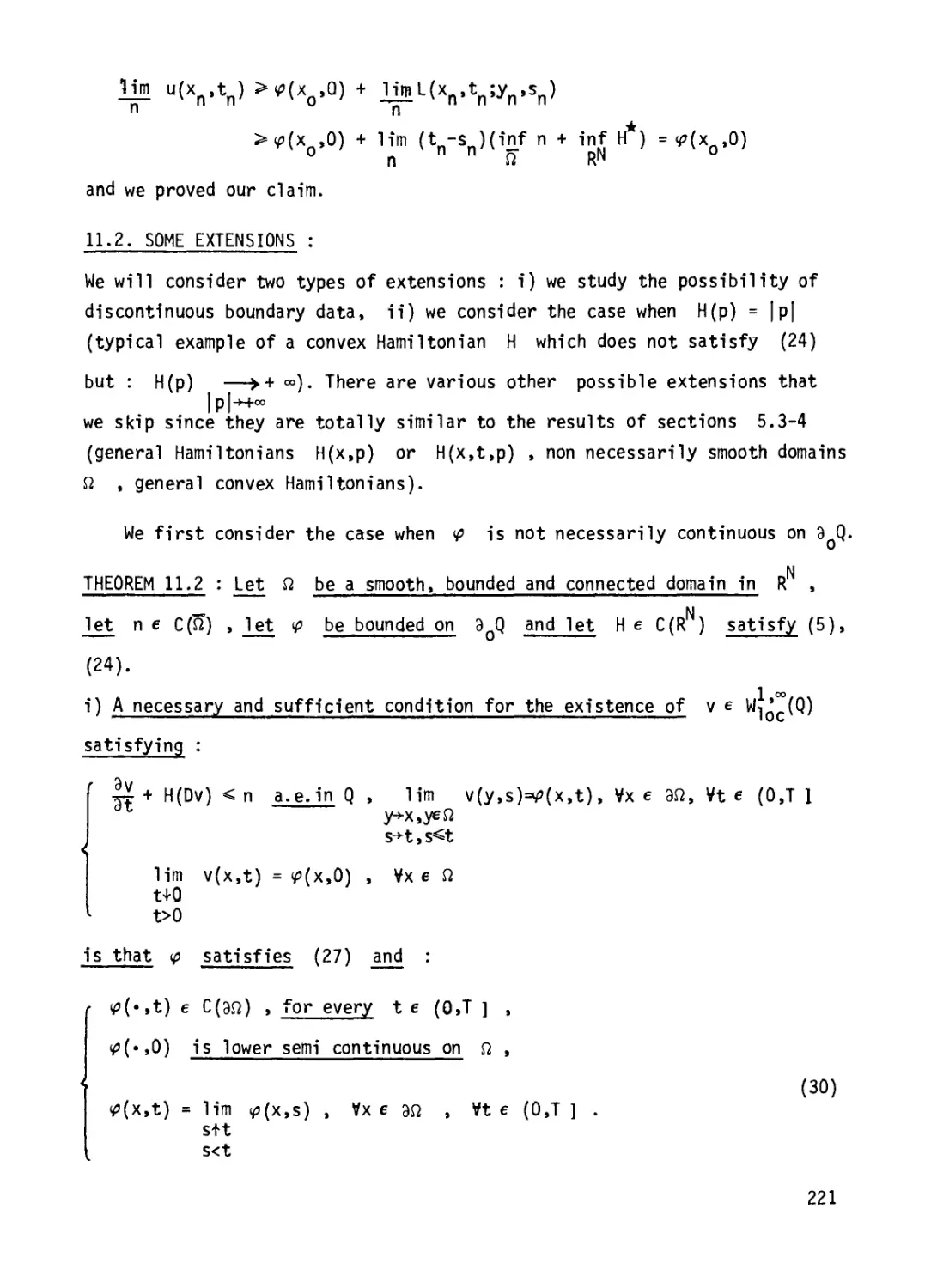
11.2 - Some extensions. 221
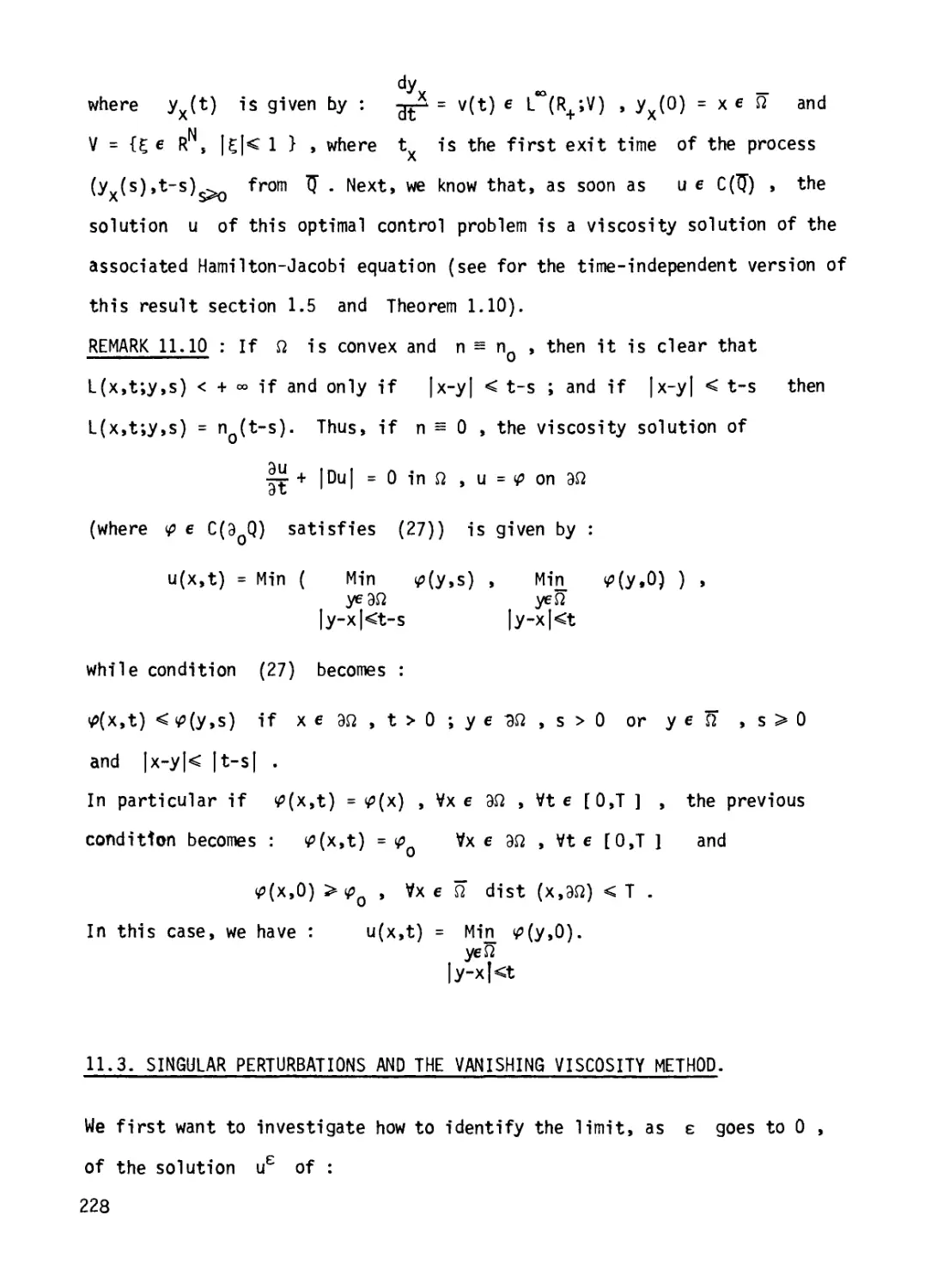
11.3 - Singular4 perturbations and the vanishing viscosity method. 228
CHAPTER 12 : Weak and classical solutions. 232
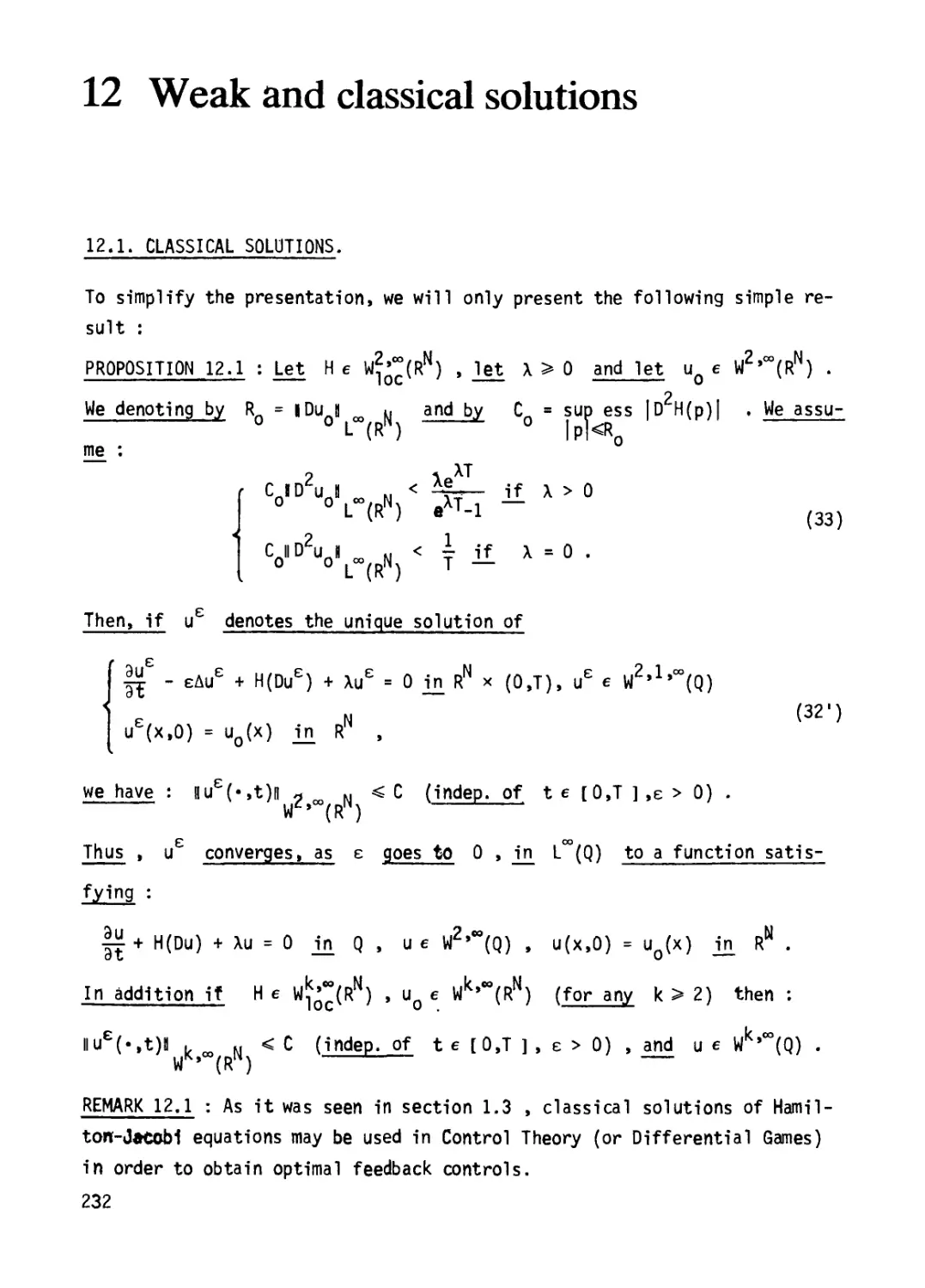
12.1 - Classical solutions. 232
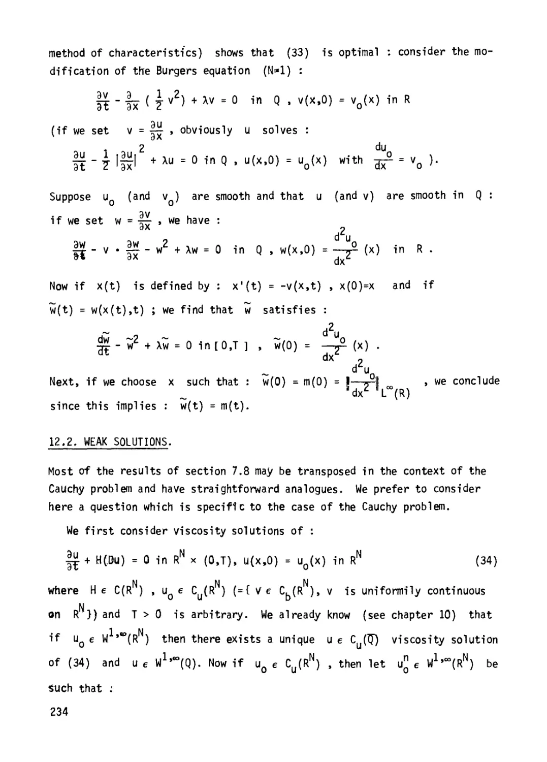
12.2 - Weak solutions. 234
CHAPTER 13 : Regularizing effect. 237
13.1 - Regularizing effect in RN. 237
13.2 - Boundary conditions. 242
CHAPTER 14 : Localization and asymptotics. 246
14.1 - Localization : the domain of dependence. 246
14.2 - Asymptotics. 250
CHAPTER 15 : Propagation of singularities. 255
15.1 - The threshold of regularity. 255
15.2 - Regularity of solutions near the boundary. 260
15.3 - Various questions. 263
CHAPTER 16 : Various questions. 267
16.1 - Applications to some hyperbolic systems. 267
16.2 - Singular perturbations and large-scale systems. 270
16.3 - Asymptotic problems. 272
16.4 - Various questions. 277
APPENDIX 1 : Existence and a priori bounds for solutions of second order
quasilinear equations. 279
APPENDIX 2 : A few results on viscosity solutions. 287
REFERENCES :
309
Introduction
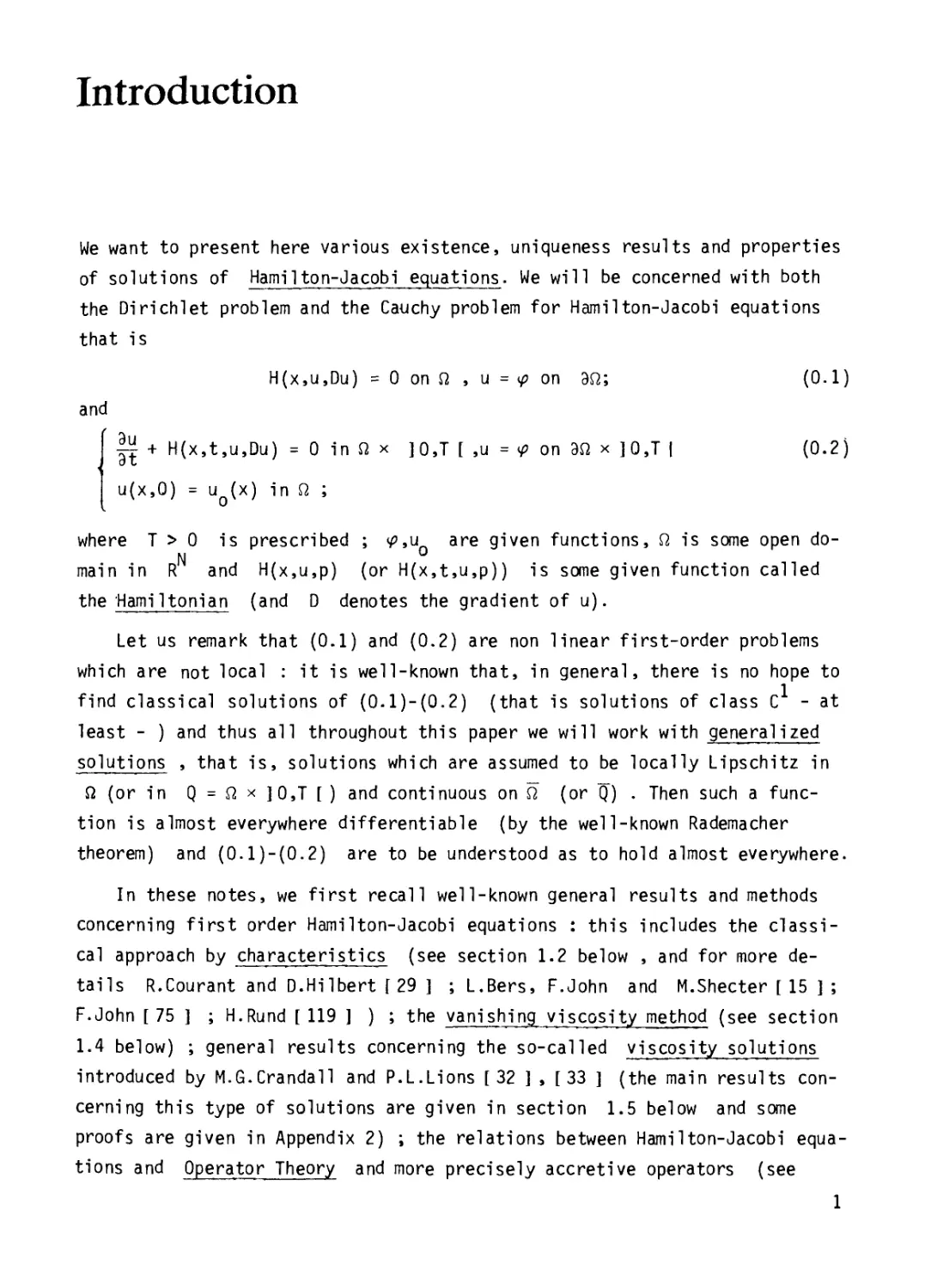
We want to present here various existence, uniqueness results and properties
of solutions of Hamilton-Jacobi equations. We will be concerned with both
the Dirichlet problem and the Cauchy problem for Hamilton-Jacobi equations
that is
H(x,u,Du) = 0 on Ω , u = φ on 9Ω; (0.1)
and
|ϊ + H(x,t,u,Du) - 0 in Ω χ ]0,T [ ,u = φ on 9Ω χ ]Q,T | (0.2)
u(x,Q) = u (x) in Ω ;
where Τ > 0 is prescribed ; </>,u are given functions, Ω is some open do-
N
main in R and H(x,u,p) (or H(x,t,u,p)) is some given function called
the Hamiltonian (and D denotes the gradient of u).
Let us remark that (0.1) and (0.2) are non linear first-order problems
which are not local : it is well-known that, in general, there is no hope to
find classical solutions of (0.1)-(0.2) (that is solutions of class С - at
least - ) and thus all throughout this paper we will work with generalized
solutions , that is, solutions which are assumed to be locally Lipschitz in
Ω (or in Q = Ω χ ]0,T [ ) and continuous on Ω (or Q") . Then such a
function is almost everywhere different!able (by the well-known Rademacher
theorem) and (0.1)-(0.2) are to be understood as to hold almost everywhere.
In these notes, we first recall well-known general results and methods
concerning first order Hamilton-Jacobi equations : this includes the
classical approach by characteristics (see section 1.2 below , and for more
details R.Courant and D.Hubert Γ 29 ] ; L.Bers, F.John and M.Shecter [ 15 ] ;
F.John [ 75 ] ; H.Rund [ 119 ] ) ; the vanishing viscosity method (see section
1.4 below) ; general results concerning the so-called viscosity solutions
introduced by M.G.Crandall and P.L.Lions [ 32 ] , [ 33 ] (the main results
concerning this type of solutions are given in section 1.5 below and some
proofs are given in Appendix 2) ; the relations between Hamilton-Jacobi
equations and Operator Theory and more precisely accretive operators (see
1
section 1.6 below).
Finally we recall and explain briefly the way Hamilton-Jacobi equations
are classically derived from the-Calculus of Venations , we will also
emphasize the relevance of the Dirichlet problem (0.1) (or (0.2)) to Optimal
Control Theory (see section 1.3 below, and for more details W.H.Fleming
and R.Rishel [ 52 ]) and the connections between Hamilton-Jacobi equations
and optimal deterministic control (at this point it is worth mentioning that
in engineering texts, the Hamilton-Jacobi equation is often called the
Bellman equation).
After these general and probably well-known results, we give in the
remainder of these notes various results, most of them being new (some have
been announced in P.L.Lions [104 ]- [105 ] ). Let us emphasize that they
essentially all concern generalized solutions (see the definition above). We
now present briefly some examples of the most characteristic results proved
below.
1. Existence results :
Let us consider for example the following case :
H(Du) = n(x) a.e. in Ω , u e W1,0°(n) , u = φ on 9Ω (0.3)
where Ω is a bounded open domain, φ and η are continuous functions.
Our main existence result for this problem states that if we assume :
H(p) -> + - , Η e c(RN) (0.4)
3. ν e (^(Ω) η (](Ω) : H(Dv) < n(x) in Ω , ν = φ on 9Ω (0.5)
then there exists a solution u of (0.3). Let us emphasize that assumptions
(0.4)-(0.5) seem to be optimal.
In addition if Η is convex , (0.5) may be relaxed to :
3 ν ί W1 ·°°(Ω) : H(Dv) < n(x) a.e. in Ω , ν = φ on 9Ω (0.5')
These existence results (and various extensions and related results) are
proved in Chapters 2 and 4 (Part 2). The corresponding results for the
Cauchy problem (equation (0.2)) are given in Chapter 9 (Part 3).
2. Uniqueness results :
It is easily seen on simple examples that in general there may be many
2
generalized solutions of (0.1) (or (0.2)).
Here we give various uniqueness criteria (of course the solutions found by
the existence results - as those described above - satisfy those criteria).
In particular when the Hamiltonian Η (and more precisely the map
ρ -*· H(x,t,p)) is convex (for all x,t) , we prove there exists (under
general conditions) a unique semi-superharmonic generalized solution of (0.1)
(or (0.3)) (in short a SSH generalized solution) that is a unique
generalized solution satisfying :
Ли < C6 in Χ»'(Ωδ) (0.6)
for some constant С > 0 , and for all δ > 0 - where Ω.= {xei2,dist(x,3n)>6}.
The class of semi-superharmonic functions has been introduced by the author
(cf. [ 98 ], [ 100 ], [ 102 ] ) in the context of the Hamilton-Jacobi-Bellman
equations occuring in Optimal Stochastic Control (which are in some sense an
extension of the classical Hamilton-Jacobi equations). This class is also
used in order to obtain stability results. Finally let us mention that this
class contains the class of semi-concave functions introduced in the context
of Hamilton-Jacobi equations by A.Douglis [ 42 ], S.N. Kruzkov [ 77 ].
These uniqueness and stability results are proved in Chapter 3 (Part 2)
while the corresponding results for the Cauchy problem (0.2) are given in
Chapter 10 (Part 3).
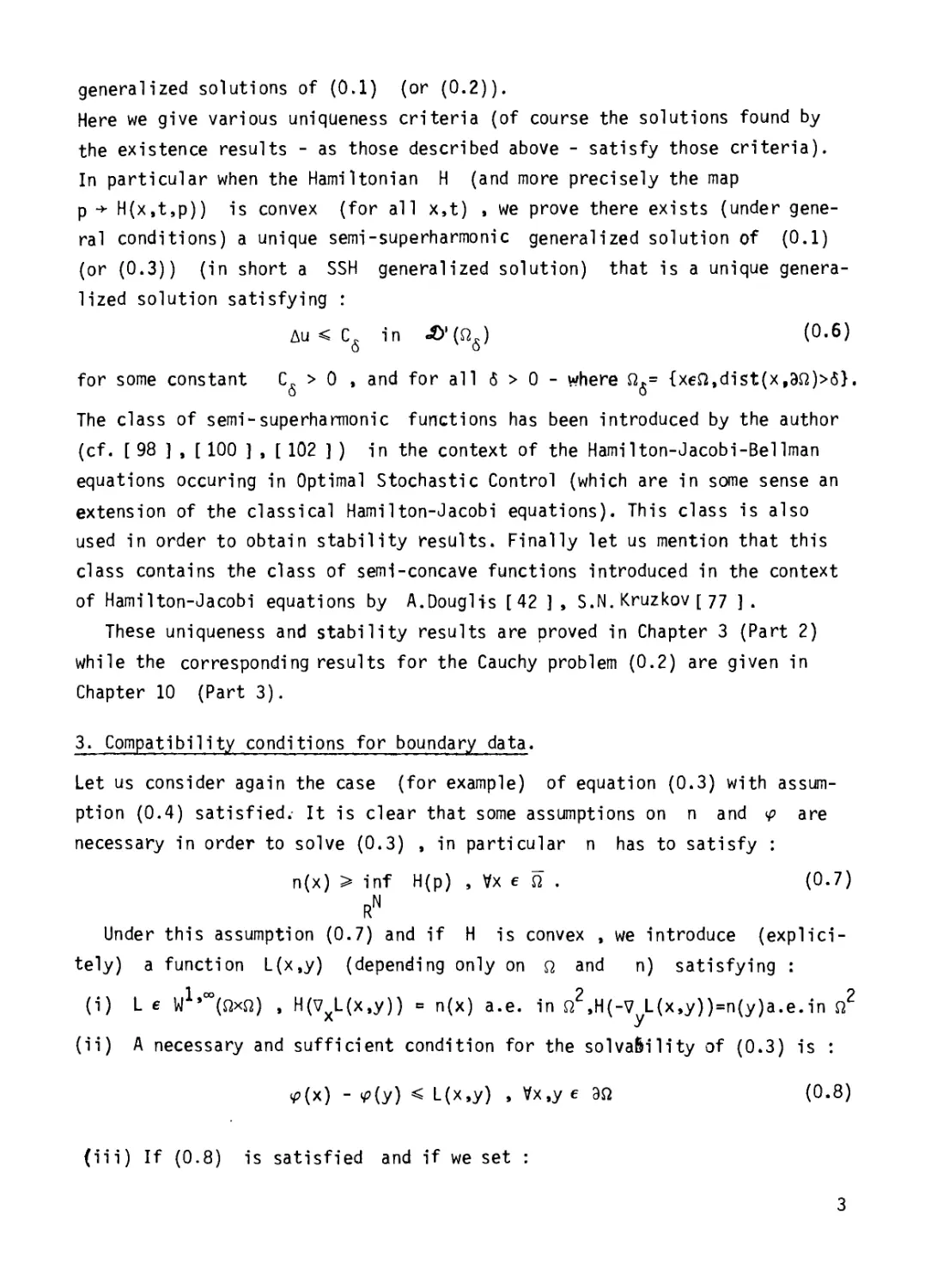
3. Compatibility conditions for boundary data.
Let us consider again the case (for example) of equation (0.3) with
assumption (0.4) satisfied.· It is clear that some assumptions on η and φ are
necessary in order to solve (0.3) , in particular η has to satisfy :
n(x) > inf H(p) , Vx e ω . (0.7)
RN
Under this assumption (0.7) and if Η is convex , we introduce (explici-
tely) a function L(x,y) (depending only on ω and n) satisfying :
(i) L e W1'"^) , H(vL(x,y)) = n(x) a.e. in Ω2,Η(-ν L(x,y))=n(y)a.e.in Ω2
л У
(ii) A necessary and sufficient condition for the solvability of (0.3) is :
^(x) " Viy) < L(x,y) , Vx.y e 9Ω (0.8)
(iii) If (0.8) is satisfied and if we set :
3
u(x) = inf Иу) + L(x,y)} (0.9)
уеЭП
then u solves (0.3) (In addition u satisfies the various uniqueness
criteria that we described above).
The introduction of this "fundamental solution" - like function L(x,y)
is motivated by optimal control considerations and strongly agrees with
the definition by physicists of optical lengths in the context of Eiconal
equations (particular cases of equations (0.1)-(0.3)).
Those results are developped in Chapter 5 (Part 2) while analogous results
for the Cauchy problem are proved in Chapter 11(Part 3). Finally let us
mention that these results extend and explain various results including some
given in S.N.Kruzkov [ 77 ] , S.H.Benton [ 14 ] , and the famous Lax formula
(P.D.Lax [95 ] ).
4. The vanishing viscosity and singular perturbations.
Most of the existence results concerning equations (0.1)-(0.3) are proved
through the introduction of some auxiliary problem - as, for example, in
the case of (0.3) :
-еДие + H(Due) = n(x) in Ω , ue = φ on 9Ω . (0.3-ε)
Thus one solves first (О.З-ε) and one lets ε -*■ 0 : by analogy with fluid
mechanics, this method is called the vanishing viscosity method. Of course for
ε > 0 fixed , (О.З-ε) is still a non trivial non linear problem and we
will need some work to solve such equations (we will rely on the results and
methods of P.L.Lions [ 101 ], which are recalled in Appendix 1).
In Chapter 6 (Part 2) , we consider two different types of questions
related to singular perturbations. The first one concerns the rate of
convergence of ue towards "the" solution u of (0.3) (of course when there
exists a solution of (0.3) i.e. when the compatibility conditions on φ and
η described above are satisfied) : we will prove that, essentially, the
norm of ue - u in L°°(n) is of order ε .
The second question concerns the case when the compatibility condition
(0.8) is not satisfied and yet (О.З-ε) can be solved for all ε > 0 : we
then identify the limit of ue as ε goes to 0 , ue converges locally
(there is a boundary layer) to a solution u of (0.3) but with a
different boundary condition namely : u = Ψ on 9Ω , where Ψ is the
maximum function satisfying (0.8), wich is less than φ .
4
5. Localization :
To simplify , we will consider for example the following problem :
f |H + H(Du) = 0 a.e. in RN χ (Ο,Τ) (0.10)
1 u(x,0) = uQ(x) in RN , u e W1'°°(RNx(0j)) ;
where Τ > 0 , uq e W1>0°(RN) and Η e w}£ (RN) .
We denote by u(x,t) (resp. v(x,t)) the solution of (0.10) with initial
condition u(x,0) = u (x) (resp. ν (χ)) which satisfies some uniqueness
criteria (as the one described in 2 above).
If we set С = sup IH'(p)| , where R = max (II Du II ет N ,11 Dv II N )
0 lpl<Ro ° ° L (RN) ° L°°(RN)
then we have the following localization principle :
u(x,t) = v(x,t) for I xl < ρ - С t , if u (x) = ν (x) for I x|< Ρ (0.11)
This result (of hyperbolic nature) has been partially proved by
A.Friedman [ 56 ] or S.N.Kruzkov [ 83 ] : we give here (Chapter 14 - Part 3) the
optimal result which we prove by the use of the vanishing viscosity method
- a similar result is proved in M.G.Crandall and P.L.Lions [ 32 ] by
different techniques.
6. Regularizing effects.
If Η is convex and satisfies :
H(p) / | p| ччч» , as |p| - +» ; (0.12)
then we prove there exists a solution u(x,t) of
|£ + H(Du) = 0 a.e.in RN χ (Ο,Τ)
1 oo Ν Ν
u e W1' (R χ (6,T)), for all & > 0 ; u(x,t) -*- u (x), Vx e RH (0.10')
^°+ °
N
under the mere assumption : u is bounded , lower semi-continuous on R .
This result (essentially well-known) is typical of some regularizing
effect since u(x,t) at a positive time t > 0 is Lipschitz in χ while
u is only l.s.c. . We extend and improve this type of results in Chapter
13 (Part 3): in particular we treat the case of boundary value problems, we
prove that lower semi-continuity for u is the best regularity one can deal
with in order to have solutions of (0.10') , and finally we give some
conditions which ensure that u(x,t) is semi-concave (or SSH) .
7. Asymptotics.
To simplify, we will consider the following problem :
|H + H(Du) = 0 a.e. in RN χ (0,+-) ,u(x,Q) = u (x) in RN
u e W1,CO(RNx(0,T)) , VT > 0 ;
(0.10)
where u e W '°°(R ) and where Η is assumed to be convex , nonnegative
and such that H(0) = 0 . Then we prove in Chapter 14 (Part 3) that "the"
solution u(x,t) of (0.10) (satisfying some uniqueness criteria)
converges as t -*■ +°° , to u(x) given explicitely by :
u(x) = infN {u (y) + max (x-y,p)} (0-13)
yeR1" ° H(p)=0
and u(x) is the maximum solution of : H(Du) = 0 a.e. in R , u e W ' °^R ),
N
u < uQ in R4 .
We also show how u(x) can be viewed as the solution of some degenerate
obstacle problem for Hamilton-Jacobi equations (see Chapter 8 - Part 2 -
for various results concerning the obstacle problem for Hamilton-Jacobi
equations - notice also that obstacle problems arise naturally as optimal
time problems in Optimal Control ).
8. The threshold of regularity.
Again we will consider a simple situation : assume that in some open domain
N 1
ω с R χ (o,°°) , there exists а С solution of
|^+H(Du)=0 in ui.ueC1^) (0.14)
2 2
where Η is convex, He С and D Η is positive definite.
Then we prove that, necessairily, we have : u e С ' (ω).
This phenomena is related to the propagation of singularities for
Hamilton-Jacobi equations (for general results concerning the propagation of
singularities in non linear Partial Differential Equations, see J.M.Bony [ 18 ],
[ 19 J , Y.Meyer [ 112 ] ) and to various results in the theory of non linear
hyperbolic equations and systems (see C.M.Dafermos [ 36 ] , R.Di Perna [40 ] ,
[ 41 ] ) . We also give many variants and extensions of this
result : in particular we treat the cases of stationary problems, of
"degenerate" Hamiltonians (as for example H(p) = |ρ|α , a f 2) and we
prove that С is the best regularity one can obtain in general (see
Chapter 15 - Part 3).
The results that we briefly described above are just examples (and
samples) of the results presented below. Let us also mention yery quickly a
list of other aspects of Hamilton-Jacobi equations as , for example, the
existence of classical solutions (see Chapters 7 and 12) ; the case of other
boundary conditions (Chapter 8) , the application of our results to optimal
control (Chapter 8) , the existence of weak solutions (Chapters 7 and 12),
the application of our results to quasilinear hyperbolic systems (Chapter 16)
various asymptotic and singular perturbations problems and their
applications to Physics or Economics (Chapter 16).
Remarks :
We would like to point out a few motivations to our work. To this end,
we will recall briefly some of the various fields where the Hamilton-Jacobi
equations arise.
First of all, the Hamilton-Jacobi equation is intimately connected with
the Calculus of Variations and with Hamiltonian Systems of Ordinary
Differential Equations - see sections 1.2, 1.3 for a yery brief account of
these connections , see also H.Rund [ 119 ] , and L.C.Young [ 132 ],
G.A.Bliss [ 16 ] and for a simple and brief presentation S.H.Benton [ 14 ] .
In particular Hamilton-Jacobi equations can be used to solve various
problems of the Calculus of Variations with many applications to physics and
for instance to Mechanics (in [ 14 ] , various references are listed).
A related application of Hamilton-Jacobi equations is Optimal Control
Theory and the theory of differential games : we will come back later on
on these aspects - see also W.H.Fleming [48 ][49 ] , W.H.Fleming and
R.Rishel [ 52 ] , A.Friedman [56][57 ] , R.Isaacs [ 70 ] , and references given
in these works. Let us also recall that often the Hamilton-Jacobi equation
(when arising from Optimal Control Theory) is also called the Bellman
equation of the associated control problem (and this because of the
intimate connection of the derivation of Hamilton-Jacobi equation with the dynamic
programming principle). We would like to emphasize that our main motivation
7
for studying the Dirichlet problem for Hamilton-Jacobi equations comes from
Optimal Control (see for more detailed explanations section 1.3) :
in many situations, the state of the system which is to be controlled in an
optimal way cannot run in the whole space, one has constraints on the state
and this means boundary value problems for Hamilton-Jacobi equations. Notice
by the way that our notion of boundary value problems does not coincide with
the one developped in S.H.Benton where , instead of (0.2) one looks for
solutions of
Щ + H(x,t,u,Du) = 0 in RN χ (0,T) , u = φ on 9Ω χ (Ο,Τ)
u(x,0) = u (x) in R
(this is by the way a non standard boundary value problem, which is of course
less general than (0.2) since a solution of this problem gives immediately
a solution of (0.2), while the converse may be false). This notion of
boundary value problems, even if not meaningless from the Optimal Control point
of view, seems to be in general unrealistic : in particular this does not
correspond to any constraint on the state of the system.
We want to mention another field where the Hamilton-Jacobi equation ari^
ses : in the WKB or geometrical optics method for expanding the solutions of
high frequency wave propagation problems -see for example A.Bensoussan ,
J.L.Lions , G.Papanicolaou [13 ] for the derivation of the Eiconal
equation equation from Schrodinger, Klein-Gordon, Maxwell or transport equations
(the equation usually called Eiconal equation is just a particular case of
the Hamilton-Jacobi equation (0.2) , namely where H(x,t,p) is of a special
form). By the way, the Eiconal equation arises in problems of spectral
representations of Schrodinger operators (see T.Ikebe [ 68 ] , T.Ikebe and
H.Isozaki [ 69 ] , H.Isozaki [ 71 ] , Y.Saito [ 121 ] , K.Mochizuki and J.Uchi-
yama [ 114 ] ).
Acknowledgements :
The author wishes to thank C.Bardos, H.Brezis, M.G.Crandall, P.Deift,
R.Di Pe-rna and L.Tartar for helpful and interesting questions and advices.
8
Part 1: Generalities
1 General methods
1.1. NOTATIONS :
Let Ω be some open domain in R , we consider the Dirichlet problem (0.1)
and the Cauchy problem (0.2) for (first-order) Hamilton-Jacobi equations :
H(x,u,Du) = 0 in Ω , u = φ on 9Ω (0.1)
Г Щ + H(x,t,u,Du) = 0 in Ωχ (ОД) , u = φ on 9Ω χ [ОД ] (0.2)
J u(x,0) = u (x) in Ω ,
where Τ > 0 is given. The function H(x,s,p) (or H(x,t,s,p)) is some
given function, called the Hamiltonian : we will always assume (except when
explicitely mentionned) that H(x,s,p) , H(x,t,s,p) are continuous on
Ω χ R χ RN , resp. on Ω χ R χ RN .
Above and everywhere below, Du or D u or Vu will denote the gradient
(in x) of u "» st" » э!< W1^ denote the derivative of u with respect to
i
t,x. ; finally, we will use the notation H'(p) , DH(p) or VH(p) for the
gradient of the Hamiltonian H(p) . Let us also mention that we will always
use throughout the usual convention for repeated indices (α. β. denotes
? a. &.). We denote by x«y or (x,y) the scalar product on R .
Let us give now a brief list of functional spaces we will use all
throughout : C(n) = {v continuous on Ω}, ί°°(Ω) = {ν measurable bounded in Ω},
С(П) = iv continuous on Ω} , Cb(fi) = C(fi) η |_°°(Ω) , СЬ(П) = С (Ω) η |_°°(Ω) ,
Cu(n) = (veCb(n) , ν uniformly continuous on Ω} , С (Ω) = {νεΟ.(Ω), ν
uniformly continuous on Ω} , (3°'α(Ω) = {νε(3(Ω)/30 > 0 |v(x)-v(y)|< C|x-y|a
Vx.yeltU for 0 < a < 1, (3°'α(Ω) = {νε(30'α(ω), V ω open bounded set such that
ω en}, Й)(П) = (3~(Ω) = {ν e С (Ω) , ν has a compact support in Ω },
W '°°(Ω) = {ν e Ι_°°(Ω) , Dv e Ι_°°(Ω)} (Dv can be taken for example in the
sense of distributions) , Wk'°°(n) = {v e |_°°(Ω) , ϋΡν e |_°°(Ω) V |α| < к} ,
L-|oc(ft) = {ν measurable bounded on each bounded open set ω such that ω<=Ω} ,
W?oc(n) = {v e LToc(n) ' ^ e LToc(fi) V Η * кЬ Notice that Wloc(") =
10
C°'V) and that, when Ω is "smooth" , Ν1,0°(ω) = 0ο,1(Ω) η ί"(Ω).
As said in the introduction we will work with generalized solutions which
we define precisely now :
DEFINITION : A function u is said to be a generalized solution of - the
Dirichlet - problem (0.1) if u e W^J (Ω) η (3(Ω) and (0.1) holds a.e. ,
orjnore precisely if u satisfies : u e W-|^(n) η С (Ω) a_nd^
H(x,u,Du) = 0 a.e. in Ω , u = φ on 9Ω (1)
DEFINITION : A function u is said to be a generalized solution of - the
Cauchy - problem (0.2) if u e W ,'°!(Q) η c(0J where we denote by
Q = Ω χ (Ο,Τ) and if u satisfies :
Ш + H(x,t,u,Du) = 0 a.e. in Q , u = φ од 9Ωχ[0,Τ ] ,u(x,0) = u (χ) in Ω (2)
Let us just recall that these definitions make sense in view of the well-
1 °°
known Rademacher theorem (see Federer [ 47 ] ) since if u e W-,' (Ω) ,
then u is a.e. differentiable and that (1) is equivalent to say that the
equation holds at almost all points of differentiability of u .
Finally we want to introduce a few notations : Ω. = {x e Ω , |x| < 1/δ ,
dist(x^) > 6} (for 6>o) , Q. = Ω. χ(δ,Τ-δ) - We need to introduce two
classes of functions :
DEFINITION : A function u e (3(Ω) is said to be semi (or demi) concave if
u satisfies :
2
νδ > 0 3 Сб > 0 ϊ-± < Сб in_ 2)' (Ωδ) , V χ β RN ΙχΙ = 1 , (3)
ЭХ
(this is equivalent to the statement : for all δ > 0 , there exists C_ such
12
that u(x) - j C- |x| is concave on every convex subset of ω ).
DEFINITION : A function u Ц (ω) is said to be semi-super harmonic (SSH
in short) if u satisfies :
νδ > 0 3 C6 > 0 Ли < Сб in, 2>·(ίϊδ)
э2
where Δ denotes Σ -2-^- .
— i г
■\
We will conclude by a last notation : if H(p) is a continuous convex
N *
function on R , we denote by Η the dual convex function of Η defined
11
by : Η (ρ) = sup ((q,p) - H(q))< +<» , Η is defined on a convex set
qeR
dom(H ) = {p e R ,H (p) < °° }, Η is convex and l.s.c. - for more details
and properties of dual convex functions, see R.T.Rockafellar [ 118 ] ,
I.Ekeland and R.Teman [ 43 ] .
Finally let us mention that formulas are numbered sequentially in each
+■ h
Part and that formula (l.n) (when referred to) will mean the η formula
of Part 1 (and similarly for (2-n) or (3.n)) while (O.n) is the η
formula of the Introduction.
1.2. CLASSICAL METHODS : CHARACTERISTICS :
In this section, we will only explain the basic ideas of the method of cha
racteristics applied to first order Hamilton-Jacobi equations (for more
explanations and more general results we refer to , for example, R.Courant
and D.Hubert [ 29 ] , F.John [ 74 ] , [ 75 ] , P.D.Lax [ 91 ] , H.Rund [ 119 1 )■
To motivate the introduction of the method of characteristics , let us
first recall a yery simple example : consider the equation :
Щ + a-Du = 0 in RN χ (0,») , u(x,0) = u (x) in RN . (5)
It is well-known that the solution of (5) is given by :
or
u(x,t) = uq(x - ta) (6)
uq(x) = u(x + ta.t) (6')
Remark that we have also :
Dxu(x,t) = Dx uQ(x - ta) , Dxu(x + ta,t) = D^x) (7)
The idea of the method of characteristics for the problem
|^ + H(Du) = 0 in RN χ (0,~) , u(x,0) = u (x) in RN (8)
is to replace the line x+ta by some other line x+t φ{χ) such that a
smooth solution u of (8) satisfies : Du(x+ti(x),t) = D u (x).
X ли
We will choose (and it is quite natural) : φ(χ) = H'(Du (χ)).
Therefore, we introduce :
X(x,t) -x+t H'(Du (x)) (9)
Next, we want to define u at the point (X(x,t),t) (in a similar way
12
as in (6')) ; in order to do so, let us consider the following ansatz :
u(X(x,t),t) = U(J(x) + t Ψ(χ) (10)
Let us now find some Ψ such that u given above satisfies both (8) and
Dxu(X(x,t),t) - Dxuq(x) (7')
From (10) we deduce (differentiating with respect to t) :
*<x)=f£(X<x.t).t)+$ -Dxu
= |H (X(x,t),t) + H'(DuQ(x)) · Dxu(X(x,t),t)
and since we want u to satisfy (8) and (7'), this yields :
Ψ(χ) = H'(Duo(x))-Duo(x) - H(DuQ(x)) .
Therefore, to surmiiarize, we find :
X(x,t) - χ + t H'(Du (x)) (9)
u(X(x,t),t) = uq(x) + t {H'(Duo(x)).Duo(x) - H(Duq(x))} (10')
and this construction is known as the method of characteristics.
The fact that, indeed, u "defined" above satisfies the equation (8) and
also (71) will be proved below under some natural assumptions. Before
giving any precise result, let us first remark that u is well defined by
(10) if and only if the map (x —>X(x,t)) (for each t) is bijective. And
this will be in general true for t small (and this will yield local
existence results) and in general false for every t .
Let us now give a few precise and rigorous results on this method for
equation (8) , we will give later on a brief description of the general
characteristics method for problems (0.1) or (0.2). We will assume :
Η e C2(RN) (11)
The first and classical result is the following :
THEOREM 1.1. : Let uq e C2(RN) and let us assume that for te[0,T) (for
some Τ > 0) the map (x —>X(x,t) = χ + t H'(Du (x)) ) is a diffeomorphism
1 1 °
of class С (i.e. bijective and with а С inverse). Let us denote by
~tj ■ ■ ■
X (x,t) the inverse map (for each t e (0,T) fixed) and let us introduce,:
u(x,t) = uo(X"1(x,t))+t{H'(Duo)-Duo-H(Duo)}(X"1(x,t)),V(x,t)eRNx[0,T) (12)
13
Then u(x,t) e C2 (RN χ [Ο,Τ)) and satisfies in RN χ ГОД) :
Dxu(x,t) = Duo(X-1(x,t)) , Щ (x,t) = - H(Duo(X-1(x,t)) ) , (13)
thus we have :
|^+ H(Du) = 0 in RN χ [Ο,Τ) , u(x,0) = u (x) Jn RN . (8')
Before giving the (elementary) proof of this result, let us mention a
few direct applications :
COROLLARY 1.1 : Let u e C2(RN) and Due C. (RN) , D2u e C.(RN) ; let
—■ О X О Dx ' X О Dx
?
Τ be the supremum of all t > 0 such that : det(IN + t H"(Du (x))-D uQ(x))>0
N
for all χ e R . Then Τ > 0 and all the assumptions of Theorem 1.1 are
N
satisfied and thus the conclusions hold and (8') is satisfied on Rx[0,T).
Indeed I., + t H"(Du (x))«D u (x) is the jacobian matrix of the map
(x —> X(x,t)) and thus for 0 < t< Τ this map is а С diffeomorphism.
To conclude we just need to remark that for small t this determinant is
obviously positive and Collary 1.1. is thus just a trivial adaptation of
Theorem 1.1. .
COROLLARY 1.2 : L_et_ u e C2(RN) be convex (resp. concave) and let Η be^
convex on R (resp. concave) then we have det (IN+t H"(Du (x))«D u (x))>l
N
for all χ e R , t > 0 . Thus the assumptions and conclusions of Theorem
1.1. hold with Τ = +°° .
Indeed this is an immediate consequence of an easy lemma of linear
algebra : let A,B be two NxN nonnegative symmetric matrices then all the
eigenvalues of AB are real and nonnegative, and thus det (IN + AB) > 1.
We now turn to the proof of Theorem 1.1 : obviously it is enough to
prove (13) . From the assumptions and from (12) , it is obvious that
u e C!(RN χ [Ο,Τ)).
And we have :
Dxu(x,t) = Duo(X-1(x,t)).{Dx X_1(x,t) + t H".(D2uo)-Dx X_1(x,t)}
14
2
(with obvious arguments for H" , D u ) , hence
Dxu(x,t) = Duo(X_1(x,t))-(IN + tH"-(D2uo))-(DxX(X_1(x,t),t))_1
= Duo(X_1(x,t))-(IN + t H"(Duo).(D2uo))-(IN + tH"(Du0).(D2uq)f1
= Duo(X_1(x,t)).
In the same way , we find :
Щ (x,t) = Оио(Х_1(хД)).з| (X_1(x,t)) + {H'(Duo)Duo - H(Duq)} +
+ t {Quo-H"-(OZuo).^ (X_1(x,t))}
now from the identity : X (X (x,t),t) = χ ,
we deduce :
^ (X_1(x,t)) = - (D^iX'^x.tJ.t))"1· Щ (X_1(x,t),t)
= - [IN + t H"-(D2uo) ]_1· H'(Duo(X_1(x,t)) ).
Therefore, we obtain :
Щ (x,t) = + (Duo-[IN + t H"-D2uo ]· g| (X_1(x,t))} + iH'(Duo) Duq - H(DuQ)}
= - Duo-H'(Duo) + H'(Duo)-DuQ - H(Duq)
= - Η (Duo(X-1(x,t)) ) ;
and this completes the proof of Theorem 1.1.
REMARK 1.1 : Let us remark that an examination of the preceding proof
shows that if u e C1,:l(RN) and if , for te [0,T) , the map (x н> X)
is a locally Lipschitz diffeomorphism (i.e. bijective with a locally Lips-
chitz inverse) .then u(x,t) defined by (12) is C1 ,]-{Rn χ [ 0 J)) and
(13), (8') hold. In particular if uq e W '°°(R ) then for some small Τ > 0
the preceding holds - we will use this technical remark later on.
In the same direction, it would be of interest to know that , if we
assume :
J Η e C1(RN) , uQ e C1(RN) and if the map (x »-> X(x,t)) is an
( homeomorphism (bijective with a continuous inverse) for t e [0,T)
15
u(x,t) defined by (12) is of class C1 on RN χ Ю,Т) and (13), (8')
hold. We know how to prove this only if Η is convex (see section 15.3 -
Part 3).
Before going to the exposition of the general method of characteristics
for problems like (0.1) or (0.2) , let us mention that the above
considerations yield local (in time) smooth solutions of the Cauchy problem (8). Of
course when two characteristics cross that is if we have :
X(xrt) φ X(x2,t) if t < tQ , X(xrtQ) = X(x2,t0)
then in general (that is if Du (xj f Du (x2)) the solution u "defined"
by (12) (at least for t < t ) has a discontinuity on its gradient : one
says in that case thet there is formation of a shock . The fact that, in
general, shocks do appear (even for smooth initial data u and for a smooth
Hamiltonian) can be seen on the following simple example : suppose that
there exists a smooth solution u (for all time t > 0) of :
2
9jj 1_
3t " 2
_3u
Эх
0 in R χ (0,-н») , u(x,0) = u (x),
Differentiating twice the equation with respect to χ , we find, denoting by
,, Э2и Эй
|? - ν |£ - w2 = 0 in R χ (0,+-) , w(x,0) = —Д .
dx
Next let x(t) be defined by : x'(t) = -v(x(t),t) , x(0) = χ and let
W(x,t) = w(x(t),t) ; we find that w satisfies :
2
|« . $ , ΐ(χ,Ο) - -Λ .
dx „
d^u
Thus as soon as, at some point χ , —«^ (x ) > 0 > this ordinary diffe-
dx
rential equation shows that w becomes unbounded in finite time :
d u dun ,
w(x,t) = ( 1 (x) ) {1 - t 1 (x) }_i
dx^ dx^
Therefore there does not exist , in general , a smooth solution for all
2
time [ remark that w (and thus w = —j ) becomes unbounded when
Эх
16
d2u
1 - t % is no longer positive that is when the jacobian of the characte-
dx du
ristic (x + x-t -r~ (x)) vanishes] .
dx
We now turn the description of the general method of characteristics for
problems like (0.1) (or (0.2)) : we will consider the problem
H(x,u,Du) = Q in Ω , u = φ on 9Ω (0.1)
where Ω is а С domain in R , Η e С (R χ R χ R ) and ^ is С on
3Ω - The extension of the preceding method for building (locally) a smooth
solution of (0.1) is the following : consider (X,U,P) (e RN χ R χ RN) the
solution of the following system of ordinary differential equations :
f X'(t) = fjj (X.U.P)
I U'(t) = Щ (X.U.P)-P (14)
P'(t) = -|£ (X.U.P) - fj (X.U.P)P
with the initial conditions : X(0) = χ e 3Ω , U(0) = φ{χ) and
P(0) = λ n(x) + э φ(χ) (15)
where λ will be determined later on , where n(x) is the outward unit
normal to 9Ω at the point χ and where 3φ denotes the gradient of φ on
9Ω .
If we are able to choose λ( = λ(χ)) in such a way that we have:
H(xw(x) , P(0)) = 0 then we claim that we have :
H(X(t),U(t),P(t) =0 , Vt > 0 (16)
Indeed in view of (14) we obtain :
^ H(X(t),U(t),P(t)) = |5 · X'(t) + -^ U'(t) + |^ · P'(t) = 0.
And (16) will allow us to define (or to try to do so) : u(X(t)) = U(t) ,
provided X(t) e Ω .
Therefore we first need to choose in a convenient way λ(χ) in (15) and
next we have to make sure that X(t) e Ω for t > 0 . We will thus assume
3 λ(χ) e С^ЭП) satisfying : H(x,^(x) ,λ(χ)η(χ) + Э φ(χ) ) = 0 on 9Ω (17)
17
And we set for such a function λ(χ) : P(x) = λ η + Э^ and of course we will
choose : P(0) = F(x) , that is we will take in (15) λ = λ(χ).
Next, we have to make sure that X(t) e Ω at least for small time
(t e [0,t )) and this is the case as soon as we have :
I? (x^(x)."P(x)) · n(x) < 0 on 9Ω (18)
dp
We will assume (18) from now on : we would like to point out that there is
a certain redundancy between (17) and (18) since, as soon as there exists
λ(χ) continuous on 9Ω satisfying : H(x,tp(x) ,λ(χ)η(χ) + Э^(х)) = 0 and
if (18) holds for the corresponding F(x) , then one deduces immediately
from the implicit function theorem that λ(χ) e С (9Ω) and thus (17) holds.
Next, assuming (17) and (18) , we define a solution u of (0.1) at
least locally near 9Ω . The idea is that , if the map X from 9Ω χ [ 0 ,tQ ]
(t > 0) which associates X(x,t) to (x,t) is a C1 diffeomorphism from
9Ω χ [0»tQ ] onto its range Σ ( Σ is a closed neighborhood of 9Ω in
Ω) , then defining :
Vx e Σ u(x) = U(X_1(x),t) (19)
we build in this way "a solution of (0.1) in Σ " (that is near 9Ω). In
addition we then have :
Vx e Σ Du(x) = P(X_1(x),t) (20)
and thus u e cz(E) . The verification of this fact is a straightforward
computation, totally similar to the one made in the proof of Theorem 1.1.
Now, it is easy to check that if (17) and (18) hold and if Ω is bounded
(if Ω is unbounded, some uniformity conditions are necessary in particular
(17) and (18) have to "hold uniformly") then for some t. > 0 , X(x,t) is
1
а С diffeomorphism from 9Ω χ [0,t ] onto its range Σ .
We will conclude this section by a few examples which illustrate this
method of characteristics and the way (17) and (18) may be satisfied :
Example : (The Cauchy problem) we choose Ω = R χ (0,+«°) and the time
will be denote by x- . . The Hamiltonian is given by :
Ν Ν
H(x,xN+1 »P»P|\|+1) where xe R , ρ e R and pN+1 e R stands for the
quantity corresponding to the time derivative. In the beginning of the
18
section we were considering an Hamiltonian of the form : PN+1+ H(p).
Obviously Эй = {0} χ R - R and ip is а С function on R : φ is the
initial condition. In this case (17) and (18) become :
3 λ(χ) e C!(RN) satisfying : H(x,0,D *>(x), - λ(χ)) - 0 (17')
|£ (x,0,D*(x), - λ(χ)) > 0 on RN . (18')
3pN+l
Obviously if we specialize Η to be of the following form :
Η = PN+1 + H(x,xN+1,p) (21)
then (18*) is trivially satisfied and (17') holds taking: A(x)=H(x,0,Dp(x)),
In what follows, we will specify Η to be of the preceding form, then
(14) decouples up to some extent and reduces to ·"
X'(t) =|£(X,t,P) , X(0) = χ
P'(t) = -|£ (X,t,P) , P(0) = Di(x)
ЭН (14'}
U'(t) =Щ (X,t,P) Ρ + PN+1 , U(0) =φ (χ)
XN+l(t) = t ' ΡΝ+1<*) = " |£ (Х'*'Р) ' W°> = "λ(χ)= "H(X'°'D *(*))·
Now, if we assume in addition to (21) that Η does not depend on χ . :
Η = ΡΝ+1 + H(x,p) (21·)
then P'N+1(t) = 0 and PN+1(t) = - H(x,0,D *(x)).
Finally, if Η is given by : Η = pN+, + H(p) , (14') reduces to :
X(t) = χ + t H'(D φ{χ))
t P(t) = D^(x)
U(t)=*(x) + t {H'(D *(x))-D φ(χ) - H(D^(x))}
and we find back (9) , (10') .
Example : Consider a bounded smooth domain Ω 1n R and let us apply the
above considerations to the following problem :
1 2
j |Du| = m(x) in Ω , u = φ on 9Ω (22)
19
where m e (32(Ω) , φ e (32(3Ω) .
Obviously (14) reduces to :
ί X'(t) = P(t) , X(0) = χ
P'(t) = " f* (χ(*)) » p(°) = э *(x) + A(x) n(x) (14')
U'(t) = |P(t)|2 , U(0) = *(x)
and we want to determine λ(χ) in order to have :
j |3 φ\2 + Ι (λ(χ))2 = m(x) on 3Ω
of course this is possible if and only if :
\ |3 φ\Ζ < m(x) on 3Ω (23)
(this compatibility condition will be ewplained in section 5.1 - Part 2).
,2 1/2
If (23) holds, we have two possibilities : λ(χ) = + (2m(x) - |Э φ\ )
In order to have a chance to check (18) , we will choose :
λ(χ) = - (2m(x) - |3 *>|2)1/2 . P(0) = Э φ(χ) - (2m(x) -\Ъ ^|2)1/2n(x).
Of course to insure that λ(χ) is smooth, we will need in general to assume :
j |Э φ\2 < m(x) on 9Ω . (23')
Now, if we assume (23') , it is clear that (18) holds with the above
choice of λ(χ) : indeed we have :
Щ (χ,Ρ(0))·η(χ) = - (2m(x) - |3 ^|2)1/2 < 0 on 3Ω.
о
Therefore, this proves that there exists а С function u satisfying
u = φ on 3Ω , -y |Du| = m(x) in a neightborhood of 3Ω
Remark also that if m(x) Ξ m then we have :
J p(t) = P(0) = 3 ^(x) - (2 mQ - |3 ^|2)1/2 n(x) , U(t) = *(x) + 2t mQ
| X(t) = x + t P(0) = χ + t {3 φ{χ) - (2 mQ - |3 ^|2)1/2n(x)}
and restricting even more our attention , if m = ~- , φ = 0 then we have :
X(t) = x-tn(x) , U(t) = t , P(t) = -n(x).
Therefore the solution built nearby the boundary is :
u(x) = dist (χ,3Ω).
20
1.3. OPTIMAL CONTROL THEORY :
The purpose of this section is to show the intimate connections between
Optimal Control Theory and first order Hamilton-Jacobi equations. We will
first briefly discuss some well-known facts about this question and then we
will briefly consider some classical problems of Calculus of Variations .
For further discussions of optimal control problems the reader is referred
to the book of W.H.Fleming and R.Rishel [ 52 ] : we will here essentially
emphasize the use of the dynamic programming principle to derive the
Hamilton-Jacobi equation for the optimal cost function of deterministic optimal
control problems. This is the reason why , in such contexts, the Hamilton-
Jacobi equation is sometimes called the Bellman equation (since the dynamic
programming principle was found by R.Bellman [8 ] ). We will not talk about
the relations between deterministic differential games and Hamilton-Jacobi
equations since these questions are more technical and the methods are
identical to those we present below : instead we refer the interested reader
to R.Isaacs [ 70 ] , A.Friedman [ 55 ], [ 57 ] , W.H.Fleming [ 48 ] , [ 49 ] ,
S.N.Kruzkov f 85 ] .
1) Optimal control problems without boundary conditions.
Let us first describe the general form of some deterministic optimal
control problems: we consider a system which state is given by the solution
у (t) of the following differential equation :
—X + b(y (t),v(t)) =0 for t > 0 , у (0) = x e RN , (24)
dt x x
Ν Ν
where b maps R χ V into R , V is some given closed convex set in
N
R (for example) which will be called the set of values of the control.
Finally v(t) , called the control , can be any measurable bounded function
from [ 0,°°) to V .
We will assume all throughout that b(x,v) satisfies :
ί |b(x,v) - b(x',v)| < C|x-x'| V x,x' e RN Vv e V ;|b(x,v)|<C V(x,v)eRNxV
< \\
b(x,v) is continuous on R χ V ;
for some constant С > 0 .
Hence (24) has a unique solution (for all χ e R ) denoted by у (t)
21
Having defined the controlled system, we now define a pay-off function
(or cost function) for each given control v(·) :
J(x.t ;v(·)) = j f(yx(s),v(s)) exp {-J ο(γχ(λ),ν(λ))dA} + (26)
+ u0(yx(t)) exp { - j c(yx(s),v(s))ds}
J(x,v(·)) = I f(yx(t),v(t)) exp { - c(y (s),v(s))ds) . (26 )
Jo -Ό
Here f(x,v) , c(x,v) are given functions that we will always assume they
satisfy : 3 С > 0 such that for ip = f ,c we have
Hx.v) - *(x',v)| < С | x-x' | , k(x,v)| < С Vx,x' e RN Vv e V (27)
<i>(x,v) is continuous on R χ V ;
and we will denote by :
λ = inf{c(x,v) / χ e RN,v e V}
The problem to solve is to minimize the cost function over all controls
ν(·) , that is to find
u(x,t) = inf J(x,t;v(·)) (28)
v(·)
u(x) = inf J(x,v(·)) (28')
v(·)
We shall call problem (28) the finite horizon problem and (28') the
infinite horizon problem.
The main purpose of optimal control theory is to characterize these
optimal cost functions and to compute optimal controls (eventually in the form
called feedback optimal controls that we will define later on)-
An essential tool to the solution of this problem is the following result
(this is the core of the dynamic programming principle) :
THEOREM 1.2 :
1) Finite horizon problem : Under assumptions (25) , (27); we have :
22
u(x,t) = inf { f f(y (λ),ν(λ)) exp [ - f с(ух(т) ,ν(τ) )dx] dX +
v(·) ;o Jo
+ Li(yx(s),t-s) exp [ - c(y (τ),ν(τ))(1τ ]}
for al 1 0 < s < t .
2) Infinite horizon problem : Under assumptions (25) , (27) and if λ > 0 ;
we have :
ft rS
u(x) = inf { f(yx(s),v(s)) exp [ - c(yx(X))dA ] + (29')
v(·)
for all t > 0.
+ u(yx(t)) exp [ - | c(yx(s),v(s))ds ]}
~ N
REMARK 1.2 : If for some t > 0 , there exists u bounded on R
satisfying (29') then ΐί = u on R . Indeed we have then by (29') :
|(u-u)(x)| < sup |(u-u)(y (t)) exp [-
v(·) x
c(yv(s),v(s))ds ]|
or
sup Iu-XTI < (sup I u —TjI ) e
-At
RN RN
and u ^ Ή .
This shows that property (29') characterizes u .
Of course this result is very natural and the proof is easy : we will
sketch it in case of the infinite horizon problem and we will assume to
N
simplify the notations : c(x»v) ξ \ , Vx e R , Vv e V . Let t > 0 ,
we first prove that we have :
i) u(x) > inf { f f(yx(s),v(s)) e"As + u(y (t)) e"Xt)
v(·) i0 X
and we will next show the converse .
Indeed let ε > 0 and let v(·) be a control such that
u(x) < J(x,v(·)) < u(x) + ε .
Obviously у (s) = у (s+t) is the solution of :
τί + b(y(s),v(s)) = 0 ,
ds
У(0) =yx(t) ,
23
where v(s) = v(s+t)
Thus - J(x,v(·))
ft
f(yx(s),v(s)) e~As ds + e~At f(y(s) ,v(s))e~As ds
0 J0
ft
f(yx(s),v(s)) e"As ds + e"At u(yx(t))
and this proves i) since ε is arbitrary.
Now, to prove the converse : let ε > 0 and let ν (·) be such that
inf {[ f(y (s),v(s))e"Asds + u(yx(t))e"At} >
v(·) Jo
}f(y;(s),v0(s))e-Asds+u(y;(t))e-At-
where yx(t) is the solution of (24) corresponding to v0(')·
Next let v,(·) be such that :
u(yj(t)) > Jiy^tbv^·)) - ε .
We now define v(·) by : v(s) = ν (s) if s e [0,t [ and v(s) = v^s-t)
if s > t . Obviously the corresponding solution of (24) is yx(t) given by
Yx(t) = y°(s) if s < t , yx(s) = y^s-t) if s > t ;
where у is the solution of (24) corresponding to v,(·) and to the
initial condition yx(t)· Therefore we have :
f(yx(s),v0(s))e"As ds + u(y°(t))e"At > '
о
f(yx(s),v(s))e"As ds +
+ e
■At
f(yx(s).v(s))e"As ds - ε e"At
u(x)
and it is then obvious to conclude,
We will need the following easy regularity result :
PROPOSITION 1.1 :
1) Finite horizon problem : Under assumptions (25) , (27) , the function
u(x,t) belongs to W1,OT(QT) for all 0 < Τ < -к» , where QT = RN χ (Ο,Τ)
2) Infinite horizon problem : We assume (25) , (27) and we denote by :
24
λ = sup N { - (b(x,v) - b(x',v))-(x-x') |х-х'Г }·
x.x'eR
veV
If λ > λ+ , then u e w1,0°(RN) ; vf λ = XQ > 0 , then u e C°'a(RN) η
LOT(RN) for all 0 < α < 1 ; and if 0 < λ < \Q , then u e C°'a(RN) η L°°(RN)
wvth a = γ- i1).
о
We will only prove this result in the case of the infinite horizon
problem (the other case is even simpler ) and to simplify the notations we
N
will assume c(x,v) = λ ( Vx e R , Vv e V) . Since λ > 0 , we have :
|u(x)| <[ sup |f(x,v(t))|e~At dt < С
J0 x
e~At dt < £
Next, in view of (29') , we have for all x,x' e RIN and for all Τ > 0 :
-AT
. I I tnyv^s,!,v^s,lj- T[y„,{S),\i[S))ie as|+ue
|u(x)-u(x')|< sup | f {f(y (s),v(s))- f(yx,(s),v(s))}e"As ds| + Ce"
v(·) io
С f |yx(s) - у ,(s)| e_As ds + Ce"
J r\
On the other hand, we have :
Ж lyx^) " V(t>|2 = " 2(Ь(УХ(*))-Ь(УХ.(*)) )-(yx(t)-yx,(t))
hence, we obtain
2λ0 |yx(t) -yx.(t)|
2λ t
|yx(t) - yx,(t)|2<e ° |x-x'|2
The inequality yields :
|u(x)-u(x')| < С |χ-χΊ [ e° e"As ds + Ce"AT
If λ > λ , we obtain for all Τ > 0
|u(x) - u(x')| < C|x-x'| + С е
and letting Τ -+ +°° , we conclude.
-AT
If λ= λ , we obtain :
,ο »α,"3Γ
(Μ Recall that Cu ,U(R )=iueC(R") / 3 00 | v(x)-v(y) |<C|x-y|a Vx,yeRN} .
25
|u(x)-u(x')| < С Τ Ιχ-χ* j + С е~АТ
ι Ιx_x ' I
and if |x-x'| < λ , then choosing Τ = - ~ Log ( '—y-1 ) , we find :
|u(x)-u(x')| < С |x-x'| Log ( |-^-|) + С |х-х'|
and we conclude.
If λ < λ , we obtain :
(λ -λ)Τ λΤ
|u(x)-u(x')| < С |χ-χΊ е ° + С е '
1 λο~λ
and if Ix-x'l < ^- , then choosing Τ = Log (|x-x'| -r— ) » we
find : VA ^D
λ/λ
|u(x)-u(x')| < C|x-x'| ° ;
and we conclude.
Our next result explains the relations between the optimal control
problems and Hamilton-Jacobi equations :
THEOREM 1.3 :
1) Finite horizon problem : Under assumptions (25) and (27) and if there
N
exists (x ,t ) e R e (0,°°) such that u is differentiable at (χ0»Ο »
then we have at the point (х0»О :
Щ- + sup { b(xo,v)-Dxu + c(xo,v)u - f(xo,v)} - 0 .
In particular under assumptions (25) and (27) , we have : u e W ' (Qj) ,
VT < со ;
Й· + sup {b(x,v)-Dxu + c(x,v)u - f(x,v)} = 0 a.e. in RN χ (0,°°)
vev N (30)
u(x,0) = u (x) in R
2) Infinite horizon problem : Under assumptions (25) , (27) and if λ > 0
and if u is differentiable at some point χ then we have :
, e—^_ 0
sup (b(xo,v)-Dxu(xo) + c(xo,v)u(xQ) - f(xQ,v)} = 0 .
In particular under assumptions (25) , (27) and if λ > λ+ then ueW '°°(R )
26
and we have :
N
sup {b(x,v)«D u + c(x,v)u - f(x,v)} = 0 a.e■iη R . (31)
veV x
REMARK 1.3 : Obviously u satisfies some Hamilton-Jacobi equation ((30)
or (31)) with the Hamiltonian defined by (in the case of (31)) :
H(x,t,p) = sup (b(x,v) ρ + c(x,v) t - f(x,v)} .
veV
This Hamiltonian is clearly Lipschitz continuous and convex in (pst)
(supremum of affine functions) .
Conversely if H(x,t,p) is a convex continuous functions (pst) (and
Lipschitz continuous at least locally in χ ) then it is possible to write
H(x,t,p) as a supremum of affine functions and in this way to write down
some associated optimal control problem : indeed let us denote by Η (x,t,p)
the dual convex function of H(x,t,p) , recall that Η is given by
Η (x,t,p) = sup N {ts + pq - H(x,s,q)} < +°° .
(s,q)eRxR"
Now, we know that
H(x,t,p) = sup ^ {ts + pq - Η (x,s,q)}
(s,q)eDom Η (χ,·)
(see for example f43 ] , [ 118 ] , [ 22 ]).
And this proves that, at least formally , we may define for each convex
Hamiltonian some associated control problem in the sense that the
corresponding optimal cost function "solves" the Hamilton-Jacobi equation.
In each case, the first part of the'Theorem implies the second part
since a Lipschitz function/is a.e. differentiable (Rademacher theorem).
Again we will only prove the infinite horizon case and to simplify the
notations we will assume c(x,v) ξ λ > 0 . As it will be seen, the method of
proof relies on Theorem 1.2 (and this explains why (30) and (31) are
often called the Bellman equations of the control problem).
Proof of Theorem 1.3 : In view of Theorem 1.2 , we have for all t > 0 :
sup { I fu(x ) - u(y (t))e"At ]-И f(y (s) ,v(s))e~As ds} = 0 . (32)
ν(·) υ Λο L -Ό ο
27
The idea of the proof is to let t + 0+ and to derive (31) . We will first
prove :
(i) Vv e V , b(x0,v)-Dxu(x0) + λ u(xQ) < f(xQ,v) ,
and then we will prove the converse :
(ii) sup {b(xo,v)-Dxu(xo) + Au(xQ) - f(xQ,v)} > 0.
First, let ν be fixed in V and let y(t) be the corresponding
solution of (24) that is of :
% + b(y(t),v) - 0 for t >0 , y(Q) = xq.
From (32) , we deduce :
| (u(x0) - u(y(t))e"At) <|J f(y(s),v)e"Asds , Vt > 0 .
Next y(t) is differentiable at t=0 and thus u(t) = u(y(t))e is
different!able at t=0 and we have :
"(°) = u(x0b Ж (°) = Dxu(xQ)- ^ (0) - Au(x0)
or ηϊ (0) = " b(vv)W " λυ(χο}
and we obtain (i) easily , letting t -► 0 ·
Next, we want to show (ii) : we proceed as follows. From (32) , we
deduce that :
sup { 1 [u(x ) - u(x - f b(y (s),v(s))ds)] - Π f(x ,v(s))ds}+Au(x ) >
v(-) x ° ° Jo xo г Jo ° °
> ε(ΐ) —» 0
t+0+
Now, since u is differentiable at χ , we have :
u(x) = u(xQ) + V(x0)-(x-*0) + |x-xQ| e(x)
where ε(χ) —> 0 .
x-+x
о
Taking χ = χ - b(y (s),v(s))ds , we deduce :
0 Jo xo
28
sup 4 f Du(xJ-b(yx (s),v(s))ds- | f f(x ,v(s))ds}+Au(x ) > e(t) —> 0 .
V(.) * Jo ° X0 Z j0 ° " t+0+
and this yields :
sup { | [ D u(x )-b(x ,v(s)) - f(x_,v(s) ds} + Au(x ) > e(t) —> 0 .
v(·) J° t-O+
Let W = {λ e R / λ - Dxu(x0)'b(x0'v) " f(x0'v) » v e V} , W is bounded.
Let W the convex hull of W ( W is a closed bounded interval) ,
obviously the above inequality gives : sup λ > 0 .
XeW
But sup λ = sup λ = sup λ, and this gives (ii) .
AeW AeW AeW
We next turn to an extension of the preceding result (which seems to
be new :
THEOREM 1.4 :
1) Finite horizon problem : Under assumptions (25) and (27) , vf
we W ' (QT) for some Τ > 0 and if w satisfies :
|^ + sup { b(x,v)«D w + c(x,v) w - f(x,v)} < 0 a.e.in QT
dt veV X " ~ ' (30-)
w(x,0) < u (x) in RN ,
then we have : w(x,t) < u(x,t) jm QT .
2) Infinite horizon problem : Under assumptions (25) , (27) and if λ > 0, u
belongs to C°'a(RN) η L°°(RN) (for some 0 < a < 1) and satisfies :
Vv e V , b(v)-Du + c(v)u - f(v) <0 ]n Sb'(^) · (3Γ)
In addition if w e C°'a'(RN) η L°°(RN) (x) for some 0 < a < 1 and if w
satisfies (31') , then we have :
w(x) < u(x) vn R .
C) Recall that C0,a(RiT)={veC(RN) / 3 С > 0 , |v(x)-v(y)| < С |x-y|a,
Vx,y e RN} and C°'a(RN) = {v e C(RN) / ν e C°'a(BR) , VR < »}
29
REMARK 1.4 : The meaning Of (3Γ) is :
j N - u(x) D · [b(x,v) *(x) ] dx + J N c(x,v)u(x)^(x)-f(x,v)^(x)dx < 0
for all ν e V and for all φ e £>+(RN) - {φ eC~(RN) , φ > 0 in RN} .
It is possible to prove (using more eleborate. arguments than those detailed
Μ
below) to prove that we L (R ) satisfying (3Γ) is enough (see P.L.Lions
[48 ] , [ 102 ] ). Of course the same is true for the finite horizon problem.
REMARK 1.5 : In the case when w is locally Lipschitz , the fact that
w satisfying (30-) (or (3Γ)) is less than u , is well-known (see for
related results S.N.Kruzkov [ 77 ], S.H.Benton [ 14 ] , R.Gonzalez [ 62 ] ,
P.L.Lions 198 1 , P.L.Lions and J.L.Menaldi [ 107 ] ).
REMARK 1.6 : Of course (3Γ) implies that each distribution B(v)u - f(v)
is a non positive measure (where B(v) = b(x,v) D + c(x,v)) . Therefore
sup {B(v)u - f(v)} has a meaning as a nonpositive measure on R . Let us
veV
denote it by v. It would be of interest to decide whether ν = 0 . We
conjecture that one has always at least the existence of a Borel set N with
zero Lebesgue measure such that : ν(ω) = ν(ω η Ν) , Vw open bounded
Ν
set in R . Some partial results along this line are given in P.L.Lions
[ 102 ] , G.Barles [ 7 ].
Again we will prove only the infinite horizon case and we will assume
to simplify the notations c(x,v) = λ > 0 . We already know that u belongs
О QL —N
to С ' (R ) (for some α depending on λ, see Proposition 1.1) . We first
want to check (31') : to this end , looking at the first part of the proof
of Theorem 1.3 , we obtain (with the notations of the proof of Theorem 1.3):
\ (u(x) - u(yx(t))e"Xt) <I| f(yx(s),v)e"As ds
where yx(t) is the solution of
dy
Jx
■^ + b(yx(t),v) - 0 for t > 0 , yx(t) = χ e R"
and ν is fixed in V .
Since the right-hand side member converges (uniformly) in R to f(xsv)
30
we just need to prove that the left-hand side member converges in o£V(R )
to the distribution B(v)u . Clearly it is enough to show that
I (u(x) - u(yx(t))) —>+ b(x,v).Du in $Zy(RN).
This is an easy consequence of the following identity :
| J N u(x)^(x)-u(yx(t))^(x)dx = - j u (lj u(yx(s))ds)Dx-(b(x,v)^(x))dx ,
for all u e Cb(RN), φ e$(RN).
By a straightforward density argument it is enough to prove that identity
for u and b smooth . Now remark that Tj(x,t) = u(y (t)) is smooth and
satisfies :
|£ + b(x,v)-Dxu = 0 in RN χ [ 0,-) , U(x.Q) = u(x) in RN
(this is by the way the method of characteristics ! ). Now multiplying the
N
equation by φ , integrating over R χ ]0,t [ , we find :
J N u(x)^(x)-u(yx(t))^(x)dx = + J N J b(x,v)-Dxu(x,s)^(x) ds dx
-\Au
(yx(s))ds}Dx.(b(x,v)^(x))dx.
We now proceed to prove the remainder of Theorem 1.4 ; to simplify the
presentation we will assume that we C°'a(R ) η LC°(RN) and satisfies (3Γ),
We first remark that if w e C1^) η L°°(RN) and if we have :
b(v)-Dw + \w - f(v) < δ in RN , Vv e V
for some constant δ > 0 , then : w < u + j- on R .
Indeed we have ; for each control v(·) :
w(x) - w(yx(t))e"At = | {Dxw(yx(s))-b(yx(s))+ Aw(yx(s))} e~As ds
f {f(yx(s),v(s)) + δ} e"Xs ds
<
and letting t -*- +°° , we obtain
w(x) < J(x,v(·)) +f
and we conclude.
31
,ο,α
Next, we show that if w e С ' (R ) π |_ (R") then there exists
w e C°°(RN) η L°°(R ) such that w converges uniformly in R to w and we
have :
b(x,v)-D w (x) + Aw (x) < f(x,v) + С εα , Vv e V
for some constant С > 0 .
If this is the case the proof of Theorem 1.4 is completed.
The existence of w is an easy consequence of the following Lemma 1.1 : we
ε Ν
first introduce a few notations, let p(x) e £>+(R ) be such that
Supp ρ с в, , N p(x)dx = 1 , and let ρ (χ) = -i p( J- ) . It is well known
ι jRi4 . ε εκ ε
that w = w* ρ = μ w(y)p (x-y) dy converges uniformly to w (actually
ε ε J β'' ε
|w - w| < С е ) . In addition we have :
ε L
LEMMA 1.1 : With the preceding notations, we have
sup {b(x,v)-D w + Aw(x) - f(x,v)} *p < 0 in RM , Ve > 0 ; (32-i)
ve V ε · -
sup К(b(x,v)-Dw) * pp - b(x,v)-DwJ m N < С εα . (32-ii)
veV ε ε L (R14)
The first part of the Lemma is obvious since w satisfies (31') and
since : sup f <£>(x,v) * ρ 1 < (sup <£>(x,v)) * ρ
veV ε veV
As we will show that the constant С in (32-ii) depends only on the norm
of w in С 'a(R ) , we may assume without loss of generality that w is
smooth. In this case (32-ii) follows from the computation :
(b(x,v) Dw) * p£} (x) - b(x,v)-Dw£(x) -
= J N b(y,v)-Dw(y)p£(x-y)dy - b(x,v) · J N Dw(y)pe(x-y)dy
К К
= ν w(y) [" div ь(У>у)Рр(х-У) + b(y,v)-D ρ (x-y) ]dy +
jrih ε ε
- b(x,v) I N w(y)Dpe(x-y)dy.
On the other hand, we have :
(i) Ij N w(y)(div b(y,v))pe(x-y)dy - J N w(x)(div b(y,v))p£(x-y)dy| <
< iwfi n εα Цdiv b|| ;
32
(ii) w(x) ί N(div b(y,v))pe(x-y)dy = w(x) j N b(y,v)DPe(x-y)dy ;
(iii) if Nib(y,v)-b(x,v)}-Dpe(x-y) w(y)dy-w(x) j N{b(y,v)-b(x,v)}Dpe(x-y)dy|
fiwfl
,ο,α
j N |b(y,v)-b(x,v)| -^ |Dp( ^ )|dy
(iv) j N b(x,v)-Dpe(x-y)dy = 0 .
This collection of inequalities or identities immediately yields (32-ii).
Thus, the proof of Lemma 1.1 and Theorem 1.4 is completed.
With the above results, we have seen the relations between some general
optimal control problems and Hamilton-Jacobi equations. We now briefly
explain a few facts about optimal controls. Obviously a control v(·) is said
to be optimal if one has J(x,v(·)) = u(x) (for example in the case of the
infinite horizon problem). Of particular interest (both theoritical and
practical) are the controls of the so-called feedback form. These are
controls determined by a Borel bounded function v(x,s) with values in V
such that there exists for each χ a solution of :
3/ + b(yx(s),v(yx(s),s)) = 0 for almost 0 < s < t , γχ(0) = x e RN.
Then ν .(s) = v(y (s)) is called a feedback. This will be an optimal
feedback if one has :
u(x,t) = J(x,t;vXjt) , Vx e RN
or u(x) = J(x,vx(·)) > Vx e RN
(depending on which problem we are looking at).
We will only give a very simple (and irrealistic) result concerning
optimal feedbacks : the interested reader is referred to W.H.Fleming and
R.Rishel's book [52 ] and to the references therein for more general results.
PROPOSITION 1.2 : (Finite horizon problem) Assume that u e С (TL) for some
Τ > 0 and that there exists a continuous function v(x,t) define on Qy
33
such that :
0 = It (x.t) + sup {b(x,v)-D u(x,t) + c(x,v)u(x,t) - f(x,v)} -
= |γ (x,t)+b(x,v(x,t))-Dxu(x,t)+c(x,v(x,t))u(x,t)-f(x,v(x,t)) .
Let yx(s) be a solution for 0 < s < t of :
^ (s) + b(yx(s),v(yx(s),t-s)) = 0 , yx(0) = xe RN .
Then the feedback ν .(s) = v(y (s),t-s) is optimal, that is, we have :
u(x,t) = J(x.t;vXjt(·)) » Vx e RN , Vt e f0,T ].
Proof : Assume for simplicity c(x,v) = 0 .
We compute : for 0 < s < t
^ (u(yx(s),t-s)) = - §£ (yx(s),t-s)-Dxu(yx(s),t-s)-b(yx(s),v(yx(s),t-s))
- - f(yx(s),v(yx(s),t-s)).
Integrating between 0 and t , we obtain :
u(yx(t),0) - u(x,t) = - f f(y (s),v(y (s),t-s))ds
t °
or u(x,t) = j f(yx(s),v(yx(s),t-s))ds + u0(yx(t))
= J(x,t;vXjt(·)).
After this simple verification result, we would like to point out on a
simple example the very general connections between optimal feedbacks and
the method of characteristics.
Consider the equation :
|£ + ! |Dxu|2 = 0 in RN χ (0,T) , u(x,0) = uQ(x)
2 N
where u e C.(R ) . We have seen (section 1.2) that if Τ is small enough,
2 N
there exists a solution u(x,t) e C.(R χ [Ο,Τ ]) built in the following
way : let X(x,t) = x+t DuQ(x) , u(x,t) - uQ(x) + | |(DuQ(x)|2 ; then, for
34
О < t < Τ , Χ is inverti"ble with a C inverse, and we have
u(x,t) - U(X-1(x,t),t) .
New let us define a natural optimal control problem associated with the
above Hamilton-Jacobi equation : indeed, let us first remark that the
equation is equivalent to
|£+ supN [v-Du - I |v|2 ] = 0 in RN χ (0,T) , u(x,0) = u (x)
at veR14 ά °
N
The associated optimal control problem is defined by : V = R and
dyx N
(i) -π: = - v(t) , у (0) = χ ; v(t) bounded borel with values in R ;
(ii) J(x,t;v(·)) = ( \ (v(s))2 ds + u (y (t)) ;
Jo
(iii) Li(x,t) = inf J(x,t;v(·)) .
v(·)
~ — N
Let us first prove that u=u on QT=R χ f0,T ]:indeed we already know by
Theorem 1.4 that u is less than u . Next, remark that since we have :
Dxu(x,t) = Dxuo(X_1(x,t}) ,
we obtain : X (x,t) = χ - t D u(x,t) , and in addition
X(X_1(x,t),t-s) = x-s Dxu(x,t),dxu(x-Dxu(x,t),t-s) = Dxu(x,t),
for 0 < s < t .
Thus, choosing v(s) = D u(x,t) for 0 < s < t , we obtain :
yx(s) -x-s Dxu(x,t) -
But u(x,t) = uo(X_1(x,t)) + \ t |D uo(X_1(x,t))|2
= u0(yx(t)) +i j lv(s)l2 ds = JiX't-'W·))·
This proves u = Ζ and in addition the simple remarks above show that the
optimal control defined in Proposition 1.2 is : ν .(s) = D u(x,t) and that
the corresponding trajectory (for 0 < s < t) is yx(s) = χ - s D u(x,t) is
nothing but X(X~ (x,t),t-s) that is the characteristic line (followed
backwards) .
35
2) Optimal control problems with boundary conditions-
Let Ω be a bounded regular domain in R (for example), we will denote
by Ω its closure , Γ = 3Ω its boundary.
We are going first to describe the general form of optimal control
problems where the state of the system is required to stop at the boundary
of Ω (think in terms of resources for example) . More precisely we keep
the notations concerning the state of the system yx(t) (given by (24)) ,
the control v(t) and we keep the assumptions (25), (27) given in the
preceding paragraph. For the sake of simplicity, we will consider here only the
time-independent problem (corresponding to the infinite horizon problem).
In general, one has to make the distinction between two types of cost
functions (and thus of problems). Indeed, for each control ν(·) , we define :
Vx e Ω :
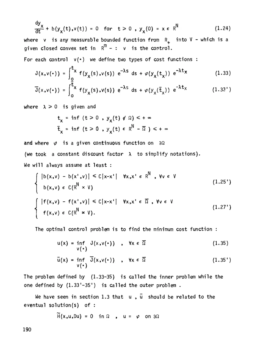
J(x,v(-))=(X f(yx(s),v(s)) exp [- ( c(y (A),v(A))dA ]ds + (33)
rt
+ *(yx(*x)) exp [- j x c(yx(t),v(t))dt] ,
T'(x.v(·)) = j X f(yx(s),v(s)) exp [- J c(yx(A),v(A))dA ]ds + (33')
+ *(yx(*x)) exp [- j x c(yx(t),v(t))dt ]
where
ΐχ = inf (t > 0 , yx(t) 4 Ω) < +oo (first exit time from Ω ) ;
ΐχ = inf (t > 0 , yx(t) e RN- Ω) < +oo (first exit time from Ω ) ;
and where ψ is a measurable function defined on 9Ω. We will assume at least:
φ(χ) is bounded on 9Ω (34)
Next, to make sure that J and J are will defined, we assume that
λ = inf c(x,v) > 0 , thus even if t or t are +°° then the integral
x,v x x
converges and we agree that in this case the term {<£>(y (t ))exp [
X X
(resp. with t ) vanishes.
Finaly in each case, we define the minimal cost function :
u(x) = inf J(x,v(·)) , Vx e Ω
ν(·)
36
ft
X(-)]>
J η
ϋ(χ) - infJ (x.v(·)) » Vx e Ω
v(-)
(35')
We call the problem defined by (33)-(35) the inner problem and the one
defined by (33')-(35') the outer problem (let us warn the reader that this
terminology is by no means standard and that there is no standard
terminology). We first give the dynamic programming property : we will denote
t л s = min(s,t) ;
THEOREM 1.5 : 1) Inner problem : Under assumptions (25) , (27) , (34) and if
λ > 0, then we have for all Τ > 0 :
u(x) = inf ί f X f(yy(s),v(s)) exp ί - [ c(yχ(λ) ,v(A))dA} +
v(-) Jo x -Ό Χ
+ l(T<t ) и(Ух(Т))ехр{- j c(yx(s),v(s))ds} + (36)
rt
+ l(1>t )^(УХ(*Х)) exp i- j X c(yx(s),v(s))ds} }
where 1(T =1 if Τ < τ , = 0 vf Τ > τ ; 1(1>г)= 0 if Τ < τ ,
= ! Л Τ > τ (ντ>τ) ·
2) Outer problem : Under assumptions (25) , (27) , (34) and if λ > 0 ;
then we have for all Τ > 0 :
ίΤΛΪχ fs
u(x) = inf { X f(yY(s),v(s)) exp {- c(yU) ,ν(λ) )dA} +
(36')
v(·) ^o
+ l(T<t ) и(Ух(т)) exp {-j c(yx(s),v(s))ds} +
1{J>1 ) ^^χ(ϊχ)) exP {"
c(yx(s),v(s))ds} }
We will skip the proof of this result since it is totally identical to
the proof of Theorem 1.3 . For the same reason, we will only state the
following result (similar to Theorem 1.4) :
THEOREM 1.6 : Under assumptions (25) , (27) , (34) and if λ > 0 ; then, if
u (resp. u) is differentiable at some point χ e Ω , we have :
sup {b(x ,v)-Du(x ) + c(x ,v)u(x ) - f(x .v)} = 0
ve V υ
37
(resp. (sup b(xo,v)-DU(xo)+ c(xo,v)u(xQ) - f(xQ,v)} = 0 ).
The following proposition shows the effect ot the exit times on the
boundary conditions of u and u on Γ .
PROPOSITION 1.3 : 1) Inner problem : Under assumptions (25),(27),(34) and if
λ > 0 , then we have :
u(x) = φ (χ) од Г
2) Outer problem : Under assumptions (25),(27) ,(34) and if λ > 0 , then
we have :
u(x) < φ (χ) од Г+
where r+ = {xer/3veV, b(x,v)-n(x) < 0} ajid n(x) is the unit
outward normal to Г at the point χ .
Proof : Since t = 0 for all controls v(·) if χ e Γ , we have
immediately u(x) = φ(χ) on Γ . Next, if χ e Γ , there exists some ν e V such
that b(x,v)«n(x) < 0 . If we choose the control v(t) = ν Vt > 0 , the
corresponding solution yx(t) of (24) satisfies : Ух(*) 4 Ω if t is
small and positive. Thus for this fixed control v(t) , we have t = 0 and
u(x) < J(x,v(.)) = *(x).
REMARK 1.7 : Let us show a simple example where i) u and u do not
coincide, ii) ΰ < φ but u φ ψ on Γ . Indeed take N=1 , V = [ -1,+1 ] ,
b(x,v) = ν , Ω = (0,1) , c(x,v) = 0 , f(x,v) = 0 , φ(0) = 0 ,
φ(1) = 1 . Then, obviously we have :
yx(t) = χ - J v(s)ds , J(x,v(·)) - ^(yx(tx)) . J(x.v(-)) = *(УХ(*Х))·
And it is straightforward to deduce from this :
u(x) =0 for 0 < χ < 1 , u(l) = 1 ; u(x) = 0 for 0 < χ < 1 ;
but clearly Г+ = Г = {0,1}.
Let us conclude this section by the following result (saying essentielly
that, if for all controls ν the vector fields b(x,v) is "oriented on
Γ towards the inside of Ω" then the situation is very similar to the
case with no boundary). We will not give its proof - see R.Gonzales [ 62 ] ,
38
R.Gonzales and F.Rofman [ 63 ] or P.L.Lions and J.L.Menaldi [107].
PROPOSITION 1.4 : Assume (25) , (27) ajid
3a > 0 , Vx e Γ , Vv e V b(x,v)-n(x) < - a (37)
Then we have : u = ϋ in Ω .
In addition if we assume :
λ > λ"!" , where λ„ = sup {-(b(x.v)-b(x' ,v) )· (x-x') |x-x'| ~2} (38)
0 0 ^v ^
χ,χ'ε Ω
3 С > 0 , Их) - *(у)| < С|х-у| , Vx,y e Г (39)
1 оо
then u = u belongs to W ' (Ω) .
Let us make a few remarks to conclude this section : first, in the
preceding result we could also add that, if 0 < λ < λ , then u = u belongs
to 0°'α(Ω) with α = v- and if λ = λη > 0 then u belongs (3°'α(Ω) ,
Vet < 1 . °
We could also give analogues of Theorem 1.3 and Proposition 1.2 but
we will not do so since these are totally similar results.
Finally we will give in section 8.4 (Part 2) much more general re-
concerning the regularity of u (these results will be direct applications
of the results and methods of Chapter 5).
3) Calculus of variations :
We will take a typical example of the Calculus of Variations (related to
the determination of geodesies). Let us consider the problem of minimizing :
Inf {J L(y(X) , & (λ)) d\]
over all functions y(A) satisfying (for example) :
y(0) = χ , y(t) = xo , ye W1,oo(0,t;RN) .
Ν Ν
Here and below t is given > 0 , χ e R and χ e R . Finally L(x,p)
(called the Lagrangian) is assumed to satisfy :
L(x,p) is bounded from bi
(40)
INN
L(x,p) e С (R xR ); L(x,p) is convex in ρ and L(x,p) is bounded from below
L(x,p) |p| —-> +°° , uniformly in xe R .
IpI-h»
39
The question here is of course to determine the value u(x,t) of the
above infimum and to determine the optimal y(A) . We first define precisely
u(x,t) :
u(x,t) = Inf {J L(y(A), -^ (A))dA/y(0)=x,y(t)=xo,y e W1 '°°(0,t;RN)} ·
Of course this problem is very similar to the ones discussed in the
preceding paragraphs : more precisely one may consider the above problem as a
N
control problem where V = R , the state of the system is given by
= v(t) (the control, arbitrary measurable bounded function)
У(0) = x .
The cost function is then :
J(x,t;v(·)) = [ L(y(A),v(A))dA .
But in addition we require as a constraint, that the control is such that:
y(t) = χ0 ■
We have then : u(x,t) = inf{J(x,t;v(·)) / v(-) such that y(t)=xQ}
REMARK 1.9 : It is worth noting that u(x,t) can be obtained by
penalizing the constraint y(t) = χ . More precisely let ue(x,t) be the
optimal cost function defined by :
ue(x,t) = inf Je(x,t;v(·))
v(·)
with Je(x,t;v(·)) = J(x,t;v(·)) +^ |y(t) - x0|p
for any ε > 0 and for some ρ > 1 .
Then it is not difficult to prove that we have :
ue(x,t) i u(x,t) as ε 4- 0 .
Under very general assumptions, it is even possible to show that if p=l
ε Ν
then for ε small enough we have : u (x,t) = u(x,t) Vx e R for some
fixed t > 0 (this is the so-called exact penalization ).
This similarity of our problem with those discussed in the previous
section enables us to state without proof :
40
Ж
PROPOSITION 1.5 : ι) We have :
u(x,t) = Inf {[ L(y(A), & (A))dA + u(y(s),t-s)}
У(") Jo
■For all 0 < s < t .
N
ii) I_f u is differentiable at some point (x,t) e R χ (Q,+°°) , then we
have :
|£ (x,t) + supN { - v-D u(x,t) - L(x,v)} = 0
REMARK 1.9 : If we define H(x,p) by H(x,p) = L (x,p) (the dual convex
function of L(x,p) - see section 1.1) :
H(x,p) = supN {q-p - L(x,q)}
qeR
then the above equation may be rewritten in the form :
Щ (x,t) + H(x,- Dxu(x,t)) = 0
(The fact that we have H(x,- Du) comes from the fact that we want x(0)=x,
x(t) = χ . If we had choosen x(0)=x , x(t)=x , we would have obtained
the equation : -^r (x,t) + H(x,D u(x,t)) = 0 ).
We now turn to a brief examination of the properties of some optimal
curve Υ(λ) that is, let Υ(λ) be such that
' Y(0) = x , Y(t) = χ , Υ e W1,o°(0,t;RN)
j u(x,t) = j L(Y(A) , ^ (A))dA
We first want to derive some optimality equation necessarily satisfied by
Y(A) . Indeed let φ e Zl{ [0,t ] ; RN) , φ{0) = <p(t) =0 ; we have :
j L(Y(A) +Εφ{\) sdY+e^)dA> j L(Y,^)dA
for all ε e R . Since L is С , we obviously obtain
rt
9L ,Y dY
Эр {U dA
dA Эх
dY,
dA
^+ ^ (Υ, £-)· Ψ dA = 0
(41)
for all ψ e С ( [0,1 ] ;R ), φ(0) = *(t) = 0
41
and this obviously a weak form of the following equation :
^<^<Y'f»+!?<*.£> = ° 1n VlO.f.tP)
dA v Эр
Υ e w1,oo(0,t;RN) ; Y(0)=x , Y(t) = xr
(42)
It is straightforward to check that if L is of class С and if
Л
=—j (x,q) is definite positive for all (x,q) in R χ R , then
Эр
Υ e C2([0,t ];RN) .
Λ
From now on , we will assume that -2-я- is definite positive. Thus we know in
2 Эр 2
particular that Υ e С , but also that H(x,p) is also of class С
(H(x,p) = L*(x,p) and Щ (x,·) = [Щ (x,·)]"1 for each χ - see for
example I. Eke land and R.Temam[43 ]for a list of properties of dual convex
functions).
Next, remark that (42) holds in the classical sense :
-^<!>·3ΐ» + !<γ.3ΐ> = ° »«io.t].
But denoting Ρ(λ) = ^ (Y, -»- ) , we have obviously :
Эр
and we find
dY Μ
dX Эр
ЭН
(Y.P) .
Y'(A) =^(Y,P)
эн
(43)
Ρ'(λ) — uf(Y.P)
together with the boundary conditions : Y(0) = χ , Y(t) = χ .
This system of ordinary differential equations (we skip the boundary
conditions) is usually called an Hamilton!an system and is nothing but
the system given by the method of characteristics for "the equation
satisfied by u" (see section 1.2 above). For further investigations on these
classical topice we refer, for example, to the books of L.C.Young [ 132 ] ,
42
G.A.Bliss [ 16 ].
1.4. THE VANISHING VISCOSITY METHOD :
Nearly all existence results concerning the Hamilton-Jacobi equations (0.1)
or (0.2) have been obtained with the help of the so-called vanishing
viscosity method : this method consists in solving first the following
approximate problem : let ε > 0
- еДие + H(x,ue,Due) =0 in Ω , ue - φ on 9Ω ; (0.1-ε)
о
and we will look for solutions ue in the space С (Ω) η c(n) (for
instance). Similarly (0.2) is approximated by :
|£ - еДие + H(x,t,ue,Due) = 0 in Ωχ(Ο,Τ) , ue = φ on 9Ω χ (Ο,Τ) (0.2-ε) ι
] υε(χ,0) - u (x) in Ω
with ue e С2,1(П χ (ОД)) η с (Ω χ [ОД] )(С2,1(П χ (0,T)) = ivcC1(n х(0,Т) ,
2
ν is twice differentiable in x on Ω χ (ОД) and D ν e 0(Ωχ(0,Τ))} ).
To simplify the discussion and the notations, we will talk only about (0·1)
and (0.1-ε) .
It may not be obvious to the reader that problem (ОЛ-ε) should be
easier to solve than the original problem (0.1). We will explain this in
a moment. The second step of the vanishing viscosity method is, after
having solved (0.1-ε) , to pass to the limit as ε goes to 0 . Obviously
this requires a priori estimates (for example L°° bounds on the gradient of
ue , independent of ε > 0 ) . The main technique to pass to the limit will
be presented in the next section (section 1.5).
We now briefly explain why (0.1-ε) , a priori, looks simpler than
(0.1) : in (0.1-ε) the term with higher order derivatives is - εΔ and
is thus linear and (0.1-ε) is no more as strongly non linear as (0.1);
(0.1-ε) is said to be a quasi linear elliptic equation (of second order).
These equations have been studied for a long time (see in particular
O.Ladyzenskaya and N.Ural'tseva [ 88 ], [ 89 ]; D.Gilbarg and N.S.Trudinger
[60 ]; J.Serrin [ 122 ] ) . Our approach to the solution of (0.1-ε) and to
the way of getting a priori estimates of ue in the Lipschitz norm will
be based on P.L.Lions [101 ] (the main results and proofs of [101 ] are
recalled in Appendix 1). A fundamental tool is a device invented
43
originally by S.Bernstein and developped by many authors (see in particular
0. Ladyzenskaya and N.N.Ural 'tseva [ 88 ] , [ 89 ] , [ 90 ] ; J.Serrin [ 122 ] ,[ 123] ;
A.V.Ivanov [ 72 ] , P.L.Lions [101 ] ).
Let us just mention that the name of this method comes from a celebrated
method in fluid dynamics where a term like (-εΔ) represents physically a
viscosity.
We now want to explain with more details the relations between (0.1-ε)
and optimal control theory. As we will see, the solution u of (0.1-ε) can
beinterpreted under very general assumptions as the optimal cost function of
some Optimal Stochastic Control problem (at least if Η is convex in (u,p) -
in the other case, one has to consider Stochastic Differential Games).
To be more specific, we will use the notations and assumptions of sec-
N
tion 1.3 : Ω is a bounded smooth domain in R and
H(x,t,p) = sup {b(x,v)«p + c(x,v)t - f(x,v)}
veV
(where b,c,f are bounded continuous in x,v ; Lipschitz in χ , uniformly
in ν and where с > 0 ).
We next describe some Optimal Stochastic Control problem : for χ e ω ,
we consider the solution yx(t) of the following stochastic equation :
rt
yx(t) = χ + /27 Bt - j b(y^(s),v(s))ds , for t > 0 (44)
where (M,F,F.,Ρ,Β.) is some probability space equipped with a normalized
adapted brownian motion В ; v(s) is any progressively measurable ,
bounded process with values in V .
For the readers who are not familiar with stochastic differential
equations, think of (44) as a perturbation (random) of the ODE (24) : in
addition, as ε- goes to 0 , the perturbation vanishes.
As in section 1.3 , we consider
ε
Je(x,v(·)) = Ε | x f(yx(s),v(s)) exp{-j c(y^(t),v(t))dt} ds +
ε
+ Ε *(νχ(τχ)) exp {- ί χ c(yx(t),v(t))dt}
44
where E denotes the expectation and where τ^ is the first exit time from
Ω (or Ω) of y^(t) : τ^ = inf(t > 0,y^(t) 4 Ω) , and where φ e (32'α(9Ω)
for some 0 < α < 1 .
Finally we introduce : for χ e Ω
ue(x) = Inf Je(x,v(·)) (45)
v(-)
We then have the following easy result :
THEOREM 1.7 : The optimal cost function ue(x) belongs to С 'α(Ω) and
? _
is the unique solution in С (Ω) of :
- εΔυε + sup {b(x,v)«Due + c(x,v)ue- f(x,v)} = 0 iji Ω
veV
ue = φ on 9Ω
(46)
REMARK 1.10 : If Ω = RN , c(x,v) > λ > 0 Vx e RN , Vv e V ; then
ue(x) = inf Ε [ f(/(t),v(t)) expi -| c(/(s) ,v(s))ds} ] (45')
v(·) Jo x -Ό χ
belongs to Cb(RN) and is the unique solution in C2(RN) η Cb(RN) of
- еДие + sup { b(x,v)-Due + c(x,v)ue - f(x,v)} = 0 in RN (46')
veV
We will not prove completely Theorem 1.7 : let us first mention that the
existence of a solution ^(x) of (46) (in 02'α(Ω)) is insured in
view of classical results on quasilinear equations (see for example [ 88 ] ,
[ 122 ] ) since the Hamiltonian H(x,t,p) = sup [ b«p + ct - f ] is locally
Lipschitz in (x,t,p) and satisfies :
If I <C ■ 0<ll<C · l|^|<C + C |p| +C|t|
for some constant С > 0 .
We want to explain why we have : ue = ue . Thus let ϋε be a C2(iT)
solution of (46) and let us prove that ΐίε = ue . We first prove that Ъе
is less than u . Indeed by Ito's formula, we have for each control v(·):
45
rtAT
Ε [^(yx(U^))exp{-J x c(y^(s),v(s))ds} ]
rtATE
X {eAUe(y^(s))-b(y^(s)sv(s)).Due(y^(s))-c(y^(s)sv(s))up(yJ(s))}. χ
0 s
χ exp { - f c(y^(A),v(A))dA} ds .
= Ε
Now in view of (46) , we deduce, letting t -*■ +°° :
uE(x) < Je(x,v(·))
and therefore
if < ue in Ω
Next, we prove formally that for each δ > 0 there exists some control
such that u^x) > J(x,v(·)) - <$.
Indeed there exists a bounded measurable function v_(x) (from Ω into V)
such that :
sup {b(x,v)·^^) + c(x,v)ue(x) - f(x,v)} < b(x,v.(x))-Due(x) +
veV °
+ c(x,v5(x))ue(x) - f(x,v6(x)) + δ .
Next, if yx(t) is a solution of
ft
yx(t) = χ + /?i Bt - b(yx(s),v6(yx(s))) ds , for t>0
(this is the formal point of our proof , since the existence of yx(t) is
true but it involves rather delicate and technical results in the theory
of Stochastic Differential Equations), we have immediately from Ito's
formula :
ττε
ir(x) - Ε
X {- etie(y(t))+b(y(t),46(t))-UUe(y(t)) +
+ c(yx(t),v(S(t))'iie(yx(t))} -exp{-
ε
/•τ
c(yx(s),v°(s))ds} +
+ Ε ^(Ух(тх)) ехр {-
X c(yx(t),v6(t))dt} ;
where v°(t) = v6(yx(t)).
But from the choice of v.(·)) , we obtain :
46
ε .
ue(x) > Οε(χ,νδ(·)) - δ ε[ χ exp{-[ c(y (s) ,v6(s))ds} dt
in 'n
> Οε(χ,νδ(·)) -Сб ;
and we conclude.
For complete proofs of this result, we refer the reader to A.Bensoussan
and J.L.Lions [ 12 ] , W.H.Fleming and R.Rishel [ 52 ].
We want to conclude this section by explaining on the simple case
Ω= R what happens as ε goes to 0 . In the case when Ω= R and
c(x,v)> λ > ο , ue is given by (45'). In addition it can be easily
proved that, as ε goes to 0 , ye(t) converges to yv(t) solution of
X X
dy
dtT = " b(yx(t),v(t)) , yx(0) = χ
ε N
and this explains why u (x) given by (45') converges (uniformly in R )
to u(x) given by (28')
with J(x,v(·))
u(x) = inf J(x,v(·))
v(·)
f(yx(t),v(t))exp {-f c(yx(s),v(s))ds}
0 J0
Recall (see section 1.3) that u(x) is (in some sense) a solution of :
sup {b(x,v)-Du(x) + c(x,v)u(x) - f(x,v)} =0 in RN .
veV
And remark that this gives some method to pass to the limit in (46') ;
unfortunately some difficulties arise in the case of a bounded domain
which prevent "to pass to the limit in this way" : this is due to the
presence of τε , it is very difficult to analyse the asymptotic behavior
of
ε
τ as ε goes to 0 (it can converge to tv , or t' depending on
X XX
the control v(t) , the vector field b(x,v) and the domain Ω ).
1.5. VISCOSITY SOLUTIONS : UNIQUENESS AND STABILITY.
We want to present here some recents results obtained by M.G.Crandall and
P.L.Lions [ 32 ] (see also [ 33 ] , [ 34 ] ). To explain the motivation of this
result, we want to remark in general there is no uniqueness and no stability
for generalized solutions of problems (0.1) or (0.2). Indeed let us consider
47
two examples :
Example : Let H(p) = |p|a (a > 0) and let us consider the equation
|£ + |Du|a - 0 in RN χ (0,<=°),u(x,0) = 0 in RN .
Obviously 0 is a classical solution, but 0 is not unique in the class of
generalized solutions. Indeed if we consider :
u(x,t) = 0 if |x| > t , u(x,t) = |x| - t if |x| < t ;
then obviously u is piecewise C°° , Lipschitz in R χ (0,«>) , bounded for
t < Τ (VT < » ) and :
§£ = |Du|a = 0 if |x| > t ; |^ = - 1 , |Du|a = 1 if |x| < t, χ t 0
thus u is a generalized solution of the above Hamilton-Jacobi equation.
Example : Let Ω = (Ο,ί) , H(p) = |р| - 1 , φ = 0 and let us consider (0.1)
that is :
|Du| = 1 a.e. in Ω , u(0) = u(l) = 0.
(Notice by the way that there cannot exist a smooth solution of this
equation since if u e C^O.l) η C([0,1 ]) , u(0) = u(l) = 0 implies that Du
vanishes at some point of (0,1)).
Obviously Uj(x) = χ if 0 < χ < 1/2 ; = 1 - χ if - < χ < 1 defines a ■
generalized solution of the problem. But u, is not unique and there exist
infinitely many solutions of this equation. In particular we may build a
sequence of generalized solutions as follows :
un(x)=x- Ц if 2J < χ < 2Mf = 2j+2 _ 2j + l < χ < 2j+2 f
nv ' 2n ? ? 7 ? 2
j = 0,1,..., 2n_1 - 1 .
One sees immediately that one has : 0 < u (x) <— on [0,1 ]
J nv ' ?n
Thus, u converges uniformly to 0 but 0 is not a solution of the
original equation.
For other examples of non-uniqueness, the reader may consult, for example,
E.D.Conway and E.Hopf [27 ] .
To resolve this uniqueness (and stability) question, in M.G.Crandall and
48
p.L.Lions [ 32 ] is introduced a new notion of solution, called viscosity
solutions (for reasons detailed below). In subsection 1 ) we give the
definition of these solutions together with their basic properties. Next, in
subsection 2) we give the main uniqueness results. Let us remark that,
for the reader's convenience, we have included the proofs of these results
in Appendix 2 .
ljVjscosity solutions : introduction and basic properties.
Let us first motivate the introduction of the notion of viscosity solutions
by the following argument : in order to solve (0.1) , we have seen (section
1.4) that it is natural to use the vanishing viscosity method and to solve
instead (O.l-ε) . Now, if ue is a solution of the approximate problem
and if ue converges uniformly (locally on compact subsets of Ω ) to some
continuous function u , we want to investigate the properties of u . More
precisely, we assume ue solves ;
- еДие + H(x,ue,Due) =0 in Ω , u e (32(Ω)
(and we do not specify any boundary conditions) ; and we assume :
ue —> u in С(П) , as ε ■+ 0 (47)
where convergence in 0(Ω) means uniform convergence on every compact
subset of Ω .
Let φ e © (Ω) , let к e R , we localize the equation satisfied by ue,
namely we consider the equation satisfied by <£>(ue - k) on the support of
φ : we have
- | Д-Иие - к)} + H(x,ue,^ f D(*(ue-k)) - D *>(ue-k)]) =
= - ε —— (и -к) D φ·Ό{[ΐ -к)
φ
= - ε k± (ue-k) - Ц D o-DMue-k)} + 2ε^|iV-k).
φ φ
Next suppose that : max <£>(u-k) > 0 , then for e small enough we have :
Ω
max <p(u -k) > α , for some α > 0 . Thus there exists χ such that
Ω ε
^(xe)(u (xe)~k) = max ^(ue-k) , obviously we have : φ(χ ) > β > 0 , for
Ω ε
some β > 0 . We may assume that χ converges, as ε goes to 0 , to
49
some x such that :
о
φ(χ )(u(x ) - к) = max ^(u-k) > 0 .
Now, if we look at the above equation at the point χε , we find
- | Δ Mue-k)} + H(xe,ue, - -^ (ue-k)) < Ce
for some constant С , since D(v(u -k))(x ) = 0 .
But, by the maximum principle, we have : - Д(<р(ие-к)) (χ ) > О , thus we
obtain :
Η(χε,υε(χε) , - D^(xe)(ue-k)(xe)(^(xe))_1) < Се.
Because of (47) , we may pass to the limit and we find :
4φ e 3) (Ω) , Vk e R such that max <£>(u-k) > 0 , there exists
Ω
x satisfying v(u-k)(x ) = max ^(u-k) such that : (48)
H<vu<x0> ' ~^r (u-kH><0)) <0 ■
By a similar argument, we would prove that u also satisfies :
V<£> e ξϋι (Ω) , Vk e R such that min <£>(u-k) < 0 ; there exists
Ω
χ satisfying v(u-k)(x ) = min v(u-k) such that : (49)
Ω
"(V^V ' "Ι/ (и-к)(хо)} >0 ■
A continuous function u satisfying both (48),(49) will be called a
viscosity solution of (0.1) (see below for precise definitions) : the name
obviously comes from the way solutions of (0.1) are built (by the
viscosity method).
- N
Let us recall that H(x,t,p) ts a continuous function from Ω χ R χ R
and we want to define a new notion of solutions of
H(x,u,Du) = 0 in Ω . (50)
DEFINITION : Let u e C(n) ; u will be said to be
i) a viscosity subsolution of (50) if u satisfies (48) ;
ii) a viscosity supersolution of (50) if u satisfies (49) ;
iii) a viscosity solution of (50) if u satisfies (48) and (49).
50
Let us immediately give some basic properties of these viscosity solutions
(recall that all the results stated here are proved in Appendix 2). We will
need some notations : if φ e С (Ω) (continuous functions with compact
support), we denote by
Ε (φ) = {χ e Ω, φ{χ) = max ψ > 0} (if φ < 0, Ε (φ) = 0) ;
Ω
Ε {φ) = {Χ е Ω, φ{Χ) = min φ < 0} = Ε (- φ) ;
Ω
d(v) = {χ e Ω , <£> is differentiable at χ} , for all φ е С(П) ;
Τ to) = {χ e Ω such that there exists ξε[*Ν , r.>0 , eeC(R) ε(0)=0
+ О +
satisfying : φ{у) < *(х)^-(у-х) + |у-х|е( |у-х| МуеП ^(х.г^)}
Т_И = T+(-*) , for all φ e С(П).
Finally if χ e Τ (φ) (resp. T_ (<£>)) for some φ e 0(Ω) we denote by
T+(v;x) = {ξ e RN such that there exists rQ> 0 , ε e C(R+) with ε(0)=0
satisfying : <p(y) < <£>(χ)+ξ·(y-x)+|y-x|e(|y-x|),VyefinB(x,ro)}
T_fo;x) = - T+(- φ;χ).
THEOREM 1.8 : Let u e (3(Ω) .
i) Λ1 u is a viscosity subsolution (resp. supersolution, resp. solution)
of (50) , we have for all φ e С (Ω)+, Ψ e (3(Ω) :
Vx e Ε Ии-Ψ)) η dto) η d(Y)
0 + (48')
Η(χο·υ(χ0))· " ΊΓ (υ_Ψ)(χο) + ^ο^ < °
(resp. Γ Vx e Ε_(<ρ(ιι-Ψ)) η dto) η (1(Ψ) (49')
J H(xo,u(xQ) , - -^-(u-Ψ) (χο) + 0Ψ(χο)) > 0 ;
(resp. (48') £nd (49')) .
ii) u is a viscosity subsolution (resp. supersolution ;, resp. solution)
of (5Q) if and only if u satisfies :
Vx e T+(u) , νξ e T+(u;x) H(x,u(x),ξ) < 0 (51)
51
(resp. Vx e T_(u) , νξεΤ_(ιι;χ) H(x,u(x) ,ξ) > 0 (52)
resp. (51) ^nd (52)).
Since, if χ e d(u) , χ e T+(u) η T_(u) and T+(u;x) = T_(u;x)={Du(x)}
we immediately deduce :
COROLLARY 1.3 :
i) ]f ue С (Ω) satisfies : H(x,u(x) ,Du(x)) < 0 jjn Ω
(resp. >0 jn SI , resp. =0 jji Ω ) ; then u jjLA yi scos i ty s ubsol uti on
(resp. supersolution , resp. solution) of (50).
ii) Jjf u is a viscosity subsolution (resp. supersolution, resp. solution)
of (50) and if χ e d(u) , then we have :
H(xo,u(xq),Du(xo)) < 0 (resp. > 0 , res£. = 0).
REMARK 1.11 : In particular we see that if u is a viscosity subsolution
(resp. supersolution, resp. solution) of (50) and if u is locally Lips-
chitz in Ω then u is a.e. differentiable in Ω and thus u is a
generalized solution of (50).
REMARK 1.12 : The above results show that the notion of viscosity solution
is a notion of "weak" solution of (50) , since u is assumed to be
only continuous and Du does not exist. But, in some sense, at a point of
maximum of ^(u-k) a good candidate for the definition of Du 1s - -——(u-k).
Let us remark that there exists some analogy between this notion of solutions
and the standard distribution theory - integration by parts is replaced here
by differentiation by parts and "is done inside the nonlinearity".
Finally let us mention that there is some parallel between the preceding
notion and the so-called "entropy condition" for scalar hyperbolic equations
of the form :
1т+э! <f<u» = °
(see E.Hopf [ 66 ] , A.Volpert [ 131 ] , S.N.Kruzkov [79 ]).
REMARK 1.13 : It is easy to prove that , if φ e (3(Ω) , Τ+{φ) , T_(<?) are
dense - and since Τ Αφ) η Τ_(^) = d(<£>), their intersection may be empty.
52
REMARK 1.14 : If we now go back to the Examples given at the beginning of
section 1.5 ; we immediately see that , in the first example, u does not
satisfy (52) . Indeed x=(Q,t) e T_(u) (for all t > 0) and
T_(u;x) = BjX {-1} ; but
Η(χ,υ(χ),ξ) = -1 + |ξ|α
and this is negative for |ξ| < 1 .
In the same way , we see that, in the second example , u , for η > 2 ,
does not satisfy (52).
In view of the definitions, the following result is obvious :
THEOREM 1.9 : i) Suppose ue e (32(Ω) solves :
- ε Δ ue + Η (x,ue,Due) = 0 ήί Ω
and that , as ε goes to 0,ue converges in 0(Ω) to some function u
and Η (x,t,p) converges to H(x,t,p) uniformly on compact subsets of
N
Ω χ R χ R ; then u is a viscosity solution of (50).
ii) Suppose ue e 0(Ω) is a viscosity solution of
Η (x,ue,Due) = 0 Ήί Ω
and that, as ε goes to 0 , ue converges in 0(Ω) to some function u
and Η (x,t,p) converges to H(x,t,p) uniformly on compact subsets of
N
Ω χ R χ R ; then u is a viscosity solution of (50).
Before concluding this section, let us mention that in [ 32 ] , many
further properties of viscosity solutions are discussed. We want now to
conclude this section by some new result explaining why any optimal cost
function of any optimal control problem discussed in section 1.3 is a
viscosity solution of the associated Hamilton-Jacobi equation as soon as it
lies in 0(Ω) . We will use the notations of section 1.3 .
THEOREM 1.10 : Let u (resp. u ) be the optimal cost functions defined
by (35) (resp. 35')) and let us assume (25) , (27), (34) ajid λ> Ο .
Then, if u (resp. u ) e 0(Ω) , u (resp. u )is a viscosity solution of
sup {b(x,v)«Du + c(x,v) u - f(x,v)} = 0 in Ω
veV
53
Proof : We will show that u , for example, satisfies (52) - the remainder
is totally similar - . Thus let χ e T_(u) and let ξ e T_(u;x) , we have:
u(y) > u(x) + ξ-(γ-χ) + |y-x|e(|y-x|) = *_(y)
for у e B(x,r ) , for some r > 0 and for some continuous function ε
such that ε(0) = 0 . Obviously , ψ_ e C(n) and is differentiable at χ
and D V_(x) = ξ ·
By Theorem 1.2 (section 1.3) we have :
rT/Nt. rs
c(yx(X),v(X))d\} +
' u(x) = inf {( X f(y (s),v(s)) exp { -
v(-) ;o J
4 + X(T<t ) и(Ух(Т)) exP{"{ c(yx(s).v(s))ds} +
+ X(T>t ) ^(yx(tx)) exP{ " | X c(yx(s),v(s))ds }}
x о
for all Τ > 0 . Since we have : |y (t) - x| < С t ; choosing Τ small
ρ
enough (T < min ( - dist (χ,9Ω) , .— )) we may assume that Vv(·)
у (t) e Ω η B(x,r ) for all te[0,T].
In particular Τ < t and we deduce from (36) :
φ (χ) = u(x) > inf {[ f(yjs), v(s)) exp {- f c(y (X),v(X))dX) +
v(-) ^o x -Ό Χ
+ ^_(УХ(Т)) exp {-( c(yx(s),v(s))ds}} .
;o
And in the same way as in the proof of Theorem 1.3 of section 1.3 , we
obtain from the preceding inequality (divide by Τ , let Τ -*- 0) since
φ is differentiable at χ :
(36)
ι .e.
sup {b(x,v)«D φ (x)+c(x,v)^(x)-f(x,v)} > 0
veV
sup {b(x,v)-C + c(x,v)u(x) - f(x,v)} > 0 ,
veV
and (52) is proved.
2) Uniqueness results for viscosity solutions.
We will first give the main uniqueness results concerning the Dirichlet
problem. Let us recall that the proofs (taken from [ 32 ]) are given in
54
Appendix 2 . Let H(x,t,p) be a continuous Hamiltonian, we will use the
following conditions :
VR > 0 , Η is uniformly continuous on Ω χ [-R,+R ]χ FR (53)
J VR > 0 , 3 YR β C([ 0,2R ]) nondecreasing such that yr(0)=0 and ,^,
| H(x,r,p) - H(x,s,p) > YR(r-s) Vx e Ω , Vp e RN, -R < s < r < R
and we will need to restrict the nature of the joint continuity of Η :
lim sup {|H(x,t,p)-H(y,t,p)| / |x-y|(l+|p|) < e,|t| < R} = 0 (55)
εΨο
for all R > 0 , or the even stronger requirement :
lim sup {|H(x,t,p)-H(y,t,p)| / |x-y||p|< Rr|x-y| < ε,|ί| < R2) = 0 (56)
εΨο
for all R15R2 > 0 .
We may now state our main result : (below, we will use the convention
9RN = 0).
THEOREM 1.11 : Let u,v Cb(H) jirui (53),(54) hold. Let u (resp.v)
be a viscosity subsolution of (50) (resp. supersolution of : H(x,v,Dv) =
= m(x) in Ω ) where m e C. (Ω) . Let R = max(Ju|| ,||v|| ) and
- b — ° Г(П) ί~(Ω) ~
γ = Υπ ·
Ro
i) 21 (56) holds , ui„ or; v, is uniformly continuous and if
lim (|u(x)-u(x )| + |v(x)-v(x )|) = 0 , uniformly for χ e 9Ω (57)
χεΩ ° ° °
x-*-x
о
then we have :
»Ύ((^ν)+)Ι „ <max(|m"|e> ,»y((u-v)+)| „ ) (58)
L (Ω) L (Ω) L (9Ω)
ii) JT (55) holds and u,v e С (a) , then (58) holds .
iii) rf u,v e U1,m{n) , then (58) holds.
REMARK 1.15 : Of course if Ω is bounded, all uniform continuity
assumptions are satisfied. And if m=0 and u,v are viscosity solutions then
55
(58) yields
||Ύ((υ-ν) + )(| ет <h((u-v) + )| β
L (Ω) L (3Ω)
and if γ is increasing ; we deduce :
H<u-v)+fl <|(u-v)+fl
L (Ω) " L (9Ω)
Assumption (54) essentially means that H(x,t,p) is non decreasing with
— N
respect to t , in some uniform way for χ e ω , ρ e R .
In [ 32 ] , many variants of the above result are given and it is proved that
the above assumptions are in general optimal.
Example : Let us give a simple sample of the above result : consider the
equations
H(Du) + Xu = n(x) in RN (50')
H(Dv) + λν - m(x) in RN (50")
where Η e C(RN) , λ > 0 , η , m e Cu(RN).
Obviously (53),(54),(56) hold with y(s) = Xs , for all R > 0 .
Therefore the above result yields: let u (resp. v) be a bounded continuous viscosity
subsolution of (50') (resp. 50")) , then we have :
i(u-v)+U M <|i(n-m)+| M .
L°°(RN) λ VV)
We now turn to the Cauchy problem, and we will consider viscosity
solutions of
3t
+ H(x,t,u,Du) = 0 in QT = Ω χ (Ο,Τ) (59)
where H(x,t,s,p) e C(i3xRxRxRN) , Τ > 0 (eventually Τ = +~).
In some sense (59) is a special case of (50) : indeed if we take
χ = (x,t), P=(p ,ρ) ρ e R., ρ e RN ; (59) is nothing but (50) with the
special choice of the Hamiltonian :
H(X,s,P) = P0 + H(x,t,s,p)
Thus the definition we gave contains the definition of viscosity sub, super
and solutions of (59). "Nevertheless the special form of the Hamiltonian
H(X,s,P) enables us to give the following Proposition :
56
PROPOSITION 1.6 : Let u e C(Q-f-) . _If_ u is a viscosity subsolution (resp.
supersolution; resp. solution) of (59) ; then, denoting by Q-j- = Ω χ (Ο,Τ ]
and by £>+(Qj) = {φ e C°°(Q.j.) , φ > 0 , Supp φ is compact с Q|} , we have
V<p e ©(Q1) , Vk e R , if (x ,t )eQ| satisfies *(u-k)(x ,t )=max ^>0,
+ 0 0 1 ■ ■■ ' 0 0 η ι
a l· D Ψ Τ (6°)
then we have: - f£( ψ )(vV+H(Wu'- JL(u-k) (xo,tQ)) < 0
(resp_.
' V^ e ^(Q-j-bVlceR, if (xo>tQ)eQ-j- satisfies ?(u-k)(x ,tQ)wmin i(u-k)< 0,
D QT (60')
then we have : - \± (^) (V V+H(VVU'_ "£- №){*0Λ0)) > 0 i
resp_. (60) ^nd (61)).
REMARK 1.18 : This result shows that we may extend the requirements
concerning u up to the upper boundary 9Ω χ {Τ} . Of course in the above result
we may assume φ to be only in С (Q-j-) (and then (x0»tQ) has to be in
ά(φ)) and the conclusion still holds.
We conclude this section by the uniqueness result for the Cauchy problem
corresponding to Theorem 1.11 . We will need some conditions on the
Hamilton! an that we now write :
HeC(T7x{0,T ]xRxRN) is uniformly continuous on Ωχ[ Ο,ΤΗ -R,R ] xBR (61)
for all R > 0 ;
r - N
VR>0 , 3. YReR such that for xefl , -R<s<r<R , 0<t<T , p e r" (62)
we have : H(x,t,r,p) - H(x,t,s,p) > yR(r-s) ;
lim sup {|H(x,t,s,p)-H(y,t,s,p)|/|x-y|(l+|p|)<e,(Kt<T,|s|< R}= 0 (63)
εΨο
for all R > 0 ;
lim sup {|H(x,t,s,p)-H(y,t,s,p)|/|x-y|< e,|x-y] |p|< R. ,0<t<T, | s|< R„}=0
ε+ο ι ά
for all Rj.R- > 0 . (64)
The main uniqueness result is :
THEOREM 1.12 : Let (61),(62) hold. Let u сСД) be a viscosity sub-
57
solution of u + H(x,t,u,Du) = 0 ήί Qt and let ν e Cb(QT) be a
viscosity supersolution of v.+H(x,t,v,Dv) = g(x,t) rn_ QT where g e C. (Qy) ■
Let R = max (HuH , || vll ) and γ = γ . S^t
0 L (QT) L°°(QT) — Ro
Эо QT = 3Ω * [0'T 1U $ x {0}) ■ Then :
i) Ц (64) holds ; U|3 Q , Vj3 g e Cu00QT) and if
lim |u(x,t)-u(x ,t ) |+|v(x,t)-v(x .t )| = 0 , uniformly
(x,t)eQ'T oo'' oo
(x.tMxo,t0)
for (x ,t ) e э QT - then we have :
x о о oi' ——™—- ■ ■
lleYL (u-v) Л < lleYL(u-v) л + eT ||g(-,s)"n ds. (65)
L°°(QT) L°°(30QT) Jo L"(Q)
ii) rf (63) holds and if u,v e Cu(TTT) > then, (65) holds .
iii) _Tf u,v e W1,OT(QT) , then (65) holds.
REMARK 1.17 : In [ 32 ] , many variants of this result are presented and
various examples showing the optimality of the assumptions are given.
1.6. ACCRETIVITY OF THE HAMILTON-JACOBI OPERATOR
We want to discuss here an interesting feature of Hamilton-Jacobi equations
namely the relation between Hamilton-Jacobi equations and accretivity
theory. Our treatment will be brief and will not be of direct use for the
remainder of these notes. For more detailed treatments of the general theory
of accretive operators, we refer to V.Barbu [6 ] ; P.Benilan, M.G.Crandall
and A.Pazy [ 10 ] ; M.G.Crandall [ 30 ] . Most of the material we present
below is taken from M.G.Crandall and P.L.Lions [ 32 ] .
Let us recall briefly the definition of accretivity : a singlevalued
operator A defined on a domain D(A) с X , where X is some Banach space,
is said to be accretive (in X) , if for all λ > 0 and for all u,v e D(A),
we have :
Л(Хи + Au)-(Xv + Αν)Οχ > Allu-vIL· .
Now, if Ω is a bounded smooth domain and if we denote by
58
Χ = С (Ω) = {u e 0(Ω) , u=0 on 9Ω} , we have :
PROPOSITION 1.7 : Let H(x,t,p) be a continuous Hamiltonian satisfying :
H(x,t,p) is noη decreasing in t , for χ e Ω , ρ e R . (66)
i) j-et D(A) - C^n) η Χ and let A be defined by :
X э Au = H(x,u,Du).
Then A is accretive .
ii) Let D(Ae) = (32(Ω) η χ and let Αε be defined by :
χ э Aeu = - ehu + H(x,u,Du) .
Then Αε is accretive .
Proof : We first prove i) . For u,v e D(A) , λ > 0 ; we set
f = Au + Xu , g = Αν + λν .
that is we have
H(x,u,Du) + Xu = f(x) in Ω , u e С (Ω) , u = 0 on 9Ω
H(x,v,Dv) + λν = g(x) in Ω ,y e С (Ω), ν = 0 on 9Ω
Let x e Ω be such that |u-v|(x ) = max |u-v| = Sli-vJw ; we want to
prove : |u-v|(x0) <^ |f-glx -
Suppose for example : (u-v)(x ) > 0 . If χ e 9Ω , u(x ) = v(x ) = 0
and we are done. If χ e Ω , we have : Du(x ) = Dv(x ) and thus in view
о v о v о
of (66) , we obtain :
f(x0) " 9(x0) = λ(ιι-ν)(χ0) + H(xo,u(xo),Du(xo))-H(xo,v(xo),Dv(xo))
> λ|ϋ-ν|(χ0) = λ|υ-ν|χ
and we conclude.
The proof of ii) is totally similar : one just remark that at χ , if
x e Ω , we have : - ε A(u-v)(x ) > 0 .
In view of the accretivity of the Hamilton-Jacobi operator A it is then
natural to try to apply the general Crandal1-Liggett generation theorem
[ 31 ]: if one checks that it is possible to define a maximal extension of A
59
(in some appropriate sense) , then, by [ 31 ] , there exists an abstract
semigroup solution to the Cauchy problem :
Γ |H + H(x,u,Du) - 0 in Ωχ (0,+~) , u=0 on 9Ω χ (0,+»)
| u(x,0) = uQ(x) e X .
This is developped in C.Burch [ 24 ] , S.ATzawa [3 ] , M.Tamburro [129 ]in
the case of a convex Hamiltonian and in M.G.Crandall and P.L.Lions [32 ]in
the general case (this being a simple application of the notion of
viscosity solutions).
Another consequence of the accretivity of the Hamilton-Jacobi operator is
the possibility to define weak solutions (in X) of problems like
H(x,u,Du) = 0 in Ω , u = 0 on 9Ω ; (67)
where we assume (66).
This is done by some non-Hilbertian extension of monotone operators theory
(see for example G.J.Minty [113] , F.E.Browder [23] for the classical
monotone operators theory). We first define a bracket in any Banach space X :
Vf,g e X [f,g] = inf i (Кf+Xg| - |f| )} .
λ>ο
It is clear from the definition of accretive operators that A , defined in
D(A) с X , is accretive if and only if :
0 < [u-v,Au-Av]+ , Vu,v e D(A) . (68)
REMARK 1.18 : If X is some Hubert space, obviously we have :
[f.g ]+ = (f.g) π^ΐΐχ1 if f f 0 , = (gnx if f = 0 ;
and the above property immediately reduces to the usual monotonicity.
In view of (68) , it is then reasonable to define for f e X a weak
solution u of : Au = f , by
0 < [u-v,f-Av ]+ , Vv e D(A) , u e X .
In addition, since (f,g) —*[f,g ]+ is obviously upper semi-continuous,
this definition is very useful for convergence purposes : indeed if u e X
is a weak solution of : А и = f and if u —>u , f —> f -, then it
П ν П у
60
is obvious that u is a weak solution of : Au = f .
These general comments have been first applied to Hamilton-Jacobi
equations similar to (67) by L.C.Evans [ 44 ] . More precisely, a reasonable
attempt to define a solution u of (67) is to look for u solution of :
0 < [*-u,H(xw>,D φ) ]+ , U e X , V φ e (^(Ω) η Χ (69)
(recall that X = С (Ω) ) , but it is possible to give a formula for [ ·,· ] + ;
indeed, see K.Sato [12 ] or E.Sinestrari [124 ] for example, we have :
' [f.g ]+ = max {g(xQ) sign f(xQ) / xQ : |f(xQ)| = |f| β > (70)
if f ф 0
- |gfl . if f = о
L
It is worth noting that by the following proposition, essentially taken
from M.G.Crandall and P.L.Lions [ 32 ] , viscosity solutions of (67)
coincide with weak solutions in the above sense that is functions satisfying
(69) provided the Hamiltonian Η satisfies (66). If it does not satisfy
(66) , the following proposition shows that viscosity solutions are weak
solutions of the equation :
H(x,Du(x)) = 0 in Ω , u e X
where H(x,p) = H(x,u(x),p) .
For various reasons (in particular for existence purposes) it is a lot
more convenient to work with viscosity solutions.
We will not give the proof of the following proposition (since it is
quite simple and presents no interest for the remainder of these notes).
PROPOSITION 1.8 : 1) A function u satisfies :
0 < [<p-u,H(x,u(x),D φ) ]+ V φ e Q1 (Q) η Χ , u e X (69')
if and only if u e X and u is a viscosity solution of :
H(x,u,Du) = 0 vn Ω .
2) J_f Η satisfies (66) , then u solves (69) if and only if u belongs
to X and u is a viscosity solution of :
H(x,u,Du) = 0 jji Ω
61
Part 2: The Dirichlet problem
2 Existence results for convex
Hamiltonians
In this chapter, we will be concerned with existence results for problem (1):
H(x,u,Du) = 0 a.e. in Ω , u = φ on 9Ω (1.1)
and our essential assumption will be that H(x,t,p) is convex in ρ for all
(x,t) e Ω χ R .
To simplify the presentation, we will treat in full details the case when
H(x,t,p) = H(p) + Xt - n(x) (for some λ e R ) and we will eacn time mention
what are the precise results for tne general case.
2.1. THE MAIN EXISTENCE RESULT :
As explained, we will take an Hamiltonian of the form :
H(x,t,p) = H(p) + At - n(x)
where we assume
N
Η is convex, continuous from R into R (1)
η e cbl!7) (2)
λ > 0 . (3)
If φ e 0(9Ω) , we will consider the problem of finding u e W '°°(Ω) η 0(Ω)
solution of
H(Du) + Xu = η a.e. in Ω , u = φ on 9Ω (4)
Let us mention that in view of the change of unknown (u ■*■ -u) (3) is not
really a restriction. Remark also that since Η satisfies (1) , Η is
locally Lipschitz and we will denote by H'(p) = V H(p) ; of course H' is
monotone i.e. : (H'(p) - H'(q) ,p-q) > 0 a.e. in p,q e R .
Our main result is the following :
THEOREM 2.1 : We assume (1) , (2) emd (3)
J case : Ω ф R ; then we assume
63
_ Ι 00
3 veC(n) n W ' (Ω) such that : H(Dv)+Av < n(x) a.e.in Ω ,v=v> on 3Ω (5)
H(p) —> +°° , jjs^ ρ —> α. . (6)
Under these assumptions there exists a viscosity solution u olF (4) and
u e С(П) η W1,0°(n) (and thus (4) holds) . In addition if λ > 0 or if Ω
is boundea then u e L (ω).
2nd case : Ω = RN ; then we assume λ > 0 and either η e W1,0°(RN) £Г
(6) . Under these assumptions there exists a viscosity solution u of (4)
and u e W1,0°(RN) .
THEOREM 2.2 : Under the assumptions and notations of Theorem 2.1 , we have :
st N
1 case : Ω f R ; then we assume :
(H'(P) - H'(q).p-q) >aR|p-q|2 a.e. p,q e BR (7)
for some aR > 0 and for all R < °° ;
η e W ' (Ω) , η j[s_ SSH (resp. demi-concave) ; (8)
loc
then u j^ SSH (resp. demi-concave)■
2n cas : Ω = R ; then we assume (8) , λ > 0 and either (7) or
2
3 С > Ο , Δη < С jin S)'(RN) (resp. ^-7< С , V χ : |x| = 1) ; (9)
ЭХ
then u j^s_ SSH (resp. demi-concave).
REMARK 2.1 : In some sense, the above assumptions are optimal : (6)
essentially means that the problem is truly nonlinear : indeed one has to avoid
the case when Η is linear since it is well-known that the solution of
linear first-order boundary value problems depends highly on the boundary
data (in general it cannot be prescribed on the whole boundary 9Ω).
Assumption (5) will be discussed later on . Let us emphasize the fact that we do
not assume anything on the regularity of Ω .
We will give below extensions of this result to tne case of a general
Hamiltonian H(x,t,p) convex in ρ .
64
REMARK 2.2 : These results extend a result due to S.N.Kruzkov [ 77 ] ,
— . о
where it is assumed that Η , η are of class С and that (5),(6),(7)
hold. The case Ω = R is contained in the general results of P.L.Lions
[98 ] concerning related problems.
REMARK 2.3 : In the case when Ω is unbounded, we did not precise what
are the boundary conditions for u at infinity i.e. what is the behavior
of u(x) as χ e Ω , |x| -*·+<». As we will see below , this has to be
precised (for uniqueness purposes) only when λ=0 ; if λ > 0 we simply
require the solution to be bounded on Ω ■
REMARK 2.4 : Of course, in the next sections, we will derive more
information on the solution we build: in particular we will see that we have: u > ν
and we will see how u is obtained via the vanishing viscosity method.
The next three sections are concerned with the proof of Theorems 2.1 and
2.2 : first (section 2.2) we consider the case when Ω is bounded,
everything is smooth and Η is superquadratic ; next (section 2.3) we treat the
general case but with Ω bounded while in section 2.4 we conclude and we
give extensions for general Hamiltonians.
2.2. THE CASE WHEN Ω IS BOUNDED AND SMOOTH, Η IS SUPERQUADRATIC.
Throughout this section, we will assume that Ω is bounded and smooth, that
о _
H,n are of class С (Ω) , that (б)-(7) hold and that (5) is strengthened
H(Dv) + λν < η in Ω , ν = φ on 9Ω, ν е С2'δ(?Τ) (for some δ > 0) (5*)
We will also assume that a stronger form of (7) holds :
(H'(p) - H'(q),p-q) >ct|p-q|2 , p,q e RN (7')
for some α > 0 .
As mentioned above, our method for proving the existence of a solution
is to introduce the following problem :
- еДие+ ri(Due)+Xue = η (x) in Ω , ue = φ on 3Ω , ue e C2(^) (10)
For technical reasons (and to simplify the presentation) we replace η by
?ί- defined by :
ε J
65
IT (x) = η(χ) + ε Μ in Ω ;
where Μ = |Δν|
L (Ω)
ε
Our program is to solve (1') and to obtain a prion estimates on u
(ind. of ε) and then we will pass to the limit. The first step is described
by the
THEOREM 2.3 : Under the above assumptions, there existsa_ujrigug. u s°lHl
tion of (10) . In addition we have :
v<uejnfi , |u I ra<max{ £ tVH<°>U .Μ... . ) (И)
L L L \d i I)
where С depends on || vjl , » Infl ι and on the behavior of Η
ν'°°(Ω) W1,0° (Ω)
as^ | ρ | -*· +°° ;
Дие < Сб in, Ω6 (13)
where С. depends on δ, ot,|ue| , m and on some upper bound of Δη £η Ω.
W
Л ε
^-т<сб in. Ωδ · for a11 χ: ΙχΙ = λ (14)
ЭХ
Э2и
where С. depends on δ, ajue|j . and on some upper bound of —~- cm
0 И1'" 9χ^
Ωδ .
Before giving the proof of this result, let us just indicate an easy
consequence (in view of Theorem 1.9): indeed by the above result there exists
a sequence ε —у 0 such that u n —^> u e w '°°(Ω) » and thus, apply-
η С (Ω)
ing Theorem 1.9 , we deduce that u is a viscosity solution of (4) and
1 °°
u e W ' (Ω) . In addition since (13),(14) pass obviously to the limit, we
see that : Ли < C6 in 3>'(Ωδ) (13)
Э2и
Ц < С in »(n.) , for all χ = |χ| = 1 (14)
ЭХ ό ό
66
with the same dependence of C* as the one indicated in Theorem 2.3.
This proves Theorems 2.1-2.2 in the case when everything is smooth
(ν,η,Ω) and when Η satisfies (7').
We now turn to the proof of Theorem 2.3 : we begin by recalling a
general result of P.L.Lions [101] ; indeed if η is Lipschitz and if Η
is convex continuous, and if there exists У satisfying :
- εΔν+Η(υν)+ v-n < 0 a.e.in Ω , ν e W 'Ρ(Ω) (ρ > Ν), ν = φ on 9Ω
then there exists a unique solution ue of (I1) and ue > ν in Ω . The
proof of this result is recalled in the Appendix 1 and is based on
estimates which are sketched below. Of course all the above conditions are
satisfied since we may take ^ - ν in view of (5') and of the choice of ri
and this proves the existence and uniqueness part of Theorem 2.3.
We are next going to prove estimates (11)-(14) and this will be done
in three steps : first we prove (12) and then (13)-(14) in the case
λ > 0 ; the last step consists in the proof for the case λ = 0 . Let us
just observe for the moment that we already know : u > ν and that the
remaining part of (11) is obvious by the maximum principle : indeed take
a point χ of maximum (or minimum) of ue , if χ e 9Ω we are done ;
on the other hand if χ e Ω , at χ we have : - еДие(х ) > 0 ,
H(Due(xQ)) - H(0) and thus
.E/
λιΛχ0) <n£(xo) - H(0) .
Step 1 : Proof of (12) when λ > 0 .
We have to obtain a bound for Vu : we first estimate Vue on 9Ω and
ε 9u^
since u - φ on 9Ω , this amounts to obtain a bound on ^— on 9Ω ( ν
9v v
denotes the unit Outward normal to 9Ω ). We are going to build a supersolu-
tion of (10) near 9Ω : indeed if p(x) = dist(x^) , it is known (see
о
[122 ]) that ρ is of class С in a neighborhood of 9Ω for example
in Ω = {x e ω, dist(x^) < 6} (for some δ > 0) and |Dp(x)| = 1 in
Ω . Thus, since we have : |u | < С , for μ large we have :
Πω)
w = ν + yp > ue on 3Ωδ .
67
On the other hand
- eAw + H(Dw) + Xw - η >-C-Cy + cty in Ω0
since Η satisfies (7') (here and everywhere below С denotes various
constants independent of ε).
Thus taking у large enough , w satisfies :
-еШ + H(Dw) + Xw > η in Ωδ , w > ue on 9Ωδ
' ε
and thus by a simple application of the maximum principle we have :
ν < u§ < w in Ωδ ;
therefore : |^ > ~- > 2£ on 9Ω , and this yields :
|Due| < С on 9Ω .
It is then straightforward to have a W *°° bound on ue . Indeed
differentiate (10) with respect to x. :
- εΔίι. + H^(DuG) u|\ + Xu? = n. in Ω
ε 9 u
(here and in all the calculations below u. = ~— and we use the implicit
summation convention on subscripts).
Since we have already a bound for |ue| on 9Ω , we deduce easily :
|u?| < С in Ω ;
and this yields (12).
Step 2 : Proof of (13)-(14) when λ=0 .
We will only make the calculation giving (13) since (14) is proved
exactly in the same way : let χ e Ω* , of course B(x ,δ) с ω . We
introduce a cutoff function χ satisfying :
f
0 < χ < 1 , χ e9){Q) , χ = 1 on B(xo, |) ,χ = 0 on Ω - B(xq,6)
'δ
2 -1
|V χ| χ < C. on Supp χ
We are going to prove that хДи remains bounded from above by a
68
constant independent of ε ■ To this end , we differentiate twice (10) and we
obtain
-Ki + Hk£ ^ U?k Ui£ + "k^Klk + 4i = "ii 1П Ω (15)
(recall that by classical regularity results, ue e W^P(n) , Vp < » and thus
ue e (33'Ύ(Ω) for any γ < 1).
We set w = хДие and we compute on the set (χ > 0) :
Xs
- eAw + H'(Due) w.+ Xw + 2ε — w. =
κ κ χ ι
= - e X4un + χ H^d/)^ + λχιι^. - (Δχ)^ + 2 ε|νχ|2 χ"1 u^ +
+ Hk<Du4 u?i
and using (15) this last quantity is less than :
< " «x(u?j)2 + C + (2ε|νχ|2 χ"1 - εΔχ)^ + H^(Due) Xr u^
(where we used (7')).
Next let χ e Ω be such that : w(x ) = max w(x) . Of course , without loss
generality we may assume that x(x0) > 0 anc· w(x0) > 0 . In particular
x„ e Ω and Dw(x ) = 0 , Δ w(x ) < 0 .
о v o' v o'
And thus the preceding inequality yields (at the point χ ) :
2
aw < С + Cw
hence : w < С in Ω . This implies (13). Let us point out that we only
used the fact that | Due| was bounded (indep. of ε).
Step 3 : The case λ = 0 :
Theorem 2.3 is proved except for the case λ = 0 , where we have to give
some additionnal argument to obtain (12) (Step 2 remains unchanged).
N
Let e be some unit vector in R , since we assume (6) there exists
\iQ such that H(y e) > η (χ) in Ω .
We next define и = С + у (х,е) where С = flv - у (x,e)|j от. We then have :
69
- ελΰ + H(Du) = H(y e) > η in Ω , u > φ on 9Ω
and this implies : ue < Ъ ; therefore ue remains bounded in L as ε goes
to 0 . As in step 1 , we obtain : |Due| < С on 3Ω.
To prove (14) , we now use a device due to Bernstein (see J.Serrin
[ 122 ] , P.L.Lions [ 101 ] ) : we introduce w = |Due| and we compute
- cAw + H'(Due)-Dw = - 2ε (и?.)2 + 2u? (- ЕДи? + HjJ(Du€)uj\)
= - 2ε (u^)2 + 2u^ η,
< - ψ (Дие)2 + 2и^ п.
< - щ (H(Due) - η)2 + 2и? п.
Let χ be a point where w attains its maximum : if χ e 9Ω , we
conclude w < С ; and if χ e ω we have : Dw(x )=0 , - Aw(x ) > 0
and we obtain at the point χ :
μ о
H(Due) < С + С w1/4
and this implies because of (7') :
α w(xQ) < С + С w1/2(xQ) + Cw1/4(xQ)
and it is then easy to conclude.
REMARK 2.5 : The fact Ω is smooth just comes in when we use p=dist(x^)
as a barrier function , using in particular the regularity of ρ near 9Ω
(notice that the only quantity which has to remain bounded is εΔρ ).
Let us also point out that by an obvious approximation process , we do
not need that Η is of class С and that for the proof of и SSH (resp.
semi-concave) (8) is enough.
2.3 : THE GENERAL CASE WITH Ω BOUNDED.
In the first part of this section we extend the results of the preceding
section to the case of a general domain and in particular we prove Theorem
2.2 in the case of a bounded domain. In the second part, we conclude the
70
proof of Theorem 2.1 in the case of a bounded domain.
To prove Theorem 2.2 , we are going to use the results and methods of the
preceding section combined with various approximation considerations : since
these arguments are somewhat technical and not important for the remainder
of these notes we will only sketch them.
First of all , we need to smoothe Ω : let Ω- be an increasing fami-
o
ly (as &i0) of subdomains of Ω which are smooth and satisfy :
Ω с Ωδ с Ωδ/2 .Let ре «>+(RN) , ρ > 0 , Supp ρ с Β(0,1) and J N pdx = 1;
we will denote by ρ = -~rr р( - ) . If ν satisfies (5) , we set :
ε
~ ~ — N —
vr = ν * ρ , where ν = ν on Ω , = 0 on R -Ω
ο ε
nr = η * ρ , where η = η on Ω , = 0 on R -Ω
ο ε
and we choose ε small enough (ε < δ/2) in order to have :
llv* - vj ra < δ , «ηδ - n| ra < δ . (16)
6 L (Ωδ/2) L (Ωδ/2>
We wil1 assume :
|H'(P)| |p| < С Н(р) , for |p| > CQ (17)
for some constants C,C > 0 .
PROPOSITION 2.1 : Under assumptions (1), (5) ,(7') ,(8) a^d (17) ; there
exists a unique solution u,. c-f
■ εΔυδ + H(Du^) + Xu^ = η + δ + ε flAvJ ra ™_ ΩΛ (18)
υδ e C^V > υδ = νδ 5Q 3V
L (Ω.)
In addition if 0 < ε < ε (δ) such that : είΔνΛ < 1 , we have :
— о —— I 6Il»(jj6)
uf is bounded in L°°(iL) and for any δ > 0 , we have for δ < δ /2
о —— v δ ■ *- о ■ — о
ί II Duf I,
< С ,
-6'L-(Q ) — · 32ε
Ди^ < С on Ω. fresp. —5^ < С on Ω. , V χ:|χ| = 1 )
δ __ 6q ^2 — δ0
(19)
71
This proposition combined with Theorem 1.9 proves Theorems 2.1 and 2.2
provided Ω is bounded and Η satisfies (71) and (17) : indeed let us
take ε -*■ 0 , as explained in the preceding section we have for a subsequence
ε —
ε : u,. —-> u- in 0(Ω*) where u,. is a viscosity solution of
~ 1 oo ~ ~
H(Du.) + Xu. = пЛх) on Ω» , u» e W ' (Ω,.), u- = v^ on 9Ω-.
In addition , by (19) , we have for any δ > 0 and for δ < 6Q/2
92u
Aufi < С on Ωδ (resp. —„г- < c on β , V χ: jχ| =1)
ο 9χ о
(and С is ind. of δ ).
Since H(p) -*· со as |p| -*■ =° and u is bounded, we deduce from the
equation satisfied by u„ that we have :
II DuJ ~ ~ < С .
1 в1Г(йб)
Therefore , for a sequence δ -*■ 0 , u. —> u uniformly locally in Ω and
1 oo П n
u e W '"(Ω) . In addition u is SSH and from Theorem 1.9 u is a
viscosity solution of the equation (4) . Finally it is easy to check that u e 0(Ω)
and u = ν = φ on 9Ω (recall that we choose v- in order to have (16)).
We now turn to the proof of Proposition 2.1 : the proof is divided in two
steps, first we prove the existence of uf and then we prove (19).
Step 1 : Existence of и? :
By the results recalled in the preceding section (see also [101] and the
Appendix 1) , we just need to prove the existence of a subsolution. But
remark that we have on Ω, :
- εΔν. + H(Dv.) + λνΛ < εΙΔν-Ι + H(Dv.) + λν.
5 δ δ δ ιΛω5) δ δ
and since Η is convex, we deduce from Jensen's inequality :
εΔν. + H(Dv-)+Xv„ < είΔνΛ _ + η. < εΙΔνχ|
δ δ δ δ L-(Q.) δ δ L"(flf.)
+ η + δ
Therefore ut; exists and : u* > v. on ΩΡ .
ο ο ο δ
In addition the argument given in steps 1-3 of the proof of Theorem 2.3
72
shows that if e||.AvJ m remains bounded then u*: is bounded in L (Ω-)
(ind. of δ). L
Step 2 : Proof of (19).
The method introduced in Step 2 of the proof of Theorem 2.3 shows that it is
enouqh to prove the local estimate : II Du_.ll < C- for δ < &
5'."(Ω. ) δ0 °
δο
This is done by a local version of the argument given in Step 3 of the proof
of Theorem 2.3 : to simplify the notations, we will write u=ufi . Let xQe^5 ,
of course B(x ,δ /2) с ω . We introduce χ satisfying :
f 0<χ<1, χ-Λ(Ω),χ=1 on Β(χο,δ/4), χ ξ 0 for χ e Ω-Β(χο,δ/2)
J 2-1
lvxl X < c* on Supp χ .
ν ο
We are going to compute the result of the application of the elliptic
operant 2 2
tor A = - εΔ + H'(Du) -~— + 2λ to the auxiliary function w = χ |Du| .
к
Let us compute : w. = 2 χχ^Ν2 + 2 χ2 uR uk.,w.. = 2 xX..|Du|2 + 8 XXi
ukuki+2x2|Du|2+2x2(uki)2+2x2ukuki.
therefore
Aw < - ^ Х2(Ди)2 - 2EXXii|Du|2 - 8εχΧι ufc _к- + 2 χ2 _k(- ε^ +
+ Hj(Du)uk. + Xuk) + 2XXk|Du|2 H^Du).
Now, remark that we have : - еДик + H!(Du)uk- + Xuk = nk
and we get :
Aw<-^X2(H(Du) + Xu-n)2 - 2exXli|Du|2 - 4 ^- w. + 8 ε | χ i |2 | Du |2
+ 2χ2 uknk +.2XXk|Du|2 H^Du).
Next, if χ e Ω* is such that w(x ) = max w , necessarily χ e {χ > 0} ,
Ω
from the preceding inequality we deduce at the point χ :
X2(H(.Du))2 <Ce X|Dx||Du|2|H'(Du)| + CX|Du|2 + С
and we may assume that |Du(x )| is large enough in order to have by (17):
|Du||H*(Du |< С H(Du).
This yields :
x2(H(Du))2 < Ce χ3/2 |Du|H(Du) + Cx}Duj24 С
or X2(H(Du))2 < Cx|Du|2 + С
73
о -
and using (7') we obtain a bound on χ|Du| , and thus w(x ) < С , and we
conclude.
Let us now complete the proof of Theorem 2.2 and explain how one gets
rid of the restrictive assumption (17) and why (7) is enough (instead of
(7')). Indeed remark first that using only (6) , we proved in step 3 of
Theorem 2.3 that : И uell < С (and II u^H < C). In particular this
ί°°(Ω) ό ί°°(Ω)
implies (taking ε -*■ 0) that the viscosity solution u built satisfies :
Hull < С and thus II Dull < С (from the equation) , where С de-
ί"(Ω) ί°°(Ω)
penas only on (6) and the behavior of Η at « .In particular, we may
modify Η as we want for |p| large enough provided (1),(6) hold
uniformly and the preceding arguments give rise to a solution of the original
problem. Therefore to end the proof of Theorem 2.2 , we just need to check
that we may modify at infinity any convex function satisfying (6) in order
to have a convex function satisfying (6),(17) (and (7') if Η satisfies
(7)). But this is easily done as follows : take for instance
Hn(p) = X(P/n)H(p) + λ(|ρ| - J )+3 where x(p) = X(|p|) and χ=1 for
|p| < 1 . Χ Ξ 0 for |p| > 2 , 0 < χ < 1 ; λ>0 and η > 1 . It is easy
to check that Η , for λ large enough, is convex ; Η satisfies (6)
uniformly in η ; Η satisfies (17) ; and if Η satisfies (7) then Hn
satisfies (7') . This completes the proof of Theorem 2.2 and of Theorem
2.1 (if Η satisfies (7)) in the case when Ω is bounded.
REMARK 2.6 : These rather complicated approximation arguments and a priori
estimates are necessary to treat in full generality the case of a general
bounded domain (let us point out that the argument given in I 77 ] seems
uncomplete since it is claimed there that the bound on the gradient at the
boundary is independent of the smoothness of Ω and if it is true that we
may approximate Ω by Ω. smooth and keep εΔρ* bounded - with
ρ. = dist (χ,3Ω.) - the point is that one cannot build a uniform barrier
function w = ν + μρ. with μ ind. of δ ).
REMARK 2.7 : Let us also notice, that instead of imposing u = φ on 9Ω,
we could as well take as a boundary condition :
74
lim (u(x) - v(x)) =0 , for any xq e 9Ω
x-*x
о
χεΩ
1 °°
where ν satisfies : H(Dv) + λν < η a.e. in Ω , ν e W ' (Ω).
In pathological domains this may lead to non-continuous boundary conditions.
We now complete the proof of Theorem 2.1 in the case of a bounded domain
Thus let ν,Η,λ,η satisfy (l)-(2)-(3) and (5)-(6) , because of the
preceding arguments we know that there exists a viscosity solution
ue e С(П) η W1,c°(n) of
H(Due) + e|Due|2 + Aue = η + еЦ DvB2 a.e. in Ω , ue = φ on 9Ω.
L°°(n)
In addition we know that : 1 uefl < С (indep. of ε) . Now because of (6)
А Л L (Ω)
we deduce : '
|uE! , < С .
εη 1 о
Thus there exists a subsequence ε —> 0 such that u ■ ■ —» u € W ' (Ω)
n η (3(Ω)
and from Theorem 1.9 we see that u is a viscosity solution of (4) and
this completes the proof of Theorem 2.1 in the case when Ω is bounded.
In addition let us recall that , from the proofs above, we know :
|u| ra <max[ i«n - H(0)| m \φ\ η }
L (Ω) λ L (Ω)' L (3Ω)
REMARK 2.8 : We want to conclude this section by explaining how the
preceding results and methods can be extended to treat the general case of
problem (1.1) :
H(x,u,Du) - 0 a.e. in Ω , u=<p on 9Ω; (1-1)
in the case when Ω is bounded and H(x,t,p) is convex in p.
The same methods as above enable us to show that, if we assume :
Γ H(x,t,p)eC(S>RxRN),H(x,t,p) is convex in ρ for (x,t)cQxR (1*)
1 VR<~3yReR H(x,t,p)-H(x,s,p) >YR(t-s), νχεΩ, V-R<s<t<R, Vp e RN ;
0% 1 oo
3v e W-!^c (Ω) η С(П) such that : H(x,v,Dv) < 0 Jn Ω , ν = ^ on 9Ω (5")
75
i) 3 Φ eC1^) such that : Η(χ,Φ,ϋΦ) > 0 in Ω , Φ > ν in Ω .
<ii) _If u e W '°°(ω) , with ω с ω , satisfies : H(x,u,Du)=n(x) (6*)
a.e. in ω and if ν < u < Φ jji ω , then |Du| < С а.е. in ω
(where С is independent of u and ω) .
then there exists u e 0(Ω) η W '°°(Ω) solution of (1.1) . In addition if
H(x,t,p) is nondecreasing with respect to t , u is a viscosity solution
of (1.1) ; and if Η satisfies in addition : lHxtЫнхр1'lHtpl'lHttl are
bounded on bounded sets and
2
ΔΗ(χ,ΐ,ρ) <C* τη »(Ωδ) (resp_. ^ (x,t,p) <C{>VX: |χ| = 1)
Эх
(for R < oo ^nd |t| < R , |p| < R) ;
(H'(x,t,p) - H'(x,t,q),p-q) > ct* |p-q|2 a^ p,qeBR ; KU& , |t| < R
then u ^s SSH (res ρ. s em i - concave).
Since the proof of this result is totally similar to the arguments given
above, we will skip it . We just want to comment (6') , and to show that
(6) implies (6') in the case when H(x,t,p) = H(p) + Xt - n|x) . Indeed
if λ > 0 , we may take :
Φ = max (I* | ет ,1 (fln-H(0)|| m )
L (9Ω) L (Ω)
and (6) implies (6l).
On the other hand, if λ = 0 and if (6) holds then we may take :
Ф(х) = С + yx2 ,
where у is large enough to have : H(y e-,) > flnfl , and where С is
1 L"(0)
larger than fa - С x,|
1 ί"(9Ω)
2.4. THE GENERAL CASE WITH Ω UNBOUNDED :
N
We first treat the case when Ω is unbounded but Ω φ R : a ^/ery simple
76
method is to approximate Ω by nR = Ω η BR (for R > RQ , this domain is
not empty) : therefore, in view of section 2.3 , there exists uR viscosity
solution of
H(DuR) + AuR = η a.e. in fiR , uR = ν on 9Ωβ
and uR e W ,c°(nR). In addition we know that if λ > 0 , then |uR| ю
is bounded (indep. of R). And this yields , using (6) and the equation :
f If λ > 0 , |uR| , < С (indep. of R)
RW1'>R)
If λ = 0 , |DuR| m < С (indep. of R) , | u || m * CR .
R L>R) R Γ(Ω ) Ro
о
And a simple examination of the proofs of the preceding section gives that
uD satisfies 9
R Э u
Дир < С ° in ©(Ω. η BR ) (resp. —~ < С , ¥χ : |χ|=1)
R о П
(for some С ° ind. of R) if R > RQ.
Therefore if we still denote by uR a subsequence converging in 0(Ω η ^)
(for all R < °°) to some u , we just have to prove that u is a viscosity
solution of (4). But since this is equivalent to u being a viscosity
solution of (4) in Ω η BR for all R < °° , the result is a trivial
consequence from Theorem 1.9.
In addition one can treat the case of a general Hamiltonian exactly as
it is indicated in Remark 2.8 in the case of a bounded domain.
(one may even assume that (1') ,(5") ,(6') hold in each Ω η BR - without
uniformity in R ).
We next treat the case Ω = R : we first assume that λ > 0, η e W '°°(R )
and Η satisfies (1). We claim there exists a unique solution ue of
- εΔυε + H(Due) + Xu = η in RN , ue e C^(RN).
This is proved for example in P.L.Lions [ 98 ] , or M.G.Crandall and
P.L.Lions [32 ] (see also below section 4.1). In addition, one knows :
11 |u\V)^'"-H(0),lV)
77
L (R14) Λ L (R14)
iii) Δη < С in 2>'(RN) => Дие < C/λ in RN
1V) Эп < c .n ^^Nj ^i| < CA in RN > νχ = |x| = 1 -
All these bounds are obtained by the differentiation of the equation
satisfied by ue and by the application of the standard maximum principle for
N
elliptic equations in R .
Therefore, for a subsequence u (ε —> °°) , we have :
ε
u ——> u , for all R < °°
C(BR)
and u e W ' (R ) (and u is SSH (resp. semi-concave) if η satisfies
(9)) . Now, in view of Theorem 1.9 , u is a viscosity solution of (4) in
BD for all R < «> which is equivalent to u being a viscosity solution of
N
(4) in R4 . This implies by Corollary 1.3 that (4) holds.
Next , if we assume λ > 0 , (6) and η e C. (R ) , we argue as follows :
let u be a viscosity solution of
ε J
H(Due) + Xue = η *ρε a.e. in RN , ue e W1,C°(RN)
(such a u exists because of the proof above). By the estimates given above
(i)) we have :
4vi<il04 "H(0,ilV)
^ I-- hc)IlV) ·
And from (6) and the equation satisfied by u , we deduce :
|UelW1-"(RN)<C (1ndeP' °f £)
And we pass to the limit using Theorem 1.9. This completes the proof of
Theorems 2.1 - 2.2 .
REMARK 2.9 : Remark that we did not make precise what are the behaviors of
78
the solutions found when |x| -+ °° , χ e Ω -In some sense, when λ > 0 ,
it is enough to know that the solution is bounded (at least for uniqueness
purposes). Let us also mention that in S.N.Kruzkov [ 77 ] , some particular
boundary conditions at infinity are considered ( u -*- ± °° - but this case
xeQ,[x|-*>°
reduces to the previous one after a simple change of unknown , or
u(x) - ω(χ) —>0 , where for example ω is a subsolution...).
χεΩ
|χ|-χ»
N
REMARK 2.10 : Let us mention briefly how the preceding results in R
extend to the case of a general Hamiltonian H(x,t,p). Two different sets of
assumptions are possible : we will always assume that Η is continuous and
that H(x,t,p) is convex in ρ .
st
1 case : We assume :
{H(x,0,0) e C. (R ) ; H(x,t,p) is non decreasing with respect to t (20)
{H(x,t,0) - H(x,s,0)} (t-s) > a(t-s)2 Vt,s e R
for some λ > 0 and we set Μ = | |H(x,0,0)|
L (R")
ί VR > 0 , vf u satisfies u e W^"(BR) , |u| < Μ a^d H(x,u,Du) < 0 (21)
I a-e- in ω с BD then II Dun < С ( = C(R) ).
L (ω)
2nd case : We assume (20) , H(x,0,0) e W1,0°(RN),H e wj^"(RNxRxRN) and that
the following holds : 3 μ > 0 , 3 δ >0 such that
2
lim inf {£ + δ ^ |p|2 + δ |5 ·ρ + μδ2|ρ|2 + μθδ(|£· ρ - Η)} > 0 (22)
|ρ| ■* ra H
uniformly for θ e [ 0,2Μ ],t e [ -Μ,+Μ ] , χ e RN , δ е [ 0,6 ].
The first set of assumptions corresponds to the assumptions λ > 0 and (6)
of Theorem 2.1 while the second set of assumptions corresponds to the
assumptions λ > 0 , η e W 'OT(RN) of Theorem 2.1 . The technical assumption
(22) provides a ]Du ц ю estimate (ind. of ε , for ε small enough) - see
[101 ] and appendix 1.
79
Under these assumptions, there exists a viscosity solution u of;
H(x,u,Du) = 0 a.e- in RN
and u e W1,0°(RN).
We will skip the proof of this result easily obtained by approximating the
above equation by
H(x,uR,DuR) = 0 a.e. in BR , uR = - Μ on 9BR .
In addition if Η is smooth and if
(H'(x,t,p) - H'(x,t,q),p-q) > aR|p-q|2 for p,q e BR, |t| < R, χ e B"R
forjsome aR > 0 , then u i s SSH (or semi -concave).
N
REMARK 2.11 : In the case when Ω = R , we have treated only the case when
λ > 0 . It is nevertheless possible to prove the existence of generalized
N
solutions of (1.1) under the following assumptions : (6) , η e c(R ) and
N
η > inf H(p) in R . But the solutions we can build are not viscosity solu-
rN NN
tions of (4) in the whole space (but actually in R - {xQ} , xQ e R ).
Indeed, this is easily done by applying Theorems 2.1-2 to the domain
Ω = R - {x } (where χ is arbitrary) : we then just have to choose
v(x) = (x,p.) where H(p ) = inf H(p) , and ν satisfies (5) with
0 ° peRN
v(x0) = (xo'po^" Let us als0 P°1nt out that il η(χο) = H^po^ then such a
N
solution u can be proved to be a viscosity solution in R (and semi-
N
concave or SSH in R as soon as H" > 0 and η is semi-concave or
SSH in RN).
80
3 Uniqueness and stability results for
convex Hamiltonians
3L1- UNIQUENESS AND STABILITY RESULTS FOR SSH SOLUTIONS.
Our main result is the following :
N
THEOREM 3.1 : Let Η be a convex continuous function from R into R and
l^t λ > 0 . Let us assume that there exist u,v satisfying :
f H(Du) + Au = η a.e.in Ω , u e wj^ (Ω) η (3(Ω) , u is SSH
[ H(Dv) + λν < m a.e.in Ω , ν e w^c (Ω) η 0(Ω)
CO
where m,n e L (Ω).
i) I_f Ω is bounded, we have :
||(v-u)+fl μ <max{fl(v-u)+|| β , ^fl(m-n)+B μ }
L (Ω) L (9Ω) λ L (Ω)
1 °°
ii) _Tf Ω is unbounded , (23) still holds provided we assume : u.veW ' (Ω).
REMARK 3.1 : We will give below some extensions of this result to the case
λ = 0 or to the case when H(p) + At - n(x) is replaced by H(x,t,p).
REMARK 3.2 : In S.N.Kruzkov [77 ], [ 78] (see also Aizawa [3 ]) a related
result is proved : in these references it is assumed that u,v are semi-
concave and the method of proof is totally different.
REMARK 3.3 : If n,m e 0(Ω) and if u is semi-concave, we above result is
a consequence of M.G.Crandall and P.L.Lions [32 1 concerning viscosity sub
and supersolutions (see Theorem 1.11) : indeed in [ 32 ] , it is proved that
if u is demi-concave then u is a viscosity supersolution of :
H(Du) + Au = η in Ω
while ν is always a viscosity subsolution of : H(Dv) + λν = m (and this
because Η is convex). This remark shows the differences between the notion
of SSH solutions and semi-concave solutions.
81
Before going into the proof of this result we state a few obvious
applications of this result : (we keep the assumptions of Theorem 3.1).
Corollary 3.1 : There exists at most one SSH solution of the problem :
H(Du) + Xu = n(x) a.e. in Ω ,u e W '^(Ω) η 0(Ω), u= φ on. 9Ω
CO
where λ > 0 and η e L (Ω) .
Corollary 3.2 : lf_ u is a SSH solution of :
H(Du) + Au = n(x) a.e. in Ω , u e μ}'°°(Ω) η с (Ω), u = φ cm 9Ω
со
with λ > 0 , η e L (Ω) and if ν satisfies :
H(Dv) + λν < η (χ) a.e. in Ω , ν e w}*°°(n) n С (Ω), ν < φ on 9Ω ;
then we have : ν < u in Ω .
In particular, u is the maximum solution of the above ΗJ equation.
REMARK 3.4 : In the preceding chapter, we proved general existence results
assuming the existence of a subsolution ν (and the proof shows that the
solutions built were larger than ν , this shows also the maximal character
of SSH solutions since ν is arbitrary) and this enables us to state :
under the assumption of Theorem 2.1 and if λ > 0 , there exists a maximum
generalized solution of the Hamilton-Jacobi equation. This is to be compared
with general features of Hamilton-Jacobi-Bellman equations (see I 98 ] ,[ 107 ]
[ 102 ] ) and also with the results of section 1.3.
REMARK 3.5 : In some sense (23) gives a stability result for SSH
solutions : indeed if u. (i=l,2) are solutions of
1 м _
H(Du.) + Xu. = n. a.e.in Ω , u. e W;' (Ω) η γ,(Ω) , u. = φ. on 9Ω
and if u. are SSH , then we have from (23) :
L (Ω) L L (9Ω) l L (Ω)
We first want to mention a variant of Theorem 3.1 concerning the case
when λ = 0 : suppose that H(0) =0 and n(x) > a > 0 in Ω . And let
u, ,u? be solutions of
H(Du.) = n(x) a.e. in ω , u- e ν}^"(ω) η C(n),u. = φ. on 9Ω
82
and suppose that υ-,,υ- are SSH . Then we have :
1 L L (Ω) X L (9Ω)
To prove this claim , we adapt a device introduced in [ 77 ] we set :
v- =\ {e~m - e Ί)(λ > 0) . Obviously Vj.v^W^n) η С (Ω) and
v,,v9 are SSH and solve (if Μ = - max |u.| - 1) :
1 L i Ί L (Ω)
(e~m - λν.)Η(+ Dv.j(e""XM - λν-J"1) = (e~W - λνη.)η a.e. in Ω .
Therefore vi>Vo are two SSH solutions for the Hamiltonian :
H(x,t,p) = (e~m~ t) H(p(e"XM- t)""1) - (е~Ш~ t)n(x)
and v, ,v? lie in some interval | α,β ] (0< α < 3 < =°)·
And for t e fa,β ], H(x,t,p) is convex in ρ and we have :
|ξ= - AHWe-^-AtfVx-^— . H'tPie'^-Atf1) + λη(χ)
e -At
and since Η is convex :
|£ > λη(χ) > γ> 0 .
We may now apply the extension of Theorem 3.1 to the case of some
Hamiltonian of the form H(x,t,p) that follows (we will skip its proof since it
is totally identical to the proof of Theorem 3.1) :
THEOREM 3.2: Let H(x,t,p) e С(Ω χ R χ RN) and assume Η is convex in p.
In addition we assume that we have : for all R > 0 , 3 aD > 0 such that
■ · ■ . · —■ .—.— к ———
(H(x,t,p)-H(x,s,p))(t-s) > aR(t-s)2 , V χ e Ω , V-R < s,t < R,VpeBR (24)
1 oo _
Let ιι,νβΜΊρ (Q)nC(n) satisfy : H(x,u,Du)=Q a.e.in Ω ,H(x,v,Dv)<0 a.e,in Ω
and suppose u j_s SSH . Then, if Ω is bounded, we have :
Hu-v)+| <|[(u-v)+| .
L (Ω) L (9Ω)
If we go back to the situation above, this result yields :
83
L (Ω) L (3Ω)
but λ is arbitrary (λ > 0) and if we take λ -*- 0 as v,=Vj(A) —> Uj
and ν2=ν2(λ) —-> u~ , we deduce the claim :
L (Ω) ί c L (9Ω)
In the same way as above, Theorem 3.2 is preserved if we replace (24) by :
{H(x,t,p) is non decreasing with respect to t for (x,p) e Ω * R (24')
3 tQ e R H(x,to,0)> ct > 0 in Ω
(for some α > 0).
There are also some obvious analogues of Theorem 3.2 in the case when Ω is
unbounded but we will not mention it here.
We now turn to the proof of Theorem 3.1 :
Proof of Theorem 3.1 :
We first consider the case when Ω is bounded. It is enough to prove
(23) with Ω replaced by Ω. and let δ -*- 0 . Therefore without loss of
generality we may assume that u e W '°°(Ω) , Δ u < С in S'(ii) . Ω is
smooth. We may even assume that m,v are smooth (replace if necessary ν
by ν * pe where Ρε = \ ρφ and peS+(RN) , | N p(x)dx=l, and ν = ν
e ' R
in Ω , = 0 outside; then m is replaced by m(x) + h (x) where h is
ε ε
bounded in L (Ω) and h —>0 a.e. and this does not change the proof
е-ю
below).
N ~ I oo Ν ~ —
Now let u be an extension of u to R : u e W ' (R ) , u = u on Ω and
set u = u • ρ of course u —> u in С(Ω) and |u | , N < С .
a a α α*ο α W1' (R14)
In addition : Du —> Du a.e. and thus H(Du ) —*H(Du) a.e. ;
06 α-иэ α ct-ьО
and iu <C in a , for α < α ·
α ot0 о
Therefore, we have for α < α
84
' - εΔ(ν-ιι ) + H(Dv)-H(Du ) + X(v-u ) < (m-n) + Се + h in Ω
2 _
v-u e С (Ω )
where h is bounded in |/°(Ω) and ha —> Q a.e.
06 ct-*o
We may write : H(Dv) - H(Du ) = В (x) · D(v-u )
where Β (χ) =
α
H'(tDv+(l-t)Du )dt is bounded in L (Ω).
We then introduce w,z solutions of
- eAw + В (x) . Dw + Xw = (m-n) + Ce in Ω
w e Ν2'Ρ(Ω ) (p < oo) , w = (v-u )+ on 9Ω
о о
and
j2. P/
εΔζ + Β (x)-Dz + λζ = h+ in Ω ,ζ e W 'Ρ(Ω )(ρ<~);ζ =0 on 9Ω
or ' α α αο η
Then, by the maximum principle and the above inequality
(v-u ) < w + ζ in Ω .
4 α' α
In addition, by Bony's maximum principle [17 ] (for example) , it is clear
that :
|W||
L (Ω„ )
< max [ sup (v-u )+ , γ ι (m-n)+|| + Ц- ]
9Ω
L (Ω)
о о
On the other hand, we deduce from classical Lp estimates (see for example
G.Stampacchia [ 125 ] ) :
zll
L (« )
< C(e) In"1
L (« )
Since h —> 0 in L (Ω ) , we obtain letting α -> 0 :
C4 06 ' 3
ot-ю о
Ι(ν-")Ί
L (Ω )
V
+ 1 +
< max [ sup (v-u) , γ II (m-n) II
9Ω λ
L(Ω )
aO
♦^
and if we let ε -*- 0 , α -*■ О , this yields (23).
85
We now turn to the case when Ω is unbounded , to simplify the
presentation we will assume u=v on 9Ω : we have again
{- εΔίν-u ) + В (x)«D(v-u ) + A(v-u ) < (m-n) + Ce + h in Ω
v-u e (32(Ω ) .
D
We next introduce Ω = Ω η BD {? 0 , for R large enough) ; and we will
α α κ
R R R
use ν ,w ,z solutions of
- cAwR + В (x)-DwR + AwR = (m-n)+ + Cc in ttR
or ' K ' α
о
1 wR e W2'P^R ) (ρ <~) , wR = 0 on 3Ω* ;
ο αο
- cAzR + В (x)-DzR + \zR = h+ in QR
or ' α α
о
( zR e W2'P^R ) (ρ < „j, VR = (v-u )+ on 9Ω^ ;
о о
and
- cAvR + В (x)-Dv + XvR = 0 in nR
or ' a
vRe W2'P(flR ) (p <-) , v = (v-uj+ on 9flR .
of course we have :
v+ < R R R · ~R
(v-u )<w+z+v in Ω
α αο
wR<x |(т-п)+|^+ % in Ω^
zR < C(R,e) |f£|
о
and we claim that we have for Ixl < Κ , χ e Ω and for R larqe
aQ
VR(x) < sup (v-u )+ + \ (25)
9Ω nBD a K
aQ R
If we admit this claim , we have for Ixl < Κ , χ e ω ·
%
(v-u/ 4 i(m-n)+ |r + ^ + C(R.e) |h^ + sup ^ (v-u/ + £
(Ω ) „.. .. ^D
ao ao R
86
and we conclude taking α -> 0 , then R -*■ °° , then ε -»- 0 and finally
η -> 0 : we obtain (23) since К is arbitrary (and v=u on 9Ω).
о
Finally to prove (25) , we use an argument taken from [98 ] using
probabilistic considerations : indeed let (yv(t)) be the diffusion process
R
associated with the operator - εΔ + В (x)«D and let τ be the first
ot л
exit time of that process from the closed set Ω η в . Then we have the
R °
following representation of ν (χ) :
л R
-λτ.
vK(x) = Ε f νκ(Υχ(τ^)) e ]
and thus R
vR(x) <sup vR+ Ε [vR(y (rR))e ^ 1 R ]
9ΩαΠΒκ x (Vx>e3BR>
о
-XiR
< sup (v-u )+ + С Ε [e X ]
9Ω OBD α
α0 R
~R —
where τ is the first exit time of yx(t) from BR .
2 -Xt
Finally if we apply Ito's formula to the function |yx(t)| e , we
obtain : ^R ^R
R2 Ε [e Τχ ] - |x|2=E f fX{2Nc-2Ba(yx(t))-yx(t))-A(yx(t))2}e""Xt dt ]
' о
hence
-AiR 2
Ε [e x ] <M- + 2Νε %CR <£ for |x| < К and R large.
R^ Ж- К
This of course proves (25) and the proof of Theorem 3.1 is complete.
REMARK 3.6 : The above proof has to be compared with those of some uniqueness
results concerning Hamilton-Jacobi-Bellman (see P.L.Lions [ 98 ], [ 102 ])
Let us also point out that we may extend Theorem 3.1 if we replace the
condition that u is SSH by the following weaker one :
Ди < g in <3'(Ω) (26)
where g e lJqc (Ω) for some ρ > N . This is a consequence of sharp esti-
87
mates on the constant C{e) (arising in the above proof) given in
N.V.Krylov [87 1. We did not want to use (26) as the definition of SSH
00
functions for existence results provide upper bounds of Δυ in L and not
in Lp (for Ν < ρ < «J
We conclude this section by a ^ery easy comparizon principle (also
observed in [ 77 ], [ 54 ] ) :
N
PROPOSITION 3.1 : L^t Ω be a bounded domain in R , }et Η be a convex
N
continuous function from R into R and let λ > 0 . Assume there exists
u,v satisfying :
H(Du) + Au > n(x) vn_ Ω , u e C1 (Ω) η с(П)
H(Dv) + λν < n(x) in il, ve wioc^ П C^
and ν < u cm 9Ω , where η e 0(Ω) η 1_°°(Ω) , then we have :
ν < u jn^ Ω .
REMARK 3.7 : This simple result may be shown to be a Corollary of Theorem
1.11 since u being С is automatically a viscosity supersolution, while
we will show in section 3.4 that any subsolution ν is a viscosity subso-
lution when the Hamiltonian is convex (in p).
REMARK 3.8 : Again we could state and prove (with similar arguments) similar
results for unbounded domains or general Hamiltonians H(x,t,p) convex in
p. We will not do so here.
Ρ roof of Ρ ropos i t i on 3.1 : The proof is мегу similar to the one of Theorem
3.1. Indeed we just need to prove that :
N(V"~U)+H oo < SUP (v~u)+ » for a11 δ > 0 .
L (Ω.) 9Ωδ
And thus we may assume Ω.ν smooth and u e с (ΤΣ) . In addition let
ε 2 -, ε cl(^) ρ C®
u e с (Ω) be such that : u > u , еди —> 0 . We then have :
ε e
- εΔ(ν-υε) + H(Dv) - H(Due) + A(v-ue) < he + еДие in Ω
where h -> 0 in C(n) . We then conclude by a simple application of the
standard maximum principle :
88
с* J. Ρ* *4- 1 F* Ρ*
И (v-u ) II < max { max (v-u ) > 7 || h +ehu ц }.
ί"(Ω) 9Ω A ί"(Ω)
Ъ.2. A LEMMA :
In this section we want to mention a simple compactness lemma showing the
role of SSH solutions :
LEMMA 3.1 : Let (ue) be a bounded family in W '"(Ω) and assume that
Ω is bounded and that we have :
V6 > 0 3 C6 > 0 Δυε < Сб in.a>'(n6) (27)
Then ue is relatively compact in W '^(Ω) (for all ρ < °°).
Before proving this result, let us give a typical application :
PROPOSITION 3.2 : Let Ω be bounded , He C(RN) be convex and let λ > 0.
We assume (for example) : H(p) > H(0) = 0 and
(H'(p) - H'(q).p-q) >aR|p-q|2 a^ p,q e B,
for some aR > 0 (V R < «).
Finally let (ηε)ε>0 be a bounded family in W '°°(Ω) such that :
V6 > 0 3 C6 > 0 Δηε < Сб ίη2)'(Ωδ) (27)
and suppose η —► η jjn С (Ω) .
ε-*-ο
Then the unique SSH solution ue £f :
H(Due) + Au = ηε a.e.in Ω , ue e w '"(Ω) η С (Ω), ue = 0 οη_ 9Ω
converges, as ε goes to 0 , _in_ W1 *Ρ(Ω) (Vp < ») to the unique SSH
solution u of :
H(Du) + Au = η a.e.in Ω , u e W '°°(Ω) η с (Ω) , u = 0 cm 9Ω
REMARK 3.9 : In view of Theorems 2.1 - 2.2 and 3.1 , the existence and
uniqueness of u ,u are known and in addition we have :
L (Ω) λ L (Ω)
89
and thus we already know that u converges in 0(Ω) to u . The main η
ew
point is that Du
Du in ίμ(Ω) .
Proof of Proposition 3.2 : In view of Theorems 2.1-2.2 , we already
know that ue is bounded in W1,c°(fl) and that (27) is satisfied. Thus by
Lemma 3.1 ue is relatively compact in W 'Ρ(Ω) (Vp < °°) . Now if
en ~
u -,——> Ζ for some sequence ε —> 0 and for some ρ > N : it is
W ·ρ(Ω) η η
quite obvious that Ό is a generalized solution of
H(Du)+Au = η a.e. in Ω , ue И1,с°ф) η с (Ω) , u = 0 on 9Ω
and, because of (27) , u is SSH thus Ζ = u and we conclude.
Proof of Lemma 3.1 : We want to prove that ue is relatively compact in
W 'Ρ(Ω) for all ρ < «> . But it is clearly enough to prove that this is the
case for some 1 < ρ <°° .
We first claim that if ψ e <& (Ω) then Δ( v?ue) is a bounded measure
in Ω and
ΝΔ( <?ub)|
Μ1)(Ω)
< С (ind. of ε)
(8)
Indeed we have
(v?ue) = (Δ φ)\ιε + 2 Vv«Vue + ν?Δυε < С in © '(Ω)
(since ue e W1·"^) and ue is SSH - use (27)).
1 N
Still denoting by ρα a convolution kernel (ρ = -ττ p( - )» ρ e 55+(R )
α
and I N p(x) dx = 1) : we have ρ * (v?ue) ε<0(Ω) for α small enough
К
and :
L p'
Δ { ρ * (*>ue)} = ρ * A(^ue) < С
α α
06 w1'»
< ц <?иья . < С
ν-(Ω)
where С denotes various constants independent of ε and α
Thus : r ,
|Δ {ρ *(*>ue)}|dx < с|П| + С - Δ{ρ *(^ε)} dx
Ja -Ώ α
90
and integrating by parts we obtain :
|A{p*k>ue)}| η < 2 С |Ω|
Now, if we let α -*■ 0 , we obtain easily (28).
From standard results on Sobolev spaces we deduce from (28) that Δ(φυι )
is bounded in the Sobolev space W~ ' '4(Ω) (for 1 < q < ~ ) and thus
by classical regularity results : φνε is bounded in W ' '4(Ω) and
therefore is relatively compact in W '4(Ω) for 1 < q < тгт · Tnis enables us to
show that u is relatively compact in W (Ωχ) for 1 < ρ < °° and for
all δ > 0 (recall that φ was arbitrary in iD (Ω) ). Thus these exists
a sequence ε such that :
^ η
1,«
w1,p(n6)
-> u (V 1 < ρ < «» , V6 > 0) , and u e W ' (Ω)
Therefore :
f ε r ε
I |D(u n-u)|P dx < {2ПDuH }P meas (Ω-Ω ) + |D(u n-u)|
^Ω L (Ω) ° Jn.
dx
and this proves that we have
nm
Ω
|D(u n - u)|p dx < С meas (Ω-Ω.) , V6 > 0
η
and thus u " —^ u in W 'Ρ(Ω) (VI < ρ < «,) , and we conclude.
3.3. APPLICATION TO SOME REGULARITY RESULTS :
The goal of this section is to prove that if u is a viscosity solution of
H(Du) + Xu = η in Ω (4)
where Η satisfies (1) and (7) , where η e 0(Ω) and λ e R ; and if
η is SSH on a subdomain ω of Ω then necessarily u is SSH on ω.
We will also give a much more general result involving general Hamiltonians
convex in ρ .
We begin by a simple result :
PROPOSITION 3.3 : Le^ u be a viscosity solution of
H(Du) + Xu = η 2D. Ω (4)
91
where Η is convex , λ > 0 , η е С(П) . We assume that Η satisfies (6),(7)
and that there exists an open set ω с Ω such that :
ne ^1ог(ш) ' n — ^^ —ω (resP· n is demi-concave on ω ) (8)
Then u e W,'"(Ω) and u j_s_ SSH £ii ω (resp. demi-concave on ω )
REMARK 3.10 : We will give below a much more general result concerning
general Hamiltonians H(x,t,p) . Let us also point out that the same result
holds if we assume that u is the maximum Lipschitz subsolution of (4) on
ω i.e. :
H(Du) + Au = η a.e. in ω , u e W ' (ω) η 0(ω)
and fif ν e Wπ'"(ω) η С(ΰΓ) , H(Dv) + λν < η a.e. in ω , ν < u on 9ω
[then : ν < u on ω .
Proof of Proposition 3.3 : Without loss of generality we may assume that ω
is bounded. In view of Theorems 2.1-2.2 and 3.1 we know there exists a
(unique) viscosity solution и of
Η(DlT) + λΐί = η in ω , ΐί = u on 9ω
1 со _
such that : u e W ' (ω) , u is SSH on ω (resp. demi-concave).
Indeed the only point we have to check is the fact that the assumption(5) is
satisfied in our case . But we first remark that , because of (6) ,
H(p) -*-+oo as |p| -*-+o° and thus :
H(p) >a|p| - С
for some a,С > 0 (recall that Η is convex).
From the definition of viscosity subsolution, we deduce immediately that u
is a viscosity subsolution of the equation
a|Du| - С = η in ω
and by a result due to M.G.Crandall and P.L.Lions [ 32 ] , this yields :
u e W1'"(w).
Now, we apply Corollary 1.3 , and we have :
92
H(Du) + Ли = η a.e. in ω ;
thus (5) is satisfied here and the existence of и" with the properties
described above is insured.
Now, in view of Theorem 1.11 , there exists at most one viscosity
solution of
H(Dv) + λν = η in ω , v=u on 9ω
and thus и = ΐί , and we conclude.
We now give a much more general result but since the proof is quite
technical, we will only give a brief sketch of the proof :
THEOREM 3.3 : U?t H(x,t,p) be a locally Lipschitz Hamiltonian , convex
in ρ (for (x,t) e Ω χ R) , having the following generalized derivatives
~~ 2 2 2 2
locally bounded in flxRxRN : -3Ji , -^ , -2Л , i| . Let ω be
3x3't ЭхЭр 3t3p Эр
an open subdomain of Ω . We assume that H(x,t,p) -*■ +c° as^ |p| -*- «
uniformly for χ e ω , t bounded and that : VR > 0 3 «n > 0
( Щ (x,t,p)- Щ (x,t,q),p-q) > aR|p-q[2 a.e. p,qeBR,|t|< R,xeu> (29)
(30)
r V6 > 0 3 C6 > 0 ΔΗ(χ,ΐ,ρ) < Сб in. <2>'(ωδ),|ί| <i ,|p| <|
j (res£. L» (X,t,p) < c6 jn *>>6),|t| <£ ,|Pl <£ . VX:|X| = 1).
Let и be a v is с о s i ty s о 1 иiti on of :
H(x,u,Du) = 0 jm Ω ,
ι
then и e W ' (ω) and и j_s SSH cm ω (resp. demi-concave on ω ).
REMARK 3.11 : The same result holds if we assume that и , instead of being
a viscosity solution in Ω , satisfies :
i) H(x,u,Du) = 0 in ω , и e W »°°(ω) η С (ω) ",
ϋ) I Vv e W^c(w) η С (ω) such that : H(x.v.Dv) < 0 a.e.i η ω , ν < и on 9ω
( then : ν < и on ω .
93
We will only give the sketch of the proof of the above result : to sim-
? - N
plify the presentation we will assume that He С (ω χ R χ R ) . Without
loss of generality , we may assume that ω is bounded and ω с Ω ; and
1 °°
exactly as in the proof of Proposition 3.3 we prove that u e W * (ω) ;and
r)H
let Μ > 1 + ИиП , . Let λ be such that : λ > 0, ^r (x.t.p) > l-λ on
ω χ [-M.+M ] χ BM . We then build а С Hamiltom'an H(x,t,p) (that we
will still denote below by H) such that :
H(x,t,p) = H(x,t,p) if хеш, |t| + |p| < Hull j „
~ W ' (ω)
H(x,t,p) is convex in ρ for' (x,t) e ώ χ R
|^> l-λ for (x.t.p) e ώ χ R χ RN
H(x,t,p) = |p[2 + t if χ e ω and |p| > Μ
2~
^Λ (x.t.p) > a if χ f ώ , t e R , ρ e RN
ЭР
(for some α > 0).
This is possible for Μ large enough. Obviously all the assumptions of
Theorem 3.3 are still true with Η insteed of Η : in particular и is
still a viscosity solution of : H(x,u,Du) =0 in ω . Therefore we may
assume Η has the properties listed above.
In view of Theorem 1.11 , и is the unique Lipschitz viscosity solution
of the following problem :
H(x,v,Dv) + λν = Au in ω , λν = и on 9ω .
We next define by induction families of functions (u ) ^ as follows :
4 ε ε>ο
и = и * ρ (with ρ choosen as in the proof of Lemma 3.1) ; и is
the unique viscosity solution of :
u/ n+1 n,,n+l\ , л n+1 , n . n+1 ,, л
H(x,u ,Du ) + Ли = Ли in ω , и = и on 9ω .
ν ε ε ' ε ε ε
In view of Theorems 2.1 and 2.2 (and the extensions given for general Ha-
miltonians) un exists and is SSH for all ε > 0 , n > 1 .
' ε
1л addition we have easily : πипц , < С (indep. of n,ε ). Finally by
ε Wi*°°(n)
Theorem 1.11 , we have :
94
u-un+1| < С, llu-ιΛ
L (ω) L (ω)
and thus
u-ιΛ < С?ци - u°|| < С? Се (31)
ε ι°°/ \ 1 ε .«», ч 1
L (ω) L (ω)
(since u e W '°°(ω) ).
On the other hand , if χ ε£+(ω) is fixed the proof of Theorem 2.2
shows that , if we denote by С „ = sup ess χ (Διι ) , we have :
η,ε ω ε
С , < С9 (С )1/2 + С (32)
η+1,ε 2 ν η,ε'
(where C,C,,C? denotes various constants indep. of η,ε ) ;
and we have easily :
Co,e*T <33»
ε
Combining (31), (32), (33) it is a simple exercise in calculus to
η
determine a sequence η such that : В и - и | т ^^ 0 and Cn ε
remains bounded. This shows :
χ Ди< С (=C(X)) in Φ'(ω)
and Theorem 3.3 is proved.
3.4. RELATIONS WITH VISCOSITY SOLUTIONS :
The results we mention in this section are taken from M.G.Crandall and
P.L.Lions [32 ] .
PROPOSITION 3.4 : j^et H(x,t,p) e c(n χ R χ RN) be convex in ρ for all
(x,t) e Ω χ R and let η e с(П) .
i) If. и с w}'°°(n) and if : H(x,u,Du)< 0 a.e. in Ω .
then и is a viscosity subsolution of : H(x,u,Du) =0 in Ω .
1 CO
ii) J_f и e W,' (Ω) , и is semi-concave and if : H(x,u,Du) > 0 a.e.in Ω
then и is a viscosity supersolution of : H(x,u,Du) =0 in Ω.
95
REMARK 3.11 : In view of Theorem 1.11 , this result explains the uniqueness
results for SSH solutions due to A.Douglis [ 42 ] , S.N.Kruzkov [ 77 ] .
It would be of interest to decide if part ii) is still true if we replace
the assumption that u is semi-concave by u being SSH . Let us also point
out that in part ii) of Proposition 4 , the fact that Η is convex in ρ
does not play any role.
Proof of Proposition 3.4 : We will use notations of section 1 .
Proof of part i) : it is enough to prove that u is a viscosity subsolution
1 · N
in each Ω-. Now if we denote by ρ =-тг p(-) where ρ e Si>+(R ) »
Supp ρ с Bj
R
p(x)dx = 1 and if u = u * ρ (u is defined on
Ω. for ε < δ ) , it is easy to show that :
H(x,ue ,Du ) < n£ —> 0 in (3(Ωδ) , for all δ > 0 . If Η de-
ε-*-ο
pends only on ρ , this is a trivial consequence of Jensen's inequality
(and we may take η ξ 0) . Now u e С (Ω,) , for δ > ε and thus u is
a viscosity subsolution of :
H(x,u,Du) = η in Ω
for δ > ε. Since u -*- u in C(^) , η +0 in C(iL) for all δ > 0
We deduce from Theorem 1.9 that u is a viscosity subsolution in each
Ω. of : H(x,u,Du) = 0 .
Proof of part ii) : In view of Theorem 1.8 , we just have to prove that
if x0 e T_(u) , ξε T_(u;x) then H(xq,u(xo) ,ξ) > 0 .
Now if χ e T_(u), ξ e T_(u;x) , xQ e Ω and there exists h > 0 ,
ε e C(R+,RN) such that e(t) -*- 0 as t ■*■ 0 , B(x ,h) с Ω and :
"(У) > u(x0) + (£»У-х0) + 1У-Х01 e(|y-x0l) . Vy с B(xo,h)
But there exists С > 0 such that :
^< С in £>'(B(x h)) , Vx:|x| = 1 ;
ЭХ
or equivalently , ν = u(x) - i C|x-xQ| is concave on B(xQ,h),
96
(34)
And (34) then implies that the superdifferential of ν at χ reduces
to ξ and that ν (and thus u) is differentiable at χ .
Next, in view of the assumptions made on u , there exists a sequence
x e B(x ,h) , χ —> χ and u is differentiable at χ and
η v о ' η n ο η
H(xn,u(xn),Du(xn)) >0.
But ν is then differentiable at χ and Dv(xJ = Du(x„) - C(x„ - xj ,
η η η v η о
now from continuity properties of the superdifferential of concave
functions we have :
Dv(xn) —* Dv(xQ) = Du(xQ) and thus Du(xn) -~> Du(xq) = ξ
Thus H(x ,u(x ),ξ) > 0 , and we conclude.
97
4 Existence results for general
Hamiltonians
This chapter consists of four sections : the first one is concerned with the
N
case Ω = R , next we consider the general case , while in section 4.3 we
treat a special case and finally we conclude in section 4.4 by recalling
some uniqueness results due to f32 ] and giving some examples of
non-uniqueness.
4.1 : THE CASE WHEN n=RN .
We begin with a simple result :
PROPOSITION 4.1 : Let Η e C(RN) , let λ > 0 and let η e W1,C°(RN) ; then
there exists a unique ue solution of :
- ЕДие + H(Due) + Xue = η jn_ RN, ueeW^P(RN) η cj (RN) (Vp < ») (36)
In addition we have :
"^ ., Ν <Ι»η-Η(°)" «, μ i (37)
L (R14) A L (R14)
IDuen β <±|Du| ет N . (38)
L (RN) λ L (R^)
Proof : We first prove the existence of u and estimates (37),(38) in
2 N
the case when Η is bounded and Η e С (R ). Indeed, it is clear by
Schauder theorem that there exists uj; of :
- eAlijJ + H(Du^) + XuR = η in BR, u^ eW2,p(BR)(p<«),uR = 0 on 9BR (36-R)
(Indeed define for ν e С (¥R) the compact map Kv by u = Kv is the
solution of :
- ЕДи + Ли = η - H(Dv) in BR , и e W2'P(BR)(рк~), u=0 on 9BR .
It is then clear that К maps С (FR) into a ball and thus К has a
98
fixed point). In addition the uniqueness of u| is clear in view of
Bony's maximum principle [17 ] and we have :
IUqI <t |П-Н(0)| m
R L-(BR) λ L°°(BR)
And by well-known regularity results (see [1 ]), this yields :
V R > 0 , "%" ? η κ C(=C(p,R )) (p <») for R>R +1.
о К w^»P(Br j о о
о
Now, if we let R -> °° , we find that uR converges to some u e L (R ) η
W*j[!(RN) (p < °°) solution of :
- еДи + H(Du ) + Au = n(x) in R
and in addition (37) holds and since Η is bounded we have :
f °°, N.
Ue e L (R4)
and by well known regularity results , we deduce :
||иеЦ 9 n < С (indep. of xn e RN), for p<~ .
W2*P(x0+B!) °
In particular this implies : ue e cJ*a(RN) (V 0 < a < 1).
1 ε 3 a N
Next, if Η is С , we deduce from Schauder estimates that и eC. ' (R ).
Now, (38) is obtained by differentiating (36) with respect to x- and
appliying the following classical Lemma to ■£-— :
i
LEMMA
4.1 : Let ν e W**[j(RN) (p > N). Assiane that ν e L°°(RN) satisfies:
- αΔν + Β. (χ) · |~ + λν = f in RN
1 ал ·
where α > 0 , f e L°°(RN) , B. e L°°(RN) , λ > 0 . Then we have :
"V,L»(RN) ^'\>»,
We are now able to conclude : since for Η bounded smooth we have a
solution и satisfying (37), (38) and that these estimates do not depend
on Η and its regularity (only on H(0)) , approximating Η by a sequence
99
of bounded smooth functions converging uniformly on each compact set, we
obtain easily the existence of ue satisfying in addition (37)-(38). Finally
the uniqueness is a straightforward consequence of Bony's maximum principle
[17 ].
An easy application of Proposition 4.1 is then :
Corollary 4.1 : Let He C(RN) , Μ λ > 0 and let η e Cb(RN) . Jf.
neW1,0°(RN) or if Η satisfies (6) :
H(p) -» -H» t g^ |p| -> +oo ; (6)
then there exists u e W '°°(R ) ν i s со s i ty sol u t i ο η of :
H(Du) + \u = η ;
(and thus the equation holds a.e.). In addition we have :
l|U" -, Nl < χ Ш - H(0)| m N . (37)
L (R14) Λ L (R14)
and, if η e W1,0°(RN) :
BDufl ю < -^ IIDnII M N . (38)
L (RN) A L {РГ)
1 oo N
Proof : If η e W ' (R ) , this follows immediately from Theorem 1.9 . Now
if Η satisfies (6) , we approximate η by η e W '"(R ) , η —► η
а-ю
uniformly locally , |n II .. < С . The corresponding viscosity solution
ua (we just proved it exists) is then bounded in W ' (R ) because of
(37) , (6) and the fact that η are uniformly bounded. We may now
conclude by a simple application of Theorem 1.9 (extract a sequence u conver-
an
ging uniformly on compact sets).
REMARK 4.1 : The preceding existence result can be extended to the case of a
Ν Ν
general Hamiltonian H(x,t,p) e C(R xRxR ). We will assume that (20) holds :
f Н(х,0,0) е Cb(RN) (20)
[ (H(x,t»0)-H(x,s,0))(t-s) >a(t-s)2 , Vx e RN , Vs,te R
100
for some α > 0 and we set Μ = - |Н(х,0,0)1 N .
" ~ a L (RIM)
In addition we will assume that one of the two sets of assumptions which
follow holds :
<;t
1 case : We assume
' V R > 0 , if u satisfies : uew}^"(BR),|u|^1 and H(x,u,Du)<0 (21)
a.e. in BR then iDul ет < C(=C(R)).
R
2 case : We assume that Η is locally Lipschitζ and that there exist
τ e {-1,+1} , μ > 0 , δ > 0 such that
lim inf {H+5|H|p|2+ fi Μ .ρ+μδ2|ρ|2+μτΘδ(Η_ |H .р)} > Q (39)
δ е [0,δ„ ]). Then there exists u e W, *°°(R ) viscosity solution of :
о —— — l oc4 —— —*·— —--——
(and these conditions hold uniformly for xeR , 111 < Μ , Θ e [ 0,2M ],
ists u e wi'°°(RN) vis
— loc4 —™
H(x,u,Du) =0 лъ_ RN .
In addition we have : II ull M < Μ , and in the second case ueW '°°(R ).
~ I-V) -—-——__
This result (and the assumptions) is totally similar to the one in the
convex case : see Remark 2.10 and remark that if Η is convex in ρ , (39)
holds for τ = -1 . Again let us mention that (39) is some assumption
which guarantees some uniform Lipschitz estimates for solutions of :
- еДие + H(x,ue,Due) =0 in RN , ue e C^(RN) (using the results of
P.L.Lions [101 ])(see also Appendix 1). Of course, taking in (39) μ = 0 ,
we see that (39) holds if there exists λ > 0 such that
lim inf { |£ |p|2 + |£ · ρ + λ Η2} > 0 (40)
|ρ|^χ>
The proof of this result is an extension of the arguments given above and is
totally similar to those concerning the convex case, and thus we will skip
it.
4.2. THE GENERAL CASE :
In this section we assume Ω f R .
101
THEOREM 4.1 : Let β Μ , jet Η б C(R4) , η е С(П) η L (Ω) , λ > 0.
We assume in addition that we have :
3v*eC (Ωδ);3νεΟ(Ω):ν^ on 9Ω;3ηδε(;(Ωδ); vg —* ν, ηδ —-> η in С(П);
J δ-ю δ-ю
H(DvJ + λν. < η. in Ω. ; и п. о < C(ind. of δ)
δ δ δ — δ δ L.(^}
(41)
Η(ρ) -> +οο , as^ |ρ| -> οο . (6)
Then there exists a viscosity solution u of (4) and u e 0(Ω) η W * (Ω)
(and thus u is generalized solution of (4) , i.e. (4) holds a.e. ) :
H(Du) + Xu = η jjl Ω , u = φ οίη 9Ω . (4)
In addition if λ > 0 or if Ω is bounded then u e ί°°(Ω) : vf_ λ > 0 ,
we have :
lul ю < max { sup \φ\ , γ |η-Η(0)| m } .
L (Ω) Э Ω Λ L (Ω)
REMARK 4.2 : Comparing this result with Theorem 2.1 (that is the case when
Η is convex) we only need to explain assumption (41). We claim that if Η
— 1 oo
is convex then (5) implies (41) : indeed if ν e 0(Ω) η W ' (Ω)
satisfies :
H(Dv) + λν < η a.e. in Ω ,
then, denoting by νδ = v * P5 (Ρδ = \ рф » Ρ e &+(rN) »
Supp pcBj , N ρ(ξ) (1ζ = 1) , νδ e C1^) , νδ —> ν in (3(Ω) and
1R δ-ю
from Jensen's inequality , we have in Ωδ :
H(Dv6) + λνδ < (H(Dv) + λν) * ρδ < η * ρΰ
and denoting by ηδ = η * ρδ , we conclude .
Proof of Theorem 4.1 : Since the proof is yery similar to the one of
Theorem 2.1 , we will only briefly sketch it in the case when Ω is smooth and
bounded , ν e С 'α(Ω) (0<α<1), η e С (Ω) , λ > 0 and Η е С . The
remaining case is obtained by a tedious approximation argument similar to those
102
made In the case of a convex Hamilton!an.
Let C, = max { sup Μ , f- |n-H(0)n } and let M be such that
1 9Ω λ ί°°(Ω)
H(p) > 1 + XCj + Π nil м for all |p| > Μ ; Μ > 1 + |Dvl
,+2
L"(«)
l»
We define Η (ρ) = χ (|ρ|) Η(ρ) +μ(1 -χ(|ρ|))(|ρ| - Μ)'
where χ = 1 on [ 0.2M ] , χ И on [ 2M+1.» [,0 < χ < 1, χ e C°°(R+) ;
and μ is such that : μ Μ > ||ηй + ХС, + 1 .
We claim that viscosity solutions u of (4) are the same for Η and
Η provided Hull ra < C, . Indeed, we then have (for Η or H) :
L (Ω)
Dull < Μ
l>)
and from a simple lemma of [ 32 ] , one deduces that
V Ψ e £>+(Ω) , Vk e R |" "~ (u-k) | < Μ on E± Ии-к)) ;
and it is then clear from the definition of viscosity solutions that this
proves that viscosity solutions of (4) coincide for Η and Η .
Next , we claim that ν satisfies :
H(Dv) + λν < η in Ω .
Indeed v_ , being С , is a viscosity subsolution and from Theorem 1.9
1
we deduce that ν is also a viscosity subsolution. But since ν e с (Ω)
this yields the above inequality. We now consider the approximated problem:
■ εΔυε + Η (Due) + Xue = n(x) + ε ΙΔν| in Ω
uE e С (Ω) , uE = φ on 9Ω
Obviously ν is a subsolution for this problem and since Η is convex
for |p| large , we see from the results of P.L.Lions [101 ] (see also
Appendix 1) that in order to prove the existence of ue , it is enough to show
the existence of a supersolution Π . But since Η satisfies (6) , there
exists С > 0 such that : H(p) > - С , Vp e RN .
103
And if u is the solution of the linear problem :
εΔιι + Xu = n(x) + εΒΔνΐ M + С in Ω
L (Ω)
2 —
u e С (Ω) , Ли = φ on 9Ω
I
then u meets the above requirement.
Finally, as in the proof of Theorem 2.1 , we obtain W *°°(Ω) estimates
on и (indep. of ε) and we conclude.
REMARK 4.3 : We just mention, without proof (which is again similar to
those made before), the extension of Theorem 4.1 to the case of a general
Ηami 1tonian . To simplify, we assume that Ω is bounded , and that we have:
J H(x,t,p) e с(П x R x RN)
{ VR<~,3 YReR,H(x,t,p)-H(x,s,p) > yR(t-s) , Vx e Ω , V-R<s<t<R , Vp e RN ;
' 3 v. e С (Ω ); 3 ν e (3(Ω) ,v^> on 9Ω; 3 hf С (Щ); νδ—^v.h^—> Q vn_ С(П)
< (41')
Η(χ,ν., ν.) < h. in Ω. , πhxii < ε„ (for some ε„ > 0) v
0 0 0 ■ Ο Ο ι °°/0 \ 0 0
i) 3 Φ с С1 (Ω) such that : Η(χ,Φ,ΰΦ)>0 τη Ω , Φ > ν _in Ω (6')
1 ο°
4 ϋ) If и e W * (ω) , with ω с ω , satisfies: H(x,u,Du) < η(χ)+ε a.e. in
ω and if v < и < Φ jn ω , then |Du| < С a.e. in ω .
(where С is independent of и and ω).
Then there exists и e C(!2) η У »°°(ω) viscosity solution of (1.11) . This
result is the analogue of the one mentioned in Remark 2.8 , except that in
Remark 2.8 we only proved the existence of a viscosity solution if Η is
non decreasing with respect to t . To prove the above result, one first
proves it in the case when Η is nondecreasing With respect to t and
then in the general case. We will explain only the second part of the proof
in the case when ν e С (Ω) (and thus H(x,v,Dv) < 0 in Ω) , and when Η
satisfies : H(x,u,p) ■> +~ as |p| -*■ +<» , uniformly in χ e Ω, и bounded.
Let Μ = max { нфц , ц ν ι } and let λ be such that : λ > 0 and
L» L>)
104
(H(x,t,p) - H(x,s,p))(t-s) > (l-X)(t-s) ;
Vx e Ω , Vt.s e [-M.+M ] , Vp e RN .
Let finally H(x,t,p) be defined by :
H(x,t,p) = H(x,t,p) if (x,t,p) e Ω χ [-Μ,+Μ ] χ RN
= H(x,M,p) if (x,t,p) e Ω χ [Μ,») x RN
= Η(χ,-Μ,ρ) if (x,t,p) с Ω χ f-оэ.-М ] χ RN .
It is clearly enough to show the existence of viscosity solution u of :
H(x,u,Du) =0 in Ω , u = φ on 9Ω
_ I CO _
satisfying : ν < и < Φ in !! , u e W ' (й) η С(П) .
Now if w e К = {w e C(iT),w = φ on 9Ω, ν < w < Φ in JT) we define
u = Tw by : u is the unique viscosity solution of
H(x,u,Du) + Xu = Xw in Ω , u = φ on 9Ω .
Such a solution exists (because of the first part of the proof), is unique
and lies in К because of Theorem 1.11 . In addition since Η and Η go
to +°° as |p| -> со , Τ maps К into
К = {w e К , II wll , < C}
W1* (Ω)
(for some С > 0).
And thus, from Schauder fixed point theorem , Τ has a fixed point u and
we conclude.
Let us remark that under the assumptions mentioned above, we have :
ν < u < Φ in Ω .
REMARK 4.4 : We want to mention on a simple example that it is possible to
relax (6) and (6') as follows. We consider the equation :
H(Du) = n(x) in Ω, u = φ on 9Ω
N —
where Ω is bounded , Η e C(R ) , η e 0(Ω) . We assume that (41) holds
and we replace (6) by :
105
ί There exist K..,K2 with K, compact, convex; K„ closed and Κ. η K„ = 0
I H(p) < йпй for some χ e Ω implies : peK, or peK9.
I L (Ω) L ά
Then there exists a viscosity solution u of : H(Du)=n in Ω , u = φ on 9Ω
In addition we have : u e W *°°(Ω) r> c(ST) , Du ε К, а.е. in Ω . Indeed let
us first remark that there exists Η e C(R ) , Η = Η on К, and
Η > Ann on RN - Κ, , Η satisfies (6) . Obviously (41) holds for
L (Ω) ι ,
Η and applying Theorem 4.1 we deduce the existence of u e W ' (Ω)
viscosity solution of : H(Du) = η in Ω , Ζ = φ on 3Ω . Thus Du e K, a.e.
in Ω and ΐί also solves :
H(Du) = η a.e.in Ω,ϋ = φ on 9Ω .
In addition, we claim that u is still a viscosity solution of :
H(Du) = η in Ω, u = ψ on 9Ω .
Indeed, if φ e ©+(Ω) , к e R and if χ e E+(^(u-k)) we have :
- JL£ (u - k) (x ) e κ. ;
ψ v ' v о 1
(this is proved exactly as in [32 ] is proved that
I" -^r (""Μ (xjl < IIDun _ ) .
fr.3. A GEOMETRICAL ASSUMPTION :
We want to mention in this section another possibility of weakening (6) :
this will turn out to be useful for optimal control problems (or
differential games problems). To illustrate the type of results which we can obtain
by this method , we will restrict ourselves to some locally Lipschitz Hamil-
tonian satisfying : VR < «>
||£ (x,t,p)| < CR + Cjlpl , V(x,t,p)e^[-R,+R ]xRN, for some C^C^ 0 (42)
~ (x,t,p) > aR + Cj > γ > 0 , V(x,t,p) e ω χ [-R.+R ] χ RN , for (43)
some aR,y > 0.
106
We first mention a typical result :
THEOREM 4.2 : Let Ω be bounded smooth domain in R , J_et Η be a locally
Lipschitz Hamiltonian satisfying (42)-(43) . We assume in addition that for
δ small enough , we have either :
r 3 ^δ»ψδ e C1^) bounded in С1 ; Э h6,g6 > 0 , h6,g6 γ 0 in C(n)
^ = Ψδ on 9Ωδ ; φ&—.>φ , Ψδ —* Ψ jn^ С (Ω) ; H(x,^,D φ&) < q& , (44)
Η(χ,Ψδ,0Ψδ) > - g6 , Η(χ,Ψδ,0Ψδ) - H(x^6,D φ&) > h& j^ Ω ;
or » denoting by M = max ( sup ||<£>JI , - |H(x,0,0)1 )
~~ ~ δ δ L (да^ γ L (Ω)
ι _δ ι
3δ0 > 0;3 VVC (Ωδ°) bounded Ί'η c J 3 W °· Vg6 —> ° ^-c^
δ
V Ψδ 2D- (ρ(χ)=δ) ; ^δ —^^ ,Ψδ ~>Ψ πι С (Ω °) ; (44')
_δη _δη
Η(χ,Ψδ,0Ψδ)-Η(χ,^,0 φδ) > h6 in Ωδ° ; H(x,^,D ^) < gfi jn_ Ω^
δ
Η(χ,Ψδ>0Ψδ) > - 9δ 1η Ωδ° ; *>δ < -Μ < Μ < Ψδ on ίρ(χ) = 6Q] .
δ
where ρ(χ) = dist (χ,3Ω) , ϋ{° = {χ e ί! , ί < ρ(χ) < δ } .
1 °°
Then there exists u e W ' (Ω) which is a viscosity solution of :
H(x,u,Du) = 0 in Ω , u = φ on 3Ω .
In addition we have : φ < u < Ψ in Ω .
REMARK 4.5 : Let us mention that it is possible to extend the preceding
result to the case of a general domain Ω Φ R and to Hamiltonians satisfying
much more general assumptions than (42)-(43) . Roughly speaking , (44) (or
(44')) is used in order to obtain a bound on |Du| on 9Ω while (42)-(43)
are then used in order to derive from the previous bound a global bound on
|Du| in Ω . In particular we may replace (42)-(43) by more general as-
. . N
sumptions similar to those mentioned in the case when Ω = R .
We surely need to explain how to satisfy (44) or (44') : this will be
achieved by giving a few Corollaries : (recall first that there exists δ
such that ρ e С (Ω°°) - see J.Serrin [ 12"2 ])
107
COROLLARY 4.1 : Let Ω be a bounded smooth domain, let Η be a locally
Lipschitz Hami1 torn'an sati s f у i η g (42)-(43) . We assume in addition
1 -δη
' 3 yQ < цг e R, 3^j£ С (Ω ) : φ = Ψ οη_ 9Ω
j>
Η(χ,Ψ+μ1ρ , υΨ+yjDp) > 0 , Η(χ,<£> + у p,D V+y Dp) < 0 in Ω ° ,
_δ
Ηίχ,Ψ+μ^,ϋΨ+μ^ρ) - Η(χ,*> +y0p, D ^+yQDp) > 0 i^ Ω ° ,
[44")
φ + yQp < -Μ < Μ < Ψ + yjp £η {р(х) = 6Q} ,
for some δ > 0 ; then (44') holds and the Conclusion of Theorem 111.2
is valid .
Let us remark that (44") holds as soon as we have :
δ
lim sup Η(χ,ψ+μρ,0Ψ+μ0ρ) > 0 , uniformly for χ e ω
у-н^о ^
lim inf H(x,<£>+yp,D ^+yDp)< 0 , uniformly for χ e Ω° ° .
•μ-»—α»
Next, let us mention that we may replace (44') by the much more
complicated assumption :
1 -&n
3 У0 < Vij e R , 3 ^£,Ψε e C1(Ωε0) : ^ = ψ£ on ίρ = ε}
_δ
J Η^,ψ^ρ,υΨ^υρ) > - ge, H(x,^+yop, D *ε+μο0ρ) < q£ in Ωε° (44"')
_δ
, Η^,Ψ^Ρ,υΨ^υρ) - H(x,^£+pop, D ^E+yQDp) > 0 in Ωε°
where g > 0 , g —> 0 .
Let us mention another type of situation where we may apply Theorem 4.2:
COROLLARY 4.2 : Ljit Ω be a bounded smooth domain, let Η be a locally
Lipschitz Hamiltonian satisfying (42)-(43) . We assume in addition that
H(x,t,p) is convex in ρ and satisfies :
3 ν e W1,m(u) , H(x,v,Dv)<0 a.e.in Ω (5)
lim stip H(x,v(x)+yp(x),p+yDp)>0, uniformly for y,eW° and for Р bounded;
108
then (44') holds and the Conclusion of Theorem 4.2 is val/id with
^|9Ω = ν|9Ω *
Indeed , we have already proved in chapter 2 that ν = ν * ρ satisfies :
H(x,v ,Dv ) <g in Ω , ν e С1 (Ω ) , Ι ν ■ , <C ;
ε ε ε ε ε ε ε ci^ j
where g > 0 and g —-> 0 . Now if we set Ψ = ν +μ, ρ where
ρ = dist(x^ ) , for y, large enough we have (by the assumption above)
J Η(χ,ψ (χ),ΟΨ (χ)) > ε > 0 , V χ e Ωε°
[ Ψε > Μ on {p(x)=6Q} , Ψ£ = ν on ίρ(χ) = ε}
and we conclude using Theorem 4.2 or more precisely a variant of Theorem
4.2 (proved by same method).
REMARK 4.6 : There are infinitely many variants of the preceding results
(we may combine (44)-(44')-(44") -(44"'), the assumptions of Corollary 4.2
... ) . But the proof is the same for all these variants (see the proof of
Theorem 4.2 below).
Let us give an example of appl;ication of Corollary 4.2 :
Example : We take the example of some Hamiltonian arising in Optimal Control
Theory :
(x.t.p) = max {b1(x,B)pi + c(x,B)t - f(x,B)}
where β belongs to some set Β , where b.(x,B), c(x,g), f(x,B) are
bounded in W '"(n) as β e В . We set C, - sup |Db.(x,e)| and (43)
β,ι Ί ί°°(Ω)
is equivalent to : inf c(x,6) > C, ·
χ,β
Now, if this is the case, we may apply Corollary 4.1 as soon as we have :
3 ν e W1'00^) , H(x,v,Dv) < 0 a.e.in Ω (5)
and inf b..(x,B)v.(x) < 0 Vx e 3Ω
β
Indeed remark that Dp = - ν on 3Ω Thus if these two conditions hold
109
1 со
there exists u e W ' (Ω) which is a viscosity solution of :
H(x,u,Du) = 0 in Ω , u = ν on 9Ω .
Proof of Theorem 4.2 : By an approximation argument, we may assume :
__ . . . -.1 «— - ^
<?*Д* e C2'a(FL) (or (32'α(Ω°)) . Without loss Of generality we may
assume 6=0 (if not apply the proof below to Ω. and pass to the limit as
δ ■+■ 0) , that is we may assume that (44) for example is replaced by :
H(x,<£>,D φ) < 0 in Ω , Η(χ,ψ,υΨ) > 0 in Ω, φ = Ψ ОП 9Ω
(and (44') by
_δ _δ
Γ Η(χ,φ,Ό φ) < 0 in Ω ° , Η(χ,Ψ,θΨ) > 0 in Ω °, φ = Ψ ОП 9Ω
1^<-Μ<Μ<ψ on ίρ(χ) = 5Q} ).
We want to solve the following problem :
- ehue + H(x,ue,Due) = 0 in Ω , ue e (32(Ω) , ue - φ on 9Ω .
Without loss of generality we may assume that Η satisfies :
_o
lim H(x,t,p) |p| =0 , uniformly in χ e Ω , t bounded .
|p|-*~
(Indeed we will prove below a W '°°(Ω) estimate on ue - indep . of e and
depending only ой (42)-(44)). Now , if Η satisfies the above condition ,
then the existence of ue is insured - see for example [ 122 ] , [4 ] .
First, we remark that one deduces from the maximum principle :
|uen < Μ = maxisup |^| , - Ж-(х,0,0)Л }.
L*(n) 9Ω Ύ Ι_°°(Ω)
Next, we claim that for ε small enough we have either :
- εΔ<£>+Η(χ,<£>,0 φ) < 0 in Ω , - εΔΨ+Η(χ,ψ,υψ) > 0 in Ω
г δ δ
or J - εΔγ>+Η(χ,<£>,0 φ) < 0 in Ω ° , - εΔΨ+Η(χ,ψ,υΨ) > 0 in Ω °
[ and ψ < -Μ < Μ < ψ on ίρ(χ) = δ }.
-δο
This implies easily : φ < и < Ψ in Ω" or ψ < и <Ψ in Ω
ПО
Hence we obtain : ifj I < max( 1^1»l^fl) on 3Ω and " ^^ „ < c ■
L (3Ω)
Finally in order to derive a global bound on |Du | from the bound on
ε 2
3Ω » we argue as follows : let w = [Du | (to simplify, we will denote by
ε Эй ч .
u = u , u. = -г- ) , we compute
1 dX ·
- eAw + %wk<2ui(- eAui + l^uik) in Ω
and
к ι
эн эн эн . _
- εΔυτ + эрГ uik = - J^ - at ui ln Ω·
Therefore :
" εΔ* + jt wk < " 2 Щ w - 2 ui §:< " 2(ci+01m) w + Cwl/2 + 2 ciw
Kk ι
< - 2 aMw + Cw in Ω .
Hence, at a point χ of maximum of w , if χ e 3Ω we conclude and if
r о о
1/2
χ e Ω we have : 2 aMw(x ) < С w (x ) , and we conclude :
w(x) < С (indep. of ε) in Ω .
4.4. UNIQUENESS RESULTS :
We first recall below the main uniqueness result concerning viscosity
solutions stated in section 1.5 (Theorem 1.11) due to M.G.Crandall and
P.L.Lions [32 ] (the proof of this result is recalled in appendix 2). Let
us first recall the main assumptions on Η :
VR > 0 , Η is uniformly continuous on Ω χ [-R.+R ] χ FR (1.53)
Γ VR > 0, 3yR e C([0,2R ]) nondecreasing such that yR(0)=0 and (1 4*
R<
H(x,r,p) - H(x,s,p) > Y„(r-s) Vxe Ω , Vp e RN, -R < s < r < R
or
lim sup i|H(x,t,p)-H(y,t,p)|/|x-y|(l+|p|) < ε,|ΐ| < R) = 0 (1.55)
εΨο
lim sup {|H(x,t,p)-H(y,t,p)|/|x-y||p|< ^,|х-у|< ε,|ΐ|< R9b0(1.56)
εΨο c
for all Rj,R2 > 0 .
Ill
We may now state our main result :
THEOREM 1.11 : Let u,v e Cb(ST) and let (1.53-54) hold. Assume that u
resp. v) is a viscosity subsolution of : H(x,u,Du) = 0 дд Ω (resp.
supersolution of : H(x,v,Dv) = m(x) jji Ω ) where m e C. (Ω) . Let
R = max ( И u| » ■ vl ra ) and γ = γ
0 L (Ω) L (Ω) Κο
i) JH; (1.56) holds and if u, o£ vi„0 is uniformly continuous and if
lim (|u(x)-u(x )| +|v(x)-v(x )|) = 0 , uniformly for χ e 9Ω (1-57)
χεΩ oo о
x+x
о
then we have :
»Y((u-v) + )|| ra «Smaxillml^ ,HY((u-v)+)n ra ) (1.58)
L (Ω) L (Ω) L (3Ω)
ii) J£ (1.55) holds and if u,v e с (Ω) , then (1.58) holds.
iii) Ц u,v e Μ1,0°(Ω) , then (1.58) holds .
The necessity of assumptions (1.55) or (1.56) is discussed in [ 32 ].
Let us explain this result on the following example : take H(x,t,p) =
= H(p) + Xt - n(x) where η e С (Ω) , Η e C(RN) and take Ω bounded.
Obviously (1.54) is equivalent to λ > 0 , and we obtain uniqueness of
viscosity solutions of
H(Du) + Xu = n(x) in Ω .
More precisely if u,v belong to 0(Ω) and are viscosity solutions of
H(Du) + Xu = n(x) in Ω .
then we have :
l(u-v)+n OT < l(u-v)+n m
L (Ω) L (3Ω)
In [ 32 ] (using the same device as in S.N.Kruzkov [ 77 ] or in Remark 3.5),
it is proved that this result still holds if λ=0 , Η is convex and
■n(x) > inf H(p) > - » in Ω . The following two examples show that this is
RN
optimal.
112
Example : Let Η be convex , λ=0 , H(p) = 0 for ρ e С where 0 e С .
Of course u ξ ο is а С (and thus a viscosity) solution of
H(Du) = 0 in Ω , u = 0 on 9Ω .
On the other hand H(p) =0 for |p| < α (for some α > 0). Thus any SSH
and Lipschitz (and viscosity) solution of :
|Du| = γ in Ω , u = 0 on 9Ω
where γ e (Ο,α ] is also a viscosity solution (Lipschitz and SSH) of
H(Du) = 0 in Ω , u = 0 on 3Ω ;
indeed u is Lipschitz , SSH and we obtain the above claim applying
Proposition 3.4.
One sees in this example that there exists infinitely many Lipschitz , SSH,
viscosity solutions (and this is due to the fact that λ = 0).
Example : We now give an example where λ = 0 and n(x) Ξ 1 > inf Η but
Η is not convex , and where we will prove that there exist infinitely many
Lipschitz , viscosity , SSH solutions of :
H(Du) = 1 in Ω , u - 0 on 9Ω .
We take Ω bounded and H(p) = H(|p|) satisfying : Η e c(R ) , Η is
nondecreasing on R , H(0) = 0 , H(r) =1 if re [α,β ] for some
0 < a < β . Now , we claim that any viscosity solution (and thus Lipschitz,
SSH and semi-concave) of
|Du| = γ in Ω , u = 0 on 3Ω
for any γ e Ια,β ] , is also a viscosity solution of the above equation.
Indeed, by the proof of Proposition 3.4 , since u is semi-concave we have:
V φ e «Ζ>+(Ω) , Vk e R u is differentiable on E_(^(u-k)) and |Du| =γ
on Е_Ии-к)) : thus |- ~£ (u-k) | = γ and H(- i-£ (u-k)) = 1 on
E_(^(u-k)) , and u is a viscosity supersolution of H(Du) =1 in Ω ,
u = 0 on 3Ω.
On the other hand -, if φ ε^)+(Ω) , к e R and Ε (<p(u-k)) ф 0 , we
113
claim that | (u-k) | <γ at some point χ of E+(<p(u-k)) . Indeed
1 · N
if we denote by u£ = u * ρε (and Ρε = -^ p(-) » Ρ ^7T + (R ) »
N p(x)dx = 1) , there exists, for ε small enough , χ e E+(<£>(ue-k)) and
χ converges to some point χ e Ε (ip(u-k)) as ε goes to 0 .
In addition : - 5-£ (x )(u (x )-k) —+ - -^/ (xj(u(xj-k).
φ ν ε'4 εν ε' ' ε+ο Ψ ο ο' '
But - — (χ )(u (χ ) -k) = Du (χ ) and we have
φ ν ε'ν ε ε' ' εν ε'
|Due(xe)| < (|Du| * ρε)(χε) <γ *
and our claim is proved . Therefore at this point χ we have :
H(- ^ (u-k) (xo)) < Η(γ) = 1 .
and this proves that u is a viscosity subsolution and we conclude.
Let us finally mention that in section 5-5 we complete this description by
studying the set of all viscosity solutions of
|Du| = n(x) in Ω , u = 0 on 9Ω
where η e С (Ω) and η > 0 except (for example) for some finite number of
points in Ω .
114
5 Compatibility conditions for boundary
data
5Λ. INTRODUCTION.
We have seen in the preceding chapters various existence and uniqueness
results concerning the Dirichlet problem for Hamilton-Jacobi equations. In the
case of a bounded domain Ω , assumptions of two types were made : we
already explained the ones describing the behavior of the Hamiltonian at infinity
(assumption (6) , in some sense expressing the fact that the problem is
really non linear). The second one is the assumption on the existence of a
subsolution of the problem (assumptions (5) or (41) ) : this assumption
may turn out to be difficult to check and means , roughly speaking, that
some condition (and thus some compatibility condition) has to be assumed
on the boundary data in order to have solutions. To explain our motivation,
let us consider the following example :
Example : Let Ω be a bounded regular domain. We consider the following
problem :
|Du| = n(x) a.e. in Ω , u = φ on 9Ω (45)
— 1 CO
where η e С (Ω),u e W * (Ω) . Now, if there exists a solution u of (45),
then necessarily (writing the equation on 9Ω) we have
n(x) > |9 φ\ on 9Ω
where Э φ denotes the tangential gradient of φ on 3Ω . Obviously this
inequality is a compatibility condition on the oscillation of φ on 9Ω.
The goal of this chapter is to give a necessary and sufficient
compatibility condition on φ such that a solution of (45) exists : we first
consider in section 5,2 the particular case of (45) , and in section 5.3
we treat the general case of a convex Hamiltonian while in section 5.4 we
consider various extensions. Finally in section 5.5, we apply our technique
and results to classify all possible С or viscosity solutions in some
degenerate situations.
115
As we will see below, our results are intimately connected with Optimal
Control Theory and (or) Calculus of Variations. Nevertheless we will only
work out the precise relations in section 8.4. below.
Let us indicate that all the results of this chapter concern only convex
Hamiltonians and that the question whether similar results hold for non
convex Hamiltonians is open.
5.2. THE CASE OF THE HAMILTONIAN : H(x,p) = lpj-n(x).
In the whole section, we will assume that Ω is a bounded, smooth and con-
N
nected domain in R and we will consider the following Hamiltoman :
H(x,t,p) = |p| - n(x)
where η e С(П) and η > 0 in Ω .
We want to solve the problem :
|Du| = n(x) in Ω , u = φ on 9Ω (45)
where φ is given on 9Ω.
Before giving our main result, we want to motivate our condition. Assume
1 со _
there exists u e W * (Ω) generalized solution of (45). Let x,yc Ω and
let ξ(ί) be any Lipschitz function from some interval [°.T ] into Ω
d£i
such that :
ξ(0) = x . ξ(Τ0) =y , |J|| < 1 a.e. in [0,TQ ]
Formally, we have :
u(y)-u(x) -
rT
c£
° Vutf(s)) · Ц (s)ds
(this is formal since u is not of class С ) and therefore we have
rT
|и(У)-и(х)'
° n(C(s))ds
Hence , we obtain
Nx)-u(y)| < L(x,y) ; V(x,y) e Ω χ Ω
where, by definition
fT
L(x,y) = inf {
0 nU(s))ds/(T0.C) such that ξ(0)=χ,ξ(Το)=Υ,|§|< 1
a.e. in [0,TQ ] , ξ(ί) e Ω Vt e [0,TQ 1).
(46)
(47)
116
Now, in particular, writing (46) on 3Ω , we deduce :
И*Жу)1 < L(x,y) , V(x,y) e 3Ω χ 9Ω (48)
Our main result states that this "necessary" condition is actually
sufficient :
N
THEOREM 5.1 : Let Ω be a bounded, smooth and connected domain in R and
Jet η e С(П) , η > 0 in Q. We define L(x,y) од Ω χ Ω by (47).
Then we have :
i) L is a semi-distance on Ω : L(x,x)=0 Vx e Ω ; L(x,y) = L(y,x)
Vx.ye ω ; L(x,z) < L(x,y) + L(y,z) Vx,y,z e ω .
1 <=°
ii) Lew' (ΩχΩ) and if L(x,y ) is differentiable at χ = χ e Ω we
have : |DvL(x .yjl = n(xj . In particular : |DvL(x,y)| = n(x) a.e. in Ω .
iii) For each yf fi, we denote by Ω = Ω - {у} . We have : L(«,y) is a
viscosity solution of :
| Du| = η jn_ Ω , u(y) - 0.
2
In addition if η Js_ SSH (resp· semi-concave) and locally Lipschitz on
Ων then L(*,y) i_s_ SSH (resp. semi-concave) on Ω .
iv) Condition (48) is a necessary and sufficient condition for the
existence of ν e W '°°(Ω) satisfying : |Dv| < n(x) a.e. in Ω , ν = φ on 3Ω
ν) _Tf (48) holds, we define :
u(x) = inf [^(y) + L(x,y) ]. (49)
yeЭΩ
1 <=°
Then u e W ' (Ω) is a viscosity solution of (45) (and thus (45) holds
a.e.). In addition u is the maximum element of the set S of subsolu-
tions of (45) :
S = {v e W ·°°{Ω) · |Dv| < n(x) a.e.in Ω , ν < φ οηι 3Ω } .
2
Finally , if η Js SSH (resp. semi-concave) and locally Lipschitz on
some open set ω с ω , then u j_s SSH ( resp. semi-concave) on ω .
117
REMARK 5.1 : We will see below similar statements for more general Hamilto-
nians and for general domains Ω .
REMARK 5.2 : The introduction of L and formula (49) is strongly
motivated by optimal control considerations. In particular (49) may be viewed as
the reformulation of some particular optimal control problem (see section
8.4 for more details). In section 8.3 below , we will also show how
formulas like (49) agree with the characteristic method (see section 1.2) in
a neighborhood of 9Ω . Finally it is quite clear that the definition of
L(*>y) is related to the problems of the Calculus of Variations discussed
in section 1.3 and that the fact that L(x,y ) satisfies the equation (45)
at some point of differentiability χ is connected with Theorem 1.3 :
indeed remark that the dual convex function of H(p) = |p| is given by
H*(p) = 0 if |p| < 1 , H*(p) = -к» if |p| > 1;
and this explains the constraint : |τ|·| < 1 a.e. in the definition of L .
REMARK 5.3 : In the particular case when Ω is convex and η = 1 , we see
that L(x,y) = |x-y| and (48) reduces to the condition :
Их)-*(у)| < |x-y| , Vx.y e 3Ω
In this ^ery particular case, the fact that this condition is sufficient has
been first proved in [77 ] .
Let us point out on this example that L(«,y) is not a viscosity solution
on Ω (but only in Ω ) : indeed if у e Ό. > у е Т_(|«-у|) and
T_(L(-,y);y) = Bj but |ξ| - 1 < 0 on Bj ; thus L(-,y) is not a
viscosity solution in a neighborhood of у .
REMARK 5.4 : In S.H.Benton [ 14 ] , less general compatibility conditions are
considered : indeed instead of (45) , [ 14 ] treats the case of (for
example)
|Du| = n(x) in R , u = φ on 9Ω
N
This amounts to treat tfee particular case of a domain £?'= R - 9Ω. In this
■*- NN
case we define L(x,y) on R xR by :
Λ
r(x,y)«inf{ ° nte(s))/(T ,ξ) such that ξ(0)=χ,ξ(Τ )=y,|g|-|< 1 a.e.in [O.T^
. о
118
Of course if (x»y) e ΩχΩ , then : L(x,y) >T(x,y) and-in general those do
not coincide. Now the compatibility condition on 9Ω1 (=3Ω) is :
|(p(x)-V(y) | < L(x,y) ; which is a more restrictive condition than (48) .
Thus we see that i) if one can solve the problem in Ω' then one can solve
the problem in Ω , ii) that the problem treated in [14 ] is a particular
case of those treated here. In addition let us mention that even for the
type of problems considered in [ 14 ] , Theorem 5.1 contains more
information than the results of [ 14 ] .
Proof of the Theorem 5.1 : The proof of Theorem 5.1 is divided in six steps:
we prove i) , ii) , iv) , the first part of v) and then iii) and the
second part of v) .
Proof of i) : Taking Τ = 0 , it is clear that L(x,x) =0 , Vx e ω . Next
,T
since
n^(s))ds
η(ξ(Τ -s))ds , we deduce easily that :
L(x,y) = L(y,x) , Vx.y e Ω .
Finally if x.y.z e ω and if ε > 0 , let ξι»ξο be such that :
ξ1(0)=Χ» C!(T0)=y,|^|< 1 a.e. in f 0,Tq ] ,ξ^ΐ) e Ω vte[0,TQ]
'To
I n^,(s))ds<L(x,y) + ε ;
■Ό
dξ
52(°)=У» ^2(To)=Z'l"3i"^l< * a-e- in [°'T0b52(t) e Ω Vt e [0.Г ]
Л"
0 n^2(s))ds < L(y,z) + ε ;
■Ό
for some Τ ,T' > 0 .
о о
If we denote by ξ the path defined by : ξ(ί) = ξ^ί) if t e [0,T ]
and ξ(ί) = ξ2(ΐ-Τ0) if t e [Τ »TQ + T^ ] . Obviously we have :
ξ(0)=Χ , ξ(Τ0+Τ^)=ζ,ξ(ί)6Ω Vte[0,To+T^ ] ,|ij|| < 1 a.e. in [0,TQ+T; ]
Д +Т' ,T ,T*
L(x,z) < nU(s))ds= ° η(ξ1(5))(ΐ5+ °n(£2(s))ds< L(x,y)+L(y,z)+2e.
Jo ■'ο -Ό
And since ε > 0 is arbitrary , this completes the proof of i) .
119
Proof of ii) : We first remark that if x e Ω , у e Ω , we have by i) :
|L(x,y) - L(x',y)| < L(x.x').
Next, since χ e Ω , we may choose x1 arbitrary in some ball B(x,h) с ω
and we obtain for such x1 e B(x,h) :
L(x.x') < ||nil | x-x* |
L°°(B(x.h))
(indeed choose E,{s) - χ + s
x-x
"x^xl
)
This proves the Lipschitz character of L and in addition we find :
|D L(x,y)| < n(x) a.e. in Ω χ Ω ;
and if L(x,y ) is differentiable at χ = χ , the above argument shows :
|ОхЦхо,уо)| < n(xQ) ·
Let us prove now that , actually, we have : |D L(x ,y )| = n(x ) .
It is clearly enough to show there exists for h small enough x. such
that : |x - x. |= h and L(x ,y ) - L(x. ,y ) > ( inf η )h . To prove the
B(xQ.h)
existence of x. , we argue as follows : for each ε > 0 , there exists
ξ , Τ > 0 such that :
ε ε
Д
n(5e(s))ds < L(xo,yo) + ε
<£,
ξε(0)=Χο,ξε(Τε)=γο * ξε(ΐ)εΩ Vtf [0,Τ ]* '^Γ1 < l a'e' 1n [0,Τε ]
We first assume that χ Φ у , then for h < h B(x ,h) с ω and
У0 4 B(x0,h) . We then denote by t = inf (t > 0 , ξ (t) 4 B(x ,h)) and
x^ = £e(t£) · Obviously : |xF - χ | = h and t > h . In addition we have:
rT Λ
L(x0,yQ) - L(x^,y0) > joe n(Se(s))ds - jte nae(s))ds - ε
\> -i.
(s))ds - ε >
0 nUE(s) ds - ε
> ( inf η ) h - ε
B(xQ,h;
120
As ε goes to 0 , there exists ε —>0 such that χ
and thus
L(x0,y0) - L(xh,yo) > ( inf ri) h .
B(xQ,h)
and we conclude, provided χ f y„ .
r oo
Now if χ = у , since L(x,y ) > 0 = L(x ,y ) it is clear that
lDx L^xo'y )l = ° ' And lf n^xo^ > ° * we claim that for l*-x0lsma11 enough
we have :
L(x,x0) > γ|χ-χ0|
for some γ > 0 ; and thus L cannot be different!able at χ = χ , this
proves : n(x ) = 0 = |D L(x ,y )| and we conclude.
To prove the above claim we argue as follows : let h > 0 be such that
n(x) > γ > 0 on B(x ,2h)
*low , if χ e B(x ,h), for each path ξ used to minimize L we have
fT
0 n^(s))ds>Y|x-xo| .
indeed ξ stays at last between 0 and |x-xQ| in the ball B(x ,2h)
and thus TQ>|x-xQ| and ξ(ΐ) e B(xQ,2h) for te[0,|x-x|].
And we conclude : L(x,x ) > γ |x-xQ| » Vx e B(x ,h) .
Proof of iv) : We first show rigorously that (48) is necessary. Indeed let
ν satisfy : ν e W *°°(Ω) , |Dv| < n(x) a.e. in Ω . Introducing again
Ρε = \ Q(j) with ρ e S)+(RN) , Supp ρ с Βχ , J N p(ξ)dξ = 1 and
ε •'К
denoting by ν = ν * ρ defined on Ω ; we have :
ε ε ε
|Dv I < Dv * ρ < η * Ρ < η + δ in Ω , ν е С^Й ) ί
whe re δ
Ο as ε—>0
Jext, let x,y e Ω and for eyery a > 0,let ξ , Τ be such that
121
ίξ(0)=χ,ξ(Το)=γ,|^|| < 1 a.e. in [OJo ],ξ(ΐ)εΩ Vte[0,TQ] ;
L(x,Y)
nU(s))ds < L(x,y) + α
Since Ω is smooth, it is clear that there exist χ , у , ξ , Τ such that
ΧεβΙΤε , y^, ξε(0) = χε .Ce(Te)=ye , ξε(ί)βΠε Vt e [0,Το ]
Λ ^ ι
||^| < ι in [θ,τε],ξε6θ1([θ,τε]),ξε(ί) ~K(t) vtefo.T0]. τε-γ^το.
Now, we have :
|ve(ye)-ve(xe)| = \\^ Dve(Ce(t)) -^(t)dt|
ε η(ξε.(ί))(1ί + δ Τ -,-» ° η(ξ(ΐ))(1ΐ < L(x,y)+a ;
ο ε ε ε ε J0
and thus, taking ε ->- О , we deduce :
|v(y)-v(x)| < L(x,y)+a , Va > 0
or |v(y)-v(x)| < L(x,y) , ¥х,уеЭП .
And if ν=φ on 9Ω , we obtain in particular (48) . This shows the
necessity of (48).
We now turn to the sufficiency of (48) . To this end we will show that u
defined by (49) satisfies :
u e W '°°(Ω), |Du| < n(x) a.e. in Ω, \χ=φ on 9Ω
But in view of the properties of L given in ii) , we immediately see that
u e w '""(Ω) . Next, since ψ satisfies (48) , we have on 9Ω:
u(x) = inf [<p(y)+L(x,y) ] > φ{χ)
yedtt
and thus u(x) = φ(χ) on 9Ω .
Finally if χ e Ω , for h small (B(x,h) с ω) and for x1 e B(x,h) we
have :
|u(x)-u(x')| < sup |L(x,y)-L(x',y)| < L(x.x') < (sup n) |x-x'|
yeЭΩ B(x,h)
and this shows
122
|Du| < n(x) a.e. in Ω.
Proof of the fact that u is the maximum solution of (45) : We first show
that u is a generalized solution of (45). One may argue as follows (for
example) : let (y ) >, be a dense sequence in 3Ω , of course we have :
u(x) = inf My ) + L(x,y )] , Vx e Ω .
η>1 П П
Now there exists a measurable set N with zero Lebesgue measure such that on
Ω-Ν , u and each L(*,y ) (n > 1) are different!able.
Let χ e Ω - Ν , we are going to prove that we have :
|Du(x)| > n(x)
and this will show (in view of the proof of iv) ) that u is a
generalized solution of (45).
We have proved in the proof of ii) that for h < h = dist (χ,3Ω) and
for each m > 1 there exists xm e 3B(x,h) such that :
L(x,y ) - L(xm,y )> ( inf η )h ·
m n m B(x,h)
Next, for all ε > 0 , there exists m such that :
ε
Wym ) + L(x»ym ) < υ(χ)+ε ;
ε ε
and thus for h < h and for all ε > 0 , there exists xf e 9B(x,h) such
о h
that
u(x)-u(x?) > ( inf η )h - ε.
B(x,h)
Taking ε ■*■ 0 , we find there exists x. e 9B(x,h) such that :
u(x)-u(x.) > ( inf η ) h i
П B(x,h)
and this yields : |v u| > n(x).
Next, let ν e S : we already proved in the proof of iv) that we have :
Vx e Ω , Vy e 3Ω
v(x) < L(x,y) + v(y) < L(x,y) + <p{y)
or v(x) < inf {L(x,y) + ^(y)} = u(x);
yeЭΩ
and this proves that u is the maximum element of S
123
Proof of iii) : Let yea and let us denote by φ = L('»y)|3n '
1 «>
We already know that L(-,y) e W ' (Ω) and that
Γ |DX L(x,y)| = n(x) a.e. in Ω , L(x,y) = φ {*) on 9Ω
I L(y,y) = *(y) .
We claim that L(«,y) is a viscosity solution of :
| Du| = η in Si .
If this is the case , L(«,y) is obviously also a viscosity solution of
|Du|2 = n2 in Ω .
And Theorem 3.3 implies the remainder of iii) - this can also be obtained
remarking that L is the maximum generalized solution of the problem :
J |Du| = η a.e. in Ω , u e W '°°(Ω), u = φ on 9Ω (50)
1 u(y) = 0 .
To prove our claim, we first show that if η > 0 in Ω~ , then L is л
viscosity solution in Ω . Indeed we prove that (without assuming η
strictly positive on Ω" ) L(«,y) is the maximum solution of (50) :
The same proof as in the proofs of iv) shows that if u solves (50) then :
|u(x) - u(z)| < L(x,z) Vx,z e Ω .
In particular : u(x) < u(y) + L(x,y) = L(x,y) , Vx e Ω .
Next, from the uniqueness result due to [ 32 ] , mentioned in section IV.4
after Theorem 1.11 (remark that L is a solution of :
2 2
|D L(x,y)| = η (χ) in Ω ) , this shows that L(«,y) is a viscosity
л у
2 2
solution of : |Du| = η in Ω or |Du| = η in Ω .
To conclude, we approximate η by η+ε : denoting by Le the
corresponding semi-distance, we know that Le is a viscosity solution of: |Du| = η+ε
in Ω^ . Now, since it is quite obvious to show that Le(x,y) >L(x,y)
uniformly on Ω" χ Ω , we conclude by a simple application of Theorem 1.9.
124
Conclusion , proof of ν) : By the same approximation argument than in the
proof of iii) , we may assume that we have : n(x) > 0 in Ω . Since we
know that u is the maximum solution of (45) and thus u is the maximum
solution of
|Du| = η a.e. in Ω , u = φ on 9Ω , u e W '°°(Ω) ;
applying Proposition 3.4 , we obtain that u is a viscosity subsolution
of (45) and applying Theorem 2.1 we know there exists u which is a Lip-
schitz viscosity solution of (45). In addition, in view of [32 ] (see also
the remarks following Theorem 1.11 in section 4.4 ) u is the maximum
solution of (45) and thus u = u .
REMARK 5.5 : In the above proof , we never used the fact that Ω is bounded
and thus Theorem 5.1 still holds when Ω is unbounded (provided one
replaces everywhere the space W '°°(Ω) by {v e C(f2),Dv e ί°°(Ω)} ). In par-
N
ticular if Ω = R , we may define L(x,y) as above and thus L(x,y)
1 со μ |\|
e W * (R χ R ) is a Lipschitz viscosity solution of :
|Dxv| = n(x) in Ωγ = R -{у}, v(y)= 0 .
In addition L(«,y) is the maximum element of S where
S = {v e C(RN), Dv e С{^) ,v(y)=0 , |Dv| < n a.e. in RN}
We would like to conclude this section by emphasizing that in the
proof of Theorem 5.1 , the proof of ii) is clearly inspirated from the
dynamic programming principle (see section 1.3).
5.3. THE GENERAL CASE OF A CONVEX HAMILTON IAN.
In this section we will first treat the case of the following equation :
H(Du) = n(x) in Ω , u = φ on 9Ω (51)
where Η is convex, continuous and satisfies :
H(p) -*■+», as ρ ->·+<» . (6)
We will then give (without proof) the extension to a general Hamiltonian
H(x,Du) =0 in Ω , u = φ on 9Ω (52)
and then
125
H(x,u Du) = 0 in Ω , u = φ on 9Ω (53)
where we will assume that H(x,t,p) is convex in (t,p) and that some
analogue of (6) holds.
Our first results concerns (Ы) and we will use the following
notations. We denote by Η the Lagrangian i.e. the dual convex function :
H*(q) = supN {(p,q) - H(p)} ,
peRM
Ν Ν
remark that {q e R , Η (q) < +<»} is a closed convex set in R that we
denote by К and 0 e К because of (6) : indeed (6) implies since Η is
convex that we have :
H(p) > ot|ρ| - С , for some constants а,С > 0.
(6')
We next define our new function L(x,y) by :
fT
L(x,y)=inf {
0 η(ξ(5)) + H*(- ij! )ds / (Τ0,ξ(ΐ)) such that
(54)
ξ(0)=χ ,ξ(Τ ) =у,-$£ К а.е. in [ 0,T ] ,ξ e Ω Vt е [ Ο,Τ ] }
els
in the infimum
0 Η (- -^| )ds has a meaning in R и {-н»} since Η
is bounded from below. Since 0 £ К , it is easy to check that L(x,y) e R
Vx,y e Si as soon as η > inf Η in Ω" (see also below). We then have the
RN
following :
N
THEOREM 5.2 : Let Ω be a bounded , smooth and connected domain in R , let
Η be a continuous convex function on R satisfying (6) and let ηεΟ(Ω)
satisfying : η > inf H(p) in Ω . We define L cm ΩχΩ b^ (54) . Then
RN
we have :
i) L(x,x) =0 Vx e Ω ; L(x,z) < L(x,y) + L(y,z) Vx.y.z e Ω
1 oo
ii) L e W ' (ΩχΩ) and if L(x,y ) is differentiable at χ = χ e Ω (resp.
L(x ,y) is differentiable at У = yQe Ω) we have :
H(Dx L(xo'yo)) = n(xo) iJ^fi" H(" Dy L(xo*yo)) = n(yo))·
126
In particular : H(D L(x,y)) = n(x) , H(- D L(x,y)) = n(y) a.e. in Ω χ Ω
— ι Χ J
iii) We have : Vx,y e Ω
L(x,y) = inf{
max (( - -дг ),P)dt / ξ such that ξ(0)=χ
οΗ(ρ)=η(ξ(1)) dt
dξ
(55)
ξ(1)=γ , ξ(ΐ) e Ω Vt e [0,1 ] , -g e L (0,1)}
iv) L(«,y) (resp. L(y,·)) is a viscosity solution of
H(Du)=n in Ωγ , u(y)=0 (resp. H(-Du)=n _in Ω^ , u(y)=0 ).
In addition if η j_s SSH (resp. semi-concave) and locally Lipschitz in Ω
and if Η satisfies :
VR < - , 3 aR > 0, (H'(p)-H'(qbp-q) > aR|p-q|2 а.д. p,q e BR;
then L(«,y) and L(y,·) are SSH (resp. semi-concave) in Ω
ν) The foil owing condition :
φ{χ) - V{y) < L(x,y) , Vx,y e 3Ω
(7)
(48')
1 о
I1 »
is a necessary and sufficient condition for the existence of ν e W ' (Ω)
satisfying : H(Dv) < n(x) a.e. in Ω , ν = φ ση 9Ω .
vi) Lf (48') holds, we define for all χεΩ
u(x) = inf fo(y) + L(x,y)}
yeЭΩ
(49)
,l.c
Then u e W ' (Ω) is a viscosity solution of (51) (and thus (51) holds
a.e. ). In addition u is the maximum element of the set S of subsolutions
of (51) : S = {v e w1'00^) , H(Dv) < n(x) a.e. in Ω , ν < φ οπι 9Ω}
Finally if η j_s SSH (resp. semi-concave) and locally Lipschitz on some
open set ω e ω and if Η satisfies (7) then u j_s SSH (resp. semi-
concave on ω ).
REMARK 5.6 : Remarks 5.1, 2 and 4 still hold here.
127
REMARK 5.7 : If Ω is convex and n(x) = nQ , remarking that
φ{ρ) = max (p.q) is convex in ρ
H(q)=nQ
we deduce from formula (55) that we have :
*. f1 d€
L(x,y) > inf φ ( - ·£■ ds) = </>(x-y) .
ξ -Ό
On the other hand choosing ξ(ί) = χ + t(y-x) , t e [0,1 ] , one concludes
L(x.y) = V(x-y) = max (x-y.p) ·
H(p)=n0
The fact that in this particular case (481) is a necessary and sufficient
condition for the existence of ν solution of (51) has been first
observed by S.N.Kruzkov in [ 77 ] .
REMARK 5.8 : Remark 5.5 still holds here that is the above result still
holds when Ω is unbounded (replacing again W '°°(Ω) by {veC($T) ,0νεί°°(Ω)}.
REMARK 5.9 : The proof below shows that in fact u is the maximum element
of S :
Si = {v e Ι.} (Ω); Vp e Κ ρ · Dv < H*(p)+n(x) in ДУ(П) ;
lim sup v(y) <φ{χ) , Vx e 3Ω}
уеП,у-*х
REMARK 5.10 : Let us make a comment on the formula (55) : for each
admissible pa-
length :
sible path ξ (i.e. ξε w1' (0,1;Ω) , ζ(0) = x^(l)=y) , we consider the
L(C) =
max - ( S , p) dt .
ο Η(ρ)=η(ξ(ί))
We call this length the optical length of the path ξ
This denomination is introduced for η = est in [77 ] and is motivated by
the fact that in the \/ery special case H(p) = |p| , η = est , this
coincides with the optical length introduced in [ 20 ], [ 53 ] ·
We now turn to the proof of Theorem 5.2 : since most of the proof is
only a repetition of the proof of Theorem 5.1 , we will only indicate some
particular points where new arguments are needed.
128
First we prove that L(x,x)=0 , Vx e ω : it is clear from the definition
that L(x,x) < 0 . Next let pn e RN be such that : H(p ) = infN H(p) .
ne R
Obviously we have : ^
and thus
Η (q) > (P0,q) - H(po)
fTo
L(x,y) > infi ° (η(ξ(ΐ)) - inf H)dt) + (p .x-y);
Jo Φ °
and in particular, since η > inf Η , L(x,y) > (p_,x-y) Vx,y e Ω .
RN °
We next prove formula (55) : the key ingredient is the following
formula that we leave as an exercise on convex analysis to the reader :
max
(q,p) = inf {U + λΗ*( Я )} , Vq e RN , Vt > inf Η
H(p)=t λ>0 Λ RN
(56)
With this formula it is then obvious to prove (55) : let us just sketch the
proof. We denote by Г (x,y) the quantity given by (55). First for e^ery
ε > 0 , let ξ be such that :
5(0)=x£(To)=y ,ξ£ Ω Vt e [0,To ], ^|e L~(0,To)
Г ° η(ξ(5)) + H*( - ·§ )ds<L(x,y) + ε .
If we now define : n(t) = ξ(Τ t) for t e [0,1 ] ; we have
L(n)
max (- -^ ,p) dt
oH(p)=n(n(t))
by (56)
hence
L(n)"
n(n(t)) + H*( L· (--^))dt
о о
° η(ξ(5)) + Η*(-·§ )ds < L(x,y) + ε
and this proves : L(x,y) < L(x,y) .
Next, for eyery ε > 0 , let ξ be such that : ί(ξ) < L(x,y) + ε
and let X(t) e C([0,1 ],(0,-н»)) be such that :
Vt e [0,1 ] η(ζ(ΐ))λ(ΐ) + λ(ΐ) H*(- ίγτττ) < max (- -ϊ ,ρ)+ε
dtA(t} Η(ρ)-η(ξ(1)) dt
129
We define ψ(ΐ) =
rt
X(s)ds and TQ = Ψ(1).
,-l,
We set £{s) = ξ(Ψ (s)) , s e [ 0 J ] . Clearly we have
*, dξ 1
T.
0 n(f(s)) + H*(--| )ds=
n(5(t))A(t)+A(t) Η (- Дщу)<К
< I max (- $ . P)dt + ε < L(x,y) + 2ε
Ό Η(ρ)=η(ξ(1)) dt
And we conclude : L(x,y) < L(x,y) .
The last point we want to prove is the following : let χ e Ω , yQ e Ω
x ϊ У0 and suppose that L(x,y ) is differentiable at χ = xQ , we show
now that we have: H(DxL(xo,yo)) = n(x ) .
x-x xQ-x
First, for any λ > 0 , choosing ξ(ί) = χ + At Ί ^τ- or ξ(ί)=χ+λί ■■-■ v ι ,
ο Ιχ_χ0Ι lx~V
we deduce from the obvious inequality :
L(x.y0) ~ L(x0»y0) < L(x,x0)
that we have for |x-xJ small enough (|x-xj < h , B(x0'ho^ c Ω) :
lx-xJ |x-x„I * x~xn
L(x.y0) - L(x0>y0) < ( sup η ) —Л- ♦ —2- Η (Χ Γχ-^ )
B(x ,h) λ λ ! о1
where h = |x-xQ| · Since λ > 0 is arbitrary , this yields , using (56) :
L(x,y0) - L(x0»y0) < max (x-x .p) , where n. = sup η , h = |x-xQ|
H(p)=nh B(xQ,h)
And we obtain easily :
N
q * DvL(xn>yJ < max (q,p) = max (q.p). Vq e R .
° ° H(p)=n(xo) H(p)<n(x0)
Next , choosing any q in the subdifferential of Η at the point
D L(x ,y ) we deduce for all ρ such that H(p) < n(x )
n(xo) > H(p) > H(DxL(xo,yo)) + (qo,p - DxL(xo.yo))
or n(x0) > H(DxL(xo,yo)) + max^ (q^p) - (q^Lfx^))
>H(DxL(xo,yo)). Р^ПХ°
130
Finally to prove the opposite inequality, we argue as follows. Let hQ be
such that : B(xQ,ho) с ω , yQ 4 B(xo,hQ). Let h be fixed in (0,ho) . For
all ε > 0 , there exists a path ζε(ΐ) such that : ξε(0) = xQ, ξε(τ0)" V
ξ (t) e Ω Vt e [ Ο,Τ ] and
LfVV*
fT * dξ
° η(ξ (s)) + Η (-^ ) ds - ε
ο ε
Let t be the first exit time of ξ£ from B(x ,h) , we have, denoting by
*h = ξε<*ε> ;
L<x0.y0)-L(xh4' * < Bjf ;}'*ε + te ri*{ -i-i ) - e
and by (56)
> max i(x - xh)*p} - ε
Η(ρ)=η^ h
where
n. = inf η . Thus, taking ε -*■ 0 , there exists x. satisfying
B(xQ,h)
lxo " xhl = h ' L(Vyo)_L( W > u/mf {<xo " xh>"p}
Dividing by h and taking h -*■ 0 , we see that there exist q such that
|q | = 1 and {D L(x ,y )}-q > max (q ,p) = max (q ,p).
0 x о о о H(p)=n(x0) ° H(p)<n(xo) °
Since qQ f 0 , the function у —> max (qQ»P) is strictly increasing
and thus we have proved :
H(p)<u
H(DxL(x0,y0))>n(x0)
and we conclude.
We next turn to the case of an Hamiltonian of the form H(x,p) that is we
look for solution of :
H(x,Du) = Oin Ω , u = φ on 3Ω (52)
— N —
where H(x,p) e (3(Ω χ R ) , Η is convex in ρ (Vx e ω) and Η satisfies :
H(x,p) -*· + oo , as |p| ■*■ °° , uniformly for χ e ω (57)
£Let us point out that , since Η is convex , this implies :
131
Η(χ,ρ) > a |p| - С , Vx e Ω , Vp e R , for some α,С > 0).
We denote by Η the Lagrangian :
Η (x,q) = supN {(p,q) - H(x,p)} < + »
peR
We now define a new function L(x,y) : Vx,y e Ω
L(x,y) = inf {[ ° Η*(ξ, - -§) ds / (Τ ξ) such that (54')
ξ(0) = χ,ξ(Το) = у , ξ(ΐ) е Ω Vt e [ 0,TQ ] , §■ e L°°(0,To)}
Just as above, one proves that L(x,y) e R if
inf H(x,p) < 0 in Ω . (58)
peRN
We may now state :
N
THEOREM 5.3 : Let Ω be a bounded smooth and connected domain in R » let
— N —
H(x,p) e 0(Ω χ R ) be convex in ρ for all χ e ω and assume Η satisfies
(57)-(58). We then define L on ΩχΩ~ by (54') . Then we have :
i) L(x,x) =0 Vx e Ω ; L(x,z) < L(x,y) + L(y,z) Vx.y.z e Ω .
li) L e W ' (ΩχΩ) and if L(x,y ) is differentiable at χ = χ e Ω
(resp. L(xQ,y) is differentiable at у = у e Ω) , we have :
^W-tVV) =0 ^resP· H^o*"DyL(xo*yo))=0 )·
In particular : H(x,DL(x,y)) = H(y,-D, L(x,y)) = 0 a.e. in ΩχΩ .
χ у —
iii) We have for all x,y e Ω :
rl Ηξ
L(x,y)-1nf{ max {-( ^r,p))dt / ξ such that ξ(0) = χ , (55')
Jo Η(ξ(ΐ),ρ)=ο dt ■
ξ(1) = У . ξ(ΐ) β Ω Vt e [0,1 ], -g|e L°°(0,1)} .
iv) L(-,y) (resp. L(y,·) ) is a viscosity solution of
H(x,Du)=0 ir> n , u(y)=0 (resp. Н(х§-0и).=0 Vn Ω , u(y)=0).
2
r)H Я Η Ν
In addition if ~ , |~- are locally bounded in Ω χ R and if Η satisfies:
132
V<S > Ο , 1 Zs > О , Δ Η(χ,ρ) < C5 In 3>'(Ω.δ). VΙ ρ Ι <| (59)
2
(resp. ^(χ,ρ) <C5 in 9>'(Ωδ), V|p| <± , VX:|X| = 1)
эх
νδ > о , а«5 > о , ( Щ (xiPl) -Щ (χ,ρ2),ρΓρ2) > «δ|ρΓΡ2Ι2 (60)
a.e. p15p2 € Β1/δ , χ e Ω^
then L(-,y) jmd L(y,·) are SSH (resp. semi-concave) in Ω„ .
ν) The following condition :
*(x) - *(У) < L(x,y) , V x,y e 3Ω (48')
is a necessary and sufficient condition for the existence of ν e W * (Ω)
satisfying : H(x,Dv) < 0 a.e. in Ω , ν = φ on 9Ω.
vi) _I_f (48') holds , we define for all χ e Ω
u(x) = inf {φ (у) + L(x,y)}. (49)
yeЭΩ
Then u e W *°°(Ω) is a viscosity solution of (52) (and thus (52) holds
a.e. ). In addition u is the maximum element of the set S of subsolutions
of (52) :
S = {v e w1'00^) , H(x,Dv) < 0 a.e. in Ω, ν < φ cm 3Ω}
2
Finally if |M , ^™J are locally bounded in Ω χ RN and if Η satisfies
■ - - - ■ ■ dX dXdp -—■—— ■ — —■ ——■—-——
(59)-(60) then u J^s SSH (resp. semi-concave) in Ω .
Let us just mention that Remarks 5.6-10 have obvious analogues for the
situation considered here . Since the above result is a trivial extension of
Theorems 5.1-2 , we will skip its proof.
We finally turn to the case of equation (53) :
H(x,u,Du) = 0 in Ω , u = φ on 9Ω (53)
— N —
where H(x,t,p) e c(nxRxR ) is convex in (t,p) (Vx e ω) and Η
satisfies :
133
H(x,t,p) -*■ +*° , as |ρ| -*■ +°° , uniformly for χ e ω, t bounded ; (57')
Ν
H(x,t,p) is nondecreasing with respect to t , for all χ e Ω, ρ e R . (61)
We now introduce the Lagrangian Η (x,t,p) :
Η (x.t.p) = sup {st + (p,q) - H(x,s,q)} < + °° ;
seR
qeRM
and we define for χ e Ω , у е 3Ω a function L(x,y) :
rT,
L(x,y) = inf{
4.
0 Η*(ξ(ί),ν(ί), - 4§ (t)) exp{-f v(s)ds) dt +
+ <p(y) expi- ° v(s)ds} / (Τ ,ν,ξ) such that ξ(0)=χ, £(TQ)=y
Jo
ξ(ΐ) e Ω Vt e [ 0,T ],$e L°°(0 J J , ν e L°°(0,T )} < + » .
(54")
Example : Take H(x,t,p) = H(x,p) + Xt where Η satisfies (57) and λ>0.
Then Η (x.t.p) = H*(x,p) if t = λ ,
= + о» if t/λ .
Thus we obtain in this case
L(x,y) = inf {
-XT.
0 Η*(ξ(ί), - ί| (t))e"Udt^(y)e ° / (Τ .ξ)}.
dt
A typical result is then :
N
THEOREM 5.4 : Let Ω be a bounded, smooth and connected domain in R , let
_ N _
H(x,t,p) e C^xRxR ) be convex in (t,p) for all χ e Ω and assume Η
satisfies (57') find (61) . We then define L(x,y) on^ Ω~χ9Ω by (54") .
Then we have :
Ό L('»y) e w '°°(Ω) , Vy e 3Ω ; and if L(x,y ) is different!able at
χ = xQ e ω , we have : H(xo,L(xo>yo) , ОхЦх0.У0)) = 0 .
In particular : H(x,L(x,y) , DL(x,y)) = 0 a.e. in Ω , Vy e 9Ω.
ii) L(«,y) is a viscosity solution of :
134
H(x,u,Du) =0 i*i Q , u(y) - 0.
iii) The following condition :
φ{χ) < L(x,y) , V x,y e 9Ω . (48")
js a necessary and sufficient condition for the existence of ν e W ' (Ω)
satisfying : H(x,v,Dv) < 0 a.e. in Ω , ν = φ cm 9Ω .
iv) I_f (48") holds , we define for all χ e Ω
u(x) = inf L(x,y). (49')
γε3Ω
Then u e W * (Ω) is a viscosity solution of (53) (and thus (53) hoids
a.e.) . In addition u is the maximum element of the set S of subsolu-
tions of (53) :
S = {v e w *°°(n) , H(x,v,Dv) < 0 a.e. in Ω , ν < φ on 3Ω}
Again all the remarks following Theorems 5.1-2 have straightforward
analogues in the case considered here. We did not mention in the result
above any SSH (or semi-concavity) regularity result concerning L or u
but they do hold under convenient assumptions that we will not specify here.
Let us emphasize that when Η depends on t (H(x,t,p)) , we do not
define L on ΩχΩ but on Ω χ 3Ω . By considering any extension of φ to
Ω , one could define L on ΩχΩ but this is not intrinsic.
REMARK 5.11 : Let us point out that in the definition (54") of L(x,y), we
could restrict ν to lie in LT(0.TQ) : indeed, in view of (61) , it is
trivial that : Η (x,t,p) = + °° if t < 0 .
5.4. EXTENSIONS.
In this section we want to consider two types of extensions of the preceding
results. In order to explain the type of results we may obtain, we will
consider only (for the sake of simplicity) two examples :
The first one concerns the equation :
|Du| = n(x) in Ω , u = φ on 9Ω (45)
135
where n e 0(Ω) and ω is a bounded , connected domain but not
necessarily smooth.
The second one concerns the equation :
H(Du) = n(x) in Ω , u = φ on 9Ω (51)
where n(x) e 0(Ω) ; Ω is a bounded, smooth and connected domain and
Η e C(R ) is convex but does not necessarily satisfy (6) (and thus this
contains the case when Η is linear).
Our goal in this paragraph is to investigate the possibility of extending
the results of the previous sections in order to treat the above two
examples.
Therefore we begin with (45). The first simple generalization of what we
did in section 5.2 is to determine the exact assumptions on the regularity
of Ω (or Ω) which are necessary in order to apply the proof of Theorem
5.1 without any changes. Since these assumptions are quite technical we
will only treat the case when Ω is smooth i.e. if Ω = ~&~ where θ is
a smooth, connected domain.
PROPOSITION 5.1 : Let Ω be a bounded domain in R such that Ω = #
where q is a smooth connected domain and let η e С (Ω) . We define L(x,y)
ση ΩχΩ by (47) . Then assertions i)-v) of Theorem 5.1 are valid
with W1'00^) replaced by W1,0°(n) η C(fi) .
Ρ roof of Propos i ti on 5.1 : Obviously the proof of i) does not use the
regularity of Ω . Next since L(x,y) is the same for both Ω and & , we
may apply ii) and iii) of Theorem 5.1 : we find in particular that
L e С (ΩχΩ) and L e W '°°(©·χ&) . It is obvious to deduce that
1 °°
L e W * (ΩχΩ). The fact that L , at a point of differentiability,
satisfies the equation does not use the regularity of Ω and thus ii) is
proved . Since we know L e С (ΩχΩ-) , the proof of iii) does not use the
regularity of Ω . Remarking that u given by (49) belongs to C(j7) » it is
tftsn easy to adapt the proof of Theorem 5.1 and thus to conclude.
The second approach we propose is totally different : it does not use
any regularity of Ω (or Ω) . We now define L(x,y) by : Vx,y e Ω
136
L(x,y) = inf{ ° n^(t))dt/(T ,ζ) such that ξ(0)=χ,ξ(Τ )=γ,ξ(ΐ) e Ω (62)
J0
V telO.TJ ,|-g|| < 1 a.e. in [0,T ]}
(remark that L Is defined only for x,y e Ω and that ξ is restricted to
lie in Ω).
If χ e ω , у e 3Ω , we define L(x,y) by :
L(x,y) = L(y,x) = 11m inf L(x,z) - lim inf L(x,z) < + °° (62')
z-»y hio zeB(y.h)
zefi ζεΩ
and if x,y e 3Ω , we define L(x,y) by :
L(x.y) = L(y,x) - lim inf L(t,z) <+ - (62")
t-*x
z-»y
ί,ζεΩ
It is quite clear that if L(x ,y ) < +«> for some χ e Ω , у е 3Ω then
L(x»y0) < +°° for χ e Ω . We may now state our main result :
N
PROPOSITION 5.2 : Let Ω be a bounded connected domain in R , Jejt
η e с (Ω) and let φ e с(ЭП) . We define L(x,y) or^ ΩχΩ by (62)-(62M):
0 < L(x,y) < + °° rf x,y e Ω , 0 < L(x,y) < + <» vf χ o£ у e 3Ω . Then
we have :
i) L is lower semi-continuous on ΩχΩ" (with values in R. и {+oo} ) ;
L(x,x) > 0 Vx e Ω ; L(x,y)=L(y,x) Vx.y e Ω ; L(x,z) < L(x,y) + L(y,z)
Vx.y.z e Ω .
ii) Lew '°°(ΩχΩ) and if for some у e Ω such that L(*,y ) < °° ,
L(x,y ) is djfferentiable at χ = χ e Ω , we have lDxL(x0'yo^ = n^xo^"
In particular we have : |D L(x,y)| = n(x) a.e. in ΩχΩ .
iii) For each у e ω such that L(«,y) < ~ , L(«,y) is a viscosity
solution of : |Du| = η _1д Ω , u(y) = 0 .
2
In addition if η is SSH (resp. semi-concave) and locally Lipschitz in
137
Ω , then L(»,y) is^ SSH (resp. semi-concave) in Ω .
1,°°
iv) If there exists ν e w (Ω) satisfying :
|Dv| < n(x) a.e. in Ω , lim v(y) = φ{χ) Vx e 3Ω
y+x
У Ω
then ψ satisfies (48) cm 9Ω.
v) _If (48) holds, we define u b^ (49) on Ω : u(x) < °° Vx e ω .
Then u e W * (Ω) is a viscosity solution of
|Du| = n(x) ήί Ω , u = φ on 3Ω
In addition we have : lim inf u(y) = <p(x) , Vx e 9Ω and thus u is
y->x
ye Ω
lower semi continuous on Ω" .
il n 1§. SSH (resp. semi-concave) and locally Lipschitz in Ω then u is
SSH (resp. semi-concave) in Ω .
Finally if there exists ν e W '°°(Ω) η с (Ω) such that : | Dv | < n(x) a.e. in
Ω , v = φ oji 9Ω ; then u e 0(Ω) and u is the maximum element of the
set S :
S = {v e w '°°(Ω) , |Dv| < n(x) a.e. in Ω , lim sup v(y)< φ(χ) νχε9Ω}
У+х
ye Ω
REMARK 5.12 : If we know a priori that L(x,y) < °° Vx.y e ω and
L(x»y) e 0(ΩχΩ") , then u e 0(Ω) .
Most of the proof of this result is totally similar to the proof of Theorem
5.1 , we will only indicate why for all у e 3Ω such that L(«,y) < + °°,
L(«,y) is a viscosity solution of : |Du| = η in Ω , u(y) = 0 ; and why
u is also a viscosity solution of : |Du| = η in Ω .
We already know that L(«,y) e W '°°(Ω) and u e W '°°(Ω) and that we have:
|DxL(x,y)| = |Du| = n(x) a.e. in Ω .
Thus by Proposition 3.4 , we deduce that L(«,y) and u are viscosity
subsolutions.
138
On the other hand, we deduce from the following Lemma that inf L(«,y)
yeB(y.h)
yen
and u are viscosity supersolutions and this enables us to conclude :
Lemma 5.1 : Lejt H(x,t,p) e C^xRxR ) ^here Ω is any domain in R and
lejt (u ) >1 be a sequence of continuous functions on Ω such that :
u = inf un e 0(Ω) . We assume that for all η > 1 , un is a viscosity su-
ri>l
persolution of :
H(x,u,Du) = 0 in Ω ,
then u is also a viscosity supersolution.
Proof : We claim it is enough to prove this lemma for a finite sequence
(и11)^ - '· indeed if this is done, we deduce from Dini's lemma that
v ' ]>nsn
о
inf u —> u in 0(Ω) and the Lemma is proved by a simple application of
l^n n
Theorem 1.9.
Now, for a finite sequence (L,n)i<n<n > we ar9ue as follows : let ψ e 5>+(Ω),
^ о
к e R be such that Е_(<£(и-к)) Φ 0 with u = min ur
Let xQe E_(«p(u-k)) : 3 j e (l,...,n0), u(xo)= uJ(x0) °
Obviously χ e E_(v?(uJ-k)) and thus :
i D ^(хо} i
H(x ,uJ(x ) , - — -±- (uJ(x )-k)) > 0
° ° ^(x0) °
η
° D*(x.)
H(x u(x ) , - 2- (u(x )-k)) >0
° ° *(x0) °
and the Lemma is proved.
We now turn to the second question we want to answer in this section:
we will only indicate a few results in this direction. Let Ω be a smooth
bounded and connected domain in R , let He C(R ) be convex , let
η e 0(Ω) and let φ e 0(9Ω) . We look for solutions of :
H(Du) = n(x) in Ω , u = φ on 9Ω (51)
Let Η be the Lagrangian (finite on some non empty convex set K) :
139
We assume
Η (Ρ) = sup {p,q) - H(q)} < -к»
qeRN
3 pQe R , H(po) < n(x) in Ω.
(63)
We now define for x,y 6 Ω ,
о
L(x,y) = inf{
0 η(ξ(5)) + H*(- i)ds / (Τ .ξ) such that
ds
^
ξ(0)=Χ,ξ(Το)=γ,ξ(ΐ)£Ω Vte[0,TQ ], -gfc L (0Jo)} .
We claim that we have : V x,y e ω
+co> L(x,y) > (p0.x-y).
Indeed : Η (q) > (p ,q) - H(p ) , and this yields the above inequality.
N
In addition since Η is defined on R , we have :
H (p) |p|~ ■* +0° as IpI ■* +co » ρ e к .
And this enables us to show that L(x,y) is lower semi-continuous on ΩχΩ"
(with values in R и {+°°} ).
We next may assume that φ satisfies (48') :
φ{χ) - <p{y) <Г(х,у) , V x,y e 3Ω (48')
and we may define u by (49) : u(x) = inf fa(y)+L(x,y)}
уеЭП
It is not difficult to show that : u(x) < +°° Vx e Ω , u is lower semi-
continuous on Ω" , u is bounded on Ω and :
Γ Vq e К (q.Du) < n(x) + H*(q) in £>' (Ω)
1 u = φ on 3Ω
This is a way of saying that u is a weak solution of :
H(Du) < n(x) in Ω , u = ψ on 9Ω
Indeed H(p) = sup {(q,p) - H*(q)} , Vp e RN .
qeK
140
Of course let us point out that φ 1s given on the Whole boundary 9Ω
and this might seem strange in comparizon with the linear case. But notice
that the only part of the boundary which eventually matters in (48') or in
(49) is the set rQ :
TQ = {y e 3Ω, 3 x с Ω Xjty , Г(х,у) < °°}
Indeed if φ is given on Γ and if φ satisfies :
*(x) " *{У) <-L(x»y) » Vx.y e TQ
then we may define u by
u(x) - irtf У{у) + Г(х,у)} , V χ e Ω
уеТо
(And then we may define φ on 9Ω by ^(x)=u(x) if χ e 9Ω-Γ , and φ
will satisfy (48')).
Let us point out that if у е 9Ω and if there exists ρ e К such that
(P0»v(y0)) < 0
then у е Г (where v(y ) is the unit outward normal to 9Ω at у ) .
Indeed, for h small enough χ = у +h ρ e ω and choosing Τ = h ,
ξ(ί) = x+(h-t)p we obtain
"l(x,y ) < h{H*(p ) + nni m } .
υ L (Ω)
Actually it is even possible to characterize exactly Γ :
Г0={уеЭП / 3 poeK=Dom(H*); 3 Χ^Ω , xjiy ; 3 Θ > 0 : х-у = Θ Pq}
Indeed if у е Г , we have :
J о
+ oo > Г(х,у) > inf (λ Min η + λ Н*(-ЭД) = max (ρ,х-у)
λ>ο Ω Η(ρ)<Μ1η η
(because we have : V χ,у е ω"
+«^L(x,y)=inf{[ max -(ρ, 4|)dt / ξ such that ξ(0)=χ , ξ(l)=y
>o Η(ρ)<η(ξ(ί)) at
^ L°°(0,l),£(t) e η Vt e [0,1]}).
And thus Γ is included in the set described above : the converse 1s proved
141
exactly as we proved before that у е г ·
J v Jо о
Let us finally point out that if Η is linear : H(p) = (ρ-,,ρ) then
L(x»y) < + °° if and only if x-y = Θρ. for some Θ > 0 , and the formula
giving u ((49)) reduces to the integration along characteristics : one
then sees that the above considerations contain the classical linear theory.
Let us finally make some comments on the necessity of (48') :
let ν e С(ГГ) satisfy :
J Vqe К (q,Du) < n(x) + H*(q) in 3)'(Ω)
{ V = φ on 9Ω
then necessarily (48') holds and v< u in Ω as soon as (for example)
some technical regularity condition holds :
V x,y e ω such that L(x,y) < + °°, for every ε > 0 , 3 \е&е » У£ е &ε
dξ
and 3 ξε(ί),Τε>0 such that : ξε(0)=χε,ξε(Τε)=Υε> ^ e L°°(0,Te) ,
fT * d^
ξ (t) e Ωε Vt e [0,T ] and ε η(ξ (s))+H (- -~) ds < L(x,y) + ε
■Ό
5.5. APPLICATION TO THE CLASSIFICATION OF SOLUTIONS IN A DEGENERATE CASE.
We want in this section to describe all viscosity solutions of the equation
|Du| = n(x) in Ω , u = 0 on 9Ω
where Ω is a bounded, smooth, connected domain ; η e С (Ω) and n(x) > 0
except at x, χ e Ω . We will keep the notations of section 5.2-3. We
already saw that if n(x) > 0 in Ω , then (45) has a unique viscosity
solution;let us show now that if n(x) > 0 in Ω except at some point Xj
there may be several viscosity solutions of (45) . Let us give immediately an
example of this situation.
Example : Let Ω - [ -l.+l] , n(x) = n(-x) e C([ -1,+1 ] ) , n(x) > 0 if |x| ^0
/■1
and n(0) = 0 . We claim that u,(x) = n(t)dt is a viscosity solutions
J|x|
Of
|u'| = n(x) in Ω , u = 0 on 9Ω.
142
This is easily obtained by a simple application of Theorem 1.8 (uj e С ) .
rXo f1
υ n(t)dt = n(t)dt and if we set:
о ■'x
Now, if we define xQ e (0,1) by
rlx|
n(s)ds for 0 < |x|< χ
u2(x) =
u2(x) - J n(s)ds for 1 > |x|
> X
then remarking that iu is С on (-x0»x0) » it 1S easy to deduce from
Theorem 1.8 that u~ is also a viscosity solution.
Let us remark that in this case there are only two С solutions u, and
- u, . This is actually a particular case of the following :
PROPOSITION 5.3 : Let η e С(ΪΤ) , n(x) > 0 πι_ Ω except at χ en (n(x )=0).
Let u e С (Ω) be a solution of (45) then we have either u(x)= inf L(x,y)
_ уеЭП
2L (-u(x)) = inf L(x»y) » Vx e ω .
;νε9Ω
REMARK 5.13 : The proof of Proposition 5.3 may be adapted to treat the
following question : let η e C, (sT) and let ue С (Ω) be a solution of (45).
+ N
Assume that if С = {n=0} then С = и C. where С are connected, clo-
j=l J J
sed, distinct and non empty ; assume in addition that we have :
J Vj e {!,... N} , 3 Ут 1 C., dist(ym, C.) -> 0 , u(ym) < u^
[ or 3 у e 3Ω η С. .
(remark that u is necessarily constant on С ).
Then we have
u(x) = inf L(x,y) , Vx e Ω .
yeЭΩ
Proof of Proposition 5.3 : Let us denote by m(x) = η (χ) . We just have to
prove that if u(x ) > 0 then : u(x) = inf L(x,y) . Now, if u(x ) > 0 ,
yeЭΩ °
we claim that min u = 0 ; indeed if u(x.) = mi_n u < 0 then x. e ω
Ω L Ω ι
and Xj φ χ . But then n(x.) = 0 and this is not possible.
143
Thus : u > 0 in Ω , and since u Ρ 0 , max u > 0 . If u(x,) = max u then
Ω Ω
χ. e Ω and thus η(χ,) = О , hence χ, = xQ . Thus we have : 0<u(xQ)=nmx u,
О < u(x) < u(x ) if χ ϊ χ , χ e Ω .
Next let χ ϊ χ , χ e Ω . Let ζ(ΐ) be any С solution of :
ξ = - 2 υϋ(ξ),ζ(0) = χ .
If ξ(ΐ) e Ω , Vt > 0 ; remarking that
^u^(t)) = - 2 |Du|2 (ξ(1))
we deduce that |Du|2(ζ(ΐ)) = η2(ξ(ΐ)) >0 and thus ξ(ΐ) > xQ .
t-*+°° t-H-°°
But then this Implies :
u(x ) = u(x) - 2 f |Du|2^(s))ds < u(x)
Jo
and we have a contradiction. Therefore 3 t < » such that : ξ(ί) e Ω
Vt e [0,t ) and у = ξ(ΐ0) e 9Ω . In addition we have :
u(x)=u(y0) +
m(e(s)) + j |lr ds
t\
°m(C(s)) +{ III2 ds
> Ux.yJ = Inf f
0 ξ Jo
max " (P. 7il)dt
Ρ|=η(ξ(ί)) αΐ
(see sections 2-3).
Thus u(x) > inf L(x,y) , Vx e Ω , χ ji χ .
yeЭΩ °
But in view of Theorem" 5.1 (part V) ) we have also : u(x) < inf L(x,y) ,
_ ^3Ω
Vx e Ω ; and we conclude.
We now turn to the case where n(x) > 0 in Ω - {χι »■· · «О where
Хл.-.-.х are m distinct paints of Ω .
PROPOSITION 5.4 : Ut Xj xm be nr distinct points of Ω and let
η e 0(Ω) be such that : n(x) > 0 jn_ Ω~ - {x,,... ,x } . We denote by Uj
the function defined by :
144
u (x) = inf L(x,y) , Vx e Ω . (49)
1 уеЭЯ
i) For every i e {l,...,m} ; let a- be a constant satisfying :
|ai - aj| < Lix-.Xj) Vi,j ; |αι| < u^y.) Vi . (64)
Then if we set : u(x) = Min (иЛх) , a. + ί(χ,χ^) Vx, u is a vl3cos~ity
solution of :
|Du| = n(x) jm Ω , u = 0 on_ 9Ω .
in addition : u(x.) = a. , Vi=l,...,m .
ii) Let u be a viscosity solution of :
| Du | = n(x) in_ Ω , u = 0 on_ 9Ω .
1 o°
Then u e W ' (Ω) and if we set a. = u(x.) , then the constants a.
satisfy (64) and we have :
u(x) = Min (u.(x) , α. + Цх.х^)) , V χ e Ω~ .
Proof : We denote by ω = Ω - {χ, χ } ; of course ώ = Ω and we may
apply Proposition 1 . Remarking that (64) is the compatibility condition
for the problem :
|Du|=n(x) in ω ; u = 0 on 9Ω , u(x.) = ai Vi ;
1 °°
we obtain that u (given in i) above) e W ' (Ω) , satisfies : u(x.) = a.
Vi and is a viscosity solution in ω of :
|Du| = n(x) in ω .
But since, clearly, u is differentiable at x^ (Vi) and Du(x-)= 0 '■> it
is easy, using Theorem 1.8 , to show that u is also a viscosity solution
in Ω and i) is proved.
Next, to prove ii) , we just have to remark that u is a viscosity
solution of : |Du|=n(x) in ω , u = 0 on 9Ω , u(x.) = a- Vi
and u e W ' (ω) , thus by Proposition 5.1 the constants a. satisfy the
compatibility condition (64) . Now since n(x) > 0 in ω , there is
145
uniqueness of the viscosity solution of
|Du| = n(x) in ω , u = 0 on 9Ω , u(x.) = α· Vi
we conclude using part i) of the Proposition.
Let us point out that it is not difficult to extend the above result to
general functions η e С (Π) , but we will not do so here.
146
6 The vanishing viscosity method and
singular perturbations
6.1. INCOMPATIBLE BOUNDARY CONDITIONS AND SINGULAR PERTURBATIONS.
Let us first consider a typical case. Let Ω be a bounded, smooth and
connected domain in R , let φ e С ,α(9Ω) (for some α e (0,1)) and let
ε > 0 . We denote by u the solution of
- еДие + |Due| = n(x) in Ω , u = φ on 9Ω, ue e С (Ω) (65)
where η e C0,06(s7) (for some α e (0,1)) and η > 0 in Ω . The
existence and uniqueness of ue is not difficult since there are obvious W ,ρ(Ω)
a priori estimates (Vp < °°) - see for example [4 ] , [ 122 ] , [ 88 ] .
The problem considered in this section is the limit of u as ε goes
to 0 . Of course if φ satisfies the compatibility condition (48) given in
section 2 then it is to be expected that ue converges to a solution of
|Du| = n(x) in Ω , u = φ on 9Ω (45)
and more precisely to u given by (49).
Our main result describes the limit of ue , as ε goes to 0 , without
assuming that (48) holds and thus in cases when (45) has no solution. We
keep the notations of section 5.2.
N
THEOREM 6.1 : Let Ω be a bounded, smooth, connected domain in R , let
φ e С ,α(9Ω) and let η e C0,a(s7) (for some 0 < α < 1) and assume :
η > 0 _j_n Ω~ . Then the solution ue erf (65) converges, as ε goes to 0,
in ίρ(Ω ) (V 1 < ρ < °°) and weakly in С°{П )* to the function u
given by :
u(x) = inf [<p{y) + L(x,y) ] , V χ e Ω (49)
уеЪО,
In particular u e W '°°(Ω) , u is a viscosity solution and is the maximum
solution of : |Du| = π(χ) _πι Ω , u = φ on 9Ω
147
where
φ {χ) = inf {φ (у) + L(x,y)} , Vx e 9Ω .
yeЭΩ
.1.-*
Therefore u is the maximum element of the set of functions ν e W ' (Ω)
satisfying : |Dv| < n(x) a.e. in Ω , ν < φ on_ 9Ω ,
and φ is the maximum element of the set of functions Ψ e С(ЭП)
satisfying (48) and : Ψ < φ on 9Ω .
REMARK 6.1 : We will see below extensions of this result to the case of a
general convex Hamiltonian . Let us give one example : take η = 0 , it is
clear that the only functions Ψ satisfying (48) are constants and thus
φ-:'= inf φ and we have : ue(x) —-> inf φ in ίρ(Ω) (VI < ρ < °°).
9Ω ε^° 9Ω
REMARK 6.2 : It is clear that if φ does not satisfy (48) (i.e. ψ f φ)
then there is a boundary layer since u |3» = φ —f·* ? as ε goes to 0.
Proof of Theorem 6.1
We
1.1,
first prove that u is bounded in L (Ω) and in W,' (Ω) and that
-> u in ίρ(Ω) (1 < ρ < «я) , ue W1,e°(iJ) and satisfies :
if u
|Du| < n(x) a.e. in Ω , u < φ on 9Ω.
Indeed remark first that we have : inf φ < u in Ω ;
9Ω
and by the proof of Theorem 2.1 , it is easy to build a supersolution of
(65) and to obtain : ue(x) < С in Ω . Therefore ue is bounded in
1_°°(Ω). Next let С > 0 be such that : ue + С > 1 in ff . And if
2 ε
φ e «?> (Ω) , multiplying (65) by φ (u + С) and integrating by parts
we obtain :
[ *>2|Vue|2dx+ f *>2|Due|(ue+C)dx=
Jo in
Ώ ;Ω
and thts yields :
f 2 ε
Ψ n(ub+C)dx-2e
Ω
φ4φ (ue+C)Vue dx
</|Due|dx < С + С ellV φι
In particular we obtain : |Due|dx < C,
L2(H)
148
This shows that ue 1s bounded in w-iqC(^) and by standard compactness
results , we deduce that ue 1s relatively compact in L (Ω.) (V6 > 0) .
This, combined with the ^(Ω) estimate, implies that ue is relatively
compact in L (Ω) and thus by Holder inequalities in Ι-Ρ(Ω) (1 < ρ < °°) -
remark that if u n —> u in L (Ω~) (V6 > 0) , then :
n °
|u-uV dx^iu-uV;1 f |u-uEn| dx
Ω
L (Ω)
Ω
ε r ε
Π u-u ΠΠΡ meas (П-Пл) + С |u-u | dx
(Ω) ..δ
Let us finally mention that from the proof of Theorem 2.1 , we deduce that
we have : 3δ>0,3λ>0 such that for all ε > 0 :
u£(x) < Φ(χ) +λρ(χ) in Ωδ = {χ e Ω,ρ(χ^ΐ5Ϊ(χ,9Ω) < δ}
where Φ е С ,α(Ω) , Φ = φ on 9Ω .
ε
Next, 1f u n »· u in ί.Ρ(Ω) (1 < ρ < °°) , we deduce from (66)
εη
u(x) < Φ(χ) + λρ(χ) in Ωδ
On- the other hand for all ξ e R , |ξ|=1 we have :
ε
- εΔυε + |H_ < n(x) 1n -Ω
and taking limits in the sense of distributions we obtain :
■|H«n in ЗЬ'(П)·
ας,
Changing ξ in - ξ , this proves that |^ e ^(Ω) and
|||| <n tn £>'(Ω).
Since this is true for all ξε R , |ξ|=1 ; we deduce
|Du| < n a.e. in Ω
and from (66') , we obtain : u < φ on 9Ω .
(66)
(66')
u e W1,co(n) and
We now claim that it 1s enough to prove Theorem 6.1 in the case when
ψ > 0 and when |Du| is replaced by |Du|+\u . Indeed by a simple
149
translation we may assume φ > 0 . If φ > 0 and if we prove, for all λ > 0,
that the solution u^ of
- Ди^ + | DuJ | + Au^ = П(х) in Ω, u^ e C2'a($7), u^ = φ on 9Ω ,
converges weakly in ΐ/°(Ω) to и maximum element of the set of functions
ι λ
w e W '°°(Ω) satisfying:
|Dw| + Aw < n(x) a.e. in Ω , w < ψ on 9Ω -,
using Theorem 5.3 (for the Hamiltonian H(x,t,p) = |p| + At - n(x)) , 1t is
easy to see that :
и (χ) = inf [ Ц(х,у) ] , Vx e Ω
λ yeЭΩ λ
fT -AT
where LA(x,y) = inf{ ° n^(s))e~AS ds + *>(y)e ° / (ξ,Τ0) such that
'o
ξ(0) = x , ξ(Τ0) = У , ξ(ΐ) е Ω Vt e [0,TQ ] and |^|| < 1 a.e. in [0,TQ ]}.
And obviously we have : Mx) ^—#■ u(x) in Ω" (u is given by (49)).
+
Now, since φ > 0 yields ue,u^ > 0 , we deduce
ue > uf > 0 in Ω , V A > 0 .
Thus if и > и , we have : и > ll , V λ > 0 and thus и > и .
w-L"* л
On the other hand , и being a subsolutlon cf (45) we have : и < и , and we
conclude.
Finally to prove our remaining claim, we argue as follows : first we
remark that the argument given above shows that uf is bounded (for λ > 0
fixed) in L™(ii) and in ν}^(Ω) and that , if u^n —*uA in Ι_Ρ(Ω)
Mxed) in L (Ω) and in W,'*
1 < ρ < oo) then iu e W1,c°to)
λ e W ' (Ω) and :
|DuJ+ λικ< n(x) a.e. in Ω , ux < φ on 9Ω .
To conclude we just need to prove that if ν e W ,ς°(Ω) and if ν satisfies
|Dv| + Av < n(x) a.e. in Ω , ν < φ on 9Ω
then : ν < и, in Ω
150
In what follows, we will denote by : ue = u^ , u = i^ .
First remark that since Ω is smooth it is possible to extend ν in the
following way : there exists ν e W ' (Ω) such that ν = ν on Ω ,
|Dv| + Av<ri(x) a.e. in Ω ; where Ω = Ωυ{χε R -ω , dist(x,ЭΩ)<h0}
for some h > 0 and where η e 0(Ω) and η = η on Ω . Indeed if hQ
is small enough, each point ξ in Ω - Ω is uniquely determined by the
equation : ξ = x+hv(x) , where χ e 3Ω , h > 0 and v(x) is the unit
outward normal to 9Ω at the point χ . In addition the map ξ —» (x,h)
is а С diffeomorphism on ω - Έ. Then we set ν(ξ)=ν(χ) and η(ξ)=η(χ)
(1+C h) for some constant С > 0 . If С is large enough , one checks
easily that ν , η satisfy what we claimed.
Next , for small enough α (α < h ) , we may define : ν = ν * ρ
- where Ρ(χ = \ p£) , ρ e S?+(RN) , supp ρ с Βχ , J Ν ρ(ξ)(1ξ = 1 - .
Of course we have in Ω :
|Dv I + λν < (IDvI + λν) * ρ < η * ρ = η
and ν^ —-* ν , η ——»· η in С(П).
α α->ο a α-»ο ν '
In addition, we obtain :
- εΔν + IDv I + λν < П + С ε in Ω , V < φ + δ on 9Ω
α ' α1 α α α α α
where δ * 0 .
α α-Κ)
Therefore , we deduce from the usual maximum principle :
+ ι ^ ε
II (ν - ue) ι < max (δ . ± in -пи + — ) .
Γ(Ω) α λ α ί~(Ω) λ
Taking ε ■*· 0 and then α -*■ 0 , we obtain : ν < υ and we conclude.
We now give an extension of Theorem 6.1 to the case of a general
convex Hamiltonian :
151
THEOREM 6.2 : Uit Ω be a bounded, smooth, connected domain in R , J_et
φ e 02,α(9Ω) and let η e 0ο,α(Ω) (for some 0 < α < 1) . Let He C(RN)
be a convex function satisfying :
H(p) ■*■ +°° , as_ |p| -*■ +00 (6)
"Πηΐ H(p) |p|"2 < со (67)
|p|-*«.
and : inf H(p) < n(x) in Ω . Finally, let λ > 0 . Then there exists
rN —
a unique ue solution of
- еДие + H(Due) + Aue = n(x) jn_ Ω , ue e C2(ST) , ue= φ on 9Ω (65')
And ue converges, as ε goes to 0 , jji ίρ(Ω) (1 < ρ < ») and"·in L (Ω)
1 CO
weak * to a function u e W * (Ω). arui u is a viscosity solution and the
maximum (sub)solution of : H(Du)+\ti=n(x) in Ω , u = φ cm 3Ω where ψ
is the maximum element of the set of functions Ψ e 0(9Ω) satisfying :
Ψ < φ £П_ 9Ω and
3 ν e ν"1,£°(Ω) , H(Dv) + λν < η(χ) a.e. in Ω, ν=Ψ on 9Ω
REMARK 6.3 : The assumptions that Ω is bounded and smooth, that φ ,η
are smooth are not necessary. Assumption (67) is used here essentially to
insure that (65) has a solution for all boundary data φ and for all
ε > 0 (in view of the general results of J.Serrin [ 122] on quasilinear
equations this assumption is natural ). Finally the fact that we assume :
inf H(p) < n(x) in ω" is necessary in order to have a sequence ue boun-
RN
ded in ^(Ω).
REMARK 6.4 : We could extend this result to treat the case of a general
Hami 1 torn"an H(x,t,p) but we will not do so here.
REMARK 6.5 : Of course, in the preceding result, u is given by
u(x) = inf L(x,y), χ e Ω (49)
yeЭΩ
152
where L(x,y) = inf{[ ° (η(ξ(5)) + H*(- 3§))e~Xs ds + *(y)e ° / (ξ,Τ0)
'о
such that ξ(0)=χ,ξ(Το)=γ,ξ(ΐ)εΩ Vte£0,To ] .^"(О·^)}.
REMARK 6.6 : The non convex case seems a lot more difficult and, except for
some partial results like Proposition 6.1 below, is an open question.
We would like to mention some interesting example :
Example : Let Ω = R xR , let Η satisfy the assumptions of Theorem 6.2,
let λ > 0 , let φ e θ|~,α(9Ω) and let η e W '"(Ω). Finally we assume that:
п(х',Хм)=п(х') for all (x',xN) e Ω = RN x(0,+»). Then if ue is the uni-
2 a —
qae solution of (65') (in C.' (Ω)) , it is possible to prove that
ue Er*0y* u (and in L? (Ω) , V 1 < ρ < ») , where u is the viscosity so-
w-L * loc
lution of :
H(Du) + Au = n(x) a.e. in Ω, u=v? on 9Ω
and where φ is the unique Lipschitz solution of :
max (H( |-£ ,..., |/ ,0) + λψ - n(x'),? - φ) = 0 a.e. in RN_1
axl axN-l
2 ~
(we identify RN_1 with 3Ω) satisfying : $-*< С in ^'(RN-1). νχ:|χ|=1 ;
эх
(for existence and uniqueness results concerning this free boundary problem,
see P.L.Lions [98 ] and chapter 8 below).
Indeed one just need to apply Theorem 6.2 , remarking that the compatibility
condition on the boundary data Ψ is in this case :
H( !£ Ц ,0)+ λΨ<η a.e. in RN_1 .
axl XN-1
Then using for example the results of [ 98 ] one sees that φ is the maximum
element of all functions Ψ satisfying this condition and less than φ .
It is worth nottng that the limit of this singular perturbation problem is
obtained via boundary data determined by a free boundary problem (on the
boundary) : the occurence of free boundary problems in singular
perturbations theory when some incompatibility is encountered seems to be a general
153
phenomenon - see [ 73 ] , [21 ] for other examples .
The proof of Theorem 6.2 is identical to the proof of Theorem 6.1 except
for two points : first, the existence of ue is a consequence of the
results in H.Amann and M.G.Crandall [4] since we assume (67) and since,
Η being convex, it is easy to build a supersolution (see [ 101 ] ) and one
N
can build a subsolation as follows : let ρ e R be such that
H(p ) = min H(p) . By assumption we have : H(p ) < n(x) in Ώ" . Then if we
° RN _ о
set : u(x) = (p ,x)-C in Ω , then , for some large enough С > 0 , we
have :
J - eau + H(Dy) + Au = H(pQ)+- A((pQ,x)-C) < n(x) in Ω
{ У(х) = (Ρ0·χ) " C <l^(x) on 3Ω.
ε
The second modification concerns the proof that, if u —* u weakly
η
in L00^)* , then u e W ,ς°(Ω) and satisfies :
H(Du) + Au < n(x) a.e. in Ω .
Let Η be the Lagrangian (H is finite on some convex set К = Dom(H )):
for all q e Κ , we have :
(q,Due) < H(Due)+H*(q) = еДие - Aue + η + H*(q) in Ω ,
and taking limits in the sense of distributions, we find :
(q.Du) < η - Au + Η (q) in 3>'(Ω) , V q e К = Dom(H*)
Since H(p) = sup {(p,q) - Η (q)} , we obtain :
qeK
H(-
D v?u dx) <
(n-Au)v? dx , V φ e 3>+(Ω) ,
φ dx
therefore if ν?ε2)(Ω) is bounded in L (Ω) , by assumption (6) ,
Ώ
1 o°
(D^) u is bounded : this implies u e W * (Ω) and thus we con
elude easily :
H(Du) < η - Au a.e. in Ω
We want to conclude this section by a simple case when the Hamiltonian is
not convex :
154
PROPOSITION 6.1 : Let Ω be a bounded, smooth, connected domain, let
Ψ e 02,α(9Ω) (for some 0 < α < 1). We assume that Η e W^~(RN) satisfies
(67) _and
H(P) > Hx(p) > 0 , Vp e RN - {0}; H(0) = H^O) = 0 (68)
where H. is convex continuous and satisfies (6).
Then there exists a unique ue solution of :
- еДие + H(Due) = 0 jn_ Ω , ue e C2,06(s7) , ue = φ οη_ 9Ω .
And ue converges, as ε goes to 0 , jm ί.ρ(Ω) (1 < ρ < °°) and in ΐ/°(Ω)
weak * to inf ψ .
9Ω
Proof : Let νε be the solution of
- εΔνε+ H1(Dve) = 0 in Ω , νε e 02,α(Ω) , νε = φ on 9Ω.
Of course we have : ue < νε in Ω~ . Since by Theorem 2 , νε—-^inf φ in
Ι-Ρ(Ω) , we just need to remark that :
ue > inf φ in Ω ,
9Ω
arid we conclude.
6.2. THE RATE OF CONVERGENCE OF THE VANISHING VISCOSITY METHOD.
We will first consider the following simple situation : let u be the
solution of :
- еДие + H(Due) + Aue = η in RN , ue e C^(RN) (36)
where Η e w|^"(RN) , η e W1,e°(RN) and λ > 0 . We already know (see in
particular Proposition 4.1) that we have :
Ι'""1 «, Ν <yin-H(Q)l . μ (37)
L (RN) λ L (RN)
Ι0"6! «, N <ylDul (38)
L (RN) л L (R14)
In addition, as ε goes to 0 , ue converges uniformly on bounded sets to
155
the unique bounded viscosity solution u of :
H(Du) + Au = η in RN
(and u e W1,C°(RN)).
The estimate which follows gives an estimate of the rate of convergence
of ue :
PROPOSITION 6.2 : Let He w{oc(RN) · l§t η e И1,в°(1^), J_et λ > 0 . Then
the unique solution ue of (36) converges in L°°(R ) , jj£ ε goes to 0,
1 и М
to u e W ' (R ) which is the unique bounded viscosity solution of :
H(Du) + Au = η jii RN .
In addition we have the following estimate :
Иие - unU m N <5л0Щ| ю N \/Έ- ΛΤ| , Υε,η>0 ; (69)
and if Η is convex and Δη is bounded from above , we have :
u'-U^il (Δη)+ί ω (ε-η) , V ε > η > 0 . (70)
Λ L (RN)
REMARK 6.7 : It is easy to see on simple examples that /ε is the best
possible rate of convergence of ue to u (in Ι_°°) in general.
REMARK 6.8 : Some estimates on the rate of convergence are given in [ 78 ] ,
but they concern the very special case : H(Du) = 1 where Η is convex (in
particular) and in addition they are less precise than the ones above. In
M.G.Crandall and P.L.Lions [ 34 ] , an estimate of the type (69) is proved
(but somewhat less precise) by a totally different method using only the
definition of viscosity solutions.
Proof of Proposition 6.2 : We first prove estimate (70) , and we thus
assume that Η is convex and : дп < С in 1D'(RN) for some С > 0 . Then
a simple computation shows that we have :
Лие < C/λ , ¥ε > 0
Next, let ε > η > 0 . We have :
-ηΔ(
ue-un)+j Щ (tDue+(l-t)Dun)dt ^-(υε-υη)+λ(υε-υηΗε-η) Δυε < £ (ε-η)
156
and this implies (70) .
Now, to prove (69) , we are going to use some stochastic differential
games considerations as in [48 ] , [ 56 ] . First let R = T IIDnfl M and
define Η by L { '
H(p) = H(p) if |p| < R . H(p) = H(||| p) if |p|> R .
Of course He W1,OT(RN) and if we define И by :
H"(p) = max min {f(y,z)p+g(y,z)}
ye RN ze RN
|y|<K' |z|«
where f(y,z) = -ШХ- у + ζ ; g(y,z) = J&L· - (y,z) .
1+1УГ 1+|У|
It is easy to check that if К, К' are choosen conveniently then :
H(p) = H(p) if |p| < R , H~e W1,a>(RN).
Then it is well-known (it is a simple verification result using I'to's
formula - see [ 12 ], [ 48 ], [ 52 ], [ 56 ]) that we have necessarly :
00
ue(x) = inf sup E{f (η[χ+ξ^.,ζ. ^)+/2^.]^(Υ.,ζ.))6""λ* dt} (71)
|y(t)|<K' |z(t)l<K Jo τ τ τ τ τ
where Wt is a Brownian motion (on some probability space (n.F.F ,P)) ;
where ξ^,ζ^,,ΐ) is defined by :
d£ = - f(yt,zt)dt , ξ(0) = 0
and where yt, z. are any progressively measurable stochastic processes with
values respectively in fL·, , BK .
Now, from formula (71) , it is clear that we have :
ue_„n
ιΛ ет < /Σ iDnl ет N \Se- ^|f E|wt|e_U dt
L (RN) L (RN) Jo Z
(R") L (R")
and this yields (69).
N
We now prove a more general result in domains ii / R :
PROPOSITION 6.3 : Let Ω be any smooth domain in RN , let He w}'~(RN)
μ к Юс4 '
and let λ > Ο , η e W ,0°(Ω). We assume that there exists u solution of :
■ ε
157
о _
- εΔη + H(Du )+Xu = П j_n Ω , u e С (Ω) η C^),u = φ 0£ 9Ω
and that we have : tlDu II < С (indep. of ε).
L°°(n)
Then u converges, as ε goes to 0 , j_n L°°(n) to u e W '°°(Ω) which is
the unique bounded viscosity solution of :
H(Du) + Xu = η in Ω , u = ψ on 3Ω
in addition we have the following estimate :
Bue-unB <C|/e~-v^| , νε,η>0 (69')
L"(0)
Proof of Proposition 6.3 : Exactly as in the proof of Proposition 2 , e
have : ε
_ . ίτχ. _ .. ™_ .. .. -xt ..
+
ue(x) = inf sup Ε [f X(n [χ+ξ.+/2Τ W. ]-g(y.,z.))e"U dt
|yJ<K' |zJ<K 'ο τ τ τ τ
_λτε (71·)
+ φ(χ+ζ ε+ Ш. W ε )e χ ]
τ τ
χ χ
with the same notations and where τε is the first exit time from Ω" of the
process (χ + ξΐ + /2~ε~ bL) . We also have (this is the mathematical
formulation of the dynamic programming principle in a particular case):
ε η
/•τ \τ ' , .
uE(x) = inf sup Ε [ x x(n[x+C.+/2Twt ] - g(v ,zt ))e~AZ dt +
|ytl<K' |zt|<K 'о ■ г z y z
+ φ(χ+ζ + /2TW )e 1- +
^ τχ}
-λτΠ
+ υε(χ+ξ + Ж W )e X 1 ] .
τη τη (τ?< τε)
χ χ ν χ χ'
Writing the same formula for un , we deduce :
Hue - unH < С \Л-Л\\ +
ί~(Ω) _λη
+ sup sup Elu (χ+ξ + /Ζε W )e 1 +
l*tl<K' \\\^ £ ^ < <« _λχη
- ο(χ+ξ +Λη W )e Τχ 1 Ι +
χ χ Ιχ x^
158
sup Ε| <Ρ(χ+ζ +/2Τ W )e x 1 +
|ytl<K' |zt|<K τεχ τ; (тЭД)
sup
-λτι
u (χ+ξ +/2η W )e x 1
η ε ε7 / ε^ ηλ
τ τ (τ <τ )
χ χ ν χ χ'
and recalling that u ,u = φ on 9Ω and that u ,u are bounded in
W1,OT(n) this yields :
_, ε η
|ue-un| ет < С l/F-ν^Ί + С \/i-^\ E|W |e ^^X
L (Ω)
ε η1
τχΛτχ
< С |/ε-/η| .
REMARK 6.9 : _Ιιι Proposition 6.3 , if we assume in addition that Η is
convex , Η satisfies (7) and if Δη is bounded from above on Ω , then
(69') enables us to prove the following a priori estimate :
f |D(ue-un) |2 dx < C, |/έ"-/η| , for all ε ,η > 0
о
(and if Ω is bounded and smooth, we may deduce from (72) :
f |D(ue-un) |2 dx < С |^ε"-ν^|1/2 , for all ε,η > 0)
'Ω
Indeed from the proof of Theorem 2.2 , one deduces :
Дие < £ (1 + -|) + С in ΩΛ , for all ε,δ > 0 ;
(72)
(72')
and thus IAuf
ι ι < с (=c )
Let x(=X<$) be such that : Χ ££>+(Ω) . χ ξ 1 on Ωδ· χΕΟ if dist (χ,3Ω)<δ/2
and 0 < χ < 1 in Ω . Then :
But then
ΑΔ(χυε)| < С (=С ) .
ιΛω) δ
|V χ(υε-υη)|2 dx = [ - X(ue-un) Δ(χ(υε-υη)) dx
Ω ^Ω
< Ιχ(^-υη)Ι m ΙΙΔ(χ(υε-υη))Η ,
L (Ω) ίΧ(Ω)
< Сб |/έ"-7η| ;
159
or
f |V(ue-un)|2 dx < С, |/i"-7n| + 2 f |νχ|2 (ιΛιΛ1
dx
< С |/ε-Λι| + С I /ε-/π"Ι'
160
7 Classical and weak solutions
In this chapter, we consider two types of questions : first we present a
simple method to obtain classical solutions (i.e. С or more regular solutions)
in cases where it is not clear to obtain any result by the characteristics
method (stationary problem in the whole space and thus there is no
boundary). And second, we introduce some \/ery weak notion of solutions of Hamilton-
Jacobi equations which seems to be useful when the data is not regular at all
(even not continuous).
7.1. A RESULT ON THE EXISTENCE OF CLASSICAL SOLUTIONS :
We want to present here a simple result which gives the existence of
classical solutions under nearly optimal conditions on the Hamiltonian. We consider
equations of the type :
H(Du) + Xu = η in RN
where H,n are smooth and λ > 0 .
PROPOSITION 7.1 :. Let Η e W^~(RN) , let ne W2,a>(RN) and let λ > 0 .
1 ..„_.. ..... , . „ ,„2,
ume
We denote by R = i IIDrill M and let C. = supess |D H(p)| . We ass
ο λ l-^Nj о |p|
that we have :
4 Cn IID2ntl N < λ2 (73)
0 lV)
then, if ue denotes the unique solution of
- еДие + H(Due) + Xue = n(x) in RN , ue e C2(RN) (36)
we have : И ue| 9 ы < С (indep. of ε ) ;
W^,a>(RIM)
and thus ue converges in L°°(R ) , as_ ε goes to 0 , jto u e W *°°(R )
which is the solution of :
H(Du) + Xu = η jn RN , u e W2,a>(RN).
161
In addition if He wi^(RN) , ne Wk,a>(RN) for k>3 and if the
following holds :
4 Cn HD2ntl μ < | λ2 , (73')
о l-^Nj g
then ue is bounded in Wk,OT(RN) and u belongs to Wk,OT(RN) .
2
REMARK 7.1 : Let us remark that the quantity С ID uR N is somewhat
reminiscent of the Jacobian of H'(Du (x)) (equal to H"(Du ))*D2uq(x))
arising in the characteristics method - see section 1.2 - and this relation
can be justified by tedious considerations on the method of
characteristics. Let us recall that the result above is proved by a simple method which
does not use at all the method of characteristics.
REMARK 7.2 : We claim that (73) is nearly optimal : indeed take N=l,n,HeCc°
satisfying : n(-x) = n(x) , n"(0) = ΙΙηΊΐ ю , Η(-ρ) = Н(р) and -Η"(0)=ΙΗΊα>.
ι L
Then if u e Cb(R) and is twice differentiable at 0 and solves :
u e Cb(R),H(u') + Xu * εη 1n R , where ε = ±1 ,
we have necessarily : H'(u')u" + u' = n' (near 0) , u(-x) = u(x)
(uniqueness of bounded viscosity solutions). Thus u'(0) = H'(0) = n'(0) = 0
and we obtain : H"(0)(u"(0))2 + λιι"(0) = ε η"(0).
A real solution of this quadratic equation exists for ε = +1 and ε = -1
if and only if :
λ2 > 4 H"(0) n"(0) = 4 ΙΗΊ^ II ηχ .
REMARK 7.3 : There is one trivial case where any generalized solution can be
proved to be classical (and thus unique) : take N=1 and let Η e C(R) be
strictly increasing (or decreasing) on R . Then, if for some 0 < a < b ,
we have :
jl.·
Чос'
H(u') + u = η a.e. in (a,b)
then of course u' = Η (η - u) and u e С (a,b) .
Proof of Proposition 7.1 : We first want to prove that if (73) holds then
162
||ueH о м < С (indep. of ε ) and we will then prove that if (73') holds
W^,a>(RN)
and Η , η are smooth then lluell ., M M < С (ind. of ε).
WK* (RN)
2 ε
Step 1 : A priori bounds Qn D u .
We may assume without loss of generality that H,n e c" (use if necessary
an obvious approximation process) . Therefore ue e C°°(R ) . We already know
that we have (see Proposition 4.1) :
L (RN) λ L (RN)
L (RN) L (R14) °
We are going to differentiate the equation several times : to simplify the
notations we will denote by φ. = \£- , u = ue , and we will use the im-
I dX ·
plicit summation convention.
Differentiating once, we get (Yi e {Ι,.,.,η} ) :
- εΔιι, + HjJ ui + Xu^ = n, in R ;
and differentiating once more we obtain for all 1 < i, j < N :
" eAuij + Hk uijk + xuij = nij " нкя uik V ™ rN . uij e cb(RN)·
Using Lemma 4.1 , this implies :
»D2ufl m <»D2m m N + С \\02Щ2т N ■
L (RN) L (RIN) ° L (RH)
And because of (73) , this yields
either : ,D2u|| m „ < C_ , or : |D2uH m > С ;
L (R14) L (R14) +
where C+ = {λ+(λ2 - 4 Cn D2n )1/2} (2 C)"1 .
Next, by a simple continuation argument, since this choice is valid for u^
solution of (36) with η replaced by θη+(1-θ) Η(0) (θβ[0,1]) and
ε 2 Ν ε
since uQ is continuous in C.(R ) with respect to θ (and u^ = 0) , we
2 ε
deduce : αD u H.oo/nNx < C_ . This argument is of course valid only
163
2 2
if : 4 С йD ull M < \ . But by a continuity argument we obtain easily
о L»(RN)
the general case.
Step 2 : Estimates for higher derivatives :
We will make the proof only for k=3 since the same proof works for all
к > 3 . Again we may assume that Η , η ' and thus u = ue are С . We
differentiate the equation a third time and we obtain for all i.j.k :
" eAuijk+H^Du)UijW+Xuijk = nijk-H£m Uij*ukm " HJm U*ik Ujm
" HJm UU ujkm " Himp uij Ujm ukp in R" '
And we deduce from this equation :
XII D3un M < С + 3 С HD2uI м П D3u» M
L~(RN) ° L"(RN) L"(RN)
< C+ 3 С C_ |D3U| m N
0 L (9Г)
and we conclude, since (73') is equivalent to : 3 С C_ < λ ·
REMARK 7.4 : The method used in Step 1 is somewhat reminiscent of the
method introduced in L.C.Evans and P.L.Lions [ 46 ].
7.2. MAXIMUM SUBSOLUTIONS IN THE CONVEX CASE.
We just want to mention in this section that in the case of a convex Hamil-
tonian it is possible to define a maximum subsolution for discontinuous data:
this provides a good concept of weak solution (which is coherent with what
is known for the general Hamilton-Jacobi-Bellman equations - see [98] ,[102]).
To simplify, we will consider only the following equation :
H(Du) + Xu = n(x) in Ω , u = 0 on 9Ω
N 1
where He C(R ) is convex, satisfies (6) and H(0) = 0 ; η e L (Ω) ,
η > 0 and λ > 0 . We will assume to simplify that Ω is bounded .
PROPOSITION 7.2 : Let Η e C(RN) be convex and satisfy (6) , H(0) = 0 ;
let η e L1^) , η > 0 a.e. in Ω and let λ > 0 .
i) There exists u e W0' (Ω) satisfying :
164
H(Du) + Ли < п(х) а.е. in Ω (74)
and such that и is the maximum element of the set S of functions
ν e Wg (Ω) satisfying :
S = {v e wJ'V) » H(Dv) + λν < n(x) a.e. in Ω } .
In particular : и > 0 a.e. in Ω and thus H(Du) e L (Ω).
ii) If_ η e Ι_Ρ(Ω) (1 < ρ < «») , then и e Wq*Ρ(Ω) .
REMARK 7.5 : It is possible to show that if N=1 , then и actually
satisfies : H(Du) + Ли = η a.e. in Ω ; while if N > 2 , it is possible to
give a counter-example with H(p) = |p| (for instance) , λ > 0 and η ψ Ο
is bounded, upper semi-continuous in Ω° and where nevertheless the only
nonnegative element of S is 0 . Details on this counterexample will
appear elsewhere.
REMARK 7.6 : Of course if η e 0(Ω) η ί.°°(Ω) , и is a viscosity solution
(and thus (75) holds).
Proof of Proposition 7.2 : Part ii) is trivial in view of part i), since,
Η being convex, (6) implies :
H(P)> ot|p| - С , Vp e RN ; for some а,С > 0 .
To prove i) , we argue as follows : we first remark that if ν.,ν^ί S
then v, ^ v? e S ; thus if ν e S then ν e S . Next if ν e S and ν > 0,
we have : ПvH , , , IH(Dv)H , < С (indep. of v) - use the equation.
W1*1^) ίχ(Ω)
J = sup
veS
I = sup v(x)dx ; obvioulsy I <
veS ^Ω f
Then we define : I = sup | v(x)dx ; obvioulsy I < » and
f
v(x)dx . Next if ν e S, ν > 0 ,
Ω П П
ν (x)dx + I then
Ω П
v is bounded in W ' (Ω) and thus there exists a subsequence of ν
a.e. ,
that we still denote by ν such that : ν » и and in L (Ω) , in
η
addition Du e Μ (ω) (the set of bounded measures on Ω ). We now claim
that и e S : indeed if Η denotes the dual convex function of Η
H*(p) = sup {(q,p)-H(q)} , {H*(p) < ~}= К = Dom (H*)
qeRN
165
we have : (qiDv ) < η - Ли + H(q) in φ' (Ω) , Vq e К .
Thus : (q, Du) < η - Ли + H(q) in φχ (Ω) , Vq e К .
Multiplying by φ e ®+(Ω) , we deduce :
Ω
- (q,D y?)u dx <
and thus
uD φάχ
{n(x) - Xu(x)+H(q)} φ{χ) dx
n(x)v?(x)dx
φ dx
v?(x)dx
Using the fact that Η satisfies : H(p) > ct|p| - С , for some а,С > 0
this implies : ue W1,1^) , H(Du) e I1 (a) and
i.e. и e S . Of course
H(Du) + Ли < η a.e. in Ω ,
Г
I = u(x)dx .
Ω
We now claim that we have : u(x) = sup v(x) a.e. in Ω .
veS
Indeed if there exists ν e S and (v-u)+ ф 0 , then и ν ν e S
(
и dx +
and
(u ν v)dx =
Ω
(v-u) dx >
Ω
и dx .
Ω
This contradiction proves our claim and the Proposition.
We now mention one simple case when we are able to conclude that и
solves (75) :
PROPOSITION 7.3 : L^t Η e C(RN) be convex and satisfy (6) jind H(0)=0
let λ > 0 and let η e ί°°(Ω) , η > 0 and let us assume that η is lower
1 °°
semi-continuous on Ω . Then there exists и e W ' (Ω) satisfying :
H(Du) + Ли = n(x) a.e. in Ω , и = 0 cm 9Ω
and и is the maximum element of the set S of functions ν satisfying :
1 oo
S = {v e W ' (Ω),Η(0ν)+λν < η a.e. in Ω , ν < 0 οη_ 9Ω }.
In addition и is a viscosity supersolution of :
H(Du) + Ли = η in Ω.
166
REMARK 7.7 : If λ > О , it is possible to prove (as in [ 32 ]) that there
exists a unique u e W (Ω) satisfying (75) and such that u is a
viscosity supersolution.
Proof of Proposition 7.3 : Let ηε e с (ST) be such that η = η * p£ ir» Ω£
(as always , ρε = i^ p( 1 ) with ρ e #>+(RN) , Supp pCBj, N pdx=l)
ε R
and ηε -^> η in Ω , 0 < ηε < С (indep. of ε > 0).
ε-ю
Remarking that if veS.v e S ; we see that if ν e S and ν > 0 ,
then Hvll , < С (indep of v) and thus for all ν e S we have :
IT* (Ω)
v(x) < С ε if dist (χ,9Ω) < 2ε , χ e Ω
Now let u be the unique viscosity solution of :
H(Due) + Xue = ηε + (λ+1) CQe in Ω£ , ue = CQe on 9Ω
we already know that ue > 0 , ue is bounded in W *°°(Ω ) , ue is the
maximum element of the set of functions ν satisfying :
H(Dv ) + λν < ηε + (λ+l) С ε in Ω , ν < С ε on 9Ω ■
ν ζ' ε ν ' ο ε ε ο ε
Thus ue converges in 0(Ω) to some function u e W '"(Ω) and u=0 on 9Ω
Next if ν e S , then ν = ν * ρ satisfies :
ε ε
H(Dv ) + λν < (H(Dv) + λν) • ρ < η in Ω
v(y) ρ (x-y)dy < CqE on 9Ω
Β(χ,ε)
and thus, ν < u . Thus yields : ν < u in Ω .
We first prove that u e S : indeed , if Η is the dual convex function
of Η :
H*(q) = supN {(p,q) - H(p)} , {H*(q) < ~} = к = Dom (Η*) ,
pelT
then we have
(q,Due) < η+{λ+1) CQe + H(q) in Ω , Vq e К
167
and thus , taking limits in the sense of distributions :
(q,Du)-< η - Ли + H(q) a.e. in Ω , Vq e К .
Therefore : H(Du) < η - Ли a.e. in Ω , and и е S.
Next, we show that и is a viscosity supersolution (and using Theorem
1.8 to deduce : H(Du) + Ли > η a.e. in Ω this will complete the proof
of Proposition 7.3 ) . Let φ e g> (ω)» let к е R and assume
E_(v?(u-k)) Φ 0 . For ε small enough , Supp φ с ω .To prove our claim
~ ε ε ^
we consider a point x in E_(v?(u -к)) (И 0 for ε small enough) such
that χε ££o>x° e Е_(^(и_,<)) ■ To conclude we just need to prove that :
lim ηε(χε) > n(x°) .
ε
Indeed if this is true , we have :
H( " ΊΓ (^"Ό (χε)) + XL,£(xe) > ηε(χε) + <λ+1) Coe
and taking ε -»■ 0 , this proves our claim.
Finally to prove the above inequality, we remark that we have :
(
_ n(y) рЛх-у) dy > inf ess n
Β(χ ·ε) Β(χε,ε)
ηε(χε) =
and thus lim ηε(χε) > lim inf η > n(x°) since η is l.s.c. .
ε ο
ь y*x
168
8 Various questions
In this chapter we want to discuss briefly some problems concerning the
Dirichlet problem for Hamilton-Jacobi equations : in section 8.1 , we will
investigate very briefly the possibility of Neumann boundary conditions for
Hamilton-Jacobi equations. In section 8.2 , the obstacle problem for
Hamilton-Jacobi equations will be considered. In section 8.3 , we will give some
results of regularity near the boundary and finally in section 8.4 we will
apply some of the results given above to various questions of Optimal Control
Theory. The last section (section 8.5) contains a list of questions and
problems which we do not treat here (we give various references for the
interested reader).
8.1. NEUMANN BOUNDARY CONDITIONS FOR HAMILTON-JACOBI EQUATIONS.
Our main motivation for this question comes from Optimal Control Theory
(control problems of solutions of differential equations with
reflection at the boundary). We will only treat here a particular example - we
will come back on the general question in a future publication - : we will
consider here the following Hamiltonian :
H(x,t,p) = |p|a + Xt - n(x),
where α > 1 , λ > 0 , η e W '"(Ω). We will assume in addition that Ω is
N
a smooth, bounded domain in R .
We want to solve equations of the form :
|Du|a + Xu = η in Ω , ψ- =0 on 9Ω
(and ν still denotes the unit outward normal to 9Ω ).
Э u
Of course an important question is to define : r— = 0 on 9Ω (indeed u
is not С ). This will be achieved for SSH functions in the following
Lemma :
LEMMA 8.1 : Let Ω be a bounded smooth domain in R and let us denote by
169
Γ its boundary. Then, we have
i) There exists a bounded linear map Π from С(Г) into the space
X = {v e С(ГГ) , Dv e L1^)} such that : V φ e С(Г) ,Φ = Π φ satisfies :
Φι„ =φ (in both senses of the restriction of a continuous function to 9Ω
9Ω
.1.1,
1 °
I1 »
and in the sense of the trace in W (Ω)).
ii) There exists a bounded linear map γ from the space Υ = {v eWx,~(n) ,
Ave Mb(n)} into Ι_°°(Γ) such that for all ν e Υ , and for all w e X
we have :
r
y(v)w dS :
(Av)w dx +
VvVw dx
Ω
(76)
REMARK 8.1
γ(ν)
1У.
9v
By Green's formula, if ν e 0(Ω) and if Δν e 0(Ω) then
(recall that ν e Μ2,ρ(Ω) for all ρ < °° , and then ν e C1^)).
In what follows if ν e Υ , we will denote by : ~ = γ(ν) e ί°°(Γ).
Proof of Lemma 8.1 : The first part of Lemma 8.1 is a simple modification
of the proof given in [ 58 ] of the following result : there exists a bounded
linear map Π from LJ(r) Into W1,1^) such that V φ e lV) , Φ = Π φ
satisfies
9Ω
φ one just has to check that the operator Π built
explicitely in [58]maps С(Г) into 0(Ω) .
The second part of Lemma 8.1 is an easy consequence of Green's formula:
indeed if ν is smooth , say С (Ώ") , then for all w e X , we have :
9v
rww<ls
(Av)w dx +
VvVw dx
In particular, for all φ e С(Г) , we have :
φ dS| < | (Av)(n*>)dx| + if VW(n^)dx
$1
9V
< с ыс{у) {Ш1 „ь(п) + nwi
L (Ω)
}
Now, an approximation argument shows that for all ν e Υ , there exists
170
ν e 02(Ω) such that : W ——^ Vv and IW I < ClVvl (indep. of
ε ε w L * L L
У) ; Δν -£-> Δν weakly in Μ. (Ω) and ν —> ν in С(Γί) .
Therefore by a simple density argument we may define a map γ from Υ into
Μ. (Γ) such that (76) holds and the preceding argument shows that γ is
bounded.
In addition if Ivl . < С , ve C2(?T) then γ(ν) = |^· e С(Г) and
ΙΓ,α>(Ω) dV
|γ(ν)« < С. This yields that, if ν is bounded in Υ , then
γ(ν) e LOT(r) and γ(ν) is bounded in C°(T).
Let us mention now some useful application of Lemma 8.1 : suppose that
ue W1,co(n) and that u satisfies :
Ди < С in φ'(Ω) "»
then we claim that и e Υ and |^ = y(u) e C°(T) .
Indeed С - Ди e Μ .(Ω) and we may apply Lemma 8.1 .
We are now able to state our main result :
N
THEOREM 8.1 : j-et Ω be a bounded, smooth and convex domain in R , let
λ > 0 and let η e Υ . We assume that η satisfies :
Δη < С in 2)'(Ω) , |^->0οη 9Ω.
О dV
Then there exists a unique solution ue £f_
- еДие + |Due|a + Xue = η jiii Ω , |^ = 0 on_ 9Ω, ue e C2(sT) (77)
С
and we have : nue| , < С , у Аиепм tc>\ < c · ^ue < — in Ω , for some
constant С > 0 (indep. of ε) .
Thus, as ε goes to 0 , ue converges in C(s7) t£ и e Υ , which is a
viscosity solution of : |Du|a + Ли = η jiri_ Ω and satisfies : ^ = 0 on Γ
С
Ди <— 1ιι 2>'(Ω). (78)
A
In addition и is the unique element of Υ , satisfying (78) jind
171
|Du|a + Xu = η a.e. in Ω , ~ = 0 on Г .
_______ j-^j __
REMARK 8.2 : It is possible to give results for more general Hamiltonians.
We do not know what happens if we do not assume Ω convex. Let us explain
why it seems that some assumption on ^— might be needed. Take
N-l
= R χ R+ , a=2 . Then 1f u solves the Hamilton-Jacobi equation
and
is С near χ^=0 , then :
2
Эи л (m„n„f Э inili2 29u Э u _ n
^.Ol-pl,»^ |Du| .- —-0
1
since either |^ = 0 , or .3u =0 for к < N . And this implies :
3XN 3Xk3xN
4^ = 0 .
3XN
A more explicit example is the following : take Ω = (0,1) , α=1 , λ=1 ,
η е С (Ω) and η is concave (remark that, then, η cannot satisfy ■£-> 0
without being constant). If Theorem 8.1 holds for such an η , then : u
is concave ((78)) therefore u' is nonincreasing which is impossible if
u 4 constant (that is η φ constant).
Proof of Theorem 8.1 : In P.L.Lions [ 101 ] , it is proved that there exists
a unique u e С (Ώ") solution of :
- еДие + |Due|a + Xue = η in Ω , |H =0 on 9Ω . (77)
The proof is based on the following observation which will be useful in the
following : if u e С (Ω) , |ϋ = 0 on 9Ω and if ω is convex then
|-|Du|2<0 on 9Ω , and thus |~j|Du|a<0 on 9Ω (Va > 1) .
ε 2
Therefore if w = |Du | and if w(x ) = max w , two cases are possi-
ble : ° Ω
i) χ e ω : then computing
-eAW + a(___L|DuS|«-l >Dw) + 2Xw<2|£ |H£
|Due| 3xi 3xi
we obtain : 2 Xw(xQ) < 2 |Dn| w1/2(Xq) , and thus w(xQ) < С .
172
ϋ) χ e 3Ω : and this implies |*j (xQ) > 0 . On the other hand, the above
remark implies ~ (xQ) < 0 and finally : |jj (xQ) = 0 . And we may now
argue as in the first case ; we obtain in both cases :
< С (ind. of ε).
IDuel
L (Ω)
Next, we want to show that Ше is bounded from above (ind. of ε)
now we first remark that we have :
|- (Δυε) = |- ( i |Due|a + λ u _ u ) < о on 9Ω.
9v ч ' 9v * ε ' ' ε ε
Thus if w = Ли , we have
εΔνί + a(
Dul
|Dufc
|0ие|а_1, Dw) + Xw < Δη < С in Ω
?< 0 on Эй
and arguing as above, we conclude : w(x) <j .
Finally to conclude for the existence part of Theorem 1 , we observe that
|Aue|dx < |C-Aue|dx + С meas (Ω)
Ω ^Ω
(С-Ди )dx + С meas (Ω)
2 С meas (Ω) +
Ω
(-Au)dx = 2 С meas (Ω),
We now turn to the proof of the uniqueness part : let ν be some solution
of the problem having the properties stated in Theorem 8.1 . We have
obviously :
- εΔν + H(Dv) + λν > - Се + η in %x (Ω) , |^ = 0 on 9Ω .
From this inequality, it is easy to deduce that we have :
(ue-v)+ < ψ- in Ω .
Thus the whole sequence ue converges , as ε goes to 0 , to a single
solution и (with all the properties mentionned above) and we have: и < ν in Ω.
2 —
In addition, we claim that there exists ν e С (Ω) such that
9V
~ = 0 on ЭЙ , H(Dv )+λν < n+o ,|V | , < С , ν ^^ ν .
3v a a αν·~(α) α C(ff)
We do not prove this claim in full generality since it is a tedious
173
localization and approximation argument : we will treat the simple case when
Ω = RN_1 χ R+ . We first define ν on RN : ν = ν in Ω , v(x',xN) =
v(x',-xN) if xN < 0 , and we also define η in the same way . Of course
we have : ve W1,,e(RN) , ne w1,a>(RN) and H(Dv) + v<n a.e. in RN .
Next, if we define va = ν * Ρα (ρα = L· p( J ) , ρ e «>+(RN), ρ is even :
f , a
p(-x) = p(x) , Μ ρ(ξ|(1ξ = 1) , we have :
ν e cl(ft) , ■*£■ = 0 on 9Ω , nv И , < С , ν -^—> ν and
a b 3XN a w1^) a С(П)
H(Dv ) + λν < (H(Dv) + λν) * ρ <η = η * ρ 1nlT.
Hence, we deduce :
- εΔ(ν -ue) + H(Dv ) - H(Due) + λ(ν -ue) < ε С + α in Ω
3(v -ue)
- =0 ОП 9Ω .
9V
and this yields : II (v -ue)+| < \ (ε С + α)
α L (Ω) λ α
and we conclude, taking ε -*■ 0 and then α ->- 0 : ν < u in Ω~ and thus
u ξ ν .
REMARK 8.3 : Obviously the proof made for the uniqueness result shows that
if n,, n„ satisfy the conditions of Theorem 8.1 and if u,, u„ are the
corresponding solutions, then we have :
1 ά L (Ω) λ ι ά L (Ω)
Let us also remark that if η e С(sT) , then η defined by :
2 ε Эп
- εΔη + η = η in Ω , η e w ,ρ(Ω) (Vp < °°) , -?-£■ =0 on 3Ω ;
ε ε ε dv
satisfies the conditions of Theorem 8.1 and η —>n in C(n) · The abo-
ε ε
ve inequality shows that the corresponding solution ue form a Cauchy
sequence in C(J7) and thus u —-* u in C(J7) , where it is clear that
ε ε-ю
u e W ,00(ω) · Obviously, u is a viscosity solution of :
174
|Du|a+Xu = η in Ω ;
but we see no way to conclude that u satisfies the boundary condition in an
appropriate sense (except in the \jery weak sense described below).
We want to conclude this section by a totally different approach : one
may define viscosity solution of :
H(Du) + Au = η in Ω , ~ = 0 on 9Ω ;
as follows : 4 Ψ e C1 (?T) , Vk e R ; if max </>(u-k)>O (resp. mj_n ^(u-k)< 0),
Ω Ω
then there exists some point χ such that
v?(u-k)(x ) = max «^(u-k) (resp. = min ^(u-k))
0 Ω Ω
and if χ e Ω :
о
H( - ^ (u-k)(xo)) + Xu(x0) < n(xQ) (resp. > n(xQ)) ;
while if x e 3Ω :
~hr £(u-kHx0> <0 (resp· >0> ·
This approach will not be discussed further here.
8.2. THE OBSTACLE PROBLEM FOR HAMILTON-JACOBI EQUATIONS :
Let us first explain what is the problem we want to discuss briefly :
max(H(x,u,Du),u-¥) =0 in Ω , u = ζ on 9Ω (79)
1 oo _
of course we define generalized solutions as functions u e W,* (Ω) η 0(Ω)
satisfying (79) a.e. .
We may also define viscosity solutions of (79) : u e 0(Ω) is said to be
a viscosity subsolution (resp. supersolution) of :
max(H(x,u,Du),u-^) = 0 in Ω
if u satisfies : V φ e Φ + (ω) , Vk e R such that E+(</?(u-k)) } 0
(resp. E_(</j(u-k)) Φ 0) , then 3y E+(v(u-k)) (resp. E_(</?(u-k))) such
that : (u-k)(xj
H(x0,u(x0) .- D ^(x0) WxJ ) < 0 . u(xQ) < Ψ(χ0)
(u-k)(xj
(resp. H(x0,u(x0) , - D *>(xQ) ^(χ ] ) > 0 if u(xQ) < Ψ(χο)).
175
Finally u e 0(Ω) is a viscosity solution if it is both a viscosity super
and subsolution.
We always assume at least : Ψ e C(sT) , Ψ > ζ on 9Ω .
We will not give any precise result, let us just claim that all results
concerning viscosity solutions are easily adapted to the case considered
here (see Barles [7 ] for the proof of this claim), and that all the
results mentioned in the sections above have analogues in the case of the
obstacle problem (of course if we want Lipschitz solutions we need to assu-
1 a»
me Ψ e W ' (Ω) , while if we want SSH solutions we need to assume : Ψ is
SSH) .
All these results (at least existence results) use standard
penalization techniques (see D.Kinderlehrer and G.Stampacchia [76 ] for a general
presentation of obstacle problems and methods of resolution) :
H(x,u ,Du ) + 3 (u-Ψ) = 0 in Ω , u = ζ on 9Ω (79-ct)
or
- εΔϋε + H(x,ue,Du ) + β (u -Ψ) = 0 in Ω , u£ = ζ on 9Ω ,
where 3 (t) = |· p(t) , 3 e (f(R) , 3 is convex , 3(t) = 0 if t < 0 ,
3'(t) > 0 if t > 0 .
In order to explain such an approximation, let us assume that there
exists a viscosity solution u of (79-ct) and that ua ^^> u in 0(Ω)
and let us prove that u is a viscosity solution of the obstacle problem.
First it is clear , since 3 > 0 , that u is a viscosity subsolution
of : H(x,ua,Dua) =0 in Ω, and thus u is a viscosity subsolution of :
H(x,u,0u) * 0 in Ω . In addition, let φ e φ+(Ω) , ke R and suppose
E+(*(u-k)) ί Φ ; then there exists xa e E+(*(ua-k)),xft ^ xQeE+Hu-k)).
Obviously we have: Η(χα.ιια(χα).- И(а -k)fx ))-^>H(x u(x ),- Щ(и-к)(х ))
а->о
and thus Н(х0,и(хо),-Я-£ (u-k)(xQ)) <0 and ^а~П(\) < С ,
or S(u -Ψ)(χ0Γ) < Са and thus u(x ) < ψ(χο) .
This proves that u is a viscosity subsolution of the obstacle problem.
176
On the other hand let φ εφ+(ϋ) , к e R and suppose E_(</>(u-k)) Φ 0 ;
then there exists x e E_(<£>(ua-k)) ,χ ^* xq e E_(</?(u-k)). We have :
H(x ,u (x ),- 2L£ (U -k)(x )) + 3 (u -Ψ)(χ ) > 0 .
x a' or a' ^ a a a a /v a'
Now if u(x ) < Ψ(χ0) . for a small enough we have :
u (x ) < Ψ(χ ) and thus 3 (u -Ψ)(x ) = 0 . Therefore we obtain :
or a * α or a 'x a'
and our claim is proved.
REMARK 4 : We already saw that the obstacle problem for Hamilton-Jacobi
equations arises naturally as the limit of the vanishing viscosity method in
the case of incompatible boundary data (see section 6.1).
Another motivation for the study of the obstacle problem is Optimal
Control Theory (or Differential Games Theory) : indeed the obstacle problem
corresponds to optimal-time problems. This will not be discussed further
here.
8.3. REGULARITY OF SOLUTIONS NEAR THE BOUNDARY :
We will consider in this section three types of results : roughly speaking
the first one concerns the equivalence of the method of characteristics and
of formula of the type (49) . The other results we give here are two
remarks on i) the possibility of obtaining global bounds from above on Дие -
where ue stands for the solution of the vanishing viscosity method,
ii) the possibility of obtaining SSH solutions without assumption (7)
satisfied in the domain Ω .
We first consider the following equation :
H(Du) = n(x) in Ω , u = φ on 9Ω ;
where Η satisfies :
Η e C2(RN) , Η is convex (Γ)
H(p) ->· +«> , as |p|->· +°° (6)
and then without loss of generality we may assume (making translations if
177
necessary) :
H(p) > H(0) =0 , Vp e RN · (80)
We have seen in section 5.3 that the condition
</>(*) - </>(y) < L(x,y) , Vx.y e 9Ω (48)
is a necessary and sufficient condition for the existence of a solution of
the above equation. In addition, if we introduce :
u(x) = inf fa(y) + L(x,y)}, x e Ω ; (49)
уеЭП
u is the maximum solution and a viscosity solution of the equation.
Here we need to assume that Ω is bounded, smooth and connected and that
n(x) > infN H(p) = 0 .
pefT
Let us recall that L(x,y) is defined by :
L(x,y) = inf {[ ° η(ξ(5)) + H*(- § )ds / (Τ ξ) ξ(0)=χ , ξ(Το)=Υ ,
■Ό
ξ(ΐ) e η Vt e [ 0,tQ ] , ^| е Г(0До)} , Vx.y e Ω .
We will in fact assume more than (48) :
3 к < 1 , φ(χ) - φ(ν) < к L(x,y) , Vx.y e 9Ω . (81)
We will also assume :
n(x) > 0 on an · (82)
We claim that this implies in particular :
Н(Э Ψ) < η on 9Ω (83)
(where 9Ω denotes the tangential gradient of φ along 9Ω ) .
Indeed, one sees easily that for lx_x0| small one has essentially :
χ-χ
*(χ) - *(χ0) < ( ψ )(τ0 n(x ) + то н*( —a )) ντο > о
о
and by computations similar to those made in sections 2-3, this yields (83)-
We want now to apply the method of characteristics to the above problem:
then - see section 1.2 - one first needs to find λ(χ) e С (9Ω) such that :
(v still denotes tfie unit outward normal to 9Ω )
H(9 φ+ λ(χ) v(x)) = n(x) on 9Ω .
178
Since Η satisfies (Γ) , (6) , (80) and since we have (83) it is clear
that there exists a unique λ(χ) e 0(9Ω) solution of the preceding equa-
and such that :
λ(χ) < 0 on 9Ω .
Next, we need to check (1.18) :
It: (э φ[χ) + λ(χ) ν(χ))·ν(χ) < 0 on 9Ω
dp
But since Η is convex, we have :
[LIB)
Ш (Э φ + λ(χ)ν(χ))·(-λν) < Н(Э </>)-H(9 Ψ + λν) = Н(Э φ) - η < 0 on 9Ω
dp
and thus (1.18) holds.
Then, these considerations imply that, if X, U, Ρ is the solution of
ЭН
' X'(t) = |f (P)
ЭН
(1.14)
I U'(t) = |f (P)-P
P'(t) = - Dn(X)
with the initial conditions : X(0)=x e 9Ω , U(0)=v>(x), Ρ(0)=λ(χ)ν(χ)+9 φ(χ)\
there exists t > 0 such that the map X from 9Ω χ [0,t ] into its
О 1
range Σ which is a closed neighborhood of 9Ω is а С diffeomorphism.
In addition, defining for all χ e Σ
Vx e Σ u(x) = U(y,t) where X(y,t) = χ ,
2 — ~
u e С (Σ) and u solves :
H(Du) = n(x) in Σ , u = φ on 9Ω , Du = 9 φ + λν on 9Ω .
Finally we have :
(1.19)
Vx e Σ Du(x) = Du(y) where X(y,t) = x
Obviously there exists δΛ > 0 such that Ω с Σ .
J о
Our main result is the following :
;i.20)
THEOREM 8.2 : Let Ω be a smooth, bounded, connected domain; let Η satis-
fy_ (l'),(6),(80) ; j_et φ e 02(9Ω) satisfy (81) and let ne С2(Щ
179
satisfy (82) jind n(x) > 0 jm Ω . Then there exists ε > 0 such that :
_ε _
u(x) = u(x) , Vx e Ω ° = {x e Ω, p(x) = dist(x,3n) < eQ} (84)
In addition we have : u(x) = inf {<p(y) + L(x,y)} = <p(y) + L(x,y) where
^3Ω
у e 9Ω , X(y,t) = x and L(x,y) = n(X(t)) + H*( - ^ ) dt , where
X(t) = X(y,t-t) , Vt e [0,t ] .
REMARK 8.5 : Many variants and extensions of this result are possible : one
can treat by similar methods the case of a general convex Hamiltonian
satisfying appropriate adaptations of the preceding assumptions.
REMARK 8.6 : This result explains the relations between the classical method
of characteristics and formula (49). In some sense (49) provides "the good
way" to extend the characteristics after shocks. Let us point out at this
stage that (83) may hold without (48) being true: in this case the method of
characteristics provides a local smooth solution near 9Ω while no global
generalized solution exists in Ω .
REMARK 8.7 : Under the assumptions of Theorem 8.2, if </>,n e Ck then
u e С (Ω °) (Vk > ε), indeed u e С (Ω °) in view of the explicit
construction.
Proof of Theorem 8.2 : We first prove two Lemmas :
LEMMA 8.2 : There exists ε. > 0 such that, for every ε e (Ο,ε,) , there
exists δ > 0 such that : δ —* 0 and
ε ε ε->·0
u(x) = inf {«/>(y) + L(x,y)} , Vx e {xe Ω,ρ(χ) = ε} (85)
ye9ftnB(x,e )
Indeed let us argue by contradiction : suppose there exists χ e{p(x) = ε}
such that : u(x ) = <p(y ) + L(x ,y ) where у е 3Ω and
ly - χ Ι > δΛ > 0 (ind. of ε) .
1 ε ε' О
Then, taking subsequences if necessary , we may assume : x —> xQ e 9Ω
180
and ye-^ yQe 9Ω and \yQ - xq| < Eq .
Now obviously
u(x0) = *>(yQ) + L(x0.y0).
On the other hand u(x ) = </>(x ) , and this contradicts (81) (remark that,
for all xo,yo e 9Ω , L(xQ,y0) > 0).
LEMMA 8.3 : There exists ε > 0 (ε0 < e^) such that, for every ε ^(O.eJ ,
for every χ e {χ e Ω~ , p(x) = ε} and for eyery у e 3Ω η Β(χ,δε) , we
have :
L(x,y) = inf{J ° η(ξ(5)) + H*(- ^|)ds | (Το,ξ) such that
ξ(0)=0 , £(Т0)=У , ξ(ΐ) e Ω ° Vte [ 0,TQ] ,■§ еГ(0,TQ)}
-δο
Indeed wi'thout loss of generality, we may assume : n(x) > η > 0 in Ω ,
since we have (82). This implies easily (remark that Η (ρ) > 0 , Vp) :
inf Ι-(ξ,η) > a > 0
51 θο
where Γδ = {χ e Ω ,p(x)= δ} (V6 > 0) , 5j = 5Q/2 .
On the other hand it is clear that
0 < sup{L(x,y) / χ e Γε , у e 9Ω η В(х,б£)} ^ 0
and we conclude since if ξ is an admissible path such that μ=ξ(ΐ ) e l\
о
then there exists t, < t such that ξ =ξ(ΐ,) e г. (recall that
ξ(0) = χ e Γ and ε is small).
We may prove now Theorem 8.2 : let ε < ε , χ е г , у е 9Ω η Β(χ,δ )
in view of Lemma 8.3 , (86) holds. Let ξ be any path occuring in the
minimization (86). We have obviously :
,T
ЭД-В(у) = f ° Щф))-(-§ (s))ds
jo
' H(DfD(e(s))) + h*(-Л (s))ds
181
Therefore we have
u(x)
inf
уеЭГЛВ(х,б )
[^(y)+L(x,y) ] = u(x) , VX e Γε , Ve < εο
^εο
On the other hand, if χ e Ω , there exists a unique couple
(y,t) с 9Ω χ tO.t ] such that : χ = X(y,t).
We now claim that ξ(ΐ) = X(y,t) (0 < t < t) satisfies : ^(tJeC^IO.t ]),
t(0)=y , ξ(ϊ)=Χ , ξ(ΐ) e Ω ° Vt e [0,t ] .
In addition
Therefore :
fl -
d£
Й- H'(P(t)) = H'(Du(C(t)))
ι*/ d£
η(ξ(ΐ)) + Η ( ^ )dt
η(ξ(ΐ)) + Η*(Η'(0υ(ξ(ΐ))^ΐ ,
now it is well-known that : H*(H'(p)) = Η'(ρ)·ρ - H(p) ., Vp e RN ; and
this yields :
Λ
n(C(t)) + Н*(^Ц )dt
H'(DU(£(t)))-Dute(t))dt
= U(x,t) - U(y,0)
= u(x) - </>(y)
Thus, taking ξ(ΐ) = ξ(ΐ-ΐ) Vte [0,t ] , we deduce
u(x) - *(y) =
hence, lj(x) > u(x) and we conclude
1 η(ξ(5)) + H*(-§ )ds>L(x,y) ,
о
REMARK 8.8 : It is possible to prove the Theorem 8.2 by a different method,
essentially based on the following result (that we do not prove here).
PROPOSITION 8.1 : Let Ω be a smooth, bounded connected domain ; let Η
satisfy (Γ) a^d : H"(p) > 0 , Vp e RN ; and UM ч- + «. as_ |p| ■*■ » .
Let ye ϋ and assume η e С (Ω~),η> inf Η in Ω~ and n(y) > inf Η ;
~~ RN ~ ~~ RN
then there exists h > 0 such that :
L(.,y) e ΖΖ(ςξ) , with Ω^ = Ω η B(y,h) - {у} .
We now give an application of Theorem 8.2 :
182
PROPOSITION 8.2 : Under the assumptions of Theorem 8.2 and if λ > 0 ,
and if we replace (81) ^y
3 к < 1 , φ(χ) < к L(x,y)+(l-k)*(y) , Vx.y e 3Ω (8Γ)
where L(x,y) = inf {( ° (η(ξ(5)) + H*(- f-))e~As ds + *(y)e ° / (ξ,Τ0)
■Ό
such that ξ(0)=χ , £(TQ)=y , ξ(ΐ) e Ω Vt e [0,TQ] , g| e L~} .
Then the conclusion of Theorem 8.1 is still valid here : that is, if we
2
set : u(x) = inf L(x,y) , Vx e 3Ω ; u coincides with the С solu-
ye 9Ω _ε
tion built by the method of characteristics in Ω for some ε > 0 .
In addition we have
iL
2
Л
д U<C jn ^)'(Ω) , VX : |x| = 1 (87)
эх
Let us remark that we did not assume that Η satisfies (7). Of course
the first part of Proposition 8.2 is a trivial extension of Theorem 8.2
and we will skip it. We want to prove (87) :
Proof of Proposition 8.2 : We first remark that for ε small enough the
assumptions of Proposition 8.2 are still valid for the Hamiltonian
H(p) + e|p| + At - n(x) . Thus in particular from the results of section
5.3 , there exists a unique viscosity solution u of
H(Du ) + e|Du| + Au = η in Ω , U = φ on 9Ω .
In addition u is semi-concave on Ω (Theorem 2.2) , u e W ' (Ω) and
we have : II u || , < С (indep. of e) , u —> u in 0(Ω) .
ε W1,OT^) ε ε+ο
Now, the same proof as the one of Theorem 2 shows that u e С (ω )
and ||uJ 9 _ε < C(indep. of e) .
C (Ω ) 32u 2
We denote by С = sup (max ( —/ )+, I в ( -^" )+n ).
0 ε,|χ|=1 -εο ЭХ2 λ ЭХ2 L»
We want to prove :
—2е- <C in »'(n) , VX : |χ|= 1 .
Эх
And, taking ε +0 , this yields (87).
183
It is quite Straightforward to extend u in a neighborhood of 9Ω
Ν —ε
(use the method of characteristics in R - Ω) in such a way that :
u. e W1,e>(n) , lu I , ет ^ < С (indep. of ε)
ε ε W1* (Ω)
H(Du ) + e[Du I + Ли = η in Ω
11 up' ? ~ εη < Ci (indep- of ε)
ε C£[ Ω °) L
о ~ ~ _ ~ ~ ~ N
where η e С (Ω) , η = η in Ω , η > 0 in Ω - Ω and ω = Ω U{x e R ,
dist (χ,9Ω) < ε0/2}.
Now if denote by ηα = η * ρα (ρα = ^ pfy , ρ e £>+(R ), supp ρ с Βχ ,
ΓΚΝ ρ(ξ) = *> and "ε = ϋε * Ρα <f°r α < εο) ' V ^ : We haVe
clearly :
' H(DlP) + ε IDlP12 + λΐΡ < η in Ω , ϋ01 = ψ on Ω
x ε' 'ε1 ε α ε α
Ι 1ξ β 02(Ω) , ιΐζι _ε0) < С (indep. of ε.α) ^ Cq .
In view of the results of P.L.Lions [101 ] (see also appendix 1) , there
exists a unique solution и е С (Ω) of :
- аДиа + H(Dua) + ε I Du0112 + Лиа = η + ctlAu01! in Ω
ε ε' Ι εΙ ε α ε ,-(Ω)
иа = φ on 9Ω
ε α
and и > и in Ω (without loss of generality , we may assume
allΔΐΡΐ -—f 0 ). The methods of section I enable us to prove :
ε L-(n) ^
Э2иа
ПиаЦ , < С (ind. of ε,α), and —^ < Cx in »'(«*) and C» = CJe).
BW1*"(n) Э/ δ δ δ δ '
In addition : иа —-ν и in 0(Ω) .
ε α+ο ε * '
Ν
Next let χ e R , |χ| = 1 : to simplify notations, we omit the superscript
α and we denote by : w™ = {ua(x + ηχ) + иа(х - ηχ) - 2иа(х)} ~2 in Ω~Η .
h
We choose h < εβ/4 and we introduce Ψ e £>+(ω) , 0 < Ψ < 1 ,
184
ψ = 1 on Ω
-о/г
, ψ ε О ОП Ω °/4
We first remark that using the convexity of Η , we have :
- ctAw" + (H'(DlP) + a Dua)«Dwj!j + XwjJ < CQ in ?Th . Let Φ(ΐ) be a non
decreasing locally Lipschitz function satisfying Φ(ΐ) =0 if t < 0 .
We multiply the above inequality by Ψ «£(wj[) and we integrate by parts :
this yields
[ (H'(Du™) + ctDu£)«DwJ[ Φ(^)Ψ dx + λ wfj Φ(w^)dx <
■Ώ r ^Ω
< ЛС Ψ Φ(ν?)άχ + a C(h).
0 h h
Now remarking that DwJJ Φ{ν§) = D *(w^) where *(t) =0 if t < 0 ,
Ψ' (t) = Φ(ΐ) Vt e R , we deduce :
\ *(wj[)dx <UQ Φ(ν^)€ΐχ + α C(h) + С |dy| *(wj|)dx +
*(H"(Dl£) + α IN)-D2u^uf;)dx
and using the above estimates , we finally get
Ψ w£ <£(w£)dx < λ CQ Ψ Φ(ν*Η) + С
Ψ *iw?)dx +
+ a C(h) + С
ΌΨ| *(wj[)dx .
Now passing to the limit as α goes to 0 and choosing Φ(ΐ) ={(t_C0) }
(with ρ > 1) , we deduce :
λί n(wh-CQ)+}P+1 dx<c| {(wh-CQ)+}P+1 dx +
" Ω'0/2
+ ^T С (ε) ί Ψ {(Wh-C )ψ+1 dx ,
ρ+Γ ε.
h V
where wh = (ue(x+hX) + ue(x-hx) - 2 u£(x)) -^
Taking ρ large , we have :
185
(λ - _!ο_1)1/(Ρ+1) { [ {(wh-CJ+}P+1 dx}1^1)
ρ+1 ^Ω
V2
h "ο
< cl/P+l{f
Ω
V2
i(wh-CJ+}P+1 dx}V(W
h °o
and if we let ρ -»· + °°, we obtain
Therefore :
max (w.-C ) < max (w.-C )
* η ο' /0 χ η ο
V2 а°П
A
Wu(x) < Сл + max ( —f- - С ) = С in φ'(Ω .„)
h ° ε /2 W7 ° ° V2
Ω
and we conclude.
We now turn to the second question of this section : we will give only a
very partial result as an example of what can be done by such techniques.
PROPOSITION 8.3 : Let Ω be a bounded smooth domain and let ue be the
solution of
.ε,2
еШе + \Que\a + Xue = n(x) Jjt_ Ω , ue e 02(Ω) , ue = Ο οιί 9Ω .
2 —
We assume λ > Ο , η e С (Ω) and :
1 > η > 0 Jji Ω~ , η = 1 £η 9Ω.
Then, we have :
Дие < С in Ω
for some constant С > 0 independent of ε .
In addition ue converges in С (IT) to the maximum viscosity solution u
of :
and
Finally we have :
|Du| +Xu=n in Ω , u = 0 on 3Ω .
u e W1,e>(ti) , ди < С In 3>'(Ω) ·
,ε _ ,M
и - uM < Ο(ε-μ) 2Л Ω , for all ε > у > О .
186
Proof of Proposition 8.3 : The only new point is to prove :
Δ4ιε < С in Ω
This will be done by proving first that we have :
|Due|2 + Xu - 1 < Ce on 9Ω .
Indeed if we admit this inequality , we have :
Aue <C on 9Ω
and since we have , setting we = Ди
- εΔwε + 2 Due»Dwe + XWE + |D2ue|2 = Δη in Ω
and this proves, using the maximum principle : Ди < С in Ω ·
Now, to prove our claim, we are going to use an argument introduced in
[59 ) (see also [ 45 ]). For all у е 9Ω , there exist xQ (that we will
take to be the origin) and R > 0 (R may be choosen ind. of y) such that :
B(0,R) nli = {y} .
Next, define : * (x) = - eed (1 - ee^R"'X^ ) and d will be determined
later on. A simple computation gives :
- ε/νε = - (Ν|*)ε exp(e(R+d-|x|)) + ε2 exp(e(R+d-|x|)) ;
|tV£|2 = exp (2e(R+d-|x|)) ;
and φ > 0 in Ω .
ε
Thus, we have :
- εΔν?ε + |D Ψ£\2 + λψ£ - η > exp(2e(R+d-|x|))- 1 - UjbU ε exp(e(R+d-|x|))
and choosing d large enough > 0 in Ω~ .
And this implies : ue < φ in Ω" .
r ε
Since we have : 0 < ue in Ω~ and 0 = ue(y) = φ (у) = 0 , we deduce :
|оие(у51 = Ι|^ε (у)I <1^(у)1 - |o*e(y)l
and thus on 9Ω :
|Due|2 + Ли - 1 <e2ed - К С ε
And this completes the proof of the Proposition.
187
The last remark we want to make concerns the possibility to find SSH (or
semi-concave) solutions of Hamilton-dacobi equations without assuming that
Η satisfies (7) (i.e. H" > 0 essentially). Again, to simplify the
presentation, we will only give an example of the results we may obtain by the
method below :
PROPOSITION 8.4 : Ut Ω be a bounded smooth connected domain, let α > 1
let λ > 0 and let φ e C2(Ω) , η e C2(Ω) satisfying :
ψ > 0 jm Ω , <£ > 0 on_ 9Ω , η > 0 ήί Ω~ .
Then, if ue is the solution of
- еШе + |Due|a + </>(x)|Due|2 + \ue = n(x) j[n_ Ω , ue e C2(sT) , ue = 0 on 9Ω;
we have : Hue| . < С (indep. of ε ) and
W1' (Ω)
92ue
^-< C6 jin ©'(Ω.) , for all χ : |x| = 1 .
эх
Therefore ue converges, as ε goes to 0 , jto С(Ω") to the viscosity
solution u of
|Du|a + φ |Du| + Xu = η jn ίί , u = 0 on_ 9Ω.
1 00
And in addition u e W * (Ω) and u is semi-concave on Ω .
REMARK 8.9 : Let us point out that the assumptions made on φ do not imply
that : φ > 0 in Ω~ . Let us also remark that applying the method of
proof of Theoirem8.2 , we see that u is of class С in a neighborhood
of 3Ω and thus in particular there exists С > 0 such that :
2
4<C In »'(Ω) , V χ e RN : |x| = 1.
ЭХ
Proof of Proposition 8.4 : We just have to prove the a priori estimates on
u ; since the remainder of the proposition then follows from the
convergence Theorem" 1.9 and the uniqueness Theorem 1.11 . Since the only new
case is α > 2 , we may assume α > 2 .
From the proof of Theorem 2.1 we already know :
188
L>) ^"(зо) L>)
Next, apply the results and methods of [101 ] (see also Appendix 1) , and
we obtain :
βι/Ί . < С (ind. of ε ).
W1,c°(ii)
In addition since we assume : φ > 0 on 3Ω . , there exists δ > 0 such
δ
that : φ > 0 on Ω . This enables us to prove like in the proof of
Theorem 2.2 :
Je _δ +γ
■2-Х- <C In !i - !1 ={χ,δ+γ> d1st(x,3ii) > γ )
ЪХС Ύ Ύ
for all ΙχΙ =1 and for all ye (0,5/2).
To conclude we argue as follows :let xeR , |χ| = 1 and let
32ue
let w = —Й- . A simple computation gives :
эх
- гЫ + 2 *>(x)(Due-Dw)+Xw < C-4 |^ (Due,D(|^)) - 2 ^|D(|^ (ue))|2 .
Using the assumptions on φ , we deduce :
- eAw + 2 </>(DuE-Dw) + Xw < С + С </>1/2 |D(|^- )| - 2 ^|D(|^-)|2
< С in Ω
Hence, by the maximum principle, this yields :
max w < max(C , у С)
Ω Ύ
and we conclude.
8.4. OPTIMAL CONTROL THEORY AND HAMILTON-JACOB I EQUATIONS.
In this section, we want to apply the results of the preceding chapters
(especially chapters 2,4 and 5) to Optimal Control Theory. We recall the
notations of section 1.4 concerning optimal control problems with boundary
conditions: to simplify v/e will assume throughout this section that Ω is a
N
smooth, bounded, connected domain in R . The state of the system we wish
to control is given by the solution yx(t) of the following differential
equation :
189
dyx N
-^ + b(yx(t),v(t)) = 0 for t > 0 , γχ(0) = χ e RM
(1.24)
where ν is any measurable bounded function from R into V - which is a
given closed convex set in R - : ν is the control.
For each control v(·) we define two types of cost functions
X1 X'
J(x.v(.)) =
J(x.v(·))
f(yx(s).v(s)) e_Xs ds + *>(yy(tj) e"Xtx
-Xs
Xtv
f(y¥(s)»v(s)) е"ль ds + *(y¥(tj) e Ab*
X4 X'
(1.33)
(1.33')
where λ > 0 is given and
tx = inf (t > 0 , yx(t) 4 Ω) < + -
ΐχ = inf (t > 0 , yx(t) e RN - Ω ) < + »
and where φ is a given continuous function on 9Ω
(we took a constant discount factor λ to simplify notations).
We will always assume at least :
Γ |b(x,v) - b(x',v)| < С|x-x'| Vx.x' e RN , Vv e V
| b(x,v) e C(RN χ V)
f |f(x,v) - f(x',v)| < С|x-x'| Vx.x' e Ω , Vv e V
1 f(x,v) e C(RN χ V).
(1.25')
(1.27')
The optimal control problem is to find the minimum cost function
u(x) = inf J(x»v(·)) » Vx e Ω
ν(·)
u(x) = inf J(x,v(·)) , Vx e Ω
ν(·)
(1.35)
(1.35')
The problem defined by (1.33-35) is called the inner problem while the
one defined by (1.33'-35') is called the outer problem .
We have seen in section 1.3 that u , u should be related to the
eventual solution(s) of :
H(x,u,Du) =0 in Ω , u = φ on 3Ω
190
where H(x,t,p) is given by : Η = H(x,p) + Xt and
H(x,p) = sup {b(x,v)-p - f(x,v)} < + «» . (89)
veV
In addition to (1.25'), (1.27') , we assume :
Vx e Ω , Vp e RN sup {b(x,v)«p - f(x,v)} < + ~ . (90)
veV
Let us point out that (1.25'),(1.27') and (90) imply Η is convex in ρ
and He W1,c°( Ω χ ]-R,R [χ BR) (for all R < ~) and that :
||& <C+ {sup|Db(x,v)|} |p|
ЭХ
эн_
3t
veV
χεΩ
= λ .
We will first consider the case when we have :
H(x,p) ->- + со t as |p| -»■ + °° , uniformly for χ e Ω .
Following the section 5.3 , we introduce the Lagrangian Η (χ,ρ)
Η*(χ,ρ) = sup,. {(p,q) - H(x,q)} < + «> .
qeR^
And we define for χ e Ω , у е 3Ω a function L(x,y)
L(x,y) = inf{
f ° H*(^(t)'-^|)e"U dt + V(y)e "° /
о UL
(57')
over all (Τ0,ξ) such that ξ(0)=χ , £(TQ)=y , ξ(ί)εΩ Vte[0,TQ ], (54")
#.L-(0.To)).
Let us now recall Theorem 5.4 : the condition
φ(χ) < L(x,y) , Vx,y e 9Ω
(48")
Д.·
is a necessary and sufficient condition for the existence of ν e W * (Ω)
satisfying : H(x,Dv) + λν < 0 a.e. in Ω , ν = φ on 9Ω . In addition, if
(48") holds, denoting by :
u(x) = inf L(x,y);
γε9Ω
.1.
then u e W ' (Ω) is a viscosity solution of (88) (and thus (88) holds
191
a.e.) and и is the maximum element of the set S of subsolutions of (88):
1 oo
S = {v e W » (Ω) , H(x,Dv) + λν < 0 a.e. in Ω , ν < φ on 9Ω}
We now explain the relations between this result and the optimal control
problems described above :
THEOREM 8.3 : Let Ω be a bounded, smooth, connected domain. We assume
(1.25'),(1.27'), (90) and (57') . rf λ = 0 , we assume in addition :
inf H(x,p) < 0 jin Ω . Then we have :
Ρ
i) The condition (48") is equivalent to the equality :
u(x) = u(x) , Vx e Ω.
ii) And if (48") holds, we have :
u(x) = ΰ(χ) = u(x) , Vx e Ω.
Proof : We first prove that we have :
L(x,y) < inf {T(x,v(»)) / v(-) such that γχ(ϊχ) = у}
for all X e Ω , у е 3Ω .
Indeed if v(·) is such that у (t ) = у , we may define TQ = t ,
5(t) = Ух(*)· Then we have :
Η*(ξ(ί),-^|) = H*(yx(t), b(yx , v) (t))
and since Η is given by (89) , a simple exercise on convex functions
shows that : H*(yx(t),b(yx,v)(t)) = f(yx(t),v(t)).
Thus : L(x,y) < inf {T(x,v(·)) / v(·) such that yx(tx)=y} .
Hence, if (48") holds, we have :
φ(χ) <3(x,v(·)) , Vx,y e 9Ω (91)
and for all v(·) such that : у (t ) = y.
Let us now deduce from this inequality the following inequality :
u > u in Ω . Indeed l#t xe Ω *, for every ε > 0 , let v(·) be such
that : u(x) + ε > T(x,v(·)). If ίχ = t we conclude :
ϋ(χ)+ε >3(x,v(·)) = J(x,v(·)) > u(x) .
192
If tx < ϊχ , we denote by xQ=yx(tx) » У=УХ(У (x0'y е 3Ω> : obvi'ously
have :
J(x.v(·)) " J(x.v(·)) -
we
-Xt.
f(yx»v)e"Xt dt + *>(y)e x - *>(x0)e
-Xtv
Now, if we denote by : v(s) = v(t +s) » clearly we have
f e X J(x0.v(·)) -
t = t - t .
x„ χ χ
0
'*х -Xt ~Xtx
f(yy,v)e At dt + *>(y)e x
And (91) yields: J(x,v(·)) - J(x,v(·)) > 0 .
We deduce : ΰ > u in Ω .
The converse inequality is always true as soon as we have (57') : indeed
if v(·) is such that t < + » , then y¥(tY) = yn e 3Ω and, because of
Χ Λ Λ U
(57'), there exists ν e V such that :
" (b(y0«v0) * vty>» > ° ·
Defining v(t) = v(t) if t < t , v(t) = vQ if t > ίχ ; we have
obviously for this control 7 : t = t and
J(x,v(·)) = J(x.v(·)) = J (x.v(·)) .
thus : u < u in Ω° .
On the other hand, if we have u^u in Ω , then necessarily (91)
holds : indeed if (91) does not hold, there exist x,y e 9Ω,ν(·) such
that :
J(x,v(·)) <*(x)
and Ух(*х) = У
Then : u(x) < J(x,v(·)) <φ(χ) = u(x).
Thus if we prove that we have :
L(x,y) = inf {3(x,v(·)) / v(·) such that γχ(ΐχ) = у} (92)
then we conclude since part i) is then proved. And part ii) comes from
193
the essential remark :
u(x) = inf {L(x,y)} = inf inf{ J(x,v(·)) / v(-)s.t. yy(tj = у }
уеЭП
уеЭП
x^ χ'
= inf {J(x,v(·))} = u(x) .
v(.)
To prove (92) , we argue as follows : first we observe that we may
assume that V is bounded (use a simple approximation argument). Then if
(x,y) e Ω χ 9Ω , for every ε > 0 fixed , let (Τ ,ξ) be such that :
L(x,y) + ε >
fT
-XT
°^(t),-f)e-XtXt + *(y)e °
dξ
with ξ(0)=χ , ?(TQ)=y , ξ(ΐ) e Ω Vt e [0,To] ,g- e L (0,TQ) .
Obviously Η (ξ(ί),- -J-) < » a.e. and thus there exists a measurable
process with values in V such that :
( -ijf ) = btf(t).v(t)) a.e.
Η*(ξ(ί)> -ij| ) = fU(t).v(t)) a.e.
Of course ν is defined on [ 0,T ]. Now let ν e V be such that
- (b(y,v0),v(y)) > 0 ; we set v(t) = vQ if t > TQ .
To this control v(·) corresponds the following cost function :
J(x,v(·)) =
Г X f(y„(t).v(t)) e-Xt dt + *(y„(tj) e x
X1 X'
0 ί(ξ(ί),ν(ί)) e"At dt + *(y) e °
fTou*
-XT.
Η"(ξ(ί), -^|) e"Xt dt + *>(y) e ""°
< L(x,y) + ε ;
and we conclude.
REMARK 8.10 : We have thus proved that the compatibility conditions (48)-
(48") are equivalent to the fact that the inner and the outer control
194
problem coincide.
We no longer assume (57') : but we now consider the case when we have
|b(x,v) - b(x',v)| < С|x-x'| Vx.x' e RN , Vv e V
|b(x,v)|< С Vx e RN , Vv e V ; b(x,v) e C(RN x V) ;
|f(x,v) - f(x',v)| < С|x-x'| , Vx.x' e RN , Vv e V
|f(x,v)| < С Vx e RN , Vv e V ; f(x,v) e C(RN χ V).
(1.25)
(1-27)
We will assume
λ > max (0Λο) (93)
where λη = sup - (b(x,v)-b(x' v)>X-x') . and
0 x,x' |x-x'|
x^x'
veV
inf (b(x.v).v(x)) < 0 on 9Ω (94)
veV
where v(x) still denotes the unit outward normal to 9Ω .
Our main result is then :
N
THEOREM 8.4 : j^et Ω be a smooth, bounded domain in R . We assume (1.25),
(1.27) , (93) and (94) . Then we have :
i) If there exists we W (Ω) such that :
H(x,Dw) Uw < 0 jn !i , w = ί on 3Ω (5)
then we have : u(x) = u(x) , Vx e Ω .
ii) _If (5) holds , then u(= u) e W '°°(Ω) ajid u is the viscosi'ty
solution of (88).
REMARK 8.11 : In Corollary 4.2 (in Remark 4.6 and in the example
following this remark) we already proved that there exists a unique viscosity
1 CO
solution u e W ' (Ω). We prove here that u is the optimal cost function.
In fact we are going to prove directly that u = u e W '°°(Ω) by a method
195
taken from P.L.Lions and J.L.Menaldi [ 107 ].
REMARK 8.12 : This result extends the results of P.L.Lions and J.L.Menaldi
[ 107 1, R.Gonzales [ 62 I , R.Gonzales and E.Rofman [ 63 ] .
Proof of Theorem 8.4 : We are first going to prove that if (5) holds then
we have :
rtAt - _ -XtAt
w(x)<] X f(yx(s),v(s))eAS ds + w(yx(tAtx))e X (95)
for all t > 0 , and for all controls v(·).
In order to prove this inequality, we argue as follows : there exists hQ
such that if χ 4 Ω , ρ(χ) = dist(x,9ft) < h then there exists a unique
couple (y,h) e 9Ω χ [ 0,hQ ] such that
У + hv(y) = χ ;
in addition the map χ -»■ (y,h) is а С diffeomorphism from
{x e R - Ω , ρ(χ) < hQ} into 9Ω χ [0,h ] . We now set :
J w(x) = w(y) , Vx e RN - Ω , ρ(χ) < hQ ;
[ f(x,v) = f(y,v) + С h , Vx e RN - Ω , p(x) < hQ , Vv e V
~ N
where С is determined below. Let Ω = Ω υ {χ e R - Ω , ρ (χ) < h } , it
~ 1 οο ~
is clear that we W ' (Ω) and if С is large enough :
sup {b(x,v)«Dw - f(x,v)} + Xw < 0 in Ω .
veV
Next, we define for ε < h :
we = w • ρε where Ρ = ^q- p(j) » Ρ e SG>+(RN). Supp pCBp
,pdx=l
We then have
f
,1,
W e W ,00(ω) and цw
Wi,00(Ω)
< С ; w
ε-»-0
w in С(ω)
H(x,Dw ) + Xw < δ in Ω ;
x ε7 ε ε
196
where d > 0 , S
ε ε
ε-ю
We deduce that if t > 0 and if v(·) is any control :
-XtM:
we(x) - we(yx(tAtx))e
rt^t dy ,
{Dwe(yx(s)).(-HJi(s))+XwE(yx(s))}e"Asds
or
w£(x) <
tAt
-Xs
-XtAt.
f(yx(s),v(s))e~A:> ds + ^+ we(yx(tAtx))e
and we conclude, taking ε -*■ 0 .
Since w = φ on 9Ω , (95) implies :
φ(χ) < 3(χ,ν(·)) » Vx.y e 9Ω, Vv(·) s.t. : yx(tx) = у
(91)
and this implies, exactly as in the proof of Theorem 8.3 : u > u in Ω .
The converse inequality is proved exactly as in the proof of Theorem 8.3 ,
using the assumption (94).
Let us also notice that (95) also implies : w < u = u in Ω .
We next want to prove that we have :
|u(x)-u(y)| < С |x-y| , Vx e Ω , Vy e 9Ω . (96)
We already know : u(x)-u(y) > - С |x-y| , Vx e Ω , Vy e 9Ω .
Indeed : u(x)-u(y) > w(x) - </>(y) = w(x)-w(y) > - С |x-y|
1 аз
since we W ' (Ω).
To prove the reverse inequality (and so (96)) we are going to prove that:
u<w+Cp ΐηΩ, for some С > 0.
To this end, we claim that there exists φ e С (Ω)
H(x,D φ ) + \φ > 0 in Ω , \φ Ц , < С (ind. of ε)
ε ε ε 0Χ(Ω)
Ι·/5 - w | < С ρ ΐη Ω , for some С independent of ε .
1-Λ)
Indeed let δ0 be such that ρ e С (Ω ) , and :
197
sup {b(x,v)«Dp} > γ > 0 in Ω
veV
for some γ > 0 (remark that on 9Ω , Dp = - v)
·+(Ω) , 0 < χ < 1 , x= l on Ωδ
Let He COT(R+) : H(0)=0 , H'(t)>0 , H(t)=t if t < 6Q/2 , H(t)=6Q if
-V2
Let χ e #χ(Ω) , 0 < χ < 1 , χ = 1 on Ω^ , χ = 0 on Ω
ο
t > δ0 . We set : φ = С Н(р)еех + w (ε,С will be determined later on),
of course φ e С (Ω) and φ is bounded in С (Ω) .
Now, remark that we have :
sup {b(x,v).D(H(p)eex) + XH(p)eex} =
sup {H(p)eex b(x,v)«Dp+ εΤΓ(ρ) b(x,v)«DX} + λΠ(ρ)θεχ = g(x) .
veV
If p(x) < 5Q/2 , then we have : g(x) > γ - Се > 0 , for ε small enough.
If 6Q/2 < ρ < δ , then we have :
λδ
g(x) > - Ce + —γ- > 0 , for ε small enough.
If ρ > δ , then we have :
g(x) > λδ0> Ο.
Thus choosing ε small enough we have :
sup {b(x,v).D(H(p)eex) + xH(p)eex} > 0 in Ω .
veV
Hence, choosing now С large enough , we prove easily the existence of
φ with the properties mentioned above. It is then obvious to show :
φ (χ) > inf {
ν(·)
f(yx(s),v(s))eAS ds +*e(yx(tx))e X}
or, since w = φ on 9Ω
ε ε
198
w (x) + Cp(x) > inf {
ν(·)
-Xs - "XtX
f(y¥(s).v(s))e AS ds + w(yit))e }
Taking ε -> 0 , we conclude : Vx e Ω
ft
(w+Cp)(x) > inf {
ν(·)
ewxx X'
-Xt.
f(yx(s),v(s))e"A:> ds + V(yx(tx))e } = u(x).
Therefore, we have : u(x) - u(y) < w(x) + Cp(x) - </>(y) =
= (w(x) + Cp(x)) - (w(y) + Cp(y)) < С |x-y| , Vx e Ω , Vy e 3Ω .
We deduce now from (96) that u e W '°°(Ω) by an argument due to
P.L.Lions and J.L.Menaldi [ 107 ] . As soon as we know : u e W '°°(Ω) ; the
theorem is proved since by Theorem 1.10 we know that u=u is then a
viscosity solution of (88) and we have the uniqueness of viscosity solutions
(Theorem 1.11). Now, let χ,χ'εΩ and let t„ = tv /s t ■ , in view of
О л Х
Theorem 1.5 (and its proof) we have :
u(x) = inf {[ ° f(yx(t),v(t))e"Xt dt + u(y (t0))e °}
v(-) Jo x x
4 л . . -Xt
u(x') = inf {
v(.)
and this yields
° f(yv.(t),v(t))e"At dt + u(y.(t ))e °} ;
X'^O'
|u(x)-u(x')| < sup f ° |f(yx(t),v(t)) - f(yxl(t),v(t))|e_At dt +
v(.) Jo x x
-At„
sup |u(yx(t0))-u(yx.(t0))|e °
-Xt.
Since we have either Ух(*0) e 9Ω , or yxi(tQ) e 3Ω , or e = 0
obtain using (96) :
|u(x)-u(x')| <C sup f ° |y (t) -yx,(t)|e_At dt +
\if.\ Jo X X
we
v(-) Jo
+ C V("5 |yx(to} "yx,(to)le
-Xt,
V
But obviously we have : Vt > 0 |УХ(*)~УХ·(*)| < e » and since we
assume (93) , we conclude :
|u(x)-u(x')| < С |x-x*| , Vx,x' e Ω .
199
Theorem 8.4 is only an example among many results which are proved by
similar methods : the existence results are all based on those of section
4.3 . Let us give a final example: assume (1.25) ,(1.27) ,(93) and :
f(x,v) > 0 in Ω χ V , φ = 0 and f(x,v) = 0 on 9Ω χ V , then u = u and
u e W1,c°(tt).
Indeed 0 is a subsolution ; u,u > 0 and u = u exactly as in the proof
above. And since f = 0 on 9Ω , it is easy to check that С \\{p)eF* is a
supersolution (exactly as in the proof of Theorem 8.4) . Then the remainder
of the proof is the same.
8.5. VARIOUS QUESTIONS.
Of course we do not pretend to treat all aspects of Hamilton-Jacobi
equations. And this is why we mention briefly in this section a few topics we
deliberately ignored (we do not even pretend to list all possible topics
related to Hamilton-Jacobi equations). The most important one is the
numerical approximation of "the" solution of Hamilton-Jacobi equations : most
of the works deal only with convex Hamiltonians (S.N.Kruzkov [ 78 ] ,
E.Rofman and R.Gonzales [ 63 ] - see also J.P. Quadrat [ 117 ] , P.L.Lions
and B.Mercier [108 ] for the numerical approximation of problems with a
small viscosity). For general Hamiltonians we refer to W.H.Fleming [ 49 ] ,
and especially to M.G.Crandall and P.L.Lions [34 ] for the numerical
approximation of the viscosity solutions (error estimates are given in [34 ]).
Let us also mention a few particular questions : in P.L.Lions and
L.Tartar [110 1 , the question of local non-trivial solutions of Hamilton-
Jacobi equations is treated. In P.Deift and R.Sylvester [ 38 ] , some
particular Hamilton-Jacobi equation - arising from a concrete problem in optics -
is investigated and all solutions classified. Let us finally mention that
in P.L.Lions [103 ] , the effect of the Schwarz symmetrisation upon
solutions of Hamilton-Jacobi equation is considered (the result being similar
to those first studied by G.Talenti [127 ] ,[128 ] ; C.Bandle [5 ]).
200
Part 3: The Cauchy problem
9 Existence results
9.1. INTRODUCTION :
We are now Interested in generalized solutions of (0.2) :
f ~ + H(x,t,u,Du) =0 in Ω χ ]0,T [ , u = Ψ on 9Ω χ ]0,T [
J dt (0.2)
] u(x,0) = uQ(x) in Ω ,
1
that is solutions u e W * (Q) η C((J) such that the equation holds a.e. .
Let us recall that Q = Ω χ ]0,T [ , Τ > 0 is prescribed , H(x,t,s,p) is
a continuous Hamiltonian and Ψ is the prescribed boundary condition while
u is the prescribed initial condition.
The very formalism of our problem shows that we will restrict our
attention to the so-called cylindrical domains Q = Ω χ ]0,T [ : some of the
methods given below easily adapt to more general space-time domains and for
general domains, we refer the reader either to the results and methods of
Part 2 (considering now the time variable t as an additionnal space
variable) or to S.H.Benton [ 14 ] (where the case of a convex Hamiltonian
is treated for general domains).
Most of the results presented in Chapter 9 will be strict adaptations of
the corresponding results in Part 2 and we will only describe the
modifications in the proofs. Let us recall that the notation (l.n) (or(2.n))
means formula (n) of Part 1 (or 2).
In the whole Chapter, we will, for the sake of simplicity , restrict
our attention to Hamiltonians H(x,t,s,p) of the form : H(t,p) - n(x)
(we give in Remarks all the extensions to the general case).
Let us give now the definitions of SSH or semi-concave functions in Q.
Let Q5 = {(t,x) e Q , 5 < t < Τ-δ , χ e Ωδ> (for any δ > 0).
DEFINITION : i) A SSH function in Q is a function ue w^~(Q) such
that :
Ди < Cfi In ®'(Q ) , for all δ > 0 .
202
(of course С, may depend on u).
1 °°
υ) A semi-concave function in Q is a function u e W^' (Q) such
that :
i-£< C6 in $&'(Qfi) , for all δ > 0 , for all χ e RN:|X| = 1 (2)
ЭХ
We will always assume at least :
H(t,p) e C(R x 1^) , η e Cb(n) (3)
, uQe Wle"(0) (4)
9.2. MAIN EXISTENCE RESULTS.
We first mention our main results in the convex case : that is we assume
H(t,p) is convex in ρ , for all t £ [0,T] (5)
Our main result is the following :
THEOREM 9.1 : We assume (3) , (4) and (5).
st N
1 case : Ω ji R ; then we assume in addition :
( J μ e W1 *°°(Ω) η С (IT) : U + H(t,Dv) < η a.e. in Q , ν = Ψ on 9Ω*[ Ο,Τ ]
J ν(χ,Ο) = uQ(x) jn Ω ; (6)
H(t,p) e W1,OT(RxBR) (VR < ») ,Ще L~(RxRN) ; (7)
H(t,p) >+ °°, uniformly in te [0,T]. (8)
|ρ|-*+<»
Under these assumptions there exists a viscosity solution u of_ :
~ + H(t,Du) = η iR Q , u=^on 9Ωχ]0,Τ [ ,u(x,0) = u (x) in, JT ; (9)
and u e W^Q) η С(TJ") , u > ν in J} .
2n case : Ω = R ; we assume either (7) , (8) air.
η e W1,a>(RN) . (10)
203
Under these assumptions there exists a viscosity solution u of (9) and
u e W1»"((}).
REMARK 9.1 : The above result remains true in the more general situation
where we replace H(t,p) - n(x) by H(x,t,s,p) - n(x,t). Of course, we
— N
assume that H(x,t,s,p) e 0(Ω χ [Ο,Τ ] xRxR ) and H is convex in ρ ,
ri(x,t) e L^Q). Many assumptions insuring the result above are possible
but they are essentially of two types :
Is possibility : We assume :
ne C(Q) nL"(Q) . §£ e L"(Q). (11)
If Ω is unbounded Η e Cb(j*[0,l ]xRxBR) (VR < ») (12)
N —
H(x,t,s,p) is locally Lipschitz in (t,s) for all (p,x) e R χ Ω
^ |" e 1_~(Ω~ χ [Ο,Τ ]x BR χ RN) (VR < ») (7')
Й- > - С on Ω χ [ 0 ,T ] χ R χ RN , for some С > 0 .
dS
3 Φ e C1(TT) , || + Η(ί,χ,Φ,0 Ф) > η in $ , Φ > Ψ on 90Q (13)
where Э Q-(Ω χ {0})и(эп χ ]0,T [);
[ 3 ν e C(U),D ν e l~(Q) : f£ + H(x,t,v,Dv) < η in ft'(Q)
[ ν = Ψ on 9Ω χ ]0,T [ , v(x,0) = uQ(x) in Ω
:6·)
H(x,t,s,p) + + »as |p| ■*■ + °° » uniformly for (x,t,s) e Ω [Ο,Τ ] χΒ^ (8')
where Μ = max{|vj , |Фц }<+«>.
L"(Q) L"(Q)
If ω = RN , we way replace (13) ,(6'),(8'), (7') by : uQ e W1,a>(RN) and
n(x,t) e W1,co(n) Vte[0,T ] and ln(.,t)l , < С (indep. of t) (10')
W1,a>fa)
Η e ]41,co(BrX[0J ]4-R,+R ]><BR) (VR < »), H(x,t,0,0) = 0 Vx.t
(14)
3s
204
ЭН > - γ on RN χ [ Ο,Τ ]χ R χ RN , for some γ e r
2
lim inf {{{- + C|p|2 +6 Щ |ρ|2+δ |£·ρ+μδ2 |ρ|2+μδθ( Щ ·ρ-Η)} > О (15)
for some C,y,60 > 0 , uniformly for <5€[0,So ] ,xeRN,te[Q,T ],θε[0,2Μ] ,|s|< Μ
and where :
Μ = - (eyT - 1) inl + еуТУи | . (16)
2nd possibility : We assume that uQ e W1,co(ii) , that (6'),(10'),(14),(8')
(with Μ given by (16)) holds and we assume in addition :
||5|,|^|,φ < CR |p| + С for (x.t.s.p) e [Ο,Τ ]χΩχ [-R.+R ]xRN (17)
N
If Ω = R , (6') is not needed and it is possible to relax (17).
Then Theorem 1 still holds under these assumptions. Many variants are
possible (including analogues of section 1.3 which have the same
applications to Optimal Control Theory as in section 8.4 - but we will not
indicate these obvious extensions here - ).
Let us just remark that one needs in general some assumption like (14).
Indeed, if we consider the following well-known example :
ti=R , H(x,t,s,p) = sp , n(x,t) = 0 then the problem reduces to Burger's
equation :
It is well-known that even if u e c°° , there is in general no global
solution in W *°°(Q) (not even in C(Q) for Τ large enough) . Remark that
only (14) fails in the second set of assumptions.
REMARK 9.2 : The Cauchy problem for Hamilton-Jacobi equations has been
considered by many authors : results for convex Hamiltonians include [81-] ,
[ 82 ], [ 83 ] , [ 84 ] , [ 56 ] , [ 3 ] , [ 24 ] , [ 129 ] but all these results
are concerned with the case Ω = R and are included either in Theorem 9.1
or in Remark 9.1 .
We indicate two easy Corollaries of the preceding result :
COROLLARY 9.1 : Under the assumpions of Theorem 9.1 , the Viscosity
solution u found satisfies the following property : if ν e CfCj) ,
205
D v e L (Q) and if ν satisfies :
|£ + H(t,Dv) < η jm »' (Q) , ν < ψ on 9Ω χ ] Ο,Τ [
1 ν(χ,Ο) < uQ(x) In. Ω ;
then we have : v(x,t) < u(x,t) in_ IT .
COROLLARY 9.2 : Under the assumptions of Theorem 9.1 and if we assume in
addition :
( Ш (t'P) - |^ (*»Я)»Р-Я) ^ 06R |p-q|2 JLJL· te [O.Tl.p.qe BR (18)
for some aR > 0 ;
then if η i_s_ SSH (resp. semi-concave) in Q , the viscosity solution u
of (9) is SSH (resp. semi-concave).
If Ω = R , we may assume , instead of (18) , that we have :
Δη < С jin $'(RN) (Vt e [0,T ]) , Ди0 < С in^>'(RN) (19)
2
then we have : Ди < C(l+t) in ^'(RN) - and we may replace Δ by —„
for all χ : |x| = 1 .
We will not prove Theorem 9.1 and Corollary 9.1 , 9.2 since their
proofs are totally similar to those made in Part 2 concerning Theorems
2.1 - 2.2 . Let us just mention that in view of (7) , differentiating with
respect to t , one obtains formally a L°°(Q) estimate on ^ and then
from (8) and the equation one deduces a w '"(Q) estimate. And (6) plays
the same role than (2.5) in the proof of Theorem 9.1.
We may now turn to the non-convex case (we will not in this case
mention the possible extensions to general Hamiltonians since these extensions
are totally similar to those given in Remark 9.1) :
THEOREM 9.2 : We assume (3), (4) :
206
1 case : Ω φ Κ ; then we assume (7) , (8) emd_
r 3 v5 e C1^) ; 3 ν e С (ТУ) : ν=Ψ оц 9Ωχ]0,Τ [ , ν(χ,Ο) = uQ(x) jin_ Ω~
J Э^· + H(t,Dv5) < η + ηδ jn_ Q5 , hfi > О , hfi —>0 in C(Q) (6")
νδ —> 0 jn^ C(Q).
6-ю
Under these assumptions there exists a viscosity solution u of (9) , and
u e W1,OT(Q) η С (IT) , u > ν Vn J$ .
2n case : Ω = R , we assume either (7),(8) ojr (10) ; and then there
exists a viscosity solution u of (9) amd u e W *°°(Q).
N
REMARK 9.3 : Let us indicate that in the case when Ω = R , related results
heve been obtained in [56] ,[48] ,[49] ,[50] ,[2].
Let us conclude this section by mentioning that it is also possible to
relax assumptions of the type (8) - (8') by the same methods as in section
4.3 : this is a simple adaptation that we skip, and we will also skip the
associated applications to Optimal Control Theory mentioned in section 8.4.
207
10 Uniqueness and stability results
10.1. UNIQUENESS FOR SSH SOLUTIONS IN THE CASE OF A CONVEX HAMILTONIAN.
Our main result is the following
THEOREM 10.1 : Let Η e C([ Ο,Τ ] χ RN) and let us assume that H(t,p) is
convex in ρ for all t e [ Ο,Τ ] . We assume there exist u,v satisfying :
~+ H(t,Du) = n(t,x) a.e. in Q , ue w}^~(Q) η C($). u i^ SSH i± Q
|jr + H(t,Dv) < n(t,x) a.e. in Q , ν e w|^~(Q) η C(Cj)
with n(t,x) e LOT(Q).
1
If Ω is bounded or if u,v e W ' (Q) , we have :
l(v-u)+|| ю <H(v-u)+ll ю . (20)
L (Q) L (3QQ)
Of course this result is the analogue for the Cauchy problem of Theorem
3.1 and is proved exactly in the same way. In addition all remarks and
Corollaries following Theorem 3.1 in section 3.1 remain valid here with
some obvious modifications : in particular the above result extends to the
ЭН
case of a general Hamiltonian H(x,t,s,p) assuming only : тр > - γ for
χ e η , t e [Ο,Τ ] , s bounded , ρ bounded.
REMARK 10.1 : This result extends various previous results (where u,v
were assumed to be semi-concave) : the most general being those of
S.N.Kruzkov [78 ] , [82 ] , [ 83 ] .
We now mention the analogue of Lemma 3.1 to show that if u is some
sequence which is "uniformly" SSH then D ue is relatively compact in
L (Q) (Vp < °°) ■ Of course this can be used to prove various stability
results which are similar to Proposition 3.2; since they are straightforward,
we will not mention them.
208
LEMMA 10.1 : Let (uJ^i be a sequence satisfying : un is bounded in
W1,a>(Q) and :
Διι.
n < Cfi jn_ £>'(Q5) , for all 6 > 0 (21)
(where Cfi is ind. of η ) . Then, if Ω is bounded , (D u )^j is
relatively compact in LP(Q) (V 1 < ρ < + °°).
Proof : Exactly as in the proof of Lemma 3.1 , it is enough to prove the
Lemma for Q. (Ϋδ > 0) instead of Q . In addition the proof of Lemma 3.1
shows there exist s > 1 , ρ > 1 such that.
П Ws*p(ttJ δ
Next it is well-known (see for example £,Magenes [111 ]) that there
exist (without loss <
Θ e (0,1) such that :
exist (without loss of generality we may assume Ω. smooth) С > 0 and
m , D <c mQ. n ml~Q , v^e ws*P(a ) .
w1^) ws*P(^5) lP(q5) δ
Hence we obtain
sup ess HD u (t)-D um(t)l _ < Сл sup (u _u ц1_Θ
*[δ,Τ-δ] X П х m LP(Q6) δ 1*[б.тУ " т\Р(й5) *
This enables us to show that (°хип)гди 1S relatively compact in
LOT(e,T-e;LP(n)) (V 1 < ρ < со) and thus in particular in LP(Q) (VI < ρ < «.)
- use the fact that (u )^, 1s bounded in W (Q).
10.2. UNIQUENESS IN THE GENERAL CASE.
Let us recall the main uniqueness result (Theorem 1.12) concerning viscosity
solutions (this result is due to M.G.Crandall and P.L.Lions [32 ], and
its proof can be found in Appendix 2).
We first need to make some assumptions: let H(x,t,s,p) be a continuous
Hamiltonian. We will use the following assumptions :
Η is uniformly constinuous on Ω χ [Ο,Τ ] χ [-R.+R ]χ BR (VR < °°) (1.61)
209
{VR > О , 3 yR e R such that for χ e Ω , -R < s < r < R,0 < t < T,p e R
H(x,t,r,p) - H(x,t,s,p) >yR (r-s) ; (1.62)
lim sup {|H(x,t,s,p)-H(y,t,s,p)| / |x-y|(l+|p|)<e, (Xt<r,|p|<R}=0
εΨο (1.63)
(VR> 0);
Γ lim sup{|H(x,t,s,p)-H(y,t,s,p)|/|x-y|<e,|x-y||pl<R1,(Xlj<T,|p|< R2>= 0
[ for all Rj.Rg > 0 . (b64)
Then we have :
THEOREM 1.12 : Let (1.61 )-(l.62) hold. Let ue Cb(TT) be a viscosity sub-
9u
solution of : jr + H(x,t,u,Du) = 0 j_n Q and let ve C.(IJ) be a
viscosity supersolution of : -^ + H(x,t,v,Dv) = g(x,t) jn_ Q where ge Cb("Q").
Let R = max (Вий , ι vH ) and let γ = γΒ .
~~ ° L (Q) L (Q) Ro
We have :
i) If (1.64) holds : "(a Q ' v|9 Qe Cu(9oQ) and if
lim |u(x,t)-u(x .t )|+|v(x,t)-v(x .t )|= 0 , uniformly for
(x,t)eQ ° ° ° °
(x.tb(x0.t0) (W е Эо Q"
then we have :
УЬЫ-м\*, < 4>411„-»λ+, χ f oYs
leTU(u-v)T|| <|eYO(u-v)T|
L"(Q) Lw(30Q)
eT=,llg(.,s) ι m ds (1.65)
О L (Ω)
ii) _If (1-63) holds and if u,v e CJIT) , then (1.65) holds,
iii) J_f u,v e W1,0Q(Q) .then (1.65) holds.
In [ 32 ], some variants of the above result are mentioned. Let us mention
N
one very particular example : take Ω = R and H(x,t,s,p) = b.(x)«p where
b(x) e Cu(RN). Then obviously (1.61)-(1.62) hold but (1.64) cannot hold
and (1.63) holds if and only if b(x) e W1,OT(RN).
On the other hand, if b(x) e W1,OT(RN) , u0 e CU(RN) then the unique
210
viscosity solution of :
|£ + £>(x)-Du = 0 in Q , u(x,0) = uQ(x)
is given by : u(x,t) = uQ(yx(t))
where yx(t) is the solution of :
■gr = " Ь(УХ(*)) for t> 0 ; Υχ(0) = χ e RN . (22)
In [ 32 ] , an example is given showing the necessity of (1.63) for the
uniqueness of viscosity solutions : indeed an example of vector field b
is given where (22) has at least two distinct semi-group solutions yx(t)
and defining u^x.t) = u0(yx(t)) (i=1»2) this yields two viscosity
solutions in С ОТ) (of course if (22) has two solutions, b is not Lipschitz
and thus (1.63) does not hold).
N
Let us mention an immediate application of Theorem 1.12: take Ω = R ,
Η e C(R ) , then, for each u e С (R ) , there exists a unique viscosity
solution u(x,t) e С (Q) (for every Τ > 0) of :
~ + H(Du) = 0 in Q = RN χ ]0,T [ , u(x,0) = и (x) in RN .
dt О
1 oo N
Indeed the uniqueness comes from Theorem 1.12 and if и e W ' (R ) we
know there exists a viscosity solution и e W '°°(Q) ; and since we have
from (1.65) : (denoting by v(x,t) a solution corresponding to some
initial conditions vj
o'
l(u(-.t) - v(.,t))+n « N<l(u - ν )+|
L (R ° ° L (R14)
we obtain by density the existence of a viscosity solution for each initial
condition uQ e CU(RN) . Hence, for any uQ e CU(RN) , we may define
S(t)uQ(x) = u(x,t) , Vx e RN
and this defines a strongly continuous semigroup of contractions in the
space С (R ) (and S(t) respects the order). The existence of such a
211
Ν
Vu e D(A) , Au = {f e CU(R ) s.t. u is a viscosity solution of :
N
Now for any λ > 0 and for any f e С (R ) , there exists a unique
semigroup might be expected in view of the general results of M.G.Crandall
and T.Liggett f 31 ] on the generation of semigroups:indeed if we denote
by A the operator defined on the space CU(RN) by :
D(ft) = {u e CU(RN) , 3 f e CU(RN) s.t. u is a viscosity solution of :
H(Du) = f in RN } .
CU(RN) s.t. u is a
H(Du) = f in RN } .
jnd for any f e С (
u = J, f e С (R14) which is a viscosity solution of :
H(Du) + Xu = f .
N
In other words : 3lu = J,f,Au + Xu = f,ue С (R ) ,
and we have : U, f - J. gl < i if-gl , V f ,g e С (RN) .
AAA U
(Remark that the existence is known if f e W1,C°(RN) and thus if feCu(RN)
by density).
Thus, using the general results of [ 31 ] , we conclude that A generates a
non linear semigroup of contractions in С (RN) and it is not difficult to
check that this semigroup conincides with the semigroup S(t) defined
above (see [32 ] for a proof of this claim).
10.3. RELATIONS WITH VISCOSITY SOLUTIONS.
We want to adapt in this section the results of section 3.4 to the Cauchy
problem : more precisely if H(x,t,s,p) is a continuous Hamiltonian convex
in ρ (Vx.t.s) we want to investigate the relations between generalized
or semi-concave solutions and viscosity solutions of :
|£ + H(x,t,u,Du) = 0 in Q
We have the
THEOREM 10.2 : Let H(x,t,s,p) e C(Q χ (Ο,Τ) χ R χ RN) .
Ν
i) Let Η be convex in ρ (for all (x.t.s) e Ω χ (Ο,Τ) χ R ) and let
u e C(Q) satisfy :
212
Dxue L"QC(Q) . §£ + H(x.t.u.Dxu) <0 In 2>'(Q).
Then u is a viscosity subsolution of :
~+ H(x,t,u,Du) = 0 jm Q .
ii) Let ue C(Q) satisfy :
Эй
X l0CV4/
Dxue LToc(Q) * lr+ H(x»t»u»Du) > ° I" ®(Q)
V6 > 0 ,3C5>0 , ^<C5 in S&'(Q ) . VX : |x| = 1 .
Then u is a viscosity supersolution of :
|£ + H(x,t,u,Du) = 0 in. Q .
This result shows that the uniqueness results of S.N.Kruzkov [78 ]
concerning semi-concave solutions for convex Hamiltonians are included in
Theorem 1.12 . Again, as in section 3.4 , we do not know if a SSH
generalized solution is a viscosity solution .
Proof of Theorem 10.2 :
Proof of j) : It is enough to show our claim for any Q» (V6 > 0). Thus
let δ > 0 , we define
u = u * ρ in IL
where ε<δ and p£ = ^ p(l), ρ e «>+(RN+1), Supp ρ с {|x|<l,|t|<l} ,
^N+1 Ρ dx dt = 1 .
We have obviously : u —> u in C((L) and
ε-ю
Эй
■g^ + ρ * H(x,t,u,Du) < 0 in (T
Эй
0Г 1ГГ +
ρ (x-y) H(y,s,u(y,s),Du(y,s))dy ds < 0 in Qx
Β(χ,ε) ε δ
- where χ = (x,t),y = (y,s).
213
and since Η and u are uniformly continuous on Q* , we deduce
- +
'Β(χ,ε)
■>0 .
3t
where δ
Ре(х-У) H(x,t,ue(x,t),Du(y,s)) dy ds < δ£ in Q5
ε-+ο
Next , Η being convex in ρ , we obtain :
A+H(x,t,ue,Dxue)<6e in Щ .
Hence, u being С is a viscosity subsolution, by Theorem 1.9 u is a
viscosity subsolution in Q. .
Proof of ii) : Since we have just to prove our claim locally , we may assume
without loss of generality that we have (making a translation if
necessary) : Ω is convex and bounded , u e С. (Ц) and Due L°°(Q) ; and finally
u is concave on Ω for e^ery t e [0,T ] . Next, let φ e g£(Q) , к е R
be such that E_(^(u-k)) Φ 0 . Then if (χ0>*0) e E_(«p(u-k)) , exactly as
in the proof of Proposition 3.4 , this yields : u is differentiable with
D φ
respect to χ at the point (χ0·Ο and °хи(х0'*о^ = —v~ (и~к)(х0>*0)·
For any δ,ε > 0 , let R - = Β (χ >ε) χ (t -δ,ί ) : we have obviously
3t
φ αχ dt +
φ H(x,t,u,D <p)dx dt < 0
or
ε,δ ε,δ
*(x»t_)(u(x,t )-k)dx
Β(χ0,ε)
Ъ<р
f£ (u-k)dx dt +
*(x,t0-fi)(u(x,t0-fi)-k)dx
φ H(x,t,u,Du)dx dt > 0 .
Β(χ0.ε)
ε,δ
ε,δ
For each δ > 0 , there exists ε~ > 0 small enough such that ε- —>0
δ->ο
f *(x,t )(u(x,t )-k)dx<
JB(Ve5) ° J
^o^
^(x»t0-6)(u(x,t -fi)-k)dx +
and thus , denoting by R. = R - , we deduce
ο ε^ ,ο
214
+ δ meas (B(x ,ε.)) ;
- L If w*dt +
ψ H(x,t,u,Du)dx dt > - S meas (Rj
Next, we divide the above inequality by V(x0.t0) meas (Rfi) and this
yields
(ιΗΟίχ.,Ο , (
H(xo»t0,u(xo,t0),Du(x,t))dxdt>r6
ULtx t ϊ (U"k)(Xo'to) , 1
at <VV ^(x0.t0)
raeas(R5) 'Rfi
where γ» e R , γ. —> 0
6+0
we conclude since
meas R* '
To conclude, we claim that we have :
sup {|ξ - D u(x.t )| / ζ e 9u(x,t)} » 0
X ° ° (x,tb(x0,t0)
where Эй denotes the super-differential of the concave function u(«,t).
If this is the case, remarking that : D u(x,t) e 9u(x,t) a.e. in R^ ,
H(x0,to,u(x0,t0),Du(x,t))dx dt ^>
H(x0,t0,u(x0,t0),Dxu(x0,t0)) - H(x0.t0.u(x0.t0).--£ (u-k) (x0,tQ)) .
The above claim is easily proved since we have :
i) V ξε 9u(x,t) \ζ\ < ID ull ю
X L (Q)
ii) u(y,t) > u(x,t) + (ξ,Υ-χ) , Vy e Ω , Vt e [Ο,Τ ] .
Thus if ξη e 9u(x,,,t ) , where xn —> xrt , t -»- t and if Kn —»ξ
Π II Π ΠΟΠΟ "П
then passing to the limit in ii) , we obtain :
u(y,tQ) > u(xQ,to) + a,y-x0) , Vye Ω
and thus : ξ e Эи(х ,t ) = {D u(x ,t )} since u is differentiable with
respect to χ at the point (*0»tQ)·
215
11 Compatibility conditions for boundary
data and singular perturbations
11.1. COMPATIBILITY CONDITIONS AND LAX FORMULA.
Let Ω be a smooth, bounded and connected domain. We are interested in this
section by solutions of
Г И + H(Du) = n(x) in Q = Ωχ (Ο,Τ)
J dt (23)
] u = φ on 9qQ =< Ω" χ {0})υ(9Ω χ [ Ο,Τ ])
where neW '"(Ω) , φ e C(9QQ) are given and Η e C(RN) and satisfies ;
Η is convex on R (5)
Um ΰί£ΐ = + со . (24)
|p|++oo IP"
Exactly as in section 5.1 , one easily sees on simple examples that some
compatibility condition on φ has to be imposed.
To introduce this condition we argue as follows : let 0 < s < t < Τ ;
x.y e Ω and let ξ(ί) satisfy : £(s)=y , ξ(ί)=χ , ξ(λ) e Ω VX e [ s,t ] ,
dE °°
-j£ e L (s,t). Formally we have for any solution u of (23") :
u(x,t)-u(y,s) =
t d
^ {u(£(X),X)} d\
οχυ(ξ(λ),λ).^| + |^ (ξ(λ),λ) dx
(Ιΐ+ Η(°χυ))(ξ(λ)'λ) + *Φ dX
* Ν
where Η denote as before the dual convex function of Η (defined on R
because of (24)): H*(p) = sua, {(q,p)-H(q)} .
qeR^
Therefore, we finally obtain :
u(x,t)-u(y,s) < L(x,t;y,s) , V 0 < s < t < Τ ; Vx,y e η (25)
216
where L Is defined by : V 0 < s < t < Τ ; Vx,y e Ω
L(x,t;y,s) = inf{
η(ξ(λ)) + H*(^|)dX / ξ such that
(26)
άζ
(27)
C(s)=y , ξ(ΐ)=χ , ξ e Ω VXe[s,t] ,Je L (s,t)} .
In particular if we choose in (25) : (x»t),(y,s) e э Q , we obtain :
( </>(x,t)- <p(y,s) < L(x,t;y,s), for all (x,t) e 9Ω χ (Ο,Τ ] and for all
I (y»s) e Э Q with s < t .
Our main result is the following :
THEOREM 11.1 : Let Ω be a smooth bounded and connected domain , let
neW1'00^), ]et φε C(9QQ) and let He C(RN) satisfy (5) ,(24). We define
L(x,t;y,s) by_ (26) for all 0 < s < t < Τ ; x,y e ω . We then have :
i) For all χ e Ω , t > 0 : L(x,t;y,s) -*- 0 if s+t,s<t;y-*x,(t-s)H*(£iir) * 0
1_(χ,ΐ;ζ,τ) < L(x,t;y,s) + L(y,s;z,f); Vx.y.z eJ7,V0<T<s<t<T.
ii) For any 0 < δ < γ < Τ : L(x,t;y,s) e W1'"^ χ (γ,Τ) χ Ω χ (Ο,δ))
and if L(x»t;y ,s ) is different!able at (x»t) = (x0>O e Q (£es_£-
L(xo,tQ;y,s) is different!able at (y,s) = (yo»s0) e Q) we have :
|^ + H(DXL) = n(xQ) (res£. - §k + H(-DyL) - n(yQ)).
iii) L(*'»y»s) (resp. L(x,t;·)) is a viscosity solution of
Эй
( rest
■^r + H(Du) = η _in Ω χ (s,T) , lim u(y,t) = 0 .
dZ t+s
~ + H(-Du) = η jn, Ω χ (0,t) , lim u(x,s) = 0)
dS s+t
iv) Condition (27) is a necessary and sufficient condition for the
existence of ν e С (IT) η wb"(Q) satisfying :
~ + H(Dv) < η a.e. in Q , ν = φ on Э 0 .
v) In addition, if (27) holds; we set, for (x.t) e Ω χ (Ο,Τ ]
217
u(x,t) = inf fo>(y,s) + L(x,t;y,s)/(y,s) e 9qQ , s < t } . (28)
1 «o
Then u e C((J) η W^* (Q) ; u is the viscosity solution of :
~ + H(Du) = njn.Q,u=</5on 9QQ (23)
(and thus (23) holds a.e.). Finally u is the maximum element of the set
S of subsolutions of (23) i.e. :
S = {v e cflj) η W:}*~(Q) , |^ + H(Dv) < η a.e.in Q , ν < φ o£ 9QQ} ·
REMARK 11.1 : This result is obviously the analogue of Theorems 5.1-2 and
the proof being also similar, we will skip it. Let us just mention that the
same result holds if fi is unbounded (provided one replaces C(IJ), С(Э Q)
by Cb(TJ), СЬ(Э Q) and similar results holds for general Hamiltonians
H(x,t,p) (analogue of Theorem 5.3) or H(x,t,s,p) (analogue of Theorem
5.4) - we will not detail these trivial extensions here.
REMARK 11.2 : Suppose y + xo?*x,s<t,s + t then it is easy to check
that : Tim L(x,t;y,s) = + °° . Thus, in some vague sense, L(· ;y,s) satisfies
the "boundary condition" :
L(x,s;y,s) = + » if χ ф у , = о if χ = у .
REMARK 11.3 : Let us point out, that φ e С(Э 0) and even if φ satisfies
(27) , ifi is not necessarily Lipschitz and thus u 4 W (Q).
Therefore, in some sense , u given by (28) is more regular in Q than
its boundary conditions : this means that there exists some regularizing
effect - this will be studied in more details in chapter 13.
REMARK 11.4 : Again, the above result is strongly motivated by Optimal
Control considerations and we could give the exact analogue of Theorem 9.3.
REMARK 11.5 : In the case πξΟ , Ω is convex ; we claim that :
L(x,t;y,s) = (t-s) H*(g).
Indeed in view of the convexity of Η :
218
L(x.t;y.s) = inf [ Н*фс1х > (t-s) H*(£|) ;
on the other hand choosing ξ (λ) = у + -jr^· (x-y) V λ e [ s,t ] , we
conclude :
L(x,t;y,s) = (t-s) H*(£Jf) ·
N
In particular if Ω = R and п=Ю (obviously Ω is convex) and
(27) becomes empty thus there is no compatibility condition (this is
obvious since 9Ω=0 ) and we just obtain a formula for the viscosity solution
of
Γ — + H(Du) = 0 in RN χ (0,~)
\ u(x.O) = φ (x) e CU(RN)
then the viscosity solution (which lies in С (Q) η W,'~(Q)) is given by:
u(x.t) = infN fo(y) + (t-s) H*(££)} .
yeR
These formula (in the particular case N=1 , φ Lipschitz) were first
discovered by P.D.Lax [ 95 ] .
As explained above, we will skip the proof of Theorem 11.1 since it is
totally similar to the one of Theorem 5.2 (with some straightforward
adaptations). Let us just explain why we have :
lim u(x,t) = 0(xo.t ) ; for every (x ,t ) e Э Q
(x.t)-(x0.t0) ° ° 000
(x,t)eQ ° °
(where u is given by (28) ). Let us consider the first case : t > 0 and
and thus χ e 9Ω . We remark that we have :
0
u(Xit) <P(x0,s) + L(x,t;x0,s) , Vs<tQ.
This implies easily : lim sup u(x,t) <V(x0»s) + L(x ,t ;x ,s) ,
for all s < tQ (recall L is continuous) and taking s -*■ t , we conclude:
lim sup u(x,t) <V(xn»0 .
(x.t)eQ ° °
219
On the other hand if χ e Ω , χ —► χ , t —^t then there exists
η η
(yn*sn) e 9oQ ' sn < *n such that :
u(xn,tn) - ИУП.*П) + L(xn.tn'.yn'5n)) 7*°
and without loss of generality, we may assume : у —>y , s —► s and
η η
^yo,so^ e 3oQ * so < *o ' If so < *o ' then we deduce :
(because of (27)) , while if s = t , χ = у , we have :
lH L(VWsn) > 1im (VSJ (™f n + infi H*) = ° ;
η " η π π Ω RN
thus : J_im u(xn,tn) > v(xQ.t ).
η
Finally if s =t , У0^х0 » then 1-(хп»гп">Уп»5п) —*+ °° and tnus contra-
n
diets the fact u is bounded. Thus we proved :
Tim u{x,t)=0 (xn.tj, Vx e 9Ω, Vtn e (0,T ] .
(x.th(x0.t0) ooo о
(x.t)eQ
In the second case t =0 , χ e $7 : we argue as follows. First, we have:
u(x,t) <V(x,0) + L(x,f,x,0) <φ(χ,0) + t {n(x) + H*(0) }
and this implies : Tun u(x,t) <φ(χ ,0).
t+o °
x+x0
On the other hand , if tn —>0 , t > Ο , χ e Ω , χ —> xQ there
η _ η
exists (yn,sn) e Э Q , yn —>y e fi , s —>0 such that :
η η
"(xn.tn) " Myn>sn) + L(xn,tn;yn,sn)} -*0 .
η
If yo ^ xo * s1nce L(W,yn,sn) —> + °° » this contradicts the bounded-
ness of u and thus у = xQ . Then we have :
220
ψ u(xn.y >^(x0,Q) + HmL(xn.tn;yn,sn)
η
>φ(χ ,0) + Tim (t -s )(inf η + inf H*) = *>(xQ,0)
0 η η Ω RN °
and we proved our claim.
11.2. SOME EXTENSIONS :
We will consider two types of extensions : i) we study the possibility of
discontinuous boundary data, ii) we consider the case when H(p) = |p|
(typical example of a convex Hamiltonian Η which does not satisfy (24)
but : H(p) —>+ °°). There are various other possible extensions that
|p|++~
we skip since they are totally similar to the results of sections 5.3-4
(general Hamiltonians H(x,p) or H(x,t,p) , non necessarily smooth domains
Ω , general convex Hamiltonians).
We first consider the case when φ is not necessarily continuous on Э Q.
N
THEOREM 11.2 : Let Ω be a smooth, bounded and connected domain in R ,
let η e Ο(Ω) , j_et φ be bounded on 9QQ and let He C(RN) satisfy (5),
(24).
1 °°
i) A necessary and sufficient condition for the existence of ν e W-j' (Q)
satisfying :
-Й + H(Dv) < η a.e.in Q , Tim v(y,s)=^(x,t), Vx e 9Ω, Vt e (0,T 1
τ y*x,yeii
s-4,s<t
Tim v(x,t) = </>(x,0) , Vx e Ω
t+0
t>0
is that φ satisfies (27) and :
¥>(*,t) e С(ЭП) , for e\/ery t e (0,T ] ,
<p(- ,0) is lower semi continuous on Ω ,
(30)
</>(x,t) = Tim p(x,s) , Vx e 3Ω , Vt e (0,T ] .
s+t
s<t
221
ii) rf (27) ^nd (30) hold, we define, for (x,t) e Q , u(x,t) by_ (28)
1 «°
Then u e W,' (Q) , u is a viscosity solution of :
|H + H(Du) = η jn Q ;
and u satisfies
Tim u(y,s) = v(x,t) , Tim sup u(y,s) = v>(x,t), V(x,t) e 9Ω χ (Ο,Τ ]
y+x,yeft y>x,ye^
s+t,s<t s-*t
Tim u(x,t) = φ(χ,Ο) , Tim inf u(y,t) =v(x,0), Vx e Ω .
t-ю y-*x,yeft
t>o t-*-o,t>o
In addition u is the maximum element of the set S define by :
S = {v e W*'OT(Q) , ~ + H(Dv) < η a.e.in Q , Tim inf v(y,s) < *(x,t)
,oc dZ y>x,yeii
s+t
V(x,t) e 9Ω χ (Ο,Τ ] , Tim inf v(x,t) < v(x,0) Vx e Ω} .
t*o,t>o
REMARK 11.6 : It is very easy to show that we have :
lim u(y,s) = V(x0»O if and only if φ is continuous at
y+x .yen
Д <VV e Ш χ (Ο,Τ ]
о
Tim u(y,t) = V(x,0) if and only if φ is continuous at
Thus, obviously , if φ e C(9Q) , u = φ on 9Q and u e С ((J) and we find
Theorem 11.1 .
COROLLARY 11.1 : Under the assumptions of Theorem 11.2 and if φ
satisfies (27) and |J£e ί"(9Ω χ (Ο,Τ)) , then φ e W1,a>(9tt χ (Ο,Τ)) ,
V>(-,0) e νί1,α>(Ω) ^nd :
Tim <^(y,0) = Tim V(y,t) , V χ e 9Ω .
У-** у->-Х,уеЭП
Уе Ω t-K),t>0
In addition u , given by (28) jn. Q · can be extended to IJ by :
222
u(x,t)=^(x,t) rf (x,t) ε(9Ω χ (Ο,Τ ])υ(Ω χ {0});u(x,0)= Tim </>(y,0), Vx e 9Ω
. yeft
and ue C°* ($) .
To prove Corollary 11.1 , let us just remark that if —- e 1_°°(9Ω χ (Ο,Τ))
then : p(x,t) - *(y,t) < v(y,t-C|x-y|) + L(x,t;y,t-C|x-y|) - v(y,t)
since ν satisfies (27) , and using —- e C° , we deduce :
¥>(x,t) - *(y,t) < CQ С |x-y| + L(x,t;y,t-C|x-y| ) , V С > 0 .
And since 9Ω is regular , we conclude for |x-y| small :
P(x.t) - P(y.t) < С |х-у|
and this shows that φ e W '°°(9Ω χ (Ο,Τ)) . In the same way , one proves
V(*»0) e W '°°(Ω) . Now, if φ is Lipschitz , it is almost trivial to deduce
from (28) that u e W1,a>(Q).
To prove Theorem 11.2 , we will only prove : 1) that if there exists
ν with the properties mentioned in part i) of Theorem 11.2 , then
necessarily φ satisfies (30) ; 2) that if φ satisfies (27) and (30) , then
u satisfies the boundary conditions mentioned in part ii).
Step 1 : Suppose there exists ν as in part i). We first remark that in
9 V
view of the equation (and of (24)) we have : тг < c in Q · Thus
v(x,t) - С t increases to V(x,0) as t decreases to 0 ; and since
v(x,t) - С t e 0(Ω) , this yields : v(x,0) is lower-semi-continuous on
Я .
Next, we remark that, in particular, we have :
Tim v(y,t) = </>(x,t) , V χ e 9Ω , V t e (0,T ] .
y->-x,yeft
And this implies by a straightforward argument that ν>(·,ΐ) e C(9ft) for
each t e (0,T ] : indeed if t e (0,T ] , xp e 9Ω -^ x e 9Ω there exists
Уп e Ω , у - χ —> 0 , v(y ,t) - P(y ,t) —> 0 . Now, у —> χ and
ii и n П П
223
thus : - v(yn,t) -fr>V(x,t). Therefore :
Tim P(y ,t) = p(x,t).
η
Finally, in the same way, if χ e 9Ω , s —>t , s < t , there exists
η
yn e Ω such that : yn —> χ , v(yn,sn) - p(x,sn) -^> 0 .
η
By the assumption made upon ν , we have : Tim v(y ,s ) = v(x,t) and thus
η
V(x»sn) -^ v(x,t).
Step 2 : We assume that (27) and (30) hold and u being defined on Q
by (28) , we want to prove that u satisfies the boundary conditions.
First, let χ e Ω , we have :
u(x,t) <</>(x,0) + L(x,t;x,0) <v(x,0) + t{n(x) + H*(0)}
thus : Tim sup u(x,t) < V(x,0) , Vx e ω .
t+o,t>o
On the other hand, if (y,s) e Э Q with s < t is such that
u(x,t) - {</>(y,s) + L(x,t;y,s)} —> 0 , χ * xQ e Ω
t-ю
then L(x,t;y,s) remains bounded and since s,t -*■ 0 , this implies :
У ■*■ xQ · Since χ e Ω , for (x,t) near (x »0), we have у e Ω and thus
s = 0 , now we have :
Tim inf u(x,t) > Tim inf v(y,0) + (t-s){ inf η + inf H* }
x+xeii y-νχ ΤΓ RN
о о
t-K),t>0
and thus, φ being l.s.c. , we deduce : Tim inf u(x,t) > φ(χο»0).
x+x εΩ
о
t+o,t>o
Next, let (xQ»t0) e 9Ω χ (0,T) and let (x,t) e Q -*■ (x0»t0) ·
For any s < t , we have for t near t · t > s and thus
J о о
u(x,t) <v(x,s) + L(x,t;xQ,s)
and thus : Tim sup u(x,t) <¥>(xQ,s) + L(xn,t;xn,s), Vs < t
x*x ,χβΩ oo о
t+t0
224
Since we assume : Vix-.s) > ^(хп**о) » we collude :
s-^tn °
Tim sup u(x,t) <^(x0»t0) ·
χ-*-χ ,χεΩ
t-*-t
о
On the other hand, if (x,t) -*- (*0»t0) » t < tQ » ^еге exists
(y,s) (depending on (x,t)) such that : (y,s) e 9QQ , s < t < tQ
and : u(x,t) - fo(y.s) + L(x,t;y,s) } -*- 0 .
Two cases are possible : either s -*■ s < t , or s -*- t (taking
subsequences if necessary) . In the first case, we remark that
L(x,r,y,s) - L(x0,t0;y,s) + 0
and thus , φ satisfying (27) :
Tim inf u(x,t) > Tim inf {</>(y,s) + L(x ,t ;y,s)}
χ+χ ,χεΩ
K'^o >*(*<>· V ·
In the second case, since L(x,t;y,s) remains bounded, this implies :
у -»■ χ . On the other hand, φ satisfying (27) , we have :
¥>(x,t) < V(x,s) + C(t-s) ,Vxe9ft,V0<s<t<T.
Thus there exists ε(χ,ΐ) -*- 0 as (x,t) -*- (x0it0)it< tQ such that :
u(x,t) >^(y,t0) - C(tQ-s) + (tQ-s) (irvf η + inf Η*) +ε(χ,ΐ)
а к
and we conclude since v(*,t ) is continuous on 9Ω :
Tim inf u(x,t) >V(xQ>tQ) .
x+x ,χεΩ
K'^o
We would like to mention one example which illustrates Theorem 11.2 :
Example : Take N=1 , Ω=(0,1) , H(p) = \ p2 (thus H*(p) = \ |p|2) , r^O ,
v?(x,0)=0 on Ω , v>(0,t) = 0(1,t) = 0 if t < 1 , = -1 if t > 1 .
Of course (30) holds if and only if v(0,l) = v>(l,l) = 0 but we will not
specify it for the moment and : v(0,l) = ^(-1,0) = 0 or -1 . It is easily
225
checked that this does not change the definition of u on Q and that we
have : u(x,t) = 0 if (x,t) e Ω χ (0,1 ] ,
1 χ2 1
u(x,t) = Min(0 , -1 + £ ^rjOif (x.t) e (0, £ ] χ (1,~) ,
u(x,t) = u(l-x,t) if (x,t) e [ £ , 1) χ (1,~) .
Therefore in particular : u(x,l) =0 if χ e ω and thus Tim u(x,l) = 0 ,
х-ю
this explains why (30) contains the assumption which implies
v?(0,l) = v(l,0) = 0 . Now even if this holds, let us remark that we do not
have in this example
Tim u(x,t) = 0
χ-Κ),χεΩ
t+1
but only Tim u(x,t) = 0 , Tim sup u(x,t) = 0 .
χ+ο,χεΩ χ+ο,χεΩ
t+1 t+1
This example shows that the complicated form of the boundary conditions
above is necessary.
We now turn to the case when H(p) = |p| (as was said before, the
result we mention can be extended to general convex Hamiltonians Η
satisfying : Tim H(p) = + «, instead of (24)).
|p|++°°
PROPOSITION 11.1 : J_et Я be a smooth bounded and connected domain, let
η e C(iT) , Jet * e C(9QQ) . We define L(x,t;y,s) for all 0 < s < t < T;
x,y e Ω by :
L(x,t;y,s) = inf {
η(ξ(λ))(1λ / ξ(λ) such that : £(s) = у , ξ(ΐ) = x,
s
ξ(λ) e a VX e [s.t ] , |^|| < 1 a.e.in [s,t ]}
(we agree that L = +~ , if no such ξ exists) .
i) The condition (27) is a necessary and sufficient condition for the
existence of ν e С (IT) satisfying : ν = φ on_ э Q .
226
||+ (ξ,ϋν) <η jln #'(Q) , Υξ e RN , |ξ|< 1
ϋ) 21 (27) holds, defining u on IJ" by_ (28) , we have : ue с (IT) ,
тг , Due Mb(Q) (the space of bounded measures on Q )
Щ + |Du| <n jn JD' (Q) , u = φ on 9oQ.
In addition, u is the viscosity solution of :
|^+|Du|=n vn_ Q , u = </? on_ 9QQ.
Finally , u is the maximum element of the set S . defined by :
S = {v e C(TT) , ν <φ on 90Q , ~ + (ξ,ϋν) < η jm <=&'(Q). *|ξ| < Π·
iii) rf (27) holds and if p(.,0) e W1,c°(ii) , φ e W1,c°(3ii χ (Ο,Τ)) then
u e W1,C°(Q).
Again we will not prove this result since it is a straightforward
modification of the preceding results.
REMARK 11.7 : A natural question is the following one : do we have
g-jj: + |Du| = η in o&'(Q) ? Let us just indicate that the conjecture that
the equation does hold - some partial results along this line have b«*n
proved by G.Barles [ 7 ] .
REMARK 11.8 : It is easy to prove that if veC(Q) satisfies :
|£+ U.Dv) <n in<a>'(Q) » ν|ξ| < 1
then U , Dv e M&(Q).
REMARK 11.9 : Is is possible to give a direct proof of the fact that u is
a viscosity solution : indeed remark first that
ft
u(x,t) = inf { x n(y (s))ds + V(yx(tx),t-tx) }
v(.) Jo
227
where yx(t) is given by : -^ = v(t) e L^R^V) , γχ(0) = χ e Ω and
V = {ξ e RN, |ξ|< 1 } , where t is the first exit time of the process
(yx(s)»t_s)^o irom 3" · Next, we know that, as soon as u e С(TJ) , the
solution u of this optimal control problem is a viscosity solution of the
associated Hamilton-Jacobi equation (see for the time-independent version of
this result section 1.5 and Theorem 1.10).
REMARK 11.10 : If Ω is convex and η = η , then it is clear that
L(x,t;y,s) < + °° if and only if |x-y| < t-s ; and if |x-y| < t-s then
L(x,t;y,s) = η (t-s). Thus, if η = 0 , the viscosity solution of
Щ + |Du| = 0 in Ω , u = φ on 9Ω
(where φ e С(э Q) satisfies (27)) is given by :
u(x,t) = Min ( Min </>(y,s) , Min_ v(y,0) ) ,
ye3ft уеП
|y-x|<t-s |y-x|<t
while condition (27) becomes :
V(x,t) <V(y,s) if χ e 3Ω , t > 0 ; у e 3Ω , s > 0 or yen , s > 0
and |x-y|< |t-s| .
In particular if V(x,t) = φ(χ) , Vxe 9Ω , Vt e [0,T ] , the previous
condition becomes : </>(x,t) = φ Vx e 9Ω , Vt e [0,T 1 and
p(x,0) > φο , Vx e Ω dist (χ,9Ω) < Τ .
In this case, we have : u(x,t) = Min_ V(y,0).
yen
|y-x|<t
11.3. SINGULAR PERTURBATIONS AND THE VANISHING VISCOSITY METHOD.
We first want to investigate how to identify the limit, as ε goes to 0 ,
of the solution ue of :
228
||j- - ε№ε + H(Due) = 0 in Q , ue = φ on 9Ω χ [ Ο,Τ ]
(31)
ue(x,0) = uQ(x) in Ω .
where we assume Ω , φ , u , Η smooth and H is convex , satisfies (24).
Of course , if φ satisfies the compatibility condition (27) , it is to be
expected that ue converges to the viscosity solution of :
|^ + H(Du) = 0 in Q , u = φ on 9Ω χ [ 0,T ] , u = u in Ω .
Now, if φ does not satisfy the compatibility condition (27) , we may ask
what is the limit of ue . It turns out that we may give an answer similar
to Theorems 6.1-2 . (Again, to simplify we will not mention easy extensions
to general Hamiltonians or general domains).
THEOREM 11.3 : Let Ω be a bounded, smooth and connected domain ; let
Η e C(RN) satisfy (5) , (24) ; Jet φ e 02,α(9Ωχ[0,Τ ]) , uQ e 02,α(Ω) -
for some 0 < a < 1 - and assume : V(x,0) = u (χ) οη_ 9Ω . Then the
solution ue e W2,1,C°(Q) of (31) converges, as ε goes to 0 , jm LP(Q)
(V 1 < ρ < +c°) and weakly in L^Q)-* to the function u given by :
u(x,t) = inf fo(y,s) + L(x,f,y,s) / (y,s) e 9QQ , s < t}. (28)
In particular u e W ,C°(Q) and u is the unique viscosity solution of
J Щ + H(Du) =0 jm Q , u = φ on 9Ω χ [ Ο,Τ ]
[ u(x,0) = uQ(x) , Vx e Ω .
1 00
Therefore u is the maximum element of the set of functions ν e w * (Q)
satisfying : |J + H(Dv) < 0 a.e. in Q , ν < φ on 3Ωχ Ι Ο,Τ ] ,v(x,0)<urt(x)
ό t 0
in Ω" ; and φ is the maximum element of the set of functions Ψ e С(э Q)
satisfying (27) aiid : Ψ < φ on 9Ω χ [ Ο,Τ ] , Ψ(χ,Ο) < uQ(x) vn. "·
The proof of Theorem 11.3 is totally similar to those of Theorems
229
6.1-2 : let us just mention that one proves exactly in the same way :
lluell < С (indep. of ε ). In addition it is easily seen, using the maxi-
L"(Q)
mum principle, that we have :
i|ju| <max (ΐεΔίι -Η(Ιλι )| , |||/fl )
■5F1L-(Q) о * o' L-(n) l3tlL-; ■
Next the same proof as in Theorems 6.1-2 yields :
r sup {llH(Due)l , + йDueH л } < С (indep. of ε)
I te[0,T ] 1/(8) |Λω)
{ ue(x,t) <</>(x,t) + С dist(x,3iJ) , V(x,t) e Q .
Now, if u —_-> u and in LP(Q) (V 1 < ρ < °°) , we have, exactly as in
the proof of Theorems 6.1-2 :
|£+ (ξ,Οιι) <Η*(ξ) in ®'(Q) . V£e RN .
In addition, from the above bounds, we deduce : -^ e L°°(Q) and thus we ob-
1 °°
tain : u e W ' (Q) . The above inequalities imply :
u(XiO) = uQ(x) Vx e Ω
u(x,t) <p(x,t) V(x,t) e 9Ω χ [0,T ] .
The remainder of the proof is then totally similar to the corresponding
arguments in the proof of Theorems 6.1-2.
The second question we raise is the rate of convergence of the vanishing
viscosity method : we will only give a simple result (without any proof)
since everything we did in section 6.2 is extended trivially in the si-
N
tuation considered here. To simplify , we take Ω = R and we consider :
f It- - ebue + H(Due) =0 in Q , ue e w2,1'°°(Q)
ue(x>0) = uQ(x) in RN
1 «β Ν 2 °o N
where Η e Wf' (R ) and where we assume to simplify : u e W * (R )
230
(actually for the result mentioned below , one can prove that is enough to
assume : uQ e w1,a>(RN)).
PROPOSITION
11.2 : Let He w}^(RN) , let uQ e W2,~(RN) and let ue be
the solution of (32) . Then, as ε goes to 0 , ue converges in LOT(R )
to the viscosity solution u of
— + H(Du) =0 hi Q , u e W1,a>(Q) , u(x,0) = uQ(x) in, RN ;
and we have :
|ue(x,t) - uy(x,t)j < /Z iDu0l ю N ΐ1/2|/ε"-/μ| in IT , for all ε,μ > 0.
L (R )
If Η is convex, we have :
ue(x,t) - uy(x,t) < I (AuJ+l M t (ε-μ) in IT , for all ε > \i > 0.
0 С{К) ~
12 Weak and classical solutions
12.1. CLASSICAL SOLUTIONS.
To simplify the presentation, we will only present the following simple
result :
PROPOSITION
12.1 : Let Η e W*£(RN) , Jet λ > 0 and let uQ e W2'~(RN)
2
We denoting by RQ = |Du И m u and by CQ = sup ess |D H(p)| . We assu-
\ / I r I л
(33)
(32')
me :
? л λΤ
CJ>D4j m μ к Чт- if λ > 0
0 ° L~(RN) βλΤ-1 -
y^W)"lj - x"0'
Then, if ue denotes the unique solution of
|£ - ЕДие + H(Du£) + Xue = 0 iji RN χ (0,T), Ue e W2,1,a>(Q)
ue(x,0) = uQ(x) in RN ,
we have : Hue(«,t)n ,, w «г С (indep. of t e [ Ο,Τ ],ε > 0) .
W^,a>(RM)
Thus , ue converges, as ε goes to 0 , Jn^ LOT(Q) to a function
satisfying :
|ϊ+ H(Du) + Xu = 0 in Q , ue W2,e°(Q) , u(x,0) = un(x) in RN .
dt О
In addition if Η e W^"(RN) , uQ e Wk,e°(RN) (for any k> 2) then :
IIU^(-»t)И ,, μ < С (indep. of t e [ Ο,Τ ] , ε > 0) , and u e Wk,°°(Q) .
WK'~(RN)
REMARK 12.1 : As it was seen in section 1.3 , classical solutions of Hamil·
ton-J*cob1 equations may be used in Control Theory (or Differential Games)
in order to obtain optimal feedback controls.
232
REMARK 12.2 : Therefore, we obtain the existence of a classical solution
9 00 ?
(w ' or С ... ) under the assumption (33) (case λ=0) . Remark that
this is also very easily obtained by the characteristics method (since (33)
then implies that χ -*- χ + t H'(Du (χ)) is a Lipschitz diffeomorphism from
Ν Ν
R into R for all t e [0,T ] and thus we may apply the method of
characteristics).
But, as we will see, the method we give below is totally different.
Of course, it is possible to treat with the same techniques more general
Hamiltonians : in particular we may replace H(p) by H(p) - n(x,t). For
example in this case (and if we assume, to simplify , λ > 0 , uQ = 0) then,
assuming
4 С С. < λ2 , with С. = sup IID2 n(-,t)ll m N ,
01 l t>o x L (RN)
N
there exists a classical solution on Q = R χ (0,+°°) . Remark (and this had
to be expected) that the above condition is the same than (2.73).
We briefly sketch the proof of Proposition 12.1 : the idea of the proof
is the same as in the proof of Proposition 7.1 : we differentiate twice
with respect to the x-variable and we find that :
HD2ue(-,t)H ю N <m(t) , Vte [0,T ]
L (IT)
Am О О
where m(t) is the solution of : тт + Xm = С m , m(0) = IID uj ., .
s ' at о x ' о l°°/rN^
Since it is easy to check that :
i) if m(0)<£- , then m(t) < y- , Vt > 0 .
λ° ° 1 Cn m(°)
ii) if m(0) > j- , then m(t) + +*· as t + L = - Log ( — ) if λ > 0
co λ CQm(0)-X
and m(t) + +«° when t + t = —= if λ = 0 .
C0m(.)
These elementary facts imply Proposition 12.1 (the higher regularity
results are proved excatly as in Proposition 7.1).
The following example (communicated by C.Bardos , deduced from the
233
method of characteristics) shows that (33) is optimal : consider the
modification of the Burgers equation (N-l) :
§τ " fx ( \ ν2) + λν = 0 in Q , v(x,0) = vQ(x) in R
(if we set ν = |^· , obviously u solves :
2 du
He " 7 'I*1 + Xu = °1n Q ■ u(*,0) = uo(x) w1th ъг= vo )■
Suppose u (and ν ) are smooth and that u (and v) are smooth in Q :
9V
if we set w = ^ , we have :
d2
|| - ν · |£ - w2 + Xw = 0 in Q , w(x,0) = —£ (x) in R .
Now if x(t) is defined by : x'(t) = -v(x,t) , x(0)=x and if
w(t) = w(x(t),t) ; we find that w satisfies :
3* - *ά + Xw = 0 1n[0,T ] , w(0) = —£- (x) .
d2u
Next, if we choose χ such that : w(0) = m(0) = j—^| ет , we conclude
since this implies : w(t) = m(t).
12.2. WEAK SOLUTIONS.
Most of the results of section 7.8 may be transposed in the context of the
Cauchy problem and have straightforward analogues. We prefer to consider
here a question which is specific to the case of the Cauchy problem.
We first consider viscosity solutions of :
|£ + Η(Эй) = 0 in RN χ (Ο,Τ), u(x,0) = uQ(x) in RN (34)
where He C(RN) , uQ e CU(RN) (={ Me C.(R ), ν is uniformily continuous
N
on R }) and Τ > 0 is arbitrary. We already know (see chapter 10) that
1 Μ
if UQ e W » (R ) then there exists a unique u e С (IJ) viscosity solution
of (34) and ue W1,co(Q). Now if uQ e CU(RN) , then let ujj e W1,0O(RN) be
Such that :
234
Vxe R , Vt > 0 where u is the viscosity solution of (34) , we have
un —»M u and let un(x,t) be the viscosity solutions of (34) (with
о r(RN} о
u replaced by u11) : u11 e W^^Q), Vn > 1 . Now, in view of Theorem 1.12,
we have :
This shows that un converges in L°°(Q) to a viscosity solution u e CU(Q)
N
of (34) . Thus for any uQ с С (R ) th-dre exists a unique viscosity
solution of (34) in C„(Q) and in addition, if we denote by S(t)uQ(x) = u(x,t)
Vx e RN , vt 5
by Theorem 1.12 :
l(S(t)U„ - ^Κ^Γ(^ * ,(VVo>V(RN) ·η>°-
And it is clear that S(t) is a strongly continuous semi-group of
contractions in С (R ) (see section 10.8 above for some comments on this
semigroup).
Of course u(x,t) = S(t)u being the viscosity solution of (34) , we
have, by the general results of the section 1.5 , a few informations on
the way equation (34) is satisfied. But we want here to investigate if it
is possible to say something more : when Η is convex, we have the
following :
PROPOSITION 12.2 : Let Hi C(RN) be convex, let uQ e Cu(RN) . We denote
•k * N *
Jby_ Η the dual convex function of Η and by К = Dom(H )={peR ,Η (ρ)<·κ»}·
Let u be the unique viscosity solution of (34) \n_ Cu("Q") (for any T>0).
Theff we have :
i) f£ + (p.Du) < H*(p) irT^'(Q) . Vpe К .
ii) u is the maximum element of the set S of functions ν satisfying :
ve Cb(S) ; v(x,0) < uQ(x) in RN; Щ+ (p.Dv) < H*(p) jn #(Q), Vp e K.
235
iii) _If lim H(p) = + · , then |£ , Du , H(Du) e Mb(Q) and we have :
|p|->+~
|£ + H(Du) <0 jn £>'(Q) ·
_If lim H(p) |ρ|_1 = + eo , then u e w}*"(Q) and we have :
ΙρΙ^κο
§£ + H(Du) = 0 a.e.in Q .
REMARK 12.3 : The last part (iii)) of the proposition is contained in the
results of sections 11.1-2 . Part ii) is in fact a consequence of the
results and methods of section 10.3 : indeed any ν e S is a viscosity
subsolution and by Theorem 3.12 , this implies ν < u in IT .
REMARK 12.4 : In the particular case when H(p) = |p| , we saw in section
11.2 that we have : u(x,t) = inf u (y) . By the result above we see
au |yx|<t ° ,u
that we have : Щ· , Du e Mb(Q) and |£ + |Du| < 0 . In G.Barles [ 7 ] ,
various partial results are given showing that the equation indeed holds :
It + |Du| = 0 in S> '(Q). And we conjecture that more generally we have .
d t
under the only assumption that Η is convex : |^- + H(Du) = 0 in ^'(Q) .
d t
(Remark that we may define in view of i) ^ + H(Bu) as a negative measure
on Q).
In view of Remark 12.3 , it just remains to show part i) of
Proposition 12.2 but this is an easy consequence of the argument preceding
Proposition 12.2 : indeed if uj e W1>0°(Q) -^ uQ in L°°(Q) and if un= S(t)u"
then un —*> u in C'iQ) and we have :
η
Щ + H(Dun) = 0 a.e. in Q ,
thus : Щ + (p,Dun) < H*(p) in ^'(Q) , Vp e К
and we conclude, passing to the limit in the sense of distributions.
236
13 Regularizing effect
13.1. REGULARIZING EFFECT IN R .
We want to investigate in this section if "the solution" of a Cauchy
problem for Hamilton-Jacobi equations may be smoother at time t > 0 than
the initial conditions. In section 13.1 we consider the simple situation
of (34) :
§| + H(Du) = 0 in RN χ (O.T) , u(x,0) = uQ(x) in RN . (34)
We will first show that if Η is convex (and satisfies (24)) the most
general class of initial conditions uQ such that there exists a solution
of (34) (in some convenient sense) is the cone of bounded lower-semi-
N
continuous functions on R and then we will define (by Lax formula) the
maximum solution u of (34) and we will prove that u e W1(J~(R x(0,T])
thus for all t > 0 : u(*,t) e W '°°(R ) while u(«,0) is merely l.s.c.
The results we present in section 13.1 are simple extensions of those
given in [14 ] , [86 ]; a special case (when Η is homogeneous of degree
α / 1 , but Η is not necessarily convex) may be found [9 ] , together
with a list of references concerning regularizing effects for various non
linear problems (see in particular M.G.Crandall and M.Pierre [35] for
some general results).
Our first result is essentially contained in Theorem 11.2 :
PROPOSITION 13.1 : Let He C(RN) be convex and satisfy :
lira Η(ρ)|ρΓ1 = + со. (24)
|p|-**~
We set : Η (ρ) = sup {(ς·ρ) - H(q)} - the dual convex function of Η .
qeRN
i) Let u(x,t) e C(Q) and assume that we have :
237
|£+ (q,Du)<H*(q) in $>■ (Q) Vq e RN, u(x.t) -^ uQ(x) Vx e RN
N
then u is lower semi-continuous on R .
N
ii) Let uQ be bounded and lower semi-continuous on R . We set
u(x.t) = infN (u0(y) HH*(^)}.
ye R
Then, for any 5 > 0 , u e W1,C°(R χ (δ,Τ)) aind u is a viscosity solu-
^^2i: f£+H(Du) = OinRNx(0,T);
N
and we have : u(x,t) —> un(x) · Vx e R .
t-H>+ °
In addition, u is the maximum element of the set S defined by :
S = {veC(Q), |£ + (q,Dv)< H*(q) jnSD'(Q) VqeRN, TTm v(x,t)<UQ(x) Vx e RN} .
t-ю
1Ϊ1) If u0e Cb(RN) (res£.Cu(RN)) , then u e Cb(U) (res£. Си(Щ) ·
Finally if Η satisfies :
{Щ (p)" Щ (ч) ■ p-q) > aR 1р-я12 L·^ p.qe BR <18)
for some aR > 0 , then, for any δ > 0 :
2
^4<C in 2>·(ΐΛ<(δ.Τ)) , VX e RNxR : |χ| = 1 .
ЭХ
REMARK 13.1 : The assumption (24) is essentially necessary as is shown by
the example : H(p) = |p| , then we have in this case :
u(x,t) = inf {un(y)}
|y-x|<t °
and u is not, in general, Lipschitz-continuous.
REMARK 13.2 : The above approach can be generalized to treat Hamlltonians
of the form H(x,t,p) or even H(x,t,s,p) convex in (s,p) but we will
not do so here.
239
Most of Proposition 13.1 is contained in Theorems 11.1-2.: Let us just
remark that to prove i) one just has to remark that :
|ϊ<Η*(0) and thus u(X,t) - H*(0)t + un(x), Vx е RN
3t Wo, °
N
and this implies : UQ is l.s.c. on R . Finally if Η satisfies (18) ,
then this implies : Η e W?*"(R ) ; and we have easily since u is bounded:
u(x,t) = inf {u (y) + t Н*(-ЗД} for δ < t < Τ , χ e RN .
|y-x|<C5 °
Hence if χ e RNxR : x = (Χι,χ2) χχ e rn , χ2 e R : |Xl|2 + χ2 = 1 ;
-j- {u(x+h Xj.t+h χ2) + u(x-h Xj.t-h χ2) - 2u(x,t)} <
h ■,
< sup -z {^y(x+hx1,t+hx2)+ ^(x-hXj.t^)^ Py(x,t)}
|y-x|<C5+h h
where *y(x,t) = t H*(^) e w2£(RN χ R+) ;
this yields for (x,t) e RN χ (δ,Τ) :
-2 {u(x+hXl,t+hx2) + uix-hxj.t-hxg) - 2 u(x,t)} < C6 .
Taking h -> 0 , the left hand side converges in the sense of distributions
2
9 U
to —j and we conclude.
The remainder of the proposition is contained in Theorems 11.1-2 .
REMARK 13.3 : It is worth noting that we may define u(x,t) for any bounded
borelian function u (replacing the infimum by the essentiel infimum) :
in this case , it is easy to check that u(x,t) —> и where
t-ю °
uQ(x) = lim inf ess u (y) - of course u is the largest l.s.c. func-
y-vx
tion (a.e.) below uQ .
To conclude, let us finally indicate another approach - due to S.N.Kruz-
kov [ 83 ] - (less general) for results concerning regularizing effects :
take for example Η e C2(RN) and assume : H"(p) > α > 0 for all ρ e RN.
239
Let u (to simplify) a smooth initial condition and let u be the
solution of :
ε
Γ |Η - εΔΐιε + H(Due) = 0 in Q , ιιε e C2(Q)
1 ue(x,0) = uQ(x) in RN .
We claim that we have
э2ие
—г < ш in Q » for a11 χe rN : Ixl =! <35)
ЭХ 2 ε
Эй
Indeed if w = t —*- , differentiating twice with respect to χ the equa-
3χρ
tion satisfied by u ; we obtain :
2 ε
!£ - EAw + | w2 + H^(Due)wk < if in Q .
эх
From the maximum principle, we deduce easily that either sup w < 0 or :
2
ot( sup w) < sup w and thus in both cases this gives (35).
f Q
Next, we observe that if u satisfies :
i-£<Co in <2)'(RN) . VX6 RN , Ixl = 1 ; ue Cb(RN) (35')
then: ι Dul N < (2 ιι uil m С )1/2 .
L~(RN) I °
12 N
Indeed remark that u(x) - j С |x-y| is concave (Vy e R ) and recalling
that for a concave function φ one has :
ID P(x)| < 2 ΐφ\\ h"1 , V h > 0 ;
L (x+Bh)
we deduce : Vy e RN , Vh > 0
С 2
|Du(x)| < С lx-y| + 2 {HUB + if- lix-yil } h_i .
10 L~ L L"(x+Bh)
Й UJI ι 00 . /l?
Taking y=x and h = ( 2 -γ- L )i/c , we finally obtain :
""Ϊ
240
IDul M w < (2 Hull CJ1/2 .
LM(RN) L~ °
Thus, in view of (35) , Ue is bounded in w ,0°(R ) and we conclude
easily , taking ε -*- 0 , that there exists, for any uQ bounded and l.s.c,
a maximum SSH solution u of (34) such that : u(x,t) u0(x)·
REMARK 13.4 : This analytical proof can be extended in order to treat the
case of general Hamiltonians H(x,t,s,p) convex in ρ only . Let us give
two different possible extensions :
i) Let He C2(RN) satisfy : H"(p) > 0 , V ρ e RN
and let X(t) = inf H"(p) (more precisely X(t) is the supremum of
|p|<t
all positive reals у satisfying : H"(p) > \i l^ (in the sense of
symmetric matrices) for all |p| < t ).
We assume : lim t X(t) = +<». Then it is possible to adapt the prece-
t*+°°
ding proof : indeed we obtain by the above considerations
«Due(-,t)l ra N = C^<C (λ(φΐ)"1/2
L (RN) Z ° Z
(for some С ind. of ε,ΐ) . And then the assumption made upon λ yields:
C^ < C^. (indep. of ε > 0) .
If we compare with Proposition 13.1, one sees immediately that this approach
gives less general results than the method using directly the Lax formula.
On the other hand, the method giving Proposition 13.1 cannot treat
Hamiltonians depending on u without being convex while the above method can as it
is seen in the example below :
ii) Take H(s,p) = f(s) + H(p) where f e C^R) , f' (s) > 0 in R ,
Η e C2(RN) and H"(p) > a IM , V ρ e RN . Then we claim that we still can
work as above : indeed we obtain exactly as above :
sup w < С sup (t |Due| )
241
(we differentiate twice and use the fact that we have easily : ИueB < C).
L (Q>
This yields : vt e (0,T I
■Dy"6(*■*)■ ~ N <C t_1/2 bup (t|Due|)}1/2
X L (RN) if
or sup t |Due| < С sup (t|Due|)1/2
Hence , sup {t|Du |} < С , sup t ^~i- < С ,
and we conclude as above.
^ '* V χ = ΙχΙ = 1 .
13.2. BOUNDARY CONDITIONS.
Again we will mention only the case of a simple Hamiltonian of the form :
H(p) , and we will skip all possible and easy extensions to general Hamilto-
nians H(x,t,p) (or H(x,t,s,p) the main requirement being in this last
case that Η is convex in (s,p)) .
Let Ω be any open set in R , let Η e C(R ) be convex and satisfy
(24) : we consider a viscosity solution u e C(Q) of
~+H(Du)= 0 in Q=flx (0,T) . (36)
We answer in the following result the question of the local regularity
of u :
THEOREM 13.1 : Let Ω be an open set in RN , Tet Η e C(RN) be convex and
satisfy (24) and let u e C(Q) be a viscosity solution of (36).
i) Then ue wj^Q) (and thus (36) holds a.e.) and u(x,t)—* uQ(x)
t-ю
for all χ e Ω , where uQ is l.s.c. on Ω with values in R и {+«}
ii) ГР Η satisfies ill addition (18) , then we have :
2
^4 < C. in 5>'(<ν<(ί.Τ)) , νχ e RNxR : |x| = 1 .
9χ Q Q
Proof : Since this result is purely local, we may assume without loss of
generality that u e C(IT) and Ω = {ξ eRN ,|ξ| < 1} .
242
Define φ e C(3QQ) by : φ = U|3 Q
We claim that u satisfies
9U
э^+ (q,Du)<H (q) in €>'(Q) , Vq e К .
Indeed , u is obviously a viscosity subsolution of
Щ + (q.Dll) < H*(q) in Q
and applying a general Lemma due to M.G.Crandall and P.L.Lions [32 ] this
implies the above inequality in the sense of distributions. But then this
implies (see Theorem 11.2 and Proposition 11.1) :
£(x,t)-^(y,s) < L(x,t;y,s) ; V(x,t) e 9Ωχ(0,Τ ] , V(y,s) e 3QQ , s < t ;
and here (since Ω is convex) we have in fact : L(x,t;y,s)=(t-s) Η (-j^r)·
In addition defining u on (J by : u = φ on э Q and on Q
u(x,t) = inf fo(y,s) + L(x,t;y,s) / (y,s) e 9QQ , s < t } (28)
we know (Theorem 11.1) that u is the viscosity solution of :
~ + H(Du) =0 in Q , u = φ on 9QQ ;
and u e W,'^(Q) . But then necessarily u = u .
If Η satisfies (18) , ί e y|j"(RN) and remarking that if t>5 ,
dist (χ,9Ω) > δ , there exists C^ such that :
u(x,t) = inf te(y,s) + (t-s) H*(£^)/(y,s) e 90Q,|y| < C6 , s < t-δ}
and we may concludei using the same argument as in the proof of Proposition
13.1 .
There just remains to prove the fact that u(x,t) converges, for all
x € Ω , to some l.s.c. function uQ(x) as t goes to 0 . But we have:
!£< С = - inf Η a.e. in Q .
3t rN
Therefore : u(x,t) - Ct is nonincreasing for t> 0 ; and this easily
implies our claim.
243
REMARK 13.5 : The same method applies for general Hamiltonians and the
analogue of part ii) still holds ; this being proved by showing that one has
г
"2 -\Λ·^·-/ ^ -δ
К, L(x,t;y,s) < Сл if (t-s) > δ .
эх
In particular if we replace the Hamiltonian H(p) by H(p) - n(x) where
Η satisfies (18) and η с С2(П), then part ii) of Theorem 13.1 still holds.
1 CO
Indeed without loss of generality, we may assume u e W · (Q) , Ω smooth
bounded and convex and we have immediately for χ e ω (νδ > 0) :
u(x,t) = inf ft>6(y,s) + L6(x,t;y,s) / (y,s) e ZQQ& , s < t}
= inf fo>fi(y,s) + L(x,t;y,s) / (y.s) e dQQ& , s < t}
where Q5 = Ω^ χ (Ο,Τ) , φζ = Uu q and
L6(x.t;y,s) = infij Η*φ + η(ζ)ά\ / ζ s.t. ξ(5) = у ,ξ(ΐ) = χ ,
^e LM(s,t) , ξ(λ) с Ωδ νλ}
L(x,t;y,s) = inf{
Η*φ + n(c)dX / ξ s.t. ξ(5) = у , ξ(ΐ) = у ,
^e LM(s,t) , ξ(λ) e Ω VX} .
And this implies obviously that if χ e Ω. then we have for |x-xj small
enough
u(x,t) = inf {^(y,s) + U5(x,t;y,s) / (y,s) e dQQ& , s < t} .
where r5(x,t;y,s) = inf{| H*(|=- + -^ ) + η(ξ(λ) + £f (x-xQ)) dx /
ξ s.t. ξ(5) = у , ξ(ΐ) = χ0 ,ξ£ Ωδ/2 VX, ^e L°°}
And by an argument similar to those gfven above , we deduce that if
(t-s) >5 , there exists = Cr > 0 such that for all unit vectors χ we
have :
\ {u(x +hx,t) + u(x -hx.t) - 2u(xQ,t)} < С , Vh < h^bVx^.
h
244
And we conclude taking h -»■ 0+
32u
^-y<C6 In $·(Ωδ) , for all δ> 0 , for all χ : |x| = 1
эх
245
14 Localization and asymptotics
14.1. LOCALIZATION : THE DOMAIN OF DEPENDENCE.
In this section we consider results of the following type ί suppose u,v are
the viscosity solutions in W '°°(RN χ (Ο,Τ)) of :
ί !£+ H(Du) = 0 = |£+ H(Dv in Q
[ u(x,0) = uQ(x) , v(x,D) = v0(x) in RN
1 CD Μ
where uQ,v e W * (R ) . If we assume that there exists ρ > 0 such that
u and ν coincide on a ball of radius ρ , we want to show here that
oo
u(*,t) and v(«,t) still coincide, for t > 0 , on a smaller ball of
radius pt . This type of result shows clearly the existence of a domain of
dependence of the solution upon the initial condition and this is obviously
the expected non linear version of well-known results on linear hyperbolic
equations.
We first present a simple situation and we show a result (extending
those of [ 83 ] , [ 56 ]) by the use of the vanishing viscosity method; we then
give an extension, taken from M.G.Crandall and P.L.Lions [32 ] (proved in
[32 ] using only the notion of viscosity solutions) that we could also
prove by the same technique.
PROPOSITION 14.1 : Let He w}^(RN) and let uQ,v0 e Cu(RN) . We denote
by u(x,t),v(x,t) the corresponding viscosity solutions of (34)- u.veC ((}).
We assume :
3p>0 UQ(X) = VQ(X) , Vxetfp = UeRN,|£| < p} (37)
ι μ IN
and we assume either u0,vQ e W ' (R ) , or Η e W ,eo(R ) : in each case we
denote_by_ C= ?ug |H'(p)| where RQ = max (| DuQ| ,ll Dvqii )
|P|<K0 L (R ) L (R )
or R = + oo . Then, for t < С ρ" , we have
246
u(x,t) = v(x,t) , for all |x| < p- CQt (38)
REMARK 14.1 : In the case when Η is convex and satisfies : lim H(p)=+ °°
we have seen that for all u e CU(R ) the viscosity solution u(x,t) of
(34) in С (Q) is given by - see for example chapter 11 :
u(x,t) = 1nfN {u (y) HH*(^)} .
y^R
Clearly the infimum may be restricted to : у e χ + BR where
21 »o» ~ *
R. = t λ"1 ( 1+ |H(0)|)
τ t
where X(t) is defined by : X(t) = inf Η (ρ).
|p|>t
Remark that since Η e C(RN) , H* satisfies : 'D' -» +» , as | p| - + »,
IpI
ρ e Dom(H ) ; and thus : X(t)t~ + °° . Therefore :
t-н-оо
X_1(t)t_1 ■♦ 0+ as t -*■ + °° (and it may well be that λ = + °° if t > tQ).
N
Obviously we have : u(x,t) = v(x,t) if u, = ν on χ + Β (Vx e R ) ,
oo Kt
and for all ε > 0 , there exists С such that : R. < ε||υ II m + C(e)t.
ε t ο ι °°
REMARK 14.2 : We claim that (38) is the best equality possible as it is
easily seen from linear examDles or by taking the case : H(p) = y|p| ·
We have in this case :
u(x,t) = inf u (χ+ξ)
Ι ξ Μ
and С = μ . It is then clear that u(x,t) depends only on u in the
ball χ + Β . and this is equivalent to (38).
We now turn to the proof of Proposition 14.1 : without loss of
generality we may assume u ,v e W '°°(R ) . We then introduce ue , νε which are
the solutions of :
|~ - «Δυε+ H(Due) = !£- - εΔνε+ Η(υνε) = 0 in Q
иь(х,0) = uQ(x) in RM , vb(x,0) = vQ(x) in R" .
247
We already know that we have :
i"E" oo +"νε» со <C,llDue! ra < R , BDveB ra <R .
L (Q) L (Q) L (Q) ° L (Q)
We next introduce on Q' = Β χ (Ο,Τ) the function :
w (χ) = Μ exp ( — (С t - ρ + β (|χ|)))
/ε
where C£ = CQ + 2 /ε , β£ e C°°([0,p ]) and β£ satisfies :
' 0<^(t)<l, 8 (t)+t as εΨθ+ , βε(ΐ)=β£(0) > 0 for t е [ Ο,ερ ]
ι β'ft)
β (ρ) = ρ , sup (|8"(t)| + (N-l) -*) =K<L·.
I (Xt<p ε Ζ ε /ε
We claim that we have : |u -ν | <w in Q' .
If this is the case , since u —> u , νε —> ν we deduce :
ε-+ο ε-+ο
Iu-vI =0 if |χ| < ρ — С t , and this proves the proposition.
To prove our claim , we first remark that we have on Э Q' :
| |ue(x,0) - νε(χ,0)| = 0< w£(x) in Bp
| |ue(x,t) - ve(x,t)| < Μ < w£(x) if |χ| = ρ , te [0,T] ,
thus : |ue -νε| < w on э Q' .
1 'ε ο
In addition, u -v satisfies :
\4"£-v£) _ ε Δ(ι/_νε)| = |H(Dve)-H(Due)| < С |D(ue-ve)| in Q ;
3t
therefore the above claim will be proved if we have :
^-£Awe-Co|Dwe| > 0 in Q' .
But a simple computation yields :
j£- £AW£ - C0|Dw£| =^-w£ {C£ - CQ| g£(|x|)| - ^(0·( |χ | ))2 +
- ε|β»(Ν)| " (H)|f|B; (|x|) }
> i-wp {С - С - 2 /Ε} = 0 in 0' ;
/ε" ε ε °
and we are able to conclude.
248
We now turn to a more general setting due to M.G.Crandall and P.L.Lions
[32 ] (let us remark that the result below may be proved as well by the me-
— N
thod indicated above) : we assume H(x,t,s,p) e 0(Ω χ [ Ο,Τ 1 χ R χ R )
where Ω is a domain in R and ¥ с Ω .
We assume in addition :
H(x,t,r,p) - H(x,t,s,p) > y(r-s) , Vx e Ω , t e [Ο,Τ ] ,r > s,p e RN (39)
for some γ e R .
THEOREM 14.1 : Let He (3(Ω χ [ Ο,Τ ] χ R χ RN) satisfy (39) where Ω is
any domain in R such that ¥ с Ω . Let u,v e C(0) be viscosity solu-
tions of
|^ + H(x,t,u,Du) = 0 in Q
We assume
u0(x) < VQ(x) , Vxe Bp (37')
and we denote by
R = max (II Dull ,H Dvll ), m = max (Hull m , llvll ) .
0 L (Q) L (Q) L (Q) L (Q)
We assume in addition :
|H(x,t,s,p)-H(x,t,s,q)| < C0|p-q|, for | p| , |q|<RQ ,te[ Ο,Τ ] ,|s|<h!,|x|<p-C0t.
Then we have :
u(x,t) < v(x,t) ; ¥x e I _r , .
Ρ lql
Moreover , (38*) still holds if RQ = + °° , u.v e C(^) and H(x,t,s,p) is
continuous in (x,t) uniformly for |s| <m , pe R .
REMARK 14.3 : The result still holds if (39) holds only for |x| < ρ - С t,
m>r>s>-m, |p|<RQ·
REMARK 14.6 : We do not mention various standard applications of the above
results. In particular take a Lipschitz Hamiltonian H(p) and let
uQ e {v e C(R ) , Dv e L°°(R )} , it is very easy to check that the
existence theorems and their proofs yield the existence of a viscosity solution u
249
|γ + H(Du) =0 in Q , u(x,0) = u (χ) in RN ;
and u e C(Q) , Du , Щ- e ^(Q) . Clearly Proposition 14.1 (and thus
Theorem 14.1) implies the uniqueness of such a solution. Another
application of Theorem 14.1 is the continuous dependence of viscosity solutions
9u
of ^r + H(x,t,u,Du) = g in the cone of dependence on the initial data
u (x) for |x| <s ρ and g for |x| < ρ - С t .
14.2. ASYMPTOTICS.
We will give in this section a few examples concerning the asymptotic
behavior of the solution of Cauchy problems as the time t goes to infinity.
To simplify the presentation, we will consider only two cases :
|£ + H(Du) + Xu = n(x) in RN x(O.-ho) , u(x,0)=u (x) in RN (40)
where λ > 0 , η e W1,0°(RN) , Η e C(RN) , uQ e W1,0°(RN) ; and
Щ: + H(Du) =0 in RN χ (0,+-) , u(x,0) = u (x) in RN (41)
dl О
N
where Η e C(R ) is convex and satisfies various conditions detailed below.
Of course we could treat as well boundary value problems or equations
with more general Hamiltonians but we will not do so since these obvious
generalizations present very little interest.
Our first result concerns (40) :
PROPOSITION 14.2 : Let He C(RN) ; Jet n,uQ e W1,0°(RN) ; Jet λ > 0 . We
denote by u(x,t) the viscosity solution in W '°°(R χ (0,-t<«)) of (40) ;
and let u_ be the viscosity solution in W '°°(R ) of_ :
H(Du ) + Xu = η in RN ·
4 CO' CO
Then we have : for al 1 t > 0
lu(-,t) - u (.)l w < { i Hn-H(0)|| μ + lu ι Μ }e"Xt
{ ' ю ' r(RN) λ L°°(RN) ° L°°(RN)
250
REMARK 14.7 : Of course the above result still holds if n,uQ e Cu(R14) .
In addition we can treat more general Hamiltonians H(x,t,s,D) : let us
mention only one case : take H(x,t,s,p) = H(p) + Xs - n(x,t) where (for
example) He C(RN) , λ > 0 , η e W1,0°(RN * (0,-)) ; assume that
n(x»t) f> η (χ) (e W1,0°(R )) , then we may show that u(x,t) rj> ura
C(RM) °° C(R14)
which is the viscosity solution in W ' (R ) of :
H(Du ) + Xu = η in RN .
(In addition if n(x,t) ^^N njx) , then u(x,t) -^>N ujx) ).
L (RIM) L (RIM)
Proof of Proposition 14.2 : Set u± (x,t) - ura(x) ± С e~Xt , it is very
easy to check that u+ is a viscosity solution of :
|^ + H(Du) + Xu = η in RN χ (Ο,-юо ) .
In addition u+ e W '°°(R x(0,°°)) . Finally, if we choose С larger than
11UJ со ν + "V - N ' we have obviously :
L (R14) ° L (RN)
u+(x,0) > uQ(x) > u_(x,0) in RN .
From Theorem 1.12, we deduce : u (x,t) > u(x,t) > u_(x,t)
N
V(x,t) e R χ [0,+ °°). And we conclude remarking that we know :
IIuj II N < i ln-H(0)l μ
°° L"(RN) λ L"(RN)
and thus we may choose С = r IIn-H(0)ц .. + \\u \\ M .
λ L°°(RN) °L>N)
N
We now turn to the case of (41) : Let Η e C(R ) satisfy :
H(p) > H(0) = 0 , for all ρ e RN .
Ν ΤΓ
Let u e Cu(R ) and let u(x,t) be the viscosity solution in Сu(Qy)
for all Τ < »(Q = RN χ (0,T)) of :
251
|^ + H(Du) = 0 in RN χ (Ο,οο),υ(χ,Ο) = u (χ) in RN (41)
As t ■+ + °° , we have the following :
PROPOSITION 14.3 : Let Η e C(RN) , J_et u e С (RN) . We assume :
H(p) > H(0) = 0 , tfo e RN . And we denote by u (e С ($т) , V Τ < ») the
viscosity solution of (41).
i) As_ t t +°° , u(x,t) ψ ura(x) - and the convergence is uniform on bounded
sets - where u satisfies : u e С (R ) , inf u„ < u < u„ in R and
oo oo uv ' RN ° ° —
u^ is the maximum element of viscosity solutions ν e С (R ) of :
H(Dv) =0inRN , such that : ν < uQ jm RN.
ii) If in addition Η is convex , ura is given by :
uoo(x) = infN {и0(У) + SUP {(x-y)'D}} , Vx e RN (42)
yeR H(p)=o
N
and ura is the maximum element of functions ν e C(R ) satisfying :
v < u0 111 rN J (q«Dv) < H*(q) in ^'(RN) . Vq e Dom (H*) .
REMARK 14.8 : Obviously, if we have : H(p) > 0 if |p| φ 0 , then
u (x) = inf u (y) . Remark also that if {p : H(p) = 0} is convex (and
RN °
Η is not necessarily convex) then ura is given by (42).
REMARK 14.9 : If Η is convex and satisfies :
(H'(P) - H'(q) . p-q) >a |p-q|2 , a.e. p,q e RN ;
for some α > 0 . Then obviously u ξ inf u (remark that H(p)>0 if Ipl^O).
00 RN °
In addition it is possible to give some estimates on the rate of convergence
of u(x,t) towards u : we refer to [ 83 ] , [ 86 ] for example; these
estimates are easily deduced from the Lax formula :
u(x.t) = infN {u (y) + t H*(*^)} .
ye R ° Z
REMARK 14.10 : It is possible to show that ura is the limit, as ε goes to
0, of the viscosity solution u e CU(R ) of the obstacle problem :
252
max (H(Du )+ειι -eu .u -и) = 0 in R
v v ε' ε ο ε θ'
(see section 8.2 for more details on obstacle problems).
In addition if Η is convex and uq e W1,0°(RN) , then ura e W1,0°(RN) and
if we assume that R / (3 - where К is the closed convex set defined by
Κ = {ρ e RN , H(p) = 0} - then we have a.e. in RN :
either Dura(x) e R and ura(x) = u (x) , or Dura(x) e ЭК .
REMARK 14.11 : The proof below will show that we have :
, sup lujx) - ujx+ξ)! < sup |u (x) - u (χ+ξ)| , Vh>0.
\K\=h \K\=h
In particular , if uQ e W1,0°(RN) , then ura e W1,0°(RN) .
Proof of Proposition 14.3: We first recall that, by Theorem 1.12 , we have :
sup |u(x,t)-u(xH^,t)| < sup |u ix) - u (χ+ξ)| , Vh,t>0.
\K\=h |ξ|-Η
Now, clearly, we have : т-г < 0 in Ф'(0) anc· tnus u(x.t) decreases
as t -> + °° to u (x) (recall that we have : inf u < u(x,t) < u„)
N
satisfying : inf u„ < u < u„ in R .
RN ° °° °
In view of the above uniform estimate on the modulus of continuity of u(«,t)
N
and recalling that u e С (R ) we next deduce that the convergence of
u(«,t) to ura(·) is uniform on compact sets and
,s?p luco(x) - uoo(x+^)l < sup Ιυ0(χ)-υ0(χ+ξ)Ι »vh>o.
U|=h |ξ| =h
Therefore : u e С (RN) .
We next prove that ura is a viscosity solution of : H(Dv) = 0 in R .
Since H(p) > 0 , Vp e R ; we just need to prove that ura is a viscosity
subsolution. Let φ e 2>+(RN) , let к e R be such that: E+(^(uoo-k)) Φ 0 .
Next let φ e £>(0,1) ,0<?<1 , φ = 1 on [| ,|], we denote by
Vn(t) = φ(~) . Obviously, for all η > 1 we have :
253
max φ It) φ{χ) (u(x,t -к) > О
Ν
R4x(o,«>)
and there exists x„ e Supp φ —>x , t —» +°° such that
η K^ n ο η n
£n(tnMxn)(u(xn,tn)-k) = max ^(u-k) .
RN (o,-)
But χ e E+(V(ura-k)) by an easy argument and therefore if we prove :
H( " V" (χο) (uoo(x0)-k)) < Ο ί we may conclude .
Since u is a viscosity solution in Q of (41) , we have :
and it is obvious to conclude since φ (t ) —> 1 .
Finally, to prove (42) , we first remark that , if Η is convex , we
have :
u(x,t) = infN {uQ(y) + t H* №)} , V(x.t) e RN χ [0.+-)
yeR
( H*( ^ ) = + oo , if *-у_ ^ Dom(H*))
To conclude, let us recall that we have the following identity (used many
times in chapter 5) :
inf {t H* (£)} = sup (q,p) .
t>o τ H(q)=0
And since Η is convex and Η (0)=0,t Η (-£) is non increasing for t > 0.
This proves (42).
254
15 Propagation of singularities
15.1. THE THRESHOLD OF REGULARITY.
We have seen that in general the solutions of Hamilton-Jacobi equations are
not of class С and that their gradient may present at some points a
discontinuity : we may call such a discontinuity a singularity. Now it may
happen that a solution u of some Hamilton-Jacobi equation is С on some
open set Q (which can be smaller than the domain of definition of the
equation) : a natural question is then to investigate whether u may be even
more regular than С on Q .
N 1
More precisely let Q be any domain in R χ R+ and assume u e С (Q)
solves :
|H + Η (Du) = 0 in Q ; (43)
we will assume that Η с C(RN) is convex and satisfies (24) :
11m H(p) |p|_1 = + « . (24)
|p|-*-K»
We then have :
THEOREM 15.1 : Let Q be some open set in RN * R+ and let u e c^Q) .
We assume that u satisfies (43) ; where Η e C(R ) is convex and
satisfies (24) .
i) _If Η satisfies (18) :
(fp Μ -Щ (чЬР-Ч) >aR 1Р-Ч|2 IiIl IpUN <R.for some gR>0(VR>0Hl81
then u e C1,*((}).
11) .If H* e c}^(RN) for some 0 < α < 1 , then ueC1,a(Q).
REMARK 15.1 : In the case when Η is convex, this result is the best
possible since as soon as H* e C1(RN) then u = t H*(£) e CX(RN χ (0,-Η) ^
a solution of :
255
|£ + H(Du) =0 in RN χ (0,-κ»)
and thus u is not more regular than Η is . (Remark that u = L(x,t;0,0)).
Let us also remark that (18) is equivalent to the assumption : Η e С ' (R ).
REMARK 15.2 : Let us mention that it is possible to adapt the above result
to more general Hamiltonians H(x,t,s,p).
REMARK 15.3 : Similar results for systems of hyperbolic equations were first
obtained by R. Di Perna [ 40 ] , [ 41 ] : the results correspond to the case
when Η satisfies (18). The results of the type ii) seem to be totally
new. We will see also in section 15.3 the relations with some general
results of Bony [ 19 ] , Meyer [ 112 ] .
REMARK 15.4 : The proof below will show actually that if Q is bounded then
С
we have : |Du(x,t)| < , V(x,t) e Q ; in the case when
dJst(/x,t),3Q)
(18) is satisfied.
JL О
Even if Η and Η are C°° , then u is not in general of class С
in Q : indeed consider the following Cauchy problem :
|£ + ^|Du|2 = 0 in RN χ (0,T) , u(x,0) = uQ(x) ;
2 со Μ
where u e W * (R ) . The method of characteristics (section 1.2) provi-
? со Ν Ν
des а lr' (R14 χ (Ο,δ)) solution in R χ (Ο,δ) for some δ > 0 :
in addition this solution satisfies :
Du(x+t Duo(x),t) = DuQ(x) ;
and thus it is easy to build examples where Du is not differentiable at
о
some point χ and Du(y,t) is not differentiable at the point
x + t Du (x ) . This shows that u is not in general of class С . In
2
other words the discontinuities of D u propagate ; while if (18) holds
"the discontinuities of Tim 1Ри(У)~Ри(х)I ·· do not propagate if 0<α<1.
y-»x |y-x|a
Proof of Theorem 15.1 : The result being purely local we just have to prove
that if B(x ,ρ) χ (tgitj) с Q (for some xq e RN , ρ > 0 , tQ < t^ then
256
ue C1,a(Q') (α=1 if (18) holds) where Q' = B(xQ,ep) χ (s ,Sj) for
some ε e (0,1) (depending only on йDull and on Η )
ιΛβ^,ρ)*^,^))
and for some s„ < s, such that t < s < s. < t..
о 1 о о 1 1
Let u e W1'00^) : u = u(x,t ) on B(x ,p),IDul ra N <IIDu(-,t )ll ra
° ° L (RN) ° L (B(x0,p))
and let u с W1,0°(RN):u=u(x,t1) on B(xn,p),|DUI „ M < lDu(· ,t, )| ra
1 ° L (RN) L L (B(x0.p))
Denote by С = sup ess |H'(p)| where R = max (lDu(«,t )Ι ,
0 IpI<R0 ° ° l (B(x0.P))
IIDu(',t,)ll ) , we claim that we have :
L°°(B(x0,p))
u(x.t) = inf. {u(y)+(t-t ) H*« )} (44)
yeR14 ° τ ο
for t < tQ + ρ С"1 , 1x-x0I < ρ - CQ(t-to) ;
u(x,t) = sup {u(y) - (t.-t)H*(f^)} (45)
yeRN 1
for t> tj - ρ Г1 , |χ-χο| < ρ - CQ(trt)
Since (t ,t..) can be choosen as small as we want , this shows that
choosing ets ,s1 in a convenient way , (44) and (45) both hold on Q' .
To prove (44) , we first remark that if we define u(x,t) by :
u(x,t) = inf { u(y) + (t-tj H* ($=£-) > , Vx e RN , Vt > t
yeRN ° τ το °
then u e W ' (R χ (t ,t,)) and ui is a viscosity solution of :
Щ + H(Du) = 0 in RN χ (t .tj) , u(x,t ) = u_(x) Vx e RN .
In addition we have : и Dun .. <S R .
Therefore, applying Theorem 14.1 , we obtain (44) since u e С (Q) and
thus u is a viscosity solution of : ^r + H(Du) =0 in Q. One proves by
the same method (45) : indeed remark that v(x,t) = u(x,t,-t) is а С
solution of : |£ - H(Dv) = 0 in B(xQ,p) χ (O.tj-tg).
257
Since u is bounded on $' , there exists Μ > 0 such that :
u(x,t) = inf {i±(y) + (t-t ) H*( £2 )} , V(x,t) e Q1 (441)
|y|*^l о
u(x,t) = sup {G(y) + (t.-t) H*( P^-)} , V(x,t) e Q1 . (45')
|y|^i L τι τ
Thus, for any hQ > 0 , if |x-xQ| < ερ - h and sQ < t < Sj we have :
V 0<h,k<hQ , V Xe RN : |x| = 1 .:
| {u(x+hx,t) - u(x,t)} - γ {u(x,t) - u(x-kx,t)} <
|y|^l oo о
н*№» )
τ το
< C(h+k)a , since Η* e C^"(RN) (or H*eCJ^(RN) if (18) holds).
In the same way one obtains :
| {u(x+hx,t) - u(x,t)} - £ {u(x,t) - u(x-kx,t)} > - С (h+k)a .
Thus, in conclusion, we proved that for lx_xJ < ερ - h ; s < t < s. ;
h,k< hQ :
|£ {u(x+hx,t)-u(x,t)} - £ {u(x,t)-u(x-kx,t)}| < С (h+k)a . (46)
We claim that (46) implies : UDuU < С ;
0°'α(Β(χο,ερ-Μο)χ[5ο,5ι ])
and we conclude since h is arbitrary.
Indeed if (18) holds i.e. a=l , we take к = h -»■ 0 and we deduce
from (46) passing to the limit in the sense of distributions :
i^<C in #'(B(xo,ep-ho) χ (s0,Sl)) , V|x|-1
2
-^<C in S)'(B(x0,ep-h0) χ (s0,Sl)) , V|x|=l
ЭХ
HD2ua „ < С
and this yields
I|D2UU
L"(B(xo.ep-ho)x(s0>s1))
258
On the other hand , if Ο < α < 1 , we may conclude from a result of
Stein [126 ] but we prefer to make the following simple argument : first we
see that without loss of generality we may assume N=1 , that is xQ e R
and B(x ,ερ-h ) = (x -ερ+h ,χ +ερ-η ). Wow, we have obviously (denoting
v(x) = t^- (x,t) and t is fixed in (s^Sj) :
|v(x)
1 fx+h
v(t)dt| < С ha , Vx e [Xj+hg.x^ ]
where v(x) e C([x..,x2 ] ) , h < h (and χ. = χ -ερ , χ,, = Χ0+ερ) .
1 fx+h
Let νκ(χ) = T7 v(t)dt and let у be the modulus of continuity of ν
■'χ
we have :
|vh(x)-vh(y)|< li^l y(h)| .
Thus for all 0 < t,h < h„ , we have :
о
y(t) <C ha + £p(h).
Of course we may set y(h) = y(h ) if h > h and for С large enough
the above inequality is still valid for all t > 0 , h > 0 .
Remarking that we also have :
μ(λη) < С ηα + λ y(h) VX > 0 , Vh > 0 ,
we choose R large and к < 1 such that : C+Rk=Rka ; and we show that :
y(t) < R ta , Vt > 0.
Indeed this inequality is certainly true for t > h . Thus if t > kh
о
y(t) = v(k£) < C^-+ к уф
.α .α α
<C— +Rk^_ = Rk- =Rta;
ka ka ka
and by induction we have : y(t) < R ta , Vt > knhQ , Vn > 1 .
We conclude since к < 1 and thus kn 0 .
о a, n
Hence, we proved that Du e С ' (Q) and since Η is locally Lipschitz,
this implies : H(Du) e C0,a(Q) and thus ut e C0,a(Q) and ue C1,a(Q).
Let us just mention without proof the analogue of the preceding result
259
for time-independent Hamilton-Jacobi equations (again we could state results
for more general Hamiltonians H(x,s,p)) :
THEOREM 15.2 : Let Ω be some open set in RN and let u e C1^). We assu-
me that u satisfies
H(Du) = n(x) in Ω
Μ Ο
where Η e C(R ) is convex and satisfies (24) ; and where η e С (Ω).
i) lf_ Η satisfies (18) then ue C1,1^) .
ii) lf_ H* e c}^(RN) for some 0<α<1 , then ue 01,α(Ω).
REMARK 15.5 : In some particular situations, we may apply the above result
even if Η does not meet the assumptions of Theorem 15.2 : indeed if Η is
convex and satisfies : lim H(p) = +» , then obviously if ηΛ = inf H(p),
|р|-н~ ° RN
(H(p)-n )a is still convex for any α > 1 and satisfies (24). In addition
о
u is still a solution of
(H(Du)-nQ)a = (n-nQ)a
a. ?
and (provided (n-n ) e С (Ω)) we may eventually apply Theorem 15.2.
2 ?
For example if H(p) = |p| , the above part i) holds if η e С (Ω).
15.2. REGULARITY OF SOLUTIONS NEAR THE BOUNDARY.
N
Let Ω be a bounded, smooth and connected domain in R , let Τ > 0 and
let us consider for example the following equation :
|^ + H(Du) = 0 in Q , u =Ψ on 9QQ (47)
where φ(* ,0) e 02(Ω) , φ € C(3QQ) and v>(*»t) e £2(9Ω χ (0.ΤΪ) i
He C2(RN) , Η is convex and satisfies (24).
We have seen in Chapter 11 that there exists a maximum viscosity
solution ue C(IT) of (47) if and only if :
V>(x,t) <v>(y.s) + L(x,t;y,s) , V(x,t) e 9Ωχ(0,Τ ] , V(y,s)e90Q s<t (27)
where L(x,t,;y,s) is defined by : V0 < s < t < Τ , Vx,y e Ω .
260
L(x,t;y,s) = inf { H*(-|)dX / ξ such that : (26)
£(s)=y , ξ(ΐ)=Χ , ξ(λ)εΩ П e[ s,t ] , ^| e L°°(s,t)} .
If (27) holds, then if we set : V(x,t) e ω χ (Ο,Τ ]
u(x,t) = inf{v>(y,s) + L(x,t;y,s)/(y,s) e 9QQ , s < t} (28)
then we saw in Chapter 11 (Theorem 11.1) that u e W ,0O(Q) is the
viscosity solution of (47) .
On the other hand, we might apply the method of characteristics develop-
ped in section 1.2 (see also section 8.3) : and we see that there exists an
open neighborhood V of Ω χ {0} in IJ such that the method of characteris-
tics yields a solution u, e С (V) of :
^=- + HiDuj) = 0 in V , u^x.O) = </>(x,0) Vx e Ω.
In addition, exactly as in section 8.3 , if we assume :
|т^ + Н(Э φ) < 0 on 9Ω x (Ο,Τ ] . (48)
- Э φ denotes the tangential gradient of φ on 9Ω - .
then there exists an open neighborhood W of Эй χ (Ο,Τ ] in IJ such that
2
the method of characteristics yields a solution u2 e С (W) of :
Эи?
■—- + H(Du2) = 0 in W , u2(x,t)= v>(*»t) Ϋ(χ,ΐ)ε3Ωχ(0,Τ ]
The following result is the analogue of Theorem 8.2 :
THEOREM 15.3 : Let ω be a smooth, bounded, connected domain; let
He C2(RN) be convex and satisfy (24), l_et ψβ C(9QQ) satisfy (48) and:
V(· ,0) e 02(Ω) , V(x,t) e С2(Э№<(0,Т ] ) and
V>(x,t) < *>(y,s)+L(x,t;y,s) , V(x,t)e9«x(0,T ] , V(y,s)e9oQ s<t. (27')
Then for each δ > 0 , there exist ε(=ε(δ)) , γ(=γ(δ)) > 0 such that :
261
{u(x,t) = u^x.t) , for all (x,t) e Ω& χ [Ο,ε ]
u(x,t) = u2(x,t) , for all (x,t) e ?f χ [ δ,Τ ]
REMARK 15.6 : Of course 1t is possible, as it is done in Theorem 8.2 to
show that where the equalities above occur the minimization giving (28) is
solved at only one point (y,s) e э Q , s < t and (y,s) and (x,t) are
connected by a characteristic (here a straight line).
It is also possible to present various extensions of the preceding result to
the case of an unbounded domain or of general Hamiltonians.
2 — 2
Finally let us mention that if φ (·,0) e С (Ω) and v>(x,t) e С (9Ωχ[0,Τ ])
and if φ satisfies the compatibility conditions :
|^ (X,0) + H(DX p(x,0)) =0 , Vx e 9Ω ; (49)
έ(x,0)" μ %(D/(X,0)) *k (D^(x,0))4k (χ.°)=°^9Ω (5°)
then there exists an open neighborhood U of Э Q such that the method
of characteristics yields a solution u e С (U) of :
Ц- + H(Du) = 0 in U , u = φ on 9QQ
and we may prove : u = u in U , under the assumptions of Theorem 15.3.
Let us mention that (49) and (50) hold if there exists а С
solution u of the Hamilton-Jacobi equation in a neighborhood U of 9Ω χ {0}.
Indeed we have : || (x,t) = |^. (x,t) V χ e 3!i , V t > 0
and Dxu(x,0) = Dx<p(x,0) Vx e ω" and thus the equation gives (49) .
Next, if we differentiate the equation with respect to t , we find :
2 2
Эй , T 3H ,n . 3 u η · ,ι
and thus we see that (50) must hold since we have :
!-£ (x,t) = i£ (x.t) Vxe 3Ω , Vt>0
9t ъгс
ж (π <χ·°» --щ (-H(V<X·0»)' -\w ([V(X,0)) шж(χ·°>·*χe =·
к к ** l к I
262
This explains the role of (49)-(50): we refer the reader interested in
these questions to the work of R.Temam [130 ] concerning related problems.
We also claim that if (49) does not hold (even if φ e C°°O0Q)) then
a singularity may propagate starting at some point of 9Ω χ {0} Indeed
consider the following example :
Example : Take Ω = (0,1) , H(p) = \ |p|2 , v(x,t) = -t if (x,t) e 9QQ .
All the assumptions of the theorem are satisfied and one computes easily
u(x,t) :
u(x,t) = min(0, Л x-t) , V(x,t) e IJ, χ < j
= u(l-x,t) , if (x,t) e IJ , χ >£ .
Obviously u e W '°°(Q) and u e С (Q-S) where
S = {(x,t) e Q, t = Л. χ , 0<χ*φ υ {(x,t) e Q ,t = SI (1-х) , ]f^Vs \
and there is a singularity at each point of S : of course these
singularities propagate from (0,0) and (1,0) (and destroy each other at
π 1
t = -^ , x = j ) and let us remark that at (0,0) (and at (1,0)) we have:
1^2- (0,0) + H(Dx^(0,0)) = -1 < 0 ;
and thus (49) does not hold.
15.3. VARIOUS QUESTIONS.
We have seen in the preceding sections two aspects of the question of the
propagation and the existence of singularities. We would like to mention
very briefly two related topics.
2
First if Η is a convex Hamiltonian of class С satisfying : H"(p) > 0
N
for all ρ in R and if u is a semi-concave generalized solution of :
|£ + H(Du) = 0 in RN χ (0,-fco) , U e W^^V χ (0,-h»));
then it is possible to show , using the results of R. Di Perna [ 40 ] , [41 ] ,
(remark Due В V]oc(RN) Vt > 0 ) that if we take (x,t) * RN x R+
we have three possibilities :
263
i) either (x,t) is a Lebesgue point of continuity of Du.
ii) or (x.t) is a jump discontinuity point (i.e. there exists an
hyperplane passing through (x,t) such that Du has two distinct
essential limits at (x,t) on each side of the hyperplane).
iii) or x(t) e г , where Н.(Г) = 0 and H. denotes the one-dimension-
nal Hausdorff measure.
In addition: L = и L и L , where L is a subset of a Lipschitz
surface in R xR+ and Hi(L0) = ° · 0ne would like to investigate the nature
of L and to prove that L is a connected characteristic surface : this
is known only in dimension N=1 and is a consequence of the results of
C.M.Dafermos [ 36 ] .
We would like also to mention the related results of J.M.Bony [ 19 ] ,
Y.Meyer [112 ] : it is possible to apply the general results of [ 19 ] ,[122 ]
on non linear equations to first-order Hamilton-Jacobi equations and this
yields some results concerning the microlocal regularity of solutions of
H.J. equations except on some characteristic set (defined in [ 19 ] , [ 112 ] )
We do not give precise results to avoid unnecessary technicalities.
Finally, we want to conclude this section by some considerations on the
method of characteristics related to the results of section 15.2 (this
problem was mentioned in section 1.2). Let He С (R ) be convex , let
u e С (RN) η Cb(RN) and let us assume that for t e [0,t ] the map
defined by :
N X(x»4 μ
R 9 χ ^ χ + t H'(Du (x)) is a homeomorphism from-. R
Ν Ν
onto R . Of course we may define for χ e R1 , t e [0,t ] :
u(x,t) = u0(X_1(x,t)) + t{H'(Du0(X"1(x,t))).Du0(X"1(x,t))+
- H(Du0(X_1(x,t)))}.
This is of course the method of characteristics : we have seen in section
2 2
1.2 that if in addition He С , u e С then u solves :
|£+H(Du)=0 in RN χ [0,To ] , u(x,0) = uq(x) in RN
264
and u satisfies :
Du(x.t) = Duo(X_1(x,t)).
We want to extend here this result assuming only that Dofn(3H ) is open and
η is С on this open set ( ЭН denotes the subdifferential of Η ).
PROPOSITION 15.1 : Let He C1(RN) be convex, let uq e CX(RN) η Cb(RN) .
We assume that for t e [0,t ] the map X(x,t) = χ + t H'(Duo(x)) is an
homeomorphism from RN onto R . We define u ^n R χ [ 0,tQ ] by :
u(x.t) = uo(X"1(x,t))+t{H,(Duo(X"1(x,t))),Ouo(X"1(xft))-fl.{Du0(X1(x,t)))}.
i) Then we have on RNx[0,tQ]
u(x.t) = inf , {uo(y)+t Η*(ψ)} = u0(X_1(x,t))+t Η*(χ-χ" (x>t)) ) .
yeRN ο τ ο t
ii) If in addition Dom(9H ) is open and Η is С on_ Dom(9H ) then :
u e C1(RN χ [0,t ]) and Du(x.t) = Du (X'^x.t)) .
REMARK 15.7 : We do not know if the assumption on н given in ii) is
necessary.
Proof of Proposition 15.1 : We define on RN χ [0,t ]
u(x.t) = infN{u0(y)+tH*(^)}
ycR
°^ ΊρΓ
|p| ·*■ +°° · ρε Dom(H ) , there exists a point у (=y(x,t)) realizing the
minimum. Thus we have : у е Dom(H )
ч0(У) + L(y) < "0(У+0 + Liy+ζ) νξ e RN
where L(y) = t Η(·*ΐ^) is a proper convex function.
Hence we have for all ξ e RN , |ξ| Φ Ο :
ЦУ+О " L(y) >\ {L(y+«) - L(y)} for all t e (0,1 ]
> i iu0(y) " u0(y+te)} —> - Du (γ).ζ .
τ ° ° t*o+ °
265
remark that since u„ is bounded on Rn , and since n, ^ -*■ -к» as
This yields : ?ψ- e Dom(8H*) and DuQ(y) e ЭН*(^·) .
Therefore : ?ψ- = H'(Du (у)) or у = X_1(x,t).
Furthermore we obtain :
u(x.t) = u0(y) + t \?(ψ)
= uQ(y) + t {H'(Du0(y)).Du0(y) - H(DuQ(y))}
= u(x,t).
To prove ii) , we remark that for χ near χ and for t e [0,t ]
x-y(xn.t) * vy(x.t) *
we have : e Dom(9H ) , — e Dom(9H ) and
t t
y(x,t) y(x0it).
x-*x
0
Therefore
* x-y(xn,t) A χη-^(χΛ»ΐ)
u(x,t)-u(x .t) < t H*( °_ )-tH*( ° <> )
x-y(xrt.,f)
{(H )■( 2— ) , x-x }
t °
and
u(x,t)-u(x0,t) > t H*( ϊψϊΐ )-tH*( ^SH^I )
>{(H*)'( -2 ) , x-x } .
t °
+ хл~У(х»*) * х_У(хлД) + x ~У(х »t)
Since (H*)'( ° ).(H*)'( ° )—> (Й*)'( ° ° ) ,
t t x-*x t
0
we deduce that u is differentiable with respect to χ and :
* хл~У(хп»*)
0хи(хо'^ - (Η )'( — )
- (H*)'(DxU0(y))) = Vo^V^ *
In the same way one proves : |r (x~»t) = - H(D u (X (x ,t)))
and thus u e cVN x [0,tQ ] ).
266
16 Various questions
16.1. APPLICATIONS TO SOME HYPERBOLIC SYSTEMS.
The first question we want to mention is the relation between the Hamilton-
Jacobi equations and some particular quasilinear hyperbolic systems. Indeed
let ν e W ,C°(Q) be a generalized solution of
f Ц. + h(Dv) = 0 a.e. in Q = RN χ (Ο,Τ)
1 ν(χ,Ο) = uQ(x) in RN
where Η is some given Hamiltonian , u is a given initial condition.
8v
Then if we denote by p(x,t) = Dv(x,t) (p^x.t) = -^ (x,t)) , we have :
ъГ + ΈΓ {H(P)} = ° in ^'(Q) ■ p e L"(Q) (51)
i
and p(x,t) satisfies in some weak sense the initial condition :
P(x.0) - P0(x) - Duo(x) in RN.
The nonlinear system (51) is an hyperbolic system of conservation laws :
this class of problems has been considerably investigated in recent years
and we refer the reader to some basic references : E.Hopf [ 64 ] , [ 65 ] ,
P.D.Lax [92 ] , [93 ] , [94 ] , [95 ] , [96 ] ; O.Oleinik [ 115 ] , [ 116 ] ;
S.N.Kruzkov [79 ] ; E.D.Conway [ 26 ] ; E.D.Conway and J.Smoller [ 28 ] ;
J.Glimm [ 61 ] ; C.Dafermos [ 36 ] ; R.Di Perna [ 39 ] , [ 40 ] , [ 41 ] .
We present below existence results for (51) which appear to be new and
are extensions of previous results due to Debenneix [37 ] (in the case of a
convex Hamiltonian).
We now formulate precisely what we mean by a solution of (51) with some
initial condition at t=0 . We look for a solution ρ e LOT(Q) of
l] iRN Pi If d*dt + iRN P0,i*>(*.°)dx^ |rN H(p) Щ dxdt = 0 MKH (52)
267
for all φ e С* (RN χ [ Ο,Τ ] ) satisfying : p(x,T) = Ο , Vx e RN .
Our main existence result is the following :
THEOREM 16.1 : bet Η e C(RN) and let pQ e (L°°(RN))N .
i) _If p0 = DuQ and u e {v e C(RN),Dv e L°°(RN)} , then there exists
ρ e L (Q) solution of (52) and ρ = Du where u is a viscosity solution
of : Й- + H(Du) =0 in Q , u(x,0) = u (x) in RN ; and |£ , Du e L°°(Q).
ii) lf_ P0 e (C(RN))N and if H(p) * -н» as |p| -» +«> , then there exists
ρ e L (Q) solution of (52) and ρ = ρ + Du where u is a viscosity
solution of : Й-+ H(pn(x)+Du)=0 in Q , u(x,0)=u (x) in RN;and ^,DueL°°(Q).
iii)J/f po e (W1,0°(RN))N and if He wj^(RN) and satisfies :
|H'(p)| < С|ρ| + С a.e. in RN , for some С > 0 (53)
then the conclusion of ii) holds.
iv) _I£. Η is convex and if we assume
either ρ = Du , div ρ < С jji £>' (R )
9L P0 e (C(RN))N , Δρο e (L°°(RN))N a_nd Η satisfies (53) or
1im H(p) = + °° then the solution ρ satisfies in addition :
| ρ |->·+«>
div ρ < С ήί g)'(Q) ·
REMARK 16.1 : If we assume in iv) that He C2 and H" > 0 , then it is
possible to localize the assumptions and the results : for example we may
assume that рл = Du and that
о о
div po < C6 in 3*'(Β1/δ) , for all δ > 0
then we have : div ρ < С in % '(Bi/5 x (°»T)) » for a11 δ > 0 .
REMARK 16.2 : We will not discuss this question further , but let us
mention the properties of the solution ρ mentioned in the Theorem 16.1
imply the uniqueness of ρ : for example in the case of i) if p0 = Du then
it is easy to show that if p" is any solution of (52) then ρ = Du where
268
ϋ is a generalized solution of :
|H + H(DU) = 0 in Q , u(x,0) = i0(x)+C in RN ; Щ , DU e L°°(Q)
and if u is a viscosity solution then by the uniqueness results : u = u+C
and thus f) = p.
REMARK 16.3 : If in iv) , instead of assuming div pQ < С or
Δρο e (L°°(RN))N , we assume : χ· ^°- < С in 2>'(RN), VX : |χ| = 1 or
p° e (W2'°°(RN))N then we have :
x. |£<c in 2>'(RN x (O.T)) . Vxe RN χ R : |x| = 1
and this implies in particular :
Г ре L°°(0,T;BV(BR)) , VR < + »
1 ρ e BV(BR χ (0,T)) , VR < + oo.
Theorem 16.1 is only a consequence of the existence results proved in
Chapter 9 . Let us just explain why ρ = Du is a solution of (52) as soon
as u is a solution of :
— + H(Du) = 0 a.e.in Q ; || , Du e L°°(Q) ; u(x,0) = uQ(x) in RN
(and P0=DuQ)
Indeed, regularizing u , it is easy to prove the existence of u e С (§)
such that : |-|У-| < \& м ; llDuell m < iDul
3t L-(Q) 3tr(Q) L-(Q) L-(Q)
IDu (x,0)11 M < IIDu(x,0)1 M i ue —*u uniformly on bounded sets
L (R14) L (RIM) ε+ο
of S ; Due—»Du a.e. ; |£ —> || a.e. ; Due(x,0)—► Du (x) a.e. .
ε-ю ε-ю ε-ю
If we denote : f = |£ + H(Due) ; we have : If ι < С , f —>· 0 a.e.
ε 3t ε ι <x>,ri\ ε
L (Q) ε-ю
in Q .
But for all φ e C*(RN χ [ Ο,Τ ]) such that ρ(·,Τ) = 0
we have :
269
'] |RN "i VT dxdt + [RN "o.i "ί*·0"1* + f '
Η(ρε) |£ dxdt
К 1
Π
N f l± dxdt , V 1 < i < N
о }RH ε 3xi
whe- ρϊ- Ulf · pSj-lsf <*.°>-
And we conclude by a straightforward passage to the limit (ε -*· 0).
16.2. SINGULAR PERTURBATIONS AND LARGE SCALE SYSTEMS.
In many applications of Optimal Control of Ordinary Differential Equations,
the system considered presents a two-time scale behavior which implies
various difficulties (in particular for the numerical resolution) ; this
two-time scale behavior being often associated with the fact that the
system has a very large dimension. An approach to this question is by the use
of singular perturbations in Hamilton-Jacobi equations. We refer the reader
interested in the motivations of the problem below to J.Chow and P.V.Kokoto-
vic [25 ] (and the references therein).
The model problem is the following : consider a system governed by :
gf- + bV^.v) = 0 for t > 0 , у*(0) = χ e RN (54)
2
ε 3^ + l>2(y1»y2»v) = ° for * > 0 . y2(0) = ζ e RP (55)
where ε is a small parameter > 0 , ν is any bounded measurable function
on R with values in a set V с Rm which we assume to be closed convex
12
- V is the control. We say that у is the slow system while у is the
fast one.
The cost function is given by :
Je(x,z,t,v(.)) = f fiyV.vJds + uj/ttl/tt)) ;
;o
and we want to minimize the cost function :
Ue(x,z,t) = inf Je(x,z,t,v(·)) . V(x,z,t) e RNxRpx[0,T ]
v(·)
where Τ > 0 (the horizon) is given.
To simplify the presentation we assume :
270
(*(x,ztv) e Ch(RNxRPxV) , ¥>(·,·,ν) e w1,c°(RNxRP) Vv e V and
i 12 <56)
1 Ι^(·.·.ν)ΐ , m μ n < С (ind. of ν e V) , for all φ = b\b\f.
I IT' (RNxRp)
uQe W1)OT(RN χ Rp). (57)
Under these assumptions, we know (section 1.3) that ue e W1,c°(RNxRpx(0,T))
and ue is the viscosity solution of (section 1.5) :
ί|ϊ + sup {b1(x,z,v)'D/4b2(x,z,v)«D/-f(x,z,v)}=0 in RNxRpx(0,T),
< VeV ν (58)
ue(x,z,0) = uQ(x,z) in R χ RP.
The question we are interested in is the behavior as ε goes to 0 of
u (x,z,t). In J.Chow and P.Kokotovic [25 ] and in A.Bensoussan [11 ] is
? 2 2 1
studied the case when у (t) —з* у (t) (y (t,y ,v)) unique solution of :
b2(y\t)t/(t)ty(t)) = 0 .
2
We consider here a totally different situation where, in particular, у (t)
does not converge in general as ε goes to 0 .
We assume that the control has a special form :
1 2
v(t)=(v (t),v (t)) e Vj χ V2 , where Vj , V2 are closed convex in
m, m„
R , R and that we have :
b1 = b^x.z.v1) , f = fix.z.v1) on RVxV^ (59)
sup {b2(x,z,v1,v2)-q} >a|q|, VqeRP,V(x,z,v1) e RNxRpxV, (60)
V2 V2
for some a > 0 .
Then we have :
THEOREM 16.2 : Under assumptions (56) ,(57) ,(59) and_ (60) ; ue is bounded
in LOT(Q) and converges weakly in LOT(Q)* to the viscosity solution
u e w1,OT(RN χ (0,T)) of :
271
г |Н + sup ib^x.z.v1)^^ - ffx.z.v1)} = 0 τη RN χ (0,T)
vXcV ,zcRp
u(x,0) = inf u (x,z) in RN .
zeRP ° ~
REMARK 16.4 : It is possible to extend a bit assumptions (59) and (60)
but we will not do so here.
Let us also remark that obviously we have :
u(x,t) = inf J(x,t,z(«),v (·))
where
^(•).z(·)
«Κχ.Ι,ζΗ.ν1^)) =
ft
f(y1(t).z(t).v1(t))ds + inf ujy^tj.z)
о zeRP °
and z(t) is any bounded measurable function with values in Rp , у (t)
is the solution of :
^ + bV.z.v1) =0 for t > 0 , y^O) = χ .
And thus the interpretation of the above result is that, because of (60) ,
as ε goes to 0 » у (t) may approximate any process z(t) in Rp if we
2
choose conveniently ν (t).
The above result is an adaptation of general results of R.Jensen and
P.L.Lions [73 ] concerning Optimal Stochastic Control and we will not give
here the proof of this result. Of course (60) is a stringent assumption
and it could be of interest to mention that we may treat situations which
are intermediate between our setting and the one of A.Bensoussan [ 11 ] (for
example) that is situations when (60) holds for all q e R ! χ {0} (and
1 < px < p) and where y?(t) -^ y?(t) for all i e {ρχ+1 ρ}.
This extension will be developped elsewhere.
16.3. ASYMPTOTIC PROBLEMS.
In this section we want to mention briefly a few examples of results
concerning some asymptotic problems (motivated by physical problems mentioned in
P.L.Lions and G.Papanicolaou [ 109 ] ).
272
To simplify the presentation, we will restrict ourselves to two
particular problems :
i) We want to investigate the limit, as ε goes to 0 , of the viscosity
solution u (x,t) of :
jf+ \ ιΐίι2 =ν Φin *х(о*ет) * u^x*°)=uoin R (61)
where uQ e W1,0°(R) , V e Cb(R) and V is periodic
ii) We consider the maximum viscosity solution of :
|HE + | |Due|2 = 0 in RN*(0,~) , ue(x,0) = l£(x) in RN ; (62)
where ue e C,(RN) and ||uE|l w is bounded (ind. of ε) .
о ΐΛ I o L~(RN}
We then study the behavior of ue with respect to ε .
Concerning the first problem ((61)) , we first recall that in view of
the results of Chapter 10 ; there exists a unique viscosity solution
ue e w (R*(0,°°)) of (61) (and ue is the maximum subsolution) . Let T
be the period of V , for any continuous periodic function W on R of pe-
riod Τ we denote by < W > = -=- ° W(t)dt .
The following result is due to P.L.Lions and G.Papanicolaou [109 ] and
we will not give its proof :
THEOREM 16.3 : Let u e W1,0°(R) , Jet V e cb(R) and let us assume that
V is periodic. We denote by ue the viscosity solution of (61) then we
have :
i) ue is bounded in W1,o°(RNx(0,~)) .
ε Ν
ii) A£ ε goes to 0 , u converges uniformly on bounded sets of R x(0,°°)
to the viscosity solution u e W1,o°(RNx(0,~)) of :
|ΐ+ "(|j) " 0 JIL RNx(0,~) . u(x.O) = uQ(x) In R (63)
where Η e C(R) is the convex function defined by :
273
ί Η(ρ) = Ο if |р|</2~<ИГ> (64)
1 If |р| > /?< ИГ> , H(p)=t > Ο is the solution of : |p|= Jl< /v+t >
In [109 ] various extensions of this result are presented (to more
general Hamiltonians and to higher dimensions).
We now turn to the second question (62) (let us immediately mention
that everything we state and prove below remains valid for more general con-
1 2
vex Hamiltonians than £ |p| -). We saw in section 6.1 that if u is
bounded and l.s.c. on R , there exists a maximum viscosity solution u
of
f£ + \ |Du|2 = 0 in RNx(0,~) , u(x,t) τ^ uQ(x) Vx e RN
and u satisfies :
2
Ц<\ in 3>'(ΐΛ(0,~)) , V χ β RN : |x| = 1 (65)
and
(lf£l + INHx.t) <C(lu0l m N ) t"1 a.e. in RNx(0,~) . (66)
L (R )
Finally let us recall that u is given by :
u(x.t) = infN {uo(y) + I 1^У-1 } , V(x.t) e RN χ (0,«) .
yeR
Next let u be a sequence of bounded l.s.c. functions on R and let
α < 3 e R be such that :
a< uJJ(x) < 3 , Vx e RN. (67)
We denote by u (x,t) the corresponding maximum viscosity solutions.
We have the :
■PROPOSITION 16.1 : With the above notations and assumptions , (u")^ js^
relatively compact in C(FR χ [i , R ] ) (for all 1 < R < + °°) and if
nk - 1
u —J» u vn C(BR χ [·£ , R ] ) (for all 1 < R < -к» ) then there exists
uQ bounded and l.s.c. on R , satisfying (67) and such that u(x,t) is a
viscosity solution of :
274
|£ + £ |Du|2 = 0 in RNx(0,~) , u(x,t) -^ uQ(x) VxeRN
and u satisfies (65) , (66).
Proof : the first part of the Proposition is trivial since (65) , (66) hold
nk
uniformly in η . Next , if u —У u , u satisfies (65) , (66) is a
η
viscosity solution of the HJ equation . In addition, we deduce easily
from (67) that : a< un(x,t) < 3 V(x,t) e RN χ (ο,») ,
therefore we have : a< u(x,t) < β V(x,t) e R χ (0,°°) .
Since u(x,t) is non increasing with respect to t , u(x,t) + u0(x)
N Uo+
l.s.c. on R , satisfying (67) .
REMARK 16.8 : We have actually :
u(x.t) = inf {u(y) + L |x-y|2} , V(x.t) e RN χ (Ο.-).
yeRN ° "
This is a consequence of the following easy uniqueness result : there exists
a unique bounded viscosity solution u of
f !£ + H(Du) = 0 in RN x (0.») , U(x,t) -gf uQ(x) Vx e RN
1 u e WliM(RN x (εφ) , νε > 0 ;
as soon as Η is convex , -\Щ- ■*■ +°° as |p| ■*■ +°° and u_ is bounded,
ι DN IPl °
l.s.c. on R .
In general, if u" —^ u„ w-Hr )* , one does not have : ил = ul as
о n о ч ' oo
to
it will be seen in the examples which follow.
But of course if uj e C(RN) —> uQ in C(RN) , then it is possible
show that ил = u .
о о
~ Ν ~
Example : Take uQ e Cu(R ) and suppose : u (x) >γ e R . Define
|χ|-»·+<*>
u = u (nx) , obviously u"—* γ wf* and uniformly except on a ball
Βδ (for any δ > 0). But we claim that :
Un(x,t) —> Min((inf Π) + L |x|2 , γ) V(x.t) e RN χ (0.-)
η rN υ "
275
thus uQ(x) = γ if |x| φ 0 , uQ(x) = inf uQ if χ = 0 .
К''
Indeed : un(x,t) = infN {uJny) + L |x-y|2} .
yeRM ° άτ
N
Thus, for any у e R , we have :
un(x,t) <uQ(y) +^|x -y/n|2 —>uQ(y) + ^|x|2
hence : Tim un(x,t) < ( inf un ) +-L |x|2 .
η RN ° "
Moreover, for all χ e RN there exists y„ such that Ix-yJ —>0 and
η ' η1 η
n|y I —> °° therefore :
n η
un(x,t)<u0(nyn) +^|х-Уп|2-> Υ
and : lim un(x,t) < γ.
η
On the other hand : if un(x,t) = uQ(nyn) + ^- |x-yn'|2 ; two cases are
possible : i) |nyJ —> +°° (or a subsequence) and then :
n η
lim un(x,t) > Vim u(nyn) = Ύ "»
η η
or ii) |ny | is bounded and in this case we have :
lim un(x,t) > inf (u ) + lim L |x-yj2= inf u + ir- |x|2 .
— RN ° η " n rN ° "
And this proves our claim .
Example : We now suppose that if α = inf ft , then ll satisfies :
c— RN ° °
ν(ξη)η|ξη|+~ ,3(nn)n uo(nn)-a->o, h^jig-^o.
We claim that un(x,t) —> α . Indeed in view of Proposition 16.1 it is
η
enough to prove this convergence for |x| / 0 : then let ξ = ηχ and let
η be as above. We have :
«<x.t><S<K)+!ir|x-i лп'
But |x - 1 nnl^i |in - nnl - |χ| |in - nn| ig4 -j»o ·.
and we deduce : lim un(x,t) < α .
n
276
Since we have obviously }rm un(x,t) > a = inf u . our claim is proved*
η
Remark also that if u is periodic , the above assumption is satisfied and
thus in this case : un(x,t) —►inf ΰ .
η RN о
(But u (n·) —ь <G > in w«L°°*).
λ о4 ' η о '
16.4. VARIOUS QUESTIONS.
As in section 8.5 , we mention briefly in this section a few topics we
deliberately ignored. The most important one, again, is the numerical
approximation of the solution of the Cauchy problem for Hamilton-Jacobi equations :
we refer the reader to M.G.Crandall and P.L.Lions {34 ] for the numerical
approximation of HJ equations , one may also consult the references
mentioned in section 8.5. Let us also mention that because of the relations
between HJ equations and quasilinear first order systems (see section
16.1) , it is possible to use the results and methods on the approximation
of entropy solutions of hyperbolic systems to approximate the gradient of
the solution of HJ equations.
Let also mention that we could adapt the results of sections 8.1-2 to the
case of the Cauchy problem, but we will not do so here.
We finally give an existence and uniqueness result for some particular
Hamilton-Jacobi equation with discontinuous data.: we consider the following
problem :
J Щ- + H(Du) = n(x,t) a.e. in Q , u e W1,C°(Q)
{ u(x.O) = uQ(x) in RN .
where Q = R χ (Ο,Τ) , He C(RN) is convex and η satisfies
(68)
ne L~(Q) , Dxn e L°(Q) , Δη < С in 2>'(Q)· (69)
Let us remark that this does not imply any continuity with respect to t of
n(x,t). We then have :
THEOREM 16.4 : Let Η e C(RN) and let η e L~(Q) . We assume that Η js.
convex and that (69) holds. Let uQ e W1,C°(RN) be such that :
AuQ < С rn #'(RN) , for some С > 0 (70)
Then, there exists a unique SSH solution u of_ (68) . Moreover u
277
satisfies : AuQ < С v± St?'(Q), for some С > 0.
ε Ι
Let us only sketch the proof of the existence part : let η e С (IT) be
such that : ΙηεΙ < Inl , 8D ηεϋ < IID nil
L~(Q) L~(Q) x L~(Q) x L~(Q)
and Δηε < С in ®'(Q) , ηε ^-+ η a.e. in Q . By the existence results
of chapter 9 , we know that there exists ue e W ,C°(Q) solution of :
ε
|£-+ H(Due) = ηε a.e. in Q , ue(x,0) = u (x) in RN .
In addition we know : lluell , < С , Дие < С in Sb'(Q) for some
W1,e(Q)
constant С > 0 independent of ε . In view of Lemma 10.1 we see that
Dxue is relatively compact in LP(BR χ (0,T)) (VR < » , V 1 < ρ < -κ» ) :
this easily enables us to pass to the limit and we conclude.
Finally let us just mention that it is possible to obtain existence and
uniqueness results for the Cauchy problem with general Hamiltonians which
are not necessarily continuous with respect to t ; but since these
extensions involve some rather technical arguments , we will not develop these
questions further here.
278
Appendix 1: Existence and a priori
bounds for solutions of second order
quasilinear equations
In this appendix, we want to present various results and methods taken from
P.L.Lions [101] concerning the existence and a priori estimates for
solutions u of :
- еДи + H(x,u,Du) =0 in Ω ; и е С2(Ω),и = φ on 9Ω (1)
where we assume throughout this section that Ω is a smooth bounded do-
main , φ is given : φ e С ' (9Ω) (for some 0 < α < 1) , and Η satisfies t
at least :
Η e W1,eo(nx(-RtR)*BR) , for all R < *» . (2)
The results we mention below have been used in parts 2 and 3 above in
various places. In section 1 below we give a simple example while in section 2
1 со
we present a device to obtain W ' (Ω) a priori estimates (uniform in
ε > 0 , at least for ε small enough). We mention in section 3 an existence
result and finally in section 4 we consider the case of Neumann boundary
condition.
Let us immediately point out that all the results below may be adapted to
the case of parabolic problems and to the case of unbounded domains : since
these adaptations are straightforward, we will skip them.
1. AN EXAMPLE OF A CONVEX HAMILTONIAN.
We choose in this section an Hamiltonian Η of the form :
H(x.t.p) = H(p) + \t - n(x) ,
where we have λ > 0 ,
ne WliC0(n) (3)
Η e C(RN) , Η is convex on RN. (4)
Our first result is taken from [ 101 ] (Theorem 1.1) : ε > 0 is fixed .
THEOREM 1 : Let H,n satisfy (3)-(4) , -let \ > 0 and let ν e w2,P(a)
(p > N) be such that :
279
- εΔν + H(Dv) + λν < η a.e. in Ω , ν = φ οη_ 9Ω . (5)
Then there exists a unique solution u e С (ГТ) of :
- еДи + H(Du) +Xu = n jn Ω , и = ί on 3Ω (Γ)
and и > ν jm Ω .
Proof : The uniqueness is a simple consequence of the maximum principle
(since λ > 0) . For the existence, we first assume : He С (R ) . Let
ϊί e C1(RN) be such that :
Η = Η on BD , lim sup |H(p)| |p| < +°° , Η is convex
R |pH~
where R > 0 will be determined later on (we choose already R >lDvll ).
L (Ω)
Next, let й be the solution of the linear problem :
- εΔϋ + H'(0)-Du + λΰ + H(0) = η in Ω , й e (32(Ω) , й = φ on 9Ω .
We then have since Ή is convex and H(0) = H(0) , H'(0) = H'(0)
- εΔϋ + H(DU) + λΰ > - εΔϋ + H'(0)«DU + ίΤ(0) + λΰ = n in Ω
and this yields : ΰ > ν in Ω~ .
But since Η is at most quadratic at infinity , we can apply the results of
H.Amann and M.G.Crandall [ 4 ] to obtain the existence of и е С (Ώ~)
solution of :
- εΔΰ + H(Dli) + Xu = η in Ω , ϊί = φ on 9Ω , ΰ > ϊί > ν in Ω~ .
We now want to prove that ϊί is in fact a solution of (Γ) :
we first remark that ΰ does not depend on Η and thus :
■ TjH < Μ = max (flul , I vH ).
ί~(Ω) ί~(Ω) Πω)
In addition, if ν denotes the outward unit normal to 9Ω , we have :
^— < τ;— < τ;— ОП 9Ω
9v 3v 3v
and thus : ODul < С (ind. of Η ) .
ί~(9Ω)
If we prove now : IDul < С (ind. of Η ) , we are able to conclude.
L~(iJ)
To this end, we consider :
280
w = IDuJ + μ(Μ-ΰ) wheee μ > 0 is fixed.
~ ~ Sty
We compute the quantity : A = - εΔν/ + H'(Du)«Dw . Denoting by Ψ. = -^ ,
we have :
wi = 2 uk u^. - 2 uiM-u)^·
(we use the convention on implicit summations)
wii = 24i)2 + 2 Vki + 2^^·)2 " 2 h(m-")"u ·
Therefore :
A < 2 uk(- еДик + Н'(0и).0ик) - 2 εμ(ϊ.)2
+ 2 μ(Μ-ϋί) (εΔυί - H^DuJ-Du) .
On the other hand we have :
- еДик + H'(Du)«Duk = nk - Лик in Ω
еДи - H'(Du) Du = H(Du) + Ли - η - Ή1 (Du)'Du
< Ή(0) + Ли - η = Н(0) + Ли - η < С .
And this yields :
A < С w1/2 - 2 εμ W + С
for some С > 0 (ind. of H) .
de
Finally, let χ be a point of maximum of w : if χ e 3!i , we conclu-
w(x) < w(xQ) = |Du|Z(xQ) + u(M-u)2 (x0) < С
(in view of the bounds already obtained) .
On the other hand, if χ e Ω , since A > 0 in view of the classical
maximum principle, we deduce from the above inequality :
w(xQ) < С w1/2(xQ) + С
and we conclude : IIdTjI < С (ind. of Η).
ιΛω)
Choosing now R large enough , we conclude.
Finally if Η is not of class С , we may approximate Η by С convex
281
functions Η such that : Η < Η in RN (therefore ν remains a subsolu-
ε ε χ
tion for the Hamiltonian Η ) - see [101 ] for more details.
The only value of the above result is of a simple example which enables
us to introduce a method to obtain a priori estimates. Remark also that the
above example is used several times in Chapter 2 .
2. A PRIORI ESTIMATES INDEPENDENT OF ε.
We present a simple extension of the above method to obtain a priori
estimates of a solution u of (1) : we will put an accent on a priori estimates
independent of ε, at least for ε small. Let us point out that Theorem 2.1 of
[101 ] gives a more general result concerning a priori estimates but the
estimates found depend on ε > 0 .
THEOREM 2 : Uit Η satisfy (2) and assume that there exist 6Q > 0 ,
μ > Ο,τ = ± 1 such that :
2
lim inf ess {jj- + δ Щ |-p|2 + δ §£ · ρ+μ δ2|ρ|2 + μΘδ τ (Η - Μ .ρ)}>0 (6)
uniformly for χ β ΪΤ , |t| < Μ , Θ e [0,2Μ ] , δ e [ ο,δ ] - where Μ > 0
is given. Let 0 < ε < δ and let u be a solution of (1). Then we have :
IDul < II Dull + С
. CO, . . CO, .
L (Ω) L (3Ω)
for some С > 0 (ind. of 0 < ε < δ ) as soon as Hull < Μ .
о'
L (Ω)
ι n
Proof : To simplify the presentation, we will assume He С ' (for some
α e (0,1)) and thus u e 03,α(Ω) η с2(Ω) . We choose for example τ = 1 .
Again we introduce : w = |Du| + u(M-u) (if τ = 1 , we take (M+u)2) .
3H
We compute : A = - εΔw + ~ · Dw .
Эр
By the computations already made in the proof of Theorem 1 , we have :
>2 _ о ЭН , ,2 о ЭН n о _ / \2 . о /u л/,. ЭН,
Эр
А = - 2 e(uk1)fc - 2 |ξ .(uk)d - 2 ^ · Du - 2 ем(икГ + 2 μ(Μ-ιι)(Η - ^Du)
On the other hand : (UL··)2 >i (Au)2 = -L- H2
Νε
and we deduce :
?82
A < - I { Й + ε It lDu'2 + ε Ur ' °U + Λΐ°υ12- ey(M-u).(H - §£ -Du)}.
Thus using (6) , there exists RQ (ind. of ε) such that if : |Du|(x) > RQ
then A < о . Therefore if w(x ) = max w and if xQ e Ω , since A > 0
at this point we have : w(xQ) < Fr + С .
Therefore in this case we have : HDull м < w(x ) < С .
On the other hand, if χ e 3Ω , we conclude easily.
REMARK 3 : Remark that for δ = 0 , (6) becomes
lim inf H2 > 0 , (6')
|р|-н<»
and (6') obviously implies that any solution u of :
H(x,u,Du) = 0 a.e. in Ω , u e W ·°°(Ω) , lul < Μ
L"(0)
satisfies : йDull <C (ind. of u).
Πω)
3. an existence result.
We mention briefly without proof an existence result related to Theorem 2
(more general results can be found in P.L.Lions [101 ]).
THEOREM 4 : Let Η satisfy (2) , Let 6Q > 0 and let ε e (0,6 ]. We
assume there exist u_ , u e W ,ρ(Ω) (ρ > Ν) satisfying :
{- гДи + H(x,£,DuJ < 0 < - εΔΰ" + H(x,u",DlT) a.e. in Ω
u_<lT in_ Ω" , u^ = ^=u" ^n_ 9Ω
and we denote by Μ = sup (lul , яТТя ) . We also assume that
~ Πω) Πω)
(6) holds (with δ , Μ defined above). Then there exists u e С (Ω)
solution of (1) satisfying : u_ < u < U jn_ Ω and HDull <C (ind.
Πω)
of ε).
We will not prove this result since the proof is totally similar to those
made in [ 161 ] : the idea is to approximate Η by a sequence Η satisfying
(6) uniformly in ε > 0 and such that (1) (with Η replaced by Ηε) can
283
be solved easily.
4. NEUMANN BOUNDARY CONDITIONS.
We mention now a few results concerning the following problem :
- εΔιι + H(x,u,Du) = 0 in Ω , -l-j = 0 on 9Ω (8)
where ν denotes the unit outward normal to 9Ω . The results which follow
have been used in section 8.1 . A crucial assumption (that we do not know
if it is really necessary) is that Ω is convex. The role of this
assumption is explained by the following Lemma :
? _
LEMMA 5 : J_et u e С (Ω) . We assume that Ω is convex and that u satisfies :
~ = 0 on 9Ω . Then we have :
9 ν —
1^· (|Du|2) < 0 on_ 9Ω .
Proof : To simplify the presentation, suppose that Ω = ίΦ(χ) < 0} where
φ is convex , Φ e С (R ) and |D φ\ + 0 on 9Ω (since Ω is smooth, it
can be proved that such а Ф exists). Then clearly :
Όφ
V"TWT
Therefore :
on 3Ω.
к lDu'2 =w\h uki ui
moreover : γ- = 0 implies : ΰ(φ. u. ) = Θν for some Θ e R .
Thus : φ.. u. + φ^ u.■ = Θν. , and we deduce :
lv-'Dul2 =7W [0ViUi "ФкТ Ukui] = "TbTT^i Uk Ui<0
since φ is convex.
Then the same proof as the one given in the proof of Theorem 2
(remark that ~ < 0 on 9Ω) yields :
THEOREM 6 : Under assumptions of Theorem 2 , and if Ω is convex ,
we have
II DuO < С
L>)
284
for some constant С > 0 (independent of 0 < ε < δ ) as soon as
2 —
lull < Μ , where u e С (Ω) is a solution of (8) .
This enables us to show :
COROLLARY 7 : Let. Ω be convex, let λ > 0 , Jjet η e W^R) and let
Η e W » (R ). Then there exists a unique solution u e 0"(Ω) of_ :
p. ε
- εΔυε + H(Due) + Aue = η νη Ω , |^ = 0 m 9Ω
and we have : llueH < γ It nil , HDueB <TlDnll
Ι_°°(Ω) λ ί°°(Ω) Ι_°°(Ω) Λ ί~(Ω)
285
Appendix 2: A few results on viscosity
solutions
This appendix consists mostly in the proofs of the results (on viscosity
solutions) stated in section 1.5 . Let us recall that these results are
taken from M.G.Crandall and P.L.Lions [32 ] (see also [ 33 ] , [ 34 ] ).
In section 1 below , we recall the definition of viscosity solutions and we
give the proof of Theorem 1.8 (we also give a few additionnal properties
that we used in several places). The section 2 is devoted to the proof of
Theorem 1.10, while in section 3 we prove the uniqueness Theorem 1.12 and
Theorem 14.1.
1. DEFINITIONS AND MAIN PROPERTIES.
Let Ω be an open set in R and let H(x,t,p) e C(iTxRxR ) an Hamiltonian.
Let us recall that, for all φ e С (Ω) , we denote by :
Ε (*) = {X e Ω , φ(χ) = max φ > 0} (if φ < 0 , Ε (φ) = 0 )
Ω
Ε (φ) = {χ e Ω , φ(χ) = min φ < 0} (if ψ > 0 , Ε {φ) = 0 ).
Ω
Definition : u e C(Ω) will be said to be
i) a viscosity solution of
H(x,u,Du) = 0 in Ω . (1)
if u satisfies :
r V φ e φ+(Ω) , Vk e R such that E+(^(u-k)) j« 0 , there exists
J xQ e E+(<p(u-k)) such that : (2)
Η(νυ(χο} * " ^Γ (u"kHx0)) < ° '
ii) a viscosity supersolution of (1), if (-u) is a viscosity subsolution of:
- H(x,-v,-Dv) = 0 in Ω , i.e. if u satisfies :
' V φ e £}+(Ω) , Vk e R such that E_(<£>(u-k)) ф 0 , there exists
\ xo e E-(^(u-k)) such that
H(xo·^^) ' ~ΊΓ (u"kHx0)) >0
287
■Mi) a viscosity solution of (1) if u is both a viscosity subsolution
and supersolution of (1).
Let us immediately point out that if u is a viscosity solution of (1) ,
then u is not in general a viscosity solution of
- H(x,u,Du) = 0 .
Let us recall a few notations : let ψ e Γ,(Ω) , we denote by
ά(φ) = {χ e Ω , φ is differentiable at χ }
Τ (*) = {Χ β Ω ; 3 ξ β R\ lim sup ^(У?^(Х)-(С»У-Х? < 0}
У+x |у - х|
!_(*) = Т+(-*)
VX е Т+(*) , Т+(о;х) = {ξ β RN ; lim sup ^W^H^-"! < 0 }
y+x ]y - x|
Vx e T_(<p) , T_(^;x) = - T+(- φ;χ) .
Then we have :
THEOREM 1.8 :Let ue (3(Ω).
i) J_f u is a viscosity subsolution (resp. supersolution ; resp. solution)
o_f_ (1) , then we have for all φ e 0ε(Ω)+ ,Ψ e 0(Ω) :
VxQ e Ε+(*(υ-Ψ)) η ά(φ) η d(Y) , H(xo,u(xo), - ^ (υ-Ψ)(χο)+ϋψ(χο))<0 (21)
(resp. (3·)
Vxq e Ε>(υ-Ψ)) η d(^) η (ΐ(ψ) , H(xo,u(xo), - ^ (u-Ψ) (xo)+Dy(xq) ) > 0) ;
(resp. (2·) and (З1)).
ii) u is a viscosity subsolution (resp. supersolution; resp. solution) of
(1) if and only if u satisfies :
Vx e T+(u) , νξ e T+(u;x) Η(χ,υ(χ),ξ) < 0 (4)
(resp. (5) Vx e T_(u) , νξ e T_(u;x) Η(χ,ιι(χ),ξ) > 0) ;
(resp. (4) £nd (5)).
288
REMARK 2 : For all φ e 0(Ω) , it is easy to show that T+(<£>) and 1_{φ)
are dense in Ω . Remark also that T+(<£>) π 1_(φ) = ά{φ) (and this set may
be empty) and if χ e ύ(φ) T+(<p;x) = T_(<p;x) = {Du(x)} .
The above remark implies immediately the
COROLLARY 1.3 :
i) _I£ u e cl(Q) satisfies : H(x,u(x) ,Du(x)) < 0 vn Ω (resp. > 0 _in
Ω ; resp. =0 jjn Ω ) ; then u is a viscosity subsolution (resp. superso-
lution ; resp. solution) of (1).
ii) Let u e 0(Ω) ; _vf u is a viscosity subsolution (resp. supersolution ;
resp. solution) of (1) and if χ e d(u) , then we have :
H(xo,u(xo) , Du(xQ)) < 0 (resp. > 0 , resp. = 0).
REMARK 3 : Another useful application of the above result concerns nonlinear
change of variables: suppose u e 0(Ω) is a viscosity subsolution (resp.
supersolution, resp. solution) of (1) and suppose : a < u(x) < b in Ω where
-°° < a < b < +oo . Let Φ be an increasing С diffeomorphism from [ a,b ]
into some interval [α,β ] ; we denote by Ψ = Φ . Obviously :
T+(u) = Т+(Ф(и)) ,and for all χ e Т+(Ф(и)) Т+(Ф(и);х) = {Ф'(и(х))£ »
where ξ e T+(u;x)} ;
and this shows that ν = Ф(и) is a viscosity subsolution (resp.
supersolution ; resp. solution) of :
Η(χ,ψ(ν),Ψ'(ν)0ν) =0 in Ω .
We now turn to the proof of Theorem 1.8 : We first prove part i) .
Obviously it is enough to prove it only for subsolutions. A key ingredient
is the following Lemma (which extends a lemma due to L.C.Evans [44 ]) :
LEMMA 4 : Let^ φ e C(n) , Jet xQ e Ί+(φ) and let ξ e T+(^;xq) . Then
there exists a function ψ e С (Ω) such that :
ψ(χ0)-^(χ0) » 0Ψ(χο) -ξ , ψ > φ vn B(xo,r)-{xQ} ,
for some r > 0 .
289
Proof : Making some obvious translations, we may assume without loss of
generality that χ = 0 , ξ = 0 and thus :
*(x) < |x| ε(|χ|) for |x| < rQ , where e(t) ^O.ee C(R+).
We set : e{r) = sup{e(s) , 0 < s < r} for r < r anC·
/-2|xl_ 2
Ψ(χ) = e(s)ds + |x| , for |x| < r (r small enough).
J|x|
Obviously ψ is С near 0 , ψ(0) = 0 , ϋψ(0) = 0 and
<ί>(χ)<|χ|ε(|χ|)<Ψ(χ) if |x| И 0 is small enough.
It is then easy to conclude.
With the help of Lemma 4 , we prove part i) of Theorem 1.8 in the case
wnen ΨξΙ< (cR). Indeed let φ e С (Ω) and let xQ e dftp) η E+(^(u-k)) . It
follows at once from Lemma 4 that there exists ψ e С (Ω) such that
*(x0) = ^(x0) » Οψ(χ0) = Щ*0) and V < Ψ on Supp Ψ - {xQ} (remark
that xQ e Ί+{-φ)). Obviously {xq} = E+(V(u-k)).
Next choose a sequence {ψ } с SD (Ω) with supports contained in a fixed
compact subset of Ω such that ψ —>ψ , ϋψ —*■ ϋψ uniformly . For
η η η η
large η , ψη(χ0) (u_k) (χ0) > ° and so Ε+(Ψ (u-k)) f 0 . Therefore
there exists χ e Ε.(Ψ (u-k)) such that :
η +v η4 ''
H(xn,u(xn), -~^- (u-k)(x ))<0 -
η
Taking a subsequence if necessary , we may assume that χ converges to a
limit x, . Clearly x, e E+(¥(u-k)) and then x, = χ . Taking η -> °° in
the preceding inequality , we obtain (2) (with Ψ and thus φ since
*(\) = Ψ(χ0) . D^(x0) = D П*0)).
We next conclude the proof of part i) of Theorem 1.8 : let φ e С (Ω) ,
let Ψε 0(Ω) and let xq e ά{φ) η Ε+(*(ιι-Ψ)) η ά(Ψ) . Set
290
where χ£®+(ίί) satisfies : 0<χ< 1 , х(У0) =1 and χ vanishes off
a neighborhood of у on which u(y) > 4f(yQ) . Then
£(y)(u(y)-y(y0)) = х(уМу)МуИ(у)) <^(у0)Ну0) -ψ^0))
and this means : у e Ε+(£(ιι-Ψ)) . Since φ and Ψ are differentiable at
У« and
u(y)-V(y) ПУПИ(У)
и(У)-*(У0) l + u(y0)^(y0)+u(y)-u(y0)
^(yJ-^(y)
■ 1+ 1шо=тю+0(,у-уо1)
ν? is differentiable at у and we have
D £(У0) * D *(У0) * °ПУ0)
и(У0)^(Уп)
(remark that Dx(y ) = 0).
Part i) now follows applying the preceding step of the proof with к = У(У0)
and φ in place of φ .
We now turn to the proof of part ii) : again it is enough to prove it for
viscosity subsolutions. Now if u is a viscosity subsolution of (1) and
if χ e Τ (u) , ξ e Τ (u;x ) then taking к < u(x ) , there exists by
Lemma 4 ψ e cj(ft)+ such that Ψ(χ0) = u(xQ)-k , υΨ(χ0) = ξ and
Ψ(χ) > u(x)-k for [x-x | small enough and x^xfl,
Set ν; =χ- , where χ e £>+(Ω) satisfies : 0 < χ < 1 , χ (xQ) = 1 and
χ vanishes off a neighborhood of χ on which Ψ(χ) > max (0,u(x)-k).
Therefore :
¥?(x)(u(x)-k) < 1 = P(x0)(u(x0)-k) , Vx e Ω x/x0 ; using (2'),
we obtain :
D 0(x )
H(x0.u(x0). - —f- (u(x )-k))<0
^(x0)
291
but D φ(χ0) = - £(u(x0)-k)"2 , φ(χ0) = (u(x0)-k)_1 and this yields (4).
On the other hand , if u satisfies (4) then take φ e ©+(Ω) , к е R
such that E+(v(u-k)) / 0 , and let xQ e E+(p(u-k)). Clearly φ(*0) > 0
and , in a neighborhood of χ , we have :
V(x )
U(x) < к + 9- (u(x )-k) = u(x ) + (ξ,χ-xj + o(|x-x0|)
φ(χ) oooo
where ξ = - -£- (u-k)(xQ). Therefore χ e T+(u) and ξ e T+(u;xq).
Applying (4) , we conclude.
We want to mention in this section two properties of viscosity solutions
that we used several times in the notes above.
PROPOSITION 5 : Le_t u,g e 0(Ω) . Then the following are equivalent :
f£ < g in jD'(n) > (6)
u(x2,x·) < uiXj.x'J+j 2 g(s,x')dt , if (s,x') e Ω Vs e [Xj^ ] . (7)
xl
u is a viscosity subsolutjon of : |— = g in Ω . (8)
Proof of Proposition 5 : It is easy to show that (7) implies (6).
In addition if u satisfies (6) , then u = u * ρ (ρ = -n- p(-)
^ N f ε
with ρ e 3)+(R ) , Supp ρ с Bj , N ρ(ξ)dξ = 1) satisfies :
Эй
■^г- < 9 * P„ Ι" Ω = {x e Ω , dist(x,3i2) > ε }
ox. ε ε
Эй
1 " F
Since ur e С (Ω ) , u is a viscosity subsolution of : ■— = g * ρ
ε ε ε dx* ε
and we conclude by Theorem 1.9 i.e. (8) holds.
N
Ws next show that if (8) holds then for all x' e R such that
Ωχ. = {у R , (χι»χ0) e Ω* * 0 we have : νί*) = и(*»хо) is a viscosity sub"
0
solution of : 1^
292
|J-g(t) in Ωχ,ο
where g(t) = git.x^). Indeed let η e £>+(Ωχ1) , к е R and r0eE+(n(v-k)).
о
Using Lemma 4 , we may assume :
rX*
irQ} - E+(n(v-k)) .
Let φ e <2>+(Β(χ^,1)) such that φ(χ^) = 1 and set φε = φ(±-) . For
ε > 0 and small , η(χ·,) φ (x') e ^+(^) and there exists
(r ,x') e Ε+(η φ (u-k)) . By assumption, we have :
n'(rj (n(r ))_i(u(r ,х')-Ю< ?(r ,x!).
Clearly x'
, x' and thus r —*· гл . We then conclude taking ε -»■ 0.
ε . _ ο ε о
ε-*ο
ε->ο
We have thus reduced the implication from (8) to (7) to the one
dimensional case i.e. we may assume that (8) holds and Ω = [0,T ] and we
want to prove :
u(t) < u(s) +
g(r)dT , for 0 < s < t < Τ
Of course it is enough to prove this inequality for s = 0 and for this it
suffices to prove that for all ε > 0
u(t) < u(0) +
g(s)ds +ε+€ΐ , 0 < t < Τ .
Assume this is false and let t e (0,T) be the least t for which
equality holds. Set ψ(ί) = u(0) + [ g(s)ds + ε and note ψ(0) > u(0) ,
Ψ(ΐ) < u(t) . Choose δ > 0 such that ψ(ί) > u(t) on [Ο,δ ] and
η e С ([0,T ])+ such that η' < 0 on [δ,Τ ] and η(Τ) = 0 . Then there
is a tQ e Ε+(η(υ-Ψ)) and tQ e (δ,Τ) .
By Theorem 1.8 , we have :
"■4τ!-(υ(ν"Ψ('ο))+,ίΓ,(ν<9(ίο)
n(t0)
but n'(to)<0 and we have : Ψ'(ΐ0) = g(tQ) < g(tQ)
which is a contradiction.
REMARK 6 : Of course we may also prove that if Τ > 0 , γ e R and
293
u,g e C([0,T ]) ; and if u is a viscosity subsolution of
^γ + γ u < g in (0,T)
then : eyt u(t) < eyS u(s) + f eyT g(x)dx , for 0 < s < t < T.
A useful application of Proposition 5 is the following : let u e 0(Ω) be
a viscosity subsolution of : H(x,u,Du) =0 in Ω . Assume that Η
satisfies :
lim inf H(x,t,p) > 0
|ph+°°
uniformly for (x,t) in compact subsets of Ω χ R .
Then u e W-,' (Ω) (and if u is bounded and the above assumption holds
uniformly on Ω χ I-R.+R ] for R = nun , we have : u e W *°°(Ω)).
L°°
Indeed for any δ > 0 , there exists α > 0 and С > 0 such that :
о
H(x,t,p) > α > 0 for χ e q , |t| < Null , |p| > Сл .
6 ί°°(Ωδ) δ
We claim now that u is a viscosity subsolution of :
|Du| = C6 in Ωδ.
Indeed if φ e 0+(Ωδ) , к е R such that E+(*(u-k)) f 0 and if
χ e E+(v(u-k)) then
^V^V * 'IT ("-Ю(хо))<0
and thus : | - ~- (u-k)(x )| < C. ; this proves our claim.
Now we deduce from Proposition 5 that for all ξ e R , |ξ| = 1 :
Щ <C6 1ηΦ'(«δ)
and taking ξ and -ξ this yields : |£ е ί°°(Ωδ) and ||bj-| < C& a.e. in
Ω. ; and we conclude.
о
The last property we want to prove is the following :
294
LEMMA 7 : Let ue w|»°°(n) and let φ e 0^(Ω)+ , к е R be such that
E+(^(u-k)) f 0 . Then for all χ e Ε (<£>(u-k)) we have :
\~- (u-k)(x0)|< lim sup ess |Du|(y) .
y-x0
Proof : Again, using Lemma 4 , we may assume :
{x0> = E+(v(u-k)).
Let h > 0 be such that B(x ,h) с Ω , we just have to prove :
\^~ (u-k)(x )| < sup ess |Du|(y)
φ |y-x0l<«
for any 0 < δ < h . Let δ be fixed in (0,h ] .We denote by u = u * ρ
where p£ = -^ ρΗ , ρ e ^ + (RN) , Ν ρ{ζ)άζ = 1 ; obviously for ε
ε , >R
small enough, u e С (B(x ,h)) and there exists χ e E+(<p(u -k)). It is
easy to show that χ —» χ and
ε->ο
D φ
l^(ue-k)(xe)|»|Due(xe)l·
But Du (xj = f pp(x -y) Du(y)dy (if supp ρ с в.) ;
ε ε JB(xe,e) ε ε L
therefore : |Du (χ ) < sup ess |Du(y)| .
ε ε |γ-χ0Ι<|γ-χεΙ+ε
We conclude since for ε small enough : |y-x | + ε < δ and
2. A UNIQUENESS RESULT FOR THE DIRICHLET PROBLEM.
This section is essentially devoted to the proof of Theorem 1.11 that we
recall below. We first need to introduce a few assumptions :
VR > 0 , Η is uniformly continuous on Ω χ [-R.+R ] χ "B"R (1.53)
VR > 0 , 9 γρ e C([ 0,2R ]) non decreasing such that γη(0)=0 and
I K (1.54)
H(x.r.p) - H(x,s,p) > yR(r-s) Vxeft,VpeRN,-R<s<r<R
295
lim sup{jH(x,t,p)-H(y,t,p)|/|x-y|(l+|p|) < e,|t| < R} = 0 (1.55)
εΨο
for all R > 0 ;
lim sup {|H(x,t,p)-H(y,t,p)|/|x-y||p| < R,,|x-y|< e,|t| < R?}= 0 (1.56)
εΨΟ
for all Rj,R2 > 0 .
N
We first recall Theorem 1.11 (we use the convention Э R =0) :
THEOREM 1.11 : Let u,v e Cb(?T) and assume (1.53) , (1.54) hold . Let u
(resp. v) be a viscosity subsolution of (1) (resp. supersolution of :
H(x,v,Dv) = m(x) i_n Ω ) ; and let m e С.(ГГ) . Lejt
Rn = max(|un m jvn m ) and let γ = γρ .
L (Ω) L (Ω) ο
i) lf_ (1.56) holds , ui or v. is uniformly continuous and if we
have :
lim (|u(x)-u(x0)|+|v(x)-v(x )|) = 0 , uniformly for χ e 9Ω (1.57)
χεΩ
x-xo
then we have :
lY((u-v)+H < max (Oml m ,SY((u-v)+)0 m ) . (1.58)
L (Ω) L (Ω) L (9Ω)
ii) Lf (1.55) holds and u,ve Cu(sT) , then (1.58) holds .
iii) Lf u,v e w1,OT(n) , then (1.58) holds .
In M.G.Crandall and P.L.Lions [ 32 ] , many variants of this result are
indicated. Of course (1.58) gives no informations if γ=0 .
But let us indicate one simple case when γ ξ 0 and still some form of
(1.58) holds : consider u e С(П) (resp. ν e Ο(Ω)) a viscosity
subsolution (resp. supersolution) of
H(Du) = n(x) in Ω
where ω (for example) is bounded , η e C(n) , Η e C(R ) is convex and :
H(p) > H(0)= 0 Vp e RN , n(x) > 0 in Ω .
Then we claim that we have :
296
I (u-v) II < sup (u-v) .
ί~(Ω) 9Ω
Indeed in view of Remark 3 above , if Φ e C°°(R) , Ф'(*) > 0 , Φ"(ΐ) > 0
on R and Ф^) = R then denoting by Ψ = Φ , *У(и) (resp. Ψ(ν)) is a
viscosity subsolution (resp. supersolution) of
—-—H(*T(w)Dw) =—-— n(x) in Ω
Ψ'(ν/) Ψ'(ν/)
and the new Hamiltonian H(x,r,p) = —ϊ— H(4"(r)p) - J№- is locally
Ψ'(γ) Ψ'(**)
Lipschitz in r and satisfies :
||L = Ψ"(Γ) - iH'(?'(r)p)'f(r)p - Η(Ψ'(Γ)ρ)} + Ψ» g n(x) .
ЭГ (Г(г))2 {Г (г))'
Since H is convex , we have : H'(q)«q-H(q) > - H(0) = 0 ; therefore
|Н>_П£Ц n(x).
Applying now Theorem 1.11 , we deduce from (1.58) :
Ι(Ψ(ιι) - Ψ(ν))+Ι m < sup (Ψ(ιι) -Ψ(ν))+ .
L (Ω) 9Ω
It is now straightforward to find a sequence of such Ψ converging
uniformly on compact sets to ^0(t) = t ; and we conclude.
(A simple modification of the above argument shows that the result is still
valid if H,n satisfy : inf η > inf И > - °°) .
Ω" RN
Let us also mention that it is not possible to relax assumptions (1.55),
(1.56) in an essential way as it can be seen in the linear case :
H(x,t,p) = t + b(x) ρ where (1.55) is equivalent to the Lipschitz
continuity of b (see next section for a more detailed example).
We now turn to the proof of Theorem 1.11 we will make the proof only in
N
two cases : Ω ■ R and Ω bounded , the remaining case is then a
combination of both cases.
We first treat the case when u,v e Cb(RN) are respectively viscosity
sub and supersolutions of :
297
H(Du) + u = n(x) in RN , H(Dv) + ν = m(x) in RN (9)
where Η e C(RN) , η e Cu(RN) , m e Cu(RN) .
The basic arguments are best illustrated by first running through the
proof under the stronger assumption :
u(x),v(x) —» 0 , as |x| -»· +» .
Of course we may assume (u-v) ψ 0 . Then let φ e £> (R ) , 0 < φ < 1
and φ(0) = 0 . We set : Μ = max v?(x-y)(u(x)-v(y)) .
RN*RN
N
Obviously (u-v)(x) < y?(x-x)(u(x)-v(x)) < Μ on R and so
0< ll(u-v)+! N <M .
L (RN)
In addition there exists хл,ул e R such that : Μ = <p(x -у )(u(x^)-v(yrt))
oo *oooo
(observe that v(x-y)(u(x)-v(y)) -»■ 0 as |x|,|y| -»■ + °°) .
Clearly xq с Е+^(«-уо)(и-к1)) , yQ e E_(^(xQ-)(v-k2)) where ^ s v(y„).
k2 = u(xQ) · Therefore applying Definition 1 ((2) and (3)) we obtain :
H( - ^(Vyo)(u(xo)-v^o))) + u(xo)<n(xo)
H( - 1Γ (vV^o^o^ * v(yo> > m^ ·
Substracting these inequalities, we deduce
U (u-v)+H от N <M< (u(xQ)-v(y0)) < n(xQ) - m(yQ) .
L (R )
Furthermore : n(xj-m(yn) < В (n-m) | w + p„(|x-yj)
x 0' v 0' v ' ι°°/ο^λ Π ' Ο 'Ό1'
where p (t) = sup {|n(x)-n(y)| / |x-y| < t} (for t > 0) .
And since we may choose the support of φ and thus |x -y | as small as we
wish , since Pn(t) ri7> 0 » we conclude :
Я(u-v)+H < У(п-т)+У ^ .
L (RN) L (RN)
We next consider the genecal equation (9) : again let φ e St)+{R ) »
298
О < φ < 1 , φ{0) = Ο , Supp φ с Β(Ο,α) . As it is was seen before , we just
need to prove :
M= sup *(x-y)(u(x)-v(y)) < ll(n-m) I N + ρ (α)
RNxRN L (RN) n
and we still may assume Μ > 0 . Let ε > 0 , set
Μ = max^(x-y)(e "ε'ΧΙ u(x) - e"e'y' v(y)) ,
х»У ? о
-ε|χ |2 -e|y |2
= ^(х£-Уе)(е ε u(x£) - e ε V(ye)) .
We want to prove that Μ —>M · Since u and ν are continuous,
ε-+ο
we have : lim Μ > Μ > 0 . Hence for ε small , Μ > Μ/2 .
ε->0
Moreover , |χ - у | < α implies easily :
Se Ix I , /ε Ι у I < С , for some С (ind. of ε).
-ε|χ |2 -e|y |2
But Με =^(xe-ye)(e ε u(xe) - e ε v(ye))
e(|x 12-1у I2)
<*(xe-ye)(u(xe)-v(ye)) + (1 -e ε ε )v(ye)
< Μ +11 vll N {exp(2a С /ε") - 1}
l"(Rn)
and this yields : Μ -> Μ , as ε -> 0 .
Furthermore , since we have :
-ε|·|2 -ε|·|2
\ e Е+И*-уе)е MjD.y^ E>(xE-)e (ν-Ψ2))
ε(|χ|2-|γεΙ2) ε(|γ|2-|χεΙ2)
where ψ^χ) = e v(y£) , У£(у) = e u(xe) ;
we deduce from Theorem 1.8 the following inequalities :
u(xe) + Η(-(υ(χε)-^) ±f- (xe-ye) + 2 ευ(χε)χε) < η(χε)
v(ye) + H(-(k2-v(ye)) ^f- (xe-ye) + 2 ev(ye)ye) > m(y.£)
e(-|>g2-iy/) ^(iyei2-ixei2)
where kj = e v(ye) » ^?= e u^x ^ *
299
We then set :
λε=- (u(xe)-v(ye))^(xe-ye) .
δε = - (1 -exp(E(|xe|2-|ye|2)))v(ye) ^ (xe-ye) + 2 eu(xe)x£ ,
\ = (1 - exp(e(|yj2-|xe|2)))u(xe)^· (xe-ye) + 2 еч(Уе)у£ .
We thus have
me + Η(λε+δε} " Η(λε+δε} < η(\)~^ε)
< tl (n-m)+|| ю N + ρ (α).
L (fT) n
And we conclude if we prove that λ remains bounded as ε -*- 0 , while
δ ,£ —> 0 . Since, for ε small enough , Μ > Μ/2 ; φ(χ -у ) re-
ε ε ε ε ε
ε->ο
mains bounded away from 0 and λ remains bounded. Moreover, as we saw
before , ε χε , ε ye , ε(|χε| -|уе| ) ^ 0 and this proves : δε,δΕ
0.
We consider now the general case Ω = R : with the notations of the
preceding argument, we obtain in the same way
Η(χε,υ(χε),λε+δε) - Η(Υε,ν(Υε),λε+δε) < lm"lLa, ν + ΡηΗ ·
We may rewrite this inequality :
{H(xe,u(xe),Ae+Se) - Η(χε,ν(Υε),λε+δε)} + ίΗ(χε,ν(Υε),λε+δε) - H(ye,v(ye),
λε+δε)} + iH(ye.v(ye).Ae+6e) - H(y£ ,v(y£) ,λ^)} < |m"| „ + pn(a) .
L (R")
This implies
y(MJ < flm II M + pfa) + A + Br
L (П
with Αε = |Η(χε,ν(Υε),λε+δε) - H(ye,v(ye),Ae+Se)|
Βε- |Η(Υε,ν(Υε),λε+δε) -Η(Υε,ν(Υε),λε+δε)| .
As we showed before χ remains bounded , <s ,£ —>0 and Βε —->0
ε ε ε ε-+ο ε-+ο
because of (1.53) . We need to estimate A . To this end we reintroduce
the support of φ explicitely by replacing φ by ψ (χ) = φ[χ/α) with
300
φ e *>+(Β(0,1)) , 0< φ < 1 , φ{0) = 1 .
Since «р((х -у )/α) remains bounded away from 0 as ε,α -> 0+ we deduce:
lim sup (|λ +δ |) < - , for some К > 0 .
εΨο
Next, since we have : |x -y | *S α , we obtain :
lim sup Αε < sup {|H(x,r,p)-H(y,r,p)|:|x-y| < α , |r| < RQ,|x-y||p|< Κ}=Λ(α).
εΨο
Therefore : γ(Μ) < IIm— II ., + Λ(α) .
ι" (IT)
If (1.56) holds , Λ(α) -—» 0 and this shows part i) of Theorem 1.11 .
°+
Next , to prove ii) , we will prove that φ can be chosen such that
TTm |x -У | < αγ(α) , where γ(α) ^0
εΨο
and the result follows as above. Now, since we already know :
n(u-v)+n „ „ < sup^(^){u(x)_v(y)) < ]im μ <
L (RIM) x,y εΨο ε
x "У
< Цт ^(-~)(u(xe)-v(ye)) + ΠVII ет Ν |ехр(2а С /ε") - l|
εΨο L (R )
< ш ^(«L^j^jx )_ν(χ ))) + ρ (01) + «νΟ ^ |ехр(2а С /ε") - l|.
εΨο L (R )
And this yields for some constants C,,C? (ind. of small α and ε ) :
а Mo+pv(a)+Cia^ ά V 1
Thus, if we choose ψ to be radial , decreasing and φ(χ) = 1 - |x| in
ρ
0< 21 χ| < 1 , this implies for ε,α small :
|хе-Уе|2<а2 C2(pv(a)+Cia^")
and we are done.
1 со М
Finally if u e w » (R ) , by Lemma 7 , we have :
|λ +δ Ι < lim sup ess |Du(x)| < |Dul N
ε ε χ -> χ L°°(R )
ε ν '
301
and it is then easy to conclude : A —>■ 0 ; since Η satisfies (53) .
ε ε-+ο
We finally treat the case when Ω is bounded. Without loss of generality
we may assume : ΙΙγ((υ-ν) )ll > sup γ ((u-v) ). Set φ (χ) = φ(-) as in
Γ(Ω) 9Ω α α
the end of the proof given above and Μ = sup _ φ (x-y)(u(x)-v(y)).
α χ,yen α
Now u,v e С (IT) = C. (Ω) since Ω is bounded and if Μ = II (u-v) Л т we
have either Мл = 0 and we are done , or Μ > 0 and
о о
Μ < Μ < φ (χ -у )(М + Ρν,(α))
о α or α ■'α'ν ο νν ''
where pw is as above the modulus of continuity of ν and χ ,y e "ω ,
ν J α α
^(x »У ) (u(x )-v(y )) = Μ . This yields :
N or or x v α' ν or 'a
Ix -y I < α γ(α) , with γ(α) —> 0 .
Moreover there is a compact Kcsj such that χ ,y e К for α small
r a Ja.
enough and thus for α small enough φ (#-ya)w> (x -·) e .£)+(Ω) and we
deduce from (2), (3) :
D φ
H(xa.u(xa). - (u(xa)-v(ya))--^(xa-ya))<0
К
H(ya.v(ya). - (u(xa)-v(y )) -/ (xa-ya)) > m(ya) .
a
And this implies as above
Ύ(Μ ) < Im'l „ + sup |H(x,t,p)-H(y,t,p)|
L |x-y|<ctY(ot)
|p|<C/a
for some С > 0 . Moreover if Du e LOT we may replace С/a by С and we
conclude as above.
3. UNIQUENESS FOR THE CAUCHY PROBLEM.
We now consider viscosity solutions of :
Щ + H(x,t,u,Du) = 0 in Q
N
where Q = Ω χ (Ο,Τ) , Ω is an open set in R , Τ > 0 .
302
We first recall and prove Proposition 1.6 (we set Q' = Ω χ (Ο,Τ ] and
Sy'(Q') = i* e COT(Q') , Supp φ is compact, included in Q'} ) :
PROPOSITION 1.6 : Let ue C(Q') . J_f u is a viscosity subsolution (resp.
supersolution ; resp. solution) of (10) then we have :
V φ e SB' (Q1) , Vk e R , if (x .t ) e Q' satisfies *(u-k) (x_,t ) =
τ —— (j (j . U U / 1 1 \
D φ ^ '
max φ > 0 then we have : - \f (^)(х0До)+Н(хо'*о*и*~ 1Г (u_k))< °
(resp.
V φ e Sb\{Ql) , Vk e R , if (x .t ) e Q' satisfies *>(u-k)(x.t) =
+ О О ' О О I ЛО\
D φ \1ά)
min Ψ < 0 then we have : - \f (~-)(><0»t0)+H(xo»to,u,- -*- (u-k)) > 0;
resp. (11) and (12)).
Let us also point out that , as in Theorem 1.8 , we may as well take
Ψ e CJ(Q')+ .
Proof of Proposition 1.6 : It is enough to treat the case of a subsolution.
Let <p,k,xolt be as in (11) and let χε e C+(R) , x'(t) < 0 in R ,
Xe(t) Ξ 0 if t > Τ-ε . Exactly as in section 2 , we may assume t =T and
<£>(u-k)(x,t) < max φ for (x,t) f (χ_»0 and thus for ε small enough the-
g, 0 0
re exists (x ,t ) e Ε+(χε *(u-k)) and x£ —> xQ , t —>t . Applying
ε->ο ε->ο
now (2), we find :
_ ^.^i (x Λ ) - x'(t ) ϋΐ!ΐ (χ ,t ) + H(x ,t ,u(x ,t ) ,
dt φ ε ε ле* ε' χ ν ε ε' ε ε· ε ε
-ψ- ^ρ~ (Χε^ε)) < °
u-k
and we conclude since - x^(t ) -— (хе»*е) > 0 .
χε
Before recalling and proving Theorem 1.12 , we recall some assumptions we
are going to use :
| Η e C(n x[ 0,T ]xRxR ) , Η is uniformly continuous on
JR
Ωχ fΟ,Τ ] χ [ -R.+R ] χ BD , for all R < + °° (!-61)
303
J VR > 0 , 3 YR e R such that : H(x,t,r ,p)-H(x,t,s,p) > YR(r-s)
(for χ e Ω , 0 < t < Τ , -R < s < r < R , ρ e R
f lim sup f|H(x,t,s,p)-H(y,t,s,p)|/|x-y|(l+|p|) < ε , 0 < t < Τ ,
J εΨο (1.63)
[ |s| < R} - 0 , for all R < + ~
f lim sup{|H(x,t,s,p)-H(y,t,s,p)|/|x-y| < ε ,|x-y||p| < R,,0 < t < T,
J εΨο χ (1.64)
I |p| < R2> = 0 , for all Rj,R2 < + «» .
Then we have :
THEOREM 1.12 : Let (1.61) ,(1.62) hold. Let u e Cb(Q") be a viscosity sub-
solution of (10) and let ν e С.(ф) be a viscosity supersolution of :
^ + H(x,t,v,Dv) = g vn Q , where g e Cb(Q") . L^t
R = max (Hub , II vl ) and let γ = γ .Set
L (Q) L (Q) Ro
3QQ =(Ω χ {0})υ(3Ω χ [Ο,Τ ]) ■ Then :
ι) J_f (1.64) holds , U|3 g,V|3 gc Cu(30Q) and if
lim {|u(x,t)-u(x_.t )|+|v(x,t)-v(x ,t )|} =0 , uniformly for
(x.t)eQ' ° ° ° °
(x,tHx0,t0)
(xo*V е 3oQ ;
then we have :
«eYt(u-v)+ll m < ieYt(u-v)+« m + f eyS lg(..s)"l ет ds. (1.65)
L (Q) L (9oQ) Jo L"(0)
ii) lf_ (1.63) holds and if u,v e С (Ц) , then (1.65) holds.
iii) 2f u,v e W1,0o(Q) , then (1.65) holds.
Much of the proof of Theorem 1.12 consists of straightforward adaptation
and modifications of the proofs given in the section 2 and we will not repeat
these. Instead we consider a model case to explain the only new features of
the proof. To this end, let γ e R and set :
H(x,t,s,p) = H(p) + Ys , V(x,t,s,p) e Ω χ [Ο,Τ ]xR χ RN .
304
Ν ι ι
We assume : Ω = R ; u(x,t) ,v(x,t) -> 0 as |x| -> » uniformly for (Kt<T .
Now, choose *α(χ)= <ρ(χ/α), Ψ(ΐ) = Ψ(ΐ/α) with * e Si +(RN), Ψ€^ + ([ Ο,Τ] ),
φ[0) = 1 , Ψ(0) =1 , 0 < φ,4 < 1 , Supp *> с Β(0,1) , Supp Ψ с (-1.+1) . Set
Μ (t) = max. (u(x,t)-v(x,t)).
xeR
Finally let η еЭ+(0,Т) and assume : Ε+(η(Μ -к)) ф 0 for some к е R .
We want to show that Μ is a viscosity subsolution of :
w1 + yw = llg(-,t)l in (0,T) that is :
L (RN)
for some t e Ε.(η(Μ -к)). Then Proposition 5 and Remark б imply (1.65).
Now define :
Μ = sup N n( ψ- ) Ψ (t-s) * (x-y)(u(x,t)-v(y,s)-k).
x.yeR
CXs.KT
Clearly Μ > n(t)(M (t)-k) on [0,T] and Μ —> max n(M-k). Next,
α ° αα+ο+[0,Τ] °
let (xa,ta) e Q , (ya,sa) e Q be such that :
t +s
Μ = η( -\^- )Ψ (t "S )φ (X -У )(u(x ,t )-v(y ,S ) - k) .
α v 2 ' av a or or a Ja'K v a a' wa a' '
Because |x -y | < α and u,v -> 0 at «> t We may assume (using
subsequences if necessary) that χ ,y —> χ ,x„ and t ,s —> t ,t . Moreover
J' a. Ja oo α α ο ο
α-κ>+ α->ο+
t e Ε(η(Μ -к)) and so t > 0 . Then n((-+s )/2)ψ (--s W> (--y ) and
о + v ο ο α' α α' α α'
n((t +·)/2)Ψ (t -·)ν? (χ-·) lie in <0+(Q') for α small enough ; hence
applying the above Proposition we find :
r n'((t +s )/2) ψ'(ΐ -s )
' α α α . α α α
n((t +s )/2) ψ (t -s )
ν ν α α αν α or
_ { α α α' + α* α α' } {υ(χ t }_v{ }_k) +
α α α α'
(u(x ,t )-v(y ,s )-k)
+ yu(x ,t ) + H( - 2L_« α α D φ (χ -у )) < О
а а φ (χ -ν ) а
or α уа.'
305
η'((ΐ +s )/2)
v v α or '
n((t +S )/2
44 α α'
+ γν(γα,5α)+Η(
Ψ'(ΐ -s )
Ψ (t -s )
α α α'
} (v(y ,s )-u(x ,t )+k) +
И**.* )-v(y„.sJ-k)
a' a
f (x "У )
D*a(xa-ya))>g(ya,sa))
Combining these inequalities we find
n'((t+sJ/2)
n((t +s )/2)
(u(x ,t )-v(y ,s )-k)+y(u(x ,t )-v(y ,s )) <
v v α or KJa or ' 'v v a or v a a"
< -g(y »s ) < ng(*»s ) и м
Now let a -> 0 ; and conclude.
We now give some example of non uniqueness showing that some form of
(1.63) is needed. Take H(x,t,s,p) = b(x)»p where be Cu(R) . We claim
that if the solutions of
HI=b(x) . x(0) -x0
are "too nonunique", then bounded viscosity solutions of :
|γ + b(x)«Du = 0 in R , u(x,0)=u (x) in R
will also not be unique. Assume that for e^/ery χ e R we may choose a
solution χ = X(x0»tQ) °f (13) defined for t e R in such a way that
X(x ,t) is continuous in (x0»t) and (x -> X(x ,t)) is a homeomorphism
of R for each t e R and X(X(x ,t),t) = X(x .t+τ) . He then claim that:
u(x,t) = u (X(x,-t)) is a viscosity solution and since it may happen for
non Lipschitz b (that is b which does not satisfy (1.63)) that
several such flows X exist this means nonuniqueness for viscosity solutions
(see Γ 32 ] for a precise example). Obviously if φ e ,£> (R χ R ) , к е R
and (x,t) e E+(v?(u-k)) ; then we have :
*(x,t)(u(x,t)-k) = *(x,t) {uo(X(x,-t))-k}
>*(x,t) iuo(X(x,-t))-k}
for all t and χ . Put χ = X(x,t-t) in this inequality to find
306
^(x.t)(u(x,t)-k) >v(X(x,t-t),t)(u(x,t)-k) ,
for all t . Thus :
0 = fc*(X(x.t-t).t)jtet - \f <*·*> + b(*)*Dx*(*»t)
and this enables us to prove that u is a viscosity solution.
We now conclude by recalling and proving Theorem 14.1 :
THEOREM 14.1 : Let H(x,t,s,p) e C( Ώ~ χ [ Ο,Τ ] χ R χ RN) satisfy
[ H(x,t,r,p)-H(x,t,s,p) > y(r-s) , V(x,t,p) e Ω χ[0,Τ ]x RN ,
] for every r > s ; for some γ e R .
(3.39)
Assume : F en , for some ρ > 0 . And let u,v e С ИТ) be viscosity so-
P
lutions of : τι + H(x,t,u,Du) = 0 in_ Q . We assume :
u0(x) < v0(x) , Vxelpi
and we denote by R = max (IIDull ,HDvl ),m=max{luH JvO ).
° L~(Q) L"(Q) L"(Q) L (Q)
We assume in addition :
|H(x,t,s,p)-H(x,t,s,q)| < Co|p-q| , (16)
for |p|,|q| < RQ , t e [0,T ) , |s| < m , |x| < p-CQt .
Then we have :
u(x,t) < v(x,t) , V χ e I r . (1.38')
ρ-υο
Moreover , (1.38') still holds if RQ = + », u,v e C(TT) and H(x,t,s,p)
I I N
is continuous in (x,t) uniformly for |s| < m , ρ e R .
N
Proof : Without loss of generality, we may assume Ω = R and γ = 0 ; and
the result is then a consequence of the following result :
PROPOSITION 8 : Let (3.39) hold and let u,v e C((}) be viscosity solutions
— : I? + H(x»t»u»Dl-0 = ° Ijl Q · Let Λ e C1^) , Λ > 0 , Λ = 0 for |x|
large, satisfy
- Aj. > |DA| JJU (supp A)° (interior of Supp Λ).
307
Assume (14) holds in (Supp Λ)0 . Then if u(x,0)<v(x,0) on {(x,0),A(x,0)>0}
then u < ν ori Supp Λ . Moreover, the result is valid with R = +» , Η
continuous in (x,t) uniformly for |s| < m , ρ e R .
Then choosing A(x,t) = g(R -C t-λ|x| a) for some convenient λ > 0 ,
a > 0 and where g e COT(R) , g(t) = 0 if t < 0 , g'(t) > 0 if t > 0 , it
is easy to deduce Theorem 14.1 from Proposition 8 .
Proof of Proposition 8 : Let φ , Ψ be as in the proof of Theorem 1.12. We
2
assume Μ = max Λ (u-v) > 0 and we will obtain a contradiction.
Set Μ = max * (x-yW (t-s) A(x,t)A(y,s)(u(x,t)-v(y,s))
α QxQ α α
-φ (x -У )Ψ (t -s )Л(х ,t )Л(у ,s )(u(x ,t )-v(y ,s )).
or a Ja' or a or x or or xjol or x x ' x ''
Clearly Μ —> Μ > 0 and so t ,s > δ > 0 and (x ,t ) e Supp Λ for ct
J α ' or α χ α or rv
small. Thus we have :
r («-») - π (τ>+ H(x0.ta.u.-(u-v)(^ ♦ ^ » < о
α α
Г <-)-|f(¥'tH(Vsa.v,-(u-v)(^--¥))>0
α α
Substracting this yields :
Г ЭЛ , . * u-v ЭЛ , „ λ u-v , u/ . , w χ^α , χ λλ ,
" ЭТ (VV Τ" " 9T (yot'Sot) ΊΓ + Н(хаДа.и,-(и^)( + )) +
a
H(ya.sa.v.-(u-v)(-£iL--f ))<o .
a
Since u(x ,t ) > v(y ,s ) , by (3.39) (and Y=0) we may replace ν by u
in the third argument of the last quantity above. Furthermore, we may assume:
(x »t )»(У »s ) —> (Χο,1:ο^ e (Supp л)° and usl'n9 (14)» thls yields :
a a a-*o+
" 2 |f (VV^HvV - 2Со1°А(*0.У Ι("-ν)(χο·ν^0
and this contradicts the assumption made upon Λ. This passage to the limit
is still valid if С = + ~ , provided H(x,t,s,p) is uniformly continuous in
(x,t) for |s| < m , |p| e R . And we conclude.
308
BIBLIOGRAPHY :
1. Agmon, S., Douglis.A. and Nirenberg, L. : Estimates near the boundary
for solutions of elliptic partial differential equations satisfying
general boundary conditions. I. Comm. Pure Appl. Math. 12(1959)
623-727.
2. Aizawa, S. : A semigroup treatment of the Hamilton-Jacobi equation in
one space variable. Hiroshima Math. J., 3 (1973) 367-386.
3. Aizawa, S. : A semigroup treatment of the Hamilton-Jacobi equation in
several space variables. Hiroshima Math. J., 6 (1976) 15-30.
4. Amann, H. and Crandall, M.G.: On some existence theorems for semi-
linear elliptic equations. Ind. Univ. Math. J.
5. Bandle, C. : Isoperimetric inequalities and applications. Pitman,
London (1980).
6. Barbu, V. : Non linear semigroups and differential equations in Banach
spaces. Noordhoff International Publishing Co., Leyden (1976).
7. Barles, G. : These de 3eme Cycle, Paris IX - Dauphine (1982).
8. Bellman, R. : Dynamic Programming. Princeton Univ. Press, Princeton,
N.J. (1957).
9. Benilan, P. and Crandall, M.G. : Regularizing effects of homogeneous
evolution equations. MRC report # 2076, Univ. of Wisconsin-Madison.
10. Benilan, P., Crandall, M.G. and Pazy, A. : Book in preparation.
11. Bensoussan, A. : Personnel communication.
12. Bensoussan, A. and Lions, J.L. : Applications des inequations variation-
nelles en controle stochastique. Dunod, Paris (1978).
13. Bensoussan, Α., Lions, J.L. and Papanicolaou, G. : Asymptotic analysis
for periodic structures. North-Holland, Amsterdam (1978).
14. Benton, S.H. : The Hamilton-Jacobi equation : a global approach.
Academic Press, New-York (1977).
15. Bers, L., John, F. and Shecter, M. : Partial Differential Equations.
Wiley, New-York (1964).
16. Bliss, G.A. : Lectures on the calculus of variations. Univ. of Chicago
Press, Chicago, 111. (1946).
17. Bony, J.M. : Principe du maximum dans les espaces de Sobolev.
Comptes-Rendus Paris, 265 (1967) 333-336.
18. Bony, J.M. : In Seminaire Goulaouic-Schwartz 79-80, Ecole Polytechnique,
309
Palaiseau (1980).
19. Bony,J.Μ.: Calcul symbolique et propagation des singularites pour les
equations aux derivees partielles non lineaires. Preprint, Dept.
Math. Univ. Paris-Sud, 91405 Orsay.
20. Born, M. and Wolf, E. : Principles of optics : electromagnetic theory of
propagation, interference and diffraction of light (3rd rev. ed.).
Pergamon Press, Oxford (1965).
21. Brauner, CM. and Nicolaenko, B. : Free boundary value problems as
singular limits of nonlinear eigenvalue problems. In Free boundary
problems, Vol. II , Proceedings Sem. Pavia 1979, Tecnoprint.Roma (1980).
22. Brezis, H. : Operateurs maximaux monotones. Lect. Notes n°5 ,
North-Holland, Amsterdam (1973).
23. Browder, F. : Variational boundary value problems for quasilinear
elliptic equations of arbitrary order. Proc. Nat. Acad. Sci., 50 (1963)
31-37.
24. Burch, C. : A semi-group treatment of the Hamilton-Jacobi equation in
several space variables. J. Diff. Eq., 23 (1977) 107-124.
25. Chow, J. and Kokotovic, P.V. : A two stage Lyapunov-Bellman feedback
design of a class of nonlinear systems.
26. Conway, E.D. : Generalized solutions of linear differential equations
with discontinuous coefficients and the uniqueness question for
multidimensional conservation laws. J. Math. Anal. Appl., 18 (1967)
238-251.
27. Conway, E.D. and Hopf, E. : Hamilton's theory and generalized solutions
of the Hamilton-Jacobi equation. J. Math. Mech., 13 (1964) 939-986.
28. Conway, E.D. and Smoller, J. : Global solutions of the Cauchy problem for
quasilinear first order equations in several space variables. Comm.
Pure Appl. Math., 19 (1966) 95-105.
29. Courant, R. and Hubert, D. : Methods of Mathematical Physics, Vol. I and
II. Wiley, New-York (1953,1962).
30. Crandall, M.G. : An introduction to evolution governed by accretive
operators. Proceedings of the International Symposium on Dynamical
Systems, Brown Univ., Providence, R.I. (1974).
31. Crandall, M.G. and Liggett, T.M. : Generation of semigroups of non linear
transformations on general Banach spaces. Amer. J. Math., 93 (1971)
265-298.
32. Crandall, M.G. and Lions, P.L. : Viscosity solutions of Hamilton-Jacobi
equations. To appear in Trans. Amer. Math. Soc. .
33. Crandall, M.G. and Lions, P.L. : Condition d'unicite pour les solutions
generalisees des equations de Hamilton-Jacobi du ler ordre. Comptes-
Rendus Paris, 252 (1981) 183-186.
34. Crandall, M.G. and Lions, P.L. : to appear.
35. Crandall, M.G. and Pierre, M. : personnel communication.
36. Dafermos, C. : Characteristics in hyperbolic conservation laws. A study
of the structure and asymptotic behavior of solutions. In Non
linear Analysis and Mechanics , Heriot-wyatt Symposium , Vol. I . Ed.
R.J.Knops, Pitman, London (1977).
37. Debenneix : Condition d'entropie pour certains systemes hyperboliques
quasilineaires de η equations a n variables d'espace. Comptes-
Rendus, Paris.
38. Deift, P. and Sylvester, J. : Some remarks on the shape-from-shading
problem in computer vision (preprint).
39. Di Perna, R. : Global solutions to a class of non linear hyperbolic
systems of equations . Comm. Pure Appl. Math., 16 (1973) Ь28.
40. Di Perna, R. : The structure of solutions of non linear hyperbolic
systems of conservation laws. Arch. Rat. Mech. Anal., 60 (1979) 75-100.
41. Di Perna : The structure of solutions to hyperbolic conservation laws.
In Non linear Analysis and Mechanics, Heriot-wyatt Symposium,
Vol.IV . Ed. R.J.Knops, Pitman, London (1979).
42. Douglis, A. : The continuous dependence of generalized solutions of
non linear partial differential equations upon initial data. Comm.
Pure Appl. Math., 14 (1961) 267-284.
43. Ekeland, I. and Temam, R. : Convex analysis and variationnal problems.
North-Holland, Amsterdam (1976).
44. Evans, L.C. : On solving certain nonlinear partial differential
equations by accretive operator methods. To appear in Israel J. of Math.
45. Evans, L.C. : A second order elliptic equation with gradient constraint.
Preprint.
46. Evans, L.C. and Lions P.L. : Fully non linear second order elliptic
311
equations with large zeroth order coefficient. Ann. Inst. Fourier,
31 (1981) 175-191.
47. Federer, H. : Geometric measure theory. Springer, Berlin (1969).
48. Fleming, W.H. : The Cauchy problem for a nonlinear first order partial
differential equation. J. Diff. Eq., 5 (1969) 515-530.
49. Fleming, W.H. : Nonlinear partial differential equations. Probabilistic
and game theoretic methods. In Problems in Nonlinear Analysis ,
C.I.M.E. , Ed. Cremonese , Roma (1971).
50. Fleming, W.H. : The Cauchy problem for degenerate parabolic equations.
J. Math. Mech., 13 (1964) 987-1008.
51. Fleming, W.H. : Exit probabilities and optimal stochastic control.
Appl. Math. Optim., 4 (1978) 329-346.
52. Fleming, W.H. and Rishel, R. : Deterministic and stochastic optimal
control. Springer, Berlin (1975).
53. Frank, P. and Von Mises, R. : Die differential und integraleichungen
der mechanik und physik. Bande 1,11, 2nd ed., Vieweg,
Braunschweig, (1930,1935).
54. Friedland, S. : personnel communication.
55. Friedman, A. : Differential Games. Wiley, New-York (1971).
56. Friedman, A. : The Cauchy problem for first order partial differential
equations. Ind. Univ. Math. J. , 23 (1973) 27-40.
57. Friedman, A. : Differential Games. No 18 , Regional Conference series
in mathematics, AMS , Providence, R.I. .
58. Gagliardo, E. : Caratterizzazioni delle tracce sulla frontiera
relative ad alcune classi di funzioni in η variabili.
59. Gerhardt, С : On the existence and uniqueness of a warpening function
in the elastic-plastic torsion of a cylindrical bar with multiply
connected crossectian» In Applications of methods of functional
analysis to problems in machanics , ed. A.Dold and B.Eckmann ,
Springer, Berlin (1976).
60. Gilbarg, D. and Trudinger, N.S. : Elliptic partial differential
equations of second order. Springer, Berlin (1977).
61. Glimm, J. : Solutions in the large for non linear hyperbolic systems of
equations. Comm. Pure Appl. Math., 18 (1965) 697-715.
62. Gonzalez·, R. : These de 3° Cycle, Univ. Paris IX-Dauphine (1980).
312
63. Gonzalez, R. and Rofman, E. : An algorithm to obtain the maximum
solutions of the Hamilton-Jacobi equation. In Optimization techniques ,
ed. J.Stoer, Springer, Berlin (1978).
64. Hopf, E. : The partial differential equation ut + uux = uu . Comm.
Pure Appl. Math. , 3 (1950) 201-230.
65. Hopf, E. : Generalized solutions of non linear equations of first order.
J.Math. Mech. , 14 (1965) 951-974.
66. Hopf, E. : On the right weak solution of the Cauchy problem for a quasi -
linear equation of first order. J. Math. Mech., 19 (1969/70) 483-
487.
67. Hudjaev, S.I. and Vol'pert, A.I. : Cauchy's problem for degenerate
second order quasilinear parabolic equations. Math. USSR Sbornik , 7
(1969) 365-387.
68. Ikebe, T. : Spectral representations for Schrodinger operators with
long-range potentials. J. Funct. Anal., 20 (1975) 158-177.
69. Ikebe, T. and Isozaki, H. : Completeness of modified viaVe operators for
long-range potentials. Publ. R.I.M.S. Kyoto Univ.,15(1979) 679-718.
70. Isaacs, R. : Differential Games. Wiley, New-York (1965).
71. Isozaki, H. : Eikonal equations and spectral representations for long-
range Schrodinger hamiltonians. J. Math. Kyoto Univ., 20-2 (1980)
243-261.
72. Ivanov, A.V. : Local estimates for the maximum of the modulus of first
derivatives of solutions of quasilinear nonuniformly elliptic and
nonuniformly parabolic equations and systems of general type.
Trudy. Mat. mst. Steklov , 92 (1966) 203-232 (In Russian).
73. Jensen, R. and Lions, P.L. : Some asymptotic problems in fully
nonlinear elliptic equations and stochastic control. To appear.
74. John, F. : Partial Differential Equations. Courant Institute, New-York
(1953).
75. John, F. : Partial Differential Equations. 2nd ed., Springer, Berlin
(1975).
76. Kinderlehrer, D. and Stampacchia, G. : An introduction to variational
inequalities and their applications. Academic Press, New-York (1980)
77. Kruzkov, S.N. : Generalized solutions of the Hamilton-Jacobi equations
of Eikonal type. I - Math. USSR Sbornik , 27 (1975) 406-446.
78. Knizlsoy* S.N. : The Cauchy-Diricblet problem for Hamilton-Jacobi equa-
313
tions of Eikonal type. Soviet Math.,Dokl., 16 (1975) 1344-1348.
79. Kruzkov, S.N. : First order quasilinear equations with several space
variables. Math. USSR Sb., 10 (1970) 217-243.
80. Kruzkov, S.N. : The Cauchy problem in the large for certain nonlinear
differential equations. Soviet Math. Dokl. , 1 (I960) 474-477.
81. Kruzkov, S.N. : Generalized solutions of nonlinear first order equations
and of certain quasilinear parabolic equations. Vestnik Moskov.
Univ. Ser. I Mat. Mech., 6 (1964) 65-74. (In Russian).
82. Kruzkov, S.N. : Generalized solutions of nonlinear first order equations
with several variables. I. Mat. Sb., 70(112) (1966) 394-415 (In
Russian).
83. Kruzkov, S.N. : Generalized solutions of nonlinear first order
with several variables. II. Math. USSR Sbornik, 1 (1967) 93-116.
84. Kruzkov, S.N. : The Cauchy problem in the large for nonlinear equations
and for certain first order quasilinear systems with several
variables. Soviet Math. Dokl., 5 (1964) 493-496.
85. Kruzkov, S.N. : On the minimdx representation of solutions of first
order non linear equations.
86. Kruzkov, S.N. : Nonlocal theory for Hamilton-Jacobi equations. In
Proceedings of the conference on partial differential equations.
Ed. P.Alexandrov and O.Oleinik , Moscow Univ. Press, Moscow (1978)
(In Russian).
87. Krylov, N.V. : Control of diffusion type processes. Moscow (1977) (In
Russian).
88. Ladyzhenskaya, O.A. and Ural'tseva , N.N. : Linear and quasilinear
elliptic equations. Academic Press, New-York (1968).
89. Ladyzhenskaya, O.A. and Ural'tseva, N.N. : On total estimates of first
derivatives of solutions of quasilinear elliptic and parabolic
equations. Zap. Nauch. Sem. Leningrad Otdel. Mat. Inst. Steklov , 2
(1969) 127-155. (In Russian).
90. Ladyzhenskaya, O.A. , Solonnikov, V.A. and Ural'tseva, N.N. :
Equations paraboliques lineaires et quasi!ineaires. Moscou (1967).
91. Lax, P.D. : Partial Differential Equations. Courant Institute, New-York
(1951).
92. Lax, P.D. : Nonlinear hyperbolic equations. Comm. Pure Appl. Math. , 6
(1953) 231-253.
314
93. Lax, P.D. : The initial value problem for nonlinear hyperbolic equations
in two independent variables. Ann. Math. Stud., 33 (1954) 211-229.
94. Lax, P.D. : Weak solutions of nonlinear hyperbolic equations and their
numerical computation. Comm. Pure Appl. Math., 7 (1954) 159-193.
95. Lax, P.D. : Hyperbolic systems of conservation laws. II. Comm. Pure
Appl. Math., 10 (1957) 537-566.
96. Lax, P.D. : Nonlinear hyperbolic systems of conservation laws. In
Nonlinear Problems, Univ. Wisconsin Press, Madison, WI (1963).
97. Leaci and Vergara : personnel communication.
N
98. Lions, P.L. : Control of diffusion processes in R . Comm. Pure Appl.
Math., 34 (1981) 121-147.
99. Lions, P.L. : Resolution analytique des problemes de Bellman-Dirichlet.
Acta Mathematica , 146 (1981) 151-166.
100. Lions, P.L. : Optimal stochastic control and Hamilton-Jacobi-Bellman
equations. In "Mathematical Control Theory", Banach Center
Publications, Varsaw.
101. Lions, P.L. : Resolution d'equations quasilineaires. Arch. Rat. Mech.
Anal., 74 (1980) 335-353.
102. Lions, P.L. : On Hamilton-Jacobi-Bellman equations. See also : Equations
de Hamilton-Jacobi-Bellman degenerees. Comptes-Rendus, 289 (1979)
329-332.
103. Lions, P.L. : To appear. See also : Quelques remarques sur la symetri-
sation de Schwarz. Proc Sem. College de France , Pitman, London.
104. Lions, P.L. : Solutions generalisees des equations de Hamilton-Jacobi
du ler ordre. Comptes-Rendus Paris 292 (1981) 953-956.
105. Lions, P.L. : On Hamilton-Jacobi equations. Delft Progress Report,
6 (1981) 72-78.
106. Lions, P.L. and Menaldi, J.L. : Problemes de Bellman avec le controle
dans les coefficients de plus haut degre. Comptes-Rendus Paris,
287 (1978) 409-412.
107. Lions, P.L. and Menaldi, J.L. : Optimal control of stochastic integrals
and Hamilton-Jacobi-Bellman equations. 1,11. SIAM J. Control Optim.
20 (1982) 58-95.
108. Lions, P.L. and Mercier, B. : Approximation numerique des equations de
Hamilton-Jacobi-Bellman. R.A.I.R.O. , 14 (1980) 369-393.
109. Lions, P.L. and Papanicolaou, G. : To appear.
315
110. Lions, P.L. and Tartar, L. : to appear.
111". Maggenes, E. : Spazi di interpolazione ed equazioni a derivate parziali.
Atti del VII Congresso dell'Unione Matematica Italiana.Genova (1963).
112. Meyer, Y. : Remarques sur un theoreme de J.M.Bony. Peprint, Dept. Math.
Univ. Paris-Sud, 91405 Orsay.
113. Minty, G.J. : Monotone (nonlinear) operators in Hubert space. Duke
Math. J. , 29 (1962) 341-346.
114. Mochizuki, K. and Uchiyama, J. : Radiation conditions ans spectral
theory for 2-body Schrodinger operators with "oscillating" long-
range potentials. II. J.Math. Kyoto Univ., 19 (1979) 47-70.
115. Oleinik, O.A. : Discontinuous solutions of nonlinear differential
equations. Usp. Mat. Nauk 12 ; AMS Trans. Ser. 2, 26 (1957) 95-172.
116. Oleinik, O.A. : The Cauchy problem for nonlinear equations in a class
of discontinuous functions. Amer. Math. Soc. Transl. Ser. 2 , 42
(1964) 7-12.
117. Quadrat, J.P. : Analyse numerique de 1'equation de Bellman stochastique.
Rapport Laboria n°140 (1975). INRIA. Rocquencourt.
118. Rockafellar.R.T. : Convex Analysis. Princeton Univ. Press (1970).
119. Rund, H. : The Hamilton-Jacobi theory in the calculus of variations.
Van Nostrand, Princeton, NJ (1966).
120. Sato, K. : On the generators of non negative contraction semigroups in
Banach lattices. J. Math. Soc. Japon, 20 (1980) 423-436.
121. Saito, Y. : Eigenfunction expansions for the Schodinger operators with
long-range potentials Q(y)=0(|y|"e) » ε>0 . Osaka J. Math., 14 (1977)
37-53.
122. Serrin, J. : The problem of Dirichlet for quasilinear elliptic
differential equations with many independent variables. Phil. Trans. Roy.
Soc. London A , 264 (1969) 413-496.
123. Serrin, J.: Gradient estimates of nonlinear elliptic and parabolic
equations. In Contributions to nonlinear functional analysis ,
Ed. E.H.Zarantonello , Academic Press, New-York (1971).
124. Sinestrari, E. : Accretive differential operators. Bull. Un. Mat.Ital.,
13 (1976) 19-31.
125. Stampacchia, G. : Le probleme de Dirichlet pour les equations ellipti-
ques du second ordre a coefficients discontinus. Ann. Inst. Fourier,
15 (1965) 189-258.
316
126. Stein, E. : Singular .integrals and differentiability properties of
functions. Princeton Univ. Press , Princeton (1970).
127. Talenti, G. : Elliptic equations and rearrangements. Ann. Sc. Norm.
Pisa, Vol. Ill , 4 (1976) , 697-718.
128. Talenti, G. : Nonlinear elliptic equations, rearrangements of functions
and Orlicz spaces.
129. Tamburro.M.B. : The evolution operator solution of the Cauchy problem
for the Hamilton-Jacobi equation. Israel J. Math., 26 (1977)232-264.
130. Temam , R. : Behaviour at time t=0 of the solutions of semilinear
evolution equations. (Peprint).
131. Vol'pert, A.I. : The spaces BV and quasilinear equations. Math. USSR
Sbornik , 2 (1967) 225-267.
132. Young, L.C. : Lectures on the calculus of variations and optimal
control theory. Saunders, Philadelphia (1969).
317