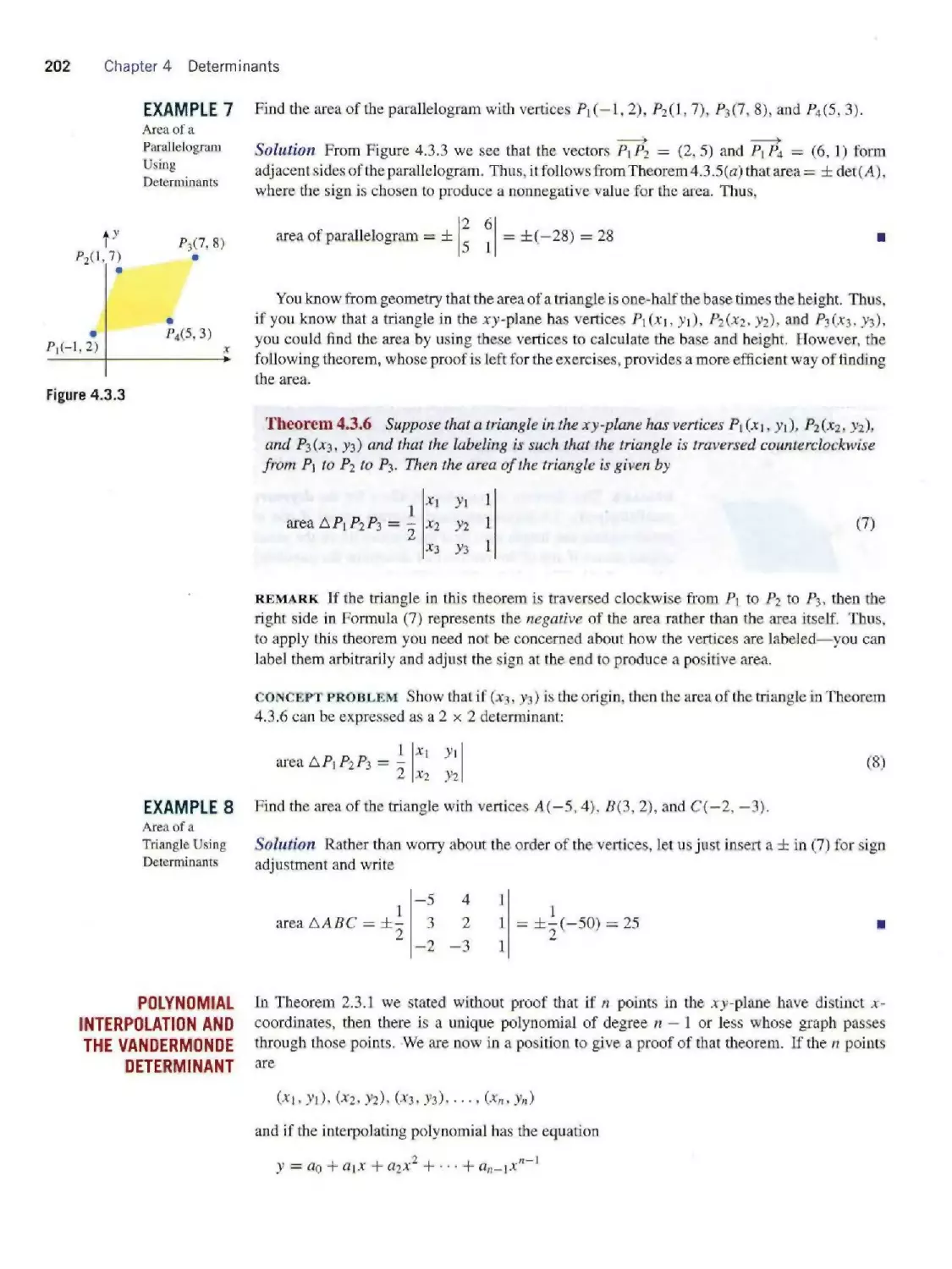
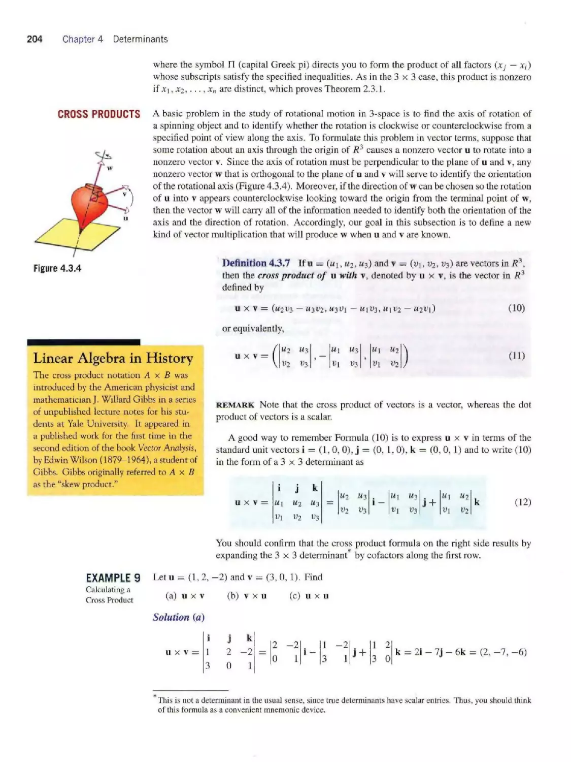
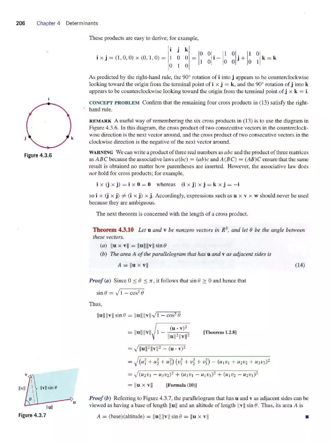
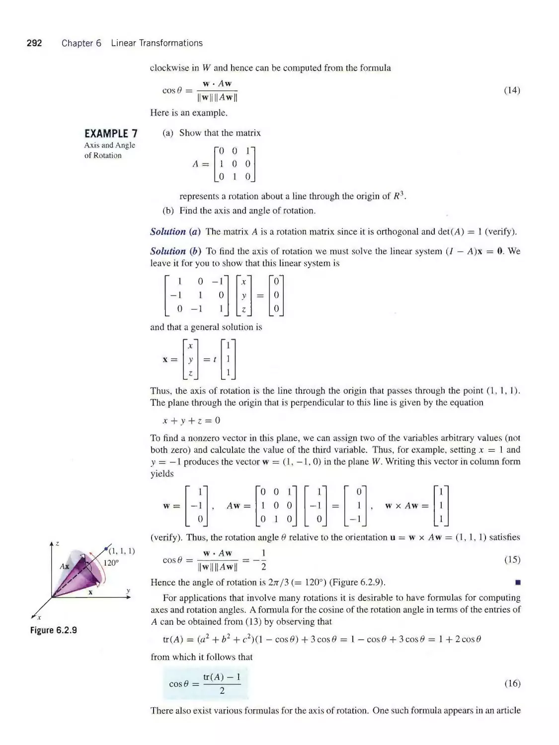
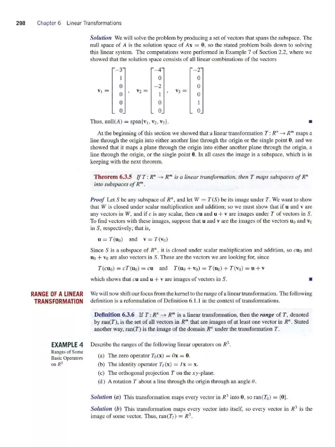
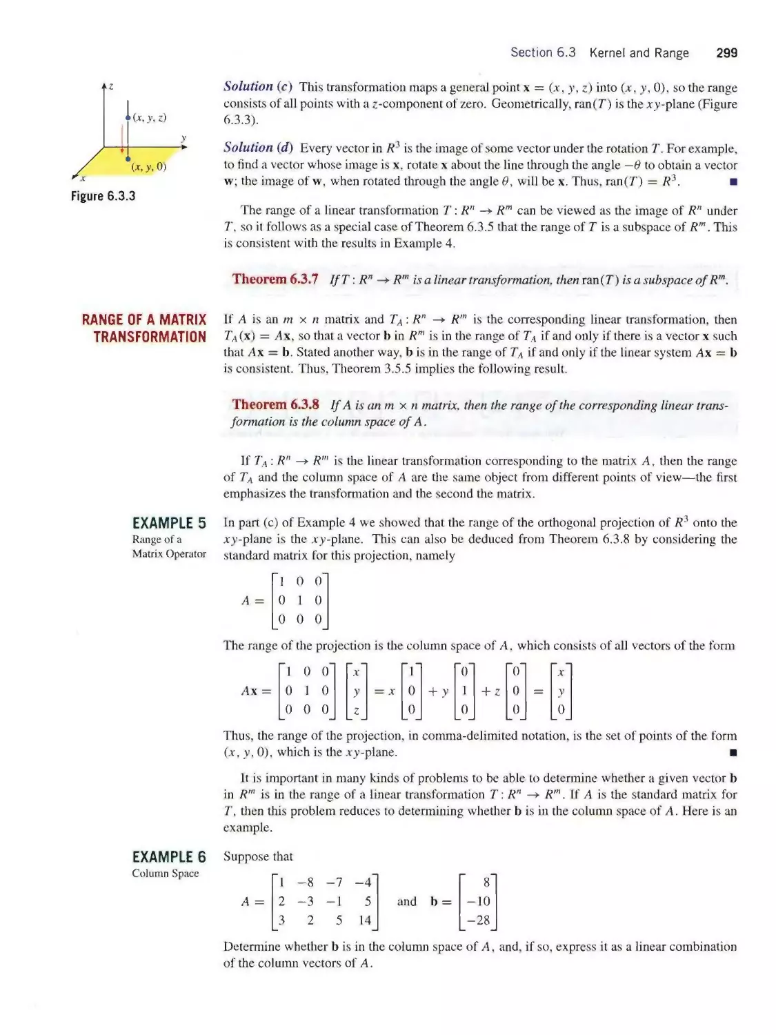
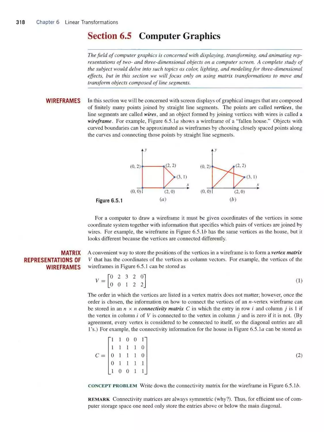
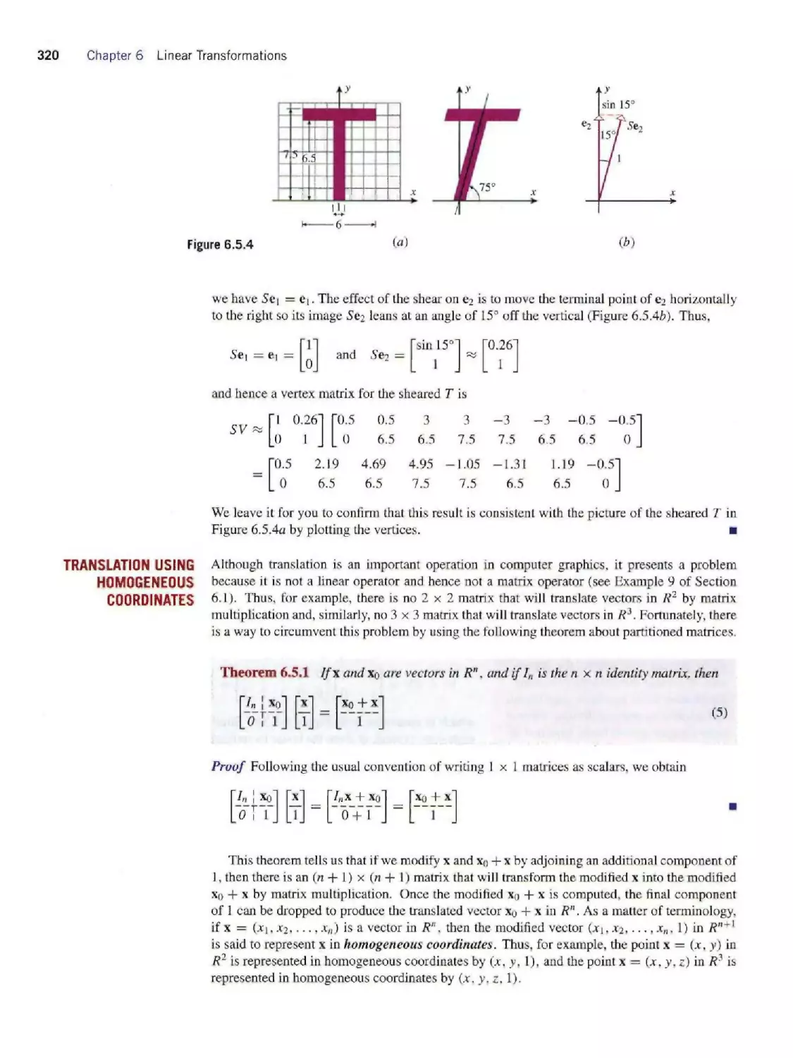
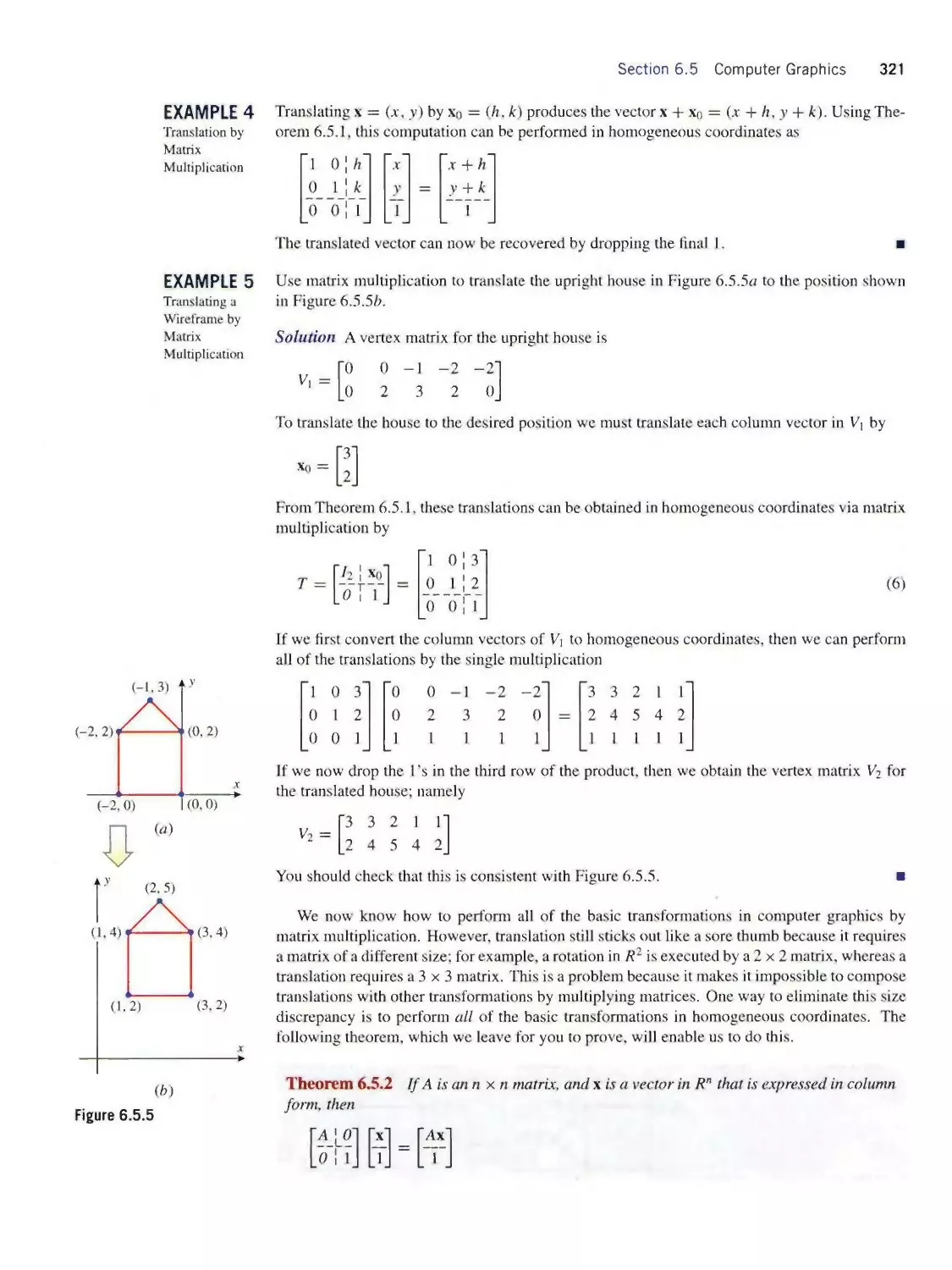
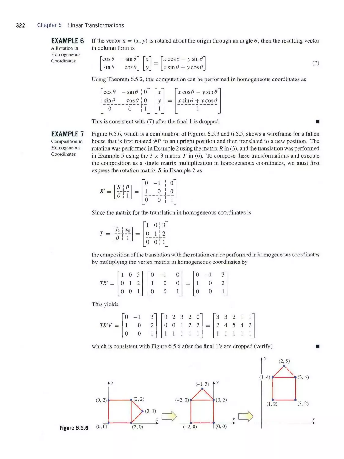
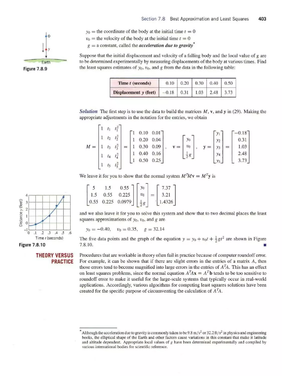
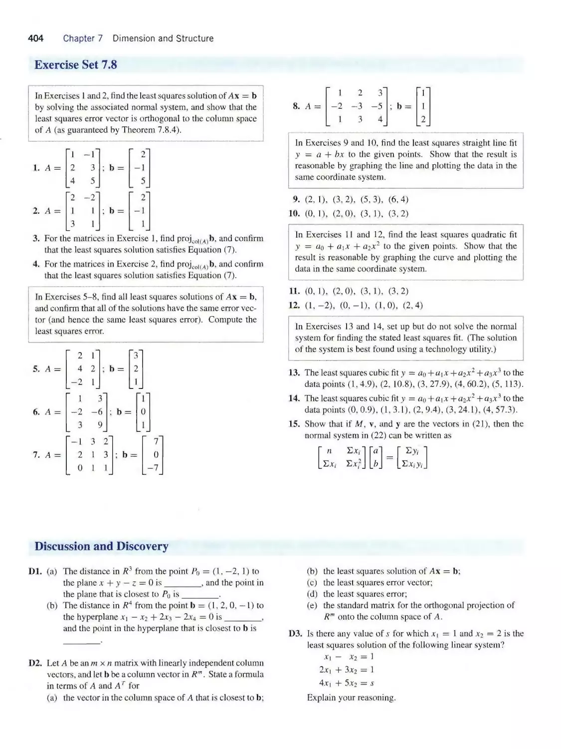
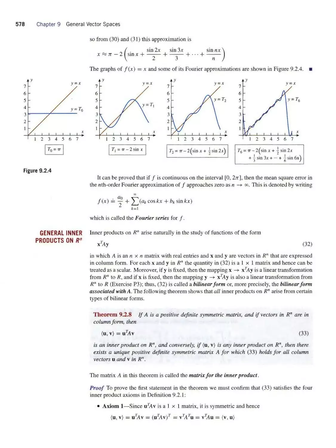
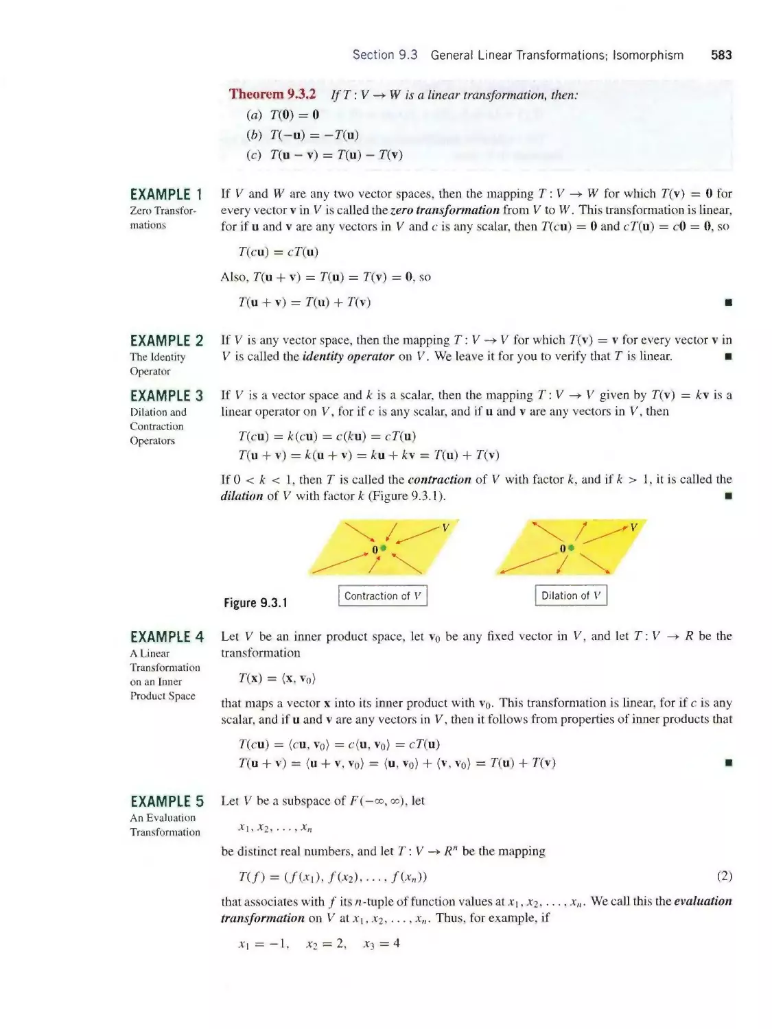
/


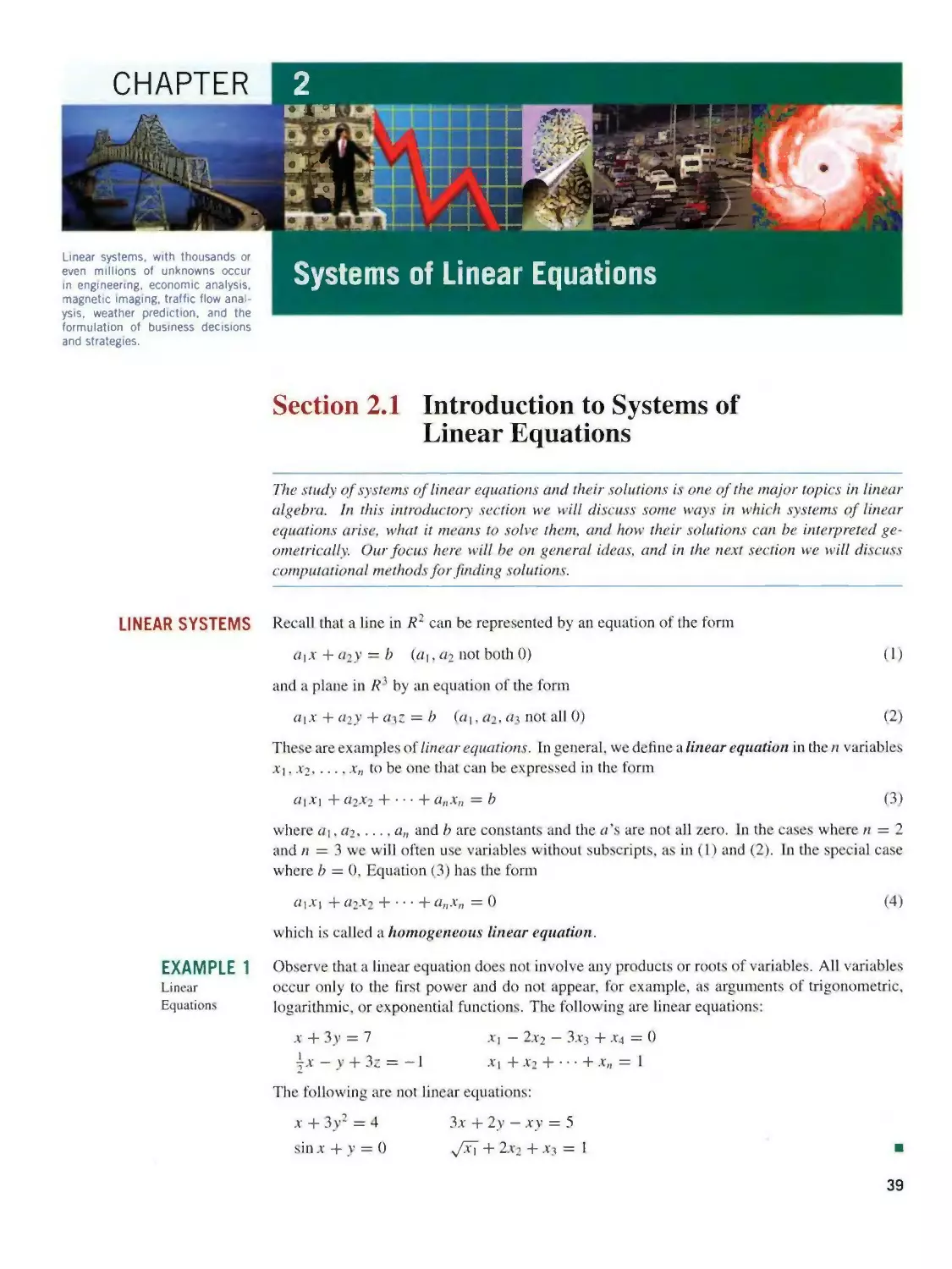


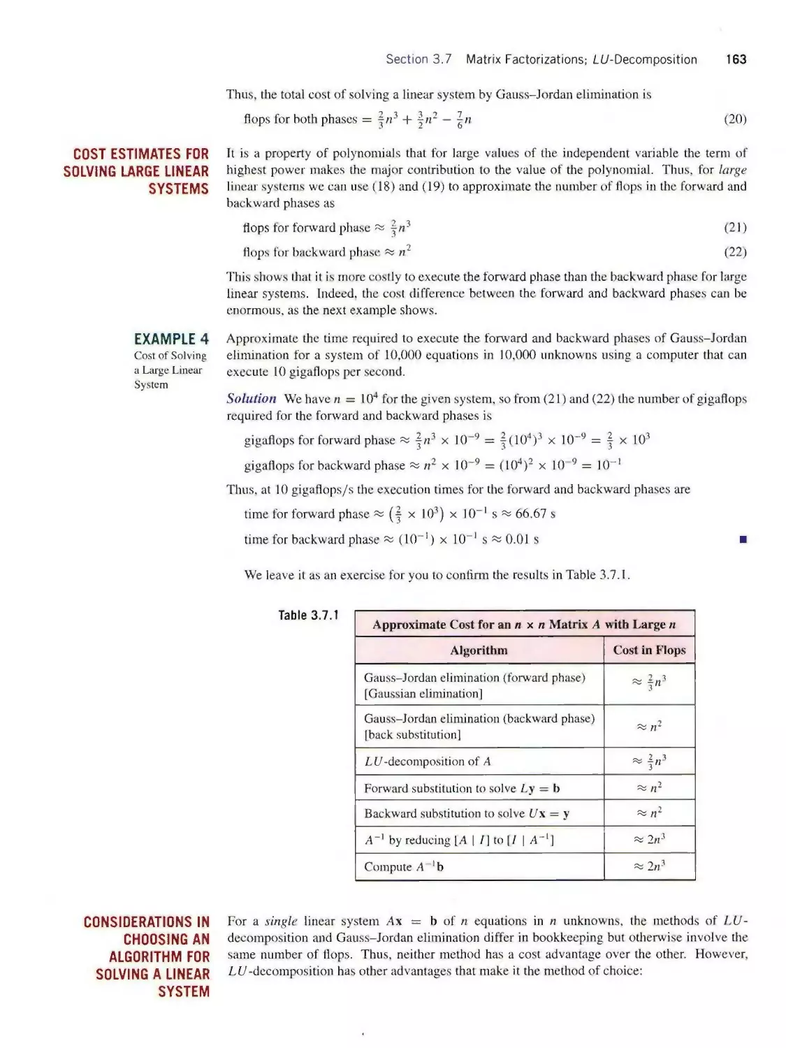


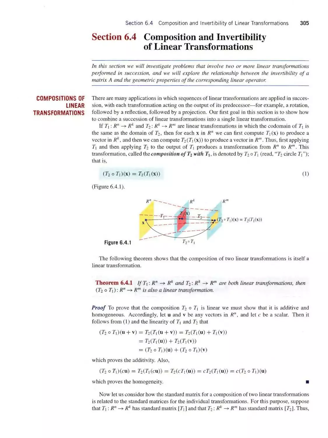


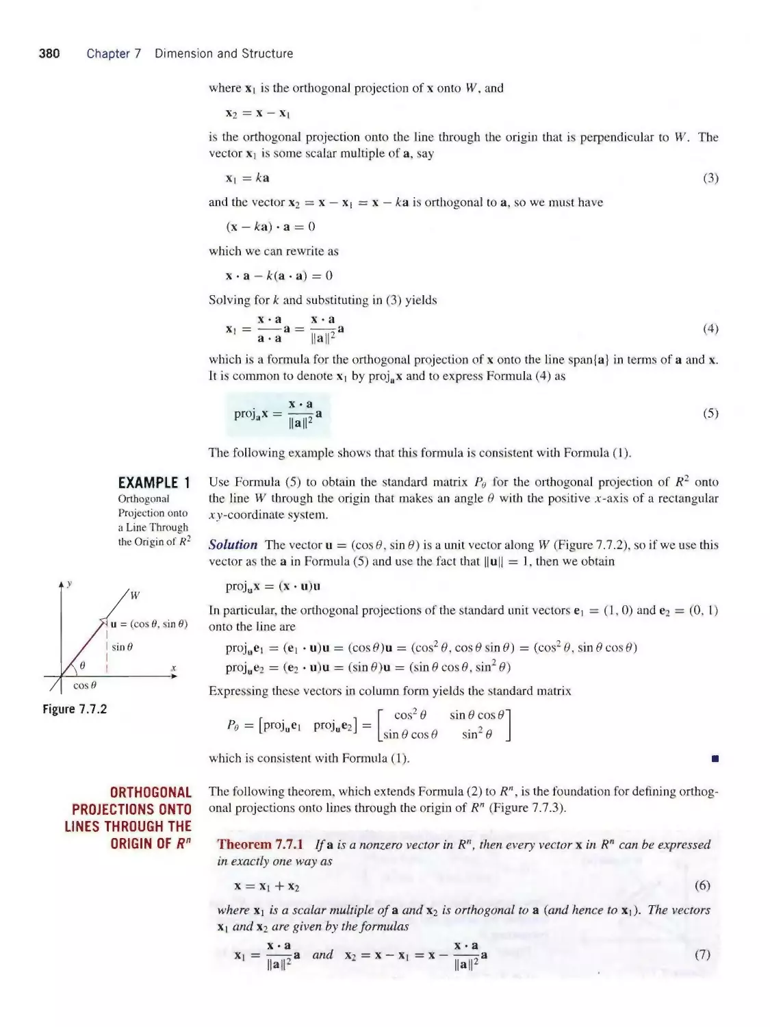


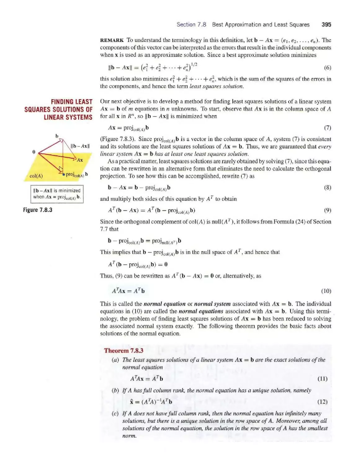


Теги: mathematics algebra higher mathematics john wiley and sons linear algebra contemporary linear algebra
ISBN: 978-0-471-16362-6
Год: 2002

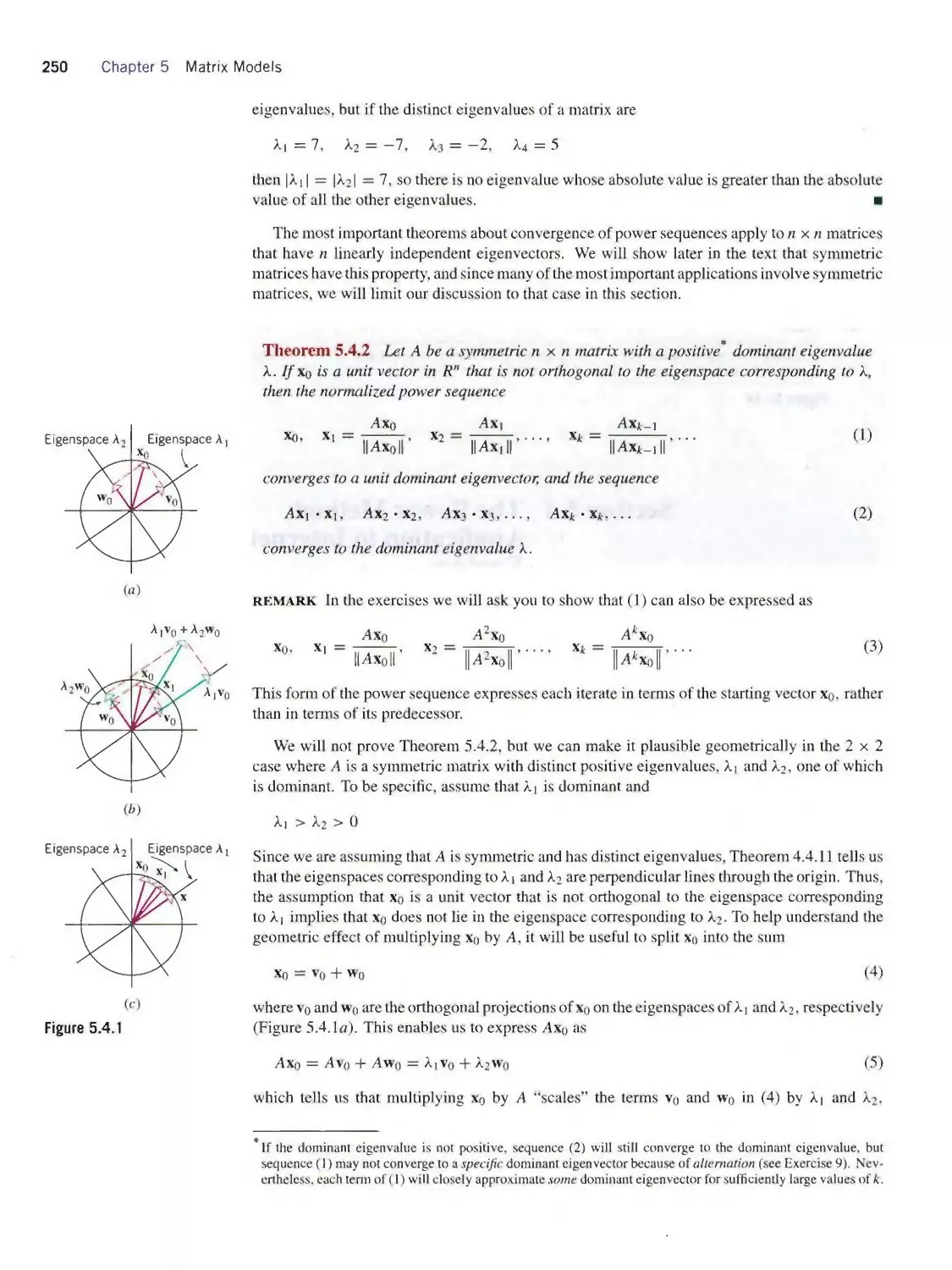
Текст
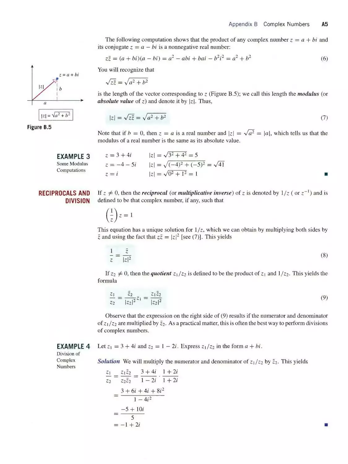
CONTEMPORARY
4KλVA
Contemporary
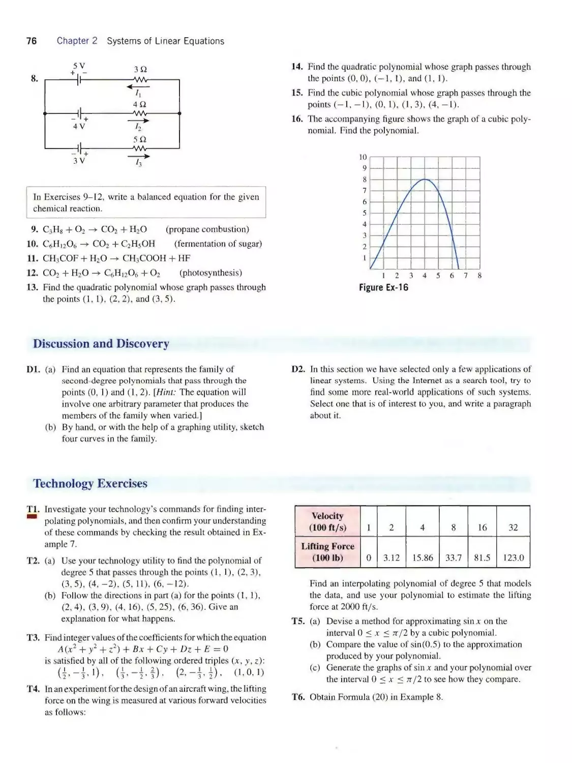
Linear Algebra
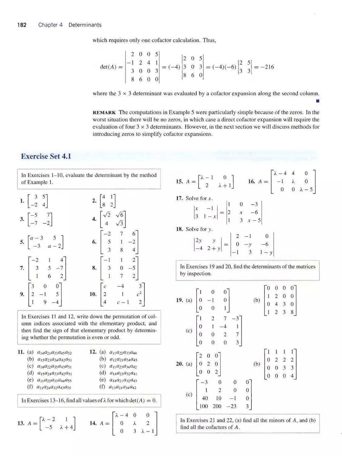
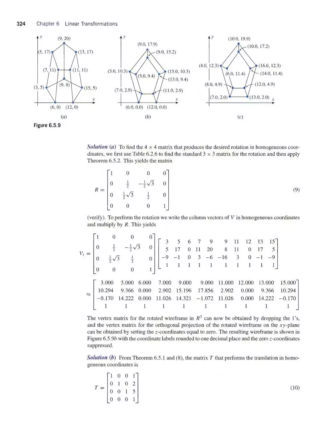
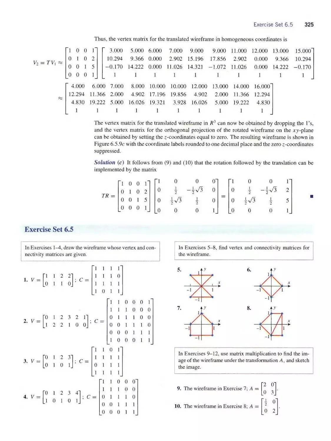
Howard Anton
Drexel University
Robert C. Busby
Drexel University
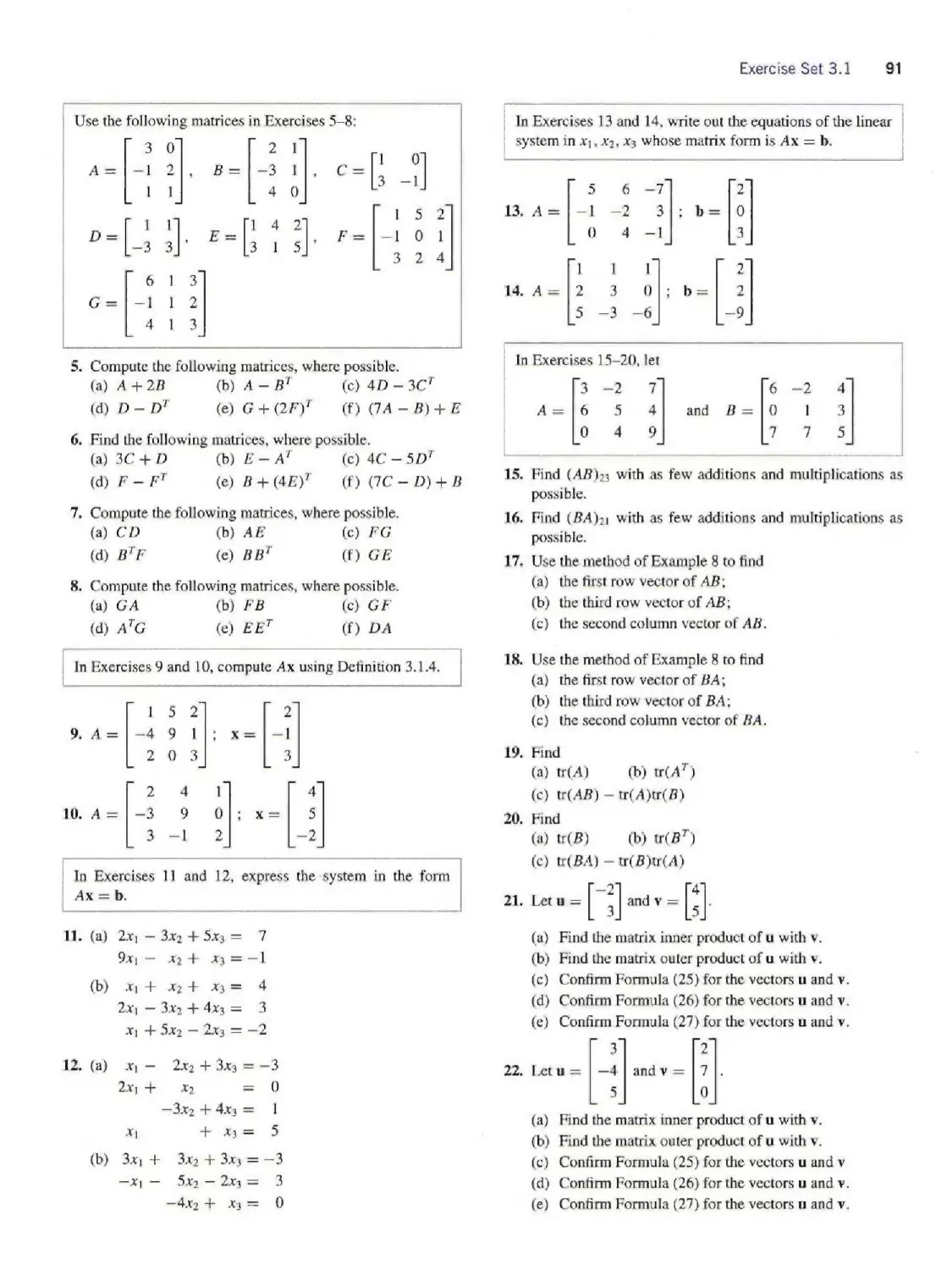
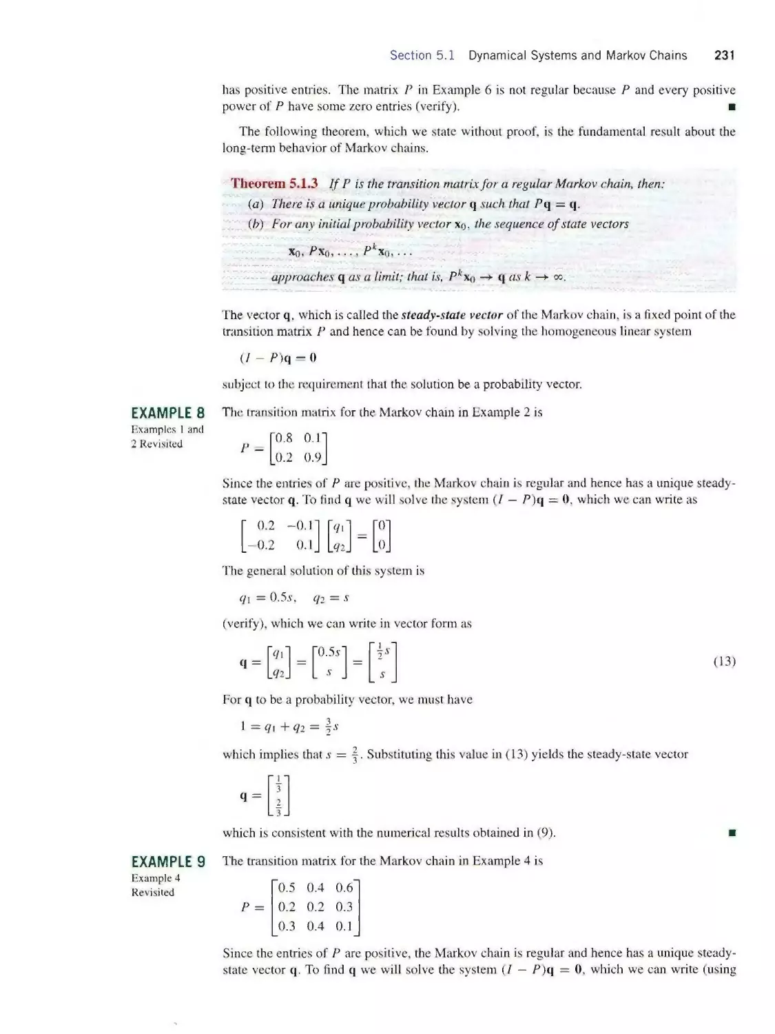
John Wiley & Sons, Inc.
ACQUISITIONS EDITOR
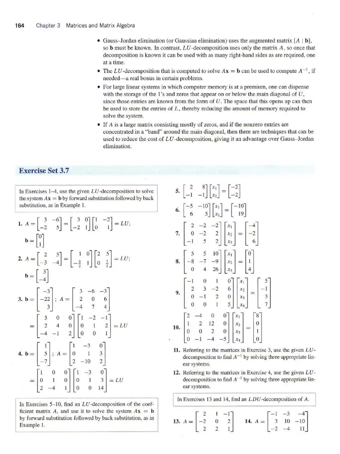
Laurie Rosatone
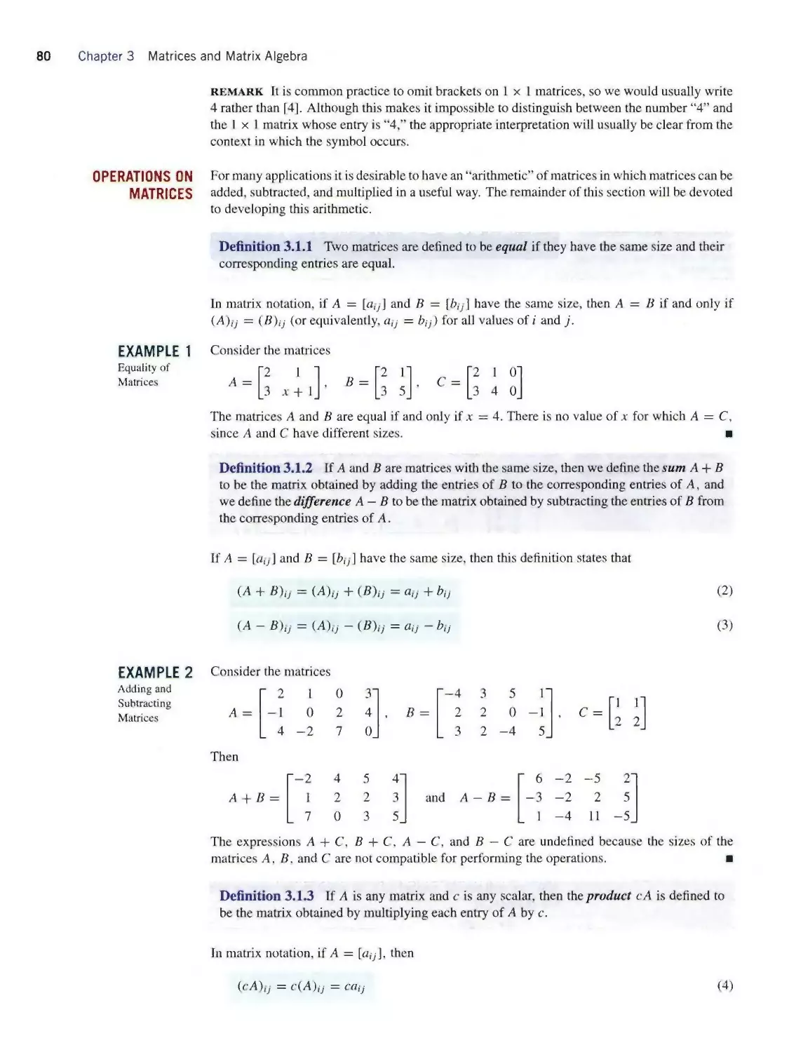
MARKETING MANAGER
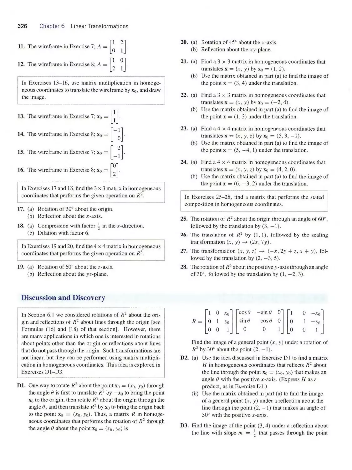
Julie Z. Lindstrom
SENIOR PRODUCTION EDITOR Ken Santor
PHOTO EDITOR
Sara Wight
COVER DESIGN
Madelyn Lesure
ILLUSTRATION STUDIO
ATI Illustration Services
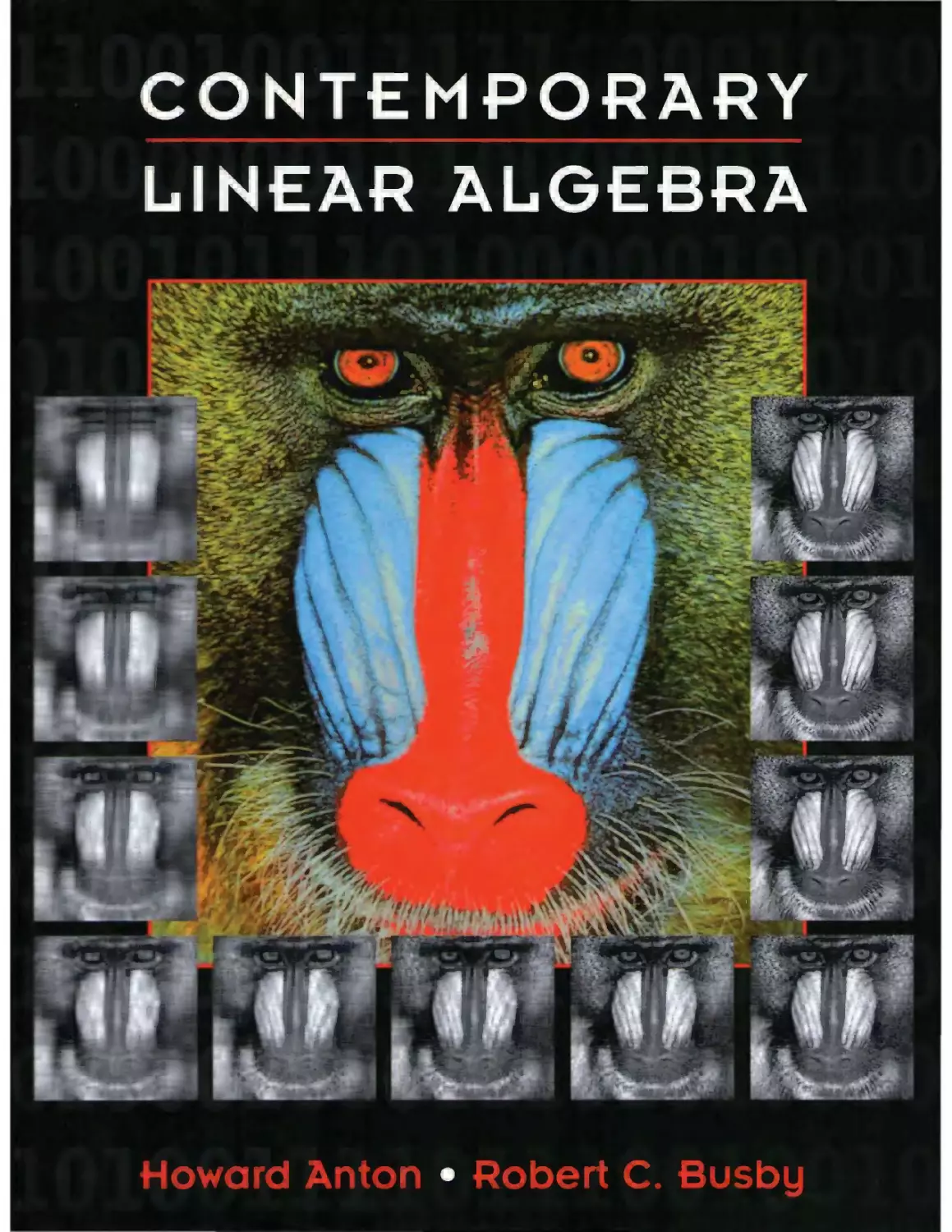
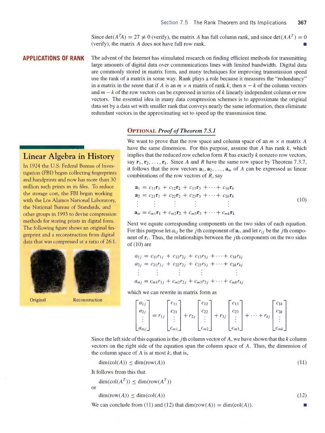
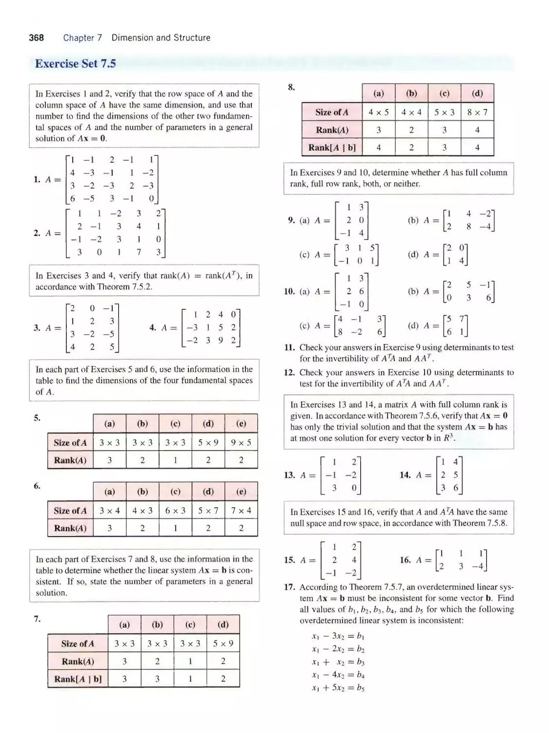
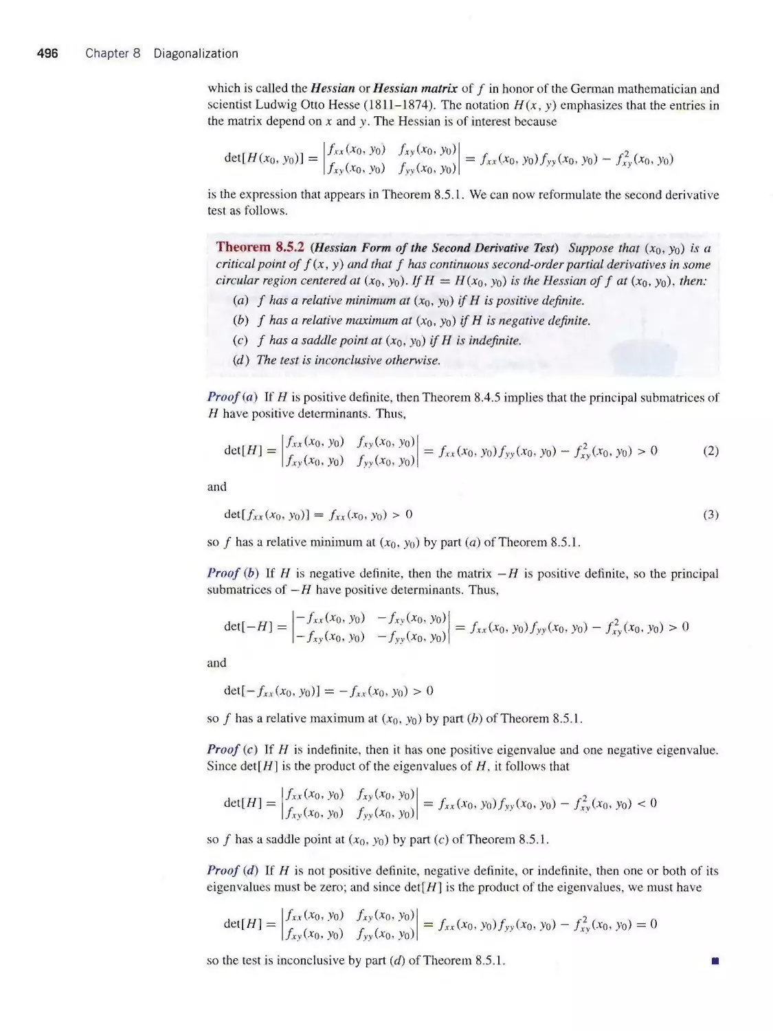
Cover Art: The mandrill picture on this cover has long been a favorite of researchers
studying techniques of image compression. The colored image in the center was scanned
in black and white and the bordering images were rendered with various levels of image
compression using the method of “singular value decomposition” discussed in this text.
Compressing an image blurs some of the detail but reduces the amount of space required
for its storage and the amount of time required to transmit it over the internet. In practice,
one tries to strike the right balance between compression and clarity.
This book was set in Times Roman by Techsetters, Inc. and printed and
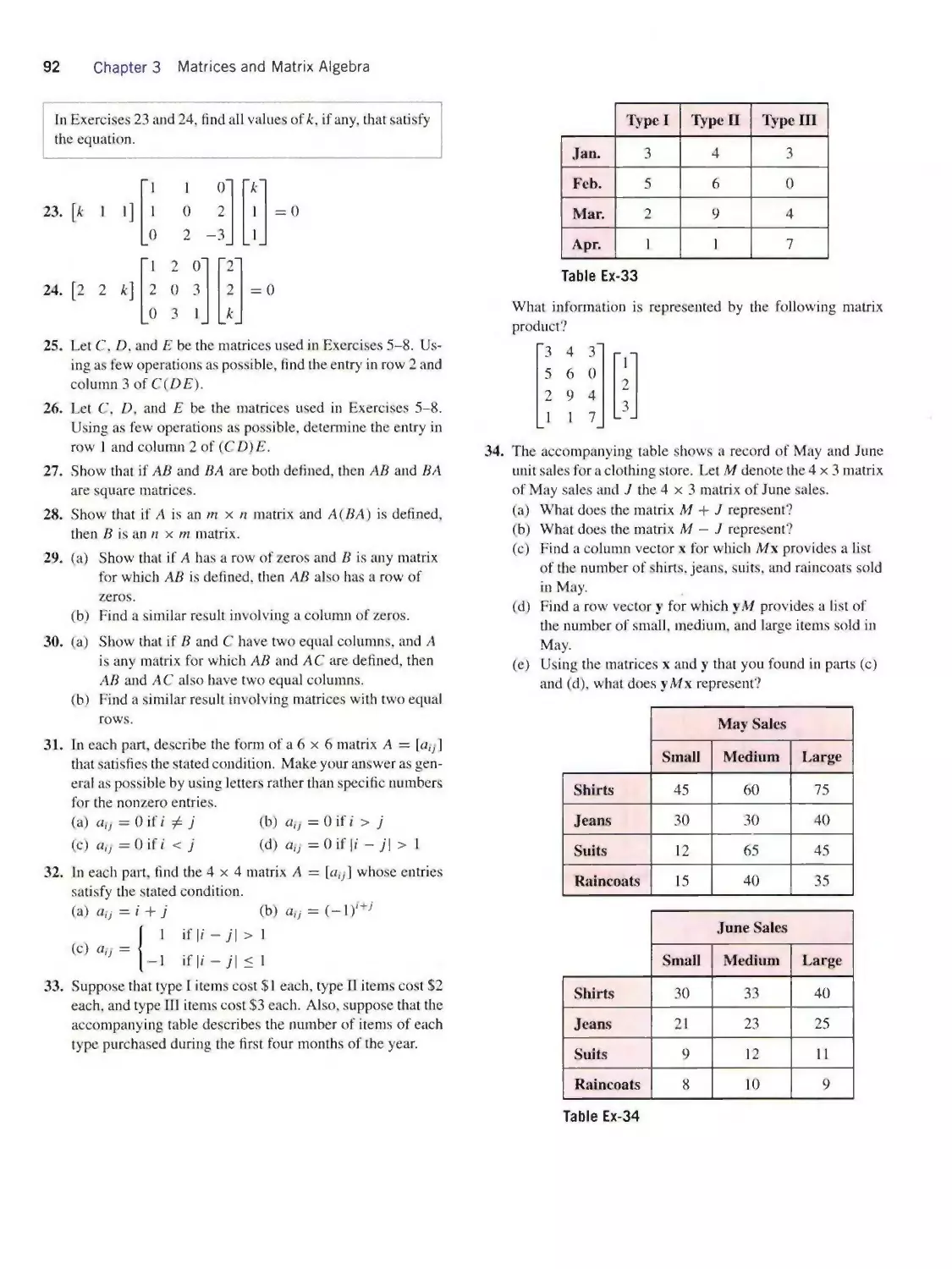
bound by Von Hoffman Corporation. The cover was printed by Phoenix Color Corporation.
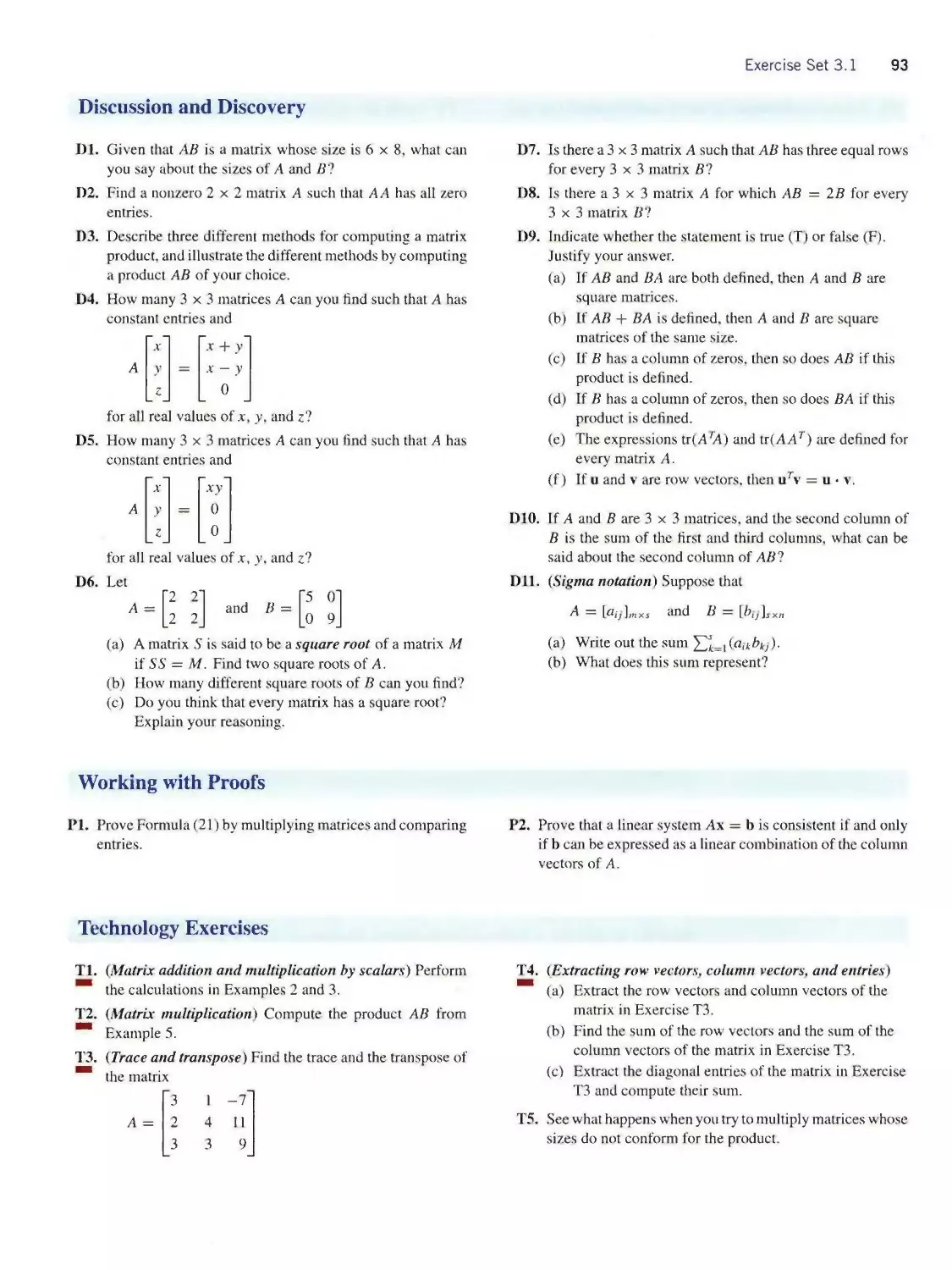
This book is printed on acid-free paper. @
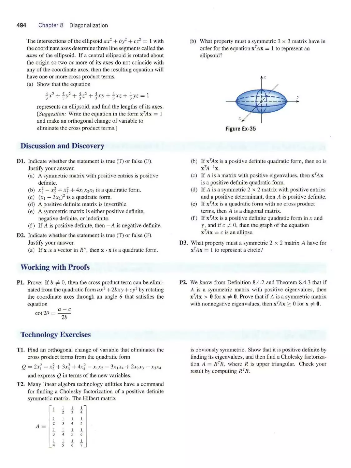
Copyright © 2003 Anton Textbooks, Inc. All rights reserved.
No part of this publication may be reproduced, stored in a retrieval system or transmitted
in any form or by any means, electronic, mechanical, photocopying, recording, scanning
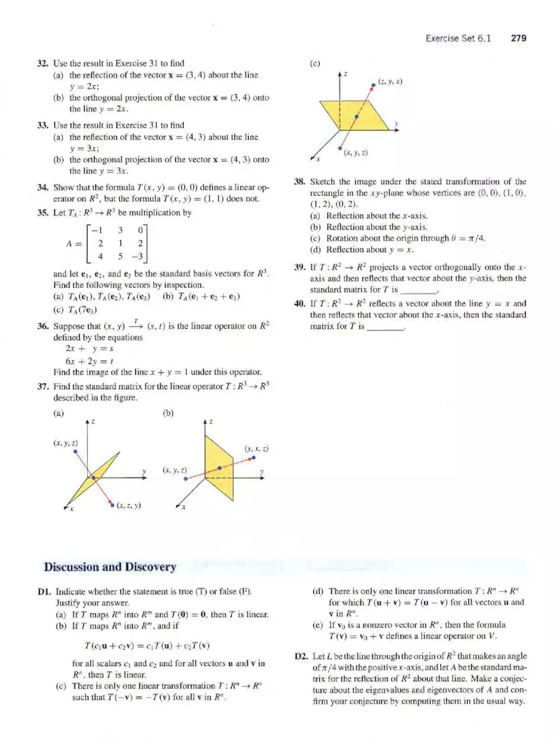
or otherwise, except as permitted under Sections 107 or 108 of the 1976 United States
Copyright Act, without either the prior written permission of the Publisher, or
authorization through payment of the appropriate per-copy fee to the Copyright
Clearance Center. 222 Rosewood Drive, Danvers, MA 01923, (978) 750-8400. fax
(978) 646-8600. Requests to the Publisher for permission should be addressed to the
Permissions Department, John Wiley & Sons. Inc., 111 River Street, Hoboken, NJ 07030,
(201) 748-6011, fax (201) 748-6008.
To order books or for customer service please, call l(800)-CALL-WILEY (225-5945).
ISBN 978-0-471-16362-6
Printed in the United States of America
10 9
ABOUT THE AUTHORS
Howard Anton obtained his B.A. from Lehigh University, his
M.A. from the University of Illinois, and his Ph.D. from the
Polytechnic University of Brooklyn, all in mathematics. In the
early 1960s he worked for Burroughs Corporation and Avco
Corporation at Cape Canaveral, Florida (now the Kennedy
Space Center), on mathematical problems related to the
manned space program. In 1968 he joined the Mathematics
Department at Drexel University, where he taught full time
until 1983. Since then he has been an adjunct professor at
Drexel and has devoted the majority of his time to textbook
writing and projects for mathematical associations. He was
president of the Eastern Pennsylvania and Delaware section
of the Mathematical Association of America (MAA), served
on the Board of Governors of the MAA, and guided the cre¬
ation of its Student Chapters. He has published numerous
research papers in functional analysis, approximation theory,
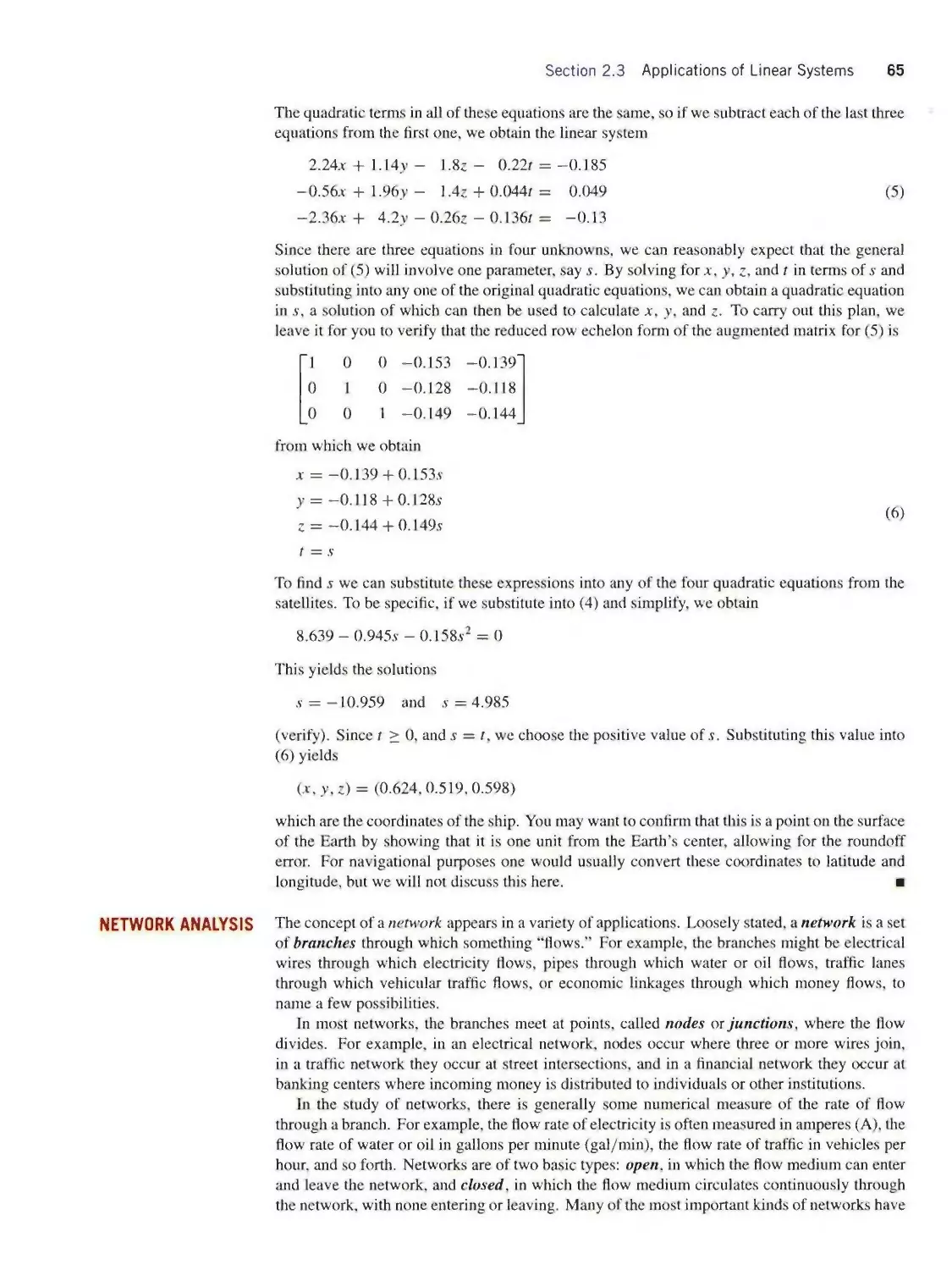
and topology, as well as various pedagogical papers. He is
best known for his textbooks in mathematics, which have
been widely used for more than thirty years. There are cur¬
rently more than 125 versions of his books used through¬
out the world, including translations into Spanish, Arabic,
Portuguese, Italian, Indonesian, French, Japanese, Chinese,
Hebrew, and German. In 1994 he was awarded the Textbook
Excellence Award by the Textbook Authors Association. For
relaxation, Dr. Anton enjoys traveling, photography, and art.
Robert C. Busby obtained his B.S. in physics from Drexel
University and his M.A. and Ph.D. in mathematics from the
University of Pennsylvania. He taught at Oakland University
in Rochester, Michigan, and since 1969 has taught full time
at Drexel University, where he currently holds the position of
Professor in the Department of Mathematics and Computer
Science. He has regularly taught courses in calculus, lin¬
ear algebra, probability and statistics, and modem analysis.
Dr. Busby is the author of numerous research articles in func¬
tional analysis, representation theory, and operator algebras,
and he has coauthored an undergraduate text in discrete math¬
ematical structures and a workbook on the use of Maple in
calculus. His current professional interests include aspects
of signal processing and the use of computer technology in
undergraduate education. Professor Busby also enjoys con¬
temporaryjazz and computer graphic design. He and his wife,
Patricia, have two sons, Robert and Scott.
CONTENTS
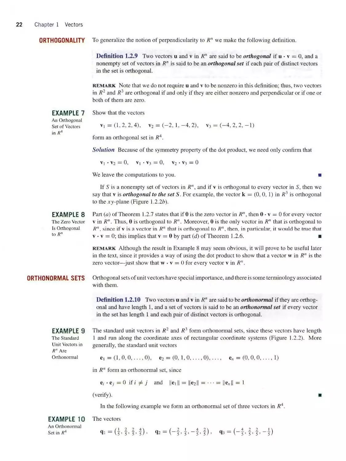
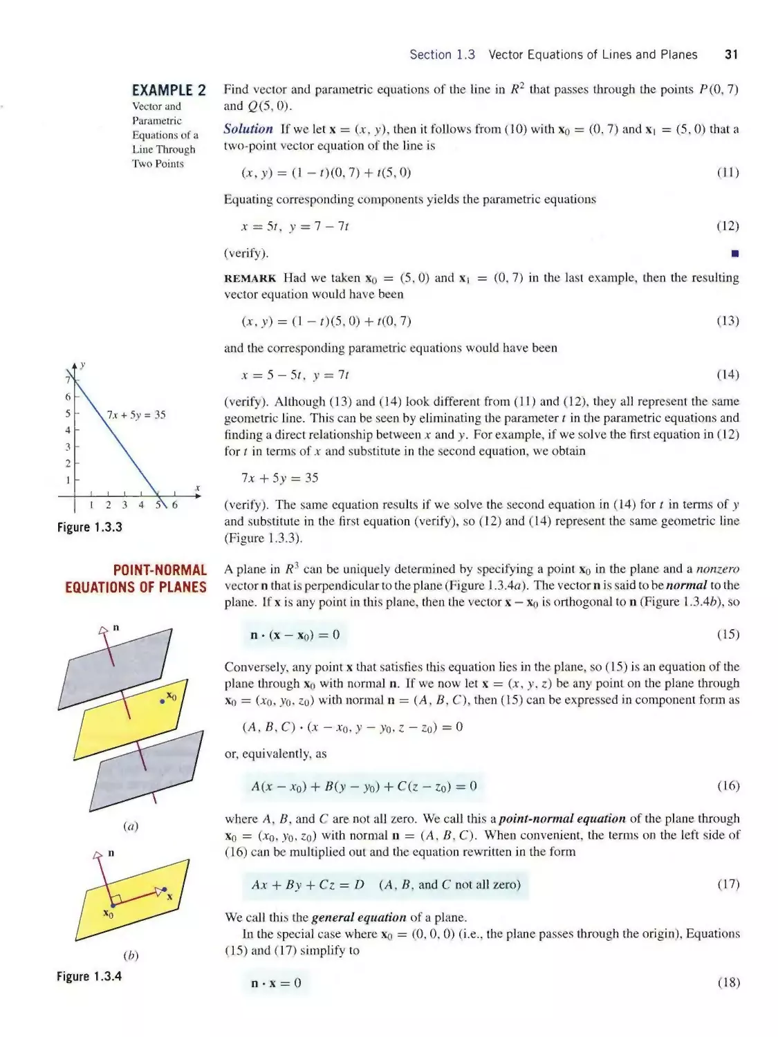
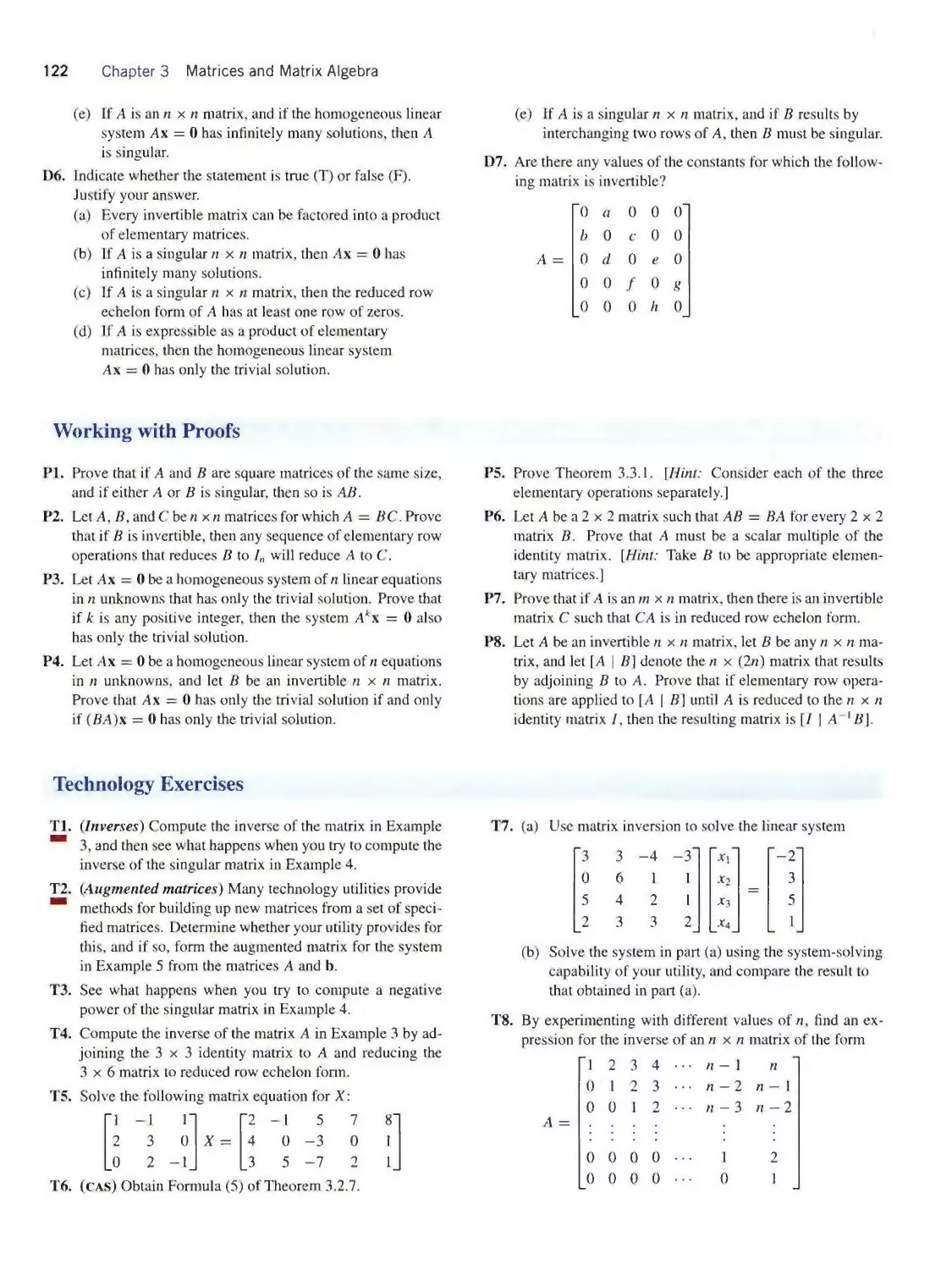
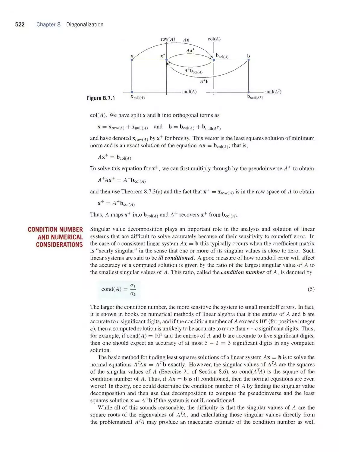
CHAPTER 1 Vectors 1
1.1 Vectors and Matrices in Engineering and
Mathematics; n-Space 1
1.2 Dot Product and Orthogonality 15
1.3 Vector Equations of Lines and Planes 29
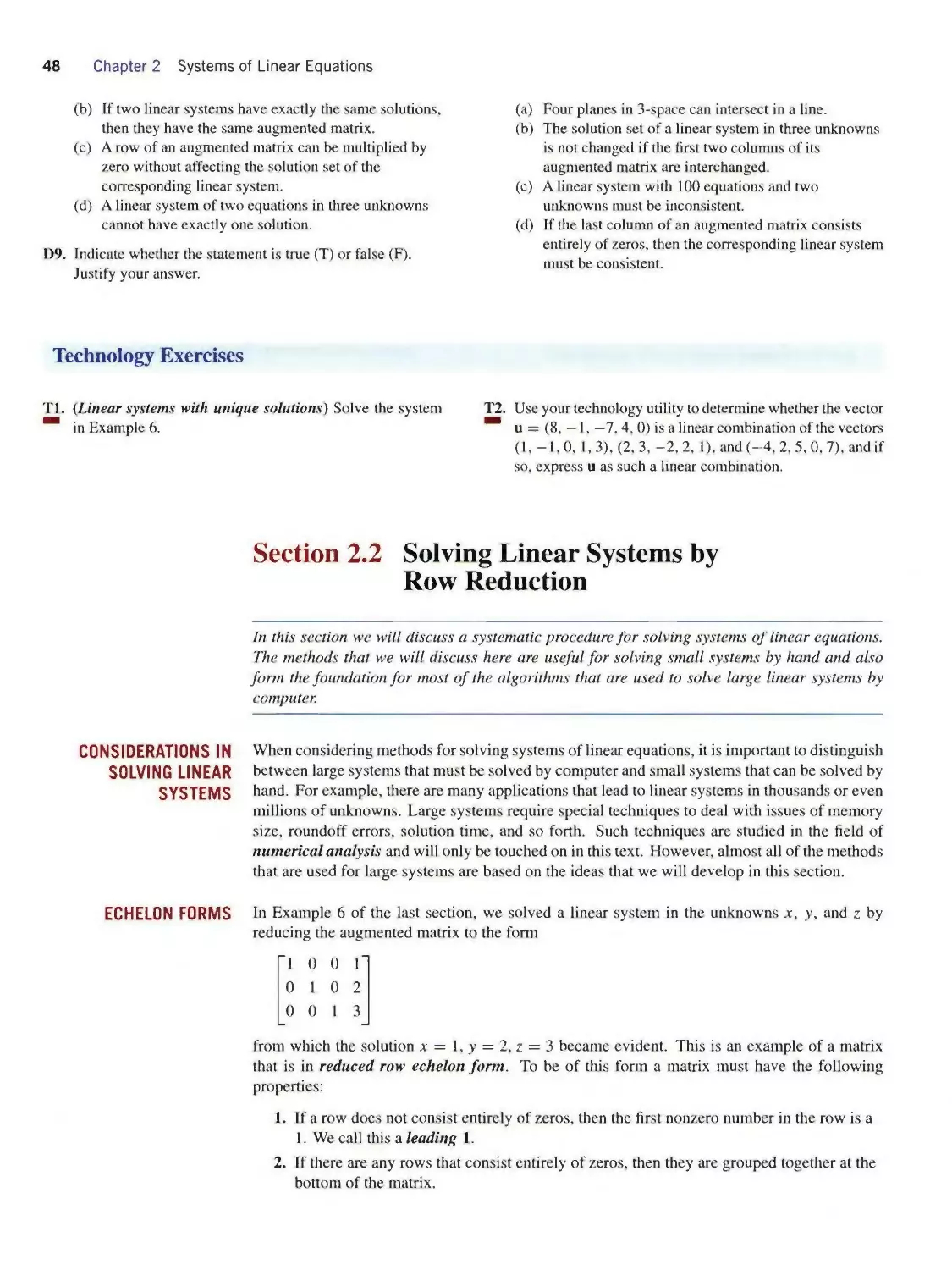
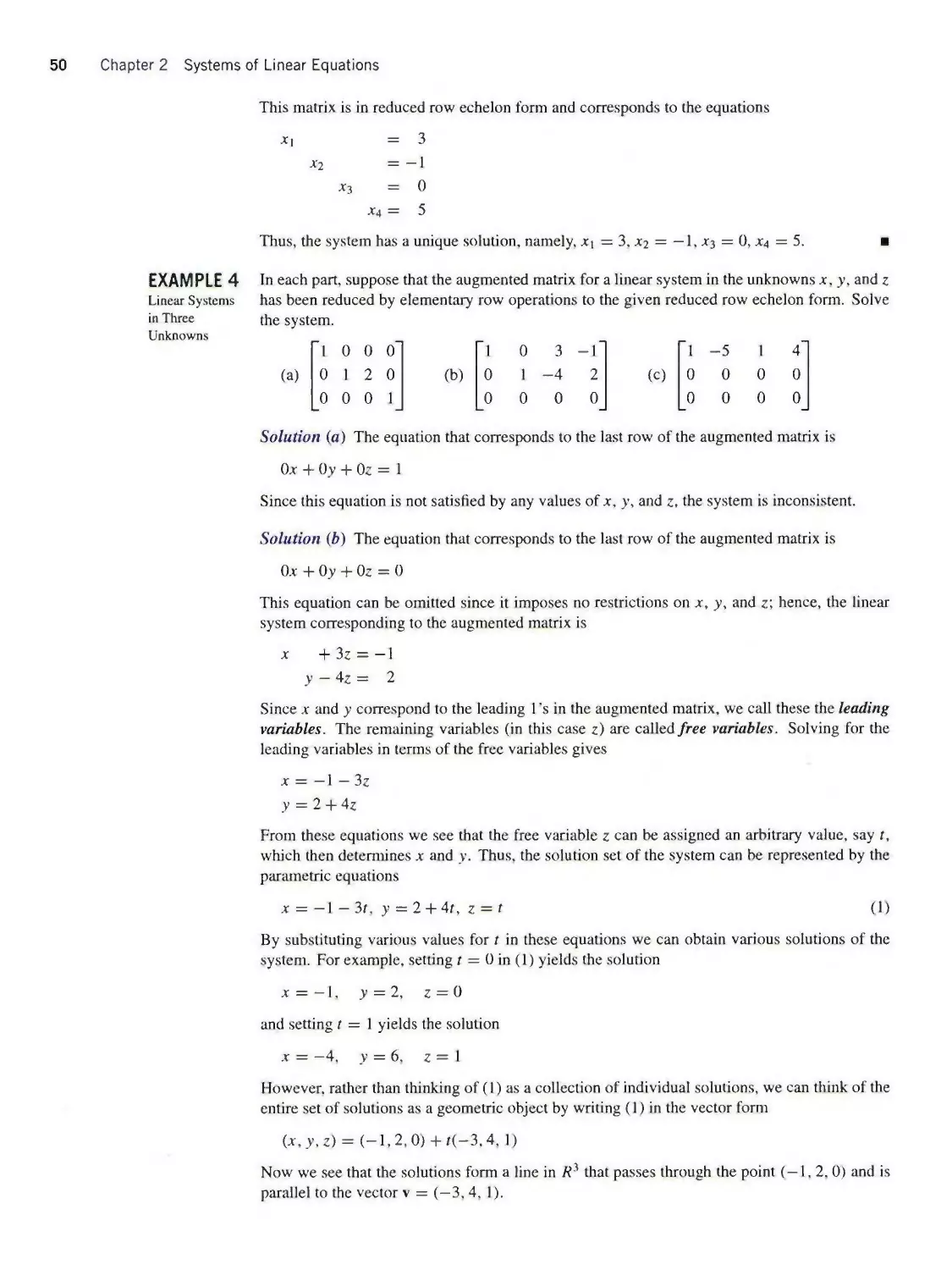
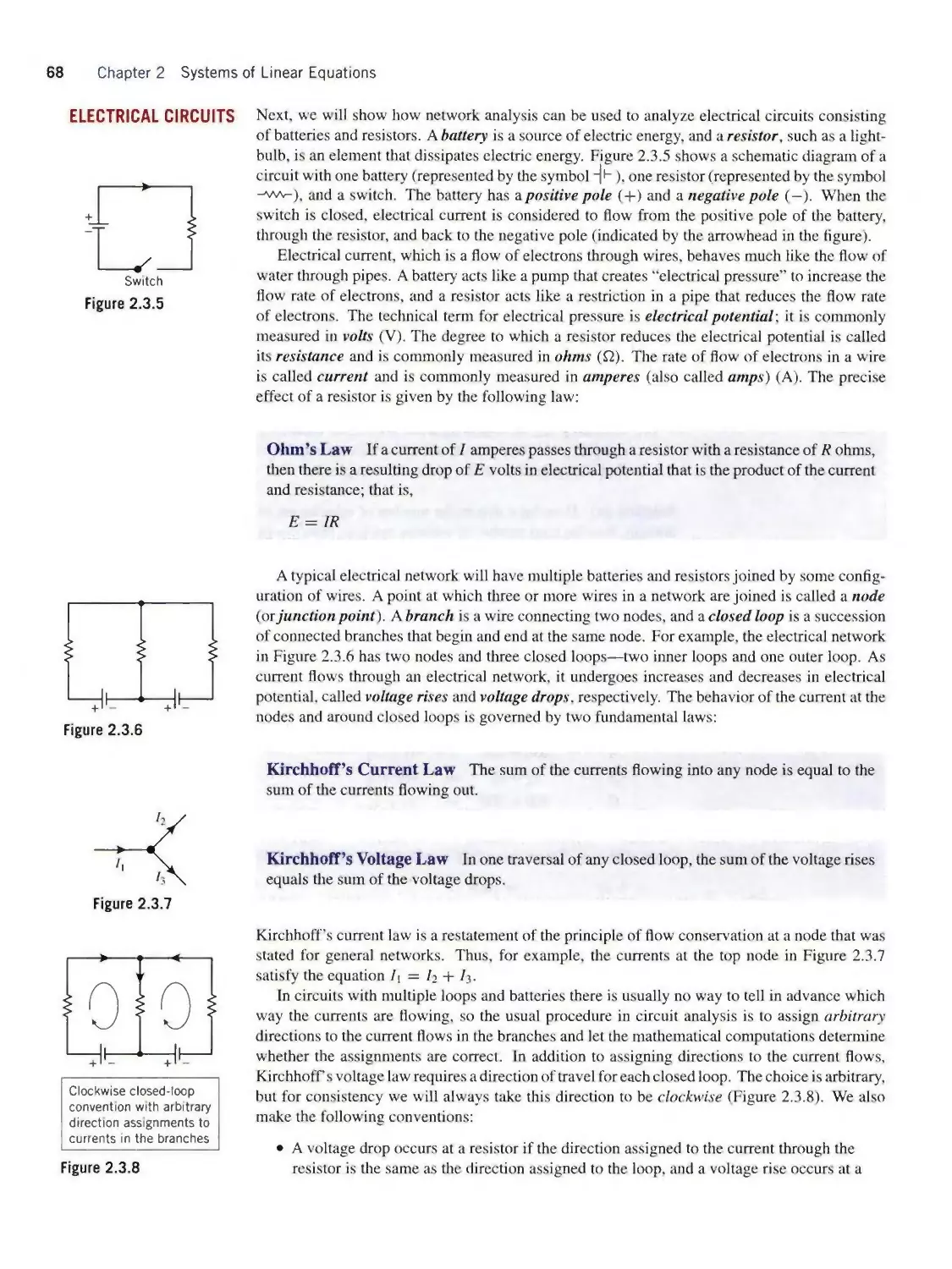
chapter 2 Systems of Linear Equations 39
2.1 Introduction to Systems of Linear Equations 39
2.2 Solving Linear Systems by Row Reduction 48
2.3 Applications of Linear Systems 63
chapter 3 Matrices and Matrix Algebra 79
3.1 Operations on Matrices 79
3.2 Inverses; Algebraic Properties of Matrices 94
3.3 Elementary Matrices; A Method for
Finding A-1 109
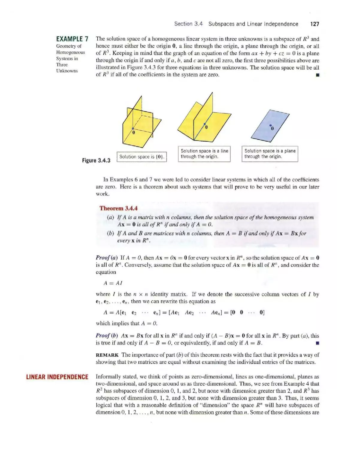
3.4 Subspaces and Linear Independence 123
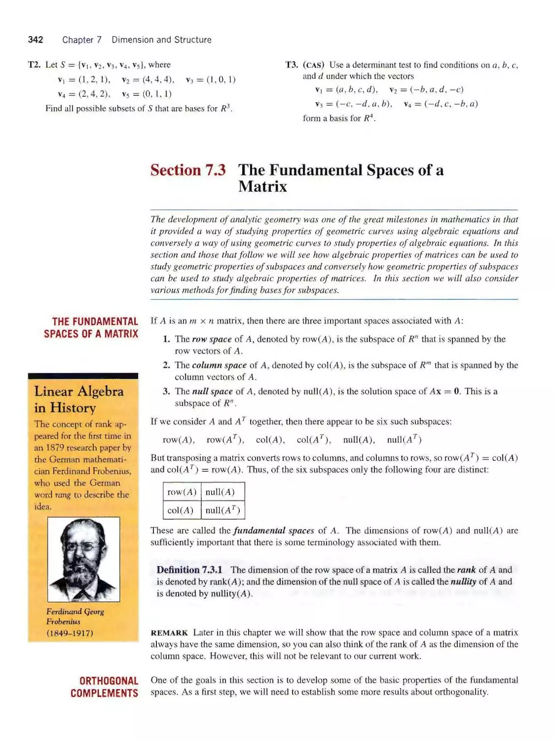
3.5 The Geometry of Linear Systems 135
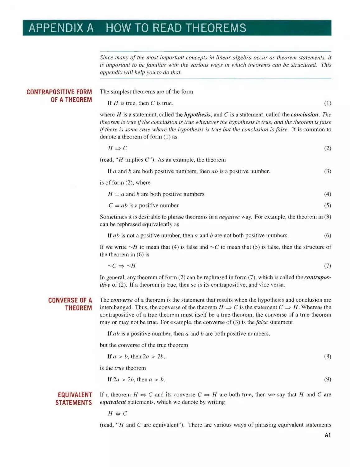
3.6 Matrices with Special Forms 143
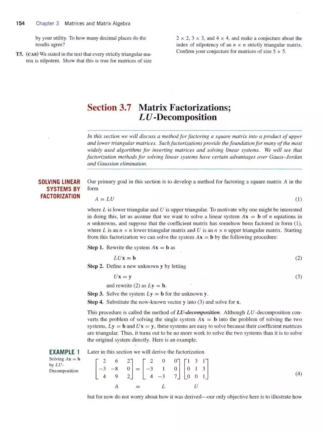
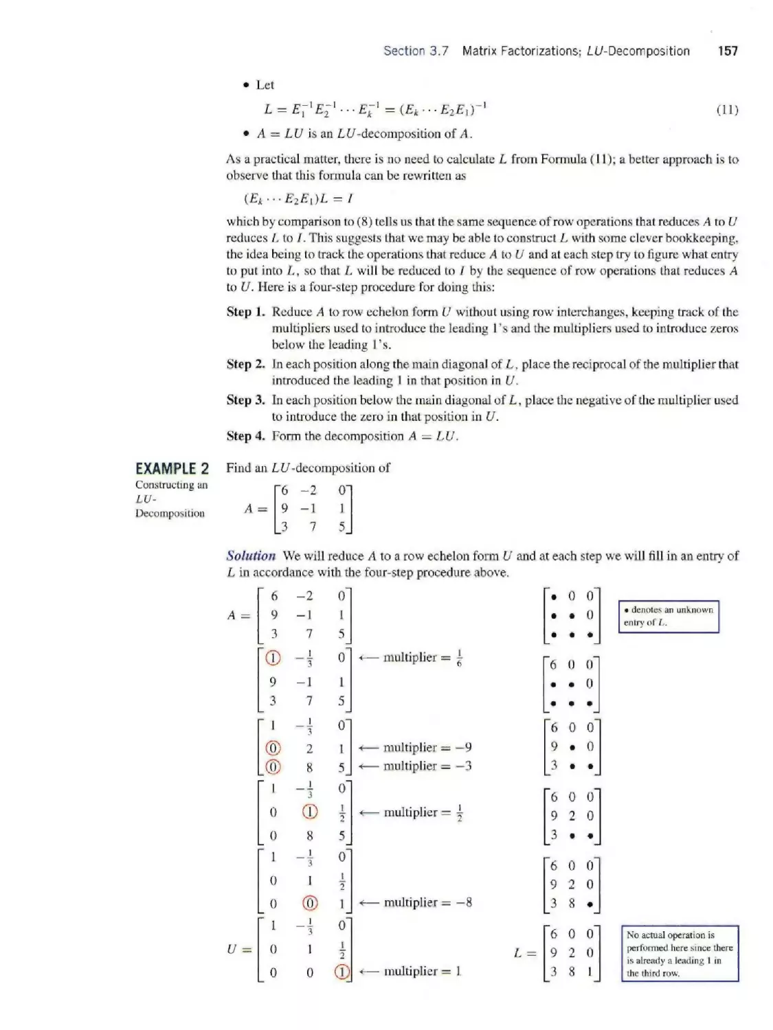
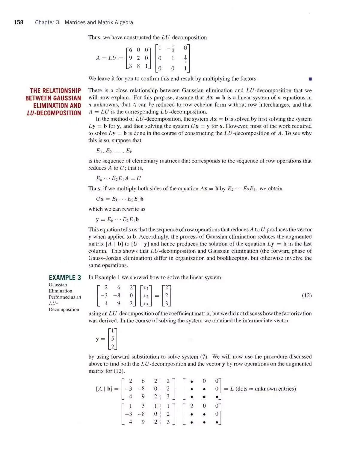
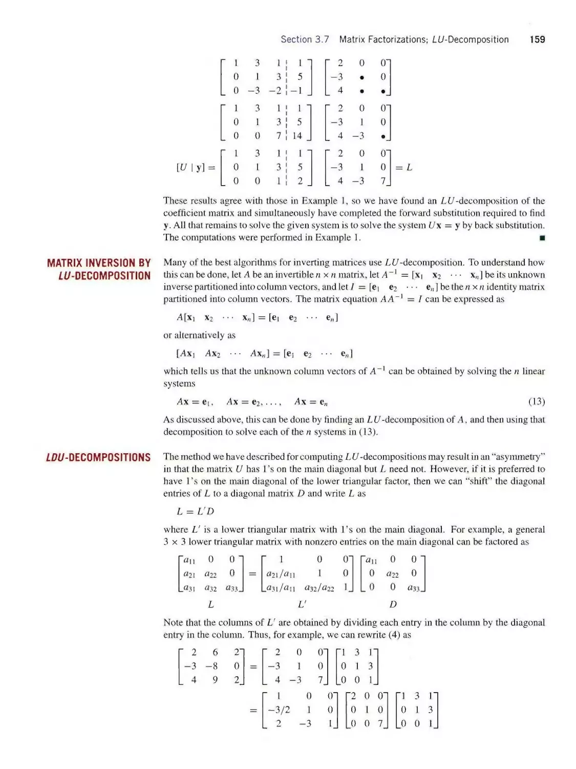
3.7 Matrix Factorizations;/.[/-Decomposition 154
3.8 Partitioned Matrices and Parallel Processing 166
chapter 4 Determinants 175
4.1 Determinants; Cofactor Expansion 175
4.2 Properties of Determinants 184
4.3 Cramer’s Rule; Formula for A^^l; Applications of
Determinants 196
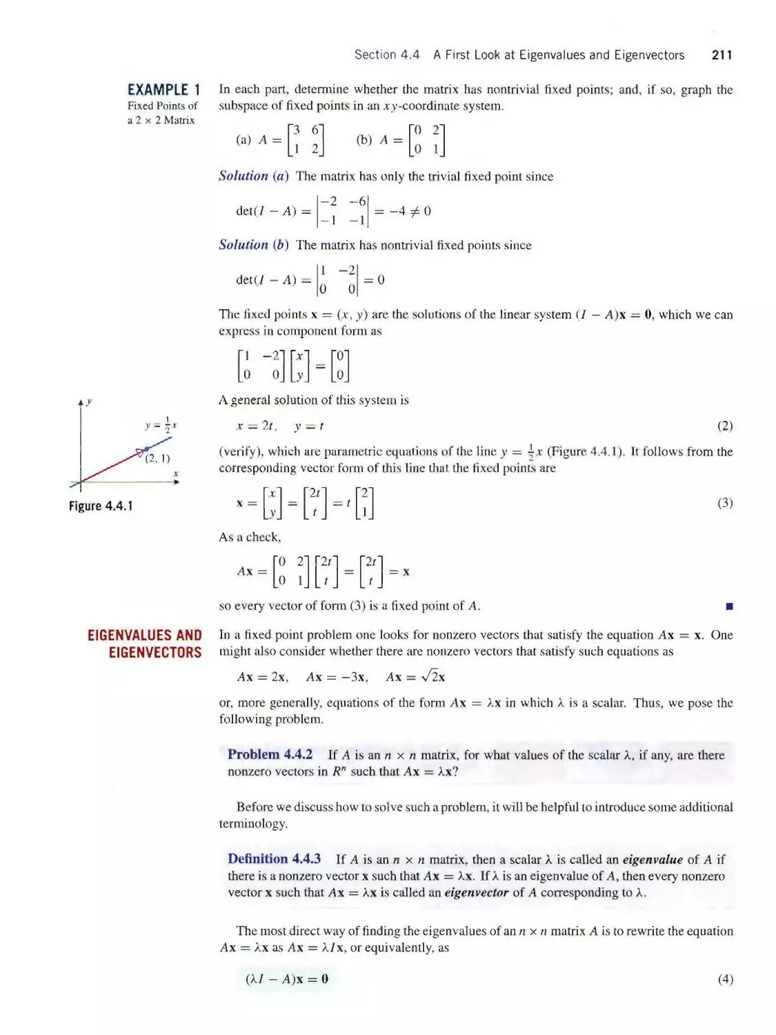
4.4 A First Look at Eigenvalues and Eigenvectors 210
chapter 5 Matrix Models 225
5.1 Dynamical Systems and Markov Chains 225
5.2 Leontief Input-Output Models 235
5.3 Gauss-Seidel and Jacobi Iteration; Sparse Linear
Systems 241
5.4 The Power Method; Application to Internet Search
Engines 249
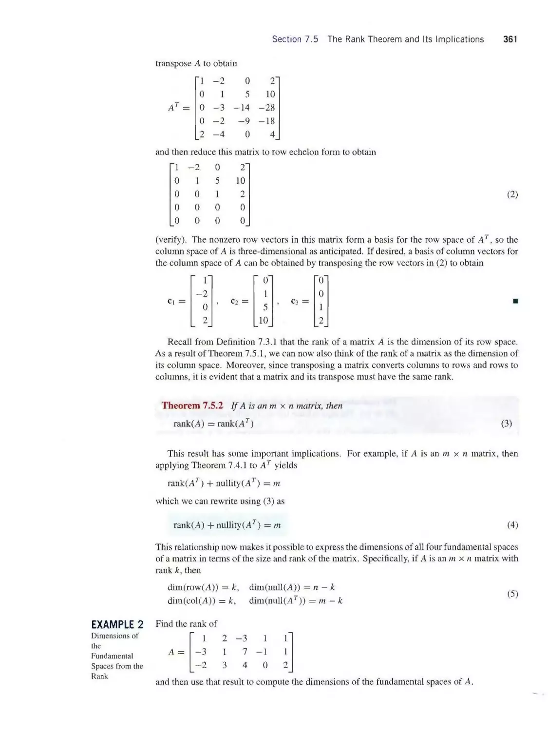
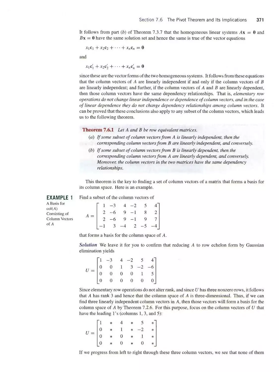
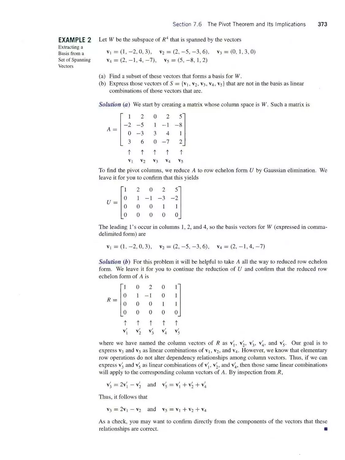
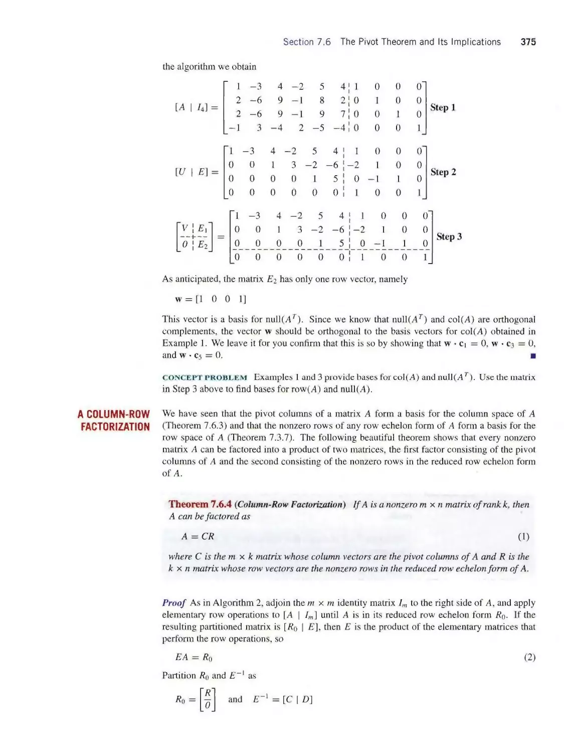
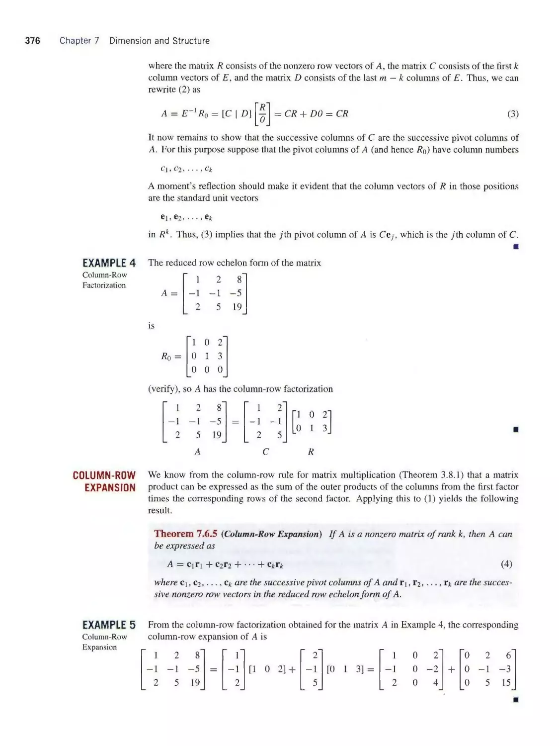
chapter 7 Dimension and Structure 329
7.1 Basis and Dimension 329
7.2 Properties of Bases 335
7.3 The Fundamental Spaces of a Matrix 342
7.4 The Dimension Theorem and Its Implications 352
7.5 The Rank Theorem and Its Implications 360
7.6 The Pivot Theorem and Its Implications 370
7.7 The Projection Theorem and Its Implications 379
7.8 Best Approximation and Least Squares 393
7.9 Orthonormal Bases and the Gram-Schmidt
Process 406
7.10 (//[-Decomposition; Householder
Transformations 417
7.11 Coordinates with Respect to a Basis 428
chapter 8 Diagonalization 443
8.1 Matrix Representations of Linear
Transformations 443
8.2 Similarity and Diagonalizability 456
8.3 Orthogonal Diagonalizability; Functions
of a Matrix 468
8.4 Quadratic Forms 481
8.5 Application of Quadratic Forms
to Optimization 495
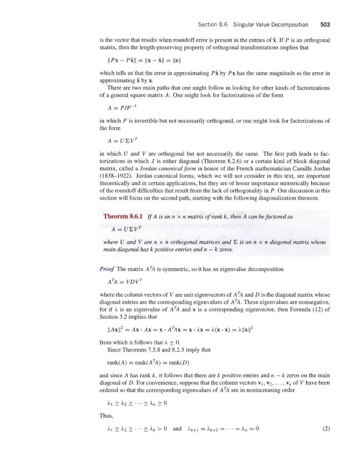
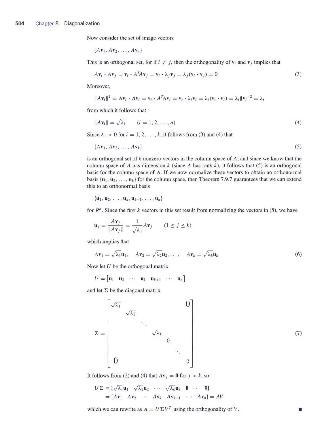
8.6 Singular Value Decomposition 502
8.7 The Pseudoinverse 518
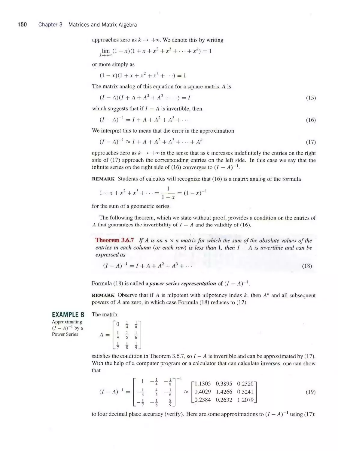
8.8 Complex Eigenvalues and Eigenvectors 525
8.9 Hermitian, Unitary, and Normal Matrices 535
8.10 Systems of Differential Equations 542
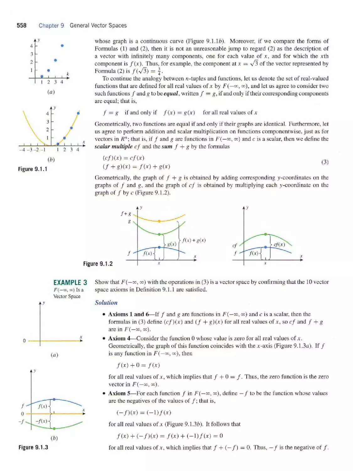
chapter 9 General Vector Spaces 555
9.1 Vector Space Axioms 555
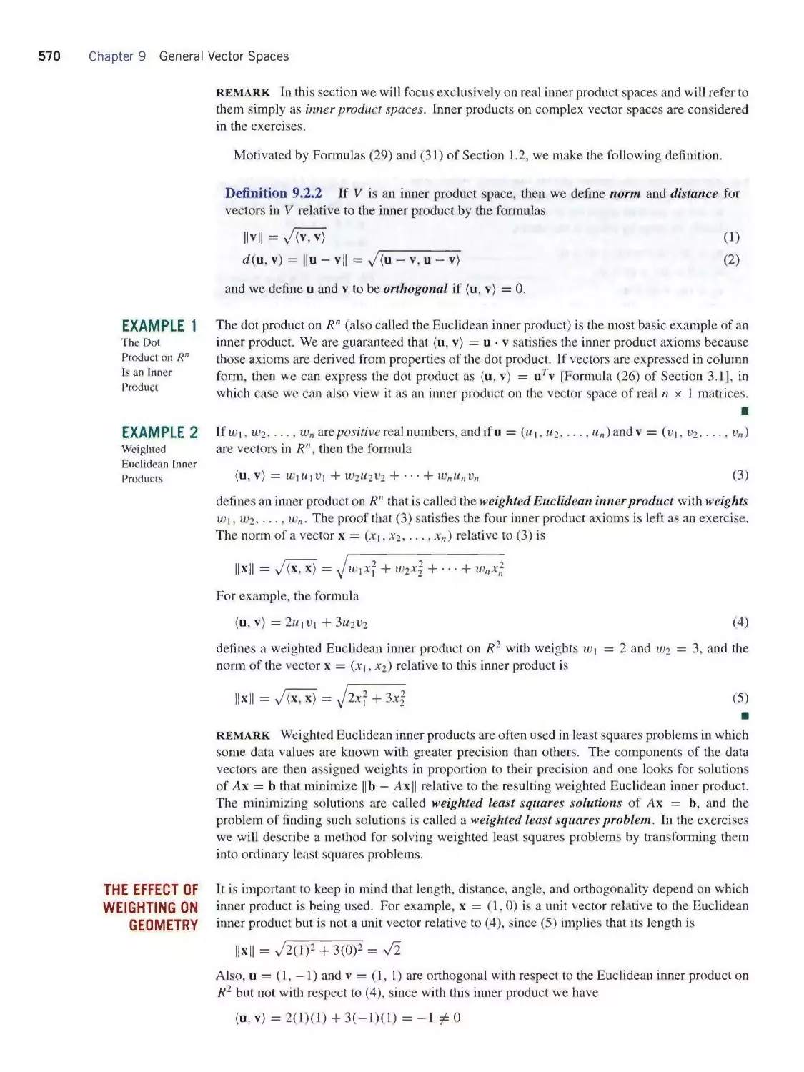
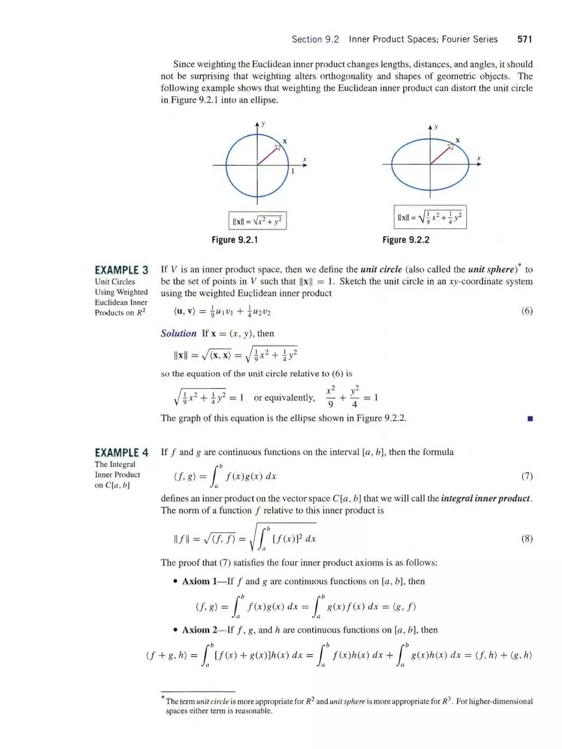
9.2 Inner Product Spaces; Fourier Series 569
9.3 General Linear Transformations;
Isomorphism 582
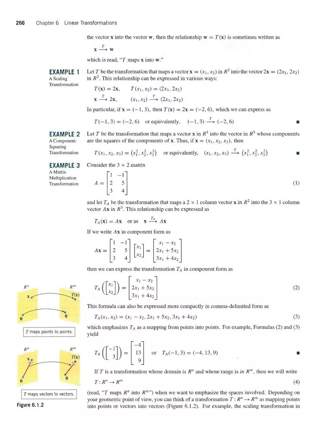
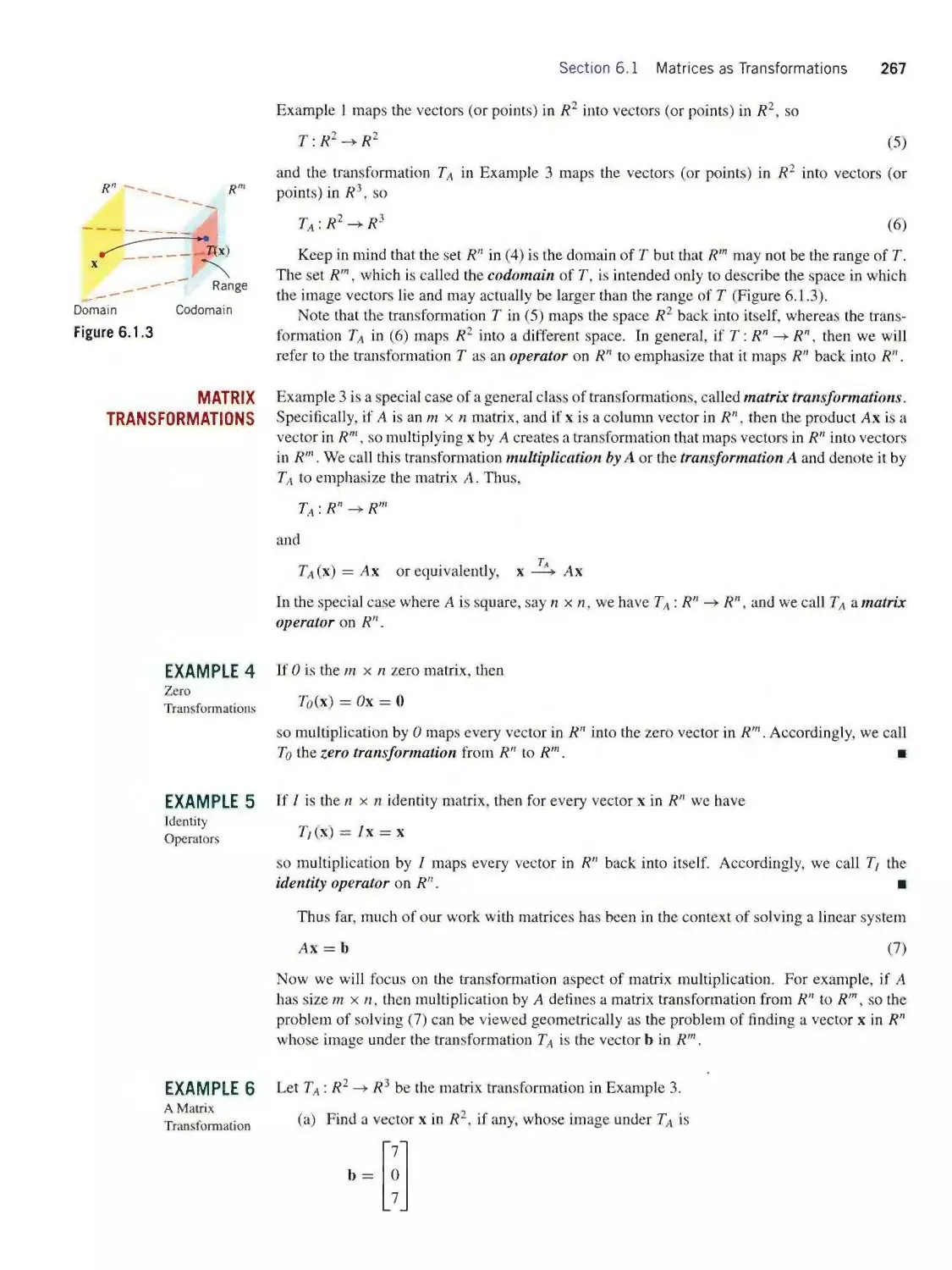
chapter 6 Linear Transformations 265
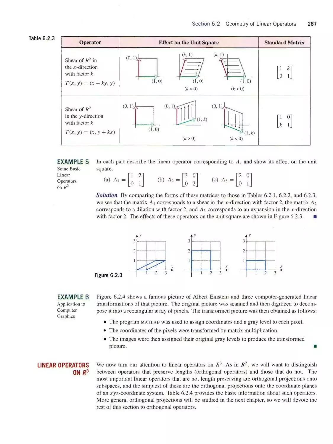
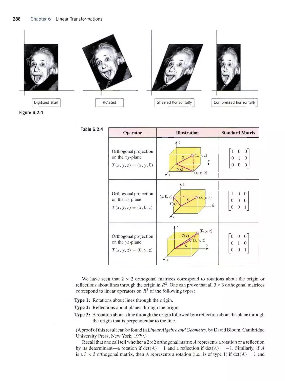
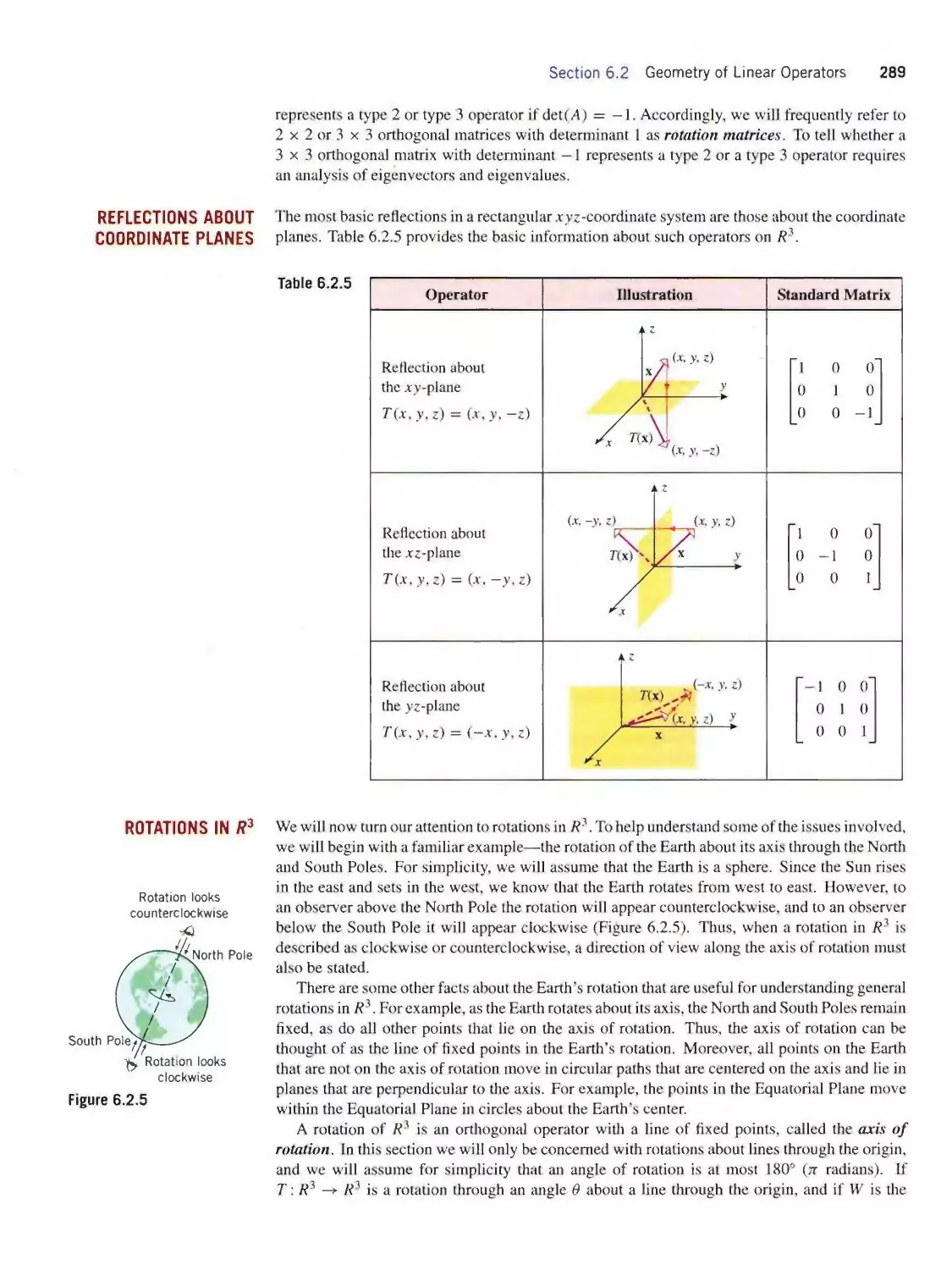
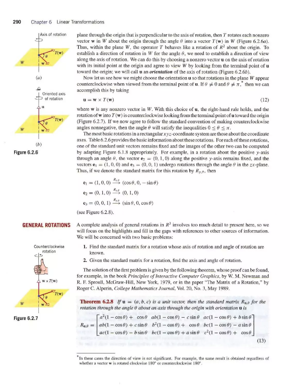
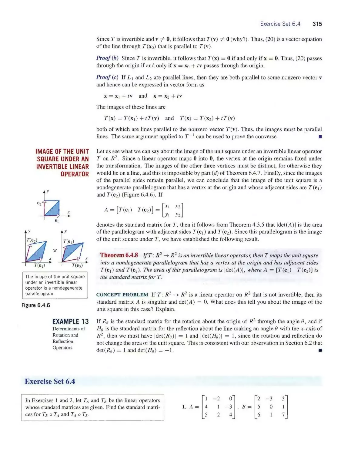
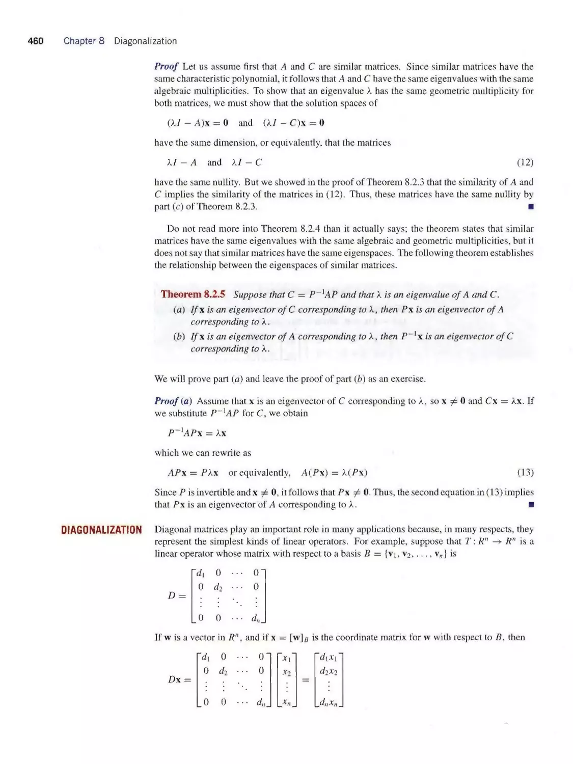
6.1 Matrices as Transformations 265
6.2 Geometry of Linear Operators 280
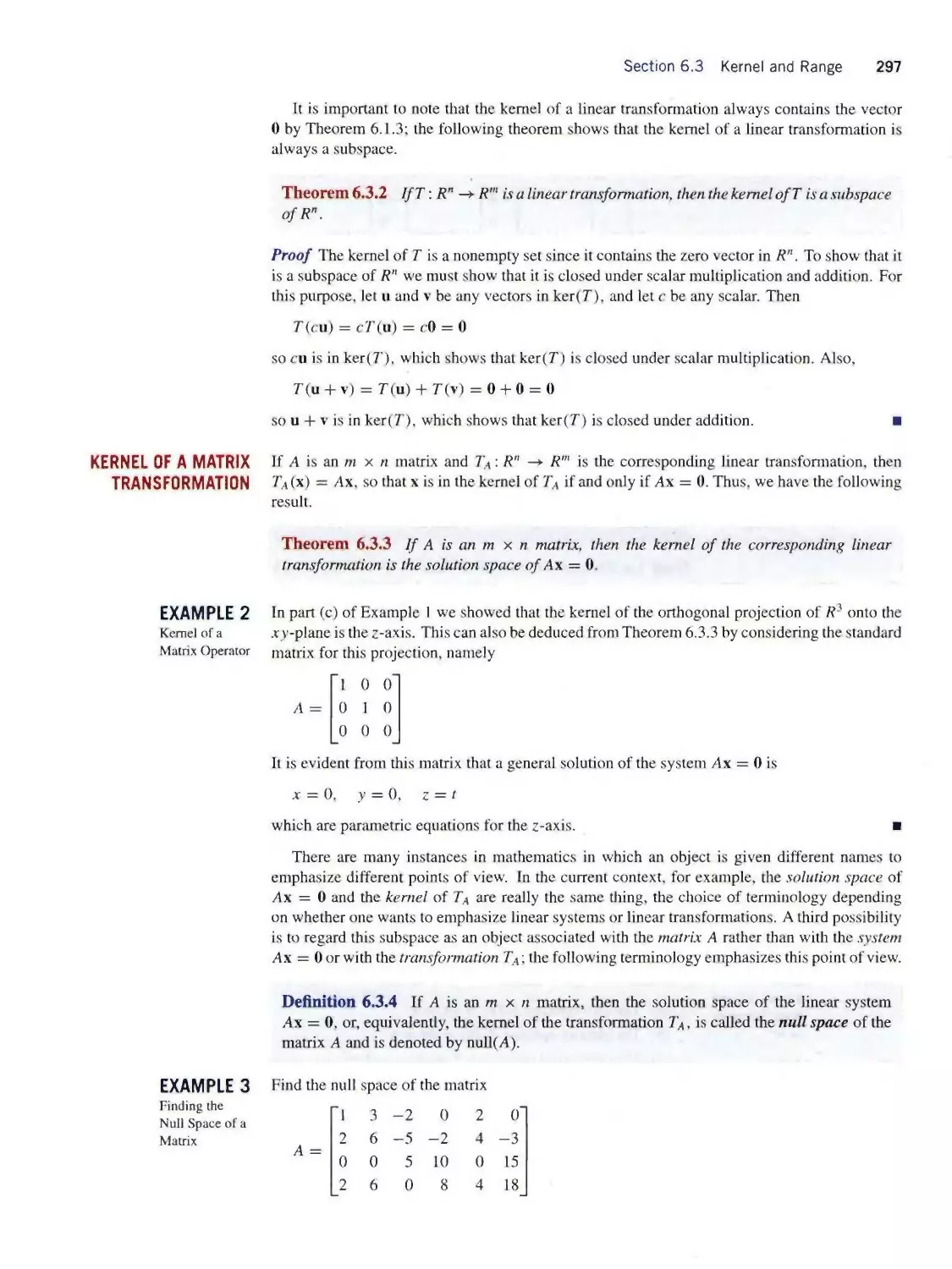
6.3 Kernel and Range 296
6.4 Composition and Invertibility of Linear
Transformations 305
6.5 Computer Graphics 318
appendix a How to Read Theorems ai
appendix b Complex Numbers A3
ANSWERS TO ODD-NUMBERED EXERCISES A9
PHOTO CREDITS C1
INDEX 1-1
xi
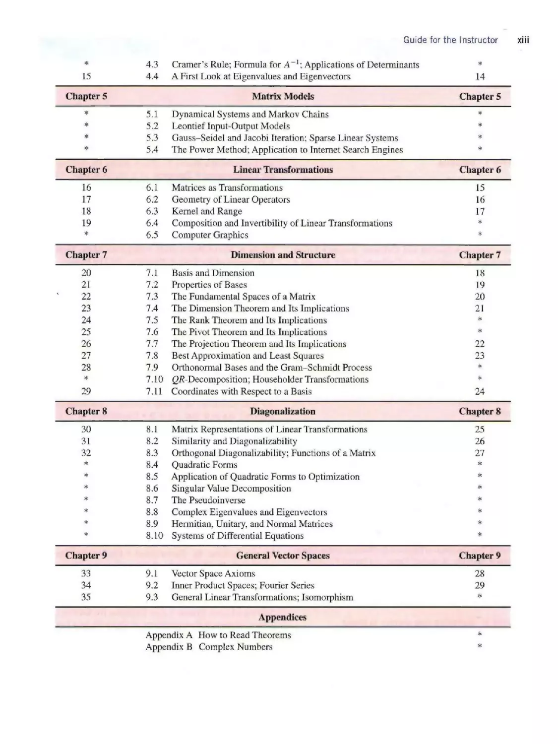
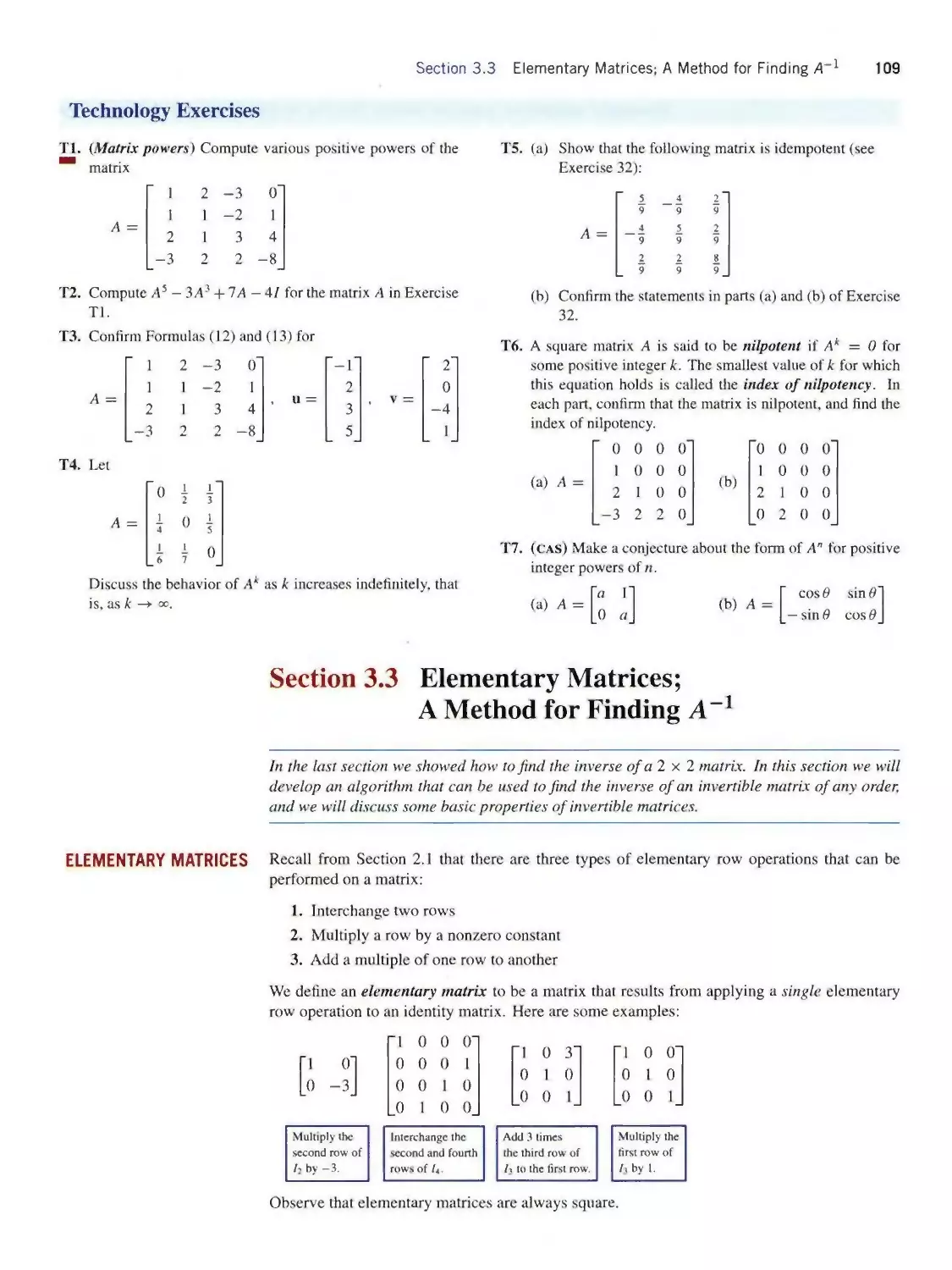
GUIDE FOR THE INSTRUCTOR
Number of Lectures
The Syllabus Guide below provides for a 29-lecture core and
a 35-lecture core. The 29-lecture core is for schools with
time constraints, as with abbreviated summer courses. Both
core programs can be supplemented by starred topics as time
permits. The omission of starred topics does not affect the
readability or continuity of the core topics.
Pace
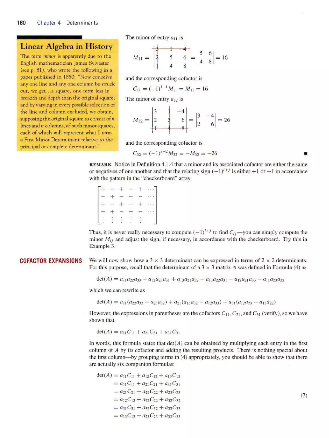
The core program is based on covering one section per lec¬
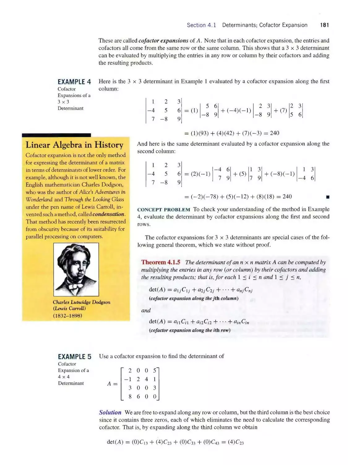
ture, but whether you can do this in every instance will depend
on your teaching style and the capabilities of your particular
students. For longer sections we recommend that you just
highlight the main points in class and leave the details for the
students to read. Since the reviews of this text have praised
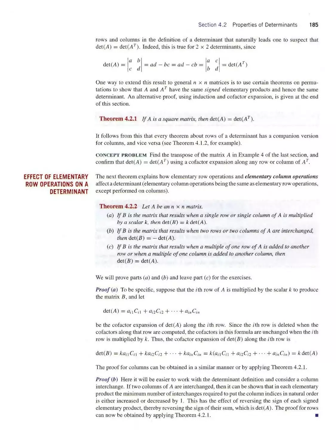
the clarity of the exposition, you should find this workable. If,
in certain cases, you want to devote more than one lecture to
a core topic, you can do so by adjusting the number of starred
topics that you cover.
By the end of Lecture 15 the following concepts will have
been covered in a basic form: linear combination, spanning,
subspace, dimension, eigenvalues, and eigenvectors. Thus,
even with a relatively slow pace you will have no trouble
touching on all of the main ideas in the course.
Organization
It is our feeling that the most effective way to teach abstract
vector spaces is to place that material at the end (Chapter 9),
at which point it occurs as a “natural generalization” of the
earlier material, and the student has developed the “linear al¬
gebra maturity” to understand its purpose. However, we rec¬
ognize that not everybody shares that philosophy, so we have
designed that chapter so it can be moved forward, if desired.
SYLLABUS GUIDE
35-Lecture
Course
CONTENTS
29-Lecture
Course
Chapter 1
Vectors
Chapter 1
1
1.1 Vectors and Matrices in Engineering and Mathematics; n-Space
1
2
1.2 Dot Product and Orthogonality
2
3
1.3 Vector Equations of Lines and Planes
3
Chapter 2
Systems of Linear Equations
Chapter 2
4
2.1 Introduction to Systems of Linear Equations
4
5
2.2 Solving Linear Systems by Row Reduction
5
*
2.3 Applications of Linear Systems
*
Chapter 3
Matrices and Matrix Algebra
Chapter 3
6
3.1 Operations on Matrices
6
7
3.2 Inverses; Algebraic Properties of Matrices
7
8
3.3 Elementary Matrices; A Method for Finding A^l
8
9
3.4 Subspaces and Linear Independence
9
10
3.5 The Geometry of Linear Systems
10
11
3.6 Matrices with Special Forms
11
*
3.7 Matrix Factorizations; LU -Decomposition
*
12
3.8 Partitioned Matrices and Parallel Processing
12
Chapter 4
Determinants
Chapter 4
13
4.1 Determinants; Cofactor Expansion
13
14
4.2 Properties of Determinants
*
xii
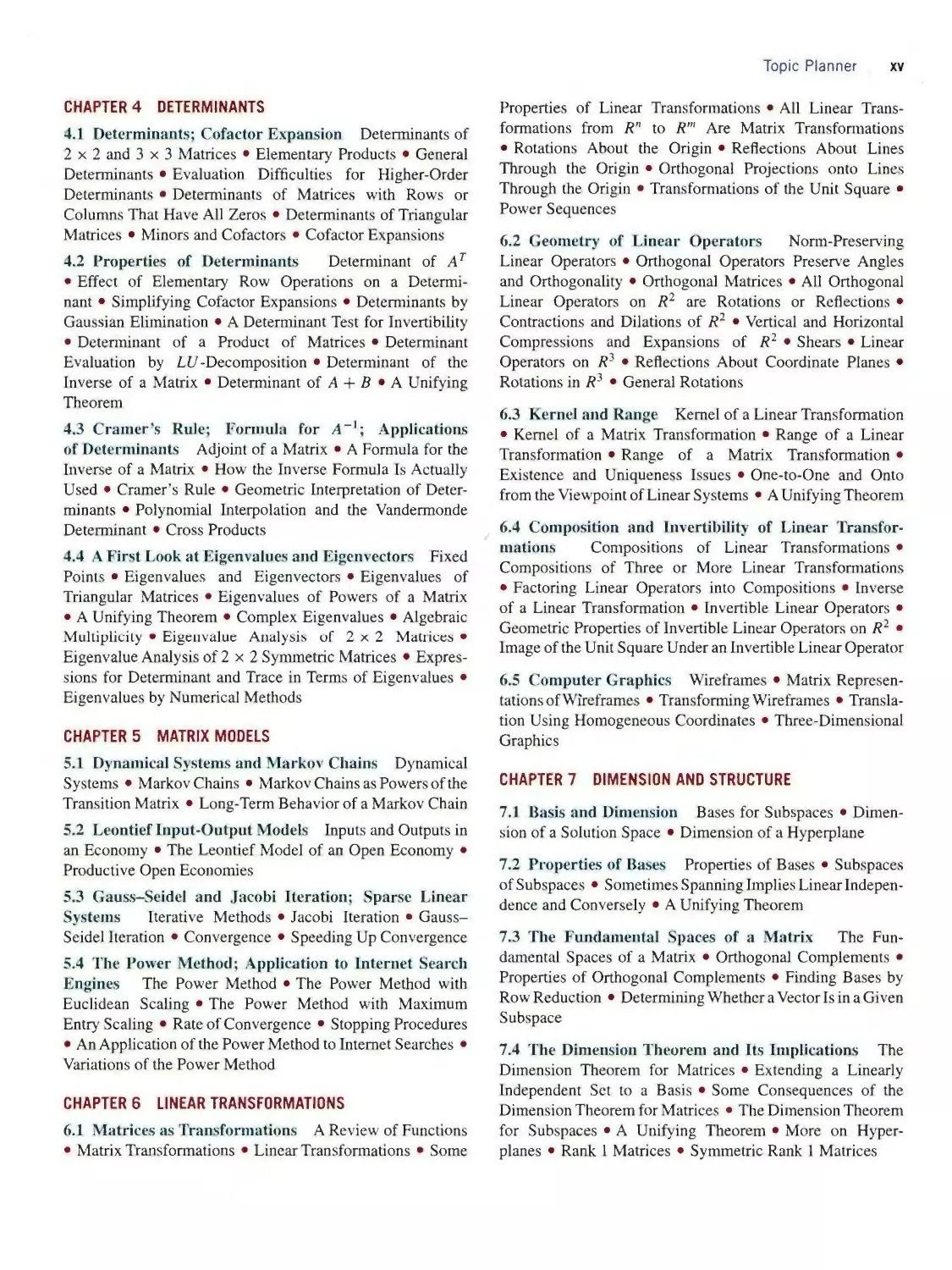
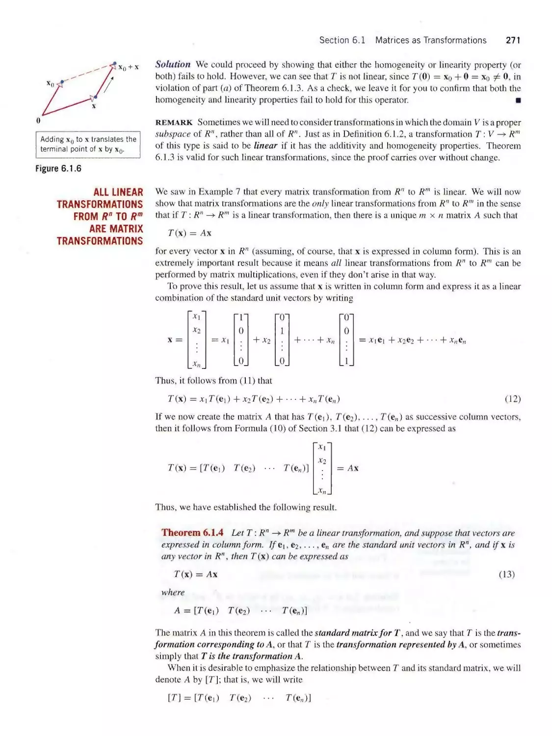
Guide for the Instructor xiii
*
4.3
Cramer’s Rule; Formula for A _l; Applications of Determinants
*
15
4.4
A First Look at Eigenvalues and Eigenvectors
14
Chapter 5
Matrix Models
Chapter 5
*
5.1
Dynamical Systems and Markov Chains
*
*
5.2
Leontief Input-Output Models
*
*
5.3
Gauss-Seidel and Jacobi Iteration; Sparse Linear Systems
*
*
5.4
The Power Method; Application to Internet Search Engines
*
Chapter 6
Linear Transformations
Chapter 6
16
6.1
Matrices as Transformations
15
17
6.2
Geometry of Linear Operators
16
18
6.3
Kernel and Range
17
19
6.4
Composition and Invertibility of Linear Transformations
*
*
6.5
Computer Graphics
*
Chapter 7
Dimension and Structure
Chapter 7
20
7.1
Basis and Dimension
18
21
7.2
Properties of Bases
19
22
7.3
The Fundamental Spaces of a Matrix
20
23
7.4
The Dimension Theorem and Its Implications
21
24
7.5
The Rank Theorem and Its Implications
*
25
7.6
The Pivot Theorem and Its Implications
*
26
7.7
The Projection Theorem and Its Implications
22
27
7.8
Best Approximation and Least Squares
23
28
7.9
Orthonormal Bases and the Gram-Schmidt Process
*
*
7.10
(^-Decomposition; Householder Transformations
*
29
7.11
Coordinates with Respect to a Basis
24
Chapter 8
Diagonalization
Chapter 8
30
8.1
Matrix Representations of Linear Transformations
25
31
8.2
Similarity and Diagonalizability
26
32
8.3
Orthogonal Diagonalizability; Functions of a Matrix
27
*
8.4
Quadratic Forms
*
*
8.5
Application of Quadratic Forms to Optimization
*
*
8.6
Singular Value Decomposition
⅛
*
8.7
The Pseudoinverse
*
*
8.8
Complex Eigenvalues and Eigenvectors
*
*
8.9
Hermitian. Unitary, and Normal Matrices
⅛
*
8.10
Systems of Differential Equations
*
Chapter 9
General Vector Spaces
Chapter 9
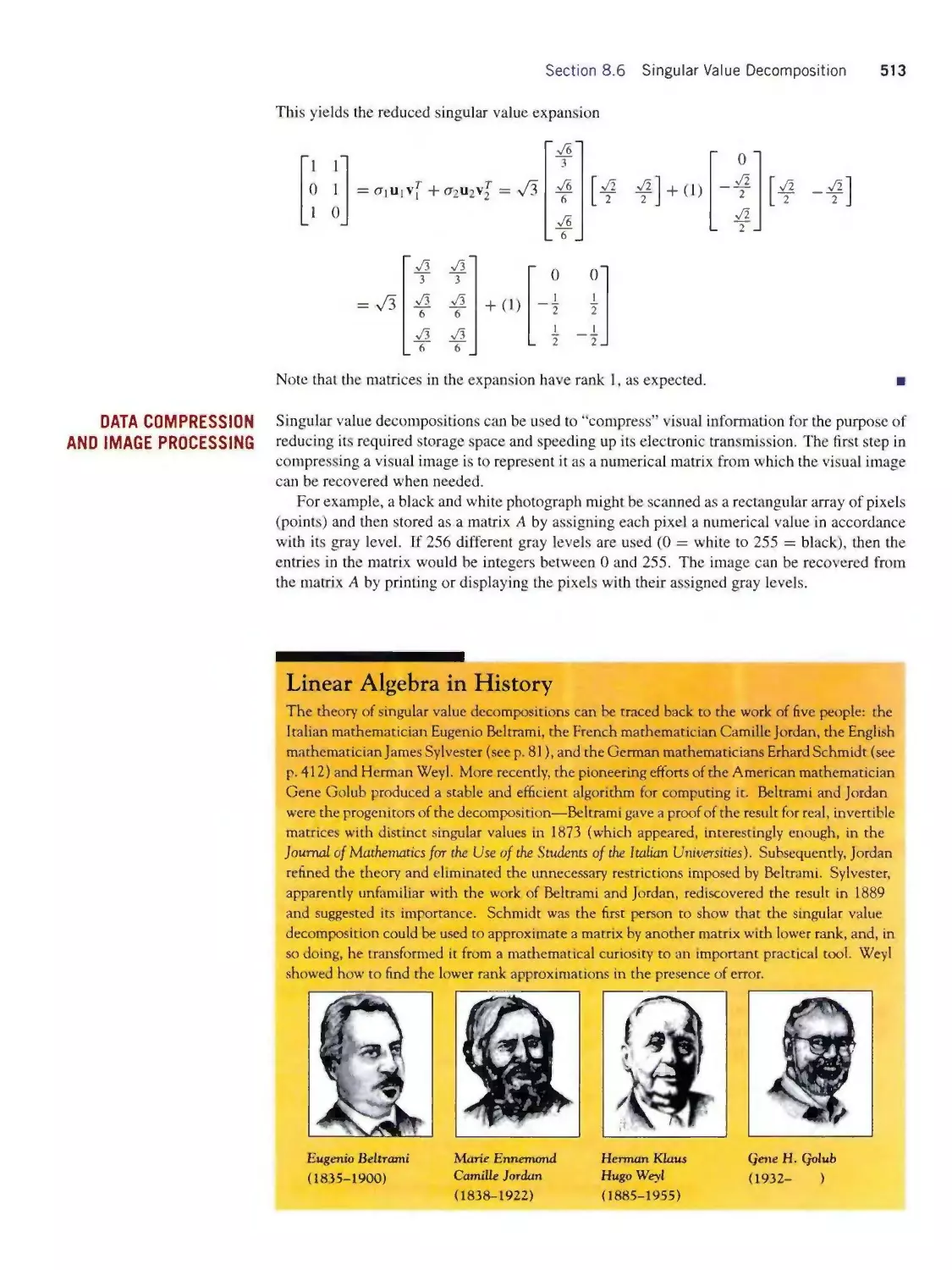
33
9.1
Vector Space Axioms
28
34
9.2
Inner Product Spaces; Fourier Series
29
35
9.3
General Linear Transformations; Isomorphism
*
Appendices
Appendix A How to Read Theorems
Appendix B Complex Numbers
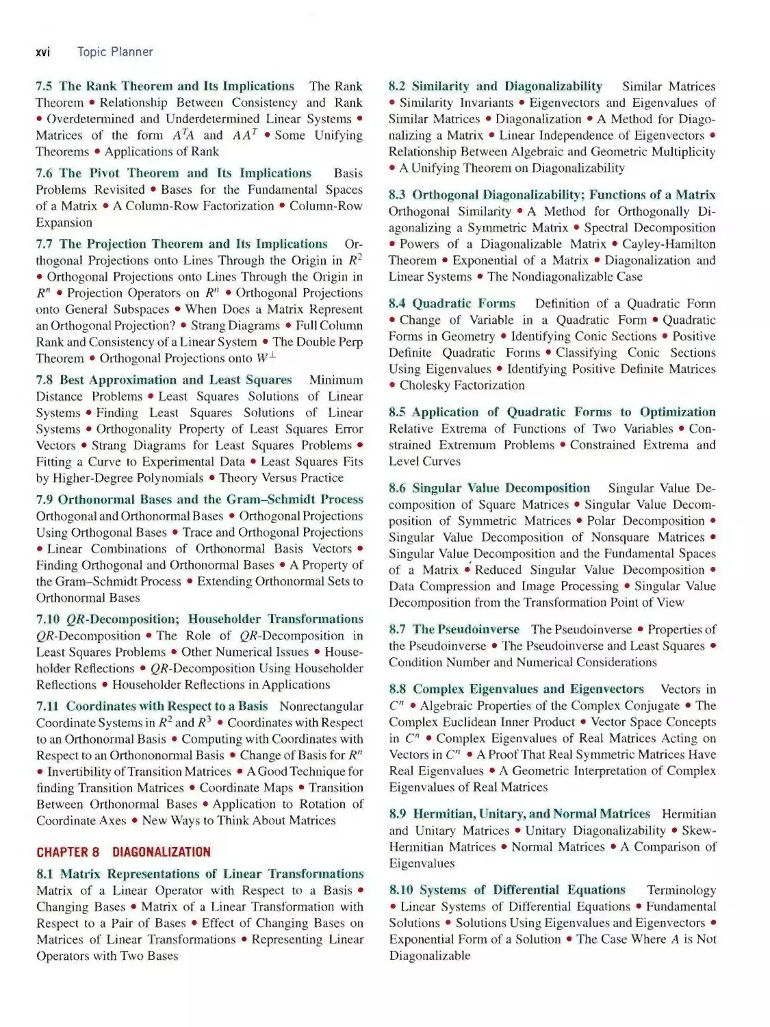
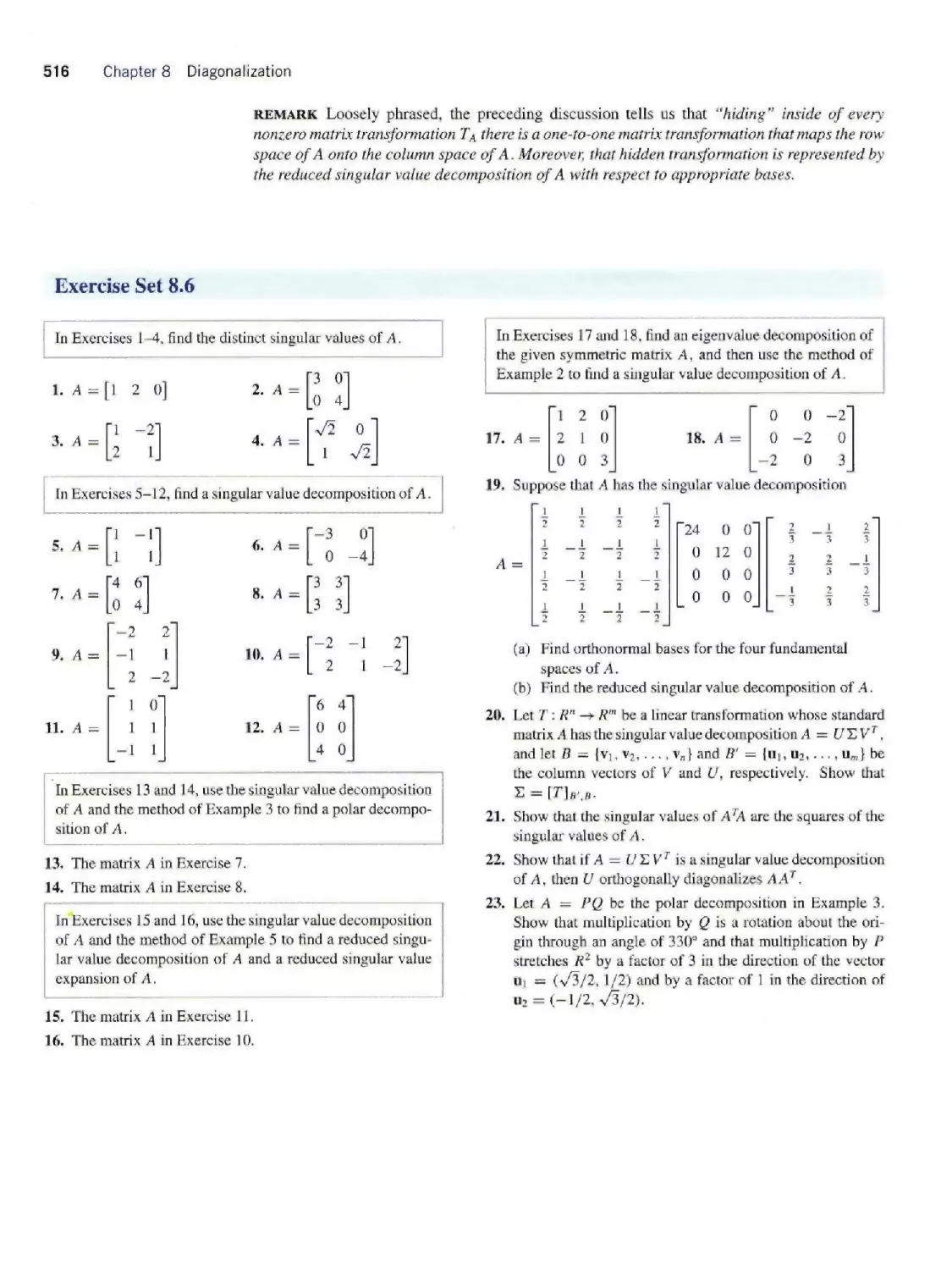
TOPIC PLANNER
To assist you in planning your course, we have provided below a list of topics that occur in each section. These topics are
identified in the text by headings in the margin. You will find additional lecture planning information on the Web site for this text.
CHAPTER 1 VECTORS
1.1 Vectors and Matrices in Engineering and Mathe¬
matics; n-Space Scalars and Vectors ∙ Equivalent Vectors
• Vector Addition ∙ Vector Subtraction ∙ Scalar Multipli¬
cation ∙ Vectors in Coordinate Systems ∙ Components of
a Vector Whose Initial Point Is Not at the Origin ∙
Vectors in R" ∙ Equality of Vectors ∙ Sums of Three
or More Vectors ∙ Parallel and Collinear Vectors ∙ Linear
Combinations ∙ Application to Computer Color Models ∙
Alternative Notations for Vectors ∙ Matrices
1.2 Dot Product and Orthogonality Norm of a Vector
• Unit Vectors ∙ The Standard Unit Vectors ∙ Distance
Between Points in R" ∙ Dot Products ∙ Algebraic Properties
of the Dot Product ∙ Angle Between Vectors in R2 and R3
• Orthogonality ∙ Orthonormal Sets ∙ Euclidean Geometry
in Rn
1.3 Vector Equations of Lines and Planes Vector and
Parametric Equations of Lines ∙ Lines Through Two Points
• Point-Normal Equations of Planes ∙ Vector and Parametric
Equations of Planes ∙ Lines and Planes in R" ∙ Comments
on Terminology
CHAPTER 2 SYSTEMS OF LINEAR EQUATIONS
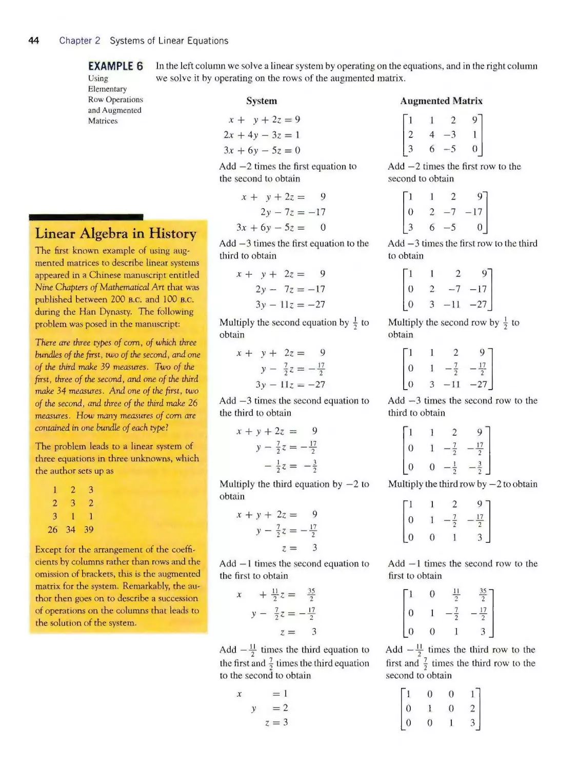
2.1 Introduction to Systems of Linear Equations Linear
Systems ∙ Linear Systems with Two and Three Unknowns ∙
Augmented Matrices and Elementary Row Operations
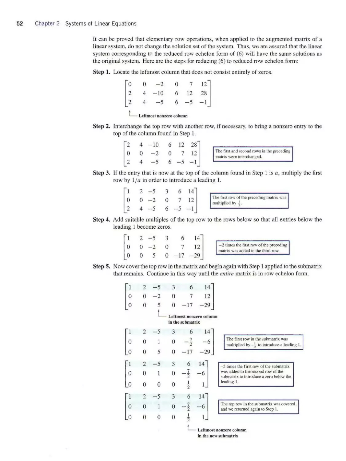
2.2 Solving Linear Systems by Row Reduction Consider¬
ations in Solving Linear Systems ∙ Echelon Forms ∙ General
Solutions as Linear Combinations of Column Vectors ∙
Gauss-Jordan and Gaussian Elimination ∙ Some Facts About
Echelon Forms ∙ Back Substitution ∙ Homogeneous Linear
Systems ∙ The Dimension Theorem for Homogeneous Linear
Systems ∙ Stability, Roundoff Error, and Partial Pivoting
2.3 Applications of Linear Systems Global Positioning ∙
Network Analysis ∙ Electrical Circuits ∙ Balancing Chemi¬
cal Equations ∙ Polynomial Interpolation
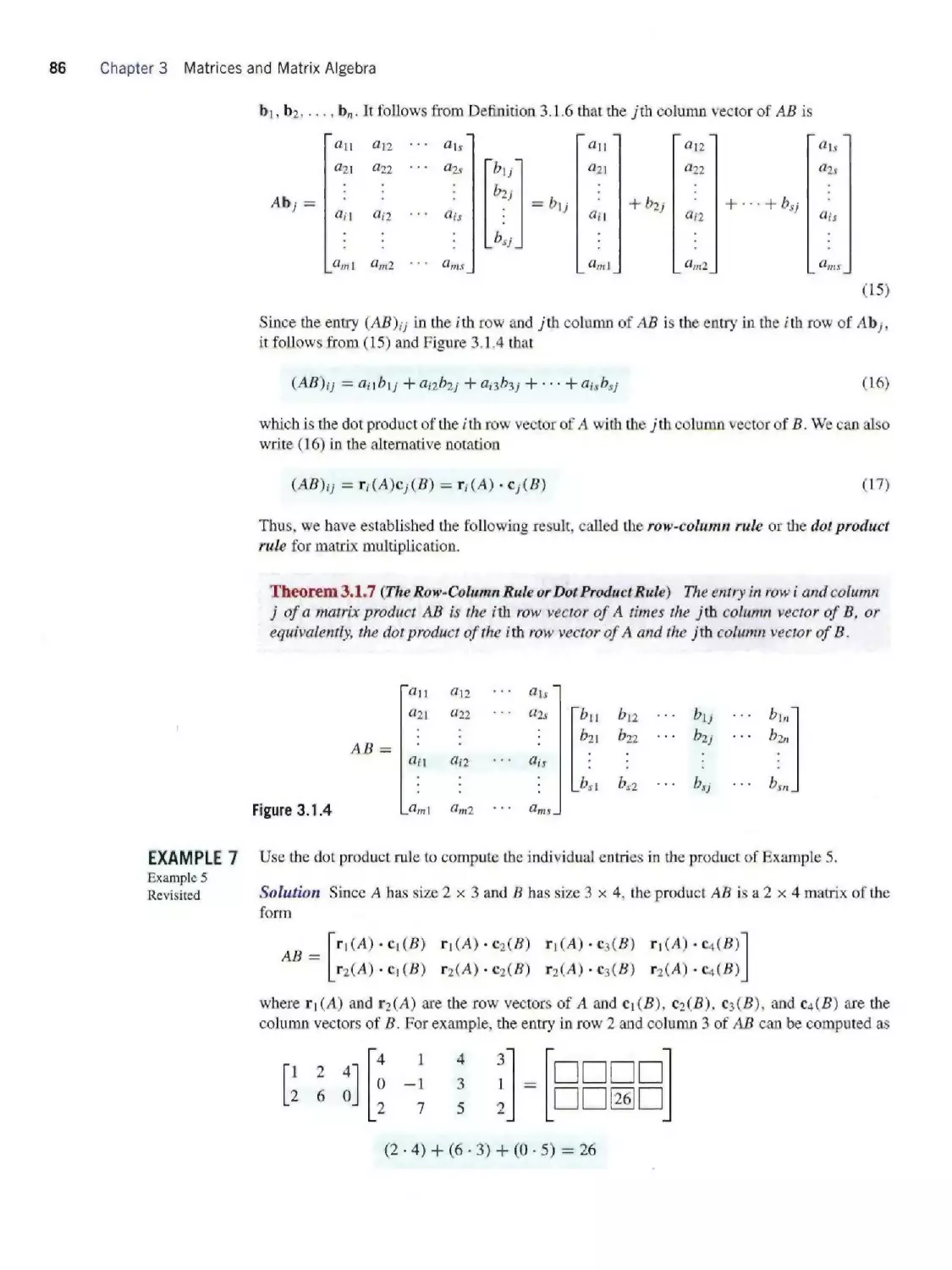
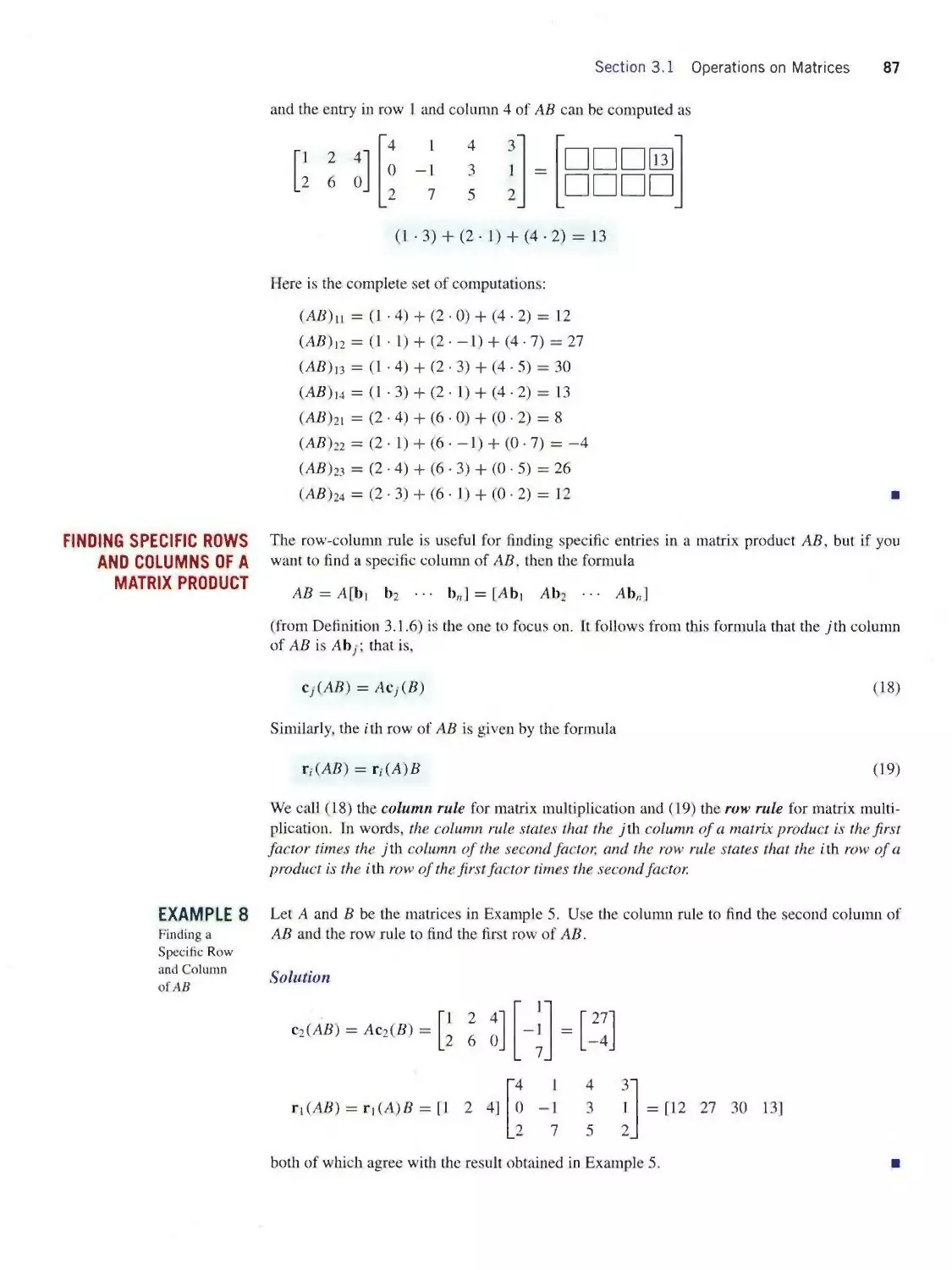
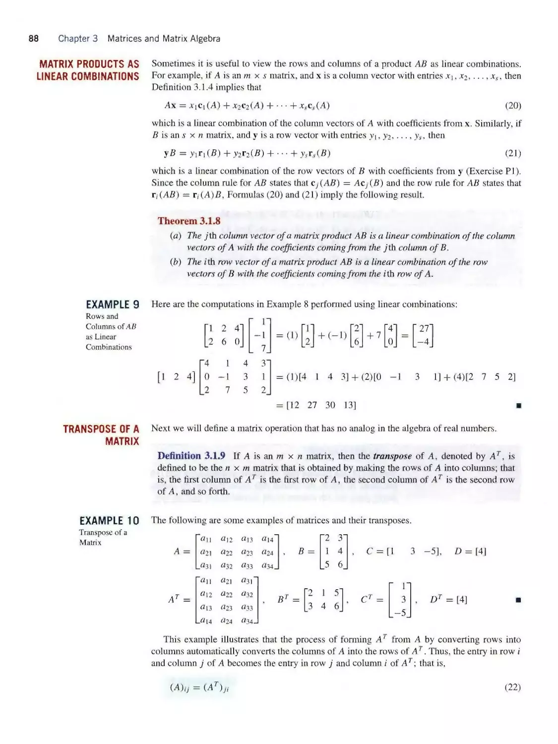
CHAPTER 3 MATRICES AND MATRIX ALGEBRA
3.1 Operations on Matrices Matrix Notation and Ter¬
minology ∙ Operations on Matrices ∙ Row and Column
Vectors ∙ The Product A× ∙ The Product AB ∙ Finding
Specific Entries in a Matrix Product ∙ Finding Specific Rows
and Columns of a Matrix Product ∙ Matrix Products as Lin¬
ear Combinations ∙ Transpose of a Matrix ∙ Trace ∙ Inner
and Outer Matrix Products
3.2 Inverses; Algebraic Properties of Matrices Properties
of Matrix Addition and Scalar Multiplication ∙ Properties of
Matrix Multiplication ∙ Zero Matrices ∙ Identity Matrices ∙
Inverse of a Matrix ∙ Properties of Inverses ∙ Powers of a
Matrix ∙ Matrix Polynomials ∙ Properties of the Transpose
• Properties of the Trace ∙ Transpose and Dot Product
3.3 Elementary Matrices; A Method for Finding A-1
Elementary Matrices ∙ Characterizations of Invertibility ∙
Row Equivalence ∙ An Algorithm for Inverting Matrices
• Solving Linear Systems by Matrix Inversion ∙ Solving
Multiple Linear Systems with a Common Coefficient Matrix
• Consistency of Linear Systems
3.4 Subspaces and Linear Independence Subspaces of
Rn ∙ Solution Space of a Linear System ∙ Linear Inde¬
pendence ∙ Linear Independence and Homogeneous Linear
Systems ∙ Translated Subspaces ∙ A Unifying Theorem
3.5 The Geometry of Linear Systems The Relationship
Between Ax = b and Ax = 0 ∙ Consistency of a Linear
System from the Vector Point of View ∙ Hyperplanes ∙
Geometric Interpretations of Solution Spaces
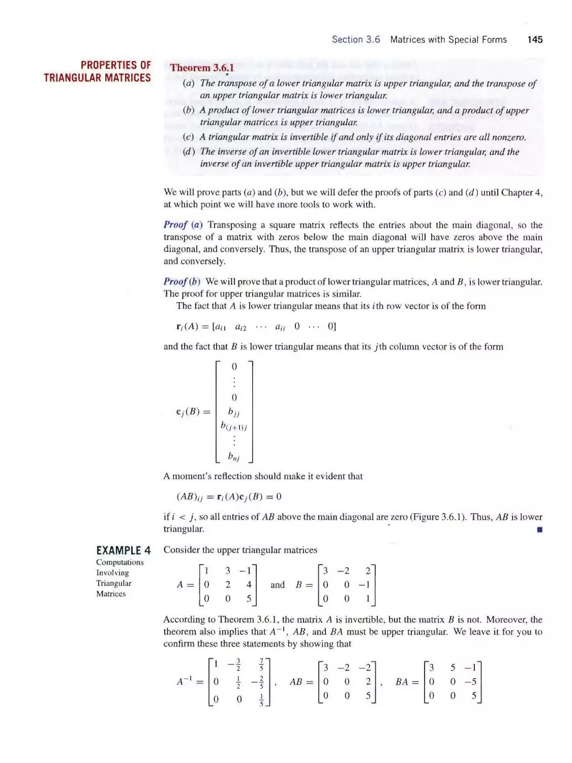
3.6 Matrices with Special Forms Diagonal Matrices
• Triangular Matrices ∙ Linear Systems with Triangular
Coefficient Matrices ∙ Properties of Triangular Matrices ∙
Symmetric and Skew-Symmetric Matrices ∙ Invertibility of
Symmetric Matrices ∙ Matrices of the Form AτA and AAr ∙
Fixed Points of a Matrix ∙ A Technique for Inverting I — A
When A Is Nilpotent ∙ Inverting I — A by Power Series
3.7 Matrix Factorizations; LL7-Dccomposition Solving
Linear Systems by Factorization ∙ Finding LL∕-Decom¬
positions ∙ The Relationship Between Gaussian Elimination
and ΔL∕-Decomposition ∙ Matrix Inversion by LU-Decom¬
position ∙ LDU-Decompositions ∙ Using Permutation Ma¬
trices to Deal with Row Interchanges ∙ Flops and the Cost of
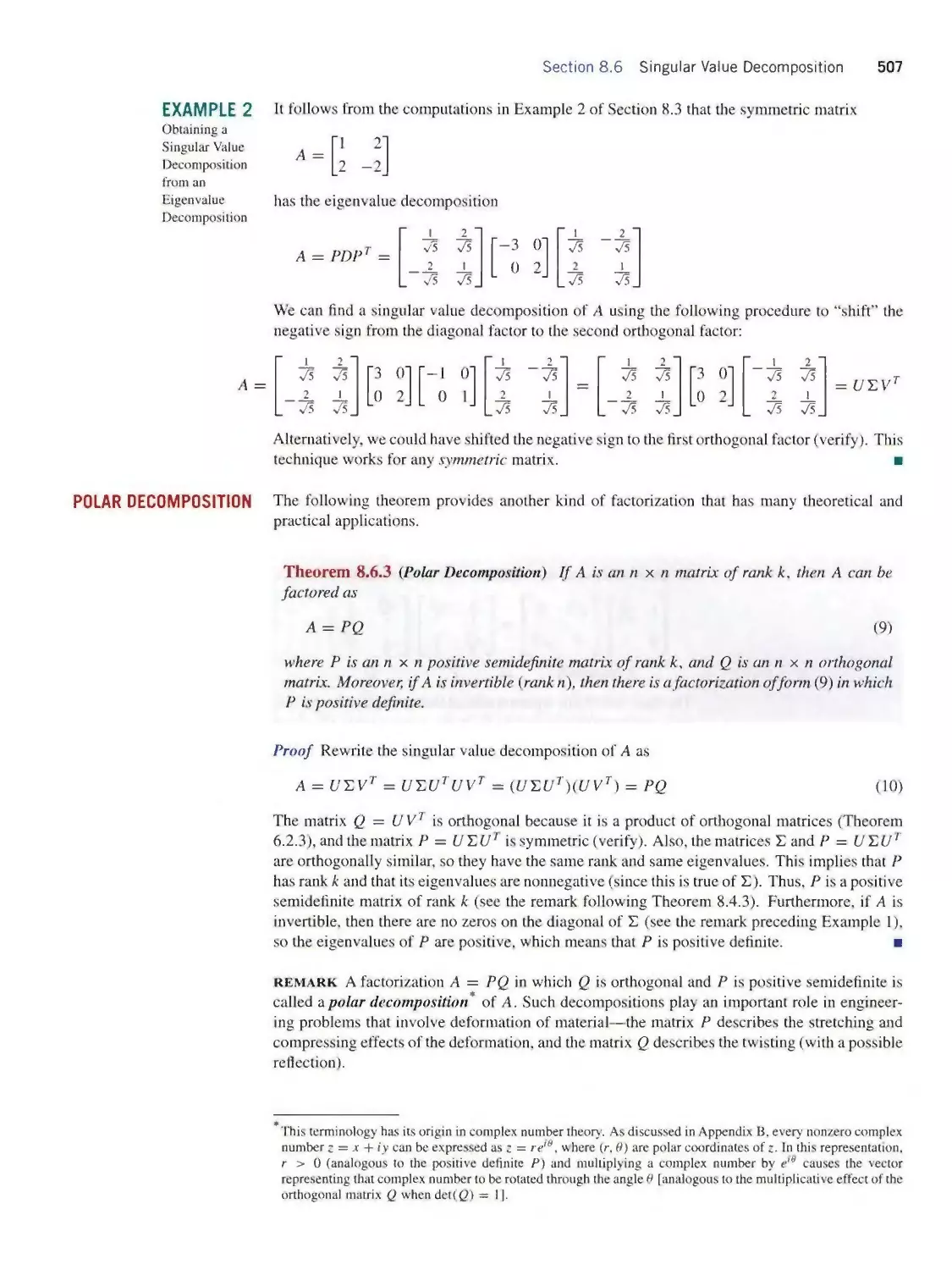
Solving a Linear System ∙ Cost Estimates for Solving Large
Linear Systems ∙ Considerations in Choosing an Algorithm
for Solving a Linear System
3.8 Partitioned Matrices and Parallel Processing Gen¬
eral Partitioning ∙ Block Diagonal Matrices ∙ Block Upper
Triangular Matrices
xiv
Topic Planner xv
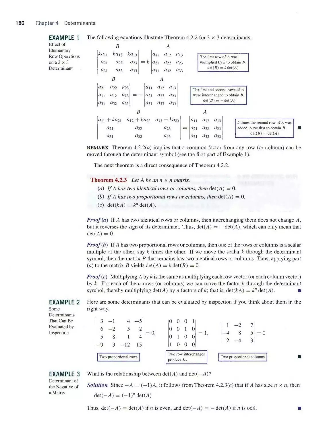
CHAPTER 4 DETERMINANTS
4.1 Determinants; Cofactor Expansion Determinants of
2x2 and 3 × 3 Matrices ∙ Elementary Products ∙ General
Determinants ∙ Evaluation Difficulties for Higher-Order
Determinants ∙ Determinants of Matrices with Rows or
Columns That Have All Zeros ∙ Determinants of Triangular
Matrices ∙ Minors and Cofactors ∙ Cofactor Expansions
4.2 Properties of Determinants Determinant of Aτ
• Effect of Elementary Row Operations on a Determi¬
nant ∙ Simplifying Cofactor Expansions ∙ Determinants by
Gaussian Elimination ∙ A Determinant Test for Invertibility
• Determinant of a Product of Matrices ∙ Determinant
Evaluation by LU -Decomposition ∙ Determinant of the
Inverse of a Matrix ∙ Determinant of A + B ∙ A Unifying
Theorem
4.3 Cramer’s Rule; Formula for A-1; Applications
of Determinants Adjoint of a Matrix ∙ A Formula for the
Inverse of a Matrix ∙ How the Inverse Formula Is Actually
Used ∙ Cramer’s Rule ∙ Geometric Interpretation of Deter¬
minants ∙ Polynomial Interpolation and the Vandermonde
Determinant ∙ Cross Products
4.4 A First Look at Eigenvalues and Eigenvectors Fixed
Points ∙ Eigenvalues and Eigenvectors ∙ Eigenvalues of
Triangular Matrices ∙ Eigenvalues of Powers of a Matrix
• A Unifying Theorem ∙ Complex Eigenvalues ∙ Algebraic
Multiplicity ∙ Eigenvalue Analysis of 2x2 Matrices ∙
Eigenvalue Analysis of 2 × 2 Symmetric Matrices ∙ Expres¬
sions for Determinant and Trace in Terms of Eigenvalues ∙
Eigenvalues by Numerical Methods
CHAPTERS MATRIX MODELS
5.1 Dynamical Systems and Markov Chains Dynamical
Systems ∙ Markov Chains ∙ Markov Chains as Powers of the
Transition Matrix ∙ Long-Term Behavior of a Markov Chain
5.2 Leontief Input-Output Models Inputs and Outputs in
an Economy ∙ The Leontief Model of an Open Economy ∙
Productive Open Economies
5.3 Gauss-Seidel and Jacobi Iteration; Sparse Linear
Systems Iterative Methods ∙ Jacobi Iteration ∙ Gauss-
Seidel Iteration ∙ Convergence ∙ Speeding Up Convergence
5.4 The Power Method; Application to Internet Search
Engines The Power Method ∙ The Power Method with
Euclidean Scaling ∙ The Power Method with Maximum
Entry Scaling ∙ Rate of Convergence ∙ Stopping Procedures
• An Application of the Power Method to Internet Searches ∙
Variations of the Power Method
CHAPTER 6 LINEAR TRANSFORMATIONS
6.1 Matrices as Transformations A Review of Functions
• Matrix Transformations ∙ Linear Transformations ∙ Some
Properties of Linear Transformations ∙ All Linear Trans¬
formations from R" to R"' Are Matrix Transformations
• Rotations About the Origin ∙ Reflections About Lines
Through the Origin ∙ Orthogonal Projections onto Lines
Through the Origin ∙ Transformations of the Unit Square ∙
Power Sequences
6.2 Geometry of Linear Operators Norm-Preserving
Linear Operators ∙ Orthogonal Operators Preserve Angles
and Orthogonality ∙ Orthogonal Matrices ∙ All Orthogonal
Linear Operators on R2 are Rotations or Reflections ∙
Contractions and Dilations of R2 ∙ Vertical and Horizontal
Compressions and Expansions of R2 ∙ Shears ∙ Linear
Operators on R3 ∙ Reflections About Coordinate Planes ∙
Rotations in R3 ∙ General Rotations
6.3 Kernel and Range Kernel of a Linear Transformation
• Kernel of a Matrix Transformation ∙ Range of a Linear
Transformation ∙ Range of a Matrix Transformation ∙
Existence and Uniqueness Issues ∙ One-to-One and Onto
from the Viewpoint of Linear Systems ∙ A Unifying Theorem
6.4 Composition and Invertibility of Linear Transfor¬
mations Compositions of Linear Transformations ∙
Compositions of Three or More Linear Transformations
• Factoring Linear Operators into Compositions ∙ Inverse
of a Linear Transformation ∙ Invertible Linear Operators ∙
Geometric Properties of Invertible Linear Operators on R2 ∙
Image of the Unit Square Under an Invertible Linear Operator
6.5 Computer Graphics Wireframes ∙ Matrix Represen¬
tations of Wireframes ∙ Transforming Wireframes ∙ Transla¬
tion Using Homogeneous Coordinates ∙ Three-Dimensional
Graphics
CHAPTER 7 DIMENSION AND STRUCTURE
7.1 Basis and Dimension Bases for Subspaces ∙ Dimen¬
sion of a Solution Space ∙ Dimension of a Hyperplane
7.2 Properties of Bases Properties of Bases ∙ Subspaces
of Subspaces ∙ Sometimes Spanning Implies Linear Indepen¬
dence and Conversely ∙ A Unifying Theorem
7.3 The Fundamental Spaces of a Matrix The Fun¬
damental Spaces of a Matrix ∙ Orthogonal Complements ∙
Properties of Orthogonal Complements ∙ Finding Bases by
Row Reduction ∙ Determining Whether a Vector Is in a Given
Subspace
7.4 The Dimension Theorem and Its Implications The
Dimension Theorem for Matrices ∙ Extending a Linearly
Independent Set to a Basis ∙ Some Consequences of the
Dimension Theorem for Matrices ∙ The Dimension Theorem
for Subspaces ∙ A Unifying Theorem ∙ More on Hyper¬
planes ∙ Rank 1 Matrices ∙ Symmetric Rank 1 Matrices
xvi Topic Planner
7.5 The Rank Theorem and Its Implications The Rank
Theorem ∙ Relationship Between Consistency and Rank
• Overdetermined and Underdeteπnined Linear Systems ∙
Matrices of the form ArA and AAl ∙ Some Unifying
Theorems ∙ Applications of Rank
7.6 The Pivot Theorem and Its Implications Basis
Problems Revisited ∙ Bases for the Fundamental Spaces
of a Matrix ∙ A Column-Row Factorization ∙ Column-Row
Expansion
7.7 The Projection Theorem and Its Implications Or¬
thogonal Projections onto Lines Through the Origin in R2
• Orthogonal Projections onto Lines Through the Origin in
R" ∙ Projection Operators on Rn ∙ Orthogonal Projections
onto General Subspaces ∙ When Does a Matrix Represent
an Orthogonal Projection? ∙ Strang Diagrams ∙ Full Column
Rank and Consistency of a Linear System ∙ The Double Perp
Theorem ∙ Orthogonal Projections onto Wj-
7.8 Best Approximation and Least Squares Minimum
Distance Problems ∙ Least Squares Solutions of Linear
Systems ∙ Finding Least Squares Solutions of Linear
Systems ∙ Orthogonality Property of Least Squares Error
Vectors ∙ Strang Diagrams for Least Squares Problems ∙
Fitting a Curve to Experimental Data ∙ Least Squares Fits
by Higher-Degree Polynomials ∙ Theory Versus Practice
7.9 Orthonormal Bases and the Gram-Schmidt Process
Orthogonal and Orthonormal Bases ∙ Orthogonal Projections
Using Orthogonal Bases ∙ Trace and Orthogonal Projections
• Linear Combinations of Orthonormal Basis Vectors ∙
Finding Orthogonal and Orthonormal Bases ∙ A Property of
the Gram-Schmidt Process ∙ Extending Orthonormal Sets to
Orthonormal Bases
7.10 QR-Decomposition; Householder Transformations
(^-Decomposition ∙ The Role of βR-Decomposition in
Least Squares Problems ∙ Other Numerical Issues ∙ House¬
holder Reflections ∙ (^-Decomposition Using Householder
Reflections ∙ Householder Reflections in Applications
7.11 Coordinates with Respect to a Basis Nonrectangular
Coordinate Systems in R2 and Ri ∙ Coordinates with Respect
to an Orthonormal Basis ∙ Computing with Coordinates with
Respect to an Orthononormal Basis ∙ Change of Basis for R',
• Invertibility of Transition Matrices ∙ A Good Technique for
finding Transition Matrices ∙ Coordinate Maps ∙ Transition
Between Orthonormal Bases ∙ Application to Rotation of
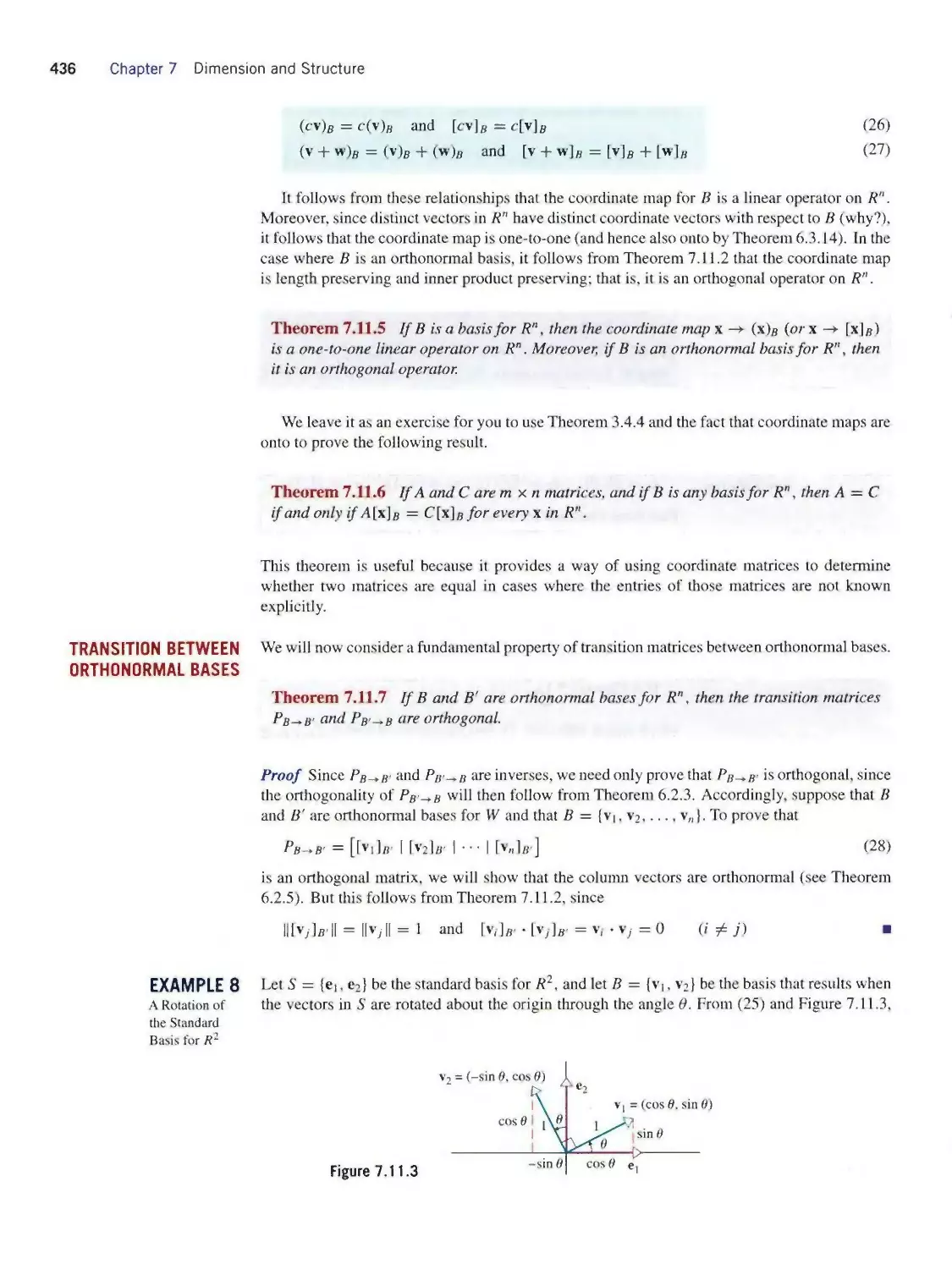
Coordinate Axes ∙ New Ways to Think About Matrices
CHAPTER 8 DIAGONALIZATION
8.1 Matrix Representations of Linear Transformations
Matrix of a Linear Operator with Respect to a Basis ∙
Changing Bases ∙ Matrix of a Linear Transformation with
Respect to a Pair of Bases ∙ Effect of Changing Bases on
Matrices of Linear Transformations ∙ Representing Linear
Operators with Two Bases
8.2 Similarity and Diagonalizability Similar Matrices
• Similarity Invariants ∙ Eigenvectors and Eigenvalues of
Similar Matrices ∙ Diagonalization ∙ A Method for Diago¬
nalizing a Matrix ∙ Linear Independence of Eigenvectors ∙
Relationship Between Algebraic and Geometric Multiplicity
• A Unifying Theorem on Diagonalizability
8.3 Orthogonal Diagonalizability; Functions of a Matrix
Orthogonal Similarity ∙ A Method for Orthogonally Di¬
agonalizing a Symmetric Matrix ∙ Spectral Decomposition
• Powers of a Diagonalizable Matrix ∙ Cayley-Hamilton
Theorem ∙ Exponential of a Matrix ∙ Diagonalization and
Linear Systems ∙ The Nondiagonalizable Case
8.4 Quadratic Forms Definition of a Quadratic Form
• Change of Variable in a Quadratic Form ∙ Quadratic
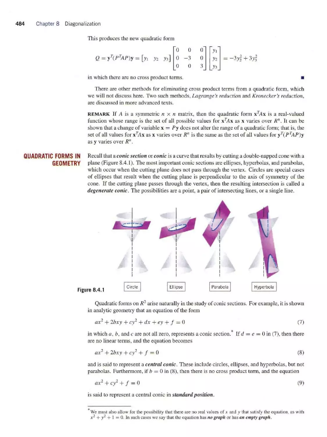
Forms in Geometry ∙ Identifying Conic Sections ∙ Positive
Definite Quadratic Forms ∙ Classifying Conic Sections
Using Eigenvalues ∙ Identifying Positive Definite Matrices
• Cholesky Factorization
8.5 Application of Quadratic Forms to Optimization
Relative Extrema of Functions of Two Variables ∙ Con¬
strained Extremum Problems ∙ Constrained Extrema and
Level Curves
8.6 Singular Value Decomposition Singular Value De¬
composition of Square Matrices ∙ Singular Value Decom¬
position of Symmetric Matrices ∙ Polar Decomposition ∙
Singular Value Decomposition of Nonsquare Matrices ∙
Singular Value Decomposition and the Fundamental Spaces
of a Matrix ∙ Reduced Singular Value Decomposition ∙
Data Compression and Image Processing ∙ Singular Value
Decomposition from the Transformation Point of View
8.7 The Pseudoinverse The Pseudoinverse ∙ Properties of
the Pseudoinverse ∙ The Pscudoinverse and Least Squares ∙
Condition Number and Numerical Considerations
8.8 Complex Eigenvalues and Eigenvectors Vectors in
Cn ∙ Algebraic Properties of the Complex Conjugate ∙ The
Complex Euclidean Inner Product ∙ Vector Space Concepts
in Cn ∙ Complex Eigenvalues of Real Matrices Acting on
Vectors in C" ∙ A Proof That Real Symmetric Matrices Have
Real Eigenvalues ∙ A Geometric Interpretation of Complex
Eigenvalues of Real Matrices
8.9 Hermitian, Unitary, and Normal Matrices Hermitian
and Unitary Matrices ∙ Unitary Diagonalizability ∙ Skew-
Hermitian Matrices ∙ Normal Matrices ∙ A Comparison of
Eigenvalues
8.10 Systems of Differential Equations Terminology
• Linear Systems of Differential Equations ∙ Fundamental
Solutions ∙ Solutions Using Eigenvalues and Eigenvectors ∙
Exponential Form of a Solution ∙ The Case Where A is Not
Diagonalizable
Topic Planner xvii
CHAPTER 9 GENERAL VECTOR SPACES
9.1 Vector Space Axioms Vector Space Axioms ∙ Func¬
tion Spaces ∙ Matrix Spaces ∙ Unusual Vector Spaces
• Subspaces ∙ Linear Independence, Spanning, Basis ∙
Wroriski’s Test for Linear Independence of Functions
• Dimension ∙ The Lagrange Interpolating Polynomials ∙
Lagrange Interpolation from a Vector Point of View
9.2 Inner Product Spaces; Fourier Series Inner Product
Axioms ∙ The Effect of Weighting on Geometry ∙ Algebraic
Properties of Inner Products ∙ Orthonormal Bases ∙ Best
Approximation ∙ Fourier Series ∙ General Inner Products
on R"
9.3 General Linear Transformations; Isomorphism Gen¬
eral Linear Transformations ∙ Kernel and Range ∙ Proper¬
ties of the Kernel and Range ∙ Isomorphism ∙ Inner Product
Space Isomorphisms
APPENDIX A HOW TO READ THEOREMS
Contrapositive Form of a Theorem ∙ Converse of a Theorem
• Theorems Involving Three or More Implications
APPENDIX B COMPLEX NUMBERS
Complex Numbers ∙ The Complex Plane ∙ Polar Form of
a Complex Number ∙ Geometric Interpretation of Multi¬
plication and Division of Complex Numbers ∙ DeMoivre’s
Formula ∙ Euler’s Formula
GUIDE FOR THE STUDENT
Linear algebra is a compilation of diverse but interrelated
ideas that provide a way of analyzing and solving problems
in many applied fields. As with most mathematics courses,
the subject involves theorems, proofs, formulas, and com¬
putations of various kinds. However, if all you do is learn
to use the formulas and mechanically perform the computa¬
tions, you will have missed the most important part of the
subject—understanding how the different ideas discussed in
the course interrelate with one another—and this can only
be achieved by reading the theorems and working through
the proofs. This is important because the key to solving a
problem using linear algebra often rests with looking at the
problem from the right point of view. Keep in mind that every
problem in this text has already been solved by somebody,
so your ability to solve those problems gives you nothing
unique. However, if you master the ideas and their inteσela-
tionship, then you will have the tools to go beyond what other
people have done, limited only by your talents and creativity.
Before starting your studies, you may find it helpful to
leaf through the text to get a feeling for its parts:
• At the beginning of each section you will find an
introduction that gives you an overview of what you
will be reading about in the section.
• Each section ends with a set of exercises that is divided
into four groups. The first group consists of exercises
that are intended for hand calculation, though there is
no reason why you cannot use a calculator or computer
program where convenient and appropriate. These
exercises tend to become more challenging as they
progress. Answers to most odd-numbered exercises
are in the back of the text and worked-out solutions to
many of them are available in a supplement to the text.
• The second group of exercises, Discussion and
Discovery, consists of problems that call for more
creative thinking than those in the first group.
• The third group of exercises, Working with Proofs,
consists of problems in which you are asked to give
mathematical proofs. By comparison, if you are asked
to “show” something in the first group of exercises, a
reasonable logical argument will suffice; here we are
looking for precise proofs.
• The fourth group of exercises, Technology Exercises,
are specifically designed to be solved using some
kind of technology tool: typically, a computer algebra
system or a handheld calculator with linear algebra
capabilities. Syntax and techniques for using specific
types of technology tools are discussed in supplements
to this text. Certain Technology Exercises are marked
with a red icon (■■) to indicate that they teach
basic techniques that are needed in other Technology
Exercises.
• Neat' the end of the text you will find two appendices:
Appendix A provides some suggestions on how to read
theorems, and Appendix B reviews some results about
complex numbers that will be needed toward the later
part of the course. We suggest that you read Appendix
A as soon as you can.
• Theorems, definitions, and figures are referenced using
a triple number system. Thus, for example. Figure 7.3.4
is the fourth figure in Section 7.3. Illustrations in the
exercises are identified by the exercise number with
which they are associated. Thus, if there is a figure
associated with Exercise 7 in a certain section, it would
be labeled Figure Ex-7.
• Additional materials relating to this text can be found
on either of the Web sites
http://www.contemplinalg.com
http://www.wiley.com/college/anton
Best of luck with your studies.
''¾⅞⅛Z Ct.
xviii
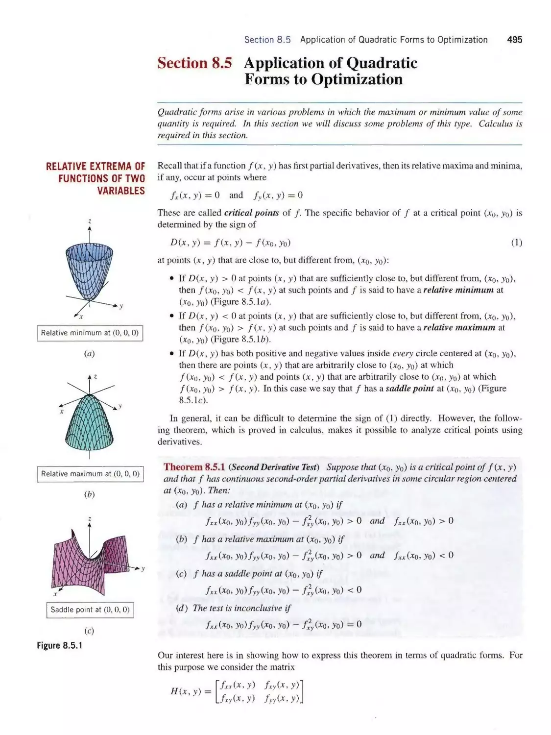
CHAPTER
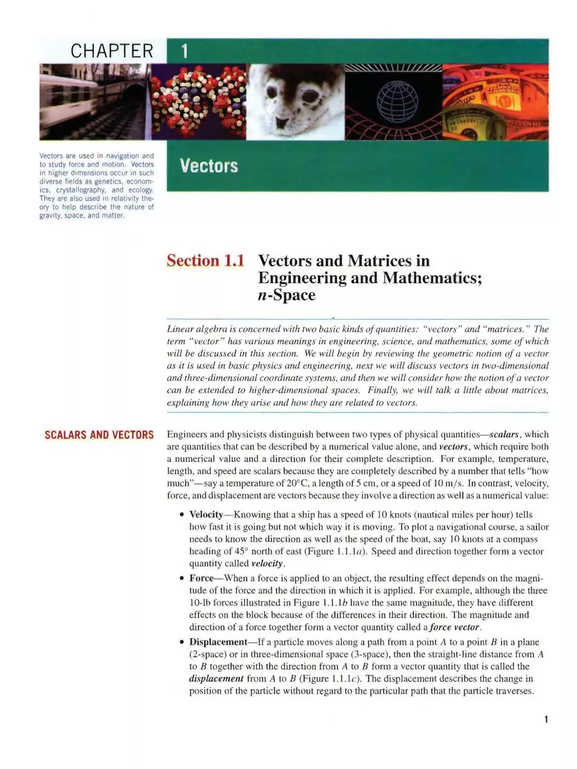
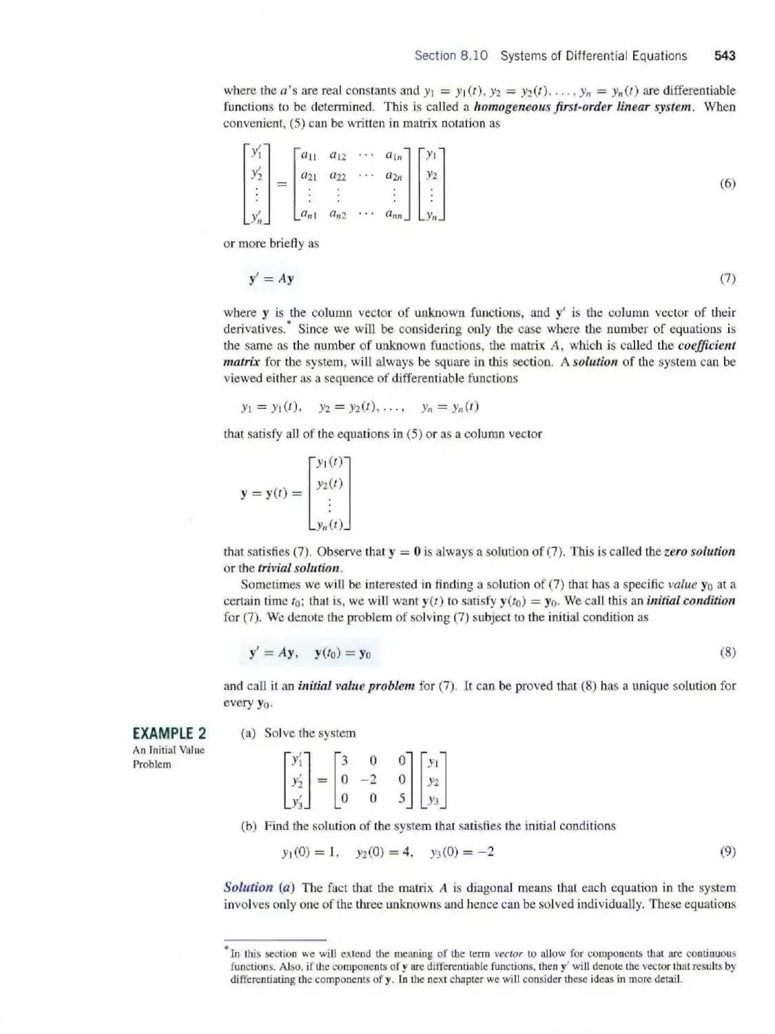
Vectors are used in navigation and
to study force and motion. Vectors
in higher dimensions occur in such
diverse fields as genetics, econom¬
ics, crystallography, and ecology.
They are also used in relativity the¬
ory to help describe the nature of
gravity, space, and matter.
Section 1.1 Vectors and Matrices in
Engineering and Mathematics;
n-Space
Linear algebra is concerned with two basic kinds of quantities: “vectors" and “matrices. ” The
term “vector" has various meanings in engineering, science, and mathematics, some of which
will be discussed in this section. We will begin by reviewing the geometric notion of a vector
as it is used in basic physics and engineering, next we will discuss vectors in two-dimensional
and three-dimensional coordinate systems, and then we will consider how the notion of a vector
can be extended to higher-dimensional spaces. Finally, we will talk a little about matrices,
explaining how they arise and how they are related to vectors.
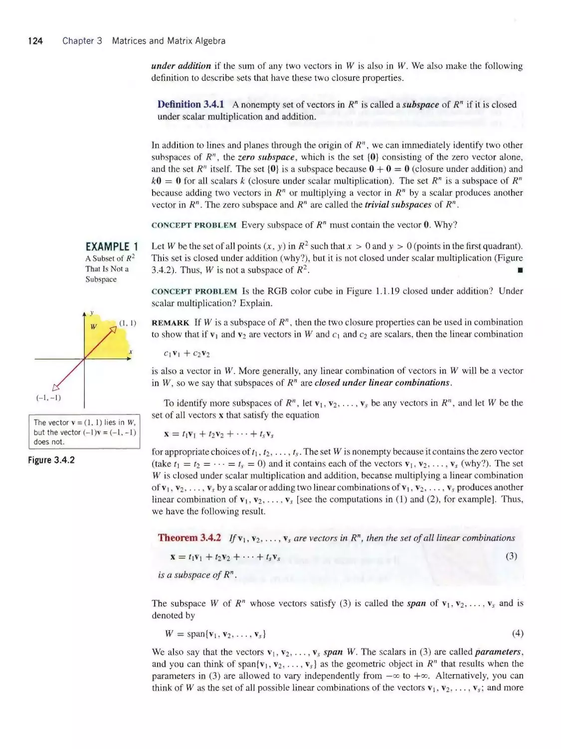
SCALARS AND VECTORS
Engineers and physicists distinguish between two types of physical quantities—scalars, which
are quantities that can be described by a numerical value alone, and vectors, which require both
a numerical value and a direction for their complete description. For example, temperature,
length, and speed are scalars because they are completely described by a number that tells “how
much”—say a temperature of 20oC, a length of 5 cm, or a speed of 10 m∕s. In contrast, velocity,
force, and displacement are vectors because they involve a direction as well as a numerical value:
• Velocity—Knowing that a ship has a speed of 10 knots (nautical miles per hour) tells
how fast it is going but not which way it is moving. To plot a navigational course, a sailor
needs to know the direction as well as the speed of the boat, say 10 knots at a compass
heading of 45o north of east (Figure 1.1. la). Speed and direction together form a vector
quantity called velocity.
• Force—When a force is applied to an object, the resulting effect depends on the magni¬
tude of the force and the direction in which it is applied. For example, although the three
10-lb forces illustrated in Figure 1.1.16 have the same magnitude, they have different
effects on the block because of the differences in their direction. The magnitude and
direction of a force together form a vector quantity called a force vector.
• Displacement—If a particle moves along a path from a point A to a point B in a plane
(2-space) or in three-dimensional space (3-space). then the straight-line distance from A
to B together with the direction from A to B form a vector quantity that is called the
displacement from A to B (Figure l.l.lc). The displacement describes the change in
position of the particle without regard to the particular path that the particle traverses.
1
2 Chapter 1 Vectors
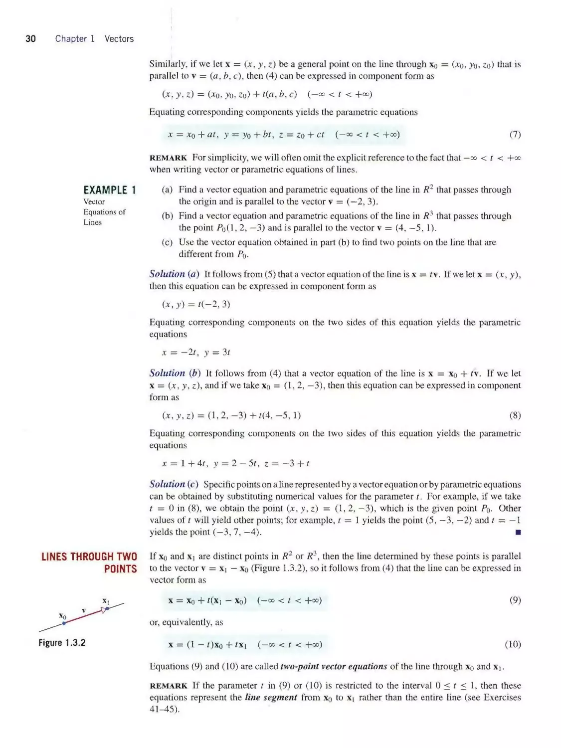
(c)
(a)
Figure 1.1.1
(⅛)
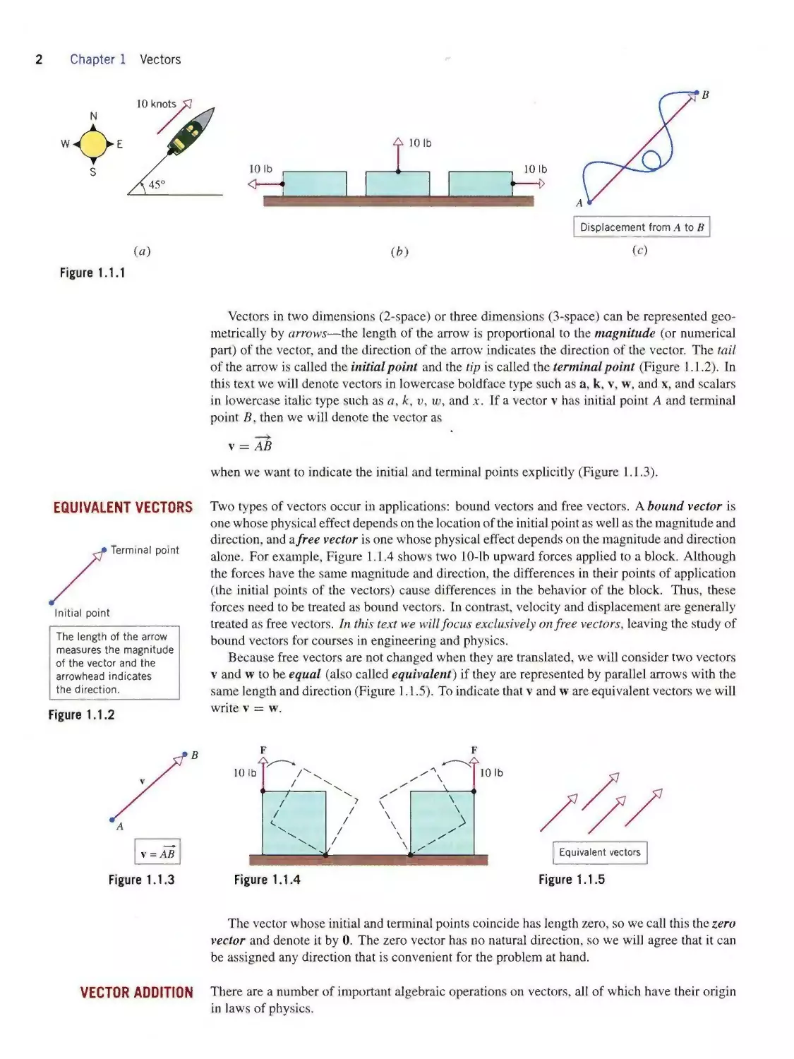
Vectors in two dimensions (2-space) or three dimensions (3-space) can be represented geo¬
metrically by arrows—the length of the arrow is proportional to the magnitude (or numerical
part) of the vector, and the direction of the arrow indicates the direction of the vector. The tail
of the arrow is called the initial point and the tip is called the terminal point (Figure 1.1.2). In
this text we will denote vectors in lowercase boldface type such as a, k, v, w, and x, and scalars
in lowercase italic type such as a, k, v, w, and x. If a vector v has initial point A and terminal
point B, then we will denote the vector as
v = AB
when we want to indicate the initial and terminal points explicitly (Figure 1.1.3).
EQUIVALENT VECTORS
Tθrmirι≡l point
Initial point
The length of the arrow
measures the magnitude
of the vector and the
arrowhead indicates
the direction.
Figure 1.1.2
Two types of vectors occur in applications: bound vectors and free vectors. A bound vector is
one whose physical effect depends on the location of the initial point as well as the magnitude and
direction, and a free vector is one whose physical effect depends on the magnitude and direction
alone. For example, Figure 1.1.4 shows two 10-lb upward forces applied to a block. Although
the forces have the same magnitude and direction, the differences in their points of application
(the initial points of the vectors) cause differences in the behavior of the block. Thus, these
forces need to be treated as bound vectors. In contrast, velocity and displacement are generally
treated as free vectors. In this text we will focus exclusively on free vectors, leaving the study of
bound vectors for courses in engineering and physics.
Because free vectors are not changed when they are translated, we will consider two vectors
v and w to be equal (also called equivalent) if they are represented by parallel arrows with the
same length and direction (Figure 1.1.5). To indicate that v and w are equivalent vectors we will
write v = w.
Figure 1.1.5
The vector whose initial and terminal points coincide has length zero, so we call this the zero
vector and denote it by 0. The zero vector has no natural direction, so we will agree that it can
be assigned any direction that is convenient for the problem at hand.
VECTOR ADDITION
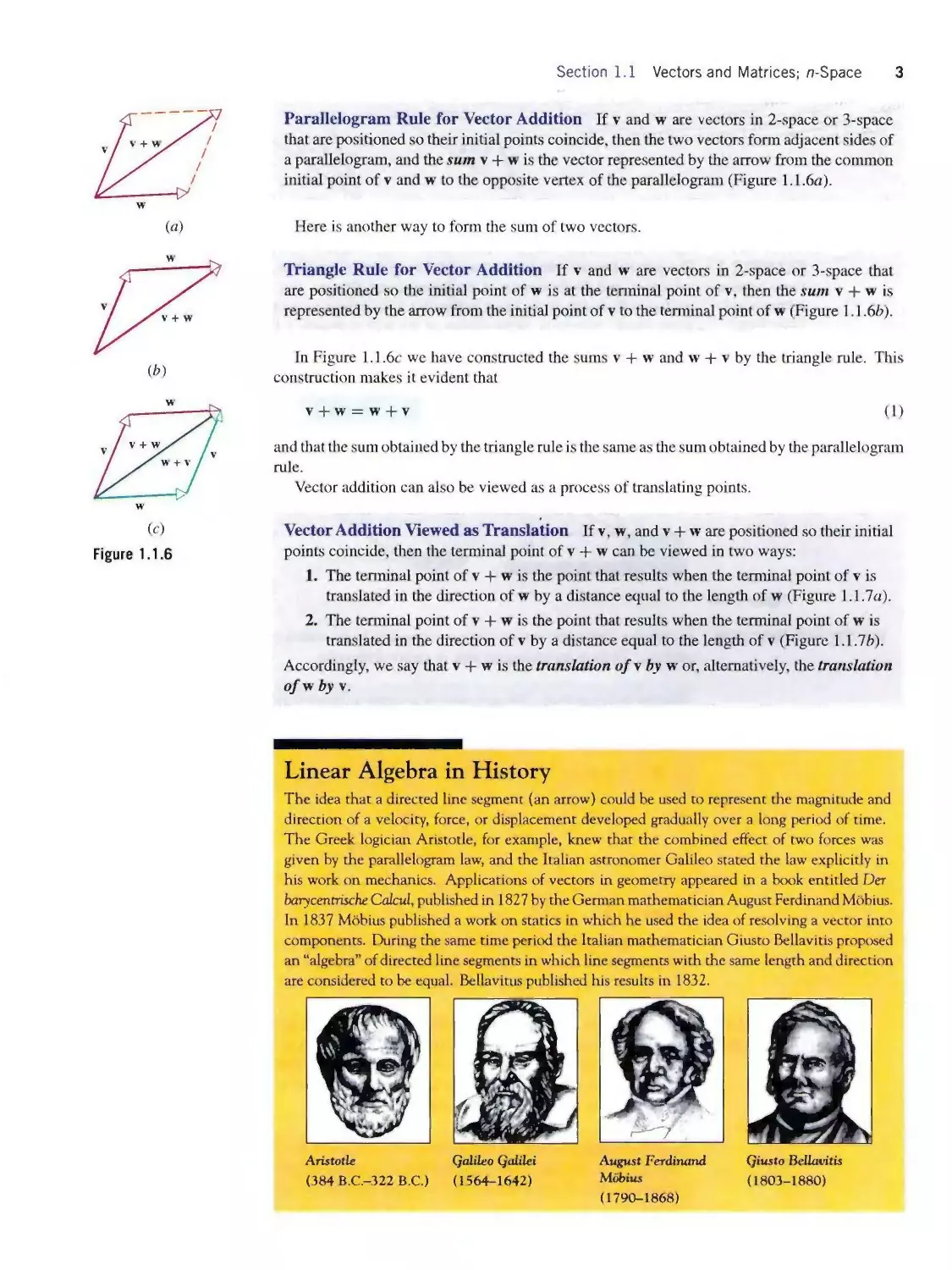
There are a number of important algebraic operations on vectors, all of which have their origin
in laws of physics.
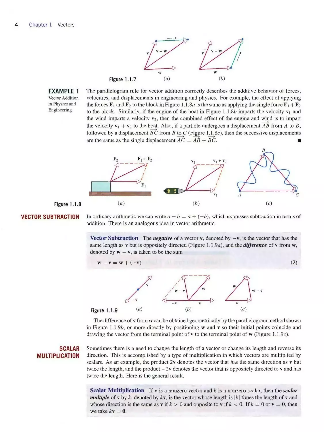
Section 1.1 Vectors and Matrices; n-Space 3
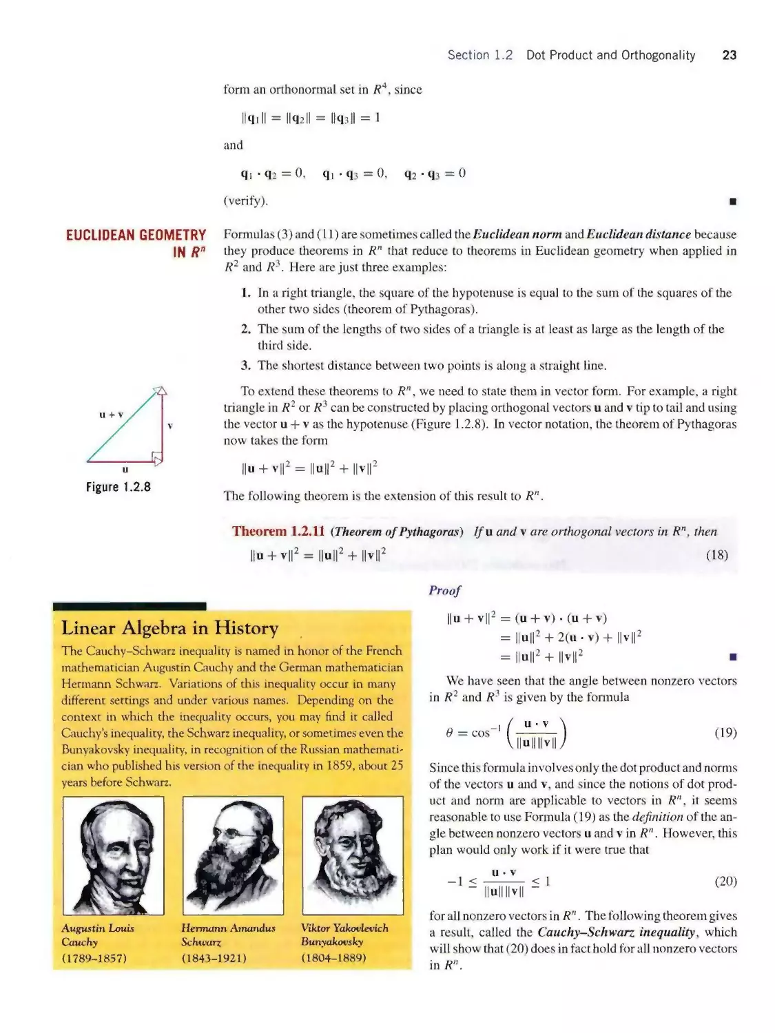
(c)
Figure 1.1.6
Parallelogram Rule for Vector Addition If v and w are vectors in 2-space or 3-spacc
that are positioned so their initial points coincide, then the two vectors form adjacent sides of
a parallelogram, and the sum v + w is the vector represented by the arrow from the common
initial point of v and w to the opposite vertex of the parallelogram (Figure 1.1.6α).
Here is another way to form the sum of two vectors.
Triangle Rule for Vector Addition If v and w are vectors in 2-space or 3-space that
are positioned so the initial point of w is at the terminal point of v, then the sum v + w is
represented by the arrow from the initial point of v to the terminal point of w (Figure 1.1.6⅛).
In Figure 1.1.6c we have constructed the sums v + w and w + v by the triangle rule. This
construction makes it evident that
v⅛w = w + v (1)
and that the sum obtained by the triangle rule is the same as the sum obtained by the parallelogram
rule.
Vector addition can also be viewed as a process of translating points.
Vector Addition Viewed as Translation If v, w, and v + w are positioned so their initial
points coincide, then the terminal point of v + w can be viewed in two ways:
1. The terminal point of v + w is the point that results when the terminal point of v is
translated in the direction of w by a distance equal to the length of w (Figure 1.1.7α).
2. The terminal point of v + w is the point that results when the terminal point of w is
translated in the direction of v by a distance equal to the length of v (Figure 1.1.76).
Accordingly, we say that v + w is the translation ofvbyw or, alternatively, the translation
of w by v.
Linear Algebra in History
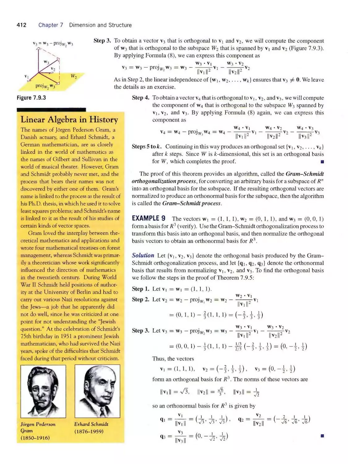
The idea that a directed line segment (an arrow) could be used to represent the magnitude and
direction of a velocity, force, or displacement developed gradually over a long period of time.
The Greek logician Aristotle, for example, knew that the combined effect of two forces was
given by the parallelogram law, and the Italian astronomer Galileo stated the law explicitly in
his work on mechanics. Applications of vectors in geometry appeared in a book entitled Der
barycentrische Calcul, published in 1827 by the German mathematician August Ferdinand Mobius.
In 1837 Mobius published a work on statics in which he used the idea of resolving a vector into
components. During the same time period the Italian mathematician Giusto Bellavitis proposed
an “algebra” of directed line segments in which line segments with the same length and direction
are considered to be equal. Bellavitus published his results in 1832.
Aristotle
(384 B.C.-322 B.C.)
Qalileo Qalilei
(1564-1642)
Augiist Ferdinand
Mobius
(1790-1868)
Qiusto Bellavitis
(1803-1880)
4 Chapter 1 Vectors
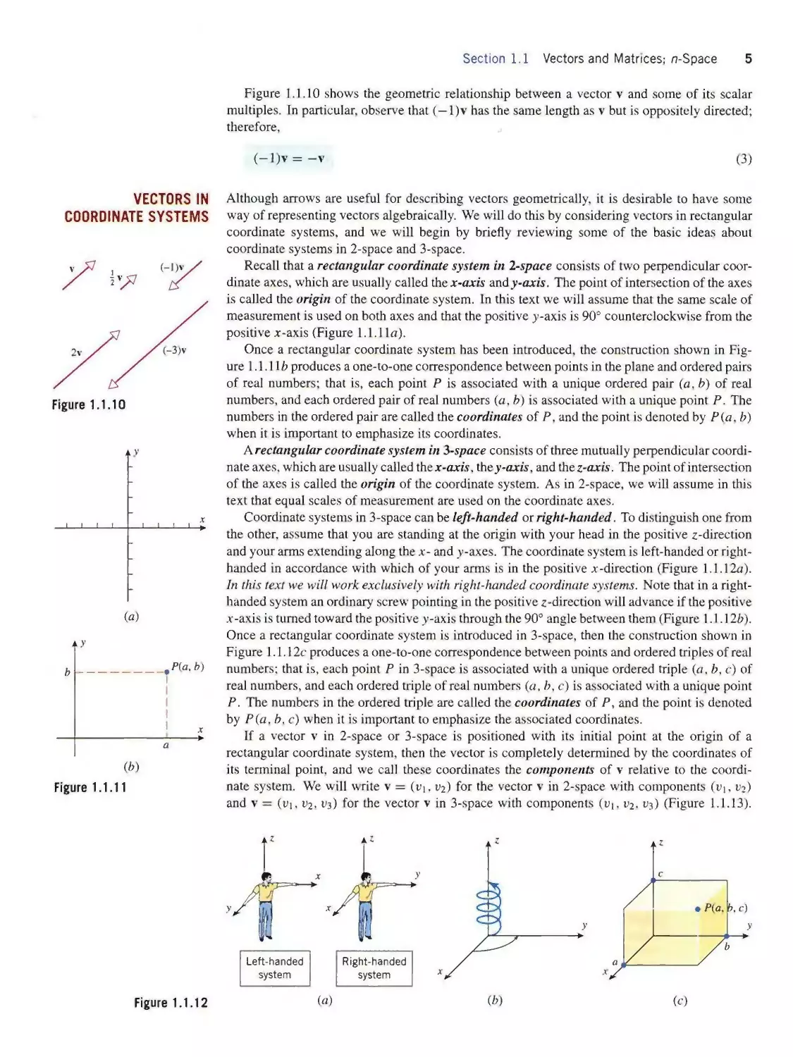
EXAMPLE 1
Vector Addition
in Physics and
Engineering
Figure 1.1.8
VECTOR SUBTRACTION
Figure 1.1.7 («)
(⅛)
The parallelogram rule for vector addition correctly describes the additive behavior of forces,
velocities, and displacements in engineering and physics. For example, the effect of applying
the forces F∣ and F2 to the block in Figure 1.1.8α is the same as applying the single force F∣ + F2
to the block. Similarly, if the engine of the boat in Figure 1.1.8b imparts the velocity v∣ and
the wind imparts a velocity V2, then the combined effect of the engine and wind is to impart
the velocity v1 + V2 to the boat. Also, if a particle undergoes a displacement AB from A to B,
followed by a displacement B C from B to C (Figure 1.1.8c), then the successive displacements
are the same as the single displacement AC = AB + BC.
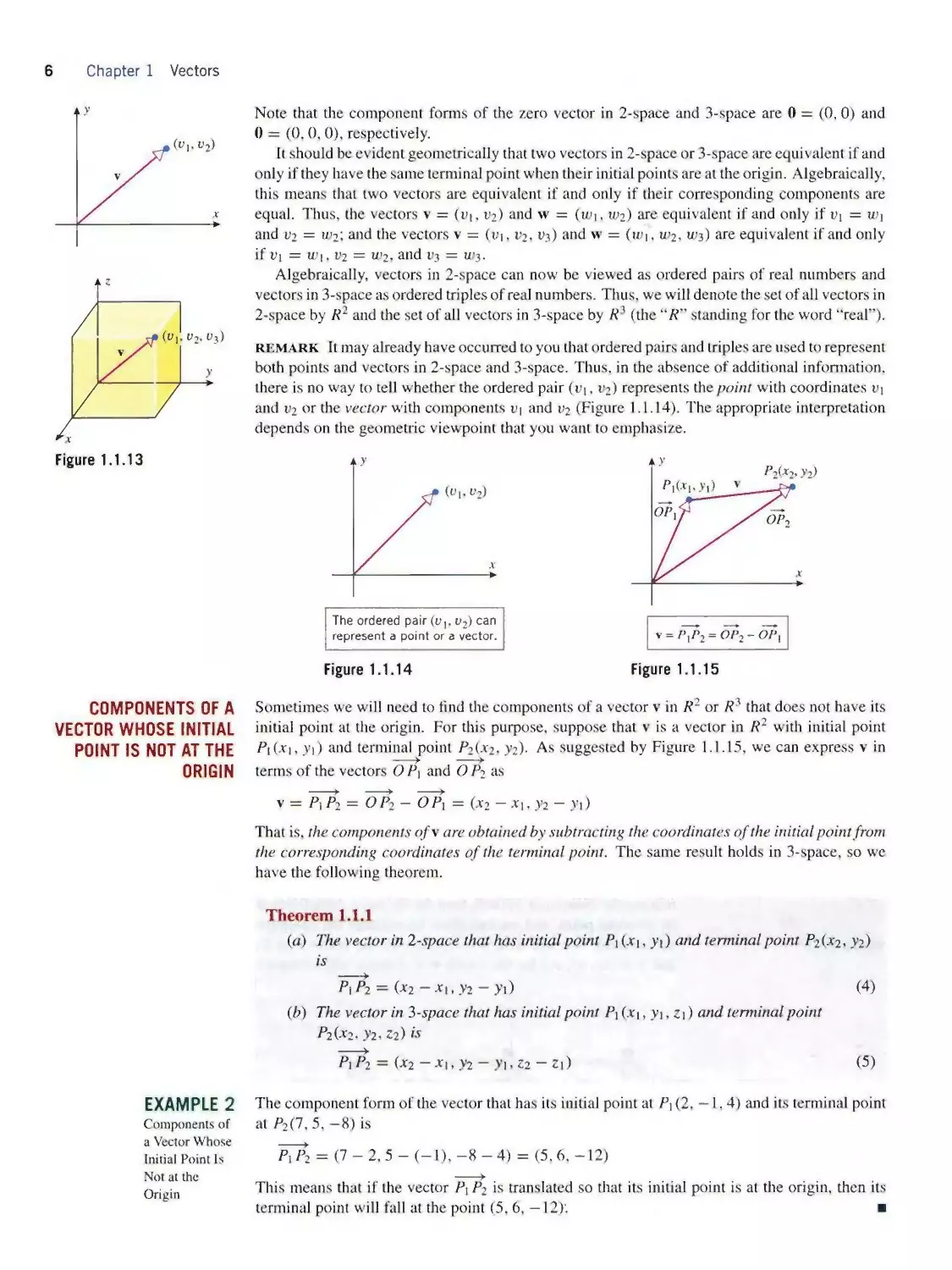
In ordinary arithmetic we can write a — b = a + (—b~), which expresses subtraction in terms of
addition. There is an analogous idea in vector arithmetic.
Vector Subtraction The negative of a vector v, denoted by —v, is the vector that has the
same length as v but is oppositely directed (Figure 1.1.9α), and the difference of v from w,
denoted by w — v, is taken to be the sum
w — v = w + (—v)
(2)
The difference of v from w can be obtained geometrically by the parallelogram method shown
in Figure 1.1.9⅛, or more directly by positioning w and v so their initial points coincide and
drawing the vector from the terminal point of v to the terminal point of w (Figure 1.1.9c).
SCALAR
MULTIPLICATION
Sometimes there is a need to change the length of a vector or change its length and reverse its
direction. This is accomplished by a type of multiplication in which vectors are multiplied by
scalars. As an example, the product 2v denotes the vector that has the same direction as v but
twice the length, and the product —2v denotes the vector that is oppositely directed to v and has
twice the length. Here is the general result.
Scalar Multiplication If v is a nonzero vector and k is a nonzero scalar, then the scalar
multiple of v by k, denoted by kv, is the vector whose length is ∣⅛∣ times the length of v and
whose direction is the same as v if k > 0 and opposite to v if k <0. If k = 0 or v = 0. then
we take kv = 0.
Section 1.1 Vectors and Matrices; π-Space 5
VECTORS IN
COORDINATE SYSTEMS
y
J I I I I I I L
Figure 1.1.10 shows the geometric relationship between a vector v and some of its scalar
multiples. In particular, observe that (—l)v has the same length as v but is oppositely directed;
therefore.
(-l)v = -v
(3)
Although arrows are useful for describing vectors geometrically, it is desirable to have some
way of representing vectors algebraically. We will do this by considering vectors in rectangular
coordinate systems, and we will begin by briefly reviewing some of the basic ideas about
coordinate systems in 2-space and 3-space.
Recall that a rectangular coordinate system in 2-space consists of two perpendicular coor¬
dinate axes, which are usually called the x-axis and y-axis. The point of intersection of the axes
is called the origin of the coordinate system. In this text we will assume that the same scale of
measurement is used on both axes and that the positive y-axis is 90o counterclockwise from the
positive x-axis (Figure 1.1.1 la).
Once a rectangular coordinate system has been introduced, the construction shown in Fig¬
ure 1.1.1 lb produces a one-to-one coσespondence between points in the plane and ordered pairs
of real numbers; that is, each point P is associated with a unique ordered pair (a, b) of real
numbers, and each ordered pair of real numbers (a, b) is associated with a unique point P. The
numbers in the ordered pair are called the coordinates of P, and the point is denoted by P(a, b)
when it is important to emphasize its coordinates.
A rectangular coordinate system in 3-space consists of three mutually perpendicular coordi¬
nate axes, which are usually called thex-αx⅛, they-axis, and the z-axis. The point of intersection
of the axes is called the origin of the coordinate system. As in 2-space, we will assume in this
text that equal scales of measurement are used on the coordinate axes.
Coordinate systems in 3-space can be left-handed or right-handed. To distinguish one from
the other, assume that you are standing at the origin with your head in the positive z-direction
and your arms extending along the x- and y-axes. The coordinate system is left-handed or right-
handed in accordance with which of your arms is in the positive x-direction (Figure 1.1.12α).
In this text we will work exclusively with right-handed coordinate systems. Note that in a right-
handed system an ordinary screw pointing in the positive z-direction will advance if the positive
x-axis is turned toward the positive y-axis through the 90o angle between them (Figure 1.1.12⅛).
Once a rectangular coordinate system is introduced in 3-space, then the construction shown in
Figure 1.1.12c produces a one-to-one correspondence between points and ordered triples of real
numbers; that is, each point P in 3-space is associated with a unique ordered triple (a, b, c) of
real numbers, and each ordered triple of real numbers (a, b, c) is associated with a unique point
P. The numbers in the ordered triple are called the coordinates of P, and the point is denoted
by P(α, b, c) when it is important to emphasize the associated coordinates.
If a vector v in 2-space or 3-space is positioned with its initial point at the origin of a
rectangular coordinate system, then the vector is completely determined by the coordinates of
its terminal point, and we call these coordinates the components of v relative to the coordi¬
nate system. We will write v = (vι, υf) for the vector v in 2-space with components (υ∣, ι⅛)
and v = (t>ι, V2, υ3) for the vector v in 3-space with components (ι∣ι, 02, υ3) (Figure 1.1.13).
Left-handed
system
Right-handed
system
Figure 1.1.12
(«)
6 Chapter 1 Vectors
COMPONENTS OF A
VECTOR WHOSE INITIAL
POINT IS NOT AT THE
ORIGIN
EXAMPLE 2
Components of
a Vector Whose
Initial Point Is
Not at the
Origin
Note that the component forms of the zero vector in 2-space and 3-space are 0 = (0,0) and
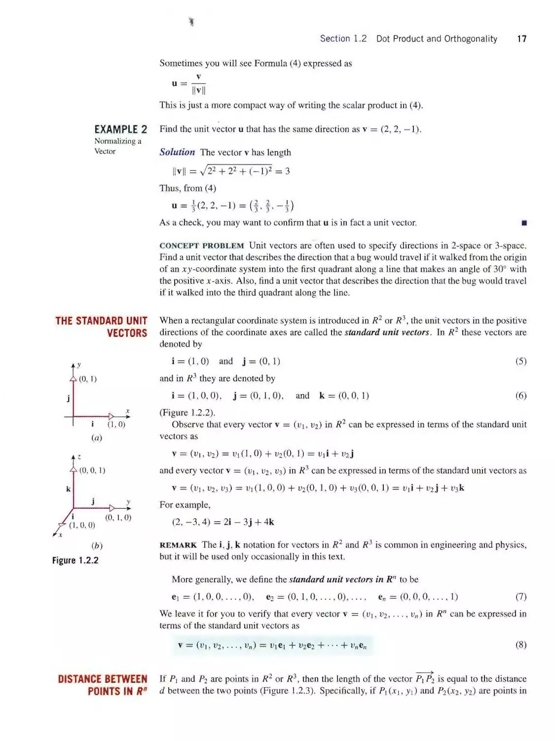
0 = (0,0,0), respectively.
It should be evident geometrically that two vectors in 2-space or 3-space are equivalent if and
only if they have the same terminal point when their initial points are at the origin. Algebraically,
this means that two vectors are equivalent if and only if their corresponding components are
equal. Thus, the vectors v = (υ∣, υ2) and w = (u>∣, w2) are equivalent if and only if ι>ι = w↑
and V2 = u⅛i and the vectors v = (υ∣, υ2, υ3) and w = (w∣, W2, u>3) are equivalent if and only
if tη = u>ι, V2 = 11>2, and υ3 = u>3.
Algebraically, vectors in 2-space can now be viewed as ordered pairs of real numbers and
vectors in 3-space as ordered triples of real numbers. Thus, we will denote the set of all vectors in
2-space by R2 and the set of all vectors in 3-space by R3 (the “R" standing for the word “real”).
remark It may already have occurred to you that ordered pairs and triples are used to represent
both points and vectors in 2-space and 3-space. Thus, in the absence of additional information,
there is no way to tell whether the ordered pair (ιη, υ2) represents the point with coordinates ιη
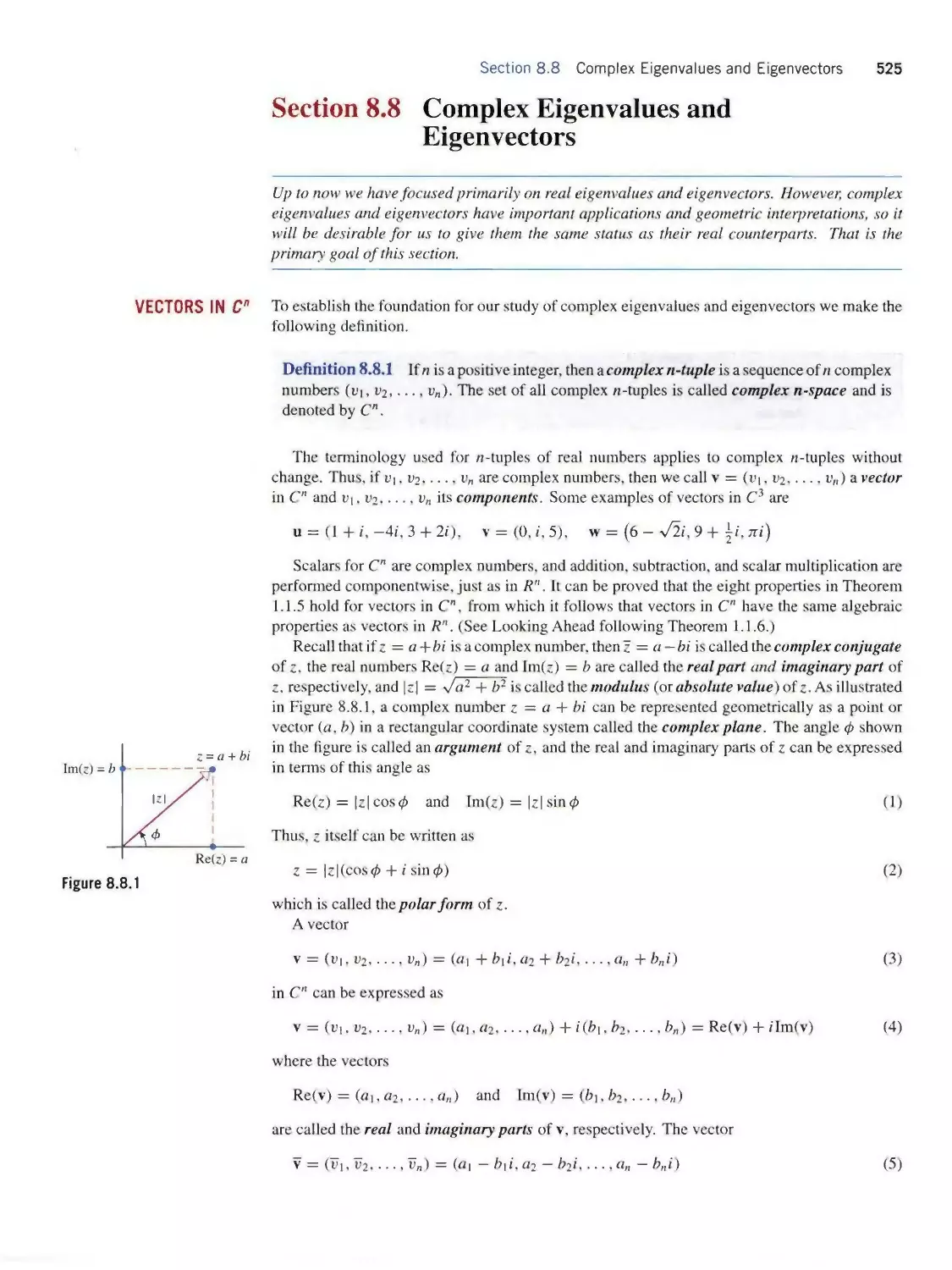
and V2 or the vector with components υj and υ2 (Figure 1.1.14). The appropriate interpretation
depends on the geometric viewpoint that you want to emphasize.
The ordered pair (υ∣, ι>2) can
represent a point or a vector.
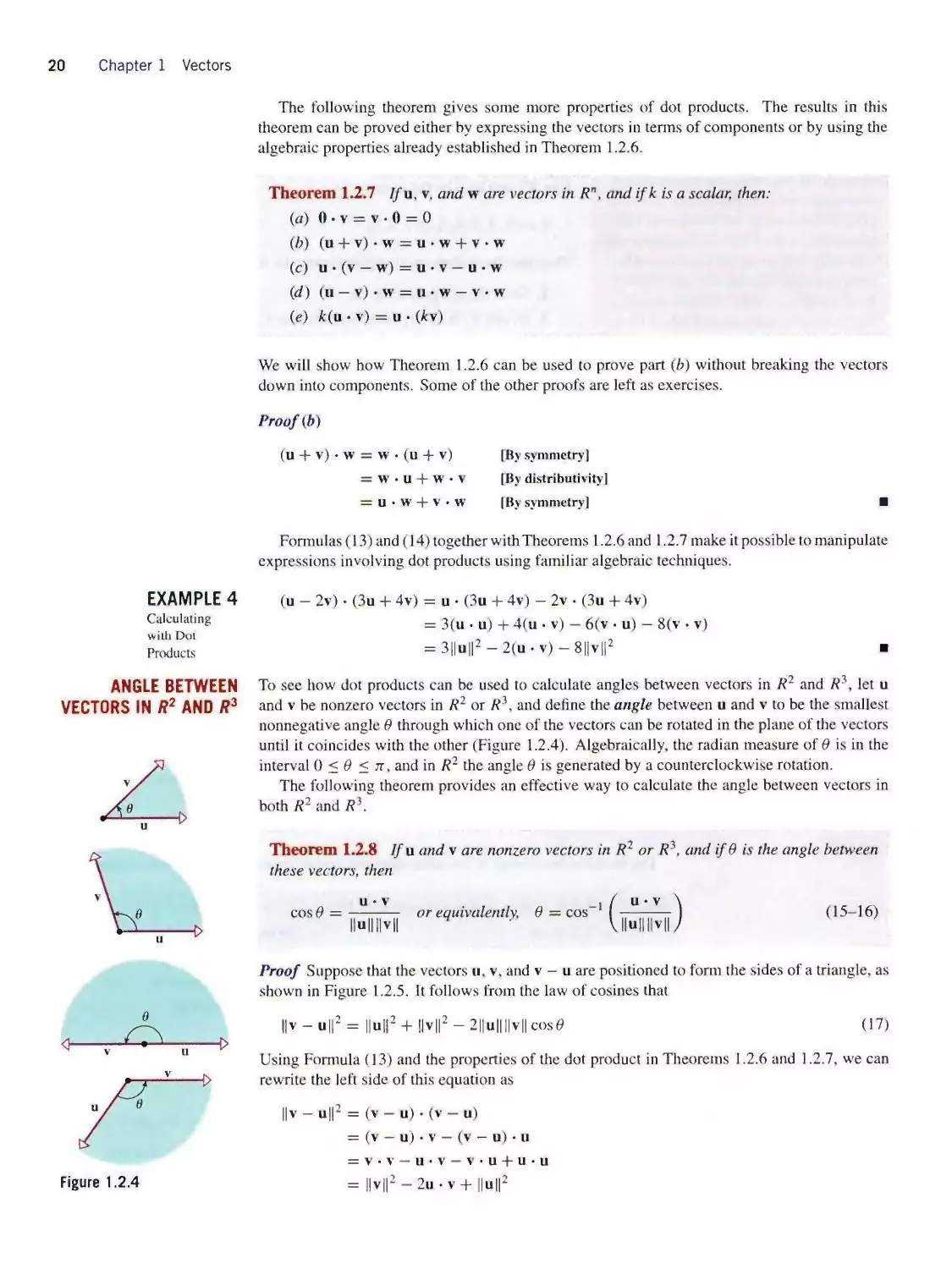
Figure 1.1.14
v = P∣P2 = OIi2 ~ OP\
Figure 1.1.15
Sometimes we will need to find the components of a vector v in R2 or R3 that does not have its
initial point at the origin. For this purpose, suppose that v is a vector in R2 with initial point
Fι(x∣, yι) and terminal point P2(x2, yz)∙ As suggested by Figure 1.1.15, we can express v in
terms of the vectors O P↑ and O P2 as
v = Pi⅛ = ~O~Pι ~ ^^ι = (×2 -xι,⅜ - y∣)
That is, the components ofv are obtained by subtracting the coordinates of the initial point from
the corresponding coordinates of the terminal point. The same result holds in 3-space, so we
have the following theorem.
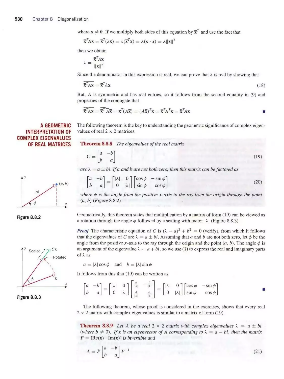
Theorem 1.1.1
(a) The vector in 2-space that has initial point Pi (x∣, yι) and terminal point P2(x2< y2)
is
p^p2≈ (χ2-χι,y2-yι) (4)
(ft) The vector in 3-space that has initial point P∣ (x∣, yι, zι) and terminal point
P2(x2. y2,Z2) «
Pi P2 = (x2-xι,y2- y1,Z2- Zl) (5)
The component form of the vector that has its initial point at P∣(2. -1,4) and its terminal point
at P2(f, 5, —8) is
P[K = (7 - 2, 5 - (-1), -8 - 4) = (5,6, -12)
This means that if the vector P↑ P2 is translated so that its initial point is at the origin, then its
terminal point will fall at the point (5,6, —12): ■
Section 1.1 Vectors and Matrices; π-Space 7
Linear Algebra in History
The German-bom physicist Albert Einstein
immigrated to the United Stares in 1935,
where he settled at Princeton University.
Einstein spent the last three decades of his
life working unsuccessfully at producing
a unified field theory that would establish
an underlying link between tire forces of
gravity and electromagnetism. Recently,
physicists have made progress on the prob¬
lem using a framework known as string
theory. In this theory the smallest, indivis¬
ible components of the Universe are not
particles but loops that behave like vibrat¬
ing strings. Whereas Einstein’s space-time
universe was four-dimensional, strings re¬
side in an 11-dimensional world that is the
focus of much current research.
—Based on an article in Time Magazine,
September 30, 1999.
VECTORS IN Rn The idea of using ordered pairs and triples of real numbers to represent points and vectors in
2-space and 3-space was well known in the eighteenth and nineteenth centuries, but in the late
nineteenth and early twentieth centuries mathematicians and physicists began
to recognize the physical importance of higher-dimensional spaces. One of the
most important examples is due to Albert Einstein, who attached a time com¬
ponent t to three space components (x, y, z) to obtain a quadruple (x, y, z, r),
which he regarded to be a point in a four-dimensional space-time universe. Al¬
though we cannot see four-dimensional space in the way that we see two- and
three-dimensional space, it is nevertheless possible to extend familiar geometric
ideas to four dimensions by working with algebraic properties of quadruples. In¬
deed, by developing an appropriate geometry of the four-dimensional space-time
universe, Einstein developed his general relativity theory, which explained for
the first time how gravity works. To explore the concept of higher-dimensional
spaces we make the following definition.
Definition 1.1.2 If n is a positive integer, then an ordered n-tuple is a
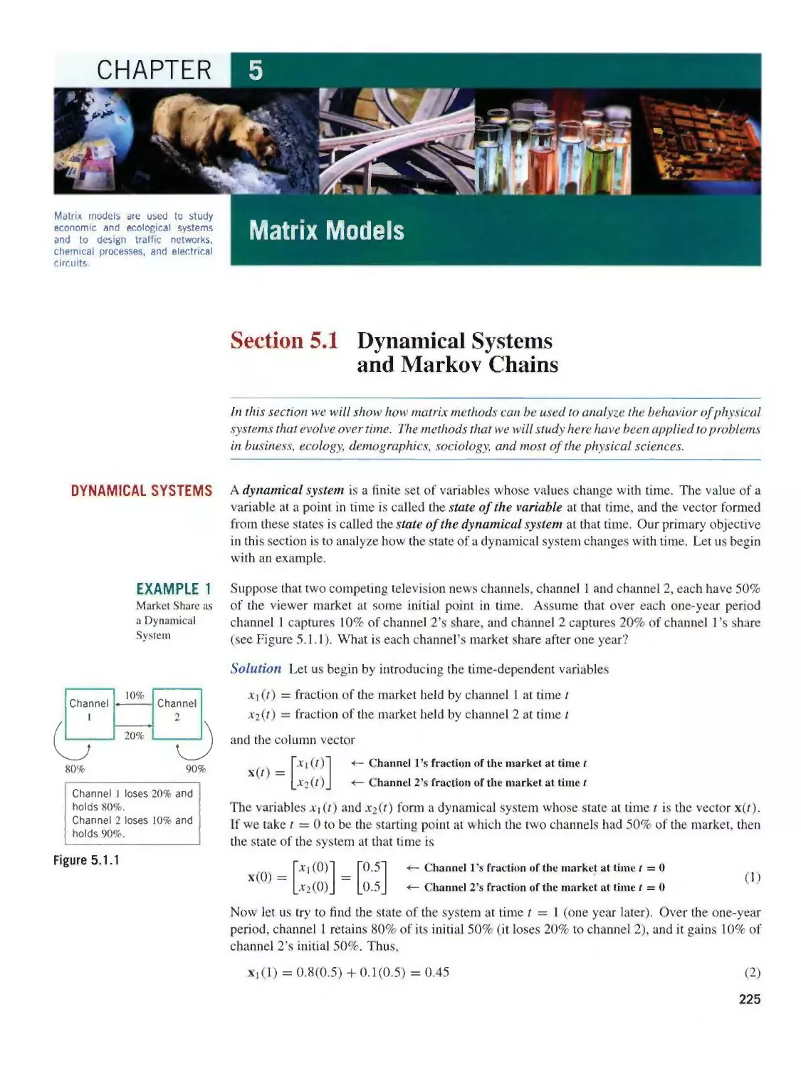
sequence of n real numbers (vι, ι⅛,..., υπ). The set of all ordered n-tuples
is called n-space and is denoted by R".
We will denote n-tuples using the vector notation v = (υ∣, V2,..., υn), and
we will write 0 = (0.0,..., 0) for the n-tuple whose components are all zero.
We will call this the zero vector or sometimes the origin of Rπ.
remark You can think of the numbers in an n-tuple (υj, V2, ∙ ■ ■ , v„) as either
the coordinates of a generalized point or the components of a generalized vector,
depending on the geometric image you want to bring to mind—the choice makes
no difference mathematically, since it is the algebraic properties of n-tuples that
are of concern.
An ordered 1-tuple (n = 1) is a single real number, so Ri can be viewed alge¬
braically as the set of real numbers or geometrically as a line. Ordered 2-tuples
(n = 2) are ordered pairs of real numbers, so we can view R2 geometrically as
a plane. Ordered 3-tuples are ordered triples of real numbers, so we can view
Ri geometrically as the space around us. We will sometimes refer to Ri, R2,
and R3 as visible space and Λ4, Rs,... as higher-dimensional spaces. Here
are some physical examples that lead to higher-dimensional spaces.
Albert Einstein
(1879-1955)
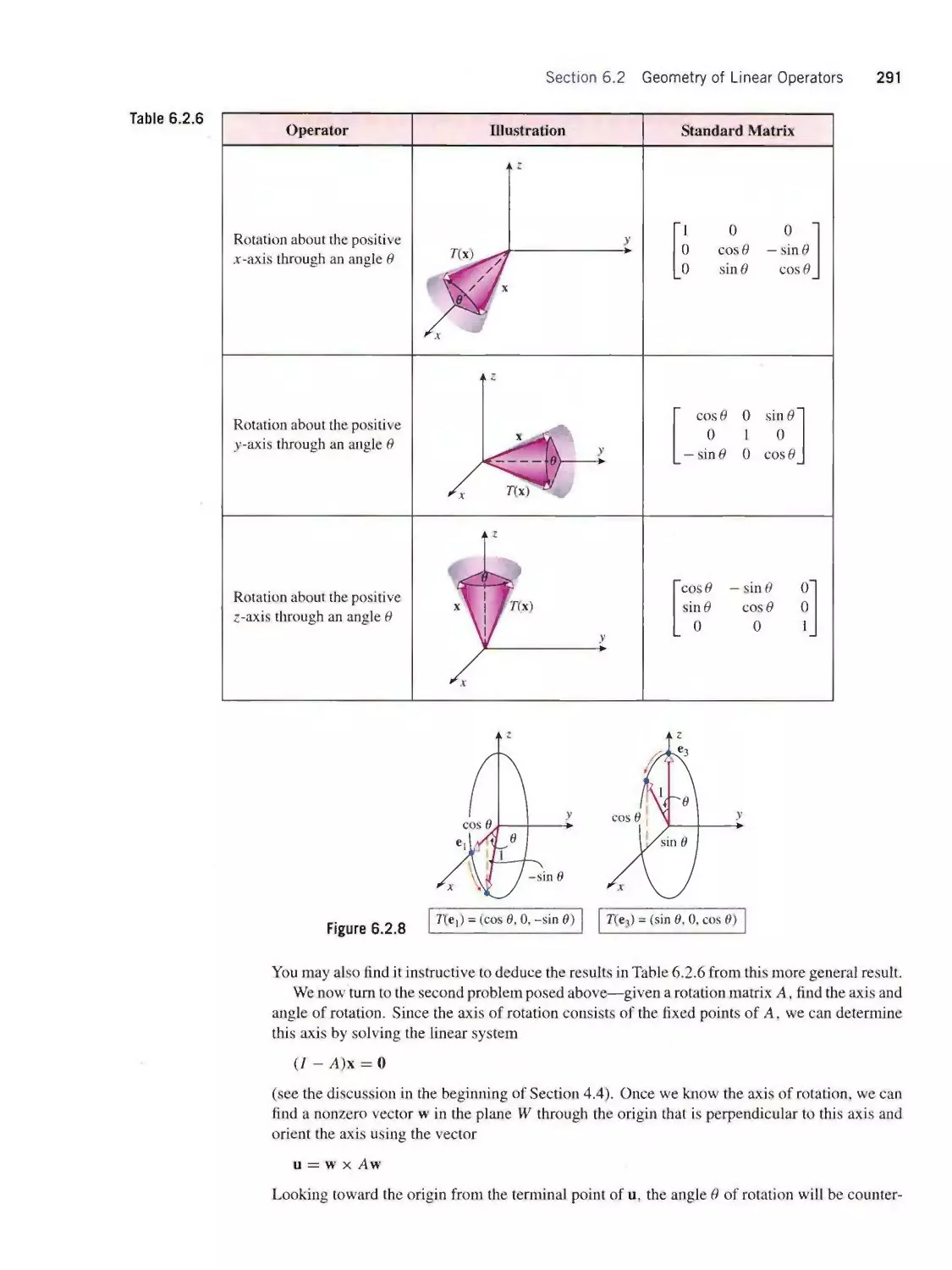
EXAMPLE 3
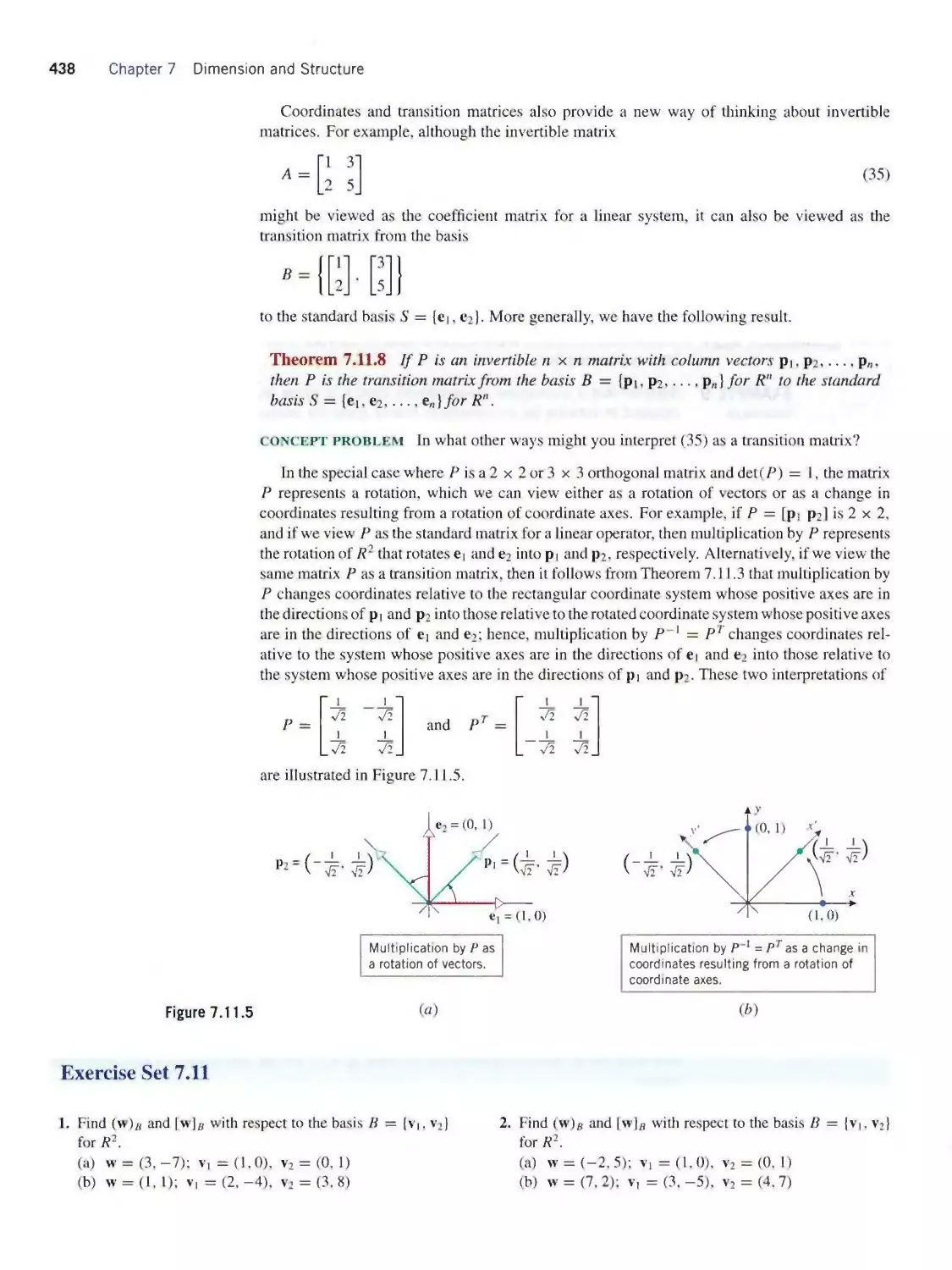
Some Examples
of Vectors in
Higher-
Dimensional
Spaces
• Experimental Data—A scientist performs an experiment and makes n numerical
measurements each time the experiment is performed. The result of each experiment can
be regarded as a vector y = (yι, y2,..., yn) in R" in which yι, y2, ■.., yn are the
measured values.
• Storage and Warehousing—A national trucking company has 15 depots for storing and
servicing its trucks. At each point in time the distribution of trucks in the service depots
can be described by a 15-tuple x = (x∣, ×2,.. ∙, x∣5) in which x∣ is the number of trucks
in the first depot, ×2 is the number in the second depot, and so forth.
• Electrical Circuits—A certain kind of processing chip is designed to receive four input
voltages and produces three output voltages in response. The input voltages can be
regarded as vectors in R' and the output voltages as vectors in R3. Thus, the chip can be
viewed as a device that transforms each input vector v = (tq, ‰ 1>3. υ4) in R4 into some
output vector w = (ιυ∣, w2, W3) in R3.
• Graphical Images—One way in which color images are created on computer screens is
by assigning each pixel (an addressable point on the screen) three numbers that describe
the hue. saturation, and brightness of the pixel. Thus, a complete color image can be
viewed as a set of 5-tuples of the form v = (x, y, h, s, b) in which x and y are the screen
coordinates of a pixel and h, s, and b are its hue, saturation, and brightness.
8 Chapter 1 Vectors
• Economics—One approach to economic analysis is to divide an economy into sectors
(manufacturing, services, utilities, and so forth) and to measure the output of each sector
by a dollar value. Thus, in an economy with 10 sectors the economic output of the entire
economy can be represented by a 10-tuple s = (s∣, s2,..., s∣o) in which the numbers
si, s2,..., sιo are the outputs of the individual sectors.
• Mechanical Systems—Suppose that six particles move along the same coordinate line
so that at time t their coordinates are xj, x2,..., x⅛ and their velocities are υ∣, υ2,..., υ⅛,
respectively. This information can be represented by the vector
v = (x1,x2,x3,x4,x5,x6, υ∣, υ2, υ3, υ4, υ5, υ6,0
in Λl3. This vector is called the state of the particle system at time t. ■
concept problem Try to think of some other physical examples in which n-tuples might
arise.
EQUALITY OF VECTORS
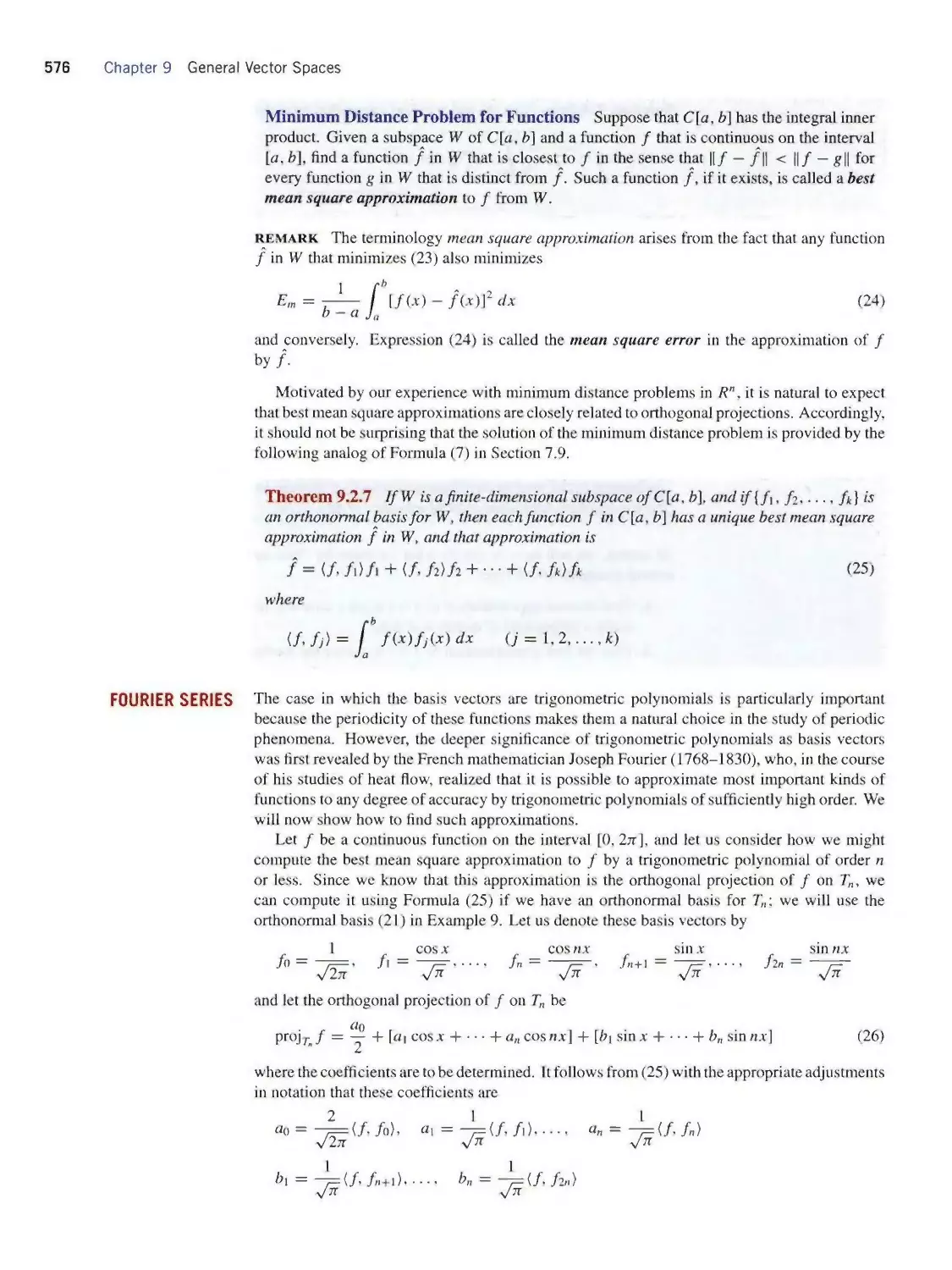
We observed earlier that two vectors in R2 or R2 are equivalent if and only if their corresponding
components are equal. Thus, we make the following definition.
Linear Algebra in History
The idea of representing vectors as n-tuples
began to crystallize around 1814 when
the Swiss accountant (and amateur math¬
ematician) Jean Robert Argand (1768—
1822) proposed the idea of representing
a complex number a + bi as an ordered
pair (a, b) of real numbers. Subsequently,
the Irish mathematician William Hamil¬
ton developed his theory of quaternions,
which was the first important example of
a four-dimensional space. Hamilton pre¬
sented his ideas in a paper given to the
Irish Academy in 1843. The concept of an
zι-dimensional space became firmly estab¬
lished in 1844 when the German mathe¬
matician Hermann Grassmann published a
book entitled Ausdehnungslehre in which he
developed many of the fundamental ideas
that appear in this text.
Definition 1.1.3 Vectors v = (ι>ι, v2,..., υ,l) and w = (uη, w2,..., wn)
in Rn are said to be equivalent (also called equal) if
υ1=wι, υ2 = w2 υn = wn
We indicate this by writing v = w.
Thus, for example.
(a,b, c,d) = (1, -4, 2, 7)
if and only if a = 1, b = —4, c = 2, and d = 7.
Our next objective is to define the operations of addition, subtraction, and
scalar multiplication for vectors in R,'. To motivate the ideas, we will consider
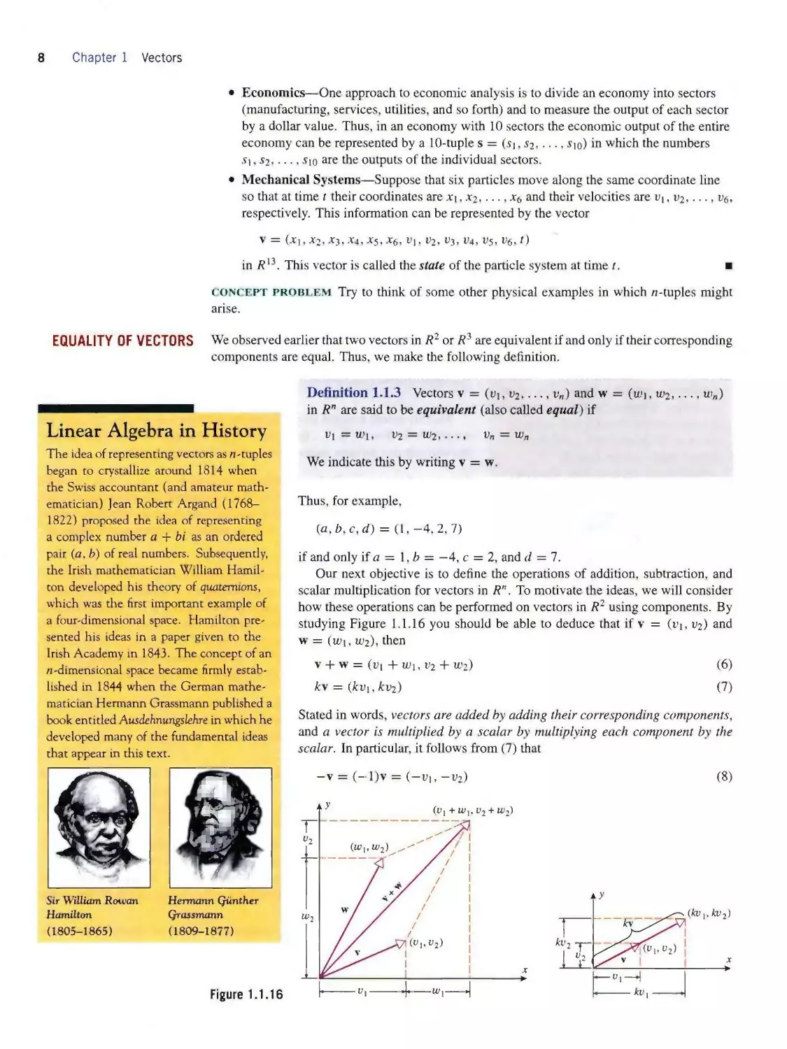
how these operations can be performed on vectors in R2 using components. By
studying Figure 1.1.16 you should be able to deduce that if v = (υι, υ2) and
w = (u»i, ιu2), then
v + w = (υ1 + w1, υ2 + w2) (6)
kv = (⅛υι,⅛υ2) (7)
Stated in words, vectors are added by adding their corresponding components,
and a vector is multiplied by a scalar by multiplying each component by the
scalar. In particular, it follows from (7) that
Sir William Rotvan
Hamilton
(1805-1865)
Hermann Qtinther
Qrassmann
(1809-1877)
Figure 1.1.16
Section 1.1 Vectors and Matrices; n-Space 9
and hence that
W — V = W + (—V) = (W∣ — υ∣, U?2 — Vz)
That is, vectors are subtracted by subtracting corresponding components.
Motivated by Formulas (6)-(9), we make the following definition.
(9)
Definition 1.1.4 If v = (υ∣, υ2, ..., υ,,) and w = (wj, u?2,..., wn) are vectors in R", and
if k is any scalar, then we define
v + w = (υ1+W1,υ2 + w2, ...,υπ + u>π) (10)
kv = (kυι,kv2,...,kυn) (11)
-v = (-υ∣, -υ2,.... —υn) (12)
w - v = w + (-v) ≈ (wi - υi, w2 - v2,..., w„ - υn) (13)
EXAMPLE 4
Algebraic
Operations
Using
Components
If v = (1, —3, 2) and w = (4, 2, 1), then
v + w = (5,-1,3), 2v = (2,-6,4)
—w = (—4, —2, -1), v - w = v + (-w) = (-3, -5, 1)
The following theorem summarizes the most important properties of vector operations.
Theorem 1.13 Ifu, v, and w are vectors in R", and if k and I are scalars, then:
(a) u + v = v + u (e) (⅛ + ∕)u = Λu + ∕u
(⅛) (u + v) + w = u + (v + w) (/) k(u + v) = ku + kv
(c) u + 0 = 0 + u = u (g) k(lu) = (λ∕)u
(d) u + (—u) = 0 (Λ) lu = u
We will prove part (⅛) and leave some of the other proofs as exercises.
Proof (b) Let u = (u∣, u2, ■.., uπ), v = (vι, t⅛,..., υz,), and w = (uη, u>2,...,wπ). Then
(u + v) + w = [(w∣, u2,..., Un) + (υ∣, υ2,..., υz,)] + (w,, w2 wn)
= (u 1 + υ∣,w2 + v2 uπ + v„) + (u>1, w2,...,wπ)
= (("ι + Vi) + w∣, (u2 + υ2) + w2,..., (un + υzl) + wn)
= (w∣ + (ι>ι + u>i),m2 + (t>2 + w2),...,u,, + (υπ + ιυz,))
= (w∣,w2 Mn) + (υι +wi,υ2 + w2,...,v„ +wn)
= u + (v + w)
[Vector addition]
[Vector addition]
[Regroup]
[Vector addition]
The following additional properties of vectors in R" can be deduced easily by expressing the
vectors in terms of components (verify).
Theorem 1.1.6 If v is a vector in Rn and k is a scalar, then:
(a) 0v = 0
(*) Λ0 = 0
(c) (-l)v = -v
looking ahead Theorem 1.1.5 is one of the most fundamental theorems in linear algebra
in that all algebraic properties of vectors can be derived from the eight properties stated in the
theorem. For example, even though Theorem 1.1.6 is easy to prove by using components, it
can also be derived from the properties in Theorem 1.1.5 without breaking the vectors into
components (Exercise P3). Later we will use Theorem 1.1.5 as a starting point for extending
the concept of a vector beyond R".
10 Chapter 1 Vectors
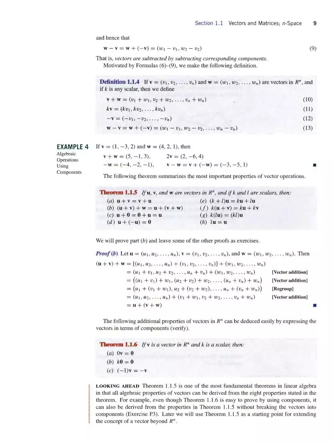
SUMS OF THREE OR
MORE VECTORS
Figure 1.1.17
PARALLEL AND
COLLINEAR VECTORS
Part (⅛) of Theorem 1.1.5, called the associative law for vector addition, implies that the ex¬
pression u + v + w is unambiguous, since the same sum results no matter how the parentheses
are inserted. This is illustrated geometrically in Figure 1.1.17α for vectors in R2 and R3. That
figure also shows that the vector u + v + w can be obtained by placing u, v, and w tip to tail
in succession and then drawing the vector from the initial point of u to the terminal point of w.
This result generalizes to sums with four or more vectors in R2 and Ri (Figure 1.1. Mb). The
tip-to-tail method makes it evident that if u, v, and w are vectors in R2 that are positioned with
a common initial point, then u + v + w is a diagonal of the parallelepiped that has the three
vectors as adjacent edges (Figure 1.1.17c).
Suppose that v and w are vectors in R2 or R2 that are positioned with a common initial point.
If one of the vectors is a scalar multiple of the other, then the vectors lie on a common line, so
it is reasonable to say that they are collinear (Figure 1.1.18α). However, if we translate one of
the vectors as indicated in Figure 1.1.18⅛, then the vectors are parallel but no longer collinear.
This creates a linguistic problem because translating a vector does not change it. The only way
to resolve this problem is to agree that the terms parallel and collinear mean the same thing
when applied to vectors. Accordingly, we make the following definition.
Definition 1.1.7 Two vectors in Rn are said to be parallel or, alternatively, collinear if at
least one of the vectors is a scalar multiple of the other. If one of the vectors is a positive
scalar multiple of the other, then the vectors are said to have the same direction, and if one
of them is a negative scalar multiple of the other, then the vectors are said to have opposite
directions.
LINEAR COMBINATIONS
remark The vector 0 is parallel to every vector v in R", since it can be expressed as the scalar
multiple 0 = 0v.
Frequently, addition, subtraction, and scalar multiplication are used in combination to form new
vectors. For example, if v∣, V2, and V3 are given vectors, then the vectors
w = 2vl + 3v2 + V3 and w = 7vι — 6v2 + 8v3
are formed in this way. In general, we make the following definition.
Section 1.1 Vectors and Matrices; n-Space 11
Definition 1.1.8 A vector w in R" is said to be a linear combination of the vectors
vι, V2,..., vt in Rn if w can be expressed in the form
w = cιvι + c2v2 d F ckvk (14)
The scalars ci, c2,..., c⅛ are called the coefficients in the linear combination. In the case
where k = 1, Formula (14) becomes w = c∣v1, so to say that w is a linear combination of v∣
is the same as saying that w is a scalar multiple of v∣.
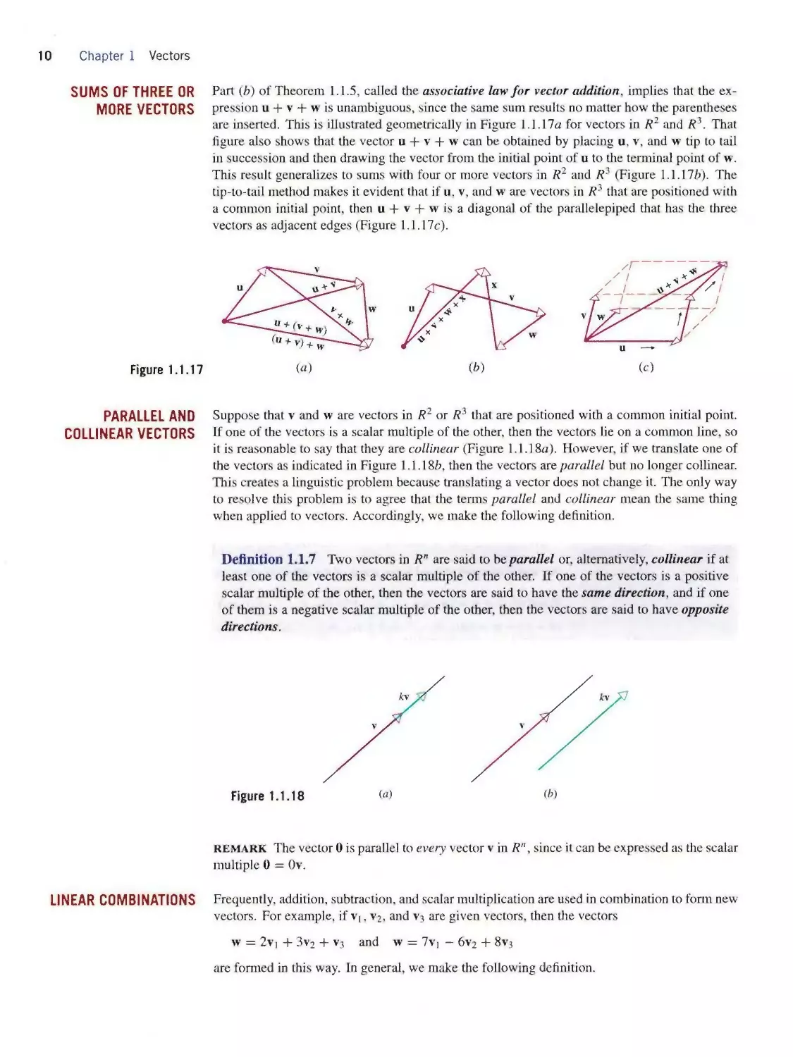
APPLICATION TO
COMPUTER COLOR
MODELS
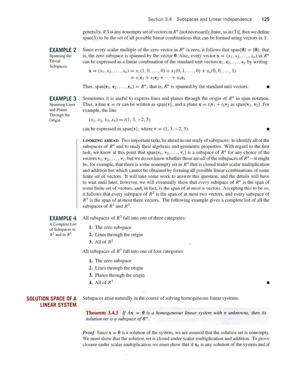
Colors on computer monitors are commonly based on what is called the RGB color model.
Colors in this system are created by adding together percentages of the primary colors red (R),
green (G), and blue (B). One way to do this is to identify the primary colors with the vectors
r = (1,0,0) (pure red), g = (0, 1,0) (pure green), b = (0, 0,1) (pure blue)
in Ri and to create all other colors by forming linear combinations of r, g, and b using coefficients
between 0 and 1, inclusive; these coefficients represent the percentage of each pure color in the
mix. The set of al 1 such color vectors is called RGB space or the RGB color cube (Figure 1.1.19).
Thus, each color vector c in this cube is expressible as a linear combination of the form
c = c∣r + c2g + c3b = c∣(l,0,0) + c2(0, 1,0) + c3(0,0, 1) = (c∣,c2, c3)
where 0 < c,∙ < 1. As indicated in the figure, the corners of the cube represent the pure primary
colors together with the colors, black, white, magenta, cyan, and yellow. The vectors along the
diagonal running from black to white correspond to shades of gray.
Figure 1.1.19
ALTERNATIVE
NOTATIONS FOR
VECTORS
Black
(0,0.0)
Magenta
(1.0, 1)
Cyan
(0, 1,1)
Green
(0.1,0)
White
(1,1,1)
Red £
(∣.0,0)
Yellow
(1, 1,0)
Up to now we have been writing vectors in R" using the notation
v = (υι,υ2 v„)
(15)
We call this the comma-delimited form. However, a vector in R" is essentially just a list of
n numbers (the components) in a definite order, so any notation that displays the components
of the vector in their correct order is a valid alternative to the comma-delimited notation. For
example, the vector in (15) might be written as
v = [υ∣ υ2 ■■■ υπ]
(16)
which is called row-vector form, or as
(17)
which is called column-vector form. The choice of notation is often a matter of taste or conve¬
nience, but sometimes the nature of the problem under consideration will suggest a particular
notation. All three notations will be used in this text.
12 Chapter 1 Vectors
MATRICES Numerical information is often organized into tables called matrices (plural of matrix'). For
example, here is a matrix description of the number of hours a student spent on homework in
four subjects over a certain one-week period:
Math
English
Chemistry
Physics
Monday
Tuesday
Wednesday
Thursday
Friday
Saturday
Sunday
2
1
2
0
3
0
1
2
0
1
3
1
0
I
1
3
0
0
1
0
1
1
2
4
1
0
0
2
Linear Algebra in History
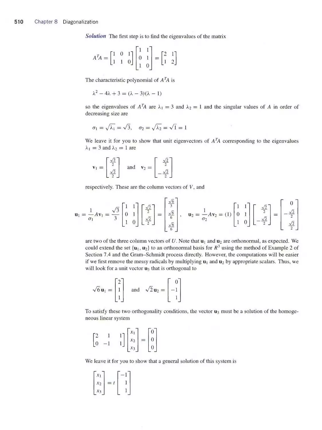
The theory of graphs originated with the Swiss mathematician
Leonhard Euler, who developed the ideas to solve a problem that
was posed to him in the mid 1700s by the citizens of the Prussian
city of Kδnigsberg (now Kaliningrad in Russia). The city is cut
by the Pregel River, which encloses an island, as shown in the
accompanying old lithograph.
The problem was to determine whether it was possible to start at
any point on the shore of the river, or on the island, and walk over
all of the bridges, once and only once, returning to the starting spot.
In 1736 Euler showed that the walk was impossible by analyzing
the graph.
Leonhard Euler
(1707-1783)
If we suppress the headings, then the numerical data that
remain form a matrix with four rows and seven columns:
-2 1 2 0 3 θΓ
2 0 13 10 1
13 0 0 10 1 (18)
1 2 4 10 0 2
To formalize this idea, we define a matrix to be a rect¬
angular array of numbers, called the entries of the matrix.
If a matrix has m rows and n columns, then it is said to have
size m × n, where the number of rows is always written
first. Thus, for example, the matrix in (18) has size 4 × 7.
A matrix with one row is called a row vector, and a matrix
with one column is called a column vector [see (16) and
(17), for example]. You can also think of a matrix as a
list of row vectors or column vectors. For example, the
matrix in (18) can be viewed as a list of four row vectors
in R7 or as a list of seven column vectors in R4.
In addition to describing tabular information, matrices
are useful for describing connections between objects, say
connections between cities by airline routes, connections
between people in social structures, or connections be¬
tween elements in an electrical circuit. The idea is to
represent the objects being connected as points, called
vertices, and to indicate connections between vertices by
line segments or arcs, called edges. The vertices and edges
form what is called a connectivity graph or, more simply,
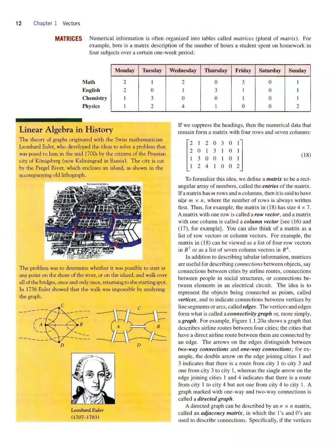
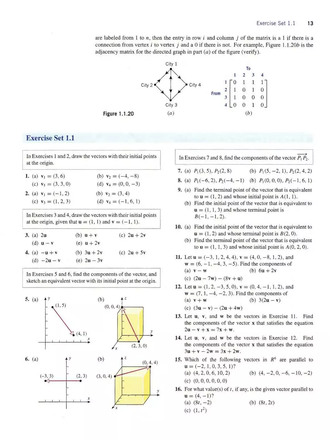
a graph. For example, Figure 1.1.20α shows a graph that
describes airline routes between four cities; the cities that
have a direct airline route between them are connected by
an edge. The arrows on the edges distinguish between
two-way connections and one-way connections’, for ex¬
ample. the double arrow on the edge joining cities 1 and
3 indicates that there is a route from city 1 to city 3 and
one from city 3 to city 1, whereas the single arrow on the
edge joining cities 1 and 4 indicates that there is a route
from city 1 to city 4 but not one from city 4 to city 1. A
graph marked with one-way and two-way connections is
called a directed graph.
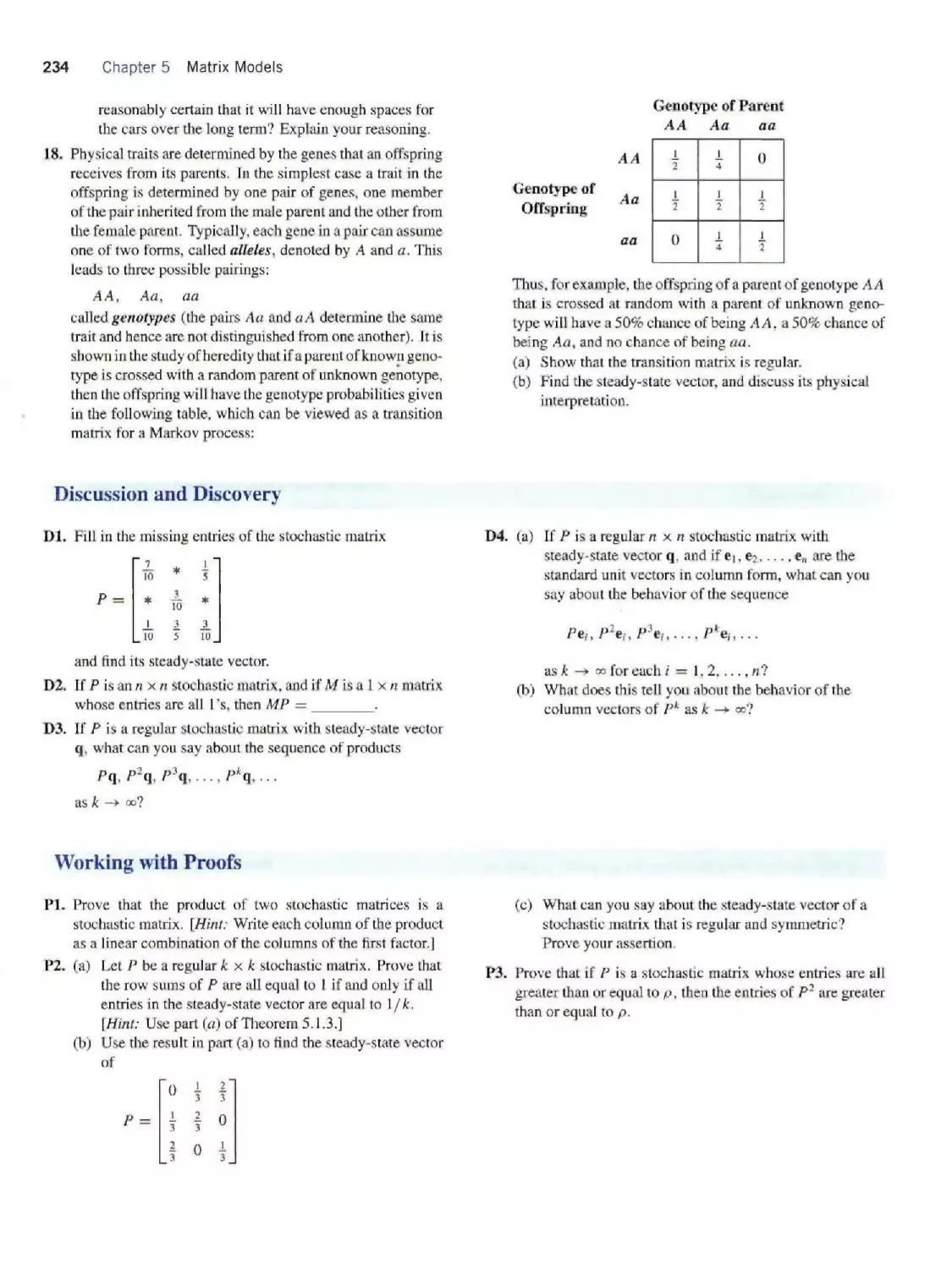
A directed graph can be described by an n × n matrix,
called an adjacency matrix, in which the 1 ,s and 0’s are
used to describe connections. Specifically, if the vertices
Exercise Set 1.1 13
are labeled from 1 to n, then the entry in row i and column j of the matrix is a 1 if there is a
connection from vertex i to vertex j and a 0 if there is not. For example, Figure 1.1.20b is the
adjacency matrix for the directed graph in part (a) of the figure (verify).
Figure 1.1.20
To
12 3 4
1
"0111"
2
From
10 10
3
10 0 0
4
.0010.
(⅛)
Exercise Set 1.1
In Exercises 1 and 2, draw the vectors with their initial points
at the origin.
1. (a) v1 = (3, 6)
(c) v3 = (3, 3,0)
2. (a) v1 =(-1,2)
(c) v3 = (1,2, 3)
(b) v2 = (-4, -8)
(d) v4 = (0,0,-3)
(b) v2 = (3,4)
(d) v4 = (-1,6,1)
In Exercises 3 and 4, draw the vectors with their initial points
at the origin, given that u = (1,1) and v = (—1,1).
3. (a) 2u
(b)
u + V
(c) 2u + 2v
(d) u - v
(e)
u + 2v
4. (a) —u + v
(b)
3u + 2v
(c) 2u + 5v
(d) —2u — v
(e)
2u-3v
In Exercises 5 and 6, find the components of the vector, and
sketch an equivalent vector with its initial point at the origin.
In Exercises 7 and 8, find the components of the vector Pl P2.
7. (a) P1(3,5), P2(2,8) (b) P1(5,-2,1), P2(2,4.2)
8. (a) P1(-6,2), P2(-4, —1) (b) P1(0,0.0). P2(-l, 6,1)
9. (a) Find the terminal point of the vector that is equivalent
to u = (1, 2) and whose initial point is Λ(l, 1).
(b) Find the initial point of the vector that is equivalent to
u = (1, 1, 3) and whose terminal point is
B(-l,-l,2).
10. (a) Find the initial point of the vector that is equivalent to
u = (1,2) and whose terminal point is B(2,0).
(b) Find the terminal point of the vector that is equivalent
to u = (1,1, 3) and whose initial point is A(0, 2,0).
11. Let u = (-3, 1,2,4,4), v = (4, 0, -8,1,2), and
w = (6, — 1, —4, 3, —5). Find the components of
(a) v — w (b) 6u + 2v
(c) (2u - 7w) - (8v + u)
12. Let u = (1,2,-3,5,0), v = (0,4, -1,1,2), and
w = (7,1, —4, —2, 3). Find the components of
(a) v + w (b) 3(2u - v)
(c) (3u — v) — (2u + 4w)
13. Let u, v, and w be the vectors in Exercise 11. Find
the components of the vector x that satisfies the equation
2u — v + x = 7x + w.
14. Let u, v, and w be the vectors in Exercise 12. Find
the components of the vector x that satisfies the equation
3u + v - 2w = 3x + 2w.
15. Which of the following vectors in R6 are parallel to
u = (-2, 1,0, 3,5,1)?
(a) (4, 2,0,6, 10,2) (b) (4, -2,0, -6, -10, -2)
(c) (0,0,0,0,0,0)
16. For what value(s) oft, if any, is the given vector parallel to
u = (4,-1)?
(a)(8t.-2) (b) (8r.2t)
(c) (I,?)
14 Chapter 1 Vectors
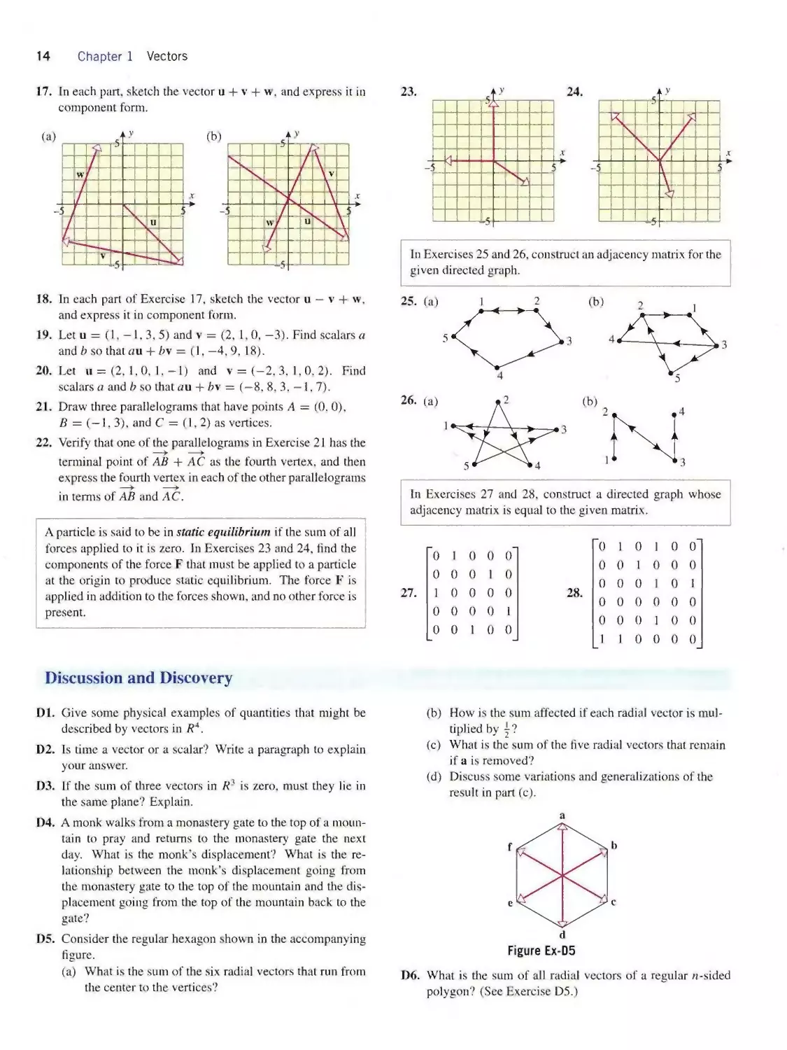
17. In each part, sketch the vector u + v + w. and express it in
component form.
18. In each part of Exercise 17, sketch the vector u — v + w.
and express it in component form.
19. Let u = (I, —1,3, 5) and v = (2, 1,0, —3). Find scalars a
and b so that αu + bv = (1, —4,9, 18).
20. Let u = (2, 1,0, 1, — 1) and v = (—2. 3. 1,0. 2). Find
scalars a and b so that «u + bv = (—8.8,3, — 1,7).
21. Draw three parallelograms that have points A = (0, 0),
B = (— 1,3), and C = (1,2) as vertices.
22. Verify that one of the parallelograms in Exercise 21 has the
terminal point of AB + AC as the fourth vertex, and then
express the fourth vertex in each of the other parallelograms
in terms of AB and AC.
In Exercises 25 and 26, construct an adjacency matrix for the
given directed graph.
In Exercises 27 and 28, construct a directed graph whose
adjacency matrix is equal to the given matrix.
A particle is said to be in static equilibrium if the sum of all
forces applied to it is zero. In Exercises 23 and 24. find the
components of the force F that must be applied to a particle
at the origin to produce static equilibrium. The force F is
applied in addition to the forces shown, and no other force is
present.
28.
0 1 0
0 0 1
0 0 0
0 0 0
0 0 0
1 0
1
0
1
0
1
0
0 0
0 0
0 1
0 0
0 0
0 0
Discussion and Discovery
Dl. Give some physical examples of quantities that might be
described by vectors in Λ4.
D2. Is time a vector or a scalar? Write a paragraph to explain
your answer.
D3. If the sum of three vectors in Ri is zero, must they lie in
the same plane? Explain.
D4. A monk walks from a monastery gate to the top of a moun¬
tain to pray and returns to the monastery gate the next
day. What is the monk’s displacement? What is the re¬
lationship between the monk’s displacement going from
the monastery gate to the top of the mountain and the dis¬
placement going from the top of the mountain back to the
gate?
D5. Consider the regular hexagon shown in the accompanying
figure.
(a) What is the sum of the six radial vectors that run from
the center to the vertices?
(b) How is the sum affected if each radial vector is mul¬
tiplied by |?
(c) What is the sum of the five radial vectors that remain
if a is removed?
(d) Discuss some variations and generalizations of the
result in part (c).
Figure Ex-D5
D6. What is the sum of all radial vectors of a regular -sided
polygon? (See Exercise D5.)
Section 1.2 Dot Product and Orthogonality 15
D7. Consider a clock with vectors drawn from the center to each
hour as shown in the accompanying figure.
(a) What is the sum of the 12 vectors that result if the
vector terminating at 12 is doubled in length and the
other vectors are left alone?
(b) What is the sum of the 12 vectors that result if the
vectors terminating at 3 and 9 are each tripled and the
others are left alone?
(c) What is the sum of the 9 vectors that remain if the
vectors terminating at 5, 11, and 8 are removed?
D8. Draw a picture that shows four nonzero vectors in the plane,
one of which is the sum of the other three.
D9. Indicate whether the statement is true (T) or false (F).
Justify your answer.
(a) If x + y = x + z, then y = z.
(b) If u + v = 0, then αu + ⅛v = 0 for all a and b.
(c) Parallel vectors with the same length are equal.
(d) If αx = 0, then either a = 0 or x = 0.
(e) If αu + bv = 0, then u and v are parallel vectors.
(f) The vectors u = (√2, √,3) and v = (-1=, ∣√3) are
equivalent.
Working with Proofs
Pl. Prove part (e) of Theorem 1.1.5.
P2. Prove part (/) of Theorem 1.1.5.
P3. Prove Theorem 1.1.6 without using components.
Technology Exercises
Tl. (.Numbers and numerical operations) Read how to enter
integers, fractions, decimals, and irrational numbers such
as π and √2. Check your understanding of the procedures
by converting π, ∙fl, and 1 /3 to decimal form with various
numbers of decimal places in the display. Read about the
procedures for performing the operations of addition, sub¬
traction, multiplication, division, raising numbers to pow¬
ers, and extraction of roots. Experiment with numbers of
your own choosing until you feel you have mastered the
techniques.
T2. (Drawing vectors) Read how to draw line segments in two-
or three-dimensional space, and draw some line segments
with initial and terminal points of your choice. If your util¬
ity allows you to create arrowheads, then you can make your
line segments look like geometric vectors.
T3. (Operations on vectors) Read how to enter vectors and how
to calculate their sums, differences, and scalar multiples.
Check your understanding of these operations by perform¬
ing the calculations in Example 4.
T4. Use your technology utility to compute the components of
u = (7.1, —3)—5(√z2, 6) + 3(0. π) to five decimal places.
Section 1.2 Dot Product and Orthogonality
In this section we will be concenιed with the concepts of length, angle, distance, and perpen¬
dicularity in R". We will begin by discussing these concepts geometrically in R2 and R3, and
then we will extend them algebraically to R" using components.
NORM OF A VECTOR The length of a vector v in R2 or R3 is commonly denoted by the symbol ∣∣v∣∣. It follows from
the theorem of Pythagoras that the length of a vector v = (υ∣, υf) in R2 is given by the formula
∣∣v∣∣ = ∖∕υ2i +υl
(1)
16 Chapter 1 Vectors
(Figure 1.2.1α). A companion formula for the length of a vector v = (v1, υ2. υ3) in R3 can be
obtained using two applications of the theorem of Pythagoras (Figure 1.2.1⅛)r
∣∣v∣∣2 = (OR)2 + (RP)2 = (OQ)2 + (QR)2 + (RP)2 = υ2 + υ2 + υ2
Thus,
II v ∣∣ = √υ2 + υ2 + υ2 (2)
Figure 1.2.1
Motivated by Formulas (1) and (2), we make the following general definition for the length
of a vector in R".
EXAMPLE 1
Calculating
Norms
UNIT VECTORS
Definition 1.2.1 If v = (υι, υ2,..., vn) is a vector in R", then the length of v, also called
the norm of v or the magnitude of v, is denoted by ∣∣v∣∣ and is defined by the formula
∣∣v∣∣ = √vj + υ2 + υ3 +∙∙∙ + vn (3)
From (3), the norm of the vector v = (—3, 2, 1) in R3 is
∣∣v∣∣ = √(-3)2 + 22 + 12 = √14
and the norm of the vector v = (2, — 1,3, —5) in ∕f4 is
∣∣v∣∣ = √22 + (-l)2 + 32 + (-5)2 = √39 ■
Since lengths in R2 and R3 are nonnegative numbers, and since 0 is the only vector that has
length zero, it follows that ∣∣v∣∣ > 0 and that ∣∣v∣∣ = 0 if and only if v = 0. Also, multiplying
v by a scalar k multiplies the length of v by ∣Λ∣, so ∣∣kv∣∣ = ∣fc∣ ∣∣v∣∣. We will leave it for you to
prove that these three properties also hold in R".
Theorem 1.2.2 Ifv is a vector in Rn, and if k is any scalar, then:
(a) ∣∣v∣∣>0
(b) ∣∣v∣∣ = 0 if and only if v = 0
(c) ll*v∣∣ = ∣*∣∣∣v∣∣
A vector of length 1 is called a unit vector. If v is a nonzero vector in R", then a unit vector u
that has the same direction as v is given by the formula
1
(4)
In words. Formula (4) states that a unit vector with the same direction as a vector v can be
obtained by multiplying v by the reciprocal of its length. This process is called normalizing v.
The vector u has the same direction as v since l∕∣∣v∣∣ is a positive scalar; and it has length 1
since part (c) of Theorem 1.2.2 with k = l∕∣∣v∣∣ yields
∣∣u∣∣ = ∣∣*v∣∣ = ∣*∣∣∣v∣∣ =*∣∣v∣∣ = ^∣∣v∣∣ = 1
1
Section 1.2 Dot Product and Orthogonality 17
Sometimes you will see Formula (4) expressed as
v
u =
I∣V∣∣
This is just a more compact way of writing the scalar product in (4).
EXAMPLE 2
Normalizing a
Vector
THE STANDARD UNIT
VECTORS
.<y
4(0.1)
Find die unit vector u that has the same direction as v = (2, 2, — 1).
Solution The vector v has length
∣∣v∣∣ = √22 + 22 + (-l)2 = 3
Thus, from (4)
u = ∣(2,2,-l) = (<.f,-∣)
As a check, you may want to confirm that u is in fact a unit vector.
concept problem Unit vectors are often used to specify directions in 2-space or 3-space.
Find a unit vector that describes the direction that a bug would travel if it walked from the origin
of an xy-coordinate system into the first quadrant along a line that makes an angle of 30o with
the positive x-axis. Also, find a unit vector that describes the direction that the bug would travel
if it walked into the third quadrant along the line.
When a rectangular coordinate system is introduced in R2 or R3, the unit vectors in the positive
directions of the coordinate axes are called the standard unit vectors. In R2 these vectors are
denoted by
i = (1,0) and j = (0,1) (5)
and in Ri they are denoted by
i = (1,0,0), j = (0, 1,0), and k = (0,0,1) (6)
(Figure 1.2.2).
Observe that every vector v = (ιη, υ2) in R2 can be expressed in terms of the standard unit
vectors as
v = (υ∣, υ2) = υι(l,0) + υ2(0, 1) = υ∣i + υ2j
and every vector v = (υ1, υ2, υ3) in Ri can be expressed in terms of the standard unit vectors as
v = (vι, υ2, V3) = υι(l, 0,0) + υ2(0,1,0) + υ3(0,0, 1) = υ∣i + υ2j + υ3k
For example,
(2, -3,4) = 2i - 3j + 4k
remark The i, j, k notation for vectors in R2 and Ri is common in engineering and physics,
but it will be used only occasionally in this text.
More generally, we define the standard unit vectors in R" to be
e, =(1,0,0 0), e2 = (0,1,0,...,0) e„ = (0,0,0,.... 1) (7)
We leave it for you to verify that every vector v = (υ1, υ2 υn) in R" can be expressed in
terms of the standard unit vectors as
v = (υ∣, υ2,..., υn) = υle1 + υ2e2 d + υπe,,
(8)
DISTANCE BETWEEN If Pl and P2 are points in R2 or Ri, then the length of the vector P∣ P2 is equal to the distance
POINTS IN Rπ d between the two points (Figure 1.2.3). Specifically, if P∣(x∣, yι) and P2(x2, y2) are points in
18 Chapter 1 Vectors
DOT PRODUCTS
EXAMPLE 3
An Application
of Dot Products
to ISBNs
R2, then Theorem 1.1.1 (a) implies that
d = l∣7w¾ll = √(χ2-χt)2 + (y2-y1)2
(9)
This is the familiar distance formula from analytic geometry. Similarly, the distance between
the points P∖ (x∣, yι, zι) and P2(x2, y2, z2) i∏ 3-space is
√(u. v) = ∣∣p[λ∣I = √ (χ2 - *ι)2 + (y2 - y∣)2 + (z2 - zι)2 (10)
Motivated by Formulas (9) and (10), we make the following definition.
Definition 1.2.3 If u = («1, «2 un) and v = (»i, t⅛,..., υn) are points in R", then
we denote the distance between u and v by d(u. v) and define it to be
<Z(u, v) = ∣∣u - v∣∣ = √(mi - υι)2 + (u2 - t>2)2 + ∙∙∙ + (wn - υ,,)2 (11)
For example, if
u = (1, 3,-2,7) and v = (0,7, 2,2)
then the distance between u and v is
<∕(u. v) = √( 1 - 0)2 + (3- 7)2 + (—2 - 2)2 + (7- 2)2 = √58
We leave it for you to use Formula (11) to show that distances in R" have the following
properties.
Theorem 1.2.4 If∖ι and v are points in Rn, then:
(a) J(u, v) > 0
(b) rf(u, v) = 0 if and only ifu = v
(c) J(u, v) = <∕(v. u)
This theorem states that distances in R" behave like distances in visible space; that is, distances
are nonnegative numbers, the distance between distinct points is nonzero, and the distance is the
same whether you measure from u to v or from v to u.
We will now define a new kind of multiplication that will be useful for finding angles between
vectors and determining whether two vectors are perpendicular.
Definition 1.2.5 If u = (wι,u2, ∙∙∙,un') and v = (ι>ι, t⅛,..., υn) are vectors in Rn, then
the dot product of u and v, also called the Euclidean inner product of u and v, is denoted
by u ∙ v and is defined by the formula
u∙v = wιυ1 + u2v2-∖ Fwb⅛ (12)
In words, the dot product is calculated by multiplying corresponding components of the vectors
and adding the resulting products. For example, the dot product of the vectors u = (-1,3,5,7)
and v = (5, —4, 7,0) in R4 is
u ■ v = (-1)(5) + (3)(-4) + (5)(7) + (7)(0) = 18
remark Note the distinction between scalar multiplication and dot products—in scalar mul¬
tiplication one factor is a scalar, the other is a vector, and the result is a vector; and in a dot
product both factors are vectors and the result is a scalar.
Most books published in the last 25 years have been assigned a unique 10-digit number called
an International Standard Book Number or ISBN. The first nine digits of this number are split
into three groups—the first group representing the country or group of countries in which the
book originates, the second identifying the publisher, and the third assigned to the book title
Section 1.2 Dot Product and Orthogonality 19
Linear Algebra in History
The dot product notation was first in¬
troduced by the American physicist and
mathematician J. Willard Gibbs in a pam¬
phlet distributed to his students at Yale
University in the 1880s. The product was
originally written on the baseline, rather
than centered as today, and was referred
to as the direct product. Gibbs’s pamphlet
was eventually incorporated into a book
entitled Vector Analysis that was published
in 1901 and coauthored by Gibbs and one
of his students. Gibbs made major con¬
tributions to the fields of thermodynamics
and electromagnetic theory and is generally
regarded as the greatest American physicist
of the nineteenth century.
Josiah Willard Qibbs
(1839-1903)
itself. The tenth and final digit, called a check digit, is computed from the first
nine digits and is used to ensure that an electronic transmission of the ISBN, say
over the Internet, occurs without error.
To explain how this is done, regard the first nine digits of the ISBN as a vector
b in R9. and let a be the vector
a = (1,2,3,4,5, 6,7, 8,9)
Then the check digit c is computed using the following procedure:
1. Form the dot product a ∙ b.
2. Divide a ∙ b by 11, thereby producing a remainder c that is an integer
between 0 and 10, inclusive. The check digit is taken to be c, with the
proviso that c = 10 is written as X to avoid double digits.
For example, the ISBN of the brief edition of Calculus, sixth edition, by Howard
Anton is
0-471-15307-9
which has a check digit of 9. This is consistent with the first nine digits of the
ISBN, since
a∙b = (1,2,3,4.5,6,7,8,9).(0.4,7,1,1,5,3,0,7)= 152
Dividing 152 by 11 produces a quotient of 13 and a remainder of 9, so the check
digit is c = 9. If an electronic order is placed for a book with a certain ISBN,
then the warehouse can use the above procedure to verify that the check digit is
consistent with the first nine digits, thereby reducing the possibility of a costly
shipping error. ■
ALGEBRAIC PROPERTIES
OF THE DOT PRODUCT
In the special case where u = v in Definition 1.2.5, we obtain the relationship
v∙v = υ2 + υ∣-F∙∙∙ + υ2 = ∣∣v∣∣2 (13)
This yields the following formula for expressing the length of a vector in terms of a dot product:
l∣v∣∣=√7TV (14)
Dot products have many of the same algebraic properties as products of real numbers.
Theorem 1.2.6 If u, v, and w are vectors in Rn, and if k is a scalar, then:
(a) u ∙ V = V ∙ U [Symmetry property]
(Z>) u∙(v-Fw) = u∙v-Fu∙w [Distributiveproperty)
(c) k(u ∙ v) = (fell) ∙ V [Homogeneity property]
(d) v ∙ v > 0 and v ∙ v = 0 if and only ifv = 0 [Positivity property]
We will prove parts (c) and (d) and leave the other proofs as exercises.
Proof (c) Let u = («i, u2, ■, u,∣) and v = (υ∣, V2...., υ∏). Then
A-(u ∙ v) = k(u∖V∖ + U2V2 4 Funυn) = (kul)vl + (ku2)v2 -I 1- (kun)υn = (A-u) ∙ v
Proofed) The result follows from parts (a) and (⅛) of Theorem 1.2.2 and the fact that
v ∙ v = υl υ∣ + υ2υ2 -I F υπυ,, = υf + υj 4 F υ2 = ∣∣v∣∣2
20 Chapter 1 Vectors
The following theorem gives some more properties of dot products. The results in this
theorem can be proved either by expressing the vectors in terms of components or by using the
algebraic properties already established in Theorem 1.2.6.
Theorem 1.2.7 lfu, v, and w are vectors in Rn, and ifk is a scalar, then:
(a) 0 ∙ v = v ∙ 0 = 0
(b) (u + v) ∙ w = u ∙ w + v ∙ w
(c) u∙(v - w) = u∙v-u∙w
(r∕) (u — v) ∙ w = u ∙ w — v ∙ w
(e) k(u ∙ v) = u ∙ (kv)
We will show how Theorem 1.2.6 can be used to prove part (b) without breaking the vectors
down into components. Some of the other proofs are left as exercises.
Proof (⅛)
(u + v) ∙ w = w ∙ (u + v)
= w ∙ u + w ∙ v
= u ∙ w + v ∙ w
[By symmetry]
[By distributivity∣
[By symmetry]
■
Formulas (13) and (14) together with Theorems 1.2.6 and 1.2.7 make it possible to manipulate
expressions involving dot products using familiar algebraic techniques.
EXAMPLE 4
Calculating
with Dot
Products
ANGLE BETWEEN
VECTORS IN R2 AND R3
Figure 1.2.4
(u - 2v) ∙ (3u + 4v) = u ∙ (3u + 4v) - 2v ∙ (3u + 4v)
= 3(u ∙ u) + 4(u ∙ v) — 6(v ∙ u) — 8(v ∙ v)
= 3∣∣u∣∣2 - 2(u ∙ v) - 8∣∣v∣∣2 ■
To see how dot products can be used to calculate angles between vectors in R2 and R3, let u
and v be nonzero vectors in R2 or R3, and define the angle between u and v to be the smallest
nonnegative angle θ through which one of the vectors can be rotated in the plane of the vectors
until it coincides with the other (Figure 1.2.4). Algebraically, the radian measure of θ is in the
interval 0 < θ < π, and in R2 the angle θ is generated by a counterclockwise rotation.
The following theorem provides an effective way to calculate the angle between vectors in
both R2 and R3.
Theorem 1.2.8 If u and v are nonzero vectors in R2 or R3, and ifθ is the angle between
these vectors, then
"sβ^ii⅛i⅛ o'→λ"',* β=cos'1(ii⅛⅛) <15-,6>
Proof Suppose that the vectors u, v, and v — u are positioned to form the sides of a triangle, as
shown in Figure 1.2.5. It follows from the law of cosines that
∣∣v - u∣∣2 = ∣∣u∣∣2 + ∣∣v∣∣2 - 2∣∣u∣∣∣∣v∣∣ cos(9
(17)
Using Formula (13) and the properties of the dot product in Theorems 1.2.6 and 1.2.7, we can
rewrite the left side of this equation as
∣∣v - u∣∣2 = (v - u) ∙ (v - u)
= (v — u) ∙ V — (v — u) ∙ u
= v∙v - u∙v - v∙u + u∙u
= ∣∣v∣∣2 - 2u - v ÷ Hull2
Section 1.2 Dot Product and Orthogonality 21
EXAMPLE 5
An Application
of the Angle
Formula
Substituting the last expression in (17) yields
∣∣v∣∣2 - 2u ∙ v + ∣∣u∣∣2 = ∣∣u∣∣2 + ∣∣v∣∣2 - 2∣∣u∣∣ ∣∣v∣∣ cost?
which we can simplify and rewrite as
u ∙ v = ∣∣u∣∣∣∣v∣∣ cos#
Finally, dividing both sides of this equation by ∣∣u∣∣ ∣∣v∣∣ yields (15).
If u and v are nonzero vectors in R2 or R3 and u ∙ v = 0, then it follows from Formula (16)
that θ = cos-1 0 = π∕2. Conversely, if θ = π∕2, then cos# = 0 and u ∙ v = 0. Thus, two
nonzero vectors in R2 or Ri are perpendicular if and only if their dot product is zero.
CONCEPT PROBLEM What can you say about the angle between the nonzero vectors u and v
in R2 or R3 if u ∙ v > 0? What if u ∙ v < 0?
Find the angle # between a diagonal of a cube and one of its edges.
Solution Assume that the cube has side a, and introduce a coordinate system as shown in
Figure 1.2.6. In this coordinate system the vector
d = (a, a, a)
is a diagonal of the cube, and the vectors v∣ = (a, 0.0), V2 = (0, a, 0), and v3 = (0,0, a)
run along the edges. By symmetry, the diagonal makes the same angle with each edge, so it is
sufficient to find the angle between d and v∣. From Formula (15), the cosine of this angle is
V] ∙ d α2 1
l∣v∣∣∣∣∣d∣∣ a(Jla2) √3
Thus, with the help of a calculating utility,
# = cos-1 ≈ 54.7o
EXAMPLE 6
Find a nonzero vector in R2 that is perpendicular to the nonzero vector v = (a, b).
Finding a
Vector in R2
That Is
Perpendicular
to a Given
Vector
Solution We are looking for a nonzero vector u for which u ∙ v = 0. By experimentation,
u = (-b, a) is such a vector, since
u ∙ v = (—b, a) ∙ (a, b) = —ha +ab = 0
The vector — u = (⅛, — a) is also perpendicular to v, as is any scalar multiple of u (Figure 1.2.7).
22 Chapter 1 Vectors
ORTHOGONALITY
EXAMPLE 7
An Orthogonal
Set of Vectors
in Ri
EXAMPLE 8
The Zero Vector
Is Orthogonal
to Rn
ORTHONORMAL SETS
To generalize the notion of perpendicularity to R" we make the following definition.
Definition 1.2.9 Two vectors u and v in R" are said to be orthogonal if u ∙ v = 0, and a
nonempty set of vectors in Rn is said to be an orthogonal set if each pair of distinct vectors
in the set is orthogonal.
remark Note that we do not require u and v to be nonzero in this definition: thus, two vectors
in R2 and Ri are orthogonal if and only if they are either nonzero and perpendicular or if one or
both of them are zero.
Show that the vectors
v∣ = (1,2,2,4), v2 = (-2, 1,-4,2), v3 = (-4, 2, 2,-1)
form an orthogonal set in R4.
Solution Because of the symmetry property of the dot product, we need only confirm that
v∣ ∙ v2 = 0, v∣ ∙ v3 = 0, v2 ∙ v3 = 0
We leave the computations to you. ■
If S is a nonempty set of vectors in R", and if v is orthogonal to every vector in S, then we
say that v is orthogonal to the set S. For example, the vector k = (0. 0, 1) in /?3 is orthogonal
to the xy-plane (Figure 1.2.2⅛).
Part (a) of Theorem 1.2.7 states that if 0 is the zero vector in R", then 0 ∙ v = 0 for every vector
v in Rn. Thus, 0 is orthogonal to Rn. Moreover, 0 is the only vector in R" that is orthogonal to
Rn, since if v is a vector in Rn that is orthogonal to Rn, then, in particular, it would be true that
v ∙ v = 0; this implies that v = 0 by part (<∕) of Theorem 1.2.6. ■
remark Although the result in Example 8 may seem obvious, it will prove to be useful later
in the text, since it provides a way of using the dot product to show that a vector w in R" is the
zero vector—just show that w ∙ v = 0 for every vector v in R".
Orthogonal sets of unit vectors have special importance, and there is some terminology associated
with them.
Definition 1.2.10 Two vectors u and v in Rn are said to be orthonormal if they are orthog¬
onal and have length 1, and a set of vectors is said to be an orthonormal set if every vector
in the set has length 1 and each pair of distinct vectors is orthogonal.
EXAMPLE 9
The Standard
Unit Vectors in
R" Are
Orthonormal
The standard unit vectors in R2 and R2 form orthonormal sets, since these vectors have length
1 and run along the coordinate axes of rectangular coordinate systems (Figure 1.2.2). More
generally, the standard unit vectors
e∣ = (1,0,0, ...,0), e2 = (0, 1,0 0) e,, = (0,0,0 1)
in R" form an orthonormal set, since
e, ∙ey =0 iff ≠ j and l∣ej ∣∣ = ∣∣e2∣∣ = ∙ ∙ ∙ = ∣∣e,,∣∣ = 1
(verify).
In the following example we form an orthonormal set of three vectors in R4.
EXAMPLE 10
An Orthonormal
Set in Ri
The vectors
Section 1.2 Dot Product and Orthogonality 23
form an orthonormal set in R∖ since
llql∣l = l∣q2∣l = llq3∣l = 1
and
q∣∙q2=0. q∣∙q3=0, q3 ∙ q3 = 0
(verify).
EUCLIDEAN GEOMETRY
IN Rn
Formulas (3) and (11) are sometimes called the Euclidean norm and Euclidean distance because
they produce theorems in R" that reduce to theorems in Euclidean geometry when applied in
R2 and Ri. Here are just three examples:
1. In a right triangle, the square of the hypotenuse is equal to the sum of the squares of the
other two sides (theorem of Pythagoras).
2. The sum of the lengths of two sides of a triangle is at least as large as the length of the
third side.
3. The shortest distance between two points is along a straight line.
To extend these theorems to R", we need to state them in vector form. For example, a right
triangle in R2 or R} can be constructed by placing orthogonal vectors u and v tip to tail and using
the vector u + v as the hypotenuse (Figure 1.2.8). In vector notation, the theorem of Pythagoras
now takes the form
∣∣u + v∣∣2 = ∣∣u∣∣2 + ∣∣v∣∣2
The following theorem is the extension of this result to R".
Theorem 1.2.11 (Theorem of Pythagoras) Ifu and v are orthogonal vectors in R", then
(18)
Proof
Linear Algebra in History
The Cauchy-Schwarz inequality is named in honor of the French
mathematician Augustin Cauchy and the German mathematician
Hermann Schwarz. Variations of this inequality occur in many
different settings and under various names. Depending on the
context in which the inequality occurs, you may find it called
Cauchy’s inequality, the Schwarz inequality, or sometimes even the
Bunyakovsky inequality, in recognition of the Russian mathemati¬
cian who published his version of the inequality in 1859, about 25
years before Schwarz.
∣∣u + v∣∣2 = (u + v) ∙ (u + v)
= ∣∣u∣∣2 ÷ 2(u - v) ÷ ∣∣v∣∣2
= l∣u∣∣2 + ∣∣v∣∣2 ■
We have seen that the angle between nonzero vectors
in R2 and Ri is given by the formula
(19)
Augustin Louis
Cauchy
(1789-1857)
Hermann Amandus
Schwarz
(1843-1921)
Viktor Yakovlevich
Bunyakovsky
(1804-1889)
Since this formula involves only the dot product and norms
of the vectors u and v, and since the notions of dot prod¬
uct and norm are applicable to vectors in R", it seems
reasonable to use Formula (19) as the definition of the an¬
gle between nonzero vectors u and v in R". However, this
plan would only work if it were true that
u ∙ v
< 1
(20)
for all nonzero vectors in R". The following theorem gives
a result, called the Cauchy-Schwarz inequality, which
will show that (20) does in fact hold for all nonzero vectors
in R".
24 Chapter 1 Vectors
Theorem 1.2.12 (Cauchy-Schwarz Inequality in R") If∖ι and v are vectors in R", then
(u ∙ v)2 < ∣∣u∣∣2∣∣v∣∣2 (21)
or equivalently (by taking square roots),
∣u∙v∣<∣∣u∣∣∣∣v∣∣ (22)
Proof Observe first that if u = 0 or v = 0, then both sides of (21) are zero (verify), so equality
holds in this case. Now consider the case where u and v are nonzero. As suggested by Fig¬
ure 1.2.9, the vector v can be written as the sum of some scalar multiple of u. say ku, and a vector
w that is orthogonal to u. The appropriate scalar k can be computed by setting w = v — A∙u and
using the orthogonality condition u ∙ w = 0 to write
0 = u∙w = u∙(v- ku) = (u ∙ v) — ⅛(u ∙ u)
from which it follows that
k U V
11 ∙ u
Now apply the theorem of Pythagoras to the vectors in Figure 1.2.9 to obtain
∣∣v∣∣2= ∣∣A-u∣∣2 + ∣∣w∣∣2 = λr2∣∣u∣∣2 + ∣∣w∣∣2
(23)
(24)
Substituting (23) for⅛ and multiplying both sides of the resulting equation by ∣∣u∣∣2 yields (verify)
∣∣u∣∣2∣∣v∣∣2 = (u ∙ v)2 + ∣∣u∣∣2∣∣w∣∣2
(25)
Since ∣∣u∣∣2∣∣w∣∣2 > 0, it follows from (25) that
(u∙v)2≤ ∣∣u∣∣2∣∣v∣∣2
This establishes (21) and hence (22). ■
remark The Cauchy-Schwarz inequality now allows us to use Formula (19) as a definition
of the angle between nonzero vectors in R".
There is a theorem in plane geometry, called the triangle inequality, which states that the
sum of the lengths of two sides of a triangle is at least as large as the third side. The following
theorem is a generalization of that result to R', (Figure 1.2.10).
Theorem 1.2.13 (Triangle Inequality for Vectors) lfu, v, and w are vectors in Rn, then
l∣u + v∣∣ ≤ ∣∣u∣∣ + ∣∣v∣∣ (26)
Proof
∣∣u + v∣∣2 = (u + v) ∙ (u +v)
= ∣∣u∣∣2 + 2(u - v) + ∣∣v∣∣2
< ∣∣U∣∣2 + 2∣U ∙ V∣ + ∣∣ V ∣∣2 [Property of absolute value]
< ∣∣U∣∣2 + 2∣∣u∣∣∣∣V∣∣ + ∣∣V∣∣2 [Cauchy-Schwarzinequality]
= (l∣u∣∣ + ∣∣v∣∣)2
Formula (26) now follows by taking square roots. ■
There is a theorem in plane geometry which states that for any parallelogram the sum of the
squares of the lengths of the diagonals is equal to the sum of the squares of the lengths of the
four sides. The following theorem is a generalization of that result to R', (Figure 1.2.11).
Exercise Set 1.2 25
Theorem 1.2.14 (Parallelogram Equation for Vectors) If u and v are vectors in Rn, then
∣∣u + v∣[2 + ∣∣u - v∣∣2 = 2(∣∣uf∣1 ÷ ∣fv∣∣2)
(27)
Proof
∣∣u + v∣∣2 + ∣∣u - v∣∣2 s= (u ⅛ v) ■ (u ÷ v) + (u - V) ∙ (u - V)
= 2(u - u) ÷ 2(v ∙ v)
= 2(∣∣u∣∣2 + ∣∣v∣∣2)
Finally, let u and v be any two points in R2 or Ry. To say that the shortest distance from u
to v is along a straight line implies that if we choose a third point w in R2 or R∖ then
c∕(u, v) < d(u. w) -¼ <√(w, v)
(Figure 1.2.12). This is called the triangle inequality for distances. The following theorem is
the extension to Rn.
Theorem 1.2.15 (Triangle Inequality for Distances) Ifu, v, and w are points in Rn, then
d(u, v) ≤ J(u, w) + d(w, v)
(28)
Proof
rf(u,v)= ∣ju-v∣∣
= ∣[(u-w) + (w-v)∣∣
< ∣∣u - w∣∣ + ∣∣w - v∣∣
= d(u. w) +√(w. v)
[Add and subtract w.]
[Tria∏n∣e inequality for vectors]
[Definition of distance∣ ■
looking ahead The notions of length, angle, and distance in R" can all be expressed in
terms of the dot product (which, you may recall, is also called the Euclidean inner product):
√(u, v) = ∣∣u - v∣∣ = √(u - v) - (u - v)
(29)
(30)
(31)
Thus, it is the algebraic properties of the Euclidean inner product that ultimately determine the
geometric properties of vectors in R1'. However, the most important algebraic properties of
the Euclidean inner product can all be derived from the four properties in Theorem 1.2.6, so
this theorem is really the foundation on which the geometry of R" rests. Because R" with the
Euclidean inner product has so many of the familiar properties of Euclidean geometry, it is often
called Euclidean n-space or n-dimensional Euclidean space.
Exercise Set 1.2
In Exercises I and 2. find the norm of v, a unit vector that has
the same direction as v. and a unit vector that is oppositely
directed to v.
1, (a) v = (4, -3)
(¢) v = (1, 0.2.1,3)
2. (a) v = (-5. 12)
(c) v = (-2, 3, 3,-1)
(b) v = (2, 2, 2)
(b) v = (1,-1,2)
26 Chapter 1 Vectors
In Exercises 3 and 4, evaluate the given expression with
u = (2. —2, 3). v = (1, —3, 4), and w = (3, 6, —4).
3. (a) l∣u÷v∣∣
(c) ∣∣-2u + 2v∣∣
4. (a) ∣∣u ÷ v + w∣∣
(c) ∣∣3v∣∣ - 3∣∣v∣∣
(b) ∣∣u∣∣ + ∣∣v∣∣
(d) ∣∣3u-5v-f-w∣∣
(b) ∣∣u - v∣∣
(d) ∣∣u∣∣ - ∣∣v∣∣
17. Solve the equation 5x — 2v = 2(w — 5x) for x. given that
v = (1,2, -4, 0) and w = (—3. 5, I, 1).
18. Solve the equation 5x - ∣∣v∣∣v = ∣∣w∣∣(w — 5x) for x with v
and w being the vectors in Exercise 17.
In Exercises 19 and 20, determine whether the expression
makes sense mathematically. If not, explain why.
In Exercises 5 and 6, evaluate the given expression with
u = (-2.-1,4,5), v = (3, I, —5.7), and w = (—6.2.1,1).
5. (a) l∣3u - 5v + w∣∣ (b) ∣∣3u∣∣ - 5∣∣v∣∣ + ∣∣u∣∣
(c) ∣∣-∣∣u∣∣v∣∣
6. (a) ∣∣u∣∣-2∣∣v∣∣-3∣∣w∣∣ (b) ∣[u∣∣ + ∣∣-2v∣∣ + ∣∣-3w∣∣
(c) ∣∣∣∣u - v∣∣w∣∣
7. Let v = (—2, 3.0, 6). Find all scalars ½ such that ∣∣kv∣∣ = 5.
8. Let v = (1,1, 2, —3. 1). Find all scalars k such that
∣∣⅛v∣∣ = 4.
In Exercises 9 and 10, find u ♦ v, u ♦ u. and v ∙ v.
19. (a) u ∙ (v ■ w)
(c) ∣∣u∙v∣∣
20, (a) ∣∣u∣∣ ∙ ∣∣v∣∣
(c) (u ♦ v) - k
(b) u - (v + w)
(d) (u∙v)-∣∣u∣∣
(b) (u ∙ v) — w
(d) k ∙ u
In Exercises 21 and 22, verify that the Cauchy-Schwarz in¬
equality holds.
21. (a) u = (3, 2), v = (4,-1)
(b) u = (—3, 1,0), v = (2, —1,3)
(c) u= (0,2,2, 1), v = (1,1,1, 1)
22. (a) u= (4. I, I), v = (1, 2,3)
(b) u= (1.2, 1,2,3), v = (0,1,1,5.-2)
(c) u = (1,3,5,2.0. 1), v = (0,2,4, 1,3.5)
10. (a) u = (I. 1,-2,3), v = (-1,0,5,1)
(b) u = (2, -1, 1,0. -2). v = (1,2,2. 2, 1)
In Exercises 11 and 12, find the Euclidean distance between
u and v.
11. (a) u = (3, 3, 3), v = (1,0,4)
(b) u = (0, —2, -1, 1), v = (-3, 2, 4,4)
(c) u = (3,-3,-2,0,-3, 13.5),
v = (-4,1,-1,5,0,-11,4)
12. (a) u = (I, 2, -3, 0), v = (5, 1,2, -2)
(b) u = (2,-1,-4, 1,0,6,-3,1),
v = (-2, -1,0,3,7,2, -5, I)
(c) u = (0, I, 1. 1,2), v = (2,1,0,-1,3)
13. Find the cosine of the angle between the vectors in each part
of Exercise 11, and then state whether the angle is acute,
obtuse, or a right angle.
14. Find the cosine of the angle between the vectors in each part
of Exercise 12, and then state whether the angle is acute,
obtuse, or a right angle.
15. A vector a in the xy-plane has a length of 9 units and points
in a direction that is 120°, counterclockwise from the pos¬
itive Jt-axis, and a vector b in that plane has a length of 5
units and points in the positive ^-direction. Find a ∙ b.
16. A vector a in the xv-plane points in a direction that is 47°
counterclockwise from the positive x-axis, and a vector b
in that plane points in a direction that is 430 clockwise from
the positive x-axis. What can you say about the value of
a ∙ b?
In Exercises 23 and 24, show that the vectors form an or¬
thonormal set.
23∙ v, = (l.l.l.l).v2 = (l.4.l,l).
V3 = G’ I’ 6’ “I)’ V< = G’ 6∙-6∙ β)
24∙ v' = (-⅛∙⅛∙⅛)v≈ = (0∙-⅛.⅛)∙
v≈ = (⅛, ⅛∙ ⅛)
25. Find two unit vectors that are orthogonal to the nonzero
vector u = (a, ⅛).
26. For what values of A, if any, are u and v orthogonal?
(a) u= (2,it,⅛), v= (1,7,A)
(b) u = (⅛,⅛, 1), v= (⅛,5,6)
27. For which values of ⅛, if any, are u and v orthogonal?
(a) u= (Jt, 1,3), v = (1,7,Jt)
(b) u = (-2,fc,⅛), v = (fc,5,⅛)
28. Use vectors to find the cosines of the interior angles of the
triangle with vertices A(0, —1), B(l, -2), and C(4, 1).
29. Use vectors to show that A(3,0,2), B(4,3,0), and
C(8, I, — I) are vertices of a right triangle. At which vertex
is the right angle?
30. In each part determine whether the given number is a valid
ISBN by computing its check digit.
(a) 1-56592-170-7 (b) O-471-O5333-5
31. In each part determine whether the given number is a valid
ISBN by computing its check digit.
(a) 0-471-06368-1 (b) 0-13-947752-3
Exercise Set 1.2
27
It will be convenient to have a more compact way of writ¬
ing expressions such as x∣y1 + X2y2 + ∙∙∙ + xπyn and
x∣ +ij + ”■ + x2 that arise in working with vectors in
Rn. For this purpose we will use sigma notation (also called
summation notation), which uses the Greek letter Σ (capital
sigma) to indicate that a sum is to be formed. To illustrate
how the notation works, consider the sum
12 + 22 + 32 + 42 + 52
in which each term is of the form k2i where k is an integer
between 1 and 5, inclusive. This sum can be written in sigma
notation as
Σ>2
λ=l
This directs us to form the sum of the terms that result by
substituting successive integers for ⅛, starting with k = I
and ending w ith ⅛ = 5. In general, if f(k) is a function of k,
and if m and n are integers with am <n, then
n
52 f (⅛) = ∕("0 + /0« + 1) + ∙ ∙ ∙ + ∕(∏)
i=oι
This is the sum of the terms that result by substituting suc¬
cessive integers for k, starting with k = m and ending with
k = n. The number m is called the lower limit of summation,
the number n the upper limit of summation, and the letter k
the index of summation. It is not essential to use k as the
index of summation; any letter can be used, though we will
generally use i, j. or k. Thus,
n n 11
y.ali = E a< = ∑aj =«i +α2 + Fαtt
i=l i=l ∕=l
If u = (U],m2, ..., Mn) and v = (υ∣, υ2,..., υjl) are vectors
in R',, then the norm of u and the dot product of u and v can
be expressed in sigma notation as
IIUII = ∕w2+nl + ∙∙∙+w2
λ
U∙V = M∣U∣ +tt2V2 + '∙∙ + MπVn = 52
32. (Sigma notation) In each part, write the sum in sigma
notation.
(a) α∣⅛∣ + a2b2 + c∣3⅛3 + α4⅛4
(b) cf + c2 + cj + q + cj
(c) ⅛3 + ⅛4 + ∙ ∙ ∙ + bl,
33. (Sigma notation) Write Formula (11) in sigma notation.
34. (Sigma notation) In each part, evaluate the sum for
c∣ = 3, q = — 1, C3 = 5, c4 = —6. C5 = 4
d∖ = 6,4/2 = 0. </3 = 7, ⅛ = —2, ⅛ = —3
4 5
(a) 52 c* ÷ E ⅛⅛
fc=l k=2
5
<b) yt(2cj-dj)
J=1
5
(c) ∑(-1)¼
t=ι
35. (Sigma notation) In each part, confirm the statement by
writing out the sums on the two sides.
n n n
(a) 52(<⅛ ÷ bk) = e⅜ ÷ E⅛
t = l i≡l t=l
n n /1
(b) ∑(ak - bk) = Eα* ~ Σ6*
*≡l ⅛=1 *=1
n n
(c) 52cα*=c∑2α*
i=l *=1
Discussion and Discovery
Dl. Write a paragraph or two that explains some of the simi¬
larities and differences between visible space and higher¬
dimensional spaces. Include an explanation of why R" is
referred to as Euclidean space.
D2. What can you say about k and v if ∣∣⅛v∣∣ = ⅛∣∣v∣∣7
D3. (a) The set of all vectors in R2 that are orthogonal to a
nonzero vector is what kind of geometric object?
(b) The set of all vectors in Ri that are orthogonal to a
nonzero vector is what kind of geometric object?
(c) The set of all vectors in R2 that are orthogonal to
two noncollinear vectors is what kind of geometric
object?
(d) The set of all vectors in R ' that are orthogonal to
two noncollinear vectors is what kind of geometric
object?
D4. Show that v1 = (∣, ∣, ∣) and v2 = (∣. ∣. -1) are or¬
thonormal vectors, and find a third vector v3 for which
{v1, V2, v--,} is an orthonormal set.
D5. Something is wrong with one of the following expressions.
Which one is it, and what is wrong?
u ∙ (v + w), U ‘ v + u ■ w. (u ∙ v) ÷ w
D6. Let x — (x, y) and x0 = (λ⅛, y0). Write down an equality
or inequality involving norms that describes
(a) the circle of radius I centered at >⅛t
(b) the set of points inside the circle in part (a);
(e) the set of points outside the circle in part (a).
D7. If u and v are orthogonal vectors in R“ such that ∣∣u∣∣ = 1
and ∣∣v∣∣ = 1, then d(u. v) — . Draw a picture
to illustrate your result in R2.
28 Chapter 1 Vectors
D8. In each part, find ∣∣u∣∣ forn = 5, 10, and 100.
(a) u = (l,√2,√3,..∙,√n)
(b) u = (1,2, 3 n)
[Hint: There exist formulas for the sum of the first n pos¬
itive integers and the sum of the squares of the first n
positive integers. If you don't know those formulas, look
them up.]
D9. Indicate whether the statement is true (T) or false (F).
Justify your answer.
(a) If ∣∣u + v∣∣2 = ∣∣u∣∣2 + ∣∣v∣∣2, then u and v are
orthogonal.
(b) If u is orthogonal to v and w. then u is orthogonal to
V + w.
(c) If u is orthogonal to v + w. then u is orthogonal to v
and w.
(d) If a ■ b = a ∙ c and a ≠ 0, then b = c.
(e) If ∣∣u + v∣∣ = 0, then ιι = —v.
(f) Every orthonormal set of vectors in R', is also an
orthogonal set.
D10. Indicate whether the statement is true (T) or false (F).
Justify your answer.
(a) If ku = 0, then either k = 0 or u = 0.
(b) If two vectors u and v in R2 are orthogonal to a
nonzero vector w in R2, then u and v are scalar
multiples of one another.
(c) There is a vector u in Ri such that
∣∣u - (1. 1, 1)∣∣ < 3 and ∣∣u - (-1,-1, -1)∣∣ < 3.
(d) If u is a vector in R3 that is orthogonal to the vectors
(1, 0, 0), (0, 1, 0), and (0, 0, 1), then u = 0.
(e) If u ∙ v = 0 and v ∙ w = 0, then u ∙ w = 0.
(f) ∣∣u + v∣∣ = ∣∣u∣∣ + ∣∣v∣∣.
Working with Proofs
Pl. Prove that if u1, u2,..., u„ are pairwise orthogonal vectors
in R", then
∣∣u∣ +u2 + + u,,∣∣2 = ∣∣u,∣∣2 + ∣∣u2∣∣2 + ∙∙∙ + ∣∣u,,∣∣2
This generalizes Theorem 1.2.11 and hence is called the
generalized theorem of Pythagoras.
P2. (a) Use the Cauchy-Schwarz inequality to prove that if al
and α2 are nonnegative numbers, then
, “1 +«2
√O1O2 < 2—
The expression on the left side is called the geometric
mean of a∣ and α2, and the expression on the right
side is the familiar arithmetic mean of a and b, so
this relationship states that the geometric mean of two
numbers cannot exceed the arithmetic mean. [Hint:
Consider the vectors u = (√α[, √α2 ) and
v = (√αl. √αΓ).]
(b) Generalize the result in part (a) for n nonnegative
numbers.
P3. Use the Cauchy-Schwarz inequality to prove that
(∏ι⅛∣ + α2⅛2 + ∙ ∙ ∙ + anbn}2
< (α2 + α2 + ∙ ∙ ∙ + a2)(b2 + b2 ÷ ∙ ∙ ∙ + b2)
P4. (a) Prove the identity u ∙ v = ∣∣∣u + v∣∣2 — ∙j∣∣u — v∣∣2 for
vectors in Rn by expressing the two sides in terms of
dot products.
(b) Find u ∙ v given that ∣∣u + v∣∣ = 1 and ∣∣u — v∣∣ = 5.
P5. Recall that two nonvertical lines in the plane are perpendic¬
ular if and only if the product of their slopes is — 1. Prove this
using dot products by first showing that if a nonzero vector
u = (a, b) is parallel to a line of slope m, then b/a = rn.
P6. Prove Theorem 1.2.4 using Formula (11).
P7. (a) Prove part (a) of Theorem 1.2.6.
(b) Prove part (⅛) of Theorem 1.2.6.
P8. (a) Use Theorem 1.2.6 to prove part (e) of Theorem 1.2.7
without breaking the vectors into components.
(b) Use Theorem 1.2.6 and the fact that 0 = (0)0 to prove
part (a) of Theorem 1.2.7 without breaking the vectors
into components.
P9. As shown in the accompanying figure, let a triangle AXB
be inscribed in a circle so that one side coincides with a
diameter. Express the vectors AX and BX in terms of the
vectors a and x. and then use a dot product to prove that the
angle at X is a right angle.
Technology Exercises
Tl. (Dotproduct and norm} Some linear algebra programs pro¬
vide commands for calculating dot products and norms,
and others only provide a command for the dot product.
In the latter case, norms can be computed from the formula
∣∣ v∣∣ = √v ∙ v. Determine how to compute dot products and
norms with your technology utility and perform the calcu¬
lations in Examples 1, 2, and 4.
Section 1.3 Vector Equations of Lines and Planes 29
T2. (Sigma notation) Determine how to evaluate expressions
involving sigma notation and compute
10 20
(a) (b) ∑ k2 COS(⅛7Γ)
*=ι *=ι
T3. (a) Find the sine and cosine of the angle between the
vectors u = (1, —2,4, 1) and v = (7,4, —3, 2).
(b) Find the angle between the vectors in part (a).
T4. Use the method of Example 5 to estimate, to the nearest
degree, the angles that a diagonal of a box with dimensions
10 cm × 15 cm × 25 cm makes with edges of the box.
T5. (Sigma notation) Let u be the vector in R'm whose / th
component is i, and let v be the vector in Rl0° whose /th
component is 1/(/ + 1). Evaluate the dot product u ∙ v by
first writing it in sigma notation.
Section 1.3
Vector Equations of Lines and
Planes
In this section we will derive vector equations of lines and planes in R2 and R3, and we will use
these equations as a foundation for defining lines and planes in higher-dimensional spaces.
VECTOR AND
PARAMETRIC EQUATIONS
(c)
Figure 1.3.1
Recall that the general equation of a line in R2 has the form
Ax + By = C (A and B not both zero) (1)
In the special case where the line passes through the origin, this equation simplifies to
Ax + By = 0 (A and B not both zero) (2)
These equations, though useful for many purposes, are only applicable in R2, so our first objective
in this section will be to obtain equations of lines that are applicable in both R2 and R3.
A line in R2 or R3 can be uniquely determined by specifying a point Xo on the line and a
nonzero vector v that is parallel to the line (Figure 1.3.la). Thus, if x is any point on the line
through Xo that is parallel to v, then the vector x — Xo is parallel to v (Figure 1.3.lb), so
x — xo = ∕v
for some scalar t. This can be rewritten as
x = x0 + tv (3)
As the variable t, called a parameter, varies from —∞ to +∞, the point x traces out the line, so
the line can be represented by the equation
x = xo ÷ tv (—∞ < t < +∞) (4)
We call this a vector equation of the line through xo that is parallel to v. In the special case
where Xo = 0, the line passes through the origin, and (4) simplifies to
x = ∕v (—∞ < t < +∞) (5)
Note that the line in (4) is the translation by ×o of the line in (5) (Figure 1.3.1c).
A vector equation of a line can be split into a set of scalar equations by equating corresponding
components; these are called parametric equations of the line. For example, if we let x = (x, y)
be a general point on the line through Xo = (xo, To) that is parallel to v = (a, b), then (4) can be
expressed in component form as
(x, y) = (xq. Vo) + t(α, b) (-∞ < t < +∞)
Equating corresponding components yields the parametric equations
x = xq ÷ ot, y ≈ yo + bt (-∞ < t < +∞)
(6)
30 Chapter 1 Vectors
EXAMPLE 1
Vector
Equations of
Lines
LINES THROUGH TWO
POINTS
Figure 1.3.2
Similarly, if we lei x = (x, y, z) be a general point on the line through ×o = (xo, yo, Zo) that is
parallel to v = (a, b, c), then (4) can be expressed in component form as
(x, y, z) = (χo. yo, zo) + t(a, b, c) (-∞ < t < +∞)
Equating corresponding components yields the parametric equations
x = xo + at, y = yo + bt, z = zo + ct (-∞ < t < +∞) (7)
remark For simplicity, we will often omit the explicit reference to the fact that —∞ < t < +∞
when writing vector or parametric equations of lines.
(a) Find a vector equation and parametric equations of the line in R2 that passes through
the origin and is parallel to the vector v = (—2, 3).
(b) Find a vector equation and parametric equations of the line in R3 that passes through
the point ∕¾(1, 2, —3) and is parallel to the vector v = (4, —5, 1).
(c) Use the vector equation obtained in part (b) to find two points on the line that are
different from Po.
Solution (a) It follows from (5) that a vector equation of the line is x = tv. If we let x = (x, y),
then this equation can be expressed in component form as
(x,y) = /(-2,3)
Equating corresponding components on the two sides of this equation yields the parametric
equations
x = —2/, y = 3/
Solution (b) It follows from (4) that a vector equation of the line is x = x<> + tv. If we let
x = (x, y, z), and if we take Xo = (1, 2, —3), then this equation can be expressed in component
form as
(x, y, z) = (1,2, —3) +/(4, —5, 1) (8)
Equating corresponding components on the two sides of this equation yields the parametric
equations
x = l+4z, y = 2 — 5/, z = — 3 + f
Solution (c) Specific points on a line represented by a vector equation or by parametric equations
can be obtained by substituting numerical values for the parameter t. For example, if we take
/ = 0 in (8), we obtain the point (x, y, z) = (1,2, —3), which is the given point Pq. Other
values of / will yield other points; for example, / = 1 yields the point (5, —3, —2) and t = —1
yields the point (—3, 7, —4). ■
If Xo and x∣ are distinct points in R2 or R3, then the line determined by these points is parallel
to the vector v = x∣ — x0 (Figure 1.3.2), so it follows from (4) that the line can be expressed in
vector form as
x = x0 + ∕(xι - xo) (-∞ < / < +∞) (9)
or, equivalently, as
x — (1 — ∕)xo + ∕Xι (—∞ < t < +∞) (10)
Equations (9) and (10) are called two-point vector equations of the line through Xo and x∣.
REMARK If the parameter / in (9) or (10) is restricted to the interval 0 < / < 1, then these
equations represent the line segment from ×o to x∣ rather than the entire line (see Exercises
41-45).
Section 1.3 Vector Equations of Lines and Planes 31
EXAMPLE 2
Vector and
Parametric
Equations of a
Line Through
Two Points
POINT-NORMAL
EQUATIONS OF PLANES
Figure 1.3.4
Find vector and parametric equations of the line in R2 that passes through the points P(0, 7)
and β(5,0).
Solution If we let x = (x, y), then it follows from (10) with ×o = (0. 7) and x∣ = (5, 0) that a
two-point vector equation of the line is
(x, y) = (1 -/)(0,7) + /(5,0) (11)
Equating corresponding components yields the parametric equations
x = 5∕, y = 7-7∕ (12)
(verify). ■
remark Had we taken x0 = (5, 0) and x∣ = (0,7) in the last example, then the resulting
vector equation would have been
(x,y) = (l -/)(5,0) + /(0.7) (13)
and the corresponding parametric equations would have been
x = 5-5∕, y = 7∕ (14)
(verify). Although (13) and (14) look different from (11) and (12), they all represent the same
geometric line. This can be seen by eliminating the parameter t in the parametric equations and
finding a direct relationship between x and y. For example, if we solve the first equation in (12)
for t in terms of x and substitute in the second equation, we obtain
7x + 5y = 35
(verify). The same equation results if we solve the second equation in (14) for / in terms of y
and substitute in the first equation (verify), so (12) and (14) represent the same geometric line
(Figure 1.3.3).
A plane in Ri can be uniquely determined by specifying a point x0 in the plane and a nonzero
vector n that is perpendicular to the plane (Figure 1.3.4α). The vector n is said to be normal to the
plane. If x is any point in this plane, then the vector x — ×o is orthogonal to n (Figure 1.3.4⅛), so
n∙(x- x0) = 0 (15)
Conversely, any point x that satisfies this equation lies in the plane, so (15) is an equation of the
plane through Xo with normal n. If we now let x = (x, y, z) be any point on the plane through
x0 = (χ0, y0, z0) with normal n = (A, B, C), then (15) can be expressed in component form as
(A. B. C) ∙ (x - xo, y - yo, z - zo) = 0
or, equivalently, as
A(x-x0) + B(y - yo) + C(z-Zo) = 0 (16)
where A, B. and C are not all zero. We call this a point-normal equation of the plane through
χ0 = (χ0, y0, zo) with normal n = (A. B, C). When convenient, the terms on the left side of
(16) can be multiplied out and the equation rewritten in the form
Ax + By + Cz = D (A, B, and C not all zero) (17)
We call this the general equation of a plane.
In the special case where Xo = (0. 0, 0) (i.e., the plane passes through the origin), Equations
(15) and (17) simplify to
n ∙ x = 0
(18)
32 Chapter 1 Vectors
and
Ax + By + Cz = 0 (A, B, and C not all zero)
(19)
respectively.
EXAMPLE 3
Finding a
Point-Normal
Equation of a
Plane
Find a point-normal equation and a general equation of the plane that passes through the point
(3, —1,7) and has normal n = (4, 2, —5).
Solution From (16), a point-normal equation of the plane is
4(x — 3) + 2(y + 1) — 5(z — 7) = 0
Multiplying out and taking the constant to the right side yields the general equation
4x +2y-5z = -25
VECTOR AND
PARAMETRIC EQUATIONS
OF PLANES
Although point-normal equations of planes are useful, there are many applications in which it
is preferable to have vector or parametric equations of a plane. To derive such equations we
start with the observation that a plane W is uniquely determined by specifying a point x0 in W
and two nonzero vectors v∣ and V2 that are parallel to W and are not scalar multiples of one
another (Figure 1.3.5«). If x is any point in the plane VV, and if Vi and V2 are positioned with
their initial points at Xq, then by forming suitable scalar multiples of v1 and V2, we can create a
parallelogram with adjacent sides rjv 1 and ⅛V2 in which x — x<> is the diagonal given by the sum
x - x0 = r∣v∣ + r2v2
(Figure 1.3.56) or, equivalently,
x = x0 + r1v∣ + ⅛v2
As the variables t∖ and f2, called parameters, vary independently from —∞ to +∞, the point x in
this formula varies over the entire plane W, so the plane through x0 that is parallel to Vi and v2
can be represented by the equation
x = x0 4- ∕∣v∣ + t2v2 (—∞ < fι < +∞, —∞ < t2 < +∞) (20)
We call this a vector equation of the plane through Xo that is parallel to v∣ and v2. In the special
case where ×o = 0, the plane passes through the origin and (20) simplifies to
x = t1v∣ + t2v2 (—∞ < tι < +∞, — ∞ < ∣2 < +∞) (21)
Note that the plane in (20) is the translation by Xo of the plane in (21).
As with a line, a vector equation of a plane can be split into a set of scalar equations by
equating corresponding components; these are called parametric equations of the plane. For
example, if we let x = (x, y, z) be a general point in the plane through xo = (x<j> yo. Zo) that
is parallel to the vectors v∣ = (<a∣, 61, Ci) and v2 = (α2∙ ½, <⅛)> then (20) can be expressed in
component form as
(x,y,z) = (xo, yo, Zo) + tι(a↑, bi, ci) + t2(a2, b2, c2)
Equating corresponding components yields the parametric equations
x =xo + αιθ +a2t2
y = yo + 6jfι + b2t2 (—∞ <t∖< +∞, —∞ < t2 < +∞)
z = zo ÷ cit↑ + c2t2
(22)
for this plane.
Section 1.3 Vector Equations of Lines and Planes 33
EXAMPLE 4
Vector and
Parametric
Equations of
Planes
EXAMPLE 5
A Plane
Through Three
Points
EXAMPLE 6
Finding a
Vector Equation
from Parametric
Equations
(a) Find vector and parametric equations of the plane that passes through the origin of Ri
and is parallel to the vectors vl = (1, —2,3) and v2 = (4,0,5).
(b) Find three points in the plane obtained in part (a).
Solution (a) It follows from (21) that a vector equation of the plane is x = ∕∣v∣ + t2v2. If we
let x = (x, y, z), then this equation can be expressed in component form as
(x, y,z) = fι(l,—2,3)+ t2(4,0,5) (23)
Equating corresponding components on the two sides of this equation yields the parametric
equations
x = f∣ + 4⅛, y = -2r1, z = 3∕∣ + 5t2
Solution (⅛) Points in the plane can be obtained by assigning values to the parameters t∣ and
r2 in (23). For example,
Γ∣ = 0 and f2 = 0
r∣ = —2 and ∕2 = 1
h = ∣ and ∕2 = ∣
produces the point (0,0,0)
produces the point (2, 4, — 1)
produces the point (⅜, — 1,4)
A plane is uniquely determined by three noncollinear points. If Xq, x∣, and x2 are three such
points, then the vectors v∣ = x∣ — x0 and v2 = x2 - x0 are parallel to the plane (draw a picture),
so it follows from (20) that a vector equation of the plane is
x = x0 + r1 (xι - x0) +t2(x2 - ×o) (24)
Use this result to find vector and parametric equations of the plane that passes through the points
P(2, —4,5), β(-l,4, -3), andΛ(l, 10, -7).
Solution If we let x = (x, y, z), and if we take ×o, Xi, and x2 to be the points P, Q, and R,
respectively, then
x∣ - x0 = Pβ = (-3, 8,-8) and x2 - x0 = PR = (-1, 14,-12) (25)
so (24) can be expressed in component form as
(x, y, z) = (2, -4,5) + r1(-3,8, -8) + r2(-l, 14, -12)
Equating corresponding components on the two sides of this equation yields the parametric
equations
x = 2 — 3/] — z2, y = —4 4- 8r∣ + 14r2, z — 5 — 8∕∣ — 12r2 ■
CONCEPT problem How can you tell from (25) that the points P. Q, and R are not collinear?
Find a vector equation of the plane whose parametric equations are
x = 4 + 5f∣ — ⅛, y = 2 — /] + 8∕2, z —1↑ + r2
Solution First we rewrite the three equations as the single vector equation
(x, y, z) = (4 + 5r∣ -t2,2-t∣ + 8t2, tι +t2) (26)
Each component on the right side is the sum of a constant (possibly zero), a scalar multiple of
t↑, and a scalar multiple of t2. We now isolate the terms of each type by splitting (26) apart:
(x, y, z) = (4, 2,0) + (5r1, — r∣, tl) + (—r2, 8⅛, t2)
34 Chapter 1 Vectors
We can rewrite this equation as
(x, y, z) = (4.2, 0) +11(5, -1,1) + r2(-l, 8,1)
which is a vector equation of the plane that passes through the point (4, 2, 0) and is parallel to
the vectors vl = (5, —1, 1) and v2 = (—1,8, 1). ■
EXAMPLE 7
Finding
Parametric
Equations from
a General
Equation
Find parametric equations of the plane x — y + 2z — 5.
Solution We will solve for x in terms of y and z, then make y and z into parameters, and then
express x in terms of these parameters. Solving for x in terms of y and z yields
x = 5 + y -2z
Now setting y = r∣ and z = r2 yields the parametric equations
x = 5 + tt - 2r2, y = tl, z = t2
Different parametric equations can be obtained by solving for y in teπns of x and z and taking
x and z as the parameters or by solving for z in terms of x and y and taking x and y as the
parameters. However, they all produce the same plane as the parameters vary independently
from —∞ to +∞. ■
LINES AND PLANES IN Rπ
The concepts of line and plane can be extended to R". Although we cannot actually see these
objects when n is greater than three, lines and planes in Rn will prove to be very useful. Motivated
by Formulas (4) and (20), we make the following definitions.
Definition 13.1
(a) If x0 is a vector in R", and if v is a nonzero vector in Rn, then we define the line
through Xo that is parallel to v to be the set of all vectors x in R" that are express¬
ible in the form
x = x0 + rv (—∞ < t < +∞) (27)
(b) If ×o is a vector in Rπ, and if Vi and v2 are nonzero vectors in Rn that are not scalar
multiples of one another, then we define the plane through xo that is parallel to v,
and v2 to be the set of all vectors x in Rn that are expressible in the form
x = x0 + t1v1 + t2v2 (—∞ < tι < +∞, — ∞ < ⅛ < +∞) (28)
remark If x0 = 0, then the line in (27) and the plane in (28) are said to pass through the
origin. In this case Equations (27) and (28) simplify to x = tv and x = r∣v1 + r2v2, the first
of which expresses x as a linear combination (scalar multiple) of v, and the second of which
expresses x as a linear combination of v∣ and v2. Thus, a line through the origin of Rn can
be viewed as the set of all linear combinations of a single nonzero vector, and a plane through
the origin of R" as the set of all linear combinations of two nonzero vectors that are not scalar
multiples of one another.
EXAMPLE 8
Parametric
liquations of
Lines and
Planes in Ri
(a) Find vector and parametric equations of the line through the origin of R4 that is parallel
to the vector v = (5, —3,6,1).
(b) Find vector and parametric equations of the plane in R4 that passes through the point
Xo = (2, —1,0, 3) and is parallel to the vectors Vi = (1,5, 2, —4) and
v2 = (0, 7, -8, 6).
Solution (a) If we let x = (x∣, x2, X3, X4), then the vector equation x = tv can be expressed as
(x∣, x2, X3, X4) = r(5, —3,6,1)
Exercise Set 1.3 35
Equating corresponding components yields the parametric equations
x∣ = 5t, xz = —3/, X3 = 6t, X4 = t
Solution (b) The vector equation x = x0 + z∣v∣ + ⅛V2 can be expressed as
(X1,X2.X3.*4) = (2, —1,0, 3) + t∣(l, 5, 2. —4) + Z2(θ. 7, —8, 6)
which yields the parametric equations
x∣ = 2 + t∣
X2 = -1 + 5z∣ + 7⅛
X3 = 2r∣ — 8⅛
X4 = 3 — 4t∣ + 6t2 ■
COMMENTS ON
TERMINOLOGY
It is evident what we mean when we say that a point lies on a line L in R2 or R3 or that a point
lies in a plane IT in R3, but it is not so clear what we mean when we say that a vector lies on
L or in W, since vectors can be translated. For example, it is certainly reasonable to say that
the vector v in Figure 1.3.6α lies on the line L since it is collinear with L, yet if we translate v
(which does not change v), then the vector and the line no longer coincide (Figure 1.3.6b). To
complicate life still further, the vector v in Figure 1.3.6c cannot be translated to coincide with
the line L, yet the coordinates of its terminal point satisfy the equation of the line when the initial
point of the vector is at the origin.
To resolve these linguistic ambiguities in R2 and R3 we will agree to say that a vector v lies
on a line L in R2 or R3 if the terminal point of the vector lies on the line when the vector is
positioned with its initial point at the origin. Thus, the vector v lies on the line L in all three
cases shown in Figure 1.3.6. Similarly, we will say that a vector v lies in a plane W in R3 if the
terminal point of the vector lies in the plane when the initial point of the vector is at the origin.
Exercise Set 1.3
In Exercises 1 and 2, find parametric equations of the lines
L∖, Lz, Lj, and £4 that pass through the indicated vertices
of the square and cube.
In Exercises 3 and 4, sketch the line whose vector equation
is given.
36
Chapter 1 Vectors
3. (a) (x,y) = ∕(2,3)
(b) (χ,y) = (l, 1) + /(1,-1)
4. (a) (x,y) = (2,0)+ r(l, 1)
(b) (x,y) = /(-1,-1)
In Exercises 5 and 6, find vector and parametric equations of
the line determined by the given points.
5. (a) (0, 0) and (3, 5) (b) (1, 1, 1) and (0, 0, 0)
(c) (1,-1,1) and (2, 1,1)
6. (a) (1,2) and (-5,6)
(b) (1,2, 3) and (-1,-2,-3)
(c) (1,2,-4) and (3,-1, 1)
In Exercises 7 and 8, find parametric and vector equations of
the line that is parallel to u and passes through the point P.
Use your vector equation to find two points on the line that
are different from Pq.
7. (a) u = (1,2); P0(l, 1)
(b) u = (1,-1, 1); ∕⅞(2,0.3)
(c) u = (3,2, -3); Po(0,0.0)
8. (a) u = (-2,4); Po(0,1)
(b) u = (5,-2, l);P0(l,6,2)
(c) u = (4, 0,-1); P0(4, 0.-1)
In Exercises 9 and 10, find a point-normal equation of the
plane that passes through the point P and has normal n.
9. n = (3,2, 1); P(-l,-1,-1)
10. n = (l, 1,4); P(3,5,-2)
In Exercises 11 and 12, find a vector equation and parametric
equations of the plane that passes through the given points.
Also, find three points in the plane that are different from
those given.
11. (1,1.4), (2, -3, 1), and (3,5, -2)
12. (3,2, 1), (-1,-1,-1), and (6, 0,2)
13. (a) Find a vector equation of the line whose parametric
equations are
x = 2 + 4/, y = —1 + /, z = /
(b) Find a vector equation of the plane whose parametric
equations are
x = 1 + 2∕ι +12, y = —2 — z∣ + 5∕2, z = 4∕∣ — ∕2
(c) Find parametric equations of the plane
3x + 4y - 2z = 4.
14. (a) Find a vector equation of the line whose parametric
equations are
x = /, y = —3 + 5/, z = 1 + /
(b) Find a vector equation of the plane whose parametric
equations are
x = tι+t2, y = 4 + 3∕∣ - ∕2, z = 4∕∣
(c) Find parametric equations of the plane
3x — 5y + z = 32.
In Exercises 15 and 16. find the general equation and a vector
equation of the plane that passes through the points.
15. P(l,2,4), β(l,-l,6), Λ(l,4,8)
16. ∕>(2, 2, 1), β(0, 3, 4), Λ(l, -1, -3)
In Exercises 17 and 18, describe the object in R4 that is repre¬
sented by the vector equation and find parametric equations
for it.
17. (a) (x∣,x2,x3,x4) = /(1,-2,5,7)
(b) (xl,x2,x3,x4) = (4,5, -6, 1) + /(1, 1, 1, 1)
(c) (x1,x2,x3,x4) = (-1,0,4. 2) + ∕ι(-3, 5, -7,4) +
∕2(6,3,-l,2)
18. (a) (x∣, x2, x3, x4) = /(-3,5, -7,4)
(b) (x∣, x2, x3, x4) = (5, 6, -5, 2) + /(3, 0, 1.4)
(c) (xι, x2, x3, x4) = /1 (-4, 7, -1,5) + ∕2(2,1, -3,0)
19. (a) The parametric equations x∣ = 3/, x2 = 4/, X3 = 7/,
X4 = /, X5 = 9/ represent a passing through
and parallel to the vector .
(b) The parametric equations
x∣ = 3 — 2∕∣ + 5∕2
x2 = 4 — 3/1 + 6∕2
X3 = —2 — 2∕ι + 7∕2
X4 = I — 2∕∣ — ∕2
represent a passing through and
parallel to .
20. (a) The parametric equations x∣ = 1 + 2/, x2 = —5 + 3/,
X3 = 6/, X4 = —2 + /, X5 = 4 + 9/ represent a
passing through and parallel
to the vector .
(b) The parametric equations
x∣ = 3∕ι + 5∕2
X2 = 4∕∣ + 6∕2
X3 = —∕∣ + 5∕2
X4 = /1 + ⅛
represent a passing through and
parallel to .
21. Find parametric equations of the plane that is parallel to
the plane 3x + 2v — z = 1 and passes through the point
P(l,l.l).
22. Find parametric equations of the plane through the origin
that is parallel to the plane x = ∕∣ + ∕2, y = 4 + 3/j — ∕2,
Z =4∕∣.
Exercise Set 1.3 37
23. Which of the following planes, if any, are parallel to the
plane 3x + y — 2z = 5?
(a) x + y - z = 3
(b) 3x + y — 2z = 0
(c) x + ∣y - ∣z = 5
24. Which of the following planes, if any, are parallel to the
plane x + 2y — 3z = 2?
(a) x + 2y — 3z = 3
(b) jχ + ∣y-∣z = 0
(c) x + 2y + 3z = 2
25. Find parametric equations of the line that is perpendicular
to the plane x + y + z = 0 and passes through the point
P(2,0, 1).
26. Find parametric equations of the line that is perpendicular
to the plane x + 2y + 3z = 0 and passes through the origin.
27. Find a vector equation of the plane that passes through the
origin and contains the points (5, 4, 3) and (1,-1, —2).
28. Find a vector equation of the plane that is perpendicular to
the x-axis and contains the point P(l, 1,3).
29. Find parametric equations of the plane that passes through
the point P(-2, 1,7) and is perpendicular to the line whose
parametric equations are
x = 4 + 2/, y = -2 + 3t, z = -5t
30. Find parametric equations of the plane that passes through
the origin and contains the line whose parametric equations
are
x =2/, y = 1 +/, z = 2 -1
31. Determine whether the line and plane are parallel.
(a) x = —5 — 4/. y = I — /, z = 3 + 2/;
x + 2y + 3z-9 = 0
(b) x = 3/, y = 1 + 2/, z = 2 — /; 4x + y + 2z = 1
32. Determine whether the line and plane are perpendicular.
(a) x = -2 - 4/. y = 3 - 2/, z = 1 + 2/; 2x + y - z = 5
(b) x = 2 + /, y = 1 — /, z = 5 + 3/; 6x + 6y — 7 = 0
33. Determine whether the planes are perpendicular.
(a) 3x—y + z — 4 = 0, x + 2z = -1
(b) x — 2y + 3z = 4, —2x + 5y + 4z = — 1
34. Determine whether the planes are perpendicular.
(a) 4x + 3y — z + 1 = 0, 2x — 2y + 2z = —3
(b) 2x - 3y - z = 1. x + 3y — 2z = 12
35. Show that the line x = 0, y = ∕, z = ∕
(a) lies in the plane 6x + 4y — 4z = 0;
(b) is parallel to and below the plane 5x — 3y + 3z = 1;
(c) is parallel to and below the plane 6x + 2y — 2z = —3.
36. Find an equation for the plane whose points are equidis¬
tant from (—1, —4. —2) and (0, —2, 2). [Hint: Choose an
arbitrary point (x, y, z) in the plane, and use the distance
formula. ∣
In Exercises 37 and 38, find parametric equations for the line
of intersection, if any, of the planes.
37. (a) 7x — 2y + 3z = —2 and —3x + y + 2z + 5 = 0
(b) 2x + 3y — 5z = 0 and 4x + 6y — 10z = 8
38. (a) —3x + 2y + z = —5 and 7x + 3y — 2z = —2
(b) 5x — 7y + 2z = 0 and y = 0
In Exercises 39 and 40, find the point of intersection, if any,
of the line and plane.
As noted in the remark following Formula (10), the equation
x = (1 - ∕)x0 + ∕Xι (0≤∕<l)
represents the line segment in 2-space or 3-space that extends
from x0 tox∣. In Exercises 41 and 42, sketch the line segment
represented by the vector equation.
41. (a) x = (1-/)(1,0) + /(0, 1) (0<∕≤l)
(b) x = (1 -/)(1, 1,0) + /(0,0, 1) (0 < / < 1)
42. (a) x = (1 -/)(1,1) + /(1,-1) (0<∕ < 1)
(b) x = (1-/)(1.1, 1) + /(1, 1.0) (0<∕<l)
In Exercises 43 and 44, write a vector equation for the line
segment from P to Q.
43. P(-2,4, 1). β(0,4,7) 44. P(0,-6, 5), β(3,-1, 9)
45. Let P = (2, 3, -2) and Q = (7, -4. 1).
(a) Find the midpoint of the line segment connecting the
points P and Q.
(b) Find the point on the line segment connecting P and
Q that is ∣ of the way from the point P to the point Q
38 Chapter 1 Vectors
Discussion and Discovery
Dl. Given that a, b, and c are not all zero, find parametric equa¬
tions for a line in ∕f 3 that passes through the point (λ⅛, Vo, Zo)
and is perpendicular to the line
x =x0+at, y = y0 + bt, z = z0 + ct
D2. (a) How can you tell whether the line x = x0 + tv in Ri
is parallel to the plane x = x0 + r1Vι + Z2v2?
(b) Invent a reasonable definition of what it means for a
line to be parallel to a plane in R".
D3. (a) Let v, w∣, and w2 be vectors in R". Show that if v is
orthogonal to both w∣ and w2, then v is orthogonal to
x = ⅛∣ w1 + ⅛2w2 for all scalars k↑ and ⅛2.
(b) Give a geometric interpretation of this result in Ri.
D4. (a) The equation Ax + By — 0 represents a line through
the origin in R^ if A and B are not both zero. What
does this equation represent in Ri if you think of it as
Ax + By + 0z = 0? Explain.
(b) Do you think that the equation Ax↑ + Bx2 + Cx2 = 0
represents a plane in Ri if A, B, and C are not all
zero? Explain.
D5. Indicate whether the statement is true (T) or false (F).
Justify your answer.
(a) If a, b. and c are not all zero, then the line x = at,
y = bt, z = ct is perpendicular to the plane
ax + by + cz = 0.
(b) Two nonparallel lines in R3 must intersect in at least
one point.
(c) If u, v, and w are vectors in /?•’ such that
u + v + w = 0. then the three vectors lie in some
plane through the origin.
(d) The equation x = zv represents a line for every vector
v in R2.
Technology Exercises
Tl. (Parametric lines) Many graphing utilities can graph para¬
metric curves. If you have such a utility, then determine
how to do this and generate the line x = 5 + 5t, y = —7z
(see Figure 1.3.3).
T2. Generate the line L through the point (1,2) that is parallel
to v = (1,1); in the same window, generate the line through
the point (1,2) that is perpendicular to L. If your lines do
not look perpendicular, explain why.
T3. Two intersecting planes in 3-space determine two angles of
intersection, an acute angle (0 < θ < 90°) and its supple¬
ment 180° — θ (see the accompanying figure). If nl and n2
are normals to the planes, then the angle between n∣ and
n2 is θ or 180° — θ depending on the directions of the nor¬
mals. In each part, find the acute angle of intersection of
the planes to the nearest degree.
(a) x = 0 and 2x — y + z — 4 = 0
(b) x + 2y - 2z = 5 and 6x — 3y + 2z = 8
T4. Find the acute angle of intersection between the plane
x — y — 3z = 5 and the line
x = 2 — r, y = 2z, z = 3z — 1
(See Exercise T3.)
CHAPTER
Linear systems, with thousands or
even millions of unknowns occur
in engineering, economic analysis,
magnetic imaging, traffic flow anal¬
ysis, weather prediction, and the
formulation of business decisions
and strategies.
Section 2.1 Introduction to Systems of
Linear Equations
The study of systems of linear equations and their solutions is one of the major topics in linear
algebra. In this introductory’ section we will discuss some ways in which systems of linear
equations arise, what it means to solve them, and how their solutions can be interpreted ge¬
ometrically. Our focus here will be on general ideas, and in the next section we will discuss
computational methods for finding solutions.
LINEAR SYSTEMS
Recall that a line in R2 can be represented by an equation of the form
aix+azy = b (al,«2 not both 0) (1)
and a plane in Ri by an equation of the form
a∣x + a2y + ajz = b (α∣, a2, a3 not all 0) (2)
These are examples of linear equations. In general, we define a linear equation in the n variables
x∣, X2.... ,xn to be one that can be expressed in the form
α∣xι + a2X2 4 F α,,x,, = b (3)
where a∣, a2,..., a,, and b are constants and the a's are not all zero. In the cases where n = 2
and n = 3 we will often use variables without subscripts, as in (1) and (2). In the special case
where b = 0, Equation (3) has the form
atxi +a2X2 4 Fα,,xπ = 0
(4)
which is called a homogeneous linear equation.
EXAMPLE 1
Linear
Equations
Observe that a linear equation does not involve any products or roots of variables. All variables
occur only to the first power and do not appear, for example, as arguments of trigonometric,
logarithmic, or exponential functions. The following are linear equations:
x + 3y = 7 x∣ — 2x2 — 3x3 ÷ X4 = 0
∣x - y + 3z = —1 x∣ + ×2 4 1- x,, = 1
The following are not linear equations:
x q- 3y2 = 4 3x + 2y - xy = 5
sinx + y = 0 √x[ + 2x2 + X3 = 1 ■
39
40 Chapter 2 Systems of Linear Equations
No solution
A finite set of linear equations is called a system of linear equations or a linear system. The
variables in a linear system are called the unknowns. For example,
4x1 — ×2 + 3xι = —1
(5)
3xι + X2 + 9x3 = —4
is a linear system of two equations in the three unknowns X1,X2, and X3. A general linear system
of m equations in the n unknowns x∖,x2,..
., x,, can be written as
α∣∣x∣ + α12X2 + ∙
• ∙ + alnxn = b∖
α21jcl ÷ a22x2 ÷ ∙
■ ∙ + α2n-rπ = b2
(6)
amιxi + am2X2 + ∙
^ ' ÷ ttmnXn = blll
Infinitely many
solutions
(coincident lines)
Figure 2.1.1
LINEAR SYSTEMS WITH
TWO AND THREE
UNKNOWNS
The double subscripting on the coefficients α,7 of the unknowns is used to specify their location—
the first subscript indicates the equation in which the coefficient occurs, and the second indicates
which unknown it multiplies. Thus, α∣2 is in the first equation and multiplies unknown x∑.
A solution of a linear system in the unknowns x∣, X2,..., xπ is a sequence of n numbers
s∣, S2,..., s„ that when substituted for x∣, X2,..., xπ, respectively, makes every equation in
the system a true statement. For example, xj = l,X2 = 2, X3 = —1 is a solution of (5), but
Xi = 1, X2 = 8, X3 = 1 is not (verify). The set of all solutions of a linear system is called its
solution set.
It will be useful to express solutions of linear systems as ordered n-tuples. Thus, for example,
the solution x∣ = 1, x2 = 2, X3 = — 1 of (5) might be expressed as the n-tuple (1,2, — 1); and
more generally, a solution x∣ = s∣,x2 = ¾> ■ .∙,xn = ⅞ of (6) might be expressed as the
n-tuple (s1,s2∙ ∙ ∙ ∙ ∙ 5∏)∙ By thinking of solutions as n-tuples, we interpret them as vectors or
points in R", thereby opening up the possibility that the solution set may have some recognizable
geometric form.
Linear systems in two unknowns arise in connection with intersections of lines in R2. For
example, consider the linear system
α∣x + ⅛ly = c∣
a2x + b2y = c2
in which the graphs of the equations are lines in the xy-plane. Each solution (x, y) of this system
corresponds to a point of intersection of the lines, so there are three possibilities (Figure 2.1.1):
1. The lines may be parallel and distinct, in which case there is no intersection and
consequently no solution.
2. The lines may intersect at only one point, in which case the system has exactly one
solution.
3. The lines may coincide, in which case there are infinitely many points of intersection
(the points on the common line) and consequently infinitely many solutions.
In general, we say that a linear system is consistent if it has at least one solution and incon¬
sistent if it has no solutions. Thus, a consistent linear system of two equations in two unknowns
has either one solution or infinitely many solutions—there are no other possibilities. The same
is true for a linear system of three equations in three unknowns
alx + b∖y + c∣z = di
a2x + b2y + c2z =■ d2
a3x + b3y + C3Z = d3
in which the graphs of the equations are planes. The solutions of the system, if any, correspond to
points where all three planes intersect, so again we see that there are only three possibilities—no
solutions, one solution, or infinitely many solutions (Figure 2.1.2).
Section 2.1 Introduction to Systems of Linear Equations 41
Figure 2.1.2
No solutions
(three parallel planes;
no common intersection)
Infinitely many solutions
(intersection is a line)
One solution
(intersection is a point)
No solutions
(two coincident planes
parallel to the third;
no common intersection)
Infinitely many solutions
(planes are all coincident;
intersection is a plane)
We will prove later that our observations about the number of solutions of linear systems
of two equations in two unknowns and three equations in three unknowns holds for all linear
systems:
Theorem 2.1.1 Every system of linear equations has zero, one, or infinitely many solutions;
there are no other possibilities.
EXAMPLE 2
A Linear
System with
One Solution
Solve the linear system
x — y = 1
2x + y = 6
Solution We can eliminate x from the second equation by adding —2 times the first equation
to the second. This yields the simplified system
x — y = 1
3y = 4
From the second equation we obtain y = ∣, and on substituting this value in the first equation we
obtain x = 1 + y — ⅛. Thus, the system has the unique solution x = j> y = ∣. Geometrically,
this means that the lines represented by the equations in the system intersect at the single point
(y, j). We leave it for you to check this by graphing the lines. ■
EXAMPLE 3
A Linear
System with No
Solutions
Solve the linear system
x + y = 4
3x + 3y = 6
Solution We can eliminate x from the second equation by adding —3 times the first equation
to the second equation. This yields the simplified system
x + y = 4
0=-6
42 Chapter 2 Systems of Linear Equations
EXAMPLE 4
A Linear
System with
Infinitely Many
Solutions
EXAMPLE 5
A Linear
System with
Infinitely Many
Solutions
AUGMENTED MATRICES
AND ELEMENTARY ROW
OPERATIONS
The second equation is contradictory, so the given system has no solution. Geometrically, this
means that the lines corresponding to the equations in the original system are parallel and distinct.
We leave it for you to check this by graphing the lines or by showing that they have the same
slope but different y-intercepts. ■
Solve the linear system
4x-2y=l
16x-8y = 4
Solution We can eliminate x from the second equation by adding —4 times the first equation
to the second. This yields the simplified system
4x — 2y = 1
0 = 0
The second equation does not impose any restrictions on x and y and hence can be eliminated.
Thus, the solutions of the system are those values of x and y that satisfy the single equation
4x-2y=∖ (7)
Geometrically, this means the lines corresponding to the two equations in the original system
coincide. The most convenient way to describe the solution set in this case is to express (7)
parametrically. We can do this by letting y = t and solving for x in terms of t, or by letting x = r
and solving for y in terms of t. The first approach yields the following parametric equations:
χ = ∣ + ∣t, y = l
We can now obtain specific solutions by substituting numerical values for the parameter. For
example, t = 0 yields the solution (∣, 0) , t = 1 yields the solution (∣, 1), and /=-1 yields
the solution , — 1). You can confirm that these are solutions by substituting the coordinates
into the given equation. ■
CONCEPT problem Find parametric equations for the solution set in the last example by
letting x = t and solving for y. Then determine the value of the parameter t in those equations
that produces the solution (∣, 1) obtained in the example.
Solve the linear system
x - y + 2z= 5
2x-2y + 4z = 10
3x — 3y + 6z = 15
Solution This system can be solved by inspection, since the second and third equations are
multiples of the first. Geometrically, this means that the three planes coincide and that those
values of x, y, and z that satisfy the equation
x-y + 2z=5 (8)
automatically satisfy all three equations. Using the method of Example 7 in Section 1.3, we can
express the solution set parametrically as
x = 5 + r∣ — 2f2. y = t∖, Z = t2
Specific solutions can be obtained by choosing numerical values for the parameters. ■
As the number of equations and unknowns in a linear system increases, so does the complexity
of the algebra involved in finding solutions. The required computations can be made more
manageable by simplifying notation and standardizing procedures. For example, by mentally
Section 2.1 Introduction to Systems of Linear Equations 43
keeping track of the location of the +,s, the x’s, and the =,s in the linear system
α∣∣xl
+ fll2X2 +∙
∙∙ + α1,1x,, = fe∣
α2∣xι
+ 022X2 + ■,
■ ∙ + a2n×n = b2
1 % I
+ Om2×2 + ∙ '
'' + amnxn — b,„
we can abbreviate the system by writing only the rectangular array of numbers
'α11
«12 ∙
• aιπ
b∖ ^
α2ι
022 ∙
• <⅛∣
b2
_^m\
ttm2 *
, ttmn
This is called the augmented matrix for the system. For example, the augmented matrix for the
system of equations
Xi + λ⅛ + 2x3 = 9
2x1 + 4x2 — 3x3 = 1 is
3xι + 6x2 — 5x3 = 0
112 9
2 4-31
3 6-50
Linear Algebra in History
The use of the term augmented matrix ap¬
pears to have been introduced by the Amer¬
ican mathematician Maxime B∂cher in his
book Introduction to Higher Algebra, pub¬
lished in 1907. In addition to being an
outstanding research mathematician and
an expert in Latin, chemistry, philosophy,
zoology, geography, meteorology, an, and
music, B6cher was an outstanding exposi¬
tor of mathematics whose elementary text¬
books were greatly appreciated by students
and are still in demand today.
Mαxime B∂chcr
(1867-1918)
remark The term matrix is used in mathematics to denote any rectangular
array of numbers. Later we will study matrices in more detail, but for now we will
only be concerned with augmented matrices. When constructing the augmented
matrix for a linear system, the unknowns in the system must be written in the
same order in each equation, and the constant term in each equation must be on
the right side by itself.
The basic method for solving a linear system is to perform appropriate alge¬
braic operations on the equations to produce a succession of increasingly simpler
systems that have the same solution set as the original system until a point is
reached where it is apparent whether the system is consistent, and if so, what the
solutions are. The succession of simpler systems can be obtained by eliminating
unknowns systematically using three types of operations:
1. Multiply an equation through by a nonzero constant.
2. Interchange two equations.
3. Add a multiple of one equation to another.
Since the rows (horizontal lines) of an augmented matrix correspond to the
equations in the associated system, these three operations correspond to the
following operations on the rows of the augmented matrix:
1. Multiply a row through by a nonzero constant.
2. Interchange two rows.
3. Add a multiple of one row to another.
These are called elementary row operations on a matrix.
In the next example we will illustrate how to use elementary row operations and augmented
matrices to solve a linear system in three unknowns. Since a systematic procedure for finding
solutions will be developed in the next section, it is not necessary to worry about how the
steps in this example were selected. Your objective here should be simply to understand the
computations.
44 Chapter 2 Systems of Linear Equations
EXAMPLE 6
Using
Elementary
Row Operations
and Augmented
Matrices
In the left column we solve a linear system by operating on the equations, and in the right column
we solve it by operating on the rows of the augmented matrix.
System
x + y + 2z = 9
2x + 4y — 3z = 1
3x + 6y — 5z = 0
Augmented Matrix
Add —2 times the first equation to
the second to obtain
Add —2 times the first row to the
second to obtain
Linear Algebra in History
The first known example of using aug¬
mented matrices to describe linear systems
appeared in a Chinese manuscript entitled
Nine Chapters of Mathematical Art that was
published between 200 B.c. and 100 B.c.
during the Han Dynasty. The following
problem was posed in the manuscript:
There are three types of corn, of which three
bundles of the first, two of the second, and one
of the third make 39 measures. Two of the
first, three of the second, and one of the third
make 34 measures. And one of the first, two
of the second, and three of the third make 26
measures. How many measures of com are
contained in one bundle of each type?
The problem leads to a linear system of
three equations in three unknowns, which
the author sets up as
1 2 3
2 3 2
3 1 1
26 34 39
Except for the arrangement of the coeffi¬
cients by columns rather than rows and the
omission of brackets, this is the augmented
matrix for the system. Remarkably, the au¬
thor then goes on to describe a succession
of operations on the columns that leads to
the solution of the system.
x+ y + 2z= 9
2y-7z = -17
3x + 6y — 5z = 0
Add —3 times the first equation to the
third to obtain
x + y+ 2z= 9
2y- 7z = -17
3y - llz = -27
Multiply the second equation by ∣ to
obtain
x+ y + 2z= 9
3y - llz = -27
Add —3 times the second equation to
the third to obtain
x + y + 2z= 9
Multiply the third equation by —2 to
obtain
x +y+ 2z= 9
z = 3
Add — 1 times the second equation to
the first to obtain
+ ⅜z =
35
2
,. 7 „
17
y~ zz =
2
z =
3
^1
1
2
9'
0
2
-7
-17
_3
6
-5
0_
Add —3 times the first row to the third
to obtain
^1
1
2
9'
0
2
-7
-17
_0
3
-11
-27_
Multiply the second row by ∣ to
obtain
^1
1
2
9^
0
1
7
2
17
2
_0
3
-11
-27.
Add —3 times the second row to the
third to obtain
^1
1
2
9
0
1 -
7
2
17
2
0
0 -
1
2
3
2 _
Multiply the third row by —2 to obtain
^1
1
2
9'
0
1
7
2
17
2
.0
0
1
3.
Add — 1 times the second row to the
first to obtain
'1
0
11
2
35-
2
0
1
7
2
17
2
_0
0
1
3_
Add — y times the third equation to
the first and ∣ times the third equation
to the second to obtain
Add — y times the third row to the
first and ∣ times the third row to the
second to obtain
x = 1
^1
0
0
1
y =2
0
1
0
2
z = 3
0
0
1
3
Exercise Set 2.1 45
The solution
χ=l, y = 2, z = 3
is now evident. Geometrically, this means that the planes represented by the equations in the
system intersect at the single point (1,2,3) in Ri. ■
EXAMPLE 7
Linear
Combinations
Determine whether the vector w = (9,1,0) can be expressed as a linear combination of the
vectors
vl =(1,2.3), v2 = (1,4,6), v3 = (2,-3,-5)
and, if so, find such a linear combination.
Solution For w to be a linear combination of v∣, v2, and v3 there must exist scalars c∣, c2, and
c3 such that
W = C1V1 +c2v2 +c3v3
or in component form,
(9, 1,0) = c∣(l,2, 3)+c2(1,4, 6) + c3(2,-3,-5)
Thus, our problem reduces to determining whether there are values of c∣, c2, and c3 such that
(9, 1, 0) = (c∣ + c2 + 2c3, 2c∣ + 4c2 — 3c3, 3c∣ + 6c2 — 5c3)
By equating corresponding components, we see that this is equivalent to determining whether
the linear system
c∣ + c2 + 2c3 = 9
2cl + 4c2 — 3c3 = 1 (9)
3c∣ + 6c2 — 5c3 = 0
is consistent. However, this is the same as the system in Example 6 (except for a difference in
the names of the unknowns), so we know from that example that the system is consistent and
that it has the unique solution
c∣ = 1, c2 = 2, c3 = 3
Thus, w can be expressed as the linear combination
w = v∣ + 2v2 + 3v3
or in component form,
(9, 1,0) = (1,2, 3) + 2( 1,4. 6) + 3(2, -3, -5)
We leave it for you to confirm this vector equality. ■
Exercise Set 2.1
In Exercises 1 and 2, determine whether the given equation
is linear.
1. (a) x∣ + 5x2 — √z2x3 = 1
(c) x1 = —7x2 + 3x3
2. (a) 3x + 28y — ∣z = 0
(c) x∣z5 — 2x2 + x3 = 4
(b) xl + 3x2 + x∣x3 = 2
(d) xj^2 + x2 + 8x3 = 5
(b) xyz=x+ 2y
(d) πx∣-√2x2 + ∣x3 =71/3
In Exercises 3 and 4, determine whether the equation is lin¬
ear, given that k and m are constants (the result may depend
on the constant).
3. (a) xι — x2 + x3 = sin(fc)
(c) xki + 7x2 — x3 = 0
4. (a) x — y + mz = m2
(c) ∖∕x + 7y + 2z = 6
(b) fcx1 - ∣χ2 = 9
(b) mx — my = 23
46 Chapter 2 Systems of Linear Equations
In Exercises 5 and 6. determine whether the vector is a solu¬
tion of the linear system.
5. 2x∣ — 4x2 — x3 = 1
Xj — 3X2 + xj = 1
3x∣ — 5x2 — 3x3 = 1
(a) (3, 1,1) (b) (3,-1,1)
(d)(-^,∣.2) (e) (17,7,5)
(0 (13,5,2)
(c) (5,8, 1)
In Exercises 7 and 8, graph the three equations in the linear
system by hand or with a graphing utility, and use the graphs
to make a statement about the number of solutions of the
system. Confirm your conclusion algebraically.
7. x + 2y = 1
2x + y = 2
3x - 3y = 3
8. x — .y = 3
x + y = 1
2x + 3y = 6
In Exercises 9 and 10, find the solution set of the given linear
equation.
9. (a) 7x - 5y = 3
(b) 3x∣ — 5x2 + 4x3 = 7
(c) —8x∣ + 2x2 — 5x3 + 6x4 = 1
(d) 3υ — 8ω + 2x - y + 4z = 0
10. (a) x + 10y = 2
(b) x∣ + 3x2 — 12x3 = 3
(c) 4x∣ + 2x2 + 3x3 + x4 = 20
(d) v + w + x — 5y + 1z = 0
11. (a) Find a linear equation in x and y whose solution set is
given by the equations x = 5 + 2/. y = t.
(b) Show that the solution set is also given by the
equations x = /, y = ∣∕ — ∣.
12. (a) Find a linear equation in the variables x∣ and x2 whose
solution set is given by the equations x∣ = -3 + /,
x2 = 2t.
(b) Show that the solution set is also given by the
equations x∣ = /, x2 — 2t + 6.
In Exercises 13 and 14, find vector and parametric equations
for the line of intersection of the planes in Ry represented by
the given equations.
13. x + y — z = 3 and 2x + y + 3z = 4
14. x + 2y + 3z = 1 and 3x - 2y + z = 2
In Exercises 15 and 16, for which value(s) of the constant k
does the system of linear equations have no solutions? Ex¬
actly one solution? Infinitely many solutions?
15. x- y = 3
2x - 2y = k
16. Xj + 4x2 = 1
3x∣ + 12x2 = k
In Exercises 17-20, find the augmented matrix for the linear
system.
17.
3x∣ — 2x2 = — 1
18.
2xl
+
2x3 = 1
4x1 + 5x2 = 3
3x∣
— X2 ÷
4x3 = 7
7xl + 3x2 = 2
6x∣
+ x2 -
x3 = 0
19.
Xi + 2x2 - x4
+ Xj =
1
3x2 + 2x3
- Xs =
2
3x2 + x3 + 7x4
=
1
20. x∣
= 1
X2 =2
x3 = 3
In Exercises 21-24, find a system of linear equations corre¬
sponding to the given augmented matrix.
^2
0
o'
'3
0
-2
5'
21.
3
-4
0
22.
7
1
4
-3
0
1
1
0
-2
1
7
^7 2
1 -3
5
'1
0
0
1
0
0
0
0
7’
-2
23.
24.
1 2
4 0
1
0
0
1
0
3
_0
0
0
1
4_
In Exercises 25 and 26, describe an elementary row opera¬
tion that produces B from A, and then describe an elementary
row operation that recovers A from B.
1
0
-2'
B ≈
-3
-2
6
2
5
1
2
5
Γ
B =
-3
-2
6
2
0
-4
2
0
-4^
B =
-3
-2
1
10
0
15
27. Suppose that a certain diet calls for 7 units of fat, 9 units
of protein, and 16 units of carbohydrates for the main meal.
Exercise Set 2.1 47
and suppose that an individual has three possible foods to
choose from to meet these requirements:
Food 1: Each ounce contains 2 units of fat, 2 units of
protein, and 4 units of carbohydrates.
Food 2: Each ounce contains 3 units of fat, 1 unit of
protein, and 2 units of carbohydrates.
Food 3: Each ounce contains 1 unit of fat, 3 units of
protein, and 5 units of carbohydrates.
Let x, y, and z denote the number of ounces of the first,
second, and third foods that the dieter will consume at the
main meal. Find (but do not solve) a linear system in x, y,
and z whose solution tells how many ounces of each food
must be consumed to meet the diet requirements.
28. A manufacturer produces custom steel products from recy¬
cled steel in which each ton of the product must contain 4
pounds of chromium, 8 pounds of tungsten, and 7 pounds
of carbon. The manufacturer has three sources of recycled
steel:
Source 1: Each ton contains 2 pounds of chromium, 8
pounds of tungsten, and 6 pounds of carbon.
Source 2: Each ton contains 3 pounds of chromium, 9
pounds of tungsten, and 6 pounds of carbon.
Source 3: Each ton contains 12 pounds of chromium, 6
pounds of tungsten, and 12 pounds of carbon.
Let .r, y, and ∑ denote the percentages of the first, second,
and third recycled steel sources that will be melted down
for one ton of the product. Find (but do not solve) a linear
system in x, y, and z whose solution tells the percentage of
each source that must be used to meet the requirements for
the finished product.
29. Suppose you are asked to find three real numbers such that
the sum of the numbers is 12, the sum of two times the first
plus the second plus two times the third is 5, and the third
number is one more than the first. Find (but do not solve) a
linear system whose equations describe the three conditions.
30. Suppose you are asked to find three real numbers such that
the sum of the numbers is 3, the sum of the second and third
numbers is 10, and the third number is six more than the
second number. Find (but do not solve) a system of linear
equations that represents these three conditions.
In each part of Exercises 31 and 32, find (but do not solve)
a system of linear equations whose consistency or inconsis¬
tency will determine whether the given vector v is a linear
combination of u∣, u2, 113, and u4.
31. u1 = (3,0,-1,2), u2 = (1.1,1,1), u, = (2, 3,0.2),
u4 = (-1,2,5,0)
(a) v = (5, 6,5,5) (b) v = (8,3, -2, 6)
(c) v = (4,4, 6, 2)
32. ul = (1,2, -4,0,5), u2 = (1,0,2,2,-1),
u3 = (2, —2, -1, 1,3), u4 = (0,5,4,-1, 1)
(a) v = (2, -2, -8,0, 12) (b) v = (5. -3, -9,4, 11)
(c) v = (4. -4, 2,0,24)
Discussion and Discovery
Dl. Consider the system of equations
ax + by = k
ex + dy = I
ex + fy = m
Discuss the relative position of each of the lines
ax + by = k, ex + dy = I, and ex + fy = m when
(a) the system has no solutions;
(b) the system has exactly one solution;
(c) the system has infinitely many solutions.
D2. Show that if the system of equations in the preceding ex¬
ercise is consistent, then at least one equation can be dis¬
carded from the system without altering the solution set.
What does this say about the three lines represented by
those equations?
D3. If a matrix B results from a matrix A by applying an ele¬
mentary row operation, is there always an elementary row
operation that can be applied to B to recover A?
D4. If k = I = m = 0 in Exercise DI, explain why the system
must be consistent. What can be said about the point of
intersection of the three lines if the system has exactly one
solution?
DS. Suppose that you want to find values fora, b, and c such that
the parabola y = αx2 + bx + c passes through the points
(1, 1), (2,4), and (— 1, 1). Find (but do not solve) a system
of linear equations whose solutions provide values fora, b,
and c. How many solutions would you expect this system
of equations to have, and why?
D6. Assume that the parabola y = ax2 + bx+c passes through
the points (x∣, y∣), (x2, y2), and (x3, y⅛). Show that α, b,
and c satisfy the linear system whose augmented matrix is
^χf ∙*∣ 1 yι'
x2 X2 1 Λ
_xj x3 1 y3.
D7. Show that if the linear equations x∣ + fcx2 = c and
x∣ + Zx2 = d have the same solution set, then the equations
are identical.
D8. Indicate whether the statement is true (T) or false (F).
Justify your answer.
(a) Every matrix with two or more columns is an
augmented matrix for some system of linear
equations.
48 Chapter 2 Systems of Linear Equations
(b) If two linear systems have exactly the same solutions,
then they have the same augmented matrix.
(c) A row of an augmented matrix can be multiplied by
zero without affecting the solution set of the
coσesponding linear system.
(d) A linear system of two equations in three unknowns
cannot have exactly one solution.
D9. Indicate whether the statement is true (T) or false (F).
Justify your answer.
(a) Four planes in 3-space can intersect in a line.
(b) The solution set of a linear system in three unknowns
is not changed if the first two columns of its
augmented matrix are interchanged.
(c) A linear system with 100 equations and two
unknowns must be inconsistent.
(d) If the last column of an augmented matrix consists
entirely of zeros, then the corresponding linear system
must be consistent.
Technology Exercises
Tl. (Linear systems with unique solutions) Solve the system
in Example 6.
T2. Use your technology utility to determine whether the vector
u = (8, — 1, —7, 4, 0) is a linear combination of the vectors
(1, -1,0,1,3), (2, 3, -2,2, 1), and (-4,2,5,0,7), and if
so, express u as such a linear combination.
Section 2.2 Solving Linear Systems by
Row Reduction
In this section we will discuss a systematic procedure for solving systems of linear equations.
The methods that we will discuss here are useful for solving small systems by hand and also
form the foundation for most of the algorithms that are used to solve large linear systems by
computer.
CONSIDERATIONS IN
SOLVING LINEAR
SYSTEMS
When considering methods for solving systems of linear equations, it is important to distinguish
between large systems that must be solved by computer and small systems that can be solved by
hand. For example, there are many applications that lead to linear systems in thousands or even
millions of unknowns. Large systems require special techniques to deal with issues of memory
size, roundoff eσors, solution time, and so forth. Such techniques are studied in the field of
numerical analysis and will only be touched on in this text. However, almost all of the methods
that are used for large systems are based on the ideas that we will develop in this section.
ECHELON FORMS
In Example 6 of the last section, we solved a linear system in the unknowns x, y, and z by
reducing the augmented matrix to the form
^1 0 0 1'
0 10 2
0 0 13
from which the solution x = l,y = 2, z = 3 became evident. This is an example of a matrix
that is in reduced row echelon form. To be of this form a matrix must have the following
properties:
1. If a row does not consist entirely of zeros, then the first nonzero number in the row is a
1. We call this a leading 1.
2. If there are any rows that consist entirely of zeros, then they are grouped together at the
bottom of the matrix.
Section 2.2 Solving Linear Systems by Row Reduction 49
3. In any two successive rows that do not consist entirely of zeros, the leading 1 in the
lower row occurs farther to the right than the leading 1 in the higher row.
4. Each column that contains a leading 1 has zeros everywhere else.
A matrix that has the first three properties is said to be in row echelon form. (Thus, a matrix in
reduced row echelon form is of necessity in row echelon form, but not conversely.)
EXAMPLE 1
Row Echelon
and Reduced
Row Echelon
Form
The following matrices are in reduced row echelon form:
"1
0
0
4'
^1
0
0^
'0
0
1
0
-2
0
0
1
Γ
3
Γ0 0
0
1
0
7
0
1
0
0
0
0
0
0
,
Io 0
0
0
1
-1
0
0
1
L -J
l∙
_0
0
0
0
0_
The following matrices are in row echelon form:
'1
4 -3
7^
'1
1 0^
^0
1
2
6
o'
0
1
6
2
0
1 0
,
0
0
1
-1
0
0
0
1
5
0
0 0
0
0
0
0
1
We leave it for you to confirm that each of the matrices in this example satisfies all of the
requirements for its stated form. ■
EXAMPLE 2
More on Row
Echelon and
Reduced Row
Echelon Form
As the last example illustrates, a matrix in row echelon form has zeros below each leading 1,
whereas a matrix in reduced row echelon form has zeros below and above each leading 1. Thus,
with any real numbers substituted for the *’s, all matrices of the following types are in row
echelon form:
* * *
* * *
* * *
* * *
0 1 *.
* 0 *^
* 0 *
* 0 *
* 0 *
0 1 *
If by a sequence of elementary row operations, the augmented matrix for a system of linear
equations is put in reduced row echelon form, then the solution set can be obtained either
by inspection, or by converting certain linear equations to parametric form. Here are some
examples.
EXAMPLE 3
Unique
Solution
Suppose that the augmented matrix for a linear system in the unknowns x∣, ×2, x‰ and X4 has
been reduced by elementary row operations to
50 Chapter 2 Systems of Linear Equations
This matrix is in reduced row echelon form and corresponds to the equations
x∣ = 3
x2 = -1
x2 = 0
X4 = 5
Thus, the system has a unique solution, namely, x∣ = 3, x2 = — 1, X3 = 0, X4 = 5. ■
EXAMPLE 4
Linear Systems
in Three
Unknowns
In each part, suppose that the augmented matrix for a linear system in the unknowns x, y, and z
has been reduced by elementary row operations to the given reduced row echelon form. Solve
the system.
^1
0
0
o'
^1
0
3
-Γ
'1
-5
1
4'
(a)
0
1
2
0
(b)
0
1
-4
2
(c)
0
0
0
0
0
0
0
1
0
0
0
0
0
0
0
0
Solution (a) The equation that corresponds to the last row of the augmented matrix is
Ox + 0y + 0z = 1
Since this equation is not satisfied by any values of x, y, and z, the system is inconsistent.
Solution (⅛) The equation that corresponds to the last row of the augmented matrix is
Ox + 0y + 0z = 0
This equation can be omitted since it imposes no restrictions on x, y, and z; hence, the linear
system corresponding to the augmented matrix is
x +3z = -l
y-4z= 2
Since x and y correspond to the leading 1 's in the augmented matrix, we call these the leading
variables. The remaining variables (in this case z) are called free variables. Solving for the
leading variables in terms of the free variables gives
x = — 1 — 3z
y = 2 + 4z
From these equations we see that the free variable z can be assigned an arbitrary value, say t,
which then determines x and y. Thus, the solution set of the system can be represented by the
parametric equations
x = -1 - 3r, y = 2 + 4r, z = t (1)
By substituting various values for t in these equations we can obtain various solutions of the
system. For example, setting t = 0 in (1) yields the solution
x = -l, y = 2, z = 0
and setting t = 1 yields the solution
x = —4, y = 6, z = 1
However, rather than thinking of (1) as a collection of individual solutions, we can think of the
entire set of solutions as a geometric object by writing (1) in the vector form
(x,y,z) = (-l,2,0) + r(-3,4, 1)
Now we see that the solutions form a line in Ri that passes through the point (—1,2, 0) and is
parallel to the vector v = (—3,4,1).
Section 2.2 Solving Linear Systems by Row Reduction 51
Solution (c) As explained in part (b), we can omit the equations corresponding to the zero
rows, in which case the linear system associated with the augmented matrix consists of the
single equation
x-5y + z=4 (2)
from which we see that the solution set is a plane in 3-space. Although (2) is a valid form of
the solution set, there are many applications in which it is preferable to express the solution set
in parametric or vector form. We can convert (2) to parametric form by solving for the leading
variable x in terms of the free variables y and z to obtain
x = 4 + 5y - z
From this equation we see that the free variables can be assigned arbitrary values, say y = s and
z = t, which then determine the valueofx. Thus, the solution set can be expressed parametrically
as
x=4 + 5s-1, y = s, z = t (3)
To obtain the solution set in vector form we can use the method of Example 6 in Section 1.3
(with s and t in place of r∣ and ⅛) to rewrite (3) as
(x,y,z) = (4,0,0) + s(5, l,0) + r(-l,0,1)
This conveys that the solution set is the plane that passes through the point (4, 0,0) and is parallel
to the vectors (5, 1,0) and (—1,0,1). ■
remark A set of parametric equations (or their vector equivalent) for the solution set of a
linear system is commonly called a general solution of the system. As in the last example, we
will usually denote the parameters in a general solution by r, s, t,..., but any letters that do
not conflict with the names of the unknowns can be used. For systems with more than three
unknowns, subscripted letters such as tι,t2,t3,... are convenient.
GENERAL SOLUTIONS AS
LINEAR COMBINATIONS
OF COLUMN VECTORS
For many purposes, it is desirable to express a general solution of a linear system as a linear
combination of column vectors. As in Example 4, the basic idea for doing this is to separate the
constant terms and the terms involving the parameters. For example, the parametric equations
in (1) can be expressed as
I
^-l -3Γ
2 + 4t
—
^-Γ
2
+
*-3r^
4r
—
'-Γ
2
+ r
1
1
4-∙ tkj
_z_
t
0
t
0
1
and similarly, the parametric equations in (3) can be expressed as
(4)
1
—
^4 + 5s∙ — t~
s
—
~4^
0
+
"55 — Γ
5
_z_
t
.0.
t
1
O 4^
1
+
1
∣n ez,∙
1
+
—t
0
^4^
0
+ s
^5^
1
+ r
'-Γ
0
0
0
t
0
0
1
(5)
GAUSS-JORDAN AND
GAUSSIAN ELIMINATION
We have seen how easy it is to solve a linear system once its augmented matrix is in reduced
row echelon form. Now we will give a step-by-step procedure that can be used to reduce any
matrix to reduced row echelon form by elementary row operations. As we state each step, we
will illustrate the idea by reducing the following matrix to reduced row echelon form:
0 0-2
0 7 12
2 4 -10
6 12 28
(6)
2 4-5
6 -5 -1
52 Chapter 2 Systems of Linear Equations
It can be proved that elementary row operations, when applied to the augmented matrix of a
linear system, do not change the solution set of the system. Thus, we are assured that the linear
system corresponding to the reduced row echelon form of (6) will have the same solutions as
the original system. Here arc the steps for reducing (6) to reduced row echelon form:
Step 1. Locate the leftmost column that does not consist entirely of zeros,
0
0
-2
0
7
12
2
4
-10
6
12
28
2
4
-5
6
-5
-1
Leftmost nonzero column
Step 2. Interchange the top row with another row, if necessary, to bring a nonzero entry to the
top of the column found in Step I.
2
4
-10
6
12
28
0
0
-2
0
7
12
2
4
-5
6
-5
-1
The first and second rows in the preceding
matrix were interchanged.
Step 3. If the entry that is now at the top of the column found in Step 1 is a, multiply the first
row by 1 ∕a in order to introduce a leading 1.
1
2
-5
3
6
14
0
0
-2
0
7
12
2
4
-5
6
-5
-1
The first row of the preceding matrix was
multiplied by ∣.
Step 4. Add suitable multiples of the top row to
leading 1 become zeros.
the rows below so that all entries below the
1
2
-5
3
6
14
0
0
-2
0
7
12
0
0
5
0
-17
-29
-2 times the first row of the preceding
matrix was added to the third row.
Step 5. Now cover the top row in the matrix and begin again with Step 1 applied to the submatrix
that remains. Continue in this way until the entire matrix is in row echelon form.
1
0
0
2 -5 3 6 14
0 -2 0 7 12
0
5 0 -17 -29
Leftmost nonzero column
in the submatrix
"1
2
-5
3
6
14
0
0
1
0
7
2
—
6
()
0
5
0
-17
—29_
“1
2
-5
3
6
14"
0
0
1
0
7
2
-6
0
0
0
0
1
2
1.
^1
2
-5
3
6
14"
0
0
1
0
7
“2
-6
_0
0
0
0
1
2
1_
-5 times the first row of the submatrix
was added to the second row of the
submatrix to introduce a zero below the
leading I.
The top row in the submatrix was covered,
and we returned again to Step I.
The first row in the subnιatrix was
multiplied by -∣∙ to introduce a leading I.
Leftmost nonzero column
in the new submatrix
Section 2.2
Solving Linear Systems by Row Reduction
53
The first (and only) row in the new
submatrix was multiplied by 2 to introduce
a leading I.
The entire matrix is now in row echelon form. To find the reduced row echelon form we need
the following additional step.
Step 6. Beginning with the last nonzero row and working upward, add suitable multiples of
each row to the rows above to introduce zeros above the leading 1 ,s.
1
2
-5
3
6
14
0
0
1
0
0
1
0
0
0
0
1
2
'1
2
-5
3
0
2^
0
0
1
0
0
1
0
0
0
0
1
2
^1
2
0
3
0
7^
0
0
1
0
0
I
0
0
0
0
1
2
∣ times the third row of the preceding
matrix was added to the second row.
—6 times the third row was added to
the first row.
5 times the second row was added to
the first row.
The last matrix is in reduced row echelon form.
The procedure (or algorithm) we have just described for reducing a matrix to reduced row
echelon form is called Gauss-Jordan elimination. This algorithm consists of two parts, a
forward phase in which zeros are introduced below the leading 1 ,s and then a backward phase
in which zeros are introduced above the leading Γs. If only the forward phase is used, then the
procedure produces a row echelon form and is called Gaussian elimination. For example, in
the preceding computations a row echelon form was obtained at the end of Step 5.
SOME FACTS ABOUT
ECHELON FORMS
There are two facts about row echelon forms and reduced row echelon forms that are important
to know, but which we will state without proof.
1. Every matrix has a unique reduced row echelon form; that is, regardless of whether one
uses Gauss-Jordan elimination or some other sequence of elementary row operations,
the same reduced row echelon form will result in the end.
2. Row echelon forms are not unique; that is, different sequences of elementary row
operations may result in different row echelon forms for a given matrix. However, all of
the row echelon forms have their leading 1 ,s in the same positions and all have the same
number of zero rows at the bottom. The positions that have the leading 1 ,s are called the
pivot positions in the augmented matrix, and the columns that contain the leading 1 ,s are
called the pivot columns.
EXAMPLE 5
Solving a
Linear System
by
Gauss-Jordan
Elimination
Solve the following linear system by Gauss-Jordan elimination:
Xi + 3x2 — 2x3 + 2xs = 0
2x∣ + 6x2 — 5x3 — 2x4 + 4x5 — 3x⅛ = —1
5x3 + 10x4 + 15x⅛ = 5
2x∣ + 6x2 + 8x4 + 4χ5 + 18xf, = 6
A proof of this result can be found in the article ‘The Reduced Row Echelon Form of a Matrix Is Unique: A
Simple Pr∞f." by Thomas Yuster, Mathematics Magazine, Vol. 57, No. 2, 1984, pp. 93-94.
54 Chapter 2 Systems of Linear Equations
Solution The augmented matrix for the system is
1
2
0
2
3
-2
0
2
0
0"
6
-5
-2
4
-3
-1
0
5
10
0
15
5
6
0
8
4
18
6
Adding —2 times the first row to the second and fourth rows gives
Linear Algebra in History
A version of Gaussian elimination first ap-
peered around 200 B.c. in the Chinese text
Nine Chapters of Mathematical Art. How¬
ever, the power of the method was not
recognized until the great German math¬
ematician Carl Friedrich Gauss used it to
compute the orbit of the asteroid Ceres from
limited dara. What happened was this: On
January 1, 1801 the Sicilian astronomer
GiuseppePiazzi (1746-1826) noticedadim
celestial object that he believed might be
a “missing planet.” He named the object
Ceres and made a limited number of posi¬
tional observations but then lost the object
as it neared the Sun. Gauss undertook
the problem of computing the orbit from
the limited data using least squares and
the procedure that we now call Gaussian
elimination. The work of Gauss caused
a sensation when Ceres reappeared a year
later in the constellation Virgo at almost
the precise position that Gauss predicted!
The method was further popularized by the
German engineer Wilhelm Jordan in his
handbook on geodesy (the science of mea¬
suring Earth shapes) entitled Handhuch der
Ve∏nessungskunde and published in 1888.
T
0
0
0
3
-2
0
2
0
0“
0
-1
-2
0
-3
-1
0
5
10
0
15
5
0
4
8
0
18
6
Multiplying the second row by —1 and then adding —5 times the new second
row to the third row and —4 times the new second row to the fourth row gives
0’
1
0
2
Interchanging the third and fourth rows and then multiplying the third row of
the resulting matrix by ~ gives the row echelon form
0-
I
ι
5
0
Adding —3 times the third row to the second row and then adding 2 times the
second row of the resulting matrix to the first row yields the reduced row echelon
form
0 0"
0 0
1 I
0 0
Carl Friedrich Qauss
(1777-1855)
Wilhelm Jordan
(1842-1899)
The corresponding system of equations is
Xi + 3x2 + 4x4 ⅛∙ 2x5 = 0
X3 + 2χ4
Solving for the leading variables we obtain
X∣ = —3X2 — 4X4 — 2X5
X3 = — 2x4
If we now assign the free variables X2, x4, and x⅛ arbitrary values r, s, and r, respectively, then
we can express the solution set parametrically as
x∣ = — 3r — 4s — 2r, x∑ = r, X3 = —2s, x4 = s, x5 = t, x⅛ = ∣
Section 2.2 Solving Linear Systems by Row Reduction 55
Alternatively, we can express the solution set as a linear combination of column vectors by
writing
xι
*2
x3
*4
*5
_*6_
^-3r - 4.v - 2t~
“o"
"-3r _ 43∙ _ 2Γ
r
0
r
—2s
0
—2s
=
+
s
0
s
t
0
t
1
3
1
_3_
0
BACK SUBSTITUTION
menled matrix to reduced row echelon form (Gauss-Jordan elimination) and then solving the
corresponding linear system. However, it is possible to use only the forward phase of the reduc¬
tion algorithm (Gaussian elimination) and solve the system that corresponds to the resulting row
echelon form. With this approach the backward phase of the Gauss-Jordan algorithm is replaced
by an algebraic procedure, called back substitution, in which each equation corresponding to the
row echelon form is systematically substituted into the equations above, starting at the bottom
and working up.
EXAMPLE 6
Gaussian
Elimination and
Back
Substitution
We will solve the linear system in Example 5 using the row echelon form of the augmented
matrix produced by Gaussian elimination. In the forward phase of the computations in Example
5, we obtained the following row echelon form of the augmented matrix:
1 3 -2
0 0 1
0 0 0
0 0 0
0 2 0
2 0 3
0 0 1
0 0 0
0
1
1
3
0
To solve the corresponding system of equations
Xi + 3^2 — 2x3 + 2x5 = 0
x3 ÷ 2x4 + 3x⅛ = 1
r. — 1
x6 — 3
we proceed as follows:
Step 1. Solve the equations for the leading variables,
x∣ = —3x2 + 2x3 — 2X5
x3 = 1 — 2x4 — 3x(,
Step 2. Beginning with the bottom equation and working upward, successively substitute each
equation into all the equations above it.
Substituting x⅛ = ∣ into the second equation yields
X[ = —3x2 + 2x3 — 2xj
x3 = -2x4
56 Chapter 2 Systems of Linear Equations
Substituting x3 = -2x⅛ into the first equation yields
x∣ = —3X2 — 4x4 — 2x5
X3 = —2X4
Step 3. Assign arbitrary values to the free variables, if any.
If we now assign X2, X4, and X5 the arbitrary values r, s, and t, respectively, we obtain
x∣ = —3r —4s— 2t, ×2 ≈r, X3 = —2s, X4 = s, X5 = r, xβ = 3
which agrees with the solution obtained in Example 5 by Gauss-Jordan elimination. ■
remark For hand calculation, it is sometimes possible to avoid annoying fractions by varying
the order of the steps in the right way (Exercise 48). Thus, once you have mastered Gauss-Jordan
elimination, you may wish to vary the steps in specific problems to avoid fractions.
HOMOGENEOUS LINEAR
SYSTEMS
Recall from Section 2.1 that a linear equation is said to be homogeneous if its constant term is
zero; that is, the equation is of the form
a∣xl + a2x2 4 F anxn = 0
More generally, we say that a linear system is homogeneous if each of its equations is homoge¬
neous. Thus, a homogeneous linear system of in equations in n unknowns has the form
α∣∣x∣
+
al2×2
+ ∙
∙∙ +
a∖nxn =θ
α2∣x∣
+
O22×2
+ ∙
∙∙ +
α2,,χπ =0
(8)
+
am2×2
+ ∙
∙∙ +
OmflXfι — 0
Infinitely many
solutions
Figure 2.2.1
EXAMPLE 7
Homogeneous
System with
Nontrivial
Solutions
Observe that every homogeneous linear system is consistent, since
x∣ = 0, X2 = 0 xπ = 0
is a solution of (8). This is called the trivial solution. All other solutions, if any, are called
nontrivial solutions. If the homogeneous linear system (8) has some nontrivial solution
xl =sb x2 = s2 xn=sn
then it must have infinitely many solutions, since
x∣ = ts∣, x2 = ts2, ...,xn= tsn
is also a solution for any scalar t (verify). Thus, we have the following result.
Theorem 2.2.1 A homogeneous linear system has only the trivial solution or it has infinitely
many solutions; there are no other possibilities.
Since the graph of a homogeneous linear equation ax + by = 0 is a line through the origin,
one can see geometrical ly from Figure 2.2.1 why Theorem 2.2.1 is true for a homogeneous linear
system of two equations in x and y: If the lines have different slopes, then their only intersection
is at the origin, which corresponds to the trivial solution x = 0, y = 0. If the lines have the
same slope, then they must coincide, so there are infinitely many solutions.
Use Gauss-Jordan elimination to solve the homogeneous linear system
x∣ + 3x2 - 2x3 + 2x5 = 0
2x∣ + 6x2 — 5x3 — 2x4 + 4χ5 — 3x6 = 0
5X3 + lθx4 + 15X6 = θ
2x∣ 4- 6x2 ÷ 8x4 4- 4x5 4* 18x6 — θ
Section 2,2 Solving Linear Systems by Row Reduction 57
Solution Observe first that the coefficients of the unknowns in this system are the same as
those in Example 5; that is, the two systems differ only in the constants on the right side. The
augmented matrix for the given homogeneous system is
1
3
-2
0
2
0
0-
2
6
-5
-2
4
-3
0
(9)
0
0
5
10
0
15
0
2
6
0
8
4
18
()_
which is the same as the augmented matrix for the system in Example 5, except for zeros in the
last column. Thus, the reduced row echelon form of this matrix will be the same as the reduced
row echelon form of the augmented matrix in Example 5, except for the last column. However, a
moment’s reflection will make it evident that a column of zeros is not changed by an elementary
row operation, so the reduced row echelon form of (9) is
“1 3 0 4 2 0 0’
0 0 1 2 0 0 0
oooooιo (10)
0 0 0 0 0 0 0
The corresponding system of equations is
x∣ + 3x2 + 4x4 + 2x5 = 0
x3 + 2x4 = 0
x6 = 0
Solving for the leading variables we obtain
x∣ = —3x2 — 4x4 — 2x5
x3 = -2x4
x6 = 0
(11)
(12)
If we now assign the free variables x2, jv4> and X5 arbitrary values r, x, and t. respectively, then
we can express the solution set parametrically as
Xi = —3r — 4,9 — 2r, x2 = r, x3 = — 2.v, x4 = s, x3 = r, x& — 0 (13)
We leave it for you to show that the solution set can be expressed in vector form as
(x1,x2,x3,x4,x5,X6) =r(-3, 1.0,0.0,0)+ .9(-4, 01 -2, 1,0,0) + t(-2. 0, 0. 0. 1.0) (14)
THE DIMENSION
THEOREM FOR
HOMOGENEOUS LINEAR
SYSTEMS
Example 7 illustrates two important points about solving homogeneous linear systems:
1. Elementary row operations do not alter columns of zeros in a matrix, so the reduced row
echelon form of the augmented matrix for a homogeneous linear system has a final
column of zeros. This implies that the linear system corresponding to the reduced row
echelon form is homogeneous, just like the original system.
2. When we constructed the homogeneous system of equations corresponding to (10) we
ignored the row of zeros because the corresponding equation
0xι + Ox? + 0x 3 + 0x4 + Ox5 + 0x⅛ = 0
58 Chapter 2 Systems of Linear Equations
does not impose any conditions on the unknowns. Thus, depending on whether or not
the reduced row echelon form of the augmented matrix for a homogeneous linear system
has zero rows, the linear system corresponding to the reduced row echelon form of the
augmented matrix will either have the same number of equations as the original system
or it will have fewer.
Now consider a general homogeneous linear system with n unknowns, and suppose that the
reduced row echelon form of the augmented matrix has r nonzero rows. Since each nonzero row
has a leading 1, and since each leading 1 corresponds to a leading variable, the homogeneous
system corresponding to the reduced row echelon form of the augmented matrix must have r
leading variables and n — r free variables. Thus, this system is of the form
¼ +∑() = o
Xk2 + ∑( ) = 0
×k, + ∑( ) = θ
(16)
where in each equation the expression ]Γ( ) denotes a sum that involves the free variables, if
any [see (11)]. In summary, we have the following result.
Theorem 2.2.2 (Dimension Theorem for Homogeneous Systems) If a homogeneous linear
system has n unknowns, and if the reduced row echelon form of its augmented matrix has r
nonzero rows, then the system has n — r free variables.
STABILITY, ROUNDOFF
ERROR, PARTIAL
PIVOTING
This theorem has an important implication for homogeneous linear systems with more un¬
knowns than equations. Specifically, if a homogeneous linear system has m equations and n
unknowns, and if m < n, then it must also be true that r < n (why?). Thus, Theorem 2.2.2
implies that there is at least one free variable, and this means that the system must have infinitely
many solutions (see Example 7). Thus, we have the following result.
Theorem 2.2.3 A homogeneous linear system with more unknowns than equations has
infinitely many solutions.
In retrospect, we could have anticipated that the homogeneous system in Example 7 would
have infinitely many solutions, since it has four equations and six unknowns.
remark It is important to keep in mind that this theorem is only applicable to homogeneous
linear systems. Indeed, there exist nonhomogeneous linear systems with more unknowns than
equations that have no solutions (Exercise 47).
There is often a gap between mathematical theory and its practical implementation, Gauss-
Jordan elimination and Gaussian elimination being good examples. The source of the difficulty
is that large-scale linear systems are solved on computers, which, by their nature, represent exact
numbers by decimal (or more precisely, binary) approximations, thereby introducing roundoff
error; and unless precautions are taken, the accumulation of roundoff error in successive cal¬
culations may degrade the answer to the point of rendering it useless. Algorithms in which this
tends to happen are said to be unstable.
In practice, various techniques are used to minimize the instability that is inherent in Gauss-
Jordan and Gaussian elimination. For example, it can be shown that division by numbers
near zero tends to magnify roundoff error—the closer the denominator is to zero, the greater the
magnification. Thus, in the practical implementation of Gauss-Jordan and Gaussian elimination,
Exercise Set 2.2 59
it is standard practice to perform a row interchange at each step to put the entry with the largest
absolute value into the pivot position before dividing to introduce a leading 1. This procedure
is called partial pivoting (Exercises 53 and 54).
Exercise Set 2.2
In Exercises 1 and 2, determine which of the matrices, if any,
are in reduced row echelon form.
7. Describe all possible 2 × 2 matrices that are in reduced row
echelon form.
^1
0
0^
’1
1
0’
"0
1
0’
(a)
0
1
0
(b)
0
1
0
(c)
0
0
1
0
0
1
0
0
0
0
0
0
^1
0
o’
^0
0
o’
(d)
0
0
I
(e)
1
0
0
0
0
0
0
0
0
^0
1
o’
’1
1
o’
^1
0
2'
(a)
1
0
0
(b)
0
1
0
(c)
0
1
3
0
0
0
0
0
0
0
0
0
"0
0
Γ
'0
0
0^
(d)
0
0
0
(e)
0
0
0
0
0
0
0
0
0
8. Describe all possible 3 × 3 matrices that are in reduced row
echelon form.
In Exercises 9-14, suppose that the augmented matrix for
a system of linear equations has been reduced by row op¬
erations to the given reduced row echelon form. Solve the
system. Assume that the variables are named xi,x2,... from
left to right.
9.
1
0
0
0 0-3
1 0 0
0 1 7
10.
1
0
2 0 2 -1
0 13 4
In Exercises 3 and 4, determine which of the matrices, if any,
are in row echelon form.
'1
0
0
’1
2
0
1
0
o’
3. (a)
0
1
0
(b)
0
1
0
(c)
0
1
0
0
0
1
0
0
0
0
2
0
^1
3
4^
’1
5
3'
^1
2
3^
4. (a)
0
0
1
(b)
0
1
1
(c)
0
0
0
0
0
0
0
0
0
0
0
1
'1
-6
0
0
3 -2'
11.
0
0
1
0
4 7
0
0
0
1
5 8
0
0
0
0
0 0.
^1
-3
0
o’
^1
0
0
-7
8^
12.
0
0
1
0
13.
0
1
0
3
2
0
0
0
1
0
0
1
1
-5
14. [1
2 0 2 -1 3]
In Exercises 5 and 6, determine whether the matrix is in row
echelon form, reduced row echelon form, both, or neither.
In Exercises 15 and 16, suppose that the augmented matrix
for a system of linear equations has been reduced by row
operations to the given row echelon form. Solve the system
by back substitution, and then solve it again by reducing the
matrix to reduced row echelon form (Gauss-Jordan elimina¬
tion). Assume that the variables are named x∣,x2,... from
left to right.
'1 0 0 5^
(b)
0 0 13
0 10 4
‘1
-3
4
7’
’1
0
8
-5
6^
15.
0
1
2
2
16.
0
1
4
-9
3
0
0
1
5
0
0
1
1
2
^1
1
3
0
0
2
2
2
0"
0
(b)
0
0
0
0
1
_0
0
0
0
0_
In Exercises 17-20, suppose that the augmented matrix for
a system of linear equations has been reduced by row op¬
erations to the given row echelon form. Solve the system
by back substitution. Assume that the variables are named
xι,x2,... from left to right.
^1
0
7
0
-2
1
0
1
-8
6
-3’
5
17.
0
0
0
1
3
9
0
0
0
0
0
0
60 Chapter 2 Systems of Linear Equations
0 5
1 -2
0 1
3 2
4 -7
1 3
In Exercises 21 and 22, solve the linear system by solving
for x∣ in the first equation, then using this result to find x2 in
the second equation, and finally using the values of x∣ and
x2 to find xj in the third equation. (This is called forward
substitution, as compared to back substitution.)
21. 2xι = 4
X∣ + 3X2 = 5
3x∣ + 2x2 + 3x3 = 12
22. 3xl = -3
2x∣ + 3x2 = 4
x1 + 4x2 + x3 = 5
In Exercises 23-28, solve the linear system by Gauss-Jordan
elimination.
23.
Xi
+ x2 + 2x3 = 8 24.
2x∣
4- 2x2 4- 2x3 = 0
--*ι
— 2x2 + 3x3 = 1
-2x∣
+ 5x2 4∙ 2x3 = 1
3xι
— 7x2 + 4x3 = 10
8x∣
+ x2 + 4x3 = - 1
25.
X
- y + 2z- w = -1
2x + y — 2z — 2u> = — 2
—x + 2y — 4z + w
=
1
3x — 3w
= -
■3
26.
-2b + 3c= 2
27.
2x∣
-
3x2 = -2
3a + 6⅛ — 3c = —2
2x∣
+
×2 = 1
6a + 6b + 3c = 5
3x∣
+
2x2 = 1
28.
3x∣ +2x2 - x3 = -
15
5x∣ + 3x2 + 2x3 =
0
3xt + x2 + 3x3 =
11
6x∣ — 4x2 + 2x3 =
30
In Exercises 29-32, solve the linear system in the referenced
exercise by Gaussian elimination.
29. Exercise 23
31. Exercise 25
30. Exercise 24
32. Exercise 26
In Exercises 33 and 34, determine whether the homogeneous
system has nontrivial solutions by inspection.
33. (a) 2x∣ — 3x2 + 4x3 — x4 = 0
7x∣ + X2 — 8x3 4- 9x4 = 0
2x∣ + 8x2 + x3 — x4 = 0
(b) x∣ + 2x2 — x3 = 0
3x2 + 2x3 = 0
4x3 = 0
34. (a) β∣∣Xι + «12X2 ÷ ∏ι3x3 = 0
∏2l∙*l + <⅛2λ⅛ + <⅛3∙*3 = θ
(b) 3x∣ — 2x2 = 0
6x∣ — 4x2 = 0
In Exercises 35-42, solve the given homogeneous system of
linear equations by any method.
35.
2x∣ +
X2 + 3x3 = 0 36. 3x, + x2 + x3 +
χ4
=
0
*ι ÷
2x2 = 0 5xl — x2 + x3 —
x4
=
0
x2 + 2x3 = 0
37.
2x + 2y + 4z = 0
w
- y-3z=O
-2w + x + 3y - 2z = 0
38.
2x -
y — 3z = 0 39. υ + 3w
-
2x
= 0
-x +
2y — 3z = 0 2u + υ — 4ιt>
+
3x
= 0
x +
y + 4z = 0 2u + 3υ + 2w
-
X
= 0
-4u — 3υ + 5w
-
4x
= 0
40.
*1 +
3x2 + x4 = 0
*1 ÷
4x2 ÷ 2x3 = 0
—2x2 — 2x3 — x4 = 0
2x1 -
4X2 + x3 + x4 = 0
x∣ -
2x2 — X3 + x4 = 0
41.
2∕ι -
∕2 + 3∕3 + 4Z4 = 0
/1
- 2∕3 + 7∕4 = 0
3∕l -
3∕2+ ∕3+5∕4=0
2∕∣ +
∕2 + 4∕3 ⅛ 4∕4 = 0
42.
z3 + z4 + z3 = 0
-Z1 -
Z2 4^ 2Z3 — 3Z4 + Z5 = 0
Z∣ + Z2 — 2Z3
2Z1 + 2Z2 - Z3
- Z5 =0
+ Z5=0
In Exercises 43-46, determine the values of a for which the
system has no solutions, exactly one solution, or infinitely
many solutions.
43.
X
+ 2y +
3z = 4
44.
X
+ 2y
+
z = 2
3x
- y +
5z = 2
2x
-2y
+
3z= 1
4x
+ y-
14z = a + 2
X
+ 2y
+ (α2∙
- 3)z = a
45.
X
+
2y= 1
2x
+ (α2 —
5)y=a-∖
46.
X
+ y +
7z = ∙
-7
2x
+ 3y +
17z = ∙
-16
X
+ 2y +
(α2 + l)z =
3a
47. Consider the linear systems
χ+y+z=l x + y+ Z = O
and
2x ÷ 2y + 2z = 4 2x + 2y + 2z = 0
(a) Show that the first system has no solutions, and state
what this tells you about the planes represented by
these equations.
Exercise Set 2.2 61
(b) Show that the second system has infinitely many
solutions, and state what this tells you about the planes
represented by these equations.
48. Reduce the matrix
"2 I 3^
0-2 7
3 4 5
to reduced row echelon form without introducing fractions
at any intermediate stage.
49. Solve the following system of nonlinear equations for
the unknown angles a, β, and γ. where 0 < a < 2τr,
0 < β < 2π, and 0 < y < π. [Hint: Begin by making the
substitutions x = sin a, y — cos β. and z — tan y.]
2 sin a — cos β + 3 tan γ = 3
4 sin cz + 2 cos β — 2 tan y = 2
6 sin a — 3 cos β + tany=9
50. Solve the following system of nonlinear equations for χ, y,
and z. [Hint: Begin by making the substitutions X — x2,
Y = y∖Z= Z2.]
χ2 + y2 ÷ z2 = 6
x2 - y2 + 2z2 = 2
2x2 + /- z2 = 3
51. Consider the linear system
2*ι — X2 — λx∣
2xι + X2 ÷ X3 — λx2
-2x1 - 2x2 + X3 = λx3
in which λ is a constant. Solve the system taking λ = 1 and
then taking λ = 2.
52. What relationship must exist between α, b. and c for the
linear system
x + y ⅛ 2z = a
x + z = b
2x + y + 2>z = c
to be consistent?
Computations that are performed using exact numbers are
said to be performed in exact arithmetic, and those that are
performed using numbers that have been rounded off to a
certain number of significant digits arc said to be performed
in finite-precision arithmetic. Although computer algebra
systems, such as Mathematica, Maple, and Derive, are capa¬
ble of performing computations using either exact or finite-
precision arithmetic, most large-scale problems are solved
using finite-precision arithmetic. Thus, methods for mini¬
mizing roundoff error are extremely important in practical
applications of linear algebra. Exercises 53 and 54 illustrate
a method for reducing roundoff error when finite-precision
arithmetic is used in Gauss-Jordan elimination or Gaussian
elimination.
53. (a) Consider the linear system
10.000 λ + y = I
x — y = 0
whose exact solution is x = y = (verify),
and assume that this system is stored in a calculator or
computer as
0.0001x + 1.000y = 1.000
1.000x - 1.000y = 0.000
Solve this system by Gauss-Jordan elimination using
finite-precision arithmetic in which you perform each
computation to the full accuracy of your calculating util¬
ity and then round to four significant digits at each step.
This should yield x 5⅛ 0.000 and y ≈ 1.000. which
is a poor approximation to the exact solution. [Note:
One way to round a decimal number to four significant
digits is to first write it in the exponential notation
M x 10i
where M is of the form M — 0.<∕1⅛⅛d1... and d↑ is
nonzero; then round off M to four decimal places and
express the result in decimal form. For example, the
number 26.87643 rounds to four significant digits as
26.88, the number 0.0002687643 rounds to four sig¬
nificant digits as 0.0002688, and the number 10.001
rounds to four significant digits as 10.000-1
(b) The inaccuracy in part (a) is due to the fact that round¬
off error tends to be magnified by large multipliers (or,
equivalently, small divisors), and a large multiplier of
10,000 was required to introduce a leading I in the firs!
row of the augmented matrix. However this large multi¬
plier can be avoided by first interchanging the equations
to obtain
1.000x - 1.000y = 0.000
0.000lx + 1.000y = 1.000
If you now solve the system using the finite-precision
procedure described in part (a), then you should obtain
x ≡s 1.000 and y 5¾ 1.000, which is a big improvement
in accuracy. Perform these computations.
(c) In part (b) we were able to avoid the large multiplier
needed to create the leading 1 in the first row of the
augmented matrix by performing a preliminary row
interchange. In general, when you are implementing
Gauss-Jordan elimination or Gaussian elimination in
finite-precision arithmetic, you can reduce the effect of
roundoff error if, when you are ready to introduce a
leading 1 in a certain row, you interchange that row
with an appropriate lower row to make the number in
the pivot position as large as possible in absolute value.
This procedure is called partial pivoting. Solve the
system
50000λ ÷ y = 1
x+y = 3
62 Chapter 2 Systems of Linear Equations
with and without partial pivoting using finite-precision
arithmetic with four significant digits, and compare
your answers to the exact solution.
54. Solve the system by Gauss-Jordan elimination with par¬
tial pivoting using finite-precision arithmetic with two
significant digits.
(a) 0.21x + 0.33y = 0.54
0.70x + 0.24y = 0.94
(b) 0.1lx∣ - 0.13x2 + 0.20x3 = -0.02
0.10x∣ + 0.36x2 + 0.45x3 = 0.25
0.50x∣ - 0.01x2 + O.3Ox3 = -0.70
Discussion and Discovery
Dl. If the linear system
α∣x + bly + c∣z = 0
a2x + b2y + c2z = 0
α3x + b3y + c3z = 0
has only the trivial solution, what can be said about the
solutions of the following system?
α∣x + bly + ciz = 3
<∕2∙r + b2y + c2z = 7
α3x + b3y + c3z = 11
D2. Consider the system of equations
ax + by = 0
ex + <∕y = 0
ex + ∕y = 0
in which the graphs of the equations are lines. Discuss the
relative positions of the lines when
(a) the system has only the trivial solution;
(b) the system has nontrivial solutions.
D3. Consider the system of equations
ax + by = 0
ex + dy = 0
(a) If x = xo, y = yo is any solution of the system and k
is any constant, do you think it is true that x = kx0,
y = kyo is also a solution? Justify your answer.
(b) If x = Xo, y = yo and x = x∣, y = y∣ are any two
solutions of the system, do you think it is true that
x = Xo + Xi, y = yo + 3,ι is also a solution? Justify
your answer.
(c) Would your answers in parts (a) and (b) change if the
system were not homogeneous?
D4. What geometric relationship exists between the solution
sets of the following linear systems?
ax + by = k ax + by = 0
. , and
ex + dy = I ex + dy = 0
D5. (a) If A is a 3 × 5 matrix, then the number of leading Γs
in its reduced row echelon form is at most .
(b) If B is a 3 × 6 matrix whose last column has all zeros,
then the number of parameters in the general solution
of the linear system with augmented matrix B is at
most
(c) If A is a 3 × 5 matrix, then the number of leading 1 ,s
in any of its row echelon forms is at most .
D6. (a) If A is a 5 × 3 matrix, then the number of leading Γs
in its reduced row echelon form is at most .
(b) If B is a 5 × 4 matrix whose last column has all zeros,
then the number of parameters in the general solution
of the linear system with augmented matrix B is at
most .
(c) If A is a 5 x 3 matrix, then the number of leading 1 ,s
in any of its row echelon forms is at most .
D7. Indicate whether the statement is true (T) or false (F).
Justify your answer.
(a) A linear system that has more unknowns than
equations is consistent.
(b) A linear system can have exactly two solutions.
(c) A linear system of two equations in three unknowns
can have a unique solution.
(d) A homogeneous system of equations is consistent.
D8. Indicate whether the statement is true (T) or false (F).
Justify your answer.
(a) A matrix may be reduced to more than one row
echelon form.
(b) A matrix may be reduced to more than one reduced
row echelon form.
(c) If the reduced row echelon form of the augmented
matrix of a system of equations has a row consisting
entirely of zeros, then the system of equations has
infinitely many solutions.
(d) A nonhomogeneous system of equations with more
equations than unknowns must be inconsistent.
D9. Show that the system
sin a + 2 cos β + 3 tan γ = 0
2 sin α + 5 cos β + 3 tan γ = 0
— sin a — 5 cos β + 5 tan y = 0
has 18 solutions if 0 < a < 2π, 0 < β < 2π, 0 < γ < 2π.
Does this contradict Theorem 2.2.1?
Section 2.3 Applications of Linear Systems 63
Working with Proofs
Pl. (a) Prove that if ad — be ≠ 0, then the reduced row
echelon form of
a b
c d
is
1 0
0 1
(b) Use the result in part (a) to prove that if ad - be ≠ 0,
then the linear system
ax + by = k
ex +dy = I
has exactly one solution.
Technology Exercises
Tl. (Reduced row echelon form) Read your documentation on
how to enter matrices and how to produce reduced row ech¬
elon forms. Check your understanding of these commands
by finding the reduced row echelon form of the matrix
T2. (Inconsistent linear systems) Technology utilities will of¬
ten successfully identify inconsistent linear systems, but
they can sometimes be fooled into reporting an inconsistent
system as consistent or vice versa. This typically occurs
when some of the numbers that occur in the computations
are so small that roundoff error makes it difficult for the
utility to determine whether or not they are equal to zero.
Create some inconsistent linear systems and see how your
utility handles them.
T3. (Linear systems with infinitely many solutions) Technol¬
ogy utilities used for solving linear systems all handle sys¬
tems with infinitely many solutions differently. See what
happens when you solve the system in Example 5.
T4. Solve the linear system
T5. In each part find values of the constants that make the equa¬
tion an identity.
zλ 3x3+4x2-6x
(a) (x2 + 2x + 2)(x2 - 1)
Ax ÷ B C ι D
= x2 + 2x + 2 + x - 1 + x+ 1
3x4 + 4x3 + 16x2 + 20x + 9
( } (x + 2)(x2 + 3)2
A Bx + C Dx + E
= x + 2 + x2 + 3 + (x2 + 3)2
[Hint: Obtain a common denominator on the right, and then
equate corresponding coefficients of the various powers of
x in the two resulting numerators. Students of calculus may
recognize this as a problem in partial fractions.]
Section 2.3 Applications of Linear Systems
In this section we will discuss various applications of linear systems, including global positioning
and the network analysis of traffic flow, electrical circuits, and chemical reactions. We will also
show how linear systems can be used to find polynomial curves that pass through specified
points.
GLOBAL POSITIONING GPS (Global Positioning System) is the system used by the military, ships, airplane pilots, sur¬
veyors, utility companies, automobiles, and hikers to locate current positions by communicating
with a system of satellites. The system, which is operated by the U.S. Department of Defense,
nominally uses 24 satellites that orbit the Earth every 12 hours at a height of about 11,000 miles.
These satellites move in six orbital planes that have been chosen to make between five and eight
satellites visible from any point on Earth.
To explain how the system works, assume that the Earth is a sphere, and suppose that there
is an xyz-coordinate system with its origin at the Earth’s center and its z-axis through the North
Pole (Figure 2.3.1). Let us assume that relative to this coordinate system a ship is at an unknown
64 Chapter 2 Systems of Linear Equations
Equator
Figure 2.3.1
EXAMPLE 1
Global
Positioning
point (x, y, z) at some time t. For simplicity, assume that distances are measured in units equal
to the Earth’s radius, so that the coordinates of the ship always satisfy the equation
x2 + y2 + z2 — I
The GPS identifies the ship’s coordinates (x, y, z) at a time t using a triangulation system
and computed distances from four satellites. These distances are computed using the speed of
light (approximately 0.469 Earth radii per hundredth of a second) and the time it takes for the
signal to travel from the satellite to the ship. For example, if the ship receives the signal at time
t and the satellite indicates that it transmitted the signal at time to, then the distance d traveled
by the signal will be
d = 0.469(/ - ∕0) (1)
In theory, knowing three ship-to-satellite distances would suffice to determine the three unknown
coordinates of the ship. However, the problem is that the ships (or other GPS users) do not
generally have clocks that can compute t with sufficient accuracy for global positioning. Thus,
the variable t in (1) must be regarded as a fourth unknown, and hence the need for the distance to
a fourth satellite. Suppose that in addition to transmitting the time to, each satellite also transmits
its coordinates (xo, yo, Zo) at that time, thereby allowing d to be computed as
d = y∕(x~ xo)2 + (y - yo)2 + (z - zo)2 (2)
If we now equate the squares of (1) and (2) and round off to three decimal places, then we obtain
the second-degree equation
(x - χ0)2 + (y - yo)2 + (z - zo)2 = 0.22(/ - ∕0)2 (3)
Since there are four different satellites, and we can get an equation like this for each one, we
can produce four equations in the unknowns x, y, z, and ⅛∙ Although these are second-degree
equations, it is possible to use these equations and some algebra to produce a system of linear
equations that can be solved for the unknowns. We will illustrate this with an example.
Suppose that a ship with unknown coordinates (x,y,z) at an unknown time t receives the
following data from four satellites in which coordinates are measured in Earth radii and time in
hundredths of a second after midnight:
Satellite
Satellite Position
Time
1
(1.12, 2.10, 1.40)
1.06
2
(0.00, 1.53, 2.30)
0.56
3
(1.40, 1.12, 2.10)
1.16
4
(2.30, 0.00, 1.53)
0.75
Substituting data from the first satellite into Formula (3) yields the equation
(x - 1.12)2 + (y - 2.10)2 + (z - 1.40)2 = 0.22(/ - 1.06)2
(4)
which, on squaring out, we can rewrite as
2.24x + 4.2y + 2.8z - 0.466/ = x2 + y2 + z2 - 0.22∕2 + 7.377
(All of our calculations are performed to the full accuracy of our calculating utility but rounded
to three decimal places when displayed.) Similar calculations using the data from the other three
satellites yields the following nonlinear system of equations:
2.24x + 4.2y +
3.06y +
2.8x 4- 2.24y -T
2.8z - 0.466/ = x2 + y2 + z2 - 0.22∕2 + 7.377
4.6z - 0.246/ = x2 + y2 + z2 - 0.22r2 + 7.562
4.2z - 0.510/ = x2 + y2 + z2 - 0.22∕2 + 7.328
4.6x + 3.06z - 0.33/ = x2 + y2 + z2 - 0.22/2 + 7.507
Section 2.3 Applications of Linear Systems 65
NETWORK ANALYSIS
The quadratic terms in all of these equations are the same, so if we subtract each of the last three
equations from the first one, we obtain the linear system
2.24x + 1.14y — 1.8z - 0.22/ = -0.185
-0.56x + 1.96y - 1.4z + 0.044r = 0.049 (5)
-2.36x + 4.2y - 0.26z - 0.136/ = -0.13
Since there are three equations in four unknowns, we can reasonably expect that the general
solution of (5) will involve one parameter, say s. By solving for x, y, z, and t in terms of s∙ and
substituting into any one of the original quadratic equations, we can obtain a quadratic equation
in s, a solution of which can then be used to calculate x. y, and z. To carry out this plan, we
leave it for you to verify that the reduced row echelon form of the augmented matrix for (5) is
^1 0 0 -0.153 -0.139“
0 1 0 -0.128 -0.118
_0 0 1 -0.149 —0.144_
from which we obtain
x = -0.139 +0.153s
y = -0.118 +0.128s
(6)
z =-0.144 + 0.149s
t = s
To find s we can substitute these expressions into any of the four quadratic equations from the
satellites. To be specific, if we substitute into (4) and simplify, we obtain
8.639 - 0.945s-0.158s2 = 0
This yields the solutions
s = -10.959 and s = 4.985
(verify). Since t > 0, and s = t, we choose the positive value of s. Substituting this value into
(6) yields
(x,y,z) = (0.624.0.519,0.598)
which are the coordinates of the ship. You may want to confirm that this is a point on the surface
of the Earth by showing that it is one unit from the Earth's center, allowing for the roundoff
error. For navigational purposes one would usually convert these coordinates to latitude and
longitude, but we will not discuss this here. ■
The concept of a network appears in a variety of applications. Loosely stated, a network is a set
of branches through which something “flows.” For example, the branches might be electrical
wires through which electricity flows, pipes through which water or oil flows, traffic lanes
through which vehicular traffic flows, or economic linkages through which money flows, to
name a few possibilities.
In most networks, the branches meet at points, called nodes or junctions, where the flow
divides. For example, in an electrical network, nodes occur where three or more wires join,
in a traffic network they occur at street intersections, and in a financial network they occur at
banking centers where incoming money is distributed to individuals or other institutions.
In the study of networks, there is generally some numerical measure of the rate of flow
through a branch. For example, the flow rate of electricity is often measured in amperes (A), the
flow rate of water or oil in gallons per minute (gal/min), the flow rate of traffic in vehicles per
hour, and so forth. Networks are of two basic types: open, in which the flow medium can enter
and leave the network, and closed, in which the flow medium circulates continuously through
the network, with none entering or leaving. Many of the most important kinds of networks have
66 Chapter 2 Systems of Linear Equations
EXAMPLE 2
Network
Analysis Using
Linear Systems
Figure 2.3.3
EXAMPLE 3
Design of
Traffic Patterns
three basic properties:
1. One-Directional Flow—At any instant, the flow in a branch is in one direction only.
2. Flow Conservation at a Node—The rate of flow into a node is equal to the rate of flow
out of the node.
3. Flow Conservation in the Network—The rate of flow into the network is equal to the
rate of flow out of the network.
The second property ensures that the flow medium does not build up at the nodes, and the third
ensures that it does not build up anywhere in the network. (In a closed network, the third property
holds automatically, since the flow rate in and out of the network is zero.)
These properties are illustrated in Figure 2.3.2, which shows an open network with four
nodes. For simplicity, the flow rates in the figure are indicated without units. Observe that the
total rate of flow into the network is 70+40 = 110 and the total rate of flow out is 50+60 = 110,
so there is conservation of flow in the network. Moreover, at each of the four nodes the rate of
flow in is equal to the rate of flow out (verify), so there is conservation of flow at all nodes.
A common problem in network analysis is to use known flow rates in certain branches to find
the flow rates in all of the branches. Here is an example.
Figure 2.3.3a shows a network in which the flow rate and direction of flow in certain branches
are known. Find the flow rates and directions of flow in the remaining branches.
Solution As illustrated in Figure 2.3.36, we have assigned arbitrary directions to the unknown
flow rates xι, x2, and x3. We need not be concerned if some of the directions are incorrect, since
an incorrect direction will be signaled by a negative value for the flow rate when we solve for
the unknowns.
It follows from the conservation of flow at node A that
xι + x2 = 30
Similarly, at the other nodes we have
X2 + X3 = 35
%3 + 15 = 60
x∣ + 15 = 55
(node B)
(node C)
(node D)
These four conditions produce the linear system
x∣ + ×2 = 30
x2 + x3 = 35
X3 = 45
xι =40
which we can now try to solve for the unknown flow rates. In this particular case the system is
sufficiently simple that it can be solved by inspection (work from the bottom up). We leave it
for you to confirm that the solution is
x∣ = 40, x2 = —10, X3 = 45
The fact that x2 is negative tells us that the direction assigned to that flow in Figure 2.3.36 is
incorrect; that is, the flow in that branch is into node A. ■
The network in Figure 2.3.4 shows a proposed plan for the traffic flow around a new park that
will house the Liberty Bell in Philadelphia, Pennsylvania. The plan calls for a computerized
traffic light at the north exit on Third Street, and the diagram indicates the average number of
vehicles per hour that are expected to flow in and out of the streets that border the complex. All
streets are one-way.
Section 2.3 Applications of Linear Systems 67
Figure 2.3.4
N
W-φ>E
S
200
j Traffic
light
J l
Market St.
500 > ω
JE
700 < £
Walnut St.
Liberty
Park
(α)
∙σ
600
►
-<-
400
400
(a) How many vehicles per hour should the traffic light let through to ensure that the
average number of vehicles per hour flowing into the complex is the same as the
average number of vehicles flowing out?
(b) Assuming that the traffic light has been set to balance the total flow in and out of the
complex, what can you say about the average number of vehicles per hour that will
flow along the streets that border the complex?
Solution (a) If we let x denote the number of vehicles per hour that the traffic light must let
through, then the total number of vehicles per hour that flow in and out of the complex will be
Flowing in: 500 + 400 + 600 + 200 = 1700
Flowing out: x -1- 700 + 400
Equating the flows in and out shows that the traffic light should let x = 600 vehicles per hour
pass through.
Solution (b) To avoid traffic congestion, the flow in must equal the flow out at each intersection.
For this to happen, the following conditions must be satisfied:
Intersection
Flow In
Flow Out
A
400 + 600 =
*1 +X2
B
x2 + X3 =
400+ x
C
500 + 200 =
x3 +x4
D
X∣ + X4 =
700
Thus, with x ≈ 600, as computed in part (a), we obtain the following linear system:
x∣ + X2 = 1000
x2 + x3 = 1000
x3 ÷ χ4 = 700
x∣ + X4 = 700
We leave it for you to show that the system has infinitely many solutions and that these are given
by the parametric equations
x∣ = 700 — t, x2 = 300 +1, x3 = 700 — t, X4 = t (7)
However, the parameter t is not completely arbitrary here, since there are physical constraints to
be considered. For example, the average flow rates must be nonnegative since we have assumed
the streets to be one-way, and a negative flow rate would indicate a flow in the wrong direction.
This being the case, we see from (7) that t can be any real number that satisfies 0 < t < 700,
which implies that the average flow rates along the streets will fall in the ranges
0 < x∣ < 700, 300 < x2 ≤ 1000. 0 < x3 < 700, 0 < x4 ≤ 700 ■
68 Chapter 2 Systems of Linear Equations
ELECTRICAL CIRCUITS
Next, we will show how network analysis can be used to analyze electrical circuits consisting
of batteries and resistors. A battery is a source of electric energy, and a resistor, such as a light¬
bulb, is an element that dissipates electric energy. Figure 2.3.5 shows a schematic diagram of a
circuit with one battery (represented by the symbol ^∣l-), one resistor (represented by the symbol
-vw-), and a switch. The battery has a positive pole (+) and a negative pole (—). When the
switch is closed, electrical current is considered to flow from the positive pole of the battery,
through the resistor, and back to the negative pole (indicated by the arrowhead in the figure).
Electrical current, which is a flow of electrons through wires, behaves much like the flow of
water through pipes. A battery acts like a pump that creates “electrical pressure” to increase the
flow rate of electrons, and a resistor acts like a restriction in a pipe that reduces the flow rate
of electrons. The technical term for electrical pressure is electrical potential', it is commonly
measured in volts (V). The degree to which a resistor reduces the electrical potential is called
its resistance and is commonly measured in ohms (Ω). The rate of flow of electrons in a wire
is called current and is commonly measured in amperes (also called amps) (A). The precise
effect of a resistor is given by the following law:
Ohm’s Law If a current of I amperes passes through a resistor with a resistance of R ohms,
then there is a resulting drop of E volts in electrical potential that is the product of the current
and resistance; that is,
E = IR
A typical electrical network will have multiple batteries and resistors joined by some config¬
uration of wires. A point at which three or more wires in a network are joined is called a node
(or junction point). A branch is a wire connecting two nodes, and a closed loop is a succession
of connected branches that begin and end at the same node. For example, the electrical network
in Figure 2.3.6 has two nodes and three closed loops—two inner loops and one outer loop. As
current flows through an electrical network, it undergoes increases and decreases in electrical
potential, called voltage rises and voltage drops, respectively. The behavior of the current at the
nodes and around closed loops is governed by two fundamental laws:
Kirchhoff’s Current Law The sum of the currents flowing into any node is equal to the
sum of the currents flowing out.
Figure 2.3.7
Clockwise closed-loop
convention with arbitrary
direction assignments to
currents in the branches
Kirchhoff’s Voltage Law In one traversal of any closed loop, the sum of the voltage rises
equals the sum of the voltage drops.
Kirchhoff’s current law is a restatement of the principle of flow conservation at a node that was
stated for general networks. Thus, for example, the currents at the top node in Figure 2.3.7
satisfy the equation ∕∣ = ∕2 + Λ∙
In circuits with multiple loops and batteries there is usually no way to tell in advance which
way the currents are flowing, so the usual procedure in circuit analysis is to assign arbitrary
directions to the current flows in the branches and let the mathematical computations determine
whether the assignments are correct. In addition to assigning directions to the current flows,
Kirchhoff s voltage law requires a direction of travel for each closed loop. The choice is arbitrary,
but for consistency we will always take this direction to be clockwise (Figure 2.3.8). We also
make the following conventions:
Figure 2.3.8
• A voltage drop occurs at a resistor if the direction assigned to the current through the
resistor is the same as the direction assigned to the loop, and a voltage rise occurs at a
Section 2.3 Applications of Linear Systems 69
Figure 2.3.9
EXAMPLE 4
A Circuit with
One Closed
Loop
resistor if the direction assigned to the current through the resistor is the opposite to that
assigned to the loop.
• A voltage rise occurs at a battery if the direction assigned to the loop is from — to +
through the battery, and a voltage drop occurs at a battery if the direction assigned to the
loop is from + to — through the battery.
If you follow these conventions when calculating currents, then those currents whose directions
were assigned correctly will have positive values and those whose directions were assigned
incorrectly will have negative values.
Determine the cunent / in the circuit shown in Figure 2.3.9.
Solution Since the direction assigned to the current through the resistor is the same as the
direction of the loop, there is a voltage drop at the resistor. By Ohm’s law this voltage drop is
E = IR = 3/. Also, since the direction assigned to the loop is from — to + through the battery,
there is a voltage rise of 6 volts at the battery. Thus, it follows from Kirchhoff’s voltage law that
3/=6
from which we conclude that the current is 1 = 2 A. Since I is positive, the direction assigned
to the current flow is correct. ■
EXAMPLE 5
A Circuit with
Three Closed
Loops
Determine the currents ∕∣, ∕2, and /3 in the circuit shown in Figure 2.3.10.
Solution Using the assigned directions for the currents, Kirchhoff’s current law provides one
equation for each node:
,∖ A l2
Figure 2.3.10
Node Current In
A ∕∣ + ∕2
B I3
Current Out
h
h+h
However, these equations are really the same, since both can be expressed as
∕1 + ∕2 - /3 = 0 (8)
To find unique values for the currents we will need two more equations, which we will obtain from
Kirchhoff’s voltage law. We can see from the network diagram that there are three closed loops,
a left inner loop containing the 50-V battery, a right inner loop containing the 30-V battery, and
an outer loop that contains both batteries. Thus, Kirchhoff’s voltage law will actually produce
three equations. With a clockwise traversal of the loops, the voltage rises and drops in these
loops are as follows:
Left Inside Loop
Right Inside Loop
Outside Loop
Voltage Rises
50
30 + 10∕2 + 2θ∕3
30 + 50+ 10∕2
Voltage Drops
5∕1 + 20/3
0
5∕l
ι
These conditions can be rewritten as
5∕∣ + 2θ∕3 = 50
10∕2 + 20/3 = -30 (9)
5∕∣ - 10∕2 = 80
However, the last equation is superfluous, since it is the difference of the first two. Thus, if we
combine (8) and the first two equations in (9), we obtain the following linear system of three
70 Chapter 2 Systems of Linear Equations
equations in the three unknown currents:
∕∣ + h. ~ h = θ
5∕l + 2θ∕3 = 50
10∕2 + 20/3 = -30
We leave it for you to solve this system and show that ∕∣ = 6 A, ∕2 = —5 A, and /3 = 1 A. The
fact that ∕2 is negative tells us that the direction of this current is opposite to that indicated in
Figure 2.3.10. ■
BALANCING CHEMICAL
EQUATIONS
Chemical compounds are represented by chemical formulas that describe the atomic makeup
of their molecules. For example, water is composed of two hydrogen atoms and one oxygen
atom, so its chemical formula is H2O; and stable oxygen is composed of two oxygen atoms, so
its chemical formula is O2.
When chemical compounds are combined under the right conditions, the
atoms in their molecules rearrange to form new compounds. For example, in
methane burning, methane (CH4) and stable oxygen (O2) react to form carbon
dioxide (CO2) and water (H2O). This is indicated by the chemical equation
Linear Algebra in History
The German physicist Gustav Kirchhoff
was a student of Gauss. His work on Kirch¬
hoff’s laws, announced in 1854, was a
major advance in the calculation of cur¬
rents, voltages, and resistances of electrical
circuits. Kirchhoff was severely disabled
and spent most of his life on crutches or in
a wheelchair.
CH4 + O2 → CO2 + H2O
(10)
Qustm Kirchhoff
(1824-1887)
The molecules to the left of the arrow are called the reactants and those to the
right the products. In this equation the plus signs serve to separate the molecules
and are not intended as algebraic operations. However, this equation does not
tell the whole story, since it fails to account for the proportions of molecules
required for a complete reaction (no reactants left over). For example, we can
see from the right side of (10) that to produce one molecule of carbon dioxide
and one molecule of water, one needs three oxygen atoms for each carbon atom.
However, from the left side of (10) we see that one molecule of methane and
one molecule of stable oxygen have only two oxygen atoms for each carbon
atom. Thus, on the reactant side the ratio of methane to stable oxygen cannot be
one-to-one in a complete reaction.
A chemical equation is said to be balanced if for each type of atom in the
reaction, the same number of atoms appears on each side of the arrow. For
example, the balanced version of Equation (10) is
CH4 + 2O2 —→ CO2 + 2H2O (11)
by which we mean that one methane molecule combines with two stable oxy¬
gen molecules to produce one carbon dioxide molecule and two water mole¬
cules. In theory, one could multiply this equation through by any positive integer. For example,
multiplying through by 2 yields the balanced chemical equation
2CH4 + 4O2 -→ 2CO2 + 4H2O
However, the standard convention is to use the smallest positive integers that will balance the
equation.
Equation (10) is sufficiently simple that it could have been balanced by trial and error, but
for more complicated chemical equations we will need a systematic method. There are various
methods that can be used, but we will give one that uses systems of linear equations. To
illustrate the method let us reexamine Equation (10). To balance this equation we must find
positive integers, x∣, x2, X3, and x4 such that
Xi (CH4) + x2 (O2) —> X3 (CO2) + x4 (H2O)
(12)
However, for each of the atoms in the equation, the number of atoms on the left must be equal
to the number of atoms on the right. Expressing this in tabular form we have
Section 2.3 Applications of Linear Systems 71
Left Side Right Side
Carbon x∣ = x3
Hydrogen 4x1 = 2x4
Oxygen 2x2 = 2x3 + x4
from which we obtain the homogeneous linear system
x∣ ~ *3 = 0
4xl — 2x4 = 0
2x2 — 2x3 — x4 = 0
The augmented matrix for this system is
'1 0-1 0 0^
4 0 0-2 0
0 2-2-1 0
We leave it for you to show that the reduced row echelon form of this matrix is
^1 0 0 -∣ 0'
010-10
00 1 -∣ 0
from which we conclude that the general solution of the system is
x∣ = t /2., X2 =t, x3 = r∕2, x4 = t
where t is arbitrary. The smallest positive integer values for the unknowns occur when we let
t = 2, so the equation can be balanced by letting x1 = 1, X2 = 2, x3 = 1, x4 = 2. This agrees
with our earlier conclusions, since substituting these values into (12) yields (11).
EXAMPLE 6
Balancing
Chemical
Equations
Using Linear
Systems
Balance the chemical equation
HC1 + Na3PO4 -→ H3PO4 + NaCl
[hydrochloric acid] + [sodium phosphate] —> [phosphoric acid] + [sodium chloride]
Solution Let x∣, x2, x3, and x4 be positive integers that balance the equation
Xi (HC1) + x2 (Na3PO4) —> x3 (H3PO4) + x4 (NaCl)
(13)
Equating the number of atoms of each type on the two sides yields
lx∣ = 3x3
Hydrogen (H)
lx∣ = lx4
Chlorine (Cl)
3x2 = lx4
Sodium (Na)
1X2 = lx3
Phosphorous (P)
4x2 = 4x3
Oxygen (O)
from which we obtain the homogeneous linear system
x∣ — 3x3 = 0
x∣ — x4 = 0
3x2 — x4 = 0
X2 - *3 = 0
4x2 — 4x3 = 0
72 Chapter 2 Systems of Linear Equations
We leave it for you to show that the reduced row echelon form of the augmented matrix for this
system is
1 00-1 0
0 1 0 -∣ 0
0 0 1 -∣ 0
0 0 0 0 0
0 0 0 0 0
from which we conclude that the general solution of the system is
x∣ = /, X2 = t∕3, x3 = //3, x4 = t
where t is arbitrary. To obtain the smallest positive integers that balance the equation, we let
t = 3, in which case we obtain x∣ = 3, x∑ = 1, X3 = 1, and ×4 = 3. Substituting these values
in (13) produces the balanced equation
3HC1 + Na3PO4 -→ H3PO4 + 3NaCl
POLYNOMIAL
INTERPOLATION
An important problem in various applications is to find a polynomial whose graph passes through
a specified set of points in the plane; this is called an interpolating polynomial for the points.
The simplest example of such a problem is to find a linear polynomial
p(x)=ax+b (14)
whose graph passes through two known distinct points, (x∣, yι) and (x∑, y2). in the xy-plane
(Figure 2.3.11). You have probably encountered various methods in analytic geometry for
finding the equation of a line through two points, but here we will give a method based on linear
systems that can be adapted to general polynomial interpolation.
The graph of (14) is the line y = ax +b, and for this line to pass through the points (x∣, y∣)
and (x2, y2), we must have
y∣ = αxι + b and y2 = ax2 + b
Therefore, the unknown coefficients a and b can be obtained by solving the linear system
αx∣ + ⅛ = y1
ax2+b = y2
We don’t need any fancy methods to solve this system—the value of a can be obtained by
subtracting the equations to eliminate b, and then the value of a can be substituted into either
equation to find b. Wc leave it as an exercise for you to find a and b and then show that they can
be expressed in the form
3⅛-y1
a =
X2 ~X∣
and
b =
ytx2 - y2x∖
×2~X∖
(15)
provided x∣ ≠ x2. Thus, for example, the line y = ax + b that passes through the points
(2,1) and (5,4)
y
Figure 2.3.12
can be obtained by taking (x∣, y∣) = (2, 1) and (x2, y⅛) = (5,4), in which case (15) yields
Therefore, the equation of the line is
y = x — 1
(Figure 2.3.12).
Section 2.3 Applications of Linear Systems 73
Now let us consider the more general problem of finding a polynomial whose graph passes
through n distinct points
(χt, yι). (χ2,j⅛). (j⅛. j⅛) (⅞. y∏) (16)
Since there are n conditions to be satisfied, intuition suggests that we should begin by looking
for a polynomial of the form
p(x) = a0 + aix + a2x2-∖ Fαπ-1xπ-1 (17)
since a polynomial of this form has n coefficients that are at our disposal to satisfy the n
conditions. However, we want to allow for cases where the points may lie on a line or have
some other configuration that would make it possible to use a polynomial whose degree is less
than n — 1; thus, we allow for the possibility that an_ ∣ and other coefficients in (17) may be zero.
The following theorem, which we will prove in a later section, is the basic result on polynomial
interpolation.
Theorem 2.3.1 (Polynomial Interpolation) Given any n points in the xy-plane that have
distinct x-coordinates, there is a unique polynomial of degree n — 1 or less whose graph
passes through those points.
Let us now consider how we might go about finding the interpolating polynomial (17) whose
graph passes through the points in (16). Since the graph of this polynomial is the graph of the
equation
y = a0 + a↑x + a2x2 4 1- an-∖xn~'
it follows that the coordinates of the points must satisfy
α0 + «ixi + 6∣2xf 4 1- an-∖x"~l = yι
a0 + aix2 + a2x^ + ■ ■ ■ + aπ-lX2~'= y2 (Jg)
a0 + a∣xn + a2x2 + ∙ ■ ■ + αn-ιx^-* = yl,
In these equations the values of x’s and y’s are assumed to be known, so we can view this as a
linear system in the unknowns ao,a↑,, an-∣. From this point of view the augmented matrix
for the system is
1
Xl
∙
n-1
’ λ1
y∖
1
X2
4 ∙
• √,~1
λ2
j⅛
(19)
1
×n
⅞2 ∙
rn-1
λzi
y»_
and hence the interpolating polynomial can be found by reducing this matrix to reduced row
echelon form (Gauss-Jordan elimination).
EXAMPLE 7
Polynomial
Interpolation by
Gauss-Jordan
Elimination
Find a cubic polynomial whose graph passes through the points
(1,3), (2,-2), (3,-5), (4,0)
Solution Denote the interpolating polynomial by
p(x) = a0 + α∣x + a2x2 + a3x3
and denote the x- and y-coordinates of the given points by
xi = 1, x2 = 2, X3 = 3, X4 = 4 and y∣ =3, y∑ = — 2, y⅛ = —5, y¼ = 0
74 Chapter 2 Systems of Linear Equations
Thus, it follows from (19) that the augmented matrix for the linear system in the unknowns
αo, a∣, a2, and α3 is
^1
a∣
x2
xι
x3
a1
yι'
'1
1
1
1
3'
1
*2
x2
x2
x3
x2
>2
1
2
4
8
-2
1
a3
x2
x3
x3
x3
y3
1
3
9
27
-5
1
2
3
_1
4
16
64
0_
x4
*4
*4
y<.
EXAMPLE 8
Approximate
Integration
(Calculus
Required)
y
PM
sin(7τx2∕2)
Figure 2.3.14
We leave it for you to confirm that the reduced row echelon form of this matrix is
from which it follows that ao = 4, a↑ = 3, <¾ = -5, <23 = 1 ∙ Thus, the interpolating polynomial
is
p(x) = 4 + 3x - 5x2 + xi
The graph of this polynomial and the given points are shown in Figure 2.3.13. ■
remark Later we will give a more efficient method for finding interpolating polynomials that
is better suited for problems in which the number of data points is large.
There is no way to evaluate the integral
directly since there is no way to express an antiderivative of the integrand in terms of elementary
functions. This integral could be approximated by Simpson’s rule or some comparable method,
but an alternative approach is to approximate the integrand by an interpolating polynomial and
integrate the approximating polynomial. For example, let us consider the five points
xo = θ. JC∣ = 0∙25, X2 = 0-5, x3 = 0.75, x4 = 1
that divide the interval [0, 1] into four equally spaced subintervals. The values of
∕(x) = sin
at these points are approximately
/(0) = 0, /(0.25) = 0.098017, /(0.5) = 0.382683, /(0.75) = 0.77301, /(1) = 1
In the Technology Exercises we will ask you to show that the interpolating polynomial is
p(x) = 0.098796x + 0.762356x2 + 2.14429x3 - 2.00544x4 (20)
and that
[ p(x)dx ≈ 0.438501 (21)
Jo
As shown in Figure 2.3.14, the graphs of / and p match very closely over the interval [0, 1], so
the approximation is quite good. ■
Exercise Set 2.3 75
Exercise Set 2.3
1. The accompanying figure shows a network in which the flow
rate and direction of flow in certain branches are known.
Find the flow rates and directions of flow in the remaining
branches.
Figure Ex-1
2. The accompanying figure shows known flow rates of hydro¬
carbons into and out of a network of pipes at an oil refinery.
(a) Set up a linear system whose solution provides the
unknown flow rates.
(b) Solve the system for the unknown flow rates.
(c) Find the flow rates and directions of flow if x4 = 50
and X(, = 0.
4. The accompanying figure shows a network of one-way
streets with traffic flowing in the directions indicated. The
flow rates along the streets are measured as the average num¬
ber of vehicles per hour.
(a) Set up a linear system whose solution provides the
unknown flow rates.
(b) Solve the system for the unknown flow rates.
(c) Is it possible to close the road from A to B for
construction and keep traffic flowing on the other
streets? Explain.
500 .
300
' >∙ ‘
a ;■
200
i x, ’
B ?
100
600
400
'x3
ι X4 ’
'×S
450
- * t
350 1
ΓδOO
400
Figure Ex-4
In Exercises 5-8, analyze the given electrical circuits by find¬
ing the unknown currents.
Figure Ex-2
3. The accompanying figure shows a network of one-way
streets with traffic flowing in the directions indicated. The
flow rates along the streets are measured as the average num¬
ber of vehicles per hour.
(a) Set up a linear system whose solution provides the
unknown flow rates.
(b) Solve the system for the unknown flow rates.
(c) If the flow along the road from A to B must be
reduced for construction, what is the minimum flow
that is required to keep traffic flowing on all roads?
5. 8V
6V
7. 20 Ω
300
400
>
k ¾ '
750
250
400
x2>
A
⅛ '
B
'x4
200
ιoo'
∖ 5' J
300
Figure Ex-3
-jzl 20 Ω<
■ l⅛ 20 Ω 5
ψ η
VΛ
20 Ω
76 Chapter 2 Systems of Linear Equations
In Exercises 9-12, write a balanced equation for the given
chemical reaction.
9. C3H8 ÷ O2 → CO2 + H2O (propane combustion)
10. C6H12O6 → CO2 + C2H5OH (fermentation of sugar)
11. CH3COF + H2O → CH,COOH + HF
12. CO2 + H2O → C6Hi2O6 + O2 (photosynthesis)
13. Find the quadratic polynomial whose graph passes through
the points (1, 1), (2, 2), and (3, 5).
14. Find the quadratic polynomial whose graph passes through
the points (0, 0). (-1. 1), and (1, 1).
15. Find the cubic polynomial whose graph passes through the
points (-1,-1), (0, 1), (1,3), (4,-l).
16. The accompanying figure shows the graph of a cubic poly¬
nomial. Find the polynomial.
Figure Ex-16
Discussion and Discovery
Dl. (a) Find an equation that represents the family of
second degree polynomials that pass through the
points (0, 1) and (1,2). [Hint: The equation will
involve one arbitrary parameter that produces the
members of the family when varied.)
(b) By hand, or with the help of a graphing utility, sketch
four curves in the family.
D2. In this section we have selected only a few applications of
linear systems. Using the Internet as a search tool, try to
find some more real-world applications of such systems.
Select one that is of interest to you, and write a paragraph
about it.
Technology Exercises
Tl. Investigate your technology’s commands for finding inter¬
polating polynomials, and then confirm your understanding
of these commands by checking the result obtained in Ex¬
ample 7.
T2. (a) Use your technology utility to find the polynomial of
degree 5 that passes through the points (1, 1), (2, 3),
(3,5), (4, -2), (5, 11), (6,-12).
(b) Follow the directions in part (a) for the points (1, I),
(2,4), (3, 9), (4. 16), (5. 25), (6, 36). Give an
explanation for what happens.
T3. Find integer values of the coefficients for which the equation
A(x2 + y2 + z2) + Bx + Cy + Dz + E = 0
is satisfied by all of the following ordered triples (x, y, z):
(l∙-∣.l). (∣.-⅛∙t)∙ (2∙-}.∣). (1.0.1)
T4. In an experiment forthe design of an aircraft wing, the lifting
force on the wing is measured at various forward velocities
as follows:
Velocity
(100 ft∕s)
1
2
4
8
16
32
Lifting Force
(100 lb)
0
3.12
15.86
33.7
81.5
123.0
Find an interpolating polynomial of degree 5 that models
the data, and use your polynomial to estimate the lifting
force at 2000 ft∕s.
T5. (a) Devise a method for approximating sin x on the
interval 0 < x < 7r∕2 by a cubic polynomial.
(b) Compare the value of sin(0.5) to the approximation
produced by your polynomial.
(c) Generate the graphs of sin x and your polynomial over
the interval 0 < x < π√2 to see how they compare.
T6. Obtain Formula (20) in Example 8.
Exercise Set 2.3 77
T7. Use the method of Example 8 to approximate the integral
by subdividing the interval into five equal parts and using
an interpolating polynomial to approximate the integrand.
Compare your answer to that produced using the numerical
integration capability of your calculating utility.
T8. Suppose that a ship with unknown coordinates (x, y, z) at
an unknown time t, shortly after midnight, receives the fol¬
lowing data from four satellites. We suppose that distances
are measured in Earth radii and that time is listed in hun¬
dredths of a second after midnight.
Satellite
Satellite Position
Time
1
(0.94, 1.2, 2.3)
1.23
2
(0, 1.35, 2.41)
1.08
3
(2.3,0.94, 1.2)
0.74
4
(2.41,0, 1.35)
0.23
Using the technique of Example 1, find the coordinates of
the ship, and verify that the ship is approximately 1 unit of
distance from the Earth’s center.
CHAPTER
3
I
K EJi⅛⅛ι
]
Ml ,
k⅛
Matrices are used, for example, for
solving linear systems, storing and
manipulating tabular information,
and as tools for transmitting digi¬
tized sound and visual images over
the Internet.
MATRIX NOTATION AND
TERMINOLOGY
Matrices and Matrix Algebra
Section 3.1 Operations on Matrices
In the last chapter we used matrices to simplify the notation for systems of linear equations.
In this section we will consider matrices as mathematical objects in their own right and define
some basic algebraic operations on them.
Recall that a matrix is a rectangular array of numbers, called entries, that a matrix with m rows
and n columns is said to have size m×n (read, “m by n”), and that the number of rows is always
written first. Here are some examples:
E×∑l EΞ3 ElΞΞJ
π -√2 ∣
Γ 1 -1
3],
0.5 1 7
»
1
_3_
• M
_ 0 0 0
∣3x3 ∣ ∣ 2× 1 ∣ ∣ 1 ×I ∣
We will usually use capital letters to denote matrices and lowercase letters to denote entries.
Thus, a general m × n matrix might be denoted as
'«11
«12 ∙
«21
«22 ∙
*
_«nl
«n2 ∙
’ &nn _
Figure 3.1.1
«11 «12 ∙∙∙ a∣,l
«21 tt22 ∙∙∙ O2n
A= : : : (1>
&m2 *** ^mn-
A matrix with n rows and n columns is called a square matrix of order n, and the entries
«n, a22,..., a,∣,, are said to form the main diagonal of the matrix (Figure 3.1.1).
When a more compact notation is needed, (1) can be written as
A = [αy]m×n or as A = [α,7]
where the first notation would be used when the size of the matrix is important to the discussion,
the second when it is not. Usually, we will match the letter denoting a matrix with the letter
used for its entries. Thus, for example,
A = [α0], B = [⅛,7], C = [c,7]
Also, we will use the symbol (A),7 to stand for the entry in row i and column j of a matrix A.
For example, if
then (A)∣∣ = 2, (A)l2 = —3, (A)2∣ = 7. and {A)22 = 0.
79
80 Chapter 3 Matrices and Matrix Algebra
OPERATIONS ON
MATRICES
remark It is common practice to omit brackets on 1 × 1 matrices, so we would usually write
4 rather than [4]. Although this makes it impossible to distinguish between the number “4” and
the 1 × 1 matrix whose entry is “4,” the appropriate interpretation will usually be clear from the
context in which the symbol occurs.
For many applications it is desirable to have an “arithmetic” of matrices in which matrices can be
added, subtracted, and multiplied in a useful way. The remainder of this section will be devoted
to developing this arithmetic.
Definition 3.1.1 Two matrices are defined to be equal if they have the same size and their
corresponding entries are equal.
In matrix notation, if A = [ay] and B = [hy] have the same size, then A = B if and only if
(A)ij = (B)ij (or equivalently, α,7 = by) for all values of i and j.
EXAMPLE 1 Consider the matrices
Equality of
Matrices
A =
∖2. 1 1∙
Γ2
B =
1. c = p
’ 1 0’
.3 -v+lj
L3
d L-
5 4 0_
The matrices A and B are equal if and only if x = 4. There is no value of x for which A = C,
since A and C have different sizes. ■
Definition 3.1.2 If A and B are matrices with the same size, then we define the sum A + B
to be the matrix obtained by adding the entries of B to the corresponding entries of A, and
we define the difference A — B to be the matrix obtained by subtracting the entries of B from
the corresponding entries of A.
If A = [ay] and B — [by] have the same size, then this definition states that
(A + B)ij = (A)y + (B)ij = αy + bij
(2)
(A - B)ij = (A)lj - (B)ij = aij - bij
(3)
EXAMPLE 2
Consider the matrices
Adding and
Subtracting
Matrices
3^
^-4
3
4
, B =
2
2
0
3
2
Then
^-2
4
5
4’
^ 6
-2
-5
2'
1
2
2
3
and A — B =
-3
-2
2
5
7
0
3
5.
1
-4
11
-5.
The expressions A + C, B + C, A — C, and B — C are undefined because the sizes of the
matrices A, B, and C are not compatible for performing the operations. ■
Definition 3.13 If A is any matrix and c is any scalar, then the product cA is defined to
be the matrix obtained by multiplying each entry of A by c.
In matrix notation, if A = [ay], then
(cA)y = c(A)y = cay
(4)
Section 3.1 Operations on Matrices 81
EXAMPLE 3
Multiplying
Matrices by
Scalars
Consider the matrices
2A
Γ4 6 8’
|_2 6 2_
remark As might be expected, we define the negative of a matrix A as — A = (—1)A.
ROW AND COLUMN
VECTORS
Recall that a matrix with one row is called a row vector, a matrix with one column is called
a column vector, and that row vectors and column vectors are denoted by lowercase boldface
letters. Thus, a general 1 × n row vector r and a general m × 1 column vector c have the forms
Linear Algebra in History
The term matrix was first used by the En¬
glish mathematician (and lawyer) James
Sylvester, who defined the term in 1850
to be an “oblong arrangement of terms.”
Sylvester communicated his work on matri¬
ces to a fellow English mathematician and
lawyer named Arthur Cayley, who then
introduced some of the basic operations on
matrices in a book entitled Memoir on the
Theory of Matrices that was published in
1858. As a matter of interest, Sylvester,
who was Jewish, did not get his college
degree because he refused to sign a required
oath to the Church of England. He was
appointed to a chair at the University of
Virginia in the United States but resigned
after swatting a student with a stick be¬
cause he was reading a newspaper in class.
Sylvester, thinking he had killed the stu¬
dent, fled back to England on the first
available ship. Fortunately, the student was
not dead, just in shock!
r = [r∣ r2 ■■■ rπ] and c =
c∣
C2
Cm
Sometimes it is desirable to think of a matrix as a list of row vectors or column
vectors. For example, if
«n
«12
«13
«14
A =
«21
«22
«23
^24
.«31
«32
«33
«34.
then A can be subdivided into column vectors as
α∣ι
«12
«13
«14
A =
«21
«22
«23
«24
= [C∣ C2 C3 C4]
.«31
«32
«33
«34.
or into row vectors as
'«11
«12
«13
«14
r∣
A =
«21
«22
«23
«24
=
r2
.«31
^32
«33
«34.
.Γ3.
(5)
(6)
(7)
James Sylvester
(1814-1897)
Arthur Cayley
(1821-1895)
and
The dashed lines in (6) and (7) serve to emphasize that the rows and columns are
being regarded as single entities. The lines are said to partition A into column
vectors in (6) and into row vectors in (7). When convenient, we will use the
symbol r,∙(A) to denote the f th row vector of a matrix A and cy (A) to denote the
jth column vector. Thus, for the matrix A in (5) we have
r∣(A) = [an
«12
«13
«141
r2(A) = [a2∣
«22
«23
«24]
r3(A) = [a3l
«32
«33
«34]
^a∣Γ
al2-
‘«13'
«14
C,(A) =
«21
. C2(A) =
^22
, c3(A) =
«23
, C4(A) =
«24
.«31.
_#32_
.«33.
_«34_
THE PRODUCT Ax Having already discussed how to multiply a matrix by a scalar, we will now consider how to
multiply two matrices. Since matrices with the same size are added by adding corresponding
entries, it seems reasonable that two matrices should be multiplied in a similar way, that is, by
requiring that they have the same size and multiplying corresponding entries. Although this is
82 Chapter 3 Matrices and Matrix Algebra
a perfectly acceptable definition, it turns out that it is not very useful. A definition that is better
suited for applications can be motivated by thinking of matrix multiplication in the context of
linear systems. Specifically, consider the linear system
«11*1 + «12*2 d b ainxπ = ⅛∣
(8)
Linear Algebra in History
The concept of matrix multiplication is due
to the German mathematician Gotthold
Eisenstein, who introduced the idea around
1844 to simplify the process of making
substitutions in linear systems. The idea was
then expanded on and formalized by Cayley
in his Memoir on the Theory of Matrices that
was published in 1858. Eisenstein was a
pupil of Gauss, who ranked him as the
equal of Isaac Newton and Archimedes.
However, Eisenstein, suffering from bad
health his entire life, died at age 30, so his
potential was never realized.
<⅛ι∙xι + «22*2 + ■■■ + a2nxn = f>2
Qotthold Eisenstein
(1823-1852)
The matrix A is called the coefficient matrix of the system. Our objective is to
define the product Ax in such a way that the m linear equations in (8) can be
rewritten as the single matrix equation
Ax = b (9)
thereby creating a matrix analog of the algebraic linear equation ax = b.
As a first step, observe that the m individual equations in (8) can be replaced
by the single matrix equation
αι∣x∣ + a↑2X2 +∙∙∙ + a↑nxn
b∖
a2ix∖ +α22x2 + -∙∙ + a2nxn
=
b2
ttm∖x↑ d” tιtll2X2 ^F * ∙ * + amnxn
which is justified because two matrices are equal if and only if their coσespond-
(verify). From (9), we want the left side of this equation to be the product Ax, so it is now clear
that we must define Ax as
Ax =
«11
«21
«12 ∙
«22 ∙
, a∖n
• Cl2n
*1
×2
= X∖
«11
«21
+ ×2
«12
«22
+ ∙
∙+∙⅛
&2n
«m 1
«m2
Xn
«ml
«/n2
Qmn
The expression on the right side of this equation is a linear combination of the column vectors
of A with the entries of x as coefficients, so we are led to the following definition.
Definition 3.1.4 If A is an m × n matrix and x is an n × 1 column vector, then the product
Ax is defined to be the m × 1 column vector that results by forming the linear combination
of the column vectors of A that has the entries of x as coefficients. More precisely, if the
column vectors of A are a∣, a2 a,,, then
*ι
X2
Ax = [al a2 aπ]
= xl a] + x2a2 4 1- xna,
(10)
Section 3.1 Operations on Matrices 83
For example.
Γl -3
2'
^3^
T
Γ-
>[-
21
^4"
|_4 0
1
= 3
+1L
1 =
-5_
.2.
_4_
5 J
_2_
' 3
0^
Γ 91
^ 3'
^0^
^ 6^
-1
2
5 =2
-1
+ (-5)
2
=
-12
4
1.
L
4.
.1.
3.
EXAMPLE 4
Writing a
Linear System
as Ax = b
remark Observe that Formula (10) requires the number of entries in x to be the same as the
number of columns of A. If this condition is not satisfied, then the product A× is not defined.
The linear system
x∣ + 2x2 + 3x3 = 5
2x∣ + 5x2 + 3x3 = 3
x∣ + 8x3 = 17
can be written in matrix form as Ax = b, where
^1
2
3'
^χΓ
^ 5^
A =
2
5
3
, x =
*2
, b =
3
.1
0
8.
.×3.
.17.
The algebraic properties of matrix multiplication in the following theorem will play a funda¬
mental role in our subsequent work. For reasons we will discuss later, the results in this theorem
are called the linearity properties of matrix multiplication.
Theorem 3.1.5 (Linearity Properties) If A is an m × n matrix, then the following relation¬
ships hold for all column vectors u and v in Rπ and for every scalar c:
(a) A(cu) = c(Au)
(b) A(u + v) = Au + Av
Proof Suppose that A is partitioned into column vectors as
A = [a1 a2 ∙∙∙ aπ]
and that the vectors u and v are given in component form as
u =
«1
«2
and v =
^υ∣'
υ2
Uπ
vn
Then
cu =
'cul
cu2
and u + v =
«1 + υ1
u2 + υ2
cun
U,, + vn
so it follows from Definition 3.1.4 that
A(cu) = [a∣ a2
cm ∣
CU2
= (cM∣)aι + (cw2)a2 4 1- (cwπ)an
cun
= c(w∣a1) +c(u2a2) + Fc(M,,a,,) = c(Au)
84 Chapter 3 Matrices and Matrix Algebra
which proves part (a). Also,
A(u + v) = [a1
W∏ 4" V∏
= («14* υ∣)aι + (w2 ÷ ι⅛)a2 H + (“« ÷ ⅛)≡n
= (u1a∣ + u2a2 4 +κπan) + (ιηa∣ + υ2a2 4 1- υ,,a,,)
= Au + Av
which proves part (b).
REMARK Part (ft) of this theorem can be extended to sums with more than two terms, and the
two parts of the theorem can then be used in combination to show that
A(cluι + qu24 Fcπu,,) = c∣(Au∣) 4-c2(Au2) 4-∙ ■ ∙ 4-cn(Aun) (11)
THE PRODUCT AB Our next goal is to build on the definition of the product Ax to define a more general matrix
product AB in which B can have more than one column. To ensure that the product AB behaves
in a reasonable way algebraically, we will require that it satisfy the associativity condition
A(Bx) = (AB)x (12)
for every column vector x in Rn (Figure 3.1.2).
Multiplication byβ Multiplication by A
Multiplication by AB
Figure 3.1.2
The condition in (12) imposes a size restriction on A and B. Specifically, since x is a column
vector in R" it has n rows, and hence the matrix B must have n columns for B× to be defined.
This means that the size of B must be of the form s × n, which implies that the size of B∖ must
be 5 × 1. This being the case, the matrix A must have .s' columns for A(Bx) to be defined, so
we have shown that the number of columns of A must be the same as the number of rows ofB.
Assuming this to be so, and assuming that the column vectors of B are b∣. b2,..., b„, we obtain
Bx = [b∣ b2 ∙∙∙ b,,]
x1
×2
= x∣b∣ + x2b2 + ∙ ■ ∙ + xnb,,
(13)
and hence
A(θx) = A(x∣b∣ 4* x2b2 4^ ∙ ∙ ∙ 4^ xπb,∣) = x∣ (Ab∣) 4- x2(Ab2) 4- ∙ ∙ ■ 4- xn(Abn)
Consequently, for (12) to hold, it would have to be true that
(AB)x = A(Bx) = Xι(Ab∣) +x2(Ab2) 4 ∣-x,1(Abn)
and by Definition 3.1.4 we can achieve this by taking the column vectors of AB to be
Ab), Ab2,..., Ab,1
Thus we are led to the following definition.
Section 3.1 Operations on Matrices 85
Definition 3.1.6 If A is an m ×s matrix and B is an 5 x n matrix, and if the column vectors
of B are b], b2...., b„. then the product AB is them × n matrix defined as
AB = [Ab, Ab2 ∙∙∙ Abn] (14)
B = AB
s s × n nι × n
Inside
Outside
Figure 3.1.3
× >>
It is important to keep in mind that this definition requires the number of columns of the first
factor A to be the same as the number of rows of the second factor B. When this condition is
satisfied, the sizes of A and B are said to conform for the product AB. If the sizes of A and B do
not conform for the product AB. then this product is undefined. A convenient way to determine
whether A and B conform for the product AB and, if so, to find the size of the product is to write
the sizes of the factors side by side as in Figure 3.1.3 (the size of the first factor on the left and
the size of the second factor on the right). If the inside numbers are the same, then the product
AB is defined, and the outside numbers then give the size of the product.
EXAMPLE 5
Computing a
Matrix Product
ΛB
Find the product AB for
^4 1
4
3'
2
4
I ,
and B =
0 -1
3
1
12 6
0
L
.2 7
5
2.
Solution It follows from (14) that the product AB is formed in a column-by-column manner
by multiplying the successive columns of B by A. The computations are
Γl 2 4'
T
'2'
^4'
Γ12^∣
12 6 0
0
= (4)
2
+ (0)
6
+ (2)
0
= N
2
l*
l* "j
l* j
EXAMPLE 6
An Undefined
Product
Find the product BA for the matrices in Example 5.
Solution The first factor has size 3 × 4, and the second has size 2 × 3. The “inside” numbers
are not the same, so the product is undefined. ■
FINDING SPECIFIC
ENTRIES IN A MATRIX
PRODUCT
Sometimes we will be interested in finding a specific entry in a matrix product without going
through the work of computing the entire column that contains the entry. To see how this can be
done, suppose that we want to find the entry (AB)ij in the /th row and √th column of a product
AB, where A = [α,∙7 ] is an m × s matrix and B = [⅛,∕] is an s × // matrix with column vectors
86 Chapter 3 Matrices and Matrix Algebra
bi, b2 bπ. It follows from Definition 3.1.6 that the jth column vector of AB is
«11
«12
«21
«22
«/t
d/2
«rttt
«/n2
α∣1
<hs
^ms
b∖j
b2j
bsj
(15)
Since the entry (AB)∕j- in the rth row and ./th column of AB is the entry in the /th row of Ab7,
it follows from (15) and Figure 3.1.4 that
(AB)ij = ailbij + ai2b2j + ai3b3j H F aisbsj (16)
which is the dot product of the /’th row vector of A with the jth column vector of B. We can also
write (16) in the alternative notation
(AB)ij = r,(A)cf(tf) = r∣(A) ■ cj∙(B)
(∣7)
Thus, we have established the following result, called the row-column rule or the dot product
rule for matrix multiplication.
Theorem 3.1.7 (The Row-Column Rule or Dot Product Rule) The entry in row i and column
j of a matrix product AB is the /th row vector of A times the jth column vector of B. or
equivalently, the dot product of the i th row vector of A and the j th column vector of B.
«2.s
«15
Figure 3.1.4
«11 <7]2
«21 «22
Jtm 1 «»i2
Al
⅛
Aι
£>12 b}j ∙∙∙ bin
b22 ∙ ∙ ■ b2j ∙ ∙ ∙ ⅛2,l
A2 ■' ■ bsj ■ ■ ∙ bsn
a
EXAMPLE 7
Example 5
Revisited
Use the dot product rule to compute the individual entries in the product of Example 5.
Solution Since A has size 2x3 and B has size 3 × 4. the product AB is a 2 × 4 matrix of the
form
r1(A)-ci(B) rι(A)∙c2(β) rι(A)∙c3(β) r∣(A)∙c4(B)
r2(A)-c1(B) r2(A)∙c2(β) r2(A).c3(B) γ2(A)∙c4(B)
where r∣(A) and r2(A) are the row vectors of A and c∣(B), c2(β), c3(/?), and c4(B) are the
column vectors of B, For example, the entry in row 2 and column 3 of AB can be computed as
1
2
1
-1
7
4
3
5
3
1
2
26
(2 ■ 4) + (6.3) ÷ (0 ■ 5) = 26
Section 3.1 Operations on Matrices 87
and the entry in row 1 and column 4 of AB can be computed as
1
2
1
-1
7
4
3
5
3
1
2
1
∣13
L
L
(1 ∙3) + (2∙ l) + (4∙2) = 13
Here is the complete set of computations:
(AB)π =(1 ∙4) + (2∙0) + (4∙2)= 12
(AB)12 = (1-1) + (2--1) +(4-7) = 27
(AB)i3 = (1 ∙ 4) + (2 ∙ 3) + (4 ∙ 5) = 30
(AB),4 = (1∙ 3) + (2 -1) + (4- 2)= 13
(AB)21 = (2 ∙ 4) + (6 ■ 0) + (0 ∙ 2) = 8
(AB)22 = (2 ∙ 1) + (6 ∙ -1) + (0 - 7) = -4
(AB)23 = (2 ∙ 4) + (6 ∙ 3) + (0 ∙ 5) = 26
(AB)24 = (2 ∙ 3) + (6 - 1) + (0 ∙ 2) = 12 ■
FINDING SPECIFIC ROWS
AND COLUMNS OF A
MATRIX PRODUCT
The row-column rule is useful for finding specific entries in a matrix product AB, but if you
want to find a specific column of AB, then the formula
AB = A[b∣ b2 b,,] = [Ab∣ Ab2 ∙∙∙ Abπ]
(from Definition 3.1.6) is the one to focus on. It follows from this formula that the 7 th column
of AB is Ab∕. that is,
c√AB) = Ac,(B) (18)
Similarly, the /th row of AB is given by the formula
r,∙(AB) = r,∙(A)B (19)
We call (18) the column rule for matrix multiplication and (19) the row rule for matrix multi¬
plication. In words, the column rule states that the √ th column of a matrix product is the first
factor times the jth column of the second factor, and the row rule states that the 7 th row of a
product is the /th row of the first factor times the second factor.
EXAMPLE 8
Finding a
Specific Row
and Column
ofΛB
Let A and B be the matrices in Example 5. Use the column rule to find the second column of
AB and the row rule to find the first row of AB.
Solution
c2(AB) = Ac2(B) =
n 2
4^
’ Γ
-1
Γ 27'
1 2 6
0
= I-4
u
7.
1- J
4
3
5
r∣(AB) = rl(A)B = [1 2
4]
‘4
0
.2
1
-1
7
3^
1
2.
= [12 27 30 13]
both of which agree with the result obtained in Example 5.
88 Chapter 3 Matrices and Matrix Algebra
MATRIX PRODUCTS AS
LINEAR COMBINATIONS
Sometimes it is useful to view the rows and columns of a product AB as linear combinations.
For example, if A is an m × s matrix, and x is a column vector with entries x∣, x2,..., xt, then
Definition 3.1.4 implies that
Ax = x∣c∣ (A) + x2c2(A) 4 Fxjcj(A) (20)
which is a linear combination of the column vectors of A with coefficients from x. Similarly, if
B is an s × n matrix, and y is a row vector with entries yι, y2,..., ys, then
yβ = yιr1(β) + y2r2(β) + ∙ ∙ ∙ + yjrj(β) (21)
which is a linear combination of the row vectors of B with coefficients from y (Exercise Pl).
Since the column rule for AB states that c7(Aβ) = Ac,(β) and the row rule for AB states that
r,(Aβ) = r,(A)B, Formulas (20) and (21) imply the following result.
Theorem 3.1.8
(a) 77ιe j th column vector of a matrix product AB is a linear combination of the column
vectors of A with the coefficients coming from the jth column of B.
{b) The i th row vector of a matrix product AB is a linear combination of the row
vectors of B with the coefficients coming from the i th row of A.
EXAMPLE 9
Rows and
Columns of AB
as Linear
Combinations
Here are the computations in Example 8 performed using linear combinations:
∏ 2
4^
^ Γ
-1
[2 6
0,
1.
7_
^4 1
4
3^
[1 2 4]
0 -1
•
1
.2 7
5
2.
= (1)[4 1 4 3] + (2)[0 -1
= [12 27 30 13]
3 l] + (4)[2 7 5 2]
TRANSPOSE OF A
MATRIX
Next we will define a matrix operation that has no analog in the algebra of real numbers.
Definition 3.1.9 If A is an m × n matrix, then the transpose of A, denoted by Ar, is
defined to be the n × m matrix that is obtained by making the rows of A into columns; that
is, the first column of Aτ is the first row of A, the second column of Aτ is the second row
of A, and so forth.
EXAMPLE 10
Transpose of a
Matrix
The following are some examples of matrices and their transposes.
^α∣∣ a∣2 a∣3 a14^
'2 3“
A =
«21 a22 a22 a24
, B =
1 4
.«31 «32 «33 «34 _
.5 6.
C = [ 1 3 -5], £) = [4]
'«n
«21
«31**
«12
«22
«32
«13
«23
«33
-«14
«24
«34-
Dτ = [4]
This example illustrates that the process of forming Aτ from A by converting rows into
columns automatically converts the columns of A into the rows of Aτ. Thus, the entry in row i
and column j of A becomes the entry in row j and column i of Ar; that is,
(A)0∙ = (Ar)yf
(22)
Section 3.1 Operations on Matrices 89
If A is a square matrix, then the transpose of A can be obtained by interchanging entries that
are symmetrically positioned about the main diagonal, or stated another way, by “reflecting” A
about its main diagonal (Figure 3.1.5).
Figure 3.1.5
r-κjC
2) JW∣
Γ-l
3
5"
A =
I
•1
II
2
7
8
gf (
4
0
-6
Interchange entries that are
symmetrically positioned
about the main diagonal.
TRACE
The following definition, which we will need later in this text, applies only to square matrices.
Definition 3.1.10 If A is a square matrix, then the trace of A, denoted by tr(A), is defined
to be the sum of the entries on the main diagonal of A.
For example, if
Γ 3 91
¼ι ⅛12 b[3
λ = L1 -8
and B =
ij2l i>22 ⅛23
L i 0J
Jz3∣ ⅛32 ⅛3m
then
tr(A) = 3 + (—8) ≡ —5 and tr( B) = ⅛>∣ ∣ ⅛ b22 d^ ^33
Note that the trace of a matrix is the sum of the entries whose row and column numbers are the
same.
INNER AND OUTER
MATRIX PRODUCTS
Matrix products involving row and column vectors have some special terminology associated
with them.
Definition 3.1.11 If u and v are column vectors with the same size, then the product u7v
is called the matrix inner product of u with v; and if u and v are column vectors of any size,
then the product uvτ is called the matrix outer product of u with v.
EXAMPLE 11
Matrix Inner and
Outer Products
REMARK To help remember the distinction between inner and outer products, think of a matrix
inner product as a “row vector times a column vector” and a matrix outer product as a “column
vector times a row vector,” If we follow our usual convention of not distinguishing between the
number a and the 1 × 1 matrix [a], then the matrix inner product of u with v is the same as u * v.
This is illustrated in the next example.
If
then the matrix inner product of u with v (row times column) is
3]
'2'
5
= [13] = 13 = u∙v
The matrix outer product of u with v (column times row) is
90 Chapter 3 Matrices and Matrix Algebra
In general, if
u =
«1
«2
and v =
^V1'
υ2
υπ
then the matrix inner product of u with v is
υι
u7v = [m∣
= [w1Vι + u2V2-i Hb⅛] = u∙v
(23)
and the matrix outer product of u with v is
«1
w∣υι
ulυ2 ∙
■ «1V„
«2
[υ∣ υ2 ∙
• υπ] =
u2υι
u2υ2 ∙
• w2υπ
u,,υl
unv2 ■
^n^n_
(24)
We will conclude this section with some useful relationships that tie together the notions of
inner product, outer product, dot product, and trace. First, by comparing the sum in Formula
(23) to the diagonal entries in (24), we see that the inner and outer products of two column
vectors are related by the trace formula
u7^v = tr(uvr) (25)
Also, it follows from (23) and the symmetry property of the dot product that
u7v = u ∙ v = v ∙ u = v7u (26)
Moreover, interchanging u and v in (25) and applying (26) yields
tr(uvr) = tr(vur) = u ∙ v (27)
Keep in mind, however, that these formulas apply only when u and v are expressed as column
vectors.
Exercise Set 3.1
In Exercises 1 and 2, solve the matrix equation for a, b, c,
and d.
a — b ⅛ + α 1 _ l"8 11
3d + c 2d - cj - |_7 6J
3. Fill in the blanks.
(a) A has size by , and Bτ has size
by ∙
(b) α32 = and α23 = .
(c) a,j = 3 for (i, √) = .
(d) The third column vector of Aτ is .
(e) The second row vector of (2B)τ is .
4. Fill in the blanks.
(a) B has size by , and Aτ has size
by ■
(b) ⅛∣2 = and ⅛ = .
(c) blj = 1 for (i, J) = .
(d) The second row vector of Aτ is .
(e) The second column vector of 3Bτ is .
Exercise Set 3.1 91
Use the following matrices in Exercises 5-8:
3
o"
2
Γ
A =
-1
2
. B =
-3
1
1
1
4
0
β-
1
Γ
. E= [
1 4
2'
1-3
3
I
3 1
5.
6 1 3
2
3
5. Compute the following matrices, where possible.
(a) A + 2B (b) A - Bτ (c) 4D - 3Cr
(d) D - Dτ (e) G + (2F)τ (f) (7 A - B) + E
6. Find the following matrices, where possible.
(a) 3C⅛D (b) E-Aτ (c) 4C-5Dz
(d) F - Fr (e) B + (4E)r (f) (7C - D) ÷ B
7. Compute the following matrices, where possible.
(a) CD (b) AE (c) FG
(d) BτF (e) BBτ (f) GE
8. Compute the following matrices, where possible.
(a) GA (b) FB (c) GF
(d) AτG (e) EEτ (f) DA
In Exercises 9 and 10, compute Ax using Definition 3.1.4.
In Exercises II and 12, express the system in the form
Ax = b.
In Exercises 13 and 14, write out the equations of the linear
system in xj, a⅛, x3 whose matrix form is Ax = b.
5
6
—7^
"2"
13. A =
-1
-2
3
; b =
0
0
4
-1
3
possible.
16. Find (BA)2∣ with as few additions and multiplications as
possible.
17. Use the method of Example 8 to find
(a) the first row vector of AB,
(b) the third row vector of AB;
(c) the second column vector of AB.
18. Use the method of Example 8 to find
(a) the first row vector of BA;
(b) the third row vector of BA,
(c) the second column vector of BA.
19. Find
(a) tr(A) (b) tr(Ar)
(c) tr(AB) — tr(A)tr(B)
20. Find
(a) tτ(B) (b) tr(Br)
(c) tr(BA) - tr(B)tr(A)
Γ-21
^4^
Let u =
3j and v =
5
11. (a)
2x1
— 3x2 + 5x3 = 7
9x1
- X2 + Λ⅛ = — 1
(b)
+ λ2 + x3 = 4
2x1
- 3j⅛ 4- 4x3 = 3
*ι
+ 5x2 - 2x3 = —2
12. (a)
x∣
- 2x2 + 3x3 = -
3
2xι
+ χ⅛ =
0
—3x2 + 4x3 =
1
xι
+ X3 =
5
(b)
3λ∣
+ 3x2 + 3xj = -
-3
→l
— 5jc2 — 2jc3 =
3
-4x2 + x3 =
0
(a) Find the matrix inner product of u with V.
(b) Find the matrix outer product of u with v.
(c) Confirm Formula (25) for the vectors u and v.
(d) Confirm Formula (26) for the vectors u and v.
(e) Confirm Formula (27) for the vectors u and v.
3“
^2^
22. Let u =
-4
and v =
7
5
0
(a) Find the matrix inner product of u with v.
(b) Find the matrix outer product of U with v.
(c) Confirm Formula (25) for the vectors u and v
(d) Confirm Formula (26) for the vectors u and v.
(e) Confirm Formula (27) for the vectors u and v.
92 Chapter 3 Matrices and Matrix Algebra
In Exercises 23 and 24, find all values of k, if any, that satisfy
the equation.
25. Let C, D, and E be the matrices used in Exercises 5-8. Us¬
ing as few operations as possible, find the entry in row 2 and
column 3 of C(DE).
26. Let C. D. and E be the matrices used in Exercises 5-8.
Using as few operations as possible, determine the entry in
row 1 and column 2 of (CD)E.
27. Show that if AB and BA are both defined, then AB and BA
are square matrices.
28. Show that if A is an m × n matrix and A(BA') is defined,
then B is an n × m matrix.
29. (a) Show that if A has a row of zeros and B is any matrix
for which AB is defined, then AB also has a row of
zeros.
(b) Find a similar result involving a column of zeros.
30. (a) Show that if B and C have two equal columns, and A
is any matrix for which AB and AC are defined, then
AB and AC also have two equal columns.
(b) Find a similar result involving matrices with two equal
rows.
31. In each part, describe the form of a 6 × 6 matrix A = [α,7]
that satisfies the stated condition. Make your answer as gen¬
eral as possible by using letters rather than specific numbers
for the nonzero entries.
(a) aij = 0 if ι ≠ √ (b) aij =0ifi>j
(c) aij = 0 if i < j (d) a∣j = 0 if ∣i — j'∣ > 1
32. In each part, find the 4 × 4 matrix A = [aj,] whose entries
satisfy the stated condition.
(a) aij = i+j (b) atj = (-l),+y
I 1 if∣i-√∣>l
(c) β,∙.∙ = I
∣-1 if∣i-J∣<l
33. Suppose that type I items cost $1 each, type II items cost S2
each, and type III items cost $3 each. Also, suppose that the
accompanying table describes the number of items of each
type purchased during the first four months of the year.
Type I
iypell
Type III
Jan.
3
4
3
Feb.
5
6
0
Mar.
2
9
4
Apr.
1
1
7
Table Ex-33
What information is represented by the following matrix
product?
3 4 3
5 6 0
2 9 4
1 1 7
34. The accompanying table shows a record of May and June
unit sales for a clothing store. Let M denote the 4 × 3 matrix
of May sales and J the 4 × 3 matrix of June sales.
(a) What does the matrix M + J represent?
(b) What does the matrix M — J represent?
(c) Find a column vector x for which M× provides a list
of the number of shirts, jeans, suits, and raincoats sold
in May.
(d) Find a row vector y for which yM provides a list of
the number of small, medium, and large items sold in
May.
(e) Using the matrices x and y that you found in parts (c)
and (d), what does yM× represent?
May Sales
Small
Medium
Large
Shirts
45
60
75
Jeans
30
30
40
Suits
12
65
45
Raincoats
15
40
35
June Sales
Small
Medium
Large
Shirts
30
33
40
Jeans
21
23
25
Suits
9
12
11
Raincoats
8
10
9
Table Ex-34
Exercise Set 3.1 93
Discussion and Discovery
Dl. Given that AB is a matrix whose size is 6 × 8, what can
you say about the sizes of A and B7
D2. Find a nonzero 2 × 2 matrix A such that A A has all zero
entries.
D3. Describe three different methods for computing a matrix
product, and illustrate the different methods by computing
a product AB of your choice.
D4. How many 3 × 3 matrices A can you find such that A has
constant entries and
D5. How many 3 × 3 matrices A can you find such that A has
for all real values of x, y, and z?
D6. Let
Γ2 2^∣ j n Γ5 01
A = I „ and B =
L2 2J Lo 9J
(a) A matrix 5 is said to be a square root of a matrix M
if 55 = M. Find two square roots of A.
(b) How many different square roots of B can you find?
(c) Do you think that every matrix has a square root?
Explain your reasoning.
D7. Is there a 3 × 3 matrix A such that AB has three equal rows
for every 3 × 3 matrix B7
D8. Is there a 3 x 3 matrix A for which AB = IB for every
3 × 3 matrix B?
D9. Indicate whether the statement is true (T) or false (F).
Justify your answer.
(a) If AB and BA are both defined, then A and B are
square matrices.
(b) If AB + BA is defined, then A and B are square
matrices of the same size.
(c) If B has a column of zeros, then so does AB if this
product is defined.
(d) If B has a column of zeros, then so does BA if this
product is defined.
(e) The expressions tr(AτA) and tr(AAr) are defined for
every matrix A.
(f) If u and v are row vectors, then urv = u ∙ v.
D10. If A and B are 3 × 3 matrices, and the second column of
B is the sum of the first and third columns, what can be
said about the second column of AB?
Dll. (Sigma notation) Suppose that
A = [^∕∕]m×s and B = [¼y]jxπ
(a) Write out the sum (aikb∣tj).
(b) What does this sum represent?
Working with Proofs
Pl. Prove Formula (21) by multiplying matrices and comparing
entries.
P2. Prove that a linear system Ax = b is consistent if and only
if b can be expressed as a linear combination of the column
vectors of A.
Technology Exercises
Tl. (Matrix addition and multiplication by scalars) Perform
the calculations in Examples 2 and 3.
T2. (Matrix multiplication) Compute the product AB from
Example 5.
T3. (Trace and transpose) Find the trace and the transpose of
the matrix
T4. (Extracting row vectors, column vectors, and entries)
(a) Extract the row vectors and column vectors of the
matrix in Exercise T3.
(b) Find the sum of the row vectors and the sum of the
column vectors of the matrix in Exercise T3.
(c) Extract the diagonal entries of the matrix in Exercise
T3 and compute their sum.
T5. See what happens when you try to multiply matrices whose
sizes do not conform for the product.
94 Chapter 3 Matrices and Matrix Algebra
T6. (Linear combinations by matrix multiplication) One way
to obtain a linear combination c'ιVι A-C2V2A Hvt of
vectors in R', is to compute the matrix Ac in which the suc¬
cessive column vectors of A are v∣, V2,..., vt and c is the
column vector whose successive entries are c∣, C2 c*.
Use this method to compute the linear combination
T7. Use the idea in Exercise T6 to compute the following linear
combinations with a single matrix multiplication.
3(7, 1,0,3)-4(-1,5,7,0) + 2(6,3,-2, 1)
5(7, 1,0,3)-(-1,5,7,0) + (6, 3, -2. 1)
2(7, 1,0,3)+4(-1,5,7,0) + 7(6,3,-2, 1)
6(8, 2, 1,4) + 17(3,9, 11,6) +9(0, 1,2,4)
Section 3.2 Inverses; Algebraic Properties
of Matrices
In this section we will discuss some of the algebraic properties of matrix operations. We will
see that many of the basic rules of arithmetic for real numbers also hold for matrices, but we
will also see that some do not.
PROPERTIES OF MATRIX
ADDITION AND SCALAR
MULTIPLICATION
The following theorem lists some of the basic properties of matrix addition and scalar multipli
cation. All of these results are analogs of familiar rules for the arithmetic of real numbers.
Theorem 3.2.1 If a and b are scalars, and if the sizes of the matrices A, B, and C are such
that the indicated operations can be performed, then:
(a) A + B = B + A [Commutative law for addition]
(b) A + (B + C) = (A + B) + C
(c) (ab)A = a(bA)
(d) (a + b)A = a A + bA
[Associative law for addition]
(e) (α - b)A =aA-bA
(f) a(A + B) = aA+aB
(g) a(A — B) = aA — aB
In each part we must show that the left side has the same size as the right side and that corre¬
sponding entries on the two sides are equal. To prove that corresponding entries are equal, we
can work with the individual entries, or we can show that corresponding column vectors (or row
vectors) on the two sides are equal. We will prove part (b) by considering the individual entries.
Some of the other proofs will be left as exercises.
Proof (b) In order for A + (B + C) to be defined, the matrices A, B, and C must have the same
size, say m × n. It follows from this that A + (B + C) and (A + B) + C also have size m × n,
so the expressions on both sides of the equation have the same size. Thus, it only remains to
show that the corresponding entries on the two sides are equal; that is,
[A + (B + C)]y = [(A + B) + C],7
for all values of i and j. For this purpose, let
A = [α,7], B = [⅛], C = [c,7]
Thus,
[A + (B + C)]y = aij + (bij + c,7∙)
= (α∣7 + ⅛∣7) + c,7∙
= [(A + B) + C],7
[Definition of matrix addition]
[Associative law for addition of real numbers]
[Definition of matrix addition]
Section 3.2 Inverses; Algebraic Properties of Matrices 95
PROPERTIES OF MATRIX
MULTIPLICATION
EXAMPLE 1
Order Matters
in Matrix
Multiplication
Do not let Theorem 3.2.1 lull you into believing that all of the laws of arithmetic for real numbers
carry over to matrices. For example, you know that in the arithmetic of real numbers it is always
true that ah = ha, which is called the commutative law for multiplication. However, the
commutative law does not hold for matrix multiplication; that is, AB and BA need not be equal
matrices. Equality can fail to hold for three reasons:
1. AB may be defined and BA may not (for example, if A is 2 × 3 and B is 3 × 4).
2. AB and BA may both be defined, but they may have different sizes (for example, if A is
2 × 3 and B is 3 × 2).
3. AB and BA may both be defined and have the same size, but the two matrices may be
different (as illustrated in the next example).
Consider the matrices
Γ-l 0'
j γ
2'
A = „ „
and B =
5 0.
L 2 3.
L∙
Multiplying gives
Γ-l -21 Γ 3 61
ΛS = [l∣ J and BA = ∣~j J
Thus, AB ≠ BA. ■
REMARK Do not conclude from this example that AB and BA are never equal. In specific cases
it may be true that AB = BA, in which case we say that the matrices A and B commute. We
will give some examples later in this section.
Although the commutative law is not valid for matrix multiplication, many familiar properties
of multiplication do carry over to matrix arithmetic.
Theorem 3.2.2 If a is a scalar, and if the sizes of the matrices A, B, and C are such that
the indicated operations can be performed, then:
(a) A(BC) = {AB)C [Associative law for multiplication]
(⅛) A(B + C) = AB + AC
(c) (B + C)A = BA + CA
[Left distributive law]
[Right distributive law]
(rf) A(B - C) = AB - AC
(e) (B - C)A = BA-CA
(f)a{BC) = (aB)C = B(aC)
In each part we must show that the left side has the same size as the right side and that
corresponding entries on the two sides are equal. As observed in our discussion of Theorem
3.2.1, we can prove this equality by working with the individual entries, or by showing that the
corresponding column vectors (or row vectors) on the two sides are equal. We will prove parts
(a) and (⅛). Some of the remaining proofs are given as exercises.
Proof (a) We must show first that the matrices A(BC) and (AB)C have the same size. For BC
to be defined, the number of columns of B must be the same as the number of rows of C. Thus,
assume that B has size k × s and C has size s × n. This implies that BC has size k × n. For
A(BC) to be defined, the matrix A must have the same number of columns as BC has rows,
so assume that A has size m × k. It now follows that A(BC) and (AB)C have the same size,
namely m × n.
Next we want to show that the corresponding column vectors of A(BC) and (AB)C are
equal. For this purpose, let cj∙ be the jth column vector of C. Thus, the √th column vector of
(AB)C is
(AB)c,
(1)
96 Chapter 3 Matrices and Matrix Algebra
Also, the Jth column vector of BC is Bcy, which implies that the j th column vector of A(BC) is
A(Bc,∙) (2)
However, the definition of matrix multiplication was created specifically to make it true that
A(Bx) = (AB)x for every conforming column vector x [see Formula (12) of Section 3.1]. In
particular, this holds for the column vector c7-, so it follows that (1) and (2) are equal, which
completes the proof.
Proof {b) We must show first that A(B + C) and AB + AC have the same size. To perform
the operation B + C the matrices B and C must have the same size, say s × n. The matrix A
must then have s columns to conform for the product A(B + C), so its size must be of the form
m × s. This implies that A(B + C), AB. and AC are m × n matrices, from which it follows that
A(J3 + C) and AB + AC have the same size, namely m × n.
Next we want to show that corresponding column vectors of A(B + C) and AB + AC are
equal. For this purpose, let b; and c7∙ be the jth column vectors of B and C, respectively. Then
the √th column vector of A(B + C) is
A(by+c,) (3)
and the yth column vector of AB + AC is
Abj + Acj (4)
But part (⅛) of Theorem 3.1.5 implies that (3) and (4) are equal, which completes the proof. ■
remark Although the matrix addition and multiplication were only defined for pairs of ma¬
trices, the associative laws A + (B + C) = (A + B) + C and A(BC^) = (AB)C allow us to
use the expressions A + B + C and ABC without ambiguity because the same result is obtained
no matter how the matrices are grouped. In general, given any sum or any product of matrices,
pairs of parentheses can be inserted or deleted anywhere in the expression without affecting the
end result.
ZERO MATRICES
A matrix whose entries are all zero is called a zero matrix. Some examples are
0 01
.0 oj’
0 0 0
0 0 0
0 0 0
[0]
We will denote a zero matrix by 0 unless it is important to give the size, in which case we will
denote the m × n zero matrix by 0mxn.
It should be evident that if A and 0 are matrices with the same size, then
A+0 = 0 + A = A
Thus, 0 plays the same role in this matrix equation that the number 0 plays in the numerical
equation a + 0 = 0 + a = a.
The following theorem lists the basic properties of zero matrices. Since the results should be
self-evident, we will omit the formal proofs.
Theorem 3.2.3 If c is a scalar, and if the sizes of the matrices are such that the operations
can be perfomed, then:
(a) A+0 = 0+A = A
(b) A—0 = A
(<?) A - A = A + (-A) = 0
(d) QA=0
(e) If cA = 0, then c = 0 or A == 0.
Section 3.2 Inverses; Algebraic Properties of Matrices 97
You should not conclude from this theorem that all properties of the number zero in ordinary
arithmetic carry over to zero matrices in matrix arithmetic. For example, consider the cancella¬
tion law for real numbers: If ab = ac, and if a ≠ 0, then b = c. The following example shows
that this result does not carry over to matrix arithmetic.
EXAMPLE 2
The
Cancellation
Law Is Not True
for Matrices
Consider the matrices
We leave it for you to confirm that
A5 = AC =
[3 41
.6 8J
Although A ≠ 0, canceling A from both sides of the equation AB = AC would lead to the
incorrect conclusion that B = C. Thus, the cancellation law does not hold, in general, for matrix
multiplication. ■
EXAMPLE 3
Nonzero
Matrices Can
Have a Zero
Product
Recall that if c and a are real numbers such that ca — 0, then c = 0 or a = 0; analogously,
Theorem 3.2.3(e) states that if c is a scalar and A is a matrix such that cA = 0, then c = 0 or
A = 0. However, this result does not extend to matrix products. For example, let
Here CA = 0, but C ≠ 0 and A ≠ 0.
IDENTITY MATRICES
A square matrix with 1 ,s on the main diagonal and zeros elsewhere is called an identity matrix.
Some examples are
[1],
10 0 0
0 10 0
0 0 10
0 0 0 1
We will denote an identity matrix by the letter 1 unless it is important to give the size, in which
case we will write l,, for the n × n identity matrix.
To explain the role of identity matrices in matrix arithmetic, let us consider the effect of
multiplying a general 2 × 3 matrix A on each side by an identity matrix. Multiplying on the
right by the 3 × 3 identity matrix yields
AZ3 =
^1
0
0'
pη∣
α∣2
«13*1
0
1
0
_ Γα>,
«12
αl3^l
L<a2l
«22
α23J
0
0
1
^^ Lα2l
«22
«23_l
A
and multiplying on the left by the 2 × 2 identity matrix yields
I2A =
p 0j
’«11
«12
a∣3^l
. Γα∣∣
«12
fll3^l
∣0 1J
.«21
«22
«23j
L«21
«22
«23 J
A
The same result holds in general; that is, if A is any m × n matrix, then
Aln = A and lmA — A
Thus, the identity matrices play the same role in these matrix equations that the number 1 plays
in the numerical equation a ■ I = I ■ a = a.
Identity matrices arise naturally in the process of reducing square matrices to reduced row
echelon form by elementary row operations. For example, consider what might happen when a
3 × 3 matrix is put in reduced row echelon form. There are two possibilities—either the reduced
row echelon form has a row of zeros or it does not. If it does not, then the three rows have leading
1 0 0
0 1 0
0 0 1
98 Chapter 3 Matrices and Matrix Algebra
INVERSE OF A MATRIX
1 ,s. However, in reduced row echelon form there are zeros above and below each leading 1, so
this forces the reduced row echelon form to be the identity matrix if there are no zero rows. The
same argument holds for any square matrix, so we have the following result.
Theorem 3.2.4 If R is the reduced row echelon form of an n × n matrix A, then either R
has a row of zeros or R is the identity matrix In ■
In ordinary arithmetic every nonzero number a has a reciprocal a~i (= l∕α) with the property
a ■ a~i = a~i ■ a = 1
The number α^^l is sometimes called the multiplicative inverse of a. Our next objective is to
look for an analog of this result in matrix arithmetic. Toward this end we make the following
definition.
Deflnition 3.23 If A is a square matrix, and if there is a matrix B with the same size as A
such that AB = BA = Z, then A is said to be invertible (or nonsingular), and B is called an
inverse of A. If there is no matrix B with this property, then A is said to be singular.
remark Observe that the condition that AB = BA = I is not altered by interchanging A and
B. Thus, if A is invertible and B is an inverse of A, then it is also true that B is invertible and
A is an inverse of B. Accordingly, when the condition AB = BA = I holds, it is correct to say
that A and B are inverses of one another.
EXAMPLE 4
An Invertible
Matrix
Let
Γ 2 -51
Γ3 51
[-> 3]
and B= I
L1 2J
EXAMPLE 5
A Class of
Singular
Matrices
PROPERTIES OF
INVERSES
Then
Mau ι>π='
Thus, A and B are invertible and each is an inverse of the other. ■
In general, a square matrix with a row or column of zeros is singular. To help understand why
this is so, consider the matrix
0-
0
0
To prove that A is singular we must show that there is no 3 × 3 matrix B such that AB = BA = I.
For this purpose let Ci, c2,0 be the column vectors of A. Thus, for any 3 × 3 matrix B we can
express the product BA as
BA = β[c1 c2 0] = [Bcl Bc2 0]
The column of zeros shows that BA ≠ 1 and hence that A is singular.
We know that if a is a nonzero real number, then there is a unique real number b such that
ab = ba = 1, namely b = a~i. The next theorem shows that matrix inverses are also unique.
Section 3.2 Inverses; Algebraic Properties of Matrices 99
Linear Algebra
in History
The formula for A^l given
in Theorem 3.2.7 first ap¬
peared (in a more general
form) in Arthur Cayley’s
1858 Memoir on the The¬
ory of Matrices (see p. 81).
The more general result
that Cayley discovered
will be studied later.
Theorem 3.2.6 If A is an invertible matrix, and if B and C are both inverses of A, then
B = C; that is, an invertible matrix has a unique inverse.
Proof Since B is an inverse of A, we have BA = I. Multiplying both sides of this equation on
the right by C and keeping in mind that IC — C yields
(BA)C = C
Since C is also an inverse of A, we have AC = I. Thus, the left side of the above equation can
be rewritten as
(BA)C = B(AC) = Bl = B
which implies that B = C. ■
remark Because an invertible matrix A can have only one inverse, we are entitled to talk
about “the” inverse of A. Motivated by the notation a~l for the multiplicative inverse of a
nonzero real number a, we will denote the inverse of an invertible matrix A by A-1. Thus,
AA^^1 = I and A^,A = 1
Later in this chapter we will discuss a general method for finding the inverse of an invertible
matrix. However, in the simple case of an invertible 2 × 2 matrix, the inverse can be obtained
using the formula in the next theorem.
Theorem 3.2.7 The matrix
is invertible if and only if ad — be ≠ 0, in which case the inverse is given by the formula
b '
ad — be
a
ad — be.
(5)
Proof The heart of the proof is to show that A A l=A lA = Z. We leave the computations to
you. (Also, see Exercise P7.) ■
Figure 3.2.1
EXAMPLE 6
Calculating the
Inverse of a
2×2 Matrix
remark The quantity ad — be in this theorem is called the determinant of the 2 × 2 matrix
A and is denoted by the symbol det(A) or, alternatively, by replacing the brackets around the
matrix A with vertical bars as shown in Figure 3.2.1. That figure illustrates that the determinant
of A is the product of the diagonal entries of A minus the product of the “off-diagonal” entries
of A. In determinant terminology, Theorem 3.2.7 states that a 2 × 2 matrix A is invertible if and
only if its determinant is nonzero, and in that case the inverse can be obtained by interchanging
the diagonal entries of A, reversing the signs of the off-diagonal entries, and then dividing the
entries by the determinant.
In each part, determine whether the matrix is invertible. If so, find its inverse.
100 Chapter 3 Matrices and Matrix Algebra
Solution (a) The determinant of A is det(A) = (6)(2) — (1)(5) = 7, which is nonzero. Thus,
A is invertible, and its inverse is
We leave it for you to confirm that A A 1 = A i A = I.
Solution (b) Since det(A) = (-1)(-6) — (2)(3) = 0, the matrix A is not invertible. ■
EXAMPLE 7
Solution of a
Linear System
by Matrix
Inversion
A problem that arises in many applications is to solve equations of the form
u = ax + by
v = ex + dy
for x and y in terms of u and υ. One approach is to treat this as a linear system of two equations
in the unknowns x and y and use Gauss-Jordan elimination to solve for x and y. However,
because the coefficients of the unknowns are literal rather than numerical, this procedure is a
little clumsy. As an alternative approach, let us replace the two equations by the single matrix
equation
u
v
'ax + by
ex + dy
which we can rewrite as
u
Γa b'
"x"
_v_
|_c d
.y.
If we assume that the 2 × 2 matrix is invertible (i.e., ad — be ≠ 0), then we can multiply through
on the left by the inverse and rewrite the equation as
which simplifies to
Γ'
b^
-∣
"u'
X
Lc
d
_V
J.
Using Theorem 3.2.7, we can rewrite this equation as
1
^ d
-b'
'ιι~
ad — be
—c
a
V
x
.y.
from which we obtain
du — bυ aυ — cu
X ad — bc' 'V ad — be
remark Readers who are familiar with determinants and Cramer’s rule may want to check
that the solution obtained in this example is consistent with that rale. Readers who are not
familiar with Cramer’s rule will learn about it in Chapter 4.
EXAMPLE 8
An Application
to Robotics
Figure 3.2.2 shows a diagram of a simplified industrial robot. The robot consists of two arms that
can be rotated independently through angles a and β and that can be “telescoped” independently
to lengths l∖ and ⅛∙ For fixed angles a and β, what should the lengths of the arms be in order to
position the tip of the working arm at the point (x, y) shown in the figure?
Solution We leave it for you to use basic trigonometry to show that
x = lι cos a +12 cos β
y = lι sinα +⅛sin β
Section 3.2 Inverses; Algebraic Properties of Matrices 101
Thus, the problem is to solve these equations for ∕∣ and I2 in terms of x and y. Proceeding as in
the last example, we can rewrite the two equations as the single matrix equation
Λ'
Γcosα cosβ'
^h^
y_
|_sin a sin β _
.⅛.
(6)
The determinant of the 2 × 2 matrix is cos a sin β — sin a cos β = sin(∕J — a). Thus, if β — a
is not a multiple of π (radians), then the determinant will be nonzero, and the 2 × 2 matrix will
be invertible. In this case we can rewrite (6) as
p∣^
Γcosα cos∕3^∣ Γx'
1
sin β — cos β^
'a'
.⅛j
|_sin a sin β J y
sin(∕J - a)
sin of cosα
.y.
from which it follows that
sin β cos β sin a cos a
1 sin(∕3 — a)X sin(∕l-a)V a° ^ sin(∕J — a)X + sin(∕J — α)
The next theorem is concerned with inverses of matrix products.
Theorem 3.2.8 If A and B are invertible matrices with the same size, then AB is invertible
and
(AB)~' = B~'A~i
Linear Algebra in History
Sometimes even brilliant mathematicians
have feet of clay. For example, the great En¬
glish mathematician Arthur Cayley (p. 81),
whom some call the “father” of matrix the¬
ory, asserted that if the product of two
nonzero square matrices, A and B, is zero,
then at least one of the factors must be singu¬
lar. Cayley was correct, but he surprisingly
overlooked an important point, namely
that if AB = 0, then A and B must both be
singular. Why?
Proof We can establish the invertibility and obtain the formula at the same time
by showing that
(AB)(B~' A^1) = (B~' A~')(AB) = I
But
(AB)(B~1A~,) = A(BB~')A~' = AIA^' = AA~' = I
and similarly, (B~' A-,)(AB) = /. ■
Although we will not prove it, this result can be extended to three or more
factors:
A product of any number of invertible matrices is invertible, and the inverse
of the product is the product of the inverses in the reverse order.
remark It follows logically from this statement that if a product of matrices
is singular, then at least one of the factors is singular.
EXAMPLE 9
The Inverse of a
Product
Consider the matrices
Γl 2^∣ Γ
1 2'
u 3j L
2 2.
We leave it for you to show that
Γ7 6^
4
-3’
[9 8.
. (AB)~' =
9
. 2
7
2.
and also that
I Γ 3
-21 ■
1 -Γ
1 -Γ
Γ 3 -21
4 -3^
a ^,-L-i
1 ’ β =
"1 1
, B-lA-* =
-' i.
-1 1 =
9 7
J
L J
.2 2.
Thus. (AB)~
= B 1A 1 as guaranteed by Theorem 3.2.8.
■
102 Chapter 3 Matrices and Matrix Algebra
POWERS OF A MATRIX If A is a square matrix, then we define the nonnegative integer powers of A to be
Ao = / and An = A A — A [n factors]
and if A is invertible, then we define the negative integer powers of A to be
A~n = (A^l)" = A-1A-' - ∙∙A~l [,∣ factors]
Because these definitions parallel those for real numbers, the usual laws of nonnegative expo¬
nents hold; for example,
ArAs = Ar+s and (Ar)j = Ars
In addition, we have the following properties of negative exponents.
Theorem 3.2.9 If A is invertible and n is a nonnegative integer, then:
(a) A-1 is invertible and (A-1)-1 = A.
(b) An is invertible and (A")-1 = A~n = (A~')n.
(c) kA is invertible for any nonzero scalar k, and (kA)~' = k~i A~1.
We will prove part (c) and leave the proofs of parts (a) and (b) as exercises.
Proof (c) Property (c) in Theorem 3.2.1 and property (/) in Theorem 3.2.2 imply that
(kA)(k~' A-1) = k~'(kA)A~' = (k~'k)AA~' = (1)/ = I
and similarly, (k^' A~l)(∕rA) = I. Thus, kA is invertible and (⅛A)-* =⅛^lA^1. ■
EXAMPLE 10 Let A and A 1 be the matrices in Example 9; that is,
Properties of ∏ Γ t -91
Exponents A _ I and A~' = I ^ j
Then
Γ! 1]U 1]=κ -u]
Also,
so, as expected from Theorem 3.2.9(b),
(A3)’1 =
1
(11)(41)-(30)(15)
Γ 41
-30^l
Γ 41
-30^∣
[-15
∏Γ
^[-15
nJ
EXAMPLE 11
The Square of a
Matrix Sum
In the arithmetic of real numbers, we can write
(a + b)2 = a2 + ab + ba + b2 = a2 + ab + ab + b2 = a2 + 2ab + b2
However, in the arithmetic of matrices the commutative law for multiplication does not hold, so
for general square matrices with the same size the best we can do is write
(A + B)2 = A2 + AB + BA + B2
It is only in the special case where A and B commute (i.e., AB = BA) that we can go a step
further and write
(A + B)2 = A2 + 2AB + B2
Section 3.2 Inverses; Algebraic Properties of Matrices 103
MATRIX POLYNOMIALS
If A is a square matrix, say n × n, and if
p(x) = a0 + alx + a2x2 H F amxm
is any polynomial, then we define the n × n matrix p(A) to be
p(A) = oqI + α∣ A + a2A~ + — + amA"' (7)
where 1 is then ×n identity matrix; that is, p(A) is obtained by substituting A forx and replacing
the constant term ao by the matrix aol. An expression of form (7) is called a matrix polynomial
in A.
EXAMPLE 12
A Matrix
Polynomial
Find p(A) for
p(x) = x2 - 2x - 3 and A = [ θ ^]
Solution
p(A) = A2-2A-3l
= [-03
1 Γ-l 2
∏ ∏ 01
-2 „ „
-3∣
J L θ 2
lJ Lo ιj
-[o :]-n 3-[o 3=[0 3
or more briefly, p(A) = 0.
REMARK It follows from the fact that ArAs = Ar+s = A'+r = A' Ar that powers of a square
matrix commute, and since a matrix polynomial in A is built up from powers of A, any two
matrix polynomials in A also commute; that is, for any polynomials p↑ and p2 we have
P∖Wp2(A) = p2(A)pl(A)
(8)
Moreover, it can be proved that if p(x) = pι(x)p2M, then
P(A) = pιlA)p2(A)
(9)
We omit the proof.
PROPERTIES OF THE
TRANSPOSE
The following theorem lists the main properties of the transpose.
Theorem 3.2.10 If the sizes of the matrices are such that the stated operations can be
performed, then:
(a) (Ar)r = A
(⅛) (A + B)τ =Aτ + Bτ
(c) (A - B)τ =Aτ- Bτ
{d) (kA)τ = kAτ
(e) (AB)r = BτAτ
If you keep in mind that transposing a matrix interchanges its rows and columns, then you should
have little trouble visualizing the results in parts (a)-(d). For example, part (a) slates the obvious
fact that interchanging rows and columns twice leaves a matrix unchanged; and part (b) states
that adding two matrices and then interchanging the rows and columns produces the same result
as interchanging the rows and columns before adding. We will omit the formal proofs. The
result in part (e) is not so obvious, so we will prove it.
104 Chapter 3 Matrices and Matrix Algebra
Proof (e) For AB to be defined, the number of columns of A must be the same as the number
of rows of B. Thus, assume that A has size m × s and B has size s × n. This implies that Aτ
has size s ×m. and Bτ has size π × s, so the sizes that conform for AB also conform for BrAr,
and the products (AB)τ and BτAτ both have size n × m.
The key to the proof is to establish the following relationship between row-column products
of AB and row-column products of BrAr:
rl(A)cy(B) = r7(Br)cl∙(Ar) (10)
Once we have proved this, the equality (AB)r = BτAτ can be established by the following
argument, which shows that the corresponding entries on the two sides of this equation are the
same:
((AB)r) .. = (AB),7
= ri(A)c,-(B)
= r,∙(Br)c,∙(Ar)
= (BγAγ)7i∙
[Formula (22), Section 3.1]
[Row-column rule,
[Formula (10)]
[Row-column rule]
To prove (10) we will write out the products, keeping in mind that we have assumed that A has
size m × s and B has size s × n:
Γi(A')cj(B') = [a,∣
ai2
bχj
= ai∖bιj + ai2b2j H F aisbsj
from which (10) follows.
remark Although we will not prove it, part (e) of this theorem can be extended to three or
more factors:
The transpose of a product of any number of matrices is the product of the transposes in the
reverse order.
The following theorem establishes a relationship between the inverse of a matrix and the
inverse of its transpose.
Theorem 3.2.11 If A is an invertible matrix, then Aτ is also invertible and
(Aτ)~' = (A-')τ
Proof We can establish the invertibility and obtain the formula at the same time by showing
that
Ar(A-')r = (A-')rAr = I
But from part (e) of Theorem 3.2.10 and the fact that I τ = I, we have
A7^(A-')γ = (A^iA)γ = 1γ = I
(A~')τAτ = (AA~,)τ = lτ = 1
which completes the proof.
Section 3.2 Inverses; Algebraic Properties of Matrices 105
EXAMPLE 13
Inverse of a
Transpose
Consider a general 2 × 2 invertible matrix and its transpose:
Since A is invertible, its determinant ad — be is nonzero. But the determinant of Aτ is also
ad — be (verify), so Aτ is also invertible. It follows from Theorem 3.2.7 that
(Ar)-'
- d
ad — be
b
_ ad — be
c
ad — be
a
ad — be „
which is the same matrix that results if A 1 is transposed (verify). Thus, (Ar) 1 = (A l)r as
guaranteed by Theorem 3.2.10. ■
PROPERTIES OF THE
TRACE
The following theorem lists the main properties of the trace.
Theorem 3.2.12 If A and B are square matrices with the same size, then:
(a) tr(Aτ) = tτ(A)
(b) tr(cA) = c tr(A)
(c) tr(A + B) = tr(A) + tr(B)
(d) tr(A - B) = tr(A) - tr(B)
(e) tr(AB) = tr(BA)
EXAMPLE 14
Trace of a Product
The result in part (a) is evident because transposing a square matrix reflects the entries about the
main diagonal, leaving the main diagonal fixed. Thus, A and Aτ have the same main diagonal
and hence the same trace. Parts (⅛) through (<Z) follow easily from properties of the matrix
operations. Part (e) can be proved by writing out the sums on the two sides (Exercise P8), but
we will also give a more insightful proof later in this chapter.
Part (e) of Theorem 3.2.12 is rather interesting because it states that for square matrices A and B
of the same size, the products AB and BA have the same trace, even if AB ≠ BA. For example,
if A and B are the matrices in Example 1, then AB ≠ BA, yet
tr(AB) = tr(BA) = 3
(verify). ■
CONCEPT problem What is the relationship between tr(A) and tr(A^l) for a 2 × 2 invertible
matrix
The following result about products of row and column vectors will be useful in our later
work.
Theorem 3.2.13 If r is a 1 × n row vector and c is an n × 1 column vector, then
rc = tr(cr) (11)
Proof Since r is a row vector, it follows that r, is a column vector, so Formula (11) is a
restatement of Formula (25) of Section 3.1 with u = rτ and v = c. ■
106 Chapter 3 Matrices and Matrix Algebra
EXAMPLE 15
Trace of a
Column Vector
Times a Row
Vector
Let r = [1
2] and c =
3
4
. Then
rc = [1
= (1)(3)+ (2)(4) = 11
and
Thus, tr(cr) — 3 + 8 — 11 = rc as guaranteed by Theorem 3.2.13.
TRANSPOSE AND DOT
PRODUCT
We conclude this section with two formulas that provide an important link between multiplication
by A and multiplication by A1 2 3 * *.
Recall from Formula (26) of Section 3.1 that if u and v are coiumn vectors, then their dot
product can be expressed as the matrix product u ∙ v = v7u. Thus, if A is an n × n matrix, then
Au ∙ v = vr(Au) = (v,A)u = (A7v)ju = u ∙ Ayv
u ∙ Av — (Av)7□ ≡ (v7Ar)u = v7 (Aτu) = Aru ∙ v
so we have established the formulas
Au■v = u■ Arv
(12)
u ∙ Av = A7u ∙ v
(13)
In words, these formulas tell us that in expressions of the form Au ∙ v or u ∙ Av the matrix A can
be moved across the dot product sign by transposing A. Some problems that use these formulas
are given in the exercises.
Exercise Set 3.2
In Exercises 1-8, use the following matrices and scalars:
2 -1
3^
^8
-3
-5^
A =
0 4
5
. B =
0
1
2
-2 1
4
4
-7
6
1. Confirm the following statements from Theorems 3.2.1 and
3.2.2,
(a) A + (B + C) ≡(A + B) + C
(b) (AB)C - A(βC)
(c) (a + b)C = aC + bC
(d) a(B -C) = aB -aC
2. Confirm tire following statements from Theorems 3.2.1 and
3.2.2.
(a) a(BC) = (aB)C = B(aC)
(b) A(B — C) = AB — AC
(c) (B + C)A = BA + CA
(d) a(bC) = (ab)C
3. Confirm the following statements from Theorem 3.2.10.
(a) (AT = A (b) (A + B)r = Aτ + Bτ
(e) (3C)r = 3Cτ (d) (AB)z = BτAτ
4. Confirm the following statements from Theorem 3.2.10.
(a) (Bτfr = B (b) (B - C)τ = Bτ - Cτ
(c) (4B)r = 4Bτ (d) (BC)r = CτBr
5. Confirm the following statements from Theorem 3.2.12.
(a) tr(Ar) = Er (A)
(b) tr(3A) = 3 tr(A)
(c) tr(A + B) = tτ(A) + tr(B)
(d) tr(Aθ) = tr(BA)
6. Confirm the following statements from Theorem 3.2.12.
(a) tr(Cr) = tr(C)
(b) tr(3C) = 3 tr(C)
(c) tr(A — B) — tr(A) — tr(B)
(d) tr(BC) = tr(CB)
7. In each part, find a matrix X that satisfies the equation,
(a) tr(B)A + 3X = BC (b) B + (A + X)1' = C
8. In each part, find a matrix X that satisfies the equation,
(a) tr(2C)C + 2X = B (b) B + (tr(A)X)r = C
In Exercises 9-18, use Theorem 3.2.7 and the following
matrices:
Exercise Set 3.2
107
9. (a) Find A-1.
(b) Confirm that (A-1)-1 = A.
(c) Confirm that (Ar)~l = (A^l)r.
(d) Confirm that (2A)-1 = ∣A-l.
10. (a) Find B~'.
(b) Confirm that (B-l)-1 = B.
(c) Confirm that (Br)^l = (B~')τ.
(d) Confirm that (3B)^^1 = ∣B-l.
11. (a) Confirm that (AB)-1 = B-lA-l.
(b) Confirm that (ABC)-1 = C-lB^l A-1.
12. (a) Confirm that (BC)-'=C-1B-1.
(b) Confirm that (BCD)-1 = D~'C-'B~'.
13. Find a matrix X, if any, that satisfies the equation
AX + B = BC.
14. Find a matrix X, if any, that satisfies the equation
BX + AB = CX.
15. (a) Find A-2.
(b) Find p(A) for p(x) = x + 2.
(c) Find p(A) for p(jc) = x2 — 2x + 1.
16. (a) Find A-3.
(b) Find p(A) for p(x) = 3x — 1.
(c) Find p(A) for p(x) = x3 — 2x + 4.
17. Find (AB)-1(AC-1)(D-1C-1)-1D~l by first simplifying
as much as possible.
18. Find (AC-l)-1(AC-1)(AC-l)-1 AD~' by first simplifying
as much as possible.
In Exercises 19 and 20, use the given information to find A.
”■ <■> λ-' - [3 "i]
20. (a) (5Ar)-' = [~3 ->]
<b> <7∙,,'l = ["ι -2]
In Exercises 21 and 22, find all values of c, if any, for which
A is invertible.
Γc 11
Γ-c -11
22. A = ,
Lc cJ
L * d
23. Find a nonzero 3×3 matrix A such that Aτ = A.
24. Find a nonzero 3x3 matrix A such that Aτ = — A.
In Exercises 25 and 26, determine whether the matrix is in¬
vertible by investigating the equation AX = I. If it is, then
find the inverse.
In Exercises 27 and 28, use the following matrices:
27. (a) Confirm the relationship rc = tr(cr) stated in
Theorem 3.2.13.
(b) Confirm the relationship Au ∙ v = u ∙ Arv given in
Formula (12).
28. (a) Use Theorem 3.2.13 to find a matrix whose trace is
urv.
(b) Confirm the relationship u ∙ Av = Aru ∙ v given in
Formula (13).
29. We showed in Example 2 that the cancellation law does not
hold for matrix multiplication. However, show that if A is
invertible and AB = AC, then S = C.
30. We showed in Example 3 that it is possible to have nonzero
matrices A and C for which AC = 0. However, show that
if A is invertible and AC = 0, then C = 0; similarly, if C
is invertible and AC = 0, then A = 0.
31. (a) Find all values of θ for which
sin#
cos#
is invertible, and find its inverse for those values.
(b) Use the inverse obtained in part (a) to solve the
following system of equations for x, and y' in terms of
x and y:
x = x' cos # + y' sin #
y = -x' sin # + y' cos #
32. A square matrix A is said to be idempotent if A2 = A.
(a) Show that if A is idempotent, then so is I — A.
(b) Show that if A is idempotent, then 2A — I is invertible
and is its own inverse.
33. (a) Show that if A, B, and A + B are invertible matrices
with the same size, then
A(A^, + B-1)B(A + B)-* = I
(b) What does the result in part (a) tell you about the
matrix A-1 + B-1?
34. Let u and v be column vectors in R", and let A = 1 + uvr.
Show that if urv ≠ — 1, then A is invertible and
1 0 Γ
1 0 0’
25. A =
1 1 0
26. A =
0 1 0
0 1 1
2 0 1
35. Show that if p(x) = x2 — (a + d)x + (ad — be) and
then p(A) = 0.
108 Chapter 3 Matrices and Matrix Algebra
36. Show that the relationship AB — BA = I„ is impossible for
two n × n matrices A and B. [Hint: Consider traces.]
37. Let A be the adjacency matrix of the directed graph shown
in the accompanying figure. Compute A2 and verify that the
entry in the i j position of A2 is the number of different ways
of traveling from / to j, following the arrows, and having
one intermediate step. Find a similar interpretation for the
powers A", n > 2.
Discussion and Discovery
Dl. (a) Give an example of two matrices with the same size
such that (A + S)(A - B) ≠ A2 - B2.
(b) State a valid formula for multiplying out
(A + B)(A - B)
(c) What condition can you impose on A and B that will
allow you to write (A + B)(A — B) = A2 — B2?
D2. The numerical equation a2 = 1 has exactly two solutions.
Find at least eight solutions of the matrix equation A2 = /3.
[Hint: Look for solutions in which all entries off the main
diagonal are zero.]
D3. (a) Show that if a square matrix A satisfies the equation
A2 + 2A + I = 0, then A must be invertible. What is
the inverse?
(b) Show that if p(x) is a polynomial with a nonzero
constant term, and if A is a square matrix for which
p(A) = 0, then A is invertible.
D4. Is it possible for A3 to be an identity matrix without A being
invertible? Explain.
D5. Indicate whether the statement is true (T) or false (F).
Justify your answer.
(a) If A and B are square matrices of the same size, then
(AB)2 = A2B2.
(b) If A and B are square matrices with the same size,
then (A - B)2 = (B - A)2.
(c) If A is an invertible matrix and n is a positive integer,
then (A-")r = (Ar)-n.
(d) If A and B are square matrices with the same size,
then tr(AB) = tr(A)tr(B).
(e) If A and B are invertible matrices with the same size,
then A ⅛ B is invertible.
D6. (a) Let e∣, e2. and e3 be the standard unit vectors in Ri
expressed in column form, and let A be an invertible
matrix. Show that the linear systems Ax = e∣,
Ax = e2, and Ax = e3 are consistent and that their
solutions are the successive column vectors of A-1.
(b) Use the result in part (a) to find the inverse of the
matrix
Γl 2
0^
0
4
D7. There are sixteen 2×2 matrices that can be made using
only the entries 0 and 1. How many of them have inverses?
D8. If A and Bare invertible n×n matrices for which AB = BA,
must it also be true that A~lB^^l = B 'lA^*7 Justify your
answer.
Working with Proofs
Pl. Prove Theorem 3.2. l(c). [Suggestion: See the proof of part
(⅛) given in the text.]
P2. Prove Theorem 3.2.1(/).
P3. Prove Theorem 3.2.2(d).
P4. Prove Theorem 3.2.2(/).
PS. Prove Theorem 3.2.3(e).
P6. Prove parts (a) and (b) of Theorem 3.2.9.
P7. (a) Confirm the validity of Formula (5) by computing
AA^1 and A^^1A.
(b) The computation in part (a) establishes that A is
invertible if ad — be ≠ 0. Prove that if ad — be = 0,
then A is not invertible. [Suggestion: First treat the
case where a, b, c, and d are all nonzero, and then turn
to cases where one or more of these entries is zero.]
P8. (Summation notation) Prove that if A and B are any two
n × n matrices, then tr(AB) = tr(BA). [Hint: Show that
tr(AB) can be expressed in sigma notation as
n In
tr(AB) = 22 I ∑‰ ¼<
/=1 ∖s=l
and find a similar expression for tr(BA). Show that the two
expressions are equal.]
Section 3.3 Elementary Matrices; A Method for Finding A-1
109
Technology Exercises
Tl. (Matrix powers) Compute various positive powers of the
matrix
1
1
2
-3
A =
2 -3
2
3
2 -8
0
I
4
1
1
2
Compute A5 — 3A3 + 7A — 4/ for the matrix A in Exercise
T2.
T4.
Let
1
2
0
0
A =
ι
4
I
_6
I
3
_1_
5
0
ι
7
Discuss the behavior of Ak as k increases indefinitely, that
is, as k → ∞.
T5. (a) Show that the following matrix is idempotent (see
Exercise 32):
^ 5 _4 2^
9 9 9
2 2 8
9 9 9 _
(b) Confirm the statements in parts (a) and (b) of Exercise
32.
T6. A square matrix A is said to be nilpotent if Ak = 0 for
some positive integer k. The smallest value of k for which
this equation holds is called the index of nilpotency. In
T7. (cas) Make a conjecture about the form of A" for positive
integer powers of n.
Γβ 11
Γ cos#
sin#l
(b) A =
cos# J
[θ αj
[—sin#
Section 3.3 Elementary Matrices;
A Method for Finding A~1
In the last section we showed how to find the inverse of al × 2 matrix. In this section we will
develop an algorithm that can be used to find the inverse of an invertible matrix of any order,
and we will discuss some basic properties of invertible matrices.
ELEMENTARY MATRICES Recall from Section 2.1 that there are three types of elementary row operations that can be
performed on a matrix:
1. Interchange two rows
2. Multiply a row by a nonzero constant
3. Add a multiple of one row to another
We define an elementary matrix to be a matrix that results from applying a single elementary
row operation to an identity matrix. Here are some examples:
10 0 0'
0 0 0 1
0 0 10
0 10 0
T 0 3'
0 1 0
0 0 1
T 0 0'
0 1 0
0 0 1
Multiply the
second row of
12 by -3.
Interchange the
second and fourth
rows of /4.
Add 3 times
the third row of
/3 to the first row.
Multiply the
first row of
6byl.
Observe that elementary matrices are always square.
110 Chapter 3 Matrices and Matrix Algebra
Elementary matrices are important because they can be used to execute elementary row
operations by matrix multiplication. This is the content of the following theorem whose proof
is left for the exercises.
Theorem 33.1 If A is anm×n matrix, and if the elementary matrix E results by performing
a certain row operation on the m × m identity matrix, then the product EA is the matrix that
results when the same row operation is performed on A.
In short, this theorem states that an elementary row operation can be performed on a matrix A
using a left multiplication by an appropriate elementary matrix.
EXAMPLE 1 Consider the matrix
Performing
Γi ∩ ? 3“1
Row Operations
by Matrix A =
2-136
Multiplication
J 4 4 0_
Find an elementary matrix E such that EA is the matrix that results by adding 4 times the first
row of A to the third row.
Solution The matrix E must be 3 × 3 to conform for the product EA. Thus, we obtain E by
adding 4 times the first row of /3 to the third row. This yields
^1
0
0^
E =
0
1
0
.4
0
1.
As a check, the product EA is
^1
0
0^
^1
0
2
3'
^1
0
2
3^
EA =
0
1
0
2
-1
3
6
=
2
-1
3
6
4
0
1
1
4
4
0
5
4
12
12
so left multiplication by E does, in fact, add 4 times the first row of A to the third row. ■
remark Theorem 3.3.1 is primarily a tool for studying matrices and linear systems and is
not intended as a computational procedure for hand calculations. It is better to perform row
operations directly, rather than multiplying by elementary matrices.
If an elementary row operation is applied to an identity matrix I to produce an elementary
matrix E, then there is a second row operation that, when applied to E. produces I back again.
For example, if E is obtained by multiplying the / th row of I by a nonzero scalar c, then I
can be recovered by multiplying the /th row of E by l∕c. The following table explains how
to recover the identity matrix from an elementary matrix for each of the three elementary row
operations. The operations on the right side of this table are called the inverse operations of the
corresponding operations on the left side.
Row Operation on /
That Produces E
Row Operation on E
That Reproduces I
Multiply row i by c ≠ 0
Multiply row i by 1 ∕c
Interchange rows i and j
Interchange rows i and j
Add c times row i to row j
Add —c times row i to row j
Section 3.3 Elementary Matrices; A Method for Finding A^1
111
EXAMPLE 2
Recovering
Identity
Matrices from
Elementary
Matrices
Here are three examples that use inverses of row operations to recover the identity matrix from
an elementary matrix.
1 0'
0 1
0'
7
Multiply the second
row by 7.
Multiply the second
row by i.
1 0'
0 1
'0 Γ
1 0
^1 0^
0 1
T
0
Interchange the first
and second rows.
51 -→ Γ1 0l
d * L° d
Interchange the first
and second rows.
second row to the
first.
Add —5 times the
second row to (he
first.
The next theorem is the basic result on the invertibility of elementary matrices.
Theorem 3.3.2 An elementary matrix is invertible, and the inverse is also an elementary
matrix.
Proof If E is an elementary matrix, then E results from performing some row operation on /.
Let Eq be the elementary matrix that results when the inverse of this operation is performed on
/. Applying Theorem 3.3.1 and using the fact that inverse row operations cancel the effect of
one another, it follows that
EqE = I and EEq = I
which proves that the elementary matrix Eq is the inverse of E. ■
CHARACTERIZATIONS OF
INVERTIBILITY
The next theorem establishes fundamental relationships between invertibility, reduced row ech¬
elon forms, and elementary matrices. This theorem will lead to a general method for inverting
matrices.
Theorem 3.3.3 If A is ann × n matrix, then the following statements are equivalent; that
is, they are all true or all false.
(a) The reduced row echelon form of A is In.
(A) A is expressible as a product of elementary matrices.
(c) A is invertible.
Proof We can prove the equivalence of all three statements by establishing the chain of impli¬
cations (a) => (⅛) => (c) => (a).
(a) => (b) Since the reduced row echelon form of A is assumed to be ∕π, there is a sequence of
elementary row operations that reduces A to l,l. From Theorem 3.3.1. each of these elementary
row operations can be performed with a left multiplication by an elementary matrix. Thus, there
exists a sequence of elementary matrices E∣. E2,..., E∣c such that
Ek ∙ ∙ ∙ E2E∖A = /,
(1)
112 Chapter 3 Matrices and Matrix Algebra
ROW EQUIVALENCE
AN ALGORITHM FOR
INVERTING MATRICES
By Theorem 3.3.2, each of these elementary matrices is invertible. Thus, we can solve this
equation for A by left multiplying both sides of (1) successively by Efi,..., E∙J^1, Ej^l. This
yields
A = EΓ,E2-1∙∙∙Et-1∕π = ^1E2-1∙∙∙Et-1 (2)
By Theorem 3.3.2, the factors on the right are elementary matrices, so this equation expresses
A as a product of elementary matrices.
(b) => (c) Suppose that A is expressible as a product of elementary' matrices. Since a product
of invertible matrices is invertible, and since elementary matrices are invertible, it follows that
A is invertible.
(c) => (a) Suppose that A is invertible and that its reduced row echelon form is R. Since R
is obtained from A by a sequence of elementary row operations, it follows that there exists a
sequence of elementary matrices E↑, Eι, ■. ■, Ek such that
E∖- ∙ ∙ ∙ E2E∖A — R
Since all of the factors on the left side are invertible, and since a product of invertible matrices
is invertible, it follows that R must be invertible. Furthermore, it follows from Theorem 3.2.4
that there are only two possibilities for the form of R—either R has a row of zeros or R — In.
However, a matrix with a row of zeros is not invertible, so R must be ln. ■
If a matrix B can be obtained from a matrix A by performing a finite sequence of elementary
row operations, then there exists a sequence of elementary matrices E∣, E2,..., Ek such that
Ek∙∙∙E2E↑A = B (3)
Since elementary matrices are invertible, this equation can be rewritten as
A = Ej-1E2-1∙∙∙Eλ-lB (4)
which tells us that A can be recovered from B by performing the inverses of the operations that
produced B from A in the reverse order. In general, two matrices that can be obtained from one
another by finite sequences of elementary row operations are said to be row equivalent. With
this terminology, it follows from parts (a) and (c) of Theorem 3.3.3 that:
A square matrix A is invertible if and only if it is row equivalent to the identity matrix of the
same size.
The following useful theorem can be proved by multiplying out the k elementary matrices in
(3) or (4).
Theorem 3.3.4 If A and B are square matrices of the same size, then the following are
equivalent:
(a) A and B are row equivalent.
(b) There is an invertible matrix E such that B = EA.
(c) There is an invertible matrix F such that A = FB.
We will now show how the ideas in the proof of Theorem 3.3.3 can be used to obtain a general
method for finding the inverse of an invertible matrix A. For this purpose, suppose that A is
reduced to /„ by a sequence of elementary row operations and that the corresponding sequence
of elementary matrices is E↑, E2, ■ ■ ■, Ek. Then from (2) we can express A as
A = EΓlE2-1∙∙∙Ei-
Section 3.3 Elementary Matrices; A Method for Finding A-1
113
Taking the inverse of both sides yields
A-1 = Ek∙∙E2E∖
which we can also write as
A ' = E∣i ■ ∙ ■ E2E∖ln
This tells us that the same sequence of elementary row operations that reduces A to ln will
produce A^^l from 7,,. Thus, we have the following result.
The Inversion Algorithm To find the inverse of an invertible matrix A, find a sequence
of elementary row operations that reduces A to I, and then perform the same sequence of
operations on 1 to obtain A-1.
The next example illustrates an efficient procedure for implementing this algorithm.
EXAMPLE 3
Applying the
Inversion
Algorithm
Find the inverse of
Γl 2 3-∣
A = 2 5 3
1 0 8
Solution We want to reduce A to the identity matrix by row operations and then apply the same
sequence of operations to / to produce A^l. A way of performing both tasks simultaneously is
to adjoin the identity matrix to the right side of A, thereby creating a partitioned matrix of the
form
∣A ∣ 7]
and then apply row operations to this partitioned matrix until the left side is reduced to /. Those
operations will convert the right side to A-1, and the final matrix will have the form
U∣A-,]
from which A~l can then be read off. Here are the computations (with dashed rules inserted for
clarity):
^1
2
3
I 1
0
0'
2
5
3
: θ
1
0
.1
0
8
! o
0
1.
'1
2
3
ι
0
0^
0
1
-3
-2
1
0
.0
-2
5
-1
0
1_
‘1
2
3
! ι
0
0'
0
1
-3
1 "2
1
0
.0
0
-1
1 -5
2
1.
^1
2
3
1
0
0’
0
1
-3
-2
1
0
.0
0
1
5
-2
-1.
^1
2
θ
-14
6
3^
0
1
0
13
-5
-3
.0
0
I
5
-2
-1.
^1
0
θ
-40
16
9"
0
1
0
13
-5
-3
.0
0
1
5
-2
-1.
We added —2 times the first
row to the se∞nd and -1 times
the first row to the third.
We added 2 times the
second row to the third.
We multiplied the
third row by —1.
We added 3 times the third
row to the second and -3 times
the third row to the first.
We added —2 times the
second row to the first.
114 Chapter 3 Matrices and Matrix Algebra
Thus,
“—40 16 9"
A'1 =
13 -5 -3
5 -2 -1.
remark Observe that in this example the invertibility of A was not known in advance—it
was only when we succeeded in reducing A to I that the invertibility was established. If the
inversion algorithm is attempted on a matrix that is not invertible, then somewhere during the
computations a row of zeros will occur on the left side (why?). If this happens, you can conclude
that the matrix is not invertible and stop the computations.
EXAMPLE 4
The Inversion
Algorithm Will
Reveal When a
Matrix Is
Singular
Consider the matrix
Γ 1 6 4-∣
4 -1
L-l 2 5.
If we apply the inversion algorithm, we obtain
1
6
4!
1
0
0"
2
4
-ι;
0
1
0
1
2
5!
0
0
1_
1
6
4!
1
0
0“
0
-8
-9;
-2
1
0
0
8
9!
1
0
1_
1
6
4!
1
0
0“
0
-8
—9 1
v 1
-2
1
0
0
0
Qi
-1
1
l_
Wc added —2 times the first
row to the second and we added
the first row to the third row.
We added the second row to
the third row.
2
Since we have obtained a row of zeros on the left side, A is not invertible.
SOLVING LINEAR
SYSTEMS BY MATRIX
INVERSION
In Sections 2.1 and 2.2 we showed how to solve a linear system
α∣ιΛ∣
«21*1
+ a 12*2 + ∙ ■
+ O22*2 ÷ ' '
■ + <ηnxn = ⅛∣
‘ ∙ + ^2nX>ι = b2
«/n ι * 1
+ «m2*2 +- '
’ ' ^f^ rnιι X∕ι — brn
(5)
by reducing the augmented matrix to reduced row echelon form (Gauss-Jordan elimination).
However, there are other important methods for solving linear systems that are based on the idea
of expressing the m equations in (5) as the single matrix equation
«11*1 + «12X2 ÷ 4 4 4 ÷ «ln*n
>Γ
«21*1 ÷ «22*2 4 1- «2/1 *∕t
=
fe2
_«/nl*l 4" «m2*2 4^ ' "4 4^ «mrt*n_
_bm_
This equation can be written as
_ 1
a i2
«22
&m2
or more briefly as
Ax = b
(6)
Section 3.3 Elementary Matrices; A Method for Finding A-1
115
Thus, we have replaced the problem of solving (5) for the unknowns x1, x2,..., χn with the
problem of solving (6) for the unknown vector x.
When working with Equation (6), it is important to keep in mind how the sizes of A, x, and
b relate to the number of equations and unknowns in system (5). The matrix A, which is called
the coefficient matrix for the system, has size m × n, where m is the number of equations and
n is the number of unknowns; the vector x has size n × 1 and hence is a column vector in R";
and the vector b has size in × 1 and hence is a column vector in Rm. Finally, observe that the
augmented matrix [A ∣ b] is obtained by adjoining b to the coefficient matrix, so it has size
m × (n + 1).
In the rest of this section we will be concerned primarily with the situation in which the
number of equations is the same as the number of unknowns, in which case the coefficient
matrix A in (5) is square. If, in addition, A is invertible, then we can solve (6) for x by left
multiplying both sides of this equation by A-1 to obtain the unique solution
x = A-lb
Thus, we are led to the following result.
Theorem 3.3.5 If Ax = b is a linear system of n equations in n unknowns, and if the
coefficient matrix A is invertible, then the system has a unique solution, namely x = A-1b.
EXAMPLE 5
Solution of a
Linear System
by Matrix
Inversion
Consider the linear system
x∣ + 2x2 + 3x3 = 5
2x∣ + 5x2 + 3x3 = 3
x∣ + 8x3 = 17
This system can be written in matrix form as Ax = b, where
'1 2
3'
*Γ
Γ 5'
A =
2 5
3
, X =
*2
, b =
3
J θ
8.
Λ.
.17.
We showed in Example 3 that A is invertible and
--40
16
9^
A~, =
13
5
-5
-2
-3
-1.
Thus, the solution of the linear system is
--40
16
9^
^ 5^
^ Γ
x = A 1b =
13
-5
-3
3
=
-1
5
-2
-1.
.17.
2.
or, equivalently, xj = 1, x2 = — 1, X3 = 2.
remark This method of solution is almost never used in professional computer programs,
since there are more efficient methods available, some of which we will discuss later. However,
the basic idea of the method provides an important way of thinking about solutions of linear
systems that will prove invaluable in our subsequent work.
The following theorem establishes a fundamental relationship between the invertibility of a
matrix A and the solutions of the homogeneous linear system Ax = 0 that has A as its coefficient
matrix.
Theorem 3.3.6 If Ax = 0 is a homogeneous linear system ofn equations in n unknowns,
then the system has only the trivial solution if and only if the coefficient matrix A is invertible.
116 Chapter 3 Matrices and Matrix Algebra
Proof If A is invertible, then it follows from Theorem 3.3.5 that the unique solution of the
system is x = A-10 = 0; that is, the system has only the trivial solution.
Conversely, suppose that the homogeneous linear system
«nX| + α∣2*2 + ∙ ∙ ∙ + alnxn = 0
«2|X) + β22*2 4 1- O2nXn = θ
an∖xι + an2x2 4 + annxn = 0
has only the trivial solution. Then the system of equations corresponding to the reduced row
echelon form of the augmented matrix for (7) is
x∣ = 0
x2 = 0
xπ = 0
Thus, it follows that there is a sequence of elementary row operations that reduces the augmented
matrix
«11
α12 ∙
• «1«
0
«21
«22 ∙
• O2n
0
O∏2
■ a∏n
0
to the augmented matrix
^1 0 ∙∙∙ 0 0'
0 1 ∙∙∙ 0 0
0 0 1 0
If we disregard the last column in each of these matrices, then we can conclude that the reduced
row echelon form of A is In. ■
According to Theorem 3.3.6, a square matrix A is invertible if and only if Ax = 0 has only
the trivial solution, and hence we can add a fourth statement to Theorem 3.3.3.
Theorem 3.3.7 If A is an n × n matrix, then the following statements are equivalent.
(a) The reduced row echelon form of A is In.
(b) A is expressible as a product of elementary matrices.
(c) A is invertible.
(J) Ax = 0 has only the trivial solution.
EXAMPLE 6
In Example 3 we showed that
Homogeneous
System with an
Invertible
Coefficient
Matrix
3'
3
8
is an invertible matrix. Thus, we can conclude from Theorem 3.3.6 without any computation
that the homogeneous linear system
%ι + 2X2 + 3X3 = 0
2xι + 5x2 + 3x3 = 0
Xi + 8x3 = 0
has only the trivial solution.
Section 3.3 Elementary Matrices; A Method for Finding A
117
A UNIFYING THEOREM
-ι
According to the definition of invertibility, a square matrix A is invertible if and only if there
is a matrix B such that AB = I and BA = I. The first part of the next theorem shows that if
we can find a matrix B satisfying either condition, then the other condition holds automatically.
We also already know that a product of invertible matrices is invertible. The second part of the
theorem provides a converse.
Theorem 3.3.8
(a) If A and B are square matrices such that AB = I or BA = I, then A and B are
both invertible, and each is the inverse of the other.
(b) If A and B are square matrices whose product AB is invertible, then A and B are
invertible.
Proof (a) Suppose that BA = I. If we can show that A is invertible, then we can multiply
both sides of this equation on the right by A^1 to obtain B = A-1. from which it follows that
B~l = (A-1)-1 = A. This establishes that B is invertible and that A and B are inverses of one
another. To prove the invertibility of A, it suffices to show that the homogeneous system Ax = 0
has only the trivial solution. However, if x is any solution of this system, then the assumption
that BA = I implies that
x = ∕x = SAx = β(Ax) = βθ = 0
Thus, the system Ax = 0 has only the trivial solution, which establishes that A is invertible. The
proof for the case where AB — I can be obtained by interchanging A and B in the preceding
argument.
Proof (b) If AB is invertible, then we can write
1 = (AB)(AB)-, = A(β(Aβ)~l) and / = (Aβ)"1(Aβ) = ((Aβ)^lA)β
By part (a), the first set of equalities implies that A is invertible, and the second set implies that
β is invertible. ■
We are now in a position to add two more statements to Theorem 3.3.7.
Theorem 3.3.9 If A is ann × n matrix, then the following statements are equivalent.
(a) The reduced row echelon form of A is I„.
(b) A is expressible as a product of elementary matrices.
(c) A is invertible.
(d) Ax = 0 has only the trivial solution.
(e) Ax = b is consistent for every vector b in R”.
(/) Ax = b has exactly one solution for every vector b in R".
Proof λNe already know that (a), (⅛), (e), and (J) are equivalent, so we can complete the proof
by showing that statements (c), (e), and (/) are equivalent, since this will automatically imply
that (e) and (/) are equivalent to (a), (⅛), and (d). To show that (c), (e), and (/) are equivalent,
we will prove that (/) =≠> (e) => (c) => (∕).
(/) => (e) If Ax = b has exactly one solution for every vector b in R", then it follows logically
that Ax = b has at least one solution for every n × 1 matrix b.
(e) => (c) If Ax = b is consistent for every vector b in R", then, in particular, this is true of the
n linear systems
Ax = et, Ax = e2,.... Ax = e,,
where e;, e2,..., e,, are the standard unit vectors in Rn written in column form [see Formula (7)
of Section 1.2). Let x∣, X2,..., x∏ be solutions of the respective systems and form the partitioned
118 Chapter 3 Matrices and Matrix Algebra
matrix
C = [xi x2 ∙ ∙ ∙ x∏]
Thus,
AC = [Axl Ax2 A×n∖=ln
It now follows from Theorem 3.3.8 that A is invertible.
(c) => (/) This is the statement of Theorem 3.3.5. ■
SOLVING MULTIPLE
LINEAR SYSTEMS WITH
A COMMON COEFFICIENT
MATRIX
In many applications one is concerned with solving a sequence of linear systems
Ax = bι, Ax = b2,.... Ax = b* (8)
each of which has the same coefficient matrix A. A poor method for solving the k systems is
to apply Gauss-Jordan elimination or Gaussian elimination separately to each system, since the
reduction operations on A are the same in all cases and there is no need to perform them over
and over. We will consider some better procedures.
If the coefficient matrix A in (8) is invertible, then each system has a unique solution, and all
k solutions can be obtained with one matrix inversion and k matrix multiplications:
x∣=A~lbl, x2 = A^lb2,..., x* = A^lb⅛
However, this procedure cannot be used unless A is invertible. An alternative approach that is
more efficient and also applies when A is not square or not invertible is to create the augmented
matrix
[A ∣b1 ∣b2 ∣ ∙∙∙ ∣bi]
in which b∣, b2,..., b* are adjoined to A, and reduce this matrix to reduced row echelon form,
thereby solving all k systems at once by Gauss-Jordan elimination. Here is an example.
EXAMPLE 7
Solving
Multiple Linear
Systems by
Gauss-Jordan
Elimination
Solve the systems
(a) x∣ + 2x2 + 3x3 = 4
2x∣ + 5x2 + 3x3 = 5
x∣ + 8x3 = 9
(b) x∣ + 2x2 + 3x3 = 1
2x∣ + 5x2 + 3x3 = 6
x∣ + 8x3 = —6
Solution The two systems have the same coefficient matrix. If we augment this coefficient
matrix with the columns of constants on the right sides of these systems, we obtain
^1 2 3 j 4∣ Γ
2 5 3 ∣ 5 ∣ 6
.1 0 8 ! 9 ! —6_
Reducing this matrix to reduced row echelon form yields (verify)
'1 0 0 ‘ 1 ∣ 2-
0 1 0 ; 01 1
.0 0 1 ! 1 I —1_
It follows from the last two columns that the solution of system (a) is x∣ = 1, x2 = 0, x3 = 1
and of system (b) is x∣ = 2, x2 = 1, x3 = —1. ■
CONSISTENCY OF
LINEAR SYSTEMS
As we progress through this text, the following problem will occur in various contexts.
3.3.10 The Consistency Problem For a given matrix A, find all vectors b for which the
linear system Ax = b is consistent.
If A is an invertible n ×n matrix, then it follows from Theorem 3.3.9 that the system Ax = b
is consistent for every vector b in R". If A is not square, or if A is square but not invertible.
Exercise Set 3.3 119
then the system will typically be consistent for some vectors but not others, and the problem is
to determine which vectors produce a consistent system.
REMARK A linear system Ax = b is always consistent for at least one vector b. Why?
The following example illustrates how Gaussian elimination can sometimes be used to solve
the consistency problem for a given matrix.
EXAMPLE 8
Solving a
Consistency
Problem by
Gaussian
Elimination
What conditions must ⅛l, b2, and ⅛3 satisfy for the following linear system to be consistent?
Λj + x2 + 2x3 = b↑
x∣ ÷ χ3 = b2
2x1 + x2 + 3x3 = b3
Solution The augmented matrix is
"1 1 2 bΓ
1 0 1 ∕>2
_2 1 3 b3_
which can be reduced to row echelon form as follows:
^l
I
2
0
-1
-1
b2 — b[
0
-I
-1
b3 - 2bi_
"1
1
2
bι
0
I
1
b∖ — b2
0
-I
-I
b3 — 2b[_
^1
1
2
tfι
0
I
I
b[ -b2
0
0
0
b3-b2- b\_
— 1 times the first row was added
to the second and —2 times the
first row was added to the third.
The second row was
multiplied by - I.
The second row was added
to the third.
It is now evident front the third row in the matrix that the system has a solution if and only if
b∣. b2, and b3 satisfy the condition
bi — b2 — b↑ = 0 or b2 = b∖ + b2
Thus, Ax = b is consistent if and only if b can be expressed in the form
b ≡
⅛1
*2
—
~b∖~
0
+
I
Φ ⅛
1
= ⅛j
"Γ
0
+ b2
^0^
I
_b\ + b2_
>∣.
>2_
_1_
_1_
where ∕>∣ and b2 are arbitrary; that is, the set of vectors in R* for which Ax = b is consistent is
the subspace of J?3 that consists of all linear combinations of the vectors
^Γ
"0"
0
and
1
_1_
_i_
This is the plane that passes through the origin and the points (1.0, 1) and (0, 1, I). ■
Exercise Set 3.3
In Exercises 1 and 2, determine whether the given matrix is
elementary.
~0 0 Γ
-0 1 0"
(C)
0 1 0
(d)
1 0 0
1 0 0
0 0 0
In Exercises 3 and 4, confirm that the matrix is elementary,
and find a row operation that will restore it to an identity
matrix.
120 Chapter 3 Matrices and Matrix Algebra
0 0
1 0
0 3
^3 4 -Γ
^-l 3 -4^
11. (a) A =
1 0 3
(b) A =
2 4 1
2 5-4
-4 2 -9
^1 2 0^
^2 0 0^
12. (a) A =
2 1 2
(b) A =
0 4 3
0 2 1
0 1 1
1 2
(0 A =
3
3
3
0 2
0 0
In Exercises 13 and 14, find the reduced row echelon form R
of the matrix A, and then find a matrix B for which BA = R.
5. Use the row operations you obtained in Exercise 3 to find
the inverses of the matrices.
6. Use the row operations you obtained in Exercise 4 to find
the inverses of the matrices.
In Exercises 7 and 8, use the matrices
1 2 3
1 0 0
13. A =
0 0 1
14. A =
2 4 0
1 2 4
4 8 0
l"
In Exercises 15 and 16, find all values of c, if any, for which
the matrix is invertible.
c
c c
c 1 θ'
15.
1
c c
16.
1 c 1
1
1 c
0 1 c
7. Find an elementary matrix E that satisfies the equation.
(a) EA = B (b) EB = A
(c) EA = C (d) EC = A
8. Find an elementary matrix E that satisfies the equation.
(a) EB = D (b) ED = B
(c) EB = F (d) EF = B
In Exercises 9 and 10, use the method of Example 3 to find the
inverse of A, and check your answer using Theorem 3.2.7.
In Exercises 11 and 12, use the method of Example 3 to find
A~, if A is invertible.
17. Let A be a 3 × 3 matrix. Find a matrix B for which BA is
the matrix that results from A by interchanging the first two
rows and then multiplying the third row by six.
18. Let A be a 3 × 3 matrix. Find a matrix B for which BA
is the matrix that results from A by adding four times the
second row to the third and then interchanging the first and
third rows of the result.
21. Consider the matrix A =
10^l∙
5 2 J
(a) Find elementary matrices Et and E2 such that
E2E∣A = ∕.
(b) Write A^l as a product of two elementary matrices.
(c) Write A as a product of two elementary matrices.
Exercise Set 3.3 121
22. Consider the matrix A = 0
0 -2
1 0
0 2
0
(a) Find elementary matrices Ei and E2 such that
E2EiA = i.
(b) Write A-1 as a product of two elementary matrices.
(c) Write A as a product of two elementary matrices.
In Exercises 23 and 24, express A and A 1 as products of
elementary matrices.
2 1 1
1 1 0
23. A =
1 2 1
24. A =
1 I 1
1 1 2
0 1 1
In Exercises 25 and 26. use the method of Example 7 to solve
the two systems at once by row reduction.
28. (a) Write the systems in Exercise 26 as Ax = b∣ and
Ax = b2. and then solve each of them by the method
of Example 5.
(b) Obtain the two solutions at once by computing
A-,(b, b2J.
In Exercises 29-32, find conditions on the⅛,s that will ensure
that the system is consistent.
29.
6x1 -
4x2 =
bt
30.
Xj
— 2X2
+
5x3 = bl
3x∣ -
■ 2x2 =
bi
4xι
- 5x2
+
8x3 = b2
—3xj
+ 3X2
-
3x3 = b3
31.
X]
- 2x2
- x3
= b∖
-2xj
+ 3X2
+ 2x3
= b2
-4xj
+ 7x2
+ 4x3
= ⅛
32.
xι
- X2
+ 3X3
+ 2x4 = hi
—2x] -p x'2 ∙J- 5x3 ÷ x4 = ⅛2
-3xι + 2x2 ÷ 2x3 — x4 = b2
4xj — 3x2 + X3 + 3x4 = ⅛4
25. xl + 2x2 + x3 = — 1
x∣ + 3x2 + 2x3 = 3
X2 + 2X3 = 4
26. x∣ T 2x2 ÷ 5x3 = — I
x2 - 3x3 = -1
x3 = 3
X] ψ 2x2 ÷ x3 — 0
and jt1 + 3x2 + 2x3 = 0
x2 + 2x3 = 4
x∣ + 2x⅛ + 5x3 = 2
and χ} — 3x3 = 1
X3 = -1
33. Factor the matrix
^ 0 1
7
8^
A =
1 3
3
8
.-2 -5
1
-8_
as A = EFGR, where E. E, and G are elementary matrices
and R is in row echelon form.
34. Show that if
27. (a) Write the systems in Exercise 25 as Ax = b∣ and
Ax = b2, and then solve each of them by the method
of Example 5.
(b) Obtain the two solutions at once by computing
A^^l[bι b2].
0
0
1
Discussion and Discovery
Dl. Suppose that A is an unknown invertible matrix, but a se¬
quence of elementary row operations is known that pro¬
duces the identity matrix when applied in succession to A.
Explain how you can use the known information to find A.
D2. Do you think that there is a 2 x 2 matrix A such that
is an elementary matrix, then ab = 0.
D4. (a) Find a matrix B for which
a b
'h
d^
c d
a
c
for all values of α. b, c, and d? Explain your reasoning.
D3. Determine by inspection (no pencil and paper) whether the
given homogeneous system has a nontrivial solution, and
then state whether the coefficient matrix is invertible.
2x∣ + x2 — 3x3 + A.| = 0
5X2 + 4X3 + 3x4 = 0
x3 + 2x4 = 0
3x4 = 0
(b) Is there more than one such B'~!
(c) Does B have an inverse?
D5. Indicate whether the statement is true (T) or false (F).
Justify your answer.
(a) Ever}r square matrix can be expressed as the product
of elementary matrices.
(b) The product of two elementary matrices is an
elementary matrix.
(c) If A is invertible, and if a multiple of the first row is
added to the second row, then the resulting matrix is
invertible.
(d) If A is invertible and AB = 0. then B = 0.
122
Chapter 3 Matrices and Matrix Algebra
(e) If A is an n × n matrix, and if the homogeneous linear
system Ax = 0 has infinitely many solutions, then A
is singular.
D6. Indicate whether the statement is true (T) or false (F).
Justify your answer.
(a) Every invertible matrix can be factored into a product
of elementary matrices.
(b) If A is a singular n × n matrix, then Ax = 0 has
infinitely many solutions.
(c) If A is a singular n × n matrix, then the reduced row
echelon form of A has at least one row of zeros.
(d) If A is expressible as a product of elementary
matrices, then the homogeneous linear system
Ax = 0 has only the trivial solution.
Working with Proofs
Pl. Prove that if A and B are square matrices of the same size,
and if either A or B is singular, then so is AB.
P2. Let A. B, and C be n × n matrices for which A = BC. Prove
that if B is invertible, then any sequence of elementary row
operations that reduces B to lll will reduce A to C.
P3. Let Ax = 0 be a homogeneous system of n linear equations
in n unknowns that has only the trivial solution. Prove that
if k is any positive integer, then the system Ak× = 0 also
has only the trivial solution.
P4. Let Ax = 0 be a homogeneous linear system of n equations
in n unknowns, and let B be an invertible n × n matrix.
Prove that Ax = 0 has only the trivial solution if and only
if (BA)x = 0 has only the trivial solution.
(e) If A is a singular n × n matrix, and if B results by
interchanging two rows of A. then B must be singular.
D7. Are there any values of the constants for which the follow¬
ing matrix is invertible?
P5. Prove Theorem 3.3.1. [Hint: Consider each of the three
elementary operations separately.]
P6. Let A be a 2 × 2 matrix such that AB = BA for every 2×2
matrix B. Prove that A must be a scalar multiple of the
identity matrix. [Hint: Take B to be appropriate elemen¬
tary matrices.]
P7. Prove that if A is an m × n matrix, then there is an invertible
matrix C such that CA is in reduced row echelon form.
P8. Let A be an invertible n × n matrix, let B be any n × n ma¬
trix, and let [A ∣ B] denote the n × (2n) matrix that results
by adjoining B to A. Prove that if elementary row opera¬
tions are applied to [A ∣ B] until A is reduced to the n × n
identity matrix /, then the resulting matrix is [/ ∣ A^l B].
Technology Exercises
Tl. (Inverses) Compute the inverse of the matrix in Example
3, and then see what happens when you try to compute the
inverse of the singular matrix in Example 4.
T2. (Augmented matrices) Many technology utilities provide
methods for building up new matrices from a set of speci¬
fied matrices. Determine whether your utility provides for
this, and if so, form the augmented matrix for the system
in Example 5 from the matrices A and b.
T3. See what happens when you try to compute a negative
power of the singular matrix in Example 4.
T4. Compute the inverse of the matrix A in Example 3 by ad¬
joining the 3 × 3 identity matrix to A and reducing the
3×6 matrix to reduced row echelon form.
T5. Solve the following matrix equation for X:
^1
-1
1'
^2
-1
5
7
8'
2
3
0
X =
4
0
-3
0
1
.0
2
-1.
.3
5
-7
2
1.
T6. (CAS) Obtain Formula (5) of Theorem 3.2.7.
(b) Solve the system in part (a) using the system-solving
capability of your utility, and compare the result to
that obtained in part (a).
T8. By experimenting with different values of n, find an ex¬
pression for the inverse of an n × n matrix of the form
1 2 3 4 ∙∙∙ n - 1
0 1 2 3 ∙∙∙ n-2
0 0 1 2 ∙∙∙ n —3
n
n - 1
n-2
0 0 0 0
2
0 0 0 0 ∙∙∙ 0
Section 3,4 Subspaces and Linear Independence 123
T9. (CAS)The n × n matrix Hl, — [Λfj∙] for which
⅛ = l∕(i +7 — 1)
is called the nth-order Hilbert matrix.
(a) Write out the Hilbert matrices ⅛ ⅛, ¾, and ⅛.
(b) Hilbert matrices are invertible, and their inverses can
be found exactly using computer algebra systems (if
n is not too large). Find the exact inverses of the
Hilbert matrices in part (a). [Note: Some programs
have a command for automatically entering Hilbert
matrices by specifying n. If your program has this
feature, it will save some typing,]
(c) Hilbert matrices are notoriously difficult to invert
numerically because of their sensitivity to slight
roundoff errors. To illustrate this, create an
approximation H to ∕f5 by converting the fractions
in H<l to decimals with six decimal places. Invert H
and compare the result to the exact inverse you
obtained in part (b).
T10. Let
2
1
2
Find a quadratic polynomial f(x) = ax2 + bx + c for
which f(A) = A~l.
Til. If A is a square matrix, and if ∕(jt) = ρ(x)∕q(x), where
p(x) and q(x) are polynomials for which q(A) is invert¬
ible. then we define f(A) = p(A)q(A)~i, Find f(A) for
f(x) — (χ3 -∣- 2)∕(x2 + I) and the matrix in Exercise T10.
Section 3.4 Subspaces and Linear
Independence
In the first chapter we extended rhe concepts of line and plane to Rπ. In this section we will
consider other kinds ofgeometric objects in R',. and we will show how systems of linear equations
can be used to study them.
SUBSPACES OF Rn
Recall from Section 1.3 that lines and planes through the origin in R,t are given by equations of
the form x = tv and x = t∣vι + t2V2> respectively. Now we will turn our attention to geometric
objects represented by equations of the general form
x = r1vl + r2v2 H F rsys
in which v1, v2,..., v5 are vectors in Rn. We will begin with some observations about lines and
planes through the origin of Rn.
It is evident geometrically that if vι and v2 are vectors that lie in a plane IF through the origin
of R2, then vl -f-v2 is also in W'. and that if v is a vector in W and A is any scalar, then Av is also in
IF (Figure 3.4.1). We describe these facts by saying that planes in R2 are closed under addition
and closed under scalar multiplication. More generally, these closure properties hold for planes
in R,'. To see why this is so, let W be the plane through the origin of R', whose equation is
x = *ιv1 + r2v2
Γf x is any vector in W and k is any scalar, then
k× = fc(z1v∣ + ∕2v2) = (⅛fι)v1 + (⅛⅛)v2 (1)
This shows that k× is a linear combination of v∣ and v2 and hence is a vector in VF. Also, if
x = r1vι + r2v2 and x' = r{vl + t⅛y2
are vectors in W. then
x + χ' = (r∣v1 + z2v2) + (r1'v1 + tfvf) ≡ (Zi + t∣)v∣ + (r2 + tj)v2 (2)
This shows that x + x' is a linear combination of vi and v2 and hence is a vector in IF.
In general, if W is a nonempty set of vectors in Rn. then we say that W is closed under scalar
multiplication if any scalar multiple of a vector in W is also in W, and we say that Wr is closed
124 Chapter 3 Matrices and Matrix Algebra
EXAMPLE 1
A Subset of Λ2
That Is Not a
Subspace
y
(-1.-1)
The vector v = (1,1) lies in VV,
but the vector (-l)v = (-1,-1)
does not.
Figure 3.4.2
under addition if the sum of any two vectors in ¼z is also in W. We also make the following
definition to describe sets that have these two closure properties.
Definition 3.4.1 A nonempty set of vectors in R" is called a subspace of Rn if it is closed
under scalar multiplication and addition.
In addition to lines and planes through the origin of R", we can immediately identify two other
subspaces of Rn, the zero subspace, which is the set {0} consisting of the zero vector alone,
and the set R" itself. The set (0) is a subspace because 0 + 0 = 0 (closure under addition) and
kθ = 0 for all scalars k (closure under scalar multiplication). The set R" is a subspace of R',
because adding two vectors in R', or multiplying a vector in R" by a scalar produces another
vector in R". The zero subspace and R" are called the trivial subspaces of R".
CONCEPT problem Every subspace of Rn must contain the vector 0. Why?
Let W be the set of all points (x, y) in R1 suchthatx > 0andy > 0 (points in the first quadrant).
This set is closed under addition (why?), but it is not closed under scalar multiplication (Figure
3.4.2). Thus, W is not a subspace of R2. ■
concept problem Is the RGB color cube in Figure 1.1.19 closed under addition? Under
scalar multiplication? Explain.
remark If W is a subspace of Rn, then the two closure properties can be used in combination
to show that if v∣ and v2 are vectors in W and c∣ and c2 are scalars, then the linear combination
c∣v∣ + c2v2
is also a vector in W. More generally, any linear combination of vectors in W will be a vector
in W, so we say that subspaces of Rn are closed under linear combinations.
To identify more subspaces of R", let v∣, v2,..., v.v be any vectors in Rn, and let W be the
set of all vectors x that satisfy the equation
x = r∣v1 + ∕2v2 + ■ ∙ ∙ + r.,vj
for appropriate choices 0f∕1, t2,..., ∕j.Theset W is nonempty because it contains the zero vector
(take Z∣ = z2 = ∙ ∙ ∙ = z1 = 0) and it contains each of the vectors v∣, v2,..., v, (why?). The set
W is closed under scalar multiplication and addition, because multiplying a linear combination
of vι, v2,..., vλ by a scalar or adding two linear combinations of v∣, v2,,.., yv produces another
linear combination of v∣, v2,..., v1 [see the computations in (1) and (2), for example]. Thus,
we have the following result.
Theorem 3.4.2 lfv↑, v2,..., yt are vectors in Rn, then the set of all linear combinations
x = ∏vι + r2v2 4 1- tsys (3)
is a subspace of Rn.
The subspace W, of R" whose vectors satisfy (3) is called the span of v∣, v2,..., vi and is
denoted by
W = span{v∣, v2,..., yt) (4)
We also say that the vectors v∣, v2 v,5 span W. The scalars in (3) are called parameters.
and you can think of span{vι, v2,..., vs} as the geometric object in R" that results when the
parameters in (3) are allowed to vary independently from —∞ to +∞. Alternatively, you can
think of W as the set of all possible linear combinations of the vectors v1, v2 vs; and more
Section 3.4 Subspaces and Linear Independence 125
generally, if S is any nonempty set of vectors in R" [not necessarily finite, as in (3)], then we define
span(S) to be the set of all possible linear combinations that can be formed using vectors in S.
EXAMPLE 2
Spanning the
Trivial
Subspaces
Since every scalar multiple of the zero vector in R" is zero, it follows that span{0} = {0}: that
is, the zero subspace is spanned by the vector 0. Also, every vector x = (x∣,X2,..., x∏) *∏ R"
can be expressed as a linear combination of the standard unit vectors e∣, β2,..., en by writing
x = (x1,X2,...,xλ) =Xι(l,0,.. .,0) +x2(0.1,...,0)+xλ(0,0, .... 1)
= xle1 +x2e2 H hx,∣e,,
Thus, span{e∣, e2,..., e,∣} = R"; that is, R" is spanned by the standard unit vectors. ■
EXAMPLE 3
Spanning Lines
and Planes
Through the
Origin
Sometimes it is useful to express lines and planes through the origin of R" in span notation.
Thus, a line x = tv can be written as span{v), and a plane x = t∣v∣ + ⅛V2 as span[v∣, V2}. For
example, the line
(xl,x2,x3,x4) = f(1.3, -2,5)
can be expressed as span{v}, where v = (1,3, —2,5). ■
LOOKING ahead Two important tasks lie ahead in our study of subspaces: to identify all of the
subspaces of R" and to study their algebraic and geometric properties. With regard to the first
task, we know at this point that span{v∣, V2,..., vj} is a subspace of R" for any choice of the
vectors vj, V2,..., v.s, but we do not know whether these are all of the subspaces of Rn—it might
be, for example, that there is some nonempty set in Rn that is closed under scalar multiplication
and addition but which cannot be obtained by forming all possible linear combinations of some
finite set of vectors. It will take some work to answer this question, and the details will have
to wait until later; however, we will eventually show that every subspace of R" is the span of
some finite set of vectors, and, in fact, is the span of at most n vectors. Accepting this to be so,
it follows that every subspace of R2 is the span of at most two vectors, and every subspace of
Ri is the span of at most three vectors. The following example gives a complete list of all the
subspaces of R2 and R∖
EXAMPLE 4
A Complete List
of Subspaces in
R2 and in R3
All subspaces of R2 fall into one of three categories:
1. The zero subspace
2. Lines through the origin
3. All of R2
All subspaces of Ri fall into one of four categories:
1. The zero subspace
2. Lines through the origin
3. Planes through the origin
4. All of R3 ■
SOLUTION SPACE OF A
LINEAR SYSTEM
Subspaces arise naturally in the course of solving homogeneous linear systems.
Theorem 3.4.3 If An = 0 is a homogeneous linear system with n unknowns, then its
solution set is a subspace of Rn.
Proof Since x = 0 is a solution of the system, we are assured that the solution set is nonempty.
We must show that the solution set is closed under scalar multiplication and addition. To prove
closure under scalar multiplication we must show that if Xq is any solution of the system and if
126 Chapter 3 Matrices and Matrix Algebra
k is any scalar, then Z,-xq is also a solution of the system. But this is so since
A(⅛x0) = ⅛(Ax0) = kθ = 0
To prove closure under addition we must show that if x∣ and x2 are solutions of the system, then
x∣ + x2 is also a solution of the system. But this is so since
A(xι + X2) = Axι + A×2 = 0 + 0 = 0 ■
When we want to emphasize that the solution set of a homogeneous linear system is a
subspace, we will refer to it as the solution space of the system. The solution space, being a
subspace of R". must be expressible in the form
x = r∣vι + ∕2v2 + ∙ ∙ ∙ + tsys
(5)
which we call a general solution of the system. The usual procedure for obtaining a general
solution of a homogeneous linear system is to solve the system, and then use the method of
Example 7 in Section 2.2 to write x in form (5).
EXAMPLE 5
Finding a
General
Solution of a
Homogeneous
Linear System
We showed in Example 7 of Section 2.2 that the solutions of the homogeneous linear system
1
2
0
2
3 -2
6 -5
0 5
6 0
0
2
0^
-2
4
-3
10
0
15
8
4
18
*1
*2
0
X3
0
x4
0
X5
0
.x6.
can be expressed in column form as
(6)
EXAMPLE 6
Geometry of
Homogeneous
Systems in Two
Unknowns
This is a general solution of the linear system. When convenient this general solution can be
expressed in comma-delimited form as
(x∣, x2, x3, x4, X5, λ⅛) = r(—3, 1,0,0,0,0) + s (— 4,0. —2, 1,0,0) + r(—2,0,0.0, 1,0) (7)
or in parametric form as
x∣ = — 3r — 4.v — 2z, x2 = r, x3 = —2s, x4 = s. X5 = t. X(, = 0
The solution space can also be denoted by span(v∣, v2, v3}, where
v∣ =(-3, 1.0, 0.0,0), v2 = (-4,0,-2,1,0,0), v3 = (-2, 0,0. 0, 1.0) ■
The solution space of a homogeneous linear system in two unknowns is a subspace of R2 and
hence must either be the origin 0. a line through the origin, or all of R2 (see Figure 2.2.1, for
example). The solution space will be all of R2 if all of the coefficients in the equations are zero;
for example, the system
0x + 0y = 0
0x + 0y = 0
is satisfied by all real values of x and y, so its solution space is all of R2. ■
Section 3.4 Subspaces and Linear Independence 127
EXAMPLE 7
Geometry of
Homogeneous
Systems in
Three
Unknowns
The solution space of a homogeneous linear system in three unknowns is a subspace of /?3 and
hence must either be the origin 0, a line through the origin, a plane through the origin, or all
of 7?3. Keeping in mind that the graph of an equation of the form ax + by + cz = 0 is a plane
through the origin if and only if a, b. and c are not all zero, the first three possibilities above are
illustrated in Figure 3.4.3 for three equations in three unknowns. The solution space will be all
of R, if all of the coefficients in the system are zero. ■
In Examples 6 and 7 we were led to consider linear systems in which all of the coefficients
are zero. Here is a theorem about such systems that will prove to be very useful in our later
work.
Theorem 3.4.4
(a) If A is a matrix with n columns, then the solution space of the homogeneous system
Ax = 0 is ail of Rn if and only if A — 0.
(b) If A and B are matrices with n columns, then A = B if and only if Ax = Bx for
every x in Rn.
Proof (a) If A = 0, then Ax = Ox — 0 for every vector x in R',. so the solution space of Ax = 0
is all of Rn. Conversely, assume that the solution space of Ax = 0 is all of R“. and consider the
equation
A ≡ A∕
where I is the n × n identity matrix. If we denote the successive column vectors of I by
β], β2,..., e,∣, then we can rewrite this equation as
A = A[e∣ e2 e,l] = [Aet Ae2 ∙∙∙ Aert] = [0 0 0]
which implies that A = 0.
Proof (t>) Ax = Bx for all x in R" if and only if (A — B)x = 0 for all x in R". By part (a), this
is true if and only if A — B = 0, or equivalently, if and only if A = B. ■
REMARK The importance of part (£>) of this theorem rests with the fact that it provides a way of
showing that two matrices are equal without examining the individual entries of the matrices.
LINEAR INDEPENDENCE Informally stated, we think of points as zero-dimensional, lines as one-dimensional, planes as
two-dimensional, and space around us as three-dimensional. Thus, we see from Example 4 that
R1 has subspaces of dimension 0, 1, and 2, but none with dimension greater than 2, and Ry has
subspaces of dimension 0, 1,2, and 3, but none with dimension greater than 3. Thus, it seems
logical that with a reasonable definition of “dimension" the space Rn will have subspaces of
dimension 0, 1.2,..., n, but none with dimension greater than n. Some of these dimensions are
128 Chapter 3 Matrices and Matrix Algebra
already accounted for by the zero subspace (dimension 0), lines through the origin (dimension
1), and planes through the origin (dimension 2), but the subspaces of higher dimension remain
to be identified. This will be done later, but we will begin developing some of the groundwork
here.
We know that planes through the origin of R" are represented by equations
of the form
Linear Algebra in History
The terms linearly independent and linearly
dependent were introduced by Maxime
Bδcher in his book Introduction to Higher
Algebra, published in 1907 (see p. 43).
The term linear combination is due to the
American mathematician G. W. Hill, who
introduced it in a research paper on plan¬
etary motion published in 1900. Hill was
a “loner” who preferred to work out of his
home in West Nyack, New York, rather
than in academia, though he did try lectur¬
ing at Columbia University for a few years.
Interestingly, he apparently returned the
teaching salary, indicating that he did not
need the money and did not want to be
bothered looking after it. Although tech¬
nically a mathematician, Hill had little
interest in modem developments of math¬
ematics and worked almost entirely on the
theory of planetary orbits.
Qeorge William Hill
(1838-1914)
x = r1v∣ + t2y2 (8)
in which vi and v2 are nonzero vectors that are not scalar multiples of one
another. These conditions on v1 and v2 are essential, for if either of the vectors
is zero, or if either vector is a scalar multiple of the other, then (8) does not
represent a plane. For example, if v∣ = v2 = 0, then (8) reduces to x = 0 and
hence represents the zero subspace {0}. As another example, if v2 = <v∣, then
(8) can be rewritten as
x = ∕ιv∣ + r2v2 = r∣vι + r2(cv∣) = (t∣ + ct2)v1
This is an equation of the form x = zv∣ and hence represents the line through the
origin parallel to v∣. Thus, we see that the geometric properties of a subspace
x = ιlv1 + r2v2 -I F tsys
are affected by interrelationships among the vectors v∣, v2,..., v,. The follow¬
ing definition will help us to explore this idea in more depth.
Definition 3.4.5 A nonempty set of vectors S = {v∣, v2,..., vj) in R" is
said to be linearly independent if the only scalars c∖,c2,... ,cs that satisfy
the equation
cjv∣ + c2y2 -I b csys = 0 (9)
are cj = 0, c2 = 0,..., cs = 0. If there are scalars, not all zero, that satisfy
this equation, then the set is said to be linearly dependent.
remark Strictly speaking, the terms “linearly dependent” and “linearly inde¬
pendent” apply to nonempty finite sets of vectors; however, we will also find it
convenient to apply them to the vectors themselves. Thus, we will say that the
vectors vj, v2,..., vj are linearly independent or dependent in accordance with
whether the set S = {v∣, v2,..., vs} is linearly independent or dependent. Also,
if S is a set with infinitely many vectors, then we will say that S is linearly inde¬
pendent if every finite subset is linearly independent and is linearly dependent
if some finite subset is linearly dependent.
EXAMPLE 8
Linear
Independence
of One Vector
A single vector v is linearly dependent if it is zero and linearly independent if it is not—the
vector 0 is linearly dependent because the equation cθ = 0 is satisfied by any nonzero scalar c,
and a nonzero vector v is linearly independent because the only scalar c satisfying the equation
cv = 0 is c = 0. ■
EXAMPLE 9
Sets Containing
Zero Are
Linearly
Dependent
A nonempty set of vectors in R', that contains the zero vector must be linearly dependent. For
example, if S = {0, v2,..., vs), then
1 (0) + 0v2 4 1- 0vs = 0
This implies that S is linearly dependent, since there are scalars, not all zero, that satisfy (9). ■
The terminology linearly dependent vectors suggests that the vectors depend on each other
in some way. The following theorem shows that this is, in fact, the case.
Section 3.4 Subspaces and Linear Independence 129
Theorem 3.4.6 A set S = (Vi, V2,..., vs} in Rπ with two or more vectors is linearly
dependent if and only if at least one of the vectors in S is expressible as a linear combination
of the other vectors in S.
Proof Assume that S is linearly dependent. This implies that there are scalars c∣, C2,..., cs,
not all zero, such that
c∣v1 + c2v2 H 1- csvs = 0 (10)
To be specific, suppose that c∣ ≠ 0. Then (10) can be rewritten as
v' = (^fi)v≈ + " +(⅛),∙
which expresses v∣ as a linear combination of the other vectors in the set. A similar argument
holds if one of the other coefficients is nonzero.
Conversely, assume that at least one of the vectors in S is expressible as a linear combination
of the other vectors in the set. To be specific, suppose that
V∣ = C2V2 + C3V3 H 1- cjvj
We can rewrite this as
v∣ + (-c2)v2 + (-c3)v3 + 1- (-cj)vj = 0
which is an equation of form (9) in which the scalars are not all zero. Thus, the vectors in 5 are
linearly dependent. A similar argument holds for any vector that is a linear combination of the
other vectors in the set. ■
EXAMPLE 10
Linear
Independence of
Two Vectors
It follows from Definition 3.4.5 that two vectors v∣ and v2 in Rn are linearly dependent if and
only if there are scalars cι and c2, not both zero, such that
C∣Vj + c2v2 = 0
This equation can be rewritten as
v'=s-(⅛)v2 or
the first form being possible if c∣ ≠ 0 and the second if c2 ψ 0. Thus, we see that two vectors in
Rn are linearly dependent if and only if at least one of the vectors is a scalar multiple of the other.
Geometrically, this implies that two vectors in Rn are linearly dependent if they are collinear
and linearly independent if they are not (Figure 3.4.4). ■
Figure 3.4.4
Linearly independent
EXAMPLE 11
Linear
Independence of
Three Vectors
Theorem 3.4.6 tells us that three vectors in R" are linearly dependent if and only if at least one
of them is a linear combination of the other two. But if one of them is a linear combination
of the other two, then the three vectors must lie in a common plane through the origin (why?).
Thus, three vectors in R" are linearly dependent if they lie in a plane through the origin and are
linearly independent if they do not (Figure 3.4.5). ■
130 Chapter 3 Matrices and Matrix Algebra
LINEAR INDEPENDENCE
AND HOMOGENEOUS
LINEAR SYSTEMS
EXAMPLE 12
Linear
Independence and
Homogeneous
Linear Systems
We will now show how to use a homogeneous system of linear equations to determine whether
a set of vectors S = {v∣, v2 v5} in R" is linearly independent. For this purpose consider
the n × s matrix
A = [vl v2 ■ ∙ ∙ vj]
that has the vectors in S as its columns. Using this matrix and Formula (10) of Section 3.1, we
can rewrite (9) as
[vl v2 ∙
■ vs]
Cl
C2
=
'0'
0
_CS_
_0_
(11)
which is a homogeneous linear system whose coefficient matrix is A and whose unknowns
are the scalars in (9). Thus, the problem of determining whether v∣, v2 vj are linearly
independent reduces to determining whether (11) has nontrivial solutions—if the system has
nontrivial solutions, then the vectors are linearly dependent, and if it has only the trivial solution,
then they are linearly independent.
Theorem 3.4.7 A homogeneous linear system Ax = 0 has only the trivial solution if and
only if the column vectors of A are linearly independent.
In each part, determine whether the vectors are linearly independent.
(a) v1 = (1,2, 1), v2 = (2, 5,0), v3 = (3, 3, 8)
(b) v1 =(1,2,-1), v2 = (6,4,2), v3 = (4,-1,5)
(c) v1 = (2, -4, 6), v2 = (0, 7, -5), v3 = (6. 9, 8), v4 = (5, 0, 1)
Solution (a) We must determine whether the homogeneous linear system
^1 2 3^
^cΓ
^0^
2 5 3
C2
=
0
_1 0 8_
.C3.
_0_
has nontrivial solutions. This system was considered in Example 6 of Section 3.3 (with different
names for the unknowns), where we showed that it has only the trivial solution. Thus, the vectors
are linearly independent.
Solution (b) We must determine whether the homogeneous linear system
■ 1 6 4^
^cΓ
^0'
2 4-1
C2
=
0
.-1 2 5.
.C3.
_0_
has nontrivial solutions. However, we showed in Example 4 of Section 3.3 that the coefficient
matrix for this system is not invertible. This implies that the system has nontrivial solutions
(Theorem 3.3.7), and hence that the vectors are linearly dependent.
Section 3.4 Subspaces and Linear Independence 131
Solution (c) We must determine whether the homogeneous linear system
' 2
0
6
5^l
Cl
^0^
-4
7
9
0
c2
0
6
-5
8
1.
C3
0
_c4_
0
TRANSLATED
SUBSPACES
A UNIFYING THEOREM
has nontrivial solutions. However, this system has more unknowns than equations, so it must
have nontrivial solutions by Theorem 2.2.3. This implies that the vectors are linearly dependent.
■
Part (c) of this example illustrates an important fact: A finite set with more than n vectors in R"
must be linearly dependent because the homogeneous linear system whose coefficient matrix has
those vectors as columns has more unknowns than equations and hence has nontrivial solutions.
Thus, we have the following theorem.
Theorem 3.4.8 A set with more than n vectors in R" is linearly dependent.
If x = tv is a line though the origin of R2 or Ri, then x = x0 + tv is a parallel line that passes
through the point xo; and, similarly, if x = t∣v∣ + ⅛V2 is a plane through the origin of Ri. then
x = x0 4- t∣v∣ + t2v2 is a parallel plane that passes through the point xo∙ Thus, we can view the
line x = xo + tv as the translation of x = tv by xo and the plane x = x0 + t∣v∣ + t2v2 as the
translation of x = t∣v∣ + t2v2 by Xo∙ More generally, if ×o, v∣, v2,..., v1 are vectors in Rn, then
the set of vectors of the form
X = X0 + t∣V[ + t2V2 + ∙∙∙ + tjV, (12)
can be viewed as a translation by xo of the subspace
x = t1v∣+t2v2d Hjvj (13)
Since (13) is an equation for W = span{vι, v2 vj}, we call (12) the translation ofWby x0
and denote it by
x0 + W or x0+ span{vι, v2,.... vs}
Translations of subspaces have various names in the literature, the most common being linear
manifolds.flats, and affine spaces. We will call them linear manifolds. It follows from Example
4 that linear manifolds in R2 fall into three categories (points, lines, and all of /?2) and that linear
manifolds in Ri fall into four categories (points, lines, planes, and all of R3).
Theorem 3.4.7 allows us to add two more statements to Theorem 3.3.9.
Theorem 3.4.9 If A is an n × n matrix, then the following statements are equivalent.
(a) The reduced row echelon form of A is ln.
(b) A is expressible as a product of elementary matrices.
(c) A is invertible.
(d) Ax = 0 has only the trivial solution.
(e) Ax = b is consistent for every vector b in R',.
(/) Ax = b has exactly one solution for every vector b in R".
(g) The column vectors of A are linearly independent.
(Λ) The row vectors of A are linearly independent.
The equivalence of (g) and (d) follows from Theorem 3.4.7, and the equivalence of (g) and (Λ)
follows from the fact that a matrix is invertible if and only if its transpose is invertible.
132 Chapter 3 Matrices and Matrix Algebra
Exercise Set 3.4
In Exercises 1 and 2. find vector and parametric equations of
span{v}.
1. (a) v = (1,-1) {b) v = (2, 1,-4)
(c) v = (l, I,-2, 3)
2. (a) v = (0. -4) (b) v = (0. -1, 5)
(c) v = (2.0,5.-4)
In Exercises 3 and 4. find vector and parametric equations of
span{v∣, v2).
3. (a) v∣ = (4, -4, 2), v2 = (-3, 5, 7)
(b) v1 = (1,2, 1,-3), v2 = (3,4,5,0)
4. (a) vι = (0,-1,0), v2 = (-2, 1,9)
(b) v1 = (1.5,-1.4.2), v2 = (2.2.0. 1, -4)
In Exercises 5 and 6. determine by inspection whether u is
in the subspace span{v}.
5. (a) u = (—2, 8,4), v = (1, —4, —2)
(b) u = (6. -9, 3. -3), v = (2. -3. 1,0)
6. (a) u = (1,0,-3), v = (2,0,0)
(b) u = (I,-2,-3,0), v = (2.-4.-6,0)
7. In each part of Exercise 5, determine whether the vectors u
and v are linearly independent.
8. In each part of Exercise 6, determine whether the vectors u
and v are linearly independent.
In Exercises 9 and 10, show that the vectors are linearly
dependent by expressing one of the vectors as a linear com¬
bination of the other two.
9. u = (l,4.4),v = (-1,3.6), w = (-3,2,8)
10. u = (8, 10,-6). v = (2,3, l),w = (0, 1.5)
In Exercises 11 and 12, what kind of geometric object is
represented by the equation?
11. (a) (x∣, x2,x3, x4) = (2, —3, 1,4)z∣ + (4. —6, 2. 8)⅛
(b) (x∣, χ2,x3, χ4) = (3, —2, 2, 5)f{ + (6. —4. 4.0)⅛
12. (a) (x∣,x2,x3,x4) = (6, —2, —4.8)∕∣+(3,0,2, —4)⅛
(b) (jc∣,λ⅛,x3, x4) = (6, -2, -4, 8)Z1 + (-3, 1,2, -4)⅛
In Exercises 13-16, find a general solution of the linear sys¬
tem, and list a set of vectors that span the solution space.
13. xj + 6x2 + 2x3 — 5x4 = 0
—Xi - 6x2 — x3 — 3x4 = 0
2xι + 12x2 + 5x3 — 18x4 = 0
14. x∣ — x2 ÷ x3 + x4 — 2x5 = 0
—2x∣ + 2x2 — x3 + x3 = 0
x∣ — x2 + 2x⅛ + 3x4 — 5xj = 0
15. x∣ + 2x2 + x3 + x4 + x$ = 0
2x∣ + 4x2 — x3 + X5 = 0
16. x1 + 2x2 — 2x3 — x4 = 0
2xt + 3x2 — 5x3 + x4 — 7xj = 0
x2 + x3 — χ⅛ + X5 = 0
-x∣ + x2 + 5x3 - x4 = 0
In Exercises 17 and 18, explain why the given sets of vectors
are linearly dependent.
17. (a) vl = (-1,2,4), v2 = (5,-10,-20)
(b) v1 = (3, -1), v2 = (4, 5), v3 = (-4, 7)
18. (a) vl =(-1.2.4), v2 = (0,0.0)
(b) vl = (3, -1, 2), v2 = (4.5, I), v3 = (-4, 7, 3),
v4 =(-4,7,3)
In Exercises 19 and 20, determine whether the vectors are
linearly independent.
19. (a) vl =(4.-1.2), v2 = (-4. 10.2)
(b) v∣ = (3. 0. 6). v2 = (-1.0. -2)
(c) v1 = (-3, 0,4), v2 = (5,-1.2), v3 = (1, 1,3)
(d) vl = (2, 5,4), v2 = (0. -6. 2), v3 = (2. 1.8),
v4 = (4, -3,7)
20. (a) v, = (3, 8, 7,-3), v2 = (1,5,3,-1),
v3 = (2,-1,2, 6), v4 = (1,4, 0, 3)
(b) v, = (0,0,2,2). v2 = (3,3.0.0). v3 = (1. 1.0, -1)
(c) v∣ = (0.0,2, 2),v2 = (3.3.0,0),
v3 =(1,1,0, -l),v4 = (4.4,2, 1)
(d) vl = (4.7,6. -2), v2 = (9. 7, 2, -1),
v3 = (4, -3, 1.5)t v4 = (6,4, 9.1), v5 = (4, -7, 0, 6)
In Exercises 21 and 22, determine whether the vectors lie in
a plane, and if so, whether they lie on a line.
21. (a) v1 = (-21 -21 0), v2 = (6, 1,4), v3 = (2, 0, -4)
(b) vf = (-6,7.2), v2 = (3.2.4), v3 = (4. -1,2)
(c) v1 =(2,-4,8), v2 = (1,-2,4). v3 = (3,-6, 12)
22. (a) v1 = (1,2,1), v2 = (-7,1,3), v3 = (-14,-1,-4)
(b) vf = (2. 1,-1), v2 = (1,3.4), v3 = (I, l,0)
(¢) V[ = (6. -4.8), v2 = (-3, 2. -4), v3 = (9, -6, -12)
1
In Exercises 23 and 24, use the closure properties of sub¬
spaces to determine whether the set is a subspace of ∕f3. If
it is not, indicate which closure properties fail.
23. (a) All vectors of the form (a, 0, 0).
(b) All vectors with integer components.
(c) All vectors (a.b,c) for which b = a + c.
(d) All vectors (a, b, c) for which a + b + c = 1.
24. (a) All vectors with exactly one nonzero component.
(b) All x for which ∣∣x∣∣ < 1.
(c) All vectors of the form (a, —a, c).
(d) All vectors (a. b. c} for which a + b + c = 0.
Exercise Set 3.4 133
25. Show that the set W of all vectors that are of the form
x = (a, 0, a, 0), in which a is any real number, is a subspace
of Λ4 by finding a set of spanning vectors for W. What kind
of geometric object is W?
26. Show that the set W of all vectors that are of the form
x = (a, b. 2a, 3b, —a) in which a and b are any real num¬
bers is a subspace of Λ5 by finding a set of spanning vectors
for W. What kind of geometric object is W?
27. (a) Show that the vectors v∣ = (0, 3,1,-1),
v2 = (6, 0, 5, 1), and v3 = (4, —7, 1.3) form a
linearly dependent set in ∕J4.
(b) Express each vector as a linear combination of the
other two.
28. For which real values of λ do the following vectors form a
linearly dependent set in Ri2
v1 = (λ, ∣,∣), v2 = (∣,λ, ∣), v3 = (∣, j,λ)
29. (a) Show that if S = {v∣, v2, v3} is a linearly independent
set of vectors in /?", then so is every nonempty subset
of S.
(b) Show that if S = {Vι. v2. v3) is a linearly dependent
set of vectors in R", then so is the set {v∣, v2, v3, v) for
every vector v in Rn.
30. (a) Show that if S = {v∣, v2,..., vr) is a linearly
independent set of vectors in R", then so is every
nonempty subset of S.
(b) Show that if 5 = {v∣, v2,..., vr) is a linearly
dependent set of vectors in R", then so is the set
{Vi, v2,..., vr, v} for every vector v in Rn.
31. Show that if u. v, and w are any vectors in Rn. then the vec¬
tors u — v, v — w, and w — u form a linearly dependent set.
32. High fidelity sound can be recorded digitally by sampling a
sound wave at the rate of 44,100 times a second. Thus, a
10-second segment of sound can be represented by a vec¬
tor in /?441000. A sound technician at a jazz festival plans to
record sound vectors with two microphones, one sound vec¬
tor s from a microphone next to the saxophone player and a
second concurrent sound vector g from a microphone next
to the guitar player. A linear combination of the two sound
vectors will then be created by a “mixer” in a sound studio to
produce the desired result. Suppose that each microphone
picks up all of the sound from its adjacent instrument and
a small amount of sound from the other instrument, so the
actual recorded vectors are u = s+0.06g for the saxophone
and v = g + 0.12s for the guitar.
(a) What linear combination of u and v will recover the
saxophone vector s?
(b) What linear combination of u and v will recover the
guitar vector g?
(c) What linear combination of u and v will produce an
equal mix of s and g, that is, ∣(s + g)?
33. Color magazines and books are printed using what is called
a CMYK color model. Colors in this model are created
using four colored inks: cyan (C), magenta (M), yellow
(Y), and black (K). The colors can be created either by mix¬
ing inks of the four types and printing with the mixed inks
(the spot color method) or by printing dot patterns (called
rosettes) with the four colors and allowing the reader’s eye
and perception process to create the desired color combi¬
nation (the process color method). There is a numbering'
system for commercial inks, called the Pantone Matching
System, that assigns every commercial ink color a number
in accordance with its percentages of cyan, magenta, yel¬
low, and black. One way to represent a Pantone color is by
associating the four base colors with the vectors
c = (1,0, 0, 0)
m = (0, 1,0, 0)
y = (0,0, 1,0)
k =(0,0,0, 1)
(pure cyan)
(pure magenta)
(pure yellow)
(pure black)
in R4 and describing the ink color as a linear combination of
these using coefficients between 0 and 1, inclusive. Thus,
an ink color p is represented as a linear combination of the
form
p = c∣c ÷ c2m + c3y + c4k = (c∣, c2, c3, c4)
where 0 < ci < 1. The set of all such linear combinations
is called CMYK space.
(a) Is CMYK space a subspace of R4r! Explain.
(b) Pantone color 876CVC is a mixture of 38% cyan, 59%
magenta, 73% yellow, and 7% black; Pantone color
216CVC is a mixture of 0% cyan. 83% magenta, 34%
yellow, and 47% black; and Pantone color 328CVC is
a mixture of 100% cyan, 0% magenta. 47% yellow,
and 30% black. Denote these colors by ps76 =
(0.38,0.59,0.73,0.07), p2∣6 = (0,0.83,0.34,0.47).
and p328 = (1, 0. 0.47, 0.30), respectively, and express
these vectors as linear combinations of c, m, y, and k.
(c) What CMYK vector do you think you would get if
you mixed p876 and p2∣6 in equal proportions? Why?
34. The following table shows the test scores of seven students
on three tests.
Test 1
Test 2
Test 3
Jones
90
75
60
Chan
54
92
70
Rocco
63
70
81
Johnson
70
71
72
Stein
46
90
63
Rio
87
72
69
Smith
50
77
83
View the columns in the body of the table as vectors c∣, c2,
and c3 in R1. and view the rows in the body of the table as
vectors r∣, r2,..., r7 in R}.
(a) Find scalars ki, fc2, and ⅛3 such that the components of
the vector x = fcjc∣ + ⅛2c2 + ⅛3c3 are the average test
scores for the students.
134
Chapter 3 Matrices and Matrix Algebra
(b) Find scalars ⅛f, ⅛2,..., fc7 such that the components of
χ = ⅛l∏ + ⅛2r2 4 1- ⅛7r7 are the average scores
for all of the students on each test.
(c) Give an interpretation of the vector
x = ⅜cl + ∣C2 + ∣c3.
35. The following table shows the populations of five Pennsyl¬
vania counties in four different years.
1950
1980
1992
1998
Philadelphia
408,762
847,170
1,552,572
1,436,287
Bucks
144,620
479,211
556,279
587.942
Delaware
414,234
555.007
549,506
542,593
Adams
44,197
68.292
81,232
86,537
Potter
16,810
17,726
16,863
17,184
Source: Population abstract of the United States, and Population Estimates
Program, Population Division, U.S. Bureau of the Census.
View the columns in the body of the table as vectors
Cι, c2, c3, and c- in Ri, and view the rows in the body of
the table as vectors rι, r2, r⅛, r4, and r5 in /?4.
(a) Find scalars ki, ⅛2. ⅛a, and ⅛4 such that the components
of the vector x = A,ic∣ ÷ ⅛2c2 + ⅛3c3 ÷ ⅛4c4 are the
average populations of the counties over the four
sampled years.
(b) Find scalars ki, k½, k$, ⅛4, and ⅛⅛ such that the
components of x = A∣ r1 4- ⅛2i⅛ + Λ3Γ3 + fc4r4 ÷ ⅛5Γ5
are the average populations of the five counties in each
sampled year.
(c) Give an interpretation of the vector
x = ∣r∣ + fr2 + }r3.
36. (Sigma notation) Express the linear combination
v = c∣vl + <⅛v2 + ■ ∙ ∙ + C,1Vπ
in sigma notation.
Discussion and Discovery
Dl. (a) What geometric property must a set of two vectors
have if they are to span 7?2?
(b) What geometric property must a set of three vectors
in Ri have if they are to span I?3?
D2. (a) Under what conditions will a set of two vectors in Rn
span a plane?
(b) Under what conditions will a set of two vectors in Rn
span a line?
(c) If u and v are vectors in R", under what conditions
will it be true that span{u} = span{v}7
D3. (a) Do you think that every set of three nonzero mutually
orthogonal vectors in R∙, is linearly independent?
Justify your answer with a geometric argument.
(b) Justify your answer in part (a) with an algebraic
argument. [Hint: Use dot products.]
D4. Determine whether the vectors Vι, v2, and v3 in each part
of the accompanying figure are linearly independent, and
explain your reasoning.
Figure Ex-D4
D5. The vectors corresponding to points in the shaded region of
the accompanying figure do not form a subspace of R2 (see
Example 1), so one or both of the closure axioms must fail.
Which one(s)?
Figure Ex-D5
D6. Indicate whether the statement is true (T) or false (F).
Justify your answer.
(a) If three nonzero vectors form a linearly dependent set,
then each vector in the set can be expressed as a linear
combination of the other two.
(b) The set of all linear combinations of two vectors v
and w in Rn is a plane.
(c) If u cannot be expressed as a linear combination of v
and w. then the three vectors are linearly independent.
(d) A set of vectors in Rn that contains 0 is linearly
dependent.
(e} If {v∣, v2, v3∣ is a linearly independent set, then so is
the set {⅛v∣. ⅛v2, Av3} for every nonzero scalar k.
Section 3.5 The Geometry of Linear Systems 135
D7. Indicate whether the statement is true (T) or false (F).
Justify your answer.
(a) If v is a vector in /?", then {v, kv} is a linearly
independent set if A ≠ 0.
(b) If Ax = b is any consistent linear system of m
equations in n unknowns, then the solution set is a
subspace of R".
Working with Proofs
Pl. Let u and v be nonzero vectors in R2 or R3, and let k = ∣∣u∣∣
and/ = ∣∣v∣∣. Prove that the linear combination w = lu+kv
bisects the angle between u and v if these vectors have their
initial points at the origin.
P2. Let ¼z∣ and W⅛ be subspaces of R". Prove that the intersec¬
tion Wz∣ ∩ Wλ2 is a subspace of R".
Technology Exercises
Tl. (Sigma notation) Use your technology utility to compute
the linear combination
25
' = ∑<W
J=ι
for Cj = 1 ∕j and yz∙ = (sin j, cos j).
T2. Devise a procedure for using your technology utility to de¬
termine whether a set of vectors in R" is linearly indepen-
(c) If W is a subspace of Rn, then span(½,) = W.
(d) If span(Sι) = span(S2), then S∣ = ⅜∙
D8. State a relationship between span(S) and span(span(S)),
and justify your answer.
P3. If Wz∣ and W2 are subspaces of R", then their sum, written
IV ∣ + W2, is defined to be the set of all vectors of the form
x + y, where x is in W1 and y is in W2. Prove that the sum
Wz1 + Wz2 is a subspace of R".
dent, and use it to determine whether the following vectors
are linearly independent.
v∣ = (4. -5,2,6), v2 = (2, -2, 1,3)
V3 = (6, —3,3,9), v4 = (4,-1,5,6)
T3. Let v∣ = (4, 3,2,1), v2 = (5,1,2,4), v3 = (7, 1,5, 3),
x = (16, 5, 9, 8), and y = (3, 1, 2, 7). Determine whether
x and y lie in span{v∣, v2, v3).
Section 3.5 The Geometry of Linear
Systems
In this section we will use some of the results we have obtained about matrices to explore
geometric properties of solution sets of linear systems.
THE RELATIONSHIP
BETWEEN Ax = b AND
Ax = 0
Our first objective in this section is to establish a relationship between the solutions of a consistent
nonhomogeneous system Ax = b and the solutions of the homogeneous system Ax = 0 that
has the same coefficient matrix. For this purpose we will call Ax = 0 the homogeneous system
associated with Ax = b.
To motivate the result we are looking for, let us consider the nonhomogeneous system
1
2
0
2
3
6
0
6
(1)
136 Chapter 3 Matrices and Matrix Algebra
(2)
and its associated homogeneous system
0 2 0
-2 4 -3
10 0 15
8 4 18
'χΓ
*2
"o’
*3
0
*4
0
x5
0
We showed in Examples 5 and 7 of Section 2.2 that the solution sets of these systems can be
expressed as
and
X]
^-3"
^-4^
“-2“
*2
1
0
0
*3
0
-2
0
= Γ
+ 5
+ t
A"4
0
1
0
*5
0
0
1
*6
0
0
0
Solution set of (2)
Thus, we see that the solution set of the nonhomogeneous system (1) is the translation of the
solution space of the associated homogeneous system (2) by the vector
The solution set of Ax = b is
a translation of the solution
space of Ax = 0.
where Xo is a specific solution of (1) (set r = s = r = 0 in the above formula for its solution
set). This illustrates the following general result.
Theorem 3.5.1 If Ax = b is a consistent nonhomogeneous linear system, and if W is
the solution space of the associated homogeneous system Ax = 0. then the solution set of
Ax = b is the translated subspace Xo + Wz, where ×q is any solution of the nonhomogeneous
system Ax = b (Figure 3.5.1).
Figure 3.5.1
Proof We must show that if x is a vector in Xq + W. then x is a solution of Ax = b, and,
conversely, that every solution of Ax = b is in the set x<) + Vf.
Section 3.5 The Geometry of Linear Systems 137
Assume first that x is a vector in ×o + W. This implies that x is expressible in the form
x = x0 4- w, where Axo = b and Aw = 0. Thus,
Ax = A(xo + w) = Axo + Aw = b + 0 = b
which shows that x is a solution of Ax = b.
Conversely, let x be any solution of Ax = b. To show that x is in the set xo + W we must
show that x is expressible in the form
x = x0 + w (3)
where w is in W (i.e., Aw = 0). We can do this by taking w = x — x0. This vector obviously
satisfies (3), and it is in W, since
Aw = A(x — Xq) = Ax — Ax0 = b - b = 0 ■
It follows from Theorem 3.5.1 that the solution set of a consistent nonhomogeneous linear
system is expressible in the form
x = x0 + r∣v∣ + ⅛v2 4 1- tsys = x0 + ×∣, (4)
where
×ι, = f∣vι +t2y2 + ∙ ∙ ∙ + Gvj
is a general solution of the associated homogeneous equation. We will call xo a particular
solution of Ax = b. and we will call (4) a general solution of Ax = b. The following theorem
summarizes these ideas.
Theorem 3.5.2 A general solution of a consistent linear system Ax = b can be obtained
by adding a particular solution of Ax = b to a general solution of Ax = 0.
remark It now follows from this theorem and Theorem 2.2.1 that every linear system has
zero, one, or infinitely many solutions, as stated in Theorem 2.1.1.
EXAMPLE 1
The Geometry
of Nonhomoge¬
neous Linear
Systems in Two
or Three
Unknowns
Since the solution set of a consistent nonhomogeneous linear system is the translation of the
solution space of the associated homogeneous system, Example 4 of Section 3.4 implies that
the solution set of a consistent nonhomogeneous linear system in two or three unknowns must
be one of the following:
Solution Sets in R2
Solution Sets in R}
A point
A point
A line
A line
All of R2
A plane
All of Λ3
CONCEPT problem Explain why translating R2 (or Λ3) by a vector x0 produces R2 (or Ri).
The following consequence of Theorem 3.5.2 relates the number of solutions of a nonhomo¬
geneous system to the number of solutions of the associated homogeneous system in the general
case where the number of equations need not be the same as the number of unknowns.
Theorem 3.5.3 If A is an m × n matrix, then the following statements are equivalent.
(a) Ax = 0 has only the trivial solution.
(b) Ax = b has at most one solution for every b in Rm (i.e., is inconsistent or has a
unique solution).
138 Chapter 3 Matrices and Matrix Algebra
CONSISTENCY OF A
LINEAR SYSTEM FROM
THE VECTOR POINT OF
VIEW
It follows from this theorem that if a homogeneous linear system Ax = 0 has infinitely many
solutions, then Ax = b is either inconsistent or has infinitely many solutions. In particular, if
Ax = 0 has more unknowns than equations, then Theorem 2.2.3 implies the following result
about nonhomogeneous linear systems.
Theorem 3.5.4 A nonhomogeneous linear system with more unknowns than equations is
either inconsistent or has infinitely many solutions.
The consistency or inconsistency of a linear system Ax = b is determined by the relationship
between the vector b and the column vectors of A. To see why this so, suppose that the successive
column vectors of A are a∣, a2,..., a„, and use Formula (10) of Section 3.1 to rewrite the system
as
x∣a∣ + x2a2 +∙∙∙ + xnan =b (5)
We see from this expression that Ax = b is consistent if and only if b can be expressed as a
linear combination of the column vectors of A. and if so, the solutions of the system are given
by the coefficients in (5).
This idea can be expressed in a slightly different way: If A is an tn × n matrix, then to say
that b is a linear combination of the column vectors of A is the same as saying that b is in the
subspace of Rm spanned by the column vectors of A. This subspace is called the column space
of A and is denoted by col(A). The following theorem summarizes this discussion.
Theorem 3.5.5 A linear system Ax = b is consistent if and only ifb is in the column space
of A.
EXAMPLE 2
Linear
Combinations
Revisited
Determine whether the vector w = (9, 1, 0) can be expressed as a linear combination of the
vectors
v1 =(1,2,3), v2 = (1,4.6), v3 = (2,-3,-5)
and, if so, find such a linear combination.
Solution We solved this problem in Example 7 of Section 2.1, but by using Theorem 3.5.5 with
an appropriate adjustment in notation we can get to the heart of that solution more directly. First
let us rewrite the vectors in column form, and consider the 3 × 3 matrix A whose successive
column vectors are v∣, v2, and v3. Our problem now becomes one of determining whether w is
in the column space of A, and Theorem 3.5.5 tells us that this will be so if and only if the linear
system
^1
2
3
1
4
6
-9-
1
0
(6)
is consistent. Thus, we have reached system (9) in Example 7 of Section 2.1 immediately, and
we can now proceed as in that example. We showed in that example that the system is consistent
and has the unique solution
Ci = 1, c2 = 2, c3 = 3 (7)
The consistency tells us that w is expressible as a linear combination of v∣, v2, and v3, and (7)
tells us that
w = v∣ + 2v2 + 3v3 ■
HYPERPLANES
We know that a linear equation a↑x + a2y = b in which α∣ and a2 are not both zero represents
a line in the xy-plane, and a linear equation α∣.r + a2y + a2z = b in which a∣, a2, and α3 are
not all zero represents a plane in an xyz-coordinate system. More generally, the set of points
Section 3.5 The Geometry of Linear Systems 139
EXAMPLE 3
Finding an
Equation for a
Hyperplane
GEOMETRIC
INTERPRETATIONS OF
SOLUTION SPACES
(x∣, x2,..., xn) in R" that satisfy a linear equation of the form
alxl+a2X2^ f-a,lx,,=b (at, a2,... ,an not all zero) (8)
is called a hyperplane in R". Thus, for example, lines are hyperplanes in R2 and planes are
hyperplanes in R3. If b = 0 in (8), then the equation simplifies to
aιXι+a2X2-i f-anxπ=0 (aι, α2,..., a„ not all zero) (9)
and we say that the hyperplane passes through the origin.
When convenient, Equations (8) and (9) can be expressed in dot product notation as
a∙x = h (a≠0) (10)
and
a∙x = 0 (a≠0) (11)
respectively, where a = (α1, α2,..., «»>) and χ = (xt.X2> ■■ - ,xn)- The form of Equation (11)
reveals that for a fixed nonzero vector a, the hyperplane a ∙ x — 0 consists of all vectors x in R"
that are orthogonal to the vector a. Accordingly, we call (11) the hyperplane through the origin
with normal a or the orthogonal complement of a. We denote this hyperplane by the symbol
aj^ (read, “a perp”).
Let a = (1, —2,4). Find an equation in the variables x, y, and z and also parametric equations
for the hyperplane aJ .
Solution The orthogonal complement of the vector a consists of all vectors x = (x, y, z) such
that a ∙ x = 0. Writing this equation in component form yields
x —2y + 4z = 0 (12)
which is an equation in the variables x, y, and z for the hyperplane (a plane in this case). To
find parametric equations for this plane, we could view (12) as a linear system of one equation
in three unknowns and solve it by Gauss-Jordan elimination. However, because the system is
so simple, we do not need the formality of matrices—we can simply solve (12) for the leading
variable x and assign arbitrary values y = z1 and z = r2 to the free variables y and z. This yields
the parametric equations
x = 2r∣ - 4t2, y = t↑, z = t2 ■
Geometrically, the equations of a homogeneous linear system
α∣∣xl
+ α12jc2 + ’'
+ — θ
α2ι-v∣
+ a22x2 + ‘'
* + d2nXn = 0
(13)
1 1
÷ Om2×2 + ‘
÷ fltn∏Xn ~ θ
represent hyperplanes through the origin in R" and hence the solution space of the system can
be viewed as the intersection of these hyperplanes. This is an extension to R" of the familiar
facts that the solution space of a homogeneous linear system in two unknowns is an intersection
of lines through the origin of R2. and the solution space of a homogeneous linear system in three
unknowns is an intersection of planes through the origin of Ri.
Another geometric interpretation of the solution space of (13) can be obtained by writing
these equations as dot products,
a∣ ∙ x = 0
am ∙ x = 0
and observing that aι, a2,..., a,,, are the row vectors of the coefficient matrix A when the system
140 Chapter 3 Matrices and Matrix Algebra
is expressed as Ax = 0. The form of the equations in (14) tells us that the solution space of the
system consists of all vectors x in /?'* that arc orthogonal to every row vector of A. Thus, we
have the following result.
Theorem 3.5.6 If A is an m × n matrix, then the solution space of the homogeneous linear
system Ax — 0 consists of all vectors in R" that are orthogonal to every row vector of A.
EXAMPLE 4
Orthogonality
of Solutionsand
As an illustration of Theorem 3.5.6. let us reexamine the system Ax — 0 that was solved in
Example 7 of Section 2.2. The coefficient matrix of the system is
Row Vectors
^1
3
-2
0
2
0“
2
6
-5
-2
4
-3
0
0
5
10
0
15
_2
6
0
8
4
18_
and we showed in that example that a general solution of the system is
>^ι = -3r - 4.s - 2/, X2 = r, Xj,≈-2s, ×4∙ = S, x$=t, x6 = 0
If we rewrite this general solution in the vector form
x = (—3r — 4s— 2/, r, —25, 5, t, 0)
and if we rewrite the first row vector of A in comma-delimited form
al = ¢1,3,-2,0.2,0)
then we see that
arx= l(-3r - 4.v - 2/) + 3(r) + (-2)(-2s) + 0(s) + 2(/) + 0(0) = 0
as guaranteed by Theorem 3.5.6. We leave it for you to confirm that the dot product of x with
each of the other row vectors of A is also zero. ■
LOOKING AHEAD You may have observed that we use the phrase “a general solution1’ and not
“the general solution.” This is because spanning vectors for the solution space of a homogeneous
linear system are not unique. However, it can be shown that Gaussian elimination with back
substitution and Gauss-Jordan elimination always produce the same general solution,
x = r1V] + ⅛v2 + ■ ∙ ∙ + ∕jvj
and we will show later that the vectors vl, v2,.... vi in this solution are linearly independent.
The number of such vectors, or equivalently, the number of parameters, is called the dimension
of the solution space. Thus, for example, in Example 7 of Section 2.2 Gauss-Jordan elimination
produced a general solution with three parameters, so the solution space is three-dimensional.
The following table shows the relationship between the dimension of the solution space and
its geometric form for a homogeneous linear system in three unknowns.
A Homogeneous Linear System in Three Unknowns
General Solution by Gauss-Jordan
Dimension of Solution Space
Description of Solution Space
x = 0
0
A point (the origin)
X = ∕∣V∣
1
A line through the origin
χ = t∣v∣ + ∕2v2
2
A plane through the origin
x = r∣vι + ∕2v2 + ∕3v3
3
All of Λ3
Exercise Set 3.5 141
Exercise Set 3.5
1. Consider the linear systems
Γ 3 2 —Γ
^A-∣'
^0'
6 4-2
X2
=
0
_-3 -2 1.
J⅛.
_0_
and
”3 2-1'
*Γ
^ 2’
6 4-2
-⅛
=
4
_-3 -2 1_
_—2_
(a) Find a general solution of the homogeneous system.
(b) Confirm thatx∣ = I, = 0, X3 = 1 is a solution of
the nonhomogeneous system.
(c) Use the results in parts (a) and (b) to find a general
solution of the nonhomogeneous system.
(d) Check your result in part (c) by solving the
nonhomogeneous system directly.
2. Consider the linear systems
-2 3“
"*Γ
"0"
1 4
a2
=
0
-7 5
_X3_
_0_
-2 3"
'χ∣'
‘ 2
1 4
-V2
=
7
-7 5.
.v3 _
-1
(a) Find a general solution of the homogeneous system.
(b) Confirm that x∣ = l,x2 = l,x3 = 1 is a solution of
the nonhomogeneous system.
(c) Use the results in parts (a) and (b) to find a general
solution of the nonhomogeneous system.
(d) Check your result in part (c) by solving the
nonhomogeneous system directly.
In Exercises 3 and 4, (a) find a general solution of the given
system, and (b) use the general solution obtained in part (a)
to find a general solution of the associated homogeneous sys¬
tem and a particular solution of the given nonhomogeneous
system.
In Exercises 5 and 6. use the method of Example 2 to confirm
that wean be expressed as a linear combination of v∣, v2,and
v3, and find such a linear combination.
5. w = (-2,0, l)jvl = (2,3,1), v2 = (4.9.5),
v3 = (—10, -21.-12)
6. w = (-18, 14, -4);v, = (3, 2,2), v2 = (8, 1,4),
v3 = (1.5,2)
In Exercises 7 and 8, use the method of Example 2 to deter¬
mine whether w is in the span of the other vectors.
7. w = (1,5, -2); v1 = (1,-1, 1), v2 = (1, 1,0),
v3 = (1,-3,2), v4 = (1.3.-1)
8. w = (3, 5, I); vl =(1, 1,1), v2 = (2,3,1)1
v3 = (0,-1,1)
In Exercises 9 and 10, find parametric equations for the hy¬
perplane a1.
9. (a) a = {—2, 3) in R2
(b) a = (4, 0, -5) in R3
(c) a = (1,2.-3, 7) in R4
10. (a) a = (1, -4) in R2
(b) a = (3. 1,-6) inf?3
(c) a = (2. -2, -4,0) in R4
In Exercises 11—14, find a general solution of the system.
State the dimension of the solution space, and confirm that
the row vectors of A are orthogonal to the solution vectors.
11. Xi + x2 + x3 = 0
2x∣ + 2x2 + 2x3 = 0
3xι + 3x2 ÷ 3x3 = 0
12. x1 + 3x2 — 4x3 = 0
2x∣ + 6x2 — 8x3 = 0
13. x∣ ÷ 5x2 + x3 + 2x4 — X5 = 0
x∣ — 2x2 — X3 + 3x4 + 2xj = 0
14. x∣ + 3x2 — 4x3 = 0
x∣ -l^ 2x2 + 3x3 = 0
15. (a) The equation χ + y + z = 1 can be viewed as a linear
system of one equation in three unknowns. Express a
general solution of this equation as a particular
solution plus a general solution of the associated
homogeneous system.
(b) Give a geometric interpretation of the result in part (a).
16. (a) The equation x ÷ y = 1 can be viewed as a linear
system of one equation in two unknowns. Express a
general solution of this equation as a particular
solution plus a general solution of the associated
homogeneous system.
(b) Give a geometric interpretation of the result in part (a).
17. (a) Find a homogeneous linear system of two equations in
three unknowns whose solution space consists of
those vectors in R3 that are orthogonal to a = (1, 1, 1)
and b = (—2, 3,0).
142
Chapter 3 Matrices and Matrix Algebra
(b) What kind of geometric object is the solution space?
(c) Find a general solution of the system you obtained in
part (a), and confirm that the solution space has the
orthogonality and geometric properties of parts (a)
and (b).
18. (a) Find a homogeneous linear system of two equations in
three unknowns whose solution space consists of
those vectors in R3 that are orthogonal to
a = (-3,2. -1) and b = (0, -2, -2).
(b) What kind of geometric object is the solution space?
(c) Find a general solution of the system you obtained in
part (a), and confirm that the solution space has the
orthogonality and geometric properties of parts (a)
and (b).
19. (a) Find a homogeneous linear system of two equations in
four unknowns whose solution space consists of all
vectors in Λ4 that are orthogonal to the vectors
v∣ = (1,1,2, 2) and v2 = (5,4,3.4).
(b) What kind of geometric object is the solution space?
(c) Find a general solution of the system you obtained in
part (a), and confirm that the solution space has the
orthogonality and geometric properties of parts (a)
and (b).
20. (a) Find a homogeneous linear system of three equations
in five unknowns whose solution space consists of all
vectors in Rs that are orthogonal to the vectors
v∣ = (1.3.4, 4, -1), v2 = (3, 2, 1,2, -3). and
v3 = (1,5.0, -2,-4).
(b) What kind of geometric object is the solution space?
(c) Find a general solution of the system you obtained in
part (a), and confirm that the solution space has the
orthogonality and geometric properties of parts (a)
and (b).
Discussion and Discovery
Dl. If Ax = b is a consistent linear system, what is the rela¬
tionship between its solution set and the solution space of
Ax = 0?
D2. If A is an invertible n × n matrix, and if v is a vector
in R" that is orthogonal to every row vector of A, then
v = . Why?
D3. If Ax = 0 is a linear system of 4 equations in 7 unknowns,
what can you say about the dimension of the solution space?
D4. Indicate whether the statement is true (T) or false (F).
Justify your answer.
(a) If Ax = b has infinitely many solutions, then so does
Ax = 0.
(b) If Ax = b is inconsistent, then Ax = 0 has only the
trivial solution.
(c) The fewest number of hyperplanes in Ri that can
intersect in a single point is four.
(d) If W is any plane in R3, there is a linear system in
three unknowns whose solution set is that plane.
(e) If Ax = b is consistent, then every vector in the
solution set is orthogonal to every row vector of A.
Working with Proofs
Pl. Prove that (a) => (⅛) in Theorem 3.5.3. [Hint: Proceed by
contradiction, assuming that the nonhomogeneous system
Ax = b has two distinct solutions, x∣ and x2, and using
those solutions to find a nontrivial solution of Ax = 0.]
P2. Prove that (⅛) => (a) in Theorem 3.5.3.
P3. Prove that if Ax = b and Ax = c are consistent, then so
is Ax = b + c. Create and prove a generalization of this
result.
Technology Exercises
Tl. (a) Show that the vector v = (—21, —60, -3, 108, 84) is
in span{v,, v2, v3), where v∣ =(1,-1,3, 11, 20),
v2 = (10.5, 15.20. 11), and v3 = (3. 3,4,4. 9).
P4. Prove: If a is a nonzero vector in R" and k is a nonzero
scalar, then a1 = (⅛a)j∙. [Note: This shows that parallel
vectors determine the same hypcrplane through the origin.]
(b) Express v as a linear combination of v∣, v2, and v3.
Section 3.6 Matrices with Special Forms 143
DIAGONAL MATRICES
EXAMPLE 1
Section 3.6 Matrices with Special Forms
In this section we will discuss matrices that have various special forms. The matrices that we
will consider arise in a wide variety of applications and will also play an important role in our
subsequent work.
A square matrix in which all entries off the main diagonal are zero is called a diagonal matrix.
Thus, a general n × n diagonal matrix has the form
^d∣
0 ∙
• 0"
D =
0
d2 ∙
• 0
.0
0 ∙
• ⅛-
(1)
where d∖.d2. ∙ ■ ■ ,dn are any real numbers.
We leave it as an exercise for you to confirm that a diagonal matrix is invertible if and only
if all of its diagonal entries are nonzero, in which case the inverse of (1) is
D~' =
^l∕dl
0
0
1∕⅛ ∙
• 0 ^
• 0
0
0 ∙
• 1∕⅛.
(2)
We also leave it as an exercise to confirm that if k is a positive integer, then the ⅛th power of (1)
is
Dk ≈
^dk 0 ∙
0 d⅛ ■
∙∙ 0'
• 0
.0 0 ∙
• C
(3)
The result is also true if k < 0 and D is invertible.
Consider the diagonal matrix
Inverses and
Powers of
^1
0
0
Diagonal
A =
0
-3
0
Matrices
0
0
2
It follows from the preceding discussion that
"1
0
0^
^1
0
0^
'1
0
0^
A^l =
0
1
3
0
, As =
0
-243
0
.∙ a"5 =
0
1
243
0
0
0
I
2.
0
0
32
0
0
1
32 _
Matrix products involving diagonal matrices are easy to compute. For example,
dl
0
o’
α<ι
«12
«13
«14
0
d2
0
«21
«22
«23
^24
0
0
«31
«32
«33
«34
«11
«12
«13
^di
0
θ'
«21
«22
«23
0
d2
0
—
«31
«32
«33
0
0
d3
«41
«42
«43
<∕∣α∣l
^1«21
d1a31
<A«4i
⅛βll <
⅛β2∣ <
⅛<23i <
ι ti2aι2
I <⅛22
I ⅛<⅛2
I ⅛α42
<∕∣αi2 <
⅛α22 1
d3a32 <
! ⅛W∣3
! ⅛fl23
! d3a33
! d3a43
<∕∣fl∣3
^2«23
<∕3<r33
<∕1α∣4
^2«24
^3«34
144 Chapter 3 Matrices and Matrix Algebra
That is, to multiply a matrix A on the left by a diagonal matrix D, multiply successive row
vectors of A by the successive diagonal entries of D. and to multiply a matrix A on the right
by a diagonal matrix D, multiply successive column vectors of A by the successive diagonal
entries of D.
TRIANGULAR MATRICES
EXAMPLE 2
EXAMPLE 3
Row Echelon
Forms of
Square Matrices
Are Upper
Triangular
LINEAR SYSTEMS WITH
TRIANGULAR
COEFFICIENT MATRICES
A square matrix in which all entries above the main diagonal are zero is called lower triangular,
and a square matrix in which all the entries below the main diagonal are zero is called upper
triangular. A matrix that is either upper triangular or lower triangular is called triangular.
General 4 × 4 triangular matrices have the forms
«11
«12
«13
«14
0
«22
«23
«24
0
0
«33
«34
_ 0
0
0
«44_
Upper triangular
«11
0
0
0
«21
«22
0
0
«31
«32
«33
0
«41
«42
«43
«44
Lower triangular
This example illustrates the following facts about triangular matrices:
• A square matrix A = [α,y∙] is upper triangular if and only if in each row all entries to the
left of the diagonal entry are zero; that is, the ith row starts with at least i — 1 zeros for
every <.
• A square matrix A = [α,∙7∙] is lower triangular if and only if in each column all entries
above the diagonal entry are zero; that is, the 7'th column starts with at least 7 — 1 zeros
for every 7.
• A square matrix A = [α,∙y∙] is upper triangular if and only if all entries to the left of the
main diagonal are zero; that is, αlj∙ = 0 if ι > j (Figure 3.6.1).
• A square matrix A = [α,7∙] is lower triangular if and only if all entries to the right of the
main diagonal are zero; that is, α,7 = 0 if i < j (Figure 3.6.1).
We omit the formal proofs.
remark It is possible for a matrix to be both upper triangular and lower triangular. Can you
find some examples?
Because a row echelon form of a square matrix has zeros below the main diagonal, it follows
that row echelon forms of square matrices are upper triangular. For example, here are some
typical row echelon forms of 4 × 4 matrices in which the *’s can be any real numbers:
1 * * *
1 * * *
1 * * *
1 * * *
'0 0 0 0’
0 1 * *
0 1 * *
0 1 * *
0 0 1 *
0 0 0 0
0 0 1 *
*
0 0 1 *
*
0 0 0 0
0 0 0 1
0 0 0 0
0 0 0 1,
_0 0 0 0_
0 0 0 0-
0 0 0 0-
0 0 0 0-
These are all upper triangular. ■
Thus far, we have described two basic methods for solving linear systems, Gauss-Jordan elim¬
ination, in which the augmented matrix is taken to reduced row echelon form, and Gaussian
elimination with back substitution, in which the augmented matrix is taken to row echelon form.
In both methods the reduced matrix has leading 1 ,s in each nonzero row. However, there are
many computer algorithms for solving linear systems in which the augmented matrix is reduced
without forcing the leading entries in the nonzero rows to be Γs. In such algorithms the divisions
that we used to produce the leading Γs are simply incorporated into the process of solving for
the leading variables.
Section 3.6 Matrices with Special Forms 145
PROPERTIES OF
Theorem 3.6.1
TRIANGULAR MATRICES
(a) The transpose of a lower triangular matrix is upper triangular, and the transpose of
an upper triangular matrix is lower triangular.
(b) A product of lower triangular matrices is lower triangular, and a product of upper
triangular matrices is upper triangular.
(c) A triangular matrix is invertible if and only if its diagonal entries are all nonzero.
(d) The inverse of an invertible lower triangular matrix is lower triangular, and the
inverse of an invertible upper triangular matrix is upper triangular.
We will prove parts (a) and (⅛), but we will defer the proofs of parts (c) and (d) until Chapter 4,
at which point we will have more tools to work with.
Proof (a) Transposing a square matrix reflects the entries about the main diagonal, so the
transpose of a matrix with zeros below the main diagonal will have zeros above the main
diagonal, and conversely. Thus, the transpose of an upper triangular matrix is lower triangular,
and conversely.
Proof (b) We will prove that a product of lower triangular matrices, A and B. is lower triangular.
The proof for upper triangular matrices is similar.
The fact that A is lower triangular means that its ith row vector is of the form
r,∙(A) = [α,∣ ai2 ■■■ aii 0 0]
and the fact that B is lower triangular means that its jth column vector is of the form
cy(5) =
0
0
bJJ
b<J+v>J
b∏j
A moment’s reflection should make it evident that
(AB)o∙ = r,(A)c,∙(B) = O
if i < j, so all entries of AB above the main diagonal are zero (Figure 3.6.1). Thus, AB is lower
triangular. ' ■
EXAMPLE 4
Consider the upper triangular matrices
Computations
Involving
Triangular
A =
^1
0
3 -1^
and B =
^3
0
-2
0
2^
-1
2
4
Matrices
0
0
5
0
0
1
According to Theorem 3.6.1, the matrix A is invertible, but the matrix B is not. Moreover, the
theorem also implies that A^l, AB. and BA must be upper triangular. We leave it for you to
confirm these three statements by showing that
"1
3
2
7“
5
^3
-2
-2^
^3
5
-Γ
A-1 =
0
1
2
2
5
, AB =
0
0
2
, BA =
0
0
-5
_0
0
1
5-
0
0
5
0
0
5
146 Chapter 3 Matrices and Matrix Algebra
Observe that AB and BA both have a zero on the main diagonal. You could have predicted this
without performing any computations by using Theorem 3.6.1. How? ■
SYMMETRIC AND
SKEW-SYMMETRIC
MATRICES
A square matrix A is called symmetric if Aτ — A and skew-symmetric if A, = —A. Since
the transpose of a matrix can be obtained by reflecting its entries about the main diagonal
(Figure 3.1.5), entries that are symmetrically positioned across the main diagonal are equal in
a symmetric matrix and negatives of one another in a skew-symmetric matrix. In a symmetric
matrix the entries on the main diagonal are unrestricted, but in a skew-symmetric matrix they
must be zero (why?). Here are some examples:
Γ 7
^1
4
5^
^0
0
0^
Symmetric:
L
•
4
-3
-6
.
0
0
0
»
J
.5
-6
7.
.0
0
0.
-
■ 0 31
-3 0
^ 0
—4
5'
'0
0
0’
Skew-Symmetric:
.
4
0
-9
♦
0
0
0
L J
.-5
9
0.
.0
0
0.
Stated algebraically, a matrix A = [α,7] is symmetric if and only if
(A)ij = (A)ji or equivalently, a∣j=aji
(4)
and is skew-symmetric if and only if
(A)ij = — (A)ji or equivalently, a∣j =-aj∣
(5)
The following theorem lists the main algebraic properties of symmetric matrices. The proofs
are all direct consequences of Theorem 3.2.10 and will be left for the exercises, as will a
discussion of the corresponding theorem for skew-symmetric matrices.
Theorem 3.6.2 If A and B are symmetric matrices with the same size, and ifk is any scalar,
then:
(a) Aτ is symmetric.
(b) A + B and A — B are symmetric.
(c) kA is symmetric.
It is not true, in general, that a product of symmetric matrices is symmetric. To see why this
is so, let A and B be symmetric matrices with the same size. Then
(AB)τ = BτAτ = BA
Thus, it follows that (AB)τ = AB if and only if AB = BA; that is, if and only if A and B
commute. In summary, we have the following result.
Theorem 3.6.3 The product of two symmetric matrices is symmetric if and only if the
matrices commute.
EXAMPLE 5
Products of
Symmetric
Matrices
Consider the product
'1 2'
2 3
^-2 Γ
-5 2
(6)
The factors are symmetric, but the product is not, so we can conclude that the factors do not
commute. We leave it for you to confirm this by showing that
You can do this by performing the multiplication or by transposing both sides of (6). ■
Section 3.6 Matrices with Special Forms 147
CONCEPT problem Do you think that the product of two skew-symmetric matrices is skew-
symmetric if and only if they commute? Explain your reasoning.
INVERTIBILITY OF
SYMMETRIC MATRICES
In general, a symmetric matrix need not be invertible. For example, a diagonal matrix with a zero
on the main diagonal is symmetric but not invertible. However, the following theorem shows
that if a symmetric matrix happens to be invertible, then its inverse must also be symmetric.
Theorem 3.6.4 If A is an invertible symmetric matrix, then A-1 is symmetric.
Proof Assume that A is symmetric and invertible. To prove the A 1 is symmetric we must show
that A-1 is equal to its transpose. However, it follows from Theorem 3.2.11 and the symmetry
of A that
(A-')r = (A7-)-1 = A~l
which completes the proof. ■
MATRICES OF THE FORM
AAτ AND AτA
Matrix products of the form A Aτ and ArA arise in many applications, so we will consider some
of their properties. If A is an rn × n matrix, then A , is an n × m matrix, so the products AA l
and ArA are both square, the matrix AAτ having size m × m and the matrix AτA having size
n × n. The products AAτ and ArA are always symmetric, since
Linear Algebra in History
The following statement appeared in an
article that was published in 1858 in the
Philosophical Transactions of the Royal Society.
“A matrix compounded with the transposed
matrix gives rise to a symmetrical matrix.”
(AAr)r = (Ar)rAr = AAτ and (AτA)τ = Aτ (Aτ)τ = AτA (7)
The symmetry of A A7 and AτA can be seen explicitly by computing the
entries in these matrices. For example, if the column vectors of A are
a∣,a2, ..., a,,
then the row vectors of A τ are
(8)
which, by Formula (23) of Section 3.1, can also be expressed as
'a∣ ∙a1
a2 ∙a∣
a∣ ∙ a2 ∙
a2 ∙ a2 ∙
• a∣ ∙ a,,^
• a2 ∙ a,,
^∣∣a1∣∣2 aι∙a2 ∙
• a∣ ∙ a,,
• a2 ∙ a,,
a∣ ∙ a2
l∣a2∣∣2 ∙
.aπ ∙ a∣
a,, ∙ a2 ∙
• a,, ∙ a„_
a∣ ∙ a„
a2 ∙ a,, ∙
• l∣a'∣∣∖
As anticipated, AτA is a symmetric matrix. In the exercises we will ask you to
obtain an analogous formula for AAτ (Exercise 30).
Later in the text we will obtain general conditions under which A Aτ and AτA
are invertible. However, in the case where A is square we have the following
result.
Theorem 3.6.5 If A is a square matrix, then the matrices A, AAτ, and
AτA are either all invertible or all singular.
We will leave the complete proof as an exercise; however, observe that if A is
invertible, then Theorem 3.2.11 implies that Aτ is invertible, so the products
AAτ and AτA are invertible.
148 Chapter 3 Matrices and Matrix Algebra
remark Observe that Equation (7) and Theorems 3.6.4 and 3.6.5 in combination imply that
if A is invertible, then (AAr)~l and (A7A)~l are symmetric matrices.
FIXED POINTS OF A
MATRIX
Square matrices of the form I — A arise in a variety of applications, most notably in economics,
where they occur as coefficient matrices of large linear systems of the form (7 — A)x = b.
Matrices of this type also occur in geometry and in various engineering problems in which the
entries of (7 — A)-1 have important physical significance.
Matrices of the form 7 — A occur in problems in which one is looking for vectors that remain
unchanged when they are multiplied by a specified matrix. More precisely, suppose that A is
an n × n matrix and we are looking for all vectors in Rn that satisfy the equation Ax = x. The
solutions of this equation, if any, are called the fixed points of A since they remain unchanged
when multiplied by A. The vector x = 0 is a fixed point of every matrix A since AO = 0, so
the problem of interest is to determine whether there are others. To do this we can rewrite the
equation Ax = x as x — Ax = 0, or equivalently, as
(7 - A)x = 0
(10)
which is a homogeneous linear system whose solutions are the fixed points of A.
EXAMPLE 6
Fixed Points of
a Matrix
Find the fixed points of the matrix
Solution As discussed above, the fixed points are the solutions of the homogeneous linear
system
(7-A)x = 0
which we can write as
Γ 0 01 Γλ∙i1 = Γ0^
L-2 θj Lx2J ∣0.
(verify). We leave it for you to confirm that the general solution of this system is
X∣ = 0. X2 = t
Thus, the fixed points of A are all vectors of the form
As a check,
Ax =
^1 0'
^0'
2 1
t
■
A TECHNIQUE FOR
INVERTING I - A WHEN
A IS NILPOTENT
Since matrix algebra for polynomials is much like ordinary algebra, many polynomial identities
for real numbers continue to hold for matrix polynomials. For example, if x is any real number
and k is a positive integer, then the algebraic identity
(1 — x)(l + x +x2 4 Ex*-1) = 1 — x*
translates into the following identity for square matrices:
(7-A)(7+A + A2 + ∙∙∙ + A*-,) = ∕-A* (11)
This can be confirmed by multiplying out and simplifying the left side.
If it happens that A* = 0 for some positive integer k, then (11) simplifies to
(7 - A)(7 + A + A2 + ∙ ■ ∙ + A*’1) = 7
Section 3.6 Matrices with Special Forms 149
in which case we can conclude that I — A is invertible and that the second factor on the left side
is its inverse. In summary, we have the following result.
Theorem 3.6.6 If A is a square matrix, and if there is a positive integer k such that Ak = 0,
then the matrix I — A is invertible and
(J - A)~'= I + A +A2+ --- + Ak~' (12)
A square matrix A with the property that Ak = 0 for some positive integer k is said to be
nilpotent, and the smallest positive power for which Ak = 0 is called the index of nilpotency.
It is important to keep in mind that Theorem 3.6.6 only applies when A is nilpotent.
Formula (12) can sometimes be used to deduce properties of the matrix (/ — A)-1 from
properties of powers of A. and in certain circumstances may involve less computation than the
method of row reduction discussed in Section 3.3.
EXAMPLE 7
Inverting I — A
When A Is
Nilpotent
Consider the matrix
0 0
1
3
0
We leave it for you to confirm that
^0 0 6^
"θ 0 θ'
a2 =
0 0 0
and A3 =
0 0 0
0 0 0
0 0 0
Thus, A is nilpotent with an index of nilpotency of 3. Thus, it follows from Theorem 3.6.6 that
the inverse of
'1
-2
-Γ
/ - A =
0
1
-3
0
0
1
can be expressed as
(/ - A)~,
=I+A+A
^1 0 o'
'θ 2 Γ
'0 0 6^
'1 2 7^
0 1 0
+
0 0 3
+
0 0 0
=
0 1 3
0 0 1
0 0 0
0 0 0
0 0 1
remark Observe that the matrix A in this example is upper triangular and has zeros on the main
diagonal; such matrices are said to be strictly upper triangular. Similarly, a lower triangular
matrix with zeros on the main diagonal is said to be strictly lower triangular. A matrix that is
either strictly upper triangular or strictly lower triangular is said to be strictly triangular. It can be
shown that every strictly triangular matrix is nilpotent. We omit the proof (but see Exercise T5).
INVERTING I - A BY
POWER SERIES
(Calculus Required}
Our next objective is to investigate the invertibility of I — A in cases where the nilpotency
requirement of Theorem 3.6.6 is not met. To motivate the idea, let us consider what happens to
the equation
(1 -x)(l + x+x2+x3 + ∙∙∙ + x*) = 1 -x*+1
(13)
if 0 < x < 1 and k increases indefinitely, that is, k → +∞.
Since raising a positive fraction to higher and higher powers pushes its value toward zero, it
follows that x*+l → 0 as k → +∞, so (13) suggests that the error in the approximation
(1 -x)(l+x+x2 + x3 + -∙∙÷x*) ≈ 1
(14)
150 Chapter 3 Matrices and Matrix Algebra
approaches zero as k → +∞. We denote this by writing
lim (1 — x)(l + x + x2 + xi 4 F xk) = 1
⅛→4-α>
or more simply as
(1 —x)(l+x+x2 + x3 + ∙∙∙) = 1
The matrix analog of this equation for a square matrix A is
(∕-A)(∕ + A + A2 + A3 + ∙∙∙) = ∕ (15)
which suggests that if 1 — A is invertible, then
(∕-A)~l = Z + A + A2 + A3 + ∙∙∙ (16)
We interpret this to mean that the error in the approximation
(/-A)'1 ≈∕ + A + A2 + A3 + ∙∙∙ + A* (17)
approaches zero as k → +∞ in the sense that as k increases indefinitely the entries on the right
side of (17) approach the corresponding entries on the left side. In this case we say that the
infinite series on the right side of (16) converges to (/ — A)-1.
remark Students of calculus will recognize that (16) is a matrix analog of the formula
1 + x + x2 + x3 + ■ ∙ ∙ = —=(1- x)"1
1 — x
for the sum of a geometric series.
The following theorem, which we state without proof, provides a condition on the entries of
A that guarantees the invertibility of I — A and the validity of (16).
Theorem 3.6.7 If A is an n × n matrix for which the sum of the absolute values of the
entries in each column (or each row) is less than 1, then I — A is invertible and can be
expressed as
(I-A)~' =∕ + A + A2 + A3 + ∙∙∙ (18)
Formula (18) is called a power series representation of (/ — A) 1.
REMARK Observe that if A is nilpotent with nilpotency index k, then Ak and all subsequent
powers of A are zero, in which case Formula (18) reduces to (12).
EXAMPLE 8
Approximating
(/ — A)^l by a
Power Series
The matrix
1 1^
4 8
1 1
5 6
1 I
8 9_
satisfies the condition in Theorem 3.6.7, so / — A is invertible and can be approximated by (17).
With the help of a computer program or a calculator that can calculate inverses, one can show
that
1
1
4
1 -
8
-1
^1.1305
0.3895
0.2320^
I
4
4
5
1
6
0.4029
1.4266
0.3241
1
_ 7
1
8
.0.2384
0.2632
1.2079.
8
9_
(19)
to four decimal place accuracy (verify). Here are some approximations to (/— A) 1 using (17):
Exercise Set 3.6 151
Jt =2
Jt =5
Jt = 10
Jt = 12
^ 1.0804 0.3156 0.1806"
0.3238 1.3233 0.2498
0,1900 0.1996 1.1621
'1.1248 0.3819 0.2265^
0.3947 1.4154 0.3162
0.2333 0.2564 1.2030
"1.1304 0.3894 0.2319'
0.4027 1.4263 0.3240
0.2382 0.2631 1.2078
^ 1.1305 0.3895 θ.232θ'
0.4029 1.4265 0.3241
0.2383 0.2632 1.2078
Note that with k — 12, the approximation agrees with (19) to three decimal places. ■
Exercise Set 3.6
In Exercises 1 and 2, determine whether the matrix is invert¬
ible; if so, find the inverse by inspection.
’1
0
o'
5. A =
0
-2
0
0
0
4
"ι
2
0
o'
6. A =
0
I
3
0
0
0
1
4 _
In Exercises 7 and 8, find all values of x for which the matrix
is invertible.
In Exercises 3 and 4, compute the products by inspection.
In Exercises 9 and 10, verify part (√) of Theorem 3.6.1 for
the matrix A.
Γι
2
3'
'l
0
o'
9. A =
0
1
-2
10. A =
2
-1
0
0
0
1
3
4
1
j
Γ
In Exercises 11 and 12. fill in the missing entries (marked
with x) to produce a skew-symmetric matrix.
X X
4^
X
0
X
11. A =
0 x
×
12. A =
X
×
-4
x -1
X
8
X
X
13. Find all values of a, b, and c for which A is symmetric.
4
-3 0 0
0 5 0
0 0 2
"2
0
o'
4 -1
3“
—3
0
o’
0
-1
0
1 2
0
0
5
0
0
0
4
-5 1
-2
0
0
2
a — 2b + 2c
5
-2
2« ⅛ b + c
a + c
I
14. Find all values of a, b, c, and d for which A is skew-
symmetric.
In Exercises 5 and 6, find A2, A^2, and A k by inspection.
2a -3b + c
0
-5
3α — 5b + 5c
5« - 8b ÷ 6c
d
152 Chapter 3 Matrices and Matrix Algebra
In Exercises 15 and 16, verify Theorem 3.6.4 for the given
matrix.
24.
3 2 0
3 4 0
0 0 2
1
-2
3^
[ ? 11
16. A =
-2
1
-7
3
-7
4
17. Verify Theorem 3.6.1 (⅛) for the matrices
In Exercises 25 and 26, show that A is nilpotent, state the
index of nilpotency, and then apply Theorem 3.6.6 to find
(/ — A)-1.
^-l
2
5^
^2 -8
o'
A =
0
1
3
and B =
0
2
1
0
0
-4
0
0
3
18. Use the given equation to determine by inspection whether
the factors in the product commute. Explain your reasoning.
« [-j "3 D 3 - U ^3
In Exercises 19 and 20, find a diagonal matrix A that satisfies
the equation.
1 0 0
9 0 0
19. A"5 =
0-1 0
20. A~2 =
0 4 0
0 0-1
0 0 1
l^ ~j
In Exercises 21 and 22, explain why AτA and AAτ are in¬
vertible and have symmetric inverses (no computations are
needed for this), and then confirm these facts by computing
the inverses.
1 0 0
1 0 0
21. A =
3 1 0
22. A =
3 1 0
1 3 1
1 2 1
l" -j
26. (a)
27. (a) Show that if A is an invertible skew-symmetric
matrix, then A-1 is skew-symmetric.
(b) Show that if A and B are skew-symmetric, then so are
A + B. A — B. Aτ, and kA for any scalar k.
28. (a) Show that if A is any n × n matrix, then A + Aτ is
symmetric and A — Aτ is skew-symmetric.
(b) Show that every square matrix A can be expressed as
the sum of a symmetric matrix and a skew-symmetric
matrix.
(c) Express the matrix in Example 6 as the sum of a
symmetric matrix and a skew-symmetric matrix.
29. Show that if u is a column vector in/?", then H = — 2uu7
is symmetric.
30. (a) Let A be an m × n matrix, and find a formula for AAτ
in terms of the row vectors r∣, Γ2,..., r,,, of A that is
analogous to Formula (8).
(b) Find a formula for AA, that is analogous to Formula
(9) for AτA.
In Exercises 23 and 24, find the fixed points of the given
matrix.
31. Find tr(A7A) given that A is an m × n matrix whose column
vectors have length 1.
Discussion and Discovery
Dl. (a) Factor the matrix
3α3∣
5α∣2
5λ32
5α32
7a∣3
7β23
7a33
into the form A = BD, where D is diagonal.
(b) Is your factorization the only one possible? Explain.
D2. Let A = [α,7] be an n × n matrix (n > 1). In each part,
determine whether A is symmetric, and then devise a
general test that can be applied to the formula for aij to
determine whether A = [βy] is symmetric.
(a) aij = i2 + j2 (b) α,7 = / - j
(c) aij = 2i + 2j (d) a∣j = 2∕2 + 2j3
D3. We showed in the text that the product of commuting
symmetric matrices is symmetric. Do you think that the
product of commuting skew-symmetric matrices is skew-
symmetric? Explain.
D4. What can you say about a matrix for which A rA = 0?
Exercise Set 3.6 153
D5. (a) Find all 3 × 3 diagonal matrices A with the property
that A2 = A.
(b) How many n × n diagonal matrices A have the
property that A2 = Al
D6. Find all 2 × 2 diagonal matrices A with the property that
A~ ⅛ 5A + 6/2 = 0.
D7. What can be said about a matrix A that is both symmetric
and skew-symmetric?
D8. What is the maximum number of distinct entries that an
n × n symmetric matrix can have? What about a skew-
symmetric matrix? Explain your reasoning.
D9. Suppose that A is a square matrix and D is a diagonal
matrix such that AD = I. What can you say about the
matrix A? Explain your reasoning.
DIO. Indicate whether the statement is true (T) or false (F).
Justify your answer.
(a) If AAτ is invertible, then so is A.
(b) If A + B is symmetric, then so are A and B.
(c) If A is symmetric and triangular, then every
polynomial p(A) in A is symmetric and triangular.
(d) An n × n matrix A can be written as
A = L + U + D, where L is lower triangular with
zeros on the main diagonal, U is upper triangular
with zeros on the main diagonal, and D is diagonal.
(e) If A is an n × n matrix for which the system Ax = 0
has only the trivial solution, then A7 x = 0 has only
the trivial solution.
Dll. Indicate whether the statement is true (T) or false (F).
Justify your answer.
(a) If A2 is symmetric, then so is A.
(b) A nilpotent matrix does not have an inverse.
(c) If A3 = A, then A cannot be nilpotent.
(d) If A is invertible, then (A~1 )τ = (Aτ)~l.
(e) If A is invertible, then so is I — A.
Working with Proofs
Pl. Prove Theorem 3.6.2 using the properties given in Theorem
3.2.10, rather than working with individual entries.
P2. Prove that if
0'
dn
P3. Prove that a diagonal matrix is invertible if and only if all
diagonal entries are nonzero.
P4. (For readers familiar with mathematical induction) Use
the method of mathematical induction to prove that if A is
any symmetric matrix and n is a positive integer (n > 2),
then A" is symmetric.
P5. Prove Theorem 3.6.5.
is a diagonal matrix, then
Technology Exercises
Tl. (Special types of matrices) Typing in the entries of a ma¬
trix can be tedious, so many technology utilities provide
shortcuts for entering identity matrices, zero matrices, di¬
agonal matrices, triangular matrices, symmetric matrices,
and skew-symmetric matrices. Determine whether your
utility has this feature, and if so, practice entering matrices
of various special types.
T2. Confirm the results in Theorem 3.6.1 for some triangular
matrices of your choice.
T3. Show that the matrix
is nilpotent, and then use Formula (12) to compute
(I —A)-1. Check your answer by computing the
inverse directly.
T4. (a) Use Theorem 3.6.7 to confirm that if
“0
4
I -
8
A =
1
4
1
8
1
10
1
1
1
-8
10
IO_
then the inverse of I — A can be expressed by the
series in Formula (18).
(b) Compute the approximation
(/ — A)-1 ≈∕ + A + A2 + A3-l + A10, and
compare it to the inverse of 1 — A produced directly
154 Chapter 3 Matrices and Matrix Algebra
by your utility. To how many decimal places do the
results agree?
T5. (cas) We stated in the text that every strictly triangular ma¬
trix is nilpotent. Show that this is true for matrices of size
2 × 2, 3 × 3, and 4x4, and make a conjecture about the
index of nilpotency of an n × n strictly triangular matrix.
Confirm your conjecture for matrices of size 5x5.
Section 3.7 Matrix Factorizations;
L U-Decomposition
In this section we will discuss a method for factoring a square matrix into a product of upper
and lower triangular matrices. Such factorizations provide the foundation for many of the most
widely used algorithms for inverting matrices and solving linear systems. We will see that
factorization methods for solving linear systems have certain advantages over Gauss-Jordan
and Gaussian elimination.
SOLVING LINEAR
SYSTEMS BY
FACTORIZATION
Our primary goal in this section is to develop a method for factoring a square matrix A in the
form
A = LU
(1)
where L is lower triangular and U is upper triangular. To motivate why one might be interested
in doing this, let us assume that we want to solve a linear system Ax = b of n equations in
n unknowns, and suppose that the coefficient matrix has somehow been factored in form (1),
where L is an n × n lower triangular matrix and U is an n × n upper triangular matrix. Starting
from this factorization we can solve the system Ax = b by the following procedure:
Step 1. Rewrite the system Ax = b as
LU∖ = b (2)
Step 2. Define a new unknown y by letting
U* = y (3)
and rewrite (2) as Ly = b.
Step 3. Solve the system Ly = b for the unknown y.
Step 4. Substitute the now-known vector y into (3) and solve for x.
This procedure is called the method of LU-decomposition. Although L U-decomposition con¬
verts the problem of solving the single system Ax = b into the problem of solving the two
systems, Ly = b and C/x = y, these systems are easy to solve because their coefficient matrices
are triangular. Thus, it turns out to be no more work to solve the two systems than it is to solve
the original system directly. Here is an example.
EXAMPLE 1
Solving Ax = b
by LV-
Decomposition
Later in this section we will derive the factorization
(4)
but for now do not worry about how it was derived—our only objective here is to illustrate how
Section 3.7 Matrix Factorizations;/.^-Decomposition 155
this factorization can be used to solve the linear system
Linear Algebra in History
Although the ideas were known earlier,
credit for popularizing the matrix formu¬
lation of the L U-decomposition is often
given to the British mathematician and
logician Alan Turing for his work on the
subject in 1948. Turing, one of the great
geniuses of the twentieth century, is the
founder of the field of artificial intelligence.
Among his many accomplishments in that
field, he developed the concept of an in¬
ternally programmed computer before the
practical technology had reached the point
where the construction of such a machine
was possible. During World War II Tur¬
ing was secretly recruited by rhe British
government’s Code and Cypher School
at Bletchley Park to help break rhe Nazi
Enigma codes; it was Turing’s statistical
approach that provided the breakthrough,
in addition to being a brilliant mathemati¬
cian, Turing was a world-class runner who
competed successfully with Olympic-level
competition. Sadly, Turing, a homosexual,
was tried and convicted of “gross indecency”
in 1952, in violation of the then-existing
British statutes. Although spared prison,
he was subjected to hormone injections to
“dampen his lust.” Depressed, he commit¬
ted suicide at age 41 by eating an apple
laced with cyanide.
2 6 2“
^*Γ
“2“
-3 -8 0
*2
=
2
4 9 2_
_*3_
_3_
A
X
≡
b
From (4) we can rewrite this system as
(5)
As specified in Step 2 above, let us define y∣, y2. and y3 by the equation
*1
y∣
*2
≡
ya
_*3_
_J3_
(6)
Alan Mathison
Turing
(1912-1954)
u χ = y
which allows us to rewrite (5) as
“ 2 0 0“
∖vΓ
“2"
-3 1 0
=
2
_ 4 -3 7.
_.Y3_
_3_
L
y
=
b
or equivalently, as
2yι
= 2
-3yι + y2
= 2
4yι - 3y2 + 7y3
= 3
(7)
This system can be solved by a procedure that is similar to back substitution,
except that we solve the equations from the top down instead of from the bottom
up. This procedure, called forward substitution, yields
yι = h J⅛ = 5, y3 = 2
(verify). As indicated in Step 4 above, we substitute these values into (6), which
yields the linear system
“1 3 Γ
~χι^
T
0 1 3
X2
=
5
.0 0 1.
*3
2
or equivalently,
x∣ + 3x2 ÷ x3 = 1
x≡ + 3x3 = 5
x3 = 2
Solving this system by back substitution yields
X; = 2, x2 = -1. x3 = 2
(verify).
156 Chapter 3 Matrices and Matrix Algebra
FINDING
Example 1 makes it clear that after A is factored into lower and upper triangular matrices, the
i(∕-DEC0MP0SITI0NS
system Ax = b can be solved by one forward substitution and one back substitution. We will
now show how to obtain such factorizations.
We begin with some terminology.
Linear Algebra in History
In the late 1970s the National Science
Foundation and the Department of Energy
in the United States supported the devel¬
opment of computer routines for inverting
matrices and analyzing and solving systems
of linear equations. That research led to
a set of programs, known as UNPACK,
later succeeded by LAPACK, which set
the standard for many of today’s computer
algorithms, including those used by mat-
lab. The LAPACK routines are organized
around four matrix factorizations, of which
the LU -decomposition is one. The primary
developers of UNPACK and LAPACK,
C. B. Moler, J. J. Dongarra, G. W. Stewart,
and J. R. Bunch, based many of their ideas
on the work of James Boyle and Kenneth
Dritz at the Argonne National Laboratories.
Definition 3.7.1 A factorization of a square matrix A as A = LU, where L
is lower triangular and U is upper triangular, is called an LU-decomposition
or LU-factorization of A.
In general, not every square matrix A has an E(∕-decomposition, nor is an
LU-decomposition unique if it exists. However, we will now show that if A
can be reduced to row echelon form by Gaussian elimination without row inter¬
changes, then A must have an L(∕-decomposition. Moreover, as a by-product
of this discussion, we will see how the factors can be obtained. Toward this
end, suppose that A is an n × n matrix that has been reduced by elementary row
operations without row interchanges to the row echelon form U. It follows from
Theorem 3.3.1 that there is a sequence of elementary matrices Ej, E2,..., Ek
such that
Ek--E2ElA = U
(8)
Since elementary matrices are invertible, we can solve (8) for A as
A = E~,E2, ---Ek,U
or more briefly as
A = LU (9)
where
L = E1~1E,^1 ∙∙∙Et^' (10)
If we can show that U is upper triangular and L is lower triangular, then (9) will be an LU-
decomposition of A. However, U is upper triangular because it is a row echelon form of the
square matrix A (see Example 3 of Section 3.6). To see that L is lower triangular, we will use the
fact that no row interchanges are used to obtain U from A and that in Gaussian elimination zeros
are introduced by adding multiples of rows to lower rows. This being the case, it follows that
each elementary matrix in (8) arises either by multiplying a row of the n × n identity matrix by
a scalar or by adding a multiple of a row to a lower row. In either case the resulting elementary
matrix is lower triangular. Moreover, you can check directly that each of the matrices on the
right side of (10) is lower triangular, so their product L is also lower triangular by part (⅛) of
Theorem 3.6.1.
In summary, we have established the following result.
Theorem 3.7.2 If a square matrix A can be reduced to row echelon form by Gaussian
elimination with no row interchanges, then A has an LU -decomposition.
The discussion that led us to this theorem actually provides a procedure for finding an LU-
decomposition of the matrix A :
• Reduce A to a row echelon form U without using any row interchanges.
• Keep track of the sequence of row operations performed, and let E∣, E2,..., E* be the
sequence of elementary matrices that corresponds to those operations.
Section 3.7 Matrix Factorizations; /.(/-Decomposition 157
• Let
L = βflE2-,...Ei-, =(E*..∙E2E1)-, (11)
• /1 = LU is an L (/-decomposition of 4.
As a practical matter, there is no need to calculate L from Formula (11); a better approach is to
observe that this formula can be rewritten as
(Ea..∙E2E1)L = ∕
which by comparison to (8) tells us that the same sequence of row operations that reduces A to U
reduces L to I. This suggests that we may be able to construct L with some clever bookkeeping,
the idea being to track the operations that reduce A to U and at each step try to figure what entry
to put into L, so that L will be reduced to I by the sequence of row operations that reduces A
to U. Here is a four-step procedure for doing this:
Step 1. Reduce A to row echelon form U without using row interchanges, keeping track of the
multipliers used to introduce the leading 1 ,s and the multipliers used to introduce zeros
below the leading 1 ,s.
Step 2. In each position along the main diagonal of L, place the reciprocal of the multiplier that
introduced the leading 1 in that position in U.
Step 3. In each position below die main diagonal of L. place the negative of the multiplier used
to introduce the zero in that position in U.
Step 4. Form the decomposition A — LU.
EXAMPLE 2
Constructing an
LU-
Decomposition
Find an £ (/-decomposition of
"6
-2
0'
A =
9
-1
1
_3
7
5.
Solution We will reduce A to a row echelon form U and at each step we will fill in an entry of
L in accordance with the four-step procedure above.
0
1
5
0
I
5
“ 1
®
3
2
8
0
1
5.
" 1
I
3
o'
0
φ
1
2
0
8
5_
^ I
- 3
0“
0
1
t
2
0
®
1
" 1
1
3
0“
U =
0
1
1
2
0
0
φ
■*—- multiplier = —9
*— multiplier = —3
4— multiplier — -8
4— multiplier = 1
<— multiplier = ∣
• 0 0
• ∙ 0
• ∙ ∙
6 0 0^
. . 0
• ∙ ∙
6 0 0
9.0
3 ∙ ∙
* denotes an unknown
entry of L.
multiplier =
No actual operation is
performed here since there
is aiready a leading I in
the third row.
1
2
6 0 0
9 2 0
3 ∙ ∙
6 0 0
9 2 0
3 8 ∙
6 0
0
0
1
158 Chapter 3 Matrices and Matrix Algebra
Thus, we have constructed the LU -decomposition
^6 0 0'
’I -1 0’
A =LC7 =
9 2 0
0 1 ⅛
.3 8 1.
0 0 1
We leave it for you to confirm this end result by multiplying the factors.
THE RELATIONSHIP
BETWEEN GAUSSIAN
ELIMINATION AND
^-DECOMPOSITION
There is a close relationship between Gaussian elimination and LU-decomposition that we
will now explain. For this purpose, assume that Ax = b is a linear system of n equations in
n unknowns, that A can be reduced to row echelon form without row interchanges, and that
A = LU is the corresponding LU -decomposition.
In the method of LU-decomposition, the system Ax = b is solved by first solving the system
Ly = b for y, and then solving the system Ux = y for x. However, most of the work required
to solve Ly = b is done in the course of constructing the LU -decomposition of A. To see why
this is so, suppose that
E∖, E2 Ek
is the sequence of elementary matrices that corresponds to the sequence of row operations that
reduces A to U; that is,
E∣ζ ■ ■ ■ E2E↑A = U
Thus, if we multiply both sides of the equation Ax = b by Ek ■ ■ ■ E2E∖, we obtain
Ux = Ek- ∙ ■ E2Eιb
which we can rewrite as
y = Ei∙∙∙E2E∣b
This equation tells us that the sequence of row operations that reduces A to U produces the vector
y when applied to b. Accordingly, the process of Gaussian elimination reduces the augmented
matrix [A ∣ b] to [L7 ∣ y] and hence produces the solution of the equation Ly = b in the last
column. This shows that LU-decomposition and Gaussian elimination (the forward phase of
Gauss-Jordan elimination) differ in organization and bookkeeping, but otherwise involve the
same operations.
EXAMPLE 3
In Example 1 we showed how to solve the linear system
Gaussian
Elimination
Performed as an
Ll∕-
Decomposition
■ 2 6 2^
"*Γ
^2^
-3 -8 0
×2
=
2
. 4 9 2.
.x-i.
.3.
(12)
using an LU-decomposition of the coefficient matrix, but we did not discuss how the factorization
was derived. In the course of solving the system we obtained the intermediate vector
by using forward substitution to solve system (7). We will now use the procedure discussed
above to find both the L(7-decomposition and the vector y by row operations on the augmented
matrix for (12).
[A ∣ b] =
^ 2
6
2I
2 ^
•
0
0^
-3
-8
θl
2
•
•
0
4
9
2;
3 _
•
•
•
•
-
■ 1
3
1 1
1 ^
■ 2
0
0"
-3
-8
o!
2
•
•
0
4
9
2 1
3 _
•
•
•_
= L (dots = unknown entries)
Section 3.7 Matrix Factorizations; /.(/-Decomposition 159
■ 1
3
1
1 ^
^ 2
0
0'
0
1
3
5
-3
•
0
0
-3
-2
-1 _
4
•
•_
■ 1
3
1
11
' 2
0
0’
0
1
3
5
-3
1
0
0
0
7
14 _
4
-3
•_
■ 1 3 1 I 1 '
^ 2 0 0'
[1/1 y] =
0 1 3 I 5
-3 1 0
. 0 0 1 I 2 _
.4-3 7.
These results agree with those in Example 1, so we have found an L U-decomposition of the
coefficient matrix and simultaneously have completed the forward substitution required to find
y. All that remains to solve the given system is to solve the system U× = y by back substitution.
The computations were performed in Example 1. ■
MATRIX INVERSION BY
Z.//-DECOMPOSITION
Many of the best algorithms for inverting matrices use LU -decomposition. To understand how
this can be done, let A be an invertible n × n matrix, let A~1 = [xj x2 ■■■ x,, ] be its unknown
inverse partitioned into column vectors, and let / = [e ι e2 ∙ ∙ ■ e,, ] be the n×n identity matrix
partitioned into column vectors. The matrix equation A A-1 = / can be expressed as
A[x∣ x2 ∙∙∙ xn] = [e∣ e2 ∙∙∙ e,,]
or alternatively as
[Axl Ax2 ∙∙∙ Ax,,] = [e1 e2 ∙∙∙ en]
which tells us that the unknown column vectors of A~l can be obtained by solving the n linear
systems
Ax = e∣, Ax = e2,.... Ax = e,, (13)
As discussed above, this can be done by finding an LU -decomposition of A. and then using that
decomposition to solve each of the n systems in (13).
/////-DECOMPOSITIONS
The method we have described for computing LU-decompositions may result in an “asymmetry”
in that the matrix U has 1 ,s on the main diagonal but L need not. However, if it is preferred to
have Γs on the main diagonal of the lower triangular factor, then we can “shift” the diagonal
entries of L to a diagonal matrix D and write L as
L = L'D
where L' is a lower triangular matrix with Γs on the main diagonal. For example, a general
3 × 3 lower triangular matrix with nonzero entries on the main diagonal can be factored as
~«n
0
0 ^
■ 1
0
0^
’«11
0
0 ■
«21
«22
0
=
«21/«11
1
0
0
«22
0
-⅛1
«32
«33.
_«31/«ll
«32/«22
1.
.0
0
«33.
L L' D
Note that the columns of L' are obtained by dividing each entry in the column by the diagonal
entry in the column. Thus, for example, we can rewrite (4) as
Γ 2 6
2^1 Γ 2 0 01 Γl 3 11
1 0 0’
^2 0 0-
-3/2 1 0
0 1 0
2 -3 1.
.0 0 7.
^1
0
0
3
1
0
Γ
3
1
160 Chapter 3 Matrices and Matrix Algebra
USING PERMUTATION
MATRICES TO DEAL WITH
ROW INTERCHANGES
FLOPS AND THE COST OF
SOLVING A LINEAR
SYSTEM
In general, one can prove that if A is a square matrix that can be reduced to row echelon form
without row interchanges, then A can be factored uniquely as
A = LDU
where £ is a lower triangular matrix with Γs on the main diagonal. D is a diagonal matrix,
and U is an upper triangular matrix with 1 ,s on the main diagonal, This is called the LDU-
decomposition (or LDU-factoriz∣ation) of A,
remark The procedure that we described for finding an LU-decomposition of a matrix A
produces Γs on the main diagonal of U because the matrix U in our procedure is a row echelon
form of A. Many programs for computing LU -decompositions do not introduce leading l’s;
rather, they leave the leading entries, called pivots, in their original form and simply add suitable
multiples of the pivots to the entries below to obtain the required zeros. This produces an upper
triangular matrix U with the pivots, rather than 1 ,s, on the main diagonal. There arc certain
advantages to preserving the pivots that we will discuss later in this text.
Partial pivoting or some comparable procedure is used in most real-world applications to reduce
roundoff error, so row interchanges almost always occur when numerically stable algorithms
are used to solve a linear system Ax = b. When row interchanges occur, LU -decomposition
cannot be used directly; however, it is possible to circumvent this difficulty by "preprocessing”
A so all of the row operations are performed prior to starting the LU -decomposition. More
precisely, the idea is to form a matrix P by multiplying in sequence those elementary matrices
that correspond to the row interchanges, and then execute all of these row interchanges on A by
forming the product PA. Since all of the row interchanges are out of the way, the matrix PA can
be reduced to row echelon form without row interchanges and hence has an L[/-decomposition
PA = LU (14)
Since the matrix P is invertible (being a product of elementary matrices), the systems Ax = b
and PAx = Pb have the same solutions (why?), and the latter system can be solved by LU-
decomposition.
REMARK If A has size n x n, then the matrix P in the preceding discussion results by reordering
the rows of l„ in some way. A matrix of this type is called a permutation matrix. Some writers
use P l for the matrix we have denoted by P. in which case (14) can be rewritten as
A = PLU (15)
This is called a PLU-decomposition of A.
There is an old saying that “time is money.” This is especially true in industry, where the cost
of solving a problem is often determined by the time it takes for a computer to perform its
computational tasks. In general, the time required for a computer to solve a problem depends
on two factors—the speed of its processor and the number of operations it has to perform. The
speed of computer processors is increasing all the time, so the natural advance of technology
works toward reducing the cost of problem solving. However, the number of operations required
to solve a problem is not a matter of technology, but rather of the algorithms that are used to
solve the problem. Thus, choosing the right algorithm to solve a large linear system can have
important financial implications. The rest of this section will be devoted to discussing factors
that affect the choices of algorithms for solving linear systems.
In computer jargon, an arithmetic operation (+, —, *, ÷) on two real numbers is called a
flop, which is an acronym for “floating-point operation.” The total number of flops required to
solve a problem, which is called the cost of the solution, provides a convenient way of choosing
Real numbers are stored in computers as numerical approximations called floating-point numbers. In base 10,
a floating-point number has the form ±,dιc⅛ ∙ - ∙dn × 10m, where m is an integer, called the mantissa, and n is
the number of digits to the right of the decimal point. The value of n varies with the computer. In some literature
the term flop is used as a measure of processing speed and stands for “floating-point operations per second." In
our usage it is interpreted as a counting unit.
Section 3.7 Matrix Factorizations;/.//-Decomposition 161
between various algorithms for solving the problem. When needed, the cost in flops can be
converted to units of time or money if the speed of the computer processor and the financial
aspects of its operation are known. For example, many of today’s PCs are capable of performing
nearly 10 gigaflops per second (1 gigaflop = 109 flops). Thus, an algorithm that costs 1,000,000
flops would be executed in 0.0001 s.
To illustrate how costs (in flops) can be computed, let us count the number of flops required
to solve a linear system of n equations in n unknowns by Gauss-Jordan elimination. For this
purpose we will need the following formulas for the sum of the first n positive integers and the
sum of the squares of the first n positive integers:
1 +2 + 3 + ∙∙∙ + n =
n(n ÷ 1)
2
(16)
,≈ + 23 + 3≈ + ... + n≈ = =<2±W⅛±2>
<17>
Let Ax = b be a linear system of n equations in n unknowns to be solved by Gauss-Jordan
elimination (or equivalently, by Gaussian elimination with back substitution). For simplicity, let
us assume that A is invertible and that no row interchanges are required to reduce the augmented
matrix [A ∣ b] to row echelon form. The diagrams that accompany the analysis provide a
convenient way of counting the operations required to introduce a leading 1 in the first row and
then zeros below it. In our operation counts, we will lump divisions and multiplications together
as “multiplications," and we will lump additions and subtractions together as “additions.”
Step 1. It requires n flops (multiplications) to introduce the leading 1 in the first row.
1 × ×
• ∙ ∙
• ∙ ∙
• ∙ ∙
• ∙ ∙
×
I
• I ∙
• I ∙
× denotes a quantity that is being computed.
• denotes a quantity that is not being computed.
The matrix size is n × (n + 1).
Step 2. It requires n multiplications and n additions to introduce a zero below the leading 1, and
there are n — 1 rows below the leading 1, so the number of flops required to introduce
zeros below the leading 1 is 2n(n — 1).
^1
0
0
•
×
×
•
× ∙
× ∙
•
• ×
• ×
•
×
×
•
X
×
•
0
×
× ∙
• ×
×
•
×
0
×
× ∙
• ×
×
×
Column 1. Combining Steps 1 and 2, the number of flops required for column 1 is
n + 2n(n - 1) = 2n2 - n
Column 2. The procedure for column 2 is the same as for column 1, except that now we
are dealing with one less row and one less column. Thus, the number of flops required
to introduce the leading 1 in row 2 and the zeros below it can be obtained by replacing
n by n — 1 in the flop count for the first column. Thus, the number of flops required for
column 2 is
2(n - 1)2 - (n - 1)
162 Chapter 3 Matrices and Matrix Algebra
Column 3. By the argument for column 2, the number of flops required for column 3
is
2(π - 2)2 - (n - 2)
Total for all columns. The pattern should now be clear. The total number of flops
required to create the n leading 1 ,s and the associated zeros is
(2n2 - n) + [2(n - 1 )2 - (n - 1)] + [2(n - 2)2 - (« - 2)] + ∙ ∙ ■ + (2 - I)
which we can rewrite as
2[λ2 + (π - l)2 + ∙→ 1]-[n + (n - l) + -→ 1]
or on applying Formulas (16) and (17) as
n(n + l)(2n+ 1) n(n+ 1) 2 , 1 2 1
2 - = -λ +-λ
Next, let us count the number of operations required to complete the backward phase
(the back substitution).
Column n. It requires n — 1 multiplications and n — 1 additions to introduce zeros
above the leading 1 in the nth column, so the total number of flops required for the
column is 2(π — 1).
"1
•
•
•
0
X
0
1
•
■ ∙
θ
×
0
0
1 ■
■ ∙
0
χ
0
0
0 ■
■ 1
0
x
_0
0
0 -
■ 0
1
•
Column (n — 1). The procedure is the same as for Step 1, except that now we are
dealing with one less row. Thus, the number of flops required for the (n — 1 )st column
is 2(n — 2).
1 ∙ ∙ ∙ ∙ ■ 0 0 j ×
o ι ∙ — o o∣ ×
ooι ∙∙. o o; ×
::: : : ] :
0 0 0 1 0; ∙
_o o o o i! •_
Column (n — 2). By the argument for column (n — 1), the number of flops required
for column (n — 2) is 2(n — 3).
Total. The pattern should now be clear. The total number of flops to complete the
backward phase is
2(n -1) + 2(π -2) + 2(n - 3) + ∙ ∙ ∙ + 2(n -n) = 2[√ - (1 + 2 + - ∙ + n)]
which we can rewrite using Formula (16) as
In summary, we have shown that for Gauss-Jordan elimination the number of flops required
for the forward and backward phases is
flops for forward phase = jn3 + ∣n2 - ∣n
flops for backward phase = n2 —n
(18)
(19)
Section 3.7 Matrix Factorizations;/.(/-Decomposition 163
COST ESTIMATES FOR
SOLVING LARGE LINEAR
SYSTEMS
EXAMPLE 4
Cost of Solving
a Large Linear
System
Thus, the total cost of solving a linear system by Gauss-Jordan elimination is
flops for both phases = ∣w3 + ∣n2 — ∣n (20)
Il is a property of polynomials that for large values of the independent variable the tenn of
highest power makes the major contribution to the value of the polynomial. Thus, for large
linear systems we can use (18) and (19) to approximate the number of flops in the forward and
backward phases as
flops for forward phase ≈ ∣n3 (21)
flops for backward phase ≈⅛ n2 (22)
This shows that it is more costly to execute the forward phase than the backward phase for large
linear systems. Indeed, the cost difference between the forward and backward phases can be
enormous, as the next example shows.
Approximate the time required to execute the forward and backward phases of Gauss-Jordan
elimination for a system of 10,000 equations in 10,000 unknowns using a computer that can
execute 10 gigaflops per second.
Solution We have n = 104 for the given system, so from (21) and (22) the number of gigaflops
required for the forward and backward phases is
gigaflops for forward phase ≈ ∣n3 × 10~9 = ∣(104)3 × 10^9 = ∣ × 103
gigaflops for backward phase ≈ n2 × 10~9 = (104)2 × 10^9 = 10~'
Thus, at 10 gigaflops/s the execution times for the forward and backward phases are
time for forward phase ⅛ (∣ × 103) × 10^^l s ≈⅛ 66.67 s
time for backward phase ≈ (10~1) × 10~l s ≈ 0.01 s ■
We leave it as an exercise for you to confirm the results in Table 3.7.1.
Approximate Cost for an n x n Matrix A with Large n
Algorithm
Cost in Flops
Gauss-Jordan elimination (forward phase)
[Gaussian elimination]
≈ ∣n3
Gauss-Jordan elimination (backward phase)
[back substitution]
≈⅜ n2
L U -decomposition of A
≈ ∣n3
Forward substitution to solve Ly = b
λ 9
≈ 7Γ
Backward substitution to solve Ux = y
A^l by reducing [A ∣ Z] to [/ ∣ A-1]
≈2n3
Compute A^lb
≈ 2zι3
CONSIDERATIONS IN
CHOOSING AN
ALGORITHM FOR
SOLVING A LINEAR
SYSTEM
For a single linear system Ax = b of n equations in n unknowns, the methods of LU-
decomposition and Gauss-Jordan elimination differ in bookkeeping but otherwise involve the
same number of flops. Thus, neither method has a cost advantage over the other. However,
LU-decomposition has other advantages that make it the method of choice:
164 Chapter 3 Matrices and Matrix Algebra
• Gauss-Jordan elimination (or Gaussian elimination) uses the augmented matrix ∣ A ∣ bj,
so b must be known. In contrast, LU-decomposition uses only the matrix A, so once that
decomposition is known it can be used with as many right-hand sides as are required, one
at a time.
• The L{/-decomposition that is computed to solve Ax = b can be used to compute A 1, if
needed—a real bonus in certain problems.
• For large linear systems in which computer memory is at a premium, one can dispense
with the storage of the 1 ,s and zeros that appear on or below the main diagonal of t∕,
since those entries are known from the form of U. The space that this opens up can then
be used to store the entries of L, thereby reducing the amount of memory required to
solve the system.
• If A is a large matrix consisting mostly of zeros, and if the nonzero entries are
concentrated in a "band” around the main diagonal, then there are techniques that can be
used to reduce the cost of L {/-decomposition, giving it an advantage over Gauss-Jordan
elimination.
Exercise Set 3.7
In Exercises 1^4, use the given ∆t∕-decomposition to solve
the system Ax = b by forward substitution followed by back
substitution, as in Example 1,
5.
6.
2
-1
^-5
6
81 Γχ∣l = r-21
-1JUJ L-2j
~10lP,l = Γ
5 J U J L
" -3^
3
-6
—3^
3. b =
-22
; A =
2
0
6
3
-4
7
4
'1
0
o'
'1
-3
o’
0
1
0
0
1
3
2
-4
1
0
0
14
^l"]
2 -2 -2
*1
—
1
7.
0-2 2
*2
=
z
-15 2
J⅛
u* —
—
5 5 10
x∣
’o’
8.
-8 —7 -9
J⅛
=
1
0 4 26
X3
4
10.
9.
1
0
1
o"
"xι"
5^
2
3
-2
6
*2
-1
0
-1
2
0
*3
3
0
0
1
5
x4
7
2
1
0
0
-4
2
0
-1
11. Referring to the matrices in Exercise 3, use the given LU-
decomposition to find A~l by solving three appropriate lin¬
ear systems.
12. Referring to the matrices in Exercise 4. use the given LU-
decomposition to find A~, by solving three appropriate lin¬
ear systems.
In Exercises 5-10, find an LU-decomposition of the coef¬
ficient matrix A, and use it to solve the system Ax — b
by forward substitution followed by back substitution, as in
Example 1.
In Exercises 13 and 14, find an LZ)[∕-decomposition of A.
13. A =
" 2
-2
1
0
-Γ
2
14. A =
^-l
3
-3
10
-4"
-10
2
2
1.
-2
-4
11_
Exercise Set 3.7 165
In Exercises 15and 16, determine whether A is a permutation
matrix.
0 1 0
(b) A = 1 0
0 0
1
1
In Exercises 19 and 20, find a PLU-decomposition of A. and
use it to solve the linear system Ax = b using the method of
Exercises 17 and 18.
16. (a)
"o
3
-2^
7^
20. A =
1
1
4
; b =
5
2
2
5
-2
In Exercises 17 and 18, use the given PIΛJ-decomposition
of A to solve the linear system Ax = b by rewriting
it as P~lAx=f,~1b and solving this system by LU-
decomposition.
^0
1
o’
’1
0
o’
’1
2
2^
A =
1
0
0
0
1
0
0
1
4
0
0
1
3
-5
1
0
0
17
= PLU
22.
21. (a) Approximate the time required to execute the forward
phase of Gauss-Jordan elimination for a system of
100,000 equations in 100.000 unknowns using a
computer that can execute 1 gigaflop per second. Do
the same for the backward phase. (See Table 3.7.1.)
(b) How many gigaflops per second must a computer be
able to execute to find the L U-decomposition of a
matrix of size 10,000 × 10.000 in less than 0.5 s? (See
Table 3.7.1.)
(a) Show that if a ≠ 0. then the matrix A has a unique
L(/-decomposition with Γs along the main diagonal
of L.
(b) Find the (.(/-decomposition described in part (a).
Discussion and Discovery
Dl. The first factor in the product
^0 0 0 Γ
2 1 3 5’
0 0 10
0 7 7 4
0 10 0
-11 12 6 9
10 0 0
3-3 6-6
is a permutation matrix. Confinn this, and then use your
observations to find PA by making appropriate row inter¬
changes.
D2. If A is symmetric and invertible, what relationship exists be¬
tween the factors L and U in the LDU-decomposition of A?
D3. Show that the following matrix A is invertible but has no
L U-decomposition.
Explain.
D4. Show that LU -decompositions are not unique by modifying
the third diagonal entries of the matrices L and U appro¬
priately in Example 1.
Technology Exercises
Tl. (LU-decoιnposition) Technology utilities vary widely on
how they handle (.(/-decompositions. For example, some
programs perform row interchanges to reduce roundoff er¬
ror and hence produce a PLU-decomposition, even if an
166 Chapter 3 Matrices and Matrix Algebra
L {/-decomposition without row interchanges is possible.
Determine how your utility handles LU -decompositions,
and use it to find an LU- or PLU-decomposition of the
matrix A in Example 1.
T2. (Back and forward substitution) L{/-decomposition
breaks up the process of solving linear systems into back
and forward substitution. Some utilities have commands
for solving linear systems with upper triangular coefficient
matrices by back substitution, some have commands for
solving linear systems with lower triangular coefficient ma¬
trices by forward substitution, and some have commands
for using both back and forward substitution to solve linear
systems whose coefficient matrices have previously been
factored into LU- or PLU-form. Determine whether your
utility has any or all of these capabilities, and experiment
with them by solving the linear system in Example 1.
T3. Use LU- or PLU-decomposition (whichever is more
convenient for your utility) to solve the linear systems
Ax = b∣, Ax = b2, and Ax = b3, where
T4. See what happens when you use your utility to find an LU
decomposition of a singular matrix.
Section 3.8 Partitioned Matrices and
Parallel Processing
In earlier sections of this chapter we found it useful to subdivide a matrix into row vectors or
column vectors. In this section we will consider other ways of subdividing matrices. This is
typically done to isolate parts of a matrix that may be important in a particular problem or
to break up a large matrix into smaller pieces that may be more manageable in large-scale
computations.
GENERAL PARTITIONING A matrix can be partitioned (subdivided) into submatrices (also called blocks) in various ways
by inserting lines between selected rows and columns. For example, a general 3 × 4 matrix A
might be partitioned into four submatrices A∣ι, A∣2, A2∣, and A 22 as
"«ll
«12
«13 ∣
«14
t∕2l
«22
«23 ∣
«24
_«31
«32
«33 ∣
«34.
a12^∣
A22J
where
[«11
«12
<≈13"∣
a12 = Γα,4^∣
L«21
«22
«23 J ’
L«24j
A21 = [«31 «32 «33]. A22 = [«34]
With this partitioning A is being viewed as a 2 × 2 matrix whose entries are themselves matrices.
Operations can be performed on partitioned matrices by treating the blocks as if they were
numerical entries. For example, if
A12'
A 22
A32.
and
Γβ∣∣ B12
[B21 B22.
and if the sizes of the blocks conform for the required operations, then the block version of the
row-column rule of Theorem 3.1.7 yields
^An
A∣2^
■fill
B21
β121 _
B22J
"A 11 Bn
+ a∣2b21
An B∖2 + A∣2B22
AB =
A21
A22
A21 B∖ ∣
+ A22B2∣
A21 β∣2 + A22B22
-A.3I
A32-
.A3∣B∣∣
÷ A32B21
A3l β∣2 + M2B22.
(1)
We call this procedure block multiplication. Keep in mind, however, that for (1) to be a valid
Section 3.8 Partitioned Matrices and Parallel Processing 167
formula the partitioning of A and B must be such that the sizes of the blocks conform for the 12
products and 6 sums.
EXAMPLE 1
Block
Multiplication
The block version of the row-column rule for the product AB of the partitioned matrices
3
-4
1 1 θ
2^
A =
-1
5
-3 1 1
4
2
0
-2 ! 1
6
A11
/21
a,2i
a22J ’
Γ 2 -ι^∣
0 2
is
A12'
A22.
β∣ι^l _ Γ'4∣∣ βn ÷ A|2#2I
.β21J LA21β∣ι + A22B2∖
This is a valid formula because the sizes of the blocks are such that all of the operations can be
performed:
Γ 3 -4 Γ
An B1∣ + A12B2∖ = 1 g
^ 2 -
3
.-5
-1^
0
1.
Γ0 21
÷[, 4]
'4 -31 Γ-ll 21
,0 2J - |_ 32 3J
2 — Γ
Γ4
—37
A2ιθι∣ + A22B2∣ = [2 0 —2]
3
0
+
tl 6] 0
J=[18 5]
-5
1
Lυ
2 J
Thus,
-11 2
λr _ ΓA∣1 B11 + A12B2i^1
32 3
|_A2i B∣∣ + A22B2J
18 5
We leave it for you to confirm this result by performing the computation
'-ll 2^
32 3
18 5
without partitioning.
concept problem Devise a different way of partitioning the matrices A and B in this example
that will allow you to compute AB by block multiplication. Perform the computations using
your partitioning.
The following special case of block multiplication, which we will call the column-row rule
for block multiplication, is particularly useful (compare to the row-column rule for matrix
multiplication in Theorem 3.1.7).
Theorem 3.8.1 (Column-Row Rule) If A has size m × s and B has size s × n, and if these
matrices are partitioned into column and row vectors as
A = [Ci c2
• ∙ ■ cj] and B =
r∣
r2
rs
then
AB = c∣rl + c2r2 + 1- cλγj
(2)
168 Chapter 3 Matrices and Matrix Algebra
remark Formula (2) is sometimes called the outer product rule because it expresses AB as
a sum of column vectors times row vectors (outer products). This formula is more important
for theoretical analyses than for numerical computations, and we will use it many times as we
progress through the text. Some computations involving this formula are given as exercises.
EXAMPLE 2
tr(∕tfi) = tr(ffA)
Here is the proof of Theorem 3,2.12(e) that we promised in Section 3.2. Assume that A and B
are m × m matrices and that they are partitioned as in Theorem 3.8.1. Then it follows from the
definition of the trace that
tr(BA) = r1cι + r2c2 d F rsc5
= tr(c∣ rl) + tr(c2r2) d 1- tr(ciri)
= tr(cιr1 +c2r2 d +cjγj)
= tr(AB)
∣Row-column rule for matrix multiplication)
[Theorem 3.2.13]
[Theorem 3.2.12(e)]
[Theorem 3.8.1] ∣
BLOCK DIAGONAL
MATRICES
A partitioned matrix A is said to be block diagonal if the matrices on the main diagonal are
square and all matrices off the main diagonal are zero: that is, the matrix is partitioned as
D↑ 0 ∙ ■ ∙ 0
0 D2 0
0 0 ... Dk
(3)
where the matrices D↑. D2...., Dk are square. It can be shown that the matrix A in (3) is
invertible if and only if each matrix on the diagonal is invertible, in which case
X'
0 ∙
0
0
P2^l ■
- 0
A-1 =
_ 0
0 ∙
D-k
(4)
EXAMPLE 3
Inverting a
Block Diagonal
Matrix
Consider the block diagonal matrix
"8
-f
0
θ
oτ
1
-JJ-θ-
0 I 0
0
0
3
1
0
0
0
5
2
0
_0
o ! o
0 ! 4_
There are three matrices on the main diagonal—two 2×2 matrices and one 1 x 1 matrix. The
2 × 2 matrices are invertible by Theorem 3.2.7 because they have nonzero deteπninants (verify),
and the I x 1 matrix is invertible because it is nonzero (its inverse is ∣). We leave it for you to
apply Theorem 3.2.7 to invert the 2 × 2 matrices and show that
"1
-7
0
0
0
1
-8
0
0
0
r
|_
0
θ
2
-1 ; o
0
0 _[-5
3 ∣ 0
0
0
0
o i ⅛J
BLOCK UPPER
TRIANGULAR MATRICES
A partitioned square matrix A is said to be block upper triangular if the matrices on the main
diagonal are square and all matrices below the main diagonal are zero; that is, the matrix is
Section 3.8 Partitioned Matrices and Parallel Processing 169
partitioned as
Linear Algebra in History
In 1990 a cooperative international effort,
called The Human Genome Project, was
undertaken to identify the roughly 100,000
genes in human DNA and to determine
the sequences of the 3 billion chemical
base pairs that make up human DNA. The
project is due for completion by the end
of 2003, two years ahead of the original
schedule, because of advances in technol¬
ogy. The first part of the project focused
on optimizing computational methods to
increase the DNA mapping and sequencing
efficiency by 10- to 20-fold. Parallel pro¬
cessing played a major role in that aspect
of the project. By parallel processing it
is possible to achieve performances in the
petaflop per second range (1 petaflop =
10l5 flops). A working draft of the human
sequence was produced in the year 2000;
it contains the functional blueprint and
evolutionary history of the human species.
A∣ι A∣2 ■■■ A;*
0 A22 A2*
0 0 ■ ■ ■ A**
(5)
where the matrices A11, A22 A** are square. The definition of a block lower
triangular matrix is similar.
Many computer algorithms for operating on large matrices exploit block
structures to break the computations down into smaller pieces. For example,
consider a block upper triangular matrix of the form
in which A11 and A22 are square matrices. In the exercises we will ask you to
show that if Aι∣ and A22, are invertible, then the matrix A is invertible and
^A11
to
1
-1
^⅞,
A[∣ A∣2A22
0
A 22
0
A^'
Λ22 J
APOE. Atherosclerotic
coronary artery disease is
associated with the gene
encoding apolipoprotein
E, a ligand for the LDL
receptor.
¼kΓ*TVMΓ*I7
Thr Human Gene Map
∣ GENOME MAPS 7 ∣ NCBI
Chromosome 19
This formula allows the work of inverting A to be accomplished by parallel
processing, that is, by using two individual processors working simultaneously
to compute the inverses of the smaller matrices, A∏ and A22- Once the smaller
matrices are inverted, the results can be combined using Formula (6) to construct
the inverse of A. Parallel processing is not only fast, since many of the compu¬
tations are performed simultaneously, but sometimes additional speed can also
be gained by inverting the smaller matrices in high-speed memory that might
not be large enough to accommodate the entire matrix A.
EXAMPLE 4
Confirm that
is an invertible block upper triangular matrix, and then find its inverse by using
Formula (6).
Solution The matrix is block upper triangular because it can be partitioned into
form (5) as
'4 7[ -5 3^
A= 3--^2- Γλ'1 λ∙2^1
0 0 j 7 2 L 0 ^22J
_0 0∣ 3 1J
where
It follows from Theorem 3.2.7 that A11 and A22 are invertible and their inverses are
170 Chapter 3 Matrices and Matrix Algebra
Moreover,
so it follows from (6) that the inverse of A is
-5 7 -133 295
3 —4 78 -173
0 0 1-2
0 0-3 7
Exercise Set 3.8
In Exercises I and 2, determine whether the product
^2
1 -1'
1
-2
-Γ
6
-7
-6^
3
0 5
3
0
-2
=
-2
9
7
4
2 1
-1
3
2
9
-5
-6
can be computed using the indicated partitioning. If so, use
it to compute the product by block multiplication.
1. (a)
'2
3
i;
θ∣
-Γ
5
4
2∣
1
^2
: 1
-Γ
(b)
3
: 0
5
4
: 2
1
^2
1
-Γ
(c)
3
0
5
4
2
1
^2
1
-Γ
(d)
3
0
5
4
2
1
^2
1:
-Γ
2. (a)
3
ol
5
4
2∣
1
^2
1;
-1^
(b)
3
o;
5
4
2;
1
^2
1
-Γ
(c)
3
0
5
4
2
1
^2
1 I 1
1 1 1
-Γ
(d)
3
1 0]
5
4
1 2]
1
1 -2 ∣ -I
__3___0_Lz2
— I 3 ∣ 2
1 -2 ∣ -1'
__3___0_LZ2
-1 3 ∣ 2
■ i :-21-1'
3j 0∣-2
.-1! 31 2
1 -2 -ι'
3 0-2
-13 2
In Exercises 3-6, determine whether block multiplication can
be used to compute the product using the partitions shown.
If so, compute the product by block multiplication.
^-l 2
1 ! 5
(b)
0 -3
1 5
4; 2
6 1 1
4. (a)
(b)
2
0
L 5
5
0
2
1 3
1 -5
-2
-1
1
i 4
4
l*
∙j
2
0
: 5
5
0
2
: 3
-2
-1
1
1 4
4
^-2
-3
i;
5j
4^
2
7
-ι!
5
0
3 i
-3_
^-2
1i
4^
-3
5]
2
7
-11
5
0
√*Γ
3 ∣
-3
^6
3
-2^
2
4
-2
0
2
1
0
3
-1_
^6
3
-2^
2
4
-2
0
2
1
_0
3
-1
Exercise Set 3.8 171
In Exercises 13 and 14, let M and N be partitioned matrices
in which A and B are 2 × 2 matrices with A being invertible.
Write a formula for the partitioned matrix MN in terms of A
and B.
In Exercises 7 and 8, compute the product using the column¬
row rule stated in Theorem 3.8.1, and check your answer by
calculating the product directly.
Γl 2-
∣r-, 21
8. P
5 ‘1
Γ 1 2 (Il
L3 -5.
IL-4 5 J
b
2 -4j
L-l 6 2j
In Exercises 9 and 10, find the inverse of the block diagonal
matrix A using the method of Example 3.
1 0 0
2 0 0
0 3 4
0 1 -1
0 0 0'
0 0 0
5 0 0
0 2 7
0 1 4_
1 0 0'
1 0 0
0 2-3
0 -3 5
0 0 0'
2 0 0
7 0 0
0 4 9
0 1 2
[aλ βl
and N = P
rl bi
Lo aJ
L<
ΓA A->∙
and N =
[λ nl
Lθ B .
J
Lb oj
15. Find β∣, given that
ΓA1 Bi]ΓA2 β2] ΓA3 β3]
Lo clJLo c2J Lo c3J
and
⅛∙
II
1 1
0 to
0
• ft-[ιl 3∙ c,∙l
G -5]
-[o’]
■ —G ’]■ b,^
G3
16. Given that lk is the k × k identity matrix, that A, B, X, Γ,
and Z are k × k matrices, and that
ΓA Bl
Y
3Z~l
-Γ4
0
01
Lθ ∕J
Lθ
0
4Γ
^Lo
0
find formulas for X, Y, and Z in terms of A and B.
17. Consider the partitioned linear system
Solve this system by first expressing it as
γa s’
’ll’
b'
[∣
V
0
. , , Au + Bv = b
or equivalently,
h j u + Dv = 0
In Exercises 11 and 12, use the method of Example 4 to find
the inverse of the block upper triangular matrix A.
^2
1
1
1
3
7
-6
4
11. A =
0
0
3
5
_0
0
2
3
^-l -1
2
5'
12. A =
2
1
-3
8
0
0
4
1
0
0
7
2
next solving the second equation for u in terms of v, and
then substituting in the first equation. Check your answer
by solving the system directly.
18. Express the product
^Al
a21Γ
/ o-∣
A3
-4d L
0 bJ
of partitioned matrices as a single partitioned matrix in terms
of Aι, A2, A3, A4, and B. (Assume that A∣ and A3 have
as many columns as / has rows and that A2 and A4 have as
many columns as B has rows.)
172 Chapter 3 Matrices and Matrix Algebra
Discussion and Discovery
Dl. Suppose that A2 = Im, B2 = l∣c, and
a
What can you say about M2?
D2. (a) Let A be a square matrix that can be partitioned as
_ A∣ι A12^l
. 0 A22J
by computing the product
Λ∣l
Ai2^
Γa~1
λ11
—A∣∣, A∣2A22l
0
A22_
0
A22i
(b) Show that
in which A11 and A22 are invertible. Confirm that A is
invertible and that its inverse is given by Formula (6)
is also invertible by discovering a formula for its
inverse that is analogous to Formula (6).
Working with Proofs
Pl. Let M be a matrix that is partitioned as
M = [A B]
in which A is invertible. Suppose that there is a sequence of
elementary row operations that reduces A to Z. Prove that
if that sequence of row operations is applied to M, then the
resulting matrix will be
M' = [l A-lβ]
[Hint: A can be expressed as a product of elementary
matrices.]
Technology Exercises
Tl. (Extracting submatrices) Many technology utilities pro¬
vide methods for extracting rows, columns, and other sub¬
matrices of a given matrix. Determine whether your utility
has this feature, and if so, extract the row vectors, column
vectors, and the four submatrices of A that are indicated by
the partitioning:
1
2
3 !
4^
-3
9
-6 ;
12
7
6
-5 1
2
0
2
-2 I
3_
T2. (Constructing matrices from submatrices) Many technol¬
ogy utilities provide methods for building up new matrices
from a set of specified matrices. Determine whether your
utility provides for this, and if so, do the following:
(a) Have your utility construct the matrix A in Exercise
Tl from the row vectors of A.
(b) Have your utility construct the matrix A in Exercise
Tl from the column vectors of A.
(c) Have your utility construct the matrix A in Exercise
Tl from the submatrices A∣∣, A∣2, A2∣, and A22
indicated by the partitioning in Exercise TL
T3. (Constructing block diagonal matrices) Many technology
utilities provide methods for constructing block diago¬
nal matrices from a set of specified matrices. Determine
whether your utility has this feature, and if so, use it to
construct the block diagonal matrix
ΓA 0'
[θ A2.
from the matrix in Exercise Tl.
T4. Compute the product
1
2
3
4^
^3
3
-4
-5"
0
2
-1
6
1
0
2
3
5
0
3
1
0
1
4
5
-7
1
3
2_
4
-4
-1
0
directly and by using the column-row rule of Theorem 3.8.1.
T5. Let A be the 9 × 9 block diagonal matrix whose successive
diagonal blocks are
D∣ =
^-2
4
3
-3
4^
-3
, £>2 =
^0
1
1
0
2^
3
4
-1
0
4
-3
8
^-l
0
-5^
o3 =
1
1
0
3
2
6
Find the inverse of A using Formula (4), and check your
result by constructing the matrix A and finding its inverse
directly.
Exercise Set 3.8 173
T6. Referring to the matrices in Exercise T5, use Formula (6)
to find the inverse of the 6 × 6 matrix
H"l S]
and check your result by finding the inverse directly.
T7. If A is an n × n matrix, u and v are n × 1 column vectors,
and q is a scalar, then the (n + 1) × (n + 1) matrix
is said to result by bordering A with u, v, and q. Border the
T8. In many applications it is important to know the effect on
the inverse of an invertible matrix A of changing a single
entry in A. To explain this, suppose that A = [α,y] is an
invertible n × n matrix whose inverse A^t = [y,j] has col¬
umn vectors c∣, C2 c„ and row vectors r∣, r⅛,..., r„.
It can be shown that if a constant λ is added to the entry
a∣j of A to obtain a matrix B, and if λ ≠ — l∕y,,, then the
matrix B is invertible, and
Consider the matrices
'1
-1 Γ
1
-1
Γ
0
2 -1
and B =
0
2
-1
2
3 0
2 + λ
3
0
(a) Find A^' and B~i for λ = 2 directly,
(b) Extract the appropriate row and column vectors from
A-1, and use them to find B~' using the formula
stated above. Confirm that your result is consistent
with part (a).
(c) Suppose that an n × n electronic grid of indicators
displays a rectangular array of numbers that forms a
matrix A(t) at time t, and suppose that the indicators
change one entry at a time at times r∣, tι, t3,... in
such a way that the matrices A(t∣), A(⅛), A(⅛),...
are invertible. Compare the number of flops required
to compute the inverse of A(⅛) from the inverse of
A (r*-1) using the formula stated above as opposed to
computing it by row reduction. [Note: Assume that n
is large and see Table 3.7.1.]
CHAPTER
Determinants are important in
geometry and the theory of linear
algebra. They also provide a way
of distinguishing left-handedness
from right-handedness in higher
dimensions.
Section 4.1 Determinants; Cofactor
Expansion
In Section 3.2 we introduced the concept of a determinant as a convenience for writing a general
formula for the inverse of a 2 × 2 invertible matrix. In this section we will extend the concept of
a determinant in a way that will eventually produce formulas for inverses of invertible matrices
of higher order as well as formulas for the solutions of certain linear systems.
DETERMINANTS OF
2 × 2 AND 3 × 3
MATRICES
Recall from Section 3.2 that the determinant of a 2 × 2 matrix
is defined to be the product of the entries on the main diagonal minus the product of the entries
off the main diagonal; that is, det(A) = ad — be. Alternatively, the determinant can be written
as
b
d
a
c
= ad — be
(1)
Historically, determinants first arose in the context of solving systems of linear equations for
one set of variables in terms of another. For example, in Example 7 of Section 3.2 we showed
that if the coefficient matrix of the system
u = ax + by
υ = ex + dy
is invertible, then the equations can be solved for x and y in terms u and v as
du — bv av — cu
ad — be' ad — be
which we can write in determinant notation as
u
b
a
u
V
d
c
v
a
∕>
a
b
c
d
c
d
(verify). In the late seventeenth and early eighteenth centuries these formulas were extended to
175
176 Chapter 4 Determinants
higher-order systems by laboriously solving the systems directly and then searching for common
patterns in the solutions. Once those patterns were discovered, they were used to define higher-
order determinants in a way that would allow the solutions of the higher-order systems to be
expressed as ratios of determinants, just as in (2). We will now discuss those definitions.
To extend the definition of det(A) to matrices of higher order, it will be helpful to use
subscripted entries for A, in which case Formula (1) becomes
det(A) =
«1!
«21
«12
«22
= «11«22 — «12«21
(3)
This is called a 2 x 2 determinant.
The determinant of a 3 x 3 matrix A, also called a 3 x 3 determinant, is
defined by the formula
Linear Algebra in History
The term determinant was first introduced by
the German mathematician Carl Friedrich
Gauss in 1801 (see p. 54), who used them
to “determine” properties of certain kinds
of functions. Interestingly, rhe term matrix
is derived from a Latin word for “womb”
because it was viewed as a container of
determinants.
«11
«12
«13
det(A) =
«21
«22
«23
«31
«32
«33
= a 11«22« 33 + «12«23«3! + «13«2I«32
— «13«22«31 - «I2«21«33 — «ll«23«32
(4)
Although this formula seems to be pulled out of thin air, it is devised so the
solution of the system
U = C71∣Λ + + fl]3Z
υ = c⅛* + a22y + *¾z
w = ⅛r + ¾y +α33Z
for x, y, and z in terms of u, υ, and u, can be expressed as a ratio of appropriate
3x3 determinants when the coefficient matrix is invertible. We will show that
this is so later.
There is no need to memorize Formulas (3) and (4), since they can both be obtained using the
diagrams in Figure 4.1.1. As indicated in the left part of the figure, Formula (3) can be obtained
by subtracting the product of the entries on the leftward arrow from the product of the entries
on the rightward arrow; and as shown in the right part of the figure. Formula (4) can be obtained
by duplicating the first two columns of the matrix, as illustrated, and then subtracting the sum of
the products along the leftward arrows from the sum of the products along the rightward arrows
(verify).
EXAMPLE 1
Evaluating
Determinants
3
4
= (3)(-2)-(1)(4) = -10
1 2
-4 5
7 -8
-0⅛J⅞2.w
Figure 4.1.1
= [45+84 + 96]
- [105-48-72] = 240
ELEMENTARY PRODUCTS
To extend the definition of a determinant to general n x n matrices, it will be helpful to examine
the structure of Formulas (3) and (4) in more detail. In both formulas the determinant is the sum
of products, each containing exactly one entry from each row and one entry from each column
of the matrix. Half of these products are preceded by a plus sign (not shown explicitly in the
first term) and half by a minus sign. The products are called the elementary products of the
matrix, and the elementary products with their associated + or — signs are called the signed
elementary products. In Formulas (3) and (4), the row indices of the elementary products are
Section 4.1 Determinants; Cofactor Expansion 177
in numerical order, but the column indices are mixed up. For example, in Formula (4) each
elementary product is of the form
«1_«2_43_
where the blanks contain some permutation of the column indices {1, 2, 3}. By filling in the
blanks with all possible permutations of the column indices, you can obtain all six elementary
products that appear in Formula (4) (verify). Similarly, the two elementary products that appear
in Formula (3) can be obtained by filling in the blanks of
«l_a2_
with the two possible permutations of the column indices {1,2}.
Although this may not be evident, the signs that precede the elementary products in Formulas
(3) and (4) are related to the permutations of the column indices. More precisely, in each signed
elementary product the sign can be determined by counting the minimum number of interchanges
in the permutation of the column indices required to put those indices into their natural order:
the sign is + if the number is even and — if it is odd. For example, in the formula
det(A) = βn<¾2 - al2a2ι
for a 2 × 2 determinant, the elementary product α∏α22 takes a plus because the permutation
(1.2} of its column indices is already in natural order (so the minimum number of interchanges
required to put the indices in natural order is 0, which is an even integer). Similarly, the
elementary product «12021 takes a minus because the permutation {2, 1} of the column indices
requires 1 interchange to put them in natural order.
Finding the signs associated with the signed elementary products of a 3 × 3 determinant is
also not difficult. A typical permutation of the column indices has the form
(71.72.73)
This can be put in natural order in at most two interchanges as follows:
1. Interchange the first index with the second or third index, if necessary, to bring the 1 to
the first position.
2. Interchange the new second index with the third index, if necessary, to bring the 2 to the
second position.
We leave it for you to use this procedure to obtain the results in the following table and then
confirm that these results are consistent with Formula (4).
Permutation of Column
Indices
Minimum Number of
Interchanges to Put
Permutation in Natural Order
Signed Elementary
Product
(1,2,3)
0
÷α∣∣ «22433
{1,3,2}
1
—«11«23«32
(2. 1,3}
1
—«12«21«33
(2, 3,1}
2
+«I2«23«31
{3,1,2}
2
+«13«21«32
{3,2,1}
1
—«I3«22“31
concept problem Devise a general procedure for putting a permutation {y∣, j2, j2, j4} of
the integers 1, 2, 3, and 4 in natural order with the minimum number of interchanges. Extend
your procedure to permutations {y'∣, J2. ∙ ∙ ∙, 7n) of 1,2,..., n.
178 Chapter 4 Determinants
GENERAL
DETERMINANTS
To define the determinant of a general n x n matrix, we need some terminology. Motivated by
our discussion of 2 x 2 and 3×3 determinants, we define an elementary product from an n × n
matrix A to be a product of n entries from A. no two of which come from the same row or same
column. Thus, if A = [αt∙j], then each elementary product is expressible in the form
' ' ’ ^ι>jn (5)
where the column indices form a permutation {jι, /2. ∙ ■ ∙, j∏} of the integers from I to n and the
row indices are in natural order. We will define this pennutation to be even ar odd in accordance
with whether the minimum number of interchanges required to put the permutation in natural
order is even or odd. The signed elementary product corresponding to (5) is defined to be
±ΛlJ∣<5∣2y1 - ∙, aπjll
where the sign is + if the permutation {y∣,j2,...t jn} is even and — if it is odd.
Definition 4.1.1 The determinant of a square matrix A is denoted by det( A) and is defined
to be the sum of all signed elementary products from A.
An n × n determinant can also be written in vertical bar notation as
We will call this an n × n determinant or an nth-order determinant. When convenient, Definition
4.1.1 can be expressed in summation notation as
det(A) = ±αιjl<⅛Λ ∙ ■ '¾
(6)
where the ∑ and the ± are intended to suggest that the signed elementary products are to be
summed over all possible permutations {J∣. jy,..., jn} of the column indices.
remark For completeness, we note that the determinant of a 1 × 1 matrix A — ∣<7∣∣ ∣ is λ1∣.
EVALUATION
DIFFICULTIES FOR
HIGHER ORDER
DETERMINANTS
Evaluating a determinant from its definition has computational difficulties, the problem being
that the amount of computation required gets out of control very quickly as n increases. This
happens because the number of signed elementary products for an n × n determinant is
λ! = n ■ (n = 1) ∙ (n — 2) 1
(Exercise P2), which increases dramatically with n. For example, a 3 × 3 determinant has 31 = 6
signed elementary products, a 4 x 4 has 4! = 24, a 5 × 5 has 5! = 120, and a 10 × 10 has
10! = 3,628.800. A 30 × 30 determinant has so many signed elementary products that today’s
typical PC would require more than 101,* years to evaluate a determinant of this size—making
it likely that the Sun would bum out first! Fortunately, there are other methods for evaluating
determinants that require much less calculation.
WARNING The methods described in Figure 4.1.1 and used in Example 1 do not work for 4 x 4
determinants or higher.
DETERMINANTS OF
MATRICES WITH ROWS
OR COLUMNS THAT
HAVE ALL ZEROS
Determinants of matrices with a row or column of zeros are easy to evaluate, regardless of size.
Theorem 4.1.2 If A is a square matrix with a row ora column of zeros, then det(A) = 0.
Section 4.1 Determinants; Cofactor Expansion 179
DETERMINANTS OF
TRIANGULAR MATRICES
Proof Assume that A has a row of zeros. Since every signed elementary product has an entry
from each row, each such product has a factor of zero from the zero row. Thus, all signed
elementary products are zero, and hence so is their sum. The same argument works for columns.
■
As the following theorem shows, determinants of triangular matrices are also easy to evaluate,
regardless of size.
Theorem 4.13 If A is a triangular matrix, then det(A) is the product of the entries on the
main diagonal.
We will illustrate the idea of the proof for a 4 × 4 lower triangular matrix. The proofs in the
upper triangular case and for general triangular matrices are similar in spirit.
Proof (4 x 4 lower triangular case) Consider a general 4 × 4 lower triangular matrix
’«11
0
0
0 ^
«21
«22
0
0
β31
«32
«33
0
«41
«42
«43
«44
Keeping in mind that an elementary product must have exactly one factor from each row and
one factor from each column, the only elementary product that does not have one of the six zeros
as a factor is α∣∣α22<233α44 (verify). The column indices of this elementary product are in natural
order, so the associated signed elementary product takes a +. Thus, det(A) = ana22«33«44- ■
EXAMPLE 2
Determinant of
a Triangular
Matrix
By inspection.
-2
0
0
= (-2)(3)(5) = -30 and
1
4
-7
3
0
9
6
8
0
0
-1
-5
0
0
0
-2
= (D(9)(-1)(-2) = 18 ■
5
3
0
7
8
5
MINORS AND
COFACTORS
We will now develop a procedure for evaluating determinants that is based on the idea of
expressing a deteπninant in terms of determinants of lower order. Although we will discuss
better procedures for evaluating determinants in later sections, this procedure plays an important
role in various applications of determinants. We begin with some terminology.
Definition 4.1.4 If A is a square matrix, then the minor of entry aij (also called the yth
minor of A) is denoted by Λfy and is defined to be the determinant of the submatrix that
remains when the /th row and jth column of A are deleted. The number Cy = (—l)'+∙'Λ∕y
is called the cofactor of entry αy (or the /√th cofactor of A).
remark We have followed the tradition of denoting minors and cofactors by capital letters,
even though they are numbers (scalars). For a 1 × 1 matrix [α∣ ∣ ]. the entry α∣∣ itself is defined
to be the minor and cofactor of <∕∣ι.
EXAMPLE 3
Minors and
Cofactors
Let
180 Chapter 4 Determinants
The minor of entry a1∣ is
Linear Algebra in History
The rerm minor is apparently due to the
English mathematician James Sylvester
(see p. 81), who wrote the following in a
paper published in 1850: “Now conceive
any one line and any one column be struck
out, we get...a square, one term less in
breadth and depth than the original square;
and by varying in every possible selection of
the line and column excluded, we obtain,
supposing the original square to consist of n
lines and n columns, n2 such minor squares,
each of which will represent what 1 term
a First Minor Determinant relative to the
principal or complete determinant.”
3
—4—
→
Mu =
5
6
4
8
5
4
and the corresponding cofactor is
C11 =(-l)1+,M∣1 = Λ∕,l = 16
The minor of entry c⅛ι is
and the corresponding cofactor is
C32 = (-l)3+‰ = = -26
remark Notice in Definition 4.1.4 that a minor and its associated cofactor are either the same
or negatives of one another and that the relating sign (—1),+-' is either +1 or —1 in accordance
with the pattern in the “checkerboard" array
"+- + - + •■■"
- + - +
+ - + - + ...
_ + „ + „ ...
Thus, it is never really necessary to compute (— l)r+7 to find Cjj—you can simply compute the
minor M∣j and adjust the sign, if necessary, in accordance with the checkerboard. Try this in
Example 3.
COFACTOR EXPANSIONS We will now show how a 3 x 3 determinant can be expressed in terms of 2 x 2 determinants.
For this purpose, recall that the determinant of a 3 x 3 matrix A was defined in Formula (4) as
det(A) = α∏fl22⅛3 + αi2α23<⅛ + «13^21 «32 — ^13^22^31 — ^12^21^33 — ^11^23^32
which we can rewrite as
det(A) ≡ «11 («22^33 — <≈23α32) +«21 («13«32 -^12^33) + ^31(^12^23 -^13^22)
However, the expressions in parentheses are the cofactors C∣ι, C2ι, and C31 (verify), so we have
shown that
det (A) = j2l∣C∣∣ + ∏2iC2ι + Λ31C31
In words, this formula states that det(A) can be obtained by multiplying each entry in the first
column of A by its cofactor and adding the resulting products. There is nothing special about
the first column—by grouping terms in (4) appropriately, you should be able to show that there
are actually six companion formulas:
det(A) = ∏nC∏ + ∏∣2C∣2 + α∣3Ci3
= α∏Cι∣ ÷α2ιC,2i + α3ιC3ι
= *⅛1C,2! + <⅞2C22 + 023^23
= «t2C∣2 + <¾C22 ÷ c⅛C32
= ¢231^31 +<232C32 ÷ <⅛3C33
= αi3C∣3 + ^23^23 + ^33^33
(7)
Section 4.1 Determinants; Cofactor Expansion 181
These are called cofactor expansions of A. Note that in each cofactor expansion, the entries and
cofactors all come from the same row or the same column. This shows that a 3 × 3 determinant
can be evaluated by multiplying the entries in any row or column by their cofactors and adding
the resulting products.
EXAMPLE 4
Cofactor
Expansions of a
3 × 3
Determinant
Here is the 3 × 3 determinant in Example 1 evaluated by a cofactor expansion along the first
column:
1 2
3
6
9
= (D
5 6
-8 9
+ (-4)(-1)
3
9
+ (7)
2 3
5 6
Linear Algebra in History
Cofactor expansion is not the only method
for expressing the determinant of a matrix
in terms of determinants of lower order. For
example, although it is not well known, the
English mathematician Charles Dodgson,
who was the author of Alice's Adventures in
Wonderland and Through the Looking Glass
under the pen name of Lewis Carroll, in¬
vented such a method, called condensation.
That method has recently been resurrected
from obscurity because of its suitability for
parallel processing on computers.
= (1)(93) + (4)(42) + (7)(-3) = 240
And here is the same determinant evaluated by a cofactor expansion along the
second column:
1
—4
2
5
7 -8
3
6
9
= (2)(-1)
-4 6
7 9
+ (5)
1 3
7 9
+ (-8)(-1)
= (-2)(-78) + (5)(-12) + (8)(18) = 240
1 3
-4 6
concept problem To check your understanding of the method in Example
4, evaluate the determinant by cofactor expansions along the first and second
rows.
Charles Lutwidge Dodgson
(Lewis Carroll)
(1832-1898)
The cofactor expansions for 3 × 3 determinants are special cases of the fol¬
lowing general theorem, which we state without proof.
Theorem 4.1.5 The determinant of an n ×n matrix A can be computed by
multiplying the entries in any row (or column) by their cofactors and adding
the resulting products; that is, for each 1 < i < n and 1 < j <n,
det(A) =aijC[j +a2jC2j d (∙anjCnj
(cofactor expansion along the jth column)
and
det(A) = α,ιCn + ai2Ci2 d FajltCin
(cofactor expansion along the sth row)
EXAMPLE 5
Cofactor
Expansion of a
4x4
Determinant
Use a cofactor expansion to find the determinant of
2
-1
0
2
0
4
5'
1
A =
3
0
0
3
8
6
0
0_
Solution We are free to expand along any row or column, but the third column is the best choice
since it contains three zeros, each of which eliminates the need to calculate the corresponding
cofactor. That is, by expanding along the third column we obtain
det(A) = (0)C13 + (4)C23 + (O)C33 + (0)C43 = (4)C23
182 Chapter 4 Determinants
= -216
which requires only one cofactor calculation. Thus,
det(Λ) =
2
-1
3
8
0 0
2 4
0 0
6 0
2 0 5
= (-4)
3 0 3
8 6 0
= (-4)(-6)
2 5
3 3
where the 3 × 3 determinant was evaluated by a cofactor expansion along the second column.
■
remark The computations in Example 5 were particularly simple because of the zeros. In the
worst situation there will be no zeros, in which case a direct cofactor expansion will require the
evaluation of four 3 × 3 determinants. However, in the next section we will discuss methods for
introducing zeros to simplify cofactor expansions.
Exercise Set 4.1
In Exercises 1-10. evaluate the determinant by the method
of Example 1.
■-]
J 3
2∙i
33]
3.
-5 7^∣
^√2
√6
-7 -2J
4∙
4
1
^-2
7
6^
5.
(I — j 3
Q x, O
6.
5
1
-2
_ —3 a — 2 J
3
8
4
^-2 1 4
^-l
1
2^
7.
3 5-7
8.
3
0
-5
1 6 2
1
7
2
^3 0 0^
c
—4
3
9.
2-1 5
10.
2
1
c2
1 9 —4
4
c —
1 2
15,λ=[V
01
λ + 1J
16. A =
λ-
-1
0
17. Solve for x.
1
0 -3
x —1
= 2
x —6
3 1 — x
1
3 x—5
4 0
λ 0
0 λ-5
18. Solve for y.
2y y
-4 2 + y
2
0
-1
-1
-y
3
0
-6
1 -y
In Exercises 19 and 20, find the determinants of the matrices
by inspection.
In Exercises 11 and 12, write down the permutation of col¬
umn indices associated with the elementary product, and
then find the sign of that elementary product by determin¬
ing whether the permutation is even or odd.
11. (a) α14U21⅛α45U52
(b) α∣5α23α34α42α5∣
(c) α∣4α22α35U43β5∣
(d) α∣5<⅛Λ33U42U51
(β) α∣1U22U33U44β55
(f) «1I«24U32«43«55
12. (a) α∣∣α22α33Λ∣4
(b) a∣2a2∣β34a43
(c) a∣∣a23a34a42
(d) β∣4a23a32Λu
(β) U∣4U21β32β43
(f) U ∣3a2i U34U42
In Exercises 13-16, find all values ofλ for which det(A) = 0.
^0
0
0
0’
^l
0
θ"
1
2
0
0
19. (a)
0
1
0
(b)
0
4
3
0
0
0
1
I
2
3
8_
^1
2
7
-3^
(c)
0
1
-4
1
0
0
2
7
0
0
0
3_
^2
0
0'
^1
1
1
Γ
0
2
2
2
20. (a)
0
2
0
(b)
0
0
3
3
0
0
2_
_0
0
0
4_
3
0
0
0’
(c)
1
2
0
0
40
10
-1
0
100
200 -
-23
3_
13. A
[λ--52
λ+4
^λ-4
0
0
14. A =
0
λ
2
0
3
λ- 1
In Exercises 21 and 22, (a) find all the minors of A, and (b)
find all the cofactors of A.
Exercise Set 4.1
183
1
-2
3’
21.
A -
6
7
-1
3
1
4
23.
Let
“4
-1
1
0
0
-3
A
—
4
1
0
_4
1
3
Find
(a) M∣3andC∣3
(c) Λ⅛> and C22
’I 1
2’
22. A =
3 3
0 I
6
4
{b) Λ∕23 and C23
(d) ΛL∣ and C2∣
"1 ft ⅛2^
"⅛ + 1 k - 1 7"
29. A =
1 k k2
30. A -
2 A —3 4
1 k k2
5 k+ 1 k
31.
32.
A =
A =
"3
2
4
2
()
0
-3
3
5"
-2
0
2
24. Let
2 3 -I
-3 2 0
4 “ 3-2 1
_ 3 -2 1
Find
(a) ∕tf∙⅛2 and Cj2
(c) Λ∕<ι and C4j
1
3
0
4_
(b) Λf44 and C44
{d) Λf24 and C24
33.
34.
25. Evaluate the determinant of the matrix in Exercise 2i by a
cofactor expansion along
(a) the first row
(c) the second row
(e) the third row
(b) the first column
(d) the second column
(f) the third column
"4
3
I
9
_2
0
3
2
4
2
1
-1
2
2
2
0-
0
3
3
3.
0
3
4
6
4
Show that the value of the determinant
sin(0)
— cos(0)
sin((9) — cos(fl)
is independent of θ.
Show that the matrices
*-62
commute if and only if
cos(0)
sin(0)
sin(0) + cos(0)
and B =
~d e'
.0 Λ
b a — c
e d-f
= 0
0
0
1
26. Evaluate the determinant of the matrix in Exercise 22 by a
cofactor expansion along
(a) the first row
(c) the second row
(e) the third row
(b) the first column
(d) the second column
(f) the third column
In Exercises 27-32. evaluate det(A) by a cofactor expansion
along a row or column of your choice.
^-3
0
7“
"3 3
Γ
2
5
1
28. A =
1 0
-4
-1
0
5
1 -3
5
35. By inspection, what is the relationship between the follow¬
ing determinants?
a b c
a + λ b c
d 1 f
and d2 =
d 1 f
g 0 1
g 0 1
36. Show that
1 tr(A) 1
det(A) = - , '
2 tr(A2) tr{A)
for any 2×2 matrix A.
Discussion and Discovery
DI. Explain why the determinant of a matrix with integer entries
must be an integer.
1)2. What can you say about an nth-order determinant all of
whose entries are 1? Explain your reasoning.
D3. What is the maximum number of zeros that a 3 x 3 matrix
can have without having a zero determinant? Explain your
reasoning.
D4. What can you say about the graph of the equation
if a∣, a2, fol, and ⅛2 are constants?
D5. What can you say about the six elementary products of
A = uv7 if 11 and v are column vectors in Λ37
184 Chapter 4 Determinants
Working with Proofs
Pl. Prove that (x∣, .v∣), (x2, >2), ar>d (*3> 3¾) are collinear points
if and only if
∙r∣ 3,ι 1
x2 Λ 1
∙*⅛ Λ 1
= 0
P2. (For readers familiar with proof by induction) Prove by
induction that there aren! permutations of n distinct integers
and hence n! elementary products for an n × n matrix.
Technology Exercises
Tl. Compute the determinants of the matrices in Exercises 23
" and 24.
T2. Compute the cofactors of the matrix in Example 3, and cal¬
culate the determinant of the matrix by a cofactor expansion
along the second row and also along the second column.
T3. Choose random 3 × 3 matrices A and B (possibly using your
technology) and then compute det(AS) = det(A) det(B).
Repeat this process as often as needed to be reasonably cer¬
tain about the relationship between these quantities. What
is the relationship?
T4. (cas) Confirm Formula (4).
T5. (CAS) Use the determinant and simplification capabilities
of a CAS to show that
1
α+x
i
∕>+.t
1
c+x
1
β+y
1
∕>+>,
1
c+y
1
1
1
(a ~ b)(g - c)(b - c)(x - y)
(a + x)(b + x)(c + x)(a + y)(b + y)(c + y)
T6. (cas) Use the determinant and simplification capabilities
of a CAS to show that
T7. (CAS) Find a simple formula for the determinant
(a + b)2
c2
c2
a2
(b + c)2
a2
b2
b2
(c + a)2
T8. The nth-order Fibonacci matrix [named for the Italian
mathematician (circa 117O-125O)] is the n × n matrix F„
that has 1 ,s on the main diagonal, 1 ,s along the diagonal
immediately above the main diagonal, — Γs along the di¬
agonal immediately below the main diagonal, and zeros
everywhere else. Construct the sequence
det(F∣), det(F2), det(F3) det(Γ7)
Make a conjecture about the relationship between a term in
the sequence and its two immediate predecessors, and then
use your conjecture to make a guess at det(F⅛). Check your
guess by calculating this number.
T9. Let A„ be the n × n matrix that has 2’s along the main
diagonal, Γs along the diagonals immediately above and
below the main diagonal, and zeros everywhere else. Make
a conjecture about the relationship between n and det(An).
Section 4.2 Properties of Determinants
In this section we will discuss some basic properties of determinants that will lead to an improved
procedure for their evaluation and also shed some new light on solutions of linear systems and
invertibility of matrices.
DETERMINANT OF Aτ Our first goal in this section is to establish a relationship between the determinant of a matrix
and the determinant of its transpose. Because every elementary product from a square matrix A
has one factor from each row and one from each column, there is an inherent symmetry between
Section 4.2 Properties of Determinants 185
rows and columns in the definition of a determinant that naturally leads one to suspect that
det(A) = det(A7). Indeed, this is true for 2 × 2 determinants, since
det(A) =
b
d
= ad — be = ad — ch =
a c
b d
= det(A7)
One way to extend this result to general n × n matrices is to use certain theorems on permu¬
tations to show that A and Ar have the same signed elementary products and hence the same
determinant. An alternative proof, using induction and cofactor expansion, is given at the end
of this section.
Theorem 4.2.1 If A is a square matrix, then det(A) = det(A7).
EFFECT OF ELEMENTARY
ROW OPERATIONS ON A
DETERMINANT
It follows from this that every theorem about rows of a determinant has a companion version
for columns, and vice versa (see Theorem 4.1.2, for example).
CONCEPT problem Find the transpose of the matrix A in Example 4 of the last section, and
confirm that det(A) = det(A7 ) using a cofactor expansion along any row or column of Aτ.
The next theorem explains how elementary row operations and elementary column operations
affect a determinant (elementary column operations being the same as elementary row operations,
except performed on columns).
Theorem 4.2.2 Let A be an n × n matrix.
(a) If B is the matrix that results when a single row or single column of A is multiplied
by a scalar k, then det(B) = k det (A).
{b) If B is the matrix that results when two rows or two columns of A are interchanged,
then det(β) = — det(A).
(c) If B is the matrix that results when a multiple of one row of A is added to another
row or when a multiple of one column is added to another column, then
det(β) = det(A).
We will prove parts (a) and (⅛) and leave part (c) for the exercises.
Proof (a) To be specific, suppose that the i th row of A is multiplied by the scalar k to produce
the matrix B, and let
det(A) = an C∣∣ -1- fl∕2^i2 4- ∙, ■ 4^ ainCjn
be the cofactor expansion of det (A) along the i th row. Since the z th row is deleted when the
cofactors along that row are computed, the cofactors in this formula are unchanged when the i th
row is multiplied by k. Thus, the cofactor expansion of det(θ) along the zth row is
det(B) — ka∣ ∖ C n 4- ka∣2Ci2 4* *"^f hajtlC jl∣ — k(aj∖Cj∖ 4^ a∣2Ci2 4- * * ■ 4- a∣ llC ∣ ll) — k det(A)
The proof for columns can be obtained in a similar manner or by applying Theorem 4.2.1.
Proof (b} Here it will be easier to work with the determinant definition and consider a column
interchange. If two columns of A are interchanged, then it can be shown that in each elementary
product the minimum number of interchanges required to put the column indices in natural order
is either increased or decreased by 1. This has the effect of reversing the sign of each signed
elementary product, thereby reversing the sign of their sum, which is det(A). The proof for rows
can now be obtained by applying Theorem 4.2.1. ■
186 Chapter 4 Determinants
EXAMPLE 1
Effect of
Elementary
Row Operations
on a 3 × 3
Determinant
The following equations illustrate Theorem 4.2.2 for 3 × 3 determinants.
B A
*«n
*«12
*«13
«11
«12
«13
«2i
U22
«23
= k
«21
«22
«23
<731
«32
«33
«31
«32
«33
The first row of A was
multiplied by k to obtain B.
det(β) = tdet(4)
B A
«21
«22
«23
α∣ι
«12
«13
«11
«12
«13
= “
«21
«22
«23
«31
«32
«33
«31
«32
«33
The first and second rows of A
were interchanged to obtain B.
det(B) = -det(A)
B A
«11 + *«21
«12 + *«22
a13 + ka2i
«11
«12
«13
«21
«22
a23
=
«21
«22
«23
«31
«32
a33
031
«32
«33
k times the second row of A was
added to the first to obtain B.
det(B) = det(A)
remark Theorem 4.2.2(α) implies that a common factor from any row (or column) can be
moved through the determinant symbol (see the first part of Example 1).
The next theorem is a direct consequence of Theorem 4.2.2.
Theorem 4.2.3 Let A be an n × n matrix.
(a) If A has two identical rows or columns, then det(A) = 0.
(b) If A has two proportional rows or columns, then det (A) = 0.
(c) det(fcA) = kn det(A).
Proof (a) If A has two identical rows or columns, then interchanging them does not change A,
but it reverses the sign of its determinant. Thus, det(A) = — det(A), which can only mean that
det(A) = 0.
Proof (b) If A has two proportional rows or columns, then one of the rows or columns is a scalar
multiple of the other, say k times the other. If we move the scalar k through the determinant
symbol, then the matrix B that remains has two identical rows or columns. Thus, applying part
(a) to the matrix B yields det(A) = k det(B) = 0.
Proof (c) Multiplying A by k is the same as multiplying each row vector (or each column vector)
by k. For each of the n rows (or columns) we can move the factor k through the determinant
symbol, thereby multiplying det(A) by n factors of k; that is, det(⅛A) = kn det(A). ■
EXAMPLE 2
Some
Determinants
That Can Be
Evaluated by
Inspection
Here are some determinants that can be evaluated by inspection if you think about them in the
right way.
0 0 0 1
0 0 10
0 10 0
10 0 0
Two proportional columns
Two proportional rows
Two row interchanges
produce /4.
EXAMPLE 3
Determinant of
the Negative of
a Matrix
What is the relationship between det(A) and det(-A)?
Solution Since — A = (—1)A, it follows from Theorem 4.2.3(c) that if A has size n × n, then
det(-A) = (-l)"det(A)
Thus, det(-A) = det(A) if n is even, and det(-A) = — det(A) if n is odd.
Section 4.2 Properties of Determinants 187
CONCEPT PROBLEM See if you can obtain the result in Example 3 directly from the definition
of a determinant as a sum of signed elementary products.
SIMPLIFYING COFACTOR
EXPANSIONS
We observed in the last section that the work involved in a cofactor expansion can be minimized
by expanding along a row or column with the maximum number of zeros (if any). Since zeros
can be introduced into a matrix by adding appropriate multiples of one row (or column) to
another, and since this operation does not change the determinant of the matrix, it is possible to
combine operations of this type with cofactor expansions to produce a computational technique
that is often better than cofactor expansion alone. This is illustrated in the next example.
EXAMPLE 4
Using Row
Operations to
Simplify a
Cofactor
Expansion
Use a cofactor expansion to find the determinant of the matrix
Solution This matrix has no zeros, so a direct cofactor expansion would require the evaluation
of four 3 × 3 determinants. However, we can introduce zeros without altering the determinant
by adding suitable multiples of one row (or column) to another. For example, one convenient
possibility is to exploit the 1 in the second row of the first column and introduce three zeros into
the first column by adding suitable multiples of the second row to the other three. This yields
(verify)
det(Λ) =
0
1
0
(1
-1
2
0
I
1
-1
3
8
3
1
3
0
DETERMINANTS BY
GAUSSIAN ELIMINATION
EXAMPLE 5
Evaluating a
Determinant by
Gaussian
Elimination
-1 1 3
0 3 3
1 8 0
-1 1 3
0 3 3
0 9 3
3
3
= -18
Cofactor expansion along the
first column
We added the first row to the
third row.
Cofactor expansion along the
first column
concept problem Evaluate the determinant in Example 4 by first exploiting the I in the
second row of the first column to introduce three zeros into the second row and then performing
a cofactor expansion along the second row.
In practical applications, determinants are usually evaluated using some variation of Gaussian
elimination (usually L(/-decomposition). We will discuss this in more detail shortly, but here
is an example that illustrates how det(4) can be evaluated by reducing 4 to row echelon form.
In this example we will give a procedure for evaluating the determinant of
188 Chapter 4 Determinants
by reducing A to row echelon form. The procedure we will give differs slightly from the usual
method of row reduction in that the leading 1 ,s are introduced by moving a common factor
through the determinant symbol:
A DETERMINANT TEST
FOR INVERTIBILITY
DETERMINANT OF A
PRODUCT OF MATRICES
0
1
5
3
-6
9
det (A) =
3
-6
9
= -
0
1
5
2
6
1
2
6
1
The first and second rows of
A were interchanged.
A common factor of 3 from the
first row was taken through the
det symbol.
—2 times the first row was
added to the third row.
-2
1
0
—10 times the second row was
added to the third row.
= (-3)(-55)(1) = 165
A common factor of —55 from
the last row was taken through
the det symbol.
In many respects the next theorem is the most important in this section.
Theorem 4.2.4 A square matrix A is invertible if and only if det(A) ≠ 0.
Proof As a preliminary step we will show that the determinant of A and the determinant of
its reduced row echelon form R are both zero or both nonzero. For this purpose, consider the
effect of an elementary row operation on the determinant of a matrix: If the operation is a row
interchange, then the effect is to multiply the determinant by —1; if a multiple of one row is
added to another, then the value of the determinant is unchanged; and if a row of the matrix is
multiplied by a nonzero constant k, then the effect is to multiply the determinant by k. In all
three cases the determinants of the matrices before and after the operation are both zero or both
nonzero. Since R is derived from A by a sequence of elementary row operations, it follows that
det(A) and det(R) are both zero or both nonzero. Now to the main part of the proof.
Assume that A is invertible, in which case the reduced row echelon form of A is I (Theorem
3.3.3). Since det(∕) ≠ 0, it follows that det(A) ≠ 0. Conversely, assume that det(A) ≠ 0.
Thus, if R is the reduced row echelon form of A, then det(Λ) ≠ 0. This implies that R does
not have any zero rows and hence that R = I (Theorem 3.2.4). Thus, A is invertible (again by
Theorem 3.3.3). ■
remark This theorem now makes it evident that a matrix with two proportional rows or
columns cannot be invertible.
Since the definition of matrix multiplication and the definition of a determinant are both fairly
complicated, it would seem unlikely that any simple relationship should exist between them.
Thus, the following beautiful theorem, whose proof is given at the end of this section, should
come as a remarkable surprise.
Section 4.2 Properties of Determinants 189
Theorem 4.2.5 If A and B are square matrices of the same size, then
det(Atf) = det(A)det(β)
(1)
The result in this theorem can be extended to three or more factors; and, in particular, if we
apply the extended theorem to A'1 = AA ∙ ■ ∙ A (n factors), then we obtain the relationship
det(A") = [det(A)]'1
(2)
EXAMPLE 6
An Illustration
of Theorem
4.2.5
Verify the result in Theorem 4.2.5 for the matrices
Solution We leave it for you to confirm that
and that det(A) = 7, det(β) = —11, and dct(A5) = —77. Thus. det(Aβ) = det(A) det(β).
DETERMINANT
EVALUATION BY
^/-DECOMPOSITION
Linear Algebra in History
In 1815 the French mathematician Au¬
gustin Cauchy (see p. 23) published a
landmark paper in which he give the first
systematic and modem treatment of deter¬
minants. It was in that paper that Theorem
4.2.5 was stated and proved for the first
time in its full generality. Special cases of
the theorem had been stated and proved
earlier, but it was Cauchy who made the
final jump.
In Example 5 we showed how to evaluate a determinant by Gaussian elimination. In prac¬
tice, computer programs for evaluating determinants use LU-decomposition, which, as dis¬
cussed in Section 3.7. is essentially just an efficient way of performing Gaussian elimination.
In the case where A has an LU-decomposition, say A = LU, the determinant of A can be
expressed as det(A) = det(L) det([∕), which is easy to compute since L and U are triangu-
lar. Thus, nearly all of the computational work in evaluating det(A) is expended in obtaining
the L [/-decomposition. Now recall from Table 3.7.1 that the number of flops
required to obtain the L [/-decomposition of an nxn matrix is on the order of ∣n3
for large values of n. This is an enormous improvement over the determinant
definition, which involves the computation of n! signed elementary products.
For example, today’s typical PC can evaluate a 30 × 30 determinant in less than
one-thousandth of a second by LU-decomposition compared to the roughly 10l°
years that would be required for it to evaluate 30! signed elementary products.
Recall from Section 3.7 that if partial pivoting is used, or if row interchanges
are required to reduce A to row echelon form, then A has a factorization of
the form A = PLU. where P~l is the permutation matrix corresponding to the
row interchanges performed on A. In this case det(A) = det(P) det(L) det((∕),
In the exercises we will ask you to show that det(β) = ±1, where the plus
occurs if the number of row interchanges is even and the minus if it is odd. As
a practical matter, the factor det( P) does not cause a complication in evaluating
det(A), since computer programs for obtaining PLU-decompositions can easily
be designed to track the number of row interchanges that are used.
concept problem Evaluate the determinant of the matrix A in Example 2 of Section 3.7
by inspection from its [.[/-decomposition, and then check your answer by calculating det(A)
directly.
DETERMINANT OF THE The following theorem provides a fundamental relationship between the determinant of an
INVERSE OF A MATRIX invertible matrix and the determinant of its inverse.
190 Chapter 4 Determinants
(3)
Theorem 4.2.6 If A is invertible, then
det(A ,)
1
det(A)
Proof Since AA 1 = 1, we have det(AA~1) = det(∕) = 1. This equation can be rewritten as
det(A) det(A~1) = 1, from which the result follows. ■
EXAMPLE 7
Verifying
Theorem 4.2.6
for 2 × 2
Matrices
Recall that if A
ad — be
is invertible, then
Thus, from part (c) of Theorem 4.2.3 we have
λ,m^'>-⅛735^a,
(ad — be)2 ( , ad — be det(A)
DETERMINANT OF A + B
Given that det(AB) = det(A)det(B), you might be tempted to believe that det(A + B) =
det(A) + det(B). However, the following example shows that this is false.
1
u =
1
EXAMPLE 8
Consider the matrices
det(Λ + B) ≠
det(A)+det(B)
We have det(A) = 1, det(B) = 8, and det(A 4- B) = 23, so det(A ÷ B) ≠ det(A) + det(B).
For a useful result about expressions of the form det(A) + det(B) see Exercise PI. ■
A UNIFYING THEOREM
In Theorem 3.4.9 we gave a theorem that tied together most of the major concepts developed at
that point in the text. Theorem 4.2.4 now allows us to weave a property of determinants into
that theorem.
Theorem 4.2.7 If A is an n × n matrix, then the following statements are equivalent.
(a) The reduced row echelon form of A is In¬
lb) A is expressible as a product of elementary matrices.
(c) A is invertible.
(d) Ax = 0 has only the trivial solution.
(e) Ax = b is consistent for every vector b in Rn.
(/) Ax = b has exactly one solution for every vector b in Rn.
(g) The column vectors of A are linearly independent.
(h) The row vectors of A are linearly independent.
(J) det(A) ≠ 0.
Optional Proof of Theorem 4.2.1
The following proof of Theorem 4.2.1 is for readers who are familiar with the principle of
induction.
Proof There are two parts to the induction proof: First we must prove that the result is true
for matrices of size 1 × 1 (the case n — 1), and then we must prove that the result is true for
Section 4.2 Properties of Determinants 191
matrices of size n × n under the hypothesis that it is true for matrices of size (n — 1) × (n — 1)
(the induction hypothesis).
The proof is trivial for a 1 × 1 matrix A = [α∏], since Aτ = A in this case. Next, assume
that the theorem is true for matrices of size (n — 1) x (n — 1), and let A be a matrix of size
n × n. We can evaluate det(A) and det(Ar) by cofactor expansions along any row or column.
In particular, if we evaluate det(A) by a cofactor expansion along the first row and det(Ar) by
a cofactor expansion along the first column, we obtain
det (A) = α∣∣Cn + a∣2C∣2 + ∙ ∙ ∙ + α∣πC∣π
det(Ar) = αι∣C'1∣ + α12C21 ^* ÷ a∣"^∏ι
where the Cy’s and the C'j 's are the appropriate cofactors and the corresponding coefficients of
the cofactors in the two equations are the same because the entries along the first column of Aτ
are the entries along the first row of A. We will now prove that
C∣ι=Cj∣, C∣2 = C2∣,..., C∣,∣ = C'ni (4)
from which it will follow that det(A) = det(Ar). To prove (4) observe that the matrices used
to compute the cofactors in these equations all have size (n — 1) × (n — 1), so the induction
hypothesis implies that transposing A does not affect the values of these cofactors; however,
transposing does interchange the row and column indices, which establishes (4) and completes
the proof. ■
OPTIONAL Proof of Theorem 4.2.5
To prove Theorem 4.2.5 we will need two preliminary results, which we will refer to as lemmas.
The first lemma follows directly from Theorem 4.2.2 and the fact that multiplying a matrix A
on the left by an elementary matrix performs the row operation on A to which the elementary
matrix corresponds.
Lemma 4.2.8 Let E be an n × n elementary matrix and In the n × n identity matrix.
(a) If E results by multiplying a row of ln by k, then det(E) = k.
(b) If E results by interchanging two rows of In, then det(E) = —1.
(c) If E results by adding a multiple of one row of ln to another, then det(E,) = 1.
The next lemma is the special case of Theorem 4.2.5 in which A is an elementary matrix.
Lemma 4.2.9 If B is an n × n matrix and E is an n × n elementary matrix, then
det(EB) =det(E)det(B)
Proof The proof is simply a matter of analyzing what happens for each of the three possible
types of elementary row operations. For example, if E results from multiplying a row of /„
by k, then EB is the matrix that results when the same row of B is multiplied by k, and hence
det(EB) = k det(B) by Theorem 4.2.2(α). But Lemma 4.2.8(α) implies that det(E) det(B) =
⅛dct(B), so dct(EB) = det(E)det(B). The argument is similar for the other two elementary
row operations (verify). ■
Lemma 4.2.9 can be applied repeatedly to prove the more general result that if E∖, E2. ∙ ∙ ∙ ■ Er
is a sequence of elementary matrices, then
det(E∣E2 ∙ ∙ ∙ ErB) = det(E1)det(E⅛) ∙ ∙ ∙ det(Er) det(B)
(5)
192 Chapter 4 Determinants
In the special case where B = I is the identity matrix, it follows from this equation that
det(E∣ E2 ∙ ∙ ∙ Er) = det(E∣) det(E2) ∙ ∙ ∙ det(Er) (6)
Now to the general proof that det(AB) = det(A) det(B).
Proof of Theorem 4.2.5 First we will consider the case where the matrix A is singular and then
the case where it is invertible. It follows from part (b) of Theorem 3.3.8 that if A is singular,
then so is AB. Thus, in the case where A is singular we have det(A) = 0 and det(AB) = 0,
from which it follows that det(A) det(B) = det(AB).
Now assume that A is invertible, in which case it can be factored into a product of elementary
matrices, say
A = EiE2- - Er (7)
Thus, from (5)
det(AB) = det(Eι E2 ■ ■ ■ ErB) = det(Eι) det(E2) ∙ ∙ ∙ det(Ef)det(B)
From (6) and (7) we can rewrite this as
det(AB) = det(E∣ E2 ■ ■ ■ Er) det(B) = det(A) det(B)
which completes the proof. ■
Exercise Set 4.2
In Exercises 1 and 2, verify that det(A) = det(Ar).
>. <■> Λ = [“J ’]
2. <.> Λ- β ’]
In Exercises 5 and 6, find the determinant given that
a b c
def
g h i
= -6
In Exercises 3 and 4, evaluate the determinants by inspection.
(c)
3. (a)
4. (a)
3
1
3
33
0
I
3
9
22
0
0
-2
12
0
0
0
2
3
-17
4
0
5
1
0
0
-2
√2
0
0
0
-8
√2
0
0
7
0
-1
0
9
5
6
1
5. (a)
d e
g h
a b
a+g
f
i
c
£
+ h
c + i
(b)
3α 3b
—d —e
4g Ah
—3a
3c
-/
4i
—3b
—3c
(c)
d
e
f
(d)
d
e
f
g
h
i
g-4d
h — 4e i — 4f
g ><
i
a h
c
6. (a)
d e
f
(b)
d e
f
a b
c
2a 2b
2c
a + d
b + e
c + f
a
b
c
(c)
-d
—e
~f
(d)
2d
2e
2f
g
h
i
h +3b i + 3c
In Exercises 7 and 8, verify that det (A: A) = k" det(A) for the
given n × n matrix A.
(c)
1 -2 3
2-4 6
5 -8 1
1 91
(a)
A =
34]
.k =
2
2 -1
3~
(b)
A =
3 2
1
j⅛ = -2
1 4
5
Exercise Set 4.2 193
21. Show that
ai bl+tai cι+rb]+sa↑
aι a2 ay
a2 b2 ÷ tu2 c2 4- rb2 4- sβ2
=
bι b2 by
a3 b3 + ta3 c3 + rb3 + sa3
C∣ C2 Cy
9. Without directly evaluating the determinant, explain why
x = 0 and x = 2 satisfy the equation
1
1
1
= (>’ - -v)(z - x)(z - y)
22. Find the determinant of the matrix
10. Without directly evaluating the determinant, explain why
a b b h
b a b b
b b a b
b b b a
b + c c + a
b + a
det
a b
c
= 0
1 1
1
In Exercises 23 and 24, show that det(A) = 0 without di¬
rectly evaluating the determinant.
In Exercises 11-18, evaluate the determinant of the matrix
by reducing it to row echelon form.
23. A =
--2
3
8
2
1
5
4^
1
1
10
6
5
'0 3
Γ
12.
1 1
2
3 2
4
3
-6
9^
14.
-2
7
-2
0
1
5
4
^-4
1
-6
1
-4
4
1
1
-3.
1
1
24. A =
1
1
1
1
1
1
-4
1
1
1
-4
1
1
1
1
1
—4
In Exercises 25 and 26, find the values of k for which A is
invertible.
3"
2
1
1
1
In Exercises 19 and 20, confirm the identities without eval
uating the determinants directly.
27. In each part, find the determinant given that A is a 3 x 3
matrix for which det(A) = 7.
(a) det(3A) (b) det(A^l)
(c) det(2A^l) (d) det((2A)^1)
α1 bl
a↑ + b↑ 4-cl
al
bι
Cl
19. (a)
a2 b2
a2 ÷ ½ ÷ c2
=
ay
bi
c2
«3 b3
a3 + b3 + c3
a3
b3
c3
α∣ + b↑
α∣ - ⅛∣ c1
α∣
bι
Cl
(b)
cι2 + b2
a2 — b2 c2
=
-2
a2
b2
C2
a3 + ⅛3
ay — by Cy
a3
bi
Ci
at + blt
Cl2 4- byt ay + byt
aι
a2
a3
20. (a)
alt + bl
a2t ÷ b2 ayt 4~ by
=
(i-
■t2)
bι
b2
bi
Cl
C2
C3
C∖
c2
Ci
28. In each part, find the determinant given that A is a 4 × 4
matrix for which det(A) = —2.
(a) det(-A) (b) det(A~1)
(c) det(2Aτ) (d) det(A3)
In Exercises 29 and 30. verify that
det(AB) =det(A)det(β)
^1
0
0^
'2
4
-5^
29. A =
3
3
0
, H =
0
1
3
5
2
-2
0
0
2
194 Chapter 4 Determinants
^2
1
θ'
^1
-1
3^
3
4
0
■ B =
7
1
2
0
0
2
5
0
1
In Exercises 31 and 32, evaluate the determinant of the ma¬
trix by forming its LU-decomposition and using Theorem
31. The matrix in Exercise 15.
32. The matrix in Exercise 16.
33. Use a determinant to show that the matrix
sin2 a sin2 β sin2 γ
cos2 a cos2 β cos2 γ
1 1 1
is not invertible for any values of a, β. and γ.
34. Find all real values of λ, if any, for which the system has a
nontrivial solution.
(a) x∣ + 2x2 = λxj (b) 2x∣ ÷ 3x2 = λx∣
2x∣ + X2 = λx2 4x∣ + 3X2 = λ%2
(c) 3x∣ + x2 = λx∣
—5x∣ — 3X2 = λX2
35. (a) Show that if A is a square matrix, then
det(ArA) = det(AAr).
(b) Show that A is invertible if and only if A rA is
invertible.
It can be proved that if a square matrix M is partitioned into
block triangular form as
[^A 0^∣ [^A C^∣
m ~ ∣c βJ or m - b βJ
in which A and B are square, then det(Λf) = det(A) det(B).
Use this result to compute the determinants of the matrices
in Exercises 38 and 39.
36. Let A and B be matrices. Show that if A is invertible, then
det(A-,BA) = det(B).
37. Show that if the vectors x = (x1, X2, X3) and y = (y∣, y2, y⅛)
are any vectors in Λ3, then
l∣χ∣l2l∣y∣l2 - (χ - y)2 =
XI
>1
X2
y2
x∣
χ3
2
+
X2
X3
y∣
.V2
J3
^ 1
2
2
5
1 0
1 0
0 0
1
38. (a)
M =
5
12
1
: 3
3
.11
-8
12
1.
" 1
2
θ 1
8
5
-9'
2
5
01
4
7
5
(b)
M =
-1
3
2∣
6
-2
0
0
0:
3
0
0
0
0
0:
2
0
0
0
01
-3
8
-4.
'2 -
I!
2
5
6"
4
3!
-1
3
4
39. (a)
M =
0
Γ
0!
1
3
5
0
0!
-2
6
2
_0
of
3
5
2_
^1 2
0
0 0'
0 1
2
0 0
(b)
M =
0 0
1
0 0
0 0
0
1 2
_2 0
0
0 1.
40. Show that if P is a permutation matrix, then det(P) = ±1.
Discussion and Discovery
Dl. What can you say about the values of s and t if the matrices
^1 2 s'
'4 5 8^
2 3 t
and
s 2 3
4 5 7
., 1 8.
are both singular?
D2. Let A and B be n × n matrices. You know from earlier
work that AB and BA need not be equal. Is this also true
for det(AB) and det(BA)? Explain your reasoning.
D3. Let A and B be n × n matrices. We know that AB is in¬
vertible if A and B are invertible. What can you say about
the invertibility of AB if A or B is not invertible? Explain
your reasoning.
D4. What can you say about the determinant of an n × n matrix
with the following form?
'0 0 ∙∙∙ 0 Γ
0 0 ∙∙∙ 1 0
0 1 ∙∙∙ 0 0
1 0 ∙∙∙ 0 0_
D5. What can you say about the determinant of an 11 × n skew-
symmetric matrix A if n is odd?
D6. Let A be an n x n matrix, and let B be the matrix that
results when the rows of A are written in reverse order.
State a theorem that describes how det(A) and det(B) are
related.
Exercise Set 4.2
195
D7. Indicate whether the statement is true (T) or false (F).
Justify your answer.
(a) det(∕ + A) = 1 +det(A)
(b) det(A4) = (det(A))4
(c) det(3A) = 3det(A)
(d) If det(A) = 0, then the homogeneous system
Ax = 0 has infinitely many solutions.
D8. Indicate whether the statement is true (T) or false (F).
Justify your answer.
(a) If A is invertible and det(ABA) = 0, then
det(β) = 0.
(b) If A = A”1, thendet(A) = ±1.
(c) If the reduced row echelon form of A has a row of
zeros, then the determinant of A is 0.
(d) There is no square matrix A such that
det(AAr) = -1.
(e) If det(A) ≠ 0, then A is expressible as a product of
elementary matrices.
Working with Proofs
Pl. Let A, B, and C be n × n matrices of the form
A = ∣c∣ ∙∙∙x∙∙∙cn], B = [c∣ ∙∙∙y ∙∙∙c,,]
C = [c∣ ∙∙∙x + y∙∙∙cπ]
where x, y, and x + y are the yth column vectors. Use co¬
factor expansions to prove that dct(C) = dct(A) + det(fl).
D9. If A = A2, what can you say about the determinant of A?
What can you say if A = A3?
D10. Let A be a matrix of the form
* 0 0 0^
*000
*000
* * * *
* * * * *
How many different values can you obtain for det(A) by
substituting numerical values (not necessarily all the same)
for the *’s? Explain your reasoning.
Dll. How will the value of an nth-order determinant change
if the first column is made the last column, and all other
columns are moved left by one position?
P2. Prove Theorem 4.2.2(c). [Hint: Theorem 4.2.3 uses only
parts (a) and (⅛) of Theorem 4.2.2, so you can use those
results in this proof. Assume that k times row i is added to
row j, then expand along the new row j.]
Technology Exercises
Tl. Find the /.(/-decomposition of the matrix A. and then use
it to find det(A) by inspection.
^-2 2 —4 -6^
_ -3 6 3 -15
A~ 5-8-1 17
. 1 1 11 7.
Check your result by computing det(A) directly.
T2. Confirm the formulas in Theorem 4.2.2 for a 5 x 5 matrix
of your choice.
T3. Let
^ 1
3
5
—8
9'
11
21
7
-3
6
A =
-12
0
3
7
8
0
-3
7
21
3
ε
-3
7
21
3.
(a) See if you can find a small nonzero value of ε for
which your technology utility tells you that
det(A) ≠ 0 and A is not invertible.
(b) Do you think that this contradicts Theorem 4.2.4?
Explain.
T4. We know from Exercise 35 that if A is a square matrix,
then det(ArA) = det(AAr). By experimentation, see if you
think that the equality always holds if A is not square.
T5. (CAS) Use a determinant to show that if a, b, c, and d are
not all zero, then the vectors
v∣ = (a, b, c, d) v2 = (—b, a, d, —c)
v-s = (-c,-d,a,b) v4 = (-d,c, -b,a)
are linearly independent.
196 Chapter 4 Determinants
Section 4.3 Cramer’s Rule; Formula for A 1j
Applications of Determinants
In this section we will use determinants to derive formulas for the inverse of a matrix and for
the solution of a consistent linear system of n equations in n unknowns. U⅛ will also discuss
some important applications of determinants.
ADJOINT OF A MATRIX
In a cofactor expansion we compute det(A) by multiplying the entries in any row or column
of 4 by their cofactors and adding the resulting products. We now inquire as to what happens
when the entries of any row (column) of A arc multiplied by the corresponding cofactors from a
different row (column) and the resulting products added. Remarkably, the result is always zero.
To see why this so, consider the 3 × 3 matrix
«11
«12
«13
A =
«21
«22
«23
«31
«32
«33
and suppose, for example, that we multiply the entries in the first row by the corresponding
cofactors from the third row and form the sum
flnC31 +Λ∣2C32+Λ∣3C33
(1)
To see that this sum is zero consider the matrix A' that results when the third row of A is replaced
by a duplicate of the first row:
«11
«12
«13
«21
«22
«23
«11
«12
«13
Without any computation we know thatdet(A') = 0 because of the duplicate rows. However,
let us evaluate det(A') by a cofactor expansion along the third row. The cofactors of the entries
in this row are the same as the cofactors in the third row of A since the third row is crossed out
in both matrices when these cofactors are computed. Thus,
det(A') = 6i∣ι C3∣ + <2∣2C32 ÷ Λ13C33 = 0
which is what we wanted to show. This argument can be adapted to produce a proof of the
following general theorem.
Theorem 4.3.1 If the entries in any row (column) of a square matrix are multiplied by
the cofactors of the corresponding entries in a different row (column), then the sum of the
products is zero.
concept problem Confirm the result in this theorem for the matrix in Example 3 of Section
4.1 using one pair of rows and one pair of columns of your choice.
To derive a formula for the inverse of an invertible matrix we will need Theorem 4.3.1 and
the following concept.
Section 4.3 Cramer’s Rule; Formula for A-1; Applications 197
Definition 4.3.2 If A is an n x n matrix and C,∙7∙ is the cofactor of <⅛z∙, then the matrix
Linear Algebra
in History
The use of the term adjoint
for the transpose of the
matrix of cofactors appears
to have been introduced
by the American mathe¬
matician L. E. Dickson in
a research paper that he
published in 1902.
Ch
C∣2 ∙
• cin^
C2ι
c22 ∙
■ C2jl
.cπl
cn2 ∙
* Cnn_
is called the matrix of cofactors from A. The transpose of this matrix is called the adjoint
(or sometimes the adjugate) of A and is denoted by adj (A).
EXAMPLE 1
The cofactors of the matrix
Leonard Eugene
Dickson
(1874—1954)
are
Cll = 12
C21 =4
C3∣ = 12
C12 = 6
C22 = 2
C32 = -10
Ci3 = -16
C23 = 16
C33 = 16
(verify) so the matrix of cofactors and the adjoint are
^12
6 -16'
12
4
12'
c =
4
2
16
and adj(A) = Cτ =
6
2
-10
12
-10
16
-16
16
16
respectively.
A FORMULA FOR THE
INVERSE OF A MATRIX
We are now in position to derive a formula for the inverse of an invertible matrix.
Theorem 4.3.3 If A is an invertible matrix, then
det(A)
adj(A)
(2)
Proof We will show first that A adj(A) = det(A)∕. For this purpose, consider the product
«n
«21
«12 ,
«22 ,
* a∖n
, Q2n
A adj(A) =
«/i
α,∙2 ∙
* ain
1
«n2 ,
Ch
c2l ∙
∙∙ cjl ■
■ Cπ∖
Cι2
c22 ∙
∙∙ Cj2 ■
■ Cn2
_C|rt
c2π ∙
, ’ Cjn
■ Cnn.
Referring to the shaded row and column in the figure, we see that the entry in the ith row and
198 Chapter 4 Determinants
(3)
j th column of this product is
+ anCj2 -F∙ ∙ ∙ ~F UinCjn
In the case where i = j the entries and cofactors come from the same row of A, so (3) is
the cofactor expansion of det(A) along that row; and in the case where r ≠ j the entries and
cofactors come from different rows, so the sum is zero by Theorem 4.3.1. Thus,
A adj(A) =
^det(A)
0
0
det(A) ∙
0 ^
0
= det(A)7
0
0
• det(A).
Since A is invertible, it follows that det(A) ≠ 0, so this equation can be rewritten as
EXAMPLE 2
Using the
Adjoint
Formula to
Calculate an
Inverse
HOW THE INVERSE
FORMULA IS USED
EXAMPLE 3
Working with
the Adjoint
Formula for
A-1
A Γ—'— adj(A) 1 = 7
Ldet(A) jv 'J
from which Formula (2) now follows. ■
Use Formula (2) to find the inverse of the matrix A in Example 1.
Solution We leave it for you to confirm that det(A) = 64. Using this determinant and the
adjoint computed in Example 1, we obtain
12 4
64 64
6 2
64 64 64
16 16 16
64 64 64
J2
64
10
concept problem Show that the formula for the inverse of a 2 × 2 matrix that was given in
Theorem 3.2.7 is a special case of Formula (2).
Formula (2) provides a reasonable way of inverting 3 × 3 matrices by hand, but for 4 × 4 matrices
or higher the row reduction algorithm discussed in Section 3.3 is usually better. Computer
programs usually use LU-decomposition (as discussed in Section 3.7) and not Formula (2) to
invert matrices. Thus, the value of Formula (2) is not for numerical computations, but rather as
a tool in theoretical analysis.
Here is a simple example of how this formula can be used to deduce properties of A-1 that
are not immediately evident from the algorithms for calculating the inverse.
If an invertible matrix A has integer entries, then its inverse may or may not have integer entries
(verify for 2 × 2 matrices). However, if an zι × n matrix A has integer entries and det(A) = 1,
then A'1 must have integer entries. To see why this so, we apply Formula (2) to write
A-1 = 1 adj(A) = adj(A)
det(A)
But the cofactors that appear in adj(A) are derived from the minors by sign adjustment and hence
involve only additions, subtractions, and multiplications (no divisions). Thus, the cofactors must
be integers. ■
concept problem If A is an invertible matrix with integer entries and det(A) ≠ 1, is it
possible for A-1 to have integer entries? Explain.
Section 4.3 Cramer’s Rule; Formula for A-1; Applications 199
In parts (c) and (d) of Theorem 3.6.1 we stated without proof that a triangular matrix A is
invertible if and only if its diagonal entries are all nonzero and that in that case the inverse is
also triangular (more precisely, upper triangular if A is upper triangular, and lower triangular if
A is lower triangular). The proof of the first statement follows from the fact that det(A) is the
product of the diagonal entries, so det(A) ≠ 0 if and only if the diagonal entries are all nonzero.
A proof that A-1 is triangular can be based on Formula (2) (Exercises 55 and 56).
CRAMER'S RULE
When we began our study of determinants in Section 4.1, we stated that determinants are defined
in a way that allows solutions of certain linear systems to be expressed as ratios of them. We
will now explain how this can be done for linear systems of n equations in n unknowns. For
motivation, let us start with a system Ax = b of two equations in two unknowns, say
«u-r + «12> = *ι
α21-v + a22y = b2
or in matrix form.
«n
«21
«12
«22.
H=ft]
If the coefficient matrix A is invertible, then by making the appropriate notation adjustments to
Formula (2) in Section 4.1, the solution of the system can be expressed as
⅛l «12
«11
t>i
/?2 &22
«21
Z?2
X =
«11
«12
-. y -
α∣ι
«12
«21
«22
«21
«22
(4)
(verify). Note the pattern here: In both formulas the denominator is the determinant of the
coefficient matrix, in the formula for x the numerator is the determinant that results when the
coefficients of x in the denominator are replaced by the entries of b, and in the formula for y
the numerator is the determinant that results when the coefficients of y in the denominator are
replaced by the entries of b. This formula is called Cramer’s rule for two equations in two
unknowns. Here is an example.
EXAMPLE 4
Cramer’s Rule
for Two
Equations in
Two Unknowns
Use Cramer’s rule to solve the system
2x - 6y = I
3x — 4y = 5
Solution From (4),
2_
To
Cramer’s rule is especially useful for linear systems that involve symbolic rather than nu¬
merical coefficients.
EXAMPLE 5
Solving
Symbolic
Equations by
Cramer’s Rule
Use Cramer’s rule to solve the equations
x' = x cos θ + y sin θ
y' = —x sin θ + y cos θ
for x and y in terms of x' and y'.
Solution The determinant of the coefficient matrix is
= cos2 θ + sin2 θ = 1
cos θ sin θ
— sin θ cos θ
200 Chapter 4 Determinants
Thus, Cramer’s rule yields
X =
X,
y'
sin#
cos#
= x' cos# — y, sin #
and
.v =
cos#
— sin#
x'
y'
= x' sin# + y'cos#
The following theorem is the extension of Cramer’s rule to linear systems of
n equations in n unknowns.
Linear Algebra in History
Variations of Cramer’s rule were fairly
well known before rhe Swiss mathemati¬
cian Gabriel Cramer discussed it in his
1750 publication entitled Introduction a
Γanalyse des lignes courbes algebriques. It was
Cramer's superior notation thar popular¬
ized rhe method and led mathematicians to
attach his name to it.
Theorem 4.3.4 (Cramer ⅛ Rule) IfA× = b is a linear system ofn equations
in n unknowns, then the system has a unique solution if and only if del (A) f- 0,
in which case the solution is
_ det(A∣) _ det(Ai) _ det(Afl)
X| det(A) Y2 det(A) det(A)
where Aj is the matrix that results when the jth column of A is replaced by b.
1ST ≡O DV CT IO if
LANALYSE
D 11
LIGNES COURBES
ALGEBRIQUES.
P∙r
G A h R t E L CRAMER.
fnftfinr Jr fUhfifUt 6^ Jr MaMnuifwι
Jtr ΛuJ∕hui fr SκiAΛ Kryβltt Jr LanJmt
Jr βrrtjΛ l Jit Jr Lyta, β∙ Jr tjJ.
raUrur Jr .rWhnti Jr Mrgħr.
Proof We already know from Theorem 4,2,7 that if det(A) ≠ 0, then Ax = b
has a unique solution. Conversely, if Ax = b has a unique solution, then Ax = 0
has only the trivial solution, for otherwise we could add a nontrivial solution
of Ax = 0 to the solution of Ax = b and get another solution of this system—
contradicting the uniqueness. Since Ax = 0 has only the trivial solution, Theo¬
rem 4.2.7 implies that det(A) ≠ 0. In the case where det(A) ≠ 0, we can use
Formula (2) to rewrite the unique solution of Ax = b as
x = A 'b =
adj(A)b =
det(A) j det(A)
C∣∣ C21 Cn]
~bl~
C]2 C22 Cn2
b2
-C]rt C2n ^ ‘ ^ C∏n-
-bn.
Therefore, the entry in the jth row of x is
A OENEVE.
C⅛z lc Fu∙u C*zuu a Cl. FHtumτ.
MP rrl
b∖Cij + ⅛2C2j -∣ b bnCnj
det(A)
(5)
Qabriel Cramer
(1704-1752)
where ⅛∣, ½ bn are the entries of b. The cofactors in this expression come
from the √th column of A and hence remain unchanged if we replace the jth
column of A by b (the jth column is crossed out when the cofactors are com¬
puted). Since this substitution produces the matrix Ay, the numerator in (5) can
be interpreted as the cofactor expansion along the √th column of Ay∙. Thus,
det(Aj)
j det(A)
which completes the proof.
EXAMPLE 6 Solve the system
x∣ + + 2x3 = 6
-3xι + 4x2 + 6x3 = 30
—xι — 2x2 + 3λ^3 = 8
Solution
A =
■ 1 0
-3 4
2“
6
, 4ι =
" 6
30
0
4
2“
6
■ ∙'½ =
- 1
-3
6
30
2^
6
, a3 =
■ 1 0
-3 4
6“
30
_-l -2
3_
_ 8
-2
3_
-1
8
3_
-1 -2
8_
Section 4.3 Cramer’s Rule; Formula for /T1; Applications 201
Therefore,
det(Al) -40 -10 det(A2) 72 18
X| - det(A) - 44 ~ 1Γ *1 ~ det(A) ~ 44 - 11
det(A3) 152 38
*3 - det(A) - 44 ~ 11
GEOMETRIC
INTERPRETATION OF
DETERMINANTS
The following theorem provides a geometric interpretation of 2 × 2 and 3×3 determinants
(Figure 4.3.1).
Theorem 4.3.5
/
(a) If A is a 2 × 2 matrix, then ∣ det(A)∣ represents the area of the parallelogram
determined by the two column vectors of A when they are positioned so their initial
points coincide.
(b) If A is a 3 × 3 matrix, then ∣ det(A)∣ represents the volume of the parallelepiped
determined by the three column vectors of A when they are positioned so their
L 1>
u
initial points coincide.
remark This theorem is intended to allow for the degenerate cases of parallelograms and
/
parallelepipeds. (A degenerate parallelogram occurs if one of the vectors that determine the
parallelogram has length zero or if the vectors lie on the same line; and a degenerate parallel¬
epiped occurs if any of the vectors that determine the parallelepiped have length zero, or if two
of those vectors lie on the same line, or if the three vectors lie in the same plane.) We define
* 1>
u
Figure 4.3.1
the area of a degenerate parallelogram and the volume of a degenerate parallelepiped to be zero,
thereby making Theorem 4.3.5 valid in the degenerate cases.
We will prove part (a) of this theorem and omit the proof of part (⅛).
Proof (a) Suppose that the matrix A is partitioned into columns as
v<λ
λ=[7 3^1u ,j
and let us assume that the parallelogram with adjacent sides u and v is not degenerate. We know
/ ∣∕--∣∣v∣∣sinβ
from elementary geometry that the area of a parallelogram is its base times its height. Thus, we
see from Figure 4.3.2 that this area can be expressed as
u
Figure 4.3.2
area = base × height = ∣∣u∣∣∣∣v∣∣ sin0
Thus, the square of the area can be expressed as
(area)2 = ∣∣u∣∣2∣∣v∣∣2sin20 = ∣∣u∣∣2∣∣v∣∣2(l - cos20) = ∣∣u∣∣2∣∣v∣∣2 - (∣∣u∣∣ ∣∣v∣∣ cos0)2 (6)
Thus, it follows from Formula (15) of Theorem 1.2.8 that
(area)2 = ∣∣u∣∣2∣∣v∣∣2 - (u ∙ v)2
= (x2 + y2)(x2 + y2) - (x,x2 + y1y2)2
= x?yf + x%yf - 2(x∣x2)(y∣y2)
= (xι,Y2 -^2>i)2 = [det(A)]2
Thus, it follows on taking square roots that the area of the parallelogram is area = ∣ det(A)∣,
which is what we wanted to show. In the degenerate cases where one or both columns of A are
0 or in which one of the columns is a scalar multiple of the other, we have det(A) = 0, so the
theorem is valid in these cases as well. ■
202 Chapter 4 Determinants
EXAMPLE 7
Area of a
Parallelogram
Using
Determinants
Find the area of the parallelogram with vertices Pl(-1,2), P2( 1.7)t P3(7, 8), and P4(5, 3).
Solution From Figure 4.3.3 we see that the vectors P∣ P2 = (2,5) and PiP½ — (6, 1) form
adjacent sidesof the parallelogram. Thus, it follows from Theorem 4.3.5(α) that area = ± det(A),
where the sign is chosen to produce a nonnegative value for the area. Thus,
r
p20√)
2 6
5 1
Pj(7. 8)
area of parallelogram = ±
= ±(—28) = 28
Pl(-∣,2)
*√5, 3)
x
Figure 4.3.3
You know from geometry that the area of a triangle is one-half the base times the height. Thus,
if you know that a triangle in the xy-plane has vertices P∣(x∣, y∣), P2(x2, ⅞), and P3(x3, yj),
you could find the area by using these vertices to calculate the base and height. However, the
following theorem, whose proof is left for the exercises, provides a more efficient way of finding
the area.
Theorem 4.3.6 Suppose that a triangle in the xy-plane has vertices Pi (xj. yι), P2(x2, y2),
and P3(x3, y3) and that the labeling is such that the triangle is traversed counterclockwise
from P∖ to P2 to Py. Then the area of the triangle is given by
area ΔP1 P2P3 =
*∣ y∣ 1
x2 J2 1
*3 y3 1
(7)
EXAMPLE 8
Area of a
Triangle Using
Determinants
POLYNOMIAL
INTERPOLATION AND
THE VANDERMONDE
DETERMINANT
remark If the triangle in this theorem is traversed clockwise from P↑ to P> to P3, then the
right side in Formula (7) represents the negative of the area rather than the area itself. Thus,
to apply this theorem you need not be concerned about how the vertices are labeled—you can
label them arbitrarily and adjust the sign at the end to produce a positive area.
concept problem Show that if (x3, y3) is the origin, then the area of the triangle in Theorem
4.3.6 can be expressed as a 2 × 2 determinant:
A n d n 1 *ι 3,∣
area Δ Pj Po P3 = -
2 x2 y2
(8)
Find the area of the triangle with vertices A (—5,4), 5(3, 2), and C(—2, —3).
Solution Rather than worry about the order of the vertices, let us just insert a ± in (7) for sign
adjustment and write
area ΔA5C = ±-
-5
4
1
= ±i(-50) = 25
3
2
1
2
-2
-3
1
2
In Theorem 2.3.1 we stated without proof that if n points in the xy-plane have distinct x-
coordinates, then there is a unique polynomial of degree n — 1 or less whose graph passes
through those points. We are now in a position to give a proof of that theorem. If the n points
are
(*ι. yι), te. ⅜), (*3. Λ) U, y∏)
and if the interpolating polynomial has the equation
y = α0 + tηχ 4- a2x2 4 F rtπ-∣xn^1
Section 4.3 Cramer’s Rule; Formula for XT1; Applications 203
then, as indicated in (18) of Section 2.3, the coefficients in this polynomial satisfy
a0 +α∣xι + O2X↑ + ∙ ■
∙∙+αn-∣x" 1
= y∣
α0 + α1X2 + «2X2 + ∙'
∙∙+αn-∣xJ-*
= >’2
a0 + aixll + «2X„ + ∙
∙ + απ-∣x"-*
= yn
This is a linear system of n equations in n unknowns, so Theorem 4.2.7 implies
that the system has a unique solution if and only if
Linear Algebra in History
The main mathematical work of the French
mathematician Alexandre Th6ophile Van¬
dermonde (1735-1796) appears in four
papers published between 1771 and 1772,
none of which contain any reference to
the determinant that bears his name. In
those papers Vandermonde became the first
person to study determinants apart from
their relation to linear equations, and in
that sense is the founder of determinant
theory. Vandermonde’s first love was music
and he did not became seriously involved
with mathematics until he was 35 years old.
Like many other mathematicians, he was
enraptured by recreational mathematical
puzzles, especially a famous chess problem
known as the Knight’s Tour. In chess,
the knight is the only piece that does not
move on a straight line, and the problem
is to determine whether a knight can visit
each square of a chessboard by a sequence
of knight’s moves, landing on each square
exactly once.
1 Xl ×↑
1 X2 X∣
1 xn x„
γn-l
^n
The n × n determinant on the left side of this equation is called the Vandermonde
determinant after the French mathematician Alexandre The'ophile Vandermonde
(1735-1796). Thus, the proof of Theorem 2.3.1 reduces to showing that the Van¬
dermonde determinant is nonzero if x∣, X2,..., x,, are distinct. For simplicity,
we will show this for the case where n = 3 and describe the procedure in the
general case.
The Vandermonde determinant for n = 3 is
1
x∣
x2
jcl
1
X2
x2
X2
1
X3
x2
x3
We could evaluate this determinant by duplicating the first two columns and
applying the “arrow method,” but the result we are looking for will be more
apparent if we use a combination of row operations and cofactor expansion. We
write
1 Xl X?
1 x∣ x?
1 Xl X?
1 X2 ×2
=
0 ×2 ~ Xl ×2 — ×ι
= (X2 -X∣)(X3 “Xl)
0 1 ×2 + Xl
1 X3 x2
0 X3 — X∣ X2 — X*
0 1 X3 + Xi
= (X2 -X1)(x3 ~x∣)
= (X2 - X1)(X3 - X∣)(X3 - X2)
a
4
*
*
L.
—
$
2
a
A
X2 + xι
X3 +*ι
For chess lovers, there is lots of information
about this problem on the Internet.
Since we assumed that x∣, x2, and X3 are distinct, the last expression makes it
evident that the determinant is nonzero, which is what we wanted to show.
The preceding computations show that the 3 × 3 Vandermonde determinant
is expressible as the product of all possible factors of the form (xj — x,∙), where
1 ≤ i < 7 < 3. In general, it can be proved that the n × n Vandermonde
determinant is expressible as the product of all possible factors of the form
(xj — xi), where 1 < i < j < n. You will often see this written as
1 *ι
x2 ∙
xl
. rπ"1
xl
2
n — 1
1 x2
x2 ∙
’ x2
1 xn
x2 ∙
λπ
γn-1
λπ
]~[ (x7 -x, )
• ≤* < j ≤n
(9)
204 Chapter 4 Determinants
where the symbol ∏ (capital Greek pi) directs you to form the product of all factors (χj — χi)
whose subscripts satisfy the specified inequalities. As in the 3 × 3 case, this product is nonzero
if Λ'ι, λ2,..., xn are distinct, which proves Theorem 2.3.1.
CROSS PRODUCTS
A basic problem in the study of rotational motion in 3-space is to find the axis of rotation of
a spinning object and to identify whether the rotation is clockwise or counterclockwise from a
specified point of view along the axis. To formulate this problem in vector terms, suppose that
some rotation about an axis through the origin of K' causes a nonzero vector u to rotate into a
nonzero vector v. Since the axis of rotation must be perpendicular to the plane of u and v, any
nonzero vector w that is orthogonal to the plane of u and v will serve to identify the orientation
of the rotational axis (Figure 4.3.4). Moreover, if the direction of w can be chosen so the rotation
of u into v appears counterclockwise looking toward the origin from the terminal point of w.
then the vector w will carry all of the information needed to identify both the orientation of the
axis and the direction of rotation. Accordingly, our goal in this subsection is to define a new
kind of vector multiplication that will produce w when u and v are known.
Definition 4.3.7 If u = (u1, t∕2, u3) and v = (uι, υ2, υ3) are vectors in Λ3,
then the cross product of u with v, denoted by u × v, is the vector in Ri
defined by
u x v = (w2ι⅛ — u3v2. M3u∣ — W1f3. υ2 — n2υ∣)
or equivalently.
Linear Algebra in History
The cross product notation A x B was
introduced by the American physicist and
mathematician J. Willard Gibbs in a series
of unpublished lecture notes for his stu-
dents at Yale University. It appeared in
a published work for the first time in the
second edition of the book Vector Analysis,
by Edwin Wilson (1879-1964), a student of
Gibbs. Gibbs originally referred to A x B
as the "skew product.”
«3
t⅛
/
It 2
m3∣
u x v = 1
t —
∖
v2
»31
M∣ U2
VI υ2
(10)
(II)
remark Note that the cross product of vectors is a vector, whereas the dot
product of vectors is a scalar.
A good way to remember Formula (10) is to express u x v in terms of the
standard unit vectors i = (1.0. 0), j = (0. 1.0). k = (0. 0. 1) and to write (10)
in the form of a 3 x 3 determinant as
i
«1
V]
j
«2
V2
k
«3
υ3
»2
υ2
«3
V3
Ml
th
«3
v3
W∣
Ui
(12)
u x v =
You should confirm that the cross product formula on the right side results by
expanding the 3 × 3 determinant by cofactors along the first row.
EXAMPLE 9
Calculating a
Cross Product
Let u = (1,2, —2) and v = (3, 0,1).
(a) u x v
(b) v x u
(c)
Find
U X 11
Solution (a)
u x v =
i
1
3
j *
2 -2
0 I
2 -2
0 1
-2
1
k = 2i - 7j - 6k = (2, -7, -6)
i —
I
3
J +
1 2
3 0
This is not a determinant in the usual sense, since true determinants have scalar entries. Thus, you should think
of this formula as a convenient mnemonic device.
Section 4.3 Cramer’s Rule; Formula for XI-1; Applications 205
Solution (b) We could proceed as in part (a), but a simpler approach is to observe that inter¬
changing u and v in a cross product interchanges the rows of the 2 × 2 determinants on the right
side of (12), and hence reverses the sign of each component. Thus, it follows from part (a) that
v × u = —(u × v) = —(2i — 7j — 6k) = (—2, 7, 6)
Solution (c) If u = v, then each of the 2 × 2 determinants on the right side of (11) is zero
because its rows are identical. Thus,
u × u = 0i - 0j + Ok = (0,0,0) = 0 ■
The following theorem summarizes some basic properties of cross products that can be
derived from properties of determinants. Some of the proofs arc given as exercises.
Theorem 4.3.8 If u, v, and w αne vectors in R3 and k is a scalar, then:
(«) u × v — V × u
(b) u × (v + w) — (u × v) + (u × w)
(c) (u + v) × w = (u x w) + (v × w)
(<f) k(u × v) = (ku) × v = ux (fcv)
(β) u × 0 = 0 × u — 0
(/) u x u =0
Recall that one of our goals in defining the cross product of u with v was to create a vector
that is orthogonal to the plane of u and v. The following theorem shows that u x v has this
property.
Theorem 4.3.9 lfu and v are vectors in R3, then:
(a) u ∙ (ll x v) = 0 [u x v is orthogonal to u]
(b) V ∙ (u × v) = 0 [u x vis orthogonal to v]
We will prove part (a); the proof of part (b) is similar.
Proof (a) If u = («i, «2, w3) and v = (ι>ι, v2, υ3), then it follows from Formula (10) that
U ■ (u X v) = ul(u2v3 — tt3υ2) +M2(W3t>l -H∣υ3) + «3(«1 V2 - "2t,l) = 0 ■
In general, if u and v are nonzero and nonparallel vectors, then the direction of u × v in
relation to u and v can be determined by the following right-hand rule: If the fingers of the
right hand are cupped so they curl in the direction of rotation that takes u into v in at most 180o,
then the thumb will point (roughly) in the direction of u × v (Figure 4.3.5). It should be evident
from this rule that the direction of rotation from u to v will appear to be counterclockwise to
an observer looking toward the origin from the terminal point of u × v. We will not prove this
fact, but we will illustrate it with the six possible cross products of the standard unit vectors i,
j, and k:
i×j = k j×k=i k×i=j
j×i = -k k×j = -i i×k = -j
(13)
Recall that we agreed to consider only right-handed coordinate systems in this text. Had we used left-handed
coordinate systems instead, then a left-hand rule would apply here.
206
Chapter 4 Determinants
These products are easy to derive: for example,
j
0
I
0
0
1
0
As predicted by the right-hand rule, the 9l)', rotation of i into j appears to be counterclockwise
looking toward the origin from the terminal point of i × j = k, and the 90o rotation of j into k
appears to be counterclockwise looking toward the origin from the terminal point of j × k = i.
concept problem Confirm that the remaining four cross products in (13) satisfy the right¬
hand rule,
remark A useful way of remembering the six cross products in (13) is to use the diagram in
Figure 4.3.6. In this diagram, the cross product of two consecutive vectors in the counterclock¬
wise direction is the next vector around, and the cross product of two consecutive vectors in the
clockwise direction is the negative of the next vector around.
WARNING We can write a product of three real numbers as a be and the product of three matrices
as ABC because the associative laws a (be) = {ab)c and A(βC) = (Aβ)C ensure that the same
result is obtained no matter how parentheses are inserted. However, the associative law does
not hold for cross products; for example.
ix(jxj) = i×0 = β whereas (i × j) x j = k x j = — i
so i x (j x j) ≠ (i x j) x j. Accordingly, expressions such as u x v x w should never be used
because they are ambiguous.
The next theorem is concerned with the length of a cross product.
Theorem 43.10 Let u and v be nonzero vectors in R3, and let θ be the angle between
these vectors.
(a) ∣∣u x v∣∣ = ∣∣u∣∣∣∣v∣∣ sin9
(b) The area A of the parallelogram that has u and v as adjacent sides is
A = ∣∣u x v∣∣ (14)
Proof (a) Since 0 ≤ θ < π, it follows that sin θ > 0 and hence that
sin# = λ∕ I — cos2 #
Thus,
∣∣u∣∣∣∣v∣∣ sinθ = ∣∣u∣∣ ∣∣v∣∣√I -cos2#
u∣l∣∣v∣∣
(u ∙ v)2
l∣u∣∣2∣∣v∣∣2
[Theorem 1.2.8]
= √l∣utl≈l∣v∣P - (u ∙ v)2
= √ ("I + "I + "D M + υ2
+ Uj) - («1 U1 + M2l,2 + «3V3)2
Figure 4.3.7
= √(u2U3 - HjV2)2 + (»3«! - U1W3)2 + (W1*>2 - U2t>l)2
U X V∣∣
[Formula <10)]
Proof (b) Referring to Figure 4.3.7. the parallelogram that has u and v as adjacent sides can be
viewed as having a base of length ∣∣u∣∣ and an altitude of length ∣∣v∣∣ sin θ. Thus, its area A is
A = (base)(altitude) = ∣∣u∣∣∣∣v∣∣ sin# = ∣∣u x v∣∣
Exercise Set 4.3 207
Find the area of the triangle in R3 that has vertices P↑ (2, 2,0), Pι(-1,0, 2), and P3(0,4. 3).
EXAMPLE 10
Area of a Triangle
in 3-Space
Thus,
Solution The area A of the triangle is half the area of the parallelogram that has adjacent sides
P∣ Pi and P∖ Pj (Figure 4.3.8). Thus.
a = ∣ ∣pΓp2 × p√⅛∣∣
We will leave it for you to show that P∖ P2 = (—3, —2, 2) and P1P3 = (—2, 2, 3) and also that
-3
-2
j
-2
2
k
2 = — 10i +5j - 10k = (-10,5,-10)
3
Exercise Set 4.3
In Exercises 1-4, find the adjoint of A, and then compute
A-1 using Theorem 4.3.3.
2
5
5
1.
A =
-1
-1
0
2
4
3
^2
-3
5^
3.
A =
0
1 -
3
0
0
2
In Exercises 5-10, solve the equations by Cramer’s rule,
where applicable.
12. Find y without solving for * and z:
* + 2y + 3z = -2
3* - y + z = 1
-* + 4y - 2z = —3
13. Show that the matrix
sinβ 0
cos# 0
0 1
is invertible for all values of θ, and use Theorem 4.3.3 to
find A^l.
14. Show that the matrix
tana
-1
0
0
5. 7*ι — 3*2 = 3
3*ι + *2 = 5
7. * — 4y + z = 6
4* — y + 2z = — 1
2* + 2y — 3z = -20
9. -*1 - 4*2 + 2*3 + *4
2*ι - *2 + 7*3 + 9*4
—*1 + *2 + 3*3 + *4
*∣ — 2*2 + *3 — 4*4
10. 2*j + 2*2 — *3 4^ *4 :
4*∣ + 3*2 — *3 + 2*4 ;
8*1 + 5*2 — 3*3 + 4*4 ;
3*∣ + 3*2 - 2*3 + 2*4
11. Find * without solving f<
6. 4* + 5y = -8
11* + y = 29
8. *1 — 3*2 + *3 = 4
2*∣ — *2 =-2
4*ι — 3*3 = 0
= -32
= 14
; 11
: —4
4
6
12
6
y and z:
A =
tana
0 0 cos2 a
is invertible for a ≠ y + nπ, where n is an integer. Then
use Theorem 4.3.3 to find A^l.
In Exercises 15 and 16, use determinants to find all values of
k for which the system has a unique solution, and for those
cases use Cramer’s rule to find the solution.
In Exercises 17 and 18, state when the inverse of the matrix
A exists in terms of the parameters that the matrix contains.
2* + 3y + 4z = 1
* — 2y — z = 2
3* + y + z = 4
208 Chapter 4 Determinants
In Exercises 19 and 20, find the area of the parallelogram
determined by the columns of A.
Γ
-2'
Γθ 3^1
1
20. A =
b -J
In Exercises 21 and 22, find the volume of the parallelepiped
determined by the columns of A.
1 2
3’
'-l 1
0“
21. A =
1 0
2
22. A =
2 -1
1
-1 2
1
I 3
I
"j
In Exercises 23 and 24, find the area of the parallelogram
with the given vertices.
23. Pl(l, 2), P2(4.4), P3(7, 5). P4(4, 3)
24. Pt(3,2), P2(5,4), P3(9,4), P4(7,2)
In Exercises 25 and 26, find the area of the triangle with the
given vertices.
25. A(2,0). 5(3.4).C(-I.2)
26. A(l, I), 5(2,2),C(3,-3)
In Exercises 27 and 28, find the volume of the parallelepiped
with sides u, v, and w.
27. u = (2. -6, 2), v = (0,4. -2), w = (2. 2. -4)
28. u = (3,1,2), v = (4,5, l),w = (1,2,4)
In Exercises 29 and 30, determine whether u, v, and w lie
in the same plane when positioned so that their initial points
coincide.
29. u = (-1. -2, 1), v = (3. 0, -2), w = (5, -4, 0)
30. u = (5. -2, 1), v = (4, -1, 1), w = (1,-1,0)
31. Find all unit vectors parallel to the yz-plane that are orthog¬
onal to the vector (3,-1, 2).
32. Find all unit vectors in the plane determined by u = (3, 0, 1)
and v = (1,-1, I) that are orthogonal to the vector
w= (1,2,0).
33. Use the cross product to find the sine of the angle between
the vectors u = (2, 3, —6) and v = (2, 3, 6).
34. (a) Find the area of the triangle having vertices A( 1.0. I),
5(0,2.3), andC(2, 1.0).
(b) Use the result of part (a) to find the length of the
altitude from vertex C to side AB.
In Exercises 35 and 36, let u = (3,2, — 1), v = (0,2, —3),
and w = (2, 6, 7). Compute the indicated vectors.
36. (a) (u x v) x (v × w)
(c) (u χ v) — 2w
(b) u x (v — 2w)
In Exercises 37 and 38, find a vector that is orthogonal to
both u and v.
37. (a) u = (-6.4,2), v = (3,1.5)
(b) u = (-2, 1, 5), v = (3,0,-3)
38. (a)
(b)
u = (1, I.-2), v = (2,-1,2)
u = (3,3, l),v = (0.4, 2)
In Exercises 39-42, show that the given identities hold for
any u, v, and w in R∖ and any scalar A.
39. u × v = —v x u
40. u × (v + w) = (u × v) + (u x w)
41. A(u x v) = (Au) × v = u × (Av)
42. u x 0 = 0 and u x u = 0
In Exercises 43 and 44, find the area of the parallelogram
determined by the given vectors u and v.
43. (a) u= (1,-1, 2), v = (0,3,1)
(b) u = (2,3,0),v = (-l,2,-2)
44. (a) u = (3. -1.4). v = (6, -2, 8)
(b) u = (1, 1, l),v = (3,2,-5)
In Exercises 45 and 46. find the area of the triangle in 3-space
that has the given vertices.
45. P∣(2,6,-I), Ad, 1. 1), A(4,6,2)
46. P(l.-I.2). β(0,3.4), K(6, 1,8)
47. Show that if a. b, c, and d are any vectors in 3-Space, then
(a +d) ■ (b x c) = a - (b x c) + d ∙ (b x c)
48. Simplify (u + v) × (u — v).
49. Find a vector that is perpendicular to the plane determined
by the points A(0,-2, 1), 5(1,-1,-2), andC(-l, 1.0).
50. Consider the vectors u = (u∣, u2, u3), v = (υt, υ2, u3),
and w = (ιvι, ιυ2, u>3) in /?’. The expression u ∙ (v x w) is
called the scalar triple product of u. v, and w.
(a) Show that
«1
“2
«3
u ∙ (v X w) =
W∣
υ2
υ3
UJ∣
w2
w3
(b) Give a geometric interpretation of ∣u ■ (v x w)∣
(vertical bars denote absolute value).
51. Let
1 3 1
2 5 2
I 3 8
35. (a) v × w
(c) (u x v) x w
(b) u x (v x w)
A =
Exercise Set 4.3 209
(a) Evaluate A^l using Theorem 4.3.3.
(b) Evaluate A ' using the method of Example 3 in
Section 3.3.
(c) Which method involves less computation?
52. Suppose that A is nilpotent, that is, Ak = 0 for some k. Use
properties of the determinant to show that A is not invertible.
53. Show that if u, v, and w are vectors in /?’, with no two of
them collinear, then u × (v × w) lies in the plane determined
by v and w.
54. Show that if u, v, and w are vectors in R∖ with no two of
them collinear, then (u × v) x w lies in the plane determined
by u and v.
55. Use Formula (2) to show that the inverse of an invertible
upper triangular matrix is upper triangular. [Hint: Exam¬
ine which terms in the adjoint matrix of an upper triangular
matrix must be zero.]
56. Use Formula (2) to show that the inverse of an invertible
lower triangular matrix is lower triangular. [Hint: Exam¬
ine which terms in the adjoint matrix of a lower triangular
matrix must be zero.]
57. Use Cramer’s rule to find a polynomial of degree 3 that
passes through the points (0,1), (1,—1), (2,-1), and
(3,7).
Discussion and Discovery
Dl. Suppose that u and v are noncollinear vectors with their
initial points at the origin in 3-space.
(a) Make a sketch that illustrates how w = v × (u × v)
is oriented in relation to u and v.
(b) What can you say about the values of u ∙ w and
v ∙ w? Explain your reasoning.
02. If u ≠ 0, is it valid to cancel u from both sides of the equa¬
tion u × v = u × w and conclude that v = w? Explain
your reasoning.
D3. Something is wrong with one of the following expressions.
Which one is it and what is wrong?
u ∙ (v × w), u × (v × w), (u ∙ v) × w
D4. What can you say about the vectors u and v if u x v = 0?
05. Give some examples of other algebraic rules that hold for
multiplication of real numbers but not for the cross product
of vectors.
D6. Solve the following system by Cramer’s rule:
cx∣ — (1 — c)x2 = 3
(1 - c)x∣ + cx2 = —4
For what values of c is this solution valid? Explain.
07. Let Ax = b be the system in Exercise 12.
(a) Solve by Cramer’s rule.
(b) Solve by Gauss-Jordan elimination.
(c) Which method involves less computation?
D8. Indicate whether the statement is true (T) or false (F).
Justify your answer.
(a) If A is a square matrix, then A adj(A) is a diagonal
matrix.
(b) Cramer’s rule can be used to solve any system of
linear equations if the number of equations is the
same as the number of unknowns.
(c) If A is invertible, then adj(A) must also be invertible.
(d) If A has a row of zeros, then so does adj(A).
(e) If u, v. and w are vectors in Λ3, then
u ∙ (v × w) = (u × v) ∙ w.
Working with Proofs
Pl. Prove that if u and v are nonzero, nonorthogonal vectors in
R}, and θ is the angle between them, then
tan (9 =
l∣u × v∣∣
(U∙V)
P2. Prove that if u and v are nonzero vectors in R2 and a and β
are the angles in the accompanying figure, then
cos(α — β) =
u ∙ v
l∣u∣∣∣∣v∣∣
210 Chapter 4 Determinants
P3. Prove the identity for vectors in R3.
(a) (u + kv) × v = u × v
(b) u ∙ (v × w) = —(u x w) ∙ v {Hint: See Exercise 50.]
P4. Prove that if a. b, c, and d are vectors in R3 that lie in the
same plane, then (a x b) x (c × d) = 0.
PS. Prove Theorem 4.3.6.
Technology Exercises
Tl. Compute the cross products in Example 9.
T2. Compute the adjoint in Example 1, and confirm the compu¬
tations in Example 2.
T3. Use Cramer’s rule to solve for y without solving for x, z,
and w, and then check your result by using any method to
solve the system.
T4. (CAS) Confirm some of the statements in Theorems 4.3.8
and 4.3.9.
T5. (cas) Confirm Formula (9) for the fourth- and fifth-order
Vandermonde determinants.
4x+ y+ z+ w = 6
3x + 7y - z + w = 1
7x + 3y — 5z + 8ιz> = —3
x+y+z + 2w = 3
Section 4.4 A First Look at Eigenvalues
and Eigenvectors
In this section we will discuss linear equations of the form Ax = x and, more generally, equations
of the form Ax = λx, where λ is a scalar. Such equations arise in a wide variety of important
applications and will be a recurring theme in the rest of this text.
FIXED POINTS Recall that a fixed point of an n × n matrix A is a vector x in R" such that Ax = x (see the
discussion preceding Example 6 of Section 3.6). Every square matrix A has at least one fixed
point, namely x = 0. We call this the trivial fixed point of A.
The general procedure for finding the fixed points of a matrix A is to rewrite the equation
Ax = x as Ax = ∕x or, alternatively, as
(∕-A)x = 0 (1)
Since this can be viewed as a homogeneous linear system of n equations in n unknowns with
coefficient matrix I — A, we see that the set of fixed points of an n × n matrix is a subspace of
R" that can be obtained by solving (1).
The following theorem will be useful for ascertaining whether a matrix has nontrivial fixed
points.
Theorem 4.4.1 If A is an n × n matrix, then the following statements are equivalent.
(a) A has nontrivial fixed points.
(b) I — A is singular.
(c) det(∕-A) = 0.
The proof follows by applying parts (d), (c), and (!) of Theorem 4.2.7 to the matrix I — A. We
omit the details.
Section 4.4 A First Look at Eigenvalues and Eigenvectors 211
EXAMPLE 1
Fixed Points of
a 2 × 2 Matrix
In each part, determine whether the matrix has nontrivial fixed points; and, if so, graph the
subspace of fixed points in an xy-coordinate system.
Solution (a) The matrix has only the trivial fixed point since
det(∕ — A) =
-2
-1
Solution (b) The matrix has nontrivial fixed points since
det(∕ — A) —
1
0
The fixed points x = (x, y) are the solutions of the linear system (/ — A)x = 0, which we can
express in component form as
Γ1 —21
x^
^0'
∣0 0J
_y_
0.
A general solution of this system is
x = 2t, y — t (2)
(verify), which are parametric equations of the line y = ∙∣∙x (Figure 4.4.1). It follows from the
corresponding vector form of this line that the fixed points are
X =
X
=P
'1=>
'2'
-.v-
L
J
1
(3)
As a check,
so every vector of form (3) is a fixed point of A.
EIGENVALUES AND
EIGENVECTORS
In a fixed point problem one looks for nonzero vectors that satisfy the equation Ax = x. One
might also consider whether there are nonzero vectors that satisfy such equations as
Ax = 2x, Ax = —3x, Ax = √2x
or, more generally, equations of the form Ax = λx in which λ is a scalar. Thus, we pose the
following problem.
Problem 4.4.2 If A is an n × n matrix, for what values of the scalar λ, if any, are there
nonzero vectors in R" such that Ax = λx7
Before we discuss how to solve such a problem, it will be helpful to introduce some additional
terminology.
Definition 4.4.3 If A is an n × n matrix, then a scalar λ is called an eigenvalue of A if
there is a nonzero vector x such that Ax = λx. If λ is an eigenvalue of A, then every nonzero
vector x such that Ax = λx is called an eigenvector of A corresponding to λ.
The most direct way of finding the eigenvalues of an n × n matrix A is to rewrite the equation
Ax = λx as Ax = λ∕x, or equivalently, as
(λ∕ - A)x = 0
(4)
212 Chapter 4 Determinants
and then try to determine those values of λ, if any, for which this system has nontrivial solutions.
Since (4) has nontrivial solutions if and only if the coefficient matrix λ∕ — A is singular, we see
that the eigenvalues of A are the solutions of the equation
det(λ∕ - A) = 0 (5)
This is called the characteristic equation of A. Also, if λ is an eigenvalue of A, then (4) has a
nonzero solution space, which we call the eigenspace of A corresponding to λ. It is the nonzero
vectors in the eigenspace of A corresponding to λ that are the eigenvectors of A corresponding
to λ.
The preceding discussion is summarized by the following theorem.
Linear Algebra in History
The term eigenvalue seems to have been
introduced around 1904 by the German
mathematician David Hilbert as the word
eigenuιert. Hilbert used rhe rerm in the con¬
text of integral equations, and it was some¬
time lateι that it was applied to matrices.
Hilbert’s work on integral equations even-
mally led to rhe study of infinite-dimensional
vector spaces, a concept that we will touch
on later in this text. Hilbert also developed
some of rhe ideas of general relativity theory
almost simultaneously wirh Einsrcin and is
known particularly for 23 problems that he
posed in a famous speech, The Problems of
Mathematics, that he gave in 1900 to the
Second International Congress of Mathe¬
maticians in Paris. Those problems, some of
which are still unsolved, have been the ba¬
sis for much of the important mathematical
research of the twentieth century.
David Hilbert
(1862-1943)
Theorem 4.4.4 If A is ann × n matrix and λ is a scalar, then the following
statements are equivalent.
(a) λ is an eigenvalue of A.
(b) λ is a solution of the equation det(λ∕ — A) = 0.
(c∙) The linear system (λ7 — A)x = 0 has nontrivial solutions.
EXAMPLE 2
(a) Find the eigenvalues and coσesponding eigenvectors of the matrix
Γl 31
A ~ |_4 2.
(b) Graph the eigenspaces of A in an a y-coordinate system.
Solution (a) To find the eigenvalues we will solve the characteristic equation
of A. Since
∏ θ^l Γ1 31 Γλ- 1 -3 1
^^ a ~ λ ∣0 1] |_4 2_| ^ [ -4 λ - 2]
the characteristic equation det(λ∕ — A) = 0 is
λ - 1 -3
. . - =°
-4 λ - 2
Expanding and simplifying the deteπninant yields
λ2 — 3λ — 10 = 0 or equivalently, (λ + 2)(λ-5) = 0 (6)
(verify), so the eigenvalues of A are λ = —2 and λ = 5.
To find the eigenspaces corresponding to these eigenvalues we must solve
the system
Γλ^1
-3 ^
.v'
‘0’
L -4
λ-2
x
0.
with λ = —2 and then with λ = 5. Here are the computations in the two cases.
Case λ = —2
In this case (7) becomes
Γ^3
—3"
"λ'
'0'
[-4
-4.
_y_
0_
Solving this system yields (verify)
χ = -t, y = t
(8)
Section 4.4 A First Look at Eigenvalues and Eigenvectors 213
so the eigenvectors corresponding to λ = —2 are the nonzero vectors of the form
As a check.
Case λ = 5
Solving this system yields (verify)
λx'∣4 [If !]'^2x
In this case (7) becomes
Γ 4
-3'
"λ'
'0'
L-4
3.
..v.
—
0,
(10)
(A =-2)
.y
(A =5)
5x √
× /
X P<
X
-2x
As a check,
so the eigenvectors coσesponding to λ = 5 are the nonzero vectors of the form
= 5
m∣∙sr
1
L4 2J
t
.5' .
t
(11)
(⅛)
Figure 4.4.2
Solution (b) The eigenspaces corresponding to λ = —2 and λ = 5 can be graphed from the
parametric equations in (8) and (10) or from the vector equations (9) and (11). These graphs are
shown in Figure 4.4.2. When an eigenvector x in the eigenspace for λ = 5 is multiplied by A,
the resulting vector has the same direction as x but the length is increased by a factor of 5; and
when an eigenvector x in the eigenspace for λ = —2 is multiplied by A, the resulting vector is
oppositely directed to x and the length is increased by a factor of 2. In both cases, multiplying
an eigenvector by A produces a vector in the same eigenspace. ■
EXAMPLE 3
Eigenvalues of
a 3 × 3 Matrix
Find the eigenvalues of the matrix
0
-1
0
A =
0
0
1
-4
-17
8
Solution We leave it for you to confirm that
det(λ∕ - A) =
λ
0
4
1
λ
17
0
-1
λ-8
= λ3 -8λ2 + 17λ-4
(12)
from which we obtain the characteristic equation
λ3-8λ2 + 17λ-4 = 0
(13)
To solve this equation we will begin by searching for integer solutions. This can be done by
using the fact that if a polynomial equation has integer coefficients, then its integer solutions, if
any, must be divisors of the constant term. Thus, the only possible integer solutions of (13) are
the divisors of —4, namely ±1, ±2, and ±4. Substituting these values successively into (13)
214 Chapter 4 Determinants
shows that λ = 4 is an integer solution. This implies that λ — 4 is a factor of (12), so we divide
λ — 4 into (12) and rewrite (13) as
(λ- 4)(λ2- 4λ+ 1) = 0
Thus, the remaining solutions of the characteristic equation satisfy the quadratic equation
λ2 - 4λ + 1 = 0
which we can solve by the quadratic formula to conclude that the eigenvalues of A are
λ = 4, λ = 2 + √3, λ = 2- √3 ■
EIGENVALUES OF
TRIANGULAR MATRICES
If A is an n ×n triangular matrix with diagonal entries a∣ 1, a 22,.... a,,n, thenλ∕-A is a triangular
matrix with diagonal entries λ — α∣∣, λ — «22 λ — ann (verify). Thus, the characteristic
polynomial of A is
det(λ∕ - A) = (λ -α∣ι)(λ -α22) (λ -αnπ)
which implies that the eigenvalues of A are
λ∣=α∣∣, λ2=Λ22. ∙∙∙. λn = ann
Thus, we have the following theorem.
Theorem 4.4.5 If A is a triangular matrix (upper triangular, lower triangular, or diagonal),
then the eigenvalues of A are the entries on the main diagonal of A.
EXAMPLE 4
Eigenvalues of
Triangular
Matrices
By inspection, the characteristic equation of the matrix
~ 1
2
0
0
0
A =
-1
2
3
0
0
7
5
8
6
0
4
_ 9
-4
3
6
is
(λ - 1) (λ + j) (λ - 6)2 = 0
so the distinct eigenvalues of A are λ = ∣, λ = —∣, and λ = 6.
EIGENVALUES OF
POWERS OF A MATRIX
Once the eigenvalues and eigenvectors of a matrix A are found, it is a simple matter to find
the eigenvalues and eigenvectors of any positive integer power of A. For example, if λ is an
eigenvalue of A and x is a corresponding eigenvector, then
A2∖ = A(Ax) = A(λx) = λ(Ax) = λ(λx) = λ2x
which shows that λ2 is an eigenvalue of A2 and x is a corresponding eigenvector. In general,
we have the following result.
Theorem 4.4.6 lfλ is an eigenvalue of a matrix A and x is a corresponding eigenvector,
and if k is any positive integer, then λ* is an eigenvalue of Ak and x is a corresponding
eigenvector.
Some problems that use this theorem are given in the exercises.
Section 4.4 A First Look at Eigenvalues and Eigenvectors 215
A UNIFYING THEOREM
Since λ is an eigenvalue of a square matrix A if and only if there is a nonzero vector x such that
Ax = λx, it follows that λ = 0 is an eigenvalue of A if and only if there is a nonzero vector
x such that Ax = 0. However, this is true if and only if det(A) = 0, so we can add another
statement to the list in Theorem 4.2.7.
Theorem 4.4.7 If A is anti × n matrix, then the following statements are equivalent.
(a) The reduced row echelon form of A is In.
(b) A is expressible as a product of elementary matrices.
(c) A is invertible.
(d) Ax = 0 has only the trivial solution.
(e) Ax = b is consistent for every vector b in R".
(/) Ax = b has exactly one solution for every vector b in R".
(g) The column vectors of A are linearly independent.
(h) The row vectors of A are linearly independent.
(f) det(A) ≠ 0.
(j) λ = 0 is not an eigenvalue of A.
remark In the exercises we will ask you to prove that if A is an invertible matrix with
eigenvalues λ∣, λ2,..., λ⅛, then l∕λ∣, 1 ∕λ2, ■ - ∙ > l∕λ* are eigenvalues of A~,. Parts (c) and ( j)
of Theorem 4.4.7 ensure that these reciprocals are defined.
COMPLEX EIGENVALUES
It is possible for the characteristic equation of a matrix A with real entries to have imaginary
solutions. For example, the characteristic equation of the matrix
(14)
(15)
Thus, the roots of the characteristic equation are the imaginary numbers λ = i and λ = —i.
This raises some important issues that need to be addressed. Specifically, up to now we
have required scalars to be real numbers, so the imaginary numbers arising from (15) cannot
be regarded as eigenvalues unless we are willing to extend the concept of a scalar to allow
complex numbers. However, if we decide to do this, then the linear system (λ∕ — A)x = 0
will have a coefficient matrix with complex entries and the solutions of this system may also
involve complex numbers. Thus, by opening the door to complex eigenvalues we are forced to
consider matrices with complex entries and vectors with complex components. It turns out that
complex eigenvalues have important applications, so for a complete discussion of eigenvalues
and eigenvectors it is necessary to allow complex scalars and vectors with complex entries.
Such matters will be taken up in more detail later, so for now we will continue to assume that
matrices have real entries and vectors have real components. We will, however, refer to complex
solutions of the characteristic equation as complex eigenvalues.
ALGEBRAIC
MULTIPLICITY
If A is an n × n matrix, then the expanded form of the determinant det(λ∕ — A) is a polynomial
of degree n in which the coefficient of λ'' is 1 (can you see why?); that is, det(λ∕ — A) is of the
form
det(λ∕ - A) = λ', + clλ"^1 + ∙ ∙ ∙ + c„
(16)
The polynomial
p(λ) = λn + c∣λ" , + ∙ ∙ ■ + cn
(17)
216 Chapter 4 Determinants
that appears on the right side of (16) is called the characteristic polynomial of A. For example,
the characteristic polynomial of the 2 × 2 matrix A in Example 2 is the second-degree polynomial
p(λ) =λ2-3λ- 10
[see (6)], and the characteristic polynomial of the 3 × 3 matrix A in Example 3 is the third-degree
polynomial
p(λ) = λ3 - 8λ2 + 17λ - 4
[see(13)].
When you try to factor a characteristic polynomial
det(λZ - A) = λn + clλ"^1 +-∙-+cn
one of three things can happen:
1. It may be possible to factor the polynomial completely into distinct linear factors using
only real numbers; for example,
λ3 + λ2 - 2λ = λ(λ2 + λ - 2) = λ(λ - l)(λ + 2)
2. It may be possible to factor the polynomial completely into linear factors using only real
numbers, but some of the factors may be repeated; for example,
λ6 - 3λ4 + 2λ3 = λ3(λ3 - 3λ + 2) = λ3(λ - l)2(λ + 2)
3. It may be possible to factor the polynomial completely into linear and quadratic factors
using only real numbers, but it may not be possible to decompose the quadratic factors
into linear factors without using imaginary numbers (such quadratic factors are said to
be irreducible over the real numbers); for example,
λ4 - 1 = (λ2 - l)(λ2 + 1) = (λ - l)(λ + l)(λ - i)(λ + i)
Here the factor λ2 + 1 is irreducible over the real numbers.
It can be proved that if imaginary eigenvalues are allowed, then the characteristic polynomial
of an n × n matrix A can be factored as
det(λ∕ — A) = λπ + c1λ',-' + ∙ ∙ ■ + cn = (λ - λ,)(λ -λ2)∙∙∙(λ - λπ) (18)
where λ∣, λ2,..., λ,, are eigenvalues of A. This is called the complete linear factorization of
the characteristic polynomial. If some of the factors in (18) are repeated, then they can be
combined; for example, if the first k factors are distinct and the rest are repetitions of the first k,
then (18) can be rewritten in the form
det(λ∕ — A) = λ', + c∣λ',-, + ∙ ∙ ■ + cn = (λ - λ∣)m,(λ - λ2)'πj ∙ ∙ ∙ (λ - λ*)mt (19)
where λι, λ2,,.., λ* are the distinct eigenvalues of A. The exponent mi, called the algebraic
multiplicity of the eigenvalue λ,, tells how many times that eigenvalue is repeated in the complete
factorization of the characteristic polynomial.
The sum of the algebraic multiplicities of the eigenvalues in (19) must be n, since the char¬
acteristic polynomial has degree n. For example, if A is a 6 × 6 matrix whose characteristic
polynomial is
λ6 - 3λ4 + 2λ3 = λ3(λ3 - 3λ + 2) = λ3(λ - l)2(λ + 2)
then the distinct eigenvalues of A are λ = 0, λ = 1, and λ = —2. The algebraic multiplicities
of these eigenvalues are 3,2, and 1, respectively, which sum up to 6 as required.
*The fundamental theorem of algebra states that if p(λ) is a nonconstant polynomial of degree n with real or
complex coefficients, then the polynomial equation p(λ) = 0 has at least one complex root. If λ∣ is any such
root, then the factor theorem in algebra states that p(λ) can be factored as p(λ) = (λ — λ∣)pι(λ), where pι(λ)
is a polynomial of degree n — 1. By applying this same factorization process to pi (λ) and then to the subsequent
polynomials of lower degree, one can eventually obtain the factorization in (18).
Section 4.4 A First Look at Eigenvalues and Eigenvectors 217
The following theorem summarizes this discussion.
Theorem 4.4.8 If A is an n × n matrix, then the characteristic polynomial of A can be
expressed as
det(λ∕ - A) = (λ - λ∣)m, (λ - λ2)m, ∙ ∙ ∙ (λ - λt)"*
where λ∣, λ2,..., λ⅛ are the distinct eigenvalues of A and m↑ + m2 H F m∣c = n.
remark This theorem implies that an n × n matrix has n eigenvalues if we agree to count
repetitions and allow complex eigenvalues, but the number of distinct eigenvalues may be less
than n.
CONCEPT problem By setting λ = 0 in (18), deduce that the constant term in the characteristic
polynomial of an n × n matrix A is
cn = (-Dπ(λ1λ2 ∙ ∙ ∙λ,,)
(20)
EIGENVALUE ANALYSIS
OF 2 x 2 MATRICES
Next we will derive formulas for the eigenvalues of 2 × 2 matrices, and we will discuss some
geometric properties of their eigenspaces. The characteristic polynomial of a general 2 × 2
matrix
is
dct(λ∕ -A) =
λ- a
—c
—b
λ-d
= (λ - α)(λ -d)-bc = λ2-(a + d)λ + (ad - be)
We can express this in terms of the trace and determinant of A as
det(λ7 - A) = λ2 - tr(A)λ + det(A)
(21)
from which it follows that the characteristic equation of A is
λ2 - tr(A)λ + det(A) = 0
(22)
Now recall from algebra that if ax2 + bx + c = 0 is a quadratic equation with real coefficients,
then the discriminant b2 — 4ac determines the nature of the roots:
b2 — 4ac > 0
b2 — Aac = 0
b2 - Aac < 0
[Two distinct real roots]
[One repeated real root]
[Two conjugate imaginary roots]
Applying this to (22) with a = 1, b = —tr(A), and c = det(A) yields the following theorem.
Theorem 4.4.9 IfAisa2×2 matrix with real entries, then the characteristic equation of
A is
λ2 - tr(A)λ + det(A) = 0
and
(a) A has two distinct real eigenvalues iftr(A)2 — 4det(A) > 0;
(b) A has one repeated real eigenvalue iftr(A)2 — 4det(A) = 0;
(c) A has two conjugate imaginary eigenvalues iftr(A)2 — 4 det(A) < 0.
218 Chapter 4 Determinants
REMARK This theorem is not valid if A has complex entries, so we have emphasized in its
statement that A must have real entries, even though these are the only kinds of matrices we
are considering now. Later we will consider matrices with complex entries, in which case this
theorem will not be applicable.
EXAMPLE 5
Eigenvalues of
a 2 × 2 Matrix
In each part, use Formula (22) for the characteristic equation to find the eigenvalues of
Solution (a) We have tr(A) = 7 and det(A) = 12, so the characteristic equation of A is
λ2-7λ+ 12 = 0
Factoring yields (λ — 4)(λ — 3) = 0, so the eigenvalues of A are λ = 4 and λ = 3.
Solution (⅛) We have tr(A) = 2 and det(A) = 1, so the characteristic equation of A is
λ2 - 2λ + 1 = 0
Factoring yields (λ — 1 )2 = 0, so λ = 1 is the only eigenvalue of A; it has algebraic multiplicity 2.
Solution (c) We have tr(A) = 4 and det(A) = 13, so the characteristic equation of A is
λ2-4λ+13 = 0
Solving this equation by the quadratic formula yields
λ =
4±√(-4)2-4(13)
2
Thus, the eigenvalues of A are λ = 2 + 3/ and λ = 2 — 3/.
EIGENVALUE ANALYSIS
OF 2 x 2 SYMMETRIC
MATRICES
Later in the text we will show that all symmetric matrices with real entries have real eigenvalues.
However, we already have the mathematical tools to prove this result in the 2 × 2 case.
Theorem 4.4.10 A symmetric 2 × 2 matrix with real entries has real eigenvalues. Moreover,
if A is of the form
-[k0]
then A has one repeated eigenvalue, namely λ = a; otherwise it has two distinct eigenvalues.
Proof If the 2 × 2 symmetric matrix is
[a b'
A = [b J
then
tr(A)2 — 4det(A) = (a + d)2 — A(ad — b2) = (a — d)2 + Ab2 > 0
so Theorem 4.4.9 implies that A has real eigenvalues. It also follows from that theorem that A
has one repeated eigenvalue if and only if
tr(A)2 - 4det(A) = (α - d)2 + 4b2 = 0
Since this holds if and only ifa=d and b = 0, it follows that the only 2 × 2 symmetric matrices
with one repeated eigenvalue are those of form (23). ■
Section 4.4 A First Look at Eigenvalues and Eigenvectors 219
In the exercises we will guide you through the steps in proving the following general result
about the eigenspaces of 2 × 2 symmetric matrices.
Theorem 4.4.11
(a) If a 2x2 symmetric matrix with real entries has one repeated eigenvalue, then the
eigenspace corresponding to that eigenvalue is R~.
(⅛) If a 2 x 2 symmetric matrix with real entries has two distinct eigenvalues, then the
eigenspaces corresponding to those eigenvalues are perpendicular lines through the
origin of R~.
EXAMPLE 6
Eigenspaces of
a Symmetric
2x2 Matrix
Graph the eigenspaces of the symmetric matrix
-∙-[Π]
in an xy-coordinate system.
Solution Since tr(A) = 6 and dct(A) = 5, it follows from (21) that the characteristic polyno¬
mial of A is
λ2-6λ + 5= (λ - l)(λ-5)
so the eigenvalues of A are λ = 1 and λ = 5. To find the corresponding eigenspaces we must
solve the system
p-3 -2 1
‘0*
-2 λ - 3J I
J'j
0.
first with λ = 1 and then with λ = 5.
Case λ = 1 In this case (24) becomes
The eigenspaces of the
symmetric matrix A are
perpendicular.
Γ-2
—2"
'x'
'0^
L-2
—2_
_.v.
_0_
Solving this system yields (verify)
x = -t. y = t (25)
which are parametric equations of the line y = —x. This is the eigenspace corresponding to
λ = 1 (Figure 4.4.3).
Case λ = 5 In this case (24) becomes
Figure 4.4.3
■ 2
-2^
"x"
‘O’
-2
2_
.y.
o.
Solving this system yields (verify)
x = C y = / (26)
which are parametric equations of the line y = x. This is the eigenspace corresponding to λ = 5
(Figure 4.4.3).
Note that the lines y = — x and y — x are perpendicular, as guaranteed by Theorem 4.4.11.
From a vector point of view, we can write (25) and (26) in the vector forms
x —
^JC^
-[-
'1=1
[-]l
and x =
X
t
1
τ
L
d
L d
.y.
Ld
Ld
220 Chapter 4 Determinants
from which we see that the spanning vectors
vι = [ ]] and v2 = i
for the two eigenspaces are orthogonal.
EXPRESSIONS FOR
DETERMINANT AND
TRACE IN TERMS OF
EIGENVALUES
EXAMPLE 7
Determinant
and Trace from
Eigenvalues
The following theorem provides expressions for the determinant and trace of a square matrix in
terms of its eigenvalues.
Theorem 4.4.12 If A isann×n matrix with eigenvalues λ∣, λ2,..., λn (repeated according
to multiplicity), then:
(a) det(A)=λ1λ2∙∙∙λπ
(b) tr(A) = λ∣ + λ2 + ∙ ∙ ∙ + λn
Proof (a) Write the characteristic polynomial in factored form:
p(λ) = det(λ∕ - A) = (λ - λ∣)(λ - λ2) ∙ ∙ ∙ (λ - λπ) (28)
Setting λ = 0 yields
det(-A) = (—l)n(λ1λ2 ■ ∙ ∙λn)
But det(-A) = (—1)" det(A), so it follows that
det(A) = λ1λ2∙∙∙λπ (29)
Proof (b) Assume that A = [αiy∙], so we can write p(λ) as
λ — α∣∣
-a∣2
■ -a↑n
p(λ) = det(λ∕ — A) =
—α2ι
λ — α22 ∙
&2n
(30)
—a∏ι
' λ — ann
If we compute p(λ) from this determinant by forming the sum of the signed elementary products,
then any elementary product that contains an entry that is off the main diagonal of (30) as a
factor will contain at most n — 2 factors that involve λ (why?). Thus, the coefficient of λπ~1 in
p(λ) is the same as the coefficient of λ"~l in the product
(λ — αι∣)(λ — α22) ∙ ∙ ∙ (λ — a,,,,)
Expanding this product we see that it has the form
λ" — (α∣∣ 4-α22 4 ∣-aππ)λ" 1+∙∙∙ (31)
and expanding the expression for p(λ) in (28) we see that it has the form
λ', — (λ1 + λ2 + ∙ ∙ ∙ + λπ)λ" 1 + ∙ ∙ ∙
Thus, we must have
tr(A) = α∏ 4- α22 4 h ann = λ∣ + λ2 4 1- λn ■
Find the determinant and trace of a 3 × 3 matrix whose characteristic polynomial is
p(λ) = λ3 - 3λ + 2
(32)
Exercise Set 4.4 221
Solution This polynomial can be factored as
p(λ) = (λ — l)2(λ+2)
so the eigenvalues, repeated according to multiplicity, are λ∣ = I, λ2 = 1. and λj = —2. Thus.
det(A) = λjλ2λ3 = —2 and tr(A) = λ∣ -t^ λ2 T λ3 = 0
Alternative Solution It follows from (31) that if p(λ) is the characteristic polynomial of an
n × n matrix A, then tr(A) is the negative of the coefficient of λfl-l, and it follows from (28)
and (29) that det(A) is the constant term in p(λ) if n is even and the negative of the constant
term if n is odd (why?). Thus, we see directly from (32) that tr(A) = 0 and det(A) = —2. ■
EIGENVALUES BY
NUMERICAL METHODS
Eigenvalues are rarely obtained by solving the characteristic equation in real-world applications
primarily for two reasons:
1. In order Io construct the characteristic equation of an π x n matrix A, it is necessary to
expand the determinant det(λ∕ — A). Although computer algebra systems such as
Mnfhematira, Maple, and Derive can do this for matrices of small size, the computations
are prohibitive for matrices of the size that occur in typical applications.
2. There is no algebraic formula or finite algorithm that can be used to obtain the exact
solutions of the characteristic equation of a general n × n matrix when n > 5.
Given these impediments, various algorithms have been developed for producing numerical
approximations to the eigenvalues and eigenvectors. Some of these will be discussed later in
the text.
Exercise Set 4.4
In Exercises I and 2, determine whether the matrix has non¬
trivial fixed points, and if so, find them.
Γ-2 4'
6. (a) [ 3 2
0’
0
'1 0'
2 1.
r∣ oi
Γ0
Γ
1. (a)
L 0]
(b)
.1
0_
Γ3 11
I
4^
2. (a)
[4 2]
(b)
J
1_
0 I
1 0
0 I
(c)
In Exercises 3 and 4, confirm by multiplication that x is an
eigenvector of A, and find the corresponding eigenvalue.
15 6
I
1
I
-16
"5 6 2
(c)
0
1
-8
-2
In Exercises 5-8, find the characteristic equation of the ma¬
trix, and then find the eigenvalues and their algebraic multi¬
plicities.
Γ3 0]
ΓI0 -9]
'2 0^
5. (a)
[8 -1]
<b, I 4 -2]
(c)
1 2_
0
-4"
5
0 1
11
(b)
1
1 0
-1
-7
1 0
In Exercises 9-12, find the eigenspaces of the matrix, and
describe them geometrically.
9. The matrices in Exercise 5.
10. The matrices in Exercise 6.
11. The matrices in Exercise 7.
12. The matrices in Exercise 8.
222 Chapter 4 Determinants
13. Find the characteristic polynomial and the eigenvalues by
inspection.
0^
0
1
Find equations for all lines in Λ2, if any, that are invariant
under the given matrix.
(a)
(b)
(c)
In Exercises 24 and 25, find a and b so that A has the stated
eigenvalues.
24∙H' *p-4∙-3
25. A
14. Find some matrices whose characteristic polynomial is
p(λ) = λ(λ - 2)2(λ + 1).
In Exercises 15 and 16, use block triangular partitioning
to find the characteristic polynomial and the eigenvalues.
[Λo∕e.∙ See the discussion preceding Exercises 38 and 39 of
; Section 4.2. ∣
In Exercises 17 and 18, find the eigenvalues and correspond¬
ing eigenvectors of A, and then use them to find the eigen¬
values and corresponding eigenvectors of the stated power
of A.
In Exercises 19 and 20, find the eigenvalues of the matrix,
and confirm the statements in Theorem 4.4.12.
L
2
1 Γ
'1 1 -3^
19. A =
2
1 -2
20. A =
2
0 6
-I
0 -2
1 -
1 5
-j
l^ ^j
In Exercises 21 and 22, graph the eigenspaces of the given
symmetric matrix in an xy-coordinate system, and use slopes
to confirm that they are perpendicular lines.
,, Γ1 21 ,, ∣ √2
21. I I 22. -
L2 4J L√2 0
23. Let A be a 2 × 2 matrix, and call a line through the origin
of R2 invariant under A if Ax lies on the line when x does.
26. For what value(s) of x, if any, will the matrix
0 0
x 2
2 x
have at least one repeated eigenvalue?
27. Show that if A is a 2 × 2 matrix such that A2 = / and if x
is any vector in R2, then y = x + Ax and z = x — Ax are
eigenvectors of A. Find the corresponding eigenvalues.
28. Show that if A is a square matrix, then the constant term in
the characteristic polynomial of A is (—1)" det(A).
Exercises 29 and 30 are concerned with formulas for the
eigenvectors and eigenvalues of a general 2x2 matrix
29. (a) Use Formula (22) to show that the eigenvalues of A
are
λ = ∣ [(α + d) ± √(<t - d)2 + 4bcj
(b) Show that A has two distinct real eigenvalues if
(a — d)2 + 4bc > 0.
(c) Show that A has one repeated real eigenvalue if
(a — d)2 + 4bc = 0.
(d) Show that A has no real eigenvalues if
(a — d)2 + 4bc < 0.
30. Show that if (a — d)2 + 4bc > 0 and b ≠ 0. then eigenvec¬
tors corresponding to the eigenvalues of A (obtained in the
preceding exercise) are
λ∣ = ∣ [<α + 6∏ + √(α - <f)2 + 4⅛cj ; x∣ = ]
λ2 = ∣ [(α +d)- yJ(a - d)2 + 4fic] ; x2 = J
31. Suppose that the characteristic polynomial of a matrix A is
p(λ) = λ2 + 3λ — 4. Use Theorem 4.4.6 and the statements
in Exercises P2, P3, P4. and P5 below to find the eigenval¬
ues of the matrix.
(a) A-1 (b) A"3 (c) A - 4/
(d) 5A (e) 4Aτ + 21
Exercise Set 4.4 223
32. Show that if λ is an eigenvalue of a matrix A and x is a
corresponding eigenvector, then
, (Ax) ∙ x
l∣χ∣l2
33. (a) Show that the characteristic polynomial of the matrix
"0
0
0 ■
• 0
-Co "
1
0
0 ∙
• 0
-Cl
0
I
0 ∙
• 0
—C2
0
0
0 ∙
• 1
—c∏-1 _
is p(λ) = c0 + c∣λ -I 1- cn-∣λ""l + λ". [Hint:
Evaluate all required determinants by adding
Discussion and Discovery
Dl. Suppose that the characteristic polynomial of A is
p(λ) = (λ — l)(λ — 3)2(λ — 4)3.
(a) What is the size of A?
(b) Is A invertible? Explain your reasoning.
D2. A square matrix whose size is 2 × 2 or greater and whose
entries are all the same must have as one of its
eigenvalues.
D3. If A is a 2 × 2 matrix with tr(A) = det(A) = 4, then the
eigenvalues of A are .
D4. If p(λ) = (λ — 3)2(λ + 2)3 is the characteristic polynomial
of a matrix A, then det (A) = and
tr(A) = .
D5. Find all 2 × 2 matrices for which tr(A) = det(A), if any.
D6. If the characteristic polynomial of A is
p(λ) = λ4 + 5λ3 + 6λ2 - 4λ - 8
then the eigenvalues of A2 are .
D7. Indicate whether the statement is true (T) or false (F).
Justify your answer. In each part, assume that A is square.
Working with Proofs
Pl. Use Formula (22) to show that if p(λ) is the characteristic
polynomial of a 2 × 2 matrix, then p(A) = 0; that is, A
satisfies its own characteristic equation. This result, called
the Cayley-Hamilton theorem, will be revisited for n × n
matrices later in the text. [Hint: Substitute the matrix
into the left side of (22).]
P2. (a) Prove that if A is a square matrix, then A and Aτ have
the same characteristic polynomial. [Hint. Consider
the characteristic equation det(λ∕ — A) = 0 and use
properties of the determinant.]
(b) Show that A and Aτ need not have the same
eigenspaces by considering the matrix
'2 0^l
2 3 J
a suitable multiple of the second row to the first to
introduce a zero at the top of the first column, and then
expand by cofactors along the first column. Then
repeat the process.]
(b) The matrix in part (a) is called the companion matrix
of the polynomial
p(λ) = Co + c∣λ + ∙ ∙ ∙ + cn-∣λπ 1 + λ"
Thus we see that if p(λ) is any polynomial whose
highest power has a coefficient of 1, then there is some
matrix whose characteristic polynomial is p(λ),
namely its companion matrix. Use this observation to
find a matrix whose characteristic polynomial is
p(λ) = 2 - 3λ + λ2 - 5λ3 + λ4.
(a) If Ax = λx for some nonzero scalar λ, then x is an
eigenvector of A.
(b) If λ is an eigenvalue of A, then the linear system
(λ2∕ — A2)x = 0 has nontrivial solutions.
(c) If λ = 0 is an eigenvalue of A, then the row vectors
and column vectors of A are linearly independent.
(d) A 2 × 2 matrix with real eigenvalues is symmetric.
D8. Indicate whether the statement is true (T) or false (F).
Justify your answer. In each part, A is assumed to be square.
(a) The eigenvalues of A are the same as the eigenvalues
of the reduced row echelon form of A.
(b) If eigenvectors corresponding to distinct eigenvalues
are added, then the resulting vector is not an
eigenvector of A.
(c) A 3 x 3 matrix has at least one real eigenvalue.
(d) If the characteristic polynomial of A is
p(λ) = λ" + 1, then A is invertible.
P3. Prove that if λ is an eigenvalue of an invertible matrix A,
and x is a corresponding eigenvector, then 1 ∕λ is an eigen¬
value of A-1. and x is a corresponding eigenvector. [Hint:
Begin with the equation Ax = λx.]
P4. Prove that if λ is an eigenvalue of A and x is a correspond¬
ing eigenvector, then λ — s is an eigenvalue of A — s7 for
any scalar .τ, and x is a corresponding eigenvector.
P5. Prove that if λ is an eigenvalue of A and x is a corresponding
eigenvector, then sλ is an eigenvalue of s A for every scalar
5. and x is a corresponding eigenvector.
P6. Prove Theorem 4.4.11 by using the results of Exercise 30.
P7. Suppose that A and B are square matrices with the same size,
and λ is an eigenvalue of A with a corresponding eigenvec¬
tor x that is a fixed point of B. Prove that λ is an eigenvalue of
both AB and BA and that x is a corresponding eigenvector.
224 Chapter 4 Determinants
Technology Exercises
Tl. Find the eigenvalues and coπesponding eigenvectors of the
matrix in Example 2. If it happens that your eigenvectors
are different from those obtained in the example, resolve
the discrepancy.
T2. Find eigenvectors corresponding to the eigenvalues of the
matrix in Example 4.
T3. Define an nth order checkerboard matrix Cn to be a matrix
that has a 1 in the upper left corner and alternates between
I and 0 along rows and columns (see the accompanying
figure for an example).
(a) Find the eigenvalues of Γ1, (<>, C3, Ci, C∙, and make a
conjecture about the eigenvalues of Cf,. Check your
conjecture by finding the eigenvalues of C6.
(b) In general, what can you say about the eigenvalues of
c ?
v w .
T5. (cas)
(a) Use the command for finding characteristic
polynomials to find the characteristic polynomial of
the matrix in Example 3, and check the result by using
a determinant operation.
{b) Find the exact eigenvalues by solving the
characteristic equation.
T6. (cas) Obtain the formulas in Exercise 29,
T7. Graph the characteristic polynomial of the matrix
“1 1
1 2
2
3
1
2
Γ
1
4 =
2 3
1
2
1
1 2
2
3
1
I 1
1
1
7.
1
0
1
0
0
1
0
1
1
0
1
0
0
1
0
1
Figure Ex-T3
and estimate the roots of the characteristic equation. Com¬
pare your estimates to the eigenvalues produced directly by
your utility.
T8. Select some pairs of 3 × 3 matrices A and B. and compute
the eigenvalues of AR and BA. Make an educated guess
about tlιe relationship between the eigenvalues of AB and
BA in general.
T4. Confirm the statement in Theorem 4.4.6 for the matrix in
Example 2 with n = 2, 3, 4, and 5.
Matrix models are used to study
economic and ecological systems
and to design traffic networks,
chemical processes, and electrical
circuits.
Matrix Models
Section 5.1 Dynamical Systems
and Markov Chains
In this section we will show how matrix methods can he used to analyze the behavior of physical
systems that evolve over time. The methods that we will study here have been applied to problems
in business, ecology, demographics, sociology, and most of the physical sciences.
DYNAMICAL SYSTEMS
A dynamical system is a finite set of variables whose values change with time. The value of a
variable at a point in time is called the state of the variable at that time, and the vector formed
from these states is called the state of the dynamical system at that time. Our primary objective
in this section is to analyze how the state of a dynamical system changes with time. Let us begin
with an example.
EXAMPLE 1
Market Share as
a Dynamical
System
Suppose that two competing television news channels, channel 1 and channel 2, each have 50%
of the viewer market at some initial point in time. Assume that over each one-year period
channel 1 captures 10% of channel 2’s share, and channel 2 captures 20% of channel Γs share
(see Figure 5.1.1). What is each channel’s market share after one year?
Channel — Channel
80% 90%
Channel I loses 20% and
holds 80%.
Channel 2 loses 10% and
holds 90%.
and the column vector
Solution Let us begin by introducing the time-dependent variables
λ∙∣ (/) = fraction of the market held by channel 1 at time t
Λ⅛(f) = fraction of the market held by channel 2 at time t
<— Channel Γs fraction of the market at time t
<— Channel 2’s fraction of the market at time t
The variables x∣ (/) and X2(t) form a dynamical system whose state at time t is the vector x(∕).
If we take t = 0 to be the starting point at which the two channels had 50% of the market, then
the state of the system at that time is
Figure 5.1.1
«— Channel l's fraction of the market at time t = 0
<— Channel 2’s fraction of the market at time t = 0
(1)
Now let us try to find the state of the system at time t = 1 (one year later). Over the one-year
period, channel 1 retains 80% of its initial 50% (it loses 20% to channel 2), and it gains 10% of
channel 2’s initial 50%. Thus,
x∣(l) = 0.8(0.5) ÷ 0.1(0.5) = 0.45
(2)
225
226 Chapter 5 Matrix Models
Similarly, channel 2 gains 20% of channel Γs initial 50%, and retains 90% of its initial 50% (it
loses 10% to channel 1). Thus,
x2(l) = 0.2(0.5) + 0.9(0.5) = 0.55
Therefore, the state of the system at time ι = 1 is
0.45-∣ ÷- Channel Γs fraction of the market at time t = 1
0.55 I <— Channel 2’s fraction of the market at time t = 1
EXAMPLE 2
Evolution of
Market Share
over Five Years
(3)
(4)
Track the market shares of channels 1 and 2 in Example 1 over a five-year period.
Solution To solve this problem suppose that we have already computed the market share of
each channel at time t = k and we are interested in using the known values of x∣ (k) and xγ{k)
to compute the market shares xl (k + 1) and xz(k + 1) one year later. The analysis is exactly the
same as that used to obtain Equations (2) and (3). Over the one-year period, channel 1 retains
80% of its starting fraction x∣ (k) and gains 10% of channel 2’s starting fraction x2(⅛). Thus,
x↑(k + 1) = (0.8)xι(fc) + (0.1)x2(⅛) (5)
Similarly, channel 2 gains 20% of channel 1 ,s starting fraction x∣ (⅛) and retains 90% of its own
starting fraction x2(⅛). Thus,
x2(*+1)≈(0.2)x1(*) + (0.9)x2(*)
(6)
Equations (5) and (6) can be expressed in matrix form as
Γxι(⅛+ 1)1 _ Γ0.8 0.11 Γx∣(fc)^∣
∣x2(⅛ + 1)J Lo.2 0.9j ∣x2(⅛)J ’
which provides a way of using matrix multiplication to compute the state of the system at time
t = k + 1 from the state at time t = k. For example, using (1) and (7) we obtain
We can now continue this process, using Formula (7) to compute x(3) from x(2), then x(4) from
x(3), and so on. This yields (verify)
Γ0.3905^∣
x(4) =
^0.37335^
, x(5) =
'0.361345'
[θ.6095j ’
.0.62665.
.0.638655.
Thus, after five years, channel 1 will hold about 36% of the market and channel 2 will hold about
64% of the market. ■
If desired, we can continue the market analysis in the last example beyond the five-year
period and explore what happens to the market share over the long term. We did so, using a
computer, and obtained the following state vectors (rounded to six decimal places):
(9)
All subsequent state vectors, when rounded to six decimal places, are the same as x(40), so
we see that the market shares eventually stabilize with channel 1 holding about one-third of the
market and channel 2 holding about two-thirds. Later in this section, we will explain why this
stabilization occurs.
Section 5.1 Dynamical Systems and Markov Chains 227
MARKOV CHAINS
In many dynamical systems the states of the variables are not known with certainty but can be
expressed as probabilities; such dynamical systems are called stochastic processes (from the
Greek word stokastikos, meaning “proceeding by guesswork”). A detailed study of stochastic
processes requires a precise definition of the term probability, which is outside the scope of this
course. However, the following interpretation of this term will suffice for our present purposes:
Stated informally, the probability that an experiment or observation will have a
certain outcome is approximately the fraction of the time that the outcome would
occur if the experiment were to be repeated many times under constant conditions—
the greater the number of repetitions, the more accurately the probability describes
the fraction of occurrences.
For example, when we say that the probability of tossing heads with a fair coin is ∣, we mean
that if the coin were tossed many times under constant conditions, then we would expect about
half of the outcomes to be heads. Probabilities are often expressed as decimals or percentages.
Thus, the probability of tossing heads with a fair coin can also be expressed as 0.5 or 50%.
If an experiment or observation has n possible outcomes, then the probabilities of those
outcomes must be nonnegative fractions whose sum is 1. The probabilities are nonnegative
because each describes the fraction of occurrences of an outcome over the long term, and the
sum is 1 because they account for all possible outcomes. For example, if a box contains one red
ball, three green balls, and six yellow balls, and if a ball is drawn at random from the box. then
the probabilities of the possible outcomes are
p∣ = prob(red) = 1/10 = 0.1
p2 = prob(green) — 3/10 = 0.3
P3 = prob(yellow) = 6/10 = 0.6
Each probability is a nonnegative fraction and
p∣ + P2 + P3 = 0∙ 1 + 0.3 + 0.6 = 1
In a stochastic process with n possible states, the state vector at each time t has the form
Probability that the system is in state 1
Probability that the system is in state 2
Probability that the system is in state n
The entries in this vector must add up to 1 since they account for all n possibilities. In general,
a vector with nonnegative entries that add up to 1 is called a probability vector.
EXAMPLE 3
Example 1
Revisited from
the Probability
Viewpoint
Observe that the state vectors in Examples 1 and 2 are all probability vectors. This is to be
expected since the entries in each state vector are the fractional market shares of the channels,
and together they account for the entire market. Moreover, it is actually preferable to interpret
the entries in the state vectors as probabilities rather than exact market fractions, since market
information is usually obtained by statistical sampling procedures with intrinsic uncertainties.
Thus, for example, the state vector
which we interpreted in Example 1 to mean that channel 1 has 45% of the market and channel
2 has 55%, can also be interpreted to mean that an individual picked at random from the mar¬
ket will be a channel 1 viewer with probability 0.45 and a channel 2 viewer with probability
0.55. ■
A square matrix, each of whose columns is a probability vector, is called a stochastic matrix.
Such matrices commonly occur in formulas that relate successive states of a stochastic process.
For example, the state vectors ×(k + 1) and x(fc) in (7) are related by an equation of the form
228 Chapter 5 Matrix Models
(10)
Linear Algebra in History
Markov chains are named in honor of the
Russian mathematician A. A. Markov, a
lover of poetry, who used them to analyze
the alternation of vowels and consonants
in rhe poem Eugene Onegin by Pushkin.
Markov believed that the only applications
of his chains were to the analysis of literary
works, so he would be astonished to learn
that his discovery is used today in rhe social
sciences, quantum theory, and gcneticsl
Andrei Andreyct,ich
Markov
(1856-1922)
x{fc + 1) ≡ Px(k) in which
_ Γ0.8 0.Γ
0.2 0.9
is a stochastic matrix. It should not be surprising that the column vectors of P
are probability vectors, since the entries in each column provide a breakdown
of what happens to each channel’s market share over the year—the entries in
column 1 convey that each year channel 1 retains 80% of its market share and
loses 20%; and the entries in column 2 convey that each year channel 2 retains
90% of its market share and loses 10%. 'Γhe entries in (10) can also be viewed
as probabilities:
∕z∣∣ = 0.8 = probability that a channel 1 viewer remains a channel 1 viewer
P2i = 0.2 = probability that a channel 1 viewer becomes a channel 2 viewer
Pi2 = 0.1 = probability that a channel 2 viewer becomes a channel 1 viewer
P22 = 0.9 = probability that a channel 2 viewer remains a channel 2 viewer
Example 1 is a special case of a large class of stochastic processes, called
Markov chains.
Definition 5.1.1 AMarkov chain is a dynamical system whose state vectors
at a succession of time intervals are probability vectors and for which the state
vectors at successive time intervals are related by an equation of the form
χ(⅛ +1) = Pχ(k)
in which P = [pij] is a stochastic matrix and pij is the probability that the
system will be in state i at time t — k + 1 if it is in state j at time t = k. The
matrix P is called the transition matrix for the system.
EXAMPLE 4
Wildlife
Migration as a
Markov Chain
remark Note that in this definition the row index i corresponds to the later state and the
column index j to the earlier state (Figure 5.1.2),
Suppose that a tagged lion can migrate over three adjacent game reserves in search of food,
reserve I, reserve 2, and reserve 3. Based on data about the food resources, researchers conclude
that the monthly migration pattern of the lion can be modeled by a Markov chain with transition
matrix
State at time t = k
Pij
State at time
t = k + 1
Reserve at Time r = k
1
2
3
"0.5
0.4
0.6’
1
P =
0.2
0.2
0.3
2 Reserve at Time t = ⅛ + 1
0.3
0.4
0.1.
3
(see Figure 5.1.3). That is,
The entry pij is the probability
that the system is in state i at
time t = k + 1 if it is in state j
at time t = k.
Figure 5.1.2
p∣t = 0.5 = probability that the lion will stay in reserve 1 when it is in reserve 1
pj2 ≡ 0.4 = probability that the lion will move from reserve 2 to reserve 1
p13 = 0.6 = probability that the lion will move from reserve 3 to reserve 1
p2ι — 0-2 — probability that the lion will move from reserve 1 to reserve 2
pi2 = 0.2 = probability that the lion will stay in reserve 2 when it is in reserve 2
P23 = 0.3 = probability that the lion will move from reserve 3 to reserve 2
p31 = 0.3 = probability that the lion will move from reserve 1 to reserve 3
P32 = 0.4 = probability that the lion will move from reserve 2 to reserve 3
p,33 = 0.1 = probability that the lion will stay in reserve 3 when it is in reserve 3
Section 5.1 Dynamical Systems and Markov Chains 229
Assuming that t is in months and the lion is released in reserve 2 at time t = 0, track its probable
locations over a six-month period.
Solution Let x↑(k), xι(k), and xι(k) be the probabilities that the lion is in reserve 1, 2, or 3,
respectively, at time t = k. and let
x(*) =
x∣(fc)
x2(A∙)
x3(Λ)
be the state vector at that time. Since we know with certainty that the lion is in reserve 2 at time
t — 0, the initial state vector is
0
We leave it for you to show that the state vectors over a six-month period are
^0.400^
^0.520^
^0.500^
x(l) = Px(0) =
0.200
, x(2) = Px(l) =
0.240
, x(3) = Px(2) =
0.224
0.400
0.240
0.276
^0.505^
^0.504^
^0.504^
x(4) = Px(3) ≈
0.228
, x(5) = Px(4) ≈
0.227
, x(6) = Px(5) ≈⅜
0.227
0.267
0.269
0.269
As in Example 2, the state vectors here seem to stabilize over time with a probability of ap¬
proximately 0.504 that the lion is in reserve 1, a probability of approximately 0.227 that it is in
reserve 2, and a probability of approximately 0.269 that it is in reserve 3. ■
MARKOV CHAINS IN
TERMS OF POWERS OF
THE TRANSITION MATRIX
In a Markov chain with an initial state of x(0), the successive state vectors are
x(l) = Px(0), x(2) = Px(l), x(3) = Px(2), x(4) = Px(3),...
For brevity, it is common to denote x(fc) by x∣c, which allows us to write the successive state
vectors more briefly as
xι = Px0, x2 = Px∣, x3 = Px2, x4 = Px3,... (11)
Alternatively, these state vectors can be expressed in terms of the initial state vector Xo as
Xi = P×0, X2 = P(Pxo) = P2xo. x3 = P(P2Xo) = P3Xo, x4 = F(P3x0) = P4x0,...
from which it follows that
¾ = P⅛ (12)
without computing all of the intermediate states. Later in the text we will discuss efficient
methods for calculating powers of a matrix that will make this formula even more useful.
230 Chapter 5 Matrix Models
EXAMPLE 5
Finding a State
Vector Directly
from xo
Use Formula (12) to find the state vector x(3) in Example 2.
Solution From (1) and (7), the initial state vector and transition matrix are
Γ0.5^] Γ0.8 0.11
X” = ,'0> " M ∙nd P = [θ.2 0.9J
We leave it for you to calculate P3 and show that
x(3) = x3 = P3x0 =
Γ0.562
0.219^l
Γ0.5'
Γ0.3905'
∣0.438
0.781 J
|_0.5_
- [θ.6095
which agrees with the result in (8).
LONG-TERM BEHAVIOR
OF A MARKOV CHAIN
We have seen two examples of Markov chains in which the state vectors seem to stabilize after a
period of time. Thus, it is reasonable to ask whether all Markov chains have this property. The
following example shows that this is not the case.
EXAMPLE 6
The matrix
A Markov
Chain That
Does Not
is stochastic and hence can be regarded as the transition matrix for a Markov chain. A simple
calculation shows that P2 = I, from which it follows that
Z = P2 = P4 = P6 = ... and P = P3 = P5 = P1 = ■■ ■
Thus, the successive states in the Markov chain with initial vector x0 are
x0, P×o, xo. P×o, ×o. ∙ ∙ ∙
which oscillate between x0 and P×o. Thus, the Markov chain does not stabilize unless both
components of Xo are ∣ (verify). ■
A precise definition of what it means for a sequence of numbers or vectors to stabilize by
approaching a limiting value is given in calculus; however, that level of precision will not be
needed here. Stated informally, we will say that a sequence of vectors
x∣,x2, ...,x*,...
approaches a limit q or that it converges to q if all entries in x⅛∙ can be made as close as we like
to the corresponding entries in the vector q by taking k sufficiently large. We denote this by
writing x* → q as k → ∞.
We saw in Example 6 that the state vectors of a Markov chain need not approach a limit in
all cases. However, by imposing a mild condition on the transition matrix of a Markov chain,
we can guarantee that the state vectors will approach a limit.
Definition 5.1.2 A stochastic matrix P is said to be regular if P or some positive power
of P has all positive entries, and a Markov chain whose transition matrix is regular is said to
be a regular Markov chain.
EXAMPLE 7
Regular
Stochastic
Matrices
The transition matrices in Examples 2 and 4 are regular because their entries are positive. The
matrix
is regular because
'0.75 0.5^∣
0.25 O.5J
Section 5.1 Dynamical Systems and Markov Chains 231
has positive entries. The matrix P in Example 6 is not regular because P and every positive
power of P have some zero entries (verify). ■
The following theorem, which we state without proof, is the fundamental result about the
long-term behavior of Markov chains.
Theorem 5.1.3 If P is the transition matrix for a regular Markov chain, then:
(a)
(⅛)
There is a unique probability vector q such that Pq = q.
For any initial probability vector xq, the sequence of state vectors
xo. P×o Pk×o,∙∙∙
approaches q as a limit; that is, Pk×o → q as k → ∞.
The vector q, which is called the steady-state vector of the Markov chain, is a fixed point of the
transition matrix P and hence can be found by solving the homogeneous linear system
(/- P)q-0
subject to the requirement that the solution be a probability vector.
EXAMPLE 8
Examples 1 and
2 Revisited
The transition matrix for the Markov chain in Example 2 is
J
P -
Since the entries of P are positive, the Markov chain is regular and hence has a unique steady¬
state vector q. To find q we will solve the system (/ — F,)q = 0, which we can write as
[
0.2 -0.1
-0.2
1H = [°^∣
o.ι J L⅛2J ∣oJ
The general solution of this system is
q↑ = 0.5s. qι = ∙s
(verify), which we can write in vector form as
V
s
<1 =
1-
(13)
For q to be a probability vector, we must have
1 = q∖ + 92 = ∣*
which implies that s = ∣. Substituting this value in (13) yields the steady-state vector
^ ι ^
3
2
-3-
which is consistent with the numerical results obtained in (9).
‘1 =
EXAMPLE 9
Example 4
Revisited
The transition matrix for the Markov chain in Example 4 is
P =
0.5
0.4
0.6
0.2
0.2
0.3
0.3
0.4
0.1
Since the entries of P are positive, the Markov chain is regular and hence has a unique steady¬
state vector q. To find q we will solve the system (/ — ∕,)q = 0, which we can write (using
232 Chapter 5 Matrix Models
(∣4)
fractions) as
(We have converted to tractions to avoid roundoff error in this illustrative example.) We leave
it for you to confirm that the reduced row echelon form of the coefficient matrix is
"I 0 -f"
0 I -g
0 0 0
and that the general solution of (14) is
<i∖ = ⅛5< <72 = ¾*, ¢3=5
(15)
For q to be a probability vector we must have r∕1 + q2 + q$ = 1, from which it follows that
5 = -^ (verify). Substituting this value in (15) yields the steady-state vector
^ M) “
119
^0.5042^
q =
27
119
S⅛
0.2269
32
0.2689
119
(verify), which is consistent with the results obtained in Example 4. ■
remark Readers who are interested in exploring more on the theory of Markov chains are
referred to specialized books on the subject such as the classic Finite Markov Chains by J.
Kemeny and J. Snell, Springer-Verlag, New York, 1976.
Exercise Set 5.1
In Exercises I and 2, determine whether A is a stochastic
matrix. If not, explain why not.
In Exercises 3 and 4. use Formulas (11) and (12) to compute
the state vector x4 in two different ways.
Γ0.4 0.3'
,∙ <a) A = [0.6 0.7.
“1
2
1 “
3
(c) A =
0
0
1
3
_0
2
1
3 _
Γ0,2 0-9
2∙ <a> a = [0.8 0.1.
“ 1
12
1
9
1 “
6
(c) A =
1
2
0
5
6
5
- 12
8
9
0
(b) A =
'0.4
.0,3
“ 1
3
0.6'
0.7.
i
3
1 “
2
(d)
A =
I
6
1
3
-
1
2
1
_2
1
3
l_
^0,2
0.81
(b)
Λ =
0.9
0.J
^-l
1
3
1 -
2
(d)
A =
0
τ
1
2
2
1
3
0
? ? ^
In Exercises 5 and 6, determine whether P is a regular
stochastic matrix.
-1
5. (a) P ≡ ’
-5
pl
6. (a) P = *
_2
1"
7
£
7 J
Γ
o
(b)
(b)
P =
■| θ
(C) P =
1-5 lJ
-
Γι
-
P -
1 3
(C) P =
0 £
1
0_
i^
3
2
3-
Exercise Set 5.1 233
In Exercises 7-10, confirm that P is a regular transition ma¬
trix and find its steady-state vector.
11. Consider a Markov process with transition matrix
State 1
State 1 Γ 0.2
State 2 0.8
State 2
0.1 '
0.9
(a) What does the entry 0.2 represent?
(b) What does the entry 0.1 represent?
(c) If the system is in state 1 initially, what is the
probability that it will be in state 2 at the next
observation?
(d) If the system has a 50% chance of being in state 1
initially, what is the probability that it will be in state 2
at the next observation?
12. Consider a Markov process with transition matrix
State 1
State 2
State 1
^ 0
I -
7
State 2
_ 1
6
7 _
(a) What does the entry ∣ represent?
(b) What does the entry 0 represent?
(c) If the system is in state 1 initially, what is the
probability that it will be in state 1 at the next
observation?
(d) If the system has a 50% chance of being in state 1
initially, what is the probability that it will be in state 2
at the next observation?
13. Ona given day the air quality in a certain city is either good
or bad. Records show that when the air quality is good on
one day, then there is a 95% chance that it will be good the
next day, and when the air quality is bad on one day, then
there is a 45% chance that it will be bad the next day.
(a) Find a transition matrix for this phenomenon.
(b) If the air quality is good today, what is the probability
that it will be good two days from now?
(c) If the air quality is bad today, what is the probability
that it will be bad three days from now?
(d) If there is 20% chance that the air quality will be good
today, what is the probability that it will be good
tomorrow?
14. In a laboratory experiment, a mouse can choose one of two
food types each day, type I or type II. Records show that
if the mouse chooses type I on a given day, then there is a
75% chance that it will choose type I the next day, and if it
chooses type II on one day, then there is a 50% chance that
it will choose type II the next day.
(a) Find a transition matrix for this phenomenon.
(b) If the mouse chooses type I today, what is the
probability that it will choose type I two days from
now?
(c) If the mouse chooses type II today, what is the
probability that it will choose type II three days from
now?
(d) If there is 10% chance that the mouse will choose type
1 today, what is the probability that it will choose type
I tomorrow?
15. Suppose that at some initial point in time 100.000 people
live in a certain city and 25,000 people live in its suburbs.
The Regional Planning Commission determines that each
year 5% of the city population moves to the suburbs and 3%
of the suburban population moves to the city.
(a) Assuming that the total population remains constant,
make a table that shows the populations of the city and
its suburbs over a five-year period (round to the
nearest integer).
(b) Over the long term, how will the population be
distributed between the city and its suburbs?
16. Suppose that two competing television stations, station 1
and station 2, each have 50% of the viewer market at some
initial point in time. Assume that over each one-year period
station 1 captures 5% of station 2’s market share and station
2 captures 10% of station 1 ,s market share.
(a) Make a table that shows the market share of each
station over a five-year period.
(b) Over the long term, how will the market share be
distributed between the two stations?
17. Suppose that a car rental agency has three locations, num¬
bered 1, 2. and 3. A customer may rent a car from any of
the three locations and return it to any of the three loca¬
tions. Records show that cars are rented and returned in
accordance with the following probabilities:
Rented from Location
12 3
1
_1_
10
1
5
3
5
Returned to
4
3
1
Location
z
5
10
5
3
1
10
1
2
1
5
(a) Assuming that a car is rented from location 1, what is
the probability that it will be at location 1 after two
rentals?
(b) Assuming that this dynamical system can be modeled
as a Markov chain, find the steady-state vector.
(c) If the rental agency owns 120 cars, how many parking
spaces should it allocate at each location to be
234 Chapter 5 Matrix Models
reasonably certain that it will have enough spaces for
the cars over the long term? Explain your reasoning.
18÷ Physical traits are determined by the genes that an offspring
receives from its parents. In the simplest case a trail in the
offspring is determined by one pair of genes, one member
of the pair inherited from the male parent and the other from
the female parent. Typically, each gene in a pair can assume
one of two forms, called alleles, denoted by A and a. This
leads to three possible pairings:
AA, An, aa
called genotypes (the pairs Aa and nA determine the same
trait and hence are not distinguished from one another). It is
shown in the study of heredity that if a parent of known geno¬
type is crossed with a random parent of unknown genotype,
(hen the offspring will have the genotype probabilities given
in the following table, which can be viewed as a transition
matrix for a Markov process:
Genotype of Parent
A 4 Aa aa
AA
Genotype of
Offspring a
aa
1
I
0
2
4
1
1
1
2
2
2
0
1
1
4
2
Thus, for example, the offspring of a parent of genotype A A
that is crossed at random with a parent of unknown geno¬
type will have a 50% chance of being AA, a 50% chance of
being Au, and no chance of being aa.
(a) Show that the transition matrix is regular.
(b) Find the steady-state vector, and discuss its physical
interpretation.
Discussion and Discovery
Dl. Fill in the missing entries of the stochastic matrix
and find its steady-state vector.
D2. If P is an n × « stochastic matrix, and if M is a 1 ×n matrix
whose entries are all Γs, then MP = .
03. IfP is a regular stochastic matrix with steady-state vector
q, what can you say about the sequence of products
Pq, P2q, P3q....,Pλq....
as ⅛ → ∞7
D4. (a) If P is a regular n x n stochastic matrix with
steady-state vector q, and if e1. e„ are the
standard unit vectors in column form, what can you
say about the behavior of the sequence
Pef, P2ef, P3ef P*ei,...
as k → ∞ for each i = 1.2,....«?
(b) What does this tell you about the behavior of the
column vectors of Pk as k → ∞7
Working with Proofs
Pl. Prove that the product of two stochastic matrices is a
stochastic matrix, [Hint: Write each column of the product
as a linear combination of the columns of the first factor.∣
P2. (a) Let P be a regular k × k stochastic matrix. Prove that
the row sums of P are all equal to I if and only if all
entries in the steady-state vector are equal to l∕⅛.
[Hint: Use part (a) of Theorem 5.1.3.]
(b) Use the result in part (a) to find the steady-state vector
of
(c) What can you say about the steady-state vector of a
stochastic matrix that is regular and symmetric?
Prove your assertion.
P3. Prove that if P is a stochastic matrix whose entries are all
greater than or equal to p, then the entries of P~ are greater
than or equal to p.
Section 5.2 Leontief Input-Output Models 235
Technology Exercises
Tl. By calculating sufficiently high powers of P, confirm the
result in part (b) of Exercise D4 for the matrix
^0.2
0.4
0.5^
P =
0.1
0.3
0.1
0.7
0.3
0.4
T2. Each night a guard patrols an art gallery with seven rooms
connected by corridors, as shown in the accompanying fig¬
ure. The guard spends 10 minutes in a room and then moves
to a neighboring room that is chosen at random, each pos¬
sible choice being equally likely.
(a) Find the 7 × 7 transition matrix for the surveillance
pattern.
(b) Assuming that the guard (or a replacement) follows
the surveillance pattern indefinitely, what proportion
of time does the guard spend in each room?
T3. Acme trucking rents trucks in New York, Boston, and
Chicago, and the trucks are returned to those cities in ac¬
cordance with the accompanying table. Determine the dis¬
tribution of the trucks over the long run.
Trucks
Returned
To
Trucks Rented At
New York
Boston
Chicago
New York
0.721
0.05
0.211
Boston
0.122
0.92
0.095
Chicago
0.157
0.03
0.694
Table Ex-T3
Figure Ex-T2
Section 5.2 Leontief Input-Output Models
In 1973 the economist Wassily Leontief was awarded the Nobel prize for his work on economic
modeling in which he used matrix methods to study the relationships between different sectors
in an economy. In this section we will discuss some of the ideas developed by Leontief
INPUTS AND OUTPUTS
IN AN ECONOMY
Manufacturing Agriculture
Utilities
Figure 5.2.1
One way to analyze an economy is to divide it into sectors and study how the sectors inter¬
act with one another. For example, a simple economy might be divided into three sectors—
manufacturing, agriculture, and utilities. Typically, a sector will produce certain outputs but
will require inputs from the other sectors and itself. For example, the agricultural sector may
produce wheat as an output but will require inputs of farm machinery from the manufacturing
sector, electrical power from the utilities sector, and food from its own sector to feed its workers.
Thus, we can imagine an economy to be a network in which inputs and outputs flow in and out
of the sectors; the study of such flows is called input-output analysis. Inputs and outputs are
commonly measured in monetary units (dollars or millions of dollars, for example) but other
units of measurement are also possible.
The flows between sectors of a real economy are not always obvious. For example, in World
War II the United States had a demand for 50,000 new airplanes that required the construction
of many new aluminum manufacturing plants. This produced an unexpectedly large demand for
certain copper electrical components, which in turn produced a copper shortage. The problem
was eventually resolved by using silver borrowed from Fort Knox as a copper substitute. In all
likelihood modern input-output analysis would have anticipated the copper shortage.
Most sectors of an economy will produce outputs, but there may exist sectors that consume
outputs without producing anything themselves (the consumer market, for example). Those
sectors that do not produce outputs are called open sectors. Economies with no open sectors
are called closed economies, and economies with one or more open sectors are called open
economies (Figure 5.2.1). In this section we will be concerned with economies with one open
236 Chapter 5 Matrix Models
sector, and our primary goal will be to determine the output levels that are required for the
productive sectors to sustain themselves and satisfy the demand of the open sector.
LEONTIEF MODEL OF AN
OPEN ECONOMY
Let us consider a simple open economy with one open sector and three product-producing
sectors: manufacturing, agriculture, and utilities. Assume that inputs and outputs are measured
in dollars and that the inputs required by the productive sectors to produce one dollar’s worth of
output are in accordance with the following table.
Table 5.2 J
Input
Output
Manufacturing
Agriculture
Utilities
Manufacturing
$0.50
$0.10
$0.10
Agriculture
$0.20
$0.50
$ 0.30
Utilities
$0.10
$0.30
$0.40
Linear Algebra in History
It is somewhat ironic that it was the
Russian-born Wassily Leontief who won
the Nobel prize in 1973 for pioneering the
modem merhods for analyzing free-market
economies. Leontief was a precocious
student who entered the University of
Leningrad at age 15. Bothered by the in¬
tellectual restrictions of the Soviet system,
he landed in jail for anti-Communist ac¬
tivities, after which he headed for the Uni¬
versity of Berlin, receiving his Ph.D. there
in 1928. He came to the United States
in 1931, where he held professorships at
Harvard and then New York University
until his recent death. Leontief explained
how his iτψut'θuφut analysis works in this
way: “When you make bread, you need
eggs, flour, and milk. And if you want more
bread, you must use more eggs. There are
cooking recipes for all the industries ill the
economy.”
Wassily Leontief
(1906-1999)
Usually, one would suppress the labeling and express this matrix as
in C list the inputs required by the manufacturing, agricultural, and utilities
sectors, respectively, to produce $1.00 worth of output. These are called the
consumption vectors of the sectors. For example, c ∣ tells us that to produce $ 1.00
worth of output the manufacturing sector needs $0,50 worth of manufacturing
output, $0.20 worth of agricultural output, and $0.10 worth of utilities output.
Continuing with the above example, suppose that the open sector wants the
economy to supply it manufactured goods, agricultural products, and utilities
with dollar values:
d∖ dollars of manufactured goods
√2 dollars of agricultural products
dτ, dollars of utilities
The column vector d that has these numbers as successive components is called
the outside demand vector. Since the product-producing sectors consume some
of their own output, the dollar value of their output must cover their own needs
plus the outside demand. Suppose that the dollar values required to do this are
Xj dollars of manufactured goods
X2 dollars of agricultural products
xy dollars of utilities
The column vector x that has these numbers as successive components is called
the production vector for the economy. For the economy with consumption
matrix (1), that portion of the production vector x that will be consumed by the
Section 5.2 Leontief Input-Output Models 237
three productive sectors is
^0.5^
"o.Γ
^o.Γ
^0.5
0.1
0.Γ
*1
*1
0.2
+ *2
0.5
+ ⅛
0.3
=
0.2
0.5
0.3
*2
0.1
0.3
0.4
0.1
0.3
0.4
/3_
Fractions
consumed by
manufacturing
Fractions
consumed by
agriculture
Fractions
consumed
by utilities
The vector Cx is called the intermediate demand vector for the economy. Once the intermediate
demand is met, the portion of the production that is left to satisfy the outside demand is x — Cx.
Thus, if the outside demand vector is d. then x must satisfy the equation
x — Cx = d
Amount
produced
Intermediate
demand
Outside
demand
which we will find convenient to rewrite as
(7-C)x = d
(2)
EXAMPLE 1
Satisfying
Outside
Demand
The matrix I — C is called the Leontief matrix and (2) is called the Leontief equation.
Consider the economy described in Table 5.2.1. Suppose that the open sector has a demand for
$7900 worth of manufacturing products, $3950 worth of agricultural products, and $1975 worth
of utilities.
(a) Can the economy meet this demand?
(b) If so, find a production vector x that will meet it exactly.
Solution The consumption matrix, production vector, and outside demand vector are
^0.5
0.1
0.Γ
*1
^7900^
C =
0.2
0.5
0.3
, X =
X2
, d =
3950
0.1
0.3
0.4
×3
1975
(3)
To meet the outside demand, the vector x must satisfy the Leontief equation (2), so the problem
reduces to solving the linear system
0.5 -0.1 -0.1
-0.2 0.5 -0.3
-0.1 -0.3 0.6
/ -C
*1
7900
∙*2
=
3950
_*3_
1975
X
d
(4)
(if consistent). We leave it for you to show that the reduced row echelon form of the augmented
matrix for this system is
1 0 0 ∣ 27,500
0 1 0 ! 33,750
0 0 1 124,750
This tells us that (4) is consistent, and the economy can satisfy the demand of the open sector
exactly by producing $27,500 worth of manufacturing output, $33,750 worth of agricultural
output, and $24,750 worth of utilities output. ■
238 Chapter 5 Matrix Models
PRODUCTIVE OPEN
ECONOMIES
In the preceding discussion we considered an open economy with three product-producing
sectors; the same ideas apply to an open economy with n product-producing sectors. In this
case, the consumption matrix, production vector, and outside demand vector have the form
01 02
C2∣ C22
_dil
where all entries are nonnegative and
dj = the monetary value of the output of the /th sector that is needed by the √th sector to
produce one unit of output
x∣ = the monetary value of the output of the /th sector
di = the monetary value of the output of the f th sector that is required to meet the demand
of the open sector
remark Note that the 7'th column vector of C contains the monetary values that the j th sector
requires of the other sectors to produce one monetary unit of output, and the /th row vector of
C contains the monetary values required of the /th sector by the other sectors for each of them
to produce one monetary unit of output.
As discussed in our example above, a production vector x that meets the demand d of the
outside sector must satisfy the Leontief equation
(/ - C)x = d
If the matrix I — C is invertible, then this equation has the unique solution
χ=(∕-C)"1d (5)
for every demand vector d. However, for x to be a valid production vector it must have non¬
negative entries, so the problem of importance in economics is to determine conditions under
which the Leontief equation has a solution with nonnegative entries.
In the case where / — C is invertible, it is evident from the form of (5) that if (/ — C)~l has
nonnegative entries, then for every demand vector d the corresponding x will have nonnegative
entries and hence will be a valid production vector for the economy. An economy for which
(/ — C)^l has nonnegative entries is said to be productive. Such economies are particularly
nice because every demand can be met by some appropriate level of production.
Since C has nonnegative entries, it follows from Theorem 3.6.7 that if the column sums of
C are all less than 1, then I — C will be invertible and its inverse will have nonnegative entries.
Thus, we have the following result about open economies.
Theorem 5.2.1 If all of the column sums of the consumption matrix C of an open economy
are less than 1, then the economy is productive.
remark The j th column sum of C represents the total dollar value of input that the √ th sector
requires to produce $1 of output, so if the √th column sum is less than 1, then the jth sector
requires less than $1 of input to produce SI of output; in this case we say that the jth sector is
profitable. Thus, Theorem 5.2.1 states that if all product-producing sectors of an open economy
are profitable, then the economy is productive. In the exercises we will ask you to show that an
open economy is productive if all of the row sums of C are less than 1. Thus, an open economy
is productive if either all of the column sums or all of the row sums of C are less than 1.
concept problem What is the economic significance of the row sums of the consumption
matrix?
Exercise Set 5.2 239
EXAMPLE 2
An Open
Economy
Whose Sectors
Are All
Profitable
The column sums of the consumption matrix C in (1) are less than 1, so (/ — C)~l exists and
has nonnegative entries. Use a calculating utility to confirm this, and use this inverse to solve
Equation (4) in Example 1.
Solution We leave it for you to show that
2.65823
(/ -C)-' ≈
1.89873
1.39241
1.13924
3.67089
2.02532
1.01266
2.15190
2.91139
This matrix has nonnegative entries, and
2.65823 1.13924
1.01266
7900
27.500
x = (/ -C)-'d ≈
1.89873 3.67089
2.15190
3950 ≈
33,750
1.39241 2.02532
2.91139
1975
24,750
which is consistent with the solution in Example 1.
Exercise Set 5.2
1. An automobile mechanic (M) and a body shop (B) use each
otlιer's services. For each $1.00 of business that M does, it
uses $0.50 of its own services and $0.25 of B’s services, and
for each $1.00 of business that R does it uses $0.10of its own
services and $0.25 of M's services.
(a) Construct a consumption matrix for this economy.
(b) How much must M and B each produce to provide
customers with $7000 worth of mechanical work and
$14,000 worth of body work?
2. A simple economy produces food (F) and housing (Z∕). The
production of $1.00 worth of food requires $0.30 worth of
food and $0.10 worth of housing, and the production of $ 1.00
worth of housing requires $0.20 worth of food and $0.60
worth of housing.
(a) Construct a consumption matrix for this economy.
(b) What dollar value of food and housing must be
produced for the economy to provide consumers
$130,000 worth of food and $130,000 worth of
housing?
3. Consider the open economy described by the accompanying
table, where the input is in dollars needed for $1.00 of output.
Output
Housing
Food
Utilities
Housing
$0.10
$0.60
$0.40
Food
$0.30
$0.20
$0.30
Utilities
$0.40
$0.10
$0.20
Table Ex-3
(a) Find the consumption matrix for the economy.
(b) Suppose that the open sector has a demand for $1930
worth of housing, $3860 worth of food, and $5790
worth of utilities. Use row reduction to find a
production vector that will meet this demand exactly.
4. A company produces Web design, software, and networking
services. View the company as an open economy described
by the accompanying table, where input is in dollars needed
for $1.00 of output.
Output
Web Design
Software
Networking
Web Design
$0.40
$0.20
$0.45
Software
$0.30
$0.35
$0.30
Networking
$0.15
$0.10
$0.20
Table Ex-4
(a) Find the consumption matrix for the company.
(b) Suppose that the customers (the open sector) have a
demand for $5400 worth of Web design, $2700 worth
of software, and $900 worth of networking. Use row
reduction to find a production vector that will meet this
demand exactly.
In Exercises 5 and 6, use matrix inversion to find the produc¬
tion vector x that meets the demand d for the consumption
matrix C.
240 Chapter 5 Matrix Models
Γ0.3 0.Γ
Γ22^∣
[θ.3 0.7.
: d=n
8. In each part, show that the open economy with consumption
matrix C is productive.
We know from Theorem 5.2.1 that if C is an n × n matrix
with nonnegative entries and column sums that are all less
than 1, then I — C is invertible and has nonnegative entries.
In Exercise P2 below we will ask you to prove that the same
conclusion is true if C has nonnegative entries and its row
sums are less than 1. Use this result and Theorem 5.2.1 in
Exercises 7 and 8.
7. In each part, show that the open economy with consumption
matrix C is productive.
^0.4 0.3 0.5^
^0.1 0.3 0.4^
(a) C =
0.2 0.5 0.2
(b) C =
0.2 0.2 0.2
0.2 0.1 0.1
0.8 0.1 0
^0.4 0.1 0.7^
^0.5 0.2 0.2^
(a) C =
0.3 0.5 0.1
(b) C =
0.3 0.3 0.3
0.1 0.2 0.1
0.4 0.4 0.1
9. Consider an open economy with consumption matrix
0.50 0
0.20 0.80
1 0.40
C =
0.25
0.10
0
Show that the economy is productive even though some of
the column sums and row sums are greater than 1. Does this
violate Theorem 5.2.1?
Discussion and Discovery
Dl. Consider an open economy with consumption matrix
(a) Show that the economy can meet a demand of d↑ =2
units from the first sector and ⅛ = 0 units from the
second sector, but it cannot meet a demand of dl = 2
units from the first sector and ⅛ = 1 unit from the
second sector.
(b) Give both a mathematical and an economic
explanation of the result in part (a).
D2. Consider an open economy with consumption matrix
If the open sector demands the same dollar value from each
product-producing sector, which such sector must produce
the greatest dollar value to meet the demand?
D3. Consider an open economy with consumption matrix
c = hι 7l
L<⅛ θ J
Show that the Leontief equation x — Cx = d has a unique
solution for every demand vector d if c2∣c∣2 < 1 — cι∣.
~ 1
2
1
4
1 “
4
c =
1
1
1
2
8
4
1
1
1
_2
4
8.
Working with Proofs
Pl. (a) Consider an open economy with a consumption matrix
C whose column sums are less than 1. and let x be the
production vector that satisfies an outside demand d:
that is, (/ — C)^ld = x. Let d7 be the demand vector
that is obtained by increasing the √th entry of d by 1
and leaving the other entries fixed. Prove that the
production vector x7∙ that meets this demand is
∖j = x + /th column vector of (/ — C)^'
(b) In words, what is the economic significance of the /th
column vector of (/ — C)-l7 [Suggestion: Look at
x∕-x∙l
P2. Prove that if C is an n × n matrix whose entries are nonnega¬
tive and whose row sums are less than 1, then I — C is invert¬
ible and has nonnegative entries. [Hint: (Ar)^l = (A-l)r
for any invertible matrix A.]
P3. Prove that an open economy with a nilpotent consumption
matrix is productive. [Hint: See Theorem 3.6.6.]
Section 5.3 Gauss-Seidel and Jacobi Iteration; Sparse Linear Systems 241
Technology Exercises
Tl. Suppose that the consumption matrix for an open economy
is
^0.29
0.05
0.04
0.0Γ
0.02
0.31
0.01
0.03
0.04
0.02
044
0.01
0.01
0.03
0.04
0.32
(h ) Confirm that the economy is productive, and then
show by direct computation that (7 C) 'has
positive entries.
(b) Use matrix inversion or row reduction to find the
production vector x that satisfies the demand
200
too
350
275
T2. The Leontief equation x - Cx = d can be rewritten as
x = Cx+d
and then solved approximately by substituting an arbitrary
initial approximation x0 into the right side of this equa¬
tion and using the resulting vector Xj — C'x∣j + d as a new
(and often better) approximation to the solution. By re¬
peating this process, you can generate a succession of
approximations χi, χ2, χ3 x⅛,... recursively from the
relationship x⅛ — Cj⅛-∣ + d. We will see in the next sec¬
lion that this sequence converges to the exact solution un¬
der fairly general conditions. Take x() = ft, and use this
method to generate a succession of ten approximations,
x∣, x>,..., x∣11, to the solution of the problem in Exercise
Tl. Compare x∣0 to the result obtained in that exercise.
T3. Consider an open economy described by the accompanying
table.
(a) Show that the sectors are all profitable.
{b) Find the production levels that will satisfy the
following demand by the open sector (units in
millions of dollars): agriculture. $1.2; manufacturing,
$3.4; trade, $2.7; services, $4.3; and energy, $2.9,
(c) If the demand for services doubles from the level in
part (b). which sector will be affected the most?
Explain your reasoning.
Output
Agriculture
Manufacturing
Trade
Services
Energy
Agriculture
$0.27
$0.39
$0.03
$0.02
$0.23
Manufacturing
$0.15
$0.15
$0.10
$0.01
$0.22
Trade
$ 0.06
$0.07
$ 0.36
$0.15
$ 0.35
Services
$0.27
$0.08
$0.07
$0.41
$0.09
Energy
$0.23
$0.19
$0.36
$0.24
$0.10
Table Ex-T3
Section 5.3 Gauss-Seidel and Jacobi Iteration;
Sparse Linear Systems
Many mathematical models lead to large linear systems in which the coefficient matrix has a
high proportion of zeros. In such cases the system and its coefficient matrix are said to be
sparse. Although Gauss-Jordan elimination and LU-decomposition can be applied to sparse
linear systems, those methods tend to destroy the zeros, thereby failing to take computational
advantage of their presence. In this section we will discuss two methods that are appropriate
for linear systems with sparse coefficient matrices.
ITERATIVE METHODS Let Ax = b be a linear system of n equations in n unknowns with an invertible coefficient matrix
A (so the system has a unique solution). An iterative method for solving such a system is an
algorithm that generates a sequence of vectors
x∣1×2 ¾,.∙∙
called iterates, that converge to the exact solution x in the sense that the entries of x⅛ can be made
242 Chapter 5 Matrix Models
as close as we like to the entries of x by making k sufficiently large. Whereas Gauss-Jordan
elimination and LU -decomposition can produce the exact solution if there is no roundoff error,
iterative methods are specifically designed to produce an approximation to the exact solution.
The basic procedure for designing iterative methods is to devise matrices B and c that allow
the system Ax = b to be rewritten in the form
x=βχ + c (1)
This modified equation is then solved by forming the recurrence relation
x*+ι = βχt + c (2)
and proceeding as follows:
Step 1. Choose an arbitrary initial approximation x0.
Step 2. Substitute x0 into the right side of (2) and compute the first iterate
Xi = Bx0 + c
Step 3. Substitute x∣ into the right side of (2) and compute the second iterate
x2 = B×l + c
Step 4. Keep repeating the procedure of Steps 2 and 3, substituting each new iterate into the
right side of (2), thereby producing a third iterate, a fourth iterate, and so on. Generate
as many iterates as may be required to achieve the desired accuracy.
Whether the sequence of iterates produced by (2) will actually converge to the exact solution
will depend on how B and c are chosen and properties of the matrix A. In this section we will
consider two of the most basic iterative methods.
JACOBI ITERATION
Let Ax = b be a linear system of n equations in n unknowns in which A is invertible and has
nonzero diagonal entries. Let D be the n × n diagonal matrix formed from the diagonal entries
of A. The matrix D is invertible since its diagonal entries are nonzero [Formula (2) of Section
3.6], and hence we can rewrite the system Ax = b as
(A — D)× + D∖ = b
Dx = (D-A)x + b
x = D-'(D-A)x + D"lb (3)
Equation (3) is of form (1) with B = D~i(D — A) and c = Z)-1b, and the corresponding
recursion formula is
x*+∣ = D-l(D-A)xt + D-'b (4)
The iteration algorithm that uses this formula is called Jacobi iteration or the method of simul¬
taneous displacements.
If Ax = b is the linear system
αl∣x∣ + al2X2 + ■■■ + a∣,,xπ = b∣
a21-xl + a22x2 +‘ 1^ β2nxn = ⅛2
anix∖ + an2×2 + ∙ ■ ∙ + annxn = bπ
then the individual equations in (3) are
xι = — (bl - al2x2 - al3x3 α∣,,xπ)
«11
x2 = -(b2- a2ιχι - a23χ3 a2πxπ)
«22
(6)
xn — (bn att 1X ∣ U,ι2x2 '*' «n(n—1)
&nn
Section 5.3 Gauss-Seidel and Jacobi Iteration; Sparse Linear Systems 243
These can be obtained by solving the first equation in (5) for x∣ in terms of the remaining
unknowns, the second equation for xj in terms of the remaining unknowns, and so forth.
Jacobi iteration can be programmed for computer implementation using Formula (4), but for
hand computation (with computer or calculator assistance) you can proceed as follows:
Jacobi Iteration
Step 1. Rewrite the system Ax = b in form (6), and choose arbitrary initial values for the
unknowns. The column vector Xo formed from these values is the initial approximation.
If no better choice is available, you can take xq = 0; that is,
x∣ = 0, X2 = 0,..., xn = 0
Step 2. Substitute the entries of the initial approximation into the right side of (6) to produce
new values of x↑, ×2, ■. ■, xn on the left side. The column vector x1 with these new
entries is the first iterate.
Step 3. Substitute the entries in the first iterate into the right side of (6) to produce new values
of X1,X2,..., xn on the left side. The column vector X2 with these new entries is the
second iterate.
Step 4. Substitute the entries in the second iterate into the right side of (6) to produce the third
iterate X3, and continue the process to produce as many iterates as may be required to
achieve the desired accuracy.
EXAMPLE 1 Use Jacobi iteration to approximate the solution of the system
Linear Algebra in History
Karl Gustav Jacobi, a great German math¬
ematician, grew up in a wealthy and cul¬
tured Jewish family but was forced to give
up Judaism to secure a teaching position.
He was a dynamic and brilliant teacher
whose lectures often left his audience spell¬
bound. Unfortunately, family bankruptcy,
ill health, and an injudicious political
speech that led the government to termi¬
nate his pension left Jacobi in a pitiful state
near the end of his life. Although primar¬
ily known for his theoretical work, he did
some outstanding work in mechanics and
astronomy, and it is in that context that the
method of Jacobi iteration first appeared.
20xι + -×2 — X3 = 17
Xi — lθx2 + X3 = 13 (7)
—x∣ + X2 + lθx3 = 18
Stop the process when the entries in two successive iterates are the same when
rounded to four decimal places.
Solution As required for Jacobi iteration, we begin by solving the first equation
forx1, the second f0rx2, and the third f0rx3. This yields
Xi = 0.85 — 0.05x2 + 0.05x3
X2 =—1.3 + 0.1xι + O.lx3 (8)
X3 = 1.8 + 0. lx∣ — 0. Ix2
λ' 20 20 χ2 ^*^ 20j^3
χ2 = - fo + 7oxl + '∏>x3 0r
v, 18 ∣ I „ ∣ v
x3 — 10 + 10x, 10x2
which we can write in matrix form as
^χΓ
^0
-0.05
0.05^
'*Γ
^ 0.85’
*2
=
0.1
0
0.1
x2
+
-1.3
.x3.
.0.1
-0.1
0
.x3.
1.8 _
(9)
Karl Qustav Jacobi
(1804-1851)
Since we have no special information about the solution, we will take the initial
approximation to be x∣ = X2 = X3 = 0. To obtain the first iterate, we substitute
these values into the right side of (9). This yields
0.85
To obtain the second iterate, we substitute the entries of x∣ into the right side of
(9). This yields
¾^
’0
-0.05
0.05’
^ 0.85’
^ 0.85’
^ 1.005’
x2 =
X2
=
0.1
0
0.1
-1.3
+
-1.3
=
-1.035
.x3.
.0.1
-0.1
0
1.8 .
1.8 _
2.015.
244 Chapter 5 Matrix Models
Repeating this process until two successive iterates match to four decimal places yields the
results in Table 5.3.1. This agrees with the exact solution x∣ = 1, x2 = — 1. X3 = 2 to four
decimal places. ■
*0
Xi
×2
*3
x4
×s
xt
X7
x∣
0
0.8500
1.0050
1.0025
1.0001
1.0000
1.0000
1.0000
×2
0
-1.3000
-1.0350
-0.9980
-0.9994
-1.0000
-1.0000
-1.0000
X3
0
1.8000
2.0150
2.0040
2.0000
1.9999
2.0000
2.0000
remark As a rule of thumb, if you want to round an iterate to m decimal places, then you
should use at least m + 1 decimal places in all computations (the more the better). Thus, in the
above example, all computations should be carried out using at least five decimal places, even
though the iterates are rounded to four decimal places for display in the table. Your calculating
utility may produce slightly different values from those in the table, depending on what rounding
conventions it uses.
GAUSS-SEIDEL
ITERATION
EXAMPLE 2
Gauss-Seidel
Iteration
Jacobi iteration is reasonable for small linear systems but the convergence tends to be too slow for
large systems. We will now consider a procedure that can be used to speed up the convergence.
In each step of the Jacobi method the new x-values are obtained by substituting the previous
x-values into the right side of (6). These new x-values are not all computed simultaneously—
first x∣ is obtained from the top equation, then x2 from the second equation, then X3 from the
third equation, and so on. Since the new x-values are expected to be more accurate than their
predecessors, it seems reasonable that better accuracy might be obtained by using the new x-
values as soon as they become available. If this is done, then the resulting algorithm is called
Gauss-Seidel iteration or the method of successive displacements. Here is an example.
Use Gauss-Seidel iteration to approximate the solution of the linear system in Example 1 to four
decimal places.
Solution As before, we will take x1 = x2 = X3 = 0 as the initial approximation. First we will
substitute x2 = 0 and X3 = 0 into the right side of the first equation in (8) to obtain the new xι,
then we will substitute X3 = 0 and the new x1 into the right side of the second equation to obtain
the new x2, and finally we will substitute the new x∣ and new x2 into the right side of the third
equation to obtain the new x3. The computations are as follows:
Linear Algebra in History
Ludwig Philipp von Seidel (1821-1896)
was a German physicist and mathematician
who studied under a student of Gauss (see
p. 54). Seidel published the method in
1874, but it is unclear how Gauss’s name
became associated with it, since Gauss, who
was aware of the method much earlier, de¬
clared the method to be worthless! Gauss’s
criticism notwithstanding, adaptations of
the method are commonly used for solving
certain kinds of sparse linear systems.
x∣ = 0.85 - (0.05)(0) + (0.05)(0) = 0.85
x2 = -1.3 + (0.1)(0.85) + (0.1)(0) = -1.215
x3 = 1.8 + (0.1)(0.85) - (0.1)(-1.215) = 2.0065
Thus, the first Gauss-Seidel iterate is
Γ 0.8500-∣
X∣ =
-1.2150
2.0065
Similarly, the computations for the second iterate are
x∣ = 0.85 - (0.05)(-1.215) + (0.05)(2.0065) = 1.011075
x2 = -1.3 + (0.1)(1.011075) + (0.1)(2.0065) = -0.9982425
x3 = 1.8 + (0.1)(1.011075) - (0.1)(-0.9982425) = 2.00093175
Thus, the second Gauss-Seidel iterate to four decimal places is
x2 ≈
1.0111^
-0.9982
2.0009
Section 5.3 Gauss-Seidel and Jacobi Iteration; Sparse Linear Systems 245
Table 5.3.2 shows the first four Gauss-Seidel iterates to four decimal places. Comparing Tables
5.3.1 and 5.3.2, we see that the Gauss-Seidel method produced the solution to four decimal
places in four iterations, whereas the Jacobi method required six. ■
xo
Xi
×2
x3
x4
*1
0
0.8500
1.0111
1.0000
1.0000
J⅛
0
-1.2150
-0.9982
-0.9999
-1.0000
J⅞
0
2.0065
2.0009
2.0000
2.0000
remark To program Gauss-Seidel iteration for computer implementation, it is desirable to
have a recursion formula comparable to (4). Such a formula can be obtained by first writing A
as
A = D-L-U
where D. —L. and —U are the diagonal, lower triangular, and upper triangular matrices sug¬
gested in Figure 5.3.1. (The matrices L and U are not those from the LU -decomposition of A.)
It can be shown that if D — L is invertible, then a recursion formula for Gauss-Seidel iteration
can be expressed in terms of these matrices as
xi+1 = (D-Δ)-1L∕xi+(D-Δ)-'b
(∣0)
We omit the proof.
Figure 5.3.1
0
0
0"
"0
—*
—*
—∙
—♦
0
0
0
0
0
— ∙
—∙
—∙
0
0
0
—
0
0
0
— ∙
—∙
—∙
0
0
0
0
0
0
—∙
—∙
•
0
•
0
0
0
0_
L
u
— ∙ denotes the negative of entry ∙ in A
CONVERGENCE
There are situations in which the iterates produced by the Jacobi and Gauss-Seidel methods
fail to converge to the solution of the system. Our next objective is to discuss conditions under
which convergence is ensured. For this purpose we define a square matrix
"«ll
«12 ,
■ «ln"
^2l
«22 1
• «2n
,«rrl
«/r2 ,
• «nnj
to be strictly diagonally dominant if the absolute value of each diagonal entry is greater than
the sum of the absolute values of the remaining entries in the same row: that is,
∣Λn ∣ > ∣α12l + ∣βi3∣ ÷ ∙ ∙ ∙ + ∣n∣j∣∣
|«221 > l«211 + l«231 + ■ ■ ■ + |«2n1
∣c⅛πl > ∣flflll + l¾2∣ + ■ ∙,÷ l«n(n—l)l
(ID
246 Chapter 5 Matrix Models
EXAMPLE 3
A Strictly
Diagonally
Dominant
Matrix
EXAMPLE 4
Convergence of
Iterates
SPEEDING UP
CONVERGENCE
The matrix
^7 -2 3^
4 1 -6
5 12 —4
is not strictly diagonally dominant because the required condition fails to hold in both the second
and third rows. In the second row 111 is not greater than ∣4∣ + |— 6∣, and in the third row |—4∣
is not greater than ∣5∣ + ∣12∣. However, if the second and third rows are interchanged, then the
resulting matrix
^7 -2 3^
5 12 —4
4 1 -6
is strictly diagonally dominant since
PI > ∣-2∣ + ∣3∣
∣12∣ > ∣5∣ + ∣-4∣
∣-6∣>∣4∣ + ∣1∣ ■
Strictly diagonally dominant matrices are important because of the following theorem whose
proof can be found in books on numerical methods of linear algebra. (Also, see Exercise P2.)
Theorem 5.3.1 If A is strictly diagonally dominant, then Ax = b has a unique solution,
and for any choice of the initial approximation the iterates in the Gauss-Seidel and Jacobi
methods converge to that solution.
The calculations in Examples 1 and 2 strongly suggest that both the Jacobi and Gauss-Seidel
iterates converge to the exact solution of system (7). Theorem 5.3.1 guarantees that this is so,
since the coefficient matrix of the system is strictly diagonally dominant (verify). ■
In applications one is concerned not only with the convergence of iterative methods but also
with how fast they converge. One can show that in the case where A is strictly diagonally
dominant, the rate of convergence is determined by how much the left sides of (11) dominate
the right sides—the more dominant the left sides are, the more rapid the convergence. Thus,
even if the inequalities in (11) hold, the two sides of the inequalities may be so close that the
convergence of the Jacobi and Gauss-Seidel iterates is too slow to make the algorithms practical.
To deal with this problem numerical analysts have devised various methods for improving the
rate of convergence. One of the most important of these methods is known as extrapolated
Gauss-Seidel iteration or the method of successive overrelaxation (abbreviated SOR in the
literature). Readers interested in this topic are referred to the following standard reference on
the subject: G H. Golub and C. F. Van Loan, Matrix Computations, Johns Hopkins University
Press, Baltimore, 1996.
Exercise Set 5.3 247
Exercise Set 5.3
In Exercises 1 and 2, approximate the solution of the system
by Jacobi iteration and by Gauss-Seidel iteration, starting
with x∣ = 0, χ2 = 0, and using three iterations. Compare
your results to the exact solution.
1. 2xj + x2 = 7
xl — 2x2 = 1
2. 3x∣ — x2 = 5
2x∣ + 3x2 = -4
In Exercises 3 and 4. approximate the solution of the sys¬
tem by Jacobi iteration and by Gauss-Seidel iteration, start¬
ing with x∣ = 0. x2 = 0. X3 = 0. and using three iterations.
Compare your results to the exact solution.
In Exercises 7-10, show that the matrix is not strictly diago¬
nally dominant, and determine whether it can be made strictly
diagonally dominant by interchanging appropriate rows.
3. 10x∣ + x2 + 2x3 = 3
x∣ + 10x2 - x3 = ∣
2x∣ ÷ x2 + lθx3 = —9
4. 20x∣ — x2 + X3 = 20
2x∣ + 10x2 — X3 = 11
x∣ + x2 — 2θx3 = -18
In Exercises 5 and 6, determine whether the matrix is strictly
diagonally dominant.
1
-2
3
7^
-6
1
0
—
J
8.
1
-2
5
3
-8
-1
1
3
-1
2'
5
1
4
0
10.
2
-1
5
1
_0
3
6
—2_
Working with Proofs
Define the infinity norm of an m × n matrix A to be the
maximum of the absolute row sums, that is.
∣∣A∣∣00 = max
I <» <m
Σ>
√=∣
Pl. (a) Prove that ∣∣αA∣∣00 = |a|||A||„.
(b) Prove that ∣∣A + β∣∣05 < ∣∣A∣∣≈ + ∣∣B∣∣..
(c) Prove that if x is a 1 × n row vector, then
l∣χβ∣L< l∣B∣LI∣x∣l≈.
(d) Prove that ∣∣ AB∣∣α,≤ ∣∣ A∣∣00∣∣S∣∣ω.
P2. (a) Let M be an n × n matrix, and consider the sequence
defined recursively by Xj = Mx*_i + y, where x0 is
arbitrary. Show that
x∣ = Λfix0 + (/ + M + M2 + ■ ∙ ∙ + Mk~')y
(b) Use part (a) together with part (d) of Exercise Pl for
the infinity norm and Theorem 3.6.7 to prove that if
∣∣Λ∕∣∣x < 1, then xt → (/ - M)~'y as k → ∞.
P3. Formula (4) states that if A is an n × n invertible matrix
with nonzero diagonal entries, and if Ax = b is a system of
equations, then the Jacobi iteration sequence approximat¬
ing x can be written in the form x⅛+∣ = M×∣c + y, where
M = D~l(D — A) and y = D~,b. (£> is the diagonal ma¬
trix whose diagonal agrees with that of A.)
(a) Show that if A is strictly diagonally dominant, then
∣∣Λ∕∣I∞ = || D~1 (D — A)∣∣ω < 1. [Hint: Write out the
entries in the ⅛th row of D^l(D — A) and then add
them.]
(b) Use part (a) and Exercise P2 to complete the proof of
Theorem 5.3.1 in the Jacobi case.
248 Chapter 5 Matrix Models
P4. Suppose that A is an invertible n × n matrix with the prop¬
erty that the absolute value of each diagonal entry is greater
than the sum of the absolute values of the remaining entries
in the same column (instead of row). Show that the Jacobi
method of approximating the solution to Ax = b works in
this case. [Hint: Define the ∖-norm of an m × n matrix A
to be the maximum of the absolute column sums; that is,
m
∣∣ AII ∣ = max V∣α,7∣
I<7≤n z->
⅛1
It can be proved that the results stated for the infinity norm
in Exercises Pl and P2 also hold for the l-norm. Accepting
this to be so, proceed as in Exercise P3 with the 1-norm in
place of the infinity norm.]
Technology Exercises
In Exercises Tl and T2, approximate the solutions using Ja¬
cobi iteration, starting with x = 0 and continuing until two
successive iterations agree to three decimal places. Repeat
the process using Gauss-Seidel iteration and compare the
number of iterations required by each method.
Tl. The system in Exercise 3.
T2. The system in Exercise 4.
T3. Consider the linear system
2x∣ — 4a⅛ + 7x3 = 8
—2x∣ 4- 5%2 -I- 2x3 = 0
4x1 + x2 + X3 = 5
(a) The coefficient matrix of the system is not strictly
diagonally dominant, so Theorem 5.3.1 does not
guarantee convergence of either Jacobi iteration or
Gauss-Seidel iteration. Compute the first five
Gauss-Seidel iterates to illustrate a lack of
convergence.
(b) Reorder the equations to produce a linear system with
a strictly diagonally dominant coefficient matrix, and
compute the first five Gauss-Seidel iterates to
illustrate convergence.
T4. Heat is energy that flows from a point with a higher temper¬
ature to a point with a lower temperature. This energy flow
causes a temperature decrease at the point with higher tem¬
perature and a temperature increase at the point with lower
temperature until the temperatures at the two points are the
same and the energy flow stops; the temperatures are then
said to have reached a steady state. We will consider the
problem of approximating the steady-state temperature at
the interior points of a rectangular metal plate whose edges
are kept at fixed temperatures. Methods for finding steady¬
state temperatures at all points of a plate generally require
calculus, but if we limit the problem to finding the steady¬
state temperature at a finite number of points, then we can
use linear algebra. The idea is to overlay the plate with a
rectangular grid and approximate the steady-state tempera¬
tures at the interior grid points. For example, the last part
of the accompanying figure shows a rectangular plate with
fixed temperatures of 0°C, 0oC, 4°C, and 16oC on the edges
and unknown steady-state temperatures tι, t2, . . . , t9 at nine
interior grid points. Our approach will use the discrete
averaging model from thermodynamics, which states that
steady-state temperature at an interior grid point is approx¬
imately the average of the temperatures at the four adjacent
grid points. Thus, for example, the steady-state tempera¬
tures tj and ∕∣ are
⅛ = ∣(U + h + ⅛ ÷ ⅛) and f∣ = j(0 + 16 + t2 + Λ∣)
(a) Write out all nine discrete averaging equations for the
steady-state temperatures z∣, t2,..., t9.
(b) Rewrite the equations in part (a) in the matrix form
t = Bt + c. where t is die column vector of unknown
steady-state vectors, B is a 9 × 9 matrix, and c is a
9 × 1 column vector of constants.
(c) The form of the equation t = Bt + c is the same as
Equation (1), so Equation (2) suggests that it can be
solved iteratively using the recurrence relation
tt+∣ = Sti + c, as with Jacobi iteration. Use this
method to approximate the steady-state temperatures,
starting with t∣ = 0, t2 = 0 ⅛ = 0 and using 10
iterations. (Comment: This is a good example of how
sparse matrices arise—each unknown depends on
only a few of the other unknowns, so the resulting
matrix has many zeros.]
(d) Approximate the steady-state temperatures using as
many iterations as are required until the difference
between two successive iterations is less than 0.001 in
each entry.
Section 5.4 The Power Method; Application to Internet Search Engines 249
Temperature 0oC
Temperature I6°C
Temperature 0°C
Square plate with temperatures
held fixed at the boundaries.
16 16 16 16 16 16 16 16 16 16 16 16 16 16
Square plate overlaid with fine grid.
Grid with 9 interior points.
Figure Ex-T4
Section 5.4 The Power Method;
Application to Internet Search
Engines
The eigenvalues of a square matrix can, in theory, he found by solving the characteristic equation.
However, this procedure has so many computational difficulties that it is almost never used in
applications. In this section we will discuss an algorithm that can be used to approximate
the eigenvalue with greatest absolute value and a corresponding eigenvector. This particular
eigenvalue and its corresponding eigenvectors are important because they arise naturally in
many iterative processes. The methods that we will study in this section have recently been
applied to produce extremely fast Internet search engines, and we will explain how that is done.
THE POWER METHOD
There are many applications in which some vector x∏ in Rπ is multiplied repeatedly by an n × n
matrix A to produce a sequence
x0. Ax0, A2x0, ..., Ak×0,...
We call a sequence of this form a power sequence generated by A. In this section we will
be concerned with the convergence of power sequences and their application to the study of
eigenvalues and eigenvectors. For this purpose, we make the following definition.
Definition 5.4.1 If the distinct eigenvalues of a matrix A are λj, λ2>..., λ⅛, and if ∣λι ∣ is
larger than ∣λ2∣,..., ∣λ⅛∣, then λι is called the dominant eigenvalue of A. Any eigenvector
corresponding to a dominant eigenvalue are called a dominant eigenvector of A.
EXAMPLE 1
Dominant
Eigenvalues
Some matrices have dominant eigenvalues and some do not. For example, if the distinct eigen¬
values of a matrix are
λ1 = -4, λ2 = -2, λ3 = 1, λ4 = 3
then λ∣ = —4 is dominant since ∣λ∣ ∣ = 4 is greater than the absolute values of all the other
250 Chapter 5 Matrix Models
eigenvalues, but if the distinct eigenvalues of a matrix are
λj — 7, λ2 = —7, λ3 = —2, λ4 ≡ 5
then ∣λ∣ ∣ = ∣λ21 = 7, so there is no eigenvalue whose absolute value is greater than the absolute
value of all the other eigenvalues. ■
The most important theorems about convergence of power sequences apply to n × n matrices
that have n linearly independent eigenvectors. We will show later in the text that symmetric
matrices have this property, and since many of the most important applications involve symmetric
matrices, we will limit our discussion to that case in this section.
Theorem 5.4.2 Let A be a symmetric n × n matrix with a positive* dominant eigenvalue
λ. If ×o is a unit vector in R" that is not orthogonal to the eigenspace corresponding to λ,
then the normalized power sequence
Figure 5.4.1
(1)
(2)
Ax0 Ax∣ A×k-t
x°' X| ^ ∣∣Ax0∣Γ *2 ~ l∣Axι∣Γ " - ∣∣Ax*-t∣Γ "'
converges to a unit dominant eigenvector, and the sequence
Ax∣∙x∣, Ax2∙X2, Ax3∙x3,..., Axk∙xk,...
converges to the dominant eigenvalue λ.
remark In the exercises we will ask you to show that (1) can also be expressed as
Ax0 A2x0 A*x0
x°, x, -∣∣ax0∣γ x2-μ⅛∣∣ x*^ ∣∣A*x0∣r'∙∙ ()
This form of the power sequence expresses each iterate in terms of the starting vector xfl, rather
than in terms of its predecessor.
We will not prove Theorem 5.4.2, but we can make it plausible geometrically in the 2 × 2
case where A is a symmetric matrix with distinct positive eigenvalues, λ∣ and λ2, one of which
is dominant. To be specific, assume that λj is dominant and
λ∣ > λ2 > 0
Since we are assuming that A is symmetric and has distinct eigenvalues. Theorem 4.4.11 tells us
that the eigenspaces corresponding to λ∣ and λ2 are perpendicular lines through the origin. Thus,
the assumption that Xo is a unit vector that is not orthogonal to the eigenspace corresponding
to λ∣ implies that x0 does not lie in the eigenspace corresponding to λ2. To help understand the
geometric effect of multiplying Xq by A, it will be useful to split Xo into the sum
x0 = v0 + w0 (4)
where Vo and w0 are the orthogonal projections of Xo on the eigenspaces of λι and λτ, respectively
(Figure 5.4. la). This enables us to express A×o as
Ax0 — A Vo + Aw0 = λ]V0 + λ2w0
(5)
which tells us that multiplying Xo by A “scales” the terms Vq and Wo in (4) by λ∣ and λ2,
If the dominant eigenvalue is not positive, sequence (2) will still converge to the dominant eigenvalue, but
sequence (1) may not converge to a specific dominant eigenvector because of alternation (see Exercise 9). Nev¬
ertheless, each term of (1) will closely approximate some dominant eigenvector for sufficiently large values of k.
Section 5.4 The Power Method; Application to Internet Search Engines 251
THE POWER METHOD
WITH EUCLIDEAN
SCALING
respectively. However, λι is larger than λ2, so the scaling is greater in the direction of Vo than
in the direction of w0. Thus, multiplying x0 by A “pulls” Xo toward the eigenspace of λι, and
normalizing produces a vector Xi = Axq∕∣∣Axo∣∣, which is on the unit circle and is closer to
the eigenspace of λ∣ than Xo (Figure 5.4.1ft). Similarly, multiplying X; by A and normalizing
produces a unit vector Xi that is closer to the eigenspace of λ∣ than x∣. Thus, it seems reasonable
that by repeatedly multiplying by A and normalizing we will produce a sequence of vectors xt
that lie on the unit circle and converge to a unit vector x in the eigenspace of λ∣ (Figure 5.4. lc).
Moreover, if x⅛ converges to x. then it also seems reasonable that Ax* ∙ x<∙ will converge to
Ax ∙ x = X;X ∙ x = λ1 ∣∣x∣∣2 = λ∣
which is the dominant eigenvalue of A.
Theorem 5.4.2 provides us with an algorithm for approximating the dominant eigenvalue and a
corresponding unit eigenvector of a symmetric matrix A, provided the dominant eigenvalue is
positive. This algorithm, called the power method with Euclidean scaling, is as follows:
The Power Method with Euclidean Scaling
Step 1. Choose an arbitrary nonzero vector and normalize it, if need be, to obtain a unit
vector xo∙
Step 2. Compute Axo and normalize it to obtain the first approximation X] to a dominant
unit eigenvector. Compute Ax, ∙ x∣ to obtain the first approximation to the dominant
eigenvalue.
Step 3. Compute Ax1 and normalize it to obtain the second approximation X2 to a dominant
unit eigenvector. Compute A×2 ∙ X2 to obtain the second approximation to the
dominant eigenvalue.
Step 4. Compute Ax2 and normalize it to obtain the third approximation X3 to a dominant
unit eigenvector. Compute Ax3 ∙ X3 to obtain the third approximation to the dominant
eigenvalue.
Continuing in this way will usually generate a sequence of better and better approximations
to the dominant eigenvalue and a corresponding unit eigenvector.
EXAMPLE 2
The Power
Method with
Euclidean
Scaling
Apply the power method with Euclidean scaling to
with
Stop at X5 and compare the resulting approximations to the exact values of the dominant eigen¬
value and eigenvector.
Solution In Example 6 of Section 4.4 we found the eigenvalues of A to be λ = 1 and λ = 5,
so the dominant eigenvalue of A is λ = 5. We also showed that the eigenspace corresponding to
λ = 5 is the line represented by the parametric equations X; = t, X2 = t, which can be written
in vector form as
(6)
* If the vector xo happens to be orthogonal to the eigenspace of the dominant eigenvalue, then the hypotheses of
Theorem 5.4.2 will be violated and the method may fail. However, the reality is that computer roundoff errors
usually perturb xo enough to destroy any orthogonality and make the algorithm work. This is one instance in
which errors help to obtain correct results!
252 Chapter 5 Matrix Models
(7)
Thus, taking t = 1∕√2 and t = — l∕√z2 yields two dominant unit eigenvectors:
V∣ =
1
√5
and V2 =
1 "
√2
1
L√2J
.^√L
Now let us see what happens when we use the power method, starting with the unit vector x0.∙
1
1
x∣ =
Ax0
l∣Ax0∣∣
■3’
√B L2J ~ 3.60555
pi as Γ().83205^∣
|_2j [θ.5547θj
Axι
Ax3
Ax4
~ [3 21 [0.734801 ~
~ |_2 3j [θ.67828j ~
≈ p 2] Γ0∙71274l«
|_2 3J [θ.7O143j
≈ p 21 p.708241 %
[2 3J ∣0.70597j
[3.605551
1x2=
Ax∣
0*
1 I
[3.605551 ^
- [0.734801
p.3282θj
l∣Axl∣∣
4.90682 ∣
[3.3282θJ
~ [θ.67828]
Γ3.560971
X3 =
A×2
1 I
[3.560971 z-
~ [0.712741
[3.50445J
l∣A⅛∣∣
4.99616 ∣
[3.50445]
“ [θ.7O143]
[3.541081
X4 =
Ax3
1 I
[3.541081 ^
~ [0.708241
[3.5297δJ
I∣Ax3∣∣
4.99985 ∣
p.52976j
' [().70597]
[3.536661
X5 =
Ax4
1 I
[3.536661 ^
_ [0.707331
[3.53440J
∣∣Ax4∣∣
4.99999 ∣
[3.5344θJ
' [θ.7O68δ]
λtυ = (Ax∣)∙x1 = (Ax∣)rx∣
[3.60555
3.32820]
λ<2> = (Axi) ∙ ×2 = (A×2')τ×2
[3.56097
3.50445]
X(3) = (Ax3) ∙ x3 = (Ax3)7x3
[3.54108
3.52976]
λ<4> = (Ax4) ∙ x4 = (Ax4)rX4
[3.53666
3.53440]
λ<5> = (Ax5) ∙ x5 = (Ax5)7x5
[3.53576
3.53531]
il
I ≈ 4.84615
∏
≈ 4.99361
'J
Γ0.71274"∣
I ≈ 4.99974
[0.70143j
[0.708241 λ nnnnn
„ ≈ 4.99999
[θ.7O597j
il
≈ 5.00000
1J
0.83205
0.55470
’0.73480'
0.67828
’0.70733'
0.70688
%
Thus, X(5) approximates the dominant eigenvalue to five decimal place accuracy (the two “fives”
are accidental) and X5 approximates the dominant eigenvector
Γ , "1
√2
’0.707106781187...-
1
L√2J
0.707106781187..._
correctly to three decimal place accuracy.
THE POWER METHOD
WITH MAXIMUM ENTRY
SCALING
Next we will consider a variation of the power method in which each iterate is scaled to make its
largest entry a 1, rather than being normalized. To describe the method we will use the notation
max(x) to denote the maximum absolute value of the entries in x. For example, if
5
3
•7
2
then max(x) = 7. The following theorem is a useful variation of Theorem 5.4.2.
Section 5.4 The Power Method; Application to Internet Search Engines 253
Theorem 5.4.3 Let Abe a symmetric n × n matrix with a positive dominant* eigenvalue
λ. If Xo is a nonzero vector in Rn that is not orthogonal to the eigenspace corresponding to
λ, then the sequence
Axo Ax; Axι∙-ι
×o. xι = 77-7. X2 = -7— x* = — r.... (8)
max(Ax0) max(Axι) max(Axt-1)
converges to an eigenvector corresponding to λ, and the sequence
Axι ∙ x∣
A×2 ’ ×2
Ax3 ∙ x3
Axi ∙ x*
(9)
X∣ ∙X1
×2∙X2
x3 ∙ x3 ’
xt ∙ ×k
converges to λ.
Linear Algebra in History
The British physicist John Rayleigh won the
Nobel prize in physics in 1904 for his dis¬
covery of the inert gas argon. Rayleigh also
made fundamental discoveries in acoustics
and optics, and his work in wave phenom¬
ena enabled him to give the first accurate
explanation of why the sky is blue.
John William Strutt
Rayleigh
(1842-1919)
remark In the exercises we will ask you to show that (8) can be expressed in
the alternative form
Ax0 A2x0 A*x0
Xθ, x∣ = , x? = z Xι∙ = : ,...(10)
max(Axo) max(A2×o) max(A*xo)
which expresses the iterates in terms of the initial vector Xq.
We will omit the proof of this theorem, but if we accept that (8) converges to
an eigenvector of A, then it is not hard to see why (9) converges to the dominant
eigenvalue. For this purpose we note that each term in (9) is of the form
which is called a Rayleigh quotient of A. In the case where λ is an eigenvalue
of A and x is a corresponding eigenvector, the Rayleigh quotient is
Ax ∙ x λx ∙ x λ(x ∙ x)
X ∙ X X ∙ X X ∙ X
Thus, if x⅛ converges to a dominant eigenvector x, then it seems reasonable that
A×k ∙ x* Ax ∙ x
converges to = λ
x* ∙ ×k x ∙ x
which is the dominant eigenvalue.
Theorem 5.4.3 produces the following algorithm, called the power method
with maximum entry scaling.
The Power Method with Maximum Entry Scaling
Step 1. Choose an arbitrary nonzero vector x0.
Step 2. Compute Axo and multiply it by the factor l∕max(Axo) to obtain the first approxi¬
mation X] to a dominant eigenvector. Compute the Rayleigh quotient of x∣ to obtain
the first approximation to the dominant eigenvalue.
Step 3. Compute Ax∣ and scale it by the factor l∕max(Ax∣) to obtain the second approxi¬
mation ×2 to a dominant eigenvector. Compute the Rayleigh quotient of ×2 to obtain
the second approximation to the dominant eigenvalue.
As in Theorem 5.4.2, if the dominant eigenvalue is not positive, sequence (9) will still converge to the dominant
eigenvalue, but sequence (8) may not converge to a specific dominant eigenvector. Nevertheless, each term of
(8) will closely approximate some dominant eigenvector for sufficiently large values of ⅛.
254 Chapter 5 Matrix Models
Step 4. Compute A×ι and scale it by the factor l∕max(Ax2) to obtain the third approximation
X3 to a dominant eigenvector. Compute the Rayleigh quotient of X3 to obtain the
third approximation to the dominant eigenvalue.
Continuing in this way will generate a sequence of better and better approximations to the
dominant eigenvalue and a corresponding eigenvector.
remark One difference between the power method with Euclidean scaling and the power
method with maximum entry scaling is that Euclidean scaling produces a sequence that ap¬
proaches a unit dominant eigenvector, whereas maximum entry scaling produces a sequence
that approaches a dominant eigenvector whose largest component is 1.
EXAMPLE 3
Example 2
Revisited Using
Maximum
Entry Scaling
Apply the power method with maximum entry scaling to
with
Stop at X5 and compare the resulting approximations to the exact values and to the approximations
obtained in Example 2.
Solution We leave it for you to confirm that
Ax∣ ≈ ∣
Γ3 21 Γ 1.000001
l∣
Γ4.333331
χ2 =
[2 3_| [θ.66667J
∣4.θθθθθj
Ax2 ≈
Γ3 21 Γ 1.000001
M
Γ4.846151
X3 =
[2 3 J Lθ.923θsj
1.4.76923J
I
Γ3 21 Γl.000001
∣ ∣
Γ4.968251
I
Ax3 ≈
[2 3 J l_0.9841.3j
H
.4.95238.
x4 =
A×4 ≈⅛ j
Γ3 21 Γ 1.000001
LI
Γ4.993611
χ5 =
[2 3J [θ.99681J
|_4.99042j
A×o 1
’3’
Γ 1.00000’
max(Axo) 3
2.
).0.66667.
Ax∣
1
’4.33333’
’1.000001
max(Ax∣) 4.33333
.4.00000.
0.9230δJ
Ax2
1
’4.84615’
’1.000001
max(Ax2) 4.84615
.4.76923.
.0.98413j
Ax3
1
’4.96825’
’1.000001
max(Ax3) 4.96825
4.95238.
.0.99681 J
A×4
1
’4.99361’
’1.000001
max(Ax4) 4.99361
.4.99042.
.0.9993δJ
λ(i) = λ×∣ ∙χ∣
X∣ ∙X∣
,(2) _ Ax2 ∙ x2
X2∙x2
,(3) _ ΛX3 ∙ X3
X3 ∙X3
(Ax1)rx∣
7’
xl' X∣
(Ax2)γx2
x2γx2
(AX3)7X3
X3X3
(AX4)7X4
X4X4
(AX5)rx5
*5*5
7.00000
1.44444
9.24852
1.85207
9.84203
1.96851
9.96808
1.99362
9.99360
1.99872
≈ 4.84615
≈ 4.99361
≈ 4.99974
≈ 4.99999
≈ 5.00000
Thus, λ<5> approximates the dominant eigenvalue correctly to five decimal places and X5 closely
approximates the dominant eigenvector
that results by taking / = 1 in (6).
Section 5.4 The Power Method; Application to Internet Search Engines 255
RATE OF CONVERGENCE
If A is a symmetric matrix whose distinct eigenvalues can be arranged so that
∣λ∣∣>∣λ2∣>∣λ3∣>∙∙∙>∣λ*∣
then the "rate” at which the Rayleigh quotients converge to the dominant eigenvalue λι depends
on the ratio ∣λ∣ ∣/∣λ21; that is, the convergence is slow when this ratio is near 1 and rapid when
it is large—the greater the ratio, the more rapid the convergence. For example, if A is a 2 × 2
symmetric matrix, then the greater the ratio ∣λ∣∣∕∣λ2∣, the greater the disparity between the
scaling effects of λ∣ and λ2 in Figure 5.4.1, and hence the greater the effect that multiplication
by A has on pulling the iterates toward the eigenspace of λ∣. Indeed, the rapid convergence in
Example 3 is due to the fact that ∣λ∣ ∣∕∣λ2l = 5/1 = 5, which is quite a large ratio. In cases
where the ratio is close to 1, the convergence of the power method may be so slow that other
methods have to be used.
STOPPING PROCEDURES
If λ is the exact value of the dominant eigenvalue, and if a power method produces the approx¬
imation λ'*, at the A'th iteration, then we call
(12)
the relative error in λrt,. If this is expressed as a percentage, then it is called the percentage
error in λw. For example, if λ = 5 and the approximation after three iterations is X(3) = 5.1,
then
relative error in a<3) =
5-5.1
= ∣-0.02∣ =0.02
percentage error in a<3) = 0.02 × 100% = 2%
In applications one usually knows the relative error E that can be tolerated in the dominant
eigenvalue, and the objective is to stop computing iterates once the relative error in the approx¬
imation to that eigenvalue is less than E. However, there is a problem in computing the relative
error from (12) since the eigenvalue λ is unknown. To circumvent this problem, it is usual to
estimate λ by λw, and stop the computations when
λ<*> - λ<*->>
λ<*>
< E
(13)
(where k > 2). The quantity on the left side of (13) is called the estimated relative error in λ<*,
and its percentage form is called the estimated percentage error in λt*,.
EXAMPLE 4
Estimated
Relative Error
For the computations in Example 3, find the smallest value of k for which the estimated percent
age error in λ*** is less than 0.1%.
Solution The percentage errors of the approximations in Example 3 are as follows:
λ<2>t
λ<3>t
λ<4>.∙
λ<5>ι
Approximation
λ<2> - λ<1>
5⅛
4.99361 -4.84615
λ<2>
4.99361
λ<3> - λ<2>
4.99974-4.99361
λ<3>
4.99974
λ<4> _ λ<3)
4.99999 - 4.99974
λ(4)
4.99999
λ<5) _ λ(4)
5.00000 - 4.99999
λ<5>
5.00000
Relative Percentage
Error Error
≈ 0.02953 = 2.953%
≈ 0.00123 = 0.123%
≈ 0.00005 = 0.005%
≈ 0.00000 = 0%
256 Chapter 5 Matrix Models
Thus, Z(4) = 4.99999 is the first approximation whose estimated percentage error is less than
0.1%. ■
remark A rule for deciding when to stop an iterative process is called a stopping procedure.
In the exercises, we will discuss stopping procedures for the power method that are based on
the dominant eigenvector rather than the dominant eigenvalue.
AN APPLICATION OF THE
POWER METHOD TO
INTERNET SEARCHES
Many Internet search engines compare words in search phrases to words on pages and in page
titles to determine a list of sites relevant to the search. Recently, the power method has been
used to develop new kinds of search algorithms that are based on hyperlinks between pages,
rather than content. One such algorithm, called the PageRank algorithm, is implemented in
the Google search engine and was developed in 1996 by Larry Page and Sergey Brin when
they were graduate students at Stanford University. A variation of that algorithm, called HITS
(Hypertext Induced Topic Search), was developed by Jon M. Kleinberg of Cornell University
in 1998 and is used in the Clever search engine under development by IBM. The basic idea
behind both methods is to construct appropriate matrices that describe the referencing structure
of pages appropriate to the search, and then use the dominant eigenvectors of those matrices to
list the pages in descending order of importance according to certain criteria. A set of pages
appropriate to the search is obtained as follows:
Linear Algebra in History
PC Magazine Names
Google to Top
100 Web Sites
171
MAGAZINE
Go gle
Google started out as a Stanford University
project to find the most relevant Web pages
(those with the most inbound links) and run
searches against them. Since February
1999 it's been a commercial venture and
destined to succeed, given its uncanny
knack for returning extremely relevant
results....
PC Magazine
TIME
Gaga over Google
After years of searching, I fell in love with
the clever little engine everybody's talking
about... what really brings out the techno¬
geek in me is a killer search engine that
finds just what Γm looking for, and fast.
That's why Google has made it to the top of
my bookmark file.
Time Magazine
• When a user asks Google or Clever to search for a word or phrase, the
first step is to use a standard text-based search engine to find an initial
collection So of relevant sites, usually a few hundred or so.
• Since words can have multiple meanings, the set So will typically contain
some irrelevant sites, and since words can have synonyms, the set So will
likely omit important sites that use different terminology for the search
words. Recognizing this, Google and Clever look for sites that reference
(or link to) those in So and then expands So to a larger set S that includes
these sites. The underlying assumption is that the set S will contain the
most important sites that are related to the search words; we call this the
search set.
• Since the search set may contain thousands of sites, the main task of the
search engine is to order those sites according to their likely relevance to
the search words. It is in this part of the search that the power method,
the PageRank algorithm, and the HITs algorithm come into play.
To explain the HITS algorithm, suppose that the search set S contains n sites,
and define the adjacency matrix for S to be the n × n matrix A = [<a,7] in which
aij = 1 if site i references site j and a∣j = 0 if it does not. We will make the
convention that no site references itself, so the diagonal entries of A are zeros.
EXAMPLE 5 Here is a typical adjacency matrix for a search set with four
Internet sites:
Referenced Site
12 3 4
1
2
Referencing Site (14)
4
0 0 11
10 0 0
10 0 1
1110
Thus, site 1 references sites 3 and 4, site 2 references site 1, and so forth. ■
*The term google is a variation of the word googol, which stands for the number 10l0° (1 followed by 100 zeros).
This term was invented by the American mathematician Edward Kasner (1878-1955) in 1938, and the story
goes that it came about when Kasner asked his eight-year-old nephew to give a name to a really big number—he
responded with “googol.” Kasner then went on to define a googolplex to be IO*°°8°l (I followed by googol
zeros).
Section 5.4 The Power Method; Application to Internet Search Engines 257
EXAMPLE 6
Initial Hub and
Authority
Vectors of an
Adjacency
Matrix
There are two basic roles that a site can play in the search process—the site may be a hub,
meaning that it references many other sites, or it may be an authority, meaning that it is referenced
by many other sites. A given site will typically have both hub and authority properties in that it
will both reference and be referenced.
In general, if A is an adjacency matrix for n Internet sites, then the column sums of A measure
the authority aspect of the sites and the row sums of A measure their hub aspect. For example,
the column sums of (14) are 3, 1,2, and 2, which means that site 1 is referenced by three other
sites, site 2 is referenced by one other site, and so forth. Similarly, the row sums of (14) are 2,
1, 2, and 3, so site 1 references two other sites, site 2 references one other site, and so forth.
Accordingly, if A is an adjacency matrix, then we call the vector ho of row sums of A the
initial hub vector of A, and we call the vector ao of column sums of A the initial authority
vector of A. Alternatively, we can think of ao as the vector of row sums of Aτ, which turns out
to be more convenient for computations. The entries in the hub vector are called hub weights
and those in the authority vector authority weights.
Find the initial hub and authority vectors for the adjacency matrix A in Example 5.
Solution The row sums of A yield the initial hub vector
2 Site 1
Site 2
Site 3
(15)
3 Site 4
and the row sums of Aτ (the column sums of A) yield the initial authority vector
Site 1
Site 2
Site 3
Site 4
The link counting in Example 6 suggests that site 4 is the major hub and site 1 is the greatest
authority. However, counting links does not tell the whole story; for example, it seems reasonable
that if site 1 is to be considered the greatest authority, then more weight should be given to hubs
that link to that site, and if site 4 is to be considered the major hub, then more weight should be
given to sites that it links to. Thus, there is an interaction between hubs and authorities that needs
to be accounted for in the search process. Accordingly, once Clever has calculated the initial
authority vector ao. it then uses the information in that vector to create new hub and authority
vectors h∣ and a∣ using the formulas
Aa0
l∣Aa0∣∣
A7h∣
and a ∣ = ∙∏—-—∏∙
l∣Arh,∣∣
(17)
The numerators in these formulas do the weighting, and the normalization serves to control
the size of the entries. To understand how the numerators accomplish the weighting, view the
product Aao as a linear combination of the column vectors of A with coefficients from ao∙ For
example, with the adjacency matrix in Example 5 and the authority vector calculated in Example
6 we have
Referenced Site
12 3 4
258 Chapter 5 Matrix Models
ι
Thus, we see that the links to each referenced site are weighted by the authority values in ao∙ To
control the size of the entries, Clever normalizes Aa∩ to produce the updated hub vector
ħ∣ =
4
A⅝ _ I 3
l∣Aa0∣∣ - √86 5
6
0.43133
0.32350
0.53916
0.64700
Site 1
Site 2
Site 3
Site 4
New Hub Weights
The new hub vector hs can now be used to update the authority vector using Formula (17).
The product A7 h∣ performs the weighting, and the normalization controls the size:
Referencing Site
12 3 4
^0 1 1
0 0 0
1 0 0
J 0 1
1
1
1
0
"0.43l33^
0.32350
0.53916
≈ 0.43133
o © —
1
+ 0.32350
"1’
0
0
+ 0.53916
^Γ
0
0
+ 0.64700
"Γ
1
1
_0.64700_
l_
_0_
_1_
_0_
1.50966
0.64700
1.07833
0.97049
Site 1
Site 2
Site 3
Site 4
Afhl _ 1
∣∣Arh∣∣∣ 2.19L42
“1.50966"
"0.68889“
Site 1
0.64700
0.29524
Site 2
1.07833
0.49207
Site 3
0.97049
0.44286
Site 4
New Authority Weights
Once the updated hub and authority vectors, hj and a∣, are obtained, the Clever engine
repeats the process and computes a succession of hub and authority vectors, thereby generating
the interrelated sequences
Aa0 Aaι
h1 = , h2 = .
l∣Aa0∣∣ l∣Aa1∣∣
/ / ι
Arhj Arh2
a"' a,= ]p⅛ir a2°∣p⅛i
Aa2
∏ι = „ .---,
l∣Aa2∣∣
. Aa⅛-∣
h⅛ =
l∣Aa*-1∣∣
I
Ayh3
Arh*
∙s^μ¾Γ"∙
' at KMΓ
(∣8)
(19)
However, each of these sequences is a power sequence in disguise. For example, if we substitute
the expression for h⅛ into the expression for a;. then we obtain
(3⅞⅛-l
∣∣(ΛrA)ajl-∣ ∣∣
which means that we can rewrite (19) as
(ArA)a0 (ArA)aj (ArA)ai-l
ao' a'~ ∣∣(Λ¾)a,,∣Γ a2~ ∣∣(Λ¾)a,∣∣ at" ∣∣(A>⅛⅛-,∣Γ-
Similarly, sequence (18) can be expressed as
Aa0 (AAr)h1 u (.4.4⅝-1
1 ^ ι∣Aa0∣∣, 2^ ∣∣(AAηhl∣∣ hi" ∣∣(AAηh^1∣Γ'∙
(20)
(21)
REMARK The matrices AA7 and A7A are symmetric, and in the exercises we will ask you to
show that they have positive dominant eigenvalues (Exercise Pl). Thus, Theorem 5.4.2 ensures
that (20) and (21) will converge to dominant eigenvectors of AτA and AAτ, respectively. The
Section 5.4 The Power Method; Application to Internet Search Engines 259
entries in those eigenvectors are the authority and hub weights that Clever uses to rank the
search sites in order of importance as hubs and authorities.
EXAMPLE 7
A Clever Search
Using the HITS
Algorithm
Suppose that the Clever search engine produces 10 Internet sites in its search set and that the
adjacency matrix for those sites is
Referenced Site
1
2
3
4
5
6
7
8
9
10
^0
1
0
0
1
0
0
1
0
0'
1
0
0
0
0
1
0
0
0
0
0
2
0
0
0
0
1
0
0
0
0
0
3
0
0
0
0
0
1
1
0
0
0
4
0
0
0
0
0
0
0
1
0
0
5
A =
0
1
1
1
1
0
0
1
0
1
Referencing Site
0
0
0
0
0
0
0
0
0
1
7
0
0
0
0
1
0
0
0
0
0
8
0
0
0
0
0
1
0
0
0
0
9
_0
0
0
0
0
1
0
0
0
0
10
Use the HITS algorithm to rank the sites in decreasing order of authority for the Clever search
engine.
Solution We will take ao to be the normalized vector of column sums of A, and then we will
compute the iterates in (20) until the authority vectors seem to stabilize. We leave it for you to
show that
a0 =
1
"o'
0
2
0.27217
1
0.13608
1
0.13608
5
'∖∕
0.68041
3
0.40825
1
0.13608
3
0.40825
0
0
2
0.27217_
and that
(ArA)a0 ≈
^0 00000000 0^
0
0
0 2 1 1 2 0 0 2 0 1
0.27217
3.26599
0 11110 0 10 1
0.13608
1.90516
0 11110 0 10 1
0.13608
1.90516
0 2 1 15 0 0 2 0 1
0.68041
5.30723
0000031000
0.40825
%
1.36083
000001 1000
0.13608
0.54433
0 2 1 1 2 0 0 3 0 1
0.40825
3.67423
0000000000
0
0
0 11110 0 10 2
0.27217_
2.17732
260 Chapter 5 Matrix Models
Thus,
(ArA)a0 1
∣∣(A7A)a0∣∣ ~ 8.15362
0
0
3.26599
0.40056
1.90516
0.23366
1.90516
0.23366
5.30723
0.65090
1.36083
0.16690
0.54433
0.06676
3.67423
0.45063
0
0
2.17732
0.26704
Continuing in this way yields the following authority iterates:
(ArA)as
(AjA)a0
(A τA )a∣
(A7A)a2
(ArA)a3
(ArA)a9
«0
a∣
j(ArA)a0∣∣ 2'
" l∣(ArA)a1∣∣
∣∣ (A7λ)a21| 1
^ ∣∣(ArA)a3∣∣ a*
∣∣(A‰∣∣ ,°
∣∣(A7A)a9∣∣
Γ 0 ^ι
r 0 -∣
Γ 0 1
- 0 -
Γ 0 π
Γ 0 -I
Γ 0 1
Site 1
0.27217
0.40056
0.41652
0.41918
0.41973
0.41990
0.41990
Site 2
0.13608
0.23366
0.24917
0.25233
0.25309
0.25337
0.25337
Site 3
0.13608
0.23366
0.24917
0.25233
0.25309
0.25337
0.25337
Site 4
0.68041
0.65090
0.63407
0.62836
0.62665
0.62597
0.62597
Site 5
0.40825
0.16690
0.06322
0.02372
0.00889
0.00007
0.00002
Site 6
0.13608
0.06676
0.02603
0.00981
0.00368
0.00003
0.00001
Site 7
0.40825
0.45063
0.46672
0.47050
0.47137
0.47165
0.47165
Site 8
0
0
0
0
0
0
0
Site 9
Lθ.272∏J
Lθ-26704J
L0.27892j
Lθ.283OO-
L0.28416J
Lo.28460_
Lθ.2846θJ
Site 10
The small changes between ag and a∣o suggest that the iterates have stabilized near a dominant
eigenvector of A,A. From the entries in a∣o we conclude that sites 1, 6. 7, and 9 are probably
irrelevant to the search and that the remaining sites should be searched in the order
site 5, site 8, site 2, site 10, sites 3 and 4 (a tie) ■
VARIATIONS OF THE Although Theorems 5.4.2 and 5.4.3 are stated for symmetric matrices, they hold for certain
POWER METHOD nonsymmetric matrices as well. For example, we will show later in the text that these theorems
are true for any n × rι matrix A that has n linearly independent eigenvectors and a dominant
eigenvalue and for stochastic matrices.
Indeed, Theorem 5.1.3 is essentially a statement about convergence of power sequences.
More precisely, it can be proved that every stochastic matrix has a dominant eigenvalue of
λ = I and that every regular stochastic matrix has a unique dominant eigenvector that is also a
probability vector. Thus, part (h) of Theorem 5.1.3 for Markov chains is just a statement of the
fact that the power sequence
χ0, Pχ0, ∕⅛ Pk×0,...
converges to the (probability) eigenvector q associated with the eigenvalue λ = 1.
In the exercises we will outline a technique, called the inverse power method, that can be used
to approximate the eigenvalue of smallest absolute value, and a technique, called shifting, that
can be used to approximate intermediate eigenvalues. In applications, the power method, inverse
power method, and shifting arc sometimes used for sparse matrices and in simple problems, but
the most widely used methods are based on a result called the QR-algorithm. A description of
that algorithm can be found in many numerical analysis texts.
Exercise Set 5.4 261
Exercise Set 5.4
In Exercises 1 and 2, the distinct eigenvalues of a matrix A
are given. Determine whether A has a dominant eigenvalue,
and if so, find it.
1. (a) λ∣ =7.λ2 = 3, λ3 = -8, λ4 = 1
(b) λ1 = -5, λ2 = 3, λ3 = 2, λ4 = 5
2. (a) λ1 = 1, λ2 = 0, λ3 = -3, λ4 = 2
(b) λ1 = -3, λ2 = -2, λ3 = -1, λ4 = 3
In Exercises 3 and 4, a matrix A and several terms in a nor¬
malized power sequence for A are given. Show that A has
a dominant eigenvalue, and compare its exact value to the
approximations in sequence (2) of Theorem 5.4.2. Find the
exact unit eigenvector that the terms in sequence (1) of The¬
orem 5.4.2 are approaching.
In Exercises 5 and 6, a matrix A and several terms in a power
sequence for A with maximum entry scaling are given. Show
that A has a dominant eigenvalue, and compare its exact
value to the approximations produced by the Rayleigh quo¬
tients in sequence (9) of Theorem 5.4.3. Find the exact eigen¬
vector that the terms in sequence (8) of Theorem 5.4.3 are
approaching.
In Exercises 7 and 8, a matrix A (with a dominant eigen¬
value) and a sequence x0, Ax0,.... A5x0 are given. Use
(9) and (10) to approximate the dominant eigenvalue and a
corresponding eigenvector.
and
a
where Xo is a unit vector and a ≠ 0. Show that even though
the matrix A is symmetric and has a dominant eigenvalue, the
power sequence (1) in Theorem 5.4.2 does not converge. This
shows that the requirement in that theorem that the dominant
eigenvalue be positive is essential.
Discussion and Discovery
Dl. Consider the symmetric matrix
Discuss the behavior of the power sequence
x0, x∣ Xt,..∙ with Euclidean scaling for a general
nonzero vector x0. What is it about the matrix that causes
the observed behavior?
D2. Suppose that a symmetric matrix A has distinct eigenvalues
λ∣ = 8, λ2 = 1.4, λ3 = 2.3, and λ4 = —8.1. What can you
say about the convergence of the Rayleigh quotients?
262 Chapter 5 Matrix Models
Working with Proofs
Pl. Prove that if A is a nonzero n × n matrix, then ArA and
AAτ have positive dominant eigenvalues.
P2. (For readers familiar with proof by induction) Let A be an
n × n matrix, let x0 be a unit vector in R", and define the
sequence x∣, x2,..., x*,... by
Axo Ax1 Ax*_i
X'= l∣Ax0∣∣' X2= ∣∣Ax1∣∣ X*= ∣∣Axt-l∣∣,∙∙∙
Prove by induction that x* = A*Xo∕∣∣Atx0∣∣.
P3. (For readers familiar with proof by induction) Let A be an
11 x n matrix, let x0 be a nonzero vector in R", and define
the sequence x∣. x2,..., x*,... by
Ax0 Ax∣
X| max(Ax0)' *2 max(Ax∣)
Ax*-∣
x* = ,...
max(Ax*~∣)
Prove by induction that xt = A*x0∕ max(A*x0).
Technology Exercises
Tl. Use the power method with Euclidean scaling to approxi¬
mate the dominant eigenvalue and a corresponding eigen¬
vector of A. Choose your own starting vector, and stop
when the estimated percentage error in the eigenvalue ap¬
proximation is less than 0.1%.
T
0 1 Γ
1
3
3^
0
2 -1 1
3
4
-1
(b)
1
-1 4 1
3
-1
10
_1
1 * 1 8.
T2. Repeat ExerciseTl. but this time stop when all correspond¬
ing entries in two successive eigenvector approximations
differ by less than 0.01 in absolute value.
T3. Repeat Exercise Tl using maximum entry scaling.
T4. Suppose that the Google search engine produces 10 Inter¬
net sites in the search set and that the adjacency matrix for
those sites is
Referenced Site
12 3 4
^0 1 I 0
0 0 10
0 0 0 0
0 110
0 0 0 1
0 10 0
0
0
0
0
0
0
0
0
0
1
1
0
0
0
0
0
5 6 7 8
110 0
0 0 0 0
0 0 0 0
0 110
0 0 0 0
0 0 0 0
0 0 0 0
0 10 0
0 10 1
0 10 0
9
0
0
0
0
0
0
1
0
0
0
2
3
4
5 Referencing
6 Site
7
8
9
10
Use the PageRank algorithm to rank the sites in decreasing
order of authority for the Google search engine.
There is a way of using the power method to approximate
the eigenvalue of A with smallest absolute value when A is
an invertible n × n matrix, and the eigenvalues of A can be
ordered according to the size of their absolute values as
∣λ∣∣>∣λ2∣>∙∙->∣λn,l∣> ∣λπ∣
The method uses the fact (proved in Exercise P3 of Section
4.4) that if λ∣, λ2 λn are the eigenvalues of A, then
l∕λ>, l∕λ2 l∕λ,, are the eigenvalues of A-1, and the
eigenvectors of A ^, coπesponding to 1 ∕λ* are the same as the
eigenvectors of A corresponding to λ*. The above inequalities
imply that A-1 has a dominant eigenvalue of l∕λπ (why?),
which together with a corresponding eigenvector x can be
approximated by applying the power method to A-1. Once
obtained, the reciprocal of this approximation will provide an
approximation to the eigenvalue of A that has smallest abso¬
lute value, and x will be a corresponding eigenvector. This
technique is called the inverse power method. In practice,
the inverse power method is rarely implemented by finding
A 1 and computing successive iterates as
A~'x*-ι A^1x*-1
X* = : or X* = ;
max(A-lxt-∣) ∣∣A-,xt.∣∣∣
Rather, it is usual to let y* = A^lx*-∣, solve the equation
x*-1 = Ay* fory*, say by Z.L∕-decomposition, and then scale
to obtain x*. The L(√-decomposition only needs to be com¬
puted once, after which it can be reused to find each new it¬
erate. Use the inverse power method in Exercises T5 and T6.
T5. In Example 6 of Section 4.4. we found the eigenvalues of
to be λ = 1 and λ = 5, and in Example 2 of this section we
approximated the eigenvalue λ = 5 and a corresponding
eigenvector using the power method with Euclidean scal¬
ing. Use the inverse power method with Euclidean scaling
to approximate the eigenvalue λ = 1 and a corresponding
eigenvector. Start with the vector x0 used in Example 2,
and stop when the estimated relative error in the eigenvalue
is less than 0.001.
T6. Use the inverse power method with Euclidean scaling to
approximate the eigenvalue of
0 0 2
A = 0 2 0
2 0 3
Exercise Set 5.4 263
that has the smallest absolute value and approximate a cor¬
responding eigenvector. Choose your own starting vector,
and stop when the estimated relative error in the eigenvalue
is less than 0.001.
There is a way of using the inverse power method to ap¬
proximate any eigenvalue λ of a symmetric n × n matrix A
provided one can find a scalar s that is closer to λ than to any
other eigenvalue of A. The method is based on the result in
Exercise P4 of Section 4.4, which states that if the eigenval¬
ues of A are λ1, λι,..., λπ, then the eigenvalues of A — si
areλ∣ — s, λ2-s λn — s, and the eigenvectors of A —si
corresponding to λ — s are the same as the eigenvectors of A
corresponding to λ. Since we are assuming that s is closer to
λ than to any other eigenvalue of A, it follows that 1 ∕(λ — s)
is a dominant eigenvalue of the matrix (A — s∕)-l, so λ — s
and a corresponding eigenvector x can be approximated by
applying the inverse power method to A — si. Adding 5 to
this approximation will yield an approximation to the eigen¬
value λ of A. and x will be a coσesponding eigenvector. This
technique is called the shifted inverse power method. Use
this method in Exercise T7.
T7. Given that the matrix
2.0800
0.8818
A =
0.8818
4.0533
0.6235 -2.7907
0.6235
-2.7907
6.0267
has an eigenvalue λ near 3, use the shifted inverse power
method with s = 3 to approximate λ and a correspond¬
ing eigenvector. Choose your own starting vector and stop
when the estimated relative error is less than 0.001.
CHAPTER
Linear transformations are used in
the study of chaotic processes and
the design of engineering control
systems. They are also important
in such applications as filtration of
noise from electrical and acoustical
signals and computer graphics.
Section 6.1 Matrices as Transformations
Up to now our work with matrices has been in the context of linear systems. In this section we
will consider matrices from an “operational” point of view, meaning that we will be concerned
with how matrix multiplication affects algebraic and geometric relationships between vectors.
A REVIEW OF FUNCTIONS
We will begin by briefly reviewing some ideas about functions. Recall first that if a variable y
depends on a variable x in such a way that each allowable value of x determines exactly one
value of y. then we say that y is a function of x. For example, if x is any real number, then the
equation y = x2 defines y as a function of x. since every real number x has a unique square y.
In the mid eighteenth century mathematicians began denoting functions by letters, thereby
making it possible to talk about functions without stating specific formulas. To understand this
idea, think of a function as a computer program that takes an input x, operates on it in some
way, and produces exactly one output y. The computer program is an object in its own right, so
we can give it a name, say f. Thus, f (the computer program) can be viewed as a procedure for
associating a unique output y with each input x (Figure 6.1.1).
f
In general, the inputs and outputs of a function can be any kinds of objects (though they
will usually be numbers, vectors, or matrices in this text)—all that is important is that a set of
allowable inputs be specified and that the function assign exactly one output to each allowable
input. Here is a more precise definition of a function.
Definition 6.1.1 Given a set D of allowable inputs, a function f is a rule that associates
a unique output with each input from D; the set D is called the domain of f. If the input is
denoted by x, then the corresponding output is denoted by f (x) (read, “/ of x”). The output
is also called the value of f at x or the image of x under f. and we say that f maps x into
f (x). It is common to denote the output by the single letter y and write y = f(x). The set
of all outputs y that results as x varies over the domain is called the range of f.
A function whose inputs and outputs are vectors is called a transformation, and it is standard
to denote transformations by capital letters such as F. T, or L. If T is a transformation that maps
265
266 Chapter 6 Linear Transformations
the vector x into the vector w, then the relationship w = T(x) is sometimes written as
EXAMPLE 1
A Scaling
Transformation
EXAMPLE 2
A Component-
Squaring
Transformation
EXAMPLE 3
A Matrix
Multiplication
Transformation
which is read, “T maps x into w.”
Let T be the transformation that maps a vector x = (x1, x2) in R2 into the vector 2x = (2x∣, 2x2)
in R2. This relationship can be expressed in various ways:
T(x) = 2x, T(x1,x2) = (2xj,2x2)
x -→ 2x, (xι, x2) -→ (2xι, 2x2)
In particular, if x = (—1,3), then T(x) = 2x = (—2,6), which we can express as
T(— 1, 3) — (—2, 6) or equivalently, (—1,3) —→ (—2,6) ■
Let T be the transformation that maps a vector x in Ri into the vector in Ri whose components
are the squares of the components of x. Thus, if x = (x∣, x2, X3), then
T(x1,x2,x3) = (xpXj,xf) or equivalently, (x1,x2,x3) —→ (x^,x2,xj) ■
Consider the 3 × 2 matrix
(1)
and let Ta be the transformation that maps a 2 × 1 column vector x in R2 into the 3 × 1 column
vector Ax in R'. This relationship can be expressed as
Ta(×) = Ax or as x-→ Ax
If we write Ax in component form as
'1 -1'
Γr.1
Xi -x2
Ax =
2 5
X =
2xι + 5x2
3 4
Lχ2J
3x∣ 4- 4x2
then we can express the transformation Ta in component form as
x1 -x2
2xι + 5x2
3xι +4x2
(2)
T maps points to points.
This formula can also be expressed more compactly in comma-delimited form as
Ta(x∖ , x2) = (x1 - x2,2xι + 5x2, 3x∣ + 4x2)
(3)
which emphasizes Ta as a mapping from points into points. For example, Formulas (2) and (3)
yield
Rn Rm
T maps vectors to vectors.
Figure 6.1.2
or Γa(-1,3) = (-4,13,9)
If T is a transformation whose domain is R" and whose range is in R'", then we will write
(4)
(read, “T maps Rn into Rm'") when we want to emphasize the spaces involved. Depending on
your geometric point of view, you can think of a transformation T: Rn → R"' as mapping points
into points or vectors into vectors (Figure 6.1.2). For example, the scaling transformation in
Section 6.1 Matrices as Transformations 267
Example 1 maps the vectors (or points) in R2 into vectors (or points) in R2, so
T-.R2→R2 (5)
and the transformation Ta in Example 3 maps the vectors (or points) in R2 into vectors (or
R" Rm
■
points) in Λ3, so
Ta-.R2→R2 (6)
χ∙^
Range
Domain Codomain
Figure 6.1.3
Keep in mind that the set Rn in (4) is the domain of T but that R"' may not be the range of T.
The set Rm, which is called the codomain of T, is intended only to describe the space in which
the image vectors lie and may actually be larger than the range of T (Figure 6.1.3).
Note that the transformation T in (5) maps the space R2 back into itself, whereas the trans¬
formation Ta in (6) maps R2 into a different space. In general, if T: R" → Rπ, then we will
refer to the transformation T as an operator on R" to emphasize that it maps R" back into R".
MATRIX
TRANSFORMATIONS
Example 3 is a special case of a general class of transformations, called matrix transformations.
Specifically, if A is an m × n matrix, and if x is a column vector in R", then the product Ax is a
vector in R,", so multiplying x by A creates a transformation that maps vectors in R" into vectors
in R"'. We call this transformation multiplication by A or the transformation A and denote it by
Ta to emphasize the matrix A. Thus,
Ta : Rn → Rm
and
Tλ(×) = Ax or equivalently, x-→ Ax
In the special case where A is square, say n × n, we have Ta : R" → /?", and we call Ta a matrix
operator on R".
EXAMPLE 4
Zero
Transformations
If 0 is the m × n zero matrix, then
T0(x) = Ox = 0
so multiplication by 0 maps every vector in Rn into the zero vector in R"'. Accordingly, we call
To the zero transformation from R" to R"'. ■
EXAMPLE 5
Identity
Operators
If 1 is the n × n identity matrix, then for every vector x in R" we have
T∕(x) = ∕x = x
so multiplication by I maps every vector in Rn back into itself. Accordingly, we call 7} the
identity operator on R". ■
Thus far, much of our work with matrices has been in the context of solving a linear system
Ax = b (7)
Now we will focus on the transformation aspect of matrix multiplication. For example, if A
has size m × n, then multiplication by A defines a matrix transformation from R" to R"', so the
problem of solving (7) can be viewed geometrically as the problem of finding a vector x in Rn
whose image under the transformation Ta is the vector b in R"'.
EXAMPLE 6
A Matrix
Transformation
Let Ta∙. R2 → R2 be the matrix transformation in Example 3.
(a) Find a vector x in R2, if any, whose image under Ta is
^7^
b = 0
7
268 Chapter 6 Linear Transformations
(b) Find a vector x in R2, if any, whose image under Ta is
Solution (a) The stated problem is equivalent to finding a solution x of the linear system
^1
-Γ
^7^
2
5
[xl"
0
3
4
L*2J
7
We leave it for you to show that the reduced row echelon form of the augmented matrix for this
system is
1 0 5
0 1 -2
0 0 0
It follows from this that (8) has the unique solution
and hence that Tλ(×) = b. This shows that the vector b is in the range of Ta.
Solution (b) The stated problem is equivalent to finding a solution x of the linear system
1
-1
*1
9^
2
5
—
-3
Xl
3
4
-1
We leave it for you to show by Gaussian elimination that a row echelon form of the augmented
matrix is
^1 -1 9^
0 1 -3
0 0 1
The last row reveals that the system is inconsistent, and hence that there is no vector x in R2 for
which Ta (x) = b. This shows that the vector b is not in the range of Ta . ■
LINEAR According to the dictionary, the term linear is derived from the Latin word linearis, meaning
TRANSFORMATIONS “of or pertaining to a line or lines.” The dictionary also gives a secondary meaning of the
term: “having an effect or giving a response directly proportional to a stimulus, force, or input.”
Finally, the dictionary describes a linear equation as “an algebraic equation whose variable
quantity or quantities are in the first power only.” Thus, we have three categories of use for the
term linear:
1. Algebraic (describing the form of an equation)
2. Geometric (describing the form of objects)
3. Operational (describing the way a system, function, or transformation responds to inputs)
In Chapter 2 we discussed the algebraic and geometric interpretations of linearity. For
example, we defined a linear equation in the n variables x↑,xz, to be one that can be
expressed in the form
a∣ x∣ + a2X2 + ∙ ∙ ∙ + anx,, = b
where α1, α2 a∏ and b are constants and the a’s are not all zero. We also showed that linear
Section 6.1 Matrices as Transformations 269
y is directly
proportional to x
Figure 6.1.4
equations correspond to lines in R2, to planes in Ri 2, and to hyperplanes in R". We will now
turn our attention to the operational interpretation of linearity.
Recall that a variable y is said to be directly proportional to a variable x if there is a constant
k, called the constant of proportionality, such that
y = kx
Hooke’s law in physics is a good example of a physical law that can be modeled by direct
proportion. It follows from this law that a weight of x units suspended from a spring stretches
the spring from its natural length by an amount y that is directly proportional to x (Figure 6.1.4);
that is, the variables x and y are related by an equation of the form y = kx, where k is a positive
constant. The constant k depends on the stiffness of the spring—the stiffer the spring, the smaller
the value of k (why?).
For convenience, we will let f (x) = kx and write the direct proportion equation y = kx in
the functional form y = f(x). This equation has two important properties:
1. Homogeneity—Changing the input by a multiplicative factor changes the output by the
same factor; that is,
f(cx) = k(cx) = c(kx) = cf(x)
2. Additivity—Adding two inputs adds the coπesponding outputs; that is,
∕(x∣ + x2) = k(xl + x2) = kxi + kx2 = ∕(x1) + f (x2)
(9)
(10)
These ideas can be illustrated physically with the weight-spring system in Figure 6.1.4. Since
the amount y that the spring is stretched from its natural length is directly proportional to the
weight x, it follows from the homogeneity that increasing the weight by a factor of c increases
the amount the spring is stretched by the same factor. Thus, doubling the weight increases this
amount by a factor of 2, tripling the weight increases it by a factor of 3, and so forth (Figure
6.1.5α). Moreover, it follows from the additivity that the amount the spring is stretched by a
combined weight of x∣ + x2 is equal to the amount of increase from x∣ alone plus the amount of
increase from x2 alone (Figure 6.1.5h).
Figure 6,1.5 («) W
Motivated by Formulas (9) and (10), we make the following definition.
Definition 6.1.2 A function T : R" → R", is called a linear transformation from Rn to Rm
if the following two properties hold for all vectors u and v in R" and for all scalars c:
(i) T(cu) = cT (ll) [Homogeneity property]
(ii) T(u + V) = T(u) + T (v) [Additivity property]
In the special case where m = n, the linear transformation T is called a linear operator
on Rn.
270 Chapter 6 Linear Transformations
Linear Algebra in History
The English scientist Robert Hooke (1635—
1702) discovered the law that bears his
name in the course of his work on the
design of spring scales. Hooke was one
of the most brilliant and diverse scientists
of the seventeenth century—he was the
first person to identify biological cells (the
word cell is due to him), he built the first
Gregorian reflecting telescope, invented an
artificial respirator, developed the cross-hair
sight for telescopes, invented the ball joint,
showed that Jupiter revolves on its axis,
made major discoveries in geology, and was
the principal architect in the rebuilding
of London after the Great Fire of 1666.
There is no known picture of Hooke, and
there are several theories about that—some
say that he was so “lean, bent and ugly”
that he may have been too embarrassed
to sit for a portrait, and some say that no
artist would paint him because of animosity
that Isaac Newton held toward him over
claims to the discovery of the inverse-square
gravitational law.
The two properties in this definition can be used in combination to show that if
V[ and v2 are vectors in /?" and c∣ and c2 are any scalars, then
T(ctv∣ + c2v2) = c∣T(v1) + c2Γ(v2)
(verify). More generally, if v∣, v2,..., v⅛ are vectors in Rn and c∣, c2t...,<⅛
are any scalars, then
T(clv∣ + c2v2 + --- + cfcv⅛) =C]T(v1) + c2T(v2) + ∙∙ + cfcT(vfc) (11)
Engineers and physicists sometimes call this the superposition principle.
EXAMPLE 7 Recall from Theorem 3.1.5 that if A is an m × n matrix, u
and v are column vectors in R't. and c is a scalar, then A(cu) = c(Au) and
A(u + v) = .4u + Av. Thus, the matrix transformation Ta : R" → Rlt' is linear
since
7,a(cu) = A(cu) = c(Au) = cTλ(u)
7a(u + v) = A(u + v) = Au + Av = 7a(u) + 7,a(v) ■
EXAMPLE 8 In Example 2 we considered the transformation
Γ(X1,J⅛,X3) = ⅛-⅛-r32)
This transformation is not linear since it violates both conditions in Definition
6.1.2 (although the violation of either condition would have been sufficient for
nonlinearity). The homogeneity condition is violated since
T(CU) = T(CM1, CM2, CM3) = (<,2⅛ C2W∣, C2U∣) = C2 (u∣, Uj, a3) = c2Γ(u)
which means that T(cu) ≠ cT(u) for some scalars and vectors. The additivity condition is
violated since
7^(u + v) = T(w∣ + v1, u2 + υ2, «3 + υ3) = ((mj + υ1)2, (u2 + υ2)2, (»3 + t⅛)2)
whereas
Γ(u) + T(v) — (wf, u2, u2) + (υ2, w2, υ2) = (n2 + υ2, «2 + u2, m3 + υ∣)
Thus, T (u + v) ≠ T(u) ÷ T(v) for some vectors in ft3. ■
SOME PROPERTIES OF
LINEAR
TRANSFORMATIONS
The next theorem gives some basic properties of linear transformations.
Theorem 6.1.3 IfTιR,'→ Rm is a linear transformation, then:
(d) Γ(0) = 0
(b) T(-u) = -T(u)
(c) T(u - v) = 7,(u) - T(v)
Proof To prove (o) set c = 0 in the formula Γ(cu) = cΓ(u), and to prove (b) set c = —1 in
this formula. To prove part (c) replace v by — v in the formula 7^(u + v) = T(u) + T(v) and
apply part (Λ) on the right side of the resulting equation. ■
concept problem We showed in Example 8 that the component-squaring operator on R2
is not linear. Show that it fails to have at least one of the properties in Theorem 6.1.3. Which
ones?
EXAMPLE 9
Translations
Are Not Linear
Recall that adding x0 to x has the effect of translating the terminal point of x by xo (Figure 6.1.6).
Thus, the operator T,(x) = xo + xon Rn has the effect of translating every point in Rn by x0.
Show that T is not linear if x0 ≠ 0.
Section 6.1 Matrices as Transformations 271
Adding x0 to x translates the
terminal point of x by x0.
Figure 6.1.6
Solution We could proceed by showing that either the homogeneity or linearity property (or
both) fails to hold. However, we can see that T is not linear, since 7(0) = x0 + 0 = x0 ≠ 0. in
violation of part (a) of Theorem 6.1.3. As a check, we leave it for you to confirm that both the
homogeneity and linearity properties fail to hold for this operator. ■
remark Sometimes we will need to consider transformations in which the domain V isaproper
subspace of R", rather than all of R". Just as in Definition 6.1.2, a transformation T:V → R"'
of this type is said to be linear if it has the additivity and homogeneity properties. Theorem
6.1.3 is valid for such linear transformations, since the proof carries over without change.
ALL LINEAR
TRANSFORMATIONS
FROM Rn TO Rπι
ARE MATRIX
TRANSFORMATIONS
We saw in Example 7 that every matrix transformation from R'' to R", is linear. We will now
show that matrix transformations are the only linear transformations from R" to R", in the sense
that if T: Rπ → R", is a linear transformation, then there is a unique m × n matrix A such that
T (x) = Ax
for every vector x in R" (assuming, of course, that x is expressed in column form). This is an
extremely important result because it means all linear transformations from R" to R"' can be
performed by matrix multiplications, even if they don’t arise in that way.
To prove this result, let us assume that x is written in column form and express it as a linear
combination of the standard unit vectors by writing
^X∣'
^Γ
^0-
^0'
X =
X2
0
+ ∙*2
1
+ ∙
• + χn
0
Xn
.0.
.0.
.1.
= xιe∣ + x2e2 ÷ ∙∙∙ +xπen
Thus, it follows from (11) that
T(x) = x1 7(e∣) ÷ x2T(e2) + ∙ ∙ ∙ + x,,T(e,,)
(12)
If we now create the matrix A that has T (e,), 7 (e2) 7(e,l) as successive column vectors,
then it follows from Formula (10) of Section 3.1 that (12) can be expressed as
7(x) = [7(e1) 7(e2)
Thus, we have established the following result.
Theorem 6.1.4 Let T: R" → R'" be a linear transformation, and suppose that vectors are
expressed in column form. If e∣. e2,..., en are the standard unit vectors in Rn, and if x is
any vector in R", then T(x) can be expressed as
7(x) = Ax (13)
where
A=∖T(*x) T(g2) 7(eπ)]
The matrix A in this theorem is called the standard matrix for T. and we say that T is the trans¬
formation corresponding to A, or that T is the transformation represented by A, or sometimes
simply that T is the transformation A.
When it is desirable to emphasize the relationship between T and its standard matrix, we will
denote A by [7]; that is, we will write
[71 = 17(6,) 7(e2)
T(en)∣
272 Chapter 6 Linear Transformations
(14)
With this notation, the relationship in (13) becomes
T(x) = [T]x
EXAMPLE 10
Standard Matrix
for a Scaling
Operator
REMARK Theorem 6.1.4 shows that a linear transformation T: Rn → R"' is completely deter¬
mined by its values at the standard unit vectors in the sense that once the images of the standard
unit vectors are known, the standard matrix [7'J can be constructed and then used to compute
images of all other vectors using (14).
In Example 1 we considered the scaling operator T: R2 → R2 defined by T(x) = 2x. Show that
this operator is linear, and find its standard matrix.
Solution The transformation T is homogeneous since
T(cu) = 2(cu) = c(2u) = cT(u)
and it is additive since
T(u + v) = 2(u + v) = 2u + 2v = T(u) + T(v)
From Theorem 6.1.4, the standard matrix for T is
(T] = [T(el) T(e2)] = [2el 2e2] = [θ θ
As a check,
Transformations from R" to R"' are often specified by formulas that relate the components
of a vector x = (x∣, x2,..., xπ) in R" with those of its image w = 7,(x) = (w∣, w2 wm)
in R",. It follows from Theorem 6.1.4 that such a transformation is linear if and only if the
relationship between w and x is expressible as w = Ax, where A = [α,∙y] is the standard matrix
for T. If we write out the individual equations in this matrix equation, we obtain
wl = α∣ιx∣
+ U∖2*2 + ''
' ∙ + Oιn×n
u>2 = «2|X1
+ α22X2 + ‘ '
■ ■ + <⅛>Xn
Wm = am↑x∖
+ ⅛2X2 + ∙
■ * 4^ anlllxn
EXAMPLE 11
Standard Matrix
for a Linear
Transformation
Thus, it follows that T(x) = (u∣∣, ιυ2,..., wm) is a linear transformation if and only if the
equations relating the components of x and w are linear equations.
Show that the transformation T: Ri → R2 defined by the formula
7-(x∣,x2,x3) = (x∣+x2,x2-x3) (15)
is linear and find its standard matrix.
Solution Let x = (x∣, x2, x3) be a vector in R∖ and let w = (w∣, w2) be its image under the
transformation T. It follows from (15) that
ιυ∣ = x∣ + χ2 and w2 = x2 — x3
Since these are linear equations, the transformation T is linear. To find the standard matrix for
T we compute the images of the standard unit vectors under the transformation. These are
7,(e,) = 7(1,0,0) = (1,0)
T(e2) = T(0,1,0) = (1,1)
T(e3) = T(0.0,1) = (0,-1)
Section 6.1 Matrices as Transformations 273
Writing these vectors in column form yields the standard matrix
[T] = [T(e∣) T(e2) ∏<⅛)] =
As a check,
which agrees with (15), except for the use of matrix notation.
concept problem What can you say about the standard matrix for the identity operator on
J?"? A zero transformation from Rn to
(⅛)
Some of the most important linear operators on R2 and R ' are rotations, reflections, and projec¬
tions. In this section we will show how to find standard matrices for such operators on R^, and
in the next section we will use these matrices to study the operators in more detail.
Let θ he a fixed angle, and consider the operator T that rotates each vector x in R2 about the
origin through the angle #* (Figure 6.1.7u). It is not hard to visualize that 7’ is linear by drawing
some appropriate pictures. For example, Figure 6.1 .lb makes it evident that the rotation T is
homogeneous because the same image of a vector u results whether one first multiplies u by c
and then rotates or first rotates u and then multiplies by c; also, Figure 6.1.7c makes it evident
that T is additive because the same image results whether one first adds u and v and then rotates
the sum or first rotates the vectors u and v and then forms the sum of the rotated vectors.
Let us now try to find the standard matrix for the rotation operator. In keeping with standard
usage, we will denote the standard matrix for the rotation about the origin through an angle θ
by R<j. From Figure 6.1.8 we see that this matrix is
Λe=[T(e1)
7∙(<⅛>] = [
cos#
sin θ
(16)
so the image of a vector x = (χ, y) under this rotation is
y
T(u + v) = Hu) + 7,(v)
(c)
⅞x =
"cos θ — sin θ^
^x'
sin θ cos θ
.y.
(17)
Figure 6.1.7
EXAMPLE 12
A Rotation
Operator
Find the image of x = (1.1) under a rotation of π∕6 radians (= 30°) about the origin.
Solution It follows from (17) with θ = π∕6 that
or in comma-delimited notation this image is approximately (0.37, 1.37).
In the plane, counterclockwise angles are positive and clockwise angles are negative.
274 Chapter 6 Linear Transformations
REFLECTIONS ABOUT
LINES THROUGH THE
Now let us consider the operator T: R2 → R2 that reflects each vector x about a line through the
origin that makes an angle θ with the positive x-axis (Figure 6.1.9). The same kind of geometric
argument that we used to establish the linearity of rotation operators can be used to establish
linearity of reflection operators. In keeping with a common convention of associating the letter
H with reflections, we will denote the standard matrix for the reflection in Figure 6.1.9 by Hβ.
From Figure 6.1.10 we see that this matrix is
so the image of a vector x = (x, y) under this reflection is
cos 20
COS (y — 20)^
Γcos20
sin 20'
sin 20
- sin (⅞ - 20)
sin 20
— cos 20
(18)
Γ cos 20
sin 2θ
sin 2θ
— cos 2θ
X
.y.
(19)
Figure 6.1.10
The most basic reflections in an xy-coordinate system are about the x-axis (θ = 0), the
y-axis (θ = π∕2), and the line y = χ (0 = π∕⅛}. Some information about these reflections is
given in Table 6.1.1.
Operator
Illustration
Images of e∣ and e2
Standard Matrix
Reflection about
the y-axis
T(x, y) = (-x, y)
7∙(el) = 7*(l,0) = (-1.0)
T(e2) = T(0, 1) = (0, 1)
[13
(-*1y)∙ξT -
τ(χ)∖
Z'"', f
Reflection about
the x-axis
T(x, y) = (x, -y)
dF(*∙y)
x∕ ∣
7 1 χ
< 1 i
T(el) = T(l,0) = (1.0)
T(e2) = T(0,1) = (0,-1)
M
T(x)-
∖ i
"∖∣
*⅛(χ,-y)
Reflection about
the line y = x
T(x, y) = (y,x)
Λx)
y, X sy = x
(y.χ) /
*∕ 7
T(el) = T(l,0) = (0,1)’
T(e2) = T(0, 1) = (1,0)
[-]
Section 6.1 Matrices as Transformations 275
EXAMPLE 13
A Reflection
Operator
Find the image of the vector x = (1, 1) under a reflection about the line through the origin that
makes an angle of τr∕6 (= 30°) with the positive x-axis.
Solution Substituting θ = π∕6 in (19) yields
or in comma-delimited notation this image is approximately (1.37, 0.37). ■
CONCEPT problem Obtain the standard matrices in Table 6.1.1 from (19).
ORTHOGONAL
PROJECTIONS ONTO
LINES THROUGH THE
ORIGIN
Orthogonal projection onto
a line through the origin
Figure 6.1.11
Figure 6.1.12
Consider the operator T: R2 → R2 that projects each vector x in R2 onto a line through the
origin by dropping a perpendicular to that line as shown in Figure 6.1.11; we call this operator
the orthogonal projection of R2 onto the line. One can show that orthogonal projections onto
lines are linear and hence are matrix operators.
The standard matrix for an orthogonal projection onto a general line through the origin can be
obtained using Theorem 6.1.4; however, it will be instructive to consider an alternative approach
in which we will express the orthogonal projection in terms of a reflection and then use the known
standard matrix for the reflection to obtain the matrix for the projection.
Consider a line through the origin that makes an angle θ with the positive x-axis, and denote
the standard matrix for the orthogonal projection by Pg. It is evident from Figure 6.1.12 that for
each x in R2 the vector Pg× is related to the vector ⅝x by the equation
Pθ×-×= ⅛(Ji0×-×)
Solving for Pθx yields
Pθ× = ⅛Hs× + ∣x = ±Hθ× + ∣∕x = ∣(∕⅛ + ∕)x
so part (⅛) of Theorem 3.4.4 implies that
Pθ = ±(Hθ + /) (20)
We now leave it for you to use this equation and Formula (18) to show that
∣(1 + cos 20)
∣ sin 20
∣ sin 20
∣(1 - cos 20)
cos2 0 sin 0 cos 0
sin 0 cos 0 sin2 0
so the image of a vector x = (x, y) under this projection is
f⅛x =
cos20
sin 0 cos 0
sin 0 cos 0
sin2 0
x
.y.
(21)
(22)
EXAMPLE 14
An Orthogonal
Projection
Operator
The most basic orthogonal projections in R2 are onto the coordinate axes. Information about
these operators is given in Table 6.1.2.
Find the orthogonal projection of the vector x = (1, 1) on the line through the origin that makes
an angle of τr∕12 (= 15°) with the x-axis.
Solution Here it is easier to work with the first form of the standard matrix given in (21), since
the angle 20 = π∕6 is nicer to work with than 0 = π∕12. This yields the standard matrix
⅛(1 + cosf)
∣sinf
276 Chapter 6 Linear Transformations
Operator
Illustration
Images of eι and e2
Standard Matrix
Orthogonal projection
on the x-axis
T(x, y) = (x, 0)
y
^↑(Ay)
j
∏x)
T(e1) = T(l,0) = (1,0)
T(e2) = T(0,1) = (0,0)
1 1
O O
ι- O1
Orthogonal projection
on the y-axis
T(x,y) = (0,y)
(0,y)
πχ)
.y
^ (*. y)
χ∕* X
Γ(e1) = T(l, 0) = (0,0)
T(e2) = T(0,1) = (0, 1)
TRANSFORMATIONS OF
THE UNIT SQUARE
for the projection. Thus, the image of x = (1, 1) under this projection is
4
1
4
τ
'⅛ (3 + √3)1 Γ1.18^l
_1.
.z(3-√3).
[_0.32j
or in comma-delimited notation this projection is approximately (1.18, 0.32). The projection is
shown in Figure 6.1.13. ■
CONCEPT problem Use Formula (22) to derive the results in Table 6.1.2.
The unit square in R2 is the square that has e∣ and e2 as adjacent sides; its vertices are (0, 0),
(1,0), (1, l),and (0, 1). It is often possible to gain some insight into the geometric behavior of
a linear operator on R2 by graphing the images of these vertices (Figure 6,1.14).
y
(1.1)
x
eι
Unit square
Unit square reflected
about the y-axis
Unit square reflected
about the liney = x
Unit square projected
onto the x-axis
Figure 6.1.14
POWER SEQUENCES There are many problems in which one is more interested in how successive applications of a
linear transformation affect a specific vector than in how the transformation affects geometric
objects. That is, if A is the standard matrix for a linear operator on R" and ×o is some fixed
vector in R". then one might be interested in the behavior of the power sequence
x0, Ax0, A2x0, ..., Ak×0,...
For example, if
3^
4
∏,
10.
and
then with the help of a computer or calculator one can show that the first five terms in the power
Exercise Set 6.1 277
sequence are
With the help of matlab or a computer algebra system one can show that if the first 100 terms
are plotted as ordered pairs (x, y), then the points move along the elliptical orbit shown in Figure
6. LI 5. An explanation of why this occurs requires a deeper analysis of the structure of matrices,
a task that we will take up in subsequent chapters.
Exercise Set 6,1
In Exercises I and 2, find the domain and codomain of the
transformation Tλ(×) = Ax.
7. (a) A =
1 2 0
0-1 3
2 5-3
1. (a) A has size 3x2. (b) A has size 2 × 3.
(c) A has size 3x3.
2. (a) A has size 4×5. (b) A has size 5x4.
(c) A has size 4x4.
3. If T(x∣,λ⅛) = (x∣ +%2, — v2. 3xι). then the domain of T is
, the codomain of T is and the image
of x = (1, —2) under T is .
4. If T(x∣,x2.x3) = (xι + 2x2,xi — 2xj), then the domain
of T is , the codomain of T is , and the
image of x = (0, — 1.4) under T is ,
In Exercises 5 and 6. the standard matrix [7,] of a linear
transformation T is given. Use it to find T(x).
In Exercises 9-12, determine whether T is linear. If not,
state whether it is the additivity or the homogeneity (or both)
that fails.
9. (a) T{x, y) = (2x, y) (b) T(x, y) = (x2, y)
(c) T(χ∙,y) = (-y,x) (d) T(x,y) = (x,0)
10. (a) T(x. y) = (2x + y, x — y)
(b) T(x,y) = (x + l,y)
(c) Γ(x,y) = (y.y)
(d) T(χ.y) = (^7,√y)
11. (a) T(x, y,z) = (x, x + y + z>
(b) T(x,y.z) = (1,1)
(c) Γ(x,y, z) = (0.x)
12. (a) Γ(x.y.z) = (0.0)
(b) T(xty,z) = (y2,z)
(c) T (x, y, z) — (3x - 4y, 2x - 5z)
In Exercises 7 and 8, let Ta be the transformation whose
standard matrix is A. Find a vector x, if any, whose image
under Tλ is b.
In Exercises 13-16, find the domain and codomain of the
7
transformation x —> w defined by the equations, and deter¬
mine whether T is linear.
278 Chapter 6 Linear Transformations
13. u>∣ = 3x∣ — 2x2 + 4x3 14. w∣ = 2xιX2 — X2
W2 = 5x∣ — 8X2 + X3 W2 = X∣ + 3X)X2X3
w3 = x1 ⅛ x2
15. w∣ = 5x∣ — x'2 + X3
W2 = —X∣ + X2 + 7X3
u>3 = 2x∣ — 4X2 — X3
16. w↑ = x2 — 3x2 + x3 — 2x4
W2 = 3x∣ — 4X2 — xj + x4
In Exercises 17 and 18. assume that T is linear, and use the
given information to find [7"].
17. T(1.0) = (3,2.4) and 7,(0. 1) = (-1,3,0)
18. T(1.0.0) = (1. 1,2), T(0, 1,0) = (1, 1,2), and
T(0,0, 1) = (0, 3, 1)
In Exercises 19 and 20, find the standard matrix for T, and
use it to compute T(x). Check your answer by calculating
T (x) directly.
19. (a) T(xι,x2) = (-x∣+x2,X2): X = (-l,4)
(b) T(x∣,X2,X3) = (2x∣ -x2 +x3.*2+*3. 0);
x = (2,1,-3)
20. (a) T(x∣, X2, X3) = (4x∣, —X2 + X3); x = (2,0. -5)
(b) T(x∣,x2) = (3xι,-5x2); x = (-4,0)
21. (a) Find the standard matrix for the linear transformation
7*
x —> w defined by the equations
tr∣ = 3xι + 5X2 — X3
11>2 = 4x∣ — x2 + X3
U>3 = 3xι + 2X2 — X3
(b) Find the image of the vector x = (— 1,2,4) under T
by substituting in the equations and then by using the
standard matrix.
22. (a) Find the standard matrix for the linear transformation
x -→ w defined by the equations
ιυ∣ = 2xt — 3x2 + X3
W2 — 3x∣ + 5X2 — X3
(b) Find the image of the vector x = (— 1,2, 4) under T
by substituting in the equations and then by using the
standard matrix.
23. Use matrix multiplication to find the image of the vector
x = (—2, 1) under the transformation.
(a) Reflection about the x-axis.
(b) Reflection about the line y = —x.
(c) Orthogonal projection on the x-axis.
(d) Orthogonal projection on the y-axis.
24. Use matrix multiplication to find the image of the vector
x = (2. — 1) under the transformation.
(a) Reflection about the .v-axis.
(b) Reflection about the line y = x.
(c) Orthogonal projection on the x-axis.
(d) Orthogonal projection on the y-axis.
25. Use matrix multiplication to find the image of the vector
x = (3, 4) under the rotation.
(a) Rotation of 45° about the origin.
(b) Rotation of 90° about the origin.
(c) Rotation of π radians about the origin.
(d) Rotation of —30° about the origin.
26. Use matrix multiplication to find the image of the vector
x = (4, 3) under the rotation.
(a) Rotation of 30° about the origin.
(b) Rotation of —90° about the origin.
(c) Rotation of 3π∕2 radians about the origin.
(d) Rotation of —60° about the origin.
27. Use matrix multiplication to find the image of the point
x = (3,4) under the transformation.
(a) Reflection about the line through the origin that makes
an angle of θ = π∕3 with the positive x-axis.
(b) Orthogonal projection on the line in part (a).
28. Use matrix multiplication to find the image of the point
x = (4, 3) under the transformation.
(a) Reflection about the line through the origin that makes
an angle of θ = 120° with the positive x-axis.
(b) Orthogonal projection on the line in part (a).
29.
Show that
A =
1
-75
I
“75 J
30.
31.
1
75
I
1
“75
1
75
is the standard matrix for some rotation about the origin, and
find the smallest positive angle of rotation that it represents.
Show that
1
75
.75
A =
is the standard matrix for a reflection about a line through
the origin. What line?
Let L be the line y = mx that passes through the origin and
has slope m, let H∣ be the standard matrix for the reflec¬
tion of R2 about L, and let Pl be the standard matrix for
the orthogonal projection of R2 onto L. Use Formulas (18)
and (21), the appropriate trigonometric identities, and the
accompanying figure to show that
(a) ¾ =
<b) Pt =
Exercise Set 6.1 279
32. Use the result in Exercise 31 to find
(a) the reflection of the vector x = (3,4) about the line
y = 2x;
(b) the orthogonal projection of the vector x = (3. 4) onto
the line y = 2x.
33. Use the result in Exercise 31 to find
(a) the reflection of the vector x = (4, 3) about the line
y = 3x;
(b) the orthogonal projection of the vector x = (4, 3) onto
the line y — 3x.
34. Show that the formula T(x, y) = (0. 0) defines a linear op¬
erator on R2. but the formula T(x, y) = (1. 1) docs not.
35. Let Tλ : R' —>■ R3 be multiplication by
and let e∣, e2. and e3 be the standard basis vectors for Ri.
Find the following vectors by inspection.
(a) 7χ(eι), Γ^(β2), 7,A(e3) (b) T4(e∣ + e2 + e3)
(c) 7,Λ(7e3)
36. Suppose that (x, y) -→ (s,i) is the linear operator on R2
defined by the equations
2x + y = s
6x + 2y = t
Find the image of the line x + y — 1 under this operator.
37. Find the standard matrix for the linear operator T; Rx → R '
described in the figure.
38. Sketch the image under the stated transformation of the
rectangle in the xy-plane whose vertices are (0. 0), (1,0),
(1.2),(0,2).
(a) Reflection about the x-axis.
(b) Reflection about the y-axis.
(c) Rotation about the origin through θ = τr∕4.
(d) Reflection about y = x.
39. If T: R2 → R- projects a vector orthogonally onto the x-
axis and then reflects that vector about the y-axis, then the
standard matrix for T is .
40. If T; R2 → R^ reflects a vector about the line y = x and
then reflects that vector about the x-axis, then the standard
matrix for T is .
Discussion and Discovery
Dl. Indicate whether the statement is true (T) or false (F).
Justify your answer.
(a) If T maps Rn into R,n and T(0) = 0, then T is linear.
(b) If T maps R" into Rrn, and if
7,(C]U ÷ c2v) = CιT(u) + c2T(v)
for all scalars c∣ and c2 and for all vectors u and v in
Rn, then T is linear.
(c) There is only one linear transformation T: R" → R,'
such that Γ(-v) = —T(v) for all v in R".
(d) There is only one linear transformation T: Rn → R"
for which 7 (u ÷ v) = T(u — v) for all vectors u and
v in Rn.
(e) If v0 is a nonzero vector in R'1, then the formula
7,(v) — vt) + v defines a linear operator on V.
D2. Let L be the line through the origin of R2 that makes an angle
ofτr∕4 with the positivex-axis, and let A be the standard ma¬
trix for the reflection of R2 about that line. Make a conjec¬
ture about the eigenvalues and eigenvectors of A and con¬
firm your conjecture by computing them in the usual way.
vector x by the matπx
cos2 θ — sin2 θ
A =
2 sin θ cos θ
280 Chapter 6 Linear Transformations
D3. In words, describe the geometric effect of multiplying a
—2sin0 cosθ
cos2 θ — sin2 θ
D4. If multiplication by A rotates a vector x in the Ay-plane
through an angle θ, what is the effect of multiplying x by
A7? Explain your reasoning.
D5. Let x0 be a nonzero column vector in R2, and sup¬
pose that T,. R2 → R2 is the transformation defined by
T(x) = Xo + Re×, where R∣∣ is the standard matrix of the
rotation of R2 about the origin through the angle θ. Give a
geometric description of this transformation. Is it a linear
transformation? Explain.
D6. A function of the form f (x) = mx+b is commonly called
a "linear function” because the graph of y = mx + b is a
line. Is f additive and homogeneous?
D7. Let x = xn + tv be a line in Rn, and let T: R" → R" be
a linear operator on R". What kind of geometric object is
the image of this line under the operator T? Explain your
reasoning.
Technology Exercises
Tl. (a) Find the reflection of the point (1, 3) about the line
through the origin of the xy-plane that makes an angle
of 12o with the positive x-axis.
(b) Given that the point (2,-1) reflects into the point
(1,2) about an unknown line L through the origin of
the xy-plane, find the reflection of the point (5, —2)
about L.
T2. (a) Find the orthogonal projection of the point (1, 3) onto
the line through the origin of the xy-plane that makes
an angle of 12o with the positive x-axis.
(b) Given that the point (5, 1) projects orthogonally onto
the point (2,3) on a line L through the origin of the
xy-plane, find the orthogonal projection of the point
(5, —2)onZ,.
T3. Generate Figure 6.1.15 and explore the behavior of the
power sequence for other choices of Xo.
Section 6.2 Geometry of Linear Operators
In this section we will study some of the geometric properties of linear operators. The ideas that
we will develop here have applications in computer graphics and are used in many important
numerical algorithms.
NORM-PRESERVING
LINEAR OPERATORS
In the last section we studied three kinds of operators on R2: rotations about the origin, reflections
about lines through the origin, and orthogonal projections onto lines through the origin; and we
showed that the standard matrices for these operators are
Re
Γcos0
[sin0
— sin 0^]
cos0j ’
Hθ =
Γcos20 sin 201
|sin20 —cos 20 J
*-
cos2 0 sin 0 cos 0"1
.sin 0 cos 0 sin2 0 J
Reflection about the line
Rotation about the origin
through the origin making
line through the origin making
through an angle Θ
an angle Θ with the positive
an angle θ with the positive
x-axis
.r-axis
(1-3)
As suggested in Figure 6.2.1, rotations about the origin and reflections about lines through the
origin do not change the lengths of vectors or the angles between vectors; thus, we say that these
operators are length preserving and angle preserving. In contrast, an orthogonal projection onto
a line through the origin can change the length of a vector and the angle between vectors (verify
by drawing a picture).
In general, a linear operator T: Rn → Rn with the length-preserving property ∣∣ T (x) ∣∣ = ∣∣ x ∣∣
is called an orthogonal operator or a linear isometry (from the Greek isometros, meaning "equal
measure”). Thus, for example, rotations about the origin and reflections about lines through the
origin of R2 are orthogonal operators. As we will see, the fact that these two operators preserve
Section 6.2 Geometry of Linear Operators 281
A rotation about the origin
does not change lengths of
vectors or angles between
vectors.
A reflection about a line
through the origin does not
change lengths of vectors or
angles between vectors.
Figure 6.2.1
ORTHOGONAL
OPERATORS PRESERVE
ANGLES AND
ORTHOGONALITY
ORTHOGONAL MATRICES
angles as well as lengths is a consequence of the following theorem, which shows that length¬
preserving linear operators are dot product preserving, and conversely.
Theorem 6.2.1 JfT-.R"→Rn is a linear operator on Rn, then the following statements
are equivalent.
(a) ∣∣ T (x) ∣∣ = ∣∣ X ∣∣ for all X in Rn. [T orthogonal (i.e., length preserving)]
(⅛) T(x) ∙ T(y) = x ∙ y for all x and y in Rn. [T is dot product preserving.)
Proof (a) => (⅛) Suppose that T is length preserving, and let x and y be any two vectors in R',.
yNe, leave it for you to derive the relationship
χ-y = ⅛(l∣χ÷y∣l2-l∣χ-y∣l2) (4)
by writing ∣∣x + y∣∣2 and ∣∣x — y∣∣2 as
l∣χ + y∣l2 = (χ + y) ∙ (χ + y) and ∣∣χ-y∣∣2 = (χ-y) ∙ (χ-y)
and then expanding the dot products. It now follows from (4) that
T(x) ∙ T(y) = ± (∣∣T(x) + T(y)∣∣2 - ∣∣T(x) - T(y)∣∣2)
= 4 (l∣T(x + y)∣∣2 — I∣7'(x — y)∣∣2) [Additivity and Theorem 6.13]
= ⅛ (∣∣X + yl∣2 - l∣X - y∣∣2) [Tis length preserving.)
= X ∙ y [Formula (4)]
Proof (b) => (a) Conversely, suppose that T is dot product preserving, and let x be any vector
in R”. Since we can express ∣∣x∣∣ as
∣∣x∣∣ = √x÷x (5)
it follows that
∣∣T(x)∣∣ = √T(x) ■ T(x) = = ∣∣x∣∣ ■
REMARK Formulas (4) and (5) are “flip sides of a coin” in that (5) provides a way of expressing
norms in terms of dot products, whereas (4), which is sometimes called the polarization identity,
provides a way of expressing dot products in terms of norms.
Recall from the remark following Theorem 1.2.12 that the angle between two nonzero vectors
x and y in Rn is given by the formula
e≡cos-√2LJL∖ (6)
∖l∣χ∣ll∣y∣l∕
Thus, if T: R" → Rn is an orthogonal operator, the fact that T is length preserving and dot
product preserving implies that
cos
T(x).Γ(y) ∖ = / x∙y ∖
l∣T(x)∣∣∣∣7'(y)∣∣∕ C°S ∖∣∣x∣∣∣∣y∣∣∕
(7)
which implies that an orthogonal operator preserves angles. In particular, an orthogonal operator
preserves orthogonality in the sense that the images of two vectors are orthogonal if and only if
the original vectors are orthogonal.
Our next goal is to explore the relationship between the orthogonality of an operator and proper¬
ties of its standard matrix. As a first step, suppose that A is the standard matrix for an orthogonal
linear operator T: Rn → R". Since T(x) = Ax for all x in Rn, and since ∣∣7'(x)∣∣ = ∣∣x∣∣. it
282 Chapter 6 Linear Transformations
follows that
∣∣Ax∣∣ = ∣∣x∣∣
(8)
for all x in R". Thus, the problem of determining whether a linear operator is orthogonal reduces
to determining whether its standard matrix satisfies (8) for all x in R". The following definition
will be useful in our investigation of this problem.
Definition 6.2.2 A square matrix A is said to be orthogonal if A~l = Aτ.
REMARK As a practical matter, you can show that a square matrix A is orthogonal by showing
that AτA = I or AA1 = /, since either condition implies the other by Theorem 3.3.8.
EXAMPLE 1
An Orthogonal
Matrix
The matrix
3
7
2
7
2 6^
7 7
3 2
7 7
6 _ 3
7 7.
is orthogonal since
A7A =
^3
7
2
7
6
.7
_ 6
7
3
7
2
7
2η ^
7
6
7
_ 3
7 J _
' 3
7
_6
7
2
7
2
7
3
7
6
7
6
7
2
7
_ 3
7.
^I
0
o’
=
0
1
0
0
0
1_
= /
and hence
A~'=Aτ =
^3
7
2
7
6
_7
_6
7
3
7
2
7
2“
7
6
7
_3
7-
The following theorem states some of the basic properties of orthogonal matrices.
Theorem 6.2.3
(a) The transpose of an orthogonal matrix is orthogonal.
(b) The inverse of an orthogonal matrix is orthogonal.
(c) A product of orthogonal matrices is orthogonal.
(d) If A is orthogonal, then det(A) = 1 ordet(A) = —1.
Proof (a) If A is orthogonal, then AτA = I. We can rewrite this as Aτ (A7 )τ = I, which implies
that (Ar)~1 = (Ar)r. Thus, Aτ is orthogonal.
Proof {b) If A is orthogonal, then A-1 = Aτ. Transposing both sides of this equation yields
(A-1)r = (Aτ)τ = A = (A-1)-*
which implies that A-1 is orthogonal.
Proof (c) We will give the proof for a product of two orthogonal matrices. If A and B are
orthogonal matrices, then
(AB)~1 = B~lA~1 = BτAτ = (AB)τ
Thus, AB is orthogonal.
Section 6.2 Geometry of Linear Operators 283
Proof (d) If A is orthogonal, then ArA = I. Taking the determinant of both sides, and using
properties of determinants yields
det(A) det(Ar) = det(A)det(A) = 1
which implies that det(A) = 1 or det(A) = -1. ■
concept problem As a check, you may want to confirm that det(A) = —1 for the orthogonal
matrix A in Example 1.
The following theorem, which is applicable to general matrices, is important in its own right
and will lead to an effective way of telling whether a square matrix is orthogonal.
Theorem 6.2.4 If A is an m × n matrix, then the following statements are equivalent.
(a) AτA = I.
(b) ∣∣ Ax ∣∣ = ∣∣x∣∣y⅛ra∕∕x in Rn.
(c) Ax ∙ Ay = x ∙ y for all x and y in Rn.
(d) The column vectors of A are orthonormal.
We will prove the chain of implications (a) => (b) => (c) => (<∕) => (β).
Proof (a) => (⅛) It follows from Formula (12) of Section 3.2 that
∣∣Ax∣∣2 = Ax ∙ Ax = x ∙ A7Ax = x ∙ ∕x = x ∙ x = ∣∣x∣∣2
from which part (b) follows.
Proof (b) => (c) This follows from Theorem 6.2.1 with T(x) = Ax.
Proof (c) => (d) Define T: R" → Rn to be the matrix operator 7,(x) = Ax. By hypothesis,
T(x) ∙ T(y) = x ∙ y for all x and y in R", so Theorem 6.2.1 implies that ∣∣7'(x) ∣∣ = ∣∣x∣∣ for all
x in R". This tells us that T preserves lengths and orthogonality, so T must map every set of
orthonormal vectors into another set of orthonormal vectors. This is true, in particular, for the
set of standard unit vectors, so
T(el) = Aeι, T(e2) = Ae2,.... T(eπ) = Aeπ
must be an orthonormal set. However, these are the column vectors of A (why?), which proves
part (d).
Proof (d) => (a) Assume that the column vectors of A are orthonormal, and denote these vectors
by a∣, ≡2,..., a,,. It follows from Formula (9) of Section 3.6 that AτA = I (verify). ■
If A is square, then the condition AτA = / in part (a) of Theorem 6.2.4 is equivalent to saying
that A-1 — Aτ (i.e., A is orthogonal). Thus, in the case of a square matrix, Theorems 6.2.4 and
6.2.3 together yield the following theorem about orthogonal matrices.
Theorem 6.2.5 If A is an n × n matrix, then the following statements are equivalent.
(a) A is orthogonal.
(b) ∣∣Ax∣∣ = ∣∣x∣∣yor all x in Rn.
(c) Ax ∙ Ay = x ∙ y for all x and y in R".
(d) The column vectors of A are orthonormal.
(e) The row vectors of A are orthonormal.
Recall that a linear operator T: R” → R" is defined to be orthogonal if ∣∣ T(x)∣∣ = ∣∣x∣∣ for all
x in R". Thus, T is orthogonal if and only if its standard matrix has the property ∣∣Ax∣∣ = ∣∣x∣∣
284 Chapter 6 Linear Transformations
for all x in R". This fact and parts (a) and (⅛) of Theorem 6.2.5 yield the following result about
standard matrices of orthogonal operators.
Theorem 6.2.6 A linear operator T: Rn → Rn is orthogonal if and only if its standard
matrix is orthogonal.
EXAMPLE 2
Standard
Matrices of
Rotations and
Reflections Are
Orthogonal
Since rotations about the origin and reflections about lines through the origin of R2 are orthogonal
operators, the standard matrices of these operators must be orthogonal. This is indeed the case,
since Formula (1) implies that
EXAMPLE 3
Identifying
Orthogonal
Matrices
=H='
and, similarly, Formula (2) implies that Hf'H0 = 1 (verify). ■
We showed in Example 1 that the matrix
~ 3
7
2
7
6“
7
A =
6
7
3
7
2
7
(9)
2
6
3
_ 7
7
7-
is orthogonal by confirming that AτA — I. In Light of Theorem 6.2.5, we can also establish the
orthogonality of A by showing that the row vectors or the column vectors are orthonormal. We
leave it for you to check both. ■
ALL ORTHOGONAL
LINEAR OPERATORS ON
R2 ARE ROTATIONS OR
REFLECTIONS
We have seen that rotations about the origin and reflections about lines through the origin of
R2 are orthogonal (i.e., length preserving) operators. We will now show that these are the only
orthogonal operators on R2.
Theorem 6.2.7 If T: R2 → R2 is an orthogonal linear operator, then the standard matrix
for T is expressible in the form
Figure 6.2.2
Γcos0
— sin 01
r, Γcos0
sin 01
|_sin θ
COS0j
or Hβ∕2 = . .
Lsιn0
—COS0j
That is, T is either a rotation about the origin or a reflection about a line through the origin.
Proof Assume that T is an orthogonal linear operator on R2 and that its standard matrix is
This matrix is orthogonal, so its column vectors are orthonormal. Thus, a2 + c2 = 1, which
means that the point P(a,c) lies on the unit circle (Figure 6.2.2α). If we now let θ be the angle
from eι = (1,0) to the vector OP = (a, c), then we can express a and c as
α = cos θ and c = sin θ
and we can rewrite A as
The orthogonality of A also implies that the second column vector of A is orthogonal to the first,
and hence the counterclockwise angle from e∣ to the vector OQ = (b, d) must be θ + τr∕2 or
Section 6.2 Geometry of Linear Operators 285
θ — π∕2 (Figure 6.2.26). In the first case we have
b = cos(# + π∕2) = — sin 6» and d = sin(# + π∕2) = cos#
and in the second case we have
h = cos(# — π,∕2) = sin# and d = sin(# — π∕2) = - cos#
Substituting these expressions in (11) yields the two possible forms in (10). ■
If A is an orthogonal 2 × 2 matrix, then we know from Theorem 6.2.7 that the corresponding
linear operator is either a rotation about the origin or a reflection about a line through the origin.
The determinant of A can be used to distinguish between the two cases, since it follows from
(1) and (2) that
det(/?o) =
cos#
sin#
— sin#
cos#
= cos2 # + sin2 # = 1
det(∕⅛∕2) =
cos#
sin#
sin#
— cos#
= —(cos2 # + sin2 #) = -1
Thus, a 2 × 2 orthogonal matrix represents a rotation if det(A) = 1 and a reflection if
det(A) = -1.
EXAMPLE 4
Geometric
Properties of
Orthogonal
Matrices
In each part, describe the linear operator on R2 corresponding to the matrix A.
Solution (a) The column vectors of A are orthonormal (verify), so the matrix A is orthogonal.
This implies that the operator is either a rotation about the origin or a reflection about a line
through the origin. Since det(A) = 1, we know definitively that the operator is a rotation. We
can determine the angle of rotation by comparing A to the general rotation matrix Re in (1).
This yields
cos# = 1∕√,2 and sin# = 1∣∖∣2
from which we conclude that the angle of rotation is # = π∕4 (= 45o).
Solution (b) The matrix A is orthogonal and det(A) = — 1, so the corresponding operator is a
reflection about a line through the origin. We can determine the angle that the line makes with
the positive x-axis by comparing A to the general reflection matrix He in (2). This yields
cos 2# = l∕√z2 and sin 2# = l∕-√z2
from which we conclude that # = π∕8 (= 22.5°). ■
CONTRACTIONS AND
DILATIONS OF R2
Up to now we have focused primarily on length-preserving linear operators; now we will consider
some important linear operators that are not length preserving.
If k is a nonnegative scalar, then the linear operator T(x,y) = (kx, ky) is called the scaling
operator with factor k. In particular, this operator is called a contraction if 0 < k < 1 and a
dilation if k > 1. Contractions preserve the directions of vectors but reduce their lengths by the
factor k. and dilations preserve the directions of vectors but increase their lengths by the factor
k. Table 6.2.1 provides the basic information about scaling operators on R2.
VERTICAL AND
HORIZONTAL
COMPRESSIONS AND
EXPANSIONS OF R2
An operator T(x, y) = (kx, y) that multiplies the x-coordinate of each point in the xy-plane by
a nonnegative constant k has the effect of expanding or compressing every figure in the plane in
the x-direction—it compresses if 0 < k < 1 and expands if k > 1. Accordingly, we call T the
expansion (or compression) in the x-direction with factor k. Similarly, T(x, y) = (x, ky) is
the expansion (or compression) in the y-direction withfactork. Table 6.2.2 provides the basic
information about expansion and compression operators on ∕f2.
286 Chapter 6 Linear Transformations
Table 6.2.2
Operator
Illustration
T(x,y) = (kx,y)
Effect on the
Unit Square
Standard
Matrix
Compression of R2
in the x-direction
with factor k
(0<* < 1)
(0, i)l-
(1.0)
Expansion of R2
in the x-direction
with factor k
(k> 1)
y
(x. y) (kx, y)
(0. 1)1
(1.0)
Operator
Illustration
T(x,y) = (x,ky)
Effect on the
Unit Square
Standard
Matrix
Compression of R2
in the y-direction
with factor k
(0 <k < I)
Expansion of R2
in the y-direction
with factor k
(k > 1)
SHEARS a linear operator of the form T(x, y) = (x + ky, y) translates a point (x, y) in the xy-plane
parallel to the x-axis by an amount ky that is proportional to the y-coordinate of the point. This
operator leaves the points on the x-axis fixed (since y = 0), but as we progress away from the
x-axis, the translation distance increases. We call this operator the shear in the x-direction with
factor k. Similarly, a linear operator of the form T(x, y) = (x, y + kx) is called the shear in
the y-direction with factor k. Table 6.2.3 provides the basic information about shears in R2.
Section 6.2 Geometry of Linear Operators 287
EXAMPLE 5
In each part describe the linear operator corresponding to A, and show its effect on the unit
Some Basic
square.
Linear
’1 2’
Operators
(a) A1 =
0 1
on K2
(c) A3 =
'2 01
0 1J
Solution By comparing the forms of these matrices to those in Tables 6.2.1, 6.2.2, and 6.2.3,
we see that the matrix A∣ corresponds to a shear in the x-direction with factor 2, the matrix A2
coσesponds to a dilation with factor 2, and A3 corresponds to an expansion in the x-direction
with factor 2. The effects of these operators on the unit square are shown in Figure 6.2.3. ■
EXAMPLE 6
Application to
Computer
Graphics
Figure 6.2.4 shows a famous picture of Albert Einstein and three computer-generated linear
transformations of that picture. The original picture was scanned and then digitized to decom¬
pose it into a rectangular array of pixels. The transformed picture was then obtained as follows:
• The program matlab was used to assign coordinates and a gray level to each pixel.
• The coordinates of the pixels were transformed by matrix multiplication.
• The images were then assigned their original gray levels to produce the transformed
picture. ■
LINEAR OPERATORS
ON R3
We now turn our attention to linear operators on R3. As in R2, we will want to distinguish
between operators that preserve lengths (orthogonal operators) and those that do not. The
most important linear operators that are not length preserving are orthogonal projections onto
subspaces, and the simplest of these are the orthogonal projections onto the coordinate planes
of an xyz-coordinate system. Table 6.2.4 provides the basic information about such operators.
More general orthogonal projections will be studied in the next chapter, so we will devote the
rest of this section to orthogonal operators.
288 Chapter 6 Linear Transformations
Digitized scan
Figure 6.2.4
Rotated
Sheared horizontally
We have seen that 2 × 2 orthogonal matrices correspond to rotations about the origin or
reflections about lines through the origin in R2. One can prove that all 3 × 3 orthogonal matrices
correspond to linear operators on Ri of the following types:
Type 1 : Rotations about lines through the origin.
Type 2: Reflections about planes through the origin.
Type 3: A rotation about a line through the origin followed by a reflection about the plane through
the origin that is perpendicular to the line.
(A proof of this result can be found in Linear Algebra and Geometry, by David Bloom, Cambridge
University Press, New York, 1979.)
Recall that one call tell whether a 2 × 2 orthogonal matrix A represents a rotation or a reflection
by its determinant—a rotation if det(A) = 1 and a reflection if det(A) = -1. Similarly, if A
is a 3 × 3 orthogonal matrix, then A represents a rotation (i.e., is of type 1) if det(A) = 1 and
Section 6.2 Geometry of Linear Operators 289
REFLECTIONS ABOUT
COORDINATE PLANES
represents a type 2 or type 3 operator if det(A) = -1. Accordingly, we will frequently refer to
2 × 2 or 3 × 3 orthogonal matrices with determinant 1 as rotation matrices. To tell whether a
3 × 3 orthogonal matrix with determinant —1 represents a type 2 or a type 3 operator requires
an analysis of eigenvectors and eigenvalues.
The most basic reflections in a rectangular xyz-coordinate system are those about the coordinate
planes. Table 6.2.5 provides the basic information about such operators on R3.
Table 6.2.5
Operator
Illustration
Standard Matrix
Reflection about
l z
Δ
(x.y. z)
1
0
o'
the xy-plane
y
0
1
0
T(χ, y,z) = (χ,y, -z)
/
/
∖
-
0
0
-1
z
∏χ)
∖
,(χ, y. -z)
Reflection about
U -y, z)
l z
, (x. y. z)
0
∖
∏x)'
1
0
the xz-plane
∖
∕x y
0
-1
0
T(x,y,z) = (x,-y,z)
0
0
1
Reflection about
.z
<-x, y, z)
-1 0
o]
the yz-plane
0 1
0
T(x,y, z) = (-x,y,z)
(χ. y. z) *
0 0
1
I
X
ROTATIONS IN R3
Rotation looks
counterclockwise
clockwise
Figure 6.2.5
We will now turn our attention to rotations in R3. To help understand some of the issues involved,
we will begin with a familiar example—the rotation of the Earth about its axis through the North
and South Poles. For simplicity, we will assume that the Earth is a sphere. Since the Sun rises
in the east and sets in the west, we know that the Earth rotates from west to east. However, to
an observer above the North Pole the rotation will appear counterclockwise, and to an observer
below the South Pole it will appear clockwise (Figure 6.2.5). Thus, when a rotation in R3 is
described as clockwise or counterclockwise, a direction of view along the axis of rotation must
also be stated.
There are some other facts about the Earth’s rotation that are useful for understanding general
rotations in R3. For example, as the Earth rotates about its axis, the North and South Poles remain
fixed, as do all other points that lie on the axis of rotation. Thus, the axis of rotation can be
thought of as the line of fixed points in the Earth’s rotation. Moreover, all points on the Earth
that are not on the axis of rotation move in circular paths that are centered on the axis and lie in
planes that are perpendicular to the axis. For example, the points in the Equatorial Plane move
within the Equatorial Plane in circles about the Earth’s center.
A rotation of R3 is an orthogonal operator with a line of fixed points, called the axis of
rotation. In this section we will only be concerned with rotations about lines through the origin,
and we will assume for simplicity that an angle of rotation is at most 1800 (π radians). If
T: R3 → R3 is a rotation through an angle θ about a line through the origin, and if W is the
290
Chapter 6 Linear Transformations
plane through the origin that is perpendicular to the axis of rotation, then T rotates each nonzero
vector w in Wz about the origin through the angle θ into a vector T(w) in IV (Figure 6.2.6λ).
Thus, within the plane Uz. the operator T behaves like a rotation of R2 about the origin. To
establish a direction of rotation in W for the angle Θ, we need to establish a direction of view
along the axis of rotation. We can do this by choosing a nonzero vector u on the axis of rotation
with its initial point at the origin and agree to view IF by looking from the terminal point of u
toward the origin; we will call u an orientation of the axis of rotation (Figure 6.2,6b).
Now let us see how we might choose the orientation u so that rotations in the plane Wz appear
counterclockwise when viewed from the terminal point of u. If θ ≠ 0 and θ ≠ π,* then we can
accomplish this by taking
u — w x T(w)
(12)
Figure 6.2.6
where w is any nonzero vector in W. With this choice of u. the right-hand rule holds, and the
rotation of w into T (w) is counterclockwise looking from the terminal point of u toward the origin
(Figure 6.2.7). If we now agree to follow the standard convention of making counterclockwise
angles nonnegative, then the angle θ will satisfy the inequalities 0 < θ < π.
The most basic rotations in a rectangular xyz-coordinate system arc those about the coordinate
axes. Table 6.2.6 provides the basic information about these rotations. For each of these rotations,
one of the standard unit vectors remains fixed and the images of the other two can be computed
by adapting Figure 6.1.8 appropriately. For example, in a rotation about the positive y-axis
through an angle θ, the vector e2 = (0, 1.0) along the positive y-axis remains fixed, and the
vectors et = (1,0, 0) and ej = (0. 0, 1) undergo rotations through the angle θ in the zx-plane.
Thus, if we denote the standard matrix for this rotation by Ryo, then
es = (1,0.0) -→ (cos#. 0. -sin#)
e2 = (0, 1.0) → (0. 1,0)
e3 = (0.0.1)
(sin θ. 0, cost?)
(see Figure 6.2.8).
GENERAL ROTATIONS
A complete analysis of general rotations in /?■’ involves too much detail to present here, so we
will focus on the highlights and fill in the gaps with references to other sources of information.
We will be concerned with two basic problems:
1. Find the standard matrix for a rotation whose axis of rotation and angle of rotation are
known.
2. Given the standard matrix for a rotation, find the axis and angle of rotation.
The solution of the first problem is given by the following theorem, whose proof can be found,
for example, in the book Principles of Interactive Computer Graphics, by W. M. Newman and
R. F. Sproull, McGraw-Hill, New York, 1979, or in the paper “The Matrix of a Rotation,” by
Roger C. Alperin, College Mathematics Journal, Vol. 20, No. 3, May 1989.
Theorem 6.2.8 If u — (a,b,c) is a unit vector, then the standard matrix Ruθ for the
rotation through the angle θ about an axis through the origin with orientation u is
α2(l — cos#) + cos&
Λu,fl =
σ⅛(l — cos#) 4- csin#
rz∂(] — cos#) — csin#
62(l-cos0)+ cos0
ac(l — cos#) — b sin#
⅛c(l — cos#) + a sin#
ac( 1 - cos#) + bsin#
bc( 1 - cos#) - a sin#
c2(l — cos#) + cos#
(13)
In these cases the direction of view is not significant. For example, the same result is obtained regardless of
whether a vector w is rotated clockwise 180° or counterclockwise 180o.
Section 6.2 Geometry of Linear Operators 291
Table 6.2.6
Operator
Illustration
Standard Matrix
Rotation about the positive
x-axis through an angle θ
λx2x<7
' /
W∕ / x
'X
l z
y
'10 0 '
0 cos# —sin#
0 sin # cos #
Rotation about the positive
y-axis through an angle θ
/
z
T(x∏y ,
cos# 0 sin#
0 1 0
— sin # 0 cos #
Rotation about the positive
Z-axis through an angle θ
X ∖
ΓX
I Z
Fλx)
/
/ y
cos # — sin # 0
sin # cos # 0
0 0 1
You may also find it instructive to deduce the results in Table 6.2.6 from this more general result.
We now turn to the second problem posed above—given a rotation matrix A, find the axis and
angle of rotation. Since the axis of rotation consists of the fixed points of A, we can determine
this axis by solving the linear system
(/ - A)x = 0
(see the discussion in the beginning of Section 4.4). Once we know the axis of rotation, we can
find a nonzero vector w in the plane W through the origin that is perpendicular to this axis and
orient the axis using the vector
u = w × Aw
Looking toward the origin from the terminal point of u. the angle θ of rotation will be counter-
292 Chapter 6 Linear Transformations
clockwise in W and hence can be computed from the formula
w ∙ Aw
cos# =
l∣w∣∣∣∣Aw∣∣
Here is an example.
(14)
EXAMPLE 7
Axis and Angle
of Rotation
(a) Show that the matrix
'0
0
Γ
A =
1
0
0
_0
1
0.
represents a rotation about a line through the origin of R∖
(b) Find the axis and angle of rotation.
Solution (a) The matrix A is a rotation matrix since it is orthogonal and det(A) = 1 (verify).
Solution (b) To find the axis of rotation we must solve the linear system (1 — A)x = 0. We
leave it for you to show that this linear system is
Thus, the axis of rotation is the line through the origin that passes through the point (1, 1, 1).
The plane through the origin that is perpendicular to this line is given by the equation
x+y+z=0
To find a nonzero vector in this plane, we can assign two of the variables arbitrary values (not
both zero) and calculate the value of the third variable. Thus, for example, setting x = 1 and
y = — 1 produces the vector w = (1, — 1,0) in the plane W. Writing this vector in column form
yields
1^
^0 0 1
1
0^
w =
-1
, Aw =
1 0 0
-1
=
1
0
0 1 0
0
-1
(verify). Thus, the rotation angle θ relative to the orientation u = w × Aw = (1,1,1) satisfies
w ∙ Aw 1
∣∣w∣∣∣∣Aw∣∣ = _2
(15)
Hence the angle of rotation is 2π∕3 (= 120o) (Figure 6.2.9). ■
For applications that involve many rotations it is desirable to have formulas for computing
axes and rotation angles. A formula for the cosine of the rotation angle in terms of the entries of
A can be obtained from (13) by observing that
tr(A) = (α2 + b2 +c2)(l — cos#) + 3 cos 0 = 1 — cos# + 3 cos# = 1 + 2 cos#
from which it follows that
cos# =
tr(A) - 1
2
(16)
There also exist various formulas for the axis of rotation. One such formula appears in an article
Exercise Set 6.2 293
entitled “The Axis of Rotation: Analysis, Algebra. Geometry,” by Dan Kalman, Mathematics
Magazine, Vol. 62, No. 4, October 1989. It is shown in that article that if A is a rotation matrix,
then for any nonzero vector x in R3 that is not perpendicular to the axis of rotation, the vector
v = Ax + A1 x + [1 — tr(A)]x
(17)
is nonzero and is along the axis of rotation when x has its initial point at the origin. Here is an
application of Formulas (16) and (17) to Example 7.
EXAMPLE 8
Example 7
Revisited
Use Formulas (16) and (17) to solve the problem in part (b) of Example 7.
Solution In this case we have tr(A) = 0 (verify), so Formula (17) simplifies to
v = Ax + Aτ× + x = (A ÷ Aτ + ∕)x
Let us take x to be the standard unit vector eι = (1,0,0), expressed in column form. Thus, an
axis of rotation is determined by the vector
v = (A + Aτ + ∕)e1 =
'1 1 Γ
^Γ
T
1 1 1
0
=
1
1 1 1
0
1
This implies that the axis of rotation passes through the point (1,1,1), which is the same result
we obtained in Example 7. Moreover, since tr(A) = 0, it follows from (16) that the angle of
rotation satisfies
cos# =
tr(A) - 1
2
1
2
which agrees with (15).
Exercise Set 6.2
In Exercises 1-4, confirm that the matrix is orthogonal and
find its inverse.
In Exercises 7 and 8, find the standard matrix for the stated
linear operator on R2.
1.
"3
5
4
_5
4
5
4^
5
3
5_
3
3"
5
2.
20
29
21
29
1
73
21 “
29
20
29 _
1
^7z
1 "
76
3.
9
25
4
5
12
25
4.
1
75
1
”75
1
75
2∣8
1
3
5
16
25.
1
5J-
0
2
”75 J
7. (a) Contraction with factor ∣.
(b) Compression in the x-direction with factor ∣.
(c) Expansion in the y-direction with factor 6.
(d) Shear in the x-direction with factor 3.
8. (a) Dilation with factor 5.
(b) Expansion in the x-direction with factor 3.
(c) Compression in the y-direction with factor ∣.
(d) Shear in the y-direction with factor 2.
In Exercises 5 and 6, confirm that the matrix A is orthogonal,
and determine whether multiplication by A is a rotation about
the origin or a reflection about a line through the origin. As
appropriate, find the rotation angle or the angle that the line
makes with the positive x-axis.
In Exercises 9 and 10, describe the geometric effect of mul
tiplication by the given matrix.
Lo ∣J
• U 3
<b> [»3
- D 3
294 Chapter 6 Linear Transformations
In Exercises 11-14, use Theorem 6.1.4 to find the standard
matrix for the linear transformation.
11. T∙.R2→R2 dilates a vector by a factor of 3, then reflects
that vector about the line y = x, and then projects that vector
orthogonally onto the y-axis.
12. T: R2 → R2 reflects a vector about the line y = —x, then
projects that vector onto the y-axis. and then compresses
that vector by a factor of ∣ in the y-direction.
13. T: Ri → R3 projects a vector orthogonally onto the xz-
plane and then projects that vector orthogonally onto the
xy-plane.
14. T: R3 → R3 reflects a vector about the xy-plane. then re¬
flects that vector about the xz-plane, and then reflects the
vector about the yz-plane.
In Exercises 15 and 16, sketch the image of the rectangle
with vertices (0, 0), (1, 0), (1, 2), and (0, 2) under the given
transformation.
15. (a) Reflection about the x-axis.
(b) Compression in the y-direction with factor ∣.
(c) Shear in the x-direction with factor 3.
16. (a) Reflection about the y-axis.
(b) Expansion in the x-direction with factor 3.
(c) Shear in the y-direction with factor 2.
In Exercises 17 and 18, sketch the image of the square with
vertices (0. 0), (1,0), (1, 1), and (0, 1) under multiplication
by A.
ι=> ^ - [o °]
Γι 0]
18. (a) A =
L0 1J
r∣ 0^l
(c) A = ’
0
2
3.
19. Use matrix multiplication to find the reflection of (2, 5, 3)
about the
(a) xy-plane (b) xz-plane (c) yz-plane
20. Use matrix multiplication to find the orthogonal projection
of (—2, 1,3) on the
(a) xy-plane (b) xz-plane (c) yz-plane
21. Fi nd the standard matrix for the 1 i near operator that performs
the stated rotation in R3.
(a) 90° about the positive x-axis.
(b) 90° about the positive y-axis.
(c) —90° about the positive z-axis.
22. Find the standard matrix for the linear operator that performs
the stated rotation in R3.
(a) —90° about the positive x-axis.
(b) —90° about the positive y-axis.
(c) 90° about the positive z-axis.
23. Use matrix multiplication to find the image of the vector
(—2, 1,2) under the stated rotation.
(a) Through an angle of 30° about the positive x-axis.
(b) Through an angle of 45° about the positive y-axis.
(c) Through an angle of —60° about the positive z-axis.
24. Use matrix multiplication to find the image of the vector
(—2. 1,2) under the stated rotation.
(a) Through an angle of 60° about the positive x-axis.
(b) Through an angle of 30° about the positive y-axis.
(c) Through an angle of —45° about the positive z-axis.
In Exercises 25 and 26, show that the matrix represents a
rotation about the origin of R3. and find the axis and angle
of rotation using the method of Example 7.
^1
0
0^
'θ
1
o'
0
0
-1
26. A =
0
0
1
_0
1
0
1
0
0
27. Solve the problem in Exercise 25 using the method of Ex¬
ample 8.
28. Solve the problem in Exercise 26 using the method of Ex¬
ample 8.
29. The orthogonal projections on the x-axis, y-axis, and z-axis
of a rectangular coordinate system in R3 are defined by
7j (x, y. z) = (x. 0.0), Γ2(x, y, z) = (0. y. 0)
T3(x,y,z) = (0,0, z)
respectively.
(a) Show that the orthogonal projections on the
coordinate axes are linear operators, and find their
standard matrices M∣, Λ∕2, and Λf3.
(b) Show algebraically that if T: R3 → R3 is an
orthogonal projection on one of the coordinate axes,
then T(x) and x — T(x) are orthogonal for every
vector x in R3. Illustrate this with a sketch that shows
x, T(x), and x — T(x) in the case where T is the
orthogonal projection on the y-axis.
30. As illustrated in the accompanying figure, the shear in the
xy-direction with factor k in R3 is the linear transformation
that moves each point (x, y, z) parallel to the xy-plane to
the new position (x ÷ kz, y + ⅛z. z).
(a) Find the standard matrix for the shear in the
xy-direction with factor k.
(b) How would you define the shear in the xz-direction
with factor k and the shear in the yz-direction with
factor k? Find the standard matrices for these shears.
Exercise Set 6.2 295
31. Deduce the standard matrices in Table 6.2.6 from Formula
(13).
Discussion and Discovery
Dl. In words, describe the geometric effect that multiplication
by A has on the unit square.
(a)
4-
Γ2 01
(b) A =
'0 01
.0 3j
Γ
(c)
A =
(d) A =
2
∣
Lv -,J
__ 2
D2. Find a, b, and c for which the matrix
a
1
71
1 “I
~√5
b
1
7β
1
7*
c
I
√3
1
7sJ
is orthogonal. Are the values of a. b, and c unique?
Explain.
D3. What conditions must a and b satisfy for the matrix
Γ<7 + b b — α"l
[_<; — b b + αj
to be orthogonal?
D4. Given that orthogonal matrices are norm preserving, what
can be said about an eigenvalue λ of an orthogonal ma¬
trix A?
D5. In each part, make a conjecture about the eigenvectors and
eigenvalues of the matrix A corresponding to the given
transformation by considering the geometric properties of
multiplication by A. Confirm each of your conjectures with
computations.
(a) Reflection about the line y = x.
(b) Contraction by a factor of ∣.
D6. Find the matrix for a shear in the x-direction that transforms
the triangle with vertices (0,0), (2, 1), and (3,0) into a right
triangle with a right angle at the origin.
D7. Given that x and y are vectors in Rn such that ∣∣x + y ∣∣ = 4
and ∣∣x — y ∣∣ = 2, what can you say about the value of x ∙ y?
D8. It follows from the polarization identity (4) that if x and
y are vectors in R" such that ∣∣x + y∣∣ = ∣∣x — y∣∣, then
x ∙ y = 0. Illustrate this geometrically by drawing a picture
in R2.
Technology Exercises
Tl. Use Formula (13) to find the image of x = (1, —2, 5) un¬
der a rotation of θ = π√4 about an axis through the origin
oriented in the direction ofu = (∣, ~, ∣).
T2. Let
T3. Let
Use Theorem 6.2.8 to construct the standard matrix for the
rotation through an angle of τr∕6 about an axis oriented in
the direction of u.
Show that A represents a rotation, and use Formulas (16)
and (17) to find the axis and angle of rotation.
296 Chapter 6 Linear Transformations
Section 6.3 Kernel and Range
In this section we will discuss the range of a linear transformation in more detail, and we will
show that the set of vectors that a linear transformation maps into zero plays an important role
in understanding the geometric effect that the transformation has on subspaces of its domain.
KERNEL OF A LINEAR
TRANSFORMATION
y *y
L
T maps L into the
point 0 if T(v) = 0.
T maps L into the
line spanned by 7T(v)
if ∏v) ≠ 0.
Figure 6.3.1
EXAMPLE 1
Kernels of
Some Basic
Operators
If x = tv is a line through the origin of R", and if T is a linear operator on R,', then the image
of the line under the transformation T is the set of vectors of the form
T(x) = T(∕v) = rT(v)
Geometrically, there are two possibilities for this image:
1. If T(v) = 0. then T(x) = 0 for all x, so the image is the single point 0.
2. If T(v) ≠ 0, then the image is the line through the origin determined by T (v).
(See Figure 6.3.1.) Similarly, if x = r∣v∣ + t2v2 is a plane through the origin of R", then the
image of this plane under the transformation T is the set of vectors of the form
T(x) = 7,(z∣v1 + ⅛v2) = t∖T(y∖) + t2T(v2)
There are three possibilities for this image:
1. If T(v∖) = 0 and T(v2) = 0, then T(x) = 0 for all x, so the image is the single point 0.
2. If T(v∣) ≠ 0 and T(v2) ≠ 0, and if T(v∣) and T(v2) are not scalar multiples of one
another, then the image is a plane through the origin.
3. The image is a line through the origin in the remaining cases.
In light of the preceding discussion, we see that to understand the geometric effect of a linear
transformation, one must know something about the set of vectors that the transformation maps
into 0. This set of vectors is sufficiently important that there is some special terminology and
notation associated with it.
Definition 6.3.1 If T: R" → Rm is a linear transformation, then the set of vectors in R"
that T maps into 0 is called the kernel of T and is denoted by ker(T).
In each part, find the kernel of the stated linear operator on Z?3.
(a) The zero operator 7o(x) = 0x = 0.
(b) The identity operator 7∕(x) = Zx = x.
(c) The orthogonal projection T on the xy-plane.
(d) A rotation T about a line through the origin through an angle θ.
Solution (a) The transformation maps every vector x into 0, so the kernel is all of Z?3; that is,
ker(T0) = Z?3.
Solution (b) Since 7}(x) = x, it follows that 7∕(x) = 0 if and only if x = 0. This implies that
ker(T∕) = {0}.
Solution (c) The orthogonal projection on the xy-plane maps a general point x = (x, y, z) into
(x, y, 0), so the points that get mapped into 0 = (0, 0, 0) are those for which x = 0 and y = 0.
Thus, the kernel of the projection T is the z-axis (Figure 6.3.2).
Solution (d) The only vector whose image under the rotation is 0 is the vector 0 itself; that is,
the kernel of the rotation T is {0}. ■
Section 6.3 Kernel and Range 297
KERNEL OF A MATRIX
TRANSFORMATION
EXAMPLE 2
Kernel of a
Matrix Operator
It is important to note that the kernel of a linear transformation always contains the vector
0 by Theorem 6.1.3; the following theorem shows that the kernel of a linear transformation is
always a subspace.
Theorem 6.3.2 IfT'. Rn → R'" is a linear transformation, then the kernel ofT is a subspace
ofRn.
Proof The kernel of T is a nonempty set since it contains the zero vector in Rn. To show that it
is a subspace of R', we must show that it is closed under scalar multiplication and addition. For
this purpose, let u and v be any vectors in ker(T), and let c be any scalar. Then
T (cu) = cT (u) = <?0 = 0
so cu is in ker(T), which shows that ker(7,) is closed under scalar multiplication. Also,
T(u + v) = T(u) + T(v) = 0 + 0 = 0
so u + v is in ker(T), which shows that ker(T) is closed under addition. ■
If A is an tn × n matrix and 7χ: Rn → Rm is the corresponding linear transformation, then
7χ(x) = Ax, so that x is in the kernel of Ta if and only if Ax = 0. Thus, we have the following
result.
Theorem 6.3.3 If A is an m × n matrix, then the kernel of the corresponding linear
transformation is the solution space of Ax = 0.
In part (c) of Example 1 we showed that the kernel of the orthogonal projection of R3 onto the
xy-plane is the z-axis. This can also be deduced from Theorem 6.3.3 by considering the standard
matrix for this projection, namely
0 0
1 0
0 0
It is evident from this matrix that a general solution of the system Ax = 0 is
x = 0, y = 0, z = t
which are parametric equations for the z-axis. ■
There are many instances in mathematics in which an object is given different names to
emphasize different points of view. In the current context, for example, the solution space of
Ax = 0 and the kernel of Ta are really the same thing, the choice of terminology depending
on whether one wants to emphasize linear systems or linear transformations. A third possibility
is to regard this subspace as an object associated with the matrix A rather than with the system
Ax = 0 or with the transformation Ta', the following terminology emphasizes this point of view.
Definition 6.3.4 If A is an m × n matrix, then the solution space of the linear system
Ax = 0, or, equivalently, the kernel of the transformation Ta , is called the null space of the
matrix A and is denoted by null(A).
EXAMPLE 3
Finding the
Null Space of a
Matrix
Find the null space of the matrix
2 0
4 -3
0 15
4 18
298
Chapter 6 Linear Transformations
Solution We will solve the problem by producing a set of vectors that spans the subspace. The
null space of A is the solution space of Ax = 0, so ιhe stated problem boils down to solving
this linear system. The computations were performed in Example 7 of Section 2.2, where we
showed that the solution space consists of all linear combinations of the vectors
At the beginning of this section we showed that a linear transformation T : Rr' → R"l maps a
line through the origin into either another line through the origin or the single point 0, and we
showed that it maps a plane through the origin into either another plane through the origin, a
line through the origin, or the single point 0. In all cases the image is a subspace, which is in
keeping with the next theorem.
Theorem 6.3.5 If T: Rn → Rm is a linear transformation, then T maps subspaces of Rn
into subspaces of Rm.
Proof Let S be any subspace of R'l, and let W = T(S) be its image under T. We want to show
that Wz is closed under scalar multiplication and addition; so we must show that if u and v are
any vectors in ¼z, and if c is any scalar, then cu and u + v are images under T of vectors in S.
To find vectors with these images, suppose that u and v are the images of the vectors ul∣ and Vo
in 5. respectively; that is,
u — 7 (ιi()) and v = Γ(Vo)
Since S is a subspace of R", it is closed under scalar multiplication and addition, so cuo and
no + v0 are also vectors in S. These are the vectors we are looking for, since
Γ(cu0) = cT(uo) = cu and ∏uo + v0) = T(u0) ÷ 7τ(v0) = u+ v
which shows that cu and u + v are images of vectors in S'. ■
RANGE OF A LINEAR
TRANSFORMATION
EXAMPLE 4
Ranges of Some
Basic Operators
on Λ3
We will now shift our focus from the kernel to the range of a linear transformation. The following
definition is a reformulation of Definition 6.1.1 in the context of transformations.
Definition 6.3.6 If T: Rn → Rm is a linear transformation, then the range of T, denoted
by ran(Γ), is the set of all vectors in Rm that are images of at least one vector in Rn. Stated
another way. ran(T) is the image of the domain R" under the transformation T.
Describe the ranges of the following linear operators on R∖
(a) The zero operator 7⅛(x) = Ox = 0.
(b) The identity operator 7∕(x) == ∕χ ≡ χ.
(c) The orthogonal projection T on the xy-plane.
(d) A rotation T about a line through the origin through an angle θ.
Solution (a) This transformation maps every vector in Ri into 0, soran(T(j) = {0}.
Solution (b) This transformation maps every vector into itself, so every vector in Ry is the
image of some vector. Thus, ran(7}) = Z?3.
Section 6.3 Kernel and Range 299
RANGE OF A MATRIX
TRANSFORMATION
EXAMPLE 5
Range of a
Matrix Operator
Solution (c) This transformation maps a general point x = (x, y, z) into (x, y, 0), so the range
consists of all points with a z-component of zero. Geometrically, ran(7") is the xy-plane (Figure
6.3.3).
Solution (d) Every vector in Ri is the image of some vector under the rotation T. For example,
to find a vector whose image is x. rotate x about the line through the angle -θ to obtain a vector
w; the image of w. when rotated through the angle θ, will be x. Thus, ran(T) = R3. ■
The range of a linear transformation T : Rn → Rm can be viewed as the image of Rn under
7^, so it follows as a special case of Theorem 6.3.5 that the range of T is a subspace of R"'. This
is consistent with the results in Example 4.
Theorem 6.3.7 IfT: Rn → R"' is a linear transformation, then ran(T) is a subspace of R",.
If A is an m × n matrix and Ta : Rn → Rm is the corresponding linear transformation, then
Tλ(x) = Ax, so that a vector b in Rm is in the range of Ta if and only if there is a vector x such
that Ax = b. Stated another way, b is in the range of Ta if and only if the linear system Ax = b
is consistent. Thus, Theorem 3.5.5 implies the following result.
Theorem 6.3.8 If A is an m × n matrix, then the range of the corresponding linear trans¬
formation is the column space of A.
If Ta : R" → R", is the linear transformation corresponding to the matrix A, then the range
of Ta and the column space of A are the same object from different points of view—the first
emphasizes the transformation and the second the matrix.
In part (c) of Example 4 we showed that the range of the orthogonal projection of Ri onto the
xy-plane is the xy-plane. This can also be deduced from Theorem 6.3.8 by considering the
standard matrix for this projection, namely
0 0
1 0
0 0
The range of the projection is the column space of A, which consists of all vectors of the form
1 0 0
X
1
0
0
X
Λx =
0 1 0
y
= X
0
+ y
1
+ z
0
=
y
0 0 0
z
0
0
0
0
Thus, the range of the projection, in comma-delimited notation, is the set of points of the form
(x, y, 0), which is the xy-plane. ■
It is important in many kinds of problems to be able to determine whether a given vector b
in R"' is in the range of a linear transformation T : R" → R",. If A is the standard matrix for
T. then this problem reduces to determining whether b is in the column space of A. Here is an
example.
EXAMPLE 6 Suppose that
Column Space
'1 -8 -7 -4^
8^
A =
2-3-1 5
and b =
-10
3 2 5 14
-28
Determine whether b is in the column space of A, and. if so, express it as a linear combination
of the column vectors of A.
300 Chapter 6 Linear Transformations
Solution The problem can be solved by determining whether the linear system Ax = b is
consistent. If the answer is “yes,” then b is in the column space, and the components of any
solution x can be used as coefficients for the desired linear combination; if the answer is “no,”
then b is not in the column space of A. We leave it for you to confirm that the reduced row
echelon form of the augmented matrix for the system is
1 0 1 4-8
0111-2
0 0 0 0 0
We can see from this matrix that the system is consistent, and we leave it for you to show that a
general solution is
A'∣ = —8 — 5 — 4r, x? = —2 — s — t, x⅛ = s, X4 = r
Since the parameters $ and t are arbitrary, there are infinitely many ways to express b as a linear
combination of the column vectors of A. A particularly simple way is to take s = 0 and t = 0,
in which case we obtain x∣ = —8, j⅛ = -2, X3 = 0, Aj = 0. This yields the linear combination
b =
8
-10
= -8
1
2
— 2
-8
-3
+ 0
-7
-1
+ 0
-4
5
-28
3
2
5
14
You may find it instructive to express b as a linear combination of the column vectors of A in
some other ways by choosing different values for the parameters s and t. ■
EXISTENCE AND
UNIQUENESS ISSUES
There are many problems in which one is concerned with the following questions about a linear
transformation T: R" → R"’;
• The Existence Question—Is every vector in R", the image of at least one vector in Rn;
that is. is the range of T all of J?m? (See the schematic diagram in Figure 6.3.4.)
• The Uniqueness Question—Can two different vectors in Rn have the same image in
R't,r! (See the schematic diagram in Figure 6.3.5.)
Rn
->
Range
of τ
Range
Distinct vectors in Rn have
distinct images in Rιn.
Rn Rm
There are distinct vectors
in Rπ that have the same
image in Rm.
The range is Rm, so every
vector in R'n is the image of
at least one vector in Rπ.
The range is not all of Rm,
so there are vectors in R",
that are not images of any
vectors in Rn.
Figure 6.3.4
Figure 6.3.5
The following terminology relates to these questions.
Definition 6.3.9 A transformation T: Rn → R,n is said to be onto if its range is the entire
codomain that is, every vector in Rm is the image of at least one vector in Rn.
Definition 6.3.10 A transformation T: Rn → R"l is said to be one-to-one (sometimes
written 1-1) if T maps distinct vectors in Rn into distinct vectors in Rm.
In general, a transformation can have both, neither, or just one of the properties in these
definitions. Here are some examples.
Section 6.3 Kernel and Range 301
EXAMPLE 7
One-to-One and
Onto
Let T: R2 → R2 be the operator that rotates each vector in the xy-plane about the origin through
an angle θ. This operator is one-to-one because rotating distinct vectors through the same angle
produces distinct vectors; it is onto because any vector x in R2 is the image of some vector w
under the rotation (rotate x through the angle -θ to obtain w). ■
EXAMPLE 8
Neither
One-to-One nor
Onto
EXAMPLE 9
One-to-One but
Not Onto
Let T : R3 → R3 be the orthogonal projection on the xy-plane. This operator is not one-to-one
because distinct points on any vertical line map into the same point in the xy-plane; it is not
onto because its range (the xy-plane) is not all of R3. ■
LetT: R2 → R3 be the linear transformation defined by the formula T(x, y) = (x, y, 0).Toshow
that this linear transformation is one-to-one, consider the images of two points x∣ = (x∣, y∣)
and ×2 = (x2, 1⅛)∙ If T(x1) = T(x2), then (x1, y1,0) = (x2, yz, θ), which implies that x∣ = yι
and X2 = yz∙ Thus if x∣ ≠ X2, then T(xl) ≠ T(x2), which means T maps distinct vectors into
distinct vectors. The transformation is not onto because its range is not all of R3. For example,
there is no vector in R2 that maps into (0, 0,1). ■
EXAMPLE 10
Onto but Not
One-to-One
Let T: R3 → R2 be the linear transformation defined by the formula T(x, y, z) = (x, y). This
transformation is onto because each vector w = (x, y) in R2 is the image of at least one vector
in R3; in fact, it is the image of any vector x = (x, y, z) whose first two components are the
same as those of w. The transformation is not one-to-one because two distinct vectors of the
form X] = (x, y, zι) and X2 = (x, y, Z2) map into the same point (x, y). ■
The following theorem establishes an important relationship between the kernel of a linear
transformation and the property of being one-to-one.
Theorem 6.3.11 IfT∙.Rn→R'n is a linear transformation, then the following statements
are equivalent.
(a) T is one-to-one.
(⅛) ker(T) = (0}.
Proof (a) => (∕>) Assume that T is one-to-one. Since T is linear, we know that T(0) = 0 by
Theorem 6.1.3. The fact that T is one-to-one implies that x = 0 is the only vector for which
T(x) =0, soker(T) = (0).
Proof (⅛) => (a) Assume that ker(T) = {0}. To prove that T is one-to-one we will show that if
Xi ≠ X2, then T(x∣) ≠ T(x2). But if x∣ ≠ X2, then Xi — X2 ≠ 0, which means that x∣ — X2 is
not in ker(7,). This being the case,
T(xι - x2) = T(x∣) - Γ(x2) ≠ 0
Thus, T(x∣) ≠ T(x2). ■
ONE-TO-ONE AND ONTO
FROM THE VIEWPOINT
OF LINEAR SYSTEMS
If A is an tn × n matrix and Ta : Rn → Rm is the corresponding linear transformation, then
T4(x) = Ax. Thus, to say that ker(T⅛) = (0) (i.e., that Ta is one-to-one) is the same as saying
that the linear system Ax = 0 has only the trivial solution. Also, to say that Ta is onto is the
same as saying that for each vector b in Rm there is at least one vector x in Rn such that Ax = b.
This establishes the following theorems.
Theorem 6.3.12 If A is an m × n matrix, then the corresponding linear transformation
Ta . Rn → R", is one-to-one if and only if the linear system Ax = 0 has only the trivial
solution.
Theorem 6.3.13 If A is an m × n matrix, then the corresponding linear transformation
Ta : R" → Rm is onto if and only if the linear system Ax = b is consistent for every b in R".
302 Chapter 6 Linear Transformations
EXAMPLE 11
Mapping
"Bigger” Spaces
inlo “Smaller”
Spaces
EXAMPLE 11
Mapping
"Bigger” Spaces
inlo “Smaller"
Spaces
EXAMPLE 12
Examples 7 and 8
Revisited
EXAMPLE 12
Examples 7 and 8
Revisited
A UNIFYING THEOREM
A UNIFYING THEOREM
EXAMPLE 13
Examples 7 and 8
Revisited Using
Determinants
EXAMPLE 13
Examples 7 and 8
Revisited Using
Determinants
Let T: R" → R", be a linear transformation, and suppose that n > m. If A is the standard matrix
for 'Γ, then the linear system Ax = 0 has more unknowns than equations and hence has nontrivial
solutions. Accordingly, it follows from Theorem 6.3.12 that T is not one-to-one, and hence we
have shown that if a matrix transformation maps a space Rn of higher dimension into a space
R"' of smaller dimension, then there must be distinct points in R" that map into the same point
in R"'. For example, the linear transformation
Γ(xi,x2.X3) = U∣ + *2.*1 ~J⅛)
maps the higher-dimensional space /?•’ into the lower-dimensional space R2, so you can tell
without any computation that T is not one-to-one. ■
We observed earlier in this section that a linear transformation T: R" → R", can be one-to-one
and not onto or can be onto and not one-to-one (Examples 9 and 10). The next theorem shows
that in the special case where T is a linear operator, the two properties go hand in hand—both
hold or neither holds.
Theorem 6.3.14 lfT-.Rn→Rn is a linear operator on R", then T is one-to-one if and
only if it is onto.
Proof Let A be the standard matrix for T. By parts (d) and (e) of Theorem 4.4.7, the system
Ax = 0 has only the trivial solution if and only if the system Ax = b is consistent for every
vector b in R". Combining this with Theorems 6.3.12 and 6.3.13 completes the proof. ■
We saw in Examples 7 and 8 that a rotation about the origin of R~ is both one-to-one and onto
and that the orthogonal projection on the xy-plane in Ri is neither one-to-one nor onto. The
“both” and “neither” are consistent with Theorem 6.3.14, since the rotation and the projection
are both linear operators. ■
In Theorem 4.4.7 we tied together most of the major concepts developed at that point in the text.
Theorems 6.3.12, 6.3.13, and 6.3.14 now enable us to add two more results to that theorem.
Theorem 63.15 If A is an n × n matrix, and if Ta is the linear operator on Rn with
standard matrix A, then the following statements are equivalent.
(a) The reduced row echelon form of A is In.
(b) A is expressible as a product of elementary matrices.
(c) A is invertible.
(rf) Ax = 0 has only the trivial solution.
(e) Ax = b is consistent for every vector b in R".
(/) Ax = b has exactly one solution for every vector b in Rn.
(g) The column vectors of A are linearly independent.
(h) The row vectors of A are linearly independent.
(i) det(A) ≠ 0.
(j) λ = 0 is not an eigenvalue of A.
(k) Ta is one-to-one.
(/) Ta is onto.
The fact that a rotation about the origin R2 is one-to-one and onto can be established algebraically
by showing that the determinant of its standard matrix is not zero. This can be confirmed using
Formula (16) of Section 6.1 to obtain
det(∕⅛) =
cos θ — sin θ
sin# cos#
= cos2 θ + sin2 θ = 1 ≠ 0
Exercise Set 6.3 303
The fact that the orthogonal projection of R3 on the xy-plane is neither one-to-one nor onto can
be established by showing that the determinant of its standard matrix A is zero. This is, in fact,
the case, since
det(A) =
1
0
0
0
1
0
0
0
0
= 0
Exercise Set 6.3
In Exercises 1 and 2, find the kernel and range of T with¬
out performing any computations. Which transformations,
if any, are one-to-one? Onto?
1. (a) T is the orthogonal projection of R2 on the x-axis.
(b) T is the orthogonal projection of Ri on the yz-plane.
(c) T: R2 → R2 is the dilation T (x) = 2x.
(d) T: R3 → R3 is the reflection about the xy-plane.
2. (a) T is the orthogonal projection of R2 on the y-axis.
(b) T is the orthogonal projection of R3 on the xz-plane.
(c) T: R2 → R2 is the contraction T(x) = ∣x.
(d) T: R3 → R3 is the rotation about the z-axis through an
angle of π∕4.
In Exercises 3-6, find the kernel of the linear transformation
whose standard matrix is A. Express your answer as the span
of a set of vectors.
^3 -2 1 5^
^2^
(a) A =
14 5-3
; b =
1
0 11-1
0
-j
3-215
4
(b) A =
14 5-3
; b =
6
0 11-1
1
In Exercises 11 and 12, determine whether w is in the range
of the linear operator T.
11. T: R3 → R3; T(x, y, z) = (2x - y, x + z, y - z);
w = (3, 3,0)
12. T : R3 → R3; T(x, y, z) = (x - y, x + y + z, x + 2z);
w = (1,2, -1)
In Exercises 13-16, find the standard matrix for the linear
operator defined by the equations, and determine whether
the operator is one-to-one and/or onto.
In Exercises 7 and 8, set up and solve a linear system whose
solution space is the kernel of T, and then express the kernel
as the span of some set of vectors.
7. T: R3 → R4; T(x, y, z) = (x - z, y - z, x - y, x + y + z)
8. T: R3 → R2-, T(x, y. z) = (x + 2y + z, x - y + z)
In Exercises 9 and 10, determine whether b is in the column
space of A, and if so, express it as a linear combination of
the column vectors of A.
13. u>∣ = 2x∣ — 3x2
W2 = 5x∣ -1- X2
15. Wι = —x∣ + 3X2 + 2X3
w2 = 2x1 + 4x3
w3 = x∣ + 3x2 + 6x3
14. w∣ = 8x1 + 4x2
w2 = 2x∣ + x2
16. w∣ = x∣ + 2x2 + 3x3
w2 = 2x∣ + 5x2 + 3X3
W3 = x∣ + 8x3
In Exercises 17and 18, show that the linear operator defined
by the equations is not onto, and find a vector that is not in
the range.
304 Chapter 6 Linear Transformations
17. wι = 4x∣ — 2x2 18. w∣ = Xi — 2x2 + X3
ιv2 = 2x∣ — x2 W2 = 5x∣ — X2 + 3x3
ιυ3 = 4x∣ + x2 + 2x3
19. Determine whether multiplication by A is a one-to-one lin¬
ear transformation.
21. Consider the linear system Ax = b given by
x1
^1
-2
-1
3^
'*1^
2
4
6
-2
*2
=
⅛2
3
0
3
3
X3
*3
l^
.*4.
1 -1
20. Determine whether the linear transformations in Exercise
19 are onto.
(a) What conditions must ⅛∣, ½, and ⅛3 satisfy for this
system to be consistent?
(b) Use the result in part (a) to express the range of the
linear transformation Tλ as a linear combination of a
set of linearly independent vectors.
(c) Express the kernel of Ta as a linear combination of a
set of linearly independent vectors.
Discussion and Discovery
Dl. Indicate whether the statement is true (T) or false (F).
Justify your answer.
(a) If the linear transformation T: Rn → R" is one-to-one
and T(u — v) = 0, then u = v.
(b) If the linear transformation T: R" → R" is onto and
T(u — v) = 0. then u = v.
(c) If det(A) = 0, then Ta is neither onto nor one-to-one.
(d) If T∙.Rn→ Rm is not one-to-one, then ker(T)
contains infinitely many vectors.
(e) Shears in R2 are one-to-one linear operators.
D2. Let a be a fixed vector in R∖ Do you think that the formula
T(v) = a × v defines a one-to-one linear operator on J?3?
Explain your reasoning.
D3. If A is an m × n matrix, and if the linear system Ax = b
is consistent for every vector b in Rm, what can you say
about the range of Ta∙. R" → Rm'l
D4. If x = rv is a line through the origin of R", and if v0 is a
nonzero vector in R", is there some linear operator on Rn
that maps x = tv onto the line x = v0 + tv? Explain your
reasoning.
Working with Proofs
Pl. Prove that if A and B are n × n matrices and x is in the null
space of B, then x is in the null space of AB.
Technology Exercises
Tl. Consider the matrix
T2. Consider the matrix
(a) Find the null space of A. Express your answer as the Show that TA : R"i → Ra is onto in three different ways,
span of a set of vectors.
(b) Determine whether the vector w = (5, —2, —3, 6) is
in the range of the linear transformation Ta . If so, find
a vector whose image under Ta is w.
Section 6.4 Composition and Invertibility of Linear Transformations 305
Section 6.4 Composition and Invertibility
of Linear Transformations
In this section we will investigate problems that involve two or more linear transformations
performed in succession, and we will explore the relationship between the invertibility of a
matrix A and the geometric properties of the corresponding linear operator.
COMPOSITIONS OF
LINEAR
TRANSFORMATIONS
There are many applications in which sequences of linear transformations are applied in succes¬
sion, with each transformation acting on the output of its predecessor—for example, a rotation,
followed by a reflection, followed by a projection. Our first goal in this section is to show how
to combine a succession of linear transformations into a single linear transformation.
If T↑: Rn → Rk and 72: Rk → R", are linear transformations in which the codomain of 7,∣ is
the same as the domain of Tι. then for each x in Rn we can first compute 7j (x) to produce a
vector in Rk. and then we can compute 72(7j (x)) to produce a vector in R"'. Thus, first applying
T∖ and then applying 72 to the output of 7j produces a transformation from R" to R"'. This
transformation, called the composition of T2 with T∖. is denoted by Γ2 0 T∖ (read, “T2 circle T↑ ”);
that is,
(T2oT∣)(x) = T2(Γl(x))
(1)
(Figure 6.4.1).
The following theorem shows that the composition of two linear transformations is itself a
linear transformation.
Theorem 6.4.1 lfT∖^.Rn → Rk and T±'. Rk → R", are both linear transformations, then
(72 0 T∖): Rn → Rm is also a linear transformation.
Proof To prove that the composition T2 0 7"1 is linear we must show that it is additive and
homogeneous. Accordingly, let u and v be any vectors in Rn, and let c be a scalar. Then it
follows from (1) and the linearity of 7j and 72 that
(7⅛ 0 7j)(n + v) = 72(7j(u +v)) = 72(7j(u) + 7j(v))
= Γ2(T1(u)) + T2(T1(v))
= (T2oT1)(u) + (T2oTl)(v)
which proves the additivity. Also,
(T2 0 7j)(cu) = 72(7j(cu)) = T2(cΓ1(u)) = c72(7j(u)) = c(T2 0 7j)(u)
which proves the homogeneity. ■
Now let us consider how the standard matrix for a composition of two linear transformations
is related to the standard matrices for the individual transformations. For this purpose, suppose
that T∖: R" → Rk has standard matrix [Zj ∣ and that Tι . Rk → R", has standard matrix [T2]. Thus,
306 Chapter 6 Linear Transformations
for each standard unit vector e, in Rn we have
(T2 o T1)(ei) = T2(T1(e,)) = T2([T1]e,) = [72]([Γι]e,∙) = ([T2][T1])e,
which implies that (T2][T∣ ] is the standard matrix for 72 o 7"ι (why?). Thus, we have shown that
[7-2oT1] = [T2][7'1] (2)
That is, the standard matrix for the composition of two linear transformations is the product of
their standard matrices in the appropriate order.
Formula (2) can be expressed in an alternative form that is useful when specific letters are
used to denote the standard matrices: If A is the standard matrix for a linear transformation
Ta : R" → Rk and B is the standard matrix for a linear transformation Tβ '. Rk → Rm. then
Formula (2) states that BA is the standard matrix for Tb o Ta', that is,
Tb o Ta = Tba
(3)
In summary, we have the following transformation interpretation of matrix multiplication.
Theorem 6.4.2 If A is ak ×n matrix and B isanm×k matrix, then the m×n matrix BA
is the standard matrix for the composition of the linear transformation corresponding to B
with the linear transformation corresponding to A.
EXAMPLE 1
Composing
Rotations in R2
Let T∖: R2 → R2 be the rotation about the origin of R2 through the angle θ∣, and let 72: R2 → R2
be the rotation about the origin through the angle 02. The standard matrices for these rotations
are
(4)
The composition
(72 o 7-ι)(x) = 72(T∣(x))
first rotates x through the angle θ↑ and then rotates T↑(×') through the angle ¾, so the standard
matrix for T2 o 7-∣ should be
cos(0∣+02) — sin(01+(⅛)^1
sin(01+02) cos(01+02)j
(5)
To confirm that this is so let us apply Formula (2). According to that formula the standard matrix
for 72 o T∖ is
Re,Rθt =
^COS02
— sin 02^l
Γcos0∣
_ sin 02
cos (⅛J
[ sin 0∣
'cos(0∣ + ⅛) - sin(6*ι + 02)"1
sin(0∣+02) cos(0ι+02)J
which agrees with (5).
In light of Example 1 you might think that a composition of two reflections in R2 would be
another reflection. The following example shows that this is never the case—the composition
of two reflections about lines through the origin of R2 is a rotation about the origin.
Section 6.4 Composition and lnvertibility of Linear Transformations 307
EXAMPLE 2
Composing
Reflections
By Formula (18) of Section 6.1, the matrices
represent reflections about lines through the origin of R2 making angles of 0∣ and ¾ with the
x-axis, respectively. Accordingly, if we first reflect about the line making the angle 0∣ and then
about the line making the angle f⅛∙ then we obtain a linear operator whose standard matrix is
cos 20 ∣
sin 20∣
cos 202 cos 20∣ + sin 2f⅛ sin 2θ↑
sin 2¾ cos 20∣ — cos 202 sin 20∣
sin 201 ^∣
— cos 20∣ J
cos 2¾ sin 20∣ — sin 2⅞ cos 20ι
sin 202 sin 20j + cos 202 cos 20∣
Γ cos(202 — 20∣) — sin(202 — 2θ↑ )^∣
sin(202 — 20∣) cos(202 — 20ι) J
Comparing this matrix to the matrix R∣l in Formula (16) of Section 6.1, we see that this matrix
represents a rotation about the origin through an angle of 202 — 20∣. Thus, we have shown that
HezHet = R2^^0li
This result is illustrated in Figure 6.4.2.
θ = 2(02 - 201 + a) + 2(0∣ - α) = 2θ2 - 2θl
remark In the last two examples we saw that in R2 the composition of two rotations about the
origin or of two reflections about lines through the origin produces a rotation about the origin. We
could have anticipated this from Theorem 6.2.7, since a rotation is represented by an orthogonal
matrix with determinant +1 and a reflection by an orthogonal matrix with determinant — 1.
Thus, the product of two rotation matrices or two reflection matrices is an orthogonal matrix
with determinant +1 and hence represents a rotation.
EXAMPLE 3
Composition Is
Not a
Commutative
Operation
(a) Find the standard matrix for the linear operator on R2 that first shears by a factor of 2 in
the x-direction and then reflects about the line y = x.
(b) Find the standard matrix for the linear operator on R2 that first reflects about the line
y = x and then shears by a factor of 2 in the x-direction.
Solution Let A ∣ and A2 be the standard matrices for the shear and reflection, respectively. Then
from Table 6.2.3 and Table 6.1.1 we have
Λ, = f∣ and Λ1 = [“ θ]
Thus, the standard matrix for the shear followed by the reflection is
308 Chapter 6 Linear Transformations
and the standard matrix for the reflection followed by the shear is
[1 21
ro ιi
'2 Γ
Lo 1J
L1 oj
.1 0.
Since the matrices A2A∣ and A1 A2 are not the same, shearing and then reflecting is different
from reflecting and then shearing (Figure 6.4.3), ■
Figure 6.4.3
Reflection
about v = x
y
Shear in the
x-direction
with k = 2
(3. ])
/
REMARK If Tj∖ and TB arc linear operators whose standard matrices are A and B. then it follows
from (3) that T^o Tβ = TroTa ifandonly if AB = BA. Thus, the composition of linear operators
is the same in either order if and only if their standard matrices commute.
COMPOSITION OF THREE
OR MORE LINEAR
TRANSFORMATIONS
Compositions can be defined for three or more matrix transformations when the domains and
codomains match up appropriately. Specifically, if
Γ1: R'1 →Rt, T2 : Rk → Rl, T3:R! → R",
then we define the composition (T3 o 72 o 7,j): R,t → Rm by
(73 o 7⅛ o T1)(x) = 73(72(T∣(x)))
(6)
In this case the analog of Formula (2) is
[Γ3o72oΓi] = [T3][Γ2][Ti]
(7)
Also, if we let A, B. and C denote the standard matrices for the linear transformations T,↑, 7g,
and Tc, respectively, then the analog of Formula (3) is
Tc o Tb o Ta = Tcha
(8)
The extensions of (6), (7), and (8) to four or more linear transformations should be clear.
EXAMPLE 4
A Composition
of Three Matrix
Transformations
Find the standard matrix for the linear operator T: Ri → R3 that first rotates a vector about the
z-axis through an angle θ, then reflects the resulting vector about the yz-plane, and then projects
that vector orthogonally onto the xy-plane.
Solution The operator T can be expressed as the composition
T = Tc o Tb o Ta = Tcba
where A. B, and C are the standard matrices for the rotation, reflection, and projection, respec-
Section 6.4 Composition and 1 nvertit>ility of Linear Transformations 309
lively. These matrices are
Linear Algebra in History
The following comtnuni cations between
astronaut Gus Grissom and the Mercury
Control Center about pitch, yaw, and roll
problems were recorded during the flight of
Liberty Bell 7 (July 21,1961). Time is given
in (minutes:seconds).
Control (0:01): “Liftoff."
Be// 7 (0:03): “Ah Roger, ...the clock is
operating."
Control (0:08): “Loud and clear...,"
Bell 7 (0:11): “Oke-doke.”
Control (0:36.5): “...pitch 88 [degrees),
the trajectory is good.”
Bell 7 (0:39): “Roger, looks good here."
Control (2:42.5): "...cap sep (capsule
separation); turnaround has started....”
Bell 7 (3:02): “...I’m in orbit attitude; I’m
pitching up. OK, 40...Wait, Γve lost some
roll here someplace.”
Control (3:10.5): “Roger, rate command is
coming on. You’re trying manual pitch.”
Bell 7 (3:15.5): “OK, I got roll back....”
Bell7 (3:24.5): u...Γmhaving trouble with
rate, ah, with the manual conrrol."
Control (3:28): “Roger.”
Bell 7 (3:31): “If I can get her stabilized
here...All axes are working right."
Control (3:36): “Roger. Understand man¬
ual conrrol is good."
Bell 7 (3:40.5): "Roger, it’s—it’s sort of
sluggish, more than I expected.”
Bell 7 (3:51-5): “OK, coming hack in yaw.
Γm a little bit late there.”
Control (3:57.5): “Roger, reading you loud
and dear Gus.”
The control problems were resolved, and
the rest of the flight was uneventful until
splashdown when the capsule hatch jet¬
tisoned prematurely, flooding the cabin
and Grissom’s space suit. Grissom nearly
drowned, and the capsule sank three miles
to the ocean floor where it rested until its
recovery in 1999. Astronaut Grissom died
in 1967 in a tragic fire that occurred during
a countdown.
cos#
— sin#
0
-1
0
0
'1
0
0^
A =
sin#
cos#
0
, B =
0
1
0
, c =
0
1
0
0
0
1
0
0
1
0
0
0
(verify) and hence the standard matrix for T is
1 0 0
-1
CBA =
0 1 0
0
0 0 0
0
— cos #
sin #
—
sin #
cos#
0
0
0
0
0
0 0
cos# —sin# 0
I 0
sin # cos # 0
0 1
0 0 1
In many applications an object undergoes a succession of rotations about
different axes through the origin. The following important theorem shows that
the net effect of these rotations is the same as that of a single rotation about some
appropriate axis through the origin.
Theorem 6.4.3 If T∖,T2,..., 7* is a succession of rotations about axes
through the origin of R∖ then the k rotations can be accomplished by a
single rotation about some appropriate axis through the origin of if'.
Proof Let A∣, A2...., A* be the standard matrices for the rotations. Each
matrix is orthogonal and has determinant 1, so the same is true for the product
A = Ak∙∙∙ A2As
Thus, A represents a rotation about some axis through the origin of /? ’. Since A
is the standard matrix for the composition 7)- 0 ∙ ∙ ∙ 0 72 0 7j. the result is proved.
■
In aeronautics and astronautics, the orientation of an aircraft or space shuttle
relative to an xyz-coordinate system is often described in terms of angles called
yaw,pitch, and roll. If, for example, an aircraft is flying along the y-axis and
the xy-ptane defines the horizontal, then the aircraft’s angle of rotation about the
Z^axis is called the yaw, its angle of rotation about the x-axis is called the∕J⅛cλ.
and its angle of rotation about the y-axis is called the roll (Figure 6.4.4). As a
result of Theorem 6.4.3, a combination of yaw, pitch, and roll can be achieved by
a single rotation about some axis through the origin. This is, in fact, how a space
shuttle makes attitude adjustments—it doesn’t perform each rotation separately;
it calculates one axis, and rotates about that axis to get the correct orientation.
Such rotation maneuvers are used to align an antenna, point the nose toward a
celestial object, or position a payload bay for docking.
Figure 6.4.4
310 Chapter 6 Linear Transformations
EXAMPLE 5
A Rotation
Problem
Suppose that a vector in R3 is first rotated 45o about the positive x-axis, then the resulting
vector is rotated 45o about the positive y-axis, and then that vector is rotated 45o about the
positive z-axis. Find an appropriate axis and angle of rotation that achieves the same result in
one rotation.
Solution Let Rx, Ry, and Rz denote the standard matrices for the rotations about the positive
x-, y-, and z-axes, respectively. Referring to Table 6.2.6, these matrices are
^1
0
I
0'
Γ 1
√2
0
1 η
√5
r 1
√2
1
~~2
0^
/?.< =
0
√2
. Λv =
0
1
0
, Λj =
1
T2
1
√2
0
0
1
√2
1
√L
∣
0
√2.
_ 0
0
1
Thus, the standard matrix for the composition of the rotations in the order stated in the problem
is
√2 _ ∣
4 2
√2 , J.
4 ^r 2
1
2
0.5
-0.1464
0.8536^
0.5
0.8536
-0.1464
-0.7071
0.5
0.5
"j
(verify). To find the axis of rotation v we will apply Formula (17) of Section 6.2, taking the
arbitrary vector x to be e∣. We leave it for you to confirm that
V =
^1 √2^
2 4
√1
4
^0.1464^
0.3536
1 √2
0.1464
_2 4 _
Also, it follows from Formula (16) of Section 6.2 that the angle of rotation satisfies
cos# =
tr(A) - 1
2
2+√2
8
⅜ 0.4268
from which it follows that θ ≈ 64.74o.
FACTORING LINEAR
OPERATORS INTO
COMPOSITIONS
EXAMPLE 6
Transforming
with a Diagonal
Matrix
We have seen that a succession of linear transformations can be composed into a single linear
transformation. Sometimes the geometric effect of a matrix transformation can best be under¬
stood by reversing this process and expressing the transformation as a composition of simpler
transformations whose geometric effects are known. We will begin with some examples in R2.
A diagonal matrix
can be factored as
Multiplication by Z>∣ produces a compression in the x-direction if 0 < λ∣ < 1, an expansion in
the x-direction if λ ∣ > 1, and has no effect if λ∣ = 1; multiplication by £>2 produces analogous
results in the y-direction. Thus, for example, multiplication by
^3
0^
Γ3 01
^1 0'
D =
=
0
1
2-
∣o ιj
.° -2.
Section 6.4 Composition and Invertibility of Linear Transformations 311
causes an expansion by a factor of 3 in the x-direction and a compression by a factor of ∣ in the
y-direction. ■
The result in the last example is a special case of a more general result about diagonal matrices.
Specifically, if
has nonnegative entries, then multiplication by D maps the standard unit vector e, into the vector
λ,∙e,∙, so you can think of this operator as causing compressions or expansions in the directions
of the standard unit vectors—it causes a compression in the direction of e, if 0 < λ1 < 1 and
an expansion if λ,∙ > 1. Multiplication by D has no effect in the direction of e, if λ,∙ = 1.
Because of these geometric properties, diagonal matrices with nonnegative entries are called
scaling matrices.
EXAMPLE 7
Transforming
with 2 × 2
Elementary
Matrices
The 2 × 2 elementary matrices have five possible forms (verify):
^1 ⅛'
.° 1.
Type 1
'1 0'
⅛ ι.
Type 2
π
Type 3
'k 0^l Γl O’]
0 IJ ∣p kJ
Type 4 Type 5
Type 1 represents a shear in the x-direction, type 2 a shear in the y-direction. and type 3 a reflec¬
tion about the line y = x. If k > 0, then types 4 and 5 represent compressions or expansions
in the x- and y-directions, respectively. If k < 0, then we can express k in the form k = —k\,
where k∣ > 0, and we can factor the type 4 and 5 matrices as
mra3
(9)
•1 oμp 0μp 01Γl 0-1
p kJ ∣p -*ιj L° -iJ l° *∣J
(10)
Thus, a type 4 matrix with negative k represents a compression or expansion in the x-direction,
followed by a reflection about the y-axis; and a type 5 matrix with negative k represents an
expansion or compression in the y-direction, followed by a reflection about the x-axis. ■
Recall from Theorem 3.3.3 that an invertible matrix A can be expressed as a product of
elementary matrices. Thus, Example 7 leads to the following result about the geometric effect
of linear operators on R2 whose standard matrices are invertible.
Theorem 6.4.4 If A is an invertible 2×2 matrix, then the corresponding linear operator
on R2 is a composition of shears, compressions, and expansions in the directions of the
coordinate axes, and reflections about the coordinate axes and about the line y = x.
EXAMPLE 8
Transforming
with an
Invertible 2×2
Matrix
Describe the geometric effect of multiplication by
in terms of shears, compressions, expansions, and reflections.
312 Chapter 6 Linear Transformations
Solution Since det(A) ≠ 0, the matrix A is invertible and hence can be reduced to 1 by a
sequence of elementary row operations; for example,
Add -3 times
the first row to
the second.
^1
0
Multiply the
second row by
_ ι
2'
p o-∣
Lo 1J
Add —2 times
the second row
to the first.
The three successive row operations can be performed using multiplications by the elementary
matrices
Inverting these matrices and applying Formula (2) of Section 3.3 yields the factorization
Γ! 01 Γl o-
'1 2'
-Γ' 0l
-1 0-∣ Γl
0l Γl 2'
|_3 1J Lo -2.
.o ι.
b ιj
Lo — ιj Lo
2J Lθ 1J
Thus, reading right to left, the geometric effect of A is to successively shear by a factor of 2 in
the x-direction, expand by a factor of 2 in the y-direction, reflect about the x-axis, and shear by
a factor of 3 in the y-direction. ■
INVERSE OF A LINEAR
TRANSFORMATION
R" Rm
(a)
ran(T)
x
7∙-ι
(b)
Figure 6.4.5
INVERTIBLE LINEAR
OPERATORS
Our next objective is to find a relationship between the linear operators represented by A and
A-1 when A is invertible. We will begin with some terminology.
If T: Rn → Rn' is a one-to-one linear transformation, then each vector w in the range of T is
the image of a unique vector x in the domain of T (Figure 6.4.5a); we call x the preimage of w.
The uniqueness of the preimage allows us to create a new function that maps w into x; we call
this function the inverse of T and denote it by T~l. Thus,
T-1(w) = x if and only if Γ(x) = w
(Figure 6.4.5b). The domain of the function T~' is the range of T and the range of T~l is the
domain of T. When we want to emphasize that the domain of T~1 is ran(T) we will write
T~': ran(T) → Rn (11)
Stated informally, T and Γ-* “cancel out” the effect of one another in the sense that if
w = T(x), then
T(T-*(w)) = T(x) = w (12)
T-1(T(x)) = 7-1(w) = x (13)
We will leave it as an exercise for you to prove the following result.
Theorem 6.4.5 If T is a one-to-one linear transformation, then so is T~'.
In the special case where T is a one-to-one linear operator on Rn. it follows from Theorem
6.3.15 that T is onto and hence that the domain of T^l is all of Rn. This, together with Theorem
6.4.5, implies that if T is a one-to-one linear operator on Rn, then so is T~l.This being the case,
we are naturally led to inquire as to what relationship might exist between the standard matrix
for T and the standard matrix for T~l.
Theorem 6.4.6 If T is a one-to-one linear operator on Rn, then the standard matrix for T
is invertible and its inverse is the standard matrix for T~l.
Section 6.4 Composition and lnvertibility of Linear Transformations 313
Proof Let A and B be the standard matrices for T and T 1, respectively, and let x be any vector
in Λ". We know from (13) that
Γ-l(T(x)) = x
which we can write in matrix form as
B(Ax) = x or (BA)x = x = ∕x
Since this holds for all x in R", it follows from Theorem 3.4.4 that BA = I. Thus, A is invertible
and its inverse is B, which is what we wanted to prove. ■
If T is a one-to-one linear operator on Λ',. then the statement of Theorem 6.4.6 is captured
by the formula
[T-1] = [T]-, (14)
Alternatively, if we use the notation 7> to denote a one-to-one linear operator with standard
matrix A, then (14) implies that
r∕1 = Tλ< (15)
REMARK A one-to-one linear operator is also called an invertible linear operator when it is
desired to emphasize the existence of the inverse operator.
EXAMPLE 9
Inverse of a
Rotation
Operator
Recall that the linear operator on R2 corresponding to
(16)
is the rotation about the origin through the angle θ. It is evident that the inverse of this operator
is the rotation through the angle -θ. since rotating x through the angle θ and then rotating the
image through the angle -θ produces the vector x back again. This is consistent with Theorem
6.4.6 since
represents the rotation about the origin through the angle — θ.
i^ cos θ
sin el
Γcos(-#)
— sin(-#)1
[— sin#
cos# J
[sin(-#)
cos(-#)J
(17)
EXAMPLE 10
Inverse of a
Compression
Operator
The linear operator on R2 corresponding to
^1 0’
is the compression in the y-direction by a factor of 5. It is evident that the inverse of this operator
is the expansion in the y-direction by a factor of 2. This is consistent with Theorem 6.4.6 since
a-i = P o1
L° 2.
is the expansion in the y-direction with factor 2. ■
EXAMPLE 11
Inverse of a
Reflection
Operator
Recall from Formula (18) of Section 6.1 that the linear operator on R2 corresponding to
[cos θ sin θ'
sin θ — cos θ
is the reflection about the line through the origin that makes an angle of θ∕2 with the positive
x-axis. It is evident geometrically that A must be its own inverse, since reflecting x about this
line, and then reflecting the image of x about the line produces x back again. This is consistent
314 Chapter 6 Linear Transformations
with Theorem 6.4.6, since
A~l = Aτ
cos θ sin θ
sin θ — cos θ
EXAMPLE 12
Inverse of a
Linear Operator
Defined by a
Linear System
Show that the linear operator 7'(λ ∣ , Λ2, X3) = (ut1, w3, u∣3) that is defined by the linear equations
w∣ = x∣ ÷ 2x2 + 3x3
w2 = 2x∣ + 5x2 + 3x3 (18)
w3 = x∣ + 8x3
is one-to-one, and find a set of linear equations that define T~l.
Solution The standard matrix for the operator is
(verify). It was shown in Example 3 of Section 3.3 that this matrix is invertible and that
(∣9)
The invertibility of A implies that T is one-to-one and that x = T ,(w) = A lw. Thus, it
follows from (19) that T~l(uq, »2, w2) = (x∣, X2,x3). where
x∣ = — 40w∣ 4- I6u>2 + 9w3
X2 = 13wι — 5u>2 — 3uj3
x3 = 5w∖ — 2u>2 — w3
Note that these equations are simply the equations that result from solving (18) for xι, x2. and
x3 in terms of uq, w2, and ιυ3. ■
GEOMETRIC PROPERTIES
OF INVERTIBLE LINEAR
OPERATORS ON R2
The next theorem is concerned with the geometric effect that an invertible linear operator on
R2 has on lines. This result will help us to determine how such operators map regions that are
bounded by polygons—triangles or rectangles, for example.
Theorem 6.4,7 If T: R2 → R1 is an invertible linear operator, then:
(a) The image of a line is a line.
(⅛) The image of a line passes through the origin if and only if the original line passes
through the origin.
(c) The images of two lines are parallel if and only if the original lines are parallel.
(<Z) The images of three points lie on a line if and only if the original points lie on a line.
(e) The image of the line segment joining two points is the line segment joining the
images of those points.
We will prove parts (a), (⅛), and (c).
Proof (a) Recall from Formula (4) of Section 1.3 that the line L through Xo that is parallel to a
nonzero vector v is given by the vector equation x = x0 -(- tv. Thus, the linearity of T implies
that the image of this line under T consists of all vectors of the form
T(x) = 7∙(Xo) + ∕T(v)
(20)
Exercise Set 6.4 315
IMAGE OF THE UNIT
SQUARE UNDER AN
INVERTIBLE LINEAR
OPERATOR
The image of the unit square
under an invertible linear
operator is a nondegenerate
parallelogram.
Figure 6.4.6
EXAMPLE 13
Determinants of
Rotation and
Reflection
Operators
Exercise Set 6.4
Since T is invertible and v ≠ 0. it follows that T(v) ≠ 0 (why?). Thus, (20) is a vector equation
of the line through T (xo) that is parallel to T (v).
Proof (b) Since T is invertible, it follows that T(x) = 0 if and only if x = 0. Thus, (20) passes
through the origin if and only if x = x0 + tv passes through the origin.
Proof (c) If L∖ and L2 are parallel lines, then they are both parallel to some nonzero vector v
and hence can be expressed in vector form as
x = χ∣ + tv and x = X2 + tv
The images of these lines are
T(x) = 7,(x∣) + tΓ(v) and T(x) = T(x2)+zT(v)
both of which are lines parallel to the nonzero vector T(v). Thus, the images must be parallel
lines. The same argument applied to T~i can be used to prove the converse. ■
Let us see what we can say about the image of the unit square under an invertible linear operator
T on R2. Since a linear operator maps 0 into 0. the vertex at the origin remains fixed under
the transformation. The images of the other three vertices must be distinct, for otherwise they
would lie on a line, and this is impossible by part (d) of Theorem 6.4.7. Finally, since the images
of the parallel sides remain parallel, we can conclude that the image of the unit square is a
nondegenerate parallelogram that has a vertex at the origin and whose adjacent sides are T(e∣)
and T(e2) (Figure 6.4.6). If
A = [T(e,) Γ(e2)] = ^'
denotes the standard matrix for T, then it follows from Theorem 4.3.5 that ∣det(A)∣ is the area
of the parallelogram with adjacent sides T(e∣) and T(e2). Since this parallelogram is the image
of the unit square under T, we have established the following result.
Theorem 6.4.8 lfT'.R2→R2 is an invertible linear operator, then T maps the unit square
into a nondegenerate parallelogram that has a vertex at the origin and has adjacent sides
T(ej) and T(e2). The area of this parallelogram is ∣det(A)∣, where A = [7-(e∣) T(e2)] is
the standard matrix for T.
CONCEPT problem If T: R2 → R2 is a linear operator on R2 that is not invertible, then its
standard matrix A is singular and det(A) = 0. What does this tell you about the image of the
unit square in this case? Explain.
If Rg is the standard matrix for the rotation about the origin of R2 through the angle θ, and if
Hg is the standard matrix for the reflection about the line making an angle θ with the x-axis of
R2, then we must have ∣det(Λo)l = 1 and ∣det(∕⅛)∣ = I, since the rotation and reflection do
not change the area of the unit square. This is consistent with our observation in Section 6.2 that
det(Λe) = 1 and det(∕⅛) = —1. ■
In Exercises 1 and 2, let Tλ and Tb be the linear operators
whose standard matrices are given. Find the standard matri¬
ces for Tβ 0 Ta and Tλ oTb.
^1
-2
o'
2
-3
3^
1. A =
4
1
-3
, β =
5
0
1
5
2
4
6
1
7
316 Chapter 6 Linear Transformations
^6
3 -Γ
4
0
4^
2
0
1
, B =
-1
5
2
4
-3
6
2
-3
8
3. Let 7j (x∣, x2) = (x∣ + ∙*2∙ λ∣ — x2) and
T2(xι, x2) = (3x,, 2x∣ + 4x2).
(a) Find the standard matrices for 7j and 72.
(b) Find the standard matrices for T2 o T↑ and 7j o 72.
(c) Use the matrices obtained in part (b) to find formulas
for T1(T2(x∣,x2)) and T2(T1(x1,x2)).
4. Let T] (x∣, x2, X3) = (4x∣, —2x∣ + x2, —x∣ — 3x2) and
T2(x∣,x2,x3) = (x∣ + 2x2, -x3,4x∣ -x3).
(a) Find the standard matrices for T↑ and T2.
(b) Find the standard matrices for 72 0 T1 and 7j 0 T2.
(c) Use the matrices obtained in part (b) to find formulas
for T1(r2(x∣,x2,x3)) and T2(T,(x1, x2, x3)).
In Exercises 5 and 6, use matrix multiplication to find the
standard matrix for the stated composition of linear opera¬
tors on R2.
5. (a) A counterclockwise rotation of 90°, followed by a
reflection about the line y = x.
(b) An orthogonal projection on the y-axis. followed by a
contraction with factor k = j.
(c) A reflection about the x-axis, followed by a dilation
with factor k = 3.
6. (a) A counterclockwise rotation of 60°, followed by an
orthogonal projection on the x-axis, followed by a
reflection about the line y = x.
(b) A dilation with factor A = 2, followed by a
counterclockwise rotation of 45°, followed by a
reflection about the y-axis.
(c) A counterclockwise rotation of 15°, followed by a
counterclockwise rotation of 105°, followed by a
counterclockwise rotation of 60°.
In Exercises 7-10, use matrix multiplication to find the stan¬
dard matrix for the stated composition of linear operators on
Λ-,.
7. (a) A reflection about the yz-plane, followed by an
orthogonal projection on the xz-plane.
(b) A counterclockwise rotation of 45° about the y-axis,
followed by a dilation with factor k = ∖Γλ.
(c) An orthogonal projection on the xy-plane, followed by
a reflection about the yz-plane.
8. (a) A reflection about the xz-plane, followed by an
orthogonal projection on the xy-plane.
(b) A counterclockwise rotation of 30° about the x-axis,
followed by a contraction with factor k = ∣.
(c) An orthogonal projection on the xz-plane, followed by
a reflection about the xy-plane.
9. (a) A counterclockwise rotation of 30° about the x-axis,
followed by a counterclockwise rotation of 30° about
the z-axis, followed by a contraction with factor
(b) A reflection about the xy-plane, followed by a
reflection about the xz-plane, followed by an
orthogonal projection on the yz-plane.
10. (a) A counterclockwise rotation of 270° about the x-axis,
followed by a counterclockwise rotation of 90° about
the y-axis, followed by a rotation of 180° about the
z-axis.
(b) A counterclockwise rotation of 30° about the z-axis,
followed by a reflection in the xy-plane, followed by
an orthogonal projection on the yz-plane.
In Exercises 11 and 12, express the matrix as a product of
elementary matrices, and then describe the effect of multi¬
plication by A as a succession of compressions, expansions,
reflections, and shears.
<w λ - D i]
ω> a=D ^1]
<wa-[° 3
<■» a - [j 3
In Exercises 13 and 14, describe the inverse of the linear
operator.
13. (a) Reflection of R2 about the x-axis.
(b) Rotation of R2 about the origin through an angle of
π∕4.
(c) Dilation of R2 by a factor of 3.
(d) Compression of R2 in the y-direction with factor ∣.
14. (a) Reflection of R2 about the y-axis.
(b) Rotation of R2 about the origin through an angle of
—π√6.
(c) Contraction of R2 with factor ∣.
(d) Expansion of R2 in the x-direction with factor 7.
In Exercises 15-18, determine whether the linear operator
T: R2 → R2 defined by the equations is one-to-one; if so,
find the standard matrix for the inverse operator, and find
T^l(w∣,u>2).
15. u>ι = x∣ + 2x2
w2 = x∣ + x2
17. u>ι = — x2
ιυ2 = x∣
16. ιυ ∣ = 4x] — 6x2
ut2 = 2xι + 3x2
18. ιι>∣ = 3x∣
w2 = 5xι
Exercise Set 6.4 317
In Exercises 19-22, determine whether the linear operator
T : R3 → R3 defined by the equations is one-to-one; if so,
find the standard matrix for the inverse operator, and find
T^l(w∣, w2, w3).
19.
W∣ = X∣
-
2x2
+
2x3
20.
w1
= X}
— 3x2 + 4x3
w2 = 2x∣
+
X2
+
×3
W2
= -Jt∣
+ x2 + x3
w3 = x1
+
J⅛
W3
=
- 2x2 + 5x3
21.
ιυι = x∣
+
4x2
-
x3
22.
W↑
= x∣
+ 2x2 + x3
w2 = 2x∣
+
7x2
+
×3
W2
= 2x∣
+ x2 + 4x3
w3 = x∣
+
3x2
W3
= 7xl
+ 4x2 + 5x3
In Exercises 23 and 24, determine whether 7j o T2 = T2 o 7j.
23. (a) T∖∙.R2→ R2 is the orthogonal projection on the
X-axis, and T2: R2→ R2 is the orthogonal projection
on the y-axis.
(b) T∖∙.R2→ R2 is the rotation about the origin through an
angle 0∣. and T2: R2 → R2 is the rotation about the
origin through an angle θ2.
(c) T∖t R3 → R3 is the rotation about the x-axis through
an angle θ↑, and T2 . Ri → R3 is the rotation about the
Z-axis through an angle θ2.
24. (a) 7j : R2 → R2 is the reflection about the x-axis, and
T2: R2 → R2 is the reflection about the y-axis.
(b) T∖: R2 → R2 is the orthogonal projection on the
x-axis, and T2: R2 → R2 is the counterclockwise
rotation through an angle θ.
(c) 7j: R3 → R3 is a dilation by a factor k and
T2: R3 → R3 is the counterclockwise rotation about
the z-axis through an angle θ.
25. Let Hπ∕2 and ⅛∕⅛ be the standard matrices for the reflec¬
tions of R2 about lines through the origin making angles of
τr∕3 and π∕6, respectively, with the positive x-axis. Find
the standard matrix for a rotation that has the same effect as
the reflection Hπ∕2 followed by the reflection Hπf6.
26. Let Wπ∕4 and ⅛∕s be the standard matrices for the reflec¬
tions of R2 about lines through the origin making angles of
π∕4 and π∕8, respectively, with the positive x-axis. Find
the standard matrix for a rotation that has the same effect as
the reflection Hπμ followed by the reflection ∕∕π∕g.
In Exercises 27 and 28, sketch the image of the unit square
under multiplication by A, and use a determinant to find its
area.
Discussion and Discovery
Dl. Indicate whether the statement is true (T) or false (F).
Justify your answer.
(a) If Ti∙-Rn→ R'" and T2: R", → Rk are linear
transformations, and if 7j is not one-to-one, then
neither is T2 o 7j.
(b) If 7j: R', → Rm and T2: R"' → Rt are linear
transformations, and if 7j is not onto, then neither is
T2 ° T∖.
(c) If 7j : Rn → Rm and T2: R'" → Rh are linear
transformations, and if 72 is not one-to-one, then
neither is T2 o Γ∣.
(d) If 7j: R" → Rm and T2: Rm → Rk are linear
transformations, and if T2 is not onto, then neither is
T2oT1.
Technology Exercises
Tl. Consider successive rotations of R3 by 30° about the z-
axis, then by 60° about the x-axis, and then by 45° about
the y-axis. If it is desired to execute the three rotations by
a single rotation about an appropriate axis, what axis and
angle should be used?
D2. Let L be the line through the origin that makes an angle
β with the positive x-axis in R2, let Rft be the standard
matrix for the rotation about the origin through an angle β,
and let Hq be the standard matrix for the reflection about
the x-axis. Describe the geometric effect of multiplication
by RβHoRβi in terms of L.
D3. Show that every rotation about the origin of R2 can be
expressed as a composition of two reflections about lines
through the origin, and draw a picture to illustrate how one
might execute a rotation of 120° by two such reflections.
T2. (CAS) Consider successive rotations of R3 through an an¬
gle θ1 about the x-axis, then through an angle θ2 about the
y-axis, and then through an angle θ3 about the z-axis. Find
a single matrix that executes the three rotations.
318 Chapter 6 Linear Transformations
Section 6.5 Computer Graphics
The field of computer graphics is concerned with displaying, transforming, and animating rep¬
resentations of two- and three-dimensional objects on a computer screen. A complete study of
the subject would delve into such topics as color, lighting, and modeling for three-dimensional
effects, but in this section we will focus only on using matrix transformations to move and
transform objects composed of line segments.
WIREFRAMES
In this section we will be concerned with screen displays of graphical images that are composed
of finitely many points joined by straight line segments. The points are called vertices, the
line segments are called wires, and an object formed by joining vertices with wires is called a
wireframe. For example. Figure 6.5.la shows a wireframe of a “fallen house.” Objects with
curved boundaries can be approximated as wireframes by choosing closely spaced points along
the curves and connecting those points by straight line segments.
For a computer to draw a wireframe it must be given coordinates of the vertices in some
coordinate system together with information that specifies which pairs of vertices are joined by
wires. For example, the wireframe in Figure 6.5.lb has the same vertices as the house, but it
looks different because the vertices are connected differently.
MATRIX
REPRESENTATIONS OF
WIREFRAMES
A convenient way to store the positions of the vertices in a wireframe is to form a vertex matrix
V that has the coordinates of the vertices as column vectors. For example, the vertices of the
wireframes in Figure 6.5.1 can be stored as
(1)
The order in which the vertices are listed in a vertex matrix does not matter; however, once the
order is chosen, the information on how to connect the vertices of an n-vertex wireframe can
be stored in an n × n connectivity matrix C in which the entry in row i and column j is 1 if
the vertex in column i of V is connected to the vertex in column j and is zero if it is not. (By
agreement, every vertex is considered to be connected to itself, so the diagonal entries are all
1 ,s.) For example, the connectivity information for the house in Figure 6.5.1« can be stored as
'1
1
1
1
0
1
0
1
Γ
0
c =
0
1
1
1
0
0
1
1
1
1
,1
0
0
1
1_
CONCEPT PROBLEM
(2)
Write down the connectivity matrix for the wireframe in Figure 6.5. lb.
remark Connectivity matrices are always symmetric (why?). Thus, for efficient use of com¬
puter storage space one need only store the entries above or below the main diagonal.
Section 6.5 Computer Graphics 319
EXAMPLE 1
Constructing a
Wireframe
Draw the wireframe whose vertex and connectivity matrices are
’1 1
0
1
Γl 2 1 0*
1 1
1
1
v = 1 . „ ,
and C =
0 1
Lo 1 2 1.
1
1
_1 1
1
1
The wireframe is shown in Figure 6.5.2. The connections were obtained from C by observing
that all vertices are connected to each other except those in the first and third columns of V. ■
TRANSFORMING
WIREFRAMES
Next we will consider how to transform a wireframe by applying an invertible linear trans¬
formation to its vertex matrix. We will assume that the underlying connectivity matrix of the
wireframe is known and the connectivity of the transformed vertices is described by the same
matrix.
Linear Algebra in History
M Adobe
Inspiration becomes reality.'"
EXAMPLE 2 The fallen house in Figure 6.5.3α can be brought to the upright
position in Figure 6.5.3b by rotating the vectors in its vertex matrix counter¬
clockwise by 90°; the standard matrix for this rotation is
^cos(90°) — sin(90o)^∣ _ Γ0 -Γ
sin(90°) cos(90°)J ~ [1 0
(3)
In 1985, Adobe Systems, Inc. developed a
programming language, called PostScript,
whose purpose is to control the appear¬
ance of printed materials by conveying
information about typefaces, page layout,
and graphics to printing devices. Most of
today’s magazines and books (this text in¬
cluded) are produced using PostScript. The
power of PostScript is derived from its abil¬
ity to calculate mathematical information
about fonts, layout, and graphic images very
rapidly using matrix transformations. For
example, PostScript font characters are rep¬
resented by mathematical formulas, called
outlines, that are manipulated by matrix
transformations to change their size and
shape. PostScript also uses rotations and
translations to change printed pages from
portrait mode (long direction vertical) to
landscape mode (long direction horizontal)
and to center or change the position of text
and graphics.
We can perform all of the rotations in one swoop by multiplying the vertex matrix
V in (1) on the left by R. Thus, the vertex matrix V∣ for the rotated house is
ΓC
) -11 I
Γ0 2 3
V,1 = RV = 1
oj
Lo 0 1
(4)
which is consistent with Figure 6.5.3b. Similarly, one could reflect, project,
compress, expand, or shear the house by multiplying its vertex matrix on the left
by the appropriate transformation matrix. ■
EXAMPLE 3 Fonts used in computer displays usually have an upright (or
roman) version and a slanted (or italic) version. The italic version is usually
created by shearing the roman version; for example. Figure 6.5.4α shows the
wireframe for a roman T and also the wireframe for the italic version that results
by shearing the roman version in the positive x-direction to an angle that is 15°
off the vertical. Find the vertices of the italic T to two decimal places.
Solution We leave it for you to show that a vertex matrix for the roman T is
0.5 0.5 3 3 -3 -3 -0.5 —0.5-∣
0 6.5 6.5 7.5 7.5 6.5 6.5 0 J
The column vectors of the shear matrix S are Se∣ and Se2, where e∣ and e2 are
the standard unit vectors in R2. Since the shear leaves points on the x-axis fixed.
320 Chapter 6 Linear Transformations
we have Sfij = eι. The effect of the shear on e2 is to move the terminal point of e2 horizontally
to the right so its image 5β2 leans at an angle of 15o off the vertical (Figure 6.5.4⅛). Thus,
P ∣ and S⅛2 =
Γsinl5o]
'0.26^
1 rf
1
L0J
L , J
and hence a vertex matrix for the sheared T is
Γl 0.26] Γθ.5
0.5
3
3
-3
-3 -
0.5 -0.5'
[o 1 J L o
6.5
6.5
7.5
7.5
6.5
6.5 0
Γ0.5 2.19
4.69
4.95
-1.05
-1.31
1.19
-0.5]
0 6.5
6.5
7.5
7.5
6.5
6.5
o J
We leave it for you to confirm that this result is consistent with the picture of the sheared T in
Figure 6.5.4α by plotting the vertices. ■
TRANSLATION USING
HOMOGENEOUS
COORDINATES
Although translation is an important operation in computer graphics, it presents a problem
because it is not a linear operator and hence not a matrix operator (see Example 9 of Section
6.1). Thus, for example, there is no 2 × 2 matrix that will translate vectors in /?2 by matrix
multiplication and, similarly, no 3 × 3 matrix that will translate vectors in /?3. Fortunately, there
is a way to circumvent this problem by using the following theorem about partitioned matrices.
Theorem 6.5,1 If× and Xq are vectors in R", and if In is the n × n identity matrix, then
Proof Following the usual convention of writing 1 × 1 matrices as scalars, we obtain
^λ, ; χ√
H-
'lftx + x0^∣
^xo + χ
.0^Γ 1.
.^o + T"J “
--γ-
This theorem tells us that if we modify x and x0 + x by adjoining an additional component of
1, then there is an {n + 1) × (n + 1) matrix that will transform the modified x into the modified
xo + x by matrix multiplication. Once the modified x0 + x is computed, the final component
of 1 can be dropped to produce the translated vector x0 + x in Rn. As a matter of terminology,
if x = (xι.X2 xλ) is a vector in R,', then the modified vector (x∣.x%, ...,xn, 1) in Λ"+'
is said to represent x in homogeneous coordinates. Thus, for example, the point x = (x, y) in
R2 is represented in homogeneous coordinates by (x. y, 1), and the point x = (x, y, z) in R' is
represented in homogeneous coordinates by (λ. y, z, 1).
Section 6.5 Computer Graphics 321
EXAMPLE 4
Translation by
Matrix
Multiplication
Translating x = (x, y) by ×o = (h, k) produces the vector x + χ0 = (x + h, y + k). Using The¬
orem 6.5.1, this computation can be performed in homogeneous coordinates as
1 0[Λ
X
'x + h
0 1 ] k
y
=
y + k
0 0 ∣ 1
1
1
The translated vector can now be recovered by dropping the final 1.
EXAMPLE 5
Translating a
Wireframe by
Matrix
Multiplication
Use matrix multiplication to translate the upright house in Figure 6.5.5α to the position shown
in Figure 6.5.5fr.
Solution A vertex matrix for the upright house is
'0 0 -1 -2 —2^l
0 2 3 2 θj
To translate the house to the desired position we must translate each column vector in V∣ by
From Theorem 6.5.1, these translations can be obtained in homogeneous coordinates via matrix
multiplication by
'1
0
3^
0
1
2
0
0
1J
(6)
If we first convert the column vectors of V∣ to homogeneous coordinates, then we can perform
all of the translations by the single multiplication
"1
0
3^
'o
0 -1
-2
—2^
^3
3
2 1 Γ
0
1
2
0
2 3
2
0
=
2
4
5 4 2
0
0
1
1
1 1
1
1
1
1
1 1 I
If we now drop the Γs in the third row of the product, then we obtain the vertex matrix V2 for
the translated house; namely
V2 =
'3 3 2 1 11
.2 4 5 4 2J
You should check that this is consistent with Figure 6.5.5.
We now know how to perform all of the basic transformations in computer graphics by
matrix multiplication. However, translation still sticks out like a sore thumb because it requires
a matrix of a different size; for example, a rotation in R2 is executed by a 2 × 2 matrix, whereas a
translation requires a 3 × 3 matrix. This is a problem because it makes it impossible to compose
translations with other transformations by multiplying matrices. One way to eliminate this size
discrepancy is to perform all of the basic transformations in homogeneous coordinates. The
following theorem, which we leave for you to prove, will enable us to do this.
Theorem 6.5.2 If A is an n × n matrix, and x is a vector in Rπ that is expressed in column
form, then
322 Chapter 6 Linear Transformations
EXAMPLE 6
A Rotation in
Homogeneous
Coordinates
If the vector x = (x, y) is rotated about the origin through an angle θ, then the resulting vector
in column form is
^cos θ — sin θ'
sin# cos#
(7)
Using Theorem 6.5.2, this computation can be performed in homogeneous coordinates as
cos#
— sin #
θ^l
sin #
cos#
o
0
0
1J
X
x cos # — y sin #
y
=
x sin # + y cos #
1
1
This is consistent with (7) after the final 1 is dropped.
EXAMPLE 7
Composition in
Homogeneous
C∞rdinates
Figure 6.5.6, which is a combination of Figures 6.5.3 and 6.5.5, shows a wireframe for a fallen
house that is first rotated 90° to an upright position and then translated to a new position. The
rotation was performed in Example 2 using the matrix R in (3), and the translation was performed
in Example 5 using the 3 × 3 matrix T in (6). To compose these transformations and execute
the composition as a single matrix multiplication in homogeneous coordinates, we must first
express the rotation matrix R in Example 2 as
ΓΛ I 01
^o
-1
0
__L_ .
.o 1 ιj
1
0
0
0
0
1J
Since the matrix for the translation in homogeneous coordinates is
^1 0∣3^
0 1 I 2
o o; i
the composition of the translation with the rotation can be performed in homogeneous coordinates
by multiplying the vertex matrix in homogeneous coordinates by
^1
0
3^
^0 -1
o’
^0
-1
3^
77?' =
0
1
2
1
0
0
=
1
0
2
0
0
1
0
0
1
0
0
1
This yields
^0 -1 3^
^0 2 3 2 0^
TR'V =
1 0 2
0 0 12 2
0 0 1
11111
3 3 2 1 1
2 4 5 4 2
11111
which is consistent with Figure 6.5.6 after the final 1 ,s are dropped (verify).
Figure 6.5.6 (θ∙ 0>
x
Section 6.5 Computer Graphics 323
THREE-DIMENSIONAL
GRAPHICS
-Vanishing
// point
///
A three-dimensional wireframe can be represented on a flat computer screen by projecting the
vertices and wires onto the screen to obtain a two-dimensional representation of the object. More
precisely, suppose that a three-dimensional wireframe is embedded in an xyz-coordinate system
whose xy-plane coincides with the computer screen and whose z-axis is perpendicular to the
screen. If, as in Figure 6.5.7, we imagine a viewer’s eye to be positioned at a point β(0.0, d)
on the z-axis, then a vertex P(x,y, z) of the wireframe can be represented on the computer
screen by the point (x*, y*, 0) at which the ray from Q through P intersects the screen. These
are called the screen coordinates of P, and this procedure for obtaining screen coordinates is
called the perspective projection with viewpoint Q.
A cube represented by
a perspective projection
(fl)
A cube represented by
an orthogonal projection
(*)
Figure 6.5.8
Perspective projections, combined with lighting and techniques for removing background
lines, are useful for creating realistic images of three-dimensional solids. The illusion of realism
occurs because perspective projections create a vanishing point in the image plane at which
lines that are parallel to the z-axis in the actual object meet in the projected image (Figure
6.5.8α). However, there are many applications of computer graphics (engineering drawings, for
example) in which perspective is not desirable. In such cases the screen image of the wireframe
is typically created using the orthogonal projection on the xy-plane (Figure 6.5.8⅛).
remark Observe that if we allow d to increase indefinitely in Figure 6.5.7, then the screen
point (x*, y*, 0) produced by the perspective projection will approach the screen point (x, y, 0)
produced by the orthogonal projection. Thus, the orthogonal projection can be viewed as a
perspective projection in which the viewer’s eye is “infinitely far” from the screen.
EXAMPLE 8
Transformations
of a Three-
Dimensional
Wireframe
Figure 6.5.9« shows the orthogonal projection on the xy-plane of a three-dimensional wireframe
with vertex matrix
3
5
6
7
9
9
11
12
13
15^
5
17
0
11
20
8
11
0
17
5
9
-1
0
3
-6
-16
3
0
-1
-9
(a) Working in homogeneous coordinates, use an appropriate 4 × 4 matrix to rotate the
wireframe counterclockwise 60o about the positive x-axis in /?’: then sketch the
orthogonal projection of the rotated wireframe on the xy-plane.
(b) Working in homogeneous coordinates, use an appropriate 4 × 4 matrix to translate the
rotated wireframe obtained in part (a) by
(8)
and then sketch the orthogonal projection of the translated wireframe on the xy-plane.
(c) Find a single 4 × 4 matrix that will perform the rotation followed by the translation.
324 Chapter 6 Linear Transformations
Figure 6.5.9
Solution (a) To find the 4 × 4 matrix that produces the desired rotation in homogeneous coor¬
dinates, we first use Table 6.2.6 to find the standard 3 × 3 matrix for the rotation and then apply
Theorem 6.5.2. This yields the matrix
10 0 0
0 ∣ -∣√3 0
0 ∣√3 ∣ 0
0 0 0 1
(9)
(verify). To perform the rotation we write the column vectors of V in homogeneous coordinates
and multiply by R. This yields
'1 0
0
o'
3
5 6
7 9
9
11
12
13 15'
0 1
-⅛√3
0
5
17 0
11 20
8
11
0
17 5
V∣ =
0 ∣√3
1
2
0
-9
-1 0
3 —6
-16
3
0
-1 -9
1
1 1
1 1
1
1
1
1 1_
0 0
0
1
3.000
5.000
6.000
7.000
9.000
9.000
11.000
12.000
13.000
15.000'
10.294
9.366
0.000
2.902
15.196
17.856
2.902
0.000
9.366
10.294
-0.170 14.222
0.000
11.026
14.321
-1.072
11.026
0.000
14.222
-0.170
1
1
1
1
1
1
1
1
1
1
The vertex matrix for the rotated wireframe in Ri can now be obtained by dropping the Γs,
and the vertex matrix for the orthogonal projection of the rotated wireframe on the xy-plane
can be obtained by setting the z-coordinates equal to zero. The resulting wireframe is shown in
Figure 6.5.9b with the coordinate labels rounded to one decimal place and the zero z-coordinates
suppressed.
Solution (b) From Theorem 6.5.1 and (8), the matrix T that performs the translation in homo¬
geneous coordinates is
10 0 1
0 10 2
0 0 15
(10)
0 0 0 1
Exercise Set 6.5 325
Thus, the vertex matrix for the translated wireframe in homogeneous coordinates is
½> = τ V, ≈
'1
0
0
0
0
1
0
0
0
0
1
0
Γ
2
5
1
3.000
10.294
-0.170
1
5.000
9.366
14.222
1
6.000
0.000
0.000
1
7.000
2.902
11.026
1
9.000
15.196
14.321
1
9.000
17.856
-1.072
1
11.000
2.902
11.026
1
12.000
0.000
0.000
1
13.000
9.366
14.222
1
15.000
10.294
-0.170
1
4.000
6.000
7.000
8.000
10.000
10.000
12.000
13.000
14.000
16.000^
12.294
11.366
2.000
4.902
17.196
19.856
4.902
2.000
11.366
12.294
4.830
19.222
5.000
16.026
19.321
3.928
16.026
5.000
19.222
4.830
1
1
1
1
1
1
1
1
1
1
The vertex matrix for the translated wireframe in Λ3 can now be obtained by dropping the Γs,
and the vertex matrix for the orthogonal projection of the rotated wireframe on the xy-plane
can be obtained by setting the z-coordinates equal to zero. The resulting wireframe is shown in
Figure 6.5.9c with the coordinate labels rounded to one decimal place and the zero z-coordinates
suppressed.
Exercise Set 6.5
In Exercises 1-4, draw the wireframe whose vertex and con¬
nectivity matrices are given.
In Exercises 5-8, find vertex and connectivity matrices for
the wireframe.
^1
1
1
Γ
1v.
Γ1 1
2
2'
1
1
1
0
o ι
1
0
:C =
1
1
1
1
L
J
_1
0
1
1
^1
1
0
0
0
1
1
1
1
0
0
0
Γ0 1
2
3
2 11
0
1
1
1
0
0
2. V =
c
—
U 2
2
1
0 oj
0
0
1
1
1
0
0
0
0
1
1
1
1
0
0
0
1
1
^1
1
0
Γ
3. V =
Γ0 1
2
31
; C =
1
1
1
1
Lo 1
0
1J
0
1
1
1
1
1
1
1
^1
1
0
0
0'
1
1
1
0
0
Γ0 1
2
3
4^∣
4. V =
1
0
i :C
=
0
1
1
1
0
J
0
0
1
1
1
0
0
0
1
1
In Exercises 9-12, use matrix multiplication to find the im¬
age of the wireframe under the transformation A, and sketch
the image.
9.
The wireframe in Exercise 7; A
10. The wireframe in Exercise 8; A =
326 Chapter 6 Linear Transformations
11. The wireframe in Exercise 7; A
12. The wireframe in Exercise 8: A
In Exercises 13-16, use matrix multiplication in homoge¬
neous coordinates to translate the wireframe by x0, and draw
the image.
13. The wireframe in Exercise 7; x0 =
14. The wireframe in Exercise 8; ×o =
[∣]∙
fo]∙
15. The wireframe in Exercise 7; xo =
16. The wireframe in Exercise 8; x0 =
In Exercises 17 and 18, find the 3 × 3 matrix in homogeneous
coordinates that performs the given operation on R2.
17. (a) Rotation of 30° about the origin.
(b) Reflection about the x-axis.
18. (a) Compression with factor ∣ in the x-direction.
(b) Dilation with factor 6.
In Exercises 19 and 20, find the 4 × 4 matrix in homogeneous
coordinates that performs the given operation on Ri.
19. (a) Rotation of 60° about the z-axis.
(b) Reflection about the yz-plane.
20. (a) Rotation of 45° about the x-axis.
(b) Reflection about the xy-plane.
21. (a) Find a 3 × 3 matrix in homogeneous coordinates that
translates x = (x, y) by Xo = (1, 2).
(b) Use the matrix obtained in part (a) to find the image of
the point x = (3, 4) under the translation.
22. (a) Find a 3 × 3 matrix in homogeneous coordinates that
translates x = (x, y) by x0 = (—2,4).
(b) Use the matrix obtained in part (a) to find the image of
the point x = (1, 3) under the translation.
23. (a) Find a 4 × 4 matrix in homogeneous coordinates that
translates x = (x, y, z) by x0 = (5, 3, —1).
(b) Use the matrix obtained in part (a) to find the image of
the point x = (5, —4, 1) under the translation.
24. (a) Find a 4 × 4 matrix in homogeneous coordinates that
translates x = (x, y, z) by x0 = (4, 2,0).
(b) Use the matrix obtained in part (a) to find the image of
the point x = (6, —3, 2) under the translation.
In Exercises 25-28, find a matrix that performs the stated
composition in homogeneous coordinates.
25. The rotation of R2 about the origin through an angle of 60°.
followed by the translation by (3. —1).
26. The translation of R2 by (1, 1), followed by the scaling
transformation (x, y) → (2x, 7y).
27. The transformation (x. y, z) → (—x, 2y + z. x + y), fol¬
lowed by the translation by (2, —3,5).
28. The rotation of R3 about the positive y-axis through an angle
of 30°, followed by the translation by (1, —2, 3).
Discussion and Discovery
In Section 6.1 we considered rotations of R2 about the ori¬
gin and reflections of R2 about lines through the origin [see
Formulas (16) and (18) of that section]. However, there
are many applications in which one is interested in rotations
about points other than the origin or reflections about lines
that do not pass through the origin. Such transformations are
not linear, but they can be performed using matrix multipli¬
cation in homogeneous coordinates. This idea is explored in
Exercises Dl-D3.
DI. One way to rotate R2 about the point Xo = (xo, yo) through
the angle θ is first to translate R2 by — x<> to bring the point
x0 to the origin, then rotate R2 about the origin through the
angle θ, and then translate R2 by Xo to bring the origin back
to the point ×o = (xo, yo). Thus, a matrix R in homoge¬
neous coordinates that performs the rotation of R2 through
the angle θ about the point x0 = (xo, yo) is
^1
0
xo
[cos#
—sin#
0^
Γ ι
0
- Xo
R =
0
1
yo
sin#
cos#
0
0
1
-.Vo
0
0
1
0
0
1
0
0
1
Find the image of a general point (x, y) under a rotation of
R2 by 30° about the point (2, —1).
D2. (a) Use the idea discussed in Exercise DI to find a matrix
H in homogeneous coordinates that reflects R2 about
the line through the point x0 = (x0, y0) that makes an
angle θ with the positive x-axis. (Express H as a
product, as in Exercise DI.)
(b) Use the matrix obtained in part (a) to find the image
of a general point (x, y) under a reflection about the
line through the point (2,-1) that makes an angle of
30° with the positive x-axis.
D3. Find the image of the point (3,4) under a reflection about
the line with slope m = ∣ that passes through the point
Exercise Set 6.5 327
(1,2). [Suggestion: See Exercise 31(a) of Section 6.1 and
Exercise D2 above.]
D4. Recall that if λ∣ and λ2 are positive scalars, then the scal¬
ing operator (x, y) → (λ∣.r, λ2y) on R2 stretches or com¬
presses .^-coordinates by the factor λ∣ and stretches or com¬
presses y-coordinates by the factor λ2. Since such scaling
operators leave the origin fixed, the origin is sometimes
called the center of scaling for linear scaling operators.
However, there also exist nonlinear scaling operators on
R2 that stretch or compress in the x- and y-directions but
leave a point x0 = (x'o> yo) different from the origin fixed.
Operators of this type can be created by first translating R2
by —Xo to bring the point x∣∣ to the origin, then applying
the linear scaling operator (x, y) → (λ1x. λ2y). and then
translating by x0 to bring the origin back to the point x0.
Find a 3 × 3 matrix S in homogeneous coordinates that
performs the three operations, and use it to show that the
transformation can be expressed as
(x, y) → (x0 + λι(x - x0), yo + λ2(y - y0))
[Note that (x0, yo) remains fixed under this transformation
and that the transformation is nonlinear if (x0, yo) ≠ (0.0),
unless λ∣ = λ2 = 1.]
D5. (a) Find a 3 × 3 matrix in homogeneous coordinates that
first translates x = (x, y) by x0 = (x«, yo) and then
rotates the resulting vector about the origin through
the angle θ.
(b) Find a 3 × 3 matrix in homogeneous coordinates that
performs the operations in part (a) in the opposite
order.
(c) What do the results in parts (a) and (b) tell you about
the commutativity of rotation and translation? Draw a
picture that illustrates your conclusion.
Technology Exercises
Tl. (a) The accompanying figure shows the wireframe of a
cube in a rectangular xyz-coordinate system. Find a
vertex matrix for the wireframe, and sketch the
orthogonal projection of the wireframe on the
xy-plane.
(b) Find a 4 × 4 matrix in homogeneous coordinates that
rotates the wireframe 30° about the positive z-axis
and then translates the wireframe by one unit in the
positive x-direction.
(c) Compute the vertex matrix for the rotated and
translated wireframe.
(d) Use the matrix obtained in part (c) to sketch the
orthogonal projection on the xy-plane of the rotated
and translated wireframe. Does the result agree with
your intuitive geometric sense of what the projection
should look like?
T2. Repeat parts (b), (c), and (d) of Exercise Tl assuming that
the wireframe is rotated 30° about the positive y-axis and
then translated so the vertex at the origin moves to the point
(1, 1, 1).
T3. The accompanying figure shows a letter L in an xy-
coordinate system and an italicized version of that letter
created by shearing and translating. Use the method of Ex¬
ample 3 to find the vertices of the shifted italic L to two
decimal places.
Figure Ex-T3
CHAPTER
Notions of dimension and structure
in n-space make it possible to
visualize and interpret data using
familiar geometric ideas. Virtually
all applications of linear algebra use
these ideas in some way.
Section 7.1 Basis and Dimension
In Section 3.5 we discussed the concept of dimension informally. The goal of this section is to
make that idea mathematically precise.
BASES FOR SUBSPACES
If V = span{v∣, v2 vj} is a subspace of R", and if the vectors in the set S = {v∣, v2,..., vj)
are linearly dependent, then at least one of the vectors in S can be deleted, and the remaining
vectors will still span V. For example, suppose that V = span(v∣, v2, V3}, where S = {v∣,v2,v3}
is a linearly dependent set. The linear dependence of S implies that at least one vector in that
set is a linear combination of the others, say
v3 = k↑ v∣ +k2∖2
(1)
Thus, every vector w in V can be expressed as a linear combination of v∣ and v2 alone by first
writing it as a linear combination of v∣, v2, and v3, say
W =C∣V∣ ÷C2V2 + C3V3
and then substituting (1) to obtain
W = C1V∣ +c2v2 + C3(⅛1V1 + fc2V2) = (c∣ +C3⅛∣)v∣ + (c2 + C3∕⅛)V2
This discussion suggests that spanning sets of linearly independent vectors are special in that
they do not contain superfluous vectors. We make the following definition.
Definition 7.1.1 A set of vectors in a subspace V of Rn is said to be a basis for V if it is
linearly independent and spans V.
Here are some examples.
EXAMPLE 1
Some Simple
Bases
• If V is a line through the origin of R", then any nonzero vector on the line forms a basis
for V.
• If V is a plane through the origin of R", then any two nonzero vectors in the plane that
are not scalar multiples of one another form a basis for V.
• If V = {0} is the zero subspace of R", then V has no basis since it does not contain any
linearly independent vectors. 1
Some writers define the empty set to be a basis for {0). but we prefer to think of (0) as a subspace with no basis.
329
330 Chapter 7 Dimension and Structure
(2)
EXAMPLE 2
The Standard
Basis for Rn
The standard unit vectors e∣, e2,..., e,, are linearly independent, for if we write
c∣e∣ + c2e2H Fcπen =0
in component form, then we obtain (cj, c2,..., cn) = (0, 0,..., 0), which implies that all of
the coefficients in (2) are 0. Furthermore, these vectors span R" because an arbitrary vector
x = (x∣, x2,.,., x„) in R" can be expressed as
x = Xι(l,0,.... 0) +x2(0,1,..., 0) H Fxπ(0,0,..., 1) = xje∣ + x2e2 H 1-x,,e,,
We call {eι. e2...., eπ} the standard basis for Rn.
We know that a set of two or more vectors S = {v∣, v2,..., v*} in R" is linearly dependent
if and only if some vector in the set is a linear combination of other vectors in the set. The next
theorem, which will be useful in our study of bases, takes this a step further by showing that
regardless of the order in which the vectors in S are listed, at least one vector in the list will be
a linear combination of those that come before it.
Theorem 7.1.2 If S = {v∣, v2,..., v⅛} is α set of two or more nonzero vectors in Rn,
then S is linearly dependent if and only if some vector in S is a linear combination of its
predecessors.
Proof If some vector in S is a linear combination of predecessors in S, then the linear dependence
of S follows from Theorem 3.4.6.
Conversely, assume that S is a linearly dependent set. This implies that there exist scalars,
not all zero, such that
∕ιv1+r2v2 + t∙⅛vt=O (3)
so let tj be that nonzero scalar that has the largest index. Since this implies that all terms in (3)
beyond the j th (if any) are zero, we can rewrite this equation as
∕ιv∣ + r2v2 H l-tjvj = 0
Since tj ψ 0, we can multiply this equation through by 1∕∕7∙ and solve for v7∙ as a linear
combination of its predecessors v∣, v2,..., vz-∣, which completes the proof. ■
EXAMPLE 3
Show that the vectors
Linear
Independence
Using Theorem
7.1.2
v∣ =(0.2,0), v2 = (3, 0,3), v3 = (-4,0.4)
are linearly independent by showing that no vector in the set {v∣, v2, v3) is a linear combination
of predecessors.
Solution The vector v2 is not a scalar multiple of Vi and hence is not a linear combination of
v∣. The vector v3 is not a linear combination of v∣ and v2, for if there were a relationship of the
form v3 = t∣ v∣ + Z2v2, then we would have to have Zι = 0 in order to produce the zero second
coefficient of v3. This would then imply that v3 is a scalar multiple of v2, which it is not. Thus,
no vector in the set (v∣, v2, v3) is a linear combination of predecessors. ■
EXAMPLE 4 The nonzero row vectors of a matrix in row echelon form are linearly independent. To visualize
Independence why this is true, consider the following typical matrices in row echelon form, where the *’s
of Nonzero denote arbitrary real numbers:
Row Vectors in
a Row Echelon
1 * * *
1 * * *
Form
0 1 * *
0 1 * *
0 0 1 *
,
0 0 1 *
_0 0 0 1_
0 0 0 0-
^0
1
*
*
*
*
*
*
*
*”
1
*
*
*
0
0
0
1
*
*
*
*
*
*
0
1
*
*
0
0
0
0
1
*
*
*
*
*
0
0
0
0
0
0
0
0
0
1
*
*
*
*
0
0
0
0
0
0
0
0
0
0
0
0
1
*
Section 7.1 Basis and Dimension 331
If we list the nonzero row vectors of such matrices in the order v1, V2,..., starting at the
bottom and working up, then no row vector in the list can be expressed as a linear combination
of predecessors in the list because there is no way to produce its leading 1 by such a linear
combination. The linear independence of the nonzero row vectors now follows from Theorem
7.1.2. ■
We now have all of the mathematical tools to prove one of the main theorems in this section.
Theorem 7.1.3 (Existence of a Basis) IfV is a nonzero subspace of Rπ, then there exists a
basis for V that has at most n vectors.
Proof Let V be a nonzero subspace of Rn. We will give a procedure for constructing a set
in V with at most n vectors that spans V and in which no vector is a linear combination of
predecessors (and hence is linearly independent). Here is the construction:
• Let v∣ be any nonzero vector in V. If V = span{v∣), then we have our linearly
independent spanning set.
• If V ≠ span{v∣), then choose any vector V2 in V that is not a linear combination of vl
(i.e., is not a scalar multiple of v∣). If V = span{vι, V2}, then we have our linearly
independent spanning set.
• If V ≠ span{v∣, V2), then choose any vector V3 in V that is not a linear combination of Vi
and V2. If V = span{v∣, V2. V3}, then we have our linearly independent spanning set. If
V ≠ span{v∣, V2, V3}, then choose any V4 in V that is not a linear combination of v∣, V2,
and V3, and repeat the process in the preceding steps.
• If we continue this construction process, then there are two logical possibilities: At some
stage we will produce a linearly independent set that spans V or, if not, we will encounter
a linearly independent set of n + 1 vectors. But the latter is impossible since a linearly
independent set in R" can contain at most n vectors (Theorem 3.4.8). ■
In general, nonzero subspaces have many bases. For example, if V is a line through the
origin of Rn, then any nonzero vector on that line forms a basis for it, and if V is a plane through
the origin of Rn, then any two noncollinear vectors in that plane form a basis for it. It is not
accidental that the bases for the line all have one vector and the bases for the plane all have two
vectors, for the following theorem shows that all bases for a nonzero subspace of Rn must have
the same number of vectors.
Theorem 7.1.4 All bases for a nonzero subspace of Rn have the same number of vectors.
Proof Let V be a nonzero subspace of Rn, and suppose that the sets B1 = (v1, v2 v*} and
B2 = {w∣, W2,.... w,n} are bases for V. Our goal is to prove that k = m, which we will do by
assuming that k ≠ m and obtaining a contradiction. Since the cases k < m and m < k differ
only in notation, it will be sufficient to give the proof in the case where k < m.
Since B∣ spans V, and since the vectors in B2 are in V, each w, in B2 can be expressed as a
linear combination of the vectors in B∣, say
w∣ =α∣∣v∣ +a2lv2 H + α*∣v*
W2 = α12v∣ + a22v2 + ■ ∙ ∙ + ak2v∣l
wm = αιmvι + a2mv2 H 1- α*mvt
(4)
332 Chapter 7 Dimension and Structure
Now consider the homogeneous linear system
of A equations in the tn unknowns c∣, c2,..., crn. Since k < m, this system has more unknowns
than equations and hence has a nontrivial solution (Theorem 2.2.3). This implies that there exist
numbers c∣,c⅛,..., cm, not all zero, such that
Linear Algebra in History
Sometimes mathematical discoveries occur
that shake the foundations of our intuition.
One such discovery occurred in 1890 when
the Italian mathematician Giuseppe Peano
produced parametric equations x — f(t),
y = g(t) for a continuous curve that passes
through every point of a square at least
once as the parameter t varies from 0 to 1.
That curve, now known as rhe Peano curve,
created havoc with the notion rhat curves
are one-dimensional objects and squares are
two-dimentional objects. Peano’s discovery
motivated mathematicians to reexamine
the entire concept of dimension and work
toward putting it on a precise mathematical
footing. Fortunately for us, the notion of
dimension for subspaces is less complex
than the notion of dimension for curves
and surfaces.
«11
«12
«lm
«21
+ c2
«22
+ ∙
■ + «»1
«2m
_«A'1_
_«*2_
_«Am_
or equivalently,
c∣fl∣∣ + C2fl12 + ■ ∙ ■ + cmα∣m = 0
C|«2] + C2tf22 + ∙ ■ ■ + Cl,,a2m = 0
C|«il + C2σ⅛2 ÷ ∙ - ∙ + Gn⅛,,∣ = 0
To complete the proof, we will show that
c∣ w∣ ⅛ c2w2 + ■ ∙ ■ + cιnyvl,, = 0
(5)
(6)
which will contradict the linear independence of w,ι, w2,.... wm. For this pur¬
pose, we first use (4) to rewrite the left side of (6) as
c1w∣ + c2w2 H FcmWffl =
C](α11vι +α21v2 H Fα⅛ιV⅛)
Qtuse∕>∫>e Pe<ino
(185B-1932)
+ «2(«12VI + «22v2 H + tf⅛2VA-)
(7)
+ Cm(<≈bnV∣ ÷ «2m*2 H ’ + ‰∣Vjt)
Next we multiply out on the right side of (7) and regroup the terms to form
a linear combination of vj, v2 v*. The resulting coefficients in this linear
combination match up with the expressions on the left side of (5) (verify), so it
follows from (5) that
c↑ wl + c2w2 q h cfltwm = 0v, + 0v2 + H 0vt = 0
which is the contradiction we were looking for. ■
EXAMPLE 5
Number of
Vectors in a
Basis
• Every basis for a line through the origin of R', has one vector.
• Every basis for a plane through the origin of Rn has two vectors.
• Every basis for R" has π vectors (since the standard basis has n vectors). ■
We see in each part of Example 5 that the number of basis vectors for the subspace matches
our intuitive concept of its dimension. Thus, we are naturally led to the following definition.
Definition 7.1.5 If V is a nonzero subspace of Rn, then the dimension of V, written
dim(V), is defined to be the number of vectors in a basis for V. In addition, we define the
zero subspace to have dimension 0.
Section 7.1 Basis and Dimension 333
EXAMPLE 6
Dimensions of
Subspaces of R"
DIMENSION OF A
SOLUTION SPACE
EXAMPLE 7
Basis and
Dimension of
the Solution
Space of
Ax = 0
DIMENSION OF A
HYPERPLANE
It follows from Definition 7.1.5 and Example 5 that:
• A line through the origin of Rn has dimension 1.
• A plane through the origin of Rn has dimension 2.
• Rπ has dimension n. ■
At the end of Section 3.5 we stated that the general solution of a homogeneous linear system
Ax = 0 that results from Gauss-Jordan elimination is of the form
x = ∕1vl + Z2v2 4 Hivj (8)
in which the vectors Vi, V2,.... vj are linearly independent. We will call these vectors the
canonical solutions of Ax = 0. Note that these are the solutions that result from (8) by setting
one of the parameters to 1 and the others to zero. Since the canonical solution vectors span the
solution space and are linearly independent, they form a basis for the solution space; we call
that basis the canonical basis for the solution space.
Find the canonical basis for the solution space of the homogeneous system
x∣ + 3x2 — 2x3 + 2x5 = 0
2x∣ + 6x2 — 5x3 — 2x4 + 4x5 — 3x⅛ = 0
5x3 + lθx4 + 15x6 = θ
2x∣ + 6x2 4- 8x4 + 4x5 4* 18x6 = θ
and state the dimension of that solution space.
Solution We showed in Example 7 of Section 2.2 that the general solution produced by Gauss-
Jordan elimination is
(x∣, x2, X3, X4, X5, Xδ) = r(—3, 1,0,0, 0,0) + 5(-4, 0, —2, 1,0, 0) 4- Z(—2, 0, 0, 0, 1,0)
Thus, the canonical basis vectors are
v∣ = (-3, 1,0,0,0,0), v2 = (-4,0,-2, 1,0,0), v3 = (-2,0,0, 0, 1, 0)
and the solution space is a three-dimensional subspace of R6. ■
Recall from Section 3.5 that if a = (αι, α2,... ,an) is a nonzero vector in R", then the hyperplane
ai through the origin of R" is given by the equation
αlx1 +α2x2 4 F‰xn =0
Let us view this as a linear system of one equation in n unknowns. Since this system has one
leading variable and n — 1 free variables, its solution space has dimension n — 1, and this implies
that dim(aj∙) = n — 1. For example, hyperplanes through the origin of R2 (lines) have dimension
1, and hyperplanes through the origin of R3 (planes) have dimension 2.
Theorem 7.1.6 If a is a nonzero vector in R", then dim(aj∙) = n — 1.
If we exclude R" itself, then the hyperplanes in R" are the subspaces of maximal dimension.
334 Chapter 7 Dimension and Structure
Exercise Set 7.1
In Exercises 1 and 2, show that the vectors are linearly depen¬
dent by finding a vector in the list that is a linear combination
of predecessors. Specify the first vector in the list with this
property. (You should be able to solve these problems by
inspection.)
1. (a) vl = (1,-3,4), v2 = (2,-6,8), v3 = (1, 1.0)
(b) vl =(1,1,1), v2 = (1,1,0), v3 = (0,0,1)
(c) v∣ = (1,0,0,0), v2 = (0,1,0,0), v3 = (0,0,0, 1),
v4 = (-1,2,0,6)
6. (a) Find three different bases for the line x = t, y = 3z in
R2.
(b) Find three different bases for the plane x = tl + t2,
y = t∣ — r2, z = 3t∣ + 2t2 in R3.
In Exercises 7-10, find the canonical basis for the solution
space of the homogeneous system, and state the dimension
of the space.
2. (a) v∣ = (8, -6, 2), v2 = (4, -3, 1), v3 = (0,0, 7)
(b) v∣ =(1,1,1), v2 = (1, 1,0), v3 = (0,0,5)
(c) v∣ = (0,0, 1,0), v2 = (0, 1,0,0), v3 = (0, 0,0,1),
v4 = (0,4.5, 8)
In Exercises 3 and 4, show that the vectors in the list are lin¬
early dependent by expressing one of the vectors as a linear
combination of its predecessors.
3. v∣ = (0. 3, 1, -1), v2 = (6,0, 5, 1), v3 = (4, -7,1,3)
4. v∣ = (2,4, 2, -8), v2 = (6, 3,9, -6),
v3 = (-1, 1,-2,-2)
5. (a) Find three different bases for the line y = 2x in R2.
(b) Find three different bases for the plane x + y + 2z = 0
in R3.
7. 3x∣ + x2 + x3 + x4 = 0 8. x∣ — x2 + x3 = 0
5x∣ — x2 + x3 — x4 = 0 2xj — x2 + 4x3 = 0
3x∣ + x2 + 1 lx3 = 0
9. 2xl + 2x2 — x3 + x; = 0
—x∣ — x2 + 2x3 — 3x4 + x5 = 0
x∣ + x2 — 2x3 — χ5 = 0
x3 + x4 + x5 = 0
10. x∣ + 2x2 — 2x3 + x4 + 3x3 = 0
x2 + 3x3 — x4 — xj = 0
2x∣ + 3x2 — 7x3 + 3x4 + 7x5 = 0
X2 — x4 + x5 = 0
In Exercises 11 and 12, find a basis for the hyperplane aj-.
11. (a) a = (1.2,-3) (b) a = (2,-1,4, 1)
12. (a) a = (-2, 1,4) (b) a = (0, -3,5,7)
Discussion and Discovery
Dl. (a) If Ax = 0 is a linear system of m equations in n
unknowns, then its solution space has dimension at
most .
(b) A hyperplane in R6 has dimension .
(c) The subspaces of R5 have dimensions .
(d) The dimension of the subspace of R' spanned by the
vectors v∣ = (1,0, 1,0), v2 = (1, 1,0,0),
v3 = (1, 1, 1,0) is .
D2. Let v∣, v2, v3, and v4 be vectors in Rf, of the form
v∣ =(1, *. *, *, *, *), v2 = (0,0. 1, *, *, *)
v3 = (0, 0, 0, 1, *, *), v4 = (0, 0. 0. 0, 1, *)
in which each entry denoted by * can be an arbitrary real
number. Is this set linearly independent? Justify your
answer.
Working with Proofs
Pl. Use Theorem 7.1.2 to prove the following results:
(a) If 5 = {v∣, v2,..., v*) is a linearly dependent set in
R", then so is the set
S' = (v1,v2
for any vectors w∣, w2,..., wr in Rn.
D3. True or false: If S = {v∣, v2,..., vt.} is a set of two or
more nonzero vectors in R". then S is linearly independent
if and only if some vector in S is a linear combination of its
successors. Justify your answer.
D4. Let
^2 4
t
A =
t -1
1
3 1
-1
For what values of t, if any, does the solution space of
Ax = 0 have positive dimension? Find the dimension for
each such t.
(b) If S = {v∣, v2,..., vt) is a linearly independent set in
Rn, then so is every nonempty subset of S.
P2. Prove that if k is a nonzero scalar and a is a nonzero vector
in Rn, then (ka)t = ai.
Section 7.2 Properties of Bases 335
Technology Exercises
Tl. Are any of the vectors in the set
S = {(2,6, 3.4. 2).(3, 1.5, 8, 3),(5, 1,2.6,7),
(8.4. 3,2.6),(5,5.6,3.4))
linear combinations of predecessors? Justify your answer.
T2. (CAS) Find the exact canonical basis (no decimal approxi¬
mations) for the solution space of Ax = 0, given that
Section 7.2 Properties of Bases
In this section we will continue our study of basis and dimension and will develop some important
properties of subspaces.
PROPERTIES OF BASES In absence of restrictive conditions, there will generally be many ways to express a vector
in span(v∣, v2,..., v*} as a linear combination of the spanning vectors. For example, let us
consider how we might express the vector v = (3,4, 5) as a linear combination of the vectors
v, =(1,0.0), v2 = (0,1,0), v3 = (0.0.1), v4 = (1,1,1)
One obvious possibility is to discount the presence of v4 and write
(3,4, 5) = 3vι + 4v2 + 5v3 + 0v4
Other ways can be discovered by expressing the vectors in column form and writing the vector
equation
Solving this system yields (verify)
C] = 3 — t, c2 = 4 — r, c3 = 5 — r, c4 = t
so substituting in (1) and writing the vectors in component form yields
(3.4, 5) = (3-0(1,0.0) + (4-0(0. 1.0) + (5-O(0.0. l) + t(l, 1, 1)
Thus, for example, taking t = 1 yields
(3,4, 5) = 2(1,0, 0) + 3(0, 1,0)+4(0, 0, 1) + (1, 1, 1)
and taking t = — 1 yields
(3,4,5) =4(1,0,0) + 5(0. 1,0) + 6(0,0, 1)-(1, 1, 1)
The following theorem shows that it was the linear dependence of v∣, v2, v3, and v4 that made
it possible to express v as a linear combination of these vectors in more than one way.
Theorem 7.2.1 ∕fS = {V], v2,..., v*} ⅛ α basis for subspace V of Rπ, then every vector
v in V can be expressed in exactly one way as a linear combination of the vectors in S.
336 Chapter 7 Dimension and Structure
Proof Let v be any vector in V. Since S spans V, there is at least one way to express v as a
linear combination of the vectors in S. To see that there is exactly one way to do this, suppose
that
v = r1v∣+r2v2H F⅛v* and v = r[v∣ + t'2v2 4 H*vi (2)
Subtracting the second equation from the first yields
0 = (∕ι — rj)v∣ + (t2 — t2)v2 + ∙ ∙ ∙ + (⅛ - t*)v*
Since the right side of this equation is a linear combination of the vectors in S, and since these
vectors are linearly independent, each of the coefficients in the linear combination must be zero.
Thus, the two linear combinations in (2) are the same. ■
The following theorem reveals two important facts about bases:
1. Every spanning set for a subspace is either a basis for that subspace or has a basis as a
subset.
2. Every linearly independent set in a subspace is either a basis for the subspace or can be
extended to a basis for the subspace.
Theorem 7.2.2 Let S be a finite set of vectors in a nonzero subspace V of Rn.
(a) If S spans V, but is not a basis for V, then a basis for V can be obtained by
removing appropriate vectors from S.
(b) IfS is a linearly independent set, but is not a basis for V, then a basis for V can be
obtained by adding appropriate vectors from V to S.
Proof (a) If S spans V but is not a basis for V, then S must be a linearly dependent set. This
means that some vector v in S is a linear combination of predecessors. Remove this vector from
S to obtain a set S'. The set S' must still span V, since any linear combination of the vectors
in S can be rewritten as a linear combination of the vectors in S' by expressing v in terms of
its predecessors. If S' is linearly independent, then it is a basis for V, and we are done. If S'
is not linearly independent, then some vector in S' can be expressed as a linear combination of
predecessors. Remove this vector from S' to obtain a set S". As before, this new set will still
span V. If S" is linearly independent, then it is a basis for V and we are done; otherwise, we
continue the process of removing vectors until we reach a basis.
Proof (ft) If S = {w∣, w2 wλ} is a linearly independent set of vectors in V but is not a basis
for V, then S does not span V. Thus, there is some vector v∣ in V that is not a linear combination
of the vectors in S. Add this vector to S to obtain the set S' = (w∣. w2,.... ws, v∣). This set
must still be linearly independent since none of the vectors in S' can be linear combinations
of predecessors. If S' spans V, then it is a basis for V, and we are done. If S' does not span
V, then there is some vector v2 in V that is not a linear combination of the vectors in S'. Add
this vector to S' to obtain the set S" = {wι, w2 ws, v∣, v2}. As before, this set will still be
linearly independent. If S" spans V, then it is a basis and we are done; otherwise we continue
the process until we reach a basis or a linearly independent set with n vectors. But in the latter
case the set also has to be a basis for V; otherwise, it would not span V, and the procedure
we have been following would allow us to add another vector to the set and create a linearly
independent set with n + 1 vectors—an impossibility by Theorem 3.4.8. Thus, the procedure
eventually produces a basis in all cases. ■
By definition, the dimension of a nonzero subspace V of R" is the number of vectors in a
basis for V; however, the dimension can also be viewed as the maximum number of linearly
independent vectors in V, for if dim(V) = k, and if we could produce more than k linearly
independent vectors, then by part (⅛) of Theorem 7.2.2, that set of vectors would either have to
be a basis for V or part of a basis for V, contradicting the fact that all bases for V have k vectors.
Section 7.2 Properties of Bases 337
SUBSPACES OF
SUBSPACES
Theorem 7.2.3 If V is a nonzero subspace of R", then dim(V) is the maximum number of
linearly independent vectors in V.
remark Engineers use the term degrees of freedom as a synonym for dimension, the idea
being that a space with k degrees of freedom allows freedom of motion or variation in at most
k independent directions.
Up to now we have focused on subspaces of Rn. However, if V and W are subspaces of R",
and if V is a subset of W, then we also say that V is a subspace of W. For example, in Figure
7.2.1 the space {0} is a subspace of the line, which in turn is a subspace of the plane, which in
turn is a subspace of R∖
Since the dimension of a subspace of Rn is the maximum number of linearly independent
vectors that the subspace can have, it follows that if V is a subspace of Wz, then the dimension
of V cannot exceed the dimension of Wz. In particular, the dimension of a subspace of R" can
be at most n, just as you would suspect. Further, if V is a subspace of Wz. and if the two spaces
have the same dimension, then they must be the same space (Exercise P8).
Theorem 7.2.4 If V and W are subspaces of Rn, and if V is a subspace of W, then:
(a) 0 < dim(V) < dim(W) < n
(b) V = W if and only if dim(V) = dim(W)
There will be occasions on which we are given some nonempty set S, and we will be interested
in knowing how the subspace span(S) is affected by adding additional vectors to S. The following
theorem deals with this question.
Theorem 7.2.5 Let S be a nonempty set of vectors in R". and let S' be a set that results by
adding additional vectors in Rn to S.
(a) If the additional vectors are in span(S), then span(S') = span(5).
(⅛) 7∕^span(S') = span(S), then the additional vectors are in span(S).
(c) If span(S') and span(5) have the same dimension, then the additional vectors are in
span(S) and span (S') = span(S).
We will not formally prove this theorem, but its statements should almost be self-evident. For
example, part (a) tells you that if you add vectors to S that are already linear combinations
of vectors in S, then you are not going to add anything new to the set of all possible linear
combinations of vectors in S. Part (⅛) tells you that if the additional vectors do not add anything
new to the set of all linear combinations of vectors in S, then the additional vectors must already
be linear combinations of vectors in S. Finally, in part (c) the fact that 5 is a subset of S' means
that span(S) is a subspace of span(S') (why?). Thus, if the two spaces have the same dimension,
then they must be the same space by Theorem 7.2.4(6); and this means that the additional vectors
must be in span(S).
338 Chapter 7 Dimension and Structure
SOMETIMES SPANNING
IMPLIES LINEAR
INDEPENDENCE, AND
CONVERSELY
In general, when you want to show that a set of vectors is a basis for a subspace V of R" you
must show that the set is linearly independent and spans V. However, if you know a priori that
the number of vectors in the set is the same as the dimension of V, then to show that the set
is a basis it suffices to show either that it is linearly independent or that it spans V—the other
condition will follow automatically.
Theorem 7.2.6
(a) A set ofk linearly independent vectors in a nonzero k-dimensional subspace of Rπ is
a basis for that subspace.
(b) A set ofk vectors that span a nonzero k-dimensional subspace of Rn is a basis for
that subspace.
(c) A set of fewer than k vectors in a nonzero k-dimensional subspace of Rn cannot
span that subspace.
(d) A set with more than k vectors in a nonzero k-dimensional subspace of R" is
linearly dependent.
Proof (a) Let S be a linearly independent set of k vectors in a nonzero ^-dimensional subspace
V of R". If S is not a basis for V, then S can be extended to a basis by adding appropriate
vectors from V. However, this would produce a basis for V with more than k vectors, which is
impossible. Thus, S must be a basis.
Proof (⅛) Let S be a set of k vectors in a nonzero ^-dimensional subspace V of R" that span V. If
5 is not a basis for V, then it can be pared down to a basis for V by removing appropriate vectors.
However, this would produce a basis for V with fewer than k vectors, which is impossible. Thus,
S must be a basis.
Proof (c) Let S' be a set with fewer than k vectors that spans a nonzero ^-dimensional subspace
V of R". Then either S is a basis for V or can be made into a basis for V by removing appropriate
vectors. In either case we have a basis for V with fewer than k vectors, which is impossible.
Proof (d) Let S be a linearly independent set with more than k vectors from a nonzero k-
dimensional subspace of R". Then either S is a basis for V or can be made into a basis for V
by adding appropriate vectors. In either case we have a basis for V with more than k vectors,
which is impossible. ■
EXAMPLE 1
Bases by
Inspection
(a) Show that the vectors v∣ = (—3, 7) and vj = (5,5) form a basis for R2 by inspection.
(b) Show that v∣ = (2,0, — 1), V2 = (4, 0, 7), and v3 = (6, 1, —5) form a basis for Λ3 by
inspection.
Solution (a) We have two vectors in a two-dimensional space, so it suffices to show that the
vectors are linearly independent. However, this is obvious, since neither vector is a scalar
multiple of the other.
Solution (b) We have three vectors in a three-dimensional space, so again it suffices to show
that the vectors are linearly independent. We can do this by showing that none of the vectors Vi,
V2, and v3 is a linear combination of predecessors. But the vector V2 is not a linear combination
of vι, since it is not a scalar multiple of v∣, and the vector V3 is not a linear combination of v∣
and V2, since any such linear combination has a second component of zero, and v3 does not. ■
EXAMPLE 2
A Determinant
Test for Linear
Independence
(a) Show that the vectors v∣ = (1,2, 1), v2 = (1, —1, 3), and v3 = (1, 1,4) form a basis
for Λ3.
(b) Express w = (4,9, 8) as a linear combination of v(, V2, and v3.
Section 7.2 Properties of Bases 339
Solution (a) We have three vectors in a three-dimensional space, so it suffices to show that the
vectors are linearly independent. One way to do this is to form the matrix
that has v1, V2, and V3 as its column vectors and apply Theorem 6.3.15. The determinant of the
matrix A is nonzero [verify that det(A) = —7], so parts (i) and (g) of that theorem imply that
the column vectors are linearly independent.
Solution (A) The result in part (a) guarantees that w can be expressed as a unique linear com¬
bination of V], V2, and V3, but the method used in that part does not tell us what that linear
combination is. To find it, we rewrite the vector equation
(4,9, 8) = cl(1, 2, 1) + c2(l, —1, 3) + c3(l, 1,4)
(3)
as the linear system
This system has the unique solution c∣ = 3, q = — 1, C3 = 2 ( verify), and substituting these
values in (3) yields
(4. 9, 8) = 3(1,2, 1)-(1,-1,3)+2(1. 1.4)
which expresses w as the linear combination w = 3v∣ — V2 + 2v3. ■
A UNIFYING THEOREM
By combining Theorem 7.2.6 with parts (g) and (A) of Theorem 6.3.15, we can add four more
statements to the latter. (Note that we have reordered the parts that appeared in Theorem 6.3.15
to bring the row and column statements together.)
Theorem 7.2.7 If A is arm ×n matrix, and if Ta is the linear operator on R" with standard
matrix A, then the following statements are equivalent.
(a) The reduced row echelon form of A is l,,.
(b) A is expressible as a product of elementary matrices.
(c) A is invertible.
(d) Ax = 0 has only the trivial solution.
(e) Ax = b is consistent for every vector b in R".
(/) Ax = b has exactly one solution for every vector b in R".
(g) det(A) * 0.
(A) λ = 0 is not an eigenvalue of A.
(i) Ta is one-to-one.
(7) Ta is onto.
(A) The column vectors of A are linearly independent.
(l) The row vectors of A are linearly independent.
(m) The column vectors of A span R".
(n) The row vectors of A span Rn.
(o') The column vectors of A form a basis for R".
(p) The row vectors of A form a basis for R".
340 Chapter 7 Dimension and Structure
Exercise Set 7.2
In Exercises I and 2, explain why the vectors do not form
a basis for the indicated vector space. (No computations
needed.)
1. (a) v1 = (1,2), v2 = (0, 3), v3 = (2,7) for R2.
(b) v∣ =(-1,3,2), v2 = (6, 1, l)fortf3.
(c) v∣ = (4,3), v2 = (8,6) for/?2.
2. (a) v∣ = (4, 3) for R2.
(b) v∣ = (1, 1, 1), v2 = (-1,2,4), v3 = (0,7,9),
v4 = (-9. 8, 6) for R3.
(c) v∣ =(1,1,1), v2 = (-1,2,4), v3 = (0, 0, 0) for Ri.
In Exercises 3 and 4, use the ideas in Example 1 to show that
the vectors form a basis for the indicated vector space.
3. (a) vl = (2, 1), v2 = (3, 0) for R2.
(b) vl =(4,1,0), v2 = (-7, 8,0), v3 = (1,1,1) for Λ3.
4. (a) v∣ = (7, 5), v2 = (4. 8) for R2.
(b) v1 = (0, 1.3), v2 = (0, 8, 0), v3 = (1,6,0) for R3.
In Exercises 5 and 6. use a determinant test to determine
whether the vectors form a basis for R3.
5. (a) v1 = (3,2, -4). v2 = (4,1, -2), v3 = (5, 2, -3)
(b) v1 =(3,4,-5), v2 = (8, 7,-2), v3 = (2,-1,8)
6. (a) vl = (5, 1. -8), v2 = (3,0, 5), v3 = (8, 1, -3)
(b) vl = (-1,1,1), v2 = (1, -1, 1), v3 = (1, 1. -1)
7. (a) Show that the vectors
vl =(1,0.0), v2 = (0,2,0)
v3 = (0,0.3), v4 = (1,1,1)
span R3 but do not form a basis for R3.
(b) Find three different ways to express the vector
v = (1,2. 3) as a linear combination of the vectors in
part (a).
8. (a) Show that the vectors
v1 =(1, 1,1), v2 = (1, 1,0)
v3 = (1,0,0), v4 = (3,2.0)
span R3 but do not form a basis for R3.
(b) Find three different ways to express the vector
v = (1,2, 3) as a linear combination of the vectors in
part (a).
In Exercises 9 and 10, show that 5 = {v1, v2} is a linearly
independent set in R3, and extend S to a basis for R3 by
adding an appropriate standard unit vector to it.
9. vl =(-1,2,3), v2 = (1,-2,-2)
10. v, =(1,-1,0), v2 = (3, 1,-2)
In Exercises 11 and 12, show that the set S = {v∣, v2, v3, v4)
spans /?’, and create a basis for R3 by removing vectors from
S that are linear combinations of predecessors. Confirm that
the resulting set is a basis.
11. v1 =(1,2,-2), v2 = (3,-1,1), v3 = (4, 1,-1),
v4 = (1, 3.6)
12. v1 = (3,2, 2), v2 = (6.4.4), v3 = (1.2, -3),
v4 = (0, 1,4)
In Exercises 13 and 14, show that B = (v∣, v2, v3) is a basis
for R3, and express v as a linear combination of the basis
vectors.
13. v∣ = (1,0,0), v2 = (1, 1,0), v3 = (1, 1, 1); v = (2,5, 1)
14. v1 = (1,1,0), v2 = (1,0, 1), v3 = (0, 1, 1);
v = (-4, 2, 3)
In Exercises 15 and 16, subspaces V and W of R3 are given.
Determine whether V is a subspace of Wz.
15. (a) V is the line through the origin spanned by
u = (1,2, — 1), and W is the plane through the origin
with normal n = (2, 0, 1).
(b) V is the line with parametric equations x = 2r,
y = —t, z = t, and W is the plane whose equation is
x + 3y + z = 0.
16. (a) V is the line through the origin spanned by
u = (1. 1, 3), and W is the plane through the origin
with normal n = (2, 1, —1).
(b) V is the line with parametric equations x — t, y = 2t,
Z = —5r, and W is the plane whose equation is
3x + 2y + z = 0.
Suppose that S = {v∣,v2,...,v,,) is a basis for R" and
that T: R" → R"' is a linear transformation. If the images
T(v∣), T(v2),.... T(v,,)ofthe basis vectors are known, then
these image vectors can be used to compute the image of any
vector x in Rn by first writing x as a linear combination of
the vectors in S, say x = c∣ v∣ 4- c2v2 4 1- c„v„, and then
using the linearity of the transformation T to express T (x)
as T(x) = CιT(v1) + c2T(v2) 4 hcnT(v,,). This fact is
sometimes described by saying that a linear transformation
is completely determined by its “values” at a basis. Use this
idea in Exercises 17 and 18.
17. Suppose that T: R3 → R3 is a linear transformation and we
know that
T(l, 1,0) = (2,1,-1), T(0, 1,2) = (1,0,2)
T(2,1,3) = (4,0, 1)
(a) Find T(3,2,-1). (b) Find T(a, b, c).
(c) Find the standard matrix for T.
Exercise Set 7.2 341
18. Suppose that T: R3 → Λ4 is a linear transformation and we
know that
T(l, 1, 1) = (3,2,0, 1), Γ(l, 1,0) = (2, 1,3,-I)
T(l,0,0) = (5,-2, 1.0)
(a) Find T(4. 3, 0). (b) Find T(a, b, c).
(c) Find the standard matrix for T.
Discussion and Discovery
Dl. Indicate whether the statement is true (T) or false (F).
Justify your answer.
(a) If S = {v∣, v2 v*) is a linearly independent set in
R", then k < n.
(b) If S = {v∣, v2,..., v⅛} spans R", then k >n.
(c) If S = {v∣, v2,..., Vi ) is a set of vectors in R", and if
every vector in R" can be expressed in exactly one
way as a linear combination of the vectors in S. then
k = n.
(d) If Ax = 0 is a linear system of n equations in n
unknowns with infinitely many solutions, then the
row vectors of A do not form a basis for R".
(e) If V and IV are distinct subspaces of Rn with the
same dimension, then neither V nor IV is a subspace
of the other.
19. Show that the vectors v∣ =(1, —7, —5), v2 = (3, —2, 8),
v-t = (4, —3,5) form a basis for R3 and express a general
vector x = (x, y, z) as a linear combination of these basis
vectors.
D2. If S = {vι, v2 v,,) is a linearly dependent set in R",
is it possible to create a basis for R" by forming appropri¬
ate linear combinations of the vectors in S? Explain your
reasoning.
D3. If B = {v∣. v2,..., v„) is a basis for R". how many dif¬
ferent one-to-one linear operators can be created that map
each vector in B into a vector in B? (See Exercise P4.)
D4. For what values of a and β, if any, do the vectors
vl = (sinα + sin β, cos β + cos a)
and
v2 = (cos β — cos a, sin a — sin β)
form a basis for B2?
D5. Explain why the dimension of a subspace Wz of R', is the
minimum number of vectors in a spanning set for W.
Working with Proofs
Pl. Prove: Every nonzero subspace of R" has a basis.
P2. Prove: If k is any integer between 0 and n, then R" contains
a subspace of dimension k.
P3. Prove that if every vector in R" can be written uniquely as
a linear combination of the vectors in 5 = (v∣, v2,..., v„},
then S is a basis for R". [Hint: Use the uniqueness assump¬
tion to prove linear independence.]
P4. Prove: If T: R" → R" is a one-to-one linear opera¬
tor, and if {Vι, v2,..., v,,) is a basis for R", then
{Γ(v∣), T(v2),..., T(v,,)} is also a basis for R"; that is,
one-to-one linear operators map bases into bases. [Hint:
Use the one-to-one assumption to prove linear indepen¬
dence.]
P5. Prove: If B = (v∣, v2,.... v,,) and B' = {w∣, w2,..., w,,)
are bases for R", then there exists a unique linear operator on
R" such that T(v∣) = w∣, T(v2) = w2,..., T(v,,) = w„.
[Hint: Since B is a basis for R", every vector x in R" can be
expressed uniquely as x = c∣v1 +c2v2 -∣ Fc,∣Vn. Show
that the formula T(x) = c∣ w∣ + c2w2 -∣ 1- c,,w„ defines
a linear operator with the required property.]
P6. (a) Prove that if {v∣, v2, v3} is a basis for R3, then so is
{u∣, u2, U3), where
U∣=V∣, U2=V,+V2, U3=V∣+V2 + V3
(b) State a generalization of the result in part (a).
P7. Prove that x is an eigenvector of an n × n matrix A if and only
if the subspace of R" spanned by x and Ax has dimension 1.
P8. Prove: If V and W are subspaces of Rn such that V C W,,
anddim(V) = dim(¼z), then V = W. [Hint: Use Theorem
7.2.2(⅛) to show that if S = (v1, v2,..., v*) is a basis for
V, then S is also a basis for W. Then use this result to show
that W ⊂ V.]
Technology Exercises
Tl. Devise a procedure for using your technology utility to
find the dimension of the subspace spanned by a set of
vectors in R", and use that procedure to find the dimension
of the subspace of Ri spanned by the vectors
v∣ =(2,2,-1,0, 1), v2 = (-1.-1,2,-3,1)
v3 = (1,1.-2,0,-1), v4 = (0,0, 1, 1, 1)
342 Chapter 7 Dimension and Structure
T2. Let S = {v∣, v2, v3, v4, v5), where
v1 = (1,2.1), v2 = (4,4,4). v3 = (l,O,l)
v4 = (2,4,2), v5 = (0,1,1)
Find all possible subsets of S that are bases for Ri.
T3. (CAS) Use a determinant test to find conditions on a, b, c,
and d under which the vectors
Vi = (a, b, c, d), v2 = (~b,a,d, —c)
v3 = (—c, — d, a, b), v4 = (-d,c,-b.a)
form a basis for Λ4.
Section 7.3
The Fundamental Spaces of a
Matrix
The development of analytic geometry was one of the great milestones in mathematics in that
it provided a way of studying properties of geometric curves using algebraic equations and
conversely a way of using geometric curves to study properties of algebraic equations. In this
section and those that follow we will see how algebraic properties of matrices can be used to
study geometric properties of subspaces and conversely how geometric properties of subspaces
can be used to study algebraic properties of matrices. In this section we will also consider
various methods for finding bases for subspaces.
THE FUNDAMENTAL
SPACES OF A MATRIX
Linear Algebra
in History
The concept of rank ap¬
peared for the first time in
an 1879 research paper by
the German mathemati¬
cian Ferdinand Frobenius,
who used the German
word rang to describe the
idea.
If A is an m × n matrix, then there are three important spaces associated with A:
1. The row space of A, denoted by row(A), is the subspace of R', that is spanned by the
row vectors of A.
2. The column space of A. denoted by col(A), is the subspace of Rπ, that is spanned by the
column vectors of A.
3. The null space of A, denoted by null(A), is the solution space of Ax = 0. This is a
subspace of R".
If we consider A and A r together, then there appear to be six such subspaces:
row(A), row(Ar), col(A), col(Ar), null(A), null(Ar)
But transposing a matrix converts rows to columns, and columns to rows, so row(Ar) = col(A)
and col(A 7) = row(A). Thus, of the six subspaces only the following four are distinct:
Ferdinand Qεoτg
Frobenius
(1849-1917)
ORTHOGONAL
COMPLEMENTS
row(A)
null(A)
col(A)
null(Ar)
These are called the fundamental spaces of A. The dimensions of row(A) and null(A) are
sufficiently important that there is some terminology associated with them.
Definition 7,3.1 The dimension of the row space of a matrix A is called the rank of A and
is denoted by rank(A); and the dimension of the null space of A is called the nullity of A and
is denoted by nullity(A).
remark Later in this chapter we will show that the row space and column space of a matrix
always have the same dimension, so you can also think of the rank of A as the dimension of the
column space. However, this will not be relevant to our current work.
One of the goals in this section is to develop some of the basic properties of the fundamental
spaces. As a first step, we will need to establish some more results about orthogonality.
Section 7.3 The Fundamental Spaces of a Matrix 343
Recall from Section 3.5 that if a is a nonzero vector in /?", then a~ is the set of all vectors in
R" that are orthogonal to a. We call this set the orthogonal complement of a (or the hyperplane
through the origin with normal a). The following definition extends the idea of an orthogonal
complement to sets with more than one vector.
Definition 7.3.2 If S is a nonempty set in Rn, then the orthogonal complement of S,
denoted by S1, is defined to be the set of all vectors in Rl' that are orthogonal to every vector
in 5.
EXAMPLE 1
Orthogonal
Complements of
Subspaces of R,
EXAMPLE 2
Orthogonal
Complement of
Row Vectors
L
∣Wj∙
Figure 7.3.1
If L is a line through the origin of R3,then Li is the plane through the origin that is perpendicular
to L, and if W is a plane through the origin of Λ3, then Wx is the line through the origin that is
perpendicular to Wz (Figure 7.3.1). ■
If S is the set of row vectors of an m × n matrix A, then it follows from Theorem 3.5.6 that S1
is the solution space of Ax = 0. ■
The set S in Definition 7.3.2 is not required to be a subspace of R". However, the following
theorem shows that the orthogonal complement of S is always a subspace of R',, regardless of
whether S is or not.
Theorem 7.3.3 If S is a nonempty set in R", then Sj^ is a subspace of R".
Proof The set S1 contains the vector 0, so we can be assured that it is nonempty. We will show
that it is closed under scalar multiplication and addition. For this purpose, let u and v be vectors
in S1 and let c be a scalar. To show that cu and u + v are vectors in Sx, we must show that
cu ∙ x = 0 and (u + v) ∙ x = 0 for every vector x in S. But u and v are vectors in S1, so u ∙ x = 0
and v ∙ x = 0. Thus, using properties of the dot product we obtain
cu ∙ x = c(u ∙ x) = c(0) = 0 and (u + v) ∙ x = (u ∙ x) + (v ∙ x) = 0 + 0 = 0
which completes the proof. ■
EXAMPLE 3
Orthogonal
Complement of
Two Vectors
Find the orthogonal complement in an xyz-coordinate system of the set S = {v∣, v2), where
vl= (1,-2,1) and v2 = (3,-7,5)
Solution It should be evident geometrically that Sj^ is the line through the origin that is per¬
pendicular to the plane determined by Vi and v2. One way to find this line is to use the result in
Example 2 by letting A be the matrix with row vectors v∣ and v2 and solving the system Ax = 0.
This system is
X
^0^
Γl —2 ∏
1 3 -7 5 J
y
=
0
L J
z
0
and a general solution is (verify)
x = 3z, y = 2t, z = t
(1)
Thus, Sj- is the line through the origin that is parallel to the vector w = (3, 2, 1).
Alternative Solution
A vector that is orthogonal to both v∣ and v2 is
v∣ × v2 =
> j
1 -2
3 —7
The vector w = — (v∣ × v2) = (3, 2, 1) is also orthogonal to Vi and v2 and is actually a simpler
344 Chapter 7 Dimension and Structure
choice because it has fewer minus signs. This is the vector w that we obtained in our first
solution, so again we find that the orthogonal complement is the line through the origin given
parametrically by (1). ■
PROPERTIES OF
ORTHOGONAL
COMPLEMENTS
The following theorem lists three basic facts about orthogonal complements.
Theorem 73.4
(a) IfW is a subspace of Rn, then W j^ ∩ W = {0}.
(⅛) If S is a nonempty subset of R", then Sx^ = span(S)x.
(c) If W is a subspace of R", then (Wj-)j^ = W.
We will prove parts (a) and (/?); the proof of part (c) will be defeπed until a later section in which
we will have more mathematical tools to use.
Proof (a) The set Wzl ∩ W contains at least the zero vector, since W and Wi are subspaces
of R". But this is the only vector in W1 ∩ Wz, for if v is any vector in this intersection, then
v ∙ v = 0, which implies that v = 0 by part (d) of Theorem 1.2.6.
Proof (b) We must show that every vector in span(S)1 is in Sx and conversely. Accordingly, let
v be any vector in span(S)j∙. This vector is orthogonal to every vector in span(S), so it has to be
orthogonal to every vector in S, since S is contained in span(S). Thus, v is in ,Sj^. Conversely,
let v be any vector in 5x. To show that v is in span(S)j-, we must show that v is orthogonal to
every linear combination of the vectors in S. Accordingly, let
W = r∣V∣ + t2V2-∣ + tkVn
be any such linear combination. Then using properties of the dot product we obtain
v ∙ w = v ∙ (r1v∣ + t2v2 + ■■■ + ⅛vt) = r1(v ∙ vl) + t2(v ∙ v2) + ∙ ∙ ∙ + ⅛(v ∙ vt)
But each dot product on the right side is zero, since v is orthogonal to every vector in S. Thus,
v ∙ w = 0, which shows that v is orthogonal to every vector in span(S). ■
remark If W is a subspace of Rn and Wx is its orthogonal complement, then the equation
(Wλ)j = W in part (c) of the last theorem states that Wz is the orthogonal complement of Wx.
This establishes a symmetry that allows us to say that W and W~ are orthogonal complements
of one another. Note, however, that it is required that W be a subspace of Rn (not just a subset)
for this to be true.
In words, part (b) of Theorem 7.3.4 states that the orthogonal complement of a nonempty set
and the orthogonal complement of the subspace spanned by that set are the same. Thus, for
example, the orthogonal complement of the set of row vectors of a matrix is the same as the
orthogonal complement of the row space of that matrix. Thus, we have established the following
stronger version of Theorem 3.5.6.
Theorem 73.5 If A is an m × n matrix, then the row space of A and the null space of A
are orthogonal complements.
Moreover, if we apply this theorem to Ar, and use the fact that the row space of A r is the column
space of A, we obtain the following companion theorem.
Theorem 73.6 If A is an m × n matrix, then the column space of A and the null space of
Aτ are orthogonal complements.
Section 7.3 The Fundamental Spaces of a Matrix 345
The results in these two theorems are captured by the formulas
row(A)j^ = null(A),
col(A)1 = null(Ar),
null(A)-l = row(A)
null(A7 )1 = col(A)
(2)
The following theorem provides an important computational tool for studying relationships
between the fundamental spaces of a matrix. The first two statements in the theorem go to the
heart of Gauss-Jordan elimination and Gaussian elimination and were simply accepted to be
true when we developed those methods.
Theorem 7.3.7
(a) Elementary row operations do not change the row space of a matrix.
(b) Elementary row operations do not change the null space of a matrix.
(c) The nonzero row vectors in any row echelon form of a matrix form a basis for the
row space of the matrix.
We will prove parts (a) and (b) and give an informal argument for part (c).
Proof (a) Observe first that when you multiply a row of a matrix A by a nonzero scalar or when
you add a scalar multiple of one row to another, you are computing a linear combination of row
vectors of A. Thus, if B is obtained from A by a succession of elementary row operations, then
every vector in row(B) must be in row(A). However, if B is obtained from A by elementary
row operations, then A can be obtained from B by performing the inverse operations in reverse
order. Thus, every vector in row(A) must also be in row(B), from which we conclude that
row(A) = row(B).
Proof (b) By part (a), performing an elementary row operation on a matrix does not change the
row space of the matrix and hence does not change the orthogonal complement of the row space.
But the orthogonal complement of the row space of A is the null space of A (Theorem 7.3.5),
so performing an elementary row operation on a matrix A does not change the null space of A.
Proof (c) The nonzero row vectors in a row echelon form of a matrix A form a basis for the row
space of A because they span the row space by part (a) of this theorem, and they are linearly
independent by Example 4 of Section 7.1. ■
concept problem Do you think that elementary row operations change the column space
of a matrix? Justify your answer.
The following useful theorem deals with the relationships between the fundamental spaces
of two matrices.
Theorem 7.3.8 If A and B are matrices with the same number of columns, then thefollowing
statements are equivalent.
(a) A and B have the same row space.
(b) A and B have the same null space.
(c) The row vectors of A are linear combinations of the row vectors of B. and
conversely.
We will prove the equivalence of parts (a) and (ft) and leave the proof of equivalence (a) O (c)
as an exercise. The equivalence (ft) O (c) will then follow as a logical consequence.
Proof (a) <⅞∙ (ft) The row space and null space of a matrix are orthogonal complements of one
another. Thus, if A and B have the same row space, then they must have the same null space;
and conversely. ■
346 Chapter 7 Dimension and Structure
FINDING BASES BY ROW
REDUCTION
We now turn to the problem of finding a basis for the subspace W of R" that is spanned by a
given set of vectors
5 = {v∣,v2,...,vλ}
There are two variations of this problem, each requiring different methods:
1. If any basis for W will suffice for the problem at hand, then we can start by forming a
matrix A that has v∣, v2,..., vs as row vectors. This makes W the row space of A, so a
basis can be found by reducing A to row echelon form and extracting the nonzero rows.
2. If the basis must consist of vectors from the original set S, then the preceding method is
not appropriate because elementary row operations usually alter row vectors. A method
for solving this kind of basis problem will be discussed later.
EXAMPLE 4
Finding a Basis
by Row
Reduction
(a) Find a basis for the subspace W of Λ5 that is spanned by the vectors
v∣ = (1,0. 0, 0, 2), v2 = (-2, 1, -3, -2, -4)
v3 = (0,5, -14, -9, 0), v4 = (2, 10, -28, -18, 4)
(b) Find a basis for W1.
Solution (a) The subspace spanned by the given vectors is the row space of the matrix
1
-2
0
1
0
-3
0
-2
1
1
A =
0
5
-14
-9
0
(3)
2
10
-28
-18
4
Reducing this matrix to row echelon form yields
^1
0
0
1
0
-3
0
-2
2^
0
U =
0
0
1
1
0
_0
0
0
0
0_
(4)
Extracting the nonzero rows yields the basis vectors
wl = (1,0,0,0,2), w2 = (0, 1,-3,-2,0), w3 = (0, 0, 1, 1,0)
which we have expressed in comma-delimited notation for consistency with the form of the orig¬
inal vectors. Since there are three basis vectors, we have shown that dim( Wz) = 3. Alternatively,
we can take the matrix A all the way to the reduced row echelon form
^1
0
0
1
0
0
0
1
2’
0
R =
0
0
1
1
0
_0
0
0
0
0_
which yields the basis vectors
w'1 = (1,0,0,0,2), w!, = (0. 1,0, 1,0), Wj = (0, 0, 1, 1,0)
(5)
(6)
Although it is extra work to obtain the reduced row echelon form, the resulting basis vectors are
usually simpler in that they have more zeros. Whether it justifies the extra work depends on the
purpose for which the basis will be used.
Solution (b) It follows from Theorem 7.3.5 that W-l is the null space of A, so our problem
reduces to finding a basis for the solution space of the homogeneous system Ax = 0. We will
use the canonical basis produced by Gauss-Jordan elimination. Most of the work has already
been done, since R in (5) is the reduced row echelon form of A. We leave it for you to use R to
Section 7.3 The Fundamental Spaces of a Matrix 347
EXAMPLE 5
Finding a
Linear System
with a Specified
Solution Space
Thus, the vectors
u∣ = (-2,0.0,0, 1) and u2 = (0,-1,-1, 1.0)
form a basis for ¼z∙*^. As a check, we leave it for you to confirm that u∣ and u2 are orthogonal
to all of the basis vectors for W that were obtained in part (a). ■
Find a homogeneous linear system Bx = 0 whose solution space is the space W spanned by the
vectors vj, v2, V3, and V4 in Example 4.
Solution In part (b) of Example 4 we found basis vectors u∣ and u2 for Wz^l. Use these as row
vectors to form the matrix
DETERMINING WHETHER
A VECTOR IS IN A GIVEN
SUBSPACE
EXAMPLE 6
Conditions for a
Vector to Lie in
a Given
Subspace
The row space of B is Wx, so the null space of B is (Wi)1 = JV. Thus, the linear system
Bx = 0, or equivalently,
—2x∣ + X5 = 0
— X2 — X3 + X4 = 0
has W as its solution space. ■
Consider the following three problems:
Problem 1. Given a set of vectors 5 = {vι, v2,..., vπ} in Λm, find conditions on the numbers
b∣, b2,..., bm under which b = (⅛ι, b2,..., bm) will lie in span(5).
Problem 2. Given an m × n matrix A, find conditions on the numbers ⅛ι, ⅛2,..., ⅛m under
which b = (⅛ι, fe2,..., bm) will lie in col(A).
Problem 3. Given a linear transformation T : R" → Rm, find conditions on the numbers
b∖,b2,... ,bm under which b = (⅛∣, ⅛,..., bm) will lie in ran(7,).
Although these problems look different at the surface, they are just different formulations of
the same problem (why?). The following example illustrates three ways of attacking the first
formulation of the problem.
What conditions must a vector b = (⅛∣, ⅛2, b3. b4, b5) satisfy to lie in the subspace of Ri spanned
by the vectors v∣, v2, V3, and v4 in Example 4?
Solution 1 The most direct way to solve this problem is to look for conditions under which the
vector equation
x∣v∣ + x2v2 + x3v3 + x4v4 = b (8)
has a solution for xj, x2, X3, and X4. This is the vector form of the linear system Cx = b in
which v∣, v2, v3, and V4 are the successive column vectors of C. The augmented matrix for this
system is
^1
-2
0
2
⅛1^
0
1
5
10
b2
0
-3
-14
-28
bi
0
-2
-9
-18
*4
_2
-4
0
4
⅛5.
(9)
348 Chapter 7 Dimension and Structure
and our goal is to determine conditions on the b's under which this system is consistent. This is
what we referred to as a “consistency problem” (see 3.3.10). As in Example 8 of that section,
we reduce the left side of (9) to row echelon form, which yields (verify)
2
10
2
0
0
'1
0
0
0
0
-2
1
0
0
0
0
5
1
0
0
⅛1
⅛3 + 3⅛2
b4-bj- b2
b5-2bt _
Thus, for the system to be consistent the components of b must satisfy the two conditions
Z>4 — bj — bi = 0 b4 = bi + ⅛
b5 -2bi = 0 °r b5 = 2⅛∣
For example, the vector (7, —2. 5, 3, 14) lies in Wz, but (7, —2,5, 3, 6) and (0,-1, 3, —2,0) do
not (verify).
Solution 2 Here is a way to attack the same problem by focusing on rows rather than columns.
It follows from Theorem 7.2.5 that b will lie in span{vι, v2, v3, v4} if and only if this space
has the same dimension as span{vl, v2, v3, v4, b∣, that is, if and only if the matrix A with row
vectors vι,v2, v3, and v4 has the same rank as the matrix that results when b is adjoined to A as
an additional row vector. The matrix A is given in (3), so that adjoining b as an additional row
vector yields
1
0
0
0
2^
-2
1
-3
-2
-4
0
5
-14
-9
0
2
10
-28
-18
4
. bl
bi
bi
⅛4
z,5.
(10)
To determine conditions under which (3) and (10) have the same rank, we will begin by reducing
the A portion of (10) to reduced row echelon form to reveal a basis for the row space of A (a
row echelon form will also work). This yields
^ 1
0
0
0
2^
0
1
0
1
0
0
0
1
1
0
0
0
0
0
0
J>l
b2
b3
fe4
For this matrix to have the same rank as A (rank 3) it would have to be possible to make the last
row zero using elementary row operations. Accordingly, we will now start “zeroing out” those
entries in the last row that lie in the pivot columns of A by adding suitable multiples of the pivot
rows of A to the bottom row. We leave it for you to verify that this yields
1
0
0
0
2
0
1
0
1
0
0
0
1
1
0
0
0
0
0
0
0
0
0
⅛4 — ⅛3 — bl
⅛-2Z>l
Thus, for (11) to have rank 3 we must have ⅛4 — by — bi = 0 and b$ — 2b↑ = 0. These are the
same conditions that we obtained by the first method.
Solution 3 Here is a third way to attack the same problem. To say that b — (⅛∣, bi, b‰ b4, ⅛5)
lies in the subspace Wz spanned by the vectors v∣, v2, v3. and v4 is the same as saying that b is
Exercise Set 7.3 349
orthogonal to every vector in Wz-l. But we showed in part (b) of Example 4 that the vectors
u∣ = (-2,0,0,0, 1) and u2 = (0,-1,-1, 1,0)
form a basis for ½,-l. Thus, b will be orthogonal to every vector in Wj- if and only if it is
orthogonal to u∣ and u2. If we write the orthogonality conditions u∣ ∙ b = 0 and u2 ∙ b = 0 in
component form, we obtain
—2⅛∣ + ⅛5 = 0 and — ⅛2 — ⅛2 + ⅛4 = 0
which are the same conditions we obtained by the first two methods. ■
EXAMPLE 7
A Useful
Algorithm
Determine which of the three vectors b∣ = (7, —2, 5, 3, 14), b2 = (7, —2,5, 3, 6), and
b2 = (0, — 1,3, —2, 0), if any, lie in the subspace of /?5 spanned by the vectors Vt, v2, V3,
and v4 in Example 4.
Solution One way to solve this problem is to consider the matrix C that has vj, v2, V3, and v4
as its successive column vectors, and determine which of the b’s, if any. lie in the column space
of C by investigating whether the systems C× = bj, Cx = b2, and Cx = b3 are consistent. An
efficient way of doing this was presented in Example 7 of Section 3.3. As in that example, we
adjoin the column vectors bi, b2, or b3 to C and consider the partitioned matrix
1
-2
0
2 1
7 !
7 :
0
0
1
5
10 !
-2 1
-2 1
-1
0
-3
-14
-28 ∣
I
5 i
I
5 ;
3
0
-2
-9
-18 1
3 1
3 :
-2
2
-4
0
4 1
14 ∣
6 I
0
If we now apply row operations to this until the submatrix C is in row echelon form, we obtain
(verify)
1
-2
0
2
7
7
θ"
0
1
5
10
-2
-2
-1
0
0
1
2
-1
-1
0
0
0
0
0
0
0
-4
0
0
0
0
0
-8
0
At this point we can see that the system Cx = b∣ is consistent but the systems Cx = b2 and
Cx = b3 are not. Thus, vector b∣ = (7, -2,5, 3, 14) lies in span{v1, v2, v3, v4) but vectors
b2 = (7, —2, 5, 3, 6) and b3 = (0,-1, 3, —2, 0) do not. This is consistent with the observation
made at the end of the first solution in Example 6. ■
Exercise Set 7.3
In Exercises 1 and 2, use the two methods of Example 3
to find the orthogonal complement of the set S = {v∣, v2}
in an xyz-coordinate system. Confirm that the answers are
consistent with one another.
1. v1 = (1. 1,3), v2 = (0,2,-1)
2. vl =(2,0,-1), v2 = (1, 1,5)
In Exercises 3 and 4, show that u is in the orthogonal com¬
plement of W = span(vι, v2, v3).
3. u = (-1,1,0, 2); v1 = (6,2, 7, 2), v2 = (1, 1,3,0),
v3 = (4.0.9.2)
4. u = (0,2, 1,-2); v1 = (4, 1,2,2), v2 = (3,5,0.5),
v3 = (1,2,2, 3)
5. Let W be the line in R2 with the equation y = 2x. Find an
equation for W1.
6. Let W be the plane in R2 with the equation x — 2y — 3z = 0.
Find parametric equations for W1.
7. Let W be the line in R2 with parametric equations x = 2t,
y = —5t, z = 4/. Find parametric equations for Wz-l.
8. Let ¼z be the intersection of the planes x + y + z = 0 and
x—y + z = 0in R2. Find parametric equations for W1.
In Exercises 9-14, let W be the space spanned by the given
vectors. Find bases for W and Wx.
350 Chapter 7 Dimension and Structure
9. vl = (1, -1,3), v2 = (5, -4, -4), v3 = (7, -6,2)
10. v∣ = (2, 0, -1). v2 = (4, 1, -2), v3 = (8. 1, -4)
11. v∣ = (1,1,0.0). v2 = (0,0, 1, 1).
v3 = (-2,0,2,2), v4 = (4,2,-1,-1)
12. v∣ = (2.4, -5.6), v2 = (1, 2, -2, 3),
v3 = (3,6,-3,9), v4 = (5,4,-1,6)
13. v∣ =(1,0,0.2,5), v2 = (0, 1,0,3,4),
v3 = (0,0, 1,4,7), v4 = (2,-3,4, 11, 12)
14. v∣ = (1,4, -2,3,5), v2 = (0, 1,6,-7, 1),
v3 = (0, 0, 1,2, -3), v4 = (0, 0, 0, 1,2),
v5 = (1,5,5,-1,5)
In Exercises 15-18, find a linear system whose solution space
is the span of the given vectors.
15. The vectors in Exercise 9.
16. The vectors in Exercise 10.
^1
2
3
6
-2
-5
0
-2
2
4
0’
-3
25.
A =
0
0
5
10
10
15
_2
6
0
8
4
18_
^2
7
4
5
8'
26.
A =
4
1
4
-9
8
-3
5
-5
4
-14
_3
5
7
5
6
In Exercises 27 and 28, find a basis for the row space of the
matrix.
27. The matrix in Exercise 25.
28. The matrix in Exercise 26.
In Exercises 29 and 30, show that the matrices A and B have
the same row space.
17. The vectors in Exercise 11.
18. The vectors in Exercise 12.
In Exercises 19-22, use the three methods in Example 6 to
determine conditions that a vector b must satisfy to lie in the
space spanned by the given vectors.
19. The vectors in Exercise 9.
20. The vectors in Exercise 10.
21. The vectors in Exercise 11.
22. The vectors in Exercise 12.
29. A =
^-l
2
-2
3 3
0 6
4 2
2^
1
4
1
-2
3
2
-3
2
30.
A =
-1
1
2
-1
1
1
2 -
-6
-6
-4
0
6
12
5
B =
0 -
-1
-2
0
_2 -
-7
-8
-4_
8'
-J
^3
-6
0
-3^
/
Λ
. B =
0
1
0
3
z÷
1
0
0
1
3
-j
31. Construct a matrix whose null space consists of all linear
combinations of the vectors
In Exercises 23 and 24, determine which of the b’s, if any,
lie in the space spanned by the v’s.
23. vl = (1, 1,0,-1,2), v2 = (-2,0, 1, 1,3),
v3 = (-1, 1,2, 1,-1), v4 = (0,2,-1, 1, 1);
b∣ =(-2,4,2,2.5), b2 = (0,-2,-3,-1,5),
b3 = (-2,2,-1,1,0)
24. v, = (0, 1,0,2.0), v2 = (1,1,3, 1,-1),
v3 = (-1,0,2,1, 1), v4 = (3, -2, 1,0,1);
b∣ = (3. -1,7,2, 1), b2 = (-2,0, -1, 2,2),
b3 = (3, 2,6,4.1)
In Exercises 25 and 26, confirm that null(A) and row(A) are
orthogonal complements, as guaranteed by Theorem 7.3.5.
Γ
2^
-I
and v2 =
0
3
-2
2_
4_
32. (a) Show that in an xyz-coordinate system the null space
of the matrix
0 0
0
0
0
consists of all points on the z-axis and the column
space consists of all points in the xy-plane.
(b) Find a 3 × 3 matrix whose null space is the x-axis and
whose column space is the yz-plane.
Discussion and Discovery
Dl. Indicate whether the statement is true (T) or false (F).
Justify your answer.
(a) The nonzero row vectors of a matrix A form a basis
for the row space of A.
(b) If E is an elementary matrix, then A and EA have the
same null space.
(c) If A is an n × n matrix with rank n, then A is
invertible.
(d) If A is a nonzero m × n matrix, then null(A) ∩row(A)
contains at least one nonzero vector.
(e) If 5 is a nonempty subset of Λ", then every linear
combination of vectors in 5^l lies in S1.
Exercise Set 7.3 351
D2. Indicate whether the statement is true (T) or false (F).
Justify your answer.
(a) The row space and column space of an invertible
matrix are the same.
{b) If V is a subspace of /?" and W is a subspace of V,
then IV x is a subspace of Vj-.
(c) If each row of a matrix A is a linear combination of
the rows of a matrix B. then A and B have the same
null space.
(d) If A and B are n × n matrices with the same row
space, then A and B have the same column space.
(e) If £ is an elementary matrix, then A and £A have the
same row space.
D3. Find all 2 × 2 matrices whose null space is the line
3x — 5y = 0.
D4. If Ta : R', → R" is multiplication by A, then the null space
of A is the same as the of Ta, and the column
space of A is the same as the of Ta .
D5. If W is a hyperplane in Rn. what can you say about Wz±?
D6. Let Ax = 0 be a homogeneous system of three equations
in the unknowns x, y, and ⅛.
Working with Proofs
Pl. Prove the equivalence of parts («) and (c) of Theorem 7.3.8,
[Hint: Show that each row space contains the other.]
P2. Prove that the row vectors of an invertible n x n matrix form
a basis for Rn.
P3. Prove: If P is an invertible n × n matrix, and A is any n × ⅛
matrix, then
rank(PA) = rank(A) and nullity( PA) = nullity(A)
[Hint: Use parts («) and (⅛) of Theorem 7.3.8.]
Technology Exercises
Tl. Many technology utilities provide a command for finding a
basis for the null space of a matrix.
(a) Determine whether your utility has this capability; if
so, use that command to find a basis for the null space
of the matrix
"3 2 1 3 5^
6 4 3 5 7
^ 9 6 5 7 9
_3 2 0 4 8_
(b) Confirm that the basis obtained in part (a) is consistent
with the basis that results when your utility is used to
find the general solution of the linear system Ax = 0.
T2. Some technology utilities provide a command for finding a
basis for the row space of a matrix.
(a) Determine whether your utility has this capability; if
so, use that command to find a basis for the row
(a) If the solution space is a line through the origin in Z?3,
what kind of geometric object is the row space of A?
Explain your reasoning.
(b) Ifιhe column space of A is a line through the origin,
what kind of geometric object is the solution space of
the homogeneous system Ar× — 0? Explain your
reasoning.
D7. Sketch the null spaces of the following matrices;
1
4'
Γi 01
A =
.0
5_
I
O
1
Γ6
2'
■() 0'
Λ =
La
1.
0 θ
Γ>8. (a) Let S be the set of all vectors on the line y = 3λ in
the τv-planc. Find equations for 5x and (Sj-)-l.
(b) Let v be the vector (1. 2) in the Λy-plane, and let
5 = ]v]. Find equations for Sj^ and (51)x.
D9. Do you think that it is possible to find an invertible n × n
matrix and a singular n x n matrix that have the same row
space? Explain your reasoning.
P4. Prove: If 5 is a nonempty subset of R", then
(3,^l)x = span(5)
[Hint: Use Theorem 7.3.4.]
P5. Prove: If A is an invertible n × n matrix and k is an integer
satisfying 1 < k < n, then the first k rows of A and the last
n — k columns of A 1 are orthogonal. [Hint: Partition A
and A"1 appropriately.]
space of the matrix
2 -1
3
5
4 -3
1
3
3 -2
3
4
4 -1
15
17
7 -6
-7
0
(b) Confirm that the basis obtained in pan (a) is
consistent with the basis that results when your utility
is used to find the reduced row echelon form of A.
T3. Some technology utilities provide a command for finding a
basis for the column space of a matrix.
(a) Determine whether your utility has this capability; if
so, use that command to find a basis for the column
space of the matrix in Exercise T2.
352 Chapter 7 Dimension and Structure
(b) Confirm that the basis obtained is consistent with the
basis that results when your utility is used to find a
basis for the row space of Aτ.
T4. Deteπnine which of the vectors b∣ = (2, 6, —17, —11,4),
b2 = (1, 16, -45, —29, 2), and b, = (7, 14,2, 1. 14), if
any, lie in the subspace of Rs spanned by the vectors in
Example 4.
THE DIMENSION
THEOREM FOR MATRICES
EXAMPLE 1
Section 7.4 The Dimension Theorem
and Its Implications
In this section we will derive a relationship between the rank and nullity of a matrix, and we
will use that relationship to explore the geometric structure of Rn.
Recall from Theorem 2.2.2 that if A× = 0 is a homogeneous linear system with n unknowns, and
if the reduced row echelon form of the augmented matrix has r nonzero rows, then the system
has n — r free variables; we called this the dimension theorem for homogeneous linear systems.
However, for a homogeneous system, the augmented matrix and the coefficient matrix have the
same number of zero rows in their reduced row echelon forms (the number being the rank of
A), so we can restate the dimension theorem for homogeneous linear systems as
number of free variables = n — rank(A)
or, alternatively, as
rank(A) + number of free variables = number of columns of A
(1)
But each free variable produces a parameter in a general solution of the system Ax = 0, so the
number of free variables is the same as the dimension of the solution space of the system (which
is the nullity of A). Thus, we can rewrite (1) as
rank(A) + nullity (A) = number of columns of A
and hence we have established the following matrix version of the dimension theorem.
Theorem 7.4.1 (The Dimension Theorem for Matrices) If A is an m × n matrix, then
rank(A) + nullity(A) = n
(2)
In Example 4 of the last section we saw that the reduced row echelon form of the matrix
The Dimension
Theorem for
1
0
0
0
2'
Matrices
A =
-2
1
-3
-2
-4
0
5
-14
-9
0
2
10
—28
-18
4_
has three nonzero rows [Formula (5) of Section 7.3], and we saw that the null space of A has
dimension 2 [Formula (7) of Section 7.3]. Thus,
rank(A) + nullity (A) = 3 + 2 = 5
which is consistent with Formula (2) and the fact that A has five columns.
EXTENDING A LINEARLY
INDEPENDENT SET TO A
BASIS
It follows from part (b) of Theorem 7.2.2 that every linearly independent set {v∣, v2,..., v*}
in R" can be enlarged to a basis for R" by adding appropriate linearly independent vectors
to it. One way to find such vectors is to form the matrix A that has v∣, v2,..., v⅛ as row
vectors, thereby making the subspace spanned by these vectors into the row space of A. By
solving the homogeneous linear system Ax = 0, we can find a basis for the null space of
A. This basis has n — k vectors, say w⅛+∣,.... w,,, by the dimension theorem for matrices,
Section 7.4 The Dimension Theorem and Its Implications 353
EXAMPLE 2
Extending a
Linearly
Independent Set
to a Basis
and each of the w’s is orthogonal to all of the v’s, since null(A) and row(A) are orthogonal.
This orthogonality implies that the set {v∣, v2 vt., w⅛+1,..., wn) is linearly independent
(Exercise P4) and hence forms a basis for R".
The vectors
v∣ = (1, 3, —1. 1) and v2 = (0. 1,1,6)
are linearly independent, since neither vector is a scalar multiple of the other. Enlarge the set
{v∣, v2} to a basis for R4.
Solution We will find a basis for the null space of the matrix
Γl 3 -1 11
by solving the linear system Ax = 0. The reduced row echelon form of the augmented matrix
for the system is
'1 0 —4 -17 ∣ O’]
0 1 1 6 ; θj
so a general solution is
SOME CONSEQUENCES
OF THE DIMENSION
THEOREM FOR MATRICES
EXAMPLE 3
Consequences
of the
Dimension
Theorem for
Matrices
EXAMPLE 4
Restrictions
Imposed by the
Dimension
Theorem for
Matrices
vl = (1,3,-1, 1), v2 = (0, 1, 1,6), w3 = (4,-1,1.0), w4 = (17,-6, 0, 1)
form a basis for /?4. ■
The following theorem lists some properties of an m × n matrix that you should be able to deduce
from the dimension theorem for matrices and other results we have discussed.
Theorem 7.4.2 If an m × n matrix A has rank k, then:
(a) A has nullity n — k.
(b) Every row echelon form of A has k nonzero rows.
(c) Every row echelon form of A has m — k zero rows.
(d) The homogeneous system Ax — 0 has k pivot variables (leading variables) and
n — k free variables.
State some facts about a 5 × 7 matrix A with nullity 3.
Solution Here are some possibilities:
• rank(A) = 7 — 3 = 4.
• Every row echelon form of A has 5 — 4 = 1 zero row.
• The homogeneous system Ax = 0 has 4 pivot variables and 7 — 4 = 3 free variables. ■
Can a 5 × 7 matrix A have a one-dimensional null space?
Solution No. Otherwise, the rank of A would be
rank(A) = 7 — nullity(A) = 7 — 1 = 6
which is impossible, since the five row vectors of A cannot span a six-dimensional space. ■
354 Chapter 7 Dimension and Structure
THE DIMENSION
THEOREM FOR
SUBSPACES
The dimension theorem for matrices (Theorem 7.4.1) can be recast as the following theorem
about subspaces of R".
Theorem 7.4.3 (The Dimension Theorem for Subspaces) If W is a subspace of R", then
dim(lV) + dim(W'L) = n (3)
Proof If W = {0}, then W1 = Rn, in which case dim(Wz) + dim(VV,1) = 0 + n = n. If
W ≠ {0}, then choose a basis for W and form a matrix A that has these basis vectors as row
vectors. The matrix A has n columns since its row vectors come from Rn. Moreover, the row
space of A is W and the null space of A is W1, so it follows from Theorem 7.4.1 that
dim(Wz) + dim(lVj^) = rank(A) + nullity(A) = n ■
EXAMPLE 5
The Dimension
Theorem for
Subspaces
In Example 4 of the last section we considered a subspace W spanned by four vectors, Vj, V2,
V3, and v4 in Rs. In part (a) of that example we found a basis for W with three vectors, and in
part (b) we found a basis for ½z~ with two vectors. Thus,
dim(W) + dim(IVj^) = 3 + 2 = 5
which is consistent with Formula (3) and the fact that Ri is five-dimensional. ■
A UNIFYING THEOREM
Unifying Theorem 7.2.7 tied together all of the major concepts that had been discussed at that
point. The dimension theorem for matrices enables us to add two additional results to Theorem
7.2.7.
Theorem 7.4.4 If A is ann×n matrix, and if Ta is the linear operator on R" with standard
matrix A, then the following statements are equivalent.
(a) The reduced row echelon form of A is 1„.
(b) A is expressible as a product of elementary matrices.
(c) A is invertible.
(d) Ax = 0 has only the trivial solution.
(e) Ax = b /5 consistent for every vector b in R".
(/) Ax = b has exactly one solution for every vector b in R".
(g) det(A) ≠ 0.
(h) λ = 0 is not an eigenvalue of A.
(/) Tλ is one-to-one.
(j) Ta is onto.
(k) The column vectors of A are linearly independent.
(!) The row vectors of A are linearly independent.
(m) The column vectors of A span R".
(n) The row vectors of A span Rn.
(0) The column vectors of A form a basis for Rπ.
(p) The row vectors of A form a basis for R".
(q) rank(A) = n.
(r) nullity (A) = 0.
Statements (q) and (r) are equivalent by the dimension theorem for matrices, and statements (r)
and (d) are equivalent since nullity (A) is the dimension of the solution space of Ax = 0. Thus,
statements (q) and (r) are equivalent to all others in the theorem by logical implication.
Section 7.4 The Dimension Theorem and Its Implications 355
MORE ON HYPERPLANES
Recall from Theorem 7.1.6 that if a is a nonzero vector, then the hyperplane ax is a subspace of
dimension n — 1. The following theorem shows that the converse is also true.
Theorem 7.4.5 If W is a subspace of Rn with dimension n — 1, then there is a nonzero
vector a for which W = a1-; that is, W is a hyperplane through the origin of R".
Proof Let W be a subspace of R" with dimension n — 1. It follows from the dimension theorem
for subspaces that dim(JVx) = 1; and this implies that W,x is the span of some nonzero vector
in R", say W,x = span{a). Thus, it follows from parts (b) and (c) of Theorem 7.3.4 that
W = (½,x)x = (span{a))x = ax
which shows that W is the hyperplane through the origin of R" with normal a. ■
Since hyperplanes through the origin of Rn are the subspaces of dimension n — 1, their
orthogonal complements are the subspaces of dimension 1, which are the lines through the
origin of R". Thus, we have the following geometric result.
Theorem 7.4.6 The orthogonal complement of a hyperplane through the origin of R" is a
line through the origin of R", and the orthogonal complement of a line through the origin of
Rn is a hyperplane through the origin ofRn. Specifically, if a is a nonzero vector in Rn, then
the line span{a) and the hyperplane ax are orthogonal complements of one another.
RANK 1 MATRICES
Matrices of rank 1 will play an important role in our later work, so we will conclude this section
by discussing some basic results about them. Here are some facts about an m × n matrix A that
follow immediately from our previous work:
• If rank(A) = 1, then nullity(A) = n— 1, so the row space of A is a line through the
origin of R" and the null space is a hyperplane through the origin of Rn. Conversely, if
the row space of A is a line through the origin of Rn, or, equivalently, if the null space of
A is a hyperplane through the origin of R", then A has rank 1.
• If rank(A) = 1, then the row space of A is spanned by some nonzero vector a, so all row
vectors of A are scalar multiples of a and the null space of A is ax. Conversely, if the
row vectors of A are all scalar multiples of some nonzero vector a, then A has rank 1 and
the null space of A is the hyperplane ax.
EXAMPLE 6
Some Rank 1
Matrices
The following matrices have rank I because in each case the row vectors are expressible as
scalar multiples of any nonzero row vector:
1 1 1
-2 -2 -2
0 0 0
Observe that in each case the column vectors are also scalar multiples of a nonzero vector. This
is because the row space and column space of a matrix always have the same dimension—a
result that will be proved in the next section. ■
Rank 1 matrices arise when outer products of nonzero column vectors are computed. To see
356 Chapter 7 Dimension and Structure
EXAMPLE 7
A Rank 1
Matrix Arising
from a Product
are nonzero, and recall from Definition 3.1.11 that the outer product of u with v is
Let
Γ
-2
3
1
and v =
-2
4
-1
l∙ -j
Then
^-2^
^-2 -6 4 2^
1
11 3 -2 -1] =
1 3-2-1
4
4 12 -8 —4
which is a matrix of rank 1. ■
We saw in (4) that the outer product of nonzero column vectors has rank 1. The following
theorem shows that all rank 1 matrices arise from outer products.
Theorem 7.4.7 If u is a nonzero m × 1 matrix and v is a nonzero n × 1 matrix, then the
outer product
A = uvr
has rank 1. Conversely, if A is an m × n matrix with rank 1, then A can be factored into a
product of the above form.
Proof Only the converse remains to be proved. Accordingly, let A be any m × n matrix of
rank 1. The row vectors of A are all scalar multiples of some nonzero row vector vr, so we can
express A in the form
where u is the column vector with components u∖,uz,..., um. These components cannot all be
zero, otherwise A would have rank 0. ■
The proof of this theorem suggests a method for factoring a rank 1 matrix into a product uv7
of a column vector times a row vector—take vr to be any nonzero row of A and take the entries
of the column vector u to be the scalars that produce the successive rows of A from vr. Here is
an example.
Exercise Set 7.4 357
EXAMPLE 8
Factoring a
Rank 1 Matrix
into the Form
We will factor the first matrix in Example 6, taking v7 to be the first row. This yields
Γ 2
-4
-6
0^
Γ Γ
[-3
6
9
C)_
3
_ 2-
0] = uvr
SYMMETRIC RANK 1
MATRICES
If u is a nonzero column vector, then
^ u2i ulu2 ∙
U2U∣ U% ∙
• U∣U,,'
• U2Un
τ
uu =
W∣^
«2
[tf∣ U2 ■
■ «n] =
.u'i.
unul unu2 ■
• un .
(5)
which, in addition to having rank 1, is symmetric. This is part of the following theorem whose
proof is outlined in the exercises.
Theorem 7.4.8 If u is a nonzero n × 1 column vector, then the outer product uur is a
symmetric matrix of rank 1. Conversely, if A is a symmetric n × n matrix of rank 1, then it
can be factored as A = uu7 or else as A = —uuτ for some nonzero n × 1 column vector u.
EXAMPLE 9 If
A Symmetric
Matrix of Rank
One Arising
from uu ,
then
"-2^
1
[-2
3] =
1
1
-2
1
-6^
3
3
-6
3
9
which we see directly is symmetric and has rank 1.
Exercise Set 7.4
In Exercises 1-6, confirm that the rank and nullity of the
matrix satisfy Formula (2) in the dimension theorem.
1
-1
3
2
0
-1
1. A =
5
-4
-4
2. A =
4
0
-2
7
—6
2
0
0
0
1
4
5
2^
3. A =
2
1
3 0
-1
3
2
2
-3'
-2
-7
-1
5 6 9’
1 4 -1
-1 -2 -1
5 7 8
In Exercises 7 and 8, use the given information to find the
number of pivot variables and the number of parameters in
a general solution of the system A× = 0.
358 Chapter 7 Dimension and Structure
7. (a) A is a 5 × 8 matrix with rank 3.
(b) A is a 7 × 4 matrix with nullity 2.
(c) A is a 6 × 6 matrix whose row echelon forms have
two nonzero rows.
8. (a) A is a 7 × 9 matrix with rank 5.
(b) A is an 8 x 6 matrix with nullity 3.
(c) A is a 7 × 7 matrix whose row echelon forms have
three nonzero rows.
In Exercises 9 and 10, find the largest possible value for
rank(A) and the smallest possible value for nullity (A).
9. (a) A is 5 × 3. (b) A is 3 × 5. (c) A is 4 × 4.
10. (a) A is 6 x 4. (b) A is 2 × 6. (c) A is 5 x 5.
11. Confirm that v∣ = (1, 1.0, 0) and V2 = (0, 3. 4, 5) are lin¬
early independent vectors, and use the method of Example
2 to extend the set {v1. V2} to a basis for Z?4.
12. Confirm that vl = (1,0,-2, 3,-5),v2 = (-2,3,3, 1,-1),
and V3 = (4, 1,-3,0,5) are linearly independent vec¬
tors, and use the method of Example 2 to extend the set
{v∣. v2. V3) to a basis for R5.
In Exercises 13 and 14, find the matrices, if any, that have
rank 1, and express those matrices in the form A = uvr, as
guaranteed by Theorem 7.4.7.
1
0
o'
(b)
A =
0
2
2
0
1
1
3
-9^
-6
18
9
-27
-
1
6
-3^
(b)
A =
0
0
0
4
-24
12
12
-6
8^
12
-6
8
18
-9
2
-6
3 -
-4
In Exercises 15 and 16, express u in column form, and con¬
firm that uur is a symmetric matrix of rank 1, as guaranteed
by Theorem 7.4.8.
15. u = (2.3, 1, 1) 16. u = (0,-4,5,-7)
In Exercises 17 and 18, express the rank of A in terms of t.
'1 1 t
/ 3 -Γ
17. A =
1 t 1
18. A =
3 6-2
t 1 1
-1 -3 t
I χ y 2 I
19. Show that if J has rank 1, then x = t, y = t2,
L> x 3,J
Z = r3 for some t.
20. Let IV be the subspace of R3 spanned by the vectors
v1 = (1, 1, 1), v2 = (1,2, -3), and v3 = (4,5,0). Find
bases for W and W,j-, and verify Theorem 7.4.3.
21. Let IV be the line in R3 given parametrically by x = 2t,
y = —t, z = —3t. Find a basis for Wx, and verify Theo¬
rem 7.4.3. Is W or IV1 a hyperplane in /?•’? Explain.
22. Let u and v be nonzero column vectors in R", and let
T: R" → R" be the linear operator whose standard matrix is
A = uvr. Show that ker(7") = vj and ran(T) = span(u).
23. (a) Show that if a matrix B results by changing one entry
of a matrix A, then A — B has rank 1.
(b) Show that if a matrix B results by changing one column
or one row of a matrix A, then A — B has rank 1.
(c) Show that if one entry, one column, or one row of an
m × n matrix A is changed, then the resulting matrix B
can be expressed in the form B = A + uvr, where u is
an m × 1 column vector and v is an n × 1 column vector.
24. Let u and v be nonzero column vectors in R". and let
A = uvr.
(a) Show that A2 = (u ∙ v)A.
(b) Use the result in part (a) to show that if u ∙ v ≠ 0, then
u ∙ v is the only nonzero eigenvalue of A.
(c) Use the results in parts (a) and (b) to show that if a
matrix A has rank 1, then I — A is invertible if and
only if A2 ≠ A.
Discussion and Discovery
Dl. Indicate whether the statement is true (T) or false (F).
Justify your answer.
(a) If A is not square, then the row vectors of A or the
column vectors of A are linearly dependent.
(b) Adding one additional nonzero row to a matrix A
increases its rank by 1.
(c) If A is a nonzero m × n matrix, then the nullity of A
is at most nι.
(d) The nullity of a square matrix with linearly
dependent rows is at least 1.
(e) If A is square, and Ax = b is inconsistent for some
vector b, then nullity (A) = 0.
(f) There is no 3 × 3 matrix whose row space and null
space are both lines through the origin.
D2. If A is an ∕n × n matrix, then rank(Ar) + nulIity(Ar) :
. Why?
Exercise Set 7.4 359
D3. If A is a nonzero 3 × 5 matrix, then the number of lead¬
ing 1 ,s in the reduced row echelon form of A is at most
, and the number of parameters in a general so¬
lution of Ax = 0 is at most .
D4. If A is a nonzero 5 × 3 matrix, then the number of lead¬
ing Γs in the reduced row echelon form of A is at most
, and the number of parameters in a general so¬
lution of Ax = 0 is at most .
D5. What are the possible values for the rank and nullity of a
3 × 5 matrix? A 5 × 3 matrix? A 5 × 5 matrix?
D6. If u and v are nonzero column vectors in R", then the
nullity of the matrix A = uvr is .
D7. If T: R" → R" is a linear operator, and if the kernel of T
is a line through the origin, what kind of geometric object
is the range of T? Explain your reasoning.
D8. What can you say about the rank of the following matrix?
D9. Find the value(s) of λ for which the matrix
^3 1 14^
_ λ 4 10 1
A ~ 1 7 17 3
2 2 4 3.
has lowest rank.
D10. Show by example that it is possible for two matrices A and
B to have the same rank and A2 and B2 to have different
ranks.
Dll. Use Sylvester’s inequalities in Exercise T4 below to show
that if A and B are n ×n matrices for which AB = 0, then
rank(A) + rank(B) < n. What does this tell you about the
relationship between the rank of A and the nullity of B?
Between the rank of B and the nullity of A?
1 0 0
0 r-2 2
0 s — 1 r + 2
0 0 3
Working with Proofs
Pl. Prove that the matrix
«11 α>2 «13
«21 «22 «23
has rank 2 if and only if one or more of the determinants
«11 «12
¢7 21 ^22
«11 «13
«21 «23
«12 «13
6?22 α23
is nonzero. [Note: This follows from the more general
result stated in Exercise T6 below, but prove this result in¬
dependently.]
P2. Prove that if A is an n × n symmetric matrix of rank 1, then
A can be expressed as A = uu7 or —uur, where u is a col¬
umn vector in Rn. [Hint: Theorem 7.4.7 and the symmetry
of A imply that A = xyz = yxz. Show that xτy ≠ 0, and
then consider the cases x7 y > 0 and xzy < 0 separately.
Show that if xzy > 0, then
has the required property, and find a similar formula in the
case where xzy < 0.]
P3. Let A and B be nonzero matrices, and partition A into col¬
umn vectors and B into row vectors. Prove that multiplying
A and B as partitioned matrices produces a decomposition
of AB as a sum of rank 1 matrices.
P4. Prove: If V = {vι, v2,..., v4} is a linearly indepen¬
dent set of vectors in Rn, and if W = {w⅛+1 w„]
is a basis for the null space of the matrix A that has
the vectors v∣,v2, ...,v4 as its successive rows, then
V U W = (v∣, v2 v⅛, wt+∣,.... w,,} is a basis for R".
[Hint: Since V U W contains n vectors, it suffices to show
that V U W is linearly independent. As a first step, rewrite
the equation
c∣ v∣ + c2v2 + ■ ∙ ∙ + c*v* + <∕∣ w∣
+ <∕2w2 -∣ 1- = 0
as
c1v∣ + c2v2 + ∙∙∙ + c4vt
= -rf∣w1 - d2w2 ⅛-*wn-4
and use this to show that the expressions on each side are
equal to 0.]
P5. Use Sylvester’s rank inequalities in Exercise T4 below to
prove the following results (known as Sylvester’s laws of
nullity): If A and B are square matrices for which the prod¬
uct AB is defined, then
nullity (A) < nullity(AB) < nullity( A) + nullity(B)
nullity(2?) < nullity(AB) < nullity(A) + nullity(B)
P6. Suppose that A is an invertible n × n matrix whose inverse
is known and that B is a matrix that results by changing
one entry, one row, or one column of A. We know from
Exercise 23(c) that B can be expressed as B = A + uvz,
where u and v are column vectors in R". Thus, one is led
to inquire whether the invertibility of A implies the invert-
ibility of B = A + uv7, and if so, what relationship might
exist between A-1 and B^1. Prove that B is invertible if
1 + v7A^1u ≠ 0 and that in that case
1 + vzA^lu
360 Chapter 7 Dimension and Structure
Technology Exercises
Tl. (a) Some technology utilities provide a command for
finding the rank of a matrix. Determine whether your
utility has this capability; if so, use that command to
find the rank of the matrix in Example 1.
(b) Confirm that the rank obtained in part (a) is consistent
with the rank obtained by using your utility to find the
number of nonzero rows in the reduced row echelon
form of the matrix.
T2. Most technology utilities do not provide a direct command
for finding the nullity of a matrix since the nullity can be
computed using the rank command and Formula (2). Use
that method to find the nullity of the matrix in Exercise Tl
of Section 7.3. and confinn that the result obtained is con¬
sistent with the number of basis vectors obtained in that
exercise.
T3. Confirm Formula (2) for some 5 χ 7 matrices of your choice.
T4. Sylvester’s rank inequalities (whose proofs are somewhat
detailed) state that if A is a matrix with n columns and B is
a matrix with n rows, then
rank(A) + rank(β) — π < rank{Aβ) < rank(A)
rank(A) + rank(β) — n < rank(Aβ) < rank(β)
Confirm these inequalities for some matrices of your choice.
T5. (a) Consider the matrices
"7
4
-2
4'
"7.1
4
-2
4^
2
-3
7
—6
, B -
2
-3
7
-6
5
6
2
-5
5
6
2
-5
_3
3
-5
8_
_ 3
3
-5
8_
which differ only in one entry. Compute A ^l and use
the result in Exercise P6 to compute B~l.
(b) Check your result by computing B^^l directly.
T6. It can be proved that the rank of a matrix A is the order of
the largest square submatrix of A (formed by deleting rows
and columns of A) whose determinant is nonzero. Use this
result to find the rank of the matrix
and check your answer by using a different method to find
the rank.
Section 7.5 The Rank Theorem
and Its Implications
In this section we will prove that the row space and column space have the same dimension, and
we will discuss some of the implications of this result.
THE RANK THEOREM
The following theorem, which is proved at the end of this section, is one of the most important
in linear algebra.
Theorem 7.5.1 (The Rank Theorem) The row space and column space of a matrix have
the same dimension.
EXAMPLE 1
Row Space and
Column Space
Have the Same
Dimension
In Example 4 of Section 7.3 we showed that the row space of the matrix
1
0
0
0
2^
2
1
-3
-2
-4
0
5
-14
-9
0
2
10
-28
-18
4
(1)
is three-dimensional, so the rank theorem implies that the column space is also three-dimensional.
Let us confirm this by finding a basis for the column space. One way to do this is to transpose
A (which converts columns to rows) and then find a basis for the row space of A7 by reducing
it to row echelon form and extracting the nonzero row vectors. Proceeding in this way, we first
Section 7.5 The Rank Theorem and Its Implications 361
transpose A to obtain
τ
-2
0
2'
0
1
5
10
0
-3
-14
-28
0
-2
-9
-18
2
-4
0
4
and then reduce this matrix to row echelon form to obtain
1
-2
0
2'
0
1
5
10
0
0
1
2
(2)
0
0
0
0
0
0
0
0.
(verify). The nonzero row vectors in this matrix form a basis for the row space of Ar, so the
column space of A is three-dimensional as anticipated. If desired, a basis of column vectors for
Recall from Definition 7.3.1 that the rank of a matrix A is the dimension of its row space.
As a result of Theorem 7.5.1, we can now also think of the rank of a matrix as the dimension of
its column space. Moreover, since transposing a matrix converts columns to rows and rows to
columns, it is evident that a matrix and its transpose must have the same rank.
Theorem 7.5.2 If A is an m × n matrix, then
rank(A) = rank(Ar)
(3)
This result has some important implications. For example, if A is an m × n matrix, then
applying Theorem 7.4.1 to Aτ yields
rank(Aτ) + nullity(A,) = m
which we can rewrite using (3) as
rank(A) + nullity(Ar) = m (4)
This relationship now makes it possible to express the dimensions of all four fundamental spaces
of a matrix in terms of the size and rank of the matrix. Specifically, if A is an m × n matrix with
rank k, then
dim(row(A)) = k, dim(null(A)) = n — k
dim(col(A)) = k, dim(null(Ar)) = m — k
EXAMPLE 2
Dimensions of
the
Fundamental
Spaces from the
Rank
Find the rank of
1
2
-3
1 1
A =
-3
1
7
-1 1
-2
3
4
0 2
and then use that result to compute the dimensions of the fundamental spaces of A.
(5)
362 Chapter 7 Dimension and Structure
Solution The rank of A is the number of nonzero rows in any row echelon form of A, so we
will begin by reducing A to row echelon form. Introducing the required zeros in the first column
yields
^1
2
-3
1
Γ
0
7
-2
2
4
.0
7
-2
2
4.
At this point there is no need to go any further, since it is now evident that the row space is
two-dimensional. Thus. A has rank 2 and
dim(row(A)) = rank = 2, dim(null(A)) = number of columns — rank = 5 — 2 = 3
dim(col(A)) = rank = 2, dim(null(Ar)) = number of rows — rank = 3 — 2 = 1 ■
concept problem If A is an m × n matrix, what is the largest possible value for the rank
of A? Explain.
RELATIONSHIP BETWEEN
CONSISTENCY AND
RANK
In the course of progressing through this text, we have developed a succession of unifying
theorems involving linear systems of n equations in n unknowns, the last being Theorem 7.4.4.
We will now turn our attention to linear systems in which the number of equations and unknowns
need not be the same. The following theorem, which is an extension of Theorem 3.5.5, provides
a relationship between the consistency of a linear system and the ranks of its coefficient and
augmented matrices.
Theorem 7.5.3 (The Consistency Theorem) If Ax = b is a linear system ofm equations in
n unknowns, then the following statements are equivalent.
(a) Ax = b is consistent.
(b) b is in the column space of A.
(c) The coefficient matrix A and the augmented matrix [A ∣ b] have the same rank.
EXAMPLE 3
Visualizing the
Consistency
Theorem
The equivalence of parts (a) and (⅛) was given in Theorem 3.5.5, so we need only prove that
(i>) <=> (c). The equivalence (a) O (c) will then follow as a logical consequence.
Proof (b) 4> (c) If b is in the column space of A, then Theorem 7.2.5 implies that the column
spaces of A and [A ∣ b] have the same dimension; that is, the two matrices have the same rank.
Conversely, if A and [A ∣ b] have the same rank, then their column spaces have the same di¬
mension, so Theorem 7.2.5 implies that b is a linear combination of the column vectors of A. ■
To obtain a better understanding of the relationship between the ranks of the coefficient and
augmented matrices of a linear system, consider the system
x∣ — 2x2 — 3x3 = —4
—3x∣ + 7x2 — X3 = — 3
2x∣ — 5x2 + 4%3 = 7
-3xι + 6x2 + 9x3 = — 1
The augmented matrix for the system is
^ 1 -2 -3)-4-
-3 7 -1 ∣ -3
2-5 4)7
.-3 6 9 I -1.
and the reduced row echelon form of this matrix is (verify)
^1 0 -23 ∣ 0'
0 1 -10 ) 0
oo o∣ι
oo o I o
(6)
Section 7.5 The Rank Theorem and Its Implications 363
The “bad” third row in this matrix makes it evident that the system is inconsistent. However, this
row also causes the corresponding row echelon form of the coefficient matrix to have smaller
rank than the row echelon form of the augmented matrix [cover the last column of (6) to see
this]. This example should make it evident that the augmented matrix and the coefficient matrix
of a linear system have the same rank if and only if there are no bad rows in any row echelon
form of the augmented matrix, or equivalently, if and only if the system is consistent. ■
The following concept is an important tool in the study of linear systems in which the number
of equations and number of unknowns need not be the same.
Definition 7.5.4 An m × n matrix A is said to have full column rank if its column vectors
are linearly independent, and it is said to have full row rank if its row vectors are linearly
independent.
Since the column vectors of a matrix span the column space and the row vectors span the
row space, the column vectors of a matrix with full column rank must be a basis for the column
space, and the row vectors of a matrix with full row rank must be a basis for the row space.
Thus, we have the following alternative way of viewing the concepts of full column rank and
full row rank.
Theorem 7.5.5 Let A be an m × n matrix.
(a) A has full column rank if and only if the column vectors of A form a basis for the
column space, that is, if and only ifrank(A) = n.
(b) A has full row rank if and only if the row vectors of A form a basis for the row
space, that is, if and only if rank(A) = m.
EXAMPLE 4
Full Column
Rank and Full
Row Rank
The matrix
has full column rank because the column vectors are not scalar multiples of one another; it does
not have full row rank because three vectors in R2 are linearly dependent. In contrast.
has full row rank but not full column rank.
concept problem If A is an m × n matrix with full column rank, what can you say about
the relative sizes of m and n? What if A has full row rank? Explain.
The following theorem is closely related to Theorem 3.5.3.
Theorem 7.5.6 If A is an m × n matrix, then the following statements are equivalent.
(a) Ax = 0 has only the trivial solution.
(b) Ax = b has at most one solution for every b in Rm.
(c) A has full column rank.
Since the equivalence of parts (a) and (⅛) is the content of Theorem 3.5.3, it suffices to show
that parts (a) and (c) are equivalent to complete the proof.
Proof (a) o (c) Let a∣, a2,..., a,l be the column vectors of A, and write the system Ax = 0 in
the vector form
xlaι + x2a2 + ∙ ∙ ∙ + x,,a,, = 0
(7)
364 Chapter 7 Dimension and Structure
Thus, to say that Ax = 0 has only the trivial solution is equivalent to saying that the n column
vectors in (7) are linearly independent; that is. Ax = 0 has only the trivial solution if and only
if A has full column rank. ■
EXAMPLE 5
Implications of
Full Column
Rank
We showed in Example 4 that
has full column rank. Thus, Theorem 7.5.6 implies that the system Ax = 0 has only the trivial
solution and that the system Ax = b has at most one solution for every b in Ri. We will leave
it for you to confirm the first statement by solving the system Ax = 0; and we will show that
Ax = b has at most one solution for every vector b = (b∣, ½, ⅛3) in R3.
Reducing the augmented matrix [A ∣ b] until the left side is in reduced row echelon form
yields
"1 θ! b∖
0 1; b2 - 2⅛∣
0 0∣b3-⅛ + 5⅛1
(verify), so there are two possibilities: b2-b2 + 5b∣ ≠ 0 or ⅛3 — b2 + 5b∖ = 0. In the first case
the system is inconsistent, and in the second case the system has the unique solution x∣ = b↑,
x2 = b2- 2b∖. In either case it is correct to say that there is at most one solution. ■
OVERDETERMINED AND
UNDERDETERMINED
LINEAR SYSTEMS
In engineering applications, the equations in a linear system Ax = b are often mathematical
formulations of physical constraints on a set of variables, and engineers generally try to match the
number of variables and constraints. However, this is not always possible, so an engineer may
be faced with a linear system that has more equations than unknowns (called an overdetermined
system) or a linear system that has fewer equations than unknowns (called an underdetermined
system). The occurrence of an overdetermined or underdetermined linear system in applications
often signals that some undesirable physical phenomenon may occur. The following theorem
explains why.
Theorem 7.5.7 Let A be an m × n matrix.
(a) (Overdetermined Case) If m > n, then the system Ax = b is inconsistent for some
vector b in Rm.
(b) (Underdetermined Case) Ifm < n, then for every vector b in Rm the system
A× = b is either inconsistent or has infinitely many solutions.
Proof (a) If m > n. then the column vectors of A cannot span R"'. Thus, there is at least one
vector b in R"' that is not a linear combination of the column vectors of A, and for such a b the
system Ax = b has no solution.
Proof (b) If m < n. then the column vectors of A must be linearly dependent (n vectors in R",).
This implies that Ax = 0 has infinitely many solutions, so the result follows from Theorem
3.5.2. ■
EXAMPLE 6
A Misbehaving
Robot
To express Theorem 7.5.7 in transformation terms, think of Ax as a matrix transformation from
Rn to Rm, and think of the vector b in the equation Ax = b as some output that we would like
the transformation to produce in response to some input x. Part (a) of Theorem 7.5.7 states
that if in > n. then there is some output that cannot be produced by any input, and part (b)
states that if m < n. then for each possible output b there is either no input that produces that
output or there are infinitely many inputs that produce that output. Thus, for example, if the
input x is a vector of voltages to the driving motors of a robot, and if the output b is a vector of
speeds and position coordinates that describe the action of the robot in response to the input, then
an overdetermined system governs a robot that cannot achieve certain desired actions, and an
Section 7.5 The Rank Theorem and Its Implications 365
underdetermined system governs a robot for which certain actions can be achieved in infinitely
many ways, which may not be desirable. ■
MATRICES OF THE FORM
A7A AND AAτ
Matrices of the form AτA and A A7 play an important role in many applications, so we will now
focus our attention on matrices of this form.
To start, recall from Formula (9) of Section 3.6 that if A is an m × n matrix with column
vectors a∣. a2,...,
a,,, then
a1∙a2 ∙
a2 ∙ a2 ∙
• a∣ ∙ a,,^
• a2 ∙ a,,
a7a =
^a∣ - a,
a2 ∙ a∣
.a,, ∙ a∣
azι ∙ 82
’ 3∕ι * 3//_
Since transposing a matrix converts columns to rows and rows to columns, it follows from (8)
that if rι, Γ2,..., rm are the row vectors of A, then
^r∣ ∙rl
r∣ ∙ r2 ∙
• r∣ ∙ r,n ^
AAτ =
r2∙r∣
r2 ∙ r2 ∙
■ r2∙rm
.rm ∙ Γ∣
rm ∙ r2 ∙
* */n_
(9)
The next theorem provides some important links between properties of a general matrix A,
its transpose Aτ, and the square symmetric matrix AτA.
Theorem 7.5.8 If A is an m × n matrix, then:
(a) A and AτA have the same null space.
(b) A and AτA have the same row space.
(c) Aτ and AτA have the same column space.
(d) A and AτA have the same rank.
We will prove part (a) and leave the remaining proofs for the exercises.
Proof (a) We must show that every solution of Ax = 0 is a solution of AτA× = 0, and con¬
versely. If Xo is any solution of Ax = 0, then Xo is also a solution of AτA× = 0 since
ArAx0 = Ar(Ax0) = Ar0 = 0
Conversely, if x<j is any solution of AτA∖ = 0, then x<> is in the null space of AτA and hence
is orthogonal to every vector in the row space of AτA by Theorem 3.5.6. However, AτA is
symmetric, so ×o is also orthogonal to every vector in the column space of A τA. In particular,
xo must be orthogonal to the vector AtA×q∖ that is, xo ∙ (A7Axo) = 0. From Formula (23) of
Section 3.1, we can write this as
×o (A7Ax0) = 0 or, equivalently, as (Axo)r(Axo) = 0
This implies that Axo ∙ Axo = 0, so Axo = 0 by part (d) of Theorem 1.2.6. This proves that Xo
is a solution of Ax = 0. ■
The following companion to Theorem 7.5.8 follows on replacing A by Aτ in that theorem
and using the fact that A and Aτ have the same rank for part (<7).
Theorem 7.5.9 If A is an m × n matrix, then:
(a) Aτ and AAτ have the same null space.
(⅛) Aτ and A A7 have the same row space.
(c) A and AAτ have the same column space.
(d) A and AAr have the same rank.
366 Chapter 7 Dimension and Structure
SOME UNIFYING
THEOREMS
CONCEPT problem What is the relationship between rank(A7A) and rank(AAr). Why?
The following unifying theorem adds another condition to those in Theorem 7.5.6.
Theorem 7.5.10 If A is an m × n matrix, then the following statements are equivalent.
(a) Ax = 0 has only the trivial solution.
(b) Ax = b has at most one solution for every b in Rm.
(c) A has full column rank.
(d) AτA is invertible.
It suffices to prove that statements (c) and (<∕) are equivalent, since the remaining equivalences
follow immediately from Theorem 7.5.6.
Proof (c) (d) Since A ,A is an n × n matrix, it follows from statements (c) and (q) of Theorem
7.4.4 that AτA is invertible if and only if AτA has rank n. However, AτA has the same rank as
A by part (<∕) of Theorem 7.5.8, so AτA is invertible if and only if rank(A) = n, that is, if and
only if A has full column rank. ■
remark We know from Theorem 3.6.5 that if A is square, then AτA is invertible if and only if
A is invertible. That result is a special case of the equivalence of (c) and (d) in Theorem 7.5.10.
The following companion to Theorem 7.5.10 follows on replacing A by Aτ.
Theorem 7.5.11 If A is an m × n matrix, then the following statements are equivalent.
(a) Aτx = 0 has only the trivial solution.
(b) Aτ× = b has at most one solution for every vector b in R".
(c) A has full row rank.
(d) AAτ is invertible.
EXAMPLE 7
A Determinant
Test for Full
Column Rank
and Full Row
Rank
Theorems 7.5.10 and 7.5.11 make it possible to use results about square matrices to deduce
results about matrices that are not square. For example, we know that AτA is invertible if and
only ifdet(A7A) ≠0. andAA7 is invertible if and only if det(AAr) ≠ 0. Thus, it follows from
Theorems 7.5.10 and 7.5.11 that A has full column rank if and only if det(A7A) ≠ 0, and A has
full row rank if and only if det(AAr) ≠ 0.
We showed in Example 4 that the matrix
has full column rank, but not full row rank. Confirm these results by evaluating appropriate
determinants.
Solution To test for full column rank we consider the matrix
and to test for full row rank we consider the matrix
1 o’
1 2 —3^
Γl 2 -31
2 1
0 1 1 =
2 5-5
-3 1
Lυ 1 1J
-3 -5 10
Section 7.5 The Rank Theorem and Its Implications 367
Since det(ArA) = 27 ≠ 0 (verify), the matrix A has full column rank, and since det(AAr) = 0
(verify), the matrix A does not have full row rank. ■
APPLICATIONS OF RANK The advent of the Internet has stimulated research on finding efficient methods for transmitting
large amounts of digital data over communications lines with limited bandwidth. Digital data
are commonly stored in matrix form, and many techniques for improving transmission speed
use the rank of a matrix in some way. Rank plays a role because it measures the “redundancy”
in a matrix in the sense that if A is an m × n matrix of rank k, then n — k of the column vectors
and m — k of the row vectors can be expressed in terms of k linearly independent column or row
vectors. The essential idea in many data compression schemes is to approximate the original
data set by a data set with smaller rank that conveys nearly the same information, then eliminate
redundant vectors in the approximating set to speed up the transmission time.
Optional Proof of Theorem 7.5.1
Linear Algebra in History
In 1924 the U.S. Federal Bureau of Inves¬
tigation (FBI) began collecting fingerprints
and handprints and now has more than 30
million such prints in its files. To reduce
the storage cost, the FBI began working
with the Los Alamos National Laboratory,
the National Bureau of Standards, and
other groups in 1993 to devise compression
We want to prove that the row space and column space of an m × n matrix A
have the same dimension. For this purpose, assume that A has rank k, which
implies that the reduced row echelon form R has exactly k nonzero row vectors,
say r∣, Γ2,..., r*. Since A and R have the same row space by Theorem 7.3.7,
it follows that the row vectors aj, a3...., am of A can be expressed as linear
combinations of the row vectors of R, say
a∣ = c∣,r∣
a2 = c21Γ∣
— C,,j∣Γ∣
+ C12l-2 + C13Γ3
+ t^22i*2 + c23Γ3
+ Gn2l*2 + C,,j3Γ3
4 F Cl*Γi∙
4 F c2krk
4 F CmkTk
(10)
methods for storing prints in digital form.
The following figure shows an original fin¬
gerprint and a reconstruction from digital
data that was compressed at a ratio of 26:1.
Next we equate corresponding components on the two sides of each equation.
For this purpose let α,∙7 be the j th component of a,, and let r,y∙ be the J th compo¬
nent of r,∙. Thus, the relationships between the yth components on the two sides
of (10) are
Original
a∖j = c∖∖r∖j + c∖2r2j + c13r3j + •■• + c∣⅛rty
a2j = C21Π√ + c22r2j + C23r3y 4 F c2jcΓkj
&mj = OnlDj 4- Cm2l'2j + Cm2r2j + ∙ ∙ ∙ + Cmk^kj
which we can rewrite in matrix form as
vectors on the right side of the equation span the column space of A. Thus, the dimension of
the column space of A is at most k; that is,
dim(col(A)) < dim(row(A))
It follows from this that
dim(col(Ar)) < dim(row(Ar))
or
dim(row(A)) < dim(col(A))
(11)
(12)
We can conclude from (11) and (12) that dim(row(A)) = dim(col(A)).
368 Chapter 7 Dimension and Structure
Exercise Set 7.5
In Exercises 1 and 2, verify that the row space of A and the
column space of A have the same dimension, and use that
number to find the dimensions of the other two fundamen¬
tal spaces of A and the number of parameters in a general
solution of Ax = 0.
In Exercises 3 and 4, verify that rank(A) = rank(Ar), in
accordance with Theorem 7.5.2.
^2
0
-Γ
1
2
4
0'
1
2
3
4. A =
-3
1
5
2
3
-2
-5
-2
3
9
2
_4
2
5_
j
In each part of Exercises 5 and 6, use the information in the
table to find the dimensions of the four fundamental spaces
of A.
(a)
(b)
(c)
(d)
(e)
Size ofA
3 × 3
3×3
3 × 3
5 × 9
9 × 5
Rank(A)
3
2
1
2
2
(a)
(b)
(c)
(d)
(e)
Size of A
3 ×4
4×3
6×3
5 × 7
7 ×4
Rank(A)
3
2
1
2
2
In each part of Exercises 7 and 8, use the information in the
table to determine whether the linear system Ax = b is con¬
sistent. If so, state the number of parameters in a general
solution.
(a)
(b)
(c)
(d)
Size of A
3 × 3
3 × 3
3x3
5×9
Rank(A)
3
2
1
2
Rank[A ∣ b]
3
3
1
2
(a)
(b)
(c)
(d)
Size ofA
4 × 5
4x4
5 × 3
8×7
Rank(A)
3
2
3
4
Rank[A ∣ b]
4
2
3
4
In Exercises 9 and 10, determine whether A has full column
rank, full row rank, both, or neither.
<b> λ - [;
<d> λ=p
11. Check your answers in Exercise 9 using determinants to test
for the invertibility of AτA and AAτ.
12. Check your answers in Exercise 10 using determinants to
test for the invertibility of AτA and AAτ.
In Exercises 13 and 14, a matrix A with full column rank is
given. In accordance with Theorem 7.5.6, verify that Ax = 0
has only the trivial solution and that the system Ax = b has
at most one solution for every vector b in R3.
1 2^
^1
4^
13. A =
-1 -2
14. A =
2
5
3 0
3
6
In Exercises 15 and 16, verify that A and AτA have the same
null space and row space, in accordance with Theorem 7.5.8.
17. According to Theorem 7.5.7, an overdetermined linear sys¬
tem Ax = b must be inconsistent for some vector b. Find
all values of h∣, ⅛, ⅛j, ⅛∣, and b∙, for which the following
overdetermined linear system is inconsistent:
x∣ — 3^2 = b∖
X∣ — 2X2 = ⅛2
X∣ + ×2 = ⅛3
X∣ — 4X2 = ⅛4
X∣ + 5X2 = ⅛5
Exercise Set 7.5 369
18. According to Theorem 7.5.7, an underdetermined linear sys¬
tem Ax = b is either inconsistent or has infinitely many so¬
lutions for each given vector b. Find all values of ⅛∣, ⅛2, and
⅛3 for which the following underdetermined linear system
has infinitely many solutions:
x∣ 4- 2x2 4^ 3x3 — X4 — b∖
3x∣ — x2 + x3 + 2x4 = ⅛2
4xl + x2 + 4x3 + x4 = b3
Discussion and Discovery
Dl. If A is a 7 × 5 matrix with rank 3, then it follows that
dim(row(Ar)) = , dim(col(Ar)) = .
and dim(null(Ar)) = .
D2. If A is an in × n matrix with rank ⅛, then it follows
that dim(row(ArA)) = and dim(row(AAr)) =
D3. If the homogeneous system Arx = 0 has a unique solution,
what can you say about the row space and column space of
A? Explain your reasoning.
D4. Indicate whether the statement is true (T) or false (F).
Justify your answer.
(a) If A has more rows than columns, then the dimension
of the row space is greater than the dimension of the
column space.
(b) If rank(A) = rank(A7), then A is square.
(c) If A is an invertible n × n matrix and b is any column
vector in R", then the matrix A and the augmented
matrix (A ∣ b] have the same rank.
(d) If A has full row rank and full column rank, then A is
square.
(e) If ArA and AΛτ are both invertible, then A is square.
(f) There is no 3 × 3 matrix whose rank and nullity are
the same.
D5. The equation x1 +x2 +x3 = b can be viewed as an underde¬
termined linear system of one equation in three unknowns.
(a) Show that this system has infinitely many solutions
for all values of b. Does this violate part (⅛) of
Theorem 7.5.7?
(b) In accordance with Theorem 3.5.2, express a general
solution of this system as the sum of a particular
solution plus a general solution of the corresponding
homogeneous system.
D6. (a) Show that if A is a 3 × 5 matrix, then the column
vectors of A are linearly dependent.
(b) Show that if A is a 5 × 3 matrix, then the row vectors
of A are linearly dependent.
(c) Generalize the results in parts (a) and (b) to an m × n
matrix for which m ≠ n.
Working with Proofs
Pl. Prove that if A is an m x n matrix, then AτA and A Aτ have
the same rank.
P2. Prove part (d) of Theorem 7.5.8 by using part (a) of the
theorem and the fact that A and AτA have n columns.
P3. (a) Prove part (b) of Theorem 7.5.8 by first showing that
row(A7A) is a subspace of row(A).
(b) Prove part (c) of Theorem 7.5.8 by using part (⅛).
P4. Prove: If A is a matrix that is not square, then either the
row vectors of A or the column vectors of A are linearly
dependent.
P5. Prove: If A is a square matrix for which A and A2 have the
same rank, then null(A) ∩col(A) = (0}. [Hint: First show
that null(A) = null(A2).]
P6, Prove: If A is a nonzero matrix with rank k, then A has at
least one invertible k × k submatrix, and all square subma¬
trices with larger size are singular. Conversely, if the size
of the largest invertible submatrix of a nonzero matrix A
is k × k, then A has rank k. (Interpret a submatrix of A to
be A itself or a matrix obtained from A by deleting rows and
columns.) For the first part of the theorem, assume that A
has rank k and proceed as follows:
Step 1. First show that there is a submatrix with k linearly
independent columns, and then show that there is
a k × k invertible submatrix of that matrix.
Step 2. Show that if C is an r x r submatrix of A for which
r > k, then those columns of A that contain the
columns of C are linearly dependent.
For the converse, assume that A has rank r, that A has an
invertible k × k submatrix, and that all square submatrices
of A with larger size are singular. Use the first part of the
theorem to show that r = k.
P7. Exercise P3 of Section 7.3 stated that if P is an invertible
n × n matrix and A is any n × k matrix, then
rank(PA) = rank(A) and nullity(PA) = nullity(A)
Use these facts and Theorem 7.5.2 to prove that if P is an
invertible n × n matrix and C is any k × n matrix, then
rank(CP) = rank(C) and nul!ity(CP) = nullity(C)
370 Chapter 7 Dimension and Structure
Technology Exercises
Tl. (Finding rank using determinants') Since a square matrix
is invertible if and only if its determinant is nonzero, it fol¬
lows from Exercise P6 that the rank of a nonzero matrix
A is the order of the largest square submatrix of A whose
determinant is nonzero. Use this fact to find the rank of A,
and check your answer by using a different method to find
the rank.
-1
-3
3
2
2
3
5^
4
A =
1
-3
-5
0
-7
_7
-5
1
4
1
Section 7.6 The Pivot Theorem and Its
Implications
∕n this section we will develop an important theorem about column spaces of matrices that will
lead to a method for extracting bases from spanning sets.
BASIS PROBLEMS Let us reconsider the problem of finding a basis for a subspace W spanned by a set of vectors
REVISITED S = {v∣, v2,..., vj}. There are two variations of this problem:
1. Find any basis for W.
2. Find a basis for W consisting of vectors from S.
We have already seen that the first basis problem can be solved by making the vectors in S
into row vectors of a matrix, reducing the matrix to row echelon form, and then extracting the
nonzero row vectors (Example 4 of Section 7.3). One way to solve the second basis problem
is to create a matrix A that has the vectors of S as column vectors. This makes Wz into the
column space of A and converts the problem into one of finding a basis for the column space of
A consisting of column vectors of A. To develop a method for doing this, we will need some
preliminary ideas.
We know from Theorem 7.3.7 that elementary row operations do not change the row space
or the null space of a matrix. However, elementary row operations do change the column space
of a matrix. For example, the matrix
can be reduced by one elementary row operation to
But these matrices do not have the same column space—the column space of A is the span of
the vector v = (1,1) and the column space of β is the span of the vector w = (1, 0); and these
are different lines through the origin of R2. Note, however, that the column vectors of A, which
we will denote by c∣ and c2, satisfy the equation
ci - ∣c2 = 0
and the column vectors of B. which we will denote by c'1 and d2, satisfy the equation
c'ι - ¼ = 0
The corresponding coefficients in these equations are the same; thus, even though the row
operation that produced B from A did not preserve the column space, it did preserve the depen¬
dency relationship between the column vectors. More generally, suppose that A and B are row
equivalent matrices that have been partitioned into column vectors as
A = [c∣ c2 ∙∙∙ cπ] and B = [c'∣ <⅛ ■■■ cj
Section 7.6 The Pivot Theorem and Its Implications 371
It follows from part (b) of Theorem 7.3.7 that the homogeneous linear systems Ax = 0 and
Bx = 0 have the same solution set and hence the same is true of the vector equations
XlCj +X2C2 + ∙∙∙+x,,cπ = 0
and
xιc'1 +x2<⅛ 4 ^-χnC,n = 0
since these are the vector forms of the two homogeneous systems. It follows from these equations
that the column vectors of A are linearly independent if and only if the column vectors of B
are linearly independent; and further, if the column vectors of A and B are linearly dependent,
then those column vectors have the same dependency relationships. That is, elementary row
operations do not change linear independence or dependence of column vectors, and in the case
of linear dependence they do not change dependency relationships among column vectors. It
can be proved that these conclusions also apply to any subset of the column vectors, which leads
us to the following theorem.
Theorem 7.6.1 Let A and B be row equivalent matrices.
(a) If some subset of column vectors from A is linearly independent, then the
corresponding column vectors from B are linearly independent, and conversely.
(b) If some subset of column vectors from B is linearly dependent, then the
corresponding column vectors from A are linearly dependent, and conversely.
Moreover, the column vectors in the two matrices have the same dependency
relationships.
This theorem is the key to finding a set of column vectors of a matrix that forms a basis for
its column space. Here is an example.
EXAMPLE 1
A Basis for
col(A)
Consisting of
Column Vectors
of A
Find a subset of the column vectors of
^ 1 -3 4 —2 5 4^
2-6 9-1 8 2
2-69-197
-1 3-4 2—5 -4_
that forms a basis for the column space of A.
Solution We leave it for you to confirm that reducing A to row echelon form by Gaussian
elimination yields
^1
0
-3
0
4
1
-2
3
5
-2
4'
-6
u =
0
0
0
0
1
5
0
0
0
0
0
0_
Since elementary row operations do not alter rank, and since (7 has three nonzero rows, it follows
that A has rank 3 and hence that the column space of A is three-dimensional. Thus, if we can
find three linearly independent column vectors in A, then those vectors will form a basis for the
column space of A by Theorem 7.2.6. For this purpose, focus on the column vectors of U that
have the leading Γs (columns 1, 3, and 5):
'1
0
*
*
4
1
*
*
5
-2
*
*
u =
0
*
0
*
1
*
0
*
0
*
0
*
If we progress from left to right through these three column vectors, we see that none of them
372 Chapter 7 Dimension and Structure
is a linear combination of predecessors because there is no way to obtain its leading 1 by such a
linear combination. This implies that these column vectors are linearly independent, and hence
so are the corresponding column vectors of A by Theorem 7.6.1. Thus, the column vectors
In this example we found that the column vectors of A occupying the column positions of
the leading Γs in the row echelon form l∕ form a basis for the column space of A. In general,
the column vectors in these positions have a name associated with them.
Definition 7.6.2 The column vectors of a matrix A that lie in the column positions where
the leading 1 ,s occur in the row echelon forms of A are called the pivot columns of A.
It is a straightforward matter to convert the method of Example 1 into a proof of the following
general result.
Theorem 7.6.3 (The Pivot Theorem) The pivot columns of a nonzero matrix A form a basis
for the column space of A.
remark At the end of Section 7.5 we gave a slightly tedious proof of the rank theorem (The¬
orem 7.5.1). Theorem 7.6.3 now provides us with a simpler way of seeing that result. We need
only observe that the number of pivot columns in a nonzero matrix A is the same as the number
of leading Γs in a row echelon form, which is the same as the number of nonzero rows in that
row echelon form. Thus, Theorems 7.6.3 and part (c) of Theorem 7.3.7 imply that the column
space and row space have the same dimension.
We now have all of the mathematical machinery required to solve the second basis problem
posed at the beginning of this section:
Algorithm 1 If W is the subspace of R" spanned by S = {V1,V2,. ..,vj}, then the
following procedure extracts a basis for W from .S' and expresses the vectors of S that are not
in the basis as linear combinations of the basis vectors.
Step 1. Form the matrix A that has vj, V2,..., vj as successive column vectors.
Step 2. Reduce A to a row echelon form U, and identify the columns with the leading Γs
to determine the pivot columns of A.
Step 3. Extract the pivot columns of A to obtain a basis for W. If appropriate, rewrite these
basis vectors in comma-delimited form.
Step 4. If it is desired to express the vectors of S that are not in the basis as linear combinations
of the basis vectors, then continue reducing U to obtain the reduced row echelon
form R of A.
Step 5. By inspection, express each column vector of R that does not contain a leading 1 as a
linear combination of preceding column vectors that contain leading Γs. Replace the
column vectors in these linear combinations by the corresponding column vectors of
A to obtain equations that express the column vectors of A that are not in the basis
as linear combinations of basis vectors.
Section 7.6 The Pivot Theorem and Its Implications 373
EXAMPLE 2
Extracting a
Basis from a
Set of Spanning
Vectors
Let W be the subspace of /?4 that is spanned by the vectors
v∣ = (1,-2,0, 3), v2 = (2,-5,-3,6), v3 = (0, 1,3,0)
v4 = (2.-1,4, -7), vs = (5,-8,1,2)
(a) Find a subset of these vectors that forms a basis for W.
(b) Express those vectors of S = {v1, v2, v3, v4, V5} that are not in the basis as linear
combinations of those vectors that are.
Solution (a) We start by creating a matrix whose column space is W. Such a matrix is
1
-2
2
-5
0
1
2
-1
5^
-8
A =
0
-3
3
4
1
3
6
0
-7
2_
t
↑
↑
↑
1
Vl
V2
v3
v4
vs
To find the pivot columns, we reduce A to row echelon form U by Gaussian elimination. We
leave it for you to confirm that this yields
"1
0
2
1
0
-1
2
-3
5’
-2
U =
0
0
0
1
1
_0
0
0
0
0_
The leading Γs occur in columns 1, 2, and 4, so the basis vectors for Wz (expressed in comma-
delimited form) are
v1 =(1,-2,0,3), v2 = (2,-5,-3, 6), v4 = (2,-1,4,-7)
Solution (⅛) For this problem it will be helpful to take A all the way to reduced row echelon
form. We leave it for you to continue the reduction of U and confirm that the reduced row
echelon form of A is
^1
0
0
1
2
-1
0
0
Γ
1
R =
0
0
0
1
1
_0
0
0
0
0_
t
↑
t
↑
t
Vj
v'3
V7S
where we have named the column vectors of R as vj, y'2, y'3, v4, and y'5. Our goal is to
express v3 and V5 as linear combinations of v∣, v2, and v4. However, we know that elementary
row operations do not alter dependency relationships among column vectors. Thus, if we can
express v3 and v3 as linear combinations of vj, y'2, and y'4, then those same linear combinations
will apply to the corresponding column vectors of A. By inspection from R,
v3 = 2v'l - y,2 and V5 = v'1 + y,2 + v4
Thus, it follows that
v3 = 2v∣ — v2 and V5 = v∣ + v2 + v4
As a check, you may want to confirm directly from the components of the vectors that these
relationships are correct. ■
374 Chapter 7 Dimension and Structure
BASES FOR THE
FUNDAMENTAL SPACES
OF A MATRIX
EXAMPLE 3
A Basis for
null(Ar) by
Row Reduction
of A
remark To find a basis for the row space of a matrix A that consists of row vectors of A, you
can apply Algorithm 1 in the following way: Transpose A, identify the pivot columns of Aτ by
row reduction, and then transpose those pivot columns to obtain row vectors of A that form a
basis for the row space of A.
We have already seen how to find bases for three of the four fundamental spaces of a matrix A
by reducing the matrix to a row echelon form U or its reduced row echelon form R:
1. The nonzero rows of U form a basis for row(A).
2. The columns of U with leading Γs identify the pivot columns of A, and these form a
basis forcol(A).
3. The canonical solutions of Ax = 0 form a basis for null(A), and these are readily
obtained from the system R× = 0.
A basis for null(Ar)can be obtained by using row reduction of Aτ to solve Aτ∖ = 0. However,
it would be desirable to have an algorithm for finding a basis for null(Ar) by row reduction of
A, since we would then have a common procedure for producing bases for all four fundamental
spaces of A. We will now show how to do this.
Suppose that A is an m × n matrix with rank k, and we are interested in finding a basis for
null(Ay) using elementary row operations on A. Recall that the dimension of null( Aτ) is m — k
(number of rows — rank), so if k = m, then null(Ar) is the zero subspace of R'", which has no
basis. This being the case, we will assume that k < m. With this assumption, we are guaranteed
that every row echelon form of A has at least one zero row (why?). Here is the procedure (which
is justified by a proof at the end of this section):
Algorithm 2 If A is an m × n matrix with rank k, and if k < m, then the following
procedure produces a basis for null(Ar) by elementary row operations on A.
Step 1. Adjoin the m × m identity matrix Im to the right side of A to create the partitioned
matrix [A ∣ Zm].
Step 2. Apply elementary row operations to [A ∣ ∕m] until A is reduced to a row echelon
form U, and let the resulting partitioned matrix be [ ¢7 ∣ £].
Step 3. Repartition [l∕ ∣ £] by adding a horizontal rule to split off the zero rows of U. This
yields a matrix of the form
?. t-i] k
0 ∖ E2 m —k
n m
where the margin entries indicate sizes.
Step 4. The row vectors of £2 form a basis for null(Ar).
Here is an example.
In Example 1 we found a basis for the column space of the matrix
1
2
-3
-6
4
9
-2
-1
5
8
4'
2
A =
2
-6
9
-I
9
7
-1
3
-4
2
-5
-4
Apply Algorithm 2 to find a basis for null(Ar) by row reduction.
Solution In Example 1 we found that A has rank 3, so we know without performing any
computations that null(A7 ) has dimension 1 (number of rows — rank). Following the steps in
Section 7.6 The Pivot Theorem and Its Implications 375
the algorithm we obtain
1
-3
4
-2
5
4
1
0
[A ∣ ∕4] =
2
-6
9
-1
8
2
0
1
2
-6
9
-1
9
7;
0
0
-1
3
-4
2
-5
-4
0
0
0 0
0
1
0
0
Step 1
'1
-3
4
-2
5
4
1
0
0
[U 1 E] =
0
0
1
3
-2
-6
-2
1
0
0
0
0
0
1
5
0
-1
1
_0
0
0
0
0
0
1
0
0
V ∣ El
o"∣^F2
'1
-3
4
-2
5
4
1
0
0
o'
0
0
1
3
-2
-6
-2
1
0
0
0
0
0
0
1
5
0
-1
1
0
_0
0
0
0
0
0
1
0
0
1_
Step 3
As anticipated, the matrix E2 has only one row vector, namely
w = [l 0 0 1]
This vector is a basis for null(A7). Since we know that null(Ar) and col(A) are orthogonal
complements, the vector w should be orthogonal to the basis vectors for col(A) obtained in
Example 1. We leave it for you confirm that this is so by showing that w ■ c∣ = 0, w ∙ C3 = 0,
and w ∙ C5 = 0. ■
CONCEPT PROBLEM Examples 1 and 3 provide bases for col( A) and null(Ar). Use the matrix
in Step 3 above to find bases for row(A) and null(A).
A COLUMN-ROW
FACTORIZATION
We have seen that the pivot columns of a matrix A form a basis for the column space of A
(Theorem 7.6.3) and that the nonzero rows of any row echelon form of A form a basis for the
row space of A (Theorem 7.3.7). The following beautiful theorem shows that every nonzero
matrix A can be factored into a product of two matrices, the first factor consisting of the pivot
columns of A and the second consisting of the nonzero rows in the reduced row echelon form
of A.
Theorem 7.6.4 (Column-Row Factorization) If A is a nonzero m ×n matrix of rank k, then
A can be factored as
A≈CR (1)
where C is the nι × k matrix whose column vectors are the pivot columns of A and R is the
k×n matrix whose row vectors are the nonzero rows in the reduced row echelon form of A.
Proof As in Algorithm 2, adjoin the m × m identity matrix Im to the right side of A, and apply
elementary row operations to [A ∣ Im] until A is in its reduced row echelon form Ro- If the
resulting partitioned matrix is [∕⅛ ∣ E], then E is the product of the elementary matrices that
perform the row operations, so
EA = Ro (2)
Partition Ro and E~l as
and E~i = [C ∣ £>]
376 Chapter 7 Dimension and Structure
where the matrix R consists of the nonzero row vectors of A, the matrix C consists of the first k
column vectors of E, and the matrix D consists of the last m — k columns of E. Thus, we can
rewrite (2) as
A = E~'R0 = [C I DJ
R^
0
= CR+ DO =CR
(3)
It now remains to show that the successive columns of C are the successive pivot columns of
A. For this purpose suppose that the pivot columns of A (and hence Ro) have column numbers
A moment’s reflection should make it evident that the column vectors of R in those positions
are the standard unit vectors
e∣∙ e2 e∣i
in Rk. Thus, (3) implies that the yth pivot column of A is Ce7, which is the 7 th column of C.
■
EXAMPLE 4
Column-Row
Factorization
The reduced row echelon form of the matrix
(verify), so A has the column-row factorization
1
2
8^
1
2^
1
-1
-5
=
-1
-1
2
5
19
2
5
A C
0 21
1 3 J
R
T
0
COLUMN-ROW
EXPANSION
We know from the column-row rule for matrix multiplication (Theorem 3.8.1) that a matrix
product can be expressed as the sum of the outer products of the columns from the first factor
times the corresponding rows of the second factor. Applying this to (1) yields the following
result.
Theorem 7.6.5 (Column-Row Expansion) If A is a nonzero matrix of rank k, then A can
be expressed as
A =Cιr∣+c2r2-1 Fcirt (4)
where C], c2 c⅛ are the successive pivot columns of A and r∣, r2,..., r* are the succes¬
sive nonzero row vectors in the reduced row echelon form of A.
EXAMPLE 5
Column-Row
Expansion
From the column-row factorization obtained for the matrix A in Example 4, the corresponding
column-row expansion of A is
1 2
8^
Γ
2^
1 0
2^
^0
2
6^
-1 -1
-5
=
-1
∣ι
0 2] +
-1
[0
3] =
-1 0
-2
+
0
-1
-3
2 5
19
2
5
2 0
4
0
5
15
Exercise Set 7.6 377
Optional Proof of Algorithm 2
Assume that A is an m × n matrix with rank k, where k < m. and apply elementary row operations
to [A ∣ ∕m] until A is reduced to a row echelon form (/. The row operations that reduce A to
U can be performed by multiplying A on the left by an appropriate product E of elementary
matrices. Thus,
EA = U
(5)
where E is invertible, since it is a product of elementary matrices, each of which is invertible.
Multiplying [A ∣ I,n] on the left by E yields
£[A ∣ ∕m] = ∖EA ∣ Elm∖ = [U ∣ E]
Now partition the matrix [t∕ ∣ E] as
[t∕ I E] =
y_[£i
0 [ £2
(6)
where V is the k × n matrix of nonzero rows in (/. It now follows from (5) and (6) that
from which we see that E2A = 0. If we view the entries in E2A as dot products of row vectors
from E2 with column vectors from A, then the equation E2A = 0 implies that each row vector
of E2 is orthogonal to each column vector of A. This places the row vectors of E2 in the
orthogonal complement of col(A), which is null(Ar). Thus, it only remains to show that the
row vectors of E2 form a basis for null(Ar). Let us show first that the row vectors of E2 are
linearly independent. Since E is invertible, its row vectors are linearly independent by Theorem
7.4.4, and this implies that the row vectors of E2 are linearly independent, since they are a subset
of the row vectors of E. Moreover, there are m — k row vectors in E2, and the dimension of
null(A7) is also m — k, so the row vectors of E2 must be a basis for null(Ar) by Theorem 7.2.6.
Exercise Set 7.6
In Exercises 1-6, find a basis for the column space of A that
consists of column vectors of A, and find a basis for the row
space of A that consists of row vectors of A.
^ 1
0
-3
3
2
6
2
0
Γ
-3
A =
2
-3
-2
4
4
3
-6
0
6
5
—2
9
2
-4
-5
1
3
2
Γ
-2
-6
0
-6
A =
3
-1
9
-3
1
-3
8
-6
1
3
2
1
4
12
1
11
378 Chapter 7 Dimension and Structure
In Exercises 7-10, find a subset of the vectors that forms a
basis for the space spanned by the vectors; then express each
of the remaining vectors in the set as a linear combination of
the basis vectors.
7. vl =(1,2,-1,1), v2 = (4, 0,-6, 2),
v3 = (1, 10,-11,3)
8. v∣ = (1,0, 1, 1), v2 = (-3,3,7.1), v3 = (-1,3,9,3),
v4 = (-5,3,5,-1)
9. v∣ = (1,-2,0,3), v2 = (2,-4,0,6), v3 = (-1, 1,2,0),
v4 = (0,-1,2,3)
10. v∣ =(1,-1,5,2), v2 = (-2,3, 1,0), v3 = (4,-5,9,4),
v4 = (0,4, 2. -3), v5 = (-7, 18, 2, -8)
In Exercises 11 and 12, use Algorithm 2 to find a basis for
null(Ar).
11. The matrix in Exercise 2. 12. The matrix in Exercise 3.
In Exercises 13 and 14, find bases for the four fundamental
spaces of A.
15. The following is a matrix A, its reduced row echelon form
1 0 0 0 ∣
4
o i o 4 o
c = 5
0 0 10 0
0 0 0 0 0
(a) Find a basis for col(A) consisting of column vectors
of A.
(b) Find a basis for row(A) consisting of row vectors of A.
(c) Find a basis for null(A).
(d) Find a basis for null(Ar).
In Exercises 16 and 17, find the column-row factorization
and column-row expansion of the matrix.
1 3
-3 -1
6 10
2
1
-4
1
2
-4
6'
-2
3
-9
8
14
0
6
-10
-10
Discussion and Discovery
Dl. (a) If A is a 3 × 5 matrix, then the number of leading Γs
in a row echelon form of A is at most , the
number of parameters in a general solution of Ax = 0
is at most , the rank of A is at most
, the rank of Aτ is at most , and
the nullity of A τ is at most .
(b) If A is a 5 × 3 matrix, then the number of leading 1 ,s
in a row echelon form of A is at most , the
number of parameters in a general solution of Ax = 0
is at most , the rank of A is at most
, the rank of Aτ is at most , and
the nullity of Aτ is at most .
(c) If A is a 4 × 4 matrix, then the number of leading Γs
in a row echelon form of A is at most , the
number of parameters in a general solution of Ax = 0
is at most , the rank of A is at most
, the rank of A τ is at most , and
the nullity of Ar is at most .
(d) If A is an m × n matrix, then the number of leading
1 ,s in a row echelon form of A is at most ,
the number of parameters in a general solution of
Ax = 0 is at most , the rank of A is at most
, the rank of A τ is at most , and
the nullity of A τ is at most .
D2. In words, what are the pivot columns of a matrix? Find the
pivot columns of the matrix
^0
0
-2
0
7
12^
A =
2
4
-10
6
12
28
2
4
-5
6
-5
-1
D3. By inspection, find a basis for null(Ar) given that the fol¬
lowing matrix results when elementary row operations are
applied to [A ∣ ∕5] until A is in row echelon form.
^1
-3
4
-2
5
4
3
1
0
0
Γ
0
0
1
3
-2
-6
-5
2
0
0
0
0
0
0
0
1
5
0
3
-4
2
2
0
0
0
0
0
θ
4
0
1
-4
5
.0
0
0
0
0
θ
o
1
0
0
1.
Section 7.7 The Projection Theorem and Its Implications 379
D4. Suppose that A = [aι a2 a3 a4 a5] is a 5 x 5 matrix
whose reduced row echelon form is
^1 0 4
0 1 -3
0 0 0
0 0 0
0 0 0
0 6^
0 7
1 2
0 0
0 0
(a) Find a subset of S = {a∣, a2. a3. a4, a5j that forms a
basis forcol(A).
(b) Express each vector of S that is not in the basis as a
linear combination of the basis vectors.
Technology Exercises
Tl. Consider the vectors
v∣ = (1,2,4, -6, 11,23,-14, 0,2, 2)
v2 = (3,1,-1,7,9, 13,-12, 8,6,-30)
v3 = (5,5,7, -5, 31,59, -40, 8. 10, -26)
v4 = (5,0. -6,20,7,3, -10, 16, 10, -62)
Use Algorithm 1 to find a subset of these vectors that forms
a basis for span{v1, v2, v3, v4), and express those vectors
not in the basis as linear combinations of basis vectors.
T2. Consider the matrix
(a) Use Algorithm 1 to find a subset of the column vectors
of A that forms a basis for the column space of A, and
express each column vector of A that is not in that
basis as a linear combination of the basis vectors.
(b) By applying Algorithm 1 to Aτ, find a subset of the
row vectors of A that forms a basis for the row space
of A, and express each row vector that is not in the
basis as a linear combination of the basis vectors.
(c) Use Algorithm 2 to find a basis for the null space of
the matrix Ar.
■ 1
3
2
Γ
-2
-6
0
-6
3
9
1
8
-1
-3
-3
-6
1
3
2
1
4
12
1
11.
Section 7.7 The Projection Theorem and
Its Implications
In this chapter we have studied three theorems that are fundamental in the study of R": the
dimension theorem, the rank theorem, and the pivot theorem. In this section we will add a fourth
result to that list of fundamental theorems.
ORTHOGONAL
PROJECTIONS ONTO
LINES IN R2
In Sections 6.1 and 6.2 we discussed orthogonal projections onto lines through the origin of R2
and onto the coordinate planes of a rectangular coordinate system in R2. In this section we will be
concerned with the more general problem of defining and calculating orthogonal projections onto
subspaces of R”. To motivate the appropriate definition, we will revisit orthogonal projections
onto lines through the origin of R2 from another point of view.
Recall from Formula (21) of Section 6.1 that the standard matrix Pg for the orthogonal
projection of R2 onto the line through the origin making an angle θ with the positive x-axis of
a rectangular xy-coordinate system can be expressed as
Figure 7.7.1
Pe =
cos2 θ
sin θ cos θ
sin θ cos 0^l
sin2 θ J
(1)
Now suppose that we are given a nonzero vector a in R2, and let us consider how we might
compute the orthogonal projection of a vector x onto the line W = span{a) without explicitly
computing θ.
Figure 7.7.1 suggests that the vector x can be expressed as
X = Xl + x2
(2)
380 Chapter 7 Dimension and Structure
where Xi is the orthogonal projection of x onto Wz, and
×2 = X — Xl
is the orthogonal projection onto the line through the origin that is perpendicular to W. The
vector x∣ is some scalar multiple of a, say
x∣ = ⅛a
(3)
and the vector x? = x — x∣ = x — ⅛a is orthogonal to a, so we must have
(x — fca) ∙ a = 0
which we can rewrite as
x ∙ a - k(a ∙ a) = 0
(4)
Solving for k and substituting in (3) yields
x ∙ a x ∙ a
x∣ = a = -a
a∙a ∣∣a∣∣2
which is a formula for the orthogonal projection of x onto the line span{a} in terms of a and x.
It is common to denote x1 by projax and to express Formula (4) as
(5)
The following example shows that this formula is consistent with Formula (I).
Use Formula (5) to obtain the standard matrix Pθ for the orthogonal projection of R2 onto
the line W through the origin that makes an angle θ with the positive x-axis of a rectangular
xy-coordinate system.
Solution The vector u = (cos θ, sin θ) is a unit vector along W (Figure 7.7.2), so if we use this
vector as the a in Formula (5) and use the fact that ∣∣u ∣∣ = 1, then we obtain
EXAMPLE 1
Orthogonal
Projection onto
a Line Through
the Origin of R2
projux = (x ∙ u)u
In particular, the orthogonal projections of the standard unit vectors e∣ =(1,0) and β2 = (0, 1)
onto the line are
projue∣ = (e∣ ∙ u)u = (cos#)u = (cos2#, cos# sin#) = (cos2 #, sin#cos#)
pr0jlle2 = (e2 ∙ u)u = (sin#)u = (sin#cos#, sin2#)
Expressing these vectors in column form yields the standard matrix
Pθ = [projue1
pr0jue2] =
cos2 #
sin # cos #
sin# cos#
sin2 #
which is consistent with Formula (1).
ORTHOGONAL
PROJECTIONS ONTO
LINES THROUGH THE
ORIGIN OF R"
The following theorem, which extends Formula (2) to R", is the foundation for defining orthog
onal projections onto lines through the origin of Rn (Figure 7.7.3).
Theorem 7.7.1 If a is α nonzero vector in Rn, then every vector x in Rn can be expressed
in exactly one way as
X = Xl + ×2
(6)
where x∣ is a scalar multiple of a and X2 is orthogonal to a (and hence to x∣). The vectors
Xi and ×2 are given by the formulas
x ∙ a , x ∙ a
x> = li^^ii2a and ×2=×-×i=×- -C-CXΛ
a 2 a 2
(7)
Section 7.7 The Projection Theorem and Its Implications 381
x∣ = vector component
of x along a
x2 = vector component
of x orthogonal to a
Figure 7.7.3
EXAMPLE 2
Calculating
Vector
Components
Proof There are two parts to the proof, an existence part and a uniqueness part. The existence
part is to show that there actually exist vectors ×ι and x2 that satisfy (6) such that x∣ is a scalar
multiple of a and x2 is orthogonal to a; and the uniqueness part is to show that if xj and xj is a
second pair of vectors that satisfy these conditions, then x∣ = xj and x2 = xj.
For the existence part, we will show that the vectors x∣ and x2 i∏ (7) satisfy the required
conditions. It is obvious that Xi is a scalar multiple of a and that (6) holds, so let us focus on
proving that x2 is orthogonal to a, that is, x2 ∙ a = 0. The computations are as follows:
/ x ∙ a ∖ x ∙ a
x2 ∙ a = (x — xl) ∙ a = I x a I ∙ a = (x ∙ a) (a ∙ a) = 0
∖ a ∙ a 7 a ∙ a
For the uniqueness part, suppose that x can also be written as x = xj + xj, where xj is a scalar
multiple of a and xj is orthogonal to a. Then
x1 + x2 = xj + xj
from which it follows that
xl - xj = xj - x2 (8)
Since Xi and xj are both scalar multiples of a, so is their difference, and hence we can rewrite
(8) in the form
ka = xj — x2 (9)
Moreover, since xj and x2 are orthogonal to a. so is their difference, and hence it follows from
(9) that
ka ∙ a = k(a ∙ a) = 0 (10)
Buta∙a = ∣∣a∣∣2 ≠ 0, since we assumed that a ≠ 0, so (10) implies that k = 0. Thus (9) implies
that x2 = xj and (8), in turn, implies that x∣ = xj, which proves the uniqueness. ■
In the special case where a and x are vectors in R∖ the formula for x∣ in (7) coincides
with Formula (5) for the orthogonal projection of x onto span(a}, and this suggests that we use
Formula (7) to define orthogonal projections onto lines through the origin in R".
Definition 7.7.2 If a is a nonzero vector in Rn, and if x is any vector in R", then the
orthogonal projection of x onto span{a) is denoted by projax and is defined as
pr°i∙κ'⅛, 'lυ
The vector projax is also called the vector component of x along a. and x — projax is called
the vector component of x orthogonal to a.
S
Let x = (2, — 1,3) and a = (4, — 1, 2). Find the vector components of x along a and orthogonal
to a.
Solution Since
x ∙ a = (2)(4) + (-1)(-1) + (3)(2) = 15 (12)
and
∣∣a∣∣2 = a ∙ a = 42 + (—1)2 + 22 = 21 (13)
it follows from (7) and (11) that the vector component of x along a is
xl = projax = ^a = ⅛(4, -1,2) = (f, -∣, f)
and that the vector component of x orthogonal to a is
x2 = x - projax = (2, -1,3) - (^, -∣, -^) = (-∣, -∣,
As a check, you may want to confirm that x∣ and x2 are orthogonal and that x = X] + x2. ■
382 Chapter 7 Dimension and Structure
Sometimes we will be interested in finding the length of projax but will not need the projection
itself. A formula for this length can be derived from (11) by writing
∣∣projax∣∣ =
x ∙ a
l∣a∣pa
which simplifies to
llprojax∣∣ =
∣x∙a∣
l∣a∣∣
(14)
EXAMPLE 3
Computing the
Length of an
Orthogonal
Projection
Use Formula (14) to compute the length of projax for the vectors a and x in Example 2.
Solution Using the results in (12) and (13), we obtain
l∣projax∣∣ =
∣x ∙ a∣
l∣a∣∣
∣15∣ _ 15
√2T √2l
We leave it for you to check this result by calculating directly from the vector projax obtained
in Example 2. ■
PROJECTION OPERATORS
ON Rn
Since the vector x in Definition 7.7.2 is arbitrary, we can use Formula (11) to define an operator
T : Rn → R" by
(15)
This is called the orthogonal projection of R" onto span{a}. We leave it as an exercise for you
to show that this is a linear operator. The following theorem provides a formula for the standard
matrix for T.
Theorem 7.73 If a is a nonzero vector in R", and if a is expressed in column form, then
the standard matrix for the linear operator T (x) = proja× is
P = -^raar (16)
a'a
This matrix is symmetric and has rank 1.
Proof The column vectors of the standard matrix for a linear transformation are the images of
the standard basis vectors under the transformation. Thus, if we denote the j th entry of a by αy∙,
then the y th column of P is given by
T(e7) = projae, =
e7∙ ∙ a aj
^∏a∣p^a = i⅛pa
Accordingly, partitioning P into column vectors yields
which proves (16). Finally, the matrix aar is symmetric and has rank 1 (Theorem 7.4.8), so P,
being a nonzero scalar multiple of aa7, must also be symmetric and have rank 1. ■
CONCEPT problem Explain geometrically why you would expect the standard matrix for the
projection T(x) = projax to have rank 1.
Section 7.7 The Projection Theorem and Its Implications 383
We leave it as an exercise for you to show that the matrix P in Formula (16) does not change
if a is replaced by any nonzero scalar multiple of a. This means that P is determined by the
line onto which it projects and not by the particular basis vector a that is used to span the line.
In particular, we can use a unit vector u along the line, in which case u,u = ∣∣u∣∣2 = 1, and the
formula for P simplifies to
P = uur
(17)
EXAMPLE 4
Example 1
Revisited
Thus, we have shown that the standard matrix for the orthogonal projection of R" onto a line
through the origin can be obtained by finding a unit vector along the line and forming the outer
product of that vector with itself
Use Formula (17) to obtain the standard matrix Pθ for the orthogonal projection of R2 onto
the line Wz through the origin that makes an angle θ with the positive x-axis of a rectangular
xy-coordinate system.
Solution Since u = (cos θ. sin θ) is a unit vector along the line, we write this vector in column
form and apply Formula (17) to obtain
Pθ = uuf
[cos#
sin#]
=[
cos2 #
sin # cos #
sin# cos #1
sin2 # j
(18)
This agrees with the result in Example 1.
EXAMPLE 5
The Standard
Matrix for an
Orthogonal
Projection
(a) Find the standard matrix P for the orthogonal projection of R3 onto the line spanned by
the vector a = (1, —4, 2).
(b) Use the matrix to find the orthogonal projection of the vector x = (2, — 1, 3) onto the
line spanned by a.
(c) Show that P has rank 1, and interpret this result geometrically.
Solution (a) Expressing a in column form we obtain
a7a = [1 —4 2]
1'
-4
= 21
and aaf =
1'
-4
[1 -4
2] =
1 -4
2^
-8
-4
16
2
2
2
-8
4
Thus, it follows from (16) that the standard matrix P for the orthogonal projection is
1
4
2 ^
1
-4
2^
21
21
21
-4
16
-8
=
4
21
16
21
8
21
2
-8
4
2
8
4
*~
21
21
21 _
(19)
[We could also have obtained this result by normalizing a and applying Formula (17) using the
normalized vector u.] Note that P is symmetric, as expected.
Solution (b) The orthogonal projection of x onto the line spanned by a is the product P× with
x expressed in column form. Thus,
projax = Px =
1
4
2
21
21
21
4
16
8
21
21
21
2
8
4
21
21
21
11
21
48
21
24
21
4
7
_I6
7
8
7
Solution (c) The matrix P in (19) has rank 1 since the second and third columns are scalar
multiples of the first. This tells us that the column space of P is one-dimensional, which makes
384 Chapter 7 Dimension and Structure
sense because the column space is the range of the linear operator represented by P, and we
know that this is a line through the origin. ■
ORTHOGONAL
PROJECTIONS ONTO
GENERAL SUBSPACES
We will now turn to the problem of defining and calculating orthogonal projections onto general
subspaces of Rn. The following generalization of Theorem 7.7.1 will be our first step in that
direction.
Theorem 7.7.4 (Projection Theorem for Subspaces) IfW is a subspace of R", then every
vector x in R" can be expressed in exactly one way as
x = x∣ + x2 (20)
where x∣ is in W and x2 is in W,-l.
Proof We will leave the case where W = (0} as an exercise, so we may assume that W ≠ {0}
and hence has a basis. Let {w∣, w2,..., w*} be a basis for Wz, and form the matrix M that has
these basis vectors as successive columns. This makes W the column space of M and W1 the
null space of Mτ. Thus, the proof will be complete if we can show that every vector x in Rn
can be expressed in exactly one way as
X = X∣ + X2
where x∣ is in the column space of M and Λf rx2 = 0. However, to say that Xi is in the column
space of M is equivalent to saying that x∣ = Mv for some vector v in Rk, and to say that
Mγx2 = 0 is equivalent to saying that M r(× — x1) = 0. Thus, if we can show that the equation
Mτ(×-Mv) =0 (21)
has a unique solution for v, then x∣ = Mv and x2 = x — x∣ will be uniquely determined vectors
with the required properties. To do this, let us rewrite (21) as
MτMv = Mτ× (22)
The matrix M in this equation has full column rank, since its column vectors are linearly
independent. Thus, it follows from Theorem 7.5.10 that MτM is invertible, so (22) has the
unique solution
v = (MτM)~lMτ× (23)
■
In the special case where W is a line through the origin of Rn, the vectors x∣ and x2 in this
theorem are those given in Theorem 7.7.1; this suggests that we define the vector x∣ in (20) to
be the orthogonal projection of x on VV. We will see later that the vector x2 is the orthogonal
projection of x on Wj-. We will denote these vectors by x∣ = projιvx and x2 = projlv.x,
respectively (Figure 7.7.4). Thus, Formula (20) can be expressed as
x = projwx + projwxX (24)
The proof of the following result follows from Formula (23) in the proof of Theorem 7.7.4
and the relationship x∣ = projlvx = Mv that was established in that proof.
Theorem 7.7.5 IfW is a nonzero subspace of Rn, and if M is any matrix whose column
vectors form a basis for W, then
projwx = M(MτM)~'Mτ ×
for every column vector x in Rn.
(25)
Section 7.7 The Projection Theorem and Its Implications 385
Formula (25) can be used to define the linear operator
T(x) = projw(x) = M(MτM)~'Mτx
on R" whose standard matrix P is
P = M(MtM)~'Mt
(26)
(27)
EXAMPLE 6
Orthogonal
Projection of
R3 onto a Plane
Through the
Origin
We call this operator the orthogonal projection of Rn onto W.
remark When working with Formulas (26) and (27), it is important to keep in mind that the
matrix M is not unique, since its column vectors can be any basis vectors for W; that is, no
matter what basis vectors you use to construct M, you will obtain the same operator T and the
same matrix P.
(a) Find the standard matrix P for the orthogonal projection of Λ3 onto the plane
x - 4y + 2z - 0.
(b) Use the matrix P to find the orthogonal projection of the vector x = (1,0,4) onto the
plane.
Solution (a) Our strategy will be to find a basis for the plane, create a matrix M with the basis
vectors as columns, and then use (27) to obtain P. To find a basis for the plane, we will view the
equation x — 4y + 2z = 0 as a linear system of one equation in three unknowns and find a basis
for the solution space. Solving the equation for its leading variable x and assigning arbitrary
values to the free variables yields the general solution
x
y
z
1
⅛
κ>
t3*
1
= h
^4^
1
+ t2
1
1
O N)
1
fi
0
1
The two column vectors on the right side form a basis for the solution space, so we take the
matrix M to be
Thus,
4 1 0T
^4
-2^
Γ 17
-8'
MτM =
1
0
.-8
—2 0 I
0
5
L J
1
and (MτM) 1
5 χ
21 21
8 17
21 21
and therefore
(28)
Solution (b) The orthogonal projection of x onto the plane x — 4y + 2z = 0 is Px with x
expressed in column form. Thus,
" 20
4
2 “
-12"
■ 4’
21
21
21
τ
21
7
Px =
4
21
5
21
8
21
0
=
36
21
=
12
7
2
8
17
4
66
22
_ 21
21
21 _
l -j
_21 _
_ 7_
386 Chapter 7 Dimension and Structure
WHEN DOES A MATRIX
REPRESENT AN
ORTHOGONAL
PROJECTION?
If preferred, this can be written in the comma-delimited form Px = (∣, y, y) for consistency
with the comma-delimited notation that was originally used for x. As a check, you may want to
confirm that Px is in the plane x —4y + 2z = 0 and x — Px is orthogonal to Px. ■
We now turn to the problem of determining what properties an n × n matrix P must have in
order to represent an orthogonal projection onto a k-dimensional subspace W of R". Some of
the properties are clear. For example, since W is ^-dimensional, the column space of P must be
/.'-dimensional, and P must have rank k. We also know from (27) that if M is any n × k matrix
whose column vectors form a basis for IV, then
Pτ = (M(MτM)~,Mτ)r = M(MrMy'Mτ = P
so P must be symmetric. Moreover,
P2 = (M(MτMy'Mτ) {M(MτMΓ'Mτ)
= M(MτMΓ'(MτM)(MτM)-'Mτ = M(MτM)-,Mr = P
so P must be the same as its square. This makes sense intuitively, since the orthogonal projection
of /?" onto Wz leaves vectors in IV unchanged. In particular, it leaves Px unchanged for each x
in Rn, so
P~x = P(Px) = Px
and this implies that P1 = P.
A matrix that is the same as its square is said to be idempotent. Thus, we have shown that
the standard matrix for an orthogonal projection of R" onto a ^-dimensional subspace has rank
k, is symmetric, and is idempotent. In the exercises we will ask you to prove that the converse
is also true, thereby establishing the following theorem.
Theorem 7.7.6 Ann × n matrix P is the standard matrix for an orthogonal projection of
R" onto a k-dimensional subspace of R" if and only if P is symmetric, idempotent, and has
rank k. The subspace W is the column space of P.
EXAMPLE 7
Properties of
Orthogonal
Projections
In Example 5 we showed that the standard matrix P in (19) for the orthogonal projection of R3
onto the line spanned by the vector a = (1, —4, 2) has rank 1, which is consistent with the fact
that the line is one-dimensional. In accordance with Theorem 7.7.6, the matrix P is symmetric
(verify) and is idempotent, since
I
4
2 “1
Γ 1
4
2 “
Γ 1
4
2 ^l
21
21
21
21
21
21
21
21
21
4
16
8
4
16
8
4
16
8
21
21
21
21
21
21
21
21
21
2
8
4
2
8
4
2
8
4
21
21
21 J
L 21
21
21 J
L 21
21
21 J
EXAMPLE 8
Identifying
Orthogonal
Projections
Show that
is the standard matrix for an orthogonal projection of R3 onto a line through the origin, and find
the line.
Solution We leave it for you to confirm that A is symmetric, idempotent, and has rank I. Thus, it
follows from Theorem 7.7.6 that A represents an orthogonal projection of R3 onto a line through
the origin. That line is the column space of A, and since the second and third column vectors
are scalar multiples of the first, we can take the first column vector of A as a basis for the line.
Section 7.7 The Projection Theorem and Its Implications 387
Moreover, since any scalar multiple of this column vector is also a basis for the line, we might
as well multiply by 9 to simplify the components. Thus, the line can be expressed in comma-
delimited form as the span of the vector a = (1, 2, 2), or it can be expressed parametrically in
xyz-coordinates as
x — t, y = 2t, z =2t ■
STRANG DIAGRAMS Formula (24) is useful for studying systems of linear equations. To see why this is so, suppose
that A is an m x n matrix, so that Ax = b is a linear system of in equations in n unknowns.
Since x is a vector in Rl'. we can apply Formula (24) with Ψ = row(A) and W1 = null(A) to
express x as a sum of two orthogonal terms
× — ^row(A) 4^ ^null(A) (29)
where xrθw(A) is the orthogonal projection of x onto the row space of A, and xnuι∣(A) is the
orthogonal projection of x onto the null space of A; similarly, since b is a vector in Rm, we can
apply Formula (24) to b with W, = col(A) and ½,'1 = null(Ar) to express b as a sum of two
orthogonal terms
b = bcoi(A) + ^∏tι∣∣(Ar) (30)
where is the orthogonal projection of b onto the column space of A. and bnu∣]t4Γ) is the
orthogonal projection of b onto the null space of A7. The decompositions in (29) and (30) can
be pictured as in Figure 7.7.5 in which we have represented the fundamental spaces of A as
perpendicular lines. We will call this a Strang diagram.
null{Ar)
The fact that the fundamental spaces are represented by lines in a Strang diagram is pictorial
only and is not intended to suggest that those spaces are one-dimensional. What we do know
for sure is that
dim(row(A)) + dim(null(A)) — n
(31)
dim(col(A)) + dim(nuIl(Af)) = m
(32)
[see (5) in Section 7.5], Also, we know from Theorem 3.5.5 that the system Ax = b is consistent
if and only if b is in the column space of A, that is, if and only if bm11i(j4r) = 0 in (30). This is
illustrated by the Strang diagrams in Figure 7.7.6.
FULL COLUMN RANK AND
CONSISTENCY OF A
The following theorem provides a deeper insight into the role that full column rank plays in the
study of linear systems.
LINEAR SYSTEM
♦
We have taken the liberty of naming this kind of diagram for Gilbert Strang, currently a professor at MIT, who
popularized them in a series of expositor)' papers. In his papers, Strang used rectangles, rather than lines, to
represent the fundamental spaces, but the idea is essentially the same.
388 Chapter 7 Dimension and Structure
null(A)
xnull(Λ)
_□ <_
R'l xrow(Λ)
row(A)
Strang diagram for a consistent linear system
Theorem 7.7.7 Suppose that A is an m × n matrix and b is in the column space of A.
(a) If A has full column rank, then the system Ax = b has a unique solution, and that
solution is in the row space of A.
(⅛) If A does not have full column rank, then the system Ax = b has infinitely many
solutions, but there is a unique solution in the row space of A. Moreover, among all
solutions of the system, the solution in the row space of A has the smallest norm.
Proof If A has full column rank, it follows from Theorem 7.5.6 that the system Ax = b is either
inconsistent or has a unique solution. But b is in the column space of A, so the system must
be consistent (Theorem 3.5.5) and hence has a unique solution. If A does not have full column
rank, then Theorem 7.5.6 implies that Ax = 0 has infinitely many solutions and hence so does
Ax = b by Theorem 3.5.2 and the consistency of Ax = b. In either case, if x is a solution, then
Theorem 7.7.4 implies that x can be split uniquely into a sum of two orthogonal terms
X — xrow(Λ) 4" X∏ulI(A) (53)
where xraw(A) >s >n row(A) and xnuι∣(A> is in null(A). Thus,
b = Ax = A(Xrow(χ) + X∏ull(Λ)) ~ Axrow(Λ) 4^ Axnu∣i(4) = Axrow(4j + 0 = Axrow(4) (34)
which shows that xrow(A) is a solution of the system Ax = b. In the case where A has full column
rank, this is the only solution of the system [which proves part (a)], and in the case where A
does not have full column rank, it shows that there exists at least one solution in the row space
of A. To see in the latter case that there is only one solution in the row space of A, suppose that
xr and x' are two such solutions. Then
A(xr — x') = Axr — Axr = b — b = 0
which implies that xr — x' is in null(A). However, xr — x' also lies in row(A) = null(A)x,
so part (a) of Theorem 7.3.4 implies that xr — x' = 0 and hence that xr = x'. Thus, there is a
Section 7.7 The Projection Theorem and Its Implications 389
unique solution of Ax = b in the row space of A. Finally, if (33) is any solution of the system,
then the theorem of Pythagoras (Theorem 1.2.11) implies that
∣∣X∣∣ = ^∕llxrow(A) ∣l^ 4“ II×null(Λ) II≥ ll×row(Λ>∣∣
which shows that the solution x∏wM) *n t∣ιe row space of /1 has minimum norm. ■
This theorem is illustrated by the Strang diagram in Figure 7.7.7. Part (a) of the figure
illustrates the case where A is an m × n matrix with full column rank and Ax = b is consistent.
In this case null(A) = {0}, so the vertical line representing the null space of A collapses to a
point, and x = xrow is the unique solution of the system. Part (Z>) of the figure illustrates the case
where the system is consistent but A does not have full column rank. In this case, if xk>w(A) is
the solution of the system that lies in the row space of A, and if w is any vector in the null space
of A, then
x' = Xrυu∙(A) + W
is also a solution of the system, since
Ax' = Axrow(4) + Aw = b + 0 = b
Thus, the solutions of Ax = b are represented by points on a vertical line through xruw(Λ) parallel
to the "null(A) axis.”
¢01( 4 >
Figure 7.7.7
THE DOUBLE PERP In Theorem 7.3.4 we stated without proof that if IV is a subspace of Rn, then ( IVl)1 = Uz.
THEOREM Although this result may seem somewhat technical, it is important because it establishes that
orthogonal complements occur in “companion pairs" in the sense that each of the spaces W and
VV1 is the orthogonal complement of the other. Thus, for example, knowing that the null space
of a matrix is the orthogonal complement of the row space automatically implies that the row
space is the orthogonal complement of the null space.
We now have all of the mathematical machinery to prove this result.
Theorem 7.7,8 (Double Perp Theorem) IfW is a subspace of R“. then (W^l)j^ = Uz.
390 Chapter 7 Dimension and Structure
ORTHOGONAL
PROJECTIONS ONTO Wl
EXAMPLE 9
Orthogonal
Projection onto
an Orthogonal
Complement
Proof Our strategy will be to show that every vector in W is in (W1)-l, and conversely that
every vector in (½z1)-l is in W. Stated using set notation, we will be showing that W c (Wzl)~
and (W1)1 C W, thereby proving that W = (Wz1)-l.
Let w be any vector in Wz. By definition, ½,-l consists of all vectors that are orthogonal to
every vector in Wz. Thus, every vector in Wi is orthogonal to w, and this implies that w is
in (Wj^)∙l. Conversely, let w be any vector in (W,-l)∙l. It follows from the projection theorem
(Theorem 7.7.4) that w can be expressed uniquely as
W = W∣ + W2
where Wι is a vector in W and W2 is a vector in Wzj^. To show that w is a vector in IV, we will
show that W2 = 0 (which then makes w = w∣, which we know to be in Wz). Toward this end.
observe that W2 is orthogonal to w, so
w2 ∙ w = 0
which implies that
(w2 ∙ Wι) + (w2 ∙ w2) = 0
However, w2 is orthogonal to w1 (why?), so this equation simplifies to w2 ∙ w2 = 0, which
implies that w2 = 0. ■
Given a subspace W of Rn, the standard matrix for the orthogonal projection projιyix can be
computed in one of two ways—you can either apply Formula (26) with the column vectors of
M taken to be basis vectors for lVx, or you can use the fact that x = projw,x + projv∣,χX to write
pr0jlv1X in terms of projlt,x as
projw,ix = x — projtt,x = ∕x — P× = (I — P)x
(35)
It now follows from (27) and (35) that the standard matrix for ρrojtt,1 x can be expressed in terms
of the standard matrix P for projlt,x as
I - P = I - M(MτM)~iMr
where the column vectors of M form a basis for IV.
(36)
In Example 6 we showed that the standard matrix for the orthogonal projection of R3 onto the
plane x — 4y + 2z = 0 is
4 _2_
21 21
5 8
21 21
A 12
21 21
In this case the orthogonal complement of the plane is the line through the origin that is perpen¬
dicular to the given plane, that is, the line spanned by the vector a = (1, —4, 2). It follows from
(36) that the orthogonal projection of R3 onto this line is
0
0
1
20
21
4_
21
2_
21
4
2 ”
1
4
2
21
-2f
21
21
21
5
8
4
16
8
21
21
21
21
21
8
17
2
8
4
21
21
21
21
21
Note that this is consistent with the result that we obtained in Example 5 using Theorem 7.7.3.
Exercise Set 7.7 391
Exercise Set 7.7
In Exercises I and 2, find the orthogonal projection of x on
span{a}, first using Formula (5) and then by finding and using
the standard matrix for the projection.
1. x = (-1.6). a = (1.2) 2. x = (2.3), a =(-2.5)
In Exercises 3 and 4, find the orthogonal projection of x on
the line /, first by using Formula (5) and then by finding and
using the standard matrix for the projection.
3. x = (l,l); /: 2x - y = 0
4. χ = (—3, 2); /: x + 3y = 0
In Exercises 5-8. find the vector components of x along a
and orthogonal to a.
5. x = (1, 1.1), a = (0, 2,-I)
6. x = (2,0, I), a = (1,2,3)
7. x = (2. 1, 1,2). a = (4, -4, 2, -2)
8. x = (5.0, -3,7), a= (2,1,-1,-1)
In Exercises 9-12, use Formula (14) to find the length of the
orthogonal projection without finding the orthogonal projec¬
tion itself.
9. x = (1,-2,4), a = (2, 3,6)
10. x = (4.-5.1), a = (2,2.4)
11. x = (2. 3,1,5). a = (-4,2, -2, 3)
12. χ = (5,-3,7, 1), a =(7, 1,0, -1)
In Exercises 13 and 14, find the standard matrix for the or¬
thogonal projection of /?’ onto span{a}, and confirm that the
matrix is symmetric, idempotent, and has rank 1, in accor¬
dance with Theorem 7.7.6.
13. a = (-1,5,2) 14. a = (7,-2,2)
In Exercises 15 and 16, find the standard matrix for the or¬
thogonal projection of /?’ onto span(aι, a2). and confirm that
the matrix is symmetric, idempotent, and has rank 2, in ac¬
cordance with Theorem 7.7.6.
15. a∣ = (3,-4, 1), a2 = (2,0,3)
16. al = (1.-2.5), a2 = (4,-2,3)
In Exercises 17 and 18, you should be able to write down the
standard matrix for the orthogonal projection of R' onto the
stated plane without performing any computations. Write
down this matrix and check your answer by finding a basis
for the plane and applying Formula (27).
17. The xz-plane
18. The yz-plane
In Exercises 19 and 20. find the standard matrix for the or¬
thogonal projection of Ry onto the plane, and use that matrix
to find the orthogonal projection of v = (2, 4. -1) on that
plane.
19. The plane with equation x + y -F z = 0.
20. The plane with equation 2λ; — y + 3z = 0.
In Exercises 21 and 22, a linearly dependent set of vectors
in R4 is given. Find the standard matrix for the orthogonal
projection of R4 onto the subspace spanned by those vectors.
21. a1 = (4, -6, 2, -4), a2 = (2, -3, I, -2),
a3 = (1,0, -2,5), a, = (5.-6,0. 1)
22. aι = (5, -3, I, -1), a2 = (3, -6. 0, 9),
ai = (8, -9, 1,8), a4 = (1, -2,0, 3)
In Exercises 23 and 24, find the orthogonal projection of v
on the solution space of the linear system Ax = 0.
23.v=(5.6.7.21:a=[; ;;"
1
2
0
In Exercises 25 and 26. use the reduced row echelon form
of /1 to help find the standard matrices for the orthogonal
projections onto the row and column spaces of A.
1 -I -1
0 1 3
2 -I 1
1
3
4
-2
5
1
6
4
9“
-1
26. A =
-1
0
-1
-2
-1
2
3
5
7
8
In Exercises 27 and 28, show that Ax = b is consistent and
find the solution xrt,w that lies in the row space of A. [Hint:
If x is any solution, then xrow = projrow^fx (Figure 7.7.7).]
1 2
-1
2
0
27. A =
3 1
0
5
; b =
-1
-1 3
-2
-1
I
^3
0
2
-Γ
^4^
28. A =
1
4
1
2
; b =
0
4
-8
2
-6
8
392 Chapter 7 Dimension and Structure
In Exercises 29 and 30, find the standard matrix for the or¬
thogonal projection of Ri onto the orthogonal complement
of the indicated plane.
29. The plane in Exercise 19. 30. The plane in Exercise 20.
31. Find the orthogonal projection of the vector v = (1, 1, 1, 1)
on the orthogonal complement of the subspace of Λ4
spanned by v∣ = (1, —2, 3, 0) and V2 = (3, 4, —1, 2).
Discussion and Discovery
Dl. (a) The rank of the standard matrix for the orthogonal
projection of R" onto a line through the origin is
and onto its orthogonal complement is
(b) If n > 2, then the rank of the standard matrix for the
orthogonal projection of R'l onto a plane through the
origin is and onto its orthogonal
complement is .
D2. A 5 x 5 matrix P is the orthogonal projection of Λ5 onto
some three-dimensional subspace of Λ5 if it has what
properties?
D3. If a is a nonzero vector in Rn and x is any vector in R",
what does the number
represent geometrically?
D4. If P is the standard matrix for the orthogonal projection
of Rn on a subspace W. what can you say about the matrix
P"?
D5. Indicate whether the statement is true (T) or false (F).
Justify your answer.
(a) If W is a subspace of Rn, then projμ,u is orthogonal
to projιv±u for every vector u in R".
(b) An n × n matrix P that satisfies the equation
P2 = P is the standard matrix for an orthogonal
projection onto some subspace of R".
(c) If x is a solution of a linear system Ax = b, then
Pr°j∏>w(Λ)x 's also a solution.
(d) If P is the standard matrix for the orthogonal
projection of Rn onto a subspace W. then I — Pis
idempotent.
(e) If Ax = b is an inconsistent linear system, then so is
A× = projcoi(Λ)b.
D6. If Wz is a subspace of R", what can you say about
((W,-l)x)-l7
D7. Find a 3 × 3 symmetric matrix of rank I that is not the
standard matrix for some orthogonal projection.
D8. Let A be an n × n matrix with linearly independent row
vectors. Find the standard matrix for the orthogonal pro¬
jection of R" onto the row space of A.
D9. What are the possible eigenvalues of an n × n idempotent
matrix?
D10. (Calculus required) For the given matrices, confirm that
the linear system Ax = b is consistent and find the solu¬
tion xrow that lies in the row space A by using calculus to
minimize the length of a general solution vector x. Check
your answer using an appropriate orthogonal projection.
[Suggestion: You can simplify the calculations by mini¬
mizing ∣∣x∣∣2 rather than ∣∣x∣∣.]
T -2 Γ
Γ
A =
2 -5 1
; b =
-1
3-7 2
0
Dll. Let R be the matrix formed from the nonzero rows of the
reduced row echelon form of a nonzero matrix A, and let G
be the transpose of R. What does the matrix G(GτG)~'Gτ
represent? Explain your reasoning.
Working with Proofs
Pl. Prove that Formula (15) defines a linear operator on R".
P2. Prove that multiplying a by a nonzero scalar does not change
the matrix P in (16).
P3. Let P be a symmetric n × n matrix that is idempotent and
has rank k. Prove that P is the standard matrix for an or¬
thogonal projection onto some A--dimensional subspace W
of R". [Hint: The subspace W is the column space of
P. Use the fact that any vector x in R" can be written as
x = P× + (I — P)× to prove that P(l - P)× = 0. To finish
the proof show that (/ — P)× is in W^l, and use Theorem
7.7.4 and Formula (24).]
Technology Exercises
Tl. (Standard matrix for an orthogonal projection) Most tech¬
nology utilities do not have a special command for comput¬
ing orthogonal projections, so several commands must be
used in combination. One way to find the standard matrix
for the orthogonal projection onto a subspace W spanned
by a set of vectors {v1, V2,..., vj is first to find a basis
for W, then create a matrix A that has the basis vectors as
columns, and then use Formula (27).
Section 7.8 Best Approximation and Least Squares 393
(a) Find the standard matrix for the orthogonal projection
of R4 onto the subspace Ψ spanned by
v∣ = (I, 2, 3, -4), v2 = (2, 3, -4, 1),
v3 = (2, -5, 8. —3), v4 = (5,26, -9, -12),
v5 = (3,-4, 1,2).
(b) Use the matrix obtained in part (a) to find projιvx,
where x = (1,0, —3,7).
(c) Find projιv j x for the vector in part (b).
T2. Confirm that the following linear system is consistent, and
find the solution that lies in the row space of the coefficient
matrix:
1 2x∣ + 14¾ — ∙5xj ÷ 23x4 + 27x⅛ = 5
16x∣ 4~ ∣8x2 — 22x3 4^ 29x4 + 37xs =
18x∣ + 20xτ — 21x3 + 32x4 + 41x5 = 9
10xj 4- 12X2 ~ 16x? ÷ 20x4 + 23χ⅞ = 4
T3. (cas) Use Formula (16) to compute the standard matrix for
the orthogonal projection of Ry onto the line spanned by the
nonzero vector a = (α∣, α2. ".J- and then confinn that the
resulting matrix has the properties stated in Theorem 7.7.6.
Section 7.8 Best Approximation and Least
Squares
The problem of finding the orthogonal projection of a vector onto a subspace of Rn is closely
related to the problem of finding the distance between a point and a subspace. In this section
we will explore this relationship and discuss its application to linear systems.
EXAMPLE 1
Distance from a
Point to a Plane
Figure 7.8.2
We will be concerned here with the following problem.
The Minimum Distance Problem in Rπ Given a subspace IV and a vector b in Rn, find
a vector w in W that is closest to b in the sense that ∣∣b — w∣∣ < ∣∣b — w∣∣ for every vector w
in W that is distinct from w. Such a vector w, if it exists, is called a best approximation to
bfrom W (Figure 7.8.1).
To motivate a method for solving the minimum distance problem, let us focus on R3, We
know from geometry that if b is a point in R3 and IF is a plane through the origin, then the
point win IV that is closest to b is obtained by dropping a perpendicular from b to IV; that
is, w = projψb. It follows from this that the distance from b to W is d = ∣∣b — projιvb]∣, or
equivalently, d = ∣∣projvv, b∣∣. where IV i is the line through the origin that is perpendicular to
IV (Figure 7.8.2).
Use an appropriate orthogonal projection to find a formula for the distance d from the point
(xo, >o, io) to the plane ax ÷ by + cz = 0.
Solution Lei b = (xo, yo. zo), let W be lhe given plane, and let I be the line through the origin
that is perpendicular to W (i.e., I is W1), The line I is spanned by the normal n = (a, b, c) and
hence it follows from Formula (14) of Section 7.7 that
∣n - b∣
d = ∣∣projwιb∣∣ = ∣∣projnb∣∣ = —-—
ll∏ll
Substituting the components for n and b into this formula yields
x√ _ , (χo> ⅜ ⅞)i _ ∣α*o + by0 + cz0∣ m
II(fl, h, c)II √α2 + b2 + c2
Thus, for example, the distance from the point (—1,5, 4) to the plane x — 2y + 3z = 0 is
f _ ∣ax0+⅛y0 + cz0∣ _ ∣(∣)(-1) ÷ ¢-2)(5) + (3)(4)∣ _ 1
√α2 + ∕>2 + c2 √12 + (-2)2 + 32 √14
394 Chapter 7 Dimension and Structure
In light of the preceding discussion, the following theorem should not be surprising.
Theorem 7.8.1 (Best Approximation Theorem) IfW is a subspace of Rπ and b is a point
in R". then there is a unique best approximation to bfrom W, namely w = projl∣,b.
Proof For every vector w in W we can write
b - w = (b — proj∣vb) + (projlvb — w)
The two terms on the right side of this equation are orthogonal (since the first term is in Wj∙, and
the second term, being a difference of vectors in W. is in Wz). Thus, we can apply the theorem
of Pythagoras to write
∣∣b - w∣∣2 = ∣∣b - projwb∣∣2 + ∣∣projw,b - w∣∣2
If w ≠ projlvb, then the second term on the right side of this equation is positive and hence
∣∣b - projιvb∣∣2 < ∣∣b-w∣∣2
This implies that ∣∣b — projlvb∣∣ < ∣∣b — w∣∣ if w ≠ projlvb, which tells us that w = proj∣vb is a
best approximation to b from W; we leave the proof of tire uniqueness as an exercise. ■
Motivated by Figure 7.8.2, we define the distance from a point b to a subspace W in Rn to
be
d = ∣∣b — proju,b∣∣ [Distance from b to W,] (2)
or equivalently,
d = ∣∣projlvιb∣∣ [Distance from b to W,] (3)
The following example extends the result in Example 1 to R',.
EXAMPLE 2
Distance from a
Point to a
Hyperplane
Find a formula for the distance d from a point b = (Zη, ⅛,..., b,,) in R" to the hyperplane
α1x∣ +a2X2 H (-anxn = 0.
Solution Denote the hyperplane by W. This hyperplane is the orthogonal complement of
a = (α∣, a2,..., α,,), so Theorem 7.4.6 implies that Wj^ = spanja). Thus, Formula (3) above
and Formula (14) of Section 7.7 imply that
d = ∣∣projlv±b∣∣ = ∣∣projab∣∣ =
∣a∙b∣
l∣a II
(4)
With the appropriate change in notation, this reduces to Formula (1) in R3.
LEAST SQUARES
SOLUTIONS OF LINEAR
SYSTEMS
There are many applications in which a linear system Ax = b should be consistent on theoretical
grounds but fails to be so because of measurement errors in the entries of A or b. In such cases,
a common scientific procedure is to look for vectors that come as close as possible to being
solutions in the sense that they minimize ∣∣b — Ax∣∣. Accordingly, we make the following
definition.
Definition 7.8.2 If A is an m × n matrix and b is a vector in R"', then a vector x in Rn is
called a best approximate solution or a least squares solution of Ax = b if
∣∣b - Ax∣∣ < ∣∣b - Ax∣∣ (5)
for all x in Rn. The vector b — Ax is called the least squares error vector, and the scalar
∣∣ b — Ax ∣∣ is called the least squares error.
Section 7.8 Best Approximation and Least Squares 395
REMARK To understand the terminology in this definition, let b — Ax = (e∣, ⅛ ■ ∙ ∙, c„). The
components of this vector can be interpreted as the errors that result in the individual components
when x is used as an approximate solution. Since a best approximate solution minimizes
∣[b-Ax∣∣ = (ef + e22+-→⅛>∕2 (6)
this solution also minimizes ef ÷ ej H 1- e∩, which is the sum of the squares of the errors in
the components, and hence the term least squares solution.
FINDING LEAST
SQUARES SOLUTIONS OF
LINEAR SYSTEMS
lib - Ax∣∣ is minimized
when Ax = projcoI(A) b.
Figure 7.8.3
Our next objective is to develop a method for finding least squares solutions of a linear system
Ax = b of m equations in n unknowns. To start, observe that Ax is in the column space of A
for all x in Rn, so ∣∣b — Ax∣∣ is minimized when
Ax = projeo∣wb (7)
(Figure 7.8.3). Since projcol(A)b is a vector in the column space of A, system (7) is consistent
and its solutions are the least squares solutions of Ax ≡ b. Thus, we are guaranteed that every
linear system Ax = b has at least one least squares solution.
As a practical matter, least squares solutions are rarely obtained by solving (7), since this equa¬
tion can be rewritten in an alternative form that eliminates the need to calculate the orthogonal
projection. To see how this can be accomplished, rewrite (7) as
b - Ax = b - projeol(A)b (8)
and multiply both sides of this equation by Al to obtain
Ar(b-Ax) = Ar(b-projcoiwb) (9)
Since the orthogonal complement of col(A) is null(Af), it follows from Formula (24) of Section
7.7 that
- Pr°jcoL(A)b — Pr°j∏uH(AτΛ
This implies that b — projc01(A>b is in the null space of Aτ, and hence that
A7 (b — projcol(A)b) = 0
Thus, (9) can be rewritten as Al (b - Ax) = 0 or, alternatively, as
A7Ax = Arb
(10)
This is called the normal equation or normal system associated with Ax = b. The individual
equations in (10) are called the normal equations associated with Ax = b. Using this termi¬
nology, the problem of finding least squares solutions of Ax = b has been reduced to solving
the associated normal system exactly. The following theorem provides the basic facts about
solutions of the normal equation.
Theorem 7.8.3
(a) The least squares solutions of a linear system Ax = b are the exact solutions of the
normal equation
ArAκ=Aτb (11)
(b) If A has full column rank, the normal equation has a unique solution, namely
x = (ArA)^1Arb (12)
(c) If A does not have full column rank, then the normal equation has infinitely many
solutions, but there is a unique solution in the row space of A. Moreover, among all
solutions of the normal equation, the solution in the row space of A has the smallest
norm.
396 Chapter 7 Dimension and Structure
Proof (a) We have already established that every least squares solution of Ax = b satisfies (11).
Conversely, if x satisfies (11), then this vector also satisfies the equation
Ar(b-Ax)=0
This implies that b — Ax is orthogonal to the row vectors of Aτ, and hence to the column vectors
of A, and hence to the column space of A. It follows from this that the equation
b = Ax + (b — Ax)
expresses b as the sum of a vector in col(A) and a vector orthogonal to col(A), which implies
that Ax = projco∣oυb by Theorem 7.7.4. Thus, x is a least squares solution of Ax = b.
Proof (b) If A has full column rank, then Theorem 7.5.10 implies that A7A is invertible, so (12)
is the unique solution of (11).
Proof (c) If A does not have full column rank, then A 7A is not invertible (Theorem 7.5.10), so
(11) is a consistent linear system whose coefficient matrix does not have full column rank. This
being the case, it follows from part (b) of Theorem 7.7.7 that (11) has infinitely many solutions
but has a unique solution in the row space of A7A. Moreover, that theorem also tells us that the
solution in the row space of A7A is the solution with smallest norm. However, the row space of
A fA is the same as the row space of A (Theorem 7.5.8), so we have proved the final assertion
of the theorem. ■
concept problem Show that if A is invertible, then (12) simplifies to x = A~lb, and
explain why this is to be expected.
EXAMPLE 3
Least Squares
Solutions
Find the least squares solutions of the linear system
X∣ “ Λ'2 = 4
3x∣ + 2x2 = 1
-2xι + 4x2 = 3
Solution The matrix form of the system is Ax = b, where
1
-Γ
^4^
A =
3
2
and b =
1
-2
4
3
Since the columns of A are not scalar multiples of one another, the matrix has full column
rank. Thus, it follows from Theorem 7.8.3 that there is a unique least squares solution given by
Formula (12). We leave it for you to confirm that
3
235
14
285
-ι
[■:
21
285
_3_
285
Thus, the least squares solution is
v _ 143
*2 ~ 285
Section 7.8 Best Approximation and Least Squares 397
ORTHOGONALITY
PROPERTY OF LEAST
SQUARES ERROR
VECTORS
Before considering another example, it will be helpful to develop some of the properties of
least squares error vectors. For this purpose, consider a linear system Ax = b, and recall from
Formula (30) of Section 7.7 that b can be written as
b = projco∣(4)b + projnull(4z >b
from which it follows that
b - Ax = (projcol(A)b - Ax) + proj„ull(Ar)b
(13)
However, we know from (7) that x is a least squares solution of Ax = b if and only if
Projcol(A)b - Ax = 0
which, together with (13). implies that x is a least squares solution of Ax = b if and only if
b - Ax = proj^n^rjb (14)
This shows that every least squares solution x of Ax = b has the same error vector, namely
least squares error vector = b — Ax = Projnui∣(Λτ)b
(15)
Thus, the least squares error can be written as
least squares error = ∣∣b — Ax∣∣ = llprojnu|i(Ar)b|| (16)
Moreover, since the least squares error vector lies in null(Ar), and since this space is orthogonal
to col(A), we have also established the following result.
Theorem 7.8.4 A vector x is a least squares solution of Ax = b if and only if the error
vector b — Ax is orthogonal to the column space of A.
EXAMPLE 4
Find the least squares solutions and least squares error for the linear system
Least Squares
Solutions and
Their Error
Vector
3xι + 2x2 — X3 = 2
xι — 4x2 + 3x3 = —2
X∣ + 10x2 - 7X3 = 1
Solution The matrix form of the system is Ax = b, where
'3 2
-Γ
2^
A =
1 —4
3
and b =
-2
1 10
-7
1
Since it is not evident by inspection whether A has full column rank (in fact it does not), we will
simply proceed by solving the associated normal system AτA× = Arb. We leave it for you to
confirm that
' 11
12
-7^
5
AτA =
12
120
-84
and Arb =
22
-7
-84
59
-15
Thus, the augmented matrix for the normal system is
^ 11
12
-7
5^
12
120
-84
22
-7
-84
59
-15
398 Chapter 7 Dimension and Structure
We leave it for you to confirm that the reduced row echelon form of this matrix is
0 0 0 I 0
Thus, there are infinitely many least squares solutions, and they are given by
v _ 2 ι,
λ> - 7 7,
„ -13,5,
X2 — 84 ^*^ 7f
*3 = '
As a check, let us verify that all least squares solutions produce the same least squares error
vector and the same least squares error. To see that this is so, we first compute
b — Ax =
1
l- NJ b□l
-
^3
1
1
2
-4
10
-Γ
3
-7
" 2
7
13
84
-¼'
+ ∣∕
t
=
2^
-2
1
-
- 7“
6
1
3
JU
=
^ 5^
6
5
3
_5
. 6 _
_ 6 _
Since b — Ax does not depend on t, all least squares solutions produce the same error vector.
The resulting least squares error is
∣∣b - Λx∣∣ = √(f)2 + (-⅜)2÷ (-i)2 = t√6
We leave it for you to confirm that the error vector is orthogonal to the column vectors of the
matrix
in agreement with Theorem 7.8.4.
STRANG DIAGRAMS FOR
LEAST SQUARES
PROBLEMS
The Strang diagrams in Figure 7.8.4 illustrate some of the ideas that we have been discussing
about least squares solutions of a linear system Ax = b. In that figure we have split b into the
sum of orthogonal terms as
b — projcol(X)b + projnu∣∣(4Γ)b
The terms in this sum are significant in least squares problems because we know from (7) that
each least squares solution x satisfies
^× = projco∣(A)b
Figure 7.8.4
col(A)
Pr°jcol(Λ)b
row(A)
ProJnull(Λrl b
Section 7.8 Best Approximation and Least Squares 399
FITTING A CURVE TO
EXPERIMENTAL DATA
y
y≈a + bx + cx2
(⅛)
y = a + bx + cx1 + dxi
(C)
Figure 7.8.5
and from (15) that the error vector is
b — Ax = projnull(Arjb
The Strang diagram in Figure 7.8.4α illustrates the case where A does not have full column rank.
In this case there are infinitely many least squares solutions, but there is a unique least squares
solution xrow in the, row space of A, this being the least squares solution with minimum norm.
The Strang diagram in Figure 7.8.4⅛ illustrates the case where A has full column rank. In this
case null(A) = {0}, so the vertical line representing null(A) collapses to a point, and xrow is the
unique least squares solution.
A common problem in experimental work is to obtain a mathematical relationship between two
variables x and y by “fitting” a curve y = f (x) of a specified form to a set of points in the plane
that correspond to experimentally determined values of x and y, say
(χι,yι), (*2,y2), ∙∙∙,(*π,yπ)
The curve y = ∕(x) is called a mathematical model for the data. The form of the function f
is sometimes determined by a physical theory and sometimes by the pattern of the data. For
example. Figure 7.8.5 shows some data patterns that suggest polynomial models. Once the form
of the function has been decided on, the idea is to determine values of coefficients that make
the graph of the function fit the data as closely as possible. In this section we will be concerned
exclusively with polynomial models, but we will discuss some other kinds of mathematical
models in the exercises.
We will begin with linear models (polynomials of degree 1). For this purpose let x and y be
given variables, and assume that there is evidence to suggest that the variables are related by a
linear equation
y=a + bx (17)
where a and b are to be determined from two or more data points
(χι.yι). (*2. 72). ..∙.(χ∏.yn)
If the data happen to fall exactly on a line, then the coordinates of each point will satisfy (17),
and the unknown coefficients will be a solution of the linear system
yi = a + bxl
yι=a + bx2
(18)
(19)
or more compactly as
My = y
where
(20)
M =
^1 *Γ
1 ∙*2
, v =
a
, y =
^7∣^
y∣
_• xn.
_7n_
(21)
400 Chapter 7 Dimension and Structure
Linear Algebra in History
On October 5, 1991 the Magellan space¬
craft spacecraft entered the atmosphere of
Venus and transmitted the temperature
T in kelvins (K) versus the altitude A in
kilometers (km) until its signal was lost at
an altitude of about 34 km. Discounting
the initial erratic signal, the data strongly
suggested a linear relationship, so a least
squares straight line fit was used on the lin¬
ear part of the data to obtain the equation
T = 737.5 - 8.125h
By setting h = 0 in this equation, the
surface temperature of Venus was estimated
at T ≈ 737.5 K.
500
2
κ
<υ
3
∏3
&
E
φ
H∙
100.
450
400
350
300
250
200
150
Temperature of Venusian
Atmos□here
⅛
1agelian orbit 3213
:
∖
D
I
ate: 5 October 1991
atitude: 67 N
qrST: 22:0
>
:
« I I 1
I » 1 ∣ I
∣ ∣ ∣ « ∣
I m 11
1 1 1 l⅛ 1
nil
Lllll
30 40 50 60 70 80 90 100
Altitude h (km)
Source: NASA
If there are measurement errors in the data, then the data points will typically
not lie on a line, and (20) will be inconsistent. In this case we look for a least
squares approximation to the values of a and b by solving the normal system
MτMv = Mτy (22)
If the x-coordinates of the data points are not all the same, then M will have
rank 2 (full column rank), and the normal system will have a unique least squares
solution
v = (MτM)~lMτy (23)
The line y = a + bx that results from this solution is called the least squares
line of best fit to the data or, alternatively, the regression line. Referring to the
equations in (18), we see that this line minimizes
s = [y∣ - (fl + f>*ι)l2 + b,2 - (α + bx2)]2 4 1- [y,, - (a + Ax,,)]2 (24)
The differences in Equation (24) are called residuals, so, in words, the least
squares line of best fit minimizes the sum of the squares of the residuals (Figure
7.8.6).
EXAMPLE 5 Find the least squares line of best fit to the four points (0, 1),
(1,3), (2,4), and (3,4).
Solution The first step is to use the data to build the matrices M and y in (21).
This yields
^1 0'
T
1 1
3
and y =
1 2
4
_1 3_
4
Since the x-coordinates of the data points are not all the same, the normal system
has a unique solution, and the coefficients for the least squares line of best fit
can be obtained from Formula (23). We leave it for you to confirm that
Thus, applying Formula (23) yields
‘1 1 I 11
1
1
0
1
M,M =
_0 1 2 3J
1
2
_1
3_
7 3 “
V =
u
h
= (MτM)-'Mτy =
10 10
3 2
10 ,0-
Thus, the approximate values of a and b are a = 1.5 and b = 1, and the least squares straight
line fit to the data is y = 1.5 + x. This line and the data points are shown in Figure 7.8.7.
Alternative Solution In the exercises we will ask you to use (21) and (22) to show that the
normal system can be expressed in teιτns of the coordinates of the data points as
(25)
n
∑xi
Section 7.8 Best Approximation and Least Squares 401
l y y = 1.5 + x
X
Figure 7.8.7
EXAMPLE 6
An Application
of Least
Squares to
Hooke’s Law
Figure 7.8.8
LEAST SQUARES FITS BY
HIGHER-DEGREE
POLYNOMIALS
where the Σ indicates that the adjacent expression is to be summed as i varies from 1 to n. For
the given data we have
∑X∕ — x∣ 4* x2 4^ x3 4^ X4 = 0 ÷ 14-24-3 = 6
Ex? = x? +xf + x32 + x2 =0 + 1 + 4 + 9 = 14
∑.v1 = 4t + >,2 + )’3 + .V4 = I + 3 + 4 + 4 = 12
∑xiyi = xly1 4- x2y2 + X3y3 + Jt4y4 = (0)(1) + (1)(3) + (2)(4) + (3)(4) = 23
so from (25) the normal system is
'4
6'
'a
'12'
6
14
b
23.
(26)
We leave it for you to show that the solution of this system is a — 1.5, b = 1, as before. ■
It follows from Hooke’s law in physics that if a mass with a weight of x units is suspended from
a spring (as in Figure 7.8.8), then under appropriate conditions the spring will be stretched to a
length y that is related to x by a linear equation y = a + bx. The constant a is called the natural
length of the spring, since it is the length of the spring with no weight attached. The constant
k = l/b is called the stiffness of the spring—the greater the stiffness, the smaller the value of
b and hence the less the spring will stretch under a given weight.
The following table shows five measurements of weights in newtons and corresponding
lengths in centimeters for a certain spring. Use a least squares line of best fit to the data to
estimate the natural length of the spring and the stiffness.
Weight x (N)
1.0
2.0
4.0
6.0
8.0
Length y (cm)
6.9
7.6
8.7
10.4
11.6
Solution We will use (25) to find the normal system. Here is a convenient way to arrange the
computations:
Xi
y.
x2
xi
X∕J.
1.0
6.9
1.0
6.9
2.0
7.6
4.0
15.2
4.0
8.7
16.0
34.8
6.0
10.4
36.0
62.4
8.0
11.6
64.0
92.8
Ex, =21.0
∑.y, = 45.2
Ex? = 121.0
Ex,v, = 212.1
Substituting the sums in (25) yields the normal system
'5 21.01 Γ<q _ Γ 45.2^∣
21.0 121.θJ ∣>J “ t2∣2.lj
We leave it for you to solve the system and show that to one decimal place the least squares
estimate of the natural length is a = 6.2 cm. and the least squares estimate of the stiffness is
k = l∕b = 1.5N∕cm. ■
The technique described for fitting a straight line to data generalizes easily to fitting a polynomial
of any specified degree to a set of data points. To illustrate the idea, suppose that we want to
find a polynomial of the form
y = ∏o + βjx 4 f amxm
(27)
402 Chapter 7 Dimension and Structure
whose graph comes as close as possible to passing through n known data points
Linear Algebra in History
The technique of least squares was devel¬
oped by the German mathematician Carl
Friedrich Gauss in 1795 (see p. 54)∙ Gauss’s
public application of the method was dra¬
matic, to say the least. In 1801 the Italian
astronomer Giuseppi Piazzi discovered the
asteroid Ceres and observed it for 1 /40 of
its orbit before losing it in the Sun. Us¬
ing three of Piazzi’s observations and the
method of least squares. Gauss computed
the orbit, but his results differed dramati¬
cally from those of the leading astronomers.
To the astonishment of all of the experts,
Ceres reappeared a year later in virtually the
exact position that Gauss had predicted.
This achievement brought Gauss instant
recognition as the premier mathematician
in Europe.
(χj,yι), (χ2,y2), ∙..,(χn,yn)
We assume that m is specified and that the coefficients αo, αι,..., am are to
be determined. For the polynomial to pass through the data points exactly, the
coefficients would satisfy the n conditions
yi = a0 + α∣%ι + a2x^ -I F amx™
y2=a0 + alx2 + a2x% 4 F amx%
yn-a0 + a∣xπ + a2x2 4 F amx%,
which is a linear system of n equations in the m + 1 unknowns αo, α∣,..., αm.
We can write this system in matrix form as
2
∣∕'~
1
*1
xι ■
' x∖
«0
y∣
1
X2
x2 ■
x2
* x2
α>
y2
1
X∏
X2 ’
‘ χH1
.¾>.
n
n
or more compactly as
Mv = y
(28)
where
'1
Xl
x2 ∙
γ,nι
’ xι
~ao'
^yΓ
M =
1
×2
x2 ■
x2
v,m
* x2
, V =
a∣
. y =
y2
1
Xn
x2 ■
γtn
λπ
.am.
,yn.
(29)
In the special case where m = n — 1, and the x-coordinates are distinct. Theorem 2.3.1 implies
that there is a unique polynomial of degree m whose graph passes through the points exactly (the
interpolating polynomial). In this case, (28) is consistent and has a unique solution. However,
if m < n — 1, it will usually not be possible to find a curve of form (27) whose graph passes
through all of the points. When that happens, system (28) will be inconsistent and we will have
to settle for a least squares solution. As in the linear case, we can find the least squares solutions
by solving the normal system
MτMv = Mτy
(30)
In the exercises we will ask you to show that if m < n and at least m + 1 of the x-coordinates
of the data points are distinct, then M has full column rank and (30) has the unique solution
v = (MτM)~'Mτy (31)
EXAMPLE 7
Application of
Least Squares
to Newton’s
Second Law of
Motion
According to Newton's second law of motion, a body near the surface of the Earth falls vertically
downward according to the equation
y = yo + v0t + jgt2 (32)
where
y = the coordinate of the body relative to the origin of a vertical y-axis pointing down
(Figure 7.8.9)
Section 7.8 Best Approximation and Least Squares 403
Earth
Figure 7.8.9
>o = the coordinate of the body at the initial time t = 0
υo = the velocity of the body at the initial time t = 0
Λ
g = a constant, called the acceleration due to gravity
Suppose that the initial displacement and velocity of a falling body and the local value of g are
to be determined experimentally by measuring displacements of the body at various times. Find
the least squares estimates of y0, ι⅛, and g from the data in the following table:
Time t (seconds)
0.10
0.20
0.30
0.40
0.50
Displacement y (feet)
-0.18
0.31
1,03
2.48
3.73
Solution The first step is to use the data to build the matrices M, v, and y in (29). Making the
appropriate adjustments in the notation for the entries, we obtain
I ⅛ ⅛
1 0.I0 0.01
1 ⅛ ⅛
1 0.20 0.04
M =
I ⅜ ⅛
=
1 0.30 0.09
1 ⅛ ⅛
1 0.40 0.16
1 0.50 0.25
∣ ⅛ ⅛
Jo
"jl'
J2
■-0.18"
0.31
v =
> y =
J3
=
1.03
J4
2.48
_J5_
3.73_
We leave it for you to show that the normal system MτMv = Mly is
1.5
7.37
Figure 7.8.10
1.5 0.55
0.55 0.225
0.225
0.0979
t⅛ = 3.21
1.4326
and we also leave it for you to solve this system and show that to two decimal places the least
squares approximations of yo, t⅛ and g are
yo = -0.40, u0 = 0.35, g = 32.14
The five data points and the graph of the equation y = y<j + ι⅛ι, + jgt2 are shown in Figure
7.8.10. ‘ ■
5
THEORY VERSUS
PRACTICE
Procedures that are workable in theory often fail in practice because of computer roundoff error.
For example, it can be shown that if there are slight errors in the entries of a matrix A, then
those errors tend to become magnified into large errors in the entries of A,A. This has an effect
on least squares problems, since the normal equation A7Ax = Arb tends to be too sensitive to
roundoff error to make it useful for the large-scale systems that typically occur in real-world
applications. Accordingly, various algorithms for computing least squares solutions have been
created for the specific purpose of circumventing the calculation of AτA.
* Although the acceleration due to gravity is commonly taken to be 9.8 m∕s2 or 32.2 ft∕s2 in physics and engineering
books, the elliptical shape of the Earth and other factors cause variations in this constant that make it latitude
and altitude dependent. Appropriate local values of g have been determined experimentally and compiled by
various international bodies for scientific reference.
404 Chapter 7 Dimension and Structure
Exercise Set 7.8
In Exercises 1 and 2, find the least squares solution of Ax = b
by solving the associated normal system, and show that the
least squares error vector is orthogonal to the column space
of A (as guaranteed by Theorem 7.8.4).
1.
2.
A =
A =
^1
-Γ
2^
2
3
; b =
-1
4
5
5
^2
-2^
2^
1
1
; b =
-1
3
1
1
3.
For the matrices in Exercise 1, find projCO|(Alb. and confirm
that the least squares solution satisfies Equation (7).
4. For the matrices in Exercise 2, find projCO|(?()b, and confirm
that the least squares solution satisfies Equation (7).
In Exercises 5-8, find all least squares solutions of Ax = b,
and confirm that all of the solutions have the same error vec¬
tor (and hence the same least squares error). Compute the
least squares error.
1
2
3^
"Γ
-2
-3
-5
; b =
1
1
3
4
2
In Exercises 9 and 10, find the least squares straight line fit
y = a + bx to the given points. Show that the result is
reasonable by graphing the line and plotting the data in the
same coordinate system.
9. (2, 1), (3,2), (5,3), (6,4)
10. (0, 1), (2,0), (3, 1), (3,2)
In Exercises 11 and 12, find the least squares quadratic fit
y = α0 + α1χ + a2x2 to the given points. Show that the
result is reasonable by graphing the curve and plotting the
data in the same coordinate system.
11. (0, 1), (2,0), (3,1), (3,2)
12. (1,-2), (0,-1), (1,0), (2.4)
In Exercises 13 and 14, set up but do not solve the normal
system for finding the stated least squares fit. (The solution
of the system is best found using a technology utility.)
5.
6.
7.
^-l 3
2
7*
A =
2 1
3
; b =
0
0 1
1
-7
13. The least squares cubic fit y = αo+α∣x+α2x2+α3x3 to the
data points (1,4.9), (2, 10.8), (3, 27.9), (4. 60.2), (5, 113).
14. The least squares cubic fit y = an+aix+a2x2+a2x3 tothe
data points (0. 0.9), (1,3.1), (2, 9.4), (3, 24.1). (4, 57.3).
15. Show that if M, v, and y are the vectors in (21), then the
normal system in (22) can be written as
n
∑x<
∑∙√
'β"l = Γ ∑y, 1
.⅛J L∑⅛yJ
Discussion and Discovery
Dl. (a) The distance in R3 from the point ∕⅞ = (1, —2, 1) to
the plane x÷y-z = 0is , and the point in
the plane that is closest to Po is .
(b) The distance in R4 from the point b = (1,2,0, — 1) to
the hyperplane x1 — x2 + 2x3 — 2x4 = 0 is ,
and the point in the hyperplane that is closest to b is
D2. Let A be an m × n matrix with linearly independent column
vectors, and let b be a column vector in Rm. State a formula
in terms of A and Aτ for
(a) the vector in the column space of A that is closest to b;
(b) the least squares solution of Ax = b;
(c) the least squares error vector;
(d) the least squares error;
(e) the standard matrix for the orthogonal projection of
Rm onto the column space of A.
D3. Is there any value of s for which Xi = 1 and x2 = 2 is the
least squares solution of the following linear system?
x1 - x2 = 1
2x1 + 3x2 = 1
4xι + 5x2 = s
Explain your reasoning.
Exercise Set 7,8 405
D4, A corporation obtains the following data relating the num¬
ber of sales representatives on its staff to annual sales:
the assumptions that you are making. [You need not per¬
form the actual computations.]
Number of
Sales Representatives
5
10
15
20
25
30
Annual Sales (millions)
3.4
4.3
5.2
6.1
7.2
8.3
D5. Find a curve of the form y = a + (b∕x} that best fits the
data points (1.7), (3, 3), (6. I) by making the substitution
X = l∕x. Draw the curve and plot the data points in the
same coordinate system.
D6. Let A be an m × it matrix and b a column vector in R",.
What is the significance of vectors x and r for which
Explain how you might use least squares methods to esti¬
mate the annual sales with 45 representatives, and discuss
Γ A An
'x^
^b'
r
A
Working with Proofs
Pl. Prove: If A has linearly independent column vectors, and
if Ax — b is consistent, then the least squares solution of
Ax = b and the exact solution of Ax = b are the same.
P2. Prove: If A has linearly independent column vectors, and
if b is orthogonal to the column space of A. then the least
squares solution of Ax = b is x = 0.
P3. Prove: The set of all least squares solutions of a linear sys¬
tem Ax = b is the translated subspace x + IV, where x is
any least squares solution and IV is the solution space of
Ax = 0. [Hint: Model your proof after that of Theorem
3.5.1, and use the fact that A and ArA have the same null
space.]
P4. Prove that the best approximation to b in Theorem 7.8.1 is
unique. [Hint: Use the fact that ∣∣b — projιvb∣∣ < ∣∣b — w∣∣
for any w in W other than projwb.]
P5. Prove: If m < n and at least m + I of the numbers
x1,x2,... ,xλ are distinct, then the column vectors of the
n × (nr ÷ 1) matrix M in Equation (29) are linearly inde¬
pendent. [∕∕rnr.' A nonzero polynomial of degree m has at
most m distinct roots.]
P6. Let M be the matrix in Equation (29). Use the result in
the preceding exercise to prove that if m < n and at least
m + I of the numbers x1, x2 x„ are distinct, then MrM
is invertible.
Technology Exercises
TL (Least squares fit to data} Most technology utilities pro¬
vide a direct command for fitting various kinds of functions
to data by minimizing the sum of the squares of the devi¬
ations between the function values and the data. Use this
command to check the result in Example 5.
T2. (Least squares solutions of linear systems} Some technol¬
ogy utilities provide a direct command for finding least
squares solutions of linear systems, whereas others require
that you set up and solve the associated normal system. De¬
termine how your utility handles this problem and check the
result in Example 3.
T3. Find the least squares fit in Exercise 13 by solving the nor¬
mal system, and then compare the result to that obtained by
using the direct command for a least squares fit.
T4. Pathfinder is an experimental, lightweight, remotely pi¬
loted. solar-powered aircraft that was used in a series of
experiments by NASA to determine the feasibility of ap¬
plying solar power for long-duration, high-altitude flight.
In August 1997 Pathfinder recorded the data in the accom¬
panying table relating altitude H and temperature T. Show
that a linear model is reasonable by plotting the data, and
then find the least squares line H = Ho + kT of best fit.
Three important models in applications are
exponential models (y = aehjl)
power function models (y = axl,)
logarithmic models {y = a + bin x)
where a and b are to be determined to fit experimental data as
closely as possible. Exercises T5-T7 are concerned with a
procedure, called linearization, by which the data are trans¬
formed to a form in which a straight-line fit by least squares
can be used to approximate the constants.
Altitude H
(thousands of feet)
15
20
25
30
35
40
45
Temperature T
(°C)
4.5
-5.9
-16.1
-27.6
-39.8
-50.2
-62.9
Table Ex-T4
406 Chapter 7 Dimension and Structure
T5. (a) Show that making the substitution K = In y in the
equation y = aehx produces the equation
Y = bx + In a whose graph in the xK-plane is a line
of slope b and K-intercept In a.
(b) Part (a) suggests that a curve of the form y = aebx can
be fitted to n data points (x,∙, yi) by letting Y∣ = In yi,
then fitting a straight line to the transformed data
points (x,∙, y,) by least squares to find b and In a, and
then computing a from In a. Use this method to fit an
exponential model to the following data, and graph
the curve and data in the same coordinate system.
(b) Part (a) suggests that a curve of the form
y = a + b In x can be fitted to n data points (x,∙, y,∙) by
letting X, = In x, and then fitting a straight line to the
transformed data points (X,∙, y, ) by least squares to
find b and a. Use this method to fit a logarithmic
model to the following data, and graph the curve and
data in the same coordinate system.
X
2
3
4
5
6
7
8
9
y
4.07
5.30
6.21
6.79
7.32
7.91
8.23
8.51
X
0
1
2
3
4
5
6
7
y
3.9
5.3
7.2
9.6
12
17
23
31
T6. (a) Show that making the substitutions X = In x and
Y = In y in the equation y = axh produces the
equation Y = bX + In a whose graph in the XT-plane
is a line of slope h and ^-intercept lnα.
(b) Part (a) suggests that a curve of the form y = axh can
be fitted to n data points (x,∙, y1) by letting X, = lnxi
and Yi = In y,∙, then fitting a straight line to the
transformed data points (Xl, Y∣) by least squares to
find b and In a, and then computing a from In a. Use
this method to fit a power function model to the
following data, and graph the curve and data in the
same coordinate system.
X
2
3
4
5
6
7
8
9
y
1.75
1.91
2.03
2.13
2.22
2.30
2.37
2.43
T7, (a) Show that making the substitution X = In x in the
equation y = a + b In x produces the equation
y = a + bX whose graph in the Xy-plane is a line of
slope b and y-intercept a.
T8. (Center of a circle by least squares) Least squares meth¬
ods can be used to estimate the center (h,k) of a circle
(x — h)2 + (y — ⅛)2 = r2 using measured data points on its
circumference. To see how, suppose that the data points are
U∣,y∣), U2.y2).-.∙.(χa,yn)
and rewrite the equation of the circle in the form
2xh + 2yk+s=x2 + y2 (*)
where
s = r2 — h2 — k2 (**)
Substituting the data points in (*) yields a linear system in
the unknowns A, k, and ,r, which can be solved by least
squares to estimate their values. Equation (**) can then be
used to estimate r. Use this method to approximate the cen¬
ter and radius of a circle from the measured data points on
the circumference given in the accompanying table. [Note:
The data in this problem are based on archaeological ex¬
cavations of a circular starting line for a race track in the
Greek city of Corinth dating from about 500 B.c. For a more
detailed discussion of the problem and its history, see the
article by C. Rorres and D. G. Romano entitled “Finding
the Center of a Circular Starting Line in an Ancient Greek
Stadium,” SIAM Review, Vol. 39, No. 4, 1997.]
X
19.880
20.919
21.735
23.375
24.361
25.375
25.979
y
68.874
67.676
66.692
64.385
62.908
61.292
60.277
Table Ex-T8
Section 7.9 Orthonormal Bases and the
Gram-Schmidt Process
In this section we will show that every nonzero subspace of R" has a basis of orthonormal
vectors, and we will discuss a procedure for finding such bases. Bases of orthonormal vectors
are important because they simplify many kinds of calculations.
ORTHOGONAL AND Recall from Definitions 1.2.9 and 1.2.10 that a set of vectors in R" is said to be orthogonal if
ORTHONORMAL BASES each pair of distinct vectors in the set is orthogonal, and it is said to be orthonormal if it is
Section 7.9 Orthonormal Bases and the Gram-Schmidt Process 407
EXAMPLE 1
Converting an
Orthogonal
Basis to an
Orthonormal
Basis
EXAMPLE 2
The Standard
Basis for R" is
an Orthonormal
Basis
EXAMPLE 3
An
Orthonormal
Basis for ∕J3
orthogonal and each vector has length 1. In this section we will be concerned with orthogonal
bases and orthonormal bases for subspaces of R". Here are some examples.
Show that the vectors
v∣ =(0,2,0), v2 = (3,0,3), v3 = (-4,0,4)
form an orthogonal basis for /?•’, and convert it into an orthonormal basis by normalizing each
vector.
Solution We showed in Example 3 of Section 7.1 that these vectors are linearly independent,
so they must form a basis for Λ3 by Theorem 7.2.6. We leave it for you to confirm that this is
an orthogonal basis by showing that
v∣ ∙ v2 = 0, v∣ ∙ v3 = 0, v2 ∙ v3 = 0
Toconvert the orthogonal basis (v∣, v2, v3} to an orthonormal basis (q∣. q2, q3), we first compute
∣∣Vi ∣∣ = 2. ∣∣v21∣ = 3√z2, and ∣∣v3∣∣ = 4√z2, and then normalize to obtain
*=⅛ = <0∙w,>∙ 1≈= n⅛ = <⅛∙0∙ ⅛)∙ *-⅛-(-⅛*∙i> ■
Recall from Example 2 of Section 7.1 that the vectors
eι = (1,0 0), e2 = (0,1 0),..., en = (0,0,..., 1)
form the standard basis for Rn. This is an orthonormal basis, since these are unit vectors and
e, ∙ ey = 0 if i ≠ j. ■
It is clear geometrically that three nonzero mutually perpendicular vectors in Λ3 must be
linearly independent, for if one of them is a linear combination of die other two, then the dιree
vectors would lie in a common plane, which they do not. This is a special case of the following
more general result.
Theorem 7.9.1 An orthogonal set of nonzero vectors in R" is linearly independent.
Proof Let S = {v∣, v2,..., v*) be an orthogonal set of nonzero vectors in R,'. We must show
that the only scalars that satisfy the vector equation
ηv∣+⅛v2 + ∙∙∙ + ⅛v* = 0 (1)
are z∣ = 0, r2 = 0 tk = 0. To do this, let vj be any vector in S; then (1) implies that
(z1v1 + r2v2 + ∙ ∙ ■ + tkvk) . v7∙ = 0 ∙ vj = 0
which we can rewrite as
fl(V1 ∙ vy) + z2(v2 ∙ v,∙) + ∙ ∙ ∙ + tk(vk ■ vj) = 0 (2)
But each pair of distinct vectors in S is orthogonal, so all of the dot products in this equation are
zero, with the possible exception of v7∙ ∙ vj. Thus, (2) can be simplified to
ry(vy ∙ v7∙) = 0 (3)
Since we have assumed that each vector in S is nonzero, this is true of V;, so it follows that
vj ∙ vj = ∣∣vy∙ ∣∣2 ≠ 0. Thus, (3) implies that tj = 0, and since the choice of j is arbitrary, the
proof is complete. ■
Show that the vectors
v> = (I’-f’l)’ v2 = (M∙f)∙ v3 = (l-l'-∣)
form an orthonormal basis for R3.
408 Chapter 7 Dimension and Structure
ORTHOGONAL
PROJECTIONS USING
ORTHONORMAL BASES
EXAMPLE 4
Standard Matrix
for a Projection
Using an
Orthonormal
Basis
Solution The vectors are orthonormal, since
l∣v1∣∣ = ∣∣v2∣∣ = ∣∣v3∣∣ = 1 and v, ∙ v2 = vl ∙ v3 = v2 ∙ v3 = 0
and hence they are linearly independent by Theorem 7.9.1. Since we have three linearly inde¬
pendent vectors in R3, they must form a basis for Ri. ■
Orthonormal bases are important because they simplify many formulas and numerical calcula¬
tions. For example, we know from Theorem 7.7.5 that if W is a nonzero subspace of R". and if
x is a vector in Rn that is expressed in column form, then
projlvx = M(MτM)~'Mτ× (4)
for any matrix M whose column vectors form a basis for ½z. In particular, if the column vectors
of M are orthonormal, then MτM = I, so (4) simplifies to
projtvx = MMτ∖
(5)
and Formula (27) of Section 7.7 for the standard matrix of this orthogonal projection simplifies
to
P = MMτ
(6)
Thus, using an orthonormal basis for Wz eliminates the matrix inversions in the projection
formulas, and reduces the calculation of an orthogonal projection to matrix multiplication.
Find the standard matrix P for the orthogonal projection of R, onto the plane through the origin
that is spanned by the orthonormal vectors v∣ = (0, 1,0) and v2 = (—j, 0, ∣).
Solution Writing the vectors in column form and applying Formula (6) shows that the standard
matrix for the projection is
The following theorem expresses Formula (5) in terms of the basis vectors for the subspace
W in the cases where the basis is orthonormal or orthogonal.
Theorem 7.9.2
(a) If{v∖. v2,..., v⅛} is an orthonormal basis for a subspace W of Rn, then the
orthogonal projection of a vector x in Rn onto W can be expressed as
projlvx = (x ∙ vι)v1 + (x ∙ v2)v2 + ∙ ∙ ■ + (x ∙ v*)vt
(7)
(⅛) If {v ∣, v2,..., v*} is an orthogonal basis for a subspace W of Rn, then the
orthogonal projection of a vector x in Rn onto W can be expressed as
projw,x =
Proof (a) If we let
M = [v1 v2 ∙ ∙ ∙ VtJ
(8)
Section 7.9 Orthonormal Bases and the Gram-Schmidt Process 409
then it follows from Formula (5) that
projv4,x = MMτ∖
Since the row vectors of Mτ are the transposes of the column vectors of M, it follows from the
row-column rule for matrix multiplication (Theorem 3.1.7) that
x∙ v,
X ∙ v2
x∙vλ
(9)
Thus, it follows from (5) and (9) that
x ∙ v1
projlvx = M(Mτ∖) = [v1 v2 vjt]
x ∙ v2
= (X ∙ V1)V1 + (x ∙ v2)v2 + ■ ∙ ∙ + (X ∙ vt)vt
X ∙ vt
which proves (7).
EXAMPLE 5
An Orthogonal
Projection
Using an
Orthonormal
Basis
Proof (b) Formula (8) can be derived by normalizing the orthogonal basis to obtain an orthonor¬
mal basis and applying (7). We leave the details for the exercises. ■
Find the orthogonal projection of x = (1, 1, 1) onto the plane W in Ri that is spanned by the
orthonormal vectors Vi = (0, 1,0) and v2 = (—1,0, ∣).
Solution One way to compute the orthogonal projection is to write x in column form and use
the standard matrix P for the projection that was computed in Example 4. This yields
Alternative Solution A second method for computing the orthogonal projection is to use For¬
mula (7). This yields
projιvx = (x ∙ v1)v∣ + (x ■ v2)v2 = (1)(0, 1,0) + (-∣) (-f,0, ∣) = (⅛, 1, -⅛)
which agrees with the result obtained using the standard matrix. ■
EXAMPLE 6
An Orthogonal
Projection
Using an
Orthogonal
Basis
Find the orthogonal projection of x = (—5, 3, 1) onto the plane W in R3 that is spanned by the
orthogonal vectors
V]=(0,1,-1) and v2 = (1,2, 2)
Solution We could normalize the basis vectors and apply Formula (7) to the resulting orthonor¬
mal basis for ½z, but let us apply (8) directly. We have
∣∣vl∣∣2 =02+ l2 + (-l)2 = 2 and ∣∣v2∣∣2 = 12 + 22 + 22 = 9
so it follows from (8) that
projH,x = if⅛v, + J⅛v2 = *(0,1' ^υ + ’(I’2,2) =
410 Chapter 7 Dimension and Structure
TRACE AND
ORTHOGONAL
PROJECTIONS
The following theorem provides a simple way of finding the dimension of the range of an
orthogonal projection.
Theorem 7.9.3 If P is the standard matrix for an orthogonal projection of R', onto a
subspace of Rn, then tr(P) = rank(P).
Proof Suppose that P is the standard matrix for an orthogonal projection of R', onto a k-
dimensional subspace ½z. If we let {vι, v2,..., v*) be an orthonormal basis for W, then it
follows from Formula (6) and Theorem 3.8.1 that
P = MMτ = [vl v2 vjt]
= V1vf + v2vf H Fvivtr
(10)
Using this result, the additive property of the trace, and Formula (27) of Section 3.1, we obtain
tr(P) = tr (v∣vf) + tr (v2vj) + ∙ ∙ ∙ + tr (v*vf)
= (v∣ ∙ v1) + (v2 ∙ v2) + ∙ ∙ ∙ + (vjt ∙ vt)
= l∣v1∣∣2 + ∣∣v2∣∣2 + ∙ ∙ ∙ + ∣∣v*∣∣2
= 1 + 1 + ∙∙∙+l = k = dim(W)
But the range of a matrix transformation is the column space of the matrix, so it follows from
this computation that tr(P) = dim(col(F)) = rank(P). ■
EXAMPLE 7
Using the Trace
to Find the
Rank of an
Orthogonal
Projection
We showed in Example 4 that the standard matrix P for the orthogonal projection onto the plane
spanned by the vectors v∣ = (0,1,0) and v2 = (—1,0, ∣) is
J2
25
1 0
Since the plane is two-dimensional, the matrix P must have rank 2, which is confirmed by the
computation
rank(P) = tr(P) = g + 1 + ⅜ = 2
LINEAR COMBINATIONS
OF ORTHONORMAL
BASIS VECTORS
If W is a subspace of R", and if w is a vector in Wz, then projlvw = w. Thus, we have the
following special case of Theorem 7.9.2.
Theorem 7.9.4
(a) If {v↑, v2,..., Vk} is an orthonormal basis for a subspace W of Rn, and if w is a
vector in W, then
w = (w∙v1)v∣ +(w∙v2)v2 + ∙∙∙ + (w∙vt)vt (11)
(⅛) If{v↑, v2,..., v⅛} is an orthogonal basis for a subspace W of Rn, and if w is a
vector in W, then
W ∙ Vι w ∙ v2 w ∙ v⅛
w = + τ-^2v2 + ∙ ■ ∙ + τ~τ2 v*
l∣vι∣∣2 ∣∣v2∣∣2 l∣vjt∣∣2
(12)
Section 7.9 Orthonormal Bases and the Gram-Schmidt Process 411
EXAMPLE 8
Linear
Combinations
of Orthonormal
Basis Vectors
Recalling Formula (5) of Section 7.7, observe that the terms on the right side of (12) are the
orthogonal projections onto the lines spanned by v∣, v2 v⅛, so that Formula (12) decomposes
each vector w in the ^-dimensional subspace Hz into a sum of k projections onto one-dimensional
subspaces. Figure 7.9.1 illustrates this idea in the case where W is R2.
Express the vector w = (l,l,l)inΛ3asa linear combination of the orthonormal basis vectors
V1 = (∣,-f,∣), V2 = (∣,∣,f), V3 = (f,∣.-∣)
Solution We showed in Example 3 that the given vectors form an orthonormal basis for Ri.
Thus, w can be expressed as a linear combination of v∣, v2, and V3 using Formula (11). We
leave it for you to confirm that
w∙vl = -∣, w∙v2 = -y, w∙v3 = ∣
Thus, it follows from Formula (11) that
W = -∣V∣ + yV2 + ∣V3
or expressed in component form,
w = -i(∣,-∣,∣) + ¼(∣,i∣) + ∣(∣,∣.-∣)
REMARK The general procedure for expressing a vector w as a linear combination
w = r1v∣ +r2v2 + F⅛v*
is to equate corresponding components on the two sides and solve the resulting linear system for
the unknown coefficients η, Z2,..., ⅛ (see Example 7 of Section 2.1). The last example illus¬
trates that if Vi, v2,..., v* are orthonormal, then the coefficients can be obtained by computing
appropriate dot products, thereby eliminating the need to solve a linear system.
FINDING ORTHOGONAL
The following theorem, which is the main result in this section, shows that every nonzero
subspace of R" has an orthonormal basis. The proof of this theorem is especially important
because it provides a method for converting any basis for a subspace of R" into an orthogonal
basis.
Theorem 7.9.5 Every nonzero subspace of R" has an orthonormal basis.
Proof Let W be a nonzero subspace of R". and let {wι, w2 w⅛} be any basis for Wz. To
prove that W has an orthonormal basis, it suffices to show that W has an orthogonal basis, since
such a basis can then be converted into an orthonormal basis by normalizing the vectors.
The following sequence of steps will produce an orthogonal basis {vi, v2,..., v⅛) for W:
Step 1. Let v∣ = w∣.
Step 2. As illustrated in Figure 7.9.2, we can obtain a vector v2 that is orthogonal to Vi by
computing the component of w2 that is orthogonal to the subspace ½,∣ spanned by v∣.
By applying Formula (8) in Theorem 7.9.2 and Formula (24) of Section 7.7, we can
express this component as
w2 ∙ v∣
V2 = W2 - proju,ιw2 = w2 - ∣∣v^∣2-Vι (13)
Of course, if v2 = 0, then v2 is not a basis vector. But this cannot happen, since it
would then follow from (13) and Step 1 that
w2 =
w2 ∙ Vi
l∣v,∣∣2 v'
W2 ∙ V∣
l∣v1∣∣2
which states that w2 is a scalar multiple of w∣, contradicting the linear independence of
the basis vectors {w∣, w2, ...,∙wk}.
412 Chapter 7 Dimension and Structure
v3 = w3 - projlv w3
Figure 7.9.3
Step 3. To obtain a vector v3 that is orthogonal to v∣ and V2, we will compute the component
of w3 that is orthogonal to the subspace W2 that is spanned by v∣ and V2 (Figure 7.9.3).
By applying Formula (8), we can express this component as
v3 = w3 - projlv,wi = w3 -
W3 ∙ V∣ W3 ∙ V2
ι∣v,∣∣2 v' ^ ∣∣v2∣∣2 v2
As in Step 2, the linear independence of {w∣, W2 wi} ensures that v3 ≠ 0. We leave
the details as an exercise.
Linear Algebra in History
Step 4. To obtain a vector v4 that is orthogonal to v ∣, v2, andv3, we willcompute
the component of W4 that is orthogonal to the subspace W3 spanned by
v∣,V2, and v3. By applying Formula (8) again, we can express this
component as
The names of Jδrgen Pederson Gram, a
Danish actuary, and Erhard Schmidt, a
German mathematician, are as closely
linked in the world of mathematics as
the names of Gilbert and Sullivan in the
world of musical theater. However, Gram
and Schmidt probably never met, and the
process that bears their names was not
discovered by either one of them. Gram’s
name is linked to the process as the result of
his Ph.D. thesis, in which he used it to solve
least squares problems; and Schmidt’s name
is linked to it as the result of his studies of
certain kinds of vector spaces.
Gram loved the interplay between the¬
oretical mathematics and applications and
wrote four mathematical treatises on forest
management, whereas Schmidt was primar¬
ily a theoretician whose work significantly
influenced the direction of mathematics
in the twentieth century. During World
War II Schmidt held positions of author¬
ity at the University of Berlin and had to
carry out various Nazi resolutions against
the Jews—a job that he apparently did
not do well, since he was criticized at one
point for not understanding the “Jewish
question.” At the celebration of Schmidt’s
75th birthday in 1951 a prominent Jewish
mathematician, who had survived the Nazi
years, spoke of the difficulties that Schmidt
faced during that period without criticism.
W4 ∙ v∣ w4 ∙ V2
V4 = W4 — proιu, W4 = w4 — v∣ ∑-V2 —
p jw, i∣vi∣∣2 ∣∣v2∣∣2
W4 ∙ v3
l∣v3∣∣2
v3
Steps 5 to Ar. Continuing in this way produces an orthogonal set {v∣, v∑,∙.., v*}
after k steps. Since W is A:-dimensional, this set is an orthogonal basis
for W, which completes the proof. ■
The proof of this theorem provides an algorithm, called the Gram-Schmidt
orthogonalization process, for converting an arbitrary basis for a subspace of R"
into an orthogonal basis for the subspace. If the resulting orthogonal vectors are
normalized to produce an orthonormal basis for the subspace, then the algorithm
is called the Gram-Schmidt process.
EXAMPLE 9 The vectors w∣ = (1, 1,1), w2 = (0, 1,1), and w3 = (0, 0, 1)
form a basis for R3 (verify). Use the Gram-Schmidt orthogonalization process to
transform this basis into an orthogonal basis, and then normalize the orthogonal
basis vectors to obtain an orthonormal basis for R3.
Solution Let {v∣, V2, v3} denote the orthogonal basis produced by the Gram-
Schmidt orthogonalization process, and let {q∣. q2, q3) denote the orthonormal
basis that results from normalizing v1. v2, and v3. To find the orthogonal basis
we follow the steps in the proof of Theorem 7.9.5:
Jargen Pederson
Qram
(1850-1916)
Erhard Schmidt
(1876-1959)
W3 ∙ V∣ W3 ∙ V2
Step 3. Let v3 = w3 - projw,2w3 = w3 - -^yvl - v2
= (0, 0. 1) - 1(1,1, 1) - $ (-f, 1,1) = (0, -1,1)
Thus, the vectors
vι =(1, 1,1), v2 = (-∣,l,l), v3 = (0,-1,1)
form an orthogonal basis for R3. The norms of these vectors are
i∣v∣∣∣ = √3. ∣∣v2∣∣ = ≠ l∣v3∣∣ = ⅛
so an orthonormal basis for R3 is given by
q, = jj7j∣ = (⅛, ⅛, ⅛) ’ φ = jj^i∣ = (-⅛ ⅛, ⅛)
Section 7.9 Orthonormal Bases and the Gram-Schmidt Process 413
EXAMPLE 10
Orthonormal
Basis for a Plane
in R,
remark In this example we first found an orthogonal basis and then normalized at the end
to produce the orthonormal basis. Alternatively, we could have normalized each orthogonal
basis vector as soon as it was calculated, thereby generating the orthonormal basis step by step.
For hand calculation, it is usually better to do the normalization at the end, since this tends to
postpone the introduction of bothersome square roots.
Use the Gram-Schmidt process to construct an orthonormal basis for the plane x + y + z = 0
in R3.
Solution First we will find a basis for the plane, and then we will apply the Gram-Schmidt
process to that basis. Any two nonzero vectors in the plane that are not scalar multiples of one
another will serve as a basis. One way to find such vectors is to use the method of Example 7
in Section 1.3 to write the plane in the parametric form
χ = -t∖ -t2, y = ti, z = t2
The parameter values r∣ = 1, t2 = 0 and r1 = 0, ⅛ = 1 produce the vectors
w∣ =(-1,1,0) and w2 = (-1,0,1)
in the given plane. Now we are ready to apply the Gram-Schmidt process. First we construct
the orthogonal basis vectors
v1 = w∣ = (-1. 1,0)
w2∙v1
v2 = w2 -
llv ll, v1 = (-1.0,l)-l(-l.l,0> = (-l.-l.l)
and then normalize these to obtain the orthonormal basis vectors
*-ji¾-(-⅛.⅛.0)
„ _ V2 _ 2 /1 1 1∖ / 1 _ 1
q2 ~ l∣V2∣l ^ √≡ k 2’ " - ' √6, √6'
A PROPERTY OF THE
GRAM-SCHMIDT
PROCESS
EXTENDING
ORTHONORMAL SETS TO
ORTHONORMAL BASES
In the exercises we will ask you to show that the vector v7∙ that is produced at the jth step of the
Gram-Schmidt process is expressible as a linear combination of w1, w2,..., w7. Thus, not only
does the Gram-Schmidt process produce an orthogonal basis {v∣, v2 v*) for the subspace Wz
spanned by (w∣, w2,.... w*}, but it also creates the basis in such a way that at each intermediate
stage the vectors {v∣, v2,..., v7∙} form an orthogonal basis for the subspace of R" spanned by
{w∣, w2,..., w7). Moreover, since v7 is constructed to be orthogonal to span{v∣, v2,..., v7∙-∣),
the vector v7∙ must also be orthogonal to span(w∣, w2,..., w7∙-ι), since the two subspaces are
the same.
In summary, we have the following theorem.
Theorem 7.9.6 If S = {wι, w2,..., w⅛} is a basis for a nonzero subspace of R',. and if
S' = {v1, v2,..., v⅛} is the corresponding orthogonal basis produced by the Gram-Schmidt
process, then:
(a) {v∣, v2,..., Vj} is an orthogonal basis for span{w1, w2,..., w7) at the jih step.
(fi) Vj is orthogonal to span{w∣, w2,..., w7.∣) at the 7 th step (j > 2).
remark This theorem remains true if the orthogonal basis vectors are normalized at each
step, rather than at the end of the process; that is, {q ι. q2,..., qj) is an orthonormal basis for
span{w∣, w2 w7) and q7 is orthogonal to span{w∣, w2,..., w7~∣}.
Recall from part (b) of Theorem 7.2.2 that a linearly independent set in a nonzero subspace W
of Rn can be enlarged to a basis for IT. The following theorem is an analog of that result for
orthogonal bases and orthonormal bases.
414 Chapter 7 Dimension and Structure
Theorem 7.9.7 If W is a nonzero subspace of Rn, then:
(a) Every orthogonal set of nonzero vectors in W can be enlarged to an orthogonal
basis for W.
(⅛) Every orthonormal set in W can be enlarged to an orthonormal basis for ½z.
We will prove part (6); the proof of part (a) is similar.
Proof (⅛) Suppose that S = {v1, v2,..., vi) is an orthonormal set of vectors in Wz. Part (⅛) of
Theorem 7.2.2 tells us that we can enlarge 5 to some basis S' = {v∣, v2,..., vv, ws+∣,.... w⅛}
for W. If we now apply the Gram-Schmidt process to the set S', then the vectors v∣, v2,..., vj
will not be altered since they are already orthonormal, and the resulting set
S" = {vι,v2 vf,vj+1 vj
will be an orthonormal basis for W. ■
In the exercises we will ask you to use the method of Example 2 in Section 7.4 and the
Gram-Schmidt process to develop a computational technique for extending orthonormal sets to
orthonormal bases.
Exercise Set 7.9
In Exercises 1 and 2, determine whether the vectors form
an orthogonal set. If so, convert it to an orthonormal set by
normalizing.
1. (a) v1 = (2,3), v2 = (3,2)
(b) v1 =(-1,1), v2 = (1,1)
(c) vl =(-2, 1,1), v2 = (1,0.2), v3 = (-2,-5,1)
(d) v1 = (-3.4, -1), v2 = (1,2,5), v3 = (4, -3,0)
2. (a) vl = (2,3), v2 = (-3, 2)
(b) v1 =(1,-2), v2 = (-2, I)
(c) vl =(1,0,1), v2 = (1,1,1), v3 = (-1,0,1)
(d) vl = (2, -2, 1), v2 = (2, 1, -2), v3 = (1,2,2)
In Exercises 3 and 4, determine whether the vectors form an
orthonormal set in Ri. If not, state which of the required
properties fail to hold.
3. (a) v1 = (∣,-∣,∣), v2 = (∣,l,-∣), v3 = (∣,f,∣)
(b) v∣=(J5.O,⅛), v2 = (-L,-E.--L),
v3 = (~⅛0∙⅛)
(e) v1 = (ζ⅛, 0. -⅛), v2 = (-⅛. -‰, 7⅛-).
Vj = (-⅞* 75’-⅜)
4∙ (a) vl = (J≈, -⅛, Jg), v2 = (0, -)-, -⅜),
v3 = (^72'⅛>⅛)
(b) v∣ = (∣, }, ∣), v2 = (0,0,0), v3 = (-⅛, 0. Jξ)
In Exercises 5 and 6, find the orthogonal projection of
x = (1,2. 0, — 1) on the subspace of ∕f4 spanned by the
given orthonormal vectors.
5. (a) v∣ = (0, -^s, --4=, --7U), v2 = (∣, ∣, ∣, 1)
(b) v∣ = (0' √⅛∙ ~i⅛∙ ~√⅛)' v≡ = (⅛∙ 6’ 6’ l)>
v3 = (√⅛∙0'√⅛'-ξ⅛)
6. (a) v1 = (∣, ∣, ∣, ∣), v2 = (∣, ∣, -∣, -∣)
(b) vl = (∣.∣.M), v2 = (i. 1,-1,-∣),
V3 = (∣.-⅛.∣.-∣)
In Exercises 7 and 8, find the orthogonal projection of
x = (1,2, 0, —2) on the subspace of Ra spanned by the given
orthogonal vectors.
7. (a) v1 =(1,1,1,1), v2 = (1,1,-1,-1)
(b) v1 =(1, 1,1,1), v2 = (1,1,-1,-1),
v3 = (l,-1,1.-1)
8. (a) vl = (0, 1,-4,-1), v2 = (3,5, 1, 1)
(b) v∣ = (0, 1,-4,-1), v2 = (3.5, 1, 1),
v3 = (1,0,1,-4)
In Exercises 9 and 10, confirm that {v∣. v2, v3) is an orthonor¬
mal basis for Ri, and express w as a linear combination of
those vectors.
9∙ v' = (⅛∙ √⅛T' Til)’ v* = (-Z⅛' ⅛ ⅛)'
*3 = (-⅛'^⅛' ⅛)ζ w = (-1,1,2)
10. vl=(j,∣,f), v2 = (∣,∣,-∣), v3 = (f,-f.-∣)l
w = (2, 0, 5)
In Exercises 11 and 12, confirm that {v∣, v2, v3, v4} is an or¬
thogonal basis for Ri, and express w as a linear combination
of those vectors.
11. vl =(1,-2,2.-3), v2 = (2,-3. 2.4), v3 = (2.2, 1,0),
v4 = (5,-2,-6,-1); w = (1,1,1,1)
Exercise Set 7.9 415
12. v1 = (1,1, 1.2), v2 = (1,2,3,-3), v3 = (1,-2, 1,0),
v4 = (25,4,-17,-6); w = (1, 1,1,1)
In Exercises 13 and 14, find the standard matrix for the or¬
thogonal projection onto the subspace of /?’ spanned by the
given orthonormal vectors.
13. v1=(∣,},∣), v2 = (},∣,-∣)
14∙ v'= (⅛∙⅜'⅛)∙ v2 = (0'⅛∙-⅛)
15. Use the matrix obtained in Exercise 13 to find the orthogonal
projection of w = (0, 2, —3) onto span{v∣, v2}, and check
the result using Formula (7).
16. Use the matrix obtained in Exercise 13 to find the orthogonal
projection of w = (4, —5, 1) onto span{vι, v2), and check
the result using Formula (7).
In Exercises 17 and 18, find the standard matrix for the or¬
thogonal projection onto the subspace of R3 spanned by the
given orthogonal vectors.
17. v1 =(1,1,1), v2 = (1, 1,-2)
18. v∣ = (2, 1,2), v2 = (1,2,-2)
19. Use the matrix obtained in Exercise 17 to find the orthogonal
projection of w = (4. —5.0) onto span(v1, v2), and check
the result using Formula (8).
20. Use the matrix obtained in Exercise 18 to find the orthogonal
projection of w = (2, —3, 1) onto span{vl, v2), and check
the result using Formula (8).
21. The range of the projection in Exercise 17 is the plane
through the origin spanned by v∣ and v2, so the standard
matrix for that projection should have rank 2. Confirm this
by computing the trace of the matrix.
22. Follow the directions of Exercise 21 for the matrix in Exer¬
cise 18.
In Exercises 23-26, use Theorem 7.7.6 to confirm that P is
the standard matrix for an orthogonal projection, and then
use Theorem 7.9.3 to find the dimension of the range of that
projection.
In Exercises 27 and 28, use the Gram-Schmidt process to
transform the basis {w∣, w2} into an orthonormal basis. Draw
both sets of basis vectors in the xy-plane.
27. w1 =(1,-3), w2 = (2,2)
28. wl = (1,0), w2 = (3,-5)
In Exercises 29-32, use the Gram-Schmidt process to trans¬
form the given basis into an orthonormal basis.
29. w∣ = (1, 1, 1), w2 = (-1, 1,0), w3 = (1,2, 1)
30. w∣ =(1,0,0), w2 = (3, 7,-2), w3 = (0,4,1)
31. w∣ = (0,2,1,0), w2 = (1,-1,0,0), w3 = (1,2,0,-1),
w4 = (1,0, 0, 1)
32. wl = (1,2, 1,0), w2 = (1, 1,2,0), w3 = (0,1,1,-2),
w4 = (1,0, 3, 1)
In Exercises 33 and 34, extend the given orthonormal set to
an orthonormal basis for R3 or Ri (as appropriate) by using
the method of Example 2 of Section 7.4 to extend the set to
a basis and then applying the Gram-Schmidt process.
33. wl = (⅛.⅛.0), w2 = (⅛.-⅛-0)
34. w∣ = (∣, ∣,0, ∣), w2 = (-∙J-, J5, -⅛,0)
35. Find an orthonormal basis for the subspace of R3 spanned
by the vectors wι = (0, 1,2), w2 = (—1,0, 1), and
w3 = (-1, 1,3).
36. Find an orthonormal basis for the subspace of Rλ spanned
by the vectors w∣ = (-1,2,4,7), w2 = (-3,0,4,-2),
w3 = (2, 2, 7, -3), and w4 = (4, 4, 7, 6).
37. Express w = (1,2,3) in the form w = w∣ + w2, where w∣
lies in the plane W spanned by the vectors u∣ = (~. 0, —1)
and u2 = (0. 1, 0), and w2 is orthogonal to W.
38. Express w = (—1, 2, 6,0) in the form w = w∣ + w2, where
w∣ is in the subspace W of R3 spanned by the vectors
u∣ = (—1,0,1,2) and u2 = (0, 1,0, 1), and w2 is orthogo¬
nal to W.
39. Show that if w = (a, b, c) is a nonzero vector, then the stan¬
dard matrix for the orthogonal projection of R3 onto the line
span{w) is
a2 ab ac
ab b2 be
ac be c2
1
a2 + b2 + c2
416 Chapter 7 Dimension and Structure
Discussion and Discovery
Dl. If a and b are nonzero, then an orthonormal basis for the
plane z = ax + by is .
D2. (a) If v∣, v2, and v3 are the orthogonal vectors that result
by applying the Gram-Schmidt orthogonalization
process to linearly independent vectors w∣, w2, and
w3, what relationships exist between span{v∣),
span{v∣, v2}, span{v1, v2, v3) and span{wi),
span{w∣, w2}, span{w∣, w2, w3J?
(b) What relationship exists between v3 and
span(w∣, w2}?
D3. What would happen if you tried to apply the Gram-Schmidt
process to a linearly dependent set of vectors?
D4. If A is a matrix whose column vectors are orthonormal, what
relationship does AAr have to the column space of A?
D5. (a) We know from Formula (6) that the standard matrix
for the orthogonal projection of R" onto a subspace W
can be expressed in the form P = MM'. What is the
relationship between the column spaces of M and P?
(b) If you know P, how might you find a matrix M for
which P = MMτ1
(c) Is the matrix M unique?
D6. Indicate whether the statement is true (T) or false (F).
Justify your answer.
(a) There are no linearly dependent orthonormal sets in
Λ".
(b) There are no linearly dependent orthogonal sets in R".
(c) Every subspace of R" has an orthonormal basis.
(d) If qι, q2, q3 are the orthonormal vectors that result by
applying the Gram-Schmidt process to w∣, w2, w3,
then q3 ∙ w∣ = 0 and q3 ∙ w2 = 0.
Working with Proofs
Pl. Prove part (⅛) of Theorem 7.9.2 by normalizing the orthog¬
onal vectors and using the result in part (a).
P2. Prove: If A is symmetric and idempotent, then A can be
factored as A = UUτ, where l∕ has orthonormal columns.
P3. Prove that the vector Vy that is produced at the y th step of
the Gram-Schmidt orthogonalization process is expressible
as a linear combination of the starting linearly independent
vectors w1, w2,.... wy, thereby proving part (a) of Theo¬
rem 7.9.6. [Hint: The result is true for j = 1, since v∣ = w∣.
Assume it is true for k = J — 1 and prove it is true for k = j,
thereby proving the statement by mathematical induction.]
Technology Exercises
Tl. (Gram-Schmidtprocess} Most technology utilities provide
a command for performing some variation of the Gram-
Schmidt process to produce either an orthogonal or or¬
thonormal set. Some utilities require the starting vectors
to be linearly independent, and others allow the set to be
linearly dependent. In the latter case the utility eliminates
linearly dependent vectors and produces an orthogonal or
orthonormal basis for the space spanned by the original set.
Determine how your utility performs the Gram-Schmidt
process and use it to check the results that you obtained in
Example 9.
T2. (Normalization} Some technology utilities have a com¬
mand for normalizing a set of nonzero vectors. Determine
whether your utility has such a command; if so, use it to
convert the following set of orthogonal vectors to an or¬
thonormal set:
v1 = (2, 1,3,-1), v2 = (3,2,-3,-1)
v3 = (1,5, 1, 10)
T3. Find an orthonormal basis for the subspace of R1 spanned
by the vectors
w∣ = (1,2. 3,4. 5,6,7), w2 = (1,0, 3, 1,1.2, -2)
w3 = (1,4,3,7,9, 10, 1)
T4. Find orthonormal bases for the four fundamental spaces of
the matrix
5'
3
4
17
0
T5. (CAS) Find the standard matrix for orthogonal projection
onto the subspace of Λ4 spanned by the nonzero vector
w = (a, b, c, d}. Confirm that the matrix is symmetric and
idempotent, as guaranteed by Theorem 7.7.6, and use The¬
orem 7.9.3 to confirm that it has rank 1.
Section 7.10 Qff-Decomposition; Householder Transformations 417
Section 7.10 QR-Decomposition;
Householder Transformations
In this section we will show that the Gram-Schmidt process can he viewed as a method for
factoring matrices, and we will show how these factorizations can be used to resolve various
numerical difficulties that occur in the practical solution of least squares problems.
flfl-DECOMPOSITION
We begin by posing the following question:
Suppose that A is an m × k matrix with full column rank whose successive column vectors
are w1, w2,..., w⅛. If the Gram-Schmidt process is applied to these vectors to produce an
orthonormal basis (qι, q2,..., q*} for the column space of A, and if we form the matrix Q
that has qι, q2,..., qt as successive columns, what relationship exists between the matrices
A and Qcl
To answer this question, let us write the matrices A and Q in the partitioned form
A = [w∣ w2 ∙∙∙ w*] and Q - [q∣ q2 qi]
It follows from Theorem 7.9.4 that the column vectors of A are expressible in terms of the
column vectors of Q as
w∣ = (w, ∙ q1)ql +(w1 ∙q2)q2 + ∙∙∙ + (w∣ ∙qt)q*
w2 = (w2 ∙ q∣) q1 + (w2 ∙ q2) q2 + ∙ ∙ ∙ + (w2 ∙ qi) qt
w* = (w* ∙q1)q∣ +(wt ∙q2)q2 + ∙∙∙ + (wt ∙qt)q*
Moreover, it follows from part (Z>) of Theorem 7.9.6 that q7 is orthogonal to w,∙ whenever the
index i is less than 7, so this system can be rewritten more simply as
w∣ = (w∣ ∙ q∣)q∣
w2 = (w2 ∙ q∣)ql + (w2 ∙q2)q2
w* = (wt ∙qι)q∣ + (wi ∙ q2) q2 + ∙ ∙ ∙ + (w* ∙q*)q*
Let us now form the upper triangular matrix
(w∣∙qι) (w2∙q1) ∙∙∙ (wi∙q1)
0 (w2 ∙ q2) ∙ ∙ ∙ (w* ∙ q2)
^ = . . . U)
0 0 (Wt«q*)_
and consider the product QR. It follows from Theorem 3.1.8 that the jth column vector of this
product is a linear combination of the column vectors of Q with the coefficients coming from
the jth column of R. But this is exactly the expression for w7 in (1), so the √th column of QR
is the same as the jth column of A. and thus A and Q are related by the equation
[wl
(w2∙qι) ∙∙∙ (w*∙q∣)
(w2 ∙ q2) ∙ ∙ ∙ (wt ∙ q2)
0 0 ∙∙∙ (w*∙qt)
(3)
A
Q
R
418 Chapter 7 Dimension and Structure
In the exercises we will ask you to show that the matrix /? is invertible by showing that its
diagonal entries are nonzero. Thus, we have the following theorem.
Theorem 7.10.1 (QR-Decomposition) If A is an m×k matrix with full column rank, then
A can be factored as
A = QR (4)
where Q is anm ×k matrix whose column vectors form an orthonormal basis for the column
space of A and R is a k × k invertible upper triangular matrix.
In general, a factorization of a matrix A as A = QR in which the column vectors of Q are
orthonormal and R is both invertible and upper triangular is called a QR-decomposition or a
QR-factorization of A. Using this terminology, Theorem 7.10.1 guarantees that every matrix A
with full column rank has a ^^-factorization, and this is true, in particular, if A is invertible. The
fact that Q has orthonormal columns implies that QτQ = I (see Theorem 6.2.4), so multiplying
both sides of (4) by Qτ on the left yields
R = QτA (5)
Thus, one method for finding a (^-decomposition of a matrix A with full column rank is to
apply the Gram-Schmidt process to the column vectors of A, then form the matrix Q from the
resulting orthonormal basis vectors, and then find R from (5). Here is an example.
EXAMPLE 1
Finding a QR-
Decomposition
Find a βΛ-decomposition of
Solution The matrix A has full column rank (verify), so it is guaranteed to have a QR-
and forming the matrix Q that has the resulting orthonormal basis vectors as columns yields
Γ 1
75
2
√6
0 '
Q =
1
75
1
√6
1
75
.75
1
√S
1
√d
(see Example 9 of Section 7.9). It now follows from (5) that
- 1 1 1 ^
d3 di √3
'1 0 o'
R = QτA =
2 1 1
√6 √6 √6
1 1 0
=
0 ⅛ 7e
. 0 ^75 75.
1 1 1
.0 0 ⅛.
from which we obtain the QR-decomposition
'ι o o-∣
-R
1
2
^√6
0 '
1 ∏
75
1 1 0
1 1 1
=
1
√5
1
√6
I
75
0
2
de
1
de
1
L√3
!
√6
1
75 J
0
0
⅛.
A Q R
Section 7.10 Q/?-Decomposition; Householder Transformations 419
THE ROLE OF
^-DECOMPOSITION IN
LEAST SQUARES
PROBLEMS
Recall from Theorem 7.8.3 that the least squares solutions of a linear system A× = b are the
exact solutions of the normal equation AτA× = Al b. and that if A has full column rank, then
there is a unique least squares solution
x = (A7A)^1Arb (6)
This suggests two possible procedures for computing the least squares solution when A has full
column rank:
1. Solve the normal equation A7Ax = A7b directly, say by an LU -decomposition of AτA.
2. Invert AτA and apply Formula (6).
Although fine in theory, neither of these methods works well in practice because slight roundoff
errors in the entries of A are often magnified in computing the entries of AτA. Thus, most
computer algorithms for finding least squares solutions use methods that avoid computing the
matrix AτA. One way to do this when A has full column rank is to use a QR-decomposition
A = QR to rewrite the normal equation AτA∖ = A7 b as
(Λ7βr)((2Λ)x = Λrβrb (7)
and use the fact that QτQ = 1 to rewrite this as
RτR× = RτQτb (8)
It follows from the definition of βΛ-decomposition that R, and hence Rτ. is invertible, so we
can multiply both sides of (8) on the left by (Rτ)~' to obtain the following result.
Theorem 7.10.2 If A is an m × k matrix with full column rank, and if A = QR is a
QR-decomposition of A, then the normal system for Ax = b can be expressed as
R× = Qτb (9)
and the least squares solution can be expressed as
χ = R~lQτb (10)
Since the matrix R in (9) is upper triangular, this form of the normal system can be solved
readily by back substitution to obtain the least squares solution x. This procedure is important in
practice because it avoids the troublesome A rA that appears in the normal equation A rA× = A τ b.
EXAMPLE 2
Least Squares
Solutions Using
(^-Decomposition x 1
*1
*1
x∣
Use a 2/(-decomposition to find the least squares solution of the linear system Ax = b given
by the equations
+ 3x2 + 5x3 = -2
+ X2 = 3
+ X2 + 2X3 = -1
+ 3x2 + 3x3 = 2
Solution We leave it for you to confirm that the coefficient matrix
^1 3 5'
1 1 θ
A ~ 1 1 2
1 3 3
has full column rank, and to use the method of Example 1 to show that a (3/(-decomposition of
420 Chapter 7 Dimension and Structure
(his matrix is
A = QR =
1
2
1
2
2
This implies that
2
”1 I 1 Γ
"-2^
2 2 2 2
1
βrb =
till
2 2 2 2
J
-1
=
-1
1111
-4
.2 2 2 2
z
so the normal system R× — Q1 b is
We leave it for you to verify that back substitution yields the least squares solution
x∣ = ∣, X2= ∣, *3 = -2
OTHER NUMERICAL
ISSUES
Although (^-decomposition avoids the troublesome ArA in least squares problems, there are
also numerical difficulties that arise when the Gram-Schmidt process is used to construct a QR-
decomposition, the problem being that slight roundoff errors in the entries of A can produce
a severe loss of orthogonality in the computed vectors of Q. There is a way of rearranging
the order of the calculations in the Gram-Schmidt process (called the modified Gram-Schmidt
process) that reduces the effect of roundoff error, but the more common approach is to compute
the (^-decomposition without using the Gram-Schmidt process at all. There are two basic
methods for doing this, one based on reflections and one based on rotations. We will just touch
on some of the basic ideas here and leave a detailed study of the subject to books on numerical
methods of linear algebra.
HOUSEHOLDER
REFLECTIONS
x- rcflaix = 2projax
Figure 7.10.1
If a is a nonzero vector in R2 or Ri, then there is a simple relationship between the orthogonal
projection onto the line span{a) and the reflection about the hyperplane aj^ that is illustrated by
Figure 7.10.1 in 7?3: If we denote the orthogonal projection of a vectorx onto the line by projax
and the reflection of x about the hyperplane by reflaι x, then the figure suggests that
x — refla-x = 2projax or. equivalently, that reflaχx = x — 2projax
Motivated by this result, we make the following definition.
Definition 7.10.3 If a is a nonzero vector in Rn, and if x is any vector in R'l, then the
reflection of x about the hyperplane ax is denoted by reflaι-X and defined as
refl1ιx = x — 2projax (11)
The operator T: Rrl → Rf' defined by T(x) = reflaιx is called the reflection of Rr, about the
hyperplane ax,
concept problem Verify that reflat is a linear operator on R,'.
It follows from Formula (11) of Section 7.7 that
n „ X ’ ⅛
renaχx = x — 2-—-a
a llal∣2
(12)
Section 7.10 Q/?-Decomposition; Householder Transformations 421
and from Theorem 7.7.3 that the standard matrix Ha± for reflaι is
⅛=∕--→af (13)
a'a
In the special case where the hyperplane is specified by a unit vector u we have u7u = ∣∣u∣∣2 = 1,
so Formulas (12) and (13) simplify to
refluιx = x — 2(x ∙ u)u and Huι = I - 2uur (14—15)
EXAMPLE 3
Reflection
About a
Coordinate
Plane in Ri
Recall from Table 6.2.5 that the standard matrix for the reflection of Ri about the yz-plane of
an xyz-coordinate system is
-10 0
0 1 0
0 0 1
This is consistent with Formula (15) because the yz-plane is the orthogonal complement of the
unit vector u = (1, 0, 0) along the positive x-axis. Thus, if we write u in column form and apply
(13), we obtain
^1 0 0^
^2 0 0^
^-l 0 0"
0 1 0
—
0 0 0
=
0 1 0
0 0 1
0 0 0
0 0 1
EXAMPLE 4
(a) Find the standard matrix H for the reflection of R* about the plane x — 4y + 2z = 0.
Reflection
About a Plane
Through the
Origin of Ri
(b) Use the matrix H to find the reflection of the vector b = (1,0,4) about the plane.
Solution (a) The vector a = (1, —4, 2) is perpendicular to the plane, so we can regard the
plane as the hyperplane a1 and apply Formula (14) to find H. Alternatively, we can normalize
a and apply Formula (15); this is the approach we will take. Normalizing a yields
Writing this in column form and computing uu7 yields
ι
7zT
4
^√π
2
√∑τ
from which we obtain
H = I - 2uur =
1
4
2 ^
1
0
o'
21
21
21
0
1
0
-2
4
21
16
21
8
21
0
0
1
2
8
4
21
21
21_
19
8
4
21
21
21
8
11
16
21
21
21
4
16
13
21
21
21
422 Chapter 7 Dimension and Structure
Solution (b) The reflection of b about the plane x - 4y + 2z = 0 is the product Hb with b
expressed in column form. Thus,
19
8
4 “
“ 3 ^
^ I -
21
21
21
T
21
7
S
21
11
21
16
21
0
=
72
21
=
24
7
4
16
13
4
48
16
21
21
21 _
21 _
_ 7 _
or in comma-delimited notation, Hb = (∣, y∙, y).
■
Linear Algebra in History
In rhe early 1950s, numerical linear al¬
gebra was a conglomeration of unrelated
algorithms thar had been developed ad hoc
for solving various kinds of problems. Jr
was rhe American mathematician Alston
Scott Householder who, during his tenure
as Director of the Oak Ridge National Lab¬
oratory, is generally credited with bringing
order and precision to the held. House¬
holder’s interest in numerical mathematics
blossomed late—he studied philosophy as
an undergraduate at Northwestern Univer¬
sity and obtained a Master’s Degree in that
field from Cornell University in 1927—it
was not until 1947 that he received his
Ph.D. in mathematics from the University
of Chicago. Following that he worked in
mathematical biology before finally settling
into the field of numerical linear algebra,
in which he gained his fame.
Alston Scott
Householder
(1904-1993)
Because of the pioneering work of the American mathematician A. S. House¬
holder in applying reflections about hyperplanes to important numerical algo¬
rithms, reflections about hyperplanes are often called Householder reflections
or Householder transformations in his honor. The terminology in the following
definition is also common.
Definition 7.10.4 An n × n matrix of the form
H≈I- -2γλht (16)
aza
in which a is a nonzero vector in R', is called a Householder matrix. Geo¬
metrically. H is the standard matrix for the Householder reflection about the
hyperplane aj^.
The following theorem, whose proof is left as an exercise, shows that House¬
holder reflections in R', have the familiar properties of reflections in R~ and Ri.
Theorem 7.10.5 Householder matrices are symmetric and orthogonal.
concept problem Show that if H is a Householder matrix, then H~] = H,
and explain why this makes sense geometrically.
The fact that Householder matrices are orthogonal means that Householder
reflections preserve lengths. The following theorem is concerned with the re¬
verse situation—it shows that two vectors with the same length are related by
some Householder reflection.
Theorem 7.10.6 If v and w are distinct vectors in Rn with the same length,
then the Householder reflection about the hyperplane (v — w)1 maps v into
w, and conversely.
Proof It fol lows from (16) with a — v— w that the image of the vector v under the Householder
reflection about the hyperplane (v — w)-l is
2 τ
Hv = v - — (v - w)(v - w) v
(v — w)' (v — w)
Since v and w have the same length, it follows that v7v = w7w. Using this and the symmetry
property v7w = w7v of the dot product, we can rewrite the denominator in the above formula
for Hv as
(v — w)r(v — w) = v7v — wrv — v7w + w7w = 2v7v — 2wyv
Section 7.10 Qff-Decomposition; Householder Transformations 423
from which it follows that
1 τ
Hv = v -(y — w)(v - w) v
v'v — w'v
= V--= =-(V - W)rv(v - W) Since (v - w)rv is a
V'v — W'V 1 × 1 matrix
= V — (v — w) = w
This shows that H maps v into w. Conversely, H maps w into v, since H∖v = H~lw = v. ■
Theorem 7.10.6 is important because it provides a way of using Householder reflections to
transform a given vector into a vector in which specified components are zero. For example,
the vectors
V =
^υ∣"
v2
and w =
^I∣V∣Γ
0
vπ
0
have the same length, so Theorem 7.10.6 guarantees that there is a Householder reflection that
maps v into w. Moreover, the scalar ∣∣v∣∣ could have been placed anywhere in w. so there are
Householder reflections that map v into a vector with zeros in any n — 1 selected positions. Here
are some examples.
EXAMPLE 5
Creating Zero
Entries Using
Householder
Reflections
Find a Householder reflection that maps the vector v = (1, 2, 2) into a vector w that has zeros
as its second and third components.
Solution Since ∣∣v∣∣ = 3, the vector w = (3,0.0) has the same norm as v; thus, it follows
from Theorem 7.10.6 that the Householder reflection about the hyperplane (v — w)-l maps v
into w. The Householder matrix H for this reflection can be obtained from (16) with the vector
a = v — w = (—2, 2, 2) written in column form. Since a7a = ∣∣a∣∣2 = 12. this yields
We leave it for you to write v and w in column form and confirm that Hv = w.
EXAMPLE 6
More on
Householder
Reflections
Show that if v = (υ1, V2,..., υπ), then there exists a Householder reflection that maps v into a
vector of the form w = (υ∣, ι⅛,..., t⅛-ι, s, 0,..., 0); that is, the reflection preserves the first
k — 1 components of v, possibly modifies v∣c, and converts the remaining components, if any,
to zero.
Solution If we can find a value of s for which ∣∣v∣∣ = ∣∣w∣∣, then Theorem 7.10.6 guarantees
that there is a Householder reflection that maps v into w. We leave it for you to show that either
of the values
5 = ±y∕v2k + υ2+1 + ∙ ■ ∙ + υ2 (17)
will work. ■
^-DECOMPOSITION
USING HOUSEHOLDER
REFLECTIONS
remark In numerical algorithms, a judicious choice of the sign in (17) can help to reduce
roundoff error.
Our next goal is to illustrate a way in which Householder reflections can be used to construct
(7/(-decompositions. Suppose, for example, that we are looking for a Q/(-decomposition of
424 Chapter 7 Dimension and Structure
(18)
some 4 × 4 invertible matrix
×
×
×
×
×
×
×
×
×
×
×
×
×
×
×
×
If we can find orthogonal matrices Qi, Q2. and Qj such that
β3 β2 βι A = Λ
is upper triangular, then we can rewrite this equation as
Λ = βΓ1β2-,β7,K = β[β2relΛ = βΛ (19)
which will be a (^-decomposition of A with Q = β[ βΓ βf.
As a first step in implementing this idea, let Q ∣ be the Householder matrix for a Householder
reflection that “zeros out” the second, third, and fourth entries of the first column of A. Thus,
the product (2∣ A will be of the form
×
×
×
×
0
×
×
×
0
×
×
×
0
×
×
×
(20)
where the entries represented by x’s here need not be the same as those in (18).
Now we want to introduce zeros below the main diagonal in the second column without
destroying the zeros already created in (20). To do this, focus on the 3 × 3 submatrix in the
lower right comer of (20), and let f∕2 be the 3 × 3 Householder matrix for a Householder reflection
that zeros out the second and third entries in the first column of the submatrix. If we form the
matrix
β2 =
"1j0-θ-0'
δ∣^
01 w2
I
then β2 will be orthogonal (verify), and β2β∣ A will be of the form
β2β,A =
×
×
×
×
0
×
×
×
0
0
×
×
0
0
×
×
(21)
Next, focus on the 2 × 2 submatrix in the lower right comer of (21), and let H$ be the 2 × 2
Householder matrix for a Householder reflection that zeros out the second entry in the first
column of the submatrix. If we form the matrix
fl3 =
then Qi will be orthogonal (verify), and β3β2β∣ A will be of the form
β3β2β∣A =
× × × ×
0 × × ×
0 0 × ×
0 0 0 ×
The matrix R on the right side of this equation is now upper triangular, so (19) provides a
(^-decomposition of A. Here is an example.
Section 7.10 Q/?-Decomposition; Householder Transformations 425
EXAMPLE 7
QR Using
Householder
Reflections
Use Householder reflections to construct a βΛ-decomposition of
Solution We showed in Example 5 that the second and third entries of the first column of A
can be zeroed out by the Householder matrix
Computing Q ∣ A yields
” 1
2
2^
3
3
3
β∣A =
2
3
1
3
2
3
2
_3
2
3
1
3_
(22)
Now consider the 2 × 2 submatrix B in the lower right comer of (22), namely
We leave it as an exercise to show that the second entry in the first column of B is zeroed out by
the Householder matrix
Now form the matrix
0 0
3 4
5 5
4 _3
5 5
and multiply (22) on the left by Qi to obtain
3 -5 -3
0 5 2
0 0 1
Thus,
which is a Q/(-decomposition of A.
426 Chapter 7 Dimension and Structure
HOUSEHOLDER
REFLECTIONS IN
APPLICATIONS
In applications where one needs to compute the Householder reflection of a vector about a
hyperplane, the Householder matrix need not be computed explicitly. Rather, if H is the standard
matrix for a Householder reflection about the hyperplane aj-, then it is usual to compute H× by
using (16) to rewrite this product as
ZZx = f Z — -^-aa' x = x - βa (23)
where β = 2a7x∕a7a. Since this formula expresses Z7x directly in terms of a and x, there is no
need to find H explicitly for the purpose of computing Z7x. In the special case where a is a unit
vector, Formula (23) simplifies to
Z7x = x — βa = x - 2(a7x)a = x - 2(a ∙ x)a (24)
Note that the term 2(a ∙ x)a in this formula is twice the orthogonal projection of x onto a.
Exercise Set 7.10
In Exercises 1-6, a matrix A with full column rank is given.
Find a (^-decomposition of A.
In Exercises 11 and 12, find the standard matrix ZZ for the
reflection of R, about the given plane, and use H to find the
reflection of b about that plane.
11. 2x-y + 3z = 0t b = (l,2,2)
12. x + y-4z = 0j b = (1, 0,1)
In Exercises 13-16, find the standard matrix H for the re¬
flection of Ri * * (or Λ4) about the hyperplane a1.
13. a = (1,-1,1) 14. a = (1,-1,2)
15. a = (0,1,-1,3) 16. a = (-1,2,3, 1)
In Exercises 17 and 18, vectors v and w with the same length
are given. Find a Householder matrix H such that Hv = w
when v and w are written in column form.
In Exercises 7-10, use the βΛ-decomposition of A and the
method of Example 2 to find the least squares solution of the
system Ax = b.
7. The matrix A in Exercise 3; b =
1
1
0
17. (a) v = (3,4), w = (5, 0)
(b) v = (3. 4), w = (0, 5)
(c) v = (3, 4), w = (2^,-^)
18. (a) v = (1, 1), w = (√2,0)
(b) v = (1, 1), w = (0, √2)
(c) v = (1,1), w = (4d.1≠)
1
2
3
In Exercises 19 and 20, find the standard matrix for a House¬
holder reflection that maps the vector v into a vector whose
last two components are zero.
8. The matrix A in Exercise 4; b =
9. The matrix A in Exercise 5; b —
^-2^
3
1
10. The matrix A in Exercise 6; b =
’ 3'
-1
2
1
19. v = (-2, 1,2) 20. v = (1,-2,2)
In Exercises 21-24, use Householder reflections and the
method of Example 7 to find a QR-decomposition of the
given matrix.
21.
22.
1 0
0 2
0 1
Exercise Set 7.10 427
'1
2
1
I 2
Γ
1
3
-2
23.
-1 -2
3
24.
0
-1
0
0 4
5
_0
0
1
25. Use the given (^-decomposition of A to solve the linear
system Ax = b without computing A1:
1 ∩ √⅛
√5 υ 3
√3 -√3
^3^
A =
1 1 1
√3 √5 √6
0 √2 0
; b =
2
∣ _ 1 _ 1
√3 √2 √6
0 0 ∣√6
0
26. (a) Confirm the validity of Formula (23). [Hint:
arx = a ∙ x is a scalar.]
(b) Let H be the standard matrix for the Householder
reflection of R3 about the hyperplane aj^, where
a = (1, 1, 1). Use Formula (23) to find the image of
the vector x = (3, 4, 1) under this reflection without
computing H. Check your result by finding H and
computing H× with x in column form.
Discussion and Discovery
DI. If e∣, β2, and e3 are the standard basis vectors for /(3, then
the standard matrices for the reflections of R3 about the hy¬
perplanes e{-, ef, and e3 are . Try to generalize
your result to R".
D2. The standard matrix for the reflection of R2 about the line
y -- nix is .
D3. For what value(s) of s, if any, does there exist a Householder
reflection that maps v = (3,4, —7, 2) into w = (3,4, s, 0)?
D4. Find a line y = mx such that the reflection of R2 about the
line maps v = (5, 12) into w = (13, 0).
D5. Find a plane z = ax + by such that the reflection of R3
about that plane maps v = (1,2,2) into w = (0,0, 3).
Working with Proofs
Pl. Use Definition 7.10.4 to prove that Householder matrices
are symmetric.
P2. Use Definition 7.10.4 to prove that Householder matrices
are orthogonal.
P3. Prove that the matrix R in (2) is invertible by showing that
it has nonzero diagonal entries. [Hint: Theorem 7.9.6 im¬
plies that vfj can be expressed as a linear combination of
<11. <12 ⅛∙]
P4. Prove that if A = QR is a ^/(-decomposition of A, then
the column vectors of Q form an orthonormal basis for the
column space of A.
Technology Exercises
Tl. Most linear algebra technology utilities have a command
for finding (//(-decompositions. Use that command to find
the (//(-decompositions of the matrices given in Examples
1 and 2.
T2. Construct a β/(-decomposition of the matrix
1
2
2
by applying the Gram-Schmidt process to the column vec¬
tors to find Q and using Formula (5) to compute R. Com¬
pare your result to that produced by the command for com¬
puting (//(-decompositions.
T3. Consider the linear system
x∣ -(- 5x2 + 3x3 = 0.8
x∣ + 3x2 + 4x3 = 0.8
Xi -f- X2 *F 5x3 = 0.6
x∣ -f- 2x2 + X3 = 0.4
Find the least squares solution of the system using the com¬
mand provided for that purpose. Compare your result to that
obtained by finding a β/(-decomposition of the coefficient
matrix and applying the method of Example 2.
428 Chapter 7 Dimension and Structure
T4. Use Householder reflections and the method of Example 7
to find a QR'decomposition of the matrix
Compare your answer to that produced by the command
provided by your utility for finding (^-decompositions.
T5. (cas) Show that if a = (a, b, c) is a nonzero vector in R∖
then the standard matrix H for the reflection of R3 about
the hyperplane a1 is
Γ 2a2
2αh
2ac
a2+b2+c2
α2 + b2 -f∙ c'2
a2 + b2 ÷ c2
H -
2ab
1 242
2bc
a2 +b2 +c2
α2 + b2 + c2
a2 + b2 + c2
2ac
2be
1 2?
L α2+⅛2+c2
a2 +b2 + c2
a2 + b2 ÷ c2-
Section 7.11 Coordinates with Respect
to a Basis
A basis that is convenient for one purpose may not be convenient for another, so it is not
uncommon in various applications to be working with multiple bases in the same problem. In
this section we will consider how results with respect to one basis can be converted to results
with respect to another basis.
NONRECTANGULAR
COORDINATE SYSTEMS
IN R2 AND R3
ω)
(b)
Figure 7.11.1
Our first goal in this section is to extend the notion of a coordinate system from R2 and Ri to R"
by adopting a vector point of view. For this purpose, recall that in a rectangular xy-coordinate
system in R2 we associate an ordered pair of coordinates (a, b) with a point P by projecting
the point onto the coordinate axes and finding the signed distances of the projections from the
origin. This establishes a one-to-one correspondence between points in the plane and ordered
pairs of real numbers. The same one-to-one correspondence can be obtained by considering the
unit vectors i and j in the positive x- and .v-directions, and expressing the vector OP as the
linear combination
O? = αi + ⅛j
(Figure 7.11. In). Since the coefficients in this linear combination are the same as the coordinates
obtained using the coordinate axes, we can view the coordinates of a point P in a rectangular
xy-coordinate system as the ordered pair of coefficients that result when OP is expressed in
terms of the ordered basis B = {i, j}. Similarly, the coordinates (σ, b, c) of a point P in a
rectangular xyz -coo rd inate system can be viewed as the coefficients in the linear combination
OP = αi + Z,j + ck
of the ordered basis B = {i. j, k) (Figure 7.11.1⅛).
For the purpose of establishing a one-to-one correspondence between points in the plane and
ordered pairs of real numbers, it is not essential that the basis vectors be orthogonal or have
length 1. For example, if B = {v∣. V2} is any ordered basis for R2, then for each point P in the
plane, there is exactly one way to express the vector OP as a linear combination
OP = αvι +
Thus, the ordered basis B associates a unique ordered pair of numbers («, b) with the point P,
and conversely. Accordingly, we can think of the basis B — {v∣, V2} as defining a ‘ generalized
*The order in which the basis vectors are listed here is important, since changing the order of the vectors would
change the order of the coordinates. In general, when the order in which the basis vectors are listed must be
adhered to, the basis is called an ordered basis. In this section we will consider all bases to be ordered, even if
not stated explicitly.
Section 7.11 Coordinates with Respect to a Basis 429
coordinate system” in which the coordinates (a, b) of a point P tell us how to reach the point
P from the origin by a displacement αv∣ followed by a displacement ⅛V2 (Figure 7.11.2). More
generally, we can think of an ordered basis B = {v∣, V2,..., v,,} for Rn as defining a generalized
coordinate system in which each point
x = α∣v1 + a2y2 H HΛ
in R', is represented by the π-luple of “coordinates” (α∣, ¢12,..., a,∣).
Motivated by this discussion, we make the following definition.
Definition 7.11.1 If B = {v∣, V2,..., v*} is an ordered basis for a subspace W of Rn, and
if
w = α1Vj +α2V2∏ ∖-akyk
is the expression for a vector w in W as a linear combination of the vectors in B, then we call
αι, fi⅛, ∙ ∙ ∙ ,an
the coordinates of w with respect to B; and more specifically, we call aj the vj-coordinate
of w. We denote the ordered fc-tuple of coordinates by
(w)β = (a∖,a2, ...,ak)
and call it the coordinate vector for w with respect to B; and we denote the column vector
of coordinates by
and call it the coordinate matrix for w with respect to B.
EXAMPLE 1
Finding
Coordinates
In Example 2(a) of Section 7.2 we showed that the vectors
v∣ =(1,2,1), v2 = (1,-1,3), v3 = (1,1,4)
form a basis for Ri.
(a) Find the coordinate vector and coordinate matrix for the vector w = (4,9, 8) with
respect to the ordered basis B = {vι, y2, v3}.
(b) Find the vector w in R' whose coordinate vector relative to B is (w)β = (1,2, —3).
430 Chapter 7 Dimension and Structure
Solution (a) In Example 2(b) of Section 7.2 we showed that w can be expressed as
w = 3v∣ — V2 + 2v3
Thus,
(w)β = (3,-1,2)
and
Solution (b) The entries in the coordinate vector tell us how to express w as a linear combination
of the basis vectors:
w = v1 + 2v2 - 3v3 = (1,2, 1) + 2(1, -1,3) - 3(1, 1,4) = (0, -3, -5) ■
EXAMPLE 2
Coordinates
with Respect to
the Standard
Basis
If S = {e∣, e2,..., e,,} is the standard basis for R", and w = (u∣∣, tυ2,..., u>n). then w can be
expressed as a linear combination of the standard basis vectors as
w = ιυ∣(l,0 0) + ιυ2(0, 1, ...,0) 4 1- tυπ(O,0,..., 1) = w∣e∣ + w2e2 4 F wne,,
Thus,
(w)s = (w∣, w2, ...,wb) = w
(1)
That is, the components of w are the same as its coordinates with respect to the standard basis.
If w is written in column form, then
[w]s =
(2)
When we want to think of the components of a vector in R" as coordinates with respect to the
standard basis, we will call them the standard coordinates of the vector. ■
COORDINATES WITH
RESPECT TO AN
ORTHONORMAL BASIS
EXAMPLE 3
Finding
Coordinates
with Respect to
an Orthonormal
Basis
Recall from Theorem 7.9.4 that if B = {vι, v2,..., v<.} is an orthonormal basis for a subspace
W of R", and if w is a vector in Wz, then the expression for w as a linear combination of the
vectors in B is
w = (w ∙ v∣)v∣ + (w ∙ v2)v2 4 1- (w ∙ vλ)v*
Thus, the coordinate vector for w with respect to B is
(w)β = ((w ∙ Vi), (w ∙ v2),..., (w ∙ vjfc)) (3)
This result is noteworthy because it tells us that the components of a vector with respect to
an orthonormal basis can be obtained by computing appropriate inner products, whereas for
a general basis it is usually necessary to solve a linear system (as in Example 1). This is yet
another computational advantage of orthonormal bases.
We showed in Example 3 of Section 7.9 that the vectors
v1 = (∣.-M). v2 = (∣,∣,f), v3 = (∣,∣,-∣)
form an orthonormal basis for Ri. Find the coordinate vector for w = (1,-1, 1) with respect
to the basis B = {v∣, v2, v3}.
Solution We leave it for you to show that
W∙V∣=y, W∙V2 = ∣, W∙V3 = ∣
Section 7.11 Coordinates with Respect to a Basis 431
Thus, (w)8 = (y, ∣, ∣), or in column form.
[w]s =
11
7
5
7
1
7
COMPUTING WITH
COORDINATES WITH
RESPECT TO AN
ORTHONORMAL BASIS
The following theorem shows that if B is an orthonormal basis, then the norm of a vector is the
same as the norm of its coordinate vector, and the dot product of two vectors is the same as the
dot product of their coordinate vectors.
Theorem 7.11.2 If B is an orthonormal basis for a k-dimensional subspace W of Rn, and
if u, v, and w are vectors in Wz with coordinate vectors
(u)fl = (mi,m2, ...,ui), (v)β = (υι,υ2 ι⅛), (w)β = (wi,w2,...,w∣l)
then:
(a) l∣w∣∣ = yjw2i + wj + ∙∙∙ + w% = ∣∣(w)fl∣∣
(⅛) u ∙ v = m∣ui + w2υ2 4 + ukυ∣c = (u)β ∙ (v)β
CONCEPT problem Do you think that this theorem is true if the basis is not orthonormal?
Explain.
EXAMPLE 4
Computing with
Coordinates
Let B = {v∣, v2, V3) be the orthonormal basis for Λ3 that was given in Example 3, and let
w = (1, -1, 1). We showed in Example 3 that (w)β = (y, ∣, ∣). Thus,
ll(w)β∣∣ = √(V)2 + (∣)2 + (∣)2 =√3 = ∣∣w∣∣
as guaranteed by part (a) of Theorem 7.11.2. ■
CHANGE OF BASIS
FOR Rπ
We now come to the main problem in this section.
The Change of Basis Problem If w is a vector in Ra, and if we change the basis for Rπ
from a basis B to a basis B', how are the coordinate matrices [w]β and [w]β' related?
To solve this problem, it will be convenient to refer to B as the “old basis” and B' as the “new
basis.” Thus, our objective is to find a relationship between the old and new coordinates of a
fixed vector w. For notational simplicity, we will solve the problem in Λ2. For this purpose, let
B = [vι, v2] and B' = [v'1, √2]
be the old and new bases, respectively, and suppose that the coordinate matrices for the old basis
vectors with respect to the new basis are
and
(4)
That is,
v∣ = αv'l + by'1
v2 = cvj +dv'2
Now let w be any vector in W, and let
(5)
(6)
432 Chapter 7 Dimension and Structure
be the old coordinate matrix; that is,
w=λ∣v1+fc2v2 (7)
To find the new coordinate matrix for w we must express w in terms of the new basis B'. For
this purpose we substitute (5) into (7) to obtain
w = ⅛1 (av'1 + bv'2) + k2(cv'1 + r/Vj)
which we can rewrite as
w = (k↑a + ⅛2c)v'1 + (⅛1⅛ + k2d)vl2
Thus,
EXAMPLE 5
Transition
Matrices
Now using (6), we can express this as
Γ⅛∣α+∕r2c1 Γα c^∣ Γ⅛∣^l [a c]
w, =k⅛+⅛<rl> <II⅛Γ∣⅛ J1”' m
which is the relationship we were looking for, since it tells us that the new coordinate matrix
can be obtained by multiplying the old coordinate matrix by
[" = [lv1]β' ∣ [v2]β] (9)
We will denote this matrix by Pg→ bi to suggest that it transforms β-coordinates to β'-coordinates.
Using this notation, we can express (8) as
[w]β∙ = Pβ→β'[w]β
Although this relationship was derived for R2 for notational simplicity, the same relationship
holds for R". Here is the general result.
Theorem 7.11.3 (Solution of the Change of Basis Problem) If w is a vector in Rn. and
if B = {v∣, v2,..., vπ} and B' = {v'1, v2,..., v'} are bases for R", then the coordinate
matrices of w with respect to the two bases are related by the equation
[w]β∙ = Pβ→β'[w]β (10)
where
Pb→b∙ = [[v1]βz ∣ [v2]β< ∣∙∙∙∣[vπ)β∕] (11)
This matrix is called the transition matrix (or the change of coordinates matrix) from B to B'.
remark Formula (10) can be confusing when different letters are used for the bases or when
the roles of B and 5' are reversed, but you won’t go wrong if you keep in mind that the columns
in the transition matrix are coordinate matrices of the basis you are transforming from with
respect to the basis you are transforming to.
Consider the bases B∖ = {e∣, e2} and B2 = {v∣, v2) for R2, where
el =(1,0), e2 = (0,1), vl = (1,1), v2 = (2, 1)
(a) Find the transition matrix from β∣ to β2.
(b) Use the transition matrix from β∣ to B2 to find [w]β, given that
[w]β, = 2
(12)
Section7.il Coordinates with Respect to a Basis 433
(c) Find the transition matrix from Bi to B↑.
(d) Use the transition matrix from B-1 to B∣ to recover the vector [w]βl from the vector
[w]β2.
Solution (a) Since we are transforming to /^-coordinates. the form of the required transition
matrix is
f⅛-*β2 = [[e∣Jβ2 ∣ [e2]β2]
We leave it for you to show that
(13)
e∣ = —v∣ + v2
e2 = 2v∣ - v2
from which we obtain
and
Thus, the transition matrix from B∣ to fi2 is
Pb↑→b, — [[e∣]β2 I [e2]β2] =
(14)
Solution (b) Using (12) and (14) we obtain
[w]β2 = Pβ,→β2[w]β,
Γ-1 2-
^τ
[ 1 -1J
_2_
(15)
As a check, (12) and (15) should correspond to the same vector w. This is in fact the case, since
(12) yields
1
0
w = 7e∣ + 2e2 = 7
7^
2
and (15) yields
w = —3v∣ + 5v2 = —3
Solution (c) Since we are transforming to Bl -coordinates, the form of the required transition
matrix is
Pb2→bi = [lvι Jβ∣ I lv2Jβ1]
But Bι is the standard basis, so if Vi and v2 are written in column form, then [v∣]βl = v∣ and
[v2]β, = v2. Thus,
Solution (d) Using (15) and (16) we obtain
Γ' 21
Γ^3l -
"7"
Li J
L 5]
2_
which is consistent with (12).
(16)
434 Chapter 7 Dimension and Structure
INVERTIBILITY OF
TRANSITION MATRICES
EXAMPLE 6
Inverse of a
Transition
Matrix
If B∖, B2, and S3 are bases for R", then it is reasonable, though we will not formally prove it,
that
⅛+Jj⅛∣→⅝ = Pbi→b> (17)
This is because multiplication by Pbi→b2 maps S∣-coordinates into β2-coordinates and multi¬
plication by Pb2→b2 maps S2-coordinates into B3-c00rdinates, so the effect of first multiplying
by Pb,→b2 a∏d tl,en by Pb2→b3 is to map B∣-coordinates into S3-coordinates. In particular, if
B and S' are two bases for W, then
Pb∙→bPb→b, = Pb→b (18)
But Pb→b = 1 (why?), so (18) implies that Pb →b and Pb→b, are invertible and are inverses
of one another.
Theorem 7.11.4 If B and B' are bases for Rπ, then the transition matrices Pb,→b and
Pb→b, are invertible and are inverses of one another; that is,
(.Pb,→b')^^' = Pb→b, and (,Pb→b')~1 = Pb,→b
For the bases in Example 5 we found that
^1 2'
Γ-l 2’
^Bι→B∖
1 1
and Pb,^b2 = 1 j
A GOOD TECHNIQUE FOR
FINDING TRANSITION
MATRICES
A simple multiplication will show that these matrices are inverses, as guaranteed by Theorem
7.11.4. ■
Our next goal is to develop an efficient technique for finding transition matrices. For this
purpose, let B = {v∣, v2,..., v,,) and S' = {v∣, vζ,.... v'} be bases for Rn, and consider how
the columns of the transition matrix
Pb→b, — [lvι]β' I [v2]b, I ∙∙∙ I [v,,]β'] (19)
are computed. The entries of [vy ]β∙ are the coefficients that are required to express v7 as a linear
combination of v'1 ,y'2,..., v', and hence can be obtained by solving the linear system
[v'1 v' ... √λ]x = v,∙ (20)
whose augmented matrix is
[v'1 v' ... vj1∣v,∙] (21)
Since vj. y'2, ...,y'n are linearly independent, the coefficient matrix in (20) has rank n, so its
reduced row echelon form is the identity matrix; hence, the reduced row echelon form of (21) is
[/ I [v2]β-]
Thus, we have shown that ∣v7]fl. is the matrix that results on the right side when row operations
are applied to (21) to reduce the left side to the identity matrix. However, rather than compute
one column at a time, we can obtain all of the columns of (19) at once by applying row operations
to the matrix
[v'1 y,2 ∙∙∙ √b∣v1 v2 ∙∙∙ v,,]
(22)
to reduce it to
[7∣[v1]β' [v2]β' ∙∙∙ [vn]β,] = [/ ∣ Pb→b]
(23)
In summary, if we call B = {v∣, v2,..., v,l) the old basis and S' = {>
'∖.y'2...
., v'} the new
Section 7.11 Coordinates with Respect to a Basis 435
basis, then the process of obtaining (23) from (22) by row operations is captured in the diagram
[new basis ∣ old basis] r° 2E^uons [/ ∣ transition from old to new] (24)
In summary, we have the following procedure for finding transition matrices by row reduction.
A Procedure for Computing Pb→b,
Step 1. Form the matrix [B' ∣ B].
Step 2. Use elementary row operations to reduce the matrix in Step 1 to reduced row echelon
form.
Step 3. The resulting matrix will be [/ ∣ Pb→b,}-
Step 4. Extract the matrix Pb→b, from the right side of the matrix in Step 3.
EXAMPLE 7
Transition
Matrices by
Row Reduction
In Example 5 we found the transition matrices between the bases B∣ = {βι, e2) and B2 = {v∣, V2}
for R2, where
e1 = (1,0), e2 = (0, 1), v1 = (1, 1), v2 = (2, 1)
Find these transition matrices using (24).
Solution To find the transition matrix ∕⅛-,j, we must reduce the matrix
[S2 I S1J = [.
2] 1 0'
110 1
to make the left side the identity matrix. This yields (verify)
[/ I ⅛→ft] = [θ
0∣-l 2]
1! 1-1]
which agrees with (14). To find the transition matrix Pb2→b↑ we must reduce the matrix
[B∣
I ⅛]
1 0; 1
0 1∣l
2’
1
to make the left side the identity matrix. However, it is already in that form, so there is nothing
to do; we see immediately that
p -Γ1 21
"b2→b↑ - l
which agrees with (16).
REMARK The second part of this example illustrates the general fact that if B = {vl, v2,..., v„}
is a basis for /?". then the transition matrix from B to the standard basis S for R" is
Pb→s = [vι I v2 I ∙∙∙ I v,,]
(25)
COORDINATE MAPS
If B is a basis for Rn, then the transformation
x→(x)b. or in column notation, x → [x]β
is called the coordinate map for B. In the exercises we will ask you to show that the following
relationships hold for any scalar c and for any vectors v and w in Rn:
436 Chapter 7 Dimension and Structure
(cv)b - c(y)e and [cv]β = c[v]β
(v + w)β = (v)β + (w)β and [v ÷ w]β = [v]β + [w]β
(26)
(27)
TRANSITION BETWEEN
ORTHONORMAL BASES
EXAMPLE 8
A Rotation of
the Standard
Basis for R1
It follows from these relationships that the coordinate map for B is a linear operator on R".
Moreover, since distinct vectors in Rπ have distinct coordinate vectors with respect to B (why?),
it follows that the coordinate map is one-to-one (and hence also onto by Theorem 6.3.14). In the
case where B is an orthonormal basis, it follows from Theorem 7.11.2 that the coordinate map
is length preserving and inner product preserving; that is, it is an orthogonal operator on R".
Theorem 7.11.5 If B is a basis for Rn, then the coordinate map x → (x)β (or x → [x]β)
is a one-to-one linear operator on R". Moreover, if B is an orthonormal basis for R", then
it is an orthogonal operator.
We leave it as an exercise for you to use Theorem 3.4.4 and the fact that coordinate maps are
onto to prove the following result.
Theorem 7.11.6 If A and C arem× n matrices, and if B is any basis for Rn, then A = C
if and only if A[x]β = C[x]β for every x in R".
This theorem is useful because it provides a way of using coordinate matrices to determine
whether two matrices are equal in cases where the entries of those matrices are not known
explicitly.
We will now consider a fundamental property of transition matrices between orthonormal bases.
Theorem 7.11.7 If B and B' are orthonormal bases for R", then the transition matrices
Pb→b' and Pb →b are orthogonal.
Proof Since Pb→b, and Pb →b are inverses, we need only prove that Pb→b, is orthogonal, since
the orthogonality of Pb —b will then follow from Theorem 6.2.3. Accordingly, suppose that B
and B' are orthonormal bases for W and that B = {v∣, v2,..., vn}. To prove that
T,β→B, = [[vιlβ'I [v2]β∙ I - - - I [vrt]βJ (28)
is an orthogonal matrix, we will show that the column vectors are orthonormal (see Theorem
6.2.5). But this follows from Theorem 7.11.2, since
l∣[v,]β-∣∣ = ∣∣vj∣ = 1 and [v,]β∙ ∙ [vy]β∙ = v, ∙ vy = 0 (i ≠ j) ■
Let S = (e∣, e2) be the standard basis for R2, and let B = {v∣, v2} be the basis that results when
the vectors in S are rotated about the origin through the angle θ. From (25) and Figure 7.11.3,
Section 7.11 Coordinates with Respect to a Basis 437
we see that the transition matrix from B to S is
P = Pb.→s = [Vi
I v2] =
cos θ
sinθ
This matrix is orthogonal, as guaranteed by Theorem 7.11.7, and hence the transition matrix
from S to B is
Pτ = Ps→b =
cos#
— sin θ
sin θ
cos θ
APPLICATION TO
ROTATION OF
COORDINATE AXES
In Chapter 6 we discussed rotations about the origin in R2 and R3. In that discussion the
coordinate axes remained fixed and the vectors were rotated. However, there are many kinds
of problems in which it is preferable to think of the vectors as being fixed and the axes rotated.
Here is an example.
EXAMPLE 9
Rotation of
Coordinate
Axes in R^
Suppose that a rectangular .vv-coυrdιnate system is given and an xfy'-coordinate system is
obtained by rotating the .v v-coordinate system about the origin through an angle θ. Since there
are now two coordinate systems, each point Q in the plane has two pairs of coordinates, a pair of
coordinates ft, y) with respect to the a y-system and a pair of coordinates (λ', y') with respect to
the √y'-system (Figure 7.11.4β). To find a relationship between the two pairs of coordinates, we
will treat the axis rotation as a change of basis from the standard basis S = {e∣, e2] to the basis
B — {v∣, v2}, where ej and e2 run along the positive x- and y-axes, respectively, and vt and v2
are the unit vectors along the positive x'~ and v'-axes1 respectively (Figure 7.l l.4Z>). Since the
vectors in B result from rotating the vectors in 5 about the origin through the angle 0, it follows
from Example 8 that the transition matrices between the two bases are
Γcos0
— sin 01
Γ cost?
sin θ~
[_sin θ
cos# J
and Py→β =
L-sm0
cost?
Thus, the relationship between two pairs of coordinates can be expressed as
or
sin θ'
COS0
X
.y.
(29-30)
(31-32)
(⅛)
Figure 7.11.4
If preferred, these matrix relationships can be expressed in equation form as
λ = x, cos θ — y' sin θ x' = x cos θ + y sin θ
y = x' sin θ + y' cos θ y' = — x sin θ + y cos θ
These are sometimes called the rotation equations for the plane.
¢33-34)
remark If you compare the transition matrix in (32) to the rotation matrix R$ in Formula (16)
of Section 6.1, you will see that they are inverses of one another. This is to be expected since
rotating the coordinate axes through an angle θ with the vectors held fixed has the same effect
as rotating the vectors through the angle ~θ with the axes held fixed.
NEW WAYS TO THINK
ABOUT MATRICES
Coordinates provide a new way of thinking about matrices. For example, although it is natural
to think of
‘2'1
*-∣a
as a vector in R2 with components x∣ = 2 and x2 = 3, we can also think of x as a coordinate
vector
x = lw∣β
in which B — {vι, v2} is any basis for R2 and w is the vector
w = 2v∣ + 4v2
438 Chapter 7 Dimension and Structure
Coordinates and transition matrices also provide a new way of thinking about invertible
matrices. For example, although the invertible matrix
[^1 3]
A = [2 5] (35)
might be viewed as the coefficient matrix for a linear system, it can also be viewed as the
transition matrix from the basis
to the standard basis 5 = {e∣,e2). More generally, we have the following result.
Theorem 7.∏.8 If P is an invertible n × n matrix with column vectors p∣,p2,..., pπ,
then P is the transition matrix from the basis B = (p∣, p2,..., pπ} for R" to the standard
basis S = {βι, e2,..., en} for Rn.
CONCEPT PROBLEM In what other ways might you interpret (35) as a transition matrix?
In the special case where Pisa2×2or3×3 orthogonal matrix and det(P) = 1, the matrix
P represents a rotation, which we can view either as a rotation of vectors or as a change in
coordinates resulting from a rotation of coordinate axes. For example, if P = [p∣ pi] is 2 × 2,
and if we view P as the standard matrix for a linear operator, then multiplication by P represents
the rotation of R~ that rotates e∣ and e2 into p∣ and p2. respectively. Alternatively, if we view the
same matrix P as a transition matrix, then it follows from Theorem 7.11.3 that multiplication by
P changes coordinates relative to the rectangular coordinate system whose positive axes are in
the directions of p∣ and p2 into those relative to the rotated coordinate system whose positive axes
are in the directions of e∣ and e2; hence, multiplication by P 1 = P' changes coordinates rel¬
ative to the system whose positive axes are in the directions of e∣ and e2 into those relative to
the system whose positive axes arc in the directions of p∣ and p2. These two interpretations of
P =
√2 √5
∣ 1
and Pτ =
I 1 "
√2 J2
.√5 √L
.~⅛ √2.
Figure 7.11.5
are illustrated in Figure 7.11.5.
Multiplication by P as
a rotation of vectors.
(«)
Multiplication by P^, = Pras a change in
coordinates resulting from a rotation of
coordinate axes.
(⅛)
Exercise Set 7.∏
1. Find (w)β and [w]β with respect to the basis B = {v∣, v2}
for R2.
(a) w = (3,-7); v∣ = (1.0), v2 = (0. 1)
(b) w = (1,1): v1 =(2.-4), v2 = (3.8)
2. Find (w)β and [w]β with respect to the basis B = {v1, v2)
for Λ2.
(a) w = (-2.5); v1 =(1,0), v2 = (0, 1)
(b) w = (7, 2); v∣ = (3, —5), v2 = (4, 7)
ExerciseSet7.il 439
3. Find (w)β and [w]β with respect to the basis
B = {v∣, v2, v3) for Λ3 given that w = (2, —1,3);
v1 = (1,0,0), v2 = (2, 2,0), v3 = (3, 3, 3).
4. Find (w)fl and (w]β with respect to the basis
B = {v∣, v2, v3) for R3 given that w = (5. —12. 3);
v1 = (1,2, 3). v2 = (-4,5,6), v3 = (7, -8, 9).
5. Let B be the basis for Λ^, in Exercise 3. Find the vector u
for which (u)β = (7, —2,1).
6. Let B be the basis for R3 in Exercise 4. Find the vector u
for which (u)β = (8, —5,4).
In Exercises 7-10, find the coordinate vector of w with re¬
spect to the orthonormal basis formed by the v’s.
7. w = (3, 7); v∣ = (⅛, -J=), v2 = (⅛. ⅛)
8. w = (-1,0,2); v1=(∣,-∣,f), v2 = (∣,∣,-∣),
*3 = (M4)
9. w = (2. _3, _1); v, = (^, 0), v2 = (-⅛, ⅛. J=),
v3 = (⅛'Js-^⅛)
10. w = (4,3,0, -2); vl = (∣, ∣, -∣, 0),
v2 = (⅛∙-⅛∙0'⅛)∙ *3 = (⅛'-⅛∙0∙-⅛)∙
v4 = (5⅛'3⅛>3⅛'0)
11. Let B = {v1, v2} be the orthonormal basis for R2 for which
V. = G∙-∣).V2 = GG)∙
(a) Find the vectors u and v that have coordinate vectors
(u)β = (1, 1) and (v)fl = (-1,4).
(b) Compute ∣∣u∣∣, ∣∣v∣∣, and u ∙ v by applying Theorem
7.11.2 to the coordinate vectors (u)β and (v)β, and
then check the results by performing the computations
directly with u and v.
12. Let B = {v∣,v2, v3} be the orthonormal basis for R3 for
which
v1 = (i,∣,∣), v2 = (∣,∣,-∣), v3 = (∣,-∣,i)
(a) Find the vectors 11 and v that have coordinate vectors
(u)β = (-2, 1, 2) and (v)β = (3, 0 - 2).
(b) Compute ∣∣u∣∣, ∣∣v∣∣, and u ∙ v by applying Theorem
7.11.2 to the coordinate vectors (u)β and (v)β, and
then check the results by performing the computations
directly with u and v.
In Exercises 13 and 14, find ∣∣u∣∣. ∣∣v∣∣, ∣∣w∣∣, ∣∣v+w∣∣, ∣∣v-w∣∣.
and v ∙ w assuming that B is an orthonormal basis for B4.
13. (u)β = (-l,2, 1,3), (v)β = (0,-3, 1,5),
(w)s = (-2, -4, 3, 1)
14. (u)β = (0.0,-1,-1), (v)fl = (5,5, -2, -2),
(w)β = (3,0, -3,0)
15. The accompanying figure shows a rectangular xy-coordinate
system and an x,y,-coordinate system with skewed axes.
Assuming 1 -unit scales are used on all axes, find the x'y'-
coordinates of the points whose xy-coordinates are given.
(a) (1,1) (b) (1.0)
(c) (0, 1) (d) (a. b)
16. The accompanying figure shows a rectangularxy-c∞rdinate
system determined by the unit basis vectors i and j. and an
x,y,-coordinate system determined by unit basis vectors
u∣ and u2. Find the x,y,-coordinates of the points whose
xy-coordinates are given.
(a)(√3, I) (b) (1,0)
(c)(0, 1) (d) (a.b)
,. y and y'
Ψ j and u2
l x
«1
÷—i
Figure Ex-16
17. Let 5 be the standard basis for Λ2, and let B = {v∣, v2) be
the basis in which v∣ = (2, 1) and v2 = (—3,4).
(a) Find the transition matrix Pb→s by inspection.
(b) Find the transition matrix Ps→b using row reduction
(see Example 7).
(c) Confirm that Pb→s and Pς→β are inverses of one
another.
(d) Find the coordinate matrix for w = (5, —3) with
respect to B, and use the matrix Pb→s to compute
[w]x from [w]β.
(e) Find the coordinate matrix for w = (3, —5) with
respect to S. and use the matrix Ps→b to compute
[w]β from [w]x.
18. Let S be the standard basis for Ri. and let B = {v1, v2, v3}
be the basis in which v∣ = (1, 2,1), v2 = (2,5,0), and
v3 = (3, 3, 8).
(a) Find the transition matrix Pb→s by inspection.
(b) Find the transition matrix Ps→b using row reduction
(see Example 7).
(c) Confirm that Pb→s and Ps-b are inverses of one
another.
(d) Find the coordinate matrix for w = (5, —3, 1) with
respect to B. and use the matrix Pb→s to compute
[w]x from [w]β.
440 Chapter 7 Dimension and Structure
(e) Find the coordinate matrix for w = (3, —5, 0) with
respect to S, and use the matrix Ps→b to compute
[w]β from [w]i.
19. Let B∖ = (u∣, u2) and B2 = (v1, v2} be the bases for
R2 in which u∣ = (2, 2). u2 = (4, —1), v∣ = (1.3). and
v2 = (-1,-1).
(a) Find the transition matrix Pβ2→β, by row reduction.
(b) Find the transition matrix Pbi→b2 by row reduction.
(c) Confirm that Pb2→b↑ a∏d Pbi→b2 arc inverses of one
another.
(d) Find the coordinate matrix for w = (5. —3) with
respect to B∣, and use the matrix Pbi→b2 to compute
[w]β, from [ w]β,.
(e) Find the coordinate matrix for w = (3, —5) with
respect to S2, and use the matrix F,β,→βl to compute
[wjβ, from [w]β2.
20. Let B∣ = {uι, u2∣ and B2 = (v∣, v2} be the bases for
R2 in which u∣ = (1,2), u2 = (2, 3), v1 = (1,3),
and v2 = (1,4).
(a) Find the transition matrix Pb2→b, by row reduction.
(b) Find the transition matrix Pb↑→b2 by row reduction.
(c) Confirm that Pb2-,bi and Pb↑→b2 are inverses of one
another.
(d) Find the coordinate matrix for w = (0, 1) with respect
to B∣, and use the matrix Fβl→β, to compute [w]β,
from [w]β,.
(e) Find the coordinate matrix for w = (2,5) with respect
to β2, and use the matrix ∕⅛2-,βl to compute [w]βi
from [w]βj.
21. Let B∣ = {u∣. u2,113) and B2 = {v∣, v2, V3) be the bases for
Ri in which Uι = (—3, 0, —3), u2 = (—3, 2, —1),
113 = (1, 6, —1), v∣ = (—6, —6, 0), v2 = (—2, —6.4), and
v3 = (-2, -3.7).
(a) Find the transition matrix Pb,→b2.
(b) Find the coordinate matrix with respect to B∣ of
w = (—5. 8, —5), and then use the transition matrix
obtained in part (a) to compute [w]β2 by matrix
multiplication.
(c) Check the result in part (b) by computing [w]β2
directly.
22. Follow the directions of Exercise 21 with the same vector
w but with u∣ = (2, 1. 1). u2 = (2, —1, 1),
u3 = (1.2, 1), v∣ = (3, 1. -5), v2 = (1, L -3), and
v3 = (-1,0,2).
23. Let B∖ = {u∣, u2,113} and B2 — {v∣, v2, V3} be the orthonor¬
mal bases for Ri in which Uι = (∙⅛, ⅛'⅛)'
uj = (⅛∙ ~⅛' 0)∙ u3 = (⅛' ⅛' -⅛)*
v>=(⅛-0∙⅛)'v2=⅛>⅛-"⅛)∙and
v3 = (ξ⅛.-⅜. -Jj)∙ Confirm that Pβl→β2 and Pb2→b1
are orthogonal matrices, as guaranteed by Theorem 7.11.7.
24. Let B∣ be the basis in Exercise 23. Confirm that the coordi¬
nate map (x) → (x)β, is an orthogonal operator (as guaran¬
teed by Theorem 7.11.5) by showing that its standard matrix
is orthogonal.
25. Let 5 = {e∣. e2} be the standard basis for R2, and let
B = {v∣, v2) be the basis that results when the vectors in S
are reflected about the line y = x.
(a) Find the transition matrix Pb→s∙
(b) Let P = Pb→s and show that Pτ = Ps→b- Give a
geometric explanation of this.
26. Let S = (e∣, e2} be the standard basis for R2, and let
B = {v∣, v2} be the basis that results when the vectors in 5
are reflected about the line that makes an angle θ with the
positive x-axis.
(a) Find the transition matrix Pb→s-
(b) Let P = Pb→s and show that Pτ = Ps→b- Give a
geometric explanation of this.
27. Suppose that a rectangular x'y,-coordinate system is ob¬
tained by rotating a rectangular xv-coordinate system about
the origin through the angle θ — 3π∕A.
(a) Find the rotation equations that express
x'y'-coordinates in terms of xy-coordinates, and use
those equations to find the x'y'-coordinates of the
point whose xy-coordinates are (—2.6).
(b) Find the rotation equations that express xy-coordinates
in terms of x'y'-coordinates, and use those equations
to find the xy-coordinates of the point whose
x'y'-coordinates are (5, 2).
28. Follow the directions of Exercise 27 with θ = π∕3.
29. Suppose that a rectangular x'y'z'-coordinate system is ob¬
tained by rotating a rectangular xyz-coordinate system coun¬
terclockwise about the positive z-axis through the angle
θ = π∕4 (looking toward the origin along the positive z-
axis).
(a) Find the x'y'z'-coordinates of the point whose
xyz-coordinates are (—1, 2, 5).
(b) Find the xyz-coordinates of the point whose
x'y'z'-coordinates are (1, 6, —3).
30. Follow the directions of Exercise 29 for a counterclockwise
rotation about the positive y-axis through the angle θ = π∕3
(looking toward the origin along the positive y-axis).
31. Suppose that a rectangular x"y"z"-coordinate system is ob¬
tained by first rotating a rectangular xyz-coordinate sys¬
tem counterclockwise 60° about the positive z-axis (look¬
ing toward the origin along the positive z-axis) to obtain
an x'y'z'-coordinate system, and then rotating the x'y'z'-
coordinate system 45° counterclockwise about the positive
y'-axis (looking toward the origin along the positive y'-
axis). Find a matrix A that relates the xyz-coordinates and
ExerciseSet7.il 441
Discussion and Discovery
Dl. If Bl, B2. and S3 are bases for R2, and if
Pβl→s2 = [5 2] a"d ⅛- = [4 J]
then ∕⅛→β, = .
D2. Consider the matrix
D3. The matrix
Γ∣ 0 01
P = 0 3 2
0 1 1
is the transition matrix from what basis B to the basis
1 0
0 2
2 1
{(1, 1, 1).(L 1,0), (1.0. 0)) for /?’?
D4. If [w]β = w holds for all vectors w in /?", what can you
say about the basis B?
D5. If [x — y]β = 0, what can you say about x and y?
(a) P is the transition matrix from what basis B to the
standard basis S = {e∣, e2, e3} for R3?
(b) P is the transition matrix from the standard basis
S = {e∣, e2. e3) to what basis B for R3?
Working with Proofs
Pl. Let B be a basis for/?". Provethatthe vectors v∣, v2, ..., vi
form a linearly independent set in R" if and only if the vec¬
tors (v∣)β,(v2)β,...,(v*)β form a linearly independent set
in R".
P2. Let B be a basis for/?". Prove that the vectors v∣, v2,..., v⅛
span /?" if and only if the vectors (v1)β, (v2)β, ∙ ∙ ∙. (v4)β
span R".
P3. Use Theorem 3.4.4 and the fact that coordinate maps are
onto to prove Theorem 7.11.6.
P4. Show that Formulas (25) and (27) hold for any scalar c and
for any vectors v and w in /?".
Technology Exercises
Tl. (a) Confirm that ∕J∣ = {u1, u2, u3, u4. u5) and
Bi = {Vι, v2, v3, v4. v5} are bases for R5, and find the
transition matrices Pb↑→b2 and Pb2→b,-
u1 = (3, 1,3,2,6)
u2 = (4, 5, 7, 2. 4)
u3 = (3, 2,1,5,4)
u4 = (2,9, 1.4.4)
115 = (3,3.6.6, 7)
v1 = (2. 6, 3,4, 2)
v2 = (3,1,5, 8, 3)
v3 = (5, 1,2,6,7)
v4 = (8.4, 3.2.6)
v5 = (5,5,6,3,4)
(b) Find the coordinate matrices with respect to β∣ and
B2 ofw = (1, 1, 1, 1, 1).
T2. An important problem in many applications is to perform a
succession of rotations to align the positive axes of a right-
handed xyz-coordinate system with the corresponding axes
of a right-handed XTZ-coordinate system that has the same
origin (see the accompanying figure). This can be accom¬
plished by three successive rotations, which, if needed, can
be composed into a single rotation about an appropriate
axis. The three rotations involve angles θ, φ, and ψ, called
Euler angles, and a vector n, called the axis of nodes. As
indicated in the figure, the axis of nodes is orthogonal to
both the z-axis and Z-axis and hence is along the line of
intersection of the xy- and XT-planes, θ is the angle from
the positive z-axis to the positive Z-axis, φ is the angle from
the positive x-axis to the axis of nodes, and ψ is the angle
from the axis of nodes to the positive X-axis. The positive
xyz-axes can be aligned with the positive XKZ-axes by first
rotating the xyz-axes counterclockwise about the positive
Z-axis through the angle φ to carry the positive x-axis into
the axis of nodes, then rotating the resulting axes counter¬
clockwise about the axis of nodes through the angle θ to
carry the positive z-axis into the positive Z-axis, and then
rotating the resulting axes counterclockwise through the an¬
gle ψ about the positive Z-axis to carry the axis of nodes
into the positive X-axis. Suppose that a rectangular xyz-
coordinate system and a rectangular XYZ-coordinate sys¬
tem have the same origin and that θ = π∕6. φ = τr∕3, and
ψ = π∕4 are Euler angles. Find a matrix A that relates the
xyz-coordinates and XLZ-coordinates of a fixed point by
CHAPTER
Transforming matrices to diagonal
form is important mathematically
as well as in such applications as
vibration analysis, face and finger¬
print recognition, statistics, and
data compression.
Diagonalization
Section 8.1 Matrix Representations of
Linear Transformations
Standard matrices for linear transformations provide a convenient way of using matrix oper¬
ations to perform calculations with transformations. However, this is not the only role that
matrices play in the study of linear transformations. In this section we will show how other
kinds of matrices can be used to uncover geometric properties of a linear transformation that
may not be evident from its standard matrix.
MATRIX OF A LINEAR
OPERATOR WITH
RESPECT TO A BASIS
We know that every linear transformation T : R" → Rm has an associated standard matrix
[T] = [T(el) ∣ T(e2)∣-∙∙ I 7∙(cπ)]
with the property that
T(x) = [Tlx
for every vector x in R". For the moment we will focus on the case where T is a linear operator
on Rn, so the standard matrix [7~] is a square matrix of size n × n.
Sometimes the form of the standard matrix fully reveals the geometric properties of a linear
operator and sometimes it does not. For example, we can tell by inspection of the matrix
^cosf
-sin ⅞
4
0^
Γ 1
75
1
75
0'
sin ⅞
cos ⅞
4
0
=
1
75
∣
√2
0
0
0
1_
_ 0
0
1_
that T∖ is a rotation through an angle of π∕4 about the z-axis of an .ryz-coordinate system. In
contrast, a casual inspection of the matrix
(2)
provides only partial geometric information about the operator 7⅛1we can tell that 7⅛ is a rotation
since the matrix [72] is orthogonal and has determinant 1, but, unlike (1), this matrix does not
explicitly reveal the axis and angle of rotation.
The difference between (1) and (2) has to do with the orientation of the standard basis. In
the case of the operator T∣, the standard basis vector e3 aligns with the axis of rotation, and the
basis vectors e∣ and e2 rotate in a plane perpendicular to e3, thereby making the axis and angle
of rotation recognizable from the standard matrix. However, in the case of the operator 72, none
443
444 Chapter 8 Diagonalization
of the standard basis vectors aligns with the axis of rotation (see Example 7 and Figure 6.2.9 of
Section 6.2), so the operator T2 does not transform e1, e2, and e3 in a way that provides useful
geometric information. Thus, although the standard basis is simple algebraically, it is not always
the best basis from a geometric point of view.
Our primary goal in this section is to develop a way of using bases other than the standard
basis to create matrices that describe the geometric behavior of a linear transformation better
than the standard matrix. The key to doing this is to work with coordinates of vectors rather
than with the vectors themselves, as we will now explain.
Suppose that
x → T(x)
is a linear operator on R', and B is a basis for R". In the course of mapping x into 7,(x) this
operator creates a companion operator
[x]β —> [7,(x)]β (3)
that maps the coordinate matrix [x]β into the coordinate matrix [T(x)]β. In the exercises we
will ask you to show that (3) is linear and hence must be a matrix transformation; that is, there
must be a matrix 4 such that
A[x]β = [T(x)]β
The following theorem shows how to find the matrix A.
Theorem 8.1.1 Let T : Rn → Rn be a linear operator, let Z? = {v∣, V2,..., v,1) he a basis
for Rn. and let
A = [[T(v1)]β ∣ [T(v2)]fl ∣ ∣ [T(vn)]β] (4)
Then
[T(x)]β = A[x]β (5)
for every vector x in R',. Moreover, the matrix A given by Formula (4) is the only matrix with
property (5).
Proof Let x be any vector in R", and suppose that its coordinate matrix with respect to B is
c∣
G∣
That is,
X = C1V∣ + c2v2 + ∙ ∙ ∙ + cπvπ
It now follows from the linearity of T that
T (x) = c∣ T(v1) + c2T(v2) + ∙∙∙+cnT (vπ)
and from the linearity of coordinate maps that
[T(x)]β = cl [T(v1)]β + c2[T(v2)lβ + ∙ ∙ ∙ + c,,[T(v,,)]β
which we can write in matrix form as
[T(x)]β = [[T(v1)]β ∣ [T(v2)]β ∣ ∙∙∙ ∣ [T(vn)Jβ]
= A[x]β
Section 8.1 Matrix Representations of Linear Transformations 445
EXAMPLE 1
Matrix of a
Linear Operator
with Respect to
a Basis S
This proves that the matrix A in (4) has property (5). Moreover, A is the only matrix with this
property, for if there exists a matrix C such that
[T(x)]β = A[x]β = C[x]β
for all x in R", then Theorem 7.11.6 implies that A = C. ■
The matrix A in (4) is called the matrix for T with respect to the basis B and is denoted by
[Th = [[T(v1)]β ∣ [T(v2)]β ∣ ∙ ∙ ■ ∣ [T(vπ)]β] (6)
Using this notation we can write (5) as
[T(x)]fl = [7^]β[x]s (7)
Recalling that the components of a vector in R" are the same as its coordinates with respect to
the standard basis S, it follows from (6) that
[T]s = [[T(v1)]s ∣ [T(v2)]s ∣ ∙∙∙ ∣ [Γ(vπ)]s] = [T(v1) ∣ T(v2) ∣ ∣ T(v,,)] = [T]
That is, the matrix for a linear operator on R" with respect to the standard basis is the same as
the standard matrix for T.
Let T : R2→ Λ2 be the linear operator whose standard matrix is
m=[’ *] (8>
Find the matrix for T with respect to the basis B = {vι, v2}, where
V1 =
-R -
and v2 =
r i “1
√5
I
.-√5.
.√2.
Solution The images of the basis vectors under the operator T are
ι
T(vl) = [T]v1
T(v2) = [T]v2
√2
I
L~√d
Γ3 2'
Γ ∣ -l
√2
Γ 5 -∣
√5
“ 1.2 3.
I
L√τJ
5
L√d
= 5v2 = 0v∣ + 5v2
= v1 = v∣ + 0v2
so the coordinate matrices of these vectors with respect to B are
^0"
5
τ
o
and [T(v2)]β =
[T(v1)]β =
1 °
0 5 J
Thus, it follows from (6) that
[Γ]β = [[T(v∣)]β ∣ [T(v2)Jβ] =
This matrix reveals geometric information about the operator T that was not evident from the
standard matrix. It tells us that the effect of T is to stretch the v2-coordinate of a vector by
a factor of 5 and to leave the v∣-coordinate unchanged. For example. Figure 8.1.1 shows the
stretching effect that this operator has on a square of side 1 that is centered at the origin and
whose sides align with v∣ and v2. ■
446 Chapter 8 Diagonalization
EXAMPLE 2
Uncovering
Hidden
Geometry
Let T: /?3 → R3 be the linear operator whose standard matrix is
1
0
0
(9)
Figure 8.1.2
We showed in Example 7 of Section 6.2 that T is a rotation through an angle of 2π∕3 about an
axis in the direction of the vector n = (1,1, 1). Let us now consider how the matrix for T would
look with respect to an orthonormal basis B = {v∣, v2, V3} in which V3 = v∣ × v2 is a positive
scalar multiple of n and {vj, V2} is an orthonormal basis for the plane W through the origin that
is perpendicular to the axis of rotation (Figure 8.1.2). The rotation leaves the vector V3 fixed, so
7,(v3) = V3 = 0vι + Ov2 + lv3
and hence
0
[T(v3)]β = 0
Also, T(v∣) and T(v2) are linear combinations of v∣ and v2, since these vectors lie in W. This
implies that the third coordinate of both [T(v∣)]β and [T(v2)]β must be zero, and the matrix for
T with respect to the basis B must be of the form
×
[T]β = [(T(v1)]β ∣ [T(v2)]β ∣ [T(v3)]β] =
× 0
× 0
0 1
×
0
Since T behaves exactly like a rotation of R1 in the plane W, the block of missing entries has
the form of a rotation matrix in Λ2. Thus,
[T]β = [[T(vl)]fl ∣ [T(v2)]β ∣ [T(v3)]β] =
0
0
1
0 0
This matrix makes it clear that the angle of rotation is 2zr∕3 and the axis of rotation is in the
direction of v3, facts that are not directly evident from the standard matrix in (9). ■
CHANGING BASES
It is reasonable to conjecture that two matrices representing the same linear operator with respect
to different bases must be related algebraically. To uncover that relationship, suppose that
T.Rn→ R" is a linear operator and that B = {vj, v2,..., vn} and B' = {v'l, v^,..., v') are
bases for R". Also, let P = Pb→b' be the transition matrix from B to B' (so P~l = Pb,→b is
the transition matrix from B, to B). To find the relationship between [T]β and [T]β<, consider
Section 8.1 Matrix Representations of Linear Transformations 447
Figure 8.1.3
the diagram in Figure 8.1.3, which links together the following four relationships schematically:
[T]b[x]b = [Γ(x>]b, [T]b⅛ = [Wifi'
P∣T(x)]s ≈ Pb→b,[T(x)]b = [T(x)]jr, P[x]fl = Pb→b [x}b = [x]fl,
The diagram shows two different paths from [x]B' to [7(x)]b'. each of which corresponds to a
different relationship between these vectors:
1. The direct path from [x]jr to [7(x)]s across the top of the diagram corresponds to the
relationship
[T]b[x]b∙ = [T(x)]β- (10)
2. The path from ∣x∣β' to [Γ(x)]b∙ that goes down the left side, across the bottom, and up
the right side corresponds to computing [T(x)]fl- from [x]a' by three successive matrix
multiplications:
(i) Multiply [x]β^ on the left by T , to obtain P^^i[x]b- = [x]b.
(ii) Multiply ∣x]β on the left by [T]b to obtain [T]b[x]b = [Γ(x)]b.
(iii) Multiply ∣7(x)]β on the left by P to obtain [T(x)]b- ,
This process produces the relationship
(P[T1sP'1)1⅛∙ = [T(x)1j. (11)
Thus, (10) and (11) together imply that
(F[T]βp-1)∣>⅛ =[Γ∣fi.∣x]s∙
Since this holds for all x in R", it follows from Theorem 7.11.6 that
P[T]bP-, =[T]jr
Thus, we have established the following theorem that provides the relationship between the
matrices for a fixed linear operator with respect to different bases.
Theorem 8.1.2 IfT.R't→Rn is a linear operator, and if B = {v ι, v≡,..., vπ} and
B, — {v'∣, Vj, ■ ∙ ∙ > v∏} are bases for R", then [71]b and [T]b are related by the equation
[T⅛ = P[T]βp-, (12)
in which
P = Pb→b, = [[v∣]a∙ I [v2]a- I ■ -. I [v.la ] (13)
is the transition matrix from B to B'. In the special case where B and B, are orthonormal
bases the matrix P is orthogonal, so (12) is of the form
[7⅛ = PITJλPγ (14)
When convenient, Formula (12) can be rewritten as
[T]b = Γ1[7⅛P (15)
and in the case where the bases are orthonormal this equation can be expressed as
[T]β = Pt[T]b'P (16)
remark When applying all of these formulas it is easy to lose track of whether P is the
transition matrix from B to Br, or vice versa, particularly if other notations are used for the bases.
448 Chapter 8 Diagonalization
A good way to keep everything straight is to draw Figure 8.1.3 with appropriate adjustments in
notation. When creating the diagram you can choose either direction for the transition matrix P
as long as you adhere to that direction when constructing the associated formula.
Since many linear operators are defined by their standard matrices, it is important to consider
the special case of Theorem 8.1.2 in which B' = S is the standard basis for R". In this case
[T]β> = [T]χ = [T], and the transition matrix P from B to B' has the simplified form
P = Pb→b, = p^s = [[v,]s I [v2]5 I... I [vπ]s] = [V, I v2 I I vn]
Thus, we have the following result.
Theorem 8.1.3 lfT'.Rn→Rn is a linear operator, and if B — {v∣, v2,..., v,,} is a basis
for R", then [T] and [T]β are related by the equation
[T] = P[T]gP-1 (17)
in which
P = [vι ∣v2∣.∙∙∣vλ] (18)
is the transition matrix from B to the standard basis. In the special case where B is an
orthonormal basis the matrix P is orthogonal, so (17) is of the form
[T↑ = P[T↑bPt (19)
When convenient, Formula (17) can be rewritten as
[T]β = P-1[T]P
and in the case where B is an orthonormal basis this equation can be expressed as
[T]β = Pr[T]∕>
(20)
(21)
Formula (17) [or (19) in the orthogonal case] tells us that the process of changing from the
standard basis for R" to a basis B produces a factorization of the standard matrix for T as
[7'] = F[T]βp-1 (22)
in which P is the transition matrix from the basis B to the standard basis S. To understand the
geometric significance of this factorization, let us use it to compute T(x) by writing
T(x) = [T]x = (P[T]βF-1)x = P[T]β(∕>-1x)
Reading from right to left, this equation tells us that T(x) can be obtained by first mapping the
standard coordinates of x to B-coordinates using the matrix P~x, then performing the operation
on the B-coordinates using the matrix [T]β, and then using the matrix P to map the resulting
vector back to standard coordinates.
EXAMPLE 3
Example 1
Revisited from
the Viewpoint
of Factorization
In Example 1 we considered the linear operator T: R2 → R2 whose standard matrix is
A = [T]
and we showed that
Section 8.1 Matrix Representations of Linear Transformations 449
with respect to the orthonormal basis B = {v∣. V2} that is formed from the vectors
V∣ =
1
∣
and v2 =
-R-
1
"√5
√5
In this case the transition matrix from B to S is
P = [v1 I v2] =
so it follows from (17) that [T] can be factored as
'3 2'
∣ =
-R∙
1
√2
[ι 01
1 1
^Tι ^^√5
.2 3.
1
√2
∣0 5
1 1
.√5 √2.
[T]
=
P
[Γ]β
p-'
Reading from right to left, this equation tells us that T(x) can be computed by first transform¬
ing standard coordinates to B-coordinates, then stretching the v2-coordinate by a factor of 5
while leaving the Vi-coordinate fixed, and then transforming B-coordinates back to standard
coordinates. ■
EXAMPLE 4
Example 2
Revisited from
the Viewpoint
of Factorization
In Example 2 we considered the rotation T: R3 → R3 whose standard matrix is
A = ∣T] = 10 0
0 0 1
0 1 0
and we showed that
0
0
1
with respect to any orthonormal basis B = {v∣, v2, V3) in which V3 = v∣ × v2 is a positive
multiple of the vector n = (1, 1, 1) along the axis of rotation and {v∣, v2} is an orthonormal
basis for the plane W that passes through the origin and is perpendicular to the axis of rotation.
To find a specific basis of this form, recall from Example 7 of Section 6.2 that the equation of
the plane W is
x + y + z = 0
and recall from Example 10 of Section 7.9 that the vectors
1
-√5
1
√6
V∣ =
1
√Σ
and v2 =
1
√6
0
2
√6.
form an orthonormal basis for W. Since
j
450 Chapter 8 Diagonalization
the transition matrix from B = {v∣, v2, V3) to the standard basis is
1
^√2
1
75
p = [vl I V2 I v3] =
1
√5
1
^√6
1
75
0
2
7S
1
75 J
Since this matrix is orthogonal, it follows from (19) that [T] can be factored as
^0
0
f
1
√2
1
√6
1 “|
75
COS y-
— sin
0^
1
75
1
75
0 ^
1
0
0
=
1
7S
1
75
sin y-
cos⅜
0
1
√6
∣
“76
2
√6
0
1
0
0
2
7S
∣
75 J
0
0
1
I
L 75
1
75
1
√3.
[7] = P [7]β Pτ
Reading from right to left, this tells us that T (x) can be computed by first transforming standard
coordinates to //-coordinates, then rotating through an angle of 2π∕3 about an axis in the direction
of V3, and then transforming B-coordinates back to standard coordinates. ■
EXAMPLE 5
Factoring the
Standard Matrix
for a Reflection
Recall from Formula (2) of Section 6.2 that the standard matrix for the reflection T of R^
about the line L through the origin making an angle θ with the positive x-axis of a rectangular
xy-coordinate system is
[7] = Hθ
=[
cos 20
sin 20
sin 20^]
— cos 20J
eι
Figure 8.1.4
The fact that this matrix represents a reflection is not immediately evident because the standard
unit vectors along the positive x- and y-axes have no special relationship to the line L. Suppose,
however, that we rotate the coordinate axes through the angle 0 to align the new x'-axis with L,
and we let v∣ and v2 be unit vectors along the x'- and y'-axes, respectively (Figure 8.1.4). Since
7(v1) = Vj = v∣ + 0v2 and Γ(v2) =-v2 = 0v∣ + (—l)v2
it follows that the matrix for T with respect to the basis B = {vι, v2) is
[7]β = [[7(v1)]β ∣ [7(v2)]β] = ~θ]
Also, it follows from Example 8 of Section 7.11 that the transition matrices between the standard
basis S and the basis B are
Γcos0
— sin 01
, τ Γ cos 0
sin 0^∣
[_sin 0
cos0j
and Pτ = Ps→b = . „
sm 0
cos0j
Thus, Formula (19) implies that
Γ cos 20
sin 20-∣
Γcos0
— sin0^∣ Γ
1 0l
I Γ cos 0
sin0^l
|_sin 20
— COS 20J
|_sin 0
cos0J |_l
) -lj
sin0
COS0j
[7] = P [7]β Pτ
Reading from right to left, this equation tells us that T (x) can be computed by first rotating the
xy-axes through the angle 0 to convert standard coordinates to B-coordinates, then reflecting
about the x'-axis, and then rotating through the angle —0 to convert back to standard coordinates.
MATRIX OF A LINEAR
TRANSFORMATION WITH
RESPECT TO A PAIR OF
BASES
Up to now we have focused on matrix representations of linear operators. We will now con¬
sider the corresponding idea for linear transformations. Recall that every linear transformation
T: Rn → Rm has an associated m × n standard matrix
[7∙] = [7(el) ∣ 7(e2) ∣ ∙∙∙ ∣ 7(e,,)]
Section 8.1 Matrix Representations of Linear Transformations 451
lτlβ∙. B
with the property that
T(x) = [Γ]x
If B and B' are bases for R" and R",, respectively, then the transformation
x → Γ(x)
creates an associated transformation
[x]β → [T(x)]β.
that maps the coordinate matrix [x]β into the coordinate matrix LT(x)]β-. As in the operator case,
this associated transformation is linear and hence must be a matrix transformation; that is, there
must be a matrix A such that
A[x]β = [7∙(x)]β<
The following generalization of Theorem 8.1.1 shows how to find A. The proof is similar to that
of Theorem 8.1.1 and will be omitted.
Theorem 8.1.4 Let T : R" → Rm be a linear transformation, let B = {vj, v2,..., v,1} and
B' = {uj, u2,..., um) be bases for R" and Rm, respectively, and let
A = [[T(vl)]β∙ ∣ [T(v2)]β< ∣ ∙∙∙ ∣ [T(vn)]β∙] (23)
Then
[T(x)]β- = A[x]β (24)
for every vector x in Rn. Moreover, the matrix A given by Formula (23) is the only matrix
with property (24).
The matrix A in (23) is called the matrix for T with respect to the bases B and B' and is
denoted by the symbol [T]β -.β. With this notation Formulas (23) and (24) can be expressed as
[T]r.β = [(T(v1)]β' ∣ [T(v2)]b< I ■ ∙ ∙ I [T(vb)]b,] (25)
and
[T(x)]r = [T]β ..β[x]β (26)
Basis for the Basis for the
codomain domain
Figure 8.1.5
[T(χ)]β∙ = [T)B:Blx]B
Γt-l
Cancellation
Figure 8.1.6
EXAMPLE 6
Matrix of a
Linear
Transformation
remark Observe the order of the subscripts in the notation [T]β .β—the right subscript denotes
the basis for the domain and the left subscript denotes the basis for the codomain (Figure 8.1.5).
Also, note how the basis for the domain seems to “cancel” in Formula (26) (Figure 8.1.6).
Recalling that the components of a vector in R" or R"' are the same as its coordinates with
respect to the standard basis for that space, it follows from (25) that if S = {e∣, e2,..., e,,) is
the standard basis for R" and S' is the standard basis for R",, then
[7⅜.s = [[T(e1)]y ∣ [T(e2)]y I ∙∙∙ I [T(eπ))y] = [T(e,) ∣ T(e2) ∣ ∙∙∙ ∣ T(en)] = [T]
That is, the matrix for a linear transformation from Rn to R"' with respect to the standard bases
for those spaces is the same as the standard matrix for T.
Let T : R2 → R3 be the linear transformation defined by
×2
-5xι + 13x2
-7x∣ + 16x2
452 Chapter 8 Diagonalization
Find the matrix for T with respect to the bases β = {v∣, v2) for R~ and B' = {v'1, v2, v's} for
R∖ where
V] =
'3'
1
, v2 =
^5'
7
Γ
0
• v' =
^-Γ
2
1
o o
I
Jk∙
-1
2
2
Solution Using the given formula for T we obtain
Γ
2’
T(v1)≡
1
1 1
'√ι !∙J
I
. T(v2) =
1
-3
(verify), and expressing these vectors as linear combinations of v'1, v2, and v3 we obtain (verify)
T(v1) =-V2 - ∣V,3 and 7τ(v2) = ∣v'l ÷ ∣√2 - ∣v'3
Thus,
[∏β-.a ≡ [[T(v1)]s, ∣ [Γ(v2)Jfi∙] =
■
EFFECT OF CHANGING
BASES ON MATRICES OF
LINEAR
TRANSFORMATIONS
Mβt WW⅛
ul I ↑ V
⅛ [⅛i [7Xx)lfl∙
Figure 8.1.7
REPRESENTING LINEAR
OPERATORS WITH TWO
BASES
EXAMPLE 7
Matrices of
Identity
Operators
Theorems 8.1.2 and 8.1.3 and the related factorizations all have analogs for linear transforma¬
tions. For example, suppose that Bl and β2 are bases for Rn, that B∖ and B2 are bases for Rrn,
that U is the transition matrix from B? to B↑, and that V is the transition matrix from B'2 to βj.
Then the diagram in Figure 8.1.7 suggests that
[r⅛.sι = v[Γ]¾f⅛σ-1 (27)
In particular, if β∣ and β] are the standard bases for R'l and /?"*, respectively, and if B and B,
are any bases for Rn and R,n. respectively, then it follows from (27) that
[T] = V[T⅛,b(J-1 (28)
where U is the transition matrix from B to the standard basis for Rn and V is the transition
matrix from β' to the standard basis for Rm.
A linear operator T : R” R', can be viewed as a linear transformation in which the domain and
codomain are the same. Thus, instead of choosing a single basis β and representing T by the
matrix [7,]b. we can choose two different bases for Rn. say β and β', and represent T by the
matrix ∣7']b-.b. Indeed, we will ask you to show in the exercises that
[Γ]b = [Γ]s,b
That is, the single-basis representation of T with respect to B can be viewed as the two-basis
representation in which both bases are B.
Recall from Example 5 of Section 6.1 that the operator Γ∕(x) = x that maps each vector in R',
into itself is called the identity operator on R,,.
(a) Find the standard matrix for T∣.
(b) Find the matrix for Tl with respect to an arbitrary basis β.
(c) Find the matrix for T1 with respect to a pair of arbitrary bases B and Bf.
Exercise Set 8.1 453
^1
0
Solution (a) The standard matrix for T∣ is the n × n identity matrix, since
0 ∙∙∙ 0'
1 ... 0
[T∕] = [77(e,) ∣ T∕(e2) I ∙∙∙ I T,(eπ)] = ∣e1 ∣ e2 ∣ ∣ e,,] =
.0
0 1.
Solution (h) If B = {v1, v2,..., v,,) is any basis for R". then
[T∕]β = [[T∕(v∣)]β ∣ [T∕(v2)]β ∣ ... ∣ [T∕(vπ)]β] = [[v1]β ∣ [v2]β ∣ ... ∣ [v,,]β]
But for each of these column vectors we have [v,]β = ei (why?), so
[77]β =[e1 ∣e2 ∣ ∙∙∙ ∣e,,]
That is, [T∣]fl is the n × n identity matrix.
Solution (c) If B = {v∣, v2 v,∣) and B' = {v'1, v2 v'l) are any bases for R',, then
Γ7∕Jb'.b = [[7∕(vι)]β' ∣ [Tz(v2)]β∙ ∣ ∣ [7∕(vn))β'] = [[v∣]β. ∣ [v2]fl∙ ∣ ∙∙∙ ∣ [v,,]βJ
which is the transition matrix Pb→b, [see Formula(ll) of Section 7.ll]. ■
Exercise Set 8.1
In Exercises 1 and 2, let T: R2 → R2 be the linear oper¬
ator whose standard matrix [T] is given. Find the matrix
[T]β with respect to the basis B = {v1, v2}, and verify that
Formula (7) holds for every vector x in R1.
7. Factor the matrix in Exercise 5 as [T] = P[T]rlP l, where
P is an appropriate transition matrix.
8. Factor the matrix in Exercise 6 as [T] = P[T]fl P~', where
P is an appropriate transition matrix.
In Exercises 9 and 10, a formula for a linear operator
T: R2 → R2 is given. Find the matrices [T]fl and [T]β.
with respect to the bases B = {v∣, v2} and B' = {v'∣, v2),
respectively, and confirm that these matrices satisfy Formula
(14) of Theorem 8.1.2.
3. Factor the matrix in Exercise 1 as [T] = P[T]βP l, where
P is an appropriate transition matrix.
4. Factor the matrix in Exercise 2 as [Γ] = P[T]bP~i, where
P is an appropriate transition matrix.
In Exercises 5 and 6, let T: R3 → R3 be the linear operator
whose standard matrix [T] is given. Find the matrix [T]s
with respect to the basis B = {v∣, v2, v3), and verify that
Formula (7) holds for every vector x in Ri.
5. IT] =
-1
1-10 1 0
.v3 =
1
1
0
10-1 1 1
^0
-2
3^
-1
3
6. [T] =
0
0
0
; v1 =
0
. v2 =
3
1
0
-2
2
3
M[>[%"*b≈[>≈U]∙
⅛-[1]
11. Factor the matrix [T]s in Exercise 9 as [T]β = P l[T]s∙P.
where P is an appropriate transition matrix.
12. Factorthematrix[T]β inExercise IOas[T]β = P~1 [T]β∙P.
where P is an appropriate transition matrix.
In Exercises 13 and 14, a formula for a linear operator
T: R2 → R2 is given. Find the standard matrix [T] and the
matrix [T]β with respect to the basis B = {v∣, v2}, and con¬
firm that these matrices satisfy Formula (17) of Theorem
8.1.3.
454 Chapter 8 Diagonalization
13. T (
V
)=
'xι — 2x2'
; vt =
[^'1
V
*2.
/
. χ2 .
L 5 J
-CMrti}-[≈≡]-=[-t]
15. Let T: Λ2 → R2 be the linear operator that is defined by
T(x. y) = (2x + 3y, x — 2y), let B = {vt. v2) be the ba¬
sis for R2 in which v1 = (—1,2) and v2 = (2, 1). and let
x = (5t —3).
(a) Find [T(x)]fi, [T]β, and [x]a.
(b) Confirm that [T(x)]a = [Γ1hΓx]b. as guaranteed by
Formula (7).
16. Let T: R3 → R3 be the linear operator that is defined by
T{x, yt z)-(x + y + z, 2y + 4z, 4z), let B = {v1, v2, v3}
be the basis for R3 in which v∣ = (1, I, 0). v2 = (— I, 1,0),
v3 = (0, 0. I), and let x = (2, —3,4).
(a) Find [T(x)Jfl, ∣TJa. and (x]s.
(b) Confirm that [T(x)]a = [Γ]fl[x]a, as guaranteed by
Formula (7).
21. Consider the basis B = {v∣. v2} for R2 in which
v1 = (—1, 2) and v2 = (2, 1), and let 7: R2 → R2 be
the linear operator whose matrix with respect to B is
(a) Find [T(vl)]s and [T(v2)]β.
(b) Find Γ(v∣) and 7(v2).
(c) Find a formula for T(x(, x2).
(d) Use the formula obtained in part (c) to compute
7(1,1).
22. Consider the bases
In Exercises 17 and 18, a formula for a linear transformation
T: R 2 —> R3 is given. Find the matrix [7']a- j3 with respect
to the bases B = {v∣, v2} and B' = {v'1, v'2, v3}, and verify
that Formula (26) holds for all x in R2.
B — {vι, v2, v3, vd} and B' = {v'1, v2, v',}
for R^i and R3, respectively, in which Vi = (0. 1,1.1).
v2 = (2. I.-l,-l).v3 = (1.4.-1.2). v4 = (6.9.4.2),
v'1 = (0, 8,8), v,2 = (—7,8, 1), Vj = (-6.9, I), and let
T: /?’’ → R3 be the linear transformation whose matrix with
respect to B and Br is
0
1
1
T
2
3
V, =
1
1
2
0
.^3 =
0
0
.V2 + X∣
x2 - X] ;
3xι + 2x2
, V2 =
’2'
L-1.
l_
In Exercises 19 and 20, a formula for a linear transformation
T : R3 → R2 is given. Find the matrix ∣TJλ∕ b with respect
to the bases B — {v∣, v2, v3} and B' = {v'1, v2}, and verify
that Formula (26) holds for all χ in R3.
'3x∣ + 2x-⅛^∣
τ
T
=
_ : v∣ =
1
■ v2 =
0
_ 2x1 - x2 J
0
1
1
I
vj =
(a) Find ∣T(v∣)]a<, ∣T(v2)J^, ∣T(v3)]r, [T(v4‰.
(b) Find Γ(v∣), T(v2), T(v3), and 7(v4).
(c) Find a formula for T(x∣,x2, x3, x4).
(d) Use the formula obtained in part (c) to compute
7(2,2, 0, 0).
23. Let T∣: R2 → R2 be the identity operator, and consider
the bases B = [v∣, v2} and Bf = {v'∣, v2} for R2 in which
v1 = (2,3), v2 = (-1,4). vj = (1,7), v' = (6, -9). Find
[7], [7]a, [7]a>, and [7]aςa.
24. Let Tl ^. R3 → R3 be the identity operator, and consider the
bases B = {v∣, v2, v3} and B' = {v'l, v,, v3} for R3 in which
v1 = (3. 4. 1), v2 = (0. 5, 2). v3 = (3, 9, 4).
v'j =(2,8, — 1), v2 = (7. -8,5), v'3 = (9, 0,2). Find [7],
[7]β,[7]β,and[7b<,β.
25. Show that if 7: → R", is the zero transformation, then
the matrix for T with respect to any bases for R" and R", is
a zero matrix.
26. Show that if T: R" → Rn is a contraction or a dilation of
R“ (see Section 6.2), then the matrix for T with respect to
any basis for R" is a positive scalar multiple of the identity
matrix.
27. Let B = {v∣. v2, v3J be a basis for R3. Find the matrix with
respect to B for the linear operator T: R → Ri defined by
7(v1) = v3, T(v2) = v∣, 7(v3) = v2.
Exercise Set 8.1 455
28. Let B = {v∣, v2, *3. v4} be a basis for Λ4. Find the matrix
with respect to B for the linear operator T : Ri → Λ4 defined
by T(v∣) = v2, T(v2) = v3, T(v3) = v4, T(v4) = v∣.
29. Let T: R2 → R2 be the linear operator whose standard ma¬
trix is
and let B = (vl, v2) be the orthonormal basis for R2 in
which v∣ = (ζ⅛.-^)andv2 = (J-, . Find [T]β, and
use that matrix to describe the geometric effect of the oper¬
ator T.
30. Let T : R3 → R3 be the linear- operator whose standard ma¬
trix is
^0
-2
0
[T] =
0
0
-2
2
0
0
and let B = (v∣, v2, v3} be the orthonormal basis for R3 in
which
Find (7-]β, and use that matrix to describe the geometric
effect of the operator T.
Discussion and Discovery
Dl. If v∣ = (2, 0) and v2 = (0,4). and if T: R2 → R2 is the
linear operator for which Γ(v∣) = v2 and T(v2) = v∣, then
the standard matrix for T is , and the matrix for
T with respect to the basis {v∣, v2} is .
D2. Suppose that T is a linear operator on R,'. that B∣ and B2
are bases for Rn. and that C is the transition matrix from
S2 to B↑. Construct a diagram like that in Figure 8.1.3, and
use it to find a relationship between [7']β, and [7']β,.
D3. Suppose that T is a linear transformation from Rn to R'n.
that B∣ and B2 are bases for R", that S3 and B4 are bases for
Rm. that C is the transition matrix from B2 to B↑, and that D
is the transition matrix from B4 to B3. Construct a diagram
like that in Figure 8.1.7, and use it to find a relationship
between [T]β,,.β, and [T]at.β2.
D4. Indicate whether the statement is true (T) or false (F).
Justify your answer.
Working with Proofs
Pl. Prove that Formula (3) defines a linear transformation.
P2. Suppose that T↑: R" → Rk and T2: Λ* → R"' are linear
transformations, and suppose that B, B', and B" are bases
for R", Rk, and Rm, respectively. Prove that
[T2 O 7j]β".β = [72]β".β'[7'∣]β-.β
[Note: This generalizes Formula (2) of Section 6.4. ]
Technology Exercises
Tl. Let T: R5 → R3 be the linear operator given by the formula
T(x∣,x2,x3,x4,x5) =
(7xι + 12x2 — 5x3, 3xi + 10x2 + 13x4 + xj, — 9xι — x3 — 3xs)
and let B = {vj, v2, v3, v4, v3) and B'= {v'∣, v3, v3} be
the bases for Rs and R3 in which v∣ =(1, 1,0, 0.0),
v2 = (0, 1, 1,0. 0), v3 = (0, 0, 1, 1,0), v4 = (0, 0. 0, 1, 1),
(a) If T↑: R" → R" and 72: R" → R" are linear operators,
and if [T∣]β-.β = [T2]βςβ with respect to two bases B
and B' for R", then 7,∣ (x) = 72(x) for every vector x
in R".
(b) If T↑tR"→ R" is a linear operator, and if
[7,∣]β = [T,]β- with respect to two bases B and B' for
Rn, then B = B'.
(c) If Γ: Λn → Λπ is a linear operator, and if [T]β = I„
with respect to some basis B for Rn, then T is the
identity operator on R".
(d) If T: R" → R" is a linear operator, and if (T]β-.β = Iπ
with respect to two bases B and B' for R", then T is
the identity operator on R".
D5. Since the standard basis for R" is so easy to work with, why
would one want to represent a linear operator on R" with
respect to another basis?
P3. Suppose that T: R" → R" is a one-to-one linear operator.
Prove that [T]β is invertible for every basis B for R', and
that [7~-,]fl = [7']^,. [Note: This generalizes Formula (14)
of Section 6.4. ]
P4. Prove that if T: R" → R" is a linear operator and B is a
basis for R", then [T]β = [T]β.β.
v5 = (1.0,0,0, 1), v'l = (1,2.-1), v,2 = (2,1,3), and
v3 = (i, ι,i).
(a) Find the matrix [T]β>,β.
(b) For the vector x = (3,7, —4,5, 1), find [x]β and use
the matrix obtained in part (a) to compute [T(x)]β'.
T2. Let [T] be the standard matrix for the linear transformation
in Exercise T1 and let B and B' be the bases in that exercise.
Find the factorization of [T] stated in Formula (28).
456 Chapter 8 Diagonalization
Section 8.2 Similarity and
Diagonalizability
Diagonal matrices are, for many purposes, the simplest kinds of matrices to work with. In this
section we will determine conditions under which a linear operator can be represented by a
diagonal matrix with respect to some basis. A knowledge of such conditions is fundamental
in the mathematical analysis of linear operators and has important implications in science,
engineering, and economics.
SIMILAR MATRICES
In our study of how a change of basis affects the matrix representation of a linear operator we
encountered matrix equations of the form
C = P~'AP
[see Formula (15) of Section 8.1, for example]. Such equations are so important that they have
some terminology associated with them.
Definition 8.2.1 If A and C are square matrices with the same size, then we say that C is
similar to A if there is an invertible matrix P such that C = P~lAP.
REMARK If C is similar to A, then it is also true that A is similar to C. You can see this by
letting Q = P~' and rewriting the equation C = P~lAP as
A = PCP~' = (P-1)-1C(P^1) = Q^'CQ
When we want to emphasize that similarity goes both ways, we will say that A and C are similar.
The following theorem gives an interpretation of similarity from an operator point of view.
Theorem 8.2.2 Two square matrices are similar if and only if there exist bases with respect
to which the matrices represent the same linear operator.
Proof We will show first that if A and C are similar n × n matrices, then there exist bases with
respect to which they represent the same linear operator on R". For this purpose, let T: R" → R"
denote multiplication by A; that is,
A = [T] (1)
Since A and C are similar, there exists an invertible matrix P such that C = P~'AP. so it fol¬
lows from (1) that
C = P^l[T]P (2)
If we assume that the column-vector form of P is
F = (v∣ ∣ v2 ∣ ∙ ∙ ∙ ∣ vπ]
then the invertibility of P and Theorem 7.4.4 imply that B = {vl, v2,..., v„) is a basis for R".
It now follows from Formula (2) above and Formula (20) of Section 8.1 that
C = P~'[T]P = [T]b
Thus we have shown that A is the matrix for T with respect to the standard basis, and C is the
matrix for T with respect to the basis B, so this part of the proof is complete.
Section 8.2 Similarity and Diagonalizability 457
Conversely, assume that C represents the linear operator T :R" → Rπ with respect to some
basis B. and A represents the same operator with respect to a basis B'; that is,
C = [Γ]fl and A = [T]r
If we let P = Pb→b∙< then it follows from Formula (12) in Theorem 8.1.2 that
[T]fl. = P[T]βP~, or. equivalently, A = PCP~'
Rewriting the last equation as C = P~iAP shows that A and C are similar. ■
SIMILARITY INVARIANTS There are a number of basic properties of matrices that are shared by similar matrices. For
example, if C = P~'AP, then
det(C) =det(P^lAP) = det(P∙*l)det(A)det(P) = —?—det(A)det(P) = det(A)
det(P)
which shows that similar matrices have the same determinant. In general, any property that is
shared by similar matrices is said to be a similarity invariant. The following theorem lists some
of the most important similarity invariants.
Theorem 8.2.3
(a) Similar matrices have the same determinant.
(b) Similar matrices have the same rank.
(c) Similar matrices have the same nullity.
(d) Similar matrices have the same trace.
(e) Similar matrices have the same characteristic polynomial and hence have the same
eigenvalues with the same algebraic multiplicities.
We have already proved part (a). We will prove part (e) and leave the proofs of the other three
parts as exercises.
Proof (e) We want to prove that if A and C are similar matrices, then
det(λ∕ - C) = det(λ∕ - A) (3)
As a first step we will show that if A and C are similar matrices, then so are λ∕ — A and λ∕ — C
for any scalar λ. To see this, suppose that C = P~'AP and write
λ∕ - C = λ∕ - P~iAP = λP~iP - P-'AP = P~'(,λP - AP)
= P~'(fIP - AP) = p-'(λl - A)P
This shows that λ∕ — A and λl — C are similar, so (3) now follows from part (a). ■
EXAMPLE 1 Show that there do not exist bases for R1 with respect to which the matrices
Similarity
A =
represent the same linear operator.
Solution For A and C to represent the same linear operator, the two matrices would have to be
similar by Theorem 8.2.2. But this cannot be, since tr(A) = 7 and tr(C) = 5, contradicting the
fact that the trace is a similarity invariant. ■
CONCEPT problem Do you think that two n × n matrices with the same trace must be similar?
Explain your reasoning.
458 Chapter 8 Diagonalization
EIGENVECTORS AND
EIGENVALUES OF
SIMILAR MATRICES
Recall that the solution space of
(λ0∕ - A)x = 0
is called the eigenspace of A corresponding to λo- We call the dimension of this solution space
the geometric multiplicity of λo∙ Do not confuse this with the algebraic multiplicity of λo, which,
as you may recall, is the number of repetitions of the factor λ — λ0 in the complete factorization
of the characteristic polynomial of A.
EXAMPLE 2
Algebraic and
Geometric
Multiplicities
Find the algebraic and geometric multiplicities of the eigenvalues of
0 0
3 0
5 3
Solution Since A is triangular its characteristic polynomial is
p(λ) = (λ - 2)(λ - 3)(λ - 3) = (λ - 2)(λ - 3)2
This implies that the distinct eigenvalues are λ = 2 and λ = 3 and that
λ = 2 has algebraic multiplicity 1
λ = 3 has algebraic multiplicity 2
One way to find the geometric multiplicities of the eigenvalues is to find bases for the
eigenspaces and then determine the dimensions of those spaces from the number of basis vectors.
Let us do this. By definition, the eigenspace corresponding to an eigenvalue λ is the solution
space of (λ∕ — A)x = 0, which in this case is
λ-2 0
-1 λ-3
3 -5
(4)
(5)
We leave it for you to show that a general solution of this system is
xι
1 “
8
*2
=
~l*
= t
1
8
/3
t
1
(6)
which shows that the eigenspace corresponding to λ = 2 has dimension 1 and that the column
vector on the right side of (6) is a basis for this eigenspace. Similarly, it follows from (4) that
the eigenspace corresponding to λ = 3 is the solution space of
^ 1 0 o'
X∣
'o'
-10 0
×2
=
0
3-5 0
/3_
0
(7)
We leave it for you to show that a general solution of this system is
x∣
0
0
*2
=
0
= t
0
*3
t
1
(8)
Section 8.2 Similarity and Diagonalizability 459
EXAMPLE 3
Algebraic and
Geometric
Multiplicities
which shows that the eigenspace corresponding to λ = 3 has dimension 1 and that the column
vector on the right side of (8) is a basis for this eigenspace. Since both eigenspaces have
dimension 1, we have shown that
λ = 2 has geometric multiplicity 1
λ = 3 has geometric multiplicity 1 ■
Find the algebraic and geometric multiplicities of the eigenvalues of
Solution We leave it for you to confirm that the characteristic polynomial of A is
p(λ) = det(λZ - A) = λ3 - 5λ2 + 8λ - 4 = (λ - l)(λ - 2)2
This implies that the eigenvalues of A are λ = 1 and λ = 2 and that
λ = 1 has algebraic multiplicity 1
λ = 2 has algebraic multiplicity 2
By definition, the eigenspace corresponding to an eigenvalue λ is the solution space of the system
(λZ — A)x = 0, which in this case is
λ 0
2 ^
*1
^0^
-1 λ-2
-1
*2
=
0
-1 0
λ-3
_*3_
0
(9)
We leave it for you to show that a general solution of this system for λ = 1 is
(10)
corresponding to λ = 2 has dimension 2 and that the column vectors on the right side of (11)
are a basis for this eigenspace. Thus,
λ = 1 has geometric multiplicity 1
λ = 2 has geometric multiplicity 2 ■
REMARK It is not essential to find bases for the eigenspaces to determine the geometric multi¬
plicities of the eigenvalues. For example, to find the dimensions of the eigenspaces in Example
2 we could have calculated the ranks of the coefficient matrices in (5) and (7) by row reduction
and then used the relationship rank + nullity = 3 to determine the nullities.
The next theorem shows that eigenvalues and their multiplicities are similarity invariants.
Theorem 8.2.4 Similar matrices have the same eigenvalues and those eigenvalues have
the same algebraic and geometric multiplicities for both matrices.
460 Chapter 8 Diagonalization
Proof Let us assume first that A and C are similar matrices. Since similar matrices have the
same characteristic polynomial, it follows that A and C have the same eigenvalues with the same
algebraic multiplicities. To show that an eigenvalue λ has the same geometric multiplicity for
both matrices, we must show that the solution spaces of
(λ∕ - A)x = 0 and (λ∕ - C)x = 0
have the same dimension, or equivalently, that the matrices
λ∕-A and λl - C (12)
have the same nullity. But we showed in the proof of Theorem 8.2.3 that the similarity of A and
C implies the similarity of the matrices in (12). Thus, these matrices have the same nullity by
part (c) of Theorem 8.2.3. ■
Do not read more into Theorem 8.2.4 than it actually says; the theorem states that similar
matrices have the same eigenvalues with the same algebraic and geometric multiplicities, but it
does not say that similar matrices have the same eigenspaces. The following theorem establishes
the relationship between the eigenspaces of similar matrices.
Theorem 8.2.5 Suppose that C = P~iAP and that λ is an eigenvalue of A and C.
(a) lf× is an eigenvector ofC corresponding to λ, then P× is an eigenvector of A
corresponding to λ.
(⅛) If x is an eigenvector of A corresponding to λ, then P~i× is an eigenvector of C
corresponding to λ.
We will prove part (a) and leave the proof of part (b) as an exercise.
Proof (a) Assume that x is an eigenvector of C corresponding to λ, so x ≠ 0 and Cx = λx. If
we substitute P~γAP for C, we obtain
P~'AP∖ = λx
which we can rewrite as
AP× = Pλx or equivalently, A(P×) = λ(Px) (13)
Since P is invertible and x ≠ 0. it follows that Px ≠ 0. Thus, the second equation in (13) implies
that P× is an eigenvector of A corresponding to λ. ■
DIAGONALIZATION
Diagonal matrices play an important role in many applications because, in many respects, they
represent the simplest kinds of linear operators. For example, suppose that T: P" → R" is a
linear operator whose matrix with respect to a basis B = {vι, V2,..., vn} is
D× =
Section 8.2 Similarity and Diagonalizability 461
Figure 8.2.1
Thus, multiplying x by D has the effect of “scaling” each coordinate of w (with a sign reversal
for negative d's). In particular, the effect of T on a vector that is parallel to one of the basis
vectors v∣, V2 v,∣ is to contract or dilate that vector (with a possible reversal of direction)
(Figure 8.2.1).
We will now consider the problem of determining conditions under which a linear operator
can be represented by a diagonal matrix with respect to some basis. Since we will generally know
the standard matrix for a linear operator, we will consider the following form of this problem.
The Diagonalization Problem Given a square matrix A, does there exist an invertible
matrix P for which P~lAP is a diagonal matrix, and if so, how does one find such a P? If
such a matrix P exists, then A is said to be diagonalizable, and P is said to diagonalize A.
The following theorem will lead to a solution of the diagonalization problem.
Theorem 8.2.6 An n × n matrix A is diagonalizable if and only if A has n linearly inde¬
pendent eigenvectors.
Proof We will show first that if the matrix A is diagonalizable, then it has n linearly independent
eigenvectors. The diagonalizability of A implies that there is an invertible matrix P and a
diagonal matrix D. say
P =
Pιι P12 ■
’ P∖n
P2n
and D =
λ1
0
0 ∙
λ2 ∙
• 0'
• 0
P2∖
P22 ■
_Pn\
Pn2 ■
Pnn _
.0
0 ∙
• λ,,.
(14)
such that P iAP = D. If we rewrite this as AP = PD and substitute (14), we obtain
AP = A[p∣ p2 p,,] = [Ap∣ Ap2 ∙∙∙ Ap,,] (16)
and the right side of (15) as
[λlp1 λ2p2 λπp,,] (17)
It follows from (16) and (17) that
Ap∣ = λ∣p∣, Ap2 = λ2P2, ∙ ∙ ∙ > Ap,, = λπp,1
and it follows from the invertibility of P that p∣, p2,..., p,1 are nonzero, so we have shown that
p∣, P2 p,, are eigenvectors of A corresponding to λj, λ2, ..., λn, respectively. Moreover,
the invertibility of P also implies that p∣, P2. ∙ ∙∙.pn are linearly independent (Theorem 7.4.4
applied to P). so the column vectors of P form a set of n linearly independent eigenvectors of A.
Conversely, assume that A has n linearly independent eigenvectors, pi, p2,..., p„, and that
the corresponding eigenvalues are λι, λ2 λn, so
Ap∣=λ∣p∣, Ap2 = λ2P2, ∙.., Ap,∣=λ∣p,
462 Chapter 8 Diagonalization
If we now form the matrices
Pιι
P∖2 ■
Pin
λ)
0 ∙
• 0'
P = [p∣ P2 ∙
• pπ] =
P2l
P22 ∙
* Pin
and D =
0
λ2 ∙
• 0
_Pn\
Pn2 ∙
a
a
1
.0
0 ∙
• λn.
then we obtain
AP = A[p∣ p2 ∙∙∙ p,,] = [Ap, Ap2 ∙∙∙ Ap,,]
A METHOD FOR
DIAGONALIZING A
MATRIX
remark Keeping in mind that a set of n linearly independent vectors in Rn must be a basis
for Rn, Theorem 8.2.6 is equivalent to saying that an n × n matrix A is diagonalizable if and
only if there is a basis for Rn consisting of eigenvectors of A.
Theorem 8.2.6 guarantees that an n × n matrix A with n linearly independent eigenvectors is
diagonalizable, and its proof provides the following method for diagonalizing A in that case.
Diagonalizing an n × n Matrix with n Linearly Independent Eigenvectors
Step 1. Find n linearly independent eigenvectors of A, say pi, p2,..., pπ.
Step 2. Form the matrix P ≈ [p1 p2 ∙ ∙ ∙ pπ].
Step 3. The matrix P~xAP will be diagonal and will have the eigenvalues corresponding to
Pi, p2,..., p,,, respectively, as its successive diagonal entries.
EXAMPLE 4
Diagonalizing a
Matrix
We showed in Example 3 that the matrix
has eigenvalues λ = 1 and λ = 2 and that basis vectors for these eigenspaces are
^-2^
^-l^
^o'
P∣ =
1
and p2 =
0
. P3 =
1
1
1
0
λ=1 λ=2
It is a straightforward matter to show that these three vectors are linearly independent, so A is
diagonalizable and is diagonalized by
"-2
-1
0
P =
1
0
1
1
1
0
Section 8.2 Similarity and Diagonalizability 463
As a check, we leave it for you to verify that
^-l
0 -Γ
^0
0
-2"
^-2
-1
0“
'1
0
0^
1
0 2
1
2
1
1
0
1
=
0
2
0
1
1 1
1
0
3
1
1
0
0
0
2
remark There is no preferred order for the columns of a diagonalizing matrix P—the only
effect of changing the order of the columns is to change the order in which the eigenvalues appear
along the main diagonal of D = P~xAP. For example, had we written the column vectors of P
in Example 4 in the order
0 —2
P = [Pa Pi PzJ = 1
0
1
1
then the resulting diagonal matrix would have been
EXAMPLE 5
A Matrix That
Is Not
Diagonalizable
We showed in Example 2 that the matrix
0 0
3 0
5 3
has eigenvalues λ = 2 and λ = 3 and that bases for the corresponding eigenspaces are
“ 1 "
8
Γo'
P∣ =
1
8
and p2 =
0
1
1
λ = 2
λ
= 3
These eigenvectors are linearly independent, since they are not scalar multiples of one another,
but it is impossible to produce a third linearly independent eigenvector since all other eigenvec¬
tors must be scalar multiples of one of these two. Thus. A is not diagonalizable. ■
LINEAR INDEPENDENCE
OF EIGENVECTORS
The following theorem is useful for finding linearly independent sets of eigenvectors.
Theorem 8.2.7 lfy↑ ,y2,... ,y∣l are eigenvectors of a matrix A that correspond to distinct
eigenvalues λj, λ2,..., λ∣i, then the set {v∣, V2,..., v*} is linearly independent.
Proof We will assume that y∣, V2,..., v* are linearly dependent and obtain a contradiction.
If v∣, V2,..., v* are linearly dependent, then some vector in this sequence must be a linear
combination of predecessors (Theorem 7.1.2). If we let vr+1 be the first vector in the sequence
that is a linear combination of predecessors, then v∣, V2,..., vr are linearly independent, and
there exist scalars c∣, ¾,..., <⅜ such that
vr+ι = c1v1 + c2v2 + ∙ ∙ ∙ + crvr
(18)
Multiplying both sides of (18) by A and using the fact that Avy∙ = λyvy∙ for each j yields
λr+∣Vr+∣ = Clλ]Vι + c2λ2v2 -I + crλrv,
(19)
464 Chapter 8 Diagonalization
Now multiplying (18) by λr+ι and subtracting from (19) yields
0 = c∣(λ∣ -λr+∣)vl + c2(λ2 - λr+j)v2 + ∣-cr(λr -λr+∣)vr (20)
Since v∣, v2 vr are linearly independent, it follows that all of the coefficients on the right
side of (20) are zero. However, the eigenvalues are all distinct, so it must be that
cl = c2 = ∙ ∙ ∙ = cr = 0
But this and (18) imply that vr+ι = 0. which is impossible since eigenvectors are nonzero.
Thus, v∣, v2,..., v* must be linearly independent. ■
remark If λ∣, λ2 λ* are distinct eigenvalues of a matrix A, then Theorem 8.2.7 tells us
that a linearly independent set is produced by choosing one eigenvector from each of the corre¬
sponding eigenspaces. More generally, it can be proved that if one chooses linearly independent
sets of eigenvectors from distinct eigenspaces and combines them into a single set, then that
combined set will be linearly independent. For example, for the matrix A in Example 4 we
had an eigenvector p∣ from the eigenspace corresponding to λ = 1 and two linearly indepen¬
dent eigenvectors p2 and p3 from the eigenspace corresponding to λ = 2, so we are guaranteed
without any computations that {p1, p2, p3) is a linearly independent set.
It follows from Theorems 8.2.6 and 8.2.7 that an n × n matrix with n distinct real eigenvalues
must be diagonalizable, since we can produce a set of n linearly independent eigenvectors by
choosing one eigenvector from each eigenspace.
An n × n matrix with n distinct real eigenvalues is diagonalizable.
Theorem 8.2.8
EXAMPLE 6
Diagonalizable
Matrix with
Distinct
Eigenvalues
The 3 × 3 matrix
2 0
0'
A =
1 3
0
-3 5
4
is diagonalizable, since it has three distinct eigenvalues, λ = 2, λ = 3, and λ = 4. ■
The converse of Theorem 8.2.8 is false; that is, it is possible for an n × n matrix to be
diagonalizable without having n distinct eigenvalues. For example, the matrix A in Example
4 was seen to be diagonalizable, even though it had only two distinct eigenvalues, λ = 1 and
λ = 2. The diagonalizability was a consequence of the fact that the eigenspaces had dimensions
1 and 2, respectively, thereby allowing us to produce three linearly independent eigenvectors.
Thus, we see that the key to diagonalizability rests with the dimensions of the eigenspaces.
Theorem 8.2.9 An n × n matrix A is diagonalizable if and only if the sum of the geometric
multiplicities of its eigenvalues is n.
Proof Let λ 1, λ2,..., λ⅛ be the distinct eigenvalues of A, let E↑, E2,..., E* denote the corre¬
sponding eigenspaces, let B∣. B2 Bk be any bases for these eigenspaces, and let B be the
linearly independent set that results when the bases are merged into a single set (i.e., B is the
union of the bases). If the sum of the geometric multiplicities is n, then B is a set of n linearly
independent eigenvectors, so A is diagonalizable by Theorem 8.2.6. The proof of the converse
is left for more advanced courses. ■
EXAMPLE 7
We showed in Example 2 that the matrix
Diagonalizability
and Geometric
Multiplicity
-3 5
0
0
3
Section 8.2 Similarity and Diagonalizability 465
has eigenvalues λ = 2 and λ = 3, both with geometric multiplicity 1. Since the sum of the
geometric multiplicities is less than 3, the matrix is not diagonalizable. Also, we showed in
Example 3 that the matrix
RELATIONSHIP BETWEEN
ALGEBRAIC AND
GEOMETRIC
MULTIPLICITY
A UNIFYING THEOREM
ON DIAGONALIZABILITY
has eigenvalues λ = 1 and λ = 2 with geometric multiplicities 1 and 2, respectively. Since the
sum of the geometric multiplicities is 3, the matrix is diagonalizable (see Example 4). ■
A full excursion into the study of diagonalizability will be left for more advanced courses, but
we will mention one result that is important for a full understanding of the diagonalizability
question: It can be proved that the geometric multiplicity of an eigenvalue cannot exceed its
algebraic multiplicity. For example, if the characteristic polynomial of some 6 × 6 matrix A is
p(λ) = (λ - 3)(λ - 5)2(λ - 6)3
then, depending on the particular matrix A, the eigenspace corresponding to λ = 6 might have
dimension 1,2, or 3, the eigenspace corresponding to λ = 5 might have dimension 1 or 2, and the
eigenspace corresponding to λ = 3 must have dimension 1. For the matrix A to be diagonalizable
there would have to be six linearly independent eigenvectors, and this will only occur if the **
geometric and algebraic multiplicities are the same; that is, if the eigenspace corresponding
to λ = 6 has dimension 3, the eigenspace corresponding to λ = 5 has dimension 2, and the
eigenspace corresponding to λ = 3 has dimension 1. The following theorem, whose proof is
outlined in the exercises, summarizes these ideas.
Theorem 8.2.10 If A is a square matrix, then:
(a) The geometric multiplicity of an eigenvalue of A is less than or equal to its
algebraic multiplicity.
(⅛) A is diagonalizable if and only if the geometric multiplicity of each eigenvalue of A
is the same as its algebraic multiplicity.
The following unifying theorem ties together some of the results we have considered in this
section.
Theorem 8.2.11 If A is ann × n matrix, then the following statements are equivalent.
(a) A is diagonalizable.
(b) A has n linearly independent eigenvectors.
(c) Rn has a basis consisting of eigenvectors of A.
(d) The sum of the geometric multiplicities of the eigenvalues of A is n.
(e) The geometric multiplicity of each eigenvalue of A is the same as the algebraic
multiplicity.
CONCEPT problem State a relationship between the rank of a diagonalizable matrix and its
nonzero eigenvalues.
466 Chapter 8 Diagonalization
Exercise Set 8.2
In Exercises 1-4, show that A and B are not similar matrices.
Γl
l^l Γl 01
H
-2.
^4 0 1'
^ 0 -1 Γ
13. A =
2 3 2
14. A =
-1 0 1
1 0 4
1 1 0
Γ4
-11 Γ4 11
A = 1
, B =
L2
4j
L
> 4_
In Exercises 15-18, find a matrix P that diagonalizes the
matrix A, and determine P~'AP.
'1 2 3^
'1 2 0'
3. A =
0 1 2
■ B =
1 1 0
0 0 1
0 0 1
Γl
0^
16. A =
-1.
^1 0
1"
'1
1 θ'
2 0
2
, B =
2
2 0
3 0
3
0
1 1
In Exercises 5 and 6, the characteristic polynomial of a ma¬
trix A is given. Find the size of the matrix, list its eigenvalues
with their algebraic multiplicities, and discuss the possible
dimensions of the eigenspaces.
In Exercises 19-24, determine whether A is diagonalizable.
If so, find a matrix P that diagonalizes the matrix A, and
determine P~'AP.
5. (a) λ(λ+ l)2(λ- 1)2
(b) (λ + 3)(λ+ l)3(λ - 8)7
6. (a) λ(λ- l)(λ + 2)(λ-3)2
(b) λ2(λ — 6)(λ — 2)3
"-l
4
-2-
'19
-9
-6'
19. A =
-3
4
0
20.
A =
25
-11
-9
-3
1
3
17
-9
-4
^5 0
0^
'o
0
0^
21. A =
1 5
0
22.
A =
0
0
0
0 1
5
3
0
1
In Exercises 7-10, find the eigenvalues of A and their alge¬
braic and geometric multiplicities.
23.
A =
^-2
0
0
0
0
-2
0
0
0
0
3
1
0'
0
0
3
24.
A =
'—2
0
0
0
0
-2
0
0
0'
0
5 -5
3
0
0
3
In Exercises 11 and 12, find the geometric multiplicities of
the eigenvalues of A by computing the rank of λ∕—A for each
eigenvalue by row reduction and then using the relationship
between rank and nullity.
-1 -1
1
2
-2
4
11. A =
-1 -1
1
12. A =
2
-6
11
1 1
-1
1
-4
7
In Exercises 13 and 14, find the rank of λl — A for each
eigenvalue by row reduction, and use the results to show that
A is diagonalizable.
25. Show that if an upper triangular matrix with 1 's on the main
diagonal is diagonalizable, then it is the identity matrix.
26. Show that if a 3 × 3 matrix has a three-dimensional eigen¬
space, then it must be diagonal. State a generalization of
this result.
27. Show that similar matrices are either both invertible or both
singular.
28. Suppose that A, P. and D are n × n matrices such that
D is diagonal, the columns of P are nonzero vectors, and
AP = PD. Show that the diagonal entries of Dare eigen val¬
ues of 4 and that the ⅛th column vector of P is an eigenvector
corresponding to the ⅛th diagonal entry of D. [Suggestion:
Partition P into column vectors.]
Exercise Set 8.2 467
If T: R'l → R" is a linear operator and B is any basis for
Λ", then we know that [Γ] and [T]∕3 are similar matrices,
so it follows from Theorem 8.2.4 that [7,] and [T]5 have
the same eigenvalues with the same algebraic and geomet¬
ric multiplicities. Since these common properties of ∣ T∣ and
[T]β are independent of the basis B, we can regard them to be
properties of the operator T. Thus, for example, we call the
eigenvalues of [∕'] the eigenvalues ofT. we call the eigen¬
vectors of [T1 the eigenvectors of T, and we say that T is a
diagonalizable operator if and only if [T] is a diagonalizable
matrix. These ideas are used in Exercises 29—31.
29. Consider the linear operator T: R3 → Ri defined by the
formula
T(x1, jc2, *3) = (-2xι + χ2 — χj, Xj “ 2x2 — x3,
-x∣ -x2- ⅛)
Find the eigenvalues of T and show that T is diagonalizable.
30. Consider the linear operator T: R3 → R3 defined by the
formula
T(X1,Λ⅛, J⅛) = (-X2 +x3, -Xl +x3,x∣ +x2)
Find the eigenvalues of T and show that T is diagonalizable.
31. Suppose that T: Rn → R“ is a linear operator and λ is an
eigenvalue of T. Show that if B is any basis for Ra, then x
is an eigenvector of T corresponding to λ if and only if [x]fl
is an eigenvector of [7,]⅛ corresponding to λ.
32. Let
^a b~
4 “ |_c d_
Show that
(a) A is diagonalizable if (a — d)2 + A∙bc > 0;
(b) A is not diagonalizable if (a — d)~ + 4⅛c < 0.
Discussion and Discovery
Dl. Devise a method for finding two n × n matrices that are not
similar. Use your method to find two 3x3 matrices that
are not similar.
D2. Indicate whether the statement is true (T) or false (F).
Justify your answer.
(a) Every square matrix is similar to itself.
(b) If A is similar to B. and B is similar to C, then A is
similar to C.
(c) If A and B are similar invertible matrices, then A l
and B~i are similar.
(d) If every eigenvalue of A has algebraic multiplicity 1,
then A is diagonalizable.
D3. Indicate whether the statement is true (T) or false (F).
Justify your answer.
(a) Singular matrices are not diagonalizable.
(b) If A is diagonalizable, then there is a unique matrix P
such that PAP is a diagonal matrix.
(c) If v∣. v2, and v3 are nonzero vectors that come from
different eigenspaces of A, then it is impossible to
express v3 as a linear combination of v∣ and v2.
(d) If an invertible matrix A is diagonalizable, then A-1
is also diagonalizable.
(e) If R" has a basis of eigenvectors for the matrix A.
then A is diagonalizable.
D4. Suppose that the characteristic polynomial of a matrix A is
p(λ) = (λ- l)(λ-3)2(λ-4)3
(a) What size is A?
(b) What can you say about the dimensions of the
eigenspaces of A?
(c) What can you say about the dimensions of the
eigenspaces if you know that A is diagonalizable?
(d) If {v1. v2, v3} is a linearly independent set of
eigenvectors of A ail of which correspond to the same
eigenvalue of A. what can you say about that
eigenvalue?
D5. Suppose that A is a 6 × 6 matrix with three distinct eigen¬
values, λ∣, λ2, and λ3.
(a) What can you say about the diagonalizability of A if
λ∣ has geometric multiplicity 2 and λ2 has geometric
multiplicity 3?
(b) What can you say about the diagonalizability of A if
λ∣ has geometric multiplicity 2, λ2 has geometric
multiplicity 1, and λ3 has geometric multiplicity 2?
(c) What can you say about the diagonalizability of A if
λ∣ and λ2 have geometric multiplicity 2?
Working with Proofs
Pl. Prove parts (⅛) and (c) of Theorem 8.2.3. [Hint: Use the
results in Exercise P7 of Section 7.5.]
P2. Prove part (J) of Theorem 8.2.3.
P3. Prove part (⅛) of Theorem 8.2.5.
P4. Prove that if A and B are similar, then so are Ak and Bk for
every positive integer k.
468 Chapter 8 Diagonalization
P5. Prove that if A is diagonalizable, then so is Ak for every
positive integer k.
P6. This problem will lead you through a proof of the fact that
the algebraic multiplicity of an eigenvalue of an n × n matrix
A is greater than or equal to the geometric multiplicity. For
this purpose, assume that λo is an eigenvalue with geometric
multiplicity k.
(a) Prove that there is a basis B = {u,, U2 u,,} for R"
in which the first k vectors of B form a basis for the
eigenspace coσesponding to λo∙
(b) Let P be the matrix having the vectors in B as col¬
umns. Prove that the product AP can be expressed as
[Hint: Compare the first k column vectors on both
sides.]
(c) Use the result in part (b) to prove that A is similar to
and hence that A and C have the same characteristic
polynomial.
(d) By considering det(λ∕ — C), prove that the charac¬
teristic polynomial of C (and hence A) contains the
factor (λ — λ0) at least k times, thereby proving that
the algebraic multiplicity of λ0 is greater than or equal
to the geometric multiplicity k. [Hint: See the instruc¬
tions preceding Exercises 38 and 39 of Section 4.2. ]
Technology Exercises
Tl. Most linear algebra technology utilities have specific com¬
mands for diagonalizing a matrix. If your utility has this
capability, then you may find it described as a “Jordan de¬
composition” or some similar name involving the word
“Jordan.” Use this command to diagonalize the matrix in
Example 4.
T2. (a) Show that the matrix
^-13
-60
-60^
A =
10
42
40
-5
-20
-18
is diagonalizable by finding the nullity of λ∕ — A for
each eigenvalue λ and calling on an appropriate
theorem.
(b) Find a basis for R3 consisting of eigenvectors of A.
T3. Construct a 4 × 4 diagonalizable matrix A whose entries
are nonzero and whose characteristic equation is
p(λ) = (λ - 2)2(λ + 3)2
and check your result by diagonalizing A. [Hint: See the
instructions for Exercises 38 and 39 of Section 4.2.]
Section 8.3 Orthogonal Diagonalizability;
Functions of a Matrix
Symmetric matrices arise more frequently in applications than any other class of matrices, so
in this section we will consider the diagonalization properties of such matrices. We will also
discuss methods for defining functions of matrices.
ORTHOGONAL
SIMILARITY
Recall from the last section that two n ×n matrices A and C are said to be similar if there exists
an invertible matrix P such that C = P~{AP. The special case in which there is an orthogonal
matrix P such that C = P~tAP = PτAP is of special importance and has some terminology
associated with it.
Definition 8.3.1 If A and C are square matrices with the same size, then we say that C is
orthogonally similar to A if there exists an orthogonal matrix P such that C = PτAP.
Using the remark following Definition 8.2.1 as a guide, you should be able to show that if C is
orthogonally similar to A, then A is orthogonally similar to C, so we will usually say that A and
C are orthogonally similar to emphasize that the relationship goes both ways.
The following analog of Theorem 8.2.2, whose proof is left as an exercise, gives an interpre¬
tation of orthogonal similarity from an operator point of view.
Section 8.3 Orthogonal Diagonalizability; Functions of a Matrix 469
Theorem 8.3.2 Two matrices are orthogonally similar if and only if the re exist orthonormal
bases with respect to which the matrices represent the same linear operator.
Our main concern in this section is determining conditions under which a matrix will be
orthogonally similar to a diagonal matrix.
The Orthogonal Diagonalization Problem Given a square matrix A, does there exist
an orthogonal matrix P for which PτAP is a diagonal matrix, and if so, how does one find
such a Pcl If such a matrix P exists, then A is said to be orthogonally diagonalizable, and
P is said to orthogonally diagonalize A.
remark If you think of A as the standard matrix for a linear operator, then the orthogonal
diagonalization problem is equivalent to asking whether this operator can be represented by a
diagonal matrix with respect to some orthonormal basis.
The first observation we should make about orthogonal diagonalization is that there is no
hope of orthogonally diagonalizing a nonsymmetric matrix. To see why this is so, suppose that
D = PrAP (1)
where P is orthogonal and D is diagonal. Since PrP = PPτ = I, we can rewrite (1) as
A = PDPτ
Transposing both sides of this equation and using the fact that Dl = D yields
Aτ = (PDPτ~)τ = (Pτ)τDτPτ = PDPτ = A
which shows that an orthogonally diagonalizable matrix must be symmetric. Of course, this still
leaves open the question of which symmetric matrices, if any, are orthogonally diagonalizable.
The following analog of Theorem 8.2.6 will help us to answer this question.
Theorem 8.3.3 Ann ×n matrix A is orthogonally diagonalizable if and only if there exists
an orthonormal set of n eigenvectors of A.
Proof We will show first that if A is orthogonally diagonalizable, then there exists an orthonor¬
mal set of n eigenvectors of A. The orthogonal diagonalizability of A implies that there exists
an orthogonal matrix P and a diagonal matrix D such that PτAP — D. However, since the
column vectors of an orthogonal matrix are orthonormal, and since the column vectors of P are
eigenvectors of A (see the proof of Theorem 8.2.6), we have established that the column vectors
of P form an orthonormal set of n eigenvectors of A.
Conversely, assume that there exists an orthonormal set {p∣, p2...., p„} of n eigenvectors
of A. We showed in the proof of Theorem 8.2.6 that the matrix
P = [Pι P2 PJ
diagonalizes A. However, in this case P is an orthogonal matrix, since its column vectors are
orthonormal. Thus, P orthogonally diagonalizes A. ■
remark Recalling that an orthonormal set of n vectors in R" is an orthonormal basis for R",
Theorem 8.3.3 is equivalent to saying that an n × n matrix A is orthogonally diagonalizable if
and only if there is an orthonormal basis for R" consisting of eigenvectors of A.
We saw above that an orthogonally diagonalizable matrix must be symmetric. The following
two-part theorem states that all symmetric matrices are orthogonally diagonalizable and gives a
property of symmetric matrices that will lead to a method for orthogonally diagonalizing them.
470 Chapter 8 Diagonalization
v
Theorem 8.3.4
(a) A matrix is orthogonally diagonalizable if and only if it is symmetric.
(ft) If A is a symmetric matrix, then eigenvectors from different eigenspaces are
orthogonal.
We will prove part (ft); the proof of part (a) is outlined in the exercises.
Proof (b) Let Vi and v2 be eigenvectors corresponding to distinct eigenvalues λ∣ and λ2, re¬
spectively. The proof that v∣ ∙ v2 = 0 will be facilitated by using Formula (26) of Section 3.1
to write λι(Vj ∙ v2) = (λ∣v∣) ∙ v2 as the matrix product (λιv∣)rv2. The rest of the proof now
consists of manipulating this expression in the right way:
λ1(v1 ∙ v2) = (λ∣v∣)rv2 = (Av1)γv2 = (vjrAr)v2
= (vfλ)v2
= v[(Av2)
= v{ (λ2v2)
= λ2vfv2
= λ2(v∣ ∙ V2)
[v∣ is an eigenvector corresponding to λ∣.J
[Symmetry of 4]
(v2 is an eigenvector corresponding to λ2.]
[Formula (26) of Section 3.1]
This implies that (λ∣ — λ2)(vι ∙ v2) = 0, so v∣ ∙ v2 = 0 as a result of the fact that λι ≠ λ2. ■
A METHOD FOR
ORTHOGONALLY
DIAGONALIZING A
SYMMETRIC MATRIX
To orthogonally diagonalize an n × n symmetric matrix A we have to construct an orthogonal
matrix P whose column vectors are eigenvectors of A. One way to do this is to find a basis for
each eigenspace, then use the Gram-Schmidt process to produce an orthonormal basis for each
eigenspace, and then combine those vectors into a single set. We know from Theorem 8.2.9
that this combined set will have n vectors, and we know from part (ft) of Theorem 8.3.4 that the
eigenvectors in the set that come from distinct eigenspaces will be orthogonal. This implies that
the entire set of n vectors will be orthonormal, so any matrix P that has these vectors as columns
will be orthogonal and will diagonalize A. In summary, we have the following procedure for
orthogonally diagonalizing symmetric matrices:
Orthogonally Diagonalizing an n × n Symmetric Matrix
Step 1. Find a basis for each eigenspace of A.
Step 2. Apply the Gram-Schmidt process to each of these bases to produce orthonormal
bases for the eigenspaces.
Step 3. Form the matrix P = [p∣ p2 ∙ ∙ ∙ p„] whose columns are the vectors constructed
in Step 2. The matrix P will orthogonally diagonalize A, and the eigenvalues on the
diagonal of D = PτAP will be in the same order as their coσesρonding eigenvectors
in P.
EXAMPLE 1
Orthogonally
Diagonalizing a
Symmetric
Matrix
Find a matrix P that orthogonally diagonalizes the symmetric matrix
2 2
2
2
4
Solution The characteristic equation of A is
det(λZ - A) = det
λ-4
-2
-2
-2
λ-4
-2
-2
-2
λ-4
= (λ - 2)2(λ - 8) = 0
(2)
Thus, the eigenvalues of A are λ = 2 and λ = 8. Using the method given in Example 3 of
Section 8.3 Orthogonal Diagonalizability; Functions of a Matrix 471
Section 8.2, it can be shown that the vectors
^-Γ
'-Γ
V∣ =
1
and v2 =
0
0
1
(3)
form a basis for the eigenspace corresponding to λ = 2 and that
(4)
is a basis for the eigenspace corresponding to λ = 8. Applying the Gram-Schmidt process to
the bases {v∣, v2} and {v3) yields the orthonormal bases {u∣, u2} and {u3}, where
1
-√5
1
√6
1
√3
U∣ =
1
√5
, u2 =
1
"√≡
and u3 =
1
√3
0
2
L √d
1
L√d
Thus, A is orthogonally diagonalized by the matrix
1
1
-⅛ι-
√6
1
√3
P =
1
√2
1
√6
1
√3
o
2
1
√6
√3.
As a check, we leave it for you to confirm that
-Γj5
1
1
1
√2
0 '
Γ4
2
2^∣
1
1
⅛J-
1
~Th
-fiS
^2
0
0^
PrAP =
1
√6
1
√6
2
Th
2
4
2
1
~Th
1
√3
=
0
2
0
∣
1
1
2
2
4
2
1
0
0
8
. √3
√3
√5j
-j
u
Th
√3J
j
SPECTRAL
If A is a symmetric matrix that is orthogonally diagonalized by
DECOMPOSITION
P = [u∣ u2 ∙∙∙ u„]
and if λj, λ2,..., λπ are the eigenvalues of A corresponding to u∣. u2,..., u,,, then we know
that D = PτAP, where D is a diagonal matrix with the eigenvalues in the diagonal positions.
It follows from this that the matrix A can be expressed as
Γλι
A = PDP1 = [u∣ u2 u,,]
0
λ2u2
Multiplying out using the column-row rule (Theorem 3.8.1), we obtain the formula
A = λ1ulu[ + λ2u2u2' + ∙ ■ ∙ + λπu,,ι√
(5)
which is called a spectral decomposition of A or an eigenvalue decomposition of A (sometimes
abbreviated as the EVD of A).
*The terminology spectral decomposition is derived from the fact that the set of all eigenvalues of a matrix A is
sometimes called the spectrum of A. The terminology eigenvalue decomposition is due to Professor Dan Kalman,
who introduced it in an award-winning paper entitled “A Singularly Valuable Decomposition: The SVD of a
Matrix," The College Mathematics Journal. Vol. 27, No. 1, January 1996.
472 Chapter 8 Diagonalization
To explain the geometric significance of this result, recall that if u is a unit vector in R"
that is expressed in column form, then the outer product uuτ is the standard matrix for the
orthogonal projection of R" onto the line through the origin that is spanned by u [Theorem 7.7.3
and Formula (17) of Section 7.7]. Thus, the spectral decomposition of A tells us that Ax can be
computed by projecting x onto the lines determined by the eigenvectors of A. then scaling those
projections by the eigenvalues, and then adding the scaled projections. Here is an example.
EXAMPLE 2
A Geometric
Interpretation
of the Spectral
Decomposition
has eigenvalues λ∣ = —3 and λ2 = 2 with corresponding eigenvectors
and
Γ2^∣
(verify). Normalizing these basis vectors yields
1
√5
, ×2
and U2 = =
1
2
L-√d
l∣x2∣l
⅛J-
1L
so a spectral decomposition of A is
P 21
= λlu∣uj + λ2u2u2 =(-3)
1
75
2
[⅛ -7
l] + (2)
1
[⅛ ⅛]
Lz zJ
L"√5j
.√s.
(6)
where the 2 × 2 matrices on the right are the standard matrices for the orthogonal projections
onto the eigenspaces.
Now let us see what this decomposition tells us about the image of the vector x = (1,1)
under multiplication by A. Writing x in column form, it follows that
'3'
0
(7)
and from (6) that
IT
[1
= (-3)
1
5
2
2“
5
4
T
1
+ (2)
"4
5
2
2“
5
1
T
1
5
5
5
5
(-3)
1
5
2
+ (2)
6
5
3
=
3
5
6
+
12
5
6
5
5
5
5
It follows from (7) that the image of (1,1) under multiplication by A is (3.0), and it follows from
(8) that this image can also be obtained by projecting (1,1) onto the eigenspaces corresponding to
λ∣ = —3 and λ2 = 2 to obtain the vectors (—1, ∣) and (∣, ∣), then scaling by the eigenvalues
to obtain (∣, —1) and (∙y, ∣), and then adding these vectors (see Figure 8.3.1). ■
remark The spectral decomposition (5) expresses a symmetric matrix A as a linear combi¬
nation of rank 1 matrices in which the coefficients of the matrices are the eigenvalues of A. In
the exercises we will ask to you to show a kind of converse; namely, if (u1, U2,..., u,,} is an
Section 8.3 Orthogonal Diagonalizability; Functions of a Matrix 473
POWERS OF A
DIAGONALIZABLE
MATRIX
orthonormal basis for R", and if A can be expressed as
A = c1u1uf + c2u2u2 + ■ - - + ς,uπu'
then A is symmetric and has eigenvalues c∣, cz, ■ ■ ■, cn.
There are many applications that require the computation of high powers of square matrices.
Since such computations can be time consuming and subject to roundoff error, there is consid¬
erable interest in techniques that can reduce the amount of computation involved. We will now
consider an important method for computing high powers of diagonalizable matrices (symmet¬
ric matrices, for example). To explain the idea, suppose that A is an n × n matrix and P is an
invertible n × n matrix. Then
(P~'AP)2 = (p-'AP)(J>-'AP) = P-,APP~,AP = P~,A∕AP = P~iA2P
and more generally, if k is any positive integer, then
(J>~lAP)k = P~'AkP (9)
In particular, if A is diagonalizable and P~xAP = D is a diagonal matrix, then it follows from
(9) that
P~xAkP = Dk (10)
which we can rewrite as
Ak = PDkP~l (11)
This equation, which is valid for any diagonalizable matrix, expresses the ⅛th power of A in terms
of the λth power of D. thereby taking advantage of the fact that powers of diagonal matrices are
easy to compute [see Formula (3) of Section 3.6].
EXAMPLE 3
Powers of a
Diagonalizable
Matrix
Use Formula (11) to find A13 for the diagonalizable matrix
Solution We showed in Example 4 of Section 8.2 that
0^
'1 0 o’
1
=
0 2 0
0
0 0 2
474
Chapter 8 Diagonalization
(12)
Thus,
^-2 -1
(Γ
^1*3
⅛∙
u>
II
1 0
1
0
1 1
0
0
P
0 0
^-l 0 -1^
2l3 0
1 0 2
0 2l3
1 1 1
—
— —
Dl3
p-1
8190
0
—16,382^
=
8191
8192
8191
8191
0
16,383
With this method most of the work is diagonalizing A. Once that work is done, it need not be
repeated to compute other powers of A. For example, to compute A1000 we need only change
the exponents from 13 to 1000 in (12). ■
In the special case where A is a symmetric matrix with a spectral decomposition
A = λ1u1u[ + λ2u2u2 d + λnuπu^
the matrix
p = [u∣ u2 ∙ ∙ ∙ u,,]
orthogonally diagonalizes A, so (11) can be expressed as
A* _ pj)kpτ
We leave it for you to show that this equation can be written as
Ak = λ]Uluf + λ.2u2u2' d F λjunuj (13)
from which it follows that Ak is a symmetric matrix whose eigenvalues are the fcth powers of
the eigenvalues of A.
CAYLEY-HAMILTON No discussion of powers of a matrix would be complete without mention of the following result.
THEOREM called the Cayley-Hamilton theorem, the general proof of which is omitted (see Exercise Pl of
Section 4.4, however).
Theorem 8.3.5 (Cayley-Hamilton Theorem) Every square matrix satisfies its characteristic
equation: that is, if A is an n × n matrix whose characteristic equation is
λn+c∣λn-1 +∙∙∙ + cπ =0
then
A" + C] A" 1 + ∙ ∙ ∙ d- cπ∕ = 0
(14)
The Cayley-Hamilton theorem makes it possible to express all positive integer powers of
an n × n matrix A in terms of /, A,..., A"-1 by solving (14) for A". In the case where A is
invertible, it also makes it possible to express A~1 (and hence all negative powers of A) in terms
of I. A,.... A'1-1 by rewriting (14) as
A An~l - — A"~2 —∕')=∕ (15)
∖ C∏ C∏ Cn /
(verify), from which it follows that A~l is the parenthetical expression on the left.
remark We are guaranteed that cn ≠ 0 in (15), for otherwise λ = 0 would be a root of the
characteristic equation, contradicting the invertibility of A [see parts (c) and (h) of Theorem
7.4.4].
Section 8.3 Orthogonal Diagonalizability; Functions of a Matrix 475
EXAMPLE 4 We showed in Example 2 of Section 8.2 that the characteristic
polynomial of
0 0
3 0
5 3
Linear Algebra in History
The Cayley-Hamilton theorem first ap¬
peared in Cayley’s Memoir on the Theory of
Matrices (see p. 81) in which he gave the
first abstract definition of a matrix, defined
addition, scalar multiplication, multiplica¬
tion, and inverses, and gave the formula for
the inverse of a matrix in terms of cofactors
(see Theorem 43.3). Cayley proved the
theorem for 2 × 2 matrices and asserted its
truth in the general case. The Irish math¬
ematician Sir William R. Hamilton proved
the theorem for 4 × 4 matrices in the course
of his research, so his name is also attached
to the result (see p. 8).
is
p(λ) = (λ - 2)(λ - 3)2 = λ3 - 8λ2 + 21λ - 18
so the Cayley-Hamilton theorem implies that
A3-8A2+21A-18/=0 (16)
This equation can be used to express A3 and all higher powers of A in terms of
/, A, and A2. For example,
A3 = 8A2 -21A + 18/
and using this equation we can write
A4 = AA3 = 8A3 - 21 A2 + 18A = 8(8A2 - 21A + 18/) - 21A2 + 18A
= 43A2 - 150A + 144/
Equation (16) can also be used to express A 1
as a polynomial in A by rewriting it as
A(A2 - 8A +21/) = 18/
from which it follows that (verify)
1
2
0
o'
A~l = ⅛(A2-8A+21∕) =
1
6
1
3
0
7
_ 9
5
9
I
3.
EXPONENTIAL OF A
MATRIX
(Calculus Required)
In Section 3.2 we defined polynomial functions of square matrices. Recall from that discussion
that if A is an n × n matrix and
p(x) = α0 + aix + a2x2 4 F amx",
then the matrix p(A) is defined as
p(A) = α0∕ + a∣ A + a2A" + ∙ ∙ ∙ + amA",
Other functions of square matrices can be defined using power series. For example, if the
function f is represented by its Maclaurin series
/•"(O’) f"'(0}
f(x) = /(0) + f'(0)x + ⅛⅛ + ∙ ∙ ∙ + 3.r"1 + ∙ ∙ - (17)
2! ml
on some interval, then we define f (A) to be
f"(0) fm(O}
f(A) = /(0)/ + ∕,(0)A + ^√γ2A2 + ∙ ∙ ∙ + 2-Jμ A", + ∙ ∙ ∙ (18)
2! ml
where we interpret this to mean that the fjth entry of /(A) is the sum of the series of the f/th
476 Chapter 8 Diagonalization
entries of the terms on the right.* In the special case where A is a diagonal matrix, say
and f is defined at the points <∕∣,⅛,..., ⅛, each matrix on the right side of (18) is diagonal,
and hence so is /(A). In this case, equating corresponding diagonal entries on the two sides of
(18) yields
f"CO) fm(0)
(∕(Λ‰ = ∕(θ) + ∕'(0)⅛ + ⅛2⅛ + ∙ ∙ ∙ + ⅛2d*, + ‘ ’ = fW>
Thus, we can avoid the series altogether in the diagonal case and compute /(A) directly as
0
0
0
∕(⅛) ∙∙∙
0
0 ∙∙∙ ∕(⅛)J
(19)
For example, if
^1
0
0‘
~e
0
0 ^
A =
0
3
0
, then e^ —
0
e3
0
0
0
-2
0
0
e~2
Now let us consider how we might use these ideas to find functions of diagonalizable matrices
without summing infinite series. If A is an n × n diagonalizable matrix and P~lAP = D, where
0 ∙∙∙ 0'
λ2 ∙ ∙ ∙ 0
0 ∙∙∙ λπ.
then (10) and (18) suggest that
f "(0) fm (0)
p-'f(A)P = f(0)I + ∕'(0)(P^^1AP) + ½^(P^iA2P) + ∙ ∙ ∙ + —^(P^lA'"P) + ∙ ∙ ∙
2! ∕n!
= /(0)/ + ∕'(0)D+ j-Ll di + ... + LΛΛ Dm + ---
2! ml
= f(D)
This tells us that f{A) can be expressed as
/(A) = Pf(D)P~' (20)
which suggests the following theorem.
Theorem 8.3.6 Suppose that A is an n × n diagonalizable matrix that is diagonalized by
P and that λ1, λ2,..., λπ are the eigenvalues of A corresponding to the successive column
vectors of P. Iff is a real-valued function whose Maclaurin series converges on some interval
containing the eigenvalues of A, then
/(A) = P
Γ∕(λ∣)
0 ∙∙∙ 0 ^
∕(λ2) ∙∙∙ 0
0 ∙∙∙ ∕(λn).
(21)
0
0
Conditions under which this series converges are discussed in the book Calculus. Vol. II, by Tom M. Apostol,
John Wiley & Sons. New York, 1969.
Section 8.3 Orthogonal Diagonalizability; Functions of a Matrix 477
Here is an example.
EXAMPLE 5
Exponentials of
Diagonalizable
Matrices
Find e'^ for the diagonalizable matrix
so applying Formula (21) with f(A) = e'^ implies that
In the special case where A is a symmetric matrix with a spectral decomposition
A = λ∣u∣uf + λ2u2u[ + ■ ∙ ∙ + λπuπunr
the matrix
P = [u1 u2 ∙∙∙ uπ]
orthogonally diagonalizes A, so (20) can be expressed as
/(A) = Pf(D)Pτ
We will ask you to show in the exercises that this equation can be written as
f(A) = ∕(λ1)u1uf + ∕(λ2)u2u2 -I 1- ∕(λπ)unιιπr (22)
(Exercise P3), which tells us that /(A) is a symmetric matrix whose eigenvalues can be obtained
by evaluating f at the eigenvalues of A.
DIAGONALIZATION AND
LINEAR SYSTEMS
The problem of diagonalizing a square matrix A is closely related to the problem of solving the
linear system Ax = b. For example, suppose that A is diagonalizable and P~^AP — D. If we
define a new vector y = P~ix. and if we substitute
x = Py
(23)
in Ax = b. then we obtain a new linear system APy = b in the unknown y. Multiplying both
sides of this equation by P~' and using the fact that P~{AP = D yields
Dy = P~'b
Since this system has a diagonal coefficient matrix, the solution for y can be read off immediately,
and the vector x can then be computed using (23).
Many algorithms for solving large-scale linear systems are based on this idea. Such algorithms
are particularly effective in cases in which the coefficient matrix can be orthogonally diagonalized
since multiplication by orthogonal matrices does not magnify roundoff error.
478 Chapter 8 Diagonalization
THE
NONDIAGONALIZABLE
CASE
In cases where A is not diagonalizable it is still possible to achieve considerable simplification
in the form of P~iAP by choosing the matrix P appropriately. We will consider two such
theorems for matrices with real entries that involve orthogonal similarity. The proofs will be
omitted. The first theorem, due to the German mathematician Issai Schur (1875-1941), states
that every square matrix A with real eigenvalues is orthogonally similar to an upper triangular
matrix that has the eigenvalues of A on the main diagonal.
Theorem 8.3.7 (Schur’s Theorem) If A is an n×n matrix with real entries
and real eigenvalues, then there is an orthogonal matrix P such that PrAP
is an upper triangular matrix of the form
Linear Algebra in History
The life of the German mathematician Issai
Schur is a sad reminder of the effect that
Nazi policies had on Jewish intellectuals
during the 1930s. Schur was a brilliant
mathematician and a popular lecturer who
attracted many students and researchers to
the University of Berlin, where he worked
and taught. His lectures sometimes at¬
tracted so many students that opera glasses
were needed to see him from the back row.
Schur’s life became increasingly difficult
under Nazi rule, and in April of 1933 he
was forced to “retire” from the university un¬
der a law that prohibited non-Aryans from
holding “civil service” positions. There
was an outcry from many of his students
and colleagues who respected and liked
him, but it did not stave off his complete
dismissal in 1935. Schur, who thought of
himself as a German, rather than a Jew,
never understood the persecution and hu¬
miliation he received at Nazi hands. He left
Germany for Palestine in 1939, a broken
man. Lacking in financial resources, he had
to sell his beloved mathematics books and
lived in poverty until his death in 1941-
^λ1
X
× ∙
• X"
0
λ2
× ∙
• ×
PτAP =
0
0
λ3 ∙
• ×
.0
0
0 ∙
• λn.
(24)
in which λ∣, λ2,..., λ,l are the eigenvalues of the matrix A repeated accord¬
ing to multiplicity.
It is common to denote the upper triangular matrix in (24) by S (for Schur), in
which case that equation can be rewritten as
A = PSPτ (25)
which is called a Schur decomposition of A.
remark Recall from Theorem 4.4.12 that if A is a square matrix, then the
trace of A is the sum of the eigenvalues of A and the determinant of A is the
product of the eigenvalues of A. Since we know that the determinant and trace
are similarity invariants, these facts become obvious by inspection of (24) for
the cases where A has real eigenvalues.
The next theorem, due to the German mathematician Gerhard Hessenberg
(1894-1925), states that every square matrix with real entries is orthogonally
similar to a matrix in which each entry below the first subdiagonal is zero (Figure
8.3.2). Such a matrix is said to be in upper Hessenberg form.
× × × × ×
Issai Schur
(1875-1941)
First subdiagonal
Figure 8.3.2
Theorem 8.3.8 (Hessenberg’s Theorem) Every square matrix with real en¬
tries is orthogonally similar to a matrix in upper Hessenberg form; that is, if
A is an n × n matrix, then there is an orthogonal matrix P such that PτAP
is a matrix of the form
PτAP =
×
X ∙ ∙
• ∙ X
X
X
×
X ∙ ■
• ∙ X
X
X
0
X
,. X
X
X
0
0 ∙
• ∙ X
X
X
0
0 ∙
∙∙ 0
X
X
(26)
Exercise Set 8.3 479
REMARK The diagonal entries in (26) will usually not be the eigenvalues of A.
Il is common lo denote the upper Hessenberg matrix in (26) by H (for Hessenberg). in which
case that equation can be rewritten as
A = PHPτ (27)
which is called an upper Hessenberg decomposition of A.
In many numerical LU~ and ¢9/?-algorithms the initial matrix is first converted to upper
Hessenberg form, thereby reducing the amount of computation in the algorithm itself. Some
computer programs have built-in commands for finding Schur or Hessenberg decompositions.
Exercise Set 83
In Exercises 1^Φ, a symmetric matrix A is given. Find the
dimensions of the eigenspaces of A by inspection of the char¬
acteristic polynomial.
16. The matrix A in Exercise 8.
17. The matrix zl in Exercise 9.
18. The matrix A in Exercise 10.
In Exercises 19-22, use the method of Example 3 to compute
the stated power of A.
In Exercises 5 and 6. verify that eigenvectors from distinct
eigenspaces of the symmetric matrix A are orthogonal, as
guaranteed by Theorem 8.3.4.
19.
21.
22.
8
4
410
20. A =
■-30
.-56
16'
30.
^-5
0 6
-3
1 3
; A
1000
-4
0 5
4
-2
6^
-2
-1
3
. ^ιooo
-3
-2
5
3 -2
5. The matrix A in Exercise 3.
6. The matrix A in Exercise 4.
23. Consider the matrix A = 2 —2
In Exercises 7-14, find a matrix P that orthogonally diago¬
nalizes A. and determine the diagonal matrix D = PτAP.
3 -6
(a) Verify that A satisfies its characteristic equation, as
guaranteed by the Cayley-Hamilton theorem.
(b) Find an expression for A4 in terms of A2, A, and /,
and use that expression to evaluate A4.
(c) Find an expression for A-1 in terms of A2, A, and I.
24. Follow the directions of Exercise 23 for the matrix A given
in Exercise 21.
In Exercises 25-28, compute e,λ for the given diagonalizable
matrix A.
2S. A is the matrix in Exercise 7.
26. A is the matrix in Exercise 8.
27. A is the matrix in Exercise 9.
28. A is the matrix in Exercise 10.
In Exercises 15-18, find the spectral decomposition of the
matrix A.
29. Compute sin(πA) for the matrix in Exercise 9.
30. Compute cos(πA) for the matrix in Exercise 10.
31. Consider the matrix A =
0 0 0
0 0
1
2
5
15. The matrix A in Exercise 7.
2 1 0
480
Chapter 8 Diagonalization
(a) Show that A is nilpotent.
(b) Compute eA by substituting the nonzero powers of A
into Formula (17).
32. For the matrix A in Exercise 31, compute sin(πA) and
cos(πA).
33. Show that if A is a symmetric orthogonal matrix, then 1 and
— 1 are the only possible eigenvalues.
Discussion and Discovery
Dl. Indicate whether the statement is true (T) or false (F).
Justify your answer.
(a) If A is a square matrix, then AAτ is orthogonally
diagonalizable.
(b) If A is an n × n diagonalizable matrix, then there
exists an orthonormal basis for R" consisting of
eigenvectors of A.
(c) An orthogonal matrix is orthogonally diagonalizable.
(d) If A is an invertible orthogonally diagonalizable
matrix, then A'1 is orthogonally diagonalizable.
(e) If A is orthogonally diagonalizable, then A has real
eigenvalues.
D2. (a) Find a 3 × 3 symmetric matrix with eigenvalues
λ∣ = — 1, λ2 = 3, λ3 = 7 and corresponding
eigenvectors v∣ = (0,1, — 1), v2 = (1,0,0),
v3 = (0,1,1).
(b) Is there a 3 × 3 symmetric matrix with eigenvalues
λ∣ = — 1, λ2 = 3, λ3 = 7 and corresponding
eigenvectors v∣ = (0, 1, —1). v2 = (1,0, 0),
v3 = (1, 1, 1)? Explain your reasoning.
D3. Let A be a diagonalizable matrix with the property that
eigenvectors from distinct eigenvalues are orthogonal. Is
A necessarily symmetric? Why or why not?
Working with Proofs
Pl. Prove: Two matrices are orthogonally similar if and only
if there exist orthonormal bases with respect to which the
matrices represent the same linear operator. [Hint: See
Theorem 8.2.2.]
P2. Prove: If {u∣. u2 u,,) is an orthonormal basis for Rn,
and if A can be expressed as
A =cu∣u[ + c2u,u2 4 t-cjluπιι^
then A is symmetric and has eigenvalues c∣, c2 cn.
P3. Prove that if A is a symmetric matrix whose spectral de¬
composition is
A = λlu∣uf + λ2u2u2 -1 1- λnunu^
then
/(A) = f(λl)u1u[ + ∕(λ2)u2u2r + ∙ ∙ ∙ + ∕(λ,,)u,,ι√
P4. In this exercise we will help you to prove that a matrix A is
orthogonally diagonalizable if and only if it is symmetric.
We have shown that an orthogonally diagonalizable matrix
is symmetric. The harder part is to prove that a symmetric
matrix A is orthogonally diagonalizable. We will proceed
in two steps: first we will show that A is diagonalizable,
and then we will build on that result to show that A is or¬
thogonally diagonalizable.
(a) Assume that A is a symmetric n × n matrix. One way
to prove that A is diagonalizable is to show that for
each eigenvalue λo the geometric multiplicity is equal
to the algebraic multiplicity. For this purpose, assume
that the geometric multiplicity of λ0 is ⅛, let
Bo = (u∣, u2 ut) be an orthonormal basis for the
eigenspace corresponding to λo, extend this to an
orthonormal basis B = {uι, u2 u,,} for R", and
let P be the matrix having the vectors of B as
columns. As shown in Exercise P6(b) of Section 8.2,
the product AP can be written as
Use the fact that B is an orthonormal basis to prove
that X = 0 [a zero matrix of size n × (n — ⅛)].
(b) It follows from part (a) and Exercise P6(c) of Section
8.2 that A has the same characteristic polynomial as
Use this fact and Exercise P6(d) of Section 8.2 to
prove that the algebraic multiplicity of λ0 is the same
as the geometric multiplicity of λ0. This establishes
that A is diagonalizable.
(c) Use part (⅛) of Theorem 8.3.4 and the fact that A is
diagonalizable to prove that A is orthogonally
diagonalizable.
Section 8.4 Quadratic Forms 481
Technology Exercises
Tl. Most linear algebra technology utilities do not have a spe¬
cific command for orthogonally diagonalizing a symmetric
matrix, so other commands must usually be pieced together
for that purpose. Use the commands for finding eigenvec¬
tors and performing the Gram-Schmidt process to find a
matrix P that orthogonally diagonalizes the following ma¬
trix A. Use your result to factor A as A = PDPτ, where D
is diagonal.
-∣ 0 ∣ 0^
o I o I
A =
I 0 1 0
_o I 0 1_
T2. Confirm that the matrix A in Exercise T1 satisfies its charac¬
teristic equation, in accordance with the Cayley-Hamilton
theorem.
T3. Compute e^ for the matrix A in Exercise Tl.
T4. Find the spectral decomposition of the matrix A given in
Exercise Tl.
Section 8.4 Quadratic Forms
In this section we will use matrix methods to study real-valued functions of several variables
in which each term is either the square of a variable or the product of two variables. Such
functions arise in a variety of applications, including geometry, vibrations of mechanical systems,
statistics, and electrical engineering.
DEFINITION OF A
QUADRATIC FORM
Expressions of the form
α∣xι +a2X2 -I ⅛xn
occurred in our study of linear equations and linear systems. Ifπ∣, α2∙ ∙ ∙ ∙ > an are treated as fixed
constants, then this expression is a real-valued function of the n variables X∖, x3,... ,xn and is
called a linear form on R". All variables in a linear form occur to the first power and there are
no products of variables. Here we will be concerned with quadratic forms on R", which are
functions of the form
alx2 + a2x2 ^∣ F anx2 + (all possible terms a∣lXiXj in which x∣∙ and xj are distinct)
The terms of the form a∣lxiXj are called cross product terms. It is common to combine the cross
product terms involving x,x7∙ with those involving x7x,∙ to avoid duplication. Thus, a general
quadratic form on R2 would typically be expressed as
atx2 + a2x% + 2a3xlx2 (1)
and a general quadratic form on R} as
alx2 +a2x2 + a3x3 + 2α4x∣x2 ÷ 2α5xlx3 + 2α6x2x3 (2)
If, as usual, we do not distinguish between the number a and the 1 × 1 matrix [a], and if we let
x be the column vector of variables, then (1) and (2) can be expressed in matrix form as
alx2 + a2x2 + a3x3 + 2α4x1x2 + 2α5x∣x3 + 2α6x2x3 = [x1 x2 x3]
«1
«4
«5
a4
α2
«6
«5
«6
a3
-<ι
*2
J⅛
= x7Ax
482 Chapter 8 Diagonalization
(verify). Note that the matrix A in these formulas is symmetric and that its diagonal entries are
the coefficients of the squared terms and its off-diagonal entries are half the coefficients of the
cross product terms. In general, if A is a symmetric n × n matrix and x is an n x 1 column
vector of variables, then we call the function
2a(x) = ×τA× (3)
the quadratic form associated with A. When convenient, (3) can be expressed in dot product
notation as
Qa(x) = χrAx = xr(Ax) = x∙Ax = Ax∙x
(4)
In the case where A is a diagonal matrix, the quadratic form Q,∖ has no cross product terms;
for example, if A is the n × n identity matrix, then
Qa(∖) = ×rI×=×τ×≈∖∙× = ∣∣x∣∣2 = x2÷x2 + ∙∙∙+x2
and if A has diagonal entries λj, λ2 λ,∣, then
EXAMPLE 1
Expressing
Quadratic
Forms in
Matrix Notation
0 ∙∙∙
λ2 ∙ ∙ ∙
0 ...
In each part, express the quadratic form in the matrix notation x7Ax, where A is symmetric.
(a) 2x2 + 6xy — 5y2 (b) x2 + 7x2 — 3x2 + 4x∣x2 — 2x∣x3 + 8x2x2
Solution The diagonal entries of A are the coefficients of the squared terms, and the off-diagonal
entries are half the coefficients of the cross product terms, so we obtain
2x2 + f>xy — 5y2 = [x
x2 + 7x2 — 3x2 + 4x1x2 — 2x1x3 + 8x2x3 = [x1
CHANGE OF VARIABLE IN
A QUADRATIC FORM
There are three important kinds of problems that occur in applications of quadratic forms:
1. If x7Ax is a quadratic form on R2 or Λ3. what kind of curve or surface is represented by
the equation x7Ax = k?
2. If x7Ax is a quadratic form on R", what conditions must A satisfy for x7Ax to have
positive values for x ≠ 0?
3. If x7Ax is a quadratic form on R", what are its maximum and minimum values if x is
constrained to satisfy ∣∣x∣∣ = 1?
We will consider the first two problems in this section and the third problem in the next section.
Many of the techniques for solving these problems are based on simplifying the quadratic
form x7Ax by making a substitution
x = Py
(5)
that expresses the variables xι,x2,...,x,∣ in terms of new variables yι, y2,..., yn∙ If P is
invertible, then we call (5) a change of variable, and if P is orthogonal, we call (5) an orthogonal
change of variable.
Section 8.4 Quadratic Forms 483
If we make the change of variable x = Py in the quadratic form ×rA×, then we obtain
x7Ax = (Py)7A(Py) = yτPτAPy — yτ(PτAP)γ (6)
The matrix B = PτAP is symmetric (verify), so the effect of the change of variable is to produce
a new quadratic form yτBy in the variables y∣, y⅛. ∙∙ ∙, yn∙ In particular, if we choose P to
orthogonally diagonalize A, then the new quadratic form will be yτDy. where D is a diagonal
matrix with the eigenvalues of A on the main diagonal; that is,
0
0
yι
>2
= λ∣yf + λ2yf + ∙ ∙ ∙ + λny2n
Thus, we have the following result, called the principal axes theorem, for reasons that we will
explain shortly.
Theorem 8.4.1 (The Principal Axes Theorem) If A is a symmetric n × n matrix, then there
is an orthogonal change of variable that transforms the quadratic form xrA× into a quadratic
form y τDy with no cross product terms. Specifically, if P orthogonally diagonalizes A, then
making the change of variable x = Py in the quadratic form ×τAx yields the quadratic form
×rAx = yτDy = λ1yji + λ2yj + ∙ ∙ ∙ + λny2
in which λι, λ2,..., λn are the eigenvalues of A corresponding to the eigenvectors that form
the successive columns of P.
EXAMPLE 2
An Illustration
of the Principal
Axes Theorem
Find an orthogonal change of variable that eliminates the cross product terms in the quadratic
form Q = x2 -x2 — 4x∖x2 + 4χ2X3, and express Q in terms of the new variables.
Solution The quadratic form can be expressed in matrix notation as
1 -2
0^
*t
Q = xτAx = [xι x2 x3]
-2 0
2
X2
0 2
-1
X3
The characteristic equation of the matrix A is
λ - 1 2
2 λ
0 -2
= λ3 - 9λ = λ(λ + 3)(λ - 3) = 0
so the eigenvalues are λ = 0, —3, 3. We leave it for you to show that orthonormal bases for the
three eigenspaces are
~2~
3
1
3
, λ = -3:
1 ^
3
2
3
, λ = 3:
2“
3
2
3
2
2
1
_3_
3_
3_
Thus, a substitution x = Py that eliminates the cross product terms is
484 Chapter 8 Diagonalization
This produces the new quadratic form
"o
0
0^
Jι
y2 b]
0
-3
0
J2
0
0
3
J3
= -⅛2 + 3v2
in which there are no cross product terms.
There are other methods for eliminating cross product terms from a quadratic form, which
we will not discuss here. Two such methods. Lagrange’s reduction and Kronecker’s reduction,
are discussed in more advanced texts.
REMARK If A is a symmetric n × n matrix, then the quadratic form x,Ax is a real-valued
function whose range is the set of all possible values for xzAx as x varies over Rn. Il can be
shown that a change of variable x = Py does not alter the range of a quadratic form; that is, the
set of all values for xrAx as x varies over Rn is the same as the set of all values for y,(PτAP)y
as y varies over R".
QUADRATIC FORMS IN
GEOMETRY
Recall that a conic section or conic is a curve that results by culling a double-napped cone with a
plane (Figure 8.4.1). The most important conic sections are ellipses, hyperbolas, and parabolas,
which occur when the cutting plane does not pass through the vertex. Circles are special cases
of ellipses that result when the cutting plane is perpendicular to the axis of symmetry of the
cone. If the cutting plane passes through the vertex, then the resulting intersection is called a
degenerate conic. The possibilities tire a point, a pair of intersecting lines, or a single line.
Figure 8.4.1
Circle
Ellipse
Parabola
Hyperbola
Quadratic forms on R2 arise naturally in the study of conic sections. For example, it is shown
in analytic geometry that an equation of the form
ax2 + 2bxy + cy2 + dx + ey + f = 0 (7)
in which «. b, and c are not all zero, represents a conic section.* If d = e = 0 in (7), then there
are no linear terms, and the equation becomes
ax2 + 2bxy +cy2 + f = 0 (8)
and is said to represent a central conic. These include circles, ellipses, and hyperbolas, but not
parabolas. Furthermore, if b — 0 in (8), then there is no cross product term, and the equation
ax2 + cy2 ÷ f = 0 (9)
is said to represent a central conic in standard position.
We must also allow for the possibility that there are no real values of x and y that satisfy the equation, as with
x2 + y2 + J = 0. Tn such cases we say that the equation has no graph or has an empty graph.
Section 8.4 Quadratic Forms 485
If f ≠ 0 in (9), then we can divide through by — f and rewrite this equation in the form
a'x2 + b'y2 = 1
(10)
Furthermore, if the coefficients a' and b' are both positive or if one is positive and one is negative,
then this equation represents a nondegenerate conic and can be rewritten in one of the four forms
shown in Table 8.4.1 by putting the coefficients in the denominator. These are called the standard
forms of the nondegenerate central conics. In the case where a = β the ellipses shown in the
table are circles.
Table 8.4.1
(α>β>0)
IDENTIFYING CONIC
SECTIONS
We assume that you are familiar with the basic properties of conic sections, so we will not
discuss such matters in this text. However, you will need to understand the geometric significance
of the constants a and β that appear in the standard forms of the central conics, so let us review
their interpretations. In the case of an ellipse, 2α is its length in the x-direction and 2β its length
in the y-direction (Table 8.4.1). For a noncircular ellipse, the larger of these numbers is the
length of the major axis and the smaller the length of the minor axis. In the case of a hyperbola,
the numbers 2a and 2β are the lengths of the sides of a box whose diagonals are along the
asymptotes of the hyperbola (Table 8.4.1). Central conics in standard position are symmetric
about both coordinate axes and have no cross product terms. A central conic whose equation has
a cross product term results by rotating a conic in standard position about the origin and hence
is said to be rotated out of standard position (Figure 8.4.2).
Quadratic forms on R' arise in the study of geometric objects called quadric surfaces (or
quadrics'). The most important surfaces of this type have equations of the form
ax2 + by2 + cz2 + 2dxy + 2exz + 2 fyz + g = 0
in which a, b, and c are not all zero. These are called central quadrics. A problem involving
quadric surfaces appears in the exercises.
We are now ready to consider the first of the three problems posed earlier, identifying the curve
or surface represented by an equation x7Ax = k in two or three variables. We will focus on the
two-variable case. We noted above that an equation of the form
ax2 + 2bxy + cy2 + f = 0 (11)
represents a central conic. If b = 0, then the conic is in standard position, and if b ≠ 0, it
is rotated. It is an easy matter to identify central conics in standard position by matching the
equation with one of the standard forms. For example, the equation
9x2 + 16y2 - 144 = 0
486 Chapter 8 Diagonalization
Figure 8.4.3
can be rewritten as
≤ + Zl-,
16 9
which, by comparison with Table 8.4.1, is the ellipse shown in Figure 8.4.3.
If a central conic is rotated out of standard position, then it can be identified by first rotating
the coordinate axes to put it in standard position and then matching the resulting equation with
one of the standard forms in Table 8.4.1. To find a rotation that eliminates the cross product
term in the equation ax2 + 2bxy + cy2 + f = 0, it will be convenient to take the constant term
to the right side and express the equation in the form
ax2 + 2bxy + cy2 = k
or in matrix notation as
τ Γ<
x Ax = [x y]
a b^∣ Γx'
.b cJ LX.
(12)
To rotate the coordinate axes, we need to make an orthogonal change of variable
x = Px'
in which det(P) = 1, and if we want this rotation to eliminate the cross product term, we
must choose P to orthogonally diagonalize A. If we make a change of variable with these two
properties, then in the rotated coordinate system Equation (12) will become
x'τDx' = [x'
= k
(13)
where λ1 and λ2 are the eigenvalues of A. The conic can now be identified by writing (13) in
the form
λιxz2 + λ2y,2 =⅛
(14)
and performing the necessary algebra to match it with one of the standard forms in Table 8.4.1.
For example, if λ∣, λ2. and k are positive, then (14) represents an ellipse with an axis of length
2√λ∕λ∣ in the x'-direction and 2√fc∕λ2 in the y'-direction. The first column vector of P, which
is a unit eigenvector corresponding to λ∣, is along the positive x'-axis; and the second column
vector of P, which is a unit eigenvector corresponding to λ2, is a unit vector along the y'-axis.
These are called the principal axes of the ellipse, which explains why Theorem 8.4.1 is called
“the principal axes theorem.” Also, since P is the transition matrix from x'y'-coordinates to
xy-coordinates, it follows from Formula (29) of Section 7.11 that the matrix P can be expressed
in terms of the rotation angle θ as
(15)
(Figure 8.4.4).
Figure 8.4.4
Section 8.4 Quadratic Forms 487
EXAMPLE 3
Identifying a
Conic by
Eliminating the
Cross Product
(a) Identify the conic whose equation is 5x2 — 4xy + 8y2 — 36 = 0 by rotating the xy-axes
to put the conic in standard position.
(b) Find the angle θ through which you rotated the xy-axes in part (a).
Term
Solution (a) The given equation can be written in the matrix form
×τAx = 36
where
The characteristic polynomial of A is
λ-5
2
2
λ-8
= (λ - 4)(λ - 9)
so the eigenvalues are λ = 4 and λ = 9. We leave it for you to show that orthonormal bases for
the eigenspaces are
λ = 4:
“ 2 “
√5
1 "
√5
I
, λ = 9:
9
.√5.
. √5.
Thus, A is orthogonally diagonalized by
(16)
Moreover, it happens by chance that det (P) = 1, so we are assured that the substitution x = P×'
performs a rotation of axes. Had it been the case that det(P) = —1, then we would have
interchanged the columns to reverse the sign. It follows from (13) that the equation of the conic
in the x'y'-coordinate system is
which we can write as
r'2 v>2
Ax'2 + 9y,2 = 36 or - + ^ = 1
We can now see from Table 8.4.1 that the conic is an ellipse whose axis has length 2α = 6 in
the x'-direction and length 2β = 4 in the y'-direction.
Solution (b) It follows from (15) that
which implies that
Figure 8.4.5
√5
2
√sj
[cos θ — sin θ
sin θ cos θ
1
2
Thus, 0 = tan 1 ∣ ≈ 26.6o (Figure 8.4.5).
488 Chapter 8 Diagonalization
REMARK In the exercises we will ask you to show that if b ≠ 0, then the cross product term in
the equation
αx2 + 2bxy + cy2 = k
can be eliminated by a rotation through an angle θ that satisfies
(17)
POSITIVE DEFINITE
QUADRATIC FORMS
POSITIVE DEFINITE
QUADRATIC FORMS
We leave it for you to confirm that this is consistent with part (b) of the last example.
We will now consider the second of the two problems posed earlier, determining conditions
under which ×τA× > 0 for all nonzero values of x. We will explain why this is important shortly,
but first we introduce some terminology.
Definition 8.4.2 A quadratic form xτAx is said to be
positive definite if xτAx > 0 for x ≠ 0
negative definite if xrAx < 0 for x ≠ 0
indefinite if xτAx has both positive and negative values
The terminology in this definition is also applied to the matrix A; that is, we say that a symmetric
matrix A is positive definite, negative definite, or indefinite in accordance with whether the
associated quadratic form ×τA× has that property.
The following theorem provides a way of using eigenvalues to determine whether a matrix
A and its associated quadratic form xlA× are positive definite, negative definite, or indefinite.
Theorem 8.4.3 If A is a symmetric matrix, then:
(a) xrA× is positive definite if and only if all eigenvalues of A are positive.
(b) xτAx is negative definite if and only if all eigenvalues of A are negative.
(c) xτAx is indefinite if and only if A has at least one positive eigenvalue and at least
one negative eigenvalue.
Proofs (a) and (b) It follows from the principal axes theorem (Theorem 8.4.1) that there is an
orthogonal change of variable x = Py for which
×τAx = yτDy = λlyf + λ2yf + ∙ ■ ∙ + λny2
(18)
Moreover, it follows from the invertibility of P that y ≠ 0 if and only if x ≠ 0, so the values
of xτAx for x ≠ 0 are the same as the values of yτDy for y ≠ 0. Thus, it follows from (18) that
xτAx > 0 for x ≠ 0 if and only if all of the λ,s in that equation (which are the eigenvalues of
A) are positive, and that x7Ax < 0 for x ≠ 0 if and only if all of the eigenvalues are negative.
This proves parts (a) and (⅛).
Proof (c) Assume that A has at least one positive eigenvalue and at least one negative eigenvalue,
and to be specific, suppose that λ∣ > 0 and λ2 < 0 in (18). Then
xrAx >0 if yι = l and all other y’s are 0
and
xτAx <0 if yz = 1 and all other y’s are 0
Section 8.4 Quadratic Forms 489
which proves that x7Ax is indefinite. Conversely, if x7λx > 0 for some x. then y, Dy > 0 for
some y, so at least one of the λ,s in (18) must be positive. Similarly, if x7¼x < 0 for some x,
then yτDy < 0 for some y, so at least one of the λ,s in (18) must be negative, which completes
the proof. ■
remark The three classifications in Definition 8.4.2 do not exhaust all of the possibilities.
For example, a quadratic form for which x7Ax > 0 if x ≠ 0 is called positive semidefinite,
and one for which x7λx < 0 if x ≠ 0 is called negative semidefinite. Every positive definite
form is positive semidefinite, but not conversely, and every negative definite form is negative
semidefinite, but not conversely (why?). By adjusting the proof of Theorem 8.4.3 appropriately,
one can prove that x7Ax is positive semidefinite if and only if all eigenvalues of A are nonnegative
and is negative semidefinite if and only if all eigenvalues of A are nonpositive.
EXAMPLE 4
Positive
Definite
Quadratic
Forms
One cannot usually tell from the signs of the entries in a symmetric matrix A whether that matrix
is positive definite, negative definite, or indefinite. For example, the entries of the matrix
3 1 1
0 2
A =
1 2 0
are nonnegative, but the matrix is indefinite, since its eigenvalues are λ = 1,4, —2 (verify). To
see this another way, let us write out the quadratic form as
Qa(×) = ×rA× = [xl
X2
J⅛l
= 3x2 + 2x(X2 + 2x∣X3 + 4x2X3
We can now see, for example, that Qa = 4 for x∣ = 0, x2 = 1, X3 = 1 and Qa = —4 for
x1 = 0, x2 = I,X3 = — 1. ■
concept problem Positive definite and negative definite matrices are invertible. Why?
CLASSIFYING CONIC
SECTIONS USING
EIGENVALUES
If x7⅛x = ⅛ is the equation of a conic, and if k ≠ 0. then we can divide through by k and rewrite
the equation in the form
x7Ax = 1
(19)
where A = (1 ∕k)B. If we now rotate the coordinate axes to eliminate the cross product term (if
any) in this equation, then the equation of the conic in the new coordinate system will be of the
form
λ∣x'2 + λ2y'2 = 1
(20)
in which λ ∣ and λ2 are the eigenvalues of A. The kind of conic represented by this equation will
depend on the signs of the eigenvalues λ∣ and λ2. For example, you should be able to see from
(20) that:
• x7Ax = 1 represents an ellipse if λ∣ >0 and λ2 > 0.
• x7Ax = 1 has no graph if λι <0 and λ2 < 0.
• x7∕lx = 1 represents a hyperbola if λ∣ and λ2 have opposite signs.
In the case of the ellipse, Equation (20) can be rewritten as
χz- y'“ ∕∏t∖
(i7√^ + (i∕√⅛j2 = , (21)
so the axes of the ellipse have lengths 2∕√λ7 and 2∕√λ2 (Figure 8.4.6).
490 Chapter 8 Diagonalization
The following theorem is an immediate consequence of this discussion and Theorem 8.4.3.
Theorem 8.4.4 If A is a symmetric 2 × 2 matrix, then:
(«) ×τAx = 1 represents an ellipse if A is positive definite.
(b) τirA× = 1 has no graph if A is negative definite.
(c) x7Ax = 1 represents a hyperbola if A is indefinite.
In Example 3 we performed a rotation that showed that the equation
5x2 - 4xy + 8y2 - 36 = 0
represents an ellipse with a major axis of length 6 and a minor axis of length 4. This conclusion
can also be obtained by rewriting the equation in the form
⅛x2 - ∣xy + ∣y2 = 1
and showing that the associated matrix
is
2
9
has eigenvalues λ∣ = ∣ and λo = ∣. These eigenvalues are positive, so the matrix A is positive
definite and the equation represents an ellipse. Moreover, it follows from (20) that the axes of
the ellipse have lengths 2∕√z∑7 = 6 and 2∕λ∕λ2 = 4, which is consistent with Example 3.
remark Motivated by part (a) of Theorem 8.4.4, a set of points in R" that satisfy an equation
of the form x7Λx = 1 in which A is a positive definite symmetric matrix is called a central
ellipsoid. In the case where A is the identity matrix the ellipsoid is called the unit sphere
because its equation xrx = 1 is equivalent to the condition ∣∣x∣∣ = 1.
IDENTIFYING POSITIVE
DEFINITE MATRICES
Positive definite matrices are the most important symmetric matrices in applications, so it will
be useful to learn a little more about them. We already know that a symmetric matrix is positive
definite if and only if its eigenvalues are all positive; now we will give a criterion that can be used
to determine whether a symmetric matrix is positive definite without finding the eigenvalues.
For this purpose we define the ⅛th principal submatrix of an n × n matrix A to be the k × k
submatrix consisting of the first k rows and columns of A. For example, here are the principal
submatrices of a general 4 × 4 matrix:
5∏J
«12
«13
«21
«22
«23
«31
«32
«33
_«4I
«42
«43
«14
«24
«34
«44
First principal submatrix
«11
«121
«13
«14
«21
«22'
«23
«24
«31
«32
«33
«34
«41
«42
«43
«44
Second principal submatrix
«11
«12
«13 1
«14
«21
«22
«23 ∣
«24
«31
«32
«33 ∣
«34
«41
«42
«43
«44
Third principal submatrix
’«11
«12
«13
«14
«21
«22
«23
«24
«31
«32
«33
«34
_«41
«42
«43
«44
Fourth principal submatrix = A
The following theorem, which we state without proof, provides a determinant test for determining
whether a symmetric matrix is positive definite.
Theorem 8.4.5 A symmetric matrix A is positive definite if and only if the determinant of
every principal submatrix is positive.
Section 8.4 Quadratic Forms 491
EXAMPLE 5
Working with
Principal
Submatrices
The matrix
is positive definite since the determinants
∣2∣=2,
-3 4 9
EXAMPLE 6
The
Factorization
A = B2
are all positive. Thus, we are guaranteed that all eigenvalues of A are positive and xτAx > 0
for x ≠ 0. ■
CONCEPT problem If the determinants of all principal submatrices of a symmetric 3 × 3
matrix are negative, is the matrix negative definite? Explain your reasoning.
The following theorem provides two important factorization properties of positive definite
matrices.
Theorem 8.4.6 If A is a symmetric matrix, then the following statements are equivalent.
(a) A is positive definite.
(b) There is a symmetric positive definite matrix B such that A = B2.
(c) There is an invertible matrix C such that A = CτC.
Proof (a) => (⅛) Since A is symmetric, it is orthogonally diagonalizable. This means that there
is an orthogonal matrix P such that PτAP = D, where D is a diagonal matrix whose entries
are the eigenvalues of A. Moreover, since A is positive definite, its eigenvalues are positive, so
we can write D as D = D2, where D∖ is the diagonal matrix whose entries are the square roots
of the eigenvalues of A. Thus, we have PτAP = D2, which we can rewrite as
A = PD2Pτ = PD↑D∖Pτ = PD∖PrPD∖Pτ = (PD∣ Pr)(PD∣ Pτ) = B2 (22)
where B = PD∖ Pτ. We leave it for you to confirm that B is symmetric. We will show that B is
positive definite by proving that it has positive eigenvalues. The eigenvalues of B are the same
as the eigenvalues of Z>∣, since eigenvalues are a similarity invariant and B is similar to Z)∣.
Thus, the eigenvalues of B are positive, since they are the square roots of the eigenvalues of A.
Proof (⅛) =≠∙ (c) Assume that A = B2. where B is symmetric and positive definite. Then
A = B2 = BB = BtB, so take C = B.
Proof (c) => (a) Assume that A = CτC, where C is invertible. We will show that A is positive
definite by showing that ×τA∖ > 0 for x ≠ 0. To do this we use Formula (26) of Section 3.1 and
part (e) of Theorem 3.2.10 to write
x7Ax = x'CτCx = (Cx)r(Cx) = Cx ∙ Cx = ∣∣Cx∣∣2 > 0
But the invertibility of C implies that Cx ≠ 0 if x ≠ 0. so x7Ax > 0 for x ≠ 0. ■
In Example 1 of Section 8.3 we showed that the matrix
4 2
2
2
4
492 Chapter 8 Diagonalization
has eigenvalues λ — 2 and λ = 8 and that
Linear Algebra in History
The history of the Cholesky factorization is
somewhat murky, but it is generally credited
to Andr⅛-Louis Cholesky, a French military
officer, who, in addition to being a battery
commander, was involved with geodesy
and surveying in Crete and North Africa
before World War I. Cholesky was killed
in action during the war, and his work was
published posthumously on his behalf by a
fellow officer.
PrAP =
√2
λ2
ι ι
√3 √3
Since the eigenvalues are positive. Theorem 8.4.6 implies that A can be factored
as A = β2 for some symmetric positive definite matrix B. One way to obtain
such a B is to use Formula (22) and take B = PD↑ Pτ, where D∖ is the diagonal
matrix whose diagonal entries are the square roots of the diagonal entries of D.
Andre-Louis Cholesky
(1875-1918}
This yields
ι
√2
1
1 1
√3
B = PD∖Pτ =
I
√2
1
√5
1
√3
0
2
J
√6
√3j
^4√2
√2
√2 ^
3
3
3
√2
4√2
√2
3
3
3
√2
√2
4√2
_ 3
3
3 _
We leave it for you to confirm that A
B1.
^√2 0 0“
Γ L _L 0 1
√2 √2 υ
0 √2 0
i_ l 2
√6 √6 √6
0 0 √8
1 1 I
L √3 √3 v'3_
CHOLESKY
FACTORIZATION
Wc know' from Theorem 8.4.6 that if A is a symmetric positive definite matrix, then it can
be factored as A = C5 6 7 8C, where C is invertible. More specifically, one can prove that if A is
symmetric and positive definite, then it can be factored as A = R',R, where R is upper triangular
and has positive entries on the main diagonal. This is called a Cholesky factorization of A.
Cholesky factorizations are important in many kinds of numerical algorithms, and programs
such as matlab, Maple, and Mathematica have built-in commands for computing them.
Exercise Set 8.4
In Exercises I and 2, express the quadratic form in the matrix
notation x7Ax. where A is a symmetric matrix.
1. (a) 3x∣ ÷ 7*2 (b) 4x^ — 9x, — 6x]X2
(c) 9xf — xj ÷ 4X3 + 6x∣xo — 8x1X3 + X2X3
2. (a) 5x∣ + 5x∣X2 (b) — 7xjΛ⅛
(c) x? + x2 - 3x∣ — 5xιX2 + 9x∣X3
2
2
0
6
Xi
*2
X3
6
3
In Exercises 5-8, find an orthogonal change of variables that
eliminates the cross product terms in the quadratic form Q,
and express Q in terms of the new variables.
In Exercises 3 and 4. find a formula for the quadratic form
that does not use matrices.
3. [x
-3^
5
5. Q = 2xj ÷ 2x2 — 2xlx2
6. Q = 5x7 + 2xτ + 4xj + 4x]Xj
7. 0 = 3χ2 + 4xj + 5xj + 4xjx2 — 4x2x3
8. Q = 2x7 ÷ 5xj + 5xj + 4x1x2 — 4a∣x3 — 8x2x3
Exercise Set 8.4 493
In Exercises 9 and 10, write the quadratic equation in the ma¬
trix form ×τA∖ + K× + f = 0. where ×τA× is the associated
quadratic form and K is an appropriate matrix.
9. (a) 2x2 + xy + x- 6y + 2 = 0
(b) y2 + lx - 8y - 5 = 0
10. (a) x2 — xy + 5x + 8y — 3 = 0
(b) 5xy = 8
In Exercises 11 and 12, identify the type of conic represented
by the equation.
11. (a) 2x24-5y2 = 20
(c) ly2 - 2x = 0
12. (a) 4x2+9y2 = 1
(c) -x2 = 2y
(b) x2 - y2 - 8 = 0
(d) x2 + y2 - 25 = 0
(b) 4x2 - 5y2 = 20
(d) x2 - 3 = -y2
In Exercises 13-16, identify the type of conic represented by
the equation by rotating the xy-axes to put the conic in stan¬
dard position. Find the equation of the conic in the rotated
coordinate system, and state the angle θ through which you
rotated the axes.
13. 2x2 - 4xy — y2 + 8 = 0 14. 5x2 + 4xy + 5y2 = 9
15. 1 lx2 4-24xy 4-4y2 — 15 = 0
16. x2+xy + y2 = ∣
In Exercises 17 and 18. determine by inspection whether
the matrix is positive definite, negative definite, indefinite,
positive semidefinite. or negative semidefinite.
« r: 3
* [»3
In Exercises 19-24, classify the quadratic form as positive
definite, negative definite, indefinite, positive semidefinite,
or negative semidefinite.
19. x2 + x2 20. -x2 — 3x2
21. (x1-x2)2 22. -(x1-x2)2
23. x2 — x2 24. x1x2
In Exercises 25 and 26, show that the matrix A is positive
definite by first using Theorem 8.4.3 and then using Theorem
8.4.5.
2
-1
0
(b) A =
-1
2
0
0
0
5
3
-1
0
(b) A =
-1
2
-1
0
-1
3
27. Express the symmetric positive definite matrices in Exercise
25 in the form A = B2. where B is symmetric and positive
definite.
28. Express the symmetric positive definite matrices in Exercise
26 in the form A — B2, where B is symmetric and positive
definite.
In Exercises 29 and 30, find all values of k for which the
given quadratic form is positive definite.
29. 5x2 4- x2 4- kx2 + 4x1x2 — 2x∣X3 — 2x2x3
30. 3x2 4-x2 4- 2x2 — 2xjX3 + 2⅛x2x3
31. Consider the matrix A =
'9 61
.6 9J’
(a) Show that the matrix A is positive definite and find a
symmetric positive definite matrix B such that
A = B2.
(b) Find an invertible upper triangular matrix C such that
A = CτC. [Hint: First find the eigenvalues of C.]
32. Let ×rA× be a quadratic form in the variables x∣, x2,..., xn,
and define T: R" → R by T(x) = ×τA×.
(a) Show that 7,(x 4- y) = T(x) 4- 2x7Λy + T(y).
(b) Show that T(cx) = c2T(x).
33. Express the quadratic form (c∣x∣ + c2x2 + ∙ ∙ ∙ ÷ c„x„)2 in
the matrix notation ×τA×. where A is symmetric.
34. In statistics the quantities
x = -(x∣ +x2 4 l-xn)
n
and
s2 = —[(x∣ - x )2 4- (*2 - x)2 4 1- (xπ - x)2]
n — 1 l j
are called, respectively, the sample mean and sample vari¬
ance of x = (Xj, x2 xn).
(a) Express the quadratic form s2 in the matrix notation
xrAx, where A is symmetric.
(b) Is s2 a positive definite quadratic form? Explain.
35. The graph in an xyz-coordinate system of an equation of
formαx24-hy24-cz2 = 1 in whichα, b, and c are positive is
a surface called a central ellipsoid in standard position (see
the accompanying figure). This is the three-dimensional
generalization of the ellipse ax2 + by2 = 1 in the xy-plane.
494 Chapter 8 Diagonalization
The intersections of the ellipsoid ax2 + by2 + czi = 1 with
the coordinate axes determine three line segments called the
axes of the ellipsoid. If a central ellipsoid is rotated about
the origin so two or more of its axes do not coincide with
any of the coordinate axes, then the resulting equation will
have one or more cross product terms.
(a) Show that the equation
∣λ2 + ∣y2 + ∣z2 + ±xy + ∣χz + ∣yz = 1
represents an ellipsoid, and find the lengths of its axes.
[Suggestion: Write the equation in the form xrAx = I
and make an orthogonal change of variable to
eliminate the cross product terms ]
(b) What property must a symmetric 3 x 3 matrix have in
order for the equation xrAx = 1 to represent an
ellipsoid?
Discussion and Discovery
DI. Indicate whether the statement is true (T) or false (F).
Justify your answer.
(a) A symmetric matrix with positive entries is positive
definite.
(b) λ2 — λ2 ÷ χ∣ + 4xjx2λj is a quadratic form.
(c) (jtι — 3x2)2 is a quadratic form.
(d) A positive definite matrix is invertible.
(e) A symmetric matrix is either positive definite,
negative definite, or indefinite.
(f) If A is positive definite, then —A is negative definite.
D2. Indicate whether the statement is true (T) or false (F).
Justify your answer.
(a) If x is a vector in Λ',. then x ∙ x is a quadratic form.
(b) If xrAx is a positive definite quadratic form, then so is
xrA-1x.
(c) If A is a matrix with positive eigenvalues, then xzAx
is a positive definite quadratic form.
(d) If A is a symmetric 2x2 matrix with positive entries
and a positive determinant, then A is positive definite.
(e) If x7Ax is a quadratic form with no cross product
terms, then A is a diagonal matrix.
(f) If x7Ax is a positive definite quadratic form in x and
y, and if c ≠ 0, then the graph of the equation
xrAx = c is an ellipse.
D3. What property must a symmetric 2 × 2 matrix A have for
xrAx = 1 to represent a circle?
Working with Proofs
Pl. Prove: If b ψ 0, then the cross product term can be elimi¬
nated from the quadratic form αx2 + 2bxy+cy2 by rotating
the coordinate axes through an angle θ that satisfies the
equation
α — c
cot 2θ = ■
2b
P2. We know from Definition 8.4.2 and Theorem 8.4.3 that if
A is a symmetric matrix with positive eigenvalues, then
xτAx > ft for X ≠ 0. Prove that if A is a symmetric matrix
with nonnegative eigenvalues, then xτAx > 0 for x ≠ 0.
Technology Exercises
Tl. Find an orthogonal change of variable that eliminates the
cross product terms from the quadratic form
Q = 2a2 — x⅛ + 3λ2 + 4jc∣ — x∣x2 — 3jc∣X4 + 2x2λ⅛ — *3X4
and express Q in terms of the new variables,
T2. Many linear algebra technology utilities have a command
for finding a Cholesky factorization of a positive definite
symmetric matrix. The Hilbert matrix
", I I
111
2 3 4
A =
1 1 1
3 4 5
111
_4 5 6
1
4
5
1
6
I
7
is obviously symmetric. Show that it is positive definite by
finding its eigenvalues, and then find a Cholesky factoriza¬
tion A = RτR, where R is upper triangular. Check your
result by computing RlR.
Section 8.5 Application of Quadratic Forms to Optimization 495
Section 8.5 Application of Quadratic
Forms to Optimization
Quadratic forms arise in various problems in which the maximum or minimum value of some
quantity is required. In this section we will discuss some problems of this type. Calculus is
required in this section.
RELATIVE EXTREMA OF
FUNCTIONS OF TWO
VARIABLES
z
Relative minimum at (0,0,0)
(a)
Relative maximum at (0,0,0)
(⅛)
z
Saddle point at (0.0.0)
(c)
Figure 8.5.1
Recall that if a function f (x, y) has first partial derivatives, then its relative maxima and minima,
if any, occur at points where
fx(*, >) = 0 and fy(x, y) = 0
These are called critical points of f. The specific behavior of f at a critical point (%o, yo) >s
determined by the sign of
D{x,y) = f(x,y) - f(x0.y0) (1)
at points (x, y) that are close to, but different from, (.to, yo)'∙
• If D(x, y) > 0 at points (x, y) that are sufficiently close to, but different from, (j⅛, yo).
then f(xo. yo) < f(x, y) at such points and f is said to have a relative minimum at
(xo. yo) (Figure 8.5. la).
• If D(x, y) < 0 at points (x, y) that are sufficiently close to, but different from, (xo, yo)>
then f (λ0, yo) > f (x, y) at such points and f is said to have a relative maximum at
(xo. yo) (Figure 8.5.1 b).
• If D(x, y) has both positive and negative values inside every circle centered at (xo∙ yo),
then there are points (x, y) that are arbitrarily close to (x0, y0) at which
∕(x0, yo) < f (*. y) and points (x, y) that are arbitrarily close to (xo> yo) at which
f (∙*o, yo) > f(x, y)∙ I∏ this case we say that f has a saddle point at (λ'o, yo) (Figure
8.5.1c).
In general, it can be difficult to determine the sign of (1) directly. However, the follow¬
ing theorem, which is proved in calculus, makes it possible to analyze critical points using
derivatives.
Theorem 8.5.1 (Second Derivative Test) Suppose that Uo, yo) is a critical point of f (x, y)
and that f has continuous second-order partial derivatives in some circular region centered
at (xo, yo)∙ Then:
(a) f has a relative minimum at (xq, yo) if
fxx(xo, yo)Λ>∙(-to. yo) ~ fty(xo, yo) >0 and fxx(x0, y0) > 0
(b) f has a relative maximum at (j⅛, yo) if
fxx(×o, yo)∕>∙>∙(xo. yo) - fχy(xo< yo) > 0 and fxx(,x0, yo) < 0
(c) f has a saddle point at (xo, y<j) if
fxx(Xθ. yθ)fyy(,Xθ, yθ) “ fxy(Xθ, .Vθ) < 0
(d) The test is inconclusive if
fxx(χo^ yo)fyy(χo, yo) - fxy(×o, yo) = o
Our interest here is in showing how to express this theorem in terms of quadratic forms. For
this purpose we consider the matrix
H(x,y)
ΓΛx(*,y)
L∕*√*.y)
Λ,(χ.y)'
Λ√∙r>y).
496 Chapter 8 Diagonalization
which is called the Hessian or Hessian matrix of f in honor of the German mathematician and
scientist Ludwig Otto Hesse (1811-1874). The notation H(x, y) emphasizes that the entries in
the matrix depend on x and y. The Hessian is of interest because
det[H(x0, y0)] =
fxχ(χo, yo)
fxy(Xθ. yo)
fxy(Xθ, yo)
fyy(Xθ, yβ)
= fxx(×O. yθ)fyy(Xθ, Jθ) “ f⅛(Xθ, >,θ)
is the expression that appears in Theorem 8.5.1. We can now reformulate the second derivative
test as follows.
Theorem 8.5.2 (Hessian Form of the Second Derivative Test) Suppose that (xq, yo) is a
critical point off(x, y) and that f has continuous second-order partial derivatives in some
circular region centered at (×o, yo). If H = H(xq, yo) is the Hessian of f at (xo, yo), then:
(a) f has a relative minimum at (xq, yo) if H is positive definite.
(b) f has a relative maximum at (xo, yo) if H is negative definite.
(c) f has a saddle point at (xq, yo) if H is indefinite.
(d) The test is inconclusive otherwise.
Proof (a) If H is positive definite, then Theorem 8.4.5 implies that the principal submatrices of
H have positive determinants. Thus,
det[Λ∕] =
fxx(χo, yo)
fxy(Xθ, yo)
(2)
and
det[∕xx(x0. yo)] — fxx (χo. yo) > θ
(3)
so f has a relative minimum at (xq, Jo) by Part (a) of Theorem 8.5.1.
Proof (b) If H is negative definite, then the matrix — H is positive definite, so the principal
submatrices of —H have positive determinants. Thus,
det[-H] =
-fxx(xo<yo)
~fxy(xo, yo)
and
det[-fxx(χ0, yo)] = ~ΛχUo, yo) > θ
so f has a relative maximum at (xq, yo) by part (b) of Theorem 8.5.1.
Proof (c) If H is indefinite, then it has one positive eigenvalue and one negative eigenvalue.
Since det[H] is the product of the eigenvalues of H, it follows that
det[W] =
fxχ(χo. yo)
fxy(X0, yo)
so f has a saddle point at (x0. yo) by part (c) of Theorem 8.5.1.
Proof (d) If H is not positive definite, negative definite, or indefinite, then one or both of its
eigenvalues must be zero; and since det(∕√] is the product of the eigenvalues, we must have
det[W] =
fxx(xo, yo)
fxy(X0' yo)
fxy(×O, yo)
fyy(X0, yo)
= fxx(χo, yo)∕w∙(*o, yo) - f‰(χo, yo) = θ
so the test is inconclusive by part (d) of Theorem 8.5.1.
Section 8.5 Application of Quadratic Forms to Optimization 497
EXAMPLE 1
Using the
Hessian to
Classify
Relative
Extrema
Find the critical points of the function
f(x, y) = yx3 4- xy2 — 8xy + 3
and use the eigenvalues of the Hessian matrix at those points to determine which of them, if any,
arc relative maxima, relative minima, or saddle points.
Solution To find both the critical points and the Hessian matrix we will need to calculate the
first and second partial derivatives of f. These derivatives are
ΛU. y) = x2 + y2 - 8y, ∕v(x, y) = 2xy - 8x. fxy(χ, y) = 2y - 8
/«(■«. y) = 2x, fyy(x,y) = 2x
Thus, the Hessian matrix is
'Ax(χ.y)
∕x>(-T y)l _
.Γ 2jc
2y-8'
.∕r,vU> y)
fyy(×, y)J "
^ ∣2y - 8
2x
To find the critical points we set fx and fy equal to zero. This yields the equations
A(x.y) =x2+ y2 - 8y = 0 and fy(x,y) = 2xy - 8λ: = 2x(y - 4) = 0
Solving the second equation yields x = 0 or y = 4. Substituting x = 0 in the first equation and
solving for y yields y = 0 or y = 8: and substituting y = 4 into the first equation and solving
for v yields x — 4 or x — —4. Thus, we have four critical points:
(0.0), (0.8), (4,4), (-4,4)
Evaluating the Hessian matrix at these points yields
H(0. 0) =
" 0 -81
-8 0
//(4,4) =
^8 01
_0 s],
h<0∙8>=[s o]
*<→4) = [^0 _J
We leave it for you to find the eigenvalues of these matrices and deduce the following classifi¬
cations of the stationary points:
Stationary Point
(χo. yo)
λ-ι
λ∙2
Classification
(0.0)
8
-8
Saddle point
(0. 8)
8
-8
Saddle point
(4, 4)
8
8
Relative minimum
(-4. 4)
-8
-8
Relative maximum
CONSTRAINED
EXTREMUM PROBLEMS
We now turn to the third problem posed in the last section, finding the maximum and minimum
values of a quadratic form xτA× subject to the constraint ∣∣x∣∣ = 1.
To visualize this problem geometrically in the case where x1A× is a quadratic form on R2,
view z = χrAx as the equation of some surface in a rectangular xyz-coordinate system and
∣∣x∣∣ = 1 as the unit circle centered at the origin of the xy-ρlane. Geometrically, the problem of
finding the maximum and minimum values of xτΛx subject to the constraint ∣∣x∣∣ = 1 amounts
to finding the highest and lowest points on the intersection of the surface with the right circular
cylinder determined by the circle (Figure 8.5,2),
498 Chapter 8 Diagonalization
Figure 8.5.2
The following theorem, whose proof is deferred to the end of the section, is the key result for
solving problems of this type.
Theorem 8.53 (Constrained Extremum Theorem) Let A be a symmetric n×n matrix whose
eigenvalues in order of decreasing size are λj > λ,2> ■ ∙ ■ >λn. Then:
(a) There is a maximum value and a minimum value for ×lA× on the unit sphere
l∣χ∣l = 1∙
(⅛) The maximum value is λι (the largest eigenvalue), and this maximum occurs if× is
a unit eigenvector of A corresponding to λj.
(c) The minimum value is λn (the smallest eigenvalue), and this minimum occurs ifx is
a unit eigenvector of A corresponding to λn.
remark The condition ∣∣x∣∣ = 1 in this theorem is called a constraint, and the maximum
or minimum value of xτAx subject to the constraint is called a constrained extremum. This
constraint can also be expressed as x7^x = 1 or as x2 + x∖ H 1- x2 = 1, when convenient.
EXAMPLE 2
Finding
Constrained
Extrema
Find the maximum and minimum values of the quadratic form
z = 5x2 + 5y2 + 4xy
subject to the constraint x2 + y2 = 1.
Solution The quadratic form can be expressed in matrix notation as
Z = 5x2 + 5y2 + 4xy = xτAx = [x
We leave it for you to show that the eigenvalues of A are λ∣ = 7 and λ2 = 3 and that corre¬
sponding eigenvectors are
Normalizing these eigenvectors yields
λ, =7:
1
√2
1
, λ2 = 3:
1
"√2
I
(4)
Thus, the constrained extrema are
constrained maximum: z = 7 at
z = 3at (m)=⅛⅛
constrained minimum:
remark Since the negatives of the eigenvectors in (4) are also unit eigenvectors, they too
produce the maximum and minimum values of z; that is, the constrained maximum z = 7
also occurs at the point (x, y) = (— l∕-√z2, —1∕√2) and the constrained minimum z = 3 at
(x,y) = (l∕√2,-l∕√2).
EXAMPLE 3
A Constrained
Extremum
Problem
A rectangle is to be inscribed in the ellipse 4x2 + 9y2 = 36, as shown in Figure 8.5.3. Use
eigenvalue methods to find nonnegative values of x and y that produce the inscribed rectangle
with maximum area.
Solution The area z of the inscribed rectangle is given by z = 4xy, so the problem is to
maximize the quadratic form z = 4xy subject to the constraint 4x2 + 9y2 = 36. In this problem,
the graph of the constraint equation is an ellipse rather than the unit circle, but we can remedy
Section 8.5 Application of Quadratic Forms to Optimization 499
A rectangle inscribed in the
ellipse 4x2 + 9y2 = 36
Figure 8.5.3
Figure 8.5.4
CONSTRAINED EXTREMA
AND LEVEL CURVES
EXAMPLE 4
Example 2
Revisited Using
Level Curves
this problem by rewriting the constraint as
and defining new variables, x∣ and y∣. by the equations
x = 3x] and y — 2y ∣
Thus, the problem can be reformulated as follows:
maximize z = 4xy = 24x∣ ys
subject to the constraint
X? + y?= 1
To solve this problem, we will write the quadratic form z — 24χ∣y∣ as
j = x⅛ = (x, y,][102
We now leave it for you to show that the largest eigenvalue of A is λ = 12 and that the only
corresponding unit eigenvector with nonnegative entries is
X =
^xι^∣ _
^ 1 ^
√2
.y>J ^^
.√2.
Thus, the maximum area is z = 12. and this occurs when
χ = 3x1 = and y = 2y1 = -2= ■
A useful way of visualizing the behavior of a function ∕(x. y) of two variables is to consider
the curves in the xy-plane along which f(x,y) is constant. These curves have equations of the
form
∕(x, y) = k
and arc called the level curves of f (Figure 8.5.4). In particular, the level curves of a quadratic
form ×rA× on R2 have equations of the form
×τA× = k (5)
so the maximum and minimum values of x7Ax subject to the constraint ∣∣x∣∣ = 1 are the largest
and smallest values of k for which the graph of (5) intersects the unit circle. Typically, such
values of k produce level curves that just touch the unit circle (Figure 8.5.5). Moreover, the
points at which these level curves just touch the circle produce the components of the vectors
that maximize or minimize xrAx subject to the constraint [∣x∣∣ = 1.
In Example 2 (and its following remark) we found the maximum and minimum values of the
quadratic form
Z = 5x2 + 5y2 + 4xy
subject to the constraint χ2 + y2 = 1. We showed that the constrained maximum z = 7 occurs at
the points (x, y) = (l∕√z21 1∕√z2) and (— 1 ∕%∕2, —1 ∕-√5>, and that the constrained minimum
Z = 3 occurs at the points (x, y) = (-l∕√2, 1∕√2) and (1∕√2, — 1 ∕√2). Geometrically, this
means that the level curve
5x2 + 5y2 + 4xy = 7
500 Chapter 8 Diagonalization
should just touch the unit circle at the points (l∕√z2, 1∕√,2) and (—l∕-√z2, —1∕‰∕2), and the
level curve
5x2 + 5y2 + 4xy = 3
should just touch it at the points (—1∕√2, i∕x∕2) and (1∕√2, —1∕√2). It also means that there
can be no level curve
5x2 + 5y2 + 4xy = k
with k > 7 or k < 3 that intersects the unit circle (Figure 8.5.6).
Proof of Theorem 8.5.3 The first step in the proof is to show that Q = xτAx has constrained
maximum and minimum values for ∣∣x∣∣ = 1. Since A is symmetric, the principal axes theorem
(Theorem 8.4.1) implies that there is an orthogonal change of variable x = Py such that
x7Ax = λ∣y∣ + λ2yf+ ∙∙∙ + λπy2 (6)
in which λ∣, λ2,..., λ,, are the eigenvalues of A. Let us assume that ∣∣x∣∣ = 1 and that the column
vectors of P (which are unit eigenvectors of A) have been ordered so that
λι > λ2 > ∙ ∙ ∙ > λn (7)
Since P is an orthogonal matrix, multiplication by P is length preserving, so ∣∣y∣∣ = ∣∣x∣∣ = 1:
that is,
y2 + y22 + ∙∙∙ + y2 = l
It follows from this equation and (7) that
λn = λn(y2 + y2 4 F y∏) ≤ λ∣),f + λ2>2 "÷ ÷-λn>n ≤ λιO'? + ?2 ∙^ ),n) = λι
and hence from (6) that
λ,, < xτAx < λ1
This shows that all values of x7Λx for which ∣∣x∣∣ = 1 lie between the largest and smallest
eigenvalues of A. Now let x be a unit eigenvector corresponding to λι. Then
x,Ax = x7 (λ∣x) = λι×rx = λ∣ ∣∣x∣∣2 = λ∣
which shows that xrAx has λ∣ as a constrained maximum and this maximum occurs if x is a unit
eigenvector of A corresponding to λ1. Similarly, if x is a unit eigenvector corresponding to λπ,
then
×τA× = xr(λnx) = λπx7x = λn ∣∣x∣∣2 = λπ
so xτAx has λn as a constrained minimum and this minimum occurs if x is a unit eigenvector of
A corresponding to λ,,. This completes the proof. ■
Exercise Set 8,5 501
Exercise Set 8.5
1. (a) Show that the function f(x, y) — 4xy — x4 — y4 has
critical points at (0, 0), (1, 1), and (—1, —I).
(b) Use the Hessian form of the second derivative test to
show f has relative maxima at (1, 1) and (— I, — 1)
and a saddle point at (0, 0).
2. (a) Show that the function f(xiy) = χ3 — 6xy — y' has
critical points at (0. 0) and (—2, 2).
(b) Use the Hessian form of the second derivative test to
show f has a relative maximum at (—2, 2) and a
saddle point at (0, 0),
In Exercises 3-6, find the critical points of f, if any, and
classify them as relative maxima, relative minima, or saddle
points.
3. f(x, y) = xi — 3xy — y3
4. ∕(x, y) = x3 — 3xy + y3
5. f(x, y) = x2 + 2y2 - x2y
6. f(xt y) = x3 + y3 - 3x - 3y
In Exercises 7-10, find the maximum and minimum values
of the quadratic form z = fix, y) subject to the constraint
λ2 + y2 = 1, and determine the values of x and y at which
those extreme values occur.
7. z = 5x2 - y2
9. z = 3x2 + 7y2
8. z = xy
10. z = 5x2 + 5xy
In Exercises 11 and 12. find the maximum and minimum
values of the quadratic form w = ∕(x, y, z) subject to the
constraint x2 + y2 + z2 = 1, and determine the values of x,
y, and z at which those extreme values occur.
11. w - 9x2 + 4y2 + 3z2
12. w — 2x2 ⅛ y1 ÷ z2 + 2xy + 2xz
In Exercises 13 and 14, find the maximum and minimum val¬
ues of the quadratic form z — f{x. y) subject to the given
constraint. [Suggestion: As in Example 3. rewrite the con¬
straint and make appropriate substitutions to reduce the prob¬
lem to standard form.]
13. z = xy; 4x2 + 8y2 = 16
14. z = x2 + xy + 2y2; x2 + 3y2 = 16
In Exercises 15 and 16. draw the unit circle and the level
curves corresponding to the constrained extrema of the
quadratic form. Show that the unit circle touches each of
these curves in exactly two places, label the points of inter¬
section, and confirm that the constrained extrema occur at
those points.
15. The quadratic form and constraint in Exercise 7.
16. The quadratic form and constraint in Exercise 8.
17. A rectangle whose center is at the origin and whose sides are
parallel to the coordinate axes is to be inscribed in the el¬
lipse x2 + 25y2 = 25. Use the method of Example 3 to find
nonnegative values of x and y that produce the inscribed
rectangle with maximum area.
18. Suppose that the temperature at a point (x. y) on a metal
plate is T(x, y) = 4x2 — 4xy + y2. An ant. walking on the
plate, traverses a circle of radius 5 centered at the origin.
What are the highest and lowest temperatures encountered
by the ant?
Discussion and Discovery
Dl4 (a) Show that the functions ∕(x, y) = x4 + y4 and
g(xl y) = χ4 — y4 have critical points at (0,0) but the
second derivative test is inconclusive at that point.
(b) Give a reasonable argument to show that f has a
relative minimum al (0. 0) and g has a saddle point at
(0,0).
D2. Suppose that the Hessian matrix of a certain quadratic form
f(χ, y) is
What can you say about the location and classification of
the critical points of /?
∏3. Suppose that A is an n × n symmetric matrix and
q(x) = ∖rAx
where x is a vector in Rn that is expressed in column form.
What can you say about the value of q if x is a unit eigen¬
vector corresponding to an eigenvalue λ of A?
502 Chapter 8 Diagonalization
Working with Proofs
Pl. Prove: If ×τA× is a quadratic form whose minimum and
maximum values subject to the constraint ∣∣x∣∣ = 1 are m
and M, respectively, then for each number c in the interval
m < c < M, there is a unit vector xc such that xl7Axt, = c.
[Hint: In the case where m < M. let u„, and u,« be unit
eigenvectors of A such that ufl Au„, = m andu{,Au w = M,
and let
Show that x,zAx, = c.]
Technology Exercises
Tl. Find the maximum and minimum values of the quadratic
form
q(×) = xj + xj — Xj — X4 + 2xiX2 — lθx∣x4 + 4χ3X4
subject to the constraint ∣∣x∣∣ = 1.
Section 8.6 Singular Value Decomposition
In this section we will discuss an extension of the diagonalization theory for n × n symmetric
matrices to general m × n matrices. The results that we will develop in this section have
applications to the compression, storage, and transmission of digitized information and are the
basis for many of the best computational algorithms that are currently available for solving
linear systems.
SINGULAR VALUE
DECOMPOSITION OF
SQUARE MATRICES
We know from our work in Section 8.3 that symmetric matrices arc orthogonally diagonalizable
and are the only matrices with this property (Theorem 8.3.4). The orthogonal diagonalizability
of an n × n symmetric matrix A means it can be factored as
A = PDPτ
(1)
where P is an n × n orthogonal matrix of eigenvectors of A. and D is the diagonal matrix whose
diagonal entries are the eigenvalues coπesponding to the column vectors of P. In this section
we will call (1) an eigenvalue decomposition of A (abbreviated EVD of A).
If an n × n matrix A is not symmetric, then it does not have an eigenvalue decomposition,
but it does have a Hessenberg decomposition
A = PHPτ
in which P is an orthogonal matrix and H is in upper Hessenberg form (Theorem 8.3.8).
Moreover, if A has real eigenvalues, then it has a Schur decomposition
A = PSPτ
in which P is an orthogonal matrix and S is upper triangular (Theorem 8.3.7).
The eigenvalue, Hessenberg, and Schur decompositions are important in numerical algo¬
rithms not only because H and S have simpler forms than A, but also because the orthogonal
matrices that appear in these factorizations do not magnify roundoff error. To see why this is so,
suppose that x is a column vector whose entries are known exactly and that
Section 8.6 Singular Value Decomposition 503
is the vector that results when roundoff error is present in the entries of x. If P is an orthogonal
matrix, then the length-preserving property of orthogonal transformations implies that
∣∣ Px - Px∣∣ = ∣∣x-x∣∣ = ∣∣e∣∣
which tells us that the error in approximating Px by Px has the same magnitude as the error in
approximating x by x.
There are two main paths that one might follow in looking for other kinds of factorizations
of a general square matrix A: One might look for factorizations of the form
A = PJP~'
in which P is invertible but not necessarily orthogonal, or one might look for factorizations of
the form
A = UΣVτ
in which U and V are orthogonal but not necessarily the same. The first path leads to fac¬
torizations in which J is either diagonal (Theorem 8.2.6) or a certain kind of block diagonal
matrix, called a Jordan canonical form in honor of the French mathematician Camille Jordan
(1838-1922). Jordan canonical forms, which we will not consider in this text, are important
theoretically and in certain applications, but they are of lesser importance numerically because
of the roundoff difficulties that result from the lack of orthogonality in P. Our discussion in this
section will focus on the second path, starting with the following diagonalization theorem.
Theorem 8.6.1 If A is an n × n matrix of rank k, then A can be factored as
A = (JΣVr
where U and V are n × n orthogonal matrices and Σ is an n × n diagonal matrix whose
main diagonal has k positive entries and n — k zeros.
Proof The matrix AτA is symmetric, so it has an eigenvalue decomposition
AτA = VDVr
where the column vectors of V are unit eigenvectors of AτA and D is the diagonal matrix whose
diagonal entries are the corresponding eigenvalues of AτA. These eigenvalues are nonnegative,
for if λ is an eigenvalue of AτA and x is a corresponding eigenvector, then Formula (12) of
Section 3.2 implies that
∣∣Ax∣∣2 = Ax∙Ax = x∙ A,A× = x ∙ λx = λ(x ∙ x) = λ∣∣x∣∣2
from which it follows that λ > 0.
Since Theorems 7.5.8 and 8.2.3 imply that
rank(A) = rank(A7A) = rank(f>)
and since A has rank k, it follows that there are k positive entries and n — k zeros on the main
diagonal of D. For convenience, suppose that the column vectors v∣, v2,..., v,, of V have been
ordered so that the corresponding eigenvalues of AτA are in nonincreasing order
λ, > λ2 > > λπ > 0
Thus,
λι > λ2 > ∙ ∙ ∙ > λ* > 0 and λ*+] = λ⅛+2 = ■■■ = λn = 0
(2)
504 Chapter 8 Diagonalization
Now consider the set of image vectors
{Av∖,Av2 Avπ}
This is an orthogonal set, for if i ≠ j, then the orthogonality of v∣ and vy implies that
Avl ∙ Avj = vi ∙ ArAvj = v, ∙ λyVj∙ = λj∙(v,∙ ∙ v7∙) = 0 (3)
Moreover,
l∣Av,∣∣2 = Av, ∙ Avi = vi ∙ AτAvi = v,- ∙ λ,v,∙ = λ,(v, ∙ v,∙) = λi∣∣v,∙∣∣2 = λ,∙
from which it follows that
∣μv,l∣ = √λ^ (i = 1,2 n) (4)
Since λι > 0 for i = 1,2,..., k, it follows from (3) and (4) that
{Av∣,Av2 Avjt} (5)
is an orthogonal set of k nonzero vectors in the column space of A; and since we know that the
column space of A has dimension k (since A has rank k), it follows that (5) is an orthogonal
basis for the column space of A. If we now normalize these vectors to obtain an orthonormal
basis (uι, u2,..., u*} for the column space, then Theorem 7.9.7 guarantees that we can extend
this to an orthonormal basis
for R". Since the first k vectors in this set result from normalizing the vectors in (5), we have
which implies that
(6)
Now let U be the orthogonal matrix
(/ = [u∣ u2 ∙ ∙ ∙ u* ut+∣
and let Σ be the diagonal matrix
Vλ7
∖∕λ2
u,,]
ol
¼∕λ*
Σ =
(7)
0
o
0
It follows from (2) and (4) that Av7 = 0 for j > k, so
(∕Σ = [√λ7uι √⅛u2 ∙∙∙ y∕Γkuk 0 ∙∙∙ 0]
= [Av1 Av2 ∙∙∙ Avt Avλ+ι ∙∙∙ Avπ] = AV
which we can rewrite as A = l∕∑ V, using the orthogonality of V. ■
Section 8.6 Singular Value Decomposition 505
It is important to keep in mind that the positive entries on the main diagonal of Σ are not
eigenvalues of A, but rather square roots of the nonzero eigenvalues of A rA. These numbers are
called the singular values of A and are denoted by
With this notation, the factorization obtained in the proof of Theorem 8.6.1 has the form
A = l∕ΣVr = ∣u∣ u2
ut ut+∣ ∙∙∙ u,,]
O⅛
0
0
0
vΓ
v2r
⅛
(8)
vI+ι
0
Linear Algebra in History
The term singular value is apparently due
to the British-born mathematician Harry
Bateman, who used it in a research paper
published in 1908. Bateman emigrated
to the United States in 1910, teaching
at Bryn Mawr College, Johns Hopkins
University, and finally at the California
Institute of Technology. Interestingly, he
was awarded his Ph.D. in 1913 by Johns
Hopkins at which point in time he was
already an eminent mathematician with 60
publications to his name.
Harry Bateman
(1882-1946)
which is called the singular value decomposition of A (abbreviated SVD of Λ).*
The vectors u∣, u2 ι⅛ are called left singular vectors of A andv∣, v2 vt
are called right singular vectors of A.
The following theorem is a restatement of Theorem 8.6.1 and spells out some
of the results that were established in the course of proving that theorem.
Theorem 8.6.2 (Singular Value Decomposition of a Square Matrix) If A
is an n × n matrix of rank k, then A has a singular value decomposition
A = U'ΣVτ in which:
(a) V = [v∣ v2 ∙∙∙ v,l] orthogonally diagonalizes AτA.
(b) The nonzero diagonal entries of∑ are
σι = √zλ∣^, σ2 = √zλ2 at = y∕λi
where λ∣, λ2,..., λ* are the nonzero eigenvalues of ArA
corresponding to the column vectors ofV.
(c) The column vectors of V are ordered so that
ft > σ2 > ∙ ∙ ∙ > σ⅛ > 0.
(rf) u' = lie'll = ~^-4v< (< = 1,2,.... k)
∣∣Λv,∣∣ σ,∙
(e) {u ι, u2,..., u⅛} is an orthonormal basis for col(A).
(/) {ut.u2 u⅛, ui+ι u,,} is an extension o∕{u1, u2 ι⅛}
to an orthonormal basis for Rn.
remark In the special case where the matrix A is invertible, it follows that
k = rank(A) = n, so there are no zeros on the diagonal of Σ. Also, there is no
extension to be made in part (/) in this case, since the n vectors in part (d)
themselves form an orthonormal basis for R".
EXAMPLE 1
Singular Value
Decomposition
of a Square
Matrix
Find the singular value decomposition of the matrix
√3 2
0 √3
* Strictly speaking we should refer to (8) as “a” singular value decomposition of A and to (1) as “an" eigenvalue
decomposition of A, since t7, V. and P are not unique. However, we will usually refer to these factorizations as
“the" singular value decomposition and "the" eigenvalue decomposition to avoid awkward phrasing that would
otherwise occur.
506 Chapter 8 Diagonalization
Solution The first step is to find the eigenvalues of the matrix
'√3 0 ^
'√3 2 ^
3 2√3^
2 √3
0 √3
2√3 7
The characteristic polynomial of AlA is
λ2- 10λ + 9= (λ-9)(λ- 1)
so the eigenvalues of AτA are λ∣ = 9 and λ2 = 1, and the singular values of A are
σ∣ = √λj = √9 = 3, σ2 = √5⅛ = √T = 1
We leave it for you to show that unit eigenvectors of A fA corresponding to the eigenvalues
λ∣ = 9 and λ2 = 1 are
^ 1 ^
2
Γ-√i^∣
and v2 =
2
v2
L 2 J
1
_ 2 _
respectively. Thus,
1 1
^√3
2 ’
1
2
^√3^
2
1
^√3
2 '
^ √3^
2
^ 1 ^
2
U∣ = — Avl = -
σl 3
0
√3,
√3
_ 2 _
1
_ 2 _
, u2 = — Av2 = (1)
σ2
0
√3,
1
2 _
√5
_ 2 _
so
U = [u∣ u2] =
Γ√3
2
1
2
and V = [v∣ v2] =
1
2
√Γ
2
1
_ 2
√3
√3
1
2 _
2 _
_ 2
It now follows that the singular value decomposition of A is
^√3
2 ^
1
1
2
^3 01
2
√3∏
2
0
√3,
1
- 2
√5
0 1J
.√3
1
2 _
u
2 J
L 2
A
=
u
Σ
vτ
You may want to confirm the validity of this equation by multiplying out the matrices on the
right side. ■
SINGULAR VALUE
DECOMPOSITION OF
SYMMETRIC MATRICES
A symmetric matrix A has both an eigenvalue decomposition A = PDPτ and a singular value
decomposition A = t∕ΣVr, so it is reasonable to ask what relationship, if any, might exist
between the two. To answer this question, suppose that A has rank k and that the nonzero
eigenvalues of A are ordered so that
∣λ1∣>∣λ2∣>∙∙∙>∣λ*∣>0
In the case where A is symmetric we have A,A = A2, so the eigenvalues of AτA are the squares
of the eigenvalues of A. Thus, the nonzero eigenvalues of AτA in nonincreasing order are
λ2 > λ∣ > ∙ ∙ ∙ > λ∣ > 0
and the singular values of A in nonincreasing order are
σ1 = ∙∕λ∣ = ∣λ∣∣, σ2 = χ∕λ∣=∣λ2∣ σi = √λj=∣λt∣
This shows that the singular values of a symmetric matrix A are the absolute values of the
nonzero eigenvalues of A; and it also shows that if A is a symmetric matrix with nonnegative
eigenvalues, then the singular values of A are the same as its nonzero eigenvalues.
Section 8.6 Singular Value Decomposition 507
EXAMPLE 2
Obtaining a
Singular Value
Decomposition
from an
Eigenvalue
Decomposition
It follows from the computations in Example 2 of Section 8.3 that the symmetric matrix
has the eigenvalue decomposition
A = PDPτ =
Γ ∣ 2 ^∣
7s 7S
Γ-3 O']
^ 1 2 ^
√5 √5
2 1
0 2
2 1
L^Ts 75J
L w x,J
.√5 √5.
We can find a singular value decomposition of A using the following procedure to “shift” the
negative sign from the diagonal factor to the second orthogonal factor:
A
^ 1 2 ^
√5 √5
Γ3 O']
1 2 “
√5 √5
2 1
∣0 2 J
2 1
_ √5 √5.
L 7 J
√5 √5.
= UΣV7^
Alternatively, we could have shifted the negative sign to the first orthogonal factor (verify). This
technique works for any symmetric matrix. ■
POLAR DECOMPOSITION
The following theorem provides another kind of factorization that has many theoretical and
practical applications.
Theorem 8.6.3 (Polar Decomposition) If A is an n × n matrix of rank k, then A can be
factored as
A = PQ
(9)
where P is an n × n positive semidefinite matrix of rank k, and Q is an n × n orthogonal
matrix. Moreover, if A is invertible (rank n), then there is a factorization ofform (9) in which
P is positive definite.
Proof Rewrite the singular value decomposition of A as
A = UΣVτ = UΣUτUVτ = (UΣUr)(UVτ) = PQ (10)
The matrix Q = UVτ is orthogonal because it is a product of orthogonal matrices (Theorem
6.2.3), and the matrix P = UΣUτ is symmetric (verify). Also, the matrices Σ and P = UΣUτ
are orthogonally similar, so they have the same rank and same eigenvalues. This implies that P
has rank k and that its eigenvalues are nonnegative (since this is true of Σ). Thus, P is a positive
semidefinite matrix of rank k (see the remark following Theorem 8.4.3). Furthermore, if A is
invertible, then there are no zeros on the diagonal of Σ (see the remark preceding Example 1),
so the eigenvalues of P are positive, which means that P is positive definite. ■
REMARK A factorization A = PQ in which Q is orthogonal and P is positive semidefinite is
called a polar decomposition* of A. Such decompositions play an important role in engineer¬
ing problems that involve deformation of material—the matrix P describes the stretching and
compressing effects of the deformation, and the matrix Q describes the twisting (with a possible
reflection).
*This terminology has its origin in complex number theory. As discussed in Appendix B. every nonzero complex
number z = x + iy can be expressed as z = reiβ, where (r, θ) are polar coordinates of z. In this representation,
r > 0 (analogous to the positive definite P) and multiplying a complex number by e'θ causes the vector
representing that complex number to be rotated through the angle θ (analogous to the multiplicative effect of the
orthogonal matrix Q when det((2) = 1).
508 Chapter 8 Diagonalization
EXAMPLE 3
Polar
Decomposition
Find a polar decomposition of the matrix
'√3 2 '
A = r-
0 √3
and interpret it geometrically.
Solution We found a singular value decomposition of A in Example 1. Using the matrices U.
V, and Σ in that example and the expressions for P and Q in Formula (10) we obtain
P = uτuτ =-
^√5
2
1
_ 2
1
" √3
1
2
Γ3 0’
2
2
√3
lθ 1.
1
√3
2 _
. 2
2 _
' 5
2 2
√3 3
_ 2 2 _
and
Q = UVτ =
2
1
. 2
^ √3 1
2 2
_± √1
_ 2 2
Thus, a polar decomposition of A is
^√3 2 '
" 5
2
√3^
2
’ √3
2
1
2
0 √3
√3 3
1
√3
L 2
2 J
_ 2
2 _
A
=
P
Q
To understand what this equation says geometrically, let us rewrite it as
1 ⅛
√3 0
^5 √3^
2 2
^ √3 I ^
2 2
0 1
0 √3
√3 3
.2 2 _
1 √3
_ 2 2 .
A (factored) = P Q
(11)
The right side of this equation tells us that multiplication by A is the same as multiplication by Q
followed by multiplication by P. In the exercises we will ask you to show that the multiplication
by the orthogonal matrix Q produces a rotation about the origin through an angle of —30° (or
330°) and that the multiplication by the symmetric matrix P stretches /?2 by a factor of λl = 3 in
the direction of its unit eigenvector u∣ = (√3∕2, 1 /2) and by a factor of λ2 = 1 in the direction
of its unit eigenvector u2 = (—1/2, ‰∕3∕2) (i.e., no stretching). On the other hand, the left side
of (11) tells us that multiplication by A produces a dilation of factor ∙∕3 followed by a shear
of factor 2∕√z3 in the x-direction. Thus, the dilation followed by the shear must have the same
effect as the rotation followed by the expansions along the eigenvectors (Figure 8.6.1). ■
Unit square
rotated -30°
Line along u1
Image of purple edge obtained
by projecting onto the lines
along u∣ and u2, scaling by
factor 3 in the direction of u∣,
by factor 1 in the direction of
u2, then adding.
Image of green edge obtained
by projecting onto the lines
along u∣ and u2, scaling by
factor 3 in the direction of u1,
by factor 1 in the direction of
u2, then adding.
The rotation and scalings produce
the same image of the uni£square
as dilating by a factor of √3 and
then shearing by a factor of 2∕√3
in the x-direction.
Figure 8.6.1
Section 8.6 Singular Value Decomposition 509
SINGULAR VALUE
DECOMPOSITION OF
NONSQUARE MATRICES
Main diagonal
Figure 8.6.2
×
×
×
×
Thus far we have focused on singular value decompositions of square matrices. However, the
real power of singular value decomposition rests with the fact that it can be extended to general
m × n matrices. To make this extension we define the main diagonal of an m × n matrix
A = [α1∙y∙] to be the line of entries for which i = j. In the case of a square matrix, this line
runs from the upper left comer to the lower right comer, but if n > m or m > n, then the main
diagonal is as pictured in Figure 8.6.2.
If A is an m × n matrix, then AτA is an n × n symmetric matrix and hence has an eigenvalue
decomposition, just as in the case where A is square. Except for appropriate size adjustments to
account for the possibility that n >motnι < n, the proof of Theorem 8.6.1 carries over without
change and yields the following generalization of Theorem 8.6.2.
Theorem 8.6.4 (Singular Value Decomposition of a General Matrix) If A is anm×n matrix
of rank k, then A can be factored as
A = UΣVτ = [u1 u2 ∙ ∙ ∙ ut ∣ ult+ι ∙ ■ ∙ u,,l]
(12)
in which U, Σ, and V have sizes m × m,m × n, and n × n, respectively, and in which:
(a) V = [v∣ v2 vn] orthogonally diagonalizes AτA.
(b) The nonzero diagonal entries of Σ are σ∣ = √λ[, σ2 = √λ2, ...,σ∣c = y∕λH. where
λ∣, λ2,..., λj⅛ are the nonzero eigenvalues of AτA corresponding to the column
vectors of V.
(c) The column vectors of V are ordered so that σ↑ > σ2 > ∙ ■ ∙ > σ⅛ > 0.
v ■ 1
(,d) u' = i∣Λ 'll = ~av', (i = ).2...., k)
l∣Av,∣∣ σ,∙
(e) {u∣, u2,..., ι⅛} is an orthonormal basis for col(A).
(/) {uj, u2,..., u⅛, u∣t+ι,..., u,n} is an extension o∕{u∣, u2,..., u<} to an orthonormal
basis for Rm.
As in the square case, the numbers σ∣, σ2,..., σ* are called the singular values of A, the vec¬
tors Uι, u2,..., u∣t are called the left singular vectors of A, the vectors v∣, v2 v* are called
the right singular vectors of A, and A = U Σ V τ is called the singular value decomposition of
the matrix A.
EXAMPLE 4
Singular Value
Decomposition
of a Matrix That
Is Not Square
Find the singular value decomposition of the matrix
1
1
0
510 Chapter 8 Diagonalization
Solution The first step is to find the eigenvalues of the matrix
^1 1^
rι 0 ι
'2 Γ
0 1
=
∣ι oj
1 0
.1 2.
The characteristic polynomial of AτA is
λ2 — 4λ + 3 = (λ — 3)(λ — 1)
so the eigenvalues of ArA are λ∣ = 3 and λ2 = 1 and the singular values of A in order of
decreasing size are
or 1 = ∖∕λ7 = x∕3, 0r2 = ∖∕λ2 = ∖∕7 = 1
We leave it for you to show that unit eigenvectors of AτA corresponding to the eigenvalues
λ∣ = 3 and λ2 = 1 are
"√2"
’ √2^
2
and V2 =
2
√2
_ 2 _
1
1
⅛
1
respectively. These are the column vectors of V, and
' Λ
'1 Γ
'√2'
2
u∣ = —Λv∣ = —
0 1
σ∣ 3
1 0
√2
_ 2 _
√6
3
√6
6
√6
6
are two of the three column vectors of U. Note that u∣ and !⅛ are orthonormal, as expected. We
could extend the set {u∣, U2} to an orthonormal basis for Ri using the method of Example 2 of
Section 7.4 and the Gram-Schmidt process directly. However, the computations will be easier
if we first remove the messy radicals by multiplying u∣ and U2 by appropriate scalars. Thus, we
will look for a unit vector 113 that is orthogonal to
^2^
0^
χ∕6u∣ =
1
and √z2u2 =
-1
1
1
To satisfy these two orthogonality conditions, the vector U3 must be a solution of the homoge¬
neous linear system
x∣
"o^
X2
=
0
X3
0
We leave it for you to show that a general solution of this system is
X∣
^-Γ
X2
= t
1
X3
1
Section 8.6 Singular Value Decomposition 511
Normalizing the vector on the right yields
-√5
ι
√5
ι
L √d
Thus, the singular value decomposition of A is
SINGULAR VALUE
DECOMPOSITION AND
THE FUNDAMENTAL
SPACES OF A MATRIX
You may want to confirm the validity of this equation by multiplying out the matrices on the
right side. ■
The following theorem shows that the singular value decomposition of a matrix A links together
the four fundamental spaces of A in a beautiful and natural way.
Theorem 8.6.5 If A is an m × n matrix with rank k, and if A = UΣV1 is the singular
value decomposition given in Formula (12), then:
(a) {uι, U2,..., u*} is an orthonormal basis for col( A).
(⅛) {u*+∣,..., um} is an orthonormal basis for col(A)j∙ = null(Ar).
(c) {v1, v2,..., v⅛) is an orthonormal basis for row(A).
(d) {vt+1,..., v,,) is an orthonormal basis for row(A)1 = null(A).
Proofs (a) and (⅛) We already know from Theorem 8.6.4 that {u∣.u2,..., u⅛) is a basis for
col(A) and that {u∣, u2 u,,,) is an extension of that basis to an orthonormal basis for
Since each of the vectors in the set {u⅛.t~1 um} is orthogonal to each of the vectors in
the set {u∣, u2,..., ι⅛}, it follows that each of the vectors in {u*+∣ u,,,} is orthogonal to
span{u∣. u2,..., u*} = col(A). Thus, {ut+ι,..., u,,,) is an orthonormal set of m — k vectors in
col(A)1 = null(Ar). But the dimension of null(Aτ) ism — k [see Formula (5) of Section 7.5],
so {u⅛+ι,..., um} must be an orthonormal basis for null(Ar).
Proofs (c) and (d) The vectors v∣, v2,..., v„ form an orthonormal set of eigenvectors of AτA
and are ordered so that the corresponding eigenvalues of A τA (all of which are nonnegative) are
in the nonincreasing order
λι > λ2 > ∙∙∙ > λn > 0
We know from Theorem 8.6.4 that the first k of these eigenvalues are positive and the subsequent
n — k are zero. Thus, {vt+∣,..., v,,) is an orthonormal set of n — k vectors in the null space of
A7A, which is the same as the null space of A (Theorem 7.5.8). Since the dimension of null(A) is
n—k [see Formula (5) of Section 7.5], it follows that [v∣⅛+∣ vn} is an orthonormal basis for
null(A). Moreover, since each of the vectors in the set {v⅛-bj,..., v„) is orthogonal to each of the
vectors in the set {v∣, V2,..., v⅛}, it follows that each of the vectors in the set {v∣, v2,..., v*}
is orthogonal to span{vχ+∣,..., vπ} = null(A). Thus, {v∣, v2,..., v⅛} is an orthonormal set of
k vectors in null(A)j∙ = row(A). But row(A) has dimension k, so {vι. v2,..., v*} must be an
orthonormal basis for row(A). ■
512 Chapter 8 Diagonalization
REDUCED SINGULAR
VALUE DECOMPOSITION
Algebraically, the zero rows and columns of the matrix Σ in Formula (12) are superfluous and
can be eliminated by multiplying out the expression (/Σ Vτ using block multiplication and the
partitioning shown in that formula. The products that involve zero blocks as factors drop out,
leaving
A = [u∣
u2
(13)
which is called a reduced singular value decomposition of A. In this text we will denote the
matrices on the right side of (13) by U∖, Σ ∣, and V,lr, respectively, and we will write this equation
as
A = (∕∣Σ∣V1r
(14)
Note that the sizes of (∕1, ∑∣, and Vlr are m × k, k × fc, and k × n, respectively, and that the
matrix ∑∣ is invertible, since its diagonal entries are positive.
CONCEPT problem Write out ∑j^'.
If we multiply out on the right side of (13) using the column-row rule of Theorem 3.8.1, then
we obtain
A = σ∣u∣vf + σ2u2v2 -I ∖-σkukvk
(15)
which is called a reduced singular value expansion of A. This result applies to all matrices,
whereas the spectral decomposition [Formula (5) of Section 8.3] applies only to symmetric
matrices. You should also compare (15) to the column-row expansion of a general matrix A
given in Theorem 7.6.5. In the singular value expansion the u’s and v’s are orthonormal, whereas
the c’s and r’s in Theorem 7.6.5 need not be so.
EXAMPLE 5
Reduced
Singular Value
Decomposition
Find a reduced singular value decomposition and a reduced singular value expansion of the
matrix
Solution In Example 4 we found the singular value decomposition
(16)
0
Since A has rank 2 (verify), it follows from (13) with k = 2 that the reduced singular value
decomposition of A corresponding to (16) is
^1
Γ
'√6
3
0
0
1
√6
■JI
6
2
1
0
√6
√2
_ 6
2 _
√2-
2
√2
2 _
Section 8.6 Singular Value Decomposition 513
This yields the reduced singular value expansion
1
0
1
1
1
0
√6
3
= σ∣u∣vf + σ2u2v^ = √3
√6
6
√6
6
^√3
3
√3^
3
0
0'
√3
6
√3
6
+ (D
1
2
1
2
√3
_ 6
1
- 2
1
2_
Note that the matrices in the expansion have rank 1, as expected.
DATA COMPRESSION
AND IMAGE PROCESSING
Singular value decompositions can be used to “compress” visual information for the purpose of
reducing its required storage space and speeding up its electronic transmission. The first step in
compressing a visual image is to represent it as a numerical matrix from which the visual image
can be recovered when needed.
For example, a black and white photograph might be scanned as a rectangular array of pixels
(points) and then stored as a matrix A by assigning each pixel a numerical value in accordance
with its gray level. If 256 different gray levels are used (0 = white to 255 = black), then the
entries in the matrix would be integers between 0 and 255. The image can be recovered from
the matrix A by printing or displaying the pixels with their assigned gray levels.
Linear Algebra in History
The theory of singular value decompositions can be traced back to the work of five people: the
Italian mathematician Eugenio Beltrami, the French mathematician Camille Jordan, the English
mathematician James Sylvester (see p. 81), and the German mathematicians Erhard Schmidt (see
p. 412) and Herman Weyl. More recently, the pioneering efforts of the American mathematician
Gene Golub produced a stable and efficient algorithm for computing it. Beltrami and Jordan
were the progenitors of the decomposition—Beltrami gave a proof of the result for real, invertible
matrices with distinct singular values in 1873 (which appeared, interestingly enough, in the
Journal of Mathematics for the Use of the Students of the Italian Universities). Subsequently, Jordan
refined the theory and eliminated the unnecessary restrictions imposed by Beltrami. Sylvester,
apparently unfamiliar with the work of Beltrami and Jordan, rediscovered the result in 1889
and suggested its importance. Schmidt was the first person to show that the singular value
decomposition could be used to approximate a matrix by another matrix with lower rank, and, in
so doing, he transformed it from a mathematical curiosity to an important practical tool. Weyl
showed how to find the lower rank approximations in the presence of error.
Eugenio Beltrami
(1835-1900)
Marie Ennemond
Camille Jordan
(1838-1922)
Herman Klaus
Hugo Wey l
(1885-1955)
Qene H. Qolub
(1932- )
514 Chapter 8 Diagonalization
If the matrix 4 has size m × n, then one might store each of its mn entries individually. An
alternative procedure is to compute the reduced singular value decoE∏position
A =σ1u∣vjr + cr2u2v2 q Fσjtujtvf (17)
in which σ∣ > στ > - ∙ > σ∣i, and store the σ,s, the u’s, and the v’s. When needed, the matrix A
(and hence the image it represents) can be reconstructed front (17). Since each u, has m entries
and each v, has n entries, this method requires storage space for
km + kn + k = k(m ÷n + 1)
numbers. Suppose, however, that the singular values σr+ι. - - - , o⅛ are sufficiently small that
dropping the corresponding terms in (17) produces an acceptable approximation
Ar = σ∣u∣vf + σ2u2v2 + ⅛-σrurvjr (18)
to A and the image that it represents. We call (18) the rank r approximation of A. This matrix
requires storage space for only
rm + rn + r = r(m + n + 1)
numbers, compared to mn numbers required for entry-by-entry storage of A. For example, the
rank 100 approximation of a 1000 × 1000 matrix A requires storage for only
100(1000+ 1000+ 1) = 200,100
numbers, compared to the 1,000,000 numbers required for entry-by-entry storage of A—a com¬
pression of almost 80%.
Figure 8.6.3 shows some approximations of a digitized mandrill image obtained using (18).
Rank 4 Rank 10 Rank 20 Rank 50 Rank 128
Figure 8.6.3
remark It can be proved that Ar has rank r, that Ar does not depend on the basis vectors used
in Formula (18), and that A, is the best possible approximation to A by in x n matrices of rank
r in the sense that the sum of the squares of the differences between the entries of A and Ar is
as small as possible.
SINGULAR VALUE
DECOMPOSITION FROM
THE TRANSFORMATION
POINT OF VIEW
Σ =
If A is
nt × n matrix and Ta : R,' → /?'"
-σ∣
0
°: q
0
στ ■ ∙ ∙
0:
, ∣ ⅛x(n-*)
0
0 ∙∙<
1
σ*∣
0{m-k)×k
i
-
is multiplication by A, then the matrix
in (12) is the matrix for Ta with respect to the bases {vj, V2 v,1} and {u∣. 112 for
Section 8.6 Singular Value Decomposition 515
R" and R'π, respectively (verify). Thus, when vectors are expressed in terms of these bases, we
see that the effect of multiplying a vector by A is to scale the first k coordinates of the vector
by the factors σj, σ2,..., σ*, map the rest of the coordinates to zero, and possibly to discard
coordinates or append zeros, if needed, to account for a decrease or increase in dimension. This
idea is illustrated in Figure 8.6.4 for a 2 × 3 matrix A of rank 2. The effect of multiplication
by A on the unit sphere in Ri is to collapse the three dimensions of the domain into the two
dimensions of the range and then stretch or compress components in the directions of the left
singular vectors Uι and ¾ in accordance with the magnitudes of the factors σι and σ2 to produce
an ellipse in R2.
Unit sphere in R-
Dimension collapsed
from three to two
Components stretched
or compressed in the
directions of the left
singular vectors
Figure 8.6.4
Some further insight into the singular value decomposition and reduced singular value de¬
composition of a matrix A can be obtained by focusing on the algebraic properties of the linear
transformation Ta(×) = Ax. Since row(A)j- = null(A), it follows from Theorem 7.7.4 that every
vector x in R', can be expressed uniquely as
x — xrow(Λ) + ×null(A)
where xrow(Aj is the orthogonal projection of x on the row space of A and xnun(A) is its orthogonal
projection on the null space of A. Since Ax∏u∣kλ) = 0, it follows that
Ta(x) = Ax = Axrow(4) + Axnu∣[(4) = Axrow(4)
This tells us three things:
1. The image of any vector in R', under multiplication by A is the same as the image of the
orthogonal projection of that vector on row(A).
2. The range of the transformation Ta, namely col(A), is the image of row(A).
3. Ta maps distinct vectors in row(A) into distinct vectors in R"' (why?). Thus, even
though Ta may not be one-to-one when considered as a transformation with domain R",
it is one-to-one if its domain is restricted to row(A).
Since the behavior of a matrix transformation Ta is completely determined by its action on
row(A), it makes sense, in the interest of efficiency, to eliminate the superfluous part of the
domain and consider Ta as a transformation with domain row(A). The matrix for this restricted
transformation with respect to the bases {v∣. V2,..., v⅛} for row(A) and {u∣, 112,..., u*) for
col(A) is the matrix
that occurs in the reduced singular value decomposition of A.
516 Chapters Diagonalization
REMARK. Loosely phrased, the preceding discussion tells us that “hiding” inside of every
nonzero matrix transformation Ta there is a one-to-one matrix transformation that maps the row
space of A onto the column space of A. Moreover, that hidden transformation is represented by
the reduced singular value decomposition of A with respect to appropriate bases.
Exercise Set 8.6
In Exercises 1-4, find the distinct singular values of A.
1. A = [1 2 0]
2.
In Exercises 17 and 18, find an eigenvalue decomposition of
the given symmetric matrix A, and then use the method of
Example 2 to find a singular value decomposition of A.
0
√2
^1
2
o"
0
0
-2’
17. A =
2
1
0
18. A =
0
-2
0
0
0
3
-2
0
3
19. Suppose that A has the singular value decomposition
In Exercises 5-12, find a singular value decomposition of A.
1
2
1
2
1
2
1
2
'24 0 0’
0 12 0
0 0 0
0 0 0
2
3
3
2
3
In Exercises 13 and 14, use the singular value decomposition
of A and the method of Example 3 to find a polar decompo¬
sition of A.
13. The matrix A in Exercise 7.
14. The matrix A in Exercise 8.
In Exercises 15 and 16, use the singular value decomposition
of A and the method of Example 5 to find a reduced singu¬
lar value decomposition of A and a reduced singular value
expansion of A.
15. The matrix A in Exercise 11.
16. The matrix A in Exercise 10.
(a) Find orthonormal bases for the four fundamental
spaces of A.
(b) Find the reduced singular value decomposition of A.
20. Let T: R" → R", be a linear transformation whose standard
matrix A has the singular value decomposition A = U∑Vτ.
and let B = {v1, v2,..., vn} and B' = {uf, u2,..., unι} be
the column vectors of V and (J, respectively. Show that
∑ = ΓTk.fl.
21. Show that the singular values of A1A are the squares of the
singular values of A.
22. Show that if A-UΣVτ is a singular value decomposition
of A. then U orthogonally diagonalizes AAr.
23. Let A — PQ be the polar decomposition in Example 3.
Show that multiplication by Q is a rotation about the ori¬
gin through an angle of 33Oα and that multiplication by P
stretches R2 by a factor of 3 in the direction of the vector
u∣ = (√3∕2, 1/2) and by a factor of 1 in the direction of
u2 = (-1/2, √⅛∕2).
Exercise Set 8.6 517
Discussion and Discovery
Dl. (a) If A = U Σ Vτ is a singular value decomposition of
an m × n matrix of rank k, then U has size ,
Σ has size , and V has size .
(b) If A = U↑ ∑ι V,r is a reduced singular value
decomposition of an m × n matrix of rank k, then U↑
has size , ∑∣ has size , and V∣ has
size .
D2. If A = U"ΣVτ is the singular value decomposition of an
invertible matrix A, then VΣ,~'Ul is the singular value
decomposition of . Justify your answer.
D3. Do orthogonally similar matrices have the same singular
values? Justify your answer.
D4. If P is the standard matrix for the orthogonal projection of
R" onto a subspace Wz, what can you say about the singular
values of P?
D5. (a) The accompanying figure suggests that multiplication
by an invertible 2 × 2 matrix A transforms the unit
circle into an ellipse. Write a paragraph that explains
more precisely what the figure indicates.
(b) Draw a picture for the matrix in Example 1.
Technology Exercises
Tl. (Singular value decomposition) Most linear algebra tech¬
nology utilities have a command for finding the singular
value decompositions, but they vary considerably. Some
utilities produce the reduced singular value decomposition,
some require that entries be in decimal form, and some pro¬
duce U in transposed form, so you will need to be alert to
this. Find the reduced singular value decomposition of the
matrix
and check your answer by multiplying out the factors and
comparing the product to A.
T2. Find the singular values of the matrix
^ 3
2
—5"
A =
-6
-8
-6
.-5
-5
8.
by finding the square roots of the eigenvalues of A 7A. Com¬
pare your results to those produced by the command for
computing the singular value decomposition of A.
T3. Construct a 3 × 6 matrix of rank 1, and confirm that the rank
of the matrix is the same as the number of nonzero singular
values. Do the same for 3 × 6 matrices of rank 2 and rank 3.
T4. (matlab and Internet access required) This problem,
which is specific to matlab, will enable you to use singular
value decompositions to recreate the mandrill pictures in
Figure 8.6.3 from a scanned image that we have stored on
our Web site for you. The following steps will enable you
to produce a rank r approximation of the mandrill image.
Step 1. Download the uncompressed scanned image man-
drill.bmp from either of the Web sites
http://www.contemplinalg.com
http://www.wiley.com/college/anton
by following the directions posted on the site. As
a check, view this image using any program or
utility for viewing bitmap images (.bmp files).
This image should look like the rank 128 picture
in Figure 8.6.3.
518 Chapter 8 Diagonalization
Step 2. Use the matlab command
graymandrill = imread('mandrill.bmp')
to assign the pixels in the bitmap image inte¬
ger values representing their gray levels. This
produces a matrix of gray level integers named
“graymandrill.”
Step 3. Use the matlab command
A = double(graymandrill)
to convert the matrix of gray level integers to a
matrix A with floating-point entries.
Step 4. Use the matlab command
(u,s,v] = svd(A)
to compute the matrices in the singular value de¬
composition of A.
Step 5. To create a rank r approximation of the mandrill
image, use appropriate matlab commands to form
the matrices ur, sr, and vr, where ur consists of
the first r columns of u, sr is the matrix formed
from the first r rows and the first r columns of s,
and vr consists of the first r columns of v. Use
appropriate matlab commands to compute the
product (ur)(sr)(vr)r and name it Ar.
Step 6. Use the matlab command
graylevelr = uint8(Ar)
to convert the entries of Ar to gray level integer
values; the matrix of gray level values is named
“graylevelr.”
Step 7. Use the matlab command
imwrite(graylevelr, ,mandrillr.bmp1)
to create a bitmap file of the rank r picture named
“mandrillr.bmp” that can be viewed using any
program or utility for viewing bitmap images.
Use the steps outlined to create and view the rank 50, rank
20, rank 10, and rank 4 approximations in Figure 8.6.3.
Section 8.7 The Pseudoinverse
The notion of an inverse applies to square matrices. In this section we will generalize this
idea and consider the concept of a “pseudoinverse. ” which is applicable to matrices that are
not square. We will see that the pseudoinverse has important applications to the study of least
squares solutions of linear systems.
THE PSEUDOINVERSE If A is an invertible n × n matrix with reduced singular value decomposition
A ={∕lΣ1V1r
then U∖, ∑∣, and fz∣ are all n × n invertible matrices (why?), so the orthogonality of If and V1
implies that
a-' = vi∑γ,uΓ (1)
If A is not square or if it is square but not invertible, then this formula does not apply. However,
we noted earlier that the matrix ∑∣ is always invertible, so the product on the right side of (1)
is defined for every matrix A. though it is only for invertible A that it represents A^l. If A is a
nonzero m × n matrix, then we call the n × m matrix
A+ = V1∑1",(∕1r (2)
the pseudoinverse* of A. If A = 0, then we define A+ = 0. The pseudoinverse is the same
as the ordinary inverse for invertible matrices, but it is more general in that it applies to all
matrices.
It can be shown that the pseudoinverse does not depend on the bases used to form (7∣ and ¼, so the terminology
“the" pseudoinverse is appropriate. The pseudoinverse is also called the Moore-Penrose inverse in honor of the
American mathematician E. H. Moore (1862-1932) and the British mathematician and physicist Roger Penrose
(1931- ) who developed the basic concept independently.
Section 8.7 The Pseudoinverse 519
EXAMPLE 1
Finding the
Pseudoinverse
from the
Reduced SVD
Find the pseudoinverse of the matrix
using the reduced singular value decomposition that was obtained in Example 5 of Section 8.6.
Solution In Example 5 of Section 8.6 we obtained the reduced singular value decomposition
A = [uι
Γσ,
0'
-vr-
Lθ
σ2.
X.
√i
3
√6
6
2∕6
6
Thus, it follows from (2) that
A+ = [vl
v2]
_l_
σ∣
0
0
«2
^√2
2
√2^
2
1
√3
o'
'√6
3
√6
6
1
" 1
3
1
3
2“
3
√2
_ 2
√2
2 _
0
1
0
2
2 J
1
_3
2
3
1
3_
The following theorem provides an alternative way of computing A+ when A has full column
rank.
Theorem 8.7.1 If A is an m× n matrix with full column rank, then
A+ = (AτA)~'Aτ
(3)
Proof Let A = U∖ ∑∣ V1r be a reduced singular value decomposition of A. Then
ArA = (V∣ ∑f (∕∣r)(t∕∣ Σ, V1r) = VlΣ2V1τ
Since A has full column rank, the matrix AτA is invertible (Theorem 7.5.10) and V,∣ is an n × n
orthogonal matrix. Thus,
(A7A)-' = V∣Σf2V1r
from which it follows that
(A7A)-*Ar = (v1∑r2vlr)(t∕1∑1v1r)r = (v1∑1-2v,r)(v1∑1σ1r) = v1∑r,t∕1r = a+ ■
EXAMPLE 2
Pseudoinverse
in the Case of
Full Column
Rank
We computed the pseudoinverse of
in Example 1 using singular value decomposition. However, A has full column rank so its
pseuodoinverse can also be computed from Formula (3). To do this we first compute
520 Chapter 8 Diagonalization
from which it follows that
2
1 ^
Γ1 0 ,1-
" 1
1
2”
3
3
3
3
3
1
2
[1 1 oj
1
2
1
3
3_
_3
3
3_
PROPERTIES OF THE
PSEUDOINVERSE
This agrees with the result obtained in Example 1. ■
The following theorem states some algebraic facts about the pseudoinverse, the proofs of which
are left as exercises.
Theorem 8.7.2 If A+ is the pseudoinverse of an m × n matrix A, then:
(a) AA+A = A
(b~) A+AA+ = A+
(c) (AA+)r = AA+
(d) {A+A)τ = A+A
(e) (Aτ)+ = (A+)τ
(/) A++ = A
The next theorem states some properties of the pseudoinverse from the transformation point
of view. We will prove the first three parts, and leave the last two as exercises.
Theorem 8.73 If A+ = lz∣ Σl^*t∕∣7 is the pseudoinverse of an m × n matrix A of rank k,
and if the column vectors ofU∖ and V∣ are u∣, u2,...,t⅛ and Vj, v2 v*, respectively,
then:
(a) A+y is in ww(A)for every vector y in R"'.
(fc) A+u,∙ = —v,∙ (/= 1,2,..., ⅛)
σ∣
(c) A+y = 0 for every vector y in null(Ar).
{d) AA+ is the orthogonal projection of Rm onto col(A).
(e) A+A is the orthogonal projection of Rn onto row(A).
Proof (a) If y is a vector in R"'. then it follows from (2) that
A+y = V1∑Γ1(7iry = V1(∑Γlt∕1ry)
so A+y must be a linear combination of the column vectors of lz∣. Since Theorem 8.6.5 states
that these vectors are in row(A), it follows that A+y is in row(A).
Proof (b) Multiplying A+ on the right by t∕1 yields
A+U↑ = V1∑j^1t∕1r(∕∣ = V1∑fl
The result now follows by comparing corresponding column vectors on the two sides of this
equation.
Proof (c) If y is a vector in null(Ar), then y is orthogonal to each vector in col(A), and, in
particular, it is orthogonal to each column vector of t∕] = [u∣ u2 ∙ ■ ∙ ι⅛]. This implies that
[∕lry = 0 (why?), and hence that
A+y = V∣ ∑j^1(∕1ry = (V∣ Σj^1)C∕∣ry = 0 ■
Section 8.7 The Pseudoinverse 521
EXAMPLE 3
Orthogonal
Projection
Using the
Pseudoinverse
Use the pseudoinverse of
to find the standard matrix for the orthogonal projection of R3 onto the column space of A.
Solution The pseudoinverse of A was computed in Example 2. Using that result we see that
the orthogonal projection of R3 onto col(A) is
"2
1
1 "
1
1
^ 1
I
2^
3
3
3
0
1
3
1
3
2
3
=
1
3
2
3
I
3
1
0
_3
3
” 3_
1
1
2
_3
3
3_
PSEUDOINVERSE AND
LEAST SQUARES
CONCEPT problem Without performing any computations, make a conjecture about the or¬
thogonal projection of R2 onto the row space of the matrix A in Example 3, and confirm your
conjecture by computing A+A.
The pseudoinverse is important because it provides a way of using singular value decompositions
to solve least squares problems. Recall that the least squares solutions of a linear system Ax = b
are the exact solutions of the normal equation ArAx = Arb. In the case where A has full column
rank the matrix AτA is invertible and there is a unique least squares solution
x = (AγA)~1A7 b = A+b (4)
Thus, in the case of full column rank the least squares solution can be obtained by multiplying b
by the pseudoinverse of A. In the case where A does not have full column rank the matrix AτA
is not invertible and there are infinitely many solutions of the normal equation, each of which is
a least squares solution of Ax = b. However, we know that among these least squares solutions
there is a unique least squares solution in the row space of A (Theorem 7.8.3), and we also know
that it is the least squares solution of minimum norm. The following theorem generalizes (4).
Theorem 8.7.4 If A is an in × n matrix, and b is any vector in R"', then
x = A+b
is the least squares solution of Ax = b that has minimum norm.
Proof We will show first that x = A+b satisfies the normal equation A7Ax = Arb and hence
is a least squares solution. For this purpose, let A = If ∑ι V1r be a reduced singular value
decomposition of A, so
A+b= V,∑j^lt∕17b
Thus,
(A7A)A+b = V∣∑fV1rV1Σj^lUlrb= V∣ ∑f∑i^1(∕l7b = V,Σ1Ul7b = Arb
which shows that x = A+b satisfies the normal equation A7Ax — Arb.
To show that x = A+b is the least squares solution of minimum norm, it suffices to show
that this vector lies in the row space of A (Theorem 7.8.3). But we know this to be true by part
(a) of Theorem 8.7.3. ■
Some of the ideas we have been discussing are illustrated by the Strang diagram in Figure
8.7.1. The linear system Ax = b represented in that diagram is inconsistent, since b is not in
522 Chapter 8 Diagonalization
CONDITION NUMBER
AND NUMERICAL
CONSIDERATIONS
col(A). We have split x and b into orthogonal terms as
X ≡ ×row(A) + ‰luιi(4) and b = bcol(A) T ^null(Ar)
and have denoted xr0w(A) by x+ for brevity. This vector is the least squares solution of minimum
norm and is an exact solution of the equation Ax = bco∣(A>t that is,
Ax = bc0∣(4j
To solve this equation forx+, we can first multiply through by the pseudoinverse A+ to obtain
A+Ax~ = A+bcoi(Λ)
and then use Theorem 8.7.3(e) and the fact that x+ = xr0w(A) is in the row space of A to obtain
x = A+bco∣(Λ)
Thus, A maps x+ into bco∣< a > and A+ recovers x+ from bcoi(A)-
Singular value decomposition plays an important role in the analysis and solution of linear
systems that are difficult to solve accurately because of their sensitivity to roundoff error. In
the case of a consistent linear system Ax = b this typically occurs when the coefficient matrix
is “nearly singular” in the sense that one or more of its singular values is close to zero. Such
linear systems are said to be ill conditioned. A good measure of how roundoff error will affect
the accuracy of a computed solution is given by the ratio of the largest singular value of A to
the smallest singular values of A. This ratio, called the condition number of A, is denoted by
cond(A) = — (5)
σ⅛
The larger the condition number, the more sensitive the system to small roundoff errors. In fact,
it is shown in books on numerical methods of linear algebra that if the entries of A and b are
accurate to r significant digits, and if the condition number of A exceeds 10c (for positive integer
c). then a computed solution is unlikely to be accurate to more than r —c significant digits. Thus,
for example, if cond(A) = 102 and the entries of A and b are accurate to five significant digits,
then one should expect an accuracy of at most 5 — 2 = 3 significant digits in any computed
solution.
The basic method for finding least squares solutions of a linear system Ax = b is to solve the
normal equations A1A× = A, b exactly. However, the singular values of AτA are the squares
of the singular values of A (Exercise 21 of Section 8.6), so cond(A7A) is the square of the
condition number of A. Thus, if Ax = b is ill conditioned, then the normal equations are even
worse! In theory, one could determine the condition number of A by finding the singular value
decomposition and then use that decomposition to compute the pseudoinverse and the least
squares solution x = A+b if the system is not ill conditioned.
While all of this sounds reasonable, the difficulty is that the singular values of A are the
square roots of the eigenvalues of AτA, and calculating those singular values directly from
the problematical AτA may produce an inaccurate estimate of the condition number as well
Exercise Set 8.7 523
as an inaccurate least squares solution. Fortunately, there are methods for finding singular
value decompositions that do not involve computing with AτA. These produce some of the
best algorithms known for finding least squares solutions of linear systems and are discussed in
books on numerical methods of linear algebra. Two standard books on the subject are Matrix
Computations, by G H. Golub and C. F. Van Loan, Johns Hopkins University Press, Baltimore,
1996; and Numerical Recipes in C, The Art of Scientific Computing, by William H. Press, Saul
A. Teukolsky, William T. Vetterling, and Brian P. Flannery, Cambridge University Press, New
York, 1999.
Exercise Set 8.7
In Exercises 1-4, a matrix A with full column rank is given.
Use Theorem 8.7.1 to find the pseudoinverse of A.
1 0
14. A = 0 0
0 0
2. A =
1 I
1 3
2 1
1
0
5
In Exercises 15 and 16, use the pseudoinverse of A to find
the standard matrix for the orthogonal projection of Ri onto
the column space of A.
15. The matrix A in Exercise 2.
16. The matrix A in Exercise 3.
5. Confirm that the six properties in Theorem 8.7.2 hold for
the matrices A and A+ in Exercise 1.
6. Confirm that the six properties in Theorem 8.7.2 hold for
the matrices A and A+ in Exercise 2.
In Exercises 7-10, use the reduced singular value decompo¬
sition of A to compute the pseudoinverse of A.
7. The matrix in Exercise 1.
8. The matrix in Exercise 2.
9. The matrix in Exercise 3.
10. The matrix in Exercise 4.
In Exercises 11 and 12, an invertible matrix A is given. Con¬
firm that A~' = A+.
11.
In Exercises 13 and 14, show that Formula (3) is not appli¬
cable, and then use any appropriate method to find A+.
In Exercises 17 and 18. use an appropriate pseudoinverse
to find the least squares solution of minimum norm for the
linear system.
17. x1 + X2 = 1
18. x∣ -∣- λ⅛ =
2x∣ 4- 2x2 = 0
2x∣ + 3x2 =
2x∣ + 2x2 = —1
2x∣ + x2 =
19. The matrix A = [ 1 2 3] does not have full column rank,
but its transpose does. Thus, (A7)~ can be computed using
Theorem 8.7.1, even though A+ cannot. Use that theorem
to compute (Ar)+ and then use your result to find A+.
20. Use the idea in Exercise 19 to find the pseudoinverse of the
matrix
without finding its reduced singular value decomposition.
21. Show that Formula (3) simplifies to A+ = A-1 in the case
where A is invertible.
Discussion and Discovery
Dl. What can you say about the pseudoinverse of a matrix A
with orthogonal column vectors?
D2. If A is a matrix of rank 1. then Formula (15) of Section 8.6
implies that the reduced singular value expansion of A has
the form A = σuvr, where u and v are unit vectors.
(a) What is the reduced singular value expansion of A+
in this case?
(b) Use the result in part (a) to compute A+A and AA+ in
this case, and explain why the resulting expressions
could have been anticipated geometrically.
524 Chapter 8 Diagonalization
D3. If c is a nonzero scalar, how are (cA)'i' and A+ related?
D4. Find A+, A+A, and AA+ for A = [2 1 —2] given that
its reduced singular value decomposition A = t∕∑ Vτ is
[2 1 —2] = [—1][3J [—∣ -∣ ∣]
D5. (a) What properties of AA+ and A+A tell you that these
matrices must be idempotent?
(b) Use Theorem 8.7.2 to show that AA+ and A+A are
idempotent.
Working with Proofs
Pl. Use Formula (2) to prove that if A is an m x n matrix, then
AA+A = A.
P2. Use Formula (2) to prove that if A is an nt × n matrix, then
(AA+)r = AA+.
P3. Use Formula (2) to prove that if A is an in × n matrix, then
(Ar)+= (A+)r.
P4. Use Formula (2) to prove that if A is an m × n matrix, then
A++ = A.
P5. Use the results in Exercises P4 and Pl to prove that if A is
an m × n matrix, then A+AA+ = A’.
P6. Use the results in Exercises P4 and P2 to prove that if A is
an m × n matrix, then (A+A)7 = A+A.
P7. Use Formula (2) to prove that if A is an m × n matrix, then
AA+ is the orthogonal projection of R" onto the column
space of A. [Hint: First show that AA+ = l∕1I∕∣r.]
P8. Apply the result in Exercise P7 to Aτ, and use appropriate
parts of Theorem 8.7.2 to prove that if A is an in × n matrix,
then A+A is the orthogonal projection of R" onto the row
space of A.
Technology Exercises
Tl. (Pseudoinverse) Some linear algebra technology utilities
provide a command for finding the pseudoinverse of a ma¬
trix. Determine whether your utility has this capability; if
so, use that command to find the pseudoinverse of the matrix
in Example 1.
T2. Use a reduced singular value decomposition to find the pseu¬
doinverse of the matrix
If your technology utility has a command for finding pseu¬
doinverses, use it to check the result you have obtained.
T3. In practice, it is difficult to find the rank of a matrix exactly
because of roundoff error, particularly for matrices of large
size. A common procedure for estimating the rank of a ma¬
trix A is to set some small tolerance ∈ (that depends on the
accuracy of the data) and estimate the rank of A to be the
number of singular values of A that are greater than ∈. This
is called the effective rank of A for the given tolerance.
(a) For a tolerance of e = 10-l4, find the effective rank of
^16 2 3 13^
5 11 10 8
A= 9 7 6 12
4 14 15 1
(b) Use Formula (5) to find the condition number of the
matrix
-149
-50
-154
A =
537
180
546
-27
-9
-25
(c) It was noted near the end of Section 8.7 that if the
entries of A and b are accurate to r significant digits
and the condition number of A exceeds 10c, then a
computed solution of Ax = b is unlikely to be
accurate to more than r — c significant digits.
Assuming that the entries of A in part (b) are exact,
how many significant digits of accuracy are needed in
the entries of a vector b if it is desired to achieve three
significant digits of accuracy in the solution of
Ax = b?
T4. Consider the inconsistent linear system Ax = b in which
Show that the system has infinitely many least squares
solutions, and use the pseudoinverse of A to find the least
squares solution that has minimum norm.
Section 8.8 Complex Eigenvalues and Eigenvectors 525
Section 8.8 Complex Eigenvalues and
Eigenvectors
Up to now we have focused primarily on real eigenvalues and eigenvectors. However, complex
eigenvalues and eigenvectors have important applications and geometric interpretations, so it
will be desirable for us to give them the same status as their real counterparts. That is the
primary goal of this section.
VECTORS IN Cn
To establish the foundation for our study of complex eigenvalues and eigenvectors we make the
following definition.
Deflnition 8.8.1 If n is a positive integer, then a complex n-tuple is a sequence of n complex
numbers (υ1, υ2,..., υπ). The set of all complex n-tuples is called complex n-space and is
denoted by C".
The terminology used for n-tuples of real numbers applies to complex /(-tuples without
change. Thus, if v∣, υ2,..., v„ are complex numbers, then we call v = (υ∣, V2,..., υ,,) a vector
in Cn and υj, V2,..., v„ its components. Some examples of vectors in C3 are
u = (1+t, —4i, 3 + 2i), v = (0, i, 5), w = (6 — √z2i, 9+∣i, πi)
Scalars for Cn are complex numbers, and addition, subtraction, and scalar multiplication are
performed componentwise, just as in R". It can be proved that the eight properties in Theorem
1.1.5 hold for vectors in Cn, from which it follows that vectors in C" have the same algebraic
properties as vectors in R". (See Looking Ahead following Theorem 1.1.6.)
Recall that if z = a + bi is a complex number, then z — a — bi is called the complex conjugate
of z, the real numbers Re(z) = a and Im(z) = b are called the real part and imaginary part of
z, respectively, and ∣z∣ = √a2 + ⅛2 is called the modulus (orabsolute value) of z. As illustrated
in Figure 8.8.1, a complex number z = a + bi can be represented geometrically as a point or
vector (a, b) in a rectangular coordinate system called the complex plane. The angle φ shown
in the figure is called an argument of z, and the real and imaginary parts of z can be expressed
in terms of this angle as
Re(z) = ∣z∣ cos0 and Im(z) = ∣z∣ sin φ (1)
Thus, z itself can be written as
z = ∣z∣(cos≠ + isin0) (2)
which is called the polar form of z.
A vector
v = (υ∣, υ2, ...,υn) = (α∣ + bli, a2 + b2i,... .an + bni)
in C" can be expressed as
v = (υl, υ2,..., vn) = (aha2,..., a„) + ∕(⅛∣ .b2,....bn) = Re(v) + ilm(v)
(3)
(4)
where the vectors
Re(v) = (α∣,α2 an) and Im(v) = (fe∣, b2,..., bn)
are called the real and imaginary parts of v, respectively. The vector
v = (υ1, υ2,..., υn) = (α∣ - bii, a2 - b2i,..., an- bni)
(5)
526 Chapter 8 Diagonalization
is called the complex conjugate of v and can be expressed in terms of Re(v) and Im(v) as
v = (αj, a2 all) - i(bl,b2, ...,bn) ≈ Re(v) - ∕Tm(v) (6)
It follows from (4) that the vectors in R" can be viewed as the vectors in C" whose imaginary
parts are 0. and from (6) that a vector v in Cn is in R" if and only if v = v.
In this section we will also need to consider matrices with complex entries, and henceforth
we will call a matrix A a real matrix if its entries are real numbers and a complex matrix if its
entries are complex numbers. Note that a real matrix must have real entries, whereas a complex
matrix may or may not have real entries. The standard operations on real matrices carry over
to complex matrices without change, and all of the familiar properties of matrices continue to
hold. If A is a complex matrix, then Re(A) and Im(A) are the matrices formed from the real
and imaginary parts of A, and A is the matrix formed by taking the complex conjugate of each
entry in A.
EXAMPLE 1
Let
Real and
, . Γl +« ~i
and A = . , _.
Imaginary Parts
v = (3 + /, -2/, 5)
of Vectors and
[4 6 - 2/
Matrices
Then
v = (3 - /, 2/, 5),
Re(v) = (3, 0, 5), Im(v)
= (1,-2, 0)
_ Γl - / /
1 Γl 01
Γl
A = I £ ,
, Re(A)= I 1, Im(A)=l
[_ 4 6 + 2/
i L4 t,J
Lυ
det(A) =
= (1+ /)(6 - 2/) - (-/)(4) = 8 + 8/
1 + i —i
4 6 — 2/
ALGEBRAIC PROPERTIES
OF THE COMPLEX
CONJUGATE
The next two theorems list some properties of complex vectors and matrices that we will need
in this section; we leave some of the proofs as exercises.
Theorem 8.8.2 Ifu and v are vectors in Cn, and if k is a scalar, then:
(a) u = u
(b) Aru = ku
(c) u + v = u + v
(d) u - v = u - v
Theorem 8.8.3 If A is an m × k complex matrix and B is a k × n complex matrix, then:
(a) A = A
(b) (£) = (A∙)τ
(c) AB = A B
THE COMPLEX
EUCLIDEAN INNER
PRODUCT
The following definition extends the notions of dot product and norm to C".
Definition 8.8.4 If u = (hj, u2, ..., u,j) and v = (vj, υ2,..., v,l) are vectors in C", then
the complex Euclidean inner product of u and v (also called the complex dot product) is
denoted by u ∙ v and is defined as
u∙ v = M]t>ι +u2υ2-∖ ∖-unυn
(7)
We also define the Euclidean norm on C" to be
√∣υ1∣2 + ∣υ2∣2 + ∙ ∙∙ + ∣υn∣2
(8)
Section 8.8 Complex Eigenvalues and Eigenvectors 527
EXAMPLE 2
Complex
Euclidean Inner
Product and
Norm
VECTOR SPACE
CONCEPTS IN Ct1
As in the real case, we call v a unit vector in Cn if ∣∣v∣∣ = 1, and we say two vectors u and v are
orthogonal if and only if u ∙ v = 0.
REMARK The complex conjugates in (7) ensure that ∣∣v∣∣ is a real number, for without them the
quantity v ∙ v in (8) might be imaginary. Also, note that (7) becomes the dot product on Rn if u
and v have real components.
Recall from Formula (26) of Section 3.1 that if u and v are column vectors in Rn, then their
dot product can be expressed as
u. v = uyv = v7u
The analogous formulas in Cn are (verify)
T— —T
U - V — UV — vu
(9)
Find u ∙ v. v « u. ∣∣u∣∣. and ∣∣v∣∣ for the vectors
u = (1+ι,∕,3-D and v = (1+ /, 2,4/)
Solution
u ∙ v = (1 + i)(T+7) + /(2) + (3- /)(4/) = (1+ /)(1 - i) + 2/ +(3- /)(-4/) = -2- 10/
v ∙ u = (1 + /)(1 + /) + 2(/) + (4/)(3 - /) = (1+ /)(1 — /) — 2/ +4/ (3 + ι) = -2+ 10/
∣∣u∣∣ = √∣1 + ∕∣2 + ∣∕∣2 + ∣3 - ∕∣2 = √2 + 1 + 10 = √13
∣∣v∣∣ = √∣1+∕∣2 + ∣2∣2 + ∣4∕∣2 = √2 + 4+ 16 = √22 ■
Example 2 reveals a major difference between the dot product on R,' and the complex Eu¬
clidean inner product on Cn. For the dot product we always have v ♦ u = u <■ v (the symmetry
property of the dot product), but for the complex Euclidean inner product the corresponding
relationship is u ∙ v = v ∙ u, which is called its antisymmetry property. The following theorem
is an analog of Theorem 1.2.6. We omit the proof.
Theorem 8.8.5 If u. v, and w are vectors in C'1. and if k is a scalar, then the complex
Euclidean inner product has the following properties:
(a) u ■ v = v ∙'u
(b) υ ∙ (v + w) — u ∙ v + u ∙ w
(c) ⅛(u ∙ v) = (Au) ∙ v
(rf) v ∙ v > 0 and v ∙ v = 0 if and only ifv = 0
(Antisymmetry property!
[Distributive property)
[Homogeneity property]
[Positivity property]
Part (c) of this theorem states that a scalar multiplying a complex Euclidean inner product can
be regrouped with the first vector, but to regroup it with second vector you must first take its
complex conjugate (see if you can justify the steps):
A'(U ∙ v) = ⅛(v ∙ u) =
= k (v ∙ u) = (⅛v) ■ u — u ∙ (⅛v)
(10)
By substituting k for k and using the fact that k — kf you can also write this relationship as
u - fcv = ⅛(u - v)
(11)
Except for the use of complex scalars, notions of linear combination, linear independence,
subspace, spanning, basis, and dimension carry over without change to Cn. as do most of the
theorems we have given in this text about them.
528 Chapter 8 Diagonalization
concept problem Is R" a subspace of C"? Explain.
COMPLEX EIGENVALUES
OF REAL MATRICES
ACTING ON VECTORS
IN Cn
EXAMPLE 3
Complex
Eigenvalues
and
Eigenvectors
Eigenvalues and eigenvectors are defined for complex matrices exactly as for real matrices. If
A is an n × n matrix with complex (or real) entries, then the complex roots of the characteristic
equation det(λ∕ — A) = 0 are called complex eigenvalues of A. As in the real case, λ is a
complex eigenvalue of A if and only if there exists a nonzero vector x in C" such that Ax = λx.
Each such x is called a complex eigenvector of A corresponding to λ. The complex eigenvectors
of A corresponding to λ are the nonzero solutions of the linear system (λ∕ — A)x = 0, and the
set of all such solutions is a subspace of Cn, called the eigenspace of A corresponding to λ.
The following theorem states that if a real matrix has complex eigenvalues, then those eigen¬
values and their corresponding eigenvectors occur in conjugate pairs.
Theorem 8.8.6 If λ is an eigenvalue of a real n x n matrix A, and if× is a corresponding
eigenvector, then λ is also an eigenvalue of A, and× is a corresponding eigenvector.
Proof Since λ is an eigenvalue of A and x is a corresponding eigenvector, we have
Ax = λx = λx (12)
However, A — A. since A has real entries, so it follows from part (c) of Theorem 8.8.3 that
Ax = Ax = Ax (13)
Equations (12) and (13) together imply that
Ax = Ax = λx
in which x ≠ 0 (why?); this tells us that λ is an eigenvalue of A and x is a corresponding
eigenvector. ■
Find the eigenvalues and bases for the eigenspaces of
Solution The characteristic polynomial of A is
λ + 2
-5
1
λ-2
= λ2 + 1 = (λ - i)(λ + ι)
so the eigenvalues of A are λ = i and λ = —i. Note that these eigenvalues are complex
conjugates, as guaranteed by Theorem 8.8.6. To find the eigenvectors we must solve the system
Γλ + 2 1 ]pιlΓθ'
L -5 λ - 2J ∣x2J ∣0.
with λ = i and then with λ = —With λ = i, this system becomes
7 + 2
1 ’
V
‘0’
. -5
i - 2
×2.
0_
(14)
We could solve this system by reducing the augmented matrix
'i + 2 1 0'
-5 i - 2 0
(15)
Section 8.8 Complex Eigenvalues and Eigenvectors 529
Linear Algebra in History
Olga Taussky-Todd was one of the pio¬
neering women in τnarrix analysis and the
first woman appointed to the faculty at the
California Institute of Technology. She
worked at the National Physical Labo¬
ratory in London during World War II,
where she was assigned to study flutter in
supersonic aircraft. It turned out that key
questions about flutter were related to the
locations of the eigenvalues of a certain
6 × 6 complex matrix, so a large staff of
young girls was appointed to perform rhe
required calculations on hand-operated ma¬
chines. Taussky-Todd had heard of a result,
called GerSgorin⅛ theorem, which provided
a simple way of identifying certain circles
containing the eigenvalues of a complex
matrix. She quickly realized that this the¬
orem could be used to provide information
about flutter that would otherwise require
laborious calculations. This observation
elevated the theorem of Ger⅛orin from
obscurity to practical importance. After
World War II Olga Taussky-Todd contin¬
ued her work on matrix-related subjects and
helped to draw many known but disparate
results about matrices into the coherent
subject that we now call matrix theory.
Olga Taussky-Todd
(1906-1995)
to reduced row echelon form by Gauss-Jordan elimination, though the complex
arithmetic is somewhat tedious. A simpler procedure here is to first observe
that the reduced row echelon form of (15) must have a row of zeros because
(14) has nontrivial solutions. This being the case, each row of (15) must be a
scalar multiple of the other, and hence die first row can be made into a row of
zeros by adding a suitable multiple of the second row to it. Accordingly, we
can simply set the entries in the first row to zero, then interchange the rows,
and then multiply the new first row by — ∣ to obtain the reduced row echelon
form
1 ∣-1∕ o'
0 0 0
Thus, a general solution of the system is
λti = (-∣ ÷ ∣i)r, x2 = t
This tells us that the eigenspace corresponding to λ = i is one-dimensional and
consists of all complex scalar multiples of the basis vector
(16)
As a check, let us confirm that Ax = ix. We obtain
Ax =
'-2 -Γ
Γ-⅛ + i∕∏
5^5*
∙-2(-f + ii)-r
Γ-L _ 2fl
5 5t
5 2_
1
.5(-∣ + ∣,)+2.
i
We could find a basis for the eigenspace corresponding to λ = —/ in a similar
way. but the work is unnecessary, since Theorem 8.8.6 implies that
(17)
must be a basis for this eigenspace. The following computations confirm that x
is an eigenvector of A corresponding to λ = —i:
L 6 2J i
--2(-∣-li)-∙'
.5H-⅜0 + <
—ix
A PROOF THAT REAL
SYMMETRIC MATRICES
HAVE REAL
EIGENVALUES
In Theorem 4.4.10 we proved that 2x2 real symmetric matrices have real eigenvalues, and we
stated without proof that the result is true for all real symmetric matrices. We now have all of the
mathematical machinery required to prove the general result. The key to the proof is to regard
a real symmetric matrix as a complex matrix whose entries have an imaginary part of zero.
Theorem 8.8.7 If A is a real symmetric matrix, then A has real eigenvalues.
Proof Suppose that λ is an eigenvalue of A and x is a corresponding eigenvector, where we
allow for the possibility that λ is complex and x is in Cn. Thus,
Ax — λx
530 Chapter 8 Diagonalization
where x ≠ 0. If we multiply both sides of this equation by xτ and use the fact that
×τAx = xr(λx) = λ(x7x) = λ(x ∙ x) = λ∣∣x∣∣2
then we obtain
x7λx
Since the denominator in this expression is real, we can prove that λ is real by showing that
xτAx = xτAx (18)
But, A is symmetric and has real entries, so it follows from the second equality in (9) and
properties of the conjugate that
xτAx = xτ Ax = xτ(Ax) = (Ax)τx — xτAτx = xτAx ■
A GEOMETRIC
INTERPRETATION OF
COMPLEX EIGENVALUES
OF REAL MATRICES
The following theorem is the key to understanding the geometric significance of complex eigen¬
values of real 2x2 matrices.
Theorem 8.8.8 The eigenvalues of the real matrix
(19)
are λ = a ± bi. If a and b are not both zero, then this matrix can be factored as
a —⅛^∣ ∏λ∣ 0^lΓcos≠ —sin<∕>'
b αj L 0 ∣λ∣J |_ sin √> cosφ
(20)
where φ is the angle from the positive x-axis to the ray from the origin through the point
(a, b) (Figure 8.8.2).
Geometrically, this theorem states that multiplication by a matrix of form (19) can be viewed as
a rotation through the angle φ followed by a scaling with factor ∣λ∣ (Figure 8.8.3).
Proof The characteristic equation of C is (λ — α)2 + b2 = 0 (verify), from which it follows
that the eigenvalues of C are λ = a ± bi. Assuming that a and b are not both zero, let φ be the
angle from the positive x-axis to the ray through the origin and the point (a, b). The angle φ is
an argument of the eigenvalue λ = a + bi, so we use (1) to express the real and imaginary parts
of λ as
α = ∣λ∣cos<∕> and b = ∣λ∣sin0
It follows from this that (19) can be written as
r∣λ∣
0l
Γcos<∕>
— sin φ^∖
Lθ
∣λ∣J
|_sin φ
cos<∕>J
The following theorem, whose proof is considered in the exercises, shows that every real
2 × 2 matrix with complex eigenvalues is similar to a matrix of form (19).
Theorem 8.8.9 Let A be a real 2 × 2 matrix with complex eigenvalues λ = a ± bi
(where ⅛ ≠ 0). If x is an eigenvector of A corresponding to λ = a — bi, then the matrix
P = [Re(x) Im(x)] is invertible and
(21)
Section 8.8 Complex Eigenvalues and Eigenvectors 531
EXAMPLE 4
A Factorization
Using Complex
Eigenvalues
Factorthe matrix in Example 3 into form (21) using the eigenvalue λ = —i and the corresponding
eigenvector that was given in (17).
Solution For consistency with the notation in Theorem 8.8.9, let us denote the eigenvector in
(17) that corresponds to λ = — i by x (rather than x as before). For this λ and x we have
a = 0, b = 1, Re(x) =
- 2-
5
, Im(x) =
’ 1 -
5
, P = ∣Re(x) Im(x)] =
“2 ι -
5 5
1
0
1 0
so A can be factored in form (21) as
'^2 ~1l = Γ-s -flro ~1]Γ 0 1'
. 5 2J 1 0J Ll oj L-5 -2.
You may want to confirm this by multiplying out the right side. ■
To understand what Theorem 8.8.9 says geometrically, let us denote the matrices on the right
side of (20) by S and Rφ, respectively, and then use (20) to rewrite (21) as
A = PSRφP~' = P
∣λ∣
0
0
∣λ∣
cosφ
sin 0
-sin 01 p~l
COS0j
(22)
If we now view P as the transition matrix from the basis B = {Re(x), Im(x)) to the standard
basis, then (22) tells us that computing a product Ax0 can be broken down into a three-step
process:
1. Map Xo from standard coordinates into fl-coordinates by forming the product P-1xo∙
2. Rotate and scale the vector fl~lxo by forming the product SRφP~'×o-
3. Map tlιe rotated and scaled vector back to standard coordinates to obtain
Ax0 = PSRφP~'×o-
EXAMPLE 5
An Elliptical
Orbit Explained
At the end of Section 6.1 we showed that if
1
3 ‘
2
4
and xq =
1
3
II
1
5
10 _
then repeated multiplication by A produces a sequence of points
x0, Ax0. A2x0 A"x0,...
that follow the elliptical orbit about the origin shown in Figure 6.1.15. We are now in a position
to explain that behavior. As the first step, we leave it for you to show that A has eigenvalues
λ = ∣ ± ∣i and that corresponding eigenvectors are
λ1 = ∣-∣κ v1 = (∣+i,l) and λ2 = ∣ + ∣κ v2 = (∣ - i, 1)
If we take λ = λ∣ = ∣ — ∣i and χ = v∣ = (∣ + i, 1) in (21) and use the fact that ∣λ∣ = 1, then
we obtain the factorization
where Rψ is a rotation about the origin through the angle φ whose tangent is
sin0 3/5 3 , _■ , „ ,
tan 0 = = = - (0 = tan 7 ≈ 36.9 )
cos0 4/5 4 y 4 ’
The matrix P in (23) is the transition matrix from the basis
fl = {Re(x), Im(x)) = {(∣, 1),(1,0)}
(23)
532 Chapter 8 Diagonalization
to the standard basis, and P 1 is the transition matrix from the standard basis to the basis B
(Figure 8.8.4). Next, observe that if n is a positive integer, then (23) implies that
A''x0 = (PΛ0P-1)"xo = PR"φP-'×o
so the product A'lXo can be computed by first mapping x0 into the point ∕j-1Xo in β-coordinates,
then multiplying by ΛJ to rotate this point about the origin through the angle nφ, and then
multiplying RlφP^l×o by P to map the resulting point back to standard coordinates. We can
now see what is happening geometrically. In β-coordinates each successive multiplication by
A causes the point Z,~lXo to advance through an angle φ, thereby tracing a circular orbit about
the origin. However, the basis B is skewed (not orthogonal), so when the points on the circular
orbit are transformed back to standard coordinates, the effect is to distort the circular orbit into
the elliptical orbit traced by AπX(> (Figure 8.8.5α). Here are the computations for the first step
(successive steps are illustrated in Figure 8.8.5⅛)r
1
2
3“
4
T
3
!!
1
5
io_
■| 1^
~4
5
3^
5
^o Γ
τ
1 0
1
IΛ∣U>
4
5_
.1 -⅛.
1
-1
1^
4
3
~ 1 “
2
5
5
1
1
0_
3
5
4
5
1
_2_
[xo is mapped to B-coordinates.]
1
0
1
2
1
[The point (1, ∣) is rotated through the angle ≠.∣
5
4
1
2
[The point (∣, 1) is mapped to standard coordinates.] ■
Figure 8.8.5
Exercise Set 8.8
In Exercises 1 and 2, find u. Re(u), Im(u), and ∣∣u∣∣.
1. u = (2 — /, 4/, 1+/) 2. u = (6, 1 +4/, 6-2/)
In Exercises 3 and 4, show that u. v, and k satisfy the rela¬
tionships stated in Theorem 8.8.2.
3. u = (3 — 4/, 2 + /, -6/), v = (1 + /, 2 — /, 4), ⅛ = /
4. u = (6, 1 + 4i, 6 - 2/), v = (4, 3 + 2/, / -3),k = -i
5. Solve the equation ∕x — 3v = u for x, where u and v are the
vectors in Exercise 3.
6. Solve the equation (1 + ∕)x + 2u = v for x. where u and v
are the vectors in Exercise 4.
In Exercises 7 and 8, find A, Re(A). Im(A), det(A), and
tr(A).
Exercise Set 8.8 533
Γ -5i 4 "I
o Γ 4i 2-3/1
1
8. A = 1
L2 — x 1 + 5i J
|_2 + 3/ 1 J
21. C =
1 √3
—√3 1
9. Let A be the matrix given in Exercise 7. Confirm that if
B = (1 — i.2i) is written in column form, then A and R
have the properties stated in Theorem 8.8.3.
10. Let A be the matrix given in Exercise 8. Confirm that if
B = (5z, 1 — 4i} in column form, then A and B have the
properties stated in Theorem 8,8.3.
In Exercises 11 and 12, compute u ∙ v. u ∙ w. and v < w, and
show that the properties stated in parts (a), (⅛), and (c) of
Theorem 8.8.5 as well as Formula (9) are satisfied.
11. u = (t, 2i, 3). v = (4, —2i, I +1), w = (2 — i, 2i, 5 ÷ 3x),
k = 2i
12. u = (1 + i, 4, 3/), v = (3, -4i, 2 ÷ 3/),
w= (1 -/, 4/, 4-5/), k = 1 + /
13. Compute (u - v) — w ∙ u for the vectors u, v. and w in Ex¬
ercise 11.
14. Compute (⅛ ∙ w) + (∣∣u∣∣v) ■ u for the vectors u, v, and w
in Exercise 12.
22.
In Exercises 23-26, a matrix A with complex eigenvalues is
given. Find an invertible matrix P and a matrix C of form
(19) such that A = PCP~i.
[-: i]
24. A = |
r:i
U3
26. A —
[∏
27. Find all complex scalars A, if any. for which u and v are
orthogonal in C3.
(a) u = (2j', /. 3t), v = (/, 6i, k)
(b) u = (A, A, 1 + /), v = (1, —1, 1 -/)
28. Show that if A is a real n x n matrix and x is a vector C,
then Re(Ax) = A(Re(x)) and Im(Ax) = A(lm(x)).
29. The matrices
Γ0 11
^0
-i^
I 0'
[1 o} σ2
/
0.
, σ3 =
.0 -1
In Exercises 15-18, find the eigenvalues and bases for the
eigenspaces of A,
called Pauli spin matrices, are used in quantum mechan¬
ics to study particles with half-integral spin, and the Dirac
matrices, which are also used in quantum mechanics, are
expressed in terms of the Pauli spin matrices and the 2 x 2
identity matrix P as
In Exercises 19—22, a matrix C of form (19) is given, so
Theorem 8.8.8 implies that C can be factored as the product
of a scaling matrix with factor ∣λ∣ and a rotation matrix with
angle φ, Find ∣λ∣ and the angle φ such that —τr < φ < π.
'h
0 1
Γo
σ,l
_0
-J
<*x -
Lσ>
oj
"0
σ2l
Γo
σ3^∣
ay =
.σ2
oj’
= ∣σ3
oj
20. C =
^ 0 5'
-5 0
(a) Show that β2 = = α3 = a*.
(b) Matrices A and B for which AB = — BA are said to be
anlicommutative. Show that the Dirac matrices are
anticommutative.
Discussion and Discovery
Dl. If u ∙ v = α + bi, then (Zu) ∙ v = , u ∙ (∕v) =
, and v ∙ (iu) — .
D2. If A is a real scalar and v is a vector in /?", then Theorem
1.2.2 states that ∣∣Av∣∣ = ∣A∣∣∣v∣∣. Is this relationship also
true if A is a complex scalar and v is a vector in C"? Justify
your answer.
D3. If λ = a + bi is an eigenvalue of a real 2×2 matrix A and
x — (u1 -∣- υ∣i, u2 -p υ2ι) is a corresponding eigenvector in
which u∣. u2, υ3, and ι⅛ are real numbers, then is
also an eigenvalue of A and is a corresponding
eigenvector.
D4. Show that the eigenvalues of the symmetric matrix
are not real. Does this contradict Theorem 8.8.7?
534 Chapter 8 Diagonalization
Working with Proofs
Pl. Prove part (c) of Theorem 8.8.2.
P2. Prove Theorem 8.8.3.
P3. Prove that if u and v are vectors in C", then
u-v = ∣ ∣∣u + v∣∣2 - ∣ ∣∣u-v∣∣2
+ j ∣∣u + iv∣∣2- i ∣∣u-iv∣∣2
P4. It follows from Theorem 8.8.8 that the eigenvalues of the
rotation matrix
are λ = cosφ ± i sinφ. Prove that if × is an eigenvector
corresponding to either eigenvalue, then Re(x) and Im(x)
are orthogonal and have the same length. [Note: This im¬
plies that P = [Re(x) ∣ Im(x)] is a real scalar multiple of
an orthogonal matrix.]
P5. Prove Theorem 8.8.9 as follows:
(a) For notational simplicity, let
and let u = Re(x) and v = Im(x), so P = [u ∣ vj.
Show that the relationship Ax = λx implies that
Ax = (αu + by) + i(-bu + αv), and then equate real
and imaginary parts in this equation to show that
AP — [Au ∣ Av] = [αu + by ∣ —bu + αv] = PM
(b) Show that P is invertible, thereby completing the
proof, since the result in part (a) implies that
A = PMP~{. [Hint: If P is not invertible, then one
of its column vectors is a real scalar multiple of the
other, say v = cu. Substitute this into the equations
Au = αu + by and Av = —bu + ay obtained in part
(a), and show that (1 + c2)bu = 0. Finally, show that
this leads to a contradiction, thereby proving that P is
invertible.]
P6. In this problem you will prove the complex analog of the
Cauchy-Schwarz inequality.
(a) Prove: If k is a complex number, and u and v are
vectors in C", then
(u — ky) ∙ (u — ky) = u ∙ u — k(u ∙ v)
- k(u ■ v) + kk(y ∙ v)
(b) Use the result in part (a) to prove that
0 < u ∙ u - k(u ■ v) — ⅛(u ∙ v) + kk(y ∙ v)
(c) Take k = (u ∙ v)∕(v ∙ v) in part (b) to prove that
∣u∙v∣≤∣∣u∣∣ ∣∣v∣∣
Technology Exercises
Tl. (Arithmetic operations on complex numbers) Most linear
algebra technology programs have a syntax for entering
complex numbers and can perform additions, subtractions,
multiplications, divisions, conjugations, modulus and argu¬
ment determinations, and extractions of real and imaginary
parts on them. Enter some complex numbers and perform
various computations with them until you feel you have
mastered the operations.
T2. (Vectors and matrices with complex entries) For most lin¬
ear algebra technology utilities, operations on vectors and
matrices with complex entries are the same as for vectors
and matrices with real entries. Enter some complex num¬
bers and perform various computations with them until you
feel you have mastered the operations.
T3. Perform the computations in Examples 1 and 2.
T4. (a) Show that the vectors
u∣ = (i, i, i), u2 = (0, i, i), u3 = (i, 2i, i)
(b) Use the Gram-Schmidt process to transform
{u∣, u2, u3} into an orthonormal set.
T5. Determine whether there exist scalars c∣, c2, and c3 such
that
c↑(i, 2-i,2 + i) + c2(l + '. -2<'. 2) + c3(3, i, 6 + i) = (i, i, i)
T6. Find the eigenvalues and bases for the eigenspaces of
2 1
1 0
0 1
T7. Factor A =
2√3 '
-l + √3
as A = PCP~',
where C is of form (19).
are linearly independent.
Section 8.9 Hermitian, Unitary, and Normal Matrices 535
HERMITIAN AND
UNITARY MATRICES
EXAMPLE 1
Conjugate
Transpose
Section 8.9 Hermitian, Unitary, and
Normal Matrices
We know that every real symmetric matrix is orthogonally diagonalizable and that the symmetric
matrices are the only orthogonally diagonalizable matrices. In this section we will consider the
diagonalization problem for complex matrices.
The transpose operation is less important for complex matrices than for real matrices. A more
useful operation for complex matrices is given in the following definition.
Definition 8.9.1 If A is a complex matrix, then the conjugate transpose of A, denoted by
A*, is defined by
A* = Aτ (1)
remark Since part (⅛) of Theorem 8.8.3 states that (Ar) = (A)r, the order in which the
transpose and conjugation operations are performed in computing A* = Ar does not matter.
Also, in the case where A has real entries we have A* = (A)r = Aτ. so A* is the same as A,
for real matrices.
Find the conjugate transpose A, of the matrix
Hιr 3.2i ■]
Solution We have
'■ 0l
3 + 2/ -/J
and hence
The following theorem, parts of which are proved in the exercises, shows that the basic
algebraic properties of the conjugate transpose operation are similar to those of the transpose
(compare to Theorem 3.2.10).
Theorem 8.9.2 If k is a complex scalar, and if A, B, and C are complex matrices whose
sizes are such that the stated operations can be performed, then:
(a)
(A,)* = A
(⅛)
(A + B)' = A*
+ B
(c)
(A - β)* = A*
- B
(<∕)
(⅛A)* =kAt
(e)
(AB)* = B*A*
remark Note that the relationship u ∙ v = v zu in Formula (9) of Section 8.8 can be expressed
in terms of the conjugate transpose as
u ∙ V = v*u
(2)
We are now ready to define two new classes of matrices that will be important in our study
of diagonalization in C".
536 Chapter 8 Diagonalization
EXAMPLE 2
Recognizing
Hermitian
Matrices
EXAMPLE 3
Eigenvalues
and
Eigenvectors of
a Hermitian
Matrix
Definition 8.9.3 A square complex matrix A is said to be unitary if
A"1 = A*
and is said to be Hermitian" if
A* = A
(3)
(4)
If A is a real matrix, then A* = Ar. in which case (3) becomes A~l = Aτ and (4) becomes
A τ = A. Thus, the unitary matrices are complex generalizations of the real orthogonal matrices
and Hermitian matrices are complex generalizations of the real symmetric matrices.
Hermitian matrices are easy to recognize because their diagonal entries are real (why?) and
the entries that are symmetrically positioned across the main diagonal are complex conjugates.
Thus, for example, we can tell by inspection that
1+i
2-i
3
is Hermitian. To see this algebraically, observe that
1 —i 1 - i~
1
i
1+i"
i —5 2 + i
, so A* — Aτ =
—i
-5
2-i
1+i 2-i 3
1 — i 2 + i
3
The fact that real symmetric matrices have real eigenvalues is a special case of the following
more general result about Hermitian matrices.
Theorem 8.9.4 The eigenvalues of a Hermitian matrix are real numbers.
The proof is left for the exercises.
The fact that eigenvectors from different eigenspaces of a real symmetric matrix are orthog¬
onal is a special case of the following more general result about Hermitian matrices.
Theorem 8.9.5 If A is a Hermitian matrix, then eigenvectors firm different eigenspaces
are orthogonal.
Proof Let v∣ and v2 be eigenvectors corresponding to distinct eigenvalues λ∣ and λ2. Using the
facts that λ∣ = λ1, λ2 = λ2, and A = A*, we can write
λ∣(v2 ∙ v1) = (λιv∣),v2 = (Av1),v2 = (v↑A*)v2
= (v*A)v2 = v*(Av2)
= vj(λ2v2) = λ2(v↑v2) = λ2(v2 ∙ vl)
This implies that (λι — λ2)(v2 ∙ v∣) = 0 and hence that v2 ∙ v∣ = 0 (since λ∣ ≠ λ2). ■
Confirm that the Hermitian matrix
has real eigenvalues and that eigenvectors from different eigenspaces are orthogonal.
Solution The characteristic polynomial of A is
det(λ∕ - A) =
λ-2
— 1 + i
= (λ - 2)(λ -3)- (-1 - i)(-l + i) = (λ - l)(λ - 4)
In honor of the French mathematician Charles Hermite (1822-1901).
Section 8.9 Hermitian, Unitary, and Normal Matrices 537
so the eigenvalues of A are λ = 1 and λ = 4, which are real. Bases for the eigenspaces of A
can be obtained by solving the linear system
with λ = 1 and with λ = 4. We leave it for you to do this and to show that the general solutions
of these systems are
λ = 1:
and λ = 4:
Thus, bases for these eigenspaces are
The vectors v∣ and v2 are orthogonal since
v1 . v2 = (-1 - /) (∣(1 +t')) + (1)(1) = 1(-1 - /)(1 -0+1=0
and hence all scalar multiples of them are also orthogonal. ■
Unitary matrices are not usually easy to recognize by inspection. However, the following
analog of Theorem 6.2.5, part of which is proved in the exercises, provides a way of ascertaining
whether a matrix is unitary without computing its inverse.
Theorem 8.9.6 If A is an n × n matrix with complex entries, then the following are
equivalent.
(a) A is unitary.
(⅛) ∣∣Ax∣∣ = ∣∣x∣∣∕or α∕∕ x ∕n C".
(c) Ax ∙ Ay = x ∙ y for all x and y in C".
(d) The column vectors of A form an orthonormal set in C" with respect to the complex
Euclidean inner product.
(e) The row vectors of A form an orthonormal set in Cn with respect to the complex
Euclidean inner product.
EXAMPLE 4
A Unitary
Matrix
Use Theorem 8.9.6 to show that
∣(l+() ∣(l + i)
A =
∣(l-i) ∣(-l+i)
is unitary, and then find A-1.
Solution We will show that the row vectors
rl=[∣(l+∕) l(l+∕)] and r2 = [l(l-∕) ∣(-l+i)]
are orthonormal. The relevant computations are
11 rt 11=y∣∣(i+o∣ +1 ⅜( 1+o∣ = y∣+1 = 1
l∣r2∣l = √∣⅛(1 -0∣2 +1⅛(-1 + 0∣2 = √∣ + ⅛ = 1
r1 ∙ r2 = (1(1 +1)) (1(1 -/)) + (1(1 + /)) (1(-1+/))
= (∣0 +'-)) (∣(1 + «)) + (⅛d + /)) (⅛(-l - 0) = ⅛∕ -1/=0
538 Chapter 8 Diagonalization
Since we now know that A is unitary, it follows that
We leave it for you to confirm the validity of this result by showing that A A* = A* A = /. ■
UNITARY
DIAGONALIZABILITY
Since unitary matrices are the complex analogs of the real orthogonal matrices, the following
definition is a natural generalization of the idea of orthogonal diagonalizability for real matrices.
Definition 8.9.7 A square complex matrix is said to be unitarily diagonalizable if there is
a unitary matrix P such that P*AP = D is a complex diagonal matrix. Any such matrix P
is said to unitarily diagonalize A.
Recall that a real symmetric n × n matrix A has an orthonormal set of n eigenvectors and is
orthogonally diagonalized by any n×n matrix whose column vectors are an orthonormal set of
eigenvectors of A. Here is the complex analog of that result.
Theorem 8.9.8 Every n × n Hermitian matrix A has an orthonormal set ofn eigenvectors
and is unitarily diagonalized by any n×n matrix P whose column vectors are an orthonormal
set of eigenvectors of A.
The procedure for unitarily diagonalizing a Hermitian matrix A is exactly the same as that
for orthogonally diagonalizing a symmetric matrix:
Step 1. Find a basis for each eigenspace of A.
Step 2. Apply the Gram-Schmidt process to each of these bases to obtain orthonormal bases
for the eigenspaces.
Step 3. Form the matrix P whose column vectors are the basis vectors obtained in the last
step. This will be a unitary matrix (Theorem 8.9.6) and will unitarily diagonalize A.
EXAMPLE 5
Unitary
Diagonalization
of a Hermitian
Matrix
Find a matrix P that unitarily diagonalizes the Hermitian matrix
Solution We showed in Example 3 that the eigenvalues of A are λ = 1 and λ = 4 and that
bases for the corresponding eigenspaces are
Γ-l -i'
'∣α+n^
[ >.
and λ = 4:
v2 =
1
Since each eigenspace has only one basis vector, the Gram-Schmidt process is simply a matter
of normalizing these basis vectors. We leave it for you to show that
Thus, A is unitarily diagonalized by the matrix
P = [Pl P2∣ =
ι
√3
I
Exercise Set 8.9 539
Although it is a little tedious, you may want to check this result by showing that
Γ-∣+' 1 ^l
√τ^ √5
' 2
1 + ∕'
Γ-l-∕
l+i^∣
√S
1-i _2_
1 - i
3
1
2
_ √6 √6.
L √3
√6 J
SKEW-HERMITIAN
MATRICES
Recall from Section 3.6 that a square matrix with real entries is said to be skew-symmetric if
A, = — A. Analogously, we say that a square matrix with complex entries isskew-Hermitian if
A* = —A
A skew-Hermitian matrix must have zeros or pure imaginary numbers on the main diagonal
(Exercise 28), and the complex conjugates of entries that are symmetrically positioned about
the main diagonal must be negatives of one another. An example of a skew-Hermitian matrix is
1-i 5
2i i
/ 0
NORMAL MATRICES
y
Pure imaginary
eigenvalues
(skew-Hermitian)
1
Real eigenvalues
(Hermitian)
Figure 8.9.1
x
A COMPARISON OF
EIGENVALUES
Hermitian matrices enjoy many, but not all, of the properties of real symmetric matrices. For
example, we know that real symmetric matrices are orthogonally diagonalizable and Hermitian
matrices are unitarily diagonalizable. However, whereas the real symmetric matrices are the
only orthogonally diagonalizable matrices, the Hermitian matrices do not constitute the entire
class of unitarily diagonalizable complex matrices; that is. there exist unitarily diagonalizable
matrices that are not Hermitian. Specifically, it can be proved that a square complex matrix A
is unitarily diagonalizable if and only if
AA* = A*A (5)
Matrices with this property are said to be normal. Normal matrices include the Hermitian,
skew-Hermitian, and unitary matrices in the complex case and the symmetric, skew-symmetric,
and orthogonal matrices in the real case. The nonzero skew-symmetric matrices are particularly
interesting because they are examples of real matrices that are not orthogonally diagonalizable
but are unitarily diagonalizable.
We have seen that Hermitian matrices have real eigenvalues. In the exercises we will ask you to
show that the eigenvalues of a skew-Hermitian matrix are either zero or purely imaginary (have
real part of zero) and that the eigenvalues of unitary matrices have modulus 1. These results are
illustrated schematically in Figure 8.9.1.
Exercise Set 8.9
In Exercises 1 and 2, find A*.
1. A =
2i
4
5 + i
1 -/
3 + /
0
In Exercises 3 and 4, substitute numbers for the x’s to make
A Hermitian.
"1
i 2-3i'
^2
0
3 + 5i^
3. A =
×
-3 1
4. A =
×
-4
—i
×
× 2
×
×
6
In Exercises 5 and 6, show that A is not Hermitian for any
choice of the × ,s.
1
i
2-
3/
5. (a)
A =
—/
-3
×
2 — 3/
×
×
×
× 3 + 5/
—
(b)
A =
0
i
—/
_3 - 5/
i
X
1
1+/
X
6. (a)
A =
1 + /
7
X
6 — 2/
×
0
540 Chapter 8 Diagonalization
In Exercises 7 and 8, a Hermitian matrix A is given. Con¬
firm that the eigenvalues of A are real and that eigenvec¬
tors from different eigenspaces are orthogonal (in accordance
with Theorem 8.9.5).
In Exercises 9-12, show that A is unitary and find A 1.
0
i 2
— 3∕"
21. (a)
A =
—/
0
X
2+3/
×
×
1
×
3 - 5∕"
(b)
A =
×
2i
—/
-3 + 5/
i
3i
/
×
2-
-3∕'
22. (a)
A =
×
0
1+/
2 + 3/
-1 -
i
X
0
—i
4 + 7∕^
(b)
A =
×
0
X
—4 - 7/
×
1
9.
10.
11.
12.
ι ι
75 Tι
-∣(i+∕) ∣(i+∕)
2⅛(^+') 2⅛(1-'v^)
575(1+'^ 5√5('-5^),
^⅛ <-l+'') 7S <1-'>'
I 2
75 ∙Λ
In Exercises 23 and 24, a skew-Hermitian matrix is given.
Confirm that the eigenvalues of A arc pure imaginary num¬
bers (real part zero).
In Exercises 25 and 26, show that A is normal.
25. A =
In Exercises 13-18, a Hermitian matrix A is given. Find a
unitary matrix P that diagonalizes A, and determine P~'AP.
26. A =
l+2i
2 + i
-2-/
2 + 2i
i
1 -/
2 + i
1+/
—i
i
-2i
1 -3f
-2-i
—i
1+/
1-/
1-3/
-3 + 8/
15.
17.
18.
3-7]
27. Show that the matrix
In Exercises 19 and 20, substitute numbers for the ×,s to
make A skew-Hermitian.
^0
i
2 - 3∕^
^0
0
3 - 5∕'
19. A =
X
0
1
20. A =
X
0
X
X
4i
X
X
0
is unitary for all real values of θ. [Note: See Formula (17)
in Appendix B for the definition of e'β.∖
28. Show that each entry on the main diagonal of a skew-
Hermitian matrix is either zero or a pure imaginary number.
29. Let A be any n × n matrix with complex entries, and define
the matrices B and C to be
B = ^(A + A,) and C = ^(A-A')
(a) Show that B and C are Hermitian.
(b) Show that A = B + iC and A* = B — iC.
(c) What condition must B and C satisfy for A to be
normal?
In Exercises 21 and 22, show that A is not skew-Hermitian
for any choice of the × ,s.
30. Show that if A is an n × n matrix with complex entries, and
if u and v are vectors in C" that are expressed in column
form, then the following analogs of Formulas (12) and (13)
of Section 3.2 hold:
Au ∙ v = u ∙ A,v and u ∙ Av = A,u ∙ v
Exercise Set 8.9 541
31. Show that if A is a unitary matrix, then so is A*.
32. Show that the eigenvalues of a skew-Hermitian matrix are
either zero or purely imaginary.
33. Show that the eigenvalues of a unitary matrix have
modulus 1.
34. Show that if u is a nonzero vector in C" that is expressed in
column form, then P — uu* is Hermitian and has rank 1.
[Hint: See Theorem 7.4.7 and Formula (4) of Section 7.4.]
35. Show that if u is a unit vector in C" that is expressed in
column form, then H = I - 2uu* is unitary and Hermitian.
Discussion and Discovery
Dl. What can you say about the inverse of a matrix A that is
both Hermitian and unitary?
D2. Find a 2 × 2 matrix that is both Hermitian and unitary and
whose entries are not al) real numbers.
D4. What geometric interpretations might you reasonably
give to multiplication by the matrices P = uu* and
H = 1 — 2uu, in Exercises 34 and 35?
D3. Under what conditions is the following matrix normal?
0 0
0 c
b 0
Working with Proofs
Pl. Prove: If A is invertible, then so is A*, and in that case
(A*)’’ =(A-')∙.
P2. (a) Use Formula (6) of Section 4.1 to prove that
det(A) = det(A).
(b) Use the result in part (a) and the fact that a square
matrix and its transpose have the same determinant to
prove that det(A,) = det(A).
P3. Use part (b) of Exercise P2 to prove:
(a) If A is Hermitian, then det(A) is real.
(b) If A is unitary, then ∣ det(A)∣ = 1.
P4. Use properties of the transpose and complex conjugate to
prove parts (a) and (e) of Theorem 8.9.2.
P5. Use properties of the transpose and complex conjugate to
prove parts (b) and (d) of Theorem 8.9.2.
P6. Prove: Ann x zι matrix A with complex entries is unitary
if and only if the column vectors of A form an orthonormal
set in Cn.
P7. Prove: If A is a Hermitian matrix, then A has real eigenval¬
ues. [Hint: Use the proof of Theorem 8.8.7 as a model, but
replace ×τ by x".]
Technology Exercises
Tl. Find a matrix P that unitarily diagonalizes the matrix
1 i
A = -i -1
1-t 1
1+Γ
1
0
T2. Find the eigenvalues and bases for the eigenspaces of the
Hermitian matrix
Γ 3 3 + 3i^∣
^∣3-3i 5 J
and confirm that they have the properties stated in Theorems
8.9.4 and 8.9.5.
T3. Approximate the eigenvalues and bases for die eigenspaces
of the Hermitian matrix
2-2ι
4 + 2ι
-4
to two decimal places.
T4. (CAS) Find the eigenvalues and bases for the eigenspaces
of the Hermitian matrix
ha or,]
542 Chapter 8 Diagonalization
Section 8.10 Systems of Differential
Equations
Many principles of physics, engineering, chemistry, and other sciences are described in terms
of “differential equations, ” that is, equations that involve functions and their derivatives. The
study of differential equations is a course in itself, so our goal in this section is simply to illustrate
some of the ways in which linear algebra applies to this subject. Calculus is required for this
section.
TERMINOLOGY
One of the most basic differential equations is
y' =ay
(1)
where a is a constant, y = y(t) is an unknown function to be determined, and y' — dy/dt is the
derivative of y with respect to the independent variable t. This is called a first-order equation
because it involves only the first derivative of the unknown function. We have used the letter t
as the independent variable because this kind of equation commonly arises in problems where
y(t) is a function of time.
A. solution of (1) is any differentiable function y = y(t) for which the equation is satisfied
when y and its derivative are substituted. For example,
y = cea, (2)
is a solution of (1) for any constant c since
y' = caea' = α(ceα') = ay
for all values of t. Conversely, one can show that every solution of (1) must be of form (2)
(Exercise Pl), so we call (2) the general solution of (1).
Sometimes we will be interested in a solution of (1) that has a specific value y<j at a specific
time to- The requirement y(⅛) = yo is called an initial condition, and we write
y' = ay, y(t0) = y0 (3)
to indicate that we want a solution of the equation y' = ay that satisfies the initial condition.
We call (3) an initial value problem for (1).
EXAMPLE 1 Solve the initial value problem
An Initial Value , „ ,-, ,
Problem = 2>’ >’(0) = 6
Solution It follows from (2) with α = 2 that the general solution of the differential equation is
y = ce2t (4)
The initial condition requires that y = 6 if t — 0, and substituting these values in (4) yields
c = 6 (verify). Thus, the solution of the initial value problem is
y = 6e2'
Geometrically, the general solution produces a family of curves in a ry-plane that depend on
the value of c, and the initial condition isolates the particular solution in the family that passes
through the point (⅛, yo) = (θ∙ 6) (see Figure 8.10.1). ■
LINEAR SYSTEMS OF
DIFFERENTIAL
EQUATIONS
In this section we will be concerned with systems of differential equations of the form
yj = «i ι yt + al2y2 + ∙ ∙ ∙ + α∣nyn
y'2 = «21 yι + α22y2 H h α⅛yn
y∏ = <2,11 y 1 + an2y2 + ∙ ∙ ∙ + allnyπ
(5)
Section 8.10 Systems of Differential Equations 543
where the ci’s are real constants and y∣ = y∣(r), y2 — y2(r) yn = yn{l) are differentiable
functions to be determined. This is called a homogeneous first-order linear system. When
convenient, (5) can be written in matrix notation as
«11
«12 ∙
• <31/
".vΓ
=
«21
«22 ∙
«2zi
y2
«n2 ∙
■ flπn.
_.y«_
(6)
or more briefly as
/ = Ay
(7)
where y is the column vector of unknown functions, and y' is the column vector of their
derivatives. Since we will be considering only the case where the number of equations is
the same as the number of unknown functions, the matrix A, which is called the coefficient
matrix for the system, will always be square in this section. A solution of the system can be
viewed either as a sequence of differentiable functions
yι = yι (0. yz = y2(t∖ ∙ ∙ ∙. yn=yπ(f)
that satisfy all of the equations in (5) or as a column vector
"y∣(0^
-yn(0-
that satisfies (7). Observe that y = 0 is always a solution of (7). This is called the zero solution
or the trivial solution.
Sometimes we will be interested in finding a solution of (7) that has a specific value yo at a
certain time ⅛1 that is, we will want y(r) to satisfy y(ro) = J,o∙ We call this an initial condition
for (7). We denote the problem of solving (7) subject to the initial condition as
y, = Ay, y(∕0) = yo
(8)
and call it an initial value problem for (7). It can be proved that (8) has a unique solution for
every y0.
EXAMPLE 2 (a) Solve the system
An Initial Value
Problem
y{
^3 0 0^
yι
yr2
=
0-2 0
y2
-yr3-
0 0 5
J3_
(b) Find the solution of the system that satisfies the initial conditions
yt(O) = l, V2(0) = 4. y3(0) = -2
(9)
Solution («) The fact that the matrix A is diagonal means that each equation in the system
involves only one of the three unknowns and hence can be solved individually. These equations
In this section we will extend the meaning of the term vector to allow for components that are continuous
functions. Also, if the components of y are differentiable functions, then y' will denote the vector that results by
differentiating the components of y. In the next chapter we will consider these ideas in more detail.
544 Chapter 8 Diagonalization
are
y'ι = 3y∣
y'2 = -2y2
y'3 = 5y3
It follows from (2) that the solutions of these equations are
(10)
Substituting the values c∣ = 1, c2 = 4, and <⅛ = —2 determined by this equation in (10) yields
which is the solution of the initial value problem. Alternatively, this solution can be expressed
as
yι=e3', y2=4e2',
y3 = -2e5'
FUNDAMENTAL
SOLUTIONS
The following theorem provides a basic result about solutions of y' = Ay.
Theorem 8.10.1 Ify∖, y2 yk are solutions ofy' = Ay, then
y = cιyι + c2y2 + ∙ ∙ ∙ + ckyk
is also a solution for every choice of the scalar constants cι,c2, ■ ■. ,ck.
Proof Differentiating corresponding components on both sides of the equation
y = c∣y∣ +c2y2 + ∙∙∙+c*y*
(11)
yields
y' = cιy'ι + c2y,2 + ∙ ■ ∙ + cky'k
Moreover, since y∣, y2,■ ∙ ∙. y⅛ are solutions of the system y' = Ay, we have
y'ι = Ayι, yi = Ay2,.... yk = Ayk
Thus, it follows from (11), (12), and (13) that
which proves that (11) is a solution of y' = Ay.
(12)
(13)
Section 8.10 Systems of Differential Equations 545
If the components of y∣, y2,..., yt are continuous functions of t, and if c1, c2. ∙ ∙ ∙. <⅛ are
scalar constants, then we call
y = Cιy∣ + <⅛y2 + ∙ ∙ ■ + ckyk
a linear combination of y ∣, y2,..., y* with coefficients c∖,C2,..., ck. To take the vector termi¬
nology still further, we will say that the set S = {y 1, y2, -.., y*} is linearly independent if no
vector in 5 is a linear combination of other vectors in S.
Using this terminology, Theorem 8.10.1 states that every linear combination of solutions of
y' = Ay is also a solution. In particular, this implies that the sum of two solutions is also a
solution (closure under addition) and a constant scalar multiple of a solution is also a solution
(closure under scalar multiplication). Thus, we will call the solution set of y' = Ay the solution
space of the system because it has the properties of a subspace.
The proof of the following theorem can be found in most standard textbooks on differential
equations.
Theorem 8.10.2 If A is an n × n matrix, then:
(a) The equation y' = Ay has a set of n linearly independent solutions.
(⅛) If S = {y ι, y2,..., y,,} is any set ofn linearly independent solutions, then every
solution can be expressed as a unique linear combination of the solutions in S.
If A is an n × n matrix, and if S = {y∣, y2,..., y,,) is any set of n linearly independent solutions
of the system y' = Ay. then we call S a fundamental set of solutions of the system, and we call
y = ciy 1 + c2y2 -1 1- c,,y,,
a general solution of the system.
EXAMPLE 3
The system
A Fundamental
Set of Solutions
y∣
^3 0 0^
y∣
y'2
=
0-2 0
-V2
-y'3-
0 0 5
√3.
was solved in Example 2. Find a fundamental set of solutions.
which is a linear combination of
(14)
^e3'^
^ 0 ^
"o^
y∣ =
0
. y2 =
e~2t
, y.t = 0
0
0
∕5'
(15)
We leave it for you to verify that these vectors are linearly independent by showing that none of
them can be expressed as a linear combination of the other two. Thus, (15) is a fundamental set
of solutions and (14) is a general solution. ■
SOLUTIONS USING
EIGENVALUES AND
EIGENVECTORS
In light of Theorem 8.10.2, we see that if A is an n × n matrix, then the general strategy for
solving the system y' = Ay is to find n linearly independent solutions. Let us consider how we
might look for solutions.
546 Chapter 8 Diagonalization
Since we know that the single equation y' = ay has solutions of the form y = cea', where c
is a constant, it seems plausible that there may exist nonzero solutions of
y' = Λy (16)
that have the form
y = eλ'x (17)
where λ is a constant scalar and x is a nonzero constant vector. (The exponent λ corresponds to
the a in y = cea', and the vector x corresponds to coefficient c.) Of course, there may or may
not be any such solutions, but let us at least explore that possibility by looking for conditions
that λ and x would have to satisfy for y to be a solution. Differentiating both sides of (17) with
respect to t, and keeping in mind that λ and x do not depend on r, yields
y' = λeλ'x
Now substituting this expression and (17) into (16) yields
λeλ,x = Aeλ,x
Canceling the nonzero factor eλ, from both sides yields
Ax = λx
which shows that if there is a solution of the form (17), then λ must be an eigenvalue of A and
x must be a corresponding eigenvector. In the exercises we will ask you to confirm that every
vector of form (17) is, in fact, a solution of (16). This will establish the following result.
EXAMPLE 4
Finding a
General
Solution
Theorem 8.10.3 If λ is an eigenvalue of A and x is a corresponding eigenvector, then
y = e,'x is a solution of the system y' = Ay.
Use Theorem 8.10.3 to find a general solution of the system
y{ = y∣ + y2
y,2 = 4y1 - 2y2
Solution The system can be written in matrix form as y' = Ay, where
The characteristic polynomial of A is
det(λ∕ — A) =
λ- 1
—4
-1
λ + 2
= λ2 + λ-6= (λ-2)(λ + 3)
so the eigenvalues of A are λ — 2 and λ = —3. We leave it for you to show that corresponding
eigenvectors are
λι =2: xj =
and λ2 = —3:
so, from Theorem 8.10.3, this produces two solutions of the system; namely,
and
These solutions are linearly independent (since neither vector is a constant scalar multiple of the
Section 8.10 Systems of Differential Equations 547
other), so a general solution of the system is
As a check, you may want to confirm that the components
yι = cιe2' — jC2e~3r and >>2 = eje2' + C2e~3'
satisfy the two given equations. ■
In the last example we were able to deduce that y∣ and .V2 were linearly independent by
arguing that neither was a constant scalar multiple of the other. The following result eliminates
the need to check linear independence.
Theorem 8.10.4 If x1, X2,..., J⅛ are linearly independent eigenvectors of A, and if
λj, λ2,..., λ⅛ are corresponding eigenvalues (not necessarily distinct), then
y1 = eλ,'x∣, y2 = eλ2'×2 yk = eλl'×k
are linearly independent solutions of y' = Ay.
Proof We already know from Theorem 8.10.3 that y∣, y2, ∙ ∙ ∙, yk are solutions, so we need only
establish the linear independence.
If we assume that
cιy∣ +c2y2 + ∙∙+c⅛y* = θ
then it follows that
cιeλ,'xι + C2eλ2'x2 d 1- cke't'∖k = 0
Setting t = 0 in this equation, we obtain
C]X∣ + C2X2 d 1- ckxk = 0
But x∣, ×2 x* are linearly independent, so we must have
ci = c2 = ∙ ∙ ■ = ci = 0
which proves that yι, y2, - ∙ ■. yt are linearly independent. ■
Since we know that an n × n matrix is diagonalizable if and only if it has n linearly independent
eigenvectors (Theorem 8.2.6), the following result follows from Theorem 8.10.4.
Theorem 8.10.5 If A is a diagonalizable n×n matrix, then a general solution of the system
y' = Ay is
y = cleλ,'x∣ + c2eλ2,X2 + ■ ∙ ∙ + cnek"'×n (18)
where x∣, X2,..., x,1 are any n linearly independent vectors and λι, λ2,..., λ,, are the cor¬
responding eigenvalues.
EXAMPLE 5
A General
Solution Using
Eigenvalues
and
Eigenvectors
Proof Use part (b) of Theorem 8.10.2 and Theorem 8.10.4. ■
Find a general solution of the system
yj = -2y3
y'2 = y∣ + 2y2 + y3
y'3 = yι + 3λ
548 Chapter 8 Diagonalization
Solution The system can be written in matrix form as
We showed in Examples 3 and 4 of Section 8.2 that the coefficient matrix for this system is
diagonalizable by showing that it has an eigenvalue λ = 1 with geometric multiplicity 1 and an
eigenvalue λ = 2 with geometric multiplicity 2. We also showed that bases for the corresponding
eigenspaces are
'-2^
^-l^
^0^
1
and λ = 2:
0
,
1
1
1
0
Thus, it follows from Theorem 8.10.5 that a general solution of the system is
y = cι
^-2^
1
e' + c2
^-Γ
0
e2' + ci
^o'
1
1
1
0
(Here we have followed a common practice of placing the exponential functions after the column
vectors rather than in front as is more common with scalars.) As a check, you may want to verify
that the components y∖,y2, and y⅞ of y satisfy the three given equations. ■
EXAMPLE 6
A Mixing
Problem
Water Mixture
40 L/min 30 L/min
Figure 8.10.2
Suppose that two tanks are connected as shown in Figure 8.10.2. At time ι = 0. tank 1 contains
80 liters of water in which 7 kg of salt has been dissolved, and tank 2 contains 80 liters of water
in which 10 kg of salt has been dissolved. As indicated in the figure, pure water is pumped into
tank 1 at the rate of 30 L/min, the saline mixtures are exchanged between the two tanks at the
rates shown, and the mixture in tank 2 drains out at the rate of 30 L/min. Find the amount of
salt in each tank at time t.
Solution Observe first that the amount of liquid in each tank remains constant because the rate
at which liquid enters each tank is the same as the rate at which it leaves. Thus each tank always
contains 80 L of liquid.
Now let
y1 (/) = amount of salt in tank 1 at time t
y2(t) = amount of salt in tank 2 at time t
and let us consider the rates of change y] and y'2. Each rate of change can be viewed as the rate
at which salt enters the tank minus the rate at which it leaves the tank. For example,
Similarly,
rate at which salt enters tank 2
rate at which salt enters tank 1
rate at which salt leaves tank 1
so the rate of change of yι (t) is
y'∣ (Z) = rate in — rate out =
rate at which salt leaves tank
y2(t) kg
8 min
y∣(<) kg
2 min
yzθ) kg
2 min
(19)
Section 8.10 Systems of Differential Equations 549
so the rate of change of y2(t) is
y'2(t') = rate in — rate out = — 'o~
Since the statement of the problem provides the initial conditions
y∣(0) = 7 and y2(0) = 10
(20)
(21)
it follows from (19), (20), and (21) that the amount of salt in each tank at time t can be obtained
by solving the initial value problem
y'ι = -⅛yι + ⅛⅜
, , y∣ (0)=7, y2(0) = 10
y'2 = ∣y∣ - f>2
The coefficient matrix
"_1 1 ^
. 2 8
A =
1 _ 1
2 2_
has eigenvalues λ∣ = — ∣ and λ2 = — ∣ with corresponding eigenvectors
"-Γ
T
X∣ =
2
and x2 =
2
(verify), so it follows from Theorem 8.10.5 that the general solution of system is
y = cle~3^4x∣ + c2e-'z4x2
EXPONENTIAL FORM OF
A SOLUTION
or equivalently,
y∣ = -cle~3'74 + c2e-'z4
y2 = 2cle-3'∕4 + 2c2e→4 ( ,
Substituting the initial conditions yι(0) = 7 and y2(0) = 10 yields the linear system
-ci + c2 = 7
2cι + 2c2 = 10
whose solution is C∖ = — 1, c2 = 6. Now substituting these values into (22) yields the solution
of the initial value problem
yι = e-3'∕4 4- 6<?“'/4
y2 = -2e~3,^ + 12e~'∕4
Figure 8.10.3 shows graphs of the two solution curves. ■
concept problem Give a physical explanation of why the curves in Figure 8.10.3 approach
the r-axis as t → +∞.
If A is an n × n matrix, then it follows from (18) that the solution of the initial value problem
y' = 4y. y(0) = y0
(23)
can be expressed as
y =
Cιeλl'x∣ + c2eλ2'x2 H F cπeλ"'xπ = [xι x2 ∙
• ‰>)
0
0 ∙
eλ*' ∙
0 ^
• 0
^c∣^
<⅛
0
0 ∙
• eλ"z
G∣
(24)
where the constants c∖, c2,..., c„ are chosen to satisfy the initial condition. Since the column
550 Chapter 8 Diagonalization
(25)
vectors of the matrix
P = [x∣ ×2 ∙∙∙ x,.l
form a set of linearly independent eigenvectors of A, this matrix is invertible and diagonalizes
A. Moreover, it follows on setting t = 0 in (24) that the initial condition is satisfied if
y0 = [x∣ x2 ∙
• χπ]
Cl
C2
= P
Cl
c2
Gι
G∣
or equivalently,
(26)
If we now substitute (26) into (24), we obtain the following expression for the solution of the
initial value problem:
0 ∙
■ 0 ^
y= P
0
e⅛t
• 0
F-,y0
_ 0
0 ∙
• βM-
But Formula (21) of Section 8.3 with f (x) = e'x allows us to rewrite this as y = e"'y0, so we
have established the following result.
Theorem 8.10.6 If A ⅛ a diagonalizable matrix, then the solution of the initial value
problem
y' = Ay, y(0) = y0
can be expressed as
y = eMyo
(27)
EXAMPLE 7
Solution Using
the Matrix e,^
Use Theorem 8.10.6 to solve the initial value problem
y∖ = -2y3
y2 = yι+2y2 + y3 y1(0) = 2, y2(0) = -1, >’3(0) = 0
y,3 = yι + 3»
Solution The coefficient matrix and the vector form of the initial conditions are
or equivalently,
y∣=4e'-2e2', y2 = e2'-2e', y3 = 2e2'- 2e'
■
remark Formula (27) is an important analytical tool because it provides a formula for the solu¬
tion of the initial value problem. However, this formula is rarely used in numerical computations
because there are better methods available.
Section 8.10 Systems of Differential Equations 551
THE CASE WHERE A IS
NOT DIAGONALIZABLE
Although we established Theorem 8.10.6 for diagonalizable matrices only, it can be proved that
the formula
y = eMyo
(28)
provides the solution of the initial value problem y' = Ay, y(0) = y∏ in all cases. However, if A
is not diagonalizable, then the matrix e'^ in this formula cannot be obtained from Formula (21)
of Section 8.3: rather, it must somehow be obtained or approximated using the infinite series
(29)
Although this can be difficult, there are certain kinds of engineering problems in which A has
properties that simplify the work. Here are some examples.
EXAMPLE 8
A Nondiagonal-
izable Initial
Value Problem
Solve the initial value problem
y'1=θ
y,2 = yι yι (0)=2, y2(0)=l, y3(O) = 3
y3 = yt + yt
Solution The coefficient matrix and the vector form of the initial conditions are
^0 0 0^
^2^
A =
1 0 0
, y(0) =
1
1 1 0
3
We leave it for you to show that A3 = 0, from which it follows that (29) reduces to the finite
sum
(verify). Thus, it follows from (28) that the solution of the initial value problem is
1 0 0^
^2^
2
t 1 0
1
=
1 +2t
r + jt2t 1
3
3 + 3/ + t2
or equivalently,
y∣ = 2, y2 = 1 + 2t, y3 = 3 + 3t + z2
EXAMPLE 9
A Nondiagonal-
izable Initial
Value Problem
Solve the initial value problem
y{ =y2
y'2 = -yι
y∣(0) = 2, y2(0) = l
Solution The coefficient matrix and the vector form of the initial conditions are
(30)
We leave it for you to show that A2 = — I, from which it follows that
A4 = /, A6 = -/. A8 = /, A10 = -/,...
A3 = -A, As = A, A7 = -A, A9 = A,...
Thus, if we make the substitutions A2k = (-1// and A2*+1 = (— 1/A (for k = 1,2,...) in
552 Chapter 8 Diagonalization
(29) and use the Maclaurin series for sin r and cos/. we obtain
Γcosr
0 ^
+
■ 0
sin t'
cos t
sin/'
L 0
cos /_
I
sin/
0
- sin ι
COSf_
Thus, it follows from (28) that the solution of the initial value problem is
Γ cosr
sin t'
'21
^2cos∕ + sin t'
L- sin t
cost
cost — 2 sin/
or equivalently,
y∣ = 2 cost + sin t, y> = cos/— 2sinf
Exercise Set 8.10
In Exercises I and 2, solve the initial value problem.
1. / = -3y, y(0) = 5 2. / = 5y. y(0) = -3
In Exercises 3 and 4, solve the system, list a fundamental
set of solutions, and find the solution that satisfies the initial
conditions.
In Exercises 5-8. use eigenvalues and eigenvectors to find
a general solution of the system, and then find the solution
that satisfies the initial conditions.
5. >'ι = 3,∣ + 4-V2
y2 = 2y∣ + 3y2
6. ∕l = v∣ + 3y2
y' = 4y1 + 5y2
y∣ (0) = 0, y2(0) = 0
yl(0) = 2, y2(0)=l
dissolved. As indicated in the figure, pure water is pumped
into tank 1 at the rate of 80 L/min, the saline mixtures are
exchanged between the two tanks at the rates shown, and the
mixture in tank 2 drains out at the rate of 80 L∕min. Find
the amount of salt in the two tanks at time r.
Water Mixture
80 L/min 10 L/min
90 L/min 80 L/min
Figure Ex-9
10. Suppose that two tanks are connected as shown in the ac¬
companying figure. At lime t = 0. tank 1 contains 30 L of
water in which 2 kg of salt has been dissolved, and tank 2
contains 30 L of water in which 5 kg of sail has been dis¬
solved. Pure water is pumped into tank I at the rate of 20
L/min. the saline mixtures are exchanged between the two
tanks at the rates shown, the mixture in tank 2 drains out at
the rate of 15 L/min, and the mixture in tank I drains out
at the rate of 5 L/min. Find the amount of salt in the two
tanks at time t.
Water Mixture
20 L/min 6 L/min
Tank 1 Tank 2
9. Suppose that two tanks are connected as shown in the ac¬
companying figure. At time t = 0, tank 1 contains 120 L
of water in which 30 kg of salt has been dissolved, and tank
2 contains 120 L of water in which 40 kg of salt has been
30 L 30 L
Mixture Mixture Mixture
5 L/min 21 L/min 15 L/min
Figure Ex-10
Exercise Set 8.10 553
13.
~y,Γ
y,2
-y,3.
=
1
1
-3
-1
3
1
-Γ
1
-1
1 1
> >. >
I I
»
^y∣(0)^
y2(0)
.y3(0).
=
2^
0
-1
r∙ / —ι
y∣
0
-1
1
yι
y∣(0)
1
14.
y2
=
-1
0
1
⅜
y2(0)
=
2
-y'ι.
1
1
1
73.
J3(θ).
-2
In Exercises 15 and 16. the system has a nilpotent coefficient
matrix. Use the method of Example 8 to solve the initial
value problem.
>Γ
^0
1
2^
y∣
^yι(θ)^
^-Γ
15.
y,2
=
0
0
-1
Λ
y2(0)
=
4
.y'i.
0
0
0
_y3_
y3(0).
2
^yj^
^1
5
—2^
y∣
y∣(0)
Γ
16.
y'2
=
1
2
-1
y2
y2(0)
=
2
-y,3-
3
6
-3
.Λ.
y3(θ)
-1
17. Use the method of Example 9 to solve the initial value
problem
y\ = ~y2 yl(0) = -l, y2(0) = 2
y2 = y∣
18. Use the method of Example 9 and the Maclaurin series for
sinh x and cosh .r to solve the initial value problem
y'=y2 yl(0) = 3, y2(0) = -l
y2 = y∣
19. Thisproblemillustratesthatitissometimespossibletosolve
a single differential equation by expressing it as a system,
(a) Make the substitutions yι = y and y2 = y' in the
differential equation y" — 6y' — 6y = 0 to show that
the solutions of the equation satisfy the system
y,l =yι
y,2 = 6yι + 6y2
(b) Solve the system, and show that its solutions satisfy
the original differential equation.
20. Use the idea in Exercise 19 to solve the differential equation
y'" — 6y" + 1 ly' — 6y = 0 by expressing it as a system with
three equations.
21. Suppose that two tanks are connected as shown in the ac¬
companying figure. At time t = 0, tank 1 contains 60 L of
water in which 10 kg of salt has been dissolved, and tank
2 contains 60 L of water in which 7 kg of salt has been
dissolved. Pure water is pumped into tank 1 at the rate of
30 L∕min, the saline mixture flows from tank 1 to tank 2
at the rate of 10 L∕min. the mixture in tank 2 drains out at
the rate of 10 L∕min, and the mixture in tank 1 drains out
at the rate of 20 L∕min. Find the amount of salt in the two
tanks at time t. [Hint: Use exponential methods to solve
the resulting system.]
Water
30 L/min
Mixture Mixture
20 L/min 10 L/min
Figure Ex-21
Mixture
10 L/min
Tank 2
Tank 1
60 L
60L
22. Show that if λ is an eigenvalue of the square matrix A, and if
x is a corresponding eigenvector, then y = eλ'x is a solution
of y' = Ay.
Working with Proofs
Pl. Prove that every solution of y' = ay has the form y = cea'.
[Hint: Let y = f(t) be a solution of the equation and show
that f (t)e~al is constant.]
Technology Exercises
Tl. (a) Find a general solution of the system
y∖ = 3y∣ + 2y2 + 2y3
y2 = y∣ + 4y2 + y3
y3 = -2y∣ - 4y2 - y3
by computing appropriate eigenvalues and
eigenvectors.
(b) Find the solution that satisfies the initial conditions
y∣(0) = 0, y2(0) = l,y3(0) = -3.
554 Chapter 8 Diagonalization
T2. The electrical circuit in the accompanying figure, called a
parallel LRC circuit, contains a resistor with resistance R
ohms (Ω), an inductor with inductance L henries (H)f and a
capacitor with capacitance C farads (F). It is shown in elec¬
trical circuit theory that the current I in amperes (A) through
the inductor and the voltage drop V in volts (V) across the
capacitor satisfy the system of differential equations
di _ V
lit ^ ~l
dV _ I V
~dt ~~^C~ ~RC
where the derivatives are with respect to the time ι. Find I
and V as functions of f if L = 0.5 H. C = 0.2 F. R = 2 Ω.
and the initial values of V and / are V(0) = IV and
I(0) = 2A.
c
ιz
. ⅛-
R
' F
Wv 1
L
∣→—w
Figure Ex-T2
CHAPTER
General vector spaces, particularly
vector spaces of functions, are used
in the analysis of waveforms and in
the new field of wavelets. Applica¬
tions include earthquake prediction,
music synthesis, fluid dynamics,
speech and face recognition, and oil
prospecting, for example.
Section 9.1 Vector Space Axioms
The concept of a vector has been generalized several times in this text. We began by viewing
vectors as quantities with length and direction, then as arrows in two or three dimensions, then
as ordered pairs or ordered triples of real numbers, and then as n-tuples of real numbers. We
also hinted at various times that other useful generalizations of the vector concept exist. In this
section we discuss such generalizations. Calculus will be needed in some of the examples.
VECTOR SPACE AXIOMS
Our primary goal in this section is to specify requirements that will allow a general set of
objects with two operations to be viewed as a vector space. The basic idea is to impose suitable
restrictions on the operations to ensure that the familiar theorems about vectors continue to hold.
The idea is not complicated—if you trace the ancestry of the algebraic theorems about R" and
its subspaces (excluding those that involve dot product), you will find that most follow from a
small number of core properties:
• All subspaces are closed under scalar multiplication and addition.
• All subspaces contain the vector 0 and the vectors in the subspace satisfy the algebraic
properties of Theorem 1.1.5.
Thus, if we have a set of objects with two operations (addition and multiplication by scalars),
and if those objects with their operations have these core properties, then those objects with their
operations will of necessity also satisfy the familiar algebraic theorems about vectors and hence
can reasonably be called vectors. Accordingly, we make the following definition.
Definition 9.1.1 Let V be a nonempty set of objects on which operations of addition and
scalar multiplication are defined. By addition we mean a rule for associating with each pair
of objects u and v in V a unique object u + v that we regard to be the sum of u and v, and
by scalar multiplication we mean a rule for associating with each scalar k and each object
u in V a unique object ku that we regard to be the scalar product of u by k. The set V with
these operations will be called a vector space and the objects in V will be called vectors if
the following properties hold for all u, v, and w in V and all scalars k and I.
1. V is closed under addition-, that is, if u and v are in V, then u + v is in V.
2. u + v = v + u
3. (u + v) + w = u + (v + w)
555
556 Chapter 9 General Vector Spaces
4. u contains an object 0 (which we call a zero vector) that behaves like an additive
zero in the sense that u ÷ 0 = u for every u in V.
5. For each object u in V, there is an object —u in V (which we call a negative of u)
such that u 4* (—u) = 0.
6. V is closed under scalar multiplication; that is, if u is in V and k is a scalar, then
Au is in V.
7. A(u ÷ v) = Au + k∖,
8. (⅛ 4-∕)u = Au + Zu
9. A(Zu) = (A∕)u
10. iu = u
The 10 properties in this definition are called the vector space axioms, and a set V with two
operations that satisfy these 10 axioms is called a vector space.
In the exercises we will help you to use these axioms to prove that the zero vector in a vector
space V is unique and that each vector in V has a unique negative. Thus, we will be entitled
to talk about rhe zero vector and the negative of a vector. If the scalars for a vector space V
are required to be real numbers, then we call V a real vector space, and if they are allowed to
be complex, then we call V a complex vector space. In this section we will consider only real
vector spaces.
EXAMPLE 1
Rn Is a Vector
Space
Since the vector space axioms are based on the closure properties and Theorem 1.1.5 for vectors
in R", these properties automatically hold for vectors in R" with the standard operations of
addition and scalar multiplication. Thus, R“ is an example of a vector space in the axiomatic
sense. ■
EXAMPLE 2
The Sequence
Space fi,x
One natural way to generalize R" is to allow vectors to have infinitely many components by
considering objects of the form
V = (V1.V2 ⅛,<.∙)
Linear Algebra in
History
The Italian mathematician Giuseppe
Peano (p. 332) was the first person to
state formally the axioms for a vector
space. Those axioms, which appeared
in a book entitled Geometrical Calculus,
published in 1888, were not appreciated
by many of his contemporaries, but in
the end they proved to be a remarkable
Landmark achievement. Peano's book
also formally defined the concept of
dimension for general vector spaces.
in which U], ι⅛ υπ.... is an infinite sequence of real numbers. Wc denote this set of infinite
sequences by the symbol R*,. As with vectors in Rn, wc regard two infinite sequences to be equal
if their corresponding components are equal, and we define operations of scalar multiplication
and addition componentwise; that is,
Av = (Au], kvz,..., kvn,...)
v÷w = (υ∣.V2, ...,υπ,...) + (wι,w2 u⅛,..-)
= (υl + tι>ι, v2 + w2,... > υn + u⅛,...)
We leave it as an exercise to confirm that R, with these operations satisfies
the 10 vector space axioms. ■
The proof of the following generalization of Theorem 1.1.6 illustrates how
the vector space axioms can be used to extend results from Rn to general vector
spaces.
Theorem 9.1.2 If v is a vector in a vector space V, and ifk is a scalar,
then:
(a) 0v = 0
(b) AO = 0
(c) (-l)v = -v
Section 9.1 Vector Space Axioms 557
Proof (a) The scalar product 0v is a vector in V by Axiom 6 and hence has a negative —0v in
V by Axiom 5. Thus,
0v = 0v + 0
= 0v + [0v + (-0v)]
= [0v + 0v] + (-0v)
= [0 + 0]v + (-0v)
= 0v + (-0v)
= 0
[Axiom 4]
[Axiom 5]
[Axiom 3]
[Axiom 8]
(Property of real numbers]
(Axiom 5]
Proof (b) The scalar product AO is a vector in V by Axiom 6 and hence has a negative —AO in
V by Axiom 5. Thus,
= ao+o
(Axiom 4)
= AO + [AO+(-AO)]
[Axiom 5]
= [AO + AO] + (-A0)
[Axiom 3]
= A[0 + 0] + (-A0)
[Axiom 7]
= AO+(-AO)
[Axiom 4]
= 0
[Axiom 5]
Proof (c) To prove that (—l)v is the negative of v, we must show that v + (—l)v = 0. The
argument is as follows:
v + (-l)v= lv + (-l)v
= Π + (-l)]v
[Axiom 10]
[Axiom 81
[Property of real numbers]
[Part (a) of this theorem]
remark Although this theorem can be proved in Rn much more easily by working with
components, the resulting theorem would be applicable only in R". By proving it using the
vector space axioms, as we have done here, we have succeeded in creating a theorem that is
valid for all vector spaces. This is, in fact, the power of the axiomatic approach—one proof
serves to establish theorems in many vector spaces.
FUNCTION SPACES Many of the most important vector spaces involve real-valued functions, so we will now consider
how such vector spaces arise as a natural generalization of R". As a first step, we will need to
look at vectors in R" from a new point of view: If u = (α∣, U2,..., u∏) is a vector in Rn, then
we can regard the components of u to be the values of a function f whose independent variable
varies over the integers from 1 to n∖ that is,
/(1) = Hi, /(2) = «2 f(n) = un
Thus, for example, the function
∕(⅛) = {⅛2 (A = 1,2,3,4) (1)
can be regarded as a description of the vector
u = (/(1),/(2),/(3), ∕(4)) = (∣,1,∣, 4)
If desired, we can graph this function to obtain a visual representation of the vector u (Fig¬
ure 9.1. la). This graph consists of isolated points because k assumes only integer values, but
suppose that we replace k by a new variable x and allow x to vary unrestricted from —∞ to ∞.
Thus, instead of a function whose graph consists of isolated points, we now have a function
fix') = ±x2 (-∞ < x < 00)
(2)
558 Chapter 9 General Vector Spaces
whose graph is a continuous curve (Figure 9.1.I⅛). Moreover, if we compare the forms of
Formulas (1) and (2), then it is not an unreasonable jump to regard (2) as the description of
a vector with infinitely many components, one for each value of x, and for which the xth
component is f(x). Thus, for example, the component at x = √z3 of the vector represented by
Formula (2) is ∕(+z3) — ∣.
To continue the analogy between n-tuples and functions, let us denote the set of real-valued
functions that are defined for all real values of a by F(—∞, ∞), and let us agree to consider two
such functions f and g to be equal, written f = g, if and only if their corresponding components
are equal; that is,
f — g if and only if f(x)- g(χ) for all real values of x
Geometrically, two functions are equal if and only if their graphs are identical. Furthermore, let
us agree to perform addition and scalar multiplication on functions componentwise, just as for
vectors in /?"; that is, if f and g are functions in F(-∞, a>) and c is a scalar, then we define the
scalar multiple cf and the sum f + g by the formulas
(ω
Figure 9.1.1
(c∕)(x) ≡ cf{x)
(/ + <g)(*) = fW + g(x)
Geometrically, the graph of f + g is obtained by adding corresponding y-coordinates on the
graphs of f and g, and the graph of cf is obtained by multiplying each y-coordinate on the
graph of f by c (Figure 9.1.2).
EXAMPLE 3
F{-∙x>, co) Is a
Vector Space
.V
x
(a)
Figure 9.1.3
Show that F(-∞, ∞) with the operations in (3) is a vector space by confirming that the 10 vector
space axioms in Definition 9.1.1 arc satisfied.
Solution
• Axioms 1 and 6—If f and g arc functions in F( — ∞, ») and c is a scalar, then the
formulas in (3) define (c∕)(x) and (/ + g)(x) for all real values of x, so cf and / + g
are in F(—∞. ∞).
• Axiom 4—Consider the function 0 whose value is zero for all real values of x.
Geometrically, the graph of this function coincides with the x-axis (Figure 9.1.3«). If /
is any function in F(—∞. ∞)τ then
∕(x)+O = ∕(x)
for all real values of x. which implies that /+0 = /. Thus, the zero function is the zero
vector in F( —∞, ∞)r
• Axiom 5—For each function / in F(—αc, ∞), define — / to be the function whose values
are the negatives of the values of /; that is,
(-∕)(x) = (-l)∕(x)
for all real values of x (Figure 9.1.3l>). It follows that
∕(x) + (-∕)(χ) = ∕(x) + (-D∕(χ) = 0
for all real values of x, which implies that ∕ + (-∕)=O. Thus, -/ is the negative of /.
Section 9.1 Vector Space Axioms 559
• Axioms 2,3,7,8,9, and 10—These properties of functions in F(-∞, ∞) follow from the
corresponding properties of real numbers applied to each component. For example, if f
and g are functions in F(—∞, ∞), then the commutative law for real numbers implies that
(/ + g)W = fM + g(×) = g(χ) + ∕(χ) = (g + ∕)(χ)
for all real values of x, and this confirms Axiom 2. The confirmations of the rest of the
axioms are similar and are left for the exercises. ■
MATRIX SPACES
An m × n matrix can be viewed as a sequence of m row vectors or n column vectors. However,
a matrix can also be viewed as a vector in its own right if we think about it in the right way. For
this purpose, let Mm,1 be the set of all in × n matrices with real entries, and consider the standard
operations of matrix addition and multiplication of a matrix by a scalar. These operations satisfy
the 10 vector space axioms by previously established theorems, so we can regard Mmn as a vector
space and the matrices within it as vectors. Thus, for example, the zero vector in this space is the
m × n zero matrix. The vector space of real m × 1 matrices can be viewed as R"' with vectors
expressed in column form, and the vector space of real 1 × n matrices can be viewed as Rn with
vectors expressed in row form.
UNUSUAL VECTOR
SPACES
The definition of a vector space allows any kinds of objects to be vectors and any kinds of
operations to serve as addition and scalar multiplication—the only requirement is that the objects
and their operations satisfy the 10 vector space axioms. This can lead to some unusual kinds of
vector spaces. Here is an example.
EXAMPLE 4
An Unusual
Vector Space
Let V be the set of positive real numbers, and for any real number k and any numbers u and υ
in V define the operations φ and ® on V to be
U φ v = UV [Vector addition is numerical multiplication.]
k ® u = uk [Scalar multiplication is numerical exponentiation.]
Thus, for example, 1 φ 1 = 1 and 2 ® 1 = 12 = 1—strange indeed, but nevertheless the set V
with these operations satisfies the 10 vector space axioms and hence is a vector space. We will
confirm Axioms 4,5, and 7, and leave some of the others as exercises:
• Axiom 4—The zero vector in this space is the number 1 (i.e., 0=1), since
u φ 1 = u ■ 1 = u
• Axiom 5—The negative of a vector u is its reciprocal (i.e, —u = 1 ∕u) since
“® « = M(w) = 1(=0>
• Axiom 7—k ® (κφv) = (uv)k = ukυk = (k ® «) φ (fc ® υ). ■
SUBSPACES
A subset of vectors in a vector space V may itself be a vector space with the operations on V, in
which case we have one vector space inside of another.
Definition 9.1.3 If IV is a nonempty subset of vectors in a vector space V that is itself a
vector space under the scalar multiplication and addition of V, then we call W a subspace
of V.
In general, to show that a set IV with a scalar multiplication and an addition is a vector space,
it is necessary to verify the 10 vector space axioms. However, if W is part of a larger set V
that is already known to be a vector space under the operations on IV. and if W is closed under
scalar multiplication and addition, then certain axioms need not be verified because they are
“inherited” from V. For example, Axiom 2 is an inherited property because ifu + v = v + u
holds for all vectors in V, then it holds, in particular, for vectors in W. The other inherited
axioms are Axioms 3, 7, 8, 9, and 10. Thus, once the closure axioms (Axioms 1 and 6) are
560 Chapter 9 General Vector Spaces
EXAMPLE 5
Zero Subspace
EXAMPLE 6
Polynomial
Subspaces of
F(—«, oo)
EXAMPLE 7
Continuous
Functions on
( — 00. Qθ)
EXAMPLE 8
Differentiable
Functions on
( — x, so)
verified for Wz, we need only confirm the existence of a zero vector in W (Axiom 4) and the
existence of a negative in IV for each vector in VV (Axiom 5) to establish that W is a subspace of
V. However, the proof of the following theorem will show that Axioms 4 and 5 for a subspace
Ψ follow from the closure axioms for W. so there is no need to check those axioms once the
closure axioms for W are established.
Theorem 9.1.4 IfW is a nonempty set of vectors in a vector space V, then Wz is a subspace
of V if and only ifW is closed under scalar multiplication and addition.
Proof If Wz is a subspace of V, then the 10 vector space axioms are satisfied by all vectors in
IV. so this is true, in particular, for the two closure axioms. Conversely, assume that VV is closed
under scalar multiplication and addition. As indicated in the discussion preceding this theorem,
we need only show that Axioms 4 and 5 hold for ¼Λ But the closure axioms imply that Au is in
Wz for every u in Wz and every scalar k. In particular, the vectors Ou = 0 and (— l)u = —u are
in VV, which confirms Axioms 4 and 5 for vectors in W. ■
If 0 is the zero vector in any vector space V. then the one-vector set VV = {0} is a subspace of
V, since < 0 = 0 for any scalar c and 0 + 0 = 0. We call this the zero subspace of V. ■
Let n be a nonnegative integer, and let Ptl be the set of all real-valued functions of the form
p(x) = αo + a↑x + - ∙ ∙ + anxn
where αo,α∣,...l a∏ are real numbers; that is, Pn is the set of all polynomials of degree n or
less. Show that Pn is a subspace of F{—∞, ∞).
Solution Polynomials are defined for all real values of x, so Pll is a subset of F(—∞, ∞). To
show that it is a subspace of F(—oo, ∞) we must show that it is closed under scalar multiplication
and addition; that is, we must show that if p and q are polynomials of degree n or less, and if c
is a scalar, then cp and p + q are also polynomials of degree zι or less. To see that this is so, let
p(x) = a0 + alx H h¾ι" and <j(x) = ⅛ + ⅛ix + - ∙ ∙ + ¼1√t
Thus,
cp(x) = eno + (cαl)x H F (c⅛)xπ
and
P(a') + q(×) = (<⅛ ÷ ⅛o) + fat + ⅛t)* 4 1^ (f3∏ ÷ bn)x',
which shows that cp and p + q are polynomials of degree n or less. ■
CONCEPT PROBLEM The set of all polynomials (no restriction on degree) is denoted by Fx.
In words, explain why Pqq is a subspace of F(—α>, oc).
There are theorems in calculus which state that a constant times a continuous function is con¬
tinuous and that a sum of continuous functions is continuous. This implies that the real-valued
continuous functions on the interval (—∞, ∞) are closed under scalar multiplication and addition
and hence form a subspace of F(—∞, »); we denote this subspace by C(—∞, ∞). Moreover,
since polynomials are continuous functions, it follows that Px and Pl, arc subspaces of C(—∞, ∞)
for every nonnegative integer n. ■
There are theorems in calculus which state that a constant times a differentiable function is
differentiable and that a sum of differentiable functions is differentiable. This fact and the
closure properties of continuous functions imply that the set of all functions with continuous
* Some authors regard only the nonzero constants to be polynomials of degree zero and do not assign a degree to
the constant 0. The reasons for doing this will not be relevant to our work in this text, so we will treat 0 as a
polynomial of degree zero.
Section 9.1 Vector Space Axioms 561
first derivatives on the interval (—∞, ∞) are closed under scalar multiplication and addition and
hence form a subspace of F(-∞, ∞)i we denote this subspace by Cl (—∞, ∞). Similarly, the real-
valued functions with continuous mth derivatives and the real-valued functions with derivatives
of all orders form subspaces of F(-∞, ∞), which we denote by Cm(-∞, ∞) and Cββ(-∞, ∞),
respectively. ■
CONCEPT PROBLEM Convince yourself that the subspaces of F(-∞, ∞) that we have discussed
so far are “nested” one inside the other as illustrated in Figure 9.1.4.
Figure 9.1.4
EXAMPLE 9
The Invertible
Matrices Are
Not a Subspace
θf M∏n
REMARK Although we have focused on functions that are defined everywhere on the interval
(—∞, ∞), there are many kinds of problems in which it is preferable to require only that the
functions be defined on a specified finite closed interval. Thus, F[n,. b] will denote the vector
space of functions that are defined for a < x: < b, and C[α, ⅛], Cm[a, h], and Cao[π. /?] denote
the obvious subspaces.
Show that the invertible n × n matrices do not form a subspace of Mnn.
Solution Let Wz be the set of invertible matrices in Mnn. This set fails to be a subspace on both
counts—it is closed under neither scalar multiplication nor addition. For example, consider the
invertible matrices
LINEAR INDEPENDENCE,
SPANNING, BASIS
EXAMPLE 10
A Linearly
Dependent Set in
F(—«,»)
in M22∙ The matrix OU is the 2 × 2 zero matrix, hence is not invertible; and the matrix U + V
has a column of zeros, hence is not invertible. You should have no irouble adapting this example
in Λf22 to Mnn. ■
concept problem Do you think that the symmetric matrices form a subspace of Mnn1
Explain.
The definitions of linear combination, linear independence, spanning, and basis carry
over to general vector spaces.
Show that the functions ∕](x) = 1, fι(x) = sin2x, and ∕j(x) = cos2x are linearly dependent
in F(—oo, ∞).
Solution We can either show that one of the functions is a linear combination of the other two,
or we can show that there are scalars c∣, c2, and C3 that are not all zero such that
C](l) ÷ c2(sin2 x) + C3(cos2x) = 0 (4)
for all real values ofx; we will do both. We know that the identity sin2 x+cos2x = I is valid for
all real values ofx. Thus, ∕1(x) = 1 can be expressed as a linear combination of ∕2(x) = sin2 x
562 Chapter 9 General Vector Spaces
EXAMPLE 11
The Span of a Set
of Vectors
EXAMPLE 12
A Basis for P„
EXAMPLE 13
A Basis for M22
and f3(χ) = cos2x as
/1 = /2 + /3
Alternatively, we can rewrite this equation as /1-/2-/3 = 0, which shows that (4) holds with
ci = 1, <⅛ = — 1» and C3 = — 1. ■
Describe the subspace of F(—∞, ∞) that is spanned by the functions 1, x, x2,..., x".
Solution The subspace of F(—∞, ∞) that is spanned by 1, x, x2,..., x,' consists of all linear
combinations of these functions and hence consists of all functions of the form
p(x) = c0 + cιx 4 t-cnxπ
These are the polynomials of degree n or less, so span{l, x, x2,..., x,l} = P,,. ■
We saw in Example 11 that the functions 1, x, x2 xπ span Pn. Show that these functions
are linearly independent and hence form a basis for Pn. This is called the standard basis for P,,.
Solution We must show that if
co + cιx4 J-cnxπ=0 (5)
for all real values of x, then co = c∣ = ∙ ∙ ∙ = cn = 0. For this purpose, recall from algebra that
a nonzero polynomial of degree n or less has at most n distinct roots. This implies that all of the
coefficients in (5) are zero, for otherwise (5) would be a nonzero polynomial for which every
real number x is a root—a contradiction. ■
The matrices
form a basis for the vector space M22 of 2 × 2 matrices. To see why this is so, observe that the
vectors span M22, since we can write a general 2×2 matrix as
a Eι + bE3 + cEi + dE^
Moreover, the matrices are linearly independent since the only scalars that satisfy the equation
are a = 0, b — 0, c = 0, d = 0.
WR0NSKΓS TEST FOR
LINEAR INDEPENDENCE
OF FUNCTIONS
Although linear independence or dependence of functions can sometimes be established from
known identities, as in Example 10, there are no general methods for determining whether or
not a set of functions in F(-∞, ∞) is linearly independent. There is, however, a method, due to
the Polish-French mathematician J6zef Wroriski that is sometimes useful for this purpose. To
explain the idea, suppose that ∕∣ (x), ∕2(x),..., ∕π(x) are functions in Cfπ-lj(-∞, ∞). If these
functions are linearly dependent, then there exist scalars A,∣ ,k3,..., k„ that are not all zero and
such that
k∖f∖(x) + ⅛2∕2W H + knf∏M = 0
for all x in the interval (—∞, ∞). Combining this equation with those that can be derived from
Section 9,1 Vector Space Axioms 563
Linear Algebra in History
The Polish-French mathematician J6zef
Hoen⅛ de Wroriski was bom J6zef Hoen6
and adopted the name Wronski after he
married. Wronski’s life was fraught with
controversy and conflict, which some say
was due to his psychopathic tendencies
and his exaggeration of the importance of
his own work. Although Wrohski’s work
was dismissed as rubbish for many years,
and much of it was indeed erroneous, some
of his ideas contained hidden brilliance
and have survived. Among other things,
Wronski designed a caterpillar vehicle
to compete with trains (though it was
never manufactured) and did research on
the famous problem of determining the
longitude of a ship at sea. He spent several
years trying to claim a prize for his work
on the longitude problem from the British
Board of Longitude, but like many things in
his life it did not go well—his instruments
were detained at Customs when he came
to England, and he was in financial distress
by the time they were returned to him. He
finally addressed the Board, but they were
unimpressed and did not award him the
prize. His final years were spent in poverty.
it by n — 1 differentiations, we see that the following equations hold for all jc in
the interval (—oo, ∞)ι
⅛∣∕∣(x) + ⅛ΛW + ∙∙∙ + ⅛ιA(*) =0
⅛ι∕∣'(*) +A2∕2U) +---+ k,lf'(x) =0
This implies that the linear system
∕∣U) f2(x) ∙∙∙ fn(x)
V
^o"
JW ⅛ω --∙ Λ,ω
*2
—
0
∕,'"^l,(χ) ∕2'"^'1(χ) Λ^-,,ω-
3+
0
has a nontrivial solution for every x in the interval (—∞, ∞)j and this, in turn,
implies that the determinant
Ψ(x) =
Λ(χ)
fι(χ)
” fn(-X)
∕1'(χ)
⅛(χ)
■ A'(-c)
∕l'"^1,⅛)
rΓυω ∙
∙∙ ∕,rυω
(6)
which is called the Wronskian of ∕∣(λ). ∕2(x) ∕∏U). is zero for every λ in
the interval (—∞, ∞), Stated in contrapositive form, we have shown that if the
Wronskian of the functions ∕∣(x). ∕2(x) fl,(x) isnor equal to zeroforevery
x in the interval (-α>, ∞), then these functions must be linearly independent.
J6zef Hoene de Wronski
(1778-1853)
Theorem 9.1.5 (Wroιiski*s Test) If the functions ∕∣(λ), f2(x), ..., ∕π(x)
have /7 — 1 continuous derivatives on the interval (—∞, ∞), and if the B⅜w-
skian of these functions is not identically zero on (—∞, ∞), then the functions
form a linearly independent set in F(-∞, ∞).
EXAMPLE 14 Show that the three functions J'∣(.r) = 1. ∕2(x) = ex, and
∕√.r) = e2x form a linearly independent set in F(—∞, ∞).
Solution The Wronskian is
W(x) =
1 ex e^x
0 ex 2e2-x
0 ex 4c2λ
(verify). This function is nonzero for all real values of x and hence is not
identically zero on (—∞, ∞). Thus, the functions are linearly independent. ■
DIMENSION We will now consider how to extend the notion of dimension to general vector spaces. For a
general vector space V there may or may not exist a finite basis (i.e., a finite set of vectors that is
linearly independent and spans V). For example, the set P≈ of all polynomials in F(—∞, ∞) is
closed under scalar multiplication and addition (verify), and hence is a subspace of F(-∞, ∞).
⅛ . .
To prove linear independence we need only show that lV(x) ≠ 0 for some value of a in (—∞, ∞). Thus, our
observation in this example that the Wronskian is nonzero for all x in (—∞, ∞) was more than we really needed
to say to conclude linear independence—it would have been sufficient to findasingle value of x for which VV(x)
is nonzero.
564 Chapter 9 General Vector Spaces
However, there is no finite set of vectors in P„ that spans F00 since the polynomials in any finite
subset of Pac would have some maximum degree, say m, and hence it would not be possible to
express any polynomial of degree greater than m as a linear combination of the vectors in the
finite subset. Accordingly, we distinguish between two types of vector spaces—those that have
a finite basis and those that do not.
Definition 9.1.6 A vector space V is said to be finite-dimensional if it has a basis with
finitely many vectors and infinite-dimensional if it does not. In addition, the zero vector
space V — {0} is defined to be finite-dimensional.
The proof that we gave of Theorem 7.1.4 carries over without change to prove the following
more general result.
Theorem 9.1.7 All bases for a nonzero finite-dimensional vector space have the same
number of vectors.
This theorem allows us to make the following definition.
Definition 9.1.8 If V is a nonzero finite-dimensional vector space, then we define the
dimension of V, denoted by dim( V), to be the number of vectors in a basis. In addition, we
define V = {0} to have dimension zero.
looking ahead We will show in Section 9.3 that vectors in an n-dimensional vector space
can be matched up with vectors in R" in such a way that the spaces are algebraically identical
except for a difference in notation. The implication of this is that all theorems about vectors
in Rn that do not involve notions of inner product, length, distance, angle, or orthogonality are
valid in any n-dimensional vector space. This is true, in particular, of Theorem 7.2.4 from which
it follows that a subspace of a finite-dimensional vector space is finite-dimensional.
EXAMPLE 15
Infinite-
Dimensional
Vector Spaces
THE LAGRANGE
INTERPOLATING
POLYNOMIALS
We saw in Example 12 that the functions l,x,x2 xn form a basis for Pn. This implies that
all bases for Pn have n +1 vectors and hence that dim(P,t) = n +1. Also, we showed above that
Pat is infinite-dimensional, so it follows that F(— ∞, ∞), C(—∞. ∞), C1(-∞, ∞), Cm(-co, ∞),
and Cω(-∞, ∞) are also infinite-dimensional, since these spaces all contain Pa> as a subspace
(Figure 9.1.4). In the exercises we will ask you to show that /?“ is infinite-dimensional. ■
We stated without proof in Theorem 2.3.1 that given any n points in the xy-plane with distinct
x-coordinates, there is a unique interpolating polynomial of degree n — 1 or less whose graph
passes through those points. We eventually proved this theorem in Section 4.3 by showing
that the Vandermonde determinant is nonzero [see Formula (9) of Section 4.3 and the related
discussion]. We also showed in Section 2.3 that interpolating polynomials can be found by
solving linear systems, but we noted that better methods would be forthcoming. We will now
discuss such a method.
Suppose, for example, that xι, x2, x3, and x4 are distinct real numbers, and we want to find
the interpolating polynomial of degree 3 or less that passes through the points
(*ι,yt). (x2>y2f (x3.y3). (x4,y4)
(7)
For this purpose, let us consider the polynomials
Pι(x) =
(x - x2)(x - x3)(x ~ ×f)
(-«1 - *2)(x1 - x3)(x∣ - x4) ’
P2<x) =
(x -xt)(x -x3)(x -x4)
(X2 - *1 )0⅛ “ X3)(X2 ~ X4)
P3(x) =
(x-x1)(x-x2)(x-x4)
(x3 - *1)(x3 - X2)(X3 ~ X»)'
p4(x) =
(X -X1)(X -x2)(x -x3)
(x4 - X∣)(X4 - X2)(X4 - X3)
(8)
Section 9.1 Vector Space Axioms 565
each of which has degree 3. These polynomials have been constructed so that their values at the
points xj, x2, ∙x⅛, and x4 are
pι(x∣)=l, p∣(x2)=0, P1(x3)=θ. pι(x4)=θ
P2(x∣) = O. P2(+2)=l. P2(x3) = θ. P2(*4) = O
p3(x∣) = 0, p3(x2)=0, p3(x3)=l, p3(x4)=0
p4(xι) = 0, p4O⅛) = θ> P4(x3) = θ∙ p4(x4) = 1
(verify). It follows from this that
p(χ) = yιPι(χ) + y2p2(χ) + y3p3(χ) + y4p4(χ) (9)
is a polynomial of degree 3 or less whose values at Xi, x2, X3, and X4 are
p(χ∖) = y∖, p<χ2) = y2, P(x3) = y3, P(x4) = y4
Thus (9) must be the interpolating polynomial for the points in (7). The four functions in (8) are
called the Lagrange interpolating polynomials at xι,x2, X3, and X4, and Formula (9) is called
the Lagrange interpolation formula, both in honor of the French mathematician Joseph-Louis
Lagrange.
What makes the Lagrange interpolating polynomials so useful is that they depend on the x’s
and not on the y’s. Thus, once the Lagrange interpolating polynomials at x∣, x2, X3, and X4 are
computed, they can be used to solve all interpolation problems at the points of form (7) simply
by substituting the y-values in the Lagrange interpolation formula in (9). This is much more
efficient than solving a linear system for each interpolation problem and is less subject to the
effect of roundoff error.
EXAMPLE 16
Lagrange
Interpolation
In Example 7 of Section 2.3 we deduced that the interpolating polynomial for the points
(1,3), (2,-2), (3,-5), (4.0) (10)
is
p(x) = 4 + 3x — 5x2 + x3 (11)
by solving a linear system. Use the appropriate Lagrange interpolating polynomials to find this
polynomial.
Solution Using the x-coordinates in (10) we obtain the Lagrange interpolating polynomials
,, (x-x2)(x-X3)(x-X4) (x - 2)(x - 3)(x - 4) 13 , 3 2 13
Pι(x) = — = — 4- ⅛x + ⅛xz - ⅛xj
(*ι - X2)(X1 - ∙*3)(*1 - *t) (1 -2)(1- 3)(1 - 4)
, . (x-xι)(x-x3)(x-X4) (x - l)(x-3)(x-4) 19 2 1 3
κw=⅛-,,>(x,-xj)te-Λ4)= (2-l>(2-3)<2-4>= 6+ ≈' fc +≈x
, . (x-xl)(x-x2)(x-x4) (x - l)(x-2)(x-4) .,.72 13
λ, A (x3-X1)(x3-x2)(*3-*4) (3-1)(3-2)(3-4) X 2* 2'λ
, . (x - xi)(x - x2)(x - X3) (x - l)(x - 2)(x - 3) 11 2 . 1 3
P4∣A^) = ≡ =l-rrΛXH-,X
(x4 — x∣)(x4 — x2)(x4 — X3) (4-1)(4-2)(4-3) 6 6
Now using Formula (9) and the y-coordinates in (10) we obtain
p(x) = 3 (4 - yX + ∣x2 — ∣x3) - 2 (-6 + yX - 4x2 + ∣x3)
— 5 (4 — 7x + ¾x2 — lχ3) -∣-0(-l-∣- yx — x2 + ∣x3)
= 4 + 3x - 5x2 + x3
which agrees with (11). ■
566 Chapter 9 General Vector Spaces
LAGRANGE
INTERPOLATION FROM A
VECTOR POINT OF VIEW
We will now reexamine the Lagrange interpolating polynomials from a vector point of view by
considering them to be vectors in ∕⅛. Suppose that x∣, x2, X3, and X4 are distinct real numbers
and that p(x) is any polynomial in P3. Since the graph of p(x) passes through the points
(xι,p(xι)), (x2, p(x2)), (a⅛. p(x3)). (x4. p(x4))
Linear Algebra in History
The Lagrange interpolation formula was
the outgrowth of work on the problem of
expressing the roots of a polynomial as
functions of its coefficients. The formula
was first published by the British mathe¬
matician Edward Waring in 1779 and then
republished by the French mathematician
Joseph-Louis Lagrange in 1795. Interest¬
ingly, Waring was a physician who practiced
medicine at various hospitals for many years
while maintaining a parallel career as a uni¬
versity professor at Cambridge. Lagrange
distinguished himself in celestial mechanics
as well as mathematics and was regarded as
the greatest living mathematician by many
of his contemporaries.
Joseph-Louis Lagrange
(1736-1813)
Edward Waring
(1734-1798)
it must be the interpolating polynomial for these points; and hence it follows
from (9) with y∣ = p(xl), y2 = p(x2), y3 = P(x3∖ and y4 = p(x4) that p(x)
can be expressed as
p(x) = p(x∖)p∖(x) + p(x2)P2(x) + P(x3)p3{x) + p(.v4)p4(-v) (12)
Since this is a linear combination of the Lagrange interpolating polynomials, and
since p(x) is an arbitrary vector in P3, we have shown that the Lagrange interpo¬
lating polynomials at x∣, x2, X3, andX4 span P3. However, we also know that P3
is four-dimensional, so we can conclude further that the Lagrange polynomials
form a basis for P3 by the generalization of Theorem 7.2.6 to P3.
Although we have restricted our discussion of Lagrange interpolation to four
points for notational simplicity,theideas generalize; specifically,ifx∣,x2, ■ <x∏
are distinct real numbers, then the Lagrange interpolating polynomials p∣(x).
p2(x),.... pn(x) at these points are defined by
(x -xt) ∙ ∙ ∙ (x -xl--ι)(x -x⅛ι) ∙ ∙ ∙ (x -xn) r.9
p' x (x,∙-x1) ■ ∙ ∙ (x,--x,~l)(xi-x,+1) ∙ ∙ ∙ (x,∙-xπ)
(13)
and the interpolating polynomial p(x) of degree n — 1 or less whose graph passes
through the points
(χ∣,yι), (χ2, y2) (χn,yn)
is given by the Lagrange interpolation formula
p(x) = yιP∖(x) + y2P2(x) d FynA>(x) (14)
Moreover, it follows, as before, that the Lagrange interpolating polynomials
at x∣, x2,..., x,, span Pn-ι and hence form a basis for this space, since it is
n-dimensional. In summary, we have the following result.
Theorem 9.1.9 If x∖,x2, ...,xn are distinct real numbers, then the La¬
grange interpolating polynomials at these points form a basis for the vector
space of polynomials of degree n — 1 or less.
Exercise Set 9.1
1. Let V be the set of all ordered pairs of real numbers, and
consider the following addition and scalar multiplication
operations on u = (u∣, u2) and v = (υ∣, d2):
u + v = (m∣ + υ∣, u2 + υ2), Au = (kα∣,O)
(a) Compute u + v and ku for u = (—1,2), v = (3,4),
and k = 3.
(b) In words, explain why V is closed under addition and
scalar multiplication.
(c) Since addition on V is the standard addition operation
on R1 2, certain vector space axioms hold for V because
they are known to hold for R2. Which axioms are
they?
(d) Show that Axioms 7, 8, and 9 hold.
(e) Show that Axiom 10 fails and hence that V is not a
vector space under the given operations.
Exercise Set 9.1
567
2. Let V be the set of all ordered triples of real numbers, and
consider the following addition and scalar multiplication
operations on u = (w∣. «2, «3) and v = (υ∣, ⅛, V3):
u + v = (u∣ + υ∣, U2 + V2, «3 + υ3), ⅛u = (kuι, 0,0)
(a) Compute u + v and ku for u = (3, —2,4),
v = (1,5, —2), and it = -1.
(b) In words, explain why V is closed under addition and
scalar multiplication.
(c) Since the addition operation on V is the standard
addition operation on ∕t3, certain vector space axioms
hold for V because they are known to hold in /?■’.
Which axioms are they?
(d) Show that Axioms 7, 8, and 9 hold.
(e) Show that Axiom 10 fails and hence that V is not a
vector space under the given operations.
3. Let V be the set of all ordered pairs of real numbers, and
consider the following addition and scalar multiplication
operations on u = («1, «2) and v = (υ∣, ι⅛)t
u + v = (u∣ + υ1 + 1, «2 + υ2 + 1), ku = (kui,ku2)
(a) Compute u + v and ku for u = (0,4), v = (1, —3),
and k = 2.
(b) Show that (0,0) ≠ 0.
(c) Show that (-1,-1) = 0∙
(d) Show that Axiom 5 holds by producing an ordered
pair —u such that u + (—u) = 0 for u = (w1, «2).
(e) Find two vector space axioms that fail to hold.
4. Let V be the set of all ordered pairs of real numbers, and
consider the following addition and scalar multiplication
operations on u = (w∣, U2) and v = (υ∣, t⅛)t
u + v = (h∣u∣, t<2t⅛). ku = (ku↑,kιi2)
(a) Compute u + v and ku for u = (1,5), v = (2, —2),
and k = 4.
(b) Show that (0,0) ≠ 0.
(c) Show that (1, 1) = 0.
(d) Show that Axiom 5 fails by showing that there is no
ordered pair —u such that u + (—u) = 0 if u has a
zero component.
(e) Find two other vector space axioms that fail to hold.
5. Which of the following are subspaces of F(—∞, ∞)7
(a) All functions f in F(— ∞, ∞) for which /(0) = 0.
(b) All functions / in F(—∞, ∞) for which /(0) = 1.
(c) All functions / in F(—00, ∞) for which
∕(-*) = ∕(x)∙
(d) All polynomials of degree 2.
6. Which of the following are subspaces of /?"?
(a) All sequences v in Rm of the form
v = (υ,0, υ,0, υ,0,...).
(b) All sequences v in /?" of the form
v = (υ, 1, υ, 1, υ, 1,...).
(c) All sequences v in Rx of the form
v = (υ, 2υ, 4υ, 8υ, 16υ,...).
(d) All sequences in Rκ whose components are 0 from
some point on.
7. Which of the following are subspaces of M,,,, (the vector
space of n × n matrices)?
(a) The singular matrices.
(b) The diagonal matrices.
(c) The symmetric matrices.
(d) The matrices with trace zero.
8. (Calculus required) Which of the following are subspaces
of C(—∞, 00)?
(a) All continuous functions whose Maclaurin series
converge on the interval (—∞, ∞).
(b) All differentiable functions for which ∕'(0) = 0.
(c) All differentiable functions for which ∕'(0) = 1.
(d) All twice differentiable functions y = f(x) for which
y" + y = 0.
9. Which of the following are subspaces of ft?
(a) All polynomials α0 + a↑x + ujx2 for which a0 = 0.
(b) All polynomials α<> + a↑x + <22x2 for which
αo + «1 + «2 = 0.
(c) All polynomials a0 + a↑x + a2x1 for which «0, «i. and
α2 are integers.
10. (Calculus required) Show that the set V of continuous func¬
tions /(x) on [0, 1] such that
[ f(x)dx = 0
Jo
is a subspace of C[0, 1].
11. (a) Show that the set V of all 2 × 2 upper triangular
matrices is a subspace of Λ∕22∙
(b) Find a basis for V, and state the dimension of V.
12. (a) Show that the set V of all 3 × 3 skew-symmetric
matrices is a subspace of Λ√33.
(b) Find a basis for V, and state the dimension of V.
In Exercises 13 and 14, use appropriate trigonometric identi¬
ties to show that the stated functions in F(-∞, ∞) are linearly
dependent.
13. (a) /](x) = sin2 2x, f2(x) = cos2 2x, and ∕3(x) = cos4x
(b) /1 (x) = sin2 (∣x) , ∕2(x) = 1, and ∕3(x) = cosx
14. (a) ∕∣ (x) = cos4 x. ∕2(x) = sin4 x, ∕3(x) = cos 2x
(b) ∕∣(x) = sinx, ∕2(x) = sin3x. ∕3(x) = sin3x
15. The functions ∕ι(x) = x and ∕>(x) = cosx are linearly in¬
dependent in F(-∞, ∞) because neither function is a scalar
multiple of the other. Confirm the linear independence using
Wrortski’s test.
16. The functions ∕∣(x) = sinx and ∕2(x) = cosx are linearly
independent in F(—∞, ∞), since neither function is a scalar
multiple of the other. Confirm the linear independence using
Wrortski’s test.
17. Use Wrortski’s test to show that the functions ∕∣(x) = ex,
∕2(x) = xe', ∕3(x) =x2ejr span a three-dimensional sub¬
space of F(—∞, ∞).
568 Chapter 9 General Vector Spaces
18. Use Wrofiski’s test to show that the functions ∕ι(x) = sinx,
∕2(x) = cosx, ∕3(x) = xcosx span a three-dimensional
subspace of F(-∞, ∞).
In Exercises 19 and 20, show that {A∣, A2, A3, A4) is a basis
for M22, and express A as a linear combination of the basis
vectors.
w∙λ∙=[! J
[0 o]' A’’[(
0'
) 1.
a, = [i i
j, *-l
13]
20. Λ, = [;
]. .-
[° H
”]
>]; 4-∣
:: 0]
In Exercises 21 and 22, show that (p∣, p2, p3∣ is a basis for
P2, and express p as a linear combination of the basis vectors.
21. p∣ = 1 + 2x + x2, p2 = 2 + 9x, p3 = 3 + 3x + 4x2;
p = 2 + 17x — 3x2
22. p∣ = 1 + x + x2. p2 = x + x2, p1 = x2;
p = 7-x + 2x2
23. The graph of the polynomial p(x) = x2 + x + 1 passes
through the points (0, 1), (1.3), and (2, 7). Find the La¬
grange interpolating polynomials at the points x = 0, 1,2,
and express p as a linear combination of those polynomials.
24. The graph of the polynomial p(x) = x2 — x + 2 passes
through the points (1,2), (2, 4), and (3, 8). Find the La¬
grange interpolating polynomials for p at x = 1,2, and 3,
and express p as a linear combination of those polynomials.
In Exercises 25 and 26, use the appropriate Lagrange interpo¬
lating polynomials to find the cubic polynomial whose graph
passes through the given points.
25. (2, 1),(3, 1),(4,-3),(5,0)
26. (1,2),(2. 1),(3,3),(6. 1)
27. Show that the set V of all 2 × 2 matrices of the form
Γ a a - bl
|_a — b b J
is a subspace of Λf22. Find a basis for the set V, and state
its dimension.
28. Verify Axioms 3, 7, 8, 9, and 10 for the vector space given
in Example 3.
29. Let V be the set of all real numbers with the two operations
Φ and ® defined by
κφυ = M÷υ-1 and k ® u = ku + (1 — k)
(a) Compute 1 φ 1. (b) Compute 0 ® 2.
(c) Show that Visa vector space. [Suggestion: You may
find it helpful to use the notation u = u, v = υ, and
w = w to emphasize the vector interpretation of the
numbers in V.j
30. Let V be the vector space in Example 4. Give numerical
interpretations of the following relationships whose validity
was established in Theorem 9.1.2.
(a) 0® v = 0 (b) k 0 0 = 0
(c) (—1) 0 v = — v
31. Let V be the set of real numbers, and consider the following
addition and scalar multiplication operations on the numbers
u and u:
u Φ v = maximum of u and υ, k 0 u = ku
Determine whether the set V is a vector space with these
operations.
32. Verify Axioms 3, 8, 9. and 10 for the vector space given in
Example 4.
Discussion and Discovery
Dl. Consider the set V whose only element is the planet Jupiter.
Is V a vector space under the operations ® and 0 defined
by the following equations?
Jupiter φ Jupiter = Jupiter and k 0 Jupiter = Jupiter
Explain your reasoning.
D2. It is impossible to have a vector space V consisting of two
distinct vectors. Explain why. [Hint: One of the vectors
must be 0, so assume that V = {0, v).]
D3. Let B be a fixed 2 × 2 matrix. Is the set of all 2 × 2 matri¬
ces that commute with B a subspace of Λf227 Justify your
answer.
D4. Draw appropriate pictures to show that a line in R2 that
does not pass through the origin does not satisfy either of
the closure axioms for a vector space.
D5. Determine the dimension of the subspace of F(-∞, ∞) that
is spanned by the functions/, (x) = sinx and
∕2(x) = 3 cos (∣π — x). Explain your reasoning.
D6. Let V be the set of positive real numbers, and for any real
number k and any numbers u and v in V define the opera¬
tions φ and 0 on V to be u φ υ = uυ and k 0 u = u. All
vector space axioms except one hold. Which one is it?
D7. Show that Λo° is infinite-dimensional by producing a lin¬
early independent set with infinitely many vectors. [Note:
See the remark following Definition 3.4.5.J
Section 9.2 Inner Product Spaces; Fourier Series 569
Working with Proofs
Pl. Prove that a vector space V has a unique zero vector. [Hint:
Assume that 0∣ and O2 are both zero vectors, and compute
0∣ + 02 two different ways to show that 0∣ = 02.]
P2. The argument that follows proves that every vector u in
a vector space V has a unique negative. We assume that
u∣ and u2 are both negatives of u and show that u1 = u2.
Justify the steps by filling in the blanks.
u1 + (u + u2) = (u∣ + u)+u2
u1 + 0 = (u∣ + u) + u2
Uj = (u1 + u) + u2
u∣ = (u + u∣) + u2
u∣ = 0 + u2
u∣ = u2 + 0
u∣ = U2
u = v (the cancellation law for vector addition). Justify
the steps by filling in the blanks.
u + w = v + w Hypothesis
(u + w) + (—w) = (v + w) + (-w) Add —w to both sides.
u + [w + (-w)] = v + [w + (-w)]
u + 0 = v + 0
u = v
P4. Prove: If u is a vector in a vector space V and k a scalar
such that ku = 0. then either k = 0 or u = 0. [Suggestion:
Show that if Au = 0 and k ≠ 0, then u = 0. The result then
follows as a logical consequence of this.]
P5. Prove: If Wz∣ and Wz2 are subspaces of a vector space V,
then Wz∣ ∩ W2 is also a subspace of V.
P3. The argument that follows proves that if u, v, and w are
vectors in a vector space V such that u + w = v + w. then
Section 9.2 Inner Product Spaces; Fourier
Series
In this section we will generalize the concept of a dot product, thereby allowing us to introduce
notions of length, distance, and orthogonality in general vector spaces. Calculus will be required
for some of the examples.
INNER PRODUCT AXIOMS The definition of a vector space involves addition and scalar multiplication but no analog of the
dot product that would allow us to introduce notions of length, distance, angle, and orthogonality.
To give a vector space a geometric structure we need to have a third operation that will generalize
the concept of a dot product. For this purpose, recall that all of the algebraic properties of the dot
product on R" can be derived from Theorem 1.2.6 (see Looking Ahead at the end of Section 1.2).
Thus, if we have an operation that associates real numbers with pairs of vectors in a real vector
space V in such a way that the properties in Theorem 1.2.6 hold, then we are guaranteed that
the geometric theorems about vectors in Rn will also be valid in V. Accordingly, we make
the following definition whose statements duplicate those in Theorem 1.2.6, but in different
notation.
Definition 9.2.1 An inner product on a real vector space V is a function that associates
a unique real number (u, v) with each pair of vectors u and v in V in such a way that the
following properties hold for all u, v, and w in V and for all scalars k.
1. (u, v) = (v, u) [Symmetry property]
2. (u + V, w) = (u, w) ÷ (v, w) [Additivity property]
3. [ku. v) = k{u, v) [Homogeneity property]
4. (v, v) > 0 and (V, v) = 0 if and only if v = 0 [Positivity property]
A real vector space with an inner product is called a real inner product space, and the four
properties in this definition are called the inner product axioms.
570
Chapter 9 General Vector Spaces
remark In this section we will focus exclusively on real inner product spaces and will refer to
them simply as inner product spaces. Inner products on complex vector spaces are considered
in the exercises.
Motivated by Formulas (29) and (31) of Section 1.2, we make the following definition.
Definition 9.2.2 If V is an inner product space, then we define norm and distance for
vectors in V relative to the inner product by the formulas
l∣v∣∣ = √b^) (1)
<f(u, v) = ∣∣u — v∣∣ = √,(u — v, u — v) (2)
and we define u and v to be orthogonal if (u, v) = 0.
EXAMPLE 1
The Dot
Product on R"
Is an Inner
Product
EXAMPLE 2
Weighted
Euclidean Inner
Products
THE EFFECT OF
WEIGHTING ON
GEOMETRY
The dot product on R" (also called the Euclidean inner product) is the most basic example of an
inner product. We are guaranteed that (u. v) = u ∙ v satisfies the inner product axioms because
those axioms are derived from properties of the dot product. If vectors are expressed in column
form, then we can express the dot product as (u, v) = u7v [Formula (26) of Section 3.1], in
which case we can also view it as an inner product on the vector space of real n × 1 matrices.
Ifwι, w2, ...,wn are positive real numbers, and if u = (m∣, m2, ..., Rn)aπdv = (υ∣, υ2,..., υπ)
are vectors in R". then the formula
(u, v) = w∖u∣υ∣ ÷ w2t<2υ2 4 F w,lunυn
(3)
defines an inner product on R" that is called the weighted Euclidean inner product with weights
ιυ∣, ιυ2,..., w,,. The proof that (3) satisfies the four inner product axioms is left as an exercise.
The norm of a vector x = (x∣, x2,..., xπ) relative to (3) is
∣∣x∣∣ = √(x, x) = y∣w∣xf + w2x2 4 1- wnx2
For example, the formula
(u, v) = 2w∣υι+3w2υ2 (4)
defines a weighted Euclidean inner product on R2 with weights w∣ = 2 and u>2 = 3, and the
norm of the vector x = (xj, x2) relative to this inner product is
∣∣x∣∣ = √(x, x) = χ∕⅛ + 3x22 (5)
■
remark Weighted Euclidean inner products are often used in least squares problems in which
some data values are known with greater precision than others. The components of the data
vectors are then assigned weights in proportion to their precision and one looks for solutions
of Ax = b that minimize ∣∣b — Ax∣∣ relative to the resulting weighted Euclidean inner product.
The minimizing solutions are called weighted least squares solutions of Ax = b, and the
problem of finding such solutions is called a weighted least squares problem. In the exercises
we will describe a method for solving weighted least squares problems by transforming them
into ordinary least squares problems.
It is important to keep in mind that length, distance, angle, and orthogonality depend on which
inner product is being used. For example, x = (1,0) is a unit vector relative to the Euclidean
inner product but is not a unit vector relative to (4), since (5) implies that its length is
∣∣x∣∣ = √2(1)2 ÷ 3(0)2 = √2
Also, u = (1, — 1) and v = (1,1) are orthogonal with respect to the Euclidean inner product on
R2 but not with respect to (4), since with this inner product we have
(u, v) = 2(1)(1) + 3(-1)(1) = -1 ≠0
Section 9.2 Inner Product Spaces; Fourier Series 571
Since weighting the Euclidean inner product changes lengths, distances, and angles, it should
not be surprising that weighting alters orthogonality and shapes of geometric objects. The
following example shows that weighting the Euclidean inner product can distort the unit circle
in Figure 9.2.1 into an ellipse.
∣∣x∣∣ = √x2 + y2
Figure 9.2.1
Figure 9.2.2
EXAMPLE 3
Unit Circles
Using Weighted
Euclidean Inner
Products on R2
If V is an inner product space, then we define the unit circle (also called the unit sphere)* to
be the set of points in V such that ∣∣x∣∣ = 1. Sketch the unit circle in an xy-coordinate system
using the weighted Euclidean inner product
(u, v) = ∣wlυι + ∣κ2v2 (6)
Solution If x = (x, y), then
∣∣x∣∣ = √M = y∕⅛x2 + iy2
so the equation of the unit circle relative to (6) is
V ∣χ2 + ⅛J2 = 1 or equivalently, - + ^- = 1
The graph of this equation is the ellipse shown in Figure 9.2.2. ■
EXAMPLE 4
The Integral
Inner Product
on C[α, Z>]
If f and g are continuous functions on the interval [a, b], then the formula
(/. g) = ( f(x)gW dx
J a
(7)
defines an inner product on the vector space C[a, b] that we will call the integral inner product.
The norm of a function f relative to this inner product is
ιι∕ιι = √(77) =
(8)
The proof that (7) satisfies the four inner product axioms is as follows:
• Axiom 1—If f and g are continuous functions on [a, /?], then
(f<g)=[ f(x)g(x)dx= [ g(x)f(x) dx = {g, f)
J a J a
• Axiom 2—If f, g, and h are continuous functions on [a, ⅛], then
{f + g∙ h>=f [f(x) +g(x)]h(x) dx = f f(x)h(x)dx+ f g(x)h(x) dx = {f, h} + {g, h)
Ja Ja Ja
The term unit circle is more appropriate for R2 and unit sphere is more appropriate for R3. For higher-dimensional
spaces either term is reasonable.
b
572 Chapter 9 General Vector Spaces
(9)
a
Γb
/ [∕W12 dx > 0
J a
• Axiom 3—If / and g are continuous functions on [a. ⅛] and k is a scalar, then
W,g}=f kf(x)g(x) dx = k f f(x)g(x)dx = k{f,g}
J a J a
• Axiom 4—If / is a continuous function on [a, 6], then
(/./) = [b fMf(x)dx =
J a
Moreover, it follows that (/, /) > 0 if there is any point x∣∣ in [a, b] at which f(xo) ≠ 0, the
reason being that the continuity of / at the point x'o forces /(x) to be nonzero on some interval
of values in [a, h] containing x0, and this in turn implies that [∕(x)]2 > 0 on that interval. Thus,
(/, /) = 0 if and only if / = 0, as required by Axiom 4. ■
EXAMPLE 5
Orthogonal
Functions in
C[0,2π]
Show that if p and q are distinct positive integers, then the functions cos px and cosqx are
orthogonal with respect to the inner product
(/. g) = [ j∖x)g(x) dx
Jo
Solution Let f(x) = cos px and g(x) = cosqx. We must show that
∕∙2π
(/, g) = / cos px cosqx dx = 0
Jo
To prove this, we will need the trigonometric identity
cos(A) cos(B) = ∣[cos(A + B} + cos(A — S)]
Using this identity yields
∕t2ττ ∣ ∕*2π
/ cos px cosqx dx = - / [cos(px + qx) + cos(px — <∕x)] dx
Jo 2 Jo
(10)
2π
√o
_ 1
- 2
_ sin[2π∙(p + <y)] sin[2π(p - <?)]
[cos(p + q)x + cos(p — q)x] dx
2(p + <7)
=0+0=0
2(p-q)
from which (10) follows.
ALGEBRAIC PROPERTIES
OF INNER PRODUCTS
Extending geometric theorems about R" to general inner product spaces is simply a matter of
changing notation appropriately if the theorems do not involve notions of basis or dimension.
Extensions of geometric theorems that involve notions of basis or dimension often require some
sort of finite-dimensionality condition to be valid. Here are generalized versions of Theorems
1.2.7, 1.2.11, 1.2.12, 1.2.13, and 1.2.15.
Theorem 9.2.3 If u, v, and w are vectors in an inner product space V, and ifk is a scalar,
then:
(a) (0, v) = (v, 0) = 0
(⅛) (u + v, w) = (u, w) + (v, w)
(c) (u. v — w) = (u, v) - (u, w)
(<∕) (u - V, w) = (u, W) - (V, w)
(?) ⅛(u, v) = (u, kv)
Section 9.2 Inner Product Spaces; Fourier Series 573
Theorem 9.2.4 (Theorem of Pythagoras) If u and v are orthogonal vectors in an inner
product space V, then
l∣u÷ v∣∣2 = ∣∣u∣∣2 + ∣∣v∣∣2
Theorem 9.2.5 (Cauchy-Schwarz Inequality) If u and v are vectors in an inner product
space V, then
(u, v)2 < ∣∣u∣∣2∣∣v∣∣2
or equivalently (by taking square roots),
l(o. v)∣ ≤ ∣∣u∣∣∣∣v∣∣
Theorem 9.2.6 (Triangle Inequalities) Ifu, v, and w are vectors in an inner product space
V, then:
(a) ∣∣u + v∣∣ ≤ ∣∣u∣∣ + ∣∣v∣∣ [Triangle inequality for vectors]
(b) d(u, V) < d(u, w) + <∕(w, v) [Triangle inequality for distances]
remark Formula (30) of Section 1.2 for the angle θ between nonzero vectors u and v can be
extended to general inner product spaces as
(ID
since the Cauchy-Schwarz inequality implies that the argument of the inverse cosine is between
— 1 and 1 (verify).
EXAMPLE 6
The Theorem of
Pythagoras
EXAMPLE 7
Some Famous
Integral
Inequalities
Show that the vectors u = (1,-1) and v = (6,4) are orthogonal with respect to the inner
product defined by (4), and then confirm the theorem of Pythagoras for these vectors.
Solution The vectors are orthogonal since
(u, v) =2(1)(6) + 3(-1)(4) = 0
To confirm the theorem of Pythagoras, we use Formula (5). This yields
∣∣u∣∣2 = 2(1)2 + 3(-l)2 = 5
∣∣v∣∣2 = 2(6)2 + 3(4)2 = 120
∣∣u + v∣∣2 = ∣∣(7,3)∣∣ = 2(7)2 + 3(3)2 = 125
Thus, ∣∣u + v∣∣2 = ∣∣u∣∣2 + ∣∣v∣∣2, as guaranteed by the theorem of Pythagoras. Note that the
vectors u and v are not orthogonal with respect to the Euclidean inner product on R", so u and
v do not satisfy the theorem of Pythagoras for that inner product. ■
Suppose that f and g are continuous functions on the interval [a, ⅛] and that C[a, b] has the
integral inner product (7) of Example 4. The Cauchy-Schwarz inequality states that
l(∕.g)l ≤ ll∕lll⅛ll
which implies that
∣y" f(x)g(x) dx < [f(x)]2 dx y* [g(x)]2 dx (12)
and the triangle inequality for vectors states that
ll∕ + g∣l < ll∕ll + W
574 Chapter 9 General Vector Spaces
which implies that
Formulas (12) and (13) play an important role in many different applications that are beyond
the scope of this text. However, the fact that we were able to deduce these inequalities from
general results about vector spaces illustrates the power of the methods that we have developed.
Formula (13) is sometimes called the Minkowski inequality for integrals in honor of the German
mathematical physicist Hermann Minkowski (1864-1909). ■
ORTHONORMAL BASES
Recall from Theorem 7.9.1 that an orthogonal set of nonzero vectors in R" is linearly independent.
The same is true in a general inner product space V.
EXAMPLE 8
An Orthogonal
Basis for Tn
A function of the form
f (x) = (Co + C∣ COS X + C2 cos 2x + 1- c,, cos nx)
+ (r∕∣ sinx + ⅛ sin2x 4 F dn sin nx)
Linear Algebra in History
Hermann Minkowski is credited with being
the first person to recognize that space and
time, which had previously been viewed
as independent quantities, could be cou¬
pled together to form a four-dimensional
space-time continuum. This provided the
framework for ideas used by Albert Einstein
to develop his theories of relativity.
is called a trigonometric polynomial. If cπ and d,, are not both zero, then ∕(x) is
said to have order n. Also, a constant function is regarded to be a trigonometric
polynomial of order zero. The set of all trigonometric polynomials of order n
or less is the subspace of C(-∞, ∞) that is spanned by the functions in the set
S = {1, cosx, cos2x cosnx, sinx, sin 2x,..., sin nx} (14)
Hermann Minkowski
(1864-1909)
We will denote this subspace by Tn. Show that S is an orthogonal basis for Tn
with respect to the integral inner product
(∕∙g>= [ f(x)g(x)dx (15)
Jo
Solution The set S spans Tn, so it suffices to show that S is an orthogonal set,
since the linear independence will then follow from the orthogonality. To prove
that S is an orthogonal set we must show that the inner product of any two distinct
functions in this set is zero; that is,
(1, cos
cos⅛x dx = 0
(k = 1,2,..., n)
(16)
(1, sinλ-χ)
(k = 1,2 n)
(17)
(p, q = 1,2,..., n and p ≠ q) (18)
(p,q = 1,2 n and p ≠ q) (19)
(p,<7 = l,2 ri) (20)
The first two integrals can be evaluated using basic integration techniques. The integration
in (18) was carried out in Example 5, and the integrations in (19) and (20) can be performed
similarly. We omit the details. ■
EXAMPLE 9
Orthonormal
Basis for T„
Find an orthonormal basis for Tn relative to the inner product in (15) by normalizing the functions
in the orthogonal basis S given in (14).
Section 9.2 Inner Product Spaces; Fourier Series
575
Solution It follows from (8) and standard integration procedures that
(p≈ 1, 2,...,n)
(ρ = 1,2 n)
Thus, normalizing the vectors in S yields the orthonormal basis
1 cos x cos 2x
cos nx
sinx
sin 2x
sinnx I
I √2π √π √π
√τr '
√π
■■ 1
BEST APPROXIMATION
We will now consider the following problem.
Best Approximation Problem for Functions Given a function f that is continuous on
an interval [n, ⅛], find the best approximation to f that can be obtained using only functions
from a specified finite-dimensional subspace W of C[α, ⅛].
Of course, we will have to clarify what we mean by “best approximation/' but here are two
typical examples of this type:
1. Find the best approximation to ∕(x) = sin x over the interval [0. I ] that can be obtained
using a polynomial of degree n or less.
2. Find the best approximation to ∕(x) = a over the interval [0, 2τr) that can be obtained
using a trigonometric polynomial of order n or less.
Now let us consider how we might interpret the term best approximation. Whenever one
quantity is approximated by another there needs to be a way of measuring the error to assess
the accuracy of the approximation. For example, if we approximate a number .τ by some other
number.?, then it is usual to take the error in the approximation to be
E = ∣x-x∣
where the absolute value serves to eliminate the distinction between positive and negative errors.
In the case where we want to approximate a continuous function f by some other continuous
function f over an interval [rt.b], the problem of describing the error is more complicated
because we must account for differences between f (x) and f (x) over the entire interval [a, ⅛],
not just at a single point. One such error measure is
E = f ∖f(x) - ∕(x)∣ dx (22)
Ja
which can be interpreted geometrically as the area between the graphs of f and f over the
interval [o. b]. Thus, the smaller the area, the better the approximation (Figure 9.2.3).
Although Formula (22) is appealing geometrically, it is often more convenient to take the
error in the approximation of f by f to be the distance between f and f relative to the integral
inner product on C[r√, /?]; that is,
E = d(f. f) = II / - /11 = J∣a [∕U) - ∕(x)l2 dx (23)
With this measure of error the best approximation for functions now becomes a minimum distance
problem that is analogous to that posed at the beginning of Section 7.8.
576 Chapter 9 General Vector Spaces
Minimum Distance Problem for Functions Suppose that C[α, ⅛] has the integral inner
product. Given a subspace W of C[a, b] and a function f that is continuous on the interval
[a, b], find a function f in W that is closest to f in the sense that ∣∣∕ — ∕∣∣ < ∣∣ f — g∣∣ for
every function g in IV that is distinct from f. Such a function /, if it exists, is called a best
mean square approximation to / from W.
remark The terminology mean square approximation arises from the fact that any function
f in IV that minimizes (23) also minimizes
Em = [ [∕(x) - ∕(x)l2 dx (24)
b-a Ja
and conversely. Expression (24) is called the mean square error in the approximation of /
t>y ∕∙
Motivated by our experience with minimum distance problems in R", it is natural to expect
that best mean square approximations are closely related to orthogonal projections. Accordingly,
it should not be surprising that the solution of the minimum distance problem is provided by the
following analog of Formula (7) in Section 7.9.
Theorem 9.2.7 IfW is a finite-dimensional subspace of C[a, b], and if {∕∣, /2, ∙ ∙ ∙, Λ} is
an orthonormal basis for W, then each function f in C[a, b] has a unique best mean square
approximation f in W, and that approximation is
f = (/, /1)/1 + <∕, /2)/2+∙ ∙ ∙ + (/, ∕i>∕* (25)
where
f(x)fj(x) dx
(7 = 1.2 k)
FOURIER SERIES
The case in which the basis vectors are trigonometric polynomials is particularly important
because the periodicity of these functions makes them a natural choice in the study of periodic
phenomena. However, the deeper significance of trigonometric polynomials as basis vectors
was first revealed by the French mathematician Joseph Fourier (1768-1830), who, in the course
of his studies of heat flow, realized that it is possible to approximate most important kinds of
functions to any degree of accuracy by trigonometric polynomials of sufficiently high order. We
will now show how to find such approximations.
Let / be a continuous function on the interval [0, 2π], and let us consider how we might
compute the best mean square approximation to / by a trigonometric polynomial of order n
or less. Since we know that this approximation is the orthogonal projection of / on Tn, we
can compute it using Formula (25) if we have an orthonormal basis for we will use the
orthonormal basis (21) in Example 9. Let us denote these basis vectors by
and let the orthogonal projection of / on 7^n be
(26)
where the coefficients are to be determined. It follows from (25) with the appropriate adjustments
in notation that these coefficients are
Section 9.2 Inner Product Spaces; Fourier Series 577
Linear Algebra in History
The 1807 memoir On the Propagation of Heat
in Solid Bodies by the French mathematician
Joseph Fourier developed the basic work on
Fourier series and is now regarded as one of
the great milestones in applied mathemat¬
ics. However, it was quite controversial at
the rime and heavily criticized for its lack
of mathematical precision. Actually, it is
only by a stroke of luck that this work even
exists, since Fourier was arrested in 1794
during the French Revolution and was in
serious danger of going to the guillotine.
Fortunately for the world of mathematics
rhe political climate changed and Fourier
was freed after Robespierre was beheaded.
Fourier subsequently became a scientific
advisor to Napoleon during the invasion
of Egypt and was embroiled in the political
problems of Napoleon's rise and fall for
many years.
Thus,
2 2 f2π 1 1 Γ2π
aG=-={f. f0) =—== f(,x)-==dx = - .f(x)dx
√2π √2π Jo √2π π Jo
1 1 ∕*2π cos x 1 f2π
«1 = -7=(/ fl) = -7= / f(x)-t=-dx = — ∣ f(x)cosxdx
y∕π √τr Jo y∕π π Jo
1 1 f2π cosnx 1 Γ2π
α,, = -7=(/ fι) = ~t= ∣ fto—-=-dx≡~] f(x)cosnxdχ
-ffπ ffπ Jo ffπ π Jo
1 1 C2π sin x 1 f2ιr
t>l ≈-(f,fη+j) = — f(x)-=-dx = -l ∕(x)sinχJx
√τr √τr Jo Jπ π Jo
or more briefly,
1 f2π
t⅞ = — / ∕(x)cosfcx dx,
Jr Jo
∕(x) s⅛λx dx
If2’ ...
b∣l = — I f(x) sin kx dx
π Jo
(27-28)
The numbers aq, αl an,b↑, ..., br, are called the Fourier coefficients of f.
and (26) is called the nth-order Fourier approximation of f. Here is a numerical
example.
Jean Baptiste Joseph Fourier
(1768-1830)
EXAMPLE 10
(a) Find the second-order Fourier approximation of ∕(x) = x.
(b) Find the nth-order Fourier approximation of ∕(x) = x.
Solution («) The second-order Fourier approximation to x is
x ≈ — + [fl∣ cosx + α2cos2x] + [⅛j sinχ 4- b2 sin2x] (29)
where ∏o, α∣, a2. b↑, and b2 arc the Fourier coefficients of x. It follows from
(27) with k = 0 that
All other Fourier coefficients can be obtained from (27) and (28) using integration by parts:
1 f2π 1 f2ff 1 Γ 1
<⅛ = — / ∕(x) cosfcx dx = — / xcosfcxr∕x = - —
π Jo π Jo ∏ Lκ^
1 f2π . 1 f2π .
bk = — I f(x) sin kx dx — — I x sin kx dx =
π Jo π Jo
cosfcx + sin ⅛xj
⅛
= 0 (30)
1 Γ 1 ■ κ x tl
— —r sin kx — — cos kx
π \_k2 k J
0
2τr
Io
2
7 <31>
k
Thus, α1 = 0. ∏2 ≡ θ∙ bj = —2, and b2 = —1. Substituting these values in (29) yields the
second-order Fourier approximation
x J⅛ π — 2 sin x — sin 2x
Solution (b) The nth-order Fourier approximation to x is
x
y + ∣α∣ cosx -∣ k an cos nx] ⅛ [⅛∣ sinx -I ft bn sin nx]
578 Chapter 9 General Vector Spaces
so from (30) and (31) this approximation is
/ . sin 2x sin 3x sin nx ∖
x≈π-2(s,∏Λ + -+ —+.∙.+ -J
The graphs of ∕(x) = x and some of its Fourier approximations are shown in Figure 9.2.4. ■
Figure 9.2.4
It can be proved that if f is continuous on the interval [0, 2τr], then the mean square error in
the nth-order Fourier approximation of f approaches zero as n → ∞. This is denoted by writing
00
∕(x) = — + y~v(a* cos kx ÷ b∣c sin kx)
2 *=ι
which is called the Fourier series for f.
GENERAL INNER
PRODUCTS ON Rn
Inner products on Rπ arise naturally in the study of functions of the form
×τAy
(32)
in which A is an n × n matrix with real entries and x and y are vectors in R" that are expressed
in column form. For each x and y in R" the quantity in (32) is a 1 × 1 matrix and hence can be
treated as a scalar. Moreover, if y is fixed, then the mapping x → x7Ay is a linear transformation
from Rn to R, and if x is fixed, then the mapping y → x7λy is also a linear transformation from
R', to R (Exercise P3); thus, (32) is called a bilinear form or, more precisely, the bilinear form
associated with A. The following theorem shows that all inner products on R" arise from certain
types of bilinear forms.
Theorem 9.2.8 If A is a positive definite symmetric matrix, and if vectors in Rn are in
column form, then
(u, v) = u7λv (33)
is an inner product on Rn, and conversely, if (u, v) is any inner product on Rn, then there
exists a unique positive definite symmetric matrix A for which (33) holds for all column
vectors u and v in R".
The matrix A in this theorem is called the matrix for the inner product.
Proof To prove the first statement in the theorem we must confirm that (33) satisfies the four
inner product axioms in Definition 9.2.1:
• Axiom 1—Since u7λv is a 1 × 1 matrix, it is symmetric and hence
(u, v) = u7λv = (u7Av)r = v7λ7u = v7Au = (v, u)
Section 9.2 Inner Product Spaces; Fourier Series 579
• Axiom 2—Using properties of the transpose we obtain
(u + v. w) = (u + v)rAw = (u7 + vr)Aw = u7Aw + v7kw = (u, w) + (v. w)
• Axiom 3—Again using properties of the transpose we obtain
{ku, v) = (ku)τAv = (⅛u7 )Av = ⅛(u7Av) = k{u. v)
• Axiom 4—Since A is positive definite and symmetric, the expression (v, v) = vτAv is a
positive definite quadratic form, and hence Definition 8.4.2 implies that
(v, v) = v7Av > 0 and (v, v) = 0 if and only if v = 0
To prove the converse, suppose that (u, v) is an inner product on R', and that e∣, e2,. . ∙, e,,
are the standard unit vectors. It can be shown that
<eι,el> (ei,e2) ■■■ (eι,e,,)
(e2,e∣) (e2,e2) ∙∙∙ (e2, e,,)
(34)
is positive definite and symmetric and that (u, v) = u7Av for all u and v in R". Moreover, this
is the only matrix with this property. ■
concept problem Show that Formula (33) in Theorem 9.2.8 can be written in dot product
notation as (u, v) = Au ∙ v.
EXAMPLE 11
Weighted
Euclidean Inner
Products
Revisited
If uη, w2,...
wn
are positive real numbers, then
^W1
0
∙∙∙ 0’
A =
0
ιυ2
... 0
.0
0
• ∙ ∙ wn_
is positive definite and symmetric (verify), so we know that (u, v) = u7Av is an inner product.
It is, in fact, the weighted Euclidean inner product with weights w ∣, u>2,...,wn, since
(U. V) = U7AV = [U∣ U2
= w∣u∣υ∣ + ιυ2t<2υ2 4 F wnunυn
EXAMPLE 12
Deriving an Inner
Product from a
Positive Definite
Matrix
Show that (u, v) = 6m∣i>i — 2u∣υ2 — 2u2ι>ι + 3κ2υ2 defines an inner product on R2.
Solution The given expression can be written in matrix form as (u, v) = u7Av, where
-U1]
The matrix A is positive definite by Theorem 8.4.5, so (u, v) is an inner product by Theorem
9.2.8. ■
580 Chapter 9 General Vector Spaces
Exercise Set 9.2
1. Let (u, v) be the weighted Euclidean inner product on Λ2
defined by
(U. v} = 3wfU∣ + 2κ2U2
and consider the vectors u = (2, —3) and v = (1.4).
(a) Compute (u. v).
(b) Compute ∣∣u∣∣ and ∣∣v∣∣.
(c) Compute the cosine of the angle between u and v.
(d) Compute the distance between u and v.
2. Follow the directions given in Exercise 1 with
(u, v) = «| u∣ + 4u2υ2. u = (—1.6), and v = (2, —5).
3. Show that the vectors u = (1, I) and v = (2, —3) arc or¬
thogonal with respect to the inner product of Exercise 1.
and confirm the theorem of Pythagoras for these vectors.
4. Show that the vectors u = (3. I) and v = (4, —3) are or¬
thogonal with respect to the inner product of Exercise 2, and
confirm the theorem of Pythagoras for these vectors.
In Exercises 5 and 6, let u = (w1, u2, u3)andv = (υ∣, v2, t⅛).
The stated expression (u. v) does not define an inner product
on Λ3 because one or more of the inner product axioms do
not hold. List all axioms in Definition 9.2.1 that fail.
5. (a)
(u, V) = U2υ2
+
m3U3
(b)
(u. v) = l√∣U]
+
u2vl + u3υ∣
(c)
(u,v) =M∣U]
—
w2u2 + W3V3
6. (a)
(ll. v) = W∣ V]
+
M3V3
(b)
(u, v) = √i7Γ
υ∣
+ w2υ2 + ιr3υ3
(c)
(u, v) = W]U]
+
u2υ2 — u3υ3
7. Verify the Cauchy-Schwarz inequality and the triangle in¬
equality for vectors for the inner product and vectors in Ex¬
ercise I.
8. Verify the Cauchy-Schwarz inequality and the triangle in¬
equality for vectors for the inner product and vectors in Ex¬
ercise 2.
In Exercises 9 and 10, confirm that 5 = {v∣. v2. v3} is an
orthogonal set relative to the given weighted Euclidean in¬
ner product on Ri. and convert S to an orthonormal set by
normalizing the vectors.
9. (u, v} = κ1υ∣ + 3u2ι⅛ + 2u∙jυ3j v∣ = (11 1, I),
v2 = (1..-1. l),v3 = (2,0.-1)
10. (u, v} = 2uιυ∣ ÷ u2v2 + 3m3u3j v∣ = (3, 3, 3),
v2 = (2. 2. -2), v3 = (-4. 8, 0)
In Exercises 11 and 12, sketch the unit circle for the inner
product.
11. (u. v) = ⅛W]Uι + }w2υ2 12. (u. v} = ∣w∣υj+u2υ2
In Exercises 13 and 14. find a weighted Euclidean inner prod¬
uct on R' whose unit circle is the given ellipse.
15. Let C[0. 1] have the integral inner product
(/. g> = f f(x)g(x) dx
Jo
and suppose that f(x) — x and g(x) = x2.
(a) Compute (/, g) for the given functions.
(b) Compute ∣∣∕∣∣ and ∣∣g∣∣.
(c) Compute the cosine of the angle between / and g.
(d) Compute the distance between / and g.
16. Let C[— I, 11 have the integral inner product
and suppose that ∕(x) = x2 — x and g(x) = jt ÷ I.
(a) Compute {f, g} for the given functions.
(b) Compute ∣∣∕∣∣ and ∣∣g-∣∣.
(c) Compute the cosine of the angle between / and g.
(d) Compute the distance between f and g.
17. Let C[0. 1 ] have the integral inner product of Exercise 15.
(a) Show that ∕l(x) = I and ∕2(x) = ∣ - x are
orthogonal.
(b) Confirm that ∕l and ∕2 satisfy the theorem of
Pythagoras.
(c) Find the best mean square approximation of the
function ∕(x) = x2 by functions in span{∕∣, ∕2}.
18. LetC[-1. 1] have the integral inner product of Exercise 16.
(a) Show that ∕∣ (x) = x and ∕2(x) = x2 — 1 arc
orthogonal.
(b) Confirm that fi and ∕2 satisfy the theorem of
Pythagoras.
(c) Find the best mean square approximation of the
constant function f(x) = 1 by functions in
span{∕∣, ∕2}.
19. Show that if p and q are distinct positive integers, then the
functions ∕(x) = sin px and g(x) = sin qx are orthogonal
with respect to the inner product in Example 8.
20. Show that if p and q arc positive integers, then the functions
∕(x) = cos px and g(x) = sin⅛x are orthogonal with re¬
spect to the inner product in Example 8.
Exercise Set 9.2 581
21. Find the second-order Fourier approximation of f (x) = ec.
22. Find the second-order Fourier approximation of
∕(j) = e^x.
23. Find the nth-order Fourier approximation of f (.r) = 3.r.
24. Find the nth-order Fourier approximation of ∕(x) = !+2λ.
In Exercises 25 and 26, show that the expression for (u, v)
defines an inner product on R2.
25. (u. v) = 2u∣υl - «2^1 — u∣V2 + 4nit⅛
26. {u, v) = 3t<∣υ∣ - 2t42i,ι — 2t<1t⅛ + 3m2i⅛
27. Theorem 1.2.14 established the parallelogram law
∣∣u + v∣∣2 ÷ ∣∣u — v)∣2 = 2(∣∣u∣]2 ÷ ∣∣v∣∣2)
for vectors in Rn. Show that this equality holds in all inner
product spaces.
28. Show that the following equality holds in all inner product
spaces:
{u, v> = ⅜ (∣∣u ÷ v∣∣2 - ∣∣u - v∣∣2)
29. Just as the inner product axioms on a real vector space are
motivated by the properties of the dot product in Theorem
1.2.6, so the inner product axioms on a complex vector space
are motivated by the properties of the complex dot product
in Theorem 8.8.5. Thus, if V is a complex vector space, then
a complex inner product on V is a function that associates
a unique complex number (u, v) with each pair of vectors u
and v in V in such a way that Axioms 2, 3, and 4 of Defini¬
tion 9.2.1 hold but Axiom 1 is replaced by (u. v) = (v, u).
A complex vector space with a complex inner product is
called a complex inner product space. Notions of length,
distance, and orthogonality in complex vector spaces are
defined by the formulas in Definition 9.2.2. just as in real
vector spaces.
(a) Show that the formula {u, v) = 3m∣υ∣ + 2⅛2Th defines
a complex inner product on C2.
(b) Let u = (i, —2i) and v = (3i, —i) and compute (u. v),
∣∣u[∣, ∣∣v∣∣, and the distance between u and v with
respect to the inner product in part (a).
Discussion and Discovery
Dl. If u and v are orthogonal unit vectors in an inner product
space, then ∣∣u - v∣∣ = . Justify your answer with
appropriate computations.
D2. Find a value of c for which
(u. v) = 5«iU] — 3u2υ∣ — 3w∣υ2 + cu2V2
defines an inner product on R2.
D3. If U = [π,∙j∙] and V = [υlj] are 2 × 2 matrices, then the
value of the expression
tr(t∕rV) = U∣∣V∣∣ + U 12 V12 + «211,21 ÷ l*22^22
is the same as the value of u ■ v if u = and if
v = . It follows that (U, V) = tr(t∕7V) satisfies
the inner product axioms and hence defines an inner product
on the vector space ,
Working with Proofs
Pl. Prove that if A is an invertible n × n matrix and u and v are
vectors in R',. then the formula (u, v) = Au ∙ Av defines an
inner product on Rn.
P2. Prove that the weighted Euclidean inner product defined by
Formula (3) satisfies the inner product axioms.
P3. Prove: If y is a fixed vector in R∖ then the mapping
x → x7Ay defines a linear transformation from Rn to R.
P4. Prove that the matrix A in Formula (34) is symmetric and
positive definite.
D4. If p and q are the polynomials p(x) = cq+cjλ-∣ l-cπxπ
and <7(x) = d0 ÷ dix + ∙ ∙ - + dnxn, then the value of the
expression
(p. q) - c0d0 + cjr∕ι -I F cndn
is the same as the value of u ∙ v for the vectors u =
and v = in the vector space . This im¬
plies that {p.q) satisfies the inner product space axioms
and hence defines an inner product on the vector space
D5. Under what conditions on the scalars r and s will the ex¬
pression (u, v) = (ru) ■ (sv) define an inner product on
Λ',7
P5. Recall that if A is an m x n matrix, then x is a least squares
solution of the linear system Ax = b if and only if x = x
minimizes ∣∣b — Ax∣∣ with respect to the Euclidean norm on
R",. More generally, if the norm is computed relative to an
inner product (u, v), then x iscalleda least squares solution
with respect to (u. v). Prove that if M is a positive definite
symmetric matrix, then x = x is a least squares solution of
Ax — b with respect to the inner product (u, v) = ∖ιτMv if
and only if it is an exact solution of AlMAx = A rMb.
582 Chapter 9 General Vector Spaces
Technology Exercises
Tl. Find the Fourier approximations of orders I. 2, 3. and 4 to
the function fix') = x2, and compare the graphs of those
approximations to the graph of f over the interval [0, 2π ].
T2. In Example 3 of Section 7.8 we found the least squares
solution of the linear system
Xl “ X2 = 4
3x∣ + 2a,2 = 1
—2xι ⅛^ 4.vj = 3
Use the result in Exercise P5 to find the least squares solu¬
tion of this system with respect to the weighted Euclidean
inner product (u, v) = 3«iUi + 2uιV2 + W3l⅛.
T3. (CAS) Let iV be the subspace of C[— 1. 1J spanned by the
linearly independent polynomials l,x,x2τ and x3. Show
that if the Gram-Schmidt process is applied to these poly¬
nomials using the integral inner product
<∕.g) = j f<x)g(x)dx
then the resulting orthonormal basis vectors for M∕ are
⅛ √Tv' ∣λ∕f(3x2-l), ∣y∣(5x3-3x)
These are called normalized Legendre polynomials in
honor of the French mathematician Adrien-Marie Legendre
(1752-1833) who first recognized their importance in the
study of gravitational attraction. [Note: To solve this prob¬
lem you will probably have to piece together integration
commands and commands for applying the Gram-Schmidt
process to functions.]
Section 9.3 General Linear Transformations;
Isomorphism
Up to now our study of linear transformations has focused on transformations from R" to Rm. In
this section ¼,6, will turn our attention to linear transformations involving general vector spaces,
and we will illustrate various ways in which such transformations occur. W⅞∙ will also use our
work on general linear transformations to establish afundamental relationship between general
finite-dimensional vector spaces and Rn. Calculus will be needed in some of the examples.
GENERAL LINEAR The definition of a linear transformation from a general vector space V to a general vector space
TRANSFORMATIONS W is similar to Definition 6.1.2.
Definition 9.3.1 If T: V → IV is a function from a vector space V to a vector space W,
then T is called a linear transformation from V to W if the following two properties hold
for all vectors u and v in V and for all scalars c:
(i) T(cu) = cT(u) [Homogeneity property]
(ii) T(U + V) = Γ(u) + T(v) [Additivity property]
In the special case where V = W. the linear transformation T is called a linear operator on
vector space Vf
The homogeneity and additivity properties of a linear transformation T:V →W can be used in
combination to show that if v∣ and v2 are vectors in V and c∣ and c2 are any scalars, then
T(c1v∣ + c2v2) = c∣7l(vl) + c2Γ(v2)
More generally, if v∣, v2,.... v⅛ are vectors in V and ∏, c2,..., c* arc any scalars, then
T(c∣v1 + c2v2 4 + ctvfc) =cjΓ(v1) + c2T(v2) + +ctT(vλ) (1)
We leave it for you to modify the proof of Theorem 6.1.3 appropriately to prove the following
generalization of that theorem.
Section 9.3 General Linear Transformations; Isomorphism 583
Theorem 93.2 If T: V → W is a linear transformation, then:
(a) T(0) = 0
(b) T(-u) = -Γ(u)
(c) T(u - v) = T(u) - T(v)
EXAMPLE 1
Zero Transfor¬
mations
EXAMPLE 2
The Identity
Operator
EXAMPLE 3
Dilation and
Contraction
Operators
If V and W are any two vector spaces, then the mapping T: V → W for which 7'(v) = 0 for
every vector v in V is called the zero transformation from V to W. This transformation is linear,
for if u and v are any vectors in V and c is any scalar, then T(cιι) = 0 and cT(u) = cθ = 0, so
Γ(cu) = cT(u)
Also, T(u + v) = T(u) = T(v) = 0, so
T(u + v) = T(u) + T(v) ■
If V is any vector space, then the mapping T: V → V for which T(v) = v for every vector v in
V is called the identity operator on V. We leave it for you to verify that T is linear. ■
If V is a vector space and k is a scalar, then the mapping T: V → V given by Γ(v) = kv is a
linear operator on V, for if c is any scalar, and if u and v are any vectors in V, then
T(cu) = k(cu) = c(ku) = cT(u)
T(u + v) = k(u + v) =ku + kv = Γ(u) + T(v)
If 0 < k < 1, then T is called the contraction of V with factor k, and if k > 1, it is called the
dilation of V with factor k (Figure 9.3.1). ■
Figure 9.3.1
o ,
/ X
Contraction of V
Dilation of V
EXAMPLE 4
A Linear
Transformation
on an Inner
Product Space
Let V be an inner product space, let vo be any fixed vector in V, and let T: V → R be the
transformation
T(x) = (x, v0)
that maps a vector x into its inner product with vo∙ This transformation is linear, for if c is any
scalar, and if u and v are any vectors in V, then it follows from properties of inner products that
T(cu) = (cu, v0) = c(u, v0) = cT(u)
T(u + v) = (u + V, v0) = (u, v0) + (v, v0) = T(u) + T(v) ■
EXAMPLE 5
An Evaluation
Transformation
Let V be a subspace of F(—∞, ∞), let
X∖,X2,...,Xn
be distinct real numbers, and let T: V → R" be the mapping
T(∕) = (∕(X1), ∕(x2) ∕Un)) (2)
that associates with f its n-tuple of function values at xj, x2,.... xn. We call this the evaluation
transformation on V at x∣, x2,..., x,,. Thus, for example, if
x∣ = — 1, x2 = 2, X3 = 4
584 Chapter 9 General Vector Spaces
and if ∕(x) = x2 — 1, then
T{f) = (∕(xl), ∕(x2), ∕(x3)) = (0, 3, 15)
The evaluation transformation in (2) is linear, for if c is any scalar, and if f and g are any
functions in V, then
T(cf) = ((c∕)(x∣), (c∕)(x2) fo∕)(xn))
= (cf (xι), c∕(x2),..., cf(xn))
= <∙(∕(χι)τ ∕(x2) ∕(Xη)) = cT(∕)
and
T(f + g) = ((∕ + tf)(x∣), (/ + g)(x2) (/ + 5)(xn))
= (∕(Λ∣) ÷g(x∣). ∕(X2) + J?(X2) f(xn) +g(xπ))
= (∕(*ι), ∕U2) ∕(xn)) + ⅛(*1),g(-r2). - ...^(Xn))
= T(∕) + T(g) ■
EXAMPLE 6
Differentiation
Transformations
Let V = Cl (—∞, ∞) be the vector space of real-valued functions with continuous first derivatives
on (—∞, ∞), let Wz = C(—∞, ∞) be the vector space of continuous real-valued functions on
(—∞, ∞), and let
D(∕) ≈ ∕'
be the transformation that maps / into its first derivative. The transformation D: V → W is
linear, for if c is any constant, and if / and g are any functions in V. then properties of the
derivative imply that
D(c∕)=cD(∕) and D(f + 8) = D(f) + D(g)
More generally, if
Di(∕) = ∕<*>
denotes the Λth derivative of /, then Dk: V → W is a linear transformation from V = CA(—∞,∞)
to Wz = C(-∞, ∞). Also, if
dl,fl2, .-∙.αrt
are any scalars, then
(α,,Dn + a„_iDn~1 + ∙ ∙ ■ + α,D + a0/)(/) = anf<n> + αfr-l∕,"-υ + ♦.. + βl∕' + flo∕
is a linear transformation from V = Cn(-∞. ≈-}to T - C(—∞. ∞). ■
EXAMPLE 7
An Integral
Transformation
Let V = C(-∞,∞) be the vector space of continuous functions on (-∞,∞),letUz = C,(-∞, ∞)
be the vector space of functions with continuous first derivatives on (—∞, ∞), and let J: V → IV
be the transformation that maps a function /(χ) in V into
/(/) = Γ f(t)dt
JQ
For example, if ∕(x) = x2, then
The transformation J: V → VV is linear, for if c is any constant, and if / and g are any functions
in V, then properties of the integral imply that
Section 9.3 General Linear Transformations; Isomorphism 585
EXAMPLE 8
Some Transfor¬
mations on
Matrix Spaces
KERNEL AND RANGE
EXAMPLE 9
Kernel and
Range of Zero
EXAMPLE 10
Kernel and Range
of the Identity
EXAMPLE 11
Kernel and Range
of an Inner
Product
Transformation
EXAMPLE 12
Kernel and Range
of an Evaluation
Transformation
Let M,,n be the vector space of real n × n matrices. In each part determine whether the transfor¬
mation T: Mnn → R is linear for n > 1.
(a) 7,(A) = tr(A) (b) T(A) = det(A)
Solution (a) It follows from parts (Z>) and (c) of Theorem 3.2.12 that
T(cA) = tr(cA) = c tr(A) = cT(A)
T(A + B) = tr(A) + tr(β) = T(A) + T(B)
so T is a linear transformation.
Solution (⅛) We know from part (c) of Theorem 4.2.3 that
det(cA) = cn det(A)
Thus, the homogeneity property Γ(A) = cT(A) does not hold for all A in M,,,,. This by itself
establishes that T is not linear. However, we also know that det(A + B) ≠ det(A) + det(B), in
general (Example 8 of Section 4.2), so the additivity property also fails. ■
concept problem Is the transformation A → A7 a linear operator on M„„? Explain.
The notions of kernel and range are similar to those for transformations from R" to R"' (compare
to Definitions 6.3.1 and 6.3.6).
Definition 9.3.3 If T: V → W is a linear transformation, then the set of vectors in V that
T maps into 0 is called the kernel of T and is denoted by ker(T).
Definition 9.3.4 If T: V → W is a linear transformation, then the range of T, denoted by
ran(T), is the set of all vectors in W that are images of at least one vector in V; that is, ran(T)
is the image of the domain V under the transformation T.
If T: V → W is the zero transformation, then T maps every vector in V into the vector 0 in Wz.
Thus, ran(T) = (0) and ker(Γ) = V. ■
Let T: V → V be the identity operator on V. Since T(v) = v, every vector in V is the image
of a vector in V (namely, itself), so ran(T) = V. Also, T(v) = 0 if and only if v = 0, so
ker(T) = {0}. ■
Let V be a nonzero inner product space, let Vo be a fixed nonzero vector in V, and let T: V → R
be the transformation
T(x) = (x, v0)
The kernel of T consists of all vectors x in V such that (x, Vo) = 0, so geometrically ker(T) is
the orthogonal complement vθ of Vo∙ Also, ran(T) = R, since every real number k is the image
of some vector in V. Specifically,
7(ii⅛Hti⅛∙v")=ii⅛',°'v°,=t
Let X], x2, ■.., xn be distinct real numbers, and suppose that T: Pn-∖ → R" is the evaluation
transformation
T(P) = (P(-∏). P(-<⅛). ∙ ∙ ∙. p(χn))
defined in Example 5. To find the kernel of T, suppose that T(p) = 0 = (0, 0 0). This
implies that
p(x∣)=0, p(x2) = 0
p(xn) = 0
586 Chapter 9 General Vector Spaces
which means that x↑,×2,... ,xn are n distinct roots of the polynomial p. However, a nonzero
polynomial of degree n — 1 or less can have at most n — 1 distinct roots, so it must be the case
that p = 0 [i.e., p(x) = 0 for all x in (—∞, ∞)]. Thus,
ker(T) = {0}
To find the range of T, let y = (y∣, y2,..., yll) be any vector in Rn. We know from Theorem
2.3.1 that there is a unique polynomial p of degree n — 1 or less whose graph passes through
the points
(χι,y∣), (χ2,y2) (χn,yπ)
and for this polynomial we have
pUι) = yι, p(χ2) = y2 p(χn') = yn
This means that Tip) = (yι, y⅛. ∙ ∙ ∙. Λ>) = y> which shows that every vector in R" is the image
of some polynomial in Pn~ι∙ Thus,
ran(7,) = Rn ■
EXAMPLE 13
Kernel and Range
of a
Differentiation
Transformation
Let D: Ci (—∞, ∞) → C(—∞, ∞) be the differentiation transformation
D(f) = f
To find the kernel of D, suppose that D(f) = 0; that is, f(x) = 0 for all x in the interval
(—∞, ∞). We know from calculus that if ∕'(x) = 0 on an interval, then f is constant on that
interval. Thus,
ker(D) = the set of constant functions on (—∞, ∞)
To find the range of D, let g(x) be any function of x that is continuous on (—∞, ∞), and define
the function ∕(x) to be
∕(x) = [ g(t)dt
Jo
It follows from the Fundamental Theorem of Calculus that
D(∕) = 4~ f g(t) dt = g(χ)
dx Jo
which shows that every function g in C(-∞, ∞) is the image under D of some function in
Cl(-∞, ∞). Thus,
ran(D) = C(—∞, ∞) ■
PROPERTIES OF THE
KERNEL AND RANGE
In Section 6.3 we proved that the kernel and range of a linear transformation from Rn to Rm
are subspaces of Rn and Rm, respectively, and that a linear transformation from R" to R"l maps
subspaces of R" into subspaces of R", (see Theorems 6.3.2, 6.3.5, and 6.3.7). If you examine
the proofs of those theorems, you will see that they use only the closure properties of subspaces
and the homogeneity and additivity properties of linear transformations. Thus, those theorems
also hold for general linear transformations.
Theorem 9.3.5 If T: V → W is a linear transformation, then T maps subspaces ofV into
subspaces of W.
Theorem 93.6 If T:V → W is a linear transformation, then ker(T) is a subspace of V
and ran(T) is a subspace ofW.
Section 9.3 General Linear Transformations; Isomorphism 587
EXAMPLE 14
Application to
Differential
Equations
Differential equations of the form
y" + ω2y = 0 (ω a positive constant) (3)
arise in the study of vibrations. The set of all solutions of this equation on the interval (—∞, ∞)
is the kernel of the linear transformation D: C2(-∞, ∞) → C(-∞, ∞), given by
D(y) = y" + ω2y
It is proved in standard textbooks on differential equations that the kernel is a two-dimensional
subspace of C2(-∞, ∞), so that if we can find two linearly independent solutions of (3), then
all other solutions can be expressed as linear combinations of those two. We leave it for you to
confirm by differentiating that
yι = cos ωx and y⅛ = sin ωx
are solutions of (3). These functions are linearly independent, since neither is a scalar multiple
of the other, and thus
y = c∖ cos ωx ÷ cz sin ωx (4)
is a “general solution” of (3) in the sense that every choice of c∣ and C2 produces a solution, and
every solution is of this form. ■
CONCEPT problem Confirm the linear independence of y∣ and y2 using Wroriski’s test (The¬
orem 9.1.5).
In keeping with the terminology of Definitions 6.3.9 and 6.3.10, we say that a transformation
T: V → W is one-to-one if it maps distinct vectors in V into distinct vectors in W, and we say
that T is onto if its range is all of W. We leave it for you to modify the proof of Theorem 6.3.11
appropriately to prove the following generalization of that theorem.
Theorem 9.3.7 If T: V → W is a linear transformation, then the following are equivalent.
(a) T is one-to-one.
(⅛) ker(7,) = {0}.
EXAMPLE 15
Polynomial
Evaluation Is
One-to-One and
Onto
Let x↑, X2,..., xn be distinct real numbers and T: Pn-∖ → R" be the evaluation transformation
T(p) = (p(x∣), p(X2) PM)
defined in Example 5. We showed in Example 12 that ker(7,) = {0}, so it follows from Theorem
9.3.7 that T is one-to-one. This implies that if p and q are polynomials of degree n — 1 or less,
and if
(p(xi), p(x2f ■ ■ ■, p(xn)) = (<7(x∣),<7(x2) q(x∏))
then p — q. You should be able to recognize that this is just a restatement of the uniqueness
part of Theorem 2.3.1 on polynomial interpolation. ■
We know from Theorem 6.3.14 that a linear operator on Rn is one-to-one if and only if
it is onto. However, if you examine the proof of that theorem, you will see that the finite-
dimensionality plays an essential role. The following example shows that a linear operator on
an infinite-dimensional vector space can be one-to-one and not onto or onto and not one-to-one.
EXAMPLE 16
One-to-One but
Not Onto and
Onto but Not
One-to-One
Let V = /?” be the sequence space discussed in Example 2 of Section 9.1, and consider the
“shifting operators” on V defined by
T∣(υ∣, v2,..., υn,...) = (0, υ∣, t⅛,..., vb-∣, ...)
588 Chapter 9 General Vector Spaces
and
72(υj, υ2,..., υn,...) = (υ2, υ3, υ4 υn-∣,...)
It can be shown that these operators are linear. The operator Tj is one-to-one because distinct
vectors in /?" have distinct images, but it is not onto because, for example, no vector in /?“
maps into (1,0, 0,..., 0,...). The operator 72 is not one-to-one because, for example, the
vectors (1,0. 0 0,...) and (0.0, 0,..., 0,...) both map into (0, 0, 0 0,...), but it is
onto (why?). ■
remark Shifting transformations arise in communications problems in which a sequence of
signals υ∣, υ2 vn.... is transmitted at clock times t∣. t2,..., tn,.... Operator 7'∣ describes
a situation in which a transmission delay causes the receiver to record signal υ∣ at time r2,
and operator T2 describes a situation in which the transmitter and receiver clock times are
mismatched, so the receiver records signal υ2 when its clock shows the time to be t↑.
ISOMORPHISM Although most of the theorems in this text have been concerned with the vector space R". this
is not as limiting as it might seem, for we will show that Rn is “the mother of all real finite¬
dimensional vector spaces” in the sense that every real n-dimensional vector space differs from
Rn only in the notation used to represent vectors. To clarify what we mean by this, consider
the n-dimensional vector space P,∣-∣ (polynomials of degree n or less). Each polynomial in this
space can be expressed uniquely in the form
p(x) = α0 4- a∣x 4 1- απ-1xπ-1
and hence is uniquely determined by its n-tuple of coefficients
(αo.<fi α∏-ι)
Thus, the transformation
T(«o + α∣A 4 1- <‰-ιx',-l) = («o. α∣, ∙ ∙ ∙, αn-ι)
which we can also denote as
α04-<Jιx4 Fαn-∣xπ-1 -→ (α0, α∣,..., απ-∣)
is a one-to-one and onto mapping from Pn-∖ to R". Moreover, T is linear, for if c is a scalar,
and if
p(x)=α0 + αιx4 t-αn-∣x"-1 and q(x) = bo + blx 4 t-⅛-ιx"^1
are polynomials in Pn-t, then
T(cp(x)) = T(cao + calx 4 1- cαπ-1x"^l)
= (ca0.ca
= c(ao. a↑,..., an-ι)
= cT(p(x))
and
Γ(p(x) + <y(x)) = T((α0 + b0) + (α1 + bi)x + ∙ ■ ∙ + (αn-ι + ⅛n-1)xπ^1)
= (αo + bo.a↑ + bι,..., aπ-ι + ¼l-ι)
= («o,«i απ-∣) + (⅛0, ⅛∣ ⅛b-i)
= T(p(x)) + T⅛(x))
The fact that the transformation T is one-to-one, onto, and linear means that it matches up
polynomials in Pπ-∣ with n-tuples in R" in such a way that operations on vectors in either space
can be performed using their counterparts in the other space. Here is an example.
Section 9.3 General Linear Transformations; Isomorphism 589
EXAMPLE 17
Matching ∕⅛ with
λ3
The following table shows how the transformation
«o + αtx + a2x2 -→ (a0, aj, a2)
matches up vector operations in P2 and R '.
Operation in P2
Operation in Ri
3(1 — 2x 4- 3x2) = 3 — 6x + 9x2
3(1.-2.3) = (3.-6, 9)
(2 + x - x2) + (1 - x + 5x2) = 3 4- 4x2
(2, 1, -1) +(1,-1, 5) = (3.0.4)
(4 + 2x + 3x2) -(2- 4x + 3x2) = 2 + 6x
(4,2,3) - (2, -4. 3) - (2,6, 0)
Linear Algebra in History
Methods of linear algebra are used in the
emerging field of computerized face recog¬
nition. Researchers are working with the
idea that every human face in a racial
group is a combination of a few dozen pri¬
mary shapes. For example, by analyzing
rhree-dimensional scans of many faces,
researchers at Rockefeller University have
produced both an average head shape in the
Caucasian group—dubbed the meanhead
(top row left in the figure below)—and
a set of standardized variations from that
shape, called eigenheads (15 of which
are shown in the picture). These are so
named because rhey are eigenvectors of a
certain matrix that stores digitized facial
information. Face shapes are represented
mathematically as linear combinations of
the eigenheads,
—Adapted from an article in Scientific
American, December 1995.
Thus, although a polynomial <zq + λ∣λ + a2x2 is obviously a different mathe¬
matical object from an ordered triple («o. α∣. a2), the vector spaces formed by
these objects have the same algebraic structure. ■
In general, if V and W are vector spaces, and if there exists a one-to-one
and onto linear transformation from V to Wz, then the two vector spaces have
the same algebraic structure. We describe this by saying that V and IV are
isomorphic (a word that has been pieced together from the Greek words iso,
meaning “identical,” and morphe, meaning “form”).
Definition 9.3.8 A linear transformation T: V → W is called an isomor¬
phism if it is one-to-one and onto, and we say that a vector space V is iso¬
morphic to a vector space W if there exists an isomorphism from V onto IV.
The following theorem, which is one of the most important results in linear
algebra, reveals the fundamental importance of the vector space /?".
Theorem 9.3.9 Every real n-dimensional vector space is isomorphic to Rn.
Proof Let V be a real rr-dimensional vectorspace. To prove that V is isomorphic
to Rn we must find a linear transformation 7: V → R', that is one-to-one and
onto. For this purpose, let
V1, v2f ∙∙∙fVf∣
be any basis for V, let
U =AlV1 + ⅛2V2 + ∙ ■ ∙ + fcnVπ
be the representation of a vector u in V as a linear combination of the basis
vectors, and define the transformation T: V → R', by
7(u) = (⅛ι.⅛2 fcfl)
We will show that T is an isomorphism (linear, one-to-one, and onto). To prove
the linearity, let u and v be vectors in V, let c be a scalar, and let
u = ΛιVj + fc2v2 4 F⅛nvn and v = c∕1 vl + <∕2v2-l }-dnvli (5)
be the representations of u and v as linear combinations of the basis vectors.
Then
7(cu) = T(ck↑v↑ + ck2v2 -I F cknvn)
= (ckl, ck2 ckn) = c(kl, k2 kπ) = c7(u)
590 Chapter 9 General Vector Spaces
EXAMPLE 18
The Natural
Isomorphism
from Pn-ι to Rn
EXAMPLE 19
The Natural
Isomorphism
from M22 ∙θ Λ4
and
Γ(u + v) = 7'((Λrι + d↑ )vl + (fc2 + <∕2)v2 ÷ ■ ∙ ∙ ÷ (⅛n + ⅛,)vn)
= (⅛∣ + d∖, k.2 ÷ d2...., kn + dn)
= (k],k2, ...,kπ) + (d∖,d2.... ,dn)
= T(u) + T(v)
To show that T is one-to-one, we must show that if u and v are distinct vectors, then so are their
images under T. But if u ≠ v, and if the representations of these vectors in terms of the basis
vectors are as in (5), then we must have k, ≠ di for at least one i. Thus,
T(u) = (fc1,k2 kn) ≠(di,d2 dn) = T(v)
which shows that u and v have distinct images under T. Finally, the transformation T is also
onto, for if
y = (⅛1,⅛2. ∙∙.,⅛n)
is any vector in R", then y is the image under T of the vector
u = fcjVι+fc2V2 4 F⅛nvπ ■
We showed earlier in this section that the mapping
«o + aix 4 f-αn-∣xn~1 -→ (α0,α∣,...,αn-ι)
from Pn- ∣ to R" is one-to-one, onto, and linear. This is called the natural isomorphism from P„
to R" because, as the following computations show, it maps the natural basis {1, x, x2,..., x',~l}
for P„_i into the standard basis for R":
1 = 1+0x+0x2 + ∙∙∙ + 0x',-, -→ (1,0,0 0)
x =0 + x+0x2 + --+0xn~' -→ (0,1,0,...,0)
xn~' =0 + 0λ∙+0x2 + ∙∙∙+xπ-i → (0,0,0 1) ■
The matrices
’1 01
ro
1 Γ0 01
Γ0 01
.° θl
• * = [θ <
>J∙ J = L
θ
. £4 =
[o J
form a basis for the vector space M22 of 2 × 2 matrices (Example 13 of Section 9.1). Thus, as
shown in the proof of Theorem 9.3.9, an isomorphism T: M22 —> R4 can be constructed by first
writing a matrix A in M22 in terms of the basis vectors as
[°l
α2l Γl
01 Γ0
o]+4θ
11 Γc
0'
4^ a4
'0 0’
= <n L
o]+4
0,
.0 1.
L«3
α4J Lo
and then defining T as
T(A) = (al,a2,a3,a4)
Thus, for example,
[i ^3j→<>.-3.4.W
More generally, this idea can be used to show that the vector space Mm,l of m × n matrices with
real entries is isomorphic to Rmn. ■
The fact that every real n-dimensional vector space is isomorphic to /?" makes it possible to
apply theorems about vectors in R" to general finite-dimensional vector spaces. For example, we
know that linear transformations from R" to R"' can be represented by m × n matrices relative to
Section 9.3 General Linear Transformations; Isomorphism 591
bases for R" and R"'. The following example illustrates how the concept of an isomorphism can
be used to represent linear transformations from one finite-dimensional vector space to another
by matrices.
EXAMPLE 20
Differentiation by
Matrix
Multiplication
Consider the differentiation operator
d-.p3→p2
on the vector space of polynomials of degree 3 or less. If we map P3 and P2 into R4 and R3,
respectively, by the natural isomorphisms, then the transformation D produces a coσesponding
transformation
t∙.r4→r3
between the image spaces. For example, the differentiation transformation produces the poly¬
nomial relationship
2 + x + 4x2 - jr3 → 1 + 8x - 3x2
and this corresponds to
(2, 1,4,-1) → (1,8, -3)
in the image spaces.
Since we know from Example 18 that the natural isomorphisms for P3 and P2 map their
natural bases into the standard bases for R4 and R3, let us consider how the standard matrix [T]
for T might relate to the transformation D. We know that the column vectors of the matrix [7^]
are the images under T of the standard basis vectors for R4. but to find these images we have to
first see what D does to the natural basis vectors for P3. Since
1
x
the corresponding relationships under the isomorphisms are
(1,0,0,0) -→ (0,0,0)
(0, 1,0,0) → (1,0,0)
(0,0, 1,0) → (0,2,0)
(0,0,0, 1) -→ (0,0.3)
and hence the standard matrix for T is
0 10 0
0
3
This matrix performs the differentiation
D(flo + a∖x + a2x2 + a3x3) = α1 + 2<¾* + 3a3x2
by operating on the images of the polynomials under the natural isomorphisms, as confirmed by
the computation
0 10 0
0 0 2 0
0 0 0 3
«0
[“ -ι
«1
ai
=
2a2
a2
3α3
a3
l^ -*
592 Chapter 9 General Vector Spaces
INNER PRODUCT SPACE
ISOMORPHISMS
We now know that every real n-dimensional vector space V is isomorphic to R', and hence
has the same algebraic structure as R". However, if V is an inner product space, then it has
a geometric structure as well, and, of course, Rπ has a geometric structure that arises from
the Euclidean inner product (the dot product). Thus, it is reasonable to inquire if there exists
an isomorphism from V to R" that preserves the geometric structure as well as the algebraic
structure. For example, we would want orthogonal vectors in V to have orthogonal counterparts
in R". and we would want orthonormal sets in V to correspond to orthonormal sets in /?".
In order for an isomorphism to preserve geometric structure, it obviously has to preserve inner
products, since notions of length, angle, and orthogonality are all based on the inner product.
Thus, if V and Wz are inner product spaces, then we call an isomorphism T: V → W an inner
product space isomorphism if
(T(u), T(v)) = (u. v)
It can be proved that if V is any real ^-dimensional inner product space and R" has the
Euclidean inner product (the dot product), then there exists an inner product space isomorphism
from V to Rn. Under such an isomorphism, the inner product space V has the same algebraic
and geometric structure as R". In this sense, every w-dimensional inner product space is a carbon
copy of R" with the Euclidean inner product.
EXAMPLE 21
An Inner Product
Space
Isomorphism
Let R" be the vector space of real n-tuples in comma-delimited form, let M,, be the vector space
of real n × 1 matrices, let R" have the Euclidean inner product (u, v) = u ∙ v, and let Mn have
the inner product (u, v) = u7v in which u and v are expressed in column form. The mapping
T -.Rn→ Λ∕π defined by
τ
(υl, υ2,.... υn) —>
ι>ι
υ2
is an inner product space isomorphism [see Formula (26) of Section 3.1], so the distinction
between the inner product space R" and the inner product space Mn is essentially notational, a
fact that we have used many times in this text. ■
Exercise Set 9.3
1. (a) If T: V → R1 is a linear transformation for which
T (u) = (1,2) and Γ(v) = (— 1, 3), then
T (2u + 4v) = .
(b) If T: V → R2 is a linear transformation for which
T(u + v) = (2,4) and T(u - v) = (-3, 5), then
T (u) = and T(v) = .
2. (a) If T: V → W is a linear transformation for which
T(u) = w1 and T(v) = w2, then
T(u — 5v) = .
(b) If T: V → W is a linear transformation for which
7,(u + 2v) = w∣ and T(u - 2v) = w2, then
T(u) = and T(v) = .
In Exercises 3-10. show that T is a linear transformation.
3. T: P2 → P2, where T(p) = xp(x).
4. T: P2 → P2, where T(p) = p(x + 1).
5. T: Mn,, → Mm, where T(A) = Aτ.
6. T : Ri → Ri, where ×o is a fixed vector in R3 4, and
T(x) = Xo × x. [Hint: See Theorem 4.3.8. ∣
7. T: C[α, Z>] → R, where Γ(∕) = // f(x) dx.
8. T'.Ci (—∞, ∞) → R, where T(/) = ∕'(0).
9. T: Mnn → M,,n, where Ao is a fixed n × n matrix and
T(X) = A0X.
10. T: Rx → R*, where T(υ∣, v2, v2,..., vn,...) =
(0, υι,υ2,υ3 ⅛-b ...).
In Exercises 11-14, show that T is not linear.
11. T: F(-∞, ∞) → F(—∞, ∞), where T(f) = x2∕2(x).
12. T: V → R, where T(x) = ∣∣x∣∣ and V is an inner product
space.
13. T: V → V, where Xo is a fixed nonzero vector in a vector
space V and T(x) = x + Xo∙
Exercise Set 9.3 593
14. T: C[0, 1] → R. where Γ(∕) = ∕0' ∣∕(t)∣ dt.
In Exercises 15-18. determine whether T is linear.
15. T: V → V, where c<j is a fixed scalar and T(x) = ¾x -f- x.
16. T: R' → /?“. where
T(Vi, v2, υ3, υ4,...) = (υi, -υ2, υ3, -ι⅛,...)
17. T: F(-∞.∞)→R, where T(∕) = ∕(O)∕(i).
18. T: V →Vi where Γ(x) = —x for all x in V.
19. (a) Let T: P↑ → P2 be the linear transformation defined
by T(p) = xp(x). Which of the following, if any, are
in the range of T?
^ι(χ) = 1 + Jt+x2, ⅞2(x) = x + 5x2, <y3(x) = O
(b) Let T : P2→ R^ be the linear transformation defined
by T(p) — (p(— 1), p(l)). Which of the following, if
any. are in the kernel of T?
⅛1(x)=x2-l. ⅛2(x) = x2+l. <j3(x)=0
20. (a) Let T: P2→ P2 be the linear operator defined by
Γ(α0 + α∣x + α2x2) = ⅜ ÷ α∣x. Which of the
following, if any, are in the range of T?
c∕1(x) = 1 + x+x2, ⅛2(λ)=1+λ, <7√x) = O
(b) Let T ; P2→ P[ be the linear transformation defined
by T{ρ) = p"(x). Which of the following, if any, are
in the kernel of T?
<∕l(x) = 1 +x +x2t <72(x) - 4 ÷ 5x, <7√x) = 0
21. Show that the mapping
'a ⅛1∖ Γα 0“
c <∣∕ = ∣0 fl.
is a linear operator on Λ722, and find bases for its kernel and
range.
22. Show that the mapping
√t 1H 4
is a linear operator on M22. and find bases for its kernel and
range.
In Exercises 23-26, show that the linear transformation is
one-to-one, and determine whether it is onto.
23. The linear transformation of Exercise 9 in the case where
Ao is invertible.
24. The linear transformation of Exercise 5.
25. The linear transformation of Exercise 3.
26. The linear transformation of Exercise 4.
27. (a) Find a basis for the kernel of the linear transformation
D: C2(-oo, ∞) → C{-∞, ∞) given by D(y) = y"(x).
(b) Find a general solution of the differential equation
y', = 0.
28. (a) Use the results in Example 14 to find a basis for the
kernel of the linear transformation
D: C2(-∞, ∞) → C(—∞, ∞)
given by D{y) = y" + 4y.
(b) Find a general solution of the differential equation
y"+4y = 0.
29. Let D: C2(-∞, ∞) → C(—∞, ∞) be given by
D(y) = y"-ω2y
It is proved in standard textbooks on differential equa¬
tions that the kernel of this linear transformation is two-
dimensional
(a) Show that if to ≠ 0, then the functions y∣ = e~ωx and
y2 = eωt form a basis for ker(D).
(b) Find a general solution of the differential equation
y" — ω2y = 0.
30. Let D: Cl(-∞, ∞) → C(—∞, ∞) be the derivative transfor¬
mation of Example 6, let J∙.C(-∞, ∞) → Cl(-∞, ∞) be
the integration transformation of Example 7, and let J°D
be the composition of J with D. Compute (J<>Z))(∕) for
(a) f{x) = x2 + 2x + 3 (b)∕(x) = cosx
(c) ∕(x) = 2√ + I
In Exercises 31 and 32. let T: P2 → Ri be the evaluation
transformation T(p) = (p(0), /?(!), p(2)). We know from
Example 15 that T is one-to-one and onto, so for each vector
v = (υ1, υ2, u3) in R' there is a unique polynomial in P2 for
which T(p) = v. Find that polynomial.
31. v =(1,3.7) 32. v = (-∣,l,5)
33. Let T: R* a, (b) (c) → R^ be the mapping defined by
Γ(υ∣, υ2, υ3,...) = (υ2, υ3, v4,.,.). Show that T is linear
and find its kernel and range.
34. Consider the weighted Euclidean inner product on R2 de¬
fined by (u, v) = 2u∣υ1 + 3u2υ2, and let v0 = (4, —2). We
know from Example 4 that the mapping T(x) = (x, v0) de¬
fines a linear transformation from R2 to R. Let x = (χ, y),
and sketch the kernel of T in the xy-plane.
35. Show that if {vi, v2,.,,, vrt} is a basis for a vector space
V, and if T: V → IV is a linear transformation for which
T(v∣) = Γ(v2) = ∙.. = T(v,j) = 0, then T is the zero
transformation.
36. Show that if {v∣, v2,..., v,1} is a basis for a vector space V,
and if T: V → V is a linear operator for which
T(v1) ≡ v1, T(v2) = v2,..., T(vn) = v,,
then T is the identity operator.
37. Consider the natural isomorphism from M22 to R∖
(a) What matrix in M22 corresponds to the vector
v = (— 1,2, 0, 3) under this isomorphism?
(b) Find a basis for the subspace of R* that corresponds to
the subspace of M22 consisting of symmetric matrices
with trace zero.
(c) Find the standard matrix for the linear operator on /?4
corresponding to the linear operator A → Ar on Λf22.
594 Chapter 9 General Vector Spaces
38. Consider the natural isomorphism from P2 to R3.
(a) What polynomial corresponds to the vector
v = (2, 3, —1) under this isomorphism?
(b) Find a basis for the subspace of R3 that corresponds to
the subspace Pt of P2.
(c) Find the standard matrix for the linear operator on R3
that corresponds to the linear operator
p(x) → p(x + 1) on P2.
39. Consider the natural isomorphisms of P2 to R3 and P2 to
R∖ and let J: P2 → P2 be the integration transformation
J(p) - f PC) dt
Jo
Find the standard matrix for the linear transformation from
R3 to R4 that corresponds to J, and use that matrix to inte¬
grate p{x) = x2 -I- x + 1 by matrix multiplication. [Hint:
See Example 20.)
40. Consider the natural isomorphisms of P∣ to R2 and f⅛ to
R4, and let D: P-i → Pl be the differentiation transforma¬
tion D(p) = p". Find the standard matrix for the linear
transformation from R4 to R2 that corresponds to D.
Discussion and Discovery
Dl. If T: P2 → P∖ is a linear transformation for which
T(l) = 1 + x,T(2x') = 1 — 2x, and T(3x2) = 1 + 3x,
then T(2 + 4x - x2) = .
D2. Indicate whether the statement is true (T) or false (F).
Justify your answer.
(a) If T is a mapping from a vector space V to a vector
space W such that T(cu + v) = cT(u) ÷ T(v) for all
vectors u and v in V and all scalars c, then T is a
linear transformation.
(b) T(a, b, c) = ax2 + bx + c defines a one-to-one linear
transformation from Ri onto P2.
(c) The mapping T: Cl[α, b] → C[a. b] defined by
T(∕) = ∕'(x) + Γ ∕(r) dt
J a
is a linear transformation.
(d) The vector space Mmn has dimension mn.
(e) The subspace of all polynomials in C(-∞, ∞) is
finite-dimensional.
D3. Let T: M22 → M22 be the mapping that is defined by
T(A} = A- Aτ.
(a) Show that T is linear.
(b) Describe the kernel of T.
(c) Show that the range of T consists of all 2 × 2
skew-symmetric matrices.
(d) What can you say about the kernel and range of the
mapping T: M22 → M22 defined by T(A) = A + Aτ2
D4. Find a linear transformation T: C“(—∞, ∞) → F(-∞, ∞)
whose kernel is J⅞.
D5. Describe the kernel of the integration transformation
T: P∖→ R defined by
T(p) = [ p(x) dx
Working with Proofs
Pl. Let V and W be vector spaces, let 7', T∣, and T2 be linear
transformations from V to IV, and let k be any scalar. Define
new transformations (T∣ + T2): V → W and (ΛrT): V → W
by
(*T)(x) = *T(x) and (T1 + T2)(x) = T1(x) + T2(x)
Prove that kT and T∣ + T2 are linear transformations.
P2. Prove Theorem 9.3.2 by modifying the proof of Theorem
6.1.3.
P3. If T: V → W is a linear transformation that is one-to-one
and onto, then for each vector x in W there is a unique
vector v in V such that T(v) = x. Prove that the inverse
transformation T~l: W → V defined by T^1(x) = v is
linear.
P4. Prove: If Vis an n-dimensional vector space and if the trans¬
formation T: V → R" is an isomorphism, then there exists
a unique inner product (u. v) on V such that T(u)∙T(v) =
(u. v). [Hint: Show that (u, v) = T(u) ∙ T(v) defines an
inner product on V.]
APPENDIX A HOW TO READ THEOREMS
Since many of the most important concepts in linear algebra occur as theorem statements, it
is important to be familiar with the various ways in which theorems can be structured. This
appendix will help you to do that.
CONTRAPOSITIVE FORM
OF A THEOREM
The simplest theorems are of the form
If H is true, then C is true. (1)
where H is a statement, called the hypothesis, and C is a statement, called the conclusion. The
theorem is true if the conclusion is true whenever the hypothesis is true, and the theorem is false
if there is some case where the hypothesis is true but the conclusion is false. It is common to
denote a theorem of form (1) as
H oC (2)
(read, “// implies C”). As an example, the theorem
If a and b are both positive numbers, then ab is a positive number. (3)
is of form (2), where
H = a and b are both positive numbers (4)
C = ab is a positive number (5)
CONVERSE OF A
THEOREM
EQUIVALENT
STATEMENTS
Sometimes it is desirable to phrase theorems in a negative way. For example, the theorem in (3)
can be rephrased equivalently as
If ab is not a positive number, then a and b are not both positive numbers. (6)
If we write ~H to mean that (4) is false and ~C to mean that (5) is false, then the structure of
the theorem in (6) is
~C => ~H (7)
In general, any theorem of form (2) can be rephrased in form (7), which is called the contrapos¬
itive of (2). If a theorem is true, then so is its contrapositive, and vice versa.
The converse of a theorem is the statement that results when the hypothesis and conclusion are
interchanged. Thus, the converse of the theorem H => C is the statement C => H. Whereas the
contrapositive of a true theorem must itself be a true theorem, the converse of a true theorem
may or may not be true. For example, the converse of (3) is the false statement
If ab is a positive number, then a and b are both positive numbers.
but the converse of the true theorem
If a > b, then 2a > 2b. (8)
is the true theorem
If 2a > 2b, then a > b. (9)
If a theorem H => C and its converse C => H are both true, then we say that H and C are
equivalent statements, which we denote by writing
H θC
(read, “H and C are equivalent"). There are various ways of phrasing equivalent statements
Al
A2 Appendix A How to Read Theorems
THEOREMS INVOLVING
THREE OR MORE
STATEMENTS
H
Figure A.1
as a single theorem. Here are three ways in which (8) and (9) can be combined into a single
theorem.
Form 1 If α > ⅛, then 2a > 2b, and conversely, if 2a > 2b, then a > b.
Form 2 a > b if and only if 2a > 2b.
Form 3 The following statements are equivalent.
(i) a > b
(ii) 2a > 2b
Sometimes two true theorems will give you a third true theorem for free. Specifically, if H => C
is a true theorem, and C => D is a true theorem, then H => D must also be a true theorem. For
example, the theorems
If opposite sides of a quadrilateral are parallel, then the quadrilateral is a parallelogram.
and
Opposite sides of a parallelogram have equal lengths.
imply the third theorem
If opposite sides of a quadrilateral are parallel, then they have equal lengths.
Sometimes three theorems yield equivalent statements for free. For example, if
H => C, C => D, Do H (10)
then we have the implication loop in Figure A. 1 from which we can conclude that
CθH, DoC. HoD (11)
Combining this with (10) we obtain
H oC, C O D, D O H (12)
In summary, if you want to prove the three equivalences in (12), you need only prove the three
implications in (10).
APPENDIX B COMPLEX NUMBERS
Complex numbers arise naturally in the course of solving polynomial equations. For example,
the solutions of the quadratic equation ax2 + bx + c = 0, which are given by the quadratic
formula
—b ± √h2 — 4ac
are complex numbers if the expression inside the radical is negative. In this appendix we will
review some of the basic ideas about complex numbers that are used in this text.
COMPLEX NUMBERS
To deal with the problem that the equation x2 = — 1 has no real solutions, mathematicians of
the eighteenth century invented the “imaginary” number
i = ∙f--∖
which is assumed to have the property
ι2 = (√≡T)2 = -l
but which otherwise has the algebraic properties of a real number. An expression of the form
a + bi or a + ib
in which a and b are real numbers is called a complex number. Sometimes it will be convenient
to use a single letter, typically z, to denote a complex number, in which case we write
z=a + bi or z=a + ib
The number a is called the real part of z and is denoted by Re(z), and the number b is called
the imaginary part of z and is denoted by Im(z). Thus,
Re(3 + 2i) = 3, Im(3 + 2/) = 2
Re(l - 5i) = 1, Im(l - 5/) = lm(l + (-5)/) = -5
Re(7∕) = Re(0 + 7/) = 0, Im(7i) = 7
Re(4) = 4, Im(4) = Im(4 + 0/) = 0
Two complex numbers are considered equal if and only if their real parts are equal and their
imaginary parts are equal; that is,
a + bi = c + di if and only if a = c and b = d
A complex number z = bi whose real part is zero is said to be pure imaginary. A complex
number z = a whose imaginary part is zero is a real number, so the real numbers can be viewed
as a subset of the complex numbers.
Complex numbers are added, subtracted, and multiplied in accordance with the standard rules
of algebra but with ∕2 = — 1:
(a + bi) + (c + di) = (a + c) + (⅛ + d)i (1)
(a + bi) — (c + di) = (a -c) + (b- d)i (2)
(α + bi)(c + di) = (ac — bd) + (ad + bc)i (3)
The multiplication formula is obtained by expanding the left side and using the fact that ∕2 = — 1
(verify). Also note that if b = 0, then the multiplication formula simplifies to
a(c + di) =ac + adi (4)
A3
A4 Appendix B Complex Numbers
The set of complex numbers with these operations is commonly denoted by the symbol C and
is called the complex number system.
EXAMPLE 1
Multiplying
Complex
Numbers
As a practical matter, it is usually more convenient to compute products of complex numbers by
expansion, rather than substituting in (3). For example,
(3 - 2/)(4 + 5/) = 12 + 15/ - 8/ - 10∕2 = (12 + 10) + 7/ = 22 + 7/ ■
THE COMPLEX PLANE
a + bi
I
I
I
I
x
a
EXAMPLE 2
Some Complex
Conjugates
A complex number z = a + bi can be associated with the ordered pair (a, ⅛) of real numbers
and represented geometrically by a point or a vector in the xy-plane (Figure B.l). We call this
the complex plane. Points on the x-axis have an imaginary part of zero and hence correspond
to real numbers, whereas points on the y-axis have a real part of zero and correspond to pure
imaginary numbers. Accordingly, we call the x-axis the real axis and the y-axis the imaginary
axis (Figure B.2).
Complex numbers can be added, subtracted, or multiplied by real numbers geometrically by
performing these operations on their associated vectors (Figure B.3, for example). In this sense
the complex number system C is closely related to R2, the main difference being that complex
numbers can be multiplied to produce other complex numbers, whereas there is no multiplication
operation on R2 that produces other vectors in R2 (the dot product produces a scalar, not a vector
in Λ2).
The sum of two complex
numbers
The difference of two
complex numbers
Figure B.3
If z = a + bi is a complex number, then the complex conjugate of z, or more simply, the
conjugate of z, is denoted by z (read, “z bar”) and is defined by
Z — a — bi
(5)
Numerically, z is obtained from z by reversing the sign of the imaginary part, and geometrically
it is obtained by reflecting the vector for z about the real axis (Figure B.4).
z = 3 + 4/
z = -2 - 5/
z = i
z = 7
z = 3 - 4/
Z = -2 + 5i
z - —i
z = l
remark The last computation in this example illustrates the fact that a real number is equal
to its complex conjugate. More generally, z = Z if and only if z is a real number.
Appendix B Complex Numbers A5
The following computation shows that the product of any complex number z = a + bi and
its conjugate z = a — bi is a nonnegative real number:
zz = (a + bi)(a — hi) = a2 — ahi + hai — h2i2 = a2 + b2
(6)
∣Z∣ = √α2 + ⅛2
Figure B.5
You will recognize that
√zz = √zα2 + ⅛2
is the length of the vector corresponding to z (Figure B.5); we call this length the modulus (or
absolute value of z) and denote it by ∣z∣. Thus,
∣Z∣ = '∕zl = vzα2 + fe2
(7)
Note that if b = 0, then z = a is a real number and ∣z∣ = √α2 = ∣α∣, which tells us that the
modulus of a real number is the same as its absolute value.
z = 3+4∕ ∣z∣ = √32 +42 = 5
z = -4 - 5/ ∣z∣ = √(-4)2 + (-5)2 = √4T
z = i ∣z∣ = √02+l2 = 1
EXAMPLE 3
Some Modulus
Computations
RECIPROCALS AND
DIVISION
If z ≠ 0, then the reciprocal (or multiplicative inverse) of z is denoted by 1/z ( or z l) and is
defined to be that complex number, if any, such that
(∑)z^1
This equation has a unique solution for 1/z, which we can obtain by multiplying both sides by
Z and using the fact that zz = ∣z∣2 [see (7)]. This yields
^ = ⅛ (8)
z ∣z∣2
If Z2 ≠ 0, then the quotient z∖∣zz is defined to be the product of z j and 1 ∕z2∙ This yields the
formula
Zl Z2 Z1Z2 ,o.
Z2 ∣Z2pzi ∣Z2∣2
Observe that the expression on the right side of (9) results if the numerator and denominator
of zι ∕Z2 are multiplied by Z2∙ As a practical matter, this is often the best way to perform divisions
of complex numbers.
EXAMPLE 4
Division of
Complex
Numbers
Let z∣ = 3 + 4/ and z2 = 1 — 2/. Express z∖∣zz in the form a + bi.
Solution We will multiply the numerator and denominator of Z1∕Z2 by Z2∙ This yields
Zι Z1Z2 3 + 4/ 1+2/
Z2 Z2Z2 1-2/ 1 + 2/
3 + 6/+ 4/ + 8∕'2
1 - 4∕2
-5 + 10/
5
= -1+2/ ■
A6 Appendix B Complex Numbers
The following theorems list some useful properties of the modulus and conjugate operations.
Theorem B.l The following results hold for any complex numbers z, Z∖, and Z2∙
(a) Zl +∑2 = Z1 +Z2
(⅛) z∣ - Z2 = Zl - Z2
(c) Z1Z2=Z1Z2
(d) Z1∕Z2 ≈ Z1∕Z2
(e) z = z
Theorem B.2 The following results hold for any complex numbers z, z∣, and zz∙
(a) ∣z∣ = ∣z∣
(⅛) ∣Z1Z2I = ∣Z1∣∣Z2∣
(c) ∣zι∕z2∣ = ∣Z1I∕∣Z2∣
(rf) ∣z∣ +∑2∣ < ∣Z1I + ∣Z2∣
POLAR FORM OF A
COMPLEX NUMBER
EXAMPLE 5
Polar Form of a
Complex
Number
GEOMETRIC
INTERPRETATION OF
MULTIPLICATION AND
DIVISION OF COMPLEX
NUMBERS
If z = a + bi is a nonzero complex number, and if φ is an angle from the real axis to the vector
z, then, as suggested in Figure B.6, the real and imaginary parts of z can be expressed as
α = ∣z∣cos<∕> and b = ∣z∣ sin φ (10)
Thus, the complex number z = a + bi can be expressed as
z = ∣z∣(cos≠+ » sin≠) (11)
which is called a polar form of z. The angle φ in this formula is called an argument of z. The
argument of z is not unique because we can add or subtract any multiple of 2π to it to obtain a
different argument of z. However, there is only one argument whose radian measure satisfies
—π < φ <π (12)
This is called the principal argument of z.
Express z = 1 — y∕3i in polar form using the principal argument.
Solution The modulus of z is
∣z∣ = √l2 + (-√3)2 = √4 = 2
Thus, it follows from (10) with a — 1 and b = — √3 that
1 = 2 cos φ and — √3 = 2 sin 0
and this implies that
th 1 d . a
cos φ = - and sm φ =
2 2
The unique angle φ that satisfies these equations and whose radian measure is in the interval
—π < φ <π isφ = -τt∣2> (Figure B.7). Thus, a polar form of z is
( / π∖ ■ ■ i
< π ∖
∖ „ / π
. 7Γ ∖
cos - — + ι sin
--)
)=2( cos —
— / sin — )
■
∖ ∖ 3/ '
< 3/
/ ∖ 3
3/
We now show how polar forms of complex numbers provide geometric interpretations of mul
tiplication and division. Let
zι = ∣zι∣(cos≠1+(sin≠ι) and z2 = ∣Z2∣(∞s≠2 + i sin<∕>2)
be polar forms of the nonzero complex numbers z∣ and z2∙ Multiplying, we obtain
Z1Z2 = ∣z1 ∣ ∣z2∣[(c0s φ∖ c0sφ2 — sin ≠] sin φ2) + / (sin φ∖ c0sφ2 + cos<∕>∣ sin φ2f]
Appendix B Complex Numbers A7
Now applying the trigonometric identities
cos(0, + φ2) = cos0∣ cos ¢2 — sin ≠∣ sin 02
sin(0ι + 02) = sin 0∣ cos 02 + cos 0∣ sin 02
yields
EXAMPLE 6
Multiplying and
Dividing in
Polar Form
DEMOIVRE’S FORMULA
Z1Z2 = ∣z∣∣∣z2∣[cos(0∣ +02) + ∣sin(0∣ +02)] (13)
which is a polar form of the complex number with modulus ∣z 11 ∣Z21 and argument 0∣ +02. Thus,
we have shown that multiplying two complex numbers has the geometric effect of multiplying
their moduli and adding their arguments (Figure B.8).
Similar kinds of computations show that
— = ∙⅛cos(0ι - 02) + t sin(0∣ - 02)] (14)
Z2 ∣Z2∣
which tells us that dividing complex numbers has the geometric effect of dividing their moduli
and subtracting their arguments (both in the appropriate order).
Use polar forms of the complex numbers z∣ = 1 + Vli and z2 = -*∕3 + i to compute z1Z2 and
Z1∕Z2.
Solution Polar forms of these complex numbers are
z∣ = 2 (cos — + i sin —) and Z2 = 2 (cos — + i sin — 1
∖ 3 3/ ∖ 6 6/
(verify). Thus, it follows from (13) that
Zlz2 = 4 [cos (j + + i s>n (y + y)] = 4 [cos (y ) + i sin g)] = 4i
and from (14) that
I’1 ∙ [ra,(j^D+,ito (I -1)]- "∙ (I)+,λ(5) ^ τ+2i
As a check, let us calculate Z1Z2 and z∣∕z2 directly:
Z1Z2 = (1 + s∕3∕)(√3 + i) = + / + 3i + √z3i2 = 4i
zi _ 1 + √3i _ l + √3t √3-∕ _ √3 - i + 3t - √3i2 _ 2√3 + 2i _ √3 1.
Z2 √3 + t √3 + t √3-i 3 —i2 4 2 + 2*
which agrees with the results obtained using polar forms. ■
REMARK The complex number i has a modulus of 1 and a principal argument of π∕2. Thus,
if z is a complex number, then iz has the same modulus as z but its argument is greater by π∕2
(= 90°); that is, multiplication by i has the geometric effect of rotating the vector z counter¬
clockwise by 90o (Figure B.9).
If n is a positive integer, and if z is a nonzero complex number with polar form
z = ∣z∣(cos0 + i sin0)
then raising z to the nth power yields
z"=z∙z z = ∣z∣"[cos(0 + 0-∣ 1- 0)] + i [sin(0 + 0-1 1- 0)]
n factors ∏ terms n terms
which we can write more succinctly as
zn = ∣z∣"(cos∏0 + i sin tι0)
(15)
A8 Appendix B Complex Numbers
In the special case where ∣z∣ = 1 this formula simplifies to
z" = cos nφ + i sin nφ
which, using the polar form for z, becomes
(cos φ + i sin φ)" = cos nφ + i sin nφ (16)
This result is called DeMoivre’s formula in honor of the French mathematician Abraham
DeMoivre (1667-1754).
EULER’S FORMULA
If θ is a real number, say the radian measure of some angle, then the complex exponential
function e'β is defined to be
e'β = cos θ + i sin θ
(17)
which is sometimes called Euler’s formula. One motivation for this formula comes from the
Maclaurin series in calculus. Readers who have studied infinite series in calculus can deduce
(17) by formally substituting iθ for x in the Maclaurin series for e* and writing
= cos θ + i sin θ
where the last step follows from the Maclaurin series for cos θ and sin θ.
If z = a + bi is any complex number, then the complex exponential ez is defined to be
ez = ea+bi = eae,b _ ea (cQS ⅛ + / sin ⅛) (18)
It can be proved that complex exponentials satisfy the standard laws of exponents. Thus, for
example,
ez' 1
ez'ez2 = ez'+z2, — = ez' z2, — = e z
ez* ez
ANSWERS TO ODD-NUMBERED EXERCISES
► Exercise Set 1.1 (Page 13)
17. (a) u + v + w = (-2, 5)
23. F≡(l. -3)
(b) u + v + w = (3. -8)
⅛j I I I 1»
^0
1
0
0
o'
^0
0
0
0
o'
1
0
1
0
0
1
0
0
1
1
0
0
0
1
0
(b)
1
0
0
1
1
0
0
0
0
1
0
0
0
0
0
1
0
0
0
0
0
0
0
0
0
7. (a)7γ⅞ = (-lt3) (b)Tγ⅞=≡(-3,6, I)
9. (a) The terminal point is B(2, 3).
(b)The initial point is A(—2, —2, —1).
11. (a) v - w = (-2, 1. -4, -2. 7)
(b) 6u + 2v = (-10, 6, -4. 26. 28)
(c) (2u - 7w) - (8v + u) = (-77. 8. 94. -25. 23)
13 jr = p 1 « 1 11)
15. (a) not parallel (b) parallel (c) parallel
► Exercise Set 1.2 (Page 25)
1. (a)∣∣v∣∣=5.⅛ = (∣,-∣),-⅛ = (-∣.∣)
(b) ∣∣v∣∣=2√3,
∣M - (√3' √3, √a) ∙ ' IM ~ (-√3, -√3, -√j)
(c) ∣∣v∣∣ = √15.
^ = ⅛(1.0.2,l,3).-⅛r = -⅛(1.0.2,l,3)
3. (a) ∣∣u + v∣∣ = √83 (b) ∣∣u∣∣ + ∣∣v∣∣ = √Γ7 + √26
(c) ∣∣ -2u + 2v∣∣ = 2√3 (d) ∣∣3u - 5v + w∣∣ = √466
5. (a) ∣∣3u-5v + w∣∣ = √2570
(b) ∣∣3u∣∣-5∣∣v∣∣ + ∣∣u∣∣ = 4√46 - 5√84
(c) ∣∣-∣∣u∣∣v∣∣ = 2√966
7. ⅛ = ∣,fc = -≥
9. (a) u ∙ v = —8. u ∙ u = 26, v ∙ v = 24
(b) u ∙ v = 0, u ∙ u = 54, v ∙ v = 21
11. (a) ∣∣u — v∣∣ = √T4 (b) ∣∣u - v∣∣ = √59
(c) ∣∣u - v∣∣ = √677 flq
A10 Answers to Odd-Numbered Exercises
13.
(a)cos0 = ∙.θ is acute.
√27√17
(b)cos0 = -
√6√45
θ is obtuse.
(c) cos θ = -
, '■ , =; 0 is obtuse.
√225√TSO
15. a∙b = 45^
14 _2 _2.\
15’ 5’ 15/
19. (a) u ∙ (v ∙ w) does not make sense because v ∙ w is a scalar,
(b) u ∙ (v + w) makes sense, (c) ∣∣u ∙ v∣∣ does not make
sense because the quantity inside the norm is a scalar.
(d) (u ∙ v) — ∣∣u∣∣ makes sense since the terms are both
scalars.
21. (a) ∣u ∙ v∣ = 10, ∣∣u∣∣∣∣v∣∣ = √T3√Γ7 ≈ 20.025
(b) ∣u ∙ v∣ = 7. ∣∣u∣∣ ∣∣v∣∣ = √iθ√14 ≈ 11.832
(c) ∣u∙v∣=5, ∣∣u∣∣∣∣v∣∣ = (3)(2) = 6
b a y∖ ( b a
∖∕a2 + b2 ∙Ja2 + b2 / ∖ √α2 + b2 x∕a2^+^b2
21.(a)k = -l (b)k = 0orfc = -3
29. Since βλ ∙ 13C = 0, there is a right angle at the vertex B.
31. (a) valid ISBN (b) not a valid ISBN
33. ∣∣v - w∣∣ = (]Γ(υ* - wk)2
∖t=l
n
35. (a) + ⅛) = («i + b↑) d F (an + bn) =
λ=l
n n
(α∣ -F ∙ ∙ ∙ + a,l) + (b∖ + ∙ —F bn) = +
M Λ≡l
n
(b) ∑(ak - bk) = (α∣ - ∕>∣) + ∙ ∙ ∙ ÷ (an - bn) =
*=ι
n n
(a↑ d F⅛) - (⅛∣ d- ∙ ∙ ∙ ÷ bn) = y2 °k ~ y? bk
*=ι *=ι
n
(c) cak = cα∣ + cα2 + ∙ ∙ ∙ + can =
*=l
n
c(a↑ + α24 1- an) = c∑at
t=ι
► Exercise Set 1.3 (Page 35)
1. possible answers:
(a) L∖∙.x = 1, y = t L2.x = t, y=l
Z,3=x = ∕,y = ∕ Li∙.x=∖-t, y = t
(—∞ < t < ∞)
3. (a)
(b) L↑.x = l,y = l,z = /
Li∙.x = 1, y = t,z = t
(—∞ < t < ∞)
5. possible answers:
(a) vector equation: (x, y) = r(3, 5)
parametric equations: x = 3t,y = 5t
(b) vector equation: (x,y, z) = (1. 1.1) -/(1, 1.1)
parametric equations: x = 1 — t,y = 1 — /, z = 1 — t
(c) vector equation: (x, y, z) = (1, —1, 1) + /(1,2, 0)
parametric equations: x = l+ ∕,y = -l+2∕,z = l
7. possible answers:
(a) vector equation: (x,y) = (1,1) + /(1.2)
parametric equations: x = l+ t,y=l+2t
other points: Q(2, 3) corresponds to t = I
Λ(3, 5) corresponds to t = 2
(b) vector equation: (x, y, z) = (2, 0. 3) + /(1, —1,1)
parametric equations: x = 2 + t,y = —t, z = 3 + /
other points: ()(.3, —1,4) corresponds to t = 1
Λ( 1, 1,2) corresponds to t = — 1
(c) vector equation:
(x, y, z) = (0,0,0) + /(3, 2, -3) = /(3,2, -3)
parametric equations: x = 3/, y = 2/, z = —3/
other points: β(-3, —2, 3) corresponds to / = — 1
Λ(6,4, —6) corresponds to / = 2
9. 3(x + l)+2(y+l) + (z+l) = 0
11. Vector equation: (x, y, z) = (1, 1,4) + ∕∣(1, — 4, — 3) +
∕2(2,4, —6) (—∞ < ∕∣, ∕2 < ∞).
Parametric equations: x = 1 + ∕1 + 2∕2, y = 1 — 4∕∣ + 4∕2,
Z = 4 — 3∕∣ — 6∕2.
Possible other points on the plane: Si (4, 1,-5),
(∕1 = 1, ∕2 = 1); S2(0, -7,7). (∕1 = 1, ∕2 = -1);
S3(2,9, l),(∕l = -l,∕2 = l).
13. (a) (x,y,z) = (2,-1.0)+ /(4, 1,1)
(b) (x,y, z) = (1, -2,0) + ∕l(2, -1,4) +∕2(1,5, -1)
(c) one possible answer: x = ∕1, y = ∕2, z = —2+1∕∣ + 2∕2
15. general equation: x = 1
vector equation: (x, y, z) = (1,0, 0) + ∕∣(0, 1, 0) +
∕2(0, 0, 1)
17. (a) The line passing through the origin and the point
P(l,-2,5,7);
parametric equations: x∣ = /, x2 = —2/, x3 = 5/, x4 = 7/.
(b) The line passing through P(4, 5, —6,1) and parallel to
v = (l, 1,1. 1);
parametric equations: X] = 4 + /, x2 = 5 + /, x3 = —6 + /,
x4 = 1 + /.
(c) The plane passing through P(—1, 0,4,2) and parallel to
v∣ = (-3.5, -7.4) and v2 = (6. 3. -1.2);
parametric equations: x∣ = — 1 — 3/j + 6∕2, x2 = 5∕∣ + 3∕2,
x3 = 4 — 7∕ι — ∕2, X4 = 2 + 4/j + 2∕2.
Answers to Odd-Numbered Exercises A11
19. (a) These are parametric equations for the line in Λ5 that
passes through the origin and is parallel to the vector
u = (3, 4.7, 1,9).
(b) These are parametric equations for the plane in R4 that
passes through the point P(3, 4, —2, 1) and is parallel to the
vectors vl = (—2, —3, —2, —2) and v2 = (5, 6, 7, — 1).
21. x = tι,y = t2,z≡ 3r∣ + 2t2 — 4 23. (b), (c)
25. x = 2 + t, y = t, z = 1 ÷ t
27. (x,y.z) = r1(5,4.3) + ⅛(1,-1,-2)
29. possible answer: x = /], y — t2, z = ∣h + ∣⅛ +
31. (a) yes (b)no 33. (a) no (b) yes
35. (a) 6(0) + 4/ — 4/ = 0 for all r (b) The line is parallel to
v = (0, 1. 1). the plane is perpendicular to n = (5. —3, 3),
and v ∙ n = 0, so the line is parallel to the plane. The line
goes through the origin; the plane intersects the z-axis at the
point (0.0. ∣). Thus the line is below the plane. (c)The
plane is perpendicular to the vector n = (6, 2, —2),
v ∙ n = 0. so the line is parallel to the plane. The line goes
through the origin, whereas the plane intersects the z-axis at
the point (0. 0, ∣). Thus the line is below the plane.
37. (a) one solution; x = —12 — 7/, y = —41 — 23/, z = t
(b) The planes do not intersect.
39. (a) (— -ψ, — y, y) (b) There is no point of intersection.
9. possible descriptions of solution sets:
7/ - 3
(a) x = r, y = —-— (—∞ < r < ∞)
7-3s+5∕
(b) x∣ = s∙, x2 -t,x3- (-∞ < s, t < oo)
4
j, 1 + 8r + 5j — 6/
(c> χ1 = r, x2 = , x3 = s,x4 = t
(—∞ < r, 5. / < ∞)
(d) v ∕∣, ιv = t2, x = /3, y — 3∕∣ — 8∕2 + 2?3 + 4λ∣,
z = ∕4 (-∞ < Λ, ⅛, h, ⅛ < cc)
11. (a) possible answer: x — 2y = 5
(b) Letting x = t, we get y = ∣t — ∣.
13. possible answer: parametric equations: x = 1—4/,
y = 2 + 5/, z = t;
vector equation: (x, y, z) = (1,2, 0) + /(—4, 5, I)
15. If A' ≠ 6. there is no solution. If A — 6, there are infinitely
many solutions.
^3
-2 ∣-11
^1
2
0
-1 1:
Γ
17.
4
5
3
19.
0
3
2
0 -1 ;
2
_7
3
2_
_0
3
1
7 0!
1
21. 2x∣
= 0 23. 7x∣ + 2x2 + x3 — 3x4 — 5
3x∣ — 4x2 = 0
x2 = 1
x∣ + 2x2 + 4x3 = 1
25. (a) B is obtained from A by adding 2 times the first row to
the second row. A is obtained from B by adding —2 times
the first row to the second row. (b) B is obtained from A
by multiplying the first row by ∣. A is obtained from B by
multiplying the first row by 2.
27. 2x + 3y + z = 7
2x + y + 3z = 9
4x + 2y + 5~ — 16
29. x÷y + z= 12
2x + y + 2z = 5
-x + z = 1
43. (x. y, z) = (1 - f)(-2,4,1) + /(0,4s 7)
45. (a)(∣,-i,-∣) Φ)(⅞.-H)
► Exercise Set 2.1 (Page 45) —
1. (a) and (c) are linear; (b) and (d) are not linear.
3. (a) is linear; (b) is linear if It ≠ 0; (c) is linear only if k = 1.
5. (a), (d), and (e) are solutions; (b) and (c) are not solutions.
7. The three lines intersect at the point (1,0). The solution is
31. (a) 3cl + c2 + 2c3 - c4 = 5
c2 + 3c3 + 2c4 = 6
—c∣ + c2 + 5c4 — 5
2cj + c2 + 2fj = 5
(b) 3c1 + e2 + 2c3 — c4 = 8
c2 + 3c3 + 2c4 = 3
-ci
+ c2
+
5c4 = -2
2c∣
÷ c2
+
2c3
= 6
(c) 3cι
+ Q
÷
2c3
—-
C-4 = 4
C2
+
3c3
+
2c4=4
-c∣
+ c2
+
5c4 = 6
2c1
+ C2
+
2c3
= 2
► Exercise Set 2.2 (Page 59)
1. (a), (c), and (d) 3. (a) and (b)
5. (a) and (c) are in reduced row echelon form; (b) is in neither.
A12 Answers to Odd-Numbered Exercises
7∙ [o o]’[o J]'[i l]∙[i o] (flW real number)
9. x∣ = —3, x∑ = 0, x3 == 7
11. x∣ =-2 + 6.v — 3r. X2 = s, x3 = 7 — 4r, x4 = 8 — 5r,
x5 == t (—∞ < s, r < ∞)
13. x∣ = 8+7r, X2 = 2—3r, x3 = — 5—t, x4 = t (—∞ < t < ∞)
15. x∣ = —37, X2 = —8, x3 = 5
17. x∣ = — 11 — 7s + 2r, x2 = s, x3 = —4 — 3r,
x4 = 9 — 3r. x3 = t
19. x∣ = —6 + 7r, x2 = 3 — 4/, x3 = t, x4 = 2
21. x∣ = 2,X2 = l,x3 = ∣ 23. x∣ = 3,X2 = l,x3 = 2
25. x = —l + r, y==2s, z = s, ut = t
27. x1 = 3, x2 = 1, x3 == 2 29. x∣ = 3, X2 = 1, x3 = 2
31. x = — 1 + r, y = 2s, z = s, w = t
33. (a) has nontrivial solutions (b) only the trivial solution
35. only the trivial solution
37. w = t,x = —t, y = t,z=O
39. u = 2s — ∣∕ι υ = —3s + 2t, w = s, x = t
41. Z4 = ∕3 = Z2 = Z∣ = 0
43. exactly one solution for every a
45. If a = 3, there are infinitely many solutions; if β = —3,
there are no solutions; if a ≠ ±3, there is exactly one
solution.
5. Z∣ = Z2 = -∣, Z3 = γ
7. Z∣ = Z4 = Z5 = ∕6 = ∣A, l2 = h= 0A
9. x∣ = 1, x2 == 5, x3 = 3, and x4 = 4; the balanced equation
is C3Hχ + 5O2 —* 3CO2 + 4H2O.
11. x∣ = x2 = x3 = x4 = r; the balanced equation is
CH3COF + H2O → CH3COOH + HF.
13. p(x) = x2 - 2x + 2 15. p(x) = 1 + ⅛x - ∣x3
► Exercise Set 3.1 (Page 90)
(d)
(e)[l 2]
(c)(l, 1),(3, 1), or (3,2)
3
9
—4
(d)
1
9
6
11
(b) not defined
(f) not defined
47. (a) If x + y + z = 1, then 2x + 2y + 2z = 2≠4j thus
there is no solution. The planes are parallel.
(b) If x + y + z = 0, then 2x + 2y + 2z = 0 also; thus the
system is redundant and has infinitely many solutions. The
planes coincide.
49. a = π∕2, β = π, γ = 0
7.
(f) not defined
6
8
19
8
(0
2
0
0
7_
32
9
25_
5
-5
8^
5
10 -
12
8
-12
16
51. If λ = 1, then x = y = z = 0. If λ = 2, then x = -(t∕2),
y = 0, z = t. where —∞ < t < ∞.
53. (c) x =
mo3w
49.999 ∙
_ 49,997
y 49,999
► Exercise Set 2.3 (Page 75)
11.
(a)
(b)
2
1
-3
-1
Γ
x∣
4^
4
X2
=
3
2
X3
-2
13. 5xl + 6x2 - 7x3 = 2 15. 59
—x∣ — 2x2 + 3x3 = 0
4X2 — X3 = 3
3. (a) x3 — x4 = —500, — x∣ + x4 = 100, x∣ — x2 = 300,
X2 — X3 = 100 (b) x∣ = —100 + r, x2 = —400 + r,
x3 = —500 + r, x4 = t (c) For all rates to be nonnega¬
tive we need t = 500 cars per hour, so x∣ = 400, x2 = 100,
x3 = 0, x4 = 500.
17. (a)∣67 41 41] (b) [63 67 57]
(0
41
21
67
19. (a) 17 (b)17 (c)-59
21.(a)7 (b)uvr=[-≡ -10
23. -1
Answers to Odd-Numbered Exercises A13
31. (a) A has 0’s off the main diagonal, (b) A hasG’s below
the main diagonal, (c) A has 0,s above the main diagonal.
^α∣1
α∣2
0
0
0
0-
<3,2I
¾2
<⅞3
0
0
0
0
<⅛
flj3
α34
0
0
0
0
β43
d44
Λ45
0
0
0
0
<⅛4
^56
_ 0
0
0
0
^65
a66_
33. The total expenditures for purchases during each of the first
four months of the year.
► Exercise Set 3.2 (Page 106)
7.
(a>!
—48 -47 -78"
^-10 2 -4"
7 -47 -53
(b)
1 2 7
41 -42 —22_
10 1 ~1-
13.
-Γ
3
“ 20
-44
20*
-46
9.
(a)
2
-5
15.
3. (a) Add 3 times the first row to the second row.
(b) Multiply the third row by ∣.
(c) Interchange the first and fourth rows.
(d) Add ∣ times the third row to the first row.
11. (a)
(b) A is not invertible.
2
S
1
1
I
η
^0
0
0
Γ
(C)
0
1
0
0
0
0
1
0
-
J
0
0
0_
^0 0 Γ
"0 0 Γ
100’
7. (a)
0 1 0
(b)
0 1 0
(c)
0 1 0
1 0 0
1 0 0
-2 0 1
-5^
14
<»[5 4
^ 9
15
3'
6
9
-25
1 Γ 4 3’
2θ'L-4 2.
J_ Γ 5
13 -3
(a)
(c)
17. —
19. (a) A =
Γ
2
(b) A = -
1Γ2 η
Ul 3 J
23. possible answer:
25∙^
I
-I
1
1
I
-1
-1
1
1
1
0
-1
0 -1
2 -2
-2 3
— sin 0^
cost?J '
(b) jc' = xcost? — y sinθ, y' = x sin θ + y cos θ
33. (b) (A-, ÷ ff-,)-, = θ(A + BΓlA
31. (a) A is invertible for all θ, and A 1 =
^0
0
0
0
1
3
Γ
0
0
0
0
0
0
2
0
0
0
0
0
0
1
37. A2 =
0
0
0
0
0
0
1
0
0
0
0
0
0
0
0
0
0
0
0
0
0
.0
0
0
0
0
0
()_
cost?
sin θ
► Exercise Set 3.3 (Page 119)
1. (a) elementary (b) not elementary (c) elementary
(d) not elementary
1
-1
(c)∣
1
1
2
1
1
^1
2
0’
13. R =
0
0
1
0
0
o_
^0
1
0^
17. B =
1
0
0
.θ
0
6-
1 -3
0'
=
0
1
0
1
-1
1
∙-j
-0
0
0
0
0
χ
19.
*3
0
χ
*2
0
χ
0
0
-*l
21.
Γ∣
ol
1 0"
= *
, ; e2 =
L5
1J
-0 1-
15. c ≠ 0, I
χ"
*♦
0
0
0
E2fl
A14 Answers to Odd-Numbered Exercises
25. first system: x∣ = —9. x2 = 4. x3 = 0
second system: x∣ = 4,x2 = -4,x3 = 4
^0
0 1
"1
0
0"
Γi 0
o'
'1 0
o'
23. A =
0
1 0
1
1
0
0 1
0
0 1
0
1
0 0
0
0
1
[2 0
1
_0 -1
1
'1
0
°ι
'1
0
0'
'1
0 2-∣
'1 1
0'
X
0
1
0
0
1
-1
0
1 0
0 1
0
0
0
-4
0
0
1
0
0 1
0 0
1
'1 -1
0
'1
0
-2'
'1
0 o'
A-, =
0 1
0
0
1
0
0
1 1
_0 0
1
_0
0
1
0
0 1_
► Exercise Set 3.4 (Page 132)
1. (a) (x∣,x2) = r(l,-1); x∣ = t,x2 = -t
(b) (x3, x2, x3) = r(2, 1, —4); x∣ = 2r, x2 — f, x3 = —4/
(c) (χ-∣,,v2,X3,.V4) = r(l, 1,-2,3); x1 = t,x2 = tl
x3 = -2t. x4 — 3ι
3. (a) (x∣, x2, xy) = s(4, -4. 2) + r(-3, 5, 7);
x∣ = 4s — 3t, x2 = —4s + 5t,xy — 2s + 7r
(b) (x∣, x2, *3,*4) = s(l. 2, I, -3) + /(3, 4. 5. 0);
Xi = s + 3/, x2 = 2s + 4r, x3, = .v ÷ 5r, x4 = —3s
5. (a) yes (b) no
7. (a) linearly dependent (b) linearly independent
9. u = 2v - w
11. (a) a line in /?4 passing through the origin and parallel to the
vector (2, —3, t, 4) (b) a plane tn J?4 passing through the
origin and parallel to (3. —2.2, 5) and (6, —4, 4. 0)
13. general solution: x3 = —6s — 11Γ. x2 = s, x3 = 8t.
x4 = t (—∞ < s, t < ∞)
spanning set: {(-6, 1,0, 0), (—11,0, 8, 1))
15. general solution: x3 = —2r — ∣s — ∣r,x2 = ∣r,
x3 = — js — ∣r, x4 = s, x5 = r (-∞<r,s,ι<∞)
spanning set: {(—2, 1,0, 0.0), (—7, 0, —∙j, 1,0),
(-J,O,-j,O,l))
17. (a) v2 = —5v∣ (b) Theorem 3.4.8
19. (a) linearly independent (b) linearly dependent
(¢) linearly independent (d) linearly dependent
21. (a) The vectors do not lie in a plane, (b) The vectors lie
in a plane but not on a line, (c) These vectors lie on a line.
23. (a) is a subspace (b) not a subspace; not closed under
scalar multiplication (c) is a subspace (d) not a sub¬
space; not closed under addition or scalar multiplication
25. A line through the origin in 7?4.
27. (a) 7v∣ - 2v2 + 3v3 = 0 (b) v1 = ∣v2 - ∣v3,
V2 = ∣V∣ + ∣v3, v3 = -2v∣ + ∣v2
33. (a) no; not closed under addition or scalar multiplication
(b) p⅛76 = 0.38c + 0.59m + 0.73y + 0.07k
p2∣6 — 0.83m + 0.34y + 0.47k
P328 -c + 0.47y + 0.3k
(c) (0.19,0.71,0.54, 0.27)
35. (a) ⅛∣ = k2 — ∣⅛3 — Jc4 — ∣
(b) k∖ = k2 = fc3 + ∕⅛ + A5 — ~
(c) The components of ∣r∣ + ∣r2 + jr3 represent the av¬
erage total population of Philadelphia. Bucks, and Delaware
counties in each of the sampled years.
► Exercise Set 3.5 (Page 141)
1. (a)x∣ = —∣j + ∣f.x2 = s,x3 = t
(c)x∣ = 1 - ∣s + ∣f, x2 = s.x3 = I +t
3. (a) x∣ = ∣ - ∣s - ∣∕,x2 = s, x3 = t, x4 = I
(b) The general solution of the associated homogeneous
system is x3 = — ∣.v — ∣t, x2 = sr x3 = ∕,χ4 = 0.
A particular solution of the given nonhomogeneous system
is xl = ∣, x2 = 0, x3 = 0, x4 = 1.
5, w = —2v∣ + 3v2 + v3 7. w is in span{v∣. v2, v3. v4}.
9. (a) χ = ∣t, y = t (-∞ < t <∞)
(b) x — ∣r, y — s, z = t (—∞ < s,t < ∞)
(c) Xj = —2r + 3s — 7t, x2 = r, x3 = s,
x4 = i (—∞ < s,t,r < ∞)
11. general solution: x3 = —s — t. x2 — s, x3 = t;
two-dimensional
13. general solution: x∣ = -r — J25 _ ∣r,
x2 = — ∣r + yj + ∣r, x3 = r. x4 = s. x5 = r;
three-dimensional
15. (a) general solution: (1,0,0) + .y(—1,1,0) ÷ r(-l, 0, 1)
(b) a plane in R ’ passing through ∕,(1,0. 0) and parallel to
(-1.1,0) and (-1.0.1)
17. (a) x + y + z = 0 (b) a line through the origin in K
-2x + 3y - 0
(c) x = -∣t,v = -fr,z = t
19. (a) x∣ + x2 + 2x3 T 2x4 = 0
5x∣ + 4x2 + 3x3 -I- 4x4 = 0
(b) a plane in Z?4 passing through the origin
(c) x∣ = 5j + 4/, χ2 = —7s — 6/, x3 = s, x4 = t
Answers to Odd-Numbered Exercises A15
► Exercise Set 3.6 (Page 151)
Γ-l
0
0^∣
ι.
(a) not invertible (b)
0
1
2
0
0
15. (a) permutation matrix
(c) permutation matrix
17. x1 = ∣∣,x2 = —⅛tJ⅛ =
(b) not a permutation matrix
0
3_
^6
3"
10
—2^
"30
-6"
3. (a)
4
-I
(b)
-20
-2
(c)
20
2
4
1θ-
10
-10
20
-20_
^1 0 0"
“3 0
19. A =
0 0 1
0 2
0 1 0
3 0
A∣ =
1 V —
^2∙x2 -
2
x3 = 3
12
17
0^
-1 4 0-
0
0 1 1
1
0 0 1
"1 0 0^
"1 0 0“
5. (a) A2 =
0 4 0
(b) A"2 =
0 | 0
0 0 16
.0 0 ⅛.
■|
0
0
21. (a) 66.67 x 104.v for forward phase. 10s for backward phase
(b)1334
► Exercise Set 3.8 (Page 170)
11.
13.
19.
23.
25.
31.
(√) A t =
A =
0
0
-4
0
0
(-⅜)*
0
7.
x ≠ I,-2,4
1.
(a) yes;
0
6 -7
-2 9
9 -5
-6
7
-6
(b) Block sizes do not conform.
(d) Block sizes conform.
a — 11, b = —9, and c = —13
A =
■|
0
0
0
-1
0
0
0
“1
all vectors of the form (a,—a) (a real)
(a) nilpotency index: 2; (/ — A) 1 =
(b) nilpotency index: 3; (/ - A) 1 =
tr(A7A) = ιι
► Exercise Set 3.7 (Page 164)
1. x1 = 21 j⅛ — 1
5. A = Lt∕ =
2
-1
7. A = ∕.U =
2
0
-I
I
1
0“
0
1
3. x1 — —2. λ-2 = 1. X3 = —3
o Γ∣
3
0
4^
I
ix∣ = 3.x2 = -1
0
-2
4
o^∣ Γ ι
0
5
0
0
13. A = L,DU -
(c) Block sizes conform.
3
23 ∣
∣
-IO
3
.JAL^JA
3.
(a)
37
-p_l
8
(b)
37
-13 f 8
25
23;
41
25
23 I 41
l~
"4
-7 j-19 -
^-3
-15
-111
2
2 I 18
5.
(a)
(b)
21
-15
44
0
5 ] 25
2
-1:
0
0“
-3
2:
0
0
9- (a)
0
—1-
0:
1
∣
7
4
7
0
0 !
∣
7
3
7_
Γ 1 -1 ; 8 -10”
11.
“1
2 !
5
-13
0
0!
-3
5
0
0!
2
-3
AB + BA
A2
17.
_2
3 !
23
24_
■-1
2 !
0:
0
0“
3
-5:
0;
0
0
(b)
0
0;
11
0
0
-1-
■ 1-
0
0:
0 1
4
-7
0
0!
0;
-1
2_
15.
Let B↑ =
.. _ 17 ,. _ _ ∙∣3 __5
X∣ — 1j , X2 — j . -X3 — 2 , —
43
6
0
0
► Exercise Set 4.1 (Page 182)
1. 22 3. 59 5. a2-5α+21 7. -65 9. -123
11. (a) {4, 1.3. 5, 2}; -α14fl21α33α45β52
(b) {5. 3. 4. 2, 1); -α∣5<W⅛<⅛>α5i
(c) {4,2, 5. 3. 1}; -αl4⅛2θ35<i43<⅛ι
(d) {5.4.3,2, 1}; +015β24a33β42α51
(e) {1,2,3,4,5); +α∣∣ 022^33^44^55
(f) {1.4.2, 3, 5}; +α∣∣α24fl32a43055
A16 Answers to Odd-Numbered Exercises
13. λ = 1 or -3
19. (a)-1 (b)0 (c)6
21. Λ∕∣1 =29,Cι∣ =29
Λ√∣3 = 27, C∣3 = 27
Λf22 = 13,C22 = 13
Λf3∣ = -19.C3∣ = -19
15. λ = 1 or —1
M}3 = 19, C33 = 19
23. (a) W∣3 = 0, C∣3 = 0
(c) M22 = -48, C22 = -48
25. (all parts) 152 27.-40 29.0
33. The determinant is sin2 θ + cos2 θ = 1.
Λfl2 = 21, C∣2 = —21
Λ∕2∣ = —11,C2∣ = 11
Λ√23 = —5, C23 = 5
W32 = -19, C32= 19
(b) W23 = —96. C23 = 96
(d) M2l = 72, C21 = -72
31. -240
35. d2 = d∖ + λ
► Exercise Set 4.4 (Page 221)
(—∞ < t < ∞)
3. 5
► Exercise Set 4.2 (Page 192)
3. (a) —4 (b) 0 (c) -30
5. (a)-6 (b)72 (c)-6 (d) 18
9. Each value makes two rows of the matrix proportional.
11. det(A) = 30 13. det(A) = -17 15. det(A) = 39
17. det(A) = -∣ 25. (a) k ≠ 5 (b) ⅛ ≠ -1
27. (a) 189 (b) ∣ (c) ∣ (d) ⅛
31.39 39. (a)-1080 (b) 1
5. (a) λ2 - 2λ - 3 = 0;
λ = 3, multiplicity 1; λ = — 1, multiplicity 1
(b) λ2 — 8λ + 16 = 0; λ = 4, multiplicity 2
(c) λ2 — 4λ + 4 = 0; λ = 2, multiplicity 2
7. (a) λ3 — 6λ2 + llλ — 6 = 0; λ = 1, multiplicity 1;
λ = 2, multiplicity 1; λ = 3, multiplicity 1
(b) λ3 — 4λ2 + 4λ = 0; λ = 0, multiplicity 1;
λ = 2, multiplicity 2
(c) λ3 — λ2 - 8λ + 12 = 0; λ = 2, multiplicity 2; λ = —3,
multiplicity 1
9.
(a) For λ = 3, x = t
For λ = — 1, x =
T
_2_
Γ0]
t .
; the line y = 2x in the xy-plane.
► Exercise Set 4.3 (Page 207)
5
-4
2
1.
adj(A) =
-3
3
-2
5
-5
3
; A^1 =
3 -5
-3 4
2 -2
-5
5
-3
3.
adj(A) =
2
0
0
5.
6
4
0
4
6
2
" 1
3
1"
2
2
; A", =
0
1
3
2
-
0
0
I
2.
7. x =
v
55 ’ ∙y
= -
11.
(b) For λ = 4, x = t
(c) For λ = 2, x = t
(a) For λ = 1, x = t
[1
'3'
2.
0'
1
o’
1
0
; the linex = 0.
; the line y = ∣x.
; the line x = 0.
; a line through the origin in ∕f3.
9.
61. _ 46
55’4 11
11. x = I
For λ = 2, x = /
1
-2
-2
; a line through the origin in Λ3.
13.
det(A) = 1; A 1 =
— sin θ
cos#
0
0
0
1
For λ = 3, x = t
-1
1
1
; a line through the origin in /?3.
15.
k ≠ 0 and k ≠ 4
COS0
sin#
0
17. y ≠ 0 and y ≠ ±x 19. 3
(b) For λ = 0, x = t
21. 4 23. 3 25. 7 27. 16
5
1
3
; a line through the origin in R3.
29. The vectors do not lie in the same plane.
33.
12√13
49
origin in R,.
35. (a) (32. -6, -4) (b) (-14, -20, -82)
(c) (27,40, -42)
5
0
2
+ r
5
2
0
; a plane through the
Answers to Odd-Numbered Exercises Al 7
13.
15.
17.
-1
1
3
15. (a)
; a line through the origin in Λ3.
-I
1 ; a line through the origin in /?■'.
-2
(a) p(λ) = λ2 -4λ-5∙-l,5
(b) p(λ)=λ3 - llλ2 + 31λ-21ζ3,7, 1
⅛) p(λ) =v - ∣λj - ⅞λ2 + μ+⅛ -f, -1.1
(λ2-8λ+ 15)(λ2 —9); 3, -3,5
2"
-1 ;
I
For λ = —3. x — r
Year
1
2
3
4
5
City
95.750
91.840
88,243
84.933
81.889
Suburbs
29,250
33,160
36,757
40,067
43,111
(b)
City
46.875
Suburbs
78,125
46
159
λ = — 1 with eigenvectors ×- t
0^
Γ
λ = 1 with eigenvectors x≡ s
-1
+ t
-1
1
0
47
159
(c) 35,50.35
The eigenvalues of A25 are λ = (— I)25 = — 1 and
λ = (I)25 = I. The corresponding eigenvectors are the
same as above.
► Exercise Set 5.2 (Page 239)
(b)
0.1
0.6
^S25.290^
$22,581
23.
3. (a) 0.3 0.2
0.4
0.1
0.4
0.3
0.2
(b)
5.
123.08"
202.56
25.
(a) y = 2x and y = r (b) no invariant lines (c) y — 0
α = 1,⅛ =4 27. λ = l,λ = -l
7. (a) productive by Theorem 5.2.1
(b) productive by Exercise P2
"16
10
5"
9. (∕-C)~, =
30
25
10
28
20
10
31.
(a) 1,-1 (b)l,-⅛ (c)-8,-3 (d)-20,5
(e)-14,6
► Exercise Set 5.3 (Page 247)
► Exercise Set 5.1 (Page 232)
1. (a) stochastic (b) not stochastic (c) stochastic
(d) not stochastic
Γ0.54545"l
[θ.45455J
5. (a) regular (b) not regular (e) regular
" 4 "
" 8 “
11
17
9.
4
11
9
_ 17 _
3
_ ll_
Gauss-Seidel;
l^3.O31"
; exact:
'3"
|_1.016_
1
'2.875^
1.375
1. Jacobi:
0.492'
0.4989'
3. Jacobi:
0.006
; Gauss-Seidel:
0.0004
-0.996
-0.9998
exact:
0.5
0
-1
5. (a) no (b) yes (c) yes
7. The matrix is not diagonally dominant, since
Γ 5 2 2“
11. (a) probability that something in state 1 stays in state I
(b) probability that something in state 2 moves to state I
(c) 0.8 (d) 0.85
1X(8)[oO5 O45] (a) (b)°93 (C)OJ42 (d)0‘63
∣-l∣ < ∣4∣ + ∣-6∣t
is strictly diagonally
dominant.
9. The matrix is not diagonally dominant, since
∣1∣ < | —2∣ + ]3∣. Interchanging rows will not make it diag¬
onally dominant.
A18 Answers to Odd-Numbered Exercises
► Exercise Set 5.4 (Page 261)
(a) λ3 dominant (b) no dominant eigenvalue
dominant eigenvalue: λ = 5
sequence (2): 6.310, 5.210. 5.040. 5.008...
ι ^
-75
ι
L √d
dominant eigenvalue: λ = 2 + χ∕10 ≈ 5.16228
sequence (9): 1.0. 4.6, 5.131,5.161 ...
r^ 1
3-√10
1.
3.
dominant eigenvector:
5.
7.
dominant eigenvector:
2.99993;
0.99180-]
1.00000j
► Exercise Set 6.2 (Page 293)
► Exercise Set 6.1 (Page 277)
1. A", = Aτ =
3
5
_ 4
5
4
5
3
5
1. (a) domain: R2'. codomain: R3
(b) domain: /?3; codomain: R2
(c) domain: R3; codomain: R3
3.
A’1 = Aτ =
4
9
12"
5
25
25
0
4
5
3
5
3
12
16
5
25
25.
3. R2. Λ3, (-1,2,3)
^-Γ
^-6^
7. (a)
1
+ r
3
0
I
(t any real number)
(b) no solution
9. In (a), (c), and (d). T is linear. In (b), T is not linear; both
additivity and homogeneity fail.
11. In (a) and (c), T is linear. In (b) T is not linear; both addi
tivity and homogeneity fail.
13. The domain is R3, the codomain is R2, and T is linear.
15. The domain is R3, the codomain is R3, and T is linear.
9. (a) expansion in the x-direction with factor 3
(b) contraction with factor ∣
(c) shear in x-direction with factor 4
(d) shear in y-direction with factor —4
3
17. T = 2
4
(-1,2) (c)(-2,0)
(d) (0, 1)
25. (a) , (b) (-4,3) (c) (-3, -4)
(d) (2+^,-∣+2√3)
27. (a)(-∣+2√3,2+^2)
(b) (∣ + √3,∣(4 + √3))
Answers to Odd-Numbered Exercises Al 9
; solution is x = 0, y = 0,
Z = 0; ker(T) = span{0}.
9.
11.
15.
17.
19.
21.
23. (a) (-2,-1 + ^, ∣ + √3) (b)(0. 1,2√2)
(c) (-1 +^,∣ + √3,2)
25. axis of rotation: x-axis; angle of rotation: π∕2
0 0 0
► Exercise Set 6.3 (Page 303)
1. (a) ker(T) is the y-axis; ran(Γ) is the x-axis; T is neither
one-to-one nor onto, (b) ker(7") is the x-axis; ran(7') is
the yz-plane; T is neither one-to-one nor onto.
(c) ker(T) = ∣ θ |; ran(T) = R2; T is both one-to-one
= R2∙. T is both one-to-one
and onto, (d) ker(T) =
0
0
0
; ran(T) = R}; T is
both one-to-one and onto.
3. ker(T) = span
5. ker(T) = span
-5
-1
2
1
2
4
6
; neither one-to-one nor onto
3
0
3
possible answer: (1, 1)
(a) one-to-one (b) not one-to-one
(a) 6⅛∣ + 3⅛2 — 4¼ = 0
(c)r,
^-Γ
^-Γ
-1
÷ h
1
1
0
0.
1.
(b)r∣
"Γ
“0“
0
+t2
1
3
3
_2_
_4_
► Exercise Set 6.4 (Page 315)
^ 5
-1
21
^-8
-3
1
1. Tb 0 T4 =
10
-8
4
,TλoTb =
-5
-15
-8
45
3
25
44
-11
45
3.
<∙>r'-[l J]∙r≈-[2"]
-[s -2]'r'°r∙-[l J]
(c) 7i(T∣(x∣,X2)) = (3xι +3x2. 6x1 - 2x2)
T1(T2(x∣.x2)) = (5x∣ +4x2,xi -4x2)
(b) T2 0 T1
9. (a)
Γ√3
8
.√3
16
1
16
0
0
0^
1
8
3
16
√3
16
(b)
0
-1
0
_0
1
8
√3
8 _
0
0
-1_
A20 Answers to Odd-Numbered Exercises
11. (a)
,^IΓ1 0"l ∙ ∙ .∙ ■
0 3 ’ expa"sl°n *n ∙>,^θlrect,on wιt"
^2 0'
0 1
factor 3 followed by expansion in x-direction with factor 2.
Γθ 1^∣Γ1 θl
1 0 2 1 ’ s*lear 'n >,^direction with factor 2
followed by reflection about the line y =
[ι i] [i -?][i 2][0 f];exP“'"
x-direction with factor 4, followed by expansion in
y-direction with factor 2, followed by reflection about the
x-axis, followed by reflection about the line y = x.
‘1 0’
4 1
factor of —3, followed by expansion in y-direction with
► Exercise Set 6.5 (Page 325)
(b)
(c)
(d)
x.
] [θ I«] [θ ∣ ]; shear in x-direction with
factor of 18, followed by shear in y-direction with
factor of 4.
13. (a) reflection of R2 about the x-axis (b) rotation of R2
through —π∕4 (c) contraction of R2, k = ∣
(d) expansion of R2 in y-direction with it = 2
-∣wι + ⅛ - 7W3)
23. (a) yes (b)yes (c)no
I
√3'
25.
2
-√3
_ 2
2
1
2 _
Answers to Odd-Numbered Exercises A21
ς∣et
1
1
2
o'
Γ1
0
o'
17. (a)
1
2
vS
2
0
(b)
0
-1
0
0
0
1
0
0
1_
1
2
√5
2
0
0
^-l
0
0
0'
Δ
1
0
0
0
1
0
0
19. (a)
2
-
(b)
0
0
1
0
0
0
1
0
0
0
0
1
0
0
0
1.
0
21. (a) 0 1
0 0
1
2
1
(b) (4.6)
23.
(a)
'1
0
0
0
0
1
0
0
5'
3
-1
I
(b) (10,-1.0)
25.
J
√3
"—1
0
0
2^
2
2
J
0
2
1
-3
√3
2
-1
27.
2
1
1
0
5
0
0
1
0
0
0
1.
19. (x, y, z) = (-Xχ - ⅛y + Jδz) v∣ +
(-∣x - {y + ∣z) V2 + (∣∣x + ⅛y - i⅛z) V3
► Exercise Set 7.3 (Page 349)
1. All multiples of (—7, 1,2) 5. y = — ∣x
7. possible answer: x = ⅜s -2t,y = s,z = t (.v and t any
real numbers)
9. possible answer: W: ((1,0,-16),(0,1,-19)):^:
((16, 19, 1)}
11. possible answer: W: ((1,0,0,0),(0,1,0,0),(0.0,1,1)):
W1: ((0,0, -1, 1))
13. possible answer:
W∙. ((1,0,0,2,0),(0, 1,0,3,0),(0,0.1,4,0),
(0, o, o,o, 1));
IV1: ((-2,-3,-4, l,0)}
15. 16x∣ + 19x2 + x3 = 0 17. —x3 + x4 = 0
19. 16⅛∣ + 19⅛2 + fe3 =0 21. —⅛3 + ⅛4=0 23. b1,b2
27. {(l,3.0,4,0,0), (0.0, 1,2,0.0),(0.0.0,0, 1.0).
(0, 0, 0.0, 0, 1)}
► Exercise Set 7.1 (Page 334)
1. (a)v2=2vι (b)v3=v∣-v2 (c) v4 =-v1+2v2+6v3
3. v3 = -∣v∣ + ∣v2
5. possible answers: (a) ((1,2)); {(2,4)}; {(—1, —2))
(b){(l,-1,0), (2,0,-1)):((1, 1,-1),(0,2,-1)):
((2,0,-1),(3,-1,-1)}
7. {(— 4, — 1, 1,0), (0, — 1,0, 1) j; dimension = 2
9. ((—1, 1,0. 0, 0), (—1,0, —1,0, 1)): dimension = 2
11. (a)((-2, 1,0).(3,0. 1))
(b) ((1.0,0, -2).(0, 0, 1,-4),(0,4. l,0))
► Exercise Set 7.2 (Page 340)
1. (a) dependent (b) do not span (c) dependent
5. (a) basis (b) not a basis
7. (b) v = v∣+v2+v3 = ∣v2+∣v3+v4 = 7v∣+4v2+3v3-6v4
9. possible answer: (v∣, v2, (1,0, 0))
11. possible answer: {v∣,v2, v4}
13. v = -3v∣ + 4v2 + v3
15. (a) not a subspace (b) subspace
17. (a)(f,f,-4)
(b) (∣α + ∣b + ∣c, ∣β + ∣fe - ∣c. -a + c)
"7 1 1"
5 5 5
(C) 1
'm 5 5 5
-1 0 1
► Exercise Set 7.4 (Page 357)
1. rank(A) = 2, nullity (A) = 1
3. rank(A) = 2, nullity (A) = 2
5. rank(A) = 3, nullity(A) = 2
7. (a) pivots = 3, parameters = 5
(b) pivots = 2, parameters = 2
(c) pivots = 2, parameters = 4
9. (a) maximum rank = 3, minimum nullity = 0
(b) maximum rank = 3, minimum nullity = 2
(c) maximum rank = 4, minimum nullity = 0
11. {v∣, v2, (f.-∣, 1.0), (∣,-1,0, 1)} isabasis.
^4
9
6 2 2"
6
3
3
15. uur =
2
3
1
1
.2
3
1
1.
17. rank 1 if t = 1, rank 2 if t = —2, rank 3 otherwise
21. Possible answer: {(1,2, 0). (3,0. 2)}; W,j∙ is a hyperplane.
A22 Answers to Odd-Numbered Exercises
► Exercise Set 7.5 (Page 368)
1. dim(row(A)) = dim(col(A)) = 2, dim(null(A)) = 3,
dim(null(A1)) = 2, parameters = 3
3. rank(A) = rank(Ar) = 3
^2"
1
3
[∙
0 -1 -1]+
1
1 1
∖o —
1
.0.
6.
(a)
(b)
(c)
(d)
(e)
dim(row(A))
3
2
1
2
2
dim(col(A))
3
2
1
2
2
dim(null(A))
0
1
2
7
3
dim(null(Aj∙))
0
1
2
3
7
► Exercise Set 7.7 (Page 391)
1. (¼,⅞) 3.(14) 5.(04,-1),(1
- -)
5’ 5>
11. φ
7. (a) consistent; parameters = 0 (b) inconsistent
(c) consistent; parameters = 2
(d) consistent; parameters = 7
9. (a) full column rank (b) neither (c) full row rank
(d) both
11. (a) det(A'rA) = 149. det(AAτ) = 0 (b) det(A7A) = 0,
det(AAr) = 0 (c) det(ArA) = 0, det(AAr) = 66
(d) det(A7A) = 64, det(AAr) = 64
17. Inconsistent unless (Z>∣, ½, ∕⅛, ⅛4, b5) satisfies the equations
Z?3 = —3⅛∣ +4⅛2. A4 = 2∕}∣ — /?2. ¼ — —7b∣ -∣- 8Z>2
9.
20
7
7 fl _1 ± _±\ (1 6 9. 21∖
∖5 ’ 5 * 10’ 10/ ’ ∖5 ’ 5 ’ 10’ 10 /
1
1 -5 -2^
1
^ 113
-84
96'
13. —
-5
25
10
15. —
-84
208
56
30
-2
10
4
257
96
56
193
17.
1
0
0
0
0
0
0
0
1
2
-1
-1
-1
2
-1
2L 220
^ 89
-105
-3
25'
-105
135
-15
15
-3
-15
31
-75
25
15
-75
185.
► Exercise Set 7.6 (Page 377)
1. column space: {(1,5, 7), (—1, —4, —6))
row space: ((1,-1,3),(5,-4,-4)}
3. column space: ((1,2,-1),(4,1,3)}
row space: ((1,4,5,2),(2,1,3.0)}
5. column space:
{(1,0,2, 3, -2), (-3,3, -3, -6,9), (2, 6, -2,0, 2)}
row space:
((1, -3, 2, 2.1), (0,3, 6,0, -3), (2, -3, -2,4,4)}
7. {vl, v2, v3} 9. {v1, v3), v2 = 2v∣, v4 = v∣ + v3
11. {(1,-∣, 0),(0,0, 1)}
13. row(A)={(l,0,-1,4),(0,1,-3,-7)}
col(A): ((1, -2, 4,0), (-1, 1, -3, -1)}
null(A): {(1,3, 1.0),(4, 7, 0, 1)}
null(Ar):{(l,0,-1,-l),(0,l,∣,-∣)}
15. (a) ((4,0,0, 0,1), (8,5,0, 3,2), (8, 15,4,9, 2)}
(b) ((4, 16, 8, 8), (0, 0, 5, 15), (0, 0, 0,4)}
(c) ((-4, 1,0,0)}
(d) {(0,-∣,0,1,0), (-∣,0,0,0,1)}
23.1
25∙⅛
I
0
-1
1
0
1
-1
-1
-1
-1
2
0
Γ
-1
0
2
^21
14
-7
r
2
-2
2
14
11
-8
-2
1
-2
5
1
-7
-8
9
11
6
1
c
7
-2
11
29_
z
J
27. (---
x,'∙ V 25 ’ 25’
3_
25’
-)
25'
29∙l
1
1
1
1
1
1
38 23 28 25 ∖
,jl∙ ∖ 89 ’ 89 ’ 89 * 89/
► Exercise Set 7.8 (Page 404)
i f2θ Λ f22 16 lθ∖
1∙ ∖ 11 * 11/ ∖ II * II ’ 11 /
5. Solution: x = (-1, |); least squares error: ∣√5
7. Solutions: x = (-∣, ∣, 0) + Z(-l,—1,1) (r a real num¬
ber); least squares error: 1√294
^2
1
-4^
1
^1
0 -∣
1 ~
3
3
-9
0
i -1
5
3_
.0
6_
Answers to Odd-Numbered Exercises A23
11. y = 1 — ∙⅛jc + ⅜x2
ly
3
2
∙∕
1'
∕∙
1
X
-1
1
2
3
► Exercise Set 7.10 (Page 426) -
21
“75
I
75
1.
possible answer:
Q =
r 1
75
2
75
Γ√5
. R =
0
√5^∣
√5
^ 5
15
55
225∏
^ao^
' 216.8^
15
55
225
979
α∣
916.0
55
225
979
4425
a2
4087.4
.225
979
4425
20515.
.a3.
.18822.4.
3.
► Exercise Set 7.9 (Page 414)
5.
1. (a) not orthogonal
(b) orthogonal; (~s^. -y) ∙ (2^∙ ^r)
(c) orthogonal; (--γ. v) ∙ (-sF∙ 0∙ >
(d) not orthogonal
3. (a) orthonormal (b) not orthonormal; v2 ∙ V3 ≠ 0
(c) not orthonormal; ∣∣V3∣∣ ≠ 1
possible answer:
possible answer:
√2
3⅝∕38
19
√I9
19
(-8. -5. 16)
R =
√2
0
0
7. (-∙i -^)
V 26 26/
3√2
2
√38
2
0
9.
5∙ (a)(l.⅛,-l,∣)
7. (a) (∣,∣,-1,-1)
9∙ w=⅛v*+⅛V3
(b)(⅛.⅜.-⅛.-⅛)
(b)(L∣.-∣.-⅛)
11. w = -∣v, + ⅛v2 + ∣v3 - ⅜V4
11.
3
2
—6
2 -6
6
3
3 ∙.Wb = (-
-2
5 20
7, 7
-I)
13.
15.
17.
19.
21.
23.
25.
Q =
β =
1
75
I
L“75
1
75
1
“75
0
(1. 1. 1)
0
1
R
I
“75
1
“75
0
1
1
~T2
0
5
~√d
∣
2√2
-√f
. R =
0
4
5
0
0
-2√2
A24 Answers to Odd-Numbered Exercises
► ExerciseSet7.il (Page 438)
3^
-7
(a) (w)β = (3, -7), [w]s =
1.
(b)(w)fl = (⅜, ⅛),[w]β =
3.
5.
28
2
_ 14 _
3“
-2
(6,-1,3) 7. (-2√2,5√2)
(w)fl = (3, -2, 1), [w]β =
9∙ ⅛^⅞'⅛)
31.
11.
15.
(a)u = (∣,-l),v=(⅛.f) (b)√2,√17,3
13. √15, √35, √30, √105. 5. 20
(0, √2), (1.0), (-1, √2), (α - b, bj2)
Γ2 —31
1 Γ 4 3’
■ Γ
17. (a)
[l J
φ⅛[-1 2.
(d) [w]β =
.-1.
, [w]β =
»
__3
11
__13
_ ιι _
(e)(w]s = [J]
[W1S = [J]
19.
,∙>ι⅛[-41] ιwE
(d) [w]β, =
ιo
8
5.
, [w]β2 =
(e) (w]β2 = , [w]fl, =
21.
(a)
Γ 3
3
1 η
4
4
12
3
17
17
4
12
12
0
2
3
2
3-
23.
(b) [w]β, =
Pβl→S2 —
τ
" 19“
12
1
. [w]β2 =
43
12
1
1
∙*r∣<n
1
2 1
-5⅛
1
3
0
4
τΓι
f,B2→Bl —
25.
2
L^3√5
2
√6
1
2
1
L-2√5
Γ0 11
(a) Pfl→s=[1 Q_
(b) Pτ = Ptb→s =
[011=
U θj
1
6
2 “
3
Ξ√3
1
6
Ps→B
27. (a)√ = -4 + 4,∕ = -4-4
√2 √2 √2 √2
x v-cooιdinates of (—2, 6) => x'y,-coordinates of
(4√2, -2√2)
,ux x' y' x' y'
(b) x = —f 7=, y = —=. -=
■Ji -Ji -Ji √2
x'y'-coordinates of (5, 2) => xy-coordinates of
(-⅞√≡.i√≡)
∞∙ω(⅛.⅛.5)
√2
4
-√3
2
√2
4
(b) (~⅛'⅞'^3)
£
2
√6
4
1
2
&
4
0
£
2
► Exercise Set 8.1 (Page 453)
2
1
2
1
2
»
17. [7⅛s =
Answers to Odd-Numbered Exercises A25
19.
[rje.B =
19.
A is diagonalizable. P =
1
1
1
3
21.
= [J].1T<v1)l, = [(
,b,r<"> = ["θ]
(a) [Γ(v,)]β
23.
27.
,r<y≈> = [l]]
(c) Γ(x1,x2) = (∣(19x∣ - 3x2), ∣(22x∣ + llx2))
(d) T(l,l) = (⅛, f)
∣τ∣-[i Γ
” Γ2
17
_51
0
0
1
[r]β-.β =
T =
0
1
0
29.
1
4
1
3
2
3
2.
21.
23.
29.
A is not diagonalizable.
A is not diagonalizable.
Eigenvalues are λ = 0 with multiplicity 1 and λ = —3 with
multiplicity 2.
∙ιrι∙-[J ?]
_5_“
17
__n
51 _
I
0
0
. Rotate counterclockwise through angle
7γ∕4 to new x'y'-coordinates. Then stretch by 4 units in the
x'-direction, reflect about the y'-axis, and stretch by 6 units
in the y'-direction. Finally, rotate clockwise through angle
π∕4.
► Exercise Set 8.2 (Page 466)
1. Possible reason: Determinants are different.
3. Possible reason: Ranks are different.
5. size: 5 × 5;
Eigenvalue
Multiplicity
Possible Dimensions
of the Eigenspace
0
1
1
1
2
1 or 2
-1
2
1 or 2
7. Eigenvalues are λ = 1 with algebraic multiplicity 2 and ge¬
ometric multiplicity 1 and λ = 2 with algebraic multiplicity
1 and geometric multiplicity 1.
9. Eigenvalues are λ = 3 with algebraic multiplicity 1 and ge¬
ometric multiplicity 1 and λ = 5 with algebraic multiplicity
2 and geometric multiplicity 1.
11. Eigenvalues are λ = 0 with geometric multiplicity 2 and
λ = —3 with geometric multiplicity 1.
► Exercise Set 8.3 (Page 479)
1. Eigenvalues: 0, 5; both eigenspaces have dimension 1.
3. Eigenvalues: 0,3; corresponding eigenspaces have dimen¬
sions 2 and 1.
75 75 ,o = p °1
÷ ÷ L° 4J
Γ 1
1
√3δ
2 ^∣
-√5
'2
0
o'
9. P =
1
Vβ
5
√30
0
, D
0
-4
0
2
2
_0
0
-4
L√s
√3(i
√5J
'θ
1
~Vi
∣
Vi
'0
0
0'
11. P =
0
1
T2
1
√5
D =
0
0
0
1
0
0
_0
0
2_
'0
0
1
Vi
1 1
Vi
^0
0
0
0^
P =
0
0
1
√5
⅛
, D =
0
0
0
0
0
1
0
0
0
0
2
0
1
0
0
0
0
0
0
4_
ι
√5δ
2
. √≡.
19.
3070 3069^l
-2046 -204sJ
1 21 -
√S √SJ
5
√30
1 0
21. 0 1
0 0
___2_"
√5
0
1
L √d
o'
0
1
23. (b)A4 = 24A2-64A÷48∕ (c)A^' = ∣A2-∣A + ∣∕
25.
p'^ — 1
-2
e2* + e4' — e2' + e4'
-e2,+ e4' e2t + e4'
5e^4' + e2' -e~4'
+ e2'
-2e~4'
+
2e2f
27.
eM=>
-e~4' + e2' 5tΓ4'
+ e2'
—2e^^4'
+
2e2'
0
-2e~4' + 2e2' -2e~4'+ 2el∙
2e~4'
+
4e2'
A26 Answers to Odd-Numbered Exercises
2x2 + 5y2 — 6xy
3.
► Exercise Set 8.5 (Page 501)
3. critical points: (—1, 1), relative maximum;
(0,0), saddle point
5. critical points: (0. 0), relative minimum;
(2, 1) and (—2, 1). saddle points
7. minimum: z = — 1 at (0, 1) and (0, —1);
maximum: z = 5 at (1.0) and (—1,0)
9. minimum: z = 3 at (1,0) and (—1,0); maximum: z = 7at
(0, l)and (0,-1)
11. minimum: w = 3 at (0,0, 1) and (0,0, — 1);
maximum: w = 9 at (1,0,0) and (— 1,0,0)
5.
7.
y∣
?2
.λ.
9. (a) [x y]
1
75
ι
L“75
2
3
2
3
1
_ 3
2
Q = X? + 3y2
; β = yf + 4y22 + 7y32
(b) [x y]
I
.2
0
0
0
1
13. minimum: z = —s/2;
maximum: z = √2
£
2
0
1
3
2
3
_2
3_
Λ
X
+ [> -61
x
.y.
+ 2 = 0
17. corner points: x = -j=, y = ∙j=
11.
13.
15.
17.
19.
23.
27.
29.
► Exercise Set 8.6 (Page 516)
x
_y.
X
,y.
(b) hyperbola (c) parabola (d) circle
2(y')2 - 3(x')2 = 8: 0 ≈ -26.6o
+ [7 -8]
-5 = 0
1. √5 3. √5
(a) ellipse
hyperbola:
hyperbola: 4(x')2 — (y')2 = 3; 0 = 36.9o
(a) positive definite (b) negative definite (c) indefinite
(d) positive semidefinite (e) negative semidefinite
positive definite
21. positive semidefinite
5.
7.
indefinite
^√5 + √Z
2 τ 2
√3 _ √Z
. 2 2
1 . √3
2 ^r 2
1 _ √I
2 2
0
(a)S =
(b)B =
k > 2
√3 _ √7^
2
⅝∕3 I √ /
2 ~r 2 .
1 _ √1
2
√Σ
2
2
1+
0
2
√2
2 _
0
0
√5
1 Γ √3 + √15
2 -√3 + √15
^3 2 ^
0 √5
The ij entry on A is ciCj.
35. (b) It must be positive definite.
31.
33.
9.
11.
A =
A =
A =
A =
1
√2
1
√5
(a) B = -
(b)C =
-√3 + √15^
√3 + √15
13.
A =
Γ ι
75
0
15. A =
∣
75
1
75
1
L"75
1
75
I “1
75
A = √3
1
75
1
L^^√d
[1 0] + √2
√5
I
75
[0 1]
Answers to Odd-Numbered Exercises A27
0
1
0
Γ-ι ι
1 Γ*
i -31
, c = ,
L 1 c
>J u
1 5j
27. (a) k = — ∣i (b) none
19. (a) basis forcol(A): {(~,
basis for null(Ar): {(∣,
basisforrow(A):
basis for null(A):
(b)
"12 0
4 -8
4 -8
12 0
6'
10
10
6
111)
2' 2’ 2/
_ 1 1
2’ 2
{(<.-∣
{(-∣4
2
1
2
1
2
I
_2
l)}
_ 1
2’
Γ24
0'
"2
3
1
3
2^
3
L θ
12
2
2
1
_3
3
3_
5.
1.
3.
9.
► Exercise Set 8.7 (Page 523)
1. A÷ = [⅛
-1
25 J
3. A+ =
I
6
_ !
6
o
0
30
_7_
30 _
11.
7.
^+=[⅛
9. A+ =
0
__1_
30
7_
30
13.
15.
13.
-1
25 J
0
A÷ =
ι
6
_ 1
6
" 1 1
1 "
" 1
1 ~
6
6
3
4
4
15.
1
29
1
1
1
6
30
15
_4
4_
1
.3
1
15
13
15 _
17.
—2(
1+(
1
—i
2 + 3(
(a) α13 ≠ α3∣
A =
A’ = A^^, =
A' = A~' =
P =
P =
P =
(
-3
1
► Exercise Set 8.9 (Page 539)
4 5-(1
3-( 0 J
2 - 3(^
1
2
(b) a22 ≠ «22
3 _4
5 5
-4j -2(
5, 5,J
-ι+√3 l-i√3~
2√2 2√2
l+>√3 -∕-√3
2√2 2√2 .
∙-[o
Γ
0
. D =
0’
6
0^
8
17.
1 “
1 “
14
18
1
19.
2
14
18_
3
_ 14_
19.
A =
0
i
—2 - 3i
0
(
0
-1
2 - 3i~
1
4(
-2
0
0
0
1
0
0
0
5
► Exercise Set 8.8 (Page 532)
1. u = (2 + (, -4i, 1 - i), Re(u) = (2,0. 1),
Im(u) = (-1,4.1), ∣∣u∣∣ = √23
21.
29.
(a) α13 ≠ -(α3,) (b) αll ≠ -βn
(c) S and C must commute.
► Exercise Set 8.10 (Page 552)
5. x = (7 - 6(, —4 -
■ 8/. 6 -
- 12()
— Γ 5( 4
Γ0 4^l
7. A = 1 .,
[_2 +1 1 —
5(J’Re(A)=[2 1J∙
Γ-5 0'
Im(A) = [-1 5
. det(A)= 17 — r,tr(A)
= 1
11. u ∙ v = — 1 + (, u
• w =
18 — 7(, v ∙ w = 12 + 6i
13. -11 - 14(
1
"2 - /1
1 , 1
Γ2 + (l
15. λ∣ = 2-(,x∣ =
.. 1
; λ2 = 2 + (, x∣ =
L11
1
ι - '"l
I
Γi + Γl
17. λ1 =4-i,x1 =
pλ2 = 4 + (,x1 =
1
19. ∣λ∣ = √2, φ = τr∕4 21. ∣λ∣ = 2, φ = -π∕3
1. y = 5e 3'
71
cle,
3. general solution:
72
=
c2e4'
73
c2e~21
fundamental set of solutions:
0
0
e~21
e,
0
0
0
e4'
0
7ι
e,
solution of initial value problem:
72
=
e4t
73
e~2t
e ' + c2
e5'
5. general solution:
= c∣
T
1
for initial conditions: c∣ = c2 = 0
A28 Answers to Odd-Numbered Exercises
7. general solution:
^-Γ
C3
13.
15.
yι
y2
.λ.
∖l
1 e3'; for initial conditions: c∣ = 1, C2 = — 1, C3 = 2
e~2t + 10e2' - e3'
-e~2t + e3'
4e-2' — 10e2' -∣-e3'
j1 = — cos(r) — 2sin(r)
y2 = 2cos(r) — sin(r)
19. y(t) = c∣e<3+'z*3,' + c2e*3-'^'3,'
21.
10e <,∕2>'
_5e-(l∕2)r + 12e^<1''6>'
► Exercise Set 9.1 (Page 566)
1. (a) u + v = (2.6), 3u = (—3. 0) (c) Axioms 1-5
3. (a) u + v = (2. 2), 2u = (0, 8)
(d) —u = (—«1 — 2, —U2 — 2) (e) Axioms 7 and 8
5. (a) subspace (b) not a subspace (c)subspace
(d) not a subspace
7. (a) not a subspace (b)subspace (c)subspace
(d)subspace
9. (a) subspace (b) subspace (c) not a subspace
1L(b)[i 0]∙[0 1]∙[S i];dimension:3
13. (a) ∕1(x) - f2(x) + ∕3(x) = 0
(b)∕1(x)-∣∕2(x)+{∕3(x) = O
15. IV (x) = —x sin x — cos x ≠ 0 for some x
17. W(x) = 2eix ≠ 0 19. A = Al + 2A2 + 3A3 + 4A4
21. p = p∣ + 2p2 - p3
23. p∣ = ∣x2 — ∣x + 1, p2 = -x2 + 2x,
P3 = ∣x2 - ∣x. p = Pl + 3p2 + 7p3
25. ⅛x3 - ⅛x2 + ψx - 55
27. basis: ∣j θ]. [ θ dimension: 2
29. (a) 1 (b) 1 31. not a vector space
► Exercise Set 9.2 (Page 580)
1. (a)-18 (b) Hull = √30, ∣∣v∣∣ = √35 (c)-⅛
5. (a) Axiom 4 fails, (b) Axioms 1 and 4 fail,
(c) Axiom 4 fails.
13. (u, v) = ⅛u1υ∣ + ⅛w2υ2
15. (a) 1 (b) 4∙ 4 (c) <d>
17. (c)x-∣
e2π - 1 / 1 1 1 . 1 „ 2
21. - + - cosx -- sinx + - cos2x sin 2x
π ∖2 2 2 5 5
, 6 sin Ax
32r-∑-η^
k=∖
23.
► Exercise Set 9.3 (Page 592)
1. (a)(-2.i6) (b)(-i,∣),(∣t-i)
15. linear 17. not linear
19. (a) <72(x) and <∕3(x) (b) <∕∣ (x) and q3{x)
21. basis for kernel:
[s p o]- [s
basis for range:
23. onto 25. not onto 27. (a)l,x (b)<⅛ + α∣x
29.
33.
37.
(b)α0e m +α∣eω∙, 31. l+x+x2
:]
0
1
0
0
(a)
^1
0
0
0
0“
0
0
1
(c)
kernel: multiples of (1,0, 0, 0,...); range:
^-l 2'
0 3
0
0
1
0
(b) (1,0.0.-1), (0, 1, 1,0)
39.
^0
1
0^
0
0
0
1
2
0
0
0
x2 x3
x + ~ + -
2 3
0
3-
INDEX
absolute value, 525
of a complex number, A5
addition, see also sum
closed under. 123-124
of matrices, 80, 94
in vector spaces. 555
of vectors, 2-4
additivity, 269
adjacency matrices, 12, 256
adjoint (of a matrix), 196-197
Adobe Systems. 319
affine spaces, 131
algebraic multiplicity, 215-217, 458, 465
algorithms, unstable, 58
alleles, 234
alternation, 250
amperes (amps), 68
angle (between vectors), 20-21
angle-preserving operators, 280
anticommutative matrices, 533
antisymmetry property, 527
Argand, Jean Robert, 8
argument, 525
of a complex number, A6
Aristotle, 3
arithmetic
exact. 61
finite-precision, 61
arithmetic mean, 28
associated homogeneous linear systems,
135-136
associative law
for addition, 94
for multiplication, 95
for vector addition, 10
authorities, 257
authority weights, 257
axis(-es)
of ellipsoid, 494
major vs. minor, 485
principal, 486
of rotation, 289-290
B
back substitution, 55-56
backward phase (Gauss-Jordan
elimination), 53
balanced chemical reactions, 70
basis(-es)
changing, for R", 431 -433
coordinates with respect to, 428-438
existence of, 331
finding, by row reduction, 346-347
for fundamental spaces of a matrix,
374-375
matrix of linear operator with respect
to, 443-446
matrix of linear representation with
respect to pair of, 450-452
orthonormal, 407-414. 574-575
and pivot theorem, 370-374
properties of, 335-337
representing linear operators with two,
452-453
standard, 330
for subspaces. 329-333
transition matrix between, 446-450
Bateman, Harry. 505
Bellavitis, Giusto, 3
Beltrami, Eugenio, 513
best approximation, 575-578
best mean square approximation, 576
bilinear form, 578
block diagonal matrices, 168
block lower triangular matrices. 169
block multiplication, 166-167
block triangular form, 194
block upper triangular matrices, 168-170
blocks. 166
Bδcher, Maxime, 43, 128
bound vectors, 2, 3
Boyle, James, 156
branches, 68
Brin. Sergey, 256
Bunch, J. R., 156
Bunyakovsky. Viktor Yakovlevich, 23
C
C", vectors in, 525-532
complex eigenvalues of real matrices,
530-532
complex Euclidean inner product of,
526, 527
definition of, 525
properties of, 526
real eigenvalues of symmetric
matrices, 529-530
vector spaces. 527
cancellation law, 97
Carroll, Lewis, 181
Cauchy, Augustin, 23, 189
Cauchy-Schwarz inequality, 23-24, 573
Cayley, Arthur, 81, 99, 101
Cayley-Hamilton theorem, 223. 474—475
center of scaling, 327
central ellipsoid, 490
in standard position, 493-494
central quadrics, 485
change of variable, 482-483
characteristic equations, 212
characteristic polynomials, 216
check digits, 19
checkerboard matrices, 224
chemical equations. 70-72
chemical formulas, 70
chess. 203
Cholesky, Andre-Louis. 492
Cholesky factorization, 492
circle(s), 484
unit, 571
circuits, electrical. 68-70
Clever search engine. 256
closed economies. 235
closed loops, 68
closed networks, 65-66
closed under addition, 123-124, 555
closed under linear combinations, 124
closed under scalar multiplication, 123,
124, 555
CMYK color model, 133
CMYK space, 133
codomain, 267
coefficient matrix(-ces), 82, 115, 543
linear systems with triangular, 144
solving multiple linear systems with
common. 118
coefficients (in linear combination), 11
cofactor expansions, 180-182, 187
cofactors, 179-180
collinear vectors, 10
column operations, elementary, 185-186
column rule for matrix multiplication, 87
column vectors, 12, 81
column-row expansion, 376-377
column-row factorization, 375
column-row rule, 167
column-vector form (vector notation), 11
comma-delimited form (vector notation),
II
commutative law
for addition, 94
for multiplication, 95
companion matrices, 223
complete linear factorization, 216
complete reactions, 70
complex conjugate, 525, 526, A4
1-1
1-2 Index
complex dot product, 526
complex eigenvalues, 215-217, 528-532
geometric interpretation of, 530-532
complex eigenvectors, 528
complex Euclidean inner product,
526-527
complex exponentials, A8
complex inner product, 581
complex inner product space, 581
complex n-spaces, 525
complex n-tuples, 525
complex number(s), 525, A3-A8
argument of, A6
division of, A7
modulus of, A5
polar form of, A6
reciprocal, A5
complex number system, A4
complex plane, 525, A4-A5
complex vector spaces, 556
components, 5, 6-7
ofC", 525
compositions)
factoring linear operators into, 310-312
of linear transformations, 305-314
of three or more linear transformations,
308-310
compression
in the x-direction with factor k, 285,
286
in the y-direction with factor k, 285,
286
computer graphics, 318-325
data compression for, 513-514
homogeneous coordinates, use of,
320-322
and matrix representations of
wireframes, 318-320
three-dimensional, 323-325
computer roundoff error, 403
condensation, 181
condition number, 522
conforming matrix sizes, 85
conic sections (conics), 484
classification of, using eigenvalues,
489-490
identification of. 485—488
types of, 484
conjugate, A4
conjugate transpose, 535
connections, one- vs. two-way, 12
connectivity graphs, 12
connectivity matrices, 318
consistency, 118-119, 138
and full column rank, 387-389
and rank, 362-364
consistent linear systems, 40
constant of proportionality, 269
constrained extremum problems, 497-500
constrained extremum theorem, 498
constraints, 498
consumption matrices, 236
consumption vectors, 236
contraction(s), 285, 583
contrapositive (of a theorem), Al
convergence, 245-246
power method and rate of, 255
of power sequences, 260
converse (of a theorem), A1
coordinate axes, rotation of, 437
coordinate maps, 435-436
coordinate planes, reflections about, 289
coordinate systems, vectors in, 5-6
coordinates, 5
with respect to basis, 428-438
Cramer, Gabriel. 200
Cramer’s rule, 199-201
critical points, 495
cross product terms, 481
cross products, 204-207
current, electrical, 68, 69
curves, level, 499-500
D
data compression, 513-514
decomposition
eigenvalue. 502
polar, 507-508
Schur, 478
singular value, 502-516
spectral, 471-473
upper Hessenberg, 479
degenerate conics, 484
degenerate parallelograms, 201-202
demand vectors
intermediate, 237
outside, 236
DeMoivre’s formula, A8
Derive (computer algebra system), 61
determinants), 99-101
of A + B, 190
effect of elementary row/column
operations on, 185-186
and elementary products, 176-179
evaluation difficulties for higher-order,
178
evaluation of, by LU -decomposition,
189
expressions for, in terms of
eigenvalues, 220-221
by Gaussian elimination, 187-188
general, 178
geometric interpretation of, 201-202
of inverse of a matrix, 189-190
and invertibility, 188
of matrices with rows or columns that
have all zeros, 178-179
and minors, 179-180
n × n (∕ιth-order), 178
of product of matrices, 188-189
properties of, 184-192
of triangular matrices, 179
of 2 × 2 and 3 × 3 matrices, 175-176
in unifying theorem, 190-192
Vandermonde, 202-204
diagonal, main, 509
diagonal matrices, 143-144,460-461
diagonalizability, 461
and unifying theorem on. 465
unitary, 538-539
diagonalizable matrices
exponential of, 475-477
powers of, 473-474
diagonalizable operators, 467
diagonalization, 460-465
definition of, 461
and linear independence of
eigenvectors, 463-465
and linear systems, 477
of a matrix, 462-463
and nondiagonalization case, 478-479
orthogonal, 469—473
of symmetric matrix, 470—473
diagonalization problem. 461
Dickson, L. E., 197
difference (of matrices), 80,94
differential equations, systems of,
542-552
eigenvalues and eigenvectors,
solutions using, 545-549
exponential form of solution, 549-550
fundamental solutions of, 544-545
linear systems of, 542-544
with nondiagonalizable matrices,
551-552
dilations, 285
dimension
definition of, 140, 332-333
of hyperplane, 333
of solution space, 140, 333
of vector spaces, 563-564
dimension theorem (for homogeneous
linear systems), 58, 352
dimension theorem (for matrices),
352-357
consequences of, 353
as dimension theorem for subspaces,
354
Index 1-3
and extension of linearly independent
sets to basis, 352-353
and hyperplanes, 355
and rank 1 matrices, 355-357
and unifying theorem, 354
dimension theorem (for subspaces), 354,
355
Dirac matrices. 533
direct proportionality, 269
directed graphs, 12
direction, 1
of vectors, 10
discrete averaging model, 248
displacement, 1
distance, 570
distributive law
left, 95
right, 95
division (of complex numbers), A7
Dodgson, Charles, 181
domains, 265
dominant eigenvalue, 249-250
dominant eigenvectors, 249-250
Dongarra, J. J., 156
dot product. 18-20, 85-87
complex, 526
and transpose of a matrix, 106
dot product rule (row-column rule), 86
dot-product-preserving operators, 281
double perp theorem, 389-390
Dritz, Kenneth, 156
dynamical systems, 225-227
E
economy(-ies)
closed, 235
inputs/outputs of, 235-236
Leontief model of open, 236-237
open, 235-239
edges, 12
eigenheads, 589
eigenspaces, 212, 250-251, 528
eigenvalue decomposition (EVD), 471,
502
eigenvalues, 211-221
algebraic and geometric multiplicity
of, 465
classification of conic sections using,
489-490
complex, 215-217, 528-532
definition of, 211
dominant, 249-250
expressions for determinant and trace
in terms of, 220, 221
of Hermitian matrices, 536, 539
of a linear operator. 467
numerical methods for obtaining, 221
of powers of a matrix, 214
of similar matrices, 458-460
solutions to systems of linear equations
using, 545-549
symmetric 2×2 matrices, analysis of,
218-220
of triangular matrices, 214
of 2 × 2 matrices, analysis of, 217-220
in unifying theorem, 215
eigenvectors, 211-213
complex, 528
and diagonalizability, 461-462
dominant, 249-250
linear independence of, 463-465
of a linear operator, 467
of similar matrices, 460
solutions to systems of linear
equations, 545-549
Einstein, Albert. 7, 212, 574
Eisenstein, Gotthold, 82
electrical circuits, 68-70
electrical current, 68-69
electrical potential, 68
elementary matrices, 109-111
elementary products, 176-179
elementary row/column operations,
43—44, 185-186
ellipses, 484
ellipsoid, 490
axes of, 494
central, in standard position, 493^194
empty graphs, 484
entries (of a matrix), 12, 79
equal functions. 558
equal (equivalent) vectors, 2
equation(s)
characteristic, 212
homogeneous, 269
Leontief, 237
with no graph. 484
equilibrium, static, 14
equivalent (equal) vectors, 2
equivalent statements, Al
equivalent vectors, 8
error(s)
computer roundoff, 403
mean square, 576
percentage, 255
relative, 255
roundoff, 58
estimated percentage error, 255
estimated relative error, 255
Euclidean distance, 23
Euclidean inner product, see dot product
Euclidean norm, 23, 526
Euclidean -spaces, 25
Euclidean scaling, 251-252
Euler, Leonhard, 12
Euler’s formula, A8
evaluation transformation, 583-584
EVD, see eigenvalue decomposition
exact arithmetic, 61
expansion
in the x-direction with factor ⅛, 285,
286
in the y-direction with factor k, 285,
286
exponential(s)
complex, A8
of a matrix, 475-477
extrapolated Gauss-Seidel iteration, 246
extrema
constrained extremum problems.
497-500
relative, of two variables, 495-497
F
factor theorem, 216
factorization
complete linear, 216
solving linear systems by, 154-155
Fibonacci matrices, 184
finite-dimensional vector spaces, 564
finite-precision arithmetic, 61
first-order equations, 542
fixed points, 148
trivial, 210-211
flats, 131
floating-point numbers, 160
flops, 160-163
flow (in networks), 65-66
force vector, 1
forward phase (Gauss-Jordan
elimination), 53
forward substitution, 155
Fourier, Joseph, 576. 577
Fourier coefficients, 577
Fourier series, 578
free variables, 50
free vector, 2
function(s), 265-267
best approximation problem for, 575
equal, 558
minimum distance problem for, 576
sum of, 558
function spaces, 557-559
fundamental set of solutions, 545
fundamental solutions (of systems of
differential equations), 544-545
fundamental spaces (of a matrix), 511
fundamental theorem of algebra, 216
1-4 Index
G
Galileo Galilei, 3
Gauss, Carl Friedrich, 54, 176, 244
Gauss-Jordan elimination, 51-53, 242
for solving linear systems, 118
theory vs. implementation of, 58-59
Gauss-Seidel iteration, 244—245
extrapolated, 246
Gaussian elimination, 53, 54, 187-188
and LU-decomposition. 156, 158-159
theory vs. implementation of, 58-59
general equation(s)
of a line, 29
of a plane, 31
general linear transformations, 582-588
general relativity theory, 7, 212
general solution
of consistent linear system, 137
of differential equations, 542
of linear system, 51, 126
generalized point, 7
generalized vector, 7
genetics, 234
geometric mean, 28
geometric multiplicity. 458, 465
geometry, quadratic forms in, 484-488
Ger.⅛orin,s theorem, 529
Gibbs, J. Willard, 204
Global Positioning System (GPS), 63-65
Golub, Gene, 513
Google search engine, 256-259
GPS, see Global Positioning System
graph(s), 12
directed, 12
equations with no, 484
Grassmann, Hermann, 8
gravity, 7,
Grissom, Gus, 309
H
Hamilton, William R., 8. 475
heat. 248
Hermitian matrices, 536-539
definition of, 536
eigenvalues of, 536, 539
and normal matrices, 539
skew-Hermitian matrices, 539
unitary diagonalization of, 538-539
Hessenberg, Gerhard, 478,479
Hessenberg’s theorem, 478-479
Hessians (Hessian matrices), 496-497
higher-dimensional spaces, 7
Hilbert, David, 212
Hilbert matrix, 123
Hill, George William, 128
HITS algorithm, 256
homogeneous coordinates, translation
using, 320-322
homogeneous equations, 269
homogeneous first-order linear systems,
543
homogeneous linear equations, 39
homogeneous linear systems, 56-58
associated, 135-136
dimension theorem for, 58
and linear independence, 130-131
solution space of, 125-127
Hooke, Robert, 270
Householder reflections, 420-426
in applications, 426
definition of, 422
(?/{-decomposition using, 423-425
hub weights, 257
hubs, 257
Human Genome Project, 169
hyperbolas, 484
hyperplane(s), 138-139, 333
distance from a point to a, 394
reflections of R" about the, 420, 421
identity matrix, 97-98
identity operators, 267, 452, 583
ill-conditioned systems, 61
images, 265
imaginary axis (of complex plane), A4
imaginary part (of complex number), 525.
A3
inconsistent linear systems, 40
indefinite quadratic forms, 488
index of nilpotency. 109, 149
index of summation, 27
infinite-dimensional vector spaces, 212,
564
initial approximation, 242
initial authority vectors, 257
initial conditions, 542, 543
initial hub vectors, 257
initial point (of vector), 2
initial value problems, 542, 543
inner produces)
algebraic properties of, 572-574
axioms, 569
complex, 581
complex Euclidean, 526-527
integral, 571-572
least squares solution with respect to,
570
matrix, 89, 90
matrix for the, 578-579
on real vector space, 569
weighted Euclidean, 570
inner product space(s)
complex, 581
general, 572-574
isomorphisms. 592
real, 569-572
input-output analysis, 235-239
inputs, 235, 265
integral inner product, 571-572
intermediate demand vectors, 237
Internet searches, 256-260
interpolating polynomials, 72-74
Introduction to Higher Algebra (Maxime
B6cher), 128
inverse, 98-101
algorithm for finding, 112-114
determinant of, 188-189
of elementary matrix. 111
formula for, 197-199
of linear transformations, 312-315
of triangular matrices. 145
inverse operations, 110, 111
inverse power method, 260, 262
shifted, 263
inverse transformations, 594
inversion, matrix
algorithm for, 112-114
solving linear systems by, 114—117
invertibile linear operators, 312-315
invertibility, 111-112
determinant test for. 188
of linear operators, 312-315
of symmetric matrices, 147
invertible matrix, 98-102. 104-105
isomorphism(s), 589-591
definition of, 589
inner product space, 592
natural, 590-591
italic fonts, 319
iterative methods, 241-246
and convergence, 245-246
Gauss-Seidel iteration, 244-245
Jacobi iteration, 242-244
J
Jacobi, Karl Gustav Jacob. 243
Jacobi iteration, 242-244
Jordan, Camille, 503, 513
Jordan, Wilhelm, 54
Jordan canonical forms, 503
junctions, 65
K
Kasner, Edward, 256
kernel
of linear transformation, 296-297,
585-587
of matrix transformation, 297-298
Index 1-5
Kirchhoff’s current law, 68
Kirchhoff’s voltage law, 68
Kleinberg, Jon M.. 256
Knight’s tour, 203
Kronecker’s reduction, 484
⅛th principal submatrix, 490
L
Lagrange, Joseph-Louis, 566
Lagrange interpolating polynomials,
564-566
Lagrange interpolation formula, 566
Lagrange’s reduction, 484
LAPACK, 156
landscape mode, 319
LD (/-decomposition, 159-160
leading numbers, 48
leading variables, 50
least squares problem(s), 394-403
and fitting a curve to experimental
data, 399-401
higher-degree polynomials, least
squares fits by, 401-403
linear systems, solution of, 394—396
orthogonality property of least squares
error vectors, 397-398
pseudoinverse and solution of,
521-522
ζ>/{-decomposition for, 419—420
Strang diagrams for solving, 398-399
weighted, 570
least squares solutions)
with respect to inner product, 581
weighted, 570
left distributive law, 95
left singular vectors, 509
left-handed coordinate systems, 5
Legendre, Adrien-Marie, 582
Legendre polynomials, 582
length, 1, 16
length-preserving operators, 280
Leontief equation, 237
Leontief input-output models, 235-239
Leontief matrices, 237
Leontief, Wassily, 235, 236
level curves, 499-500
line(s)
general equation of a, 29
parametric equations of, 29-30
through two points, 30-31
vector equation of, 29, 30
linear combination(s), 10-11, 128, 545
matrix products as, 88
linear dependence, 128-131
linear equations, 39
homogeneous, 39
systems of, see linear system(s)
linear factorization, complete, 216
linear independence, 127-130, 545,
561-563
of eigenvectors, 463-465
and homogeneous linear systems,
130-131
and spanning, 338-339
of vectors, 330-331
linear isometry, 280
linear manifolds, 131
linear operators, 269-270, 582
factoring, as a composition, 310-312
geometry of, 280-293
invertible, 312-315
lines through the origin, orthogonal
projections onto, 275-276
lines through the origin, reflections
about, 274-275
matrix of, with respect to basis.
443-446
norm-preserving, 280-281
origin, rotations about the, 273
orthogonal, 281-285
on R∖ 287-293
representation of, with two bases,
452-453
linear system(s), 40
augmented matrix of, 43-44
choosing an algorithm for solving,
163-164
coefficient matrix of, 82
consistency of, 118-119, 138
consistent, 40
cost estimates for solving large, 163
and diagonalization, 477
of differential equations, 542-544
elementary row operations for solution
of, 43-44
flops and cost of solving, 160-163
general solution of, 51
geometry of, 135-140
homogeneous, see homogeneous linear
systems
homogeneous first-order, 543
inconsistent, 40
linear independence and homogeneous,
130-131
nonhomogeneous, see
nonhomogeneous linear systems
one-to-one and onto from viewpoint of,
301-302
overdetermined vs. underdetermined,
364-365
solution space of, 125-127
solutions to, 40-42
solving, by factorization, 154-155
solving, by matrix inversion, 114-117
solving, by row reduction, 48-59
solving, with common coefficient
matrix, 118
sparse, 241-246
with triangular coefficient matrices,
144
with two or three unknowns, 40-42
linear transformation(s), 268-277
compositions of, 305-314
definition of, 269-270, 582
effect of changing bases on matrices
of, 452
general, 582-588
inverse of, 312-315
kernel of, 296-297, 585-587
lines through the origin, orthogonal
projections onto, 275-276
lines through the origin, reflections
about, 274-275
matrix of, with respect to pair of bases,
450-452
origin, rotations about the, 273
and power sequences, 276-277
properties of, 270-271
from Rn to Rm, 271-273
range of, 298-299, 585-587
unifying theorem for, 302-303
of unit square, 276
vector spaces, involving, 582-588
LINPACK, 156
lower limit of summation, 27
lower triangular matrices, 144, 145, 149
block, 169
LRC circuits, parallel, 554
{.{/-decomposition, 154-159, 198, 242
determinant evalution by, 189
and Gaussian elimination, 156,
158-159
matrix inversion by, 159
M
Maclaurin series, 476
magnitude (of a vector), 2, 16
main diagonal, 509
major axis, 485
mantissa, 160
Maple (computer algebra system), 61,492
mapping, 265, 298
Markov, A. A., 228
1-6
Index
Markov chains, 227-237
definition of, 228
long-term behavior of, 230-232
and powers of transition matrix,
229-230
regular, 230-231
steady-state vectors of, 231
Mathematica (computer algebra system),
61,492
matlab, 156,492,517-518
matrix(-ces), 12, 43, 79-90
adjacency, 12,256
adjoint of, 196-197
anticommutative, 533
augmented, 43-44
block diagonal, 168
block lower triangular, 169
block upper triangular. 168-170
checkerboard, 224
coefficient, see coefficient matrix(-ces)
companion, 223
connectivity, 318
consumption, 236
determinant of a, 99-101
diagonal, 143-144,460-461
diagonalization of a, 462-463
difference of, 80, 94
dimension theorem for, 352-357
Dirac, 533
elementary, 109-111
elementary row operations on, 43, 44
entries of, 79
equal, 80
exponential of, 475-477
Fibonacci, 184
fixed points of a, 148
fundamental spaces of, 342-344, 511
Hessian, 496-497
Hilbert, 123
identity, 97-98
for the inner product, 578-579
inverse of a, 98-101
invertibility of, 111-112
invertible, 98-102, 104-105
Leontief, 237
of linear operator with respect to basis,
443-446
of linear transformation with respect to
pair of bases, 450-452
negative of, 81
nilpotent, 109, 148-151
nondiagonalizable, 551, 552
nonsingular, see invertible matrix
normal, 539
operations on, 80-81
orthogonal, 281-285
partitioned, 166-170
Pauli spin, 533
permutation, 160
positive definite, 490-492
powers of a, 102
product of, 81-88
product of scalar and, 80-81, 94
real, 526
rotation, 289
row-column rule for, 86
scaling, 311
similar, 456-460
singular, 98
size of, 79
skew-Hermitian, 539
skew-symmetric, 146-147
square, of order n, 79-80
square root of, 93
stochastic, 227-228
sum of, 80, 94
symmetric, see symmetric matrix(-ces)
for T with respect to the bases B and
B',451
technology, 236
trace of a, 89, 105-106
transition, 228-231
transpose of a, 88-89, 103-106
triangular, see triangular matrices
unitary, 536-539
vertex, 318
zero, 96-97
matrix inner products, 89, 90
matrix inversion
algorithm for, 112-114
LU -decomposition, 159
solving linear systems by, 114-117
matrix operators, 267
matrix outer products, 89-90
matrix polynomials, 103
matrix spaces, 559
matrix theory, 529
matrix transformations, 267-268
kernel of, 297-298
range of, 299-300
maximum, relative, 495
maximum entry scaling, 252-254
mean
arithmetic, 28
geometric, 28
sample, 493
mean square error, 576
meanhead, 589
Memoir on the Theory of Matrices
(Arthur Cayley), 81, 99
method of simultaneous displacements,
see Jacobi iteration
method of successive displacements, see
Gauss-Seidel iteration
method of successive overrelaxation, 246
minimum, relative, 495
minimum distance problems, 393-394
Minkowski, Hermann, 574
Minkowski inequality, 574
minor axis, 485
minors, 179-180
Mobius, August Ferdinand, 3
modulus, 525
of complex number, A5
Moler,C. B., 156
Moore-Penrose inverse, 518
multiplication, see also dot product;
produces)
by A, 267
block, 166-167
closed under scalar, 123, 124
column and row rules for matrix, 87
of complex numbers, A6, A7
of matrices, 80-88, 94-96
scalar, 555
of scalars, 4-5
multiplicative inverse, 98
of a complex number, A5
multiplicity
algebraic, 458, 465
geometric, 458,465
N
n × ιι determinants (nth-order
determinants), 178
Napoleon, 577
natural isomorphisms, 590-591
n -dimensional Euclidean spaces, 25
negative(s), 556
of a matrix, 81
negative definite quadratic forms, 488
negative semidefinite quadratic forms,
489
network analysis, 65-67
networks, 65-66
Newton, Isaac, 270
nilpotent matrices, 109, 148-151
nodes, 65, 68
nondiagonalizable matrices, 551-552
nonhomogeneous linear systems,
135-138
nonsingular matrix, see invertible matrix
nontrivial solutions, 56
norm, 15, 16, 570
normal matrices, 539
normal vectors, 31
normalization (of vectors), 16-17
norm-preserving linear operators,
280-281
n-tuples, ordered, 7
null space, 297-298, 342, 344, 345
nullity, 342
numerical analysis, 48
0
ohms, 68
one-to-one correspondence, 428
one-to-one transformations, 300-302,
587-588
Index 1-7
one-way connections, 12
onto transformations, 300-302
open economies, 235-239
open networks, 65-66
open sectors, 235
operators), 267
diagonalizable, 467
identity, 267, 452, 583
linear, 269-270, 582
matrix, 267
optimization, application of quadratic
forms to, 495-500
ordered n-tuples, 7
orientation (of axis of rotation), 290
origin, 7
hyperplanes passing through, 139
orthogonal projections onto lines
through, 275-276
reflections about lines through,
274-275
rotations about, 273
orthogonal bases, 407
orthogonal change of variable, 482
orthogonal complement(s), 139
properties of, 344-345
orthogonal diagonalization. 469-473
of symmetric matrix, 470-473
orthogonal diagonalization problem, 469
orthogonal matrices, 281-285
orthogonal operators, 280-285
orthogonal projection(s), 294, 379-390
computing length of, 382
finding dimension of the range of. 410
onto general subspaces, 384-386
onto lines in Λ2, 379-380
onto lines through the origin, 275-276
onto lines through the origin of R".
380-382
matrices as representations of, 386-387
orthonormal bases using, 408-410
of R" onto span(a), 382
standard matrix for, 383-384
onto W1, 390
of x onto span{a), 381
orthogonal similarity, 468-470
orthogonal vectors, 22,406-407,527, 570
orthonormal bases, 407—414
coordinates with respect to, 430-431
definition of, 407
extending orthonormal sets to, 413-414
finding, 411-413
and Gram-Schmidt process, 413
linear combinations of orthonormal
basis vectors, 410-411
orthogonal projections using, 408-410
of Tn, 574-575
transition between, 436, 437
orthonormal sets, 22, 23
orthonormal vectors, 22, 406-407
outer product rule, 168
outer products, matrix. 89-90
outputs, 235, 265
outside demand vectors, 236
overdetermined linear systems. 364-365
P
Page, Larry. 256
PageRank algorithm, 256
Pantone Matching System, 133
parallel lines/planes, 34
parallel LRC circuits, 554
parallel processing, 169
parallel vectors, 10
parallelogram, degenerate, 201-202
parallelogram equation for vectors, 24—25
parallelogram rule for vector addition, 3,4
parameters, 29, 32, 124
parametric equations
of the line, 29-30
of the plane, 32-34
partial pivoting, 59, 61-62
particular solution (of consistent linear
system), 137
partitioned matrices, 166-170
partitioning, 81, 166-170
Pauli spin matrices, 533
Peano, Giuseppe. 332, 556
percentage error, 255
permutation matrices, 160
perpendicular vectors, 21-22
perspective projection, 323
Piazzi, Giuseppe, 54
pivot columns, 53
pivot positions, 53
pivot theorem, 372
pivots, 160
pixels, 7
ρlane(s)
complex, 525, A4—A5
in n-dimensional spaces, 34-35
par ametric equations of, 32-34
point-normal equations of, 31-32
translation of, 32
vector equation of, 32-34
PLU -decomposition, 160
point(s), 6
critical, 495
distance between, in vector space,
17-18
generalized, 7
lines through two, 30-31
saddle, 495
trivial fixed, 210-211
vanishing, 323
point-normal equations, 31-32
polar decomposition, 507-508
polar form, 525, A6
polarization identity, 281
polynomial interpolation. 72-74
polynomials
characteristic, 216
matrix, 103
trigonometric, 574
portrait mode, 319
positive definite matrices, 490-492
positive definite quadratic forms, 488^189
positive semidefinite quadratic forms, 489
PostScript. 319
power method. 249-260
with Euclidean scaling, 251-252
Internet searches, application to,
256-260
inverse, 260, 262
with maximum entry scaling, 252-254
and rate of convergence, 255
shifted inverse, 263
and stopping procedures, 255-256
variations of, 260
power sequence(s), 276-277
generated by A, 249
power series representation, 150
power sources, 68
powers (of a matrix), 102
diagonalizable matrices, 473-474
eigenvalues of, 214
and Markov chains, 229-230
preimage, 312
principal argument (of a complex
number), A6
principal axes (of an ellipse), 486
principal axes theorem, 483
probability, 227
probability vectors, 227
The Problems of Mathematics (David
Hilbert), 212
process color method, 133
product(s)
of coefficient matrix and column
vector, 81-84
cross, 204-207
determinant of, 188-189
dot, see dot product
elementary, 176-179
linear combinations, matrix products
as. 88
of matrix and scalar, 80-81,94
matrix inner, 89, 90
matrix outer, 89-90
scalar triple, 208
signed elementary, 176-179
of triangular matrices, 145
of two matrices, 84-88
undefined, 85
production vectors, 236-237
productive open economies, 238-239
products from chemical reactions, 70
projection theorem for subspaces, 384
projections
orthogonal, 294, 379-390
perspective. 323
1-8 Index
pseudoinverse, 518-522
defintion of, 518
finding, 519-520
and least squares, 521-522
properties of, 520-521
pure imaginary numbers, A3
Pythagoras, theorem of, 15-16
Q
(^-algorithm, 260
2/{-decomposition, 417-420
Householder reflections for, 423-425
for least squares problems, 419-420
theorem of, 418
quadratic form(s), 481-490
application of, to optimization,
495-500
associated with, 482
change of variable in, 482-484
and conic sections, 485-490
definition of. 481 -482
in geometry, 484—488
matrix notation for, 482
negative definite. 488
negative semidefinite, 489
positive definite, 488-489
quadratic surfaces (quadrics), 485
quotient (complex numbers), A5
R
range(s), 265
of linear transformation, 298-299,
585-587
of matrix transformations, 299, 300
rank
applications of, 367
and consistency, 362-364
definition of, 342
of matrices of the form AτA and AAτ,
365
unifying theorems related to, 366-367
rank theorem, 360-362
Rayleigh, John, 253
Rayleigh quotient, 253
reactants, 70
real axis (of complex plane), A4
real inner product spaces, 569-572
real matrix, 526
real part, 525, A3
real vector spaces, 556
reciprocal (of a complex number), A5
rectangular coordinates, 5
recurrence relations, 242
reduced row echelon form, 48-55
and homogeneous linear systems,
57-58
uniqueness of, 53
reduced singular value decomposition,
512-513
reduced singular value expansion,
512-513
reflections
coordinate planes about, 289
about lines through the origin, 274-275
orthogonal linear operators as, 284-285
regular Markov chains, 230-231
relative error, 255
relative maximum, 495
relative minimum, 495
relativity, theories of, 212, 574
resistance, 68
resistors, 68
RGB space (RGB color cube), 11
right distributive law, 95
right singular vectors, 505
right-handed coordinate systems, 5
Robespierre, 577
roll (term), 309
roman fonts, 319
rosettes, 133
rotated out of standard position, 485
rotation(s)
axis of, 289-290
about origin, 273
orthogonal linear operators as, 284-285
in Ri, 289-293
rotation matrices, 289
roundoff error, 58
row echelon form, 49
row equivalence, 112
row operations, elementary, 185-186
row reduction, 48-59
row rule for matrix multiplication, 87
row vectors, 12, 81
row-column rule (dot product rule), 86
row-vector form (vector notation), 11
S
saddle point, 495
sample mean, 493
sample variance, 493
scalar(s), 1
multiplication of, 4-5
multiplication of vectors by, 8-10
product of matrix and, 80-81, 94
scalar multiple, 558
scalar multiplication (in vector spaces),
555
scalar triple products, 208
scaling
center of, 327
Euclidean, 251-252
scaling matrices, 311
scaling operator with factor k, 285, 286
Schmidt, Erhard, 412, 513
Schur, Issai, 478
Schur decomposition, 478
Schur’s theorem, 478
Schwarz, Hermann, 23
screen coordinates, 323
search set, 256
second derivative test, Hessian form of,
496
sectors, 235
Seidel, Ludwig Philipp von, 244
shear(s), 286-287
in the x-direction with factor k,
286-287
in the xv-direction with factor k. 294
in the v-direction with factor k,
itf>-281
shifted inverse power method, 263
shifting. 260
sigma notation, 27
signed elementary products, 176-179
similar matrices, 456-460
eigenvectors/eigenvalues of, 458^160
properties shared by, 457
similarity, orthogonal, 468-470
similarity invariants, 457
simultaneous displacements, method of,
see Jacobi iteration
singular matrix, 98
singular value decomposition (SVD),
502-516
for data compression, 513-514
and fundamental spaces of a matrix,
511
of nonsquare matrices, 509-511
and polar decomposition, 507-508
reduced, 512-513
of square matrices, 502-506
of symmetric matrices, 506-507
from transformation point of view,
514-516
singular value expansion, reduced, 512,
513
skew-Hermitian matrices, 539
skew-symmetric matrices, 146-147
solutions)
of differentiable function, 542
general, 51
of linear systems, 40-42
nontrivial, 56
of system of differential equations, 543
trivial, 56
solution set, 40
solution space(s), 125-127, 297, 545
dimension of, 140, 333
geometric interpretation of, 139-140
space-time continuum, 7, 574
Index 1-9
spanning, 338-339
spans, 124
sparse linear systems, 241-246
spectral decomposition, 471—473
sphere, unit, 490, 571
spot color method, 133
square matrix(-ces)
invertibility of, 112
of order n. 79-80
square root (of a matrix), 93
standard basis, 330, 562
standard forms, 485
standard matrix for T, 271
standard position, 484, 485
standard unit vectors, 17
state (of particle system), 8
state of the dynamical system, 225
state of the variable, 225
static equilibrium, 12
steady state, 248
steady-state vectors (of Markov chain),
231
Stewart, G W., 156
stochastic matrices, 227-228
stochastic processes, 227
stopping procedures, 256
Strang diagrams, 387-389
strictly diagonally dominant (square
matrices), 245-246
strictly lower triangular matrices, 149
strictly triangular matrices, 149
strictly upper triangular matrices, 149
string theory, 7
subdiagonals, 478
submatrix(-ces), 166
A'th principal, 490
subspace(s), 123-125, 559-561.564
bases for, 329-333
determining whether a vector is in a
given, 347-349
projection theorem for, 384
as solution space of linear system,
125-127
of subspaces, 337
translated, 131
trivial, 124
zero, 124
substitution, forward, 155
subtraction, see also difference
of matrices, 80, 94
of vectors, 4
successive displacements, method of, see
Gauss-Seidel iteration
successive overrelaxation, method of. 246
sum
of functions, 558
of matrices, 80, 94
summation notation, 27
superposition principle, 270
SVD, see singular value decomposition
Sylvester, James, 81, 180
symmetric matrix(-ces), 146-148
eigenvalue analysis of 2 × 2, 218-220
orthogonal diagonalization of, 470-473
positive definite, 490—491
singular value decomposition of,
506-507
symmetric rank 1 matrices, 357
symmetry property, 527
systems, linear systems. 241-246
T
Taussky-Todd, Olga, 529
technology matrices, 236
terminal point (of vector), 2
theorem of Pythagoras, 573
theorems, Al-A2
contrapositive form of, A1
converse of, Al-A2
involving three or more statements, A2
thermodynamics, 248-249
3 × 3 determinants, 175-176
three-dimensional graphics, 323-325
3-space, rectangular coordinate system in,
5-6
trace, 89
expressions for, in terms of
eigenvalues, 220-221
properties of, 105-106
transformation(s), 265-266
corresponding to A, 271
evaluation. 583-584
inverse , 594
matrix, 267-268
one-to-one, 300-302, 587-588
onto, 300-302
and singular value decomposition,
514-516
zero, 267, 583
transition matrices, 228-231
between bases, 446-450
finding, 434-435
invertibility of, 434
translated subspaces, 131
translation, 32,131
vector addition as, 3
transpose, 88-89, 147
conjugate, 535
and dot product, 106
properties of, 103-105
of triangular matrices, 145
triangle inequality, 573
for distances, 25
for vectors, 24
triangle rule for vector addition, 3
triangular matrices, 144—146, 149
block lower, 169
block upper, 168-170
determinants of, 179
eigenvalues of, 214
trigonometric polynomials, 574
triple products, scalar, 208
trivial fixed points, 210-211
trivial solutions, 56, 543
trivial subspace(s), 124
Turing, Alan, 155
2 × 2 matrices
determinants of, 175-176
eigenvalue analysis of, 217-220
two-point vector equations, 30-31
2-space, rectangular coordinate system in,
5-6
two-way connections, 12
∪
undefined product, 85
underdetermined linear systems, 364-365
unified field theory, 7
uniqueness, 300
unit circle, 571
unit sphere, 490, 571
unit square, linear transformations of the,
276
unit vector(s), 16-17
in C",527
unitarily diagonalizable square complex
matrices, 538-539
unitary matrices, 536-539
definition of, 536
diagonalizability, unitary, 538-539
properties of, 537-538
unknowns (linear systems), 40
unstable algorithms, 58
upper Hessenberg decomposition, 479
upper Hessenberg form, 478
upper limit of summation, 27
upper triangular matrices, 144, 145, 149
block, 168-170
V
values (of a function), 265
Vandermonde, Alexandre Thdophile, 203
Vandermonde determinants, 202-204
vanishing point, 323
variable(s)
change of, in quadratic form, 482-484
free, 50
leading, 50
state of the, 225
1-10
Index
variance, sample, 493
vector(s), 1-13
addition of, 2-4, 8
angle between, 20-21
bound, 2, 3
in C", 525-532
collinear, 10
column, 12, 81
components of, 5-7, 381
consumption, 236
in coordinate systems, 5-6
direction of, 10
dot product of, 18-20
equivalent, 2, 8
force. 1
free, 2, 3
generalized, 7
intermediate demand, 237
left singular, 509
length of, 16
linear combinations, 10-11
lines/planes parallel to, 34
magnitude of, 16
multiplication of, by scalars, 8-10
norm of, 15-16
normal. 31
normalization of, 16-17
notation for, 2, 11
orthogonal, 22, 406-407, 527, 570
orthonormal, 22,406-407
parallel, 10
perpendicular, 21-22
probability, 227
production, 236-237
right singular, 505
row, 12, 81
scalars vs., 1
standard unit, 17
subtraction of, 4
unit, 16-17
in vector spaces, 555-557
zero,2
Vector Analysis (Edwin Wilson), 204
vector component
of x along a, 381
of x onto span{a), 381
of x orthogonal to a, 381
vector equation(s)
of the line, 29, 30
of the plane, 32-34
vector space(s)
axioms, 556
in C", 527
complex, 556
definition of, 555-556
dimension of, 563-564
finite-dimensional, 564
function spaces, 557-559
general inner product spaces, 572-574
infinite-dimensional, 564
Lagrange interpolating polynomials as
basis for, 566
and linear independence, 561-563
matrix spaces, 559
real. 556
real inner product spaces, 569-572
subspaces of, 559-561
unusual types of, 559
vectors in, 555-557
velocity, 1
vertex matrices, 318
vertices, 12, 318
visible space, 7
voltage, 68-69
drop, 68-69
rise, 68-69
volts, 68
W
Waring, Edward, 566
weighted Euclidean inner product, 570
weighted least squares problems, 570
weighted least squares solutions, 570
weights, 570
authority, 257
hub, 257
Weyl, Herman, 513
Wilson, Edwin, 204
wireframes, 318-320
wires, 318
Wrofiski, J6zef, 562, 563
Wronskians, 563
Wrofiski ,s test, 563
Y
yaw, 309
Z
zero matrix, 96-97
zero solution, 543
zero subspace(s), 124,560
zero transformation, 267, 583
zero vector, 2, 7