Probability Metrics
and the Stability of
Stochastic Models
SVETLOZAR T. RACHEV
Department of Statistics and Applied Probability
University of California
Santa Barbara
USA
JOHN WILEY & SONS
Chichester . New York . Brisbane . Toronto . Singapore

Copyright © 1991 by John Wiley & Sons Ltd.
Baffins Lane, Chichester
West Sussex PO19 1UD, England
All rights reserved.
No part of this book may be reproduced by any means,
or transmitted, or translated into a machine language
without the written permission of the publisher.
Other Wiley Editorial Offices
John Wiley & Sons, Inc., 605 Third Avenue,
New York, NY 10158-0012, USA
Jacaranda Wiley Ltd, G.P.O. Box 859, Brisbane,
Queensland 4001, Australia
John Wiley & Sons (Canada) Ltd, 22 Worcester Road,
Rexdale, Ontario M9W 1L1, Canada
John Wiley & Sons (SEA) Pte Ltd, 37 Jalan Pemimpin 05-04,
Block B, Union Industrial Building, Singapore 2057
Library of Congress Cataloging-in-Publication Data:
Rachev, S. T. (Svetlozar Todorov)
Probability metrics / Svetlozar T. Rachev.
p. cm. — (Wiley series in probability and mathematical
statistics. Applied probability and statistics section)
Includes bibliographical references and index.
ISBN 0 471 92877 1
1. Limit theorems (Probability theory) 2. Metric spaces.
I. Title. II. Series.
QA273.67.R33 1991
519.2—dc20 90-43733
CIP
British Library Cataloguing in Publication Data:
Rachev, Svetlozar T.
Probability metrics.
1. Probabilities & statistical mathematics
I. Title
519.2
ISBN 0 471 92877 1
Typeset by Techset Composition Ltd, Salisbury, UK.
Printed in Great Britain by Courier International, Tiptree, Essex

To my children
Borjana and Vladimir

Contents
Preface xi
PART I GENERAL TOPICS IN THE THEORY OF
PROBABILITY METRICS
Chapter 1 Main Directions in the Theory of Probability Metrics 3
Chapter 2 Probability Distances and Probability Metrics: Definitions 5
2.1 Some examples of metrics in probability theory 5
2.2 Metric and semimetric spaces; distance and semidistance spaces 7
2.3 Definitions of probability distance and probability metric 10
2.4 Universally measurable separable metric spaces 12
2.5 The equivalence of the notions of p. (semi-)distance on ^2 and on 3: 17
Chapter 3 Primary, Simple and Compound p. Distances. Minimal
and Maximal Distances and Norms 21
3.1 Primary distances and primary metrics 21
3.2 Simple distances and metrics; co-minimal functionals and minimal
norms 25
3.3 Compound distances and moment functions 39
Chapter 4 A Structural Classification of the Probability Distances 51
4.1 Hausdorff structure of p. semidistances 51
4.2 A-structure of p. semidistances 68
4.3 (-structure of p. semidistances 71
PART II RELATIONS BETWEEN COMPOUND,
SIMPLE AND PRIMARY DISTANCES
Chapter 5 Monge-Kantorovich Mass Transference Problem.
Minimal Distances and Minimal Norms 89
5.1 Statement of Monge-Kantorovich problem 89
5.2 Multi-dimensional Kantorovich theorem 89
vii

viii CONTENTS
5.3 Dual representation of the mimimal norms ?ic; a generalization of the
Kantorovich-Rubinstein theorem 107
5.4 Application: explicit representations for a class of minimal norms 115
Chapter 6 Quantitative Relationships between Minimal Distances and
Minimal Norms 119
6.1 Kantorovich metric fic is equal to Kantorovich-Rubinstein norm fic if
and only if the cost function c is a metric 119
6.2 Inequalities between fic, ?ic 121
6.3 Convergence, compactness and completeness in (^(U), fic) and
mu),[ic) no
6.4 fic- and ^-uniformity 134
6.5 Generalized Kantorovich and Kantorovich-Rubinstein functionals 136
Chapter 7 ^-minimal Metrics 141
7.1 Definition; general properties 141
7.2 Two examples of X-minimal metrics 146
7.3 X-minimal metrics of given probability metrics; the case U = R 147
7.4 The case: U is a separable metric space 155
7.5 Relations between multi-dimensional Kantorovich and Strassen
theorems; convergence of minimal metrics and minimal distances 162
Chapter 8 Relations between Minimal and Maximal Distances 167
8.1 Duality theorems and explicit representations for jlc and % 167
8.2 Convergence of measures with respect to minimal distances and
minimal norms 174
Chapter 9 Moment Problems Related to the Theory of Probability
Metrics. Relations between Compound and Primary
Distances 185
9.1 Primary minimal distances; moment problems with one fixed
pair of marginal moments 185
9.2 Moment problems with two fixed pairs of marginal moments;
moment problems with fixed linear combinations of moments 191
PART III APPLICATIONS OF MINIMAL p. DISTANCES
Chapter 10 Uniformity in Weak and Vague Convergence 201
10.1 (-metrics and uniformity classes 201
10.2 Mdtrization of the vague convergence 208

CONTENTS ix
Chapter 11 Glivenko-Cantelli Theorem and Bernstein-Kantorovich
Invariance Principle 211
11.1 Fortet-Mourier, Varadarajan and Wellner Theorems 211
11.2 Functional central limit theorem and Bernstein-Kantorovich
invariance principle 218
Chapter 12 Stability of Queuing Systems 223
12.1 Stability of G \ G | 11 oo-system 223
12.2 Stability of GI | GI111 oo -system 226
12.3 Approximation of a random queue by means of deterministic
queueing models 229
Chapter 13 Optimal Quality Usage 241
13.1 Optimality of quality usage and the Monge-Kantorovich problem 241
13.2 Estimates of the minimal total losses t^((/)*) 248
PART IV IDEAL METRICS
Chapter 14 Ideal Metrics with Respect to Summation Scheme for i.i.d.
Random Variables 257
14.1 Robustness of x2-test of exponentiality 257
14.2 Ideal metrics for sums of independent random variables 264
14.3 Rates of convergence in the CLT in terms of metrics with uniform
structure 274
Chapter 15 Ideal Metrics and Rate of Convergence in the CLT for
Random Motions 283
15.1 Ideal metrics in the space of random motions 283
15.2 Rates of convergence in the integral and local CLTs for random
motions 288
Chapter 16 Applications of Ideal Metrics for Sums of i.i.d. Random
Variables to the Problems of Stability and Approximation
in Risk Theory 299
16.1 The problem of stability in risk theory 299
16.2 The problem of continuity 301
16.3 Stability of the input characteristics 307

X CONTENTS
Chapter 17 How Close are the Individual and Collective Models in
the Risk Theory? 313
17.1 Stop-loss distances as measures of closeness between individual and
collective models 313
17.2 Approximation by compound Poisson distributions 326
Chapter 18 Ideal Metric with Respect to Maxima Scheme of i.i.d.
Random Elements 337
18.1 Rate of convergence of maxima of random vectors via ideal metrics 337
18.2 Ideal metrics for the problem of rate of convergence to max-stable
processes 351
18.3 Doubly ideal metrics 373
Chapter 19 Ideal Metrics and Stability of Characterizations of
Probability Distributions 387
19.1 Characterization of an exponential class of distributions
{Fp, 0 < p < oo} and its stability 389
19.2 Stability in de Finnetti's theorem 400
19.3 Characterization and stability of environmental processes 406
Bibliographical Notes 423
References 435
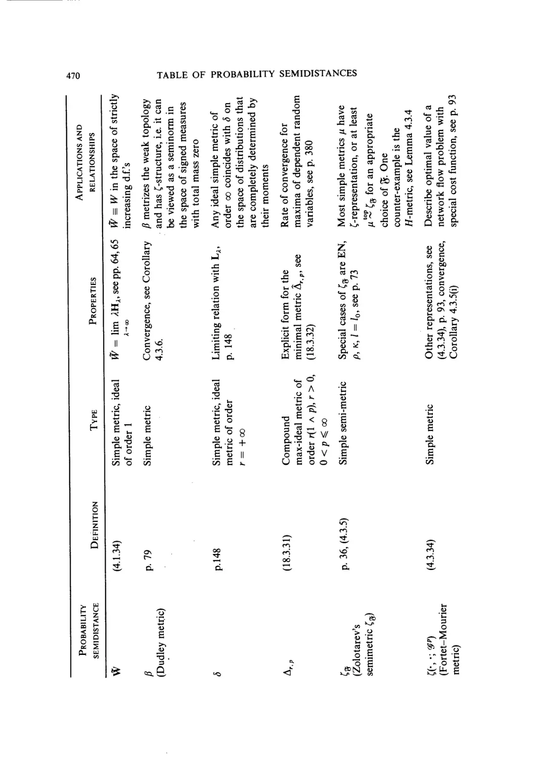
Table of Probability Semidistances 463
Index of Symbols and Abbreviations 479
Index 487

Preface
The study of limit theorems and a number of other questions in probability
theory makes it necessary to introduce functional, defined either on classes of
probability distributions or on classes of random elements, and evaluating their
nearness in one or another probabilistic sense. Thus various metrics have
appeared, among which are the well known Kolmogorov (uniform) metric, V
metrics, the Prokhorov metric, the metric of convergence in probability (Ky
Fan metric) and others. The use of metrics in many problems in probability
theory is connected with the following fundamental question:
'Is the proposed stochastic model a satisfactory approximation to the real
model, and if so, within what limits?' To answer this question, an investigation
of the qualitative and quantitative stability of the stochastic model is required.
Analysis of quantitative stability assumes the use of metrics as measures of
comparability. The main idea of the method of metric distances (MMD),
developed by V. M. Zolotarev and his students to solve stability problems, is
reduced to the following two aspects.
Problem 1 (Choice of ideal metrics). Find the most appropriate (ideal) metrics
for the stability problem under consideration. Then, solve the problem in terms
of these ideal metrics.
Problem 2 (Comparison of metrics). If it is required to write the solution of
the stability problem in terms of other metrics, one must solve the problem of
comparison of these metrics with the chosen (ideal) metrics.
Unlike Problem 1, Problem 2 does not depend on the specific stochastic
model under consideration. Thus, the independent solution of the second
problem allows its re-use in any particular situation. In addition, it enables us
to use. a variety of metric relationships without making any effort in different
kinds of stability problems. Moreover, following the stated two-stage approach,
we get a clear comprehension of the specific regularities which form the stability
effect.
In probability theory, metrics have been used for a long time, although one
usually exploits a very limited class of metrics. Also, some ideas of the MMD
have been used for a long time in approximation theory and functional analysis.
In view of the variety of stability problems, there are no regular selection rules
xi

xii PREFACE
determining the 'ideal' metric for the given problem. Therefore, the development
of the MMD demands the creation of a theory of probability metrics (TPM).
The term 'probability metric' means simply a semimetric in a space of
random variables (taking values in some separable metric space). In probability
theory, sample spaces are usually not fixed and one is interested in those metrics
whose values depend on the joint distributions of the pairs of random variables
being considered. Each such metric can be considered just as given by a function
defined on the set of probability measures on the Cartesian square of the sample
space. Complications connected with the question of existence of pairs of
random variables on a given space with given probability laws can be easily
avoided. Although such a function is not a metric on a space of probability
distributions (it is not a function of pairs of measures), small values of it say
that the measure is concentrated near the diagonal. Therefore its marginal
distributions are close to each other. Fixing these marginal distributions, one
can find the infimum of the values of our function on the class of all measures
with the given marginals. Such an infimum is a metric on the class of probability
distributions and in some concrete cases (for example, for the L, distance in
the space of random variables—Kantorovich's theorem; for the Ky Fan
metric—Strassen-Dudley's theorem; for the indicator metric—Dobrushin's
theorem) were found earlier (giving, respectively, the Kantorovich (or Wasser-
stein) metric, the Prokhorov metric and the total variation distance).
The necessary classification of the set of probability metrics {p. metrics) is
naturally carried out from the point of view of metric structure and generating
topologies. That is why the following two research directions arise.
Direction 1. Description of the basic structures of p. metrics.
Direction 2. Analysis of the topologies in the space of probability measures,
generated by different types of p. metrics. This analysis can be carried out with
the help of convergence criteria for different metrics.
At the same time, more specialized research directions arise. Namely,
Direction 3. Characterization of the ideal metrics for the given problem.
Direction 4. Investigations of the main relationships between different type
of p. metrics.
In this book, all four directions are considered as well as applications to
different problems of probability theory. Much attention is paid to the possi-
possibility of giving equivalent definitions of p. metrics (for example, in direct and
dual terms, in terms of the Hausdorff metric for sets, etc). Indeed, in concrete
applications of p. metrics, the use of different equivalent variants of the
definitions in different steps of the proof is often a decisive factor.
One of the main classes of metrics considtred is the class of minimal metrics,
the ideii of which goes back to the work of Kantorovich in the 1940s on the

PREFACE xiii
transportation problems in linear programming. Such metrics have been found
independently by many authors in several parts of probability theory (Markov
processes, statistical physics, etc.). They are connected with the widely known
method of 'coupling.' Then it is natural to evaluate the distance between'
variables with metrics of the indicated type. Distances for such metrics are hard
to compute, but it is easy to give upper bounds, attained by at least one joint
probability distribution. Another useful class of metrics studied in this book
is the class of 'ideal' metrics having satisfied the following properties: A)
lAPc,Qc)<\cW,Q) for all ce[-C,C],c#0, where Pc(A)-.= P{{l/c)A) for
any Borel set A on a Banach space U, and B) /i(Pj * Q, P2*Q) < lAP\> Pi),
where * denotes the convolution. This class is convenient for the study of
functionals of sums of independent random variables, giving nearest bounds of
the distance to limit distributions.
The presentation here is given in a general form, although specific cases are
considered as they arise in the process of finding supplementary bounds, or in
applications to important special cases.
The MMD given herein is illustrated in some concrete problems. First, there
are problems of the type of the Glivenko-Cantelli theorem on the convergence
of the empirical measures. Originally, this kind of problem was different in view
of the various possible natural modes of convergence and was considered as a
problem needing an ad hoc approach. Here it is shown that from a general
point of view such results turn out to be obvious consequences of the SLLN
and general properties of metrics. Analogously, we considered a generalization
of the Prokhorov theorem on convergence of random polygons to the Wiener
process in the case where one considers the question of convergence of
distributions of unbounded functionals. Also considered are applications to the
rate of convergence for sums and maxima of random variables and convolution
of random motions. Special sections are devoted to application of TPM to the
solution of stability problems in queueing theory, risk theory, quality usage,
and others.
I would like to thank a number of people who have directly contributed to
this project. V. M. Zolotarev introduced me to the subject of theory of
probability metrics and stability of stochastic models. He has been a constant
source of intellectual guidance and inspiration. R. M. Shortt, L. Ruschendorf,
L. de Haan, J. Yukich, E. Omey, L. Baxter, P. Todorovich, M. Taksar and J.
Beirlant worked with me on papers which formed the foundation of this book.
R. M. Dudley's lecture notes from Aarhus University have been a rich source
of ideas. In addition, I want to thank H. Robbins, S. Cambanis, G. Simons, H.
Kellerer, S. Resnick and G. Samorodnitski for many helpful discussions during
the last three years. My warm thanks and appreciation go to Ruth Bahr,
Michelle Bebb and Lee Trimble for their expert typing of this manuscript.
Finally, I must thank the editorial and production department of Wiley for their
support, patience and superb final product.

xiv PREFACE
While trying to correct all the mistakes in my manuscript, I realize that all
of them have not been found. I will be very happy to learn of any mistakes
found by the reader together with any comments one might havef.
Svetlozar T. Rachev
f Research supported by NATO Scientific Affairs Division Grant CRG 900798 and Grant from
UC Regents, University of California, Santa Barbara.

PART I
General Topics
in the Theory of
Probability Metrics

CHAPTER 1
Main Directions in the Theory of
Probability Metric
In the period of the formation of probability theory as a mathematical science,
the first limit theorems (the Law of Large Numbers, De Moivre and Laplace
Central Limit Theorems) were obtained (cf. Feller 1970, Chap. VI, 4, and Chap.
VII, 3). In applications of these limit theorems, a given probability distribution
is often approximated by some limiting distribution. In such cases, the con-
convergence rate problem arises. As mentioned in the Preface, the convergence rate
problem requires the concept of a metric as a measure of comparability.
Even in the case of probability distributions on the real line, several different
types of metrics (Levy metric, Kolmogorov metric, Lp-metric) are often used
to estimate the closeness between distributions. Since the early thirties, the
demands of various applications resulted in the creation of new, more compli-
complicated probability models. Both the theory of random processes and the theory
of distributions on functional spaces were extensively developed. In connection
with limit theorems in general spaces, Fortet and Mourier A953), Prokhorov
A956), Kantorovich and Rubinstein A958), and Dudley A966a) suggested a
series of new metrics on spaces of distributions. Certainly, the study of metric
properties is not confined to probability theory; such investigations have
occurred in other mathematical areas. In fact, some metrics on spaces of
measures (e.g. the Kantorovich-Rubinstein metric, total variation norm, and
Lp-metrics) play an important role in functional analysis (see Dunford and
Schwartz 1988, Kantorovich and Akilov 1984). In probability theory, an even
greater variety of such metrics arises in completely natural ways. This variety
and suitability can be partly explained by the fact that the stochastic problem
under consideration often dictates the choice of an appropriate metric. Fre-
Frequently, this choice will determine the investigation's success.
Questions concerning the bounds within which stochastic models can be
applied (as in all probabilistic limit theorems) can only be answered by
investigation of qualitative and quantitative stability. Such stability is
very often convenient to express in terms of a metric. This was the case with
Zolotarev's Method of Metric Distances (MMD) and the Theory of
Probability Metrics (TPM) (see Zolotarev 1976a-d, 1977a,b, 1983a,b, Zolotarev
and Rachev 1985).

MAIN DIRECTIONS PROBABILITY METRICS
Figure 1.1.1 summarizes the problems concerning MMD and TPM.
THEORY OF PROBABILITY METRICS (TPM)
Classification of
p. metrics
Description of the basic
metric and topological
structures of p. metrics
Ideal metrics problem
Characterizations of
the 'ideal' (suitable,
natural) metrics w.r.t.
the specific character
of the given
approximating problem
Comparison of metrics
Analysis of the metric
and topological
relationships between
different classes of
p. metrics
First stage of MMD
Solutions of the stability
problem in terms of
approximate metrics
Second stage of MMD
Transition from the initial
appropriate metrics to the
metric required (w.r.t. the
final solution)
METHODS OF METRIC DISTANCES (MMD)
Figure 1.1.1 Theory of the probability metrics as a necessary tool to investigate the method of
metric distances. (From Rachev and Shortt, 1990. Reproduced by permission of the American
Mathematical Society.)

CHAPTER 2
Probability Distances and Probability
Metrics: Definitions
2.1 SOME EXAMPLES OF METRICS IN PROBABILITY THEORY
Below is a list of various metrics commonly found in probability and statistics.
1. The engineer's metric
EN(X, Y)-.= |EpO - EG)| X, YeX1 B.1.1)
where 3?pis the space of all real-valued random variables (r.v.s) with E| X\p < oo.
2. The uniform (or Kolmogorov) metric
, Y)-.= sup{|F^(x) - Fy{x)\:xeU} X,YeX = X(R) B.1.2)
where Fx is the distribution function (d.f.) of X, R = (— oo, + oo), and X is the
space of all real-valued r.v.s.
3. The Levy metric
, Y) ¦¦= inf{e > 0: Fx(x - e) - e < Fy(x) ^ Fx(x + e) + e Vx e R}. B.1.3)
Remark 2.1.1. We see that p and L may actually be considered as metrics on
the space of all distribution functions. However, this cannot be done for
EN simply because EN(X, Y) = 0 does not imply the coincidence of Fx and FY,
while p(X, Y) = 0oL{X, Y) = 0oFx = FY. The Levy metric metrizes weak
convergence (convergence in distribution) in the space J5", whereas p is often
applied in the CLT, cf. Hennequin and Tortrat A965).
4. The Kantorovich metric
k(X, Y) = f \Fx(x) - Fy(x)\dx X,YeXl.

PROBABILITY DISTANCES AND PROBABILITY METRICS
5. The Lp-metrics between distribution functions
Qp(X, Y)-.= M IF
\i/P
- Fy(t)|"dtJ p > 1
B.1.4)
Remark 2.1.2. Clearly, k = 0t. Moreover, we can extend the definition of 9P
when p = oo by setting 9^ = p. One reason for this extension is the following
dual representation for 1 ^ p ^ oo
QP(X, Y) = sup \Ef(X) - Ef(Y)\, X, YgX1
where ^p is the class of all measurable functions / with ||/||9 < 1. Here,
,9(l/p + \jq = 1) is defined, as usual, by
I/I'
ess sup |
q = oo.
(The proof of the above representation is given by Dudley A989), p. 333, for
the case p = 1.)
6. The Ky Fan metrics
K(X, y):=inf{e>O:Pr(|X- Y\ > e) < e}
and
K*{X, Y):= E |X ~ 7|
\X-Y\
B.1.5)
B.1.6)
Both metrics metrize convergence in probability on X = X(U), the space of real
random variables (Lukacs 1968, Chapter 3, Dudley 1976, Theorem 3.5).
7. The Lp-metric
, Y)-.= {E\X - Y\p}llp p > 1 X, YeX".
Remark 2.1.3. Define
and
mp{X):= {E\X\p}llp p^l XeXp
X, Y)-.= \mp(X) - mp(Y)\ p > 1 X, YeXp.
B.1.7)
B.1.8)
B.1.9)

METRIC AND SEMIMETRIC SPACES 7
Then we have, for Xo, Xv .. .'in Xp
see, for example, Lukacs A968), Chapter 3.
All of the (semi-)metrics on subsets of ? mentioned above may be divided
into three main groups: primary, simple, and compound (semi-)metrics. A
metric n is primary if n(X, Y) = 0 implies that certain moment characteristics
of X and Y agree. As examples, we have EN B.1.1) and MOMP B.1.9). For
these metrics
MOMP(I, Y) = Oomp(X) = mp(Y).
A metric n is simple if
B.1.12)
Examples are p B.1.2), L B.1.3), and 9P B.1.4). The third group, the compound
(semi-)metrics have the property
H{X, y) = 0oPr(I= Y)= 1. B.1.13)
Some examples are K B.1.5), K* B.1.6), and Sep B.1.7).
Later on, precise definitions of these classes will be given, and a study made
of the relationships between them. Now we shall begin with a common
definition of probability metric which will include the types mentioned above.
2.2 METRIC AND SEMIMETRIC SPACES; DISTANCE AND
SEMIDISTANCE SPACES
First of all, let us recall the notions of metric and semimetric space. Generaliza-
Generalizations of these notions will be needed in TPM.
Definition 2.2.1. A set S--= (S, p) is said to be a metric space with the metric p
if p is a mapping from the product S x S to [0, oo) having the following
properties for each x, y, z e S
A) Identity property: p(x, y) = Oox = y;
B) Symmetry: p(x, y) = p(y, x);
C) Triangle inequality: p(x, y) < p(x, z) + p(z, y).
Some well known examples of metric space are the following.
(a) The n-dimensional vector space W endowed with the metric p(x, y) =

PROBABILITY DISTANCES AND PROBABILITY METRICS
= (xl,...,xn)eW 0<p<oo
Wloo™ SUP \Xil
1
(b) The Hausdorff metric between closed sets
r{Cu C3) = max^ sup inf p(xl5 x2), sup inf p(xu x2) >
where C,s are closed sets in a bounded metric space (S, p) (Hausdorff 1949).
(c) The H-metric. Let D(U) be the space of all bounded function /: U -> U,
continuous from the right and having limits from the left,/(x —) = limtT xf(t).
For any f eD(U) define the graph Tf as the union of the sets {(x, y): xeU,
y = /(*)} and {(x, y): x e U, y = f(x -)}. The H-metric H(f, g) in D(U) is defined
by the Hausdorff distance between the corresponding graphs, H(f,g)-=
r(Tf, Tg). Note that in the space J^(IR) of distribution functions, H metrizes
the same convergence as the Skorokhod metric:
s(F, G) = inf< e > 0: there exists a strictly increasing continuous function
X: U -> U, such that A(R) = R, sup|A(t) - t\ <e
te U
and sup\F(A(t))-G(t)\<s\.
teU J
Moreover, H-convergence in #" implies convergence in distributions (the
weak convergence). Clearly, p-convergence (see B.1.2)) implies H-convergence.
(A more detailed analysis of the metric H will be given in Section 4.1.)
If the identity property in Definition 2.2.1 is weakened by changing A) to
A*) x = y=>p(x,y) = 0,
then S is said to be a semimetric space (or pseudometric space) and p a semimetric
(or pseudometric) in S. For example, the Hausdorff metric r is only a semimetric
in the space of all Borel subsets of a bounded metric space (S, p).
Obviously, in the space of real numbers EN (see 2.1.1) is the usual
uniform metric on the real line U, i.e. EN(a, b)-.= \a - b\, a, beU, For p ^ 0,
define i*rp as the space of all distribution functions F with J?, F(x)p dx +
Jo' A — F(x))p dx < oo. The distribution function space J^ = J^0 can be con-
considered as a metric space with metrics p and L, while 9PA ^ p < oo) is a metric

METRIC AND SEMIMETRIC SPACES 9
in 2F*. The Ky-Fan metrics (see B.1.5), B.1.6)) [resp. ifp-metric (see 2.1.7)] may
be viewed as semimetrics in X (resp. 3?p) as well as metrics in the space of all
Pr-equivalence classes
X-.= {YeX:Pr{Y = X) = 1} VX e ? [resp. ?"]. B.2.1)
EN, MOMp, 9p, ?fp can take infinite values in 3? so we shall assume,
in the next generalization of the notion of metric, that p may take infinite values;
at the same time we shall extend also the notion of triangle inequality.
Definition 2.2.2. The set S is called a distance space with distance p and
parameter IK = Kp if p is a function from S x S to [0, oo], IK ^ 1 and for
each x,y,zeS the identity property A) and the symmetry property B) hold
as well as the following version of the triangle inequality: C*) (Triangle
inequality with parameter K)
P(x, y) ^ K[p(x, z) + p(z, y)l B.2.2)
If, in addition, the identity property A) is changed to A*) then S is called
a semidistance space and p is called a semidistance (with parameter IK^).
Here and in the following we shall distinguish the notions 'metric' and
'distance', using 'metric' only in the case of 'distance with parameter IK = 1,
taking finite or infinite values'.
Remark 2.2.1. It is not difficult to check that each distance p generates a
topology in S with a basis of open sets B(a, r)-= {x eS; p(x, a) <r},aeS,r > 0.
We know, of course, that every metric space is normal and that every
separable metric space has a countable basis. In much the same way, it is easily
shown that the same is true for distance space. Hence, by Urysohn's Metrization
Theorem (Dunford and Schwartz 1988, 1.6.19), every separable distance space
is metrizable.
Actually, distance spaces have been used in functional analysis for a long
time as is seen by the following examples.
Example 2.2.1. Let 3tf by the class of all nondecreasing continuous functions
H from [0, oo) onto [0, oo) which vanish at the origin and satisfy Orlicz's
condition
< oo. B.2.3)
r>0 "W
Then p-.= H(p) is a distance in S for each metric p in S and Kp = KH.
Example 2.2.2. (Birnbaum-Orlicz distance space, Birnbaum and Orlicz A931),
and Dunford and Schwartz A988), p. 400.)

10 PROBABILITY DISTANCES AND PROBABILITY METRICS
The Birnbaum-Orlicz space LH(H e #?) consists of all integrable functions
on [0, 1] endowed with Birnbaum-Orlicz distance
-/2(*)|)dx. B.2.4)
Jo
Obviously, KPh = KH.
Example 2.2.3. Similarly to B.2.4) Kruglov A973) introduced the following
distance in the space of distribution functions
Kr(F, G) = (j)(F(x) - G(x)) dx B.2.5)
where the function cj) satisfies the following conditions
(a) (j) is even and strictly increasing on [0, oo), 0@) = 0,
(b) for any x and y and some fixed A ^ 1
0(x + y) ^ A{<t>{x) + fry)). B.2.6)
Obviously, IKKr = A.
2.3 DEFINITIONS OF PROBABILITY DISTANCE AND
PROBABILITY METRIC
Let U be a separable metric space (s.m.s.) with metric d, Uk = U x • • • x U the
k times
fe-fold Cartesian product of U and ^k = ^k(U) the space of all probability
measures defined on the a algebra 0$k = &k(U) of Borel subsets of Uk. We shall
use the terms 'probability measure' and 'law' interchangeably. For any set
{a, /?,..., y} c |i5 2,..., k} and for any Pe^k let us define the marginal of
P on the coordinates a,f$,...,y by Ta p yP. For example, for any Borel
subsets A and B of U, T,P{A) = P{Ax U x ••• x U), Tl3P(AxB) =
P(A x U x B x ¦• • x U). Let B be the operator in U2 defined by B(x, y)¦¦=
{y,x) {x,ye U). All metrics n(X, Y) cited in Section 2.1 (see B.1.1H2.1.9)) are
completely determined by the joint distributions ^rx Y{?rx yg^2(U)) of the
random variables X, Y eX(U). In the next definition we shall introduce the
notion of probability distance and thus we shall describe the primary, simple,
and compound metrics in a uniform way. Moreover, the space where the r.v.s
X and 7 take values will be extended to U, an arbitrary s.ms.
Definition 2.3.1. A mapping ft defined on 0>2 and taking values in the extended
interval [0, oo] is said to be a probability semidistance with parameter K ¦¦=

DEFINITIONS OF PROBABILITY DISTANCE 11
K^ ^ 1 (or briefly, p. semidistance) in g?2 > if it possesses the three properties listed
below
A) ID {Identity Property). If P e 0>2 and P{[JxeU {(x, x)}) = 1 then /x(P) = 0
B) SYM {Symmetry). If P e 0>2 then /*(P o B"*) = /*(P)
C) TI {Triangle Inequality). If P13, P12, P23e^2 and there exists a law
Qe&3 such that the following 'consistency' condition holds:
Tl3Q = Pl3 Tl2Q = P12 T23Q = P23, B.3.1)
then
) + fi(P23I
If IK = 1 then jx is said to be a probability semimetric. If we strengthen
the condition ID to
TD:IfPeP2, then
P{\J {{x, x): xeU})= l<=>fi{P) = 0,
then we say that fx is a probability distance with parameter K = K^ ^ 1 (or
briefly,/?, distance).
Definition 2.3.1 acquires a visual form in terms of random variables, namely,
let X ¦¦= ?{U) be the set of all r.v.s on a given probability space (Q, s/, Pr) taking
values in {U, &J. By if X2 ¦¦= ^X2{U) ¦¦= ^X2{U; Q, j*, Pr) we denote the space
of all joint distributions Pr^- y generated by the pairs X,YeX. Since i?3E2 c g>2,
then the notion of p. (semi-)distance is naturally defined on if X2. Considering
jx on the subset SCX2, we shall put
and call n a /?. semidistance on X. If /i is a p. distance, then we use the phrase
p. distance on 3E. Each p. semidistance [resp. distance] /x on X is a semidistance
[resp. distance] on 3E in the sense of Definition 2.2.2. Then the relationships
ID, TO, SYM, and TI have simple 'metrical' interpretations:
ID(*> Pr(X =Y)=l=> n{X, Y) = 0
TD(*> Pr(X =Y) = lon{X, Y) = 0
SYM(*> pipe, Y) = n{Y,X)
TI<*> n{X, Z) < K\XX, Z) + n{Z,
Definition 2.3.2. A mapping jx: <?X2 -»• [0, oo] is said to be a probability
semidistance in X [resp. distance] with parameter K-.= K^ ^ 1, if /i(X, Y) =
fj.{T>rx Y) satisfies the properties ID(*> [resp. Ito1**], SYM(*) and TI(*> for
all r.v.s X,Y,ZeX{U).

12 PROBABILITY DISTANCES AND PROBABILITY METRICS
Example 2.3.1. Let H e Jf (see Example 2.2.1) and (U, d) be a s.m.s. Then
&H(X, Y) = EH(d[X, Y)) is a p. distance in X(U). Clearly, ??H is finite in the
subspace of all X with finite moment EH(d(X, a)) for some ae U. The Kruglov's
distance Kr(X, Y)-.= Kr(Fx, FY) is a p. semidistance in X(U).
Examples of p. metrics in X(U) are the Ky Fan metric
K{X, Y)¦¦= inf{? > 0: Pr{d(X, Y) > e) < e} {X, YeX{U) B.3.2)
and the ^-metrics @ < p < oo)
S?P{X, Y)-.= {W(X, Y)}minA-llp) 0 < p < oo, B.3.3)
&JX, Y) -.= ess sup d(X, Y) ¦.= inf {e > 0: Pr(d(X, Y) > s) = 0} B.3.4)
2>0(X, Y) == E/{X, 7} := Pr(X, 7). B.3.5)
The engineer's metric EN, Kolmogorov metric p, Kantorovitch metric k,
and the Levy metric L (see Section 2.1) are p. semimetrics in X(U).
Remark 2.3.1. Unlike Definition 2.3.2, Definition 2.3.1 is free of the choice of
the initial probability space, and depends only on the structure of the metric
space U. The main reason for considering not arbitrary but separable metric
spaces ([/, d) is that we need the measurability of the metric d in order to connect
the metric structure of U with that of X(U). In particular, the measurability of
d enables us to handle in a well defined way, p. metrics such as the Ky Fan
metric K and Jzfp-metrics. Note that S?o does not depend on the metric d,
so one can define Jzf0 on X(U), where U is an arbitrary measurable space,
while in B.3.2)-B.3.4) we need d(X, Y) to be a random variable. Thus the natural
class of spaces appropriate to our investigation is the class of s.m.s.
2.4 UNIVERSALLY MEASURABLE SEPARABLE METRIC SPACES
What follows is an exposition of some basic results regarding universally
measurable separable metric spaces (u.m.s.m.s.). As we shall see, the notion of
u.m.s.m.s. plays an important role in TPM.
Definition 2.4.1. Let P be a Borel probability measure on a metric space (U, d).
We say that P is tight if for each e > 0, there is a compact K ^ U with
P(K) > 1 - a. See Dudley A989), Section 11.5.
Definition 2.4.2. A s.m.s. (U, d) is universally measurable (u.m.) if every Borel
probability measure on U is tight.
Definition 2.4.3. A s.m.s. (U, d) is Polish if it is topologically complete (i.e. there
is a topologically equivalent metric e such that (U, e) is complete). Here the

UNIVERSALLY MEASURABLE SEPARABLE METRIC SPACES 13
topological equivalence of d and e simply means that for any x, xt, x2,... in U
d{xn, x) ^Ooe{xn, x) -»• 0.
Theorem 2.4.1. Every Borel subset of a Polish space is u.m.
Proof. See Billingsley A968) Theorem 1.4, Cohn A980) Proposition 8.1.10, and
Dudley A989), p. 391.
Remark 2.4.1. Theorem 2.4.1 provides us with many examples of u.m. spaces,
but does not exhaust this class. The topological characterization of u.m. s.m.s.
is a well known open problem (see Billingsley 1968, Appendix III, p. 234).
In his famous paper on measure theory, Lebesgue A905) claimed that the
projection of any Borel subset of U2 onto U is a Borel set. As noted by Souslin
and his teacher Lusin A930), this is in fact not true. As a result of the
investigations surrounding this discovery, a theory of such projections (the
so-called 'analytic' or 'Souslin' sets) was developed. Although not a Borel set,
such a projection was shown to be Lebesgue-measurable, in fact u.m. This train
of thought leads to the following definition.
Definition 2.4.4. Let S be a Polish space and suppose that / is a measurable
function mapping S onto a separable metric space U. In this case, we say that
U is analytic.
Theorem 2.4.2. Every analytic s.m.s. is u.m.
Proof. See Cohn's A980), Theorem 8.6.13, p. 294 and Dudley A989), Theorem
13.2.6.
Example 2.4.1. Let Q be the set of rational numbers with the usual topology.
Since Q is a Borel subset of the Polish space R, then Q is u.m., however, Q is
not itself a Polish space.
Example 2.4.2. In any uncountable Polish space, there are analytic (hence u.m.)
non-Borel sets. See Cohn's A980) Corollary 8.2.17 and Dudley A989), Proposi-
Proposition 13.2.5.
Example 2.4.3. Let C[0, 1] be the space of continuous functions /: [0, 1] -»• IR
under the uniform norm. Let E ^ C[0, 1] be the set of / which fail to be
differentiable at some t e [0, 1]. Then a theorem of Mazurkiewicz A936) says
that E is an analytic, non-Borel subset of C[0, 1]. In particular, E is u.m.
Recall again the notion of Hausdorff metric r-.= rp in the space of all subsets

14 PROBABILITY DISTANCES AND PROBABILITY METRICS
of a given metric space (S, p)
r(A, B) = max< sup inf p(x, y), sup inf p(x, y) >
LxeA yeB yeB xeA J
= inf{8 > 0: AE 2 B, BE 2 A] B.4.1)
where ,4? is the open 8-neighborhood of A, Ae = {x: d(x, A) <&}.
As we noticed in the space 2b of all subsets A^0ofS, the Hausdorff distance
r is actually only a semidistance. However, in the space # = ^(S) of all closed
non-empty subsets, r is a metric (see Definition 2.2.1) and takes on both finite
and infinite values, and if S is a bounded set then r is a finite metric on c€.
Theorem 2.4.3. Let (S, p) be a metric space, and let (^(S), r) be the space
described above. If (S, p) is separable [resp. complete; resp. totally bounded],
then (^(S), r) is separable [resp. complete; resp. totally bounded].
Proof. See Hausdorff A944), Section 29; Kuratowski A969), Sections 21 and 23.
Example 2.4.4. Let S = [0, 1] and let p be the usual metric on S. Let M be the
set of all finite complex-valued Borel measures m on S such that the Fourier
transform
P
m(t) = exp(iut)m(du)
Jo
vanishes at t = ± oo. Let Jl be the class of sets E e ^(S) such that there is some
mei% concentrated on E. Then Jl is an analytic, non-Borel subset of (#(S), rp),
see Kaufman A984).
We seek a characterization of u.m. s.m.s. in terms of their Borel structure.
Definition 2.4.5. A measurable space M with cr-algebra Jl is standard if there
is a topology &~ on M such that (M, ^") is a compact metric space and the
Borel cr-algebra generated by 3~ coincides with Jl.
A s.m.s. is standard if it is a Borel subset of its completion (see Dudley 1989,
p. 347). Obviously, every Borel subset of a Polish space is standard.
Definition 2.4.6. Say that two s.m.s. U and Fare called Borel-isomorphic if
there is a one-one correspondence/of U onto Ksuch that Be@(U) if and only
Theorem 2.4.4. Two standard s.m.s. are Borel-isomorphic if and only if they
have the same cardinality.
Proof. See Cohn A980), Theorem 8.3.6 and Dudley A989), Theorem 13.1.1.

UNIVERSALLY MEASURABLE SEPARABLE METRIC SPACES 15
Theorem 2.4.5. Let U be a separable metric space. The following are equivalent:
A) U is u.m.
B) For each Borel probability m on U, there is a standard set S e3$(U) such
that m(S) = 1.
Proof. 1 =>2: Let m be a law on U. Choose compact Kn^ U with m(Kn) ^
1 — 1/n. Put S= [Jn2i Kn. Then S is cr-compact, and hence standard. So
m(S) = 1, as desired.
2 <= 1: Let m be a law on [/. Choose a standard set S e @(U) with m(S) = 1.
Let U be the completion of U. Then S is Borel in its completion S, which is
closed in U. Thus, S is Borel in U. It follows from Theorem 2.4.1 that
1 = m(S) = sup{m(K): K compact}.
Thus, every law m on U is tight, so that U is u.m. QED
Corollary 2.4.1. Let (U, d) and (V, e) be Borel-isomorphic separable metric
spaces. If (U, d) is u.m., then so is (V, e).
Proof. Suppose that m is a law on V. Define a law n on U by n{A) = m{f(A))
where/: U -*¦ V is a Borel-isomorphism. Since [/ is u.m. there is a standard set
Sg(/ with n(S) = 1. Then/(S) is a standard subset of Kwith m{f{S)) = 1. Thus,
by Theorem 2.4.5, V is u.m. QED
The following result, which is in "essence due to Blackwell A956), will be used
in an important way later on (cf. the basic theorem of Section 3.2, Theorem
3.2.1).
Theorem 2.4.6. Let U be a u.m. separable metric space and suppose that Pr is
a probability measure on U. If js/ is a countably generated sub-cr-algebra of
), then there is a real-valued function P(B\x), Be3${U), xeU such that
A) for each fixed Be&(U), the mapping x -*¦ P{B\x) is an jsZ-measurable
function on U;
B) for each fixed x e U, the set function B -*¦ P{B\x) is a law on U;
C) for each Aestf and Be &(U), we have jA P(B\x) Pr(dx) = Pr(^4 n B);
D) there is a set N e si? with Pr(iV) = 0 such that P(B\x) = 1 whenever
xeU -N.
Proof. Choose a sequence Fl,F2,... of sets in @{U) which generates
and is such that a subsequence generates s/. We shall prove that there exists
a metric e on U such that ([/, d) and ([/, e) are Borel-isomorphic and for which
the sets F1; F2, ¦.. are clopen, i.e., open and closed.

16 PROBABILITY DISTANCES AND PROBABILITY METRICS
Claim 1. If (I/, d) is a s.m.s. and Alt A2,... is a sequence of Borel subsets of
U, then there is some metric e on U such that
(i) (U, e) is a separable metric space isometric with a closed subset of U;
(ii) A1,A2,... are clopen subsets of (U, e);
(iii) (U, d) and (U, e) are Borel-isomorphic (see Definition 2.4.6).
Proof of claim. Let Bu B2,... be a countable base for the topology of (U, d).
Define sets Clt C2,... by C2n_ t = >ln and C2n = Bn (n = 1, 2,...) and
/: 1/ -> R by /(x) = Xn°°= i 2/c,,(x)/3n. Then / is a Borel-isomorphism of {U, d)
onto f(U) ^ K, where K is the Cantor set,
an/3": ans take value 0 or 2 >.
Define the metric e by e(x, y) = |/(x) — f(y)\, so that (I/, e) is isometric with
f(U) ^ K. Then >ln = /" l{x e K; x(n) = 2}, where x(n) is the nth digit in the
ternary expansion of x e K. Thus, An is clopen in (U, e), as required.
Now (U, e) is (Corollary 2.4.1) u.m., so there are compact sets K1 ^ K2^ ...
with Pr(KJ -»• 1. Let ^ and ^2 be the (countable) algebras generated by the
sequences F1; F2,... and F1; F2,...,K1, K2,..., respectively. Then define
P^^lx) so that A) and C) are satisfied for B e CS2. Since CS2 is countable, there
is some set N e j/ with Pr(iV) = 0 and such that for xe N,
(a) P^-lx) is a finitely additive probability on ^2;
(b) P^Alx) =lfoTAestfn<g2 and xeX;
(c)
C/a/m 2. For xeJV, the set function B -> P^B] x) is countably additive on ^.
Proof of claim: Suppose that H 1; H2,... are disjoint sets in <§x whose union
is U. Since the Hn are clopen and the Kn are compact in (U, e), there is, for
each n, some M = M(n) such that Kn^HlvH2(j---(j HM. Finite additivity
of P,{x, ¦) on ^2 yields, for x ? N, P^KJx) < ?? .P^H^x) < ^i" i ^i(H,-|x).
Let n -»• oo and apply (c) to obtain ^]?i t P^H.-lx) = 1, as required.
In view of the claim, for each xeN, we define B -*¦ P(B\x) as the unique
countably additive extension of P^ from <§x to 3$(U). For xeN, put
PE|x) = Pr(?). Clearly, B) holds. Now the class of sets in &(U) for which A)
and C) hold is a monotone class containing ^1; and so coincides with @(U).
Claim 3. Condition D) holds.
Proof of claim. Suppose that A e $? and x e A — N. Let Ao be the js/-atom
containing x. Then Ao ^ A and there is a sequence Ax, A2,... in ^ such that

NOTIONS OF p. (SEMI-)DISTANCE ON ^2 AND ON X 17
Ao = Ax n A2 n •••. From (b), P{An\x) = 1 for n > 1, so that P^olx) = 1, as
desired. QED
Corollary 2.4.2. Let U and V be u.m. s.m.s. and let Pr be a law on U x V.
Then there is a function P:@{V) x [/ -> U such that
A) for each fixed B e ^(K), the mapping x -»• P(B | x) is measurable on U;
B) for each fixed xeU, the set function 5 -»• P(B\x) is a law on V;
C) for each Ae3$(U) and 5 e ^(K), we have
P{B\x)P1(dx) = T>r(AnB)
Ja
where Px is the marginal of Pr on U.
Proof. Apply the preceding theorem with stf the cr-algebra of rectangles A x U
for A g @(U). QED
2.5 THE EQUIVALENCE OF THE NOTIONS OF
p. (SEMI-)DISTANCE ON ^2 AND ON X
As we have seen in Section 2.3, every p. (semi-)distance on g?2 induces (by
restriction) a p. (semi-)distance on 3E. It remains to be seen whether every
p. (semi-)distance on X arises in this way. This will certainly be the case whenever
J?X2(U, (Q, s/, Pr)) = 0>2{U). B.5.1)
Note that the left member depends not only on the structure of (U, d) but also
on the underlying probability space.
In this section we will prove the following facts.
(i) There is some probability space (Q, stf, Pr) such that B.5.1) holds for every
separable metric space U.
(ii) If U is a separable metric space, then B.5.1) holds for every non-atomic
probability space (Q, s/, Pr) if and only if U is universally measurable.
We need a few preliminaries.
Definition 2.5.1 (see Loeve 1963, p. 99; Dudley 1989, p. 82). If (Q, s4, Pr) is
a probability space, we say that A e s4 is an atom if Pr(yl) > 0 and PrE) = 0
or Vx{A) for each measurable B c A. A probability space is non-atomic if it has
no atoms.
Lemma 2.5.1 (Berkes and Phillip 1979). Let v be a law on a complete s.m.s.
(U, d) and suppose that (Q, js/, Pr) is a non-atomic probability space. Then
there is a [/-valued random variable X with distribution S?(X) = v.

18 PROBABILITY DISTANCES AND PROBABILITY METRICS
Proof. Denote by d* the following metric on U2: d*(x, y) •¦= d(x^ x2) + d(yu y2)
for x = (x1,yl) and y = (x2,y2)- For each k, there is a partition of U2
comprising non-empty Borel sets {Aik: i = 1, 2,...} with diam(yllfc) < l//c and
such that Aik is a subset of some Ajk_ t.
Since (fi, stf, Pr) is non-atomic, we see that for each # e js/ and for each
sequence p; of non-negative numbers such that Pi + p2 + '" = Pr(#), there
exists a partitioning <€x,<€1,...oi<€ such that Pr(#?) = pt, i = 1, 2,... (see e.g.
Loeve 1963, p. 99).
Therefore, there exist partitions {Bik: i = 1,2,...} ^ s/,k = 1,2,... such that
Bik c #.fc_ j for some; =j@ and PrEifc) = y(ylIfc) for all i, k. For each pair (i,j),
let us pick a point xlfc g >llfc and define U2-valued Xk(co) = xik for co e Bik. Then
d*(Xk + m(a>), Xk(co)) < \jk, m = 1, 2,... and since (U2, d*) is a complete space,
then there exists the limit X(co) = lim^^ Xk(a>). Thus
d*(X(co), Xk(co)) ^ lim ld*(Xk+m(co), X(co)) + d*(Xk + m(co), Xfc(co))] < \.
Let Pk:= Pr^ and P*:= Pr^. Further, our aim is to show that P* = v. For
each closed subset A c jj
Pk(A) = Pr(Xfc e 4) < Pr(X e ^41/fc) = P*(,41/fc) < Pfc(^2/fc) B.5.2)
where Ailk is the open l//c-neighborhood of A. On the other hand,
Pk(A) = X {Pfc(x/fc): xik eA} = Yj {T>r(Bik): xik e A}
= X {v(Aiky. xik eA}^Z {V(A* " AllkY- x* e A}
^ v(Al'k) ^ X {v(Aik): xik e A2'k} < Pk(A2'k). B.5.3)
Further, we can estimate the value Pk(A2lk) in the same way as in B.5.2) and
B.5.3) and thus, we get the inequalities
P*{A1/fc) ^ Pk{A2lk) < P*(A2'k) B.5.4)
v{Ailk) ^ Pfc(y42/fc) < v(A3lk). B.5.5)
Since y(yl1/fc) tends to v(A) with /c -»• oo for each closed set A and analogously
P*(Allk) -^ P*(A) as /c -v oo, then by B.5.4) and B.5.5) we obtain the equalities
P*{A)= limPk{A2'k) =
fc-oo
for each closed A and hence, P* = v. QED
Theorem 2.5.1. There is a probability space (Q, jrf, Pr) such that for every
separable metric space U and every Borel probability n on [/, there is a random
variable X. Q -> [/ with

NOTIONS OF p. (SEMI-)DISTANCE ON <3»2 AND ON X 19
Proof. Define (fi, s/, Pr) as the measure-theoretic (von Neumann) product (see
Hewitt and Stromberg A965), Theorems 22.7 and 22.8, pp. 432-433) of the
probability spaces (C, @(C), v), where C is some non-empty subset of U with
Borel cr-algebra @(C), and v is some Borel probability on (C, @{C)).
Now, given a separable metric space U, there is some set CeK Borel-
isomorphic with U (cf. Claim 1 in Theorem 2.4.6). Let f\C -*U supply the
isomorphism. If n is a Borel probability on U, let v be a probability on C such
that f(v)-.= vf~l =fi. Define X.Q^U as X = /°tt, where tt:Q->C is a
projection onto the factor (C, ^(C), v). Then =Sf(X) = /*, as desired.
Remark 2.5.1. The result above establishes the claim (i) made at the beginning
of the section. It provides one way of ensuring B.5.1): simply insist that all r.v.s
be defined on a 'super-probability space' as in Theorem 2.5.1. We make this
assumption throughout the sequel.
The next theorem extends the Berkes and Phillips's Lemma 2.5.1 to the case
of u.m. s.m.s. U.
Theorem 2.5.2. Let U be a separable metric space. The following are equivalent.
A) U is u.m.
B) If (Q, s/, Pr) is a non-atomic probability space, then for every Borel
probability P on U, there is a random variable X: Q -*¦ U with law JS?(X) = P.
Proof. 1 => 2: Since U is u.m. there is some standard set Se3$(U) with P(S) = 1
(Theorem 2.4.5). Now there is a Borel-isomorphism / mapping S onto a Borel
subset B of U (Theorem 2.4.4). Then f{P)-= P°/"' is a Borel probability on
U. Thus, there is a random variable g: Q -»• U with Sf{g) = f{P) and #(Q) c B
(Lemma 2.5.1 with (U,d) = (U, |-|)). We may assume that g(Q) c B since
PT[g-\B))= 1. Define x:Q->[/ by x{co) =f~\g{co)). Then Se{X) = v, as
claimed.
2 => 1: Now suppose that v is a Borel probability on U. Consider a random
variable X: Q -»• U on the (non-atomic) probability space (@, 1), ^@, 1), I) with
if(X) = y. Then range (X) is an analytic subset of U with u*(range(X)) = 1.
Since range(X) is u.m. (Theorem 2.4.2), there is some standard set S ^ range(X)
with P(S) = 1. This follows from Theorem 2.4.5. The same theorem shows that
U is u.m. QED
Remark 2.5.2. If U is u.m. s.m.s., we operate under the assumption that all
[/-valued r.v.s are defined on a non-atomic probability space. Then B.5.1) will
be valid.

CHAPTER 3
Primary, Simple and Compound
p. Distances. Minimal and Maximal
Distances and Norms
In this chapter we shall give a more detailed analysis of the notions of p. distance
and p. metric in order to provide the first (crude) classification of p. semi-
distances.
3.1 PRIMARY DISTANCES AND PRIMARY METRICS
Let h: 0>x -»• UJ be a mapping, where ^ = ^(U) is the set of Borel probability
measures (laws) for some s.m.s. (U, d) and J is some index set. This function h
induces a partition of 2?2 = ^(U) (tne set of laws on U2) into equivalence classes
for the relation
P~Qoh(Pi) = KQi) and h(P2) = h(Q2) Pr.= TtP, Qr.= TtQ C.1.1)
where Pt and Q( (i = 1, 2) are the ith marginals of P and Q, respectively. Let fx
be a p. semidistance on 0>2 with parameter KM (Definition 2.3.1), such that fx is
constant on the equivalence classes of ~, i.e.
P~Qo»{P) = m- C-1.2)
Definition 3.1.1. If the p. semidistance jx = jxh satisfies Relation C.1.2), then we
call /x a primary distance (with parameter KM). If KM = 1 and /x assumes only
finite values, we say that fx is a primary metric.
Obviously, by Relation C.1.2), any primary distance is completely de-
determined by the pair of marginal characteristics {hPx, hP2). In case of primary
distance /x we shall write /x{hPi, hP2)-= jx(P) and hence fx may be viewed as a
21

22 PRIMARY, SIMPLE AND COMPOUND p. DISTANCES
distance in the image space hffi) ^ RJ, i.e., the following metric properties hold
hP1 = hP2of4hPlt hP2) = 0
SYMA)
TIA) If the following marginal conditions are fulfilled
a = hG;/>A)) = WJiI*^) b = h{T2P{2)) = hG\PC)) c = h{T2P(l)) = h(T2PC))
for some law P{1), PB\ P{3) e 0>2 then n(a, c) ^ KM|>(fl, b) + jx{b, c)].
The notion of primary semidistance /xh becomes easier to interpret assuming
that a probability space (fi, st, Pr) with property B.5.1) is fixed (see Remark
2.5.1). In this case jxh is a usual distance (see Definition 2.2.1) in the space
h(X)-.= {hX-.= h Pr*, where XeX{U)} C.1.3)
and thus, the metric properties of fx •¦= fxh take the simplest form (cf. Definition
2.2.2):
hX =
SYMB*> n(hX, hY) = n{hY, hX),
TIC*> n(hX, hZ) ^ K^nihX, hY) + n{hY, hZ)~\.
Further, we shall consider several examples of primary distances and metrics.
Example 3.1.1. Primary minimal distances. Each p. semidistance jx and each
mapping h^l -*¦ UJ determine a functional p.h -*¦ p.h: H,^) x h{^) -* [0, oo] de-
defined by the following equality
M&» 52):= inf{/i(P): hPt = ah i = 1, 2} C.1.4)
(where Pt are the marginals of P) for any pair (au a2) e h(^) x
Further, we shall prove (see Chapter 5) that jxh is a primary distance for
different special functions h and spaces U.
Definition 3.1.2. The functional jlh is called a primary h-minimal distance with
respect to the p. semidistance fx.
Open problem 3.1.1. In general it is not true that the metric properties of a
p. distance fx imply that ]x is a distance. The following two examples illustrate
this fact (see further Chapter 9):
(a) Let U = U, d(x, y) = |x — y\. Consider the p. metric
H(X, Y) = ?0(X, Y) = Pr(X * Y) X, YeX(U)
and the mapping h: ?(M)-+ [0, oo] given by hX = $L\X\. Then (see further
Section 9.1)
*, b) = inf{Pr(X # Y): E|X| = a, E| Y\ = b} = 0

PRIMARY DISTANCES AND PRIMARY METRICS 23
for all a ^ 0 and 6^0. Hence in this case the metric properties of n imply only
semimetric properties for juh.
(b) Now let jx be defined as in (a) but h: X(R) -*¦ [0, oo] x [0, oo] be defined
by hX = (\E\X\,\EX2). Then
= inf{Pr(X ± Y): E\X\ = au EX2 = a2, E| Y\ = bu EY2 = b2) C.1.5)
where Jxh is not even p. semidistance since the triangle inequality TI{3*] is not
valid.
With respect to this, the following open problem arises: under which condition
on the space U, p. distance /j. on X(U) and transformation h: ?{U) -*¦ RJ the
primary h-minimal distance jlh is a primary p. distance in h(?I
As we shall see later on (Section 9.1), all further examples 3.12 to 3.15 of
primary distances are special cases of primary Jz-minimal distances.
Example 3.1.2. Let H ejf (see Example 2.2.1) and 0 be a fixed point of a s.m.s.
(U, d). For each Pe^ with marginals Pt= TtP, let m1P,m2P denote the
'marginal moments of order p > 0',
mtP¦¦= m\p)P-.= ({ dp(x, 0)P,.(dx)Y p > 0 p'-.= min(l, l/p).
Then
<^h,p(P)--= MH^{mxP, m2P)-.= H^m^P - m2P\) C.1.6)
is a primary distance. One can also consider MH p as a distance in the space
m(p\^) ¦¦= \m(p)P ¦.= ( dp{x, a)P{dx)\P < oo, P e 0>{U) I C.1.7)
of moments m(p)P of order p > 0. If H(t) = t then
A(x OVP P~Md\
Ltia3 V 1 2/V
it;
is a primary metric in m(p)(^).
Example 3.1.3. Let g: [0, oo] -> 1R and H e Jf. Then
is a primary distance in g ° mffi) and
Ji{g\mxP, m2P)-.= igim.P) - g(m2P)\ C.1.9)
is a primary metric.

24 PRIMARY, SIMPLE AND COMPOUND p. DISTANCES
If U is a Banach space with norm|| • || then we define the primary dis-
distance ^HP{g)as follows
^ m^Y)-.= H(\g(m^X) - g{m^Y)\) C.1.10)
where (cf. B.1.8)) m(p)X is the 'p-th moment (norm) of X'
m(p)X:={E\\X\\py.
By Equation C.1.9), JtH p(g) may be viewed as a distance (see Definition
2.2.2) in the space
gom(X)-.= {gom(X):= g({E\\X\\p}p'), XeX} p'= mind,?-1), * = X(U)
C.1.11)
of moments g o m(X). If U is the real line 1R and g{t) = H(t) = t{t ^ 0) then
JtH p(g)(m(p)X, m(p)Y) is the usual deviation between moments m(p)X and m(p)Y
(see'B.1.9)).
Example 3.1.4. Let J be an index set (with arbitrary cardinality), g{ (i eJ) be
real functions on [0, oo] and for each P e ^(U) define the set
hP:={9i(mP),ieJ} C.1.12)
Further, for each P e ^(U) let us consider hPx and hP2 where P/s are the
marginals of P. Then
^ C.1.13)
otherwise
is a primary metric.
Example 3.1.5. Let [/ be the «-dimensional Euclidean space W, H eJ^. Define
the 'engineer distance'
EN(X, Y;H):=H[
i= 1
C.1.14)
where X = (XU..., Xn), Y= {Yu ..., Yn) belong to the subset X(W) ? X(W) of
all n-dimensional random vectors that have integrable components. Then
EN( •, •; H) is a p. semidistance in j^R"). Analogously, the 'Lp-engineer metric'
X|EXI.-E^.
X|EXI.-E^.H ,P>0 C.1.15)
is a primary metric in X(W). In the case p = 1 and n = 1, the metric EN( •, •; p)
coincides with the engineer metric in X(U) (see B.1.1)).

SIMPLE DISTANCES AND METRICS 25
3.2 SIMPLE DISTANCES AND METRICS; CO-MINIMAL
FUNCTIONALS AND MINIMAL NORMS
Clearly, any primary distance /x(P) (P e g?2) is completely determined by the pair
of marginal distributions P{ = T(P (i = 1, 2), since the equality Pl = P2 implies
hP^ = hP2 (see Relations C.1.1), C.1.2) and Definition 3.1.1). On the other
hand, if the mapping h is 'rich enough' then the opposite implication
t =hP2=>Pl=P2
takes place. The simplest example of such 'rich' h: 3P(U)-* R3 is given by the
equalities
HP) ¦¦= {P(C), Ce<$,Pe 0>(U)} C.2.1)
where J = <& is the family of all closed non-empty subsets C ^ U. Another
example is
h{P) = \pf-.= fdP:feCb{U)\ Pe0>{U)
where Cb(U) is the set of all bounded continuous functions on U. Keeping in
mind these two examples we shall define the notion of 'simple' distance as a
particular case of primary distance with h given by Equality C.2.1).
Definition 3.2.1. The p. semidistance /x is said to be a simple semidistance in
0> = 0>{U), if for each P e 0>2
^(P) = 0<=T1P= T2P.
If, in addition, n is a p. semimetric, then jx will be called a simple semimetric.
If the converse implication (=>) also holds, we say that jx is simple distance. If,
in addition, /x is a p. semimetric, then /x will be called a simple metric.
Since the values of the simple distance /x(P) depend only on the pair marginals
P^,P2 we shall consider /x as a functional on ^ x 0>2 and we shall use the
notation
where Px x P2 means the measure product of laws Px and P2. In this case the
metric properties of jx take the form (cf. Definition 2.3.1) (for each P^,P2,
IDB) Pl=P2on(Pl,P2) =
SYM<2>
TI<2>
Hence, the space 0> of laws P with a simple distance jx is a distance space (see
Definition 2.2.2). Clearly each primary distance is a simple semidistance in J<\

26 PRIMARY, SIMPLE AND COMPOUND p. DISTANCES
The Kolmogorov metric p B.1.2), the Levy metric L B.1.3) and the 0p-metrics
B.1.4) are simple metrics in 0>(U).
Let us consider a few more examples of simple metrics which we shall use
later on.
Example 3.2.1. Minimal distances.
Definition 3.2.2. For a given p. semidistance jx on 0>2 the functional jx on & x &
defined by the equality
/}(/>!, P2)-= inf{/*(P); TtP = Ph i = 1, 2} Pu P2e0> C.2.2)
is said to be (simple) minimal (w.r.t. n) distance.
As we showed in Section 2.5.1, for a 'rich enough' probability space, the
space 0>2 of all laws on U2 coincides with the set of joint distributions Pr* y
of [/-valued r.v.s. Thus always n(P) = /x(Ptx Y) for some X, YeX(U) and
therefore Equation C.2.2) can be rewritten as follows
ft(Pv P2) = inf{MX, Y): Pr* = Pu Pry = P2}.
The last is the Zolotarev definition of a minimal metric (Zolotarev, 1976b).
In the next theorem we shall consider the conditions on U that guarantee jx
to be a simple metric.
We use the notation -^ 'to mean weak convergence of laws' (cf., Billingsley,
1968).
Theorem 3.2.1. Let U be a u.m. s.m.s. (see Definition 2.4.2) and let jx be a p.
semidistance with parameter K^. Then (x is a simple semidistance with para-
parameter Kfr = K^. Moreover, if n is a p. distance satisfying the following 'con-
'continuity' condition
Then jx is a simple distance with parameter K(i= K^.
Remark 3.2.1. The continuity condition is not restrictive; in fact, all p. distances
we are going to use satisfy this condition.
Remark 3.2.2. Clearly, if /x is a p. semimetric then, by the above theorem, jx is
a simple semimetric.
Proof. IDB): If Px g ^ then we let X eX(U) have the distribution P^ Then,
by ID(*> (Definition 2.3.2),

SIMPLE DISTANCES AND METRICS 27
Suppose now that jx is a p. distance and the continuity condition holds.
If jx{P1,P1) = 0 then there exists a sequence of laws P(n)G0>2 with fixed
marginals 7;P(n) = P, (i = 1, 2) such that ix{P(n)) -> 0 as n -»• oo. Since P,. is a tight
measure then the sequence {Pn, n ^ 1} is uniformly tight, i.e., for any 8 > 0
there exists a compact K? c t/2 such that P(n)(JQ ^ 1 - 2 for all n > 1 (cf.
Dudley, 1989, Section 11.5). Using Prokhorov compactness criteria (see, for
instance, Billingsley 1968, Theorem 6.1) we choose a subsequence P(n ] that
weakly tends to a law P e 0>2, hence, TtP = P, and n(P) = 0. Since /x is a p.
distance P is concentrated on the diagonal x = y and thus Pt = P2 as desired.
SYMB): Obvious.
TIB): Let Pu P2, P3e^. For any e>0 define a law P12e0»2 with
marginals TtPl2 = Pt (i = 1, 2) and a law P23 e 0>2 with 7^P23 = Pi+1 (i = 1, 2)
such that fi(Pl,P2) >n{Pl2) -s and fi(P2, P3) > n{P23) - e. Since [/ is a
u.m. s.m.s. then there exist Markov kernels P'{A/z) and P"(A/z) defined by the
equalities
C.2.3)
P23(A2 * A3)-.= \ P"(A3/z)P2(dz) C.2.4)
JA2
for all Au A2, ^3el, (see Corollary 2.4.2). Then define a set function Q
on the algebra si of finite unions of Borel rectangles A1 x A2 x A3 by the
equation
Q(A1 x A2 x A3)-.= P'(A1/z)P"(A3/z)P2(dz). C.2.5)
It is easily checked that Q is countably additive on si and therefore extends
to a law on U3. We use '<2' to represent this extension also. The law Q has the
projections Tl2Q = Pl2,T23Q = P23. Since jx is a p. semidistance with parameter
IK = K^ we have
i,P3)<Mr136XiK|>(p12)H
Letting ?-^0we complete the proof of TIB). QED
As will be shown later (Part 2), all simple distances in the next examples are
actually simple minimal (x distances with respect to p. distances jx that will be
introduced in Section 3.3 (see further examples 3.3.1 to 3.3.3).
Example 3.2.2. (Kantorovich metric and Kantorovich distance). In Section 2.1,

28 PRIMARY, SIMPLE AND COMPOUND p. DISTANCES
we introduced the Kantorovich metric k and its 'dual' representation
*(/>!, P2)= I \Fl(x)-F2(x)\dx
fd(Pl-P2)
: /: R -> R, /' exists a.e. and |/'| < 1 a.e.
where P;s are laws on 1R with d.f.s F{ and finite first absolute moment. From
the above representation it also follows that
fd(Pl-P2)
: f: R -> R, / is A, 1)-Lipschitz,
i.e., \f(x)-f(y)\ t:\x-y\Vx, ye
In this example we shall extend the definition of the above simple p. metric
of the set ^(U) of all laws on a s.m.s. {U, d). For any a e @, oo) and /? e [0, 1]
define the Lipschitz functions class
Lip^l/):= {/: U - R: | f(x) - /(y)| < a d'(x, y) Vx, y e I/} C.2.6)
with the convention
d°(x, y)<= {[ ^^ C.2.7)
[0 if x = y.
Denote the set of all bounded functions /eLipa/?([/) by Lip^([/). Let
&H(U) be the class of all pairs (/, g) of functions that belong to the set
Lipb(U):= [JUpaA(U) C.2.8)
a>0
and satisfy the inequality
fix) + g(y) ^ H(d(x, y)) Vx,yeU C.2.9)
where H is a convex function from Jf. Recall that H e Jf if H is a nondecreasing
continuous function from [0, oo) onto [0, oo), vanishes at the origin and
KH-= supf>0 HBt)/H(t) < oo. For any two laws Pt and P2 on a s.m.s. (U, d)
define
4(^1, P2)-= supj f /dP! + L dP2: (/, ^) g ^H([/)|. C.2.10)
We shall prove further that {H is a simple distance with K^ = KH in the
space of all laws P with finite '//-moment', j" H{d(x, a))P(dx) < oo. The
proof is based on the representation of <fH as a minimal distance tH =
?&H (Corollary 5.2.2) with respect to a p. distance (with K<?H = KHyH{P) =

SIMPLE DISTANCES AND METRICS
29
Jj/2 H(d{x, y))P(dx, dy) and then an appeal to Theorem 3.2.1 proves that ?H is a
simple p. distance if (U, d) is a universally measurable s.m.s. In the case H(t) = tp
A < p < oo) define
l<P<oo.
C.2.11)
In addition, for p e [0, 1] and p = oo, denote
4(Pi,P2):=sup<
/eLip*lpP(l/)j pe@,l]
/d(Pi-P2)
:/eLipltO(l/
C.2.12)
C.2.13)
= o(P1,P2):=
'•(Pi,
C.2.14)
where, as above, 3§1 = ^(U) is the Borel cr-algebra on a s.m.s. ([/, rf), and
Ae-.= {x:d{x,A)<e}.
For any 0 < p < 1, p=oo, ^, is a simple metric in ^([/) which follows
immediately from the definition. To prove that i^ is a p. metric (taking
possibly infinite values) one can use the equality
sup \?,{A) - P2(A<)-] = sup IP2(A) - P,{AE)l
The equality <f0 = a in Equation C.2.13) follows from the fact that both
metrics are minimal with respect to one and the same p. distance Sfo{P) =
P((x, y):x^ y), see further Corollary 6.1.1 and Corollary 7.4.2. We shall prove
also (see Corollary 7.3.2) that ?H = <?„, as a minimal distance w.r.t. ?n defined
above, admits the Birnbaum-Orlicz representation (see Example 2.2.2)
4(Pi. P2) = 4(Pi,
in the case of U = U and d(x, y) = \x — y\. In Equation C.2.15),
is the (generalized) inverse of the d.f. F{ determined by P{ (i
H(i) = twe claim that
C.2.15)
C.2.16)
1, 2). Letting
= K(Pl,P2)-.= \ \Fl(x)-F2(x)\dx Pf
i = 1, 2.
C.2.17)

30 PRIMARY, SIMPLE AND COMPOUND p. DISTANCES
Remark 3.2.3. Here and in the sequel, for any simple semidistance jx on
we shall use the following notations interchangeably
u X2)-.= MPr*,, Pr*2) VX1; X2eX(W)
= piFu F2):= fi(Pi, Pi) VFi, F2 G jrflT)
where Prx is the distribution of Xh F; is the d.f. of P, and &(M") stands
for the class of d.f.s on W.
The ^-metric C.2.17) is known as the average metric in !F{R) as well as the
first difference pseudomoment, and it is also denoted by k (see Zolotarev, 1976b).
A great contribution in the investigation of ^-metric properties was made by
Kantorovich A942, 1948), Kantorovich and Akilov A984, 4, Chap. VIII). That
is the reason the metric ?x is called the Kantorovich metric. Considering ?H
as a generalization ?x, we shall call ?H the Kantorovich distance.
Example 3.2.3 (Prokhorov metric and Prokhorov distance). Prokhorov A956)
introduced his famous metric
n{Pu P2)-.= inf{e > 0: PX{C) < P2{O) + e, P2(C) < P^C) + e VC e #}
C.2.18)
where <€-.= ^(U) is the set of all nonempty closed subsets of a Polish space
[/and
(?:= {x:d{x, C)<e}. C.2.19)
The metric n admits the following representations: for any laws Pt and P2
on a s.m.s. (U, d)
n{P,, P2) = inf{8 > 0: P^C) < P2(O) + e for any C e #}
= inf{8 > 0: P^C) < P2{CE]) + e, for any C e #}
= inf{e > 0: P^A) < P2(A?) + e, for any A e &x) C.2.20
where
Ce]-.= {x:d(x, C)^e} . C.2.21)
is the e-closed neighborhood of C (see, for example, Theorem 8.1, Dudley,
1976).
Let us introduce a parametric version of the Prokhorov metric
«*tfV ^2)" inf{e > 0: Pi(Q < P2(C'E) + e for any CeV}. C.2.22)
The next lemma gives the main relationship between the Prokhorov-type
metrics and the metrics 4 and 4, defined by Equalities C.2.13) and C.2.14).

SIMPLE DISTANCES AND METRICS 31
Lemma 3.2.1. For any Pu P2 e0>(U)
lim nx(Pu P2) = <x(P1; P2) = 'S0(Plt P2) C.2.23)
;i-o
lim Xnx(PuP2) = SJPuP2).
Proof. For any fixed A > 0 the function A?{X)-.= supjP^C) - P2{CXe): CeV],
A ^ 0 is non-increasing on e > 0, hence
nx(pu P2) = inf{? > 0: Ae(X) < ?} = max min(8, v
?>0
For any fixed s > 0, AE(-) is non-increasing and
lim AE(X) = AE@) = surfP^Q - P2(C)) = sup {P,{A) ~
= sup |P1(^)-P2M)| ==0(^1,^2)
Thus
lim nx{Pu P2) = max mini e, lim ^?(A)) = max min(8, a(P1; P2)) = o(Pu P2).
X-+0 ?>0 V X-+0 ) ?>0
Analogously, as X -* 00
An^P!, P2) = inf{A8 > 0: A,{X) < 2}
= inf{8 > 0: A,{\) < a/A} -> inf{? > 0: ^4?A) < 0}
= C(Pi, P2). QED
As a generalization of nx we define the Prokhorov distance
nH(Pu Pi) ¦¦= inf{H(?) > 0: P^/l8) < P2(^) + H(?), V^ e #J C.2.24)
for any strictly increasing function H &3^. From Equation C.2.24),
"h(^i> -P2) = inf{<5 > 0: P^/l) < P2{AH~Hd)) + 5 for any AE&J C.2.25)
and it is easy to check that nH is a simple distance with KnH = KH (see
Condition B.2.3)). The metric nx is a special case of nH with H(t) = f/A.
Example 3.2.4 (Birnbaum-Orlicz distance @H) and Qp-metric in &(M)). Let
U = U, d{x,y) = \x — y\. Following Example 2.2.2 we define the Birnbaum-
Orlicz average distance
I t He3V F;g^(!R) i = 1,2 C.2.26)

32 PRIMARY, SIMPLE AND COMPOUND p. DISTANCES
and the Birnbaum-Orlicz uniform distance
!, F2)== H(p(F1? F2)) = sup H(|Ft(x) - F2(x)|). C.2.27)
xeR
The Qp-metric {p > 0)
( f °° ~) p'
8P(F1? F2) == < | Ft(r) - F2(r)|p dr > p' == min(l, 1/p) C.2.28)
V. J — oo J
is a special case of 8H with appropriate normalization that makes 8P
p. metric taking finite and infinite values in the distribution functions space
). In case p = oo we denote 8^ to be the Kolmogorov metric
0.(^1, F2)-= p(Flt F2)-.= suplF^x) - F2(x)\. C.2.29)
xeR
In the case p = 0 we put
Oo^i, Fi)-= P I{t: Fi@ # F2@} d' = Leb{F1 ^ F2).
J — xi
Here as in the following, I(A) is the indicator of the set A.
Example 3.2.5 (Co-minimal metrics). As we have seen in Section 3.1 each
primary distance fx{P) = ^h^P, h2P) (Pe^2) determines a semidistance (see
Definition 2.2.2) in the space of equivalence classes
{Pe&2:hvP = a,h2P = b} a,beRJ. C.2.30)
Analogously, the minimal distance
#P):=/iGiP, T2P)
¦¦= inf {n{P): P g ^2(^X P and P have one and the same marginals,
TiP=TiP,i=l,2}tPeP2(U)
may be viewed as a semidistance in the space of classes of equivalence
{Pe0>2:TlP=Pl,T2P = P2} Pl,P2c0>l. C.2.31)
Obviously, the partitioning C.2.31) is more refined than Equation C.2.30)
and hence each primary semidistance is a simple semidistance. Thus
{the class of primary distances (Definition 3.1.1)}
c= {the class of simple semidistances (Definition 3.2.1)}
<= {the class of all p. semidistances (Definition 2.3.1)}.
Open problem 3.2.1. A basic open problem in TPM is to find a good classifi-

SIMPLE DISTANCES AND METRICS 33
cation of the set of all p. semidistances. Does there exist a 'Mendeleyev
periodic table' of p. semidistances?
One can get a classification of probability semidistances considering more
and more refined partitions of ^2. For instance, one can use a partition finer
than Equation C.2.31), generated by
{Pe0>2:TlP = Pl,T2P = P2,Pe0><#t} teT C.2.32)
where Pt and P2 are laws in ^ and ^^t{t e T) are subsets of ^2, whose
union covers 0>2. As an example of the set ^"^ one could consider
^t = jpe^2: j fidP^b;, iej\ t = (J,b,f) C.2.33)
where J is an index set, b-.= {bhieJ) is a set of reals and /= {fhieJ}
is a family of bounded continuous functions on U2 (Kemperman 1983, Levin
and Rachev 1990).
Another useful example of a set 0*61 is constructed using a given probability
metric v(P){P e ^2) and has the form
= ^6^: v(P) ^ t) C.2.34)
where t e [0, oo] is a fixed number.
Open problem 3.2.2. Under which conditions is the functional
li(Plt P2; 0«t)¦¦= inf\ti{P): Pe0>2,TiP = Pfc = 1, 2), Pe ^(P^ P2 e^2)
a simple semidistance (resp., semimetric) w.r.t. the given p. distance (resp. metric)
Further, we shall examine this problem in the special case of C.2.34)
(see Theorem 3.2.2). Analogously, one can investigate the case of ^% =
{P e ^2: v,(P) ^ a;, i = 1, 2,...} {t = (at, a2,...)) for fixed p. metrics v; and
a,, e [0, oo ].
Following the main idea of obtaining primary and simple distances by means
of minimization procedures of certain types (see Definitions 3.1.2 and 3.2.2) we
shall give the notion of'co-minimal distance'.
For a given compound semidistances \i and v with parameters K^ and Ky,
respectively, and for each a > 0 denote
/iv(P1? P2, a) = inf{/z(P): P e ^2, T,P = P1? T2P = P2, v(P) ^ a} Pl5 P2 e ^
C.2.35)
(cf. Equation C.2.32) and C.2.34)).
Definition 3.2.4. The functional /xv(P1? P2, a) (P1? P2 e ^, a > 0) will be called
the co-minimal (metric) functional w. r. t. the p. distances \i and v (see Fig. 3.2.1)

34
PRIMARY, SIMPLE AND COMPOUND p. DISTANCES
As we will see in the next theorem, the functional /zv( •, •, a) has some metric
properties but nevertheless it is not a p. distance, however, fiv{ •, •, a) induces
p. semidistances as follows.
Let [xv be the so-called co-minimal distance
Hv(Pu P2) = inf{a > 0; fxv(Pl P2, a) < a}
(see Fig. 3.2.1) and let
C.2.36)
i, P2) = Km sup a/iv(P1? P2, a).
a-»0
Then the following theorem is true.
Theorem 3.2.2. Let U be an u.m. s.m.s. and n be a p. distance satisfying the
'continuity' condition in Theorem 3.2.1. Then, for any p. distance v,
(a) fiv( •, •, a) satisfies the following metric properties
SYMC>:
lt P3, Kv(a
l5 P2, a)
, P3,
for any P1? P2, P3 e ^, a ^ 0, j8 ^ 0.
(b) fiv is a simple distance with parameter K^v = max[K/J, KJ. In particular,
if \i and v are p. metrics then \iv is a simple metric.
(c) Jiv is a simple semidistance with parameter K^ = 2K/JKV.
Figure 3.2.1 Co-minimal distance fiv{PlyP2). (From Rachev and Shortt, 1990. Reproduced by
permission of the American Mathematical Society.)

SIMPLE DISTANCES AND METRICS 35
Proof.
(a) By Theorem 3.2.1, and Fig. 3.2.1, ^v(P1? P2, a) = 0=>/z(P,, P2) = 0=>
Pl= P2 as well as if Pt e ^ and X is a r.v. with distribution Pt then
/xv(P1? Pj; a) ^ MPr*,x) = 0. So, IDC) is valid. Let us prove TIC). For each
Pt, P2, P3e^y a ^ 0,' /? ^ 0 and a ^ 0 define laws P,2 g ^2 and P23 g .^2 such
that TiPl2 = Pi,TiP23 = Pi+l(i=l,2), v(P12Ka, v(P23HP and /iv(Pl5 P2, a)^
v(Pi2) ~ e, M^2' ^3, a) ^ M^23) - ?• Define a law g g 0>3 by Equation C.2.5).
Then Q has bivariate marginals T12<2 = P12 and T23Q = P23, hence, v(T130 ^
Kv[v(P12) + v(P23)] ^ Kv(a + ?) and
,, P2, a) + fiv(P2, P3, p) + 2e].
Letting e -* 0, we get TIC).
(b) If tiv(Py, P2) < a and A*v(P2, ^3) < /?, then there exists P12 (resp. P23) with
marginals Pi and P2 (resp. P2 and P3) such that /x(P12) < a, v(P12) < a,
n(P23) < P- In a similar way, as in (a) we conclude that /xv(P1? P3, Kv(a + /?)) ^
K^(a + ?), thus, MPl P2) < max(K^, Kv)(a + j8).
(c) Follows from (a) with a = p. QED
Example 3.2.6. (Minimal norms). Each co-minimal distance fiv is greater than
the minimal distance p. (see Fig. 3.3.1). We now consider examples of simple
metrics fa corresponding to given p. distances \i that have (like fxv) a 'minimal'
structure but fa s$ fi.
Let Jfk be the set of all finite non-negative measures on the Borel cr-algebra
g$k = &(Uk) (U is a s.m.s.). Let Jf0 denote the space of all finite signed measures
v on J\ with total mass m{U) = 0. Denote by ^^{U2) the set of all continuous,
symmetric and non-negative functions on U2. Define the functional
lic(m) ¦¦= c(x, y)m(dx, dy), meJl2 ce %Sf(U2) C.2.37)
and
{ic{v)-.= inf{/ic(m): 7> - T2m = v} v g jMq C.2.38)
where T{in means the zth marginal measure of m.
Lemma 3.2.2. For any c g %>?f{U2) the functional fic is a seminorm in the space
Jt0.
Proof. Obviously, fic ^ 0. For any positive constant a we have
/tc(flv) = inf{nc{m): ^(l/ajm - T2(l/a)m =¦ v}
m): T^l/^m - T2(l/a)m = v}

36
PRIMARY, SIMPLE AND COMPOUND p. DISTANCES
If a *$ 0 and m(A x B) ¦¦= m(B x A)(A, B g ^t) then by the symmetry of c we get
Hc(av) = ini{fic(m): T2(-l/a)m - Tt(- l/a)m = v}
= inf{/ic(m): Tx(— l/a)m — T2(— l/a)m = v}
= |fl|Ac(v).
Let us prove now that fic is a subadditive function. Let v1? v2eJt. For m1?
m2 g ^2 with T^rrii — T2m; = v,- (i = 1, 2), let 111 = 171^^ + m2. Then we have
fic(m) = ficim^ + fxc(mi) and ^m — T2m = vt + v2, hence, lic(vi + v2) < ^(vj +
/tc(v2). QED
In the next theorem we give a sufficient condition for
a (P., P2)-= h (P, — P2) P,, P2 g ^1 C.2.39)
to be a simple metric in ^. In the proof we shall make use of the Zolotarev 's
semimetric (,&. Namely, for a given class 3F of bounded continuous function
/: U -*¦ U, we define
L, P2) = sup
Clearly, (,& is a simple semimetric. Moreover, if the class 3F is 'rich enough'
to preserve the implication C,^{P^,P2) = 0=>P± = P2, we have the (,<?¦ is a
simple metric.
), iic{P^P2) defined by Equality C.2.39) is a semi-
Theorem 3.2.3.
(i) For any c
metric in 0>y.
(ii) Further, if the class &c-.= {/: U->U, \f{x) - f{y)\ ^ c(x, y) Vx,y g U}
contains the class ^ of all functions
fix) ¦¦= fkX(x) ••= max{0, 1/fc - d(x, C)} xeU
{k is an integer greater than some fixed k0, C is a closed non-empty set) then
fic is a simple metric in ^.
Proo/
(i) The proof follows immediately from Lemma 3.2.2 and the definition of
semimetric (see Definition 2.2.1).
(ii) For any me M2 such that Tym — T2m = Pl — P2 and for any /g3Fc we
have
fix) - f(y)m(dx, dy)
\f(x)-f(y)\m(dx,dy)^»c(m)

SIMPLE DISTANCES AND METRICS 37
hence, the Zolatarev's metric (^.(P^ ^2) is a lower bound for fi^Py, P2). On
the other hand, by assumption, (^ ^ (#. Thus assuming ^(P^ P2) = 0 we get
0 *$ C^(/\, P2) < C^{Pi,P2) < /UK. ^2) = 0. Next, for any closed nonempty
set C we have
, P2) + * f /t>cdP2 ^ P2(C1/k).
Ju Ju
Letting k -*¦ 00 we get P^Q ^ P2(Q and hence, by the symmetry, Pl = P2.
QED
Remark 3.2.1. Obviously 3Fd ^ ^ and hence pid is a simple metric in ^
however, if p > 1 then /idP is not a metric in ^ as is shown in the following
example. Let U = [0, 1], d{x, y) = \x — y\. Let Pt be a law concentrated on the
origin and P2 a law concentrated on 1. For any n = 1, 2,... consider a measure
m(n) g .^2 with total mass min)(U2) = 2n+ 1 and
(see Fig. 3.2.2). Then obviously, T{m(n) - T2min) = Pl- P2 and
\x - y\pmw(dx, dy)= ? - =«1"P
'[/x[/ , = 0 VV
hence, if p > 1 then
\, -P2) < inf I |x - y\"mw(dx, dy) = 0
n > 0 J [/:
and thus/tdP(P1,P2) = 0.
Definition 3.2.5. The simple semimetric /ic (see Equality C.2.39)) is said to be
the minimal norm w.r.t. the functional nc.
Obviously, for any c e
MPlt P2) < ^(Pi, P2)== M{fxc(P):P e ^2, T,P = P,, i = 1, 2} P1? P2 e ^2
C.2.40)
hence, for each minimal metric of the type jxc we can construct an estimate
from below by means of fic, but what is more important, fic is a simple
semimetric even though fic is not a probability semidistance. For instance, let

38
PRIMARY, SIMPLE AND COMPOUND p. DISTANCES
/Ml) =
1
n-\
n
3
n
2
~n
1 ,
n
- 1 <
i
<
• <
>
<
»
i 1
0 111 ••• 2=1 1
n n n n
Figure 3.2.2 Support of the measure m(n) with marginals Pt and P2- (From Rachev and Shortt,
1990. Reproduced by permission of the American Mathematical Society.)
ch(x, y) := d(x, y)/i(max(d(x, a), d(y, a))), where h is a nondecreasing non-negative
continuous function on [a, oo) for some a > 0. Then, as in Theorem 3.2.3, we
conclude that (Ch *$ ftCh and CCh(Pi, ^2) = 0=>Pi = P2. Thus ftCh is a simple
metric, while if h(t) = tp(p > \)fiCh is not a p. distance. Further (Section 5.3),
we shall prove that ft admits the dual formula: for any laws Py and P2 on a
s.m.s. (U, d), with finite J d(x, a)h{d{x, a)){Pl + P2)(dx),
! - P2)
:f:U
\f(x)-f(y)\^ch(x,y) \/x,yeU\ C.2.41)
From Equality C.2.41) it follows that if U = U and d(x, y) = \x - y\, ;hen
ftc may be represented explicitly as an average metric with weight h{- —a)
between d.f.s
ftCh{Pl,P2) = ftCh{Fl,F2)-.= \ |F1(x)-F2(x)|/i(|x-a|)dx C.2.42)
J — 00
where F; is the d.f. of P; (see further Section 5.4).

COMPOUND DISTANCES AND MOMENT FUNCTIONS 39
3.3 COMPOUND DISTANCES AND MOMENT FUNCTIONS
We continue the classification of probability distances. Recall some basic
examples of p. metrics on a s.m.s. (U, d):
(a) The moment metric (see Example 3.1.2):
, Y) = |Ed(X, a) - Ed{Y,a)\ X,YcX{U)
'ys, a primary metric in the space X{U) of [/-valued r.v.s).
(b) The Kantorovich metric (see Example 3.2.2):
k{X, Y) = sup{|E/(X) - E/( y) |: /: U -> U bounded,
l/W-/(y)|^d(x,y) Vx and yet/}
(k is a simple metric in 3?([/)).
(c) The Lt-metric (see B.3.3)):
&AX, Y) = Ed(X, Y) X,Ye X(U).
The ^-metric is a p. metric in X(U) (Definition 2.3.2). Since the value of
¦&i(X, Y) depends on the joint distribution of the pair (X, Y) we shall call ?fy
a compound metric.
Definition 3.3.1. A compound distance (resp., metric) is any probability distance
H (resp., metric). See Definitions 2.3.1 and 2.3.2.
Remark 3.3.1. In many papers on probability metrics, 'compound' metric
stands for a metric which is not simple, however, all 'non-simple' metrics that
have been used in these papers are in fact 'compound' in the sense of Definition
3.3.1. The problem of classification of p. metrics which are neither compound
(in the sense of Definition 3.3.1) nor simple is open (see Open problems 3.2.1
and 3.2.2).
Let us consider some examples of compound distances and metrics.
Example 3.3.1. (Average compound distances). Let (U, d) be a s.m.s. and
HeJf (see Example 2.2.1). Then
<?„(?)¦¦= \ H(d(x, y))P(d.x, dy) Pe^2 C.3.1)
is a compound distance with parameter KH (see B.2.3)), and will be called
H-average compound distance.
If H(t) = t",p>0 and p' = min(l, l/p) then
Pe0>2 C.3.2)

40 PRIMARY, SIMPLE AND COMPOUND p. DISTANCES
is a compound metric in
&f(U):=<Pe0>2: dp(x, a)[P(dx, dy) + P{dy, dx)] < 00 I.
In the space
#r\U):= {X g X(U): Edp{X, a) < 00}
the metric &p is the usual p-average metric
<?P(X, Y)-.= [Edp(X, Y)Y 0 < p < 00. C.3.3)
In the limit cases p = 0, p = 00 we shall define the compound metrics
and
:= inf{s > 0: P(d(x, y) > e) = 0} Pe^ C.3.5)
that on X have the forms
^0(X, Y)-.= U{X *Y} = ?r(X * Y) X, Y e 3E C.3.6)
and
^(X, 7) := ess sup d{X, Y) ¦.= inf{? > 0: ?r(d{X, Y) > e) = 0}. C.3.7)
Example 3.3.2. (Ky Fan distance and Ky Fan metric). The Ky Fan metric
K in X(U) was defined by Equality B.1.5) and we shall extend that definition
considering the space 0>l2(U) f°r a s.m.s. (U, d). We define the Ky Fan metric
in 0>2(U) as follows
K(P) := inf{s > 0: P(d(x, y) > s) < s} Pe0>2
and on X(U) by K(X, Y) = K(PrAry). In this way K takes the form of the
distance in probability in 36 = %(U)
K{X, Y) ¦¦= inf{E > 0: Pr{d{X, Y) > e) < s} X,Ye X. C.3.8)
A possible extension of the metric structure of K is the Ky Fan distance:
KFH(P) := inf{s > 0: P(H(d(x, y)) > s) < s} C.3.9)
for each H e jf. It is easy to check that KFH is a compound distance with
parameter KKF:= KH (see B.2.3)). A particular case of the Ky Fan distance is
the parametric family of Ky Fan metrics
Kx(P)-.= inf{s > 0: P(d(x, y) > as) < e}. C.3.10)

COMPOUND DISTANCES AND MOMENT FUNCTIONS 41
For each X > 0
KX{X, Y) := inf{a > 0: Pr{d{X, Y) > Ae) < s} X, Y e X
metrizes the convergence 'in probability' in X{U), i.e.
Kx(Xn, Y) ->0o?r(d(Xn, Y) > e) -> 0 for any e > 0.
In the limit cases,
lim Kx = &0 lim XKX = <?^ C.3.1
X-0
we get, however, average compound metrics (see Equalities C.3.4)-{3.3.7)) that
induce convergence, stronger than convergence in probability, i.e.,
&0(Xn, Y) -+ 0 J Xn -* Y ' in probability'
and
&JXH, Y)->0j:Xn->Yiin probability'.
Example 3.3.3 (Bimbaum-Orlicz compound distances). Let U = U, d(x, y) =
\x — y\. For each p e [0, oo] consider the following compound metrics in
BJ[XU X2)-.= xp{t; Xlt X2)dt 0 < p < oo p'¦¦= min(l, 1/p) C.3.12)
Soo^l X2) ¦¦= sup t(r; X1? X2) C.3.13)
teR
r°°
©o^!, X2):= I{t:x{f,Xl,X2)^0}dt
J — oo
where
t(r; Xu X2)-.= Pt(X, ^t<X2) + ?r(X2 < t < X,). C.3.14)
If H g Jf then
0H(X1? X2)-.= f H(t(f; X1? X2)) dt C.3.15)
J — oo
is a compound distance with Ke;; = KH. The functional 0H will be called a
Bimbaum-Orlicz compound average distance and
RH(X1? X2)-.= H(ejXlt X2)) = supH(T(f; Xy, X2)) C.3.16)
teR
will be called a Bimbaum-Orlicz compound uniform distance.

42 PRIMARY, SIMPLE AND COMPOUND p. DISTANCES
Each example 3.3.i. (i = 1, 2, 3) is closely related to the corresponding example
3.2.i. In fact, we shall prove (Corollary 5.2.2) that ?H (see Equation 3.2.10) is a
minimal distance (see Definition 3.2.2) w.r.t. <?H for any convex H e Jf, i.e.
?H = &H. C.3.17)
Analogously, the simple metrics ?p (see C.2.11)—C.2.14)), the Prokhorov metric
nx (see C.2.22)), and the Prokhorov distance nH (see C.2.24)) are minimal
with respect to the ^-metric, Ky Fan metric Kx and Ky Fan distance KFH, i.e.
4 = 4(pe[0,a>]) nx = K,(A > 0) nH = KFH. C.3.18)
Finally, the Birnbaum-Orlicz metric and distance 8p and 8H (see Equations
C.2.28) and C.2.26)) and the Birnbaum-Orlicz uniform distance pH (see Equa-
Equation C.2.27)) are minimal with respect to their 'compound versions' 0p, 0H
and RH, i.e.
8p = 0p(pe[O,o)]) QH = eH pH = RH. C.3.19)
The equalities C.3.17) to C.3.19) represent the main relationships between
simple and compound distances (resp., metrics) and serve as a framework for
TPM (see Fig. 1.1.1, comparison of metrics).
Analogous relationships exist between primary and compound distances. For
example, we shall prove (Section 9) that the primary distance
C.3.20)
(see C.1.5)) is a primary minimal distance (see Definition 3.1.2) w.r.t. the
p. distance H{&^ {H e Jf), i.e.,
jf.i(«, $)¦-= infjtf^P)): j d(x, a)P(dx, dy) = a, j d(a, y)P(dx, dy) = p\.
C.3.21)
Since a compound metric \i may take infinite values we have to determine
a concept of /z-boundedness. With that aim in view we introduce the notion of
a 'moment function' which differs from the notion of simple distance in the
'identity' property only (cf. Definition 3.2.1 and IDB), TIB)).
Definition 3.3.2. A mapping M: ^ x ^ -+ [0, oo] is said to be a moment
function (with parameter KM ^ 1) if it possesses the following properties for
allP1,P2,P3G^1.
SYMD): M(P1? P2) = M(P2, Pt),
M(P1? P3) ^ KM[M(P1? P2) + M{P2, P3)].
We shall use moment functions as upper bounds for p. distances pi. As
an example, we shall now consider n to be the p. average distance (see

COMPOUND DISTANCES AND MOMENT FUNCTIONS 43
Equalities C.3.2) and C.3.3))
<ej,P):= I dp(x,y)P(dx,dy)\ p>0 p'¦¦= min(l, 1/p) Pe&2. C.3.22)
For any p > 0 and oe[/ define the moment function
\JPu Pi) ¦¦= \\ dp(x, ^(dx)J + [j dp(x, a)P2(dx)J. C.3.23)
By the Minkovski inequality we get our first (rough) upper bound for the
value <?' p[P) under the convention that the marginals TtP = P, (i = 1, 2) are
known
S ApJPi, Pi)- C.3.24)
Obviously, by the Inequality C.3.24), we can get a more refined estimate
SejF) < AP(P1? P2) C.3.25)
where
AptfY P2) •= inf Ap,a(Pi, P2). C.3.26)
Further, we shall consider the following question.
Problem 3.3.1. What is the best possible inequality of the type
<ep{P) ^ &JLPlt P2), C.3.27)
where <?p is a functional that depends on the marginals P; = TtP (i = 1, 2)
only?
Remark 3.3.1. Suppose (X, Y) is a pair of dependent random variables taking
on values in s.m.s. (U, d). Knowing only the marginal distributions Py = Prx
and P2 = Pry, what is the best possible improvement of the 'triangle inequality'
bound
&AX, Y) := Ed(X, Y) < Ed(X, a) + Ed{Y, a). C.3.28)
The answer is simple: the best possible upper bound for Ed(X, Y) is given by
CP (p p \ ciin/ <y IY Y V Pr Pi 1 9\ A1 1Q\
More difficult is to determine dual and explicit representations for i?t similar
to those of the minimal metric ??x (the Kantorovich metric). We shall discuss
this problem in Section 8.1.
More generally, for any compound semidistance /z(P) (P e ^2) let us define

44 PRIMARY, SIMPLE AND COMPOUND p. DISTANCES
the functional
jj{Pl,P2):=sup{ii(P): TiP=Pi,i= 1,2} PuP2c0>v C.3.30)
Definition 3.3.3. The functional fir. 0>y x ^-+[0,00] will be called maximal
distance w.r.t. the given compound semidistance \i.
Note that, by definition, a maximal distance need not be a distance. We prove
the following theorem.
Theorem 3.3.1. If (U, d) is an u.m. s.m.s. and \i is a compound distance with
parameter K^ then jx is a moment function and K^= K^. Moreover, the
following stronger version of the TID) is valid
lt P3) < K^Pl P2) + KPi, P3)] P» P2,P3e &i C-3.31)
where p. is the minimal metric w.r.t. fx.
Proof. We shall prove Inequality C.3.31) only. For each e > 0 define laws
P12,P13e^2 such that
TlPl2 = Pl T2Pl2 = P2 TlP13 = Pl T2Pl3 = P3
and
lt P2) ^ MP12) - «, /KPi, P3)
As in Theorem 3.2.1, let us define a law Qe0>3 (cf. C.2.5)) having marginals
Tl2Q = Pl2,Tl3Q = Pl3. By Definitions 2.3.1, 3.2.2 and 3.3.3 we have
i, P3) < MT136) + e < KMQi(P12) + MP23)] + «
< KM[/i(Pi, P2) + « + /i(P2, P3)] + s.
Letting ?->0we get Equation C.3.31). QED
Definition 3.3.4. The moment functions jx will be called a maximal distance
with parameter K^ = K^ and if K^ = 1, then jx will be called maximal metric.
As before, we note that a maximal distance (resp. metric) may fail to be
distance (resp. metric). (The ID property may fail.)
Corollary 3.3.1. If {U, d) is an u.m. s.m.s. and \i is a compound metric on 0>2 then
IflPi, P3) - HP2, P3)l < ftP» Pi) C-3.32)
for all PuP2,P3e0>l.
Remark 3.3.2. By the triangle inequality TIC) we have
i, P3) - /i(P2, P3)l < /i(Pi, P2)- C.3.33)

COMPOUND DISTANCES AND MOMENT FUNCTIONS 45
Inequality C.3.32) thus gives us refinement of the triangle inequality for
maximal metrics.
We shall further investigate the following problem, which is related to a
description of the minimal and maximal distances.
Problem 3.3.2. If c is a non-negative continuous function on U2 and
fic(P)--= \ c(x, y)P(dx, dx) Pe0>2 C.3.34)
J
then what are the best possible inequalities of the type
0(P1? P2) ^ fxc(P) ^ HPu Pi) C.3.35)
when the marginals T(P = p., / = 1, 2 are fixed?
If c{x,y) = H{d{x,y)), H e Jf then nc = <?H (see Equation C.3.1)) and the
best possible lower and upper bounds for &H{P) (with fixed P, = T(P (i = 1, 2))
are given by the minimal distance 0(P1? P2) = &h{P\> Pi) and the maximal
distance if/{Pl,P2) = ??h(Pi> Pi)- F°r rnore general functions c the dual and
explicit representations of p.c and p.c will be discussed later (Chapter 8).
Remark 3.3.3. In particular, for any convex non-negative function i^onR and
c(x, y) = if/(x — y) (x, y e U), the functional of ifH and ?fH have the following
explicit forms
h(Pu P2)-= [H(FTl(t) - F2\l - t))dt
where Ff-1 is the generalized inverse function C.2.16) w.r.t. the d.f. F; (see
further Section 8.1).
Another example of a moment function that is an upper bound for
Se^H g Jf) is given by
AHj0(P1, P2) -.= KH I H(d(x, OW, + P2)(dx) C.3.36)
Ju
where 0 is a fixed point of U. In fact, since H e Jf then H(d(x, y)) <
KH[H{d{x, 0)) + H(d{y, 0))] for all x, y g U and hence
AHj0(P1, P2). C.3.37)

46 PRIMARY, SIMPLE AND COMPOUND p. DISTANCES
One can easily improve Inequality C.3.37) by the following inequality
<eH{P) ^ AflfJY P2) ¦¦= inf AHJPU P2). C.3.38)
aeU
The upper bounds AH<a, AH of ifH depend on the sum Pt + P2 only, hence, if
P is an unknown law in 0>2 and we know only the sum of marginals
pt + p2 = TyP + T2P, then the best improvement of Inequality C.3.38) is given
by
<eH{P) < STfliPi + Pi) C-3.39)
where
T,P + T2P = P,+ P2}. C.3.40)
Remark 3.3.9. Following Remark 3.3.1, we have that if (X, Y) is a pair of
dependent [/-valued r.v.s, and we know only the sum of distributions Ptx + Pry,
then $?^'(Pr* + Pry) is the best possible improvement of the triangle inequality
C.3.28). Further (Section 8.1), we shall prove that in the particular case
U =U, d(x, y) = \x - y\, and p ^ 1
/fi y/p
+ ^2) = (I \v-\t) - v-\i - t)\"dtj
where V~1 is the generalized inverse (see Equation C.2.16)) of V(t) = ^(F^r) +
F2{t)), t g U and Ft is the d.f. of P{ (i = 1, 2).
For more general cases we shall use the following definition.
Definition 3.3.5. For any compound distance fi, the functional
(kP, + P2)-= sup{MP): TyP + T2P =pl + P2)
will be called the \i-upper bound with marginal sum fixed.
Let us consider another possible improvement of Minkovski's inequality
C.3.24). Suppose we need to estimate from above (in the best possible way) the
value yp(X, Y)(p > 0) having available only the moments
mp(X) -.= [_W(X, 0)? p' -.= min(l, 1/p) C.3.41)
and mp(Y). Then the problem consists in evaluating the quantity
ipp(ai,a2):= sup ji?p(P): P g &(U), (i dp(x, 0O]P(dx)Y = ait i = 1, 21
p' = min(l, 1/p)
for each at ^ 0 and a2 ^ 0.

COMPOUND DISTANCES AND MOMENT FUNCTIONS 47
Obviously, \\ip is a moment function. Further, (see Section 9.1) we shall obtain
an explicit representation of typ{ax, a2).
Definition 3.3.6. For any p. distance fi, the function
V W a2) ¦¦= supL(P): P e 0>2(U), (\ d"(x, 0O;P(dx)Y = ah i = 1, 21
where at ^ 0," a2 ^ 0, p > 0 is said to be the \i-upper bound with fixed
pth marginal moments at and a2.
Hence, & (fll? a^ is the best possible improvement of the triangle inequality
C.3.28) when we know only the 'marginal' moments
a, = U{X, 0) a2 = U{Y, 0).
We shall investigate improvements of inequalities of the type
\Ed{X, 0) - Ed(y, 0) < \Ed{X, Y) < U{X, 0) + EdG, 0)
for dependent r.v.s X and Y. We make the following definition.
Definition 3.3.7. For any p. distance n,
(i) the functional
^K, a2)¦¦= infL(P): P e 0>(U), \ | ^(x, 0O;P(dx)T =
T = ait i = 1, 21
where ax ^ 0, a2 ^ 0, p > 0 is said to be the fi-lower bound with fixed marginal
pth moments ax and a2;
(ii) the functional
(fl! + a2; m, p) ¦.= sup</i(P): P e ^2(t7), rfp(x, 0)T1P(dx)
I LJ[/
I
where «! ^ 0, a2 ^ 0, p > 0 is said to be the \i-upper bound with fixed sum
of marginal pth moments ax + a2;
(iii) the functional
Mfli - a2; m, p) ¦.= infL(P): P e 0>2(U), | j d"(x,
- I d"(x, 0)T2P(dx) \ =
¦7
I-.,-!

48 PRIMARY, SIMPLE AND COMPOUND p. DISTANCES
where at ^ 0, a2 ^ 0, p > 0 is said to be the fi-lower bound with fixed difference
of marginal p. moments at — a2.
Knowing explicit formulae for /i and \i (see Section 9.1), we can easily
(m,p)
determine J^a^ + a2; m, p) and J^a^ — a2; m, p) by using the representations
fi(a; m, p) = sup< "]u (a1? a2): ax ^ 0, a2 ^ 0, ax + a2 = a>
and
n(a; m, p} = inf< \i (au a2): ax ^ 0, a2 ^ 0, ax — a2 = a\.
((m,p) J
Let us summarize the bounds for /z we have obtained up to now. For any
compound distance \i (see Fig. 3.3.1), the maximal distance jj. (see Definition
3.3.9) is not greater than the moment distance
PJ: [ f rfp(x, 0)P;(dx)T = flj, i = 1, 2}. C.3.42)
I LJu- J J
As we have seen, all compound distances \i can be estimated from above
by means of jx, fi, // ,fi(;m,p) and in addition, the following inequality holds
(s) (m,p)
imjx^H^ji{-;m,p),jx^ \i . C.3.43)
The p. distance \i can be estimated from below by means of the minimal
metric p. (see Definition 3.2.2), the co-minimal metric ftv (see Definition 3.2.4),
the primary minimal distance jlh (see Definition 3.1.2), as well as for such \i as
\i = \ic (see Equation C.2.40)) by means of minimal norms fic (see Definition
3.2.5).
Thus
fj{-; m, p) ^ jih < p. ^ fiv < n, fcc < /ie C.3.44)
and moreover, we can compute the values of Jih by using the values of the
minimal distances fx, since
?*(fli, a2) = (Mau a2) ¦¦= inf{jj{Pi, P2Y hPt = at, i = 1, 2} C.3.45)
Also, if c(x, y) = H(d{x, y)),H g Jf, then fic is a p. distance and
A, *S A, *S Ai. C.3.46)

COMPOUND DISTANCES AND MOMENT FUNCTIONS 49
The inequalities C.3.42H3-3.46) are represented in the following scheme
. 3 3 -* \x—upper bound with fixed sum of marginal
A 2 moments— \i{ ¦; m, p)
\ y 2 -> \i—upper bound with fixed marginal moments— \i
I A -* \i—upper bound with marginal sum fixed—\i
0 1 -> maximal distance p.
| 0 -»¦ compound distance \i
- 1 — 1 -> co-minimal distance \iv
» — 2 -»¦ minimal distance p.
ir._ o
— A -> minimal norm /i (for /i = /ic)
_ A _ 3 — 3 -> primary minimal distance /zh (in particular, lower
\ ^ bound with fixed marginal moments \i )
_ (m,p)
I — 4 -> /z—lower bound with fixed difference of marginal
- 4 moments—\i (¦;m,p)
Figure 3.3.1 The lower and upper bounds for values /i(P)(Pea>*2) of a s compound distance
fi when different kinds of marginal characteristics of P are fixed. (From Rachev and Shortt, 1990.
Reproduced by permission of the American Mathematical Society.)
The functionals labeled —4, —3, —2, — 1, 0, 1, 2, 3 are listed in order of
numerical size, however, those labeled A and — A do not fit into this scheme,
e.g. the functional \i labeled by (A) dominates Ji (labeled A)), but \i and \i are
not generally comparable. The left margin of Fig. 3.3.1 indicates the ordering
of these functionals.
As an example illustrating the list of bounds in Fig. 3.3.1 let us consider the
case p = 1 and n{X, Y) = Ed{X, Y). Then for a fixed point 0 e U
(*) /((«! + a2; m, 1) = sup{Erf(X, Y): U{X, 0) + U{Y, 0) = a, + a2)
fl! + fl! 2* 0 ' C.3.47)
(**) VW a2) = sup{Erf(X, Y): U{X, 0) = alt Ed{Y, 0) = a2},
a^O a2 ^ 0 C.3.48)
+ P2) = sup{?d(X, Y): Pvx + Pry = Pl+ P2) Pu P2 e ^
C.3.49)
(****) ftPi> Pi) = sup{Ed(X, Y): Prx = Plt Pry = P2} Plt P2 e ^ C.3.50)
and each of these functionals gives the best possible refinement of the inequality

50 PRIMARY, SIMPLE AND COMPOUND p. DISTANCES
under the respective conditions
(**) U{X, 0) = a, Ed(Y, 0) = a2
(***) Prx + Pry = Py + P2
(****) Prx = Py, Pry = P2.
Analogously, the functional
(i) fia, - a2; m, 1) = M{\Ed(X, Y): U(X, 0) - U(Y, 0) = ax - a2]
au a2eU C.3.51)
(ii) n (a,, a2) = inf{?d(X, Y): U{X, 0) = alt U(Y, 0) = a2)
(m, 1)
ax ^ 0 a2 ^ 0 C.3.52)
(iii) ii{Pu P2) = M{a\Ed(X, Y): for some a>0, XeX, YeX such that
C.3.53)
a(Prx - Pry) = P, - P2] Pl,P2<=0>2
(iv) %Plt P2) = ini{Ed(X, Y): Prx = Plt Pry = P2) Plt P2 e 9X C.3.54)
(v) nviP,, P2, a) = inf{Erf(X, Y): Prx = Plt Pry = P2, v(X, Y) < a}
C.3.55)
(P1? P2 g ^^ v is a p. distance in ?(?/))
describe the best possible refinement of the inequality
U{X, Y) > Ed(.Y,0) - Ed(y, 0)
under the respective conditions,
(i) U{X, 0) -Ed(Y,0) = al- a2
(ii) U(X,0)=al Ed{Y, 0) = a2
(iii) a(Pr* - Pry) = Pt - P2 for some a > 0
(iv) Pr* = .Pi Pry = P2
(v) Prx = P, Pry = P2 v(X, Y) < a.
Remark 3.3.4. If tfX, Y) = Ed(X, Y), then ji = p. (see further Theorem 6.1.1),
hence, in this case,
,, P2) = inf{?d(X, Y): ?rx - Pry = PX- P2}. C.3.56)

CHAPTER 4
A Structural Classification of the
Probability Distances
Chapter 3 was devoted to a classification of p. (semi-)distances n(P) (P e 02) with
respect to various partitionings of the set 0*2 into classes 0"$ such that \i(P)
takes a constant value on each 0*€. For instance, if W:=^(?!,P2):=
{Pe0>2:TlP = Pl, T2P = P2}, Plt P2 e ^ and fx{P') = n{P") for each P',
P" g 0*€ then \i was said to be a simple semidistance. Analogously, if
0*€-.= 0><€{a^ d2)-.= {P<=0>2: h^P = auh2P = d2)
(cf. C.1.2) and Definition 3.1.1) and fx{P') = n(P") as F, P" g &W(au a2) then \i
was said to be a primary distance.
In the present section, we shall classify the probability semidistances on the
basis of their metric structure. For example, a p. metric which admits a
representation as a Hausdorff metric (cf. B.4.1)) will be called a metric with
Hausdorff structure. See, for instance, the H-metric introduced in Section 2.2.
On the other hand, some simple p. distances \i can be represented - as
^-metrics, namely,
-= sup
|/d(P!-P2)
where SF is a class of functions on a s.m.s. U which are P-integrable for any
P e 0.ln this case, \i is said to be p. metric with C-structure. Examples of such
\i are the Kantorovich metric {x C.2.12), the total variation metric <r C.2.13),
the Kolmogorov metric p B.1.2), and the 8p-metric (Remark 2.1.2).
4.1 HAUSDORFF STRUCTURE OF p. SEMIDISTANCES
The definition of Hausdorff p. semidistance structure (briefly, /i-structure) is
based on the notion of Hausdorff semimetric in the space of all subsets of a
given metric space (S, p):
r(A, B) = inf{a > 0: AE => B, BE => A}
= max{inf{8 > 0: AE 2 B}, inf{s > 0: BE 2 A\] D.1.1)
where AE is the open a-neighborhood of A.
51

52
STRUCTURAL CLASSIFICATION OF PROBABILITY DISTANCES
From Definition D.1.1) follows immediately the second Hausdorff semi-
distance representation
where
r(A, B):=max(r', r") D.1.2)
r' ¦¦= sup inf p(x, y)
xeA yeB
and
r" ¦¦= sup inf p(x, y).
yeB xeA
As an example of a p. metric with representation closed to that of Equality
D.1.2) let us consider the following parametric version of the Levy metric for
X > 0, X, Ye X(U) (see Fig. 4.1.1)
LX(X, Y) ¦¦= LX(FX, FY) ¦¦= inf{? > 0: Fx(x - X&) - s ^ FY(x) ^ Fx(x + X?) + s
VxeR}. D.1.3)
Obviously, LA is a simple metric in 3E(U) for any X > 0, and L:= Lx is the
usual Levy metric (cf. B.1.3)). Moreover, it is not difficult to check that
LA(F, G) is a metric in the space & of all d.f.s. Considering hx as a function of
2h
Figure 4.1.1 StfF*, h) is the strip in which the graph of FY has to be positioned in order that the
inequality L^(X, Y) ^ h obtains.

HAUSDORFF STRUCTURE OF p. SEMIDISTANCES 53
X we see that Lx is non-increasing on @, oo) and the following limit relations
hold
lim LX(F, G) = p(F, G) F, G e & D.1.4)
and
lim XLX(F, G) = W(F, G). D.1.5)
In Equality D.1.4), p is the Kolmogorov metric (see B.1.2)) in 2F
p(F,G):=sup|F(x)-G(x)|. D.1.6)
jceR
In Equality D.1.5), W(F, G) is the uniform metric between the inverse functions
F-\G~l
W(F, G)-= sup \F-\t)-G~x(t)\ D.1.7)
0<r< 1
where F is the generalized inverse of F
F(O==sup{x:F(x)<r}. D.1.8)
The Equality D.1.4) follows from D.1.3) (see Fig. 4.1.1). Likewise, D.1.5) is
handled by the equalities
lim XLX{F, G) = inf {<5 > 0: F(x) < G(x + 3), G(x) ^ F(x + 5) Vx e U}
A-oo
= W(F, G).
Another way to prove Equation D.1.5) is to use the representation of
LA(F, G) in terms of the inverse functions F and G
LX(F, G) = inf {a > 0: F^ x(t - a) - Is ^ Fy \t), Fy \t - a) - Xe < F^ x(f)
V? ^ t ^ 1}
We shall prove further (Corollary 7.3.1 and G.4.15)) that W coincides with
the 4,-metric
4,
4,(^1, ^2) ¦= UPu P2) ¦¦= inf{e > 0: P,
where P,- is the law determined by F{. The equality W = ^ illustrates, together
with Equality D.1.5), the main relationship between the Levy metric and Z^.

54 STRUCTURAL CLASSIFICATION OF PROBABILITY DISTANCES
Let us define the Hausdorff metric between two bounded functions on the
real line U. Let dmx(X > 0) be the Minkovski metric on the plane U2, i.e. for
each A = (x^yj and B = (x2,y2) we have dmx(A, B)-= max{(l/A)|x1 — x2|,
\yi-yil}- The Hausdorff metric rx{X > 0) in the set <#(U2) (of all closed
non-empty sets G c R2) is denned as follows: for Gx c U2 and G2 c U2
rx(Gu G2)-.= max< sup inf dmx(A, B), sup inf dmx(A, B)>. D.1.9)
KAeG\ BeG2 BeG2 AeG\ J
We shall say that rx is generated by the metric dmx as in Equality D.1.2)
the Hausdorff distance r was generated by p. Let/e D(U), the set of all bounded
right-continuous functions on U having limits f(x —) from the left. The set
/= {(x, y):xeR and either /(x-) < y < f(x) or f(x) ^ y ^ /(x-)}
is called the completed graph of the function /
Remark 4.1.1. Obviously, the completed graph F of a d.f. F e 3F is given by
F:= {(x, y): xg R, F(x-) ^ y < F(x)}. D.1.10)
Using Equality D.1.9) we define the Hausdorff metric rx = rx(f,g) in the
space of completed graphs of bounded, right-continuous functions.
Definition 4.1.1. The metric
rx(f,g)--=rx(f,g) f,geD(U) D.1.11)
is said to be the Hausdorff metric in D(U).
Lemma 4.1.1 (Sendov, 1969). For any f,ge D(U)
p inf dmx{{x,f{x)),{x2,y2)),sup inf
LxeU {X2,yi)eg xeR (x
Proof. It is sufficient to prove that if for each x0 e U there exist points
(xi'yje/, (x2,y2)^9 such that max{(l/A)|x0 - xj, |gi(x0) - yj} < 5,
max{(l/A)|x0 — x2|, |/(x0) — y2|} ^ 5 then rx(f,g) ^ 5. Suppose the contrary
is true. Then there exists a point (x0, y0) in the completed graph of one of the
two functions, say /(x), such that in the rectangle |x — xo| ^ Ad, \y — yo\ ^ 3
there is no point of the completed graph g. Writing
y'o = min y, y^ = max y
{xo,y)ej (jco,y)e/
we then have y'o ^ y0 < y'^. From the definition of (x0, y'o) and (x0, y'o) it follows
that there exist two sequences {xj,} and (x^,'} in U, converging to x0, such
that lim^^/fx;) = y'o, limn^00/(x;') = y'^. Then from the hypothesis and the

HAUSDORFF STRUCTURE OF p. SEMIDISTANCES 55
fact that g is a closed set, it follows that there exist two points (xx, yj, (x2, y2) e g
for which x1,x2e [x0 — X5, x0 + Xb"\, yx ^ y'o, y2 ^ }>q . This contradicts our
assumptions since by the definition of the completed graph g, there exists
x0 g [x0 - X5, x0 + Xb"\ such that (x0, y0) e g. QED
Remark 4.1.2. Before proceeding to the proof of the fact that the Levy
metric is a special case of the Hausdorff metric (Theorem 4.1.1), we shall mention
the following two properties of the metric rx(f, g) that can be considered as
generalizations of well known properties of the Levy metric.
Property 4.1.1. Let p be the uniform distance in D(U), i.e., p{f,g)--=
supueR|/(u) - ^andletco^)^ sup{|/(u) - f(u')\: \u - u'\ < <5},/e Cb(U),
5 > 0 be the modulus of/-continuity. Then
rJJ, g) ^ P(f, g) < rx(f, g) + mm((of(Xrx(f, g)), (og(Xrx(f, g))) D.1.12)
Proof. If rx(f,g) = supae}infbe§ dmx(a, b), then following the proof of Lemma
4.1.1 we have
rx(f, g) = sup inf dmx({x, f{x)), (x2, y2))
infmax^-|x-y|, \f(x) - g(y)\ >i
For any xeR there exists (y0,zo)eg such that
rx(f, g) > inf dmx((xj(x)), (y, z)) = max( - |x - yo\, |/(x) - zo|
Hence
^ r(f,g) + max(|0(x) - ^(yo-)l, \g(x) - g(yo)\)
< r(f, g) + cog{Xrx{f, g)). QED
As a consequence of Inequalities D.1.12) we obtain the following property.
Property 4.1.2. Let {/n(x), n = 1, 2,...} be a sequence in D(U), and let/(x) be a
continuous bounded function on the line. The sequence {/„} converges uni-
uniformly on U to/(x), if and only if lim,,^ rx{fn,f) = 0.
Theorem 4.1.1. For all F, G e & and X > 0
LX(F, G) = rx(F, G). D.1.13)

56 STRUCTURAL CLASSIFICATION OF PROBABILITY DISTANCES
Proof. Consider the completed graphs F and G of the d.f.s F and G and denote
by P and Q the points where they intersect the line A/X)x + y = u, where u can
be any real number. Then
LX(F, G) = max\PQ\(l + X2)~112 D.1.14)
ueU
where | PQ | is the length of the segment joining the points P and Q. (The proof
of Equation D.1.14) is quite analogous to that given in Hennequin and Tortrat
A965), Chapter 19, for the case X = 1.) We shall show that rx(F, G) ^ LX(F, G)
by applying Lemma 4.1.1.
Choose a point x0 e U. The line (\/X)x + y = (l/X)x0 + F(x0) intersects F and
G at the points P(x0, F(x0)) and Q(xlf yx). It follows from Equation D.1.14) that
\F(*o) ~ yi\< la(^» G) and A/X)\xo - xx |< LX(F, G). Permuting F and G, we
find that for some (x2, y2) g F
maxl i|x0 - x2\, \G(x0) -y2\U hx(F, G).
By Lemma 4.1.1, this means that rx(F, G) ^ LX(F, G).
Now let us show the reverse inequality. Assume otherwise, i.e. assume
LX(F, G) > rx(F, G). Let P0{x', y') and Q0(x", y") be points such that
Suppose that x' < x". Since the points Po and Qo lie on some {1/X)x + y = u0,
and, say u0 > 0, we have y' > y". By the definition of the metric rx(F, G) and
our assumptions, it follows that
n ,°,2U/2 > maX min^>l(^, B)
(*¦+*¦)' AeF BeG
see Equation D.1.9). Since Po e F, there exists a point B0{x*, y*) e G such that
JP°?W2 > m™dmx(po> B) = dmx(P0, Bo).
A + / ) ' BeG
Thus
dmx(P0,B0) = maxU|x' -x*|, |/ - y*\\ < \POQO\A + X2)'1'2. D.1.15)
Suppose that x' ^ x*. Then x* ^ x' < x". The function G is non-decreasing, so
y* ^ y", i.e.
- y* > y> - y" =
y ^y y

HAUSDORFF STRUCTURE OF p. SEMIDISTANCES 57
which is impossible by virtue of D.1.15). If x' < x* then
Then x* < x" and y* ^ y", which is impossible, as we have proved. Thus
LX(F, G) ^ rx(F, G). QED
In order to cover other p. metrics by means of the Hausdorff metric structure
the following generalization of the notion of Hausdorff metric r is needed. Let
3F?f be the space of all real-valued functions FA: A -»• U where A is a subset of
the metric space (S, p).
Definition 4.1.2. Let f = fA and g = gB be elements of fFSf. The quantity
rx(f, g)-.= max^/, g), r'x(g,f)) D.1.16)
where
r'xif, g)--= sup inf max]- p(x, y), f(x) - g(y) I
xeA yeB (/• J
is called the Hausdorff semimetrie between the functions fA, gB.
Obviously, if/(x) = g{y) = constant for all x e A, y e B then rx(f, g) = r(A, B)
(cf. Equation D.1.2)). Note that fx is a metric in the space of all upper
semi-continuous functions with closed domains.
The next two theorems are simple consequences of a more general theorem,.
Theorem 4.2.1.
Theorem 4.1.2. The Levy metric LA D.1.3) admits the following representa-
representation in terms of metric f D.1.16)
LX(X, Y) = rx(fA, gB) D.1.17)
where fA = Fx, gB = FY,A = B= U, p(x, y) = |x - y\.
The Levy metric hx, thus, has two representations in terms of rx and in
terms of rx. Concerning the Prokhorov metric nx C.2.22) only a representation
in terms of rx is known. Namely, let Sf = #((?/, d)) be the space of all closed
non-empty subsets of a metric space (U, d) and let r be the Hausdorff distance
D.1.1) in y. Any law P g ^(C) can be considered as a function on the metric
space (?f, r) because P is determined uniquely on ?f, namely
P{A)-= sup{P(C): C e &, C ^ A} for any A e @v
Define a metric rx(Pu P2)(Pi, P2 e &(U)) by putting A = B = Sf and p = r in
Equality D.1.16).

58 STRUCTURAL CLASSIFICATION OF PROBABILITY DISTANCES
Theorem 4.1.3. For any X > 0, the Prokhorov metric nx takes the form
- (p p \ — z (p p \ (p p p <%>,(TJ\\
X\ 1 y 2/ — AV 1 > 2/ V 1 * 2 1V //
where U = (U, d) is assumed to be arbitrary metric space.
Remark 4.1.3. By Theorem 4.1.3, for all P1,P2e??l we have the following
HausdorfiF representation of the Prokhorov metric nx, X > 0
| sup inf max - r(A, B), P,(A) - P2(B) L
sup inf max - r{A, B), P2(B) - P^A) >. D.1.18)
Problem 4.1.1. Is it possible to represent the Prokhorov metric nx by means
of rx or to find a p. metric with rrstructure that metrizes the weak convergence
in P(U) for a s.m.s. I/?
Remark 4.1.4. We can use the HausdorflF representation D.1.18) of n = 7rx in
order to extend the definition of Prokhorov metric over the set <b(U) that strictly
contains the set ??(U) of all probability laws on an arbitrary metric space (U, d),
namely, let <I>A/) be the family of all set functions 0: (y, r) -* [0,1] which are
continuous from above, i.e., for any sequence {Cn}n>0 of closed subsets of U
r(Cn, Co) - 0 => iu5 4>{Cn) ^ 0(CO).
Clearly each law P g $([/). We extend the Prokhorov metric over <&{U) by
simply setting
i> 02) = max< sup inf max[r(Ci, C2), (p^CJ - 02(C2)],
{
sup inf maxCKCi,C2), 02(C2) -
C2e6f
For 0; = P{g ^(U) the above formula gives
n{Pu P2) = inf{? > 0: P^C) < P2(C?) + s, P2{C) ^ P^C) + s, VC e
i.e., the usual Prokhorov metric (see Theorem 4.2.1 for details).
The next step is to extend the notion of weak convergence. We shall use
the analogue of the HausdorfiF topological convergence of sequences of sets. For

HAUSDORFF STRUCTURE OF p. SEMIDISTANCES 59
a sequence {(pn} <= Q)(U), define the upper topological limit 0 = ft(pn by
^ lim 0n(Cn): Cn e ^ r(Cn, C) - 0 \.
Analogously, define the lower topological limit (j) = (t$n by
0(C):= sup|hjtn0n(Cn): Cn e ST, r(Cn, C) -oj.
If ft(f)n = ?t(pn, {(/>„} is said to be topologically convergent and 0 := ft(f)n •¦=
is said to be the topological limit of {(/>„}. One can see that 0 = A0n e <b{U).
For any metric space (U, d) the following hold:
(a) Suppose Pn and P are laws on U. If P = <?tPn, then Pn A P. Conversely,
if (C, d) is a s.m.s. then the weak convergence Pn^* P yields the topological
convergence, P = APn.
(b) If 7r@n, 0) - 0 for {0n} c 0>(l/), then <\> = A0n.
(c) If {0n} is fundamental (Cauchy) with respect to n, then 0n is topologically
convergent.
(d) If (U, d) is a compact set, then the n-convergence and the topological
convergence coincide in 0>{U).
(e) If (U, d) is a complete metric space, then the metric space @A/), n) is also
complete.
(f) If (U, d) is totally bounded, then (<S>(U), n) is also totally bounded.
(g) If (U, d) is a compact space, then (<t>(l/), n) is also a compact metric space.
The extension <!>(?/) of the set of laws ^(U) seems to enjoy properties that
are basic in the application of the notions of weak convergence and Prokhorov
metric. Note also that in a s.m.s. {U, d) if {Pn} <= 0>(U) is n-fundamental then
clearly {Pn} may not be weakly convergent, however, by (c) {Pn} has a
topological limit, 0 = ttPn e <S>(U).
Next, taking into account Definition 4.1.2, we shall define the Hausdorff
structure of p. semidistances.
Without loss of generality (cf. Section 2.5), we assume that any p. semidistance
n(P), Pe^iU) nas a representation in terms of pairs of U-valued random
variables AT, YeX-.=
Let @0 c g$(U) and let the function 0: X2 x @\ -> [0, oo] satisfy the relations
(a) if Pr {X = Y) = 1 then 0(AT, Y; A, B) = 0 for all A, B e @O;
(b) there exists a constant K^^l such that for all A, B, C e 380 and r.v.
X,Y,Z
(P(X, Z; A, B) ^ K+WX, Y; A, C) + 0G, Z; C, B)].

60 STRUCTURAL CLASSIFICATION OF PROBABILITY DISTANCES
Definition 4.1.3. Let ft be p. semidistance. The representation of \i in the
following form
r v\ — U (V v\ mavth' IY Y\ h' (Y Y\\ (A\ 10^
where
K+,ao(x>y) = sup inf maxnr^ B)' ^x>y' A> Bn D-L2°)
is called the Hausdorff structure of n, or simply h-structure.
In D.1.20), r(A, B) is the Hausdorff semimetric in the Borel a-algebra @((U, d))
(see D.1.1) with p = d), X is a positive number, Bo ^ Ji([/) and 0 satisfies
conditions (a) and (b).
Using the properties (a) and (b) we easily obtain the following lemma.
Lemma 4.1.2. Each \i in the form D.1.19) is a p. semidistance in X with a
parameter Kft = K^.
In the limit cases X -»• 0, X -* oo the Hausdorff structure turns into a 'uniform'
structure. More precisely, the following limit relations hold.
Lemma 4.1.3. Let \i have Hausdorff structure D.1.19), then, as X -*¦ 0, fi(X, Y) =
hXi4>i?0(X, Y) has a limit which is defined to be
V**o(*> y) = max1 SUP inf <?(*' y' ^' B)' SUP inf
As A -»• 00 the limit
lim Xhx^o(X, Y) = h^^X, Y) D.1.21)
exists and is defined to be
max< sup inf r(A, B), sup inf r(A, B) >.
L ;A.B) = 0 Ae&o Ae&o,<HY.X;A,B) = O J
Remark 4.1.5. Since \imx^cohx<<t>^Q(X,Y) = Q we normalized the quantity
h* 4, &0(X, Y), multiplying it by X so that X -»• oo yields a non-trivial limit

HAUSDORFF STRUCTURE OF p. SEMIDISTANCES 61
Proof. We shall prove Equality D.1.21) only. Namely, for each X, YeX
\^o(X, Y)
A-oo
= lim sup inf max< r(A, B), - 4>{X, Y; A, B) (•
X^>0 Ae&oBe&o I X J
= lim inf]& > 0: inf - <j)(X, 7; A, B) < & for all Ae@0
A-0 I Be30,r(A,B)<t *¦ J
= infj s > 0: inf <j)(X, Y; A, B) = 0 for all Ae@A
I BeBo,r(A,B)<? J
= sup inf r(A, B).
Be&o,4>(X,Y;A,B) = O
Now, by Equality D.1.19), we claim Equality D.1.21). QED
Let us consider some examples of p. semidistances with Hausdorff structure.
Example 4.1.1 (Universal Hausdorff representation). Each p. semidistance \i
has the trivial form hx ^ &o = \i where the set ^0 is a singleton, say ^0 = {Ao},
and k
Example 4.1.2 (Hausdorff structure of the Prokhorov metric nx). The Prokhorov
metric C.2.22) admits a Hausdorff structure representation hxt4> ^o = \i (see
Representations D.1.18) and D.1.19)) where 380 is either the class # of all
non-empty closed subsets of U or ^0 = &(U) and <j)(X, Y; A, B) = Pr(Z e A)-
PrGe B), A, B e @(U). As X -> 0 and A -+ oo (cf. Lemma 3.2.1) we obtain the
limits
ho,<t>,&o = CT (distance in variation)
and
Example 4.1.3 {Levy metric LA(A > 0) in the space ^(R")). Let ^(R") be the
space of all right continuous d.f.s F on W. We extend the definition of
the Levy metric (Lx, X > 0) in J^R1) (see Definition D.1.3)) considering the
multivariate case Lx in
la(^i , Pi) ¦¦= ^x(Fu F2) ¦¦= inf{a > 0: Fx(x - Xse) - a < F2(x) < Fx(x
VxeR"} D.1.22)
where Ft is the d.f. of Pt (i = 1, 2) and e = 1,1,..., 1) is the unit vector in W.

62 STRUCTURAL CLASSIFICATION OF PROBABILITY DISTANCES
The Hausdorff representation of hx is handled by Representation D.1.19)
where 3§0 is the set of all multivariate intervals (— oo, x](x e U") and
<j)(X, Y; (- oo, x], (- oo, y])-.= Fx(x) - F2(y)
i.e., for r.v.s X and Y with d.f.s Fx and F2, respectively,
LX{X, Y) = Lx(Flt F2):= max] sup inf max - ||x - ylL, Fx(x) - F2(y) ,
sup inf max - ||x - yW^, F2(y) - Fx(x) > D.1.23)
for all Fl5 F^J^R") where || • || stands for the Minkovski norm in W,
||(x1,...,xn)||00:=max1$^n|xi|. Letting A->0in Definition D.1.23) we get the
Kolmogorov distance in
lim L^F1} F2) = p(Fx, F2)== sup |Fx(x) - F2(x)| D.1.24)
A-»0 xeU"
The limit of XLX as X -> oo is given by D.1.21), i.e.
lim ALA(FX, F2)
A-oo
= inf{a > 0: inf[Fx(x) - F2(y): y g W, \\x -y\\a0^e]= 0,
inf [F2(x) - Fx(y): x e R", ||x - yll. < a] = 0 Vx e W}
= W(F1, F2):= inf{e > 0: Fx(x) ^ F2(x + ee), F2(x) ^ Fx(x + ee)
VxeR"}. D.1.25)
Problem 4.1.2. If n = 1 then
lim ALA(Pi, P2) = 4(PX, P2), Pl5 P2 e ^(R") D.1.26)
where 4(PX, P2)== inf{a > 0: P^A) ^ P2(A?) for all borel subsets of W} (see
D.1.5) and further Corollary 7.3.2 and G.4.15)). Is it true that the equality
D.1.26) is valid for any integer n?
Example 4.1.4 (Levy p. distance Lx H, X > 0, H e #?). The Levy metric Lx
D.1.22) can be rewritten in the form
La(F1} F2)-.= inf{? > 0:(F!(x) - F2(x - Xse))+ < e,(F2(x) - Fx(x - Xse))+ < e
VxeR"} (¦)+:= max(-,0)
which can be viewed as a special case (H(t) = t) of the Levy p. distance

HAUSDORFF STRUCTURE OF p. SEMIDISTANCES 63
>0,HeJ^) defined as follows .
F2)-= inf{? > 0: H(Fx(x) - F2(x + tee)) < s,
H(F2(x) -F^x + tee)) <s Vx e W} D.1.27)
where
«»-{?¦:::.
Lx H admits a Hausdorff representation of the following type
lx,h(fi, Fi) = maxi SUP inf max 7 II* - y\\> R(Fi(x) - F2(y)) \,
UeR"jeR" L^ J
sup inf maxU ||x - y||, H(F2(y) - Fx(x)) 1 j. D.1.28)
yeU" xeU" L^ JJ
The last representation of Lx H shows that Lx H is a simple distance with
parameter KVui-= KH (see B.2.3)). Also, from D.1.28) as A->0, we get the
Kolmogorov p. distance
^Fi, F2) = H{p{F,, F2)) = 9ii{F„ F2)-.= sup H^F^x) - F2(x)\).
A-0 xeR-
D.1.29)
Analogously, letting X -*¦ oo in D.1.28), we have
M{F,, F2) = W(F!, F2). D.1.30)
A-oo
We prove Equality D.1.30) by arguments provided in the limit relation D.1.25).
Example 4.1.5 {Hausdorff metric on &(U) and P(U)). The Levy metric in
& ¦¦= &(U) D.1.22) has a Hausdorff structure (see D.1.23)), however, the function
D((x, Fx(x)), (y, F2(y)))-.= max|i|x - y\, Fx(x) - F2(y)\
is not a metric in the space U x [0, 1] and hence D.1.23) is not a 'pure'
Hausdorff metric (see D.1.2)). In the next definition we shall change the
semimetric D with the Minkovski metric dmx in R x [0,1]
dmx((x, Fx(x)), (y, F2(y)))-.= max|i|x - y\, |Fx(x) - F2(y)\ j. D.1.31)
By means of Equality D.1.31) we define the Hausdorff metric in &(Un) as
follows.

64 STRUCTURAL CLASSIFICATION OF PROBABILITY DISTANCES
Definition 4.1.4. The metric
HX(F, G) ¦= max< sup inf dmx((x, F(x)), (y, G{y))),
LceR" yeR"
sup inf dmx((x, F(x)), (y, G(y)))\ F,Ge<F" D.1.32)
yen" xeU" J
is said to be the Hausdorff metric with parameter X (or simply, #rmetric)
in distribution functions space &'.
Lemma 4.1.4. (a) For any X > 0, Hx is a metric in 3P'.
(b) Hx is a non-increasing function of X and the following holds:
lim HX{F, G) = p(F, G) D.1.33)
and
, G)
A-oo
== inf{? > 0: (Fx(x) - F2(x + e))+ = 0, (F2(x - e) - Fl(x))+ =0 Vx e U}.
D.1.34)
(c) If F and G are continuous d.f.s then HX(F, G) = LX(F, G).
Proof, (a) By means of the Minkowski metric
dm^x^y^, (x2,y2)):=maxj-|x1 - x2|, \y1 - y2\ I
in the space D-.= U x [0, 1], define the Hausdorff (semi)metric in the space
2D of all subsets Bgfl
hx(Bu B2) ¦•= max< sup inf dm^b^ b2), sup inf dmx{bx, b2) ?••
In the Hausdorff representation D.1.11) of the Levy metric the main role was
played by the notion of the completed graph F of a d.f. F. Here, we need the
notion of the closed graph TF of a d.f. F defined as follows
rf := ( U (x, F(x))) u ( U (x, F(x - 0))) D.1.35)
\jceR / \xeU /
i.e., the closed graph TF is handled by adding the points (x, F(x —)) to the
graph of F, where x denotes points of F-discontinuity, cf. Fig. 4.1.1 and Fig.
4.1.2.

HAUSDORFF STRUCTURE OF p. SEMIDISTANCES
65
2h
2X/?
->— x
Figure 4.1.2 St(F, h) is the strip into which the graph of the d.f. G has to be located in order that
HX{F, G)^h for F,Ge &'.
Obviously, HX(F, G) = hx{TF, TG). Moreover, if the closed graphs of F and G
coincide, then F(x) = G(x) for all continuity points x of F and G. Since F and
G are right-continuous, then TF = TGoF = G.
(b) The limit relation D.1.33) is a consequence of D.1.24) and
x1 FltF2e&. D.1.36)
Analogously to D.1.25) we claim that
lim XHX{F, G) = inf{? > 0: inf{|Fx(x) - F2(y)\: y e U, \x - y\ ^ e] = 0,
inf{\F2(x)-Fl(y)\:yeU, \x - y\ ^ s} =0 VxgR}
= W(F, G).
(c) See Fig. 4.1.1 and Fig. 4.1.2.
Remark 4.1.6. Further we need the following notations: for two metrics py and
p2 on a set S, px ^ p2 means that p2-convergence implies px-convergence, and
\
g
\
top
top top top \ top top
< p2 means px ^ p2 but not p2 ^ py. Finally px ~ p2 means that py ^ p2
and p2^Pi- By D.1.36) it follows that
top
to
D.1.37)
Moreover, the following simple examples show that
T tOP w-r tOP
LA < HA < p

66
STRUCTURAL CLASSIFICATION OF PROBABILITY DISTANCES
Example 1. Let
FJLx) =
,0 x<-
n
1
r
Then p(Fn, F) = 1, HA(Fn, F) = l/Xn -> 0 as n -> oo.
Example 2. Let
</>„(*) = <
0 x <0
1
2
1 x^-.
n
1
< -
n
Then
as n -»• oo
but
Hx((pn, Fo) > inf max
yeU
f;
In
-y
for any n = 1,2,
Remark 4.1.7. For any 0 < X < oo, HA metrizes one and the same topology. We
characterize the H-topology (H:= Hx) by the following compactness criterion.
Recall that a subset «c/ of a metric space (S, p) is said to be p-relatively compact
if any sequence in «s/ has a p-convergent subsequence. Define the Skor-
Skorokhod-Billingsley metric in the space J^ of distribution functions on U
SB(F, G)= inf max<sup
XeA ls*t
log
- X{t)
s - t
teR
where A is the class of all strictly increasing continuous functions X from U
onto U. The metrics H and SB generate one and the same topology in 3F, the
metric space ($F, H) is not complete while (J*\ SB) is complete. To show that
H is not a complete metric, observe that (pn introduced in Example 2 is
H-fundamental but not H-convergent. The proof that (J^, SB) is complete is
the same as the proof that D[0, 1] is complete with the Skorokhod-Billingsley

HAUSDORFF STRUCTURE OF p. SEMIDISTANCES 67
metric d0 (see Billingsley 1968, Theorem 14.2). The equivalence of H- and
SB-topology is a consequence of the compactness criterion given below.
Consider the following moduli of H-continuity (cf. Billingsley 1968, pp. 110,118)
(i) co)r(<5) := inf
where the infimum is taken over all {t0, tx,..., tr) satisfying the conditions:
— oo = t0 < tx < ¦¦ ¦ < tr = oo, tt — t;_! > 3, i = 1,... ,r;
(i) co'F ¦¦= sup min{F(x + d/2) - F(x), F{x) - F(x - 3/2)} Fe^,5e@, 1).
xeR
For any/e ^ lim^^ eo'^d) = 0 and co'tfd) ^ <o'^2S) (cf. Billingsley 1968, §14).
Let si <= #". Then the following are equivalent (Rachev 1984a; Kakosyan et
ah, 1988, Section 2.5):
(a) si is H-relatively compact,
(b) si is SB-relative compact,
(c) lim sup co'fid) = 0,
(d) si is weakly compact (i.e., L-relative compact) and lim sup co?(<5) = 0.
<5->oo Fe
Moreover, for F, Ge 3F and b > 0 the following hold
H(F, G) < SB(F, G)
<*>'g(8) < ^f(<5 + 2H(F, G)) + 4H(F, G)
H(F, G) ^ max{co?DL(F, G)), co^DL(G, G)}L(F, G).
Next, let (U,d) be a metric space and define the following analog of
H-metrics
Pl5 P2)-= max< sup inf max -r{A, B), \Py(A) - P2(B)\
sup inf maxUrK B), |P1(X)-P2(B)| 11 D.1.38)
L^ JJ
for any laws PUP2
Lemma 4.1.5. (a) For any X > 0, the functional nHx on ^\ x ^ is a metric
in ^ = P(U).
(b) nHA is a non-increasing function of X and the following holds
PlsP2e^ D.1.39)

68 STRUCTURAL CLASSIFICATION OF PROBABILITY DISTANCES
lim XnHx(P1,P2) = nHJP1,P2)
X-oo
:= inf{? > 0: inf[|P^/4) - P2(B)\: Bg^u r(A, B) < s] = 0,
inf[\P2(A)-Pl(B)\:Bea1,r(A,B)<E]=0 Vie^}. D.1.40)
(c) nHx is 'between' the Prokhorov metric nx D.1.18) and the total variation
metric a, i.e.
nx < nHx < a D.1.41)
and
tOD tOP
nx <lnUx <:<r. D.1.42)
Proof. Let us prove only D.1.40). We have
irH^P,, P2) = inf{e > 0: inf U^M) - P2(B)\: B e &lt r(A, B) < Xe] < s,
iRfl\P2(A)-Pi(B)\:Bealyr{AyB)<Xs]<s V^e^}. D.1.43)
Further multiplying the two sides of D.1.43) by X and letting X -* oo we get
D.1.40). QED
4.2. A-STRUCTURE OF p. SEMIDISTANCES
The p. semidistance structure A in SC = ?(U) is defined by means of a
non-negative function v on SC x SC x [0, oo) that satisfies the relationships: for
all X,Y,Ze X,
(a) If Pr(AT = Y) = 1 then v(X, Y;t) = 0 Vt > 0
(b) v(X,Y;t) = v(Y,X;t)
(c) If t' < t" then v{X, Y; t') ^ v{X, Y; t")
(d) For some Kv ^ 1, v(X, Z; t' + t") ^ Kv[v(AT, Y; t') + v(Y,Z; t"].
If v(X, Y; t) is completely determined by the marginals Px = Prx, P2 = Pry,
we shall use the notation viP^,?^, t) instead of v(X, Y; t). For the case Kv = 1,
the following definition is due to Zolotarev A976b).
Definition 4.2.1. The p. semidistance \i has a A-structure if it admits a A-
representation, i.e.,
fi(X, Y) = AXJX, Y)-.= inf{s > 0: v(X, Y; Xs) < s] D.2.1)
for some X > 0 and v satisfying (a) to (d).
Obviously, if \i has a A-representation D.2.1), then \i is a p. semidistance with
IK,, = Kv. In Example 4.1.1 it was shown that each p. semidistance has a
Hausdorff representation hxt<t>,®0. In the next theorem we shall prove that each
p. semidistance \i with Hausdorff structure (see Definition 4.1.3) also has a

A-STRUCTURE OF p. SEMIDISTANCES 69
A-representation. Hence, in particular, each p. semidistance has a A-structure
as well as a Hausdorff structure.
Theorem 4.2.1. Suppose a p. semidistance \i admits the Hausdorff representa-
representation n = hx<t>jgo D.1.19). Then \x enjoys also a A-representation
K*.aiX* Y) = AX,V(X,Y) D.2.2)
where
v(X, Y; t)-.= max] sup inf 4>{X, Y; A, B), sup inf 0G, X; A, B)i
KAe3SQBeA(t) AeBQ BeA(t) J
and A(t) is the collection of all elements B of @0 such that the Hausdorff
semimetric r(A, B) is not greater than t.
Proof. Let Ax V(X, Y) < a. Then for each Ae@0, there exists a set Be A(Xz)
such that (j)(X, Y; A, B) < s, i.e.
sup inf max]- r(A, B), <j)(X, Y; A, B)> < e.
By symmetry, it follows that hXt4>^0(X, Y) < a. If conversely, hx<t>jgo(X, Y) < s,
then for each A e @0 there exists B e 380 such that r(A, B) < Is and cj)(X, Y;
A, B) < s. Thus
sup inf (p(X, Y; A, B) < a. QED
Ae&o BeA(Xe)
Example 4.2.1 (A-structure of the Levy metric and the Levy distance). Recall
the definition of the Levy metric in ^(W) (see D.1.22))
0: sup(Fx(x) - F2(x
xeR"
and sup(F2(x) — Fx(x + Xee)) ^ e>
xeU" J
where obviously Ft is the d.f. of P(. By Definition 4.2.1, Lx has a A-representation
where
v{Pu P2; t)-.= sup max{(F1(x) - F2(x + Xte)\ (F2(x) - Fx(x +*ti
xeR"
and F, is the d.f. of P,. With an appeal to Theorem 4.2.1, for any Fl,F2e

70 STRUCTURAL CLASSIFICATION OF PROBABILITY DISTANCES
we have that the metric h defined below admits a A-representation:
h(FuF2)-.= max<sup inf max<- ||x — ylL, Fx(x) - F2(y)>,
LxeR" jieR" {.*¦ J
sup inf max<- ||x — ylU, F2(x) —
where
v(Pi, P2\t) = max< sup inf (Fx(x) - F2(y)),
sup inf (F2(x)-F!(y))k
xeR" y: ||x-y|U«t J
By virtue of the A-representation of the Lx we conclude that h(F1,F2) =
LX(F1,F2) which proves D.1.23) and Theorem 4.1.2.
Analogously, consider the Levy distance Lx H D.1.27) and apply Theorem
4.2.1 with
:= h( sup max{Fi(x) - F2(x + Ate}, {F2(x) - Fx(x + Xte] j
to prove the Hausdorff representation of Lx H D.1.28).
Example 4.2.2 (A-structure of the Prokhorov metric nx). Let
v(Pu P2; s)-.= sup maxiPM) ~ PzW, P2(A) -
Ae3S(V)
= sup {P^A) - P2(A*)}
(see Dudley 1976; Theorem 8.1). Then Ax V(PU P2) is the A-representation of
the Prokhorov metric nx(Px, P2) (cf. C.2.22)). In this way, Theorem 4.1.3 and
the equality D.1.18) are corollaries of Theorem 4.2.1.
For each X > 0 the Prokhorov metric nx induces the weak convergence in
^i, thus,
Remark 4.2.1. As is well known, the weak convergence Pn^P means that
[ fdPn - [ fdP D.2.3)
Ju Ju

(STRUCTURE OF p. SEMI DISTANCES 71
for each continuous and bounded function / on (U, d). The Prokhorov metric
n C.2.20) metrizes the weak convergence in ^(U) where U is a s.m.s. (see
Prokhorov, 1956; Dudley, 1989; Theorem 11.3.3). The next definition was
essentially used by Dudley A966a), Ranga Rao A962), Bhattacharya and Ranga
Rao A976).
Definition 4.2.2. Let G be a non-negative continuous function on U and 0>G be
the set of laws P such that jy G dP < oo. The joint convergence
Pn^P \-G dPn -+ I G dP (Pn,Pe 0>G) D.2.4)
Ju Ju
will be called G-weak convergence in 0>G.
As in Prokhorov A956) one can show that the G-weighted Prokhorov metric
nx,G(Pv Pi)-= inf{? > 0: *M) ^ X2(AXs) + a, X2{A) < X^A^) + s VAe@(U)}
D.2.5)
where X^A)— §A A + G(x))P,(dx), metrizes the G-weak convergence in
where U is a s.m.s., see further Theorem 10.1.2 for details.
The metric nx G admits A-representation with
v(Pu P2;s)-.= sup maxjA^) - X2(A% X2(A) - X^A*)}-
Example 4.2.3. (A-structure of the Ky Fan metric and Ky Fan distance). The
A-structure of the Ky Fan metric Kx (see C.3.10)) and the Ky Fan distance KF#
(see 3.3.9)) is handled by assuming that in D.2.1), v(*, Y; Xt) ¦.= Pr(d(AT, Y) > Xt)
and v(X, Y; t)-.= Pr(H(d(X, Y)) > t), respectively.
4.3 ^-STRUCTURE OF p. SEMIDISTANCES
In Example 3.2.6 we considered the notion of a minimal norm fic
Ac(Pl5 -P2):= infj cdm:meJ{2,Tlm-T2m = Pl-P2\ D.3.1)
where U = (U,d) is a s.m.s. and c is a non-negative, continuous symmetric
function on U2.
Let &cA be the space of all bounded (c, 1)-Lipschitz functions/: U -> U, i.e.
,= sup M<t D.3.2)
c(jc, y) # 0 C(.X> y)

72
STRUCTURAL CLASSIFICATION OF PROBABILITY DISTANCES
Remark 4.3.1. If c is a metric in U, then J*c j is the space of all functions with
Lipschitz constant < 1, w.r.t. c. Note that, if c is not a metric, the set 2FC x might
be a very 'poor' one. For instance, if U = U, c(x, y) = \x — y\p (p > 1) then 3FCtX
contains only the constant functions.
By D.3.2), we have that for each non-negative measure m on U2 which
marginals T}m, i= 1, 2 satisfy Txm - T2m = Px - P2, and for each/ e^j, the
following inequalities hold:
- P2)(dx)
(/(*) - f(y)Mdx, dy)
c(x,
, dy).
u*
The minimal norm /tc then has the following estimate from below
where
i - P2)
D.3.3)
D.3.4)
Further, Sections 5.3 and 6.1, we shall prove that for some c (as, for example,
c = d) we have equality in D.3.3).
Let C\U) be the set of all bounded continuous functions on U. Then, for
each subset g of Cb(U), the functional
fd(P1 - P2)
D.3.5)
on ^ x ^2 defines a simple p. semimetric in ^. The metric ?g was introduced
by Zolotarev A976) and it is called the Zolotarev ^-metric (or briefly ^-metric).
Definition 4.3.1. A simple semimetric fi having the ^-representation
/x(P1? P2) = faPi> pi) D-3-6)
for some SF c Cb(l7), is called semimetric with (-structure.
Remark 4.3.2. In the space 3E = X{U) of all [/-valued r.v.s, the (g-metric
(8f <= Cb(t/)) is defined by
, Y):=
, Pry):= sup|E/(X) -
D.3.7)
Simple metrics with ^-structure are well known in probability theory. Let us
consider some examples of such metrics.

C-STRUCTURE OF p. SEMIDISTANCES
73
Example 4.3.1 (engineer metric). Let U = U and 3EA) be the set of all real
valued r.v.s X with finite first absolute moment, i.e. E|X| < oo. In the set 3EA)
the engineer metric EN(X, Y)-= \EX — E7| admits the (^-representation,
where 3F is a collection of functions
D.3.8)
> N, N = 1,2,...
Example 4.3.2 (Kolmogorov metric and S?p-metric in the distribution function
space). Let 2F = ^(U) be the space of all d.f.s on R. The Kolmogorov metric
p(Fl5 F2)== sup^gR |Fj(x) — F2(x)\ in 3F has Cg-structure. In fact
D.3.9)
p(F1,F2)=
Here and subsequently || • || A < p < oo) stands for the S?p-norm
yip
|u(x)|pdx>
J
oo
xeU
Further, let us denote, by 5(pX the space of all (Lebesgue) a.e. differentiable
functions/such that the derivative/' has i?p-norm ||/'||p < 1, hence, integrating
by parts the right-hand side of D.3.9) we obtain a (-representation of the uniform
metric p
p(F1? F2)-.= sup
/(x)d(Fx(x)-F2(x))
D.3.10)
Analogously, we have a ^^-representation for 0p-metric (p ^ 1) (see C.2.28))
- F2(x)) dx
= C(F1? F2;
D.3.11)
Next, we shall examine some ^-dimensional analogs of D.3.9) and D.3.10) by
investigating the (-structure of (weighted) mean and uniform metrics in the
space ^" = ^(W) of all distribution functions F(x), x e W.
Let g(x) be a positive continuous function on W and let pe[l, oo]. Define

74 STRUCTURAL CLASSIFICATION OF PROBABILITY DISTANCES
the distances
%(F,G;g) = ([ \F(x) - G(x)\'g(xY 6x\" pe[l,oo] D.3.12)
\Jr» /
ejF, G; g) = sup{^(x)|F(x) - G(x)|: x e W}. D.3.13)
Remark 4.3.3. In D.3.2), for n ^ 2, the weight function gr(x) must vanish for all
x with llxl^ = maxj <;<„ = oo in order to provide finite values of 9p.
Let A^p be the class of real functions/on U" having a.e. the derivatives D"/,
where
d/' = (x1,...,xn)eUn k=l,2,...,n D.3.14)
dxj • • • dxk
and
dx<l ^ + ^=1 if p > 1 D.3.15)
P q
g(x)
and
|D"/(x)|<fl(x)a.e.ifp=l.
Denote by g*(x) a continuous function on W such that for some point
a = (al5..., aB) the function g*{x) is non-decreasing (respectively, non-increas-
non-increasing) in the variables X; if X; ^ at (resp., xt < at), i = 1,..., n, and g* ^ g.
Theorem 4.3.1. Suppose that p e [1, oo] and the functions F, G e ^" satisfy the
following conditions:
A) ep(F, G; <?) < oo.
B) The derivative D" 1(F — G) exists a.e. and for any k = 1,..., n the limit
relation
lim |xk|1VW|Dk(F-GXx)|=O x = (x1?..., xn) D.3.16)
xk-+ ±00
holds a.e. for x,- eU1,j^k,j= 1,..., n. Then
%(F, G; g) = C(F, G; ^n,p). D.3.17)
Proof. As in Equalities D.3.9) to D.3.11) we use the duality between S?p and
??q spaces. Integrating by parts, and using the tail condition D.3.16) we get
D.3.17). QED
In the case n = 1, we get the following (-representation for the mean and
uniform metrics with a weight.

C-STRUCTURE OF p. SEMIDISTANCES 75
Corollary 4.3.1. If p e [1, oo], F, G e &\ and
lim | x |1 lpg*{x) \ F(x) - G(x) | = 0 D.3.18)
x-* ± oo
then
%(F, G; g) = ?(F, G; AUp). D.3.19)
As a consequence of Theorem 4.3.1 we shall investigate further upper
estimates of some classes of ^-metrics with the help of metrics of type 9p( •, •; g).
This is connected with the problem of characterizing 'uniform classes' with
respect to 9p( •, •; ^-convergence.
Definition 4.3.2. If fi is a metric on &", then a class A of measurable functions
on W is called a uniform class with respect to \i-convergence (briefly, a /i-u.c.) if
for any Fn (n = 1,2,...) and F e 2Fn the condition \AFn, F) -»• 0 (n -»• oo) implies
Bhattacharya and Ranga Rao A976), Kantorovich and Rubinstein A958),
Billingsley A968) and Dudley A976) have studied uniform classes w.r.t. weak
convergence. It is clear that Anv is an 9( •, •; gf)-u.c. in the set of distribution
functions satisfying A) and B) of Theorem 4.3.1.
Let ^B>p be the class of all functions in Anp such that for any tuple
I = (!,..., k), 1 < fc < n — 1, we have
Difix1) = 0 a.e. x7 e R", x\ = < *l
ifiel
oo if/ 41.
Any function in An<p constant outside a compact set obviously belongs to the
class &„ p. Now we can omit the restriction D.3.16) to get:
Corollary 4.3.2. For any F,GeS?"
?(F, G; 9n<p) < 9p(F, G; g) pe [1, oo]. D.3.20)
In the case of uniform metric
pn(F, G):= sup|F(x) - G(x)| = eoo(F, G; 1) D.3.21)
xeU"
we get the following refinement of Corollary 4.3.2. Denote by Bn the set of all
real functions on W having a.e. the derivatives D"/ such that for any I =
(*!,..., ik), 1 < k < n, 1 < /j < • • • < ik < n,

76 STRUCTURAL CLASSIFICATION OF PROBABILITY DISTANCES
Denote by F7(x1?. ..,x,) = Fix1) the marginal distribution of Fe2Fn on the
first k coordinates.
Corollary 4.3.3. For any F, GeS?"
Pk(F7, G7). D.3.22)
The obvious inequality (see D.3.22))
«F, G; BJ < npn(F, G) D.3.23)
implies that Bn is pn-u.c.
Open problem 4.3.1. Investigating the uniform estimates of the rate of con-
convergence in the multi-dimensional central limit theorem the authors (see, for
instance, Sazonov A981), Senatov A980)) consider the following metric
p(P, Q; VO) = sup{ | P{A) - Q{A)|: Ae<e&, P, Qe ^{W)} D.3.24)
where ^ffl denotes the set of all convex Borel subsets of W. The metric
p( •, •; <^) may be viewed as a generalization of the notion of uniform metric
p on ^(R1); that is why p( •, •; <$@) is called the 'uniform metric' in 0>(W).
However, using the (-representation D.3.10) of the Kolmogorov metric p on
^(R1) it is possible to extend the notion of uniform metric in a way which is
different from D.3.24). Namely, define the 'uniform pt>-metric' in &(W) as follows
pi;(P,Q):=C(P,Q;AnA(l)) D.3.25)
where Anl(l) is the class of real functions/on W having a.e. the derivatives
D"/and '
I |D"/(x)|dx<l. D.3.26)
What kind of quantitative relationships exist between the metric pn, p( •, •;
and p? (see D.3.21), D.3.24), D.3.25)? Such relationships would yield the rate of
convergence for the CLT in terms of
Example 4.3.3. ((-metrics that metrize G-weak convergence). In Example 4.2.2
we have considered A-metric that metrizes G-weak convergence in ^G <= ^( U)
(see Definition 4.2.2 and D.2.5)). Now, we shall be interested. in (-metrics
generating G-weak convergence in ^G. Let F = F(G) be the class of real-valued
functions/on a s.m.s. U such that the following conditions hold:
(i) F is an equicontinuous class, i.e.,
lim sup|/(x)-/(y)|=0
d(y,x)->0 fe?

C-STRUCTURE OF p. SEMIDISTANCES 77
(ii) • sup |/(x) | <G(x) Vxet/
(iii) <xG e F for some constant a ^ 0;
(iv) For each non-empty closed set C <= U and for each integer k, the function
/k,c(x):=max{0, l/k-d(x, C)}
belongs to F.
Note that if F satisfies (i) and (ii) only, then F is nx G-u.c. (see Definition 4.3.2
and D.2.5)), i.e. G-weak convergence implies ^-convergence (cf. Bhattacharya
and Ranga Rao 1976, Rao 1962). The next theorem determines the cases in
which Cp-convergence is equivalent to G-weak convergence.
Theorem 4.3.2. If F = F(G) satisfies (i)-(iv) then ?F metrizes the G-weak con-
convergence in 0>G.
In fact, we shall prove a more general result (cf. further Section 10.1, Theorem
10.1.2).
Let us consider some particular cases of the classes F(G).
Case A. Let c be a fixed point of 17, a and b positive constants, and
h: [0, oo] -»• [0, oo] a non-decreasing function, h@) = 0, h(oo) < oo. Define the
class S = S{a, b, h) of all functions /: U -*¦ R such that
ll/lloo:=sup|/(x)|<a D.3.27)
xeU
and
T7T<&. D.3.28)
Corollary 4.3.4. (a) If 0 < a < oo, 0 < b < oo, then ?S(a,b,/,) metrizes the weak
convergence in ??{U).
(b) If a = oo, b < oo and
sup I""»U.»(O}""»{'.»M}I < „ D.3.29)
\t - s\msix{l, h{t), h{s)}
then ^S(a,b,h) metrizes the G-weak convergence with
G(x) = d(x, c)max{l, h(d(x, c))}.
Case B. Fortet and Mourier A953) investigated the following two (F-metrics.
(a) ?(•,•; &p) (p > 1), where the class y is defined as follows. For each

78 STRUCTURAL CLASSIFICATION OF PROBABILITY DISTANCES
function /: U -> U let
UJ, t) ¦.= sup\m~{iy) :x*y, d(x, c) < t, d(y, c) < t\ D.3.30)
I d(x, y) J
and
M(/):=sup—~^-rv D.3.31)
t>omax(l, t" J)
Then
<$* := {/: U -+ U, M{f) < 1}. D.3.32)
(b) ;(-,;#") where
#*:={/e^, ||/IL<1}. D.3.33)
Lemma 4.3.1. Let hp(r) = rp~1 (p > 1, r > 0). Then
;(P, 6; <$*) = ;(P, 6; S(oo, 1, hp)) D.3.34)
and
, Q, $>) = ;(P, 6; S(l, 1, hp)). D.3.35)
Proo/ It is enough to check that Liphp(f) = M(f). Actually, let x ^ y and
ro:=max{<2(x,c), d(y, c)}. Then t0 > 0 and |/(x) - f(y)\ < L(/, r0) ti(x, y) <
M(/)max(l, rg)^, y), hence, Liphp(/) < M(/). Conversely, for each r>0
Uf, t) < Lip,p(/)max(l, t"-1) and thus M(f) < Lip,p(/). QED
Corollary 4.3.4 and Lemma 4.3.1 imply the following corollary.
Corollary 4.3.5. Let A7, d) be a s.m.s. Then
(i) C(',"; ^p) metrizes the weak convergence in
(ii) In the set
-.= lp e 0>(U), I dp(x, c)P(dx) < oo 1 D.3.36)
the C( •, •; ^p)-convergence is equivalent to the G-weak convergence with G(x) =
d'(x, c).
Case C Dudley A966a, 1976) considered p-metric in 0>(U) that is defined as
(p-metric with
F:={/:l/-IIM/|L+ sup m*]~ fiy)l < li D.3.37)
I x.yeU,x*y d(X, y) J

C-STRUCTURE OF p. SEMIDISTANCES 79
Corollary 4.3.6 (Dudley 1966a). The Dudley metric P = ?F defined by D.3.7)
and D.3.37) metrizes the weak convergence in 0>(U)
Proof. Using Corollary 4.3.5 (i) with p = 1 and the inequality
K(P, Q; #*) < p(P, Q) < ?(P, Q, #J) P,Qe <?(U) D.3.38)
we claim that p induces weak convergence in 0>(U). QED
Case D. The Kantorovich metric €x (see C.2.12), C.2.17)) admits the (-
representation ?( ¦, •; ^J), as well as <fp@ < p ^ 1) (see C.2.12)) has the form
<fp(P1? P2) = C(P1? P2; #') P1? P2e^(t/) t/ = (t/,O. D-3.39)
In the right-hand side of D.3.39), U is a s.m.s. with metric dp, i.e., in the definition
of C( •, •; yl) (see D.3.30), D.3.34)) we replace the metric d with dp.
Now let us touch on some special cases of D.3.39).
(a) Let U be a separable normed space with norm || • || and Q: U -*¦ U be a
function on U such that the metric dQ(x, y) = \\Q(x) — Q{y)\\ metrizes the space
U as a s.m.s. For instance, if Q is a homeomorphism of U, i.e. Q is a one-to-one
function and both Q and Q'1 are continuous, then A7, dQ) is a s.m.s. Further,
let p = 1 and d = dQ in D.3.39). Then
D.3.40)
J
is called a Q-difference pseudomoment in ^(U).
If U is a separable normed space and Q is a homeomorphism of U then
(noting our earlier discussions in Theorem 2.5.1 and Example 3.2.2), in the space
X(U) of [/-valued r.v.s, kq(X, Y)-= kq(Ptx, Pry) is the minimal metric w.r.t. the
compound Q-difference pseudomoment
xQ{X, Y)-.= Ed^X,Y) D.3.41)
and
kq(X, Y) = xQ(X, Y) = sup{|E[/(e(X)) - /(Q(y))]|:/: U - R,
\ f(x) - f(y)\ < \\x - y\\ Vx,yeU}. D.3.42)
In the particular case U = U, \\x\\ = \x\,
Q(x) ¦.= q(u) du q{u) ^ 0, u e R, x e R
Jo

80
STRUCTURAL CLASSIFICATION OF PROBABILITY DISTANCES
the metric kq has the following explicit representation
D.3.43)
If, in D.3.40), ?>(x) = x||x||s 1 for some s > 0, then xs—xQ is called s-
difference pseudomoment (see Zolotarev 1976b, 1977b, 1978, Hall 1981).
(b) By D.3.39), we have that
iu
fdiP, - p2) :/: 1/ _ R, \f(x)-f(y)\ < d>(x,y), x, y e U\
D.3.44)
for any p e @, 1). Hence, letting p -*¦ 0 and defining the indicator metric
i(x, y) =
|0 x = y
we get
lim
p-»0
, p2)
= sups
i - Pi)
Vx,yeU)
= c(Pv P2) = 4(Plt Pi)
where a (resp., <f0) is the total variation metric (see C.2.13)).
Examples 4.3.1 to 4.3.3 show that the C-structure encompasses the simple
metrics {p that are minimal with respect to the compound metric Z?v (see C.3.18)
for pe[0, 1]). If however p> 1 then ?p=&p (see Equalities C.3.18), C.3.3),
C.2.11)) has a form different from the (-representation, namely
tJLPlt P2) = sup
! + ig dP
JP: (/,
g) g
D.3.46)
where <SV is the class of all pairs (/, g) of Lipschitz bounded functions /,
g g Lipb(G) (cf. C.2.8)) that satisfy the inequality
fix) + G(y) < d"(x, y) x,yeU. D.3.47)
The following lemma shows that <fp = J^p (p > 1) has no (-representation.
Lemma 4.3.2. (Neveu and Dudley 1980). If a s.m.s. A7, d) has more than one
point and the minimal metric ??p (p ^ 1) has a (-representation D.3.5), then
P=l.

C-STRUCTURE OF p. SEMIDISTANCES
81
Proof. Assuming that ifp has (p-representation for a .certain class F c Cb(U)
then
sup
D.3.48)
If in D.3.48), the law P1 is concentrated at the point x and P2 is concentrated
at y, then sup{|/(x) — f{y)\:fe F} < d(x, y). Thus, F is contained in the Lip-
schitz class
:= {/: U - R, / bounded, |/(x) - /(y)| < d(x, y) Vx, y e U}. D.3.49)
For each law P e2P2 with marginals Pj and P2
P2) < sup
sup
Next, we can pass to the minimal metric J^ in the right-hand side of the above
inequality and then claim &v = Z?v In particular, by the Minkovski inequality
we have
"
, fl)P2(dx)
,, P2) = ^(P1? P2).
D.3.50)
Assuming that there exists be U such that d(a, b) > 0, let us consider the
laws P1? P2 with P^jfl}) = re@, 1), P^b}) = 1 - r, P2({fl}) = 1, then, the C-
representation of ^ = ^ (see C.2.12), C.3.18)),
^(PuPi) = sup \rf(a) + A -
and hence
A - r)d(a, b)
i.e., p = 1.
= (l-r) sup
1? P2)
QED
Remark 4.3.4. A. Szulga made a conjecture that J^p(p > 1) has a dual form close
to that of C-metric, namely
1? P2) = ASP(P1? P2) P1,P2e^"\U). D.3.51)

82 STRUCTURAL CLASSIFICATION OF PROBABILITY DISTANCES
In D.3.49), the class ^P)(U) consists of all laws P with finite 'pth moment',
f dp{x, a)P(dx) < oo and
ASp(P1?P2): =
\f\pdPA -\\ \f\pdP2
. D.3.52)
Ju J LJu J
By the Minkovski inequality it follows easily that
ASP ^ ?p. D.3.53)
Moreover, the following lemma shows that the Szulga's conjecture is partially
true in the sense that ^p'~ ASp.
Lemma 4.3.3. In the space ^(p)(l0 the metrics ASP and !?p generate one and the
same topology.
Proof. It is known that (see further Section 8.2, Corollary 8.2.1) ifp metrizes
Gp-weak convergence in 0>(P)(U) (cf. Definition 4.2.2), where Gp(x) = dp{x, a).
Hence, by D.3.51) it is sufficient to prove that ASp-convergence implies, Gp-weak
convergence. In fact, since Gx e Lipj x then
ASp(Pn, P) - 0 => I dp(x, a)Pn(dx) - I dp(x, a)P(dx). D.3.54)
Ju Ju
Further, for each closed non-empty set C and s > 0 let
/c(x):=max(o, l--d(x, C)\
Then/Ce Lip1/?l(l7) (see C.2.6)) and
6
1
pPn, P)
which implies
pPn,P)^0^Pn^P D.3.55)
as desired. QED
By Lemma 4.3.2 it follows, in particular, that there exist simple metrics that
have no (F-representation. in the case of ^-metric, however, we can find a

C-STRUCTURE OF p. SEMIDISTANCES 83
(p-metric which is topologically equivalent to &p. Namely
gp^W D-3.56)
(see D.3.6), D.3.34) and Corollary 4.3.5(ii)). Also, it is not difficult to see that the
Prokhorov metric n (see C.2.20)) has no (^-representation, even in the case
U = R, d(x, y) = \x — y\. In fact, assume that
n(P, Q) = ^(P, Q) VP,Qe<?(U). D.3.57)
Denoting the measure concentrated at the point x by Px we have
n(Px, Py) = min(l, |x->>|)<|x-}>| D.3.58)
and hence, by D.3.56)
\x-y\> n(Px, Py) = sup|/(x) - f(y)\
hence,
n(P, Q) < sup
fd(F - G)
:/: [/->[R, /-bounded,
\f(x)-f(y)\^\x-y\,x,yeU\
|F(x)-G(x)|dx=:K(F, G)
where F is the d.f. of P and G is the d.f. of Q. Obviously n{P, Q) ^ L(F, G) where
L is the Levy metric in the distribution function space 2F (cf. D.1.3)). Hence,
the equality D.3.57) implies
L(F, G) < k(F, G) VF,Ge3?. D.3.59)
Let 1 > 6 > 0 and
f° *<° ro x^o
e 0<x<6, G?(x) = ji ^>Q
( X > 6, I X •
Then the equalities
k(F, G) = 62 = L2(F, G)
contradict D.3.59), hence, n does not admit a (-representation.
Although there is no (-representation for the Prokhorov metric n, neverthe-
nevertheless n is topologically equivalent to various (-metrics. To see this, simply note
that both n and certain (-metrics metrize weak convergence (Corollary 4.3.4a).

84 STRUCTURAL CLASSIFICATION OF PROBABILITY DISTANCES
Therefore the following question arises: is there a simple metric fi such that
fails for any set F c Cb{U)l The following lemma gives an affirmative answer
to this question where n = rcH (see Equations D.1.38) and D.1.43)) and if C/ = R,
d(x, y) = \x — y\ then one can take p = H (see D.1.33) and Fig. 4.1.2).
Lemma 4.3.4. Let X > 0 and let A7, d) be a metric space containing a non-
constant sequence ax, a2, ¦.. -*¦ a e U;
(i) If A7, d) is a s.m.s then there is no set F c Cb(U) such that nHA'~
Cf-
(ii) If U = U, d{x, y) = \x — y\, then there is no set F ? Cb{U) such that
Proof. We shall consider only the case (i) with X = 1. Choose the laws Pn and
P as follows: P({a}) = 1, Pn({a}) = Pn{{an}) = \. Then for each Be^, the
measure P takes values 0 or 1 and thus
P., P) > inf max{rf(an, B), \Pn(an) - P(B)\} > \. D.3.60)
Assuming that nHx'~ Cf we have, by D.3.60), that
0 < lim sup CfCPb, P)
i-/(an) |. D.3.61)
Further, let Qn({an}) = 1. Then nH1(Qn, P)->0 and hence
0 = lim sup CfCQb, P)
n-»oo
= lim sup|/(a)-/(*„)!. D.3.62)
The relationships D.3.61) and D.3.62) give the necessary contradiction. QED
Lemma 4.3.4 claims that the (-structure of simple metrics does not describe
all possible topologies arising from simple metrics. Next, we shall extend the
notion of (-structure in order to encompass all simple p. semidistances as well
as all compound p. semidistances. To this end, note first that for the compound

C-STRUCTURE OF p. SEMIDISTANCES 85
metric &JJC, Y) (p ^ 1, X, Y e 3E(R)) (see C.3.3) with d(x, y) = |x - y\, U = U)
we have the dual representation (Neveu, 1965)
, Y) = sup{|E(XZ -YZ)\:Ze
1 < p < oo l/p+l/q=l. D.3.63)
The next definition generalizes the notion of (-structure as well as the metric
structure of ^-distances (see C.2.10), C.3.17)) and ^-metrics (see C.3.3)).
Definition 4.3.3. We say that a p. semidistance fi admits a (structure if n can
be written in the following way
H(X, Y) = C(X, Y; f(X, Y)) = sup E/ D.3.64)
where F(X, Y) is a class of integrable functions /: Q ->• (R, &(R)) given on a
probability space (Q, s#, Pr).
In general C is not a p. semidistance, but each p. semidistance has a
C-representation. Actually, for each p. semidistance p, the equality D.3.64) is
valid where F(X, Y) contains only a constant function pi(X, Y).
Let us consider some examples of C-structures of p. semidistances.
Example 4.3.4. S?H (see C.3.1)) has a trivial (-representation, where f(X, Y)
contains only the function H(d(X, Y)).
Example 4.3.5. ?Pp on 3E(R) (see D.3.63)) enjoys a non-trivial (-representation
where
, Y) = {fz(X, Y) = XZ- YZ: 2>q{Z, 0) < 1}.
Example 4.3.6. The simple distance <fH (see C.2.10)) has a (-representation,
where
F(X, Y) = {f(X, Y) = MX) + f2(Y), (/1?/2) e <ZH(U)}
for each X,YeX.
Example 4.3.7. (F-structure of the simple metrics is a particular case of (-
structure with
HX, Y) = {f(X, Y) = f(X) -/(Y):/eF}u {f(X, Y) = f(Y) - f(X):/eF}.
We completed the investigation of the three universal metric structures
(h, A, and Q. The reason we call them universal is that each p. semidistance
fi has h-, A- and (-representation simultaneously. Thus, depending on the
specific problem under consideration, one can use one or another p. semi-
distance representation.

PART II
Relations Between
Compound, Simple and
Primary Distances
In this part we shall concern ourselves with the study of the dual and explicit
representations of minimal distances and norms as well as the topologies
which these metric structures induce in the space of probability measures.

CHAPTER 5
Monge-Kantorovich Mass
Transference Problem. Minimal
Distances and Minimal Norms
5.1 STATEMENT OF MONGE-KANTOROVICH PROBLEM
This section should be viewed as an introduction to the Monge-Kantorovich
problem (MKP) and its related probability semidistances. There are six known
versions of the MKP.
(I) Monge transportation problem. In 1781, Monge formulated the following
problem in studying the most efficient way of transporting soil.
Split two equally large volumes into infinitely small particles and then associate
them with each other so that the sum of products of these paths of the particles
to a volume is least. Along what paths must the particles be transported and what
is the smallest transportation cost?
In other words, two sets Sx and S2 are the supports of two masses nx, \i2
with equal total weight /^(Si) = ^i{S2). The 'initial' mass \ix is to be transported
from Sj to S2 so that the result is the 'final' mass \i2. The transportation should
be realized in such a way as to minimize the total labor involved.
(II) Kantorovich 's mass transference problem. In the Monge problem let A
and B be initial and final volumes. For any set a <= A and b <= B let P(a, b) be
the fraction of volume of A that was transferred from a into b. Note that P(a, B)
is equal to the ratio of volumes of a and A and P(A, b) is equal to the ratio of
volumes of b and B, respectively.
In general we need not assume that A and B are of equal volumes; rather
they are bodies with equal masses though not necessarily uniform densities. Let
Pj() and P2() be the probability measures on a space U, respectively describing
the masses of A and B. Then a shipping plan would be a probability measure
P on U x U such that its projections on the first and second coordinates are
Pi and P2, respectively. The amount of mass shipped from a neighborhood dx
of x into the neighborhood dy of y is then proportional to P(dx, dy). If the unit
89

90 MONGE-KANTOROVICH MASS TRANSFERENCE PROBLEM
cost of shipment from x to y is c(x, y) then the total cost is
c(x, y)P(dx, dy). E.1.1)
Thus we see that minimization of transportation costs can be formulated in
terms of finding a distribution of U x U whose marginals are fixed, and such
that the double integral of the cost function is minimal. This is the so-called
Kantorovich formulation of the Monge problem which in abstract form is as
follows:
Suppose that Px and P2 are two Bor el probability measures given on a separable
metric space (s.m.s.) (U, d) and g?(PuPl) is the space of all Bor el probability
measures P on U x U with fixed marginals Pj( •) = P( • x U) and P2( •) =
P2{U x •). Evaluate the functional
j4?Pu P2) = infi c(x, y)P{dx, dy): P e &¦*»** \ E.1.2)
where c(x, y) is a given continuous non-negative function on U x U.
We shall call the functional E.1.2) Kantorovich's functional, (resp. Kantorovich
metric) if c = d (cf. Example 3.2.2, C.3.18), C.3.54)).
The measures Pj and P2 may be viewed as the initial and final distribution
of mass and ??(PuP2) as the space of admissible transference plans. If the infimum
in E.1.2) is realized for some measure P* e ^{PuP2) then P* is said to be the
optimal transference plan. The function c(x, y) can be interpreted as the cost of
transferring the mass from x to y.
Remark 5.1.1. Kantorovich's formulation differs from the Monge problem in
that the class <?(PuP2) is broader than the class of one-to-one transference plans
in Monge's sense. Sudakov A976) showed that if measures Px and P2 are given
on a bounded subset of a finite-dimensional Banach space and are absolutely
continuous with respect to Lebesgue measure, then there exists an optimal
one-to-one transference plan.
Remark 5.1.2. Another example of the MKP is assigning army recruits to jobs
to be filled. The flock of recruits has a certain distribution of parameters such
as education, previous training, and physical conditions. The distribution of
parameters which are necessary to fill all the jobs might not necessarily coincide
with one of the contingents. There is a certain cost involved in training of an
individual for a specific job depending on the job requirements and individual
parameters, thus the problem of assigning recruits to the job and training them
so that the total cost is minimal can be viewed as a particular case of the MKP.
Comparing the definition of s/c(P1,P2) with Definition 3.2.2 (cf. C.2.2)) of

STATEMENT OF MONGE-KANTOROVICH PROBLEM 91
minimal distance /t we see that
sfe = fi E.1.3)
for any compound distance n of the form
H(P) = nJLP) = [ c(x, y)P(dx, dy) Pe<?2. E.1.4)
JVx-U
(Recall that &k is the set of all Borel probability measures on the Cartesian
product Uk.) If n(P) = Se^P) ¦¦= J H(d(x, y))P(dx, dy), H e Jf, P e ^2 is the #-
average compound distance (see C.3.1)), then s/c = 1&H. This example seems to
be the most important for the point of view of the theory of probability metrics.
For this reason we will devote special attention to the mass transportation
problem with cost function c(x, y) = H(d(x, y)).
(Ill) Kantorovich-Rubinstein-Kemperman problem of multistaged shipping. In
1957, Kantorovich and Rubinstein studied the problem of transferring masses
in cases where transits are permitted. Rather than shipping a mass from a certain
subset of U to another subset of U in one step, the shipment is made in n stages.
Namely, we ship A = Ax to volume A2, then A2 to A2,...,An-1 to An = B.
Let yn(a1,a2,a3,...,an) be the measure equal to the total mass which was
removed from the set ax and on its way to an passed the sets a2,a3,. ..,an_1.
If c(x, y) is the unit cost of transportation from x to y then the total cost under
such a transportation plan is
c(x, y)yn{dx x dy x U"'2) + ^ c{x,y)yn{Ui-1 x dx x dy x
Ju*u J
I c(x, y)yn{U"-2 x dx x dy) =.- | c(x, y)Tn(dx x dy). E.1.5)
A more sophisticated plan consists of a sequence of transportation subplans yn,
n = 2, 3,..., due to Kemperman A983). Each subplan yn need not transfer the
whole mass from A to B, rather only a certain part of it. However, combined
they complete the transshipment of mass, that is,
tMxU*-1) E.1.6)
and
P2(B)= EyF-'xB). E.1.7)
The total cost of transshipment under this sequential transportation plan
will be the sum of costs of each subplan and is equal to
c(x, y)Q(dx, dy) E.1.8)

92 MONGE-KANTOROVICH MASS TRANSFERENCE PROBLEM
where
Q(A x B) = | Tn(A x B) E.1.9)
and Fn is defined by E.1.5),
n-2
+ S yn(U1'1 +Ax BxU"-i'1) + yn(U"-2 x A x B).
i = 2
Note that now Q is not necessarily a probability measure. The marginals
of Q are equal to
QM) = t [yJA x u1) + lyniu1 xAx ir-*-1)) E.1.10)
n = 2 \ i=l /
and
e2(B) = Z fynlt/" x B) + "jfy^t/' x B x ll"-'-1)) E.1.11)
n=2\ i=l /
respectively. Combining Equalities E.1.6), E.1.7) and E.1.10), E.1.11), we obtain
Q,{A) ~ PM) = Q2(A) - P2(A) = t "lyniU1 xAx U"-1-1) E.1.12)
for any A e&(U). Denote the space of all translocations of masses (without
transits permitted) by 0>(PuPl) (cf. E.1.2)). Under the translocations of masses with
transits permitted we will understand the finite Borel measure Q on &(U x U)
such that
Q(A x 17) - Q(U xA) = P,{A) ~ P2(A) E.1.13)
for any Ae@{U). Denote the space of all Q satisfying E.1.13) by
Let a continuous non-negative function c(x, y) be given that represents the cost
of transferring a unit mass from x to y. The total cost of transferring the given
mass distributions Px and P2 is given by
HJiP) ¦¦= c(x, y)P(dx, dy) if P e &*-** E.1.14)
JU*U
(cf. E.1.2)) or
= I c(x, y)Q(dx, dy) if Q e ^"^ E.1.15)

STATEMENT OF MONGE-KANTOROVICH PROBLEM 93
hence, if fic is a p. distance then the minimal distance
JUPU P2) = inf{/xc(P): P e <?^'p*} E.1.16)
may be viewed as the minimal translocation cost while the minimal norm (cf.
Definition 3.2.5)
/UPi, P2) = infWQ): Q e 3PuF*} E-1.17)
may be viewed as the minimal translocation cost in case of transits permitted.
The problem of calculating the exact value of flc (for general c) is known as
the Kantorovich problem and fic is called the Kantorovich functional (see
Equality E.1.2)). Similarly, the problem of evaluating jxc is known as the
Kantorovich-Rubinstein problem and fic is said to be the Kantorovich-Rubin-
stein functional. Some authors refer to fic as the Wasserstein norm if c = d. In
Example 3.2.6 we defined /ic as the minimal norm.
The functional /ic is frequently used in mathematical-economical models
(cf. for example, Bazaraa and Jarvis, 1971, Chapter 9), but it is not applied in
probability theory. Observe, however, the following relationship between the
Fortet-Mourier metric
«P, Ql yp) = sup j I fd(P - Q): /: 17 - R, and
\f(x) ~ f(y)\ < d(x, jOmax[l, d(x, a)?'1, d(y, df~J] Vx, y e U j
(see Lemma 4.3.1, D.3.35)) and the minimal norm /ic:
C(P, Q;$P) = ftc(P, Q)
where the cost function is given by c(x, y) = d(x, y)max[l, d(x, a), dp~1(y, a)],
p $s 1 (see further Theorem 5.3.3).
Open problem 5.1.1. The last equality provides a representation of the
Fortet-Mourier metric in terms of the minimal norm jxc. It is interesting to find
a similar representation but in terms of a minimal metric jl. On the real line
(U = U, d(x, y) = \x — y\) one can solve this problem as follows
= I max(l, |x - ar^KP - 0(-oo, x]|dx
= infj (Pt(X ^ t < Y) + PrG < t < X))max(l, \t - a]"'1) dt,
X, Y \

94 MONGE-KANTOROVICH MASS TRANSFERENCE PROBLEM
(see further Theorems 5.4.1 and 6.5.1). Thus, in this particular case, C,(P, Q;
= ?c(p, 0 where the cost function c is given by
c(x,y)= \(l{x^t<y} + I{y^t<x} jmax(l, \t - a\p~lNt.
However, if U is a s.m.s. then the problem of determining a minimal
metric p. such that ?( •, •; ^p) = fi is still open. Note that we can define a minimal
metric, namely ?p = (AiPI/p (see D.3.54)) that metrizes the same topology as
Example 5.1.1. Kantorovich functionate and the problem of classification. In
the multivariate statistical analysis the problem of classification is well known
(see, for example, Anderson 1984, Chapter 6). Let us give one popular example
of an alternative problem of classification.
The army recruits are given a battery of tests to determine their fitness for
different jobs: the scores are a set of measurements xeU, where (U, d) is a
s.m.s., for example, U = Uk, d(x, y) = \\y — x\\. The distribution of scores is given
by the measure Pt,
Number of the recruits with scores in A
p (a) =
Total number of the recruits
On the other hand, the needs of the army can be expressed by a probability
measure P2 on U which represents the desired distribution of scores for the
jobs needed to be filled in. The problem is to choose an optimal classification
(or assignment) of the recruits to the jobs. A classification can be specified by
choosing a bounded measure Q on &(U x U). If classification satisfies the
balancing conditions
Q{A x U) = Pt(A) Q{U x B) = P2{B) E.1.18)
then we view the quantity of recruits with scores x e A which are classified
as satisfying (after retraining) the needs of the jobs which require scores yeB.
If we think that the training procedure might be a multistaged one, in which
the same individual gradually changes his scores (and fitness for different jobs
respectively) in a sequence of n retraining stages then the measure Q satisfies
the balancing conditions
Q(A xU)- Q(U xA) = Pt(A) - P2(A). E.1.19)
The interpretation of Q(A x B) is the combined number of GIs at all
stages who had scores x in A and who were trained to fit the jobs which require
scores y in B. Let co(x, y) be the cost of training the person with score x to fit
the job which requires score j/. Consider the joint cost c(x, y) = co(x, y) +
co(y> x). (Non-symmetric cost functions will be considered in Section 7.3; see

STATEMENT OF MONGE-KANTOROVICH PROBLEM 95
Theorem 7.3.2.) -The obvious assumption on c is that
c{x, x) = 0. E.1.20)
Moreover we can assume that
d(x', /) ^ d(x", y") => c(x', y') < c(x", y") E.1.21)
i.e., the cost c(x,y) increases with d(x, y). In particular E.1.21) implies
d(x', a) < d{x", a) => c(x', a) < c(x", a) E.1.22)
d(a, y') < d(a, y") => c(a, y') < c(a, y") E.1.23)
for a fixed point aeU which one can consider as the 'center' of recruit
possibilities and the army's needs. The implications E.1.21)—E.1.23) imply that
one reasonable form of c is given by
c(x, y) = d(x, y)max(h(d(x, a)), h(d(y, a))) E.1.24)
where h is a continuous non-decreasing function on [0, oo), h@) ^ 0, h(x) > 0
for x > 0. Another natural choice of c might be
c(x, y) = H(d(x, y)) E.1.25)
where HeJf (see Examples 2.2.1 and 3.3.1). Fixing the cost function c we
conclude that the total cost involved in using the classification Q is calculated
by the integral
TC(Q) = [ c(x, y)Q(dx, dy). E.1.26)
JUxU
The following problems therefore arise:
Problem 5.1.1. Considering the set of classifications g?(PuP2) we seek to char-
characterize the optimal P* e ^>(PuP^ (if p* exists) for which
TC{P*) = inf{TC(P): P e ^(PuPl)) E.1.27)
as well as to evaluate the bound
fic(Pu p2) = inf{TC(P): P g ^(PuPl)). E.1.28)
Problem 5.1.2. Considering the set of classifications Q(PuP2) we seek to char-
characterize the optimal Q* e .2(i>1-i>2> (if Q* exists) for which
TC(Q*) = inf{TC(Q): Q e &p»p*} E.1.29)
as well as to evaluate the bound

96 MONGE-KANTOROVICH MASS TRANSFERENCE PROBLEM
Problem 5.1.3. What kind of quantitative relationships exist between p.c and ?c?
In the next three sections, we shall attempt to give some answers to Problems
5.1.1 to 5.1.3.
Example 5.1.2. Kantorovich functionate and the problem of the best allocation
policy. Karatzas A984) (see also the general discussion in Whittle A982) pp.
210-211) considers d 'medical treatments' (or 'projects' or 'investigations') with
the state of the jth of them (at time t ^ 0) denoted by x/t). At each instant of
time t, it is allowed to use only one medical treatment denoted by i(t), which
then evolves according to some Markovian rule; meanwhile, the states of all
other projects remain frozen.
Now we will consider the situation when one is allowed to use a combination
of different medical treatments (say, for brevity, medicines) denoted by
Mt,..., Md. Let d = 2 and (U, d) be a s.m.s. The space U may be viewed as the
space of patient's parameters. Assume that for / = 1, 2 and for any Borel set
Ae &(U) the exact quantity P^A) of the medicine Mt (which should be
prescribed to the patient with parameters A is known. Normalizing the total
quantity P,{U) which can be prescribed by 1, we can consider P, as a probability
measure on &(U). Our aim is to handle an optimal policy of treatments with
medicines Mt, M2. Such a treatment should be a combination of the medicine
Mt and M2 varying on different sets A a U.
A policy can be specified by choosing a bounded measure Q on &(U x U)
and the quantity of medicines M, on the case of 'patient parameter's interval'
Ah i = 1, 2, by following the policy Q. The policy may satisfy the balancing
condition:
Q(A xU) = PX{A) Q{U x A) = P2(A) A e @(U) E.1.30)
i.e., Q g ^>(Pl'i>2> or (in the case of a multistaged treatment)
Q{A xU)- Q{U x A) = PX{A) - P2(A) A e @{U) E.1.31)
i.e., Q e&PuPl). Let c(xl,x2) be the cost of treating the patient with instant
parameters x,- with medicines Mh i = 1, 2. The p. and fa (see Equation E.1.16)
and E.1.17)) represent the minimal total costs under the balancing conditions
E.1.30) and E.1.31) respectively. In this context Problems 5.1.1 to 5.1.3 are of
interest.
(IV) Gini's index of dissimilarity. Already at the beginning of this century,
the following question arose among probabilists: What is the proper way to
measure the degree of difference between two random quantities (see the review
article (Kruskal 1958))? Specific contributions to the solution of this problem,
which is closely related to Kantorovich's problem 5.1.2, were made by Gini,

STATEMENT OF MONGE-KANTOROVICH PROBLEM 97
Hoeffding, Frechet and by their successors. In 1914 Gini introduced the
concept of 'simple index of dissimilarity', which coincides with Kantorovich's
metric sfJJJ = R1, d(x, y) = \x — y\). Namely, Gini studied the functional
X\Flt F2) = infjj \x-y\ dF(x, y): F e &{FU F2)\ E.1.32)
in the space 2F of one-dimensional distribution functions (d.f.) F\ and F2.
In E.1.32) 3F{FX,F2) is the class of all bivariate d.f. F with fixed marginal
distributions Ft(x) = F(x, oo) and F2(x) = F(co,x), x e U1 (see Equation
C.3.54)). Gini and his students devoted a great deal of study to the properties
of the sample measure of discrepancy, Glivenko's theorem and goodness-of-fit
tests in terms of X. Of especial importance in these investigations was the
question of finding explicit expressions for this measure of discrepancy and its
generalizations. Thus in 1943, Salvemini showed that
*"(FU F2) = T \Ft(x) - F2(x)\ dx E.1.33)
J — oo
in the class of discrete d.f. and Dall'Aglio in 1956, extended to all of 3F.
This formula was proved and generalized in many ways (cf. Example 3.3.3,
C.3.19) and further Section 7.3).
(V) Ornstein metric. Let (U, d) be a s.m.s. and let dna, ae[0, oo], be the
analog of the Hamming metric on Un (Gray, 1988, p. 48), namely
1 / " Y
dn.a(x, y) =* -1 X da{Xi, yt) 1 , x = (xlf..., xj e U",
y = (y1)...,j;Je[/") 0 < a < oo, a'= min(l, I/a),
1 "
ni=l
dn, oo(x, y) = - max{d(x,, 3;,): 1 = 1,...,«}.
n
For any Borel probability measures P and Q on U", define the following
analog of the Kantorovich metric:
Dn,a(P, Q) = infjj ^ dn,a dP: P e &(PA. E.1.34)
The simple p. metric Dno is known among specialists in the theory of dynamical
systems and coding theory as Ornstein's <i-metric, while Dnl is called the
p-distance. In information theory, the Kantorovich metric D1A is known
as the Wassertein (sometimes Levy-Wassertein) metric. We shall show

98 MONGE-KANTOROVICH MASS TRANSFERENCE PROBLEM
that
, Q) = sup<
\fd(P-Q)
LnJf) = sup{|/(x) - /GOIAUx, y), x / y, y e U"}
E.1.35)
for all a6[0,oo) (see Corollary 6.1.1 for the case 0 < a < oo and Corollary 7.4.2
for the case a = 0).
(VI) Multi-dimensional Kantorovich problem. We now generalize the preced-
preceding problems as follows.
Let P = {Ph i = 1,..., N} be the set of probability measures given on a
s.m.s. (U, d) and let ty(P) be the space of all Borel probability measures P on
the direct product UN with fixed projections P, on the ith coordinates, i =
1,..., N. Evaluate the functional
y4c(P) = inf|| cdP:PGW)\ E-1.36)
where c is a given continuous function on UN.
This transportation problem of infinite-dimensional linear programming is
of interest in its own right in problems of stability of stochastic models (see
Kalashnikov and Rachev 1988, Chapters 3 and 6). This is related to the fact
that if {P^K ..., P$}, i = 1, 2, are two sets of probability measures on (U, d) and
p<'> := pf x • • • x P$ are their products, then the value of the Kantorovich
functional
\ PB)) = inf{ f c* dP: P e j^"-')} E.1.37)
with cost function c* given by
c*(xt,...,xN,yl,...,yN)-.= <Kci(xt, yt),..., cN(xN,yN)) E.1.38)
Xj.^e U, i = 1, ...,N
where (p is some non-decreasing non-negative continuous function on UN,
coincides with
= inf j f c* dP: P e ^(P[l\ ..., PJJ>, Pf\ ..., P$>\. E.1.39)
See further Theorem 7.1.3.

MULTI-DIMENSIONAL KANTOROVICH THEOREM
99
5.2 MULTI-DIMENSIONAL KANTOROVICH THEOREM
In this section we shall prove the duality theorem for the multi-dimensional
Kantorovich problem (see Equation E.1.36)).
For brevity, 0> will denote the space 0>v of all Borel probability measures on
a s.m.s. (U, d). Let N = 2, 3,... and let ||b||(b eUm, m = (?)) be a monotone
seminorm ||-||, i.e., ||-|| is a seminorm in Um with the following property: if
0 < b'i ^ b", i = 1,..., m, then ||b'|| ^ ||b"||. For example,
Mp
||b||00:=max{|&f|:i=l,...,m}
\i=l
l|b|h =
and ||b||:=
I*<
Z bt
p\i/p
For any x = (xt,..., xN)e UN, let
9{x) = H^Xi, x2), d(xlt x3),..., d{xt, xN), d(x2, x3),...,
Let P = (P!,..., Pjv) be a finite set of measures in 0> and let
AD(P)-.= i
E.2.1)
where D(x)-.= H{2{x)), x e l/N and H e Jf * = {H e Jf (see Example 2.2.1), H
convex}.
Let 0>H be the space of all measures in & for which \v H(d(x, a))P(dx) < oo,
aeU. For any Uo ^ U define the class Lip((/0):= \<ja>0 Liplja((/0), where
LiPl.a((/0):= {/: U - R1: |/(x) - /(j;)| ^ ad(x, y) Vx, yeU0
and sup{|/(x): xg Uo] < ex)}.
Define the class
for xf g l/0, /; g Lip((/0), f = 1,...,
and for any class 31 of vectors i = (ft,... ,fN) of measurable functions, let
K(P; 31) = supi X f/(dP|:/e«l|
u=i Ju
assuming that Pt g 3?h and _/J is P-integrable.
Lemma 5.2.1.
AD(P) > K(P; ©((/)).
E.2.2)
E.2.3)

100 MONGE-KANTOROVICH MASS TRANSFERENCE PROBLEM
Proof Let f = C/i,... ,fN) e ©((/) and P e 95(P) where as in E.1.36) &(P) is the
set of all laws on UN with fixed projections P{ on the ith coordinates,
i = 1,..., N. Then
I f ffrdPtfrd = f I -feW*!,..., dxw)
i = 1 J t/ JVNi=l
I,
DdP.
The last inequality together with E.2.1) and E.2.2) completes the proof E.2.3).
QED
The next theorem (an extension of Kantorovich's A940) theorem to the
multi-dimensional case) shows that exact equality holds in E.2.3).
Theorem 5.2.1. For any s.m.s. (U, d) and for any set P = (Pt,..., PN), Pt e &H,
i=l,...,N,
AD(P) = K(P; ©((/)). E.2.4)
If the set P consists of tight measures, then the infimum is attained in E.2.1).
Proof (I) Suppose first that d is a bounded metric in U and let
Pi(Xh yd = sup{|D(xl5..., xN) - D(yu..., yN)\: Xj = ys e U, j = 1,..., N, j # i}
E.2.5)
for Xj, j/,. g U, i = 1,..., N. Since H is a convex function and d is bounded,
p x,..., pN are bounded metrics. Let U0^U and let <5'(?/0) be the space
of all collections f = (ft, ...,fN) of measurable functions on Uo such that
/i(*i) + • • • + fN(xN) ^ ?>(Xi,..., xN), xl,...,xNeU0.Ltt <5"(?/0) be a subset of
E'(U0) of vectors f for which |/-(x) -f&y)\ ^ pt{x, y), x,yeU0, i = 1,..., N.
Observe that <5" <z E <z ©'. We wish to show that if Pt{U0) = 1, i = 1,..., N,
then
K(P; ©Wo)) = »<(^; ©"(I/)). E.2.6)
Let f g E"(t/0). We define sequentially the functions
/?(xt) = inf {D(xl5..., xN) - /2(x2) - • • • - fN{xN): x2,...,xNe Uo} xt e U,
f*2{x2) = inf{D(xl5..., xN) - f*l(xl) - /3(x3) - • • • -fN(xN):
x1?[/,x3,...,xJV6[/0} x2eU,...,
f%(xN) = inf{D(xl5..., xN) - ft(Xl) /^_ t(xw_ t): xl5..., xN_ t g (/}
XN G (/.
Since D is continuous, it follows that/? are upper semi-continuous, hence Borel

MULTI-DIMENSIONAL KANTOROVICH THEOREM 101
measurable. Also, f^(xt) Jt---+ f^{xN) ^ D(xu .. .,xN) Vxl5..., xwg [/.
Furthermore, for any xl5 yx g U
*(xi) - f*(yi) = inf{D(x!,...,xN) - f2{x2) -¦¦¦- fN(xN): x2,...,xNe Uo}
+ sup{/2(j;2) + • • • + fN{yN) - D(yu ..., yN): y2,..., yN e Uo}
^ sup{D(xl5 y2,..., yN) - D(yu ..., yN): y2,...,yN e Uo]
A similar argument proves that the collection f* = (/?, ...,/?) belongs to the
set ©"(?/). Given xt g Uo, we have /(xx) < D(xt, x2,..., xN) — f2(x2) — •¦¦ —
fN(xN) for all x2,..., xN e Uo. Thus,/(Xi) ^/"Cxi). Also, if x2 g Uo, then
/*(x2)= inf {D(xu...,xN)
x\eU,X3,...,XNeUo
- inf lD(xl,y2,...,yN)-f2(y2)----fN{yN)']
inf {D(xl,...,xN)-D(xl,x2,...,xN)+f2(x2)
} xngUq
+ fN(xN) -/3(x3) - • • • -
Similarly, f*(xj) ^/(x,) for all i = 1,..., N and x,- g Uo. Hence,
N
Z \ftdPt< E /fdP,
i = l J i=l J
which implies the inequality
K(P; E'((/0)) ^ »<(^; ©"((/)) E.2.7)
from which E.2.6) clearly follows.
Case 1. Let U be a finite space with the elements ul,...,un. From the duality
principle in linear programming, we have (see, for example, Bazaraa and Jarvis,
1977, Chapter 6)
AD(P) = infi t ¦¦¦ t DK> • • - ".>0'i> • • - *w):
Ul = l 1N=1
n(iu ..., iN) ^ 0, X «(*'i» •••»*"*) = pt("»»)» /c = 1,..., iV V
Z Z fj(ui)pj(ui)- Z //
i=lj=l j=l
= K(P; ©'((/)).

102 MONGE-KANTOROVICH MASS TRANSFERENCE PROBLEM
Therefore E.2.7) implies the chain of inequalities
K(P; ©([/)) ^ K(P; <5"(U)) ^ K(P; ©;((/)) ^ AD(P)
from which E.2.4) follows by virtue of E.2.3).
Case 2. Let U be a compact set. For any n = 1,2,..., choose disjoint non-
nonempty Borel sets Ax,..., Amn of diameter less than 1/n whose union is U. Define
a mapping hn: U -> Un = {ut,..., um} such that^ hn{A^ = uh i = 1,..., mn.
According to E.2.6) we have for the collection Pn = (Pt o h~ \ ..., PN ° h~l)
the relation
K(Pn; ©WJ) = sup{ ? f fMuWidu): f e ©'((/)}. E.2.8)
U=i Ji; J
If f €©'((/„), then ??= ^-(^(u^^D^U!),...,^^))^ D(filf ...,uN) +
K/n, where the constant K is independent of n and ut,..., uN g [/. Hence, from
E.2.8) we have
K(Pn; ©'(?/„)) ^ ^; ©W)) + K/n. E.2.9)
According to Case 1, there exists a measure P(n) e ^(Pn) such that
I D dP^ = K(Pn; &(Un)). E.2.10)
Since P^h'1 converges weakly to Ph i= 1,..., N, the sequence {P{"\ n =
1,2,...} is weakly compact (Billingsley, 1968, Section 6, App. III). Let P* be
a weak limit of it. From the estimate E.2.9) and Equality E.2.10) it follows that
DdP* ^ K(P; E'
which together with Lemma 5.2.1 implies E.2.4).
Case 3. Let (U, d) be a bounded s.m.s. Since §v H(d(x, a))P;(dx) < oo, the
convexity of H and E.2.5) imply that $v p{{x, a) Pf(dx) < oo, i = 1,..., N. Let
the P{ be tight measures (see Definition 2.4.1). Then for each n = 1,2,... there
exists a compact set Kn such that
sup [ (l+Pl-(x,a))Pi(dx)<-. E.2.11)
JU\Kn n
For any A e 95((/), put
Pi(A n Kn) + P^U^^iA) Pn¦¦=

MULTI-DIMENSIONAL KANTOROVICH THEOREM 103
where
@ a ? A.
By Equation E.2.6),
K(Pn; ®'(Kn u {a})) = K(Pn; ©"((/))
supi ? I fi(x)Pt{dx) + I p,(x, a)P.-(dx): f e ©((/)
^ K(P; ©((/)) + N/n. E.2.12)
According to Case 2, there exists a measure P(n) e ^(P), such that
I D dP(n) ^ K(Pn; E'(Xn u {a})). E.2.13)
Similarly to Case 2 we then obtain E.2.4) from relations E.2.12) and E.2.13).
Now let P!,..., PN be measures that are not necessarily tight. Let U be the
completion of U, To any positive e, choose the largest set A such that
d(x,y)^e/2 Vx,yeA. The set A is countable: A = {xl,x2,...}. Let Xn =
{x etJ: d{x, xn) < e/2 ^ d(x, xj) Vj < n} and let An = An n (/. Then Xn, n =
1, 2,..., are disjoint Borel sets in U and An, n = 1, 2,..., are disjoint sets in U
of diameter less then e. Let P{ be the measure generated on U by Ph i = l,...,N.
Then for Q = (Pt,..., FN) there exists a measure ? e ty(Q) such that
Dd?= K(Q ;©((/)).
Let P,-,m(B) = Pi{B n XJ for all B e ©((/), i = 1,..., N. To any multiple index
m = (mt,..., mN), m,- = 1, 2,..., i = 1,..., N, define the measure
^m = cm^l,m, X '" X ^W.mN
where the constant cm is chosen so that
Hm(Ami x • • • x AmN) = fi(Ami x • • • x AmN).
Let nE = Sm ^m. Then for any B e,
n
n
N,mN\/imN)

104 MONGE-KANTOROVICH MASS TRANSFERENCE PROBLEM
where YJm indicates summation over all m such that P}- m.(Am} > 0 for all
j = 1,..., mN. Note that if PUmi(Ami) > 0, we have
x
mi mN ' l,ni|\ i«|J
This, together with analogous calculations for nE(Uk x B x [/*"*" *), k =
1, 2,..., N — 1, shows that nE e ^(P), hence, to each positive e,
where e is a unit vector in Um. Since H(t) is strictly increasing and D(x) =
f D(xK(dx)= IiiE(®(x) > t) dH(t)
uN Jo
h2E||e||) + HBE||e||)
D(x)/i(dx) + I
J Of JO"
From the Orlicz condition, it follows that for any positive p, the inequality
f (H(D(x) + 2e||e||)-D(x))/i(dx)
Ju"
^ sup{H(t + 2e||e||) - H(t): t e [0,
I H(d(x, a))I{d(x, a) >
holds, where ct is a constant independent of e and p. As e -»• 0 and p -*¦ cxd, we
obtain
lim sup D d^? ^ D d/i = K(Q; ©((/)) = R(P; ©([/)).
?-0 Jt/'1' J{7'v
(II) Let U be any s.m.s. Suppose that Pt,..., PN are tight measures. For any
n = 1, 2,..., define the bounded metric dn = min(n, d). Write D^Xx,..., xw) =
H{\\dn(xl,x2),...,dn(xt,xN), dn{x2, x3),...,dH(xN.lt xN)\\). According to Part I

MULTI-DIMENSIONAL KANTOROVICH THEOREM 105
of the proof, there exists a measure P(n) e S#(P) such that
f DndPM = K(P;®(U,dn)). E.2.14)
Since P(n), n= 1, 2,..., is a uniformly tight sequence, passing on to a sub-
subsequence if necessary, we may assume that P{n) converges weakly to P@) e ty(P).
By Skorokhod-Dudley's theorem (see Theorem 11.7.1, Dudley 1989), there exist
a probability space (Q, n) and a sequence {Xk, k = 0, 1,...} of iV-dimensional
random vectors defined on (Q, n) and assuming values on UN. Moreover, for
any k = 0, 1,..., the vector Xk has distribution P{k) and the sequence Xt,X2,. ¦¦
converges ^-almost everywhere to Xo. According to E.2.14) and the Fatou
lemma
lim inf K(P; ©((/, dn)) = lim inf ^Dn{Xn) ^ E^ lim inf Dn(Xn)
o)-E^limsup|DII(XB)-D(Xo)|
n-»oo
where
\Dn(Xn) - D(X0)\ ^ \Dn(Xn) - DJLX0)\ + \Dn(X0) - D(X0)\ - 0 jmlc as n - oo
and
E^ lim sup (Dn(Xn) + D(X0)) ^ const x ? H(d(x, a))P,(dx) < oo.
n-»oo i= 1 J 1/
Hence
K(P; ©((/)) ^ lim K(P; ©((/, dj) ^ XD(P)
Ac-»oo
which by virtue of E.2.3) implies E.2.4). If Pt,..., PN are not necessarily tight,
one can use arguments similar to those in Case 3 of Part I and prove E.2.4),
which completes the proof of the theorem. QED
As already mentioned, the multi-dimensional Kantorovich theorem can be
interpreted naturally as a criterion for the closeness of n-dimensional sets of
probability measures. Let ([/,-, d{) be a s.m.s., and Ph Q( e <?Vi, i = 1,..., n. Write
P = (Pl,..., Pn), Q = (Ql,..., <2J, Pit Qt g PVl and A(x, y) = Hdld^x,, yj,...,
dn(xn, yn)\\), where x = (xt,..., xj and y = 0x ,...,yn) e Ux x • • • x Un = 31 and
||-||n is a monotone seminorm in W. The analog of the Kantorovich distance
in $ = 0>Vx x • • • x 0>Vn is defined as follows
XH(P, Q) = inf j f A(x, y)P(dx, dy): P e $(P, Q)\ E.2.15)
U J

106 MONGE-KANTOROVICH MASS TRANSFERENCE PROBLEM
where ^(P, Q) is the space of all probability measures on 31 x 31 with fixed
one-dimensional marginal distributions Pl9...,Pn, Qi,--,Qn- Further (see
Chapter 7) we shall consider more examples of minimal functionals of the type
E.2.15) (the so-called K-minimal metrics).
Case N = 2. Dual representation of the Kantorovich functional $4C{PX, P2).
??H = ?H. Let (? be the class of all functions c(x, y) = H(d(x, y)), x,yeU, where
the function H belongs to the class Jf of all non-decreasing continuous
functions on [0, oo) for which H@) = 0 and which satisfy Orlicz' condition
KH = sup{H{2t)/H{t): t > 0} < oo. E.2.16)
We also recall that Jf* is the subset of all convex functions in jf and let (?*
be the set of all c(x, y) = H(d(x, y)), H e Jf *.
Corollary 5.2.1. Let (U, d) be a s.m.s. and Pt, P2 be Borel probability measures
on U. Let ce(?* and sfc{PuP2) be given by E.1.2). Let Lipt a(U)~
{/: U - M:\f(x) - /(y)| < <xd(x, y), x,ye U),
and
Lipc((/) = \(f,g)G U [LiPl,a((/)]x2;/(x) + g(y) ^ c(x,y), x,yeu
(. a>0
jiPu P2) = sup j f fdPx + f g dP2: (/, g) g Lipc((/)l
If jy c(x, aXPi + P2)(dx) < ex) for some aeU, then
sitfu P2) = ajLPu P2).
Moreover, if Pt and P2 are tight measures, then there exists an optimal
measure P* e^(Plii>2) for which the infimum in E.1.2) is attained.
The corollary implies that if 31 is a class of pairs (/, g) of Pr (resp. P2-)
integrable functions satisfying f(x) + g(y) ^ c(x, y) for all x,yeU and 31 =>
[Lipc([/)] x 2, then the Kantorovich functional E.1.2) admits the following dual
representation
silPu P2) = supjj fdPt + J g dP2: (/, ^) e 31 j.
The equality stfc = &c furnishes the main relationship between the H-average
distance ?eH{X, Y) = EH(d(X, Y)) C.3.1), (resp. p-average metric S?p{X, Y) =
[Edp(X, 7)]llp, p g A, oo), C.3.3)) and the Kantorovich distance €H (resp. ^-metric,
see C.2.11)).

DUAL REPRESENTATION OF THE MINIMAL NORMS fic 107
Corollary 5.2.2 (i) If (U, d) is a s.m.s., H e jf* and
Pu P2 e0>H(U)-.= <Pe&(U): H(d(x, a))P(dx) < oo I
then
4(^i, Pi) = &h(Pi, Pi)-= inS{?e^Xu X2): Xt e *([/), Prx, = Ph i = 1, 2}.
E.2.17)
More, if U is u.m. s.m.s., then {H is a simple distance in 8?H(U) with parameter
K,H = KH, i.e., for any PUP2 and P3e0>H(U), tJP^PJ ^ K^P^P,) +
fH(P3, P2))- In this case the infimum in E.2.17) is attained,
(ii) If 1 < p < oo, (U, d) is a s.m.s. and
Pi, P2 e ^(p)(l0:= JP g^((/): dp(x, a)P(dx) < oo i
then
tp{Pl,P2) = ?p{Pl,P2). E.2.18)
In the space 0>P(U), ?p is a simple metric, provided (/ is u.m.s. m.s..
Proof. See Theorem 3.2.1, Corollary 5.2.1, and Remark 2.5.1. QED
5.3 DUAL REPRESENTATION OF THE MINIMAL NORMS /tc;
A GENERALIZATION OF THE
KANTOROVICH-RUBINSTEIN THEOREM
The Kantorovich-Rubinstein duality theorem has a long and colorful history,
originating in the 1958 work of Kantorovich and Rubinstein on the mass
transport problem. For a detailed survey, we refer the reader to the article of
Kemperman A983). Given probabilities Pt and P2 on a space U and a
measurable cost function c(x, y) on U x U, satisfying some integrability condi-
conditions, let us consider the Kantorovich-Rubinstein functional
k(Pi, P2)-= inf I c(x, y) db(x, y) E.3.1)
where the infimum is over all finite measures b on U x U with marginal
difference bt — b2 = Pt — P2, where b{ = Ttb is the fth projection of b (cf.
E.1.17)). (jxc is sometimes called the Wasserstein functional; in Example 3.2.6
we defined /ic as a minimal norm.)
Duality theorem for frc is of the general form
A«(Pi, P2) = sup f fd(P, - P2) E.3.2)
Ju

108 MONGE-KANTOROVICH MASS TRANSFERENCE PROBLEM
with the supremum taken over a class of/: U->M satisfying the 'Lipschitz'
condition/(x) —f(y) ^ c(x, y). When the probabilities in question have a finite
support, this becomes a dual representation of the minimal cost in a network
flow problem (see Chapter 9, Bazaraa and Jarvis 1977 and Section 9.8, Berge
and Chouila-Houri 1965).
Results for E.3.2) were obtained by Kantorovich and Rubinstein A958) with
cost function c(x, y) = d(x, y) where (U, d) is a compact metric space. Levin and
Milyutin A979) proved the dual relation E.3.2) for U a compact space and for
c(x,y) an arbitrary continuous cost function. Dudley A976) (Theorem 20.1)
proved E.3.2) for s.m.s. U and c = d. Following the proofs of Kantorovich and
Rubinstein A958) and Dudley A976), we shall show E.3.2) for cost functions
c(x, y) which are not necessarily metrics. The supremum in E.3.2) is shown to
be attained for some optimal function /
Let (U, d) be a separable metric space. Suppose that c: U x U -*¦ [0, oo) and
X: U -*¦ [0, oo) are measurable functions such that
()(j) j
(C2) c(x, y) = c(y, x) for x, y in U;
(C3) c(x, 3>) ^ X(x) + X{y) for x,yeU;
(C4) X maps bounded sets to bounded sets;
(C5) sup{c(x, jO: x,ye B(a; R), d{x, y) ^ 5} tends to 0 as 5 -> 0 for each aeU
and R > 0. Here, B{a; R) ¦¦= {x e U: d(x, a) < R}.
We give two examples of function c satisfying (C1)-(C5) which are related to
our discussion in Section 5.1 (cf. Examples 5.1.1 and 5.1.2):
(i) c(x, 3;) = H(d(x, 3O), Hejf (see E.2.16);
(ii) c(x, 3O = d(x, 30max(l, h(d(x, a)), h(d(y, a))), where h: [0, co) -> [0, co) is a
continuous non-decreasing function.
Given a real-valued function /: U -*¦ U, we define
Il/L== sup{|/(x) -/C0IM*, y): x*y] E.3.3)
and set
<+oo}. E.3.4)
It is easy to see that || • ||c is a seminorm on the linear space L Notice that for
/e L we have |/(x) - f(y)\ ^ \\f\\cc(x,y) Vx,yeU. It follows from Condition
(C5) on c that each function in L is continuous and hence measurable. Note
also that ||/||c = 0 if and only if/is constant. Define Lo to be the quotient of
L modulo the constant functions. Then ||-[|c is naturally defined on Lo, and
Ao> II'lie) is a normed linear space (Fortet and Mourier 1953).
Now suppose that M = Jt\(U) denotes the linear space of all finite signed

DUAL REPRESENTATION OF THE MINIMAL NORMS ?c 109
measures m on U such that
m([/) = 0 and Ad|m|^oo. E.3.5)
Here |m\ ¦¦= m + + m~, where m = m+ — m~ is the Jordan decomposition of m.
For each m e Ji, let B(m) be the set of all finite measures b on U x U such
that
b{A xU)- b(U x A) = m(A) E.3.6)
for each Borel A ^ U. Note that B(m) is always non-empty, since it con-
contains (m+ x m~)/m+(U). Here, m+ x m~ denotes the product measure
m+ x m~(A) = m+(A)m~(A). A e @(U). Define a function m -* ||m||w on Ji by
||m||w == inf< c(x, y)b{dx, dy): b e B(m) y E.3.7)
We have
IML < c(x, j/)(m + x m~Xdx, dj/)/m+([/)
r r
^ X(x)m (dx) + /.(j;)m (dy)
= Ad|m| < oo. E.3.8)
For c(x, y) = d(x, y), ||m||w is sometimes called the Kantorovich-Rubinstein or
Wasserstein norm of m (see also C.2.38) and Definition 3.2.5).
We shall demonstrate that for probabilities P and Q on U with P — QeJi,
we have
IIJ* - GIL = sup< \fd(P - Q) : \\f\\e ^ 1 y E.3.9)
U 3
which furnished E.3.2) with cost function c satisfying (Cl) to (C5). When
c(x, y) = d(x, y) and A(x) = <i(x, a), a some fixed point of U, this is a straightfor-
straightforward generalization of the classical Kantorovich-Rubinstein duality theorem
(see Dudley 1976, Lecture 20).
First note that ||-||w is a semi-norm on Ji (see Lemma 3.2.2). Now given
meJi,fe L, and a fixed a e U, we have
- /(a)| + |/(a)| ^ ||/||cc(x, a) + |/(a)|
Mx) + Mfl)) + I/WI = KiMx) + *2 Vx g U
for constants Kl,K2> 0. Thus, each/e L is |m|-integrable and induces a linear

110 MONGE-KANTOROVICH MASS TRANSFERENCE PROBLEM
form (pf: Ji -*U defined by
(j)f(m):= If dm. E.3.10)
Note that if/and g differ by a constant, then (pf = (pg. Given b e B(m), we have
\4>f(m)\ =
\fdm
(fix) - f(y))b(dx, dy)
\f(x)-f(y)\b(dx, dy) ^ \\f\\c I c(x, y)b(dx, dy).
Taking the infimum over all bs B(m), this yields \(f)f(m)\ ^ ||/||c||m||w, so that
(pf is a continuous linear functional with dual norm ||$j||* such that
Thus, we may define a continuous linear transformation
(A-o» II" lie) -^ (^*> II" II*) E.3.12)
by D(f) = 4>f.
Lemma 5.3.1. The map D is an isometry, i.e. ||/||c = ||#/||*.
Proof. Given xeU denote the point mass at x by Sx. Note first that if
mxy:= &x ~ by f°r some x,yeU, then
\\mxy\\w ^ c(u, t)(Sx x Sy)(du, dt) = c(x, y).
Then for each fe L,
||/||c = sup{|/(x) -f(y)\/c(x, y): x ^ y] = snp{\(pf(mxy)\/c(x, y): x ^ y)
so that ||/||c = H^||* by E.3.11). QED
We now set about proving that the map D is subjective and hence an isometric
isomorphism of Banach spaces. Recall that an isometric isomorphism between
two normed linear spaces At and A2 is a one-to-one continuous linear map
T: At -> A2 with TAt = A2 and ||Tx|U2 = ||x||Al (see Dunford and Schwartz
1988, p. 65).
We need some preliminary facts. Let Jf0 be the set of signed measures of
the form m = nti — m2, where mt and m2 are finite measures on U with bounded
support such that m^U) = m2(U). Condition (C4) on X implies that JlQ c j{.

DUAL REPRESENTATION OF THE MINIMAL NORMS ?c 111
Lemma 5.3.2. MQ is a dense subspace of {Ji, ||-||w).
Proof. Given m e Jt{m # 0), fix a e U and put
Bn = B(a, n) ¦¦= {x e U: d(x, a) < n]
for n = 1, 2, For all sufficiently large n, we have m+(Bn)m~(Bn) > 0. For
such n, let us denote
m + (AnBn) m'(An Bn)~\
mn(A)-.= m+
m+(Bn) m-(Bn)
m (Bn) " m+(Bn)
Then En, en -> 0 as n -*¦ oo. Also
(m — mnX^4) = m(A\Bn) — enm+(A n Bn) + Enm~(/l n
Define finite measures fin and vn on U by
h 5nm~(/l n Bn)
h e.m+(A n
Then m — mn = fin — vn. Moreover, fin and vn are absolutely continuous with
respect to \m\. Letting P, N be the supports of m+ and m~ in the Jordan-
Hahn decomposition for m, we determine the Radon-Nikodym derivatives
.., xeNnBn —^-(y) = <lEn yePnBn
a|m| @ otherwise d|m| @ otherwise.
Then the measure bn = (^n x vn)/nn(U) belongs to B(m — mn). Noting that
= nn(U) = m+(U\Bn) + 5nm-(Bn)
we write the Radon-Nikodym derivative
tt \ db» ( \ l d^» , \ dv»
Then we claim the following.
Claim. The function g(x, y) = supn fn(x, y)c(x, y) is \m\ x |m|-integrable.
of Claim. We show that g is integrable over various subsets of U x U.

112 MONGE-KANTOROVICH MASS TRANSFERENCE PROBLEM
(i) g is integrable over P x N: We suppose that xe P and yeN. Then
<a(x, v) ^ > Ir (x, v)
n=l lml(i>n)
where Cn = {&„ x Bcn) - (Bcn+l x J^ +1) and /<., is the indicator of (• )• So
I g d|m| x |m| ^ ? —^— | (A(x) + A(j;))|m| x |m|(dx, dy)
n= 1 I
oo
ll-Dj J(b;i-b;,+,)xb;i
= 2 X A(x)|m|dx
J
n=l
. = 2 A d|m| < +oo.
JB,
(ii) g(x, y) ^ Kc(x, 3;) for some K > 0 on P x P: We suppose xjeP. Then
m\{Wn) nrm+{BnY * ' " n"\m\{B<n)
= m + (Bcn) c(x, y) ^ c{x, y)
"SUnP |m|(B5) m+iBJ^m+iBJ
Very similar arguments serve to demonstrate
(iii) g(x, y) < Kc(x, y) for some K ^ 0 on N x N.
(iv) gf(x, y) ^ Kc(x, 3;) for some K ^ 0 on N x P.
Combining (i)-(iv) establishes the claim.
Now fn(x, y)^0 as n -*¦ 00 Vx, 3; g [/. In view of the claim, Lebesgue's
dominated convergence theorem implies that
IIm ~~ mnllw ^ c(xi y)bn(dx, dy)
= c(x, y)fn(x, y)(\m\ x |m|)(dx, dy) -^0
as n -»• 00. QED
Call a signed measure on U simple if it is a finite linear combination of signed
measures of the form 5X — Sr Jl contains all the simple measures. In the next
lemma we shall use the Strassen-Dudley theorem.
Theorem 5.3.1. Suppose that (U, d)isa. s.m.s. and that Pn->P weakly in
Then for each e, 5 > 0 there is some N such that whenever n ^ N, there is some

DUAL REPRESENTATION OF THE MINIMAL NORMS Jic 113
law bn on U x U with marginals Pn and P. such that
bn{(x, y): d(x, y) > S) < e. E.3.13)
Proof. Further (Corollary 7.4.2; see also Dudley 1989, Theorem 11.6.2), we shall
prove that the Prokhorov metric n is minimal with respect to the Ky Fan metric
K. In other words
!, P2) = inf {K(P): Pe^iUx U), P( • x U) = Pt( -),P(Ux-) = P2( ¦)}
where K(P) = inf{e > 0: P((x, y): d(x, y) > e) < e}. Since re metrizes the weak
topology in &(U) (Dudley 1989), the above equality yields E.3.13). QED
Lemma 5.3.3. The simple measures are dense in {M, || -||w).
Proof. In view of Lemmas 3.2.2 and 5.3.2, it is no loss of generality to assume
that m = P — Q, where P and Q are laws on U supported on a bounded set
Uo ^ U. Then there are laws Pn^P, Qn^*Q such that for each n, we have
Pn(Uo) = Qn(Uo)= 1 and Pn — Qn is simple (see, for example, the Glivenko-
Cantelli-Varadarajan theorem (Dudley 1989)). To prove the lemma, it is
enough to show that \\Pn — P||w -»• 0 as n -»• oo.
Given e > 0, use the boundedness of Uo and Condition (C5) on c to find
S > 0 such that c(x, y) < e/2 whenever x,yeU0 with <i(x, 3;) ^ S. Put K =
sup{A(x): x e Uo}. By Theorem 5.3.1, for all large n, there is a law bn on [/ x [/
with marginals Pn and P such that bn{{x, y): d(x, y) > 5} < 5} < e/4K. Put
A = {(x,y):d(x,y)>6}. Then
11^ " PL ^ \c(x, y)bn(dx, dy) = I c(x, y)bn(dx, dy) + f c(x, y)bn(dx, dy)
J JA JU/A
I n(dx, dy) + e/2 ^ 2Kfcn(X) + e/2 < e
JA
for all large n. QED
Lemma 5.3.4. The linear transformation D E.3.12) is an isometric isomorphism
of(L0, ||• lie) onto (^*, ||-lit).
Proof. Suppose that 4>:Jf-*R is a continuous linear functional on Ji. Fix
aeU and define f:U -*¦ U by /(x) = ^EX — 5a). For any x,yeU
I/W -/C^)l = lflSx " «,)I < ||^||:i|ax - 5y\\w ^ \\4>\\Zc(x, y)
so that ||/||c < ||#||* < 00. We see that (f)(m) = (f)f(m) for m = Sx — Sy and hence
for all simple m e Ji. Lemma 5.3.3 implies that <p(m) = 4>f(m) for all m e Jl.
Thus (j> = D(f).

114 MONGE-KANTOROVICH MASS TRANSFERENCE PROBLEM
We have shown that D is subjective. Earlier results now apply to complete
the argument. QED
Now we consider the adjoint of the transformation D. As usual, the Hahn-
Banach theorem applies to show that (LJ, ||-||*?(M**, ||J**) is an iso-
isometric isomorphism, see Theorem II 3.19, Dunford and Schwartz A988). Let
(Jt**, || • ||**) •? (Jt, || • || w) be the natural isometric isomorphism of Jt into its
second conjugate Jt**. Then @_o*, ||-||*)<—— (Jt, ||-||w) is an isometry. A
routine diagram shows that ||m||w = sup{J/dm: ||/||c ^ 1}.
We summarize by stating the following, the main result of this section.
Theorem 5.3.2. Let m be a measure in Jt. Then
IML = sup j J/dm: f(x) - f(y) < c(x, y)\.
We now show that the supremum in Theorem 5.3.2 is attained for some
optimal /
Theorem 5.3.3. Let m be a measure in Jt. Then there is some fe Q_ with
||/||c=l such that ||m||w = J/dm.
Proof. Using the Hahn-Banach theorem, choose a linear functional <? in J/*
with || 0||* = 1 and such that <?(m) = ||m||w. By Lemma 5.3.4, we have (j) = (j)f
for some/e L with ||/||c = \\<j>\\* = 1. QED
Given probability measures Pt, P2 on U, define the minimal norm
Utfu P2) = infjjc(x, y)b(dx, dy): b e B(Pt - P2)\ E.3.14)
(see E.3.6) and Example 3.2.6). Let 0>X(U) be the set of all laws P on U such
that X is P-integrable. Then fic{Pl,P2) defines a semimetric on ^(f/) (see
Remark 3.2.1). In the next section, we shall analyze the explicit representations
and the topological properties of these semimetrics.
It should also be noted that if X and Y are random variables taking values
in U, then it is natural to define
fic{X, Y) = MPtx, Pry)
where Pr* is the law of X. We shall freely use both notations in the next section.
Example 5.3.1. Suppose that c(x, y) = d{x, y) and put X{x) = d(x, a) for some

EXPLICIT REPRESENTATIONS FOR A CLASS OF MINIMAL NORMS 115
aeU. Then Conditions (Cl) to (C5) are satisfied, and Theorem 5.3.2 yields
infi f d(x, y)b(dx, dy): b e B(Pt - P2)\
= sup<M/d(P1-P2):
1
E.3.15)
where P1,P2e ^(U) and || /1|L is the Lipschitz norm off. In this case, ji^P^, P2)
is a metric in ^(U). This, the classic situation, has been much studied; see
Kantorovich and Rubinstein A988) and Dudley A976), Lecture 20. In particu-
particular, E.3.15) gives us the dual representations of A(Pl5 P2) given by C.3.53)
!, P2) = inf{<*Ed{X, Y): for some coOJe ?([/), YeX(U),
such that <x(Ptx - Pry) = Pt - P2}
< ll. E.3.16)
5.4 APPLICATION: EXPLICIT REPRESENTATIONS
FOR A CLASS OF MINIMAL NORMS
Throughout this section we take U = U, d(x, y) = \x — y\ and define
c:Rxi^[0,+oo) by
c(x, y) = \x-y\ max(/i(|x - a\), h{\y - a\))
E.4.1)
where a is a fixed point of U and h: [0, oo) -»• [0, oo) is a continuous non-
decreasing function such that h(x) > 0 for x > 0. Note that the cost function in
Example 5.1.1 (cf. E.1.24)) has precisely the same form as E.4.1). Define
A:R^[0, oo) by
It is not difficult to verify that c and X satisfy Conditions (Cl) to (C5) specified
in Section 5.3. As in Section 5.3, the normed space @_o, ||-||c) and the set Jl,
comprising all finite signed measures m on U such that m(U) = 0 and
J Xd\m\ < +oo are to be investigated.
We consider random variables X and Y in 3? = 3?(R) with EA(X)) +
E(A(Y)) < oo. Then m = T>rx — Pry is an element of M, and Theorem 5.3.2
implies the dual representation of \ic:
fic{X, Y) = inf{aE(c(X', Y')): X', Y' e X, a > 0, ^Pr*, - Prr) = m}
/dm
:\f(x)-f(y)\^c(x,y),Vx,ye
E.4.2)
An explicit representation is given in the following theorem.

116
MONGE-KANTOROVICH MASS TRANSFERENCE PROBLEM
Theorem 5.4.1. Suppose c is given by E.4.1) and X, Ye 3? with E{X{X)) +
E(A(Y)) < oo then
lic{X, Y)=T
J — i
E.4.3)
Proof. We begin by proving the theorem in the special case where X and Y
are bounded. Suppose that \X\ < N and |Y | < N for some N. Application of
Theorem 5.3.2 with U ¦¦= UN-.= [-JV, JV] yields fic{X, Y) = sup{|J/dm|:
/: Un -> R, |/(x) - f(y)\ < c(x, y), Vx,y e ?/„}, where m = Pr* - Pry. It is easy to
check that if |/(x) — f(y)\ < c(x, y) as above, then / is absolutely continuous
on any compact interval. Thus, / is differentiate a.e. on [ — AT, AT], and
|/'(x)| < h(\x — a\) wherever /' exists. Therefore
fic{X, Y)
using integration by parts.
On the other hand, if/is absolutely continuous with \f'(x)\ < h(\x — a\) a.e.,
then |/(x) - f(y)\ = \ %f\t) dt| < |x - y|max(/i(|x - a\), h(\y - a\)) = c(x, y).
Define f*: R^R by
f'Jx) = h(\x- a|
- Fy(x)) a.e.
Then
, Y) = sup<
Fx(x) - Fy(x))/'(x) dx
(Fx(x) - FY(x))f'(x) dx
We have shown that whenever X and Y are bounded random variables then
E.4.3) holds. Now define H: U -> U by
H(t)= h(\x-a\)dx.
E.4.4)
For t ^ 0, H(t) < /i(|a|)|a| + |t - a\h(\t - a\) so that E{X(X)) + E(X(Y)) < oo
implies that E\H(X)\ + E\H(Y)\ < oo. Under this assumption integrating by
parts we obtain
E\H(X)\ = f °°/K|x - a|)(l - Fx(x)) dx + P h(\x - a\)Fx(x) dx.
Jo J - oo

EXPLICIT REPRESENTATIONS FOR A CLASS OF MINIMAL NORMS 117
An analogous equality holds for the variable Y. These imply that
| h(\x - a\)\Fx(x) - FY(x)\dx < co.
J — oo
For n > 1, define random variables XH, Yn by
(n \iX>n (n if Y>n
if-n^X^n Yn = < Y if-n<Y<n.
-n HX < -n {-n ifY< -n
Then Xn ->X, Yn -> 7in distribution, and for n ^ \a\
(ic{Xn, X) ^ Ec(Xn, X) ^ *{\X\I{\X\ > n}h(\X - a\))
which tends to 0 as n -> oo(E(l(X)) < oo). Similarly, fic{Yn, 7)^0. Then
frc(Xn, Yn) -*¦ lic{X, Y) as n ->¦ oo. Also, we have
iir ^ it < u j\Fx(x)-FY(x)\ for -n^x<n
Fv x — FY(x)\ = <
x" } y"V n [0 otherwise
Applying dominated convergence, we see that as n -»• oo
j Mix - a\)\FXn(x) - FYn(x)\ dx - U(|x - a\)\Fx(x) - Fy(x)\ dx.
Combining this with fic{Xn, Yn) ->¦ fic{X, Y) and the result for bounded random
variables yields
[lc(X, Y) = p h(\x - a\)\Fx(x) - FY(x)\ dx. QED
J — oo
For h(x) = 1, this yields a well known formula presented in Dudley A976),
Theorem 20.10. We also note the following formulation, which is not hard to
derive from the strict monotonicity of H (see E.4.4)).
Corollary 5.4.1. Suppose c is given by E.4.1) and X, YeX with
< oo and put P = Prx, Q = Pry. Then
00
KiP, Q)=\ I Fmx)(x) - FmY)(x) | dx E.4.5)
J - oo
where H is given by E.4.4).
For h(x) = 1, we see that H(t) = t and that fic gives the Kantorovich metric
(cf. Section 2.1).
Corollary 5.4.2. In this context, /tc(P1,P2) defines a metric on
{P:JRldP<oo}.

CHAPTER 6
Quantitative Relationships between
Minimal Distances and
Minimal Norms
In Chapter 5 we discussed Problems 5.1.1 and 5.1.2 of evaluating the minimal
distances fic and minimal norms /ic. In this chapter we shall concern ourselves
with Problem 5.1.3: what kind of relationships exist between /tc and /ic?
6.1 KANTOROVICH METRIC ?c IS EQUAL TO
KANTOROVICH-RUBINSTEIN NORM fic IF
AND ONLY IF THE COST FUNCTION c IS A METRIC
Levin A975) proved that if U is a compact, c(x, x) = 0, c(x, y) ^ 0, and
c(x, y) + c(y, x) > 0 for x ^ y, then jxc = fic if and only if c(x, y) + c(y, x) is a
metric is U. In the case of a s.m.s. U we have the following version of Levin's
result.
Theorem 6.1.1. (Neveu and Dudley 1980) Suppose U is a s.m.s. and c e (?* (cf.
Corollary 5.2.1). Then
UP» Pi) = k(Pi, P2) F.1.1)
for all Pt and P2 with
| c(x, aXPi + P2)(dx) < oo F.1.2)
Ju
if and only if c is a metric.
Proo/ Suppose F.1.1) holds and put Pt = 5X and P2 = <5y for x,yeU. Then
the set &(PuP2) of all laws in U x U with marginals Pl and P2 contains only
119

120 MINIMAL DISTANCES AND MINIMAL NORMS
Pj X P2 = <5(Xiy) and by Theorem 5.3.2,
UPu Pi) = 4x, y) = iUP» P2) = supUfdiP, - P2):
< sup{|/(x) -f(z)\ + \f(z)-f(y)\:
< c(x, z) + c(z, y).
By assumption c e (?* and hence the triangle inequality implies that c is a
metric in U.
Now define ^(U) as the set of all pairs (/, g) of continuous functions/: U -*¦ U
and g: U -> U such that/(x) + g{y) < c(x, y) Vx, yeU. Let ^^U) be the set of
all pairs (/, g) e ^(U) with/and g bounded.
Now suppose that c(x, y) is a metric and that (/, g)e ^B(U). Define h(x) =
inf{c(x, y) — g(y): y e U}. As the infimum of a family of continuous functions, h
is upper semi-continuous. For each x e U, we have/(x) ^ /i(x) ^ — g(x). Then
/i(x) - h(x') = inf (c(x, u) - ^(u)) - inf (c(x', i;) - g(v))
u t'
< sup (g(v) - c(x', ») + c(x, ») - g(v))
V
= sup (c(x, ») - c(x', i;)) ^ c(x, x')
so that \\h\\c < 1. Then for Plt P2 satisfying F.1.2) we have
jfdPl+\gdP2^\hd(Pl-P2)
so that (according to Corollary 5.2.1 and Theorem 5.3.2) we have
MPU P2) = supUfdP, + \g dP2: (/ g) g 9,tfJ)\
< sup j [h d(Pt - P2): \\h\\c < l| = kXPu Pi)-
Thus MPuPi) = MPx, Pi)- QED
Corollary 6.1.1. Let (U, d) be a s.m.s. and aeU. Then
15 P2) = iUPu pi) = supj I fd(Pt - P2): ||/||L < ll F.1.3)

INEQUALITIES BETWEEN jxc, jic 121
whenever
j d{x, a)P,.(dx) < oo i = l,2. F.1.4)
The supremum is attained for some optimal f0 with ||/0|Il:= supx^y (|/(x) —
f(y)\/d(x,y)}.
If Pt and P2 are tight, there are some boe^{PuP2) and fo:U^>U with
H/oIIl < 1 such that
Pi) = U(x, y)bo(dx, dy) = \f0 d(Pt - P2)
where /0(x) - fo(y) = d{x, y) for bo-a.e. (*> y) in U x U.
Proof. Put c(x, y) = d(x, y). Application of the theorem proves the first sentence.
The second (existence of/0) follows from Theorem 5.3.3.
For each n ^ 1, choose bn e ^»(i>'-i>2) with
\d(x,y)bn(dx,dy)<fiJ<Pl,P2) + -.
J n
If Pt and P2 are tight then by Corollary 5.2.1, there exists b0 e 0>(PuPl) such that
MPl,P2)={d(x,y)b0(dx,dy)
i.e., that b0 is optimal. Integrating both sides of /0(x) — fo(y) ^ d(x, y) with
respect to b0 yields J/od^ — P2) < J d(x, y)bo(dx, dy). However, we know that
we have equality of these integrals. This implies that/0(x) — fo(y) = d(x, y) bo-a..e.
QED
6.2 INEQUALITIES BETWEEN ?c, fic
In the previous section we have studied conditions under which p.c = fic. In gen-
general fic t* }ic. For example, if U = U, d(x, y) = \x — y\,
c(x, y) = d(x, y)max(\, dp~\x, a), dp~l(y, a)) p ^ 1 F.2.1)
then for any laws P,(i = 1,2) on &(U) with distribution functions (d.f.s) Fh
we have the following explicit expressions
iUT» Pi) = [\Fx\t\ F2\t))dt F.2.2)
Jo
where Ffx is the function inverse to the d.f. Fh see further Theorem 7.3.2. On

122 MINIMAL DISTANCES AND MINIMAL NORMS
the other hand
A^i, Pi) = P |Fi(x) - F2(x)|max(l, |x - a|'~^dx F.2.3)
J
(see Theorem 5.4.1). However, in the space Jfp = Ji'p(U) (U = (U, d) is s.m.s.)
of all Borel probability measures P with finite J dp(x, a)P(dx), the functionals p.c
and fic (where c is given by F.2.1)) metrize one and the same topology. Namely,
the following p.c- and /^-convergence criterion will be proved.
Theorem 6.2.1. Let (U, d) be a s.m.s., c be given by F.2.1) and P,PneJ?p
(n = 1, 2,...). Then the following are equivalent
(I) MPH,F)^0
(II) fIc(Pn, P)^0
(III) Pn converges weakly to P (Pn A P) and
lim supn dp(x, a)l{d{x, a) > N}Pn(dx) = 0,
AT-oo J
(IV) Pn A P and dp{x, a)Pn(dx) -> dp{x, a)P(dx).
(The assertion of the theorem is an immediate consequence of Theorems
6.2.2 to 6.2.5 below and the more general Theorem 6.3.1.)
Theorem 6.2.1 is a qualitative /ic(/ic)-convergence criterion. One can rewrite
(III) as
n(Pn, P)->0 and lim supn co(s; Pn; X) = 0
where n is the Prokhorov metric
n(P, Q) ¦.= inf{a > 0: P(A) < Q(AE) + e VX e O{U)}
(Ae-.= {x: d(x, A)<e}) F.2.4)
(see Examples 3.2.3 and 4.2.2) and co(e; P; X) is the following modulus of
1-integrability,
co(e; P, X)¦¦= I X(x)l\d(x, a)>-}P(dx) F.2.5)
J I eJ
where X(x) ~ max(d(x, a), dp(x, a)). Analogously, (IV) is equivalent to
n(Pn,P)-+0 and D(Pn,P;X)^0 (IV*)

INEQUALITIES BETWEEN Ar.Ac
123
where
D(P,Q;X)-.=
X(x)(P - Q)(dx)
F.2.6)
In this section we investigate quantitative relationships between jxc, p.c, n, co
and D in terms of inequalities between these functionals. These relationships
yield convergence and compactness criteria in the space of measures w.r.t. the
Kantorovich type functionals fic and fic (cf. Examples 3.2.2 and 3.2.6) as well
as the /^-completeness of the space of measures.
In the following we assume that the cost function c has the form considered
in Example 5.1.1:
c(x, y) = d{x, y)ko(d(x, a), d{y, a)) x,yeU F.2.7)
where ko(t, s) is a symmetric continuous function non-decreasing on both
arguments t ^ 0, s ^ 0, and satisfying the following conditions:
\K(t)-K(s)\
(Cl)
<x-= sup
t-s\ko(t,s)
< oo
where K(t)-.= tko(t, t), t > 0;
(C2)
where k(t) = ko{t, t) t ^ 0; and
(C3)
y-= sup
koBt, 2s)
< oo.
If c is given by F.2.1) then c admits the form F.2.7) with ko(t, s) =
max(l, tp~\ sp~l) and in this case a = p, p = 1, y = 2p~l. Further, let &x =
^(U) be the space of all probability measures on the s.m.s. {U, d) with finite
1-moment
X(x)P{dx) < oo
F.2.8)
where X(x) = K(d(x, a)) and a is a fixed point of U.
In Theorems 6.2.2 to 6.2.5 we assume that Pt e ^, P2 e 0>x, e> 0, and
denote /v= fic{Pu P2) (cf. E.1.16)), /v= ^(^1,^2) (cf. E.1.17)), n-.= n(Pu P2),
,.(e):=cu(?; P.t; X)-.= \ X(x)I{d(x, a)
-.= D(PUP2;X):=
, - P2)
and the function c satisfies conditions Cl to C3. We begin with an estimate
of jxc from above in terms of n and a>i(e).

124 MINIMAL DISTANCES AND MINIMAL NORMS
Theorem. 6.2.2.
fa < n[4K(l/?) + 0^A) + «2A) + 2/c(l)] + Sco^e) + 5co2(e). F.2.9)
Proof. Recall g?(PuP2) to be the space of all laws P on U x U with prescribed
marginals Pt and P2. Let K = Kt be the Ky Fan metric with parameter 1 (see
Example 3.3.2)
K(P) := inf{<5 > 0: P(d(x, y) > 5) < 6} Pe&x( U). F.2.10)
Claim 1. For any N > 0 and for any measure P on U2 with marginals Pt
and P2, i.e. Pe^(PuP2), we have
f c(x, >>)P(dx, dy) < K(P)\4K(N) + \ k(d(x, a))^ + P2)(dx) 1
+ 5co!(l/iV) + 5co2(l/N). F.2.11)
Proof of claim. Suppose K(P) <ff<l,Pe ^Ci.ft). Then by F.2.7) and (C3),
j c(x,y)P(dx,dy) < \d(x, y)k(max{d(x, a), d(y, a)})P(dx, dy)
< /i + /2
where
and
I, -.= d(x, y)k(d(x, a))P(dx, dy)
JUxU
2 ¦¦= d(x, y)k(d(y, a))P(dx, dy).
Jl/x[7
Let us estimate It
h ¦¦= j d(x, y)k(d(x, a))U{d(x, y) < 3} + I{d(x, y) > 5}]P(dx, dy)
< <5 k(d(x, a))P(dx, dy) + \ d(x, y)k(d(x, a))I{d(x, y) ^ d}P(dx, dy)
J J
</ii+/i2 + /i3 F.2.12)
where
In:=d\ k(d(x, a))U{d(x, a)>\} + I{d(x, a) < iftP^dx)
I12-= d(x, a)k(d{x, a))I{d(x, y) ^ 6}P(dx, dy)

INEQUALITIES BETWEEN fie,fie 125
and
713:= \d(y, a)k(d(x, a))I{d(x, y) > <5}P(dx, dy).
Obviously, by X(x)-.= K(d(x, a)), 7n ^ <5 J k(d(x, a))I{d{x, a) >
dk(l) ^ dco^l) + dk{\). Further
712 = j K(d(x, a))I{d(x, y) ^ d}[I{d(x, a)> N} + I{d(x, a) ^ JV}]P(dx, dy)
^ I l(x)I{d(x, a) > N}Pt(dx) + K(N) \ I{d(x, y) ^ d}P(dx, dy)
JU JU*U
^ co^l/N) + K(N)d.
Now let us estimate the last term in the estimate F.2.12)
/13 = f d{y, a)k{d{x, a))I{d{x, y) > 5}[/{d(x, a) > d{y, a) > N}
f
Ju*u
+ I{d{y, a) > d(x, a)>N}+ I{d(x, a) > N, d{y, a) < N}
+ I{d(x, a) ^ N, d{y, a) > N] + I{d{x, a) ^ N, d(y, a) ^ N}]P(dx, dy)
/ 17x17
X(x)I{d(x, a) > d{y, a) > N}P{dx, dy)
X{y)I{d{y, a) > d(x, a) > N}P(dx, dy)
I l(x)I{d(x, a) > N}Pt(dx) + I X(y)I{d(y, a) > N}P2(dy)
u Ju
K(N) f I{d(x, y) > d}P(dx, dy)
JUxU
1/JV) + 2«2(l/iV) + K(N)d.
' Summarizing the above estimates we obtain It ^ Sco^l) + dk(l) + ScOii
2oo2(\/N) + 2K(NM. By symmetry we have I2 ^ 5a>2{\) + 5k(\) + 3eo2(\/N) +
2a>1(l/JV) + 2K(N)d. Therefore the last two estimates imply
co2(l) + 2k(l) + 4K{N)) + Sco^l/N) + 5co2(l/N).
Letting d -*¦ K(P) we obtain F.2.11) which proves the claim.

126 MINIMAL DISTANCES AND MINIMAL NORMS
Claim 2 (Strassen-Dudley Theorem).
inf{K(P): P e &r<>™} = n{Plt P2). F.2.13)
Indication: Dudley A989), Section 11.6 (see further Corollary 7.4.2).
Claims 1 and 2 complete the proof of the theorem. QED
The next theorem shows that jxc- and /^-convergence implies the weak con-
convergence of measures.
Theorem 6.2.3.
fin2 ^iic*k k- F-2-14)
Proof. Obviously, for any continuous non-negative function c,
k^k F-2.15)
and
k > Cc F.2.16)
where ?c is the Zolatarev simple metric with C-structure (see Definition 4.3.1)
¦¦= sup<
- P2)
R, \f(x)-f(y)\ < c(x, y) Vx,ye l/|.
F.2.17)
Now, using assumption (C2) we have that c(x, y) ^ fid(x, y) and hence,
Thus, by F.2.16)
F.2.18)
Claim 3.
C,d>n2. F.2.19)
Proof of claim 3. Using the dual representation of jxd (see F.1.3)) we are led to
k = C F.2.20)
which in view of the inequality
\d(x, y)P(dx, dy) ^ K2(P) for any P e 0>(PuP2) F.2.21)
establishes F.2.19). The proof of the claim is now completed.

INEQUALITIES BETWEEN fic, fic
127
The* desired inequalities F.2.14) are the consequence of F.2.15), F.2.16),
F.2.18) and Claim 3. QED
The next theorem establishes the uniform 1-integrability
lim sup co{e, Pn, X) = 0
of the sequence of measures Pn e f?x /^-converging to a measure Pg^.
Theorem 6.2.4.
aBy + l)?c + 2(y + I)co2(e).
F.2.22)
Proof. For any AT > 0, by the triangle inequality, we have
where
and
-^ X(x)I{d{x, a)
X(x)I{d(x, a) > 2iV}(P1 - P2Xdx)
-.= X(x)I{d(x, a) > N}P2(dx) = co2(\/N).
F.2.23)
Claim 1.
x < *fic + KBN) I{d(x, a) > 2N}(Pt + P2)(dx). F.2.24)
Proof of claim 1. Denote fN(x)-.= (l/a)max(/l(x), KBN)). Since X(x) =
K{d(x, a)) = d{x, a)ko{d{x, a), d(x, a)) then by (Cl),
^ \d{x, a) - d{y, a)\ko{d{x, a), d(y, a)) ^ c(x, y)
for any x,yeU. Thus the inequalities
i - ^Xdx)
F.2.25)
follow from F.2.16) and F.2.17). Since <xfN(x) = max{K(d(x, a)), K{2N)) and

128
MINIMAL DISTANCES AND MINIMAL NORMS
F.2.25) holds, then
K(d(x, a))I{d(x, a) > 2N}(Pl - P2)(dx)
- f KBN)I{d(x, a) ^ 2N}(Pl - P2)(dx)
Ju
f I{d(x, a) ^ 2N}(Pl - P2)(dx)
Ju
+ KBN)
, - P2)(dx)
+ KBN)
, a) > 2N}(Pl - P2)(dx)
ilic + KBN) \I{d(x, a) > 2N}(Pt + P2)(dx)
which proves the claim.
Claim 2.
A(Pt):= KBN) I I{d(x, a) > 2N}Pl{dx) ^ 2u.yfic + 2yco2(l/N). F.2.26)
Ju
Proof of claim 2. As in the proof of Claim 1 we choose an appropriate
Lipschitz function. Namely, write
gN(x) = (l/Bay))min{KBA0, KBd(x, 0{a, N)))}
where 0(a, N)-.= {x: d(x, a) ^ N}. Using (Cl) and (C3),
\9n(x) - gN{y)\ < (l/Bay))\K{2d(x, 0{a, N))) - KBd(y, 0{a, N)))\
(by Cl)
< (l/y)\d(x, 0(a, N)) - d(y, 0(a, N))\koBd(x, 0(a, N)), 2d(y, 0(a, N)))
(by C3)
< d{x, y)ko(d(x, 0{a, N)\ d{y, 0{a, N))) ^ c(x, y).
Hence
S Cc ^ fic. F.2.27)
Using F.2.27) and the implications
d{x, a)>2N^ d(x, 0(a,
KBd{x, 0{a, N))) > KBN)

INEQUALITIES BETWEEN (ic,
129
we obtain the following chain of inequalities:
2ay \ gN(x) P^dx)
, - P2)(dx)
2ayfic + KBd(x, O(a,
+ lay gN(x)P2(dx)
, a) ^ N}P2(dx) F.2.28)
tk(t t) ^ V
K(t) tko(t,
2ay/ic + 2y j K(d(x, 0(a,
2ay/ic + 2ycu2(l/iV)
, a) > N}P2(dx)
which proves the claim.
For A(P2) (see F.2.26)) we have the following estimate
A(P2) < I K(d(x, a))I{d(x, a) > 2N}P2(dx) ^ co2(l/N). F.2.29)
Summarizing F.2.23), F.2.24), F.2.26) and F.2.29) we obtain
o^l/ay) < «Ac + APJ + A(P2) + co2(l/N) ^ (a + 2ay)/ic + By + 2)co2(\/N)
for any N > 0 as desired. QED
The next theorem shows that /^-convergence implies convergence of the
A-moments.
Theorem 6.2.5.
D
F.2.30)
Proof. By Cl, for any finite non-negative measure Q with marginals Pt and
P2, we have
D-=
i - P2)(dx)
- Ky)Q(dx, dy)
a\d(x, a) - d(y, a)\ko(d(x, a), d(y, a))Q(dx, dy)
a c(x, y)Q(dx, dy)
JUxU
which completes the proof of F.2.30).
QED

130 MINIMAL DISTANCES AND MINIMAL NORMS
The inequalities F.2.9), F.2.14), F.2.22) and F.2.30) described in Theorems
6.2.2 to 6.2.5 imply criteria for convergence, compactness and uniformity in the
spaces of probability measures (?P(U), /ic) and (?P(U), jkc) (cf. also the next section).
Moreover, the estimates obtained for /ic and jxc may be viewed as quantitative
results demanding conditions that are necessary and sufficient for p.c- and
/^-convergence. Note that in general quantitative results require assumptions
additional to the set of necessary and sufficient conditions implying the
qualitative results. The classic example is the CLT where the uniform con-
convergence of the normalized sum of i.i.d. r.v.s can be at any low rate assuming
only the existence of the second moment.
6.3 CONVERGENCE, COMPACTNESS AND COMPLETENESS
IN @>(U), fa) AND @>(U), k)
In this section we assume that the cost function c satisfies conditions Cl to C3
in the previous section and X(x) = K(d(x, a)). We begin with the criterion for
/tc- and /^-convergence.
Theorem 6.3.1. If Pn and P e ^(?7), then the following statements are equivalent
(A) fic(Pn, P)-0;
(B) ftc(Pn,P)^0;
(C) Pn A P (Pn converges weakly to P) and X d{Pn - P) -> 0 as n -> oo;
(D) Pn A p and lim sup con(e) = 0
where coH(e)-.= eo(e; Pn; X) = J X(x)I{d(x, a) > l/e}PH(dx).
Proof. From the inequality F.2.14) it is apparent that A => B and B=> Pn^> P.
Using F.2.30) we obtain that B implies J Xd(Pn - P) -> 0 and thus B => C. Now,
let C hold.
Claim 1. C=>D.
Proof of claim 1. Choose a sequence ?1>?2>- ->0 such that
P(d(x, a) = l/en) = 0 for any n = 1, 2, Then for fixed n
X(x)l{d(x, a) ^ l/eH}(Pk - P)(dx) ^0 as k -> oo
by Billingsley A968) (see Theorem 5.1). Since Pe^, co{en) ¦¦= co{en; P; c) -> 0 as

COMPACTNESS AND COMPLETENESS IN (:J>(U), p.) AND {#{U\ (ic) 131
n -*¦ oo and hence
lim sup cok(en) ^ lim sup X(x)l{d(x, a) > l/en}(Pk - P)(dx)
fc — oo fc — oo I J
+
lim sup
fc-oo
X(x)(Pk - P)(dx)
+ lim sup
fc — oo
, a) ^ l/en}(Pk - P)(dx)
)-> 0 as n-> oo.
The last inequality and Pk e 0>x imply lim?_0 supn con(e) = 0 and hence D holds.
The claim is proved.
Claim 2. D=>A.
Proof of claim 2. By Theorem 6.2.2,
/ic(Pn, P) ^ n{Pn, P)[4XA/?J + wn{\) + cu(l) + 2/c(l)] + 5con(en) + 5cu(?J
where «„, and co are defined as in Claim 1 and moreover en > 0 is such that
J + sup con(\)
Hence, using the last two inequalities we obtain
(n(Pn,
and hence D => A, as we claimed.
QED
The Kantorovich-Rubinstein functional fic is a metric in ^{U) while /ic is
not a metric except for the case c = d (see the discussion in the previous section).
The next theorem establishes criterion for /ic-relative compactness of sets of
measures. Recall that a set stf <= ^ is said to be ^-relatively compact if any
sequence of measures in stf has a /^-convergent subsequence and the limit
belongs to &k. Recall that the set stf a 0>(U) is weakly compact if stf is
n-relatively compact, i.e. any sequence of measures in s/ has a weakly (n-)
convergent subsequence.
Theorem 6.3.2. The set stf
weakly compact and
is /^-relatively compact if and only if stf is
lim sup co(e; P; X) = 0.
?-0
F.3.1)

132 MINIMAL DISTANCES AND MINIMAL NORMS
Proof. 'If part: If stf is weakly compact, F.3.1) holds and {Pn}n^i <= >&, then
we can choose a subsequence {Pn-} <= {Pn} which converges weakly to a
probability measure P.
Claim 1. Pe&x.
Proof of claim 1. Let 0 < at < a2 < • • •, lim <xn = oo be such a sequence that
P(d(x, a) = <xn) = 0 for any n ^ 1. Then, by Theorem 5.1 (Billingsley 1968) and
F.3.1)
\X(x)I{d(x,a)^<xn,}P(dx) = lim | X(x)I{d(x, a) ^ aH.}PH.(dx)
< lim inf X(x)Pn.(dx) < oo
n-* oo J
which proves the claim.
Claim 2.
Proof of claim 2. Using Theorem 6.2.2, Claim 1 and F.3.1) we have, for any
<5>0,
frc{Pn,, P) ^ tic{Pn; P) < n(Pn,
+ 5 sup co(Pn.; e; X) + oj(P; e; X)
^ n(Pn,,
if e = e(d) is small enough. Hence, by n(Pn., P) -*¦ 0, we can choose N = NE)
such that fic(Pn-, P) < 23 for any ri ^ N as desired.
Claim 1 and Claim 2 establish the 'if part of the theorem.
'Only if part: If stf is /^-relatively compact and {Pn} c= s/ then there exists
a subsequence {Pn-} <= {Pn} that is convergent w.r.t. fic and let P be the limit.
Hence, by Theorem 6.2.3, /ic(Pn, P) ^ ?rc2(P,,, P) -> 0 which demonstrates that
the set j?/ is weakly compact.
Further, if F.3.1) is not valid, then there exists 5 > 0 and a sequence {Pn}
such that
/n; Pn; X)>5Vn^l. F.3.2)
Let {?„,} be a /^-convergent subsequence of {?„} and P e&x be the
corresponding limit. By Theorem 6.2.4, co{l/ri;Pn.; X)^{2y + 2){<xfr(Pn.,P) +
co(\/ri; P; X))^0 as ri -> oo which is in contradiction with F.3.2). QED

COMPACTNESS AND COMPLETENESS IN (9(U\ A) AND (9(V\ Ac) 133
In the light of Theorem 6.3.1 we can now interpret Theorem 6.3.2 as a
criterion for /^-relative compactness of sets of measures in &k by simply
changing p.c with p.c in the formation of the last theorem.
The well known Prokhorov theorem says that if(U,d) is a complete s.m.s.,
then the set of all laws on U is complete w.r.t the Prokhorov metric n (see,
for example, Hennequin and Tortrat, 1965; Dudley, 1989, Theorem 11.5.5).
The next theorem is an analog of the Prokhorov theorem for the metric space
(^. Ac)-
Theorem 6.3.3. If (U, d) is a complete s.m.s., then (^(?7), Ac) is also complete.
Proof. If {Pn} is a /^-fundamental sequence, then by Theorem 6.2.3, {Pn} is also
n-fundamental and hence there exists the weak limit P e ^(U).
Claim 1. Pe&x-
Proof of claim 1. Let e > 0 and jJ.(Pn, Pm) ^ e for any n, m ^ ne. Then, by
Theorem 6.2.5 | J X(x\Pn — PnJ{dx)\ ^ <xe for any n > n?, hence,
sup U(x)Pn(dx) <ae+ | l(x)Pjdx) < oo.
J J
Choose the sequence 0 < <xt < <x2 < ¦ ¦ •, limk^<X) <xk = oo, such that P(d(x, a) =
cck) = 0 for any k ^ 1. Then
f X(x)I{d(x, a) ^ ak}P(dx) = lim f X(x)I{d(x, a) ^ ak}Pn(dx)
J n-*oo J
lim inf X{x)Pn{dx) ^ sup X(x)Pn(dx) < oo.
j J
Letting k -*¦ oo the assertion follows.
Claim 2. MPH,P)->0.
Proof of claim 2. Since (i(Pn, Pn) < e for any n ^ n?, then, by Theorem 6.2.4,
supco(<5; Pn, X) *k 2(y + l)(a? + co{25; Pn;, X))
for any 6 > 0. The last inequality and Theorem 6.2.2 yield
frc{Pn,P) ^ MPmt P) ^ n(Pn,
+ sup cbA; Pn; X) + cu(l; P; X) + 2XA)]
+ 10{y + 1X«? + 0*25; Pn;, X) + 5co(<5; PMe; X)) F.3.3)

134 MINIMAL DISTANCES AND MINIMAL NORMS
for any n ^ rjE and <5 > 0. Next, choose dn = dnE > 0 such that 5n -*¦ 0 as n -»• oo
and
4K(\/dn) + sup cu(l; Pn; X) + cu(l; P; X) + 2/c(l) ^ 1 2 F.3.4)
Combining F.3.3) and F.3.4) we have that fic(Pn, P) ^ const, e for n large
enough, which proves the claim. QED
6.4 ?c- AND ^-UNIFORMITY
In the previous section we saw that jxc and jxc induce one and the same
convergence in &x. Here we would like to analyze the uniformity of jxc- and
/^-convergence. Namely, if for any Pn, Qn e @x, the equivalence
fic(Pn, Qn) -+ 0o/ic(Pn, Qn) -+ 0 n -> oo F.4.11)
holds. Obviously, <= holds, by /ic ^ jxc. So, if
Ac(^, 6) ^ MAP, Q)) P,Qt&x F.4.2)
for a continuous non-decreasing function, <^@) = 0, then F.4.1) holds.
Remark 6.4.1. Given two metrics, say \i and v, in the space of measures, the
equivalence of fi- and v-convergence does not imply the existence of a contin-
continuous non-decreasing function $ vanishing at 0 and such that \i ^ <?(v). For
example, both the Levy metric L (see D.1.3)) and the Prokhorov metric n
(see C.2.18)) metrize the weak convergence in the space ?P(U). Suppose there
exists cj) such that
n(X, Y) < <t>(L(X, Y)) F.4.3)
for any real-valued r.v.s X and Y (Recall our notation n(X, Y)-.= n{T*rx, Pry)
for any metric fi in the space of measures.) Then, by D.1.4) and C.2.23),
UX/X, Y/X) = L,X{X, Y) -> p(X, Y) as X -> 0 F.4.4)
and
n(X/X, Y/X) = nx{X, Y) -> o(X, Y) as X -> 0 F.4.5)
where p is the Kolmogorov metric (see D.1.6)) and <r is the total variation metric
C.2.13). Thus, F.4.3) to F.4.5) imply that a(X, Y) < <j>(p(X, Y)). The last in-
inequality simply is, however, not true because in general p-convergence does
not yield ©-convergence. (For example, if Xn is a random variable taking values
k/n, k= 1, ...,n with probability 1/n, then p(Xn, Y)->-0 where Y is a @,1)-
uniformly distributed random variable. On the other hand, a(Xn, Y) = 1.)
We are going to prove F.4.2) for the special but important case when jxc is

lic- AND /^-UNIFORMITY 135
the Fortet-Mourier metric on ^(R), i.e. ?C(P, Q) = C,(P, Q; <#p) (see D.3.34)); in
other words, for any P, Q e &x,
fic(P, Q) = supjj/d(P - Q):f: R -+ R, \f(x) - f(y)\ < c(x, y) Vx, ye R}
where
c(x,y) = \x-y\m2ix(l,\x\p-1,\y\p-1) p>\. F.4.6)
Since X(x)-= 2 max(|x|, |x|p), then ^(R) is the space of all laws on R, with finite
pth absolute moment.
Theorem 6.4.1. If c is given by F.4.6) then
h(P, Q) < p[ic(P, Q) VP, Q 6 nm- F.4.7)
Proo/ Denote h{t) = max(l, |t|p~J), teR and H{x) = }g MO dt, x e R. Let Z
and Y be real-valued random variables on a non-atomic probability space
(Q, .s/, Pr) with distributions P and Q respectively. Theorem 5.4.1 gives us
explicit representation of fic. Namely
up, q) = r
h{t)\Fx{t)-FY{t)\dt F.4.8)
J - oo
and thus,
MP, fi) = P
J —
Claim 1. Let X and Y be real-valued r.v.s with distributions P and Q,
respectively. Then
A^P, G) = inf{E|H(Z) - H(f )|: Fjp = Fx, Ff = FY}. F.4.10)
Proo/ o/ claim 1. Using the equality p.d = fad (see F.1.3)) and E.4.5) with
H(t) = t we have that
MF, G) = MF, G) = inf{E|Z' -Y'\:FX, = F, Fr. = G) = f °° |F(x) - G(x)|dx
J - oo
F.4.11)
for any d.f.s F and G. Hence, by F.4.9)
/ic(P, fi) = inf{E|Z' -Y'\:FX, = FH{X), FY, = FmY)}
= inf{E|H(Z) - H(Y)\: Fx = Fx., F? = FY}
which proves the claim.

136 MINIMAL DISTANCES AND MINIMAL NORMS
Next we use Theorem 2.5.2 which claims that on a non-atomic probability
space, the class of all joint distributions Pr^ y coincides with the class of all
probability Borel measures on U2. This implies
UP, Q) = inf{Ec(Z, Y): F* = Fx, F, = Fy}. F.4.12)
Claim 2. For any x,y?R, c(x, y) < p\H{x) - H(y)\.
Proof of claim 2. (a) Let y > x > 0. Then
c{x, y) = {y- x)h(y) = yh(y) - xh{y) < yh(y) - xh(x)
*M) sup
y>x>o
Since H(t) is a strictly increasing continuous function, then
yh(y) - xh(x) f{t) - f(s)
B-= sup = sup
y>X>0 H(y)~ H(X) t>s>0 t-S
where /(?)— H'^tjhiH'1^)) and H is the function inverse to H, hence,
B = ess sup, \f'(t)\ <p.
(b) Let y > 0 > x > -y. Then c(x, y) = \x - y\h(y) = (y + (-x))h(y) =
yh(y) + (-x)M|x|) + ((-x)h(y) - (-x)M|x|)) < yh(y) + (-x)h(|x|). Since
ft ifO<t<l
th(t) = \t * '^ H(t)= <p- 1 1
w V ifr ^ 1 w )!- + -tp ift ^ 1
I P p
then yh(y) + (-x)h{\x\)^p(H(y) + H{-x)) = p(H{y) - H(xj). By symmetry,
the other cases are reduced to (a) or (b). The claim is shown. Now, F.4.7) is a
consequence of Claims 1, 2, and F.4.12). QED
6.5 GENERALIZED KANTOROVICH AND
KANTOROVICH-RUBINSTEIN FUNCTIONALS
In this section we shall consider a generalization of the Kantorovich type
functional /ic and fa (see E.1.16) and E.1.17)).
Let U = (U,d) be a s.m.s. and J?{U x U) be the space of all non-negative
Borel measures on the Cartesian product U x U. For any probability measures
Pi and P2 define the sets eP(PuPl) and J(i>li>2) as in Section 5.1 (cf. E.1.2) and
E.1.13)).
Let A: J?(U x U) -*¦ [0, oo] satisfy the conditions
(i) A(aP) = aA(P) Va^O.
(ii) A(P + Q) < A(P) + A(Q) VP and Q in Jt{U x U).

KANTOROVICH AND KANTOROVICH-RUBINSTEIN FUNCTIONALS 137
We introduce the generalized Kantorovich functional
A(Plt P2)-.= inf{A(P): P e p^-™
and the generalized Kantorovich-Rubinstein functional
i, P2):= inf{A(P): Pe
F.5.1)
F.5.2)
Example 6.5.1. The Kantorovich metric (see Example 3.2.2)
1-P2)|:/:l7-R,|/(x)-/G0
in the space of measures P with finite 'first moment', J <i(x, a)P(dx) < oo, has
the dual representations S1{P1,P2) = A(Pt P2) = A(Pt, P2), where
A(P) :=
:= Ai(P) := I d(x,
JUxU
y)P(dx, dy).
F.5.3)
Example 6.5.2. Let 17 = R, d(x, y) = |x - y\. Then
I
u
where Ft is the d.f. of P? and
Ai(P) = (Pr(Z < t < 7) + Pr(Y < t < X)) dt
Ju
= Pr(Z < t) + PrG < t) - 2Pr(max(Z, Y) < t) dt
Ju
= EB max(Z, Y) - X - Y) = E\X - Y\
for r.v.s X and 7 with Pr^ y = P. We generalize F.5.3) as follows: for any
1 < p < 00, define
[ [
A(P) == AP(P) := { ess suP>l c,(x,
~inf<6>0: A<t: cfdP>6> = 0> p = 00
F.5.4)
where ct(t e R) is the following semimetric in R
ct(x, y)¦¦= I{x < t < y} + I{y < t < x} Vx, y.teR F.5.5)

138
MINIMAL DISTANCES AND MINIMAL NORMS
and X{ ¦) is a non-negative measure on U. In the space 3E = 3E(R) of all
real-valued r.v.s on a non-atomic probability space (fi, stf, Pr), the minimal
metric with respect to A is given by
tf(X, Y)A(dt)TP: X, Ye X, Pr* = Plt Pry = P2\
i> P2) =
J
1 < p < oo
p = oo.
F.5.6)
Similarly, the minimal norm with respect to A is
infia 4>?{X, Y)X(dt) |: a > 0, X, Ye X,
i, Pi) = <
<x(Ptx - Pry) = P^ - P2 V if p < oo
infj a supA <f>t{X, Y): a > 0, X, Y e 3E,
a(Pr* - Pry) = Pt - P2
where in F.5.6) and F.5.7)
(f>t{X, Y) := Pr(Z < t < Y) + PrG < t < X).
The next theorem gives the explicit form of Ap and Ap.
Theorem 6.5.1. Let F, be the d.f. of P, (i = 1, 2). Then
X^p p\_A^p p\_i^r r\
where
if p = oo
F.5.7)
F.5.8)
F.5.9)
1, F2) =
)
J
ess supA \FX-F2\= inf{s > 0: X{t:
- F2(t)| > s) = 0}
p = oo.
F.5.10)
Claim 1.
P2).

KANTOROVICH AND KANTOROVICH-RUBINSTEIN FUNCTIONALS 139
Proof of claim 1. Let Pe J(i>ui>2). Then in view of Remark 2.5.2, there exist
a > 0, X e 3E, Ye 3E such that aPr* y = P and a{Fx — FY) = Fx — F2, thus
\F1(x)-F2(x)\ = <x\Fx(t)-FY(t)\
= a[max(F^(t) - Fy(t), 0) + max(Fy(t) - Fx(t), 0)]
^<x<f>t(X, Y). F.5.11)
By F.5.7) and F.5.11), it follows that kp{F1,F2) ^ Ap(P1,P2) as desired.
Further
Ap(Pu P2) < A^P,, P2) F.5.12)
by the representations F.5.6) and F.5.7).
Claim 2.
Proof of claim 2. Let X ¦¦= Ff \V), Y ¦¦= F2 \V) where Ffl is the generalized
inverse to the d.f. Ft (cf. C.2.16)) and Kis a @,l)-uniformly distributed r.v. Then
FXt?(t,s) = min(F1(t), F2(s)) for all t,seU. Hence, (f>t(X,Y) = \F1(t)-F2(t)\
which proves the claim by using F.5.6) and F.5.7).
Combining Claims 1, 2 and F.5.12), we obtain F.5.9). QED
Problem 6.5.1. In general dual and explicit solutions of Ap and Ap in F.5.1)
and F.5.2) are not known.

CHAPTER 7
K-minimal Metrics
7.1 DEFINITION; GENERAL PROPERTIES
As we have seen in the previous two chapters the notion of minimal distance
/)(P1,P2) = inf{MP):Pe^(C/2), 7JP = P,., i = 1, 2} PitP2eP(U) G.1.1)
represents the main relationship between compound and simple distances (cf.
the general discussion in Section 3.2). In view of the multi-dimensional Kantor-
ovich problem (cf. Section 5.1, VI) we have been interested in the n-dimensional
analog of the notion of minimal metrics. Namely, we have defined the following
distance between n-dimensional vectors of probability measures (cf. E.2.15))
<R(P, Q) = inf{ I A(x, y)P(dx, dy): P e W, Q)\ G.1.2)
where P = {PU..., Pn\ Q = «2i, •_• • ,J2J, Pi, Qi e &(U), A(x, y) is a distance in
the Cartesian product U" and ty(P, Q) is the space of all probability measures
on U2" with fixed one-dimensional marginals P1,...,Pn, Qi,...,Qn. In the
sixties, H. G. Kellerer investigated the multi-dimensional marginal problem. His
results on this topic were the major source for the famous Strassen A965) work
on minimal probabilistic functionals. In this section we shall study the prop-
properties of metrics in the space of vectors # which have representation similar to
that of 9t.
Definition 7.1.1. Let ft be a p. distance in 0>?Un) (U is a s.m.s.). For any two
vectors Pt = (Pj",..., P<n)), i = 1,2 of probability measures PP e ^(Uydefine
the K-minimal distance
UP1, P2) = inW): P 6 W?i, Pi)} G-1-3)
where ^(Pu P2) = {P e 0>2(UN): TjP = Pf, Tj+nP = Pf, j = 1,..., n}.
Obviously n = fi. One of the main reasons to study K-minimal metrics is
based on the simple observation that in most cases the minimal metric between
the product measures /((P^ x • •• x P(?\ PB1} x ••• x PBn)) coincides with
1i{P~i, Pi)- Surprisingly it is much easier to find explicit representations
141

142 K-MINIMAL METRICS
for fi(Pi, P2)(Pi e &(UY) than for }j{Plt P2) (Pt e 0>{U")). Some general relations
between compound, minimal and K-minimal distances are given in the
next four theorems. Recall that for any P e 0>(Uk), /c ^ 2, the law
Tai amPe^{Um) A <m </c) is the marginal distribution of P on the co-
coordinates at < a2 < • ¦ ¦ < am.
Theorem 7.1.1. Let \j/ be a right semi-continuous (r.s.c.) function on @, oo) and
(/>(?!,..., ?„) non-decreasing function in each argument ?,- ^ 0, i = 1,..., n.
Suppose that a p. distance n on 0>2(Un) and p. distances /*!,...,//„ on
satisfy the following inequality: for any Pe ^(P^, P2)
<t>(fi(TUn+1P), H2(T2,n + 2P),..., fin(Tn,2nP)). G.1.4)
Then
wkPi, Pi)) > mw, p{21}i • • •. ot, nn)))-
Proo/ Given s > 0 there exists P(?) e ^(P^ P2) such that |^| < e, where ^? =
(?)))- Thus by G.1.4),
i, P2)) = <W(?))) + ^ > <MfiiiP\x\ Pi2)l ¦¦¦,MPV, P?)) ~ e. QED
Theorem 7.1.2. Let Ju1,...,Juk, V!,...,vk be probability distances on
and suppose
) ^ ^v^PJ,..., vk(PJ), P.- e 0>2(W)
where 0 is non-decreasing in each argument and \j/ is an r.s.c. on U". Then
h)>M )
The proof is straightforward.
In the following Pt x ¦¦¦ x Pn denotes the product measure generated by
P1,...,Pn. The next theorem describes conditions providing an equality
between ^(P1; P2) and n(P[1] x ¦¦¦ x P[n), PBl) x ¦¦¦ x PBn)).
Theorem 7.1.3. Suppose that a p. distance ft on ^2(C7") and p. distances
fii,..., nn on ^2{U) satisfy the equality
Tx,n+ ,P),..., fin(Tn,2nP)) G.1.5)
where <j> is an r.s.c. function, non-decreasing in each argument. Then for any
vectors of measures P1; P2 e ^{
fapup2) = ?t(P[" x ¦¦¦ x P?>, PBl) x ¦ ¦ ¦ x PBn))
% G.1-6)

DEFINITION; GENERAL PROPERTIES 143
Proof. Given s > 0, choose <5? e @, e) and P(e) e ^(P^, P2) such that
UP1, P2) = fi(P{i)) -3. = <t>{^{TUn + 1P(?)),.-., fin(Tn,2nP'E))) - SE. G.1.7)
Take
Q(?) _ f D(?) v • • • v T P(?)
~~ Jl,n + lr X X Jn,2nr •
Then,
Ti nQ(?) = P\" x -. x J*C>,7;+1 2nQ(?) = PBn x ••• x P<2">
and by G.1.5), n{P{E)) = n(Q{E)), which together with G.1.7) implies
and
On the other hand, fi{Pi, P2) < HP{i] x ••• x P?>, P^) x ••• x PBn)) and if
D?:= ^^P^), P^),...,K(PV, P?)) ~ ^(T^^P^),..., nn{Tn,2nP(»))
then taking into account G.1.5) we get
fl/^PV*, P^), • • ¦, ^(Pr, PS0)) = M^(?)) + ^e ^ ^1, ?2) + f>e
where D? -> 0 as & -+ 0. QED
In terms of distributions of random variables the last theorem can be
rewritten as follows: Let Xt = (X\1\..., Z<n)) (i = 1, 2) be two vectors in X(U")
with independent components and suppose that the compound metric n in
3?(C/n) has the following representation:
, Y) = (KnAXW, yd)),. _ ^XWt ywj) Z y g
where 0 is defined as in Theorem 7.1.3. Then
lt x2) = ft(xu x2) = (MiHA", x$\ • • •, Mx[n\ xn- G.1.9)
Remark 7.1.1. The implication G.1.8) => G.1.9) is often used in problems of
estimating the closeness between two random vectors with independent compo-
components. In many cases working with compound distances is more convenient
than working with simple ones. Namely, when we are seeking inequalities,
estimators and so on, then, considering all random variables on a common
probability space, we deal with simple operations (as, e.g., sums and maximums)
in the space of r.v.s. However, considering inequalities between simple metrics

144 K-MINIMAL METRICS
and distances, we must evaluate functionals in the space of distributions
involving, e.g., convolutions or product of distribution functions. Among many
specialists this simple idea is referred to as 'the method of one probability space'.
A particular case of Theorem 7.1.3 asserts that the equality
fi(X1,X2) = <t>(fii(X1,X2)) X1,X2eX(U) G.1.10)
yields
Xl,XJ) G.1.11)
for any r.s.c. non-decreasing function 0 on [0, oo). The next theorem is a variant
of the implication G.1.10) => G.1.11) and essentially says that if
^,, X2) = /#(*i), <j>{X2)) G.1.12)
then
/*¦ = (A), G-1.13)
for any measurable function 0. More precisely, let (U, si), {V,@)be measurable
spaces and (f>: U -*¦ V be a measurable function. Let n be a p. distance on ^(V2);
then define
[0, oo] iiJQ):=i*Q^ Qe&(V2) G.1.14)
where Q^,^ is the image of Q under the transformation ((f>, <f>)(x, y) = @(x), (t>{y)).
Similarly, if v is a simple distance v<jt(P1,P2) = v(P1<t>, P2<t>), where &l4>{A) =
It is easy to see that /^ defines a p. semidistance on P(U2). In terms of random
variables the above definition can also be written in the following way:
, Y) = n((j>(X), ({>(?)).
Definition 7.1.2. A measurable space {U,stf) is called a Borel space, if there
exists a Borel subset Be^ = ^(U1) and a Borel isomorphism ty:{U
(B,Bn^,), i.e., if U and B are Borel-isomorphic (cf. Definition 2.4.6).
Theorem 7.1.4. Let {U,stf) be a Borel-space, {V,SS) a measurable space such
that {v} e & for all u e K and (f>: U -* V be a measurable mapping. Let /i, /i^,
denote the minimal distance corresponding to ft, fi^. Then
for all/VPje
Proof. We need an auxiliary result on the construction of random variables.
Let (Q, S, Pr) be a probability space and let (S,Z):Q-+Fx R be a pair of
independent random variables, where S is a K-valued r.v. and Z is uniformly

DEFINITION; GENERAL PROPERTIES 145
distributed on [0,1]. Let P be-a probability measure on {U,s/) such that
P ° <f>~1 coincides with the law of S, Prs.
Lemma 7.1.1. There exists a U-valued r.v. X such that
Ptx = P and (j>{X) = S a.e. G.1.16)
Proof. We start with the special case (U,s/) = (R,&1). Let /: R -> R denote
the identity, I(x) = x, and define the set (Ps)seV of regular conditional distribu-
distributions Ps-= P/i^^j, seV. Let Fs be the distribution function of Ps, se V. Then
it is easy to check that
F: V x R -+ [0, 1], F{s, x):= Fs(x) G.1.17)
is product-measurable. For se V, let F~1(x)-= sup{y:Fs(y) < x}, xe@, 1) be
the generalized inverse of Fs and define the random variable X ¦¦= Fsl{Z). For
any Aej^ = ^1,we have
For the regular conditional distributions we obtain, by the independence of S
and Z,
Since Prfr,(Z) = Ps = PIl4>=s then Pr(Z e A) = f Pn<t>=s(A)Po 0-i(ds) =
Thus, the law of X is P. To show that 0Z = S a.e., observe that, by Prs
P o (j>~x and PrAr,s=s = Pn<t>=s, we have
Pr((/>(Z) = S) = I Pr^|s=s(x: 0(x) = s)Prs(ds)
Let now (C7, st) be a Borel space. Let \j/: (U, s/) -*¦ (B: Bn n ^J, B e ^, be
a measure isomorphism and define P''••= P°\j/~l, cj>'•.= (j>o\p~l. By part one
of this proof there exists a random variable X'\ Q -+ B such that Pr*- = P' and
(j)' oX' = S a.e., thus, Pr^ = P and 0 o X = S a.e. where X = \j/ ~l o Z' as desired
in G.1.16). QED
Now let ^»(i>1'i>2) be the set of all probability measures on U x U with
marginals Pi,P2- Then
and hence

146 K-MINIMAL METRICS
On the other hand, suppose P e ^>(i>1*-i>2*). Let (Q, $, Pr) be a probability space
with K-valued random variables S, S' such that Pr(S S) = P and rich enough
to contain a further random variable Z: M -*¦ [0, 1] uniformly distributed on
[0,1] and independent of S, S'. By Lemma 7.1.1 there exist [/-valued r.v.s
X and 7 such that Pr* = Px, Pry = P2 and <j>{X) = S, 0G) = S' a.e. Therefore,
fi(P) = i44>oX,<l>oY) = n+iX, 7), implying that
, 7): P* = Plf PY = P2}
, S'): Prs = P1#, Ps. = P2<t>} = JHPl4, P2<t>). QED
Remark 7.1.2. Theorem 7.1.4 is valid under the alternative condition of U
being u.m.s.m.s. and V being s.m.s.
Remark 7.1.3. Let U = Vbe a Banach space, ds{x,y) = \\x\\x\\*-1
x,yeU, where s ^ 0 and x|x|s~1 - 0 for x = 0. Let fis(X, 7) = Eds{X, 7). Then
the corresponding minimal metrics ks(X, Y)-.= fis(X, 7) are the absolute pseudo-
moments of order s (see D.3.40)-D.3.43)). By Theorem 7.1.4 ks can be expressed
in terms of the more simple metric Kl5 k^P^ P2) = k1(P1<(>, P2<t>), where <f>(x) =
7.2 TWO EXAMPLES OF tf-MINIMAL METRICS
Let (U, d) be a s.m.s. with metric d and Borel c-algebra <%(U). Let U" be the
Cartesian product of n copies of the space U. We consider in U" the metrics
pa{x, y), a e [0, oo], x = (xt,..., xj, y = (yi,...,yn)eUn of the following form
/ n \min(l,l/a)
PJLx, y) = ( Z da(xh y,)) for a e @, oo)
Pao(x, y) = max{d(x,-, yd; i = 1,...,«}
i= 1
where / is the indicator in U2n. Let X{U") = {X = {X1,..., Xn)} be the space
of all n-dimensional [/-valued r.v.s defined on a probability space (Q, s/, Pr)
which is rich enough (see Section 2.5 and Remark 2.5.1).
Let fi be a probability semimetric in the space 3?(J7"). For every pair of random
vectors X = {X1,..., Xn), 7= Gt,..., Yn) in ?([/") we define the K-minimal
metric
where the infimum is taken over all joint distributions Pr* y with fixed one-
dimensional marginal distributions Pr*., Pry(, i = 1,..., n. In the case n = 1,
H = p. is the minimal metric with respect to ft. Following the definitions in
Section 2.3, a semimetric n in 3T(U") is called a simple semimetric if its values

K-MINIMAL METRICS OF GIVEN PROBABILITY METRICS 147
fi(X, Y) are determined by the pair of marginal distributions Pr^, Pry. A
semimetric n(X, Y) in 9?(Un) is called componentwise simple (or K-simple) if its
values are determined by the one-dimensional marginal distributions Pr^, Pry(,
i = 1,..., n. Obviously, every K-simple semimetric is simple in X(Un).
We give two examples of K-simple semimetrics that will be used frequently
in what follows:
Example 1. Suppose that in U" a monotone seminorm ||x|| is given; that is,
(a) ||x|| ^ 0 for any x e U"; (b) ||Ax|| = |A| • ||x|| for X e U, x e U"; (c) ||x + y\\ <
ll^ll + \\y\\l (d) if 0 < xf < yh i = 1, ...,n, then ||x|| ^ ||_y||. Examples of mono-
monotone seminorms:
(i) a monotone norm
NL = ( Zla«M Ka<oo a = (au...,an)eU", G.2.2)
||a||00 = max{|al.|,i=l,...,«}; G.2.3)
(ii) a monotone seminorm
Hall =
i= 1
G.2.4)
Let n{1\..., fx{n) be simple metrics in X{U). The semimetric n(X, Y) =
A*i, Yt\ ..., fi{n)(Xn, Yn)\\ is K-simple in
Example 2. Denote by ? a random variable uniformly distributed on @, 1), and
for every X = (Xlf..., Xn)e?(M") denote by XE the random vector XE =
(F^(E),...,Fxn1(E)), where Fl\t) = sup{x: Fxj(x) ^ t}. For any p. metric
H(X, Y) in the space X(U")
fi(X, Y) = fi(XE, YE) G.2.5)
*
is K-simple in 3?(R"). Obviously, fi < p..
In the next two sections, for some simple and compound probability metrics,
we shall find the explicit form of the corresponding K-minimal metrics. We
shall often use the following obvious assertion.
Theorem 7.2.1. Let v = /). Then Ji = v.
13 tf-MINIMAL METRICS OF GIVEN PROBABILITY
METRICS; THE CASE U = R
In this section we shall examine the representations of the K-minimal metrics
w.r.t. the following p. metrics in X(W): Levy metric, Kolmogorov metric,
and the p-average metric S?p (see D.1.22), D.1.24), C.3.3)).

148 X-MINIMAL METRICS
Let 0 < a < oo and pa be defined by G.2.1). The expression x^y or
x e ( — oo, y] for x, y e W means that x,- ^ yh for all i = 1,..., n. As a metric d
in U = U1 we take the uniform metric d(x1,y1) = \xt — yt\ for xl5 yx e-U. For
every a e @, oo) we define a Levy metric in 3?(R")
UX, 7; a) = inf{s > 0; Pr(Z ^ xK PrGe (- oo, x]*) + s,
(-oo,x]^) + 6, VxeR"}
where A\ = {x:pa(x, A) ^ s} for any A c U". As is well known, L(Z, 7; a),
a e @, oo] metrizes the weak convergence in 3?(R"). In 3E(R1) we define the
Levy metric L{X1,Y1\(x) in the above manner. Obviously, L(Z1,y1;a) =
L(Xi, 7l5 1) for as [1, oo] is the usual Levy metric B.1.3) (see Fig. 4.1.1). We
recall the uniform metric (Kolmogorov metric) p(X, Y) in 3?(R")
p(X, Y) = sup{|Pr(Z ^ x) - PrG ^ x)|: x e R"}.
Denote by W and 8 the following simple metrics in X(U")
W(Z, Y; a) := inf{? > 0; Pr(Z ^ x) ^ Pr( Ye (- oo, x]^),
PrG ^ x) ^ Pr(Z e (- oo, x]?), Vx e W}
and S(X, Y) is the discrete metric: S(X, Y) = 0 if Fx = FY, and S(X, Y) = + oo if
Fx # FY. The following relations are valid (see Example 4.1.3)
l(-X,-Y;ol)-+p(X, Y) asA->0, A > 0, <xe(O, oo] G.3.1)
lim 111 - X, - Y; <x ] = W(Z, 7; a), for a e [1, oo] G.3.2)
lim m - X, - 7; a ] = 8(Z, 7), for a e @, 1).
For any X = (x,,..., Xn)e 3E(R") we denote by Mx{x) = ^
FxMn)) = Pr^x/CE) < xlf..., F^(?) < xj, x = (xt,..., xn) e R" the maximal
distribution function having fixed one-dimensional marginal distributions
FXj, i= 1,..., n. For any semimetric fi(X, 7) in X(U") we denote by n(Xh 7,),
i = 1,..., n, the corresponding semimetric in 3?(R).
Theorem 7.3.1. For any a e @, oo] and X, 7e 3E(R")
max L(X,., 7?; a)a* ^ L(Z, 7; a) ^ max IXn1^,-, n11*^; a) a*:= max(l, I/a).
G.3.3)

K-MINIMAL METRICS OF GIVEN PROBABILITY METRICS 149
n
Proof. The lower estimate for L follows from the inequality
max{L(Zj, Yf; a); i = 1, ...,«}< L(X, Y; af, &¦¦= min(l, a)
for any X,Ye 3E(R"). Let max{L(n1/aZ,., nllaYt; a); i = 1,..., «} < e and x e R".
Then for any i = 1,...,«, any x,- e R
PxiXi ^ xj) ^ Pr( Y? < x, + n" 1/aa) + 8
and thus
min Pr(X,. < x,) ^ min Pr( Yf ^ xt + n~lla- e™*1-11*) + e. G.3.4)
Given X, Ye 3E(R") denote X = XE, Y = YE (see Example 2 in Section 7.2). Then
X and Y have d.f.s M* and MY, respectively. Now, G.3.4) implies that
Mx{x) = Pr(Z ^ x) ^ Pr(f e (- oo, x]J) + s. Therefore, L(Z, Y; a) < s and thus
the upper bound in G.3.3) is established. QED
Letting a = oo in G.3.3) we obtain the following corollary immediately.
Corollary 7.3.1. For any X and Ye3E(Rn),
UX, Y; oo) = L(Z?, 7?; oo) = max{UXt, Yt, oo); i = 1,..., n}. G.3.5)
Corollary 7.3.2. For any X and Ye3E([T)
p(Z, 7) = p(Z?, 7?) = rmix{p(Xh 19; i = 1,..., n}. G.3.6)
Proof. One can prove G.3.6) using the same arguments as in the proof of
Theorem 7.3.1. Another way is to use G.3.5) and G.3.1). QED
Corollary 7.3.3. For every a e @, oo] and X, Ye 3E(R"),
max W(Z,-, Yt; <x)a* ^ W(Z, Y; a) ^ max W(n1/aZ,., n1/aYf; a)
, Y; oo) = supdF^r) - Ff/^l; t e [0, 1], i = 1,...,«}. G.3.7)
/ The first estimates follow from G.3.3) and G.3.2). The representation
for W(Z, Y, oo) is a consequence of the above estimates. QED
Corollary 7.3.4. For any X, Ye3E(R")
Yf); i =!,...,«}. G.3.8)

150 K-MINIMAL METRICS
The equalities G.3.5)-G-3.8) describe the sharp lower bounds of the simple
metrics L(X, Y), p(X, Y), W(X, Y) and 8(X, Y) in 3E(R") in case of fixed one-
dimensional distributions, FXj, FYl (i = 1,...,«).
We shall next consider the K-minimal metric with respect to the average
compound distance
SeH{X, Y) = EH(d(X, Y)), X,Ye X(U") G.3.9)
(see Example 3.3.1 and C.3.3)) where d(x, y) = pa{x, y) (G.2.2H7.2.4)) (a ^ 1)
and H is a convex function on [0, oo), H@) = 0. We shall examine minimal
functional that are more general than LH.
Definition 7.3.1. (Cambanis et al., 1976). A function <j>: E c U2 -> U is said to
be quasiantitone if
<f>(x, y) + <f>(x', y') ^ <f>(x', y) + <f>(x, y') G.3.10)
for all x' > x, y' > y, x, x', y, y' e E. We call (f>: E cz MN -> M quasiantitone if it
is an quasiantitone function of any two coordinates considered separately.
Some examples of quasiantitone functions are the following: f(x — y) where
/is a non-negative convex function on U, \x — y\p, for p ^ 1, max(x, y), x, y e U,
any concave function on UN and any distribution function of a non-positive
measure in U" are quasiantitone.
At first we shall find an explicit solution of the multi-dimensional Kantor-
ovich problem (see Section 5.1, VI, and E.1.36)) in the case of U = U, d = pa,
and a cost function c being quasiantitone. Namely, let F = {Fh i = 1,..., N}
be the vector of N distribution functions F1,..., FN on U and ^(F) be the set
of all distribution functions F on UN with fixed one-dimensional marginals
F1,...,FN. The pointwise upper bound of the distributions F in ^(F) is
obtained at the Hoeffding distribution
M(x):=min(F1{x1),...,FN(xN)) x = (x,,..., xN). G.3.11)
The next theorem shows that the minimal total cost in the multi-dimensional
Kantorovich transportation problem
s#c{F) = infi cdF.Fe <${?) \ G.3.12)
coincides with the total cost of JR* c dM, i.e., M describes the optimal plan of
transportation.
Lemma 7.3.1. (Lorentz, 1953) For a p-tuple (xx,..., xp) let (xt,..., xp) denote
its rearrangement in increasing order. Then, given N p-tuples (x^1*,....x^),
..., (x(!N),..., xpN)), for any quasiantitone function 0, the minimum of

K-MINIMAL METRICS OF GIVEN PROBABILITY METRICS 151
Yj=i (frix^K..., x\N)) over all the rearrangements of the p-tuples is attained
Proof. Let X{k) = (x(k), ..., x*J°). Further, in inequalities containing values of the
function <$> at different points, we shall omit those of the arrangements which
take the same but arbitrary values. For a group / of indices i, 1 ^ i ^ N, we
denote U,-= {«,},./> U', = {«;}le/, and Ut + U\ = {ut + u\}UI.
Claim. For any two disjoint groups of indices /, J and hh h( > 0,
(j){Uj + Hj, Uj + Hj) - (/>([/, + Hj, Uj) - <j>(Uj, Uj + Hj) + (/>(t/7, Uj) < 0.
G.3.13)
Proof of the claim. Let /' be the group consisting of / and the index k, which
belongs neither to / nor to J. Then
4>{Ur + Hr, Uj + Hj) - <j>{Ur + Hr, Uj) - <KUr, Uj + Hj) + (j>{Ur, Uj)
= {0A7, + Hj, Uk + hk, Uj + Hj) ~ (j>{UJ + H,, U, + hk, Uj)
Uk + hk, Uj + Hj) + <t>(Uj, Uk + V Uj)}
, Uk + hk, Uj + Hj) ~ <t>(Uj, Uk + hk, Uj)
, Uk, Uj + Hj) + (/>(C/7, Uk, Uj)}.
Starting the inductive arguments with the inequality
0(x', /) - (f>(x', y) - 0(x, /) + (f>(x, y)^0 x'> y, y'> y
we prove the claim by induction with respect to the number of elements of /
and J.
Further, for any 1 ^ s < p we consider the following operation which gives
a new set of p-tuples X(k). We put xf° = xf° for i # s, i # s + 1 and x?k) =
min(xjk), xjftx), x^ = max(xf}, xf+i). If / consists of indices k, for which
x(k) ^ xf+i, J of indices k for which x?k) > x^k| 1} uk is the smaller, uk + hk is the
larger of the two values, then
f flxi»..., xn > i <k&\ .. •, xn G.3.14)
i=l i=l
is exactly the inequality G.3.13). Continuing in the same manner we prove the
theorem after a finite number of steps. QED
Theorem 7.3.2. (Tchen, 1980). Let F = (Fu ..., FN) be a set of N distribution
functions on U and M be defined by G.3.11). Given a quasiantitone function
<f>: RN->R, suppose that the family {(j){X),X distributed as Fe95(F)} is
uniformly integrable. Then
st4>{F)= LdM. G.3.15)

152 K-MINIMAL METRICS
Remark 7.3.1. For N = 2 this theorem is known as the Cambanis et al. A976)
Theorem (see Kalashnikov and Rachev 1988, Theorem 7.1.1).
Proof. Suppose first that the F,s have compact support. Let X = (X1,...,XN)
be distributed as F e ty(F) and defined on [0,1] with Lebesgue measure. By
Lemma 7.3.1, if the distribution F is concentrated on p atoms (x^,..., x\N))
(i=l,...,p) of mass 1/p, E0(X) ^ E0(Z?) where XE = (F^\E),..., F^
E(a>) = a>, a>e [0, 1] (see Section 7.2, Example 2). In the general case, let
x?tk = 2mE{Zl/[/c2-ffl ^ Xt < (k + 1J-™]}
and
XT{co)= X xT,k-Ilk2-m^co^(k + lJ-ffl] i = 1,..., JV, we [0,1].
k = 0
X™, X™,. • •, X™ are step functions and bounded martingales_converging a.s. to
XU...,XN respectively, cf. Breiman A968), p. 94. Call X?, i =_l,..., N the
reorderings of X? . X? and X™ have the same distribution and X? = F^m{E);
hence X™ -»• F^^E) a.s., so that in the bounded case the theorem follows by
bounded convergence.
Consider the general case. Let BN = ( — B, B)N and let FB be the distribution
which is F outside EN and FB{A} = F{A n ECN} + FB{A n EN} for all Borel sets
on UN, where FB is the maximal sub-probability with sub-distribution function
MB(x) = min1^NF{(-B,By-1 x (-B,xJ x (-B,BY'1}
for
x = (x1,...,xJV)eBJv.
Clearly, FBe ty(F) and FB converges weakly toMasB->oo, which completes
the proof of the theorem. QED
As a consequence of the explicit solution of the iV-dimensional Kantorovich
problem, we shall find an explicit representation of the following minimal
functional
-.= inf {EDp,q(Z): X = (Xu ...,XN)s X(UN), Fx_ = Fh i=l,...,N}
G.3.16)
where DpJx) = [?i**<;<* I*,- - x/]*, p ^ 1, q ^ 1, and F = (F,,..., FN) is a
vector of one-dimensional d.f.s.
Corollary 7.3.5. For any p ^ 1 and q ^ 1
(*°°Z)p,,(Fr ^r),..., F^ \t)) dt. G.3.17)

K-MINIMAL METRICS OF GIVEN PROBABILITY METRICS 153
As a special case of Theorem 7.3.2 (JV = 2, 0(x, y) = H(\x — y\), H convex
on [0, oo), H e Jf, cf. Example 2.2.1), we obtain the following corollary.
Corollary 7.3.6. Let H be a convex function from Jf and
be the H-average distance on 3?(R) (cf. Example 3.3.1). Then
f1
^H{X, Y) = &H{X, Y) = H{\Fx\t) - Fy\t)\)dt. G.3.18)
o
Further, we shall consider other examples of explicit formulae for K-minimal
and minimal distances and metrics. Denote by m(X, Y) the following probability
metric:
m(X, Y) = E^max^,..., XHt Yt,..., Yn) - i f (*, + yA G.3.19)
Theorem 7.3.3. Suppose that the set of random vectors X and Y with fixed
one-dimensional marginals is uniformly integrable. Then
, Y) = m(X, Y)=T if [_F4u) + Fy,(W)]
J-oo«i=l
- 2 mmtFXi(u),..., FXn(u), FYi(u),..., Fy-(«)] da. G.3.20)
Proof. Suppose E|Z,| + E| Y(\ < oo, i = 1,..., n. Then from the representation
m(X, Y)=r -t [**,(«) + FyjLu)] - 2 Pidnax^,..., Xn, Ylt..., 7J < u) du
J-oo «i=l
and the Hoeffding inequality,
P^max^!,..., Xn, Y,,..., Yn) ^ u) ^ min{FXx{u),..., FXa(u), FYi(u),..., FYn(u)),
we obtain G.3.20). The weaker regularity condition is obtained as in the previous
theorem. QED
Consider the special case n = 1. We shall prove the equality
p(X, Y) = ftX, Y) ¦¦= fi(Fx \E), Fy \E)) G.3.21)
(E is uniformly distributed on @,1)) for various compound distances in 3?(R).

154 K-MINIMAL METRICS
In Example 3.3.3 we introduced the Birnbaum-Orlicz compound distances
&^Xlt X2) = I h(Pt(X1 ^ t < X2) + Pr(Z2 ^ t < xS) dt H e Jf
G.3.22)
RH{X1,X2) = supH(Pr(Z! ^ t < X2) + Pr(Z2 ^ t < ZJ)
and compound metrics
®P{X,,X2) = |j [Pr(Zt ^ t < X2) + Pr(Z2 ^ t < XJYdtV p' = min(l, 1/p)
0J*!, X2) = sup[Pr(Z! ^ t < X2) + Pr(Z2 ^ t < ZJ].
feR
Note that &i{Xu X2) = E|Zt - X2\ for H{t) = t. In Example 3.2.4 we consider
the corresponding simple Birnbaum-Orlicz distances
^-F.WIjdx Hejf G.3.23)
xeR
and simple metrics
W,F2)=(Tl-
0.(^1, F2) = p(Ft, F2) = sup |Ft(x) - F2(x)|.
xeU
Theorem 7.3.4
QH = ®H = ®H pH = RH = R 9p = @p = ^p 0<p^c». G.3.24)
/ To prove the first equality in G.3.24), consider the set of all random
pairs (Xlf X2) with marginal d.f.s Fx and F2. For any such pair
H(XU X2)=r H(Ft(r) + F2(t) - 2 Pr(Zt v X2 ^ t)) dt
J — oo
^ &H(XU X2) = [ HiF.it) + F2(t) - 2 min^t), F2(t)) dt
J - oo
= P H(|F1(r)-F2(r)|)dr =
J - oo

THE CASE: U IS A SEPARABLE METRIC SPACE 155
Thus €>H — <s>H = 9H. In a similar way one proves the other equalities in
G.3.24). QED
Remark 7.3.2. Theorem 7.3.2 for N = 2 shows that the infimum of E<f>(Xu X2)
@ is a quasiantitone function G.3.10) over ty(F1,F2) (the set of all possible
joint d.f. H = FXi X2 with fixed marginals Fx. = F,) is attained at the upper
Hoeffding-Frechet bound H(x, y) = mii^F^x), F2{y)). Similarly (see Cambanis
et al, 1976, Tchen 1980)),
X2): H e Wi, F2) = \ frF^t), F2(l - t)) dt G.3.25)
J
i.e., the supremum of E<f>(X1,X2) is attained at the lower Hoeffding-Frechet
bound H(x, y) = max@, F^x) + F2(y) — 1). The multi-dimensional analogs of
G.3.25) are not known. Notice that the multivariate lower Hoeffding-Frechet
bound H(x!,..., xN) = max@, F^xJ + • • • + FN(xJ - N + 1) is not a d.f. on
Uy in contrast to the upper bound H(x1,..., xN) = mii^F^xJ,... ,FN(xN))
which is a d.f. on UN. That is why we do not have an analog of Theorem 7.3.2
when the supremum of E(f>(X1,..., XN) over the set of iV-dimensional d.f.s with
fixed one-dimensional marginals is considered.
Remark 7.3.3. Kolmogorov in 1981 stated the following problem to Makarov:
find the infimum and supremum of Pr(Z + Y < z) over ^{F^, F2) for any fixed
z. The problem was solved independently by Makarov A981) and Ruschendorf
A982). Ruschendorf A982) considered also the multivariate extension. Another
solution was given by Frank et al. A987). Their solution was based on the
notion of'copula' linking the multi-dimensional d.f.s to their one-dimensional
marginals (see Sklar 1959, Schweizer and Sklar 1983, Sect. 6.5, Wolff and
Schweizer 1981, Genest and MacKay 1986).
7.4 THE CASE: U IS A SEPARABLE METRIC SPACE
We begin with a multivariate extension of the Strassen theorem, n = IC; n being
the Prokhorov metric (see Example 3.2.3 and C.2.18)).
The following theorem was proved by Schay A979) in the case where (U, d)
is a complete separable space. We shall use the method of Dudley A976,
Theorem 18.1) to extend this result in the case of a separable space.
Denote by ^(U) the space of all Borel probability measures (laws) on a s.m.s.
(U, d). Let N^-2 be an integer, let ||x||, x e Um, be a monotone norm (if
0 < x < y then ||x|| < ||y||) in Um, where m = B), and let
¦ ¦ ¦, xN) = \\d(xlt x2),..., d(xu xN), d{x2, x3),..., d{xN_u xN)\\. G.4.1)

156 K-MINIMAL METRICS
Theorem 7.4.1. For any PU...,PN in 0>(U), a ^ 0, $ > 0 the following two
assertions are equivalent:
(I) For any a > a there exists a \i e 0>(UN) with marginal distributions
PU...,PN such that
>fl}^^. G.4.2)
(II) For any Borel sets Blt...tBN.le@(U)
fi + N - 2 G.4.3)
where B{a) = {xN e U: 2(xl9 ...,xN)^<x, for some xx e Bl5..., xN_ t e ?#_ x}. If
Pl5..., PN are tight measures, then a = a.
Proof. Assertion (I) implies (II), since
a) +
{x, ? ?,}, ^(xlf..., xw) ^ a
1 = 2
As a -*¦ a we obtain (II).
To prove that (II) =>(I) suppose first that Pt,..., PN are tight measures. Let
{x{: i = 1, 2,...} be a dense sequence in U, and P, n(i = 1,..., N) be probability
measures on the set L/n== {xl5..., xn}. We first fix n, and prove (II) -+ (I) for
a = <x,Un and Pln,..., PN „ in place of 1/ and Pl9..., PN and then let n -»• oo.
For any 7 = (il5..., iN)e {1,..., n}N and Xj = (xh,...,xiN) define the in-
indicator: Ind(AT7) = 1 if ^(AT7) ^ a and Ind(AT7) = 0 otherwise. To obtain the \i
of the theorem we consider \in on U". We denote
?/ = /<„({*/}) PikJ=Pj.n({Xik}) h= I ¦¦¦>", k,j=l,...,N.
Since we want \in to have Pt „,..., PN,n as one-dimensional projections, we
require the constraints
^Pfcj ;=1,...,N ik=l,...,n, G.4.4)
where in G.4.4) x( runs from 1 to n for all / e {1,..., k — 1, k + 1,..., N}.
If we denote by fi* the 'optimal' \in that assigns as much probability as
possible to the 'diagonal cylinder' Ca in U" given by ^(AT7) < a, then we shall
determine /i*(CJ by looking at the following linear programming problem of

THE CASE: U IS A SEPARABLE METRIC SPACE 157
canonical form
maximize Z = ]T Inc^ATj)^ subject to G.4.4) G.4.5)
l n}N
The dual of the above problem is easily seen to be
n N
minimize W = ? ? pikjutk.j
subject to «ilkj ^ 0
Vik=l,...,n,/c=l,...,JV,;=l,...,JV G.4.6)
and by the duality theorem (see for example, Section 5.2, Berge and Ghouila-
Houri 1965) the maximum of Z equals the minimum of W. Let us write
uikJ = 1 — uikJ. Then G.4.6) becomes
n N-l n
minimize W = N - 1 - ? ? Pik,j*ik.j + Z Pr*. *".*,*
subject to u,w ^ 1,; = 1,..., N - 1, uiktN ^ 0,
and uiktN > (Ind(X7) - N - 1) + Y".w
Vik=l,...,n /c=l,...,N. G.4.7)
We may also assume
fifcj^O ;=1,...,N-1 MfciW^l G.4.8)
since these additional constraints cannot affect the minimum of W. Now the
set of 'feasible' solutions uikJ,j = 1,..., N — l,utk<N,ik= 1,..., n, k = 1,..., JV
for the dual problem G.4.7), G.4.8) is a.convex polyhedron contained in the
unit cube [0, i]Nn, the extreme points of which are the vertices of the cube.
Since the minimum of W is attained at one of these extreme points, there exists
"iW ">'*.* eclual to 0 or 1 which minimize W under the constraints in G.4.7) and
G.4.8). Thus without loss of generality we may assume that uik j, uik<N are 0s
and Is.
Define the sets Fs a Un,j = 1,..., JV - 1 such that uikJ = 1 for all; such that
xikeFj and uhj = 0 otherwise. Then, by G.4.7), uhN = 1 for all k such that
Tj) = 1 when uiktj = 1, j = 1,..., JV — 1, that is, whenever xlN satisfies
j) ^ a with xfy e Fp j = 1,..., JV - 1. Hence
min W = N - 1 - maxCP^Fi) + • • • + PN- 1>n(F*_ J - P*,n(O]
where
F<a)-.= {xlN: DiXi) ^ a for some xtieFJtj = 1,..., JV - 1}.

158 K-MINIMAL METRICS
Thus, by the duality theorem in linear programming, maximum Z = minimum
W, and then
= 2 - N + max{[Pltll(F1) + ••• + PN-Un(FN-i)
-PN,n(F?)-]:Fl,...,FN.l^Un}.
The latter inequality is true for any a > 0 and therefore,
inf{a: //*(<?« > a) < «}
= infja: max [?JF,) + ••• + /V^F^)
I F, Fn_i«=1/b
Given Py (y = 1,..., N) one can take PJin concentrated in finitely many atoms,
say in Un, such that the Prokhorov distance n(Pj „, Pj) ^ e. The latter follows,
for example, by the Glivenko-Cantelli-Varadarajan Theorem (see Dudley 1989,
Theorem 11.4.1). As Pj is tight then Pjn is uniformly tight and thus there is a
weakly convergent subsequence Pi<n{k) -*¦ Pj. The corresponding sequence of
optimal measures /i*(k) with marginals Pj,n{k) (j = 1.---.N) is also uniformly
tight. Now the same 'tightness' argument implies the existence of a measure \i
for which G.4.2) holds.
Remark 7.4.1. It is easy to see that (II) is equivalent to G.4.3) for all closed sets
Bj(j=l,...,N- 1) and/or B{a) given by {xN e U: @(xt,..., xN) < a}.
Now, suppose that Pt,...,PN are not tight. Let U be a completion of the
space U. For a given a > diets e @, (a — a)/2||e||), where e = A,..., 1) and A is
a maximal subset of U such that d(x, y) ^ g/2 for x ^ y in A. Then /I is
countable; A = {xk}?°= x. Let Ak = {x e C7; d(x, xk) < g/2 ^ d(x, Xj), j = 1,...,
fc — 1} and /I = Ak n U. The measures Pl5..., PN on 1/ determine probability
measures Pl,...,PN on C7. Then Pl,...,PN are tight and, consequently, there
exists p.e0>(UN) with marginal distributions FU...,PN for which G) holds for
a = a. Let Pk,m(B) = Pk(B n Am), k = 1,..., N, for any B e ^(L/). We define the
measures
where the number cmi mN is chosen so that
X ••• X

THE CASE: U IS A SEPARABLE METRIC SPACE 159
We set
Then \it has marginal distributions Pt,..., PN (see the proof of Case 3, Theorem
5.2.1) and
X /*m, mN(®(yi, ...,yN)>a + 2e\\e\\)
mi bin
, x ••• x AmN):®(xl,...,xN)><x + e\\e\\}
Thus (II) -»(I) as desired. QED
Let us apply Theorem 7.4.1 to the set ?(U) of random variables defined on
a rich enough probability space (see Remark 2.5.1), taking values in the s.m.s.
(U,d).
Given a > 0 and a vector of laws P = (Pu..., PN)e (&(U))N, define
SX(P;a) = inf{PrE>(X)> a): X = (Xu ...,XN)eX(UN), PrXi = P{, i=l,...,N}
G.4.9)
and
S2(P; a) = supJP^) + • • • + PN_ &„. x) - PN(Btf) - N + 2:
Bl,B2,...,BN.leO(V)} G.4.10)
where @(xu...,xN) = \\d(xu x2),..., d(xu xN),..., d(xN_u xN)\\, \\-\\ isamono-
tone seminorm and Bffl is defined as in Theorem 7.4.1. Then the following
duality theorem holds.
Corollary 7.4.1. For any a > 0
SX(P; a) = S2(P; a). G.4.11)
If P,s are tight measures then the infimum in G.4.9) is attained.
In the case N = 1 we obtain the Strassen-Dudley theorem.
Corollary 7.4.2. Let KA(A > 0) be the Ky Fan metric (see C.3.10)), and nk the
Prokhorov metric (see C.2.22)). Then nk is the minimal metric relative to KA, i.e.
** = **• G-4.12)
In particular, by the limit relations: nx -*l-o^o = <r (see Lemma 3.2.1) and

160 K-MINIMAL METRICS
KA -*A_oi?o (see C.3.11), C.3.6)) we have that the minimal metric relative to the
indicator metric ?P0(X, Y) = E/{AT ^ 7} equals the total variation metric
<s(X, Y) = sup | Pr(AT eA)- Pr(Ye A)\
i.e., (Dobrushin, 1970) &0 = a.
By the duality theorem 7.4.1, for any X > 0 and P = (Pu ..., PN) e
inf X*X(X) = UX(P) G.4.13)
XeX(UN)
PrXi=Pi.i=l N
where jf&x is the Ky Fan functional in X(UN)
jf^x{X)-.= inf{e > 0: Pr(^(AT) > Xe) < e]
and nA(P) is the Prokhorov functional in {!?{U))N with parameter X > 0
nA(P) = inf(e > 0: S2(P, Xe) ^ e}.-
Letting X-+0 in G.4.13) we obtain the following multivariate version of the
Dobrushin A970) duality theorem
inf Pr(Arf * Xj VI < i < j ^ JV)
XeX(VN)
PrXi = P\,i=l N
sup
B, BN_i
\pl(Bl) + ¦¦¦ + PN^iB^J - Pn(NC]b) -N + 2~\
PJ (]bA - PABJ - • • • - /V t(BN. J .
L \i=l / J
sup PJ (]bA - PABJ - • • • - /V t(BN. J . G.4.14)
Bt Bn-i6L / J
Note that the above quantities are symmetric with respect to any rearrange-
rearrangement of the vector P.
Multiplying both sides of G.4.13) by X and then letting X -*¦ oo (or simply using
G.4.11)), we obtain
inf ess sup ®{X) = inf{e > 0: S2(P; s) = 0}.
XeX(UN)
Prx. = i>,,i=l N
Using the above equality for N = 2, we obtain that the minimal metric
relative to &JX, Y) = ess sup d(X, Y) (see C.3.5), C.3.7), C.3.11)) is equal to
/„ (see C.2.14) and Lemma 3.2.1), i.e.,
^, = 4. G.4.15)
Suppose that dt,..., dn are metrics in U and that U is a separable metric

THE CASE: U IS A SEPARABLE METRIC SPACE 161
space with respect to each dh i = 1,..., n. We introduce in U" the metric
n
<h?x, y) = ? dJLx,, >>,), x = (xu..., xn), y = (ylf..., yn) e Un. G.4.16)
We consider in 3E(L/n) the metric xz(X, Y)-.= fcd^X, 7). Denote by k(AT,, 7f;
the Kantorovich metric in the space X(U, dt)
K(Xh Y-, 4) = sup{|E[/(X,) - f(YJ]\: \\f\\f-.= sup m*] ™ < 1
G.4.17)
(see Example 3.2.2).
Theorem 7.4.2. Suppose that for X = (Xu ..., Xn), Y= (Yu ..., YJe3E(l/n),
tz(X, a) + zz(Y, a) < + oo for some a e U". Then
^(X, 7)= ? k(X,., y,; dt). G.4.18)
Proof. By the Kantorovich theorem (Corollary 6.1.1) the minimal metric
relative to the metric x(Xt, Y{; d{) = ?dpClt 7.) in X(U) is k(X(, Y{; d^. Hence
h(X, Y) > ? *(*.' Yf* di) = t <xn Yt\ d{). G.4.19)
i = i i = i
Conversely, let fi^, i = 1, 2,..., be a sequence of joint distributions of random
variables Xt, 7, such that k(AT,, y,;d,.) = lim^^ x{Xtt Yt; dit Q%), where
x(Xh Yc dt; fi^) is the value of the metric x for the joint distribution fi^.
Then x^X, 7) ^ JJ= x T(Arf, 7,; d,, flj?) and as m -* + oo we get the inequality
"xz(X, 7) ^ ? k(X{, Yt; dt). G.4.20)
i =
Inequalities G.4.19) and G.4.20) imply Equality G.4.18). QED
Corollary 7.4.3. For any a e [0, 1]
"x(X, 7; d<) = ? K(Xf, y,; d<) for 0 < a < 1 G.4.21)
"x(X, 7; d°) = ? 4Xlt Yd. G.4.22)
1 = 1
The proof of G.4.21) follows from G.4.18) if we set dt = da. Equality G.4.22)
follows from Equality G.4.21) as a -*¦ 0.

162 K-MINIMAL METRICS
7.5 RELATIONS BETWEEN
MULTI-DIMENSIONAL KANTOROVICH AND STRASSEN
THEOREMS; CONVERGENCE OF MINIMAL METRICS AND
MINIMAL DISTANCES
Recall the multi-dimensional Kantorovich theorem (see E.2.1), E.2.2) and E.2.4)
AD(P)=K(P):=K(P,®(U)) G.5.1)
where P = (Pl5..., P*)
= inf j f Z> dP, P e <P(P) 1, D = H{®). G.5.2)
In the above minimal functional 3>{x) is given by
@(x) = \\d[xlt x2), d(xu x3),..., d(xuxN), d(x2, x3),..., d{xN.ly xN)\\.
|| • || is a monotone seminorm on Um, m = B), and 93(P) is the space of all Borel
probability measures P on UN with fixed one-dimensional marginals Pt,..., PN
(see Section 5.2).
Next we turn our attention to the relationship between G.5.1) and the
multi-dimensional Strassen theorem (cf. G.4.13)).
Theorem 7.5.1. Suppose that A7, d) is a s.m.s.
X3F(P) = inf{a > 0: P@(x) > a) < a} G.5.3)
is the Ky Fan functional in 0>(UN) and
U(P) = inf{a > 0: P^) + ¦ •• + P^^B^^
^ PN(B{a)) + a + N-2fora\\Bl,...,BN_l, Borel subsets of 17} G.5.4)
is the Prokhorov functional in (&(U))N, where B(a) = {xN e U: %,..., xN) ^ a
for some xt e Bl,...,xN^l eB^.J. Then
inf{jf 3F(P); P e %(?)} = U(P) G.5.5)
and if P is a set of tight measures, then the infimum is attained in G.5.3).
The next inequality represents the main relationship between the Kantor-
Kantorovich functional AD(P) and the Prokhorov functional Il(P).
Theorem 7.5.2. For any H e JtT* (i.e., H e Jf, Example 2.2.1, and H is convex),
M > 0 and aeU
U(P)H(U(P)) ^ K(P) ^ H(U(P)) + C!//(M)n(P)
+ c2 X f H(d(x, a))I(d(x, a) > M)Pf(dx) G.5.6)
i=l JU

CONVERGENCE OF MINIMAL METRICS AND MINIMAL DISTANCES 163
where c2-.= KeH (see B.2.3)), /:= [log2(^mN2)] + l,cl = Nc2,-[x] is the integer
part of x and
Am == max {\\(ily..., ij||: ik = Qyk*j,ij=l} m = I ).
Proof. For any probability measure P on UN and ? > 0 the inequality
H(@(x))P(dx) <d = eH(s) follows from P(@(x) > e) < s; hence,
From G.5.1), G.5.2) and G.5.5), it follows that U(P)H(U(P)) ^ AD(P). We shall
now prove the right-hand side inequality in G.5.6). Given JTJ^(P) < S and a e U
we have
H(S) + I jrf
J2i(x)>6
H(S) + WAmN2 max d(xt, a)jP(dx)
J2i(x)>6 \
(by B.2.3), HBkt) < KkHi
^ H(d) + K'H | /,
where
c,, a))P(dx)
2i(x)>6
[ f W a))P(dx)
f
j, a) > W J ®(x) > <5, d(Xj, a) $ W/
^ j H(d(x{, a))P(dx) + H(M)S.
Jd(Xi,a)^M
Hence,
c2NH{M)Jf3?{P)
H(d(x{, a))P,(dx)).

164 K-MINIMAL METRICS
Together with G.5.1) and G.5.5) the latter inequality yields the required
estimate G.5.6). QED
The inequality G.5.6) provides a 'merging' criterion for a sequence of
vectors Pw = (P^,..., PjJP).
As in Diaconis and Freedman A984b), D'Aristotile et al. A988), Dudley A989)
(Section 11.7), we call two sequences {Pin)}n^u {Qin)}n>i eP(U) ^-merging
where \i is a simple p. metric if /i(P(n), Q{n)) -*¦ 0 as n -»¦ oo. More generally, we
say the sequence {Pln)}n&i c (&(U))N is ^.-merging if
/i(P|n), Pf) -+ 0 as n -+ oo
for any i,j = 1,...,N.
The next corollary gives criteria for merging with respect to the Prokhorov
metric n and the minimal distance /H C.2.10).
Corollary 7.5.1. Let {P(n)}n?1 <= (W))". Then the following hold:
(i) {P(n)}n3:i is n-merging if and only if
n(p») -* 0 as n -+ oo. G.5.7)
(ii) if H e Jf * and J H(rf(x, a))Pi(dx) < oo, i = 1,..., JV then {P{n)}n>l is (H-
merging if and only if
K(P{n)) -+ 0 asn-»oo.
Proof.
(i) There exist constants Ct and C2 depending on the seminorm || • || such that
where K is the Ky Fan distance in ^-(L/) (cf. Example 3.3.2). Now, Theorem
7.5.1 can be used to yield the assertion.
(ii) The same argument is applied. Here we make use of the multi-dimensional
Kantorovich theorem G.5.1). QED
Theorem 7.5.2 and the last corollary show that ^-merging implies 7r-merging.
On the other hand, if
lim max \ H(d(x, a))I{d(x, a) > M}P\"\dx) = 0
then /H-merging and rc-merging of {P{n)}n^i are equivalent.
Regarding the K-minimal metric xz (see G.4.16) and G.4.18)), we have the
following criterion for the Ts-convergence.

CONVERGENCE OF MINIMAL METRICS AND MINIMAL DISTANCES 165
Corollary 7.5.2. Given X{k) = (Xl?\ ..., X™)e X(Un) such that U}{Xf, a) < oo,
; = 1,..., n, k = 0,1,..., the convergence z^X{k\ X{0)) -+ 0 as k -+ oo is equi-
equivalent to convergence in distributions, X{k) ^ X(p, and the moment convergence
U/XP, a) -* U3{Xf\ a) V; = 1,..., n.
The latter corollary is a consequence of Theorem 7.4.2 and Theorem 6.3.1
(for X{x) = d{x, a), c(x, y) = d(x, y)).
To conclude, we turn our attention to the inequalities between minimal
distances &H, Kantorovich distance 4 (see C.2.10), C.2.15), E.2.17)) and the
Prokhorov metric n (see C.2.18)).
Corollary 7.5.3. (i) For any HeJf, M > 0, a e U and PuP2e&(U) such
that
f H(d(x, aMPl + P2Xdx) < oo G.5.8)
the following inequality holds:
H{n{Pu P2)MPl, P2) ^ ?H{Pu P2)
u P2)) + KH\2n(Pu P2)H{M) + \ H(d(x, aWi + P2Xdx) .
L Jd(x,a)>M J
G.5.9)
If H e Jf is a convex function, then one can replace S?H with ?n in G.5.9).
(ii) Given a sequence Po,Pu...e0>{U) with \H{d{x, a))P}{dx) < oo,
(j = 0, 1,...) the following assertions are equivalent as n -+ oo:
(a) SfaP,,, Po) -* 0,
(b) Pn converges weakly to P(Pn %¦ P) and H(d(x, a)){Pn - P)(dx) -+ 0,
(c) Pn A P and lim lim sup H(d(x, a))I{d(x, a) > N}Pn(dx) = 0.
Af-»oo n J
This theorem is a particular case of more general theorems (see further
Theorems 8.2.1 and 10.1.1).

CHAPTER 8
Relations between Minimal and
Maximal Distances
The metric structure of the functional p.c, /it, jxc, $ has been discussed in Chapter
3 (see Fig. 3.3.1). Dual and explicit representations for the minimal distance p.c
and minimal norm p.c have been found in Chapter 6 for some special choice of
the function c. Here we shall deal mainly with the following two questions:
A) What are the dual representations and the explicit forms of jxc, %C1
B) What are the necessary and sufficient conditions for limn_00 p.c(Pn, P) = 0,
resp. lim,,^ ?c(Pn, P) = 0?
8.1 DUALITY THEOREMS AND EXPLICIT REPRESENTATIONS
FOR jxc AND %
First of all let us consider the dual form for the maximal distance jj.c and
and let us compare them with the corresponding dual representations for the
minimal metric p.c and minimal norm p.c (see Definitions 3.2.2, 3.2.5, 3.3.4 and
3.3.5). Recall that
iic{Pu Pi) ^ kiPu Pi) ^ MPi, Pi) < VjLPi, Pi)- (8-1.1)
In the following, we shall use the following notation
La ={f:U-+ R1; |/(x) - f(y)\ ^ <xd(x, y), x,yeU}
Lip:=
a>0
Lipb:={/eLip:sup{|/(x)|:xeC/} < 00}
c(x, y) ¦¦= H(d(x, y)), x,yeU,Hejf? (see Example 2.2.1)
:Jc(x,a)P(dx)<oo|
1m ¦¦= ((/> g)' f>9e Lip", f(x) + g{y) ^ c(x, y), x, y e U} (8.1.2)
167

168 RELATIONS BETWEEN MINIMAL AND MAXIMAL DISTANCES
^h := {(/, 9)- f,ge Lip", f(x) > 0, g(y) > 0, f(x) + g(y) > c(x, y)x,ye U}
(8.1.3)
h(x, y)-.= d(x, y)ho(d(x, a) v d(y, a)) x,yeU, v ¦¦= max (8.1.4)
where a is a fixed point of U and h0 is a non-negative, non-decreasing,
continuous function on [0, oo)
Lip*- {/: U -* R1: \f(x)-f(y)\ < h(x, y), x,yeU}
JT* := {convex H e jf}
<F:={feUpb:f(x)+f(y)^c(x,y),x,yeU} (8.1.5)
and
T(Plf P2; &)¦¦= infj I /d(Px + P2): /eJ^l (8.1.6)
Theorem 8.1.1. Let (C/, d) be a s.m.s.
(i) If H e Jf* and Pl,P2e^H then the minimal distance,
k(Pi, Pi)¦¦= inf{//C(P): Pe^([/x [/), T,P = Plf i = 1, 2} (8.1.7)
relative to the compound distance,
liJLP) = f c(x, y)P(dx, dy) (8.1.8)
J[7x[7
admits the dual representation
P2) = supjlfdPl + \g dP2: (/, g)e <?A (8.1-9)
If Pt and P2 are tight measures then the infimum in (8.1.7) is attained,
(ii) If J h(x, a)(Pl + P2)(dx) < oo then the minimal norm
fih(Pu ^2):= mf{/i>i(m): m-bounded non-negative measures with fixed
7> - T2m = Pt- P2} (8.1.10)
has a dual form
MPu Pi) = SUP| [fd{Pl - P2)
:feUph} (8.1.11)
and the supremum in (8.1.11) is attained,
(iii) If H e Jf * and Pl,P2e &H then the maximal distance
!,P2)-.= sup{/*?(P1, P2): Pe^(C/ x [/), 7JP = Pif i = 1, 2} (8.1.12)

EXPLICIT REPRESENTATIONS FOR fic AND/? 169
has the dual representation
jxXPi, P2) = mfjf/dP! + LdP2: {f,g)^X (8.1.13)
If Pt and P2 are tight measures then the supremum in (8.1.12) is attained,
(iv) If H e jf * and Pt, P2 e 0>H then
-.= sup{/i(P): P e P(U x U), 7\P +T2P = Pl+ P2) (8.1.14)
has the dual representation
%{PU P2) = T(Plf P2; ^). (8.1.15)
If Px and P2 are tight measures then the supremum in (8.1.14) is attained.
Proof, (i) This is Corollary 5.2.2.
(ii) This is a special case of Theorems 5.3.2 and 5.3.3 with c(x, y) = h(x, y)
given by (8.1.9).
(iii) The proof here is quite similar to that of Corollary 5.2.2 and Theorem
5.2.1 and thus it is omitted.
(iv) For any probability measures Pt and P2 on U, any P e ??(U x U) with
fixed sum of marginals, TtP + T2P = Pt + P2, and any fe & (see (8.1.5)) we
have
[fdiP, + P2) = J/dOlP + T2P) = f
J T2P) = f/(x) + f(y)P(dx,dy) > L(x,y)P(dx,dy)
hence
+ P2) ^ T(Plf P2; &). (8.1.16)
Our next step is to prove the inequality
and here we shall use the main idea of the proof of Theorem 5.2.1. To prove
(8.1.17) we first treat
Case A. (U, d) is a bounded s.m.s. For any subset l^ <= [/ define
J = {f:U-> R1, f(x) +f(y) > c(x, y) for all x, y e UJ
where Lip^U^-^ {/: U -» R1: |/(x) - f(y)\ ^ t(x, y), for all x,ye C/J and
T(x» y)•= SUP{Ic(x»z) ~ c(y, z)\:ze U}, x,yeU. We need the following equality.
ifP1(C/1) = P2(C/1)= 1 then
T(Plf P2; #(C/X)) = T(Plf P2; i^(C/)). (8.1.18)

170 RELATIONS BETWEEN MINIMAL AND MAXIMAL DISTANCES
Let fe #(C/i). We extend /to a function on the whole U letting/(x) = oo
for x $ Ut and hence
f(x)>f*(x):=sup{c(x,y)-f(y):yeU} VxeC/. (8.1.19)
Since for any x, y e U
/*(*) ~ f*(y) = sup {c(x, z) - f(z)} - sup {c(y, w) - /(w)}
Z6l7
< sup {c(x, z) - c{y, z)} ^ t(x, y)
zeU
then /* e J^C/). Moreover, if P^C/J = /^(l^) = 1 then by (8.1.19)
T(/Y P2; J^t/J) > T(Plf P2; JF(C/)) (8.1.20)
which yields (8.1.18).
Case Al. Let ([/, d) be a finite set, say, U = {ult..., «„}. By (8.1.18) and the
duality theorem in the linear programming we obtain
i + P2) = T(Plf P2; *{U)) = T(Plf P2; #"([/)) (8.1.21)
as desired.
The remaining cases A2 (([/, rf) is a compact space), A3 (([/, d) is a bounded
s.m.s.) and B((U,d) is a s.m.s.) are treated in a way quite similar to that in
Theorem 5.2.1. QED
In the special case c = d one can get more refined duality representations for
(^c. This is the following corollary.
Corollary 8.1.1. If ([/, d) is a s.m.s. and P,, P2 e 0>{U), J d(x aX^i + P2)(^) < oo,
then
(A(/\, P2) = infjj/dCP! + P2):/e Llf /(x) + /(y) ^ d(x, y) Vx, y e u\.
(8.1.22)
Here the proof is a copy of the proof of (iv) in Theorem 8.1.1 with some
simplifications due to the fact that c = d.
Open problem 8.1.1. Let us compare the dual forms of p.d, fid, jxd and %. The
Kantorovich metric p.d in the space ^>1 of all measures P with finite moment

EXPLICIT REPRESENTATIONS FOR fic AND/i' 171
J d{x, a)P(dx) < oo has two dual representations
Pi) = supiJ/dPi + \g dP2:f, g e L, f(x) + g(y) < d(x, y), x,yell\
= supjj/d^ - P2):feLl\ = ^(P,, P2) (8.1.23)
(see Section 6.1, E.3.15) and (8.1.9)). On the other hand, by (8.1.13) and (8.1.16),
a dual form of fa is
fa(PuP2) = iniUfdP, + \gdP2:f,geLl,f(x) + g(y) > d(x,y) \/x,ye u\
(8.1.24)
which corresponds to the first expression for fa in (8.1.23) so an open problem
is to check whether the equality
P2) (8-1-25)
holds (here, % is given by (8.1.22)). In the special case (U, d) = (U, |-|) the
equality (8.1.25) is true (see further Remark 8.1.1).
Next we shall concern ourselves with the explicit representations for fa, fa,
fa and % in the case U = U, d(x, y) = \x — y\.
Suppose (f>: U2 -*¦ U is a quasiantitone upper-semicontinuous function (cf.
Section 7.3). Then fa, fa and (/^ have the following representations:
Lemma 8.1.1. Given Pt and P2e0>(M) with finite moments j0(x,a)dP,(x)<oo,
i = 1,2, we have:
(i) (Cambanis-Simons-Stout)
fa(Pl,P2)={i<f>(F:l(t),F2l(t))dt (8.1.26)
Jo
where JF, is the d.f. of Pt and
fa(Pu Pi) = f Wf'W, FJHI - t))dt. (8.1.27)
Jo
(ii) Assuming that (f)(x, y) is symmetric,
%{Pi + Pi) = I \{A{t\ A{\ - t)) dt (8.1.28)
Jo
where A(t) = ^(F^t) + F2(t)).

172 RELATIONS BETWEEN MINIMAL AND MAXIMAL DISTANCES
Proof, (i) The Equality (8.1.26) follows from Theorem 7.3.2 (with N = 2).
Analogously, one can prove (8.1.27). Namely, let 3F{F\, F2) be the set of all d.f.s
F on U2 with marginals Fx and F2. By the well known Hoeffding-Frechet
inequality, 2F(F\, F2) has a lower bound
i, x2)== max@, F^xJ + F2(x2) - 1), F_ e ^{F,, F2) (8.1.29)
and a lower bound
F+(xl5 x2) = min^xa F2(x2)), F+ e *(Flt F2). (8.1.30)
Consider the space 3?(K) of all random variables on a non-atomic probability
space (see Remark 2.5.2). Then
Wi, Pi) = inf{E0(Jfi, *2): *« 6 3E(K), FX| = F,, i = 1, 2} (8.1.31)
Wp* p2) = sup{E0(Jf lf X2): Jf, e 3E(K), FX| = Fh i = 1, 2}. (8.1.32)
If ? is a @, l)-uniformly distributed r.v. then F_(xl5 x2) = P(Xi ^ xl5
AT2 ^ x2) where AT ~ Ff *(?), A"J := F2 l(l - E) and Fr l(u)-.= inf{t: Ft(t) >u)
is the generalized inverse function to F,-. Similarly, F+(xl5 x2) = P{Xi < xl5
X$ ^ x2) where X? = Ff \E), i = 1, 2. Thus
A#(J\, ^2) ^ E0(Jf f. X2) = f V^r'W, FJ^I - 0) dt (8.1.33)
Jo
and
A^Plf P2) ^ E^(Jf r, X+) = f V^r HO, Fi HO) dt. (8.1.34)
J
In Theorem 7.3.2 (in the special case N = 2), we showed that (8.1.34) is true
with equality sign. Using the same method one can check that
T, X2"), see Kalashnikov and Rachev A988), Theorem 7.1.1.
(ii) From the definition of f(Plt P2) (see (8.1.14)) it follows that
%iPi + P2) = %(Fi + F2)
¦¦= sup{Efl*lf X2): Xu X2 e3E(R), Fx, + F^2 = Fx + F2 ==
or in other words,
^i + F2) = supjj $(x, y) dF(x, y): F e ^(Flf F2), i(Fx + F2) = AJ.
For any F e ^(Fl5 F2) denote F(x, y) = ?[F(x, y) + F(y, x)]; then, by the sym-

EXPLICIT REPRESENTATIONS FOR ific AND/?, 173
metry of (f)(x, y),
%(Fl, F2) = sup jj <P(x, y) dF(x, y): F e J%4, A) |
, A) = \<t>{A-\t), A-\\ - t))dt. QED
Jo
Remark 8.1.1. It is easy to see that for any symmetric cost function c
%(Pi + Pi) = M?(Pi + P2l i(Pi + P2)), Pi e nU). (8.1.35)
On the other hand, in the case U = U, c(x, y) = \x — y\, by Lemma 8.1.1.
J
\F;\t) - F^\\ - t)\ dt
o
(8.1.36)
where a is the point of 'intersection' of the graphs of Ft and 1 — F2, i.e.
Ft(a - 0) ^ 1 - F2(a - 0) but F^a + 0) > 1 - F2(a + 0). Hence, by (8.1.1) and
(8.1.37)
- a\ + E|X2 - a\: Xu X2 e 3E(K), FXf + FXl = Ft + F2}
By virtue of Lemma 8.1.1 (with 0(x, y) = c(x, y)--= H(\x — y\), H convex
on [0, oo)), we obtain the following explicit expressions for p.c, jxc, % and fih.
Theorem 8.1.2. (i) Suppose Pl,P2e&(R) have finite //-absolute moments,
J H(|x|XPi + P2)(dx) < oo, where H e Jf *. Then
lf P2) = [lc{FT\t\ F2\t)) dt (8.1.37)
O
^2)= ciF^itlF^il-tydt (8.1.38)
Jo

174 RELATIONS BETWEEN MINIMAL AND MAXIMAL DISTANCES
and
'1
-1/
15P2)= c(A-l(t),A-\i-t))dt (8.1.39)
Jo
where Ft is the d.f. of Pt, F,~* is the inverse of F, and A = ^(Fx + F2).
(ii) Suppose Jz: K2 -> R is given by (8.1.4), where d(x, y) = \x — y\ and h(t) > 0
for t > 0. Then
f00
>2)= Jz(|x-a|)|F1(x)-F2(x)|dx. (8.1.40)
8.2 CONVERGENCE OF MEASURES WITH RESPECT
TO MINIMAL DISTANCES AND MINIMAL NORMS
In this section we investigate the topological structure of minimal distances (p.c)
and minimal norms p.h defined as in Section 8.1.
First, note that the definition of a simple distance v (say v = pc or v = p.h)
does not exclude infinite values of v. Hence, the space ^ = 0>(U) of all laws P
on a s.m.s. (U, d) is divided into the classes 3>{v, Po)-= {P e ^\: v(P, Po) < oo},
Po e &l with respect to the equivalence relation Pt ~ P2ov(Pl,P2) < oo. In
the previous Sections 6.2, 6.3 and 7.5 the 'topological' structure of the Kantor-
ovich distance ifH = fic, where c(x, y) = H(d(x, y)), H e Jf (see Example 3.2.2
and E.2.17)) was analyzed only in the set 3>{p.c, SJ, aeU, where da({ot.}) = 1. Here
we shall consider the p.c convergence in the following sets: @(p.c, Po), ^C(PO):=
{P e 0>i: fic(P x Po) := f c; x u c(x> y)P(dx)po(dy) < °o} and ®(h> po) := {p e &i ¦
p.c(P, Po) < °o}, where p. is the maximal distance relative to /ic (see (8.1.12)) and
Po is an arbitrary law in ^\. Obviously, 3){Jic, Po) «= ^Xpo) c ^(Ac» ^o) f°r any
Po e 9X and ^(/ic, 5J = ®c{5a) = $>(&; da), a e U.
Let //^(O = H(t)I{t > N} for H e Jf, t ^ 0, N > 0 and define cw(x, y):=
HN(d(x, y)\ /xCn, /iCN, /iCN by (8.1.8), (8.1.7) and (8.1.12), respectively. Therefore
Po) = {pe&l: lim PJP, Po) = 0j (8.2.1)
Pt: lim PJP x Po) = 0j (8.2.2)
Po) =5 ^(?c, Po):= <Pe^: lim /iCN(P, Po) = 0j. (8.2.3)
iCN(
AT-»oo
As usual, we denote the weak convergence of laws {Pn}™= i to the law P by
P»^P.

CONVERGENCE OF MEASURES AND MINIMAL NORMS 175
Theorem 8.2.1. Let (U, d) be a u.m. s.m.s. (see Section 2.4), H e j>iT (H(t) > 0
t > 0) and Po be a law in ^\.
(i) If {Pl5 P2,...} c ^(/}c, Po) and Q e @(jic, Po) then
lim ?c(Pn, Q) = 0 (8.2.4)
if and only if the following two conditions are satisfied:
A*) Pn^Q
B*) lim sup/iCN(Pn,Po) = 0.
N ~* oo fi
(ii) If {Q, Pt, P2,...,} c ®C{PO) then (8.2.4) holds if and only if the conditions
A*) and
C*) lim sup /xc(Pn x Po) = 0
N —* oo ft
are fulfilled.
(iii) If {Plt P2,...,} c §{\ic, p0) and Q e ^(/ic, Po), then (8.2.4) holds if and
only if the conditions A*) and
D*) lim sup jxc(Pn, Po) = 0
N~* 00 71
are fulfilled.
Theorem 8.2.1 is an immediate corollary of the following lemma. Further we
use the same notation as in (8.1.1), (8.1.2) and (8.1.3).
Lemma 8.2.1. Let U be a u.m. s.m.s., n is the Prokhorov metric in ^>, and
HeJf. For any P0,Pl,P2e 0[ and N > 0, the following inequalities are
satisfied
jtJLPlt P2) < JfW?lf P2)) + KH{2n(P1, P2)H(N) + fiJP,, Po) + /iCN(P2, Po)}
(8.2.5)
ftc(Pi,P2) < *Wi. P2)) + ^h{2«(Pi, P2)H(JV) + /xJPi x Po) + /xCN(P2 x Po)}
(8.2.6)
*!. Pi)) ^ KiPu Pi) (8-2.7)
\>P2) + frcm(P2, Po)) (8.2.8)
P2) + HcJP2 x Po)) (8-2.9)
kJLPi, Po) < K(/UPlf P2) + /iCN/2(P2, Po)) (8.2.10)
where KH is given by B.2.3) and K = KH + Kjj.

176 RELATIONS BETWEEN MINIMAL AND MAXIMAL DISTANCES
Remark 8.2.1. Relationships (8.2.5) to (8.2.10) give us necessary and sufficient
conditions for /^-convergence as well as quantitative representations of these
conditions. Clearly, such treatment of the /^-convergence is preferable because
it gives not only a qualitative answer when p.c(Pn, Q) -*¦ 0 but also establishes
a quantitative estimate of the convergence p.c(Pn, Q) -*¦ 0.
Proof of Lemma 8.2.1. In order to get (8.2.5) we require the following relation
between the //-average compound fic = ??H and the Ky Fan metric K (see
Examples 3.3.1 and 3.3.2):
ajKP) ^ H(K(P)) + KH{2K(P)H(N) + SeBJLF) + &Hn(P")} SeBlt-.= ^ (8.2.11)
for JV > 0 and any triplet of laws (P, P', P") e &2 such that there exists a law
Qe^3 with marginals
T12Q = P T13Q = F T23Q = P". (8.2.12)
If K(P) > 8 then, by B.2.3)
\H(d(x, y))P(dx, dy)
^ KH \lH(d(x, x0)) + H(d(y, xo))V{d(x, y) > 3}Q(dx, dy, dx0) + H(S)
KH{2H(N)8 + <eHN{P') + <eHN{P")}.
Letting 8 -+ K(P) completes the proof of (8.2.11).
For any ? > 0 we choose Pe&2 with marginals P1(P2 and P'e^2 with
marginals Pt and Po such that
t(Plt P2) > K(P) - ? &BJLPt, Po) > &BH(n - e. (8.2.13)
Choosing Q with property (8.2.12) (cf. C.2.5)) we obtain
P2) + ?) + KH{2(g(P1, P2) + s)H(N) + <?Hn(Pu Po)
+ ? + &BJLT23Q)}
by (8.2.11) and (8.2.13). The last inequality together with the Strassen theorem
(see Corollary 7.4.2) proves (8.2.5).
If /\ x Po and P2 x Po stand for P' and P", respectively, then (8.2.11) implies
(8.2.6). To prove that (8.2.7) to (8.2.10) hold we use the following two inequalities:
for any Pe^2 with marginals Px and P2
K(P)H(K(P)) ^ <?n{P) (8.2.14)
and
")~] (8.2.15)

CONVERGENCE OF MEASURES AND MINIMAL NORMS 177
where (P,P',P") are subject to the conditions (8.2.12) and N > 0. Using the
same arguments as in the proof of (8.2.5), we get (8.2.7) to (8.2.10) by means of
(8.2.14) and (8.2.15). QED
Given an u.m. s.m.s. (U, d) and a s.m.s. (V, g) let </>: U -> V be a measurable
function. For any p. distance n on <?(V2) define the p. distance ^ on <?(U2) by
G.1.14). Theorem 7.1.4 states that (cf. Remark 7.1.2)
or in terms of [/-valued random variables
U X2) = JWZiU <KX2)\ Xlt X2 e X(U). (8.2.17)
Next we shall generalize Theorem 8.2.1, considering criteria for fic ^-con-
^-convergence. We start with the special but important case of nc = SfpXp ^ 1). Define
the ifp-metric in 0>(V2)
&P{QY={\ gp(x, y)Q(dx, dy)\IP p>\ Qe0>(V2).
Then, by G.1.14), Sep4> is a probability metric in 0>(U2) and S&p ^ is the
corresponding minimal metric. In the next corollary we apply Theorems 7.1.4
and 8.1.1 in order to get a criterion for &p ^-convergence.
Let Q,Pl,P2,--, be probability measures on ^(U). Denote nn<t> =
n(Pn<t>, Qj), n being the Prokhorov metric in
\i/p / r \i/p
g>(x, a)PnJdx) - g'(x, a)Q^(dx)
)v / \Jv J
(a is a fixed point in V)
¦=[p \ (g(x,a)+ ly-^dx))
N)-.= (\ g"(x, a)I{g(x, a)
Corollary 8.2.1. For all n= 1, 2,... let
M(PnJ + M(QJ < oo. (8.2.18)
Then <?p<<t>(Pn, 0 ->0 as n-> oo if and only if Pn<t> weakly tends to Q^ and

178 RELATIONS BETWEEN MINIMAL AND MAXIMAL DISTANCES
Dn $ -*¦ 0 as n -> oo. Moreover, the following quantitative estimates are valid
&PJPn, Q) > max(Dn^, (nnjl + l)p) (8.2.19)
&PJPn, Q)<A + 2N)nnt<t> + 5M{Q+, N) + (nn,<t>)l>V^(Q<t>) + 22 + llpN) + ?>„,,
(8.2.20)
for each positive N.
Proof. The first part of Corollary 8.2.1 follows immediately from (8.2.19),
(8.2.20) (for the 'if part put, for instance, N = {nn^)'mp). Relations (8.2.19) and
(8.2.20) establish additionally a quantitative estimate of the convergence of
<?pt<t>(Pn, Q) to zero. To prove the latter relations we use (8.2.16) and the following
inequalities
Q2) ^ maxKQ!, Q2I + llp, D(gl5 Q2)) (8.2.21)
li,Q2)^^+2N)n(Ql,Q2)+M(Ql,N) + M(Q2,N) (8.2.22)
and
M(QU 2N) ^ D(Q,, Q2) + 4M(O2, JV) + 71@., Q2I/pCj/(Q2) + 22 + llpN)
(8.2.23)
for each positive N and Ql5 Q2 e <?(V), where D is the primary metric given
by
c \iip / r v/
gp(x, ayQ^dx) - gp(x, a)Q2(dx)
. (8.2.24)
Claim 1 (8.2.21) holds.
For any K-valued random variables Xt and X2 with distributions Qt and Q2
respectively,
lt X2) = [Egp(Xu X2)V'P > DFi, Q2)
by the Minkovski inequality. Thus &p(QltQ2) > D(Qi, Qi\ Using (8.2.7) with
H(t) = tp we have also that <?p ^ n1 + 1/p.
Claim 2 (8.2.22) holds.
We start with the Chebyshev's inequality: for any Xt with laws Q,
J?P(XU X2) ^ A + 2N)K(XU X2) + M(QU N) + M(Q2, N)
where K is the Ky Fan metric in X(V) and M(Qt) = {\v gp{x, a)Ql{dx))ilp.
The proof is analogous to that of (8.2.11). By virtue of the Strassen
theorem K = n the above inequality yields (8.2.22).
Claim 3 (8.2.23) holds.

CONVERGENCE OF MEASURES AND MINIMAL NORMS
179
Observe that
M(QU2N):=( gp(x,a)I{g(x,a)>2N}Q(dx)
Mp
gp(x, a)I{g(x, a) ^ 2N}(Qt -
i/p
+ M(Q2,2N).
Denote/(x):=min{^p(x, a), BN)"}, h(x) ¦¦= min{2p gp(x,O(a,N)), BN)P} where
0(a, N) ¦¦= {x e V: g(x, a) ^ N}. Then
/:=
gp(x, a)I{g(x, a) ^ 2N}(Ql - Q2)(dx)
+ 2N
i/p
, a) > 2N}(Ql -
i/p
Using the inequality
\f(x)-f(y)\^\gp(x,a)-g"(y,a)\
< p mzx(gp-\x, a), gp~\y, a))\g(x, a) - g{y, a)\
- \
x, a), gp~ \y, a))g(x, y) x,yeV
we get for any pair (Xl,X2) of V-valued random variables with marginal
distributions Qt and Q2
J - f{X2)\I{g{Xu X2) < y)
I + \f{X2)\V{g{Xu X2) > y)
< ypHg{X2, a) + y)p~1 + 2BiV)"Pr(fif(X1, X2) > y) for any y e [0, 1].
Let K = K(XUX2) be the Ky Fan metric in X(V). Then from the above
bound
\p + 2BN)pVlp i
Now let us estimate the second term in the upper bound for /
BN)pI{g(x, a) > 2N}(Ql -
^ {[ BN)pI{g(x, a) > 2N}Q1(dx)X"> + M(Q2, 2N).

180 RELATIONS BETWEEN MINIMAL AND MAXIMAL DISTANCES
If g(x, c) > 2N, then g(x, O(c, N)) ^ N and, therefore
[ f BNYI{g(x, a) > 2iV}<21(dx)TP
^ \EKXJ - Bi{X2)\llp
The inequality
\h(x) -h(y)\^ 2p\gp(x, 0(a, N)) - g"(y, 0(a, N))\
^ 2"p max^-^x, 0(a, N)), g"-l{y, 0(a, N))]g(x, y)
implies
I\ < [E|M^i) " h(X2)\I{g(Xu X2) ^ y}Vlp
+ [ECMXJ + KXMdiX,, X2) > y}Vlp
^ 2{yEp[g(X2,O(a,N))+iy-1}1">+{2BNyPr(g(Xl,X2)>yy">,foTK<y.
On the other hand, by the definition of h,
I'2:= [_Bi{X2)Vlp < lEBNYI{g(X2, a) > N}V"> ^ 2M(Q2, N).
Combining the above estimates we get
I2 < 3M(Q2, N) + 2Kllp^(Q2) + 2l + l)pNKllp.
Making use of the estimates for It and I2 and the Strassen theorem, we get
/ ^ I, + I2 ^ 3M(Q2, N) + n(Qu Q2)llpC^(Q2) + 22 + l'pN).
This completes the proof of (8.2.23). QED
We can extend Corollary 8.2.1 considering the H-average compound distance
¦¦= [ c(x, y)Q(dx, dy) Q e 0>(V2) (8.2.25)
where c(x, y) = H(g(x, y)) and H(t) is a non-decreasing continuous function on
[0, oo) vanishing at zero (and only there) and satisfying the Orlicz con-
condition
KH-.= sup{HBt)/H@; t > 0} < oo (8.2.26)
see C.3.1) and Example 2.2.1.
Corollary 8.2.2. Assume that \vc{x,a){Pn^ + Q^)(dx) < oo. Then the conver-
convergence /ic,<t>(Pn,Q)-*0 as «-»¦ oo is equivalent to the following relations: Pn^
tends weakly to Q^ as n -*¦ oo, and for some ae U,
lim HE c(x, a)I{g(x, a) > N}PnJdx) = 0.
N-»oo n JV

CONVERGENCE OF MEASURES AND MINIMAL NORMS 181
Proof: See Theorems 8.2.1 and 7.1.4. QED
Note that the Orlicz condition (8.2.26) implies a power growth of the function
H. In order to extend the fic $ convergence criterion in the last corollary we
consider functions H in (8.2.25) with exponential growth. Let RB be the class
of all bounded from above real-valued r.v.s. Then
ZeRBo (8.2.27)
t(?) := inf{a > 0: E exp A? ^ exp Xa VA > 0} = sup - In E exp(A?) < oo.
In fact, clearly, if ?eRB then t(?) < oo. On the other hand, if F^x) < 1
for x g U then for any a > 0, E exp[A(? — a)] ^ exp(Aa)Pr(<^ > 2a) -»¦ oo as
X -> oo. By the Holder inequality one gets
<Z + *X <Q + 41) (8-2-28)
and hence if Qg^(V2) and (Yt, Y2) is a pair of F-valued r.v.s with joint
distribution Q, then
r(Q)--=T(g(Yu y2)) (8.2.29)
determines a compound metric on 0>(V2) (see Section 2.3). The next theorem
gives us a criterion for t^-convergence, where t^ is defined by (8.2.16) and
(8.2.17).
Theorem 8.2.2. Let Xn, n = 1,2,..., and Y be [/-valued r.v.s with distributions
Pn and Q respectively and let x(g((j)(Xn), a)) + x(g((/>(Y), a)) < oo. Then the con-
convergence t^(Pn, Q) -> 0 as n -> oo is equivalent to the following relations:
(a) Pn $ tends weakly to Q^, and
(b) lim^^ UEn x(g((f>(Xn), a)I{g{(f>{Xn\ a) > N) = 0.
Proof. As in Corollary 8.2.1 the assertion of the theorem is a consequence of
(8.2.16) and the following three claims. Let V-valued random variables Yt and
y2 have distributions Qt and Q2, respectively.
Claim 1
*2(Qu Qi) ^ i(Qi, Qi\ (8.2.30)
By the Strassen theorem, ? = n, see Corollary 7.4.2, it is enough to prove
that z{g{Yly y2)) ^ K2(yl5 Y2). Let ? = g(Yu Y2) and t@ < e2 ^ 1; then
Letting e2
?r(? > e) <
we obtain
Ee<- 1
" e- 1
(8.2.30).
~ e?
>- 1
- 1
l
l
s.

182 RELATIONS BETWEEN MINIMAL AND MAXIMAL DISTANCES
Claim 2
x(g(Yu a)I{g(Yu a) > N}) ^ 2x(Qu Q2) + 2x(g(Y2, c)I{g(Y2, a) > N/2}). (8.2.31)
Note that the inequality ? ^ rj with probability one implies r(<f) ^ z(ri).
Hence
T(g(Yl,a)I{g(Yl,a)>N})
Y2) + g(Y2, a))I{g(Y2, a) + g{Yu Y2) > N}]
u Y2) + g(Y2, a))max(/{fif(y2, a) > N/2}, I{g(Yu Y2) > N/2})]
,, Y2)I{g{Y,, Y2) > N/2}) + z{g{Yu Y2)I{g{Y,, Y2) ^ N/2}
x I{g(Y2, a) > N/2}) + r(g(Y2, a)I{g(Y2, a) > N/2}) + x{g{Y2, a)
x I{g(Y2,a) ^ N/2}I{g(Yu Y2) > N/2})
^ 2T(g(Yu Y2)I{g(Yu Y2) > N/2}) + 2z(g(Y2, a)I{g{Y2, a) > N/2})
< 2r(g(Yl, Y2)) + 2r(g(Y2, a)I{g(Y2, a) > N/2}).
Passing to the minimal metric t we get (8.2.31).
Claim 3
r(Qi, Qi) ^ <Qi, 62X1 + 2N) + z{g{Yu a^g^, a) > N}) (8.2.32)
+ z(g(Y2, a)I{g(Y2, a) > N}) ViV > 0, a e V.
For each S the following holds: x{g{Yu Y2)) ^ t^^, Y2)I{g(Yu Y2) < S}) +
*(g(Yu Y2)I{g{Yu Y2) > S}) =:It + I2. For It we obtain the estimate
/x =sup I/A In E exp(^(yl5 Y2)I{g(Yu Y2) ^ S}) ^ sup I/A In E exp AS = S.
X>0 X>0
For 12 we have:
a) + g(Y2, a))I{g(Yu Y2) > S})
+ T(g(Y2,a)I{g(Yu Y2) > 6}) =-.A, + A2.
Furthermore
A, ^ T(gYu a)l{g{Yu Y2) > S}I{g(Yl, a) ^ N})
+ T(g(Yu a)I{g(Yu Y2) > S}I{g(Yu a) > N})
^ T(NI{g(Yu Y2) > S}) + T(g(Yu a)I{g(Yu a) > N}).
Hence, ifK(yl5y2)<5, then
^(n, y2)) ^A + 2N)S + TigiY^cVigiY^c) > N}) + z(g(Y2, a)I{g(Y2, a) > N}).
Letting S -^K(yl5 Y2) and passing to the minimal metrics we obtain (8.2.32).
QED
In the rest of this section we look at the topological structure of the minimal

CONVERGENCE OF MEASURES AND MINIMAL NORMS 183
norms ^h(PltP2\ Pi,P2e&i (see (8.1.IT))) where the function h(x,y) = d(x,y)
ho(d(x, a) v d(y, a)), x, y e U is defined as in (8.1.4).
Theorem 8.2.3. Let (U, d) be a s.m.s.
(a) If g¦¦= d/Q. + d) and an-.= supf>0 hoBt)/ho(t) < oo, then
+ Bah + 4) h(x, a)I{d(x, a) > iV}^ + P2Xdx) for N > 1.
(b) If bh-.= supo<s<t[(l+ t-s)ho(t)y1< co then
(c)If
ch ¦¦= sup [tho(t) — sho(s)]/[(t — s)ho(t)] < oo
0<s<t
then
Uh(x,a)XPl-P2){dx)
(d) If ah + bh + ch < oo and j" h(x, a)(Pn + P)(dx) < oo, « = 1, 2,... then
lim [ih(Pn, P) = 0
n-*oo
if and only if Pn %¦ P and
lim h(x, a)(Pn - P)(dx)
= 0.
The proof of the theorem is similar to that of Theorem 6.3.1 and can therefore
be omitted. Note that, in contrast to Theorems 6.2.2 and 6.2.3, the above bounds
are based only on the relationships between minimal norms.
Open problem 8.2.1. A question of great interest concerning the topological
structure of minimal distances is the necessary and sufficient conditions for the
convergence fic(Pn, P) -> 0 where {P, Pn, n = 1, 2,... } c S(?c, Po) and Po is an
arbitrary law of ^\. Note that in the case (U, d) = (R1, | • |), if
{P, Pn, n = 1, 2,...} c 9{fxd, Po) then faPn, P) = $"„ | Fn(x) - F(x)\ dx =
P) -+ 0 if and only if Pn ^ P and
lim sup I |Fn(x)-Fo(x)|dx = 0
where Fn is a d.f. of Pn, n = 0,1,..., and F is the d.f. of P.

CHAPTER 9
Moment Problems Related to the
Theory of Probability Metrics.
Relations between Compound
and Primary Distances
In Chapters 5 to 8, we investigated the relationships between compound and
simple distances. The main method we used was based on the dual and explicit
solutions of the following.
(A) Marginal problem. For fixed probability measures (laws) Pt and P2 on
a s.m.s. (U, d) and a continuous function c on the product space U2 = U x U
minimize (maximize) c(x, y)P(dx, dy)
where the laws P on U2 have marginals Pt arid P2, i.e. TtP = Ph i = 1, 2.
Similarly, we shall study the connection between compound and primary
distances (see Section 3.1) solving the following:
(B) Moment problem. For fixed real numbers atj and real-valued continuous
functions/jj (i = 1, 2, j = 1,..., n)
minimize (maximize) c(x, y)P(dx, dy)
where the law P on U2 satisfies the marginal moment conditions
ftJ dPt = au i = 1, 2,; = 1,..., n.
Ju
9.1 PRIMARY MINIMAL DISTANCES; MOMENT PROBLEMS
WITH ONE FIXED PAIR OF MARGINAL MOMENTS
Let U be a separable norm space with norm ||||, X = X(U) the space of all
[/-valued r.v.s, |i be a compound metric in X(U) and Jt be the class
of all strictly increasing continuous functions /: [0, oo] -> [0, oo], /@) = 0,
/(oo) = oo. Following the definition of primary distances (see Section 3.1) let
185

186 COMPOUND, SIMPLE AND PRIMARY DISTANCES
us define the spaces h(X) = {Eh(\\X\\): XeX} (cf. C.1.3)), for a fixed h e M and
a primary minimal distance jih (in h(X))
th(a,b):=mi{(x(X, Y):X, YeX, Eh(\\X\\) = a, Eh(\\Y\\) = b}. (9.1.1)
Given the H-average compound distance
H(X, Y) = SeH{X, Y) = EH(\\X - Y\\) HeM n Jf (9.1.2)
(see Example 3.3.1) we shall treat the explicit representations of the following
extremal functional
b). (9.1.3)
Moreover, we shall consider the following upper bound for fi{X, Y) ¦¦= ??H{X, Y)
S(H, h; a, b)-.= sup{MX, Y): X, YeX, Eh(\\X\\) = a, Eh(\\Y\\ = b) (9.1.4)
which explicit form will lead to the expression for the moment functions,
discussed in Section 3.3 (see Definition 3.3.6). Denote for all p ^ 0, q ^ 0 the
values
I(p, q;a,b) ¦¦= I(H, h; a, b)(H(t) = t", h(t) = t") (9.1.5)
S(p, q;a,b) ¦¦= S(H, h; a, b)(H(t) = t", h(t) = t") (9.1.6)
where here and in the sequel 0° means 0 and thus E||X — Y\\° means Pr(X ^ Y).
Clearly, I{p, q; a, b)min<11/p) represents the primary h-minimal metric {<?p h) with
respect to the ^,-metric
, Y):= {E\\X - y||P}-nd,l/pM ^(^ y) =
where hX-= E||X||«, q > 0, cf. Definition 3.1.2, i.e.,
lip, q; a, br«ullp) = J%>, b)-.= inf(ifp(X, Y): hX = a, hY = b).
Further (Corollary 9.1.1), we shall find explicit expressions for <?p h for any p ^ 0
and any q ^ 0. The scheme of the proofs of all statements here is as follows:
first we prove the necessary inequalities that give us the required bounds and
then we construct pairs of random variables which achieve the bounds or
approximate them with arbitrary precision.
Let /,/,,/2e^ and consider the following conditions (in the following
/"Ms the inverse function of/e Jt)
A (/i,/2):/i ° fi\t) (t > 0) is convex
B (f):f-l(Ef(\\X+ y)K/-1(E/(ll*ll)) + /~W(lir|l)) for any X,YeX
C (/): E/(||X + Y\\) < Ef(\\X\\) + Ef(Y)) for any X, YeX
D(/1,/2):limf.oo/1@//2@ = 0
E (fiJiY-fi °fi{t) (* > 0) is concave
F (/i,/2):/i is concave and/2 is convex
G (fl,f2):\imt^oofl(t)/f2(t)=cX).

MOMENT PROBLEMS 187
Obviously, if H(t) = tp, h(t) = tq(p>O,q> 0), then A(H, h)op^q, B{h)o
q^l, C(h)oq^l, D(H,h)oq>p, E(H,h)oq>p, F(H,h)op < 1 ^ q,
G(H, h)op> q and hence the conditions A to G cover all possible values of
the pairs {p, q).
Theorem 9.1.1. For any a ^ 0 and b ^ 0, a + b > 0 the following equalities
hold
(H(\h~\a) - h-l(b)\) if A(H,h)andB(h)hold
(i) I{H, h;a, b) = <Hoh-i(\a-b\) if A(H,b)and C(h)hold (9.1.7)
@ if D(H,h) holds.
(ii) For any H e M and
inf{Pr{X ^ 7}: Efc(||X||) = a, Efc(|| Y||) = b} = 0 (9.1.8)
inf{EH(||X- y||):Pr{AT^u} =a,Pr{y^u} = 0 (u e t/, a, b e [0, 1]). (9.1.9)
(iii)
(H(h-i(a) + h- l(b)) if F(H, h) holds or if B(h) and E(H, h) hold,
5(H, h;a,b) = <Hoh-1(ot + P) ifC(/i)and?(H,h)hold,
(oo if G(H,h) holds. (9.1.10)
(iv) For any u e U, H e Jt, h e Jf,
sup{Pr{X ^ y}: Eh(\\X\\) = a, Eh(\\Y\\) = b) = 1 (9.1.11)
sup{Pr{X * y}: Pr{X ^ u} = a, Pr{y ^ u} = b) = min(a + b, l)(a, b g [0, 1])
(9.1.12)
sup{EH(||X - y||): Pr(X * u) = a, Pr{y ^ u} = b) = oo. (9.1.13)
Proof, (i) Case 7. Let A(H, h) and B(fi) be fulfilled. Denote (j>{a,b)-.=
Claim 1. I(H, h, a, b) ^ </>(a, b).
By Jensen's inequality and A(H, h)
Hoh-\EZ)^EHoh~l{Z). (9.1.14)
Taking Z = h(\\X - Y\\) and using B(h) we obtain H'^EHdlX - y||)) =
H-\EHoh-\Z))> h~\mx - Y\\))>\h-\Eh(\\X\\)) ~ h-l(Eh(\\Y\\))\ for
any X,YeX, which proves the claim.
Claim 2. There exists an 'optimal' pair (X*, Y*) of r.v.s such that
EK\\X*\\)= a, EMU 7*11) = b, EH(\\X* - Y*\\) = 0(a, b).
Let e here and in the following be a fixed point of U with ||e|| = 1. Then
the required pair (X*, Y*) is given by
X* = h~\a)e Y* = h~l{b)e (9.1.15)
which proves the claim.

188 COMPOUND, SIMPLE AND PRIMARY DISTANCES
Case 2. Let A(H, h) and C(h) be fulfilled. Denote ^(f)-— H ° h~\t), t ^ 0.
As in Claim 1 we get I(H, h;a,b)^ (f>i(\a — b\). Suppose that a > b and for
each s > 0 define a pair (Xe, Ye) of r.v.s as follows: Pr{X? = cte, Yt = 0} = p?,
Pr{X? = dee, Yt = dte) = 1 - p?, where
fl~b ( \ (9-1-16)
a-b + e \1 - P«
Then (X?, re) enjoys the side conditions in (9.1.1) and EH(\\Xe - Ye\\) =
0x(a - b + 8)(a - b)/(a - b + e). Letting s -> 0 we claim (9.1.7).
3. Let D(H,h) be fulfilled. In order to obtain (9.1.7) it is sufficient to
define a sequence (Xn, Yn) (n^N) such that lim^^ EH(||Xn - yj|) = 0,
E/ifllXJ) = a, Eh(\\ Yn\\) = b. An example of such sequence is the following one:
Pr{Xn = 0, Yn = 0} = 1 - cn - dn, Pr{Xn = nae, Yn = 0} = cn, Pr{Xn = 0, Yn =
nbe] = dn, where cn = a/h(na), dn = b/h(nb) and N satisfies cN + dN < 1.
(ii) Define the sequence (Xn, Yn) (n = 2,3,...) such that Pr{Xn = h~l(na)e,
Yn = h-\nb)} = l/n, Pr(Xn = 0, Yn = 0} = (n - l)/n). Hence, Eh(\\XJ) = a,
EMU yj|) = b and Pr(Xn ^ Yn) = l/n which shows (9.1.8J.
Further, suppose a ^ b. Without loss of generality we may assume that u = 0.
Then consider the random pair (Xn, Yn) with the following joint distribution:
Pr{Xn = 0, Yn = 0} = 1 - a, Pr{Xn = (l/ri)e, Yn = 0}=a-b, Pr{Xn = (l/n)e,
Yn = (l/n)e} = b. Obviously (Xn, Yn) satisfies the constraints Pr(Xn ^ 0) = a,
Pr(?n * 0) = b and lim,,^ EH(\\Xn - Yn\\) = 0, which proves (9.1.9).
The proofs of (iii) and (iv) are quite analogous to those of (i) and (ii),
respectively. QED
Remark 9.1.1 If A(H, h) and B(h) hold we have constructed an optimal pair
(X*, Y*) (see (9.1.15)), i.e. (X*, Y*) realizes the infimum in I(H, h; a, b). How-
However, if D(H, h) holds and a ^ b then optimal pairs do not exist, because
EH(||X — Y\\) = 0 implies a = b. Note that the latter was not the case when we
studied the minimal or maximal distances on a u.m.s.m.s. (U, d) since, by
Theorem 8.1.1, there do exist (X*, Y*) and (AT**, Y**) such that
flc(X, Y) := mf{(ic(X, Y):X,Yg X(U, d), Pr* = Prx, Prf = Prr} = nc(X*, Y*)
and
fic(X, Y) ¦.= sup{fxc(X, Y):X,YgX(U, d), Pr* = Prx, Pr? = Prr} = (xc(X**, Y**).
Corollary 9.1.1 For any a ^ 0, b ^ 0, a + b > 0, p ^ 0, q ^ 0,
\allq-bllq\p ifp^q^l,
O 0 < <J < 1,
<J < 1,
or q = 0,p > 0, (9"L17)
ifp = q = O,

MOMENT PROBLEMS 189
and in particular, the primary h-minimal metric,- ??p h (hX = E\\X\\q), admits
the following representation
\ailq-bilq\
\a-b\ilq
\a-b\"'q ifl^p^>0, (9.1.18)
0 ifO^p <qorq = 0,p> 0,
\a — b\ if p = q = 0<
One can easily check that if fi is a compound or simple probability distance
with parameter KH then
M(PU P2)-.= sup<M*i, X2):XU X2 e X, EJifllXJI) = h(\\x\\)PAdx), i = 1, 2}
I Ju J
(9.1.19)
is a moment function with the same parameter KM = 1KM (see Definition 3.3.2).
In particular, in (9.1.4) S(H, h: a, b) (H e Jff n Jt) and in (9.1.6) MP{PUP2) =
S(p, q; a, b)minA-1/p), a = J Hx^P^dx), b = J ||x||<JP2(dx) may be viewed as mo-
moment functions with parameters KM = KH (cf. B.2.3)) and KM = 1, respectively.
Corollary 9.1.2. For any a ^ 0, b ^ 0, a + b > 0, p ^ 0, q ^ 0,
I
(a + b) ifO^p^<?< 1,4*0,
ifP>^o (9L20)
min(a + b, 1) if p = q = 0.
Obviously, if q = 0 in (9.1.17), (9.1.18) or (9,1.20) the values of / and 5 make
sense for a, be [0,1].
The following theorem is an extension for p = q = 1 of Corollaries 1 and 2
to a non-normed space U such as the Skorokhod space D[0, 1] (see, for example,
Billingsley 1968).
Theorem 9.1.2. Let (U, d) be a separable metric space, 3E = X(U), the space of
all [/-valued r.v.s, and let u e U, a ^ 0, b ^ 0. Assume that there exists zet/
such that d(z, u) ^ max(a, b). Then
min{E<pr, 7): X, Ye X, U{X, u) = a, Ed(Y, u) = b) = \a - b\ (9,1.21)
and
max{Ei(X, Y): X, Ye X, Ed(X, u) = a, Ed(Y, u) = b} = a + b. (9.1,22)
Proof. Let a < b, y = d(z, u). By the triangle inequality the minimum in (9.1.21)
is greater than b — a. On the other hand, if Pr(X = u, Y= u) = 1 — b/y,

190 COMPOUND, SIMPLE AND PRIMARY DISTANCES
Pr(X = u, Y= z) = (b- a)/y, Pr(X = z, Y= u) = 0, Pr(X = z, Y= z) = a/y,
then Ed(X, u) = a, Ed(Y, u) = b, Ed(X, Y) = b - a, which proves (9.1.21). Analog-
Analogously, one proves (9.1.22). QED
From (9.1.21) it follows that the primary h-minimal metric, ^ h(hX, hY), with
respect to the average metric ^(X, Y) = Ed(X, Y) with hX = Ed(X, u) is equal
to \hX — hY\. The above theorem provides the exact values of the bounds
C.3.48) and C.3.52).
Open problem 9.1.1. Find the explicit solutions of moment problems with one
fixed pair of marginal moments for r.v.s with values in a separable metric space
U. In particular, find the primary ft-minimal metric J&ph(hX, hY), with respect
to <?p{X, Y) = {Edp(X, Y)Ylp, p > 1 with hX = Edq(X, u), q^O.
Suppose that U = W and d(x, y) = \\x — y\\ l5 where ||(xl5..., xn)||x =
l*iI + "•• + I*J- Consider the H-average distance Se^Xt Y)-.= EH(||X - y^),
with convex He Jf, and the Lp-metric <?p{X, Y) = {E\\X - Y^}11". Define the
engineer distance EN(X, Y; H) = H(\\ EX - EY\\ t), where EX = (EXlt..., EXn)
in the space of X(W) of all w-dimensional random vectors with integrable
components (see Example 3.1.5). Similarly, define '^-engineer metric',
EN(X, 7, p) = (??=! |EX", - Ey,|pI/P, p ^ 1 (cf. C.1.14)). Let hX = EX for any
X e X(W). Then the following relations between the compound distances ??H,
S?p and the primary distances EN( •, •; H), EN( •, •; p) hold.
Corollary 9.1.3. (i) If H is convex then
&H,h(hX, hY)-.= min{j^(X, Y): hX = hX, hY = hY} = EN(X, Y; H).
(9.1.23)
(ii) For any p ^ 1
J%,h(hX, hY) = EN{X, Y;p). (9.1.24)
Proof. Use Jensen's inequality to obtain the necessary lower bounds. The
'optimal pair' is X = EX, Y = EY. QED
Combining Theorems 8.1.1, 8.1.2 and 9.1.1, we obtain the following sharp
bounds of the extremal functionals ^P, Q) (P, Q) e &(U)) and <?U(P, Q) (see
Theorem 8.1.1) in terms of the moments
a = I h(x)P(dx) b = I h(x)Q(dx). (9.1.25)
J
u
Corollary 9.1.4. Let (U, \\ • ||) be a separable normed space and H e^
(i) If A(H, h) and B(h) hold, then ^(P, Q) ^ H{\h~\a) -hT\b)\).
(ii) If B{h) and E(H, h) hold, then &H(P, Q) ^ H(h~ l(a) + h-\b)).

MOMENT PROBLEMS 191
• Moreover, there exist Ph QiG^{U), i = 1, 2 with a = $v h(x)P,(dx), b =
^uh(x)Qi(dx) such that ?H{Pl,Ql) = H{\h-\a)-h-\b)\) and ^P2,Q2) =
9.2 MOMENT PROBLEMS WITH TWO FIXED PAIRS OF
MARGINAL MOMENTS; MOMENT PROBLEMS
WITH FIXED LINEAR COMBINATION OF MOMENTS
In this section we shall consider the explicit representation of the following
bounds
, hu h2; au bu a2, b2)-.= inf EH(||X - Y\\) (9.2.1)
S(H, hlt h2; au blt a2, b2)-.= sup EH(\\X - Y\\) (9.2.2)
where H, ht, h2e Jt, and the infimum in (9.2.1) and the supremum in (9.2.2)
are taken over the set of all pairs of r.v.s X, Ye ?(U), satisfying the moment
conditions
EfcXM) = fli 01X1111) = *i i=l,2 (9.2.3)
and U is a separable normed space with norm || • ||. In particular, if H(t) = tp,
= tqi, i = 1, 2 (p ^ 0, q2 > qt ^ 0), we write
I(P, 1u Qi', &u bu a2, b2)-.= I(H, hu h2; au bu a2, b2) (9.2.4)
S(p, <?i, q2; au bua2, b2)¦¦= S(H, hu h2; au bu a2, b2). (9.2.5)
If H e Jf, the functional / represents a primary h-minimal distance with
respect to Se^Xt Y) = EH(\\X - Y\\) with hX = (EM||A1|), ^2(||X||)) (cf. Sec-
Section 3.1). In particular, I(p, qt,q2; al,bl,a2, b2)mia(l<l/p) is a primary fi-minimal
metric with respect to ?ep{X, Y) = {E||X - Y\\"}min{l'llp). The functional (9.2.2)
and (9.2.5) may be viewed as moment functions with parameters KH and 2min(liP),
respectively, see Definition 3.3.2. The moment problem with two pairs of
marginal conditions is considerably more complicated and in the present
section, our results are not as complete as in the previous one. Further, the
conditions A to G are defined as in the previous section.
Theorem 9.2.1. Let the conditions A^,^) and G(h2> M hold- Let ai > °>
b{ ^ 0, i = 1, 2, at + a2 > 0, bt + b2 > 0 and
K Vi) < h2 \a2) K \bt) < h2 l(b2). (9.2.6)
(i) If A(H, h^, BihJ and D(H, h2) are fulfilled, then
, hlt h2; au bu a2, b2) = I(H, ht; au bj = H(\h;\ai) - h^ibj]). (9.2.7)

192 COMPOUND, SIMPLE AND PRIMARY DISTANCES
(ii) Let D(H, h2) be fulfilled. If F(H, ht) holds or if B(ht) and E(H, hj hold,
then
S(H, hlt h2; alt blt a2, b2) = S(H, ht; alt bt) = H(hll(ai) + Jif^i)). (9.2.8)
(iii) If G(H, h2) is fulfilled and hi ^i) * h2 l(a2) or hi ^i) * h2 l(b2), then
S(H, hlt h2; alt blt a2, b2) = S(H, ht; alt bj = oo. (9.2.9)
Proof. By Theorem 9.1.1 (i) we have
I(H, hu h2; au bu a2, b2) ^ I(H, ht; au bj
= #*!, bt):= H(\hll(ai) - hl'ibJl). (9.2.10)
Further, we shall define an appropriate sequence of r.v.s (Xt, Yt) that satisfy the
side conditions (9.2.3) and lim,^ EH(\\Xt - Yt\\) = 0(al5 bj. Let f(x) =
h2°hll{x). Then, by Jensen's inequality and A(h2, ht)
= a2 (9.2.11)
as well as/(bx) < b2. Moreover, lim^^/^Vt = oo by G(^l5 Az2).
Case 1. Suppose that/(ax) < a2,f(bl) < b2.
Claim. If the convex function /e Jt and the real numbers cl,c2 possess the
properties
f(Cl)<c2 lim/@A=oo (9.2.12)
t-»ao
then there exist a positive t0 and a function k(t) (t ^ t0) such that the following
relations hold for any t ^ t0
and
tf(cl - /
0
it)) +1
k(t
k(t)-
1
< k(t) < Cl
k(t)f(Cl + t) =
) ^ c2
f t " f{c, + t]
imk(t) = O.
c2(k(t) + t)
)
(9.2.13)
(9.2.14)
(9.2.15)
(9.2.16)
t-»0O
Proof of the claim: Let us take such t0 that/(cx + t)/(ci + 0 > C2/Ci> f ^ fo
and consider the equation
F(t, x) = c2
where F(t, x)~ (/(cx - x)t +/(cx + t)x)/(x + t). For each t^t0 we have
, cx) > c2, F(t,0) =f(cl) < c2. Hence, for each t ^ to there exists such x =

MOMENT PROBLEMS 193
k(t) that /cCOeCCCi) and F(t, k(t)) = c2, which provides (9.2.13) and (9.2.14).
Further, (9.2.14) implies (9.2.15), and (9.2.13), (9.2.15) imply (9.1.16). The claim
is established.
From the claim, we see that there exist t0 > 0 and functions t(t) and m(t)
(t ^ t0) such that for all t > t0 we have
tffri
tfibi
o < e(t)
- m +
- m(t)) +
lim <f(t)
<at 0<
^@/(fli "i"
m(t)/(b1 +
= 0 lim
m(t)
0 =
¦t) =
m(t)
< ^i
a2(«f(t) 4
b2(m(t) -
= 0.
0
ft)
(9.2.17)
(9.2.18)
(9.2.19)
(9.2.20)
Using (9.2.17) to (9.2.20) and the conditions A(H, ht), D(H, h2) and G(h2, h^
one can readily obtain that the r.v.s (Xt, Yt\t > t0) determined by the equalities
Pr{Xf = Xi(t), Yt = yp)} = Pij(t), i,j = 1, 2,
where
Xl(t) ¦¦= hi \at - t{t)% x2(t) ¦•= K l(at + t)e
yi(t) ••= h; \bl - m(t))e, y2(t) :=h;\bl + t)e
Pll(t)-.= min{W(t) + t), t/(m(t) + t)}, p12@:= W(t) + t) - Pll(t)
p2l(t):= t/(m(t) + t)-Plx(t), p22(t) ¦¦= min{t{tW(t) + t), m(t)/m(t) + t)}
possess all the desired 'optimal' properties.
Case 2. Suppose/(ax) = a2 (i.e., hf x(ax) = h2 1(a2)),/(bx) < b2. Then we can
determine (Xt, Yt) by the equalities Pr{Xf = hrViX Yt = y^t)} = t/(m(t) + t),
Pr{Xt = h;l(ai), Yt = y2(t)} = m(t)/(m(t) + t).
Case 3. The cases (/(ax) < a2, f{b^) = b2), (/(ax) = a2, /(^i) = b2) are con-
considered in the same way as in Case 2.
(ii) and (iii) are proved by analogous arguments. QED
Corollary 9.2.1. Let at ^0, bt ^ 0, at + a2> 0, bl+b2> 0, a\lqi ^ a\!q\
b\"» < b\lq\
(i) If 1 ^ qt ^ p < q2, then
, qu q2; au bu a2, b2) = I(p, qt; au bj = {a\'« - b\'«y. (9.2.21)
(ii) If 0 < p ^ qt, 1 ^ qt < q2 then
S(P, qu q2; «i, bu a2, b2) = S(p, qt; au bt) = (a\"» + b\'*y. (9.2.22)
(iii) If 0 < qt < q2 < p and a\lq> = ai1 or b\lqx = b^ then
, qu q2; au bu a2, b2) = S{p, qt; au bx) = co.

194 COMPOUND, SIMPLE AND PRIMARY DISTANCES
Corollary 9.2.1 describes situations in which the 'additional moment informa-
information' a2 = E||Xp2, b2 = E|| 71| does not affect the bounds
I(p,ql,q2;altbl,a2,b2) =
S(qlt q2l altbu a2, b2) = S(p, qt; alta2)
(and likewise Theorem 9.2.1).
Open problem 9.2.1. Find the explicit expression of I{p,qi,q2; al,bl,a2,b2)
and S(p, qt,q2; al,bl, a2, b2) for all p ^ 0, q2 > 0,qt ^ 0, (see 9.2.4), Corollary
9.2.1 and Theorem 9.2.1). One could start with the following one-dimensional
version of the problem. Let ht: [0, oo) -> U(i = 1, 2) and H:M-*U be given
continuous functions with H symmetric and strictly increasing on [0, oo).
Further, let X and Y be nonnegative random variables having fixed moments
at = &it{X), bi = &it{Y), i= 1, 2. The problem is to evaluate
/ = inf EH(X -Y) S = sup EH(X + Y). (9.2.23)
If desired one could think of X = X(t) and Y = Y(t) as functions on the unit
interval (with Lebesgue measure), see Karlin and Studden A966), Chapter 3
and Rogosinski A958). The five moments ax, a2, bl,b2 and EH(X ± Y) depend
only on the joint distribution of the pair (X, Y) and the extremal values in
(9.2.23) are realized by a probability measure supported by six points. (See
Rogosinski 1958, Theorem 1, Karlin and Studden 1966, Chapter 3, Kemperman
1983.) Thus the problem can also be formulated as the nonlinear programming
problem to find
6 6
/ = inf X PjH(uj - vj) S = sup X ?.,#(«; + »j)
subject to
6
Such a problem becomes simpler when the functions ht and H on U+ are convex
(see, for example, Karlin and Studden 1966, Chapter 14). Note that in the case
when U is a normed space, the moment problem was easily reduced to the
one-dimensional moment problem (U = U). This is no longer possible for
general (non-normed) spaces U rendering the problem quite different from that
considered in Sections 9.1 and 9.2.

MOMENT PROBLEMS 195
Open problem 9.2.2. Let n(X, Y) be a given compound p. metric in ((/, || • ||),
/ an arbitrary index set, a,, ft (iel) be positive constants and h^Jt, iel.
Find
I{tx; a,, ft, i g 1} = inf{fi(X, Y): X,Ye X(U),
= «i EMI r II) = ft, iel} (9.2.24)
and define S{n; a,, ft, i e 1} by changing inf to sup in (9.2.24). One very special
case of the problem is
fO ifPr(X=y)=l
see Example 3.1.4. Then one can easily see that
;«. A, I e I}-{» if;' A Vi6/ (9.2.25)
A otherwise
and
ai.,ft,iG/) = l. (9.2.26)
In Section 3.3 we introduced the ji-upper bound with fixed sum of marginal
<?th moments
Jl{c; m, q) -.= sup{MX, Y): X, Ys X(U), mq(X) + mq(Y) = c] (9.2.27)
where n is a compound p. distance in X(U) and mp(X) is the '<jth moment'
mq(X):=Ed(X,a)« q>0
mo(X)-.= EI{d(X, a) * 0} = Pr(X * a).
Similarly, we defined the ji-lower bound with fixed difference of marginal qth
moments,
Me; m, q)-.= inf {MX, Y): X, Ye X(U), mq(X) - mq(Y) = c). (9.2.28)
The next theorem gives us explicit expressions for fx(c; m, q) and ft(c; m, q)
when n is the p-average metric (cf. Example 3.3.1), n(X, Y) = ??p{X, Y) =
{E||X - y||p}p', p' = min(l, 1/pXp > 0) or n is the indicator metric, n(X, Y) =
yo(X, Y) = E\\X- Y\\° = U{X * Y}. (We assume as before that (U, d),
d(x,y)--= ||x — y||, is a separable normed space.)
We shall generalize the functional ^ and Ji given by (9.2.27) and (9.2.28) in
the following way. For any p ^ 0, q ^ 0, a, ft c e U, consider
lip, q, c, a, P)-.= inf{E||X - y||": am, + Pmq = c} (9.2.29)
and
S{p, q, c, a, 0):= sup{E||X - y||p: am, + ^mq = c). (9.2.30)

196 COMPOUND, SIMPLE AND PRIMARY DISTANCES
Theorem 9.2.2. For any a > 0, /? > 0, c> 0, p > 0, q > 0, the following hold
u n J° ifq*0,orifq 0,c^cc + P
lip, q, c, a, 0) = < (9.2.31)
( + oo if <? = 0,c> a +/?
(the value + oo means that the infimum in (9.2.29) is taken over an empty set)
Iip,q,c,a, -fl = Oif jff < a, p2 + q2 * 0, or 0 ^ p < q,
or q = 0, p > 0 and c < a
= [_c(fill(q-l) - oill{q-l))q-l/(oiP)Ylq if a < p, p ^ p > 1
= (c/a)p/« if a ^ pt p ^ q, 0 < <? ^ 1
~a+
( ,0) ifp = <? = 0, j8<a, c^oc
V a /
= + oo if q = 0, c> a. (9.2.32)
Proof. Clearly, if c > a + 0 then there is no (X, Y) such that amo(X) +
0mo(y) = C. Suppose q > 0. Define the 'optimal' pair (X*, Y*) by X* = Y* =
(c/(a + 0)I/<Je, where \\e\\ = 1. Then ^fp(X*, 7*) = 0 for all 0 ^ p < oo and
clearly ocmq + f}mq = c, i.e., (9.2.31) holds.
To prove (9.2.32) we will make use of Corollary 9.1.1 (cf. (9.1.17)). By the
definition of the extremal functional I(p, q; a,b) (9.1.5)
I{p, q, c, a, -P) = inf{/(p, q; dj): d^O,f> 0, ad - ft = c) (9.2.33)
where I{p, q;a,b) admits the explicit representation (9.1.17). Solving the mini-
minimization problem (9.2.33) yields to (9.2.32). QED
Similarly we have the following explicit formulae for S(p, q, c, a, P) (9.2.30).
Theorem 9.2.3. For any a > 0, P > 0, c> 0, p ^ 0, q ^ 0
r+oo ifp > 0, q > 0, orp > 0, q = 0, c ^ a
S(p, q, c, a, -P) = 11 if p = q = 0, c < a, or p = 0, q > 0
[—oo ifg = 0,c > a,
(the value — oo means that the supremum in (9.2.30) is taken over an empty set)
S{p, q, c, a, P) = [_ci«ll(q-l) + ^q~ l))q~lH*mplq if 0 ^ p ^ q, q > I
= l-min(a,0)j ifO^p^q^l, q>0
= +oo ifp><3f>0orp>g = 0,
= min[l, c/min(a, /?)] if p = q = 0, c ^ a +
= -oo if <j = 0, c> oi + P

MOMENT PROBLEMS 197
Using Corollary 9.2.1 one can study similar but more general moment
problems:
minimize {<?p(X, Y): F(mqi(X), mq2(X), mqi(Y), mq2(Y)) = 0}.
(maximize)

PART III
Applications of Minimal
p. Distances
As was clarified in the preceding chapter, the minimal distance studies natural
metrical structures. The Kantorovich functional stfc E.1.2), minimal distance jxc
E.1.16) and minimal norm jj.c E.1.17) have nice metrical and topological
properties. In this chapter, we shall show that the minimal structure of jj.c and
jj.c is especially useful in problems of approximations and stability of stochastic
models. It is natural to use the topological structure of the space of laws with
the metric functionals p.c and jxc in the limit-type theorems providing weak
convergence plus convergence of moments.
In this part we shall study the vague convergence, the Glivenko-Cantelli
theorem, a functional limit theorem, and the stability of queueing systems in
terms of minimal distances and metrics.

CHAPTER 10
Uniformity in Weak and Vague
Convergence
10.1 ^-METRICS AND UNIFORMITY CLASSES
Let (U, d) be a separable metric space (s.m.s) with Borel cr-algebra 95. Let 931
denote the set of all bounded non-negative measures on 93 and ^\ = ^(U) the
subset of probability measures. Let 931' <= 931. For each class & of yu-integrable
functions /on U (yu e 931') define on 931' the semimetric
= sup<
:fe3?\ A0.1.1)
with (-structure (cf. Definition 4.3.1). There is a special interest in finding, for
a given semimetric p on 93V, a semimetric (^ which is topologically equivalent
to p. Note that this is not always possible, see Lemma 4.3.4.
Definition 10.1.1. The class J57 is said to be p-uniform if C^(yun, yu) -* 0 as «-* oo
for any sequence {fit, fi2, ...}<= 931' p-convergent to fi e 931'.
Such p-uniform classes were studied in Section 4.3. Here we shall investigate
p-uniform classes in a more general setting. We generalize the notion of
p-uniform class as follows. Let IK be the class of pairs (/, g) of real measurable
functions on U which are yu-integrable for any /j. e 931' <= 931. Consider the
functional
jf L\ fi',n"eM. A0.1.2)
The functional fj.K may provide dual and explicit expressions for minimal
distances. For example, define for any measures yu', yu" with n'(U) = /j."(U) the
class 3l(ju', yu") of all Borel measures jj. on the direct product U x U with fixed
marginals /j!(A) = fl(A x U), n"(A) = jJ.(U x A), A e 95. Then (see Corollary
5.2.2), for 1 < p < oo, if J dp(x, aW + jO(dx) < oo, we have that A0.1.2) gives
201

202 UNIFORMITY IN WEAK AND VAGUE CONVERGENCE
the dual form of the p-average metric, i.e.,
ifK(>\ if) = infj(V(x, y)ftdx x dy): fi e «fo\ if)\ A0.1.3)
where IK(p) is the set of all pairs (/, g) for which /(x) + g(y) < dp(x, y), x, y e I/.
Definition 10.1.2. We call the class IK a p-uniform class (in a broad sense) if for
any sequence {nx,n2, ¦ ¦ ¦} <= 90T <= 3K, the p-convergence to jueSOi' implies
The notation ;un A ju denotes as usual the weak convergence of the sequence
1*2,...} <= 9M to |*e501.
Theorem 10.1.1. Let ;u, ji^, ju2, •.. be a sequence of measures in 90? and juA7) =
Hn(U),n= 1, 2, Let B(t), t ^ 0, be a convex non-negative function, B@) = 0,
satisfying the Orlicz condition: sup{BBt)/B(t): t > 0} < oo. If
oo
then the joint convergence
r
)->0 A0.1.4)
is equivalent to the convergence rjB(iJ.n, yu) -* 0, where B is the class of pairs (/, g)
such that f(x) + g(y) ^ B(d(x, y)), x,yeU.
Proof. Let n be the Prokhorov metric in 90?, i.e.,
n(fi', fi") = inf{e > 0: fi'(A) < p"(Ae) + ?, fi"(A) ^ ii'iA*) + e
for any closed set Ac[/} A0.1.5)
(see, for example, Hennequin and Tortrat 1965).
Then, as in Lemma 8.2.1 (see (8.2.5), (8.2.7)) we conclude that
:', tfW, fi") ^ r,B(ji', fi")
F f
:', ju")) + KB\ 2n(/j.', /J.")B(M) + B(d(x, a)(n' + Ai")(dx)
L Jd(x,a)>M
A0.1.6)
for any n', ff e 9W, M > 0, a e U and KB ¦¦= sup{BBt)/B(t); t > 0}. Hence, A0.1.4)
provides rjB(ij.n, /j) -> 0.
To prove A0.1.4) provided that r\B(nn, /j) -*• 0, we use the following inequality:
for any n\ ff g m with fi'(U) = ff(U) and J B(d(x, a))(^' + fi")(dx) < oo, and

(-METRICS AND UNIFORMITY CLASSES 203
for any M > 0 and a'e U we have
j B(d(x, a))I{d(x, a) > M}fi'(dx)
(KB + KBt<2BW, li") + [B(d(x, a))I{d(x, a)
A0.1.7)
In the above inequality, <^(ju', yu") := inf{j2^0u): p. e $1(ij.', /j.")} is the minimal
distance relative to &B{Ji)-= J B(d(x, y))fi(dx, dy). To prove A0.1.7) observe that
for any /j. e 2l()u', yu") we have
, a)
KB [B(d(y, a))I{d(x, a) > M}?(dx, dy)
where
J , a) > M}/i(dx, dy)
^ B(M)n'(d(x, a)>M)+ \B(d(y, a))I{d(y, a) > M}fi"(dy)
and
( ^ , a)
Combining the last three inequalities we obtain
[B(d(x, a))I{d(x, a) > M}n'(dx)
KB [
K2B [
, a)
, a) > M/2}fx"(dy).
Passing to the minimal distances <?B in the last estimate yields the required
A0.1.7). Then rjB(fin, n)-+0 together with A0.1.6), and A0.1.7) implies
f
Hn -+ it, lim sup B{d{x, a))I{d(x, a) > M}^n(dx) = 0.
M-*oo n J

204 UNIFORMITY IN WEAK AND VAGUE CONVERGENCE
The above limit relations complete the proof of A0.1.4), cf. Billingsley A968),
Theorem 5.4. QED
Recall that if G(x) is a non-negative continuous function on U and
{)U0, fit, ...}<= 90t, J G d;un < oo, n = 0,1,..., then the joint convergence
fxn^fi0 \Gd(tiH-no)-+0 »-oo A0.1.8)
is called G-weak convergence, cf. Definition 4.2.2.
Theorem 10.1.2. The G-weak convergence A0.1.8) in
WlG:=ltiem: \Gdfi< oo I
is equivalent to the weak convergence An A Ao, where
= I A + G(x)K(dx) n = 0, 1,..., X g 95. A0.1.9)
A
Proof. Suppose A0.1.8) holds, then define the measures v,(B).= JBG
(i = 0,1,...) on AG n 95 where AG-= {x: G(x) > 0}. For any continuous and
bounded function /,
[/d(vn - v0)
(/(I + G)I{G ^ N} d(fin - fi) +J||/||A
A0.1.10)
where ||/|| == sup{|/(x)|: x g U} and N > 0. For any N with fxo(G(x) = N) = 0,
by the weak convergence fin A fi0, we have that the first integral on the
right-hand side of A0.1.10) converges to zero and hence A0.1.10) and A0.1.8)
imply Xn^* Xo.
Conversely, if An A Ao then for any continuous and bounded function /
and g =//(l + G) we have J g dAn -> J g dA0 since g is also continuous and bounded
i.e., ]fdfin -»• J/d/v Finally, by J^ dAn -> J^ dA0, we have pJJJ) + J G d/in -»•
+ J G d/io and thus A0.1.8) holds. QED
Recall the G-weighted Prokhorov metric (cf. D.2.5)),
*a.g(Mi, M2) = inf{? > 0: A^X) < ^(A^) + ?
^(^4) < h{AXt) + ? VXg95} A0.1.11)
where A, is defined by A0.1.9) and A > 0.

C-METRICS AND UNIFORMITY CLASSES 205
Corollary 10.1.1. nXG metrizes the G-weak convergence in 93lG.
Proof. For any fi0, fin e 3TCG, n A G(^n, fx0) -+ 0 if and only if n t _ G(^n, ju0) -»• 0 which
by the Prokhorov A956) theorem is equivalent to Xn^*X0. An appeal to
Theorem 10.1.2 proves the corollary. QED
In the next theorem, 10.1.3, we shall omit the basic restriction in Theorem
10.1.1, /j.n(U) = n(U), n= 1,2, Define the class 001 of continuous non-
negative functions B(t), t^O, limt_0 supo<s^t B(s) = 0, satisfying the following
condition: there exist a point t0 ^ 0 and a non-decreasing continuous function
B0(t), t ^ 0, KBo-.= sup{B0Bt)/B0(t): t > 0} < oo, Bo@) = 0, such that B(t) =
B0{t) for t^t0.
Lemma 10.1.1. Let B e ®& and fj., fj.l9 /j.2, ... be a sequence of measures in 99?
satisfying A0.1.4), fi(U) = fin(U), J B(d(x, a)){nn + fi)(dx) < oo, n = 1, 2,.... Then
j/B()Un, ju) -* 0 as n -* oo, where B is defined as in Theorem 10.1.1.
Proof. One can easily see that the joint convergence A0.1.4) is equivalent to
fin -+ fi, lim sup B0(d(x, a))I{d(x, a) > M}fin(dx) = 0 A0.1.12)
M-*oo n J
(see Billingsley 1968, Theorem 5.4 and the proof of Theorem 6.3.1). Then, as in
the proof of (8.2.6) we conclude that for any M ^ t0
supi f/djun +- \gdn:f(x) + g(y) < B(d(x, y)) Vx,yeu\
B\
+ j B0{d{x, a))I{d(x, a)
where B(i) = sup{B(s):0 < s < t}. The last inequality implies f7B(j"n> A1) -* 0, see
A0.1.2). QED
Theorem 10.1.3. Let B e 0^ and /x, /x1, /x2,... be a sequence of measures in 99?
satisfying A0.1.4) and J B(d(x, a))(fin + fx)(dx) < oo. Then
lim ijK.te,, A*) = 0 A0.1.13)
n-»oo
where (Kx = {(/, g):f{x) + g{y) < B(d(x, y)), \g(x)\ ^ B(d(x, b)), x,ye U], and b is
an arbitrary point in U.

206 UNIFORMITY IN WEAK AND VAGUE CONVERGENCE
Proof. As Bs@& it is enough to prove A0.1.13) for b = a. Setting cn =
n{U)liin{U) we have lim,,^ r\B{cnixn, fi) = 0 by Lemma 10.1.1. Hence, as n -* oo,
0 < r,Kl(fin, n) < l/cnr,B(cnfin, fi) + | 1/c. - 11 f B(d(x, b)Mdx) - 0. QED
In the next theorem we omit the condition B e &M but shall assume that the
class & = {g:(f,g)eKl} is equicontinuous, i.e.,
lim sup{ | g(x) - g(y) \: g g $} = 0 xeU. A0.1.14)
y-x
Theorem 10.1.4 (cf. Ranga-Rao, 1962). Let G be a non-negative continuous
function on U and h a non-negative function on U x U. Let IK be the class of
pairs (/, g) of measurable functions on U such that @,0) e IK and/(x) + g(y) <
h(x, y), x,yeU. Then IK is a 7rG-uniform class (cf. Definition 10.1.2 with
W = 9P?G) if at least one of the following conditions holds:
(a) lim^x h(x, y) = h(x, x) = 0 for all xeU, the class & = {/: (/, g) e IK} is
equicontinuous, and |/(x)| < G(x) for all xeU,fe^;
(b) lim^x h(y, x) = h(x, x) = 0 for all x e U and the class # = {g: (/, g) e IK}
is equicontinuous, \g{x)\ < G(x) for all x e U, g e ^.
Proof. Suppose that G = 1. Let s > 0 and (a) holds. For any zeU there is
5 = 5(z) > 0 such that if B(z) ¦¦= {x: d(x, z) < 8} then
sup h(z, x) < e/2 sup sup |/(x) - f(z)\ < e/2. A0.1.15)
xeB(z) fe^ xeB(z)
Without loss of generality we assume that ju(.$(z)) = 0 (B is the boundary of B).
As U is a s.m.s, there exists zl5 z2,... such that [jfL t ?(z,). Setting At ¦¦= B(zr),
Aj:=B(z})\Ui-=\B(zk),j = 2,3,..., we have f(x) + g{y)=f(x)-f{z^+f(z^ +
9iy) < fi/2 + Mz;» y) ^ ? f°r any x,ye Ay Let XjeAj,j= 1,2, Then, by
/(*) + ^y) < ? Vx, y g ^,; = 1, 2,... A0.1.16)
it follows that
Z fixMiAj) + \9 dju = X /(xj) + 0(*Mdx) < ?)"(^) f°r any (/, g) e K.
A0.1.17)
Also,
C °°
A0.1.18)
and
Z I fix^JiAj) - vtAj))] < Z lA*«(^4j) " M^)l - 0 asn-^w A0.1.19)

C-METRICS AND UNIFORMITY CLASSES 207
by A0.1.15) and fin(Aj) -* fi(A}), respectively. Combining relations A0.1.17)
to A0.1.19) and taking into account that fin(U) -> fi(U) we have that
In the general case, let AG-= {x: G(x) > 0}. Define measures vn and v on 95
by vn(B) = JB G d;un and v(B) = JB G dyu respectively. Convergence nG(/j.n, yu) -> 0
implies vn A v as n -* oo. To reduce the general case to the case G = 1, denote
A(x):=f(x)/G(x), gi(x):=g(x)/G(x) for xcAG, Kt-.= {(f^gj: (f,g) e K},
1 G(x)
G(y)
Then
G(x)
and thus r{K{iin, fi) = rjK,(vn> v) -* 0 as n -* 00. By the symmetry (ft) also implies
W*.'11)-*0- QED
For any continuous non-negative function b(t), t^0, b@) = 0, we define the
class Ab = Ab(c), c e U, of all real functions fonU with /(c) = 0 and norm
Lip6(/) = sup{|/(x) - f(y)\/D(x, y):x*y,x,yeU}^l
where D(x, y) = d(x, y){l + b(d(x, c)) + b(d(y, c))}.
Let C(t) = t(l + b(ij), t^0, and p(x, y) be a non-negative function on U x U
continuous in each argument, p(x, x) = 0, x e U, and let d be the set of pairs
(/, g)eAbx Ab for which f(x) + g(y) < p(x, y), x,yeU.
Corollary to 10.1.2 (cf. Fortet and Mourier A953)). Let
C(d(x, c))(fxn + Mdx) < 00, n = 1, 2,....
Then
(a) If
I*.*? (c(d(x,c))<jin-Mdx)-+0 A0.1.20)
then
A*)-* 0. A0.1.21)
(b) If p(x, y) ^ D(x, y), x,yeU and
K ¦¦= sup{I C(s) - C(t)\/l(s - tXl + Ms) + *#))]: s > t > 0} < 00 A0.1.22)
then A0.1.21) implies A0.1.20).

208 UNIFORMITY IN WEAK AND VAGUE CONVERGENCE
Proof, (a) For any xeU and/e Ab, | /(x)| < C(d(x, c)). The class Ab is clearly
equicontinuous and thus A0.1.21) follows from Theorem 10.1.4.
(b) As p(x, y) ^ D(x, y), x,yeU, it follows that
H*)>ZAjj*',in A*',A*we9K. A0.1.23)
Applying Theorem 10.1.4 with g = —f and h = D we see that (^-convergence
yields fin A ^. As K < oo in A0.1.22), the function (l/K)C(d(x, c)), x g 1/ belongs
to the class X6 and hence A0.1.21) implies J C(d(x, c)XnH - ^)(dx) -+ 0. QED
10.2 METRIZATION OF THE VAGUE CONVERGENCE
In this section we shall study p-uniform classes in the space 91 of all Borel
measures v: 95 -* [0, oo] finite on the ring 95O of all bounded Borel subsets of
(U, d). In particular, this will give two types of metrics metrizing the vague
convergence in 91.
Definition 10.2.1. The sequence of measures {vl5 v2,...} c 91 vaguely converges
to v g 91(vn A v) if
oo
/dv.- /dv for/G \]3Fm A0.2.1)
m=l
where J^m, m = 1, 2,..., is the set of all bounded continuous functions on U
equal to zero on Sm = {x: d(x, a) < m] (see Kallenberg 1975, Kesten et al.
1978).
Theorem 10.2.1. Let h be a non-negative function on U x U, limy_x h(x, y) =
h(x, x) = 0. Let Km be the class of pairs (/, g) of measurable functions such that
@, 0) g Km, f{x) + g{y) < h(x, y), x,yeU, fix) = g(x) = 0, x $ Sm, and let the
class <I>m = {/: (/, g) g Km} be equicontinuous and uniformly bounded. Then, if
for the sequence {v0, vlf...}, vn -^ v0, then lim^^ f/Km(vn, v0) = 0, where rjKm
is given by A0.1.2), with W replaced by 91.
Proof. Let 0(x) == max@, 1 - d(x, SJ), xeU and finiA) ¦¦= JX 6 dvn, Ae 95,
n = 0, 1,.... Then by vn -^ v0, we have fin -* /j.o. By virtue of Theorem 10.1.4
we obtain rjKmifin, fx0) = rjKmivn, v0) -»• 0 as n -> oo. QED
Now we shall look into the question of metrization of vague convergence.
Known methods of metrization (see Kallenberg 1975, Szacz 1975, Kersten et
al.. 1978) are too complicated from the viewpoint of the structure of the
introduced metrics or use additional restrictions on the space 91.

METRIZATION OF THE VAGUE CONVERGENCE 209
Let &&m = {f:U-+ U, \f(x) - f(y)\ < d(x, y), x,yeU, f(x) = 0, x ? Sm},
m = 1, 2,.... Set Km to be the following (-metric (cf. A0.1.1)
Km(V, v") = ?^m(V, v"), v', v" g 91 m = 1, 2,... A0.2.2)
and define the metric
K(v', v") = ? 2-"-Km(v', v")/[l + Km(v', v")] v', v" e 91. A0.2.3)
m=l
Clearly, in the subspace 3K0 of all Borel non-negative measures with common
bounded support the metric K is topologically equivalent to the Kantorovich
metric
:/: U -> U, bounded,
I/W - f(y)\ < d(x, y), x,yeu\ A0.2.4)
see Example 3.2.2.
Corollary 10.2.1. For any separable metric space (U, d) the metric K metrizes
the vague convergence in 91.
Proof. For any metric space (U, d), a necessary and sufficient condition for
vn -> v is
j/dvn -+ j/dv for any /e 3F <?¦¦= (J 9 <?m. A0.2.5)
Actually, if A0.2.5) holds, then for any s > 0, B e 95O (i.e. B is a bounded
Borel set) we have
j/?,
Bdvn-+J/?,Bdv A0.2.6)
where /?>B(x):= max@, 1 — d(x, B)/e). For any ? > 0, B e93, define the sets
B?:={x:'rf(x,B)<?}, B_?:={x:d(x, l/\B) ^ s}, B?B==B?\B_?. For any n\
and hence,

210
UNIFORMITY IN WEAK AND VAGUE CONVERGENCE
and
fe,
n'\WB).
By the symmetry,
/..*_. dfo'-
Hence, lim sup^. MB) - (j(B)\ ^ ^WB) and thus vn A v.
In particular, from A0.2.5) it follows that the convergence K(vn, v) -> 0 implies
vn->v.
Conversely, suppose vn -^ v. By virtue of Theorem 10.2.1, if 0m is a class of
equicontinuous and uniformly bounded functions/(x), xeU such that/(x) = 0
for x$Sm, then sup{| J/d(vn - v)|:/e 0m} -*0 as n -+ oo. Setting <Dm = <F2>m,
m= 1,2, ...we get K(vn,v)-^-0. QED
For all m = 1, 2,... / define
nm(v', v"):= inf{s > 0: v'(B) < v"
and the Prokhorov metric in 91
e, v"(B) < v'(B?) + e,
VB e 93, ? c Sm} v', v" e 91
n(v', v") = x 2"mnm(v', v")/[i + njv', v")].
m=l
A0.2.7)
Obviously, the metric II does not change if we replace 95 by the set of all
closed subsets of U as well as if we replace Be = {x: d(x, B) < e.) by its closure.
In 3K0 (the space of Borel non-negative measures with common bounded
support) the metric II is equivalent to n. We find from Corollary 10.2.1 that II
metrizes the vague convergence in 91. If (U, d) is a complete separable metric
space, then (91, K) and (91, II) are also complete separable metric spaces.
Here we refer to Hennequin and Tortrat A965) for the similar problem (the
Prokhorov completeness theorem) concerning the metric space 901 = yJl(U) of all
bounded non-negative measures with Prokhorov metric
n(fx, v) = sup{s > 0: fi(F) < v(F) + e, v(F) < n(Fe) + e V closed fci}.
A0.2.8)

CHAPTER 11
Glivenko-Cantelli Theorem and
Bernstein-Kantorovich Invariance
Principle
11.1 FORTET-MOURIER, VARADARAJAN
AND WELLNER THEOREMS
Let (U, d) be a s.m.s. and let ^(U) be the set of all probability measures on U.
Let Xl,X2,...be a sequence of r.v.s with values in U and corresponding
distributions Pl,P2,-. e^(U). For any n ^ 1, define the 'empirical measure'
and the 'average' measure
Let stfc be the Kantorovich functional E.1.2),
Pi) = inf{ I c(x, y)P(dx, dy): P e &^-pA A1.1.1)
where ced. Recall that ^<Pli>2) is the set of all laws on U x U with fixed
marginals Pt and P2 and (? is the class of all functions c(x, y) = H(d(x, y)),
x,yeU, where the function H belongs to the class #? of all non-decreasing
functions on [0, oo) for which H@) = 0 and which satisfy the Orlicz condition
KH = sup{HBt)/H(t): t > 0} < oo A1.1.2)
see Example 2.2.1.
We now state the well known theorems of Fortet and Mourier A953),
Varadarajan A958a), and Wellner A981) in terms of stfc relying op the following
criterion for ^-convergence of measures (cf. Theorem 10.1.1).
211

212 APPLICATIONS OF MINIMALS AND DISTANCES
Theorem 11.1.1. Let c e (? and \v c(x, a)Pn(dx) < oo, n = 0, 1, Then
lim ^c{Pn, Po) = 0 if and only if Pn A Po, lim | c(x, b)(Pn - P0)(dx) = 0
A1.1.3)
for some (and therefore for any) beU.
Theorem 11.1.2. (Fortet-Mourier 1953). If Pt = P2 = ••• = p. and co(x, y) =
d(x, y)/(l + d(x, y)), then ^Co0un, yu) -* 0 almost surely (a.s.) as n -* oo.
Theorem 11.1.3 (Varadarajan 1958a). If i\ = P2 = ••• = ji and c(ceff) is a
bounded function, then j4()"n. A1) -* 0 a.s. as n -* oo.
Theorem 11.1.4 (Wellner 1981). If Fl,F2,... is a tight sequence, then
•<,0*n> -PJ -¦ 0 a.s. as n -^ oo.
/ We follow the proof of the original Wellner's Theorem (see Wellner
1981, Dudley 1969, Theorem 8.3). By the SLLN
I -PJ-O a.s, asn-^oo A1.1.4)
for any bounded continuous function on U. Since {Pn}n^i is a tight sequence;
then for any s > 0 there exists a compact Ke, such that Pn(K^) ^ 1 — ? for all
n = 1,2, — Denote
Lipjt/) = {f:U-+ U:\f(x) - f(y)\ < co(x, y) Vx, y e U}. A1.1.5)
Thus, for some finite m there are fi,f2, ¦¦¦ ,fm e LipCo(l/) such that
sup inf sup|/(x)-/fc(x)|<?
/eLipC0(t7)
consequently
sup inf sup|/(x)-/fc(x)|<3s A1.1.6)
feLipCQ(V) l*Zk^m xeK$
where K\ means the s-neighborhood of Ke with respect to the metric c0. Let
g(x)-.= max@, 1 - d(x, !Q/e). Then, by A1.1.4) and Pn(K?) >\g&Pn> Pn(K) ^
1 — s, we have
ja*1) > I flf d^n > \g d(fin - Pn) + 1 - ? ^ 1 - 2s a.s. A1.1.7)

GLIVENKO-CANTELLI THEORY
213
for n large enough. The inequalities A1.1.6) and A1.1.7) imply that
sups
:/GLipCo(l/)Ul0?a.s.
A1.1.8)
for n large enough. Note that the left-hand side of A1.1.8) is equal to the minimal
norm jUCo(jUn, Fn) and thus coincides with jj.cn(jj.n, Pn) (see Theorem 6.1.1). QED
The following theorem extends the results of Fortet-Mourier, Varadarajan
and Wellner to the case of an arbitrary functional stfc, c e (E.
Theorem 11.1.5 (generalized Wellner theorem). Suppose that sl5 s2,... is a
sequence of operators in U and denote
X). = sup{d(s,x, x): x e U}
Lt = sup{d(SiX, sty)/d(x, y): x # y, x, y e U}
0, = min[D,., (L, + l)s/JSXl, Pt), 1], i = 1, 2,....
Let Y{ = s.-pQ, Qt be the distribution of Yh Qn = (Qt + • • • + QJ/n and vn =
(<5ri + • • • + SY)/n. If Qt, Q2,... is a tight sequence
@B = @ ! + ••• +QB)/n-*0 a.s. n -> oo A1.1.9)
cett and for some aeU
lim sup c(x, a)/{d(x, a) > M}(/in + Pn)(dx) = 0 a.s. A1.1.10)
M-oo n Jt/
then ^()Un, Pn) -* 0 a.s. as n -* oo.
/ From Wellner's theorem it follows that limn ^0(vn, Qn) = 0 a.s.. We
next estimate «^0(jUn, Pn) obtaining
l+-+ Bn)/n
A1.1.11)
where
B,- = sup<
f - P,-)(dx)
In fact, by the duality representation of stfCo (see Corollary 6.1.1)
1 »
= SUP
- Z f(x)(SXi - P,Xdx)
:feLvpC0(U)\

214
APPLICATIONS OF MINIMALS AND DISTANCES
and thus
K, Qn) + SUP
- [f(x)(SYi -
= <K, Qn) + sup
n _
1 "
- l~ [/(xX^,
We estimate Bt as follows
Bt < sup f | f(SiXt) - f(x) | (SXi
/eLiP<.0(t/) J
sup
> X)
(SXi + Pf)(dx) < 2 min^., 1)
and moreover, since for g(x):= f(skx)— f(x),fe LipCo(l/) we have
\g(x) - g(y)\ < d(stx, Siy) + d(x, y) ^ (L, + l)d(x, y)
d(x, y)
\g(x) - g(y)\ < 2
1 + d(x, y)
(Lt + 1) if d(x, y)
and thus
~ d(x,y)
2 TTT<—^ lf
1 + d(x, y)
:g:U-+R, \g(x) -
8(L, + l)co(x,
8(L,.
Using the above estimates for Bt and the assumption A1.1.9), we obtain that
l + --- + Bn)/n-+0. According to A1.1.11)
<K*0 a.s. asn-^oo. A1.1.12)
If K is the Ky Fan metric (see Example 3.3.2) and /j.Co is the probability metric
co(x, y)P(dx, dy),

GLIVENKO-CANTELLI THEORY 215
then by Chebyshev's inequality we have
K2 K
K
^K+.
Passing to the minimal metrics in the last inequality and using the Stra-
sen-Dudley theorem (see Corollary 7.4.2) we get
n2 n
<<<* +
1 + n 1 + n
A1.1.13)
where n is the Prokhorov metric in &(U). Applying A1.1.13) and G.5.9) (see
also Lemma 8.2.1) we have, for any positive M
^ <(,», P.) «*(,., P.) + -*±\ A1.1.14)
and
, Pn) < H(n(fin, Pn)) + 2KHn(fin, Pn)H(M)
+ KH I c(x, a)I{d(x, a) > M}(/in + PJ(dx). A1.1.15)
Ju
From A1.1.12), A1.1.14), A1.1.15) and A1.1.10), it follows that
a.s. asn->oo. QED
Corollary 11.1.1 If c(ced) is a bounded function and ©n->0 a.s., then
*n, Pn) -+ 0 a.s. as n -^ oo.
Corollary 11.1.1 is a consequence of the above theorem when s^x) = x, x e U,
and clearly is a generalization of the Varadarajan theorem 11.1.3. It is also clear
that Theorem 11.1.3 implies Theorem 11.1.2. The following example shows that
the conditions imposed in Corollary 11.1.1 are actually weaker as compared to
the conditions of Wellner's theorem 11.1.4.
Example 11.1.1 Let (U, \\ • ||) be a separable normed space. Let xfc be ke where
e is the unit vector in U and let Xk = xk a.s.. Set sfc(x) := x — xfc) then Qn = So
and 0n = 0 a.s.. Clearly, ^c(jUn, Pn) = 0 a.s. but Pn is not a tight sequence.
In the following we shall assume that Pt = P2 = • • • = = fi. In this case, the
Glivenko-Cantelli theorem can be stated as follows in terms of stfc and the
minimal metric ?p = <?p @ < p < oo) (see the definitions C.2.11), C.2.12); the
representations C.3.18), E.3.16); and Theorem 8.1.1).
Corollary 11.1.2 (Generalized Glivenko-Cantelli-Varadarajan theorem). Let

216 APPLICATIONS OF MINIMALS AND DISTANCES
c e (E and J^ c(x, a)[i{dx) < oo. Then j<(jun, n) -> 0 a.s. as n -> oo. In particular, if
\ dp(x, a)n(dx) < oo 0 < p < oo A1.1.16)
then <?p(^n, p) -+ 0 a.s. as n -^ oo.
According to Theorem 6.2.1 and Corollary 7.5.3, the minimal norm p.Cp with
cp(x, y) = d(x, y)max(l, dp~ l(x, a), dp-l(y, a)) p > 1
and the minimal metric ?p metrizes one and the same convergence in the space
= {P g 0>{U): Jt; dp(x, a)P(dx) < oo}, namely
P. -^ P and
. A1.1.17)
dp{x, a\Pn - P)(dx) -> 0
'u
Thus Corollary 11.1.2 implies the following theorem stated by Fortet and
Mourier A953).
Corollary 11.1.3. If A1.1.16) holds, then
jj.c (jj.n, ju) -* 0 a.s. as n -* oo.
Remark 11.1.1. One could generalize Corollaries 11.1.2 and 11.1.3 by means
of Theorem 6.3.1, see also Ranga Rao A962) for extensions of the original
Fortet-Mourier result. We write 34? * for the subset of all convex functions in
34? and (?* for the set {H o d: H e 3f*}. Theorem 8.1.2 gives an explicit
representation of the functionals stfc, ce(E*, when U = Ul (see (8.1.38)).
Corollary 11.1.2 may be formulated in this case as follows.
Corollary 11.1.4. Let ce?*, U = U\ and d(x,y) = \x-y\. Let Fn(x) be the
empirical distribution function corresponding to the distribution function F(x)
with J c(x, 0) dF(x) finite. Then
\ c{F~l(x)tF-\x))dx-*0 a.s. A1.1.18)
Jo
In particular, if
|x|pdF(x)<oo p^l A1.1.19)
then
?pp{Fn, F)= \ \F~ l(x) - F~ \x)\p dx.-^ 0 a.s. A1.1.20)
Jo

GLIVENKO-CANTELLI THEORY 217
and
hP{Fn, F) = P max(l, |x|'~ ^x) - F(x)\ dx -0 a.s. A1.1.21)
J - oo
Remark 11.1.2. Corollary 11.1.4 was proved for the case p = 1 by Fortet and
Mourier A953), and p = 2, F(x) a continuous strictly increasing function by
Samuel and Bachi A964).
We study next the estimation of the convergence speed in the Glivenko-
Cantelli theorem in terms of stfc. Estimates of this sort are useful if one has to
estimate not only the speed of convergence of the distribution yun to yu in weak
metrics but also the speed of convergence of their moments. Thus, for example,
if E«?p(jun, ju) = O((f>(n)), n -* oo,. for some p e @, oo), then Lemma 8.2.1 implies
that (E(*(^n, #+ 1)/p' = O((f)(n)), n -+ oo, where p' = max(l, p) (cf. (8.2.7)) and by
Minkowski's inequality it follows that
E
fj
-]l/p'
d"(x, aMtx) I - I I d"(x, a
for any point aeU.
We shall estimate Estfc(jxn, fi) in terms of the s-entropy of the measure fj. as
was suggested by Dudley in 1969. Let N(/j., s, S) be the smallest number of sets
of diameter at most 2s whose union covers U except for a set Ao with fJ.(A0) ^ S.
Using Kolmogorov's definition of the s-entropy of a set U, we call log N(n, e, e)
the E-entropy of the measure yu. The next theorem was proved by Dudley A969)
for c = c0.
Theorem 11.1.6. (Dudley 1969). Let c = Hoded and H(t) = tah(t), where
0 < a < 1 and h(t) is a non-decreasing function on [0, oo). Let /?r =
u cr(x, a) ju(dx) < oo for some r > 1 and aeU.
(a) If there exist numbers k ^ 2 and K < oo such that
N(fi, s1/a, ?fc/<fc-2>) ^ Ke~k A1.1.22)
then
where C is a constant depending just on a, k and K.
(b) If h@) > 0 and, for some positive ct and S
N(fi, s1/a, 1/2) ^ c^-k A1.1.23)
then there exists a c2 = c2(/j) such that
llk. A1.1.24)

218 APPLICATIONS OF MINIMALS AND DISTANCES
The proof of Theorem 11.1.6 is based on Dudley A969) and the inequality
v) < 2H(N)sfeJji, v) + 2cH \c(x, a)I{d(x, a) > N/2}(fi + v)(dx) A1.1.25)
where ca = da/(l + da), N > 0 and yu and v are arbitrary measures on
The detailed proof is given in Kalashnikov and Rachev A988) (Theorem 9.7,
pp. 147-150), where the constant C is bounded from above by f(N/X32fc+1).
If (U, d) = (Ud, || • ||), my = J ||x|| V(dx) < oo, where y = kad/l(ka -d\k- 2)],
ka. > d, k > 2, then requirement A1.1.22) is satisfied. If (U, d) = (Uka, \\ ¦ ||), where
ka is an integer and yu is an absolutely continuous distribution, then condition
A1.1.23) is satisfied. The estimate Estfc(fxn, yu) < cn~l/k has exact exponent (l/k)
when ka is an integer, U = Uka and yu is an absolutely continuous distribution
having uniformly bounded moments /?r, r > 1, and my,y > 1.
Open problem 11.1.1. What is the exact order of n as J5/C(yun,yu) ->0 a.s.? For
the case yu being uniform in [0, 1] and
c(x, y) = co(x, y) = :
\x-y\
it follows immediately from a result of Yukich A989) that there exist constants
c and C such that
lim Pric < (JLX12*^, fi)^c]= 1. A1.1.26)
11.2 FUNCTIONAL CENTRAL LIMIT THEOREM AND
BERNSTEIN-KANTOROVICH INVARIANCE PRINCIPLE
Let ?nl, ?n2> • • • > ?nkn> n= 1, 2,..., be an array of independent r.v.s with d.f. Fnk,
k = l,...,kH, obeying the condition of limiting negligibility
lim max Pr(|?nfc| > s) = 0 A1.2.1)
and the conditions
E<^nfc = 0 E^2fc = t72fc>0 |>2fc=l. A1.2.2)
fc=i
Let (n0 = 0 and (nfc = ?ni + • • + ?nk> 1 ^ ^ ^ K, and f°rm a random polygonal
line (n(t) with vertices (EBfc, (nfc) (see Prokhorov 1956). Let Pn, from the space
of laws on C[0,1] with the supremum norm ||x|| = sup{|x(t)|". t e [0, 1]}), be

GLIVENKO-CANTELLI THEORY 219
the distribution of (n(t) and let W be a Wiener measure in C[0, 1]. On the basis
of Theorem 8.2.1 we have the following j4"conver8ence criterion
^P.-VW-O (U.2.3)
C[O,1]
for any c e (? = {c(x, y) = H(\\x - y\\), Hej4f, see A1.1.2)}.
The limit relation A1.2.3) implies the following version of the classical
Donsker-Prokhorov theorem (see, for example, Billingsley 1968, Theorem 10.1).
Theorem 11.2.1 (Bernstein-Kantorovich functional limit theorem). Suppose
that conditions A1.2.1) and A1.2.2) hold and that EH(|^nJ)<oo, k =
l,2,...,kn,n= 1, 2,..., H g 3V. Then the convergence s#c{Pn, W) -> 0, n -> oo,
is equivalent to the fulfilment of the Lindeberg condition
fc,, f
lim ? x2dFnfc(x) = 0 ?>0 A1.2.4)
n-»oo fc= 1 J |x|>?
and the Bernstein condition
lim lim sup ? H(\x\) dFnk(x) = 0. A1.2.5)
N-»oo n-»oo fc=lJ|x|>N
Proof. By the well known Prokhorov A956) theorem, the necessity of A1.2.4)
is a straightforward consequence of Pn A W. Let us prove the necessity of
A1.2.5). Define the functional b: C[0, 1] -> R by b(x) = x(l). Since, for any
> t) dH(t) ^ 2 f Pr(|Cn>fcJ Zt-y/2) dH(t)
JN
\ Pr(|Cn,fcJ > t) dHBt) ^2KH\ PiflC. J
JV/2 J
where M(N) increases to infinity with N | oo (see, for example, Billingsley 1968,
p. 69). From the last inequality, it follows that Etf(||(J) < oo for all n = 1, 2,....
By Theorem 11.1.1 and s?(Pn, W) -+ 0 the relations Pn A Wand

220 APPLICATIONS OF MINIMALS AND DISTANCES
hold as n -*¦ oo and since, for any iV
EH(\b(U\)I{\b(Cn)\ >
^ 2 [Pr(||Cn|| > t) dH(t)
JM,(JV)
where Mt(N) | oo together with iV | oo, we have (i) Pn ° b~1 A W ° b~1 and (ii)
J h(\\x\\)(Pn o b~l - W o b~ l)(dx) -40asn-4oo.
By virtue of Kruglov's moment limit theorem (given (i), then (ii) is equivalent
to A1.2.5), cf. Kruglov 1973, Theorem 1), the necessity of condition A1.2.5), has
been proved. The sufficiency of A1.2.4) and A1.2.5) is proved in a similar way.
QED
Next we state a functional limit theorem which is based on the Bernstein
CLT (cf. Bernstein 1964, p. 358). We formulate the result in terms of the minimal
metric €p C.2.11), C.3.18) and A1.1.17).
Corollary 11.2.1. Let ?x, ?2, ••• be a sequence of independent r.v.s such
that Etf = bt and E|^|"< oo, / = 1,2,...,p> 2. Let Bn = bl + --- + bn, ?„ =
?i + " *' + ?n and let the sequence B~ 1/2^y, j = 1, 2,..., satisfy the limiting
negligibility condition. Let Xn(i) be the random polygonal line with vertices
(BJBn, Bn~1/2Ck) and let Pn be its distribution. Then the convergence
p +0 n-+oo A1.2.6)
is equivalent to the fulfilment of the condition
Hm 5/'2 ?EI?IP = O- A1-2.7)
n-*oo i= 1
Proof. The proof is analogous to that of Theorem 11.2.1. Here, conditions
A1.2.4) and A1.2.5) are equivalent to A1.2.7) (cf. Bernstein 1969, Kruglov 1973,
Acosta and Gine 1979). QED
Corollary 11.2.2 (Bernstein-Kantorovich invariance principle). Suppose that c,
c'e(?, the array {?nk} satisfies the conditions of Theorem 11.2.1, and conditions
A1.2.4) and A1.2.5) hold. Then $2c(Pn ob~\ Wo b'1) ->-0 as n -> oo for any
functional on C[0,1] for which N(b; c, c') = sup{c'(b(x), b(y))/c(x, y): x ^ y,
x,yeC[0,l]}< oo.
Proof. Observe that sfc(Pn, W)->0 implies $tc(Pn ° b ~ \ W ° b~l) -*¦ 0 as n -*¦ oo,
provided N(b; c, c') < oo. Now apply Theorem 11.2.1. QED
Let c'(t, s) = H'(\t - s\) and t,seU. Consider the following examples of
functionals b with finite N(b; c, d).

GLIVENKO-CANTELLI THEORY
221
(a) If H = H' and b has a finite. Lipschitz norm
|L = sup{|Z>(x) - b(y)\/\\x - y\\: x * y, x, y e C[0, 1]} < oo A1.2.8)
then N(b; c, c') < oo. Functionals. such as these are bx{x) = x(a), ae [0, 1];
b2(x) = max{x(r): te [0, 1]}; b2(x) = \\x\\ and b4(x) = jo <i>(x(t))dt, where
Uh--= sup{|</>(x) - <t>(y)\/\x - y|: x, y e [0, 1]} < 1.
(b) Let H(t) = tp and H'(t) = tp', 0 < p < p'. Then N(bl'p'; c, d) < oo and
; c, c') < oo if
\<Kx)-<My)\k\x-y\>" x, ye [0,1].
A1.2.9)
Further, as an example of Corollary 11.2.2 we shall consider the functional
fe4 and the following moment limit theorem.
Corollary 11.2.3. Suppose ?i, ?2,... are independent random variables with
Hi = 0, Uf = o2 > 0 and
lim n~pl2 ? E|^|p = 0 for some p > 2. A1.2.10)
n-*oo j— 1
Suppose also that </>: [0, 1] -* U has a finite Lipschitz seminorm \\<f>\\L. Then
/I " (ix A 1- <ft\ f1 \
C(- E <t>\ 7=—" 1. </>(w(t)) dt -* 0 asn-*oo A1.2.11)
\n k = 1 \ G^/« / J 0 /
where the law of w is W
Proof. Let Xn( •) be the random polygon line with vertices (k/n, SJa-Jn) where
So = 0,Sk = ll + --- + ?k. From Corollaries 11.2.1 and 11.2.2, it follows that
lim ?J <f>(Xn(tj) dt, <f>(W(t)) dt) = O.
A1.2.12)
n-*co
Readily (cf. Gikhman and Skorokhod 1971, p. 491, or p. 416 of the English
edition), we have
K
cf>(xn(t)) dt - -
,0
A1.2.13)
K being the Ky Fan metric. By virtue of the maximal inequality (Billingsley
1968, p. 69),
f°°Pr
Jn
du"
n
oSn
1U\l
A1.2.14)

222 APPLICATIONS OF MINIMALS AND DISTANCES
Corollary 11.2.1 and A1.2.10) imply that the right-hand side of A1.2.14) goes
to zero uniformly on n as N -*¦ oo. From A1.2.13) and A1.2.14), it follows that
E
'1
dt - -
10
Finally, A1.2.15) and A1.2.13) imply
p
0. A1.2.15)
A \\{XM dt, i ? 4-^r)) - ° as n -^ oo
VJo »k = i \(TyJn//
which, together with A1.2.12), completes the proof of A1.2.11). QED
We state one further consequence of Theorem 11.2.1. Let the series scheme
{?nk} satisfy the conditions of Theorem 11.2.1 and let t]n(t) = Cnk for
t e (tn(k_!,, tnk), tnk == ECL, k=l,...,kn, rjn(O) = 0. Let Pn be the distribution of
t]n. The distribution Pn belongs to the space of probability measures defined on
the Skorokhod space D[0, 1] (Billingsley 1968, Chap. 3).
Corollary 11.2.4. The convergence $tc(Pn, W) -*¦ 0 as n -*¦ oo is equivalent to the
fulfilment of A1.2.4) and A1.2.5).

CHAPTER 12
Stability of Queueing Systems
12.1 STABILITY OF G|G|l|oo-SYSTEM
As a model example of the applicability of Kantorovich's theorem in the
stability problem for queueing systems, we consider the stability of the system
G|G| 11 oo. (A detailed discussion of this problem is presented in Kalashnikov
and Rachev A988).) The notation G|G|l|oo means that we consider single-
server queue with 'input flow' {eB}"=0 and 'service flow' {sn}"=0 consisting of
dependent nonidentically distributed components. Here, {en}™=0 and {sn}"=0
are treated as sequences of the lengths of the time intervals between the nth
and (n + l)th arrivals and the service times of the nth arrival, respectively.
Define the recursive sequence
wo = 0 wn+1 =max(wn+ <>„-<?„, 0) n = 1, 2,.... A2.1.1)
The quantity wn may be viewed as the waiting time for the nth arrival to begin
to be serviced. Introduce the notation: ej>k = (e,,..., ek), sy k = (sj,..., sk), k > j,
e = (eo,el,...), and s = (so,sl,...). Along with the model defined by relations
A2.1.1), we consider a sequence of analogous models by indexing it with the
letter r(r ^ 1). Namely, all quantities pertaining to the rth model will be
designated in the same way as the model A2.1.1) but will have a superscript r:
enr), 4r), wnr), and so on. It is convenient to regard the value r = oo (which can
be omitted) as corresponding to the original model. All of the random variables
are assumed to be defined on the same probability space. For brevity, func-
tionals Q> depending just on the distributions of the r.v.s X and Y will be denoted
by <D(X, Y).
For the system G \ G \ 11 oo in question, define for k ^ 1 non-negative functions
(j)kon(Uk, \\x\\), IKx^-.-.x^H =|x1| + --- + |xt|, as follows
== max[0, rjk - ?k, (nk - ?k) + (nk_ t - ?k_ J,..., (rjk - ?k) + • • • + (nt - ^)].
It is not hard to see that </>k(en_k n_l5 sn_k n_J is the waiting time for the nth
arrival under the condition that wn_k = 0.
Let c e G = {c(x, y) = H(d(x, y)), He/, see A1.1.2)}. The system G\ G\ 11 oo
is uniformly stable with respect to the functional s/c on finite time intervals if,
223

224 STABILITY OF QUEUEING SYSTEMS
for every positive T, the following limit relation holds: as r -*¦ oo
<5(r)(T; sQ := sup max sfc((f>k(en,n+k_ lt sn>n+k_ J, <l>M!n + k-i> »lT.V+k-1)) -> 0
A2.1.2)
where s/c is the Kantorovich functional on X(Uk)
$tc{X, Y) = inf{Ec(X, Y): X = X, Y = Y} A2.1.3)
(cf. A1.1.1)).
Similarly, we define <5(r)(T; {p\ where ?p = SCp@ < p < oo) is the minimal metric
w.r.t. .^-distance (see C.2.11), C.2.12), C.3.18), E.3.16), Theorem 6.1.1).
The relation A2.1.3) means that the largest deviation between the variables
wn+k and w^]+k, k= 1,..., T, converges to zero as r -* oo if at time n both
compared systems are free of 'customers', and for any positive T this con-
convergence is uniform in n.
Theorem 12.1.1. If for each r= 1,2, ...,oo the sequences e(r) and s(r) are
independent, then
<5<'>(r; sfe) < KH
A2.1.4)
where KH is given by A1.1.2). In particular
d(p{T;Q ^ sup ^e^ + r-i.e^+r-!) + sup#sIItlI + r_1,s<l?,. + r-i)-
A2.1.5)
Proof. We shall prove A2.1.4) only. The proof of A2.1.3) is carried out in a
similar way. For any 1 ^ k ^ T, we have the triangle inequality
¦+
-i, •„.,, +r-i,
Changing over to minimal metric Cp and using the assumption that e(r) and s(r)
are independent (r = 1,..., oo)
-i) + 4(»«.« + r-i. s^ + r-i)- A2.1.6)

STABILITY OF G|G|l|oo-SYSTEM 225
The infimum in the last inequality is taken over all joint distributions
F(x,y, Z,ri) = Pr(en>B + k_! < x, e^ + k-i < y)Pr(sn<n + k-i < & sin% + k^l < rj)
x, y,Z,rie Uk
with fixed marginal distributions
Ft(x, Z) = Pr(en,n + k_! < x, sn,n+k_! < Q
F2(y, n) = Pr(e^+k-i < y, <r!n+k-i < n)
and thus the left-hand side of A2.1.5) is not greater than
^»@k(en,n + k-l» Sn,n + k-l)» fpki^n.n + k- l> Sn'n + k-l))
which proves A2.1.4). QED
From A2.1.3) and A2.1.4) it is possible to derive an estimate of the stability
of the system G\ G\ 11 oo in the sense of A2.1.2). It can be expressed in terms of
the deviations of the vectors e^+j-i and s^.+ r-i fr°m e«,n + r-i and
sn,n, + t-u respectively. Such deviations are easy to estimate if we impose
additional restrictions on e(r) and s(r), r = 1,2, For example, when the terms
of the sequences are independent, the following estimates hold
] + l A2.1.7)
4@...+ r_ lf •«+r. J < i ijfijt ef) for 0 < p < oo. A2.1.8)
Let us check A2.1.8). (Similarly, one gets A2.1.7).) By the minimality of ?p, for
any vectors X = (Xt,..., XT), Y= (Yl,..., YT)e 3E(RT) with independent com-
components, we have that the Minkovski inequality
, Y) = m\X - Y\W ^ X <t>p(Xh Yd p' = max(l, p) A2.1.9)
implies
i.e, A2.1.8) holds.
The estimates A2.1.7) and A2.1.8) can be even further simplified when the
terms of these sequences are identically distributed. On the basis of A2.1.3) and
A2.1.4), it is possible to construct stability estimates for the system that are
uniform over the entire time axis (see Kalashnikov and Rachev 1989, Chap. 5).

226 STABILITY OF QUEUEING SYSTEMS
12.2 STABILITY OF G7|G7|l|oo-SYSTEM
The system GI \ GI | 11 oo is a special case of G \ G \ 11 oo. For this model the random
variables ?„ = sn — en are i.i.d. and we assume that E?t < 0. Then the one-
dimensional stationary distribution of the waiting time coincides with the
distribution of the following maximum
w = sup7k Yk= X Cj Yo = 0 t-j = tj. A2.2.1)
k?0 j=-k
The perturbed model (i.e., e[r), skr\ Y[r)) is assumed to be also of type GI\GI\ 11 oo.
For reference to these problems we refer to Gnedenko A970), Kennedy A972),
Iglehart A973), Whitt A974 a,b), Borovkov A984), Chap. IV, and Kalashnikov
and Rachev A988). Borovkov A984), p. 239, noticed that one of the aims of
the stability theorems is to estimate the closeness of E/(r) {W(r)) and E/(W) for
various kind of functions /,/(r). On pp. 239,240 he proposed to consider the case
flr)(x) - f(y) <A\x-y\ Vx, y e R. A2.2.2)
He proved on p. 270 that
D = sup{|E/(W<'>) - Ef(w)|: |/(x) - f(y)\ ^ A\x - y\, x, y e U} < ce A2.2.3)
assuming that |?ir) — Cil ^ e a.s. Here and in the following c stands for an
absolute constant which may be different in different places.
By C.2.12), C.3.18), E.3.16) and Theorem 6.1.1, we have for the minimal metric
w{r\ w) = sup{E/(r)(w(r)) - E/(w); (/(r),/) satisfy A2.2.2)} = D A2.2.4)
provided that E| w(r)| + E| w\ < oo. So the estimate in A2.2.3) essentially says that
4K>, w) < cUCV, Ct) A2-2.5)
where for any X, Ye 3E(R),
€JX, Y) = <?JX, Y) = sup \Fjl(t) - Fy\t)\ A2.2.6)
see B.3.4), C.2.14), C.3.18), G.4.15), Corollary 7.3.2. Actually, using G.3.18) with
H(t) = tp, we have
ai \i/p
IF^iD-Fy'itYdt) A2.2.7)
where Fx 1 is the generalized inverse of the d.f. Fx
t}. A2.2.8)
Letting p-^oowe obtain A2.2.6).
The estimate in A2.2.5) needs strong assumptions on the disturbances in

STABILITY OF G/|G/|l|oo-SYSTEM 227
order to conclude stability. We shall refine the bound A2.2.5) considering
bounds of
\ w) = sup{E/<Vr)) - E/(w);/(r)(x) - f(y) < A\x - y\p
Vx, yei1} 0<p<oo A2.2.9)
assuming that E|w(r)|p + E|w|p < oo. The next lemma considers the closeness of
the prestationary distributions of wn = max@, wn_ t + („- J, wo = 0 and of wj,r),
see A2.1.1).
Lemma 12.2.1. For any 0 < p < oo and E?t = ECir) the following holds
pf^^ep,c min n1^*'^^,,) for pe @,1]
\ *¦ l/p-l<S<2/p-l /
where
Ap-.= cnllpep for 1 <p<2
Ap-.= cnl'2ep forp>2
and
Remark 12.2.1. The condition ECt = ECir) means that we know the mean of CV
for the perturbed 'real' model and we chose an 'ideal' model with d having
the same mean.
Proof. The distributions of the waiting times wn and w* can be determined as
follows
wn = max@, C-i, C-i +C«-2.---.C«-i +-" + Ci)= max Y},
<> = max@, e!, Cirli + Cirl2,.-., ei!+••• + C(!r)) = max Vp.
Further (see A8.3.41), Theorem 18.3.6), we shall prove the following estimates
of the closeness between wj,r) and wn
:p^l A2.2.11)
z
and
<f (w<,r), w ) < —— Bpnltpep if 1 < p < 2 A2.2.12)
p- 1

228 STABILITY OF QUEUEING SYSTEMS
where Bt = 1, Bp = 18p3/2/(p- 1I/2 for 1 < p < 2. From A2.2.12) and €p <
4d +d) for any 0 < p < 1, and A/p) - 1 < <5 ^ 2/p - 1 we have 1 ^ p(l + <5) ^ 2
and
^>vnK™1/A+%i+a)- A2.2.13)
For p ^ 2 we have
k=1 k=1
P-1
E| Yn - Y<'>|p < cn2^, CVY- A2.2.14)
This last inequality is a consequence of the Marcinkiewicz-Zygmund inequality
(cf. Chow and Teicher 1978, p. 357). Passing to the minimal metrics {p = S?p in
A2.2.14) we get A2.2.10). QED
Remark 12.2.2. (a) The estimates in A2.2.10) are of the right order as can be
seen by examples. If, for example, p ^ 2, consider d = N@,1) and C;r) = 0, then
<f(wj,r), wn) = en1'2.
" (b) If p = oo, then ?Jy%\ wj < nex.
Define the stopping times
e=ini\k:wk= max Yj = w = sup Yj I A2.2.15)
d(r) = inf{k: wlkr) = w(r)}.
From Lemma 12.2.1 we now obtain estimates for ^p(w(r), w) in terms of the
distributions of 6, 6{r\ Define G(n)-.= Pr(max@(r), 6) = n) ^ Pr@(r) = n) +
Pr@ = n).
Theorem 12.2.1. If 1 < p < 2, X, fi^l with (I/A) + (l/fi) = 1 and Ed =
EC(!r) < 0, then
), w) < cepX f nllkG{n)lllx. A2.2.16)
n=l
Proo/
), w) = E|w(r) - w|" = f E|w(r) - w|p/{max@(r), 6) = n}
n = 0
n=0 n=0

DETERMINISTIC QUEUEING MODELS 229
and thus by A2.2.10)
Ow<r)> w) < I ^A^nI = ? cnllxepXG(n)ll>l. QED
n=0 n=0
fomarA: 12.2.3. (a) if
G(nKcn-"A/A+1+?) A2.2.17)
for some 6 > 0, then ^^"^(nI ^ c J^°=i n/A+?) ^ oo. For conditions
on Ci, C* ensuring A2.2.17), compare Borovkov A984), pp. 229, 230, 240.
(b) For 0 < p ^ 1 and p > 2, in the same way we get from Lemma 12.2.1
corresponding estimates for ^(w(r), w).
(c) Note that ^(w(r), w) ^ ^p(w(r), w), i.e., <fp-metric represents more functions
w.r.t. the deviation (see the side conditions in A2.2.9)) than €x. Moreover,
?pA = fPx(tt\ Ci) ^ C(Cir), Ci). Therefore, Theorem 12.2.1 is a refinement of the
estimates given by Borovkov A984), p. 270.
12.3 APPROXIMATION OF A RANDOM QUEUE BY MEANS
OF DETERMINISTIC QUEUEING MODELS
The conceptually simplest class of queueing models are those of the determinis-
deterministic type. Such models are usually explored under the assumption that the
underlying (real) queueing system is close (in some sense) to a deterministic
system. It is common practice to change the random variables governing the
queueing model with constants in the neighborhood of their mean values. In
this section we evaluate the possible error involved by approximating the
random queueing model with the deterministic one. In order to get precise
estimates we explore relationships between distances in the space of random
sequences, precise moment inequalities and the Kemperman A968, 1987)
geometric approach to a certain trigonometric moment problem.
More precisely, as in Section 12.1, we consider a single-channel queueing
system G\ G\ 11 oo with sequences e = (e0, ex,...) and s = (s0, st,...) of inter-
arrival times and service times respectively, assuming that {ej}j^i and {s^j^i
are dependent and nonidentically distributed r.v.s. We denote by ? = (f0, d,...)
the difference s — e and let w = (w0, w,,...) be the sequence of waiting times,
determined by A2.1.1).
Along with the queueing model G | G111 oo defined by the input random
characteristics e, s, ( and the output characteristic w, we consider an approx-
approximating model with corresponding inputs e*, s*, C,* and output w*,
wS=0 <+1=« + sn*-en*)+ n=l,2,... A2.3.1)
where (•)+ = max@, •). The latter model has a simpler structure; namely, we
assume that e* and/or s* are deterministic. We also assume that estimates of

230 STABILITY OF QUEUEING SYSTEMS
the deviations between certain moments of e} and ef (resp. s-3 and sf or ?, and
?*) are given.
We shall consider two types of approximating models
(a) D|G|l|oo (i.e., ef are constants and in general, ef ^ ef for i ^j) and
(b) D|D|l|oo (i.e., ef and sf are constants).
The next theorem provides a bound for the deviation between the sequences
w = (w0, wu ...) and w* = (w?, wf,...) in terms of the Prokhorov metric n (see
Example 3.2.3 and C.2.18)). We denote by U = R00 the space of all sequences
with metric
00
d(x,y)= X 2"i|xi-yi| (x--= (x0, xlt...), y--= (yo,yi, •••))
which may take infinite values. Let X°° = 3E(R°°) be the space of all random
sequences defined on a 'rich enough' probability space (Q, s/, Pr), see Remark
2.5.2. Then the Prokhorov metric in 3E°° is given by
n(X, Y) -.= inf{6 > 0: Pr(X e A) ^ Pr(Ye Ae) + e, V Borel sets A c R00}
A2.3.2)
where Ae is the open 6-neighborhood of A. Recall the Strassen-Dudley theorem
(see Corollary 7.4.2)
n(X, Y) = K(X, Y) ¦¦= inf{K(X, 7): X, 7e 3E00, X = X, 7 = Y} A2.3,3)
where K is the Ky Fan metric
K(X, Y) ¦¦= inf{6 > 0: Pr(d(X, Y) > e) < e] X, Ye 3E00 A2.3.4)
see Example 3.3.2.
In stability problems for characterizations of 6-independence the following
concept is frequently used (see Kalashnikov and Rachev 1988, Chapter 4). Let
6>0 and X = (X0,Xl,... )e3EG0; the components of X are said to be 6-
indevendent if
IND(X) = n(X, X) < a
where the components X,- of X are independent and X; = X,(i ^ 0). The
Strassen-Dudley theorem gives upper bounds for IND(X) in terms of the Ky
Fan metric K(X, X).
Lemma 12.3.1. Let the approximating model be of the type D \ G \ 11 oo. Assume
that the sequences e and s of the queueing model G|G|l|oo are independent.
Then
n(w, w*) < IND(s) + IND(s*) + ? {n{e}, ef) + k(Sj, sf)). A2.3.5)

DETERMINISTIC QUEUEING MODELS 231
Proof. By A2.1.1) and A2.3.1),
<*(w,w*) = f 2--IW.-WJI
n=l
, sn.! - en_l5 ...,(sn-i ~ en-t) + •¦ + (s0 - e0))
-max@, sn*_ !-?„*_!,..., (s*_ t - en*_ J + • • • + (s$ - eg))|
00
j2"n|max@, sn_! - en_l5 ...,(sn-i - en-t) + ••¦ + (sQ - e0))
n= 1
-max@, sB_! - e*_!,..., (sB_!-<?_!) + ¦•¦+ (so - ej))|
00
+ X 2-"|max@, Sn_ t _ e*_ u ..., (Sn_ t - e*_ J + • • • + (s0 - e%)
n= 1
-max@, s*. i - e*_!,..., (sn*_ t - en*_ t)
^ f 2""
00
?2 "maxds,,.! — s*_11,..., |sn_x - s*_11 + ••• + \s0 - sg|
n=l
oo
n=l j=0
^ <2(e, e*) + d(s, 8*).
Hence, by the definition of the Ky Fan metric A2.3.4), we obtain K(w, w*) <
K(e, e*) + K(s, s*). Next, using the representation A2.3.3) let us choose in-
independent pairs (e?, e*), (s?, s*) (a > 0) such that n(e, e*) > K(e?, e*) - 6,
re(s, s*) > K(s?, s*) - a, and e = e?, e* = e*, s = s?, s* = s*. Then by the
independence of e and s (resp. e* and s*) we have
re(w, w*) = inf{K(w0, wj): w0 = w, wj = w*}
< inf{K(e0, eg) + K(s0, s*0): (e0, s0) = (e, s), (eg, sg) = (e*, s*)}
^ inf{K(e0, ej) + K($, sj): e0 = e, s0 = s, ej = e*, sj = s*,
e0 is independent of s0, e is independent of s,
eg is independent of sg, e* is independent of s*}
< K(e?, e*) + K(s?, s?*) < n(e, e*) + n(s, s*) + 2e

232 STABILITY OF QUEUEING SYSTEMS
which proves that
n(w, w*) < n(e, e*) + n(s, s*). A2.3.6)
Next let us estimate n(e, e*)) in the above inequality. Observe that
K(X, Y) < f K(Xlt n) A2.3.7)
j = 0
for any X, Ye 3E00. In fact, if K(Xh YJ < et and 1 > 6 = ??°=o e,- then
6 > ? PiflX, - yf| > 6,.) ^ ? PrB-'-|X,- - Yt\ > s,)
j = 0 « = 0
>Pr(fj2-i\Xi-Yi\>e).
\j = o /
Letting e, -»¦ K(Xh YJ we obtain A2.3.7). By A2.3.7) and n(e, e*) = K(e, e*) we
have
n(e, e*) < f K(elf ef) = f *(«„ ef). A2.3.8)
j = 0 f = 0
Next we shall estimate re(s, s*) on the right-hand side of A2.3.6). By the
triangle inequality for the metric n we have
n(s, s*) < IND(s) + IND(s*) + n(s, s*), A2.3.9)
where the sequence s (resp. s*) in the last inequality consists of independent
components such that Sj = Sj (resp. s* = sf). We now need the 'regularity'
property of the Prokhorov metric
n(X + Z,Y + Z)^ n(X, Y) A2.3.10)
for any Z independent of X and Y in 3E°°. In fact, A2.3.10) follows from
the Strassen-Dudley theorem A2.3.3) and the corresponding inequality for the
Ky Fan metric
K(X + Z, Y + Z) < K(X, Y) A2.3.11)
for all X, Y and Z in 3E00. By the triangle inequality and A2.3.10) we have
n( ? Xh t y) < ? n(Xh Yt) A2.3.12)
\j = 0 j = 0 / i = 0
for all X, Ye X°°, X = {Xo, Xit.'..) and Y = (Yo, Yu ...) with independent
components. Thus re(s, s*) < Yf=o n(sP s*l which together with A2.3.6), A2.3.8)
and A2.3.9) completes the proof of A2.3.5). QED
In the next theorem we shall omit the restriction that e and s are independent,
but we shall assume that the approximation model is of a completely determinis-

DETERMINISTIC QUEUEING MODELS 233
tic type D|D|l|oo. (Note that for this approximation model ef as well as sf
can be different constants for different j.)
Lemma 12.3.2. Under the above assumptions we have the following estimates
*(w, w*) = K(w, w*) < n(S, C*) < f 7t(Cp Cf) = ? K(Cy, Q) A2.3.13)
j=0 j=0
tc(w, w*) < ? (K(ep ef) + n(Sj, sf)) = ? (K(ej, ef) + K(Sj, sf)). A2.3.14)
The proof is similar to that of the previous theorem.
Lemmas 12.3.1 and 12.3.2 transfer our original problem of estimating the
deviation between w and w* to the problem of obtaining sharp or nearly sharp
upper bounds for K(e,, ef) = n(ej, ef) (resp. K(?,, ??)), assuming that certain
moment characteristics of e} (resp. ?,) are given. The problem of estimating
n(Sj, sf) in A2.3.5) was considered in Kalashnikov and Rachev A988), Chapter
4, under different assumptions such as sf being exponentially distributed and
Sj possessing certain 'aging' or 'lack of memory' properties; therefore, the
problem is to estimate the terms IND(s), IND(s*) and n{e},ef) in A2.3.5).
IND(s) and IND(s*) can be estimated using the Strassen-Dudley theorem and
the Chebychev inequalities. The estimates for n{es, ef), n(Cj, Cf), ef, C* being con-
constants, are given in the next Lemmas 12.3.3 to 12.3.8.
Lemma 12.3.3. Let a > 0, <5 e [0, 1] and </> be a nondecreasing continuous
function on [0, oo). Then the Ky Fan radius {with fixed moment </>)
R = R(ol, 5, 4>)-.= max{K(X, a): E<ft|X - a|) < 3} A2.3.15)
is equal to min(l, ij/(d)), where \j/ is the inverse function of t(\){t), t ^ 0.
Proof. By Chebychev's inequality K(X, a) < i^(<5) if E<f>(\X - a|) < <5, and thus
R < min(l, ^(<5)). Moreover, if i^(<5) < 1 (otherwise, we have trivially that R = 1),
then by letting X = Xo + a, where Xo takes the values —6, 0, e-= ^f{d) with
probabilities a/2,1 — 6, e/2 respectively, we obtain K(X, a) = <A(<5) as is required.
QED
Using Lemma 12.3.3 we obtain a sharp estimate of K(?,-, CfXCf constant) if
it is known that E0(|(,- — (* I)< <5. However, the problem becomes more
difficult if one assumes that
Cj e S^j, e2j, fp gj) A2.3.16)
where for fixed constants a e U, et ^ 0 and e2 > 0
SJielt e2, f, g)-.= {X e X: |E/(X) - /(a)| < elf \Eg(X) - g(<x)\ < e2] A2.3.17)
and X is the set of real-valued r.v.s for which Ef(X) and Eg(X) exist.

234 STABILITY OF QUEUEING SYSTEMS
Suppose that the only information we have on hand concerns estimates of
the deviations |E/(Cy) — /(C*)l and |E#(C,-) — g(C*)\- Here, the main problem is
the ©valuation of the Ky Fan radius
D = DJLelt e2, f, g) = sup K(X, a) = sup n(X, a). A2.3.18)
The next theorem deals with an estimate of Da(el,e2,f, g) for the 'classical'
case
f(x) = x g(x) = x2. A2.3.19)
Lemma 12.3.4. If/(x) = x, g(x) = x2 then
4/3 < Da(?l, e2, f, g) < min(l, y) A2.3.20)
where y = (a2 + 2|a|6!I/3.
Proof. By Chebychev's inequality for any X e S^, e2,f, g), we have K3(X, a) <
EX2 — 2ccEX + a2 := /. We consider two cases
If a > 0 then / < a2 + e2 - 2a(a - et) + a2 = y3.
If a < 0 then / < 2a2 + e2 - 2a(a + et) = y3.
Hence the upper bound of D A2.3.20) is established.
Consider the r.v. X which takes the values a — 6, a, a + 6 with probabilities
p, q, pBp + q = l) respectively. Then EX = a, so that \EX — a\=0^el.
Further EX2 = a2 + 2a2p = e2 + a.2, if we choose 6 = a|/3, p = e^/3/2. Then
Fx{a + 6 - 0) - F*(a - e) = q = 1 - e\13 and thus K(X, a) 3* e\13, which proves
the lower bound of D in A2.3.20). QED
Using Lemma 12.3.4, we can easily obtain estimates for D^j, e2,f, g) where
/(x):= A + fix + Cx2 x, X, fi, C e U
and
g(x) ¦¦= a + bx + ex2 x, a, b, c e U.
are polynomials of degree two. Namely, assuming c ^ 0, we may represent
/as follows: f(x) = A + Bx + Cg(x), where A = X - ?a/c, B = n~ Cb/c, C = ?/c.
QED
Lemma 12.3.5. Let/and g be defined as above. Assume c ^ 0, and B ^ 0. Then

DETERMINISTIC QUEUEING MODELS 235
where.
*" /1 /~^ i ¦ \ "" I /1 /~^ i i \i I y*/ \ ***/ \ ?
1^1 \c\l B J
In particular, D^, e2,/, g) < (e2 + 2|a|6!I/3 = (Ci62 + c26iI/3, where
h|/i-Cft| + 2|a||Cc|)
\c\\fi-Cb\
and
c-> =
2|a|.
Proo/ First we consider the special case f(x) = x and g(x) = a + bx + ex2,
xeU, where a,b,c^0 are real constants. We prove first that
, ?2, /, 9) < ^«(ei, e2. /. 9) A2.3.21)
where I2:= (l/lcDd&le! + e2) and gf(x) = x2. Thus, by A2.3.20) we get
e2, f, g) < (e2 + 2|a|?lI/3. A2.3.22)
Since |E/(X) - /(a)| = |EX - a| < 6l and |Eg(X) - g(a)\ = \b(EX - a) +
c(EX2 - a2)| < 62, we have that |c||EX2 - a2| < |fe||EX - a| + e2 ^ |fe|?l +
62. That is, I EX2 — oc2| < e2, which establishes the required estimate A2.3.21).
Now we consider the general case of f{x) = X + fix + ?x2. From/(x) = A +
Bx + Cgix) and the assumptions that |E/(X) -/(<x)| < eu \Eg(X) - g(a)\ ^ e2,
we have |B||EX - <x| < IE/W - /(«)l + |C||E^(X) - ^(a)| < 8i + |C[62, that
is, I EX - a I < ev Therefore, DJ(elte2tft g) ^ Daieue2,f, g), where f(x) = x.
Using A2.3.22), we have that DJiu e2, f, g) < DJilt i2, f, g), where
~?2=r-,(\l>\el + e2)
\c\
which by means of Lemma 12.3.4 completes the proof of Lemma 12.3.5. QED
The main assumption in Lemmas 12.3.3 to 12.3.5 was the monotonicity of
</>,/and g, which allows us to use the Chebychev inequality. More difficult is
the problem of finding DJ^e^, e2,f g) when/and g are not polynomials of degree
two.
We are going to meet a quite difficult case, namely, when
fix) = cos x #(x) = sin x x e [0, 2n\.
Remark 12.3.1. If fact, we shall investigate the rate of the convergence of
K(Xn,a)-*0 @ < Xn < 2k) as n -* 00, provided that EcosXn-*cosa and

236 STABILITY OF QUEUEING SYSTEMS
E sin Xn -* sin a. In the next lemma we show Berry-Essen type bounds for the
implication
E exp(iXn) - exp(ia) => K(Xn, a) = n(Xn, a) - 0.
In the following we consider probability measures \i on [0, 2rc] and let
M(e) =
¦SHI
cos t dfi — cos a
sin tdfi — sin a
k A2.3.23)
We would like to evaluate the trigonometric Ky Fan (or Prokhorov) radius
for M(e) defined by
D = sup{n(fi, Sa):fie M(e)} A2.3.24)
where da is the point mass at a and n(n, <5J is the Ky Fan (or Prokhorov)
metric
n(fi, <5J = inf{r > 0: //([a - r, a + r]) ^ 1 - r} A2.3.25)
Our main result is as follows.
Lemma 12.3.6. Let fixed a e [1, 2n - 1] and ee@, A/^/2X1 - cos 1)). We get
D as the unique solution of
D - D cos D = 6(|cos a| + |sin a|). A2.3.26)
Here we have that D e @,1).
Remark 12.3.2. By A2.3.24) one obtains
D ^ [26(| cos a | + | sin a|)]1/3. A2.3.27)
From A2.3.26), A2.3.27) (and see also further A2.3.28), we have that D->0
as a -»¦ 0. The last implies that n(fi, <5J -»¦ 0 which in turn gives that \i ^ <5a,
where da is the point mass at a. In fact, D converges to zero quantitatively
through A2.3.24), A2.3.27), i.e., the knowledge of D gives the rate of weak
convergence of n to da, see also further Lemma 12.3.7.
The proofs of Lemmas 12.3.6 and 12.3.7, while based on the solution of certain
moment problems (see Section 9), need more facts on the Kemperman geometric
approach for the solution of the general moment problem (see Kemperman
1968, 1987), and will be omitted. For the necessary proofs we refer to Anastas-
siou and Rachev A990).
Lemma 12.3.7. Let f(x) = cos x, g(x) = sin x; ae [0, 1) or aeBn — 1, 2n).
Define
D = Da(e,f, g) = sup{K(X, a): |E cos X — cos a| < 6, |E sin X - sin a| < e}.

DETERMINISTIC QUEUEING MODELS 237
Let p = a + 1 if a e [0, 1), and p = a - 1 if oceBn - 1, 2n). Then
Da(e, f, g) < Dp(e(cos 1 + sin 1),/, g).
In particular, by A2.3.27),
Da(e, f, g) ^ O(cos 1 + sin l)(|cos <x| + |sin a|I/3 A2.3.28)
for any 0 < a < 2;r and e e @, A/^/2X1 - cos 1)).
Further, we are going to use A2.3.28) in order to obtain estimates for Da(e,f, g)
where f(x) = X + n cos x + ( sin x, x e [0,2n\, X, //, C e U, and g(x) = a +
b cos x + c sin x, x e [0, 27r], a,b,ce U. Assuming c#0we have /(x) = A +
B cos x + Q(x), where A = X - (,a/c, B = // - Cfc/c, C = (/c.
Lemma 12.3.8. Let the trigonometric polynomials/and ^ be defined as above.
Assume c ^ 0 and B ^ 0. Then DaF,/, #) < DaFT>/, /, ^), for any 0 < a < 2n,
where
and
j (
/(x) = cos x, ^(x) = sin x. If
0
l -COS 1)
then we obtain
Da(e, f, g) ^ [2exrj(cos 1 + sin IX | cos a| + |sin a|)]1/3 A2.3.29)
for any 0 < a < 2n.
The proof is similar to that of Lemma 12.3.5.
Now we can state the main result determining the deviation between the
waiting times of a deterministic and random queueing models.
Theorem 12.3.1. (i) Let the approximating queueing model be of type
D|G|l|oo. Assume that the sequences e and s of the 'real' queue of type
G|G| 11oo are independent. Then the Prokhorov metric between the sequences
of waiting times of D \ G\ 11 oo queue and G\ G\ 11 oo queue is estimated as follows
w(w, w*) < IND(s) + IND(s*) + jr (n(ep ej) + n(sp sj)). A2.3.30)

238 STABILITY OF QUEUEING SYSTEMS
(ii) Assume that the approximating model is of type D|D| 1| oo and the 'real'
queue is of type G\G\ 11 oo. Then
n(w, w*K 2 ? ntfj, CJ) A2.3.31)
and
n(w, w*)< 2 ? (n(ej, ef) + n(Sj, sj)). A2.3.32)
(iii) The right-hand sides of A2.3.30), A2.3.31) and A2.3.32) can be estimated
as follows: let n(X,X*) denote n{eJteJ) in A2.3.30) or n(?j, ?f) in A2.3.31) or
n(ej, ef)(n(Sj, sf)) in A2.3.32) (note that X* is a constant). Then
(a) If for a function </> which is non-decreasing on [0, oo) and continuous
on [0,1] holds
S<1 A2.3.33)
then
n(X, X*) < min(l, \f/(d)) A2.3.34)
where ij/ is the inverse function of t(f)(t)
(b) If \Ef(X) - f(X*)\ < ?l, \VLg(X) - g(X*)\ < e2, where
f(x) = X + lix + ?x2 x,X,n,?eU
g(x) = a + bx + ex2 x, a, b, ceU
c ?" 0, \i ^ ?b/c, then for any et > 0 and e2 > 0,
n(X, 1
where 6t and l2 are linear combinations of e^ and e2 defined as in Lemma 12.3.5.
(c) If Xe [0,2;:] a.e. and \Ef(X) - f(X*)\ ^ e, \Eg(X) - g(X*)\ ^ e, where
f(x) = X + \x cos x + C sin x, and g(x) = a + b cos x + c sin x for x e [0, 2n], a,
b, c, X, //, C e U, c i- 0, \i i- Cb/c, then
K(X, X*) < [26T//(cos 1 + sin l)(|cos X*\ + |sin
where the constants t and // are defined as in Lemma 12.3.8.
Open problem 12.3.1. First, one can easily combine the results of this section
with those of Kalashnikov and Rachev A988, Chapter 5), in order to obtain
estimates between the outputs of general multi-channel and multi-stage models
and approximating queueing models of types G|D|l|oo and D|G|l|oo. How-
However, much more interesting and difficult is to obtain sharp estimates for n(e, e*),
assuming that e and e* are random sequences satisfying
\E(ej - ej)\ ^ ?lj \Efl\ej\) - ffJL\eJ\) ^ e2J.

DETERMINISTIC QUEUEING MODELS 239
Here even the case/)(x) = x2 is open (see Section 9).
Open problem 12.3.2. It is interesting to get estimates for <fp(w, w*), @ < p < oo),
where €p - <?p (see Sections 12.1 and 12.2).

CHAPTER 13
Optimal Quality Usage
13.1 OPTIMALITY OF QUALITY USAGE AND THE
MONGE-KANTOROVICH PROBLEM
The quality of an item of a product is usually described by a collection of its
characteristics x = (xl,.. ,,xm) where m is a required number of quality char-
characteristics and x, is the real value of the ith characteristic.
The quality of all produced items of a given type is described by a probability
measure n{A\ A e 93m, where, as before, 95m is the Borel cr-algebra sets in Um.
The measure fi{A) represents the proportion of items with quality x satisfying
x e A. On the other hand the usage (consumption) of all produced items can
be represented by another probability measure v(B), B e 95m, where v(B) de-
describes the necessary consumption product for which the quality characteristics
satisfy xeB. We call n(A) the production quality measure and v(B) the consump-
consumption quality measure A, B e 95m and assume that fi(Um) = v(Um) = 1. Clearly, it
happens often that n(A) ^ v(A) at least for some A e 95m.
Following the formulation of the Monge-Kantorovich problem (see Section
5.1) we introduce the loss function (f>(x, y) defined for all xeR™ and yeUm and
taking positive values whenever an item with quality x is used in place of an
item with required quality y. Finally, we propose the notion of a distribution
plan for production quality (with given measure n(A)) to satisfy the demand for
consumption (with given measure v(B)). We define for any distribution plan (for
short 'plan') a non-negative Borel measure d(A, B) on the direct product
Um x Um = U2m. The measure 6(A, B) indicates the part of produced items with
quality x e A, which is planned to satisfy a required consumption of items with
quality ye B. The plan 6(A, B) is called admissible if it satisfies the balance
equation
6(A, Um) = fi{A); 9{Um, B) = v{B) VX, BeW. A3.1.1)
In reality the balance equations express the fact that any produced item will
be consumed and any demand for an item will be satisfied.
Denote 0(jx, v) the collection of all admissible plans. For a given plan
6 e 0(jx, v) the total loss of consumption quality is defined by the following
241

242 OPTIMAL QUALITY USAGE
integral
= *ffl ¦¦= f <Kx, y)9(dx, dy). A3.1.2)
J
9* is said to be the optimal plan for consumption quality if it satisfies the
relationship
T*@*) = f^v):= inf t@). A3.1.3)
Relations A3.1.1) express the balances between the production quality mea-
measure fi(A), the consumption quality measure v(B) and the distribution plan
6(A, B). It assumes that full information on the marginals \i and v is available
when constructing the plan. In most practical cases the information about
production and consumption quality concerns only the set of distributions of
x,s (i = 1,..., m). In this case it is assumed that the balance equations can be
expressed in terms of the corresponding one-dimensional marginal measures.
This leads to formulation of the multi-dimensional Kantorovich problem (see
Section 5.1, IV and E.1.36)). If we denote the /th marginal measure of production
quality by n?At) and the jth marginal measure of the consumption quality by
Vj{Bj), then the following hold
x x At x Rm-') At e 93x
v/B,-) = v(Uj~l x Bjx Rm--0 Bj e 93x.
We say a distribution plan 6(A, B) is weakly admissible when it satisfies the
conditions
V~1 x At x Um ', Um) = n^Ad i= 1,..., m A3.1.4)
", Uj~l x BjX Um-j) = Vj{Bj) j = 1,..., m. A3.1.5)
Denote by ©(^l5..., nm; vl5..., vm) the collection of all weakly admissible
plans. Obviously
Q(H, v) c ®(nu ...,nm,vu..., vj. A3.1.6)
A distribution plan 6° is called weakly optimal if it satisfies the relation
t@°)= infT@) A3.1.7)
06©
where zF) is defined by A3.1.2) for a given loss function (f>(x, y). A3.1.6) mean
we have t@°) < t@*), where 6° and 9* are determined by A3.1.3) and A3.1.7).
Therefore z(9°) is an essential lower bound on the minimal total losses.
First we shall evaluate t@*) and determine 9*. We consider two types of loss
functions </>(x, y), when the item with quality x is used instead of an item with
required quality y.

OPTIMALITY OF QUALITY USAGE 243
The first type has the following form
<f>(x, y) = a(x) + b(x, y) A3.1.8)
where a(x) is the production cost of an item with quality x and b{x, y) =
fro(x> y) + ^o(y» XX ^ofo y) is the consumer's expenses resulting from replacing the
required item with quality y by a product with quality x. We can assume that
b(x, y) = 0 for all x = y and b(x, y) ^ 0, a{x) 5* 0 Vx e Um.
From A3.1.3) and A3.1.8)
t,@*):= inf if [a(x) + b(x, y)]0(dx, dy)
= a(x)Mdx)+ inf b(x, y)9(dx, dy) =-.1^ + 12. A3.1.9)
) JU2m
Here
1,-.= f a(x)Mdx) A3.1.10)
represents the expected (complete) production price of items with quality
measure \i, whereas
l2-.= inf b(x, y)9{dx, dy) A3.1.11)
)JR2m
represents the minimal (expected) means of consumer's expenses from exchang-
exchanging the required product for consumption with quality v by the produced item
with quality fi, under its optimal distribution among consumers, according to
plan 6*. Since lt in A3.1.10) is completely determined by the measure \i, the
only problem is the evaluation of 12.
The second type of loss function which is of interest has the form
<t>(x, y) = H(d(x, y)) A3.1.12)
where H(t) is a non-decreasing function and d is a metric in Um, characterizing
the deviation between the production quality x and the required consumption
quality y. The function H{t) is defined for all t ^ 0, and represents the user's
expenses as a function of the deviation d(x, y). Notice that the function b(x, y)
in A3.1.11) may also be written in the form A3.1.12), so without loss of generality
we may assume that (f> has the form A3.1.12).
The dual representation for f^, A3.1.3) is given by Corollary 5.2.1, i.e., if the
loss function (f>{x,y) is given by A3.1.12) where H is convex and KH-.=
supf<00 [HBt)/H(t)] < oo (see 2.2.3), then f^, is a minimal distance with dual

244 OPTIMAL QUALITY USAGE
representation
t^, v) = sup] f&n + gdv:f,ge Lip Um,
U J
/(*) + giy) < H(d(x, y)); x, y e Um\ A3.1.13)
where
Lip Um-.= {/: R" -> R1: U/ll. = sup |/(x)| < oo,
(
sup |/(x)-/(y)|Mx,y)<ooj.
By the Cambanis-Simons-Stout formula, see (8.1.26) in the case of m = 1
and d(x, y) = \x - y\, the minimal total losses can be expressed by
M * [\x) - G-l(x)\)dx A3.1.14)
Jo
where F(x) = ^i((— oo, x]) and G(x) = v((— oo, x]) are the distribution functions
of the production quality and the required quality characteristics for usage,
respectively. The functions F^) and G~l(x) are their generalized inverses
defined by F~l(x)--= sup{t: F(t) ^ x}. Furthermore, the optimal distribution
plan is given by
0*((-oo, x] x (- oo, y]) = min(F(x), G(y)). A3.1.15)
The equality A3.1.15) essentially means that if F(x) is a continuous d.f., then
the optimal correspondence between the item of quality x and the item with
required quality y is given by
y=G-\F(x)). A3.1.16)
The last formula follows immediately from A3.1.14), A3.1.15), since the
minimal distance
- Y\): Fx = F,FY = G} A3.1.17)
is equal to EH(\X* - Y*\), where Y* = G~\F(X*)) and the joint distribution
of X*, Y* is given by 6*. Thus, the case of m = 1 is solved for any (f> given by
A3.1.2). However, A3.1.16) holds in a more general situation when 0 is a
quasiantitone function (see Definition 7.3.1, Theorem 7.3.2 and Remark 7.3.1).
The next theorem deals with the special case where <j>(x, y) is ||x — y\\2 and
II • || is the Euclidean distance in Um. Let \x and v be two probability measures
on 95m such that
f v)(dx)< oo.

OPTIMALITY OF QUALITY USAGE 245
Recall that the pair of m-dimensional vectors (X*, Y*) with joint distribution
9* and marginal distributions \i and v is optimal if
t,@*) = E||*» - r*||2 = inf{E||* - Y\\2: Ptx = n, Pry = v}. A3.1.18)
In the next theorem we describe the necessary and sufficient condition for a
pair (X*, Y*) to be optimal. To this end we recall the definition of a sub-
differential (cf. Rockafellar, 1970). For a lower semicontinuous convex (LSC)
function/on Um let/* denote the conjugate function
/*(y):=sup{<x,y>-/(x)}
j A3.1.19)
j
and denote the subdifferential of/in x by
df(x) = {ye Um: f(z) - f(x) > (z - x, y>, z e Um}. A3.1.20)
The elements of df(x) are called subgradients of/ at x. Then it holds that for
all x, y
f(x) + f*(y)><x,y> A3.1.21)
with equality if and only if y e df(x).
Theorem 13.1.1. (X*, Y*) is optimal if for some LSC function/
Y* e df(X*)(Pr a.s.). A3.1.22)
Remark 13.1.1. Note that we can always reduce to the case where the means
mM: = {jRn, x,^(dx), / = 1,..., m} and mv are zero vectors. Simply note that if X
and 7are Rm-valued random variables with distributions Prx = \jl, Pry = v and
?, = X — mM, rj = Y — mv, then
Ell* - Y\\2 = EM ~ >7ll2 + K - »*vll2- A3-1.23)
Proof. We begin with
E||* - IT = E||*||2 + E|| 7||2 - 2E<X, 7>. A3.1.24)
Therefore, the problem A3.1.18) is equivalent to
Find (X*, Y*) such that
E<**, 7*> = sup{E<X, 7>: Prx = \x, Pry = v}. A3.1.25)
By the duality theorem (cf. Theorem 8.1.1, A3.1.13)) and A3.1.24), it follows

246 OPTIMAL QUALITY USAGE
that
sup{E<X, 7>: Ptx = n, Pry = v}
= I IM|2(ji + v)(dx) - inf{E||X - Y\\: Prx = n, Pry = v}
v)(dx) - sup< \g dfi + \h dv: g, he Lip Um,
and Vx, y e Um, g(x) + h(y) < ||x - y||
< oo, \\h\ dv < oo, ^(x) + h(y) ^ <x,
^ sup{E<X, 7>: Prx = n, Pry = v}. A3.1.26)
Here, the last inequality follows from the 'trivial' part of the duality theorem
and therefore the last two inequalities are valid with equality signs.
Now, let Prx, = fi, Pty* = v and assume that Y* e df(X*) (Pr-a.s.) for a
LSS function/. Then for any other random variables X and Y with distributions
\i and v we have
E<?, ?> < E(f(X) +f*(Y)) = E(f(X*) +f*(X*)) = E(X*, 7*>.
Therefore, A3.1.25) holds. QED
Remark 13.1.2. Condition A3.1.18) is also necessary.
Sketch of the proof: Let, conversely, {X*, 7*> be a solution of A3.1.25). Then,
by A3.1.26),
sup{E<AT, Y>: Prx = \x, Pry = v}
= inf< \q du + h dv:
A3.1.27)
Note that the supremum in A3.1.27) is attained, see Corollary 5.2.1 and A3.1.26).
Moreover, one could see that the infimum in A3.1.26) is also attained, see the
proof of Theorem 5.2.1, Kellerrer A984a) (Theorem 2.21), and Knott and Smith
A984) (Theorem 3.2). Suppose /(x) and g(y) are 'optimal', i.e., E(X*, 7*> =
f g dn + j h dv and g(x) + h(y) ^ <x, y>. Then g*(y) = supx «x, y> - ^(x)} <
Hy), and thus (g, g*) is also optimal. In the same way, defining f=g**
we see that <x, y> < /(x) + f*{y) and also / is a LSC function. This implies
that {X*, Y*)=f(X*)+f*{Y*) (Pr-a.s.) and therefore by A3.1.21) that
Y* e d/(X*XPr-a.s.).

OPTIMALITY OF QUALITY USAGE 247
Remark 13.1.3. If m = 1 arid F, G are d.f.s of \jl and v, then, as we have seen
by A3.1.14) (with H(t) = t2), the optimal pair X*, Y* is given by X* = F~l(V),
Y* = G~l{V), where V is uniform on @,1). Denning 9(x)-.= G'^Fix) and
f(x) = ft 6(y)dy, f is convex and Y = G~1{V)q df{F~\V)). So, A3.1.14) is a
consequence of Theorem 13.1.1.
Remark 13.1.4. For a symmetric positive semidefinite (m x m) matrix Tdefine
f(x) = ±<x, Tx> and g(y) = ^<y, T~ly>. Then /(x) + g(Tx) = <x, Tx>. There-
Therefore, ifv = ^oT~1 (T denotes the More-Penrose inverse), then the pair
(X*, TX*) is optimal. This leads to the explicit expression for x^{9*) A3.1.14)
when \i and v are Gaussian measures on Um with means mM, mv and non-singular
covariance matrices SM and Sv.
Corollary 13.1.1 (Olkin and Pukelheim 1982). In the Gaussian case, \i and v
being normal laws with means mM and mv and covariance matrices ?M and ?v,
- 2 tr?J/2 ^v Zi/2I/2- A3.1.28)
Proof. We can assume that mtl = mv = 0, see A3.1.22). Applying Remark 13.1.4
we have that the pair (X*, TX*) with
t — V1/2 rV1/2 V V1/2^/2 V1/2 f 1 ¦* 1 9Qi
¦* — Zjv (Zjv ZjmZjv ) Zjv (li.i.zy)
is optimal. Hence, by A3.1.29) E<X*, 7X*> = tr(?J/2 ?v ?J/2I/2 is the maximal
possible value for E<AT, 7> with Prx = \i and Pry = v. QED
Thus, if both production quality measure \i and the consumption quality
measure v are Gaussian, then the optimal plan for consumption quality 9* is
determined by the joint distribution of (AT*, TX*), where T is given by A3.1.29).
In order to determine 9* we need to have complete information on the
measures \jl and v. It is much more likely that we can have only the one-
dimensional distributions fit and Vj, see A3.1.4), A3.1.5), i.e. we deal with the
set of weakly admissible plants 0(^l5..., \Lm\ vl5..., vm) and we would like to
determine the weakly optimal plan 9° and evaluate z(9°), see A3.1.7).
We make use of the multi-dimensional Kantorovich Theorem (see Section
5.2) in order to obtain a dual representation for x(9°). As in A3.1.13), suppose
the cost function <j> is given by A3.1.12), where H is convex and KH < oo. Then,
by Theorem 5.2.1, there exists a weakly optimal plan 9° for which the minimal
value of the total loss function is
x4>{9°)= sup (t [ f&Mdx) + ? f gj(y)Vj{dy)) A3.1.30)

248 OPTIMAL QUALITY USAGE
where C^ denotes the collection of all functions/-(x,), gfy) on U satisfying the
constraints
Lip(/) := sup |/Xx) - /<y)l/|x - yI < oo Lip(^.) < oo A3.1.31)
and
| UM + 9M1 < #*. y\ Vx, y e Um. A3.1.32)
Moreover, by Theorem 7.3.2 we can get explicit representations for 9° and
t^@°), for any cost function (f> that is quasiantitone, see Definition 7.3.1. Denote
F, the d.f.s of ^, and G, the d.f.s of v,. Define the random variables j?; = F;~ l(V);
f = GJ l(V), i,j = 1,..., m and the random vectors t = {tu ..., tj\Y =
(Yu ..., ^J where Fj~ 1(x), Gj 1(x) are the inverses of the distribution functions
F,(x), Gj{x) respectively, and V is uniform on [0, 1].
Theorem 13.1.2. For any cost function (f>: U2m -*¦ U which is quasiantitone, the
weakly distribution plan 9° with distribution function Fo given by
F0(xl5 ...,xm;yl,...,ym) = mi^F^xO, • • •, Fm(xJ, G^yJ,..., GJyJ)
A3.1.33)
is optimal. Moreover, in this case the minimal total cost is given by
xJF) = E#*,f) = A<KF-l(t)), ...,F~\t\ Gf l(t),..., G~l(t))dt. A3.1.34)
Jo
For example, let (f> be the following metric in Um, for x = (xl5.. .,xm),
l m
<f>(x, y) = 2 max(xl5..., xm, ylt..., ym) ^ (xi + yd
mi=l
(see also G.3.19)). Then, by Theorem 13.1.2 and Theorem 13.1.3, 9° with d.f. Fo
is an optimal plan and
f
-
J
oo 1 n
(F,-(u) + G,-(u)) — 2 minijr^u),...,Fn(u), G^u),..., Gn(u)j du.
-oo "i=l
13.2 ESTIMATES OF THE MINIMAL TOTAL LOSSES x^*)
Consider the multi-dimensional case, when the quality vector x = (xl5..., xm)
has m > 1 one-dimensional characteristics. We derive an upper bound for x^{9*)

ESTIMATES OF THE MINIMAL TOTAL LOSSES z^>*) 249
(see A3.1.3)) in the special case when the loss function has the form
m
(p{x, y)^J\. y, l^i — yi\> x, y g IHi x:= (,^i» • • • > Xm) y-= (yi» • • •, y»i)-
A3.2.1)
Remark 13.2.1. In this particular case
x^e*) = Kftin, v) := K supj I ud(fi-v) :ue UpblA(Um) I A3.2.2)
where <fx is the minimal metric with respect to the S?x -distance
m
^i{X, Y) = E\\X - YWi X, YeX(Um) \\x - y\\i-.= X lx; - ttl ^,yeRm
A3.2.3)
see C.2.2), C.3.3) and E.2.18).
Remark 13.2.2. Dobrushin A970) called <fx the Vasershtein (Wasserstein) dis-
distance. In our terminology <fx is the Kantorovich metric, see Example 3.2.2. The
problem of estimating ^ from above also arises in connection with the sufficient
conditions implying the uniqueness of the Gibbs random fields, see Dobrushin
A970, Sections 4 and 5).
By A3.2.2) we need to find precise estimates for <fx in the space 0>(Um) of all
laws on (Um, \\ • || x). The next two theorems provide such estimates and in certain
cases even explicit representations of ^.
We suppose that Pu P2 e 0>(Um) have densities pt and p2, respectively.
Theorem 13.2.1. (i) The following inequality holds
4(Plf P2) ^ a!(Pl5 P2) A3.2.4)
with
f If1,
ai(^i> pi) •= IMIi f m (Pi - P2XVO dt dx.
Jr- I Jo
(ii) If
I ||x||1i(P1 + P2)<oo A3.2.5)
Jum

250
OPTIMAL QUALITY USAGE
and if a continuous function g: W" -*¦ Ul exists with derivatives dg/dxh i =
1,..., m, defined almost everywhere (a.e.) and satisfying
dg
dx
-(x) = sgnL j f "•"- V - P2\x/t) dt a.e. i = 1,..., m A3.2.6)
then A3.2.4) holds with the equality sign.
Proof, (i) It is easy to see that the constraints set for
u Pi) = sup<
, - P2)
: u:
I, bounded
\u(x) - u(y)\ < ||x - y||, x, y e Um} A3.2.7)
coincides with the class of continuous bounded functions u (ue Cb(U)) which
have partial derivatives u\ defined a.e. and satisfying the inequalities | u-(x) | < 1
a.e., i = 1,..., m. Now, using the identity
u(x) = u@) + E x,. I u;(tx) dt
i = 1 Jo
passing on from the coordinates t, x to the coordinates t' = t, x' = tx, and
denoting these new coordinates again by t, x, one obtains
'ip, - p2)(x/t) dt dx
: « e Cb(Um),
|«;i<l,...,|u;|<la.el. A3.2.8)
The estimate A3.2.4) follows obviously from here,
(ii) If the moment condition A3.2.5) holds, then, by Corollary 6.1.1,
ud(/\-P2)
: u e C(Um),
Vx,ye
u
, - P2)
:ueC(Um), |u;|< 1 a.e, i = l,...,m
A3.2.9)
where C(Um) is the space of all continuous functions on Um.
Then, in A3.2.8), Cb(Um) may also be replaced by C(Um). It follows from A3.2.6)
and A3.2.8) that the supremum in A3.2.8) is attained by u = g, and hence
4(Plf P2) = ai(Plf P2).
A3.2.10)

ESTIMATES OF THE MINIMAL TOTAL LOSSES x
251
The proof is complete.
QED
Next we give simple sufficient conditions assuring the equality A3.2.10).
Denote
J(PuP2;x):= [rm-\pl-p2txli)dt.
Corollary 13.2.1. If the moment condition A3.2.5) holds and J(Pl,P2; x) ^ 0
a.e. or J(Pi, P2; x) ^ 0 a.e., then the equality A3.2.10) takes place.
Proof. Indeed, one can take g(x) ¦¦= \\x\\ x in Theorem 3.2.1 (ii) if J(Pt , P2: x) ^ 0
a.e. and g(x) = - \\x\\ t if J(PX, P2; x) ^ 0 a.e. QED
Remark 13.2.3. The inequality J(Pt, P2;x)^0 a.e. holds, for example, in the
following cases:
(a) 0 < A ^ I: Pl(x) = Veib^x)^ fja,-A(Ax,f ~x exp(-(Ax,)a/ a; > 0, and
p2(x) = Weibi(x);
(b) 0 < A ^ A: Pl(x) = GamA(x).= ni^xf-HHa,))-1 exp(-Ax,-), a; > 0, and
i= 1
p2(x) = Gami(x);
(c) A ^ A > 0: Pl(x) = Normi(x):= f[ (l/iy2^)exp[-(x?/2A2)] and
p2{x) = Norm^x).
i= 1
Theorem 13.2.2. (i) The inequality
4(Plf P2) < a2(Plf
holds with
A3.2.11)
00
- 00
m
J-
f
i = 2 JlR
Hi
00
c
r
J - oo
ax
r
00
dt
dt)dx1--dx1_1 A3.2.12)

252 OPTIMAL QUALITY USAGE
where
(Pi - Pifau • • •. * J dxi+ 1, • • • > d*m / = 1,.• •, m - 1,
<7m(*(m)) ¦= (Pi -
(ii) If A3.2.5) holds and if a continuous function ft: Rm -»R1 exists with
derivatives h\, i = 1,..., m, defined a.e. and satisfying the conditions
0) = sgn[F11(f)-F21(f)]
h'2(xl,t,0,...,0)= i
-sgn I g2(*B))dx2 iff 6@,+00), X! 6
*t
,sgn <?m(x(m))dxm iffe(-oo,0],x1,...,xM_1eR1
J — oo
f00
-sgn qm(x{m))dxm if te @, +oo),xl5 ...,xm_1 e U1
then A3.2.11) holds with the equality sign. Here Fj( stands for the d.f. of the
projection (Tt Pj) of P, over the ith coordinate.
Proof, (i) Using the obvious formulae
<7i(*(i)) = <?;+ i(x(i+1)) dx1 +! i = 1,..., m - 1
*/ — oo
*oo
(P! - p2)(x) dx = 0
and applying repeatedly the identity
"oo ^oo po / pt \
a(t)b(t) dt = a(O)b(t) dt - a'(t)l b(s) ds ) dt
~oo J — oo J — oo \ J — oo /
*00 / /*00
( b(s)ds)dt
Jo \Jt /
for a(t) = u(xx,..., x,_!, f,..., 0), b(t) = g,(^i> • • • > *.-1> 0> i = 1,..., m, one

ESTIMATES OF THE MINIMAL TOTAL LOSSES
253
obtains
u'1(f,0,.'..,0)
( - "X*i, • • •. *.- l5 t,
= 2 JlR'-1 \ J -oo
., 0)
df
,df I
ueCb(Um), l«il
A3.2.13)
which obviously implies A3.2.11).
(ii) In view of A3.2.5), Cb(Um) in A3.2.13) may be replaced by C(Rm). Then
the function u = h yields the supremum in the right-hand side of A3.2.13), and
hence
4(Plf P2) = a2(Plf P2). A3.2.14)
QED
Remark 13.2.4. The bounds A3.2.4) and A3.2.14) are of interest by themselves.
They give two improvements of the following bound (Zolotarev, 1986, Section
1.5):
4(Plf P2) ^ v(Plf P2)
where
v(Pi,P2)'=
r<«
is the first absolute pseudomoment. Indeed, one can easily check that
*AP» Pi) < v(Plf P2) i = 1, 2.
Remark 13.2.5. Consider the sth-difference pseudomoment (see Section 4.3,
Case D).
u d(Pl - P2)
lU"
: u: Um -* R1,
where
s>0 A3.2.15)
A3.2.16)

254 OPTIMAL QUALITY USAGE
Since
15 P2) = ^(P, o j2s- \ P2 o 5<- *) A3.2.17)
then by A3.2.4) and A3.2.11) we obtain the bounds
itfPi.PaKaitfW.-SJVSf1) '=1*2 A3.2.18)
which are better than the following one (see Zolotarev 1986, Section 1.5,
A.5.37))
5 P2) ^ v(Pt o 2.; \ P2 o j2s" i). A3.2.19)

PART IV
Ideal Metrics
Any concrete stochastic approximation problem requires 'appropriate' or
'natural' metric (topology, convergence, uniformities, etc.) having properties
which are helpful in solving the problem. If one needs to develop the solution
of the approximation problem in terms of other metrics (topology, etc.) the
transition is carried out by using general relationships between metrics (topol-
(topologies, etc.). This two-stage approach (selection of the appropriate metric and
comparison of metrics) is the basis of the theory of probability metrics, see Fig.
1.1.1.
In this part we shall determine the structure of 'appropriate' ('ideal')
p. distances for various probabilistic problems. The fact that a certain metric is
(or is not) appropriate depends on the concrete approximation (or stability)
problem we deal with, i.e. any particular approximation problem has its own
'ideal' p. distance (or distances) on which terms we can solve the problem in
the most 'natural' way. We shall study the structure of such 'ideal' metrics in
various stochastic approximation problems, like stability of characterizations
of probability distributions, rate of convergence for the sums and maxima of
random variables, convergence of random motions and stability in risk theory.

CHAPTER 14
Ideal Metrics with Respect to
Summation Scheme for i.i.d.
Random Variables
Since there is not a satisfactory definition of an 'ideal' ('natural') metric, we
shall use different examples to explain this approach. The first illustrative
example deals with approximation of exponential families of distributions.
14.1 ROBUSTNESS OF *2-TEST OF EXPONENTIALITY
Suppose that Y is exponentially distributed with density (p.d.f.) /y(x) =
A/ a)exp(x/a), (x ^ 0; a > 0). To perform hypothesis tests on a, one makes use of
the fact that, if Yt, Y2,..., Yn are n independent, identically distributed random
variables, each with p.d.f. fY, then 2 ?"_ x Y-Ja « xln- In practice, the assumption
of exponentiality is only an approximation; it is therefore of interest to enquire
how well the x^-distribution approximates that of 2??=1ATj/a where Xt,
X2,..., Xn are independent, identically distributed, non-negative random vari-
variables with common mean a, representing 'perturbation', in some sense, of
an exponential random variable with the same mean. The usual approach
requires one either to make an assumption concerning the class of random
variables representing the possible 'perturbations' of the exponential distribu-
distribution or to identify the nature of the 'mechanism' causing the 'perturbation'.
(A) The case when X's belong to an aging class distribution. A non-negative
random variable X with distribution function F is said to be HNBUE (harmonic
new better than used in expectation) if J™ F(u) du ^ a exp( — x/a) for all x ^ 0
where a = E(X) and F = 1 — F. It is easily seen that if X is HNBUE, moments
of all orders exist. Similarly, X is said to be HNWUE (harmonic new worse than
used in expectation) if J" F(u) du ^ a exp(—x/a) for all x ^ 0 assuming that a
is finite. The class of HNBUE (HNWUE) distributions include all the standard
'aging' ('anti-aging') classes—IFR, IFRA, NBU and NBUE (DFR, DFRA,
NWU and NWUE); see Barlow and Proschan A975), Chapter 4, and Kalashni-
kov and Rachev A988), Chapter 4, for the necessary definitions.
257

258
SUMMATION SCHEME FOR i.i.d. RANDOM VARIABLES
It is well known that if X is HNBUE with a = EX and a2 = var X then X is
exponentially distributed if and only if a = a. To investigate stability of this
characterization we must select a metric fi(X, Y) = n(Fx, FY) in the distribution
functions space 1F(U) such that
(a) p. guarantees the convergence in distribution plus convergence of the first
two moments;
(b) \x satisfies the inequalities
4>i(\a - o|) ^ n(X, E(a)) ^ (f>2{\a - <t\) (X e HNBUE, EX = a, a2 = var X)
where </>,- are some continuous increasing functions with 0@) = 0, E(a) denotes
an exponential variable with mean a.
Clearly, the most appropriate metric \jl should satisfy (a) and (b) with <$>v = (f>2.
Such a metric is the so-called Zolotarev ?2-metric
, Y):= 12{F.X, FY) = sup
- f(Y))\ EX2 < oo, E72 < oo A4.1.1)
where F2 is the class of all functions / having almost everywhere second
derivative /" and |/"| ^ 1 a.e. To check (a) and (b) for n = C,2 first notice that
the finiteness of C,2 implies oo > C,2(X,Y)^ supa>0\E{aX) — E{aY)\, i.e.
EX = EY Secondly, if EX = EYthen ^2(X, Y) admits second representation
, Y) =
(Fx(t) ~ Fy{t)) dt
dx.
A4.1.2)
In fact, by Taylor's theorem, or integrating by parts
= sup
I
f(t) d(FX(t) - Fy(t))
= sup
- oo
oo
(FX(t) - Fy(t)) dt
dx.
Now use the isometric isomorphism between L%- and Lro-spaces (see, for
example, Dunford and Schwartz A988) Theorem IV.8.3.5) in order to obtain the
equality A4.1.2).
In the next lemma, using both representations for ?2, we show that \i = ?2
satisfies (a).
Lemma 14.1.1. (i) In the space X2(U) of all square integrable random variables
$\EX2 -EY2\^i;2(X,Y)
A4.1.3)
and
, Y)
A4.1.4)

ROBUSTNESS OF x2-TEST OF EXPONENTIALITY 259
where L is the Levy metric B.1.3). In particular, if Xn, X e 3E2(R) then
(Xn -*¦ X in distribution
(ii) Given AToe3E2(R) let 3E2(R, Xo) be the space of all XeX2(U) with
EX = EX0. Then for any X, Ye 3E2(R, Xo)
2i;2(X,Y)^K2(X,Y) A4.1.6)
where k2 is the second pseudomoment
K2(X, Y) = 2\ \x\\Fx(x) - FY(x)\ dx. A4.1.7)
In particular, for Xn, X e 3E2(R, Xo)
[Xn -*¦ X in distribution
A4.1.8)
Proo/ (i) Clearly, the representation A4.1.1) implies A4.1.3). To prove A4.1.4),
let \j{X, Y) > e > 0; then there exists zeU such that either
Fx(z) -Fy(z + e)>e A4.1.9)
or Fy{z) — Fx(z + e) > e. Suppose A4.1.9) holds; then put
A4.1.10)
where (•)+ = max@, •). Then /O(x) =1 for x ^ z, = — 1 for x > z + e and
|/0| ^ 1. Since ||/5IL== ess sup|/"(x)| = 8e, we have
1) d(Fx(x) - FY(x))
1) dFy(x)) ^ e2/4.
\J-oo Jz + e /
Letting e -»L(AT, Y) implies A4.1.4).
(ii) Using the representation A4.1.2) and EX = EY, one obtains A4.1.6).
Clearly
,Y) = Sl(X\X\,Y\Y\) A4.1.11)
where <fx is the Kantorovich metric ^{X, Y) = j"f ro \Fx(x) — FY(x)\ dx, see also
D.3.39), A3.2.17). For any Xn and X with E\Xn\ + E\X\ < oo we have by

260 SUMMATION SCHEME FOR i.i.d. RANDOM VARIABLES
Theorem 6.2.1, that
{Xn -> X in distribution
A4.1.12
E | ATn | -* E | AT |
which together with A4.1.11) completes the proof of (ii). QED
Thus ^2-conver8ence preserves the convergence in distribution plus con-
convergence of the second moments and so the requirement (a) holds. Concerning
the property (b), we use the second representation of ?2, A4.1.2), to get
, Y) =
Fx{t)dt-a exp(-x/a)
dx
= 1 (aexp(-x/a)-j Fx(t) dt J dx
= - (a2 - a2) for X being HNBUE, Y ¦¦= E{a). A4.1.13)
Now if one studies the stability of the above characterization in terms of a
'traditional' metric as the uniform one
p(X, Y)-.= sup \\Fx(x) - Fy(x)\ A4.1.14)
xeU
then one simply compares ?2 with p. Namely, by the well known inequality
between the Levy distance L and the Kolmogorov distance p, we have
p(X, Y)^\l + supfx(x)]ux, Y) A4.1.15)
iffx = F'x exists. Thus, by A4.1.4) and A4.1.15)
r t t/3
p(X, Y) ^ 1 + sup/cv(t) A^2{cX, cY)
L « JL J
= (c2/3 + Mxc~ 1/3)[4;2(AT, 7)]1/3 for any c> 0
where Mx = sup, fx(t). Minimizing the right-hand side of the last inequality
with respect to c, we obtain
p(X, Y) ^ 3M|/3(;2(X, 7)I/3 A4.1.16)
Thus, for any X e HNBUE with EX = a, var Y = a2
p(X, E{a)) ^ 3(a/2I/3 a = 1 - a2/a2. A4.1.17)
Remark 14.1.1s Note that the order 1/3 of a is precise, see Daley A988), for an
appropriate example.

ROBUSTNESS OF X2-TEST OF EXPONENT!ALITY 261
Next, using the 'natural' metric C,2, we derive a bound on the uniform distance
between the xL distribution and the distribution of 2 ??= x XJa, assuming that
X is HNBUE. Define Xt = (Xt - a)/a and Yt = {Yi-a)/a (i = 1, 2,...,«)
and write ft; = 2 ??= x X</a, WM = lS=l Xjjn, Zn = 2jJ-i ^ and Zn =
S"=i ^A/"- Let /a. denote the p.d.f. of Zn and let Mn = supx/2(x). Then by
A4.1.16)
Now we use the fact that C2 is the ideal metric of order 2 (see further Section
14.2), i.e.,for any vectors {-X",}?=1 and {^}?=i with independent components and
constants cl,...,cn
cj) ^ t \ct\2UXt, Y() A4.1.18)
\i = 1 i = 1 / i = 1
Remark 14.1.2. Since ?2 is a simple metric, without loss of generality, we may
assume that {X,} and {y;} are independent. Then A4.1.18) follows from single
induction arguments, triangle inequality and the following two properties: for
any independent X, Yand Z, and any ceU
+ Z, Y + Z) ^ p{X, Y) (regularity) A4.1.19)
and
fi(cX, cY) = c2n{X, Y) (homogeneity of order 2) A4.1.20)
cf. further Definition 14.2.1. Thus, by A4.1.18); ^2{Wn, Zn) ^ ^2(X, Y)/a2, and
finally the required estimate is
p(Wn, Zn) ^ ^ M2J\\ - (ff/aJ]1/3 A4.1.21)
and it is a straightforward matter to show that
Vfririrtciu. A4,22)
(n - 1)! V
Expression A4.1.22) may be simplified by using the Robbins-Stirling inequality
nne-"B7mI'2 exp[l/A2« + 1)] < n\ < nn e-nBnnI12 exp(l/12«)
(e.g., Erdos and Spencer 1974, page 17) to give the following simple bound
n V'2
)
2n{n - \)
A4.1.23)
Further, if X is HNWUE, a similar calculation shows that ^2{X, Y) =
fa2 — a2), assuming that a2 is finite. In summary, we have shown that if X is

262 SUMMATION SCHEME FOR i.i.d. RANDOM VARIABLES
HNBUE or HNWUE, then
p(Wn, Zn) < ^ M2'3\ 1 - {alaJ\l'3 A4.1.24)
where Mn can be estimated by A4.1.23).
It follows from A4.1.22) that if X is HNBUE or HNWUE, and if the co-
coefficient of variation of X is close to unity, then the distribution of
2 Yj= i XJa is uniformly close to the xln distribution.
(A) The case where X is arbitrary. Contamination by mixture. In practice a
'perturbation' of an exponential random variable does not necessarily yield an
HNBUE or HNWUE variable, in which case the bound A4.1.24) will not hold.
If we make no assumptions concerning X, it is necessary to make an assumption
concerning the 'mechanism' by which the exponential distribution is 'per-
'perturbed'. Further, we shall deduce bounds for the three most common possible
'mechanisms': contamination by mixture, contamination by an additive error
and right-censoring.
Suppose that an exponential random variable is contaminated by an arbitrary
non-negative random variable with distribution function H, i.e. Fx(t) =
A - e)exp(-t/X) + sH(t). Then a = A - e)X + eh where h = $t dH(t). It is
assumed that e > 0 is small. Now since Y = E(a)
lFx(t)-exp(-t/a)}dt
dx < t\Fx(t) - exp(- t/a)\ dt
)o
t\ exp( - t/X) - exp( - t/a)\ dt
-
t\H{t) -exp(-t/a)\dt
o
^ A - e)\X2 - a2\ + s(b/2 + a2) (where b = \ t2 dH(t))
\ Jo /
= el\h - X\(X + a) + b/2 + a2l
Thus ;2(X, Y) = O(e) and so, from A4.1.16), it follows that p(Wn, Zn) = O(e1/3).
(B) Contamination by additive error. Suppose now that an exponential
random variable is contaminated by an arbitrary additive error, i.e. X = Yx +
V, V is an arbitrary random variable and Yx is an exponential random variable
independent of V with mean X = a — E(F). Consider the metric k2 A4.1.7). For
any N > 0 simply estimate k2, by the Kantorovich metric <fl5
±K2(X,Y)=[\t\\Fx(t)-FY(t)\dt
X, Y) + N

ROBUSTNESS OF *2-TEST OF EXPONENTIALITY 263
and hence the least upper bound of k2{X, Y) obtained by varying N is
K2(X, Y) ^ 2A + l/d)l^(X, Y)]*i{1+*X5P)ini+d) A4.1.25)
where j8 = E(\X\2 + d) + E(\Y\2 + d). By the triangle inequality
€X{X, Y) = ^(Yx + V, Ya) ^ ^(Yx + V, Yx) + ^(Yx, Ya)
^ 4( F, 0) 4- | exp( - x/X) - exp( - x/a)\ dx =
Jo
A4.1.26)
It follows from A4.1.25) and A4.1.26) that
K2(X, Y) < 2A 4- l/c5)[2E(| V\)fl(l + <5)(c50I/A +<5). A4.1.27)
Clearly from A4.1.27), we see that if E|F| is close to zero, then k2(X, Y)
is small. But k2(X, Y) ^ 2^2{X, Y) (cf. A4.1.6)) and so, from A4.1.16) it
follows that if E|F| is small, the uniform distance between the distribution of
2 Yj = i XJa and the xln distribution is small.
(C) Right-censoring. Suppose, lastly, that X = Yx a N where N is a non-
negative random variable independent of Yx = E(X) so that a = E(YX a N). Now,
for r\ > 0
$2(X, Y) < $k2(X, Y) = \k2{Yx a N, Ya)
= \t\exp( - t/a) - exp( - t/X)FN(t)\ dt
Jo
4- t\exp(-t/a) - exp(-t/X)FN(t)\<*t-
It can easily be shown that
f"
11 exp( - t/a) — exp( - t/X)FN(t) \ dt < | X2 - a2 \ + X2FN(rj)
Jo
and that
f00
11 exp( — t/a) — exp( — t/X)FN(t) \ dt < a(rj + a)exp( — r\/a) 4- X{r\ 4- A)exp( — rj/X).
Hence, for any rj > 0,
2?2(X, Y) ^ | X2 - a21 + X2FM + 2y(r] + y)exp(-r,/y), y.= max(a, A).
A4.1.28)
For fixed rj the value of FN(rj) is small if N is big enough. Thus A4.1.28)
together with A4.1.16) gives an estimate of ^2(X, Y) as N -i oo. Finally, by
Zn) ^ C2(X, Y)/a2 and p(Wn, Zn) = p(Wn, Zn) ^ 3M2J3&2(Wn, ZJ]1/3, it

264 SUMMATION SCHEME FOR i.i.d. RANDOM VARIABLES
follows that the distribution of 2 ?"= t XJa is uniformly close to the xln
distribution.
The derivation of the estimates for p(Wn, Zn) is just an illustrative example
of how one can use the theory of probability metrics. Clearly, in this simple
case one can get similar results by traditional methods. However, in order to
study stability of characterization of multivariate distributions, rapidity in the
multivariate CLT and other approximation type stochastic problems one
should use the general relationships between probability distances which will
considerably simplify the task.
14.2 IDEAL METRICS FOR SUMS OF
INDEPENDENT RANDOM VARIABLES
Let (t/, ||"||) be a complete separable Banach space equipped with the usual
algebra of Borel sets @(U) and let X= 3?(U) be the vector space of all random
variables defined on a probability space (Q, s#, Pr) and taking values in U. We
will choose to work with simple probability metrics on the space BE instead of
the space ^(U), cf. Section 2.3 and 3.2. We will show that certain 'convolution'
metrics on BE may be used to provide exact rates of convergence of normalized
sums to a stable limit law. They will play the role of 'ideal metrics' for the
approximation problems under consideration. 'Traditional' metrics for the rate
of convergence in the CLT are uniform type metrics. Having exact estimates
in terms of the 'ideal' metrics we shall pass to the uniform estimates by using
the Bergstrom convolution method. The rates of convergence, which hold
uniformly in n will be expressed in terms of a variety of uniform metrics on 3?.
Definition 14.2.1 (Zolotarev). A p. semimetric \i: 3? x 3E-> [0, oo] is called an
ideal (probability) metric of order re U if for any random variables Xt, X2,
Z e 3? and any non-zero constant c the following two properties are satisfied
(i) Regularity: fi(Xx + Z, X2 + Z) ^ fi(Xx X2), and
(ii) Homogeneity of order r: n(cXt, cX2) = |c|'7*(.X'1, X2).
When \i is a simple metric (see Section 3.2), i.e., its values are determined by
the marginal distributions of the random variables being compared, then it is
assumed in addition that the random variable Z is independent of Xt and X2
in condition (i). All metrics /x in this section are simple.
Remark 14.2.1. Zolotarev A976 b,d) (cf. Zolotarev 1986, Chapter 1) showed
the existence of an ideal metric of a given order r ^ 0 and he defined the ideal
metric
lt X2)-.= sup{ I E(/(A-1) - /(A-2)) |: \ f(m\x) - f(m\y)\ < ||x - yf} A4.2.1)
where m = 0,1,... and yS e @, 1] satisfy m + p = r and /(m) denotes the mth

IDEAL METRICS FOR SUMS OF INDEPENDENT RANDOM VARIABLES 265
Frechet derivative of/for m ^ 0 and/@)(x) = /(x).'He also obtained an upper
bound for ?k (k integer) in terms of the difference pseudomoment Kk where for
r>0
u X2)-.= supdEOW -f(X2))\: |/(x) - f(y)\ ^ \\x\\x\r1 - y\\y\\r-l\\}
(see D.3.40) and D.3.42)). If U = U, \\x\\ = |x|, then (see D.3.43))
Kr(*l5 X2):=r\\xrl\FXl(x) - FX2(x)\dx r > 0 A4.2.2)
where Fx denotes the distribution function for X.
In this section we introduce and study two ideal metrics of convolution type
on the space 3E. These ideal metrics will be used to provide exact convergence
rates for convergence to an a-stable random variable in the Banach space
setting. Moreover, the rates will hold with respect to a variety of uniform metrics
on 3E.
Remark 14.2.2. Further in this and the next section for each Xx, X2 e3? we
write Xt + X2 to mean the sum of independent random variables with laws
PrA-l and Pr^ respectively. For any X e 3?, px denotes the density of X if it
exists. We reserve the letter Ya (or Y) to denote a symmetric stable random
variable with parameter a e @, 2], i.e. Ya = — Ya and for any n = 1,2,...,X\ +
•¦¦ + X'n= nl'aYa, whereX'^ X'2,...,X'n are i.i.d. random variables with the
same distribution as Ya. If Ya e 3?(R) we assume that Ya has characteristic
function
M0 p{Ma} ten.
For any/: U -»¦ U,
„ ,.. !/(*)-/GOI
ll/IL:=sup— —
x*y \\x-y\\
denotes the Lipschitz norm of/ || /1| „ the essential supremum of/ and when
U = uk, || f\\p denotes the U norm,
ll/llf'= [ I/Wlpdx, p>\.
Letting X,Xt,X2,... denote i.i.d. random variables and Ya denote an
a-stable random variable we shall use ideal metrics to describe the rate of
convergence

266 SUMMATION SCHEME FOR i.i.d. RANDOM VARIABLES
with respect to the following uniform metrics on BE, (A stands for the weak
convergence).
Total variation metrics
a(Xl,X2)-.= sup \Pr{XleA}-Pr{X2eA}\,
¦¦= sup{IEfiXJ - Ef(X2)\:f U -> U is measurable and .
for any x, y e B, \f(x) — f(y)\ ^ D(x, y) where
0(x, y) = 1 if x * y and 0 otherwise}, A^, X2 e X(U) A4.2.4)
(see Lemma 3.2.1, C.3.18) and C.2.13)) and
Yar(X1,X2):= supdE/p^) - Ef(X2)\:f: U -> U is measurable and H/H. < 1}
= 2o(Jf lf X2), Xl5 Z2 e 3E([/). A4.2.5)
In 3E(R") we have Var^, *2):= f |d(FXl - F^2)|.
Uniform metric between densities (px denotes the density for X e 3?{Uk))
i, A-2).-= ess sup \pXi(x) - pX2(x)\. A4.2.6)
X
Uniform metric between characteristic functions
I— sup \<f>Xl(t) - <}>X2(t)\ Xu X2 e X(U) A4.2.7)
teR
where (f>x denotes the characteristic function of X. The metric x is topologically
weaker than Var, which is itself topologically weaker than <f by Scheffe"s
theorem, see Billingsley A968, p. 224).
We will use the following simple metrics on 3E(R).
Kolmogorov metric
A4.2.8)
Weighted
LF-version
P<
X-metric
7Lr(>
)¦
¦=
= sup | Fx (
xeU
sup |t|~r|<j
teR
x)-FX3(x)\.
t>x,(t) - <t>Xl(t
A4.2.9)
l/p+l/q=l m = 0, 1, 2,.... A4.2.10)

IDEAL METRICS FOR SUMS OF INDEPENDENT RANDOM VARIABLES 267
t, X2) =
ml
see Kalashnikov and Rachev A988), Chapter 3, Section 8.2 and further Lemma
17.1.1.
Kantorovich {p-metric:
u X2)-.= supj \fdFXi + \g dFX2: U/H. + \\f\\L ^ oo
+ \\9\\l < oo,/(x) + g(y) < ||x - y\\" Vx, y g R|, p > 1
A4.2.11)
(see C.2.11) and C.3.18)).
Now we define the ideal metrics of order r — 1 and r, respectively.
Let 9 g 3?(Rfc), 6 = —6 and define for every r > 0 the convolution (probability)
metric
.XX-!, X2)-.= sup\h\r^(Xl + h9, X2 + h$) Xt, X2 e X(Uk). A4.2.12)
heU
Thus, each random variable 6 generates a metric \ie r, / > 0. When 6 e 3?(G)
we will also consider convolution metrics of the form
veAxi> xi):= sup \h\r Var^! + h0, X2 + hd) Xu X2 e 3E(t/). A4.2.13)
Lemmas 14.2.1 and 14.2.2 below show that \l6 r and ve r are ideal of order r — 1
and r, respectively. In general, \ie r and ve r are actually only semimetrics, but
this distinction is not of importance in what follows and so we omit it, see
Sections 2.2 and 2.3.
When 9 is a symmetric a-stable random variable we will write \ia r and va r
or simply \ir and vr when it is understood, in place of \ie r and ve r.
The remainder of this section describes the special properties of the ideal
convolution (or smoothing) metrics \ie r and ve r. We first verify ideality.
Lemma 14.2.1. For all 9 e X and r > 0, \ie r is an ideal metric of order r — 1.
Proof. If Z does not depend upon Xt and X2 then ?{XX + Z, X2 + Z) ^
t(Xx,X2\ and hence v^JXy + Z, X2 + Z) < \t6tr{Xu X2). Additionally, for

268
SUMMATION SCHEME FOR i.i.d. RANDOM VARIABLES
any c # 0
= sup
l + h9, cX2 + hd)
= sup \ch\rt(cXl + chd, cX2 + chO) = \c\r~ Ve,r(*i, X2).
heU
QED
The proof of the next lemma is analogous to the one above.
Lemma 14.2.2. For all 0 e X and r > 0 ve r is an ideal metric of order r.
We now show that both \ie r and ve r are bounded above by the difference
pseudomoment whenever 6 has a density which is smooth enough.
Lemma 14.2.3. Let k e N + := {0, 1, 2,... } and suppose that X, Ye X(U) satisfy
EXj = EYj, j = 1,..., k - 2. Then for every 0 e X(U) with a density g which is
k — 1 times differentiate
H,,k(Xlt X2)
\\9'
(fc-i)i
(k - 1)!
x2).
A4.2.14)
Proof. In view of the inequality (Zolotarev 1986, Chapter 3, Kalashnikov and
Rachev 1988, Theorem 10.1.1),
1
(k - 1)!
- i\Xi, X2)
it suffices to show that
but with H(t) = FXi(t) - FXi(t) we have
A4.2.15)
A4.2.16)
heU xeU \n\
= sup\h\k~l sup
heU xeR
'x — y
dH(y)
- y
jdy
= sup\h\ 2 sup
heU xeR
sup | h | sup
heU xeR
V

IDEAL METRICS FOR SUMS OF INDEPENDENT RANDOM VARIABLES 269
where
Fxk(x)-.= K——^dFx(t). A4.2.18)
J -00 *'
Therefore, by A4.2.10) and ?k_! = ?k_2,i, we have
QED
Similar to Lemma 14.2.3 one can prove a slightly better estimate.
Lemma 14.2.4. For every 0 e 3E(R) with a density g which is m times differenti-
able and for all Xlt X2 e X(U),
KtJLXlt X2) ^ C(m, p, ^m_ Up{X,, X2) A4.2.19)
where r = m + 1/p, m e f^J+, and
C(m, p, g) -.= \\gim% \jp + 1/q = 1. A4.2.20)
Proof. For any r > 0 and Xt,X2, H(t) = FXl{t) - FXi(t), we have, using inte-
integration by parts (cf. A4.2.17)) and Holder's inequality
) - Px2+h0(x)\
h>0 xeU
= sup hr m l sup
h>0 xeU
jd ~m)ll
h>0
By Theorem 10.2.1 of Kalashnikov and Rachev A988), ;m_ljP(Xl5 X2) < oo
implies Cim-i,p{Xl, X2) = ||HA~m)||p, completing the proof of the lemma.QED
Lemma 14.2.5. Under the hypotheses of Lemma 14.2.4 we have
v9tAXlt X2) ^ C(r, gKAXlt X2) A4.2.21)
where C(r, g) is a finite constant, reN + .
The proof is similar to the proof of Lemma 14.2.4 and left to the reader.
Lemma 14.2.6. (See Section 3, Theorem 10.1 of Kalashnikov and Rachev

270 SUMMATION SCHEME FOR i.i.d. RANDOM VARIABLES
A988).) Let meN+ and suppose E(X{ - X{) = 0, ; = 0, 1,..., m. Then for
pe[l, oo)
Ik\Ip(X1,X2) ifm = 0
— Kr(Xl,X2) ifm= 1,2, ...,r= m +1/p.
A4.2.22)
Also, for r = m 4- 1/p
Lemmas 14.2.4, 14.2.5 and 14.2.6 describe the conditions under which ?e r
(resp. ve r) is finite. Thus, by A4.2.19) and A4.2.22) we have that for r > 1
:= m+l/p =>He.JLxu Xi) < °° A4-2.23)
Kr_l(Xl,X2)<CO
for any 9 with density g such that||^(m~ X)||€ < oo, 1/p + \/q = 1. In particular,
if 9 is an a-stable, then
Lj d(FXl - FX2)(x) = 0,; = 0,1,..., m - 1,
V+Aut)>- A4-2.24)
Kr.l(Xl,X2)< OO
Similarly,
v..f(Jf1,Jf2)<oo. A4.2.25)
We conclude our discussion of the ideal metrics \ia r and va r by showing that
they satisfy the same weak convergence properties as do the Kantorovich
distance {p and the pseudomoments Kr.
Theorem 14.2.1. Let ke N +, 0 < a ^ 2, and Xn, Ue X(U) with EXjn = EUj,
j= l,...,/c-2and EIXJ*1'1 + E\U\k'1 < 00. If k is odd then the following
are equivalent as n -*¦ 00:
(i) iiatk(Xn, U)^0
(ii) (a) Xn Z U and (b) E\Xn\k-l - E| L/^
(iii) 4-i(^, t/)-0

IDEAL METRICS FOR SUMS OF INDEPENDENT RANDOM VARIABLES 271
(iv)
(v)
., l/)-0.
Proof. We note that (ii)o(iii) follows immediately from Theorem 8.2.1 with
c(x, y) = \x - y\k~1 or from (8.2.21) to (8.2.24) and 4_ t = ^k_ v Also, (ii)o(iv)
follows from the following three relations
UX, Y) = kx(X, Y) = f \Fx(x) - FY(x)\dx
(see Corollary 5.4.1 and Theorem 6.1.1),
Kr(X, Y) = K,(XK V)
for any r > 0 and XTr =\X\r sgn X, and
[/T9 -»0o^Ir^ t/Tr and
(see Theorem 6.3.1) (or Theorem 8.2.1) with c(x, y) = \x — y\). Finally, (iv)^>(i)
by A4.2.24) and (iv) => (v) by A4.2.25).
Thus the only new result here are the implications (i) => (ii) and (v) => (ii).
Now (i) => (ii) (a) follows easily from Fourier transform arguments since the
Fourier transform of g never vanishes. Similarly, if (v) holds, then Xn +
Ya ¦%¦ U + Ya and thus (ii) (a) follows. To prove (i) => (ii) (b) we need the following
estimate for fia,k(X, U).
Claim. Let 0 < a ^ 2 and consider the associated metric \ir-= Hra. For all k
there is a constant /?:= /?(a, k) < go such that for all X, U e 3E(R)
IR
A4,2.26)
Here FB~k) is as in A4.2.18).
Proof of the claim. Integration by parts yields
, U) = sup^sup \px + hY(x) - Pu+hY(x)\ (Y -.= Ya)
heU xeU
sup|/z|ksup
heU xeU
sup|/i|ksup
heU xeU
phY(z) dH(x - z))
(H ¦¦= Fx - Fv)
<-l),
\z)dz
A4.2.27)

272
SUMMATION SCHEME FOR i.i.d. RANDOM VARIABLES
Now 27i phY(z) = Jexp(-itz)exp(-|fa|a)d? and differentiating phYk
gives (setting t = th)
- 1 times
2n\hkp%~l\z)\ =
hk \{kf-lexp(-itz-\ht\a)dt
hk
1 exp(-itz/h- \t\a)dt
Since
< oo
we obtain
h-* ao
1
27^
\im(it)k'lexp{itz/h- \t\a)dt
Now multiply both sides of A4.2.27) by y?. Since /? and ^-^X, U) are both
finite, p~l\Lk{X,U) is
sup
- z) lim
) dz
= sup
xeR
HB~k)(x-z)dz
HB-k)(z)dz
which proves the claim.
Now, using equality of the first k — 2 moments and applying A4.2.26) to Xn
and U yields
(z - t)
k-2
— oo

(k - 2)!
(•)dt+ I
Hn(dt) dz
(Hn:=FXn-Fv)
A4.2.28)
To estimate It and 72 we first note that since
(z - t)k-2Hn(dt) = E(z - Xnf-2 -E(z-U)k-2 = 0
Jr

IDEAL METRICS FOR SUMS OF INDEPENDENT RANDOM VARIABLES 273
we obtain •
(k - 2)!
Hn(dt) = -
(k - 2)!
HJLdt)
= (-l)k'1
' oo t+ -\k - 2
(/c - 2)!
Hn(dt). A4.2.29)
Thus by A4.2.29) and Fubini's theorem we obtain
!oJz
dz
. A4.2.30)
/0 JO I"- *-)• JO
Another application of Fubini's theorem gives
J-ooJ, (*-2)!
Combining A4.2.29), A4.2.30) and A4.2.31) gives
A4.2.31)
\k- 1
(/c - 1)!
H.(dt)
1
(k - 1)!
which gives the desired implication (i) => (ii) (b).
To prove (v) => (ii) (b) we integrate by parts to obtain
— oo
- z)dx
(k - 1)!
(/c - 1)!
dx
dz
\k-l
(/c - 1)!
dHJLt) dz
dx
By A4.2.28) to A4.2.31) we obtain
n, U)
E(Xkn - Uk)\
showing (v)^>(ii) (b) and completing Theorem 14.2.1.
QED

274 SUMMATION SCHEME FOR i.i.d. RANDOM VARIABLES
14.3 RATES OF CONVERGENCE IN THE CLT IN TERMS OF
METRICS WITH UNIFORM STRUCTURE
First we develop rates of convergence with respect to the Var-metric A4.2.5).
We suppose that X, Xt, X2, ¦ ¦ ¦ denotes a sequence of i.i.d. random variables
in ?([/), where U is a separable Banach space. Ye3t(U) denotes a symmetric
a-stable random variable. The ideal convolution metric vr— va r (see A4.2.13)
with 9 = Y) will play a central role.
Our main theorem is the following.
Theorem 14.3.1. Let Y be an a-stable random variable. Let r = s + 1/p > oc for
some integer s and p e [1, oo), a = l/2r/M, and A ¦¦= 2B(r/a)~l + 3r/a). If X e X(U)
satisfies
i0 ••= to(X, Y) ¦¦= max(Var(X, Y), va,r(X, Y)) ^ a A4.3.1)
then for any n ^ 1
VarfXl + 1/g+ X", Y) < A(a)ronl ~r/a < I'^rx1 ~r/a. . A4.3.2)
Remark 14.3.1. A result of this type was proved by Senatov A980) for the case
U = Uk, s = 3, and a = 2 via the ?r metric A4.2.1). We will follow Senatov's
method with some refinements.
Before proving Theorem 14.3.1 we need a few auxiliary results.
Lemma 14.3.1. For any Xt, X2 e 3?(U) and a > 0
+ aY, X2 + oY) < ff-'v^X"!, X2). A4.3.3)
Proof. Since Y and (— Y) have the same distribution
vr(Xl5 X2) = sup/ir Var(X! + /i7, X2 + hY)
h>0
and thus
Var(Z! + hY,X2 + hY) ^ h~rsuphr Var^! + h7, X2
= h"rvr(X1,X2). QED
Lemma 14.3.2. For any Xx, X2, U, VeX(U) the following inequality holds
, X2)Var([/, K) + \ar(Xl + V,X2 + V).

RATES OF CONVERGENCE
275
Proof. By the definition A4.2.5) and the triangle inequality
+ U,X2 + U) = mp{\mXi + V)~ V&2 + U)\:
= sup<
sup<;
¦ 11/11
: 11/11
+ V, X2 + V)
where
:= /(uXPr^ - PiyXdti - x) = f(u
and where Pr^ denotes the law of the [/-valued random variable X. Since
H/IL < 1 then
xeU
< Var([/, V), by A4.2.5)
and thus
is bounded by
, X2)\ar(U, V). QED
We now prove Theorem 14.3.1; throughout, Yx, Y2,... denote i.i.d copies of Y.
Proof We proceed by induction; for n = 1 the assertion of the theorem is
trivial. For n = 2 the assertion follows from the inequality
Xx +X2 \ Xx
Var 1 T( , Y = Var —l-
V 21/a ' / \
X
2l/a ' 21/a
Y2)
since A(a) ^ 2r/a. A similar calculation holds for n = 3. Suppose now that the

276 SUMMATION SCHEME FOR iid. RANDOM VARIABLES
estimate
\ar(Xl + '^a+Xj, Y) ^ A(a)xojl'«• A4.3.4)
holds for all; < n. To complete the induction we only need to show that A4.3.4)
holds for ; = n.
Thus assuming A4.3.4) we have by A4.3.1)
/X.+--- + X, \
Varl 1 .1/g J-, YJ ^ A(a)a = 2"^. A4.3.5)
For any integer n ^ 4 and m = [n/2], where [ • ] denotes integer part, the
triangle inequality gives
f*+ •;; + *», Y). (X + " + xr + "- + 11)
)
n1/a ) \ nlla nlla
nll* nll*
Var
-.= Var —
nll*
Hence, by Lemma 14.3.2
V^It + I2 + I3 A4.3.6)
where
nlla ' nlla

RATES OF CONVERGENCE 277
and
n1'*
We first estimate lr. By A4.3.5)
It ^ 2~rlaA{a)x0{n - mI ~r/a < \A{a)xonl ~r/a. A4.3.7)
In order to estimate I2 and 73 we will use Lemma 14.3.1 and the relation
Yl+^.+ K=y- A4.3.8,
Thus, by A4.3.8), Lemma 14.3.1, and the fact that vr is ideal of order r, we
deduce
= Var( — '-^-
X fn- mY * Yl+-+Ym (n- m\
) 7 )
*
Vr
Analogously, we estimate 73 by
lf Yt). A4.3.9)
\n) ' nl" +\n)
^3^1-^^^ yj A4.3.10)
Taking A4.3.6), A4.3.7), A4.3.9) and A4.3.10) into account we obtain
V < (jA(a) + 2rl"~l + 3rl")xonl~r/a ^ A{a)xonl~r/a
since A(a)/2 = 2(r/a)"l + 3r/a. QED
Further, we develop rates of convergence in A4.2.3) with respect to the x
metric A4.2.7); our purpose here is to show that the methods of proof for
Theorem 14.3.1 can be easily extended to deduce analogous results with respect
to x- The metric xr A4.2.9) will play a role analogous to that played by vr in
Theorem 14.3.1.

278 SUMMATION SCHEME FOR i.i.d. RANDOM VARIABLES
Theorem 14.3.2. Let Y be an a-stable random variable in 3E(R). Let r > a,
b-.= l/2r'aB, and B.= maxCr/a, 2CrB(r/a)~1 + 3r/a)) where Cr == (r/ae)r/a. If
X e 3E(R) satisfies
rr:= rr(X, 7):= max{x(X, Y), xr(X, Y)}^b A4.3.11)
then for all n > 1
x( 1 + **+ ", Y) < Bxy-'i* ^ 2~rlanl-rla. A4.3.12)
Remark 14.3.2. (i) In comparing conditions A4.3.1) and A4.3.11) it is useful to
note that the metric x is topologically weaker than Var, i.e., Var(Arn, Y)-*0
implies x(^«> Y) -»0 but not conversely. Also, if r = m + /?, m = 0, 1,...,
0 e @, 1] then (cf. A4.2.1) and A4.2.9)),
A4.3.13)
where Cp:= sup, |t|~'|l - eif|.
Proof of inequality A4.3.13). By the definitions of xr and ^r we have
teU
where yj(x):= t~rexp(itx) and
ULX, Y)-.= sup{|E(/(X) - f(Y)\:f: R - C, and |/^(x) - /(m)();)| ^ |x -
where r = m + 0, m = 0, 1,... and j5 e @, 1]. For any t e R
/Jm)(x)= rT exp(itx)
and thus
Isl" \s\p \sf
where s — x — y. We observe that for any Dr > 0
Dr;r(*, 7) = sup{|E(/(X) - /G))|: |/^(x) - f™(y)\ ^Dr\x - y\>}
and
sup li» W ;,
IX ~ yl seU
A simple calculation shows that Cp < oo and this completes the proof of
inequality A4.3.13). QED

RATES OF CONVERGENCE 279
Finally, we note that since $m(X, Y)-.= sup{|E(/(X) - f(Y))\: |/(m+1)(x)| ^ 1
a.e.} and since |/[m+1)(x)| = |zm+1 exp(ioc)| = 1, we obtain %m < ?m-
Remark 14.3.3. One may show that for r gN + the metric xr has a convolution
type structure. In fact, with a slight abuse of notation,
JLr(FXi, FX2) = X(FXl * Pr, FX2 * Pr)
where pr(t) = (tr/r\)I{t>0] is the density of an unbounded positive measure on
the half-line [0, oo).
The proof of Theorem 14.3.2 is very similar to that of Theorem 14.3.1 and
uses the following auxiliary results, which are completely analogous to Lemma
14.3.1 and 14.3.2. We leave the details to the reader to complete the proof of
Theorem 14.3.2.
Lemma 14.3.3. For any Xt, X2 e 3E(R), a > 0, and r > a
%(Xl + gY, X2 + aY) ^ Cra-rTUXlt X2)
where Cr-.= (r/ae)r/a.
Proof. We have
i + gY, X2 + gY)-.=
ten
= sup 1^,@ - 4>X2(t)\exp{- \Gt\"}
teU
teU u>0
= CrG-Xr(X, Y)
since Cr = supu>0 ur exp( — u") by a simple computation. QED
Lemma 14.3.4. For any Xt, X2, Z, We 3t(M) the following inequality holds:
\, X2)X(Z, W) + x{X, + W,X2 + W).
Proof. From the inequality
- <t>w{t)\
we obtain the desired result. QED

280 SUMMATION SCHEME FOR i.i.d. RANDOM VARIABLES
Finally, we develop convergence rates with respect to the /-metric A4.2.6)
and thus we naturally restrict attention to the subset X* of X(Uk) of random
variables with densities. Let X, X\, X2,..., denote a sequence of i.i.d. random
variables in X* and Y = Ya denote a symmetric a-stable random vector. The
ideal convolution metric fir-= fiar and vr:= var (i.e., 6 = Y) will play a central
role.
Theorem 14.3.3. Let Y be a symmetric a-stable random variable in X(Uk). Let
r = m + 1/p > a for some integer m and p e [1, oo), a-= l/2r/M, A-=
2Br/a~1 + 3(r+1)/a) and D-= 31/a 2r/a. If X e X* satisfies
(i) t(X, Y) ¦¦= max(/(Ar, Y), \ia,XX, Y)) < a
1 A4.3.14)
(ii) ro(X, y):=max(Var(X, Y), xa,XX,Y)) '
A4.3.15)
4(a)D
then
Remark 14.3.4. (i) Conditions (i) and (ii) guarantee /-closeness (of order n1 r/a)
between Y and the normalized sums n~ll"(X1 + • • • + Xn).
(ii) From Lemmas 14.2.3, 14.2.5 and 14.2.6 we know that nar+1(Ar, 7)
and va r(X, Y),r = m— 1 + 1/p, m = 1,2,... can be approximated from above
by the rth difference pseudomoment Kr whenever X and Y share the same first
(m - 1) moments (see A4.2.23) to A4.2.25)). Thus conditions (i) and (ii)
could be expressed in terms of difference pseudomoments, which of course
amounts to conditions on the tails of X.
To prove Theorem 14.3.3 we need a few auxiliary results similar in spirit to
Lemma 14.3.1 and 14.3.2.
Lemma 14.3.5. Let XuX2e X(Uk). Then
t(Xx + oY, X2 + gY) ^ a-ViXXt, X2).
Proof. t(Xx + aY, X2 + oY) ^ <7~V/p^ + aY, X2 + oY) ^ <rrM*i, X2).
QED
Lemma 14.3.6. For any (independent) X, Y,U,Ve 3?*(Uk) the following in-
inequality holds:
+U,Y +U)^ ?{X, Y) Var([/, V) + f(X + V, Y + V).

RATES OF CONVERGENCE 281
Proof. Using the triangle inequality we obtain
?{X + U,Y+U)= sup
(px(x-y)-pY(x-y))Pr(Uedy)
- 30 - Py(* ~ yWr{U e dy} - Pr{Fe dy}
xeUk
^ sup
xeUk
+ sup
xeUk
^ ?(X, Y) Var(t/, V) + ?{X + V, Y + V). QED
To prove Theorem 14.3.3 one only needs to use the method of proof for
Theorem 14.3.1 combined with the above two auxiliary results. The complete
details are left to the reader. A more general theorem will be proved in the next
section, see Theorem 15.2.2.
The results above show that the 'ideal' structure of the convolution metrics
\ir and vr may be used to determine optimal rates of convergence in the general
central limit theorem problem. The rates are expressed in terms of the uniform
metrics Var, % and ? and hold uniformly in n under the sufficient conditions
A4.3.1), A4.3.11), and A4.3.14), respectively. We have not explored the possible
weakening of these conditions or even their possible necessity.
The ideal convolution metrics \ir and vr are not limited to the context of
Theorems 14.3.1, 14.3.2 and 14.3.3, but they can also be successfully employed
to study other questions of interest. For example, we only mention here that
vr can be used to prove a Berry-Esseen type of estimate for the Kolmogorov
metric p A4.2.8).
More precisely, if X, Xt, X2, ¦. ¦ denotes a sequence of i.i.d. random variables
in 3E(R) and Ye X(U) a symmetric a-stable random variable, then for all r > a
and n ^ 1
r(X, lV""- + C max{p(X, Y), vaA(X, Y), vi«-a)(X,
A4.3.16)
where C is an absolute constant. Whenever va t(X, Y) < oo and va r(X, Y) < oo
we obtain the right order estimate in the Berry-Esseen theorem in terms of the
metric var.
Thus, metrics of the convolution type, especially those with the 'ideal'
structure, are appropriate when investigating sums of independent random
variables converging to a stable limit law. We can only conjecture that there
are other ideal convolution metrics, other than those explored in this section,
which may furnish additional results in related limit theorem problems.

CHAPTER 15
Ideal Metrics and Rate of Convergence
in the CLT for Random Motions
This chapter considers the rate of the convergence problem for a-stable
distributions on the non-commutative group of motions in Ud. The techniques
involve the careful use of convolution ideal metrics on the space of random
motions.
15.1 IDEAL METRICS IN THE SPACE OF RANDOM MOTIONS
Let M(d) be the group of rigid motions on Ud, i.e. the group of one-to-one
transformations of Ud to Ud preserving the orientation of the space and the
inner product. M(d) is known as the Euclidean group of motions of d-
dimensional Euclidean space. Letting SO(d) denote the special orthogonal
group in Ud, any element geM(d) can be written in the form g = (y, u), where
yeUd represents the translation parameter and u e SO(d) is a rotation about
the origin. Note that for all x e Ud, g(x) = y + ux. If g{ = (y^ u{) 1 ^ i ^ n, then
the product g(n) = g± ° g2 ° • • • ° gn has the form g(n) = (y(ri), u(n)), where u(ri) =
ul,...,un and y(n) = y-^ + ury2 + ¦•• + ut ¦¦¦un-lyn. For any ceU and g =
(y, u) g M(d), define eg = (cy, u).
Next, let (Q, 3F, Pr) be a probability space on which is defined a sequence of
i.i.d. random variables Gh i ^ 1, with values in M(d). A natural problem involves
finding the limiting distribution (i.e. CLT) of the product Gx ° ••• <> Gn, which
leads to the notion of a-stable random motion. The definition of an a-stable
random motion resembles that for a spherically symmetric a-stable random
vector, that is, Ha is an a-stable random motion if for any sequence of i.i.d-
random motions G{, with Gx = Ha
Ha 4 n~ 1/a(G! o • ¦ • o Gn) for any n ^ 1, and Ha = uHa for any u e SO(d).
A5.1.1)
Baldi A979) proved that Ha = (Ya, Ua) is an a-stable random motion if and only
if Ya has a spherically symmetric a-stable distribution on Ud and Ua is uniformly
distributed on SO(d). Henceforth, we write Ha = (Ya, Ua) to denote an a-stable
283

284 RATE OF CONVERGENCE IN THE CLT
random motion. In this section, we will be interested in the rate of convergence
of i.i.d. random motions to a stable random motion. First we shall define and
examine the properties of ideal metrics related to this particular approximation
problem.
Let ?(M(<Q) be the space of all random motions G = (Y, U) on (Q, &, Pr),
Ye XiU^ the space of all ^-dimensional random vectors, and U e X(SO(d)) the
space of all random 'rotations' in Ud. X*(Ud) denotes the subspace of X(Ud) of
all random variables with densities: X*(M(d)) is defined by X*(Ud) x X(SO(d)).
Define the total variation distance between elements G and G* ofX(M(d)) by
Var(G, G*) ¦¦= sup Var(G(x), G*(x)) A5.1.2)
xeW
where for X and Y in X(Ud)
Var(X, Y) ¦¦= 2 sup{ | Pr{X e A} - Pr{ Ye A} |, Ae ®{Ud)}
@{Ud) denoting the Borel sets in W, see A4.2.5).
Let 6 g XiW) have a spherically symmetric a-stable distribution on Ud. As in
Section 14.2, define smoothing metrics associated with the Var and ? distances
vr(X, Y)-.= sup\h\r Var(X + hd, Y + hO) X,Ye X(Ud) A5.1.3)
heU
and
H,(X, Y)¦¦= sup\h\V(X + h6,Y+ hd) X,Ye?*(IRd) A5.1.4)
heU
where ?(X, Y),X,Ye X*(U ), is the ess sup norm distance between the densities
px and pY of X and Y, respectively, that is,
t(X, Y):= ess sup \px{y) - pY(y)\ A5.1.5)
yeW
see A4.2.6), A4.2.12), A4.2.13).
Next, extend the definitions of vr and \ir to ?(M(d)) and X*(M(d}), respectively
vr(Gl5 G2).= sup vr(Gx(x), G2(x)) Gl5 G2 g X(M(d}) A5.1.6)
xeW
and
rlf G2):= sup nr(Gi(x), G2(x)) Gu G2 g X*(M(d}). A5.1.7)
As in Chapter 14, vr and \ir will play important roles in establishing rates of
convergence in the integral and local limit CLT theorems. Zolotarev's ?r metric

IDEAL METRICS IN THE SPACE OF RANDOM MOTIONS 285
defined by A4.2.1) on X(Ud) is similarly extended in 3E(M(d))
lf G2)-.= sup WGi(x), G2(x)). A5.1.8)
The following two theorems record some special properties of vr and jir and
is proved by exploiting their ideality on X(Ud) (cf. Lemmas 14.2.1 and 14.2.2).
Theorem 15.1.1. \ir is an ideal metric on X*(M(d)) of order r — 1, i.e., \ir satisfies
the following two conditions:
(i) Regularity: \ir(Gi °G,G2°G)^ nr(Gl5 G2) and
for any Gx and G2 which are independent of G;
(ii) Homogeneity: nr(cGl5 cG2) ^ \c\r~ 1fiJLGl, G2) for any cgU.
Proof. The proof rests upon two auxiliary lemmas.
Lemma 15.1.1. For any independent G e 3?*(M(d)), Yl5 72 e X*(Ud)
J, G(Y2)) ^ vAYu Y2). A5.1.9)
Proof of Lemma 15.1.1. By definition of \ir and the regularity of ?, we have, for
G.= (Y,U)
, G(Y2)) = sup IfclVfGTO + W, G(y2) + M)
xeU
= sup\h\rt(Y + t/^ + w, y + t/y2
xeR
i + h6, UY2 + h6). A5.1.10)
xeU
Next, we show t(UYu UY2) ^f{Ylt Y2) for any independent U e 3E(SO(rf)). To
see this, notice that
u UY2) ^ sup sup \puYi(x) - PuY2(x)\
ueSO(d)
= sup sup I (pYi - pY2)(x !(zl5..., zd),...,
ueSO(d) z = i
Since the determinant of the Jacobian equals 1
lt y2). A5.1.11)

286
RATE OF CONVERGENCE IN THE CLT
Combining A5.1.10) and A5.1.11) and using U~l6 = 6, where UU~i = 1,
we have
i + hU~l6), U(Y2 + hU~l6f))
heR
V(y! + hU~lO, Y2
heU
Lemma 15.1.2. If Gl5 G2, and Yare independent, then
, G2(Y)) ^ sup nXG.ix), G2(x)).
xeff
Proof of Lemma 15.1.2. We have, for Gt = {Yh IQ
G2(Y)) = sup |fc|V(y!
heU
h6,Y2
sup I h |r sup | pY, + Vl Y+h0(x) -
heR xeW
sup |/i|r sup
heR xeR*
IR'
- \
-u2y)Pr(U2 e du2)
sup | h |r sup sup
heR yeW xeW
- u2y)Pr(U2 e du2)
= sup
yeW heU xeU*
G^), G2(y)).
Now we can prove property (i) of the theorem. By A5.1.9),
pr(G ° Glf G o G2) = sup fxr(G ° Gx(x), G ° G2(x))
lt Y2).
QED
A5.1.12)
h6)
h0(x)
dy)
QED
sup nr(
xefV
G2).

IDEAL METRICS IN THE SPACE OF RANDOM MOTIONS 287
Similarly, by A5.1.12)
\ir(Gi °G,G2°G)= sup \ir(Gi o G(x), G2 ° G(x))
xeW
^ sup pAGiix), G2(x)) = nAGt, G2)
xeW
which completes the proof of the 'regularity' property. To prove the 'homo-
'homogeneity', observe that by the ideality of ]ir on X(Ud)
= sup nAcYt + UlX, cY2 + U2x)
xeW
sup J
QED
Theorem 15.1.2. vr is an ideal metric on ?(M(d)) of order r.
The proof is similar to that of the previous theorem.
The usefulness of ideality may be illustrated in the following way. If fi is ideal
of order r on 3?*(M(rf)), then for any sequence of i.i.d. random motions Gx,
G2,... it easily follows that
lKn-l"{GKo • • • o Gn), Ha) ^ nl-^i4Gu HJ A5.1.13)
is a 'right order' estimate for the rate of convergence in the CLT. Estimates
such as these will play a crucial role in all that follows.
The next result clarifies the relation between the ideal metrics \ir, vr and ?r.
It shows that upper bounds for the rate of the convergence problem, when
expressed in terms of C,r are necessarily weaker than bounds expressed in terms
of either \ir or vr (as in Theorems 15.2.1 and 15.2.2 below).
Theorem
and
15.1.
3.
For
M
v(G
any
ir(Gl5
G2
Gi
G
and
2X'
; C2(t
G2
e?(^
G,, G
(Gl5 G
2) r;
2)
r^ 1
r-integer
A5.1.
A5.1.
14)
15)
where C^r) is a constant depending only on r.
The proof follows from the similar inequalities between ]ir, vr and C,r in the
space X(Ud) (see Section 14.2, Lemmas 14.2.4, 14.2.5, 14.2.6). As far as the

288 RATE OF CONVERGENCE IN THE CLT
finiteness of C,r (Gl5 G2) is concerned we have that the condition
L~L*
^x) g dy) - Pr(G2(x) g dy))
= 0 A5.1.16)
for all x g Ud, j = 0, 1,..., m, m + (} = r, /? g @, 1], m-integer, implies
1
where the metric Varr is the rth absolute pseudomoment in X(M(d)), that is
JLGu G2)-.= sup f |MriPrClW - Pr^Kdy). A5.1.18)
xeW J
15.2 RATES OF CONVERGENCE IN THE INTEGRAL AND LOCAL
CLTS FOR RANDOM MOTIONS
Let Gu G2 ¦ ¦. be a sequence of i.i.d random motions and Ha an a-stable random
motion. We seek precise order estimates for the rate of convergence
n-^G^-oGJ-H. A5.2.1)
in terms of Kolmogorov's metric p, Var and ? distances on 3?(M(rf)). Here, the
uniform (Kolmogorov's) metric between random motions G and G* is defined
by
p(G, G*) := sup p(G(x), G*(x)) A5.2.2)
xeW
where p(X, Y) is the usual Kolmogorov distance between the ^-dimensional
random vectors X and Y in ?@^), that is
p(X, 7):=sup|Pr{XG/l} -Pt{YgA}\ A5.2.3)
AeC
C being the convex Borel sets in Ud. Recall that the total variation metric Var
in X(M(d)) is defined by A5.1.2) and ? in ?*(M(d)) is given by
AG, G*)== sup ?{G(x\ G*(x)) A5.2.4)
xeW
(cf. A5.1.5)).
The first result obtains rates with respect to p. Here and henceforth C denotes
an absolute constant whose value may change from line to line.
The next theorem establishes the estimates of the uniform rate of convergence
in the integral CLT for random motions.

INTEGRAL AND LOCAL CLTS FOR RANDOM MOTIONS 289
Theorem 15.2.1. Let r > a. and set p—pCG^HJ and rr-.= xr(Gl,Ha):=
max{p,vr,va1/(r"a)}. Then
p(n- l'\Gl o • • • o Gn), Ha) ^ C(Vy ''I* + xrn~^ A5.2.5)
Proof. As in Section 14.3, it is helpful to establish first three smoothing
inequalities for p and Var. Throughout, recall that Ha has components Ya (= 6)
and Ua and let Ha denote the projection of Ha on Ud. The purpose of the next
lemma is to transfer the problem of estimating the p-distance between two
random motions to the same problem involving smoothed random motions.
Here and in the following, G°G means that G ° G is a random motion whose
distribution is a convolution of the distributions of G and G. QED
Lemma 15.2.1. For any G and G* in 3E(M(rf)) and S > 0
p(G, G*) ^ Cp(<5Ha o G, SHa ° G*) + Cb A5.2.6)
where C is an absolute constant.
Proof of Lemma 15.2.1. The required inequality is a slight extension of the
'smoothing inequality' in X(Ud) (see Paulauskas, 1974, 1976); Zolotarev, 1986
(Lemma 5.4.2) and Bhattacharya and Ranga Rao, 1976 (Lemma 12.1)):
p{X, Y) ^ Cp{X + S6,Y+ 66) + Cb X, Ye X(Ud) A5.2.7)
where 6 is a spherically symmetric a-stable random vector independent of X
and Y and C is a constant depending upon a and d only. By A5.2.7) we have
p(G, G*) = sup p(Y + Ux, Y* + U*x)
xeW
^ C sup p(<50 + 7 + t/x, 50 + Y* + t/*x) + CS
xeW
= Cp(SHa o G, <5Ha o G*) + CS. QED
The next estimate is the analog of Lemma 14.3.1 and will be used several
times in the proof.
Lemma 15.2.2. Let G,Ge X(M(d)), Xt ^0,i= 1, 2; Xa-= X\ + Xa2; Ha = Ha. For
all r > 0
^ o G o X2Ha, X^H. ° G oX2HJ ^ X~rvr(G, G). A5.2.8)
Proof of Lemma 15.2.2. Let Ha ¦¦= (fa, Ua), G ¦¦= G, U), and G ¦¦= (f, V). Then by

290 RATE OF CONVERGENCE IN THE CLT
definition of the Var metric
H. o G o X2Ha, X,Ha ° G ° X2Ha)
= sup Var^ tf a oGo(l2yt+ ff ,x), Ax tf a ° G ° (A2 f. + ff.x))
X
= sup Var^tfi Y + UX2 Ya + UUax), l^HJJ + UX2 Ya + UUax))
= sup VarCAi 7a + UJJ + UX2 Ya) + Ua UUax, X, Ya
X
+ Ua(Y+UX2Ya)+UaUUax).
= supVarCAiYa+UaY+X2Ya+ UaUUax, XlYa
X
+ UaY + X2Y+UaUUax).
Using XiYa + X2Ya = XYa, the right-hand side equals
sup Var(AYa + UJJ + UUax), XYa + UJJ + Wax))
^ X~r sup sup \Xh\r \zr(hXYa + UJY + UUax), hXYa + UJY + UUax))
x heR
= X~r sup vr(UJY + UUax), UJJ + UUax))
= X~r sup vrG + UUax, Y + VUax))
X
= X~rxr(G, G)
by definition of vr, and since Var (and hence vr) is invariant with respect to
rotations. QED
The third and final lemma may be considered as the analog of Lemma 14.3.2.
Lemma 15.2.3. For any G?, G?, G\, G2 in 3E(M(rf)) and A ^ 0
p(XHa o G? o Glt XHa o G? o G2)
^ p(G*, G*) Var(AHa ° Gl5 XHa o G2) + p{AHa ° G* ° 5lf AHa ° G
A5.2.9)
*

INTEGRAL AND LOCAL CLTS FOR RANDOM MOTIONS
291
G*2
Also,
p(XHa o G* o Gu XHa o G* o Gt)
^ P(G1, GJ) VarBtfa o Gu XHa ° G2) + p(XHa ° Gf o G2,
and
o G? ° Gl5 XHa ° G^ ° 5X)
Var(G* Gf) VarBHa ° G\, 2Ha ° G2) + VarBHa ° Gt ° G2, XHa ° G* ° G2).
A5.2.10)
Proof. We shall prove only A5.2.9). The proof of the other two inequalities is
similar. We have
p(XHa oG*oGu XHa o G* o G2) = p(G* o XHa o Gl5 G*
G2)
= sup sup
AeC
Pr{G?
x - XHa
sup sup
AeC
(Pv{G*log(x)GA}
- XHa o G2
+ sup sup
xeW AeC
g(x) G
G2) dg
\, G*2) \*r(XHa o Glt XHa o G2) + p{G*2 o XHa o G\, G*2 o XHa o G2)
= p{G\, GJ) VarBHa ° 5lf 2Ha ° 52) + p(XHa ° G^ ° Gl5 2Ha ° G^ ° G2).
QED
From these three lemmas, Theorem 15.2.1 may now be proved. The proof
uses induction on n. First, note that for a fixed n0 and n ^ n0, the estimate
A5.2.5) is an obvious consequence of the hypotheses. Thus, let n^ n0 and
assume that for any j < n
pU~ ^(G, o • • • o Gj), Ha) < BivJ1""" + t,r1/a) A5.2.11)
where B is an absolute constant.
Remark 15.2.1. We shall use the main idea of Theorem 2 of Senatov A980),
where the case a = 2 is considered and rates of convergence for CLT of random
vectors in terms of (r are investigated.

292 RATE OF CONVERGENCE IN THE CLT
Set m = [n/2] and
d := A maxCv^Gi, Ha), v™r-*\Glt HJ)n/a A5.2.12)
where A is a constant to be determined later. Note that d ^ Axrn~lla, which
will be used in the sequel.
Let G\, G'2,... be a sequence of i.i.d. random motions with G- = Ha. By the
definition of symmetric a-stable and Lemma 15.2.1, it follows that
= Pin' l"{Gl ° • • • ° GJ, n" ^Gi o • • • o GJ),
^ Cp(dHa o n" 1/a(Gx o • • • o GJ, <5Ha o n" lla(G\ ° • • • o g;)) +
A5.2.13)
Applying the triangle inequality m times, the first term in A5.2.13) is bounded by
o • • • o n~ 1/aGn, SHa° n~u*Gi ° • • • ° n~ 1/aGn_x ° n" 1/aG;)
n ^-G! o • • • o n ^aGn_,- o „ l"G'H.J+1 ° • • • ° n ;,
o n" 1/aGx o • • • o n" 1/aGn_;_! o n" 1/aG;_; ° • • • o n~ llaG'n)
=-.Al+A2 + A3. A5.2.14)
Next, using Lemma 15.2.3, A^ and X2 may be bounded as follows
A, ^ p(n- ^G, o • • • o n" 1/aGn_ lf n" 1/aG'x ° • • • o n" ^aG;_ x)
x VarEHa ° n" ^"G,,, 5Ha o n" ll*G'n)
+ p(SHa o n" 1/aG'x o ¦ • • o „- i/-g;_ ! o n" 1/aGn, 5Ha ° n" 1/aG'x ° • • • o „" U'G'J
=¦¦1, + ^. A5.2.15)
Similarly,
t Gi ° •' • ° Gn-j- iX n~ 1/a(G\ o • ¦ • o G;_;_ x))
° n~ l"GH.j ° n" 1/aG'n_j+ x o • • ¦ o „
on-li\G\o--oG'n)):=I2 + Il. A5.2.16)
Combining A5.2.13H15.2.16) and letting 73:= 7'3 + 7'^, 74== A3 yields
p(n" ^-(G! ° • ¦ • ° GJ, Ha) ^ C{1, + 72 + 73 + 7J + C5. A5.2.17)

INTEGRAL AND LOCAL CLTS FOR RANDOM MOTIONS 293
Next, Lemma 15.2.2 will be used to successively estimate each of the
quantities /l5I2, /3 and 74.
By the induction hypothesis, Lemma 15.2.2 (with Ax = I = S and X2 = 0
there), and the ideality of vr it follows that
/x < B{vr(n - II'"* + xr(n - lI-r/a)v1(rr1/aG1, n~1/BG\)/5
^ C{BIA$yrnl-rl* + T.n1"^) A5.2.18)
by definition of 6.
To estimate I2, apply the induction hypothesis again, Lemma 15.2.2 (with
Ax = S, X2 =(j/nI/a), ideality of vr and the definition of S to obtain
° n" 1/aGn_} o (y/nI^, 5Ha o n
B(vr(n - mI "^ + rr(n - m)" ^ ? \ vJLn-l"Glt n
1 + J/n)
j J/n)
B(vr n1 ~r/a + rr n /a) X vr/(/lav?/(r ~ a) + j)r'a
^ CB{vrnl~rla + xrn-1/a)/Aa-r A5.2.19)
where C again denotes some absolute constant.
To estimate
o • • • o g;_,._ f o Gn_,° g;_j+, o ¦ • • o G'n\
use 2p ^ Var, Lemma 15.2.2 (with Xx = ((n -; - l)/(n - l)I/a, 22 = (j/(n - l)I/a
and 2=1) and the ideality of vr to obtain
j=o
^n1"^ A5.2.20)
where it is assumed that n0 is chosen so that (n/(n — l))r/a ^ 2.

294 RATE OF CONVERGENCE IN THE CLT
Similarly, using Lemma 15.2.2 with 2X = 0 and X2 = U we may bound 74
^ Var(m" ^ ° • • • ° Gn_m_ x) o Ha, m~
<vr(m-^(G1o---oGn_m_1),m-^(G'1o--.oG;_m_1))
< m"r/a(n -m- l)vr(Gl5 G'x) < 2r/V~r/avr A5.2.21)
since we may assume that ((n — m — l)/n)(n/m)r/a is bounded by 2r/a for n^n0.
Finally, combining the estimates A5.2.17)—A5.2.21) and the definition of d
yields
p(n~ 1/a(Gx o • • o Gn), HJ ^ C(/x + /2 + /3 + /J + Cd
< C^ + A'-OB^n1-^ + rrn~1/a) + Cvrnl-rta + CAxrn~lla.
Choosing the absolute constant A such that C(A~l + Aa~r) ^ \ shows, for
sufficiently large B
p(n-1"iGlo.- o GJ, Ha) ^ B(vrnx-r>* + xrn~^
completing the proof of Theorem 15.2.1. QED
The main theorem in the second part of this section deals with uniform rates
of convergence in the local limit theorem on M(d) (see further Theorem 15.2.2).
Again, ideal smoothing metrics play a considerable role. More precisely, if
{G,} = {Yj, ?/{},-?! are i.i.d. random motions and Gx(x) has a density pGl(x) for
any X e Ud, then ideal metrics are used to determine the rate of convergence
in the limit relationship
?{n~ u\Gx o • • • o GJ, Ha) - 0 A5.2.22)
where ? is determined by A5.1.5) and A5.2.4).
The result considers rates in A5.2.22) under hypotheses on vr:= vr(Gi,Ha),
t-.= S(Glt Ha) and, fxr-= \ir(GuHa), where
Hr(G1; tfa):= sup supl/iMG^x) + hO, Ha(x) + hO)
heU
= sup\h\Y((hHa) o G,, (hHa) o Ha) A5.2.23)
xeU
and Ha.= (Ya, I) denotes, as before, the projection of Ha on Ud.
The proof of the next theorem depends heavily upon the ideality of vr and
Hr. As in the proof of Theorem 15.2.1 ideality is first used to establish some
critical smoothing inequalities. The first smoothing inequality provides a rate
of convergence in A5.2.1) with respect to the Var-metric and could actually be
considered as a companion lemma to the main result. The proof of the next
lemma is similar to that of Theorem 14.3.1 and is thus omitted.

INTEGRAL AND LOCAL CLTS FOR RANDOM MOTIONS 295
Lemma 15.2.4. Let r > a. and
Kr-.= Kr(Gu HJ:= max{Vu(Glt Ha), vr(Gl5 Ha)} ^ a
where a~l-.= 21 +'/*B(r/a)-x + 3r/a). If A ¦¦= 2B(r/a)"x + 3r/a) then
Var(n~ ^ ° ¦ ¦ ¦ ° GJ, Ha) ^ AKrn^\
The next estimate, the companion to Lemma 15.2.2 is the analog of Lemma
14.3.5.The proof is similar to that of Lemma 15.2.2 and will be omitted.
Lemma 15.2.5. Let GuG2eX(M(d)), X{ > 0, i = 1, 2; Xa = X\ + l\, Ha = Ha.
For all r > 0
AAitfa o G, o l2Ha, X^H. o G2 o X2Ha) ^ Xr~ Vr(G1; G2) A5.2.24)
and
H, o G^^^ A^. o G2 o A2J?J < X'- Vr(G1; G2). A5.2.25)
The following smoothing inequality may be considered as the analog of
Lemma 14.3.7. Only A5.2.27) is used in the sequel.
Lemma 15.2.6. Let G\, G\*, G1,G2e X(M(d)) and X^O. Then
S{XHa o G* o Gu XHa o G* o G2) ^ t(G\, G*2) Vzr(XHa o 5l5 XHa ° G2)
+ A^Ha o G$ o G1; 2Ha o G% o E2) A5.2.26)
and
J, G J) Var(AHa o Gl5 AHa ° G2)
o Gf o G2, AHa o G$°G2). A5.2.27)
Proof. Since Ha o G = G o Ha we see that ^(AHa o G^f o G\, AHa o G^ o G2) equals
= sup esssup|pGWflaOEi(x)(z) - pG*«xn^G2(x){z)\
= sup ess sup pG,o_(x)(z)[Pr(AjQfa o^ed^)- Pr(AHa <>62e
X Z
^ sup ess sup|pG.0S(x)(z) - pG^g(x){z)\ | Pr(AHa ° G^ e
J, Gf) Var(AHa o <5l5 AHa ° 52) + A^« ° G$ ° Gl5 AHa o G
*

296 RATE OF CONVERGENCE IN THE CLT
This proves A5.2.26); A5.2.27) is proved similarly. QED
With these three smoothing inequalities the main result may now be proved.
Theorem 15.2.2. Let the following two conditions hold
XJLGlt Ha) := max{/(Glf Ha), »r+ X(GU Ha)} < oo A5.2.28)
and
Kr-.= Kr(Gu HJ:= max{Var(G1, Ha), vr(Glf Ha)} ^ l/DA A5.2.29)
where r > a, A ¦¦= 2B(r/a) + 3r/a) and D ¦¦= 2C"x + (r+ 1)/a). Then
?{n~ ^(G, o ¦ ¦ • o Gn), Ha) ^ AkXGu Ha)nl"'/-. A5.2.30)
Proof. Let G\, G'2,... be a sequence of i.i.d. random motions with G- = Ha. Now
A5.2.30) holds for n = 1, 2 and 3. Let n > 3.
Suppose that for all j < n
nr1i\Glo---oGj),Ha)^AXrj1-^. A5.2.31)
To complete the induction proof, it only remains to show that A5.2.31)
holds for; = n. By A5.2.27) with X = 0 and m = [n/2]
t(n-lla(Glo---oGn),n-1i*(G'lo...oG'n))
is bounded by
^ K(n~ 1/a(Gx o • • ¦ o Gm) o n" 1^(Gm+ x ° • ¦ ¦ o Gn),
+ /(n- 1/a(G'x o • • • o GJ o n" 1/a(Gm+, o • • • o Gn),
< /(n- 1/a(Gx o • ¦ • o GJ, n~ lla(G\ o • • • o GJ) Var(n" 1^(Gm+ x o • • • o Gn),
+ /(n- 1/a(Gx o ¦ ¦ • o GJ o n-li\G'm+ x o
n-
+ t(n-l*{G\ o ¦ • ¦ o GJ o n" 1^(Gm+ x o ¦ ¦ • o GJ,
As in the proof of Lemma 15.2.4, it may be shown via Lemma 15.2.5 that
12 + 73 < B(r/a) + 3r/aK+1n1"r/a ^ \AXrnx'rl\
It remains to estimate Ix. By the homogeneity property ?{X, Y) = cf(cX,cY)

INTEGRAL AND LOCAL CLTS FOR RANDOM MOTIONS 297
and the induction hypothesis, the first factor in /x is bounded by
(n/mIi*S(m-l"\Gl ° • ¦ • ° Gm), Ha) ^ (n/m)llaAXrm1-r'a ^ 3(r+ 1)/a' lAXrnl~r/a.
By Lemma 15.2.4 the second factor in 7X is bounded by
Var(n" l'\Gm+ x o • ¦ ¦ o Gn\ n~ l*(G'm+ x o • • • o G'n))
^ AKr(n - mI ~r/a ^ AKr ^D'1.
Hence, 7X ^\AXrn1~rla. Combining this with the displayed bound on lx + I2
shows that
as desired. QED
The conditions A5.2.28), A5.2.29) in Theorem 15.2.2 as well as conditions
vr = vr((?i, Ha) < oo, rr = Tr(Gl5 Ha) < oo in Theorem 15.2.1 can be examined
via Theorem 15.1.3 and the estimate A5.1.16).

CHAPTER 16
Applications of Ideal Metrics for
Sums of i.i.d. Random Variables to the
Problems of Stability and
Approximation in Risk Theory
16.1 THE PROBLEM OF STABILITY IN RISK THEORY
When using a stochastic model in insurance risk theory one has to consider
this model as an approximation of the real insurance activities. The stochastic
elements derived from these models represent an idealization of the real
insurance phenomena under consideration. Hence the problem arises of estab-
establishing the limits in which one can use our 'ideal' model. The practitioner has
to know the accuracy of our recommendations, resulting from our investigations
based on the ideal model.
Mostly one deals with the real insurance phenomena including the following
main elements: input data (epochs of claims, size of claims,...) and, resulting
from these, the output data (number of claims up to time t, total claim
amount...)
In this section we apply the method of metric distances (cf. Fig. 1.1.1) to
investigate the 'horizon' of widely used stochastic models in insurance mathe-
mathematics. The main stochastic elements of these models are the following.
(a) model input elements:
the epochs of the claims, denoted by To = 0, Tx, T2,..., where {Wt =
T{ — 7]_x; i = 1, 2,...} is a sequence of positive r.v.s;
the sequences of claim sizes Xo = 0,Xl,X2, ¦ ¦¦, where Xn is the claim
occurring at time Tn.
(b) model output elements:
the number of claims up to time t
N(t) = sup{n: Tn ^ t} A6.1.1)
the total claim amount at time t
X(t) = X X{. A6.1.2)
i = 0
299

300 STABILITY IN RISK THEORY
In particular let us consider the problem of calculating the distribution of
X(t). As in Teugels A985) it is written:
'The evaluation of the compound distribution Gt(x) of X(t)
G,(x) = f Pri f *,- < x\N{t) = n|pr{JV(t) = n} + Pr{JV(t) = 0} x ^ 0
n=l (.i=l J
A6.1.3)
is generally extremely complicated and one is forced to rely on approxima-
approximations, even in the case when the sequences {X{} and {W^ are independent
and consist of i.i.d. r.v.s.'
Using approximations means here that we investigate 'ideal' models
which are rather simple, but nevertheless close in some sense to the real
(disturbed) model.
For example, as an ideal model we can consider W{= Tt— f) _ x; i =
1,2,..., to be independent with a common simple distribution (e.g. an
exponential). Moreover, one often supposes that the claim sizes X{ in the
ideal model are i.i.d. and independent of H^.
We consider Wh X{ as input elements for our ideal model. Correspond-
Correspondingly, we define
N(t) = sup{n: fn ^ t) A6.1.4)
(
X(t)=lXi A6.1.5)
; = o
as the output elements of our ideal model, related to the output elements
N(t), X(t) of the real model.
More concretely, our approximation problem can be stated in the
following way. if the input elements of the ideal and real model are 'close'
to each other, then can we estimate the deviation between the correspond-
corresponding outputs? Translating the concept of closeness in a mathematical way
one uses some measures of comparisons between the characteristics of the
random elements involved.
In this section we confine ourselves to investigating the sketched pro-
problems when the sequences {X{} and {WJ have i.i.d. components and are
mutually independent. Then we can state our mathematical problem in the
following way.
PR I. Let pi, v, t be simple probability metrics on X(U), i.e. metrics (as before,
we shall write fx(X, Y), v(X, Y), x{X, Y) instead of fi(Fx, FY), v(Fx, FY),
t(Fx, Fr)) in the distribution function space. Find a function ij/: [0, oo) x
[0, oo) -> [0, oo) non-decreasing in both arguments, vanishing and continuous
at the origin such that for every e, S > 0
' V' f <X(t), X(t)) < iK*, <*). A6.1.6)

THE PROBLEM OF CONTINUITY 301
The choice of x is dictated by the user who also wants to be able to check
the left-hand side of A6.1.6).
For this reason one has to solve the next stability problem.
PR II. Find a qualitative description of the e-(resp. S-) neighborhood of the
set of ideal model distributions F^ (resp. F%).
16.2 THE PROBLEM OF CONTINUITY
In this section we consider PR I, see A6.1.6). Usually, in practice, the metric
t is chosen to be the Kolmogorov (uniform) metric
p(Z, Y) = snp\Fx(x) - FY(x)\. A6.2.1)
xeU
Moreover, we will choose fi = v = Kr, where
Kr(X, Y) = r\ |x|r1Fx(x) - FY(x)\ dx r > 0 A6.2.2)
is the difference pseudomoment, see Section 4.3, Case D. The usefulness of Kr
will follow from the considerations in the next section, where PR II is treated.
The metric Kr metrizes the weak convergence, plus the convergence of the
rth absolute moments in the space of r.v.s X with E|Z|r < oo, i.e.,
{X A F
x as n -> oo
see Theorems 5.4.1 and 6.3.1. Note that
Kr(X, Y) = Kl(X\Xr1, YIYr1). A6.2.3)
First, let us simplify the right-hand side of A6.1.6). Using the triangle
inequality we get
p(X(t), X(t)) = P
\i = 0 i = 0 /
/N{t) N{t) _ \ /N(t) _ ^@ _ \
^ PI 2j Xi, 2_, Xt 1 + pi 2_, *i> Zj *i I =:^1 + ^2-
\i = 0 i = 0 / \i = 0 i = 0 /
A6.2.4)
Assuming H(t) = EN(t) to be finite we have
/N(t) N(t) \ /I N(t) 1 N(t) \
h = p( I X,, I X,) = p( — I X,, — I X,). A6.2.5)

302 STABILITY IN RISK THEORY
From this expression we are going to estimate /x from above, by
This will be achieved in two steps:
(i) estimation of the closeness between the r.v.s
in terms of an appropriate ('ideal' for this purpose) metric;
(ii) passing from the ideal metric to p and Kr respectively, via inequalities of
the type
0i(p) ^ ideal metric ^ </>2(icr) A6.2.7)
for some non-negative, continuous functions </>,: [0, oo) -> [0, oo) with
0.@) = 0, </>,(') > 0 if t > 0, i = 1, 2.
Considering the first step, we choose ?m p (m = 0, 1,..., p ^ 1) as our ideal
metric where ?m,p(X, Y) is given by A4.2.10). The metric ^mp is ideal of order
r = m + l/p, see Definition 14.2.1, i.e. for each X, Y, Z with Z independent
of X and Y and every cgU
;m,p(cX + Z, cY+ Z) ^ \c\%mtP(X, Y). A6.2.8)
These and other properties for C,m p will be considered in the next section, cf.
Lemma 17.1.2.
Lemma 16.2.1 Let {X,} and {XJ be two sequences of i.i.d. r.v.s and let N(t)
be independent of the sequences {X,}, {X,} and have finite moment H(t) =
EN(t) < oo. Then
;mtP(Z(t), Z(t)) ^ H(t)l-%^JiXv Xt) A6.2.9)
where r = m + l/p.
Proof. The following chain of inequalities proves the required estimate:
;m,p(Z@, 2{t))
/N(t) N(t) \
(a) aw-vni,, S^i
\i=0 i=0 /
(b) < H{tyr ? Pv(N(t) = kKmJ ? Xh
k=l \i=l i=l
(c) < H{tyr ? Pr(iV@ = k) X ;m,p(X,, X,-)
oo
k=l
1-%
= H(tI-%mJXl,X1).

THE PROBLEM OF CONTINUITY 303
Here (a) follows from A6.2.8) with Z = 0 and c = H(t)~l. Inequality (b) results
from the independence of N(t) with respect to {Xj, {Zj. Finally (c) can be
proved by induction using the triangle inequality and A6.2.8) with c = 1.
QED
The obtained estimate A6.2.9) is meaningful if ?mip(Xl5 X^) ^ oo. This im-
implies, however, that
f x> d(FXl(x) - FXl(x)) = 0 for ; = 0, 1,..., m. A6.2.10)
(Indeed, if A6.2.10) fails for some j = 0, 1,..., m, then C,m P{XX, XJ^ sup.
c>0|E(cX{-cl{)|=+oo.)
Let us now find a lower bound for C,m p(Z(t), Z(t)) in terms of p. (An upper
bound for ^m P(ZX, A\) in terms of Kr (r = m 4- 1/p) is given by Lemma 14.2.6.)
Lemma 16.2.2. If Y has a bounded density pY, then
p(X, YX (l + suppr(x)V p<;m,p(X, y))^ + 1> A6.2.11)
where
Bm + 2)! Bm + 3I/2
Proof. To prove A6.2.11) we use similar estimates between the Levy metric
L = Lx (see D.1.3)) and ?m>p; for any r.v.s X and Y,
1<cm<?mJX,Y) A6.2.12)
see Theorem 3.10.2 (Kalashnikov and Rachev, 1988). Next, since the density
of Y exists and is bounded we have
PCX", Y) ^ A + suppY(x))L(X, Y) A6.2.13)
xeR
which implies A6.2.11). QED
In addition, let us remark that ?0>00 =p and ^0,i =Ki- So, combining
Lemmas 14.2.6, 16.2.1, and 16.2.2, we find immediately the following lemma.
Lemma 16.2.3. Let {Zj, {Zj be two sequences of i.i.d. r.v.s and let N(t) be
independent of {Zj, {J?J with H(t) = EN(t) < oo. Suppose that
OO

304 STABILITY IN RISK THEORY
and
j xj d(FXt(x) - F*,(x)) = 0 ; = 0, 1,..., m A6.2.14)
for some r = m + 1/p > 1 (m = 1, 2,... ; 1 < p < oo). Moreover, let Z(t) (see
A6.2.6)) have a bounded density p%(t). Then
(N@ Af(O \
i = O i = O /
-r)/(l+r) A6.2.15)
where
rK\lp m = 0,1 < p < oo
A6.2.16)
Kr m > 0,1 < p < oo.
Now, going back to A6.2.4), we need also to estimate
(N(t) fl(t) \
i = o i = 0 /
from above by some function, \j/2, say, of k^,, Wy).
Lemma 16.2.4. Let {W^}, {W^} be two sequences of i.i.d. positive r.v.s, both
independent of {Xt}. Suppose that H{t) = EN{t) < oo, H{t) = EiV(r) < oo
9{Wl) = sup sup pk-v2Yt_, w,(x) < oo Kr(Wu WY) < oo A6.2.17)
and
j d(FWi(x) - F^(x)) = 0 ; = 0, 1,..., m A6.2.18)
o
for some r = m + l/p{>2) (m = 1, 2,... ; 1 < p < oo). Finally let F^,(a) < 1
Va > 0, and EA\ < oo. Then
/N(t) a7@ \
^2 = P I ^, Z ^ U <A2(
\i=l i = l /
inf {2(cm,p(l
a>0
! max(H(r), H(r))} A6.2.19)

THE PROBLEM OF CONTINUITY
305
where (fJ is given by A6.2.16) and
Remark 16.2.1. The normalization k~1'2 of the sum ??=!#! in A6.2.17)
comes from the quite natural assumption that the Wts, the claim's inter-
arrival times for the ideal model, are in the domain of attraction of the normal
law. Actually, this is the case which we are going to consider in the next
section. However, for example, if we need to approximate Wp with W^s,
where W^s are in the normal domain of attraction of symmetric a-stable
distribution with 0 < 2, we should use the normalization k~11" in A6.2.17).
Remark 16.2.2. Note that if Kr(Wi, W^) tends to zero, then the right-hand
side of A6.2.19) also tends to zero since, for each a > 0, xxur{a) < oo.
Proof of Lemma 16.2.4. By the independence of N{t) and N(t) with respect
to {Xi}, we find that, for every a > 0
I2 = sup
[Pr(iV(r) = k)- Pr(N(t) = /c)] Pr
+ sup
x>a
/N(t)
Pr
> x
- Pr Y X,
> X
\; =
i=l
+ | Pr(iV(r) = 0) - Pr(iV(r) = 0)| ==: JUa + J2,fl + J3.
Estimating J x a we get
(a)
ua^ I
Pr X Wt < T - Pr
fc+1
-Pr
' k
vi=l
A + 1 k + 1
JPrl max J
' \i = i *
fc=l (. \i=l
i=l
(b)
2A

306 STABILITY IN RISK THEORY
Inequality (a) follows from
Pr(JV(r) = k) = Pr
^
We derived (b) from Lemmas 16.2.2 and 14.2.6, see also A6.2.16) and A6.2.17).
Furthermore, one finds with Chebychev's inequality that
/ /N(t) \ /%) \\
J2>fl < max( Pr( ? Xt > a\ Pr( ? Xt > a\\
The inequality A4.2.22) can be extended in the case m = 1, p = oo (so ^0<00 = p)
to
P^,(x) k(^, ^
S I 1 + sup p^(x) M Wl5 ^I/(r+l). A6.2.20)
By virtue of A6.2.13) we see that to prove A6.2.20) it is enough to show the
following estimate.
Claim. For any non-negative r.v.s X and Y
L{X, Y) < Kr{X, Y)l/{l+r). A6.2.21)
Indeed, if the Levy metric L(X, Y) is greater than ? e @,1), then there is x0 ^ 0
such that \Fx{x) - FY{x)\ > ? Vx e [x0, x0 + s]. Thus
rxo + e
Kr{X, Y)^r\ xr~l\ Fx(x) - FY(x)\ dx^er+l.
Jx0
Letting ? -¦ L(AT, 7) proves the claim. Finally, since J3 < p(W^i, W^i), the lemma
follows. QED
We can conclude by the following theorem which follows immediately by
combining A6.2.4) and Lemmas 16.2.3 and 16.2.4.
Theorem 16.2.1 Under the conditions of Lemma 16.2.3 and 16.2.4,
), X(t)) < <A(
where ^(resp. <A2)is given by A6.2.15) (resp. A6.2.19)).
The preceding theorem gives us a solution to PR I (see A6.1.6)) with
[i = v = Kr, and x = p under some moment conditions (see Lemmas 16.2.3
and 16.2.4).

STABILITY OF THE INPUT CHARACTERISTICS 307
16.3 STABILITY OF THE INPUT CHARACTERISTICS
In order to solve PR //(see Section 16.1.1) we will investigate the conditions
on the real input characteristics that imply /z(Wi, Wy) < s and v(ATl5 J?x) < d
for ft = v = Kr (see A6.1.6)). We consider only r = 2 and qualitative conditions
on the distribution of Wy implying k2(W1, \Vy) < s. One can follow the same
idea to check k^W^, Wx) < e, r j± 2, and Kr(Xl5 J5\) < 5. We will characterize
the input 'ideal' distribution FWj supposing that the 'real' FWl belongs to
one of the so-called 'aging' classes of distribution
IFR <z IFRA <z NBU c NBUE <z HNBUE A6.3.1)
(cf. Section 14.1). These kinds of quantitative conditions on Fw^ (see Barlow
and Proschan, 1975; Kalashnikov and Rachev, 1988) are quite natural in an
insurance risk setting. For example, FW] e IFR if and only if the residual
lifelength distribution Pr(Wl ^ x + t\Wl > t) is non-decreasing in t for all
positive x.
The above assumption leads in a natural way to the choice of an exponential
ideal distribution in view of the characterizations of the exponential law given
in the next Lemma 16.3.1. Moreover, we emphasize here the use of the NBUE
and HNBUE classes as we want to impose the weakest possible conditions on
the 'real' (unknown) FWx. Let us recall the definitions of these classes.
Definition 16.3.1. Let W be a positive r.v. with EW < oo, and denote F =
1 - F. Then Fw e NBUE if
f00-
Fw{u) du < (EW)Fw(t) Vr>0 A6.3.2)
and Fw e HNBUE if
fV(u)du<(EWOexp(-r/EWO Vr > 0. A6.3.3)
Lemma 16.3.1. (i) If Fw e NBUE and mt = EW{ < oo, i = 1, 2, 3, then
iffot:=m?+ —- —= 0. A6.3.4)
2 3
(ii) If Fw e HNBUE and m, = EWl < oo, i = 1, 2, then
Fn(t) = exv(-t/ml) iff j8:= 2 - ^§ = 0. A6.3.5)
mi
m
The 'only if parts of Lemma 16.3.1 are obvious. The 'iff' parts result from
the following estimates of the stability of exponential law characterizations

308 STABILITY IN RISK THEORY
(i) and (ii) in Lemma 16.3.1. Further, denote E{X\ an exponentially distributed
r.v. with parameter X > 0.
Lemma 16.3.2. (i) If Fw e NBUE and mt = EWl < oo, i = 1, 2, 3, then
K2(W, ?(A)) < 2a + 2|A~2 - m?|. A6.3.6)
(ii) If Fw e HNBUE and mt = EWl < oo, i = 1, 2, then
k2(W, ?(A)) < Cim^ m2)P11* + 2\X~2 - m\\ A6.3.7)
where
C{my, m2) = 8^6 m^^fn^ + mlN/2). A6.3.8)
/ (i) The proof of the first part relies on the following claim concerning
the stability of the exponential law characterizations in the class NBU. Let
us recall that if Fw has a density then Fw e NBU if the 'hazard rate function'
hw(t) = F'w{t)/Fw{t) satisfies
MO > h = MO) Vr ^ 0. A6.3.9)
Claim. Let Fw e NBU and //,- = ^W) = kW1 < oo, i = 1, 2. Then
f00
- h tx.p(ht)\&t ^ iix -hfi2 + h~l. A6.3.10)
Proof of the claim. By A6.3.9) it follows that H(t) = hF^t) - F'^t) is a
non-positive function on [0, oo). Clearly,
Fyy{t) = exp(-fa)( 1 + H{u) e\p{hu) du I.
Hence
t\F'w(t)-hexp(-ht)\dt=
h exp( - fit) H{u) exp(fm) du - H{t)
dt
Aitexp( —fit) I \H(u)\exp{hu)dudt+\ t\H{t)\dt
o Jo Jo
= - ( faexp(fa)drW«)exp(/iu)du- tH(t)dt.
Jo VJo / Jo
Integrating by parts in the first integral and replacing H{t) by hFw(t) — F'w{t) we
obtain the required inequality A6.3.10).
Now, continuing the proof of Lemma 16.3.2 (i), note that F^eNBUE

STABILITY OF THE INPUT CHARACTERISTICS 309
implies Fw* e NBU where Fw*(t) = my l Jo Fw(u) du, t ^ 0. Also
K2(W, ?(mr1)) = 2m1 | t\F'w.(t) - hw.@)exp(-t/hw.@))\dt A6.3.11)
Jo
where
V@) = mr1 EW* = m2/2ml A6.3.12)
and
E(W*J = m3/3m1. A6.3.13)
Using the claim A6.3.11)-{ 16.3.13), we get
\k2(W, E(m;l))^--^ + m2. A6.3.14)
2 3ml
On the other hand, for each X > 0 one easily shows that
Etrnr1)) = 2|m2 - X~2\. A6.3.15)
From A6.3.14), A6.3.15), using the triangle inequality, A6.3.6) follows,
(ii) To derive A6.3.7) we use the representation of k2 as a minimal metric:
for any two non-negative r.v.s X and Y with finite second moment
K2(X, Y) = inf{E|X2 - Y2\: X = X, Y = Y}. A6.3.16)
(Use Theorem 8.1.2 with c(x, y) = \x — y\ and the representation A6.2.3), see
also Remark 7.1.3.) Similarly, by Theorem 8.1.2 with c(x, y) = \x — y\2
S2{X, Y) = (\l\Fx\t) - Fyl(t)\\'2
= inf{(E(J? - ?JI/2: X = X, f = Y}. A6.3.17)
By Holder's inequality we obtain that
E|?2 - Y2\ < (E(J? - fJI/2((EX2I/2 + (E?2I/2).
Hence, by A6.3.16) and A6.3.17)
Kr(X, Y) < ?2(X, y)((EAT2I/2 + (EY2I'2). A6.3.18)
In Kalashnikov and Rachev A988) (Lemma 4.2.1) it is shown that for
WeNBUE
?2(W,E{m\l)) < Zjlm^11*. A6.3.19)
By A6.3.18) and A6.3.19) we now get that
K2(W, E(m;l)) < C(mu m2)Pll\ A6.3.20)
The result in (ii) is a consequence of A6.3.15) and A6.3.20). QED

310 STABILITY IN RISK THEORY
Remark 16.3.1. Note that the term \X~2 - m\| in A6.3.6) and A6.3.7) is zero
if we choose the parameter X in our 'ideal' exponential distribution Fw to
be mi1, and hence the 'if parts of Lemma 16.3.1 follow.
Reformulating Lemma 16.3.2 towards our original problem PR II we can
state the following theorem.
Theorem 16.3.1. Let W = E{1). Then
K2{W, W) < ? F.3.21)
where ? = 2a + 2\X~2 - m\| if Fw e NBUE, and
if Fw e HNBUE.
Remark 16.3.2. In the case where Fw belongs to IFR, IFRA, or NBU the
preceding estimate A6.3.21) can be improved by using more refined estimates
than A6.3.19) (see Kalashnikov and Rachev A988), Lemma 4.2.1).
The above results concerning PR I and PR II lead to the following re-
recommendations.
(i) One checks if Fw^ belongs to some of the classes in A6.3.1). (Basu and
Ebrahimi, 1985) proposed some statistical procedures for checking that
FWt e HNBUE. See the references in the above paper for testing whether FWt
belongs to the ageing classes.)
(ii) If, for example, FWi e HNBUE, one computes mx = EWl5 m2 = EW2 and
P = 2 — m2/m2. If ft is close to zero, we can choose the 'ideal' distribution
Fyf,(x) = 1 — exp(x/mi). Then the possible deviation between FWx and F#x in
K2-metric is given by Theorem 16.3.1
8 = ?• A6.3.22)
(iii) In a similar way choose F%x and estimate the deviation
S. A6.3.23)
(iv) Compute the approximating compound Poisson distribution F^o^,
(see Teugels, 1985). Then the possible deviation between the 'real' compound
distribution Fpw^. the 'ideal' F^)Jt. in terms of the uniform metric is
/N(t) #(t) \
P E*«. I?,U<AM) A6.3.24)
\i=i , = i /
(see Theorem 16.2.1).
If Fw does not belong to any of the classes in A6.3.1), then one can com-

STABILITY OF THE INPUT CHARACTERISTICS 311
pute the empirical distribution function F$( ¦, co) based on N observa-
observations Wj, W2,..., WN. Choosing X > 0 (or F^(x) = 1 — exp( —Ax)) such that
Ek,(F($, Fw) < fi, we get that
K2(FWl, FWl) < e + Ek2(F<$, FWi). A6.3.25)
Dudley's theorem (see Theorems 4.9.7 and 4.9.8 of Kalashnikov and Rachev
A988)) implies that the second term in the right-hand side of A6.3.25) can be
estimated by some function <j>(N), tending to zero as N -* oo.

CHAPTER 17
How Close are the Individual and
Collective Models in the Risk Theory?
17.1 STOP-LOSS DISTANCES AS MEASURES OF CLOSENESS
BETWEEN INDIVIDUAL AND COLLECTIVE MODELS
In Chapters 15 and 16 we defined and used an ideal metric of order r = m +
1/p > 0,
;m,p(X, Y) = sup{|E/(X) - Ef(Y)\: \\fm+l% < 1} A7.1.1)
m = 0, 1, 2,..., p e [1, oo], 1/p + 1/q = 1. The 'dual' representation of
gives for any X and Y with equal means
.xeR
(x - t) d(Fx(t) - FY(t))
A7.1.2)
where Fx stands for the d.f. of X.
The latter distance is well known in risk theory as stop-loss metric (cf. Gerber
1981, p. 97) and d is used to measure the distance between the so-called
individual and collective models. More precisely, let Xx,..., Xn be independent
real valued variables with d.f.s F,, 1 < i < n, of the form
F,. = (l-p,)?0 + Pl.K- 0<p,<l. A7.1.3)
Here Eo is the one point mass d.f. concentrated at zero and V{ is any d.f. on
U. We can, therefore, write Xt = C,D,, where C, has d.f. Vh D? is Bernoulli
distributed with success probability p, and C,, D, are independent. Then
CfD,. A7.1.4)
i = 1 i = 1
has the d.f. F = Fx * • ¦ • * Fn where * denotes the convolution of d.f.s.
The notation S'nd comes from risk theory (see Gerber 1981, Chapter 4), where
Sind is the so-called aggregate claim in the individual model. Each of n policies
leads with (small) probability p, to a 'claim amount' Cf with d.f. Vt.
313

314 INDIVIDUAL AND COLLECTIVE MODELS IN THE RISK THEORY
Consider approximations of Sind by compound Poisson distributed r.v.s
N
Scoll:= ? Z-, A7.1.5)
;= 1
where {Z,} are i.i.d., Z, = V (i.e. Z, has d.f. V), N is Poisson distributed with
parameter // and {Zj, TV are independent. The empty sum in A7.1.5) is defined
to be zero. Sco" is called collective model in the risk theory setting. The usual
choice of V and ft in the collective model is
ti V=V-=i-Vi=i - FCl A7.1.6)
A4 A4
see Gerber A981), Section 1, Chapter 4. This choice leads to the following
representation of Sco"
Scoll = ? Scoll A7.1.7)
i= 1
Here, S-°" = YjLi Zu, JV,= ^(p.) (i.e. Poisson distribution with parameter p,),
Zo = V^, and Nh ZV} are independent, i.e. one approximates each summand AT,
by a compound Poisson distributed r.v. S?0".
Our further objective is to replace the usual choice A7.1.6) in the compound
Poisson model by a scaled model, i.e. we choose Zi} = u^i, n = ?"=1 //,- with
scale factors uf and with /z,- such that //ie ^zrj/ /wo moments of Smd and Sco"
Remark 17.1.1. In the usual collective model A7.1.6)
ESind = ? p.EC,- = ESCO" A7.1.8)
and if qt = 1 - pt,
Var(Sind) = Y Pi Var(C;) + "
< Var(Sco") = ? Pi Var(C,.)) + ? p^EC,-J A7.1.9)
i = l i =1
(cf. Gerber 1981, p. 50).
To compare the scaled and individual model we shall use several distances

STOP-LOSS DISTANCES BETWEEN INDIVIDUAL/COLLECTIVE MODELS 315
well known in risk theory. Among them is the stop-loss metric of order m
dm(X,7):=sup
m\
d(Fx(x) - FY(x))
= sup(l/m!)|E(X - t)m+ - EG - t)m+\, me N == {1, 2, ...}, (-) +
t
:=max(-, 0). A7.1.10)
This choice is motivated by risk theory and allows us to estimate the difference
of two stop-loss premiums (cf. Gerber 1981, p. 97 for s = 1).
We shall also consider the Lp-version of ds, namely
dm,p(X,Y):=(\\Dm(tW
dm,JX,Y):=dm(X, Y)
where
A7.1.11)
- t)m+ - E(Y - t)m+). A7.1.12)
The rest of this section is devoted to the study of the stop-loss metrics
<L and
, P'
Lemma 17.1.1. If E(A^ - Yj) = 0,1
dm(X, Y) = ^(X, Y),
then
X, Y) < \\Fx(x) - FY(x)\ dx
A7.1.13)
and
dm,p(X, Y) = ;m,p(X, Y).
A7.1.14)
Proof. We shall prove A7.1.13) only. The proof of A7.1.14) is similar.
Here and in the following we use the notation
H0(t)-.= H(t)-.= Fx(t) - Fy(t) A7.1.15)
and
,(r):= H(u)du Hk{t)-.=
A7.1.16)

316 INDIVIDUAL AND COLLECTIVE MODELS IN THE RISK THEORY
Claim 1. (a) If xH(x) -> 0 for x -> oo, then for k = 1,..., m,
J f °°(x - tr~lH(x) dx
f
- 1)! J,
(x-
(m - k)\ J,
= -Wm(r). A7.1.17)
(b) \EX - E7| < (M*, 7) < J^.0 |//(x)| dx.
The proof of (a) follows from repeated partial integration, (b) follows from
(a).
Claim 2. If / is (m + l)-times differentiate, E(XJ - Yj) exists, 1 <; < m,
and f(X), f(Y) are integrable, then
m fU)(Q\
A7.1.18)
and
-/A0) = f ?>m@/(m+1)W dr = (-lf+1 [ Djt)f<m+l\t) dr
Jr Jr
A7.1.19)
where
Dm(t):=Dm^Y(t):=(l/m\)mt-X)m+-E(t-Yr+) 5^1. A7.1.20)
The proof of A7.1.18) follows from the Taylor series expansion,
m(X)-f(Y))= f/(x
J
x(x t)m
r r vm Cx(x — t) l
= /@) + • • • + ~/(m)@) + K- -J-/<« + l\t) dr dH(x)
JrL m\ J m! J
m\
o m! J
Z ^ E(^' - P) + (- ir+1Dm(r)/("-+1)(r) dr
j = 0 J- J-co

STOP-LOSS DISTANCES BETWEEN INDIVIDUAL/COLLECTIVE MODELS 317
To prove A7.1.19) observe that if E(XJ - Yj) is finite, 1 <; ^ m, then
DJt) = A/m!) ? (mW' - Yty-tr-J + (-l)m+lDm(t). A7.1.21)
\J/
Now A7.1.19) follows from A7.1.18) and A7.1.21) and thus the proof of
Claim 2 is completed.
It is known that for a function h on R with
|| Ji|| „„ = ess sup |fi(x)|
.xeR
the following dual representation holds:
= supj f MOflW dr: \\g\\, < lj A7.1.22)
see, for example, Dunford and Schwartz A988), Section IV.8 and Neveu
A965). Recall that
?...(*, Y)-.= sup{|E(/(X) -f(Y))\;fe3?m} A7.1.23)
where .FM:= {/: R1->R1;/(M + 1) exists and ||/(m+1)||1 < 1}.
Thus A7.1.19), A7.1.22) and A7.1.23) imply
;mi00(*,y)= sup
Dm(t)pm+l\t)dt
QED
The next lemma shows that the moment condition in Lemma 17.1.1. is
necessary for the finiteness of ?m „ (cf. condition A6.2.10) for C,mp in the previous
section).
Lemma 17.1.2. (a) ^m<00(X, Y) < oo implies that
E(X} - YJ) = 0 l^j^m. A7.1.24)
(b) C,mi00 is an ideal metric of order m, i.e., C,m<a0 is a simple probability
metric such that
for Z independent of X, Y and
^JcX, cY) = |cr;m>00(X, Y) for ce R A7.1.25)
(cf. Definition 14.2.1).
(c) For independent Xy,...,Xn and Yj,..., Yn and for c, e R the following
inequality holds.
Ji ctXtt t cj) < t \Ci\%m,JXh Yl A7.1.26)

318 INDIVIDUAL AND COLLECTIVE MODELS IN THE RISK THEORY
Proof, (a) For any a > 0 and 1 <; < m,fa{x)-.= axJ e#"m and, therefore,
?„..(*, 10 > sup a|E(*>-y>) |
a>0
i.e., E{Xj - Y}) = 0.
(b) Since for zeU and fe&m, fz(x)-.= f(x + z)e&m, the first part follows
from conditioning on Z = z. For the second part note that for ce M}:felFm
if and only if \c\~mfce^m with/c(x) =/(cx).
Finally, (c) follows from (b) and the triangle inequality for ?m „. QED
The proof of the next lemma is similar.
Lemma 17.1.3. (a) dm is an ideal metric of order m.
(b) For Xl,...,Xn independent, ^,..., Yn independent and ct > 0
t ctXt, t ct y\ < t <7*JLXt> Yi). A7.1.27)
1 =
(c) dm{X + a,Y + a) = dm(X, Y), for all a e U.
(d) If EAT = E7 = n, a2 = Var(X) = VarG), then with X = (X - fi)/a, Y =
(Y - fi)/a
dm(l, Y) = a-mdm(X, Y). A7.1.28)
Recall the definition of the difference pseudomoment of order m
Km(X, Y)-.= m p \x\m-l\H(x)\ dx. A7.1.29)
J — 00
In the next lemma we prove that the finiteness of dm + 1 implies the moment
condition A7.1.24).
Lemma 17.1.4. (a) If X, Y ^ 0 a.s., E{Xj - Yj) exists and is finite, 1 <; ^ m, and
dm(X, Y) < oo, then E(XJ - Yj) = 0, 1 <; < m - 1.
(b) Ifdm(X, Y) < oo and Km{X, Y) < oo, then E(XJ - YJ) = 0,1 <; < m - 1.
Proof, (a) From A7.1.16) we obtain for t < 0
(m - l)!Dm(r)
'mV
*oo
{x-t)m-lH(x)dx
J'00
o
(x - t)m -l H(x) dx = X (- 0"'"' xJ7/(x) dx
;=o VJo /\ 7
A

STOP-LOSS DISTANCES BETWEEN INDIVIDUAL/COLLECTIVE MODELS 319
Since dm(AT, Y) = sup, Dm(t) < oo, all coefficients of the above polynomial for
j = 0,..., m — 2 have to be zero,
(b) By the assumptions
m! dm(X, Y) = sup
xeU
(t - X)m
-1
(m - 1)!
H{t) dt | < oo
and thus
lim sup
. 1\-x)m-l-J tJH{t)dt
< oo. A7.1.30)
Further, by Km(X, Y) < oo (see A7.1.29))
lim sup
tm~lH(t)dt
(l/m)Km(X, Y) < oo.
Thus,
lim sup
m~2 (m — i
J
f00
-xr-2-J mt)
Jx
= 0. A7.1.31)
Since
lim sup
tm-2H{t) dt
t
m — 1
(l/m)Km(X, Y)<od
by A7.1.31), we have
lim sup
"iz,3 (m - T
j=o
_xy-3-j
tJH(t) dt
= 0. A7.1.32)
Similar to A7.1.31) and A7.1.32) we obtain
lim sup
m — k
fm-
tJH(t)dt
= 0 A7.1.33)
for all k = 2,..., m. In the case where k = m, we have
0 = lim sup
H(t) dt
= lim sup
t dH(t)
A7.1.34)
and thus E(AT - Y) = 0. Put k = m - 1 in A7.1.33), then
0 = lim sup
(-x) H(t)dt
tH{t)dt
A7.1.35)

320 INDIVIDUAL AND COLLECTIVE MODELS IN THE RISK THEORY
By A7.1.34) and Km(X, Y) < oo
lim sup
x H{t)dt
= lim sup
x H(t)dt
< lim sup
x-*
Combining A7.1.35) and A7.1.36) implies
A7.1.36)
x-+ — oo J — oo
lim sup
t H{t) dr
= 0
and hence E{X2 - Y2) = 0. In the same way we get E{Xj - Yj) = 0 for all
; = 1, ...,m-1. QED
We next establish some relations between the different metrics considered so
far. (Further, ?m:= C,mA stands for the Zolotarev metric, see A4.2.1).)
Lemma 17.1.5 (a) If X, Y ^ 0 a.s., E(XJ - YJ) is finite, 1 <; < m and dm(X, Y) <
oo, then
dm(X, Y)
- Ym)\, Km(X, Y)}. A7.1.37)
(b)
dm(X,
;m, JX, Y) <
dmjx, y) = ;m,p(x, y) < ;m+
, y) if xsH(x) -+ 0
x-* oo
:, Y) if^JX,Y)<oo
f, y) if 1 < p < oo and
(c) If E{XJ - Yj) = 0, 1 < ; < m, then
dm(x, y) = ;m>00(x, y) < (i/m!)Km(x, y).
A7.1.38)
:, y) < oo.
A7.1.39)
(d) Km(X,
i _ Y\Y\m~l\^E\X\m + E\Y\m.
Proof, (a) For t ^ 0 it follows from A7.1.16) that
(x-t)m-lH(x)dx
{x-t)m-l\H{x)\dx

STOP-LOSS DISTANCES BETWEEN INDIVIDUAL/COLLECTIVE MODELS 321
For t < 0 it follows from Lemma 17.1.4(a) that
(m-l)!Dm(r)= (x-t)m-lH(x)dx= (x -
Jt Jo
= (l/m)E(ym- Xm).
(b) From A7.1.16) it follows that if xmH{x) -* 0, then
dm(X, Y) = sup \Dm(t)\ = sup \HJt)\ = sup
|Dm_1(u)|du=
dx
= dm_1,1(X, Y).
If E(XJ - YJ) = 0, 1 <; < m, then ^(X, Y) = dm(X, Y) < dm_1,1(X, Y) =
;m(AT, y). The relation ^P(X, Y) < ;m+1/p(AT, Y) follows from the inequality
for any function/with ||/(m + 1)||<l < 1 and 1/p + 1/q = 1.
(c) By (b) and Lemma 17.1.1,
Further, by A7.1.14) with p = 1,
A7.1.40)
* "»!
By the assumption, E{Xj — Yj) = 0,j = 1,..., m
(r-x)
dtf@
dx.
A7.1.41)
(m-l)!
//(r) dr
dx
(r - xI
m-l
(m-l)!
//(r) dr
dx +
(x - t)
,m— 1
— oo I J — oo
(t - X)
,m — 1
drdx
JO Jx \m — l)-
(d) Clearly, for any X and y,
— 00 J — 00
(m-l)!
(m - 1)!
H(t)dt
dx
|//(r)| drdx
- Fy(x)\ dx < ?|X - Y\
see, for example, F.4.11). Now use the representation
Km(X, Y) = Kl(X\X\m-\ Y\Y\m~l)
to complete the proof of (d).
QED

322 INDIVIDUAL AND COLLECTIVE MODELS IN THE RISK THEORY
The next relations concern the uniform metric
p(X, Y)-.= sup \Fx(x) - Fy(x)\ A7.1.42)
xeR
the stop-loss distance dm A7.1.10) and the pseudomoment Km(X, Y) A7.1.29).
Lemma 17.1.6. (a) If AT has a bounded Lebesgue density fx, \fx{t)\ < M, then
m(A, I) ^ K(mj(l + M) Pv-^5 Y) {ll.lAj)
where K(m) = . - .
Bm + 2)!N/2m + 3
(b) If for some 5 > 0, md-.= mX\m+6+ \Y\m+d\)< oo, then
kjx, y) < 27 wx, yr-+d) -^. A7.1.44)
V2m/ S
Proof (a) We first apply Lemma 17.1.1, dm = ?moo. Then Lemma 16.2.2
completes the proof of A7.1.43).
(b) For a > 0 and p = p(X, Y)
f00
K (v y\ — m \r\m~
KmlA > * ) — m \ \x\
< 2p am + ^ =:/(«).
Minimizing /(a) we obtain A7.1.44) QED
Remark 17.1.2. The estimate A7.1.44) combined with A7.1.39) shows that
Em \m/<m+<5) m + S
—* (p(X, Y)rm +» if ;m, JX, Y)<co.
2m J m
A7.1.45)
Under the assumption of a finite moment generating function this can be
improved to p(X, y){log(;(AT, Y))}a for some a > 0.
An important step in the proof of the precise rate of convergence in the CLT,
the so-called Berry-Esseen type theorems, is the smoothing inequality (cf.
Lemma 15.2.1, A5.2.7) and Lemma 15.2.3). For the stop-loss metrics there are
some similar inequalities leading also to the Berry-Esseen type theorems.

STOP-LOSS DISTANCES BETWEEN INDIVIDUAL/COLLECTIVE MODELS 323
Lemma 17.1.7 (Smoothing inequality), (a) Let Z be independent of AT and Y,
?m>00(X, 7) < oo, then for any e > 0 holds
dm(X, Y) < dJA" + ?Z, y + fiZ) + 2 — E|Z|"\ A7.1.46)
(b) If AT, y, Z, W are independent, xmH{x) -> 0, x -> oo, then
dJAT + Z, y + Z) < 2dm(Z, ^A, y) + dm(X + W, Y + W) A7.1.47)
and
dm(X + Z,Y + Z)< 2dm(AT, y)<r^, Z) + dm(X + W, Z + W) A7.1.48)
where a is the total variation metric, see A4.2.4).
Proof, (a) From Lemmas 17.1.3 and 17.1.5
dm(X, Y) < dm(X, X + eZ) + dm(X + sZ, Y + eZ) + dm(Y + sZ, Y)
< dm(X + eZ,Y + eZ) + 2dm@, eZ)
dm(X
= dm(X 4
(b) dm(X + Z,Y + Z)
— km@, Z)
m!
— E|Z|m.
m!
(m
(m
1
—
1
—
1)!
1)!
sup
X
sup
X
1
(m-1)!
1
sup
' X [_•/ — 00
'oo r~ coo
(m - 1)!
sup
(t-x)m-l(Fx+z(t)-FY+z(t))dt
I T (r - xr'1^ - «) d(Fx(u) - Fyiu))] dr
L J — oo J
(r — x)m~l{Fz(t — u) — Fw(t — u)} dH(u) dr
00 _l
rr°° , i
(r - x)m" lF^(t - u) dH(u) dr
L J - oo J
oo I r oo
< dm(Z, W)\dH(u)\ + dm(X + W, Y + W)
J ~ 00
= 2dm(Z, W)a(X, Y) + dm(X +W,Y + W).
The inequality A7.1.48) is derived similarly.
QED

324 INDIVIDUAL AND COLLECTIVE MODELS IN THE RISK THEORY
From the smoothing inequality we obtain the following relation between dl5
Lemma 17.1.8. If E(ATJ' - Yj) = 0, 1 <; < m, then
dx(X, Y) < XJAJLX, Y))llm A7.1.49)
where
M m Km:=
1/
is the Hermite polynomial of order m; Kt = 1, IK2 = {2/kI'2. In particular,
2(X, Yf'2. A7.1.50)
Let Z be a N@, l)-distributed r.v. independent of X, Y. Then for
e > 0 from A7.1.46)
r, Y) < di(AT + ?Z, Y + sZ) + 2?B/tiI/2. A7.1.51)
With W-.= eZ it follows from Lemma 17.1.1 (see A7.1.13)) that
dx(X + W, Y + W) = sup{|E(/(X + W)-f(Y + WO)|; ll/B)|li < 1}
where
9f(t) ¦¦= I /(x)/ir(x - t) dx = / • /^(r) fw ¦¦= F'w-
The derivatives of gr^ have the following representation:
gf\t) = {-\)m P f(x)fW(x-t)dx = (-l)m P /(x + t)f%\x) dx
— oo
and
'oo
gf+l\t) = {-XT'1 /B)(x + t)f%-l)(x) dx = (-
J
- oo
For the L^norm we therefore obtain

STOP-LOSS DISTANCES BETWEEN INDIVIDUAL/COLLECTIVE MODELS 325
Therefore, from Lemma 17.1.1
dt(x + sz, y + ez) = ?1,oo(;
eZ)
f
m(X, Y). A7.1.52)
From the smoothing inequality A7.1.46) we obtain
, Y)
Minimizing the right-hand side with respect to e, we obtain A7.1.49). QED
Lemma 17.1.9. Let Z be independent from X, Y with Lebesgue density fz.
(b) If CStZ-=
Z,Y + Z)^ |C3,zd2! ,{X, Y). A7.1.53)
^IU < oo, and if C,m,JX, Y) < oo, then for m ^ 1
m(X + Z, 7 + Z) < Cs^m+s(X, Y). A7.1.54)
.Proo/ (a) With H(t) = Fx(t) - FY(t)
2a(X + Z,Y + Z)
= 111
Jr Ju
-flf/*-
Jr I Jr
t) dH(t)
dx
dx =
!U
f'z(x -t)d{\ H(u) du
dx
H(u) du )fz(x - t) dt
ir I Jr \Jx
r r p(«-x)
Jr Jr Jx
dx
1!
H(u) du
|/<?>(x-t)|dtdx
\E(X- tJ+ - E(Y - tJ+1 dt = C3,2d2>1(X, Y).
(b) If Cs>2 = ||/g>|| l < oo and Cm,JX, Y) < oo, then by A7.1.38), similar to
(a), we get
dm(X
, Y)
(cf. Zolotarev A936), Theorem 1.4.5, and Kalashnikov and Rachev A988),
Chapter 3, p. 10, Theorem 10).

326 INDIVIDUAL AND COLLECTIVE MODELS IN THE RISK THEORY
Theorem 17.1.1. Let {Xn} be i.i.d. EXt = 0, EAT? = 1, Sn = n~l/2 JJ=1 Xt, and
Y be a standard normal r.v. Then, for m = 1, 2,
dm(Sn, Y) ^ C(m) max^,^, Y), d3A(X, Y)}^1'2 A7.1.55)
where C(m) is an absolute constant, and
d3(Sn, Y)^d3(Xlt 7)n/2. A7.1.56)
/ The inequality A7.1.56) is a direct consequence of Lemma 17.1.3(b).
The proof of A7.1.55) is based on Lemmas 17.1.3, 17.1.5, 17.1.7 and 17.1.9, and
follows the proof of Theorem 15.2.1 step by step. QED
Remark 17.1.3. In terms of ?s metrics, a similar inequality is given by Zolotarev
A986), Theorem 5.4.7,
^(Sn, Y) < 11.5 max(UXl, Y)UXU Y))n~112. A7.1.57)
Open problem 17.1.1. Regarding the right-hand side of A7.1.55) one could
expect that the better bound should be C(m)max{dm(ATu Y), d3A(Xt, Y)}n~1/2.
Is it true that for m = 1,2, pe A, oo]
dm,p(Sn, Y) ^ C(m, ^maxjd^^!, Y), d3A(Xu Y)}^1'2! A7.1.58)
What is a good bound for C(m, p) in A7.1.58)?
17.2 APPROXIMATION BY COMPOUND POISSON
DISTRIBUTIONS
We now consider the problem of approximation of the individual model
Sind = ??=i X{ = y>!=1 ctDi (see A7.1.3), A7.1.4)) by a compound model (cf.
A7.1.5)), i.e., by a compound Poisson distributed r.v.
? , ± ? srl\ sr" = ?
Choose Zij = UiCi and Nt to be Poisson (^-distributed. Then N is Poisson
We choose fth u( in a way such that the first two moments of Sf°" coincide
with the corresponding moments of AT,.

APPROXIMATION BY COMPOUND POISSON DISTRIBUTIONS 327
Lemma 17.2.1. Let a,:= EC,-, bi-= EC,2, and define
Pib; V; b; — v-.a}
A7.2.2)
h 2 * L
Then
ES?011 = EX, = Piat and Var(Sr") = Var(AT,) = pfo - (Pi.a,.J. A7.2.3)
Since AT, = 9(p& ZtJ = u?{ we obtain EZy = u^,., EZ?- =
ESr" = E \ Zi} = ft8|flj = pifli = EX,
and
= Var(Sr"). QED
So in contrast to the 'usual' choice A7.1.6) of \i = ft, v = v we use a scaling
factor U; and n, such that the first two moments agree. We see that
lk>pi forPi>0 A7.2.4)
and u, < 1.
Theorem 17.2.1. Let fih u{ be as defined in A7.2.2), then
4 / " \1/2
XpAJ A7-2.5)
d2(Sind,
: By A7.1.50) we have d^S1"*, Sco") ^ D/^/n) (d2(Sind, ScollI/2. Now
/ n n \ n
d/cind ccolh — A \ \ Y V Cco" \ < V A (Y Ccolh
\i=l i=l / i=l
by Lemma 17.1.3. By Lemma 17.1.5(b), (d), it follows that
d2(Xh Sr") < ±(EXf + E(Sr"J) = EXf = ptbt. QED
Remark 17.2.1. Note that in our model d2(Sind, Sco") = { supr |E(Sind - t)\ -
E(SCO" — t)\ | is finite. In view of Lemma 17.1.4 this is not necessarily true

328 INDIVIDUAL AND COLLECTIVE MODELS IN THE RISK THEORY
for the usual model. By Lemma 17.1.2 the ?2> ro-distance between Sind and
is infinite in the usual model while s>00(Sind, Sco") = d2(Sind, Sco") is finite in our
'scaled' model determined by A7.2.1)—A7.2.3). Moreover, the d3-metric for the
usual model is infinite as follows from Lemma 17.1.4. This indicates more
stability in our new scaled approximation.
We shall next consider the special case where {-X^^i are i.i.d. For this
purpose we shall use a Berry-Esseen type estimate for dl5 see Theorem 17.1.1
and Remark 17.1.2. In the next theorem we use the following moment char-
characteristic
X — EAT
x3(X, Y):=max((Em + E|Y|), i(E|X|3 + E|Y|3)) *:=__.
Var(A)
Theorem 17.2.2. If {Xt} are i.i.d. with a = ECl5 a2 = VaitQ), p = Pr(D, = 1),
then
Y) + t3^| Ch
A7.2.6)
where Y has a standard normal distribution and Nt =
Proof. By the ideality of dt (see Lemma 17.1.3)
\i=l i=l /
(In 1 " \
V y v y 1
j La * / La * I
yjni=i y/ni=i J
where Y, := (Sf0"). By the triangle inequality, A7.1.57) and Lemma 17.1.5(c),
» ,.\ / l
'n«=i / \Jm=\ J w«i=i /
+ max(K1(Y1, nd2.i(Yi, r))K1/2
where Kt = ^ = ?lA is the first difference pseudomoment, see A7.1.29). With
it (Y V\ <^IPIV I _i_ ICIVI A /"? V\ t^ WlT I V |3_i_ICIV|3\
and similarly for the second term we get
:i(Yl5 Y), d2jl(Yl5 Y)) ^ i3(ylf Y) ^ xi ? C,, y\ QED
m'=i

APPROXIMATION BY COMPOUND POISSON DISTRIBUTIONS 329
The next theorem gives a better estimate for d^S11, Sco") when pi are
relatively small.
Theorem 17.2.3. Let nt, ut be as in A7.2.2) and let C, ^ 0 a.s., then for any
A7.2.7)
i= 1
where t, := a, + A,i>, + max(A,aii;l., 2a, S,- + A + A,a,i>,p,)i<j), vt-= af/bt ^ 1/Pi,
Pivt < 1 - Af \ and u,:= af/(bi - ptaf).
Proof. Since dt is an ideal metric, for the proof it is enough to establish
r", Xt) ^ p^ A7.2.8)
see A7.1.4), A7.1.7) and A7.1.26). We shall omit the index i in the following.
Since the first moments of Sind, Sco" are the same, IjDi.scoh^OI determined by
A7.1.12) admits the form
(t -
- dFx(x))
Further, we shall consider only the case where t > 0 since the case where
t < 0 can be handled in the same manner using the above equality. For t > 0,
:= (* -
J t
00
(x-r)dF*ck(x)-p (x - t)
k=l
where
and
It-.=
p(x - r) dFuC(x) - p f°°(
= L 7TexP(~i
-t)
Since u = p/n, it follows that
A7.2.9)
u.
— exp(—^i)/cua = ^ exp( —
= pay.. A7.2.10)

330 INDIVIDUAL AND COLLECTIVE MODELS IN THE RISK THEORY
Using n = pb/(b - pa2) = p/(l - pa2/b) we obtain
+ A
A7.2.11)
therefore,
/ a2p\ . A a2p3
I2 ^ pan < papi 1 + A — J = p2a + A —
A7.2.12)
For the estimate of It we use Fc== 1 — Fc to obtain
/*00 /*00
/i = ^ exp(-^) FuC(x) dx - p \ Fc(x) dx
Since by A7.2.11) u = pj\i ^ 1 and, therefore, F^x) ^ Fc(x), we obtain
/*00
FuC(x)dx-p
/*0
-4
A7.2.13)
On the other hand, by A7.2.1 l),exp(-^) > 1 - \i > 1 - p(l + Aa2p/b) implying
-A*) Pf-cM dx
- / aP\ r_
Fc(x) dx - p( 1 - p - A-^-J I FuC(x)dx
p( pFc(x) dx - Tf^x) dx) + p2(l + A
A7.2.14)
Now since
u = p/n =
(b -pa2) _ pa2
then
-r
a
2\ /*oo
p( | Fc(x) dx - Fc(y) dy ) + P2( ~ I I
t/u / \0/ Jt/u
dx

APPROXIMATION BY COMPOUND POISSON DISTRIBUTIONS 331
2a3 (\ \ p2a3
( 1J v
I
dx + ^ pc()
(\ \ p2a3 „ _ a3
pa - - 1 + ^— < 2p2 -. A7.2.15)
\u J ft b — pa2
Thus by A7.2.14), A7.2.15)
2 a + p2l 1 + A °f
A ^ 2p2 a + p2l 1 + A °-f]au. A7.2.16)
b — pa \ b J
The estimates A7.2.16) and A7.2.14) imply
/t ^ max A , 2p2 + ap \ 1 + A — \u
\ ft b-pa2 \ ft J J
( a2 a2 a2u \
= ap2 max A— ,2- + u + A -— p . A7.2.17)
\ ft ft — pa ft /
Thus the required bound A7.2.7) follows from A7.2.12) and A7.2.17). QED
Remark 17.2.2. From the regularity of dt it follows that
i= 1
r,) = 2? a.p... A7.2.18)
Clearly, for p, small the estimate A7.2.7) is a refinement of the above bound.
We next give a direct estimate for d2 and use the relation between d2 and dt
in order to obtain an improved estimate for dt for p, not too small.
Theorem 17.2.4. Let C, $s 0 a.s. and let /iit u, be as in A7.2.2); then
n
d/cind ocolh ^- 1 \"" _.2_* /17 i in\
where
xf ¦¦= ft; + 3a? + A;a? + 2v{bf + btf + AtaiPi A7.2.20)
and Ai5 0, are defined as in Theorem 17.2.3. Moreover,
(n \l/2
Z P.2^* • A7.2.21)
• =i /

332 INDIVIDUAL AND COLLECTIVE MODELS IN THE RISK THEORY
Proof. Again it is enough to consider d^S?0", X) and we shall omit the index
i. Then for t > 0
(x - tJ
- Fx(x))
(x - tJ
k=l
I
- p | (x-rJdFc(x)
A7.2.22)
where
(x - tJ dFuC(x) -p\ (x-tY
and
(x - rJ dF*ck(x).
Since u = p/^i, we obtain the following
= u2bfi exp( —
uC,Y = «2 ? n
2a2n2
u2a2n2 exp( —
- l)a2)
u2(b + a
= p2(b + a2). A7.2.23)
Furthermore, from the fact that uC < C and A7.2.11)
{x) dx — p (x — t)Fc(x) dx =:|>1|
Jr
A7.2.24)
and
A ^ p 1 + A
^Hx-
bJ)tK
dx - p \ (x -
dx
A7.2.25)
On the other hand, by n ^ p, exp(-ji) ^1— n^ 1 - p{l + A(a2/b)p) and
f
p | (x - t) Fc(x) dx - p( 1 - p - A
(x - t)FuC(x) dx
p{\ (x - t)Fc(x) dx - (x - t)FuC(x) dx) + p2( 1 + A -y)u2b/2

APPROXIMATION BY COMPOUND POISSON DISTRIBUTIONS 333
and
I (x - r)Fc(x) dx - I (x - t)FuC(x) dx
It
/*00
= 1 xFc(x)dx-J xFuC(x)dx + j t(FuC(x) - Fc(x)) dx
It
*00
) dx - yFc(y)u2 dy
Jt J t/u
< xFc(x) dx — yFc(y)[ 1 — I dj;
Jt Jt/u \ O J
C"u - Bpa2\ f00
= xFc(x) dx + -=-— xFc(x) dx
Jt \ b J Jt
u (b — pa )
Thus,
b2p2a2 v 2/
""" (ft — pa2J \ b J 2
So we obtain
It ^ maxl Aa2p2, — — + 2p2a2 + p2[ 1 H -— pu2 I,
\ (o — pa ) \ b J J
which together with A7.2.23) implies A7.2.19).
A7.2.21) is a consequence of A7.2.19) and A7.1.50). QED
As corollary we obtain an estimate for
V2(Sind, Scoll)-= sup |Var((Sind - t)+) - Var((Sco" - t)+)\.
t
Corollary 17.2.1.
V2(Sind, Sco») < 2 ? pfxf + (t Pf*J t Pi"i
«=1 \«=1 / i=l
where tf is defined by A7.2.20) and xt is the same as in A7.2.7).

334 INDIVIDUAL AND COLLECTIVE MODELS IN THE RISK THEORY
Proof.
V2(Sind, Sco")
< sup |E(SCO" - t)\ - E(Sind - tJ+1 + sup |(E(SCO" - t)+J - (E(Sind - t)+J\
t t
^ 2d2(Sco", Sind) + d!(Sind, Sco") sup (E(Sco11 - t)++ E(Sind - t)+)
t
< 2d2(Sco", Sind) + d!(Sind, Scoll)(ESco" + ESind)
the last inequality follows from A7.2.19) and A7.2.7). QED
Remark 17.2.3. One could try to find r.v. {Zy}^ (not necessarily scaled
versions of AT,) such that the first k moments of Sc°u coincide with those of AT,.
For this purpose (omitting the index i) let (t>x(s) = Esx denote the generating
function of AT. Then for Y = Yj=i Zj> a compound Poisson distributed r.v. with
N, Poisson &{n), we have </>y(s) = </>at(</>z(s))> where (j)z-= </>Zl-
Now for the Poisson r.v. N we obtain the factorial moments ^^(l) =
EN(N - 1) • • • (N - k + 1) = nk. Denote the factorial moments bk ¦•= EX(X - 1)
••¦(X-k + 1), ak-.= EZ(Z - 1) • • • (Z - k + 1). This implies E7 = fflXl) =
/iauEY(Y - 1) = (/>(y2)(l) = ii2a\ + ixa2, EY(Y - 1)(Y - 2) = </><y3)(l) =
So we obtain the equations
mi) = mi = bx
= b2
etc., i.e.,
= b2 — b\ fta3 = b3 — b\ — 3ft1(ft2 — b2) = b3 — 3btb2 + 2b\
etc. In contrast to the scaled model where we have two free parameters ft,
u, we here have more 'nearly' free parameters. These equations can easily be
solved but one has to find solutions n > 0 such that {a,} are factorial moments
of a distribution. In our case where X = CD this is seen to be possible for p
small. With X = p/n we obtain for the first three moments X, of Z: At = Xcx,
A2 = X{c2 + 2cj — pct), A3 = X(c3 — O(p)), where c{ are the corresponding
moments of C. For p small At, A2, A3 is a moment sequence. For an example
concerning the approximation of a binomial r.v. by compound Poisson dis-
distributed r.v.s with three coinciding moments and further three moments close

APPROXIMATION BY COMPOUND POISSON DISTRIBUTIONS 335
to each other see Arak and Zaitsev A988), p. 80. Arak and Zaitsev used the
closeness in this case to derive the optimal bounds for the variation distance.
By Lemmas 17.1.8 and 17.1.5(c),(d), it follows that if one can match the first
s moments of X{ and Sf°", then
[1 n -|l/s
- S(EW + E|S?ollr) • A7.2.26)
S- i= 1 J
This implies that in the case of E|AT,|S + E|Sfoll|s <Cwe have the order n1/s as
n ->¦ oo and, in particular, finiteness of the ds distance.

CHAPTER 18
Ideal Metric with Respect to Maxima
Scheme of i.i.d. Random Elements
18.1 RATE OF CONVERGENCE OF MAXIMA OF RANDOM
VECTORS VIA IDEAL METRICS
Suppose Xt, X2,..., Xn are i.i.d. random vectors (r.v.s) in Um with d.f. F. Define
the sample maxima as Mn = (M^,..., M{,m)) where M^ = max1<;:gn Xf. For
many d.f. F there exist normalizing constants a{,° > 0, b^ e U (n ^ 1, 1 < i < m)
such that
am
where Y is a r.v. with non-degenerate marginals. The d.f. H of Y is said to
be a max-extreme value d.f The marginals H, of H must be one of the three
extreme value types </>a(x) = exp( —x~a), (x ^ 0, a > 0), i/^a(x) = ij/a(— x) or
A(x) =</>1(eJC). Moreover, necessary and sufficient conditions on F for con-
convergence in A8.1.1) are known (see, e.g., Resnick 1987a and the references
therein).
Throughout we will assume that the limit d.f. H of Y in A8.1.1) is simple
max-stable, i.e., each marginal Y(l) has d.f. H,(x) = (f>i(x) = exp(—x-1Xx > 0).
Note that if Yls Y2,... are i.i.d. copies of Y, then
- ( max Yf, ...,
max Y$m)) = Y.
In this section we are interested in the rate of convergence in A8.1.1) with
respect to different 'max-ideal' metrics. In the next section we shall investigate
similar rate of convergence problems, but with respect to compound metrics
and their corresponding minimal metrics.
Definition 18.1.1. A probability metric \i on space ?¦= X(Um) of r.v.s is called
a max-ideal metric of order r > 0 if for any r.v.s X, Y, Ze? and positive
constant c the following two properties are satisfied:
(i) Max-regularity: n(Xt vZJ2vZ)< n(Xu X2), where x v y.= (xA) v
y{l), ..., x(m) v y{m)) for x, j; e Um, v ~ max;
337

338 MAXIMA SCHEME OF i.i.d. RANDOM ELEMENTS
(ii) Homogeneity of order r: fi(cXt, cX2) = crfi(Xl, Y2).
If ft is a simple p. metric, i.e., fi(Xt, X2) = fi(PrXl, Prx,), it is assumed that
Z is independent of X and Y in (i).
The above definition is similar to Definition 14.2.1 of an ideal metric of order
r w.r.t. the summation scheme. Taking into account the metric structure of the
convolution metrics fie r and ve r (cf. A4.2.12) and A4.2.13)) we can construct in
a similar way a max-smoothing metric (vr) of order r as follows: for any r.v.s
X' and X" in X, and Y being a simple max-stable r.v., define.
vr(X',X") = sup hrp(X' v hY, X" v hY)
h>0
= sup hT sup \Fx.(x) ~ Fr(x)\FY(x/h) A8.1.2)
h>0 xeRm
where p is the Kolmogorov metric in 3E
p(X', X") = sup \Fx.(x) - Fr{x)\. A8.1.3)
xeRm
Here and in the following in this section, X' v X" means a r.v. with d.f.
Lemma 18.1.1. The max-smoothing metric vr is max-ideal of order r > 0.
The proof is similar to that of Lemma 14.2.1 and thus omitted.
Another example of max-ideal metric is given by the weighted Kolmogorov
metric
pr(X', X")-.= sup M'(x)\Fx,(x) - Fr{x)\ A8.1.4)
xeRm
where M(x)-.= mmUi^ |x(l)| for x== (xA),..., x(m)).
Lemma 18.1.2. pr is a max-ideal metric of order r > 0.
Proof. The max-regularity property follows easily from \Fx,vZ(x) — Fx»vZ(x)\
^ \Fx'(x) — Fr(x)\ for any Z independent of X' and X". The homogeneity
property is also obvious. QED
Next we consider the rate of convergence in A8.1.1) with a{,° = 1/n and b(*] = 0
by means of a max-ideal metric ft. In the sequence, for any X we write
X lX
Lemma 18.1.3. Suppose Xlt X2,... are i.i.d. r.v.s, Mn-= \/"=i -^m ^ is simple
max-stable and y.r is a max-ideal simple p. metric of order r > 1. Then
fir(Mn, FJO'-Wi, Y). A8.1.5)

RATE OF CONVERGENCE OF MAXIMA OF RANDOM VECTORS 339
Proof. Take Yt, Y2,... to be i.i.d. copies of Y, Nn¦¦= Yt v • • • v Yn. Then
n, Y)
= nr(Mn, Nn) (by the max-stability of Y)
= n~rpLr(Mn, Nn) (by the homogeneity property)
n
^ n~r Z Pr(Xi> Yi) (by the triangle inequality and max-regularity of fir)
i- 1
= nl-'fir(Xl,Y). QED
By virtue of Lemmas 18.1.1 to 18.1.3 we have that for r > 1 and n -*¦ oo
vJLXlt Y) < oo => vr(Mn, Y) ^ nl-rvr{X,, Y) ->0 A8.1.6)
as well as
l5 7) < oo=>pr(Mn, 7) ^ n'-'p^i, 10-0. A8.1.7)
The last two implications indicate that the right order of the rate of the
uniform convergence p(Mn, Y)->0 should be O(n1-r) provided that vr(Xt, Y)
< oo or p^!, Y) < oo. The next theorem gives the proof of this statement for
1 < r ^ 2.
Theorem 18.1.1. Let r > 1.
(a) If
\?XU Y) < oo A8.1.8)
then
p(Mn, Y) < ^[v.n1 ~r + Kit' l~\ -> 0 as n -> oo. A8.1.9)
In A8.1.9) the absolute constant A(r) is given by
A(r)-.= 2[ClDr + 2r) v Clc24C/2r v c2DCl47(r - l)I^*] A8.1.10)
where ct ~ 1 + 4e~2m, c2-= mcl, ?¦¦= 1 v (r — 1), and vr, k are the following
measures of deviation of FXt from FY
k-.= max(p, vlf v^-1}) p.= p(Xl5 7) vt .= v^Jflf 7) vr:= vr(^i, Y).
A8.1.11)
(b) Ifpr(Arl5 7)<oo then
p(Mn, 7) < B(r)[prnl ~r + xn~x] -> 0 as n -+ oo A8.1.12)
where
B(r)-.= (lvK,vJ(rv Xr1/(r-1))X('-) ^r:= (r^)r A8.1.13)
and
t== max(p, Pl, pr1/(|-1}) p:= p(Xl5 7) Pl := pi(Xl, 7) pr:= pr(Xl5 7).
A8.1.14)

340 MAXIMA SCHEME OF i.i.d. RANDOM ELEMENTS
Remark 18.1.1. Since the simple max-stable r.v. Y is concentrated on U™ then
p(Mn, Y) = p(Yy x) , y\ = p(n-l\J M+, y) A8.1.15)
where (x) + := ((xA))+,..., (x(m))+), (x(i))+ == 0 v x(l). Therefore, without loss of
generality we may consider AT,s being non-negative r.v.s. Thus further, we
assume that all r.v.s X under consideration are non-negative.
Similar to the proof of Theorem 15.2.1 the proof of the above theorem is
based on relationships between the max-ideal metrics vr and pr and the uniform
metric p. These relationships have the form of max-smoothing type inequalities,
see further Lemmas 18.1.4 to 18.1.7. Recall that in our notations X' v X" means
maximum of independent copies of X' and X". The first lemma is an analog of
Lemma 15.2.1 concerning the smoothing property of stable random motion.
Lemma 18.1.4 (Max-smoothing inequality). For any S > 0
p(X, Y) ^ CipiX v 3Y,Y v SY) + c2d A8.1.16)
where
cl = 1 +4e~2m c2 = mcv A8.1.17)
Proof. Let UX'X") be the Levy metric
UX\ X") = inf{e > 0: Fx.(x - ee) - e < Fr<x) < Fx.(x + ee) + e} A8.1.18)
in 3T = ?@*7), e = A, 1, ..., 1) e Um, see Example 4.1.3.
Claim 1. If ct is given by A8.1.17), then
p(X, YX(l+Cl)L(X, Y). A8.1.19)
Since FYv{t) = exp(— 1/t), t > 0, it is easy to see that
p(X, Y) ^ (l + ? sup A FjuwYta*, Y) = A + 4e-2m)UX, Y)
\ j=i t>o X*" //
which proves A8.1.19).
Claim 2. For any X e 3Em and a simple max-stable r.v. Y,
UX, Y)^p(X v SY, Y v 3Y) + dm 3 > 0. A8.1.20)
Proof of claim 2. Let L(AT, Y) > y. Then there exists x0 e R7 (i.e., x0 ^ 0, i.e.,
x$ ^ 0, i = 1,..., m) such that
\Fx(x)-FY(x)\>y for any x0 ^ x ^ x0 + ye. A8.1.21)
By A8.1.21) and the Hoeffding-Frechet inequality
FY(x) ^ max@, Yj= 1 FYu{x) - m + 1)

RATE OF CONVERGENCE OF MAXIMA OF RANDOM VECTORS 341
we have that
I Fx(x0 + ye) - Fy(x0 + ye) | FdY(x0 + ye)
> yFiY(ye) = yFYU ej > y( ? Fy0,(y/<5) - m + 1 j
= y( X exp(-<5/y) - m + 1) > y(m(l - <5/y) - m + 1) = y - mS.
Therefore, p(X v 5Y, Y v 57) $s y - 5m. Letting y -+ L(AT, 7) we obtain
A8.1.20).
Now A8.1.16) is a consequence of Claims 1 and 2. QED
The next lemma is an analog of Lemmas 15.2.2 and 14.3.1.
Lemma 18.1.5. For any X', X" e 3T
p(X' v SY,X" v <5Y) ^ 5"rvr(AT', X") A8.1.22)
and
p(AT' v 5Y, X" v 57) < Krb~r^r{X\ *") A8.1.23)
where
Kr:=(r/<0'. A8.1.24)
Proof of Lemma 18.1.5. The inequality A8.1.22) follows immediately from
the definition of vr (see A8.1.2)). Using the Hoeffding-Frechet inequality
Fy(x)< min FY(i(x{i)) = min exp{-l/x(i)} A8.1.25)
we have
p(X' vdY,X"v3Y)= sup F,y(
< sup min exp(-5/x(i))|FA:.(x) -
x 6 Um 1 < i < m
= sup min t—\ expf - ^J
/ s v
<Xrsup min I —I \Fx.(x) - Fx~(x)
xeUm l<i<m \X J
= Krd-'pr(X', X")
which proves A8.1.23). QED

342 MAXIMA SCHEME OF i.i.d. RANDOM ELEMENTS
Lemma 18.1.6. For any X' and X"
vr(X', X") < KrPr(X', X") A8.1.26)
Proof. Apply A8.1.23) and A8.1.2) to get the above inequality. QED
Lemma 18.1.7. For any independent r.v.s X', X", Z, WeXm
p(X' v Z, X" v Z) ^ p(Z, W)p(X', X") + p(X' v W, X" v W). A8.1.27)
Proof. For any xeR™
Fz(x)\Fx,(x)-FA*)\
^ \Fjix) - Fw(x)\\Fx.(x) ~ FAx)\ + FvMlFAx) - ^-Wl
which proves A8.1.27). QED
The last lemma resembles Lemmas 14.3.2 and 14.3.4 dealing with 'smoothing
for sums of i.Ld.' Now we are ready for the proof of the theorem.
Proof of Theorem 18.1.1. (a) Let 7l5 72,... be a sequence of i.i.d. copies of Y,
Wn:=\/?=i Yf Hence
p(Mn, Y) = p(Mn, Nn). A8.1.28)
By the smoothing inequality A8.1.16),
p(Mn, Nn) ^ clP(Mn v 5Y, Nn v 57) + c2d. A8.1.29)
Consider the right-hand side of A8.1.29) and obtain for n ^ 2
p(Mn v 57, iVn v 57)
m+l //- 1 n /
;=1 \i=l i = j f=l i = j+l /
(m+l n m+l n \
V fj v V ^ v 57, V ?/ v V ^ v 5y A8-L3°)
;=1 j=m+2 j=l j=m+2 /
where m is the integer part of n/2 and Vj=i := ^- ^y Lemma 18.1.7 we can
estimate each term in the right-hand side of A8.1.30) as follows
p(V% v V*. v SY, V f, v V ^ v 57)
\i=l i = j i=l i = j+l /
< p( V ^«. V ?M V ^v^v«y,v^v 57)
i = j+l / \i=l i = l /
+ p(V ^ v ^ v 57 v \/ ^, V ^ v 57 v \/ ?\ A8.1.31)
\i=l i=j+l i=l i /

RATE OF CONVERGENCE OF MAXIMA OF RANDOM VECTORS 343
Combining A8.1.28) to A8.1.31) and using Lemma 18.1.7 again we have
p(V*;, Y\ ^ Cl(It + 72 + 73 + /„) + c2d A8.1.32)
where
n n
Ix := P V^«. V *l M^l
\i = 2 i = 2 /
m+1 / n n \ //-I ; >
h-= Z P V ^i. V ^ P V ^ v X,. v 57, V ^ v 5Y
j=2 \i = j+l i = j+l / \i=l i=l /
m+1 / n n \
h-= SpU;v v r^v V ^
and
(m+1 n m+1 n \
\jfjv V Xp \ffjv V fA
j=l j = m + 2 j=i j = m + 2 /
Take n ^ 3. We estimate 73 by making use of Lemmas 18.1.1 and 18.1.5,
m+1 /M_W,_1\-'- m+1
< (m + ljn-'v^!, ytLr < 4rn1"rvr. A8.1.33)
In the same way we estimate 74
/ *, v ?Y=^)"
n /
^ 2r(n - m)n-r\AXit YJ ^ 2'n1 "rvr. A8.1.34)
Set
5 ¦¦= A max(vr, vr1/(r"l))n~l A8.1.35)
where A > 0 will be chosen later. Suppose that for all k < n
pfk-'yXj, k~l \/ Y,.) ^ A{r\vrkl~r + ^-1) A8.1.36)
\ j=i j=i /
where vr = vAXu Y), k = k{Xu Y) = max(p, vl5 vr1/(r-1}) (cf. A8.1.11)). Here A(r)
is an absolute constant to be determined later. For k = 1, A8.1.36) holds with
A{r) > 1. For k = 2, p^ \/J=i *;, 2 V?=i yj) < 2P<*i> y2), i.c, A8.1.36) is
valid with A(r) ^ 4 v 2r.

344 MAXIMA SCHEME OF i.i.d. RANDOM ELEMENTS
Let us estimate /t in A8.1.32). By A8.1.22), A8.1.35) and A8.1.36),
Ix ^ A(r)(vr(n - II ~r + K(n - 1)~ %(*" %, n~l YJ J
Avtn
Similarly, we estimate I2
m+l / n-j n-i \ /// _ 1
m+l
(Vr(n -jf-r + K{n _;)-!) r /' \f
j = 2 / J
+
(r)(vr(n - m - II"' + K(n - m - I)) " . A*1? *>
4(r-i)
^
Now we can use the above estimates for It, I2, combine them with A8.1.33)
to A8.1.35) and A8.1.32) to get
P(y */. y) < (caw/a) + c^yz~{ ^rWxvr"' + ™-2)
+ C2^r + 2r)vrn1~r + c2AKn~l f-.= max(l, r - 1).
/ . / . i y\
Now choose A = max 4ctC/2)r, 4ct4r . Then
V V r-lj )
+ (ClDr + T) v c2A\vrnl-r + Kn~2).
Finally, letting \A(r)-.= ctDr + T) v c2A completes the proof. QED

RATE OF CONVERGENCE OF MAXIMA OF RANDOM VECTORS 345
(b) By (a) and Lemma 18.1.6,
f>(\JXj
A(r)lKrPrn1-' + max(p, KlPr, K^
1]. QED
Further, we shall prove that the order O(n1~r) of the rate of convergence
in A8.1.9) and A8.1.12) is precise for any r > 1 under the conditions vr < oo or
pr < oo. Moreover, we shall investigate more general 'tail' conditions than
pr = f>r(Xl,Y)<cc.
Let \J/: [0, oo)-> [0, oo) denote a continuous function, increasing to oo as
x -*¦ oo. Let us consider the metrics p^ and ^ defined by
p+(X', X") == sup iKM(x)) I Fx.(x) - FAx) | X', X" e Xm
xeMi
(cf. the definition of pr, see A8.1.4)) and
; X")-.= sup ^(M(x))|log Fx.(x) - log Fx,(x)\
and recall that M(x) := min{x(i): i = 1,..., m}, x e U1.
M 4
We shall investigate the rate of convergence in Mn 4. Y, assuming that either
p^,(Xl, Y) < oo or m^ATj, Y) < oo. Obviously, p^,(X1, Y) < oo implies that for
eachi,p^Xf, Y{i))¦¦= sup{\jf(x)\F^x) - t^x)]: xeR+}< p^{Xu Y) < oo, where
Ft is the d.f. of Xf. We.also define
: i = 1, ..., m}
and whenever ^(Xf, Y{i))-.= sup{i/r(x)|log F{(x) - log (p^x)]: x e U+} < oo we
also define
/V'= max{p+(Xf, 7(i)): i = 1, ..., k}.
In the proofs of the results below we shall often use the following inequalities.
Since H(x) ¦•= Pr( Y < x) < iJ,<x(i)) •= PrG(l) < x(i)) = (f)^) for each i, we have
H(x)
A8.1.37)
For a, b > 0 we have
n\a-b\ min(an-\bn-1)
and
n\a-b\ max(a"-1, b"'1) A8.1.38)
min(a, b)
a
log r
\a — b\ < max(a, b)
a
log 7
A8.1.39)

346 MAXIMA SCHEME OF i.i.d. RANDOM ELEMENTS
Theorem 18.1.2. Assume that
g{a)-.= sup———
is finite for all a ^ 0. For n ^ 2 define R{n)-.= ng(l/{n - 1)).
(i) If p^ ¦.= p^{Xu Y) < oo and /^ < oo, then for all n ^ 2, p(Mn, 7) < R{n)x,
where r ¦¦= max(p1/, exp /i^, 1 + exp /i^).
(ii) If p^ < oo, then
limsup—-p(Mn, y)<r
where r ~ max(pl/, exp p^, 1 + exp p^).
(iii) If p^ < oo and if there exists a sequence 8n of positive numbers such that
lim -^— = lim — <f>A-^- ) = 0
^J R(rir\l)
then in (ii) f may be replaced by p^.
Remark 18.1.2. (a) In Theorem 18.1.2 we normalize the partial maxima Mn by
n; in Theorem 18.1.4 below we prove a result in which other normalizations
are allowed.
(b) If Y is not simple max-stable but has marginals H; = </>a.(x) (a,- > 0),
then using simple monotone transformations Theorem 18.1.2 can be used to
estimate
1/ai, ..., M(?n- ll*% Y) where M</>:= \J Xf.
Proof of Theorem 18.1.2. Using A8.1.38) and H{x) = H"{nx) we have
/:= \F"{nx) - H(x)\ ^ n\F(nx) - H(nx)\ max(F"~1(nx), H"-l(nx
where F is the d.f. of Xt. Let us consider Il-= n\F(nx) — H^
Using A8.1.37) we have
Hence It ^ ng(l/(n — l))ij/(nM(x))\F{nx) — H(nx)\ and we obtain
/x ^ R{n)p+. A8.1.40)
Next consider I2 ¦¦= n\F(nx) — /f(nx)|F"~1(nx) and let 5n denote a sequence of
positive numbers to be determined later. Observe that for each / and u ^ 5n

RATE OF CONVERGENCE OF MAXIMA OF RANDOM VECTORS 347
we have
|log Ft{u) - log </>i(w)| ^ —— sup xl/{u)
log
EM
so that
Fi(u) < 4>i{u) exp
If nxt ^ 5n for each i we obtain
- \nx)
d exp
This implies that
72 ^ R{n)il/(nXi)\F(nx) - H{nx)\ exp
Choosing i such that xf = M(x) it follows that
n-1 ,..
A8.1.41)
A8.1.42)
On the other hand, if nx( ^ 5n for some index i we have I ^ F"(EJ + </>"En).
Using A8.1.41) with nxt = dn it follows that
A8.1.43)
Using #T'ft,) = </>i(
n ~ 1)) we obtain
+ exp
/4,° . A8.1.44)
Proo/ of (i). Choose 5n such that n — 1 ^ ^(<5J ^ n; since /4,° ^ /i^, the
inequalities A8.1.40), A8.1.42), and A8.1.44) yield
(R{ri)p^ exp /L, if nM{x) ^ 5n
[R(nXl + exp/i^) if nM(x) < 5n.
This proves (i).
Proof of (ii). Again choose ?„ such that n — 1
obtain
lim sup /4,° ^ pJX^
n. Using A8.1.39) we
A8.1.45)

348 MAXIMA SCHEME OF i.i.d. RANDOM ELEMENTS
Combining A8.1.40), A8.1.42), A8.1.44) and A8.1.45) we obtain the proof of
(ii).
Proof
theorem
" of (Hi). Using the sequence 5n satisfying the assumption of the
, it follows from A8.1.40), A8.1.42), A8.1.43) and A8.1.45) that
1
lim sup — p{Mn, Y)
which completes the proof. QED
Suppose now that \\i is regularly varying with index r ^ 1 (see Resnick, 1987a),
i.e., if/(x) ~ xrL(x) as x -* oo and L(x) varying slowly, \j/eRVr. We may assume
that i/f' is positive and xj/' eRVr_v In this case g(a) = (^(xayi/^x) where x is a
solution of the equation x2^/'(x)l^/{x) = I/a. It follows that xa -* \jr as a -+ 0
and hence that g{a) ~ K{r) l/iA(l/a) {a -* 0), where K(r) = (r/e)r. In particular, if
\j/{t) = t\ then p^ = pr (see A8.1.4)) and both Theorem 18.2.1 (for 1 < r ^ 2) and
Theorem 18.2.2 (for any r > 1) state that pr(Xu Y) < oo implies p(Mn, Y) =
Oin1''). Moreover, in Theorem 18.2.1 we obtain an estimate for p(Mn, Y) (cf.
A8.1.12)), which is uniform on n = 1, 2,.... The next theorem shows that the
condition pr(Xl9 Y) < oo is necessary for having rate CXn1"') in the uniform
convergence p(Mn, Y) -* 0 as n -* oo.
Theorem 18.1.3. Assume that ij/eRVr, r^l and that lim^-^ if/{x)/x = oo.
Let Y denote a r.v. with a simple max-stable d.f. H, and X^, X2,... be i.i.d. with
common d.f. F. Then
(i) p^(Xt, Y) < oo holds if and only if lim supn_>a0 (i/^(n)/n)p(Mn, Y) < oo
and
(ii) if r > 1, then lim sup^^ <A(M(x))|F(x) - H{x)\ = 0 if and only if
lim — p(Mn, 7) = 0.
Proo/ (i) If p^ < oo the result is a consequence of Theorem 18.1.2. To prove
the 'if part, use the inequality A8.1.38) to obtain
n|F(x) - H(x)\ min(F"-x(x), H"~\x)) ^ p(Mn, Y).
Now if M(x)-*oo, choose n such that n<M(x)<n+l; then F"-1(x)^
F"-l{ne) and H"-\x) ^ Hn~\ne) and it follows that
^(M(x))|F(x)-tf(x)|<^
min{Fn~1{ne),H"~1{ne))'

RATE OF CONVERGENCE OF MAXIMA OF RANDOM VECTORS 349
Since i//(n + 1) ~ i/^(n) (n -*¦ oo) it follows that
lim sup il/(M(x))\F(x) - H(x)\ < oo
M(jc)-»oo
and consequently that p^A^, Y) < oo.
(ii) If
lim ^ p(Mn, Y) = 0
n-ao n
it follows as in the proof of (i) that lim sup^,^ i/f(M(x))|F(x) — H(x)\ = 0. To
prove the 'only if part choose A such that ^(M(x))|F(x) — H(x)\ ^ e, M(x) ^ A.
Now we proceed as in the proof of Theorem 18.1.2: if M(nx) ^ dn > A we
have
I2 ^ ep^Rin) exp ^
If M(nx) ^ 5n, A8.1.43) remains valid. If we choose 5n such that il/(dn) = ns
with 1 < s < r, it follows that
and hence that
lim sup —- p(Mn, Y)
n-ao R(n)
Now let ? 10 to obtain the proof of (ii). QED
Remark 18.1.3. (a) In a similar way one can prove that p^ < oo holds if and only
if for each marginal,
«A(") (Mn V(I)\
hm sup p , Y(l) < oo.
n \ n )
(b) If 1/^@) = 0, if ^ is 0-regularly varying (^/eORV, i.e., for any x > 0,
lim sup,^ \j/(xt)l^/(t) < oo) and if lim sup^^ (<A(x)/x) = oo, Theorem 18.1.3 (i)
remains valid. To prove this assertion we only prove that lim sup,,-^ il/(a)g(l/a)
< oo. Indeed, since \jj is increasing we have \j/{a) ^ i/^(x) if a < x, and since
il/eORV we have \j/{a) ^ A{a/x)ail/(x) if x ^ a ^ x0 for some positive numbers
x0, A and a. Using supp?0 pVi(Vp) < oo we obtain
i/^(a)</I(x/a)
lim sup ij/(a)g(l/a) = lim sup sup —— < oo.
Remark 18.1.4. Up to now we have normalized all partial maxima by n~l and
we have always assumed that the limit d.f. H of Y in A8.1.1) is simple
max-stable. We can remove these restrictions as follows. For simplicity we

350
MAXIMA SCHEME OF i.i.d. RANDOM ELEMENTS
analyze the situation in U. Assume that H(x) is a simple max-stable and assume
there exists an increasing and continuous function r: [0, oo) -»• [0, oo) with an
inverse s such that for the d.f. F of Xt we have
or equivalently
F(r(x)) = H(x)
F(x) = H(s(x)).
A8.1.46)
A8.1.47)
For a sequence an of positive numbers to be determined later, it follows
from A8.1.47) that
Pr(Mn < anx) = F"(anx) = H"(s(anx)) = H^*^
n
For a > 0 we obtain
\F"(anx) - H(x«)\ =
n
A8.1.48)
If seRVa (or equivalently reRVljlx) and if we choose an = r(n) it follows
that A8.1.1) holds, i.e.,
lim Fn{anx) = H(xa). A8.1.49)
n-» oo
If s is regularly varying, we expect to obtain a rate of convergence which
results in A8.1.49). We quote the following result from the theory of regular
variation functions.
Lemma 18.1.8 (Omey and Rachev, 1990). Suppose heRV^, fa > 0) and that
h is bounded on bounded intervals of [0, oo). Suppose 0 ^ peORV and such
that
A2{x/y)t for each x ^ y ^ x0
p(y)
for some constants At > 0, x0 e U, t; < r\ and ? e U. If for each x > 0,
lim sup
t-»oo
h(t)
t"p(t)
h(tx)
h(t)
-x"
< 00
then
h(t)
lim sup sup
,^00 t"P(t)
< 00.
A8.1.50)
A8.1.51)
If s satisfies the hypothesis of Lemma 18.1.8 (with an auxiliary function
p and r\ = a) then take h{t) = s{t) = n, t = an, in A9.1.51) to obtain
lim sup
n
sup
<P(an) xzoo
n
< 00.

IDEAL METRICS FOR THE PROBLEM OF RATE OF CONVERGENCE 351
Combining these results with A8.1.48) we obtain the following theorem.
Theorem 18.1.4. Suppose H(x) = </>x(x) and assume there exists an increas-
increasing and continuous function r: [0, oo) -* [0, oo) with an inverse s such that
F(r(x)) = H(x).
(a) If se RVa{a > 0), then lim^^ Pr{Mn ^ anx} = H(xa) where an = r(n).
(b) If seRVa with remainder term as in A8.1.50), then
lim sup -^—- f>(MJan, Ya) < oo
where Ya has d.f. H(xa). QED
18.2 IDEAL METRICS FOR THE PROBLEM OF RATE OF
CONVERGENCE TO MAX-STABLE PROCESSES
In this section we extend the results on the rate of convergence for maxima of
random vectors (Section 18.1) by investigating maxima of random processes.
In the new setup we need another class of ideal metrics simply because the
weighted Kolmogorov metrics pr and p^ (see A8.14) and Theorems 18.1.1,18.1.2)
cannot be extended to measure the distance between processes, cf. Open
problem 4.3.2.
Let B = (Lr[T], || • ||r), 1 ^ r ^ oo, be the separable Banach space of all
measurable functions x: T -+ U (T is a Borel subset of U) with finite norm ||x||r,
where
||x||r = i |x(t)|rdrl l^r<oo A8.2.1)
and if r = oo, La0(T] is assumed to be the space of all continuous functions on
a compact subset T with the norm
x@|. A8.2.2)
teT
Suppose X = {Xn,n ^1} is a sequence of (dependent) random variables
taking values in B. Let # be the class of all sequences C = {Cj{n);j, n = 1,2,...}
satisfying the conditions
Cl(n)>0 cjn)>0 j=l,2,..., ? c}{n) = 1. A8.2.3)
For any X and C define the normalized maxima Xn-= V.T=i cjin)Xj> where
V == max and Xn(t) ¦.= Vf= i c,<n)Z,<0, t e T.
In the previous section we have considered the special case of the sequence

352 MAXIMA SCHEME OF i.i.d. RANDOM ELEMENTS
Cj{ri), namely cfn) = 1/n for j ^ n and cfn) = 0 for j > n, and that Xn were i.i.d.
random vectors. Here we are interested in the limit behavior of Xn in the
general setting determined above. To this end we explore an approximation
(denoted by Yn) of Xn with a known limit behavior. More precisely, let
Y = {Yn,n$sl} be a sequence of i.i.d. r.v.s and define Yn = \Jf=lc}{n)Yj.
Assuming that
?n=y! for any Cg^ A8.2.4)
we are interested in estimates of the deviation between Xn and ?„. The r.v. Yx
satisfying A8.2.4) is called a simple max-stable process.
Example 18.2.1 (de Haan 1984). Consider a Poisson point process on U+ x
[0, 1] with intensity measure (dx/x2) dy. With probability 1 there are denumer-
ably many points in the point process. Let {?k, rik}, k = 1, 2,..., be an enumera-
enumeration of the points in the process. Consider a family of non-negative functions
{/,(¦), teT} defined on [0, 1]. Suppose for fixed t e T the function /,(¦) is
measurable and jo/t(y)dy < oo. We claim that the family of random variables
Y(t) ¦¦= supk? j ft{rjk) ?k form a simple max-stable process. Clearly, it is sufficient
to show that for any C e # and any 0<t1<-i-<tleT the joint distribution of
(y(fj),..., Y{tk)) satisfies the equality
= Pr{ y(t J <)>!,..., Y(tk) < yk} where Cj = c}{n).
Now
= ft Pr{/.jfoJk < Vi/cj, i=h..-,k; m = 1,2,...}
ao
= Y[ Pr{there are no points of the point process above the graph of the
function g{v) = {\/c}) mm yjf^v), v e [0, 1]}
= fiexp(- [Tf
j=l V JoLJ{
x-2dx\)
{x>g(v)} J / j=l V Jo
exp X cl - max ft[v)/yt) dy = exp( - ( max
J V J
o
(
o \

IDEAL METRICS FOR THE PROBLEM OF RATE OF CONVERGENCE 353
In this section we seek the weakest conditions providing an estimate of
the deviation n(Xn, Yn) with respect to a given compound or simple p. metric
pL. Such a metric will be defined on the space 3?(B) of all r.v.s X: (fi, s4, Pr) -»•
(B, 93(B), where the probability space (fi, si, Pr) is assumed to be nonatomic,
see Section 2.5 and Remark 2.5.2.
Our method is based on exploring compound max-ideal metrics of order r > 0,
i.e. compound p. metrics /zr satisfying
, v Y), c(X2 v Y)) ^ <fnAXu X2) X,, Y2, Ye 3E(B) c > 0 A8.2.5)
(cf. Definition 18.1.1).
In particular, if the sequence X consists of i.i.d. r.v.s we will derive estimates
of the rate of convergence of Xn to Yt in terms of the minimal metric p.r
defined by
, Y) -.= pr(Prx, Pry):= inf{fir(X', Y'): X', Y' e 3E(B), X' ±X,Y'± Y}
A8.2.6)
see Definition 3.2.2. By virtue of /zr-ideality, p.r is a simple max-ideal metric of
order r > 0, i.e. A8.2.5) holds for Y independent of X$.
We start with estimates of the deviation between Xn and Yn in terms of the
^^-probability compound metric, cf. Example 3.3.1 with d(x, y) = \\x — y\\r.
For any r e [1, oo] define
&p,r(X, Y)-.= [E||A" - y||r']1/p p > 1 A8.2.7)
St^AX, Y)-.= ess supl* - Y||r. A8.2.8)
Let
Let us recall some of the metric and topological properties of ^>,r
, 4>r). The duality theorem for the minimal metric w.r.t. S?pr implies
AX, Y) = sup{E/(Z) + \Eg(Y):f- B - U, g: B - U,
1:=sup{|/(x)|:xeB} < oo, ||flf|L < oo,
Lip(/):= sup '^X) fly)l < oo, Lip(g) < oo,
fix) + g(y) <\\x- y\\r for any x,ye B}, for any p e [1, oo)
A8.2.10)
see Corollary 5.2.2 and C.2.12). Moreover, by Corollary 6.1.1, the representa-
representation A8.2.10) can be refined in the special case of p = 1:
SUJLX, Y) = sup{\Ef(X) - Ef(Y)\:f: B - R, II/IL < oo, Lip(/) < 1}.

354 MAXIMA SCHEME OF i.i.d. RANDOM ELEMENTS
Corollary 7.4.2 and G.4.15) give the dual form for 4, r
C,,(*, Y) = inf{? > 0: nE(X, Y) = 0} A8.2.11)
where Ue{X,Y)-.= sup[Pr{X e A} - Vr{Ye AE}: Ae95(B)} and AE is the ?-
neighborhood of A w.r.t. the norm || ¦ ||r.
If B = U, then ?p = {pr has the explicit representation
,lr) = |) \Fx\x)-Fyl{x)\pdx \" Up<oo A8.2.12)
{JX, Y) = supllF^^x) - Fyl(x)\: xe [0,1]} A8.2.13)
where Fxx is the generalized inverse of the d.f. Fx of X, see Corollary 7.3.2
and G.4.15).
As far as the ^-convergence in ^(B) is concerned, if n is the Prokhorov metric
n(X, Y) ••= inf{? > 0: UE{X, Y) < e} A8.2.14)
and cox{N)-.= {E\\X\\PI{\\X\\r > N}}llp, N > 0, Xe X(B), then for any N > 0,
X, Ye it(B)
fp,r(X, Y) ^ n{X, Y) + 2Nnl/p(X, Y) + cox(N) + coY(N), A8.2.15)
tp,r(X, Y) > n{X, Y)(p+ l)/p C,r(^ Y) ^ n(X, Y) A8.2.16)
and
eox{N) ^ 3D,r(J5r, 7) + coY(N)). A8.2.17)
In particular, if E\\XJP + E||X||P < oo, n = 1, 2,..., then
fp,r{Xn, X) ->Qon{Xn, X)-+0 and lim sup coXn(N) = 0 A8.2.18)
JV-»ao n
see Lemma 8.2.1 and Corollary 8.2.1.
Define the sample maxima with normalizing constants cfti) by
X^X/cjWXj Yn = \/ cjn)Yj. A8.2.19)
In the next theorem we obtain estimates of the closeness between Xn
and Yn in terms of the metric <?p r. In particular, if X and Y have i.i.d.
components and Yt is a simple max-stable process (cf. A8.2.4)) we obtain the
rate of convergence of Xn to Yt in terms of the minimal metric <fp r. With
this aim in mind we need some conditions on the sequences X, Y and C, see
A8.2.3).
Condition 1. Let
r oo ~\p
:p{n) for p e @, oo), p ¦.= min(l, 1/p) A8.2.20)

IDEAL METRICS FOR THE PROBLEM OF RATE OF CONVERGENCE 355
and
ajn):= sup Cj(n). A8.2.21)
Assume that
aa{n) < oo for some fixed a e @, 1) and all n ^ 1 A8.2.22)
a^n) =1 Vn 5* 1, ap{n) -+-0 as n -* oo Vp > 1.
The main examples of C satisfying Condition 1 are the Cesaro and Abel
summation schemes.
Cesaro sum:
A/n ;= 1,2,....n ,,....,
ciri) = < A8.2.23)
* ' [0 j = n+l,n + 2,...
<nl-r for pe @,1]
«» = {n-1 + 1/P forpe[ifG0].
y4Z>e/ sum:
Cj{n) = (exp(l/n) - l)exp(-//n) ; = 1,2,..., n = 1, 2,... A8.2.25)
ap(n) = (l -exp(-l/n)O(l -exp(-p/n))-(l/p)n1-"
as n -* oo for any p e @, 1) A8.2.26)
ap(n) = A - exp(- l/n)Xl - exp(-p/n))-1/p ~ p~ 1/pn~x + 1/p
as n -* oo for any p e [1, oo)
ap(n) = 1 — exp( — 1/n) ~ 1/n as n -* oo for p = oo.
The following condition concerns the sequences X and Y.
Condition 2. Let a e@, 1) be such that aa{n) < oo (see A8.2.22)) and assume
that
sup E| Xj{t)\a < oo for any t e T A8.2.27)
sup E| Yj{t)\a < oo for any t e T. A8.2.28)
Condition 2 is quite natural. For example, if Y,, j ^ 1, are independent
copies of a max-stable process (see, e.g., Resnick, 1987a), then all one-dimen-
one-dimensional marginal d.f.s are of the form exp( - P(t)/x), x > 0 (for some fi(t) ^ 0)
and hence A8.2.28) holds. In the simplest m-dimensional case T={tk}™=l,

356 MAXIMA SCHEME OF i.i.d. RANDOM ELEMENTS
Xj = {XJtk)}k= i,j ^ 1 are i.i.d. random vectors (r.v.s) as well as Yj = {Y,{f*)}*"= 1,
j ^ 1 are i.i.d. r.v.s with simple max-stable distribution, see Section 18.1. One
can check that the condition A8.2.27) is necessary to have a rate O(nx ~r) (r > 1)
of the uniform convergence of the d.f. of (l/n)\/"= x X} to the simple max-stable
distribution FY], see Theorem 18.1.3.
Theorem 18.2.1. (a) Let X, Y and C satisfy Condition 1 and Condition 2.
Let 1 < p ^ r ^ oo and
,» j , yx) < oo v/ = 1,2,... A8.2.29)
Then
&p,r(Xn, Yn) ^ ap(n)&p,r(X\, YJ-0 as n - oo. A8.2.30)
(b) If X and Y have i.i.d. components, 1 < p ^ t ^ oo and {pr{X\, Yi) < oo,
then
fp,r(Xtt, Ytt) ^ ap{n)^r{Xu YX)-*Q as n - oo A8.2.31)
where <fp r is determined by A8.2.10).
In particular, if Y satisfies the 'max-stable property'
Yn = Yx A8.2.32)
then
tp,AXinY1)<taJfi)tPtAXuY1)-+O asn-*oo. A8.2.33)
Proof, (a) Let l<p<r<oo. By Condition 1, Condition 2 and Chebychev's in-
inequality, we have
n(t) > X) ^ X-'aJn) sup EX Jit)' -+ 0 as A -* oo
and hence
n(t) + FB@ < oo} = 1 for any t e T.
For any a> e Q such that Xn(t\(o) + ?n@(<*>) < oo, we have
XM°>) = V cJn)XJt){d) + ejm) lim ea(m) = 0
j—l m -»cx>
Y~M<*>) = V c/"I70(«) + W lim 5Jm) = 0
}='¦
and hence
V WrlfXjMfo) - c}{n)Y}{t){a>)\ + \?(O(m)\

IDEAL METRICS FOR THE PROBLEM OF RATE OF CONVERGENCE 357
So, with probability 1,
!*„(') - Yn(t)\ < V c/n)| JT/t) - y/t)|. A8.2.34)
Using the Minkowski inequality and the fact that p/r ^ 1, we obtain
sr,,AXm, ?„) = \e\\ \xn(t) - ?tt(t)\rdtTV1"
1/p
"IP/O I/P
^iJr/o-y/oi'dtJ I
o r r np/r-) i/p
C?(")|J \X/t)-Y/t)\'6t\ I
If p < r = oo then
r oo "IpIi
sup V c/n)\Xjt) - Y/t)\ \
LteT j=l J J
;oo
E X cj(n) sup |^.(r) -
j=l teT
The statement for p = r = oo can be proved in an analogous way.
(b) By the definition of the minimal metric (cf. A8.2.6) and Section 7.1) we have
,,&, Yn) = inf{^p,r(l, T): X 4 Xn, ? 4 ?„}
Coo ni/p
Z c%n)Sei^j, Yj)\ : {XjJ > 1} are i.i.d.,
{?jj > 1} are i.i.d., (Xj3 Yj) 4 (Xu YJ, Xx = Xlt Yt 4 y
Coo ni/p ")
Z cftn&UX!, ?M : J?t ^ Xlt Y, 4 ^j
By A8.2.9) and A8.2.10) we obtain A8.2.31).

358 MAXIMA SCHEME OF i.i.d. RANDOM ELEMENTS
Finally, A8.2.33) follows immediately from A8.2.31) and A8.2.32). QED
Corollary 18.2.1. Let {Xj,j ^ 1} and {YjJ^- 1} be random sequences with
i.i.d. real-valued components and FYl{x) = exp{ — 1/x}, x ^ 0. Then
A \/ cjinjXj, Yt) ^ ap(nyp(Xu Yt) p e [1, oo] A8.2.35)
where the metric ?p is given by A8.2.12) and A8.2.13). In particular, if for
some 1 < p ^ oo, fp(Xlf Yj) < oo then «fp(Vj°=i c/") xp yi) ~* ° as n ~* °°-
Note that ^p(Xl, Yt) < oo for 1 < p < oo may be viewed as a 'tail' condition
similar to the condition pr{Xl, Yt) < oo (r > 1) in Theorem 18.1.1 (b).
Open problem 18.2.1. It is not difficult to check that if E\Xn\p + E\X\P < oo
then, as n -* oo
fp(Xn,X) = If' \F;mHt) - FjHWdr|1/P-0 A8.2.36)
provided that for some r > p
pr(Xn,X)-.= sup IxHMx) - Fx(x)\ -0. A8.2.37)
Since on the right-hand side of A8.2.35) the conditions tp{Xx, Yt) < oo and
E| Yt \p = oo imply E| Xx \p = oo it is a matter of interest to find necessary and
sufficient conditions for pr(Xn, X)->0 (r > p), respective ?p{Xn, X) -+0, in the
case of Xn and X having infinite pth absolute moments; for example under
the assumption: ?p(Xn, Y) + tp{X, Y) < oo, p > 1, where Y is a simple max-
stable r.v.
Let n be the Prokhorov metric A8.2.14) in the space 3E(B, || • ||r). Using the
relationship between n and ?pr A8.2.16), we get the following rate of convergence
of X(n) to Yj under the assumptions of Theorem 18.2.1(b).
Corollary 18.2.2. Let the assumptions of Theorem 18.2.1(b) be valid and
A8.2.32) hold.
Then
n(X(n), YJ ^ ap{nfi(l +%,JiXlt Y^1 +p\ A8.2.38)
The next theorem is devoted to a similar estimate of the closeness between
Xn and Yn but now in terms of the compound Q-difference pseudomo-
ment
X-QpY\\r p>0 A8.2.39)

IDEAL METRICS FOR THE PROBLEM OF RATE OF CONVERGENCE 359
where the homeomorphism Qp on B is defined by
Fp*X0 = I*@\P sgn x{t) A8.2.40)
see Example 4.3.3 and D.3.41). Recall that the minimal metric Kp r = xp r
admits the following form of Qp-difference pseudomoment, see D.3.42), D.3.43)
and Remark 7.1.3
Kp,r(*, Y) = sup{|E/(Z) - E/(Y)|:/: B - R, ||/IL < oo,
\f(x)-f(y)\^\\Qpx-Qpy\\r Vx,yeB} A8.2.41)
and if B = R, Kp>r =-Kp is the pth difference pseudomoment
Kp(X,Y) = p ^ \xrl\Fx(x)-FY(x)\dx
J — oo
= \ \FQpX(x)-FQpY(x)\dx. A8.2.42)
J — ao
Recall also (see Remark 7.1.3) that
K,tJLX, Y) = fUp(QpX, QpY) = xp<r{X, Y) VJT, Ye 3E(B)
and thus, by A8.2.18), if E||A:jrp + E||AT||f < oo, n = 1, 2,..., then
KPtr(Xn,X)-+0on(Xn,X)-+0 and
In the next theorem we relax the restriction 1 < p ^ r ^ oo imposed in
Theorem 18.2.1.
Theorem 18.2.2. (a) Let Condition 1 and Condition 2 hold, p > 0 and 1/p <
r ^ oo. Assume that
Ptp Yj) < Tp>r(*x, yx) < oo j= 1,2,... A8.2.43)
Then _ _
xPtXXH, Yn) ^ oi^x^XX,, YJ - 0 as n - oo A8.2.44)
where ocp{n) ¦¦= YJL i cf{n), p-=p min(l, r).
(b) If X and Y consist of i.i.d. r.v.s, then Kp)r(^i> ^i) < °° implies
Kp,XXn, Yn) < oiP{n)Kp<XX„ YX)-*Q as n - oo. A8.2.45)
Moreover, assuming that A8.2.32) holds, we have
Kp,XXn, YJ < ^(n)^,^!, yx) - 0 as n - oo. A8.2.46)
Proof, (a) By Condition 1 and Condition 2,
Pr( \/ <%MQ,Xjlt) + \/ cM )

360
MAXIMA SCHEME OF i.i.d. RANDOM ELEMENTS
Hence, as in Theorem 18.2.1 we have
V CjWXjjit) - Qp\^ V c^Yj
V cfrnXQpXW - V cpj{n\QpY
Next, denote f = min(l, 1/r) and then
Yn) = E
[L
Qp
AXj \t)-Q
V/=l
V/=1
"I
j
< Z cf %n)rp,r(Xj, Yj) ^ zp{ri)xp,r(X\, Yt).
(b) Passing to the minimal metrics, as in Theorem 18.2.1(b), we obtain
A8.2.45) and A8.2.46). QED
The next corollary can also be proved directly by using Lemma 18.1.3, noting
that Kp is a max-ideal metric of order p.
Corollary 18.2.3. Let X and Y consist of i.i.d. real-valued r.v.s and FYl(x) =
exp{ — 1/x}, x ^ 0. Then
Kp(Xtt, Yt) ^ ap(n)Kp(Zl5 Yt) p > 1 A8.2.47)
where ap(n) = ?j°=1 c^(n) and Kp is given by A8.2.42).
The main assumption in Corollary A8.2.38) is ?p r(Xi, Yt) < oo. In order to
relax it we shall consider a more refined estimate than A8.2.38). For this purpose
we introduce the following metric
supt'Pr{||*-Y||r>t}
t>o J
p>0,re[l,oo]. A8.2.48)
Lemma 18.2.1. For any p > 0, xP r is a compound probability metric in
3E(B).
Proof. Let us check the triangle inequality. For any a e [0,1] and any t > 0,
Pr{\\X - Y\\r >t}^ Pr{\\X - Z\\r > at} + Pr{||Z - Y\\r >A - a)t}

IDEAL METRICS FOR THE PROBLEM OF RATE OF CONVERGENCE 361
and hence %PP+\X, Y) ^ ol'pXpX1(X, Z) + A - *ypipp+r\Z, Y). Minimizing the
right-hand side of the last inequality over all a e @, 1), we obtain xp XX, Y) <
Y). ' QED
We shall also use the minimal metric w.r.t. xp,r
^r(X, Y) ¦.= tPtAX, Y) p > 0. A8.2.49)
The fact that t,pr is a metric follows from Theorem 3.2.1.
j
Lemma 18.2.2. (a) Let
suptp Pr{ UAX >t}\ N>0,Xe 3E(B) A8.2.50)
t>N J
and
supfUt(X,Y)\ A8.2.51)
where nt is defined as in A8.2.11). Then for any N > 0 and p > 0
;?Pi(\ +p) jf p > ^
,?¦„ if^, («¦"?)
where «fPir, p < 1, is determined by C.2.12), C.3.18) with d{x, y) = \\x - y\\p:
<2p(X, Y) = SPtJLX, Y)-.= sup{|E/(Z) - E/G)|: /: B - R bounded,
\f(x)-f(y)\<\\x-y\\P Vx,yGB}.
Moreover,
cox(N) ^ 2>v+»lr,,tJLX, Y) + &Y(N/2)-] A8.2.53)
and
t>+l(X, Y) < max[n"(Z, Y), {2N)pn{X, Y), 2p{cbpAN) + ©flJV))]. A8.2.54)
(b) In particular, if lirtijv^^ {cbXn{N) + c%(iV)) = 0, n ^ 1, then the following
statements are equivalent:
$PtAXm,X)-0 A8.2.55)
i\p,r(Xtt,X)-+O A8.2.56)
n(Xn, X)-+0 and lim sup ebXn{N) = 0. A8.2.57)
JV-»oo n? 1
Proof. Suppose n(X, Y)>e>0. Then Ue{X, Y) > e (cf. A8.2.14)) and thus
%,r(X, Y)^e which gives i\Ptr ^ n. By using i\pr ^ xP,r and passing to the

362 MAXIMA SCHEME OF i.i.d. RANDOM ELEMENTS
minimal metric \pr = xp,r we get r\pr ^ ^pr. For p>\, by Chebychev's
inequality, xp,r < Sefrl+P) which implies \p,r k ?*$ +p). The case of p e @,1) is
handled in the same way which completes the proof of A8.2.52).
The proof of A8.2.54) and (b) is similar to that of Lemma 8.2.1 and Theorem
8.2.1. For details see Lemmas 2.4.1, 2.4.2 and Theorem 2.4.1 in Kakosjan et al.
A988). QED
Open problem 18.2.2. The equality r\p r = \pr may fail in general. The problem
of getting dual representation for 4P,r» similar to that of &p r (see A8.2.9),
A8.2.10)), is open.
The main purpose of the next theorem is to refine the estimate A8.2.38)
in the case of r = oo. By Lemma 18.2.2 (b) and A8.2.18) we know that ?paa
is topologically stronger than ^p „ = %P, <x> ¦ So, in the next theorem we shall
show that it is possible to replace ^ ^ with \p< ^ in the right-hand side of the
inequality A8.2.38) (r = oo).
Theorem 18.2.3. (a) Let Condition 1 and Condition 2 hold and X and Y be
sequences of r.v.s taking values in ?A.^) such that
Xp, JXj, Yj) < Xp. oo(*i, *i) < oo V; ^ 1. A8.2.58)
Then
Xp.coC**, Z) < *llll+>Knyi,,n(Xlt YO-0 as n- oo A8.2.59)
where ap-.= app,p> 1.
(b) If X and Y have i.i.d. components and Yn= Yx, then
SP..(*„, Yi) < °cp/A +p)(n)^p. JXU Yt). A8.2.60)
In particular,
yx)P/(i+P)_ A8.2.61)
Proof, (a) By A8.2.2) and A8.2.34)
xl^p(Xn, Yn) < supu'Prjsup \/ \c}{n)X}{t) - c}{ri)Y}{t)\ > u]
< X SUP "P Pr^sup \XjLt) - Yj{t)\ > u/cjin) \
j=lu>0 UeT J
oo
== 2j ^jvvXp, oo (¦^,/> ^j) ^ ap(^/Xp, oo V^ 1» m)-
(b) Passing to the minimal metrics in A8.2.59), similar to part (b) of

IDEAL METRICS FOR THE PROBLEM OF RATE OF CONVERGENCE 363
Theorem 18.2.1, we get A8.2.60). Finally, using the inequality A8.2.52), we
obtain A8.2.61). QED
• Further, we shall investigate the uniform rate of convergence of the distribu-
distributions of maxima of random sequences. Here we assume that X:= {X, X J > 1},
Y:= {Y, YjJ ^ 1} are sequences of i.i.d. r.v.s taking on values in W% and
Xn:=\JcJ{n)Xj ?„-.= \/ cjin)Yj A8.2.62)
j=i j=i
where the components Y(I), i ^ 1, of Y have extreme-value distribution FYU{x) =
0j(x) = exp( —1/x), x ^ 0.
Further, we shall consider C e # (see A8.2.3)) subject to the condition
ap(n):= ? c?An) ~* ° as n -* oo for any p > 1. A8.2.63)
Denote a°x== (aA)xA), aB)xB),...), bx-.= {bx{1\bx{2\...) for any a =
(aA), aB), ...) e R°°, x = (x1}, xB),...) e R°°, b e R.
We shall examine the uniform rate of convergence p(Xn, Y) -* 0 (as n -* oo)
where p is the Kolmogorov {uniform) metric
, Y)-.= sup{|Fx(x) - FY(x)\: x g R00}. A8.2.64)
Here, Fx(x)== Pr{f|i" i [*@ < ^@]}, x = (*A), ^B), • • •) is the d.f. of X. Our
aim is to prove an infinite-dimensional analog of Theorem 18.1.1 concerning
the uniform rate of convergence for maxima of m-dimensional random vectors
(see 18.1.12)).
First, note that the assumption, that the components Xf] of Xj are non-
negative, is not a restriction since p(Xn, Y) = p(Vj°=i c/.n)Xj, Y), where Xf]--=
rmLx(Xf\0) k > 1 (see Remark 18.1.1)). As in A8.1.4) we define the weighted
Kolmogorov probability metric
pp{X, Y)-.= sup{Mp(x)|Fx(x) - Fy(x)|: xe R00} p > 0 A8.2.65)
where M(x) := inf,> t \x(i)\, x e R°°.
First, we shall obtain an estimate of the rate of convergence of Xn to Y in
terms of pp, p > 1 (see Lemmas 18.1.2 and 18.1.3 for similar results).
Lemma 18.2.3. Let p > 1. Then
pp(Xtt, Y) ^ xp(n)pp(X, Y). A8.2.66)
Proof. For any x e R°°
- Fy(x)| = Mtx)\FXm(x) - FFn(x)|
M»(x)\FXj(x/cj(n)) - FYj(x/Cj{n))\ ^ xp(n)pp(X, Y). QED

364 MAXIMA SCHEME OF i.i.d. RANDOM ELEMENTS
The problem now is how to pass from the estimate A8.2.63) to a similar
estimate for p(Xn, Y). We were able to solve this problem for the case of
finite-dimensional random vectors (see Theorem 18.1.1). A close look at the
proof of Theorem 18.1.1 shows that in the infinite-dimensional case the
max-smoothing inequality (Lemma 18.1.4) is not valid. (The same is true for
the summation scheme, see A5.2.7).) Further, we shall use relationships between
p, pp and other metric structures which will provide estimates for p(Xn, Y)
'close' to that in the right-hand side of A8.2.63).
The next lemma deals with inequalities between p, pp and the Levy metric
in the space 3?°° = ^(R00) of random sequences. We define the Levy metric as
follows
, Y) ¦¦= inf{e > 0: Fx{x - ee) - e < FY{x) ^ Fx(x + se) + e} A8.2.67)
for all x e K°°, where e := A, 1,...).
Open problem 18.2.3. What are the convergence criteria for L, p and pp in 3?°°?
Since L, p and pp are simple metrics the answer to this question depends on
the choice of the norm
[
|xlT . \\x\\n = sup
i=l J
in the space of probability laws ^((R00, ||-|L)).
Lemma 18.2.4. (a) For any j3 > 0, X, Ye 3E00
LP+1{X, Y) ^ E\\X - Y\\i A8.2.68)
where 11x11^:= sup,-?1 |x@|
UX, Y) ^ p(X, Y) A8.2.69)
and
Lp+ \X, Y) ^ 2ppp(*, Y). A8.2.70)
(b) If Y=(Y{1\ yB),...) has bounded marginal densities py,0, i = 1, 2,...,
with Ai'.= supxgR Py«{x) < °o and A-= Yj°=i Ah then
p(X, Y) < A + A)L{X, Y). A8.2.71)
Moreover, if X, Ye3E+ = X{U+) (i.e. X, Y have non-negative components),
then
U+\X, Y)^Pp(X,Y) A8.2.72)
and
p(X, Y) ^ A(p)Apl{l +PYPI{1+P\X, Y) p > 0 A8.2.73)

IDEAL METRICS FOR THE PROBLEM OF RATE OF CONVERGENCE 365
where
A(p):=(l+p)p-p/<i+p>. A8.2.74)
Proof, (a) The inequalities A8.2.68) and A8.2.69) are obvious. The first follows
from Chebychev's inequality, the second from the definitions of L and p. One
can obtain A8.2.70) in the same manner as A8.2.71) which we are going
to prove completely.
(b) Let L{X, Y) < s. Further, for each xeT and n = 1, 2,..., let xn ¦¦=
(xA),...,x("),oo,oo,...). Then Fx(xn) - FY(xn) < ? + Fy(xn + ee) - FY(xn) ^
? + [Ai + • ¦ • + An~]e. Analogously,
FY(xn) - Fx(xn) ^ FY(xn) - FY(xn - ee) + ? ^ ? + \_A, + ¦ ¦ ¦ + An~\e.
Letting n -* oo, we obtain p(X, Y) ^ A + A)s, which proves A8.2.71).
Further, let L{X, Y) > ? > 0. Then there exists x0 e R? such that
\Fx{x) ~ Fy{*)\ > ? for all x e [x0, x0 + ?e] (i.e., x@ e [x{?, x{,° + e] for all i ^ 1).
Hence
pp{X, Y) > sup{Mp(x)?: x g [x0, x0 + ?e]}
^? inf sup
Letting ? -> L(Z, Y), we obtain A8.2.72).
By A8.2.71) and A8.2.72) we obtain
p(X, 7X A + A)?1/1 +P\X, Y). A8.2.75)
Next we shall use the homogeneity of p and pp in order to improve A8.2.75).
Namely, using the equality
p(cX, cY) = p(X, Y) pp(cX, cY) = c"pp(X, Y) c> 0 A8.2.76)
we have, by A8.2.75)
p{X, Y) ^ (l +-cA\p1/l+"\cX,cY)
= (Cp/d +p) + ci/d +pU)pJ/A +P
= (Cp/d +p) + ci/d +pU)pJ/A +P\X, Y). A8.2.77)
Minimizing the right-hand side of A8.2.77) w.r.t. c> 0, we obtain A8.2.73).
QED
Theorem 18.2.4. Let y > 0 and a = (aA), aB), ...)eR? be such that A{a, y) ¦.=
Yj?=i {a{k))lly < oo. Then for any p > 1 there exists a constant c = c{a, p, y) such
that
p(Xtt, Y) ^ cap(n)x/A +^9p{a <>X,ao Y)l/{1 +»\ A8.2.78)

366 MAXIMA SCHEME OF i.i.d. RANDOM ELEMENTS
Remark 18.2.1. In the estimate A8.2.78) the 'convergence index' ap(nI/A+pv)
tends to the right one ap(n) as y -> 0, see Lemma 18.2.3. The constant c has the
form
c ¦.= A + p)pMl +\A{a, y)My)Ynl +i>) A8.2.79)
where p-= py and
My) ¦¦= 7 exp[(l + l/y)(ln(l + 1/y) - 1)]. A8.2.80)
Choosing a = a(y)e R00 such that (a{k)yily My) = k~e tor any k ^ 1 and some
6 > 1, one can obtain that c = c(a(y), p, y) -> 1 as y -> 0. However, in this case,
a(k) = a(k)(y) -»• oo as y -> 0 for any fc ^ 1 and hence pp(a ° X, a o y) -»• oo as y -»• 0.
Proof of Theorem 18.2.4. Denote
Xj ¦¦= a o Xj f, == a o Yj, pk(y) ¦¦= sup^^i^x) A8.2.81)
where px() means the density of a real-valued r.v. X. Using the inequality
A8.2.73), we have that for any p > y, i.e. p > 1,
(k J PPyA +'\ V ^)^X)'\ ?*») A8.2.82)
where A(p) is given by A8.2.74). Next we exploit Lemma 18.2.3 and obtain
( *7, Ylly) < ^ly(n)Ppiy(Xp Yj). A8.2.83)
(
Now we can choose p-.= py. Then, by A8.2.82) and A8.2.83)
/ oo \P/A+P)
p(Xn, Y) < A(p) Z pk(y) <xp(n)^1+^Pp(Xj, ?j)W+». A8.2.84)
\k=l /
Finally, note that since the components of Y have common d.f. $l5 then
pk(y) = (alkY ll7My), where A(y) is given by A8.2.80). QED
In Theorem 18.2.4 we have no restrictions on the sequence of C of normalizing
constants c}{n) (see A8.2.3) and A8.2.63)). However, the rate of convergence
ap(nI/A +P7) is close but not equal to the exact rate of convergence, namely ccp(n).
In the next theorem we impose the following conditions on C which allow
us to reach the exact rate of convergence.
(A.I) There exist absolute constants Kt > 0 and a sequence of integers m(n),

IDEAL METRICS FOR THE PROBLEM OF RATE OF CONVERGENCE 367
n = 2, 3,..., such that
m(n) oo
cfn) ^K^ X c/») A8.2.85)
and m(n) < n.
(A.2) There exist constants jg e @,1), 6 > 0, ejn) and SJn), i = 1, 2,...,
n = 2, 3,..., such that
ci+m(n) = ?m(n)Cl.(n-m) + 5im(n) A8.2.86)
and
C oo ") 1/U+/J)
|liaj»)l'j ^^p(») A8.2.87)
for all i = 1, 2,..., n = 2, 3,... and m = m(n) defined by (A.I).
(A.3). There exists a constant K2 such that
<xp(n - m(ri)) ^ K2(xp(n). A8.2.88)
We shall check now that the Cesaro sum (for any p > 1) satisfy (A.I) to (A.3).
Example 18.2.2 Cesaro sum (see A8.2.23)). For any p ^ 1 we have ap(n) = nl~p.
(A.I) Take m(n) = [n/2], where [a] means the integer part of a ^ 0. Then
A8.2.85) holds with Kt < \ and, obviously, m(n) < n.
(A.2) The equality A8.2.86) is valid with em(n) = (n - m)/n and <5im = 0. Hence,
6 = 0 in A8.2.87).
(A.3) K2:=2p-1.
Theorem 18.2.5. Let 7 be max-stable sequences (see A8.2.4)) and C satisfy (A.I)
to (A.3). Let ae R? be such that
s/(a)-.= ? l/a(l)< oo. . A8.2.89)
Let p > 1, X = a o X, Y = a ° 7 and
V= Ap(Z, 7)== max(pp^+1)(^, 7), Pp(X, 7),
where
and j8,0 are given by (A.2). Then there exist absolute constants A and B such
that
p{Xn, 7) ^ BApap(n). A8.2.90)

368 MAXIMA SCHEME OF i.i.d. RANDOM ELEMENTS
Remark 18.2.2. As appropriate pairs (A, B) satisfying A8.2.90) one can take any
A and B such that A ^ C8(p, a), B ^ Cg(p, a), where the constants C8 and Cg
are defined in the following way. Denote
t C2(a)-.= Cl(a)(l + K2) A8.2.91)
CM ¦¦= B/eJsf(a) C^{p, a) -.= (p/ey<%(a)-" A8.2.92)
where @{a)-.= minl51 a(i) > 0, cf. A8.2.89),
C5(p, a) -.= 4C4(p, a)K;r C6(p, a) -.= A(p)( -^J A8.2.93)
where A(p) is given by A8.2.74),
C7(p,a):=A(p)C3(ay/<1 + *>
C8(p,a)-.= BC6(p,a)C2(a))-1-p A8.2.94)
and
C9(p, a) -.= max{l, C5(p, a), C7(p, a)(l v apB))"^A +")}.
The proof of Theorem 18.2.5 is essentially based on the next lemma. (In the
following X' v X", for X', X" e 3?(R?), always means a random sequence with
d.f. Fx.(x)Fx(x), x e U+, as well as J? means a°X where ae IR? satisfies
A8.2.89).)
Lemma 18.2.5. (a) (pp /s a max-ideal metric of order p > 0) For any X', X",
Z e 3?(R?) and c> 0, pp(cZ', cZ") = cppp(X\ X"), p > 0, and
pp(X' v Z, X" v Z) < Pp(X', X").
(b) (Max-smoothing inequality) If 7 is a simple max-stable sequence, then
for any X', X" e 3?(R?) and 6 > 0,
p(X' v 5 7, X" v S Y) ^ C4(p, a)S ~ ppp(X', X") A8.2.95)
p(X', f) ^ Cn(p, a)pl/l+"\X', Y)
where C4, C7 are given by D.19) and D.21) respectively.
(c) For any X', X", U, Ve
p(X' v U, X" v U) ^ p(X', X")p(U, V) + p(X' v F, X" v F). A8.2.97)
Remark 18.2.3. Lemma 18.2.5 is the analogue of Lemmas 14.2.2, 14.3.1, and
14.3.2 concerning the summation scheme of i.i.d. r.v.s.
Proof, (a) and (c) are obvious, see Lemmas 18.1.2 and 18.1.7.

IDEAL METRICS FOR THE PROBLEM OF RATE OF CONVERGENCE 369
(b) Let G(x):- exp(- 1/x), x > 0, and
C(p)-.= (p/e)p = supx~pG(x). A8.2.98)
then
IS) ^ minFaWY{i)(x{i)/S) = min G(x{i)/a{i)S) ^ C(p)<%(a)-pM(x)pd-p.
Hence, by A8.2.92) and A8.2.98), p(X' v SY, X" v SY) ^ C4(p, a)S-ppp(X', X"),
which proves A8.2.95). Further, by Lemma 18.2.4 (see A8.2.73)) we have
/ oo \P/A+P)
p(X', Y) ^ A(p) CB) X l/a(i> pp(X\ Y)l*1+*
\ i=l /
= C1(p,a)Pp(X',Y)l«l + p\ QED
Proof of Theorem 18.2.5. The main idea of the proof is to follow the 'max-
Bergstrom' method as in Theorem 18.1.1 but avoiding the use of max-
smoothing inequality A8.1.16). If n = 1, 2, then by A8.2.96) and Lemma 18.2.4
we have
p(Xn, Y) ^ C7(p,a)p^1 + "( V
Since kp > p*/A + p)(X, Y) and C7(p, a)ap(nI/A+p) ^ ^ap(n) for n = 1, 2, we
have proved A8.2.90) for any A and n = 1, 2.
We now proceed by induction. Suppose that
V cfflXj, YJ ^ mp<xp(k) Vfc=l,...,n-1. A8.2.99)
\j=i /
Let m = m(n), n ^ 3, be given by (A.I). Then using the triangle inequality we
obtain
p( \/ cjL")Xj> f)^Jl+ J2 A8.2.100)
where
Ji:= p(xCj{n)*j v v Cj{n)*j' yCj{n)fj v y+lCj<n)j?v
and
/ m oo \
J •= ol \/ clri\Y v \/ c iyi)X Y I

370 MAXIMA SCHEME OF i.i.d. RANDOM ELEMENTS
Now we will use the inequality A8.2.97) in order to estimate Jt
Jt < J\ + J\ A8.2.101)
where
J\--=p(y c^Xj, \/ Cj(n)YX( \/ Cj(n)Xj, \/ Cj(n)Y^
and
/ m oo m oo \
c^XjV V cjn)?j, \/cjLn)?j v \/ cJLn)?\
Let us estimate J\. Since Y is a simple max-stable sequence
V cJLn)?j±ao( f c/n)V A8.2.102)
j-m+l \j = m+l /
(see A8.2.3) and A8.2.4)). Hence, by A8.2.102), A8.2.71), (A.I) and (A.2), we have
P( V cJL»)Xj> V c/")f/)
V=m+1 j=m+l /
\ \e/ i=l \ j = m+l / / \j=l j=l /
-m) + Sjm(n))Xj, \/ (em(n)Cj(n - m) + Sjm(n))Yj)
dCajTl/ \/ (eJLn)cJLn - m) + Sjm(n))Xj, \J em(n)Cj(n - m)x)j
+ L( \/ em(n)Cj(n - m)Xj, \J em(n)Cj(n - m)Y^]
\j=i j=i /
y U")c/n - m)fJf V (?m(n)c/n - m) + Sjm(n))f)j]
=:C1(a)(/1+/2 + /3) A8.2.103)
where C^a) is given by A8.2.91). Let us estimate It by using (A.2) and the
inequality A8.2.68):
{oo -I/A+/})
E V ll(?m(«)c/n - w) + ^m(n))Z, - em(n)C/n - m)XyJ
f oo ") 1/A+/?)
< JE Z l^l'll^lltj ^fla^KEII^Ht}1^1*^ A8.2.104)

IDEAL METRICS FOR THE PROBLEM OF RATE OF CONVERGENCE 371
Analogously,
J3^fla|1(i!){E||?||?)}1«1+« A8.2.105)
In order to estimate I2 we use the inductive assumption A8.2.99) condition
(A.3) and A8.2.69)
12 < p( V ?m(»)c/n - m)Xp \/ ?m(n)cj(n - m)?j]
\j=i j=i /
p«p(n - m) < K2@XpOLp{n). A8.2.106)
Hence, by A8.2.103H18.2.106) and A8.2.91) we have
\ j = m + 1 j = m + 1 /
< C2(a)^Apap(n). (8.2.107)
Next, let us estimate p(\/7=i cj(n)Xj> VjT=i c/n)f/) m ^'i- Since Y is a simple
max-stable sequence (cf. A8.2.3) and A8.2.4)) we have
m
d
V c^Yj 4 X Cj(lI)f. A8.2.108)
Thus, by A8.2.73), A8.2.93) and (A.I),
P(\/ Cj(n)Xj, )
[oo / m \-l-|
B/eJ X ^@ I cW) J
-l-|p/(l+p)
J
^ C6(p, a)X1/1 +* ^ C6(p, a)A1*1 +"\ (8.2.109)
Using the estimates in A8.2.107) and A8.2.109), we obtain the following bound
for J\
J\ ^ C6(p, aM1/A+^C2(a)^Apap(n) < i^Apap(n). A8.2.110)
Now let us estimate J\. By A8.2.95), A8.2.102), (A.I) and A8.2.66), we have
3\ < C4(p,a)p/ V c^Xj, V cjn)?X ? c/n)) '
\j=l j = l /\j = m+l /
^ C4(p, a)XrpApap(n). A8.2.111)
Analogously, we estimate J2 (see A8.2.100))
J2 ^ C4(p,a)pp( \/ c/n)^-, \/ ^n)y,)( )
\j = m+l j = m+l / \j=l /
< C4(p, a)Kr%,ap(n). A8.2.112)

372 MAXIMA SCHEME OF i.i.d. RANDOM ELEMENTS
Since 2C4(p, a)Kip ^ a/2 (see Remark 18.2.2),
J\ + J2 < ±mpxp(n) A8.2.113)
by A8.2.111) and A8.2.112). Finally, using A8.2.100), A8.2.101), A8.2.110) and
A8.2.113), we obtain A8.2.99) for k = n. QED
In the case of the Cesaro sum A8.2.23) one can refine Theorem 18.2.5
following the proof of the theorem and using some simplifications (see Example
A8.2.1)). Namely, the following assertion holds.
Corollary 18.2.4. Let X, Xt, X2, ¦ ¦ ¦ be a sequence of i.i.d. r.v.s taking values
in R?. Let Y= (YA), YB),...) be a max-stable sequence (cf. A8.2.4)) with
FYii{x) = exp(- 1/x), x > 0. Let ae R00 satisfy A8.2.89). Denote lp-.= lp(X, ?)¦.=
max{p(Z, f), pp(X, ?)}, X-.= a°X,Y-.= a°Y. Then there exist constants C and
D such that
lp < C=>p((l/n) \/ Xk, Y)) ^ Dlpnl-p. A8.2.114)
\ /
Remark 18.2.4. As an example of a pair (C, D) that fulfils A8.2.114) one can
choose any (C, D) satisfying the inequalities
' ^ \ D> maxB", 4C4(p, a)B"-' + 6"))
where C^a) is defined by A8.2.92).
Remark 18.2.5. Let Zl5 Z2,... be a sequence of i.i.d. r.v.s taking values in the
Hilbert space H = (IR00, ||||2) with EZX = 0 and covariance operator V. The
central limit theorem in H states that the distribution of the normalized sums
Zn = n~1/2?"=i Z, weakly tends to the normal distribution of a r.v. ZeX(H)
with mean 0 and covariance operator V; however, the uniform convergence
p(Fzn, Fz)-.= sup \F2m(x) - F^x)\ -^0 n - co
may fail (see, for example, Sazonov 1981, pp. 69-70). In contrast to the
summation scheme, Theorem 18.2.5 shows that under some tail conditions the
distribution function of the normalized maxima Xn of i.i.d. r.v.s X{ e B^IR00)
converge uniformly to the d.f. of a simple max-stable sequence Y Moreover,
the rate of uniform convergence is nearly the same as in the finite-dimensional
case (see Theorems 18.1.1 and 18.1.3). Furthermore, in our investigations we
did not assume that IR00 has the structure of Hilbert or even normed space.
Openproblem 18.2.4. Smith A982), Cohen A982), Resnick A987b) and Balkema
and de Haan A988) consider the univariate case (X,Xl,X2,. ..e3i{U)) of

DOUBLY IDEAL METRICS 373
general normalized maxima
P(an y Xi-bH,Y^ c(Xu Y)<}>X{(n), n = 1, 2,...
(see also Theorem 18.2.4). In order to extend results of this type to the
multivariate case (X, Xt, X2,... e X(B)) using the method developed here, one
needs to generalize the notions of compound and simple max-stable metrics
(see A8.2.5) and Lemma 18.2.5(a)) by determining a metric ^ in 3?(B) such that
for any Xu X2, Ye 3?(B) and c> 0
^(c(Zx v Y), c(X2 v Y)) ^ 0(c)^(Zl5 X2)
where $: [0, oo) -» [0, oo) is suitably chosen regular-varying with non-negative
index, strictly increasing continuous function, 0@) = 0.
18.3 DOUBLY IDEAL METRICS
The minimal ^-metrics are ideal w.r.t. summation and maxima of order
rp = min(p, 1). Indeed, by Definitions 14.2.1 and 18.1.1 the p-average probability
metrics
Sep{X, Y) = (E\\X - Y\\p)min{1'1/p) 0 < p < oo
&JX, Y) = ess sup \\X - Y\\ X, Ye Xd-.= X(Ud) A8.3.1)
(see Example 3.3.1) are compound ideal metrics w.r.t. sum and maxima of
random vectors, i.e., for any X, Y,ZeXd
p Z)^ \c\r><ep(X, Y) ceU A8.3.2)
and
&p(cX v Z,cYv Z) ^ cr><ep{X, Y) c^0 A8.3.3)
where x v y ¦¦= (xA) v yA),..., x{d) v y{d)). Denote as before by ^p, the corre-
corresponding minimal metric, i.e,
gp(X, Y) = inf{2>p(X, Y);X = X,Y=Y} 0 < p < oo. A8.3.4)
Then, by A8.3.2) and A8.3.4), the 'ideality' properties hold:
&p(cX + Z, cY + Z)^\c\r^p(X, Y) ceU A8.3.5)
and
?ep{cX v Z,cYv Z) ^ c"&p(X, Y) c> 0 A8.3.6)
for any X, Y e Xd and Z independent of X and Y, see, for example, Theorem
7.1.2. In particular, if Xt, X2, ¦ ¦ ¦ are i.i.d. r.v.s and Ya has a symmetric stable

374 MAXIMA SCHEME OF i.i.d. RANDOM ELEMENTS
distribution with parameter a e @, 1), and p e (a, 1], then one gets from A8.3.2)
n \
which gives a precise estimate in the CLT under the only assumption that
S&?XU Y{a)) < oo. Note that ^P(X, Y) < oo @ < p ^ 1) does not imply the
finiteness of pth moments of ||X|| and \\Y\\; for example, in the one-dimensional
case, d = 1,
,Y)=\ \Fx(x)-FY(x)\dx X,YeXl A8.3.8)
Ju
see Corollary 7.3.2, and therefore, ^l(Xl, Y{a)) < oo is a 'tail' condition on the
d.f. Fx implying E\XX\ = +oo. Similarly, by A8.3.6), if Z(a) is a-max-stable
distributed r.v. on U1 (i.e., FZ(it)(x) ¦¦= exp( — x ~a), x > 0), then for 0 < a < p ^ 1
Z(a)) A8.3.9)
V . = i /
for any i.i.d. r.v.s Xt.
In this section we shall investigate the following problems posed by Zolotarev
A983b, p. 300): 'It is known that there are ideal metrics or order s < 1 both in
relation to the operation of ordinary addition of random variables and in the
relation to the operation ma.x(X, Y). Such a metric of first order is the
Kantorovich metric (cf. A8.3.8)). "Doubly ideal metrics" may be useful in
analyzing schemes in which both operations are present (schemes of this kind
are actually encountered in certain queueing systems). However, not a single
"doubly ideal" metric of order 5 > 1 is known. The study of the properties of
these doubly ideal metrics and those of general type is an important and
interesting problem.'
We shall prove that the problem of the existence of doubly ideal metrics of
order r > 1 has an essential negative answer. In spite of this, the minimal
ifp-metrics behave like ideal metrics of order r > 1 with respect to maxima and
sums.
First we shall show that ??p, in spite of being only a simple (rp, +)-ideal
metric, i.e. ideal metric of order rp w.r.t. summation scheme, (cf. Definition 14.2.1)
rp = min(l,p), it acts as an ideal (r, +) metric of order r = 1 + a — cc/p for
0 < a ^ p ^ 2. We formulate this result for Banach spaces U of type p. Let
be a sequence of independent random 'signs',
Definition 18.3.1 (cf. Hoffman-Jorgensen 1977). For any pe-[l, 2], a separable
Banach space (U, || • ||) is said to be of type p, if there exists a constant C such

DOUBLY IDEAL METRICS
375
that for all n e N and xl,'...,xneU
E
i= 1
P n
^C? Hx,|
i= 1
A8.3.10)
The above definition implies the following condition (cf. Hoffman-Jorgensen
and Pisier 1976): there exists A > 0 such that for all n e N := {1, 2,...} and
independent Xu ..., Xn e X(U) with EXt = 0 and finite E||Z,||P the following
holds
E
I*.
A8.3.11)
Remark 18.3.1. (a) Every separable Banach space is of type 1.
(b) Every finite-dimensional Banach space and every separable Hilbert space
is of type 2.
(c) if"== {X e X1: E\X\q < oo} is of the type p = minB, q) Vg ^ 1.
(d) 4~ <X e R00, ||x|||:= f] |xo)|" < oo > is of type p = minB, g), q^l.
Theorem 18.3.1. If 1/ is of type p, 1 ^ p ^ 2 and 0 < a < p < 2, then for any
i.i.d. r.v.s Xl,...,XneX(U) with EZ; = 0 and for a symmetric stable r.v. Y{a)
the following bound holds
~1/a
llp~lla
Y
a))
A8.3.12)
where Bp is an absolute constant.
Proof. We use the following result of Woyczynski A980): if U is of type p then
for some constant Bp and any independent Zl5..., Zn e 3?(l/) with EZ,- = 0
E
A8.3.13)
Let Yu ..., Yn e X(U) be independent, Y{ = YM; then Z, = X, - 7f, 1 ^ i ^ n are
also independent. Take l^a) = n/aX"=i Yt. Then from A8.3.13) with q = p
follows
n'1'* ? Xh Y{a) U B'nl-'*Sr>ILXl, YJ.
A8.3.14)
By passing to the minimal metrics in the last inequality we establish A8.3.12).
QED

376 MAXIMA SCHEME OF i.i.d. RANDOM ELEMENTS
From the well known inequality between the Prokhorov metric n and ?&p (see
(8.2.7) and (8.2.21)):
n*>+l^{gpy p>l A8.3.15)
we immediately obtain the following corollary.
Corollary 18.3.1. Under the assumptions of Theorem 18.3.1,
/ ? Xt, Y{a) < B>">+l)rtl->Mll>+n&liLXu 7(a))p/(p+1) A8.3.16)
for any p e [1, 2] and p > a.
Remark 18.3.2. For r = pe[l, 2] the rate in A8.3.16) and in Zolotarev's
estimate
n\ n
I*.
i= 1
YM\\ < Cn^-"^+1^+l\Xlt Y{a)) A8.3.17)
@ ^ a ^ r < oo, C is an absolute constant) are the same. On the right-hand
side C,r is Zolotarev's metric A4.2.1). A problem with the application of C,r for
r > 1 in the infinite-dimensional case was pointed out by Bentkus and Rach-
kauskas A985). In Banach spaces the convergence w.r.t. C,r, r > 1, does not imply
weak convergence. Gine and Leon A970) showed that in Hilbert spaces C,r does
imply the weak convergence while by results of Senatov A981) there is no
inequality of the type C,r ^ en", a > 0, where c is an absolute constant. Under
some smoothness conditions on the Banach space, Zolotarev A976b), Theorem
5, obtained the estimate
nl+r{\\X\\,\\Y\\)*zajLX,Y) A8.3.18)
where C = C(r). Therefore, under these conditions A8.3.17) follows from the
ideality of ^: WiT ^JJ-i Xt, YJ ^ n1-^^, YJ. It was proved by
Senatov A981) that the order in A8.3.17) is the right one for r = 3, a = 2, namely
n~1/8. The only known upper estimate for C,r applicable in the stable case is (cf.
Zolotarev 1978, Theorem 4)
?< vr r = m + a 0 < a ^ 1, meN A8.3.19)
r)
where
vJLX, Y) = f||x|nPrx - Prr|(dx) A8.3.20)
is the rth absolute pseudomoment. So yr(X{, Y)M) < oo ensures the validity of
A8.3.17).

DOUBLY IDEAL METRICS
377
In contrast to the bound A8.3.17), which concerns only the distance between
the norms of X and Y, the estimate A8.3.16) concerns the Prokhorov distance
n(X, Y) itself which is topologically strictly stronger than n(||X||, || Y||) in the
Banach space setting and it is more informative. Furthermore, from Zolotarev
A978), p. 272, it follows that
&JLX, Y) ^ 2'wp{X, Y) < 2"vp(X, Y) A8.3.21)
where Kr, r > 0, is the rth difference pseudomoment
kJLX, Y) = inf{Erfr(X, ?); X 4 X, Y 4 y}
= sup{|E/(Z) - E/(Y)|:/: 1/ -> R bounded
\f(x)-f(y)\^dr(x,y),x,yeU}
A8.3.22)
and dr(x,y)= \\x\\x\\r~l -yllyll1"!! (see Remark 7.1.3). Since the problem,
whether wr(X, Y) < oo, E(Z — Y) = 0 implies L,r{X, Y) < oo is still open for
1 < r < 2, the right-hand side of A8.3.16) seems to contain weaker conditions
than the right-hand side of A8.3.17).
Remark 18.3.3. If U = <?p (cf. Remark 18.3.1 (c)) then with an appeal to the
Burkholder inequality one can choose the constants Bp in A8.3.16) as follows
t = 1 Bp= 18p3/2/(p - 1I/2 for 1 < p ^ 2
A8.3.23)
see Chow and Teicher A978), p. 396.
Remark 18.3.4. Let 1 ^ p < 2, let (?, E, ju) be a measurable space and define
4.M:= {X:(E,t) x (n,.sO->(R1,0l): II^IIP,M < oo} A8.3.24)
where \\X\\Ptll--= E(J \X(t)\p dfi(t))l/p; (/PM, || ||PM) is a Banach space of stochastic
processes. (It is identical to 5?p for one point measures ju). Let X^,...,Xne
aE(/PtM) with EX,- = 0. Recall the Marcinkiewicz-Zygmund inequality: if
{?„, n > 1} are independent integrable r.v.s with E?n = 0, then for every p > 1
there exist positive constants Ap and Bp such that
1
see Shiryaev A984, p. 469) and Chow and Teicher A988, p. 367).
By the Marcinkiewicz-Zygmund inequality
n P C / « \Pl2
I
A8.3.25)
E
I-
i= 1
P.M

378
MAXIMA SCHEME OF i.i.d. RANDOM ELEMENTS
Since p<2 we obtain from the Minkowski inequality
E
i
1 = 1
i.e., /p M is of type p and, therefore, one can apply Theorem 18.3.1 and
Corollary 18.3.1 to stochastic processes in (p M.
For 0 < a < 2p ^ 1 we have the following analog of Theorem 18.3.1. Using
the same metric as in Section 18.2, see Lemma 18.2.2 and Theorem 18.2.3. Again
let (U, || ¦ ||) be of type p and let \p be the minimal metric w.r.t. the compound
metric
XJLX,Y)-.= supt*Pr{||X- Y||>t]
p>0.
_r>0
Then the following bound for the ^-distance between the normalized sums
of i.i.d. random elements in ? = ?{U) holds.
Theorem 18.3.2. Let Xl,...,Xne3i be i.i.d., let Yl5..., Yne? be i.i.d. and
let 0 < a < 2p < 1. Then
A8.3.26)
where Bp is an absolute constant.
Proof. We have
E
n
-H-1/*
1^1
= n
Z (Xt - Yd
Bpn-pl*jn[ sup c2
\c>0
1/2
! - YJ" > c)
the last inequality follows from Lemma 5.3 of Pisier and Zinn A977). Passing
to the minimal metrics A8.3.26) follows. QED
Remark 18.3.5. From the ideality of order p of ?p (cf. A8.3.5)) for 0 < p ^ 1,
one obtains for 0 < a < 2p ^ 1 the bound
A8.3.27)
i= 1
i= 1

DOUBLY IDEAL METRICS 379
and by the Holder inequality
(Zi5 Yi) A8.3.28)
Since (^(X^ Yl))l + 2p ^ ^2p(Xu Yt) for p < 1/2, see A8.2.52), the condition
Z,2p(xi, Yt) < oo is weaker than the condition ^2p{Xl, YJ < oo. Comparing
the estimates A8.3.27) and A8.3.26) it is clear that A8.3.26) has the better order
A - p/a > 1 - 2p/a > (l/2p) - (I/a)). However,
<?p(Xu YJ ^ 2^2p(Xu Yty"+1 A8.3.29)
and thus the 'tail condition' in A8.3.27) is weaker than that in A8.3.26). To
prove A8.3.29), it is enough to show that
Yt) < 2X2p(Xl, Yjp+ »'2. A8.3.30)
The last inequality follows from the bound
Edp(Xu
after a minimization with respect to T.
Up to now we have investigated the ideal properties of ??p w.r.t. the sums
of i.i.d. r.v.s. Next we shall look at the max-ideality of &p and this will lead
us to the 'doubly ideal' properties of 2?p.
First let us point out that there is no compound ideal metric of order r > 1
for the summation scheme while compound max-ideal metrics of order r > 1 exist.
Remark 18.3.6. It is easy to see that there is no non-trivial compound ideal
metric ju w.r.t. the summation scheme when r > 1. Since the ideality (see
Definition 14.2.1) would imply
n n
i.e., fi(X, Y)e {0, oo} VZ, Y eX(U).
On the other hand the following metrics are examples of compound max-ideal
metrics of any order. For U = Rrand any 0 < p ^ oo define for X, YeX(Ul)
LrJX, Y) = (^ flUxJIxl" dxj A8.3.31)

380 MAXIMA SCHEME OF i.i.d. RANDOM ELEMENTS
and
\r^(X, 7)=sup |x|rfo,y(x)
xeW
where q = min(l, 1/p) and 0x,r(x) = Pr(X < x < Y) + Pr(Y ^ x < X). It is
easy to see that Ar p is a compound probability metric. Obviously, for any c> 0
the following holds
(^? l dxY = c'"Ar,p(X, Y)
and Ari00(cZ, cT) = crAri00(X, Y). Furthermore, from {ZvZ^x<7vZ}c
{X < x < Y}, which can be established for any r.v.s X, Y, Z by considering the
different possible order relations between X, Y, Z, it follows that Ar p is a
compound max-ideal metric or order r(l a p)for 0 < p ^ oo, 0<r<oo.
Note that Ar p is an extension of the metric 0p defined in Example 3.3.3;
0p = Ax p. Following step by step the proof of Theorem 7.3.4 one can see that
the minimal metric Ar p has the form of the difference pseudomoment
- K,P(X, Y) = (r \Fx(x) - FJx)\>\x\"-l dxY A8.3.32)
for pe@, oo) and AriOO(X, Y) = supxeR. |x|r|-Fx(x) — FY(x)\ is the weighted
Kolmogorov metric pr, see A8.1.4). Thus if Z(a) is a a-max-stable distributed
r.v., then as in A8.1.5), A8.3.9) we obtain
""hjXlt Z(a))
where r* •¦= r(l a p).
We next want to investigate the properties of the ifp-metrics (cf. A8.3.1) and
Example 3.3.1) w.r.t. maxima. Following the notations in Remark 18.3.4 we
consider for 0 < A < oo the Banach space U = ?x (l= {X: (E, S) x (Q, stf) ->
(R1,^1); \\X\\^ < oo} where
\\X\\^-.= e( I \X(t)\x di4t)j for 0 < A < oo, A* = 1 v A
and define for X, Y e U, X v Y to be the pointwise maximum, (X v 7X0 =
X(t) v Y(t), t e E. Following the definition of a simple max-stable process
(see A8.2.41)) we call Z(a) cc-max-stable process if
for any neN and Y,s are i.i.d. copies of Z(a).
The proof of the next lemma and theorem are similar to that in-Theorem
17.8.1 and thus left to the reader.

DOUBLY IDEAL METRICS 381
Lemma 18.3.1. (a) For 0 < A ^'oo and 0 < p ^ oo ?fp is a compound ideal
metric of order r = 1 a p, with respect to maxima scheme, i.e., A8.3.6) holds.
(b) If Xu ¦.., Xn e ?D, M) are i.i.d. and if Z(a) is a a-max stable process, then
for r = 1 a p
\/ Xh Zw) ^ n1 -^(Xl5 Zw\ A8.3.34)
i= 1
The estimate A8.3.34) is interesting for r ^ a only; for 1 < p ^ X < oo one can
improve it as follows (cf. Theorem 18.2.1):
Theorem 18.3.3. Let 1 ^ p ^ A < oo, then for Xu ..., Xne3?(/A M) i.i.d. the
following holds
j?jVl" \/ Z,., Zw) ^ n^~ l^p{Xu Z(a)). A8.3.35)
i= 1
Remark 18.3.7. (a) Comparing A8.3.35) with A8.3.34) we see that actually
??p 'acts' in this important case as a simple max-ideal metric of order a + 1 —
a/p. For 1 < p it holds that \jp — I/a < 1 — I/a, i.e. A8.3.35) is an improvement
over A8.3.34).
(b) An analog of Theorem 18.3.3 holds also for the sequence space 4 c K00,
see Remark 18.3.1 (d).
Now we are ready to investigate the question of the existence and con-
construction of doubly ideal metrics. Let U be a Banach space with maximum
operation v.
Definition 18.3.2. (double ideal metrics). A probability metric ju on X(U) is
called
(a) (r, I)-ideal, if ju is compound (r, + )-ideal and compound (r, v )-ideal, i.e. for
any Xt, X2, Y and Ze3?(l/) and c > 0
+ Y, X2 + Y) ^ fx(Xu X2) A8.3.36)
t v Z, Z2 v Z) ^ i4Xu X2) A8.3.37)
and
u cX2) = crn{X,, X2). A8.3.38)
(b) (r, II)-ideal, if ju is compound (r, v)-ideal and simple (r, +)-ideal, i.e.
A8.3.36H18-3.38) hold with Y independent of Xts,
(c) (r, III)-ideal, if ju is simple (r, v)-ideal and simple (r, +)-ideal, i.e. A8.3.36)-
A8.3.38) hold with Y and Z independent of Xts.

382 MAXIMA SCHEME OF i.i.d. RANDOM ELEMENTS
Remark 18.3.8. In the above definition (c) the metric ju can be compound or
simple. An example of a compound A/p, III)-ideal metric is 0p-metric (p ^ 1)
(see C.3.12) and A8.3.31))
QP(X, Y)-=U (Pr(Xx ^ t < X2) + Fr(X2 ^ t < XJY dt > 1 < p < oo
QJX, Y)-.= sup (Pr^ ^ t < X2) + Pt(X2 ^ t < X,)).
teW
Remark 18.3.9. Note that if ju is a (r, II)-ideal metric, then one obtains for
,} i-i-d., {Xf} Lid.
the estimate
*: n A1! V ^k>
n n
?f
\k=i
jf A8.3.40)
k=l k=l j=l
and hence for the minimal metric p. we get
KZ.t Z?) ^ ^^ n-^(Zl5 A-f) < n2-«WXu Xt) A8.3.41)
which gives us a rate of convergence if 0 < a < r/2. Therefore, from the known
ideal metrics of order r ^ 1 one gets a rate of convergence for a e @, ?). It is
therefore of interest to study Zolotarev's question for the construction of doubly
ideal metrics of order r > 1.
Remark 18.3.10. ^p, 0 < p < oo, is an example of a A a p, I)-ideal metric. We
have seen in Remark 18.3.6 that there is no (r, I)-ideal metric for r > 1. S?p is
(r, III)-ideal metric of order r = min(l, p).
We now show that Zolotarev's question on the existence of a (r, II) or a
(r, III)-ideal metric has essentially a negative answer.
Theorem 18.3.4. Let r > 1 and let the simple probability metric ju be (r, III)-
ideal on 3?(IR) and assume that ju satisfies the following regularity conditions.
Condition 1. \iXn (resp. Yn) converges weakly to a constant a (resp. 6), then
IIS M**, rj > Ma, b) A8.3.42)

DOUBLY IDEAL METRICS 383
Condition 2. ju(a, b) = 0 o a = b.
Then for any integrable X, Ye X(U) the following holds: n(X, Y)e {0, oo}.
Proof. If [x is a simple (r, +)-ideal metric, then for integrable X, Y e ^(IR1) the
following holds: M(V")I?=i *„ (V")I?=i *9 ^ nwM*, Y), where (Xu Yf)
are i.i.d. copies of (X, Y). By the weak law of large numbers and Condition 1
we have
u(EX, EY) < B5 j/± ? *„ i t y\
Assuming that fx(X, Y) < oo, we have n(EX, EY) = 0, i.e., EX = EY by
Condition 2. Therefore, fx(X, Y) < oo implies that EX" = EX Therefore, by
ji(X v a, 7 v a) ^ M*, Y) we have that E(X v a) = E(Y v a), for all a e R1,
i.e. f_ooPr(X<x)-Pr(Y<x)dx = 0 for all aeR1. Thus X=Y and
therefore fi(X, Y) = 0. QED
Remark 18.3.11. Condition I seems to be quite natural. For example, let 3F be
a class of non-negative lower semicontinuous functions (l.s.c.) on IR2 and
4>: [0, oo)-> [0, oo) continuous, nondecreasing. Suppose ju has the form of a
'minimal' functional,
fx(X, Y) = inf|</)(sup Ef(X, Y)): X = X, Y = Y\ A8.3.43)
with respect to a compound metric Ef(X, Y) with ^-structure, see D.3.64). Then
H is l.s.c. on 3?(R2), i.e., (Xn, Yn) ^ (X, Y), implies
liminf ii(Xn, Yn) ^ KX, Y) A8.3.44)
so Condition 1 is fulfilled. Actually, suppose liminf,,^ fi(Xn, Yn) < ju(Z, Y).
Then for some subsequence {m} <= N ju(Zm, YJ converges for some a < fx(X, Y).
For fe & the mapping hf: X(U2) -> U, hf(X, Y)== E^X, Y) is J.s.c^ There-
Therefore, also 0(sup/e^r hf) is l.s.c. and there exists a sequence (Xm, YJ with
Xm 4 Zm, Ym 4 Ym such that ^Xm, YJ = 0(sup/e^ fc/^m, YJ). The sequence
{Am.= Pr^m ?m}m>1 is tight. For any weakly convergent subsequence Xm with
limit A, obviously A has marginals Prx and Prr. Then for (X, Y) with distribution
X
a = liminf fi(Xm, YJ = liminf E(f>(sup fc/^^, fj)
m, YJ
k k
which is in contradiction with our assumption. Therefore A8.3.44) holds.

384 MAXIMA SCHEME OF i.i.d RANDOM ELEMENTS
Despite the fact that (r, III)-ideal and thus (r, II)-ideal metrics do not exist,
we shall show next that for 0 < a < 2 the metrics ??p for 1 < p ^ 2 'act' as
(r, II)-ideal metrics in the rate of convergence problem ?fp(Zn, Z*) -> 0 (n -> oo),
where Zn and Z* are given by A8.3.39). The order of (r, II)-ideality is r = 2a +
1 — a/p > 2a and, therefore, we obtain a rate of convergence n2~r/a (cf. below
A8.3.48)).
We consider at first the case that {Zj, {Xf} in A8.3.39) are i.i.d. r.v.s in
(U II . |i\ _ // || . || \ where for x — (y<J)\ c / ||v|| —(Y00 |yC/)|pU/p see
V *— -» 11 11,/ — V'pi II II ph WX1CIC 1O1 A — ^A ] t= lp, || A ||p vZjJ = 1 I I ' '
Remark 18.3.1 (d). For x,ye/p we define x v y = {xw v y0)}.
Theorem 18.3.5. Let 0 ^ a < p ^ 2, 1 < p ^ 2 and E(ZX - Xf) = 0; then for
Zn and Z* giioeii by A8.3.39)
(p/(p - l))Bpnlir-li*gp(Xu XI) A8.3.45)
where the constant Bp is the same as in the Marcinkiewicz-Zygmund inequality
A8.3.25). In the Hilbert space (/2, || • ||2) the following holds
?2(Zn, Z*) < Jln^-^g^X^ X\). A8.3.46)
In particular, for the Prokhorov metric n we have
n(Zn, Z*) < (p/(p - I))"""* "Bfp+l)n(l -pi-)Kp+^^pKp+^\xu X\). A8.3.47)
Proof. Let (Xh Xf) be independent pairs of random variables in 3?(/p). Then
for Sk = JJ-i *i, ^ = B=1 Xf we have
\k=l k=l
j=l
y sp -
j=l k=l
j=l k=l
(p/(p -
the last inequality following from Doob's inequality, see Chow and Teicher
A988) p. 247. Therefore, we can continue applying the Marcinkiewicz-Zygmund

DOUBLY IDEAL METRICS 385
inequality A8.3.25) with
oo r n ~\p/2
< n-p'* ? (p/(p - 1))*B*E ? (Xp> - X?^
j=i U=i J
= iP/iP - l))pBppnl -pl*<epp{Xu XX) A8.3.48)
the last inequality following from the assumption that p/2 ^ 1. Passing to
the minimal metrics we obtain A8.3.45) and A8.3.46). Finally, by means of
itp+1^^we have A8.3.47). QED
The same proof also applies to the Banach space /p M (cf. A8.3.24) and
Theorem 18.3.3).
Theorem 18.3.6. If 0 ^ a < p ^ 2, 1 ^ p ^ 2 and Xt,..., Xn e 3E(/P M) are i.i.d.
and Xt..., X* e WPJ are i.i.d. such that E(Xt - XX) = 0, then '
&p(n-1'* \J Sk,n-l*\J S*k)*:(p/(p - l))Bpnlip-l*J?p(Xu XX) A8.3.49)
and
n, Z*) ^ (p/(p - l))^1 + ^/A+^nA-p/a)/(p+1)^/(p+1)(Z1, XJ). A8.3.50)
For an application of Theorem 18.3.6 to the problem of stability for
queuing models, we refer to Section 12.2.

CHAPTER 19
Ideal Metrics and Stability of
Characterizations of Probability
Distributions
No probability distribution is a true representation of the probabilistic law of
a given random phenomenon: assumptions such as normality, exponentiality,
etc., are seldom if ever satisfied in practice. This is not necessarily a cause for
concern, as many stochastic models characterizing certain probability distribu-
distributions are relatively insensitive to 'small' violations of the assumptions. On the
other hand, there are models where even a slight perturbation of the assump-
assumptions that determine the choice of a distribution will cause a substantial change
in the properties of the model. It is therefore of interest to investigate the
invariance or stability of the set of assumptions characterizing certain distribu-
distributions by examining the effects of perturbations of the assumptions.
There are several approaches to this problem. One is based on the concept
of statistical robustness (e.g., Hampel 1971; Huber 1977; Papantoni-Kazakos
1977; Roussas 1972); another makes use of information measures (e.g. Akaike
1981; Csiszar 1967; Kullback 1959; Ljung 1978; Wasserstein 1969); a third
utilizes different measures of distance (see Zolotarev 1977, 1983a; Kalashnikov
and Rachev 1985, 1986a,b, 1988; Hernandez-Lerma and Marcus 1984; Rachev
1989a).
It is this third approach which we adopt in this book; it allows us to derive
not merely qualitative results but also bounds on the distance between a
particular attribute of the ideal distribution, the theoretical representation of
the law of the physical random phenomenon under consideration, and a
perturbed distribution, obtained from the ideal distribution by an appropriate
weakening of the assumptions.
This stability analysis is formalized as follows: given a specific ideal model,
we denote by °U the class of all possible 'input' distributions and by V the class
of all possible 'output' distributions of interest. Let !F: ^ -* -f be the transfor-
transformation that maps <% on V. For example, in the next section, 19.1, °U is the
class of all distribution functions F on @, oo) satisfying the moment normalizing
condition: J xp dF(x) = 1 for some positive p. For a given Fe* the 'output'
387

388 CHARACTERIZATIONS OF PROBABILITY DISTRIBUTIONS
e V is the set of distributions of random variables
where ?l5 ?2, • • • is a sequence of i.i.d r.v.s with d.f. F.
The characterization problem we are interested in is the following: Does there
exist a (unique?) d.f. F = Fp such that Xk^p has a beta B(k/p, (n — k)/p)-
distribution for any fc<n,neN?
It is well known that Ft is the standard exponential distribution and F2 is
the absolute value of a standard normal r.v. (see, for example, Cramer 1946,
Section 18, and Diaconis and Freedman 1987a). Having a positive answer to
the problem our next task is to investigate the stability of the characterization
of the input distribution Fp. The stability analysis may be described as follows:
given e > 0, we seek conditions under which there exist strictly increasing
functions ft and /2, both continuous strictly increasing and vanishing at the
origin such that the following two implications hold:
(a) Given a simple probability metric nt on ?(U)
(al) n^Fp, Fp) = A^i(Ci, Ci) < ? implies
(a2) sup Hi(^k,n,p, Xk<n<p) < fx{&).
In (a2) Xknp is determined as above where {,-s are Fp-distributed (and thus
Xk np has a B(k/p, (n — /c)/p)-distribution). Further, in (a2) the r.v. Xk np-.=
Yj= i ?f/Z"= i Cf is determined by a 'disturbed' sequence Ci> C2> • - - °f i-ici-
non-negative r.v.s with common d.f. Fp close to Fp in the sense that (al) holds
for some 'small' e > 0.
Together with (a) we shall prove the continuity of the inverse mapping !F~x
(b) Given a simple p. metric \i2 on 3?(R) the following implication holds
sup n2(XktH,p, XktHtP) < e => n2{Fp, Fp) < f2(e).
k,n
If a small value of e > 0 yields a small value of/2(8) > 0, i = 1, 2,... then the
characterization of the input distribution U €<% (in our case U = Fp) can be
regarded as being relatively insensitive to small perturbations of the assump-
assumptions, or stable. In practice, the principal difficulty in performing such a stability
analysis is in determining the appropriate metrics fi{ such that (a) and (to)^ioW.
The procedure we use is first to determine ideal metrics nx and \i2. These are
the metrics most appropriate to the characterization problem under considera-
consideration. What is meant by 'most appropriate' will vary from characterization to
characterization, but ideal metrics have so far been identified for a large class
of problems, see Chapters 14 to 17. The detailed discussion of the above problem
of stability will be given in Sections 19.1 and 19.2.

EXPONENTIAL CLASS OF DISTRIBUTIONS {Fp, 0 < p =$ 00} 389
In Section 19.3 we shall consider the stability of the input distributions. Here
the characterization problem arises from the soil erosion model of Todorovich
and Gani A987) and its generalization (Rachev and Todorovich 1989, Rachev
and Samorodnitski 1990). The outline of the generalized erosion model is as
follows: Let Y, Yl5 Y2,... be i.i.d. sequence of random variables; Y, represents
the yield of a given crop in the ith year. Let Z,Zt,Z2,... be independent of
Ys sequence of i.i.d. r.v.s; Z, represents the proportion of crop yield maintained
in the year i, Zx < 1 corresponds to a 'bad' year due to erosion, Z, > 1
corresponds to a 'good' year in which rain comes at the right time. Further,
let t be a geometric random variable independent of Ys and Zs representing a
disastrous event such as a drought. The total crop yield until the disastrous
year is
k=l
Now the input distributions are U ¦•= (FY, Fz) and the output distribution
V= F(U) is the law of G. In general, the description of the class of compound
distributions V(x) = Pr(G < x) is a complicated problem (cf. the problem of
stability in risk theory, Section 16.1). Consider the simple example of V being
E(X), i.e., exponential with parameter X > 0 (for the general case, see Section
19.3). Here, the 'input' U = (FY, Fz) consists of a constant Z = z e @, 1) and the
mixture FY(x) = F?(x) ¦¦= zE(X/p) + A - z)(E(X/p) * E(Xz)), where p-.= A + Ex)~l
and * stands for the convolution. Again we can put the problem of stability of
the exponential distribution E(X) as an output of the characterization problem
U = (F?, F;) 5K= E{X).
As in the previous example, the problem is to choose an 'ideal metric' providing
the implication
v(Z*, z)
where V* = ^{FY*, Fz,) and <p is a continuous strictly increasing function in
both arguments on R+ and vanishing at the origin.
19.1 CHARACTERIZATION OF AN EXPONENTIAL CLASS
OF DISTRIBUTIONS {Fp, 0 < p < 00} AND ITS STABILITY
Let (l5 B, • • • be a sequence of i.i.d. r.v.s with d.f. F satisfying the normalization
E(i = 1, 00 > p > 0 and define
l^k^n neN-.= {l,2,...,}. A9.1.1)

390 CHARACTERIZATIONS OF PROBABILITY DISTRIBUTIONS
Theorem 19.1.1. For any 0 < p < oo there exists exactly one distribution
F = Fp, such that for all k < n, neN, Xknp has a beta distribution
B(k/p, (n - /c)/p)f- Fp has the density
i - up / P\
f^) 0
Proof. Let the r.v.s {(JieN have the common density fp. Then
4x/p) x>0
is the F(l/p, l/p)-density. Recall that F(a, v)-density is given by
1 .. ... .
F(v)
x>0, v > 0, a > 0.
The family of gamma densities is closed under convolutions, F(a, fi) *
F(a, v) = F(a, n + v) (Feller 1971) and hence ??=i Cf is F(l/p, /c/p)-distributed.
Usual calculations show that
where
it?
i= 1
K-=
and
Jk n-k\ T(n/p)
J r(/c/p)F((n - k)/p)
This leads to the B(k/p, (n — /c)/p)-distribution ot Xknp, cf. Cramer A946),
Section 18 for the case p = 2.
On the other hand, assuming that Xt n p has a B(l/p, (n — l)/p)-distribution
for all n e N, by the SLLN, nXltHtP -»• C? a!s. Further, the density of (nXltI1<pI/j'
f The density of beta distribution with parameters a. and /? is given by

EXPONENTIAL CLASS OF DISTRIBUTIONS {Fp,0 < p ^ 00} 391
given by
n =
•Wcr)
converges pointwise to/p(x), since
iw^rru; i1 —n \
\
p)
as n -*¦ 00 (see e.g., Abramowitz and Stegun 1970, page 257). Thus^ =/ as
required. QED
Remark 19.1.1. One simple extension is to the case that (l5 B,... be i.i.d. r.v.s
on the whole real line satisfying the conditions ECt =0, E|?ilp= 1. Then
**,*,, =Jj=i IC//S-JCilp is.B(fe/P' (» " fe)/p)-distributed if and only if the
density fp of Ci satisfies fp(x) + fp( — x) = /p(|x|). In this way one gets for p = 2
the normal distribution (cf. Cramer 1986, Section 18), for p = 1 one gets the
Laplace distribution. Uniqueness can be obtained by the additional assumption
of symmetry of F.
Remark 19.1.2. To obtain a meaningful result for p = 00, we have to normalize
Xk,n,P in A9.1.1) by looking at the limit distribution of
/ k \i/p
)
as p -*¦ oo.
Let /? be a B(k/p, (n - /c)/p)-distributed r.v. and define yk >np = jS1/p, then yk np
has a density given by
fyk.njx) = B(-,?—^)pxk-x(l - xpY"-l)lp 0 < x ^ 1.
\P P )
By Theorem 19.1.1 (; are Fp-distributed if and only if X\[ltP = ykiIltP.

392 CHARACTERIZATIONS OF PROBABILITY DISTRIBUTIONS
Let yk>n>00 be the weak limit of yk>n,p as p -*¦ oo, i.e.,
{n - k .
xk ifO<x<l,
n A9.1.3)
1 if x ^ 1.
Thus the above d.f. plays the role of the normalized B(k/p, (n — /c)/p)-distribution
as p-> oo. Clearly, -X"k/?p converges to
Xk.n.»--= V C./v C< (VC,--max« A9.1.4)
/
as p -*¦ oo. Now, similarly to the case p e @, oo), we pose the following question:
Does there exist a (unique?) d.f. F^ of ?i such that Xk noo = yk,,,i00 for any
Theorem 19.1.2. Let (l5B,... be a sequences of positive i.i.d. r.v.s and let F^
stand for the uniform distribution on [0, 1]. Then Xk >noo and yk,ni00 are equally
distributed for any k < n, n 6 N if and only if (x is F^-distributed.
Proo/ Assuming that (x is F^-distributed, the d.f. of Xk „>00 has the form
Pr(X ^ x(X v 7)) where X, Y are independent with d.f.s Fx(t) = tk, FY(t) = t"~k,
0 < t < 1. Therefore, for 0 < x ^ 1
= Pr(t < xY, Y > t) dtk + Pr(t ^ xt, Y < t) dt*
Jo Jo
=:71(X) + /2(X).
Now 7x(x) = [(n - k)/ri]xk for x e [0, 1] and 72(x) = 0 for 0 < x < 1, 72A) = k/n.
This implies that Xk „>00 has a distribution given by A9.1.3).
On the other hand, ifXlilli00:= CJ\f"=iCi;nas the same distribution asyx n>00,
then letting n ^ co the distribution of \J"i= x (,- converges weakly to 1 and
therefore the limit of Fx = Fv is Fc = F^. QED
A l,n.oo /l.n,oo SI aj ^-
Theorems 19.1.1 and 19.1.2 show that the basic probability distributions—ex-
distributions—exponential, normal, and uniform—correspond to Fx, F2 and F^ in our character-
characterization problem.
Next we shall examine the stability of the exponential class Fp, 0 < p ^ oo.
We now consider a 'disturbed' sequence Ci, I2, ¦ ¦ ¦ of i.i.d. non-negative r.v.s
with common d.f. Fp close to Fp in the sense that the uniform metric
A9.1.5)

EXPONENTIAL CLASS OF DISTRIBUTIONS {Fp, 0 < p ^ 00} 393
is close to zero. (Here as before p(X, Y)-= supx\F-x{x) — FY(x)\.) The next
theorem says that the distribution of Xk>n,p = J}= 1 Cf/j"= 1 Cf is close to the
beta B(k/p, (n — /c)/p)-distribution w.r.t. the uniform metric. In the following c
denotes absolute constants which may be different in different places, and c(...)
denotes quantities depending only on the arguments in the parenthesis.
Remark 19.1.3. In view of the comments at the beginning of the section, the
choice of the metric p as a 'suitable' metric for the problem of stability is
dictated by the following observation. In the stability analysis of the character-
characterization of the 'input' distribution Fp, we require the existence of simple metrics
Hi and \i2 such that
„ p) < 8=>sup ^i{Xk >np, Xk >n,pX/i(e) A9.1.6)
k,n
and
sup ti2(Xk,n,P, Xk>n<p) ^ e^n2(Fp, Fp) < f2(e) A9.1.7)
k,n
(cf. (al), (a2) and (b)). Clearly we would like to select metrics /ix and \i2 in such
a way that as n -»• oo
i.e., fits generate one and the same uniformities (see Dudley 1989, Section 11.7)
and, in particular, nts metrize one and the same topology in the space of laws.
The 'ideal' choice will be to find a metric such that both A9.1.6) and A9.1.7)
are valid with \i = \i^ = \i2. The next two theorems show that this choice is
possible with \i = p.
Theorem 19.1.3. For any 0 < p < 00 and {Cj i.i.d. with E(? = 1 and md-=
El[2+d)p < 00 E > 0), we have
A:= supp(Xk,n)P,Xk,n,p) < cE,m6,p)p*<™ + s». A9.L8)
k,n
Proof. The proof follows the two stage approach of the MMD, see Fig. 1.1.1.
(a) First stage: solution of the problem in terms of'ideal' metric (Claim 2).
(b) Transition from the 'ideal' metric to the 'traditional' metric (see Claim
1, 2, 4).
We start with the first claim:

394
CHARACTERIZATIONS OF PROBABILITY DISTRIBUTIONS
Claim 1 The 'traditional' metric p is a regular metric (cf. Definition 14.2.1
(i)). In particular
,n,p, Xk „ p)
< pf Z Cf, t Cf) + p
Cf,
Cf) < "P(Ci, Ci). A9-1.9)
i=l
To prove A9.1.9) observe that
Xk'np
xt+x2 "'"•" xt+x2
where A\=X?=1Cf, X2 = ??=k+1 Cf, A%=^=1Cf, *i = Z?-*+i If- Since
= t/(l + t) is strictly monotone and Xk „ p = <p(XJX2), we have that
k,n,p) — Pi
2 A 2
Choosing X\ = Xl5 Xf independent of X2, we obtain
P h^.ir
= sup
+ sup
< sup
Jo
x/ V x,
oo
sup \P{Xl
= P(^l, -^l) + P(-^2, -^2)-
The second part of A9.1.9) follows from the regularity of p, i.e.
p(X + Z, Y + Z) < p(X, Y)
for Z independent of X, Y
Claim 2 (Boundfrom above of the 'traditional' metric p by the 'ideal' metric
?2). Let n > p, EC? = EC? = 1, a\ ¦¦= Var(C?), a\ •¦= Var(C?) < 00. Then
p(? Cf, I Cf
A9.1.10)

EXPONENTIAL CLASS OF DISTRIBUTIONS {Fp,0 < p ^ 00} 395
where
and
ux,y)-.= r r (FX(t)-FY(t))dt\dx
J — oo J — oo
is the Zolotarev ?2-metric A4.1.1) and A4.1.2).
Proof. For any n = 1, 2,... the following holds:
From A4.1.16) we have
p(X, Y) < 3M2/3(^2(X, Y)I/3 A9.1.11)
where M = supxeR ^(x) and the density of X is assumed to exist. We have
and
/fe-.crW = TT \(~ - l\-2+nlpexp(-x/p) - - x-1+^exp(-x/p)l = 0
P"ipr(-) LVp / . p J
if and only if (n/p) — 1 = (l/p)x.
The sum ?"=i (f is F(l/p, n/p)-distributed and hence for n > p the following
holds
- n/p)
using F(z) ^ zz-1/2e~zB7iI/2.
This implies that
'npnlp-1
'n V'2.
and thus A9.1.11) and A9.1.12) together imply A9.1.10).

396 CHARACTERIZATIONS OF PROBABILITY DISTRIBUTIONS
Since the metric ?2 is an ideal metric of order 2 (see A4.1.18)) we get
Claim 3 (Solution of the estimation problem in terms of ideal metric ?2).
Z" ~1= t Z) < WZi, ^i)- A9-1.13)
/
Claim 4 (Boundfrom above of the ideal metric ?2 ^ ^ 'traditional' metric
p). If md < oo,
md, p)pd«2 + 6\ A9.1.14)
Proo/ For r.v.s X, Y with E(X - Y) = 0 the following holds
, Y) + $EX2I{\X\ >N}+ iE72/{| Y\ > N}
N2p(X, Y) + ±N-%E\X\2 +d + E| Y\2
Minimizing the right-hand side over N > 0 we get A9.1.14).
Combining Claims 2, 3 and 4 we get p??= t ??, J?= i Cf) < cE, m,, p)d/3B+5)
if p/n < 1. From Claim 1 we then obtain
P\Xk „ p, Xk n p)
2pp if p ^ -
n A9.1.15)
which proves A9.1.8). QED
Remark 19.1.4. Claim 1 of the proof of Theorem 19.1.3 remains also true for
the total variation metric <r (see C.2.13)). But p seems to be the appropriate
metric for this problem since p is related to the ideal metric ?2 °f order 2, see
A9.1.11), while the total variation metric is too 'strong' to be estimated from
above by C,2 or any other ideal metric of order 2.
Open problem 19.1.1. (Topological structure of the metric space (^(U), n) of
d.fs where \i is an ideal metric of order r > 1). Consider the space Xr(X0), r > 1,
of all random variables X such that EXJ = EXj0, j = 0, 1,..., [r] and
E\X\r < oo. Let \x be an ideal metric of order r > 1 in ?(X0), i.e., \i is a simple
metric, and for any X, Y and Z e 3?r(X0) (Z is independent of X and Y) and
any ceU,
n{cX + Z, cY + Z) < |c|>(X, Y)

EXPONENTIAL CLASS OF DISTRIBUTIONS {Fp,0 < p ^ 00} 397
(see Remark 18.3.6). What is the topological structure of the space of laws of
X e 3Er(X0) endowed with the metric /*?
Theorem 19.1.3 implies the following result on qualitative stability (cf. A9.1.6)
with /^ = p)
For the stability in the opposite direction we prove the following result (cf.
A9.1.7) with fi2 = p).
Theorem 19.1.4. For any 0 < p < oo and any i.i.d. sequences {(,}, {?.} with
ECi = ECi = 1 and d> Ci having continuous distribution functions, the following
holds
p(d, d) < supp(Xk,n,p, Xk,n<p). A9.1.16)
k,n
Proof. Denote Xi = Cf,Xi = tf. Then
/ k In k I n \
Pi Z Cf / Z Cf, Z Cf / Z Cf) ^ sup {
k,n \i=l / 1=1 1=1 / i=l / n I V V V V
i
i = 1 i = 1
= supp
1 n+1 ' 1 n+1
" 'Z^Z
- Z *i
i = 2
By the SLLN and the assumption EXt = EX = 1
^ >Xi a.s. and —-^ > Xx a.s. A9.1.17)
=;?,*¦ «¦?/¦¦
Since Xx and Xx have continuous d.f.s the convergence in A9.1.17) is valid w.r.t.
the uniform metric p. Hence supk „ p(Xknp, Xkn<p) ^ p(Xl, -X\) = p(Cl5 Ci) as
required. QED
Next we would like to prove similar results for the case p = oo and

398 CHARACTERIZATIONS OF PROBABILITY DISTRIBUTIONS
Xk,n, oo = V?= i ?>A/"= i Ci- In this case the structure of the ideal metric is totally
different. Instead of C,2 (an ideal metric for the summation scheme) we shall
explore the weighted Kolmogorov metrics pr, r > 0 (cf. A8.1.4)) which are ideal
for the maxima scheme.
We shall use the following condition.
Condition 1. There exists a non-decreasing continuous function (j>(t) =
0c,(O"- [0, 1] -»• [0, oo), 0@) = 0 and such that
sup (-
1
Obviously Condition 1 is satisfied for ?x = ?l5 uniformly distributed on [0, 1].
Let \j/(t) = -log(l - tL>(t) and let i//'1 be the inverse of \j/.
Theorem 19.1.5. (i) If Condition 1 holds and if F^(l) = 1, then
A== sup p(Xk,n>00, *Mi J ^ c(cj> o r Hp)I/2 where p:= p(Cl5 Ci).
fc,n
(ii) If lt has a continuous d.f., then A ^ p.
Proof, (i) Claim 1. For any 1 ^ /c ^n the following holds:
«, V&) + p( V c», V c»\ A9.1.18)
i=l i=l / \i = k+l i = fc +1 /
Proo/ We use the representation
where
k n k n
X l = Y Ci -^2 = V 'i X i '=¦ \J Qi X2= \J 4i-
Following the proof of A9.1.9), since p is a simple metric, we may assume
(Xx, X2) is independent of (Xt, A^)- Thus by the regularity of the uniform metric
and its invariance w.r.t monotone transformations we get
k „
= p —, -= — I = p 1 v
the last inequality following by taking conditional expectations.

EXPONENTIAL CLASS OF DISTRIBUTIONS {Fp,0 < p ^ 00} 399
Claim 2. Let
P* = P*(Ci,(i):= sup (-]
plays the role of 'ideal metric' for our problem.) Then
pfvc-,
n n
Proo/ Consider the transformation/^) = (-log t)/a @ < t < 1). Then
P( v c, V c.) = pG( V 4 /( V cY) = p( V -x-f. V *«) (i9-i-20)
\i=l 1=1/ \ \i=l / \i=l // \i=l i=l /
where Xt =/(C,), X{ = /(C,-). Since Xx has extreme value distribution with
parameter a, so does Zn:= n~1/a \/"= x Xt. The density of Zn is given by
Fzm(x) = —exp(-x"a) = ax"a~1exp(-x"a)
and thus
/a+lV+1/a / a+l\
Cn-=supfZn(x) = a[ exp . A9.1.21)
x>o V a / V « /
Let pa be the weighted Kolmogorov metric
pJLX, Y) = sup xa|Fx(x) - FY(x)\ A9.1.22)
x>0
see Lemma 18.1.2. Then by A8.2.73), Lemma 18.2.4
p(X, Y) ^ AaAalil +a)plia +a\X, Y) A9.1.23)
where Aa:= A + a)a~aA+a) and A-= sup:c>0 F'Y(x) (the existence of the density
being assumed). Hence, by A9.1.20), A9.1.21) and A9.1.23),
pf V C«, V &) = P(Zn, Zn) ^ AaCr+aVJil+a\Zn, Zn) A9.1.24)
\i = i . = 1 /
where Zn = n~l/a \/"= x J?f. The metric pa is an ideal metric of order a w.r.t. the
maxima scheme for i.i.d. r.v.s (see Lemma 18.1.2) and in particular
pa(Zn, Zn) ^ PJLXl3 XJ = p*(Cl5 Ci). A9.1.25)
From Condition 1 we now obtain
Claim 3. p* ^ <p° i(f~l(p).

400 CHARACTERIZATIONS OF PROBABILITY DISTRIBUTIONS
Proof. For any 0 ^ t < 1 the following holds:
p* = max<^ sup (-logx)|F?](x) - x|, sup (-log x)~1|F?](x) - x| V
(.OsSxJSl-t l-t$x$l J
^ max((-log(l - z))~lp, #0)- A9.1.26)
Choosing e by <p(e) = ( —log(l — e))~1p, ie-, P = <A(eX one obtains the claim.
From Claims 1, 2 and 3 we obtain
p(Xk np, Xk n p) ^ min(np, c(<p ° \j/~ 1(pI12) A9.1.27)
which proves (i).
(ii) For the proof of (ii) observe that F\y»_] j.(x) = F"\-> 1 for any x with
F^(x) > 0. As in the proof of Theorem 19.1.4 we then obtain
k k
Vc ,_,
lim sup p / J*1 , ~-^-
supp
k,n
Vc-
i=;
Vc-
vi=l
i=l / \i=l
since Ci, Ci have continuous d.f.s. QED
Remark 19.1.5. In Theorem 19.1.5(i) the constant c depends on a > 0 (see
A9.1.23)). Thus, one can optimize c by choosing a appropriately in A9.1.22).
19.2 STABILITY IN DE FINETTI'S THEOREM
In this section we apply the characterization of distributions Fp @ < p ^ oo) (cf.
A9.1.2), Theorems 19.1.1 and 19.1.2) to show that the uniform distribution on
the 'positive p-sphere' Sp „,
?,„¦¦= <x = (xl5 ..., xje U\: ? xf = n\,
A9.2.1)
i= 1
has approximately independent Fp-distributed components. This will lead
us to the stability of the following de Finetti's type theorem: Let C = (Ci, • • •» CJ

EXPONENTIAL CLASS OF DISTRIBUTIONS {Fp, 0 < p ^ 00} 401
be non-negative r.v.s and Cn p be the class of (-laws with the property that
given JJ= x (f = s (for p = 00 given \/JL x (, = s), the conditional distribution
of C is uniform on Sp „. Then the joint distribution of i.i.d. {* with common
Fp-distribution is in the class Cn p. Moreover, if Pe0>(R+) and for any n ^ 1
the projection Tx 2 nP on the first n-coordinates belongs to Cn then p is a
mixture of i.i.d Fp-distributed random variables (de Finetti's theorem).
The de Finetti theorem will follow from the following stability theorem: if n
non-negative r.v.s (,- are conditionally uniform on Spn given ?"=i Cf = s (resp.
\/?=i (,- = s for p = 00) then the total variation metric <r between the law of
(Ci,...,Ck) (k fix, n large enough) and a mixture of i.i.d. Fp-distributed r.v.
(Ci..., Ck) is less than const • k/n.
Remark 19.2.1. An excellent survey on de Finetti's theorem is given by Diaconis
and Freedman A987a), where the cases p = 1 and p = 2 have been considered
in detail.
We start with another characterization of the exponential class of distribu-
distributions Fp (cf. Theorem 19.1.1).
Let
denote the p-sphere of radius s in W+, 0 < p < 00. (The next two lemmas are
simple applications of the well known formulae for conditional distributions.)
Lemma 19.2.1. Let ?l5..., ?„ be i.i.d. r.v.s with common d.f. Fp where 0 < p <
00. Then the conditional distribution of (?l5..., ?„) given Yj=i Cf = s, denoted
by
PS,P—
is uniform on Sp s „.
Similarly, we examine the case p = 00; let (l5 ...,(„ be i.i.d. F^-distributed
(recall that F^ is the @, l)-uniform distribution). Denote the conditional
distribution of (d,..., CJ given \/?=i Cs = « by PS@0:= Pr(?1 Wivr_,«(=»-
Lemma 19.2.2. Ps ^ is uniform on S00,s,n:= {xe IR + : \/?=i xi = s)
all s e [0, 1].
Now, using the above lemma, we can prove a stability theorem related to de
Finetti's theorem for p = 00.
Let Pna«> for a > 0 be the law of (ad,..., a?n) and let Q^s\k be the law of
('/l? • ••' *lk) where r\ = (rfl,..., rjn) (n>k) is uniform on S^^.n- In tne next

402
CHARACTERIZATIONS OF PROBABILITY DISTRIBUTIONS
theorem we evaluate the deviation between Q{n™s\k and Pks' °° in terms of the total
variation metric
«(Q{n?k\ Pks^) ¦¦= sup \QiSKA) - /*-%4)|
95k being the cr-algebra of Borel sets in Uk.
Theorem 19.2.1. For any s > 0 and 0 < k ^ n
A9.2.2)
Proof. We need the following invariant property of the total variation metric a.
Claim 1 (Sufficiency theorem). If T: R" -»• R is a sufficient statistic for P,
Q e ^(R") then
ff(P, Q) = <j(p0 T, go T). A9.2.3)
Proo/ Take /x = ?(P + Q) and let/— dP/d/z , 9 == dQ/dfi. Since T is suffi-
sufficient then/= hxoT, g = h2°T and
dPoT _dQ°T~l
d/ioT d/^oT
Clearly, <r(P ° T'1, Q ° T) ^ <r(P, 0. On the other hand,
<t(P, <2) = sup
Ae'S"
< sup
i! o T - h2 o T)
— h2)
'-1
= sup
'dPoT"
Kdfi°T
dQ°T
~l
-1
which proves the claim.
Further, without loss of generality we may assume s = 1 since
by the zero-order ideality of a (cf Definition 14.2.1). Let Q be the law of
rji v ••• v rjk determined by Qlal, the distribution of (»h, ...,»/*) where the
vector r\ = (nl,..., rjk, nk+1,..., nn) is uniformly distributed on the simplex
Soo. i.B = {x e 1R"+: \/fL t xf = 1}. Let P be the law of d v • • • v ?k where C,s are
i.i.d. uniforms. Then with yk>ll> „ = V?= i CA/"= i ^. 2 = PrVM.x and Q has a d.f.

EXPONENTIAL CLASS OF DISTRIBUTIONS {Fp,0 < p < 00} 403
given by A9.1.3). On the other hand P((- 00, x]) = x\ 0 ^ x ^ 1. Hence
n — k „ k
Q =P d
n n
is the mixture of P and <5l5 the point measure at 1. Consider the total
variation distance
= sup
!, ...,rjk)eA
We realize QnA<k as the law of d/M,..., CJM where M = V?=i d, so Q
is the law of max(Ci/M,..., Ck/M). By Claim 1,
k
n
Q,P)
sup
a rink
= sup
S^A) —
n
—
n
A)
k .
| =
\A)
k
n
k
n
as required. QED
Let Cn be the class of distributions of X = (Xt,..., Xn) on IR+ which share
with the i.i.d. uniforms (see Lemma 19.2.1) the property that given M —
V"=i^i = s' tne conditional joint distribution of X is uniform on S^ s „.
Clearly P"'00 e Cn. As a consequence of Theorem 19.2.1 we get the stability form
of de Finetti's theorem:
Corollary 19.2.1. If P e Cn, then there is a /* such that for all /c < n
11^ - /Vll < kin A9.2.4)
where Pk is the P-law of the first /c-coordinates (Xt,..., Xk) and Pllk-=
Proof Define /x = Pr^.,*,, then Pk = J <2<^k Mds), P,k = f Pks-°° //(ds) and,
therefore, <r(Pk, P,k) ^ J a(Qifk\ Pks-«) ^(ds) = fc/n. QED
In particular, one gets the de Finetti's type characterization of scale mixtures
of i.i.d. uniform variables.
Corollary 19.2.2. Let P be a probability on R? with Pn being the P-law of the
first n coordinates. Then P is a uniform scale mixture of i.i.d. uniform distributed
r.v.s, if and only if Pn e Cn for every n.
Following the same method we shall consider the case pe@, 00). Let
Ci, C21"' be i.i.d r.v.s with d.f. Fp given by Theorem 19.1.1. Then by Lemma

404 CHARACTERIZATIONS OF PROBABILITY DISTRIBUTIONS
19.2.1 the conditional distribution of (d,...,CJ given Yj=itf = s is Q(?s<k
where Q(^s,k is the distribution of the first k coordinates of a random vector
(fi, ...,>/„) uniformly distributed on the p-sphere of radius s, denoted by Sps „.
Let P"a'p be the law of the vector (GA,..., <jQ. The next result shows that q[p}sJ(
is close to P\s?nyip w.r.t. the total variation metric.
Theorem 19.2.2. Let 0 < p < 00; then for k < n — p and k, n big enough,
v(Qip)s,k, /%S,./,) < const • k/n. A9.2.5)
Proof. By the zero-ideality of <r,
<*(Qip)s,k, PisM = sup I Prfai, ..., »fc) e (A/tf + • • ¦ + r/^ = s)
= sup
Thus it suffices to take s = n. Let Ek be the Q?j,,k-law of r/f + • • • + r/^ and Pk
be the P^-law of ?? + • • • + Cf. Then <T(e<^,k, Hp) = <r(ek, Pk) as in the proof
of Theorem 19.1.1. By Lemma 19.1.1 we may consider Qnnk as the law of
{CJR,..., ?JR), where R' «= (l/n^U 1 Cf- So Qk is the law 'of ?*, x (C^y =
*=i Cf/(Z?=i Cf)- Thus, as in the proof of Theorem 19.1.1 Qk has a density
for 0 ^ x ^ n and f(x) = 0 for x > n. On the other hand, Pk has a gamma
, /c/p)-density
! ^x^oo. A9.2.7)
k/PI!

EXPONENTIAL CLASS OF DISTRIBUTIONS {Fpy 0 < p < 00} 405
By Scheffe's theorem (see Billingsley, 1968)
'0
/*oo /'oo
= 2 I max@, f(x) - g(x)) dx = max( 0, ^ - 1 )g(x) dx.
Jo Jo \ 9\x) )
A9.2.8)
By A9.2.6) and A9.2.7)//# = Ah, where
and
for x e [0, n] and h(x) = 0 for x > n. We have
log h(x) = - + (-1 + (n - /c)/p)logf 1 - -)
and
— log h(x) 7* 0
5x
if and only if x ^ k + p. Hence, if k + p ^ n
k + p fn — k \ ( k + p\
log h(x) ^ v- + ( 1 log 1 V- . A9.2.9)
P \ P J \ n J
We use the following consequence of the Stirling expansion of the gamma
function (cf. Abramowitz and Stegun 1970, p. 257).
T(x) = exp(-x)x*~ 1/2BtiI/2 exp@/12x) 0 ^ 9 < 1. A9.2.10)
This imples that
with

406
CHARACTERIZATIONS OF PROBABILITY DISTRIBUTIONS
and 0 s$ 0,. < 1. Hence,
'n-k-p\*-
6
n
_
n — /c
f
n — k — p \n — k
/2
n-k-p \l - k/n
We use the following estimate
sup
exp(-x)- 1 --
fly
implying that
e 1 -
n — kj
Furthermore, we use the estimates
/ kY1'2
c/fl withc:= sup x exp( — x) = 1/e fl>l
A9.2.11)
- 1
n-k
/ n \
( -?-
to obtain
- and 0^ exp ^
2n V12n/
n
exp(l/12)
pexp(l/12)\
i + i + i + ,:
\ n-k) n-k-p\ nj\ 12n /
implying that Ah - 1 is bounded by the right-hand side of A9.2.5). QED
Analogous to Corollary 19.2.1 and 19.2.2 we can state de Finetti's theorem
(and its stable version) for the class Cnp of distributions of Xx,..., Xn which
share with i.i.d. Fp-distributed r.v.s (?l5...,?n) the property that given
Yj = i X? = s'tne conditional joint distribution of X is uniform on the positive
pth sphere SPtS,„.
19.3 CHARACTERIZATION AND STABILITY OF
ENVIRONMENTAL PROCESSES
The objective of this section is the study of four stochastic models which take
into account the effect of erosion on the annual crop production. More precisely,
we are concerned with the limit behavior of four recursive equations modelling

STABILITY OF ENVIRONMENTAL PROCESSES 407
environmental processes:
So=0, S^iY + S^JZ A9.3.1)
Mo = 0 Mn±(Yv M^JZ A9.3.2)
G = (Y + SG)Z A9.3.3)
and
H = (Y v SH)Z A9.3.4)
where the random variables in the right-hand sides of A9.3.1)—A9.3.4) are
assumed to be independent. Y^^^^M^^G and H are random variables
taking on values in the Banach space B = C(T) of continuous functions x on
the compact set T with the usual supremum norm ||x||. For any x, y e B define
the pointwise maximum and multiplication: (x v y%t) = x(t) v y(t) and
(x • yXO = x(t) ¦ y(t). Z in A9.3.2) and A9.3.4) is assumed to be non-negative, i.e.
Z(t) ^ 0 for all teT. Finally, S = d(d) is a Bernoulli random variable in-
independent of 7, G, H, Z with success probability d.
Equation A9.3.1) arises in modelling the total crop yield over n years. Namely,
consider a set of crop-producing areas At(te T) and denote by {YJ^t)}^^ the
sequence of annual yields. For fixed n, the real-valued r.v.s Yn(t), teT are
dependent. Let Zn(t) be the proportion of crop yield maintained in year n after
the environmental effect from the previous year: Zn(t) < 1 corresponds to a
'bad' year, probably due to erosion, while Zn(t) ^ 1 corresponds to a good
year. The random variables Zn are assumed to be i.i.d. and independent of {Yn}.
Assuming that the crop-growing area At is subject to environmental effects, the
resulting sequence of annual yields is
Xn(t) = Yn(t) fl Zit). A9.3.5)
;=i
Let us denote by
Sn(t)= txk(t) neN A9.3.6)
the total crop yield over n years. Then clearly the process Sn satisfies the
recursive equation A9.3.1) where here and in the following Y and Z are generic
independent random variables with Y = Yx and Z = Z±, and independent of
Yfi and Z,s.
Analogously, the maximal crop yield over n years
Mn=\JXk A9.3.7)
has distribution determined by A9.3.2).

408 CHARACTERIZATIONS OF PROBABILITY DISTRIBUTIONS
Next we consider the situation when each year a disastrous event may occur
with probability 1 — d e @, 1). The year of the disaster is a geometric random
variable t = x(d), Pr(r(d) = k) = A - d)dk~\ fce N. Thus, the total crop yield
until the disastrous year can be modelled by
t 1+<5t 1+t
G:=St= ?**= E*
fc=l
^ YZ + SZ^Y^iHZ^iY + SG)Z A9.3.8)
fc = 2 i=l k = 2 i = 2
i.e., G satisfies the recurrence A9.3.3). Analogously, the maximal crop yield
until the year of the disaster
H-.= Mx= \JXk A9.3.9)
jt=i
satisfies A9.3.4).
Further, our goal is to prove that Sn has a limit S (a.s.) and S satisfies
S 4 (Y + S)Z. A9.3.10)
Similarly, the limit M of Mn in A9.3.2) satisfies
M = (YvM)Z. A9.3.11)
The problem is to characterize the set of solutions of the equations A9.3.10),
A9.3.11), A9.3.3) and A9.3.4). Since the general solution seems to be difficult to
obtain we shall use appropriate approximations and will evaluate the error
involved in these approximations.
Following the main idea of this book that each approximation problem
has 'natural' ('suitable', 'ideal') metrics in terms of which the problem can be
solved easily and completely, we choose ifp-metric and its minimal ?v for our
approximation problem. Recall that 3?(B) is the set of all random elements on a
non-atomic probability space {Q, j/, Pr} with values in B and
7||Y if 0 < ocp^
Y} ifp = O A9.3.12)
(ess sup||X- 7|| if p = oo, X, Ye3E(B).
The corresponding minimal (simple) metricYP(X, Y) = ^,(Prx, Prr) is given
by
, Y) = inf{<?p{X, ?); X,Ye3E(B), X = X, Y ^ Y}. A9.3.13)

STABILITY OF ENVIRONMENTAL PROCESSES 409
The basic properties of ^-metrics were summarized in Section 18, see
A8.2.9H18-2.18).
In what follows we shall need some analogs to the ifp-metric in the space
3?(B°°). The space B00 is a Banach space with usual supremum norm defined
by ||X|| = sup{||X;||: i ^ 1} where X = (Xlt X2,...). Now, on 3E(B°°) we con-
consider the following metrics
K(X, 7) = inf{e > 0: Pr(||X - Y\\ > e) < e} (Ky Fan) A9.3.14)
<ep{X, 7) = (l\\X- Y||p)lAP~' forO<p<oo A9.3.15)
<eo{X, 7) = Pr{X * 7} and &JX, 7) = ess sup||X - 7\\.
Clearly, if Xn and X are random elements in X(B) then Xn -*¦ X(Pr — a.s.)
if and only if K(X*,X*)^0, where X*-.= (Xn, Xn+l,...) and X* =
(X, X,...). Similar to the proof of Lemma 8.2.1, we have that if
for some p e [1, oo) then as n ->• oo
<?P{X*, X*)^ 0 if and only if Xn -> X (Pr-a.s.) and E sup ||Xm||p^ E||X||P.
A9.3.16)
In both 'limit' cases p = 0, p = oo,
0=>Xn^X (Pr-a.s.). A9.3.17)
Theorem 19.3.1. (a) (Existence of the limit S) Suppose that {Yn}n>N c 3E(B) is
an i.i.d. sequence with NP(Y) < oo, where 0 < p < oo and
j 0<p<oo
Np(Y)-.= &p(Y, 0) = ?p{Y, 0) = ^esssup|| Y|| p = oo A9.3.18)
(Pr(Y ^0), p = 0.
Assume also that {Zn}n€N c 3?(B) is an i.i.d. sequence independent of
such that NP(Z) < 1. Given Sn by A9.3.6) there exists S such that Sn^S
(Pr-a.s.). Moreover, S satisfies the equation A9.3.10) with Y, Z and S mutually
independent.
(b) (Rate of convergence ofSn to S) Let p e [0, oo], Np(Y) < oo and Np(Z) < 1.
Assume that the laws of Sn and S are specified by the equations A9.3.1) and
A9.3.10), respectively. Then
N (Y)
S) ^ N"P(Z) pK . A9.3.19)

410 CHARACTERIZATIONS OF PROBABILITY DISTRIBUTIONS
Proof, (a) For any k, n e N, 1 < p < oo,
= E max
m + k
J»V/J»
yip
= iVp(Y)(iVp(Z)O(l - N^
On the other hand, the space of all sequences X with ?||X||P < oo is complete
with respect to ??p and thus, S* = (S, S,...) exists. Finally, notice that
^p(S*,S*)^(Np(Z))n Np(Y)/(l - Np(Z)) holds. This proves the assertion for
1 < p < oo. The cases 0 < p < 1 and p = oo are treated analogously. The
equation A9.3.10) follows from Sn->S (Pr-a.s.) and A9.3.1)
(b) From A9.3.1), A9.3.10) we have for 0 < p < oo
Sp(Sn, S) < seji(Y + Sn^)Z, (Y + S)Z) K &p(Sn_ ,Z, SZ)
^ {ehs,,-! - svwzvy*'-1 = sejLSn-lt s)Np(Z) A9.3.20)
the last inequality follows from the independence of (Sn_l,S) and Z. Taking
the minimum of the right-hand side of A9.3.20) over all the joint distributions
of Sn_ l and S we obtain
^p(Sn,S)<^(Sn^,S)Np(Z). A9.3.21)
Hence,
tp(Sn, S) ^ 4@, S)N"P(Z) = Np(S)N"p(Z). A9.3.22)
From the Minkovski inequality
Np(S) < Np(Z)Np(Y + S)< Np(Z){Np(Y) + Np(S)}
which implies that Np(S)^Np(Y) {l-Np(Z)}-\ This and A9.3.22) prove
A9.3.10). The cases p = 0 and p = oo can be handled similarly. QED
The problem of characterization of distribution of S as a solution of
S = (S + Y)Z is still open. Here we consider two examples.
Example 19.3.1. Let the distribution of SgX{B) by symmetric a-stable. In
other words, the characteristic function of S-t = (S(fx),..., S(tn)), t = (tl,..., tn),
0 < t i < • • • < tn < 1, is
?exp{i@,SF)} = exp{- j |@, S)|'rS;(ds)}
I Jr- J

STABILITY OF ENVIRONMENTAL PROCESSES 411
where TSi(•) is the spectral, finite symmetric measure of a symmetric a-stable.
random vector St (see Kuelbs 1973; Samorodnitsky and Taqqu 1989). For any
zg@, 1) let us choose an a-stable Yt = (Y(t{),..., Y(tn)) with spectral measure
rr,(ds) = 1^ rSf(ds)
then S satisfies A9.3.8) with Z = z and Y having marginals Y-t. For other
similar examples, see the class L, Feller A971), Section 8, Chapter XVII.
Example 19.3.2 (Rachev and Samorodnitsky, 1990). Let B = U, Z be uniformly
@, l)-distributed r.v. Consider the equation A9.3.10) with non-negative Y and
S. If (j)x stands for the Laplace transform of a non-negative random variable
X, then by A9.3.10), 00S@) = $ 4>s(x)dY(x) dx for all d > 0. By differentiating
we obtain
eY(e) = i + e<t>m/<t>s@)
and thus
U0) = expf - T 1 ~^r(x) dx\ A9.3.23)
It follows, from A9.3.23), that
oo > dx = I exp(-xy)(l - Fr(y)) dy 1 dx
Thus,
P°° A ~ FY(y))
Ji y
Thus, in the equation
C F . ^(lexp(y0)
= A - FY(y)) dy.
Jo y
dy < oo or (In y)FY(dy) < oo.
S = (Y + S)Z Z is uniformly distributed A9.3.24)
7 must satisfy
E ln(l + Y) < oo. A9.3.25)
With an appeal to Feller A971), Theorem XIII 4.2, we conclude the following.
(a) Any r.v. Y satisfying A9.3.25) gives a unique solution Fs of A9.3.24) for
which the Laplace transform is given by 0S(^) in A9.3.23). More detailed
analysis of Equation A9.3.24) shows:

412 CHARACTERIZATIONS OF PROBABILITY DISTRIBUTIONS
(b) Any distribution Fs determined by A9.3.24) is infinitely divisible. More
precisely, let Y correspond to S in A9.3.24), and let 0 < /? < 1. Then there is a
distribution Fs with Laplace transform (fr^'Y', Fsfi solves A9.3.24) and the
corresponding FY is the mixture FYf)(x) = A — C)F0(x) + fiFY{x).
(c) The class § of random variables S solving A9.3.24) consists of infinitely
divisible random variables, whose Levy measure X (cf. Shiryaev 1984, p. 337)
is of the following form
X < Leb and X(dx) = H(x) dx A9.3.26)
where H@) e [0, 1], H is non-increasing and H(x) j 0 as x -*¦ oo. The corre-
corresponding Y has 1 — H as its distribution function.
Finally note that if S is the solution of A9.3.24) with given Y and uniformly
distributed Z, then for any a > 0,
S = (S + Ya)Za S, Ya, Za independent A9.3.27)
where FY is the mixture
a 1
F F
1 + a 1.+ a
and Za has density fz{z) = A + <x)za, 0 < z < 1.
As we have seen, in general the problem of evaluating the distribution of S
is a difficult one, and in most cases we have to resort to approximations. Here
we start with the analysis of stability of the set of solutions Prs of
S = (Y + S)Z Y, S, Z are independent r.v.s in 3E(B) A9.3.28)
with some Y and Z for which we only know that they are 'close' to some
given Y* and Z*.
Suppose we want to approximate the distribution of S in A9.3.28) by the
distribution of S* defined by
S* = (Y* + S*)Z* Y*, S*, Z* are independent A9.3.29)
and such that we can evaluate the law of S* given the laws of Z* and Y*,
respectively. Assume also that the distributions of Z and Z* (respectively, Y
and 7*) are close w.r.t. the minimal metric ?p; i.e., for some small e > 0 and
<5>0
<fp(Z, 2*) < e and ?p{Y, Y*) < S. —A*330)"
Theorem 19.3.2. Assume that A9.3.30) holds,
NP(Z*) < 1 - s,
and
NP(Y*) + Np(S*) < oo.

STABILITY OF ENVIRONMENTAL PROCESSES 413
Then
(e + NJZ*))S + {NJY*) + NJS*)}?
fp(S, S*) ^ E-f X * J eL-^-. A9.3.31)
Proof. From the definition of S and S*
4(s, s*) = ev(Z{Y + s), z*(y* + s*))
< €p{Z{Y + S), Z(Y* + S*)) + ep{Z{Y* + S*), Z*(Y* + S*))
^ Np(Z)Sp(Y +S,Y* + S*) + Np(Y* + S*YP(Z, Z*)
< Np(Z)Vp(Y, Y*) + #S, S*)] + 4(Z, Z*)lNp(Y*) + Np(S*)-]
and thus
Finally, by the triangle inequality and A9.3.18), Np(Z) = tp{Z, 0) < e +
which proves the assertion. QED
In a similar fashion one may evaluate the rate of convergence of Mn ->• M,
where Mn = sup^k^nXk, Mn = (Y v Mn-l)Z (here Z ^ 0 and the product and
maximum are pointwise). Similar to Theorem 19.3.1, by letting n -*¦ oo, one
obtains A9.3.11). Further, since Z and Y are independent,
?p(Mn, M) ^ XJHY v Mn_ X)Z, (YvM)Z)
^ &p{Mn_ ,Z,M v Z) < ifp(Mn_ 15 Af)Np(Z).
From this, as in Theorem 19.3.1 (b), we get
OM)^N"JZ)
NP(Y)
1 - Np(Z)
Suppose now that the assumption of Theorem 19.3.1 (b) holds, then
M„ -> M(a.s.), and
where Mn* = (Mn, Mn+ u ...), M* = (M, M,...).
Example 19.3.3. All simple max-stable processes are solutions of M =
(Y v M)Z. Given an a-max-stable process M, i.e. one whose marginal distribu-
distributions are specified by
i ( max(A,xfi

414 CHARACTERIZATIONS OF PROBABILITY DISTRIBUTIONS
where a > 0, t = (tl,..., tn) and U{m) is a finite measure on
Q = l(Xl,...1Xn);Xi>O,i=l,...,n1fdXl=l\
(see Resnick 1987b). For any z e @,1) define the max-stable
with max-stable measure
UYJLdX) = ]
then M satisfies A9.3.11) with Z = z and Y being a-max-stable with marginals
having spectral measure MY.. A more general example for M as a solution of
the above equation is given by Balkema et al. A990), where the class L for
maxima scheme is studied.
Example 19.3.4. Suppose B = U and Z is @, l)-uniformly distributed. Then
M = (Yv M)Z implies that
FM(x) = expf- r-tFY(t)dt\ FY-.= 1 - FY. A9.3.22)
For example, if Y has Pareto distribution, FY(t) = min(l, t~p), P > 1, then M
has a truncated extreme value distribution
r ( xl~f\
exp(-l+x-)
)
FM(x)=l ~ A9.3.33)
'exp/-—— j forx^l.
From A9.3.11) it also follows that
FM(x) > 0 Vx > 0o E ln(l + Y) < oo. A9.3.34)
Note that if M has an atom at the origin, then
0 < Pr(M ^ 0) = Pr(M < 0)Pr(Y < 0)
i.e., Y = 0, the degenerate case. Moreover, the condition Eln(l + Y) < oo is
necessary and sufficient for the existence of the non-degenerate solution of
M = {Y v M)Z given by A9.3.32) {Rachev and Samorodnitsky, 1990). Clearly,
the latter assertion can be extended for any Z such that Za is @, l)-uniformly
distributed for some a > 0, since M = (M v Y)Z => Ma = (Ma v Ya)Za.
As far as the approximation of M is concerned we have the following theorem,

STABILITY OF ENVIRONMENTAL PROCESSES 415
Theorem 19.3.3. Suppose the distribution of M is determined by A9.3.11) and
= Z*(Y*vM*) Sp(Z,Z*)<e tp{Y, Y*)<S. A9.3.35)
Assume also that Np(Z*) < 1 - e and Np(Y) + Np(M*) < oo, then as in
Theorem 19.3.2 we arrive at
(e + NJZ*))S + [NJY*) + NJM*)]e
, M*) <K- l-N(Z*)-s •
Proof. Recall that ^-metric is regular with respect to the sum and maxima of
independent r.v.s, i.e., ?p{X + Z,Y + Z)^ ?p{X, Y) and ip(X v Z,Y v Z) <
Sp(X, Y) for any X, Y, Ze 3E(B) and Z-independent of X and Y, see A8.3.2)-
A8.3.6). Thus, one can repeat step by step the proof of Theorem 19.3.2 by
replacing the equation S = (S + Y)Z with M = (M v Y)Z. QED
Remark that in both Theorem 19.3.2 and 19.3.3, the ^-metric was chosen as
a suitable metric for the stability problems under consideration. The reason is
the 'double ideality' of ?p (cf. Section 18.3), i.e., {p plays the role of ideal metric
for both summation and maxima schemes.
Next we consider the relation
G = Z(Y + SG) A9.3.37)
where as before, Z, Y and G are independent elements of B = C(T), and S is a
Bernoulli r.v., independent of them, with Pr{<5 = 1} = d. If Z = 1, G could be
chosen to have a 'geometric infinitely divisible distribution', i.e., the law of G
admits the representation
. *(d)
G = ? Yt A9.3.38)
i= 1
whereas are i.i.d. and x{d) is independent of Y(s geometric random variable with
mean 1/A - d), see A9.3.8).
Lemma 19.3.1. In the finite-dimensional case B = Rm, a necessary and sufficient
condition for G to be geometric infinitely divisible is that its characteristic
function is of the form
fG(t) = (I-log <f>(t)rl A9-3-39)
where </>(#) is an infinitely divisible characteristic function.
The proof is similar (but slightly more complicated) to the proof of Lemma
19.3.2 which we shall write in detail.

416 CHARACTERIZATIONS OF PROBABILITY DISTRIBUTIONS
Example 19.3.5. Suppose Z has a density
Pz(z) = A + a)za for z e @, 1). A9.3.40)
Then from A9.3.37) we have
where/(#) stands for the characteristic function of the r.v. (#). By differentiating
we obtain the equation
^ ^ A - d)fYF)
which solution clearly describes the distribution of G for given Z and Y Next
let us consider the approximation problem assuming that Z = z is a constant
'close to 1'. Suppose further that the distribution of Y belongs to the class of
'aging' distributions HNBUE (see Definition 16.3.1). Then our problem is to
approximate the distribution of G defined by
G = Z(Y + SG) Z = z(const) FY e HNBUE, Y, G A9.3.41)
independent by means of G* specified by
G*±Y* + SG F$(t) = 1 - exp(-f//*) t > 0, Y*, G* independent.
A9.3.42)
Given that EY = \i and Var Y = v2, we obtain the following estimate of the
deviation between the distributions of Y and Y* in terms of the metric ?p (see
Kalashnikov and Rachev A988), Chapter 4, Section 2, Lemma 10)
7, Y*) < 7{n2 - v2I12 A9.3.43)
and for p > 1
4,G, Y*) < {fx2 - u2I/4p8/*rBpI/p. A9.3.44)
The following proposition gives an estimate of the distance between G and G*.
Theorem 19.3.4. Suppose that G satisfies A9.3.37) where Z, Y and G are
independent elements of B = C(T) and S is a Bernoulli r.v. independent of them,
and consider
G* 4 (Y* + SG*)Z* G*, Z*, Y* e X(B)
where G*, Z*, Y* and S are again independent. Assume also that
4(Z, Z*) < s, 4( Y, Y*) < S, Np(Z*)d <l-ed.

STABILITY OF ENVIRONMENTAL PROCESSES 417
Then
,tr ™ ^ (« + NP(Z*))S + lNp(Y*) + dNp(G*)-]s
p 1 - diVp(Z*) - de
Proof. Analogous to Theorem 19.3.2,
?p(G, G*) < ^(ZG + SG), Z(Y* + SG*)) + tp(Z(Y* + SG*), Z*(Y* + SG*))
< Np(Zyp(Y + SG, Y* + SG*) + Np(Y* + SG*)€p{Z, Z*)
< Np(Z)Vp(Y, Y*) + d?p{G, G*)] + \Np{Y*) + dNp(G*)yp(Z, Z*).
A9.3.45)
From this and NP(Z) < e + Np(Z*) the assertion follows. QED
In the special case given in A9.3.41) and A9.3.42) the inequality
holds and moreover NP(Y*) + dNp(G*) < A + d)/(l - d)fi(r(p + l)I/p. Finally,
since e = <fp(Z, Z*) = 1 - z, and S can be defined to be the right-hand side of
A9.3.43) or A9.3.44), we have the following theorem.
Theorem 19.3.5. If G and G* are given by A9.3.41) and A9.3.42) respectively,
, G*) < -5—^- rfT(p + I)I'" i±ij + -^- A9.3.47)
1 — zd 1 — d \ — zd
where
_ |2(/z2 - v2I'2
p'~ \rBp)llp(fi2 - y2I/4p8/z if p > 1
and Np(Y) = (EYPI/P-
For p = 1 we obtain from A9.3.47)
f00 2 [71-z\ , , ,,,1
I^gW - ^g*WI ^ < i : i—i h + z(v - v2I12
J-co \-zd\_\\-dJ J
Finally, consider the geometric maxima H defined by
H = Z(Y v SH) or equivalent^ H=\/Ykf\ Zj A9.3.48)
where Z, Y, S, H, x(d), Yk and Z3 are assumed to be independent Yk = Y,Zk = Z,
Z>0,Y>0,H>0.

418 CHARACTERIZATIONS OF PROBABILITY DISTRIBUTIONS
Example 19.3.6. If Z = 1, then H has a geometric maxima infinitely divisible
(GMID) distribution, i.e. for any d e @, 1)
x(d)
H = \jYk A9.3.49)
i
where Yk = Ykd), k e N are i.i.d non-negative r.v. and r(d) is independent of Yks
geometric random variable
d) = k) = A - d)dk-l fc > 1. A9.3.50)
Let B = Rm. Let Pr(# < x) = G(x), xeRm+! Pr^ < x) = Gd(x) and then
A9.3.49) is the same as
G(x) = f A - ^"-^(x) = (|^G;(f. A9.3.51)
A 1 dG^)
If we solve for Gd in A9.3.51) we get
Gd(x) = G(x)/A -d + dG(x)) A9.3.52)
which is clearly equivalent to
H=YvSH A9.3.53)
where Y = Yf (cf. A9.3.49)).
We now characterize the class GMID. We shall consider the slightly more
general case of H and Yk being not necessarily non-negative. The characteriza-
characterizations are in terms of max-infinitely divisible (MID) distributions, exponent
measures and multivariate extremal processes. For background on these con-
concepts see Resnick A987a), Chapter 5. A MID-distribution F with exponent
measure \i has the property that the support [x: F(x) > 0] is a rectangle. Let
€ g Um be the 'bottom' of this rectangle (cf. Resnick 1987a, p. 260). Clearly, in
the one-dimensional case m = 1, any d.f. F is MID-distribution.
Lemma 19.3.2. For a distribution G on Um the following are equivalent:
(i) GeGMID.
(ii) exp(l - 1/G) is a MID-distribution.
(iii) There exists ^e[— oo, oo)m and an exponent measure \x concentrating
on the rectangle {xe Um, xg/} such that for any x ^ ^
()
(iv) There exists an extremal process {Y(t), t > 0} with values in Um and an
independent exponential random variable E with mean 1 such that G(x) =
Pr(Y(?) < x).

STABILITY OF ENVIRONMENTAL PROCESSES 419
Proof, (i) => (ii) We have the following identity
G = lim 1 / 1 + i A - G ) 1 A9.3.54)
aio II «\ . « + (l -a)C?/J
Therefore,
exp(l - 1/G) = lim exp - - ( 1
If G g GMID, then G/(a + A - a)G) is a d.f. for any a e @, 1) which implies
(from Resnick A987a), pp. 257-258) that
is MID-distribution. Since the class of MID-distributions is closed under weak
convergence, it follows that exp(l - 1/G) is MID-distribution.
(ii)=>(iii) If exp(l — 1/G) is MID-distribution then, by the characterization
of MID-distribution, there exists / e [ — oo, oo)m and an exponent measure \i
concentrating on {x: x ^ /} such that for
x > it expjl - ~X = exp{ -tfR"\iy, *])}
and equating exponents yields (iii).
(iii) => (iv) Suppose \i is the exponent measure assumed to exist by (iii) and
let {Y(t), t > 0} be an extremal process with
Pr(Y(f) < x) = exp{ - tn(Mm\tf, x])}. A9.3.55)
Then
Pr(Y(?)<x)= e-'PrG@^x)df = e-'exp{-t/*([Rm\|7, x])} dt
J J
o
= 1/A +
as required,
(iv) => (i) Suppose G(x) = PrG(?) < x). If A9.3.55) holds then
To show G g GMID we need to show that
G(x)
l-d + dG(x) 1 + A - d)n(UmW, x])
is a distribution and this follows readily by observing
Pr(Y((l - d)E) < x) = . QED
1 + (I - d)fi(Um\U, xT)

420 CHARACTERIZATIONS OF PROBABILITY DISTRIBUTIONS
In particular, Lemma 19.3.2 implies that the real-valued r.v. H has a
GMID-distribution if and only if its d.f. FH can be represented as FH(t) =
A — log OCOKSwhere <!>(?) is an arbitrary d.f. For instance, if
d>(x) = exp(-x"a)(x>0)
then
1 + xa
is the 'log logistic' distribution with parameter a > 0. If <I> is the Gumbel
distribution, i.e., <I>(x) = exp( —e"x), xeU, then clearly FH is the exponential
distribution with parameter 1.
Example 19.3.7. Consider the Equation A9.3.53) for real-valued r.v.s Z, Y and
H.
Assume Z has the density A9.3.40); then
FH(x) = f V/-Tl + dFH(-)\ + l)z« dz
Jo WL WJ
or
x-'-^x) = (a + 1) r^Cl + dFH(y)-]y-*-2 dy.
J X
This equation is easily solved to obtain:
FH(x) = (exp - (a + 1) T i[1 - dFY(u)-] du)
x (a + 1) (exp(a +1) - [1 - dFY{u)~] du J - FY(y) dy.
jx \ Jy u / y
A9.3.56)
The stability analysis is handled in a similar way to Theorem 19.3.4. Consider
the equations
H = (Y v H)Z and H* = (Y* v H*)Z* A9.3.57)
where 7, H, Z (respectively 7*, H*, Z*) are independent non-negative elements
of 3?(B). Following the model in the beginning of Chapter 19, suppose that the
'input' distributions (Prr, Prz) and (Prr», Prz*) are close in the sense that
/G 7*) < f /(Y Y*) < S H9 3 581
Then the 'output' distributions PrH, PrH* are also close as the following theorem
asserts.

STABILITY OF ENVIRONMENTAL PROCESSES 421
Theorem 19.3.6. Suppose H and H* satisfy A9.3.57) and A9.3.58) holds.
Suppose also that Np(Z*) < 1 - ed. Then
fJH, H*)
(s + Np(Z*))S + LNp(Y*) + dNp(H*j]e
1 - dNp(Z*) - ds
The proof is similar to that of Theorem 19.3.4.

Bibliographical Notes
PART I
Metrics in the space of probability measures and in the space of random
elements have been studied by a great number of researchers; among them are
Levy A925, 1950), Frechet A937), Fortet and Mourier A953), Kolmogorov
A953), Prokhorov A956), Kantorovich and Rubinstein A958), Strassen A965),
Dudley A976, 1989) and Zolotarev A976 a-d, 1986).
Below are a few monographs which treat the probability metrics as a separate
subject:
A) Levy A925) (pp. 199-200; definition of Levy metric);
B) Frechet A937) (pp. 193-195; definition of a metric between random
variables);
C) Lukacs A968) (Chap. 3; definition and properties of the Ky Fan metric
and ifp-metrics between random variables);
D) Hennequin and Tortrat A965) (Prokhorov metric, total variation
metric);
E) Dudley A976, 1989) (duality representation of Prokhorov and Kantor-
ovich-Rubinstein metrics in the space of probability measures, prop-
properties of metrics that metrize the weak convergence);
F) Shorack and Wellner A986) (Section 3.6; Kantorovich-Wasserstein
metric);
G) Le Cam A986) (Section 16.4; Hellinger metric);
(8) Zolotarev A986) (Chap. 1; main concepts and applications of the theory
of probability metrics (TPM));
(9) Kalashnikov and Rachev A988) (Chap. 3; review on the results in the
TPM until 1984);
A0) Kakosyan et al. A988) (Chap. 2; compactness criteria in the space of
measures endowed with different metrics);
A1) Reiss A989) (Section 5.2; Hellinger metric).
Chapters 2 and 3
The results of Chapters 2 and 3 are given in Rachev and Shortt A989). The
dual representation for 9P (see B.1.4) and Remark 2.1.2) is probably well known;
423

424 BIBLIOGRAPHICAL NOTES
for some extensions see Maejima and Rachev A987). More examples of metric
and semimetric (pseudometric) spaces can be found in Dunford and Schwartz
A988), Kelley A955), Billingsley A968). The notion of probability metric on the
space of distributions Prx r of pairs or random variables X, Y taking on values
in a complete separable metric space (U, d) was introduced in the basic paper
of Zolotarev A976b). The extension of p. metrics on universally measurable
separable metric space is given by Rachev A985a) and Rachev and Shortt A989).
For additional facts on universally measurable spaces and analytic sets, we refer
to Dudley A989). Lemma 2.5.1 is due to Berkes and Phillip A979). The notions
of simple and compound metrics were introduced by Zolotarev A976b, 1983b).
The measure Q in C.2.5) is defined as in Berkes and Phillip A979), p. 53.
Regarding the open problem 3.2.1, A. V. Skorokhod posed the problem of
characterization of the set of simple metrics generating the weak topology.
Chapter 4
The necessary facts on Hausdorff metric can be found in Section 29, Hausdorff
A949) and Sections 21, 31, Kuratovski A966, 1969). The Hausdorff metric
between functions /: [0, 1] -> U (cf. D.1.9)) was introduced by Sendov and
Penkov A962) as an appropriate metric in the space D[0, 1]. The problem of
characterization of the class of 'suitable' metrics in D[0, 1] was posed by
Kolmogorov (see Kolmogorov 1956, Skorokhod 1956, Section 2; Prokhorov
1956, Appendix 1; Billingsley 1968, Sendov, 1969).
The Hausdorff distance has been used in approximation theory very extens-
extensively (see, e.g., the survey Sendov A969) and the monograph Sendov A979)).
Lemma 4.11, Properties 4.1.1 and 4.1.2 are due to Sendov A969). For more
details concerning Remark 4.1.4 see Rachev A980). The Hausdorff structure of
probability measures was introduced and studied by Rachev A979a,b, 1980,
1985b).
The A-structure was introduced by Zolotarev A976b). The 'duality' between
the A-representation and the Hausdorff representation of a p. semidistance
(Theorem 4.2.1) was given in Rachev A983a).
(-structure for simple p. metrics was introduced and studied by Zolotarev
A976b, 1983b). Section 4.3 is based on the results of Fortet and Mourier A953),
Bartoszynski A961), Rao, A962), Dudley A966a, 1976), Bhattacharya and
Ranga Rao A976), Zolotarev A977a,b, 1978), Neveu and Dudley A980), A.
Szulga (private communication), Rachev A984b, 1985c).
PART II
The Monge-Kantorovich problem (MKP) has been the center of attention of
many specialists in various areas of mathematics for a long time:

BIBLIOGRAPHICAL NOTES 425
A) differential geometry—see Germaine A886), Appell A884, 1928),
Vygodskii A936), Sudakov A976);
B) functional analysis—Kantorovich and Akilov A984), Levin and Milyutin
A979);
C) linear programming—Hoffman A961), Berge and Ghouila-Houri A965,
Chap. 9), Vershik A970), Rubinstein A970), Kemperman A983), Knott
and Smith A984), Smith and Knott A987), Barnes and Hoffman A985),
Anderson and Nash A987), Kellerer A988);
D) probability theory—Kantorovich and Rubinstein A958), Fernique A981),
Dudley A976, 1989), Zolotarev A983b), Kellerer A984a,b), Ruschendorf
A985b);
E) mathematical statistics—Huber A981), Bickel and Freedman A981);
F) information theory and cybernetics—Wasserstein A969), Gray et al.
A975), Gray and Ornstein A979), Gray et al. A980);
G) statistical physics—Dobrushin A970), Cassando et al. A978);
(8) the theory of dynamical systems—Ornstein A971), A985), Gray A988);
(9) matrix theory—Olkin and Pukelheim A982).
Currently, it is now appropriate to talk about the MKP as being a whole
range of problems with applications to many mathematical theories that seem
different at first glance. Entire schools have been formed developing different
offshoots of the MKP by making use of diversified mathematical language.
Gini introduced his 'L'indice di dissomiiglianza' in 1914 for a goodness-of-fits
test. There exists a vast literature in Italy on statistical aspects of the Gini's
index of dissimilarity (cf. Bertino 1971, 1972, Forcina and Galmacei 1974, Gini
1951, 1965, Herzel 1963, Landenna 1956, 1961, Leti 1962, 1963, Lucia 1965,
Pompilei 1956, Salvemini 1939, 1943, 1949, 1953, 1957a,b, Samuel and Bachi
1964).
The fundamental work of Hoeffding A940) and Frechet A951, 1957) on the
marginal problem was extended in three areas of mathematics:
(a) Linear programming—Hoffman A961), Barnes and Hoffman A985),
Derigs, Goecke and Schrader A986), Goldfarb A985), Kleinschmidt, Lee
and Schannath A987).
Note that the Hoffman's North-West corner rule for solutions of
transportation problems in linear programming gives a 'greedy algo-
algorithm' for computing the Frechet bounds in the class of bivariate distribu-
distributions with fixed marginals. Balinski and Rachev A989) proposed to exploit
the connection between discrete transportation and apportionment pro-
problems (Balinski and Gonzalez 1988, Balinski and Rachev 1989, Balinski
and Young 1982), and the 'continuous' Monge-Kantorovich problem
(MKP) (Rachev 1984d). For example, the explicit solutions of MKP for
laws on U give rise to new 'greedy algorithms' for transportation linear
programming problems. Vice versa, greedy algorithms for marginal

426 BIBLIOGRAPHICAL NOTES
problems on Uk (k ^ 2) could suggest explicit solutions of the continuous
MKP.
(b) Statistics—concordance, associativeness and correlation of random
quantities—Kruskal A958), Lehman A966), Robbins A975), Lai and
Robbins A976), Mallows A972), Rinott A973), Bartfai A970), Whitt
A976), Cambanis et al. A976), Cambanis and Simons A982), Wolff and
Schweizer A981), Ruschendorf A980, 1981, 1985a,b, 1989), Gaffke and
Ruschendorf A981, 1984), Cuesta and Matran A989).
(c) Marginal problems and doubly stochastic matrices—Beasley and Gibson
A975), Berkes and Phillip A979), Brown A965), Brown and Shiflett A970),
Brunaldi and Czima A975), Deland and Shiflett A980), Isbell A955,1962),
Douglas A964, 1966), Dowson and Landau A982), Kellerer A961-88),
Hoffmann-Jorgensen A977), Major A978), Mukerjee A985), Shortt
A983-87), Vorob'ev A962, 1963), Sudakov A972-76), Levin A977-86),
Levin and Milyutin A979), Haneveld A985).
Ornstein's d distance (cf. Ornstein 1971, 1975) as well as the p-distance (Gray
1988) were applied to communication theory (Gray et al. 1975).
The term 'Wasserstein metric' appeared first in Dobrushin's 1970 paper to
denote the Kantorovich metric (in our notations). The work of Wasserstein
A969) was very influential among specialists in statistical physics, dynamical
systems and probability (cf. Dobrushin 1970, Gray et al. 1975, Dudley 1976,
Vallander 1973, De Acosta 1982, Riischendorf 1985b, Tchen 1980, Valkeila
1986, Gelbrich 1988, Gray 1988, Cuesta and Matran 1989).
Chapters 5 and 6
Problem E.1.2) was first formulated and studied by Kantorovich A940, 1942,
1948) for a compact metric space (U, d) and cost function c = d. The MKP with
a continuous cost function on a compact space U was studied by Levin
A974-78) and Levin and Milyutin A979) (see also Vershik 1970, Rubinstein
1970). Duality in MKP for u.m. s.m.s. U and continuous cost- function c was
studied by Kellerer A984a, see also the reference there), Kemperman A983) and
Levin A984). In our representation (Chapter 5) we consider cost function c such
that the corresponding Kantorovich functional E.1.2) is a probability semi-
distance. In this case we obtain duality theorems for s.m.s. U which are more
refined than the general duality theorems for the MKP.
Kantorovich's formulation differs from the Monge problem in that the class
of all laws on U2 with fixed marginals is broader than the class of one-to-one
transference plans in Monge's sense (Vershik 1970). Sudakov A976) showed
that if the marginals are given on a bounded subset of a finite-dimensional
Banach space and are absolutely continuous with respect to Lebesgue measure,
then there exists an optimal one-to-one transference plan.
In Chapters 5 and 6 we follow the results of Rachev A984d), Rachev and

BIBLIOGRAPHICAL NOTES 427
Taksar A989), Rachev and Shortt A990). In the proof of Theorem 5.2, we
borrow some ideas from Dudley A968), Szulga A978, 1982), Fernique A981).
De Acosta A982) referred to the Kantorovich metric as the Wasserstein metric
and called the Kantorovich-Rubinstein functional the Wasserstein norm. The
concept of uniformity (merging) in the set of laws was investigated by Senatov
A977), Dudley A989), D'Aristotile, Diaconis and Freedman A988), Rachev,
Riischendorf and Schief A988).
Chapter 7
Relationships between minimal metrics similar to these in Theorems 7.1.1 to
7.1.3 were studied by Zolotarev A976b, 1977a; 1986, Theorem 1.2.4). Theorem
7.1.4 was proved by Rachev and Riischendorf A990a) (see also Ignatov and
Rachev A983) for some particular cases). Its extension (see Remark 7.1.2) was
pointed out by Shortt.
Kellerer A984a,b, 1988) investigated the dual representation of the gen-
generalized Monge-Kantorovich problem. K-minimal metrics were introduced by
Rachev A981b). Chapter 7 includes results of Lorentz A953) Lemma 7.3.1;
Tchen A980), see Theorem 7.3.2; Cambanis et al. A976), see Corollary 7.3.2;
Dudley A968), Schay A974, 1979), see Theorem 7.4.1; Strassen A965), Dudley
A968), Garsia-Palomares and Gine A977), see Corollary 7.4.2; Dobrushin
A970), see Corollary 7.4.2; Rachev A981b), see Theorems 7.3.1, 7.3.3; Rachev
A984d), see Theorems 7.5.1, 7.5.2; Rachev A982a,b, 1984c), see Corollary 7.5.3.
Special cases of Theorem 7.3.2 were considered by Salvemini A943), Bass A955),
Bertino A966), Kantorovich and Rubinstein A958), Bartfai A970), Dall'Aglio
A956), Day A972), Hardy et al, A952, p. .278), Rinott A973), Robbins A975),
Lai and Robbins A976), Rachev A981b), Riischendorf A980). The linear
programming transportation problems related to the discrete version of
Theorem 7.3.2 were considered by Hoffman A961) and Balinski and Rachev
A989). Hoffman A961) proposed a 'greedy algorithm' (the famous North-West
corner rule) for determining the optimal distribution in the Lorentz Lemma
7.3.1 (for N = 2). The general case (N ^ 2) was considered by Balinski and
Rachev A989).
The definitions 'Monge sequence' (Hoffman 1961), quasimonotone function
(Cambanis et al. 1976), and superadditive function (Tchen 1980) are'used to
explain equivalent notions. Quasimonotone is a function / for which (—/) is
quasiantitone (cf. Definition 7.3.1).
Chapter 8
Dall'Aglio A956) found the explicit representation (8.1.27) for cp(x, y) =
I x - y \p, p > 1. Cambanis et al. extended his result for any antitone function 0.
Theorem 8.2.1 was proved in Rachev A985a). Dual representations for jj.c (8.1.12)
were also given by Kellerer A988). Special cases of Corollary 8.2.1 (U-complete

428 BIBLIOGRAPHICAL NOTES
separable metric space) was proved by Bickel and Freedman A981), de Acosta
A982), Givens and Shortt A984), Dotto A989). The case p = 1, U separable
metric space was considered by Dudley (A966a, 1968) (U, d) bounded) and
Dobrushin A970). Zolotarev A975a) proved inequalities similar to (8.2.21) and
(8.2.22). The results in Chapter 8 are due to Rachev A982a,b, 1984a,b,c, 1985a)
and Rachev and Riischendorf A990a).
Chapter 9
Owing to the number of its important applications (see Shohat and Tamarkin
1943, Ahiezer and Krein 1962, Karlin and Studden 1966, Hoeffding 1955,
Hoeffding and Shrikhande 1955, Basu and Simons 1983, Kemperman 1972,
1983, Haneveld 1985), the moment problem can also be treated as an approx-
approximation of the marginal problem. The significance of the moment problem for
the theory of probability metrics was also stressed by Sholpo A983), Rachev
A985a, 1989b), Anastassiou and Rachev A989, 1990).
General dual representations of moment problems on a compact space U
are given in Kemperman A972, 1983), Haneveld A985). In a more general case
of a completely regular topological space U, dual expressions are given in
Kemperman A983) under some 'tightness' conditions. The results of Chapter
9 are due to Kuznezova-Sholpo and Rachev A989).
PART III
Chapter 10
A systematic study of the structural and topological properties of ^-metrics
was made in the articles of Fortet and Mourier A953), Rao A962), Dudley
A966a) and Zolotarev A976-83). p-uniform classes were studied by Prokhorov
A956), Bartoszynski A61), Rao A962), Dudley A966a), Bhattacharya and Ranga
Rao A976). The results of this section were stated in Rachev A985c). Rao A962)
proved Theorem 10.1.3 for g = —/.
Chapter 11
In 1953, Fortet and Mourier introduced the metrics C,( •, •; #p) (see Section 4.3,
Example B, Lemma 4.3.1). Their goal was the Glivenko-Cantelli theorem for
measures on a separable metric space. Among other results they showed that
C,(fin, //; #*) -> 0 a.s. where \in is the empirical measure based on n observations
of fi. By virtue of Theorem 11.1.1 and 6.1.1, this result is equivalent to
si'c(nn, n) ->0 a.s. (Theorem 11.1.2). Surprisingly, they did not check that their
metric (?(•,• ;#x)) metrizes the weak convergence in 0>(U). Three years later
Prokhorov introduced his famous metric n in order to metrize the space of

BIBLIOGRAPHICAL NOTES 429
non-negative bounded Borel measures on a complete s.m.s. Independently of
Fortet and Mourier's work, Kantorovich and Rubinstein A957, 1958) con-
considered ?( •, •; #*) on the space of laws on a compact space and noticed that in
that case ?(•,•; #*) metrizes the weak convergence. Dudley A966a) proved the
equivalence of ?(•,• | #*) and n. The results of Section 11.1 are based on the
work of Wellner A981), Dudley A976) and Rachev A984d). For some related
results, see Shorack and Wellner A986, pp. 62-65), and Yukich A989).
The Bernstein CLT deals with the joint weak and moment convergence of
the normalized sums of i.i.d. r.v.s (cf. Kruglov 1973, 1976, Acosta and Gine
1979). The functional limit theorems 11.2.1 (Rachev 1984d) is an application of
the classical Donsker-Prokhorov theorem (see Prokhorov 1956, Billingsley
1968, Gikhman and Skorokhod 1971).
Chapter 12
In the investigation of queuing systems it is a common technique to replace
the complicated stochastic elements that govern the queuing systems by simpler
ones which are in some sense 'close' to the real stochastic elements. The
constructed queuing model represents the idealization of the real queuing
systems and hence the 'stability' problem arises in establishing the limits in
which one can use the 'ideal' queuing model. In other words, the stability
problem in queuing theory is concerned with the 'domain' within which the
ideal queuing model may be applied as a good approximation to the real
queuing system under consideration; see Gnedenko A970), Kennedy A972),
Iglehart A973), Whitt A974a,b), Zolotarev A977a,b), Borovkov A984, Chap. 2),
Stoyan A983, Chap. 8), Kalashnikov and Rachev A988), Rachev A989b). The
results in this section are based on Rachev A984b), Kalashnikov and Rachev
A984) (cf. Section 12.1), Rachev and Ruschendorf A989b) (cf. Section 12.2), and
Anastassiou and Rachev A990) (cf. Section 12.3).
Chapter 13
Corollary 13.1.1 was proved first by Olkin and Pukelheim A982) (see also
Dowson and Landau 1982, Givens and Shortt 1984). The L2-Wasserstein metric
in Hilbert spaces was investigated by Gelbricht A988), Cuesta and Matran
A989). Theorem 13.1.1 was proved by Ruschendorf and Rachev A990); see also
Knott and Smith A984), Smith and Knott A987).
Explicit representations for ?p(X, Y) (X, Ye X(U.m), m > 1) are not known. The
special case considered in Theorem 13.2.1 (Rachev A984d), Levin and Rachev
A990)) deals only with p = 1 and || • || = || • Hj. The concept of optimality of
quality usage was essentially introduced by Kantorovich in the late thirties (for
details, see Rachev et al. 1990).

430 BIBLIOGRAPHICAL NOTES
PART IV
Chapter 14
The approach adopted in Chapter 14 is based on the notion of 'ideal' metric
(Zolotarev 1976-1983, 1986, Rachev 1987). 'Ideality' of ?2 for stability of
characterizations of the exponential law via 'aging' property was noticed in
Obretenev and Rachev A985b). The main results in this section are stated in
Baxter and Rachev A990a); see Tibshirani and Wasserman A988) for an
alternative approach to the use of probability metrics to analyze robustness.
14.2. The structure of ideal metrics is currently an important topic of study
in the theory of probability metrics. Zolotarev A976-1983), Senatov A980),
Kalashnikov and Rachev A988), Kakosyan et al. A988). Ideal metrics provide
a useful apparatus in approximation problems which arise in probability theory
and its applications (Zolotarev 1986, Kalashnikov and Rachev 1988). Zolotarev
A976b) introduced ideal metrics with (-structure in the space ? = ?(B) of
Banach space-valued random variables
ax,Y,&) = sup{|E[/(*) - f(Yy]\:fe &},
where 3F is a class of integrable functions (cf. A4.2.1)). Other examples
of ideal metrics on X(M) are given by Rachev and Ignatov A984) and Maejima
and Rachev A987); see the definition of ?m p A4.2.10). In applications we often
use ideal metrics which have several representations. Thus, for instance (cf.
Zolotarev A979a), p = 1, Maejima and Rachev A987), p > 1), ^P(X, Y) =
\\&~m(F — G)\\p, where <^~m is the m-fold integration operator
f* (x _ t)
J-oo ml
=/A)(x) and F(x\ G(x) are the distribution functions of the r.v.s X and
Y, respectively. The Plancherel theorem ensures yet another representation for
the metric ?m 2,
1 /f \1/2
$m,2(X, Y) = —— M r2s\fx(t) - fY(t)\2 dtj
where fx(t) is the characteristic function of X.
The use of ideal metrics goes back to Kolmogorov A931, 1933). Further we
shall sketch out the Kolmogorov method for the CUT by use of ideal type metrics.
(For details, see Borovkov A983), Rachev and Ignatov A984).) Let \i be a
(K, r)r-weakly perfect metric in 3E(B), i.e., \i is a simple probability metric and
PL satisfies the following properties: for any X,Y e ?(B), (a) n(X + Z,Y + Z) ^
H(X, Y) for any Z independent of X and Y, and (b) n(cX, cY) ^ \c\r n(X, Y) for
any c # 0, \c\ ^ K (see Zolotarev 1976b). Clearly a (oo, r)-weakly perfect metric
is ideal of order r (cf. Definition 14.2.1). For some k > 0 define a non-negative

BIBLIOGRAPHICAL NOTES 431
function gk(h), heU with the following property: if \c] ^ K, then gk(ch) ^
\c\kgk(h), heU. Let 1 ^ p ^ oo. Define the 'smoothing' metric fik ^X, Y)-.=
\\H()(X, Y)\\p, X, Ye ?(B), where n(h)(X, Y)-.= gk(%(* + h®, Y + h®) and the
r.v. 0 is independent of the pair (X, Y). It is easily seen that nk p is a
(K,r + k+ l/p)-weakly perfect metric. To ensure nontriviality of the metric pLkp
(see Theorem 2, Rachev and Ignatov 1984), we assume that 0 depends on k,
e.g., 0 = Yj=i ®i» wnere n ^ k and 0l5..., 0n are independent identically dis-
distributed r.v.s having a density, B = Uk. The metrics nkp are essentially used in
Kolmogorov A931, 1933). As an example of the use of/ikp, let us consider the
proof of the central limit theorem assuming the Lindeberg condition for
absolute pseudomoments (cf. Zolotarev 1967ab, 1970). Let ?ln, <^2 „,...,
n = 1, 2,... be a sequence of independent r.v.s in the series scheme Sk „ =
L"=i ?j... E^> = 0. BL = Var ^n, B2n = 2f=1 b\n, FkJx) = Pr(?M < xBn),
?n = Sn,JBn- By N(t) we denote a @, t)-normally distributed random variable.
Let Nk n be the distribution function N(blJBl). Denote
MkJx) = f u2\ d(FkJu) - NkJu))\ MR{x) = t Mk,n(t).
J|u|>t k = l
Let xn be the solution of the equation Mn(x) = x. By the Lindeberg condition,
xn -*¦ 0 for n -*¦ oo. Consider the A, 2)-perfect metric
Vt(X, Y) = sup(fc2 a h3))p(X + hU{3), Y + hU{3))
h>0
where a = min and GC) is a sum of three i.i.d. uniforms independent of X and
Y It can be shown (cf. Kolmogorov 1931, 1933, Borovkov 1983, Rachev and
Ignatov 1984) that W(C, JVA)) < 2xn. Also note that from the inequality
p(X, Y) < 4M3/4W1/4(*, Y), for
d
, Y) ^ M = sup — PrG < x)
d
we obtain p(Cn, iV(l)) < 4t^/4. The metric approach used to construct the above
bounds is simple and clear and provides a construction to prove limit theorems
for different schemes, summation, maxima, generalized sums (Urbanik convolu-
convolutions), convolution of random motion, etc.
14.3. The rate of convergence to a-stable distribution was investigated by
Zolotarev A962), Cramer A963), Paulauskas A974), Mitalauskas and Statulevi-
cius; A976), Christoph A979a,b, 1980), Hall A981), Dubinskaite A983), Mijn-
heer A975, 1983).
The approach we accepted (see Rachev and Yukich 1989, 1990) is based on
the combination of the method of metric distances (the use of ideal metrics)
and the classic method of Bergstrom, which provides the rate of convergence
in the CLT with respect to the uniform metric (cf. Bergstrom 1945, Senatov
1980, Sazonov 1972, Sazonov and Ul'yanov 1979).

432 BIBLIOGRAPHICAL NOTES
The topological structure of the space of measures supplied with a convolu-
convolution metric was studied by Ignatov and Rachev A983), Yukich A985), Rachev
and Ignatov A984), Zolotarev A986), and Rachev and Yukich A990).
Chapter 15
The rate of convergence problem in the central limit theorem (CLT) for a-stable
random variables with respect to summation and maxima of i.i.d. random
elements arises in various areas of probability theory and its applications,
including
(a) limit theorems for sums of random elements (see Ibragimov and Linnik
1971, Paulauskas 1976, Hall 1981, Banys 1976, Sazonov 1981, Zolotarev
1986, Maejima and Rachev 1987, Rachev and Yukich 1989, Rachev and
Riischendorf 1989b and references there),
(b) limit theorems for maxima of random elements (see Smith 1982, Cohen
1982, Zolotarev and Rachev 1985, Resnick 1987b, Omey and Rachev
1988, de Haan and Rachev 1989, Balkema and de Haan 1988),
(c) stochastic models of economic phenomena (see Du Mouchel 1971, Mitt-
nik and Rachev 1989, Rachev and Todorovich 1989), and
(d) queuing models (see Borovkov 1984, Kalashnikov and Vsekhsvyatskii
1985, Rachev 1989a,b).
The main similarity in (a) and (b) involves the fact that summation and
maxima are commutative operations. Hohlov A986) considers the rate of
convergence problem for a-stable distributions on the noncommutative group
of motions in Ud. His results are based on the CLT for random motions studied
by Tutubalin A967), Roynette A974), Hohlov A982, 1986), Grincevicius A985).
The integral and local limit theorems 15.2.1 and 15.2.2 are proved by Rachev
and Yukich A990).
Chapter 16
A general scheme of stability of stochastic models is given by Zolotarev A977a,
1983a,b). Stability of queuing models was analyzed by many authors (see the
references in Kalashnikov and Rachev A988)). The problem of stability in
insurance mathematics was analyzed by Beirlant and Rachev A987). Similar
results can be obtained regarding the maximal and minimal claim amounts.
Chapter 17
Gerber A981) and Goovaerts et al. A984) are excellent surveys on mathematical
risk theory. For the usual compound Poisson model Sco11 A7.1.5), several bounds
have been proved via different choices of Vt and \i (cf. A7.1.3H17-1-6)): for the

BIBLIOGRAPHICAL NOTES 433
total variation metric
<r(Sind, Sco11) ^ ? p? (cf. Le Cam 1986 p. 424),
and for the uniform metric,
p(Sind, Sco11) < c max p,- (cf. Zaitsev 1983).
For ^ = ?;—the one point distribution at 1—i.e., for the problem of the Poisson
approximation of sums of binomials (cf. A7.1.6)), some different choices of \i
turned out to be better for 'small' ph i.e., Yj= i Pj-> a,0 ^ a ^ yfl (cf. Serfling
1975, Deheuvels and Pfeifer 1986, Presman 1983). For a comprehensive discus-
discussion of these results we refer to the recent book by Arak and Zaitsev A988).
The results of this section are due to Rachev and Riischendorf A990b), where
a numerical example comparing the distributions of Sind, Sco11 (traditional model
A7.1.5), A7.1.6)) and Sco11 (scaled model G9.2.1), 17.2.2)) is also given.
Chapter 18
The extreme value theory is the main topic of five well-known monographs (de
Haan 1970, Galambos 1978, Leadbetter etal. 1980, Resnick 1987a, Reiss 1989).
The results of Section 18.1 are based on Omey and Rachev A988, 1990). The
rate of convergence in univariate extreme value theory has been studied
extensively. Smith A982) relates uniform rates of convergence to slow variation
with remainder. In his paper he considers domain of attraction of </>a(x) and
i/fa(x). Balkema and de Haan A988) obtain uniform rates of convergence to the
limit d.f. A(x). Omey and Rachev A988) consider rates of convergence in terms
of probability metrics. We also refer to Leadbetter et al., A980), Resnick
A987a,b), Omey A988), Zolotarev A983), de Haan and Rachev A989), Reiss
A989) for the discussion related to this topic. For some generalizations of the
results in Section 18.1, including asymptotic expansions, see Omey and Rachev
A988, 1990). Zolotarev A985) suggested pr as an ideal metric for maxima of
i.i.d. random variables. Rachev A986), de Haan and Rachev A989) studied the
max-ideality of ^-minimal metrics in the space of Banach-valued random
variables. Zolotarev A976b) introduced the difference pseudomoments; their
'ideality' properties for maxima scheme were studied by de Haan and Rachev
A989), Levin and Rachev A990). The results of Section 18.2 are due to de Haan
and Rachev A989). One could easily reformulate the results of Section 18.2
considering the rate of convergence for the CLT for summability methods (see
Maejima A988) and the references there). The role of an ideal metric in this
case will be played by C,mp A4.2.10).
Zolotarev A976) conjectured that, w.r.t. the summation scheme, compound
ideal metrics of order greater than 1 do not exist (see Ignatov and Rachev A983)

434 BIBLIOGRAPHICAL NOTES
for a detailed discussion). Rachev A986) and Rachev and Ruschendorf A989b)
showed that max-ideal compound metrics for any order do exist. For a
comprehensive discussion on limit theorems for Banach-valued random vari-
variables, we refer to Hoffman-Jorgensen and Pisier A976), Hoffman-Jorgensen
A977), Pisier and Zinn A977), Woyczynski A980). The properties of the ideal
metrics ?s were studied by Zolotarev A976a,b, 1977a,b, 1979a,b, 1981, 1983b),
Senatov A980, 1981), Bentkus and Rachkauskas A985). The main results in
Section 18.3 are due to Rachev and Ruschendorf A989b) where an application
to the stability of queuing models is also given.
Chapter 19
Stability problems for characterization of distributions were discussed in the
monographs of Kagan et al. A972), Kakosyan et al. A984), Azlarov and Volodin
A986) (see also Galambos and Kotz 1978, Kakosyan et al. 1988). A general
scheme for stability of characterizations of distributions was proposed by
Zolotarev A976a, 1977a, 1979a). Sections 19.1 and 19.2 are motivated by the
paper of Diaconis and Freedman A987a). The results in these two sections are
due to Rachev and Ruschendorf A989a), where some additional results concern-
concerning stability of Fp-class can be found. For additional relevant references we
refer to Berk A977), Csiszar A967), Diaconis and Freedman A984a,b, 1987a,b),
Kullback A959), Ressel A985), Zabell A980). Diaconis and Freedman A987a)
investigated the stability of the Fp-distributions (for p = 1, 2) with respect to
the total variation metric. The proof of Theorem 19.2.2 is based on their method.
The Kolmogorov metric p seems to be suitable for the stability problem since
two-side estimates for Fp-stability can be found (Section 19.1). To carry out an
analysis of Fp-stability (p < oo) w.r.t. to the total variation metric <r, one needs
refine Berry-Esseen estimates in the CLT w.r.t. <r (see Chapter 14, Senatov 1980,
Sazonov 1981). Similarly in the case of p = oo one needs estimates of the rate
of convergence in the extreme value limit theorems w.r.t. a (cf. Omey 1988).
The characterization of the 'discrete' version of the class Fp is related to the
famous Waring problem in number theory (see Vinogradov 1975, Ellison 1971
and Rachev and Ruschendorf 1989a for details).
19.3. Section 19.3 is inspired by the paper of Todorovich and Gani A987)
who consider the stochastic model A9.3.1) in the special case of Z e @,1); see
also Todorovich et al. A987). Puri A987) proved the following: if {YH}f and
{Zn}f are independent, {Yn}f strictly stationary, {Zn}f is an i.i.d. sequence with
P{0 < Z < 1} and Sn = JJ = 1 Yk Y\kj=1 Zp then Sn^-S a.s. provided" Tfiat
E(ln \Y\) < oo. The equation A9.3.2) regarding maximal crop yield for n years
was studied by Todorovich A987) where the weak convergence of Mn to M (cf.
A9.3.11)) was proved. Equation A9.3.3) with Z= 1 determines the class of
geometric infinitely divisible laws (Klebanov et al. 1984). Similarly, the distribu-
distribution of H satisfying A9.3.4) is called geometric max-infinitely divisible distribu-

BIBLIOGRAPHICAL NOTES 435
tion (Rachev and Resnick 1989). Theorem 19.3.1-19.3.6 are due to Rachev and
Todorovich A989). Lemma 19.3.2 is proved by Rachev and Resnick A989). For
additional references and possible generalizations see Rachev and Samor-
odnitski A990).
Additional examples of the use of the theory of probability metrics in the
problems of stability of stochastic models can be found in the following
proceedings.
A) A980) Stability Problems for Stochastic Models, Proceedings, VNIISI,
Moscow (in Russian); (Engl. transl. A986) J. Sov. Math., 32)
B) A981) Stability problems for Stochastic Models, Proceedings, VNIISI,
Moscow (in Russian); (Engl. transl., A986) J. Sov. Math., 34)
C) A982) Stability Problems for Stochastic Models, Proceedings, VNIISI,
Moscow (in Russian); (Engl. trans. A986) J. Sov. Math., 35)
D) A983) Stability Problems for Stochastic Models, Proceedings, VNIISI,
Moscow (in Russian); (Engl. transl., A986) J. Sov. Math., 32)
E) A983) Stability Problems for Stochastic Models, (Lect. Notes Math. 982),
Springer, Berlin.
F) A984) Stability Problems for Stochastic Models, Proceedings, VNIISI,
Moscow, (in Russian); (Engl. transl., A986) J. Sov. Math., 35)
G) A985) Stability Problems for Stochastic Models, Proceedings, VNIISI,
Moscow, (in Russian); (Engl. transl. A988) J. Sov. Math., 40).
(8) A985) Stability Problems for Stochastic Models, (Lect. Notes Math. 1152)
Springer, Berlin.
(9)" A986) Stability Problems for Stochastic Models, (Lect. Notes Math., 1233)
Springer, Berlin.
A0) A989) Stability Problems for Stochastic Models, (Lect. Notes Math.,
1412) Springer, Berlin.
Ideal metrics and their applications to the rate of convergence to self-similar
processes were studied by Maejima and Rachev A987). Extensive study of ideal
metrics related to the CLT are given by Zolotarev A986). Ideal metrics for
approximation of queuing models are described by Kalashnikov and Rachev
A988).
References
* Additional references related to the context of the book
Abramowitz, M. and Stegun, I. A. A970). Handbook of Mathematical Functions. 9th
Printing, Dover, New York.
Ahiezer, N. I. and Krein, M. A962). Some Questions in the Theory of Moments. American
Mathematical Society, Providence, RI.
*Akaike, H. A981). Modern development of statistical methods. In: Trends and Progress
in System Identification. P. Eykhoff (ed.), Pergamon, Oxford, pp. 169-184.

436 BIBLIOGRAPHICAL NOTES
Anastassiou, G. A. and Rachev, S. T. A989). Approximation of a random queue by
means of deterministic queueing models. In: Approximation Theory VI, Vol. 1, C. K.
Chui, L. L. Shumaker, and J. D. Ward (eds.), Academic Press, New York, pp. 9-11.
Anastassiou, G. A. and Rachev, S. T. A990). Moment problems and their applications
to the stability of queueing models. Comput. Math. Appl. (to appear).
Anderson, E. J. and Nash, P. A987). Linear Programming in Infinite-Dimensional Spaces.
Wiley, New York.
Anderson, T. W. A984). An Introduction to Multivariate Statistical Analysis. Wiley,
New York.
Appell, P. A884). Memoires sur les deblais et remblais des systemes continues et
discontinues. Memoires des sav. etr, 2 ser., 29, 3 memoire.
Appell, P. A928). Le probleme geometrique des deblais et remblais. Mem. des Sci. Math.,
Paris.: Fasc. 27, 1-34.
*Arak, T. V. A981). On the convergence rate in Komogorov's uniform limit theorem I
and II. Theory Prob. Appl, 26, 219-239, 437^51.
Arak, T. V. and Zaitsev, A. Yu. A988). Uniform Limit Theorems for Sums of Independent
Random Variables. Proc. Steklov Institute of Math. 174, AMS.
*Arjas, E. A981). A stochastic process approach to multivariate reliability systems:
notions based on conditional stochastic order. Math. Oper. Res., 263-276.
* Arnold, B. C. A975). A characterization of the exponential distribution by multivariate
geometric compounding. Sankhya, 37A, 164-173.
Azlarov, T. A. and Volodin, N. A. A986). Characterization Problems Associated With
the Exponential Distribution. Springer, Berlin.
*Baldessari, B. A974). Metodi di quantificazione basati sugli indici di dissomiglianza di
inequaglianza, Metron, XXXII, 197-219.
Baldi, P. A979). Lois stables sur les deplacements de R". In: Probability Measures on
Groups. (Led. Notes Math., 706,) Springer, Berlin, pp. 1-9.
Balinski, M. L. and Gonzalez, J. A988). Maximum matchings in bipartite graphs via
strong spanning trees. Technical Report, January.
*Balinski, M. L. and Rispoli, F. A988). On signature methods and the Hirsch conjecture
for transportation polytopes. In preparation.
Balinski, M. and Rachev, S. T. A989). On Monge-Kantorovich problems. Preprint, SUNY
at Stony Brook, Dept. of Applied Mathematics and Statistics.
*Balinski, M. L. and Russakoff, A. A984). Faces of dual transportation polyhedra. Math.
Progr. Study, 22, 1-8.
*Balinski, M. L. and Young, H. P. A982). Fair Representation: Meeting the Ideal of One
Man, One Vote. Yale University Press, New Haven.
Balkema, A. A. and De Haan, L. A988). A convergence rate in extreme-value theory.
Preprint, Erasmus Universiteit, Rotterdam.
Balkema, A. A., de Haan, L., and Karandikar, R. L. A990). The maximum of independent
stochastic processes. Preprint, Erasmus University, Rotterdam.
Banys, J. A976). On the convergence rate in the multidimensional local limit theorem
with limiting stable law. Lithuanian Math. J. 16, 320-325.
Barlow, R. E. and Proschan, F. A975). Statistical Theory of Reliability and Life Testing:
Probability Models. Holt, Rinehart, and Winston, New York.
Barnes, R. and Hoffman, J. A985). On transportation problems with upper bounds on
leading rectangles. SI AM J. Alge. Discr. Meth., 6, 487-496.
*Barsilovich, I. Ju., Beljaev, Ju. K., Solovyev, A. D. and Ushakov, I. A. A983). Problems
of Mathematical Reliability Theory. B. U. Gnedenko (ed.) Radio and Svjaz, Moscow.
(in Russian).
Bartfai, P. A970). Uber die Entfernung der Irrahrttswegge. Studia Sci. Math. Hungar.,
V, 41^9.

BIBLIOGRAPHICAL NOTES 437
Bartoszynski, R. A961). A characterization of the weak convergence of measures. Ann.
Math. Stat., 32, pp. 561-576.
Bass, J. A955). Sur la compatibility des fonctions de repartition. C.R. Acad. Sci. 240A
839-841.
*Basu, A. P. and Block, H. W. A975). On characterizing univariate and multivariate
exponential distributions with applications. Statistical Distributions in Scientific Work,
Vol. 3. G. P. Patil, S. Kotz, and J. Ord (eds.) Reidel, Dordrecht, pp. 399-491.
Basu, A. P. and Ebrahimi, N. A985). Testing whether survival function is harmonic new
better than used in expectation. Ann. Inst. Stat. Math., 37, 347-359.
Basu, A. P. and Ebrahimi, N. A986). HNBUE and HNWUE distributions. In: A survey.
Reliability and Quality Control, A. P. Baum, (ed.), North-Holland, Amsterdam.
*Basu, A. P., Ebrahimi, H. and Klefsijo, B. A983a). Multivariate HNBUE distributions.
Scand. J. Statist., 10, 19-25.
*Basu, A. P., Ebrahimi, N., and Klefsijo, B. A983b). Multivariate harmonic new better
than used in expectation. Ann. Inst. Statist. Math., 37A, 347-359.
*Basu, S. A976). On a local limit theorem concerning variables in the domain of normal
attraction of a stable law of index a, 1 < a < 2. Ann. Prob., 4, 486-489.
Basu, S. K. and Simons, G. A983). Moment spaces for IFR distributions, applications,
and related material. Contributions in Statistics: Essays in Honour of Norman L.
Johnon, P. K. Sen (ed.), North-Holland, Amsterdam, pp. 27-46.
*Bauer, H. A972). Probability Theory and Elements of Measure Theory. Holt, Rinehart,
and Winston, New York.
Baxter, L. A. and Rachev, S. T. A990a). A note on the stability of the estimation of the
exponential distribution. Stat. Prob. Lett., 10, 37-41.
Baxter, L. A. and Rachev, S. T. A990b). The stability of a characterization of the bivariate
Marshall-Olkin distribution. J. Math. Anal. Appl. To appear.
Bazaraa, M. S. and Jarvis, J. J. A977). Linear Programming and Network Flows. Wiley,
New York.
*Beasley, E. T. and Gibson, P. M. A975). A generalization of doubly stochastic matrices
over a field. Lin. Algebra. Appl., 10, 241-257.
*Behnen, K. and Neuhaus, G. A975). A central limit theorem under contiguous
alternatives. Ann. Statist. 3, 1349-1353.
Beirlant, J. and Rachev, S. T. A987). The problems of stability in insurance mathematics,
Insurance: Math. Econ. 6, 179-188.
*Benson, R. A966). Euclidean Geometry and Convexity. McGraw-Hill, New York.
Bentkus, V. Yu. and Rackauskas, A. A985). Estimates of the distance between sums of
independent random elements in Banach spaces. Theory Prob. Appl. 29, 50-65.
Berge, C. and Chouila-Houri, A. A965). Programming, Games, and Transportation
Networks. Wiley, New York.
Bergstrom, H. A945). On the central limit theorem in the space Rk, k > 1. Skand.
Aktuatietdskr., 28, 106-127.
Berk, R. H. A977). Characterizations via conditional distributions. J. Appl. Prob., 14,
806-816.
Berkes, I. and Phillip, W. A979). Approximation theorems for independent and weakly
independent random vectors. Ann. Prob. 7, 29-54.
*Berkes, I., Dabrowski, A., Dehling, H. and Phillip, W. A986). A strong approximation
theorem for sums of random vectors in the domain of attraction to a stable law. Ada.
Math. Hungar., 48, 161-172.
Bernshtein, S. N. A964). Collected Works. Vol. 4. Nauka, Moscow. (In Russian).
Bertino, S. A966). Una generalizzazione della dissomiglianza di C. Gini tra variabili
casuali semplici. Giorn. 1st. Italiano Attuari, 29, 155-178.
Bertino, S. A971). Gli indici di dissomiglianza e la stima dei parametri. In: Studi di

438 BIBLIOGRAPHICAL NOTES
probabilitd, Statistica e ricerca operativa in onore di Guiseppe Pomlilej, Oderisi,
Gubbio, Rome.
Bertino, S. A972). Sulla media e la varianza dell'indice semplice di dissomiglianza caso
di campioni provenienti da una stessa variable casuale assolutamente continua.
Metron, XXX, 256-281.
Bhattacharya, R. M. and Ranga Rao, R. A976). Normal Approximation and Asymptotic
Expansions. Wiley, New York.
¦Bickel, P. J. and Breiman, L. A983). Sum of functions of nearest neighbor distances,
moment bounds, limit theorems and a goodness of fit test. Ann. Prob., 11,
185-219.
¦Bickel, P. J. and Doksum, K. A960). Tests for monotone failure rate based on
normalized spacings. Ann. Math. Stat., 40, 1216-1235.
Bickel, P. J. and Freedman, D. A. A981). Some asymptotic theory for the bootstrap.
Ann. Stat., 9, 1196-1217.
¦Bildikar, S. and Patil, G. P. A968). Multivariate exponential type distributions. Ann.
Math. Stat., 39, 1316-1326.
Billingsley, P. A968). Convergence of Probability Measures. John Wiley, New York.
Birnbaum, Z. W. and Orliz, W. A931). tlber die verallgemeinerung des begriffes der
zueinander Konjugierten Potenzen. Studia Math., 3, 1-67.
¦Blackwell, D. A953). Equivalent comparisons of experiments. Ann. Math. Stat., 24,
265-272.
¦Blackwell, D. A956). On a class of probability spaces. Proceedings of the 3rd Berkeley
Symposium on Mathematical Statistics and Probability. Vol. 2, University of California
Press, Berkeley, pp. 1-6.
¦Block, H. W. and Basu, A. P. A974). A continuous bivariate exponential distribution.
J. Amer. Statist. Assoc, 69, 1031-1037.
¦Block, H. W. and Savits, T. H. A980). Multivariate IFRA distributions. Ann. Prob., 8,
793-801.
¦Block, H. W. and Savits, T. H. A981). Multivariate classes in reliability theory. Math.
Oper. Res., 6, 453^61.
¦Block, H. W., Savits, T. H., and Shaked, M. A982). Some concepts of negative
dependence. Ann. Prob., 10, 765-772.
¦Bochner, S. A956). Positive zonal functions on spheres. Proc. Nat. Acad. Sci. USA, 40,
1141-1167.
¦Borovkov, A. A. A983). Limit problems, the invariance principle, large deviations. Usp.
Math. Nauk., 28, 227-254.
Borovkov, A. A. A984). Asymptotic Methods in Queueing Theory. Wiley, New York.
Breiman, L. A968). Probability. Addison-Wesley, Reading.
¦Brown, J. R. A965). Doubly stochastic measures and Markov operators. Michigan
Math. J., 2, 367-375.
¦Brown, J. R. and Shiflett, R. C. A970). On extreme doubly stochastic measures.
Michigan Math. J., 2, 249-254.
¦Brown, M. A980). Bounds, inequalities, and monoicity properties for some specialized
renewal processes. Ann. Prob., 8, 227-240.
¦Brown, M. A983). Approximating IMRL distributions by exponential distributions,
with applications to first passage times. Ann. Prob., 11, 419-427.
¦Brown, M. A987). Inequalities for distributions with increasing failure rate. In:
Contributions to the theory and Application of Statistics. A. E. Gelfand (ed.) Academic,
New York, pp. 3-17.
¦Brown, M. and Ge, G. A984). Exponential approximations for two classes of aging
distributions. Ann. Prob., 12, 869-875.
¦Brualdi, R. A. A968). Convex sets of non-negative matrices. Can. J. Math., 20,144-157.

BIBLIOGRAPHICAL NOTES 439
*Brualdi, R. A. and Czima, J. A975). Extremal plane stochastic matrices of dimensional
three. Linear Algebra Appl, 11, 105-133.
*Brualdi, R. A., Parter, S. V., and Schneider, H. A966). The diagonal equivalence of a
non-negative matrix to a stochastic matrix. J. Math. Anal. Appl., 16, 31-50.
Cambanis, S. and Simons, G. A982). Probability and expectation inequalities. Z
Wahrsch. Verw. Geb., 59, 1-25.
Cambanis, S., Simons, G., and Stout, W. A976). Inequalities for Ek(X, Y) when the
marginals are fixed. Z. Wahrsch. Verw. Geb., 36, 285-294.
Cassando, E., Olivieri, E., Pellegrinotti, A., and Presutti, E. A978). Existence and
uniqueness of DLR measures for unbounded spin systems. Z. Wahrsch. Verw. Geb.,
41, 313-334.
Chow, Y. S. and Teicher, H. A978). Probability Theory: Independance, inter changeability,
martingales. Springer, New York.
"Christensen, J. P. R. A974). Topology and Borel Structure. North-Holland-Elsevier,
Amsterdam.
Christoph, G. A979a). Convergence rate in integral limit theorem with stable limit law.
Lithuanian Math. Trans., XIX, 91-101.
Christoph, G. A979b). Konvergenzaussagen und asymptotische Entwicklungen fur die
Verteilungsfunktion einer Summe unabhangiger identisch verteilter Zufallsgroben im
Falle einer stabilen grenzverteilungs funktion. Akademie der Wissenschaften der DDR,
Berlin.
Christoph, G. A980). Uber notwendige und hinreichende Bedingen fur Konvergenz-
geschwindigkeitsaussagen im Falle einer stabilen Grenzverteilung. Z. Wahrsch. Verw.
Geb., 54B, 29-40.
*Christoph, G. A983). Asymptotic expansions for sums of random variables and of
reciprocals of these with a non-normal stable limit law. Preprint. Technische Uni-
versitat, Dresden.
*Clayton, D. G. A978). A model for association in bivariate life tables and its applications
in epidemiological studies of familial tendency in chronic disease incidence. Bio-
metrika, 65, 141-151.
Cohen, J. P. A982). Convergence rate for the ultimate and penultimate approximation
in extreme-value theory. Adv. Appl. Prob., 14, 833-854.
Cohn, D. L. A980). Measure Theory. Birkhauser, Boston.
*Cosares, S. A988). Some properties of primal and dual transhipment polyhedra. Preprint,
Dept. of Industrial Engineering and Operations Research, University of California,
Berkeley.
*Cox, G. V. A980). Lusin properties in the product space S. Fund. Math., 108,199-120.
*Cox, L. H. and Ernst, L. R. A982). Controlled rounding. INFOR, 20, 423^32.
Cramer, H. A946). Mathematical Methods of Statistics. Princeton University Press, New
York.
Cramer, H. A963). On asymptotic expansions for sums of independent random variables
with a limiting stable distribution. Sankhya a25, 13-24.
Csiszar, I. A967). Information-type measures of difference of probability distributions
and indirect observations. Studia Sci. Math. Hungar., 2, 299-318.
*Csiszar, I. A975). I-divergence geometry of probability distributions and minimization
problems. Ann. Prob. 3, 146-158.
Cuesta, J. A. and Matran, C. A989). Notes on the Wasserstein metric in Hilbert spaces.
Ann. Prob., 17, 1264-1278.
*Daley, D. J. A988). Tight bounds on the exponential approximation of some aging
distributions. Ann. Prob., 16, 414-423.
Dall'Aglio, G. A956). Sugli estremi dei momenti delle funzioni di ripartizione doppie.
Ann. Scuola Normale Superiore Di Pisa, Cl. Sci., 3, 33-74.

440 BIBLIOGRAPHICAL NOTES
*Dall'Aglio, G. A960). Les fonctions extremes de la classe de Frechet a 3 dimensions,
Publ. Inst. Stat. Univ. Paris, IX, 175-188.
*Dall'Aglio, G. A961). Sulle distribuzioni doppie con margini assegnati soggette a delle
limitazioni. Giorn. 1st. Ital. Attuari, 1, 94.
*Dall'Aglio, G. A972). Frechet classes and compatibility of distribution functions, Symp.
Math., 9, 131-150.
*D'Aristotile, A., Diaconis, P., and Freedman, D. A988). On a merging of probabilities.
Technical Report, vol. 301, Dept of Statistics, Stanford University.
*Darst, R. B. A971). On universal measurability and perfect probability. Ann. Math.
Stat., 42, 352-354.
*Davies, R. O. A971). A non-Prokhorov space. Bull London Math. Soc, 3, 341-342.
*Day, P. W. A972). Rearrangement inequalities. Can. J. Math. XXIV, 930-943.
de Acosta, A. A982). Invariance principles in probability for triangle arrays of B-valued
random vectors and some applications. Ann. Prob., 10, 346-373.
*de Acosta, A. and Gine, E. A979). Convergence of moments and related functionals
in the general central limit theorem in Banach spaces. Z. Wahrsch. Verw. Geb., 48,
213-231.
de Haan, L. A970). On Regular Variation and Its Application to the Weak Convergence
of Sample Extremes. Mathematical Centre Tract 32, Mathematics Centre, Amsterdam,
Holland,
de Haan, L. A984). A spectral representation for max-stable processes. Ann. Prob., 12,
1197-1204.
de Haan, L. and Rachev, S. T. A989). Estimates of the rate of convergence for max-stable
processes. Ann. Prob., 17, 651-677.
*de Haan, L. and Resnick, S. I. A977). Limit theory for multivariate samples extremes.
Z. Wahrsch. Verw. Geb., 40, 317-333.
*Deheuvels, P. and Pfeifer, D. A986). A semigroup approach to Poisson approximation.
Ann. Prob. 14, 663-678.
*Deland, P. N. and Shiflett, R. C. A980). Covariance linear functionals on doubly
stochastic measures. Appl. Anal., 10, 213-220.
*Dellacherie, C. and Meyer, P. A. A983). Probabilites et potentiel. Herrmann, Paris. Ch.
IX-XI.
Derigs, U., Goecke, O., and Schrader, R. A986). Monge sequences and a simple
assignment algorithm. Discr. Appl. Math., 15, 241-248.
*Deshpande, J. V. A983). A class of tests against IFRA alternatives. Biometrika, 70,
531-535.
*Deshpande, J. V. and Kochar, S. C. A983). A linear combination of two U-statistics
for testing new better than used. Comm. Statist., 12, 153-160.
*Deshpande, J. V. and Kochar, S. C. A985). A new class of tests for testing exponentiality
against positive aging. J. Ind. Statist. Assoc, 23, 89-96.
*Deshpande, J. V. and Kusum, K. A987). Two sample distribution free tests for shape.
J. Ind. Stat. Assoc, 25, 13-20.
*Deshpande, J. V., Kalpana, K. and Kochav, S. C. A986). Testing the star equivalence
of two probability distributions. J. Ind. Statist. Assoc, 24, 21-30.
*Deshpande, J. V., Bagai, J. and Kochar, S. C. A989a). A distribution free test for the
equality of failure rates due to two competing risks. Comm. Statist. (Theor. Meth.),
18, 107-120.
*Deshpande, J. V., Bagai, J. and Kochar, S. C. A989b). Distribution free tests for
stochastic ordering among two independent competing risks. Biometrika. Submitted.
*Diaconis, P. and Freedman, D. A979). On rounding percentages. J. Amer. Stat. Assoc,
74, 359-364.

BIBLIOGRAPHICAL NOTES 441
*Diaconis, P. and Freedman, D. A984a). Parital exchangeability and sufficiency. In:
Sufficiency in Statistics, Applications and new Directions. J. K. Ghosh and J. Roy, (eds.)
Proc. Indian Stat. Inst., Calcutta, pp. 205-236.
Diaconis, P. and Freedman, D. A984b). A note on weak star uniformities. Technical
report, 39, Dept. of Statistics, University of California, Berkeley.
Diaconis, P. and Freedman, D. A987a). A dozen de Finetti-style results in search of a
theory. Ann. Inst. H. Poincare, 23, 397-623.
Diaconis, P. and Freedman, D. A987b). A finite version of de Finetti's theorem for
exponential families with uniform asymptotic estimates. Technical Report, University
of California.
* Diego, H. and Germani, H. A972). Extreme measures with prescribed marginals. J.
Combin. Theor, 13, 353-366.
*Dimitrov, B., Klebanov, L., and Rachev, S. T. A982). Stability of the characterization
of the exponential law. In: Stability Problems for Stochastic Models. Proceedings,
Moscow, VNIISI, pp. 39-76. (In Russian). (Engl. transl. A986), J. Sov. Math., 35,
2479-2485)
¦Dobrushin, R. L. A968a). Gibbsian random fields for lattice systems with pairwise
interaction. Fund. Anal. Appl, 2, 292-301.
¦Dobrushin, R. L. A968b). Uniqueness problem for a Gibbsian random field and the
problem of phase transitions. Fund. Anal. Appl., 2, 302-312.
Dobrushin, R. L. A970). Prescribing a system of random variables by conditional
distributions. Theor. Prob. Appl., 15, 458-486.
* Dobrushin, R. L. A979). Gaussian and their subordinated generalized fields. Ann. Prob.,
7, 1-28.
Dotto, O. J. A989). A note on p-metrics on MpE). J. Math. Anal. Appl., 142, 403-412.
¦Douglas, R. G. A964). On extremal measures and subspace density. Michigan Math.
J., 11, 243-246.
* Douglas, R. G. A966). Extremal measures and subspace density, II. Proc. Am. Math.
Soc, 17, 1363-1365.
Dowson, C. D. and Landau, B. U. A982). The Frechet distance between multivariate
normal distributions, J. Multivar. Anal., 12, 450-455.
Dubinskaite, J. A983). On the accuracy of stable approximation of the distribution
functions of sums independent random variables. Lithuanian Math. Trans., XXIII,
74-91.
Dudley, R. M. A966a). Convergence of Baire measures, Studia Math., XXVII, 251-268.
¦Dudley, R. M. A966b). Weak convergence of probability measures on non separable
metric spaces and empirical measures on Euclidean spaces. Illinois J. Math., 10,
109-126.
¦Dudley, R. M. A967). Measures on non separable metric spaces. Illinois J. Math., 11,
449-453.
Dudley, R. M. A968). Distances of probability measures and random variables. Ann.
Math. Statist., 39, 1563-1572.
Dudley, R. M. A969). The speed of mean Glivenko-Cantelli convergence. Ann. Math.
Statist., 40, 40-50.
¦Dudley, R. M. A972). Speeds of metric probability convergence. Z. Wahrsch. Verw.
Geb., 22, 323-332.
Dudley, R. M. A976). Probabilities and Metrics: Convergence of Laws on Metric Spaces,
With a View to Statistical Testing. Aarhus University Mathematics Institute Lecture
Notes Series no. 45, Aarhus.
Dudley, R. M. A989). Real Analysis and Probability. Wadsworth & Brooks-Cole, Pacific
Grove, California.

442 BIBLIOGRAPHICAL NOTES
¦Duffin, R. J. A956). Infinite programmes, linear inequalities and related systems. Ann.
Meth. Stud., 38, 157-170.
*Duffin, R. J. and Karlowitz, L. A. A965). An infinite linear program with a duality gap.
Management Sci., 12, 122-134.
*Du Mouchel, W. A971). Stable Distributions in Statistical Inference. PhD, Yale
University.
Dunford, N. and Schwartz, J. A988). Linear operators. Vol. 1. Wiley, New York.
*Ebrahimi, N. and Ghosh, M. A981). Multivariate negative dependence. Comm. Statist.,
A10, 307-337.
*Edwards, D. A. A978). On the existence of probability measures with given marginals.
Ann. Inst. Fourier, 28, 53-78.
Ellison, W. J. A971). Waring's problem. Amer. Math. Monthly, 78, 10-36.
Erdos, P. and Spencer, J. A974). Probabilistic Methods in Combinatorics. Academic, New
York.
*Esary, J. D. and Marshall, A. W. A974). Multivariate distributions with exponential
minimum. Ann. Stat., 2, 84-93.
*Esary, J. D. and Marshall, A. W. A979). Multivariate distributions with increasing
hazard rate average. Ann. Prob., 7, 354-370.
*Esary, J. D., Proschan, F., and Walkup, D. W. A967). Association of random variables,
with applications. Ann. Math. Stat., 38, 1466-1474.
* Feller, W. A946). A limit theorem for random variables with infinite moments. Am. J.
Math., 68, 257-262.
Feller, W. A970). An Introduction to Probability Theory and its Applications. Vol. 1, 3rd
edn., Wiley, New York.
Feller, W. A971). An Introduction to Probability Theory and Its Applications. Vol. II.
2nd ed. Wiley, New York.
Fernique, X. A981). Sur le theoreme de Kantorovich-Rubinstein dans les espaces polonais.
(Led. Notes Math., 850) Springer, Berlin, pp. 6-10.
*Fishburn, P. C. A980). Stochastic dominance and moments of distributions. Math.
Oper. Res., 5, 94-100.
*Fomenko, A. T. and Rachev, S. T. A990). Volume functions of historical texts and the
amplitude correlation principle. Computers and Humanities. To appear.
Forcina, A. and Galmacei, G. A974). Sulla distribuzione dell'indice semplice di dis-
somiglianza. Metron, XXII, 361-378.
Fortet, R. and Mourier, B. A953). Convergence de la repartition empirique vers la
repetition theoretique. Ann. Sci. Ecole Norm., 70, 267-285.
Frank, M. J., Nelsen, R. B., and Schweizer, B. A987). Best-possible bounds for the
distribution of a sum—a problem of Kolmogorov. Prob. Theory. Rel. Fields, 74,
199-211.
Frechet, M. A937). Sur la distance de deux lois de probability. Publ. Inst. Stat. Univ.
Paris, 6, pp. 185-198.
Frechet, M. A951). Sur les tableaux de correlation dont les marges sont donnees. Ann.
Univ. Lyon, 14, 53-77.
Frechet, M. A957). Les tableaux de correlation dont les marges sone donnes. Ann. Univ.
Lyon S. A 20, 13-31.
*Friendrich, V. A972). Stetige Transportoptimierung ihre Beziehungen zur Theorie der
holderstetigen. Funktionen und einige ihrer Anwendungen. VEB, Berlin.
*Gaffke, N. and Riischendorf, L. A981). On a class of extremal problems in statistics.
Math. Operations Forsch. Stat, Optimization, 12, 123-136.
Gaffke, N. and Riischendorf, L. A984). On the existence of probability measures with
given marginals. Stat. Decisions, 2, 163-174.

BIBLIOGRAPHICAL NOTES 443
Galambos, J. A978). The Asymptotic Theory of Extreme Order Statistics. Wiley, New
York.
Galambos, J. and Kotz, S. A978). Characterizations of Probability Distributions, Springer,
Berlin.
*Gale, D. A960) Theory of linear economic models. McGraw-Hill, New York.
*Ganssler, P. A970). A note on a result of Dudley on the speed of Glivenko-Cantelli
convergence. Ann. Math. Stat., 41, 1339-1343.
*Ganssler, P. A971). Compactness and sequential compactness in spaces of measures.
Z. Wahrsch. Verw. Geb., 17, 124-146.
*Garel, B. B. A981). Calcul approchede la distance de Prokhorov. C.R Acad. Set, 293,
697-690.
Garsia-Palomares, U. and Gine, E. M. A977). On the linear programming approach to
the optimality property of Prokhorov's distance, J. Math. Anal. Appl., 60, 596-600.
*Geffroy, M. J. and Quidel, M. P. A974). Convergence stochastiques des repartitions
ponctuelles aleatoires. Revista da Faculdad de Ciencias da Universidade de Coimbra,
vol. XLIX.
*Geffroy, M. J. and Zeboulon, M. A975). Sur certaines convergences stochastiques des
mesures aleatoires et des processus ponctuels. C.R.A.S.P., 280A, 291-293.
Gelbrich, M. A988). On a formula for the Lp Wasserstein metric between measures on
Euclidean and Hilbert spaces. Preprint, Sektion Mathematic der Humboldt—Uni-
versitat zu Berlin, no. 179, Berlin.
Genest, C. and MacKay, J. A986). The joy of copulas, bivariate distributions with
uniform marginals. Amer. Statist., 40, 280-283.
Gerber, H. A981). An Introduction to Mathematical Risk Theory. Huebner Foundation
Monograph.
*Gerber, H. A984). Error bounds for the compound Poisson approximation. Insurance:
Math. Econ., 3, 191-194.
Germaine, A. A886). Etudes sur le probleme des deblais et reblais. Extrait des Memoires
de l'Academie Nationale de Caen.
*Getoor, K. R. A961). Infinitely divisible probabilities on the hyperbole plane. Pacific
J. Math., 11, 81-115.
Ghosh, M. and Ebrahimi, N. A981). Multivariate NBU and NBUE distributions.
Egyptian Statist. J., 25, 36-55.
Gikhman, I. I. and Skorokhod, A. V. A971). The Theory of Stochastic Processes. (In
Russian). Nauka, Moscow (Engl. Transl. A976) Springer, Berlin).
Gine, E. and Leon, J. R. A980). On the central limit theorem in Hilbert space. Stochastica,
4, 43-71.
Gini, C. A914). Di una misura delle relazioni tra le graduatorie di due caratteri, In:
L 'Elezioni Generali Politiche del 1913 nel comune di Roma, A. Hancini (ed), Ludovico
Cecehini, Rome.
*Gini, C. A914-1915). Di una misura della dissomiglianza tra due gruppi di quatita e
della sue applicazioni allo studio delle relazioni statitiche. Atti del Reale Instituo
Veneto di Sci., Lettera ed Arti, LXXIV, 185-213.
*Gini, C. A915-1916). Sul criterio di concordanza tra due caratteri. Atti del Reale
Instituto Vento di Sci., Lettera ed Arti, LXXV, 309-331.
Gini, C. A951). Corso di statistica. Veschi, Rome.
Gini, C. A965). La dissomiglianza. Metron, XXIV, 309-331.
Givens, C. R. and Shortt, R. M. A984). A class of Wasserstein metrics for probability
distributions. Michigan Math. J., 31, 231-240.
*Gnedenko, B. V. A970). On some unsolved problems in queueing theory. Sixth Interna-
International Telegraphic Conference, Munich. (In Russian).

444 BIBLIOGRAPHICAL NOTES
¦Gnedenko, B. V. A983). On some stability theorem. (Led. Notes in Math., 982) Springer,
Berlin.
*Gnedenko, B. V. and Kolmogorov, A. N. A954). Limit Distributions for Sums of
Independent Random Variables. Addison-Wesley, Reading, MA.
*Gnedenko, C. R. A943). Sur la distribution limite du terme maximum d'une serie
aleatorie. Ann. Math., 44, 423-453.
Goldfarb, D. A985). Efficient dual simplex algorithms for the assignment problem. Math.
Prog., 33, 187-203.
*Gol'shtein, E. G. A978). Dual problems of convex and fractional convex programming
in function spaces, in the collection: Studies in Mathematical Programming, Nauka,
Moscow. (In Russian).
*Goovaerts, M. J., de Vylder, F., and Haezandonck, J. A984). Insurance Premiums.
North-Holland, Amsterdam.
*Gorostiza, L. G. A973). The central limit theorem for random motions of d-dimensional
Euclidean space. Ann. Prob., 1, 603-612.
Gray, R. M. A988). Probability, Random Processes, and Ergodic properties. Springer,
New York.
Gray, R. M. and Ornstein, D. S. A979). Block coding for discrete stationary d-continuous
channels. IEEE Trans. Inform. Theory, IT25, 292-306.
Gray, R. M., Neuhoff, D. L., and Shields, P. C. A975). A generalization to Ornstein's
d-distance with applications to information theory. Ann. Prob., 3, 315-328.
Gray, R. M., Ornstein, D. S., and Dobrushin, R. L. A980). Block synchronization,
sliding-block coding, invulnerable sources and zero error codes for discrete noisy
channels. Ann. Prob., 8, 639-674.
*Grigorevski, N. N. and Shiganov, I. S. A976). On certain modifications of Dudley's
metric. Zap. Naucn. Sem. Leningrad. Otdel. Math. Inst. Steklov (LOMI), 41,17-27.
Grincevicius, A. K. A985). Some limit theorems for weakly dependent random variables.
Fourth International Vilnius conference on probability theory and mathematical
statistics, Abstracts of communications, IV, pp. 106-108.
*Gross, L. A979). Decay of correlation in classical lattice models at high temperature.
Comm. Math Phys., 68, 9-27.
*Gross, L. A981). Absence of second order phase transition in the Dobrushin uniqueness
region. J. Stat. Phys., 25, 57-72.
*Grzegorek, E. and Ryll-Nardzewski, C. A980). A remark on absolutely measurable sets.
Bull. Acad. Polon. Sci., 28, 229-232.
*Gumbel, E. J. A960). Bivariate exponential distributions. J. Am. Stat. Assoc, 55,
698-707.
Hall, P. A981). Two-sided bounds on the rate of convergence to a stable law. Z. Wahrsch.
Verw. Geb., 57, 349-364.
*Halmos, P. R. A950). Measure Theory. Van Nostrand, Princeton.
*Hammersely, J. M. A952). An extension of the Slutzky-Frechet theory. Ada Math., 87,
243-257.
Hampel, F. R. A971). A general qualitative definition of robustness. Ann. Math. Stat.,
42, 1887-1896.
Haneveld, W. K. K. A985). Duality in Stochastic Linear and Dynamic Programming.
Centrum voor Wiskunde en Informatica, Amsterdam.
*Hansel, G. and Troallic, J. P. A978). Mesures marginales et theoremelde Ford-Fulk-
erson. Z Wahrsch. Verw. Geb., 43, 245-251.
*Hansel, G. and Troallic, J. R. A986). Sur le probleme des marges. Prob. Theo. Rel.
Fields, 71, 357-366.
*Hardy, G. H. A969). Divergent Series. Oxford University Press, London.

BIBLIOGRAPHICAL NOTES 445
Hardy, G. H., Littlewood, J. E. and Polya, G. A952). Inequalities. Cambridge University
Press, London.
""Harris, R. A970). A multivariate definition for increasing hazard rate distribution
function. Ann. Math. Stat., 41, 713-717.
Hausdorff, F. A949). Set Theory. Dover, New York.
Hennequin, P. L. and Tortrat, A. A965). Theorie des probabilites et quelques applications,
Masson, Paris.
""Hettich, R. (Editor). A979). Semi-infinite programming. (Led. Notes Control Inform.
Set, 15) Springer, Berlin.
Hernandez-Lerma, O. and Marcus, S. I. A984). Identification and Approximation of
Queueing Systems, IEEE Trans. Automatic Control. AC29, 472-474.
Herzel, A. A963). // valore media e la varianza dell 'indice semplice di dissomiglianza negli
universideicampioni(Biblioteka. del "Metron", serie C: Note e commentivol.), Roma.
Hewitt, E. and Stromberg, K. A965). Real and Abstract Analysis. Springer, New York.
*Hipp, C. A985). Approximation of aggregate chains distributions by compound Poisson
distributions. Insurance: Math. Econ., 4, 227-232, (Correction: A987), 6, 165).
*Hipp, C. A987). Improved approximations for the aggregate chains distribution in the
individual model. Astin Bull., 16, 89-100.
Hoeffding, W. A940). Masstabvariate korrelations theorie, Sehr. Math. Inst. Univ. Berlin,
5, 181-233.
Hoeffding, W. A955). The extrema of the expected value of a function of independent
random variables. Ann. Math. Stat., 26, 268-275.
Hoeffding, W. and Shrikhande, S. S. A955). Bounds for the distribution function of a
sum of independent random variables. Ann. Math. Stat. 26, 439-449.
*Hoeffding, W. and Wolfowitz, J. A958). Distinguishability of sets of distributions. Ann.
Math. Statist., 29, 700-718.
Hoffman, A. J. A961). On simple linear programming problems. Convexity, Proceedings
of Symposia in Pure Mathematics, Vol. 7, American Mathematical Society, Providence,
RI, pp. 317-327.
""Hoffman-Jorgensen, J. A970). The Theory of Analytic Spaces. Publications Series, no.
10, Aarhus.
Hoffman-Jorgensen, J. A977). Probability in Banach spaces. Ecole D 'Ete de Probabilites
de Saint-Flour VI. (Lect. Math., 598), Springer, Berlin, pp. 1-186.
Hoffman-Jorgensen, J. and Pisier, G. A976). The law of large numbers and the central
limit theorem in Banach spaces. Ann. Prob., 4, 587-599.
Hohlov, Yu. S. A982). On the convergence of distribution of the translation parameter
of the composition of Euclidean random motions to multidimensional stable distribu-
distribution. Theory Prob. Appl, 26, 342-344. (In Russian).
Hohlov, Yu. S. A986). The estimation of the rate of convergence in the integral limit
theorem in the Euclidean motion group. (Lect. Notes Math., 1233) Springer, Berlin,
pp. 1-10.
""Hougaard, P. A987). Modelling multivariate survival. Scand. J. Stat., 14, 291-304.
Huber, P. J. A977). Robust Statistical Procedures. CBMS Regional Conference Series in
Applied Mathematics, 27, Society for Industrial and Applied Mathematics, Phila-
Philadelphia.
Huber, P. J. A981). Robust Statistics. Wiley, New York.
""Ibragimov, I. A. A966). On the accuracy of Gaussian approximation to the distribution
functions of sums of independent variables. Theory Prob. Appl, XI, 559-580.
Ibragimov, I. A. and Linnik, Yu. V. A971). Independent and stationary sequences of
random variables. Wolters-Noorhoff, Groningen.
""Ibragimov, I. A. and Presman, E. L. A973). On the rate of approach of the distributions

446 BIBLIOGRAPHICAL NOTES
of sums of independent random variables to accompanying distributions. Theo. Prob.
Appi, 18, 713-727.
Iglehart, D. L. A973). Weak convergence in queueing theory. Adv. Appl. Prob., 5,
570-594.
Ignatov, Ts. G. and Rachev, S. T. A983). Minimal ideal probability metrics. In: Stability
of Stochastic Models, VNIISI, Moscow, pp. 36-48. (In Russian).
*Ioffe, A. D. and Tikhomirov, V. M. A968). Duality of convex functions and extremal
problems. Russian Math. Surveys, 23, 53-124.
¦"Ireland, C. T. and Kullback, S. A968). Contingency tables with given marginals.
Biometrika, 55, 179-188.
¦"Isbell, F. R. A955). Birkhoffs problem III. Proc. Am. Math. Soc, 6, 217-218.
""Isbell, F. R. A962). Infinite doubly stochastic matrices. Can. Math. Bull., 5, 1-4.
*Isii, K. A960). The extrema of probability determined by generalized moments (I):
Bounded random variables. Ann. Inst. Math. Statist, 12, 119-133.
* Jacob, P. A979a). Convergence uniforme a distance finie des mesures positives. C. R.
Acad. Sci., 288A, 295-297.
*Jacob, P. A979b). Convergence uniforme a distance finie des mesures signees. Ann. Inst.
Poincare, XV, 355-373.
*Joag-Dev, K. A984). Measures of dependence. Handbook of Statistics, Vol. 4, (P. R.
Krishnaiah and P. K. Sen (eds), North-Holland, Amsterdam, pp. 79-85.
""Johnson, J. A985). An elementary characterization of weak convergence of measures.
Am. Math. Monthly, 92, 136-137.
Kagan, A. M., Linnik, Yu. V., and Rao, S. R. A972). Characterization Problems of
Mathematical Statistics. Nauka, Moscow (in Russian), (Engl. Transl. A973) Wiley,
New York).
Kakosyan, A. B., Klebanov, L., and Melamed, J. A. A984). Characterization of Distribu-
Distributions by the Method of Intensively Monotone Operators. (Led. Notes Math., 1088)
Springer, Berlin.
Kakosyan, A. B., Klebanov, L., and Rachev, S.T. A988). Quantitative Criteria for
Convergence of Probability Measures. Ayastan Press, Erevan. (In Russian). (Engl.
Transl. Springer, Berlin, to appear).
""Kalashnikov, V. V. A978). Quantitative Analysis of the Behavior of Complex Systems
by the Method of Test Functions. Nauka, Moscow. (In Russian).
* Kalashnikov, V. V. A983). Estimates of the rate of convergence in Renyi theorem, In:
Proc. Stability problems for stochastic models. Moscow: Institute for System Studies.
pp. 48-57. (In Russian).
""Kalashnikov, V. V. and Anichkin, S. A. A981). Continuity of random sequences and
approximation of Markov chains. Adv. Appl. Prob., 13, 402-414.
Kalashnikov, V. V. and Rachev, S. T. A984). Characterization problems in queueing
and their stability. In: Stability Problems for Stochastic Models, Proceedings, VNIISI,
Moscow, pp. 49-86. (In Russian); (Engl. Transl. A986) J. Sov. Math., 35,2336-2360).
* Kalashnikov, V. V. and Rachev, S. T. A985). Characterization problems in queueing
and their stability. Adv. Appl. Prob., 17, 868-886.
¦"Kalashnikov, V. V. and Rachev, S. T. A986a). Characterization of inverse problems in
queueing and their stability. J. Appl. Prob., 23, 459-473.
""Kalashnikov, V. V. and Rachev, S. T. A986b). Characterization of queueing models and
their stability in Probability theory and mathematical Statistics. Yu. K. Prohorov
et al. (eds) VNU Science Press, 2, 37-53.
""Kalashnikov, V. V. and Rachev, S. T. A986c). Average stability of characterization of
queueing models in Stability Problems for Stochastic Models, Proceedings, VNIISI,
Moscow, pp. 67-75. (In Russian). (Engl. transl.: J. Sov. Math., 40, 502-509.)

BIBLIOGRAPHICAL NOTES 447
Kalashnikov, V. V. and Rachev, S. T. A988). Mathematical Methods for Construction
of Stochastic Queueing Models. Nauka, Moscow. (In Russian). (Engl. transl., A990)
Wadsworth, Brooks-Cole, Pacific Grove, California).
Kalashnikov, V. V. and Vsekhvyatskii, S. Yu. A985). Metric estimates of the first
occurrence time in regenerative processes, In: Proc. Stability problems for stochastic
models, (Led. Notes Math., 1155.) Springer, Berlin, pp. 102-130.
¦Kalashnikov, V. V. and Zolotarev, V. M. A984). Stability Problems for Stochastic
Models. Proceedings, (Led. Notes Math., 1155) Springer, Berlin, pp. 102-130.
¦Kalashnikov, V. V., Rachev, S. T., and Fomenko, A. T. A986). New methods for
comparison of volume functions of historical texts, In: Stability Problems for Stochas-
Stochastic Models, Proceedings, VNIISI, Moscow. (In Russian), pp. 33—45.
Kallenberg, O. A975). Random Measures. Akademie, Berlin.
*Kamae, T. and Krengel, U. A978). Stochastic partial ordering. Ann. Prob., 6,
1044-1049.
*Kamae, T., Krenkel, U., and O'Brien, G. I. A977). Stochastic inequalities on partially
ordered spaces. Ann. Prob., 5, 899-912.
*Kandelaki, N. P. A976). On a metric in the space of distributions. Soobshch. Akad.
Nauk. Gruzin. SSR, 82, 549-552. (In Russian).
Kantorovich, L. V. A940). On one effective method of solving certain classes of extremal
problems. Dokl. Akad. Nauk, USSR, 28, 212-215.
Kantorovich, L. V. A942). On the transfer of masses. Dokl. Akad. Nauk. USSR, 37,
227-229.
Kantorovich, L. V. A948). On a problem of Monge. Usp. Mat. Nauk, 3, 225-226. (In
Russian).
Kantorovich, L. V. and Akilov, G. P. A984). Functional Analysis, Nauka, Moscow. (In
Russian).
*Kantorovich, L. V. and Gavurin, M. K. A949). Application of mathematical methods
to questions of the analysis to freight traffic. Collection 'Problems of improving the
efficiency of transport,' Akad. Nauk SSSR. (In Russian).
Kantorovich, L. V. and Rubinshtein, G. Sh. A957). On a function space and some
extremum problems. Dokl. Akad. Nauk. SSSR, 115, 1058-1061. (In Russian).
Kantorovich, L. V. and Rubinshtein, G. Sh. A958). On the space of completely additive
functions. Vestni LGU Ser. Mat., Mekh. i Astron., 7, 52-59.
Karatzas, I. A984). Gittins indices in the dynamic allocation problem for diffusion
processes. Ann. Prob. 12, 173-192.
*Karlin, S. and Rinott, Y. A980). Classes of orderings of measures and related correlation
inequalities. J. Mult. Anal. 10, 467-498.
Karlin, S. and Studden, W. A966). Tchebycheff Systems: With Applications in Analysis
and Statistics. Wiley, New York.
Kaufman, R. A984). Fourier transforms and descriptive set theory. Mathematika 31,
336-339.
*Keisler, H. J. and Tarski, A. A964). From accessible to inaccessible cardinals. Fund.
Math., 53, 225-308.
Kellerer, H. G. A961). Funktionen auf Produktraumen mit vorgegebenen Marginal
funktionen. Math. Ann., 144, 323-344.
Kellerer, H. G. A962). Die Schnittma-Funktionen Me barer Teilmengen eines Produk-
traumes. Math. Ann., 146, 123-128.
Kellerer, H. G. A963a). Distribution functions with given marginal distributions. Ann.
Math. Stat., 32,1120.
Kellerer, H. G. A963b). Ein Zerlegungsproblem fur Lebesguesche Mengen. Math. Z.,
80, 306-313.

448 BIBLIOGRAPHICAL NOTES
Kellerer, H. G. A964a). Bemerkung zu einem Satz von H. Richter. Archiv Math., 15,
204-207.
Kellerer, H. G. A964b). Schittmab-Funktionen in mebrfachen Produktraumen. Math.
Ann., 155, 369-391.
Kellerer, H. G. A964c). MaBtheoretische Marginal probleme. Math. Ann., 153,168-198.
Kellerer, H. G. A964d). Marginal probleme fiir Funktionen. Math Ann., 154, 147-156.
Kellerer, H. G. A964e). Verteilungsfunktionen mit gegebenen Marginalverteilungen. Z.
Wahrsche., 3, 247-270.
Kellerer, H. G. A984a). Duality theorems for marginal problems. Z. Wahrsch. Verw.
Geb., 67, 399-432.
Kellerer, H. G. A984b). Duality theorems and probability metrics. Proc. 7th Brasov Conf.,
Bucuresti, 211-220.
Kellerer, H. G. A988). Measure-theoretic versions of linear programming. Math. Z, 198,
367-400.
*Kelley, J. L. A955). General Topology. Van Nostrand, Princeton.
*Kelley, J. L. and Namioka, I. A963). Linear Topological Spaces. Van Nostrand,
Princeton.
Kemperman, J. H. B. A968). The general moment problem, a geometric approach. Ann.
Math. Stat., 39, pp. 93-122.
Kemperman, J. M. B. A972). On a class of moment problems. Proceedings Sixth Berkeley
Symposium on Mathematical Statistics and Probability, vol. 2, pp. 101-126.
*Kemperman, J. H. B. A977). On the FKG-inequality for measures on a partially Ordered
space. Proc. Nederl. Akad. Wet., 80, 313-331.
Kemperman, J. H. B. A983). On the role of duality in the theory of moments. Semi-infinite
programming and applications (Led. Notes Economic Math. Syst., 215) Springer,
Berlin, pp. 63-92.
Kemperman, J. H. B. A987). Geometry of the moment problem, a geometric approach.
Proc. SIAM, 5, 16-53.
* Kendall, D. G. A960). On infinite doubly-stochastic matrices and Birkhoffs problem
III. J. London Math. Soc, 35, 81-84.
* Kendall, D. G. A968). Delphic semigroups, infinitely divisible regenerate phenomena
and arithmetic of p-functions. Z Wahrsch. Verw. Geb., 9, 163-195.
Kennedy, D. A972). The continuity of the single server queue. J. Appl. Prob., 9, 370-381.
Kerstan, J., Matthes, K., and Mecke, J. A978). Infinitely Divisible Point Processes. Wiley,
New York.
*Kesten, M. and Spitzer, F. A979). A limit theorem related to a new class of self-similar
processes. Z Wahrsch. Verw. Geb., 50, 5-25.
*Kimeldorff, G. and Sampson, A. R. A975). Uniform representations of bivariate
distributions. Commun. Stat., 4G), pp. 617-627.
*Kimeldorff, G. and Sampson, A. R. A978). Monotone dependence. Ann. Stat., 6,
895-903.
*Kingman, T. F. A963). Random walks with spherical symmetry. Ada Math., 109,11-53.
*Klebanov, L. B. and Rachev, S. T. A985). Stability of lack of memory property of
multivariate exponential distributions infinite number of points. (Led. Notes Math.,
1155), Springer, Berlin, pp. 131-143.
Klebanov, L. B., Maniya, G. M., and Melamed, I. A. A984). A problem of Zolotarev
and analogs of infinitely divisible and stable distributions in a scheme for summing
a random number of random variables. Theor. Prob. Appl, 29, 791-794.
*Klefsjo, B. A982). The HNBUE and HNWUE classes of life distributions. Naval Res.
Logistics Q., 29, 331-344.
* Klein, D. A982). Dobrushin uniqueness techniques and decay of correlations in
continuum statistical mechanics. Comm. Math. Phys., 86, 149-160.

BIBLIOGRAPHICAL NOTES 449
*Kleinschmidt, P., Lee, C. W., and Schannath, H. A987). Transportation problems which
can be solved by the use of Hirsch paths for the dual problems. Math. Prog., 37,
153-168.
Knott, M. and Smith, C. S. A984). On the optimal mapping of distributions. J. Opt.
Theor. Appl., 43, 39-49.
Kolmogoroff, A. N. A931). Eine Verallgemeinerung des Laplace-Liapounoffschen Sat-
sen. Izs. Akad. Nauk. SSSR, Math. Nat. Sci., 7, 959-962.
Kolmogoroff, A. N. A933). Uber die Grenzwersatze der Wahrscheinlichkeitsrechnung.
Izv. Akad. Nauk SSSR, Math. Nat. Sci., 3, 363-373.
Kolmogorov, A. N. A953). Some latest works on limit theorems in probability theory.
Vestnik MGU, 10, 28-39. (In Russian).
Kolmogorov, A. N. A956). On the convergence of A. V. Skorokhod. Theory Prob. Appl.,
1, 237-247.
*Krein, M. G. A951). The ideas of P. L. Cebysev and A. A. Markov in the theory of
limiting values of integrals and their further development. Usp. Mat. Nauk., 6, 3-130.
(In Russian); (Engl. Transl. A959), Am. Math. Soc. Transi, Series 2, 12, 1-121).
*Krein, M. G. and Nudel'man, A. A. A977). The Markov moment problem and extremal
problems. American Mathematical Society, Providence, RI.
*Kretschmer, K. S. A961). Programmes in paired spaces. Can. J. Math., 13, 221-229.
Kruglov, V. M. A973). Convergence of numerical characteristics of independent random
variables with values in a Hilbert space. Theory Prob. Appl, 18, 694-712.
Kruglov, V. M. A976). Global limit theorems. Zap. Nauchn. Sem. LOMI, 61, 84-101.
(In Russian).
Kuelbs, T. A973). A representation theorem for symmetric stable processes and stable
measures. Z. Wahrsch. Verw. Geb., 26, 259-271.
*Kullback, S. A959). Information Theory and Statistics. Wiley, New York.
Kruskal, W. M. A958). Ordinal measures of association. J. Am. Stat. Assoc, 53, 814-861.
¦Kumar, A. and Pathak, P. K. A977). Sufficiency and tests of goodness of fit. Scand. J.
Stat., 4, 39^3.
*Kunsch, M. A982). Decay of correlations under Dobrushin's uniqueness condition and
its applications. Comm. Math. Phys., 84, 207-222.
Kuratowski, K. A966). Topology, Vol. I. Academic, New York.
Kuratowski, K. A969). Topology, Vol. II. Academic, New York.
*Kuznezova-Sholpo, I. A. A985). Compound metrics with fixed minimal ones. (Lect. Notes
Math., 1155) Springer, Berlin.
Kuznezova-Sholpo and Rachev, S. T. A989). Explicit solutions of moment problems.
Probability and Mathematical Statistics, X, Fasc. 2, pp. 297-312.
*Ky Fan A959). Convex sets and their applications. Argonne National Laboratory,
Argonne.
Lai, T. L. and Robbins, M. A976). Maximally dependent random variables. Proc. Nat.
Acad Sci. USA, 73, 286-288.
*Lamperti, A. A964). On extreme order statistics. Ann. Math. Stat., 35, 1726-1737.
Landenna, G. A956). La dissomiglianza. Statistica, XVI, 21-57.
Landenna, G. A961). L'indice semplice di dissomiglianza tra campioni ottenuti con
estrazione in blocco. Statistica, XXI H., Luglio settembre.
*Landford, III, O. E. A973). Entropy and Equilibrium States in Classical Statistical
Mechanics. (Lect. Notes Phys., 20), Springer, Berlin.
*Lange, K. A973). Borel sets of probability measures. Pacific J. Math., 48, 141-161.
Leadbetter, M. R., Lindren, G., and Rootzen, H. A980). Extremes and Related Properties
of Random Sequences and Processes. Springer, New York.
Lebesgue, H. A905). Sur les fonctions representables analytiquement. J. Math. Pures
Appl., V, 139-216.

450 BIBLIOGRAPHICAL NOTES
*Le Cam, L. A957). Convergence in distribution of stochastic processes. Univ. California
Publ. Stat., 2, 207-236.
Le Cam, L. A986). Asymptotic Methods on Statistical Decision Theory. Springer, New
York.
*Lee, M. L. T. A985). Dependence by total positivity. Ann. Prob., 13, 572-582.
*Lee, M. L. T., Rachev, S. T. and Samorodnitsky, G. A990). Association of stable random
variables, Ann. Prob. (to be published).
*Lehmann, E. L. A959). Testing Statistical Hypotheses. Wiley, New York.
*Lehmann, E. L. A966). Some concepts of dependence. Ann. Math. Stat., 37,1137-1153.
Leti, G. A962). II termine generico delle tabelle di congraduazione e di contro-
graduazione. Biblioteca del Metron, 1-27.
Leti, G. A963). Una misura della mutabilita dell 'universo dei campioni. Atti della XXII
Riunione Scientifica della Societa Italiana di Statistica, Roma 27-28. Ottobre, Roma.
Levin, S. L. A980). Applications of Dobrushin's uniqueness condition and its applica-
applications. Comm. Math. Phys., 84, 65-74.
Levin, V. L. A974). Duality and approximation in the problem of mass transfer. In:
Mathematical Economics and Functional Analysis, Nauka, Moscow, pp. 94-108. (In
Russian).
Levin, V. L. A975). On the problem of mass transfer. Sov. Math. Dokl, 16,1349-1353.
Levin, V. L. A977). On duality theorems in the Monge-Kantorovich problem. Usp. Mat.
Nauk., 32, 171-172. (In Russian).
Levin, V. L. A978a). The Monge-Kantorovich problem on mass transfer. In: Methods
of Functional Analysis in Mathematical Economics, Nauka, Moscow, pp. 23-55. (In
Russian).
Levin, V. L. A978b). The mass transfer problem, strong stochastic domination, and
probability measures on the product of two compact spaces with given projections.
Preprint, TsEMI, Moscow. (In Russian).
Levin, V. L. A984). The mass transfer problem in topological space and probability
measures on the product of two spaces with given marginal measures. Dokl. Akad.
Nauk USSR, 276, 1059-1064. (Engl. Transl. Sov. Math. Dokl, 638-643.)
*Levin, V. L. A985). Convex Analysis in Spaces of Measurable Functions and Its
Applications in Mathematics and Economics. Nauka, Moscow. (In Russian).
Levin, V. L. A986). Measurable selectors of multivalued mappings and the mass transfer
problem. Dokl. Acad. Sci. USSR. (In Russian).
Levin, V. L. and Milyutin, A. A. A979). The mass transfer problem with discontinuous
cost function and a mass setting for the problem of duality of convex extremum
problems. Usp. Mat. Nauk, 34, 3-68. (In Russian). (Engl. Transl. A979) Russian Math.
Surveys 34, 1-78.)
Levin, V. L. and Rachev, S. T. A990). New duality theorems for marginal problems with
some applications in stochastics. (Led. Notes Math., 1412) Springer, Berlin, pp.
137-171.
Levy, P. A925). Calcul des Probabilites. Gauthier-Villars, Paris.
Levy, P. A950). Distance de deux variables aleatoires et distance de deux probabilites.
In: Generalites sur les probabilites. M. Frechet (ed.) Gauthiers-Villars, Paris.
*Lindenstrauss, J. A965). A remark on extreme doubly-stochastic measures. Am. Math.
Monthly, 72, 379-382.
Ljung, L. A978). Convergence analysis of parametric identification models. IEEE Trans.
Automat. Contr., AC-23, 770-783.
Loeve, M. A963). Probability Theory, 3rd Edn. Van Nostrand, Princeton.
*Loomis, H. A975). Dilations and extremal measures. Adv. Math. 17, 1-13.
Lorentz, G. G. A953). An inequality for rearrangements. Am. Math. Monthly, 60,
176-179.

BIBLIOGRAPHICAL NOTES 451
Lucia, L. A965). Variabilita superficial e dissomiglianza tra distribuzioni semplici.
Metron, XXIV, 225-331.
Lukacs, E. A968). Stochastic Convergence. D. C. Heath, Lexington, Mass.
*Lusin, N. A914). Sur un probleme de M. Baire. C.R. Acad. Set 158, 1258-1260.
Lusin, N. A930). Lecons Sur les Ensembles Analytiques. Gauthier-Villars, Paris.
*Maharam, D. A942). On homogeneous measure algebras. Proc. Nat. Acad. Sci. USA
28, 108-111.
*Maharam, D. A971). Consistent extensions of linear functional and of probability
measures. Proc. 6th Berkeley Sympos. Math. Statist. Probab. Univ. Calif. 2, pp.
127-147.
Maejima, M. A988). Some limit theorems for stability methods ofr.r.d. random variables.
(Led. Notes Math. 1233) Springer, Berlin, pp. 57-68.
Maejima, M. and Rachev, S. T. A987). An ideal metric and the rate of convergence to
a self-similar process. Ann. Prob., 15, 702-727.
Major, P. A978). On the invariance principle for sums of independent identically
distributed random variables. J. Multivariate Anal, 8, 487-517.
*Maitra, A. and Ryll-Nardzewski, C. A970). On the existence of two analytic non-Borel
sets which are not isomorphic. Bull. Acad. Polon Sci., 18, 177-178.
Makarov, G. D. A981). Estimates for the distribution function of a sum of two random
variables when the marginal distributions are fixed. Theory Prob. Appl, 26,803-806.
Mallows, C. L. A972). A note on asymptotic joint normality. Ann. Math. Stat., 43,
508-515.
*Marshall, A. W. A975). Multivariate distributions with monotone hazard rate. In:
Reliability and Fault Tree Analysis. R. E. Barlow et al. (eds.) SIAM, Philadelphia, pp.
259-284.
Marshall, A. W. and Olkin, I. A967). A generalized bivariate exponential distribution.
J. Appl. Prob., 4, 291-302.
¦Marshall, A. W. and Olkin, I. A983). Domains of attraction of multivariate extreme
value distributions. Ann. Prob., 11, 168-177.
¦Marshall, A. W. and Shaked, M. A982). A class of multivariate new better than used
distributions. Ann. Prob., 10, 259-264.
*Mazukiewicz, S. A936). Uber die Menge der differenzierbaren Funktionen. Fund Math.,
27, 247-248.
¦Meyer, P. A. A966). Probability and Potentials. Blaisdell, Waltham, MA.
Mijnheer, J. L. A975). Sample path properties of stable processes. Math. Centre Tracts
59. Amsterdam, Math. Centrum.
Mijnheer, J. L. A983). On the rate of convergence to a stable limit law. Colloquia
mathematica societatis Janos Bolyai. Limit theorems in probability and statistics.
Hungary, Veszprem.
*Mirksy, L. A963). Results and problems in the theory of doubly stochastic matrices.
Z. Wahrsch. Verw. Geb., 1, 319-334.
Mitalauskas, A. and Statulevicius, V. A976). An asymptotic expansion in the case of a
stable approximation law. Lith. Math. J. 16, 574-587.
*Mittnik, S. and Rachev, S. T. A989). Stable distributions for asset returns. Appl. Math.
Lett., 2/3, 301-304.
*Moeschberger, M. L., A974). Life test under competing causes of failure. Technometrics,
16, pp. 39-47.
*Monge, G. A781). Memoire sur la theorie des deblais et des remblais. Histoire de
I'Academie des sciences de Paris, avec les Memoires de mathematique et de physique
pour la meme annee, pp. 666-704, avec 2 pi.
¦Montague, J. S. and Plemmons, R. J. A973). Doubly stochastic matrix equations. Israel
J. Math., 15, 216-229.

452 BIBLIOGRAPHICAL NOTES
Mukerjee, H. G. A985). Supports of extremal measures with given marginals. Illinois J.
Math., 29, 248-260.
*Musial, K. A972). Existence of proper conditional probabilities. Z. Wahrsch. Verw.
Geb., 22, 8-12.
*Nachbin, L. A951). Linear continuous functionals positive on the increasing continuous
functions. Summa Brazil. Math., 2, 135-150.
*Nachbin, L. A965). Topology and Order. New York, Van Nostrand.
Neveu, J. A965). Mathematical Foundations of the Calculus of Probability. Holden-Day,
San Francisco.
Neveu, J. and Dudley, R. M. A980). On Kantorovich-Rubinstein theorems (transcript).
*Novak, J. A965). On convergence spaces and their sequential envelopes. Czech. Math.
J. 15, 74-100.
*Obretenov, A. and Rachev, S. T. A983a). Characterization of the bivariate exponential
distribution and Marshall-Olkin distribution and stability. (Lect. Notes Math., 982),
Springer, Berlin, pp. 136-150.
*Obretenov, A. and Rachev, S. T. A983b). Stability of some characterization properties
of the exponential distribution, In: Stability Problems for Stochastic Models. Proceed-
Proceedings, Moscow, VNIISI, 1983, pp. 79-87. (In Russian). (Engl. Transl., A986) J. Sov.
Math., 32, 643-651.)
*Obretenov, A. and Rachev, S. T. A987). Estimates of the deviation between the
exponential and new classes of bivariate distribution. (Lect. Notes Math., 1233),
Springer, Berlin. 93-102.
*Obretenov, A., Dimitrov, B., and Rachev, S. T. A983). Stability of the service process
in a system of type M/M/I, In: Stability Problems for Stochastic Models, Proceedings,
Moscow, VNIISI, pp. 71-79. (In Russian). (Engl. transl. A986), J. Sov. Math., 32,
634-643).
Olkin, I. and Pukelheim, F. A982). The distance between two random vectors with given
dispersion matrices. Linear Algebra Appl, 48, 257-263.
Omey, E. A988) Rates of convergence for densities in extreme value theory. Ann. Prob.,
16, 479-486.
Omey, E. and Rachev, S. T. A988). On the rate of convergence in extreme value theory.
Theory Prob. Appl, 33, 601-607.
Omey, E. and Rachev, S. T. A990). Rates of convergence in multivariate extreme value
theory. Preprint, EH SAL, Brussels.
Ornstein, D. S. A971). Entropy is enough to classify Bernoulli shifts but not K-
automorphisms. In: The Collection Congress International Mathematicians, Vol. 2,
Nauka, Moscow, pp. 571-575.
Ornstein, D. S. A975). Ergodic Theory, Randomness and Dynamical Systems. Yale Math.
Monographs No. 5, Yale University Press, New Haven, CT.
*Oxtoby, J. A971). Measure and Category. Springer, New York.
Papantoni-Kazakos, P. A977). Robustness in Parameter Estimation. IEEE Trans.
Inform. Theory, IT-23, 223-231.
*Parthasarathy, K. R. A967). Probability Measures on Metric Spaces. Academic, New
York.
*Partasarathy, K. R., Ranga, R. R., and Varadhan, S. R. S. A962). On the category of
idecomposable distributions on topological groups. Trans. Am. Math Soc. 102,
200-217.
*Partasarathy, K. R., Ranga, R. R., and Varadhan, S. R. S. A963). Probability distribu-
distributions on locally compact abelian groups. Illinois J. Math., 1, 337-369.
*Paulauskas, V. I, A973). Some nonuniform estimates in limit theorems of probability
theory. Sov. Math. Dokl, 14, 1125-1127.

BIBLIOGRAPHICAL NOTES 453
Paulauskas, V. I. A974). Estimates of the remainder term in limit theorems in the case
of stable limit law. Lith. Math. Trans., XIV, 127-147.
Paulauskas, V. I. A976). On the rate of convergence in the central limit theorem in
certain Banach spaces. Theory Prob. Appl, 21, 754-769.
*Peck, J. E. L. A959). Doubly stochastic measures. Michigan Math. J., 6, 217-220.
* Peterson, A. V. A976). Bounds for a joint distribution function with fixed subdistribu-
tion functions, applications to competing risks. Proc. Nat. Acad. Sci. USA, 73,11-13.
Petrov, V. V. A975). Sums of Independent Random Variables. Springer, Berlin.
*Phellps, R. R. A966). Lectures on Choquet's Theorem. Princeton University Press,
Princeton, NJ.
* Phillip, W. A980). Weak and Zf-invariance principles for sums of 2?-valued random
variables. Ann. Prob., 8, 68-82.
*Phillip, W. and Stout, S. A975). Almost sure invariance principles of partial sums of
weakly dependent random variables. Mem. Am. Math. Soc, 161.
* Pitt, L. D. A982). Positively correlated normal variables are associated. Ann. Prob. 10,
496-499.
Pisier, G. and Zinn, J. A977). On the limit theorems for random variables with values
in the spaces If. Z. Wahrsch. Verw. Geb., 41, 289-305.
Pompilij, G. A956). La mutabilita dell 'universo dei campioni. Scritti matematici in onore
di Filippo Sibirani. Bologna.
*Potts, R. B. and Oliver, R. M. (eds.) A972). Editors, Social Accounting Matrices: A
Basis for Planning. World Bank, Washington, DC.
*Preiss, D. A973). Metric spaces in which Prohorov's theorem is not valid. Z. Wahrsch.
Verw. Geb., 27, 109-116.
*Presman, E. L. A983). Approximation of binomial distributions by infinitely divisible
ones. Theory Prob. Appl., 28, 393^403.
Prokhorov, Yu. V. A956). Convergence of random processes and limit theorems in
probability theory. Theory Prob. Appl., 1, 157-214.
Puri, P. S. A987). On almost sure convergence of an erosion process due to Todorovic
and Gani. J. Appl. Prob. 24, 1001-1005.
*Puri, P. S. and Rubin, H. A974). On a characterization of the family of distributions
with constant multivariate failure rates. Ann. Prob. 2, 738-740.
*Rachev, S. T. A978). Hausdorff metric structures of the space of probability measures.
Zap. Nauchn. Sem. Leningrad. Otdel Math. Inst. Steklov. (LOMI), 87, 87-103. (In
Russian). (Engl. transl., A981) J. Sov. Math., 17, 2218-2232).
*Rachev, S. T. A979a). Metric structure in the space of random variables and distributions.
Ph.D. Thesis, Lomonosov State University, Moscow. (In Russian).
*Rachev, S. T. A979b). On a Hausdorff metric construction in the space of probability
measures. Zap. Nauchn. Sem. LOMI, 87, 87-103. (In Russian). (Engl. transl. 1981, J.
Sov. Math., 17, 2218-2232).
Rachev, S. T. A980). Levy-Prokhorov distance in a space of semi-continuous set
functions, In: Stability Problems for Stochastic Models. Proceedings, Moscow, VNIISI,
1980, pp. 76-88. (In Russian). (Engl. transl. A986) J. Sov. Math., 32, 64-74.)
*Rachev, S. T. A981a). On minimal metrics in the space of real-valued random variables,
Sov. Dokl. Math., 23, 425^32.
Rachev, S. T. A981b). Minimal metrics in a space of random vectors with fixed
one-dimensional marginal distributions, In: Stability Problems for Stochastic Models.
Proceedings, Moscow, VNIISI, pp. 112-128. (In Russian). (Engl. transl. A986) J. Sov.
Math., 34, 1542-1555).
Rachev, S. T. A982a). Minimal metrics in the minimal variables space. Publ. Inst. Stat.
Univ. Paris., XXVI, 27-47.

454 BIBLIOGRAPHICAL NOTES
Rachev, S. T. A982b). Minimal metrics in the random variables space. In: Probability
and Statistical Inference Proceedings of the 2nd Pannonian Symp., W. Grossmann et
al, (eds.) Reidel, Dordrecht, pp. 319-327.
*Rachev, S. T. A982c). Minimal metrics in the random variable space. Pub. Jnst. Stat.,
Univ. Paris, XXVII, 27-47.
Rachev, S. T. A983a). Minimal metrics in the real valued random variables space. (Lect.
Notes in Math., 982), Springer, Berlin, pp. 172-190.
*Rachev, S. T. A983b). Compactness in the probability measures space. In: Proceedings
of the third European Young Statisticians Meeting, Galyare, M. et al. (eds.), Leuven,
Katholieke University, Leuven, pp. 148-152.
Rachev, S. T. A984a). Hausdorff metric construction in the probability measure space.
Pliska Studia Mathem. Bulgarica, 7, 152-162.
Rachev, S. T. A984b). On the (-structure of the average and uniform distances. Dokl.
Akad. Nauk., 278, 282-285. (In Russian). (Engl. transl., A984) J. Sov. Math. Dokl,
30, 369-372).
Rachev, S. T. A984c). On a class of minimal functionals on a space of probability
measures. Theory Prob. Appl, 29, 41—49.
Rachev, S. T. A984d). The Monge-Kantorovich mass transfer problem and its stochastic
applications. Theory Prob. Appl, 29, 647-676.
¦Rachev, S. T. A984e). On a problem of Dudley. Sov. Math. Dokl, 29, 162-164.
Rachev, S. T. A985a). Extreme functionals in the space of probability measures. Proc.
Stability problems for stochastic models. (Lect. Notes in Math., 1155,) Springer, New
York, pp. 320-348.
*Rachev, S. T. A985b). Probability metrics and their applications to the stability problems
for stochastic models. Author's review of the Doctor of Sciences Thesis, Steklov
Mathematical Institute, USSR Academy of Sciences, Moscow. (In Russian).
Rachev, S. T. A985c). Uniformity in weak and vague convergences. Theory Prob. Appl,
30, 573-576.
Rachev, S. T. A986). Extreme functionals in the space of probability measures, Prob.
Theory and Math. Statist., Yu. V. Prokhorov et al. (Eds.), VNU Science Press,
471^76.
Rachev, S. T. A987). Probability metrics and their applications to problems of stability of
stochastic models. Proceedings of the Sixteenth Spring Conference of the Union of
Bulgarian Mathematicians, Sunny Beach, April 1987, pp. 53-60.
Rachev, S. T. A989a). The stability of stochastic models. Applied Prob. Newsletter,
ORSA, 12, 3-4.
Rachev, S. T. A989b). The problem of stability in queueing theory. Queueing Systems
Theory Appl, 4, 287-318.
*Rachev, S. T. and Chobanov, G. S. A983). Existence and uniqueness on a boundary
Gibbsian distribution. Dobrushin-Sinai approach. In: Lectures on Stochastic Prob-
Problems in Contemporary Physics, Izd-vo Sofia University, Sofia, pp. 42-60. (In Bulgar-
Bulgarian).
Rachev, S. T., Dimitrov, B., and Khalil, Z. A990). A probabilistic approach to optimal
quality usage. Comput. Math. Appl. To appear.
*Rachev, S. T. and Ignatov, Zv. A984). Ideal quadratic metrics, In: Stability problems
for stochastic models. Proceedings, Moscow, VNIISI, 1984, pp. 119-128. (In Russian).
(Engl. transl. A989) J. Sov. Math., 35, 2386-2394.)
*Rachev, S. T., Klebanov, L. B., and Yakovlev, A. I. A988). An estimate of the rate of
convergence to the limit distribution for the minima scheme for random number of
identically distributed random variables: Stability Problems of Stochastic Models
Proceedings, Moscow, VNIISI, pp. 120-124. (In Russian).

BIBLIOGRAPHICAL NOTES 455
Rachev, S. T. and Resnick, S. A989). Geometric max-infinitely divisible and geometric
max-stable distributions. Stochastic Models (to appear).
Rachev, S. T. and Riischendorf, L. A989a). Approximation independence of distributions
on spheres and their stability properties. Preprint, Angewandte Mathematik und
Informatik, Universitat Munster, Ann. Probability to appear.
Rachev, S. T. and Riischendorf, L. A989b). Rate of convergence for sums and maxima
and doubly ideal metrics. Theory Prob. Appl. (to appear).
Rachev, S. T. and Riischendorf, L. A990a). A transformation property of minimal metrics.
Theory Prob. Appl., 96, 131-137.
Rachev, S. T. and Riischendorf, L. A990b). Approximation of sums by compound
Poisson distributions with respect to stop-loss distances. Adv. Appl. Prob., 22, 350-374.
*Rachev, S. T. and Riischendorf, L. A990c). Recent results in the theory of probability
metrics. Statistics and Decisions (to appear).
*Rachev, S. T. and Riischendorf, L. A990d). A counterexample to a.s. constructions.
Stat. Prob. Lett., 9, 307-309.
*Rachev, S. T., Riischendorf, L., and Schief, A. A988). On the construction of almost
surely convergent random variables. Preprint, Angewandte Mathematik und In-
Informatik, Universitat Munster.
* Rachev, S. T. and Samorodnitsky, G. A990) Distributions arising in modelling environ-
environmental processes. Preprint. Operations Research and Industrial Engineering, Cornell
University.
Rachev, S. T. and Shortt, R. M. A989). Classification problem for probability metrics.
Contemporary Mathematics, "Measure and Measurable Dynamics," J. Am. Math.
Soc, 96, 221-262.
¦Rachev, S. T. and Shortt, R. M. A990) Duality Theorems for Kantorovich-Rubinstein
and Wasserstein Functionals. Dissertationes Mathematicae. Vol. 299.
Rachev, S. T. and Taksar, M. A989). Kantorovich's functionals in space of measures.
Technical Report no. 103, Nov. 1989, Dept. of Statistics and Applied Probability,
University of California, Santa Barbara.
Rachev, S. T. and Todorovic, P. A990). On the rate of convergence of some functionals
of a stochastic process. J. Appl. Prob., 27 (to be published).
*Rachev, S. T. and Yakovlev, A. Yu. A988a). Bounds for the probabilistic characteristics
of latent failure times within competing risks framework. Serdica, 14, 325-332.
¦Rachev, S. T. and Yakovlev, A. Yu. A988b). Theoretical bounds for the tumor treatment
efficacy. Syst. Anal. Model Simul., 5, 37-42.
Rachev, S. T. and Yukich A989a). Rates for the CLT via new ideal metrics. Ann. Prob.,
17, 775-778.
Rachev, S.T. and Yukich, J. E. A989b). Smoothing metrics for measures on groups. Ann.
Inst. H. Poincare, 25, 429-441.
Rachev, S. T. and Yukich, J. E. A990). Rates of convergence of a-stable random motions.
J. Theor. Prob. (to appear).
¦Rachev, S. T., Yakovlev, A. J., Kadyrova, N. O., and Myasnikova, E. M. A988). On
the statistical inference from survival experiments with two types of failure. Biometrical
J. 30, 835-842.
Ranga, R. R. A962). Relations between weak and uniform convergence of measures with
applications. Ann. Math. Stat., 33, 659-680.
*Rao, B. V. A969). On discrete Borel sets and projective spaces. Bull. Am. Math. Soc,
75, 614-617.
*Rao, B. V. A971). Lattice of Borel structures. Colloq. Math., 23, 213-216.
*Rao, B. V. and Bhaskara Rao, K. P. S. A981). Borel Spaces. Dissertationes Mathemati-
Mathematicae CXC.

456 BIBLIOGRAPHICAL NOTES
*Rao, C. R. and Shanbhag, D. N. A986). Recent results on characterization of probability
distributions: a unified approach through extensions of Denny's theorem. Adv. Appl.
Prob., 18, p. 660-1986.
*Rao, M. A971). Measurable selections of representing measures. Q. J. Math., 22,
571-573.
*Rattray, B. A. and Peck, J. E. L. A955). Infinite stochastic matrices. Trans. Roy. Soc.
Canada, Sec. Ill, 49, 55-57.
*Reiss, R. D. A981). Approximation of Product Measures With an Application to Order
Statistics. Ann. Prob. 9, 335-341.
*Reiss, R. D. A989). Approximate Distributions of Order Statistics. Springer,
New York.
Resnick, S. I. A987a). Extreme values, Regular Variation and Point Processes. Springer,
New York.
Resnick, S. I. A987b). Uniform rates of convergence to extreme-value distributions. In:
Probability and Statistics: Essays in honor of Franklin A. Graybill (J. Srivastava, (ed.).
North-Holland, Amsterdam.
*Ressel, P. A985). De Finetti-type theorems: an analytic approach. Ann. Prob. 13,
898-922.
*Revesz, P. A962). A probabilistic solution of problem III of G. Birkhoff. Ada Math.
Acad Sci. Hungar., 13, 187-198.
* Richardson, G. D. A982). A convergence structure on a class of probability measures.
Rocky Mountain J. Math., 12, 30-41.
*Richter, H. A957). Parameterfreie Abschatzung und Realisierung von Erwartungswer-
ten. Blatter Deutscher Gesellschaft Versicherungsmathematik, 3, 147-161.
Rinott, Y. A973). Multivariate majorization and rearrangement inequalities with some
applications to probability and statistics. Israel J. Math., 45, 60-77.
Robbins, H. A975). The maximum of identically distributed random variables. I.M.S.
Bull, March (abstract), pp. 75-76.
Rockafellar, R. T. A970). Convex Analysis. Princeton University Press.
Rogosinky, W. W. A958). Moments of non-negative mass. Proc. R. Soc. 245A, 1-27.
*Rolski, T. A975). Mean residual life. Bull. ISI, 46, 266-270.
*Rolski, T. A976). Order relations in the set of probability distributions and their
applications in queueing theory. Dissertationes Mathematicae, Warszawa.
*Rolski, T. A983). Mean residual life. Z. Wahrsch. Verw. Geb., 33, 714-718.
*Rosenblatt, M. A979). Some limit theorems for partial sums of quadratic forms of
stationary Gaussian variables. Z Wahrsch. Verw. Geb., 49, 125-132.
*Roussas, G. G. A972). Contiguity of Probability Measures: Some Applications in
Statistics. Cambridge University Press, Cambridge.
*Rota, G. C. A960). On the representation of averaging operators. Rend. Sem. Math.
Univ. Padova, 30, 52-64.
*Rota, G. C. A962). An "alternierende verfahren" for general positive-operators. Bull.
Amer. Math. Soc, 68, 95-102.
*Royden, H. L. A968). Real Analysis. McGraw Hill, New York.
*Rubinstein, G. Sh. A965). Studies of dual external problems, DSc. Dissertation, Novosi-
Novosibirsk.
Roynette, B. A974). Theoreme central-limite pour le group de deplacements de Rd Ann.
Inst. H. Poincare, 10B, 391.
Rubinstein, G. Sh. A970). Duality in mathematical programming and some questions
in convex analysis. Usp. Mat. Nauk., 25, 171-201. (In Russian).
*Rudin, M. E. A977). McFartin's Axiom. In: The Handbook of Mathematical Logic,
North-Holland, Amsterdam, pp. 491-501.

BIBLIOGRAPHICAL NOTES 457
Riischendorf, L. A980). Inequalities for the expectation of A-monotone functions. Z
Wahrsch., Verw. Geb., 54, 341-349.
Riischendorf, L. A981). Sharpness of Frechet-Bounds. Z. Wahrsch. Verw. Geb., 57,
293-302.
Riischendorf, L. A982). Random variables with maximum sums. Adv. Appl. Prob 14
623-632.
Riischendorf, L. A983a). Solution of a statistical optimization problem by rearranging
methods. Metrika 30, 55-62.
Riischendorf, L. A983b). On the multidimensional assignment problem. Meth. OR 47,
107-113.
*Riischendorf, L. A984). On the minimum discrimination information theorem. Stat.
Decisions, Suppl. 1, 263-283.
*Riischendorf, L. A985a). Construction of multivariate distributions with given margi-
marginals. Ann. Inst. Stat. Math., 37, 225-233.
Riischendorf, L. A985b). The Wasserstein distance and approximation theorems. Z.
Wahrsch. Verw. Geb., 70, 117-129.
Riischendorf, L. A989). Conditional stochastic order and partial sufficiency. Preprint
'Angewandte Mathematik und Informatik', Universitat Munster.
*Riischendorf, L. and Rachev, S. T. A990). A characterization of random variables with
minimum L2-distance. J. Multivariate Anal., 32, 48-54.
*Ryff, J. V. A963). On the representation of doubly stochastic operators. Pacific J. Math.,
13, 1379-1386.
*Saks, S. A932). On the functions of Besicovitch. Fund. Math., 19, 211-219.
Salvemini, T. A939). Sugli indici di omofilia. Atti 1 Riunione della Soc. Ital. di Statistica,
Pisa.
Salvemini, T. A943). 5m/ calcolo degli indici di concordanza tra due caratteri quatitativi.
Atti della VI Riunione della Soc. Ital. di Statistica, Roma.
Salvemini, T. A949). Nuovi procedimenti per il calcolo degli indici di dissomiglianza e
di connessione, Statistica, IX, pp. 3-36.
Salvemini, T. A953). L 'indice quadratico di dissolianza fra distruzioni gaussiane. Atti dell
XIII e XIV Riunione Scientifica, Societa Italiana di Statistica, pp. 297-301.
Salvemini, T. A957a). L'indice di dissomiglianza fra distributioni continue. Metron, 16,
75-100.
Salvemini, T. A957b). L'indice quadratico di dissomiglianza fra distribuzioni guassiane.
Atti della XIII e XIV Riunione Scientifica, Societa Italiana di Statistica, 1953-1954,
pp. 297-301.
Samorodnitski, G. and Taqqu, M. S. A989). Stable Random Processes. In preparation.
Samuel, E. and Bachi, R. A964). Measures of the distance of distribution functions and
some applications. Metron, XXIII, 83-122.
*Sarbadhikari, H., Bhaskara Rao, K. P. S., and Grzegorek, E. A974). Complementation
in the lattice of Borel structures. Colloq. Math., 31, 29-32.
*Sazonov, V. V. A954). On perfect measures, Am. Math. Soc. Trans. Series 2, D8),
229-254.
*Sazonov, V. V. A972). On a bound for the rate of convergence in the multi-dimensional
central limit theorem. Proc. Sixth Berkeley Symp. Math. Statist. Probab. 2, pp.
563-581. University Calif. Press.
Sazonov, V. V. A981). Normal Approximation—Some Recent Advances. (Lect. Notes
Math., 879) Springer, New York.
Sazonov, V. V. and Ul'Yanov, V. V. A979). On the speed of convergence in the central
limit theorem. Adv. Appl. Prob., 11, 269-270.
*Schaefer, M. A976). Note on the ic-dimensional Jensen inequality. Ann. Prob., 2,
502-504.

458 BIBLIOGRAPHICAL NOTES
Schay, G. A979). Nearest random variables with given distributions. Ann. Prob., 2,
163-166.
Schay, G. A979). Optimal joint distributions of several random variables with given
marginals. Stud. Appl. Math., LXI, 179-183.
*Schilling, M. F. A983). Goodness of fit testing based on the weighted empirical
distribution of certain nearest neighbor distances. Ann. Stat., 11, 1-12.
Schweizer, B. and Sklar, A. A983). Probabilistic metric spaces. Elsevier-North-Holland,
New York.
Senatov, V. V. A977). On some properties of metrics in the set of distribution functions.
Math, USSR Sbornik, 31, 379-387.
Senatov, V. V. A980). Uniform estimates of the rate of convergence in the multi-
multidimensional central limit theorem. Theory Prob. Appl., 25, 745-759.
Senatov, V. V. A981). Some lower estimates for the rate of convergence in the central
limit theorem in Hilbert space. Sov. Math. Dokl., 23, 188-192.
Sendov, B. A969). Some problems of the theory of approximations of functions and sets
in the Hausdorff metrics. Usp. Mat. Nauk, 24/5, 141-173.
Sendov, B. A979). Hausdorff Approximations. Bulgarian Academic Scientific Press, Sofia.
Sendov, B. and Penkov, B. A962). e-entropy and e-capacity on the space of continuous
functions. Izv. Math. Inst. Bulgarian Akad. Nauk, 6, 27-50. (In Bulgarian).
*Serfling, R. J. A975). A general Poisson approximation theorem. Ann. Prob., 3,726-731.
*Shaked, M. A977b). A concept of positive dependence for exchangeable random
variables. Ann. Stat., 5, 505-515.
* Sherman, S. A952). On a conjecture concerning doubly stochastic matrices. Proc. Am.
Math. Soc, 3,511-513.
*Shiganov, I. S. A970). A refinement of the upper bound of the constant in the remainder
term of the central limit theorem. In: Stability problems for Stochastic Models, VNIISI,
Moscow, pp. 109-115. (In Russian).
Shiryayev, A. N. A984). Probability. Springer, New York.
*Shnirman, M. G. A980). On the question of ergodicity of a Markov chain, Problemy
Kib., 20, 125-222. (In Russian).
Sholpo, I. A. A983). e-minimal metrics. Theory Prob. Appl., 28, 854-855.
Shohat, J. A. and Tamarkin, J. D. A943). The Problem of Moments. American Mathe-
Mathematical Society, Providence, RI.
*Shor, P. W. and Yukich, J. E. A990). Minimal grid matching and empirical measures.
Ann. Prob. To appear.
Shorak, G. R. and Wellner, J . A. A986). Empirical Processes With Applications to
Statistics. Wiley, New York.
*Shortt, R. M. A983a). Universally measurable spaces: an invariance theorem and
diverse characterizations. Fund. Math., 121 35-42.
*Shortt, R. M. A983b). Strassen's marginal problems in two or more dimensions. Z.
Wahrsch. Verw. Geb., 64, 313-325.
*Shortt, R. M. A983c). Combinatorial methods in the study of marginal problems over
separable spaces. J. Math. Anal. Appl, 97, 462-479.
*Shortt, R. M. A983d). Empirical measures. Am. Math. Monthly, 91, 358-360.
*Shortt, R. M. A984a). Products of Black well spaces and regular conditional probabili-
probabilities. Real Analysis Exchange, 10, 31^41.
*Shortt, R. M. A984b). Minimal completion and maximal conjugation for partitions,
with an application to Blackwell sets. Fund. Math., CXXIII, 211-223.
*Shortt, R. M. A984c). Borel-density, the marginal problem and isomorphism types of
analytic sets. Pacific J. Math., 113, 183-200.
*Shortt, R. M. A985a). Uniqueness and extremality for a class of multiply-stochastic
measures. Prob. Math. Stat., 5, 225-233.

BIBLIOGRAPHICAL NOTES 459
*Shortt, R. M. A985b). Reticulated sets and the isomorphism of analytic powers. Pacific
J. Math., 119, 215-226.
*Shortt, R. M. A986a). Product sigma-ideals. Topology Appl., 32, 279-290.
*Shortt, R. M. A986b). The singularity of extremal measures. Real Analysis,
12, 205-215.
*Sierpinski, W. A930). Sur l'extension des fonctions de Baire definies sur les ensembles
lineaires quelconques, Fund. Math., 16, 31.
*Sierpinski, W. A931). Sur deux complementaires analytiques non separables. B., Fund
Math., 17, 296.
*Sierpinski, W. A934). Sur une properte des ensembles lineaires quelconques. Fund
Math., 23, 125-134.
* Simon, B. A. A979). A remark on Dobrushin's uniqueness theorem. Comm. Math.
Phys., 68, 183-185.
*Sinkhorn, R. A967). Diagonal equivalence to matrices with prescribed row and column
sums. Am. Math. Monthly, 74, 402-405.
*Sinkhorn, R. and Knopp, P. A967). Concerning nonnegative matrices and doubly
stochastic matrices. Pacific J. Math., 21, 343-348.
Sklar, M. A959). Fonctions de repartition a dimensions et leurs marges. Institute of
Statistics, University of Paris 8, Paris, pp. 229-231.
Skorokhod, A. V. A956). Limit theorems for stochastic processes. Theory Prob. Appl,
1, 261-290.
Smith, R. L. A982). Uniform rates of convergence in extreme-value theory. Adv. Appl.
Prob., 14, 600-622.
Smith, C. S. and Knott, M. A987). Note on the optimal transportation of distributions.
J. Optim. Theory Appl., 52, 323-329.
Strassen, V. A965). The existence of probability measures with given marginals. Ann.
Math. Stat., 36, 423^39.
*Steerneman, T. A983). On the total variation and Hellinger distance between signed
measure; an application to product measures. Proc. Am. Math. Soc, 88, 684—688.
*Stout, W. F. A974). Almost sure convergence. Academic Press, New York.
Stoyan, P. A983). Comparison Methods for Queues and Other Stochastic Models. Wiley,
Chichester.
*Sudakov, V. N. A972a). Measures on subsets of direct products. Zap. Nauchn. Sem.
LOMI, 29, 113-128. (In Russian).
*Sudakov, V. N. A972b). On the existence of bistochastic densities. Zap. Nauchn. Sem.
LOMI, 29, 129-146.
*Sudakov, V. N. A975). Measures on subsets of direct products, J. Sov. Math., 3,
825-839.
Sudakov, V. N. A976). Geometric problems in the theory of infinite-dimensional probability
distributions, Tr. Mat. Inst. V. A. Steklov, Akad. Nauk, SSSR, 141. (In Russian). (Engl.
transl. A979) Proc. Steklov Inst. Math. A979). no 2, 141).
Szasz, D. A975). On a metrization of the vague convergence. Studia Sci. Math.
Hungarica, 9, 219-222.
Szulga, A. A978) On the Wasserstein metric. In: Transactions of the 8th Prague
Conference on Information theory, Statistical Decision Functions, and Random Proces-
Processes, Prague, vol. B. Akademia, Prague, pp. 267-273.
Szulga, A. A982). On minimal metrics in the space of random variables. Theory Prob.
Appl., 27, 424-430.
*Szulga, A. A983). On the metrics of the type (. (Lect. Notes Math., 982) Springer,
Berlin, pp. 238-243.
*Szwarc, W. and Posner, M. A984). The tridiagonal transportation problem. Op. Res.
Lett., 3, 25-30.

460 BIBLIOGRAPHICAL NOTES
Tanaka, H. A978). Probabilistic treatment of Boltzmann equation of Maxwellian
molecules. Z. Wahrsch. Verw. Geb., 46, 67-105.
Tchen, A. H. A980). Inequalities for distributions with given marginals. Ann. Prob., 8,
814-827.
Temel't, V. A969) Duality of infinite-dimensional problems of linear programming and
some related questions. Kibernetika 4, 80-87. (In Russian).
Teugels, J. L. A985). Selected Topics in Insurance Mathematics. Katholieke Universiteit
Leuven, Leuven.
Thompson, W. A. and Brindley, E. C. Jr. A972). Dependence and aging aspects of
multivariate survival. J. Am. Stat. Assoc, 67, pp. 822-830.
Tibshirani, R. and Wasserman, L. A. A988). Sensitive parameters. Can. J. Stat., 16,
185-192.
Timan, A. F. A960). Theory of Approximation of Real Functions. Fimatgiz, Moscow.
(In Russian).
Todorovic, P. A987). An extremal problem arising in soil erosion modeling. In: Applied
Probability, Stochastic Processes and Sampling Theory, I. B. MacNeil and G. J.
Umphrey (eds), Reidel, Dordrecht, pp. 65-73.
Todorovic, P. and Gani, J. A987). Modeling of the effect of erosion on crop production.
J. Appl. Prob., 24, 787-797.
Todorovic, P. , Woolhiser, D. A., and Renard, K. G. A987). Mathematical model for
evaluation of the effect of soil erosion on crop productivity. Hydro log. Process., 1,
181-198.
Toom, A. L. A968). A family of networks of formal neutrons. Sov. Math. Dokl, 9,
1338-1344.
Topsoe, F. A970). Topology and Measure. (Lect. Notes Math. 133) Springer, Berlin.
Tutubalin, V. N. A967). The central limit theorem for random motions of Euclidean
space. Vestnik MGU, ser. I, Math, and Mech., 22, 100-108 (In Russian).
*Ulam, S. A930). Zur Masstheorie in der allgemeinen Mengenlehre. Fund. Math. Dokl,
9, 1338-1344.
*Urbanik, K. A964). Generalized convolutions. Studia Math., 23, 217-245.
Valkeila, E. A986). Studies on distributional properties of counting processes. PhD Thesis,
University of Helsinki.
Vallander, S. S. A973). Calculation of the Wasserstein distance between probability
distributions on the line. Theory Prob. Appl., 18, 784-786.
Varadarajan, V. S. A958a). Weak convergence of measures on separable metric space,
Sankhya, 19, 15-22.
*Varadarajan, V. S. A958b). Measures on topological spaces. Am. Math. Soc. Trans.
Series 2, 48, 15-22.
*Varadarajan, V. S. A963). Groups of automorphism of Borel spaces. Trans. Am. Math.
Soc, 109, 191-220.
*Varadarajan, V. S. A965). Measures on topological spaces. Am. Math. Soc. Transl., 11,
161-228.
Vershik, A. M. A970). Some remarks on infinite-dimensional linear programming
problems. Usp. Mat. Nauk, 25, 117-124. (In Russian).
* Vershik, A. M. and Temel't, V. A968). Some questions of approximation of the optimal
value of infinite-dimensional linear programming problems. Siberian Math. J., 9,
591-601.
Vinogradov, I. M. A975). Trigonometrical sums in number theory. Statistical Publishing
Society, Calcutta.
*Vitale, R. E. and Pirkin, A. C. A976). Conditions on the regression function when both
variables are uniformly distributed. Ann. Prob., 4, 869-873.

BIBLIOGRAPHICAL NOTES 461
*Vlach, M. A983). On the three planar sums transportation poly tope. Report n. 83312-OR,
Institut fur Okonmetrie und Operations Research, Bonn, FRG.
*Von Alexits, G. A930). Uber die Erweiterung einer Baireschen Funktion. Fund. Math.,
15, 51-56.
*Von Bahr, B. and Esseen, C. G. A965). Inequalities for the rth absolute moment of a
sum of random variables, 1 r 2. Ann. Math. Stat., 36, 299-303.
*Vorob'ev, N. N. A962). Consistent families of measures and their extensions. Theory
Prob. Appl, 7, 147-163.
*Vorob'ev, N. N. A963). Markov measures and Markov extension. Theory Prob. Appl.,
8, 420-429.
Vygodskii, M. Ya. A936). The origins of differential geometry. In: G. Monge, Applications
of Analysis to Geometry, Main Editorial Staff of General Technical Disciplines,
Moscow. (In Russian).
*Vyndev, S., Ignatov, T., and Rachev, S. T. A982). Metrics that are invariant relative to
monotone transformations. In: Stability problems for stochastic models. Proceedings,
VNIISI, Moscow, pp. 25-36. (In Russian). (Engl. transl A986), J. Sov. Math., 35,
2466-2476).
Wasserstein, L. N. A969). Markov processes over denumerable products of spaces
describing large systems of automata. Prob. Inf. Transmission, 5, 47-52.
Wellner, Jon A. A981). A Glivenko-Cantelli theorem for empirical measures of in-
independent but nonidentically distributed random variables, Stochastic Process. Appl.,
11, 309-312.
*Whitmore, G. A. A970). Third degree stochastic dominance. Am. Economic Rev., 60,
457-459.
Whitt, W. A974). Heavy traffic limit theorems for queues: A survey. (Led, Notes
Economics Math. Syst., 98) Springer, Berlin.
Whitt, W. A974). The continuity of queues. Adv. Appl. Prob., 6, 175-183.
* Whitt, W. A976). Bivariate distributions with given marginals. Ann. Stat., 4,
1280-1289.
* Whittle, P. A982). Optimization Over Time: Dynamic Programming and Stochastic
Control. Wiley, New York.
Wolff, E. F. and Schweizer, B. A981). On nonparametric measures of dependence for
random variables. Ann. Stat., 9, 879-885.
Woyczynski, W. A. A980). On Marcinkiewicz-Zygmund laws of large numbers in
Banach spaces and related rates of convergence. Prob. Math. Stat., 1, 117-131.
*Yakovlev, A. Ju. and Rachev, S. T. A988). Bounds for crude survival probabilities
within competing risks framework and their statistical application. Stat. Prob. Lett.,
6, 389-394.
*Yamukov, G. I. A977). Estimates of generalized Dudley metrics in spaces of finite-
dimensional distributions. Theory Prob. Appl., 22, 579-584.
*Yanagimoto, T. A972). Families of positively dependent random variables. Ann. Inst.
Stat. Math., 24, 559-573.
*Yosida, K. A978). Functional Analysis. Springer, Berlin.
* Young, H. P. A987). On dividing an amount according to individual claims or liabilities.
Math. Oper. Res., 12, 398-414.
Yukich, J. E. A985). The convolution metric dg. Math. Proc. Cam. Phil. Soc,
98, 533-540.
Yukich, J. E. A989). Optimal matching and empirical measures. Proc. Am. Math. Soc,
107, 1051-1059.
Zabell, S. L. A980). Rates of convergence for conditional expectations. Ann. Prob., 8,
928-941.

462 BIBLIOGRAPHICAL NOTES
Zaitsev, A. Yu. A983). On the accuracy of approximation of distributions of sums of
independent random variables that are nonzero with small probability by accompany-
accompanying laws. Theory Prob. Appl., 28, 657-669.
Zolotarev, V. M. A962). Counterpart of the Edgeworth-Cramer asymptotic expansion for
the case of approximation with stable distribution law. Proc. Sixth All-Union Conf.
Vilnius, pp. 49-50.
Zolotarev, V. M. A967a). Sur une generalization du theoreme de Lindeberg-Feller et
des questions qui s'y rattachent. C.R. Acad. Sci., 265, 260-267.
Zolotarev, V. M. A967b) Theoremes limites pourles sommes des variables aleatoires
independentes qui ne sont pas infinitesimales. C.R. Acad. Set, 264, 799-800.
Zolotarev, V. M. A970). Theoremes limites generaux pour les sommes des variables
aleatoires independentes. C.R. Acad. Sci., 270, 899-902.
Zolotarev, V. M. A975a). On the continuity of stochastic sequences generated by
recurrence procedures. Theory Prob. Appl., 20, 819-832.
*Zolotarev, V. M. A975b). Qualitative estimates in problems of continuity of queueing
systems. Theory Prob. Appl., 20, 211-213.
Zolotarev, V. M. A976a). The effect of stability for characterization of probability
distributions. Zap. Nauchn. Sem. LOMI, 61, 38-55. (In Russian).
Zolotarev, V. M. A976b). Metric distances in spaces of random variables and their
distributions. Math. USSR sb., 30, 373-401.
Zolotarev, V. M. A976c). On stochastic continuity of queueing systems of type G\G\1.
Theory Prob. Appl., 21, 250-269.
Zolotarev, V. M. A976d). Approximation of distributions of sums of independent
random variables with values in infinite-dimensional spaces. Theory Prob. Appl., 21,
721-737.
Zolotarev, V. M. A977a). General problems of mathematical models. Proceedings of 41st
session of ISI, New Delhi, pp. 382-401.
Zolotarev, V. M. A977b). Ideal metrics in the problem of approximating distributions
of sums of independent random variables. Theory Prob. Appl., 22, 433-449.
Zolotarev, V. M. A978). On pseudomoments. Theory Prob. Appl., 23, 269-278.
Zolotarev, V. M. A979a). Ideal metrics in the problem in topological space and
probability theory. Austral. J. Stat., 21, 193-208.
Zolotarev, V. M. A979b). On properties and relationships between certain types of
metrics. Zap. Nauchn. Sem. LOMI, 87, 18-35. (In Russian).
Zolotarev, V. M. A981). On the structure of ideal metrics, In: Stability Problems for
stochastic models. VNISI, Moscow, pp. 30-38. (In Russian).
Zolotarev, V. M. A983a). Foreword. (Lee. Notes Math., 982) Springer, New York. pp.
VII-XVII.
Zolotarev, V. M. A983b). Probability metrics. Theory Prob. Appl., 28, 278-302.
Zolotarev, V. M. A986). Contemporary Theory of Summation of Independent Random
Variables. Nauka, Moscow. (In Russian).
Zolotarev, V. M. and Rachev, S. T. A985). Rate of convergence in limit theorems for the
Max-scheme. (Led. Notes in Math. 1155) Springer, Berlin, pp. 415-442.
*Zubkov, A. M. A985). On compound probabilistic metrics with given minimal metrics.
(Lect. Notes Math., 1155) Springer, Berlin, pp. 443-447.

Table of Probability Semidistances

Probability
semidistance
Definition
Type
Properties
Applications and
relationships
ASp D.3.53)
(Szulga's metric)
D (8.2.24)
(the metric in the
space of pth moments)
DBa E.1.34)
(Ornstein type metric)
dm A7.1.10)
(stop-loss metric of
order m)
dm,p(Lp-versionofdJ A7.1.11)
EN B.1.1)
(engineer's metric in
the space of random
variables)
EN (•, •; p) C.1.15)
(Lp-engineer's metric)
Simple metric, ideal
metric of order 1
Primary metric
Simple metric, ideal
metric of order 1
Simple metric, ideal
metric of order m
Simple metric, ideal
of order r = m + -
P
Primary metric, ideal
metric of order 1
Convergence, see Lemma
4.3.3
Inequalities, see (8.2.21),
(8.2.22), (8.2.23)
See <^-metric
Relation with other
metrics, see A7.1.14),
A7.1.37), A7.1.39), A7.1.40),
A7.1.43), A7.1.45), A7.1.49),
A7.1.54); smoothing in
equality, see Lemma 17.1.7
Dual representation,
K,P = Cm.p. see Lemmas
17.1.1, 17.1.5
Relation with ?
Corollary 9.1.3
see
Dual representation for $p,
see pp. 81, 82
Quantitative criteria for
^-convergence
Dynamical systems and
information theory, see pp. 97,
98
Risk theory, see Theorems
17.2.1, 17.2.2, 17.2.3, 17.2.4;
CLT, see Theorem 17.1.1
See the applications of Cm,;
Primary h-minimal metric
w.r.t. J2\
Primary metric, ideal Relation with 5?p see (9.1.24) Primary h-minimal metric
metric of order 1 w.r.t. S?.
>
00
r
m
O
CO
CO
r
H
m
5
n
m
C/3

EN(-, •; H)
(engineer's distance
between random
vectors)
H,
(Hausdorff metric
with parameter X)
K
(Ky Fan metric)
K*
(Ky Fan metric)
C.1.14)
D.1.32)
B.1.5), B.3.2), C.38),
p. 40
B.1.6)
Primary distance
Simple metric, A,
0)-weakly perfect
metric, see p. 430
Compound metric
Compound metric
Relation with SCH, see
(9.1.23)
Limiting properties, see
D.1.33) p. 65; convergence,
completeness, see pp. 65-67
Minimality: K = n,
Corollary 7.4.2
Version of K(X, Y), see
B.1.5); minimal metric:
K* = s/c = fic = fic, see
Sections 6.1.1. 11.1.1 with
Primary h-minimal metric
w.r.t. S?H
Hx metrizes the same topology
as SB-metric and has
Hausdorff representation
K-metrizes convergence in
probability. The minimal
metric n = K has a Hausdorff
representation
K*'~ K. The minimal metric
K* has a C-representation
00
m
0
73
0
w
00
ILIT
KA,0<A<oo C.3.10), pp. 40, 41
(parametric family of
Ky Fan metrics)
C.3.9)
(Ky Fan distance)
Compound metric
Compound distance
l+d{x,y)
Minimality Kx = nx, see
G.4.12); limit relations, see
C.3.11); A-structure, see
Example 4.2.3
A-structure, see
Example 4.2.3
~P
x ~ K, lir
-1-0
lim XKX = Si
For any strictly increasing
^KFH~PK
m
in
H
s
Continued

Probability
semidistance
Definition
Type
Properties
Applications and
relationships
Kr
(Kruglov's distance
in the space of d.f.'s
on U)
B.2.5)
Simple distance
L B.1.3), p. 148,A8.2.67) Simple metric;
(Levy metric between weakly A, 0)-perfect
the d.f.'s) metric
Lx, 0 < X < oo D.1.3), D.1.22)
(parametric version
of the Levy metric)
Simple metric;
weakly A, O)-perfect
metric
D.1.27)
(Levy distance in the
space of
n-dimensional d.f.'s)
(Lp-metric in the
space of [/-valued
Simple distance
B.3.2H2.3.5),
C.3.3H3-3.7), B.1.7)
Compound metric;
A a p, 7)-ideal
metric, see pp. 381,
Kr is a suitable metric for the
problem of rate of
convergence in the moment
(global) limit theorems, see
p. 220, Kruglov A973)
L metrizes the weak
convergence in the space
of multivariate d.f.'s
Convergence: if Kr(FB, G)
< oo for n ^ 0, then
Kr(FB, Fo) ^0 iff FB^F0
andKr(FB,G)^Kr(F0)G)
(see p. 183)
K-minimality: see G.3.5);
estimates from above: see
A6.2.12), A6.2.21);
estimates from below: see
A8.1.19)
Limit relations: see D.1.4),
D.1.5), D.1.24), D.1.25);
Hausdorff representations:
see D.1.13), D.1.17), D.1.23); A"°°
A-structure, see Example
4.2.1
Limit relations: see D.1.29), For any strictly increasing
D.1.30); Hausdorff
representation: see D.1.28);
A-structure: see p. 70
Dual representations:
D.3.63); tp is the minimal
metric w.r.t. <?v, see
L^'~ L, lim hx = p,
x->o
lim XLX = W
L^-L,
lim hXH = pH, lim XLXH = W
-1-0 -l-oo
Rate of convergence for
maxima of sums of i.i.d. r.v.'s,
see Theorems 18.3.5, 18.3.6
>
oo
m
T3
73
O
00
CO
r
H
in
ffl
5
c75
n

r.v.'s, or in the space
382
(^probability
metric in the space of
Lr(T)-valued r.v.'s
&H (H-average
compound distance
in the space of
[/-valued random
variables, or in the
space
&(U x 10)
(uniform metric
between densities)
(the minimal distance
w.r.t.
A8.2.7)
C.3.1), p. 12
On R", see A4.2.6);
on the space of
random motions, see
A5.2.4)
C.2.12H3.2.14)
Compound metric
A a p, 7)-ideal
metric, see pp. 381,
382
Compound distance
Simple metric, ideal
metric of order (—1)
Simple metric
Corollary 5.2.2.(ii); the
primary h-minimal metric
has explicit representation
(9.1.18)
The minimal metric, ^p>r,
equals <^>r, see A8.2.10)
Rate of convergence for
maxima of dependent r.v.'s,
see Theorem 18.2.1
Minimality property, see
Corollary 5.2.2 (i)
Convergence, see p. 266
Dual representation:
tp = j?p, E.2.18). Explicit
representation: Corollary
7.3.6, p. 153
SeH{P) is the total cost of
transportation of mass in
MKP with cost function
c(x, y) = H(d(x, y)), see E.1.1),
A3.1.2)
CLT, see Theorems 14.3.3,
15.2.2
Solution of an infinite
dimensional transportation
problem with cost function
c(x, y) = d"(x, y), Section 5.2;
TABLE
O
73
OBABl
r
m
a
n
metrization of the vague
convergence, Section 10.2;
Glivenko-Cantelli theorem,
Corollary 11.1.4, Theorem
11.1.6; functional CLT,
Continued

Probability
semidistance
Definition
Type
Properties
Applications and
relationships
oo
(the minimal metric
w.r.t j& r)
A8.2.9)
tH C.2.10)
(the minimal distance
w.r.t. ?eH)
Jt p. 39
(moment metric)
h.p> P > 0
C.18)
Simple metric, ideal
of order 1, max-ideal
of order 1
Simple distance
Primary metric
Primary distance
Corollaries 11.2.1, 11.2.3;
stability of queueing systems,
see Theorems 12.1.1, 12.2.1;
convergence of processes,
A9.3.19), A9.3.31), Theorem
Duality representation,
A8.2.10); relations with
other metrics, see A8.2.15),
A8.2.16); convergence, see
A8.2.18)
Dual representation:
*h = &h, E.2.17); explict
representation, G.3.18)
Primary Ji-minimal metric
J*?!, see Theorem 9.1.2
Primary Ji-minimal
metric, see Theorems
9.1.1, 9.2.1 if
<\{x \j\ = || y — vll
Rate of convergence of
maxima of i.i.d. r.v.'s, see
Theorem 18.2.1
Solution of an infinite
dimensional transportation
problem with cost function
c(x, y) = H(d(x, y)\ see Section
5.2; Bernstein-Kantorovich
functional limit theorem, see
Theorem 11.2.1, Corollary
11.2.7; quality usage, see
Section 13.1
Solution of a moment
problem on a s.m.s. A7, d),
Theorem 9.1.2
Solution of moment
problems (9.1.1), (9.2.1)
BLE (
70
O
00
00
HO
5
oo
3
oo
n
m
oo

MOMp, p > 0
(metric in the space
of pth absolute
moments)
B.1.9)
Primary metric
m
(an n-dimensional
extension of
E\X-Y\)
G.3.19)
Primary Jt-minimal metric, Solution of moment problems
see (9.1.18), (9.2.21) (9.1.5), (9.2.4)
Compound metric, K-minimal metric w.r.t. m, Optimal quality usage, p. 248
ideal metric of order see G.3.20)
1
(Birnbaum-Orlicz
compound uniform
distance)
s
(Skorokhod metric in
the space of d.f.'s on
R)
SB
(Skorokhod-
Billingsley metric in
the space of d.f.'s)
Var
(total variation
metric)
W
(uniform metric
between the inverse
functions of the d.f.'s)
C.3.16)
p. 8
p. 66
A4.2.5)
D.1.7) multivariate
analog, see p. 148
Simple distance
Simple metric
Simple metric
Ideal metric of order 0
Simple metric, ideal
metric of order 1,
max-ideal metric of
order 1
Minimality: ftH = pH, see
G,3.24)
Convergence, see p. 8
Compactness,
completeness, see pp. 66, 67
Smoothing inequalities:
Lemmas 14.3,1, 14.3.2
Limit relations, see p. 53,
D,1.25); K-minimality, see
Corollary 7.3.3
R« = lim LXH
s metrizes topology that is
'between' the weak-star
topology and that of the
Kolmogorov metric
SB ~p s ~p H, and (SB, &) is a
complete metric space
Rate of convergence in the
CLT, see Theorem 14,3.1,
Lemma 15.2.4
Rate of convergence for
maxima of i.i.d, r.v.'s, see
A8,2.35) with 4, = W
00
m
O
73
n
00
00
hn-4
s Air
m
O
00
O
m
00
Continued

Probability
semidistance
Definition
Type
Properties
Applications and
relationships
¦fe.
o
w
(Dudley metric)
5
(Zolotarev's
semimetric C
D.1.34)
p. 79
p. 148
A8.3.31)
p. 36, D.3.5)
«', S $") D.3.34)
(Fortet-Mourier
metric)
Simple metric, ideal
of order 1
Simple metric
Simple metric, ideal
metric of order
r = +oo
Compound
max-ideal metric of
order r(l a p), r > 0,
0 <p < oo
Simple semi-metric
Simple metric
Convergence, see Corollary
4.3.6.
W = lim XHX, see pp. 64,65 W = W in the space of strictly
X~*QO increasing d.f.'s
/? metrizes the weak topology
and has (-structure, i.e. it can
be viewed as a seminorm in
the space of signed measures
with total mass zero
Any ideal simple metric of
order oo coincides with 5 on
the space of distributions that
are completely determined by
their moments
Rate of convergence for
maxima of dependent random
variables, see p. 380
Limiting relation with Lx,
p. 148
Explicit form for the
minimal metric Ar p, see
A8.3.32)
Special cases of (g are EN,
p, k, I = l0, see p. 73
Other representations, see
D.3.34), p. 93, convergence,
Corollary 4,3.5(i)
Most simple metrics /i have
(-representation, or at least
H'~ E for an appropriate
choice of g. One
counter-example is the
H-metric, see Lemma 4.3.4
Describe optimal value of a
network flow problem with
special cost function, see p. 93
2
r
m
13
o
w
>
S
r
H
<
2
>
n

D.3.35)
Simple metric
(Fortet-Mourier
bounded metric)
C,
(Zolotarev's ideal
metric of order r)
P
(weighted Prokhorov
metric)
A4.2.1); on the space Simple metric, ideal
of random motions metric of order r > 0
Cr is defined by A5.1.8)
Cm,p A4.2.10)
(//-version of (J
A8-2.51)
C.3.12), p. 382
®H C.3.12), C.3.15)
(Birnbaum-Orlicz
compound distance)
Simple metric, ideal
metric of order
r = m + 1/p, see
A6,2.8)
Simple metric, ideal
of order
Compound metric
A/p, III) ideal metric
Compound distance
Other representations, see
D.3,35); convergence, see
Corollary 4.3.5(ii)
Convergence, see A4.1.5);
bounds from above
A4.2.15), A5.1.17), A8.3.20);
bounds from below
A4.2.21), p. 270, A8.3.19)
Relations with other ideal
metrics, see A4.2.19), p.
270; bounds from below,
see A6.2.11), A6.2.12)
Bounds, see A8.2.52);
convergence, see Lemma
18.2.2(b)
0p = 6p, see G.3.24); for
possible generalizations, see
®h and Ar,p
Minimality property:
&H = 0H, see G,3.24)
((•, •, gp) metrizes the weak
convergence. The structure of
C(-, •,'&) is similar to that of-0
Characterization of aging
distributions, see Section 14.2;
limit theorems, see Section 14.2
Rate of convergence to
self-similar processes, p. 435;
stability in risk theory, see pp.
302, 303, 313
r\pT metrizes convergence that
is 'between' the weak
convergence and
lp ..-convergence. It can be
used in rate of convergence
problem when the limit law is
stable with index a < 2, see
Kakosyan et al. A988)
See generalized Kantorovich
and Kantorovich-Rubinstein
functionals, pp. 137, 138
&H is the only known
'protominimal' distance for
6H, see Rachev A981a),
Zolotarev A986)
2
a
r
m
T3
70
O
00
>
00
r
><
on
m
n
m
on
Continued

Probability
semidistance
Definition
Type
Properties
Applications and
relationships
-J
Oh
(Birnbaum-Orlicz
distance between
distribution
functions)
(Lp-mctric between
the d.f.'s of X and Y)
(difference
pseudomoment of
order r > 0)
(Q-difference
pseudomoment)
C.2,26)
B,1.4), C.2.28), p. 32
ep(',-;g) D.3.12)
(weighted Lp-metric
between d.f.'s on IR")
k p. 5
(Kantorovich metric
in the space of d.f.'s)
Simple distance
Simple metric, ideal
metric of order
A3.2.15), pp. 265, 359
D.3.40)
max-ideal metric of
order min(l, 1/p)
Simple metric
Simple metric, ideal
metric of order 1,
max-ideal metric of
order 1
Simple metric,
max-ideal metric of
order r > 0
Simple metric
Representation as a
minimal metric, see
Theorem 7.3.4
Global limit theorems, see
Kruglov A973)
Dual representation, p. 6; Rate of convergence in the
representation as a minimal CLT in terms of 0p, see
metric, see G.3.24) Ibragimov and Linnik A971)
(-representation, see
Theorem 4.3.1
Possible multivariate analog
of0.
Dual representation, pp. 6, Gini's index of dissimilarity,
28 marginal problem, see p. 97
Relations with ideal
metrics, A4,2.14), A4.2.15);
convergence kt '~ (T, see p.
271; bounds, A7,1.44),
A8.3.21)
Explicit representation,
D.3.43)
The problem of stability in
risk theory, see Sections 16.2,
16.3; rate of convergence for
maxima of i.i.d, random
vectors, see Theorem 18.2.2
CLT, see Hall A981),
Zolotarev A976b,d)
-a
50
o
1/3
m
2
>
n
m
1/3

Definition 2.3,1, p. 10 p, semidistance
General definition
Basic notion in the TPM
(probability (p)
semidistance on
x U))
, Y)
(probability (p.)
semidistance on the
space of G-valued
r.v.'s)
Definition 2.3.2
p. semidistance
Definition 3.2.2, p. 26 Simple distance
P2 6 &(U) (minimal
distance w.r.t. a
compound distance n)
Pil Pi,
P2 e &{U) (minimal
norm)
C.2.39)
Simple semimetric
Given a 'rich enough'
probability space (Remark
2.5,1) any n on ^2 is
induced by n{X, Y), see
Section 2.5
Example 3,2,1, pp, 26, 27;
dual representations,
Theorem 5,2,1 (N = 1);
relationships with /i, see
F.1.1), Theorem 6.2,1;
convergence see Theorems
6.3.1, 8,2.1; uniformity,
Section 6.4; explicit
representations, see (8,1,26),
(8,1.37)
Example 3.2,6, pp. 35, 36,
37; dual representation, see
E,4.2); explicit
representation, see
Theorem 5.4,1, (8,1.40);
convergence, see Theorem
6.3,1; compactness, see
Theorem 6.3.2;
completeness, see Theorem
6.3.3; uniformity, see
Theorem 6,4,1
Basic notion in the TPM
Optimal translocation of
masses, marginal problems,
pp, 92, 93; ftc(Pu P2) is a
solution of a transportation
problem if P{s are discrete
measures
Optimal translocation of
masses in case of transits
permitted, see pp. 92, 93;
fic{Pi, P2) is a solution of a
network flow problem if P;'s
are discrete measures;
Glivenko-Cantelli theorem,
see Corollaries 11,1,3, 11.1.4
2
GO
r
m
5O
O
00
00
r
00
m
S
1/3
>
n
m
00
Continued

Probability
semidistance
Definition
Type
ocivi iljio i /\i'»\^c Msur inniuii lire
Hh{P), P 6 &2 (primary Definition 3.1,1, p. 21 Primary distance
distance determined
by a p. semidistance
and a partition of
)
Properties
Applications and
relationships
Section 3,1
(co-minimal distance
w.r.t. compound
distances n and v).
(convolution metric,
a smoothing version
of /), If 8 is a-stable,
pOtf = /*r. see A5,1.4),
A5.1.7)
v
(the first absolute
pseudomoment) (vr
C.2,36)
p. 34
A4-2.12)
p. 253, A8,3.20)
Simple metric
Example 3.2.5, pp. 32-35
Simple semidistance Example 3.2.5, pp. 32-35
Simple metric, ideal
metric of order
r — 1; in case of
random motions, see
Theorem 15.1,1
Simple metric
Bounds from above, see
A4.2.14), A4.2.19); bounds
from below, see A4.2,26);
smoothing inequality, see
Lemma 14.3.5
Bounds, pp. 253, 254,
A8.3.19), A8.3.21)
Most of the primary distances
in the TPM arise as solutions
moment problems, see
Sections 9.1, 9.2
If Pt and P2 are discete
measures, nv{Pu P2, a) and
/xv(Pj, P2) are solutions of
transportation problems with
additional capacity
constraints, see Barnes and
Hoffman A985)
Jiv(Pi, P2) is a limiting case of
an infinite dimensional mass
transportation problem with
additional constraints
Rate of convergence in the
local CLT, see Theorems
14.3.3, 15.2.2
Rate of convergence for sums
of i.i.d, random motions, see
pp. 288, 376
>
r
m
?
O
00
>
00
r
on
m
n
m
oo

the rth absolute
pseudomoment)
ve,r A4,2,13)
(convolution metric,
a smoothing version
of Var). If 0 is
a-stable vfl r = vr, see
A5.1.3), A5.1.6)
vr A8.1,1)
(max-smoothing
metric of order r > 0)
(trie minimal metric
w.r.t, xP,r)
A8.2.49)
n C,2.18), C,2.20)
(Prokhorov metric in
the space of laws on
a s,m.s.)
Simple metric, ideal
metric of order
r > 0; r-ideal metric
for random motions,
see Theorem 15.1.2
Simple metric,
max-ideal metric of
order r > 0
Simple metric, ideal
metric of order
p
, max-ideal
metric of order
Simple metric; if
{U, d) is a Banach
space, it is A,0)-
weakly perfect
metric, see p, 430
Bounds from above, see
A4,2.21), A4.2,15); bounds
from below, see p, 273;
convergence, see Theorem
14.2,1
Max-smoothing inequality,
A8.1,22); bounds from
above, A8.1.26)
Bounds, see A8,2.52),
A8,2.54); convergence, see
Lemma 18.2,2(b)
Hausdorff representation,
see D.1.18) with X = 1;
bounds, see A8.3,15),
A8.3,18)
Rate of convergence in the
CLT w.r.t. the total variation
metric, see Theorem 14.3.1,
Lemma 15.2.4
Rate of convergence for
maxima of i.i.d. random
vectors, see Theorem 18.1.1
Rate of convergence for
maxima of i.i.d. random
variable, Theorem 18.2.3(b);
rate of convergence for sums
of i.i.d. r.v.'s, see Theorem 18.3.2
Metrization of the weak,
G-weak and vague
convergences, see Corollary
10.1.1, p. 210; rate of
convergence for maxima of
random processes, see
A8,2.61); stability of queueing
models, see Theorem 12.3.1;
rate of convergence for
maxima of sums of i.i.d. r.v.'s,
see A8.3.47), A8.3.50)
>
73
O
00
CO
r
oo
m
>
n
m
on
Continued

Probability
semidistance
Definition
Type
Properties
Applications and
relationships
(parametric version
of the Prokhorov
metric)
(Prokhorov distance
in the space of laws
on a s.m.s.)
nHx
(parametric version
ofnHx)
(Kolmogorov
(uniform) metric)
Pr
(weighted
Kolmogorov metric)
C.2.22)
C.2.24), C.2.25)
D.1.38)
On R, see B.12); on
R" see D.1.24); on
Rm, see A8.2.65); on
the space of random
motions, see A5.2.2)
On R", see A8.1.14);
on R00, see A8,2.65)
Simple metric; if
(U, d) is a Banach
space, nx is A,0)-
weakly perfect
metric
Simple metric
Simple metric
Simple metric, ideal
metric of order 0,
max-ideal metric of
order
Simple metric,
max-ideal metric of
order r > 0
*%¦
n, lim nx = a,
x-o
lim lnx = t to
Limit relations, see Lemma
3.2.1, p. 31; Hausdorff
representation, see D,1.18);
A-structure, see Example
4.2.2, p. 70; minimality
w.r.t. Kx, see Corollary 7.4.2
nH = ftFH, see Theorem For any strictly increasing
7.4.1, with N = 2
Limit relations, see D.1.39),
D.1,40); topological
structure, see Lemma 4.3.4
Dual representation, see p.
6; limiting relation, see
D.1.4); multivariate
analogs, D.1.24), D.3,24),
D.3.25); smoothing
inequality, A5.2.7);
max-smoothing inequality,
see A8.1.16), A8.1.27)
max-smoothing inequality,
see A8.1.23), A8.2.95);
bound from below, see
nHx is a Hausdorff metric that
is 'between' n and a and it is
an important example in the
TPM, see Lemma 4.3,4
Berry-Esseen estimates in the
CLT, see A4.3,16), A5.2,5);
rate of convergence for
maxima of random vectors
and sequences, see Theorems
18.1.1, 18.1.2, 18,1,3, 18.2.5;
characterization of
distributions, see Theorems
19,1.3, 19,1.5
Rate of convergence for
maxima of i.i.d. random
vectors, see Theorems 18.1.1,
CO
r
tn
O
oo
00
r
1/3
m
i
I
on

Ph
(Birnbaum-Orlicz
uniform distance)
a
(total variation
metric)
(compound
Q-difference
pseudomoment)
X
(uniform metric
between
characteristic
functions)
Xr
(weighted ^-metric)
Xp, r
(weighted Ky Fan
metric)
Q
(discrete metric in
the space of
moments of random
variables)
C.2.27)
C.2.13), A4.2.4)
D.3.41)
A4.2.7)
A4.2.9)
A8,2.48)
C.1.13)
Simple distance
Simple metric, ideal
metric of order 0
Compound metric
Simple metric, ideal
metric of order 0
Simple metric, ideal
metric of order r
Compound
Primary metric
Representation as a
minimal distance, see
G.3.24)
Dual representation a = t
see C.2.13); limiting
relations, see C,2.23),
D.1.39), p. 80; minimality
w.r.t. J2f0, see p. 160;
sufficiency theorem, see
A9.2.3)
kq = xQ, see p. 79
pH is a limiting case for the
Levy distance Lx H, see D.1.29)
Berry-Esseen estimates, see
Theorem 14.3.1 with Var = 2<r
A4.2.5); stability of
characterizations of
distribution, see Corollary
19.2.1, Theorem 19.2.2
Rate of convergence for
maxima of dependent r. v.'s, see
Theorem 18.2.2(a)
Convergences, see p. 266 CLT, see Theorem 14.3.2
Smoothing inequalities,
Lemmas 14.3.3, 14.3.4;
bounds, see A4.3.13)
Bounds:
see pp. 361, 362
A p. metric with simplest
structure
Rate of convergence in the
CLT w.r.t. x, see Theorem
14.3.2
Rate of convergence for
maxima of dependent r.v.'s,
see Theorem 18.2.3
Moment problems, see p. 195
>
r
m
73
O
00
2
r
00
n
m
on

Index of Symbols and Abbreviations
Symbol
r.v.
EX
EN
X"
d.f.
P
K
CLT
%
INI,
K, K*
eg
MOMp
Pr
(S,P)
u C2)
s(F, G)
Ph
Description
Definition
Random variable
The expectation of X
The engineer's metric
The space of real-valued r.v.'s with E\X\P < oo
The distribution function
The uniform (Kolmogorov) metric by definition
The space of real-valued r.v.'s
The distribution function of X
The Levy metric
Implication in both directions
The Kantorovich metric
The Central Limit Theorem
The Lp-metric between distribution function
The norm in Lp-space
The Ky Fan metrics
The Lp-metric between r.v.'s
The metric between the pth moments
Probability
Metric space with metric p
The n-dimensional vector space
The Hausdorff metric (semimetric between sets)
The Skorokhod metric
Parameter of a distance space
The class of Orlicz's functions (Example 2.2.1)
Kfl = sup,>0[HBt)/H(t)],H6Jf
The Birnbaum-Orlicz distance
Page
5
5
5
5
5
5
5,53,
148, 363
5
5
5, 148,
364
5
5, 28, 39
5
6,32
6,8
6,40
6
6
7
7
7
8, 14, 51,
52
8
9
9
9
10
479

480
Symbol
Kr
U, (U, d)
s.m.s
Uk
p.semidistance
, Y)
&P(X, Y)
u.m.
u.m.s.m.s.
m.p = OT<
Jl{g)
n
EN(X, Y; H)
EN(X, 7; p)
7t
Ph
i, P2, a)
u P2)
fic(m)
INDEX OF SYMBOLS AND ABBREVIATIONS
Description Page
The Kringlov distance 10
Separable metric space with metric d 10
Separable metric space 10
The fc-fold Cartesian product of U 10
The Borel tr-algebra on Uk 10
The space of probability laws on 3^ 10
The marginal of P e 0>k on the coordinates a,
P,...,y 10
The distribution of X 10
A probability semidistance 10
Probability semidistance 11
The set of [/-valued random variables 11,79
The space of Prx, y, X, Y e ?([/) 11
The Ky Fan metric in X 12
The ^.-metrics in ? 12, 40
Universally measurable 12
Universally measurable separable metric space 12
Primary distance generated by a
p.semidistance \i and mapping h 21
Primary /i-minimal distance 22
Marginal moment of order p 23
A primary distance generated by g, H, p 23
A primary metric generated by g 23
The discrete primary metric 24
The engineer's distance 24
The Lp-engineer's metric 24
The weak convergence of laws 26, 202
Minimal distance w.r.t. fi 26
The minimal distance w.r.t. ifH (the
Kantorovich distance) 28, 30,42
The minimal metric w.r.t. yp 29
The total variation metric 29, 266
The generalized inverse of the d.f. F 29
The Prokhorov metric 30
The parametric version of the Prokhorov metric 30
The Prokhorov distance 31
Birnbaum-Orlicz distance 31
Birnbaum-Orlicz uniform distance 32
Co-minimal metric functional w.r.t. the
p.distances \i and v 33
Simple semidistance with K^ = 2KUKV 34
luz c dm (the total cost of transportation of

INDEX OF SYMBOLS AND ABBREVIATIONS 481
Symbol Description Page
masses under the 'plan' m) 35, 90
fic The minimal norm w.r.t. fic 35, 36,
37, 167
C^r The Zolotarev semimetric 36, 72
Jt(X, Y) The moment metric 39
3?H H-average compound distance 39
KFH The Ky Fan distance 40
Kx The parametric family of Ky Fan metrics 40,41
0p Birnbaum-Orlicz compound metric 41
0H Birnbaum-Orlicz compound distance 41
RH Birnbaum-Orlicz compound average distance 41
(i The maximal distance w.r.t. \l 44, 169
\l /x-upper bound with marginal sum fixed 46,49,
168
//' /x-upper bound with fixed pth marginal
moments 47,49
\i /x-lower bound with fixed pth marginal
<m-p) moments 47,49
jl /x-upper bound with fixed sum of marginal pth
moments 47,49
\i /x-lower bound with fixed difference of
marginal pth moments 47,48,49
hx The parametric version of the Levy metric 52, 61
W The uniform metric between the generalized
inverses 53
rx The Hausdorff metric with parameter A 54, 55
fx The Hausdorff semimetric between functions 57
hx^3ia Hausdorff representation of a p.semidistance 60
jfr" = &(W) The space of df.'s on W 61, 73
& = ^{U) The space of d.f.'s on R 61
e The unit vector A, 1, ..., 1) in W 61, 62
LXH The Levy p-distance 63
Hx The Hausdorff metric in ^(W) 64
W The limit of XHX as A -> 00 64, 65
t0P • ,• re
pl < p2 p2'convergence implies px-convergence 65
top top top
Pi<p2 Pl t^pPlbut nOt Pl <Pl 65
Pi~Pp2 Pi <P2 and Pz^Pi 65
SB The Skorokhod-Billingsley metric 66
oi'F, co'p Moduli of continuity in the space of
distribution functions 67
Metric with Hausdorff structure and
nx ^ nHx < a 67, 68

482 INDEX OF SYMBOLS AND ABBREVIATIONS
Symbol Description Page
AXi v A-structure of a p.semidistance 68
Cb(U) The set of bounded continuous functions of U 72, 84
((•,•; ©p), ((•, •; ©p) Fortet-Mourier metrics 77,78,93
p The Dudley metric 79
kq Q-difference pseudomoment 79
xQ Compound Q-difference pseudomoment 79
ASP The A. Szulga metric 81, 82
s/c The Kantorovich functional 90
^<PliP2) The space of all laws on U x U with
marginals Py and P2, or in other words,
the space of all translocations of masses
without transits permitted 90, 92
P* The optimal transference plan 92, 95
c(x, y) The cost of transferring the mass from x to y 92
^<P|P2) The space of all translocations of masses
with transits permitted 92
Dn a Ornstein type metric 97
P A vector of probability measures Pu ..., PN 98
^B(P) The space of laws on UN with fixed one
dimensional marginals 98
AC(P) The multidimensional version of the
Kantorovich functional ^{Pu P2) 98, 162
Jf * All convex functions in Jf 99, 106
g> = g>v = 0>(y) The space of laws on U 99, 130,
155
0>H The space of laws on (U, d) with finite
H(d(-,a))-moment 99
2{x) \\{d{xu x2), d(xlt x3), ..., d(xN_ u xN)\\ 99, 155,
162
D(x) H{2{x)) 99, 162
K(P, U) The dual form of AC(P) 99, 100,
162
&H A multivariate analog of the Kantorovich
distance tH 105
/ic Kantorovich-Rubinstein functional (minimal
norm w.r.t. nc) 107, 115
m = m+ + m~ The Jordan decomposition of a signed
measure m 109
H'llw Kantorovich-Rubinstein or Wasserstein norm 109
mx x m2 Product measure 109
&x = &x(U) The space of laws with finite A-moment 123
A The generalized Kantorovich functional 137

INDEX OF SYMBOLS AND ABBREVIATIONS 483
Symbol Description Page
A The generalized Kantorovich-Rubinstein
functional 137
pi The K-minimal distance w.r.t. a p. distance \i
on 0>2{\Jn) 141, 146
A metric on the Cartesian product U" 146
@, l)-distributed r.v. 147
Xn)E Random vector with components FX(E), i = 1,
..., n 147
For a given compound distance \i,
fi(X,Y)-.= n(XE,YE) 147
The Levy distance in the space of random
vectors on (IR2, pa) 148
The limit Ali - X, - Y; a ) as A -> oo 148
The discrete metric in the space of d.f.'s on IRn 148
The Ky Fan functional in %{UN) 160
The Prokhorov functional in &{Uf 160
The integer part of x 163, 296
The set of bivariate d.f.'s with fixed marginals
Fl and F2 172
The Hoeffding-Frechet lower bound in
Wi, F2) 172
The Hoeffding-Frechet upper bound in
The metric between the pth moments 178
The space of bounded non-negative measures 201
A generalization of <fH on an 201
G-weighted Prokhorov metric 204
9t The space of non-negative measures finite on
any bounded set 208
^> Vague convergence 209
K(v', v") Kantorovich type metric in 91 209
n(v', v") The Prokhorov metric in 9i 210
C[0, 1] The space of continuous functions on [0, 1] 218
W The Wiener measure 219
The Skorokhod space 222
Single-server queue with general flows of
interarrival times and service times, and
infinitely large 'waiting room'. 223
e = (e0, eu ...) The 'input' flow of interarrival times 223
s = (s0, si,...) The flow of service times 223
p«
E
xE =
HX,
W(X,
5
na(/)
D
an
IK
Y;a)
Y;<x)
,F2)
,x2)

484
Symbol
INDEX OF SYMBOLS AND ABBREVIATIONS
Description
D\G\IL
D\D\IL
IND(AT)
, v)
l5..., vn)
LSC
df(x)
i, P2)
IFR, IFRA, NBU,
NBUE, HNBUE
DFR, DFRA, NWU,
NWUE, HNWUE
Var
1,
'»>. p
Mfl.r
ve,r
SO(d)
9 = (y, u)
with <gn = sn- e_
Scoll
The flow of waiting times
Equality in distributions
A special case of G | G111
being i.i.d. r.v.'s
GIGIll^-system with deterministic input flow
Deterministic single-server queueing model
Deviation of Prx from the product measure
The collection of admissible plans
The total loss of consumption quality
The collection of weakly admissible plans
Lower semicontinuous function
The subdifferential of / in x
The first absolute pseudomoment
The sth difference pseudomoment
'Aging' classes of distributions
'Anti-aging' classes of distributions
The Zolotarev ideal metric of order r
Total variation metric, Var = 2<r
The uniform metric between densities
The uniform metric between the characteristic
functions
Kolmogorov metric
U-version of ?m
A smoothing version of t
A smoothing version of Var
Special case of \ir e with 8 being a-stable
Special case of vr e with 0 being a-stable
The group of rigid motions on Ud
Weakly optimal plan
The special orthogonal group in W
Element of M(d)
Convolution of two motions
a-stable random motion
The number of claims up to time t
Total claim amount
Convolution of df.'s
Aggregate claim in the individual model
Collective model
Stop-loss metric of order m
Page
223, 229
224, 283
226
230
230
230
241
241, 242
242
245
245
253
253
257, 258,
307
257, 258
264
266
266
266
266
266
266
267
267
267
283
272
283
283
283
283
299
299
313
313
314
315

INDEX OF SYMBOLS AND ABBREVIATIONS
485
Symbol
V, A
Pr
P*
B
KIT]
X
C
Xp,r
SLLN
r(p)
T(a, v)
"p,n,s' "p,n '
\\P~QW
GMID
MID
p,n,n
Description
Inversion of dm
Max, min
The weighted Kolmogorov metric
Kolmogorov metric with weight function (M(x))
Weighted metric between the logarithms of d.f.'s
Separable Banach space
Lr-space of measurable functions on T
Sequence of random processes Sn, n ^ 1
Sequence of constants satisfying normalizing
conditions
Sequence of i.i.d max-stable processes
ifn on
The minimal metric w.r.t. i?
p r
A 'weighted' version of Ky Fan metric
The minimal metric w.r.t. xp,r
A 'weighted' version of the Prokhorov metric
Compound max-ideal metric
Strong Law of Large Numbers
Beta distribution with parameters a and /?
Gamma function
Gamma density
p-spheres on IR"
Var(P, Q)
Absolute continuity
The geometric maxima infinitely divisible
distribution
The max-infinitely divisible distribution
Page
315
337, 380
338, 363
338
345
345
351
351
351
351
352
353
353
360, 378,
379
361
361
380
390
390
390
390
400, 401
403
412
418
418

Index
Greek letters are alphabetized by their Roman equivalent (m for \i, and so on).
Names in the bibliography are not indexed separately.
Abel sum 355
absolute pseudomoment of order s
146
admissible plan 241
aggregate claim in the individual
model (Sind) 313
aging class of distributions 257,307
Ahiezer 428
Akaike 387
Akilov 3,425
analytic (Souslin) set
analytic space 13
Anastassiou 428, 429
Appel 425
Arak 433
atom 17
average compound distances 39
average metric (first difference
pseudomoment) 30
Bachi 425
balance equation 241
Balinski 425,427
Balkema 372,414,432,433
Banach space of type p 374
Barlow 257
Barnes 425
Bartfai 426, 427
Bartoszynski 424, 428
Basu 428
Baxter 430
Bazaraa 93, 108
Beasley 426
Beirlant 432
Bentkus 434, 476
Berge 108, 425
Bergstrom 431
Berk 434
Berkes 17, 157, 424, 426
Bernstein 220
Bernstein CLT 220
Bernstein condition 218
Bernstein-Kantorovich functional
limit theorem 218
Bernstein-Kantorovich invariance
principle 218, 220
Berry-Esseen theorem 281
Bertino 425, 427
beta density 390
Bhattacharya 75, 289, 429
Bickel 425, 428
Billingsley 13, 66, 75, 102, 189, 219,
222, 424, 429
Birnbaum 9
Birnbaum-Orlicz (distance) space 9,
10
Birnbaum-Orlicz distance 10
(compound) @H) 41
(simple) FH) 31
Birnbaum-Orlicz uniform
distance 32
Blackwell 15
Borel space 144
Borel-isomorphic spaces
Borovkov 226, 228, 429-432
Brown J. 426
Brunaldi 426
Cambanis 150, 152, 171, 426, 427
Cambanis-Simons-Stout
formula 244
Cassandro 425
Cesaro sum 355, 367
characterization of a distribution
(stability) 388
Chebyshev's inequality 178
487

488
INDEX
chi square (xz) distribution 261
chi square (x) test of
exponentiality 257
Chouila-Houri 108
Chow 228, 377, 384
Christoph 431
claim sizes 299
clopen set 15, 16
co-minimal distance 34
co-minimal metric 32
functional 33
Cohen 372
Cohn 13, 14
collective model (Sco11) 314
collective model in risk theory 313
compactness in the space of
measures 130
completed graph of a function 54
completeness in the space of
measures 130
componentwise simple (K-simple)
semimetric 147
compound (r, +)-ideal and
compound (r, v )-ideal metrics
((r, I)-ideal metrics) 381
compound (r, v )-ideal and simple
(r, +)-ideal metrics
((r, II)-ideal metrics) 381
compound distance 39
compound max-ideal metric 380
compound max-ideal metrics of
order r > 0 353
compound metric 39
compound Poisson distribution
(approximation) 326
compound Poisson model in risk
theory 314
compound Q-difference
pseudomoment 79
condition of limiting
negligibility 218
conjugate function 245
consumption quality measure 241
contamination by additive
factor 262
contamination by mixture 262
convergence in the space of
measures 130
convolution metrics (/x0 r and
v0 r-metrics) 267
cost of transferring the mass 90
covariance operator 372
Cramer 390, 391, 431
Csiszar 387, 434
Cuesta 426, 429
Czima 426
D'Aristotile 164,427
Daley 260
Dall'Aglio 97,427
Day 427
de Acosta 426-428
de Finetti's type characterization of
scale mixtures of i.i.d.
r.v.'s 403
de Finetti's theorem 400, 401
de Haan 352, 372, 432, 433
Deheuvels 433
Deland 426
Derings 425
DFR class of distributions 257
DFRA class of distributions 257
Diaconis 164, 401, 427, 434
difference pseudomoment 265, 312,
318, 359
discrete metric 148
distance space 9
Dobrushin 160, 249, 425-^28
Donsker-Prokhorov theorem 429
Doob's inequality
Dotto 428
doubly ideal metrics 373, 374, 381
Douglas 426
Dowson 426, 429
Du Mouchel 432
dual representation of the
Kantorovich functional 106
duality theorem 167
Dubinskaite 431
Dudley 3, 6, 13, 14, 17, 75, 78-80,
105, 108, 109, 113, 115, 119,
155, 158, 164,217,423-^29
metric 79
Dunford 3,9,110,114,258,317,424
D | D111 „ queueing model 230, 23 3,
238
D | G111 „ queueing model 230, 237
Ellison 434
engineer's distance 24
engineer's metric 5, 73
epochs of claims 299

INDEX
489
e-independence 230
e-entropy of a measure 217
equicontinuous class of
functions 206
factorial moments 334
Feller 390,411
Fernique 425, 427
final distribution of mass 90
first difference pseudomoment
(average metric) 30
Forcina 425
Fortet 3,77,108,207,211,212,
424, 428, 429
Fortet-Mourier metric 93
/p-density (density of
Fp-distribution) 390
Fp-distribution 388
Frank 155
Frechet 423,425
bounds 425
Freedman 164, 401, 425, 427, 428,
434
functional central limit theorem 218
G-weak convergence 76, 204
G-weighted Prokhorov metric 71,
204
Gaffke 426
Galambos 433
Galmacei 425
gamma density 390
Gani 434
Garsia-Palomares 427
Gaussian measure 247
Gelbricht 426,429
generalized Glivenko-Cantelli-
Varadarajan theorem 215
generalized inverse of a distribution
function 29
generalized Kantorovich
functional 137
generalized Kantorovich-Rubinstein
functional 137
generalized Wellner theorem 213
Genest 155
geometric infinitely divisible
distribution 415
geometric maxima infinitely divisible
(GMID) distribution 418,
420
Gerber 432
Germaine 425
Ghouila-Houri 157,425
Gibbs random field 249
Gibson 426
Gikhman 221, 429
Gine 376, 427
Gini 96, 97, 425
index of dissimilarity 96
Givens 428, 429
G/IG/ll^ system 226
Glivenko-Cantelli-Varadarajan
theorem 113, 158
Glivenko-Cantelli-Varadarajan
(generalized) theorem 215
GMID (geometric maxima infinitely
divisible) distribution 418,
420
Gnedenko 226, 429
Goecke 425
Goldfarb 425
Gonzales 425
Goovaerts 432
Gray 97,425,426
greedy algorithm 425
Grinchevicius 432
group of rigid motions on Rd
G|G|l|00-system223, 225,
226, 237, 238
H-average compound distance 39,
180
H-metric 8
Hahn-Banach theorem 114
Hall 80, 431, 432
Hamming metric 97
Hampel 387
Haneveld 426
Hausdorff 13,424
metric 8, 13
between bounded functions 54
structure of a probability
distance 60
structure of the Prokhorov
metric 60
hazard rate function 308
Hellinger metric 423
Hennequin 210, 423
Hilbert space 372
HNBUE class of distributions .257,
260,261,262,307,310
HNBUE-distribution 416

490
INDEX
HNWUE class of
distributions 257, 261, 262
Hoeffding distribution 150
Hoeffding-Frechet inequality 172,
340
Hoffman 425
Hoffman-Jorgensen 374, 375, 434
Hohlov 432
homogeneity of order r 338
Huber 387, 425
Ibragimov 432
ideal (probability) metric 264
ideal metrics 256
identity property 7
IFR class of distributions 257, 307
IFR A class of distributions 257, 307
Iglehart 226, 429
Ignatov 427, 430-433
individual model in risk theory 313
infinite divisible distribution 412,
415
initial distribution of mass 90
input flow 223
insurance risk theory 299
integral limit theorem for random
motions 288
inverse (generalized) of a distribution
function 29
Isbell 426
Jarvis 93, 108
Jensen's inequality 187
K-minimal metrics 141, 146, 147,
164
K-simple (componentwise simple)
semimetric 147
Kagan 434
Kakosjan 423,430,434
Kalashnikov 152, 172, 223, 257,
387, 416, 423, 429, 430, 432,
435
Kallenberg 208
Kantorovich 3, 75, 100, 108, 115,
425-^27, 429
distance (/„) 27, 30
functional 90, 93, 94, 96, 224
metric 5, 27, 28, 30, 39, 90, 117,
161, 170, 259, 267
theorem 105
Kantorovich (generalized)
functional 137
Kantorovich (multi-dimensional)
problem 98
Kantorovich's mass transference
problem 89
Kantorovich-Rubinstein
(generalized) functional 137
Kantorovich-Rubinstein duality
theorem 109
Kantorovich-Rubinstein
functional 93, 107
Kantorovich-Rubinstein
problem 93
Kantorovich-Rubinstein-
Kemperman problem of
multistaged snipping 91
Karlin 194, 428
Kaufman 14
Kellerer 141, 246, 425, 427
Kelley 424 .
Kemperman 33, 194, 425, 426, 428
Kemperman geometric approach to
moment problems 229, 236
Kennedy 226,429
Kersten 208
Klebanov 434
Kleinschmidt 425
Knott 246, 425, 429
Kolmogorov 155, 424, 430, 431
distance 259
method for the CLT by use of
ideal type metrics 430
metric 32, 53, 73, 148, 281
Kolmogorov (uniform) metric 3
Krein 428
Kruglov 10, 220
distance 12
Kruskal 96,426
Kuelbs 411
Kullback 387, 434
Kuratowski 424
Kuznezova-Sholpo 428
Ky Fan distance 40
Ky Fan functional 160, 162
Ky Fan metric (parametric
family) 40
Ky Fan metrics 6,8,40,113,159,
176, 179, 231
Ky Fan radius 234

INDEX
491
A-representation 68, 69, 70
A-structure of probability
semidistances 68, 69, 70
A-structure of the Ky Fan metric
and the Ky Fan distance 71
Lai 426, 427
Landau 426, 429
Landenna 425
law (probability measure) 10
Le Cam 423
Leadbetter 433
Lebesgue 13
Lee 425
Lehman 426
Leon 376
Leti 425
Levin 33, 119, 425, 426, 433
Levy 423
measure 412
metric 3, 5, 148
in the space of n-dimensional
distribution functions 61
in the space of random
vectors 364
(parametric version) 52
Levy-Wasserstein metric 97
«fH-distance 28, 106
limiting negligibility 218
Lindeberg condition 218
Linnik 432
Ljung 387
local limit theorems for random
motions 294
Loeve 17
Lorentz 150, 427
loss function 243, 247, 249
lower semicontinuous convex (LSC)
function 245
lower topological limit 59
^p-metric (Kantorovich metric) 267
Lp-engineer's metric 24, 190
«fp-metric 29, 106
Lp-metric between distribution
functions 6, 73
Lp-version of ZM 266
Lp-probability compound
metric 353
Lp-version of stop-loss metric of
order m (dmp) 315
LSC (lower semicontinuous) convex
function 245
Lucia 425
Lukacs 6, 423
Lusin 13
//-lower bound with fixed difference
of marginal moments 48, 49
//-upper bound with fixed marginal
moments 47, 49
//-upper bound with fixed sum of
marginal moments 47, 49
//-upper bound with marginal sum
fixed 46, 49
MacKay 155
Maejima 423, 430, 433, 435, 436
Major 426
Makarov 155
Mallows 426
Marcinkiewicz-Zygmund
inequality 228, 377, 384
marginal problem 185
Matran 426, 429
max-extreme value distribution
function 337
max-ideal metric (compound) 380
max-ideal metric of order r 337,368
max-infinitely divisible (MID)
distributions 418
max-regularity 337
max-smoothing inequality 340, 368
max-smoothing metric of order
r 338
max-stable process 380
max-stable property 356
max-stable sequence 372
maximal distance 44, 168, 174
maximal metric 44
merging of sequence of measures
Method of Metric Distances
(MMD) 3,4
metric space 7
MID (max-infinitely divisible)
distributions 418
Mijnheer 431
Milyutin 425, 526
minimal (K-minimal) metrics 141,
146, 147
minimal distance 26, 167, 168, 174
minimal metric 353, 373
minimal metric with respect to xP,r
minimal norm 35, 37, 93, 107, 167,
168, 174

492
INDEX
Minkovski inequality 225
Mitalauskas 431
Mittnik 432
MKP (Monge-Kantorovich
problem) 89, 424
MMD 3, 4
HOr and v0 r-metrics (convolution
metrics) 267
moment function 42
moment metric 39
moment problem 185, 191
Monge transportation problem 89
Monge-Kantorovich problem
(MKP) 89, 424
More-Penrose inverse 247
Mourier 3, 77, 108, 207, 211, 212,
424, 428, 429
Mukerjee 426
multi-dimensional Kantorovich
problem 98, 141, 150
multi-dimensional Kantorovich
theorem 99, 105, 164, 247
n-dimensional space 7
NBU class of distributions 257,
307, 308
NBUE class of distributions 257,
307, 308
Neveu 80, 119, 317, 424
non-atomic space 17
North-West corner rule 425
number of claims up to time t 299
NWU class of distributions 257
NWUE class of distributions 257
Obretenov 430
Olkin 425,429
Omey 350, 432, 433
optimal plan 242
optimal transference plan 90
Orlicz 9
Orlicz's condition 9
Ornstein 425,426
Ornstein metric 97
p-average metric («fp) 106
p-average metric 40
p-average probability metrics 373
p-difference pseudomoment 359
p. distance 11
p. semidistance 10
Papantoni-Kazakos 387
Pareto distribution 414
Paulauskas 289, 431, 432
Penkov 424
Pfeifer 433
Phillip 17,424,426
Pisier 375, 378, 423
Poisson point process 352
Polish space 12
Pompilei 425
Presman 433
primary (probability) distance 21,
23
primary (probability) metric 21
primary /i-minimal distance 21
primary minimal distances 21, 185
probability distance (p.distance) with
parameter K 11
probability measure (law) 10
probability semidistance
• (p. semidistance) with
parameter K 10
probability semimetric 11
problem of classification 94
problem of the best allocation
policy 96
production quality measure 241
Prokhorov 3, 218, 219, 424, 428
completeness theorem 210
(completeness) theorem 133
distance 30, 31
functional 160, 162
metric 30, 58, 113, 122, 155, 175
in the space of non-negative
measures 210
metric (parametric version) 30
Proschan 257
pseudometric space 8
Pukelheim 425,429
Puri 434
Q-difference pseudomoment 79
Qp-difference pseudomoment 359
quasiantitone function 150, 248
(r, +)-ideal metric (simple) 374
(r, I)-ideal metrics (compound
(r, +)-ideal and compound
*(r, v )-ideal metrics) 381

INDEX
493
(r, II)-ideal metrics (compound
(r, v )-ideal and simple
(r, +)-ideal metrics) 381
(r, III)-ideal metrics) simple
(r, v )-ideal and simple
(r, +)-ideal metrics 381
rth absolute pseudomoment 376
rth difference pseudomoment 377
Rachev 3, 152, 172, 223, 257, 350,
387,411,414,416,423-435
Rachkauskas 376,434
random motion 283
Ranga Rao 75, 206, 289, 424, 428
regularly varying function with
index r^O 348, 349
Reiss 423,433
relatively compact set 66, 131
Resnick 337, 355, 372, 418, 419,
432-435
Ressel 434
p-uniform class (in a broad
sense) 202
p-uniform class 201
right-censoring 263
Rinott 426,427
Robbins 426, 427
robustness 257
Rockafellar 245
Rogosinski 194
Roussas 387
Roynette 432
Rubinstein 3,108,115,425,427,429
Ruschendorf 155, 425-429, 432-434
s-difference pseudomoment 80
s.m.s. 10
Salvemini 97, 425, 427
Samorodnitski 411,414,435
Samuel 425
Sazonov 76, 372, 431, 432, 434
scaled model in risk theory 314
Schader 425
Schannath 425
Schay 427
Schief 427
Schwart 317
Schwartz 3, 9, 110, 114, 258, 424
Schweizer 155, 426
semimetric space 8
Senatov 76, 376, 430, 431, 434
Sendov 424
separable metric space (s.m.s.) 10
Serfling . 433
service flow 223
Shiflett 426
Shohat 428
Shorack 423, 429
Shortt 34, 38, 423, 424, 426-428
Shrikhande 428
Simons 171, 426, 428
simple (probability) distance 25
simple (probability) semidistance 25
simple (probability) semimetric 25
simple (r, +)-ideal metric 374
simple (r, v )-ideal and simple
(r, +)-ideal metrics
((r, II)-ideal metrics) 381
simple max-ideal metrics of order
r > 0 353
simple max-stable distribution
function 337
simple max-stable process 352
simple max-stable random
processes 413
Sklar 155
Skorokhod 221, 424
metric 8
space D[0,1] 189, 222
Skorokhod-Billingsley metric 66
Skorokhod-Dudley theorem 105
Smith 246,372,425,429
Souslin 13
Strassen-Dudley theorem 232, 233
stability
analysis 387
form of de Finetti's theorem 403
of G/IG/llL-system 226
of GIGIlL-system 223
of queueing system 223
of the characterization of a
distribution 388
of the input distributions 389
standard space 14
Statulevicius 431
stop-loss metric 313
of order m(dm) 315
Stout 171
Stoyan 429
Strassen 141,427
theorem (multi-dimensional) 162
Strassen-Dudley theorem 112,126
Studden 194,428

494
INDEX
subdifferential 245
subgradient 245
Sudakov 90,425,426
symmetric a-stable random
vector 411
symmetric stable random
variable 265, 281
symmetry 7
Szacz 208
Szulga 81, 82, 424, 427
Tamarkin 428
Taqqu 411
Taylor series expansion 316
Tchen 151, 426, 427
Teicher 228, 377, 384
Teugels 300
Theory of Probability Metrics
(TPM) 3,4
Tibshirani 430
tight family of probability
measures 12
tight measures 169
Todorovic 432, 434
topological limit 59
topologically complete space 12
Tortrat 210, 423
total claim amount at time t 299
total variation metric 266, 402
total variation norm 3
TPM 3,4
triangle inequality 7
triangle inequality with parameter
K 9
trigonometric Ky Fan (Prokhorov)
radius 236
Tutubalin 432
type of Banach spaces 374, 375
u.m. (universally measurable) 12,13
Ul'anov 431
uniform (Kolmogorov) metric 5
uniform class of measurable
functions 75
uniform metric between
characteristic functions
(x-metric) 266, 279
uniform metric between
densities 266, 280, 281
uniform metric between the inverse
distribution functions 53
uniformity 134
uniformly stable (queueing)
system 223
universally measurable separable
metric space (u.m.s.m.s.) 12
upper topological limit 59
vague convergence 208
Valkeida 426
Vallander 426
Var-metric 266,274,278
Varadarajan 211,212
Vasserstein (Wasserstein) 249
Vershik 425,426
Vinogradov 434
Vorob'ev 426
Vsekhsvyatskii 432
Vygodskii 425
waiting time 223
Waring problem 434
Wasserstein 430, 387, 425
functional 107
norm 93
weakly admissible plan 242
weakly compact set 131
weakly optimal plan 242, 247
weakly perfect metric 430
weighted Kolmogorov (probability)
metric in the space of random
vectors 363
weighted Kolmogorov metric 338
weighted x-metric (xr-metric) 266,
278
Wellner (generalized) theorem 213
Wellner 211, 212
0-regularly varying function 349
Zolotarev 3, 80, 253, 254, 258, 264,
289, 374, 376, 377, 387, 423,
424, 428^35
(CF) metric 36