Fund n als
^ A First Text on Geographic Information Systems ,v
f .' , Third Edition *
r
•A
1 \",
t
) \
I
)
•\
\
\
"'- , ^;,> • ■■■ - '
' \' - . • ' v v >* ft ■ •
v>
■ \
\
V
v^
>: -'V • Paul Bolstad
C\ f

GIS Fundamentals:
A First Text on Geographic
Information Systems
3rd Edition
Paul Bolstad
College of Food, Agricultural and Natural
Resource Sciences
University of Minnesota - St. Paul

Eider Press
White Bear Lake,
Minnesota
Front cover: Shaded relief map of the western United States, developed
by Tom Patterson of the U.S. National Park Service, Harper's Ferry
National Monument. As ably described by Mr. Patterson at his website
www.shadedrelief.com, this map uses blended hypsometric tints to
convey both elevaton and vegetation, using modified regional digital
elevation data. Data and images for download, a description of
techniques, and links to techniques may be found at his website.
Errata and other helpful information about this book may be found at
http://www.paulbolstad.net/gisbook.html
GIS Fundamentals: A first text on geographic information systems, 3rd
edition.
copyright (c) 2008 by Paul Bolstad
All rights reserved. Printed in the United States of America. No part of
this book may be reproduced for dissemination without permission,
except for brief quotation in written reviews.
First printing April, 2008
Eider Press, 2303 4th St. White Bear Lake, MN 55110
book available from AtlasBooks for $40
www.atlasbooks.com
(800) 247-6553
Instructor resources available at www.paulbolstad.org, or at
www.paulbolstad.net
ISBN 978-0-9717647-2-9
LCCN 2008901027

Acknowledgements
I must thank many people for their contributions to this book. My aim in the
first two editions was to provide a readable, thorough, and affordable
introductory text on GIS. Although gratified by the adoption of the book at
more than 200 colleges and universities, there was ample room for
improvement, and the theory and practice of GIS has evolved. Students and
faculty offered corrections, helpful suggestions, and enthusiastic
encouragment, and for these I give thanks. They have led to substantial
improvements in this third edition, improvements that include 80 pages of
new text, modifications of most sections in most chapters, improved clarity
in a few of the more difficult passages, and more worked examples and
homeworks problems with answers.
Many friends and colleagues deserve specific mention. Tom Lillesand
pointed me on this path and inspired by word and deed. Lynn Usery helped
clarify my thinking on many concepts in geography, Paul Wolf on
surveying and mapping, and Harold Burkhart was a great a mentor as one
could hope to encounter early on in a career. Several colleagues and
students caught both glaring and subtle errors. Andy Jenks, Lynn Usery,
Esther Brown, Sheryl Bolstad, Margaret Bolstad, and Ryan Kirk spent
uncounted hours reviewing draft manuscripts, honing the form and content
of this book. Colleagues too numerous to mention have graciously shared
their work, as have a number of businesses and public organizations.
Finally, this project would not have been possible save for the
encouragement and forbearance of Holly, Sam, and Sheryl, and the support
of Margaret.
While many helped in the 3rd edition of this book and I've read it too many
times to count, I'm sure I've left many opportunities for improvement. If
you have comments to share or improvements to suggest, please send them
to Eider Press, 2303 4th Street, White Bear Lake, MN 55110, or
pbolstad@umn.edu.
Paul Bolstad

Companion Resources
There are a number of resources available to help instructors use
this book. These may be found at the website:
www.paulbolstad.org/gisbook.html
Perhaps the most useful are the book figures, made available in
presentation-friendly formats. Most of the figures used in the
book are organized by chapter, and may be downloaded and
easily incorporated into common slide presentation packages. A
few graphics are not present because I do not hold copyright, or
could not obtain permission to distribute them.
Sample chapters are available for download, although figure
detail has been downsampled to reduce file sizes. These are
helpful for those considering adoption of the textbook, or when a
bookstore doesn't order enough copies. Copies sometimes fall
short, and early chapters may help during the first few weeks of
class.
Lecture and laboratory materials are available for the
introductory GIS course I teach at the University of Minnesota,
via a link to a campus website. Lectures are available in
presentation and note format, as well as laboratory exercises,
homeworks, and past exams.
A updated list of errors is also provided, with corrections. Errors
are listed by printing, since errors are corrected at each
subsequent print run. Errors that change meaning are noted, as
these are perhaps more serious than the distracting errors in
grammar, spelling, or punctuation.

Table of Contents v
Chapter 1: An Introduction to GIS 1
Introduction 1
What is a GIS? 1
GIS: A Ubiquitous Tool 3
Why Do We Need GIS? 4
GIS in Action 8
Geographic Information Science 12
GIS Components 13
Hardware for GIS 13
GIS Software 14
ArcGIS 15
GeoMedia 15
Maplnfo 16
Idrisi 16
Manifold 1 6
AUTOCAD MAP 17
GRASS 17
Microimages 17
ERDAS17
GIS in Organizations 18
Summary 19
The Structure of This Book 20
Chapter 2: Data Models 25
Introduction 25
Coordinate Data 27
Attribute Data and Types 31
Common Spatial Data Models 32
Vector Data Models 33
Polygon Inclusions and Boundary Generalization 35
The Spaghetti Vector Model 37
Topological Vector Models 37
Vector Features and Attribute Tables 41
Raster Data Models 42
Models and Cells 42
Raster Features and Attribute Tables 46
A Comparison of Raster and Vector Data Models 48
Conversion Between Raster and Vector Models 50
Triangulated Irregular Networks 52
Multiple Models 53
Object Data Models 54
Data and File Structures 57
Binary and ASCII Numbers 57

vi Table of Contents
Pointers 58
Data Compression 59
Common File Formats 61
Summary 61
Chapter 3: Map Projections and
Coordinate Systems 69
Introduction 69
Early Measurements 69
Specifying the Ellipsoid 72
TheGeoid 75
Geographic Coordinates, Latitude, and Longitude 77
Horizontal Datums 80
Commonly Used Datums 86
Datum Transformations 88
Vertical Datums 92
Control Accuracy 93
Map Projections and Coordinate Systems 94
Common Map Projections in GIS 100
The State Plane Coordinate System 102
Universal Transverse Mercator Coordinate System 106
Continental and Global Projections 110
Conversion Among Coordinate Systems 112
The Public Land Survey System 114
Summary 116
Chapter 4: Maps, Data Entry, Editing,
and Output 123
Building a GIS Database 123
Introduction 123
Hardcopy Maps 125
Map Scale 127
Map Generalization 129
Map Media 131
Map Boundaries and Spatial Data 132
Digitizing: Coordinate Capture 133
On-screen Digitizing 133
Hardcopy Map Digitization 134
Characteristics of Manual Digitizing 136
The Digitizing Process 137

Table of Contents vii
Digitizing Errors, Node and Line Snapping 138
Reshaping: Line Smoothing and Thinning 140
Scan Digitizing 142
Editing Geographic Data 144
Features Common to Several Layers 145
Coordinate Transformation 146
Control Points 147
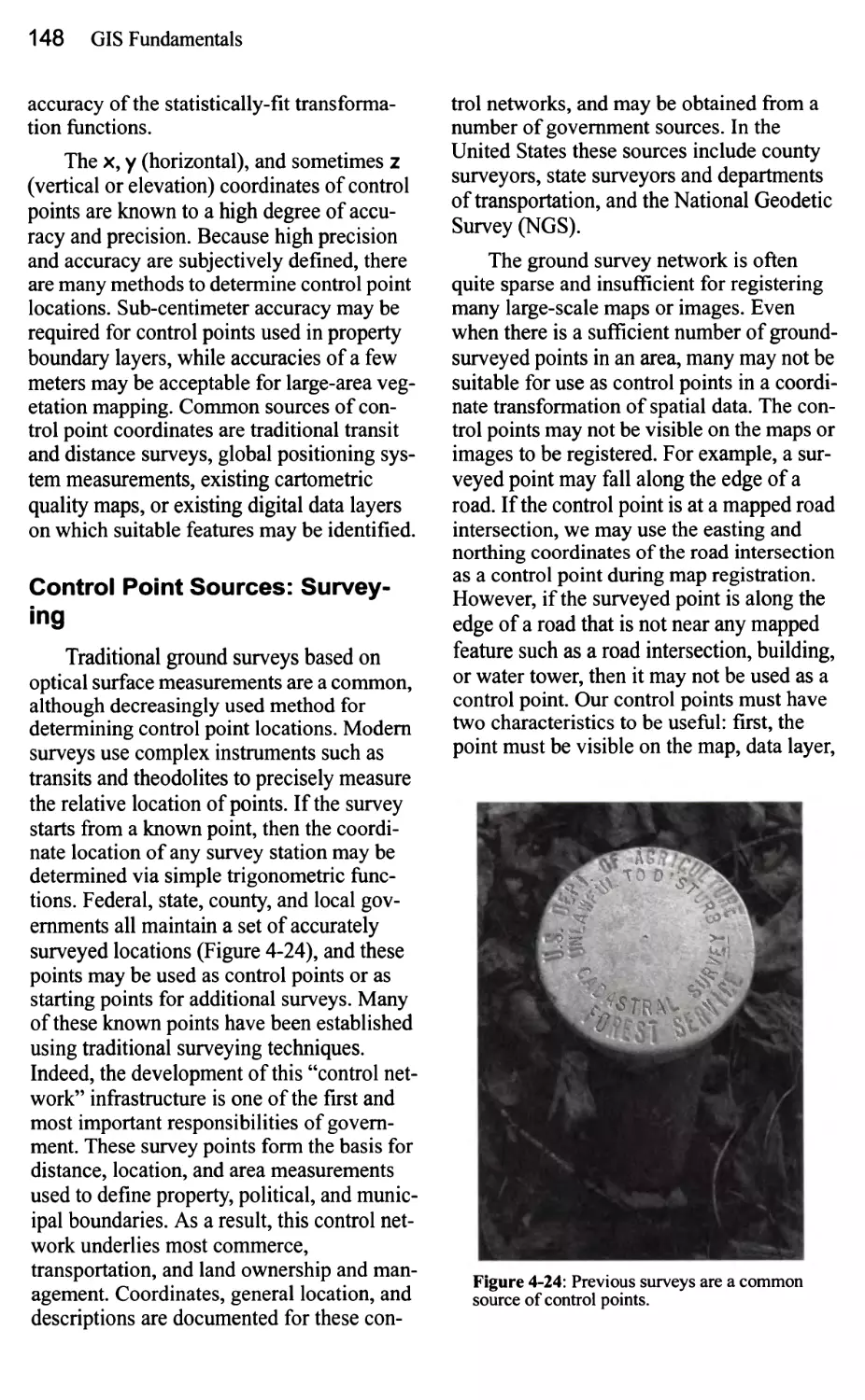
Control Point Sources: Surveying 148
GNSS Control Points 149
Control Points from Existing Maps and Digital Data 149
The Affine Transformation 151
Other Coordinate Transformations 153
A Caution When Evaluating Transformations 155
Raster Geometry and Resampling 156
Map Projection vs. Transformation 157
Output: Hardcopy Maps, Digital Data, and Metadata 159
Cartography and Map Design 159
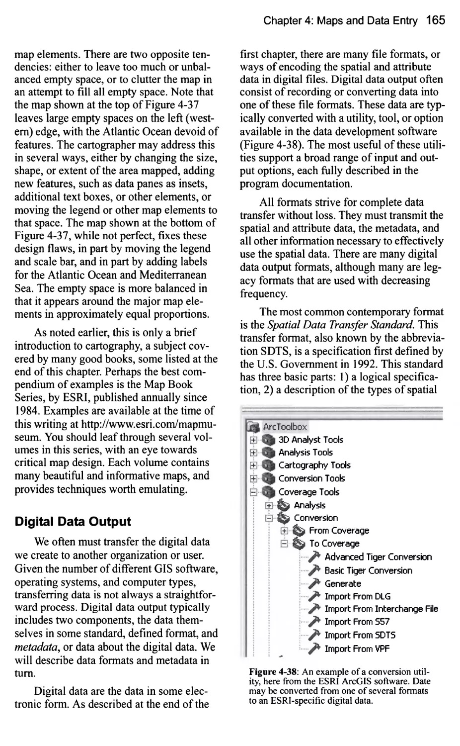
Digital Data Output 165
Metadata: Data Documentation 166
Summary 169
Chapter 5: Global Navigation Satellite
Systems 175
Introduction 175
GNSS Basics 175
GNSS Broadcast Signals 178
Range Distances 179
Positional Uncertainty 181
Sources of Range Error 182
Satellite Geometry and Dilution of Precision 183
Differential Correction 186
Real-Time Differential Positioning 189
WAAS and Satellite-based Corrections 189
A Caution on Datums 191
Optical and Laser Coordinate Surveying 192
GNSS Applications 196
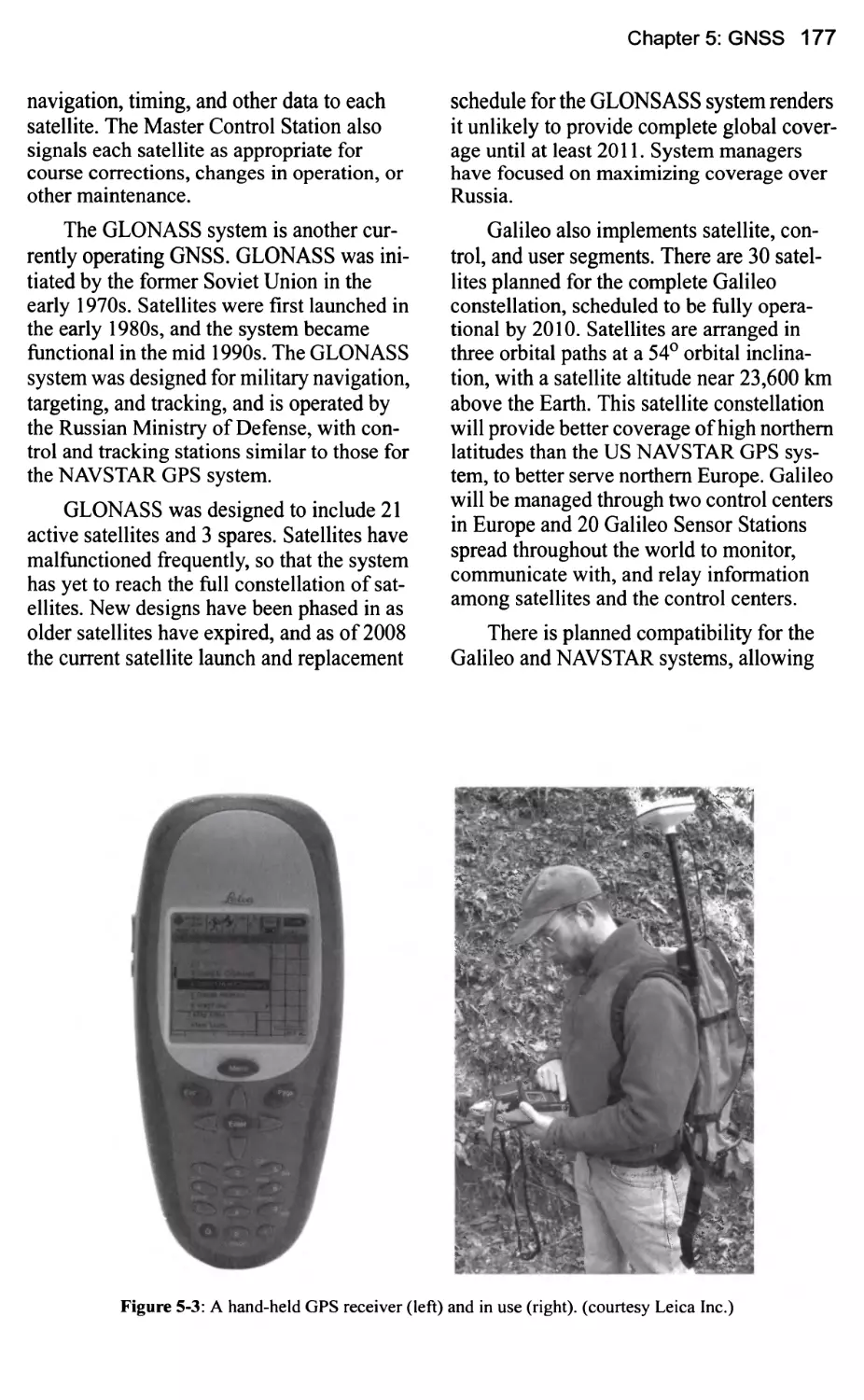
Field Digitization 196
Field Digitizing Accuracy and Efficiency 1 99
Rangefinder Integration 202
GNSS Tracking 203
Summary 206

viii Table of Contents
Chapter 6:Aerial and Satellite Images 211
Introduction 211
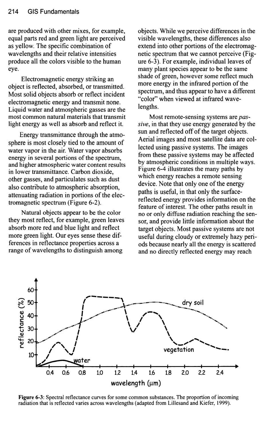
Basic Principles 213
Aerial Images 216
Primary Uses of Aerial Images 216
Photographic Film 217
Camera Formats and Systems 219
Digital Aerial Cameras 221
Geometric Quality of Aerial Images 223
Terrain and Tilt Distortion in Aerial Images 225
System Errors: Media, Lens, and Camera Distortion 228
Stereo Photographic Coverage 230
Geometric Correction of Aerial Images 232
Photointerpretation 236
Satellite Images 238
Basic Principles of Satellite Image Scanners 239
High-Resolution Satellite Systems 241
SPOT 244
Landsat 245
MODIS and VEGETATION 247
Other Systems 248
Satellite Images in GIS 250
Aerial or Satellite Images in GIS: Which to Use? 251
Image Sources 252
Summary 253
Chapter 7: Digital Data 259
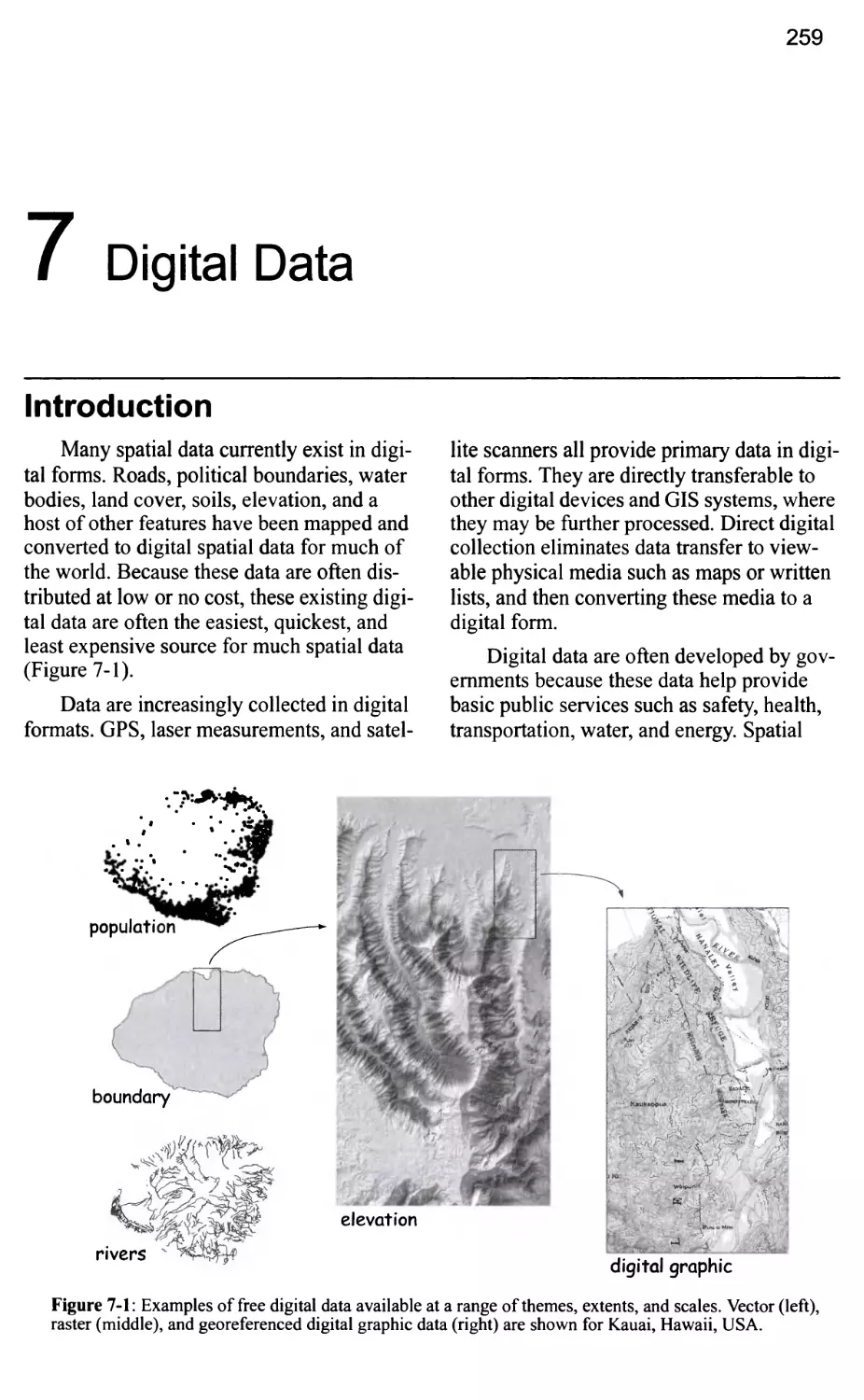
Introduction 259
National and Global Digital Data 260
Digital Data for the United States 262
National Spatial Data Infrastructure 262
The National Atlas 262
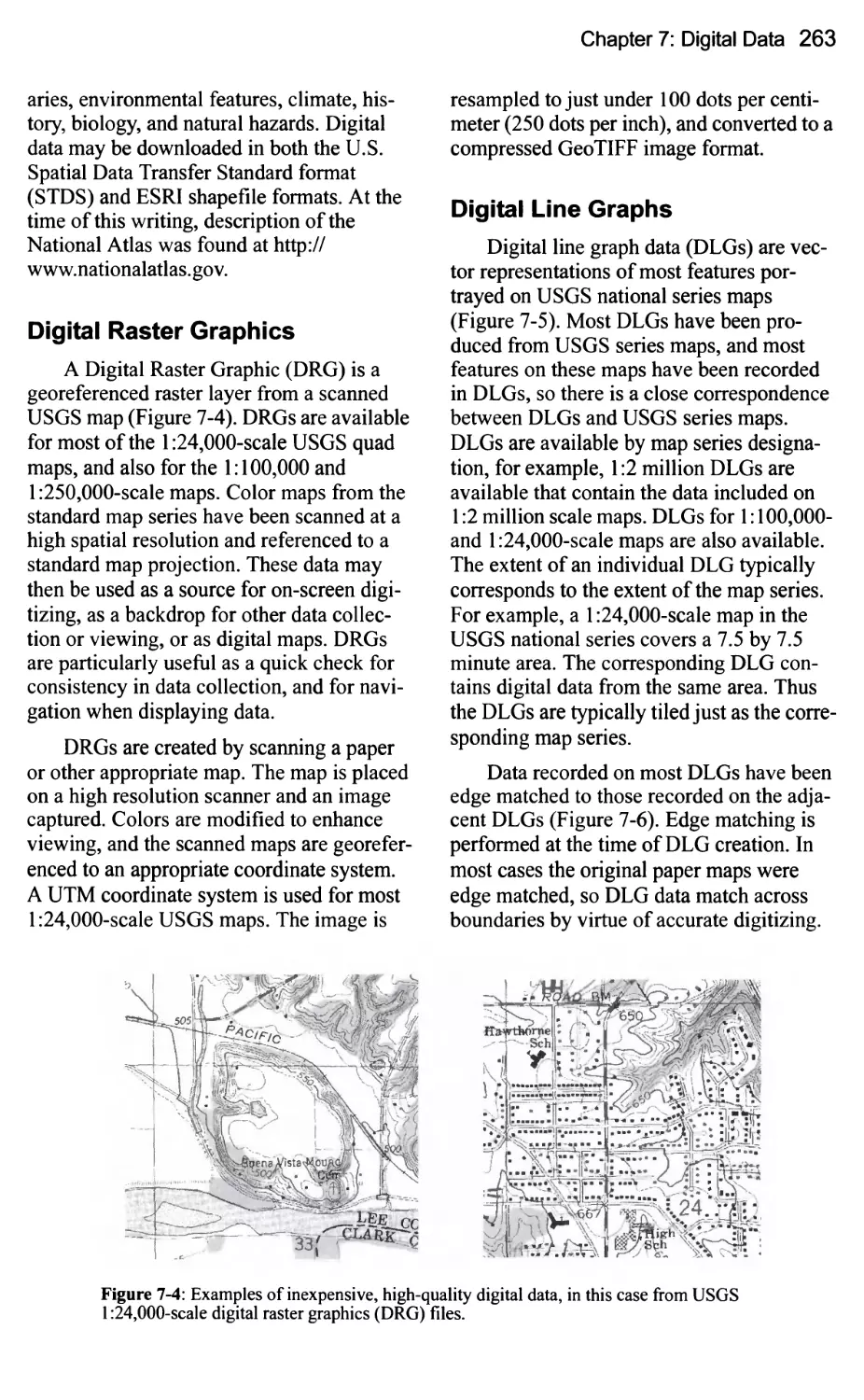
Digital Raster Graphics 263
Digital Line Graphs 263
Digital Elevation Models 265
Digital Orthophoto Quadrangles 270
NAIP Digital Images 272
Hydrologic Data 273
National Wetlands Inventory 275
Digital Soils Data 277
Digital Floodplain Data 281
Digital Census Data 282
National Land Cover Data 284
Summary 286

Table of Contents ix
Chapter 8: Attribute Data and Tables 291
Introduction 291
Database Components and Characteristics 293
Physical, Logical, and Conceptual Structures 297
Relational Databases 298
Hybrid Database Designs in GIS 303
Selection Based on Attributes 305
The Restrict Operator: Table Queries 305
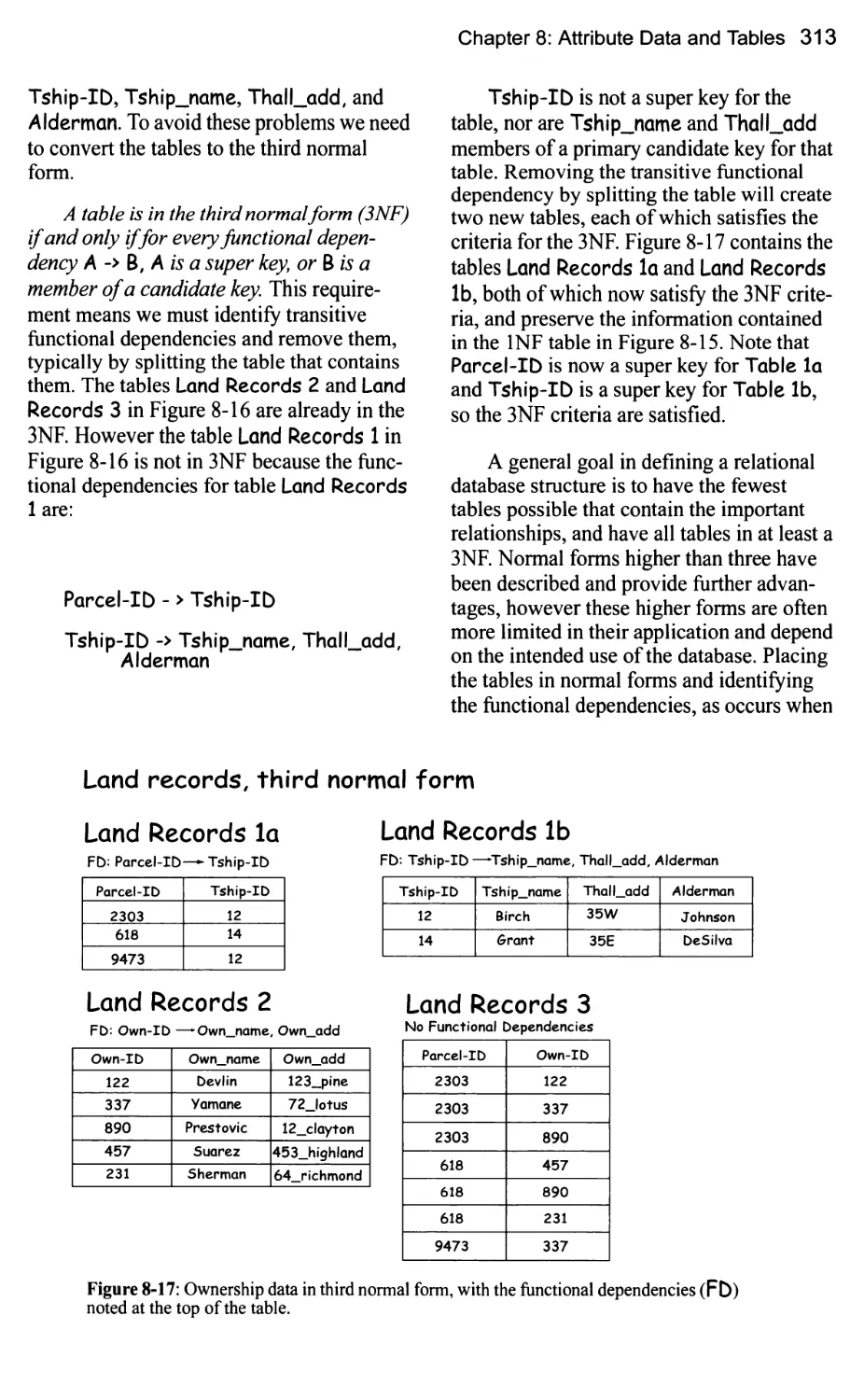
Normal Forms in Relational Databases 307
Keys and Functional Dependencies 307
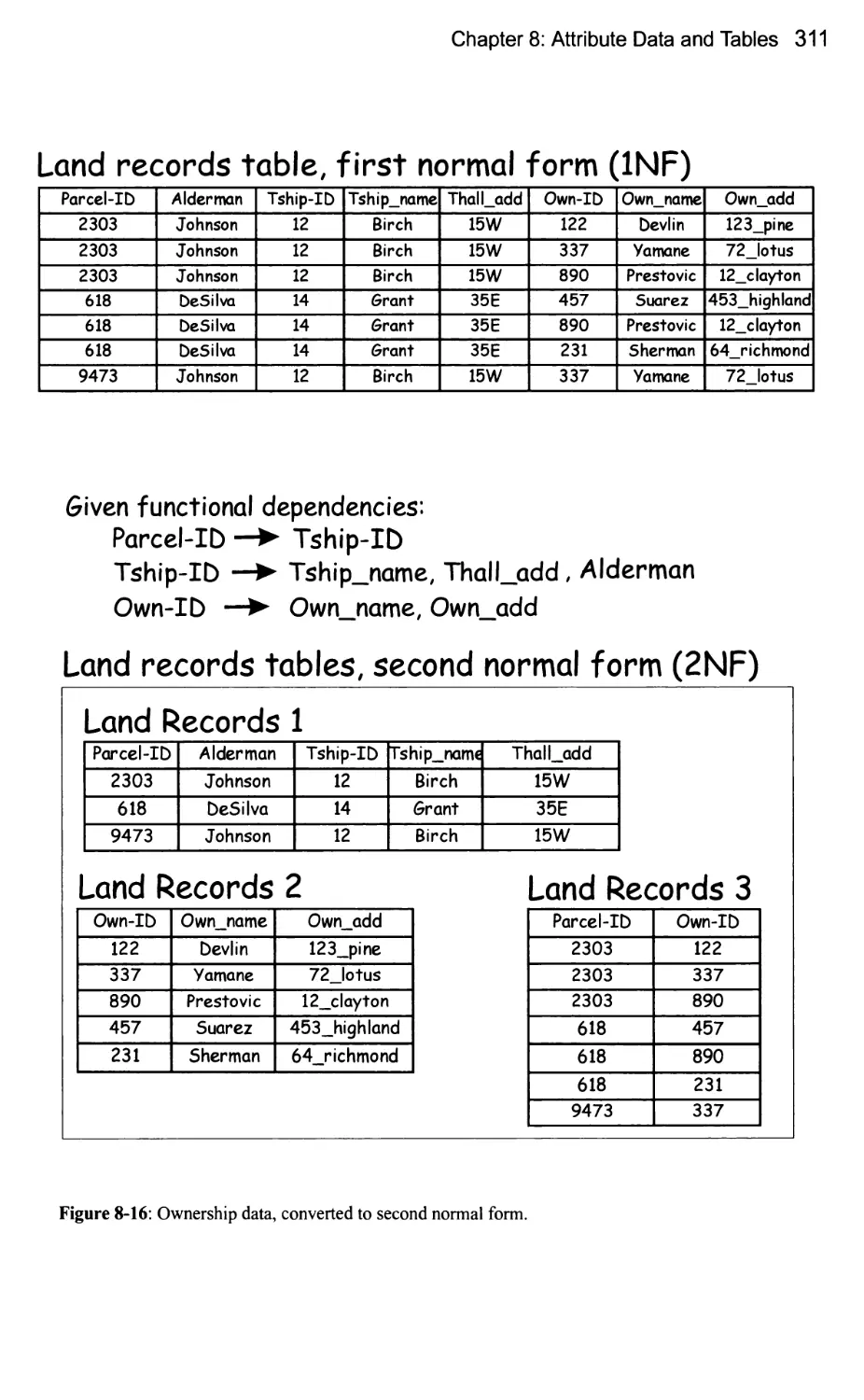
The First and Second Normal Forms 310
The Third Normal Form 312
Object-Relational Data Models 314
Trends in Spatial DBMS 315
Summary 315
Chapter 9: Basic Spatial Analysis 321
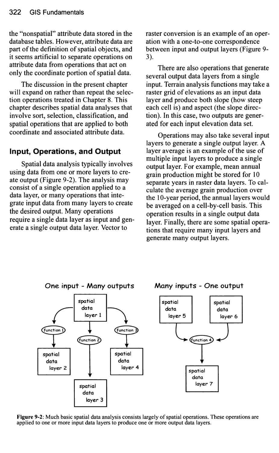
Introduction 321
Input, Operations, and Output 322
Scope 323
Selection and Classification 326
Set Algebra 326
Boolean Algebra 328
Spatial Selection Operations 330
Classification 332
The Modifiable Areal Unit Problem 339
Dissolve 340
Proximity Functions and Buffering 342
Buffers 343
Raster Buffers 344
Vector Buffers 345
Overlay 350
Raster Overlay 351
Vector Overlay 352
Clip, Intersect, and Union: Special Cases of Overlay 357
A Problem in Vector Overlay 360
Network Analysis 362
Geocoding 367
Summary 368

x Table of Contents
Chapter 10: Topics in Raster Analysis 379
Introduction 379
Map Algebra 380
Local Functions 384
Mathematical Functions 384
Logical Operations 384
Reclassification 387
Nested Functions 388
Overlay 390
Neighborhood, Zonal, Distance, and Global Functions . 395
Zonal Functions 403
Cost Surfaces 404
Summary 408
Chapter 11: Terrain Analysis 413
Introduction 413
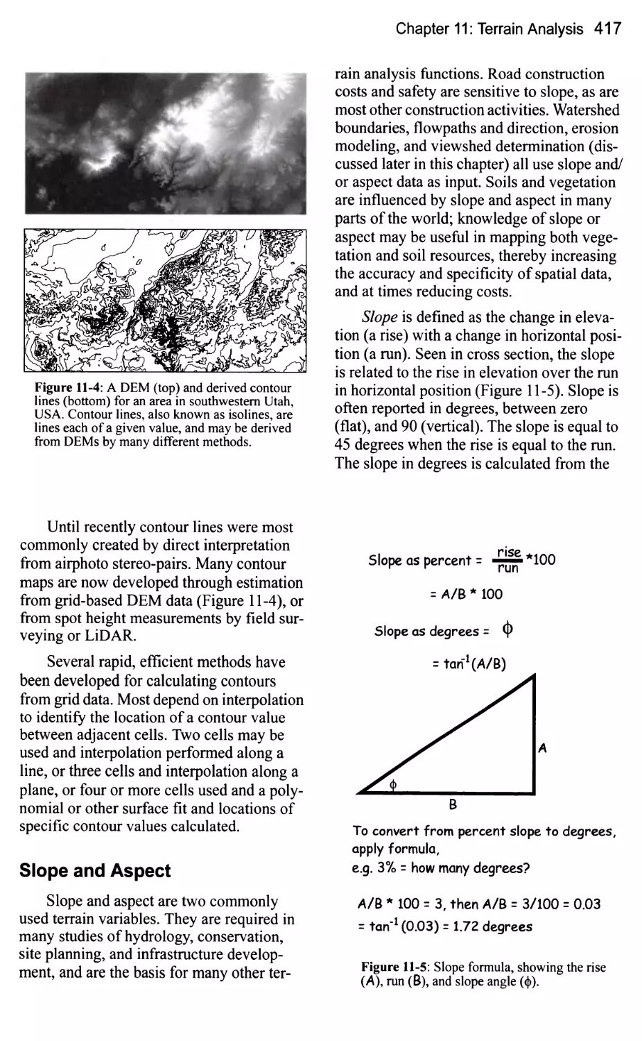
Contour Lines 415
Slope and Aspect 417
Hydrologic Functions 424
Viewsheds 426
Profile Plots 428
Shaded Relief Maps 428
Summary 430
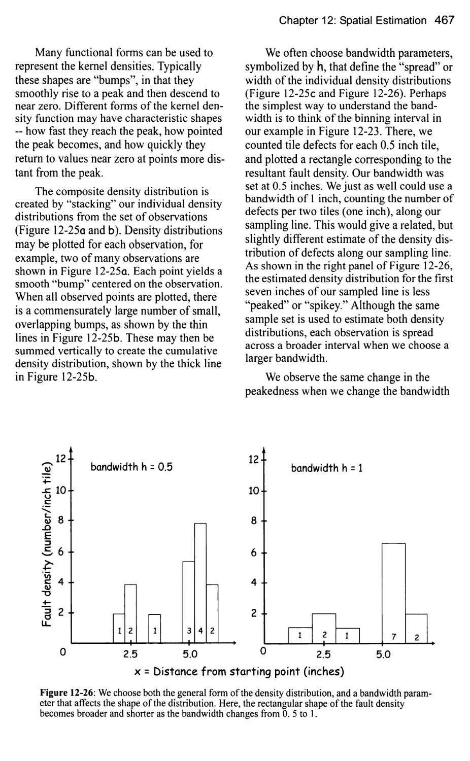
Chapter 12: Spatial Estimation: Interpolation,
Prediction, and Core Area Delineation 437
Introduction 437
Sampling 439
Sampling Patterns 439
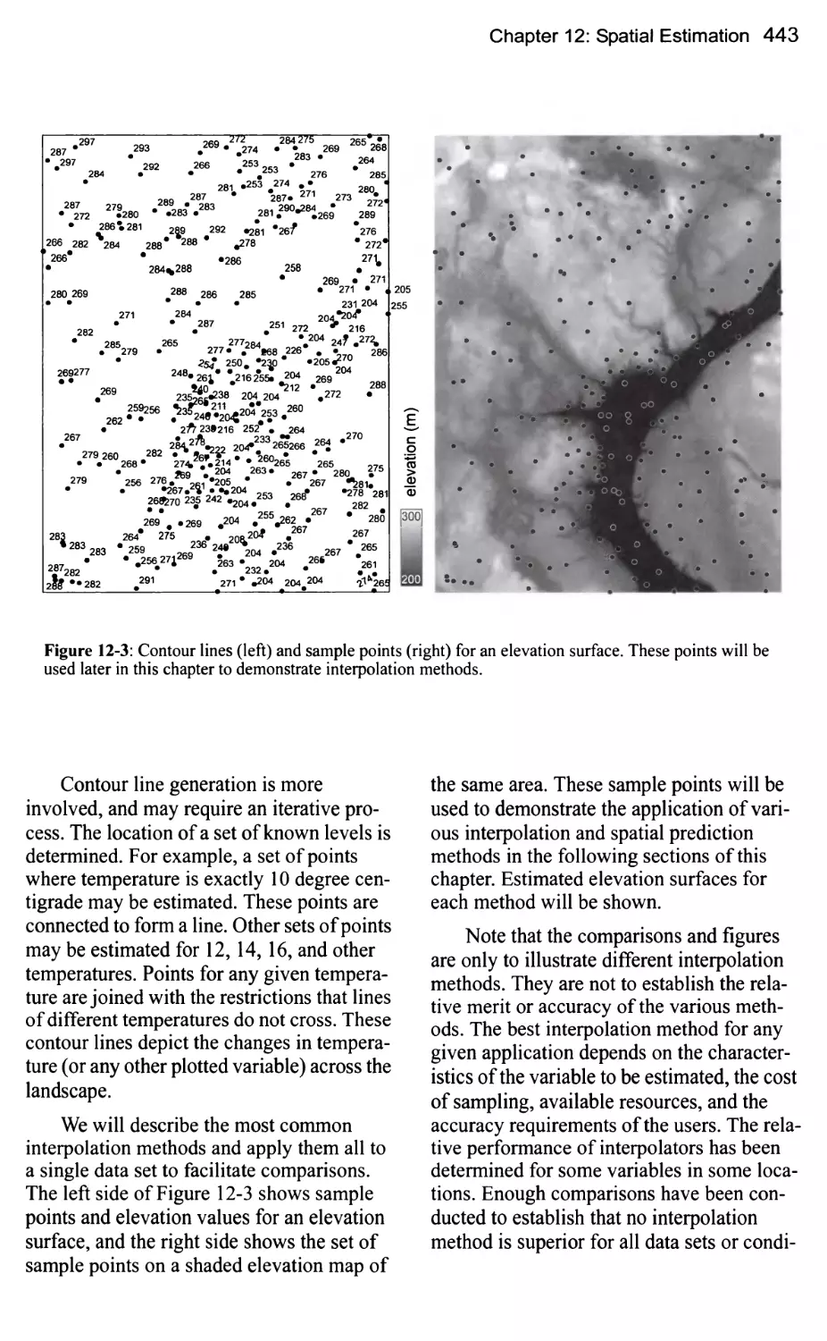
Spatial Interpolation Methods 442
Nearest Neighbor Interpolation 444
Fixed Radius - Local Averaging 445
Inverse Distance Weighted Interpolation 447
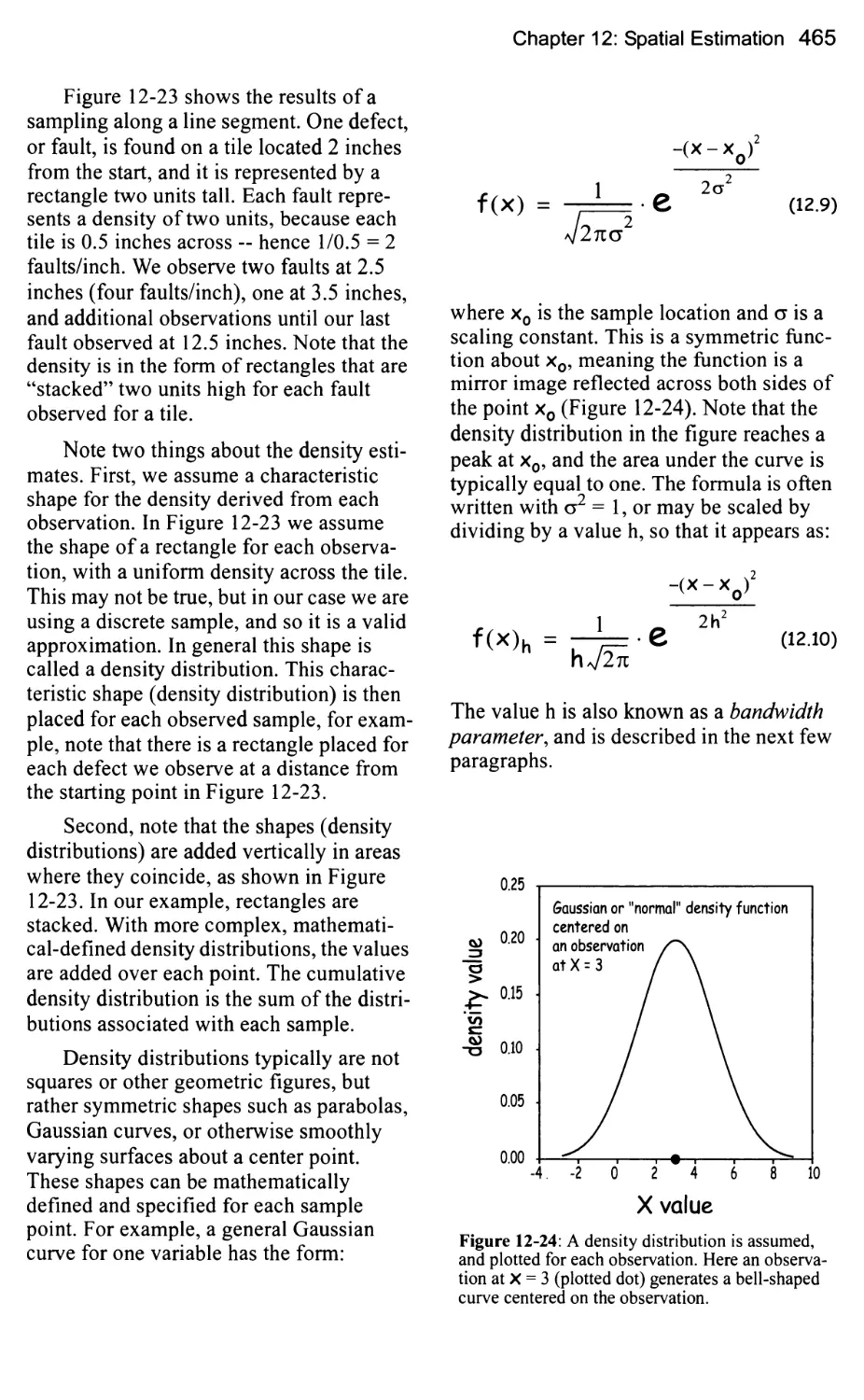
Splines 450
Spatial Prediction 451
Spatial Regression 455
Trend Surface and Simple Spatial Regression 455
Kriging and Co-Kriging 457

Table of Contents xi
Core Area Mapping 461
Mean Center and Mean Circle 461
Convex Hulls 462
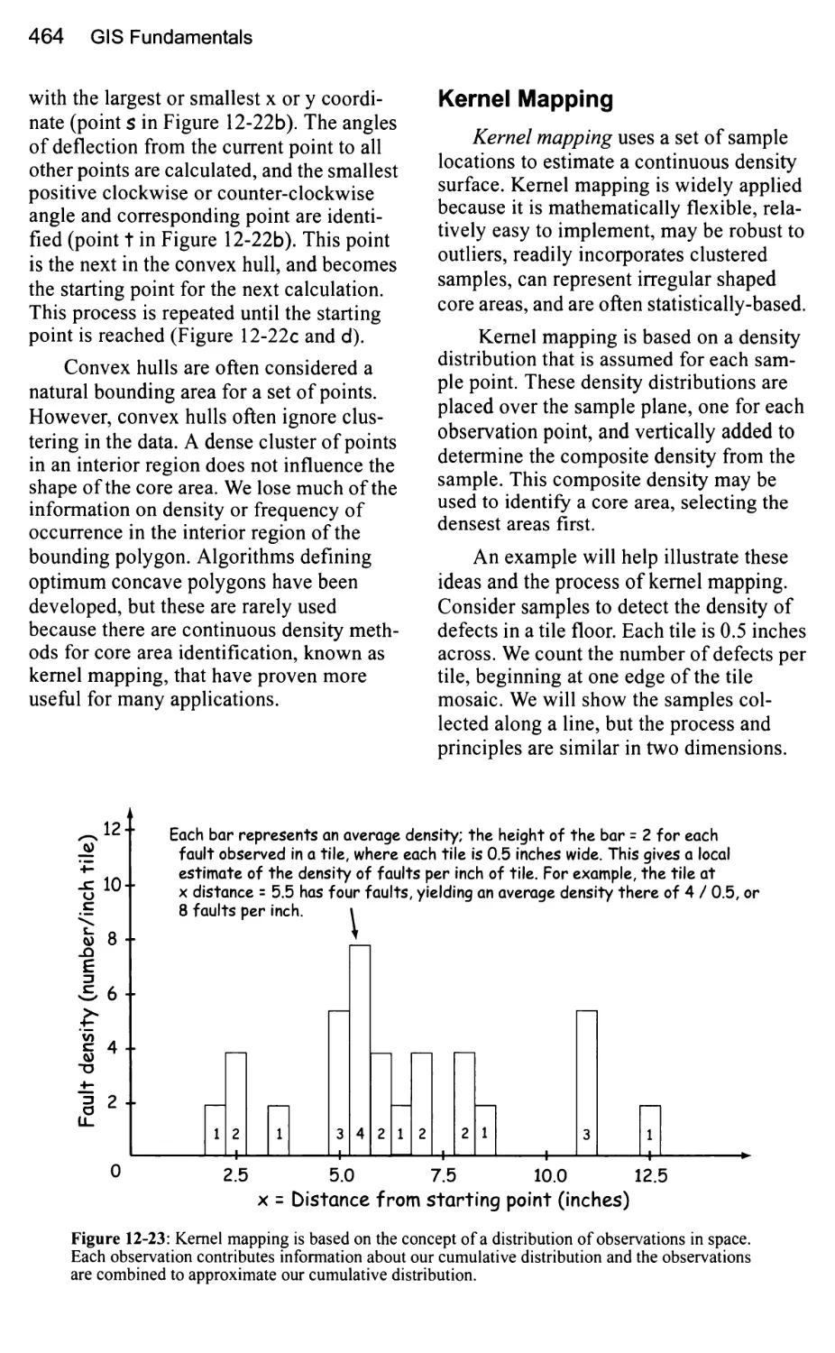
Kernel Mapping 464
Summary 470
Chapter 13: Spatial Models and Modeling 477
Introduction 477
Cartographic Modeling 479
Designing a Cartographic Model 481
Weightings and Rankings 481
Rankings Within Criteria 482
Weighting Among Criteria 484
Cartographic Models: A Detailed Example 487
Spatio-temporal Models 496
Cell-Based Models 498
Agent-based Modeling 500
Example 1: Process-based Hydrologic Models 500
Example 2: LANDIS, a Stochastic Model of Forest Change 503
LANDIS Design Elements 504
Summary 507
Chapter 14: Data Standards and
Data Quality 511
Introduction 511
Spatial Data Standards 511
Data Accuracy 514
Documenting Spatial Data Accuracy 515
Positional Accuracy 517
A Standard Method for Measuring Positional Accuracy 521
Accuracy Calculations 523
Errors in Linear or Area Features 526
Attribute Accuracy 527
Error Propagation in Spatial Analysis 529
Summary 530

xii Table of Contents
Chapter 15: New Developments in GIS 533
Introduction 533
GNSS 533
Mobile Real-time Mapping 535
Improved Remote Sensing 541
Web-Based Mapping 544
Visualization 547
Open GIS 550
Open Standards for GIS 550
Open Source GIS 550
Summary 551
Appendix A: Glossary 555
Appendix B: Sources of Geographic
Information 569
Appendix C: Useful Conversions
and Information 573
Length 573
Area 573
Angles 573
Scale 573
State Plane Zones 574
Trigonometric Relationships 575
Appendix D: Answers to Selected
Study Questions 585
Chapter 1 585
Chapter 2 586
Chapter 3 587
Chapter 4 589
Chapter 5 591
Chapter 6 592
Chapter 7 594
Chapter 8 595
Chapter 9 596
Chapter 10 599
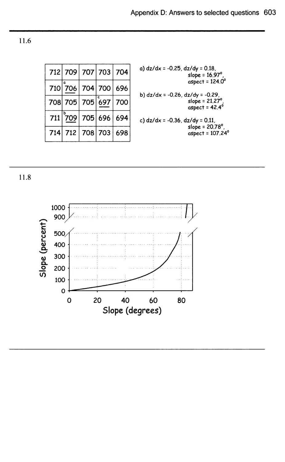
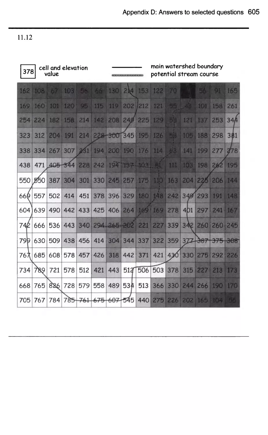
Chapter 11 602
Chapter 12 607
Chapter 13 609
Chapter 14 610

1
An Introduction to GIS
Introduction
Geography has always been important
to humans. Stone-age hunters anticipated
the location of their quarry, early explorers
lived or died by their knowledge of
geography, and current societies work and play
based on their understanding of who
belongs where. Applied geography, in the
form of maps and spatial information, has
served discovery, planning, cooperation,
and conflict for at least the past 3000 years
(Figure 1-1). Maps are among the most
beautiful and useful documents of human
civilization.
Most often our geographic knowledge
is applied to routine tasks, such as puzzling
a route in an unfamiliar town or searching
for the nearest metro station. Spatial
information has a greater impact on our lives
then we realize, by helping us produce the
food we eat, the energy we burn, the clothes
we wear, and the diversions we enjoy.
Because spatial information is so
important, we have developed tools called
geographic information systems (GIS) to
help us with our geographic knowledge. A
GIS helps us gather and use spatial data (we
will use the abbreviation GIS to refer to
both singular, system, and plural, systems).
Some GIS components are purely
technological; these include space-age data
collectors, advanced communications networks,
and sophisticated computing. Other GIS
components are very simple, for example, a
pencil and paper used to field verify a map.
As with many aspects of life in the last
five decades, how we gather and use spatial
data has been profoundly altered by modern
electronics, and GIS software and hardware
are primary examples of these technological
developments. The capture and treatment of
spatial data has accelerated over the past
three decades, and continues to evolve.
Key to all definitions of a GIS are
"where" and "what." GIS and spatial
analyses are concerned with the absolute and
relative location of features (the "where"), as
well as the properties and attributes of those
features (the "what"). The locations of
important spatial objects such as rivers and
streams may be recorded, and also their
size, flow rate, or water quality. Indeed,
these attributes often depend on the spatial
arrangement of "important" features, such
as land use above or adjacent to streams. A
GIS aids in the analysis and display of these
spatial relationships.
What is a GIS?
A GIS is a tool for making and using
spatial information. Among the many
definitions of GIS, we choose:
A GIS is a computer-based system to aid in
the collection, maintenance, storage,
analysis, output, and distribution of spatial data
and information.
When used wisely, GIS can help us live
healthier, wealthier, and safer lives.

2 GIS Fundamentals
A
k±rr> e, r
£:s
I A N D \T
' 1 ,;, < . , <A«„. Minne...Mcl oft* '<*W, <:?«£. J* ' >«*- . t3?I' -rfVtf'" >.£- --***1
Konrlto Uvl'-^rtx^'***
S... c.u«f.k.n«uSIT -AC^
1.M-
r**
*^&&
^.■&** "-«&»^-
Figure 1-1: A map of New England by Nicolaes Visscher, published about 1685. Present-day Cape
Cod is visible on the right, with the Connecticut and Hudson Rivers near the center of this map. Early
maps were key to the European exploration of new worlds.
GIS and spatial analyses are concerned
with the quantitative location of important
features, as well as properties and attributes
of those features. Objects occupy space.
Mount Everest is in Asia, Pierre is in South
Dakota, and the cruise ship Titanic is at the
bottom of the Atlantic Ocean. A GIS
quantifies these locations by recording their
coordinates, numbers that describe the position
of these features on Earth. The GIS may also
be used to record the height of Mount
Everest, the population of Pierre, or the depth of
the Titanic, as well as any other defining
characteristics of each spatial feature.
Each GIS user may decide what features
are important, and what is important about
them. For example, forests are important to
us. They protect our water supplies, yield
wood, harbor wildlife, and provide space to
recreate (Figure 1-2). We are concerned
about the level of harvest, the adjacent land
use, pollution from nearby industries, or
when and where forests burn. Informed
management of our forests requires at a
minimum knowledge of all these related factors,
and, perhaps above all, the spatial
arrangement of these factors. Buffer strips near
rivers may protect water supplies, clearings
may prevent the spread of fire, and polluters
downwind may not harm our forests while
polluters upwind might. A GIS aids
immensely in analyzing these spatial rela-

Chapter 1: An Introduction 3
tionships and interactions. A GIS is also
particularly useful at displaying spatial data and
reporting the results of spatial analysis. In
many instances GIS is the only way to solve
spatially-related problems.
GIS: A Ubiquitous Tool
GIS are essential tools in business,
government, education, and non-profit
organizations, and GIS use has become mandatory in
many settings. GIS have been used to fight
crime, protect endangered species, reduce
pollution, cope with natural disasters, treat
the AIDS epidemic, and to improve public
health; in short, GIS have been instrumental
in addressing some of our most pressing
societal problems.
GIS tools in aggregate save billions of
dollars annually in the delivery of
governmental and commercial goods and services.
GIS regularly help in the day-to-day
management of many natural and man-made
resources, including sewer, water, power,
and transportation networks. GIS are at the
heart of one of the most important processes
in U.S. democracy, the constitutionally
mandated reshaping of U.S. congressional
districts, and hence the distribution of tax
dollars and other government resources.
ll
'#*
*!M
«»>
m :
>
•"■'-.J
*'r;:*
' *%'
Figure 1-2: GIS allow us to analyze the relative spatial location of important geographic features. The
satellite image at the center shows a forested area in western Oregon, USA, with a patchwork of lakes
(dark area, upper left and mid-right), forest and clearings (middle), and snow-covered mountains (right).
Spatial analyses in a GIS may aid in ensuring sustainable recreation, timber harvest, environmental
protection, and other benefits from this and other globally important regions (courtesy NASA).

4 GIS Fundamentals
Why Do We Need GIS?
GIS are needed in part because human
populations and consumption have reached
levels such that many resources, including
air and land, are placing substantial limits on
human action (Figure 1-3). Human
populations have doubled in the last 50 years,
reaching 6 billion, and we will likely add
another 5 billion humans in the next 50
years. The first 100,000 years of human
existence caused scant impacts on the
world's resources, but in the past 300 years
humans have permanently altered most of
the Earth's surface. The atmosphere and
oceans exhibit a decreasing ability to
benignly absorb carbon dioxide and
nitrogen, two primary waste products of
humanity. Silt chokes many rivers and there are
abundant examples of smoke, ozone, or
other noxious pollutants substantially
harming public health (Figure 1-4). By the end of
the 20 century most suitable lands had
been inhabited and most of the Earth's
surface had not been farmed, grazed, cut, built
over, drained, flooded, or otherwise altered
by humans (Figure 1-5).
GIS help us identify and address
environmental problems by providing crucial
information on where problems occur and
who are affected by them. GIS help us
identify the source, location, and extent of
adverse environmental impacts, and may
help us devise practical plans for
monitoring, managing, and mitigating
environmental damage.
Human impacts on the environment
have spurred a strong societal push for the
adoption of GIS. Conflicts in resource use,
concerns about pollution, and precautions to
protect public health have led to legislative
mandates that explicitly or implicitly require
the consideration of geography. The U.S.
Endangered Species Act of 1973 (ESA) is an
example of the importance of geography in
resource management. The ESA requires
adequate protection of rare and threatened
Human population growth and poor
management require we feed, cloth,
power, and warm a rapidly expanding
population with increasingly scarce
resources. Geographic information
systems help us more effectively
improve human life while conserving
our planet.
K
3
D
3
-o
O
o
o*
o
(A
1600
1700
1800
year
1900
2000
Figure 1-3: Human population growth during the past 400 years has increased the need for
efficient resource use (courtesy United Nations and Ikonos).

Chapter 1: An Introduction 5
\
4
Figure 1-4: Wildfires, shown here in a satellite image of western North America, are among the human
forces behind the societal push to adopt GIS. Fires surround Los Angeles, near the center of this October,
2003 image. The smoke plumes from multiple fires extend across the homes and workplaces of more than
10 million people, and out over the Pacific Ocean to the lower left. GIS may be used to help prevent, fight,
and recover from such fires (courtesy NASA).
970s . 1980s
Figure 1-5: The environmental impacts wrought by humans have accelerated in many parts of the world
during the past century. These satellite images from the 1970s (left) to 1990s (right) show a shrunken Aral
Sea due to the overuse of water. Diversion for irrigation has destroyed a rich fishery, the economic base
for many seaside villages. GIS may be used to document change, mitigate damage, and to effectively
manage our natural resources (courtesy NASA).

6 GIS Fundamentals
organisms. Effective protection entails
mapping the available habitat and analyzing
species range and migration patterns. The
location of viable remnant populations
relative to current and future human land uses
must be analyzed, and action taken to ensure
species survival. GIS have proven to be use-
fill tools in all of these tasks.
Legislation has spurred the use of GIS in
many other endeavors, including the
dispensation of emergency services, protection
from flooding, disaster assessment and
management (Figure 1-6), and the planning and
development of infrastructure.
Public organizations have adopted GIS
because of legislative mandates, and because
GIS aid in governmental functions. For
example, emergency service vehicles are
regularly dispatched and routed using GIS.
Callers to E911 or other emergency response
dispatchers are automatically identified by
telephone number, and their address
recalled. The GIS software matches this
address to the nearest fire, police, or
ambulance station. A map or route description is
immediately generated by the software,
based on information on location and the
street network, and sent to the appropriate
station with a dispatch alarm.
Many businesses have adopted GIS
because they provide increased efficiency in
the delivery of goods and services. Retail
businesses locate stores based on a number
of spatially-related factors. Where are the
potential customers? What is the spatial
distribution of competing businesses? Where
are potential new store locations? What is
traffic flow near current stores, and how easy
is it to park near and access these stores?
Spatial analyses are used every day to
answer these questions. GIS are also used in
v^.
A
JM?'
-J**-
'* ■
V
'. -p',. - * \ >v
♦v
-
r ■
June 23,
***
■if7 **■
/l /•■—*
2004
v ,,*«#•
<T< v-
*
Dec. 28, 2004
\
\
Figure 1-6: GIS may aid in disaster assessment and recovery. These satellite images from Banda Aceh,
Indonesia, illustrate tsunami-caused damage to a shoreline community. Emergency response and longer-
term rebuilding efforts may be improved by spatial data collection and analysis (courtesy DigitalGlobe).

Chapter 1: An Introduction 7
hundreds of other business applications,
such as to route delivery vehicles, guide
advertising, design buildings, plan
construction, and sell real estate.
The societal push to adopt GIS has been
complemented by a technological pull in the
development and application of GIS.
Intercontinental mariners were vexed for more
than four centuries by their inability to
determine their position. Thousands of lives and
untold wealth were lost because ship
captains could not answer the simple question,
"Where am I?" Robust nautical navigation
methods eluded the best minds on Earth until
the 18th century. Since then there has been a
continual improvement in positioning
technology to the point where today, anyone can
quickly locate their outdoor position to
within a few meters. A remarkable
positioning technology, known as the global
positioning system (GPS), was originally
developed primarily for military
applications. Because this positioning technology is
available, people expect to have access to it.
GPS is one of several Global Navigation
Satellite Systems (GNSS) now incorporated
in cars, planes, boats, and trucks. GNSS are
indispensable navigation and spatial data
collection tools in government, business, and
recreation. GNSS and other GIS-related
technologies contribute to commerce,
planning, and safety.
The technological pull has developed on
several fronts. Spatial analysis in particular
has been helped by faster computers with
more storage. Most real-world spatial
problems were beyond the scope of all but the
largest government and business
organizations until the 1990s. The requisite
computing and storage capabilities were beyond any
reasonable budget. GIS computing expenses
are becoming an afterthought, as computing
resources often cost less than a few months
salary for a qualified GIS professional. Costs
decrease and performance increases at
dizzying rates, with predicted plateaus pushed
back each year. Computer capabilities have
reached a point that computational limits on
most spatial analysis are minor. Powerful
field computers are lighter, faster, more
t™
O PAQ O (!)
pocket pc
Eite L<& yfew Iheme £nab« Surface Ciap)**:]
ffl E3 BBS) MBBJ El
innn.N-'-bRinriSi j-*mttti
Madikwe Resources Reserve
-<*
HI
\l
.1^
Figure 1-7: Portable computing is one example
of the technological pull driving GIS adoption.
These hand-held devices substantially improve
the speed and accuracy of spatial data collection
(courtesy Compaq Computer Corp.).
capable, and less expensive each year, so
spatial data display and analysis capabilities
may always be at hand (Figure 1-7). GIS on
rugged, field-portable computers has been
particularly useful in field data entry and
editing.
In addition to the computing
improvements and the development of GNSS,
current "cameras" deliver amazingly detailed
aerial and satellite images. Initially,
advances in image collection and
interpretation were spurred by World War II and then
the Cold War because accurate maps were
required, but unavailable. Turned toward
peacetime endeavors, imaging technologies
now help us map food and fodder, houses
and highways, and most other natural and
human-built objects. Images may be rapidly
converted to accurate spatial information
over broad areas (Figure 1 -8). A broad range
of techniques have been developed for

8 GIS Fundamentals
-y-^
■T
■• ^~>-
: ■■&'.••
0
W
f
^■^
*. <f
. 4
) ■■>
Figure 1-8: Images taken from aircraft and satellites (left) provide a rich source of data, which may be
interpreted and converted to information about landcover and other characteristics of the Earth surface
(right).
extracting information from image data, and
ensuring this information faithfully
represents the location, shape, and characteristics
of features on the ground. Visible light, laser,
thermal, and radar scanners are currently
being developed to further increase the
speed and accuracy with which we map our
world. Thus, advances in these three key
technologies - imaging, GNSS, and
computing - have substantially aided the
development of GIS.
GIS in Action
Spatial data organization, analyses, and
delivery are widely applied to improve life.
Here we describe three examples that
demonstrate how GIS are in use.
Marvin Matsumota is alive today
because of GIS. The 60 year-old hiker
became lost in Joshua Tree National Park, a
300,000 hectare desert landscape famous for
its distinct and rugged terrain. Between six
and eight hikers become lost there in a
typical year, sometimes fatally so. Because of
the danger of hypothermia, dehydration, and
death, the U.S. National Park Service (NPS)
organizes search and rescue operation that
include foot patrols, horseback, vehicle, and
helicopter searches (Figure 1-9).
The search and rescue operation for Mr.
Matsumota was organized and guided using
GIS. Search and rescue teams carried field
positioning devices that recorded team
location and progress. Position data were
downloaded from the field devices to a field GIS
center, and frequently updated maps were
produced. On-site incident managers used
these maps to evaluate areas that had been
searched, and to plan subsequent efforts in
real time. Accurate maps showed exactly
what portions of the park had been searched
and by what method. Appropriate teams
were tasked to unvisited areas. Ground
crews could be assigned to areas that had
been searched by helicopters, but contained
vegetation or terrain that limited visibility
from above. Marvin was found on the fifth
day, alive but dehydrated and with an injured
skull and back from a fall. The search team
was able to radio its precise location to a
rescue helicopter. Another day in the field and
Marvin likely would have died, a day saved
by the effective use of GIS. After a week in
the hospital and some months convalescing
at home, Marvin made a full recovery.

Chapter 1: An Introduction 9
GIS are also widely used in planning
and environmental protection. Oneida
County is located in northern Wisconsin, a
forested area characterized by exceptional
scenic beauty. The County is in a region with
among the highest concentrations of
freshwater lakes in the world, a region that is also
undergoing a rapid expansion in the
permanent and seasonal human population.
Retirees, urban exiles, and vacationers are
increasingly drawn to the scenic and
recreational amenities available in Oneida
County. Permanent county population grew
by nearly 20% from 1990 to 2000, and the
seasonal influx almost doubles the total
county population each summer.
Population growth has caused a boom
in construction and threatened the lakes that
draw people to the County. A growing
number of building permits are for near-shore
houses, hotels, or businesses. Seepage from
septic systems, runoff from fertilized lawns,
Point Last Sean
04-31 <§ 1530 ]
\
or erosion and sediment from construction
all decrease lake water quality. Increases in
lake nutrients or sediment may lead to turbid
waters, reducing the beauty and value of the
lakes and nearby property.
In response to this problem, Oneida
County, the Sea Grant Institute of the
University of Wisconsin, and the Land
Information and Computer Graphics Facility of the
University of Wisconsin have developed a
Shoreland Management GIS Project. This
project helps protect valuable nearshore and
lake resources, and provides an example of
how GIS tools are used for water resource
management (Figure 1-10).
Oneida County has revised zoning and
other ordinances to protect shoreline and
lake quality and to ensure compliance
without undue burden on landowners. The
County uses GIS technology in the
maintenance of property records. Property records
Figure 1-9: Search and rescue
operations, such as the one for
Marvin Matsumoto (upper left,
inset) are spatial activities.
Searchers must combine
information on where the lost person was
last seen, likely routes of travel,
maps of the areas already
searched, time last searched, and
available resources to effectively
mount a search campaign
(courtesy Tom Patterson, US-NPS).

10 GIS Fundamentals
include information on the owner, tax value,
and any special zoning considerations. The
county uses these digital records when
creating parcel maps, processing sale,
subdivision, or other parcel transactions, and when
integrating new data such as aerial or boat-
based images to help detect property
changes and zoning violations.
GIS may also be used to administer
shoreline zoning ordinances, or to notify
landowners of routine tasks, such as septic
system maintenance. Northern lakes are
particularly susceptible to nutrient pollution
from near-shore septic systems (Figure 1-
11). Frequent, verified maintenance of each
septic system is required. A GIS may be
used to automatically generate notification
of non-compliance. For example,
landowners may be required to provide proof of
septic systems maintenance every three years.
The GIS can automatically identify owners
not in compliance and generate an
appropriate notification.
Our third example illustrates how GIS
helps save endangered species. The black-
footed ferret is a small carnivore of western
North America, and is one of the most
endangered mammals on the continent
(Figure 1-12). The ferret lives in close
association with prairie dogs, communally-living
rodents once found over much of North
America. Ferrets feed on prairie dogs and
live in their burrows, and prairie dog
colonies provide refuge from coyotes and other
larger carnivores that prey on the ferret. The
blackfooted ferret has become endangered
because of declines in the range and number
of prairie dog colonies, coupled with ferret
sensitivity to canine distemper and other
diseases.
The U.S. Fish and Wildlife Service
(USFWS) has been charged with preventing
the extinction of the blackfooted ferret. This
.A " ' - ot ink «w V: ^ ,:^ s ,
1 _J Bird JN
*> 1
II*
1 1 Buildings
■i
l| Pnotos shp
1 I Parctl Lines
1 V Wjttr
LZD
11 c:\coastgit\oneN
♦,
^
la\bl«g29.g*
11
11 **
II """ »* » "* , '"" *
11 PVScatelmaqej
11 ' -4\
—— ■■—'-Jfl*|
-r ml
• »• • 1
* * 1
h 1
# * •--
♦ ♦ * 1
BO El
„ -*»
1 »* A
r ♦ ♦ • *
v '. •
* - ; * 1
- * m
.1— J
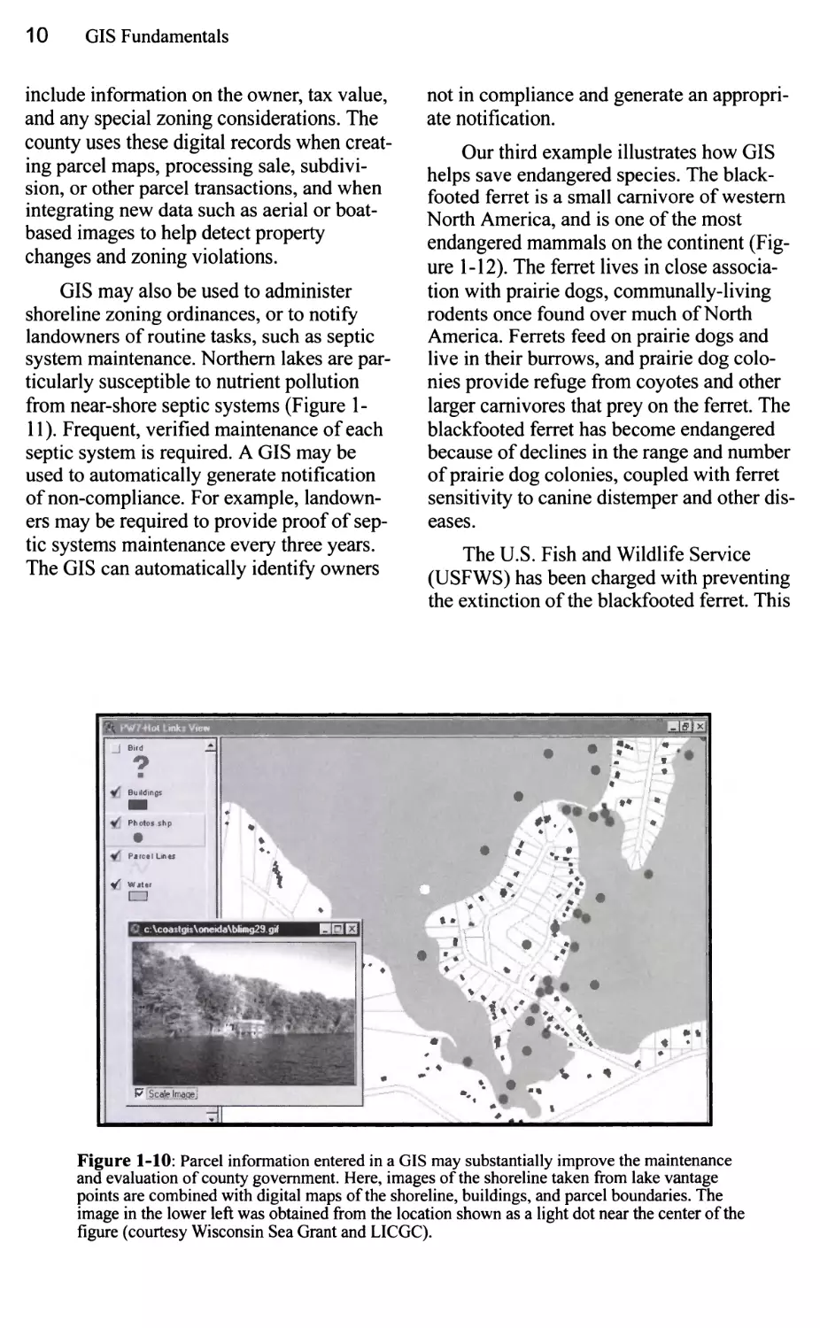
Figure 1-10: Parcel information entered in a GIS may substantially improve the maintenance
and evaluation of county government. Here, images of the shoreline taken from lake vantage
points are combined with digital maps of the shoreline, buildings, and parcel boundaries. The
image in the lower left was obtained from the location shown as a light dot near the center of the
figure (courtesy Wisconsin Sea Grant and LICGC).

Chapter 1: An Introduction 11
^ 4.<«t
** o
y^ Fioticbus Septic T*i*s _
V Parcafc
* ..Ficticious Septic Tanks
HDD I
0 __
1990
1991 "
(7 UpdateVak**
••w..
Figure 1-11: GIS may be used to streamline government function. Here, septic systems not compliant
with pollution prevention ordinances are identified by white circles (courtesy Wisconsin Sea Grant
Institute and LICGC).
entails establishing the number and location
of surviving animals, identifying the habitat
requirements for a sustainable population,
and analyzing what factors are responsible
for the decline in ferret numbers, so that a
recovery plan may be devised.
Because blackfooted ferrets are
nocturnal animals that spend much of their time
underground, and because ferrets have
always been rare, relatively little was known
about their life history, habitat requirements,
and the causes of mortality. For example,
young ferrets often disperse from their natal
prairie dog colonies in search of their own
territories. Dispersal is good when it leads to
an expansion of the species. However, there
are limits on how far a ferret may
successfully travel. If the nearest suitable colony is
too far away, the dispersing young ferret
may likely die of starvation or be eaten by a
larger predator. The dispersing ferret may
reach a prairie dog colony that is too small to
support it. Ferret recovery has been
hampered because we don't know when prairie
dog colonies are too far apart, or if a colony
is too small to support a breeding pair offer-
rets. Because of this lack of spatial
knowledge, wildlife managers have had difficulty
selecting among a number of activities to
enhance ferret survival. These activities
include the establishment of new prairie dog
colonies, fencing colonies to prevent the
entry of larger predators, removing
predators, captive breeding, and the capture and
transport of young or dispersing animals.
GIS have been used to provide data
necessary to save the blackfooted ferret (Figure
1-12). Individual ferrets are tracked in
nighttime spotlighting surveys, often in
combination with radiotracking devices. Ferret
location and movement are combined with
detailed data on prairie dog colony
boundaries, burrow locations, surrounding
vegetation, and other spatial data (Figure 1-13).
Individual ferrets can be identified and vital
characteristics monitored, including home
range size, typical distance travelled,
number of offspring, and survival. These data are

12 GIS Fundamentals
combined and analyzed in a GIS to improve
the likelihood of species recovery.
•»••
/
Figure 1-12: Specialized equipment is used to
collect spatial data. Here a burrow location is
recorded using a GPS receiver, as an interested
black footed ferret looks on (courtesy Randy
Matchett, USFWS).
Geographic Information Science
Although we have defined GIS as
geographic information systems, there is another
GIS: geographic information science. The
abbreviation GIS is commonly used for the
geographic information systems, while
GIScience is used to abbreviate the science.
The distinction is important, because the
future development of GIS depends on
progress in GIScience.
GIScience is the theoretical foundation
on which GIS are based. GIS research is
typically concerned with technical aspects of
GIS implementation or application.
GIScience includes these technical aspects,
but also seeks to redefine concepts in
geography and geographic information in the
context of the digital age. GIScience is
concerned with how we conceptualize
geography and how we collect, represent, store,
visualize, analyze, use, and present these
geographic concepts. The work draws from
many fields, including traditional geography,
geodesy, remote sensing, surveying,
computer science, cartography, mathematics,
statistics, cognitive science, and linguistics.
GIScience investigates not only technical
questions of interest to applied geographers,
Figure 1-13: Spatial data, such as the boundaries of prairie dog colonies (gray polygons) and
individual blackfooted ferret positions (triangle and circle symbols) may be combined to help
understand how best to save the blackfooted ferret (courtesy Randy Matchett, USFWS).

Chapter 1: An Introduction 13
business-people, planners, public safety
officers, and others, but GIScience is also
directed at more basic questions. How do we
perceive space? How might we best
represent spatial concepts, given the new array of
possibilities provided by our advancing
technologies? How does human psychology help
or hinder effective spatial reasoning?
Science has been described as a
handmaiden of technology in the applied world.
A more apt analogy is perhaps that science is
a parent of technology. GIS, narrowly
defined, is more about technology than
science. But since GIS is the tool with which
we solve problems, we are mistaken if we
consider it as the starting and ending point in
geographic reasoning. An understanding of
GIScience is crucial to the further
development of GIS, and in many cases, crucial to
the effective application of GIS. This book
focuses primarily on GIS, but provides
relevant information related to GIScience as
appropriate for an introductory course.
GIS Components
A GIS is comprised of hardware,
software, data, humans, and a set of
organizational protocols. These components must be
well integrated for effective use of GIS, and
the development and integration of these
components is an iterative, ongoing process.
The selection and purchase of hardware and
software is often the easiest and quickest
step in the development of a GIS. Data
collection and organization, personnel
development, and the establishment of protocols for
GIS use are often more difficult and time-
consuming endeavors.
Hardware for GIS
A fast computer, large data storage
capacities, and a high-quality, large display
form the hardware foundation of most GIS
(Figure 1-14). A fast computer is required
because spatial analyses are often applied
over large areas and/or at high spatial
resolutions. Calculations often have to be repeated
over tens of millions of times, corresponding
to each space we are analyzing in our
geographical analysis. Even simple operations
may take substantial time on
general-purpose computers, and complex operations can
Coordinate and
text input
devices
Rapid access
mass storage
Archival
storage
Large, high
resolution
display
High-speed
computer
High-quality hard-
copy graphic and
text output devices
Network and web
data communication
Figure 1-14: GIS are typically used with a number of general-purpose and specialized hardware
components.

14 GIS Fundamentals
Data entry
- manual coordinate capture
- attribute capture
- digital coordinate capture
- data import
Editing
- manual point, line and area
feature editing
- manual attribute editing
- automated error detection
and editing
Data management
- copy, subset, merge data
- versioning
- data registration and projection
- summarization, data reduction
- documentation
Figure 1-15: Functions commonly provided by
be unbearably long-running. While advances
in computing technology during the 1990s
have substantially reduced the time required
for most spatial analyses, computation times
are still unacceptably long for a few
applications.
While most computers and other
hardware used in GIS are general purpose and
adaptable for a wide range of tasks, there are
also specialized hardware components that
are specifically designed for use with spatial
data. While many non-GIS endeavors
require the entry of large data volumes, GIS
is unique in the volume of data that must be
entered to define the shape and location of
geographic features, such as roads, rivers,
and parcels. Specialized equipment,
described in Chapters 4 and 5, has been
developed to aid in these data entry tasks.
Analysis
- spatial query
- attribute query
- interpolation
- connectivity
- proximity and adjacency
- buffering
- terrain analyses
- boundary dissolve
- spatial aata overlay
- movinq window analyses
- map algebra
Output
- map design and layout
- hardcopy map printing
- digital graphic production
- export format generation
- metadata output
- digital map serving
software.
GIS Software
GIS software provides the tools to
manage, analyze, and effectively display and
disseminate spatial data and spatial information
(Figure 1-15). GIS by necessity involves the
collection and manipulation of the
coordinates we use to specify location. We also
must collect qualitative or quantitative
information on the non-spatial attributes of our
geographic features of interest. We need
tools to view and edit these data, manipulate
them to generate and extract the information
we require, and produce the materials to
communicate the information we have
developed. GIS software provides the
specific tools for some or all of these tasks.
There are many public domain and
commercially available GIS software packages,
and many of these packages originated at
academic or government-funded research
laboratories. The Environmental Systems
Research Institute (ESRI) line of products,
including ArcGIS, is a good example. Much

Chapter 1: An Introduction 15
of the foundation for early ESRI software
was developed during the 1960s and 1970s
at Harvard University in the Laboratory of
Computer Graphics and Spatial Analysis.
Alumni from Harvard carried these concepts
with them to Redlands, California when
forming ESRI, and included them in their
commercial products.
Our description below, while including
most of the major or widely used software
packages, is not meant to be all-inclusive.
There are many additional software tools
and packages available, particularly for
specialized tasks or subject areas. Appendix B
lists sources that may be helpful in
identifying the range of software available, and for
obtaining detailed descriptions of specific
GIS software characteristics and
capabilities.
ArcGIS
ArcGIS and its predecessors, Arc View
and Arc/Info, are the most popular GIS
software suites at the time of this writing. The
Arc suite of software has a larger user base
and higher annual unit sales than any other
competing product. ESRI, the developer of
ArcGIS, has a world-wide presence. ESRI
has been producing GIS software since the
early 1980s, and ArcGIS is its most recent
and well-developed integrated GIS package.
In addition to software, ESRI also provides
substantial training, support, and
fee-consultancy services at regional and international
offices.
ArcGIS is designed to provide a large
set of geoprocessing procedures, from data
entry through most forms of hardcopy or
digital data output. As such, ArcGIS is a
large, complex, sophisticated product. It
supports multiple data formats, many data types
and structures, and literally thousands of
possible operations that may be applied to
spatial data. It is not surprising that
substantial training is required to master the full
capabilities of Arc/Info.
ArcGIS provides wide flexibility in how
we conceptualize and model geographic
features. Geographers and other GIS-related
scientists have conceived of many ways to
think about, structure, and store information
about spatial objects. ArcGIS provides for
the broadest available selection of these
representations. For example, elevation data
may be stored in at least four major formats,
each with attendant advantages and
disadvantages. There is equal flexibility in the
methods for spatial data processing. This
broad array of choices, while responsible for
the large investment in time required for
mastery of ArcGIS, provides concomitantly
substantial analytical power.
GeoMedia
GeoMedia and the related MGE
products are a popular GIS suite. GIS and related
products have been developed and supported
by Intergraph, Inc. of Huntsville, Alabama,
for over 30 years. GeoMedia offers a
complete set of data entry, analysis, and output
tools. A comprehensive set of editing tools
may be purchased, including those for
automated data entry and error detection, data
development, data fusion, complex analyses,
and sophisticated data display and map
composition. Scripting languages are available,
as are programming tools that allow specific
features to be embedded in custom
programs, and programing libraries to allow the
modification of GeoMedia algorithms for
special-purpose software.
GeoMedia is particularly adept at
integrating data from divergent sources, formats,
and platforms. Intergraph appears to have
dedicated substantial effort toward the
OpenGIS initiative, a set of standards to
facilitate cross-platform and cross-software
data sharing. Data in any of the common
commercial databases may be integrated
with spatial data from many formats. Image,
coordinate, and text data may be combined.
GeoMedia also provides a
comprehensive set of tools for GIS analyses. Complex
spatial analyses may be performed,
including queries, for example, to find features in
the database that match a set of conditions,
and spatial analyses such as proximity or
overlap between features. Worldwide web

16 GIS Fundamentals
and mobile phone-based applications and
application development are well supported.
Maplnfo
Maplnfo is a comprehensive set of GIS
products developed and sold by the Maplnfo
Corporation, of Troy, New York. Maplnfo
products are used in a broad array of
endeavors, although use seems to be concentrated
in many business and municipal
applications. This may be due to the ease with
which Maplnfo components are
incorporated into other applications. Data analysis
and display components are supported
through a range of higher language
functions, allowing them to be easily embedded
in other programs. In addition, Maplnfo
provides a flexible, stand-alone GIS product
that may be used to solve many spatial
analysis problems.
Specific products have been designed
for the integration of mapping into various
classes of applications. For example, Map-
Info products have been developed for
embedding maps and spatial data into
wireless handheld devices such as telephones,
data loggers, or other portable devices.
Products have been developed to support internet
mapping applications, and serve spatial data
in worldwide web-based environments.
Extensions to specific database products
such as Oracle are provided.
Idrisi
Idrisi is a GIS system developed by the
Graduate School of Geography of Clark
University, in Massachusetts. Idrisi differs
from the previously discussed GIS software
packages in that it provides both image
processing and GIS functions. Image data are
useful as a source of information in GIS.
There are many specialized software
packages designed specifically to focus on image
data collection, manipulation, and output.
Idrisi offers much of this functionality while
also providing a large suite of spatial data
analysis and display functions.
Idrisi has been developed and
maintained at an educational and research
institution, and was initially used primarily as a
teaching and research tool. Idrisi has
adopted a number of very simple data
structures, a characteristic that makes the
software easy to modify in a teaching
environment. Some of these structures,
while slow and more space-demanding, are
easy to understand and manipulate for the
beginning programmer. The space and speed
limitation have become less relevant with
improved computers. File formats are well
documented and data easy to access and
modify. The developers of Idrisi have
expressly encouraged researchers, students,
and users to create new functions for Idrisi.
The Idrisi project has then incorporated user-
developed enhancements into the software
package. Idrisi is an ideal package for
teaching students both to use GIS and to develop
their own spatial analysis functions.
Idrisi is relatively low cost, perhaps
because of its affiliation with an academic
institution, and is therefore widely used in
education. Low costs are an important factor
in many developing countries, where Idrisi
has also been widely adopted.
Manifold
Manifold is a relatively inexpensive GIS
package with a surprising number of
capabilities. Manifold combines GIS and some
remote sensing capabilities in a single
package. Basic spatial data entry and editing
support are provided, as well as projections,
basic vector and raster analysis, image
display and editing, and output. The program is
extensible through a series of software
modules. Modules are available for surface
analysis, business applications, internet map
development and serving, database support,
and advanced analyses.
Manifold GIS differs from other
packages in providing sophisticated image
editing capabilities in a spatially-referenced
framework. Portions of images and maps
may be cut and pasted into other maps while
maintaining proper geographic alignment.

Chapter 1: An Introduction 17
Transparency, color-based selection, and
other capabilities common to image editing
programs are included in Manifold GIS.
AUTOCAD MAP
AUTOCAD is the world's
largest-selling computer drafting and design package.
Produced by Autodesk, Inc., of San Rafael,
California, AUTOCAD began as an
engineering drawing and printing tool. A broad
range of engineering disciplines are
supported, including surveying and civil
engineering. Surveyors have traditionally
developed and maintained the coordinates
for property boundaries, and these are
among the most important and often-used
spatial data. AUTOCAD MAP adds
substantial analytical capability to the already
complete set of data input, coordinate
manipulation, and data output tools provided
by AUTOCAD.
The latest version, AUTOCAD MAP
3D, provides a substantial set of spatial data
analysis capability. Data may be entered,
verified, and output. Data may also be
searched for features with particular
conditions or characteristics. More sophisticated
spatial analysis may be performed, including
path finding or data combination.
AUTOCAD MAP 3D incorporates many of
the specialized analysis capabilities of other,
older GIS packages, and is a good example
of the convergence of GIS software from a
number of disciplines.
GRASS
GRASS, the Geographic Resource
Analysis Support System, is a free, open
source GIS that runs on many platforms. The
system was originally developed by the U.S.
Army Construction Engineering Laboratory
(CERL), starting in the early 1980s, when
much GIS software was limited in access
and applications. CERL followed an open
approach to development and distribution,
leading to substantial contributions by a
number of university and other government
labs. Development was discontinued in the
military, and taken up by an open source
"GRASS Development Team", a
self-identified group of people donating their time to
maintain and enhance GRASS. The software
provides a broad array of raster and vector
operations, and is used in both research and
applications worldwide. Detailed
information and the downloadable software are
available at http://grass.itc.it/index.php.
Microimages
Microimages produces TNTmips, an
integrated remote sensing, GIS, and CAD
software package. Microimages also
produces and supports a range of other related
products, including software to edit and
view spatial data, software to create digital
atlases, and software to publish and serve
data on the internet.
TNTmips is notable both for its breadth
of tools and the range of hardware platforms
supported in a uniform manner.
Microimages recompiles a basic set of code for each
platform so that the look, feel, and
functionality is nearly identical irrespective of the
hardware platform used. Image processing,
spatial data analysis, and image, map, and
data output are supported uniformly across
this range.
TNTmips provides an impressive array
of spatial data development and analysis
tools. Common image processing tools are
available, including ingest of a broad
number of formats, image registration and
mosaics, reprojection, error removal, subsetting,
combination, and image classification.
Vector analyses are supported, including support
for point, line, and area features, multi-layer
combination, viewshed, proximity, and
network analyses. Extensive online
documentation is available, and the software is
supported by an international network of
dealers.
ERDAS
ERDAS (Earth Resources Data Analysis
System), now owned and developed by
Leica Geosystems, began as an image pro-

18 GIS Fundamentals
cessing system. The original purpose of the
software was to enter and analyze satellite
image data. ERDAS led a wave of
commercial products for analyzing spatial data
collected over large areas. Product development
was spurred by the successful launch of the
U.S. Landsat satellite in the 1970s. For the
first time, digital images of the entire Earth
surface were available to the public.
The ERDAS image processing software
evolved to include other types of imagery,
and to include a comprehensive set of tools
for cell-based data analysis. Image data are
supplied in a cell-based format. Cell-based
analysis is a major focus of sections in three
chapters of this book, so there will be much
more discussion in later pages. For now, it is
important to note that the "checkerboard"
format used for image data may also be used
to store and manipulate other spatial data. It
is relatively easy and quite useful to develop
cell-based spatial analysis tools to
complement the image processing tools.
GIS in Organizations
Although new users often focus on GIS
hardware and software components, we
must recognize that GIS exist in an
institutional context. Effective use of GIS requires
an organization to support various GIS
activities. Most GIS also require trained people to
use them, and a set of protocols guiding how
the GIS will be used. The institutional
context determines what spatial data are
important, how these data will be collected and
used, and ensures that the results of GIS
analyses are properly interpreted and
applied. GIS share a common characteristic
of many powerful technologies. If not
properly used, the technology may lead to a
significant waste of resources, and may do
more harm than good. The proper
institutional resources are required for GIS to
provide all its potential benefits.
GIS are often employed as decision
support tools (Figure 1-16). Data are collected,
ERDAS and most other image
processing packages provide data output formats
that are compatible with most common GIS
packages. Many image processing software
systems are purchased explicitly to provide
data for a GIS. The support of ESRI data
formats is particularly thorough in ERDAS.
ERDAS GIS components can be used to
analyze these spatial data.
This review of spatial data collection
and analysis software is in no way
exhaustive. There are many other software tools
available, many of which provide unique,
novel, or particularly clever combinations of
geoprocessing functions. GRASS, PCI, and
ENVI are just a few of the available software
packages with spatial data development or
analysis capabilities. In addition, there are
thousands of add-ons, special purpose tools,
or specific modules that complement these
products. Websites listed in Appendix B at
the end of this book will provide more
information on these and other GIS software
products.
entered, and organized into a spatial
database, and analyses performed to help make
specific decisions. The results of spatial
analyses in a GIS often uncover the need for
more data, and there are often several
iterations through the collection, organization,
analysis, output, and assessment steps before
a final decision is reached. It is important to
recognize the organizational structure within
which the GIS will operate, and how GIS
will be integrated into the decision-making
processes of the organization.
One important question that must be
answered early is "what problem(s) are we
to solve with the GIS?" GIS add significant
analytical power through the ability to
measure distances and areas, identify vicinity,
analyze networks, and through the overlay
and combination of different information.
Unfortunately, spatial data development is
often expensive, and effective GIS use

Chapter 1: An Introduction 19
requires specialized knowledge or training,
so there is often considerable expense in
constructing and operating a GIS. Before
spending this time and money there must be
a clear identification of the new questions
that may be answered, or the process,
product, or service that will be improved, made
more efficient, or less expensive through the
use of GIS. Once the ends are identified, an
organization may determine the level of
investment in GIS that is warranted.
Summary
GIS are computer-based systems that aid
in the development and use of spatial data.
There are many reasons we use GIS, but
most are based on a societal push, our need
to more effectively and efficiently use our
resources, and a technological pull, our
interest in applying new tools to previously
insoluble problems. GIS as a technology is
based on geographic information science,
and is supported by the disciplines of
geography, surveying, engineering, space
science, computer science, cartography,
statistics, and a number of others.
GIS are comprised of both hardware and
software components. Because of the large
volumes of spatial data and the need to input
coordinate values, GIS hardware often have
large storage capacities, fast computing
speed, and ability to capture coordinates.
Software for GIS are unique in their ability
to manipulate coordinates and associated
attribute data. A number of software tools
The physical world
*
Decide and act
9 t
\
V 1
Report results
Define
protocols
v
Collect and
edit spatial data
Analyze
ta3
VI
Figure 1-16: GIS exist in an institutional context. Effective use of GIS depends on a set of
protocols and an integration into the data collection, analysis, decision, and action loop of an
organization.

20 GIS Fundamentals
and packages are available to help us
develop GIS.
While GIS are defined as tools for use
with spatial data, we must stress the
importance of the institutional context in which
GIS fit. Because GIS are most often used as
decision-support tools, the effective use of
GIS requires more than the purchase of
hardware and software. Trained personnel and
protocols for use are required if GIS are to
be properly applied. GIS may then be
incorporated in the question-collect-analyze-
decide loop when solving problems.
The Structure of This Book
This book is designed to serve a
semester-long, 15-week course in GIS at the
university level. We seek to provide the relevant
information to create a strong basic
foundation on which to build an understanding of
GIS. Because of the breadth and number of
topics covered, students may be helped by
knowledge of how this book is organized.
Chapter 1 (this chapter), sets the stage,
providing some motivation and a background
for GIS. Chapter 2 describes basic data
representations. It treats the main ways we use
computers to represent perceptions of
geography, common data structures, and how
these structures are organized. Chapter 3
provides a basic description of coordinates
and coordinate systems, how coordinates are
defined and measured on the surface of the
Earth, and conventions for converting these
measurements to coordinates we use in a
GIS.
Chapters 4 through 7 treat spatial data
collection and entry. Data collection is often
a substantial task and comprises one of the
main activities of most GIS organizations.
General data collection methods and
equipment are described in Chapter 4. Chapter 5
describes Global Navigation Satellite
Systems (GNSS), a relatively new technology
for coordinate data collection. Chapter 6
describes aerial and space-based images as a
source of spatial data. Most historical and
contemporary maps depend in some way on
image data, and this chapter provides a
background on how these data are collected and
used to create spatial data. Chapter 7
provides a brief description of common digital
data sources available in the United States,
their formats, and uses.
Chapters 8 through 13 treat the analysis
of spatial data. Chapter 8 focuses on
attribute data, attribute tables, database
design, and analyses using attribute data.
Attributes are half our spatial data, and a
clear understanding of how we structure and
use them is key to effective spatial
reasoning. Chapters 9, 10, 11, and 12 describe
basic spatial analyses, including adjacency,
inclusion, overlay, and data combination for
the main data models used in GIS. They also
describe more complex spatio-temporal
models. Chapter 13 describes various
methods for spatial prediction and interpolation.
We typically find it impractical or inefficient
to collect "wall-to-wall" spatial and attribute
data. Spatial prediction allows us to extend
our sampling and provide information for
unsampled locations. Chapter 14 describes
how we assess and document spatial data
quality, while Chapter 15 provides some
musings on current conditions and future
trends.
We give preference to the International
System of Units (SI) throughout this book.
The SI system is adopted by most of the
world, and is used to specify distances and
locations in the most common global
coordinate systems and by most spatial data
collection devices. However, some English units
are culturally embedded, for example, the
survey foot, or 640 acres to a Public Land
Survey Section, and so these are not
converted. Because a large portion of the target
audience for this book is in the United
States, English units of measure often
supplement SI units.

Chapter 1: An Introduction 21
Suggested Reading
Amdahl, G (2001). Disaster Response: GISfor Public Safety, ESRI Press: Redlands,
California.
Burrough, P.A.& Frank, A.U. (1995). Concepts and paradigms in spatial information: Are
current geographical information systems truly generic?, International Journal of
Geographical Information Systems, 1995, 9:101-116.
Burrough, P. A. & McDonnell, R. A. (1992). Principles of Geographical Information Systems,
Oxford University Press: New York, 1998.
Campbell, H. J. & Masser, I., GIS in local government: some findings from Great Britain,
InternationalJournal of Geographical Information Systems, 1992, 6:529-546.
Commission on Geoscience (1997). Rediscovering Geography: New Relevance for Science
and Society, National Academy Press: Washington D.C.
Goodchild, M. F. (1992). Geographical information science, InternationalJournal of
Geographical Information Systems, 6:31-45.
Grimshaw, D. (2000). Bringing Geographical Information Systems Into Business, 2nd
Edition. Wiley: New York.
Haining, R. (1990). Spatial Data Analysis in the Social and Environmental Sciences,
Cambridge University Press: Cambridge.
Huxhold, W. E. (1991). An Introduction to Urban Geographic Information Systems, Oxford
University Press: Oxford.
Johnston, C. (1998). Geographic Information Systems in Ecology, Blackwell Scientific:
Boston.
MaGuire, D.J., Goodchild, M.F., & Rhind, D.W., (Ed.), Geographic Information Systems,
Longman Scientific: New York.
Martin, D. (1996). Geographical Information Systems: Socio-economic Applications (2nd
ed.). Routledge: London.
McHarg, I. (1995) Design with Nature, Wiley: New York, 1995.
National Research Council of the National Academies (2006). Beyond Mapping: Meeting
National Needs through Enhanced Geographic Information Science. National Academies
Press: Washington D.C.
Peuquet, D. J. & Marble, D. F. (Eds.). (1990). Introductory Readings in Geographic
Information Systems, Taylor and Francis, Washington D.C, 1990.

22 GIS Fundamentals
Pickles, J. (Ed.). (1995). Ground Truth: The Social Implications of Geographic Information
Systems, Guilford: New York, 1995.
de Smith, M.G, Goodchild, M.F. & Longley, P.A. (2007). Geospatial Analysis: A
Comprehensive Guide to Priciples, Techniques, and Software Tools. Winchelsea Press: Leicester.
Smith, D. A. & Tomlinson, R. F. (1992). Assessing costs and benefits of geographical
information systems: methodological and implementation issues, International Journal of
Geographical Information Systems, 6:247-256.
Theobald, D. M. (2003). GIS Concepts and ArcGIS Methods, Conservation Planning
Technologies, Fort Collins, 2003.
Tillman Lyle, J. (1999). Design for Human Ecosystems: Landscape, Land Use, and Natural
Resources, Island Press, Washington.
Tomlinson, R. (1987). Current and potential uses of geographical information systems. The
North American experience, International Journal of Geographical Information Systems,
1:203-218.

Chapter 1: An Introduction 23
Exercises
1.1 - Why are we more interested in spatial data today than 100 years ago?
1.2 - You have probably collected, analyzed, or communicated spatial data in one way
or another during the past month. Describe each of these steps for a specific
application you have used or observed.
1.3 - How are GIS software different from most other software?
1.4 - Describe the ways in which are GIS hardware different from other computer
hardware?
1.5 - What are the limitations of using a GIS? Under what conditions might the
technology hinder problem solving, rather than help?
1.6 - Are paper maps and paper data sheets a GIS? Why or why not?

24 GIS Fundamentals

25
2
Data Models
Introduction
Data in a GIS represent a simplified view
of physical entities or phenomena. These data
include information on the spatial location
and extent of the physical entities, and
information on their non-spatial properties.
Each entity is represented by a spatial
feature or cartographic object in the GIS, and
so there is an entity-object correspondence.
Because every computer system has limits,
only a subset of essential characteristics are
recorded. As illustrated in Figure 2-1, we
may represent lakes in a region by a set of
polygons. These polygons are associated with
a set of essential characteristics that define
each lake, perhaps average lake depth, the
name, or some measure of water quality.
Only lake boundaries and essential lake
characteristics have been saved in this example.
Essential characteristics are defined and
subjectively chosen by the person or group
that develops the spatial data. The essential
characteristics of a forest would be different
in the eyes of a logger than in the eyes of a
water conservation officer, a hunter, or a
hiker. Objects are abstract representations of
reality that we store in a spatial database, and
i '
Figure 2-1: A physical entity is represented by a spatial object in a GIS. Here, the physical boundaries of
lakes are represented by lines.

26 GIS Fundamentals
they are imperfect representations because
we can only record a subset of the
characteristics of any entity. No one abstraction is
universally better than any other, and the
goal of the GIS user is to define objects that
support the intended use at the desired level
of detail and accuracy.
A spatial data model may be defined as
the objects in a spatial database plus the
relationships among them. The term "model" is
fraught with ambiguity because it is used in
many disciplines to describe many things.
Here the purpose of a spatial data model is to
provide a formal means of representing and
manipulating spatially-referenced
information. In our lake example in Figure 2-1, our
data model consists of two parts. The first
part is a set of polygons (closed areas)
recording the shoreline of the lake, and the
second part is a set of numbers or letters
associated with each polygon. The data
model may be considered the most
recognizable level in our computer abstraction of the
real world. Data structures and binary
machine code are successively less
recognizable, but more computer-compatible forms
of the spatial data (Figure 2-2).
Coordinates are used to define the
spatial location and extent of geographic
objects. A coordinate most often consists of
a pair of numbers that specify location in
relation to a point of origin. The coordinates
quantify the distance from the origin when
measured along a standard direction. Single
Real world
Data model
\ '*>
K
ID
1
2
3
4
Area
16.3
7.9
121.8
10.1
Type
PUB
PEM
U
PUB
Data
structure
X
1.2
5.8
8.9
y
4.7
3.6
7.2
Machine
code
10011101
00110110
10110100
Figure 2-2: Levels of abstraction in the representation of spatial entities. The real world is
represented in successively more machine-compatible but humanly obscure forms.

Chapter 2: Data Models 27
Coordinates:
(3,12)
(14,5)
1,8
3,12
8,10
14,5
5,1.5
1,8
Attributes:
lot # :1347
street: Willow Lane
town: Hopkins
(5,1.5)
0,0 X
Figure 2-3: Coordinate and attribute data are used to represent entities.
or groups of coordinates are organized to
represent the shapes and boundaries that
define the objects. Coordinate information is
an important part of the data model, and
models differ in how they represent these
coordinates. Coordinates are usually
expressed in one of many standard
coordinate systems. The coordinate systems are
usually based upon standardized map
projections (discussed in Chapter 3) that
unambiguously define the coordinate values for every
point in an area.
Typically, attribute data complement
coordinate data to define cartographic
objects (Figure 2-3). Attribute data are
collected and referenced to each object. These
attribute data record the non-spatial
components of an object, such as a name, color, pH,
or cash value. Keys, labels, or other indices
are used so that the coordinate and attribute
data may be viewed, related, and
manipulated together.
Most conceptualizations view the world
as a set of layers (Figure 2-4). Each layer
organizes the spatial and attribute data for a
given set of cartographic objects in the
region of interest. These are often referred to
as thematic layers. As an example consider a
GIS database that includes a soils data layer,
a population data layer, an elevation data
layer, and a roads data layer. The roads layer
contains only roads data, including the
location and properties of roads in the analysis
area (Figure 2-4). There are no data
regarding the location and properties of any other
geographic entities in the roads layer.
Information on soils, population, and elevation
are contained in their respective data layers.
Through analyses we may combine data to
create a new data layer, for example, we may
identify areas that have high elevation and
join this information with the soils data. This
combination creates a new data layer with a
new, composite soils/elevation variable.
Coordinate Data
Coordinates define location in two or
three-dimensional space. Coordinate pairs, x
and y, or coordinate triples, x, y, and z, are
used to define the shape and location of each
spatial object or phenomenon.

28 GIS Fundamentals
Spatial data in a GIS most often use a
Cartesian coordinate system, so named after
Rene Descartes, a French mathematician.
Cartesian systems define two or three
orthogonal (right-angle) axes.
Two-dimensional Cartesian systems define x and y axes
in a plane (Figure 2-5, left).
Three-dimensional Cartesian systems define a z axis,
orthogonal to both the x and y axes. An
origin is defined with zero values at the
intersection of the orthogonal axes (Figure 2-5,
right). Cartesian coordinates are usually
specified as decimal numbers that, by
convention, increase from bottom to top and
from left to right.
Two-dimensional Cartesian coordinate
systems have historically been the logical
and most common choice for mapping small
areas. Small is a relative term, but here we
wetlands
soils
roads
elevation
political
boundaries
Earth
surface
Figure 2-4: Spatial data are often stored as separate thematic layers, with objects grouped based on a set of
properties, e.g., water, roads, or land cover, or some other agreed-upon set.

Chapter 2: Data Models 29
2 - Dimensional
3 - Dimensional
§
A A A A A
I I I I I »
I I I I I »
I I I I I »
I I I I I P
k—-L—-L—L—I »
ongin O 10 20 30 40 50 x
Figure 2-5: Two dimensional (left) and three dimensional (right) Cartesian coordinate systems.
mean maps of farm fields, land and property,
cities, and counties. We typically introduce
acceptably small errors for most applications
when we ignore the Earth's curvature over
these small areas. When we map over larger
areas, or need the highest precision and
accuracy, we usually must choose a three-
dimensional system.
Coordinate data may also be specified in
a spherical coordinate system. Hipparchus, a
Greek mathematician of the 2nd century
B.C., was among the first to specify
locations on the Earth using angular
measurements on a sphere. The most common
spherical system uses two angles of rotation
and a radius distance, r, to specify locations
on a modeled Earth surface (Figure 2-6).
The first angle of rotation is along the
equator. The equator is the imaginary line
halfway between the north and south poles. The
equator splits the globe into northern and
southern hemispheres. The longitude (k)
measures an angle in an east-west direction
along the equator. A second angle of
rotation, measured in a north-south direction, is
used to define a latitude ((()).
There are two primary conventions used
for describing latitude and longitude values
(Figure 2-7). The first uses a leading letter,
N, S, E, or W to indicate direction, followed
by a number to indicate location. Latitudes
increase from 0 at the equator to 90 degrees
at the poles. Northern latitudes are preceded
by an N and southern latitudes by an S, for
example, N90°, S10°. Longitude values are
preceded by an E or W, respectively, east or
Spherical
coordinates
Figure 2-6: Three-dimensional, spherical
coordinates may define location by two angles of
rotation, X and <|>, and a radius vector, r, to a
point on a sphere.

30 GIS Fundamentals
Figure 2-7: Spherical coordinates of latitude and
longitude are most often expressed as directional
(N/S, E/W), or as signed numbers. Latitudes are
positive north, negative south, longitudes are
positive east, negative west.
west of a longitude of origin, for example
WHO0. Longitudes range from 0 to 180
degrees east or west. Note that the east and
west longitudes meet at 180 degrees, so that
E180° equals W180°.
Signed coordinates is the second
common convention for specifying latitude and
longitude in a spherical coordinate system.
Northern latitudes are positive and southern
latitudes are negative, and eastern longitudes
positive and western longitudes negative.
Latitudes vary from -90 degrees to 90
degrees, and longitudes vary from -180
degrees to 180 degrees. By this convention
the longitudes "meet" at the maximum and
minimum values, so -180° equals 180°.
Coordinates may easily be converted
between these two conventions. North
latitudes and east longitudes are converted by
removing the leading N or E, respectively.
South latitudes and west longitudes by
removing the leading S or W, respectively,
and then changing the sign of the remaining
number from a positive to a negative value.
Spherical coordinates are most often
recorded in a degrees-minutes-seconds
(DMS) notation, for example N43° 35' 20",
signifying 43 degrees, 35 minutes, and 20
seconds of latitude. Minutes and seconds
range from zero to sixty. Alternatively,
spherical coordinates may be expressed as
decimal degrees (DD). By convention under
DD the degrees take their normal -180 to 180
(longitude) and -90 to 90 (latitude) ranges,
and minutes and seconds are reported as a
decimal portion of a degree (from 0 to
0.99999...). In our previous example, N43°
35' 20" would be reported as 43.5888.
DMS may be converted to DD by:
DD = DEG + MIN/60 + SEC/3600 (2.1)
Examples of the forward and reverse
conversion between decimal degrees and
degrees-minutes-seconds units are shown in
Figure 2-8.
DD from DMS
DD = D ♦ M/60 ♦ S/3600
e.g.
DMS = 32° 45' 28"
DD = 32 ♦ 45/60 ♦ 28/3600
= 32 ♦ 0.75 ♦ 0.0077778
= 32.7577778
DMS from DD
D = integer part
M = integer of decimal part x 60
S = 2nd decimal x 60
e.g.
DD = 24.93547
D = 24
M = integer of 0.93547 x 60
= integer of 56.1282
= 56 J*^
S = 2nd decimal x 60
= 0.1282 * 60 = 7.692
so DMS is
24° 56' 7.692"
Figure 2-8 Examples for converting between
DMS and DD expressions of spherical
coordinates.

Chapter 2: Data Models 31
Attribute Data and Types
Attribute data are used to record the
non-spatial characteristics of an entity.
Attributes, also called items or variables,
may be envisioned as a list of characteristics
that help describe and define the features we
wish to represent in a GIS. Color, depth,
weight, owner, component vegetation type,
or landuse are examples of variables that
may be used as attributes. Attributes have
values, for example, a fire hydrant data layer
may have color restricted to red, yellow, or
orange, flanges from 1 to 4, and rating to
high, medium, or low. Attributes are often
presented in tables and arranged in rows and
columns (Figure 2-9). Each row corresponds
to an individual spatial object, and each
column corresponds to an attribute. Tables are
often organized and managed using a
specialized computer program called a database
management system (DBMS, described
more fully in Chapter 8).
Attributes of different types may be
grouped together to describe the non-spatial
properties of each object in the database.
Object:
fire hydrant
Spatial data:
hydrants in a district
Attribute data:
properties of hydrants
ID
1
2
3
4
Flanges
3
3
2
3
Color
red
red
green
red
Rating
high
high
low
mid
Figure 2-9: Attribute are typically envisioned as
arranged by columns and rows, with objects
arranged in rows, and attributes aligned in
columns.
These attribute data may take many forms,
but all attributes can be categorized as
nominal, ordinal, or interval/ratio attributes.
Nominal attributes are variables that
provide descriptive information about an
object. The color is recorded for each
hydrant in Figure 2-9. Other examples of
nominal data are vegetation type, a city
name, the owner of a parcel, or soil series.
There is no implied order, size, or
quantitative information contained in the nominal
attributes.
Nominal attributes may also be images,
film clips, audio recordings, or other
descriptive information. Just as the color or
type attributes provide nominal information
for an entity, an image may also provide
descriptive information. GIS for real estate
management and sales often have images of
the buildings or surroundings as part of the
database. Digital images provide
information not easily conveyed in any other
manner. These image or sound attributes are
sometimes referred to as "BLOBs" for
binary large objects.
Ordinal attributes imply a ranking or
order by their values. An ordinal attribute
may be descriptive, such as high, mid, or
low (the rating column in Figure 2-9), or it
may be numeric; for example, an erosion
class may be given a value from 1 to 10. The
order reflects only rank, and does not specify
the form of the scale. An object with an
ordinal attribute that has a value of four has a
higher rank for that attribute than an object
with a value of two. However we cannot
infer that the attribute value is twice as large,
because we cannot assume the scale is linear.
Interval/ratio attributes are used for
numeric items where both rank order and
absolute difference in magnitudes are
reflected in the numbers, for example, the
number of flanges in the second column,
Figure 2-9). These data are often recorded as
real numbers, most often on a linear scale.
Area, length, weight, value, height, or depth
are a few examples of attributes that are
represented by interval/ratio variables.

32 GIS Fundamentals
Common Spatial Data Models
Spatial data models begin with a
conceptualization, a view of real world
phenomena or entities. Consider a road map suitable
for use at a statewide or provincial level.
This map is based on a conceptualization
that defines roads as lines. These lines
connect cities and towns that are shown as
discrete points or polygons on the map. Road
properties may include only the road type,
e.g., a limited access interstate, state
highway, county road, or some other type of
road. The roads have a width represented by
the drawing symbol on the map, however
this width, when scaled, may not represent
the true road width. This conceptualization
identifies each road as a linear feature that
fits into a small number of categories. All
state highways are represented by the same
type of line, even though the state highways
may vary. Some may be paved with
concrete, others with asphalt. Some may have
wide shoulders, others not, or dividing
barriers of concrete, versus a broad vegetated
median. We realize these differences can
exist within this conceptualization.
There are two main conceptualizations
used for digital spatial data. The first
conceptualization defines discrete objects using
a vector data model Vector data models use
discrete elements such as points, lines, and
polygons to represent the geometry of real-
world entities (Figure 2-10).
A farm field, a road, a wetland, cities,
and census tracts are examples of discrete
entities that may be represented by discrete
objects. Points are used to define the
locations of "small" objects such as wells,
buildings, or ponds. Lines may be used to
represent linear objects, e.g., rivers or roads,
or to identify the boundary between what is a
part of the object and what is not a part of
the object. We may map landcover for a
region of interest, and we categorize discrete
areas as a uniform landcover type. A forest
may share an edge with a pasture, and this
boundary is represented by lines. The
boundaries between two polygons may not
be discrete on the ground, for example, a
forest edge may grade into a mix of trees and
grass, then to pasture; however in the vector
conceptualization, a line between two land-
cover types will be drawn to indicate a
discrete, abrupt transition between the two
types. Lines and points have coordinate
locations, but points have no dimension, and
lines have no dimension perpendicular to
their direction. Area features may be defined
by a closed, connected set of lines.
Vector
Raster
points
line
area
ri.
Figure 2-10: Vector and raster data models.

Chapter 2: Data Models 33
The second common conceptualization
identifies and represents grid cells for a
given region of interest. This
conceptualization employs a raster data model (Figure 2-
10). Raster cells are arrayed in a row and
column pattern to provide "wall-to-wall"
coverage of a study region. Cell values are
used to represent the type or quality of
mapped variables. The raster model is used
most commonly with variables that may
change continuously across a region.
Elevation, mean temperature, slope, average
rainfall, cumulative ozone exposure, or soil
moisture are examples of phenomena that
are often represented as continuous fields.
Raster representations are also commonly
used to represent discrete features, for
example, class maps of vegetation or political
units.
Data models are at times
interchangeable in that many phenomena may be
represented with either the vector or raster
conceptual approach. For example, elevation
may be represented as a surface (continuous
field) or as a series of lines representing
contours of equal elevation (discrete objects).
Data may be converted from one conceptual
view to another, for example, the location of
contour lines (lines of equal elevation) may
be determined by evaluating the raster
surface, or a raster data layer may be derived
from a set of contour lines. These conver-
Vector Data Models
A vector data model uses sets of
coordinates and associated attribute data to define
discrete objects. Groups of coordinates
define the location and boundaries of
discrete objects, and these coordinate data plus
their associated attributes are used to create
vector objects representing the real-world
entities (Figure 2-11).
There are three basic types of vector
objects: points, lines, and polygons (Figure
2-12). A point uses a single coordinate pair
to represent the location of an entity that is
considered to have no dimension. Gas wells,
sions entail some costs both computationally
and perhaps in data accuracy.
The decision to use either a raster or
vector conceptualization often depends on
the type of operations to be performed. For
example, slope is more easily determined
when elevation is represented as a
continuous field in a raster data set. However,
discrete contours are often the preferred format
for printed maps, so the discrete
conceptualization of a vector data model may be
preferred for this application. The best data
model for a given organization or
application depends on the most common
operations, the experiences and views of the GIS
users, the form of available data, and the
influence of the data model on data quality.
In addition to these two main data
models, there are other data models that may be
described as variants, hybrids, or special
forms by some GIS users, and as different
families of data models by others. A
triangulated irregular network (TIN) is an example
of such a data model. This model is most
often used to represent surfaces, such as
elevations, through a combination of point,
line, and area features. Many consider this a
special type of vector data model. Variants
or other representations related to raster data
models also exist. We will introduce and
discuss variants later in this and other chapters.
light poles, accident location, and survey
points are examples of entities often
represented as point objects. Some of these have
real physical dimension, but for the purposes
of the GIS users they may be represented as
points. In effect, this means the size or
dimension of the entity is not important,
only its location.
Attribute data are attached to each point,
and these attribute data record the important
non-spatial characteristics of the point
entities. When using a point to represent a light
pole, important attribute information might

34 GIS Fundamentals
> *
^
-I .... ..
: t » ufl • re
« * ■ : ,
r idea >
polygon 2:
Turtle Lake
land use: park
area:
102 ha
.Vvl
coordinates are
used to define
feature boundaries
. i
' -!'
• • «.n3
Spend * -. all
\ar\d use**& - rcial
area; 174 ha
attributes define
feature properties
Figure 2-11: Coordinates define spatial location and shape. Attributes record the important non-spatial
characteristics of features in a vector data model.
be the height of the pole, the type of light
and power source, and the last date the pole
was serviced.
Linear features, often referred to as lines
or arcs, are represented as lines when using
vector data models. Lines are most often
represented as an ordered set of coordinate
pairs. Each line is made up of line segments
that run between adjacent coordinates in the
ordered set (Figure 2-12). A long, straight
line may be represented by two coordinate
pairs, one at the start and one at the end of
the line. Curved linear entities are most often
represented as a collection of short, straight,
line segments, although curved lines are at
times represented by a mathematical
equation describing a geometric shape. Lines
typically have a starting point, an ending point,
and intermediate points to represent the
shape of the linear entity. Starting points and
ending points for a line are sometimes
referred to as nodes, while intermediate
points in a line are referred to as vertices
(Figure 2-12). Attributes may be attached to
the whole line, line segments, or to nodes
and vertices along the lines.
Area entities are most often represented
by closed polygons. These polygons are
formed by a set of connected lines, either
one line with an ending point that connects
back to the starting point, or as a set of lines
connected start-to-end. Polygons have an
interior region and may entirely enclose
vertex
Figure 2-12: Points, nodes and vertices define
points, line, and polygon features in a vector
data model.

Chapter 2: Data Models 35
other polygons in this region. Polygons may
be adjacent to other polygons and thus share
"bordering" or "edge" lines with other
polygons. Attribute data such as area, perimeter,
landcover type, or county name may be
linked to each polygon.
Note that there is no uniformly superior
way to represent features. Some feature
types may appear to be more "naturally"
represented one way: manhole covers as points,
roads as lines, and parks as polygons.
However, in a very detailed data set, the manhole
covers may be represented as circles, and
both edges of the roads may be drawn and
the roads represented as polygons. The
representation depends as much on the detail,
accuracy, and intended use of the data set as
our common conception or general shape of
the objects.
A single set of features may be
alternatively represented as points, lines, or
polygons (Figure 2-13). Some applications may
require that only the location of some
portion of a feature be recorded, e.g., general
building location, and select a point
representation as sufficient (Figure 2-13, top).
Other users may be interested in the outline
of the feature and so require representation
by lines, while polygon representations may
be preferred for another application (Figure
2-13 mid and lower, respectively). Our
intended use often determines our
conceptual model of a feature, and hence the vector
type we use to represent the features).
Polygon Inclusions and
Boundary Generalization
Vector data often contain two
characteristics, polygon inclusions and boundary
generalization, that must be noted. These
characteristics are oft-ignored, but may
affect the use of vector data, occasionally
with dire consequences. These concepts
must be understood, their presence
evaluated, and effects weighed in the use of vector
data sets.
Polygon inclusions are areas in a
polygon that are different from the rest of the
polygon, but still part of the polygon.
Inclusions occur because we typically assume an
area represented by a polygon is homoge-
Multiple Representations:
Buildings as point, line, or
area features in
a data layer
lines
Figure 2-13: Alternate conceptualizations may be
used to represent features. Here a set of buildings are
represented by either point (top), line (middle), or
polygon features (bottom). The preferred
representation depends on the intended use of the data.

36 GIS Fundamentals
neous, but this assumption may be wrong, as
illustrated in Figure 2-14. The figure shows
a vector polygon layer representing raised
landscaping beds (a). The general attributes
for the polygon may be coded, for example,
the surface type may be recorded as cedar
mulch. The area noted in Figure 2-14b
shows a walkway that is an inclusion in a
raised bed. This walkway has a concrete
surface. Hence, this walkway is an unresolved
inclusion within the polygon.
One solution to the problem of
inclusions is to create a polygon for each
inclusion. This often is not done because it may
take too much effort to identify and collect
the boundary location of each inclusion, and
there typically is some lower limit, or
minimum mapping unit, on the size of objects we
care to record in our data. Inclusions are
present in some form in nearly all polygon
data layers.
Boundary generalization is the
incomplete representation of boundary locations.
This problem stems from the typical way we
represent linear and area features in vector
data sets. As shown in Figure 2-14c,
polygon boundaries are typically represented as a
set of connected, short, straight-line
segments. The segments are a meant to trace the
position of a line feature or the boundary
separating two area features. For curved
lines, these straight line segments may be
viewed as a sampling of the true curve, and
there is typically some deviation of the line
segment from the "true" curved boundary.
The amount of generalization depends on
a)
b)
c)
Figure 2-14: Examples of polygon inclusions (sidewalk inclusion in flowerbed shown in a and b), and
boundary generalization (c) in a vector data model. These approximations typically occur as a consequence
of adopting a vector representation, and their impacts must be considered when using vector data.

Chapter 2: Data Models 37
many factors, and generally should be so
small as to be unimportant for any intended
use of the spatial data. However, since many
data sets may have unforeseen uses, or may
be obtained from a third party, the boundary
generalization should be recognized and
evaluated relative to the specific
requirements of any given spatial analysis. There
are additional forms of generalization in
spatial data, and these are described more
thoroughly in Chapter 4.
The Spaghetti Vector Model
The spaghetti model is an early vector
data model that was originally developed to
organize and manipulate line data. Lines are
captured individually with explicit starting
and ending nodes, and intervening vertices
are used to define the shape of the line. The
spaghetti model records each line separately.
The model does not explicitly enforce or
record connections of line segments when
they cross, nor when two line ends meet
(Figure 2-15a). A shared polygon boundary
may be represented twice, with a line for
each polygon on either side of the boundary.
Data in this form are similar in some
respects to a plate of cooked spaghetti, with
no ends connected and no intersections when
lines cross.
The spaghetti model severely limits
spatial data analysis and is little used except for
very basic data entry or translation.
Rudimentary data entry and editing software may
initially store data as "spaghetti." Because
spaghetti data are unstructured and lines
often do not connect when they should,
many common spatial analyses are
inefficient or impossible, or the results incorrect.
Area calculation, layer overlay, and many
other analyses require "clean" spatial data in
which all polygons close and lines meet
correctly. Spaghetti data are processed into
more structured, useful forms.
Topological Vector Models
Topological vector models specifically
address many of the shortcomings of
spaghetti data models. Early GIS developers
realized that they could greatly improve the
speed, accuracy, and utility of many spatial
data operations by enforcing strict
connectivity, by recording connectivity and
adjacency, and by maintaining information on
the relationships between and among points,
lines, and polygons in spatial data. These
early developers found it useful to record
information on the topological
characteristics of data sets.
a) spaghetti
b) topological
c) topological
warped
Figure 2-15: Spaghetti (a), topological (b), and topological-warped (c) vector data. Figures b and c
are topologically identical because they have the same connectivity and adjacency.

38 GIS Fundamentals
Non-planar
Planar
crossed lines
Line
node
Polygon
Figure 2-16: Non-planar and planar topology in lines and polygons.
Topology is the study of geometric
properties that do not change when the forms are
bent, stretched or undergo similar
transformations. Polygon adjacency is an example
of a topologically invariant property,
because the list of neighbors to any given
polygon does not change during geometric
stretching or bending (Figure 2-15, b and c).
Topological vector models explicitly record
topological relationships such as adjacency
and connectivity in the data files. These
relationships may be recorded separately from
the coordinate data and hence do not change
for certain operations that alter the shape of
features, for example, when converting
between coordinate systems.
Topological vector models may also
enforce particular types of topological
relationships. Planar topology requires that all
features occur on a two-dimensional surface.
There can be no overlaps among lines or
polygons in the same layer (Figure 2-16).
When planar topology is enforced, lines may
not cross over or under other lines. At each
line crossing there must be an intersection.
The top left of Figure 2-16 shows a non-
planar graph. Four line segments coincide.
At some locations the lines intersect and a
node is present, but at some locations a line
passes over or under another line segment.
These lines are non-planar. The top right of
Figure 2-16 shows planar topology enforced
for these same four line segments. Nodes,
shown as white-filled circles, are found at
each line crossing.
Polygons can also be non-planar, as
shown at the bottom of Figure 2-16. Two
polygons overlap slightly at an edge. This
may be due to an error, for example, the two
polygons share a boundary but have been
recorded with an overlap, or there may be
two areas that overlap in some way. On the
left the polygons are non-planar, that is, they
occur one above the other. If topological pla-
narity is enforced, these two polygons must
be resolved into three separate,
non-overlapping polygons. Nodes are placed at the
intersections of the polygon boundaries (lower
right, Figure 2-16).

Chapter 2: Data Models 39
There are additional topological
constructs besides planarity that may be
recorded or enforced in topological data
structures. For example, polygons may be
exhaustive, in that there are no gaps, holes or
"islands" in a set of polygons. Line direction
may be recorded, so that a "from" and "to"
node are identified in each line.
Directionality aids the representation of river or street
networks, where there may be a natural flow
direction.
There is no single, uniform set of
topological relationships that are included in all
topological data models. Different
researchers or software vendors have incorporated
different topological information in their
data structures. Planar topology is often
included, as are representations of adjacency
(which polygons are next to which) and
connectivity (which lines connect to which).
However, much of this information can be
generated during processing. Topological
relationships may be constructed only as
needed, each time a data layer is accessed.
Some GIS software create and maintain
detailed topological relationships in their
data. This results in more complex and
perhaps larger data structures, but access is
often faster, and topology provides more
consistent, "cleaner" data. Other systems
maintain little topological information in the
data structures, but compute and act upon
topology as needed during specific
processing.
Topology may also be specified between
layers, because we may wish to enforce
spatial relationships between entities that are
stored in different data layers. As an
example, consider a data layer that stores property
lines (cadastral data), and a housing data
layer that stores building footprints (Figure
2-17). Rules may be specified that prevent
polygons in the housing data layer from
crossing property lines in the cadastral data
layer. This would indicate a building that
crosses a property line. Most such instances
occur as a result of small errors in data entry
or misalignment among data layers.
Topological restrictions between two data layers
avoid these inconsistencies. Exceptions may
housing data layer
/\/ property line data layer
Figure 2-17: Topological rules may be enforced
across data layers. Here, rules may be specified to
avoid overlap between objects in different layers.
be granted in those few cases when a
building truly does cross property lines.
There are many other types of
topological constraints that may be enforced, both
within and between layers. Dangles, lines
that do not connect to other lines, may be
proscribed, or limited to be greater or less
than some threshold length. Lines and points
may be required to coincide, for example,
water pumps as points in one data layer and
water pipes as lines in another, or lines in
separate layers may be required to intersect
or be coincident. While these topological
rules add complexity to vector data sets, they
may also improve the logical consistency
and value of these data.
Topological vector models often use
codes and tables to record topology. As
described above, nodes are the starting and
ending points of lines. Each node and line is
given a unique identifier. Sequences of
nodes and lines are recorded as a list of
identifiers, and point, line, and polygon topology
recorded in a set of tables. The vector
features and tables in Figure 2-18 illustrate one
form of this topological coding.
Many GIS software systems are written
such that the topological coding is not
visible to users, nor directly accessible by them.
Tools are provided to ensure the topology is

40 GIS Fundamentals
created and maintained, that is, there may be
directives that require that polygons in two
layers do not overlap, or to ensure planarity
for all line crossings. However, the
topological tables these commands build are often
quite large, complex, and linked in an
obscure way, and therefore hidden from
users.
Point topology is often quite simple.
Points are typically independent of each
other, so they may be recorded as individual
identifiers, perhaps with coordinates
included, and in no particular order (Figure
2-18, top).
Line topology typically includes
substantial structure, and identifies at a
minimum the beginning and ending points of
each line (Figure 2-18, middle). Variables
record the topology and may be organized in
a table. These variables may include a line
identifier, the starting node, and the ending
node for each line. In addition, lines may be
assigned a direction, and the polygons to the
left and right of the lines recorded. In most
cases left and right are defined in relation to
the direction of travel from the starting node
to the ending node.
Polygon topology may also be defined
by tables (Figure 2-18, bottom). The tables
may record the polygon identifiers and the
list of connected lines that define the
polygon. Edge lines are often recorded in
sequential order. The lines for a polygon
form a closed loop, and thus, the starting
node of the first line in the list also serves as
the ending node for the last line in the list.
Note that there may be a "background"
polygon defined by the outside area. This
background polygon is not a closed polygon like
all the rest, however it may be defined for
consistency and to provide entries in the
topology tables.
Poinls
hQ
+S
1 Point IE)
Q
R
S
1 etc...
X
32.7
76.3
22.7
y
45.6
19.5
15.8
12^-v.2. 13
Lines
i o.
[Line
ID
11
12
52
elc..
Begin
node
1
4
2
End Left
node poly
4
2
3 B
Right
A
A
Polygons
Polygon
A
B
i
Lines
11,12,52,53,54
52,53,19,15,14,13
Figure 2-18: An example of possible vector feature topology and tables. Additional or different
tables and data may be recorded to store topological information.

Chapter 2: Data Models 41
Finally, there may be coordinate tables
(not shown in Figure 2-18) that record the
identifiers and locations of each node, and
coordinates for each vertex within a line or
polygon. Node locations are recorded with
coordinate pairs for each node, while line
locations are represented by an identifier and
a list of vertex coordinates for each line.
Figure 2-18 illustrates the inter-related
structure inherent in the tables that record
topology. Point or node records may be
related to lines, which in turn may be related
to polygons. All these may then be linked in
complex ways to coordinate tables that
record location.
Topological vector models greatly
enhance many vector data operations.
Adjacency analyses are reduced to a "table
lookup", a quick and easy operation in most
software systems. For example, an analyst may
want to identify all polygons adjacent to a
city. Assume the city is represented as a
single polygon. Adjacency analysis reduces to
1) scanning the polygon topology table to
find the polygon labeled "city" and reading
the list of lines that bound the polygon, and
2) scanning this list of lines for the city
polygon, accumulating a list of all left and right
polygons. Polygons adjacent to the city may
be identified from this list. List searches on
topological tables are typically much faster
than searches involving coordinate data.
Topological vector models also enhance
many other spatial data operations. Network
and other connectivity analyses are
concerned with the flow of resources through
defined pathways. Topological vector
models explicitly record the connections of a set
of pathways and so facilitate network
analyses. Overlay operations are also enhanced
when using topological vector models. The
mechanics of overlay operations are
discussed in greater detail in Chapter 9,
however we will state here that they involve
identifying line adjacency, intersection, and
resultant polygon formation. The interior
and exterior regions of existing and new
polygons must be determined, and these
regions depend on polygon topology. Hence,
topological data are useful in many spatial
analyses.
There are limitations and disadvantages
to topological vector models. First, there are
computational costs in defining the
topological structure of a vector data layer. Software
must determine the connectivity and
adjacency information, assign codes, and build
the topological tables. Computational costs
are typically quite modest with current
computer technologies.
Second, the data must be very "clean",
in that all lines must begin and end with a
node, all lines must connect correctly, and all
polygons must be closed. Unconnected lines
or unclosed polygons will cause errors
during analyses. Significant human effort may
be required to ensure clean vector data
because each line and polygon must be
checked. Software may help by flagging or
fixing "dangling" nodes that do not connect
to other nodes, and by automatically
identifying all polygons. Each dangling node and
polygon may then be checked, and edited as
needed to correct errors.
These limitations are far outweighed by
the gains in efficiency and analytical
capabilities provided by topological vector
models. Many current vector GIS packages use
topological vector models in some form.
Vector Features and Attribute
Tables
Topological vector models are used to
define spatial features in a data layer. As we
described earlier in this chapter, these
features are associated with non-spatial
attributes. Typically a table is used to
organize the attributes, and there is a linkage
between rows in the table and the spatial
data in the topological data layer (Figure 2-
19). The most common relationship is a one-
to-one linkage between each entry in the
attribute table and feature in the data layer.
This means for each feature in the data layer
there is one and only one entry in the table.
Occasionally there may be layers with a

42 GIS Fundamentals
ID
1
CVJ
3
4
type
A
B
C
D
area
16.8
22.2
18.4
20.7
Figure 2-19: Features in a topological data layer typically have a one-to-one relationship with entries in an
associated attribute table. The attribute table typically contains a column with a unique identifier, or ID, for
each feature.
many-to-one relationship between table
entries and multiple features in a data layer.
The table typically has an "identifier"
(ID) column of the table. This ID column
has a unique value for each unique spatial
feature in the data layer. The ID item is often
used to distinguish each unique feature in the
data layer when editing, in analysis, or when
combining data across several layers.
Additional attributes are organized in respective
columns, with values appropriate for the
corresponding spatial feature. The ID may be
used to tie these values to the specific
feature. For example, the area of a polygon may
be stored in an area column, and associated
with the polygon through the unique ID
(Figure 2-19).
Raster Data Models
Models and Cells
Raster data models define the world as a
regular set of cells in a grid pattern (Figure
2-20). Typically these cells are square and
evenly spaced in the x and y directions. The
phenomena or entities of interest are
represented by attribute values associated with
each cell location.
Raster data models are the natural
means to represent "continuous" spatial
features or phenomena. Elevation,
precipitation, slope, and pollutant concentration are
examples of continuous spatial variables.
These variables characteristically show
significant changes in value over broad areas.
The gradients can be quite steep (e.g., at
cliffs), gentle (long, sloping ridges), or quite
variable (rolling hills). Because raster data
may be thought of as a dense sampling of
points in two dimensions, they easily
represent all variations in the changing surface.
Raster data models depict these gradients by
changes in the values associated with each
cell.
Raster data sets have a cell dimension,
defining the size of the cell (Figure 2-20).
The cell dimension specifies the length and
width of the cell in surface units. For
example, the cell dimension may be specified as a
square 30 meters on each side. The cells are
usually oriented parallel to the x and y
directions, and the coordinates of a corner
location are specified.

Chapter 2: Data Models 43
t
I cell di
mcnsion
coordinates of lower-left cell
Figure 2-20: Important defining characteristics of
a raster data model.
When the cells are square and aligned
with the coordinate axes, the calculation of a
cell location is a simple process of counting
and multiplication. A cell location may be
calculated from the cell size, known corner
coordinates, and cell row and column
number. For example, if we know the lower-left
cell coordinate, all other cell coordinates
may be determined by the formulas:
NCCII = Nlower-left + row * cell size (2.2)
ECC|| = E|0wer_|eft + column * cell size (2.3)
where N is the coordinate in the north
direction (y), E is the coordinate in the east
direction (x), and the row and column are
counted starting with zero from the lower
left cell.
There is often a trade-off between
spatial detail and data volume in raster data sets.
The number of cells required to cover a
given area increases quadratically as the cell
dimension gets smaller. Cutting the cell
dimension in half causes the number of cells
to increase by a factor of four (Figure 2-21).
Reducing the cell dimension by four causes
a sixteen-fold increase in the number of
cells. Smaller cells may be preferred because
they provide greater spatial detail, but this
detail comes at the cost of larger data sets.
The cell dimension also affects the
spatial precision of the data set, and hence
positional accuracy. The cell coordinate is
usually defined at a point in the center of the
cell. The coordinate applies to the entire area
covered by the cell. Positional accuracy is
typically expected to be no better than
approximately one-half the cell size. No
matter the true location of a feature,
coordinates are truncated or rounded up to the
100 meter, 4 cells
50 meter, 16 cells
25 meter, 64 cells
a)
b)
c)
Figure 2-21: The number of cells in a raster data set depends on the cell size. For a given area, a linear
decrease in cell size cause an exponential increase in cell number, e.g., halving the cell size causes a
four-fold increase in cell number.

44 GIS Fundamentals
a
a
a
a
a
a
a
h
f
f
f
Ll
a
a
a
a
a
f
f
h
f
f
f
f
a
a
a
a
a
f
f
h
r
r
f
f
a
a
f
r
r
r
r
h
u
f
r
J_,
r
r
r
r
f
f
f
h
u
u
f
r
f
f
f
f
f
f
u
h
u
u
f
f
f
f
f
f
f
f
f
h
u
a
a
a
a
a
a
a
a
a
a
h
a
a
a
a
a
a
a
a
a
a
a
h
a
a
a
a
a
a
a
a
a
a
a
h
a
a
a
a
a
a
a
a
a
a
a
h
a
a
a
a
a
a
a
a
a
a
a
h
a
a
a
a
a = agriculture
f = forest
h = highways
u = developed
r = river
Figure 2-22: Discrete or categorical data may
be represented by codes in a raster data layer.
nearest cell center coordinate. Thus, the cell
size should be no more than twice the
desired accuracy and precision for the data
layer represented in the raster, and often it is
specified to be smaller.
Each raster cell represents a given area
on the ground and is assigned a value that
may be considered to apply to the entire cell.
If the variable is uniform across the raster
cell, the value will be correct over the cell.
However, under most conditions there is
within-cell variation, and the raster cell
value represents the average, central, or most
common value found in the cell. Consider a
raster data set representing annual weekly
income with a cell dimension that is 300
meters (980 feet) on a side. Further suppose
that there is a raster cell with a value of 710.
The entire 300 by 300 meters area is
considered to have this value of 710 pesos per
week. There may be many households
within the raster cell that do not earn exactly
710 pesos per week. However the 710 pesos
may be the average, the highest point, or
some other representative value for the area
covered by the cell. While raster cells often
represent the average or the value measured
at the center of the cell, they may also
represent the median, maximum, or another
statistic for the cell area.
An alternative interpretation of the
raster cell applies the value to the central point
of the cell. Consider a raster grid containing
elevation values. Cells may be specified as
200 meters square, and an elevation value
assigned to each square. A cell with a value
of 8000 meters (26,200 feet) may be
assumed to have that value at the center of
the cell, but this value will not be assumed to
apply to the entire cell.
A raster data model may also be used to
represent discrete data (Figure 2-22), for
example, to represent landcover in an area.
Raster cells typically hold numeric or single-
letter alphabetic characters. Some coding
scheme must be defined what land cover
type each discrete value signifies. Each code
may be found at many raster cells .
Raster cell values may be assigned and
interpreted in at least seven different ways
(Table 2-1). We have described three: a
raster cell as a point physical value (elevation),
as a statistical value (average income), and
as discrete data (landcover). Raster values
may also be used to represent points and
lines, as the IDs of lines or points that occur
closest to the cell center.
Point and line assignment to raster cells
may be complicated when there are multiple
features within a single cell. For example,
when light poles are represented in a raster
data layer, cell value assignment is
straightforward when there is only one light in a cell
(Figure 2-23, near A). When there are
multiple poles in a single cell there is some
ambiguity, or generalization in the assignment
(Figure 2-23, near B). One common solution
represents one feature from the group, and
retains information on the attributes and
characteristics of that feature. This entails
some data loss. Another solution is to reduce
the raster cell size so that there are no
multiple features in a cell. This may result in
impractically large data sets. More complex
schemes will record multiple instances of
features in a cell, but these then may slow
access or otherwise decrease the utility that
comes from the simple raster structure.

Chapter 2: Data Models 45
Table 2-1: Types of data represented by raster cell values (from L. Usery, pers.
comm.).
Data Type
point ID
line ID
contiguous
region ID
class code
table ID
physical
analog
Statistical
value
Description
alpha-numeric ID of closest point
alpha-numeric ID of closest line
alpha-numeric ID for dominant
region
alpha-numeric code for general
class
numeric position in a table
numeric value representing
surface value
numeric value from a statistical
function
Example
nearest
hospital
nearest road
state
vegetation
type
table row
number
elevation
population
density
Since attributes are assigned by cells, some
precedence must be established, and cells
assigned.
Raster cell assignment also may be
complicated when representing what we
typically think of as discrete, uniform areas.
Consider the area in Figure 2-24. We wish to
represent this area with a raster data layer,
with cells assigned to one of two class codes,
one each for land or water. Water bodies
appear as darker areas in the image, and the
raster grid is shown overlain. Cells may
contain substantial areas of both land and water,
and the proportion of each class may span
from zero to 100 percent. Some cells are
purely one class and the assignment is
unambiguous, for example, the cell labelled A in
the Figure 2-24 contains only land. Others
are unambiguous, such as cell B (water) or D
(land). Some are nearly equal in their
proportion of land and water, as in cell C.
One common method to assign classes
for mixed cells is called "winner-take-all".
The cell is assigned the class of the largest
area type. Cells A, C, and D would be
assigned the land class, cell B the water
Similar problems may occur when there
are multiple line segments within a raster
cell, for example, when linear features such
as roads are represented in a raster data set.
When two or more roads meet, they will do
so within a raster cell, and some set of
attributes must be assigned (Figure 2-23C).
Figure 2-23: Raster cell assignment requires
decisions when multiple objects occur in the same
cell.

46 GIS Fundamentals
\^-
•
f* .
■** J
•'.. .1
c
t.
Figure 2-24: Raster cell assignment with
mixed landscapes. Upland areas are lighter
greys, water the darkest greys.
class. Another option applies preference in
cell assignment. If any of an "important"
type is found, then the cell is assigned that
value, regardless of the proportion. If we
specify a preference for water, then cells B,
C, and D in Figure 2-24 would be assigned
the water type, and cell A the land type.
Regardless of the assignment method
used, Figure 2-24 illustrates two phenomena
when discrete objects are represented using a
raster data model. First, some areas that are
not the assigned class are included in some
rasters cells. These "inclusions" are
inevitable because cells must be assigned to a
discrete class, the cell boundaries are rigidly
assigned, and the class boundaries on the
ground rarely line up with the cell
boundaries. Some mixed cells occur in nearly all
raster layers. The GIS user must
acknowledge these inclusions, and consider their
impact on the intended spatial analyses.
Second, differences in class assignment
rules may substantially alter the data layer,
as shown in our simple example. In more
complex landscapes, there will be more
potential cell types, which may increase the
assignment sensitivity. Decreasing the raster
cell size reduces the significance of classes
in the assignment rule, but at the cost of
increased data volumes.
The occurrence of more than one line or
point within a raster cell can result in similar
assignment problems. If two points occur,
then which point ID is assigned? If two lines
occur, then which line ID should be
assigned? Some rule must be developed, for
example, the point that falls nearest the
center may be assigned, or the line with the
longest segment within the raster cell.
Similar to when area features are assigned to
rasters, "inclusions" and dependence on the
class assignment rules affect the output.
Raster Features and Attribute
Tables
Raster layers may also have associated
attribute tables. This is most common when
nominal data are represented, but may also
be adopted with ordinal or interval/ratio
data. Just as with topological vector data,
features in the raster layer may be linked to
rows in an attribute table, and these rows
may describe the essential non-spatial
characteristics of the features.
Figure 2-25a and b show data
represented in both vector (a) and raster (b) data
models. Vector data are shown in Figure 2-
25a with a one-to-one correspondence
between polygon features and rows in the
attribute table. The IDorg column identifies
each polygon, and an attributes class and
area are assigned for each. Figure 2-25b
shows a raster data set that represents the
same data and maintains a one-to-one
relationship in the data table. An additional
column, cell-ID, must be added to uniquely
identify each raster location. The
corresponding attributes IDorg, dass, and area
are repeated for each cell. Note that the area
values are the same for all cells and thus all
rows in the table.
The nature of the raster data model often
affects the characteristics of associated
attribute tables and may require adjustments
in how attribute and spatial data are
represented. Note that maintaining a one-to-one

Chapter 2: Data Models
a) Vector, one-to-one
attribute table
A /
C
B
D
IDorq
A
B
C
D
E
class
10
11
15
21
10
area
16.8
22.2
18.4
16.4
3.8
b) Raster, one-to-one
A
A
A
A
A
C
C
C
C
C
A
A
A
A
A
C
C
C
C
C
A
A
A
A
A
C
C
C
C
C
A
A
A
B
C
C
C
C
C
C
B
B
B
B
C
C
C
C
C
C
B
B
B
B
B
D
D
D
D
D
B
B
B
B
B
D
D
D
D
D
B
B
B
B
B
D
D
D
D
E
B
B
B
B
B
D
D
D
E
E
B
B
B
B
B
D
D
D
E
E
attribute table
(cell 1 is upper-left corner)
cell-ID
1
CVJ
3
4
5
6
7
•
100
IDorg
A
A
A
A
B
B
B
•
E
class
10
10
10
10
11
11
11
•
10
area
0.8
0.8
0.8
0.8
0.8
0.8
0.8
•
0.8
Raster,
10
10
10
10
10
15
15
15
15
15
10
10
10
10
10
15
15
15
15
15
10
10
10
10
10
15
15
15
15
15
many
10
10
10
11
15
15
15
15
15
15
11
11
11
11
15
15
15
15
15
15
-to-one
ll
11
11
11
ll
21
21
21
21
21
11
11
11
11
11
21
21
21
21
21
11
11
11
11
11
21
21
21
21
10
11
11
11
11
11
21
21
21
10
10
11
11
11
11
11
21
21
21
10
10
attribute table
class
10
11
15
21
area
18.4
24.0
21.6
13.6
Figure 2-25: Raster data models may combine spatial and attribute data in manners similar to or
different from vector data. A typical vector representation of area features is shown in a, above, that
maintains a one-to-one relationship between polygons and table rows. Raster data may also maintain this
one-to-one relationship (b). A many-to-one relationship between cells and table rows may be adopted
(C) because raster data sets often contain a prohibitively large number of cells.

48 GIS Fundamentals
correspondence between raster cells and
rows in the attribute table comes at some
cost - the large size of the attribute table.
While the vector representation of these data
requires an attribute table with five rows,
representing these same features using a
raster data model results in 100 rows. As the
cells are smaller, the number of raster cells
increase to cover a given dimension, and the
data volume grows exponentially.
We often use raster data sets with
billions of cells. If we insist on a one-to-one
cell/attribute relationship, the table may
become too large. Even simple processes
such as sorting, searching, or subsetting
records become prohibitively time
consuming. Display and redraw rates become low,
reducing the utility of these data, and
decreasing the likelihood that GIS will be
effectively applied to the problem.
To avoid these problems, a many-to-one
relationship is usually allowed between the
raster cells and the attribute table (Figure 2-
25c). Many raster cells may refer to a single
row in the attribute column. This
substantially reduces the size of the attribute table
for most data sets although it does so at the
cost of some spatial ambiguity. There may
be multiple, non-contiguous patches for a
specific type. For example, the upper left
and lower right portion of the raster data set
in Figure 2-25c are both of class 10. Both are
recognized as distinct features in the vector
and one-to-one raster representation, but are
represented by the same attribute entry in the
many-to-one raster representation. This
reduces the size of the attribute table, but at
the cost of reducing the flexibility of the
attribute table. Many-to-one relationships
effectively create multipart areas. The data
for the represented variable may be
summarized by class; however, these classes may or
may not be spatially contiguous.
An alternative is to maintain the one-to-
one relationship, but to index all the raster
cells in a contiguous group, thereby reducing
the number of rows in the attribute table.
This requires software to develop and
maintain the indices, and to create them and
reconstitute the indexing after spatial
operations. These indexing schemes add overhead
and increase data model complexity, thereby
removing one of the advantages of raster
data sets over vector data sets.
A Comparison of Raster and
Vector Data Models
The question often arises, "Which are
better, raster or vector data models?" The
answer is neither and both. Neither of the
two classes of data models is better in all
conditions or for all data. Both have
advantages and disadvantages relative to each
other and to additional, more complex data
models. In some instances it is preferable to
maintain data in a raster model, and in others
in a vector model. Most data may be
represented in both, and may be converted among
data models. As an example, land cover may
be represented as a set of polygons in a
vector data model or as a set of identifiers in
each cell in a raster grid. The choice often
depends on a number of factors, including
the predominant type of data (discrete or
continuous), the expected types of analyses,
available storage, the main sources of input
data, and the expertise of the human
operators.
Raster data models exhibit several
advantages relative to vector data models.
First, raster data models are particularly
suitable for representing themes or phenomena
that change frequently in space. Each raster
cell may contain a value different than its
neighbors. Thus trends as well as more rapid
variability may be represented.
Raster data structures are generally
simpler than vector data models, particularly
when a fixed cell size is used. Most raster
models store cells as sets of rows, with cells
organized from left to right, and rows stored
from top to bottom. This organization is
quite easy to code in an array structure in
most computer languages.
Raster data models also facilitate easy
overlays, at least relative to vector models.
Each raster cell in a layer occupies a given
position corresponding to a given location

Chapter 2: Data Models 49
Table 2-2: A comparison of raster and vector data models.

Characteristic
data structure
storage
requirements
coordinate
conversion
analysis
positional
precision
accessibility
display and
output
Raster
usually simple
large for most data sets
without compression
may be slow due to data
volumes, and require
resampling
easy for continuous
data, simple for many
layer combinations
floor set by cell size
easy to modify or
program, due to simple data
structure
good for images, but
discrete features may
show "stairstep" edges
Vector
usually complex
small for most
data sets
simple
preferred for
network analyses,
many other
spatial operations
more complex
limited only by
positional
measurements
often complex
map-like, with
continuous curves,
poor for images
on the Earth's surface. Data in different
layers align cell-to-cell over this position. Thus,
overlay involves locating the desired grid
cell in each data layer and comparing the
values found for the given cell location. This
cell look-up is quite rapid in most raster data
structures, and thus layer overlay is quite
simple and rapid when using a raster data
model.
Finally, raster data structures are the
most practical method for storing,
displaying, and manipulating digital image data,
such as aerial photographs and satellite
imagery. Digital image data are an important
source of information when building,
viewing, and analyzing spatial databases. Image
display and analysis are based on raster
operations to sharpen details on the image,
specify the brightness, contrast, and colors
for display, and to aid in the extraction of
information.
Vector data models provide some
advantages relative to raster data models. First,
vector models generally lead to more
compact data storage, particularly for discrete
objects. Large homogenous regions are
recorded by the coordinate boundaries in a
vector data model. These regions are
recorded as a set of cells in a raster data
model. The perimeter grows more slowly
than the area for most feature shapes, so the
amount of data required to represent an area
increases much more rapidly with a raster
data model. Vector data are much more
compact than raster data for most themes and
levels of spatial detail.

50 GIS Fundamentals
Vector data are a more natural means for
representing networks and other connected
linear features. Vector data by their nature
store information on intersections (nodes)
and the linkages between them (lines).
Traffic volume, speed, timing, and other factors
may be associated with lines and
intersections to model many kinds of networks.
Vector data models are easily presented
in a preferred map format. Humans are
familiar with continuous line and rounded
curve representations in hand- or machine-
drawn maps, and vector-based maps show
these curves. Raster data often show a
"stairstep" edge for curved boundaries,
particularly when the cell resolution is large relative
to the resolution at which the raster is
displayed. Cell edges are often visible for lines,
and the width and stair-step pattern changes
as lines curve. Vector data may be plotted
with more visually appealing continuous
lines and rounded edges.
Vector data models facilitate the
calculation and storage of topological information.
Topological information aids in performing
adjacency, connectivity, and other analyses
in an efficient manner. Topological
information also allows some forms of automated
error and ambiguity detection, leading to
improved data quality.
Conversion Between Raster and
Vector Models
Spatial data may be converted between
raster and vector data models.
Vector-to-raster conversion involves assigning a cell
value for each position occupied by vector
features. Vector point features are typically
assumed to have no dimension. Points in a
raster data set must be represented by a value
in a raster cell, so points have at least the
dimension of the raster cell after conversion
from vector-to-raster models. Points are
usually assigned to the cell containing the point
coordinate. The cell in which the point
resides is given a number or other code
identifying the point feature occurring at the cell
location. If the cell size is too large, two or
more vector points may fall in the same cell,
and either an ambiguous cell identifier
assigned, or a more complex numbering and
assignment scheme implemented. Typically
a cell size is chosen such that the diagonal
cell dimension is smaller than the distance
between the two closest point features.
Vector line features in a data layer may
also be converted to a raster data model.
Raster cells may be coded using different
criteria. One simple method assigns a value
to a cell if a vector line intersects with any
part of the cell (Figure 2-26a, left). This
ensures the maintenance of connected lines
in the raster form of the data. This
assignment rule often leads to wider than
appropriate lines because several adjacent cells may
be assigned as part of the line, particularly
when the line meanders near cell edges.
Other assignment rules may be applied, for
example, assigning a cell as occupied by a
line only when the cell center is near a vector
line segment (Figure 2-26a, right). "Near"
may be defined as some sub-cell distance,
for instance, 1/3 the cell width. Lines
passing through the corner of a cell will not be
recorded as in the cell. This may lead to
thinner linear features in the raster data set, but
often at the cost of line discontinuities.
The output from vector-to-raster
conversion depends on the algorithm used. The
output data layer may differ when a different
conversion algorithm is used, even though
you use the same input. This brings up an
important point to remember when applying
any spatial operation. The output often
depends in subtle ways on the spatial
operation. What appear to be quite small
differences in the algorithm or key defining
parameters may lead to quite different
results. Small changes in the assignment
distance or rule in a vector-to-raster conversion
operation may result in large differences in
output data sets, even with the same input.
There is often no clear a priori best method
to implement a spatial operation. Empirical
tests or previous experiences are often useful
guides to determine the best method with a
given data set or conversion problem. The
ease of spatial manipulation in a GIS
provides a powerful and often easy-to-use set of

Chapter 2: Data Models 51
tools. The GIS user should bear in mind that
these tools can be more efficient at
producing errors as well as more efficient at
providing correct results. Until sufficient
experience is obtained with a suite of
algorithms, in this case vector-to-raster
conversion, small, controlled tests should be
performed to verify the accuracy of a given
method or set of constraining parameters.
Up to this point we have covered vector-
to-raster data conversion. Data may also be
converted in the opposite direction, from
raster to vector data. Point, line, or area
features represented by raster cells are
converted to corresponding vector data
coordinates and structures. Point features are
represented as single raster cells. Each
vector point feature is usually assigned the
coordinate of the corresponding cell center.
Linear features represented in a raster
environment may be converted to vector
lines. Conversion to vector lines typically
involves identifying the continuous
connected set of grid cells that form the line.
Cell centers are typically taken as the
locations of vertices along the line (Figure 2-
26b). Lines may then be "smoothed" using a
mathematical algorithm to remove the
"stairstep" effect.
a) Any cell rule
+ T
Near cell center rule
b)
Raster
Cell center points Smoothed line
Figure 2-26: Vector-to-raster conversion (a) and raster-to-vector conversion (b). In a, cells are assigned
in a raster if they intersect with a converted vector. The left and right panels show how two assignment
rules result in different raster coding near lines. Panels in b show how raster data may be converted to
vector formats, and may involve line smoothing or other operations to remove the "stair-step" effect.

52 GIS Fundamentals
Triangulated Irregular Networks, Object Data Models
A triangulated irregular network (TIN)
is a data model commonly used to represent
terrain heights. Typically the x, y, and z
locations for measured points are entered into the
TIN data model. These points are distributed
in space, and the points may be connected in
such a manner that the smallest triangle
formed from any three points may be
constructed. The TIN forms a connected
network of triangles (Figure 2-27). Triangles
are created such that the lines from one
triangle do not cross the lines of another. Line
crossings are avoided by identifying the
convergent circle for a set of three points
(Figure 2-27).The convergent circle is defined as
the circle passing through all three points. A
triangle is drawn only if the corresponding
convergent circle contains no other sampling
points. Each triangle defines a terrain
surface, or facet, assumed to be of uniform
slope and aspect over the triangle.
The TIN model typically uses some
form of indexing to connect neighboring
points. Each edge of a triangle connects to
two points, which in turn each connect to
other edges. These connections continue
recursively until the entire network is
spanned. Thus, the TIN is a rather more
complicated data model than the simple
raster grid.
While the TIN model may be more
complex than simple raster models, it may also
be much more appropriate and efficient
when storing terrain data in areas with
variable relief. Relatively few points are
required to represent large, flat, or smoothly
continuous areas. Many more points are
desirable when representing variable,
discontinuous terrain. Surveyors often collect
more samples per unit area where the terrain
is highly variable. A TIN easily
accommodates these differences in sampling density,
resulting in more, smaller triangles in the
densely sampled area. Rather than imposing
a uniform cell size and having multiple
measurements for some cells, one measurement
for others, and no measurements for most
Figure 2-27: A TIN data model
defines a set of adjacent triangles
over a sample space (left). Sample
points, facets, and edges are
components of TIN data models. Triangles
are placed by convergent circles.
These intersect the vertices of a
triangle and contain no other possible
vertices (below).
acceptable
convergent circles
\ unacceptable circle -
contains a sample point

Chapter 2: Data Models 53
cells, the TIN preserves each measurement
point at each location.
Multiple Models
Digital data may often be represented
using any one of several data models. The
analyst must choose which representation to
use. Digital elevation data are perhaps the
best example of the use of multiple data
models to represent the same theme (Figure
2-28). Digital representations of terrain
height have a long history and widespread
use in GIS. Elevation data and derived
surfaces such as slope and aspect are important
in hydrology, transportation, ecology, urban
and regional planning, utility routing, and a
number of other activities that are analyzed
using GIS. Because of this widespread
importance, digital elevation data are
commonly represented in a number of data
models.
Raster grids, triangulated irregular
networks (TINs), and vector contours are the
most common data structures used to
organize and store digital elevation data. Raster
and TIN elevation data are often called
digital elevation models (DEMs) or digital
terrain models (DTMs) and are commonly used
in terrain analysis. Contours are lines of
equal elevation, most often used as a form of
input, or as a familiar form of output.
Historically, hypsography (terrain heights) was
depicted on maps as contour lines (Figure 2-
28). Because many important analyses are
more difficult using contour lines, most
digital elevation data are represented in raster or
TIN models.
Raster DEMs are a grid of regularly
spaced elevation samples (Figure 2-28).
Raster DEM
Detailed view of
raster cells
645
664
678
703
728
730
650
666
682
708
732
739
654
670
684
714
738
744
658
672
693
721
744
749
653
668
689
719
745
748
648
659
680
716
732
735
Vector contours
Figure 2-28: Data may often be represented in several data models. Digital elevation data are commonly
represented in raster (DEM), vector (contours), and TIN data models.

54 GIS Fundamentals
These samples, or postings, typically have
equal frequency in the grid's x and y
directions. Derived surfaces such as slope or
aspect are easily and quickly computed from
raster DEMs, and storage, processing,
compression, and display are well understood
and efficiently implemented. However, as
described earlier, sampling density cannot be
increased in areas where terrain changes are
abrupt, so either flat areas will be oversam-
pled or variable areas undersampled. A
linear increase in raster resolution causes a
geometric increase in the number of raster
cells, so there may be significant storage and
processing costs to oversampling. TINs
solve these problems, but at the expense of a
more complicated data structure.
Object Data Models
The object data model is a relatively
recent alternative for structuring spatial data.
The object data model incorporates much of
the philosophy of object-oriented
programming into a spatial data model. A main goal
is to raise the level of abstraction so that the
data objects may be conceptualized and
addressed in a more natural way. Object
models attempt to encapsulate the
information and operations (often called "methods")
into discrete objects. These objects could be
geographic features, such as a city. Spatial
and attribute data associated with a given
city would be incorporated in a single city
object. This object may include not only
information on the city boundary, but also
streets, building locations, waterways, or
other features that might be in separate data
structures in a layered topological vector
model. The topology could be included, but
would likely be incorporated within the
single object. Topological relationships to
exterior objects such as adjacent cities or
counties may also be represented.
Object model approaches have been
adopted by at least one major vendor of GIS
software and are gaining acceptance and
finding application in a number of fields. We
typically conceptualize a small set of
features, or types of real-world objects, that we
wish to represent in our GIS database. These
features themselves might be composed of
other features, and these features by yet
other features. Buildings might contain
floors, and floors contain rooms. We easily
conceptualize a building as a nesting of these
sometimes complex objects or features.
As another example, we might want to
represent an electrical power distribution
system using a GIS. This would include a
number of different types of features,
including power plants, transportation networks to
bring fuel to the plants, plant buildings,
power lines, and customer buildings. We
might represent these as vector points, lines,
and polygons. However, these might be
difficult to conceptualize and cumbersome to
manage if we separate the features into a set
of vector layers. Complex objects, for
example, a substation, might be composed of
transformers, regulators, interconnected
networks, and powerlines. We might have
difficulty representing this with simple vector
layers. We might need multiple point layers
or types to represent transformers vs.
regulators, and one or more vector layers to
represent the interconnections and the power
lines. We might also need to enforce rules
about specific kinds of connections or
relationships, for example, there is always a
regulator between a power source and a
transformer.
Object models for spatial data often
follow a logical model, a user's view of the real
objects we portray with a GIS (Figure 2-29).
This model includes all the "things" of
interest, and the relationships among them.
Things, or objects, might include power
poles, transformers, powerlines, meters, and
customer buildings, and relationships among
them would include a transformer on a pole,
lines between poles, and meters at points
along the lines. The logical model is often
represented as a box-and-line diagram.
Most object models define the
properties of each object, and the relationships
among the same and different types of
objects. Pipes may have a diameter, material
type, and date of last inspection, and be
connected to valves and tanks, and run through

Chapter 2: Data Models 55
fields or under buildings. The pipes may be
represented by lines and the valves by
points, but these vector elements are
enhanced in the object model because the
specific pipe and pipe properties may be
linked to the specific valve attached a given
location. The properties of the pipe are
encapsulated within the pipe object. Valves
may be required to be coincident with pipes,
to match pipe properties, and pipelines
required to begin and end with a valve.
Because relationships are stored in the
database, we can transparently represent the
topology and change the topological rules as
needed. Relationships are an explicit part of
the object-oriented design, so rules on object
properties, such as "pipe materials may be
only clay, steel, PVC, or copper," or "service
lines must connect to main lines" may be
explicitly embedded in the database. In other
data models these relationships are often
embedded in specific, hard-to-modify
computer code, a disadvantage that adds cost and
time to modifying a database.
a
OWNER
name
address
phone number
PARCEL
tax ID number
location
size
value
Figure 2-29: Objects in a GIS database may be
conceptualized in a diagram, or logical model of
how they are related. Here, three types of objects
are represented, with owners associated with
parcels, and parcels associated with counties.
Object models can be specified to
automatically transfer properties within classes
of objects, a capability called inheritance.
We may create a generic valve object, with a
maximum pressure rating, cost, and material
type. Within this general class we may create
a number of valve subclasses, for example,
emergency cut-off valves, primary control
valves, or shunt valves. These subclasses
will inherit all the property variables from a
generic valve in that each has a cost,
maximum pressure, and material, and is required
to exist on a pipe, but each subclass may also
have additional, unique properties.
Figure 2-30 shows an example of an
object data model for hydrologic basins and
related stream networks and features. The
top frame shows graphics of the features,
here basins, sub-basins, a stream network,
and features on the stream network such as
measurement or sampling stations. The
bottom panel shows the feature types, attributes,
and properties in the object model. Note that
there are both object properties and
topological relationships represented, and that
multiple feature types may be represented in the
object model. Main basins, sub-basins, and
stations are all types of water features.
Basins may be made up of multiple kinds of
area features. Sub-basin objects may be
composed of point, line, and area features,
all constrained topologically to be within
basins or coincident with stream segments,
as appropriate. Stream networks are defined
as segments and junctions, and stations of
several types may be present, all constrained
to be located on stream segments.
The object data model has both
advantages and disadvantages when compared to
traditional topological vector and raster data
models. Some geographic entities may be
naturally and easily identified as discrete
units for particular problems, and so may be
naturally amenable to an object-oriented
approach. Some proponents claim object
models are more easily implemented across
a wider range of database software,
particularly for complex models. However, object-
data models are less useful for representing
continuously varying features, such as eleva-

56 GIS Fundamentals
Objects
Basin
Sub-basins
Stream net
Stations
Schematic Diagram
Basin
Waterfeature
WaterlD
WaterCode
J.
Basinfeature
BasinID
BasinArea
^1
Watershed
Catchment 1
District
Sub-basin
Waterfeature
WaterlD
WaterCode
I
RouteFeature
RoutelD
RouteType
\*r
Route Area
area_sqkm|
RouteLine
RoutePointl
point_ID |
|Outlet| 1 [DaTn]
[GaugePointl
Stream net
Streamfeature
StreamID
StreamCode
Reachname
j.
StreamJunction
JunctionID
Streamsegment
SegmentID
Reachname
Bankwidth
Stations
Waterfeature
WaterlD
WaterCode
*e
r
FlowMeasure
Benthic
H20Chemistry
Topological Constraints:
*a - Route Areas must be contained within Basin
*b - RouteLines must be on Streamsegment
*c - RoutePoints must be on RouteLines
*d - Streamsegments must be in sub-basin
*e - Stations must be on Streamsegment
Figure 2-30: Object-oriented data models allow us to encapsulate complex objects that may be a
combination of many different features and feature types, while explicitly identifying the embedded complexity in a
standard way. Constraints such as topological relationships across objects may also be represented.

Chapter 2: Data Models 57
tion. In addition, for many problems object
definition and indexing may be quite
complex. Software developers have had
difficulty developing generic tools that may
quickly implement object models, so there is
Data and File Structures
Binary and ASCII Numbers
No matter which spatial data model is
used, the concepts must be translated into a
set of numbers stored on a computer. All
information stored on a computer in a digital
format may be represented as a series of O's
and 1 's. These data are said to be stored in a
binary format, because each digit may
contain one of two values, 0 or 1. Binary
numbers are in a base of 2, so each successive
column of a number represents a power of
two.
We use a similar column convention in
our familiar ten-based (decimal) numbering
system. As an example, consider the number
47 which we represent using two columns.
The seven in the first column indicates there
are seven units of one. The four in the tens
column indicates there are four units often.
Each higher column represents a higher
power often. The first column represents
one (10 -1), the next column represents tens
(101=10), the next column hundreds
(10 =100), and upward for successive
powers often. We add up the values represented
in the columns to decipher the number.
Binary numbers are also formed by
representing values in columns. In a binary
system each column represents a successively
higher power of two (Figure 2-31). The first
(right-most) column represents 1 (2° = 1),
the second column (from right) represents
twos (21 = 2), the third (from right)
represents fours (22 = 4), then eight (23 = 8),
sixteen (2 = 16), and upward for successive
powers of two. Thus, the binary number
1001 represents the decimal number 9: a one
an added level of specialized training
required. Finally, we note that there is no
widely-accepted, formal definition of what
constitutes an object data model.
from the rightmost column, and eight from
the fourth column (Figure 2-31).
Each digit or column in a binary number
is called a bit, and eight columns, or bits, are
called a byte. A byte is a common unit for
defining data types and numbers, for
example, a data file may be referred to as
containing 4-byte integer numbers. This means each
number is represented by 4 bytes of binary
data (or 8 x 4 = 32 bits).
Several bytes are required when
representing larger numbers. For example, one
byte may be used to represent 256 different
values. When a byte is used for non-negative
integer numbers, then only values from 0 to
255 may be recorded. This will work when
all values are below 255, but consider an
elevation data layer with values greater than
255. If the data are not rescaled, then more
than one byte of storage is required for each
value. Two bytes will store up to 65,536
different numbers. Terrestrial elevations
measured in feet or meters are all below this
value, so two bytes of data are often used to
store elevation data. Real numbers such as
12.19 or 865.3 typically require more bytes,
and are effectively split, that is, two bytes for
the whole part of the real number, and four
bytes for the fractional portion.
Binary numbers are often used to
represent codes. Spatial and attribute data may
then be represented as text or as standard
codes. This is particularly common when
raster or vector data are converted for export
or import among different GIS software
systems. For example, ArcGIS, a widely used
GIS, produces several export formats that
are in text or binary formats. Idrisi, another

58 GIS Fundamentals
popular GIS, supports binary and
alphanumeric raster formats.
One of the most common number
coding schemes uses ASCII designators. ASCII
stands for the American Standard Code for
Information Interchange. ASCII is a
standardized, widespread data format that uses
seven bits, or the numbers 0 through 126, to
represent text and other characters. An
extended ASCII, or ANSI (American
National Standards Institute) scheme, uses
these same codes, plus an extra binary bit to
represent numbers between 127 and 255.
These codes are then used in many
programs, including GIS, particularly for data
export or exchange.
ASCII codes allow us to easily and
uniformly represent alphanumeric characters
such as letters, punctuation, other characters,
and numbers. ASCII converts binary
numbers to alphanumeric characters through an
index. Each alphanumeric character
corresponds to a specific number between 0 and
Binary columns
00001001
8+0+0+1 = 9
255, which allows any sequence of
characters to be represented by a number. One byte
is required to represent each character in
extended ASCII coding, so ASCII data sets
are typically much larger than binary data
sets. Geographic data in a GIS may use a
combination of binary and ASCII data stored
in files. Binary data are typically used for
coordinate information, and ASCII or other
codes may be used for attribute data.
Pointers
Data files may be linked by file pointers
or other structures. A pointer is an address or
index that connects one file location to
another. Pointers are a common way to
organize information within and across multiple
files. Figure 2-32 depicts an example of the
use of pointers to organize spatial data. In
Figure 2-32, the polygon is composed of a
set of lines. Pointers are used to link the set
of lines that form each polygon. There is a
pointer from each line to the next line, form-
Equivalent numbers
binary
00000001
00000010
00000011
00000100
00000101
1 00000110
00000111
looooiooo
00001001
00001010
decimal
1
2
3
4
5
6
7
8
9
10
Figure 2-31: Binary representation of decimal numbers.

Chapter 2: Data Models 59
ing a chain that defines the polygon
boundary.
Pointers help by organizing data in such
a way as to improve access speed.
Unorganized data would require time-consuming
searches each time a polygon boundary was
to be identified. Pointers also allow efficient
use of storage space. In our example, each
line segment is stored only once. Several
polygons may point to the line segment as it
is typically much more space-efficient to add
pointers than to duplicate the line segment.
Data Compression
We often compress spatial data files
because they are large. Data compression
reduces file size while maintaining the
information contained in the file. Compression
algorithms may be "lossless," in that all
information is maintained during
compression, or "lossy," in that some information is
lost. A lossless compression algorithm will
produce an exact copy of the original when it
is applied and then the appropriate
decompression algorithm applied. A lossy
algorithm will alter the data when it is applied
and the appropriate decompression
algorithm applied. Lossy algorithms are most
often used with image data and are
uncommonly applied to thematic spatial data.
Data compression is most often applied
to discrete raster data, for example, when
representing polygon or area information in
a raster GIS. There are redundant data
elements in raster representations of large
homogenous areas. Each raster cell within a
homogenous area will have the same code as
most or all of the adjacent cells. Data
compression algorithms remove much of this
redundancy.
Run-length coding is a common data
compression method. This compression
technique is based on recording sequential
runs of raster cell values. Each run is
recorded as the value found in the set of
adjacent cells and the run-length, or number
of cells with the same value. Seven
sequential cells of type A might be listed as A7
instead of AAAAAAA. Thus, seven cells
would be represented by two characters.
Consider the data recorded in Figure 2-33,
where each line of raster cells is represented
by a set of run-length codes. In general run-
length coding reduces data volume, as
shown for the top three rows in Figure 2-33.
Note that in some instances run-length
coding increases the data volume, most often
when there are no long runs. This occurs in
memory address
coordinates
i
r —
0011
1,9
0100
5,10
Arc A\
0101
8,8
0110
11,3
inter
f
AvcAZ
memory address
coordinates
1000
11,3
1001
9,0
1010J
0,2
pointer
Arc A3
1110
0,2
1111
1,9
_,
pointer
memory address
coordinates
Figure 2-32: Pointers are used to organize vector data. Pointers reduce redundant storage and
increase speed of access.

60 GIS Fundamentals
Raster Run-length codes
99666667 2:9,5:6,1:7
66666666 8:6
99666677 2:9,4:6,2:7
98966775 1:9,1:8,1:9, 2:6, 2:7,1:5
Figure 2-33: Run-length coding is a common and relatively simple method for compressing raster
data. The left number in the run-length pair is the number of cells in the run, and the right is the cell
value. Thus, the 2:9 listed at the start of the first line indicates a run of length two for the cell value 9.
the last line of Figure 2-33, where frequent
changes in adjacent cell values result in
many short runs. However, for most
thematic data sets containing area information,
run-length coding substantially reduces the
size of raster data sets.
There is also some data access cost in
run-length coding. Standard raster data
access involves simply counting the number
of cells across a row to locate a given cell.
To locate a cell in run-length coding we must
sum along the run-length codes to identify a
cell position. This is typically a minor
additional cost, but in some applications the
trade-off between speed and data volume
may be objectionable.
Quad tree representations are another
raster compression method. Quad trees are
similar to run-length codings in that they are
most often used to compress raster data sets
when representing area features. Quad trees
may be thought of as a raster data structure
with a variable spatial resolution. Raster cell
sizes are combined and adjusted within the
data layer to fit into each specific area
feature (Figure 2-34). Large raster cells that fit
entirely into one uniform area are assigned
the value corresponding to that area, for
example, the three largest cells in Figure 2-
34 are all assigned the value a. Successively
smaller cells are then fit, halving the cell
dimension at each iteration, again fitting the
largest possible cell into each uniform
area.This is illustrated in the top-left corner
of Figure 2-34. Successively smaller cells
are defined by splitting "mixed cells" into
four quadrant, and assigning the values a or
b to uniform areas. This is repeated down
the smallest cell size that is needed to
represent uniform areas at the required detail.
The varying cell size in a quad tree
representation requires more sophisticated
indexing than simple raster data sets.
Pointers are used to link data elements in a
treelike structure, hence the name quad trees.
There are many ways to structure the data
pointers, from large to small, or by dividing
quandrants, and these methods are beyond
the scope of an introductory text. Further
information on the structure of quad trees
b
b
b
b
b
b
b
b
b
b
a
a
b
b
b
a
b
b
b
a
a
b
a
a
a
a
a
a
a
a
a
Figure 2-34: Quad tree compression.

Chapter 2: Data Models 61
may be found in the references at the end of
this chapter.
A quad tree representation may save
considerable space when a raster data set
includes large, homogeneous areas. Each
large area may be represented mostly by a
few large cells representing the main body,
and sets of recursively smaller cells along
the margins to represent the spatial detail at
the edges of homogenous areas. As with
most data compression algorithms, space
savings are not guaranteed. There may be
conditions where the additional indexing
itself requires more space than is saved. As
with run-length coding, this most often
occurs in spatially complex areas.
There are many other data compression
methods that are commonly applied. JPEG
and wavelet compression algorithms are
often applied to reduce the size of spatial
data, particularly image or other data.
Generic bit and byte-level compression
methods may be applied to any files for
compression or communications. There is
usually some cost in time to the compression
and decompression.
Common File Formats
A small number of file formats are
commonly used to store and transfer spatial data.
Some of these file structures arose from
distribution formats adopted by governmental
departments or agencies. Others are based
on formats specified by software vendors,
and some have been devised by standards-
making bodies. Some knowledge of the
types, properties, and common naming
conventions of these file formats is helpful to
the GIS practitioner.
Common geographic data formats may
be placed into three large classes: raster,
vector, and attribute. Raster formats may be
further split into single-band and multi-band
file types. Multi-band raster data sets are
most often used to store and distribute image
data, while single-band raster data sets are
used to store both single-band images and
non-image spatial data. Table 2-3
summarizes some of the most common spatial data
formats.
Summary
In this chapter we have described the
main ways of conceptualizing spatial
entities, and of representing these entities as
spatial features in a computer. We commonly
employ two conceptualizations, also called
spatial data models: a raster data model and
a vector data model. Both models use a
combination of coordinates, defined in a
Cartesian or spherical system, and attributes, to
represent our spatial features. Features are
usually segregated by thematic type in
layers.
Vector data models describe the world
as a set of point, line, and area features.
Attributes may be associated with each
feature. A vector data model splits that world
into discrete features, and often supports
topological relationships. Vector models are
most often used to represent features that are
considered discrete, and are compatible with
vector maps, a common output form.
Raster data models are based on grid
cells and represent the world as a
"checkerboard," with uniform values within each
cell. A raster data model is a natural choice
for representing features that vary
continuously across space, such as temperature or
precipitation. Data may be converted
between raster and vector data models.
We use data structures and computer
codes to represent our conceptualizations in
more abstract, but computer-compatible
forms. These structures may be optimized to
reduce storage space and increase access
speed, or to enhance processing based on the
nature of our spatial data.

GIS Fundamentals
Table 2-3: Common formats for spatial data.
Type and
source
DLG, USGS
DXF,
AutoDesk
DWG,
Autodesk
Interchange,
ESRI
shapefile,
ESRI
VPF,USDept.
of Defense.
TIGER, U.S.
Census
MIF/MID,
Maplnfo
SDTS, U.S.
Government
GeoTIFF,
Work Group
DEM,
U.S.G.S
Imagine,
ERDAS
Extension
or other
naming
convention
.opt, .ddf, .dbf
.dxf
.dwg
.eOO
.shp, .shx, .dbf,
.prj, and others
various
tgrxxyyy, stf zz
.mif, .mid
none
.TIF, TFF
.dem
.img
Characteristics
(R=Raster, V=Vector, A=Attribute,
I=Image)
Digital Line Graph data (V, A).
Drawing exchange file, an ASCII or binary file
for exchanging spatial data (V).
Native binary file used by AutoDesk to store
geographic data and drawings in AutoCAD (V).
ASCII text file for vector and identifying
attribute data (V).
Three or more binary files that include the
vector coordinate, attribute, and other information
(V).
Vector Products Format, Defense Mapping
Agency distribution specification.
Set of files by U.S. census areas, xx is a state
code, yyy an area code, zz numbers for various
file types
Map Interchange File, vector and raster data
transport from Maplnfo (V,R).
Spatial Data Transfer Standard, specifies the
spatial objects, attributes, reference system,
data dictionary, and other information (R,V, A).
An extension for geo-referencing Aldus-Adobe
public domain TIFF format (R).
ASCII text format used to distribute elevation
information (R).
Multiband-capable image format (R)

Chapter 2: Data Models 63
Suggested Reading
Batcheller, J.K., Gittings, B.M., & Dowers, S. (2007). The performance of vector
oriented data storage in ESRI's ArcGIS. Transactions in GIS, 11:47-65.
Batty, M. & Xie, Y. (1991). Model structures, exploratory spatial data analysis, and
aggregation. International Journal of Geographical Information Systems, 8:291-
307.
Bhalla, N. (1991). Object-oriented data models: a perspective and comparative
review. Journal of Information Science, 17:145-160.
Bregt, A.K., Denneboom, J, Gesink, H.J., & van Randen, Y (1991). Determination of
rasterizing error: a case study with the soil map of The Netherlands. International
Journal of Geographical Information Systems, 5:361-367.
Carrara, A., Bitelli, G, & Carla, R. (1997). Comparison of techniques for generating
digital terrain models from contour lines. International Journal of Geographical
Information Systems, 11:451 -473.
Congalton, RG (1997). Exploring and evaluating the consequences of
vector-to-raster and raster-to-vector conversion. Photogrammetric Engineering and Remote
Sensing, 63:425-434.
Downs, R.M. (1998). The geographic eye: seeing through GIS. Transactions in GIS,
2:111-121.
Holroyd, R, & Bell, S. B. M. (1992). Raster GIS: Models of raster encoding.
Computers andGeosciences, 18:419-426.
Joao, E.M. (1998). Causes and Consequences of Map Generalization. Taylor and
Francis: London.
Kumler, M.R (1994). An intensive comparison of triangulated irregular networks
(TINs) and digital elevation models. Cartographica, 31:1-99.
Langram, G (1992). Time in Geographical Information Systems. Taylor and Francis:
London.
Laurini, R. & Thompson, D. (1992). Fundamentals of Spatial Information Systems,
Academic Press: London.
Lee, J. (1991).Comparison of existing methods for building triangular irregular
network models of terrain from grid digital elevation models. International Journal
of Geographical Information Systems, 5:267-285.

64 GIS Fundamentals
Maquire, D.J., Goodchild, M.F., & Rhind, D. (Eds.) (1991). Geographical
Information Systems: Principles and Applications, Longman Scientific, Harlow.
Masser, I. (2005). GIS Worlds: Creating Spatial Data Infrastructures. ESRI Press:
Redlands
Nagy, G & Wagle, S.G. (1979). Approximation of polygonal maps by cellular maps.
Communications of the Association of Computational Machinery, 22:518-525.
Peuquet, D.J. (1984). A conceptual framework and comparison of spatial data
models. Cartographica, 21:66-113.
Peuquet, D.J. (1981). An examination of techniques for reformatting digital
cartographic data. Part II: the raster to vector process. Cartographica, 18:375-394.
Piwowar, J.M., LeDrew, E.F., & Dudycha, D.J. (1990). Integration of spatial data in
vector and raster formats in geographical information systems. International
Journal of Geographical Information Systems, 4:429-444.
Peuker, TK.& Chrisman, N. (1975). Cartographic Data Structures. The American
Cartographer, 2:55-69.
Rana, S. (2004). Topological Data Structures for Surfaces: An Introduction to
Geographical Information Science. Wiley: New York.
Rossiter, D.G. (1996). A theoretical framework for land evaluation, Geoderma,
72:165-190.
Shaffer, C.A., Samet, H., & Nelson R C. (1990). QUILT: a geographic information
system based on quadtrees, International Journal of Geographical Information
Systems, 4:103-132.
Slocum, T.A., McMaster, R.B, Kessler, F.C. & Howard, H.H. (2005). Thematic
Cartography and Geographic Visualization, 2nd Ed., Prentice-Hall: New York.
Tomlinson, R.F. (1988). The impact of the transition from analogue to digital
cartographic representation. The American Cartographer, 15:249-262.
Wedhe, M. (1992). Grid cell size in relation to errors in maps and inventories
produced by computerized map processes. Photogrammetric Engineering and
Remote Sensing, 48:1289-1298.
Wise, S. (2002). GIS Basics, Taylor & Francis, New York.
Worboys, M.F. & Duckham, M. (2004). GIS: A Computing Perspective (2nd ed.).
CRC Press: Boca Raton.

Chapter 2: Data Models 65
Zeiler, M. (1999). Modeling Our World: The ESRI Guide to Geodatabase Design.
ESRI Press: Redlands.
Zhi-Jun L. & D.E. Weller (2007). A stream network model for integrated watershed
modeling. Environmental Modeling and Assessment, DOI: 10.1007/s 10666-007-
9083-9.

66 GIS Fundamentals
Study Questions
2.1 - How is an entity different from a cartographic object?
2.2 - Describe the successive levels of abstraction when representing real-world
spatial phenomena on a computer. Why are there multiple levels, instead of just one level
in a spatial data representation?
2.3 - Define a data model and describe three primary differences between the two
most commonly used data models.
2.4 - Characterize the following lists as nominal, ordinal, or interval/ratio:
a) 1.1, 5.7,-23.2, 0.4, 6.67
b) green, red, blue, yellow, sepia
c) white, light grey, dark grey, black
d) extra small, small, medium, large, extra large
e) forest, woodland, grassland, bare soil
f) 1,2, 3,4, 5, 6, 7.
2.5 - Complete the following coordinate conversion table, converting the listed
points from degrees-minutes-seconds (DMS) to decimal degrees (DD), or from
DD to DMS. See Figure 2-8 for the conversion formula.
Point
1
2
3
4
5
6
7
DMS
36°45'12"
114°58'2"
85°19'7"
183°19'22"
Decimal Degrees
36.75333
14.00917
275.00001
0.99528
2.6 - What is topology, and why is it important? What is planar topology, and when
might non-planar be more usefiil than planar topology?

Chapter 2: Data Models 67
2.7 - What are the respective advantages and disadvantages of vector data models vs.
raster data models?
2.8 - Under what conditions are mixed cells a problem in raster data models? In what
ways may the problem of mixed cells be addressed?
2.9 - The following figure shows change in raster resolution, combining four small
cells on the left to create and output for each corresponding larger cell on the right.
Fill in the two rasters on the right, for the interval/ratio data (top), and the nominal
data (bottom).
2
2
1
4
2
2
2
5
1
2
1
3
1
2
2
null
Q I Q | Q | Q
Q | Q | a b
a I b I alb
c c c d
2.10 - What is a triangulated irregular network?
2.11 - What are binary and ASCII numbers? What are the binary equivalents of the
following decimal numbers to a binary form: 8, 12, 244?
2.12 - Why do we need to compress data? Which are most commonly compressed,
raster data or vector data? Why?
2.13 - What are pointers when used in the context of spatial data, and how are they
helpful in organizing spatial data?
2.14 - What are the main concepts behind object data models, and how do they differ
from other data models?

68 GIS Fundamentals

69
O Geodesy, Datums, Map
Projections, and Coordinate Systems
Introduction
Geographic information systems are
different from other information systems
because they contain spatial data. These
spatial data include coordinates that define
the location, shape, and extent of
geographic objects. To effectively use GIS, we
must develop a clear understanding of how
coordinate systems are established and how
coordinates are measured. This chapter
introduces geodesy, the science of
measuring the shape of the Earth, and map
projections, the transformation of coordinate
locations from the Earth's curved surface
onto flat maps.
Defining coordinates for the Earth's
surface is complicated by two main factors.
First, most people best understand
geography in a Cartesian coordinate system on a
flat surface. Humans naturally perceive the
Earth's surface as flat, because at human
scales the Earth's curvature is barely
perceptible. Humans have been using flat
maps for more than 40 centuries, and
although globes are quite useful for
perception and visualization at extremely small
scales, they are not practical for most
purposes.
A flat map must distort geometry in
some way because the Earth is curved.
When we plot latitude and longitude
coordinates on a Cartesian system, "straight"
lines will appear bent, and polygons will be
distorted. This distortion may be difficult to
detect on detailed maps that cover a small
area, but the distortion is quite apparent on
large-area maps. Because measurements on
maps are affected by the distortion, we
must somehow reconcile the portrayal of
the Earth's truly curved surface onto a flat
surface.
The second main problem in defining a
coordinate system results from the irregular
shape of the Earth. We learn early on that
the Earth is shaped as a sphere. This is a
valid approximation for many uses,
however, it is only an approximation. Past and
present natural forces yield an irregularly
shaped Earth. These deformations affect
how we best map the surface of the Earth,
and how we define Cartesian coordinate
systems for mapping and GIS.
Early Measurements
Humans have long speculated on the
shape and size of the Earth. Babylonians
believed the Earth was a flat disk floating
in an endless ocean, a notion adopted by
Homer, one of the more widely known
Greek writers. The Greeks were early
champions of geometry, and they had many
competing views of the shape of the Earth.
One early Greek, Anaximenes, believed the
Earth was a rectangular box, while
Pythagoras and later Aristotle reasoned that the
Earth must be a sphere. Their deduction
was based on many lines of evidence, and
also on a belief of divine direction by the
gods. Pythagoras believed the sphere was

70 GIS Fundamentals
the most perfect geometric figure, and that
the gods would use this perfect shape for
what he considered their greatest creation.
Aristotle also observed that ships
disappeared over the horizon, the moon appeared
to be a sphere, and that the stars moved in
circular patterns, and he noted reports from
wandering fishermen on shifts in the
constellations. These observations were all
consistent with a spherical earth.
After scientific support for a spherical
earth became entrenched, Greek scientists
turned toward estimating the size of the
sphere. Eratosthenes, a Greek scholar in
Egypt, performed one of the earliest well-
founded measurements of the Earth's
circumference. He noticed that on the summer
solstice the Sun at noon shone to the bottom
of a deep well in Syene. He believed that the
well was located on the Tropic of Cancer, so
that the Sun would be exactly overhead
during the summer solstice. He also observed
that 705 km north in Alexandria, at exactly
the same date and time, a vertical post cast a
shadow. The shadow/post combination
defined an angle which was about 7° 12' or
about l/50th of a circle (Figure 3-1).
Eratosthenes deduced that the Earth
must be 805 multiplied by 50, or about
40,250 kilometers in circumference. His
calculations were all in stadia, the unit of
measure of the time, and have been converted
here to the metric equivalent, using our best
idea of the length of a stadia. Eratosthenes'
estimate differs from our modern
measurements of the Earth's circumference by less
than 4%.
The accuracy of Eratosthenes' estimate
is quite remarkable, given the equipment for
measuring distance and angles at that time,
and because a number of his assumptions
were incorrect. The well at Syene was
located about 60 kilometers off the Tropic of
parallel light rays
light rays vertical
at Syene
Figure 3-1: Measurements made by Eratosthenes to determine the circumference of the Earth.

Chapter 3: Geodesy, Projections, and Coordinate Systems 71
Canopus
*...
local
horizon line q""
Center of
the earth
1) measure
2) radius = —
J e
3) circumference
= 2 7i radius
Figure 3-2: Poseidonius approximated the Earth's radius by simultaneous measurement of zenith angles
at two points. Two points are separated by an arc distance a measured on the Earth surface. These points
also span an angle 9 defined at the Earth center. The Earth radius is related to a and 9. Once the radius is
calculated, the Earth circumference may be determined. Note this is an approximation, not an exact
estimate, but was appropriate for the measurements available at the time (adapted from Smith, 1997).
Cancer, so the Sun was not directly
overhead. The true distance between the well
location and Alexandria was about 729
kilometers, not 805, and the well was 3°3' east
of the meridian of Alexandria, and not due
north. However these errors either
compensated for or were offset by measurement
errors to end up with an amazingly accurate
estimate.
Posidonius made an independent
estimate of the size of the Earth by measuring
angles from local vertical (plumb) lines to a
star near the horizon (Figure 3-2). Stars
visible in the night sky define a uniform
reference. The angle between a plumb line and a
star location is called a zenith angle. The
zenith angle can be measured
simultaneously at two locations on Earth, and the
difference between the two zenith angles can
be used to calculate the circumference of the
Earth. Figure 3-2 illustrates the observation
by Posidonius at Rhodes. The star named
Canopus was on the horizon at Rhodes,
meaning the zenith angle at Rhodes was 90
degrees. He also noticed Canopus was above
the horizon at Alexandria, meaning the
zenith angle was less than 90 degrees. The
surface distance between these two locations
was also measured, and the measurements
combined with an approximate geometric
relationships to calculate the Earth's
circumference. Posidonius calculated the difference
in the zenith angles at Canopus as about 1/
48th of a circle between Rhodes and
Alexandria. By estimating these two towns to be
about 800 kilometers apart, he calculated the
circumference of the Earth to be 38,600
kilometers. Again there were compensating

72 GIS Fundamentals
errors, resulting in an accurate value.
Another Greek scientist determined the
circumference to be 28,960 kilometers, and
unfortunately this shorter measurement was
adopted by Ptomely for his world maps. This
estimate was widely accepted until the
1500s, when Gerardus Mercator revised the
figure upward.
During the 17th and 18th centuries two
developments led to intense activity directed
at measuring the size and shape of the Earth.
Sir Isaac Newton and others reasoned the
Earth must be flattened somewhat due to
rotational forces. They argued that
centrifugal forces cause the equatorial regions of the
Earth to bulge as it spins on its axis. They
proposed the Earth would be better modeled
by an ellipsoid, a sphere that was slightly
flattened at the poles. Measurements by their
French contemporaries taken north and
south of Paris suggested the Earth was
flattened in an equatorial direction and not in a
polar direction. The controversy persisted
until expeditions by the French Royal
Academy of Sciences between 1730 and 1745
measured the shape of the Earth near the
equator in South America and in the high
northern latitudes of Europe. Complex,
repeated, and highly accurate measurements
established that the curvature of the Earth
was greater at the equator than the poles, and
that an ellipsoid flattened at the poles was
indeed the best geometric model of the
Earth's surface.
Note that the words spheroid and
ellipsoid are often used interchangeably. For
example, the Clarke 1880 ellipsoid is often
referred to as the Clarke 1880 spheroid, even
though Clarke provided parameters for an
ellipsoidal model of the Earth's shape. GIS
software often prompts the user for a
spheroid when defining a coordinate projection,
and then lists a set of ellipsoids for choices.
An ellipsoid is sometimes referred to as
a special class of spheroid known as an
"oblate" spheroid. Thus, it is less precise but
still correct to refer to an ellipsoid more
generally as a spheroid. It would perhaps cause
less confusion if the terms were used more
consistently, but the usage is widespread.
Ellipsoid i = &f* ta*
pole
Figure 3-3: An ellipsoidal model of the Earth's
shape.
Specifying the Ellipsoid
Once the general shape of the Earth was
determined, geodesists focused on precisely
measuring the size of the ellipsoid. The
ellipsoid has two characteristic dimensions
(Figure 3-3). These are the semi-major axis,
the radius rj in the equatorial direction, and
the semi-minor axis, the radius v^ in the
polar direction. The equatorial radius is
always greater than the polar radius for the
Earth ellipsoid. This difference in polar and
equatorial radii can also be described by the
flattening factor, as shown in Figure 3-3.
Earth radii have been determined since
the 18th century using a number of methods.
The most common methods until recently
have involved astronomical observations
similar to the those performed by Posido-
nius. These astronomical observations, also
called celestial observations, are combined
with long-distance surveys over large areas.
Star and sun locations have been observed
and cataloged for centuries, and combined

Chapter 3: Geodesy, Projections, and Coordinate Systems 73
with accurate clocks, the positions of these
celestial bodies may be measured to
precisely establish the latitudes and longitudes
of points on the surface of the Earth.
Measurements during the 18th, 19th and early
20th centuries used optical instruments for
celestial observations (Figure 3-4).
Measurement efforts through the 19
and 20th centuries led to the establishment of
a set of official ellipsoids (Table 3-1). Why
not use the same ellipsoid everywhere on
Earth, instead of the different ellipsoids
listed in Table 3-1? Different ellipsoids were
adopted in various parts of the world,
primarily because there were different sets of
measurements used in each region or continent,
and these measurements often could not be
Table 3-1: Official ellipsoids. Radii may be specified more precisely than the 0.1 meter
shown here (from Snyder, 1987 and other sources).
Name
Airy
Bessel
Clarke
Clarke

International

Australian
W6S72
6RS80
WGS84
Year
1830
1841
1866
1880
1924
1965
1972
1980
1984-
cur-
rent
Equatorial
Radius, ri
meters
6,377,563.4
6,377,397.2
6,378,206.4
6,378,249.1
6,378,388.0
6,378,160.0
6,378,135.0
6,378,137.0
6,378,137.0
Polar
Radius, ?z
meters
6,356,256.9
6,356,079.0
6,356,583.8
6,356,514.9
6,356,911.9
6,356,774.7
6,356,750.5
6,356,752.3
6,356,752.3

Flattening
Factor,
f
1/
299.32
1/
299.15
1/
294.98
1/
293.46
1/
297.00
1/
298.25
1/
298.26
1/
298.26
1/
298.26
Users
Great
Britain
Central
Europe,
Chile,
Indonesia
North
America;
Philippines
Most of
Africa;
France
Much of
the world
Australia
NASA, US
Defense
Dept.
Worldwide
Worldwide

74 GIS Fundamentals
Figure 3-4: An instrument used in the early 1900s
for measuring the position of celestial bodies.
tied together or combined in a unified
analysis.
Historically, geodetic surveys were
isolated by large water bodies. For example,
surveys in Australia did not span the Pacific
Ocean to reach Asia. Geodetic surveys relied
primarily on optical instruments prior to the
early 20th century. These instruments were
essentially precise telescopes, and thus
sighting distances were limited by the
Earth's curvature. Individual survey legs
greater than 50 kilometers (30 miles) were
rare, so during this period there were no
good ways to connect surveys between
continents.
Because continental surveys were
isolated, ellipsoidal parameters were fit for
each country, continent, or comparably large
survey area. These ellipsoids represented
continental measurements and conditions.
Because the Earth's shape is not a perfect
ellipsoid (described in the next section),
surveys of one portion of the Earth will
produce different ellipsoidal parameters
than surveys of any other portion of the
Earth. Measurements based on Australian
surveys yielded a different "best" ellipsoid
than those in Europe. Likewise, Europe's
best ellipsoidal estimate was different from
Asia's, and from South America's, North
America's, or those of other regions. One
ellipsoid could not be fit to all the world's
survey data because during the 18th and 19th
centuries there was no clear way to combine
a global set of measurements.
Differences in the ellipsoids were also
due to differences in survey methods and
data analyses. Computational resources, the
sheer number of survey points, and the
scarcity of survey points for many areas were
barriers to the development of global
ellipsoids. Methods for computing positions,
removing errors, or adjusting point locations
were not the same worldwide, and led to
differences in ellipsoidal estimates. It took time
for the best methods to be developed, widely
recognized, and adopted.
More recently, data derived from
satellites, lasers, and broadcast timing signals
have been used for extremely precise
measurements of relative positions across
continents and oceans. A global set of
measurements became possible, and with it
an increase in computing capability that
allows us to combine and compare
measurements on all continents simultaneously. This
has led to the calculation of globally
applicable ellipsoids. Global ellipsoids such as
WGS72, GRS80, or WGS84 have become
widely used as more precise measurements
have been developed over a larger portion of
the globe.

Chapter 3: Geodesy, Projections, and Coordinate Systems 75
The Geoid
As noted in the previous section, the true
shape of the Earth varies slightly from the
mathematically smooth surface of an
ellipsoid. Differences in the density of the Earth
cause variation in the strength of the
gravitational pull, in turn causing regions to dip or
bulge above or below a reference ellipsoid
(Figure 3-5).This undulating shape is called
a geoid.
Geodesists have defined the geoid as the
three-dimensional surface along which the
pull of gravity is a specified constant. The
geoidal surface may be thought of as an
imaginary sea that covers the entire Earth
and is not affected by wind, waves, the
Moon, or forces other than Earth's gravity.
The surface of the geoid is in this way
related to mean sea level, or other references
against which heights are measured. Geode-
'^
Y^ v
V;
Figure 3-5: Depictions of the Earth's gravity field,
as estimated from satellite measurements. These
show the undulations, greatly exaggerated, in the
Earth's gravity, and hence the geoid (courtesy
University of Texas Center for Space Research,
and NASA).
geoidal
height
h = H + N
ellipsoidal height = orthometric height + geoidal height
Figure 3-6: Ellipsoidal, orthometric, and geoidal
height are interrelated. Note that values for N
are highly exaggerated in this figure - values for
N ar are typically much less than H.
sists often measure surface heights relative
to the geoid, and at any point on Earth there
are three important surfaces, the ellipsoid,
the geoid, and the Earth surface (Figure 3-6).
Because we have two reference
surfaces, a geiod and an ellipsoid, against which
we measure the Earth's surface, we also
have two bases from which to measure
height. Elevation is typically defined as the
vertical distance above a geoid. This height
above a geoid is also called the orthometric
height. Heights above the ellipsoid are often
referred to as ellipsoidal height. These are
illustrated in Figure 3-6, with the ellipsoidal
height labeled h, and orthometric height
labeled H. The difference between the
ellipsoidal height and geoidal height at any
location, shown in Figure 3-6 as N, has various
names, including geoidal height and geoidal
separation.
The absolute value of the geoidal height
is less than 100 meters over most of the

76 GIS Fundamentals
Geoidal Height
v
&,
^ \
'X v
\
+85
n
v i
fl«
V
B*~
-106
meters
Figure 3-7: Geoidal heights vary across the globe. This figure depicts positive geoidal heights in lighter
tones (geoid above the ellipsoid) and negative geoidal heights in darker tones. Note that geoidal heights are
positive for large areas near Iceland and the Philippines (A and B, respectively), while large negative values
are found south of India (C). Continental and country borders are shown in white.
Earth (Figure 3-7), Although it may at first
seem difficult to believe, the "average"
ocean surface near Iceland is more than 150
meters "higher" than the ocean surface
northeast of Jamaica. This height difference
is measured relative to the ellipsoid. Since
gravity pulls in a direction that is
perpendicular to the geoidal surface, the force is at a
right angle to the surface of the ocean,
resulting in permanent bulges and dips in the
mean ocean surface. Variation in ocean
heights due to swells and wind-driven waves
are more apparent at local scales, but are
much smaller than the long-distance geoidal
undulations.
The geoidal height is quite small relative
to the polar and equatorial radii. As noted in
Table 3-1, the Earth's equatorial radius is
about 6,780,000 meters, or about 32,000
times the range of the highest to lowest
geoidal heights. This small geoidal height would
be imperceptible in an object at human
scales. For example, the largest geoidal
height is less than the relative thickness of a
coat of paint on a ball three meters in
diameter. However, while relatively small, the
geoidal variations in shape must still be
considered for accurate vertical and horizontal
mapping over continental or global scales.
The geoid is a measured and
interpolated surface, and not a mathematically
defined surface. The geoid's surface is
measured using a number of methods, initially
by a combination of plumb bob, a weighted
line that indicates the direction of gravity,
and horizontal and vertical distance
measurements, and later with various types of
gravimeters. These instruments measure the
gravitational pull as they are towed, flown,
or driven on or above the Earth's surface.
Variation in the orbits of artificial satellites
may also be used to estimate the shape of the
geoid. The height from the satellite to the
geoid is estimated by measuring the change
in gravity with elevation. Gravimetric
surveys have been conducted for the entire
globe, although measurements are more
frequent over the continents and in developed
countries.
Satellite-based measurements in the late
20th century substantially improved the
coverage, quality, and density of geoidal height
measurements across the globe. The
GRACE experiment, initiated with the

Chapter 3: Geodesy, Projections, and Coordinate Systems 77
launch of twin satellites in 2002, is an
example of such improvements. Distances
between a pair of satellites are constantly
measured. The satellites are pulled closer or
drift farther from the Earth due to variation
in the gravity field. Satellites speed up as
they are pulled lower, so the leading satellite
increases its separation as it speeds up ahead
of the following satellite, thereby increasing
distance. The lead satellite slows down as it
rises higher in regions of weaker
gravitational pull. Because the orbital path changes
slightly each day, we eventually have nearly
complete Earth coverage of the strength of
gravity, and hence the location of the
reference gravitational surface. GRACE
observations have substantially improved our
estimates of the gravitational field and geoi-
dal shape (Figure 3-5).
GRACE and other observations are used
by geodesists to develop geoidal models.
Models are needed because we measured
geoidal heights at points or along lines at
various parts of the globe, but we need
geoidal heights everywhere. Equations are
statistically fit that relate the measured geoidal
heights to geographic coordinates. Given
any set of geographic coordinates, we may
then predict the geoidal height. These
models provide an accurate estimation of the
geoidal height at unmeasured heights for the
entire globe.
Geoidal variation in the Earth's shape is
the main cause for different ellipsoids being
employed in different parts of the world. The
best local fit of an ellipsoid to the geoidal
surface in one portion of the globe may not
be the best fit in another portion. This is
illustrated in Figure 3-8. Ellipsoid A fits well
over one portion of the geoid, ellipsoid B in
another, but both provide a poor fit in many
other areas of the Earth.
"best" local
"best" local /
ellipsoid B
Figure 3-8: An ellipsoid that fits well in one
portion of the Earth may fit poorly in another.
Geographic Coordinates,
Latitude, and Longitude
Once a size and shape of the reference
ellipsoid has been determined, the Earth
poles and equator are also defined. The poles
are defined by the axis of revolution of the
ellipsoid, and the equator is defined as the
circle mid-way between the two poles, at a
right angle to the polar axis, and spanning
the widest dimension of the ellipsoid. We
estimate these locations from precise surface
and astronomical measurements. Once the
locations of the polar axis and equator have
been estimated, we can define a set of
geographic coordinates. This creates a reference
system by which we may specify the
position of features on the ellipsoidal surface.
Geographic coordinate systems
consist of latitude, which varies from north to
south, and longitude, which varies from
east to west (Figure 3-9). Lines of constant
longitude are called meridians, and lines of
constant latitude are called parallels.
Parallels run parallel to each other in an east-
west direction around the Earth. The

78 GIS Fundamentals
North Pole Greenwich
meridians ^90° / meridian
South Pole- ^90°
< longitude
parallels
Figure 3-9: The geographic coordinate system.
meridians are geographic north/south lines
that converge at the poles.
By convention, the equator is taken as
zero degrees latitude, and latitudes increase
in absolute value to the north and south
(Figure 3-9). Latitudes are thus designated by
their magnitude and direction, for example
35°N or 72°S. When signed values are
required, northern latitudes are designated
positive and southern latitudes designated
negative. An international meeting in 1884
established a longitudinal origin intersecting
the Royal Greenwich Observatory in
England. Known as the prime or Greenwich
meridian, this north-to-south line is the
origin, or zero value, for longitudes. East or
west longitudes are specified as angles of
rotation away from the Prime Meridian.
When required, west is considered negative
and east positive.
There is often confusion between
magnetic north and geographic north. Magnetic
north and the geographic north do not
coincide (Figure 3-10). Magnetic north is the
magnetic
north \
geographic
North ~
Pole
Figure 3-10: Magnetic north and the geographic
North Pole.

Chapter 3: Geodesy, Projections, and Coordinate Systems 79
location towards which a compass points.
The geographic North Pole is the northern
pole of the Earth's axis of rotation. If you
were standing on the geographic North Pole
with a compass, it would point
approximately in the direction of northern Canada,
towards magnetic north some 600 kilometers
away.
Because magnetic north and the
geographic North Pole are not in the same place,
a compass does not point at geographic north
when observed from most places on Earth.
The compass will usually point east or west
of geographic north, defining an angular
difference in direction to the poles. This
angular difference is called the magnetic
declination and varies across the globe. The
specification of map projections and
coordinate systems is always in reference to the
geographic North Pole, not magnetic north.
Geographic coordinates do not form a
Cartesian system (Figure 3-11). As
previously described in Chapter 2, a Cartesian
system defines lines of equal value to form a
right-angle grid. Geographic coordinates are
defined on a curved surface, and the
longitudinal lines converge at the poles. Because
lines of equal longitude converge at the
poles, the distance spanned by a degree of
longitude varies from south to north. A
degree of longitude spans approximately
111.3 kilometers at the equator, but 0
kilometers at the poles. This means figures
specified in geographic coordinates appear
distorted when displayed in Cartesian
coordinates.
This distortion is seen on the left in
Figure 3-11. Circles with a fixed 5 degree radius
appear distorted near the poles when drawn
on a globe. The circles become flattened in
the east-west direction. In contrast, circles
appear as circles when the geographic
coordinates are plotted in a Cartesian system, as
at the right of Figure 3-11, but the
underlying geography is distorted; note the
erroneous size and shape of Antarctica. While the
ground distance spanned by a degree of
longitude changes markedly across the globe,
the ground distance for a degree of latitude
varies only slightly, from 110.6 kilometers at
the equator to 111.7 kilometers at the poles.
Spherical coordinates are most often
recorded in a degrees-minutes-seconds
(bthS) notation, for example N43° 35' 20",
signifying 43 degrees, 35 minutes, and 20
seconds of latitude. Minutes and seconds
range from 0 to 60. Alternatively, spherical
coordinates may be expressed as decimal
degrees (DD). Examples for conversion DMS
to DD and back are shown in Figure 2-7.
-^
hr
-i—|—i—r
"$-
-0-
"t
-©1-&
0-
-t
<£>-r<k-^>-
-0H
<£-
Figure 3-11: Geographic coordinates on a spherical (left) and Cartesian (right) representation. Notice the
circles with a 5 degree radius appear distorted on the spherical representation, illustrating the change in surface
distance represented by a degree of longitude from the equator to near the poles.

80 GIS Fundamentals
Horizontal Datums
The geographic coordinate system we
have just described provides for specifying
locations on the Earth. However, this gives
us the exact longitude of only one location,
the zero line of longitude. By definition the
longitude was agreed to be through an
observatory in Greenwich, England. We must
estimate the longitudes and latitudes of all other
locations through surveying measurements,
primarily by observing stars and by
measuring distances and directions between points.
Through these methods we establish a set of
points for which the horizontal and vertical
positions have been accurately determined.
All other coordinate locations we use are
measured with reference to this set of
precisely surveyed points, including the
coordinates we enter in our GIS to represent spatial
features.
Many countries have a government
body charged with making precise geodetic
surveys. For example, nearly all horizontal
locations in the United States are traceable to
a national network of highly accurate survey
points established or maintained by the
National Geodetic Survey (NGS). This unit
of the U.S. federal government establishes
geodetic latitudes and longitudes of known,
specifically marked (monumented) points.
These points, taken together, form the basis
for a geodetic datum, upon which most
subsequent surveys and positional
measurements are based.
A datum is a reference surface. A
geodetic datum consists of two major
components. The first component is the previously
described specification of an ellipsoid with a
spherical or three-dimensional Cartesian
coordinate system and an origin. The second
part of a datum consists of a set of points and
lines that have been painstakingly surveyed
using the best methods and equipment, and
an estimate of the coordinate location of
each point in the datum. Some authors
define the datum as a specified reference
surface, and a realization of a datum as that
surface plus a physical network of precisely
measured points. In this nomenclature, the
measured points describe a Terrestrial
Reference Frame. This clearly separates the
theoretical surface, the reference system or
datum, from the terrestrial reference frame, a
specific set of measurement points that help
fix the datum. While this more precise
language may avoid some confusion, datum
will continue to refer to both the defined
surface and the various realizations of each
datum.
Different datums are specified through
time because our realizations, or estimates of
the datum, change through time. New points
are added and survey methods improve. We
periodically update our datum when a
sufficiently large number of new survey points
has been measured. We do this by
re-estimating the coordinates of our datum points
after including these newer measurements,
thereby improving our estimate of the
position of each point.
v ^ >
•4*
-" ' - ■ «• .
. . : I
3.,
* ^ "V
Figure 3-12: Astronomical observations were
used in early geodetic surveys to measure
datum locations (courtesy NMSI)

Chapter 3: Geodesy, Projections, and Coordinate Systems 81
Historically, the relative positions of a
set of datum points were determined using
celestial measurements in combination with
high-accuracy ground measurements. Most
early measurements involved precise field
surveys with optical instruments (Figure 3-
12). These methods have been replaced in
recent years by sophisticated electronic and
satellite-based surveying systems.
Precisely surveyed points used in
developing a datum are often monumented, and
these monumented points are known as
benchmarks. Benchmarks usually consist of
a brass disk embedded in rock or concrete
(Figure 3-13), although they also may
consist of marks chiseled in rocks, embedded
iron posts, or other long-term marks. Due to
the considerable effort and cost of
establishing the coordinates for each benchmark, they
are often redundantly monumented, and
their distance and direction from specific
local features are recorded. For example, in
areas of deep soil, the NGS may bore a hole
one to three meters deep at the point
location. Successive concrete posts may be
placed one atop another in the hole, with a
brass monument affixed to each post, with
the top of the final post resting flush with the
ground surface. If the surface monument is
Figure 3-13: A brass disk used to monument a
survey benchmark.
IT S OST
r pli s do
H DISTURB
NEARBY
SURVEY
ARKER
I fQR IHfOBMATlON WRITE TO
I TNI OlRfUOR • j
1 HATIOKAL GEOOETIC SURVET '
DEPARTMENT Of COMMERCE
WASKIHCTOM 0 C 20250
Figure 3-14: Signs are often placed near control
points to warn of their presence and aid in their
location.
lost, buried, or destroyed, for example,
covered during road improvements, the point
may still be recovered, albeit with some
effort. Control survey points are often
identified with a number of nearby signs to aid in
recovery (Figure 3-14).
Geodetic surveys in the 18th and 19th
centuries combined horizontal
measurements with repeated, excruciatingly precise
astronomical observations to determine
latitude and longitude of a small set of points.
Only a few datum points were determined
using astronomical observations.
Astronomical observations were typically used at the
starting point, a few intermediate points, and
near the end of geodetic surveys. This is
because star positions required repeated
measurements over several nights. Clouds,
haze, or a full moon often lengthened the
measurement times. In addition, celestial
measurements required correction for
atmospheric refraction, a process which bends
light and changes the apparent position of
stars. Refraction depends on how high the
star is in the sky at the time of measurement,
as well as temperature, atmospheric
humidity, and other factors.
Horizontal measurements were as
precise and much faster than astronomical
measurements when surveys originated at known

82 GIS Fundamentals
locations. These horizontal surface
measurements were then used to connect these
astronomically surveyed points and thereby
create an expanded, well-distributed set of
known datum points. Figure 3-15 shows an
example survey, where open circles signify
points established by astronomical
measurements and filled circles denote points
established by surface measurements.
Figure 3-15 shows an triangulation
survey, until recently the method commonly
used to establish datum points via horizontal
surface measurements. Triangulation
surveys utilize a network of interlocking
triangles to determine positions at survey
stations. Because there are multiple
measurements to each survey station, the
location at each station may be computed by
various paths. The survey accuracy can be
field checked, because large differences in a
calculated station location via different paths
indicate a survey error. There are always
some differences in the measured locations
when traversing different paths. An accept-
Figure 3-15: A triangulation survey network.
Stations may be measured using astronomical (open
circles) or surface surveys (filled circles).
Figure 3-16: A metal survey chain, an early
device used to measure distances (courtesy
NMSI).
able error limit is often set, usually as a
proportion of the distance surveyed, for
example, differences in the measured
location of more than 1 part in 100,000 would be
considered unacceptable. When
unacceptable errors were found, survey lines were re-
measured.
Triangulation surveys were also adopted
because they required few surface distance
measurements. This was an advantage
between the late 18th and early 20th century,
the period during which the widespread
networks of datum points were established.
During that time it was much easier to
accurately measure horizontal and vertical angles
than to measure horizontal distances. Direct
measurements of surface distances were less
certain because they relied on metal tapes,
chains, or rods (Figure 3-16). Tapes and
chains sagged by varying amounts. Metal
changed length with temperature and
stretched with use. Ingenious bi-metallic
compensation bars were developed n the
1700s that combined two metals along their
length. These metals changed length at dif-

Chapter 3: Geodesy, Projections, and Coordinate Systems 83
ferent rates with temperature. A scale
engraved in the bars indicated the amount of
expansion and facilitated a compensation to
offset the temperature-caused error.
Nonetheless, laying the bars end-to-end over great
distances was a painstaking, slow process,
and so surface measurements were to be
avoided.
Traditional triangulation surveys started
with a precisely known point, and then
surface measurement of an initial baseline,
giving a second known point. From these, angle
measurements are combined with geometric
relationships between angles and distances
in triangles to calculate all subsequent
distances. This minimizes errors. Figure 3-17
shows a sequence of measurements for a
typical triangulation survey conducted in the
19th or early 20th century. The positions of
stations SI and S2 (Figure 3-17, top) were
determined by celestial observations, and the
length A was measured using compensation
bars or equally precise methods. A
surveying instrument was placed at stations SI, S2,
and S3 and used to measure angles a, b, and
c. The law of sines allows the calculation of
lengths B and C, and combined with the
angle measurements allows precise
estimates of the location of station S3. Angles
e, f, and g (Figure 3-17, bottom) were then
measured, and the precise location of station
S4 estimated. The geodetic survey could
then be extended indefinitely by repeated
application of angle measurements and the
law of sines, with only occasional surface
distance measurements as a check on
positions.
If we measure the initial baseline length A,
and measure the angles a, b, and c, we are
then able to calculate the lengths B and C
by the law of sines, -
then B
A^P, and
sine (a)
sine (a)
sine (b)
sine (c)
s\r\e (a)
With the length C known, angles
e, f, and g may then be measured.
The law of sines may be used with
the now known distance C to
calculate lengths E and F.
Successive datum points may
be established to extend
the network using primarily
angle measurements.
Figure 3-17: Early geodetic surveys used triangulation networks to reduce the number of surface
distance measurements.

84 GIS Fundamentals
Survey stations were typically placed on
high vantage points to lengthen the distance
between triangulation stations. Longer
distances meant fewer stations were required to
cover a given area. Since the triangulation
networks spanned continents, there was a
strong incentive to keep costs down. The
survey stations were quite far apart, up to
tens of kilometers, and measurements were
often made from tall objects such as moun-
taintops, church steeples, or specially
constructed Bilby towers to give long sight lines
and hence long survey legs (Figure 3-18).
Triangulation networks spanned long
distances, from countries to continents
(Figure 3-19). Individual measurements of these
triangulation surveys were rarely longer than
a few kilometers, however triangulations
were nested, in that triangulation legs were
combined to form larger triangles spanning
hundreds of kilometers. These are
demonstrated in Figure 3-19 where the sides of
each large triangle are made up themselves
of smaller triangulation traverses.
Although triangulation surveys and
angle measurements were effective ways to
control measurement errors, surveys still
included errors, and these errors
accumulated over long surveys. Despite repeated
measurements, periodic checks and
astronomical observations, and careful
calibration of instruments and calibration for
changes in temperature and humidity,
inconsistencies remained when data were
combined across large areas. For example, the
length of a 30 kilometer (20 mile) survey leg
may differ by 30 centimeters (1 foot) when
measured using two independent methods.
These errors had to be accounted for when
calculating survey positions.
The positions of all points in a reference
datum are estimated in a network-wide
datum adjustment. The datum adjustment
reconciles errors across the network, first by
weeding out blunders or obvious
mis-measurements or other mistakes, and also by
mathematically minimizing errors by
combining repeat measurements and statistically
assigning higher influence to consistent or
more precise measurements. Errors are
reduce and reconciled across the network
through these datum adjustments.
Periodic datum adjustments result in
series of regional or global reference
datums. Each datum is succeeded by an
improved, more accurate datum. For
example, there are several reference datums for
North America. New datums are
periodically established as measurement networks
expand and as survey instruments and com-
l •
~\
•; Vi
L -
#■'
■■/•-*' 'i
x f
' S ,
-J
Figure 3-18: A Bilby tower near Bozeman,
Montana, USA, used as a platform for a
triangulation survey. Towers or other high vantage
points increased the distance between survey
stations, (courtesy NCGS)

Chapter 3: Geodesy, Projections, and Coordinate Systems 85
Th* count or' tht, L»tlLuuf cpvaOcru ia shmwn, fy a, dottmd/ luw...
Tht tturtion* vherx the Latitude has h*mv obsen-ed attrvrumwaJ.
The -Haticrut »htr* an Aximuth> ha* bmn> eburvui a/ttrorwmiru
Tht. l\nttulurn, Mauont.thus _
Tht Pnntxpal truAttaylniitm, dont, before tht. yrar fSSO M <Wi
a/to- that-year ty tmeA lines.
Be Smetmdary triangulatimv is ahsum. atctptuuj that to the. pea
the Turrthtrrv frorutur
Figure 3-19: A map of the triangulation survey network established across India in the 1800s. Each leg
of the triangles, shown here as a single line, is in turn a triangulation survey. This nested triangulation
provides reinforcing measurements, thereby increasing the accuracy of the surveyed positions (courtesy
NMSI).

86 GIS Fundamentals
putational methods improve. When enough
new survey points have been collected, a
new datum is estimated. This means new
coordinate locations are estimated for all the
datum points. The datum points do not
move, but our best estimates of the datum
point coordinates will change. Differences
between the datums reflect differences in the
control points, survey methods, and
mathematical models and assumptions used in the
datum adjustment.
The calculation of a new datum requires
that all surveys must be simultaneously
adjusted to reflect our current "best"
estimate of the true positions of each datum
point. Generally a statistical least-squares
adjustment is performed, but this is not a
trivial exercise, considering the adjustment
may include survey data for tens of
thousands of old and newly surveyed points from
across the continent, or even the globe.
Because of their complexity, these
continent-wide or global datum calculations have
historically been quite infrequent.
Computational barriers to datum adjustments have
diminished in the past few decades, and so
datum adjustments and new versions of
datums are becoming more common.
Commonly Used Datums
Three main series of horizontal datums
have been used widely in North America.
The first of these is the North American
Datum of 1927 (NAD27). NAD27 is a
general least-squares adjustment that included
all horizontal geodetic surveys completed at
that time. The geodesists used the Clarke
Ellipsoid of 1866 and held fixed the latitude
and longitude of a survey station in Kansas.
NAD27 yielded adjusted latitudes and
longitudes for approximately 26,000 survey
stations in the United States and Canada.
The North American Datum of 1983
(NAD83) is the immediate successor datum
to NAD27. It was undertaken by the
National Coast and Geodetic Survey to
include the large number of geodetic survey
points established between the mid-1920s
and the early 1980s. Approximately 250,000
stations and 2,000,000 distance
measurements were included in the adjustment. The
GRS80 ellipsoid was used as reference.
NAD83(1986) uses an Earth-centered
reference, rather than the fixed station selected
for NAD27. We place the (1986) after and
NAD83 designator to indicate the year, or
version, of the datum adjustment.
The World Geodetic System of 1984
(WGS84) is also commonly used, and was
developed by the U.S. Department of
Defense (DOD). It was developed in 1987
based on Doppler satellite measurements of
the Earth, and is the base system used in
most DOD maps and positional data.
WGS84 has been updated based on more
recent satellite measurements and is
specified using a version designator, e.g., the
update based on data collected up to January
1994 is designated as WGS84 (G730). The
WGS84 ellipsoid is very similar to the
GRS80 ellipsoid.
You should note that there are several
versions of both NAD83 and of WGS84, and
not acknowledging the version may cause
significant confusion. Geodesists at the U.S.
National Geodetic Survey have adjusted the
NAD83 datum at least four times since the
initial 1986 estimation. Precise GPS data
became widely available soon after the
initial NAD83(1986) adjustment, and these
were often more accurate than
NAD83(1986) position estimates. State
governments and the National Geodetic Survey
collaborated in creating High Accuracy
Reference Networks (HARNs), also known as
High Precision Geodetic Networks (HPGN)
in each state. New GPS points were
established, adjustments were made within each
state, and then combined to produce an
updated datum known as NAD83(HARN),
also known as NAD83(HPGN).
Subsequent NAD83 adjustments have
been based on the Continuously Operating
Reference Station (CORS) network (Figure
3-20). This growing network of satellite
observation stations is the basis for newer
datums, including NAD83(CORS93),
NAD83(CORS94), and NAD83(CORS96).
These are all datum adjustments, or new

Chapter 3: Geodesy, Projections, and Coordinate Systems 87
#V T « • • • -*
• •
6f,
^
^ <T\:
Figure 3-20: Partial distribution of the CORS network, as of 2000. This evolving network is the basis
for the NAD83 (1993), NAD83(1994), NAD83(1996), and subsequent U.S. datum adjustments.
datum realizations, based on improved sets
of survey and satellite measurements.
Position estimates for locations vary by less then
2 cm when compared among the
NAD83(CORSxx) datums, important
improvements for geodesists and extremely
precise surveying, but small relative to
spatial error budgets for many GIS projects.
Differences among current and future
NAD83(CORSxx) datums are likely to
remain small.
The WGS84 datum also has several
versions. WGS84 was originally based on a set
of observations from the TRANSIT satellite
system. These observations resulted in a
positional accuracy of key datum parameters
to within between one and two meters.
Subsequent satellite observations improved
accuracies. A re-analysis was conducted on
data collected through week 730 of the GPS
satellite schedule, resulting in the more
accurate WGS84(G730). Successive
readjustments in weeks 873 and 1150 are
known as WGS84(G873) and WGS(G1150),
respectively. There will likely be more
adjustments in the future.
Another set of datums used worldwide,
known International Terrestrial Reference
Frames, (ITRF), and are annual realizations
of the International Terrestrial System
(ITRS). A primary purpose for ITRS is to
estimate continental drift and crustal
deformation by measuring the location and
velocity of points, using a worldwide network of
measurement locations. Each annual datum
is noted by the year, e.g., ITRF89, ITRF90,
ITRF91, and so forth, and includes the X, Y,
and Z location of each point and the velocity
of each point in three dimensions. The
European Terrestrial Reference System (ETRS89
and annual updates thereafter) is based on
ITRF measurements.

88 GIS Fundamentals
We must underscore that while many
spatial data are collected using the WGS84
series of datums due to their use in GPS
satellite positioning systems, these WGS84
datums are not often used as a base
coordinate system for GIS. For a datum to be
practically useful in a a GIS, we typically need
the datum coordinates for a widely
distributed and uniformly documented set of mon-
umented benchmarks. The development of
new data through local surveys and image
interpretation requires that we tie our new
data to this existing network of surveyed
points. In the U.S., the widely distributed set
of benchmarked points are reported in the
NAD83 (CORSxx) datums, and state,
county, and local surveys referenced to these
points. In the U.S., we generally must
convert any data, such as GPS or other GNSS
data, from WGS84 to NAD83 datums before
using them. The error introduced in ignoring
the differences between versions of WGS84
and the NAD83 datums can be quite large,
generally up to 1 meter or more (Figure 3-
21). Errors in ignoring differences among
older datums are larger still, up to 100's of
meters. We must use a technique called a
datum transformation to correctly convert
data among datums.
Datum Transformations
Since different datums are based on
different sets of measurements and ellipsoids,
the coordinates for benchmark datum points
typically differ between datums. For
example, the latitude and longitude location of a
given benchmark in the NAD27 datum will
likely be different from the latitude and
longitude of that same benchmark in NAD83 or
WGS84 datums. This is described as a
datum shift. Figure 3-21 indicates the
relative size of datum shifts at an NGS
benchmark between NAD27 and NAD83(86),
based on estimates provided by the National
Examples of Datum Shifts
New Jersey control point, successive datum transformations applied
Datum Longitude (W) Latitude(N) Shift(m)
NAD27 74° 12' 3.86927"
NAD83(1986) 74° 12' 2.39240"
NAD83(HARN) 74° 12' 2.39069"
NAD83(CORS96)74° 12' 2.39009"
WGS84(G1150) 74° 12' 2.39720"
40° 47' 0.76531"
40° 47' 1.12726"
40° 47' 1.12762
40° 47' 1.12936"-
40° 47' 1.15946"^ °'95
'^)36.3
J) 0.04
,^> 0.05
NAD27
A
0
I
10
20
-4-
0.5
<3>
0
Meters
WGS84(G1150)
NAD83 CORS96
\\
1986 g© HARN
40
Meters
Figure 3-21: Datum shifts in the coordinates of a point for some common datums. Note that the estimate
of coordinate position shifts approximately 36 meters from the NAD27 to the NAD83(1986) datum,
while the shift from NAD83(1983) to NAD83(HARN) then to NAD83(CORS96) are approximately 0.05
meters. The shift to WGS84(G1150) is also shown, here approximately 0.95 m. Note that the point may
not be moving, only our datum estimate of the point's coordinates. Calculations are based on NGS NAD-
CON and HTDP software.

Chapter 3: Geodesy, Projections, and Coordinate Systems 89
Geodetic Survey. Notice that the datum shift
between NAD27 and NAD83(86) is quite
large, approximately 40 meters (140 feet).
Note that a datum shift does not imply
that points have shifted physical location.
Most monumented points have not moved
relative to their immediate surroundings.
Physically, the points remain in the same
location, except in technically active areas
such as coastal California; for most locations
it is just our estimates of the coordinates that
have changed. As survey measurements
improve through time and there are more of
them, we obtain better estimates of the true
locations of the monumented datum points.
Generally, the differences among later
versions of modern datums are small when
compared to shifts from "legacy" datums
such as NAD27. While the datum shifts
from NAD27 to any of the NAD83-based
datums are often in the tens to hundreds of
meters, shifts among recent versions of
NAD83 are typically less than a few
centimeters (Figure 3-21). Datum shifts from
NAD83 to WGS84 are different yet, and
differences among WGS versions are often
from one to a few meters. Note that the
original versions of WGS84 and NAD83 were
quite similar, but they have diverged over
successive adjustments, such that the
differences between WGS84(1150) and
NAD83(CORS96) are often over a meter (3
feet).
Estimating the shift and converting
geographic coordinates from one datum to
another typically requires a datum
transformation. A datum transformation provides
the latitude and longitude of a point in one
datum when we know them in another
datum, for example, we can calculate the
latitude and longitude of a benchmark in
NAD83(HARN) when we know these
geographic coordinates in NAD83(CORS96)
(Figure 3-22).
Datum transformations are often more
complicated when they involve older
datums. As described earlier in this chapter,
datums are defined by both an ellipsoid and
a set of measured points on the Earth, and
many older datums were created piecemeal
to optimize fit for a country or continent.
The amount of shift between one datum and
another often varies across the globe because
the errors in measurements may be
distributed idiosyncratically. Measurements in one
area or period may have been particularly
accurate, while another area or time they
may exhibit particularly large errors. These
errors are an historical artifact, contingent on
the unique methods and events associated
with the geodetic measurements. When they
are included in the datum adjustment, they
affect the local and global differences among
datums in their own unique way. Simple
formulas often do not exist for transformations
involving many older datums, for example
from NAD27 to NAD83. Specialized datum
transformations may be provided, usually by
government agencies, using a number of
different methods. As an example, in the
United States the National Geodetic Survey
has published a number of papers on datum
transformations and provided datum
transformation software tools, including NAD-
CON to convert between NAD27 and
NAD83 datums, and HTDP for conversion
among a subset of NAD and ITRF datums.
A common, alternative approach relies
on a mathematical datum transformation
between three-dimensional, Cartesian
coordinate systems (Figure 3-22). These Earth-
centered (geocentric) coordinate systems
have been adopted for most modern global
datums, including the WGS84 and ITRF
systems, and are supported in large part by
improved global measurements from
artificial satellites, as described in the previous
few pages. This three-dimensional approach
typically allows for a shift in the origin, a
rotation, and a change in scale from one
datum to another.
A mathematical geocentric datum
transformation is typically a multi-step process.
These datum transformations are based on
one of a few methods, for example, a
Molodenski transformation using a system
of equations with three or five parameters, or
more commonly, a Helmert transformation
using seven parameters (Figure 3-22). First,

90 GIS Fundamentals
a) convert source datum j Z ^ ^
geographic to _j_ <T ' to
Cartesian
b) shift origin
(translation)
x,y,z
y
c) scale
d) rotate
e) convert target datum j 7,
Cartesian to !
geographic
x',y\z'
< to
A.', (J)'
v
Figure 3-22: Application of a modem datum transformation. Geographic coordinates (longitude, X, and
latitude, (|)), are transformed to a new datum by a) conversion from geographic to Cartesian coordinates in
the old datum (through a set of equations that are not shown), b) applying an origin shift, C) scaling and d)
rotating these shifted coordinates, and e) converting these target datum Cartesian coordinates, X', y, Z', to
the longitude and latitude, X\ $\ in the target datum.
geographic coordinates on the source datum
ellipsoid are converged from longitude (k)
and latitude (c|)) to X, Y, and Z Cartesian
coordinates. An origin shift (translation),
rotation, and scale are applied. This system
produces new X', Y', and X coordinates in
the target datum. These X', Y', and Z'
Cartesian coordinates are then converted back to
geographic coordinates, longitudes and
latitudes (k' and ((/), in the target datum.
There are a number of factors that we
should keep in mind when applying datum
transformations. First, changing a datum
changes our best estimate of the coordinate
locations of most points. These differences
may be small and ignored with little penalty
in some specific instances. However, many
datum shifts are quite large, from meters to
tens of meters. One should assume that
coordinate shifts between datums are significant
until specifically proven otherwise.
Second, datum transformations are
estimated, or empirical relationships which are
developed with a specific data set and for a
specific area and time. There is typically
some spatial error or uncertainty in the
transformations, and are specific to the input and
output datums and versions. There is no
generic transformation between NAD83 and
WGS84. Rather, there are transformations
between specific versions of each, for
example, from NAD83(96) to WGS84(1150).
Finally, GIS projects should not mix
datums except under special circumstances.
All data should be converted to the same
coordinate system, based on the same datum.
If not, data may mis-align.
Much caution is required when
converting among datums because the best datum
transformation to use is often not well
documented in software, nor always clearly
identified in the relevant literature. Until quite
recently, spatial error due to improper datum

Chapter 3: Geodesy, Projections, and Coordinate Systems 91
transformation has been below a detectable
threshold in many analyses, so it caused few
problems. As data collection accuracies
improve, datum transformation errors
become more apparent. The datum
transformation method within any software package
should be documented and the accuracy of
the method known before it is adopted.
Unfortunately, both of these
recommendations are too often ignored or only partially
adopted by software vendors and users.
The NGS maintains and disseminates a
list of control points in the United States,
including those points used in datum
definitions and adjustment. Point descriptions are
provided in hardcopy and digital forms,
including access via the world wide web
(http://www.ngs.noaa.gov). Stations may be
found based on a station name, a state and
county name, a type of station (horizontal or
GT0651 DESIGNATION - GUERNSEY
GT0651 PID - GT0651
GT0651 STATE/COUNTY- CA/KINGS
GT0651 USGS QUAD - GUERNSEY (1954)
GT0651 *CURRENT SURVEY CONTROL
GT0651
GT0651* NAD 83(1992)- 36 12 41.51519(N) 119 38 24.98749(W) ADJUSTED
GT0651* NAVD 88 - 65.61 (+/-2cm) 215.3 (feet) VERTCON
GT0651
GT0651 EPOCH DATE - 1991.35
GT0651 LAPLACE CORR- 4.10 (seconds) DEFLEC99
GT0651 GEOID HEIGHT- -33.14 (meters) GEOID03
GT0651
GT0651 HORZ ORDER - FIRST
GT0651 VERT ORDER - FIRST CLASS II (See Below)
GT0651
GT0651
GT0651 STATION DESCRIPTION
GT0651
GT0651'DESCRIBED BY COAST AND GEODETIC SURVEY 1944 (JCS)
GT0651'STATION IS LOCATED ABOUT 8 MILES S OF HANFORD, AND 0.1 MILE
GT0651'SE OF GUERNSEY RAILROAD STATION, IN THE SE CORNER OF
GT0651'SECTION 1, T 20 S., R. 21 E., ON LAND OWNED BY THE ATCHISON,
GT0651'TOPEKA AND SANTA FE RAILWAY.
GT0651*
GT0651* UNDERGROUND MARK IS A BRONZE STATION DISK SET IN THE TOP OF
GT0651'A CONCRETE POST.
vertical), by survey order or accuracy, date,
or coordinate location.
Figure 3-23 is a partial description of a
control point data sheet for a station named
Guernsey, located in Kings County,
California. This station was first surveyed in 1944,
and is a first-order horizontal and vertical
control point. Only a portion of the multi-
page description is shown here. Datasheets
for each point include the name, history,
physical description, directions for location,
coordinates, relevant datums, and
adjustment history.
A description of precisely surveyed
points may also be obtained from state,
county, city, or other surveyors. The
accuracy of these points is usually available, and
point description and location may be
obtained from the appropriate surveying
authority. These control points may then be
Figure 3-23 A portion of a National Geodetic Survey control point data sheet.

92 GIS Fundamentals
used as starting locations for local surveys to
develop a denser network of control points,
and as a basis for the development of spatial
data.
Vertical Datums
Just as there are networks of
well-measured points to define horizontal position,
there are networks of points to define
vertical position and vertical datums. Vertical
datums are used as a reference for specifying
heights. Much like horizontal datums, they
are established through a set of painstakingly
surveyed control points. These point
elevations are precisely measured, initially
through a set of optical surface
measurements, but more recently using GPS, laser,
satellite, and other measurement systems.
Establishing vertical datums also requires
estimating the strength and direction of the
gravitational force near the surface of the
Earth.
Leveling surveys, or leveling, involve
the precise measurement of horizontal and
vertical distance, and are among the oldest
surveying techniques.(Figure 3-24).
Distances and elevation differences are
precisely measured from an initial point. Early
leveling surveys were performed with the
simplest of instruments, including a plumb
Figure 3-24: Ancient surveys often used
"level" bars placed on vertical posts, hence
the name leveling surveys.
bob to establish leveling posts, and a simple
liquid level to establish horizontal lines.
Early surveys used an approach known as
spirit leveling, illustrated in Figure 3-24.
Horizontal rods were placed between
succeeding leveling posts across the landscape
to physically measure height differences.
The number, accuracy, and extent of
leveling surveys increased substantially in the
18th and 19th centuries. Grand and epic
surveys that lasted decades were
commissioned, such as the Great Arc, from southern
India to the Himalayas. These surveys were
performed at substantial capital and human
expense; in one portion of the Great Arc
more than 60% of the field crews died due to
illness and mishaps over a six year period.
Surface leveling provided most height
measurements for vertical datums until the mid
to late 20th century, when a variety of
satellite-based methods were introduced.
Most leveling surveys from the late
1700s through the mid 20th century
employed trigonometric leveling. This
method uses optical instruments and
trigonometry to measure changes in height, as
shown in Figure 3-25. Surface distance
along the slope was measured to avoid the
tedious process of establishing vertical posts
and leveling rods.The vertical angle was also
measured from a known station to an
unknown station. The angle was typically
measured with a small telescope fitted with a
precisely scribed angle gauge. The gauge
could be referenced to zero at a horizontal
position, usually with an integrated bubble
level, or later, with an electronic level.
Surface distance would then be combined with
the measured vertical angle to calculate the
horizontal and vertical distances. Early
surveys measured surface distance along the
slope with ropes, metal chains, and steel
tapes, but these physical devices have
largely been replaced by improved optical
methods, or by laser-based methods.
Leveling surveys for geodetic reference
may be thought of as beginning at a station
near the ocean. This ocean station has been
vertically referenced to a mean ocean height
nearby. Leveling surveys may then be used

Chapter 3: Geodesy, Projections, and Coordinate Systems 93
horizontal distance = h
horizontal and vertical
distance, h and v may
be calculated by:
h = d • cos (a)
v = d • sin (a)
Figure 3-25:Leveling surveys often employ optical measurements of vertical angle (a) with
measurements of surface distance (d) and knowledge of trigonometric relationships to calculate horizontal
distance (h) and vertical distance (v).
to establish the heights of points that are far
from the coast, but relative to the standard
coastal benchmark or station. Leveling
surveys often share stations with horizontal
datum surveys because the horizontal
positions are precisely known. Independent
leveling surveys may be conducted, but they
must also include precise horizontal distance
and direction measurements to ensure high
mapping accuracy.
As with horizontal datums, the primary
vertical datums in use have changed through
time as the number, distribution, and
accuracy of vertical survey points have
increased. The two most common vertical
datums in North America are the National
Geodetic Vertical Datum of 1929
(NGVD29) and the North American Vertical
Datum of 1988 (NAVD88). The NGVD29
was derived from a best fit of the average
elevation of 26 stations in North America.
The 1988 datum is based on over 600,000
kilometers (360,000 miles) of control
leveling performed since 1929, and also reflects
geologic crustal movements or subsidence
that may have changed benchmark
elevation. NAVD88 adjusted the estimate of mean
sea level slightly.
Control Accuracy
In most cases the horizontal datum
control points are too sparse to be sufficient for
all needs in GIS data development. For
example, precise point locations may be
required when setting up a GPS receiving
station, to georegister a scanned photograph
or other imagery, or as the basis for a
detailed subdivision or highway survey. It is
unlikely there will be more than one or two
datum points within any given work area.
Because a denser network of known points is
required for many projects, datum points are
often used as a starting locations for
additional surveying. These smaller area surveys
increase the density of precisely known
points. The quality of the point locations
depends on the quality of the intervening
survey.
The Federal Geodetic Control
Committee of the United States (FGCC) has
published a detailed set of survey accuracy
specifications. These specifications set a

94 GIS Fundamentals
minimum acceptable accuracy for surveys
and establish procedures and protocols to
ensure the advertised accuracy has been
obtained. The FGCC specifications establish
a hierarchy of accuracy. First order survey
measurements are accurate to within 1 part
in 100,000. This means the error of the
survey is no larger than one unit of measure for
each 100,000 units of distance surveyed. The
maximum horizontal measurement error of a
5,000 meter baseline (about 3 miles) would
be no larger than 5 centimeters (about 2
inches). Accuracies are specified by Class
and Orders, down to a Class III, 2nd order
point with an error of no more than 1 part in
5,000.
ellipsoid
Map Projections and Coordinate Systems
Datums tell us the latitudes and
longitudes of a set of points on an ellipsoid. We
need to transfer the locations of features
measured with reference to these datum
points from the curved ellipsoid to a flat
map. A map projection is a systematic
rendering of locations from the curved Earth
surface onto a flat map surface. Points are
"projected" from the Earth surface and onto
the map surface.
Most map projections may be viewed as
sending rays of light from a projection
source (Figure 3-26). Rays radiate from a
source to intersect both the ellipsoid surface
and the map surface. The rays specify where
each point from the ellipsoid surface is
projection
"light" source
distance ab < AB
distance de > DE
Figure 3-27: Distortion during map projection.
ellipsoid
Figure 3-26: A conceptual view of a map
projection.
placed on the map surface. In some
projections the source is not a single point;
however the basic process involves the
systematic transfer of points from the curved
ellipsoidal surface to a flat map surface.
Distortions are unavoidable when
making flat maps, because as we've said,
locations are projected from a complexly curved
Earth surface to a flat or simply curved map
surface. Portions of the rendered Earth
surface must be compressed or stretched to fit
onto the map. This is illustrated in Figure 3-
27, a side view of a projection from an
ellipsoid onto a plane.The map surface intersects
the Earth at two locations, I] and I2. Points
toward the edge of the map surface, such as
D and E, are stretched apart. The scaled map
distance between d and e is greater than the
distance from D to E measured on the
surface of the Earth. More simply put, the dis-

Chapter 3: Geodesy, Projections, and Coordinate Systems 95
tance along the map plane is greater than the
corresponding distance along the curved
Earth surface. Conversely, points such as A
and B that lie in between Ij and I2 would
appear compressed together. The scaled map
distance from a to b would be less than the
surface-measured distance from A to B.
Distortions at I{ and I2 are zero.
Figure 3-27 demonstrates a few
important facts. First, distortion may take different
forms in different portions of the map. In
one portion of the map features may be
compressed and exhibit reduced areas or
distances relative to the Earth's surface
measurements, while in another portion of
the map areas or distances may be expanded.
Second, there are often a few points or lines
where distortions are zero and where length,
direction, or some other geometric property
is preserved. Finally, distortion is usually
less near the points or lines of intersection,
where the map surface intersects the
imaginary globe. Distortion usually increases with
increasing distance from the intersection
points or lines.
Different map projections may distort
the globe in different ways. The projection
source, represented by the point at the
middle of the circle in Figure 3-27, may change
locations. The surface onto which we are
projecting may change in shape, and we may
place the projection surface at different
locations at or near the globe. If we change any
of these three factors, we will change how or
where our map is distorted. The type and
amount of projection distortion may guide
selection of the appropriate projection or
limit the area projected.
Figure 3-28 shows an example of
distortion with a projection onto a planar surface.
This planar surface intersects the globe line
of true scale, the solid line labeled as the
standard circle shown in Figure 3-28.
Distortion increases away from the line of true
scale, with features inside the circle
compressed or reduced in size, for a negative
Figure 3-28: Approximate error due to projection distortion for a specific oblique stereographic
projection. A plane intersects the globe at a standard circle. This standard circle defines a line of true scale,
where there is no distance distortion. Distortion increases away from this line, and varies from -1% to
over 2% in this example (adapted from Snyder, 1987).

96 GIS Fundamentals
Great Circle Distance .^^
Consder two points / \, 9^eat circle
on the Earth' s surface, / - - ]\J
A with geographic / / A
coordinates (latjon.) / yy /^J \ small circle
(<t>A AaX and I y' >/ - ' A /
B, with geographic \ / >/ ,x' / JJ
coordinates Nr^^^ -''' s' /
The great circle distance from point A to point B is given by the formula:
d = r • cos^tCcos^^^^os^B^osC^-^)} + sin(<J)A)sin(<l)B)]/
where d is the shortest distance on the surface of the Earth from A to B,
and r is the Earth's radius, approximately 6378 km.
This formula may be used to find the distance distortion caused by a
projection between two points, for example, between Ursine and Moab,
Utah, when using UTM Zone 12N coordinates, NAD83?
Great circle distance:
Latitude, longitude of Ursine, Utah = 37.98481°, -114.216944°
Latitude, longitude of Moab, Utah = 38.57361° -109.551111°
d = 6378 • coS"1[(cos(37.98481)cos(38.57361)cos(-114.216944 -109.551111} +
sin(37.98481)sin(38.57361) ]
= 412.906 km
Grid distance (UTM Zone 12N coordinates):
Grid coordinates of Ursine, Utah = 217,529.8, 4,208,972.8
Grid coordinates of Moab, Utah = 626,239.2,4,270,405.9
d9=[(XA-XB)2-(YA-yB)2]a5
= [(217,529.8 - 626,239.2)2 + (4,208,972.8 - 4,270,405.9)2]05
= 413.300 km
distortion is 412.906 - 413.300 = -0.394 km, or a 394 meter lengthening
Figure 3-29: Example calculation of the distance distortion due to a map projection. The great circle and
grid distances are compared for two points on the Earth's surface, the first measuring along the curved
surface, the second on the projected surface. The difference in these two measures is the distance
distortion due to the map projection. Calculations of the great circle distances are approximate, due to the
assumption of a spheroidal rather than ellipsoidal Earth, but are very close.

Chapter 3: Geodesy, Projections, and Coordinate Systems 97
scale distortion. Conversely, features outside
the standard circle are expanded, for a
positive scale distortion. Calculations show a
scale error of-1% near the center of the
circle, and increasing scale error in concentric
bands outside the circle to over 2% near the
outer edges of the projected area.
An approximation of the distance
distortion may be obtained for any projection by
comparing grid coordinate distances to great
circle distances. A great circle distance is a
distance measured on the ellipsoid and in a
plane through the Earth's center. This planar
surface intersects the two points on the
Earth's surface and also splits the spheroid
into two equal halves (Figure 3-29). The
smallest great circle distance is the shortest
path between two points on the surface of
the ellipsoid, and by approximation, Earth.
As noted earlier, a straight line between
two points on the projected map is likely not
to be a straight line on the surface of the
Earth, and is not the shortest distance
between two points when traveling on the
surface of the Earth. Conversely, the shortest
distance between points when traveling on
the surface of the Earth is likely to appear as
a curved line on a projected map. The
distortion is imperceptible for large scale maps
and over short distances, but exists for most
lines.
Figure 3-30 illustrates straight line
distortion. This figure shows the shortest
distance path between Adelaide, Australia, and
Tokyo, Japan. Tokyo lies almost due north of
Adelaide, and the shortest path approximates
a line of longitude, by definition a great
circle path. This shortest path is distorted and
appears curved by the projection used for
this map.
The magnitude of this distortion may be
approximated by simple formulas (Figure 3-
29). Coordinates may be identified for any
two points in the grid system, and the
shortest.
\ * distance
| path
Figure 3-30: Curved representations of straight lines are a manifestation of projection distortion. A
great circle path, shown above, is the shortest route when traveling on the surface of the Earth. This
path appears curved when plotted on this sinusoidal projection.

98 GIS Fundamentals
Pythagorean formula used to calculate
distance between the two points. The resulting
distance will be expressed in the grid
coordinate system, and therefore will include the
projection distortion. The distance may also
be calculated for a great circle route along
the spheroid surface. This calculation will
approximate the unprojected distance,
measured on the surface of the Earth. This is
only an approximation, as we know from the
previous section, because the Earth is shaped
more like an ellipsoid, and has geoidal
undulations. However, the approximation is quite
accurate, generally off by less than a few
parts per thousand over several hundred
kilometers. The great circle and grid
coordinate distance may then be compared to
estimate the distance distortion (Figure 3-29).
Projections may also substantially
distort the shape and area of polygons. Figure
3-31 shows various projections for
Greenland, from an approximately "unprojected"
view from space through geographic
coordinates cast on a plane, to Mercator and
transverse Mercator projections. Note the
changes in size and shape of the polygon
depicting Greenland.
Most map projections are based on a
developable surface, a geometric shape onto
which the Earth surface locations are
projected. Cones, cylinders, and planes are the
most common types of developable surfaces.
A plane is already flat, and cones and
cylinders may be mathematically "cut" and
"unrolled" to develop a flat surface (Figure
3-32). Projections may be characterized
according to the developable surface, for
b)
70°W 60°W 50°W 40°W 30°W 20°W
90° 1 . , . 1 1 90°
80°N
70°N
60°N
50°N
80°N
70°N
60°N
50°N
70°W 60°W 50°W 40°W 30°W 20°W
c)
90°W 70°W 50°W 30°W 10°W 0° 10°E
I I A I I 1 [
• i I
••i III
d)
80°N
Z
s
90°W 70°W 50°W 30°W 10°W0° 10°E
80°W 70°W 60°W 50°W 40°W 30°W 20°W 10°W
Figure 3-31: Map projections can distort the shape and area of features, as illustrated with these various
projections of Greenland, from a) approximately unprojected, b) geographic coordinates on a plane, c) a
Mercator projection, and d) a transverse Mercator projection.

Chapter 3: Geodesy, Projections, and Coordinate Systems 99
projection
surface
Cylindrical
v_
developable
surface
j
Conic
Figure 3-32: Projection surfaces are derived from curved "developable" surfaces that may be
mathematically "unrolled" to a flat surface.
example, as conic (cone), cylindrical
(cylinder), and azimuthal (plane). The orientation
of the developable surface may also change
among projections, for example, the axis of a
cylinder may coincide with the poles
(equatorial) or the axis may pass through the
equator (transverse).
Note that while the most common map
projections used for spatial data in a GIS are
based on a developable surface, many map
projections are not. Projections with names
such as pseudocylindrical, Mollweide,
sinusoidal, and Goode homolosine are examples.
These projections often specify a direct
mathematical projection from an ellipsoid
onto a flat surface. They use mathematical
forms not related to cones, cylinders, planes,
or other three-dimensional figures, and may
change the projection surface for different
parts of the globe. For example, projections
such as the Goode homolosine projection are
formed by fusing two or more projections
along specified line segments. These
projections use complex rules and breaks to reduce
distortion for many continents.
We typically have to specify several
characteristics when we specify a map
projection. For example, for an azimuthal
projection we must specify the location of the
projection center (Figure 3-33) and the
location and orientation of the plane onto which
the globe is projected. Azimuthal projections
are often tangent to (just touch) the ellipsoid
at one point, and we must specify the
location of this point. A projection center
("light" source location) must also be
specified, most often placed at one of three
locations. The projection center may be at the
center of the ellipsoid (a gnomonic
projection), at the antipodal surface of the ellipsoid
(diametrically opposite the tangent point, a
stereographic projection), or at infinity (an
orthographic projection). Scale factors, the
location of the origin of the coordinate sys-
orthographic:
projection center
at infinity
map
surface
stereographic:
projection
center
at the antipode
gnomonic:
projection center
at the ellipsoid
center
ellipsoid
Figure 3-33: The projection center of map
projections is most often placed at the center of the
ellipsoid, or the antipode, or at infinity.

100 GIS Fundamentals
tern, and other projection parameters may be
required. Defining characteristics must be
specified for all projections, such as the size
and orientation of a cone in a conic
projection, or the size, intersection properties, and
orientation of a cylinder in a cylindrical
projection
Note that the use of a projection defines
a projected coordinate system and hence
typically adds a third version of North to our
description of geography. We have already
described magnetic north, towards which a
compass points, and geographic north, the
pole around which the globe revolves
(Figure 3-10). We must add grid north to these,
defined as the direction of the Y axis in the
projection. Grid north is typically defined by
some meridian in the projection, often
known as the central meridian. Grid north is
typically not the same as geographic or
magnetic north over most of the projected area.
Common Map Projections in GIS
There are hundreds of map projections
used throughout the world, however most
spatial data in GIS are specified using
projections from a relatively small number of
projection types.
The Lambert conformal conic and the
transverse Mercator are among the most
common projection types used for spatial
data in North America and much of the
world (Figure 3-34). Standard sets of
projections have been established from these two
basic types. The Lambert conformal conic
(LCC) projection may be conceptualized as
a cone intersecting the surface of the Earth,
with points on the Earth's surface projected
onto the cone. The cone in the Lambert
conformal conic intersects the ellipsoid along
two arcs, typically parallels of latitude, as
shown in Figure 3-34 (top left). These lines
of intersection are known as standard
parallels.
Distortion in a Lambert conformal conic
projection is typically smallest near the
standard parallels, where the developable
surface intersects the Earth. Distortion
increases in a complex fashion as distance
from these intersection lines increases. This
characteristic is illustrated at the top right
and bottom of Figure 3-34. Circles of a
constant 5 degree radius are drawn on the
projected surface at the top right, and
approximate lines of constant distortion and
a line of true scale are shown in Figure 3-34,
bottom. Distortion decreases towards the
standard parallels, and increases away from
these lines. Those farther away tend to be
more distorted. Distortions can be quite
severe, as illustrated by the apparent
expansion of southern South America.
Note that sets of circles in an east-west
row show are distorted in the Lambert
conformal conic projection (Figure 3-34, top
right). Those circles that fall between the
standard parallels exhibit a uniformly lower
distortion than those in other portions of the
projected map. One property of the Lambert
conformal conic projection is a
low-distortion band running in an east-west direction
between the standard parallels. Thus, the
Lambert conformal conic projection may be
used for areas that are larger in an east-west
than a north-south direction, as there is little
added distortion when extending the mapped
area in the east-west direction.
Distortion is controlled by the
placement and spacing of the standard parallels,
the lines where the cone intersects the globe.
The example in Figure 3-34 shows parallels
placed such that there is a maximum
distortion of approximately 1% midway between
the standard parallels. We reduce this
distortion by moving the parallels closer together,
but at the expense of reducing the area
mapped at this lower distortotion level.
The transverse Mercator is another
common map projection. This map projection
may be conceptualized as enveloping the
Earth in a horizontal cylinder, and projecting
the Earth's surface onto the cylinder (Figure
3-35). The cylinder in the transverse
Mercator commonly intersects the Earth ellipsoid
along a single north-south tangent, or along
two secant lines, noted as the lines of true
scale in Figure 3-35. A line parallel to and
midway between the secants is often called
the central meridian. The central meridian

Chapter 3: Geodesy, Projections, and Coordinate Systems 101
Lambert Conformed Conic
Cone-ellipsoid
intersection
standard Map from
/ parallels "developed" cone
Figure 3-34: Lambert conformal conic (LCC) projection (top) and an illustration of the scale distortion
associated with the projection. The LCC is derived from a cone intersecting the ellipsoid along two
standard parallels (top left). The "developed" map surface is mathematically unrolled from the cone (top
right). Distortion is primarily in the north-south direction, and is illustrated in the developed surfaces by
the deformation of the 5-degree diameter geographic circles (top) and by the lines of approximately equal
distortion (bottom). Note that there is no scale distortion where the standard parallels intersect the globe,
at the lines of true scale (bottom, adapted from Snyder, 1987).

102 GIS Fundamentals
extends north and south through transverse
Mercator projections.
As with the Lambert conformal conic,
the transverse Mercator projection has a
band of low distortion, but this band runs in
a north-south direction. Distortion is least
near the line(s) of intersection. The graph at
the top right of Figure 3-35 shows a
transverse Mercator projection with the central
meridian (line of intersection) at 0 degrees
longitude, traversing western Africa, eastern
Spain, and England. Distortion increases
markedly with distance east or west away
from the intersection line, for example, the
shape of South America is severely distorted
in the top right of Figure 3-35. The drawing
at the bottom of Figure 3-35 shows lines
estimating approximately equal scale
distortion for a transverse Mercator projection
centered on the USA. Notice that the
distortion increases as distance from the two lines
of intersection increases. Scale distortion
error may be maintained below any
threshold by ensuring the mapped area is close to
these two secant lines intersecting the globe.
Transverse Mercator projections are often
used for areas that extend in a north-south
direction, as there is little added distortion
extending in that direction.
Different projection parameters may be
used to specify an appropriate coordinate
system for a region of interest. Specific
standard parallels or central meridians are
chosen to minimize distortion over a mapping
area. An origin location, measurement units,
x and y (or northing and easting) offsets, a
scale factor, and other parameters may also
be required to define a specific projection.
Once a projection is defined, the coordinates
of every point on the surface of the Earth
may be determined, usually by a closed-
form or approximate mathematical formula.
The State Plane Coordinate
System
The State Plane Coordinate System is a
standard set of projections for the United
States. The State Plane coordinate system
specifies positions in Cartesian coordinate
systems for each state. There are one or
more zones in each state, with slightly
different projections in each State Plane zone
(Figure 3-36). Multiple State Plane zones are
used to limit distortion errors due to map
projections.
State Plane systems greatly facilitate
surveying, mapping, and spatial data
development in a GIS, particularly when whole
county or larger areas are involved. Over
relatively small areas, the surface of the Earth
can be assumed to be flat without
introducing much distortion. As noted earlier,
distortion typically increases over larger distances.
The State Plane system provides a common
coordinate reference for horizontal
coordinates over county to multi-county areas
while limiting error to specified maximum
values. Zones are specified in each state
such that projection distortions are kept
below one part in 10,000. State Plane
coordinate systems are used in many types of
work, including property surveys, property
subdivisions, large-scale construction
projects, and photogrammetric mapping, and
the zones and state plane coordinate system
are often adopted for GIS.
One State Plane projection zone may
suffice for small states. Larger states
commonly require several zones, each with a
different projection, for each of several
geographic zones of the state. For example
Delaware has one State Plane coordinate
zone, while California has 6, and Alaska has
10 State Plane coordinate zones, each
corresponding to a different projection within the
state. Zones are added to a state to ensure
acceptable projection distortion within all
zones (Figure 3-37, left). Within most zones,
the distance on the curving. Zone boundaries
are defined by county, parish, or other
municipal boundaries. For example, the
Minnesota south/central zone boundary runs

Chapter 3: Geodesy, Projections, and Coordinate Systems 103
Cylinder-ellipsoid
intersection
central meridian
/r
Transverse
Mercator
Map from
"developed" cylinder
central meridian
/* ' *\
/ i
/ *-
/ o
/ *-
' t_
ft)
«)
a
o
r
i
h
\l o
> i_
1 w
..*>
to
u
w
ft)
3
M-/
o,
ft)/
s
or -l*/. /
C_
ft)
a
v>
1 T
4P \
7l I
r—"^
i i e
i *?
7 r~^ h- ---
1 ( 1 c
°
Vs"'^f ^
•^ V_L—4
1 51
!ft) i J
_4^ IV*
?« it
qJ-^^W
**\
y-t
1
-ft
1_ J
ft)
r-Sh
a
u
w
wf
*(,
b£
V *
\
rf
.^
KP
1
ft)
ft)
a
u
v>
"?5F^
o\
t_\
C- \
ft) \
ft) \
s \
Figure 3-35: Transverse Mercator (TM) projection (top), and an illustration of the scale distortion
associated with the projection (bottom). The TM projection distorts distances in an east-west direction, but has
relatively little distortion in a north-south direction. This TM intersects the sphere along two lines, and
distortion increases with distance from these lines (bottom, adapted from Snyder, 1987).

104 GIS Fundamentals
Figure 3-36: State plane zone boundaries, NAD83.
approximately east-west through the state
along defined county boundaries (Figure 3-
37, left).
The State Plane coordinate system is
based on two basic types of map projections:
the Lambert conformal conic and the
transverse Mercator projections. Because
distortion in a transverse Mercator increases with
distance from the central meridian, this
projection type is most often used with states
that have a long north-south axis (e.g.,
Illinois or New Hampshire). Conversely, a
Lambert conformal conic projection is most
often used when the long axis of a state is in
the east-west direction (e.g. North Carolina
and Virginia). When computing the State
Plane coordinates, points are projected from
their geodetic latitudes and longitudes to x
and y coordinates in the State Plane systems.
first
standard
parallel
second
standard
parallel
Figure 3-37: The State Plane zones of Minnesota, and details of the standard parallel placement for the
Minnesota central State Plane zone.

Chapter 3: Geodesy, Projections, and Coordinate Systems 105
The Lambert conformal conic projection
is specified in part by two standard parallels
that run in an east-west direction. A different
set of standard parallels is defined for each
State Plane zone. These parallels are placed
at one-sixth of the zone width from the north
and south limits of the zone (Figure 3-37,
right). The zone projection is defined by
specifying the standard parallels and a
central meridian that has a longitude near the
center of the zone. This central meridian
points in the direction of geographic north,
however all other meridians converge to this
central meridian, so they do not point to
geographic north. The Lambert conformal conic
is used to specify projections for State Plane
zones for 31 states.
As noted earlier, the transverse Merca-
tor specifies a central meridian. This central
meridian defines grid north in the projection.
A line along the central meridian points to
geographic north, and specifies the Cartesian
grid direction for the map projection. All
parallels of latitude and all meridians except
the central meridian are curved for a
transverse Mercator projection, and hence these
lines do not parallel the grid x or y
directions. The transverse Mercator is used for 22
State Plane systems (the sum of states is
greater than 50 because both the transverse
Mercator and Lambert conformal conic are
used in some states, e.g., Florida).
Finally, note that more than one version
of the State Plane coordinate system has
been defined. Changes were introduced with
the adoption of the North American Datum
of 1983. Prior to 1983, the State Plane
projections were based on the NAD27 datum.
Changes were minor in some cases, and
major in others, depending on the state and
State Plane zone. Some states, such as South
Carolina, Nebraska, and California, dropped
zones between the NAD27 and NAD83
versions (Figure 3-38). Others maintained the
same number of State Plane zones, but
changed the projection by the placement of
the meridians, or by switching to a metric
coordinate system rather than one using feet,
or by shifting the projection origin. State
Plane zones are sometimes identified by the
Federal Information Processing System
(FIPS) codes, and most codes are similar
FIPS codes of State Plane
zones for use with NAD27
FIPS codes of State Plane
zones for use with NAD83
401
401
402
402
404
404
405
V407
405
406
406
Figure 3-38: State Plane coordinate system zones and FIPS codes for California based on the NAD27 and
NAD83 datums. Note that zone 407 from NAD27 is incorporated into zone 405 in NAD83.

106 GIS Fundamentals
across NAD27 and NAD83 versions. Care
must be taken when using older data to
identify the version of the State Plane coordinate
system used because the FIPS and State
Plane zone designators may be the same, but
the projection parameters may have changed
fromNAD27toNAD83.
Conversion among State Plane
projections may be additionally confused by the
various definitions used to translate from
feet to meters. The metric system was first
developed during the French Revolution in
the late 1700s, and it was adopted as the
official unit of distance in the United States, by
the initiative of Thomas Jefferson. President
Jefferson was a proponent of the metric
system because it improved scientific
measurements based on well-defined, integrated
units and thus reduced commercial fraud and
improve trade within the new nation. The
conversion was defined in the United States
as one meter equal to exactly 39.97 inches.
This yields a conversion for a U.S. survey
foot of:
1 foot = 0.3048006096012 meters
Unfortunately, revolutionary tumult,
national competition, and scientific
differences led to the eventual adoption of a
different conversion factor in Europe and most
of the rest of the world. They adopted an
international foot of:
1 foot = 0.3048 meters
The United States definition of a foot is
slightly longer than the European definition,
by about one part in five million. Both
systems were used in measuring distance, the
U.S. conversion for surveys in the U.S., and
the international conversion of surveys or
measurements elsewhere. The European
conversion was adopted as the standard for
all measures under an international
agreement in the 1950s. However, there was a
long history of the use of the U.S.
conversion in U.S. geodetic and land surveys.
Therefore, the U.S. conversion was called
the U.S. survey foot. This slightly longer
metric-to-foot conversion factor should be
used for all conversions among geodetic
coordinate systems within the United States,
for example, when converting from a State
Plane coordinate system specified in feet to
one specified in meters.
Universal Transverse Mercator
Coordinate System
Another standard coordinate system has
been based on the transverse Mercator
projection, distinct from the State Plane system.
This system is known as the Universal
Transverse Mercator (UTM) coordinate
system. The UTM is a global coordinate
system. It is widely used in the United States
and other parts of North America, and is also
used in many other countries.
The UTM system divides the Earth into
zones that are 6 degrees wide in longitude
and extend from 80 degrees south latitude to
84 degrees north latitude. UTM zones are
numbered from 1 to 60 in an easterly
direction, starting at longitude 180 degrees West
(Figure 3-39). Zones are further split north
and south of the equator. Therefore, the zone
containing most of England is identified as
UTM Zone 30 North, while the zones
containing most of New Zealand are designated
UTM Zones 59 South and 60 South.
Directional designations are here abbreviated, for
example, 30N in place of 30 North. The
UTM system also defines a subzone
numbering system called the Military Grid
Reference System (MGRS). The MGRS is
rarely used in civilian settings.
The UTM coordinate system is common
for data and study areas spanning large
regions, for example, several State Plane
zones. Many data from U.S. federal
government sources are in a UTM coordinate
system because many agencies manage large
areas. Many state government agencies in
the United States distribute data in UTM
coordinate systems because the entire state

Chapter 3: Geodesy, Projections, and Coordinate Systems 107
lis
5N
1
01
^
lpN
2C
)N
25
^
1°
N
2
5N
40N
A
?N
50N
i
55N
60N
IS 5S • 5 5 Q5 355 S 55 5DS 555 60S
Figure 3-39: UTM zone boundaries and zone designators. Zones are six degrees wide and numbered from 1
to 60 from the International Date Line, 180°W. Zones are also identified by their position north and south of
the equator, e.g., Zone 7 North, Zone 16 South.
Figure 3-40: UTM zones for the lower 48 contiguous states of the United States of America. Each UTM
zone is 6 degrees wide. All zones in the Northern Hemisphere are north zones, e.g., Zone 10 North, 11
North,... 19 North.

108 GIS Fundamentals
fits predominantly or entirely into one UTM
zone (Figure 3-40).
As indicated before, all regions for an
analysis area must be in the same coordinate
system if they are to be analyzed together. If
not, the data will not co-occur as they
should. The large width of the UTM zones
accommodates many large-area analyses,
and many states, national forests, or multi-
county agencies have adopted the dominant
UTM coordinate system as a standard.
We must note that the UTM coordinate
system is not always compatible with
regional analyses. Because coordinate
values are discontinuous across UTM zone
boundaries, analyses are difficult across
these boundaries. UTM zone 15 is a different
coordinate system than UTM zone 16. The
state of Wisconsin approximately straddles
these two zones, and the state of Georgia
straddles zones 16 and 17. If a uniform,
statewide coordinate system is required, the
choice of zone is not clear, and either one
zones must be chosen, or some compromise
projection must be chosen. For example,
statewide analyses in Georgia and in
Wisconsin are often conducted using UTM-like
systems that involve moving the central
meridian to near the center of each state.
Distances in the UTM system are
specified in meters north and east of a zone origin
(Figure 3-41). The y values are known as
northings, and increase in a northerly
direction. The X values are referred to as eastings
and increase in an easterly direction.
The origins of the UTM coordinate
system are defined differently depending on
whether the zone is north or south of the
equator. In either case, the UTM coordinate
system is defined so that all coordinates are
positive within the zone. Zone easting
coordinates are all greater than zero because the
central meridian for each zone is assigned an
easting value of 500,000 meters. This
effectively places the origin (E = 0) at a point
500,000 meters west of the central meridian.
UTM
Zone 11
North
Coordinates are
eastings (E)
relative to an origin
500,000 meters
west of the zone
central meridian,
and northings (N)
relative to the equator
e.g., E = 397,800 m
N = 4,922,900 m
central meridian
at W1170, zone
is 6° wide
zone boundaries
at W12CT
and
W1140
origin
N = 0 at the equator
E = 0 at 500,000 meters west of
the central meridian
Figure 3-41: UTM zone 1 IN.
All zones are less than 1,000,000
meters wide, ensuring that all eastings will
be positive.
The equator is used as the northing
origin for all north zones. Thus, the equator is
assigned a northing value of zero for north
zones. This avoids negative coordinates,
because all of the UTM north zones are
defined to be north of the equator.
University Transverse Mercator zones
south of the equator are slightly different
than those north of the equator (Figure 3-
42). South zones have a. false northing value
added to ensure all coordinates within a zone

Chapter 3: Geodesy, Projections, and Coordinate Systems 109
are positive. UTM coordinate values
increase as one moves from south to north in
a projection area. If the origin were placed at
the equator with a value of zero for south
zone coordinate systems, then all the
northing values would be negative. An offset is
applied by assigning a false northing, a
nonzero value, to an origin or other appropriate
location. For UTM south zones, the northing
values at the equator are set to equal
10,000,000 meters, assuring that all northing
coordinate values will be positive within
each UTM south zone (Figure 3-42).
UTM Zone
52 South
N= 10,000,000 at the equator
E=0 at 500,000 meters west of
the central meridian
Coordinates are
eastings (E) relative
to an origin 500,000
meters west of the
central meridian, and
northings (N) relative
to an origin 10,000,000
meters south of the
equator
central meridian
at E1290, zone -
\s 6° wide
zone boundaries at
E1260
and
E1320
Figure 3-42: UTM south zones, such as Zone 52S shown here, are defined such that all the
northing and easting values within the zone are positive. A false northing of 10,000,000 is applied to the
equator, and a false easting of 500,000 is applied to the central meridian to ensure positive
coordinate values throughout each zone.

110 GIS Fundamentals
Continental and Global
Projections
There are map projections that are
commonly used when depicting maps of
continents, hemispheres, or regions. Just as with
smaller areas, map projections for
continental or larger areas may be selected based on
the distortion properties of the resultant map.
Sizeable projection distortion in area,
distance, and angle are observed in most large-
area projections. Angles, distances, and
areas are typically not measured or
computed from these projections, as the
differences between the map-derived and surface-
measured values are too great for most uses.
Large-area maps are most often used to
display or communicate data for continental or
global areas.
There are a number of projections that
have been or are widely used for the world.
These include variants of the Mercator,
Goode, Mollweide, and Miller projections,
among others. There is a trade-off that must
be made in global projections, between a
continuous map surface and distortion. If a
single, uncut surface is mapped, then there is
severe distortion in some portion of the map.
Figure 3-43 shows a Miller cylindrical
projection, often used in maps of the world.
This projection is similar to a Mercator
projection, and is based on a cylinder that
intersects the Earth at the equator. Distortion
increases towards the poles, although not as
much as with the Mercator.
Distortion in world maps may be
reduced by using a cut or interrupted
surface. Different projection parameters or
surfaces may be specified for different parts of
the globe. Projections may be
mathematically constrained to be continuous across the
area mapped.
Figure 3-44 illustrates an interrupted
projection in the form of a Goode homo-
losine. This projection is based on a
sinusoidal projection and a Mollweide projection.
These two projection types are merged at the
parallels of identical scale. The parallel of
kfs
I **
■ I '
o*
\
I
I
t
i
%"
■ J j j +*
u
]jj .. I ~"
V
,%*
*
-J
V
-
Figure 3-43: A Miller cylindrical projection, commonly used for maps of the world. This is an example
of an uninterrupted map surface.

Chapter 3: Geodesy, Projections, and Coordinate Systems 111
Figure 3-44: A Goode homolosine projection. This is an example of an interrupted projection,
often used to reduce some forms of distortion when displaying the entire Earth surface, (from
Snyder and Voxland, 1989)
identical scale in this example is set near the
mid-northern latitude of 44° 40' N.
Continental projections may also be
established. Generally, the projections are
chosen to minimize area or shape distortion
for the region to be mapped. Lambert con-
formal conic or other conic projections are
often chosen for areas with a long east-west
dimension, for example when mapping the
contiguous 48 United States of America, or
North America (Figure 3-45). Standard
parallels are placed near the top and bottom of
the continental area to reduce distortion
across the region mapped. Transverse
cylindrical projections are often used for large
north-south continents.
None of these worldwide or continental
projections are commonly used in a GIS for
data storage or analysis. Uninterrupted
coordinate systems show too much distortion to
be of use in measuring most spatial
quantities, and interrupted projections do not
specify a Cartesian coordinate system that
defines positions for all points on the Earth
surface. Worldwide data are typically stored
in geographic coordinates (latitudes and
longitudes). These data may then be projected
to a specific coordinate system for display or
document preparation.
Figure 3-45: A Lambert conformal conic
projection of North America. Standard parallels are
placed to reduce distortion within the projected
continent.

112 GIS Fundamentals
Conversion Among Coordinate
Systems
You might ask, how do I convert
between geographic and projected
coordinate systems? Exact or approximate
mathematical formulas have been developed to
convert to and from geographic (latitude and
longitude) to all commonly used coordinate
projections (Figure 3-46). These formulas
are incorporated into "coordinate calculator"
software packages, and are also integrated
into most GIS software. For example, given
a coordinate pair in the State Plane system,
you may calculate the corresponding
geographic coordinates. You may then apply a
formula that converts geographic
coordinates to UTM coordinates for a specific zone
using another set of equations. Since the
backward and forward projections from
geographic to projected coordinate systems are
known, we may convert among most
coordinate systems by passing through a
geographic system (Figure 3-47, a).
Care must be taken when converting
among projections that use different datums.
If appropriate, we must insert a datum
transformation when converting from one
projected coordinate system to another (Figure
3-47, b). A datum transformation is a
calculation of the change in geographic
coordinates when moving from one datum to
another.
Users of GIS software should be careful
when applying coordinate projection tools
because the datum transformation may be
omitted, or an inappropriate datum manually
or automatically selected. For some
software, the projection tool does not check or
maintain information on the datum of the
input spatial layer. This will often lead to an
inappropriate or no datum transformation,
and the output from the projection will be in
error. Often these errors are small relative to
other errors, for example, spatial imprecision
in the collection of the line or point features.
As shown in Figure 3-21, errors between
NAD83(1986) and NAD83(CORS96) may
be less than 10 cm (4 inches) in some
regions, often much less than the average
spatial error of the data themselves.
However, errors due to ignoring the datum
transformation may be quite large, for example,
10s to 100s of meters between NAD27 and
most versions of NAD83, and errors of up to
a meter are common between recent versions
of WGS84 and NAD83. Given the sub-
meter accuracy of many new GPS and other
GNSS receivers used in data collection,
datum transformation error of one meter is
significant. As data collection accuracy
improves, users develop applications based
on those accuracies, so datum
transformation errors should be avoided in all cases.
Conversion from geographic
(lon# lat) to projected coordinates
Given longitude = k, latitude = 0
Mercator projection coordinates are:
x = R-(A.-Xo)
y = R • In (tan (90° + 0/2)
where R is the radius of the sphere
at map scale (e.g.# Earth's radius),
In is the natural log function, and
Xo is the longitudinal origin
(Greenwich meridian)
Figure 3-46: Formulas are known for most
projections that provide exact projected
coordinates, if the latitude and longitudes are
known. This example shows the formulas
defining the Mercator projection.

Chapter 3: Geodesy, Projections, and Coordinate Systems 113
a) From one projection to another - same datum
projected
coordinates,
e.g.,
UTM NAD83
Zone 15
back projection,
an exact conversion
projected
coordinates,
e.g.
Iowa State Plane
North, NAD83
projection, an
exact conversion
b) From one projection to another - different datums
projected
coordinates,
e.g.,
UTM NAD83
Zone 15
datum transformation,
an empirical model
projected
coordinates,
e.g.
Iowa State Plane
North, NAD27
back
projection, an
exact
conversion
projection,
an exact
conversion
Figure 3-47: We may project between most coordinate systems via the back (or inverse) and forward
projection equations. These calculate exact geographic coordinates from projected coordinates (a), and then
new projected coordinates from the geographic coordinates. We must insert an extra step when a projection
conversion includes a datum change. A datum transformation must be used to convert from one geodetic
datum to another (b).

114 GIS Fundamentals
The Public Land Survey System
For the benefit GIS practitioners in the
United States we must cover one final land
designation system, known as the Public
Land Survey System, or PLSS. The PLSS is
not a coordinate system, but PLSS points are
often used as reference points in the United
States, so the PLSS should be well
understood for work there. The PLSS is a
standardized method for designating and
describing the location of land parcels. It
was used for the initial surveys over most of
the United States after the early 1800s,
therefore nearly all land outside the original
thirteen colonies uses the PLSS. An
approximately uniform grid system was
established across the landscape, with
periodic adjustments incorporated to account for
the anticipated error. Parcels were
designated by their location within this grid
system.
The PLSS was developed for a number
of reasons. First, it was seen as a method to
remedy many of the shortcomings of metes
and bounds surveying, the most common
method for surveying prior to the adoption
of the PLSS. Metes and bounds describe a
parcel relative to features on the landscape,
sometimes supplemented with angle or
distance measurements. In colonial times a
parcel description might state "beginning at the
joining of Shope Fork and Coweeta Creek,
downstream along the creek approximately
280 feet to a large rock on the right bank,
thence approximately northwest 420 feet to a
large chestnut oak blazed with an S, thence
west 800 feet to Mill Creek, thence down
Mill Creek to Shope Fork Road, thence east
on Shope Fork Road to the confluence of
Shope Fork and Coweeta Creek."
Metes and bounds descriptions require a
minimum of surveying measurements, but it
was a less than ideal system for describing
locations or parcels. As you might surmise,
these metes and bounds descriptions could
be vague, the features in the landscape might
be moved or change, and it was difficult to
describe parcels when there were few readily
distinguished landscape features. Subdi-
'
6
7
18
19
30
31
5
8
17
20
29
32
4
9
16
21
28
33
3
10
15
22
27
34
2
11
14
23
26
35
1
12
13
24
25
36
Figure 3-48: Typical layout and section numbering
of a PLSS township
vided parcels were often poorly described,
and hence the source of much litigation, ill
will, and many questionable real estate
transactions.
The U.S. government needed a system
that would provide unambiguous
descriptions of parcels in unsettled territories west
and south of the original colonies. The
federal government saw public land sales as a
way to generate revenue, to pay
revolutionary war veterans, to expand the country, and
to protect against encroachment by
European powers. Parcels could not be sold until
they were surveyed, therefore the PLSS was
created. Land surveyed under the PLSS can
be found in thirty states, including Alaska
and most of the midwestern and western
United States. Lands in the original 13
colonies, as well as West Virginia, Tennessee,
Texas, and Kentucky were not surveyed
under the PLSS system.
The PLSS divided lands by north-south
lines running parallel to a principal
meridian. New north-south lines were surveyed at
six mile intervals. Additional lines were
surveyed that were perpendicular to these
north-south lines, in approximately east-
west directions, and crossing meridian lines.
These east-west lines were also run at six-
mile intervals. These lines form townships
that were six miles square. Each township
was further subdivided into 36 sections, each
section approximately a mile on a side. Each

Chapter 3: Geodesy, Projections, and Coordinate Systems 115
section was subdivided further, to quarter-
sections (one-half mile on a side), or
sixteenth sections, (one-quarter mile on a side,
commonly referred to as quarter-quarter
sections). Sections were numbered in a zig-zag
pattern from one to 36, beginning in the
northeast corner (Figure 3-48).
Surveyors typically marked the section
corners and quarter-corners while running
survey lines. Points were marked by a
number of methods, including stone piles, pits,
blaze marks chiseled in trees, and pipes or
posts sunk in the ground.
Because the primary purpose of the
PLSS survey was to identify parcels, lines
and corner locations were considered static
on completion of the survey, even if the
corners were far from their intended location.
Survey errors were inevitable given the large
areas and number of different survey parties
involved. Rather than invite endless dispute
and re-adjustment, the PLSS specifies that
boundaries established by the appointed
PLSS surveyors are unchangeable, and that
township and section corners must be
accepted as true. The typical section
contains approximately 640 acres, but due in
part to errors in surveying, sections larger
than 1200 acres and smaller than 20 acres
were also established (Figure 3-49).
The PLSS is important today for several
reasons. First, since PLSS lines are often
property boundaries, they form natural
corridors in which to place roads, powerlines, and
other public services, so they are often
evident on the landscape. Many road
intersections occur at PLSS corner points, and these
can be viewed and referenced on many maps
or imagery used for GIS database
development efforts. Thus the PLSS often forms a
convenient system to co-register GIS data
1 30
31
6
7
18
19
30
31
6
7
18
19
30
31
29
32
5
8
17
20
29
32
5
8
17
20
29
32 |
28
33
4
9
16
21
28
33
4
9 j
16
21
28
33 I
I 2?
34
3
10
15
22
27
34
3
10
15
22
27
34 j
I 26
35
' 2
11
14
23
26
35
2
11
14
23
26
35 |
I 25
36
1
12
13
24
25
36
1
12
13
24
25
36 |
H
pi
H
H
[T
9
16
21
28
33
\
)
6
15
22
27
34
I ~
10
15
22
27
34
3
10
15
14
23
26
35
| 2
11
14
23
26
35
2
11
14
13
24
25
36 I
I ^
12
13
24
25
36
1
12
I 13
18
19
30
31
J 6
7
I 18
I 19
I 30
31
6
7
18
8 I
17
20
29
32
I ^
8
17
20
29
32
5
8
17
9 I
16
21
28
33
| 4
9
16
21
28
33
4
9
16
10 I
15
22
27
34
| 3
10
15
22
27
34
3
10
15
11 I
14
23
26
35
| 2
11
14
23
26
35
2
11
14
12 1
13 I
24 I
25 I
36 I
|l
12
13
24
25
36
1
12
13
7 I
18
19
30
31
| 6
7
I 18
I 19
I 30
31
I 6
I 7
18
17
20
29
32
Figure 3-49: Example of variation in the size and shape of PLSS sections. Most sections are
approximately one mile square with section lines parallel or perpendicular to the primary meridian, as
illustrated by the township in the upper left of this figure. However, adjustments due to different primary
meridians, different survey parties, and errors result in irregular section sizes and shapes.

116 GIS Fundamentals
^
S2
tf
cs
Figure 3-50: A PLSS corner that has been
surveyed and marked with a monument. This
monument shows the physical location of a
section comer. These points are often as
control point for further spatial data development.
layers. PLSS corners and lines are often
plotted on government maps (e.g., 1:24,000
quads) or available as digital data (e.g.,
National Cartographic Information Center
Digital Line Graphs). Further, PLSS corners
are sometimes re-surveyed using high
precision methods to provide property line
control, particularly when a GIS is to be
developed (Figure 3-50). Thus these points
may be useful to properly locate and orient
spatial data layers on the Earth's surface.
Summary
In order to enter coordinates in a GIS,
we need to uniquely define the location of all
points on Earth. We must develop a
reference frame for our coordinate system, and
locate positions on this system. Since the
Earth is a curved surface and we work with
flat maps, we must somehow reconcile these
two views of the world. We define positions
on the globe via geodesy and surveying. We
convert these locations to flat surfaces via
map projections.
We begin by modeling the Earth's shape
with an ellipsoid. An ellipsoid differs from
the geoid, a gravitationally-defined Earth
surface, and these differences caused some
early confusion in the adoption of standard
global ellipsoids. There is a long history of
ellipsoidal measurement, and we have
arrived at our best estimates of global and
regional ellipsoids after collecting large,
painstakingly-developed sets of precise
surface and astronomical measurements. These
measurements are combined into datums,
and these datums are used to specify the
coordinate locations of points on the surface
of the Earth.
Map projections are a systematic
rendering of points from the curved Earth surface
onto a flat map surface. While there are
many purely mathematical or purely
empirical map projections, the most common map
projections used in GIS are based on
developable surfaces. Cones, cylinders, and
planes are the most common developable
surfaces. A map projection is constructed by
passing rays from a projection center
through both the Earth surface and the
developable surface. Points on the Earth are
projected along the rays and onto the
developable surface. This surface is then
mathematically unrolled to form a flat map.
Standard sets of projections are
commonly used for spatial data in a GIS. In the
United States, the UTM and State Plane
coordinate systems define a standard set of
map projections that are widely used. Other
map projections are commonly used for
continental or global maps, and for smaller
maps in other regions of the world.
A datum transformation is often
required when performing map projections.
Datum transformations account for
differences in geographic coordinates due to
changes in the shape or origin of the
spheroid, and in some cases to datum adjustments.
Datum transformation should be applied as a
step in the map projection process when
input and output datums differ.
A system of land division was
established in the United States known as the

Chapter 3: Geodesy, Projections, and Coordinate Systems 117
Public Land Survey System (PLSS). This is nates have been precisely measured for
not a coordinate system but rather a method many of these survey lines, and are often
for unambiguously and systematically defin- used as a reference grid for further surveys
ing parcels of land based on regularly spaced or land subdivision,
survey lines in approximately north-south
and east-west directions. Intersection coordi-
Suggested Reading
Bossier, J.D. (2002). Datums and geodetic systems, In J. Bossier (Ed.), Manual of
Geospatial Technology. London: Taylor and Francis.
Brandenburger, A.J. & Gosh, S K. (1985). The world's topographic and cadastral
mapping operations. Photogrammetric Engineering and Remote Sensing, 51:437-
444.
Burkholder, E.F. (1993). Computation of horizontal/level distances. Journal of
Surveying Engineering, 117:104-119.
Colvocoresses, A.P. (1997). The gridded map. Photogrammetric Engineering and
Remote Sensing, 63:371-376.
Doyle, F.J. (1997). Map conversion and the UTM Grid. Photogrammetric
Engineering and Remote Sensing, 63:367-370.
Habib, A. (2002). Coordinate transformation. In J. Bossier (Ed.), Manual of
Geospatial Technology. London: Taylor and Francis.
Flacke, W., & Kraus, B. (2005). Working with Projections and Datum
Transformations inArcGIS: Theory and Practical Examples. Halmstad: Points Verlag Nor-
den.
Iliffe, J.C. (2000). Datums and Map Projections for Remote Sensing, GIS, and
Surveying. Boca Raton: CRC Press.
Keay, J. (2000). The Great Arc. London: Harper Collins.
Leick, A. (1993). Accuracy standards for modern three-dimensional geodetic
networks. Surveying and Land Information Systems, 53:111-127.
Maling, D.H. (1992). Coordinate Systems and Map Projections. London: George
Phillip.

118 GIS Fundamentals
Schwartz, C.R. (1989). North American Datum of 1983, NOAA Professional Paper
NOS 2, Rockville: National Geodetic Survey.
Smith, J. (1997). Introduction to Geodesy: The History and Concepts of Modern
Geodesy, New York: Wiley.
Sobel, D. (1995). Longitude. New York: Penguin Books.
Soler, T. & Snay, R.A.(2004). Transforming positions and velocities between the
International Terrestrial Reference Frame of 2000 and the North American Datum
of 1983. Journal of Surveying Engineering, 130:49-55.
Snay, R.A. & Soler, T. (1999). Modern terrestrial reference systems, part 1.
Professional Surveyor, 19:32-33.
Snay, R.A. & Soler, T. (2000). Modern terrestrial reference systems, part 2. the
evolution of NAD83, Professional Surveyor, 20:16-18.
Snay, R.A., & Soler, T. (2000). Modern terrestrial reference systems, part 3. WGS84
and ITRS, Professional Surveyor, 20:24-28.
Snay, R.A., & Soler, T. (2000). Modern terrestrial reference systems, part 4, practical
considerations for accurate positioning. Professional Surveyor, 20:32-34.
Snyder, J. (1993). Flattening the Earth: Two Thousand Years of Map Projections.
Chicago: University of Chicago Press, Chicago.
Snyder, J. P. (1987). Map Projections, A Working Manual, USGS Professional Paper
No. 1396. Washington D.C.: United States Government Printing Office.
Snyder, J.P., & Voxland, P.M. (1989). An Album of Map Projections, USGS
Professional Paper No. 1453. Washington D.C.: United States Government Printing
Office.
Tobler, W.R. (1962). A classification of map projections. Annals of the Association of
American Geographers, 52:167-175.
Van Sickle, J. (2004). Basic GIS Coordinates. Boca Raton: CRC Press.
Welch, R., & Homsey, A. (1997). Datum shifts for UTM coordinates. Photogrammet-
ric Engineering and Remote Sensing, 63:371-376.
Wolf, P. R., & Ghilani, CD. (2002). Elementary Surveying (10th ed.). Upper Saddle
River: Prentice-Hall.

Chapter 3: Geodesy, Projections, and Coordinate Systems 119
Yang, Q., Snyder, J.P. & Tobler, W.R. (2000). Map Projection Transformation:
Principles and Applications. London: Taylor & Francis.
Zilkoski, D., Richards, J. & Young, G. (1992). Results of the general adjustment of
the North American Vertical Datum of 1988. Surveying and Land Information
Systems, Prentice-Hall 53:133-149
Study Questions
3.1 - Can you describe how Eratosthenes estimated the circumference of the Earth?
What value did he obtain?
3.2 - What is an ellipsoid? How does an ellipse differ from a sphere? What is the
equation for the flattening factor?
3.3 - Why do different ellipsoids have different radii? Can you provide three reasons?
3.4 - Can you define the geoid? How does it differ from the ellipsoid, or the surface
of the Earth? How do we measure the position of the geoid?
3.5 - Can you define a parallel or meridian in a geographic coordinate system? Where
do the "horizontal" and "vertical" zero lines occur?
3.6 - How does magnetic north differ from the geographic North Pole?
3.7 - Can you define a datum? Can you describe how datums are developed?
3.8 - Why are there multiple datums, even for the same place on Earth? Can you
define what we mean when we say there is a datum shift?
3.9 - What is a triangulation survey, a Bilby tower, and a benchmark?

120 GIS Fundamentals
3.10 - Use the NADCON software available from the U.S. NOAA/NGS website
(http://www.ngs.noaa.gov/TOOLS/program_descriptions.html) to fill the following
table. Note that all of these points are in CONUS, and longitudes are west, but
entered as positive numbers.
Pnt
1
2
3
4
5
6
7
8
NAD27
latitude
32°44'15"
47°27'55"
43°07'59"
29°58'07"
40°00'00"
24°33'30"
longitude
117°09'42"
122°18'06"
89°20'11"
95°21'31"
105°16'01"
81°45'19"
NAD83(86)
latitude
32°44'15.1827"
47°27'54.3574"
43°07'58.9806"
29°58'07.7975"
38°51'10.4052"
46o52'0.1524"
longitude
117°09'45.1202"
122°18'10.4453"
89°20'11.4226"
95°21'31.7705"
77°02'19.9165"
68°00'59.0974"
HPGN
latitude
32°44'15.1820"
47°27'54.3642"
39°59'59.9552"
24°33'31.5216"
38°51'10.4063"
46°52'0.1580"
longitude
117009'45.1200"
122°18'10.4366"
105°16'02.9712"
81°45' 18.3362"
77°02'19.9041"
68°00'59.0995"
3.11 - Use the web version or download and start the HTDP software from the U.S.
NOAA/NGS site listed above, and complete the following table. Enter epoch start
and stop dates of 1, 1, 1986 and 1,1, 2005, respectively, and specify a zero height or
z.
NAD83(CORS96) WGS(G1150)
ITRF2005
Pnt
1
2
3
4
5
6
7
8
latitude
32°44'15"
47°27'55"
43°07'59"
29°58'07"
40°00'00"
24°33'30"
longitude
117°09'42"
122018'06"
89°20'11"
95°21'31"
105°16'01"
81°45'19"
latitude
32°44'15.0321"
47°27'55.0183"
43°07'59.0283"
29°58'07.0177"
38°51'1.0288"
46°52'0.0363"
longitude
117°09'42.0662"
122018'06.0583"
89°20'11.0293"
95°21'31.0293"
77°02,21.0137"
68°01'00.0061"
latitude
32°44'15.0325"
47°27'55.0186"
40°00'00.2143"
24°33'30.0164"
38°51'1.0293"
46052'0.0367"
longitude
117°09,45.0663"
122018'06.0583"
105°16'01.422"
81°45'19.0145"
77o02'21.0136"
68001'01.0061"

Chapter 3: Geodesy, Projections, and Coordinate Systems 121
3.12 - What is a developable surface? What are the most common shapes for a
developable surface?
3.13 - Can you describe the State Plane coordinate system? What type of projections
are used in a State Plane coordinate system?
3.14 - Can you define and describe the Universal Transverse Mercator coordinate
system? What type of developable surface is used with a UTM projection? What are
UTM zones, where is the origin of a zone, and how are negative coordinates avoided?
3.15 - What is a datum transformation? How does it differ from a map projection?
3.16 - Can you describe the Public Land Survey System? Is it a coordinate system?
What is its main purpose?

122 GIS Fundamentals

123
4 Maps, Data Entry, Editing, and
Output
Building a GIS Database
Introduction
Spatial data entry and editing are
frequent activities for many GIS users. A large
number of coordinates is needed to represent
features in a GIS, and each coordinate value
must be entered into the GIS database. This
is often painstakingly slow, even with
automated techniques, and spatial data entry and
editing take significant time for most
organizations.
Most spatial data sources may be
categorized as either hardcopy or digital. Hardcopy
forms are any drawn, written, or printed
documents, including hand-drawn maps,
manually measured survey data, legal records, and
coordinate lists with associated tabular data.
Most historical spatial data were recorded on
maps (Figure 4-1), and although not all maps
are suitable for conversion to digital formats,
many maps are. Much data were collected
from hardcopy sources in the early years of
* -v,
v.
* ../ 2 >*~- • ^:ij*4r9ir'**~* ? ^ s * ~^- I A*-
,4bT- *5.»
>J
'%, ■■>■•-
*. ■-, .
$J5£3I" i^1
* >w,.. x\l/
..— ._, i>*.
%V5- ■>V-\. #?T^& ■*■■>
""°^^>
Blfttl
Figure 4-1: Maps have served to store geographic knowledge for at least the past 4000 years. This early map
of northern Europe shows approximate shapes and relative locations.

124 GIS Fundamentals
GIS via digitizing, the process of collecting
digital coordinates. Digitizing is a common
data entry method today.
Hardcopy data are an important source
of geographic information for many reasons.
First, nearly all geographic information
produced before 1960 was recorded in hardcopy
form. Advances in optics, metallurgy, and
industry during the 18th and 19th centuries
allowed the mass production of precise
surveying devices, and by the mid 20th century,
much of the world had been plotted on car-
tometric quality maps. Cartometric maps are
those that faithfully represent the relative
position of objects and thus may be suitable
as a source of spatial data. This 200 year
burst in mapping created a substantial
archive of coordinate data, much of which
merits conversion to digital forms.
Historical and current photographs are
also valuable sources of geographic data.
Although photographs do not typically
provide an orthographic (flat, undistorted) view,
they are a rich source of geographic
information, and standard techniques may be used to
remove major systematic distortions.
Surveyor's notes and coordinate lists may also
provide positional information in a hardcopy
format that may be entered into a GIS.
Digital forms of spatial data are those
provided in a computer-compatible format.
These include text files, lists of coordinates,
digital images, and coordinate and attribute
data in electronic file formats. Digitized data
are a very common source of spatial
information. These data often come from hard-
copy maps that have already been converted
to digital formats. Files and export formats
can be used to transfer them to a local GIS
system. Global Navigation Satellite
Systems (GNSS), such as the U.S. Global
Positioning System (GPS) described in Chapter
5, are direct measurement system that can be
used to record coordinates in the field and
report them directly into digital formats.
Most modern surveying instruments also
may be used to take direct measurements,
reduce these measurements to coordinates
using integrated computers, and output
digital coordinate or attribute data in specific
GIS formats. Finally, a number of digital
image sources are available, such as satellite
or airborne images that are collected in a
digital raster format, or hardcopy aerial pho-
media edge
title
-T4-
neat line
Recreational Lands of the Contiguous U.S.
I I Park/Forest
Lake
— State boundary
\
legend -
^
0 500 1000
kilometers
>ftn~
data pane
scale bar
north arrow
Figure 4-2: An example of a map and its components.

Chapter 4: Maps and Data Entry 125
120°E 130°E 140°E 150°E
300,000 450.000 600,000
H30°S
110°E 120°E 130°E 140°E 150°E
a
5,500,000-
5,100.000'
300.000 450.000 600,000
b
■5,500.000
'5.100.000
Figure 4-3: Maps often depict lines representing (a) a graticule of constant latitude and longitude or (b) a
grid of constant x and y coordinates.
tographs that have been scanned to produce
digital images.
While much spatial data has been
collected from hardcopy sources, data entry
from digital sources now the dominates.
Coordinates are increasingly captured via
interpretation of digital image sources (these
sources are described in Chapter 6) or
collected directly in the field by satellite-based
positioning services (Chapter 5).
Our objective in this chapter is to
introduce spatial data entry via digitizing and
coordinate surveying. We will also cover
basic editing methods and data
documentation, and rudimentary cartography and
output.
Hardcopy Maps
Hardcopy maps and tables were the
most common storage medium for spatial
data until the widespread adoption of GIS in
the 1980s. Prior to this time, nearly all
spatial data were collected with the aim of
recording the numerical coordinates on
paper or plotting them on hardcopy maps.
Maps were and still are a relatively stable,
permanent, familiar, and useful way to
summarize and communicate spatial data. Hard-
copy maps are produced as intermediate
documents, as durable records, for
inexpensive, portable, flexible communication, and
are still among the most common methods
for presenting spatial data. Because of these
reasons and because archival hardcopy maps
are a source of so much digital data, most
GIS users should be familiar with basic map
properties.
Most maps contain several components
(Figure 4-2). A data area ox pane occupies
the largest part of the map, and contains
most of the depicted spatial data. A neatline
is often included to provide a frame around
all map elements, and insets may contain
additional map elements. Scalebars,
legends, titles, and other graphic elements such
as a north arrow are often included. All
maps have a map scale, defined as the ratio
of the distance on the map to corresponding
distance on the ground. (Figure 4-2).
Maps often depict coordinate lines
(Figure 4-3). When the lines represent constant
latitude and longitude, a set of coordinate
lines is called a graticule (Figure 4-3a).
These lines may appear curved, depending
on the map scale, the map coordinate
system, and the location of the area on the
Earth's surface. Maps may also depict a grid
consisting of lines of constant coordinates.
Grid lines are typically drawn in both the x
and y directions, and appear straight on most
maps (Figure 4-3 b).

126 GIS Fundamentals
Feature map
• Cities
^^ Highways
Choropleth map
persons/sq.mi
LJO-25
101-1000 -^ r ^
H>1000 n» r J ^
0 50 100 200
■ Miles
Dot density map
Population
1 dot = 50,000
Contour map
Figure 4-4: Common hardcopy map types depicting New England, in the northeastern United States.
Graticules and grids are useful because
they provide a reference against which
location may be quickly estimated. Graticules
are particularly useful for depicting the
distortion inherent in a map projection, because
they show how geographic north or east
lines are deformed, and how this distortion
varies across the map. Grids may establish a
map-projected north, in contrast to
geographic north, and may be useful when
trying to navigate or locate a position on the
map.
Many types of maps are produced, and
the types are often referred to by the way
features are depicted on the map. Feature
maps are among the simplest, because they
map points, lines, or areas and provide
nominal information (Figure 4-4, upper left). A
road may be plotted with a symbol defining
the type of road or a point may be plotted
indicating the location of a city center, but
the width of the road or number of city
dwellers are not provided in the shading or
other symbology on the map. Feature maps
are perhaps the most common map form,
and examples include most road maps, and
standard map series such as the 7.5 minute
topographic maps produced by the U.S.
Geological Survey.
Choropleth maps depict quantitative
information for areas. A mapped variable
such as population density may be
represented in the map (Figure 4-4, top right).
Polygons define area boundaries, such as
counties, states, census tracts, or other
standard administrative units. Each polygon is
given a color, shading, or pattern
corresponding to values for a mapped variable,
for example, in Figure 4-4, top right, the

Chapter 4: Maps and Data Entry 127
darkest polygons have a population density
greater than 1000 persons per square mile.
Dot-density maps are another map form
commonly used to show quantitative data
(Figure 4-4, bottom left). Dots or other point
symbols are plotted to represent values. Dots
are placed in the polygon such that the
number of dots equals the total value for the
polygon. Note that the dots are typically
placed randomly within the polygon area.
Each dot on the map in the lower left of
Figure 4-4 represents 50,000 people, however
each point is not a city or other concentration
of inhabitants. Note the position of points in
the dot-density map relative to the city
locations in the feature map directly above it in
Figure 4-4.
Isopleth maps, also known as contour
maps, display lines of equal value (Figure 4-
4, bottom right). Isopleth maps are used to
represent continuous surfaces. Rainfall,
elevation, and temperature are features that are
commonly represented using isopleth maps.
A line on the isopleth map represents a
specified value, for example, a 10°C isopleth
defines the position on the landscape that is
at that temperature. Lines typically do not
cross, in that there cannot be two different
temperatures at the same location. However,
isopleth maps are commonly used to depict
elevation, and cliffs or overhanging terrain
do have multiple elevations at the same
location. In this case the lower elevations
typically pass "under" the higher elevations, and
the isopleth is labeled with the tallest height
(Figure 4-5). Note that the isopleths are
typically estimated surfaces, with the lines
drawn based on measurements at a set of
point locations; various methods for
estimating isopleth lines from points are described
in chapter 12.
Not all maps are appropriate as a source
of information for GIS. The type of map,
how it was produced, and the intended
purpose must be considered when interpreting
the information on maps. Consider the dot-
density map described above. Population is
depicted by points, but the points are plotted
with random offsets or using some method
that does not reflect the exact location of the
Figure 4-5: Lines on isopleth maps typically do
not cross. However, as shown at the arrow in this
image, lines may coincide when there is a
common value. Here cliffs or overhangs result in
converging isopleth lines.
population within each polygon. In truth the
population may be distributed across the
polygon in isolated houses and small
villages. Dot density maps use a point symbol
to represent a value that is aggregated from
the entire polygon. If we digitized the point
locations of each dot when entering data into
a GIS, we would record unwarranted
positional information in our data. Before the
information in the dot density map is entered
into a GIS, the map should be interpreted
correctly. The number of dots in a polygon
should be counted, this number multiplied
by the population per dot, and the population
value assigned to the entire polygon.
Map Scale
Most hardcopy maps have a fixed map
scale. The scale is typically reported as a
distance conversion, such as one inch to a mile,
or as a unitless ratio, such as 1:24,000,
indicating a unit distance on the map is equal to
24,000 units of that same distance on the
Earth's surface (Figure 4-6). Maps may also
report scale as a bar or line of known
distance, labeled on the map.
The notion of large vs. small scale is
often confused because scale is often
reported as a ratio. A larger ratio signifies a
large-scale map, so a l:24,000-scale map is
considered large-scale relative to a
l:100,000-scale map. Many people
mistakenly refer to a 1:100,000-scale map as larger

128 GIS Fundamentals
l:250,000-scale (smaller scale) LL
'ooo rwf •!. t
W5L
l:100,000-scale (mid-scale)
:?' "/f- iv/m;*i'i
''-■•' ' > »- r\-- '/■ '■//'///,/,'¥ f" vA
- » • / -'m( ,^/' ' **/ ; i/ **c 4* bay <i
44
r: r"--
V +f -/T .
-^-^ T ' \S- -^- _^ ^i__^
*' * /' .'* ivlL .>^F'Vv> P " ---• -
<^-*
4^
l:24,000-scale (larger scale)
■ ■*■"-' o • ZCem
■Nl-Fc-^i-5'^"1 *-
J1;'/. -Docks Beacon 0, " - -w T gch&j j-4^H LH^ | f ' '' O * ^tttfiJov.^*^ . ,
" '~~ ' j- .J—• ; '. t~P ■■-•^-HX* + • -; , '.- I I
v .*„~:y^r'"*. t r^f%^.f\t *■ ii ,-1 ■•;.-} 1
> .. 1, ,„. -. ? j. r+T-r Mii-J33 'j_i J 1 -1
; ,ut?r4' ■ :I? j4h
Figure 4-6: Coverage, relative distance, and detail change from smaller-scale (top) to larger scale
(bottom) maps. Note the changes in the depiction of Eureka (arrow), the city at the right center of the top two
panels.

Chapter 4: Maps and Data Entry 129
scale than a l:24,000-scale map because it
covers a larger area. A l:100,000-scale map
that is 50 cm (20 inches) on a side covers
more ground than a l:24,000-scale map that
is 50 cm on a side. However, it is the size of
the ratio or fraction, and not the area covered
that determines the map scale. It is helpful to
remember that features appear larger on a
large-scale map (Figure 4-6). It is also
helpful to remember that large scale maps of a
given paper size show more detail, but less
area. Notice in Figure 4-6, the larger scale
map at the bottom shows details of the town
of Eureka, but little additional area. Eureka
shrinks in the successively smaller scale
maps, but large additional areas are covered.
The larger the ratio (and smaller the
denominator), the larger the map scale.
Because maps often report an average
scale, and because there are upper limits on
the accuracy with which data can be plotted
on a map, large-scale maps generally have
less geometric error than small-scale maps if
the same methods were used to produce
them. Small errors in measurement, plotting,
printing, and paper deformation are
magnified by the scale factor. These errors, which
occur during map production, are magnified
more on a small-scale map than a large-scale
map.
Map Generalization
Maps are abstractions of reality, as are
spatial data in a GIS database. This
abstraction introduces map generalization, the
unavoidable approximation of real features
when they are represented on a map. Not all
the geometric or attribute detail of the
physical world are recorded; only the most
important characteristics are included. The set of
features that are most important is
subjectively defined and will differ among users.
The mapmaker determines the set of features
to place on the map, and selects the methods
to collect and represent the shape and
location of these features on the map.
The choice of data sources and map-
making methods will unavoidably set limits
on the size and shape of features that may be
represented. Consider a project to map lakes,
based on image data with a 250 meter cell
size (Figure 4-7). The abstraction of the
shoreline will not represent bays and
peninsulas that are smaller than approximately
250 meters across, by conscious choice of
the mapmakers. Small features will be
missed, edge detail will be lost, and
distances along boundaries will depend on the
resolution of the source image.
v ^
.1"
h '- v > -
*. -^
A%
.*»'
.v
Figure 4-7: A mapmaker chooses the materials and methods used to produce a map, and so imposes a
limit on spatial detail. Here, the choice of an input image with a 250 meter resolution (left) renders it
impossible to represent all the details of the real lake boundaries (right). In this example, features
smaller than approximately 250 meters on a side may not be faithfully represented on the map.

130 GIS Fundamentals
A finer resolution source, such as a 30
meter resolution, may more faithfully depict
map detail, but may not be an appropriate
choice. The finer resolution may be more
expensive, difficult to reproduce,
unavailable for the entire mapping area, or
inappropriate because it does not show important
features, for example, vegetation types or
recent developments. Cartographers often
must balance several factors in map design,
and their choices inevitably lead to some
form of map generalization.
Feature generalization is one common
form of generalization. Feature
generalization is a modification of features when
representing them on a map. The geographic
aspects of features are generalized because
there are limits on the time, methods, or
materials available when collecting
geographic data. These limits also apply when
compiling or printing a map. These feature
generalizations, depicted in Figure 4-8, may
be classed as:
Fused, multiple features may be grouped to
form a larger feature,
Simplified: boundary or shape details are
lost or "rounded off',
Displaced, features may be offset to
prevent overlap or to provide a standard
distance between mapping symbols,
Omitted: Small features in a group may be
excluded from the map, or
Exaggerated, standard symbol sizes are
often chosen, e.g., standard road
symbol widths, which are much larger
when scaled than the true road width.
Generalization is present at some level
in every map, and should be recognized and
evaluated for each map that is used as a
source for data in a GIS (Figure 4-9). Large-
scale maps typically cover smaller areas and
show more detail. This usually results in less
map generalization on large-scale maps, as
shown by fewer omissions, less
simplification, and fewer fused or aggregated features
in larger-scale maps relative to smaller-scale
maps. If generalization results in omission or
degradation of data beyond acceptable
levels, then the analyst or organization should
switch to a larger-scale map if appropriate
and available, or return to the field or
original source materials to collect data at the
required precision.
Truth
<£°°
XV
Fused
Simplified
polygon detail
simplified
Displaced
\
road displaced *•
from polygons
Omitted
V
small polygons
omitted
Exaggerated
exaggerated road
width due to
standard symbol
Figure 4-8: Generalizations common in maps.

Chapter 4: Maps and Data Entry 131
Figure 4-9: Examples of map generalization.
Portions are shown for three maps for an area in central
Minnesota. Excerpts from a large scale
(a, 1:24,000), intermediate scale (b, 1:62,500), and
small scale (c, 1:250,000) map are shown. Note
that the maps are not drawn at true scale to
facilitate comparison. The smaller-scale maps (b
and c) have been magnified more than a to better
show the effects of generalization. Each map has a
different level of map generalization.
Generalizations increase with smaller-scale maps, and include
omissions of smaller lakes, successively greater
road width exaggerations, and increasingly
generalized shorelines as one moves from maps a through
C.
Magnified portion of a l:62,500-scale map
Map Media
Most maps have been printed on paper,
introducing geometric errors because paper
is not a stable medium. Paper is ubiquitous,
inexpensive, and easily printed. However
paper is most often composed of a mat of
wood fibers, and these fibers shrink and
swell with changes in humidity. Because
many fibers are oriented in a common
direction and because fiber shrinkage or
expansion is greater longitudinally than laterally,
the paper does not change shape uniformly.
Under controlled environmental conditions
this is often not a significant problem,
because deformation is usually quite small.
Shrinkage and swelling may at times be
significant, particularly under extreme environ-
Magnif icd portion of a l:24,000-scale map
Magnified portion of a 1:250,000-scale map
c
■A
mental conditions or when the maps are
constrained in some manner. For example,
maps are often taped to the rigid surface of a
digitizing board when they are manually
converted to digital coordinates. Changes in
humidity may cause the maps to expand and
"pucker", or rise off the digitizing surface,
introducing horizontal uncertainty during
digitization. Creases, folds, and wrinkles can
also lead to non-uniform deformation of
paper maps.
Maps are sometimes printed on dimen-
sionally stable materials to avoid the
deformations that occur when using paper. Plastic
or other hydrocarbon-based media are
sometimes used. These materials are highly
resistant to expansion or contraction over broad

132 GIS Fundamentals
ranges of temperature and humidity. They
typically do not fold easily, although when
crushed, the materials will retain the
deformation. These materials are more likely to
split or splinter than paper. However, stable-
base media are not common. These media
are more expensive to produce per unit area
for a number of reasons, including low print
volumes and because specialized inks and
equipment are often required.
Map Boundaries and Spatial Data
One final characteristic of maps affects
their use as a source of spatial data: maps
have edges, and discontinuities often occur
at these edges. Large-scale, high-quality
maps generally cover small areas. This is
because of the trade-off between scale and
area coverage, and because of limits on the
practical size of a map. Cartometric maps
larger than a meter in any dimension have
proven to be impractical for most
organizations. Maps above this size are expensive
and difficult to print, store, or view. Thus,
human ergonomics set a practical limit on
the physical size of a map.
The fixed maximum map dimension
when coupled with a fixed map scale defines
the area coverage of the map. Larger scale
maps generally cover smaller areas. A
l:100,000-scale map that is 18 inches (47
centimeters) on a side spans approximately
28 miles (47 kilometers). A l:24,000-scale
map that is 18 inches on a side represents 9
miles (15 kilometers) on the Earth's surface.
Because spatial data in a GIS often span
several large-scale maps, these map boundaries
may occur in a spatial database. Problems
often arise when adjacent maps are entered
into a spatial database because features do
not align or have mismatched attributes
across map boundaries.
Differences in the time of data collection
for adjacent map sheets may lead to
inconsistencies across map borders. Landscape
change through time is a major source of
differences across map boundaries. For
example, the U.S. Geological Survey has
produced l:24,000-scale map sheets for all
of the lower 48 United States of America.
The original mapping took place over
several decades, and there were inevitable time
lags between mapping some adjacent areas.
As much as two decades passed between
mapping or updating adjacent map sheets.
Thus, many features, such as roads, canals,
or municipal boundaries, are discontinuous
or inconsistent across map sheets.
Different interpreters may also cause
differences across map boundaries. Large-
area mapping projects typically employ
several interpreters, each working on different
map sheets for a region. All professional,
large-area mapping efforts should have
protocols specifying the scale, sources,
equipment, methods, classification, keys, and
cross-correlation to ensure consistent
mapping across map sheet boundaries. In spite of
these efforts, however, some differences due
to human interpretation occur. Feature
placement, category assignment, and
generalization vary among interpreters. These
problems are compounded when extensive
checking and guidelines are not enforced
across map sheet boundaries, especially
when adjacent areas are mapped at different
times or by two different organizations.
Finally, differences in coordinate
registration can lead to spatial mismatch across
map sheets. Registration, discussed later in
this chapter, is the conversion of digitizer or
other coordinate data to an earth-surface
coordinate system. These registrations
contain unavoidable errors that translate into
spatial uncertainty. There may be
mismatches when data from two separate
registrations are joined along the edge of a map.
Spatial data stored in a GIS are not
bound by the same constraints that limit the
physical dimensions of hardcopy maps.
Digital storage enables the production of
seamless digital maps of large areas. However,
the inconsistencies that exist on hardcopy
maps may be transferred to the digital data.
Inconsistencies at map sheet edges need to
be identified and resolved when maps are
converted to digital formats.

Chapter 4: Maps and Data Entry 133
Digitizing: Coordinate Capture
Digitizing is the process by which
coordinates from a map, image, or other sources
are converted into a digital format in a GIS.
Points, lines, and areas on maps or images
represent real-world entities or phenomena,
and these must be recorded in digital forms
before they can be used in a GIS. The
coordinate values that define the locations and
shapes of entities must be captured, that is,
recorded as numbers and structured in the
spatial database. There is a wealth of spatial
data in existing maps and photographs, and
new imagery and maps add to this source of
information on a nearly continuous basis.
Manual digitization is human-guided
coordinate capture from a map or image
source. The operator guides an electronic
device over a map or image and signals the
capture of important coordinates, often by
pressing a button on the digitizing device.
Important point, line, or area features are
traced on the source materials, and the
coordinates are recorded in GIS-compatible
formats. Valuable data on historical maps may
be converted to digital forms through the use
of manual digitizing. On-screen digitizing
and hardcopy digitizing are the two most
common forms of manual digitization.
On-screen Digitizing
On-screen digitizing, also known as
heads-up digitizing, involves manually
digitizing on a computer screen, using a digital
image as a backdrop. Digitizing software
allows the operator to trace the points, lines,
or polygons that are identified on the
scanned map (Figure 4-10). Digitizing
software allows the human operator to specify
the type of feature to be recorded, the extent
and magnification of the image on screen,
the mode of digitizing, and other options to
&:■
■' \
Figure 4-10: An example of on-screen digitizing. Images or maps are displayed on a computer screen and
feature data digitized manually. Buildings, roads, or any other features that may be distinguished on the
image may be digitized.

134 GIS Fundamentals
control how data are input. The operator
typically guides a cursor over points to be
recorded using a mouse, and depresses a
button or sequence of buttons to collect the
point coordinates. On-screen digitizing can
be used for recording information from
scanned aerial photographs, digital
photographs, satellite images, or other images.
On-screen digitizing offers advantages
over hardcopy and scan-digitizing, digitizing
methods that are described in the following
sections. Many data sources are inherently
digital, for example, image data collected
from aerial photographs and airborne or
satellite scanners.These data may be magnified
on screen to any desired scale. Converting
the image to a paper or other hardcopy form
would likely introduce error through the
slight deformation of the paper or printing
media, reduce flexibility when digitizing,
and add the cost of printing.
On-screen digitizing is often more
accurate than manual digitizing because manual
map digitization is often limited by the
visual acuity and pointing ability of the
operator. The pointing imprecision of the
operator and digitizing systems translates to a
fixed ground distance when manually
digitizing a hardcopy map. For example,
consider an operator that can reliably digitize a
location to the nearest 0.4 millimeters (0.01
inch) on a l:20,000-scale map. Also assume
the best hardcopy digitizing table available
is being used, and we know the observed
error is larger than the error in the map. The
0.4 millimeter error in precision translates to
approximately 8 meters of error on the
Earth's surface. The precision cannot be
appreciably improved when using a
digitizing table, because a majority of the
imprecision is due to operator abilities. In contrast,
once the map is scanned, the image may be
displayed on a computer screen at any map
scale. The operator may zoom to a 1:5,000-
scale or greater on-screen, and digitizing
accuracy and precision improved. While
other factors affect the accuracy of the
derived spatial data (for example map
plotting or production errors, or scanner
accuracy), on-screen digitizing may be used to
limit operator-induced positional error when
digitizing. On-screen digitizing also
removes or reduces the need for digitizing
tables or map scanners, the specialized
equipment used for capturing coordinates
from maps.
Hardcopy Map Digitization
Hardcopy digitizing is human-guided
coordinate capture from a paper, plastic, or
other hardcopy map. An operator securely
attaches a map to a digitizing surface and
traces lines or points with an electrically
sensitized puck (Figure 4-11). The puck
typically has cross-hairs and multiple input
buttons. When a button is pressed, a signal is
sent to the digitizing device to record a
coordinate location. Points are captured
individually. Line locations are recorded by tracing
over the line, capturing coordinate locations
along the line at frequent intervals so that the
line shape is faithfully represented. Areas
are identified by digitizing the coordinates
for all bounding lines.
The most common hardcopy digitizing
devices are digitizing tables or digitizing
tablets (Figure 4-12). The digitizing table
typically has a hard, flat surface, although
portable digitizing mats are available that are
flexible enough to roll up and easily
transport. The most common digitizers are based
on a wire grid embedded in or under a table.
Depressing a button specifies the puck
location relative to the digitizer coordinate
system. Digitizing tables can be quite accurate,
with a resolution of between 0.25 and 0.025
millimeters (0.01 and 0.001 inches). If a
puck is held stationary and points captured
repeatedly, they will differ by less than this
resolution.
The map must be securely fixed to the
digitizing surface. For example, a map shift
of 2.5 millimeters (0.1 inches) while
digitizing a 1:100,000-scale map would result in an
error equal to 250 meters (800 feet)
measured on the Earth's surface. The error
would be less for an equivalent map shift
when digitizing from a larger scale map,
however it may still be quite large, under-

Chapter 4: Maps and Data Entry 135
scoring the need to firmly fix the map to the
/. " digitizing surface.
^ ' Digitizing tablets may include a
mechanism for securing the map. Some tablets are
: r r \ ~ built with a transparent plastic mat attached
^-i * along an edge of the digitizing surface. The
t - *~ -. ^ plastic mat may be lifted off of the surface,
' m / 1 "% the map placed on the tablet, and the mat
Mtt?j ; % placed back down into position. The mat
i "' * . t% - then holds the map securely to the surface.
7 ' Other digitizing tablets are built with a dense
„ » pattern of small perforations in the table
surface. A pump creates a partial vacuum just
below the tablet surface. This pressure
causes a suction at each perforation, pulling
the map down onto the digitizing table, and
ensuring the map does not move during
digitizing.
Large, expensive digitizing tables
require significant space, and are specialized
Figure 4-11: Digitizing puck. for a single use. Operator expenses are
typically higher than hardware costs; if manual
digitizing is an infrequent activity, the cost
h
XT
Figure 4-12: Manual digitizing on a digitizing table.

136 GIS Fundamentals
of hardware per unit map digitized may be
significant. Although high quality scanning
equipment is quite expensive, maps may be
sent to a third-party for scanning at relatively
low cost.
Characteristics of Manual
Digitizing
Manual digitizing is common because it
provides sufficiently accurate data for many,
if not most, applications. Manual digitizing
with precision digitizing equipment may
record data to at least the accuracy of most
maps or images, so the equipment, if
properly used, does not add substantial error.
Manual digitizing also requires lower initial
capital outlays than most alternative
digitizing methods, particularly for larger maps.
Not all organizations can afford the high cost
of precise, large-format map scanners, or
they may not digitize enough maps to justify
the cost of purchasing such a scanner; in
these instances maps may be scanned by
third-party contractors for relatively low
costs.
The human ability to interpret hardcopy
maps in poor condition is a unique and
important benefit of manual digitizing.
Humans are usually better than machines at
interpreting the information contained on
faded, stained, or poor quality maps and
images. Finally, manual digitizing is often
best because short training periods are
required, data quality may be frequently
evaluated, and digitizing tablets are
commonly available. For these reasons manual
digitization is likely to remain an important
data entry method for some time to come.
There are a number of characteristics of
manual digitization that may negatively
affect the positional quality of spatial data.
As noted earlier, map scale impacts the
spatial accuracy of digitized data. Table 4-1
illustrates the effects of map scale on data
quality. Errors of one millimeter (0.039
inches) on a 1:24,000-scale map correspond
to 24 meters (79 feet) on the surface of the
Earth. This same one millimeter error on a
1:1,000,000-scale map corresponds to 1000
meters (3281 feet) on the Earth's surface.
Thus, small errors or intentional offsets in
map production may cause significant
positional errors when scaled to distances on the
Earth, and these errors are greater for
smaller-scale maps. Errors due to human
pointing ability are reduced for on-screen
digitizing, because the operator can zoom in
to larger scales as needed. However, this
does not overcome errors inherent in original
scanned documents.
Equipment characteristics also affect
data accuracy. There is an upper limit on the
precision of each digitizing tablet, and tablet
precision reflects the digitizer resolution.
Precision may be considered the minimum
distance below which points cannot be
effectively digitized as separate locations. The
precision is often reported as repeatability:
how close points are clustered when the
digitizing puck is not moved. Although these
points should be placed at the same location,
many are not. There will be some variation
in the position reported by the electronic or
mechanical position sensors, and this affects
the digitizing accuracy.
Both device precision and map scales
should be considered when selecting a
digitizing tablet. Map scale and repeatability
Table 4-1: The surface error caused by a
one millimeter (0.039 inch) map error
will change as map scale changes. Note
the larger error at smaller map scales.
Map Scale
1:24,000
1:50,000
1:62,500
1:100,000
1:250,000
1:1,000,000
Error
(m)
24
50
63
100
250
1,000
Error
(ft)
79
164
205
328
820
3,281

Chapter 4: Maps and Data Entry 137
16,
12
o
I81
0 digitized points
— fit probability distribution
-0.4 -0.2 0.0 0.2
error in x direction (mm)
0.4
Figure 4-13: Digitizing error, defined by repeat
digitizing. Points repeatedly digitized cluster
around the true location, and follow a normal
probability distribution, (from Bolstad et al.,
1990).
both set an upper limit on the positional
quality of digitized data. The most precise
digitizers may be required when attempting
to meet a stringent error standard while
digitizing small-scale maps.
The abilities and attitude of the person
digitizing (the operator) may also affect the
geometric quality of manually digitized data.
Operators vary in their visual acuity,
steadiness of hand, attention to detail, and ability
to concentrate. Some operators will more
accurately capture the coordinate
information contained in maps. The abilities of any
single operator will also vary through time,
due to fatigue or difficulty maintaining focus
on a repetitive task. Operators should take
frequent breaks from digitizing, and
comparisons among operators and quality and
consistency checks should be integrated into any
manual digitization process to ensure
accurate and consistent data collection.
The combined errors from both
operators and equipment have been
well-characterized and may be quite small. One test
using a high-precision digitizing table
revealed digitizing errors averaging
approximately 0.067 millimeters (Figure 4-13).
Errors followed a random normal
distribution, and varied significantly among
operators. These average errors translated to an
approximately 1.6 meter error when scaled
from the 1:24,000 map to a
ground-equivalent distance. This average error is less than
the acceptable production error for the map,
and is suitable for many spatial analyses.
The Digitizing Process
Manual digitizing involves displaying a
digital image on screen or placing a map on
a digitizing surface, and tracing the location
of feature boundaries. Coordinate data are
sampled by manually positioning the puck or
cursor over each target point and collecting
coordinate locations. This position/collect
step is repeated for every point to be
captured, and in this manner the locations and
shapes of all required map features are
defined. Features that are viewed as points
are represented by digitizing a single
location. Lines are represented by digitizing an
ordered set of points, and polygons by
digitizing a connected set of lines. Lines have a
starting point, often called a starting node, a
set of vertices defining the line shape, and an
ending node (Figure 4-14). Hence, lines may
node
vertex
Figure 4-14: Nodes define the starting and
ending points of lines. Vertices define line
shape.

138 GIS Fundamentals
be viewed as a series of straight line
segments connecting vertices and nodes.
Digitizing may be in point mode, where
the operator must depress a button or
otherwise signal to the computer to sample each
point, or in stream mode, where points are
automatically sampled at a fixed time or
distance frequency, perhaps once each second.
Stream mode is not appropriate when
digitizing point features, because it is usually not
possible to find and locate points at a
uniform rate. Stream mode may be
advantageous when large numbers of lines are
digitized, because vertices may be sampled
more quickly and the operator may become
less fatigued.
The stream sampling rate must be
specified with care to avoid over- or
under-sampled lines. Too rapid a collection frequency
results in redundant points not needed to
accurately represent line or polygon shape.
Too slow a collection frequency in stream
mode digitizing may result in the loss of
important spatial detail. In addition, when
using time-triggered stream digitizing, the
operator must remember to continuously
move the digitizing puck; if the operator
rests the digitizing puck for a period longer
than the sampling interval there will be
multiple points clustered together. These will
redundantly represent a portion of the line
and may result in overlapping segments.
Pausing for an extended period of time often
creates a "rat's nest" of lines that must later
be removed.
Minimum distance digitizing is a variant
of stream mode digitizing that avoids some
of the problems inherent with simple
streaming. Minimum distance digitizing is similar
to stream mode digitizing in that points are
collected automatically as the operator traces
along a line or polygon boundary. Minimum
distance digitizing differs from stream mode
digitizing in that a new point is not recorded
unless it is more than some minimum
threshold distance from the previously digitized
point. The operator may pause without
creating a rat's nest of line segments. The
threshold must be chosen carefully - neither too
large, missing useful detail, nor too small, in
effect reverting back to stream digitizing.
As an alternative, digitizing may be in
point mode, wherein a button is depressed
for each sample point, node, or vertex. Point
mode digitizing allows the operator to
complete control over the location of each point,
thereby controlling sampling frequency.
This comes at the cost of having to manually
collect each point.
Digitizing Errors, Node and Line
Snapping
Positional errors are inevitable when
data are manually digitized. These errors
may be "small" relative to the intended use
of the data, for example the positional errors
may be less than 2 meters when only 5 meter
accuracy is required. However, these
relatively small errors may still prevent the
generation of correct networks or polygons. For
example, a data layer representing a river
system may not be correct because major
tributaries may not connect. Polygon
features may not be correctly defined because
their boundaries may not completely close.
These small errors must be removed or
avoided during digitizing. Figure 4-15
shows some common digitizing errors.
Undershoots and overshoots are
common errors that occur when digitizing.
Undershoots are nodes that do not quite
reach the line or another node, and
overshoots are lines that cross over existing
nodes or lines (Figure 4-15). Undershoots
cause unconnected networks and unclosed
polygons. Overshoots typically do not cause
problems when defining polygons, but they
may cause difficulties when defining and
analyzing line networks.
Node snapping and line snapping are
used to reduce undershoots and overshoots
while digitizing. Snapping is a process of
automatically setting nearby points to have
the same coordinates. Snapping relies on a
snap tolerance or snap distance. This
distance may be interpreted as a minimum
distance between features. Nodes or vertices

Chapter 4: Maps and Data Entry 139
Figure 4-15: Common
digitizing errors.
undershoot
overshoot
missing
label point
line crossing
- no node
closer than this distance are are moved to
occupy the same location (Figure 4-16).
Node snapping prevents a new node from
being placed within the snap distance of an
already existing node; instead, the new node
is joined or "snapped" to the existing node.
Remember that nodes are used to define the
ending points of a line. By snapping two
nodes together, we ensure a connection
between digitized lines.
Line snapping may also be specified.
Line snapping inserts a node at a line
crossing and clips the end when a small overshoot
is digitized. Line snapping forces a node to
connect a nearby line while digitizing, but
only when the undershoot or overshoot is
less than the snapping distance. Line
snapping requires the calculation of an
intersection point on an already existing line. The
snap process places a new node at the
intersection point, and connects the digitized line
to the existing line at the intersection point.
before snapping:
■»undershoots
snap
tolerance
overshoot
Figure 4-16: Undershoots, overshoots, and snapping. Snapping may join nodes, or may place a node onto
a nearby line segment. Snapping does not occur if the nodes and/or lines are separated by more than the
snap tolerance.

140 GIS Fundamentals
This splits the existing line into two new
lines. When used properly, line and node
snapping reduce the number of undershoots
and overshoots. Closed polygons or
intersecting lines are easier to digitize accurately
and efficiently when node and line snapping
are in force.
The snap distance must be carefully
selected for snapping to be effective. If the
snap distance is too short, then snapping has
little impact. Consider a system where the
operator may digitize with better than 5
meter accuracy only 10% of the time. This
means 90% of the digitized points will be
more than 5 meters from the intended
location. If the snap tolerance is set to the
equivalent of 0.1 meters, then very few nodes will
be within the snap tolerance, and snapping
has little effect. Another problem comes
from setting the snap tolerance too large. If
the snap tolerance in our previous example is
set to 10 meters, and we want the data
accurate to the nearest 5 meters, then we may
lose significant spatial information that is
contained in the hardcopy map. Lines less
than 10 meters apart cannot be digitized as
separate objects. Many features may not be
represented in the digital data layer. The
snap distance should be smaller than the
desired positional accuracy, such that
significant detail contained in the digitized map is
recorded. It is also important that the snap
distance is not below the capabilities of the
system used for digitizing. Careful selection
of the snap distance may reduce digitizing
errors and significantly reduce time required
for later editing.
Reshaping:
Thinning
Line Smoothing and
Digitizing software may provide tools to
smooth, density, or thin points while
entering data. One common technique uses spline
functions to smoothly interpolate curves
between digitized points and thereby both
smooth and densify the set of vertices used
to represent a line. A spline is a connected
set of polynomial functions with constraints
between functions (Figure 4-17).
Polynomial functions are fit to successive sets of
points along the vertices in a line; for
example, a function may be fit to points 1 through
5, and a separate polynomial function fit to
points 5 through 11 (Figure 4-17). A
constraint may be placed that these functions
connect smoothly, usually by requiring the
first and second derivatives of the functions
be continuous at the intersection point. This
means the lines have the same slope at the
intersection point, and the slope is changing
at the same rate for both lines at the
intersection point. Once the spline functions are
calculated they may be used to add vertices. For
example, several new vertices may be
automatically placed on the line between
digitized vertices 8 and 9, leading to the
"smooth" curve shown in Figure 4-17.
Data may also be digitized with too
many vertices. High densities may occur
when data are manually digitized in stream
mode, and the operator moves slowly
relative to the time interval. High vertex
densities may also be found when data are derived
from spline or smoothing functions that
one polynomial equation
is fit to points one
through five, y = f(x)
at the join point
f (x) = g(x)
slope of f(x) = slope of g(x)f
change in slope of f (x) equa'
the change in slope of g(x)
^smoothed
jr line
join point
a second polynomial equation
is fit to points five
through eleven, y = g(x)
Figure 4-17: Spline interpolation to smooth
digitized lines.

Chapter 4: Maps and Data Entry 141
specify too high a point density. Finally,
automated scanning and then
raster-to-vector conversion may result in coordinate pairs
spaced at absurdly high densities. Many of
these coordinate data are redundant and may
be removed without sacrificing spatial
accuracy. Too many vertices may be a problem in
that they slow processing, although this has
become less important as computing power
has increased. Point thinning algorithms
have been developed to reduce the number
of points while maintaining the line shape.
Many point thinning methods use a
perpendicular "weed" distance, measured from
a spanning line, to identify redundant points
(Figure 4-18, top). The Lang method
exemplifies this approach. A spanning line
connects two non-adjacent vertices in a line. A
pre-determined number of vertices is
spanned initially. The initial spanning
number has been set to 4 in Figure 4-18,
meaning four points will be considered at each
starting point. Areas closer than the weed
distance are shown in gray in the figure. A
Q)
b)
c)
d)
straight line is drawn between a starting
point and an endpoint that is the 4th point
down the line (Figure 4-18a). Any
intermediate points that are closer than the weed
distance are marked for removal. In Figure 4-
18a, no points are within the weed distance,
therefore none are marked. The endpoint is
then moved to the next closest remaining
point (Figure 4-18b), and all intermediate
points tested for removal. Again, any points
closer than the weed distance are marked for
removal. Note that in Figure 4-18b, one
point is within the weed distance, and is
removed. Once all points in the initial
spanning distance are checked, the last remaining
endpoint becomes the new starting point,
and a new spanning line drawn to connect 4
points (Figure 4-18c, d).
The process may be repeated for
successive sets of points in a line segment until all
vertices have been evaluated (Figure 4-18e
to h). All close vertices are viewed as not
recording a significant change in the line
shape, and hence are expendable. Increasing
;
9)
o
h)
o
Figure 4-18:The Lang algorithm is a common line-thinning method. In the Lang method vertices are
removed, or thinned, when they are within a weed distance to a spanning line (adapted from Weibel, 1997).

142 GIS Fundamentals
the weed distance thins more vertices, and at
some upper weed distance too many vertices
may be removed. A balance must be struck
between the removal of redundant vertices
and the loss of shape-defining points,
usually through a careful set of test cases with
successively larger weed distances.
There are many variants on this basic
concept. Some look only at three
immediately adjacent points, testing the middle
point against the line spanned by its two
neighboring points. Others constrain or
expand the search based on the complexity
of the line. Rather than always looking at
four points, as in our example above, more
points are scrutinized when the line is not
complex (nearly straight), and fewer when
the line is complex (many changes in
direction).
Scan Digitizing
Optical scanning is another method for
converting hardcopy documents into digital
formats (Figure 4-19). Scanners have
elements that emit and sense light. Most
scanners pass a sensing element over an
illuminated map. This device measures both
the precise location of the point being sensed
and the strength of the light reflected or
transmitted from that point. Reflected light
intensities are sensed and converted to
numbers.
A threshold is often applied to
determine if the sensed point is part of a feature.
For example, a map may consist of dark
lines on a white background. A threshold
might be set such that if less than 10% of the
light striking the map is returned to the
sensor, the sensed point is considered part of a
line. If 10% or more of the energy is
reflected back to the sensor, the point is
considered part of the white space between
lines. The scanner then produces a raster
representation of the map. Values are
recorded where points or lines exist on the
map and null or zero values are recorded in
the intervening spaces.
Most scanners are either bed or drum
designs. Bed scanners provide a flat surface
Figure 4-19: A map scanner (courtesy Cal-
comp).
on which the map is placed. A mat or hinged
cover is then placed on top of the map,
flattening and securing the map to the bed. On
some bed scanners an optical train is passed
over the map, emitting light and sensing the
light reflected back from the map. Sensing
arrays are typically used to measure the
reflectance so that one to several rows of
cells may be scanned simultaneously. A
motor then moves the optical train to the
adjacent lines and the process is repeated.
Positional accuracy depends on an optical
device moving in one direction (along the
sensing array) and on a mechanical device
moving in the other direction (as the optical
head travels down the scanning bed).
Positional accuracy is generally greater in the
direction of the sensing array. Significant
distortion may be introduced by the motor or
other drive mechanism, due to variations in
the scanning speed or orientation of the
optical train. These errors must be considered
when selecting a flatbed scanning device.
Drum scanners differ from flatbed
scanners in that they employ a rotating cylinder.
A map is fixed onto the surface of this
cylinder, and the cylinder set to rotate at a
uniform velocity. The angular velocity of a
rotating cylinder is easier to control than the
straight-line motion of a bed scanner, so
many of the early high-precision scanners
used drums. Many drum scanners are similar
to bed scanners in that they use optical
detection of reflected light to sense map ele-

Chapter 4: Maps and Data Entry 143
ments. Alternative designs are also
available, using light sensitive lines or arrays on a
drum. Sensors are pointed at the rotating
drum and moved down the drum in a set of
steps. Output is sensed and stored in a raster
data set, as with flatbed scanners.
Scanners work best when very clean
maps are available. Even the most expensive
scanners may report a significant number of
spurious lines or points when old, marked,
folded, or wrinkled maps are used. These
spurious features must be subsequently
removed via manual editing, thus negating
the speed advantage of scanning over
manual digitizing. Scanning also works best
when maps are available as map separates,
with one thematic feature type on each map.
Editing takes less time when maps do not
contain writing or other annotation. Strongly
contrasting colors are preferred, such as
black lines on a white background, rather
then dark grey on light grey. Finally,
scanning is most advantageous when a large
number of cartographic elements is found on
the maps.
Scan digitization usually requires some
form of skeletonizing, or line thinning,
particularly if the data are to be converted to a
vector data format. Scanned lines are often
wider than a single pixel (Figure 4-20). One
of several pixels may be selected to specify
the position of a given portion of the line.
The same holds true for points. A pixel near
the "center" of the point or line is typically
chosen, with the center of a line defined as
the pixel nearest the center of the local
perpendicular bisector of the line. Skeletonizing
reduces the widths of lines or points to a
single pixel.
Editing Geographic Data
Spatial data may be edited, or changed,
for several reasons. Errors and
inconsistencies are inevitably introduced during spatial
data entry. Undershoots, overshoots, missing
or extra lines, missing or extra points or
labels are all errors that must be corrected.
Spatial data can change over time. Parcels
are subdivided, roads extended or moved,
forests grow or are cut, and these changes
may be entered in the spatial database
through editing. New technologies may be
developed that provide more accurate
positional information, and even though existing
data may be consistent and current, the more
accurate data may be more useful, leading to
data editing.
Identifying errors is the first step in
editing. Errors may be identified by printing a
map of the digitized data and verifying that
each point, line, and area feature is present
and correctly located. Plots are often printed
both at a similar scale and at a significantly
larger scale than the original source
materials. The large-scale plots are often paneled
with some overlap among panels. Plots at
scale are helpful for identifying missing fea-
Bef ore thinning
nK
IBf
isi
jn mi n Hit It
il\Lllili.jil J
nfifr
ffjfff
After thinning
Figure 4-20: Skeletonizing, a form of line thinning that is often applied after scan-digitizing.

144 GIS Fundamentals
Editor
Editor ▼ h
Start Editing
Stop Editing
Save Edits
^ Task: Create New Feature
r <p
^i
n
£* Build Edit Cache
Move...
Split...
/ Divide...
^ Buffer...
'* Copy Parallel...
Merge
Union
Intersect
Clip...
gP Integrate
X Validate Selection..
Snapping...
Create New Feature
Create Link
Limit Adjustment
Auto Complete Polygon
Select Features Using a Line
Select Features Using an Area
Extend/Trim Features
Mirror Features
Modify Feature
Reshape Feature
Cut Polygon Features
Figure 4-21: GIS software provide for a flexible and complete
set of editing tools. These tools provide for the rapid, precise,
controlled creation and modification of coordinates and
attributes of spatial data (courtesy ESRI).
Options...
tures, and large-scale plots aid in identifying
undershoots, overshoots, and small
omissions or additions. Operators typically
annotate these plots as they are checked
systematically for each feature.
Software help operators identify
potential errors. Line features typically begin and
end with a node, and nodes may be classified
as connecting or dangling. A connecting
node joins two or more lines, while a
dangling node is attached to only one line. Some
dangling nodes may be intentional, for
example, a cul-de-sac in a street network,
while others will be the result of under- or
overshoots. Dangling nodes that are plotted
with unique symbols can be quickly
evaluated, and if appropriate, corrected.
Attribute consistency may also be used
to identify errors. Operators note areas in
which contradictory theme types occur in
different data layers. The two layers are
either graphically or cartographically
overlain. Contradictory co-occurrences are
identified, such as water in one layer and upland
areas in a second. These contradictions are
then either resolved manually, or
automatically via some pre-defined precedence
hierarchy.
Many GIS software packages provide a
comprehensive set of editing tools (Figure 4-
21). Editing typically includes the ability to
select, split, update, and add features.
Selection may be based on geometric attributes, or
with a cursor guided by the operator.
Selections may be made individually, by geo-

Chapter 4: Maps and Data Entry 145
graphic extent (select all features in a box,
circle, or within a certain distance of the
pointer) or by geometric attributes (e.g.,
select all nodes that connect to only one
line). Once a feature is selected, various
operations may be available, including
erasing all or part of the feature, changing the
coordinate values defining the feature, and
in the case of lines, splitting or adding to the
feature. A line may be split into parts, either
to isolate a segment for future deletion, or to
modify only a portion of the line.
Coordinates are typically altered by interactively
selecting and dragging points, nodes or
vertices to their best shape and location. Points
or line segments are added as needed.
Groups of features in an area may be
adjusted through interactive rubbersheeting.
Rubbersheeting involves fitting a local
equation to adjust the coordinates of features.
Polynomial equations are often used due to
their flexibility and ease of application.
Anchor points are selected, again on the
graphics screen, and other points are
selected by dragging interactively on the
screen to match point locations. All lines and
points except the anchor points are
interactively adjusted. One common application of
rubbersheeting involves adjusting linework
representing cultural features, such as a road
network, when higher geometric-accuracy
photo or satellite image data are available.
The linework is overlain on an image
backdrop and subsequently adjusted.
All edits should be made with due
attention to the magnitude of positional change
introduced during editing. On-screen
editing to eliminate undershoots should only be
performed when the "true" locations of
features may be identified accurately, and the
new features can be confidently placed in the
correct location. Automatic removal of
"short" undershoots may be performed
without introducing additional spatial error in
most instances. A short distance for an
undershoot is subjectively defined, but
typically it is below the error inherent in the
source map, or at least a distance that is
insignificant when considering the intended
use of the spatial data.
Features Common to Several
Layers
One common problem in digitizing
derives from representation of features that
occur on different maps. These features
rarely have identical locations on each map,
and often occur in different locations when
digitized into their respective data layers
(Figure 4-22). For example, water
boundaries on soil survey maps rarely correspond
to water boundaries found on USGS
topographic maps.
Features may appear differently on
different maps for many reasons. Perhaps the
maps were made for different purposes or at
different times. Features may differ because
the maps were from different source
materials, for example, one map may have been
based on ground surveys while another was
based on aerial photographs. Digitizing can
also compound the problem due to
differences in digitizing methods or operators.
There are several ways to remove this
"common feature" inconsistency. One
involves re-drafting the data from
conflicting sources onto one base map.
Inconsistencies are removed at the drafting stage. For
example, vegetation and roads data may
s- border from
f state map
border from
county map
Figure 4-22: Common features may be
spatially inconsistent in different spatial data
layers.

146 GIS Fundamentals
show vegetation type boundaries at road
edges that are inconsistent with the road
locations. Both of these data layers may be
drafted onto the same base, and the common
boundaries fixed by a single line. This line is
digitized once, and used to specify the
location of both the road and vegetation
boundary when digitizing. Re-drafting, although
labor intensive and time consuming, forces a
resolution of inconsistent boundary
locations. Re-drafting also allows several maps
to be combined into a single data layer.
A second, often preferable method
involves establishing a "master" boundary
which is the highest accuracy composite of
the available data sets. A digital copy or
overlay operation establishes the common
features as a base in all the data layers, and
Coordinate transformation is a common
operation in the development of spatial data
for GIS. A coordinate transformation brings
spatial data into an Earth-based map
coordinate system so that each data layer aligns
with every other data layer. This alignment
ensures features fall in their proper relative
position when digital data from different
layers are combined. Within the limits of data
accuracy, a good transformation helps avoid
inconsistent spatial relationships such as
farm fields on freeways, roads under water,
or cities in the middle of swamps, except
where these truly exist. Coordinate
transformation is also referred to as registration,
because it "registers" the layers to a map
coordinate system.
Coordinate transformation is most
commonly used to convert newly digitized data
from the digitizer coordinate system to a
standard map coordinate system (Figure 4-
23). The input coordinate system is usually
based on the digitizer or scanner-assigned
values. An image may be scanned and
coordinates recorded as a cursor is moved across
the image surface. These coordinates are
usually recorded in pixel, inch, or centimeter
this base may be used as each new layer is
produced. For example, water boundaries
might be extracted from the soil survey and
USGS quad maps and these data combined
in a third data layer. The third data layer
would be edited to produce a composite,
high-quality water layer. The composite
water layer would then be copied back into
both the soils and USGS quad layers. This
second approach, while resulting in visually
consistent spatial data layers, is in many
instances only a cosmetic improvement of
the data. If there are large discrepancies
("large" is defined relative to the required
spatial data accuracy), then the source of the
discrepancies should be identified and the
most accurate data used.
units relative to an origin located near the
lower left corner of the image. The absolute
values of the coordinates depend on where
the image happened to be placed on the table
prior to scanning, but the relative position of
digitized points does not change. Before
these newly digitized data may be used with
other data, these "inch-space" or "digitizer"
coordinates must be transformed into an
Earth-based map coordinate system.
Control Points
A set of control points is used to
transform the digitized data from the digitizer or
photo coordinate system to a map-projected
coordinate system. Control points are
different from other digitized features. When we
digitize most points, lines, or areas, we do
not know the map projection coordinates for
these features. We simply collect the
digitizer x and y coordinates that are established
with reference to some arbitrary origin on
the digitizing tablet or photo. Control points
differ from other digitized points in that we
know both the map projection coordinates
and the digitizer coordinates for these points.
Coordinate Transformation

Chapter 4: Maps and Data Entry 147
These two sets of coordinates for each
control point, one for the map projection and
one for the digitizer system, are used to
estimate a coordinate transformation. Control
points are used to estimate the coefficients
for transformation equations, usually
through a statistical, least-squares process.
The transformation equations are then used
to convert coordinates from the digitizer
system to the map projection system.
The transformation may be estimated in
the initial digitizing steps, and applied as the
coordinates are digitized from the map or
image. This "on-the-fly" transformation
allows data to be output and analyzed with
reference to map-projected coordinates. A
previously registered data layer or image
may be displayed on screen just prior to
digitizing a new map. Control points may then
be entered, the new map attached to the
digitizing table, and the map registered. The new
data may then be displayed on top of the
previously registered data. This allows a quick
check on the location of the newly digitized
objects against corresponding objects in the
study area.
In contrast to on-the-fly transformations,
data can also be recorded in digitizer
coordinates and the transformation applied later.
All data are digitized, including the control
point locations. The digitizer coordinates of
the control point may then be matched to
corresponding map projection coordinates,
and transformation equations estimated.
These transformation equations are then
applied to convert all digitized data to map
projection coordinates.
Control points should meet or exceed
several criteria. First, control points should
be from a source that provides the highest
feasible coordinate accuracy. Second,
control point accuracy should be at least as good
as the desired overall positional accuracy
required for the spatial data. Third, control
points should be as evenly distributed as
possible throughout the data area. A
sufficient number of control points should be
collected. The minimum number of points
depends on the mathematical form of the
transformation, but additional control points
above the minimum number are usually
collected; this usually improves the quality and
Source
coordinate system
Target
coordinate system
2
.''
1
3'
,
T*-
•
_2j
/
*
,*
4
,-'
5
"•
—*;
» ••
**-..
v\
x/v^
Figure 4-23: Control points in a coordinate transformation. Control points are used to guide the
transformation of a source, input set of coordinates to a target, output set of coordinates. There are five
control points in this example. Corresponding positions are shown in both coordinate systems.

148 GIS Fundamentals
accuracy of the statistically-fit
transformation functions.
The x, y (horizontal), and sometimes z
(vertical or elevation) coordinates of control
points are known to a high degree of
accuracy and precision. Because high precision
and accuracy are subjectively defined, there
are many methods to determine control point
locations. Sub-centimeter accuracy may be
required for control points used in property
boundary layers, while accuracies of a few
meters may be acceptable for large-area
vegetation mapping. Common sources of
control point coordinates are traditional transit
and distance surveys, global positioning
system measurements, existing cartometric
quality maps, or existing digital data layers
on which suitable features may be identified.
Control Point Sources:
Surveying
Traditional ground surveys based on
optical surface measurements are a common,
although decreasingly used method for
determining control point locations. Modern
surveys use complex instruments such as
transits and theodolites to precisely measure
the relative location of points. If the survey
starts from a known point, then the
coordinate location of any survey station may be
determined via simple trigonometric
functions. Federal, state, county, and local
governments all maintain a set of accurately
surveyed locations (Figure 4-24), and these
points may be used as control points or as
starting points for additional surveys. Many
of these known points have been established
using traditional surveying techniques.
Indeed, the development of this "control
network" infrastructure is one of the first and
most important responsibilities of
government. These survey points form the basis for
distance, location, and area measurements
used to define property, political, and
municipal boundaries. As a result, this control
network underlies most commerce,
transportation, and land ownership and
management. Coordinates, general location, and
descriptions are documented for these
control networks, and may be obtained from a
number of government sources. In the
United States these sources include county
surveyors, state surveyors and departments
of transportation, and the National Geodetic
Survey (NGS).
The ground survey network is often
quite sparse and insufficient for registering
many large-scale maps or images. Even
when there is a sufficient number of ground-
surveyed points in an area, many may not be
suitable for use as control points in a
coordinate transformation of spatial data. The
control points may not be visible on the maps or
images to be registered. For example, a
surveyed point may fall along the edge of a
road. If the control point is at a mapped road
intersection, we may use the easting and
northing coordinates of the road intersection
as a control point during map registration.
However, if the surveyed point is along the
edge of a road that is not near any mapped
feature such as a road intersection, building,
or water tower, then it may not be used as a
control point. Our control points must have
two characteristics to be useful: first, the
point must be visible on the map, data layer,
A
■"■" iM
Figure 4-24: Previous surveys are a common
source of control points.

Chapter 4: Maps and Data Entry 149
or image that we wish to register, and
second, we must have precise ground
coordinates in our target map projection. The first
requirement, visibility on the source map or
photograph, is often not met for survey-
defined control. Therefore, we must often
obtain additional control points.
One option for obtaining control points
is to perform additional surveys that measure
the coordinates of features that are visible on
the source materials. Precise surveys are
used to establish the coordinate locations of
a well-distributed, sufficient set of points
throughout the area covered by the source
map. While used sparingly because field
surveys are often quite expensive, new surveys
are the chosen method when the highest
accuracies are required. Costs were
prohibitive with traditional optical surveying
methods, however, new positioning technologies
allow more frequent, custom collection of
control points.
Control Points from Existing
Maps and Digital Data
Registered digital image data are
common source of ground control points,
particularly when natural resource or municipal
databases are to be developed for managing
large areas. Digital images often provide a
richly detailed depiction of surface features
(Figure 4-25). Digital image data may be
obtained that are registered to a known
coordinate system. Typically, the coordinates of a
corner pixel are provided, and the lines and
columns for the image run parallel to the
easting (E) and northing (N) direction of the
coordinate system. Because the pixel
dimensions are known, the calculation of a pixel
coordinate involves multiplying the row and
column number by the pixel size, and
applying the corner offset, either by addition or
subtraction. In this manner, the image row/
column may be converted to an E, N coordi-
■vy ^ V.
A
/ Potential
1 control points
o
Figure 4-25: Potential control points, indicated here by arrows, may be extracted from digital reference
images. Permanent, well-defined features are identified and coordinates determined from the digital image.
Note the white cross, circled in the lower right corner. This is a photogrammetric panel, typically a plastic
or painted wooden target placed prior to photo capture, and with precisely surveyed coordinates. These
targets are used to create the corrected digital image with a known coordinate system, a process described in
Chapter 6.

150 GIS Fundamentals
nate pair, and control point coordinates
determined.
Existing maps are another common
source of control points. Point locations are
plotted and coordinates often printed on
maps, for example the corner location
coordinates are printed on USGS quadrangle
maps. Road intersections and other well-
defined locations are often represented on
maps. If enough recognizable features can
be identified, then control points may be
obtained from the maps. Control points
derived in this manner typically come only
from cartometric maps, those maps
produced with the intent of giving an accurate,
map-projected representation of features on
the Earth's surface.
Existing digital data may also provide
control points. A short description of these
digital data sources are provided here, and
expanded descriptions of these and other
digital data are provided in Chapter 7. The
coordinates of any identifiable feature may
be obtained from the digital data layer. For
example, the USGS has produced Digital
Raster Graphics (DRG) files that are
scanned images of the l:24,000-scale
quadrangle maps. These DRGs come referenced
to a standard coordinate system, so it is a
simple and straightforward task to extract
the coordinates of road intersections or other
well-defined features that have been plotted
on the USGS quadrangle maps. Digital line
graph data (DLGs) are also available that
contain vector data, and control points may
be identified at road intersections and other
distinct features.
GNSS Control Points
The global positioning system (GPS),
GLONASS, and Galileo are Global
Navigation Satellite Systems (GNSS) that allow us
to establish control points. GNSS, discussed
in detail in Chapter 5, can help us obtain the
coordinates of control points that are visible
on a map or image. GNSS are particularly
useful for determining control point
coordinates because we may quickly survey
widely-spaced points. GNSS are often
preferred because it is typically faster and often
less expensive than traditional surveying
methods. GNSS positional accuracy depends
on the technology and methods employed; it
typically ranges from sub-centimeter (tenths
of inches) to a few meters (tens of feet).
Most points recently added to the NGS and
other government-maintained networks were
measured using GNSS technologies.
To sum up: control points are necessary
for coordinate transformation, and typically
a number of control points are identified for
a study area. The x and y coordinates for the
control points are obtained from a digitized
map or image, and the map projection
coordinates, E and N, are determined from
survey, GPS, or other sources (Figure 4-26).
These coordinate pairs are then used with a
set of transformation equations to convert
data layers into a desirable map coordinate
system. There are several different types of
coordinate transformations, which we will
discuss next.
The Affine Transformation
The affine coordinate transformation
employs linear equations to calculate map
coordinates. Map projection coordinates are
often referred to as eastings (E) and
northings (N), and are related to the x and y
digitizer coordinates by the equations:
E = TE+ajX+agy (4.1)
N = TN+b!X+b2y (4.2)
Equations 4.1 and 4.2 allow us to move
from the arbitrary digitizer coordinate
system to the project map coordinate system.
We know the x and y coordinates for every
digitized point, line vertex, or polygon
vertex. We may calculate the E and N
coordinates by applying the above equations to
every digitized point.
Tg and T^ are translation changes
between the coordinate systems, and can be

Chapter 4: Maps and Data Entry 151
Control points
V-^yH1/
Digitizer coordinates
ID
1.0
2.0
3.0
4.0
5.0
6.0
7.0
8.0
9.0
10.0
11.0
12.0
13.0
X
103.0
0.8
-20.0
-60.0
-102.0
-101.7
-86.0
-40.0
11.0
63.0
63.0
63.0
106.0
V
-100.1
-69.1
-69.0
-47.0
-47.2
10.8
75.8
45.7
36.8
34.0
17.7
64.3
47.7
Projection
coordinates fUTAAl
E
500.083.4
504.092.3
504.907.5
506.493.3
508.101.3
508.090.1
507.475.9
505.689.2
503.679.2
501.657.9
501.669.1
501.680.3
500.005.3
N I
5.003.683.5
5.002.499.5
5.002.499.5
5.001.673.5
5.001.651.0
4.999.384.0
4.996.849.0
4.998.022.0
4.998.368.0
4.998.479.5
4.999.116.0
4.997.296.0
4.997.943.5I
Figure 4-26: An example of control point locations from a road data layer, and corresponding digitizer
and map projection coordinates.
thought of as shifts in the origins from one
coordinate system to the next. The a{ and bj
parameters incorporate the change in scales
and rotation angle between one coordinate
system and the next. The affine is the most
commonly applied coordinate
transformation because it provides for these three main
effects of translation, rotation, and scaling
when converting from a digitizer to map
coordinates, and because it requires
relatively fewer control points and often
introduces less error than higher-order
polynomial transformations.
The affine system of equations has six
parameters to be estimated, TE, TN, aj, a2, bi,
and b2. Each control point provides E, N, x,
and y coordinates, and allows us to write two
equations. For example, we may have a
control point consisting of a precisely surveyed
center of a road intersection. This point has
digitizer coordinates of x= 103.0 centimeters
and y = -100.1 centimeters, and
corresponding Earth-based map projection coordinates
of E = 500,083.4 and N = 4,903,683.5. We
may then write two equations based on this
control point:
SOO^^Te+aKlOS.O^C-lOO.l) (4.3)
4,903,683.5=TN+b1(103.0>b2(-100.1) (4.4)
We cannot find a unique solution to this
system of equations, because there are six
unknowns (TE, TN, alt a2, bj, b2) and only
two equations. We need as many equations
as unknowns to solve this system. Each
control point gives us two equations, one for the
easting and one for the northing, so we need
a minimum of three control points to
estimate the parameters of an affine
transformation. If we wish to use a statistical technique
to estimate the transformation parameters,
we need at least one additional control point,
for a total of four control points. As with all
statistical estimates, more control points are
better than fewer, but we will reach a point
of diminishing returns after some number of
points, typically somewhere between 18 and
30 control points.
The affine coordinate transformation is
usually fit using a statistical method that

152 GIS Fundamentals
minimizes the root mean square error,
RMSE. The RMSE is defined as:
L2 ~2 ~2 ~2
RMSE /cf^ca-^ (4 5)
where the e,- are the residual distances
between the true E and N coordinates and
the E and N coordinates in the output data
layer:
e=V(xt-xd)2+(yt-yd)2 (4.6)
This residual is the difference between the
true coordinates Xt, yt, and the transformed
output coordinates Xd, yd. Figure 4-27
shows examples of this lack of fit. Individual
residuals may be observed at each control
point location. The location of the control
points predicted from the transformation
equations do not equal the true locations of
the control points, and this difference is the
residual or positional error at that control
point.
A statistical method for estimating
transformation equations is preferred
because it provides us with an indication of
'V; "* \
e^o
Control point:
® true location
+ c5 . =.* + fit location
> ^/error
Figure 4-27: Examples of control points,
predicted control locations, and residuals from
coordinate transformation.
the quality of the transformation.
Measurement and digitizing uncertainty introduce
unavoidable spatial errors into the control
point coordinate values. These uncertainties
result in (hopefully) small differences in the
transformed and true coordinates of our
control points.
The RMSE provides a summary of the
difference between the "true" (measured)
and predicted control point coordinates. It
provides one index of transformation
quality. Transformations are often fit iteratively,
and control points with large errors
inspected, corrected, or deleted until an
acceptable RMSE is obtained (Figure 4-28).
The RMSE will usually be less than the true
transformation error at a randomly selected
point, because we are actively minimizing
the N and E residual errors when we
statistically fit the transformation equations.
However, the RMSE will be an index of
transformation accuracy, and a lower RMSE
generally indicates a more accurate affine
transformation.
Estimating the coordinate
transformation parameters is often an iterative process.
First, the control point x and y coordinates
may not be precisely digitized. Manual
digitization requires the operator place a pointer
at the control point and record the location.
Poor eyesight, a shaky hand, fatigue, lack of
attention, mis-identification of the control
location, or a blunder may result in
erroneous x and y values. Control point locations
may not be accurately represented on the
map, for example when road intersections
are used as control and wide road symbols or
offsets are applied. There may also be errors
in the E and N coordinates. Typically,
control points are entered, the affine
transformation parameters estimated, and the overall
RMSE and individual point E and N errors
evaluated (Figure 4-27, Figure 4-28).
Suspect points are fixed or dropped, and the
transformation re-estimated and errors
evaluated. This process continues until a
satisfactory transformation is fit. The
transformation is then applied to all features
to convert them from digitizer to map
coordinates.

Chapter 4: Maps and Data Entry 153
ID
1
2
3
4
5
6
7
8
9
10
11
12
13
Residual E
-16.9
1.1
4.3
27.6
-4.0
-4.7
-9.8
0.4
-18.3
-9.5
2.4
11.6
15.9
Residual N
-17.4
-0.5
1.4
30.0
-3.7
-9.7
-9.2
-5.3
-1.1
3.0
3.2
2.8
6.5
ID
2
3
5
6
7
8
10
11
12
13
Residual E
-1.7
3.0
1.1
1.5
-3.5
2.8
-14.7
-3.2
6.9
7.8
Residual N
-2.4
1.0
2.6
-1.6
-0.1
-0.5
-0.1
-0.4
0.7
0.8 |
1 ID
2
3
5
6
7
8
1 U
12
1 13
Residual E
-3.0
2.1
1.9
1.8
-4.1
1.5
-6.6
3.2
3.2
Residual N 1
-2.4
1.0
2.6
-1.6
-0.1
-0.5
-0.4
0.7
0.7 1
E = 504,124.3 -39.00x + 0.0951y
N = 4,999,803.5 -0.048x -38.94y
r.m.s.e = 10.2 meters
Remove control points 1,4,
and 9, and re-fit model
E = 504,126.8 -38.9x + 0.022y
N = 4,999,805.9 -0.007x -39.02y
r.m.s.e = 6.2 meters
Remove control point 10 and
re-fit model
E = 504,128.6 -38.94x + 0.0299y
N = 4,999,805.9 -0.007x -39.02y
r.s.m.e = 3.7 meters
Below 5 meter RMSE, after visual
inspection of each residual on the
map and ensuring remaining control
points are well distributed,
accept transformation
Figure 4-28: Iterative fitting of an affine transformation. The data from Figure 4-26 were used. Four
control points were removed in the first two iterations. The final model fit in iteration three meets the
RMSE criteria. It is better to examine control points with large residuals to determine if the cause for
the error may be identified. If so, the control point coordinates may be modified, and the control points
retained while fitting the transformation.

154 GIS Fundamentals
Other Coordinate
Transformations
Other coordinate transformations are
sometimes used. The conformal coordinate
transformation is similar to the affine, and
has the form:
E = TE + ex - dy (4.7)
N = TN + dx + cy (4.8)
The coefficients TE, TN, c, and d are
estimated from control point data. Like the
affine transformation, the conformal
transformation is also a first-order polynomial.
Unlike the affine, the conformal
transformation requires equal scale changes in the x
and y directions. In the affine, scale changes
in the x and y directions can be different.
Note the symmetry in the equations 4.7 and
4.8, in that the x and y coefficients match
across equations, and there is a change in
sign for the d coefficient. This results in a
system of equations with only four unknown
parameters, and so the conformal may be
estimated when only two control points are
available.
Higher-order polynomial
transformations are sometimes used to transform
among coordinate systems. An example of a
2nd-order polynomial is:
E = b1+b2X+b3y+b4x2+b5y2+b6xy (4.9)
Note that the combined powers of the x
and y variables may be up to 2. This allows
for curvature in the transformation in both
the x and y directions. A minimum of six
control points is required to fit this 2nd-order
polynomial transformation, and seven are
required when using a statistical fit. The
estimated parameters Tg, T^, aj, 02, bj, and bz
will be different in equations 4.1 and 4.2
when compared to 4.9, even if the same set
of control points is used for both statistical
fits. We change the form of the equations by
including the higher-order squared and xy
cross-product terms, and all estimated
parameters will vary.
A Caution When Evaluating
Transformations
Selecting the "best" coordinate
transformation to apply is a subjective process,
guided by multiple goals. We hope to
develop an accurate transformation based on
a large set of well-distributed control points.
Isolated control points that substantially
improve our coverage may also contribute
substantially to our transformation error.
There are no clear rules on the number
of points versus distribution of points
tradeoff, but it is typically best to strive for the
widest distribution of points. We strive for a
minimum of two control points in each
quadrant of the working area, with a target
of 20% in each quadrant. This is often not
possible, either because appropriate features
do not exist, or because it is impractical to
obtain adequate control. This latter reason is
less common with the development of
GNSS. The transformation equation should
be developed with the following
observations in mind.
First, bad control points happen, but we
should thoroughly justify the removal of any
control point. Every attempt should be made
to identify the source of the error, either in
the collection or in the processing of field
coordinates, the collection of image
coordinates, or in some blunder in coordinate
transcription. A common error is the mis-
identification of coordinate location on the
image or map, for example, when the control
location is placed on the wrong side of a
road.
Second, a lower RMSE does not mean a
better transformation. The RMSE is a useful
tool when comparing among transformations
that have the same model form, for example,
when comparing one affine to another affine
as in Figure 4-28. The RMSE is not useful

Chapter 4: Maps and Data Entry 155
when comparing among different model
forms, for example, when comparing an
affine to a 2nd-order polynomial. The RMSE
is typically lower for a 2nd and other higher-
order polynomials than an affine
transformation, but this does not mean the higher-order
polynomial provides a more accurate
transformation. The higher-order polynomial will
introduce more error than an affine
transformation on most orthographic maps, and an
affine transformation is preferred. High-
order polynomials allow more flexibility in
warping the surface to fit the control points.
Unfortunately, this warping may
significantly deform the non-control-point
coordinates, and add large errors when the
transformation is applied to all data in a
layer (Figure 4-29). Thus, high order
polynomials and other should be used with
caution.
Finally, independent tests of the
transformations make the best comparisons
among transformations. A completely
independent set of well distributed test points
would appear to be ideal, but these rarely
exist. The extra points either haven't been
collected, or suitable locations do not exist.
The best way to test the accuracy of the
transformation typically uses a "bootstrap"
approach that treats each point as an
independent test point. One point is withheld, the
transformation estimated, and the error at the
withheld point calculated. The point is
replaced in the estimation set, and the next
point withheld, fitting the same type of
transformation. The equations will be
slightly different. The error at this second
withheld point is then calculated. This
process is repeated for each control point, and a
mean error calculated.
First order transformation
RMSE = 6.7 m
r..v
i
'V^^iE;
V.V.:#
— .-'/
*
/
.1
3rd order transformation
RMSE = 4.2 m
r -1 •
«■*">
/"
\. {
Figure 4-29: An illustration that RMSE should not be used to compare different order
transformations, nor should it be used as the sole criterion for selecting the best transformation. Above
are portions of a transformated image that was registered to a road network. This area is
interstitial to 18 well distributed control points. Because the 3rd-order polynomial is quite flexible in
fitting the points and reducing RMSE, it distorts areas between, but non near, the control points.
This is shown by the poor match between image and vector roads, above right. Although it has a
higher RMSE, the first order transformation is better overall.

156 GIS Fundamentals
Raster Geometry and
Resampling
Data often must be resampled when
converting between coordinate systems, or
changing the cell size of a raster data set
(Figure 4-30). Resampling involves
reassigning the cell values when changing raster
coordinates or geometry. Resampling is
required when changing cell sizes because
the new cell centers will not align exactly
with old cell centers. Changing coordinate
systems may change the direction of the x
and y axes, and GIS systems often require
that the cell edges align with the coordinate
system axes. Hence, the new cells often do
not correspond to the same locations or
extents as the old cells.
Common resampling approaches
include the nearest neighbor (taking the
output layer value from the nearest input layer
cell center), bilinear interpolation (distance-
based averaging of the four nearest cells),
and cubic convolution (a weighted average
of the sixteen nearest cells, Figure 4-30).
An example of a bilinear interpolation is
shown in Figure 4-31. This algorithm uses a
distance-weighted average of the four
nearest cells in the input to calculate the value for
the output. The new output location is
represented by the black post. Initially, the height,
or Zout value, of the output location is
unknown. Zout is calculated based on the
distances between the output locations and the
input locations. The distance in the x
direction is denoted in Figure 4-31 by d1? and the
distance in the y direction by d2. The values
in the input are shown as gray posts and are
labeled as T\ through Z4. Intermediate
heights Zb and Zu are shown. These
represent the average of the input values when
taken in pairs in the x direction. These pairs
are, Zj and Z2, to yield Zu, and Z3 and Z4, to
yield Zb. Zu and Zb are then averaged to cal-
Input raster
\ 1
,,-\
\
v.
-\
\
\"""
\
>.
.-'"
\\
N
v
\
\
.-•*'" N
C
1 1
V
-H
\
\
h^
<"'
\
,...--\
\
V
- ,J
N
\\
\
Output
raster
a
nearest neighbor assigns an
output cell value from the
nearest corresponding input
cell
bilinear interpolation uses the
nearest cell and next three closest
cells in a weighted average
cubic-convolution includes the
cells used for bilinear interpolation and
the next 12 closest cells to compute
a weighted average for each output cell
Figure 4-30: Raster resampling. When the orientation or cell size of a raster data set is changed,
output cell values are calculated based on the closest (nearest neighbor), four nearest (bilinear
interpolation), or sixteen closest (cubic convolution) input cell values.

Chapter 4: Maps and Data Entry 157
What is the value of Znll+?
out*
Zb = Z4*(Z3-Z4)*d1
c
zu=z2 ♦ (z, - z2)*d,
c
zout = zb+(zu-zbrd2
Zb = 1.4 + (4.6 -1.4)*2.9 = 3.26
5
Zu = 4 + (6 - 4)*2.9 = 5.16
5
Zout = 3.26 + (5.16 - 3.26)*2.2 = 4.1
Figure 4-31: The bilinear interpolation method uses a distance weighted average to assign the output
value, Zout, based on input values, Zj through Z4.
culate Zout, using the distance d2 between
the input and output locations to weight
values at each input location. The cubic
convolution resampling calculation is similar,
except that more cells are used, and the
weighting is not an average based on linear
distance.
Map Projection vs.
Transformation
Map transformations should not be
confused with map projections. A map
transformation typically employs a
statistically-fit linear equation to convert
coordinates from one Cartesian coordinate system
to another. A map projection, described in
Chapter 3, differs from a transformation in
that it is an analytical, formula-based
conversion between coordinate systems,
usually from a curved, latitude/longitude
coordinate system to a Cartesian coordinate
system. No statistical fitting process is used
with a map projection.
Map transformations should rarely be
used in place of map projection equations
when converting geographic data between
map projections. Consider an example
when data are delivered to an organization
in Universal Transverse Mercator (UTM)
coordinates and are to be converted to State
Plane coordinates prior to integration into a
GIS database. Two paths may be chosen.
The first involves projection from UTM to

158 GIS Fundamentals
geographic coordinates (latitude and
longitude), and then from these geographic
coordinates to the appropriate State Plane
coordinates. This is the correct, most
accurate approach.
The software may hide the
intermediate geographic coordinates, but most
projections among coordinate systems go
through an intermediate set of geographic
coordinates. This is because we know the
forward and inverse conversions to and
from latitude/longitude coordinates to the x
and y grid coordinates for all analytical
map projections, but we do not know the
equations to convert from one projection
x,y coordinate system to another projection
x,y coordinate system. For example, there
are not any general equations that will
allow us to directly compute a set of State
Plane coordinates directly from a known
set of UTM coordinates. As described in
Chapter 3, we must first calculate the
intermediate geographic latitude and longitude
coordinates from the UTM coordinates,
then calculate the State Plane coordinates
from these geographic coordinates. This
correct method of applying an inverse and
then forward projection rather than a
transformation may involve substantial
computation because the projection equations
may be quite complex, but this path doesn't
require the identification of control points.
An alternate and often less-accurate
approach involves using a transformation
to convert between different map
projections. In this case a set of control points
would be identified and the coordinates
determined in both UTM and State Plane
coordinate systems. The transformation
coefficients would be estimated and these
equations applied to all data in the UTM
data layer. This new output data layer
would be in State Plane coordinates. This
transformation process should be avoided,
as a transformation may introduce
additional positional error.
Transforming between projections is
used quite often, inadvertently, when
digitizing data from paper maps. For example,
USGS 1:24,000-scale maps are cast on a
polyconic projection. If these maps are
digitized, it would be preferable to register
them to the appropriate polyconic
projection, and then re-project these data to the
desired end projection. This is often not
done, because the error in ignoring the
projection over the size of the mapped area is
typically less than the positional error
associated with digitizing. Experience and
specific calculations have shown that the
spatial errors in using a transformation
instead of a projection are small at these
map scales under typical digitizing
conditions.
This second approach, using a
transformation when a projection is called for,
should not be used until it has been tested
as appropriate for each new set of
conditions. Each map projection distorts the
surface geometry. These distortions are
complex and nonlinear. Affine or
polynomial transformations are unlikely to
remove this non-linear distortion.
Exceptions to this rule occur when the area being
transformed is small, particularly when the
projection distortion is small relative to the
random uncertainties, transformation
errors, or errors in the spatial data.
However, there are no guidelines on what
constitutes a sufficiently "small" area. In our
example above, USGS 1:24,000 maps are
often digitized directly into a UTM
coordinate system with no obvious ill effects,
because the errors in map production and
digitizing are often much larger than those
in the projection distortion for the map
area. However, you should not infer this
practice is appropriate under all conditions,
particularly when working with smaller-
scale maps.

Chapter 4: Maps and Data Entry 159
Output: Hardcopy Maps, Digital Data, and Metadata
We create spatial data to use, share, and
archive. Maps are often produced during
data creation and distribution, as
intermediate documents while editing, for analysis, or
as finished products to communicate some
aspect of our data. To be widely useful, we
must also generate information, or
"metadata," about the spatial data we've created,
and we may have to convert our data to
standard forms. This section describes some
characteristics of data output. We start with a
brief treatment of cartography and map
design, by which we produce hardcopy and
digital maps. We then provide a description
of metadata, and some observations on data
conversion and data transfer standards.
Cartography and Map Design
Cartography is the art and techniques of
making maps. It encompasses both mapmak-
ing tools and how these tools may be
combined to communicate spatial information.
Cartography is a discipline of much depth
and breadth, and there are many books,
journal articles, conferences, and societies
devoted to the science and art of
cartography. Our aim in the next few pages is to
provide a brief overview of cartography with a
particular focus on map design. This is both
to acquaint new students with the most basic
concepts of cartography, and help them
apply these concepts in the consumption and
production of spatial information. Readers
interested in a more complete treatment
should consult the references listed at the
end of this chapter.
A primary purpose of cartography is to
communicate spatial information. This
requires identification of the
-intended audience,
-information to communicate,
-area of interest,
-physical and resource limitations,
in short, the whom, what, where, and how
we may present our information.
These considerations drive the major
cartographic design decisions we make each
time we produce a map. We must consider
the:
-scale, size, shape, and other general
map properties,
-data to plot,
-symbol shapes, sizes, or patterns,
-labeling, including type font and size,
-legend properties, size, and borders,
and
-the placement of all these elements on
a map.
Map scale, size, and shape depend
primarily on the intended map use. Wall maps
for viewing at a distance of a meter or more
may have few, large, boldly colored features.
In contrast, commonly produced street maps
for navigation in metropolitan areas are
detailed, to be viewed at short ranges, and
have a rich set of additional tables, lists, or
other features.
Map scale is often determined in part by
the size of the primary objects we wish to
display, and in part by the most appropriate
media sizes, such as the page size possible
for a document. As noted earlier, the map
scale is the ratio of lengths on a map to true
lengths. If we wish to display an area that
spans 25 kilometers (25,000 meters) on a
page that spans 25 centimeters (0.25 meters),
the map scale will be near 0.25 to 25,000, or
1:100,000. This decision on size, area, and
scale then drives further map design. For
example, scale limits the features we may
display, and the size, number, and labeling of
features. At a 1:100,000 scale we may not be
able to show all cities, burgs, and towns, as
there may be too many to fit at a readable
size.
Maps typically have a primary theme or
purpose that is determined by the intended
audience. Is the map for a general
population, or for a target audience with specific
expectations for map features and design?

160 GIS Fundamentals
General purpose maps typically have a wide
range of features represented, including
transportation networks, towns, elevation or
other common features (Figure 4-32a).
Special purpose maps, such as road maps, focus
on a more limited set of features, in this
instance road locations and names, town
names, and large geographic features (Figure
4-32b).
Once the features to include on a map
are defined, we must choose the symbols
used to draw them. Symbology depends in
part on the type of feature. For example, we
have a different set of options when
representing continuous features such as elevation
or pollution concentration than when
representing discrete features. We also must
choose among symbols for each of the types
of discrete features, for example, the set of
symbols for points are generally different
from those for line or area features.
Symbol size is an important attribute of
map symbology, often specified in a unit
called a point. One point is approximately
equal to 0.467 mm, or about 1/72 of an inch.
The point number most often used to specify
the size of symbols, for example, the
dimensions of small squares to represent houses on
a map, or the characteristics of a specific
pattern used to fill areas on a map. A line
width may also be specified in points.
Setting a line width of two points means we
want that particular line plotted with a width
of 0.93 mm. It is unfortunate that "point" is
both the name of the distance unit and a
general property of a geographic feature, as in
"a tree is a point feature." This forces us to
talk about the "point size" of symbols to
represent points, lines, or area fills or patterns,
but if we are careful, we may communicate
these specifications clearly.
The best size, pattern, shape, and color
used to symbolize each feature depends on
the viewing distance, the number, density,
and type of features, and the purpose of the
map. Generally, we use larger, bolder, or
Figure 4-32: Example of a) a detailed, general-purpose map, here a portion of a US Geological Survey
map, and b) a specialized map focusing a specific set of selected features, here showing roads. The
features chosen for depiction on the map depend on the intended map use.

Chapter 4: Maps and Data Entry 161
Cordoba # #tf* 0°^%
Cordoba
thicker symbols for maps to be viewed from
longer distances, while we reduce this limit
when producing maps for viewing at 50 cm
(18 inches). Most people with normal vision
under good lighting may resolve lines down
to near 0.2 points at close distances,
provided the lines show good contrast with the
background. Although size limits depend
largely on background color and contrast,
point features are typically not resolvable at
sizes smaller than about one half a point, and
distinguishing between shapes is difficult for
point features smaller than approximately
two points in their largest dimension.
The pattern and color of symbols must
also be chosen, generally from a set
provided by the software (Figure 4-33).
Symbols generally distinguish among feature
type by characteristics, and although most
symbols are not associated with a feature
a ^ ^ $ in
+ DQ <•> ¥
Figure 4-33: Examples of point (top), line (mid),
and area (bottom) symbols used to distinguish
among features of different types. Most GIS
software provide a set of standard symbols for point,
line, area, and continuous surface features.
Madrid □ Sevilla □ Alcantara
Figure 4-34: Common labeling options,
including straight, angled, wrapped text, and
graduated labels for points, (top two sets), and
angled, wrapped, fronting, and embedded
labels for line and polygon features (bottom
two sets).
type, some are, such as, plane outlines for
airports, numbered shields for highways, or
a hatched line for a railroad.
We also must often choose whether and
how to label features. Most GIS software
provides a range of tools for creating and
placing labels, and in all cases we must
choose the label font type and size, location
relative to the feature, and orientation.
Primary considerations when labeling point
features are label placement relative to the
point location, label size, and label
orientation (Figure 4-34). We may also use
graduated labels, that is, resize them according to
some variable associated with the point
feature. For example, it is common to have
larger features and label fonts for larger
cities (Figure 4-34). Labels may be bent,

162 GIS Fundamentals
angled, or wrapped around features to
improve clarity and more efficiently use
space in a map.
Label placement is very much an art,
and there is often much individual editing
required when placing and sizing labels for
finished maps. Most software provides for
automatic label placement, usually specified
relative to feature location. For example, one
may specify labels above and to the right of
all points, or lines labels placed over line
features, or polygon labels placed near the
polygon centroid. However, these automatic
placements may not be satisfactory because
labels may overlap, labels may fall in
cluttered areas of the map, or features associated
with labels may be ambiguous. Some
software provides options for simple to
elaborate automatic label placement, including
automatic removal or movement of
overlapping labels. These often reduce manual
editing, but sometimes increase it.
Figure 4-35 shows a portion of a map of
southern Finland. This region presents
several mapping problems, including the high
Kankaanpaa
• Ikaalinen
Ylojari
• Tampere
Kangasala
\&rf^ #Valkeakoski
''" ..tftankoi
Figure 4-35: Example label placement for cities
in southern Finland.
density of cities near the upper right, an
irregular coastline, and dense clustering of
islands along the coast. Most labels are
placed above and to the right of their
corresponding city, however some are moved or
angled for clarity. Cities near the coast show
both, to avoid labels crossing the water/land
boundary where practical. Semi-transparent
background shading is added for Parainen
and Hanko, cities placed in the island matrix.
This example demonstrates the individual
editing often required when placing labels.
Most maps should have legends. The
legend identifies map features succinctly and
describes the symbols used to depict those
features. Legends often include or are
grouped with additional map information
such as scale bars, north arrows, and
descriptive text.The cartographer must choose the
size and shape of the descriptive symbol,
and the font type, size, and orientation for
each symbol in the legend. The primary goal
is to have a clear, concise, and complete
legend.
The kind of symbols appropriate for
map legends depends on the types of
features depicted. Different choices are
available for point, line, and polygon features, or
for continuously variable features stored as
rasters. Most software provides a range of
legend elements and symbols which may be
used. Typically these tools allow a wide
range of symbolizations, and a compact way
of describing the symbolization in a legend
(Figure 4-36).
The specific layout of legend features
must be defined, for example the point
feature symbol size may be graduated based on
some attribute for the points. Successively
larger features may be assigned for
successively larger cities. This must be noted in the
legend, and the symbols nested, shown
sequentially, or otherwise depicted (Figure
4-36, top left).
The legend should be exhaustive.
Examples of each different symbol type that
appears on the map should appear in the
legend. This means each point, line, or area
symbol is drawn in the legend with some

Chapter 4: Maps and Data Entry 163
descriptive label. Labels may be next to,
wrapped around, or embedded within the
features, and sometimes descriptive numbers
are added, for example, a range of
continuous variables (Figure 4-36, upper left). Scale
bars, north arrows, and descriptive text
boxes are typically included in the legend.
Map composition or layout is another
primary task. Composition consists of
determining the map elements, their size, and
their placement. Typical map elements
shown in Figure 4-2 and Figure 4-3, include
one or more main data panes or areas, a
legend, a title, a scale bar and north arrow, a
grid or graticule, and perhaps descriptive
text. These each must be sized and placed on
the map.
These map elements should be
positioned and sized in accordance with their
importance. The map's most important data
pane should be largest, and it is often
centered or otherwise given visual dominance.
Other elements are typically smaller and
located around the periphery or embedded
within the main data pane. These other
elements include map insets, which are smaller
data panes that show larger or smaller scale
views of a region in the primary data pane.
Good map compositions usually group
related elements and uses empty space
effectively. Data panes are often grouped and
legend elements placed near each other, and
grouping is often indicated with enclosing
boxes.
Neophyte cartographers should avoid
two tendencies in map composition, both
depicted in Figure 4-37. First, it is generally
easy to create a map with automatic label
and legend generation and placement. The
map shown at the top of Figure 4-37 is
typical of this automatic composition, and
includes poorly placed legend elements and
too small, poorly placed labels. Labels
crowd each other, are ambiguous, cross
water/land or other feature boundaries, and
fonts are poorly chosen. You should note
that automatic map symbol selection and
placement is nearly always sub-optimal, and
the novice cartographer should scrutinize
these choices and manually improve them.
The second common error is poor use of
empty space, those parts of the map without
Graduated
Symbols
Legend
25 50 75
100
oOOO
100
Area Legend
Grassland
-18000
H V V V V U
p 9 9 9 9 d
p 9 9 9 9 d
p 9 9 9 9 9j
b s Forest • g
Beach
iKteWJtfgi^lwSSl:
Line Legend
Major
Road
&
*J
d£V
Scale Bars
North Arrows
Figure 4-36: Examples of legend elements and representation of symbols. Some symbols may be
grouped in a compact way to communicate the values associated with each symbol, e.g., sequential or
nested graduated circles to represent city population size, area pattern or color fills to distinguish
among different polygon features, line and point symbols, and informative elements such as scale bars
and north arrows.

164 GIS Fundamentals
Spain
I
<WJWAH
jrwAM
S°OlO"W
I
0°0'0"
I
swe
Gijon
hkwai
Santander
Zaragoza
uadiz Malaga
Ail nte
Mur a
: artagena
Totouse MontDe
Perpignan
:-rc-lona
i
Legend '
• City
■^- River
Aime la
Height
N
■W°0'0"N
10°0'On\IU
sww
ow
SW6
iSTjrrw
40°0,0"NH
SS'W'N-
N
10o0'0"W
5o0'0"W
0o0'0"
STJ'fJ-E
Spain LaCoruna
• City
^- River
2000 m
Height
Bordeaux
Gijon
Oviedo
Santander
silbao
Usboa
\
*>K
Q
ce.
Sevilla
Cadiz
Cordoba
# ■, Murcia
Tolouse
Zaragoza
Valencia
Alicante
Mont-
pellier

Perpignan
i
Barcelona
■*)
A*
***te ^
Cartagena v^
#
^
^e
^"O'CTN
■40o0'0"N
10°0'0"W
STJTTW
O'O'O"
5°0*0"E
Figure 4-37: An example of poor map design (top). This top panel shows a number of mistakes common
for the neophyte cartographer, including small labels (cities) and mismatched fonts (graticule labels,
title), poor labeling (city labels overlapping, ambiguously placed, and crossing distinctly shaded areas),
unlabeled features (oceans and seas), poorly placed scale bar and legend, and unbalanced open space on
the left side of the map. These problems are not present in the improved map design, shown in the lower
panel.

Chapter 4: Maps and Data Entry 165
map elements. There are two opposite
tendencies: either to leave too much or
unbalanced empty space, or to clutter the map in
an attempt to fill all empty space. Note that
the map shown at the top of Figure 4-37
leaves large empty spaces on the left
(western) edge, with the Atlantic Ocean devoid of
features. The cartographer may address this
in several ways, either by changing the size,
shape, or extent of the area mapped, adding
new features, such as data panes as insets,
additional text boxes, or other elements, or
moving the legend or other map elements to
that space. The map shown at the bottom of
Figure 4-37, while not perfect, fixes these
design flaws, in part by moving the legend
and scale bar, and in part by adding labels
for the Atlantic Ocean and Mediterranean
Sea. The empty space is more balanced in
that it appears around the major map
elements in approximately equal proportions.
As noted earlier, this is only a brief
introduction to cartography, a subject
covered by many good books, some listed at the
end of this chapter. Perhaps the best
compendium of examples is the Map Book
Series, by ESRI, published annually since
1984. Examples are available at the time of
this writing at http://www.esri.com/mapmu-
seum. You should leaf through several
volumes in this series, with an eye towards
critical map design. Each volume contains
many beautiful and informative maps, and
provides techniques worth emulating.
Digital Data Output
We often must transfer the digital data
we create to another organization or user.
Given the number of different GIS software,
operating systems, and computer types,
transferring data is not always a
straightforward process. Digital data output typically
includes two components, the data
themselves in some standard, defined format, and
metadata, or data about the digital data. We
will describe data formats and metadata in
turn.
Digital data are the data in some
electronic form. As described at the end of the
first chapter, there are many file formats, or
ways of encoding the spatial and attribute
data in digital files. Digital data output often
consist of recording or converting data into
one of these file formats. These data are
typically converted with a utility, tool, or option
available in the data development software
(Figure 4-38). The most useful of these
utilities support a broad range of input and
output options, each fully described in the
program documentation.
All formats strive for complete data
transfer without loss. They must transmit the
spatial and attribute data, the metadata, and
all other information necessary to effectively
use the spatial data. There are many digital
data output formats, although many are
legacy formats that are used with decreasing
frequency.
The most common contemporary format
is the Spatial Data Transfer Standard. This
transfer format, also known by the
abbreviation SDTS, is a specification first defined by
the U.S. Government in 1992. This standard
has three basic parts: 1) a logical
specification, 2) a description of the types of spatial
, ArcToolbox
El * 3D Analyst Tools
K Analysis Tools
E i Cartography Tools
Ejr ■'"*; Conversion Tools
&• f.' Coverage Tools
S-^ Analysis
fi-^i Conversion
$^ From Coverage
Izl l§* T° Coverage
;•• -j* Advanced Tiger Conversion
j—-^ Basic Tiger Conversion
\'-& Generate
\- ^ Import From DLG
]- ^ Import From Interchange File
'■r^ Import From S57
\-/* Import From SDTS
L-/* Import From VPF
Figure 4-38: An example of a conversion
utility, here from the ESRI ArcGIS software. Date
may be converted from one of several formats
to an ESRI-specific digital data.

166 GIS Fundamentals
features supported, and 3) the International
Standards Organization (ISO) encoding
used. There are four additional parts which
define profiles, or descriptions of how
vector, raster, point, and computer aided design
data are stored for transfer. Digital data in
SDTS formats typically span multiple data
files, each holding various data components.
At the time of this writing the U.S.
Geological Survey was in charge maintaining the
SDTS, with the full specification found at
http://mcmcweb.er.usgs.gov/sdts/stan-
dard.html.
There are many legacy digital data
transfer formats that were widely used
before the publication of the SDTS. Among
these are several US Geological Survey
formats for the transfer of digital elevation
models or digital vector data, or software
specific formats, such as an ASCII format
known as the GEN/UNGEN format that was
developed by ESRI. These were useful for a
limited set of transfers, but shortcoming in
each of these transfer formats led to the
development of the SDTS. They will not be
discussed further here.
Metadata: Data Documentation
Metadata are information about spatial
data. Metadata describes the content, source,
lineage, methods, developer, coordinate
system, extent, structure, spatial accuracy,
attributes, and responsible organization for
spatial data.
Metadata are required for the effective
use of spatial data. Metadata allow the
efficient transfer of information about data, and
inform new users about the geographic
extent, coordinate system, quality, and other
data characteristics. Metadata aid
organizations in evaluating data to determine if they
are suitable for an intended use - are they
accurate enough, do they cover the area of
interest, do they provide the necessary
information? Metadata may also aid in data
updates by guiding the choice of appropriate
collection methods and formats for new
data.
Most governments have or are in the
process of establishing standard methods for
reporting metadata. In the United States, the
Federal Geographic Data Committee
(FGDC) has defined a Content Standard for
Digital Geospatial Metadata (CSDGM) to
specify the content and format for metadata.
The CSDGM ensures that spatial data are
clearly described so that they may be used
effectively within an organization. The use
of the CSDGM also ensures that data may be
described to other organizations in a
standard manner, and that spatial data may be
more easily evaluated by and transferred to
other organizations.
The CSDGM consists of a standard set
of elements that are presented in a specified
order. The standard is exhaustive in the
information it provides, and is flexible in
that it may be extended to include new
elements for new categories of information in
the future. There are over 330 different
elements in the CSDGM. Some of these
elements contain information about the spatial
data, and some elements describe or provide
linkages to other elements. Elements have
standardized long and short names and are
provided in a standard order with a
hierarchical numbering system. For example, the
western-most bounding coordinate of a data
set is element 1.5.1.1, defined as follows:
1.5.1.lWest Bounding Coordinate -
western-most coordinate of the limit of
coverage expressed in longitude.
Type: real
Domain: -180.0 < = West Bounding
Coordinate < 180.0
Short Name: westbc
The numbering system is hierarchical.
Here, 1 indicates it is basic identification
information, 1.5 indicates identification
information about the spatial domain, 1.5.1
is for bounding coordinates, and 1.5.1.1 is
the western-most bounding coordinate.
There are 10 basic types of information
in the CSDGM:
1) identification, describing the data set,

Chapter 4: Maps and Data Entry 167
4. Spatial_Reference_Information:
4.1 Horizontal_Coordinate_System_Definition:
4.1.2 Planar:
4.1.2.2 Grid_Coordinate_System:
4.1.2.2.1 Grid_Coordinate_System_Name:
Universal Transverse AAercator
4.1.2.2.2 Universal_Transverse_Mercator:
4.1.2.2.2.1 UTAA_Zone_Number: 10-19
4.1.2.4 Planar_Coordinate_Information:
4.1.2.4.1 Planar_Coordinate_Encoding_Method:
coordinate pair
4.1.2.4.2 Coordinate_Representation:
4.1.2.4.2.1 Abscissa_Resolution: 2.54
4.1.2.4.2.2 Ordinate_Resolution: 2.54
4.1.2.4.4 Planar_Distance_Units: meters
4.1.4 £eodetic_AAodel:
4.1.4.1 Horizontal_Datum_Name: North American Datum 1927
4.1.4.2 Ellipsoid_Name: Clark 1866
4.1.4.3 Semi-major_Axis: 6378206.4
4.1.4.4 Denominator_of_Flattening_Ratio: 294.98
4.2 Vertical_Coordinate_System_Definition:
4.2.1 Altitude_System_Definition:
4.2.1.1 Altitude_Datum_Name:
National Geodetic Vertical Datum of 1929
4.2.1.2 Altitude_Resolution: 1
4.2.1.3 Altitude_Distance_Units: feet or meters
4.2.1.4 Altitude_Encoding_Method: attribute values
4.2.2 Depth_System_Def inition:
4.2.2.1 Depth_Datum_Name: Mean lower low water
4.2.2.2 Depth_Resolution: 1
4.2.2.3 Depth_Distance_Units: meters or feet
4.2.2.4 Depth_Encoding_AAethod: attribute values
Figure 4-39: Example of a small portion of the FGDC recommended metadata for a 1:100,000 scale
derived digital data set.

168 GIS Fundamentals
2) data quality,
3) spatial data organization,
4) spatial reference coordinate system,
5) entity and attribute,
6) distribution and options for obtaining the
data set,
7) currency of metadata and responsible party,
8) citation,
9) time period information, used with other
sections to provide temporal information, and
10) contact organization or person.
The CSDGM is a content standard and
does not specify the format of the metadata.
As long as the elements are included,
properly numbered, and identified with correct
values describing the data set, the metadata
are considered to conform with the CSDGM.
Indentation and spacing are not specified.
However, because metadata may be quite
complex, there are a number of conventions
that are emerging in the presentation of
metadata. These conventions seek to ensure
that metadata are presented in a clear, logical
way to humans, and are also easily ingested
by computer software. There is a Standard
Generalized Markup Language (SGML) for
the exchange of metadata. An example of a
portion of the metadata for a 1:100,000 scale
digital line graph data set is shown in Figure
4-39.
Metadata are most often created using
specialized software tools. Although
metadata may be produced using a text editor, the
numbering system, names, and other
conventions are laborious to type. There are
often complex linkages between metadata
elements, and some elements are repeated or
redundant. Software tools may ease the task
of metadata entry by reducing redundant
entries, ensuring correct linkages, and
checking elements for contradictory
information or errors. For example the metadata
entry tool may check to make sure the
western-most boundary is west of the
easternmost boundary. Metadata are most easily
and effectively produced when their
development is integrated into the workflow of
data production.
Although not all organizations in the
United States adhere to the CSDGM
metadata standard, most organizations record and
organize a description and other important
information about their data, and many
organizations consider a data set incomplete if it
lacks metadata. All U.S. government units
are required to adhere to the CSDGM when
documenting and distributing spatial data.
Many other national governments are
developing metadata standards. One
example is the spatial metadata standard
developed by the Australia and New Zealand
Land Information Council (ANZLIC),
known as the ANZLIC Metadata Guidelines.
ANZLIC is a group of government,
business, and academic representatives working
to develop spatial data standards. The
ANZLIC metadata guidelines define the
core elements of metadata, and describe how
to write, store, and disseminate these core
elements. Data entry tools, examples, and
spatial data directory have been developed to
assist in the use of ANZLIC spatial metadata
guidelines.
There is a parallel effort to develop and
maintain international standards for
metadata. The standards are known as the ISO
19115 International Standards for Metadata.
According to the International Standards
Organization, the ISO 19115 "defines the
schema required for describing geographic
information and services. It provides
information about the identification, the extent,
the quality, the spatial and temporal schema,
spatial reference, and distribution of digital
geographic data".
There is a need to reconcile international
and national metadata standards, because
they may differ. National standards may
require information not contained in
international standards, or vice versa. Governments
typically create metadata profiles that are
consistent with the international standard.
These profiles establish the correspondence
between elements in the different standards,
and identify elements of the international
profile that are not in the national profile.

Chapter 4: Maps and Data Entry 169
Summary
Spatial data entry is a common activity
for many GIS users. Although data may be
derived from several sources, maps are a
common source, and care must be taken to
choose appropriate map types and to
interpret the maps correctly when converting
them to spatial data in a GIS.
Maps are used for spatial data entry
due to several unique characteristics. These
include our long history of hardcopy map
production, so centuries of spatial
information are stored there. In addition, maps are
inexpensive, widely available, and easy to
convert to digital forms, although the
process is often time consuming, and may be
costly. Maps are usually converted to
digital data through a manual digitization
process, whereby a human analyst traces and
records the location of important features.
Maps may also be digitized via a scanning
device.
The quality of data derived from a map
depends on the type and size of the map,
how the map was produced, the map scale,
and the methods used for digitizing. Large-
scale maps generally provide more
accurate positional data than comparable small-
scale maps. Large-scale maps often have
less map generalization, and small
horizontal errors in plotting, printing, and
digitizing are magnified less during conversion of
large-scale maps.
Snapping, smoothing, vertex thinning,
and other tools may be used to improve the
quality and utility of digitized data. These
methods are used to ensure positional data
are captured efficiently and at the proper
level of detail.
Map and other data often need to be
converted to a target coordinate system via
a map transformation. Transformations are
different from map projections, which were
discussed in Chapter 3, in that a
transformation uses an empirical, least-squares
process to convert coordinates from one
Cartesian systems to another.
Transformations are often used when registering
digitized data to a known coordinate system.
Map transformations should not be used
when a map projection is called for.
Cartography is an important aspect of
GIS, because we often communicate
spatial information through maps. Map design
depends on both the target audience and
purpose, setting and modes of map
viewing, and available resources. Proper map
design considers the scale, symbols, labels,
legend, and placement to effectively
communicate the desired information.
Metadata are the "data about data."
They describe the content, origin, form,
coordinate system, spatial and attribute
data characteristics, and other relevant
information about spatial data. Metadata
facilitate the proper use, maintenance, and
transfer of spatial data. Metadata standards
have been developed, both nationally and
internationally, with profiles used to cross-
reference elements between metadata
standards. Metadata are a key component of
spatial data, and many organizations do not
consider data complete until metadata have
been created.

170 GIS Fundamentals
Suggested Reading
Aronoff, S. (1989). Geographic Information Systems, A Management Perspective.
Ottawa: WDL Publications.
Bolstad, P., Gessler, P., & Lillesand, T.M. (1990). Positional uncertainty in manually
digitized map data. International Journal of Geographical Information Systems,
4:399-412.
Burrough, P.A., & Frank, A.U. (1996). Geographical Objects with Indeterminate
Boundaries. London: Taylor & Francis.
Chrisman, N.R. (1984). The role of quality information in the long-term functioning
of a geographic information system. Cartographica, 21:79-87.
Chrisman, N.R. (1987). Efficient digitizing through the combination of appropriate
hardware and software for error detection and editing. International Journal of
Geographical Information Systems, 1:265-277.
DeMers, M. (2000). Fundamentals of Geographic Information Systems (2nd ed.).
New York: Wiley.
Douglas, D.H. & Peuker, T.K. (1973). Algorithms for the reduction of the number of
points required to represent a digitized line or its caricature. Canadian
Cartographer, 10:112-122.
Gesch, D., Oimoen, M., Greenlee, S., Nelson, C,. Steuck, M., & Tyler C, (2002). The
National Elevation Dataset. Photogrammetric Engineering and Remote Sensing,
68:5-32.
Holroyd, F. & Bell, S.B.M. (1992). Raster GIS: Models of raster encoding. Computers
and Geosciences, 18:419-426
Joao, E. M. (1998). Causes and Consequences of Map Generalization. London: Taylor
& Francis.
Laurini, R. & Thompson, D. (1992). Fundamentals of Spatial Information Systems.
Londong: Academic Press.
Maquire, D. J., Goodchild, M. F., & Rhind, D. (Eds.). (1991). Geographical
Information Systems: Principles and Applications. Harlow: Longman Scientific.
McBratney, A.B., Santos, M.L.M., & Minasny, B. (2003). On digital soil mapping.
Geoderma, 117:3-52.
Muehrcke, P.C. & Muehrcke, J.P. (1992). Map Use: Reading, Analysis, and
Interpretation (3rd ed.). Madison: J.P. Publications.
Nagy, G. & Wagle, S.G. (1979). Approximation of polygonal maps by cellular maps.
Communications of the Association of Computational Machinery, 22:518-525.

Chapter 4: Maps and Data Entry 171
Peuquet, D.J. (1984). A conceptual framework and comparison of spatial data models,
Cartographica, 21:66-133.
Peuquet, D.J. (1981). An examination of techniques for reformatting digital
cartographic data. Part II: the raster to vector process. Cartographica, 18:21-33.
Peuker, T. K. & Chrisman, N. (1975). Cartographic data structures. The American
Cartographer, 2:55-69.
Shaeffer, C.A., Samet, H., & Nelson R.C. (1990). QUILT: a geographic information
system based on quadtrees, Inter nationalJour nal of Geographical Information
Systems, 4:103-132.
Shea, K.S., & McMaster, R.B. (1989). Cartographic generalization in a digital
environment: when and how to generalize. Proceedings AutoCarto 9, pp.56-67.
Warner, W. & Carson, W. (1991). Errors associated with a standard digitizing tablet.
ITC Journal, 2:82-85.
Weibel, R. (1997). Generalization of spatial data: principles and selected algorithms.
In van Kreveld, M., Nievergelt, J., Roos, T., & Widmayer, P. (Eds.), Algorithmic
Foundations of Geographic Information Systems, Berlin: Springer-Verlag.
Wolf, PR., & C. Ghilani (2002). Elementary Surveying, an Introduction to Geomatics
(10th ed.). New Jersey: Prentice-Hall.
Zeiler, M. (1999). Modeling Our World: The ESRI Guide to Geodatabase Design.
Redlands: ESRI Press.

172 GIS Fundamentals
Study Questions
4.1 - Why have so many digital spatial data been derived from hardcopy maps?
4.2-Which is a larger scale map, 1:20,000 or 1:1,000,000?
4.3 - Can you describe three different types of generalization?
4.4 - What are the most common map media? Why?
4.5 - Is media deformation more problematic with large scale maps or small scale
maps? Why?
4.6 - Which map typically shows more detail — a large-scale map or a small-scale
map? Can you give three reasons why?
4.7 - Complete the following table that shows scale measurements and calculations:
Ground distance
and units
13,280 feet
126.4 kilometers
123.6 miles
40.7 meters
Correpsonding map
distance and units
6.4 inches
25.28 centimeters
22.8 inches
4.62 inches
Map Scale
1 : 24,900
1 : 502.5
1 : 249,685
4.8 - What is snapping in the context of digitizing? What are undershoots and
overshoots, and why are they undesirable?

Chapter 4: Maps and Data Entry 173
4.9 - Sketch the results of combined node (open circle), vertex (closed circle) and edge
(lines) snapping with a snap tolerance of a) a distance of 5 units, and b) a distance of
10 units, as shown snap circles. Note the radius and not the diameter of these circles
defines the snapping distance.
4.10 - What is a spline, and how are they used during digitizing?
4.11 - Why is line thinning sometimes necessary? Can you describe a line-thinning
algorithm?
4.12 - Can you contrast manual digitizing to the various forms of scan digitizing?
What are the advantages and disadvantages of each?
4.13 - What is the "common feature problem" when digitizing, and how might it be
overcome?
4.14 - Can you describe the general goal and process of map registration?
4.15 - What are control points, and where do they come from?
4.16 - Can you define an affine transformation, including the form of the equation?
Why is it called a linear transformation?
4.17 - What is the root mean square error (RMSE), and how does it relate to a
coordinate transformation?

174 GIS Fundamentals
4.18 - Is the average positional error likely be larger, smaller, or about equal to the
RMSE? Why?
4.19 - Why are higher order (polynomial) projections to be avoided under most
circumstances?
4.20 - Define and describe metadata. Why are metadata important?

175
D Global Navigation Satellite
Systems and Coordinate Surveying
Introduction
There are two general classes of
methods for collecting new coordinate positions.
The first class involves field measurements,
in their broadest sense, and are described in
this chapter. These methods involve
geometric measurements while physically
occupying unknown locations. Positioning
and measurement systems have become
quite sophisticated, incorporating satellite
and laser technologies, primarily Global
Navigation Satellite Systems (GNSS), as
well as traditional ground surveying
methods. Field measurements may be accurate to
within millimeters (tenths of inches).
The second class includes remote data
collection, primarily from aerial and
satellite images. Coordinate positions accurate
to within a few centimeters (inches) can be
obtained from properly collected, carefully
processed images. Image systems,
characteristics, and measurements are described in
Chapter 6.
GNSS are satellite-based technologies
that gives precise positional information,
day or night, in most weather and terrain
conditions. GNSS technologies may help
navigate and track moving objects large
enough to carry a receiver. Receivers shrink
in size, weight, and power requirements
with each year.
Coordinate surveying encompasses
traditional surveying through angle and
distance measurements. A subset of these
measurements has been described in
Chapter 3, in the section on geodesy. Coordinate
surveying uses measurements of distances
and angles to estimate coordinate locations.
Coordinate surveying is often combined
with precise GNSS measurements. Because
both measurement methods are important,
they will be covered in this chapter, first by
describing GNSS and coordinate surveying
tools and methods, and then discussing
common applications.
GNSS Basics
Because they are inexpensive, accurate,
and easy to use, GNSS have significantly
changed surveying, navigation, shipping,
and other fields, and is also having a
pervasive impact in the geographic information
sciences. GNSS have become the most
common method for field data collection in
GIS.
As of 2008 there are two functioning
satellite GNSS systems, and two more in
advanced stages of development. The
NAVSTAR Global Positioning System
(GPS) was the first deployed and is the
most widely used system, developed and
operated by the U.S. Department of
Defense. There is an operational Russian
system named GLONASS that has been
little used internationally, but is being updated
at the time of this writing. A third system,
Galileo, is being developed by a consortium
of European governments and industries. A
fourth system, the Chinese Compass
Satellite Navigation System, is also under
development. We will describe the U.S. GPS
system in most detail as it represents all
four, but will provide information on others
as appropriate.

176 GIS Fundamentals
Note that GPS usually refers to the U.S.
NAVSTAR system, but is widely used as a
generic term for GNSS because it was the
first broadly used satellite navigation
system. In the following discussion we use
GNSS as a generic term, and use GPS to
refer specifically to the U.S. NAVSTAR
system.
There are three main components, or
segments, to any GNSS (Figure 5-1). The
first is the satellite segment. This segment is
a constellation of satellites orbiting the Earth
and transmitting positioning signals (Figure
5-2). The second component of any GNSS is
a control segment. The control segment
consists of the tracking, communications, data
gathering, integration, analysis, and control
facilities. The third part of GNSS is the user
segment, the set of individuals with one or
more receivers. A GNSS receiver is an
electronic device that records data transmitted by
each satellite, and then processes these data
to obtain three-dimensional coordinates
(Figure 5-3). There is a wide array of
receivers and methods for determining position.
Receivers are most often small, handheld
devices with screens and keyboards, or
electronic components mounted on trucks,
planes, cargo containers, or cell phones.
The satellite and control segments differ
for each GNSS. The NAVSTAR GPS
includes a constellation of satellites orbiting
the Earth at an altitude of approximately
20,000 kilometers. Initial system design
included 21 active GPS satellites and 3
satellite segment
# *& k
user segment contro| segment
Figure 5-1: The three segments that comprise a
GNSS.
Satellite segment
21+ satellites
6 orbital planes
12 hour return interval for
each satellite
Figure 5-2: Satellite orbit characteristics for the
NAVSTAR GPS constellation.
spares, distributed among six offset orbital
planes. Every satellite orbits the Earth twice
daily, and each satellite is usually above the
flat horizon for eight or more hours each
day. Experimental and successive
operational satellites have outlasted their design
life, so there have typically been more than
24 satellites in orbit simultaneously.
Between four to eight active satellites are
typically visible from any unobstructed
viewing location on Earth.
GPS is controlled by a set of ground
stations. These are used to observe, maintain,
and manage satellites, communications, and
related systems. There are five tracking
stations in the GPS system, with a Master
Control Station is in Colorado, USA, and the
remaining stations spread across the Earth.
Data are gathered from a number of sources
by the stations, including satellite health and
status from each GPS satellite, tracking
information from each tracking station,
timing data from the U.S. Naval Observatory,
and earth data from the U.S. Defense
Mapping Agency. The Master Control Station
synthesizes this information and broadcasts

Chapter 5: GNSS 177
navigation, timing, and other data to each
satellite. The Master Control Station also
signals each satellite as appropriate for
course corrections, changes in operation, or
other maintenance.
The GLONASS system is another
currently operating GNSS. GLONASS was
initiated by the former Soviet Union in the
early 1970s. Satellites were first launched in
the early 1980s, and the system became
functional in the mid 1990s. The GLONASS
system was designed for military navigation,
targeting, and tracking, and is operated by
the Russian Ministry of Defense, with
control and tracking stations similar to those for
the NAVSTAR GPS system.
GLONASS was designed to include 21
active satellites and 3 spares. Satellites have
malfunctioned frequently, so that the system
has yet to reach the full constellation of
satellites. New designs have been phased in as
older satellites have expired, and as of 2008
the current satellite launch and replacement
schedule for the GLONSASS system renders
it unlikely to provide complete global
coverage until at least 2011. System managers
have focused on maximizing coverage over
Russia.
Galileo also implements satellite,
control, and user segments. There are 30
satellites planned for the complete Galileo
constellation, scheduled to be fully
operational by 2010. Satellites are arranged in
three orbital paths at a 54° orbital
inclination, with a satellite altitude near 23,600 km
above the Earth. This satellite constellation
will provide better coverage of high northern
latitudes than the US NAVSTAR GPS
system, to better serve northern Europe. Galileo
will be managed through two control centers
in Europe and 20 Galileo Sensor Stations
spread throughout the world to monitor,
communicate with, and relay information
among satellites and the control centers.
There is planned compatibility for the
Galileo and NAVSTAR systems, allowing
~ ^/\t£-
w <\
i ' ■».
y
■■v.-*
•V ;
A ■*'
'A-
•<j.-v
Figure 5-3: A hand-held GPS receiver (left) and in use (right), (courtesy Leica Inc.)

178 GIS Fundamentals
dual-system receivers to decode signals from
both NAVSTAR and Galileo satellites.
GNSS Broadcast Signals
GNSS positioning is based on radio
signals broadcast by each satellite. The
NAVSTAR GPS satellites broadcast at a
fundamental frequency of 10.23 MHz (MHz =
Megahertz, or millions of cycles per
second). GPS satellites also broadcast at other
frequencies that are integer multiples or
divisors of the fundamental frequency (Table 5-
1). There are two carrier signals, LI at
1575.42 MHz and L2 at 1227.6 MHz. These
carrier signals are modulated to produce two
coded signals, the C/A code at 1.023 MHz
and the P code at 10.23 MHz. The LI signal
carries both the C/A and P codes, while the
L2 carries only the P code. Planned upgrades
to the GPS system include additional,
higher-power L bands that may provide
additional information and be easier to
receive. These other signals have been added
to improve function, for example, the L2C to
ease GPS tracking for navigation, L5 for
worldwide safety of life applications, and M
for enhanced military applications. The
coded signals (C/A, P, and M) are
sometimes referred to as the pseudo-random
code, because they appear quite similar to
random noise. However, short segments of
Table 5-1 : GPS Signals
Name
LI, L1C
L2, L2CM,
L2CL
L5
P,M
C/A
Frequency (MHz)
1575.42
1227.6
1176.45
10.23
1.023
the code are unique in that the signal pattern
for each satellite and time is different from
other time periods. A receiver may decode
each signal to recognize which unique
satellite the code came from, when the signal was
sent, and where the satellite was at the time
the signal was sent. The receiver then uses
this information for positioning. The coded
signal does repeat, but the repeat interval is
long enough to not cause problems in
positioning.
Positions based on carrier signal
measurements (LI, L2, and L5 frequencies for
the NAVSTAR GPS, and sometimes referred
to as carrier phase measurements) are
inherently more accurate than those based on the
code signal measurements. The mathematics
and physics of carrier measurement are
better suited for making positional
measurements. However, the added accuracy incurs
a cost. Carrier measurements require more
sophisticated and expensive receivers.
Perhaps a greater constraint on carrier
measurements is that carrier receivers must record
signals for longer periods of time than C/A
code receivers. If the satellite passes behind
an obstruction, such as a building, mountain,
or tree, the signal may be momentarily lost
and carrier phase measurements begun
anew. Satellite signals are frequently lost in
heavily obstructed environments,
substantially reducing the efficiency of carrier phase
data collection.
Each GPS satellite also broadcasts data
on satellite status and location. Information
includes an almanac, data used to determine
the status of satellites in the GPS
constellation. The broadcast also includes ephemeris
data for the satellite constellation. These
ephemerides allow a GPS receiver to
accurately calculate the position of the
broadcasting satellite and the expected positions of
other satellites. Satellite health, clock
corrections, and other data are also transmitted.
The Galileo system also broadcasts
signals on radio frequencies similar to those of
the NAVSTAR GPS. Galileo broadcasts a
total of 10 different signals to support an
Open Service (OS), Safety of Life (SoL),
Commercial Service (CS), and Public Regu-

Chapter 5: GNSS 179
Service Broadcast Signal
os.cs
OS, CS,
SoL
PRS
CS
PRS
""" 1 E5a
IDE5b
~S=^Z^3 E6
Frequency
1164 MHz
1215 MHz
1260 MHz
1300 MHz
1599MHz
1610 MHz
Figure 5-4: Proposed Galileo broadcast signals,
frequencies, and positioning services. An
additional signal, for a global distress system, is not
shown. Frequencies are not spaced to scale
(courtesy ESA).
lated Service (PRS). Six signals serve OS
and SoL services, such as search and rescue
operations. These are free, and intended for
use by everyone. Four signals serve PRS and
CS services, and are broadcast with higher
accuracy. Access to these high-accuracy
signals is granted via fees or other payments,
and access controlled through signal
encryption. Shipping, airline navigation and
control, and other applications are expected
users of these high-accuracy services.
Substantial effort has been directed at
ensuring the NAVSTAR and Galileo systems
do not interfere with each other, and are as
compatible as practical. Galileo frequencies
for free services are similar GPS for free
services, but chosen to avoid signal
interference. This simplifies the production of dual-
system receivers that are capable of using
both NAVSTAR GPS and Galileo signals,
although many receivers are available that
also access GLONASS signals.
Range Distances
GNSS positioning is based primarily on
range distances determined from the carrier
and coded signals. A range distance, or
range, is a distance between two objects. For
GNSS, the range is the distance between a
satellite in space and a receiver on or above
the Earth's surface (Figure 5-5). GNSS
signals travel at the speed of light. The range
distance from the receiver to each satellite is
calculated based on signal travel time from
the satellite to the receiver:
Range = speed of light * travel time (5.1)
Coded signals are used to calculate
signal travel time by matching sections of the
code. Timing information is sent with the
coded signal, allowing the GNSS receiver to
calculate the precise transmission time for
each code fragment. The GNSS receiver also
observes the reception time for each code
fragment. The difference between
transmission and reception times is the travel time,
which is then used to calculate a range dis-
Figure 5-5: A single satellite range
measurement.

180 GIS Fundamentals
code sent from satellite
at time to matches code
/ generated at receiver
/ at time ti
I^efiit™m j-u-ui_r-iniLni-innji I
signal from n nn nnn n/nnn n
receiver
range distance from satellite,
d = speed of light * (ti - to)
Figure 5-6: A decoded C/A satellite signal provides a
tance (Figure 5-6). Range measurements can
be repeated quite rapidly, typically up to a
rate of one per second; therefore several
range measurements may be made for each
satellite in a short period of time.
Carrier phase GNSS is also based on a
set of range measurements. In contrast to
coded signals, the phase of the satellite
signal is measured. Each individual wave
transmitted at a given frequency is identical, and
at any given point in time there is some
unknown integer number of waves plus a
partial wave that fit in the distance between
the satellite and the receiver. Carrier signal
observations over extended intervals allow
the calculation of wavelength number over
the measurement interval, and then the
calculation of very precise satellite ranges.
Simultaneous range measurements from
multiple satellites are used to estimate a
receiver's location. A range measurement is
combined with information on satellite
location to define a sphere. A range
measurement from a single satellite restricts the
receiver to a location somewhere on the
surface of a sphere centered on the satellite
(Figure 5-7a). Range measurements from
two satellites identify two spheres, and the
receiver is located on the circle defined by
the intersection of the two spheres (Figure 5-
7 b). Range measurements from three
satellites define three spheres, and these three
spheres will intersect at two points (Figure
a range measurement.
5-1 c). A sequence of range measurements
through time from three satellites will reveal
that one of the points remains stationary,
while the other point moves rapidly through
space. The second intersection point moves
through space because the size and relative
geometry of the spheres changes through
time as the satellites change position on their
orbital paths. One of the intersection points
moves large distances between position
fixes, while the other at the receiver location
does not. If system and receiver clocks were
completely accurate it would be possible to
determine the position of a stationary
receiver by taking measurements from three
satellites over a short time interval.
However, simultaneous measurements from four
satellites (Figure 5-7d) are usually required
to reduce receiver clock errors and to allow
instantaneous position measurement with a
moving receiver, e.g., on a plane, in a car, or
while walking. Data may be collected from
more than four satellites at a time, and this
usually improves the accuracy of position
measurements.
Positional Uncertainty
Errors in range measurements and
uncertainties in satellite location introduce
errors into GNSS-determined positions.
Range errors vary substantially even if range
measurements are taken just a few seconds

Chapter 5: GNSS 181
a) with a ranqe measurement from
one satellite, the receiver is
positioned somewhere on the sphere
defined by the satellite position and
the range distance, r
b) with two satellites, the receiver is
somewhere on a circle where the two
spheres intersect
c) with three satellites
the receiver is at one
of two points where the
three spheres intersect
d) with four
satellites, the receiver
is at the one point
where the four
spheres intersect.
Figure 5-7: Range measurements from multiple GNSS satellites. Range measurements are combined to
narrow down the position of a GNSS receiver. Range measurements from more than four satellites may be
used to improve the accuracy of a measured position, (adapted from Hum, 1989)
apart. Errors in the ephemeris data lead to
erroneous estimates of the satellite position,
and also result in an offset or positioning
error. This causes the intersection of the
range spheres to change through time, even
when the GNSS receiver is in a fixed
location. This results in a band of range
uncertainty encompassing the GNSS receiver
position (Figure 5-8).
Several methods are used to improve
our estimates of receiver position. One
common method involves collecting multiple
estimates of receiver location while keeping
the receiver stationary. Most receivers may
estimate a new position, or fix, every
second. Receivers collect and average multiple
position fixes, yielding a mean position
estimate. Multiple fixes enable the receivers to
Figure 5-8: Uncertainty in range measurements
leads to positional errors in GNSS
measurements.

182 GIS Fundamentals
estimate the variability in the position
locations, for example a standard deviation,
predicted accuracy, or some other figure of
merit. While the standard deviation provides
no information on the absolute error, it does
allow some estimate of the precision of the
mean GNSS position fix. The magnitude and
properties of this variation may be useful in
evaluating GNSS measurements and the
source of errors. However, multiple position
fixes are not possible when data collection
takes place while moving, for example,
when determining the location of an airborne
plane. Also, averaging does not remove any
bias in the calculated position. Alternative
methods for reducing positional error rely on
reducing the several sources of range errors.
Sources of Range Error
Ionospheric and atmospheric delays are
major sources of GNSS positional error.
Range calculations incorporate the speed of
light. Although we usually assume the speed
of light is constant, this is not true. The
speed of light is constant only while passing
through a uniform electromagnetic field and
in a vacuum. The Earth is surrounded by a
blanket of charged particles called the
ionosphere. These charged particles are formed
by incoming solar radiation, which strips
electrons from elements in the upper
atmosphere. Changes in the charged particle
density through space and time result in a
changing electromagnetic field surrounding
the Earth.
The atmosphere is below the
ionosphere, and atmospheric density is
significantly different from that of a vacuum.
Variation in the atmospheric density is due
largely to changes in temperature,
atmospheric pressure, and water vapor. The
atmospheric density is highly variable through
space and time. Range errors occur because
the travel speed of the GNSS signal is
altered slightly as it passes through the
ionosphere and atmosphere.
We can attempt to reduce ionospheric
errors by adjusting the value used for the
speed of light when calculating the range
distance. Physical models can be developed
that incorporate measurements of the
ionospheric charge density. Because the charge
density varies both around the globe and
through time, and because there is no
practical way to measure and disseminate the
variation in charge density in a timely manner,
physical models are based on the average
charge. These physical models reduce the
range error somewhat. Alternatively,
correction could be based on the observation that
the change in the speed of light depends on
the frequency of the light. Specialized dual
frequency receivers collect information on
multiple GNSS signals simultaneously, and
use sophisticated physical models to remove
most of the ionospheric errors. Dual
frequency receivers are limited though, because
they are typically much more expensive than
code-based receivers, and because they must
maintain a continuous fix for a longer period
of time. Finally, there are no good models
for atmospheric effects, thus there is no
analytical method to remove range errors due to
atmospheric delays.
System operation and delays are other
sources of range uncertainty. Small errors in
satellite tracking cause errors in satellite
positional measurements. Timing and other
signals are relayed from globally-distributed
monitoring stations to the Master Control
Center and up to the satellites, but there are
uncertainties and delays in signal
transmission, so timing signals may be slightly
offset. Atomic clocks on the satellite may be
un-synchronized or in error, although this is
typically one of the smaller contributions to
positional errors.
Receivers also introduce errors into
GNSS positions. Receiver clocks may
contain biases or may use algorithms that do not
precisely calculate position. Signals may
reflect off of objects prior to reaching the
antenna. These reflected, or multipath
signals travel a further distance than direct
GNSS signals, and so introduce an offset
into GNSS positions. Multipath signals often
have lower power than direct signals, so
some multipath signals may be screened out
by setting a threshold signal-to-noise ratio.

Chapter 5: GNSS 183
range
uncertainty
intersection
area of range
measurements
Figure 5-9: Relative GPS satellite position affects positional accuracy. Range uncertainties are associated
with each range measurement. These combine to form an area of uncertainty at the intersection of the range
measurements.
Signals with high noise relative to the mean
signal strength are ignored. Multipath
signals may also be screened out by properly
designed antennas. Multipath signals are
most commonly a problem in urban settings
that have an abundance of corner reflectors,
such as the sides of buildings and streets.
Satellite Geometry and Dilution
of Precision
The geometry of the GNSS satellite
constellation is another factor that affects
positional error. Range errors create an area of
uncertainty perpendicular to the
transmission direction of the GNSS signal. These
areas of uncertainty may be visualized as a
set of nested spheres, with the true position
somewhere within the volume defined by the
intersection of these nested spheres (Figure
5-9). These areas of uncertainty from
different satellites intersect, and the smaller the
intersection area, the more accurate the
position fixes are likely to be (Figure 5-10).
Signals from widely spaced satellites are
complementary because they result in a
smaller area of uncertainty. Signals from
satellites in close proximity overlap over broad
areas, resulting in large areas of positional
uncertainty. Widespread satellite
constellations provide more accurate GNSS position
measurements.
Satellite geometry is summarized in a
number called the Dilution of Precision, or
DOR There are various kinds of DOPs,
including the Horizontal (HDOP), Vertical
(VDOP), and Positional (PDOP) Dilution of
Precision. The PDOP is most used and is the
ratio of the volume of a tetrahedron created
by the four most widespread, observed
satellites to the volume defined by the ideal tetre-
hedron. The ideal tetrahedron is formed by
one satellite overhead and three satellites
spaced at 120-degree intervals around the
horizon. This constellation is assigned a
PDOP of one, and closer groupings of
satellites have higher PDOPs. Lower PDOPs are
better. Most GNSS receivers review the

184 GIS Fundamentals
High PDOP - satellites
close together
large area of
uncertainty
Low PDOP-
satellites
widely spaced
small area of
uncertainty
Figure 5-10: GPS satellite distribution affects positional accuracy. Closely-space satellites result in
larger positional errors than widely-spaced satellites. Satellite geometry is summarized by PDOP with
lower PDOPs indicating better satellite geometries.
almanac transmitted by the GNSS satellites
and attempt to select the constellation with
the lowest PDOP. If this best constellation is
not available, for example, some satellites
are not visible, successively poorer
constellations are tested until the best available
constellation is found. The receivers typically
provide a measurement of PDOP while data
are collected, and a maximum PDOP
threshold may be specified. Data are not gathered
when the PDOP is above the threshold
value.
Range errors and DOPs combine to
affect GNSS position accuracies. There are
many sources of range error, and these
combine to form an overall range uncertainty for
the measurement from each visible GNSS
satellite. If more precise coordinate locations
are required, then the choices are to use
equipment that makes more precise range
measurements, and/or to collect data when
DOPs are low.
GNSS accuracies depend on the type of
receiver, atmospheric and ionospheric
conditions, the number of range measurements,
the satellite constellation, and the algorithms
used for position determination (Figure 5-
11). Current C/A code receivers typically
provide accuracies between 3 and 30 meters
for a single fix. Errors larger than 100 meters
for a single fix occur occasionally.
Accuracies may be improved substantially, to
between 2 and 15 meters, when multiple
fixes are averaged. The longer the data
collection time the greater the accuracy.
Improvements come largely from reducing
the impact of rarer, large errors, but average
accuracies are rarely below one meter when
using a single C/A code receivers.
Accuracies when using carrier phase or
similar receivers are much higher, on the
order of a few centimeters. These accuracies
come at the cost of longer data collection
times, and are most often obtained when
using differential correction, a process
described in the following section.

Chapter 5: GNSS 185
12
10
CO
in
CM
£ 6 "l
o
§ 4
3
C7
0
GPS Positional Error (meters), Subcanopy, PDOPS < 6
Inexpensive receiver (< $300)
fl
Mean error = 9.8 meters
Std. deviation = 6.6 meters
10% < 3.1 meters
50% < 7.8 meters
Maximum error = 43.9 meters
03
10 20 30
Error (meters)
40
OKJ I
25
o
00
^20 1
n ^ 1
c
^9
^15
&10
LL
5 J 1
n
GPS Position Error (meters), Subcanopy, PDOPS < 6
,1
GIS-grade GPS Receiver ($5000)
Mean error =1.6 meters
Std. deviation = 1.5 meters
10% < 0.3 meters
50% < 1.1 meter
Maximum error = 8.6 meters
10 20 30
Error (meters)
40
Figure 5-11. Observed GPS error distributions for single fix observations under a forest canopy.
Results show a lower accuracy for an inexpensive recreational GPS receiver (top) when compared to an
expensive GPS receiver optimized for accurate spatial data collection (bottom). Note the differences in
average and maximum errors. Errors will vary with equipment and conditions, and should decrease as
technology develops.

186 GIS Fundamentals
Differential Correction
The previous sections have focused on
GNSS position measurements collected with
a single receiver. This operating mode is
known as autonomous GNSS positioning.
An alternative method, known as differential
positioning, employs two or more receivers.
Differential positioning measurements are
used primarily to remove most of the range
errors and thus greatly improve the accuracy
of GNSS positional measurements.
However, differential positioning is not always
employed, because single receiver
positioning is accurate enough for some
applications, and differential positioning requires
more time and greater expense.
Differential GNSS positioning entails
establishing a base station receiver at a
known coordinate point (Figure 5-12). The
true coordinate location of the base station is
typically determined using high-accuracy
surveying methods, for example, repeated
astronomical observations,
highest-accuracy GNSS, or precise ground surveys, as
described in Chapter 3.
We use the base station to estimate a
portion of the range measurement errors for
each position fix. Remember that GNSS is
based on a set of range measurements, and
Differential Positioning:
simultaneous GPS
measurments at
field-roving (unknown)
and base (known)
sites
roving receiver base station
Figure 5-12: Differential GPS positioning.
these range measurements contain errors.
Some of these errors are due to uncertainty
in the measured travel times from the
satellite to the receiver. These travel time errors,
also known as timing errors, are often
among the largest sources of positional
uncertainty.
In differential correction we use the
known base station position to estimate the
timing errors and hence range errors. Each
GNSS satellite broadcasts its position along
with the ranging signal. The "true" distance
from a given satellite to the base station can
be calculated because the base station and
satellite locations are known. However, note
the qualifying quote marks around the
"true." We can not exactly define where the
satellite is, and the base station coordinates
have some (usually small) level of
uncertainty associated with them. However, if we
are very careful about surveying the location
of our base station, then the errors in the
base-to-satellite measurement are usually
smaller than the range errors contained in
our uncorrected timing measurement.
The difference between the true
distance and GNSS-measured distance is used
to estimate the timing error for a given
satellite at any given second. The timing errors
change each second, so they should be
measured frequently.
Timing corrections may be applied to
the range measurements collected by a
roving receiver (Figure 5-13). These roving
receivers are used to measure GNSS
positions at field locations with unknown
coordinates. The timing error, and hence range
error, for each satellite observed at a field
location is assumed to be the same as the
range error observed simultaneously at the
base station. We adjust the timing of each
satellite measurement made by the rover,
then calculate the rover's position in the
field. This adjustment usually reduces each
range error and substantially improves each
position fix taken with the roving field
receivers.

Chapter 5: GNSS 187
Base
station
GPS measured
position '
Roving
receiver
range
correction
GPS measured
position
Figure 5-13: Differential correction is based on measuring GPS timing and range errors at a base
station, and applying these errors as corrections to simultaneously measured rover positions.
The timing errors change across the
surface of the Earth, and this places a restriction
on the use of differential GNSS correction.
Our roving receivers must be "near" our
base station for differential correction to
work. A substantial portion of the range
error is due to atmospheric and ionospheric
interference with the GNSS signal.
Fortunately, these conditions often vary slowly
with distance through the atmosphere, so
interaction in one location is likely to be
similar to interaction, and thus error, in a
nearby location. Therefore, as long as the
rover is close to the base station we may
expect differential correction to improve our
position measurements.
Differential correction requires the base
station and roving receivers to collect data
from a similar set of satellites. We cannot fix
a timing error we do not measure. Any four
satellites providing acceptable PDOPs will
suffice.
The simultaneous viewing requirement
limits the distance between the base and
roving receivers. The farther apart the receivers,
the more likely they will not view the same
set of satellites. While differential
positioning has been successful at distances of over
1500 kilometers (1000 miles), best
performance is achieved when the roving receiver
is within 300 kilometers (180 miles) of the
base station.
Successful differential correction also
requires near simultaneity in the base and
rover measurements. Errors change rapidly
through time. If the base and rover
measurements are collected more than a few tens of
seconds apart, they do not correspond to the
same set of errors, and thus the difference at
the base station cannot be used to correct the
rover data. Many systems allow data
collection to be synchronized to a standard timing
signal, thereby ensuring a good match when
the error vectors are applied to correct the
roving-receiver GNSS data.
Base station data and roving receiver
data must be combined for differential
correction. A base station correction may be
calculated for each fix, but this correction
must somehow be joined with the roving
receiver data to apply the correction. Many
receivers allow large amounts of data to be
stored, either internal to the receiver, or in an
attached computer. Files may be
downloaded from the base station and roving units
to a common computer. Software provided
by most GNSS system vendors is then used
to combine the base and rover data and
compute and apply the differential corrections to
the position fixes. This is known as
post-processed differential correction, as corrections
are applied after, or post, data collection
(Figure 5-14, top).
Post-processed differential positioning
is suitable for many field digitization activi-

188 GIS Fundamentals
Post-processed
differential
GPS
correction
rover and base station
data are transported to a
computer and the differential
corrections from the base
station are applied to the rover data
computer
roving receiver
base station
Real-time
differential
GPS
correction
roving receiver , ...
* base station
Figure 5-14: Post-processed and real-time differential GPS correction.
ties. Road locations may be digitized with a
GNSS receiver mounted to the top of a
vehicle. The vehicle is driven over the roads to
be digitized, and rover data recorded
simultaneously with a base station. Base and rover
data are downloaded to a process computer
and differential corrections computed and
applied. These roads data may then be
further processed to create a data layer in a GIS.
Post-processing differential positioning
has one serious limitation. Because precise
positions are not known when the rover is in
the field, post-processing technologies are
useless when precise navigation is required.
A surveyor recovering buried or hidden
property corners often needs to navigate to
within a meter of a position while in the
field, so that monuments, stakes, or other
markers may be recovered. When using
post-processed differential GNSS the field
receiver is operating as an autonomous
positioning device, and accuracies of a few
meters to tens of meters are expected. This is
not acceptable for many navigation purposes
because too much time will be spent
searching for the final location when one is close to
the destination. Alternative methods,
described in the next section, provide more
precise in-field position determination.
Real-Time Differential
Positioning
An alternative GNSS correction method,
known as real-time differential correction,
may be appropriate when precise navigation
is required. Real-time differential correction
requires some extra equipment and there is

Chapter 5: GNSS 189
some cost in slightly lower accuracy when
compared to post-processed differential
GNSS. However, the accuracy of real-time
differential correction is substantially better
than autonomous GNSS, and accurate
locations are determined while still in the field.
Real-time differential GNSS positioning
requires a communications link between the
base station and the roving receiver (Figure
5-14, bottom). Typically the base station is
connected to a radio transmitter and an
antenna. FM radio links are often used due
to their longer range and good transmission
through vegetation, into canyons or deep
valleys, or into other constrained terrain. The
base station collects a GNSS signal and
calculates range distances. The error is
calculated for each range distance. The magnitude
and direction of each error is passed to the
radio transmitter, along with information on
the timing and satellite constellation used.
This continuous stream of corrections is
broadcast via the base-station radio and
antenna.
Roving GNSS receivers are outfitted
with a receiving radio, and any receiver
within the broadcast range of the base station
may receive the correction signal. The
roving receiver is also recording GNSS data and
calculating position fixes. Each position fix
by the roving receiver is matched to the
corresponding correction from the base-station
radio broadcast. The appropriate correction
is then applied to each fix and accurate field
locations are computed in real time.
Real-time differential correction
requires a broadcasting base station;
however, every user is not required to establish a
base station and radio or other
communication system. The U.S. Coast Guard has
established a set of GPS radio beacons or
Continuous Operation Reference Stations
(CORS) in North America that broadcast a
standardized correction signal (Figure 5-
15). Any roving GPS receiver within the
broadcast range of these radio beacons can
use the standardized signal for differential
correction. These GPS beacon receivers
typically have an additional antenna and elec-
\ LI
Distance, km|
□
□
■
100
200
300
400
Figure 5-15: The location of GPS radio beacons (triangles) in the Pacific Northwest of the U.S, on
June, 2004. Station locations and names and distances from the nearest beacon are shown.

190 GIS Fundamentals
tronics for receiving and decoding the radio
beacon signal. The radio beacons were
originally intended to aid in ship navigation and
control in coastal and major inland waters,
so beacons are concentrated near the
Atlantic, Pacific, and Gulf Coasts of the United
States, the Great Lakes/St. Lawrence
Seaway, and along the Mississippi River. At
some point the federal government may
extend the network to the entire United
States so that the beacons will form the basis
for real-time differential correction
anywhere in the country. Many GPS
manufacturers sell beacon receiver packages that
support real-time correction using the Coast
Guard beacon signal.
WAAS and Satellite-based
Corrections
There are alternatives to ground-based
differential correction for improving the
accuracy of GNSS observations. One
alternative, known as the Wide Area
Augmentation System (WAAS), is administered by the
U.S. Federal Aviation Administration to
provide accurate, dependable aircraft
navigation. WAAS is designed to provide real-time
accuracies from single fixes to within seven
meters or less. Accuracies should be better
when multiple fixes are averaged.
WAAS is based on a network of ground
reference stations scattered about North
America, and it works only with the
NAVSTAR GPS. Signals from GPS
satellites are received at each station and errors
calculated, as with differential GPS. A
generalized correction is calculated based on
location and this correction is transmitted to
a geo-stationary satellite. The correction
signal may then be broadcast. The correction is
collected by WAAS-compatible roving
receivers and applied to each position
measurement. Preliminary tests indicate
individual errors are less than 7 meters 95% of the
time, and average errors when collecting
data for 30 minutes are between 1 and 3
meters. This is a substantial improvement
over uncorrected C/A code, in which errors
above 15 meters are common. WAAS is not
as accurate as differential correction, but
may be a substantial improvement over
uncorrected GPS.
Commercial, satellite-based differential
correction systems are also available. These
systems, such as Omnistar and Landstar,
consist of a set of GPS base stations
distributed across a region. Stations may be widely
spaced. Data are gathered from these base
stations, including GPS positioning signals
and satellite location, and correction vectors
calculated. These vectors are then packaged
and relayed to communications satellites,
from which they are broadcast back to
roving GPS receivers. Satellite-based
differential correction systems require the use of a
compatible GPS receiver. The primary
modification to an autonomous capable receivers
is an additional antenna to receive the
satellite signal, plus electronics to decode and
apply error vectors. These commercial
services claim to provide real-time accuracies
better than one meter.
A Caution on Datums
Errors may be easily injected into GNSS
data because insufficient attention is paid to
datums. This is in part due to the way GNSS
satellite systems have been developed, and
in part due to design decisions by the GNSS
receiver and software manufacturers. One
must be cautious in using GNSS data, either
directly, or after applying a projection or
differential correction because the datum
transformation used is often not transparent, and
selecting the incorrect transformation may
cause positional error. The U.S. NAVSTAR
GPS system provides a good example of the
confusion that may occur.
GPS satellite locations are reported in
the most current WGS84 datum. This datum
is rarely used as the basis for GIS data
because most older data and thus projects are
in national or local datums, for example
NAD83(HARN), and because there is not a
dense network of points with accurate
WGS84 coordinates that are readily found in
the field by surveyors and other users. GPS

Chapter 5: GNSS 191
data are typically transformed and projected
to another coordinate system. As noted in
Chapter 3, ignoring or selecting the wrong
datum transformation will introduce error
into this process. The vendors of GPS
hardware and software typically provide an
option to report data in one of these
commonly used coordinate systems, for
example, the user may set the GPS receiver to
display UTM or State Plane coordinates, and
write these to point, line, or area features
collected in files. However, the GPS receiver
and software vendors often do not
specifically identify the datum transformation used.
As noted in Chapter 3, early versions of the
NAD83 datum that underlies the UTM
system were nearly identical to the original
WGS84 datum. However, these have
diverged over time, and because there is a
much as a meter difference between later
versions, significant error may be injected
into the collected data. Errors may be tens of
meters or worse for different
transformations.
Confusion may also be introduced
during differential correction. During
differential correction, the base station coordinates
are entered in the calculations of the time-
Historically, coordinate surveys from
optical instruments such as transits,
theodolites, and electronic distance meters were
the primary means of collecting geographic
data. While these methods are slowly being
replaced by satellite-based positioning and
ground-based lasers, they are still quite
common, and any competent GIS user should be
familiar with optically-based, field
surveying methods. Spatial data layers are often
produced directly from field surveys, or
from field surveys combined with
measurements on aerial photographs.
Surveying is particularly common when
a highly valued data layer is to be developed
or when very precise coordinates are
required. Property lines are a good example.
varying corrections. These coordinates may
be based on a datum different from the WGS
used for GPS data, hence the data may be
reported or corrected across datums.
Appropriate transformations between these datums
must be applied to maintain accuracy. For
example, the CORS network of GPS stations
is a common source of base data for
differential corrections. The coordinates for these
base stations are typically reported in the
most recent CORS realization of the NAD83
datum. An appropriate datum transformation
must be applied when using these as a base
for correction if the highest accuracies are to
be maintained. As noted earlier, the
differences between the later NAD83(CORS)
datums and most recent realizations of
WGS84 are typically less than a meter, so
introduced errors may be small relative to
the accuracy required for intended analyses.
However, some projects require submeter
accuracy, and for some conditions the errors
may be quite large, to tens or hundreds of
meters, depending on the datums and
projections involved. These errors may be avoided
at little cost with the application of
appropriate knowledge.
Real estate in upscale markets may be
valued at hundreds to thousands of dollars per
square meter or foot, and buildings, pools, or
other improvements add substantial value.
Zoning ordinances often specify the
minimum distances between improvements and
property boundaries. These factors raise the
importance of precisely locating property
lines, and justify precise and expensive
coordinate surveys (Figure 5-16). Other
commonly surveyed features include power
lines, fiber-optic cables, sewers, pipelines,
and other high valued utilities.
Plane surveying is horizontal surveying
based on a planar (flat) surface. The
assumption of a flat surface provides a significant
computational advantage; the mathematics
Optical and Laser Coordinate Surveying

192 GIS Fundamentals
used to calculate positions in plane surveys
are substantially less complicated than those
required for geodetic surveys. The flat
surface in a plane survey is usually defined by a
map projection, with a known point serving
as the starting location for the survey.
In plane surveying we typically assume
plumb lines are perpendicular to the surface
at all points in the survey. A plumb bob or
weight suspended from a string, and is
assumed to hang in a vertical direction and
intersect the plane surface at a 90° angle.
This is a valid assumption when the errors
inherent with ignoring the Earth's curvature
and density variations are small compared to
the accuracy requirements of the survey or to
the errors inherent in the survey
measurements themselves. The distance error due to
assuming a flat rather than curved surface
over 10 kilometers (6 miles) is 0.72
centimeters (0.28 inches). Therefore, plane surveys
are typically restricted to distances under a
few tens of kilometers. This restriction is
met in many surveys, and a substantial
majority of the lines and points surveyed to
date have been measured using plane
surveying methods. Plane surveying is
sufficient for most subdivisions, public works,
construction projects, and property surveys.
Historically, plane surveys have been
conducted with optical instruments similar
to those described for geodetic surveys.
These instruments typically have angle
gauges in the horizontal and vertical planes
and an optical sight, usually with some
degree of telescopic magnification. The
instruments go by a number of different
names, including, in increasing order of
sophistication and capabilities, a level, a
transit, a theodolite, and a total station
(Figure 5-17).
Distance and angle measurements are
the primary field activities in plane
surveying. Distances are measured between two
survey stations, which are points occupied
on the ground. The direction is specified by
an angle between a standard direction,
usually North or South, and the direction of the
\
•i
*
Figure 5-16: Surveying establishes the coordinates for most property lines. Field measurements of
distance and direction are used to establish the set of vertices that define property boundary lines.This is
the only way to collect these data, as the features are not visible on any other source.

Chapter 5: GNSS 193
Figure 5-17: A surveying instrument for
the collecting coordinate geometry data,
(courtesy Leica Corporation)
surveyed line between the two stations
(Figure 5-18). The distance is in some standard
units, for example, standard international
meters.
There are two common ways of
specifying angles. The first uses the azimuth. An
azimuth angle is measured in a clockwise
direction, typically relative to grid or
geographic North (Figure 5-18). Angles may
also be specified by bearings, which use a
reference direction, an angle direction, and
an angular amount (Figure 5-18). The
reference direction is either North or South, and
the angle direction is East or West. The angle
and direction are specified as "N71°W", or
"S27°W", as shown in Figure 5-18.
Most surveys have been conducted as
traverses, a series of connected lines that
have a marked beginning and ending point.
Traverses typically start at a known control
point, or start at a point that has been
referenced to a known control point. As
described in the preceding sections, the
control points are often part of a geodetic
control network, or part of a subnetwork
established by a municipal surveyor. A
distance and angle is measured from the control
point to the first survey station. Coordinate
geometry (COGO) may be used to calculate
the station coordinates. Subsequent distance
and angle measurements may be taken, and
in turn used to calculate the coordinates of
subsequent stations. A traverse may be open,
with a different beginning and ending point,
or closed with the traverse eventually
connecting back to the starting location. Most of
Azimuth Angles
Bearing Angles
N = 0°
W = 270(
bearing =
N71°E
Azimuth = 71°
E = 90°
Azimuth = 217°
bearing = S37°W 5
Figure 5-18: Angles in surveys are typically reported one of two ways, as azimuth angles (above
left) measured clockwise relative to North, or as bearing angles (above right) measured relative to
North or South with the turning direction specified as East or West, e.g., S37°W.

194 GIS Fundamentals
the millions of miles of property lines in
North America have been established via
plane surveys of open and closed traverses.
Coordinate geometry consists of a
starting point (a station) and a list of directions
(bearings) and distances to subsequent
stations. The COGO defines a connected set of
points from the starting station to each
subsequent station. A sample COGO
description follows:
"The starting point is a 1-inch iron rod
that \s approximately 102.4 feet north
and 43.1 feet west of the northeast
quarter of the southeast quarter section of
section 16 of Township 24 North, Range
16 East, of the 2nd Principal Meridian.
Starting from the said point, thence 102.7
feet on a bearing north 72.3 degrees east,
to a 1-inch iron pipe; thence 429.6 feet on
a bearing south, 64.3 degrees east to a 2-
inch iron pipe "
Basic trigonometric functions are used
to calculate the coordinates for each survey
station. These stations are located at the
vertices that define lines or areas of interest. In
the past, these distance and bearing data
were manually plotted onto paper maps.
Most survey data are now transferred
directly to spatial data formats from the
surveying instrument or associated software.
Field measurements may be directly
entered and coordinate locations derived in
the GIS software, or the coordinate
calculations may be performed in the surveying
instrument first. Many current surveying
instruments contain an integrated computer
and provide for digital data collection and
storage. Coordinates may be tagged with
attribute data in the field, at the
measurement location. These data are then
downloaded directly from a coordinate measuring
device to a computer. Specialized surveying
programs may be used for error checking
and other processing. Many of these
surveying packages will then output data in formats
designed for import into various GIS
software systems.
COGO calculations are illustrated on the
left of Figure 5-19. Starting from a known
coordinate, x0/ y0, we measure a distance L
and an angle 0. We may then calculate the
distances in the x and y directions to another
set of coordinates, Xj and y^. The
coordinates of Xj and yi are obtained by addition of
the appropriate trigonometric functions.
COGO calculations may then be repeated,
using the Xj and yj coordinates as the new
starting location for calculating the position
of the next traverse station.
The right side of Figure 5-19 shows a
sequence of measurements for a traverse.
Starting at xs, ys, the distance A and bearing
angle, here 45°, are measured to station xm,
ym. The bearing and distance are then
measured to the next station, with coordinates
xn, yn. Distances and angles are measured
for all subsequent stations. Starting with the
known coordinates at the starting station, xs,
ys, coordinates for all other stations are
calculated using COGO formulas.
Past survey records of bearings and
distances may serve as a source of COGO
input. Most of these measurements were
recorded for property boundary locations,
and are stored in notebooks, on deeds, and in
plat books. These paper records must be
converted to an electronic format prior to
conversion to the coordinate locations. As
described above, trigonometric functions
may then be used to calculate the position of
each station.
The direct entry of COGO data, when
available and where practical, will usually
lead to more accurate digital databases than
the digitization of cartometric maps. Spatial
errors, approximations, and positional
uncertainty are introduced during the transition
from survey measurement to hardcopy
maps. Limits on plotting precision, printing
alignment and distortion, deformation in the
paper or other media, map generalization,
and other factors compound to add
uncertainty to the plotted locations on maps.
Manual or automated digitizing may introduce
additional error. However the survey data,
converted to the coordinate geometry,
contain none of these errors.

Chapter 5: GNSS 195
Coordinate
geometry (COGO)
x0,yc
Xi=x0+dx
Yi=y0+dy
dx = Lcos(e)
dy = L-sin (0)
therefore
x2= x0+ L-cos (0)
yi=yo+L-sin(0)
m'/rn i.
Traverse
Wn
xs,ys
Figure 5-19: Coordinate geometry (COGO) allows the calculation of coordinate locations from open
(shown above) or closed traverses. Distance and angle measurements are combined with
trigonometric formulas to calculate coordinates.

196 GIS Fundamentals
GNSS Applications
Tracking, navigation, field digitizing,
and surveying are the main applications of
GNSS. Navigation is finding a way or route,
and tracking involves noting the location of
objects through time. A common example is
tracking delivery vehicles in near real time.
Large delivery and distribution
organizations frequently require information on the
location of a fleet of vehicles. Vehicles
equipped with a GNSS receiver and a radio
broadcast link may report back to a dispatch
office every few seconds. In effect, the
dispatcher may have a real-time map of the
vehicle location. Icons on a digital map are
used to represent vehicle locations, and a
quick glance can reveal which vehicle is
nearest a delivery or retrieval site, or which
driver overly frequents a donut shop.
Navigation is a second common GNSS
application. GNSS receivers have been
developed specifically for navigation, with
digital maps or compasses set into on-screen
displays (Figure 5-20). Digital maps may be
uploaded to these GNSS receivers from
larger databases, and streets, water features,
topography, or other spatial data shown as a
background. Directions to identified points
may be displayed, either as a route on the
digital map, or as a set of instructions, for
example, directions to turn at oncoming
streets. These GNSS receivers and digital
maps are extremely specialized GIS
systems. These systems are useful when
collecting or verifying spatial data, such as to
navigate to the approximate vicinity of
communications towers for which a set of
attribute measurements will be collected.
Field Digitization
Field digitization is a primary
application of GNSS in GIS. Data may be recorded
directly in the field to update point, line, or
area locations. Features are visited or
traversed in the field, and an appropriate
number of GNSS fixes collected. GNSS
receivers have been carried in automobiles,
on boats, bicycles, or helmets, or by hand to
capture the coordinate locations of points
and boundaries (Figure 5-21).
GNSS data are often more accurate than
data collected from the highest-quality carto-
metric maps. For example, differentially
corrected C/A code GPS data typically have
N »■
«.«r
/ ■>»
MS?
00. jo
Figure 5-20: A GPS receiver developed for field navigation, (courtesy Garmin Corp.)

Chapter 5: GNSS 197
\
-* -£-•*•
«-*=".--
V
Figure 5-21: Line features may be field-digitized via
GPS, as in this example of a GIS/GPS system mounted
in an automobile. Data display and digitizing software
on a portable computer are used to record coordinates
collected by a GPS receiver (left image, above). An
antenna placed on the roof (right image, above) reduces
obstruction (courtesy USDI, left, and G. Johnson, Ducks
Unlimited, right).
?.-.
il
Ti
accuracies below 5 meters, and often below
2 meters, while accuracies are often near 15
to 20 meters for data collected via manual
digitization of 1:24,000-scale maps. Precise
differential correction of carrier-phase
GNSS data often yield centimeter-level
accuracies, far better than can be obtained
from digitizing all but the largest-scale
maps.
GNSS is often used to directly digitize
new control points. Remember that control
points are used to correct and transform map
or image data to real-world coordinates.
Aerial photographs may be available, and
the coordinates may be unknown for features
visible on the aerial image. Control points
may be difficult or impossible to obtain
directly from the information plotted on a
map, particularly when graticule or gridlines
are absent. GNSS offers a direct method for
measuring the coordinates for potential
control points represented on the image or map.
Road intersections or other points may be
identified and then visited with a GNSS
receiver.
GNSS-measured control points are the
basis for almost all current projects that
perform analytical correction of aerial imagery
(see Chapter 6). Most image data are not
initially in a map coordinate system, yet images
are often particularly useful for developing
or updating spatial data. Aerial photographs
contain detailed information. However,
aerial photographs are subject to geometric
distortion. These errors may be analytically
corrected through suitable methods (see
Chapter 6), but these methods require
several control points per image, or at least per
project when multiple, overlapping aerial
photographs are used. GNSS significantly
reduces the cost of control point collection,
thereby making single- or multi-photo
correction a viable alternative for most
organizations that collect spatial data.
Digitization with GNSS often involves
the capture of both coordinate and attribute
data in the field. Typically the GNSS
receiver is activated and detects signals from
a set of satellites. A file is opened and
position fixes are logged at some fixed rate, such
as every two seconds. Attribute data may
also be entered, either while the position
fixes are being collected, or before or after
positional data collection. In some software
the position fixes may be tagged or
identified. For example, a specific corner may be
tagged while digitizing a line. Multiple
features may be collected in one file and the

198 GIS Fundamentals
identities maintained via attached attributes.
Data are processed as needed to improve
accuracy, and converted to a format
compatible with the GIS system in use. GNSS data
collection and data reduction tools often
provide the ability to edit, split, or aggregate
collected data, for example, converting
multiple fixes into a single point average. These
functions may be applied for all position
fixes in a file, or for a subset of position
fixes embedded in a GNSS file.
GNSS field digitization is most
commonly used for collection of point and line
features. Lines and points can be
unambiguously digitized using GNSS. Multiple
position fixes provide higher accuracies, so
multiple fixes are often collected for point
locations. Multiple position fixes also may
be collected for important vertices in line
data. However, GNSS data collection for
area features suffer from a number of unique
difficulties. First, it takes considerable time
to traverse an area, so relatively large parcels
or many small parcels may be impractical to
digitize in the field. Second, the problem of
multiple representations of the same
boundary occurs when digitizing polygonal
features. It is impossible to walk exactly the
same line and record the same coordinates
when GNSS-digitizing a new polygon that is
adjacent to an already digitized polygon.
Attempting to re-trace the common
boundary wastes time and provides redundant and
conflicting data. The alternative is to digitize
only the new lines, and snap to "field-
nodes", much as when capturing data using a
coordinate digitizer (see Chapter 4). This
method is often used, with additional editing
in a GIS after data transfer.
Large, field portable displays and
advance editing software may be combined
with real-time differential correction to
improve field digitizing. Tablet computers
are now on the market with large color
screens (Figure 5-22). Scanned digital
images may be displayed simultaneous with
existing digital data. New data may be input
via a GNSS receiver, in real time, or via pen-
strokes on the screen. The operator may
digitize new features, edit old ones, or perform
some combination of the two while in the
field (Figure 5-23). Snapping tolerances,
maximum overshoots, and all other
digitizing controls may be applied in the field,
much like when digitizing on-screen in an
office.
Field digitizing software primarily
supports basic data entry. Points, lines, and
polygon coordinates may be entered via a
GNSS receiver attached to the tablet
computer, and associated attribute data added.
Software often supports specialized
operations, such as moving an existing vertex to
the current GNSS position, or snapping
existing lines to a GNSS-recorded line.
GNSS field software are often
optimized to streamline the input of attributes
that are associated with spatial data. Forms
may be developed that provide menus, pick
lists, and variable entry boxes in a pre-deter-
: « v
Figure 5-22: Ruggedized tablet computers may be
carried in the field and used for data entry. Large
screens allow efficient display and field editing of
spatial data.

Chapter 5: GNSS 199
ArcPad 485347.6 4981569.2,^ VertexMoving
V^
Figure 5-23: Features may be entered and
edited in the field using a GPS receiver and
appropriate software.
mined order. These software often improve
attribute data accuracy, in part by helping
avoid blunders. For example, the entry
options for a specific attribute such as fire
hydrant color may restricted to red, green, or
yellow from a "pick list", if we know that
those are the only possible values. These
attribute entry forms also increase
completeness, in part by ensuring that every variable
is presented to the operator, and these forms
also can be configured to show a warning
when all variables have not been entered.
Field Digitizing Accuracy and
Efficiency
Field GNSS collections are affected by
an obstructed sky. Terrain, trees, buildings,
or other objects block out portions of the
sky, causing temporary interruptions in
satellite reception, or forcing the GNSS
receiver to estimate position from a
constantly changing set of satellites. Maximum
collection rates when GNSS digitizing are
typically near one fix per second.
Obstructions may increase collection intervals to
several seconds or minutes.
Obstructions may halt GNSS field
digitization entirely if they reduce the number of
visible satellites to three or less. Sky
obstructions reduce the efficiency of field
digitization because more time is spent
collecting a given number of fixes, and
personnel must wait for the satellite constellation to
change when too few or poorly distributed
satellites are visible. Alternately, they may
collect fewer positions, thereby reducing
positional accuracy.
Reductions in the efficiency of GNSS
digitization depend on the nature of the
obstruction, the type of equipment, the
equipment configuration, and satellite
number and position. GNSS signals may pass
through foliage when collecting data below a
forest canopy, although signals become
weaker as they pass through several canopy
layers. Satellite signals are blocked by stems
and branches, though individual satellites
are typically obstructed by stems for
relatively short durations. Under dense canopy,
the available satellite constellation may
change frequently; by slightly changing the
position of the GNSS antenna, for example,
by raising or lowering it, may result in a new
constellation of visible satellites. Despite
these efforts, efficiency reductions may be
substantial, doubling or tripling collection
times, but single-fix collection times are
rarely longer than a few seconds to minutes
in duration when forest canopy is the
primary sky obstruction. Collection times will
increase correspondingly when multiple
fixes are required per feature, as when
collecting 100 fixes for each point feature.
Terrain may block satellites, and this
becomes a significant problem when the
blocked satellites are greater than 15° above
the local horizontal plane. Satellites less than
15° above the local horizontal plane are of
limited use, even in open conditions,
because they exhibit large range errors.
Atmospheric interference is magnified at
low horizon angles, substantially reducing
GNSS accuracy. GNSS receivers designed
for GIS data collection typically provide set-

200 GIS Fundamentals
tings that automatically reject satellites
below a specified horizon angle.
Terrain obstructions often rise above
15°, such as when mountains, hillslopes, or
canyon walls reduce the number of useful
GNSS satellites (Figure 5-24). Terrain limits
on visible satellites in turn may reduce
collection efficiencies and accuracies. Because
the GNSS signals do not pass through soil,
rock, wood, or concrete, any satellite that is
below the local terrain or building horizon
angle cannot be used for GNSS positioning.
In some instances a short wait may result in
a rearrangement of the satellite constellation,
such as from point c to point b in Figure 5-
24. However, on average, an obstructed sky
results in a reduced constellation of GNSS
satellites and lower PDOPs when compared
to flat terrain. This problem is particularly
vexing in urban settings because the horizon
angles change substantially over short
distances. This makes it difficult to predict
when GNSS satellite coverage will be
adequate, and thus plan data collection efforts.
Forest and terrain effects may occur
together, further reducing accuracies and
decreasing efficiencies. Terrain or buildings
may reduce the set of visible satellites,
which may then be reduced further by
canopy interference. This is a common
occurrence in forested, mountainous terrain, and
in urban areas with both tall buildings and
mature trees. Forest and urban inventories
may be substantially hampered by the
combination of terrain, building, and canopy
obstructions.
The use of a range pole is perhaps the
easiest, most common, and often most
effective method to improve collection efficiency.
A range pole is an extendable pole on which
a GNSS antenna is mounted. Raising the
antenna often provides a better satellite
constellation. This may help in non-forest
conditions to reduce the horizon angle, for
example by raising the antenna above
relatively short structures near the collection
point.
A range pole is often particularly
effective in urban and forested conditions, where
canopy gaps and building obstructions vary
vertically. A range pole facilitates the search
for an acceptable set of satellites. The
antenna is raised and lowered during data
collection as the satellite constellation
changes through time and long pauses are
encountered.
receiver
X
Figure 5-24: GPS satellite signals may be blocked by terrain or built structures. This reduces the
constellation of available satellites, increasing error and reducing collection efficiency. Here, satellites a
and b are visible with corresponding local horizon angles of a and p. The signal from satellite c is
blocked by local terrain.

Chapter 5: GNSS 201
100
80
el 60
40 L
20
Any POOP,
. 4 satellites
15 25 35 45
mean horizon elevation (deg.)
POOP < 8
15 25 35 45
mean horizon elevation (deg.)
100t
80
60
401
£ 20
PDOP < 4
15 25 35 45
mean horizon elevation (deg.)
Figure 5-25:The percentage of GPS position fixes that are successfully collected decreases in valleys, or in
any other location where the angle to the horizon increases. This may be offset somewhat by allowing
poorer (larger) PDOPs, as shown in the leftmost vs. rightmost figures above (adapted from Scrinzi and Flo-
ris, 1998).
A range pole is perhaps most useful
when digitizing point features or important
vertices in line features, when the receiver
remains stationary. This allows the range
pole to be raised or lowered while collecting
a point.
Backpack-mounted poles commonly
improve efficiency for line and area
digitization with GNSS by raising the antenna just a
few meters off the ground, avoiding low
obstructions such as the body and thick skull
of the human carrying the GNSS receiver.
There is often a trade-off between
accuracy and efficiency during field digitization,
particularly in obstructed locations (Figure
5-25). This series of graphs shows data
collected by Scrinzi and Floris (1998), in rough
terrain and under forest canopy. As shown in
the left-most graph of Figure 5-25, they
found that 100% of the possible fixes may be
collected when the average horizon angle is
near 15°. They also collected data at various
points in hilly terrain, where the horizon
angle was greater because mountains and
ridges block lower portions of the sky.
Efficiency dropped to near 70% as average
horizon angle increased to near 30° (left-most
graph, Figure 5-25). Collections took about
30% longer or fixes were 30% less frequent
when in valley locations compared to flat
terrain. However, the left-most graph gives
optimistic estimates in that it shows
efficiencies when accepting fixes with any PDOP.
Since we know accuracy decreases at higher
PDOPs, we often set a maximum PDOP
threshold. This increases the accuracy and
increases collection times when using a
GNSS.
The center and right graphs in Figure 5-
25 show the increased impact of horizon
angle when keeping PDOPs below specified
thresholds. The center graph shows that
collection efficiency falls off more rapidly
when the PDOP threshold is set at eight.
Collection efficiency is approximately 50%
when horizon angles average 30° — in other
words, it takes approximately twice as long
to collect the same amount of data, or
approximately one-half the fixes are
collected in the same amount of time. These
effects are magnified when PDOPs are
restricted to less than 4 (Figure 5-25, right
graph). Approximately 20% of the possible
position fixes were recorded at a 30° average
terrain angle and PDOP threshold of 4,
suggesting only one in five position fixes will be
obtained. While Figure 5-25 was generated
with a specific, high quality receiver
optimized for field digitization, the general
patterns are true for all currently available
GNSS systems - efficiency decreases in
obstructed terrain, and the rate of decrease
changes with the allowable PDOP.
We may improve the efficiency of
GNSS digitization by altering PDOP and
signal strength thresholds, but this often

202 GIS Fundamentals
comes at the expense of decreased positional
accuracy. As shown above, accepting higher
PDOPs increases the number of fixes
recorded, but at lower accuracies.
Sophisticated receivers allow multiple settings; a
target PDOP, above which the receiver will
search for better satellite constellations, and
a maximum PDOP, above which data
collection will cease. This allows the user to
balance the trade-off between accuracy and
efficiency.
Some GNSS receivers allow
adjustments in the threshold for acceptable signal
strength. For example, satellite signals that
pass through a forest canopy are weaker.
Including these weaker signals improves the
number and often the distribution of
satellites, thereby increasing collection efficiency
and perhaps accuracy. However, weak
signals may also result from reflected or multi-
path transmissions. As described in the
section on sources of range error, multi-path
signals take a longer than straight-line path
to the receiver because they are reflected
from nearby solid objects, such as buildings,
tree trunks, or the ground. These weaker,
reflected signals introduce error through
incorrect range measurements. Lowering the
threshold for acceptable signal strength is
likely to increase positional error, as it
increases the likelihood of multi-path
measurements. However, some data are often
better than none, and lowering the PDOP
threshold for collection is sometimes the
only way to collect data. In some cases,
lowering the PDOP threshold may increase
accuracy, if a substantially lower PDOP may
be achieved, and the multipath effects are
not severe.
GNSS receivers specifically designed
for GIS data collection may be fitted with a
sensitive antenna that also reduces multipath
reception. Manufacturers such as Leica Geo-
systems, Sokkia, and Trimble have invested
substantially in optimizing antenna design
and collection systems to control these
multiple trade-offs. The availability of
specifically optimized antennas is a primary
difference between GIS-grade receivers and
recreational receivers costing much less.
Recreational receivers are substantially less
accurate in obstructed terrain, and the user
has little control over how data are collected.
Recreational receiver thresholds for signal
strength or PDOP are often configured for
highest efficiency and thus lowest accuracy
under obstructed conditions, and these
thresholds often may not be adjusted by the
GNSS user. Irrespective of the equipment,
there is a trade-off between the acceptable
signal strength and the introduction of multi-
path errors. Setting the PDOP or signal
strength thresholds lower will increase
efficiency of collection, but often at the cost of
increased error.
Figure 5-26: A laser rangefinder may
substantially improve the efficiency of field data
collection with GPS. Here, a system integrates a
binocular unit to automatically calculates
positions from GPS measurements and distance and
angle observations. Also note the rangepole to rais
the GNSS antenna above the collector's head
(courtesy Leica Geosystems).

Chapter 5: GNSS 203
Rangefinder Integration
There are other limits to GNSS data
collection. For example, the need to occupy
every vertex and node in the field is a
primary drawback of GNSS digitizing.
Sometimes it may be dangerous to physically
place the GNSS receiver over each point, for
example, when a stream to be digitized is in
a field full of rutting buffalo. Features may
be difficult to reach, costing the user more
time in travel than in GNSS data collection.
This is particularly common when point
features to be digitized are widely dispersed.
Features may be numerous, intervisible, but
separated by a barrier, for example, a
sequence of fence posts or power poles on
opposite sides of a limited access highway.
Peripheral measuring devices, such as
laser rangefinders, may be attached to GNSS
data collectors to substantially improve field
data collection (Figure 5-26). These devices
typically measure distance with a laser and
measure direction with a compass.
Measurements are made from each occupied GNSS
point to the nearby features of interest. The
target coordinate calculations are often
automatic because direction is measured with an
integrated electronic compass. The
rangefinder is pointed at the feature to be
digitized. The system calculates the
observer's position from the GNSS, and this
position is combined with distance and angle
measurements in coordinate geometry to
calculate the feature coordinates. The person
operating the GNSS/laser rangefinder may
stand in one location and collect positions
for several to tens of features, thereby saving
substantial travel time. These systems are
most often used to inventory point features
such as utility poles, signs, wells, trees, or
buildings.
Laser rangefinders are available that can
measure features at distances up to 600
meters (2000 feet). Realized accuracies
depend on both the quality of the GNSS
receiver and the distance measuring
subsystem, however, submeter accuracies are
possible under open sky conditions.
GNSS Tracking
GNSS tracking of people, vehicles,
packages, or animals is an innovative and
growing applications of GNSS. GNSS
receivers are routinely placed on trucks,
ships, buses, boats, or other transport
vehicles. These receivers are often part of
systems that include information on local
conditions, speed of travel, and perhaps the
condition of the shipped equipment or cargo.
GNSS tracking for individual or fleets
of vehicles typically involves a number of
subsystems (Figure 5-27). GNSS receivers
and radio transmitters must be placed on
each vehicle to record and transmit position.
Satellite or ground-based receiver networks
collect and transmit positional and other data
to a computer running a tracking and
management program that may be used to
display, analyze, and control vehicle
movement. Information or instructions may
be passed back to vehicles on the road.
ROI ttor<**«»I*OT5 li«.««SPIB».1Xl.«MfH)S m tVW tl/UtMU 6<fm fc/l?/JM}»«»,»»rt. «2/1«/J0fc>t J3«W
Figure 5-27: Real-time tracking via GPS
substantially improves vehicle fleet management,
particularly when combined with other data in a GIS.

204 GIS Fundamentals
GNSS-aided vehicle management may
be combined with other spatial data in a GIS
framework to add immense value to spatial
analyses. Vehicle location can be monitored
in real-time, and compared to delivery
locations. Delivery planning may be optimized
and delivery windows specified with much
greater accuracies. This in turn may
substantially reduce costs, increase data gathering,
and improve profits for participating
businesses. Transport may be dispatched more
efficiently, recurring problems analyzed, and
solutions more effectively tailored.
GNSS is also increasingly applied to
track individual organisms. This is
revolutionizing animal movement analysis because
of the frequency and density of points that
may be collected (Figure 5-28). More
position fixes can be collected in a month using
GNSS equipment than may be collected in a
decade using alternative methods.
Animal movement analysis has long
been based on observation of recognizable
individuals. Each time a known animal is
seen the location is noted. The number of
position fixes is often low, however, because
some animals are difficult to spot, elusive, or
live in areas of dense vegetation or varied
terrain. Early alternatives to direct human
observations were based primarily on radio-
telemetry. Radiotelemetry involves the use
of a transmitting and receiving radio unit to
determine animal location. A transmitting
radio is attached to an animal, and a
technician in the field uses a radio receiver to
determine the position of the animal. Mea-
..!*•
Figure 5-28: A wildebeest fit with a GPS tracking collar. The antenna is visible as the white patch on
top of the collar, and the power supply and data logging housing is visible at the bottom of the collar.
Animal position is tracked day and night, yielding substantially improved information on animal
activity and habitat use. (Courtesy Gordon T. Carl, Lotek Wireless Inc.)

Chapter 5: GNSS 205
surements from several directions are
combined and the approximate location of the
animal may be plotted.
GNSS animal tracking is a substantial
improvement over previous methods. GNSS
units are fit to animals, usually by a harness
or collars (Figure 5-29). The animals are
released, and positional information
recorded by the GNSS receiver. Logging
intervals are variable, from every few
minutes to every few days, and data may be
periodically downloaded via a radio link.
Systems may be set up with an automatic or
radio-activated drop mechanism, so that data
may be downloaded and the receiver
reused. While only recently developed, GNSS-
based animal tracking units are currently in
use on all continents in the study of
threatened, endangered, or important species
(Figure 5-30).
Imaginative uses of GNSS are arising
almost daily as this technology
revolutionizes positional data collection. GNSS
equipment has been interfaced with grain
Figure 5-29: A GPS collar used in tracking
animal movement, (courtesy Lotek Wireless,
Inc.).
****,*•
1'-**&&/'-
S> ° ° * • • • . - *
Figure 5-30: GPS tracking data for wildebeest in the Serengeti and Ngorongoro Crater regions of
Tanzania. Studies of travel routes and habitat use by migratory animals are substantially improved by GPS data
collection (courtesy S. Thirgood, A. Mosser, and M. Borner).

206 GIS Fundamentals
harvesting equipment. Grain production is
recorded during harvest, so that yield and
grain quality is mapped every few meters in
a farm field. This allows the farmer to
analyze and improve production on a
site-specific basis, for example, by tailoring
fertilizing applications for each square meter
in the field. The mix of fertilizers may
change with position, again controlled by a
GNSS receiver and software carried aboard
a tractor.
Summary
GNSS is a satellite-based positioning
system. It is composed of user, control, and
satellite segments, and allows precise
position location quickly and with high accuracy.
GNSS is based on range measurements.
These range measurements are derived from
measurements of a broadcast signal that may
be either coded or uncoded. Uncoded,
carrier-phase signals are the basis for the most
precise position determination, but are of
limited use for locating features due to
measurement requirements. Code-phase
measurements are primarily used for feature
collection and entry into GIS. Range
measurements from multiple satellites may be
combined to estimate position.
GNSS positional estimates contain error
due to uncertainties in satellite position,
atmospheric and ionospheric interference,
multipath reflectance, and poor satellite
geometry. These uncertainties vary in time
and space.
There are a number of ways to ensure
the highest accuracy when collecting GNSS
data. Perhaps the greatest improvement
comes from differentially correcting GNSS
positions. Differential correction is based on
simultaneous GNSS measurements at a
known base location and at unknown field
locations. Errors are calculated for each
position fix at the base station, and
subtracted to the field collections to improve
accuracy. Accuracy may also be improved
by collecting with low PDOPs, averaging
multiple position fixes for each feature,
avoiding multipath or low-horizon signals,
and using a GNSS receiver optimized for
accurate GIS data collection.
GNSS is most commonly used in GIS to
digitize features in the field, either for
primary data collection, to update existing data,
or for secondary data collection to support
orthoimage creation. Terrain, buildings, or
tree canopy commonly obstruct the sky,
leading to reduced accuracy and efficiencies.
Modifying PDOP and signal strength
thresholds to account for these obstructions may
increase collection efficiencies, but often at
the expense of reducing accuracies.
Specialized antennas and firmware help, and these
are commonly available on GIS-grade
receivers, but not on commercial receivers.
GNSS receivers are also used for
tracking, navigation, and field surveying. Vehicle
tracking applications require GNSS,
transmission, and interpretation subsystems, and
are becoming widely applied. Animal and
human movements are increasingly being
tracked via GNSS.

Chapter 5: GNSS 207
Suggested Reading
Abidin, H. (2002). Fundamentals of GPS signals and data. In Bossier, J. (Ed.).
Manual of Geospatial Science and Technology. London: Taylor and Francis.
Bergstrom, G. (1990). GPS in forest management. GPS World, 10:46-49.
Bobbe, T. (1992). Real-time differential GPS for aerial surveying and remote sensing.
GPS World, 4:18-22.
Deckert, C.J. & Bolstad, P. V. (1996). Forest canopy, terrain, and distance effects on
global positioning system point accuracy. Forest Science, 62:317-321.
Dominy, N.J., & Duncan, B. (2002). GPS and GIS in an African rain forest:
Applications to tropical ecology and conservation. Conservation Ecology, 5:537-549.
Dwolatzky, B., Trengove, E., Struthers, H., Jclntyre, J.A., & Martinson, N.A. (2006).
Linking the global positioning system (GPS) to a personal digital assistant (PDA)
to support tuberculosis control in South Africa: a pilot study. Internationa
[Journal of Health Geographies, 5:34
Gao, J., & Liu, Y.S. (2001). Applications of remote sensing, GIS and GPS in glaciol-
ogy: a review. Progress in Physical Geography, 25:520-540.
Gao, J. (2002). Integration of GPS with remote sensing and GIS: Reality and prospect.
Photogrammetric Engineering & Remote Sensing, 68:447-453.
Fix, R. A. & Burt, T. P. (1995). Global Positioning Systems: an effective way to map a
small area or catchment. Earth Surface Processes andLandforms, 20:817-827.
Jagadeesh, G.R., Srikanthan, T. & Zhang, X.D. (2004). A map matching method for
GPS based real-time vehicle location. Journal of Navigation, 57:429-440.
Johnson, C.E. & Barton, C.C. (2004). Where in the world are my field plots? Using
GPS effectively in environmental field studies. Frontiers in Ecology & the
Environment, 2:475-482.
Hum, J. (1989). GPS, a guide to the next utility. Sunnyvale: Trimble Navigation Ltd.
Kennedy, M. (1996). The Global Positioning System and GIS. Ann Arbor: Ann Arbor
Press.
Mintsis, G, Basbas, S., Papaioannou, P., Taxiltaris, C, & Tziavos, N. (2004).
Applications of GPS technology in the land transportation system. European Journal of
Operational Research, 152:399-409.
Naesset, E., & Jonbeister, T. (2002). Assessing point accuracy of DGPS under forest
canopy before data acquisition, in the field, and after processing. Scandinavian
Journal of Forest Research, 17:351-358.

208 GIS Fundamentals
Scrinzi, G, & Floris, A. (1998). Global Positioning Systems (GPS), una nuova realta
nel rilevamento forestale, Atti del Convegno "Nuovi orizzonti per l'assestamento
forestale" 14-56
Small, E.D., Wilson, J.S., & Kimball, A.J. (2007). Methodology for the re-location of
permanent plot markers using spatial analysis. Northern Journal of Applied
Forestry, 24:30-36.
Thirgood, S., Mosser, A., Tham, S. Hopcraft, G Mwangomo, M. Mlengeya, T.
Kilewo,M. Fryxell, J., Sinclair,A.R.E., and Borner, M. (2004). Can parks protect
migratory ungulates? The case of the Serengeti wildebeest. Animal Conservation,
7:113-120.
Welch, R., Remillard, M., & Alberts, J. (1992). Integration of GPS, remote sensing,
and GIS techniques for coastal resource management. Photogrammetric
Engineering and Remote Sensing, 58:1571-1578.
Wilson, J.P., Spangrud, D.S., Nielsen, GA.Jacobsen, J.S., & Tyler, D.A. (1998). GPS
sampling intensity and pattern effects on computed terrain attributes. Soil Science
Society of America Journal, 62:1410-1417.
Zygmont, J. (1986). Keeping tabs on cars and trucks. High Technology, 18-23.

Chapter 5: GNSS 209
Study Questions
5.1 - Can you describe the general components of GNSS, including the three common
segments and what they do?
5.2 - What is the basic principle behind GNSS positioning? What is a range
measurement, and how does it help you locate yourself?
5.3 - Can you describe the GNSS signals that are broadcast, and the basic difference
between carrier and coded signals?
5.4 - How many satellites must you measure to obtain a 3-dimensional position fix?
5.5 - What are the main sources and relative magnitudes of uncertainty in GNSS
positioning?
5.6 - How accurate is GNSS positioning? Be sure you specify a range, and describe
under what conditions accuracies are at the high and low end of the range.
5.7 - What is a dilution of precision (DOP)? How does it affect GNSS position
measurements?
5.8 - Can you describe the basic principle behind differential positioning?
5.9 - What is the difference between post-processed and real-time differential
positioning? Can you list three pros and cons of each?
5.10 - How is GNSS accuracy affected by the local terrain horizon? How is it affected
by canopy cover or building obstructions? Why does positional accuracy change as
these conditions change?
5.11 - How are GNSS data accuracy and efficiency (points collected per given time
interval) related when collecting data in obstructed environments? Why? How is this
controlled by field personnel?
5.12 - What is WAAS? Is it better or worse than ground-based differential positioning?
5.13 - Why are distance measurements devices and offset used when collecting GNSS
data?
5.14 -What is COGO?

210 GIS Fundamentals
5.15 - Complete the table below, calculating missing elements according to the
formulas presented in this chapter. Distances are in meters, the angle 0 in degrees.
*i,Yi
x0,y0
*0
10
400
937
1540
369
1036
115
y0
20
97
12
1088
280
5380
423
0
30
60
84
45
10
76
90
L
500
1012
1524
85
220
407
100
dx
433
506
60
dy
250
876
*i
443
1096
Yi
270
1528
1148
5.16 - Complete the table below, with L and 0 defined as above. However, note that 0
is an azimuth angle, and may need adjustment prior to applying trigonometric
functions.
*o
0
500
1185
1540
369
1036
115
y0
50
435
2120
1088
280
5380
423
0
135
190
227
135
210
176
340
L
100
852
1000
85
220
407
100
dx
71
-148
-732
dy
-71
-839
-682
*i
71
352
454
Yl
-21
-404
1438
5.17-
Complete the table below for a traverse with the listed distances and bearings, given as
azimuth degrees (drawing a rough sketch may help with the calculations). What is the
distance and azimuth from P6 to P0?
Starting point P0, X = 10,128.3, Y = 6,096.4
Point ID
PI
P2
P3
P4
P5
P6
Azimuth
32.4
91.7
123.3
212.5
273.9
355.5
Distance
122
207
305
193
206
145
Delta X
65.4
206.9
-60.1
Delta y
103.0
-6.1
131.9
X
10,193.7
10,400.6
10,334.9
y
6,199.4
6,193.3
6,021.6

211
U Aerial and Satellite Images
Introduction
Aerial and satellite images are a valuable
and common source of data for GIS. These
images are data recorded from a distance;
thus, photos and satellite images are often
referred to as remotely-sensed data.
Remotely-sensed data come in many forms,
however in the context of GIS we usually use
the term to describe aerial images taken from
aircraft using film or digital cameras, or
satellite images recorded with satellite scanners.
Until the 1970s, most mapping images were
taken with film and aerial cameras. Digital
aerial cameras are now a primary source of
images and will soon substantially replace
film cameras. In addition, satellite scanners
covering a range of resolutions are finding
wide use. Whatever their origin, images are a
rich source of spatial information and have
been used as a basis for mapping for more
than seven decades.
Remotely-sensed images are valuable
sources of spatial data for many reasons,
including:
Large area coverage - images capture data
from large areas at a relatively low cost and
in a uniform manner (Figure 6-1). For
example, it would take months to collect enough
ground survey data to accurately produce a
topographic map for 10 square kilometers.
Images of a region this size may be collected
in a few minutes and the topographic data
extracted and interpreted in a few weeks.
Extended spectral range - photos and
scanners can detect light from wavelengths
outside the range of human eyesight. Some
kinds of aerial photographs are sensitive to
infrared wavelengths, a portion of the light
spectrum that the human eye cannot sense.
Aerial and satellite scanners sense even
broader spectral ranges, up to thermal
wavelengths and beyond. This expanded spectral
range allows us to detect features or
phenomena that appear invisible to the human eye.
Geometric accuracy - remotely-sensed data
may be converted to geometrically accurate
spatial data. Aerial images are the source of
many of our most accurate large-area maps.
Under most conditions, aerial images contain
geometric distortion due to imperfections in
the camera, lens, or film systems, or due to
camera tilt or terrain variation in the target
area. Satellite scanners may also contain
errors due to the imaging equipment or
satellite platform. However, distortion removal
methods are well established, and provide
highly accurate spatial data from images.
Cameras and imaging scanners have been
developed specifically for the purpose of
quantitative mapping. These systems are
combined with techniques for identifying
and removing most of the spatial error in
aerial or satellite images, so spatially
accurate data may be collected from images.
Permanent record- an image is fixed in
time, so the conditions at the time of the
photograph may be analyzed many years hence.
Comparison of conditions over multiple
dates, or determination of conditions at a
specific date in the past are often quite
valuable, and remotely-sensed images are often
the most accurate source of historical
information.

212 GIS Fundamentals
v. X&f
- 4*
■g:;
• 'ft%
I.
t-"v-v*r* wr -..
v^r
>v
* ^
;•*..«
:?'-:>
Figure 6-1: Images are a valuable source of spatial data. The upper image, centered on northeastern Egypt,
illustrates the broad-area coverage provided by satellite data. The lower image of pyramids in Egypt
illustrates the high spatial detail that may be obtained (courtesy NASA, top, and Space Imaging, bottom).

Chapter 6: Aerial and Satellite Images 213
Basic Principles
The most common forms of remote
sensing are based on reflected
electromagnetic energy. When energy from the sun or
another source strikes an object, a portion of
the energy is reflected. Different materials
reflect different amounts of incoming
energy, and this differential reflectance gives
objects a distinct appearance. We use these
differences to distinguish among objects.
Light is the principal energy form
detected in remote sensing for GIS. Light
energy is characterized by its wavelength,
the distance between peaks in the
electromagnetic stream. Each "color" of light has a
distinctive wavelength, for example, we
perceive light with wavelengths between 0.4
and 0.5 micrometers (|im) as blue. Light
emitted by the sun is composed of several
different wavelengths, and the full range of
wavelengths is called the electromagnetic
spectrum. A graph of this spectrum may be
used to represent the amount of incident
light energy across a range of wavelengths
(Figure 6-2). The amount of energy in each
wavelength is typically plotted against each
wavelength value, yielding a curve depicting
total electromagnetic energy reaching any
object. Notice in Figure 6-2 that the amount
of energy emitted by the sun increases
rapidly to a maximum between 0.4 to 0.7 |im,
and drops off at higher wavelengths. Some
regions of the electromagnetic spectrum are
named;. X-rays have wavelengths of
approximately 0.0001 |im, visible light is between
0.4 and 0.7 (im, and near-infrared light is
between 0.7 and 1.1 |im.
Our eyes perceive light in the visible
portion of the spectrum, between 0.4 and 0.7
|im. We typically identify three base colors:
blue, from approximately 0.4 to 0.5 |im,
green from 0.5 to 0.6 |um, and red from 0.6
to 0.7 |im. Other colors are often described
as a mixture of these three colors at varying
levels of brightness. For example, an equal
mixture of blue, green, and red light at a high
intensity is perceived as "white" light. This
same mixture but at lower intensities
produces various shades of gray. Other colors
C
solar radiation transmitted
through the atmosphere
solar radiation above the atmosphere
wavelength (nm) 10
io1 io2 io3 io4 io5
&
Figure 6-2: Electromagnetic energy is emitted by the sun and transmitted through the atmosphere (upper
graph). Solar radiation is partially absorbed as it passes through the atmosphere. This results in variable
surface radiation in the visible and infrared (IR) wavelength regions (lower graph).

214 GIS Fundamentals
are produced with other mixes, for example,
equal parts red and green light are perceived
as yellow. The specific combination of
wavelengths and their relative intensities
produce all the colors visible to the human
eye.
Electromagnetic energy striking an
object is reflected, absorbed, or transmitted.
Most solid objects absorb or reflect incident
electromagnetic energy and transmit none.
Liquid water and atmospheric gasses are the
most common natural materials that transmit
light energy as well as absorb and reflect it.
Energy transmittance through the
atmosphere is most closely tied to the amount of
water vapor in the air. Water vapor absorbs
energy in several portions of the spectrum,
and higher atmospheric water content results
in lower transmittance. Carbon dioxide,
other gasses, and particulates such as dust
also contribute to atmospheric absorption,
attenuating radiation in portions of the
electromagnetic spectrum (Figure 6-2).
Natural objects appear to be the color
they most reflect, for example, green leaves
absorb more red and blue light and reflect
more green light. Our eyes sense these
differences in reflectance properties across a
range of wavelengths to distinguish among
objects. While we perceive differences in the
visible wavelengths, these differences also
extend into other portions of the
electromagnetic spectrum that we cannot perceive
(Figure 6-3). For example, individual leaves of
many plant species appear to be the same
shade of green, however some reflect much
more energy in the infrared portion of the
spectrum, and thus appear to have a different
"color" when viewed at infrared
wavelengths.
Most remote-sensing systems are
passive, in that they use energy generated by the
sun and reflected off of the target objects.
Aerial images and most satellite data are
collected using passive systems. The images
from these passive systems may be affected
by atmospheric conditions in multiple ways.
Figure 6-4 illustrates the many paths by
which energy reaches a remote sensing
device. Note that only one of the energy
paths is useful, in that only the surface-
reflected energy provides information on the
feature of interest. The other paths result in
no or only diffuse radiation reaching the
sensor, and provide little information about the
target objects. Most passive systems are not
useful during cloudy or extremely hazy
periods because nearly all the energy is scattered
and no directly reflected energy may reach
60+
50J
8 40
c
o
t3 30
20 4.
10+
.,.-/''
\ dry soil
vegetation
■+■
■+■
■+■
■+■
■+-
0.4 0.6 0.8 1.0 1.2 1.4 1.6 1.8 2.0 2.2 2.4
wavelength (|im)
Figure 6-3: Spectral reflectance curves for some common substances. The proportion of incoming
radiation that is reflected varies across wavelengths (adapted from Lillesand and Kiefer, 1999).

reflection absorption
Figure 6-4: Energy pathways from source to sensor. Light and other electromagnetic energy may be
absorbed, transmitted, or reflected by the atmosphere. Light reflected from the surface and transmitted to
the sensor is used to create an image. The image may be degraded by atmospheric scattering due to water
vapor, dust, smoke, and other constituents. Incoming or reflected energy may be scattered.
the sensor. Most passive systems rely on the
sun's energy, so they have limited use at
night.
Active systems are an alternative for
gathering remotely sensed data under cloudy
or nighttime conditions. Active systems
generate an energy signal and detect the energy
returned. Differences in the quantity and
direction of the returned energy are used to
identify the type and properties of features in
an image. Radar (radio detection and
ranging) is the most common active remote
sensing system, while the use of LiDAR systems
(light detection and ranging), is increasing.
Radar focuses a beam of energy through an
antenna, and then records the reflected
energy. These signals are swept across the
landscape, and the returns are assembled to
produce a radar image. Because a given
radar system is typically restricted to one
wavelength, radar images are usually
monochromatic (in shades of gray). These images
may be collected day or night, and most
radar systems penetrate clouds because
Chapter 6: Aerial and Satellite Images 215
water vapor does not absorb the relatively
long radar wavelengths.
Image scale and extent are important
attributes of remotely sensed data. Image
scale, as in map scale, is defined as the
relative distance on the image to the
corresponding distance on the ground. For example, one
inch on a l:15,840-scale photograph
corresponds to 15,840 inches on the Earth's
surface. As we shall see later, photographs and
other images may contain distortions
typically not found in maps, and these
distortions often result in a non-uniform scale
across the photograph. Thus, we usually
specify an average scale for a photograph.
Image extent is the area covered by an
image. The extent depends on the physical
size of the recording media (e.g., 9x9 inch
photographic film), and the lens system and
flying height, which determine image scale.
The scale multiplied by the edge sizes of the
photograph gives the dimensions of the
image extent. For example, a l:15,840-scale
photograph on 9 x 9 inch paper has an image

216 GIS Fundamentals
extent of approximately 2.25 by 2.25 miles,
or 5.1 square miles. In metric equivalents
this corresponds to a 22.5 by 22.5 centimeter
photograph, or an area of 12.7 square
kilometers on the surface of the Earth.
Image resolution is another important
concept. The resolution is the smallest object
that can reliably be detected on the image.
Typically, resolution is measured between
two highly contrasting colors, for example, a
black object on a white background. The
resolution on aerial photographs depends on the
Aerial Images
Images taken from airborne cameras are
and have historically been a primary source
of geographic data. Aerial photography
quickly followed the invention of portable
cameras in the mid-19th century, and
became a practical reality with the
development of dependable airplanes in the early
20th century (Figure 6-5). Photogrammetry,
the science of measuring geometry from
images, was well-developed by the early
1930s, and there have been continuous
refinements since. Aerial images underpin
most large-area maps and surveys in most
Figure 6-5: Aerial surveys began shortly after
the development of reliable airplanes and
portable, film-based cameras (courtesy Canadian
Government Photographic Archives).
film grain size in analog cameras, and the
sensor density in digital cameras. Resolution
also depends on exposure properties, and is
often tested via photographs of alternating
patterns of black and white lines. At some
threshold of line width, the difference
between black and white lines cannot be
distinguished, and so the film resolution may be
reported as this threshold number of lines
per millimeter. Digital image resolution is
often equated with the raster cell size.
countries. For example, aerial photographs
form the basis of the most detailed national
map series in the United States, the USGS
1:24,000-scale quadrangle maps. Aerial
photographs and photogrammetry are routinely
used in urban planning and management,
construction, engineering, agriculture,
forestry, wildlife management, and other
mapping applications.
Primary Uses of Aerial images
Although there are hundreds of
applications for aerial images, most applications in
support of GIS may be placed into three
main categories. First, aerial images are
often used as a basis for surveying and
topographic mapping, to measure and identify
the horizontal and vertical locations of
objects in a study area. Measurements on
images offer a rapid and accurate way to
obtain geographic coordinates, particularly
when image measurements are combined
with ground surveys. In a second major
application, image interpretation may be
used to categorize or assign attributes to
surface features. For example, images are often
used as the basis for landcover maps, and to
assess the extent of fire or flood damage.
Finally, images are often used as a backdrop
for maps of other features, as when
photographs are used as a background layer for

Chapter 6: Aerial and Satellite Images 217
soil survey maps produced by the U.S.
National Resource Conservation Service.
Photographic Film
Many aerial images are based on the
exposure of film. Film consists of a
sandwich of light-sensitive coatings spread on a
thin plastic sheet. Film may be black and
white, with a single layer of light-sensitive
material, or color, with several layers of
light-sensitive material. Each film layer is
sensitive to a different set of wavelengths
(Figure 6-6). These layers, referred to as the
emulsions, undergo chemical reactions when
exposed to light. More light energy falling
on the film results in a more complete
chemical reaction, and hence a greater film
exposure.
Most black and white films are made
with a thin emulsion containing silver halide
crystals (Figure 6-6). These crystals change
when exposed to light. Color films are a
more complex combination of several dye
layers, each sensitive to a different set of
wavelengths (Figure 6-6). The basic
principles of exposure and development apply.
Normal color film has blue, green, and red
sensitive layers. In addition, there is
typically a filter layer that blocks blue light,
Black and white
film cross section
emulsion
polyester base
backing
because the green and red sensitive dyes are
also sensitive to blue light. Color is
represented by the differences in densities of
color in the dye layers when the film is
developed.
Films may be categorized by the
wavelengths of light they respond to. The most
commonly used films are sensitive to light in
the visible portion of the spectrum, from 0.4
to 0.7 |im (Figure 6-7). Black and white
films sensitive to this range of wavelengths
are often referred to as panchromatic films.
Panchromatic films are often used for aerial
photography because they are relatively
inexpensive and have a wide exposure range
relative to some color films. This wider
range means we can obtain a useful image
over a wider range of light conditions. True
color film is also sensitive to light across the
visible spectrum, but in three separate
colors.
Infrared films have been developed and
are widely used when differences in
vegetation type or density are of interest. Black and
white infrared films are sensitive through the
visible spectrum and longer infrared
wavelengths, up to approximately 0.95 |im
(Figure 6-7). In black and white infrared film,
these wavelengths are recorded on a single
Color film cross section
blue sensitive dye layer
blue filter
green sensitive dye layer
red sensitive dye layer
polyester base
backing
Figure 6-6: Black-and-white and color film are composed of a sandwich of layers. Emulsions on the film
change in response to light, resulting in an image, (adapted from Kodak, 1982).

218 GIS Fundamentals
layer of emulsion, resulting in shades of gray
from black (little reflected energy) to white
(much reflected energy). Healthy vegetation
typically appears as a range of grays on
black and white infrared film. Small
differences in the internal leaf structure and in
canopy shape and texture are accentuated on
infrared film, so differences among
vegetation types are more easily distinguished
when using this film type. Color infrared
film is also sensitive through infrared
wavelengths, to about 0.95 |im. Differences in
infrared reflectance are particularly apparent
when using color infrared film, although
color infrared photographs at first appear
strange to many users, because vegetation
appears as shades of red.
Infrared films are also quite sensitive to
differences in brightness and thus have high
contrast. High-contrast films accentuate
differences between low and high reflectances,
so slight differences in infrared reflectance
can change the shade of red substantially.
Vegetation mapping projects most often
specify infrared film at times when leaves
are present.
^ 1
V)
c
V)
CTJ
o
0.4 0.5 0.6 0.7
wavelength (jam)
—I 1
-blue sensitive dye layer
Color infrared film
green sensitive
dye layer
V)
CTJ
o
red sensitive -i
dye layer /
0.4 0.5 0.6
wavelength (|nm)
Figure 6-7: Spectral sensitivity curves for black-and-white and color infrared films. Higher
sensitivity means a greater response to incoming light at the specified wavelength (adapted from
Kodak, 1982).

Camera Formats and Systems
Chapter 6: Aerial and Satellite Images 219
A simple camera consists of a lens and a
body (Figure 6-8). The lens is typically
made of several individual glass elements,
with a diaphragm to control the amount of
light reaching the film. A shutter within the
lens or camera controls the length of time the
film is exposed to light. Cameras also have
an optical axis, defined by the lens and lens
mount. The optical axis is the central
direction of the incoming image, and it is
precisely oriented to intersect the film in a
perpendicular direction. Film is typically
wound on a supply reel (unexposed film)
and a take-up reel (exposed film). Film is
exposed as it is fed across the camera's^oca/
plane. Aerial photographs are commonly
advanced by a motor drive because
photographs are taken in quick succession. The
time, altitude, and other conditions or
information regarding the photographs or
mapping project may be recorded by the camera
on the data strip, a line of text in the margin
of the photograph.
Photographs come in various formats, or
sizes. These formats are usually specified by
the edge dimension of the imaged area, for
film, focal plane rcc|
body
^floptical
axis
lens and
diaphragm
*** T0ptS
Figure 6-8: A simple camera.
Figure 6-9: A large-format film camera
(courtesy Z/I Imaging Systems).
example, a 240 mm (9-inch) format specifies
a square photograph 240 millimeters on a
side, and a 35mm format specifies a film
with an imaging area 24 millimeters by 36
millimeters. These are the two most
common film formats, the former most often
used for precise geometric mapping, the
latter for inexpensive qualitative surveys,
although 70 millimeter systems are also
used. Camera systems based on 35 mm and
70 mm film are considered small-format,
while cameras capable of using 240 mm film
are considered large-format. All other things
being equal, larger formats cover more
ground area for each photograph.
Large-format cameras (Figure 6-9) are
most often used to take photographs that will
be used for spatial data development. These
cameras are carried aboard specialized
aircraft designed for photographic mapping
projects. These aircraft typically have an
instrument bay or hole cut in the floor,
through which the camera is mounted. The
camera mount and aircraft control systems
are designed to maintain the camera optical
axis as near vertical as possible. Aircraft
navigation and control systems are special-

220 GIS Fundamentals
ized to support aerial photography, with
precise positioning and flight control.
The largest differences between small-
and large-format camera systems are
geometric accuracy and cost. Large-format
camera systems are most often specifically
designed for mapping, so the camera and
components are built to minimize geometric
distortion and maximize image quality.
Mapping cameras have features such as
motorized film advancement that allow
rapid, automatic collection of photographs,
and image motion compensation, which
moves the film backwards at a speed
proportional to the forward motion of the aircraft,
thereby reducing image blur. These camera
systems are precisely made, sophisticated,
highly specialized, and expensive. Small-
format camera systems are typically general-
purpose, lightweight, relatively
inexpensive, simple, and portable. However, small-
format cameras typically introduce
significant geometric distortion in the images, and
this may cause significant geometric error in
derived maps or digital spatial data.
Accurate mapping systems have been developed
that are based on small-format cameras,
however most mapping projects that require
geometrically accurate spatial data should
use photographs from large-format mapping
cameras.
fiducial #7 x = 0.009 mm
y = 112.995 mm
v
"\
fiducial #3
x = -112.997 mm
y = 112.983 mm
fiducial #2
x = 113.011 mm
y= 112.993 mm
fiducial #6
x = 113.028 mm
y = -0.004 mm
■fiducial #5
x = -112.987 mm
y = -0.021 mm
fiducial #1
x = -113.001 mm
^y y = -113.020 mm
fiducial #4
x = 113.015 mm
y = -113.020 mm
k fiducial #8 x = 0.026 mm
y = -113.006 mm
Figure 6-10: A fiducial coordinate system, defined by the fiducial marks on the edges of the
camera and resultant photographs

Chapter 6: Aerial and Satellite Images 221
Large-format aerial cameras typically
imprint a set of marks on the margin of the
photographs known as fiducials. The fidu-
cials are typically small crosses or points in
the four corners and/or at the midpoints
along the margins of the photographs
(Figure 6-10). Fiducials are typically etched or
otherwise fixed in a rigid frame as part of the
camera and are therefore dimensionally
stable, and fixed in position from one
photograph to the next.
The fiducials serve as a reference
system for specifying locations on the
photographs. A photo coordinate system may be
established for each photograph and the x
and y coordinates defined with relationship
to these fiducial marks. Fiducial locations
are precisely measured on each camera, and
do not change from photograph to
photograph. A photographic origin is typically
established at the center of the photo, where
lines from opposing fiducial points cross.
Photo measurements relative to fiducials
allow precise geometric correction of aerial
photographs.
Digital Aerial Cameras
Digital aerial cameras are replacing film
cameras in aerial mapping (Figure 6-11).
There are many similarities between digital
and film aerial cameras in that both collect
images for accurate mapping. Modern day
mapping is almost entirely performed using
a computer; therefore, images must be in
digital formats. Digital aerial cameras
provide an advantage over film cameras
because the images are collected in a digital
form. This eliminates the film-to-digital
scanning step required when film cameras
are used. Digital cameras are usually more
complex and expensive than film cameras,
but both are owned and operated primarily
by specialized private businesses or large
public agencies, where total costs, including
processing and image rectification, must be
considered. Costs are dropping as digital
cameras become more widespread, and
better control systems are becoming available
(Figure 6-12). Film camera production will
likely cease in a few years.
Digital cameras typically have a
housing, lens system, and control subsystems as
in film cameras, however, there are some
important differences. Digital cameras
typically sense light energy using a charge
coupled device (CCD) or similar electronic
scanning element. A CCD is a rectangular
array of pixels, or picture elements, that
respond to light. The intensity of light
typically affects a voltage or current passing
through each pixel, and these values may be
calibrated and converted to measures of light
intensity. Since the pixels are in an array, the
array then defines an image.
ftp*:.' jtf$
* : ^
Figure 6-11: Digital aerial cameras are
superficially similar to film aerial cameras, but
typically contain many and more sophisticated
electronic components (Courtesy Leica Geo-
systems).

222 GIS Fundamentals
\~)e\ 8Zjii?v;:
Figure 6-12: An example of the sophisticated system (upper left) for controlling digital image collection,
here with a Leica Geosystems ADS40 digital aerial camera (lower right). These systems record and display
flight paths and camera stations in real-time, and may be used to plan, execute, and monitor image data
collection (courtesy Leica Geosystems).
Digital cameras sometimes us a multi-
lens cluster rather than a single len, or they
may split the beam of incoming light via a
prism, diffraction grating, or some other
mechanism (Figure 6-13). CCDs are
typically configured to be sensitive to only a
narrow band of light. Hence, multiple CCDs
may be used, each with a dedicated lens and
a specific waveband. Multiple CCDs
typically allow more light for each pixel and
waveband, but this increases the complexity
of the camera system. If a multi-lens system
is used, the individual bands from the
multiple lenses and CCDs must be carefully co-
registered, or aligned, to form a complete
multiband image.
Digital cameras have many features
analogous to those found on film cameras.
For example, digital cameras may employ
electronic image motion compensation,
combining information collected across
several rows of CCD pixels. This may lead to
sharper images while reducing the likelihood
of camera malfunction due to fewer moving
CCD sensor triplet
blue green red
Trichroid
prism
w
Light reflected
from the ground
Figure 6-13: Digital cameras often use a prism or
other mechanism to separate and direct light to
appropriate CCD sensors (adapted from Leica
Geosystems).

Chapter 6: Aerial and Satellite Images 223
parts. In addition, digital data may be
recorded in long, continuous strips, easing
the production of image mosaics. While
higher spatial resolutions were possible with
film in times past, digital aerial cameras
have surpassed film aerial cameras in quality
and affordability (Figure 6-14).
Geometric Quality of Aerial
Images
Aerial images are a rich source of spatial
information for use in GIS, but aerial images
inherently contain geometric distortion.
Most geometrically precise maps are carto-
metric, also known as orthographic. An
orthographic map plots the position of
objects after they have been projected onto a
common plane, often called a datum plane
(Figure 6-15, center). Objects above or
below the plane are vertically projected
down or up onto the horizontal plane. Thus,
the top and bottom of a vertical wall are
projected onto the same location in the datum
plane. An orthographic view is equivalent to
looking vertically downward onto a scene
from an infinite height. The tops of all
vertical structures are visible, and all portions of
the orthographic surface are visible (Figure
6-15, left). The only exception is when there
is an overhanging cliff, where the ground
below is vertically obscured.
Unfortunately, most aerial images
provide a non-orthographic perspective view
(Figure 6-15, right). Perspective views give
a geometrically distorted image of the
Earth's surface (Figure 6-16). Distortion
affects the relative positions of objects, and
uncorrected data derived from aerial images
may not directly overlay data in an accurate
orthographic map.The amount of distortion
in aerial images may be reduced by selecting
the appropriate camera, lens, film, flying
height, and type of aircraft. Distortion may
Figure 6-14: Digital images may provide image quality equal to or better than film images. This figure
shows images collected at 15 cm resolution at an equivalent scale of 1:12,000. Extreme detail is visible,
including roof vents, curb locations, and power transmission wires (courtesy Washington County, MN).

224 GIS Fundamentals
orthographic view
perspective view
-— datum plane —►
Figure 6-15: Orthographic (left) and perspective (right) views. Orthographic views project at
right angles to the datum plane, as if viewing from an infinite height. Perspective views project
from the surface onto a datum plane from a fixed viewing location.
«•• a
• f< :
kL s-
<t -i A'v^
*. -'J*'
Figure 6-16: Relief (terrain or height) distortion
is pronounced in vertical aerial images,
demonstrated here by buildings that appear to lean
outward from the center of the image (courtesy J.
Murphy, City of Minneapolis, MN).
also be controlled by collecting images
under proper weather conditions during
periods of low wind and by employing skilled
pilots and operators. However, some aspects
of the distortion may not be controlled, and
no camera system is perfect, so there is some
geometric distortion in every uncorrected
aerial image. The real question becomes "is
the distortion and geometric error below
acceptable limits, given the intended use of
the spatial data?" This question is not unique
to aerial images, it applies equally well to
satellite images, spatial data derived from
GPS and traditional ground surveys, or any
other data.
Distortion in aerial images comes
primarily from six sources: terrain, camera tilt,
film deformation, the camera lens, other
camera errors, and atmospheric bending.
The first two sources of error, terrain
variation and camera tilt, are usually the largest
sources of geometric distortion when using
an aerial mapping camera. The last four are
relatively minor when a mapping camera is
used, but they may still be unacceptable,
particularly when the highest quality data are
required. Established methods may be used
to reduce the typically dominant tilt and ter-

Chapter 6: Aerial and Satellite Images 225
rain errors and the usually small geometric
errors due to lens, camera, and atmospheric
distortion.
Camera and lens distortions may be
quite large when nonmetric, small-format
cameras are used, such as 35 mm or 70 mm
format cameras. Small-format cameras can
and have been used for GIS data input, but
great care must be taken in ensuring that
geometric distortion is reduced to acceptable
levels when using small-format cameras.
Terrain and Tilt Distortion in
Aerial Images
Terrain variation, defined as differences
in elevation within the image area, is often
the largest source of geometric distortion in
aerial images. Terrain variation causes relief
displacement, defined as the radial
displacement of objects that are at different
elevations.
Figure 6-17 illustrates the basic
principles of relief displacement. The figure shows
the photographic geometry over an area with
substantial differences in terrain. The
reference surface (datum plane) in this example is
chosen to be at the elevation of the nadir
point directly below the camera, N on the
ground, imaged at n on the photograph. The
camera station P is the location of the camera
at the time of the photograph. We are
assuming a vertical photograph, meaning the
optical axis of the lens points vertically below
the camera and intersects the reference
surface at a right angle at the nadir location.
The locations for points A and B are
shown on the ground surface. The
corresponding locations for these points occur at
A' and B' on the reference datum surface.
These locations are projected onto the film,
as they would appear in a photograph taken
over this varied terrain. In a real camera the
film is behind the lens, however it is easier
to visualize the displacement by showing the
film in front of the lens, and the geometry is
Figure 6-17: Geometric
distortion on an aerial photograph due
to relief displacement, r is the
camera stations, N is the nadir
point (adapted from Wolf, 1983,
and Lillesand and Kiefer, 1999).

226 GIS Fundamentals
the same. Note that the points a and b are
displaced from their reference surface
locations, a and b\ The point a is displaced
radially outward relative to a', because the
elevation at A is higher than the reference
surface. The displacement of b is inward
relative to b\ because B is lower than the
reference datum.
Note that any points that have elevations
exactly equal to the elevation of the
reference datum will not be displaced, because
the reference and ground surfaces coincide
at those points.
Figure 6-17 illustrates a few key
characteristics of terrain distortion in vertical aerial
images.
Terrain distortions are radial - that is, relief
displacement causes points to be displaced
outward or inward from the image center.
Elevations higher than the image central
point are displaced outward, and elevations
lower than the central point are displaced
inward relative to the center point. Points at
the same elevation as the central point are
not displaced.
Relief distortions affect angles and distances
on an aerial image. Relief distortion
changes the distances between points, and
may change measured angles. Straight lines
on the ground will not appear to be straight
on the image, and areas are likely to be too
large or too small when measured on
uncorrected aerial images.
Scale is not constant on aerial images. This
is particularly true for photographs taken
over varied terrain. Scale changes across the
photograph and depends on the magnitude of
the relief displacement. Thus, we may
describe an average or nominal scale for a
vertical aerial photograph over varied
terrain, but the true scale between any two
points may be different than the average
scale.
A vertical aerial image taken over varied
terrain is not orthographic. We cannot
expect geographic data digitized from
images over varied terrain to match
orthographic data in a GIS. If the distortions are
Figure 6-18: An example of tilt convergence.
Crop bands of equal width appear narrower
towards the horizon in this highly tilted image
(courtesy USDA).
small relative to digitizing error or other
sources of geometric error, then data
digitized directly from aerial images may appear
to match data from orthographic sources.
However, if the relief displacement is large,
then the relief displacement errors will be
significant, and the spatial locations of
features digitized from aerial images will be in
error unless these errors are removed.
Camera tilt may be another large source
of positional error in aerial images. Camera
tilt, in which the optical axis points at a non-
vertical angle, results in complex
perspective convergence in aerial images (Figure 6-
18). Objects farther away appear to be closer
together than equivalently-spaced objects
that are nearer the observer (Figure 6-19).
Tilt distortion is zero in vertical
photographs, and increases as tilt increases.
Contracts for aerial mapping missions
typically specify tilt angles of less than 3
degrees from vertical. Perspective distortion
caused by tilt is somewhat difficult to
remove, and removal tends to reduce
resolution near the edges of the image. Therefore,
efforts are made to minimize tilt distortion
by maintaining a vertical optical axis when
images are collected. Camera mounting sys-

Chapter 6: Aerial and Satellite Images 227
terns are devised so the optical axis of the
lens points directly below, and pilots attempt
to keep the aircraft on a smooth and level
flight path as much as possible. Planes have
stabilizing mechanisms, and cameras may be
equipped with compensating mechanics to
maintain an untilted axis. Despite these
precautions, tilt happens, due to flights during
windy conditions, pilot or instrument error,
or system design.
Tilt is often characterized by three
angles of rotation, often referred to as omega
(co), phi (())), and kappa (k). These are angles
of rotation about the X, Y, and Z axes that
define three dimensional space (Figure 6-
20). Rotation about the Z axis alone does not
result in tilt distortion, because it occurs
around the axis perpendicular with the
surface. If co and <|> are zero, then there is no tilt
distortion. However, tilt is almost always
present, even in small values, so all three
rotation angles are required to describe and
correct it.
Tilt and terrain distortion may both
occur on aerial images taken over varied
terrain. Tilt distortion may occur even on
vertical aerial images, because tilts up to 3
degrees are usually allowed. The overall
level of distortion depends on the amount of
tilt and the variation in terrain, and also on
the photographic scale. Not surprisingly,
errors increase as tilt or terrain increase, and
as photographic scale becomes smaller.
Figure 6-21 illustrates the changes in
total distortion with changes in tilt, terrain,
and image scale. This figure shows the error
that would be expected in data digitized
from vertical aerial images when only
applying an affine transformation, a standard
procedure used to register orthographic maps
(see Chapter 4). The process used to produce
these error plots mimics the process of
directly digitizing from uncorrected aerial
images. Note first that there is zero error
across all scales when the ground is flat
(terrain range is zero) and there is no tilt (bottom
Vertical
Tilted
film
Side
view
Resulting
distortion
Figure 6-19: Image distortion caused by a tilt in the camera optical axis relative to the ground surface. The
perspective distortion, shown at the bottom right, results from changes in the viewing distance across the
photograph.

228 GIS Fundamentals
line, left panel in Figure 6-21). Errors
increase as image scale decreases, shown by
increasing errors as you move from left to
right in both panels. Error also increases as
tilt or terrain increase.
Geometric errors can be quite large,
even for vertical images over moderate
terrain (Figure 6-21, right side). These graphs
clearly indicate that geometric errors will
occur when digitizing from vertical aerial
images, even if the digitizing system is
perfect and introduces no error. Thus the
magnitude of tilt and terrain errors should be
assessed relative to the geometric accuracy
required before digitizing from uncorrected
aerial images.
System Errors: Media, Lens, and
Camera Distortion
The film, camera, and lens system may
be a significant source of geometric error in
aerial images. The perfect lens-camera-film
system would exactly project the viewing
geometry of the target onto the image
recording surface, either film or CCD. The
relative locations of features on the image in
a perfect camera system would be exactly
the same as the relative locations on a
viewing plane an arbitrary distance in front of the
*B
go, rotation
about the ^
x axis
c|>, rotation
about the
y axis
k, rotation
about the
z axis
Figure 6-20: Image tilt angles are often specified by rotations about the X-axis (angle
co), the Y-axis (angle (|>), and the Z-axis (angle k).

Chapter 6: Aerial and Satellite Images 229
Flat terrain
P 40
Terrain range 500 meters
- tilt o°
- tilt 0 to 1.4°
- tilt 1.4 to 2.8°
15 20 25 30 35 40
photo scale denominator (1000s)
15 20 25 30 35 40
photo scale denominator (1000s)
Figure 6-21: Terrain and tilt effects on mean positional error when digitizing from uncorrected aerial
images. Distortion increases when tilt and terrain increase, and as photo scale decreases (from Bolstad,
1992).
lens. Real camera systems are not perfect
and may distort the image. For example the
light from a point may be bent slightly when
traveling through the lens, or the film may
shrink or swell, both causing a distorted
image.
Radial lens displacement is one form of
distortion commonly caused by the camera
system. Whenever a lens is manufactured
there are always some imperfections in the
curved shapes of the lens surfaces. These
cause a radial displacement, either inward or
outward, from the true image location
(Figure 6-22). Radial lens displacement is typi-
Figure 6-22: An example of a radial lens
distortion curve. Negative distortion (inward) and
positive distortion (outward) are found at different
distances from the center of the lens.
cally quite small in mapping camera
systems, but it may be quite large in other
systems. A radial displacement curve is
often developed for a mapping camera lens,
and this curve may be used to correct radial
displacement errors when the highest
mapping accuracy is required.
Systematic camera distortion also may
occur. For example, the platten is a flat
surface behind the film in a traditional mapping
camera. The platten holds the film in a
planar shape during exposure. If the camera
does not have a platten, or the platten is
deformed, then the image will be
geometrically distorted. There may be problems with
camera mounts, take-up rolls may be
misaligned, or there may be other imperfections
in the camera body that affect the geometric
quality of an image.
We wish to emphasize that mapping
camera systems are engineered to minimize
systematic errors. Lenses are designed and
precisely manufactured so that image
distortion in minimized. Lens mountings, the
platten or CCD, and the camera body are
optimized to ensure a faithful rendition of
image geometry. Films are designed so that
there is limited distortion under tension on
the camera spools, and films are relatively
insensitive to changes in temperature and
humidity or other conditions that might
cause them to swell or shrink non-uniformly.

230 GIS Fundamentals
This optimization leads to extremely high
geometric fidelity in the camera/lens system.
Thus, camera and lens distortions in
mapping cameras are typically much smaller
than other errors, for example, tilt and terrain
errors, or errors in converting the image data
to forms useful in a GIS.
We also wish to emphasize that camera-
caused geometric errors may be quite high
when a non-mapping camera is used, such as
when photographs are taken with
small-format 35 mm or 70 mm camera system. Lens
radial distortion may be extreme; typically
there is no platten, and the films may stretch
non-uniformly from photo to photo or roll to
roll. While digital cameras will not have this
film distortion, lens distortion is often
substantial. Hence, these systems are likely to
have large geometric distortion relative to
mapping cameras. That is not to say that
mapping cameras must always be used. In
some circumstances the distortions inherent
in small-format camera systems may be
acceptable, or may be reduced relative to
Figure 6-23. Vertical aerial photographs from
non-mapping cameras may be used as a spatial
data source. Care must be taken to ensure their
geometric accuracy is sufficient for the intended
use. This photo illustrates the use of large-scale
vertical photos to determine white pelican density
(courtesy Laurence Strong, NPWRC-USFWS).
other errors, for example, when very large
scale photographs are taken, and when
qualitative or attribute information are required
(Figure 6-23). However, the geometric
quality of any non-mapping camera system
should be evaluated prior to use in a
mapping project.
Atmospheric distortion is another source
of geometric error in aerial images, although
it is usually small relative to other errors.
Light bends when passing through the
atmosphere, and this may result in spatial
displacement and hence distortion. Distortion
increases with increasing atmospheric depth,
and is largest when photographs are taken
from extremely high altitudes or at oblique
angles through the atmosphere. Under most
conditions, atmospheric distortion is quite
small relative to other errors, and it is
corrected only when the highest spatial
accuracies are required.
Stereo Photographic Coverage
As noted above, relief displacement in
vertical aerial images adds a radial
displacement that depends on the relative terrain
heights. The larger the terrain differences,
the larger the relief displacement. This relief
displacement may be a problem if we wish
to produce a map from a single photograph.
Photogrammetric methods can be used to
remove the distortion. However, if two
overlapping photographs are taken, called a ste-
reopair, then these photographs may be used
together to determine the relative elevation
differences. Relief displacement in a ste-
reopair may be a positive phenomenon
because it may be used to rapidly and
inexpensively determine elevation. Many
mapping projects collect stereo photographic
coverage in which sequential photographs in
a flight line overlap, and adjacent lines
overlap (Figure 6-24). Overlap in the flight
direction is termed endlap, and overlap in
adjacent flight lines is termed sidelap. Stereo
photographs typically have near 65% endlap
and 25% sidelap.
Planes or jets used for image acquisition
often have integrated display and control

Chapter 6: Aerial and Satellite Images 231
+*
J sidelap \
endlap
Figure 6-24: Aerial images often overlap. This allows three-dimensional measurements and the
correction of relief displacement. Overlap is characterized as endlap and sidelap.
mechanisms that allow the pilot to precisely
follow a prescribed flight path. These
systems may take a specific set of lines and
photo stations as input (Figure 6-25). The
pilot may then navigate along these lines,
with on-screen or other cues to guide
navigation, and in the more sophisticated systems
the camera may be triggered automatically
to collect the desired set of stereo imagery.
Stereopairs reveal elevation due to
parallax, a shift in relief displacement due to a
shift in observer location. Figure 6-26 illus-
In-flight Evaluation - graphic viaw
Project Wald-2X
I Plan WALD-2X
I Line # 16
LineLbl 016
Figure 6-25: An example of an inflight aerial image
acquisition display. Flightlines and photostations for
a project may be displayed, and used to guide image
acquisition.
trates parallax. The block (closer to the
viewing locations) appears to shift more than
the sphere when the viewing location is
changed from the left to the right side of the
objects. The displacement of any given point
is different on the left vs. the right ground
views because the relative viewing geometry
is different. Points are shifted by different
amounts, and the magnitude of the shift
depends on the distance from the observer
(or camera) to the objects. This shift in
position with a shift in viewing location is by
definition the parallax, and is the basis of
depth perception.
A stereomodel is a three-dimensional
perception of terrain or other objects that we
see when viewing a stereopair. As each eye
looks at a different, adjacent photograph
from the overlapping stereopair, we observe
a set of parallax differences, and our brain
may convert these to a perception of depth.
When we have vertical aerial images, the
distance from the camera to each point on
the ground is determined primarily by the
elevations at each point on the ground. We
may observe parallax for each point and use
this parallax to infer the relative elevation
for every point. Stereo viewing creates a
three-dimensional stereomodel of terrain
heights, with our left eye looking at the left

232 GIS Fundamentals
Ground view - left
k
i 1 r-
f>
observer
location
Plan view - left
Ground view - right
^s
i i
Plan view - right
4
observer
location
Figure 6-26: Parallax is the relative shift in the position of objects when the observer location changes. The
top panels show a ground view and the bottom panels show the plan view (from above) of observer
locations. The relative positions of the sphere and the tower change when the observer moves from left to right.
photo and our right eye looking at the right
photo. The three-dimensional stereomodel
can be projected onto a flat surface and the
image used to digitized a map. We may also
interpret the relative terrain heights on this
three-dimensional surface, and thereby
estimate elevation wherever we have stereo
coverage. We can use stereopairs to draw
contour lines or mark spot heights. This has
historically been the most common method
for determining elevation over areas larger
than a few hundred hectares.
Geometric Correction of Aerial
Images
Due to the geometric distortions
described above, it should be quite clear that
uncorrected aerial images should not be used
directly as a basis for spatial data collection
under most circumstances. Points, lines, and
area boundaries may not occur in their
correct relative positions, so length and area
measurements may be incorrect. Worse,
when spatial data derived from uncorrected
photographs are combined with other
sources of geographic information, features
may not occur at their correct locations. A
river may fall on the wrong side of a road or
a city may be located in a lake. Given all the
positive characteristics of aerial images, how
do we best use this rich source of
information? Fortunately, photogrammetry provides
the tools needed to remove geometric
distortions from photographs.
Geometric correction of aerial images
involves calculating the distortion at each
point, and then shifting the image location
accordingly. Consider the image in Figure 6-
27. This image shows a tower located in a

Chapter 6: Aerial and Satellite Images 233
flat area. The bottom of the tower at B is
imaged on the photograph at point b, and the
top of the tower at point A is imaged on the
photograph at point a. Point A will occur on
top of point B on an orthographic map. If we
consider the flat plane at the base of the
tower as the datum, we can use simple
geometry to calculate the displacement from
a to b on the image. We'll call this
displacement d, and go through an explanation of the
geometry used to calculate the displacement.
Observe the two similar triangles in
Figure 6-27, one defined by the points S-N-C,
and one defined by the points a-n-C. These
triangles are similar because the angles are
equal, that is, the angle interior angle n and
N are both 90°, the triangles share the angle
at C, and the interior angles at S equals the
interior angle at a. C is the focal center of the
camera lens, and may be considered the
location through which all light passes. The
film in a camera is placed behind the focal
center; however, as in previous figures, the
film is shown here in front of the focal center
for clarity. Note that the following ratios
hold for the similar triangles:
D/P = h/H
and also
d/p = D/P
so
d/p = h/H
rearranging
d = p*h/H
(6.1)
(6.2)
(6.3)
(6.4)
where:
d = displacement distance
p = distance from the nadir point, n, on
the vertical photo to the imaged
point a
H = flying height
h = height of the imaged point
Figure 6-27: Relief displacement may be
calculated based on geometric
measurement. Similar triangles S-N-C and a-n-
C relate heights and distances in the
photograph and on the ground. We usually
know flying height, H, and can measure d
and p on the photograph.

234 GIS Fundamentals
We usually know the flying height, and
can measure the distance p. If we can get h,
the height of the imaged point above the
datum, then we can calculate the
displacement. We might climb or survey the tower to
measure its height, h, and then calculate the
photo displacement by Equation (6.4). Relief
displacement for any elevated location may
be calculated provided we know the height.
Equation 6.4 applies to vertical aerial
images. When photographs are tilted they
may contain both tilt and terrain
displacement. The geometry of the image distortion
is much more complicated, and so are the
equations used to calculate tilt and elevation
displacement. Equations may be derived that
describe the three-dimensional projection
from the terrain surface to the
two-dimensional film plane. These equations and the
methods for applying them are part of the
science of photogrammetry, and will not be
discussed here.
The correction process requires the
measurement of the image coordinates and their
combination with ground x, y, and z
coordinates. Image coordinates may be measured
using a physical ruler or calipers, however,
they are most often measured using digital
methods. Typically images are taken with a
digital camera, or if taken with a film
camera, the images are scanned. Measurements
of image x and y are then determined
relative to some image-specific coordinate
system. These measurements are obtained from
one or many images. Ground x, y, and z
coordinates come from precise ground
surveys. A set of equations is written that
relates image x and y coordinates to ground
x, y, and z coordinates. The set of equations
is solved, and the displacement calculated
for each point on the image. The
displacement may then be removed and an
orthographic image or map produced.
How do we use displacement equations
to correct data collected from aerial images?
Several methods have been developed. With
the most common method, the photograph is
typically scanned to produce a digital raster
image. The displacement is then calculated
for each point in the raster image, and the
#*.,<«
Figure 6-28: A softcopy photogrammetric
workstation, used in the production of orthophotographs
(courtesy Z/I Imaging Systems).
distortion removed for each raster cell. The
raster image is orthographic, defined as an
image with terrain and perspective
distortions removed. Distances, angles, and areas
can be measured from the image. These
orthographic images, also known as ortho-
photographs or digital orthographic images,
have the positive attributes of photographs,
with their rich detail and timely coverage,
and some of the positive attributes of carto-
metric maps, such as uniform scale and true
geometry.
Digital orthophotographs are most often
produced using a softcopy photogrammetric
workstation (Figure 6-28). This method uses
digital (softcopy) images, either scanned
versions of aerial images or images from a
digital aerial camera. Softcopy
photogrammetry uses mathematical models of photoge-
ometry to remove tilt, terrain, camera,
atmospheric, and other distortions from
digital images. Control points are identified on
sets of photographs, stereomodels
developed, and geometric distortions estimated.
These distortions are then removed, creating
an orthophotograph. Multiple photographs
may be analyzed, corrected, and put in a
mosaic at one time (Figure 6-29).This pro-

Chapter 6: Aerial and Satellite Images 235
a)
% \
b)
c)
1 '
•iv
d)
* *^ v«
■f *»'
~V ."1££
Figure 6-29: Multiple photographs may be a) scanned, b) controlled with GPS or other precise control point
data, c) corrected using projection geometry, and d) mosaiced using a softcopy photogrammetric workstation
This process yields digital images with the orthographic view of maps and the detailed content of photograph:
(courtesy Z/I Imaging Systems).

236 GIS Fundamentals
cess of developing photomodels of multiple
photographs at once is often referred to as a
bundle adjustment and utilizes interrelated
sets of equations to find a globally optimum
set of corrections across all photographs.
The USGS has undertaken production of
orthophotographs for the United States.
These Digital Orthophoto Quadrangles
(DOQs) are available for most of the United
States, and the USGS plans on complete
national coverage. In addition, digital ortho-
photographs of higher precision or for
specific time periods are regularly produced by
photogrammetric engineers in public and
private organizations.
Photointerpretation
Photographs and other images are useful
primarily because we may use them to
identify the position and properties of interesting
features. Once we have determined that the
film and camera system meet our spatial
accuracy and information requirements, we
need to collect the photographs and interpret
them. Photo (or image) interpretation is the
process of converting images into
information. Photo interpretation is a
well-developed discipline, with many specialized
techniques. We will provide a very brief
description of the process. A more complete
description may be found in several of the
sources listed at the end of this chapter.
Interpreters use the size, shape, color,
brightness, texture, and relative and absolute
location of features to interpret images
(Figure 6-30). Differences in these diagnostic
characteristics allow the interpreter to
distinguish among features. In the figure, the
polygon near the center of the image labeled Pa-
C, a pasture, is noticeably smoother than the
polygons surrounding it, and the polygon
above it labelled As-Yl shows a finer
grained texture, reflecting smaller tree
crowns than the polygon labelled NH-M11
above it and to the right. Different
vegetation types may show distinct color or texture
variations, road types may be distinguished
by width or the occurrence of a median strip,
and building types may be defined by size or
shape.
The proper use of all the diagnostic
characteristics requires that the
photo-interpreter develop some familiarity with the
features of interest. For example, it is difficult
to distinguish the differences between many
crop types until the interpreter has spent time
in the field, photos in hand, comparing what
appears on the photographs with what is
found on the ground. This "ground-truth" is
invaluable in developing the local
knowledge required for accurate image
interpretation. When possible, ground visits should
take place contemporaneously with the
photographs. However, this is often not possible,
and sites may only be visited months or
years after the photographs were collected.
The affects of changes through time on the
ground-to-image comparison must then be
considered.
Photointerpretation most often results in
a categorical or thematic map. Identified
features are assigned to one of a set of discrete
classes. A crop may be corn or soybean, a
neighborhood classed as urban or suburban,
or a forest as evergreen or deciduous. Mixed
classes may be identified, for example,
mixed urban-rural, but the boundaries
between features of this class and the other
finite numbers of categories are discrete.
Photointerpretation requires we
establish a target set of categories for interpreted
features. If we are mapping roads, we must
decide what classes to use, for example, all
roads will be categorized into one of these
classes: unpaved, paved single lane, paved
undivided multi-lane, and paved divided
multi-lane. These categories must be
inclusive, so that in our photos there must be no
roads that are multi-lane and unpaved. If
there are roads that do not fit in our defined
classes, we must fit them into and existing
category, or we must create a category for
them.
Photointerpretation also requires we
establish a minimum mapping unit, or MMU.
A minimum mapping unit defines the lower
limit on what we consider significant, and

Chapter 6: Aerial and Satellite Images 237
■ i *. T" ■■'* V
*^*- .....■.-.■* ."' *: * ■'
■ • , r * ■ ' , ^ ^, , * „ * V
*■.*»■ ^ - '. "^ '*
*«. ■■ ■ ■* *' '
";-; *■* & -" ■. ^ ' ' " 1. ;■ '■""' ■
*' *'.*"
■*
;,
>*
A
' A ■
*
*
■V-
~
«;
. .'
£* '.
. ^ :;,:v
*
%tx.
V
':'£'
■ *
. . .*- *
;4k ;* ■
- ^v
•
'•.1
'Hfc'*:
. . «v. ■ *\
■f. * ' ~.
v" A5*v -> * "
wv . '* ♦•
,"- \ >J "> ■
"":■ .T^ * » * *
. ■'.■;■;>. *V;
.Jr a»*
•_ . ""
• - *'- \- ''V *W ■
" ^ - '-.■*
. "' ► * "Nf A.
^ ^.-'--■ ■' '"*•■
' » —. /^
a-C
> "v ■ ' * 5 *
*■♦ ■
» >v ** .»
,,l!i->-"'
/ -M
- «.'
;.». *s$*
-V*
• ».
^
**f
V-:„:
*"
*
c**\ '*
-' * . '
*.
>;^..
V*
* *
V"^
" ,K ■
-' ':''
.^i/:- .
■ . , ,,
t
; ««"^ , •■■.*
^V
• '-y \
** t1
" ;?
lUi "
* <
■ "' %' -
V- ^
«;T^;
!:.: \-->'X
^ ■
■' "*" %-'^ ■'.
;• F-ssu-'
* J*-
&• Vv..
;iv *"f ;■
*^ * ** • ,♦
*
* J> ■. " »
i-,*" - V
--,*i ■
tv1
:?'
■ ♦
V."
As-
^l*
♦ **.
»). ."■■. '^%V'. • ■
eC-1
h«» * **y «
*-.'^.
*&*■■'
We
■.'..<■
• «"
*.*♦*.
&
, ■• v%|-^ "
, ^*
**
-" ■ *:
,%
„^ *■'-■"*■■'»
\
:■ i "•
*t
;.' »»*■ -!
«i'v.
'*■$■
■ #„/'..
\-
■*«*^,
*
V
' * *
i ■%
Figure 6-30: Photointerpretation is the process of identifying features on an image. Photointerpretation in
support of GIS typically involves digitizing the points, lines, or polygons for categories of interest from a
georeferenced digital or hardcopy image. In the example above, the boundaries between different
vegetation types have been identified based on the tone and texture recorded in the image. The arrow at the
lower right shows an "inclusion area", non-delineated because it is smaller than the minimum mapping
unit.

238 GIS Fundamentals
usually defines the area, length, and/or width
of the smallest important feature. The arrow
in the lower right corner of Figure 6-30
points to a forest opening smaller than our
minimum mapping unit for this example
map. We may not be interested in open
patches smaller than 0.5 hectares, or road
segments shorter than 50 meters long.
Although they may be visible on the image,
features smaller than the minimum mapping
unit are not delineated and transferred into
the digital data layer.
Finally, photointerpretation to create
spatial data requires a method for entering
the interpreted data into a digital form.
Onscreen digitizing is a common method.
Point, line, and area features interpreted on
the image may be manually drawn in an edit-
Satellite Images
In previous sections we described the
basic principles of remote sensing and the
specifics of image collection and correction
using aerial images. In many respects
satellite images are similar to aerial images when
used in a GIS. The primary motivation is to
collect information regarding the location
and characteristics of features. However,
there are important differences between
photographic and satellite-based scanning
systems used for image collection, and these
differences affect the characteristics and
hence uses of satellite images.
Satellite scanners have several
advantages relative to aerial imaging systems.
Satellite scanners may have spectral range
beyond wavelengths that are detectable by
aerial film. These extended ranges are
particularly important in the longer mid- and
far-infrared wavelengths, where differences
in vegetation and mineral reflectance
properties make some scanners particularly useful
for landcover and geological mapping.
Satellite scanners also have a very high
perspective, which significantly reduces terrain-
caused distortion. Equation 6.4 shows the
terrain displacement (d) on an image is
ing mode, and captured directly to a data
layer. On-screen digitizing requires a digital
image, either collected initially, or by scaling
a hardcopy photograph.
Another common method consists of
interpretation directly from a hardcopy
image. The image may be attached to a
digitizing board and features directly interpreted
from the image during digitizing. This
entails either drawing directly on the image
or placing a clear drafting sheet and drawing
on the sheet. The sheet is removed on
completion of interpretation, taped to a digitizing
board, and data are then digitized as with a
hardcopy map. Care must be taken to
carefully record the location of control features
on the sheet so that it may be registered.
inversely related to the flying height (H).
Satellites have large values for H, typically
600 kilometers (360 miles) or more above
the Earth's surface, so relief displacements
are correspondingly small. Because satellites
are flying above the atmosphere, their
pointing direction (attitude control) is very
precise, and so they can be maintained in a near
perfect vertical orientation.
There may be a number of
disadvantages in choosing satellite images instead of
aerial images. Satellite images typically
cover larger areas, so if the area of interest is
small, costs may be needlessly high.
Photographs are often available in hardcopy
prints, which may be interpreted and entered
using a coordinate digitizer. Satellite images
may require specialized image processing
software. Acquisition of aerial images may
be more flexible because a pilot can wait for
optimum weather, and decide to fly on short
notice. Satellite image acquisition often
must be scheduled days or weeks in
advance, and follows fixed flight schedules.
Many aerial images have better effective
resolution than satellite images. Finally, aerial
images are often available at reduced costs

Chapter 6: Aerial and Satellite Images 239
from government sources. Many of these
disadvantages of using satellite images
diminish as more, higher-resolution, point-
able scanners are placed in orbit (Figure 6-
31).
Basic Principles of Satellite
Image Scanners
Scanners operate by pointing the
detectors at the area to be imaged. Each detector
has an instantaneous field of view, or IFOV,
that corresponds to the size of the area
viewed by each detector (Figure 6-32).
Although the IFOV may not be square and a
raster cell typically is square, this IFOV may
be thought of as approximately equal to the
raster cell size for the acquired image.
The scanner builds a two-dimensional
image of the surface by pointing a detector
or detectors at each cell and recording the
reflected energy. Data are typically collected
in the across-track direction, perpendicular
to the flight path of the satellite, and in the
along-track direction, parallel to the
direction of travel (Figure 6-32). Several scanner
designs achieve this across- and along-track
scanning. Some older designs use a spot
detector and a system of mirrors and lenses
to sweep the spot across track. The forward
motion of the satellite positions the scanner
for the next swath in the along-track
direction. Other designs have a linear array of
detectors - a line of detectors in the across-
track direction. The across-track line is
sampled at once, and the forward motion of the
satellite positions the array for the next line
in the along-track direction. Finally, a two-
dimensional array may be used, consisting
of a rectangular array of detectors.
Reflectance is collected in a patch in both the
across-track and the along-track directions.
A remote sensing satellite also contains
a number of other subsystems to support
image data collection. A power supply is
required, typically consisting of solar panels
and batteries. Precise altitude and orbital
control are needed, so satellites carry
navigation and positioning subsystems. Sensors
evaluate satellite position and pointing
direction, and thrusters and other control compo-
•<**,v*'t^
?;;*- '*[ "•
1 «.
\
J$
w
.*■:■.
r
> s^T-
-t
/*-
1 h
Figure 6-31: A comparison of a 1 m resolution satellite image (left) and photograph (right).

240 GIS Fundamentals
nents orient the satellite. There is a data
storage subsystem, and a communications
subsystem for transmitting the data back to
Earth and for receiving control and other
information. All of these activities are
coordinated by an onboard computing system.
Several remote sensing satellite systems
have been built, and data have been
available for land surface applications since the
early 1970s. The detail, frequency, and
quality of satellite images have been improving
steadily, and there are several satellite
remote sensing systems currently in
operation. The following sections describe the
satellite systems most often used as data
sources for GIS-based analyses.
Satellite data are often nominally
collected in a path/row system. A set of
approximately North-South paths are designated,
with approximately East-West rows
identified across the paths. Satellite scene location
may then be specified by a path/row number
(Figure 6-33). Satellite data may also be
ordered for customized areas, depending on
the flexibility of the acquisition system.
Because most satellites are in near-polar
orbits, images overlap most near the poles.
Adjacent images typically overlap a small
amount near the equator, with more than a
50% image overlap for adjacent paths in the
far north and south. The inclined orbits are
often sun-synchronous, meaning the satellite
passes overhead at approximately the same
local time.
IFOV-
instantaneous
field of view
scanner sweep in the
across-track
direction
orbital path in the
along-track direction
Figure 6-32: A spot scanning system. The scanner sweeps an instantaneous field of view (IFOV) in an
across-track direction to record a multispectral response. Subsequent sweeps in an along-track direction
are captured as the satellite moves forward along the orbital path.

Chapter 6: Aerial and Satellite Images 241
izl
200054 199054
d>54 9
Figure 6-33: A portion of the path and row layout for Landsat satellite images. Each slightly
overlapping, labelled rectangle corresponds to a satellite image footprint. Paths are the first three label digits,
rows the last two digits. The region shown is north of the Bight of Benin, in tropical west Africa. Data
may be searched, identified, and ordered by these path/row labels.
High-Resolution Satellite
Systems
There are a number of operating or
planned high-resolution satellite systems.
These systems provide resolutions below 1
meter, and record both panchromatic and
multispectral data. Commercial systems
providing better than 50 centimeter resolution
are in the planning and early deployment
stages. These resolutions begin to blur the
distinction between satellite and photo-based
images. While the inherent resolution of
many aerial images is much better than 50
centimeters at typical scales, this resolution
is often unneeded. Most features in many
applications may be accurately identified at
1-meter or coarser resolutions. Spectral
range, price, availability, reliability,
flexibility, and ease of use may become more
important factors in selecting between aerial
images and satellite images. Satellite data
are replacing aerial images in many projects
because satellites may be used to collect data
for larger areas more efficiently, satellites
can collect data where it is unwise or unsafe
to operate aircraft, and because the data for
large areas may be geometrically corrected
for less cost and time.
Data from high resolution satellites
demonstrate the image quality and utility
they provide. These data have been applied
by government and industry in a range of
data acquisition and development contexts,
including urban planning, disaster
management, agricultural production, real estate,
and transportation.
As of this writing (late 2007) there are
two operational systems capable of 1 meter
resolution or better: Ikonos and QuickBird.
A new high-resolution satellite, Worldview-
1, should become operational in early 2008,
and another, GeoEye-1 should be launched
later in 2008. These satellites and related
systems are commercial, for-profit
enterprises, funded and operated by businesses.
The Ikonos satellite was launched in Sep-

242 GIS Fundamentals
*%*■
-X.
v*-
I * .'■■ ' K "1U * V'
-.%;;
,:V- *>W„
* .*'
tt"
-?#i:
:,*;-.
.WUM8T i „ '
V 4
%-> ■ , ■>•■■ 1
&'
Figure 6-34. A 1-meter resolution image of an urban setting collected by the Ikonos satellite system.
Individual streets, small trees, and automobiles may be identified from Ikonos data, rendering it a useful
tool for many urban applications (courtesy GeoEye Corp.).
tember, 1999, and after a brief test period,
began providing commercial images (Figure
6-34). The satellite has an orbital altitude of
680 kilometers and an orbital period of 98
minutes. The Ikonos systems provides 1-
meter panchromatic and 4-meter visible/
infrared images. The swath width is 13
kilometers directly below the satellite, but
because the Ikonos system is pointable off
nadir, large areas are visible from any
satellite track. Revisit times are typically one to
three days.
QuickBird was developed by a group of
companies, including ITT Industries and
Hitachi (Figure 6-35). QuickBird is similar
to Ikonos in that it provides both
panchromatic and multispectral data. It differs
mainly in the resolution available, down to
0.65 meters panchromatic and 2.44 meters
multispectral, and a larger image footprint of
16.5 kilometers, compared to 13 kilometers.
Images from high-resolution satellite
systems may provide a suitable source for
spatial data in a number of settings. These
images provide substantial detail of man-
made and natural features, including
individual houses, portions of roads, bridges, and
other important infrastructure. High
resolution systems have been used for construction
monitoring, and land use, crop, and fire
mapping. All the systems have pointable
optics, resulting in short revisit times, on the
order of one to a few days.
The WorldView high-resolution
satellites, provides 0.5-meter panchromatic
images (Figure 6-36). Data are collected as
often as a 1.7 day return interval when
providing a 1-meter resolution, and 6 days with
a 0.5-meter resolution. Images have a swath
width of 18 km. Images are collected at
approximately 10:30 a.m. local time, a
common characteristic of these polar orbiting,
sun-synchronous systems.
The number and/or resolution of
satellite imaging systems will continue to
improve, further blurring the line between
aerial images and satellite images. The
GEOEYE-1 satellite was nearing launch in

Chapter 6: Aerial and Satellite Images 243
•N,
■m
• . •■,;.-■ ■■/■ " ->> ...
Figure 6-35: A 60 cm resolution image collected by the QuickBird satellite of a portion of the port of
Hamburg, Germany. Individual shipping containers, small boats, waves, and other features are visible on this
satellite image collected from 450 km (280 miles) above the Earth's surface (courtesy DigitalGlobe).
£f
'V '
i%
.?
•>►
, \ * .*y.,
/^:-
i"'
7 < *■•■ £
.%
v.
!xv
;>-
Figure 6-36: A 0.5 meter resolution image from the WorldView-1 satellite (courtesy DigitalGlobe).

244 GIS Fundamentals
early 2008, and has a planned panchromatic
resolution of 0.41 meters and multispectral
resolution of 1.64 meters, pointable optics
for quick revisit and stereo images, and a 15
km swath width. The Indian government
launched the CARTOSAT-1 satellite with a
2.5 meter panchromatic resolution. Data
from these high resolution satellites should
become more widely available and less
expensive with time.
SPOT
The French Government led the
development of the Systeme Pour VObservation
de la Terre, or SPOT (Figure 6-37). In
February 1986, SPOT-1 was launched, and there
have since been four additional SPOT
satellites, labeled two through five, placed in
orbit. SPOT was the first satellite system
designed and operated specifically to serve
commercial interests, and to operate in a
high-volume, production mode.
All SPOT satellites have provided at
least two imaging modes, a panchromatic
\
Figure 6-37: The SPOT satellites carry two
imaging modules (upper left) as well as solar
panels for power (lower right) and
communications antennas (center).
mode and a high-resolution visible (HRV)
mode. The panchromatic mode on SPOT-1
through SPOT-3 contained one image band
in the visible wavelengths, 0.51 to 0.73 fim,
and the HRV mode had three bands, one
band each in the green, red, and
near-infrared portions of the spectrum. The
panchromatic mode on these first satellites had a
spatial resolution of 10 meters, and the HRV
mode has a spectral resolution of 20 meters.
SPOT-4 and SPOT-5 also provided
panchromatic and HRV modes, however the
resolution for the panchromatic modes were
increased to between 2.5 and 10 meters, and
a mid-infrared band was added to the HRV
mode with a resolution between 10 and 20
meters. This combination provides high
resolution over large areas (Figure 6-38), and
SPOT data are routinely used in a number of
resource management, urban planning,
facilities management, and other applications.
The SPOT scanners were developed
with pointable optics, to areas up to 27° to
either side of the satellite path. The effective
revisit time is reduced to between one and
five days. Pointable optics also allow for the
collection of satellite stereopairs, and hence
SPOT data may be used to map elevation,
much as with photographic stereopairs.
SPOT image resolution has been
surpassed by the more recently-launched
Ikonos and QuickBird (1.0 or 0.6 meters vs.
SPOT 2.5 meters at the highest resolution),
but SPOT data strike a balance between
coverage and resolution. Each SPOT image
covers an area approximately 60 kilometers (36
miles) on a side, while Ikonos images are
generally available at a minimum image size
of 10 kilometers (6 miles) on a side. The
Landsat satellites, described in the next
section, provide data at a coarser resolution, but
for images that are 185 kilometers (110
miles) on a side. This general trade-off
between resolution and delivered image size
is repeated across the range of satellite
image data available. Higher resolution data
such as Ikonos or QuickBird are more
expensive per unit area than SPOT, and
generally cover smaller areas.

Chapter 6: Aerial and Satellite Images 245
SPOT images may also be used to create
elevation data, due to the pointable sensors.
Just as parallax may be used with aerial
images to determine terrain heights, parallax
may be measured from a satellite to estimate
elevation. Scanners may point forward and
back along the flight path, or across separate
flight paths to image an area. The relative
displacement on the image depends on the
relative elevations on the ground. Careful
measurements allow us to convert image
displacement to elevations with little ground
control.
Landsat
The Landsat satellite program began
with the launch of the first Landsat satellite
on July 23, 1972. This satellite was the first
system specifically designed to gather data
about the Earth's land surface. Previous
satellite systems had focused on observing the
weather, oceans, or other features. While
earlier systems hinted at the exciting
possibilities of land surface remote sensing, these
possibilities were not realized until Landsat
(Figure 6-39). The success of the first satel-
■,v
** 4 ' * ^*
■?*&&\,
/■■ ^'-; ..*-
X
V«?*MI
I t
■ *,%■
A.
A <V.,
4 .. . '
, *
->\
■ a - -■ ■■ ■■' . -v
.vVVv
* "\ -
Figure 6-38: An example of an image from the SPOT satellite system. The active volcano Popocatepetl, in
Mexico, is visible in the center of the image. A bright thermal glow is visible in the center of the crater. This
image demonstrates the broad area coverage and fine detail available from the SPOT system (courtesy
SPOT Image Corp.).

246 GIS Fundamentals
lite led to the development and launch of six
more, and Landsat satellites have been
operating continuously since the launch of the
first - more than three decades of coverage.
This record will be broken, however, due to
lack of continuity in funding. Planning is
proceeding for the Landsat Data Continuity
Mission (LCDM), but the earliest possible
launch is beyond the life of currently
orbiting Landsat satellites.
Landsat satellites have carried three
primary imaging scanners. The first three
Landsat satellites also carried video
cameras, but these have been little-used. The
Multispectral Scanner (or MSS) was the first
satellite-based land scanner, and it has been
carried on board Landsat satellites 1 through
5. The original MSS sensed four portions, or
bands, of the light spectrum: a green, a red,
and two infrared bands. Landsat 4 and 5
added a fifth band to the MSS. MSS data
provide raster cells at a resolution of
approximately 80 meters.
Later Landsat satellites also carried the
Thematic Mapper (TM) or Enhanced
Thematic Mapper (ETM+). These scanners
included more and different bands than
MSS, higher spatial resolutions, better
geometric quality, and more exact radiometric
calibration. TM data contain seven spectral
bands (three visible, a near-infrared, two
mid-infrared, and a thermal band), and
provide data at approximately a 30 meter grid-
cell resolution for the first six bands. The
ETM+ added a 15 meter resolution
panchromatic band covering the visible
wavelengths, and improves the thermal band
resolution to 60 meters.
Return intervals have varied among
systems, to between 16 and 18 days at mid
latitudes. This return interval does not
guarantee a usable image, as cloud cover may
obscure an area for much of the year. Some
desert locations routinely have 20 cloud free
images a year, while some tropical forest
locations have only a few cloud free images
collected during the past 20 years. Mean fre-
' '.if"
W *■ a '*'::^V
*0*V,
' *>
-vn
* '
' *- Tri*
K
Figure 6-39: A portion of a Landsat ETM+ image for an area in South Africa. Vegetation is a mix of savanna
and woodland on abandoned grazing land, and agriculture. The image spans approximately 40 km east to
west and 30 km north to south.

»5f.
"' ^
**<
' -3k
Figure 6-40: A MODIS 250 meter resolution image of northern Italy and Switzerland. The snow-covered
Alps cross through the center of this image, north of the Po River Valley in Italy. Small cumulus clouds
are visible, as is turbidity in the Mediterranean Sea and variation in land cover (Courtesy NASA).
quency of cloudy days over most of the
inhabited world varies from 10 to 60%, so
the probability of getting one cloud-free
image in a year is quite high.
Data from the ETM+ aboard Landsat 7
became degraded in 2003 due to a scanning
mirror failure, substantially reducing the
utility of approximately the outside 30% of
each image. Scenes from the high polar
regions are little affected because there is
much overlap between paths. However,
approximately this proportion of area in
tropical regions is effectively unsampled by
Landsat 7. A data continuity mission was in
the planning stages in late 2007.
Chapter 6: Aerial and Satellite Images 247
MODIS and VEGETATION
There are currently two widely-used,
coarse resolution sensors, the Moderate
Resolution Imaging Sensor, or MODIS, and
VEGETATION. MODIS is a NASA
research system that collects data at a range
of resolutions and wavebands, from visible
through thermal infrared bands. Resolutions
depend on bands and vary from 250 meters
to 1 kilometer, and it has a repeat frequency
of every one to two days for the entire
Earth's surface when images are sampled at
the 1 kilometer resolution. Thirty-six bands
are collected when operated in the one
kilometer mode, ranging from 0.4 |im to 14.4
|im. Only two bands are collected at the 250
meter resolution, one each in the red and
infrared portions of the light spectrum.
These are somewhat unique in that the reso-

248 GIS Fundamentals
Figure 6-41: Dense fog blankets the Central
Valley of California in this example image from the
VEGETATION sensor (courtesy CNES).
lution is finer than the 1 kilometer resolution
of AVHRR and most MODIS data, but
substantially larger than Landsat, SPOT, and
similar satellites. Large area coverage is
possible at an intermediate level of detail when
using MODIS 250 data (Figure 6-40).
VEGETATION was developed by the
French national space agency, CNES. It
collects data in the blue, red, near infrared, and
short-wave infrared portions of the
spectrum, with a nadir resolution of 1.15
kilometers and a swath width of 2400 kilometers,
yielding daily coverage. The scanning
system was designed specifically to monitor
vegetation and physical environments for
continental and larger areas, and it has been
used to monitor crops, fires, storms, and
other phenomena (Figure 6-41).
Other Systems
There are several other airborne and
satellite remote sensing systems that are
operational or under development. Although some
are quite specialized, each may serve as an
important source of data. Some may
introduce entirely new technologies, while others
replace or provide incremental upgrades to
existing systems. Space prevents our
offering more than a brief description of these
satellite systems here.
Passive optical systems — there are
several other remote sensing systems in
operation that are based on reflected incident
radiation. These include the IRS system
deployed by the Indian government, with a
5-meter panchromatic band with a five-day
revisit interval, three 24-meter bands that
span the green through near-infrared portion
of the spectrum, and one 70-meter band in
mid-infrared.
Other high-resolution satellites include
FORMOSAT-2 and KOMPSAT-2. The
Taiwanese National Space Organization has
developed and launched the FORMOSAT-2,
with up to 2-meter panchromatic resolution
images and 8-meter visible and infrared
images, and a daily revisit capability in a 24
kilometer swath. This is due to viewing
angles of up to 45 degrees off-nadir, leading
to some reduction in resolution at high
angles. KOMPSAT-2 was developed and
launched by the Korean Aerospace Research
Institute, and includes 1-meter panchromatic
resolution, and four bands at 4-meter
resolution in the visible through infrared
wavelengths.
Radar Systems ~ a number of radar-
based satellite systems have been used as a
source of spatial data for GIS. Radar
wavelengths are much longer than optical remote-
sensing systems, from approximately one to
tens of centimeters, and may be used day or
night, through most weather conditions.
Radar images are panchromatic, because
they provide information on the strength of
the reflected energy at one wavelength.
Radar systems have been successfully used
for topographic mapping and some land-
cover mapping, particularly when large
differences in surface texture occur, such as
between water and land, or forest and
recently clearcut areas. Operational systems
include the ERS-1, operated by the
European Space Agency, the JERS-1, by the
National Space Development Agency of
Japan, and the Radarsat system, developed
and managed by the Canadian Space
Agency.

Chapter 6: Aerial and Satellite Images 249
Laser Systems -- A number of laser-
based (LiDAR) systems have been
developed and seeing increasing deployment.
Lasers are pointed at the Earth's surface,
pulses of laser light emitted, and the
reflected energy is recorded (Figure 6-42).
Like radar, laser systems are active because
they provide the energy that is sensed.
Unlike radar, lasers have limited ability to
penetrate clouds, smoke, or haze.
Experimental systems have been used to
gather data about topography, vegetation,
and water quality. A series of studies by
NASA has demonstrated that lasers may
provide information on vegetation density,
height, and structure. Laser pulses are
scattered from the canopy and the ground, and
the strength and timing of the return may be
used to estimate ground height, canopy
height, and other canopy characteristics
(Figure 6-42). Similar conditions allow
multiple measurements from water, including
O.
ft)
O
c
V)
ft)
E :
laser
pulse
^vegetation
signal
ground
" signal
laser
return
return —
strength
surface
Figure 6-42: Laser mapping systems operate
by generating and then sensing light pulses.
The return strength may be used to distinguish
between vegetation and the ground, and the
travel time may be used to determine heights.
Mapping systems take measurements in a grid
pattern.
water surface height and returns from
various depths, so lasers may be used to measure
water clarity.
Commercial laser mapping systems are
a recent phenomena and have been used
primarily for collecting elevation data. A laser
pulse may be directed at the ground. Some
energy is reflected from vegetation,
buildings, or other features above ground, but
under most conditions a high density of
ground signals may be detected from
airborne laser platforms, often better than
several pulse returns per square meter. The time
interval between laser pulse generation and
the strong ground return may be used to
calculate aircraft height above the terrain. If
flying height is known, then the terrain
elevation may be calculated for each pulse.
These pulses may be sent several thousand
times a second, so a trace of ground heights
may be measured from every few
centimeters to a few meters along the ground. Point-
able lasers allow the measurement of a raster
grid of elevations.
These airborne laser systems provide
detailed elevation and infrastructure
mapping over large areas (Figure 6-43). There
are a growing number of statewide LiDAR
projects, often driven by floodplain mapping
or for improved topographic measurements.
Ground resolutions of 10 centimeters (4
inches) or better are possible when LiDAR is
combined with precise GPS and aircraft
orientation measurements. Horizontal and
vertical errors less than a few centimeters are
possible, allowing the use of airborne lasers
to measure building height, floodplain
location and extent, forest canopy heights, and
urban growth.
Most laser systems have been carried
aboard aircraft. The beam power required
and the laser ground footprint both increase
as the flying height increases, therefore, it is
more difficult to build a laser for a satellite
platform. Satellite-based systems have been
flown experimentally, and an additional
system is currently planned by NASA.

250 GIS Fundamentals
4' • ,V| 1."' ' . , r' ; «« I ■
i
■&
W**''' \\ A ' * .v ■*. '■■■■ •--' *
''•' • \ - • ■ :**-'■■■'■■■< , v /.. iK ' -, ■ :' •
■* ■'ii%e*» ., Matt* , *%v
v
Figure 6-43: Elevation data from lower Manhattan collected with a LiDAR system, shown in a three-
dimensional perspective view. Individual buildings are visible, as are bridges, docks, elevated freeways,
and other structures. Data such as these may be collected rapidly over large areas and at high spatial
resolution (courtesy NOAA).
Satellite Images in GIS
Satellite images have two primary uses
in GIS. First, satellite images are often used
to create or update landcover data layers.
Satellite images are particularly appropriate
for landcover classification by virtue of their
uniform data collection over large areas.
Landcover classes often correspond to
specific combinations of spectral reflectance
values. For example, forests often exhibit a
distinct spectral signature that distinguishes
them from other landcover classes (Figure 6-
44).
Satellite image classification involves
identifying the reflectance patterns
associated with each landcover class, and then
applying this knowledge to classify all areas
of a satellite image. Many techniques have
been developed to facilitate landcover
mapping using satellite data, as well as
techniques for testing the classification accuracy
of these landcover data. Regional and
statewide classifications are commonly
performed, and these data are key inputs in a
number of resource planning and
management analyses using GIS.
Satellite images are also used to detect
and monitor change. The extent and
intensity of disasters such as flooding, fires, or
hurricane damage may be determined using
satellite images. Urbanization, forest cutting,
agricultural change, or other changes in land
use or condition have all been successfully
monitored and analyzed based on satellite
data. Change detection often involves the
combination of new images with previous
landcover, infrastructure, or other
information in spatial analyses to determine the
extent of damage, to direct appropriate
responses, and for long-range planning.

Chapter 6: Aerial and Satellite Images 251
Aerial or Satellite Images in GIS:
Which to Use?
The utility of both satellite images and
aerial images as data sources for GIS should
be clear by now. Several sources are often
available or potentially available for a given
study area. An obvious question is "Which
should I use?" A number of factors should
be considered when selecting an image
source.
First, the spatial detail required in the
analysis should be considered. Acquired
image data should provide the necessary
spatial resolution. The resolving power of a
system depends in part on the difference in
color between two adjacent objects, but
resolution is generally defined by the smallest
high-contrast object that can be detected.
Current high-resolution satellite systems
have effective spatial resolutions of from
one to several meters. Images from mapping
cameras, when taken at typical scales and
with commonly used film, have maximum
resolutions as fine as a few centimeters.
Thus the resolving power of aerial images is
typically much greater than that of satellite
systems. Although the gap is narrowing as
higher resolution satellite systems are
deployed, aerial images are currently
selected in many spatial analyses that require
the highest spatial resolution.
Multiband image data
forest
sand
pasture
Spectral
domain
s
s
s
s
s
w
w
w
w
w
w
w
s
s
w
w
w
s
w
w
w
w
w
w
f
w
w
w
w
w
s
w
w
w
w
w
p
p
w
w
w
s
s
s
w
w
w
w
p
p
p
p
p
p
f
s
w
w
w
w
p
p
r
r
r
P
P
s
w
w
w
f
r
r
r
r
r
r
r
P
s
s
w
f
r
r
r
r
r
P
P
P
w
f
f
J
\
r
r
r
r
P
P
P
P
f
f
f
f
f
f
r
P
P
P
P
f
f
f
f
f
f
r
r
P
P
P
f
f
f
f
f
f
f
p
p
P
P
P
f
f
f
Classified image
f = forest
p = pasture
w = water
r = row crop
s = sand
Figure 6-44: Landcover and land use classification is a common application of satellite images. The
spectral reflectance patterns of each cover type are used to assign a unique landcover class to each cell.
These data may then be imported into a GIS as a raster data layer.

252 GIS Fundamentals
Second, the size of the analysis area
should be considered. Aerial images are
typically less expensive in small-area analyses.
Large-scale aerial images are often available
from government sources at low cost. Each
photograph covers from tens to hundreds of
square kilometers, and cost per square
kilometer may be quite low. As the size of the
study area increases, the costs of using
photographs may increase. Multiple
photographs must often be placed in a mosaic, and
this is typically a time-consuming operation.
Terrain distortion may be significant in
mountainous areas, and distortion removal
may be more costly with aerial images than
with satellite images. Satellites, because of
their high view and large area coverage, are
less likely to require the creation of mosaics
and may have significantly less terrain
distortion. Therefore, satellite images may be
less expensive for larger study areas.
Satellite scanners provide a broader
spectral range and narrower bands relative to
aerial images. As noted earlier, satellite
scanners may be designed to detect well
beyond the visible and near-infrared portions
of the spectrum to which aerial photographs
and some aerial scanners are limited. If
important features are best detected using
these portions of the spectrum, then satellite
data are preferred. Specialized sensors may
be particularly important under specific
conditions, for example when clouds prevent the
use of aerial images. In such cases radar
remote sensing may be used.
The inherent digital format is another
slight advantage for images from satellite
scanners in relation to film-based aerial
photographs. Aerial photographs are analog, and
must be converted if digital images are
required. Expensive scanners are required to
ensure geometric fidelity, in addition to the
time required for scanning and processing
each photograph. Scanners may also
introduce non-linear distortions into the scanned
image, and these distortions may be difficult
to remove. Aerial images from digital
cameras suffer from none of these disadvantages,
and choosing between high resolution
satellite images and digital camera images is
more often based on resolution, cost,
coverage, and availability.
Finally, the budget of the project should
be considered. Satellite images may require
specialized software and training to be
effectively utilized. Satellite images are often
quite useless for analysis in a printed form.
Single images printed on standard or large-
sized media result in quite small scales.
Most features of interest are not visible at
these small scales, and satellite images must
be viewed and manipulated with a computer.
Image display and manipulation systems
may be quite sophisticated and require
specialized training. In contrast, under many
conditions printed photographs may show all
the features of interest with little or no
magnification. Tilt and terrain distortion may be
quite low on vertical photographs taken in
relatively flat portions of the Earth. If
geometric distortion is within acceptable limits,
features may be digitized directly from aerial
images. Data may be converted to digital
formats using standard digitizing software
and hardware, and require no additional
training or equipment.
Image Sources
National, state, provincial, or local
governments are common sources of aerial
images. These photographs are often
provided at a reduced cost. For example, the
National Aerial Photography Program
(NAPP) provides full coverage of the lower
48 United States on at least a 10-year return
interval. State cost-sharing may reduce the
interval to as short as five years. NAPP
provides 1:40,000-scale color infrared aerial
photographs with stereographic coverage.
Photographs may be acquired during the
leaf-off or leaf-on season. The NAPP
program is coordinated through the USGS, and
online and hardcopy indexes are available to
aid in identifying appropriate photographs.
Aerial images may also be purchased
from other government agencies or from
private organizations. The U.S. Natural
Resource Conservation Service (NRCS) and
the U.S. Forest Service (USFS) both rou-

Chapter 6: Aerial and Satellite Images 253
tinely take aerial images for specialized
purposes. The USFS uses aerial images to map
forest type and condition, and often requires
images at a higher spatial resolution and
different time of year than those provided by
NAPP. The NRCS uses aerial images in the
development of county soil surveys, and the
Farm Services Agency uses them to monitor
crops and agricultural program compliance.
These organizations are also excellent
sources of historical aerial images. Many
government agencies contribute to a national
archive of aerial images, which may be
accessed at the internet addresses listed in
Appendix B.
Satellite images may be obtained from
various sources. Current Landsat data are
available through the NASA and the USGS.
SPOT, Ikonos, QuickBird, and other satellite
system data may be obtained directly from
the managing sources, listed in Appendix B.
Summary
Aerial and satellite images are valuable
sources of spatial data. Photos and images
provide large-area coverage, geometric
accuracy, and a permanent record of spatial
and attribute data, and techniques have been
well-developed for their use as a data source.
Remote sensing is based on differences
among features in the amount of reflected
electromagnetic energy. Chemical or
electronic sensors record the amount of energy
reflected from objects. Reflectance
differences are the basis for images, which may in
turn be interpreted to provide information on
the type and location of important features.
Aerial images are a primary source of
coordinate and attribute data. Camera-based
mapping systems are well-developed, and
are the basis for most large-scale
topographic maps currently in use. Camera tilt
and terrain variation may cause large errors
on aerial images; however, methods have
been developed for the removal of these
errors. Terrain-caused image displacement is
the basis for stereophotographic
determination of elevations.
Satellite images are available from a
range of sources and for a number of specific
purposes. Landsat, the first land remote
sensing system, has been in operation for
nearly 30 years, and has demonstrated the
utility of satellite images. SPOT, AVHRR,
Ikonos, and other satellite systems have been
developed that provide a range of spatial,
spectral, and temporal resolutions.
Aerial and satellite images often must be
interpreted to provide useful spatial
information. Aerial images are typically interpreted
manually. An analyst identifies features
based on their shape, size, texture, location,
color, and brightness, and draws boundaries
or locations, either on a hardcopy overlay, or
on a scanned image. Satellite images are
often interpreted using automated or semi-
automated methods. Classification is a
common interpretation technique that involves
specifying spectral and perhaps spatial
characteristics common to each feature type.
The choice of photographs or satellite
imagery depends on the needs and budgets
of the user. Aerial images often provide
more detail, are less expensive, and are
easily and inexpensively interpreted for small
areas. Satellite images cover large areas in a
uniform manner, sense energy across a
broader range of wavelengths, and are
provided in a digital format.

254 GIS Fundamentals
Suggested Reading
American Society of Photogrammetry. (1983). Manual of Remote Sensing, (2nd ed.).
Falls Church: American Society of Photogrammetry.
Atkinson, P. & Tate, N. (1999). Advances in Remote Sensing and GIS Analysis. New
York: Wiley.
Avery, T. E. (1973). Interpretation of Aerial Photographs. Minneapolis: Burgess.
Befort, W. (1986). Large-scale sampling photography for forest habitat-type
identification. Photogrammetric Engineering and Remote Sensing, 52:101-108.
Campbell, J. B. (2006). Introduction to Remote Sensing. (4th ed.). New York:
Guilford.
Bolstad, PV. (1992). Geometric errors in natural resource GIS data: the effects of tilt
and terrain on aerial photographs. Forest Science, 38:367-380.
Dial, G, Bowen, H., Gerlach, R, Grodecki, J., & Oleszczuk, R. (2003). IKONOS
satellite, imagery, and products. Remote Sensing of Environment, 14:23-36.
Drury, S. A. (1990). A Guide to Remote Sensing: Interpreting Images of the Earth.
New York: Oxford University Press.
Ehlers, M. (1991). Multisensor image fusion techniques in remote sensing. Journal of
Photogrammetry and Remote Sensing, 46:19-30.
Elachi, C. (1987). Introduction to the Physics and Techniques of Remote Sensing.
New York: Wiley.
Goetz, S.J., Wright, R.K., Smith, A.J., Zinecker, E., & Schaub, E. (2003). IKONOS
imagery for resource management: Tree cover, impervious surfaces, and riparian
buffer analysis in themid-Atlantic region. Remote Sensing of Environment,
8:195-208.
Hodgson, M.E. & Bresnahan, P. (2004). Accuracy of airborne LiDAR-derived
elevation: Empirical assessment and error budget. Photogrammetric Engineering &
Remote Sensing, 70:331-339.
Kodak.(1982). Data for Aerial Photography. Rochester: Eastman Kodak Company,
Rochester.

Chapter 6: Aerial and Satellite Images 255
Light, D. (1993). The National Aerial Photography Program as a geographic
information systems resource. Photogrammetric Engineering and Remote Sensing,
59:61-65.
Lillesand, T.M., Kiefer, R.W., & Chipman, J. (2007). Remote Sensing and Image
Interpretation, 6th Edition. New York: Wiley.
Meyer, M.P. (1982). Place of small-format aerial photography in resource surveys.
Journal of Forestry, 80:15-17.
Richards, J.A., & Jia, X. (2005). Remote Sensing Digital Image Analysis.New York:
Springer.
Ryan, R., Baldbridge, B., Schowengerdt, R.A., Choi, T., Helder, D.L., & Blonski, S.
(2003). IKONOS spatial resolution and image interpretability characterization.
Remote Sensing of Environment, 16:37-52.
Schowengerdt, R.A. (2006). Remote Sensing: Models and Methods for Image
Processing (3rd ed.). New York: Academic Press.
Nelson, R. & Holben, B. (1986). Identifying deforestation in Brazil using multireso-
lution satellite data, InternationalJournal of Remote Sensing, 1986, 7:429-448.
Teng, W. L. (1990). AVHRR monitoring of U.S. crops during the 1988 drought.
Photogrammetric Engineering and Remote Sensing, 56:1143-1146.
Warner, W. (1990). Accuracy and small-format surveys: the influence of scale and
object definition on photo measurements. ITC Journal, 1:24-28.
Welch, R. (1987). Integration of photogrammetric, remote sensing and database
technologies for mapping applications. Photogrammetric Record, 12:409-428.
Woodcock, C.E., & Strahler, A.H. (1987). The factor of scale in remote sensing.
Remote Sensing of Environment, 21:311-332.
Wolf, PR., DeWit, B. (2000). Elements ofPhotogrammetry with Applications ofGIS.
New York: McGraw-Hill.
Yang, C, Everitt, J.H., and Bradford, J.M. (2006). Comparison of QuickBird satellite
imagery and airborne imagery for mapping grain sorghum yield. Precision
Agriculture, 7:33-44.

256 GIS Fundamentals
Study Problems and Questions
6.1 - Can you describe several positive attributes of images as data sources?
6.2 - What is the electromagnetic spectrum, and what are the principle wavelength
regions?
6.3 - Define a spectral reflectance curve? Draw typical curves for vegetation and soil
through the visible and infrared portions of the spectrum.
6.4 - Can you describe the structure and properties of the main types of photographic
film, including their spectral sensitivity curves? Can you describe the structure and
properties of digital sensors in digital aerial cameras?
6.5 - What are the basic components of a camera used for taking aerial photographs?
6.6 - Can you describe the most commonly used camera formats for aerial
photography, and their relative advantages?
6.7 - What are the major sources of geometric distortion in aerial images, and why?
What are other, usually minor, sources of geometric distortion in aerial images?
6.8 - What are typical magnitudes of geometric errors in uncorrected aerial images?
How might these be reduced?
6.9 - A tall building is recorded on two vertical aerial photographs, the first
photograph at a nominal scale of 1:20,000, the second photograph at a nominal scale of
1:40,000. The building is near the edge of both photographs, and terrain is level
throughout the photograph. Which image will show a larger displacement, d, as
shown in Figure 6-27?
6.10 - Can you describe stereo photographic coverage, and why it useful?
6.11 - What is parallax, and why is it useful?
6.12 - Can you describe the basic process of terrain distortion removal?

Chapter 6: Aerial and Satellite Images 257
6.13 - Why do the buildings lean in different directions in the images below?
^ \ ■ ■ ' I v A \ „ . —
• , •■tic - » J.
n
6.14 - What is photointerpretation, and what are the main photographic characteristics
used during interpretation?
6.15 - How are images from satellite scanners different from photographs? How are
they similar?
6.16 - Can you describe and contrast the Landsat ETM+, SPOT HRV, Ikonos, and
QuickBird satellite imaging systems?
6.17 - What is a LiDAR? What type of information can LiDAR produce?
6.18 - What are some of the criteria used in selecting the type of images for spatial
data development?

258 GIS Fundamentals

259
7
Digital Data
Introduction
Many spatial data currently exist in
digital forms. Roads, political boundaries, water
bodies, land cover, soils, elevation, and a
host of other features have been mapped and
converted to digital spatial data for much of
the world. Because these data are often
distributed at low or no cost, these existing
digital data are often the easiest, quickest, and
least expensive source for much spatial data
(Figure 7-1).
Data are increasingly collected in digital
formats. GPS, laser measurements, and
satellite scanners all provide primary data in
digital forms. They are directly transferable to
other digital devices and GIS systems, where
they may be further processed. Direct digital
collection eliminates data transfer to
viewable physical media such as maps or written
lists, and then converting these media to a
digital form.
Digital data are often developed by
governments because these data help provide
basic public services such as safety, health,
transportation, water, and energy. Spatial
:****:
population
boundary
elevation
rivers
h
i
*7*
<**
i
4: ..1
digital graphic
Figure 7-1: Examples of free digital data available at a range of themes, extents, and scales. Vector (left),
raster (middle), and georeferenced digital graphic data (right) are shown for Kauai, Hawaii, USA.

260 GIS Fundamentals
data are required for disaster planning and
management, national defense,
infrastructure development and maintenance, and
other governmental functions. Many
national, regional, and local governments
have realized that once these data have been
converted to digital formats for use within
government, they may also be quite valuable
for use outside government. Business,
nonprofit, education, science, as well as
governmental bodies may draw benefit from the
digital spatial data, as these organizations
benefited in prior times from government-
produced paper maps. Some data commonly
available throughout the United States and
the world are described in this chapter.
Digital data are typically provided in
one of three general forms: 1) single layer,
thematic or continuous rasters, 2)
multilayer continuous rasters, often image data,
and 3) vector data. Land use and elevation
data are examples of thematic and
continuous raster data that are commonly provided
by governments, Landsat satellite data are an
example of multi-band raster data, and
county or state boundaries are examples of
commonly available vector data. These
spatial data may have various types of attribute
information associated with them.
National and Global Digital Data
National governments commonly
develop, organize, archive, and distribute
national data sets. The standardization of
weights and measures is a primary function
of most national governments, and spatial
data may be viewed as measurements of
land, sea, or other national territories.
Governments must oversee the planning,
construction, and management of public
infrastructure such as roads, waterways, and
power distribution systems, and these
activities, among many others, require spatial data
sets that are national in extent.
National digital data often may be
obtained from a central source via the
internet. For example, Geosciences Australia, a
part of the Australian national government,
provides a suite of data layers that may be
accessed via a website or may be requested
in hardcopy form (Figure 7-2). Similar
resources are available for Canadian, most
European, and many Asian and Latin
American countries. A partial list of available data
resources is included in appendix B near the
end of this book.
Global data sets are also available but
are less common than national data sets.
Global data are scarce because few
governments collect spatial data in the same way or
with the same set of attributes. Different
governments specify different datums,
standard map projections, data variables, and
attributes or have different requirements for
survey accuracy or measurement units. Data
reduction or documentation methods may be
different across national boundaries. There is
substantial work in reconciling differences
across national boundaries, therefore, global
data sets are only occasionally built from a
composite of national data sets.
A few global data sets are available that
have been collected using a standard set of
tools and methods. Global data sets have
most often been developed using global
satellite data at a relatively coarse resolution
Geophysical Archive Data Delivery System
DafliM your araa of interest
Figure 7-2: National governments often create
portals through which digital data may be
accessed.

Chapter 7: Digital Data 261
(e.g., AVHRR or MODIS at one to eight
kilometer cell sizes). Using a uniform global
data source avoids the problem of
reconciling differences among disparately collected
data sets, but substantially reduces the
number and type of global data sets that may be
obtained, because a limited set of data may
be derived from satellite images. These data
must be visible from coarse-resolution
satellites, and there must be an organization
interested in collecting and processing
global data. NASA provides the largest and
most diverse group of global spatial data
sets, due to their leadership in the
development and application of satellite images at a
range of spatial scales. Global raster data
sets available from NASA include elevation,
land use, ecosystem type, and a number of
measures of vegetation productivity,
phenology, structure, and health (Figure 7-3).
Other global spatial data sets are
available. For example, the Max Planck Institute
in Germany has led an effort to create a grid-
ded data set of historical global precipitation
by combining data from 40,000
meteorological stations in 173 countries. These data are
compiled, quality checked, and processed to
create gridded data sets for normal
precipitation. Data sets of annual anomalies, the
number of gauges, and systematic error are also
provided. This was an expensive and time-
consuming undertaking due to the number of
different methods used to collect and report
precipitation. Considerable time was spent
reconciling data collection methods and
results. A more complete description of
these data is found at http://gpcc.dwd.de.
Given the substantial difficulties in
compiling data from disparate global sources, the
Global Spatial Dataset Infrastructure (GSDI)
initiative was formed. GSDI is an attempt to
coordinate collection and processing
methods worldwide to ensure that spatial data are
broadly suitable for global-level analysis.
The primary goal is to improve the
development, use, and sharing of spatial data across
the globe. This will be achieved through the
adoption of common standards and
complimentary policies across governments and
regions.
*r
■ v<% > „
)
.3s
;^
V
Figure 7-3: A diverse set of global spatial data types is available from NASA; most are derived
from coarse-resolution satellite scanners that provide frequent global coverage. Land cover/land
use data for Eurasia are shown here (courtesy NASA).

262 GIS Fundamentals
The GSDI initiative began in the late-
1990s, and is still a work in progress.
Activities during the first few years include
identifying participants, developing goals and
organizational structure, and identifying and
prioritizing early actions. Activities on the
GSDI initiatives may be found at
www.gsdi.org.
Digital Data for the United
National Spatial Data
Infrastructure
The United States has defined the
National Spatial Data Infrastructure (NSDI)
as the policies, technologies, and personnel
required to ensure the efficient sharing and
use of spatial data. The goal of the NSDI is
to reduce duplication of effort among
agencies, improve quality and reduce the costs of
geographic information, to make
geographic data more accessible to the public, to
increase the benefits of available data, and to
establish key partnerships with states,
counties, cities, tribal nations, academia and the
private sector to increase data availability
(www.fgdc.gov).
The NSDI has developed a framework
that identifies core data sets commonly used
by many organizations. The framework
consists of geodetic control, orthoimagery,
elevation, transportation, hydrography,
cadastral data (property boundaries), and
governmental unit boundaries. A primary
goal of the NSDI is to foster the efficient
development of these core data.
Framework data are to be created and
maintained by a diverse set of organizations,
both within and outside of governments.
Framework data may reside anywhere, but
will be submitted to the National Geospatial
Data Clearinghouse (NGDC) for
certification. These data will be made available for
the cost of providing access.
The Global Map is one early GSDI
initiative. The Global Map specifies eight
thematic layers: boundaries, elevation, land
cover, vegetation, transportation, population
centers, and drainage. Scale, feature classes,
feature types, and feature names are
specified, as are attributes, metadata, tiling
schemes, and delivery mechanisms.
Countries submit data to the Global Map project,
which then serves as a distribution node.
States
United States data are also available
from the USGS National Map, an online
resource for vector and raster data. The
National Map primarily provides access to
USGS data, although data developed by
other federal agencies and state and local
governments are also available.
The National Geospatial Data
Clearinghouse (NGDC) provides parallel access to
many of the same data sets in the National
Map, as well as additional data sets. The
NGDC website, at http://
clearinghousel.fgdc.gov/ is perhaps the best
current resource when searching for
geospatial data covering the United States. The
U.S. Geological Survey (USGS), http://
www.usgs.gov/, is the best single source of
geospatial data from the U.S. federal
government, and many of these data will be
described in the following sections.
The National Atlas
The U.S. Geological Survey is
developing a set of base digital data for the United
States, harmonizing the digital spatial data of
more than 20 federal agencies and providing
them through a single portal. These are
generally small-scale, widely-used data of
national extent. Map layers may be viewed
online, or downloaded in various data
formats.
The themes of the National Atlas data
vary broadly, and include political bound-

Chapter 7: Digital Data 263
aries, environmental features, climate,
history, biology, and natural hazards. Digital
data may be downloaded in both the U.S.
Spatial Data Transfer Standard format
(STDS) and ESRI shapefile formats. At the
time of this writing, description of the
National Atlas was found at http.7/
www.nationalatlas.gov.
Digital Raster Graphics
A Digital Raster Graphic (DRG) is a
georeferenced raster layer from a scanned
USGS map (Figure 7-4). DRGs are available
for most of the 1:24,000-scale USGS quad
maps, and also for the 1:100,000 and
1:250,000-scale maps. Color maps from the
standard map series have been scanned at a
high spatial resolution and referenced to a
standard map projection. These data may
then be used as a source for on-screen
digitizing, as a backdrop for other data
collection or viewing, or as digital maps. DRGs
are particularly useful as a quick check for
consistency in data collection, and for
navigation when displaying data.
DRGs are created by scanning a paper
or other appropriate map. The map is placed
on a high resolution scanner and an image
captured. Colors are modified to enhance
viewing, and the scanned maps are
georeferenced to an appropriate coordinate system.
A UTM coordinate system is used for most
1:24,000-scale USGS maps. The image is
resampled to just under 100 dots per
centimeter (250 dots per inch), and converted to a
compressed GeoTIFF image format.
Digital Line Graphs
Digital line graph data (DLGs) are
vector representations of most features
portrayed on USGS national series maps
(Figure 7-5). Most DLGs have been
produced from USGS series maps, and most
features on these maps have been recorded
in DLGs, so there is a close correspondence
between DLGs and USGS series maps.
DLGs are available by map series
designation, for example, 1:2 million DLGs are
available that contain the data included on
1:2 million scale maps. DLGs for 1: 100,000-
and l:24,000-scale maps are also available.
The extent of an individual DLG typically
corresponds to the extent of the map series.
For example, a 1:24,000-scale map in the
USGS national series covers a 7.5 by 7.5
minute area. The corresponding DLG
contains digital data from the same area. Thus
the DLGs are typically tiled just as the
corresponding map series.
Data recorded on most DLGs have been
edge matched to those recorded on the
adjacent DLGs (Figure 7-6). Edge matching is
performed at the time of DLG creation. In
most cases the original paper maps were
edge matched, so DLG data match across
boundaries by virtue of accurate digitizing.
Figure 7-4: Examples of inexpensive, high-quality digital data, in this case from USGS
1:24,000-scale digital raster graphics (DRG) files.

264 GIS Fundamentals
Hydrography Roads Hypsography
igure 7-5: Examples of digital line graph data (DLG) from 1:100,000-scale USGS maps. Data are available
If the map on one side of the boundary has
been revised, or the original maps were not
edge matched, edges are matched at the time
of DLG creation. This edge matching
ensures smooth transitions and consistent
features when joining multiple DLGs.
DLGs are provided in separate themes,
and these themes vary by map series. For
example, there are typically four DLGs for
the l:100,000-scale map series: boundaries,
hydrography (water bodies), roads, and
hypsography (elevation contours). There are
commonly nine separate DLGs for the
1:24,000-scale map series: hypsography,
hydrography, transportation, boundaries
(political and administrative), vegetation
features, non-vegetation features (e.g., sand,
gravel, lava), monuments and control points,
Public Land Survey System, and man-made
features. Each of these features is provided
in a separate data layer. Not all data layers
may be available for every mapped area, as
some features may not exist on a map sheet,
or were not recorded at the time the map was
produced. For example the Public Land
Survey System (PLSS) was used in the original
surveys of many western territories, and is
included on most 1:24,000-scale maps and
corresponding DLGs for western states.
at this and other scales for most of the United States.
Figure 7-6 Data from DLGs are often edge
matched along the map seams. Here the vertical
line visible near the center of the figure shows
the edge between DLGs.

Chapter 7: Digital Data 265
PLSS was not defined or used in many
eastern states, and so it is not a DLG layer on
most maps for that region.
DLG data provide a limited set of
attribute information, and are highly
structured to convey topological relationships.
Numeric codes categorize point, line, and
area features. Categories are typically
similar to those represented on hardcopy USGS
maps, resulting in a few broad classes such
as major road, minor road, or unpaved road.
DLG data are topological in the sense that
the full set of adjacency and connectivity
information is provided.
Digital Elevation Models
Digital elevation models (DEMs)
provide elevation data in a raster format and are
available for most of the Earth. The United
States and other governments have created
DEMs at a range of scales, and coarse-scale
data are available for every continent (Figure
7-7). Worldwide coverage currently exists at
relatively coarse resolutions of a few
kilometers or more, although DEMs for small
areas are available at very high resolutions.
These small-area DEMs are most often
produced for specific projects, such as dam or
road construction, and they may be created
via standard photogrammetric methods, or
using optical satellite measurements
(Chapter 6). New technologies promise improved
global data sets, such as those based on
space-based radar topographic
measurement. At present high-resolution DEMs are
common in developed countries.
Ground and aerial surveys are the
primary source of original elevation
measurements for most DEMs. Traditional distance
and angle measurements with surveying
equipment may provide precise elevations at
Figure 7-7: Digital elevation models (DEMs) are available at various resolutions and coverage areas
for most of the world. This figure of North America was produced using data that have been derived
from 1:2,000,000-scale maps and are available from the USGS.

266 GIS Fundamentals
specified locations. Because these methods
are relatively slow, they can only provide a
dense network over small areas. Large-area
surveys typically can only provide a sparse
network of points. Global positioning
system technologies have greatly improved
survey speed and accuracy, but even these
technologies are too slow to be the sole
elevation data collection method over all but
the smallest areas.
Aerial images complement field
surveying by increasing the number and density of
measured elevations. Accurate elevation
data may be collected over broad areas with
the appropriate selection of cameras, survey
points, photo locations, and subsequent
analysis and processing. These photogrammet-
ric methods are discussed in Chapter 6.
Much of the currently available
elevation data is derived from contour lines that
were produced using photogrammetric
techniques. These contours mark lines of equal
elevation across a surface, best envisioned as
the level water would reach were it to flood
to each contour elevation. Photogrammetry
has been used since the 1930's to map
elevation contours and spot heights, and data have
been developed for much of the Earth's
surface using these techniques. These lines are
printed on cartometric-quality maps,
typically published by national mapping
agencies such as the U.S. Geological Survey or
the British Ordnance Survey (Figure 7-8).
Many high-resolution DEMs are derived
from manual or automatic digitization of
these mapped contour lines.
Completely digital, "softcopy"
photogrammetric workstations are now standard
equipment, used in most large projects today
(see Chapters 4 and 6). Parallax
measurements on digital images are combined with
camera location and orientation to generate
contours. These systems may support full or
semi-automated DEM and contour
generation, techniques that greatly improve the
efficiency of DEM creation in new surveys.
Softcopy systems are often a good choice
when new or improved digital elevation data
are required, although they are rapidly being
replaced by airborne or satellite-based laser
or radar systems. While the bulk of the DEM
data available by the mid 1990's was
developed from manual or automated digitizing of
mapped contour lines, airborne and satellite
LiDAR, and softcopy photogrammetry from
digital images are used to create most
current digital elevation data.
Laser-based elevation mapping and
DEM generation are becoming more
common. These systems, also known as LiDAR,
are based on a downward-pointing laser
placed on an aircraft (see Chapter 6). The
laser measures height above terrain, and may
include pointing optics that can measure the
heights of locations both directly below and
to either side of the aircraft. A precise GNSS
system measures flying heights, and these
flying heights may be combined with laser
measurements to produce a set of terrain
heights from across the landscape. Height
measurements may be combined to create a
TIN or grid-based DEM. Laser systems are
most often used when precise elevation
measurements are required, for example, for
floodplain mapping. LiDAR DEMs are

Chapter 7: Digital Data 267
increasingly available statewide LiDAR
(Figure 7-9).
DEMs with 10- to 30-meter horizontal
sampling frequency are available for most of
the United States, excluding Alaska. These
high-resolution DEMs are delivered in a
number of formats and for a range of
footprints. Currently, the USGS delivers these
DEMs as part of the National Elevation
Dataset (NED). These are a seamless
combination of the highest-resolution DEM data
for the United States, typically data used to
produce the 7.5-minute quadrangle maps,
described below, but augmented by newer
data in cases where they already exist.
Coarser-resolution sources are used in the
rare instances where 30-meter or higher
resolution data are lacking. NED elevation
values are provided as decimal meters in the
NAD83 datum, and all data are recast in a
geographic projection. Data are available at
a 30-meter resolution for almost all of the
United States, and 10-meter resolution is
available for large areas.
NED is an improvement over previous
sources because it is a high resolution,
seamless data source. Previous high resolution
DEM data from the USGS were provided
over small areas with fixed boundaries.
Substantial time was needed to assemble these
tiles into a mosaic when DEMs were
required for large areas. Artifacts such as
gaps or discontinuities were sometimes
introduced at edges, and tiles were
sometimes produced using different datums,
projections, or units. A seamless data set avoids
these problems.
NED is also an improvement over
previous DEM sources because new algorithms
Figure 7-9: LiDAR-based elevation data for an area in coastal North Carolina. Data are provided with
a six-meter grid spacing and shown here with a one-meter contour interval. These data are a
substantial improvement in resolution and accuracy over previous elevation data sets (courtesy State of North
Carolina).

268 GIS Fundamentals
remove many errors or artifacts caused by
the original data processing (Figure 7-10).
DEM creation methods have progressed
substantially in the past 20 years. Techniques
used for tiled DEMS produced pits, spikes,
or linear drainage systems. The NED
assembly process is designed to remove most of
these artifacts. This improves the quality of
the slope, aspect, shaded-relief, and drainage
information that may be derived from the
elevation data.
DEM data for the United States are also
available with various other sampling
frequencies and area coverage:
Tiled 1:24,000 USGSquadrangle data:
These data are delivered in 10- or 30-meter
resolution in tiles 7.5 minutes on a side,
corresponding to the 1:24,000-scale map sheets
published by the USGS. These DEMs have
been produced using a number of methods,
including contour digitizing and conversion,
optical-mechanical instruments specialized
for DEM generation, and directly from
scanned and parallax-matched aerial
photographs. Data are provided in a south to north
sequence of elevation postings, arrayed from
west to east across the 7.5-minute
quadrangle (Figure 7-11). Data are projected in a
UTM coordinate system, clipped by the
straight lines between the 7.5-minute
coordinate corners. Data are also provided with
each DEM that describes the quadrangle
name, corner coordinates, format, method of
data production, and other important
information.
2 arc-second DEMs: these data have an
elevation posting frequency every two seconds
of arc (remember, there are 360 degrees
around the equator, 60 minutes per degree,
and 60 seconds, or arc-seconds, per minute).
Columns and rows are in approximately
northerly and easterly directions. Data are
>s
V
rW^
Figure 7-10: Stream network derived from USGS 1:24,000 quad-based DEM (left) and NED data set
(right). Notice the parallel streams and right-angle turns derived from the quadrangle data are removed by
the error processing in creating the NED data (recreated from USGS data for the Rockypoint, WY
quadrangle, based on a USGS example).

Chapter 7: Digital Data 269
quadrangle
boundary
constant
Eastings
elevation
posting
CTI
/
'otn
Wtude
Easting
Figure 7-11: DEMs provided by the USGS are arranged as a series of postings in lines parallel to the local
Northing direction. Data are provided at a fixed sampling frequency that is usually constant along and
between posting lines.
provided in tiles covering 30 minutes of
latitude and longitude. Tile edges correspond to
the edges of USGS l:24,000-scale, 7.5-
minute quadrangle maps. Data are available
for the conterminous United States and
Hawaii.
3 arc-second DEMs: these data are provided
with an elevation posting frequency in both
northerly and easterly directions at 3 seconds
of arc. This corresponds to approximately 80
meters over most of the United States. These
data are available for the entire United
States, and were produced by the Defense
Mapping Agency (for a subsequent period
named the National Imagery and Mapping
Agency, NIMA, and now named the
National Geospatial Intelligence Agency,
NGA). These data are distributed by the
USGS in 1 degree by 1 degree blocks.
Alaska DEMs: there are two DEM series
available for Alaska, one at a 1 by 2
arc-second spacing corresponding to 7.5-minute
quadrangles, and one at 2 by 3 arc-second
spacing in tiles covering 15 minutes of
latitude to between 20 and 36 minutes of
longitude. Variation in size is due to longitudinal
convergence from south to north. Spacing in
meters varies with location and also from
longitudinal convergence.
SRTMDEMs: Radar has also been used to
map elevation for much of the Earth's
surface, most notably through the Shuttle Radar
Topography Mission (SRTM). Elevations
were collected from C- and X-band radars
over 11 days in February 2000, and
processed to yield 1-km and 90-meter resolution
elevation data worldwide, and 30-meter
resolution data for the United States. The data
are generally of high quality, with vertical
elevation generally tested to average
between 4 and 8 meters absolute error, and
lower relative or local error. SRTM and
other radar-based data have the advantage of
large, seamless data sets that may be
downloaded from a single location and in standard
formats, balanced by the disadvantage of
poor contour representation due to noise in

270 GIS Fundamentals
Figure 7-12: The extent of mountain-top removal strip mining in eastern Kentucky is evident in this
comparison of older NED data (left) and year 2000 SRTM elevation data (right). Ridgetops are light colored,
valley bottoms dark colored. Mines appear as areas of uniform tone on ridgetops. Mine sites labeled a,
above, have expanded substantially, while large new mines have also been developed (b).
the radar response over short distances.
Other radar systems have been used for
measuring elevation, including those on board
the Radarsat and ERS satellite series.
Because it is a radar product, there are
gaps in SRTM coverage in very steep
terrain, for example, in canyons of the western
United States. However, these gaps occur for
a very small portion of the landscape. SRTM
elevation data are a useful complement to
older NED data collected in the United
States during the 1950s and 1960s (Figure 7-
12). For much of the rest of the world,
SRTM 90 meter (300 feet) data provide 10
times the spatial resolution of the next
available source.
Digital elevation data sets that cover
most of the world are available from the US
government. The most uniform global
dataset with highest resolution are the 90-
meter SRTM data, although these data were
not collected in the high arctic and antarctic
latitudes. Current world-wide coverage is
provided at rather coarse scales. This data
set is known as GTOP03 and covers the
complete land surface of the Earth. Data are
available at a 30 arc-second sampling
frequency, approximately 1 kilometer (0.6
miles) for all continents. These data are tiled
and provided in latitude/longitude
coordinates.
Many developed countries have higher-
resolution elevation data specific to their
areas of control. For example, elevation data
on a 20-meter contour or 3-second grid are
available for Australia through the
Australian National Mapping Division, and data for
the United Kingdom are provided at a 50-
meter (160 foot) raster cell size by the
Ordnance Survey of Britain.
Digital Orthophoto Quadrangles
Digital orthophoto quadrangles (DOQs)
are scanned photographic images that have
been corrected for distortions due to camera
tilt, terrain displacement, and other factors.
These corrections yield photographs that are
planimetrically correct, similar to large-scale
topographic maps. The DOQs are registered
to an Earth coordinate system. These
photographs may be a valuable source of spatial
information, because they may be used as
the basis for creating or updating thematic
data layers such as roads, vegetation, or
buildings (Figure 7-13).

Chapter 7: Digital Data 271
~l /j ' * *\ \ fir' "'
T*
M ^ s ' ~ i ' ' * * ^>
\ > v 4 ^ : ^ ?
* * *•<
,:. ,1^ /1'-,v "
^•^ '
^^•v * ^
w r
-..\ >i< ^ * ■
?*?' ~f< ' f i,'
.' r'<> .;-v
* ri:\;( ■ . ^' $0* .'■■•*'• .
.w ;
\;:.--
Figure 7-13: An example of a digital orthophotoquadrangle (DOQ) for an area in eastern Minnesota.
DOQs are available for much of the United States, and provide geometrically corrected images at a 1
meter resolution. The USGS plans on providing nationwide coverage based on a tiling scheme compatible
with the 1:24,000-scale map series.

272 GIS Fundamentals
DOQs are available for much of the
United States. The USGS leads production
of DOQs for use by a number of agencies
and non-government organizations. The U.S.
Natural Resource Conservation Service uses
DOQs in farm tracking and regulation
compliance, the U.S. Forest Service uses them in
forest management, and many county and
city governments and private firms use
DOQs for digital data development.
DOQs are produced by first scanning a
transparency, known as a diapositive, of an
aerial photograph. Transparencies are
scanned at a high resolution with a precision
scanner. The scanned image is combined
with ground coordinate information to
remove positional errors. Geometric
distortion due to camera tilt, camera systematic
errors, and terrain displacement are removed
through the application of projection
geometry, as described in Chapter 6.
This projection geometry should not be
confused with a map projection. Although
similar terms are used, projection geometry
is used here to describe the photogrammetric
projection from the distorted location on a
photograph onto a corrected location on a
planar, mapped surface. A photogrammetric
process called a space resection combines
elevation data, the image data, and precise
ground survey information to calculate
where each point on the image would fall in
an undistorted (orthographic) projection.
Each point in an image is projected onto the
orthographic plane. Images are often
provided in compressed formats to ease
distribution and reduce storage requirements.
DOQs have many uses in GIS. One
primary use is to identify additional geographic
control points. We often need to register
maps or imagery that lack adequate control
information. Most features larger than 1-
meter in size are visible on DOQs. Any
small, well-defined feature on both the map
to be registered and the DOQ may serve as a
control point because the DOQ is a
registered image. Because DOQs are usually
provided in a known coordinate system we may
obtain the coordinates of many potential
control points, including road intersections,
small buildings, or other well-defined
features.
DOQs are also useful as a source for
creating new or updating old data sets.
Urban expansion, road construction, or other
changes in land use have occurred over
many areas since hardcopy maps were
produced or updated. Uncorrected for changes
over time, these data may lead to erroneous
conclusions because of changes through
time. Imagery such as DOQs provide
detailed spatial and categorical information
about these changes, and they can be used as
a backdrop in on-screen digitizing.
NAIP Digital Images
The National Aerial Imagery Program
(NAIP) acquires photographs during the
growing season in the continental United
States. These photographs may be obtained
in hardcopy or digital formats. The
photographs are collected primarily for
agricultural surveys, crop compliance, and yield
estimates by the U.S. government, annually
for most counties with substantial
agricultural land.
Images are most often derived from
natural color photographs, although sometimes
infrared photographs are taken, and digital
aerial scanner images will be adopted at
some point. NAIP images are orthorectified
and provided at 1- and 2-meter ground
resolutions, with corresponding horizontal
accuracies at 5 to 10 meters. Images are provided
as photomosaics, either as quarter
quadrangles (described above for DOQs) or as com-

Chapter 7: Digital Data 273
pressed county mosaics (CCMs). Data are
provided in an NAD83 UTM coordinate
system corresponding to the image area.
NAIP images are most useful as a base
for digitizing, particularly when information
on vegetation type or condition is important
(Figure 7-14). The other widely available
image set, digital orthophotoquads, are
typically collected during leaf-off conditions to
ease observation of the ground surface and
constructed features. Much information on
vegetation is lost, because differences are
most often expressed in the color,
brightness, and texture of foliage. While the
natural color images typically used for NAIP
images are inferior to infrared images,
substantial information can be collected. This,
plus the annual image collection cycle, make
these data a valuable source of spatial data.
Hydrologic Data
The National Hydrologic Dataset
(NHD) contains digital spatial data about
surface waters, including rivers, streams,
canals, ditches, lakes, ponds, springs, and
wells. The NHD combines data from USGS
digital line graph data and US
Environmental Protection Agency (EPA) river "reach"
data. A reach is a segment of a stream, river,
or coastline considered homogenous under
an EPA classification scheme. NHD data are
based on 1:100,000 scale USGS DLG data,
but may be improved as new data are
developed. Naturally occurring and built features
are represented in NHD data (Figure 7-15).
These include water bodies, canals,
pipelines, dams, and other natural or control
structures. Attributes may be provided for
these features, for example, a lake type or
name, if a dam is earthen or concrete, or
ditch type. Features may be points, lines, or
polygons.
V \
«f
fc
I X
B
I;
P*zz£
f--
/*-■ „,-
Figure 7-14: An example NAIP image showing fallow farm fields (A), grassland (B), forest (C), and new
construction (D). These images are particularly useful for agricultural assessments and detecting fine-detail
changes at annual time steps.

274 GIS Fundamentals
NHD data also represent network
topology, the connection among stream features,
and include information on connections and
flow directions. Line segments have a
designated flow direction, and connections or
crossings may be represented as full
connections, or noted as a bypass, for example,
when a spillway or pipeline crosses a river
without the possibility of discharging water
into the river. Coding schemes have been
developed to identify each reach in the
hydrographic network, and to represent
network connections among reaches.
These NHD data are a substantial
improvement on previous sources of hydro-
logic data. These previous data were digital
versions of hydrologic lines and polygons
shown on USGS maps. These data are of
mixed type, and did not represent accurate
topology. Streams are represented by line
features and larger rivers and lakes by
polygonal features. These typically were not
joined to form a network, and flow direction
and location is typically ill-defined in a
polygonal region. Substantial work is
required to connect the lines and generate a
connected network through which water
flow may be analyzed.
The US EPA also provides data on
waters and watersheds of various types and
formats. EPA River Reach Files organize
data in a series of versions, from RF1
through the most recent and detailed RF3
data. RF3 data are designed to provide a
nationally consistent hydrographic database
that records the geography and assigns
unique identifiers to all surface water
features. It allows the hydrologic ordering of
reaches so that larger rivers and segments
may be accurately defined, along with river
connectedness and flow direction. RF3 data
also record the locations and characteristics
of additional elements, including gauges,
dams, and other hydrologic features (Figure
7-16). RF3 data have been created for more
than 3 million river reaches in the United
States.
River reach data are precursors to NHD
data, and so contain much of the same base
information. RF files are available for most
of the contiguous United States.
Figure 7-15: An example of sub-basin data obtained from the National Hydrologic Dataset. A number of
feature types are represented, including stream segment endpoints (unfilled circles), connected stream
networks (solid lines), water bodies (dark polygons), and adjacent wetlands (grey polygons).

Chapter 7: Digital Data 275
H dam
0 gauge
r^i river
watershed
Figure 7-16: River reach data (RF1 through RF3) contain location and connectivity data for river and
stream segments. These data are based on 1:250,000 through 1:100,00 USGS map sources, and have been
further enhanced via coding to show river direction, ordering, and other characteristics.
There are complementary efforts
underway to provide improved hydrologic data,
called Elevation Derivatives for National
Applications (EDNA), and NHDPlus.
Managers need consistent elevation, stream, and
watershed boundary data sets at high
resolution to solve many water resource and
planning problems at resolutions higher than the
NHD. EDNA is a program to combine the
recently completed National Elevation
Dataset (NED) and the National Hydrologic
Dataset (NHD) to generate consistent, high
quality elevation and hydrographic data.
These data, plus landcover and derived
watershed boundary data are combined for
reaches in the NHDPlus datasets.
National Wetlands Inventory
Data on the location and condition of
wetlands are available for much of the
United States through the National Wetlands
Inventory (NWI) program. NWI data are
produced by the US Fish and Wildlife
Service. NWI data portray the extent and
characteristics of wetlands, including open water
(Figure 7-17), and are available for
approximately 90% of the conterminous United
States. About 40% of the conterminous
United States is available in digital formats.
NWI data were produced through the 1970s
and 1980s, with an update in the 1990s.
Decadal updates are planned.
NWI data are produced through a
combination of field visitation and the
interpretation of aerial photographs. Spring
photographs at a range of scales and types
are used. Color infrared photographs at a
scale of 1:40,000 are commonly used,
however black and white photographs and scales
ranging between 1:20,000 and 1:62,500 have
been employed. Spring photographs
typically record times of highest water tables
and are most likely to record ephemeral
wetlands. There is substantial year-to-year
variability in surface water levels, and hence
there may be substantial wetland omission
when photographs are acquired during a dry
year.

276 GIS Fundamentals
NWI data provide information on
wetland type through a hierarchical
classification scheme, with modifiers (Figure 7-18).
Wetlands are categorized as part of a
lacustrine (lake), palustrine (pond), or riverine
system. Subsystem designators then specify
fUrther attributes, to record if the wetland is
perennial, intermittent, littoral or deep water.
Further class and subclass designators and
modifiers provide additional information on
wetland characteristics. A shorthand
designator is often used to specify the wetland
class. A wetland may be designated
L1UB2G, as system = lacustrine (L),
subsystem = limnetic (1), class =
unconsolidated bottom (UB), with subclass = sand (2),
and a modifier indicating the wetland is
intermittently exposed (G). Wetland data are
often provided in a DLG format.
The minimum mapping unit (MMU) is
the target size of the smallest feature
captured. Features smaller than the MMU are
not recorded in these data. NWI data
typically specify MMUs of between 0.5 and 2
hectares. MMUs vary by vegetation type,
film source, region, and time period. MMUs
are typically largest in forested areas and
smallest in agricultural or developed areas,
because it is more difficult to detect many
forested wetlands. MMUs also tend to be
larger on smaller-scale photographs. The
MMU, scale, and other characteristics of the
wetlands data are available in map-specific
metadata.
NWI data do not exhaustively define the
location of wetlands in an area. Because of
the photo scales and methods used, many
wetlands are not included. Statutory wetland
definition typically includes not only surface
water, but also characteristic vegetation or
evidence on the surface or in the soils that
indicates a period of saturation. Since this
saturation may be transient or the evidence
may not be visible on aerial photographs,
many wetlands may be omitted from the
NWI. Nonetheless, NWI data are an
effective tool for identifying the location and
extent of large wetlands, the type of wetland,
and for directing further, more detailed
ground surveys.
c **
h Wetland , ^ \ *
Type
PE
r ipf
Figure 7-17: An example of national wetlands inventory (NWI) data. Digital NWI data are available for most
of the United States, and provide information on the location and characteristics of wetlands.

Chapter 7: Digital Data 277
SYSTEM
SUBSYSTEM CLASS
RB = Rock Bottom
L = Lacustrine
L2UB1 indicates a wetland
that is Lacustrine, Littoral,
with an unconsolidated bottom
of cobble/gravel
AB = Aauatic Bed
RS = Rocky Shore
SUBCLASS
1= bedrock
2 = rubble
1 = cobble/gravel
2 = sand
3 = mud
4 = organic
1 = algal
2 = aquatic moss
3 = rooted vascular
4 = floating vascular
5 = unknown submergent
6 = unknown surface
1 = bedrock
2 = rubble
1 = cobble/gravel
2 = sand
3 = mud
4 = organic
1 = algal
2 = aquatic moss
3 = rooted vascular
4 = floating vascular
5 = unknown submergent
6 = unknown surface
1= bedrock
2 = rubble
Figure 7-18: A portion of the hierarchical classification system provided in NWI wetlands designation.
Attribute data on the wetland system, subsystem, class, modifiers, and other characteristics are provided.
Digital Soils Data
The Natural Resource Conservation
Service (NRCS) of the United States
Department of Agriculture has developed three
digital soils data sets. These data sets differ
in the scale of the source maps or data, and
thus in the spatial detail and extent of
coverage. The National Soil Geography
(NATSGO) data set is a highly generalized
soils map for the continental United States,
developed from small scale maps. NATSGO
data have limited use for most regional or
more detailed analyses and will not be
further discussed here. State Soil Geographic
(STATSGO) data are intermediate in scale
and resolution, and Soil Survey Geographic
(SSURGO) data provide the most spatial and
categorical detail.
SSURGO data are intended for use by
land owners, farmers, and planners at the
large farm to county level. SSURGO maps
indicate the geographic location and extent
of the soil map units within the soil survey
area (Figure 7-19). Soil map units typically
correspond to general grouping, called
phases, of detailed soil mapping types.
These detailed mapping types are called soil
series. There are approximately 18,000 soil
series in the United States, and several
phases for most series, so there are
potentially a large number of map units. Only a
small subset of series is likely to occur in a
mapped area, typically fewer than a few
hundred soil series or series phases. A few to
thousands of distinct polygons may occur.
SSURGO data are not intended for use
at a site-specific level, such as crop yield
predictions for an individual field or septic
system location within a specific parcel.
SSURGO data are more appropriate for
broader-scale application, such as
identifying areas most sensitive to erosion, or
planning land use and development. SSURGO

278 GIS Fundamentals
data and the soil surveys on which they are
based are the most detailed soils information
available over most of the United States.
SSURGO data are developed from soil
surveys. These surveys are produced using a
combination of field and photo-based
measurements. Trained soil surveyors conduct a
series of field transects in an area to
determine relationships between soil mapping
units and terrain, vegetation, and land use.
Aerial photographs at scales of 1:12,000 to
1:40,000 are used in the field to aid in
location and navigation through the landscape.
Soil map unit boundaries are then interpreted
onto aerial photographs or corresponding
orthophotographs or maps. Typical photo
scales are 1:15,840, 1:20,000, or 1:24,000.
These maps are then digitized in a manner
that does not appreciably affect positional
accuracy. Soil linework is joined and
archived in tiles corresponding to USGS
quadrangle maps. Soil surveys are often
conducted on a county basis, so county mosaics
of SSURGO data are common.
SSURGO data are reported to have
positional accuracy no worse than that for
1:24,000-scale quadrangle maps. This
corresponds to a positional error of less than 13
meters (40 feet) for approximately 90% of
the well-defined points when SSURGO data
are compiled at l:24,000-scale. SSURGO
data are provided using standard DLG
formatting.
SSURGO data are linked to a Map Unit
Interpretations Record (MUIR) attribute data
base (Figure 7-20). Key fields are provided
with the SSURGO data, including a unique
identifier most often related to a soil map
unit, known as the map unit identifier
(muid). Tables in the MUIR data base are
linked via the muid, and other key fields.
Most tables contain the muid field, so a link
may be created between the muid value for a
polygon and the muid value in another table,
such as the Compyld table (Figure 7-20).
This creates an expanded table that may be
further linked through cropname, clascode,
. /VtU^v ^Wr^c^i^ /-i <ii^><Pn{i IS
' rW iSp^^iTils^S^Sfe'^
^^^ir<^^^^»lMl
^500 0 500 1000 1500 ? f/^Z^
0^°)^)^
111
0M
M
Wil\ W\ K-"3^
pM
^MB
SBt
J$ss<<
3^?$
^t-ifp
w.
§Sk
fW
) I^^T] ))(]
§
IP
J3ktLJ/cd
Figure 7-19: An example of SSURGO digital soils data available from the NRCS. Each polygon
represents a soil mapping unit of relatively uniform soil properties.

Chapter 7: Digital Data 279
SSURGO Attribute Data Tables
MAP UNIT TABLES
Mapunit
stssaid
muid
ssaid
musym
muname
mukind
mlra
primfml
muacres
Inclusn
muid
seqnum
indsoil
inclpct
hydric
landfmlo
condition
hydcrit
Muyid
muid
cropnamc
stssaid
nirryld
irryld
AAucoacre
muid
cntycodc
stssaid
mucoacre
Helclass
muid
helcfact
helrfact
muwndhel
muwathel
muhelcl
AREA TABLES
Ssarea
stssaid
state
ssanum
ssaid
ssaname
ssQacres
cordate
status
edstat
eddate
comment
Ssacoac
stssaid
cntycodc
cntyname
ssacoac
LOOKUP TABLES
Taxclass
clascode
class
order
suborder
grtgroup
subgroup
partsize
minalogy
reaction
soiltemp
otherfam
Yldunits
cropnamc
yldunits
Rangenm
rsicf
rsname
pcd unit of a
cecil clay soil
LAYER
TABLE
Layer
muid
seqnum
layernum
laydeph
texture
tfact
inchlOl
clayl
caco3l
Mapunit
muid : 043CeC
muname Ceres
Component tables
Comp
muid
seqnum
clascode
musym
compname
comppct
slope!
surftex
compacre
anflood
gsflood
wtdep
Forest
muid
seqnum
pi antsy m
plantcov
stssaid
Interp
muid
seqnum
grpcode
rating
restctl
mpyld
Jia
Comp
muid
seqnum
cropname
irryld
Plntcom
muid
seqnum
plantsym
plantpct
Compyld
muid:043CeC
cropnamc: corn
irryld: 80
Woodland
muid
seqnum
plantsym
stssaid
suitcode
sitind
woodprod
Woodmgt
muid
seqnum
plantsym
stssaid
wderosn
Windbrk
muid
seqnum
plantsym
wndbrkht
Wlhabit
muid
seqnum
wlgrain
wlgrass
wlconif
wlwood
Rsprod
muid
seqnum
rsid
Yldunits
s* cropnamc: corn
J yldunits: bushcl/acrc
Comp
►muid: 043CeC
clascode: 124f
Taxclass
►clascode: 124f
reaction: acid
Figure 7-20: The database schema associated with the SSURGO digital soils data. Variables describing
soil characteristics are provided in a set of relatable tables. Keys in each table, shown in bold, provide
access to items of interest. Codes provided with the digital geographic data, e.g., the muid, provide a link to
these data tables. The relation of a mapped soil polygon to attribute data is shown in the example at the
bottom. The muid is related from the MAP UNIT and COMP tables, which in turn are used to access other
variables through additional keys.

280 GIS Fundamentals
■\
?*
%■
V
, «i* Vl
X
' ■ , ■ ■■•*' Jk
V
>
<r
s> > .. :
J \
k
V
>,
* ¥*v*
" , --
STATSGO
data,
Colorado,
USA
clay %
surface
layer
□ 0-10
1 □ 10-20
20-30
30-40
tm 40-50
Figure 7-21: An example of STATSGO data for Colorado, USA.
or other key fields. These table structures
and linkages are discussed in Chapter 8.
Tables are linked via keys so that the
specific variables of interest may be
accessed for each soil type. Variables
include an extensive set of soil physical and
chemical properties. Data are reported for
water capacity, soil pH, salinity, depth to
bedrock, building suitability, and most
appropriate crops or other uses. Most MUIR
data report a range of values for each soil
property. Ranges are determined from
representative field-collected samples for each
map unit, or from data collected from similar
map units. Samples are analyzed using
standardized chemical and physical methods.
STATSGO digital soil maps are smaller
scale and cover broader areas than SSURGO
soil data. STATSGO data are typically
created by generalizing SSURGO data. If
SSURGO data are not available, STASGO
data may be generated from a combination
of topographic, geologic, vegetation, land
use, and climate data. Relationships between
these factors and general soil groups are
used to create STATSGO maps. STASTGO
map units are larger, more generalized, and
do not necessarily follow the same
boundaries as SSURGO map units (Figure 7-21).
In addition, STATSGO polygons contain
from one to over 20 different SSURGO
detailed map units. A SSURGO map unit
type is a standard soil type used in mapping.
It is often a phase of a map series. Each
STATSGO map unit may be made up of
thousands of these more detailed SSURGO
polygons, and many different SSURGO map
unit types can be represented within a
STATSGO polygon. STATSGO data provide
information on some of this variability. Data
and properties on multiple components are
preserved for each STATSGO map unit.
STATSGO data are developed via a
redrafting of more detailed data onto
1:250,000-scale base maps. These data may
be existing county soil surveys that form the
basis for SSURGO data, or a combination of
these and other materials such as previously

Chapter 7: Digital Data 281
published statewide soil maps, satellite
imagery, or other statewide resource maps.
Soil map units are drafted onto mylar sheets
overlain on l:250,000-scale maps. A
minimum mapping unit of 625 hectares is
specified, and map unit boundaries are
edgematched across adjoining 1:250,000-
scale maps. These features are then digitized
to produce digital soils data for each
1:250,000-scale map. Data may then be
joined into a statewide soils layer.
Geographic data are then attached to appropriate
attributes. Data are most often digitized in a
local zone UTM coordinate system, and
converted to a common Alber's equal area
projection. STATSGO data are provided in a
USGS DLG format.
Digital Floodplain Data
Floods cause between $5 billion and $ 18
billion in damage each year in the United
States, and this damage could be reduced
with the effective application of GIS. A first
step in reducing damage is the mapping of
flood prone areas. The Federal Emergency
Management Agency (FEMA) develops and
disseminates flood hazard maps, commonly
known as floodplain maps. Floodplain maps
were produced via a variety of methods prior
to 1968. These maps located the boundary of
areas with a 1% or higher annual chance of
flooding, commonly known as 100-year
floodplain maps.
FEMA occasionally updates these
floodplain maps. The objectives are to
develop maps of flood hazard via an
improved process, better input data, to
provide them in a uniform digital format, and to
integrate map creation into ongoing local
and state government mapping and planning
efforts.
Floodplain maps are used for a number
of purposes. A primary use is to help set
flood insurance rates. Over 19,000
communities participate in the National Flood
Insurance Program (NFIP). The NFIP allows the
U.S. federal government to guarantee flood
insurance for communities that agree to
adopt floodplain management ordinances
that reduce flooding risks for new
construction. This helps communities manage risk
and avoid losses due to flooding.
Flood Hazard
Outside 100-year
Inside 100-year
%(^"*
Figure 7-22: An example of FEMA floodplain data for a region near Colusa, California.

282 GIS Fundamentals
Digital floodplains maps are produced,
often by cooperating partners or agencies, to
define regions within a 100-year floodplain.
Boundary accuracy may be challenged,
usually by individual landowners, businesses, or
municipalities, and the proposed
adjustments evaluated and included in the flood-
plain map if they improve accuracy.
Maps are most often produced by
cooperating technical partners (CTP). Expertise,
training, and demonstrated capabilities are
required of each CTP. Best technical
practices for digital floodplain data development
are defined by FEMA, and training is offered
to teach best available methods and increase
data quality. Guidelines and specifications
are defined for the use of LiDAR, datum
conversions, and the analysis and mapping
of specific landforms. Protocols for
verifying and revising maps are defined as part of
the data evaluation process.
Digital Census Data
The U.S. Census Bureau developed and
maintains a database system to support the
national census. This system is known as the
Census TIGER system (Topologically
Integrated Geographic Encoding and
Referencing). The TIGER system is used to organize
areas by state, county, census tract, and other
geographic units for data collection and
reporting. It also allows the assignment of
individual addresses to geographic entities.
The census TIGER system links geographic
entities to census statistical data on
population size, age, income, health, and other
factors (Figure 7-23). These entities are
typically polygons defined by roads,
streams, political boundaries, or other
features. The TIGER system is a key
government tool in the collection of census data.
TIGER also aids in the application of census
data during the apportionment of federal
government funds, in congressional
re-districting, in transportation management and
planning, and in other federal government
activities.
Population change by census tract, 1990-1999
persons increase
7,182 -13,685 |H
4,174- 7,181 |H
. . 2.380-4,173
\ \ 500 - 2,379
\ ?'**♦ \ 0-500
\ ' • * \-S90-0; I
Figure 7-23: Digital census data provide spatially
referenced demographic and other data for the U.S.
TIGER/Line files are at the heart of the
system. They define line, landmark, and
polygon features in a topologically
integrated fashion. Lines (called chains in the
TIGER system) most often represent roads,
hydrography, and political boundaries,
although railroads, power lines, and
pipelines are also represented. Polygon features
include census tabulation areas such as
census block groups and tracts, and area
landmarks such as parks and cemeteries. Point
landmarks such as schools and churches may
also be represented. Points, lines, and
polygons are used to define these features
(Figure 7-24).
Nodes and vertices are used to identify
line segments. Topological attributes are
attached to the nodes and lines, such as the
polygons on either side of the line segment,
or the line segments that connect to the node.
Point landmarks and polygon interior points
are other topological elements of TIGER/
Line files.
TIGER/Line files contain information to
identify street address labels. Starting and
ending address numbers are recorded corre-

Chapter 7: Digital Data 283
Each polygon is defined
by a set of closed chains
and a label point *
Figure 7-24: TIGER data provide topological
encoding of points, lines (chains), and polygons,
(from U.S. Dept. of Commerce)
sponding to starting and ending nodes
(Figure 7-25). Addresses may then be assigned
within the address range. The system does
not allow specific addresses to be assigned
to specific buildings. However it does
restrict the addresses on a city block to a
limited range of numbers, something of great
use to field workers responsible for
collecting census information.
TIGER/Line files are organized in 17
different record types. A collection of
records reports the location and attribute
information about a set of census features,
including the location, shape, addresses and
other census attributes for a county. There is
an identifier based on the U.S. Federal
Information Processing Standards Code (FIPS)
that is used to identify the file and record
type. The record types for a county are
organized in files that include the unique FIPS
code. For example, all records of type 1 for
Pulaski County, Georgia, FIPS code 13235,
are delivered in a file named tgrl3235.rtl.
Actual Address
Potential Address
Range ]
105 107
(101-119) Oak Ave Left
100-118
100 102 104 106 108 110
Right
Figure 7-25: TIGER data provide address ranges for line (chain) segments. These ranges may be
distributed across the line, giving approximate building locations on a street, (from U.S. Dept. of
Commerce)

284 GIS Fundamentals
All or part of the 17 files are used to describe
geographic features within the county.
Separate records define the end nodes for lines,
the vertices for lines, line identifiers,
landmark features, names, internal points, ZIP
codes, and index and linkage attributes. The
index and linkage attributes are used to
combine the data across record types. The
linkages and indices allow groups of points,
lines, or areas to represent features.
Identifiers are also included to link areas to
Summary Tape (STF) files, Congressional
District files, County files, Census Tract/
Block Numbering files, and other data files
produced by the U.S. Census Bureau.
Specialized software packages are
available to convert TIGER/Line and related
census files to data layers in specific GIS
formats, and most GIS provide utilities to
ingest TIGER/Line and census data. These
products are often bundled with census data
and enable the selection of areas based on
states, counties, zip codes, or other area
units, and allow selection of available
attribute data. TIGER/Line files contain a
wealth of attributes for line and area
features, including state and county boundaries,
school district, city, township, and other
minor civil divisions; place names, park
locations, road and other infrastructure
attributes, as well as summary population
data. These data may be extracted in a
customized manner.
National Land Cover Data
While land cover is important when
managing many spatially distributed
resources, data on land cover are quite
expensive to obtain over large areas. These
data are often scarce, at low categorical or
spatial resolution, and rarely available over
broad areas. While individual states,
counties, metropolitan areas, or private
landholders have developed detailed land cover
maps, there have been few national efforts to
map land cover in a consistent manner.
There are two national data sets available,
the Land Use Land Cover (LULC) data from
the 1970s and early 1980s, and the National
Land Cover Data (NLCD) from the 1990s
(Figure 7-26), and from 2001 (Figure 7-27).
LULC data were developed by the
USGS by the interpretation of 1970s and
,$*A*
* • Y v "^ ->4--1&^' ^ ~,""'Yi ■'■* -
'*• ?>JrV '"* Z^- •■■■ *
i
)
Figure 7-26: An example of 1992 National Land Cover Data (NLCD) for the state of Virginia. NLCD
categorizes land cover into 21 classes, and are provided in a 30-meter raster cell format. In this example
forests are shown in darker tones, with urban and agricultural areas in lighter tones of gray.

Chapter 7: Digital Data 285
I
K Landcover
' NLCD 2001
>&,'
water
J/l woody wetland
mixed forest
pasture/hay
; D low intensity . *\ *'%?„" *', -V %, ^^», *?r , -
developed V- - •"*£• * - ' "* T • '" "
5km. I ^V-\&-*-§^ " V ^-i-o*V r *V / ■,--"
Y
A.v .«« ^&'*>
4 »C
■4 \ */
4
Figure 7-27: An example of NLCD 2001 landcover for a rural region in northern Wisconsin, USA. Note
that fine grain features, including road corridors and small lakes, are represented in these data.
early 1980s aerial photographs. These
photographs were taken at a range of scales,
although scales between 1:40,000 and
1:60,000 were most commonly used. Land
use was manually photointerpreted. Photoin-
terpretation involved viewing the
photographs and assigning land use and land cover
based on differences in the color, tone,
shape, and other information contained in
the photograph. Technicians were trained to
become familiar with the land cover and
land uses common to an area, and to see how
these land uses appeared on photographs.
The knowledge of image/land use
relationships was most often developed through
extensive field surveys in areas for which
photographs were available. Interpreters
visited a number of sites representing each land
use type. These interpreters noted how
variation in land use, terrain, and other factors
interacted with the film type and other photo
characteristics and this allowed interpreters
to classify land use and land cover for unvis-
ited locations.
LULC data were interpreted onto hard-
copy maps. Land use/land cover polygons
were drafted from the photographs onto
paper or plastic material using monocular or
stereo viewing equipment (see Chapter 6).
Minimum mapping units of 4 to 16 hectares
were applied, depending on the feature type.
Maps were then manually digitized. LULC
data are available in either vector or raster
formats. Data are tiled by 1:100,000 or
1:250,000 USGS map series boundaries.
NLCD are a more recent and detailed
source of national land cover information.
NLCD are produced in a cooperative effort
by a number of U.S. federal government
agencies. Their goal is a consistent, current
land cover data record for the conterminous
United States. NLCD data have been
produced twice, known respectively as NLCD

286 GIS Fundamentals
1992 and NLCD 2001, corresponding to the
primary data collection years.
NLCD land cover classifications are
based primarily on 30 meter Landsat
Thematic Mapper data. NLCD 1992 land cover
was assigned to one of 21 classes. Full
coverage is obtained from adjacent or
overlapping, cloud-free Landsat images. Multiple
dates are often acquired in order to improve
accuracy and categorical detail through phe-
nologically-driven changes. For example,
evergreen forests are more easily
distinguished from deciduous forests when both
leaf-off and leaf-on images are used. Other
spatial data sets are used to improve the
accuracy and categorical detail possible
through spectral data alone. These data
include digital elevation, slope, aspect,
Bureau of Census population and housing
density data, USGS LULC data, National
Wetlands Inventory data, and STATSGO
soils data.
Data are processed in a uniform manner
within each state or region, and a national set
of categories and protocols is followed. All
classifications were subjected to a
standardized accuracy assessment, and reported and
delivered in a standard format. Accuracy
assessments were based on NAPP or other
medium- to high-resolution aerial
photographs. Areas were stratified based on the
photographs, and sampling units were
defined. Photointerpretations of land cover
were assumed true, and compared to NLCD
classification assignments. Errors were
noted and reported using standard methods.
NLCD 2001 data differ slightly from
NLCD 1992 data. The analysis process for
NLCD 2001 was refined to yield more
categories, higher accuracy, and a more uniform
classification. The classification combined
Landsat data from three periods, digital
elevation data, population density, road
locations, NLCD 1992, and city lights data.
NLCD 2001 are mapped to a set of 29
categories (Table 7-1). The base data were also
used to estimate percent impervious surface,
and tree canopy density.
NLCD 2001 data were developed using
lessons learned in the NLCD 1992 project.
Mapping zones were regionally defined by
biogeography and land cover. Image data
from up to three dates corresponding to
distinct phenological windows were selected
and prepared. Processing included geometric
correction, calibration of satellite image data
to remove sensor noise, haze, and other
atmospheric effects, and normalization for
scanner effects and illumination geometry.
Ground truth and training data were
collected from a variety of sources, and entered
into classification system to provide the
desired classes and accuracies.
Summary
Digital data are available from a number
of sources, and provide a means for rapidly
and inexpensively populating a GIS
database. Most of these data have been produced
by government organizations and are
available at little or no cost, often via the internet.
Data for elevation, transportation, water
resources, soils, population, land cover, and
imagery are available, and should be
evaluated when creating and using a GIS.

Chapter 7: Digital Data 287
Table 7-1: NLCD 2001 Land cover classes. NLCD 1992 use a somewhat different
numbering scheme.
Water
11 open water
12 perennial ice/snow
Developed
21 open space
22 low intensity
23 medium intensity
24 high intensity
31 bare rock/sand/clay
32 unconsolidate shore
Forested Upland
41 deciduous forest
42 evergreen forests
43 mixed forests
Shrubland
51 dwarf shrub
52 shrub/scrub
Herbaceous Upland Natural
71 grassland/herbaceous
72 sedge/herbaceous
73 lichens
74 moss
Herbaceous Planted/
Cultivated
81 pasture/hay
82 cultivated crop
90 Woody Wetlands
91 palustrine forested wetlands
92 palustrine shrub/scrub wetlands
94 esturine forested wetland
95 Emergent Herbaceous Wetlands
96 palustrine emergent wetlands
97 esturine emergent wetlands
98 palustrine aquatic bed
99 estuarine aquatic bed

288 GIS Fundamentals
Suggested Reading
Broome, F.R. and Meixler, D.B. (1990). The TIGER database structure. Cartography and
Geographic Information Systems, 17:39-47.
Carter, J.R. (1988). Digital representations of topographic surfaces, Photogrammetric
Engineering and Remote Sensing, 54:1577-1580.
Chrisman, N.R.(1990). Deficiencies of sheets and tiles: Building sheetless databases,
International Journal of Geographical Information Systems, 4:157-168.
Decker, D. (2001). GIS Data Sources. New York: Wiley.
Elassal, A.A. & Caruso, V.M. (19840. Digital Elevation Models. Geological Survey Circular
895-B. Reston: United States Geological Survey.
Gesch, D., Oimoen, M., Greenlee, S., Nelson, C, Steuck, M., & Tyler, D. (2002). The national
elevation dataset. Photogrammetric Engineering and Remote Sensing, 68:5-11.
Goodchild, M F., Anselin, L., & Deichmann, U. (1993). A framework for the areal
interpolation of socioeconomic data. Environment and Planning, 25:383-397
Gorokhovich, Y., and Voustianiaouk, A. (2006). Accuracy assessment of the processed
SRTM-based elevation data by CGIAR using field data from USA and Thailand and its
relation to the terrain characteristics. Remote Sensing of Environment, 104:409-415.
Horner, C, Huang, C, Yang, L., Wylie, B, and Coan, M. (2004). Development of a 2001
national land-cover database for the United States. Photogrammetric Engineering and
Remote Sensing, 70:829-840.
Luzio, M.di, Arnold, J.G, & Srinivsan, R. (2004). Integration of SSURGO maps and soil
parameters within a geographic information system and nonpoint source pollution model
system. Journal of Soil and Water Conservation, 59:123-133.
Lytle, D.J., Bliss, N.B., and Waltman, S.W. (1996). Interpreting the State Soil Geographic
Database (STATSGO). In Goodchild, M.F., Steyaert, L.T., Parks, B.O., Johnston, C,
Maidment, D., Crane, M., & Glendinning, S. (Eds.). GIS and Environmental Modeling:
Progress and Research Issues. Fort Collins: GIS World.
Marx R.W. (1986). The TIGER system: automating the geographic structure of the United
States Census. Government Publications Review, 13:181 -201.
Maune, D.F. (2007). Digital Elevation Model Technologies and Applications: The DEM User s
Manual (2nd ed.). Bethesda: American Society of Photogrammetry and Remote Sensing.
Openshaw, S. & Taylor, P. (1979). A million or so correlation coefficients: thre exeriments on
the modifiable areal uit problem. In N. Wrigle (Ed.), Statistical Applications in the Spatial
Sciences (pp. 127-144). London: Pion.
Smith, B., & Sandwell, D. (2003). Accuracy and resolution of shuttle radar topography
mission data. Geophysical Research Letters, 30:1-20

Chapter 7: Digital Data 289
Taylor, P. J., & Johnston, R.J. (1979). Geography of Elections. Hammondsworth: Penguin.
Wilen, B.O., & Bates, K.M. (1995). The US Fish and Wildlife Service's National Wetlands
Inventory Project. Vegetatio, 118:153-169.
Study Questions
7.1 - What are some advantages and disadvantages of using digital spatial data?
7.2 - What are the most important question you must ask before using
already-developed spatial data?
7.3 - For each of the following data sets, tell us who produces them, what are the
source materials, what do the datasets contain, their grain sizes and accuracies, and
they how are they delivered: digital raster graphics (DRGs), digital line graphs
(DLGs), digital elevation models (DEMs), digital orthophotoquads (DOQs), digital
floodplain data, National Wetlands Inventory data (NWI), SSURGO and STATSGO
soils data, TIGER census data, and national land cover data (NLCD) sets.
7.4 - What is edge matching and why is it important?
7.5-Can you identify and describe the characteristics of three different sources of
digital elevation data? What are the pros and cons of each source?
7.6 - Visit one of the websites mentioned in this chapter, or in the appendices at the
end of this book, and download several data layers of an area of interest. If you have
access to a GIS, try to import these data and display them.

290 GIS Fundamentals

291
8
Attribute Data and Tables
Introduction
We have described how spatial data in a
GIS are often split into two components, the
coordinate information that describes object
geometry, and the attribute information that
describes the non-spatial properties of
objects (Figure 8-1). Because these
non-spatial data are frequently presented to the user
in tables, they are often referred to as tabular
data. Tabular data summarize the most
important nonspatial characteristics of each
cartographic object. For example, we may
store county boundaries as coordinate data in
appropriately structured files. We also may
define the nonspatial attributes
characterizing counties. These attributes might include
the county name, Federal Information
Processing Standards (FIPS) code, population,
area, and population density. Values for each
of these attributes may be collected for each
county and organized into tables.
Attribute information in a GIS are
typically entered, analyzed, and reported using a
database management system (DBMS). A
DBMS is a specialized computer program
for organizing and manipulating data.
According to C.J. Date, a leading expert on
database systems, a DBMS is a computerized
Name
Whatcom
Skagit
Clallam
Snohomish
Island
Jefferson
Kitsap
King
Mason
Gray Harbor
Pierce
Thurston
Pacific
Lewis
FIPS
53073
53057
53009
53061
53029
53031
53035
53033
53045
53027
53053
53067
53049
53041
Pop90
128
80
56
466
60
20
190
1507
38
64
586
161
19
59
Area
2170
1765
1779
2102
231
1773
391
2164
904
1917
1651
698
945
2479
PopDn
59
45
32
222
261
11
485
696
42
33
355
231
20
24
Figure 8-1: Data in a GIS include both spatial (left) and attribute (right) components.

292 GIS Fundamentals
record keeping system. The DBMS stores
the properties of geographic objects and the
relationships among the objects. A DBMS
incorporates a specialized set of software
tools for managing tabular data, including
those for efficient data storage, retrieval,
indexing, and reporting. DBMS were
initially developed in the 1960s, and
refinements since then have led to robust,
sophisticated systems employed by
government, businesses, and other organizations. A
somewhat standard set of DBMS tools and
methods have been developed and are
provided by many vendors.
Note that the terms DBMS and database
are sometimes used interchangeably. In most
cases this is incorrect and in all cases
imprecise. A DBMS is a computer program that
allows you to work with data. A database is
an organized collection of data, often created
or manipulated with the help of a DBMS.
The database may have a specific form
dictated by a DBMS, but it is not the system.
A DBMS provides many useful
functions. DBMS often provide data
independence, a valuable characteristic when
working with large data sets. Data
independence allows us to make changes in the
database structure in ways that are transparent to
any use or program. This means
restructuring the database does not require a user or
programmer to modify their procedures.
Before data independence became
widespread, organizations frequently spent
considerable time and money re-writing
applications and re-training users with each
change of the data structure. Data
independence avoids this.
DBMS may also provide for multiple
user views. Different users may require
different information from the database, or the
same information delivered in different
formats or arrangements. Profiles or forms can
be developed that change the way data are
provided to each program or user. DBMSs
are able to automatically reformat data to
meet the specific input requirements of
various users. The DBMS eliminates the need to
have copies of the data for each user, by
changing the presentation to meet each
specific need.
A DBMS also allows centralized control
and maintenance of important data. One
"standard" copy of the data may be
maintained, and updated on a regular, known
basis. These data may be time stamped or
provided with a version number to aid in
management. These data are then distributed
to the various users. A single person or
group may be charged with maintaining data
currency, quality, and completeness, and
with resolving contradictions or differences
among various versions of the database.
Adopting a DBMS may come at some
cost. Specialized training may be required to
develop, use, and maintain a database.
Defining the components of a database and
relationships among them may be a complex
task that may require database specialists.
Structuring the database for efficient access
or creating customized forms will often
require a specialist. The software itself may
be quite expensive, particularly when
multiple users will access the database
simultaneously. However, for many users, the value
of the DBMS and database development far
outweighs these costs.

Chapter 8: Attribute Data and Tables 293
Database Components and
Characteristics
The basic components of a traditional
database are data items or attributes, the
indivisible named units of data (Figure 8-2).
These items can be identifiers, sizes, colors,
or any other suitable characteristic used to
describe the features of interest. Attributes
may be simple, for example one word or
number, or they may be compound, for
example an address data item that consists of
a house number, a street name, a city, and a
zip code.
A collection of related data items that
are treated as a unit represents an entity. In a
GIS, the database entities are typically roads,
counties, lakes, or other types of geographic
features. A specific entity, such as a specific
county, is an instance of that entity. Entities
are defined by a set of attributes and
associated geographic data. In our example in
Figure 8-2, the attributes that describe a county
include the name, a FIPS code, the 1990
Figure 8-2: Components of an attribute data table.
population in thousands of persons, area, and
the population density. These related data
items are often organized as a row or line in
a table, called a record. A file may then
contain a collection of records, and a group of
files may define the database. Specific
database systems often defined the terms
differently for each of these parts. For example, in
the relational database model the record is
called a row or an n-tuple, and the records
are typically organized into a relational
table.
You should note that the concept of an
entity, when referred to in a database, may
be slightly different than an entity in a GIS
data model. This difference stems from two
different groups, geographers and computer
scientists, using a word for different but
related concepts. An entity in a geographic
data model is often used for the real-world
item or phenomenon we are trying to
represent with a cartographic object. These
entities are typically a physical phenomenon, for
example, a lake, city, or building, but they
Attribute
or Item
Record

294 GIS Fundamentals
may also be a conceptual phenomenon, such
as a property boundary. In contrast,
computer scientists and database managers often
define an entity as the principal data objects
about which information will be collected.
In the DBMS literature, the entity is the data
object that denotes a physical thing, and not
the thing itself. Thus properties of entities
and relationships among entities refer to the
structure of the DBMS. These properties and
relationships are used to represent the real-
world phenomenon. This is a subtle
distinction in terminology, but these different
definitions can lead to confusion unless the
difference in meanings is noted. For the
remainder of this chapter we will use the
definition of an entity as a data object.
A DBMS typically supports complex
structures, primarily to provide data security,
stability, and to allow multiple users or
programs to access the same data
simultaneously. Database users often demand
shared access, that is, multiple users or
programs may be allowed to open, view, or
modify a data set simultaneously. However
if each program or user has direct file access,
then multiple copies of a database may be
open for modification at the same time
(Figure 8-3, top). With direct file access,
multiple users may try to write to the data file
simultaneously, with unforeseen results. The
data saved may be the most recent, the first
updates, or some mix in between. Because
data may be lost or modified in unforeseen
ways with direct file access, a DBMS may
be designed to manage multi-user access
(Figure 8-3, bottom). Some DBMS manage
shared files and data, and enforce a
predetermined precedence in simultaneously
accessed files. The DBMS may act as an
intermediary between the files and the
application programs or user. The DBMS may
prevent errors due to simultaneous access.
Other DBMS programs do not manage
simultaneous access, and users of such
systems generally must avoid opening multiple
copies of the database at one time.
The DBMS is sometimes referred to as a
database server, and the applications
programs as clients. The server provides or
"serves up" data to the client applications.
Clients may be built in by the DBMS
vendor, written by the DBMS user, or sold as
add-ons by third party software developers.
These clients may operate on the same
computer as the DBMS server software, or they
may provide requests from remote machines
over a network connection. A single server
may be configured to respond to many client
programs running on separate machines.
The separation of data and functions
into multiple levels is often referred to as a
multi-tiered architecture (Figure 8-4). Data
are primarily stored at the lowest tier. These
data may be of diverse types, including
coordinate data, attributes, text, images, sound,
video recordings, or other important,
persistent data.
Data sets at the lowest tier may be
managed by an individual database system
(Figure 8-4). The system or programs that access
the first tier, at the bottom of a multi-tier
system is often called a transaction manager.
This transaction manager typically takes
requests from higher tiers and searches the
relevant portions of the database to identify
the requested data, or perform the requested
operation.
The next tier in the multi-tier
architecture is often referred to as an applications
server (Figure 8-4). The use of the term
server may be a bit confusing, because
server is also used to describe a computer on
which data are stored, and also to describe
the database management program in two-
tier systems. In the context of a multi-tiered
database architecture, an applications server
is software that passes requests from higher-
level tiers to the transaction manager. It
converts input from above into a set of
instructions the transaction manager below can
"understand." A single request from a higher
tier may require the applications server to
query several databases. For example, a real-
estate agent may want to identify all houses
in a certain price range, in good school
districts, and near rapid transit stations for a

Direct File Access
Outputs
Application
programs
program 1
J
program 2
^
^
L
r
w
W
w
W
output A
output B
file 1
file 2
file 3
file 4
DBMS File Access
Application
programs
DBMS-
databasc
management
system
Y
program 1
program 2
Outputs
.
i
output A
output B
Figure 8-3: Direct and database management system file access (adapted from Aronoff, 1989).
prospective buyer. The applications server
may generate three different requests — one
to identify houses in a price range, a second
to identify good school districts, and a third
to find rapid transit stations. The
applications server may then perform the operations
to determine where these important criteria
are met: to identify the set of houses that are
in the given price range, to narrow the search
to those that are only in the good school
districts, to find the distance for each of these
houses to the nearest rapid transit station,
Chapter 8: Attribute Data and Tables 295
and to identify the station by name and
station characteristics.
Besides passing requests to lower tiers,
the application server may also perform
other tasks. For example, it may determine if
the real-estate agent has the proper clearance
to access the housing data. In addition, the
applications server may check to see if the
agent has a profile, and so handle requests in
a certain way.

296 GIS Fundamentals
upper tier/client
e.g., web browser
middle tier(s) - applications server(s)
e.g., web server
e.g., utility program
bottom tier - DBMS or
transaction manager
F^ ~^\
datal
f*^- —^1
data 2
C^J ^
data 3
Figure 8-4: An example of a multi-tier
architecture. Data are accessed by the bottom tier, and
requests made at an upper tier. There may be
several middle tiers that act upon the request and
translate/process information passed between
upper and bottom tiers.
The uppermost tier of multi-tier
architectures is typically a user interface (Figure
8-4). This tier may be a display by a single-
purpose program, or a web-based interface
with the primary purpose of gathering
requests from the user, and presenting
information back to the user based on those
requests.
Multi-tiered architectures are adopted
primarily to insulate the user interface from
the processing and data at lower tiers, and to
allow access to a more diverse set of data
through the lowest tiers. The parts are easier
to change when they are isolated, and new,
different resources may be more easily
integrated. If a company decides to redesign
their data entry interface, they may do so
easily if the user interface is distinct from the
tiers below. They do not have to worry about
how the applications server or transaction
manager operate. The integration of a new
database technology is often easier with
multi-tiered architectures. For example, new
data types or programs may be incorporated
into the system by adding the new data to the
database and modifying the transaction
manager at the lowest tier, without modifying the
applications server or user interface in the
tiers above.
Multi-tier architectures are by their
nature more complex and variable than two-
tier architectures. For example, different
implementations of multi-tier architectures
may split operations differently between the
tiers. In our real-estate example above, one
architecture may incorporate all the database
query and processing operations into the
transaction manager. Another multi-tier
architecture may perform the query with the
transaction manager, and perform the spatial
operations (houses in good school districts,
and good houses near transit stations) in the
applications server tier. Neither architecture
is universally better, but an organization
must adopt an architecture that best suits
their needs.
Multi-tiered architectures are typically
implemented when the databases are large,
there are diverse types of data, there are
many users, and these users will be
accessing the data simultaneously. Each of these
conditions places additional constraints on
the database system, constraints that may be
best addressed by a multi-tier system.
Multi-user access adds substantial
overhead and complexity to processing. For
example, the server must ensure that when
several copies of a database are accessed,
changes to the database must be reconciled
on resubmission. If two different clients
have altered different variables in a database,
these two sets of changes must be integrated
when the database is stored. If the updates
from two clients conflict, such as when one
client deletes a record while a second client

Chapter 8: Attribute Data and Tables 297
modifies a value for the same record, the
program must resolve the differences;
perhaps one user has higher priority, the most
recent changes are enforced, or a message is
sent to an operator noting the ambiguity.
Physical, Logical, and
Conceptual Structures
A database may be viewed as having
conceptual, logical, and physical structures.
These structures define the entities and their
relationships and specify how the data files
or tables are related one to another.
The conceptual structure is often
represented in a schema. This structure may be
succinctly described in standard shorthand
notations, e.g., using entity-relationship
diagrams, also known as E-R diagrams. We will
not describe E-R diagrams or other
conceptual methods here.
A schema is a compact graphical
representation of the conceptual model, the
entities, and the relationships among them. The
relationships may be one-to-one, between
one entity and another. They may be one-to-
many, or many-to-many, connecting several
objects. These relationships are represented
by lines connecting the entities, and can
indicate if the relationships are between one
or many entities.
Databases also have a logical database
design. Most databases are developed using
commercial programs that use a specific
database model or type. This constrains the
specific way a conceptual model may be
implemented, and so the conceptual model
must be converted to a specific set of
elements that define the structure and
interaction of database components. The logical
structure influences the specific physical
structures that are adopted.
Physical structuring may by achieved in
many ways. One common method uses file
pointers to connect records in one file with
those in other files. Much of this structure is
designed to speed access, aid updates, and
provide data integrity. This structuring is
part of the physical design of the database.
The design typically strives to physically
cluster or link data used together in
processes so that these processes may be
performed quickly and efficiently.
Consider the data in Figure 8-5. These
data describe a set of forests, trails in the
forests, and types of recreational features found
on the trails. These data may be physically
structured in a database to respond to
frequent requests, for example, "what trails
Forests
Forest Name
Nantahala
Cherokee
Location
North Carolina
North Carolina
Size
184,447
92,271
Trail features
Recreation features
Feature
Wfall
Ogrth
Vista
Wlife
Cmp
Description
Waterfall
Old-Growth Forest
Scenic overlook
Wildlife Viewing
Camping
Activities
Photography, Swimming
Photography, Hiking
Photography, viewing
Photography, Birding
Camping
Trail Name
Bryson's Knob
Slickrock Falls
North Fork
Cade's Cove
Appalachian
Difficulty
E.M
M
M
E
M, D
Forest
Nantahala
Cherokee
Nantahala
Cherokee,
Nantahala
Nantahala,
Cherokee
Feature
Vista, Ogrth
Wfall, Ogrth
-
Ogrth, Wlife
Wfall, Ogrth,
Vista,
Wlife, Cmp
Figure 8-5: Forest data that are used in examples below of different database organization schemes.
Data are provided for forests, trails within the forests, and recreational features.

298 GIS Fundamentals
pass by waterfalls?". This structuring might
involve placing direct links between the
forest and waterfalls data, or physically placing
the data in adjacent locations on storage
media to increase access speed. Databases
have been organized in many ways,
including hierarchical and network structures and
optimize some operations. However, these
will not be discussed here because the
relational database model is much more
commonly applied.
Relational Databases
Relational databases have grown to
become the most common database design
since their introduction in 1968. There are a
number of reasons relational databases are
used widely.
The relational model is more flexible
than most other designs. The tables structure
does not restrict processing or queries, and
the organization is simple to understand,
learn, and implement relative to other
database designs. It can accommodate a wide
range of data types, and it is not necessary to
know in advance the kind of queries, sorting,
and searching that will be performed on the
database.
Because of their lack of structure,
processing a relational database may be slow
relative to other database designs.
Performance may be improved when information
on the types of processes is used to optimize
the relational database structure. In addition,
modern computers provide acceptable
access times in extremely large relational
databases, reducing the performance
differences between relational and other database
designs.
The tables in a relational database
design are also called relations (Figure 8-6).
Forests
Forest Name
Nantahala
Cherokee
Forest-ID
1
2
Location
N. Carolina
N. Carolina
Size
184,447
92,271
Trails
Trail Name
Bryson's Knob
Slickrock Falls
North Fork
Cade's Cove
Cade's Cove
Appalachian
Appalachian
Forest-ID
1
2
1
1
2
1
2
Characteristics
Recreational features
Feature
Wfall
Ogrth
Vista
Wlife
Cmp
Description
Waterfall
Old-Growth Forest
Scenic Overlook
Wildlife Viewing
Camping
Activityl
Photography
Photography
Photography
Photography
Camping
Activity2
Swimming
Hiking
Viewing
Birding
-
Trail Name
Bryson's Knob
Bryson's Knob
Slickrock Falls
Slickrock Falls
North Fork
Cade' s Cove
Cade's Cove
Appalachian
Appalachian
Appalachian
Appalachian
Appalachian
Feature
Vista
Ogrth
Ogrth
Wfall
-
Ogrth
Wlife
Wfall
Ogrth
Vista
Wlife
Cmp
Difficulty
E.M
E.M
M
M
M
E
E
M,D
M,D
M,D
M,D
M,D
Figure 8-6: Forest data in a relational database structure.

Forests
Trails
Forest Name
Nantahala
Cherokee
Forest-ID
1
2
Location
N. Carolina
N. Carolina
Size
184,447
92,271
Relational table
Trail Name
Bryson's Knob
Slickrock Falls
North Fork
Cade's Cove
Cade's Cove
Appalachian
Appalachian
Forest-ID
1 -4-
2
1 <*"
1 <«-
2
1 <-
2
Forest Name
Nantahala
Nantahala
Nantahala
Nantahala
Cherokee
Cherokee
Cherokee
Forest-ID
1
1
1
1
2
2
2
Location
N. Carolina
N. Carolina
N. Carolina
N. Carolina
N. Carolina
N. Carolina
N. Carolina
Size
184,447
184,447
184,447
184,447
92,271
92,271
92,271
Trail Name |
Bryson's Knob
North Fork
Cade's Cove
Appalachian
Slickrock Falls
Cade's Cove
Appalachian
Figure 8-7: Forest and trails data in a relational data structure. Rows hold records associated with an
entity, and columns hold items. A key, here Forest-ID, is used to join tables.
Each instance of an entity is represented by a
row in a table. In our forest data example,
there may be a forest table with a row for
each forest, and other tables representing the
trails, trail features, and recreational
opportunities. The rows are also called records or
tuples. Columns contain attributes that
describe entities. Attributes may also be
referred to as items or variables.
Tables are related through keys, one or
more columns that meet certain
requirements and may be used to index the rows. A
database with fewer key fields is generally
simpler, has smaller data files, and may be
searched more quickly. Some keys are used
to index and add flexibility in selecting data.
Too few keys may result in difficulties
searching or sorting the database. Figure 8-7
shows our forest and trails data in a
relational data structure, with a primary key
Forest-ID in the Forests table. Note that
not all data need be represented in one table,
and thus a mechanism is required to link
between tables.
E.F. Codd's specification of a relational
database defined a relational algebra. This
Chapter 8: Attribute Data and Tables 299
relational algebra takes relations (tables) as
input and returns relations as output. The
algebra combines or splits tables, either by
rows or columns, to generate subset or
expanded tables. The relational algebra may
also be used to specify constraints,
requirements, and security on a database.
The relational algebra supports eight
primary operators: restrict, project, union,
intersection, difference, product (all
combinations of a given set of variables recorded
in a database), join (combine tables based
on matching attribute values), and divide
(facilitate queries based on condition). These
operations are combined in queries to select
specific records and items. These operations
are depicted graphically in Figure 8-8 and
Figure 8-9.
Restrict and project operations select
based on rows and columns, respectively, to
provide reduced tables. Restrict, also known
and described as a table query, below, serves
up records based on values for given
variables. The restrict in Figure 8-8a is specified
to restrict the current set to those that have a
size that is big or huge - all other entries in

300 GIS Fundamentals
a) restrict
ID 1
1
2
3
4
5
6
1 7 1
type 1
a 1
c J
a |
d
x |
9
c |
color |
blue
green 1
red |
black |
mauve|
dun
ecru |
size |
big |
big 1
small |
Wff
tiny |
huge |
small |
age |
old
young |
mid |
older |
oldest|
young|
mid |
b) project
1 ID
l
2
3
4
5
6
1 7
[type
1 a
1 c
1 a
d
1 x
9
1 c
| color
[blue
[green
jred
[black
[mauve
[dun
[ecru
1 size
1 big
1 k'9
small
bf9
[tiny
1 nu9c
1 small
1 a9e
old
|young
mid
|older
[oldest
|young
jmid
restrict
project
rrs~
i
4
6
1 2
type
a
d
9
c
color
blue
black
dun
green
Size
big
biq
huge
big
age
old
older 1
young
young
ID
1
2
3
4
5
6
7
color
blue
green
red
black
mauve
dun
ecru
size
big
big
small
big
tiny
huge
small
c) product
No.
1
1 2
Dir.
N
S
product
*PP-
Yes
Yes
No
No.
1
2
1
1 2
Dir.
N
S
N
5
App.
Yes
Yes
No
No
d) divide
type
m
divide by
size
per
type
m
m
m
m
n
1 r
1 r
size
1
2
3
4
2
1
3
type
m
Figure 8-8: Relational algebra as originally defined supported eight operators, and the first four are
shown here: restrict, project, product, and division, and four are shown in the next figure (modified from
C.J. Date, 2004).

Chapter 8: Attribute Data and Tables 301
the relation are not selected (remember,
tables are called "relations" in a relational
database). The restrict then only returns four
of the seven records, as shown in Figure 8-
8a.
Restrict operations can be compound
and complex and involve more than one
attribute. Restrict operations most often
return a reduced set of rows for a table as
output. Examples of more complex restrict
operations, or table queries, will be shown
later in this chapter.
Project operations return entire columns
for a table, in effect subsetting the table
vertically, as shown in Figure 8-8b. Database
tables may be quite large, and contain
hundreds of items. A given analysis may
concern only a few of those items, and so the
project operation allows only those columns
of interest from the table to be subset. This
may substantially increase processing speed,
reduce the storage space required, and ease
viewing and analysis. In the example shown,
ID, color, and size are selected from a base
relation to create a new relation.
Product operations combine all unique
values in one table with all unique values in
another table to output a larger table (Figure
8-8c). The values may be single fields, or
they may be n-tuples (multiple fields), sets
of items taken together in a row. The product
defines the complete set of possible
combinations that may occur when combining two
relations.
The divide operation is often the most
confusing of the eight original relational
operators, at least to new users. The divide
operation is not obviously related to a
mathematical divide, at least until the user has
accrued some experience using the relational
divide. The relational divide is analogous to
the mathematical divide in that there is a
target (the dividend) that is divided by another
table (divisor). However, the confusion
comes in that this is done relative, or per, a
third table.
Divide operations are generally used in
queries that would use the word "all" in a
natural language description of the request,
for example, "get states with all three major
ethnic groups". A dividend is divided by a
divisor over a table. For example, the state
list is divided by the ethnic group list over a
table containing state and ethnic group
items. Only those states with all three ethnic
groups are returned.
An example of a relational divide
operation is shown in Figure 8-8d. The first table
with the item named type is divided by the
table with the item named size over the table
with type and size. This returns a table with
the item type and one entry, m. Only those
values of type that have records with all
values of size are returned. Note that in Figure
8-8d the n is missing size 1,3, and 4, and r
is missing size 2 and 4.
The remaining four primary relational
operators, as defined by E.F. Codd, typically
return records based on membership in two
or more tables. These operators are union,
intersection, difference, and join, and they
are illustrated in Figure 8-9, and described in
turn in the following paragraphs.
Before we describe the union, intersect,
and difference operations, we must introduce
a restriction on them (note that this
restriction does not hold for the join operation).
The tables used in these three relational
operations must be of the same kind. That
means they must have the same set of
variables or items before they can be used in
these three operations. It makes little sense
to find the intersection of two tables when
they do not share the same set of items, for
example, a table of home addresses and a
table of plant species. These tables will
always have an empty intersection set, and
so this is senseless application of the
intersect operation. There are similar problems
when the union and difference relational
operations are performed on tables that do
not have the same set of items. Therefore,
these operations are only defined and
allowed in the context of tables of the same

302 GIS Fundamentals
a) union
r^~
i
1 6
type
a
9
color
blue
dun
size
big
huge
age
old
young
ID
2
4
type
c
d
color
green
black
size
big
big
age |
young
older J
union
ID
1
4
6
2
type
a
d
9
c
color
blue
black
dun
green
size
big
biq
huge
big
age
old
older
young
young
b)intersect
ID
1
2
3
4
5
6
7
color
blue
green
red
black
mauve
dun
ecru
size 1
big |
big 1
small |
big
tiny
huge
small
ID
1
CJl
1 9
color
blue
mauve
ivory
size
big
tiny
big
intersect
ID
1
5
color
blue
mauve
size
big
tinyj
c) difference
ID
1
2
3
4
5
6
7
color
blue
green
red
black
mauve
dun
ecru
size
big
big
small
big
tiny
huge
small
ID
1
CJl
1 9
color
blue
mauve
ivory
size
big
tiny
big |
difference
r~iD
2
3
4
6
7
color
green
red
black
dun
ecru
size
big
small
big
huge
small
d) join
[ID
1
2
3
4
type
a
b
b
a
type
a
b
color
blue
dun
size
big
tiny
age
old
old
join
pier
i
2
3
4
type
a
b
b
a
color
blue
dun
dun
blue
size
big
tiny
tiny
big
age
old
old
old
old
Figure 8-9: Four of the eight relational algebra operators as originally defined by E.F. Codd: union,
intersect, difference, and join.

Chapter 8: Attribute Data and Tables 303
kind - that is, tables that have exactly the
same items, defined in exactly the same way.
This doesn't mean the tables are identical --
there will be different values in the various
columns. Rather, the columns for both tables
must be of the same data type (e.g., integer,
text, real), and all columns must be present
in both tables.
A union operation combines tables to
return records found in either or both tables.
As shown in Figure 8-9a, the tables are
"stacked" to return a new table with
members of both, but it does not show duplicate
records for those entries that appear in both
tables. As such, the result of a union is at
least the size of the largest of the two tables,
and no larger than the sum of the two tables.
The intersection operation returns
records that occur in both input tables, and
omits records found in only one of the two
input tables (Figure 8-9b). Note that the
records with ID values of 1 and 5 are the
only two that are found in both tables, and so
they are the only two included in the output
table.
The difference operation returns those
records that are in the first, but not the
second table (Figure 8-9c). This example shows
all those records that are not in both tables,
in our example 2 through 4, plus 6 and 7.
Note that with the union and intersection
operation, order of input does not change
output. However, with the difference
operator, order usually matters. The set of records
returned from the difference of the first table
from the second, shown in Figure 8-9c
would be expected to be different from the
application of the difference of the second
table from the first in Figure 8-9c.
A join operation combines two tables
through values found in keys. Values in one
or more keys are matched across tables, and
the information is combined based on the
matching. Figure 8-9d shows an example of
a join across two tables, in this case joined
through the type item. Each type entry in
the table on the left is matched to the type
value in the center table, and the data are
then joined or related through the values of
type. The output records to the right of
Figure 8-9d are the combined attributes of both
tables. Records in the output table with ID
values equal to 1 and 4 have type values
equal to a as well as the color, size, and age
associated with type a. Those records with
type b have the appropriate IDs (2, 3) and
the color, size, and age associated with
type b.
Hybrid Database Designs in GIS
Data in a GIS are often stored using
hybrid designs. Hybrid designs store
coordinate data using specialized database
structures, and attribute data in a relational
database. Thousands to millions of
coordinate pairs or cells are typically required to
represent the location and shape of objects in
a GIS. Even with modern computers, the
retrieval of coordinate data stored in a
relational database design is often too slow.
Therefore, the coordinate data are frequently
stored using structures designed for rapid
retrieval. This involves grouping coordinates
for cartographic objects, for example,
storing ordered lists of coordinate pairs to define
lines, and indexing or grouping lines to
identify polygons. Pointers are used to link
related lines or polygons, and unique
identifiers link the geographic features (points,
lines, or polygons) to corresponding
attribute data (Figure 8-10).
Topological relationships may be
explicitly encoded to improve analyses or to
increase access speed. Addresses to the
previous and next data are explicitly stored in
an indexing table, and pointers are used to
connect coordinate strings. Explicitly
recording the topological elements of all
geographic objects in a data layer may
improve geographic manipulations,
including determination of adjacencies, line
intersection, polygon overlay, and network
definition. Coordinates for a given feature or
part of a feature may be grouped and these
groups indexed to speed manipulation or
display.

304 GIS Fundamentals
Attribute data
Arc-ID
1
2
3
4
5
6
7
last-arc
6
1
2
2
6
5
3
next-arc
2
4
5
5
7
1
6
type
A
C
F
D
A
F
B
Coordinate Data
Arc-ID coordinates
pointer to
next arc
12.7,14.2 24.1,16.1
33.1,13.8
U
66.3, 9.3
74.1. KM 10213
C
74.2,10J 70.2, 7.3
65.2, 0.8
U
42.1,-7.2
36.1, -6lJ 44862
c
10.1,0.8
21.1,10.1 E9.0, 21.8
II
18.3,11.3
12.7,14.2
99999
Figure 8-10: A small example of a hybrid database system for spatial data. Attribute data are stored in a
relational table, while coordinate data are stored in a network or other structure.
Hybrid data designs typically store
attribute data in a DBMS. These data are
linked to the geographic data through unique
identifiers or labels that are an attribute in
the DBMS. Data may be stored in a manner
that facilitates the use of more than one
brand of DBMS, and allows easy transport
of data from one DBMS to another.

Chapter 8: Attribute Data and Tables 305
Selection Based on Attributes
The Restrict Operator: Table
Queries
Queries are among the most common
operations in a DBMS. A query may be
viewed as the selection of a subset of records
based on the values of specified attributes.
Queries may be simple, using one variable,
or they may be compound, using conditions
on more than one variable, or using multiple
conditions on one variable. In concept,
queries are quite simple, but basic query
operations may be combined to produce quite
complex selections.
The left side of Figure 8-11
demonstrates the selection from a simple query. A
single condition is specified, Area > 20. The
set of selected records is empty at the start of
the query. Each record is inspected and
added to the selected set if the attribute Area
meets the specified criteria. Each record in
the selected set is shown in gray in Figure 8-
11.
The right side of Figure 8-11
demonstrates a compound query based on two
attributes. This query uses the AND
condition to select records that meet two criteria.
Records are selected that have a Landuse
value equal to Urban, and a Municip value
equal to City. All records that meet both of
these requirements are placed in the selected
set, and records that fail to comply with
these requirements are in the unselected set.
The Boolean operations AND, OR, and
NOT may be applied in combination to
select records that meet multiple criteria.
AND combinations typically decrease
the number of records in a selected set. They
add restrictive criteria, and they provide a
more strenuous set of conditions that must
be met for selection. In the example on the
right side of Figure 8-11, the record with ID
= 7 meets the first criterion, Landuse =
Urban, but it does not meet the second
criterion specified in the AND, Municipality =
City. Thus, the record with ID = 7 is not
Simple selection:
records with Area > 20.0
AND selection:
records with (Landuse = Urban) AND
(Municip = City)
^
1
2
3
4
5
6
7
Area
10.5
330.3
2.4
96.0
22.1
30.2
4.4
Landuse
Urban
Farm
Suburban
Suburban
Urban
Farm
Urban
Municip
City
County
Township
County
City
Township
County
ID
1
2
3
4
5
6
7
Area
10.5
330.3
2.4
96.0
22.1
30.2
4.4
Landuse
Urban
Farm
Suburban
Suburban
Urban
Farm
Urban
l^unlclp
City
County
Township
County
City
Township
County
Figure 8-11: Simple selection, applying one criterion to select records (left), and compound
selection, applying multiple requirements (right).

306 GIS Fundamentals
OR selection:
records with (Area > 20.0)
OR (Municip = City)
ID
1
2
3
4
5
6
7
Area
10.5
330.3
2.4
96.0
22.1
30.2
4.4
Landuse
Urban
Farm
Suburban
Suburban
Urban
Farm
Urban
Municip
City
County
Township
County
City
Township
County
Figure 8-12: OR and NOT compound selections.
selected. ANDs add restrictions that winnow
the selected set.
OR combinations typically increase or
add to a selected set in compound queries.
OR conditions may be considered as
inclusive criteria. The OR adds records that meet
a criterion to a set of records defined by
previous criteria. In the query on the left side of
Figure 8-12, the first criterion, Area > 20,
results in the selection of records 2,4, 5, and
6. The OR condition adds any records that
satisfy the criterion Municip = City, in this
case the record with ID = 1.
The NOT is the negation operation, and
may be interpreted as meaning "select those
records that do not meet the condition
following the NOT." The right side of Figure 8-
12 demonstrates the negation operation. The
operation may be viewed as first substituting
equals for the NOT, and identifying all
records. Then the remaining records are
placed in the selected set, and the identified
records placed in the unselected set. On the
right side of Figure 8-12, all records that
have a value of Landuse equal to Urban are
identified. These are placed in the unselected
set. The remaining records, shown in gray,
are placed in the selected set (Figure 8-12,
right side).
NOT selection:
records with
Landuse NOT Urban
ID
1
2
3
4
5
6
7
Area
10.5
330 3
2.4
96.0
22.1
30.2
4.4
Landuse
Urban
Farm
Suburban
Suburban
Urban
Farm
Urban
Municip
City
County ]
Township
County
City
Township
County
ANDs, ORs, and NOTs can have
complex effects when used in compound
conditions, and the order or precedence is
important in the query. Combinations of
these three operations may be used to
perform very complex selections.
Figure 8-13 demonstrates that queries
are not generally distributive. For example,
if OP1 and OP2 are operations, such as AND
or NOT, then,
OP1 (ConditionA OP2 ConditionB) (8.1)
is not always the same as
(OP1 ConditionA)OP2(OPl ConditionB) (8.2)
For example,
NOT [(Landuse = Urban) AND
(Municipality = County)] (8.3)
does not yield the same set of records as the
expression
[NOT (Landuse = Urban)] AND
[NOT (Municipality = County)] (8.4)

NOT [ (Landuse = Urban) AND
(Municip = County) ]
ID
1
2
3
4
5
6
7
Area
10.5
330.3
2.4
96.0
22.1
30.2
4.4
Landuse
Urban
Farm
Suburban
Suburban
Urban
Farm
Urban
Municip
City
County
Township
County
City
Township
County
Parentheses or other delimiters should
be used to ensure unambiguous queries.
Relational databases may support a
structured query language known as SQL
(pronounced both sequel and "ess kyou el").
SQL was initially developed by the
International Business Machines Corporation but is
supported by a number of software vendors.
SQL is a non-procedural query language in
that the specification of queries does not
depend on the structure of the data. The
language can be powerful, general, and
transferable across systems, and so has become
widely adopted.
Keys and Functional
Dependencies
Although relational tables are among the
most commonly-used database designs, they
can suffer from serious problems in
performance, consistency, redundancy, and
maintenance. If all data are stored in one large
Chapter 8: Attribute Data and Tables 307
[NOT (Landuse =
[NOT (Municip = <
ib
l
2
3
4
1 5
6
7
Area
10.5
330.3
2.4
96.0
22.1
30.2
4.4
Urban)] AND
County)]
Landuse
Urban
Farm
Suburban
Suburban
Urban
Farm
Urban
Municip
City
County
Township
County
City
Township
County
SQL provides the capability to both
define and manipulate data. Data types may
be defined, and tables containing variables
of a given type may be specified. Standard
operations are used to manipulate data, e.g.,
to select, delete, insert, and update a
database.
Because SQL as initially defined has
limitations for spatial data processing, many
spatial operations are not easily represented
in SQL. Many more selections may be
specified only with complex queries, so various
SQL extensions appropriate for spatial data
have been developed.
table there may be large amounts of
redundant data or wasted space, and long searches
may be needed to select a small set of
records. Updates on a large table may be
slow, and the deletion of a record may result
in the unintended deletion of valuable data
from the database.
Figure 8-13: Selection operations may not be distributed, and the order of application is very important.
When the NOT operation is applied after the AND (left) a different set of records is selected than when
the NOT operation is applied before the AND (right side). Order of operation is important, and ambiguity
should be removed by using parentheses or other delimiters.
Normal Forms in Relational Databases

308 GIS Fundamentals
Consider the data in Figure 8-14, in
which building records are stored in a single
table. Attributes include Parcel-ID,
Alderman, Tship-ID, Tship__name, ThalLadd,
Own-ID, Own__name, and Own_add. Some
information is stored redundantly, for
example, changing the Alderman for Tship-ID
12 would require changing many rows, and
identifying all parcels with Yamane as an
owner would require a search of all records
for several columns in the table. This storage
redundancy is costly both because it takes up
disk space and because each extra record
adds to the search and access times. A
second problem comes with changes in the data.
For example, if Devlin, Yamane, and Pre-
stovic sell the parcel they jointly own (first
data row), deleting the parcel record for
Devlin would purge the database of her
address and tax payment history. If these
data on Devlin were required later, they
would have to be re-entered from an external
source.
We may place relational databases in
normal forms to avoid many of these
problems. Data are structured in sequentially
higher normal forms to improve correctness,
consistency, simplicity, non-redundancy, and
stability. There are several levels in the
hierarchy of normal forms, but the first three
levels, known as the first through third
normal forms, are most common. Data are
usually structured sequentially, that is, first all
tables are converted to first normal forms,
then converted to 2nd and then 3rd normal
forms as needed. Prior to describing normal
forms we must introduce some terminology
and properties of relational tables.
As noted earlier, relational tables use
keys to index data. There are different kinds
of keys. A super key is one or more
attributes that may be used to uniquely
identify every record (row) for a table. A subset
of attributes of a super key may also be a
super key, and is called a candidate key. The
primary key for indexing a table is chosen
from the set of candidate keys. There may be
many potential primary keys for a given
table; however it is usual to use only one
primary key per table. The Parcel-ID is a
primary key for the table in Figure 8-14,
because it uniquely identifies each row in the
table.
Functional dependency is another
important concept. Attributes are
functionally dependent if at a given point in time
each value of the dependent attribute is
determined by a value of another attribute.
In our example in Figure 8-14, we may
know that Own_add is functionally
dependent on Own__name, and for each
Land Records table, unnormalized form
parcel-ID
2303
618
9473
Alderman
Johnson
DeSilva
Johnson
Tship-ID
12
14
12
Tship_name
Birch
Grant
Birch
Thall-add
15W
35E
15W
Own-ID
122
457
337
Own_name
Devlin
Suarez
Yamane
Own_add
123_pine
453_highland
72_lotus
Own-ID
"•••.... 337
890
-
Own_name
Yamane
Prestovic
-
Own_add
72_lotus
12_clayton
-
Own-ID
890
231
-
Own_name
Prestovic
Sherman
-
Own_add
12_clayton
64_richmond
-
Figure 8-14: Land records data in unnormalized form. The table is shown in two parts because it is too
wide to fit across the page.

Tship__name there is only one Thall-add. In
other words, each owner can only have one
resident address, so for a given Own_name,
let's say, Prestovic, the Own_add is
determined. In a similar manner, there is only one
Township name, Tship__name, for each
Town Hall address, Thall-add. Functional
dependency is often denoted by
Own_name -> Own_add
Tship_name -> Thall-add
These indicate that Own_add is functionally
dependent on Own_name, and Thall-add is
functionally dependent on Tship_name.
Functional dependencies are transitive,
so if A -> B, and B -> C, then A -> C. This
notation means that if B is functionally
dependent on A, and C is functionally depen-
Land Records table, unnormalized form
parcel-ID
2303
618
9473
Alderman
Johnson
DeSilva
Johnson
Tship-ID
12
14
12
Tship_name
Birch
Grant
Birch
Thall-add
15W
35E
15W
Own-ID
122
457
337
Own_name
Devlin
Suarez
Yamane
Own_add
123_pine
453_highland
72_lotus
Own-ID
337
890
-
Own_name
Yamane
Prestovic
-
Own_add
72_lotus
12_clayton
-
Own-ID
890
231
-
Own_name
Prestovic
Sherman
-
Own_add
12_clayton
64_richmond
-
Land Records table, first normal form (INF)
Parcel-ID
2303
2303
2303
618
618
618
9473
Alderman
Johnson
Johnson
Johnson
DeSilva
DeSilva
DeSilva
Johnson
Tship-ID
12
12
12
14
14
14
12
Tship_name
Birch
Birch
Birch
Grant
Grant
Grant
Birch
Thall_add
15W
15W
15W
35E
35E
35E
15W
Own-ID
122
337
890
457
890
231
337
Own_name
Devlin
Yamane
Prestovic
Suarez
Prestovic
Sherman
Yamane
Own_add
123_pine
72_lotus
12_clayton
453_highland
12_clayton
64_richmond
72_lotus
Figure 8-15: Relational tables in unnormalized (top) and first normal forms (bottom).
Chapter 8: Attribute Data and Tables 309
dent on B, then C is functionally dependent
on A.
While relational database designs are
flexible, the use of keys and functional
dependencies places restrictions on
relational tables:
•There cannot be repeated records, that
is, there can be no two or more rows
where all attributes are equal.
•There must be a primary key in a table.
This key allows each record to be
uniquely identified.
•No member of a column that forms
part of the primary key can have a null
value. This would allow multiple
records which could not be uniquely
identified by the primary key.

310 GIS Fundamentals
The First and Second Normal
Forms
We begin creating tables in normal
forms by first gathering all our data, often in
a single table. Normal forms typically result
in many compact, linked tables, so it is quite
common to split tables as the database is
normalized, or placed in normal forms. After
normalization the tables have an indexing
system that speeds searches and isolates
values for updating.
Tables with repeat groupings, as in the
table at the top of Figure 8-15, are
unnormalized. A repeating group exists in a
relational table when an attribute is allowed to
have more than one value represented within
a row. Owner-ID repeats itself for dwellings
with multiple owners.
A table is in first normal form when
there are no repeat columns. The Land
Records table at the bottom of Figure 8-15
has been normalized by placing each owner
into a separate row. This is a table in the first
normal form (also INF), because each
column appears only once in the table
definition. A INF is the most basic level of table
normalization. However, the INF table
structure still suffers from excessive storage
redundancy, inefficient searches, and
potential loss of data on updating. First normal
forms have an advantage over unnormalized
tables because queries are easier to code and
implement. Tables in INF are usually
converted to higher-order normal forms, usually
to at least third normal form, 3NF, but it is
useful to understand second normal forms
before describing 3NF tables.
A table is in second normal form (2NF)
if it is in first normal form and every non-key
attribute is functionally dependent on the
primary key. Remember that functional
dependency means that knowing the value
for one attribute of a record automatically
specifies the value for the functionally
dependent attribute. The non-key attributes
may be directly dependent on the primary
key through some functional dependency, or
they may be dependent through a transitive
dependency. The Land Records table at the
bottom of Figure 8-15 has only one possible
primary key, the composite of Parcel-ID
and Own-ID. No other combination
uniquely identifies each row. However, this
table is not in second normal form because it
has non-key attributes that are not
functionally dependent on the primary key attributes.
For example, Tship_name and Thall_add
are not functionally dependent on the
composite key made up by Parcel-ID and Own-
ID.
The Land Records table at the bottom
of Figure 8-15 is repeated at the top of
Figure 8-16. This table exhibits the primary
disadvantages of the first normal form. Parcel-
ID, Alderman, and Tship-ID are duplicated
when there are multiple owners of a parcel,
causing burdensome data redundancy. Each
time these records are updated, for example
when a new Alderman is elected, data must
be changed for each duplicate record. If a
parcel changes hands and the seller does not
own another parcel represented in the table,
then information on the seller is lost.
Some of these disadvantages can be
removed by converting the first normal form
table to a group of second normal form
tables. To create second normal form tables,
we make every non-key attribute fully
dependent on a primary key in the new
tables. Note that the INF table will often be
split into two or more tables when
converting to 2NF, and each new table will have its
own key. Any non-key attributes in the new
tables will be dependent on the primary
keys. The bottom of Figure 8-16 shows our
Land Records converted to second normal
form. Each of the three tables in second
normal form isolates an observed functional
dependency, so each table and dependency
will be described in turn.
We know that parcels occur in only one
township, and that each township has a
unique Tship-ID, a unique Tship_name, a
unique Thall_add, and one Alderman. This
means that if we have identified a parcel by

Chapter 8: Attribute Data and Tables 311
Land records table, first normal form (INF)
Parcel-ID
2303
2303
2303
618
618
618
9473
Alderman
Johnson
Johnson
Johnson
DeSilva
DeSilva
DeSilva
Johnson
Tship-ID
12
12
12
14
14
14
12
Tship_name
Birch
Birch
Birch
Grant
Grant
Grant
Birch
ThalLadd
15W
15W
15W
35E
35E
35E
15W
Own-ID
122
337
890
457
890
231
337
Own_name
Devlin
Yamane
Prestovic
Suarez
Prestovic
Sherman
Yamane
Own_add
123_pine
72_lotus
12_clayton 1
453_highland|
12_clayton |
64_richmond|
72_lotus
Given functional dependencies:
Parcel-ID —► Tship-ID
Tship-ID —► Tship_name, ThalLadd, Alderman
Own-ID —► Own_name, Own_add
Land records tables, second normal form (2NF)
Land Records 1
Parcel-ID
2303
618
9473
Alderman
Johnson
DeSilva
Johnson
Tship-ID
12
14
12
Tship__name
Birch
Grant
Birch
ThalLadd |
15W
35E
15W
Land Records 2 Land Records 3
Parcel-ID
2303
2303
2303
618
618
618
9473
Own-ID
122
337
890
457
890
231
337
Own-ID
122
337
890
457
[_ 231
Own__name
Devlin
Yamane
Prestovic
Suarez
Sherman
Own__add
123_pine
72_lotus
12__clayton
453_highland
64__richmond
Figure 8-16: Ownership data, converted to second normal form.

312 GIS Fundamentals
its Parcel-ID, the Alderman, Tship-ID,
Tship_name, and ThalLadd are known. We
assign a unique identifier to each parcel of
land, and the Alderman, Tship_name, and
ThalLadd are all dependent on this
identifier. This means if we know the identifier,
we know these remaining values. This is the
definition of functional dependency. We
represent these functional dependencies by:
Parcel-ID -> Alderman
Parcel-ID -> Tship-ID
Parcel-ID -> Tship_name
Parcel-ID -> ThalLadd
This functional dependency is
incorporated in the table named Land Records 1 in
Figure 8-16.
Second, note that once Own-ID is
specified, the Own_name and Own_add are
determined. Each owner has a unique
identifier and only one name (aliases not allowed).
Also, each owner has only one permanent
home address. Own_name and Own_add
are functionally dependent on Own-ID. The
functional dependencies are:
Own-ID -> Own_name
Own-ID -> Own_add
These functional dependencies are
represented in the table Land Records 2 in
Figure 8-16.
Finally, note that we need to tie the
owners to the parcels. These relationships are
presented in the table Land Records 3 in
Figure 8-16. Note that some parcels are
jointly owned, and so there are multiple
owner IDs for each parcel.
The three tables Land Records 1
through 3 satisfy the conditions of a second
normal form. Second normal form
eliminates some of the redundancies associated
with the INF. Note that the redundancy in
storing the information on Alderman,
Tship-ID, Tship_name, and ThalLadd
have been significantly reduced, and the
minor redundancy in Own_name has also
been removed. Editing the tables becomes
easier; for example, changes in Alderman
entail modifying fewer records. Finally,
deletion of a parcel does not have the side
effect of deleting the information on the
owner, Own-ID, Own_name, and
Own_add.
The Third Normal Form
The 2NF still contains problems,
although they are small compared to a table
in INF. They can still suffer from transitive
functional dependencies. If a transitive
functional dependency exists in a table, then
there is a chain of dependencies. A transitive
dependency occurs in our example table
named Land Records 1 (Figure 8-16). Note
that Parcel-ID specifies Tship-ID, and
Tship-ID specifies Tship_name and
ThalLadd. In our notation of functional
dependencies:
Parcel-ID - > Tship-ID
and
Tship-ID -> Tship_name, ThalLadd,
Alderman
This causes a problem when we delete a
parcel from the database. To delete a parcel
we remove the parcel from tables Land
Records 1 and Land Records 3. In so doing
we might also lose the relationship between

Chapter 8: Attribute Data and Tables 313
Tship-ID, Tship_name, ThalLadd, and
Alderman. To avoid these problems we need
to convert the tables to the third normal
form.
A table is in the third normal form (3NF)
if and only if for every functional
dependency A -> B, A is a super key, or B is a
member of a candidate key This
requirement means we must identify transitive
functional dependencies and remove them,
typically by splitting the table that contains
them. The tables Land Records 2 and Land
Records 3 in Figure 8-16 are already in the
3NF. However the table Land Records 1 in
Figure 8-16 is not in 3NF because the
functional dependencies for table Land Records
1 are:
Parcel-ID - > Tship-ID
Tship-ID -> Tship_name, ThalLadd,
Alderman
Tship-ID is not a super key for the
table, nor are Tship_name and ThalLadd
members of a primary candidate key for that
table. Removing the transitive functional
dependency by splitting the table will create
two new tables, each of which satisfies the
criteria for the 3NF. Figure 8-17 contains the
tables Land Records la and Land Records
lb, both of which now satisfy the 3NF
criteria, and preserve the information contained
in the INF table in Figure 8-15. Note that
Parcel-ID is now a super key for Table la
and Tship-ID is a super key for Table lb,
so the 3NF criteria are satisfied.
A general goal in defining a relational
database structure is to have the fewest
tables possible that contain the important
relationships, and have all tables in at least a
3NF. Normal forms higher than three have
been described and provide further
advantages, however these higher forms are often
more limited in their application and depend
on the intended use of the database. Placing
the tables in normal forms and identifying
the functional dependencies, as occurs when
Land records, third normal form
Land Records la
FD: Parcel-ID—-Tship-ID
Parcel-ID
2303
618
9473
Tship-ID
12
14
12
Land Records 2
FD: Own-ID —*Own_name, Own_add
Own-ID
122
337
890
457
231
Own_name
Devlin
Yamane
Prestovic
Suarez
Sherman
Own_add
123_pine
72_lotus
12_clayton
453_highland
64_richmond
Land Records lb
FD: Tship-ID —*Tship_name, ThalLadd, Alderman
Tship-ID
12
14
Tship_name
Birch
Grant
ThalLadd
35W
35E
Alderman
Johnson
DeSilva
Land Records 3
No Functional Dependencies
Parcel-ID
2303
2303
2303
618
618
618
9473
Own-ID
122
337
890
457
890
231
337
Figure 8-17: Ownership data in third normal form, with the functional dependencies (FD)
noted at the top of the table.

314 GIS Fundamentals
data are in 3rd normal form, is a valuable
exercise. Normalization significantly
improves database maintenance, integrity,
and significantly reduces redundancy.
While relational tables in normal forms
have certain useful characteristics, they may
suffer from relatively long access times for
specific queries. Databases may be
organized around usage, or optimized for the
most common processes. Relational
databases may purposely be denormalizedwhen
access speed is of primary importance.
These denormalizations typically add extra
columns or permanent joins to the database
structure. This may add redundancy or move
a table to a lower normal form, but these
disadvantages often allow significant gains in
processing speed. The need to denormalize
tables has diminished with improvements in
computing power. However, denormaliza-
tion may be required for extremely large
databases, or where access speed is of
primary importance.
Object-Relational Data Models
While relational models have a strong
theoretical base, are available on all
computer platforms, and have been widely
adopted in a number of disciplines, they still
suffer from a number of shortcomings.
Relational databases can be quite complicated to
use, with substantial expertise often needed
for somewhat simple tasks. One must think
of a set of independent "tuples" or "records"
when identifying objects. To represent a new
house in a database, one must create the
record, populate the items, and ensure the
record does not violate any of the structuring
assumptions of normal forms. We may be
required to use an arcane series of SQL
commands to "insert" the new house "tuple" into
the appropriate table.
Relational models also suffer from one
particular drawback when used with spatial
data — the quantity and redundancy of
coordinate data. Given the large amounts of
spatial data, it is difficult to ensure rapid access
to all coordinate data in spatial analyses.
More than millions of coordinates are
regularly used in moderately-sized spatial
databases. Spatial operations often require
searches for coordinates that are near each
other, or are connected in the same line, or
are in a direction in relation to a point, line,
or area feature. There are clever indexing
schemes that may be used to organize the
data for one type of rapid access, however
these optimized schemes usually help for
only a narrow range of analyses.
Object-oriented databases have been
developed as an alternative, loosely based on
object-oriented programming philosophies
developed and implemented during the
1990s. Object orientation adopts "object
classes" to represent things like houses,
lakes, or rivers. These object classes are
clusters of variables to represent "things,"
for example, a river may have a size, color,
flow rate, and location. These object classes
have associated "actions" or behaviors,
known as methods, for example, the river
may flood or freeze. "Messages" may be
exchanged among objects to perform
operations and communicate, for example, one
river may send water to another river. Data
may be "encapsulated" within the classes,
and subclasses may be defined that inherit
most of the properties of the class.
Encapsulation and messaging should
simplify modification of special-purpose
computer programs and allow flexibility in
redefining the object classes as needed
because the program does not access the
object directly. It sends a message, and the
object returns a response. Much like passing
a note under a door, programs need only be
able to read the response, so the specific
form of the data encapsulated in the object
need not be known by the requesting
program.
Unfortunately, while object-oriented
programming has been widely and
successfully applied in many fields, it is not
universally desirable in GIS. Object-oriented
approaches are sometimes too inflexible and
require substantial effort to adapt to new

Chapter 8: Attribute Data and Tables 315
conditions. Organizing spatial data as
objects frequently reduces the scope of
problems which may be solved. For example, an
object of street networks may be optimized
for traffic routing, but this may render it
extremely difficult to use for modeling the
runoff of rainwater.
There is much to be gained from
adopting the useful aspects of object models into
relational models, in as much as this is
possible. Many vendors now sell
"object-relational" database systems, such as, the
Universal Database version of DB2 or
Oracle's Universal Server. These products differ
from previous versions of relational
databases primarily by supporting objects
through an expanded set of types, and the
ability to specify domains for those types. In
addition to integer, string, real number,
images, generic binary objects or other
common types, more complex features may be
developed and supported such as
coordinates, shapes, complex or nested shapes, and
domains for each of these types. Data of
these types may be stored in relational
tables, as may the components such as lines
or coordinates.
C.J. Date and others argue that object
database systems contain two good ideas —
proper data type support, and encapsulation,
and that these two good ideas may be easily
integrated into relational models. By letting
users define their own types and develop
operations to folly support those types,
objects may be completely incorporated into
a relational model.
Trends in Spatial DBMS
Computer database technologies
continue to evolve, and one of the most striking
evolutions in recent years is the widespread
adoption of a multi-tiered database
architecture. In the past, data were often housed on
one large computer and accessed via one
program. This might be considered a single-
tiered system. Shared databases evolved, as
described earlier in this chapter, with a
server program providing data as requested
by client programs, perhaps running on
different computers, in a two-tiered system.
Multi-tiered systems are becoming common.
A third tier may be added, e.g., a general
analysis program, that may spawn a request
to a database access program, which in turn
queries a database server. Internet
applications often interface with databases in this
way, passing requests as required to a server.
Distributed database systems are also
increasingly common phenomena. A
distributed database system maintains multiple
data files across different sites on a computer
network. Different users can access the
database without interfering with or substantially
reducing the response of each other. New
nodes, often computers, may be added to the
network, to add storage and improve
performance. The database must be periodically
synchronized across the network to reflect
any changes by the various users.
Distributed databases are becoming more common
as we realize the power of combining data
from disparate database systems, for
example, a DBMS containing information on
potential customers and demand may be
combined with one for businesses to manage
supply of goods or services. These may be
tied together in a distributed database
system, often with a multi-tier approach.
Summary
Attribute data are an important
component of spatial data in a GIS. These data may
be organized in several ways, but data
structures that use relational tables have become
the most common method for organizing and
manipulating attribute data in GIS.
Selections, or queries, are among the
most common analyses conducted on
attribute data. Queries mark a subset of
records in a table, often as a precursor to
subsequent analyses. Queries may use AND,
OR, and NOT operations, among others,
alone or in combination.
Relational tables are often placed in
normal forms to improve correctness and con-

316 GIS Fundamentals
sistency, to remove redundancy, and to ease
updates. Normal forms seek to break large
tables into small tables that contain simple
functional dependencies. This significantly
improves the maintenance and integrity of
the database. Normal forms may cause some
cost in speed of access, although this is a
diminishing problem as computer hardware
improves.
Object-relational database systems have
been developed that incorporate the strong
typing and domains of object-oriented
models with the flexibility, logic, and ubiquity of
relational data models. These evolutionary
improvements to the relational approach will
continue as database technologies are
extended across networks of computers and
the world wide web.

Chapter 8: Attribute Data and Tables 317
Suggested Reading
Adam, N., & Gangopadhyay, A. (1997). Database Issues in Geographic Information
Systems. Dordrecht: Kluwer Academic Publishers.
Adler, D.W. (2000). IBMDB2 Spatial Extender - Spatial data within a RDBMS.
Proceedings 27th International Conference on Very Large Databases. Rome Italy.
Arctur, D., & Zeiler, M. (2004). Designing Geodatabases: Case Studies in GIS Data
Modeling. ESRI Press: Redlands.
Bhalla, N. (1991). Object-oriented data models: a perspective and comparative
review. Journal of Information Science, 17:145-160.
Date, C. J. (2004). An Introduction to Database Systems (8th ed.). Boston: Pearson/
Addison-Wesley.
Frank, A.U. (1988). Requirements for a database management system for a GIS. Pho-
togrammetric Engineering and Remote Sensing, 54:1557-1564.
Lorie, R.A. & Meier, A. (1984). Using a relational DBMS for geographical databases.
Geoprocessing, 2:243-257.
Milne, P., Milton, S., & Smith, J.L. (1993). Geographical object-oriented databases: a
case study. Inter nationalJour nal ofGeographical Information Systems, 7:39-55.
Rigaux, P., Scholl, M., and Voisard, A. (2002). Spatial Databases With Applications
To GIS. San Francisco: Morgan Kaufman.
Teorey, T. J. (1999). Database Modeling and Design (3rd ed.). San Francisco: Morgan
Kaufmann.
Ullman, J.D., & Widom, J. (2008). A First Course in Database Systems. New York:
Prentice Hall.
Zeiler, M. (1999). Modeling Our World: An ESRI Guide to Geodatabase Design. Red-
lands: ESRI Press.
Study Questions
8.1 - What are the main components of a database management system?
8.2 - What are the primary functions of a database management system?
8.3 - Can you describe the difference between single and multiple user views?

318 GIS Fundamentals
8.4 - What is a one-to-one relationship between tables? A many-to-one relationship?
8.5 - Why have relational database structures proven so popular?
8.6 - What are the eight basic operations formally defined by E.F. Codd for the
relational model?
8.7 - Can you describe and perform basic selection operations on a database table,
including simple selections and compound selections using combinations of ANDs,
ORs, and NOTs?
8.8 - Identify the countries that meet the following criteria (selected country day for
1994-1998), in the following table.
a) Per capita energy use > 4000 and population < 20,000,000
b) Infant mortality < 7 and life expectancy > 79.0
c) Per capita energy use < 4,000 or ((population > 40 million) and (car theft < 1))
d) [Per capita energy use < 4,000 or (population > 40 million)] and (car theft < 1)
e) not (population > 40,000,000)
f) Population < 20,000,000 and not (car theft > 1.5 )
Infant Life Car
Population Energy Use Mortality expect. Theft
Country (millions) (bl.oil/per) (per 1000) (years) (%)
Australia
Britain
Finland
France
Japan
Netherlands
Norway
South Africa
Spain
U.S.A.
19.9
59.3
5.2
59.7
127.2
16.2
4.6
45.3
41.1
291.0
5,668
5,945
6,456
4,350
4,071
5,993
6,019
3,703
2,945
8,066
4
5
4
4
3
5
4
52
5
7
79.2
77.5
78.0
79.2
81.6
78.3
78.9
46.5
78.3
77.3
2.2
2.6
0.5
1.8
0.1
0.5
1.5
2.4
0.5
0.5

Chapter 8: Attribute Data and Tables 319
8.9 - What are normal forms in relational databases? Why are they used, and what are
the advantages of putting data in higher normal forms?
8.10 - Can you define the basic differences between first, second, and third normal
forms?
8.11 - Can you give an example of a functional dependency?
8.12 - List the functional dependencies in the following table, using the arrow
notation described in this chapter.
ID
1
2
3
4
5
6
7
Size
large
medium
small
medium
medium
large
large
Shape
round
round
round
knobbed
knobbed
round
round
Color
blue
green
red
green
green
blue
blue
Age
10
5
10
5
5
10
10
Source
A
B
C
D
E
F
A
8.13 - What is the object-relational data model? How does it differ from a relational
model?

320 GIS Fundamentals

9
Basic Spatial Analyses
Introduction
Spatial data analysis is the
application of operations to coordinate and
related attribute data. Spatial analyses are
most often applied to solve a problem, for
example, to identify high crime areas, to
generate a list of road segments that need
repaying, or to select the best location for
a new business. There are hundreds of
spatial operations or spatial functions
that involve the manipulation or
calculation of coordinates or attribute variables.
We note that the terms spatial
operations and spatial functions are often used
interchangeably. Some practitioners insist
an operation does not necessarily produce
any output, while a function does.
However, in keeping with many authors, GIS
practitioners, and software vendors, we
will use the terms function and operation
interchangeably.
Spatial operations can be applied
sequentially to solve a problem. A chain
of spatial operations is often specified,
with the output of each spatial operation
serving as the input of the next (Figure 9-
1). Part of the challenge of geographic
analysis is selecting appropriate spatial
operations, and applying them in the
appropriate order.
The table manipulations we described
in Chapter 8 are included in our definition
of a spatial operation. Indeed, the
selection and modification of attribute data in
spatial data layers are included at some
time in nearly all complex spatial
analyses. Many operations incorporate both the
attribute and coordinate data, and the
attributes must be further selected and
modified in the course of a spatial
analysis. Some might take issue with our
inclusive definition of a spatial operation, in
that an operation might be applied only to
Figure 9-1: A sequence of spatial operations is often applied to obtain a desired final data layer.

322 GIS Fundamentals
the "nonspatial" attribute data stored in the
database tables. However, attribute data are
part of the definition of spatial objects, and
it seems artificial to separate operations on
attribute data from operations that act on
only the coordinate portion of spatial data.
The discussion in the present chapter
will expand on rather than repeat the
selection operations treated in Chapter 8. This
chapter describes spatial data analyses that
involve sort, selection, classification, and
spatial operations that are applied to both
coordinate and associated attribute data.
Input, Operations, and Output
Spatial data analysis typically involves
using data from one or more layers to
create output (Figure 9-2). The analysis may
consist of a single operation applied to a
data layer, or many operations that
integrate input data from many layers to create
the desired output. Many operations
require a single data layer as input and
generate a single output data layer. Vector to
raster conversion is an example of an
operation with a one-to-one correspondence
between input and output layers (Figure 9-
3).
There are also operations that generate
several output data layers from a single
input. Terrain analysis functions may take a
raster grid of elevations as an input data
layer and produce both slope (how steep
each cell is) and aspect (the slope
direction). In this case, two outputs are
generated for each input elevation data set.
Operations may also take several input
layers to generate a single output layer. A
layer average is an example of the use of
multiple input layers to produce a single
output layer. For example, mean annual
grain production might be stored for 10
separate years in raster data layers. To
calculate the average grain production over
the 10-year period, the annual layers would
be averaged on a cell-by-cell basis. This
operation results in a single output data
layer. Finally, there are some spatial
operations that require many input layers and
generate many output layers.
One input - Many outputs
Many inputs - One output
^-^ (wtioM) Mr'
spatial
data
layer 2
>
r
spatial
data
layer 4
Figure 9-2: Much basic spatial data analysis consists largely of spatial operations. These operations are
applied to one or more input data layers to produce one or more output data layers.

Chapter 9: Basic Spatial Analyses 323
Input layer
Output layer
vector
to
raster
conversion
Figure 9-3: Vector to raster conversion, an example of a spatial data operation.
Spatial operations are basic
components of spatial data analyses, and several
operations are often used in quite long
sequences when problem solving with
spatial data. A single operation alone is
usually not sufficient to solve many problems.
Most significant spatial analyses require
multiple primary data inputs. Tens of
spatial operations are applied, many of which
generate new data layers, all of which may
be used in creating output.
The output from a spatial operation
may be spatial, in that a new data layer is
produced, or the output may be non-spatial,
in that the spatial operation may produce a
scalar value, a list, or a table, with no
explicit geometric data attached. A layer
mean function may simply calculate the
mean cell value found in a raster data layer.
The input is a spatial data layer, but the
output is a scalar.
Other operations create aspatial output.
For example, a list of all landcover types
may be extracted from a data layer. The list
indicates all the different types of land-
cover that can be found in the layer, but is
non-spatial, because it does not attach each
landcover to specific locations on the
surface of the Earth. One might argue that the
list is referenced in a general way to the
area covered by the spatial data layer, but
each landcover class in the list is not
explicitly related to any specific polygons
or points of interest in the data layer. Thus,
a spatial input is passed through this
"occurrence" operator and provides a list
output.
Scope
Spatial data operations may be
characterized by their spatial scope, the extent or
area of the input data that are used in
determining the values at output locations
(Figure 9-4). There is often a direct
correspondence between input data at a
location and output data at that same
location. The geographic or attribute data
corresponding to an input location are acted on
by a spatial operation, and the result is
placed in a corresponding location in the
output data layer. Spatial operations may
be characterized as local, neighborhood, or
global, to reflect the extent of the source
area used to determine the value at a given
output location (Figure 9-4).

324 GIS Fundamentals
Figure 9-4: Local, neighborhood, and global operations. Specific input and output regions are shown
for Utah, the shaded area on the right side of the figure. Shaded areas on the left contribute to the
values shown in the shaded area on the right. Local operation output (top right) depends only on data at
the corresponding input location (top left). Neighborhood operation output (middle right) depends on
input from the local and surrounding areas (middle left). Global operation output (bottom right)
depends on all features in the input data layer (bottom left).

Chapter 9: Basic Spatial Analyses 325
Local operations use only the data at
one input location to determine the value at
a corresponding output location (Figure 9-
4, top). Attributes or values at adjacent
locations are not used in the operation.
Neighborhood operations use data
from both an input location plus nearby
locations to determine the output value
(Figure 9-4, center). The extent and relative
importance of values in the nearby region
may vary, but the value at an output
location is influenced by more than just the
value of data found at the corresponding
input location.
Global operations use data values from
the entire input layer to determine each
output value. The value at each location
depends in part on the values at all input
locations (Figure 9-4, bottom).
The set of available spatial operations
depends on the data model and type of
spatial data used as input. Some operations
may be easily applied to raster or vector
data. While the details of the specific
implementation may change, the concept
of the operation does not. Other operations
may be possible in only one data model.
Characteristics of a data model will
determine how the concept of any given
operation is applied. The specific
implementation of many operations, for
example, multi-layer addition, depends on the
specific data model. A raster operation may
produce a different outcome than a vector
operation, even if the themes are meant to
represent the same features. In a like
manner, the specific set and sequence of
operations in a spatial analysis will depend on
the data model used and the specific
operations available in the GIS software.
Operation scope provides a good
example of this influence of data models.
Cells in a raster data set have uniform size
and shape. Therefore, a local operation
applied to a raster data layer collects
information from a well defined area. In
contrast, polygons usually vary in size and
shape. A local operation for a vector
polygon data set is likely draw from this
variable size, shape, and location. In Figure 9-4
the local operation follows a state
boundary. Therefore, the operation applies to a
different size and shape for each state.
Neighborhood analyses are affected by
the shape of adjacent states in a similar
manner. Summary values such as
populations of adjacent states may be greatly
influenced by changes in neighborhood
size, so great care must be taken when
interpreting the results of a spatial
operation. Knowledge of the algorithm behind
the operation is the best aid to interpreting
the results.
While most operations might be
conceptually compatible with most spatial data
models, some operations are easier to apply
in some models. Most neighborhood
operations are quite easy to program when using
raster data models, and quite difficult when
using vector data models. The reverse is
true for network operations, which are
generally easier to apply in vector models. In
many instances it is more efficient to
convert the data between data models and
apply the desired operations, and if
necessary, convert the results back to the original
data model.

326 GIS Fundamentals
Selection and Classification
Selection operations identifies
features that meet one to several conditions or
criteria. In these operations, attributes or
geometry of features are checked against
criteria, and those that satisfy the criteria
are selected. These selected features may
then be written to a new output data layer,
or the geometry or attribute data may be
manipulated in some manner.
Figure 9-5 shows an example of a
selection operation that involves the
attributes of a spatial data set. Two
conditions are applied and the features that
satisfy both conditions are included in the
selected set. This example shows the
selection of those states in the "lower 48"
United States, that are a) entirely north of
Arkansas, and b) have an area greater than
84,000 square kilometers. The complete set
of features that will be considered is shown
at the top of the figure. This set is
comprised of the lower 48 states, with the state
of Arkansas indicated by shading. The next
two maps of Figure 9-5 shows those states
that match the individual criteria. The
second map from the top shows those states
that are entirely north of Arkansas, while
the third map shows all those states that are
greater than 84,000 square kilometers. The
bottom part of Figure 9-5 show those states
that satisfy both conditions. This figure
illustrates two basic characteristics of
selection operations. First, there is a set of
features that are candidates for selection,
and second, these features are selected
based singly or on some combination of the
geographic and attribute data.
The simplest form of selection is an
on-screen query. A data layer is displayed,
and features are selected by a human
operator. The operator uses a pointing device to
locate a cursor over a feature of interest and
sends a command to select, often via a
mouse click or keyboard entry. On-screen
(or interactive) query is used to gather
information about specific features, and is
often used for interactive updates of
attribute or spatial data. For example, it is
common to set up a process such that when
a feature is selected the attribute
information for the feature is displayed. These
attribute data may then be edited and the
changes saved.
Queries may also be specified by
applying conditions solely to the aspatial
components of spatial data. These
selections are most often based on the attribute
data tables for a layer or layers. These
selection operations are applied to a set of
features in a data layer or layers. The
attributes for each feature are compared to
a set of conditions. If the attributes match
the conditions, they are selected; if the
attributes fail to match the conditions, they
are placed in an unselected set. In this
manner, selection splits the data into either the
selected set or the unselected set. The
selected data are then typically acted on in
some way, often saved to a separate file,
deleted, or changed in some manner.
Selection operations on tables were
described in general in Chapter 8. The
description here expands on that
information and draws attention to specific
characteristics of selections applied to spatially-
related data. Table selections have spatial
relevance because each record in a table is
associated with a geographic feature.
Selecting a record in a table simultaneously
selects the associated spatial features: cells,
points, lines, or areas. Spatial selections
may be combined with table selections to
identify a set of selected geographic
features.
Set Algebra
Selection conditions are often
formalized using set algebra. Set algebra uses the
operations less than (<), greater than (>),
equal to (=), and not equal to (< >). These
selection conditions may be applied either
alone or in combination to select features
from a set.

Chapter 9: Basic Spatial Analyses 327
Arkansas
V*l
States entirely
north of Arkansas
i
■"*!
States larger
than 84,000 sq. km.
P /
States both v
entirely north of 4
Arkansas ~>
and
larger than 84,000 sq. km.
Figure 9-5: An example of a selection operation based on multiple conditions.

328 GIS Fundamentals
state = Vermont
te
state <> New York
area >= 1000 sq. mi.
population ^ 250 _*
densityx pers./sq.mi. | U
F
t*
Figure 9-6: Examples
of expressions in set algebra and their outcome. Selected features are shaded.
Figure 9-6 shows four set algebraic
expressions and the selection results for a
set of counties in the northeastern U.S. The
upper two selections show equal to (=) and
not equal to (< >) selections. The upper-left
shows all counties with a value for the
attribute state that equals Vermont, while
the upper right shows all counties with a
value for state that are not equal to New
York. The lower selections in Figure 9-6
show examples of ordinal comparisons.
The left figure shows all counties with a
size greater than or equal to (> =) 1000
square miles, while the right side shows all
counties with a population density less than
(<) 250 persons per square mile.
The set algebra operations greater than
(>) or less than (<) may not be applied to
nominal data, because there is no implied
order in nominal data. Green is not greater
than yellow, and red is not less than blue.
Only the set algebra operations equal to (=)
and not equal to (< >) apply to these or other
nominal variables. All set algebra
operations may be applied to ordinal data, and all
are often applied to interval/ratio data.
Boolean Algebra
Boolean algebra uses the conditions
OR, AND, and NOT to select features.
Boolean expressions are most often used to
combine set algebra conditions and create
compound spatial selections. The Boolean
expression consists of a set of Boolean
operators, variables, and perhaps constants
or scalar values.
Boolean expressions are evaluated by
assigning an outcome, true or false, to each
condition. Figure 9-7 shows three example
Boolean expressions. The first is an
expression using a Boolean AND, with two
arguments for the expression. The first
argument specifies a condition on a
variable named area, and the second argument
a condition on a variable named
farm__income. Features are selected if they
satisfy both arguments, that is, if their area
is larger than 100,000 AND farmjncome
is less than 10 billion.
Expression 2 in Figure 9-7 illustrates a
Boolean NOT expression. This condition
specifies that all features with a variable
state which is not equal to Texas will
return a true value, and hence be selected.

Chapter 9: Basic Spatial Analyses 329
Boolean expressions
1. (area > 100,000)
AND
(farm_income < 10 billion)
2. NOT(state = Texas)
3. [( rainfall > 1000 )
AND
(taxes = low) ]
OR
[ (house_cost < 65,000)
AND
NOT (crime = high) ]
Figure 9-7: Example Boolean expressions.
NOT is also often known as the negation
operator. This is because we might
interpret the application of a NOT operation as
exchanging the selected set for the unse-
lected set. The argument of expression 2 in
Figure 9-7 is itself a set algebra expression.
When applied to a set of features, this
expression will select all features for which
the variable state is equal to the value
Texas. The NOT operation reverses this,
and selects all features for which the
variable state is not equal to Texas.
The third expression in Figure 9-7
shows a compound Boolean expression,
combining four set algebra expressions
witn AND, OR, and NOT. This example
shows what might be a naive attempt to
select areas for retirement. Our grandparent
is interested in selecting areas that have
high rainfall and low taxes (a gardener on a
fixed income), or low housing cost and low
crime.
The spatial outcomes of specific
Boolean expressions are shown in Figure 9-8.
The figure shows three overlapping
circular regions, labeled A, B, and C. Areas may
fall in more than one region, for example,
the center, where all three regions overlap,
is in A, B, and C. As shown in the figure,
Boolean AND, OR, or NOT may be used to
select any combination or portions of these
regions.
OR conditions return a value of true if
either argument is true. Areas in either
region A or region B are selected at the top
center of Figure 9-8. AND requires the
conditions on both sides of the operation be
met; an AND operation results in a reduced
selection set (top right, Figure 9-8). NOT is
the negation operator, and flips the effect of
the previous operations, that is, it turns true
to false and false to true. The NOT shown
in the lower left portion of Figure 9-8
Figure 9-8: Examples of
expressions in Boolean
algebra, and their
outcomes. Sub-areas of
three regions are
selected by combining
AND, OR, and NOT
conditions in Boolean
expressions. Any sub-
area or group of sub-
areas may be selected by
the correct Boolean
combination.
Regions
A OR B
A AND B
NOT (A OR B)
NOT (A AND B)
(A AND B)OR C

330 GIS Fundamentals
returns the area that is only in region C.
Note that this is the converse, or opposite
set that is returned when using the
comparative OR, shown in the top center of Figure
9-8. The NOT operation is often applied in
combination with the AND Boolean
operator, as shown at the bottom center of Figure
9-8. Again, this selects the converse (or
complement) of the corresponding AND.
Compare the bottom center selection to the
top right selection in Figure 9-8. NOTs,
ANDs, and ORs may be further combined
to select specific combinations of areas, as
shown in the lower right of Figure 9-8.
Note that as with table selection
discussed in Chapter 8, the order of
application of these Boolean operations is
important. In most cases you will not select
the same set when applying the operations
in a different order. Therefore, parentheses,
brackets, or other delimiters should be used
to specify the order of application. The
expression A AND B OR C will give
different results when interpreted as (A AND B)
OR C, as shown in Figure 9-8, than when
interpreted as A AND (B OR C). Verify this
as an exercise. Which areas does the
second Boolean expression select?
Spatial Selection Operations
Many spatial operations select sets of
features. These operations are applied to a
spatial data layer and return a set of
features that meet a specified condition.
Adjacency and containment are commonly used
spatial selection operations.
Adjacency operations are used to
identify those features that "touch" other
features. Features are typically considered to
touch when they share a boundary, as when
two polygons share an edge. A target or
key set of polygon features is identified,
and all features that share a boundary with
the target features are placed in the selected
set.
Figure 9-9a shows an example of a
selection based on polygon adjacency. The
state of Missouri is shaded on the left side
of Figure 9-9a, and states adjacent to
Missouri are shaded on the right portion of
Figure 9-9a. States are selected because they
include a common border with Missouri.
There are many ways the shared border
may be detected. With a raster data layer an
exhaustive cell-by-cell comparison may be
conducted to identify adjacent pairs with
different state values. Vector adjacency
may be identified by observing the
topological relationships (see Chapter 2 for a
discussion of topology). Line and polygon
topology typically record the polygon
identifiers on each side of a line. All lines with
Missouri on one side and a different state
on the other side may be flagged, and the
list of states adjacent to Missouri extracted.
Adjacency is defined in Figure 9-9a as
sharing a boundary for some distance
greater than zero. Figure 9-9b shows how a
different definition of adjacency may affect
selection. The left of Figure 9-9b shows the
state of Arizona and a set of adjacent
(shaded) western states. By the definition
of adjacency used in Figure 9-9a, Arizona
and Colorado are not adjacent, because
they do not share a boundary along a line
segment. Arizona and Colorado share a
border at a point, called Four Corners,
where they join with Utah and New
Mexico. When a different definition of
adjacency is used, with a shared node
qualifying as adjacent, then Colorado is
added to the selected adjacent set (right,
Figure 9-9b). This is another illustration of
an observation made earlier; there are often
several variations of any single spatial
operation. Care must be taken to test the
operation under controlled conditions until
the specific implementation of a spatial
operation is well understood.
Containment is another spatial
selection operation. Containment selection
identifies all features that contain or surround a
set of target features. For example, the
California Department of Transportation may
wish to identify all counties, cities, or other

Chapter 9: Basic Spatial Analyses 331
b)
Figure 9-9: Examples of selections based on adjacency, a) Missouri, USA is shown on the left and all states
adjacent to Missouri shown on the right, b) Different definitions of adjacency result in different selections.
Colorado is not adjacent to Arizona when line adjacency is required (left), but is when node adjacency is
accepted (right).
governmental bodies that contain some
portion of Highway 99, because they wish
to improve road safety. A spatial selection
may be used to identify these governmental
bodies.
Figure 9-10 illustrates a containment
selection based on the Mississippi River in
North America. We wish to identify states
that contain some portion of the river and
its tributaries. A query is placed,
identifying the features that are contained, here the
Mississippi River network, and the target
features that may potentially be selected.
The target set in this example consists of
the lower 48 states of the United States. All
states that contain a portion of the
Mississippi River or its tributaries are shaded as
part of the selected set.

332 GIS Fundamentals
Figure 9-10: An example of a selection based on containment. All states containing a
portion of the Mississippi River or its tributaries are selected.
Classification
Classification is a spatial data
operation that is often used in conjunction with
selection. A classification, also known as a
reclassification or recoding, will categorize
geographic objects based on a set of
conditions. For example, all the polygons larger
than one square mile may be assigned a
size value equal to Large, all polygons
from 0.1 to 1 square mile may be assigned
a size equal to Mid, and all polygons
smaller than 0.1 square miles may be
assigned a size equal to Small (Figure 9-
11). Classifications may add to or modify
the attribute data for each geographic
object. These modified attributes may in
turn be used in further analyses, such as for
more complex combinations in additional
classification.
Classification may be used for many
other purposes. One common end is to
group objects for display or map
production. These objects have a common prop-
^
Size
□ Small
Mid
f/l Large
6
i-A-TO.^
s^s
\
Figure 9-11: Land parcels re-classified by area.

Chapter 9: Basic Spatial Analyses 333
erty, and the goal is to display them with a
uniform color or symbol so the similar
objects are identified as a group. The
display color and/or pattern is typically
assigned based upon the values of an
attribute or attributes. A range of display
shades may be chosen, and corresponding
values for a specific attribute assigned. The
map is then displayed based on this
classification.
A classification may be viewed as an
assignment of features from an existing set
of classes to a new set of classes. We
identify features that have a given set of values,
for example, parcels that are above a
certain size, and assign them all a
classification value, in this case the class "large".
Parcels in another range of sizes may be
assigned different class values, for
example, "mid" and "small". The attribute that
stores the parcel area is used as a guide to
assigning the new class value for size.
The assignment from input attribute
values (area) to new class values (here,
size) may be defined manually, or the
assignment may be defined automatically.
For manual classifications, the class
transitions are specified entirely by the human
analyst.
Classifications are often specified by a
table or array. The table identifies the input
class or values, as well as the output class
for each of this set of input values. Figure
9-12 illustrates the use of a classification
table to specify class assignment. Input
values of A or B lead to an output class value
of 1, an input value of E leads to an output
value of 2, and an input value of I leads to
an output value of 3. The table provides a
complete specification for each
classification assignment.
Figure 9-12 illustrates a classification
based on a manually defined table. A
human analyst specifies the In items for
the source data layer via a classification
table, as well as the corresponding output
value for each In variable. Out values must
be specified for each input value or there
will be undefined features in the output
layer. Manually defining the classification
table provides the greatest control over
class assignment. Alternatively,
classification tables may be automatically assigned,
in that a number of classes may be
specified and some rule embodied in a computer
algorithm used to assign output classes for
each of the input classes.
Source layer
Classification
table
In
A
B
E
I
Out
1
1
2
3
Output layer
Figure 9-12: The classification of a thematic layer. Values are given to specific attributes in a
classification table, which is used, in turn, to assign classes in an output layer.

334 GIS Fundamentals
States west of the main
branch of the Mississippi
River assigned 1, east of
the River assigned 0
Classification table
state name
A labama
Arizona
Arkansas
Colorado
Connecticut
Wyoming
is_west
0
1
1
1
0
1
Figure 9-13: An example of a binary classification. Features are placed into two classes in a binary
classification, west (1) and east (0) of the Mississippi River. The classification table codifies the assignment.
A binary classification is perhaps the
simplest form of classification. A binary
classification places objects into two
classes: 0 and 1, true and false, A and B, or
some other two-level classification. A set
of features is selected and assigned a value,
and the complement of the set, all
remaining features in the data layer, is assigned
the different binary value.
A binary classification is often used to
store the results of a complex selection
operation. A large number of Boolean and
set algebra expressions may be used to
select a set of features. A specific target
attribute is identified for the selected set of
features. The value of this target attribute is
assigned a unique value. The target
attribute for all features in the unselected
set to a different value. In this way we
identify the selected set based on a given
selection criterion, and record that identity in the
target attribute.
For example, we may wish to select
states at least partially west of the
Mississippi River as an intermediate step in an
analysis (Figure 9-13). We may be using
this classification in many subsequent
spatial operations. Thus, we wish to store this
characteristic, whether the state is west or
east of the Mississippi River. States are
selected based on location and reclassified.
We record this classification by creating a
new attribute and assigning a binary value
to this attribute, 1 for those parcels that
satisfy the criteria, and 0 for those that do not
(Figure 9-13). The variable is_west
records the state location relative to the
Mississippi River. Additional selection
operations may be applied, and the created
binary variable preserves the information
generated in the initial selection.
Manually defining the classification
table may not always be necessary, and
may be tedious or complex. Suppose we
wish to assign a set of display colors to a

Chapter 9: Basic Spatial Analyses 335
set of elevation values. There may be
thousands of distinct elevation values in the
data layer, and it would be inconvenient at
best to assign each color manually.
Automatic classification methods are often used
in these instances.
An automatic classification uses some
rule to specify the input class to output
class assignments. The input and output
class boundaries are often based on a set of
parameters used to guide class definition.
A potential drawback from an
automated class assignment stems from our
inability to precisely specify class
boundaries. A mathematical formula or algorithm
defines the class boundaries, and so
specific classes of interest may be split. Thus,
the analyst sacrifices precise control over
class specification when an automated
classification is used. Considerable time may
be saved by automatic class assignment,
but the analyst may have to manually
change some class boundaries as the only
way to achieve a desired classification.
Figure 9-14 describes a data layer we
will use to illustrate automatic class
assignment. The figure shows a set of
"neighborhoods" with populations that range from 0
to 5133. We wish to display the
neighborhoods and populations in three distinct
classes, high, medium, and low population.
High will be shown in black, medium in
gray, and low in white. We must decide
how to assign the categories - what
population levels define high, medium, and low?
In many applications the classification
levels are previously defined. There may be an
agreed-upon standard for high population,
and we would simply use this level.
However, in many instances the classes are not
defined, and we must choose them.
Figure 9-14 includes a bar graph
depicting the population frequency
distribution; this type of bar graph is commonly
called a histogram. The frequency
histogram shows the number of neighborhoods
that are found in each bar (or "bin") of a set
of very narrow population categories. For
Neighborhoods
- 1074 polygons
- population for neighborhoods
ranges from 0 to 5133 (3 outliers > 3300)
A bar graph shows the frequency of
neighborhood population, e.g., 8.1 % of the
neighborhoods have a population between
3000 and 3100
5 6
llBnnn
1000 2000 3000
population
Figure 9-14: Neighborhood polygons and population levels used in subsequent examples of classification
assignment. The populations for these 1074 neighborhoods ranges from 0 to 5133. The histogram at the
lower right shows the frequency distribution. Note that there is a break in the chart between 3500 and 5000
to show the three "outlier" neighborhoods with populations above 3300.

336 GIS Fundamentals
^»
Equal-interval classification
H
0 - 1711
1712 - 3422
3422 - 5133
1000 2000
population
Figure 9-15: An equal interval classification. The range 0 to 5133 is split into three equal parts.
Colors are assigned as shown in the map of the layer (left), and in the frequency plot (right). Note the
relatively few polygons assigned to the high classes in black. A few neighborhoods with populations
near 5000 shift the class boundaries upward.
example, we may count the number of
neighborhoods that have a population
between 3000 to 3100. If a neighborhood
has 3037, 3004, 3088, or any other number
between 3000 and 3100, we add one to our
frequency sum for the category covering
3000 and 3100. We review all
neighborhoods in our area, and we plot the
percentage of neighborhoods that have a
population between 3000 and 3100 as a
vertical bar on the histogram.
Approximately 8.4 percent of the neighborhoods
have a population in this range, so a
vertical bar corresponding to 8.4 units high is
plotted. We count and plot the histogram
values for each of our narrow categories
(e.g., the number from 0 to 100, from 100
to 200, from 200 to 300), until the highest
population value is plotted.
Our primary decision in class
assignment is where to place the class
boundaries. Should we place the boundary
between the low and medium population
classes at 1000, or at 1200? Where should
the boundary between medium and high
population classes be placed? The location
of the class boundaries will change the
appearance of the map, and also the
resulting classification.
One common method for automatic
classification specifies the number of
output classes and requests equal interval
classes over the range of input values. This
equal-interval classification simply
subtracts the lowest value of the classification
variable from the highest value, and
defines equal-width boundaries to fit the
desired number of classes into the range.
Figure 9-15 illustrates an
equal-interval classification for the population
variable. Three classes assigned over the range
of 0 to 5133 are specified. Each interval is
approximately one-third of this range. This
range is evenly divided by 1711. The small
class extends from 0 to 1711, the medium
class from 1712 to 3422, and the large class
from 3423 to 5133. Population categories

Chapter 9: Basic Spatial Analyses 337
are shown colored accordingly on the map
and the bar graph, with the small (white),
medium (gray), and large (black) classes
shown.
Note that the low population class
shown in white dominates the map; most of
the neighborhoods fall in this population
class. This often happens when there are
features that have values much higher than
the norm. There are a few neighborhoods
with populations above 5000 (to the right
of the break in the population axis of the
bar graph), while most neighborhoods have
populations below 3000. The outliers shift
the class boundaries to higher values, 1711
and 3422, resulting in most neighborhoods
falling in the small population category.
Another common method for class
assignment results in an equal-area
classification (Figure 9-16). Class boundaries are
defined to place an equal proportion of the
study area into each of a specified number
of classes. This usually leads to a visually-
balanced map because all classes have
approximately equal extents. Equal-area
classes are often desirable, for example,
when resources need to be distributed over
equal areas, or when equally-sized
overlapping sales territories may be specified.
Note that the class width may change
considerably with an equal-area
classification. An equal-area classification sets class
boundaries so that each class covers
approximately the same area. A class may
consist of a few or even one large polygon.
This results in a small range for the large-
polygon classes. Classes also tend to have a
narrow range of values near the peaks in
the histogram. Many polygons are
represented at the histogram peaks, and so these
may correspond to large areas. Both of
these effects are illustrated in Figure 9-16.
The middle class of the equal-area
classification occurs at population values between
903 and 1223. This range of populations is
near the peak in the frequency histogram,
and these population levels are associated
with larger polygons. This middle class
Equal-area classification
0-902
903 - 1223
1224 - 5133
IKK^aSL-'JrJI
S-S 8
CmarivJin..19!
i-SB! «L J '" I11
S *
ZJ
*- 4
Jill
1000 2000
population
3000
Figure 9-16: Equal-area classification. Class boundaries are set such that each class has
approximately the same total area. This often leads to a smaller range when groups of frequent classes are
found. In this instance the medium class spans a small range, from 903 to 1223, while the high
population class spans a range that is almost 10 times broader, from 1224 to 5133.

338 GIS Fundamentals
Natural breaks classification
O - 1130
1130-2156
2156 - 5133
>-6
o
c
1000 2000
population
Figure 9-17: Natural breaks classification. Boundaries between classes are placed where natural gaps
or low points occur in the frequency distribution.
spans a range of approximately 300
population units, while the small and large
classes span near 900 and 4000 population
units, respectively.
Note that equal-area assignments may
be highly skewed when there are a few
polygons with large areas, and these
polygons have similar values. Although not
occurring in our example, there may be a
relationship between the population and
area for a few neighborhoods. Suppose in a
data set similar to ours there is one very
large neighborhood dominated by large
parks. This neighborhood has both the
lowest populations and largest area. An equal-
area classification may place this
neighborhood in its own class. If a large parcel also
occurs with high population levels, we may
get three classes: one parcel in the small
class, one parcel in the high population
class, and all the remaining parcels in the
medium population class. While most
equal-area classifications are not this
extreme, unique parcels may strongly
affect class ranges in an equal-area
classification.
We will cover a final method for
automated classification, a method based on
natural breaks, or gaps, in the data. Natural
breaks classification looks for "obvious"
breaks. It attempts to identify naturally
occurring clusters of data, not clusters
based on the spatial relationships, but
rather clusters based on an ordering
variable.
There are various methods used to
identify natural breaks. Large gaps in an
ordered list of values are one common
method. The values are listed from lowest
to highest, and the largest gaps in values
selected. Baring gaps, low points in the
frequency histogram may be identified. There
is usually an effort to balance the need for
relatively wide and evenly distributed
classes and the search for natural gaps.

Chapter 9: Basic Spatial Analyses 339
Many narrow classes and one large class
may not be acceptable in many instances,
and there may be cases where the specified
number of gaps does not occur in the data
histogram. More classes may be requested
than obvious gaps, so some natural break
methods include an alternative method, for
example, equally-spaced intervals, for
portions of the histogram where no natural
gaps occur.
Figure 9-17 illustrates a natural break
classification. Two breaks are evident in
the histogram, one near 1300 and one near
2200 persons per neighborhood. Small,
medium, and large populations are
assigned at these junctures.
Figure 9-15 through Figure 9-17
strongly illustrate an important point: you
must be careful when producing or
interpreting class maps, because the apparent
relative importance of categories may be
manipulated by altering the starting and
ending values that define each class. Figure
9-15 suggests most neighborhoods are low
population, Figure 9-16 suggests that high
population neighborhoods cover the largest
areas, and that these are well mixed with
areas of low and medium population, while
Figure 9-17 indicates the area is dominated
by low and medium population
neighborhoods. Precisely because there are no
objectively defined population boundaries
we have great flexibility in manipulating
the impression we create. The legend in
class maps should be scrutinized, and the
range between class boundaries noted. A
histogram, as shown in these figures, and
an indication of the highest and lowest data
values are valuable when interpreting the
legend.
The Modifiable Areal Unit
Problem
When there are no objectively
recognizable boundaries, polygons may be
reclassified and grouped in many ways.The
aggregate values for the resulting polygons
variables such as population, age, and
income will depend on the size, shape, and
location of the aggregated polygons. This
general phenomenon, known as the
modifiable areal unit problem or MAUP, has been
exploited by politicians in the U.S. and
elsewhere to redraw political boundaries to one
party or another's—but generally not the
country's-advantage. The process of
aggregating neighborhoods to create majority
blocks for political advantage was named
gerrymandering after Massachusetts
governor Eldbridge Gerry, when he crafted a
political district shaped like a salamander.
There are two primary characteristics of
the MAUP that may be manipulated to affect
aggregate polygon values. The first is the
zoning effect, that aggregate statistics may
change by the shape of the units, and the
second is the size effect, that aggregate statistics
may change with the area of the units. For
example, the mean income of a unit will
change when the boundaries of a unit
change, either because of a change in zone
or a change in size.
MAUP effects may substantially
influence the values for each unit, and they affect
many analyses based on the collected data.
Openshaw and Taylor published results in
1979 that illustrate MAUP dependencies
particularly well. They analyzed the
percentage of elderly voters and the number of
Republican voters for the 99 counties in
Iowa. They showed that the correlation
between the elderly voters and republican
voter numbers ranged from 0.98 to -0.81 by
varying the scale and aggregation units that
grouped counties. Additional work has
shown that multivariate statistical models
based on aggregate data are similarly
dependent on the aggregation units, leading to
contradictory results in developing
multivariate predictions.
Numerous studies of the MAUP have
resulted in a number of recommendations to
identify and/or reduce the primary negative
impacts of the zoning and size effects. The
primary recommendation is to work with the
basic units of measure. In our census
example, this would be to collect and maintain
information on the individual person or
household. This is often not possible, for

340 GIS Fundamentals
example, aggregation is specifically required
to maintain the anonymity of the census
respondents. However, many efforts allow
recording and maintaining data on the
primary units within a GIS framework, and this
should be implemented when possible.
A second way to address the MAUP is
based on optimal zoning. Zones are designed
that maximize interzonal variation while
minimizing intrazonal variation. Optimal
zones are difficult to define for more than
one variable, because variables often do not
change in concert. For example, an optimal
set of zones for determining traffic densities
may not be an optimal set of zones for
average age. Old people are no more nor less
likely to live near busy areas than near roads
with little traffic. Optimum zoning
approaches are best applied when interest in
one variable predominates.
Dissolve
A dissolve function is primarily used to
combine similar features within a data
layer. Adjacent polygons may have
identical values for an attribute. For example, a
wetlands data layer may specify polygons
with several sub-classes, such as wooded
wetlands, herbaceous wetlands, or open
water. If an analysis requires we identify
only the wetland areas vs. the upland areas,
then we may wish to dissolve all
boundaries between adjacent wetlands. We are
only interested in preserving the wetland/
upland boundaries.
Dissolve operations are usually applied
based on a specific "dissolve" attribute
associated with each feature. A value or set
of values is identified that belongs in the
same grouping. Each line that serves as a
boundary between two polygon features is
assessed. The values for the dissolve
attribute are compared across the boundary
line. If the values are the same, the bound-
Another approach to solving the MAUP
involves conducting a set of sensitivity
analyses. Units are aggregated and rezoned
across a range of sizes and shapes and the
analyses performed for each set. Changes in
the results are observed, and the sensitivity
to zone boundaries and sizes noted. These
tests may identify the relative sensitivities of
different variables to size and zoning effects.
Robust results may be identified, for
example, average age may not change over a
range of sizes and unit combinations, yet
may change substantially over a narrow
range of sizes in some areas. A high
computational burden is the primary drawback of
this approach, because it depends on
replicated runs for each set of variable, zone
levels, and shapes. This often overwhelms the
available computing resources for many
problems and agencies.
ary line is removed, or dissolved away. If
the values for the dissolve attribute differ
across the boundary, the boundary line is
left intact.
Figure 9-18 illustrates the dissolve
operation that produces a binary
classification. This classification places each state of
the contiguous United States into one of
two categories, those entirely west of the
Mississippi River (1) and those east of the
Mississippi River (0). The attribute named
is__west contains values indicating
location. A dissolve operation applied on the
variable is_west removes all state
boundaries between similar states. This reduces
the set from 48 polygons to two polygons.
Dissolve operations are often needed
prior to applying an area-based selection in
spatial analysis. For example, we may wish
to select areas from the natural breaks
classification shown on the left of Figure 9-19.
We seek polygons that are greater than
three square miles in area and have a
medium population. The polygons may be

Chapter 9: Basic Spatial Analyses 341
composed of multiple neighborhoods. We
typically must dissolve the boundaries
between adjacent, medium-sized
neighborhoods prior to applying the size test.
Otherwise two adjacent, medium population
neighborhoods may be discarded because
both cover approximately two square
miles. Their total area is four square miles,
above the specified threshold, yet they will
not be selected unless a dissolve is applied
first.
Dissolves are also helpful in removing
unneeded information. After the
classification into small, medium, and large size
classes, many boundaries may become
redundant. Unneeded boundaries may
inflate storage and slow processing. A
dissolve has the advantage of removing
unneeded geographic and tabular data,
thereby improving processing speed and
reducing data volumes and complexity.
Figure 9-19 illustrates the space saving
and complexity reduction common when
applying a dissolve function. The number
of polygons is reduced approximately
ninefold by the dissolve, from 1074 on the left
to 119 polygons on the right of Figure 9-19.
Dissolve operation
Dissolve table
state name
Alabama
Arizona
Arkansas
Colorado
Connecticut
Wyoming
is_west
0
1
1
1
0
1
dissolve
value
E
W
W
W
E
W
w
Figure 9-18: An illustration of a dissolve operation. Boundaries are removed when they separate states
with the same value for the dissolve attribute is west.

342 GIS Fundamentals
Before dissolve
After dissolve
Figure 9-19: An example of a dissolve operation. Note the removal of lines separating
polygons of the same size class. This greatly reduces the number of polygons.
Proximity Functions and Buffering
Proximity functions or operations are
among the most powerful and common
spatial analysis tools. Many important
questions hinge on proximity, the distance
between features of interest. How close are
schools to an oil refinery, what
neighborhoods are far from convenience stores, and
which homes will be affected by an
increase in freeway noise? Many questions
regarding proximity are answered through
spatial analyses in a GIS.
Proximity functions modify existing
features or create new features that depend
in some way on distance. For example, one
simple proximity function creates a raster
of the minimum distance from a set of
features (Figure 9-20). The figure shows a
distance function applied to water holes in a
wildlife reserve. Water is a crucial resource
for nearly all animals, and the reserve
managers may wish to ensure that most of the
area is within a short distance of water. In
this instance point features are entered that
represent the location of permanent water.
Water holes are represented by individual
points, and rivers by a group of points set
along the river course. A proximity
function calculates the distance to all water
points for each raster cell. The minimum
distance is selected and placed in an output
raster data layer (Figure 9-20). The
distance function creates a mosaic of what
appear to be overlapping circles. Although
the shading scheme shows apparently
abrupt transitions, the raster cells contain a
smooth gradient in distance away from
each water feature.

Chapter 9: Basic Spatial Analyses 343
?
a water point
distance to
water (m)
6000
Figure 9-20: An example of a distance function. This distance function is applied to a point data layer and
creates a raster data layer. The raster layer contains the distance to the nearest water feature.
Distance values are calculated based
on the Pythagorean formula (Figure 9-21).
These values are typically calculated from
cell center to cell center when applied to a
raster data set. Although any distance is
possible, the distances between adjacent
cells change in discrete intervals related to
the cell size. Note that distances are not
restricted to even multiples of the cell size,
because distances measured on diagonal
angles are not even multiples of the cell
dimension. There may be no cells that are
exactly some fixed distance away from the
target features; however there may be
many cells less than or greater than that
fixed distance.
Buffers
Buffering is one of the most
commonly used proximity functions. A buffer
is a region that is less than or equal to a
specified distance from one or more
features (Figure 9-22). Buffers may be
determined for point, line, or area features, and
for raster or vector data. Buffering is the
distance = U[ x2 + y2)
«10
► «10
28\
20
10
20
14
10
10
10
10
10
10
20
10
14
22
A)
10
10
14
22
28
20
20
20
22
28
36
distance from nearest
target cell
10
units
Figure 9-21: A distance function applied to a
raster data set.

344 GIS Fundamentals
Vector buffer
Raster buffer
buffer
distance
r« ►
input
feature
output
buffer
output
buffer
Figure 9-22: Examples of vector and raster buffers derived from polygonal features. A buffer is defined
by those areas that are within some buffer distance from the input features.
process of creating buffers. Buffers
typically identify areas that are "outside" some
given threshold distance compared to those
"inside" some threshold distance.
Buffers are used often because many
spatial analyses are concerned with
distance constraints. For example, emergency
planners might wish to know which
schools are within 1.5 kilometers of an
earthquake fault, a park planner may wish
to identify all lands more than 10
kilometers from the nearest highway, or a business
owner may wish to identify all potential
customers within a given radius of her
store. All these questions may be answered
with the appropriate use of buffering.
Buffer distance = 15 units
distance from nearest
target cell
28
20
10
•
I
t
20
14
10
•
10
10
10
10
•
t
10
20
i
i
•
10
14
22
10
10
10
14
22
28
10
units
20
20
20
22
28
36
Raster Buffers
Buffer operations on raster data entail
calculating the distance from each source
cell center to all other cell centers. Output
cells are assigned an \r\ value whenever the
cell-to-cell distance is less than the
specified buffer distance. Those cells that are
further than the buffer distance are
assigned an out value (Figure 9-23).
outside within target
buffer buffer cell - 0
distance distance distance
reclassed re classed reclassed
as out as in as in
Figure 9-23: Raster buffering as a combination
of distance and classification. Here, cells less
than 15 units from the target cells are identified.

Chapter 9: Basic Spatial Analyses 345
Raster buffers combine a minimum
distance function and a binary
classification function. A minimum distance
function calculates the shortest distance from a
set of target features and stores this
distance in a raster data layer. The binary
classification function splits the raster cells into
two classes: those with a distance greater
than the threshold value, and those with a
distance less than or equal to a threshold
value.
Buffering with raster data may
produce a "stair-step" boundary, because the
distance from features is measured between
cell centers. When the buffer distance runs
parallel and near a set of cell boundaries,
the buffer boundary may "jump" from one
row of cells to the next (Figure 9-23). This
phenomenon is most often a problem when
the raster cell size is large relative to the
buffer distance. A buffer distance of 100
meters may be approximated when applied
to a raster with a cell size of 30 meters. A
smaller cell size relative to the buffer
distance results in less obvious
"stair-stepping". The cell size should be small
relative to the spatial accuracy of the data,
and small relative to the buffer distance. If
this rule is followed, then stairs-stepping
should not be a problem, because buffer
sizes should be many times greater than the
uncertainty inherent in the data.
Vector Buffers
Vector buffering may be applied to
point, line, or area features, but regardless
of input, buffering always produces an
output set of area features (Figure 9-24). There
are many variations in vector buffering.
Simple buffering, also known as fixed
distance buffering, is the most common form
of vector buffering (Figure 9-24). Simple
buffering identifies areas that are a fixed
distance or greater from a set of input
features. Simple buffering does not distinguish
between regions that are close to one
feature from those that are close to more than
one feature. A location is either within a
given distance from any one of a set of
features, or farther away.
points
Vector buffers
lines
polygons
input
source
features
output
buffer
features
o o
Figure 9-24: Vector buffers produced from point, line, or polygon input features. In all cases the output is
a set of polygon features.

346 GIS Fundamentals
Simple buffering uses a uniform buffer
distance for all features. A buffer distance
of 100 meters specified for a roads layer
may be applied to every road in the layer,
irrespective of road size, shape, or location.
In a similar manner, buffer distances for all
points in a point layer will be uniform, and
buffer distances for all area features will be
fixed.
Buffering on vector point data is based
on the creation of circles around each point
in a data set. The equation for a circle with
an origin at x=0, y=0 is:
r = Vx2 + y2 (9.1)
where r is the buffer distance. The more
general equation for a circle with a center
at xh yi, is:
r = V(*-*i)2*(y-yi)2 (9-2)
Equation (9.2) reduces to equation (9.1) at
the origin, where Xj = 0, and yj = 0. The
general equation creates a circle centered
on the coordinates Xj, yj, with a buffer
distance equal to the radius, r. Point buffers
are created by applying this circle equation
successively to each point feature in a data
layer. The x and y coordinate locations of
each point feature are used for xj and yj,
placing the point feature at the center of a
circle (Figure 9-25).
Buffered circles may overlap, and in
simple buffering, the circle boundaries that
occur in overlap areas are removed. For
example, areas within 10 kilometers of
hazardous waste sites may be identified by
creating a buffer layer. We may have a data
layer in which hazardous waste sites are
represented as points (Figure 9-26a). A
circle with a 10 kilometer radius is drawn
Figure 9-25: The formation of a
point buffer boundary.
around each point. When two or more
circles overlap, internal boundaries are
dissolved, resulting in non-circular polygons
(Figure 9-26b).
More complex buffering methods may
be applied. These methods may identify
buffer areas by the number of features
within the given buffer distance, or apply
variable buffer distances depending on the
characteristics of the input features. We
may be interested in areas that are near
multiple hazardous waste sites. These areas
near multiple hazardous sites may entail
added risk and therefore require special
monitoring or treatment. We may be
mandated to identify all areas within a buffer
distance of a hazardous waste site, and the
number of sites. In most applications, most
of the dangerous areas will be close to one
hazardous waste site, but some will be
close to two, three, or more sites. The
simple buffer, described above, will not
provide the required information.
A buffering variant, referred to here as
compound buffering, provides the needed
information. Compound buffers maintain
all overlapping boundaries (Figure 9-26c).
All circles defined by the fixed-radius
buffer distance are generated. These circles

Chapter 9: Basic Spatial Analyses 347
a) point layer
b) simple buffer
overlap dissolved •—x^
c) compound buffer,
overlap identified
d) nested buffers
Figure 9-26: Various types of point buffers. Simple buffers dissolve areas near multiple features,
more complex buffers do not. Multi-ring buffers provide distance-defined zones around each
feature.
are then intersected to form a planar graph.
For each area, an attribute is created that
records the number of features within the
specified buffer distance.
Nested (or multi-ring) buffering is
another common buffering variant (Figure
9-26d). We may require buffers at multiple
distances. In our hazardous waste site
example, suppose threshold levels have
been established with various actions
required for each threshold. Areas very
close to hazardous waste sites require
evacuation, intermediate distance require
remediation, and areas farther away require
monitoring. These zones may be defined
by nested buffers.
Buffering on vector line data is also
quite common. The formation of line
buffers may be envisioned as a sequence of
steps. First, circles are created that are
centered at each node or vertex (Figure 9-27).
Tangent lines are then generated. These
tangerrtjmi-
Figure 9-27: The creation of a line buffer at a
fixed distance r.

348 GIS Fundamentals
lines are parallel to the input feature lines
and tangent to the circles that are centered
at each node or vertex. The tangent lines
and circles are joined and interior circle
segments dissolved.
The location of the tangent lines and
their intersections with the circles are based
on a complicated set of rules and algebra.
These operations identify the buffer
segments that define the boundaries between
in and out areas. These segments are saved
to create a buffer for an individual line.
Buffers for separate lines may overlap.
With simple line buffering, the internal
boundaries in the overlap areas are
dissolved.
Note that three different types of areas
may be found when creating simple line
buffers (Figure 9-28). The first type of area
is within the buffer distance of the line
features. An example of this area is labeled
inside buffer in Figure 9-28. The second
type of area is completely outside the
buffer. This area is labeled outside buffer
in Figure 9-28. The third type of area is
labeled enclosed area in Figure 9-28. This
type of area is farther than the buffer
distance from the input line data, but
completely enclosed within a surrounding
buffer polygon. These enclosed areas occur
occasionally when buffering points and
polygons, but enclosed areas are most
frequent when buffering line features.
Area buffers are developed in a manner
similar to line buffers. Each polygon is
defined by a set of lines. Circles are
calculated for each vertex and node, and tangent
lines placed and intersected. A bounding
polygon is defined by these geometric
figures, and assembled for each polygon.
Polygon buffering may be simple, in which
case overlapping lines between separate
polygon buffers are dissolved. Area buffers
may also be more complex, maintaining
location and number of overlaps.
Variable-distance buffers (Figure 9-29)
are another common variant of vector
buffering. As indicated by the name, the buffer
distance is variable, and may change
among features. The buffer distance may
increase in steps, for example, we may
have one buffer distance for a given set of
Line features
Buffer
enclosed
area
Figure 9-28: Simple buffers that are based on line features may result in three types of areas. Areas
are defined inside the buffer distance. Those areas outside the buffer area may be either completely
outside the buffer distance, or outside the buffer distance, but enclosed within surrounding buffer

Chapter 9: Basic Spatial Analyses 349
Variable-distance buffer
river_identifier
mississippi
missouri
arkansas
ohio
tennessee
st. croix
illinois
Wisconsin
buffdist
100
50
50
75
75
75
75
75
Figure 9-29: An illustration of a variable-distance buffer. A line buffer is shown with a variable buffer
distance based on a river__identif ier. A variable buffer distance, buffdist, is specified in a table and
applied for each river segment.
features, and a different buffer distance for
the remaining features. In contrast, the
buffer distance may vary smoothly; for
example, the buffer distance around a city
may be a function of the population density
in the city.
There are many instances for which we
may require a variable-distance buffer.
Public safety requires different zones of
protection that are dependant on the
magnitude of the hazard. We may wish to specify
a larger buffer zone around large fuel
storage facilities when compared to smaller
fuel storage facilities. We often require
more stringent protections further away
from large rivers than for small rivers, and
give large landfills a wider berth than small
landfills.
Figure 9-29 illustrates the creation of
buffers around a river network. These
buffers may be used to analyze or restrict land
use near rivers. We may wish to increase
the buffer distance for larger rivers. The
increase in distance may be motivated by
an increased likelihood of flooding
downstream, or an increased sensitivity to
pollution, or a higher chance of bank erosion as
river size increases. We may specify a
buffer distance of 50 kilometers for small
rivers, 75 kilometers for intermediate size
rivers, and 100 kilometers for large rivers.
There are many other instances when
variable distance buffers are required, for
example, larger distances from noisier
roads, smaller areas where travel is
difficult, or bigger buffers around larger
landfills.
The variable buffer distance is often
specified by an attribute in the input data
layer. This is illustrated in Figure 9-29. A
portion of the attribute table for the river
data layer is shown. The attribute table
contains the river name in river_identif ier
and the buffer distance is stored in
buffdist. The attribute buffdist is
accessed during buffer creation, and the
size of the buffer adjusted automatically for
each line segment. Note how the buffer size
depends on the value in buffdist.

350 GIS Fundamentals
Overlay
Overlay operations are powerful
spatial analysis tools, and were an important
driving force behind the development of
GIS technologies. Overlays involve
combining spatial and attribute data from two
or more spatial data layers, and they are
among the most common and powerful
spatial data operations (Figure 9-30). Many
problems require the overlay of themati-
cally different data. For example, we may
wish to know where there are inexpensive
houses in good school districts, where
whale feeding grounds overlap with
proposed oil drilling areas, or the location of
farm fields that are on highly erodible soils.
In the latter example a soils data layer may
be used to identify highly erodible soils,
and a current land use layer may be used to
identify the locations of farm fields. The
boundaries of erodible soils will not
coincide with the boundaries of the farm fields
in most instances, so these soils and land
use data must somehow be combined.
Overlay is the primary means of providing
this combination.
An overlay operation requires that data
layers use a common coordinate system.
Overlay uses the coordinates that define
each spatial feature to combine the data
from the input data layers. The coordinates
for any point on the Earth depend on the
coordinate system used (Chapter 3). If the
coordinate systems used in the various
layers are not exactly the same, the features in
the data layers will not align correctly.
Overlay may be viewed as the vertical
stacking and merger of spatial data (Figure
9-30). Features in each data layer are set
one "on top" another, and the points, lines,
or area feature boundaries are merged into
Layer A
Layer B
attributes for layer A
attributes for layer B
overlay attributes, combined
attributes for layers A A B
Figure 9-30: Spatial data overlay. Overlay combines both the coordinate information and the attribute
information across different data layers.

Chapter 9: Basic Spatial Analyses 351
a single data layer. The attribute data are
also combined, so that the new data layer
includes the information contained in each
input data layer.
Raster Overlay
Raster overlay involves the cell-by-cell
combination of two or more data layers.
Data from one layer in one cell location
correspond to a cell in another data layer.
The cell values are combined in some
manner and an output value assigned to a
corresponding cell in an output layer.
Raster overlay is typically applied to
nominal or ordinal data. A number or
character stored in each raster cell represents a
nominal or ordinal category. Each cell
value corresponds to a category for a raster
variable. This is illustrated in the input data
sets shown at the left and center of Figure
9-31. Input Layer A represents soils data.
Each raster cell value corresponds to a
specific soil value. In a similar manner, input
Layer B records land use, with values 1, 2,
and 3 corresponding to particular land
uses. These data may be combined to
create areas combining the two input layers-
cells with values for both soil type and land
use.
There are as many potential output
categories as there are possible combinations
of input layer values. In Figure 9-31 there
are two soil types in Layer A, and three
land use types in Layer B. There may be 3
X 2, or six different combinations in the
output layer. Not all combinations will
necessarily occur in the overlay, as shown in
Figure 9-31. In this example only four of
the six overlay combinations occur. Unique
identifiers must be generated for each
observed combination, and placed in the
appropriate cell of the output raster layer.
The number of possible combinations
is important to note because it may change
the number of binary digits or bytes
required to represent the output raster data
layer. A raster cell typically contains a
number or character, and may be a one-
byte integer, a two-byte integer, or some
other size. Raster data sets typically use the
smallest required data size. As discussed in
Chapter 2, one unsigned byte may store up
to 256 different values. Raster overlay may
result in an output data layer that requires a
higher number of bytes per cell. Consider
the overlay between two raster data layers,
one layer that contains 20 different nominal
classes, and a second layer with 27
different nominal classes. There is a total of 20
Layer A
Geographic data
A
A
A
B
B
A
B
B
B
Attribute data
Layer B
Type
A
8
soil_name
Evard loam
Cecil clay
overlay
Geographic data
2
2
2
3
3
1
3
1
1
Attribute data
Output layer
ID
1
2
3
land use
Forest
Urban
Farm
Geographic data
A2
A2
A2
B3
B3
Al
B3
Bl
Bl
Attribute data
ID
Al
A2
81
83
land use
Forest
Urban
Forest
Farm
soi l_name
Evard loam
Evard loam
Cecil clay
Cecil clay
Figure 9-31: Cell-by-cell combination in raster overlay. Two input layers are combined in raster
overlay. Nominal variables for corresponding cells are joined, creating a new output layer. In this example a
soils layer (Layer A) is combined with a land use layer (Layer B) to create a composite Output layer.

352 GIS Fundamentals
Layer 1
i—i—i—i—i
cell A
Figure 9-32: Overlain raster layers should be
compatible to ensure unambiguous overlay. In
the overlay depicted here it is not clear which
cells from Layer 2 should be combined with
cell A in Layer 1.
times 27, or 540 possible output
combinations. If more than 256 combinations occur,
the output data will require more than one
byte for each cell. Typically two bytes will
be used. This causes a doubling in the
output file size. Two bytes will hold more than
65,500 unique combinations; if more
categories are required, then four bytes per cell
are often used.
Raster overlay requires that the input
raster systems be compatible. This
typically means they should have the same cell
dimension and coordinate system,
including the same origin for x and y coordinates.
If the cell sizes differ, there will likely be
cells in one layer that match parts of
several cells in the second input layer (Figure
9-32). This may result in ambiguity when
defining the input attribute value. Overlay
may work if the cells are integer multiples
with the same origin, for example, the
boundaries of a 1 by 1 meter raster layer
may be set to coincide with a 3 by 3 raster
layer, however this rarely happens. Data
are normally converted to compatible raster
layers before overlay. This is most often
done using a resampling, as described in
Chapter 4. In our example, we might
choose to resample Layer 2 to match Layer
1 in cell size and orientation. Values for
cells in Layer 2 would be combined
through a nearest neighbor, bilinear
interpolation, cubic convolution, or some other
resampling formula to create a new layer
based on Layer 2 but compatible with
Layer 1.
Vector Overlay
Overlay when using a vector data
model involves combining the point, line,
and polygon geometry and associated
attribute data. This overlay creates new
geometry. Overlay involves the merger of
both the coordinate and attribute data from
two vector layers into a new data layer. The
coordinate merger may require the
intersection and splitting of lines or areas and
the creation of new features.
Figure 9-33 illustrates the overlay of
two vector polygon data layers. This
overlay requires the intersection of polygon
boundaries to create new polygons. The
overlay combines attribute data during
polygon overlay. The data layer on the left
is comprised of two polygons. There are
only two attributes for Layer 1, one an
identifier (ID), and the other specifying
values for a variable named class. The
second input data layer, Layer 2, also contains
two polygons, and two attributes, ID and
cost. Note that the two tables have an
attribute with the same name, ID. These
two ID attributes serve the same function
in their respective data layers, but they are
not related. A value of 1 for the ID attribute
in Layer 1 has nothing to do with the ID
value of 1 in Layer 2. It simply identifies a
unique combination of attributes in the
output layer.
Vector overlay of these two polygon
data layers results in four new polygons.
Each new polygon contains the attribute
information from the corresponding area in
the input data layers. For example, note
that the polygon in the output data layer
with the ID of 1 has a class attribute with a
value of 0 and a cost attribute with a value
of 10. These values come from the values

Chapter 9: Basic Spatial Analyses 353
found in the corresponding input layers.
The boundary for the polygon with an ID
value of 1 in the output data layer is a
composite of the boundaries found in the two
input data layers. The same holds true for
the other three polygons in the output data
layer. These polygons are a composite of
geographic and attribute data in the input
data layers.
The topology of vector overlay output
will likely be different from that of the
input data layers. Vector overlay functions
typically identify line intersections during
overlay. Intersecting lines are split and a
node placed at the intersection point. Thus
topology must be re-created if it is needed
in further processing.
Any type of vector feature may be
overlain with any other type of vector
feature, although some overlay operations
rarely provide useful information and are
performed infrequently. In theory, points
may be overlain on point, line, or polygon
feature layers, lines on all three types, and
polygons on all three types. Point-on-point
or point-on-line overlay rarely results in
intersecting features, and so are rarely
applied. Line-on-line overlay is sometimes
required, for example, when we wish to
identify the intersections of two networks
such as road and railroads. Overlays
involving polygons are the most common
by far.
Overlay output typically takes the
lowest dimension of the inputs. This means
point-in-polygon overlay results in point
output, and line-in-polygon overlay results
in line output. This avoids problems when
multiple lower-dimension features intersect
with higher-dimension features.
Figure 9-34 illustrates an instance
where multiple points in one layer fall
within a single polygon in an overlay layer.
Output attribute data for a feature are a
combination of the input data attributes. If
polygons are output (Figure 9-34, right,
top) there is ambiguity regarding which
point attribute data to record. Each point
feature has a value for an attribute named
class. It is not clear which value should be
recorded in the output polygon, the class
value from point A, point B, or point C.
When a point layer is output (Figure 9-34,
Layer 1
geographic data
Layer 2
geographic data
a
Output layer
geographic data
— *--►
attribute data
ID Class
1 1
1 2
0
100
ove
attribute data
ID Cost
1
2
10
5
w
W
attribute data
ID Class Cost
1
2
3
4
0
100
0
100
10
10
5
5
Figure 9-33: An example of vector polygon overlay. In this example output data contain a combination of
the geographic (coordinate) data and the attribute data of the input data layers. New features may be created
with topological relationships distinct from those found in the input data layers.

354 GIS Fundamentals
right, bottom), there is no ambiguity. Each
output point feature contains the original
point attribute information, plus the input
polygon feature attributes.
One method for creating polygon
output from point-in-polygon overlay involves
recording the attributes for one point
selected arbitrarily from the points that fall
within a polygon. This is usually not
satisfactory because important information may
be lost. An alternative involves adding
columns to the output polygon to preserve
multiple points per polygon. However this
would still result in some ambiguity, such
as, what should be the order of duplicate
attributes? It may also add a substantial
number of sparsely used items, thus
increasing file size inefficiently. Forcing
the lower order output during overlay
avoids these problems, as shown in the
lower right of Figure 9-34.
Output polygon layer
Input polygon
layer
Input point
layer
Output point layer
Figure 9-34: Overlay output typically takes the dimension
of the lowest-order input. Polygon output from point and
polygon overlay (right, top) results in uncertainty because
there are several points that fall within each polygon. Point
output is unambiguous (bottom right).
X
ID
X
y
z
type
county
county
county
name
Greene
Greene
Greene
class
HIC
Ur2
yo
^ -*

Chapter 9: Basic Spatial Analyses 355
Note that the number of attributes in
the output layer increases after each
overlay. This is illustrated in Figure 9-34, with
the combination of a point and polygon
layer in an overlay. The output point
attribute table shown in the lower right
portion of the figure contains four items. This
output attribute table is a composite of the
input attribute tables.
Large attribute tables may result if
overlay operations are used to combine
many data layers. When the output from an
overlay process is in turn used as an input
for a subsequent overlay, the number of
attributes in the next output layer will
usually increase. As the number of attributes
grows, tables may become unwieldy, and
there may be a need to delete redundant or
superfluous attributes.
Figure 9-35 illustrates the most
common types of vector overlay. Each row in
the figure represents an overlay operation
with point, line, or polygon input. The
input data layers are arranged in the left
and middle columns and the output data
layer is in the right-hand column. Rather
than show the complete attribute tables,
labels are used to represent the
combination of attributes. The bottom row
illustrates this for polygon overlay. The two
polygons in the first input data layer are
labeled 100 and 200. The two polygons in
the second input layer (middle panel) are
labeled R and S. The resultant composite
polygons in the output layer are shown on
the left with labels 100R, 100S, 200R, and
200S to represent the combination of
attributes from both input data layers.
Common characteristics of various
types of overlay are apparent in Figure 9-
35. Point-on-line overlay is shown in the
top row. Point-on-line overlay is rare,
because only in special circumstances to
point features intersect with line features
(e.g., points representing accident
locations). Points have no dimension, and lines
have zero width. If the features do not
intersect, then the attributes for one of the
data layers are not recorded in the output.
In our example, the overlay results in
joining line data for only one point, 2, which in
the overlay layer is labeled 2B. The other
points do not intersect a line, as indicated
by the minus in the labels denoting
attributes, e.g., 3-. This indicates the
attributes for point 3 are recorded in the
output, but there are no attributes for line
features associated with this point
Point features result from point-in-
polygon overlay, as shown in the second
row of Figure 9-35. Points take the
attributes of the coincident polygon. Point
location is not changed nor are any
geographic data from the polygon features
typically incorporated into output point
features.
Vector line-on-line overlay results in a
line data layer (middle row, Figure 9-35). A
planar graph is produced, meaning nodes
(open circles) are placed at each line
intersection. Each respective line segment
maintains the attributes from the source
data layer. Node attribute tables, if they
exist, may contain information that
originated from lines in each of the input data
layers.
Line-on-polygon overlay is shown in
the fourth row of Figure 9-35. This type of
overlay typically produces a vector line
output layer. Each line in the output data
layer contains attributes from both the
original input line data layer and the coincident
polygon attribute layer. Line segments are
split where they cross a polygon boundary,
e.g., the line segment labeled 10 in Input
layer 1 is split into two segments in the
Output layer. Each segment of this line
exhibits a different set of attributes: 10R
and 10S. Note that not all line segments
may contain a complete set of attributes
derived from polygons. Line segments
falling outside all polygons may lack polygon
attributes, such as the segment at the lower
right of line-on-line output panel. This
segment is labeled 12-. The minus (-) denotes
that polygon attributes are not recorded.
These "outside" line segments typically
contain null or flag values in the attribute
table for the polygon items.

356 GIS Fundamentals
Figure 9-35: Examples of vector overlay. In this example, point, line, or polygon layers are combined in
an inclusive overlay. The combination results in an output layer that contains the attribute and geographic
data from input layers. The output data are typically the minimum order of the input, e.g., if point data are
used as input, the output will be point. If line and line or line and polygon data are used, the output will be
a line data layer.

Chapter 9: Basic Spatial Analyses 357
A polygon-on-polygon overlay is
shown in the bottom row of Figure 9-35.
The combination of polygon features has
been discussed on page page 352 and will
not be described here.
Overlays that include a polygon layer
are most common. We are often interested
in combination of polygon features with
other polygons, or in finding the
coincidence of point or line features with
polygons. What counties include hazardous
waste sites? Which neighborhoods does
one pass through on E Street? Where are
there shallow aquifers below cornfields?
All these examples involve the overlay of
area features, either with other area
features, or with point or line features.
Clip, Intersect, and Union:
Special Cases of Overlay
There are three common ways overlay
operations are applied: as a clip, an
intersection, or a union (Figure 9-36). The basic
layer-on-layer combination is the same for
all three. They differ in the geographic
extent for which vector data are recorded,
and in how data from the attribute layers
bounding
layer
data
layer
output
layer
£
Intersect
~g
1
8 ^^>i
i
Union
~£
&
y( £ A V*
*
f Y c
■ / »v
+
•%.
-^,.
■*c
\fr
1
V.
Figure 9-36: Common variations of overlay operations. Clip, intersect, and union operations are used
to combine data from separate layers. The clip preserves information only from the data layer and
only for the area of the bounding layer. An intersect is restricted to the area of the bounding layer, but
combines data from both input layers. The union combines data from both input layers over the
combined extent of both layers.

358 GIS Fundamentals
are combined. Intersection and union are
derived from general set theory operations.
The intersection operation may be
considered in some ways to be a spatial AND,
while the union operation is related to a
spatial OR. The clip operation may be
considered a combination of an intersection
and an elimination. All three are common
and supported in some manner as
standalone functions by most GIS software
packages.
A clip may be considered a "cookie-
cutter" overlay. A bounding polygon layer
is used to define the areas for which
features will be output. This bounding
polygon layer defines the clipping region.
Point, line, or polygon data in a second
layer are "clipped" with the bounding
layer. In most versions of the clip function
the attributes for the clipping layer are not
included in the output data layer.
An example of a clip is shown on the
left side of Figure 9-36. The bounding data
layer consists of two polygons, and the data
layer contains many small wetland
boundaries. The presence of polygon attributes in
the bounding layer is indicated by the
different shades for the two polygons in that
layer. The output from the clip consists of
those portions of wetlands in the area
contained by the bounding layer polygons.
Note that the polygon boundaries defining
the bounding layer are not included in the
output data layer.
An intersection may be defined as an
overlay that combines data from both
layers but only for the region where both
layers contain data. This is illustrated in the
central panel of Figure 9-36. Features from
the bounding layer and the data layer are
combined at the bottom of the central
panel. Note that all or parts of polygons in
the data layer that are outside the bounding
layer are clipped and discarded. A spatial
intersection operation differs from a clip in
that data from the bounding layer are also
included in the output layer. Each polygon
in the output layer includes attributes
defined in the bounding layer and the data
layer.
A union is an overlay that includes all
data from both the bounding and data
layers. A union for our example is shown on
the right of Figure 9-36. No geographic
data are discarded in the union operation,
and corresponding attribute data are saved
for all regions. New polygons are formed
by the combination of coordinate data from
each data layer.
Many software packages support
additional variants of overlay operations. Some
support a complement to the clip function,
in which the areas covered by the input
layer are "cut out" or erased from the
bounding layer. Other software packages
support other variants on unions or
intersections. Most of these specialized overlay
operations may be created from the
application of union or overlay operations in
combination with selection operations.
Vector overlay is often a
time-consuming computational process, due to the large
number of lines that must be compared. A
vector overlay typically requires repeated
tests of line intersection. Determining if
two lines intersect entails a relatively
simple set of calculations (Figure 9-37), but
this process is often time consuming
because of the immense number of line
segments that define most spatial data sets.
Each line segment must be checked against
every other line segment, pair by pair,
whether the line segments span nodes,
vertices, or a mix of the two. Remember that
curved lines are often represented by
numerous short line segments. Since it is
common for vector data sets to contain
thousands to millions of line segments,
overlay may require millions to billions of
tests for line intersection.
A Problem in Vector Overlay
Polygon overlays often suffer when
there are common features that are
represented in both input data layers. We define
a common feature as a different
representation of the same phenomenon. Figure 9-38
illustrates this problem. A county boundary
may coincide with a state boundary. How-

Chapter 9: Basic Spatial Analyses 359
xry,
Given that we know the
coordinates for the endpoints
for segments of lines 1 and 2,
then what are the
coordinates X5, ys, where
line segements 1 and 2
intersect?
4'
y4
xvV
3' '3
Line 1
Line 2
x5-y5
Line 1 and Line 2
intersect when
their linear equations are
equal.
\ *2,y2
Equation of a line: y = mx + b
m is the slope, the rise over the run, which is equal to the change in y over a change
in x. We may calculate the slope of any line segment from the end points:
rise
m = -puff ; ml' the slope of line 1 is:
Y2-Y1
mi =
x2-xi
The intercept, bi, of line 1 is:
bi = y! - mi X!
We know xi, X2, yi, and y2, so we can calculate mi and b\ by the equations, above.
We may also calculate the slope and intercept for line 2:
m2 =
Y3-Y4
X3-X4
b2 = y3 - m2 x3
y5 = mi X5 + bi and ys = m2 X5 + bz
so mi X5 + bi = m2 X5 + b2
rearranging yields
_ b2- bi
*5 ~ mi - m2
we may then calculate y$ by
y5 = mix5+ bi
Note that before we go to the trouble
of searching for an intersection point,
we can apply a test to see if the line
segments possibly intersect. A common
test involves sorting the x and y coordinates
by value. In our example, the orders would be:
x4, xv x2, x3/ and y2, y4, y3, yr
Lines cannot intersect if the coordinate values
are in order by line. If the x's for each line
are together, then the line segments do not
intersect. In our example, if x^ and x^ were
in sequence, and x3 and X4 in sequence, and the
same held for the ys, then the lines could not
intersect. This test is commonly applied in GIS
software,for example, when performing a vector
overlay to avoid un-neccesary computations.
Figure 9-37: Line intersection is a common operation in vector data overlay. While computationally simple,
this operation is repeated many times, hence vector overlay may require substantial time or computing
resources.

360 GIS Fundamentals
ever, different versions of the state and
county boundaries may be created
independently from two adjacent states, using
different source materials, at different times,
and using different systems. Thus, these
two representations may differ even though
they identify the same boundary on the
Earth surface.
In most data layers the differences will
be quite small, and will not be visible
except at very large display scales, for
example, when the on-screen zoom is quite
high. The differences are shown in the
larger-scale inset in Figure 9-38. When the
county and state data layers are overlain,
many small polygons are formed along the
boundary. These polygons are quite small,
but they are often quite numerous.
These "sliver" polygons cause
problems because there is an entry in the
attribute table for each polygon. One-half
or more of the polygons in the output data
layer may be these slivers. Slivers are a
burden because they take up space in the
attribute table but are not of any interest or
use. Analyses of large data sets are
hindered because all selections, sorts, or other
operations must treat all polygons,
including the slivers.
Processing times often increase
exponentially with the number of entries in a
table, or polygons in a list. When much of
the data are redundant, most of the process-
common
boundary
Figure 9-38: Sliver polygons may occur when two representations of a feature are combined. A common
boundary between two features has been derived from different sources. The representations differ
slightly. This results in small gaps and "sliver" polygons along the margin between these two layers.
While slivers may be removed during initial data development, they often occur as a result of overlay
operations. Some form of automated or manual sliver removal is often required after multi-layer overlay.

Chapter 9: Basic Spatial Analyses 361
ing time may be dedicated to vanishingly
small polygons at the margins of larger
polygons. These slivers should be
minimized, and removed where possible.
There are several methods to reduce
the occurrence of these slivers. One
method involves identifying all common
boundaries across different layers. The
boundary with the highest coordinate
accuracy is substituted into all other data layers,
replacing the less accurate representations.
Replacement involves considerable editing,
and so is most often used as a strategy
when developing new data layers.
Another method involves manually
identifying and removing slivers. Small
polygons may be selected, or polygons
with two bounding arcs, as commonly
occurs with sliver polygons. Bounding
lines may then be adjusted or removed.
However, manual removal is not practical
for many large data sets due to the high
number of sliver polygons.
A third method for sliver reduction
involves defining a snap distance during
overlay. Much as with a snap distance used
during data development (described in
Chapter 4), this forces nodes or lines to be
coincident if they are within a specified
proximity during overlay. As with data
entry, this snap distance should be small
relative to the spatial accuracy of the input
layers and the required accuracy of the
output data layers. If the two representations
of a line are within the snap distance then
there will be no sliver polygons. In
practice, not all sliver polygons are removed,
but their numbers are substantially
reduced, thereby reducing the time spent
on manual editing.
We note that care should be taken in
applying automatic sliver detection and
removal methods; they may delete valuable
data. Only small slivers should be
removed, with small defined as smaller
than an area, length, or width that is worth
tracking. This distance may be set by the
accuracy of the data collection, or by the
requirements of the analysis. If polygon
edge locations are only digitized to within
one meter of their true position, it makes
little sense to maintain polygons that are
less than a meter in any dimension.
However, if slivers are removed that are
substantially wider and longer than a meter,
some valuable information may be lost.
The GIS user typically may set thresholds
for size or area, above which a target sliver
polygon will not be removed.

362 GIS Fundamentals
Network Analysis
Networks are common in our lives.
Roads, powerlines, telephone and television
cables, and water distribution systems are all
examples of networks we utilize many times
each day (Figure 9-39). As networks are
crucial to civilization, they need to be
effectively managed. These networks also
represent substantial investments, and their
expansion and management merits
considerable attention. Spatial analysis tools have
been developed to help us use and maintain
networks.
A network may be defined as a set of
connected features, often termed centers.
These features may be centers of demand,
centers of supply, or both (Figure 9-40).
Centers are connected to at least one and
possibly many network links. Links
interconnect and provide paths between centers.
Traveling from one center to another often
requires traversing many separate links.
Network analyses, also known as
network models, are used to represent and
analyze the cost, time, delivery, and
accumulation of resources along links and
between the connected centers. Resources
flow to and from the centers through the
networks. In addition, resources may be
generated or absorbed by the links themselves.
The links that form the networks may
have attributes that affect the flow. For
example, there may be links that slow or
speed up the flow of resources, or a link may
allow resources to flow in only one
direction. Link attributes are used to model flow
characteristics of the real network, for
example, travel on some roads is slower than
others, or cars may legally move in one
direction only on a one-way street.
The concept of a transit cost is key to
many network analysis problems. A transit
cost reflects the price one pays to move a
resource through a segment of the network.
Transit costs are typically measured in time,
distance, or monetary units, for example, it
costs 10 seconds to travel through a link.
x
*•*
,N
"K
Figure 9-39: Networks in a GIS are used to represent roads, pipelines, power transmission grids, rivers,
and other connected systems through which important resources flow.

Chapter 9: Basic Spatial Analyses 363
Costs may be constant such that it always
takes 10 seconds to traverse the link
regardless of direction or time of day.
Alternatively, costs may vary by time of day or
direction, so it may take 15 seconds to
traverse an arc during morning and evening
rush hours, but 10 seconds otherwise, or it
may take twice as long to travel north to
south than to travel south to north.
We will discuss three types of problems
that are commonly analyzed using networks:
route selection, resource and territory
allocation, and traffic modeling. There are many
types of networking problems; however
these three are among the most common and
provide an indication of the methods and
breadth of network analyses.
Route selection involves identifying a
"best" route based on a specified set of
criteria. Route selection is often applied to find
the least costly route that visits a number of
centers. Two or more centers are identified
within a network, including starting and
ending centers. These centers must all be visited
by traversing the network. There are usually
a very large number of alternative routes, or
pathways, which may be used to visit all
centers. The best route is selected based on
some criteria, usually the shortest, quickest,
or least costly route. Further restrictions may
be placed on the route, for example, the
order in which centers are visited may be
specified.
Route selection may be used to improve
the movement of public transportation
through a network. School buses are often
routed using network analyses. Each bus
must start and finish at a school (a center)
and pick up children at a number of stops
(also centers). The shortest path or time
route may be specified. Alternate routes are
analyzed, and the "best" route selected.
Selection of the best route involves an
algorithm that recursively follows a least-
network links
• centers
transit cost
from A to B
along this link
is 12.4 units.
All links have
an associated
transit cost.
h.
V
1
Figure 9-40: Basic network elements. Centers are connected by a set of links. Costs may be associated
with traversing the links. Network analysis typically involves moving resources or demands among
centers.

364 GIS Fundamentals
cost set of arcs, beginning at the current
node. A set of interconnected network links
is identified, as well as start and destination
centers (Figure 9-41). The route from start to
destination locations is typically built itera-
tively. One route-finding algorithm adds the
least-cost link at each step. Multiple paths
are tested until a path connects the start and
destination centers.
This simple method begins at the start
center. Paths are extended by adding the link
that gives the lowest total cost for all paths
currently pursued. The initial set of
candidate links consists of all those connecting to
the starting point. The lowest cost link is
added, as shown in Figure 9-42a. The link
with a value of six is chosen. Now the set of
candidate links consists of any link
connected to this selected link (the two links
with costs of 15 and 8, respectively), plus
any connected to the starting point. All paths
are examined, and the link added which
gives the lowest total path length. In Figure
9-42b, two links are added. Note that the
links added are not connected to the initially
selected link. This would have given a total
cost of 14 (6 plus 8) or 21 (6 plus 15), while
the selected links give a lower path cost of
12. Now, the candidate links are those
connected to any of the selected links or to the
start point. Since all links from the start
point have been selected, only those
connected to candidate links are examined. Of
these, the lowest cost path is added. The link
with a cost of 8 that is attached to the
initially selected link is chosen (Figure 9-42c).
The candidate set expands accordingly, and
is evaluated again. Verify that the links
shown in Figure 9-42d and Figure 9-42e
should be the next, cumulative low-cost
paths selected. This method is used until the
destination is reached, and the least-cost
path identified (Figure 9-43).
destination
/
4 ' 6
Q
13
12
13
15
12
15
12
12
start
Figure 9-41: An example network. Start and destination centers and costs for link traversal
are shown.

Chapter 9: Basic Spatial Analyses 365
Many different pathfinding algorithms
have been developed, most of which are
much more sophisticated than the one
described above. Note that the described
pathfinding algorithm has a rapidly
expanding number of links to evaluate at each step.
Computational burdens increase
accordingly. A subset of all possible candidate
paths may be examined because it becomes
too computationally time-consuming to
examine all possible paths. Most pathfinding
algorithms periodically review the total
accumulated cost thus far for each candidate
path and stop following the highest cost or
least promising paths.
There are many variations on this route-
finding problem. There may be multiple
centers that must be visited in a specific order,
and carriers defined to transport specific
amounts to or from centers. Centers may add
to or subtract from a carrier, for example,
some centers might represent houses with
children, other centers may represent
schools, and carriers represent buses that
transport children. Houses must be visited to
pick up children, but a bus has a fixed
capacity. These children must be transported to the
school, and there may be time constraints,
for example, children cannot be picked up
before 7 a.m. and must be at school by 7:55
a.m. Network-based route selection has been
successfully used to solve these and related
problems.
Resource allocation problems involve
the apportionment of a network to centers.
One or more allocation centers are defined in
a network. Territories are defined for each of
these centers. Territories encompass links or
non-allocation centers in the network. These
links or non-allocation centers are assigned
to only one allocation center. The features
are usually assigned to the nearest center,
where distance is measured in time, length,
or monetary units.
Resource allocation algorithms may be
similar to route finding algorithms in that the
distance out from each center is calculated
along each path. Each center or arc is
assigned to the nearest or least-cost center.
The route finding method is exhaustive in
Creating the least cost path
a)
b)
c)
12
12
12
12
d) t
e) 4
Figure 9-42: Steps in the identification of the least-cost path.

366 GIS Fundamentals
11
12
13
> 13 : ,
p*+ ►
8 9 t
10
12
11
11
15 3|
7
, 12
* ►
12
Figure 9-43: Least cost path for the example route-finding algorithm described in
the text.
resource allocation, in that all routes are
pursued, not just the least-cost route. The routes
are measured outward from each allocation
center. (Figure 9-44).
Variations on resource allocation
include setting a center capacity. The center
capacity sets an upper limit on resources that
may be encompassed by a territory. Links
are assigned to the nearest center, but once
the capacity is reached, no more are added.
Maximum distance also serves to limit the
range of the territory from the center. Both
of these restrictions may result in some unas-
signed areas, that is, portions of the network
that are not allocated to a center.
Resource allocation analyses are used in
many disciplines. School districts may use
resource allocation to assign neighborhoods
to schools. The type and number of
dwellings in a district may be included as nodes
on a network. The number of children along
each link is added until the school capacity is
reached. Resource allocation may also be
used to define sales territories, or to
determine if a new business should be located
between existing businesses. If enough
customers fall between the territories of existing
business centers, a new business between
existing business centers may be justified.
Traffic modeling is another oft-applied
network analysis. Streets are represented by
a network of interconnected arcs and nodes.
Attributes associated with arcs define travel
speed and direction. Attributes associated
with nodes identify turns and the time or cost
required for each turn. Illegal or impossible
turns may be modeled by specifying an
infinite cost. Traffic is placed in the network,

Chapter 9: Basic Spatial Analyses 367
□ •
III]
Le
n
hr
allocation center
sr.
t
■^
t™™
li Mi
i D
U
Vt
u-
^F1
f*T-
' ^ .
« J
~1 1 1
►
N
J
-1-
1
i
Ul
ffl
1
na
m
1—-n
Figure 9-44: Allocation of network links to distinct centers. Network links or
resources are assigned to the "nearest" center, where distance may be determined by
physical distance, or by cost, travel time, or some other factor.
and movement modeled. Bottlenecks, transit
times, and under-used routes may be
identified, and this information used to improve
traffic management or build additional
roads.
Traffic modeling through networks is a
sub-discipline in its own right. Due to the
cost and importance of transportation and
traffic management, a great deal of emphasis
has been placed on efficient traffic manag-
ment. Transportation engineers, computer
scientists, and mathematicians have been
modeling traffic via networks for many
years. An in-depth discussion of network
analyses for traffic management may be
found in literature listed at the end of this
chapter.
Geocoding
Geocoding, also known as linear
referencing, is another common application of
spatial data networks. Geocoding is the
process of spatially referencing point features
based on the address of the feature and
knowledge of an address range for the linear
network. Geocoding is commonly applied
for business sales, marketing, in vehicle
dispatch and delivery operations, and for
organizing censuses and other government
information gathering and dissemination
activities.
Geocoding requires a set of addresses
associated with a set of linear features.
Typically at least the starting and ending
addresses for links in a network are known.
These starting and ending addresses define
an address range, and the range is assumed
to linearly span the connecting line. Points
on the line may be "geographically coded"
(hence the name geocoding), in that given an
address, we may calculate approximately
where the address should occur on the
network link (Figure 9-45).
Geocoded addresses are typically
assumed to vary linearly along the link. The
starting and ending address are assumed to
be at the ends of the link. The estimated
location of the geocoded address is based on

368 GIS Fundamentals
a linear interpolation, beginning at the
starting address and adding a length proportional
to the address divided by the address range
(Figure 9-45). The estimated location may
be placed within the block or line segment.
Because geocoding only estimates
address locations, these locations may
contain substantial error. These errors may be
larger than the error associated with the
linear features along which the geocoded
addresses are placed. Figure 9-46 illustrates
some sources of error. Geocoding typically
involves a regular, linear interpolation of an
address across an address range. Address
ranges are usually assigned ordinally, while
the geocode is an interval estimate. In Figure
9-46a address 250 is not halfway between
200 and 300, and address 240 takes up an
entire block. This ordinal/interval mismatch
may be particularly bad in rural areas, where
development over a long time period may
result in substantial nonlinear address
arrangements. Figure 9-46b illustrates this,
with address 1007 almost opposite address
1026, and numerous inconsistent intervals,
for example, the 22 address units between
1071 and 1093 are separated by a shorter
distance than the 12 address units between
995 and 1007. These nonlinear addresses
can cause substantial confusion, so any
application of geocoded data must allow for
these inconsistencies, or the data must be
evaluated and corrected.
Geocoding is often combined with
network analyses to determine shortest path or
time travels to a set of locations. Delivery
locations may be generated from a list of
orders to a business. The locations of these
addresses are generated via geocoding. The
locations may then be entered into a network
search algorithm and the optimal route
planned. Businesses save millions of dollars
each year applying these basic spatial
analyses.
Summary
Spatial analysis, along with map
production, is one of the most important uses
of GIS. Spatial analytical capabilities are
often the reason we obtain GIS and invest
substantial time and money to develop a
Geocoding: the address 321 M.L King Drive
is placed at the location that is
(321-301)/(359-301) = 0.34
of the distance from the 301 location toward
the 359 location, between Third and Fourth
streets. Coordinate values are estimated to
be approximately
X321 = *30i + 0-34-(X359-X3oi)
Y32i = Y30i + 0.34-(y359-y30i)
J I K
Lincoln Ave.
~\ r
■n r
estimated location
J \301_
M.L. King Dr.
35^/ ^
M )f
Figure 9-45: Geocoding is the process of estimating the location of an address based on knowledge of
an address range along a linear feature. Here an address location is linearly interpolated along a city
block, giving the approximate location of a building.

Chapter 9: Basic Spatial Analyses 369
a) 100 200
T 130 170 |
110 I 150 | 190| 210 250
300
400
t 330 370 t
310 I 350 | 390
120 140 180
^«i ■■■ ■
240 I | 320 | 360 |
302 340 388
b)
Figure 9-46: Idiosyncratic development may result in non-linear address sequences on the ground,
so errors may result when geocoding is applied. Geocoding is typically applied with an assumption
of a linear distribution of addresses across a range. When this is not true, as illustrated with address
250 in part a, above, or 1026 in part b, geocoded locations will be in error.
working system. Any analytical operation
we perform on our spatial or associated
attribute data may be considered as spatial
analysis.
Spatial operations are applied to input
data and generate output data. Inputs may
be one to many layers of spatial data, as
well as non-spatial data. Outputs may also
number from one to many. Operations also
have a spatial scope, the area of the input
data that contributes to output values.
Scopes are commonly local, neighborhood,
or global.
Selection and classification are among
the most oft-used spatial data operations. A
selection identifies a subset of the features
in a spatial database. The selection may be
based on attribute data, spatial data, or
some combination of the two. Selection
may apply set or Boolean algebra, and may
combine these with analyses of adjacency,
connectivity, or containment. A selected set
may be classified in that variables may be
changed or new variables added that reflect
membership in the selected set.
Classifications may be assigned
automatically, but the user should be careful in
choosing the assignment. Equal-area,
equal-interval, and natural-breaks
classifications are often used. The resulting
classifications may depend substantially on the
frequency histogram of the input data layer,
particularly when outliers are present.
A dissolve operation is often used in
spatial analysis. Dissolves are routinely
applied after a classification, as they
remove redundant boundaries that may
slow processing.
Proximity functions and buffers are
also commonly applied spatial data
operations. These functions answer questions
regarding distance and separation among
features in the same or different data layers.
Buffering may be applied to raster or
vector data, and may be simple, with a uniform
buffer distance, or complex, with multiple
nested buffers or variable buffer distances.

370 GIS Fundamentals
Overlay involves the vertical
combination of data from two or more layers. Both
geometry (coordinates) and attributes are
combined. Any combination of points,
lines, and area features is possible,
although overlays involving at least one
layer of area features are most common.
The results of an overlay usually take the
lowest geometric dimension of the input
layers.
Overlay sometimes creates gaps and
slivers. These occur most often when a
common feature occurs in two or more
layers. These gaps and slivers may be
removed by several techniques.
Network models may be temporally
dynamic or static, but they are constrained to
model the flow of resources through a
connected set of linear and point features.
Traffic flow, oil and gas delivery, or electrical
networks are examples of features analyzed
and managed with network models. Route
finding, allocation, and flow are commonly
modeled in networks.
Geocoding, or linear referencing, is
used to calculate approximate locations
along a linear segment when the end-point
addresses are known. Often used in census
and delivery applications, geocoding works
best when addresses are uniformly spaced
across the segment. Because it is an
approximation, geocoded locations are
expected to sometimes be in error, and
these errors are often more frequent in rural
or sparsely addressed segments. Linear
referencing may also be used to locate
changes in linear feature characteristics, for
example, road surface or accident
locations.

Chapter 9: Basic Spatial Analyses 371
Suggested Reading
Ahuja, R.K., Magnanti, T.L., & Orlin, J.B. (1993). Network Flows: Theory,
Algorithms, and Applications. Englewood Cliffs: Prentice Hall.
Aronoff, S. (1989). Geographic Information Systems, A Management Perspective.
Ottawa: WDL Publications.
Batty, M & Xie, Y. (1994). Model structures, exploratory spatial data analysis, and
aggregation. International Journal of Geographical Information Systems, 8:291-
307.
Bonham-Carter, G. F. (1996). Geographic Information Systems for Geoscientists:
Modelling with GIS, Ottawa: Pergamon.
Carver, S. J. (1991). Integrating multi-criteria evaluation with geographical
information systems. Inter nationalJour nal ofGeographical Information Systems, 5:321-
340.
Chou, Y. H. (1997). Exploring Spatial Analysis in Geographic Information Systems.
Albuquerque: Onword Press.
Cliff, A.D & Ord, J.K. (1981). Spatial Processes: Models and Applications. London:
Pion.
Cooper, L. (1963). Location-allocation problems. Operations Research, 11:331-342.
Dale, P. (2005). Introduction to Mathematical Techniques Used in GIS. Boca Raton:
CRC Press.
Daskins, M.S. (1995). Network and Discrete Location - Models, Algorithms, and
Applications. New York: Wiley.
DeMers, M. (2000). Fundamentals of Geographic Information Systems (2nd ed.) New
York: Wiley.
Heuvelink, G.B.M. & Burrough, P.A. (1993). Error propagation in cartographic
modelling using Boolean logic and continuous classification. International Journal of
Geographical Information Systems, 7:231-246.
Laurini, R. & Thompson, D. (1992). Fundamentals of Spatial Information Systems.
London: Academic Press.
Malczewski, J. (1999). GIS and Multicriteria Decision Analysis. New York: Wiley.
Martin, D. (1996). Geographical Information Systems and their Socio-economic
Applications (2nd ed.). London: Routledge, London.
McMaster, S., & R.B. McMaster (2002). Biophysical and human-social applications.
In J.D. Bossier (Ed.), Manual of Geospatial Science and Technology. London:
Taylor and Francis.

372 GIS Fundamentals
Monmonier, M. (1993). How To Lie With Maps. Chicago: University of Chicago
Press.
National Research Council of the National Academies (2006). Beyond Mapping:
Meeting National Needs Through Enhanced Geographic Information Science.
Washington D.C.: The National Academies Press.
Openshaw, S. & Taylor, P. (1979). A million or so correlation coefficients: three
experiments on the modifiable areal unit problem. In N. Wrigley (Ed.) Statistical
Applications in the Spatial Sciences. London: Pion.
Smith, M.J.de, Goodchild, M.F., & Longley, P.A. (2007). Geospatial Analysis: A
Comprehensive Guide to Principles, Techniques and Software Tools. Leicester:
Winchelsea Press.
Stillwell, J.A., & Clarke, G. (2004). Applied GIS and Spatial Analysis. New York:
Wiley,.
Steinitz, C P. & Jordan, L. (1976). Hand-drawn overlays: their history and prospective
uses. Landscape Architecture, 56:146-157.
Worboys, M.F., & Duckham, M. (2004). GIS: A Computing Perspective (2nd
ed.).Boca Raton: CRC Press.

Chapter 9: Basic Spatial Analyses 373
Study Problems and Questions
9.1 - Can you define and give examples of local, neighborhood, and global spatial
operations?
9.2 - Describe selection operations.
9.3 - Can you describe set and Boolean algebra?
9.4 - Write the simplest Boolean expression that results in the grey area selections:
a) b)
B
C)
Ay

374 GIS Fundamentals
9.5 - Perform the following reclassification:
in
c
f
a
b
e
1 d
out
1
5
3
9
2
7
type
Us
LP
Ir
Ty
Mg
Fi
9.6 - Reclassify the following polygons, according to the column Area, into small
(< 18000), medium (18000 to 45000), and large (> 45000).
ID
0
l
2
3
4
5
6
7
8
9
!0
11
12
13
14
15
16
17
18
19
Area
100,074
30,240
14,228
17,770
43,923
8,688
46,169
87,915
7,762
23,318
62,201
104,749
19,036
15,239
111,718
14,854
16,948
77,985
8,281
27,437
Type
low
high
high
high
low
high
mid
low
high
mid
low
mid
mid
high
low
high
high
low
high
mid
9.7 - List and describe three different classification methods.
9.8 - What is the modifiable area unit problem (MAUP)? Why is it important? What
is the zone effect, and what is the area effect?
9.9 - What is a dissolve operation? What are they typically used for?

Chapter 9: Basic Spatial Analyses 375
9.10 - Perform a dissolve operation on the variable Type, for the layer depicted
below:
ID
0
1
2
3
4
5
6
7
8
9
10
11
12
13
14
15
16
17
18
19
Area
100,074
30.240
14,228
17,770
43,923
8,688
46,169
87.915
7,762
23,318
62,201
104,749
19,036
15,239
111,718
14,854
16,948
77,985
8.281
27.437
Type
low
high
high
high
low
high
mid
low
high
mid
low
mid
mid
high
low
high
high
low
high
mid
9.11 - Select the most appropriate charactersitics for the buffer below.
Is it simple, multi-distance, or variable distance?
Does it retain or dissolve intersections?
Is it interior or exterior?
1,000
meters

376 GIS Fundamentals
9.12 - Sketch out the output from a variable distance buffer applied to the set of
points shown below. Draw output buffers that dissolve the boundaries between areas
that fall within multiple buffers.
1,000
meters
ID
1
2
3
4
5
6
7
8
distance
250
0
1500
500
0
500
250
250
9.13 - How are raster proximity functions different from vector proximity functions?
9.14 - What is the basic concept behind layer overlay?
9.15 - Can you diagram and contrast raster and vector overlay?
9.16 - Why are output features in vector overlay typically set to the minimum
dimensional order (point, line or polygon) of the input features?
9.17 - Sketch both the output polygons and the resultant attirbute table from the
overlay shown below:
Spatial Data
Tables
ID
1
2
3
type
fee
lease
common
year
1902
2007
1957
ID
10
20
county
Polk
Tule
status
public
private
value
2.9
1.2AA
T

Chapter 9: Basic Spatial Analyses 377
9.18 - What is the sliver problem in vector layer overlay? How might this problem be
resolved?
9.19 - Sketch the output of the raster overlay, below, providing both cell values and
the output table with ID and count variables.
Layer 1 Layer 2
A
A
A
A
A
A
C
C
A
B
C
B
B
B
B
B
Hx
w
w
w
X
w
w
w
X
X
w
w
xl
X
X
w
+-
pID
1
2
3
type
A
B
C
count
7
6
3
9.20 - Can you describe/define network models? What distinguishes them from other
spatial or temporal models?
9.21 - What are the common uses for network models? Why are these models so
important?
[id
1
Li-
type
X
w
count
7
9

378 GIS Fundamentals

379
U Topics in Raster Analysis
Introduction
Raster analyses range from the simple to
the complex, largely due to the early
invention, simplicity, and flexibility of the raster
data model. Rasters are based on two-
dimensional arrays, data structures
supported by many of the earliest programming
languages. The raster row and column
format is among the easiest to specify in
computer code and is easily understood, thereby
encouraging modification, experimentation,
and the creation of new raster operations.
Raster cells can store nominal, ordinal, or
interval/ratio data, so a wide range of
variables may be represented. Complex
constructs may be built from raster data,
including networks of connected cells, or
groups of cells to form areas.
The flexibility of raster analyses has
been amply demonstrated by the wide range
of problems they have helped solve. Raster
analyses are routinely used to predict the
fate of pollutants in the atmosphere, the
spread of disease, animal migration, and
crop yields. Time varying and wide-area
phenomena are often analyzed using raster
data, particularly when remotely-sensed
inputs are available. Raster analyses are
applied to a range of scales, from
finegrained problems, for example by the U.S.
Environmental Protection Agency in hazard
analysis of urban superfiind sites, to global-
scale estimates of forest growth. Local,
state, and regional organizations have used
raster analyses at many scales in between.
Numerous research projects have
expanded and embellished the basic raster
data structure, and developed a general set
of raster tools for spatial data analyses. Yale
University, the Ohio State University, the
Idrisi Project of Clark University, and the
Harvard School of Design are among public
institutions that have developed raster
analysis packages for research over the past four
decades. Commercial raster GIS software
has been created by a number of companies.
The long history of raster analyses has
resulted in a set of tools that should be
understood by every GIS user. Many of
these tools have a common conceptual basis
and form a set of generic methods that may
be adapted to several types of problems. In
addition, specialized raster analysis methods
have been developed for less frequently
encountered problems. The GIS user may
more effectively apply raster data analysis if
she understands the underlying concepts and
has become acquainted with a range of
raster analysis methods.

380 GIS Fundamentals
Map Algebra
Map algebra is the cell-by-cell
combination of raster data layers. The combination
entails applying a set of local and
neighborhood functions, and to a lesser extent global
functions, to raster data.
The concept of map algebra is based on
the simple yet flexible and useful data
structure of numbers stored in a raster grid. Each
number represents a value at a raster cell
location. Simple operations may be applied
to each number in a raster. Further, raster
layers may be combined through operations
such as layer addition, subtraction, and
multiplication.
Map algebra entails operations applied
to one or more raster data layers. Unary
operations apply to one data layer. Binary
operations apply to two data layers, and
higher-order operations may involve many
data layers.
A simple unary operation applies a
function to each cell in an input raster layer, and
records a calculated value to the
corresponding cell in an output raster. Figure 10-la
illustrates the multiplication of a raster by a
scalar (a single number). In this example the
raster is multiplied by two. This might be
denoted by the equation:
Outlayer = Inlayer * 2
(10.1)
Each cell value of Injayer is multiplied
by two, and the result placed in the
corresponding cell in Outlayer. Other unary
functions are applied in a similar manner, for
example, each cell may be raised to an expo-
2x
5
9
8
7
8
7
10
8
7
7
2
4
3
4
4
3
6
4
4
3
®:
7
3
3
2
i
10
18
16
14
16
14
20
16
14
14
4
8
6
8
8
6
12
8
8
6
©
14
6
6
4
GO
0)
3*2 = 6
d)
fr
0)
jr
£
5
9
8
7
10
8
®
4
3
+
2
2
0
3
1
2
®!
4
3
1
7
11
8
10
11
10
®
8
6
1 + 2 = 3
J
(a)
(b)
Figure 10-1: An example of raster operations. On the left side (a) each input cell is multiplied by
the value 2, and the result stored in the corresponding output location. The right side (b) of the
figure illustrates layer addition.

Chapter 10: Raster Analyses 381
Layerl
Layer2
cell A
I II i*
H I I I II
cell B
Figure 10-2: Incompatible cell sizes and boundaries confound multi-layer raster operations. This figure
illustrates ambiguities in selecting input cell values from Layer2 in combination with Layerl. Multiple
full and partial cells may contribute values for an operation applied to cell A. A portion of cell B is
undefined in Layer2. These ambiguities are best resolved by resampling prior to layer combination.
nent, divided by a fixed number, or
converted to an absolute value.
Binary operations are similar to unary
operations in that they involve cell-by-cell
application of operations or functions, but
they combine data from two raster layers.
Addition of two layers might be specified
by:
Sumlayer = LayerA + LayerB (10.2)
Figure 10-lb illustrates this raster
addition operation. Each value in LayerA is
added to the value found in the
corresponding cell in LayerB. These values are then
placed in the appropriate raster cell of Sum-
layer. The cell-by-cell addition is applied for
the area covered by both LayerA and LayerB,
and the results are placed in Sumlayer.
Note that in our example LayerA and
LayerB have the same extent - they cover the
same area. This may not always be true.
When layer extents differ, most GIS
software will either restrict the operation to the
area where input layers overlap. A null or a
"missing data" number is usually assigned to
cells where input data are lacking. This
number acts as a flag, indicating there are no
results. It is often a number, such as -9999,
that will not occur from an operation, but
any placeholder may be used as long as the
software and users understand the
placeholder indicates no valid data are present.
Incompatible raster cell sizes cause
ambiguities when raster layers are combined
(Figure 10-2). This problem was described
briefly in the previous chapter, and is
illustrated with an additional example here.
Consider cell A in Figure 10-2 when Layerl and
Layer2 are combined in a raster operation.
Several cells in Layer2 correspond to cell A
in Layerl. If these two layers are added, there
are likely to be several different input values
for Layer2 corresponding to one input value
for Layerl. The problem is compounded in
cell B, because a portion of the cell is not

382 GIS Fundamentals
defined for Layer2. It falls outside the layer
boundary. Which Layer2 value should be
used in a raster operation? Is it best to
choose only the values in Layer2 from the
cells with complete overlap, or to use the
median number, the average cell number, or
some weighted average? This ambiguity will
arise whenever raster data sets are not
aligned or have incompatible cell sizes.
While the GIS software may have a default
method for choosing the "best" input when
cells are different sizes or do not align, these
decisions are best controlled by the human
analyst prior to the application of the raster
operation. The analyst may resample the
data into a compatible coordinate system,
using transformation and resampling
methods described in Chapter 4.
As with vector operations, raster
operations may be categorized as local,
neighborhood, or global operations (Figure 10-3).
Local operations use only the data in a single
cell to calculate an output value.
Neighborhood operations use data from a set of cells,
and global operations use all data from a
raster data layer.
The concepts of local and neighborhood
operations are more uniformly specified
with raster data analysis than with vector
data. Cells within a layer have uniform size,
so a local operation has a uniform input area.
In contrast, vector areas represented by
polygons may have vastly different areas.
Irregular polygonal boundaries cover differing
areas and have differing footprints, for
example, the local area defined by Alaska is
different than the local area defined by
Rhode Island. A local operation in a given
raster is uniform in that it specifies a
particular cell size and dimension.
Neighborhood operations in raster data
sets are also more uniformly defined than in
vector data sets. A neighborhood may be
defined by a fixed number of cells in a
specific arrangement, for example, the
neighborhood might be defined as a cell plus the
eight surrounding cells. This neighborhood
has a uniform area and dimension for most
of the raster, with some minor adjustments
needed near the edges of the raster data
layer. Vector neighborhoods may depend not
only on the shape and size of the target
feature, but the shape and sizes of adjacent
vector features.
Global operations in map algebra may
produce uniform output, or they may
produce different values for each raster cell.
Global operations that return a uniform
value are in effect returning a single number
that is placed in every cell of the output
layer. For example, the global maximum
function for a layer might be specified as:
Out_num = globalmax(lnjayer) (10.3)
This would assign a single value to
Out_num. The value would be the largest
number found when searching all the cells of
Injayer. This "collapsing" of data from a
two-dimensional raster may reduce the map
algebra to scalar algebra. Many other
functions return a single global value placed in
every cell for a layer, for example, the global
mean, maximum, or minimum.
Global operations are at times quite
useful. Consider an analysis of regional
temperature. We may wish to identify the areas
where daily maximum temperatures were
warmer this year than the highest regional
temperature ever recorded. This analysis
might help us to identify the extent of a
warming trend. We would first apply a
maximum function to all previous yearly weather
records. This would provide a scalar value, a
single number representing the regional
maximum temperature. We would then
compare a raster data set of maximum
temperature for each day in the current year against
the "highest ever" scalar. If the value for a
day were higher than the regional maximum,
we would output a flag to a cell location. If it
were not, we would output a different value.
The final output raster would provide a map
of the cells exceeding the previous regional
maximum. Here we use a global operation
first to create our single scalar value (highest
regional temperature). This scalar is then
used in subsequent operations that output
raster data layers.

Chapter 10: Raster Analyses 383
Local
function
e.g.,
plus 4
10
30
-12
14
12
16
13
12
42
15
46
19
Neighborhood
function
e.g.,
10
30
-12|
neighborhood
maximum
12
33
42
42
30
42
15
42
42
17
Global
function
e.g.,
10
30
-12
global
maximum
42
42
42
12
42
42
42
42
15
42
42
42
Figure 10-3: Raster operations may be local, neighborhood, or global. Target cells are shown in black,
and source cells contributing to the target cell value in the output are shown in gray. Local operations
show a cell-to-cell correspondence between input and output. Neighborhood operations include a group
of nearby cells as input. Global operations use all cells in an input layer to determine values in an output
layer.

384 GIS Fundamentals
Local Functions
There are a broad number of local
functions (or operations) that can be
conveniently placed in one of four classes:
mathematical functions, Boolean or logical
operations, reclassification, and multi-layer
overlay.
Mathematical Functions
We may generate a new data layer by
applying mathematical functions on a cell-
by-cell basis to input layers (Figure 10-1,
Table 10-1). Most functions use one input
layer and create one output layer, but any
number of inputs and outputs may be
supported, depending on the function.
A broad array of mathematical functions
may be used, limited only by the constraints
of the raster data model. Raster data value
and type are perhaps the most common
constraints. Most raster models store one data
value in a cell. Each raster data set has a data
type and maximum size that applies to each
cell, for example, a two-byte signed integer
may be stored. Mathematical operations that
create non-integer values, or values larger
than 32,768 (the capacity of a two-byte
integer), may not be stored accurately in a two-
byte integer output layer. Most systems will
do some form of automatic type conversion,
but there are often limits on the largest
values that can be stored, even with automatic
conversion. Most raster GIS packages
support a basic suite of mathematical functions
(Table 10-1). Although the set of functions
and function names differs among software
packages, nearly all packages support the
basic arithmetic operations of addition
through division, and most provide the
trigonometric functions and their inverses (e.g.,
sin, asin). Truncation, power, and modulus
functions are also commonly supported, and
vendors often include additional functions
they perceive to be of special interest.
Examples of addition and
multiplication functions are shown in Figure 10-1. We
will not show additional examples because
Table 10-1: Common local mathematical
functions
Function
Add, subtract,
multiply, and
divide
ABS
EXP, EXP10, LN,
LN10
SIN, COS, TAN,
ASIN, ACOS,
ATAN
INT, TRUNC
MODULUS
ROUND
SQRT, ROOT
POWER
Description
cell-by-cell combination
with the arithmetic
operation
Absolute value of each
cell
Applies base e and base
10 exponentiation and
logarithms
Apply trigonometric
functions on a cell-by-
cell basis
Truncate cell values,
output integer portion
Assigns the decimal
portion of each cell
Rounds a cell value up or
down to nearest
integer value
Calculates the square
root or specifies other
root of each cell value
Raises each cell to a
defined power
most differ only in the function that is
applied.
Logical Operations
There are a large number of local
functions that apply logical (also known as
Boolean) operations to raster data. A logical
operation typically involves the comparison
of a cell to a scalar value or set of values and
outputs a "true" or a "false" value. True is
often represented by an output value of 1,
and false by an output value of 0.
There are three basic logical operations,
AND, OR, and NOT (Figure 10-4). The

Chapter 10: Raster Analyses 385
AND and OR operations require two input
layers. These layers serve as a basis for
comparison and assignment. AND requires both
input values be true for the assignment of a
true output. Typically, any non-zero value is
considered to be true, and zeros false. Note
in Figure 10-4a that output values are
typically restricted to 1 and 0, even though there
may be a range of input values. Also note
that there may be cells where no data are
recorded. How these are assigned depends
on the specific GIS system. Most systems
assign null output when any input is null;
others assign false values when any input is
null.
Figure 10-4b shows an example of the
OR operation. This cell-by-cell comparison
assigns true to the output if either of the
corresponding input cells are true. Note that the
cells in either layer or both layers may be
true for a true assignment, and that in this
example, null values (N) are assigned when
either of the inputs is null. Some
implementations assign a true value to the output cell
if any of the inputs is non-null and non-zero;
the reader should consult the manual for the
specific software tool they use.
Figure 10-4c shows an example of the
NOT operation. This operation switches true
for false, and false for true. Note that null
input assigns null output.
Finally, note that many systems provide
an XOR operation, known as an exclusive
OR (not illustrated in our examples). This is
similar to an OR operation, except that true
values are assigned to the output when only
Input
Output
a)
b)
1
0
1
1 °
3
N
2
1
1
2
m
N
1
-1
0
N
1
0
1
0
3
N
2
1
1
2
5
N
1
-1
0
N |
AND
OR
0
0
0
0
0
0
0
0
1
5
2
-3
1
5
2
-3
0
2
N
4
0
2
N
4
9
5
2
8
9
Ol
2
8 |
0
0
0
1 °
1
N
1
1
0
1
N
N
1
1
0
N
1
0
1
0
1
N
1
1
1
1
N
N
1
1
1
N J
c)
NOT
1
0
1
0
3
N
2
1
1
2
5
N
1
-1
0
N
=
0
1
0
1
0
N
0
0
0
0
0
N
0
0
1
N
Figure 10-4: Examples of logical operations applied to raster data. Operations place true
(non-zero) or false values (0) depending on the input values. AND requires both
corresponding input cells be true for a true output, OR assigns true if either input is true, and NOT
simply reverses the true and false values. Null or unassigned cells are denoted with an N.

386 GIS Fundamentals
one or the other of the inputs is true, but not
when both inputs are true. This is a more
restrictive case than the general OR, and
may be used in instances when we wish to
distinguish among origins for a true
assignment.
Logical operations may be provided
that perform ordinal or equality
comparisons, or that test if cell values are null
(Figure 10-5). Ordinal comparisons include less
than, greater than, less than or equal to,
greater than or equal to, equal, and not equal.
Examples of these logical comparisons are
shown in Figure 10-5a and b, respectively.
These operations are applied cell-by-cell,
and the corresponding true or false output
assigned. As shown in Figure 10-5a, the
upper left cell of the first input layer is not
less than the upper left cell of the second
input layer, so a 0 (false) is assigned to the
upper left cell in the output layer. The upper
right cell in the first layer is less than the
corresponding cell in the second input layer,
resulting in the assignment of 1 (true) in the
output layer.
We often find useful a test for missing or
unassigned values in a raster data layer. This
operation is perhaps less familiar. The
operation has no standard or common name, and
may be variously described as an ISAAISS-
ING, ISNULL, or some other descriptive
operator name. The operation simply tests
each cell for a null value, shown as N in
Figure 10-5c. A 0 is assigned to the
corresponding output cell if a non-null value is found,
otherwise a 1 is assigned. These tests for
missing values are helpful when identifying
and replacing missing data, or when
determining the adequacy of a data set and
identifying areas in need of additional sampling.
Input
Output
a)
b)
1
0
1
0
3
N
2
1
1
2
5
N
1
-1
0
N
1
0
1
0
3
N
2
1
1
2
5
N
1
-1
0
N
less
than
equal
0
0
0
0
0
0
0
0
1
5
2
-3
0
2
N
4
1
5
2
-3
0
2
N
4
9
5
2
8
9
5
2
8
0
0
0
0
0
N
0
0
0
0
N
N
1
1
1
N
0
1
0
1
0
N
1
0
0
1
N
N
0
0
0
N
ISNULL
1
0
1
0
3
N
2
1
1
2
5
N
1
-1
0
N
=
0
0
0
0
0
1
0
0
0
0
0
1
0
0
0
1
Figure 10-5: Examples of logical comparison operators for raster data sets. Output values record the
ordinal comparisons for inputs, with a 1 signifying true and a 0 false. The ISNULL operation assigns
true values to the output whenever there are missing input data.

Chapter 10: Raster Analyses 387
Reclassification
Raster reclassification assigns output
values that depend on the specific set of
input values. Assignment is most often
defined by a table, ranges of values, or a
conditional test.
Raster reclassification by a table is
based on matching input cell values to a
reclassification table (Figure 10-6a). The
reclassification table specifies the mapping
between input values and output values.
Each input cell value is compared to entries
for an "in" column in the table. When a
match is found, the corresponding "out"
value is assigned to the output raster layer.
Unmatched input values can be handled in
one of several ways. The most logically
consistent manner is to assign a null value, as
shown in Figure 10-6a for the input value of
-1. Some software simply assigns the input
cell value when there is no match. As with
all spatial processing tools, the specifics of
the implementation must be documented and
understood.
Figure 10-6b illustrates a
reclassification by a range of values. This process is
similar to a reclassification by a table, except
that a range of values appears for each entry
in the reclassification table. Each range
corresponds to an output value. This allows a
more compact representation of the
reclassification. A reclassification over a range is
also a simple way to apply the automated
reclassification rules discussed at length in
Chapter 8 — the equal interval, equal area,
natural breaks, or other automated
class-creation methods. These automated assignment
methods are often used for raster data sets
because of the large number of values they
contain.
Data can also be reclassified to select
the input source based on a condition. These
"conditional" functions have varying syntax,
but typically require a condition that results
Input
a)
b)
1
0
1
0
3
N
2
1
1
2
5
N
1
-1
0
N
1
0
1
1 0
3
N
2
1
1
2
5
N
1
-1
0
N
Reclass
by
table
Reclass
by
ranges
1 ln
0
1
2
3
4
1 5
out
a
X
b
f
c
s
in range
0 to 1.5
1.5 to 3.5
3.5 to 10
N
=
out
a
b
c
d
Output
X
a
X
a
f
N
b
X
X
b
s
N
X
N
a
N
a
a
a
a
b
d
b
b
a
b
c
d
a
N
a
d
Figure 10-6: Raster reclassification by table matching (a) and by table range (b). In both cases,
input cell values are compared to the "in" column of the table. A match is found and the
corresponding "out" values assigned.

388 GIS Fundamentals
in a true or false outcome. The value or
source layer assigned for a true outcome is
specified, as is the value or source layer
assigned for a false outcome. An example of
one conditional function may be:
Output = CON (test, out if true, out if false)
where CON is the conditional function, test
is the condition to be tested, out if true
defines the value assigned if the condition
tests true, and out if false defines the value
assigned if the condition tests false (Figure
10-7). Note that the value that is output may
be a scalar value that will be assigned to the
output cell, for example, the number 2, or
the value output may come from the
corresponding location in a specified raster layer.
The condition is applied on a cell-by-cell
basis, and the output value assigned based
on the results of the conditional test.
Nested Functions
Local functions may be nested in
analyses. Functions are nested when a function is
used as the argument of another function.
For example, we may wish to take the
natural logarithm (LN) of all the cells in a layer.
The mathematical LN function is only
Output = CON (LayerA < 3, LayerB, LayerC)
LayerA
LayerB
x x y y
xx x y
x x y y
y y y y
1
0
4
0
3
5
2
1
1
2
5
7
1
-1
0
5
(is LayerA < 3?)
yes
no
Out
X
X
a
y
put
b
b
X
y
y
X
b
a
y
y
y
a
LayerC
b | b | b | b
alb I b I a
abba
a I a I a a
Figure 10-7: Reclassification by condition assigns an output based on a conditional test. In this
example, each cell in LayerA is compared to the number 3. For Layer A cells with values less
than 3, the condition evaluates to true, and the output cell value is assigned from LayerB. If
the LayerA cell value is equal to or greater than 3, then the output cell value is assigned from
LayerC.

Chapter 10: Raster Analyses 389
Output = CON (ISNULL(LayerA), LayerB, LayerC)
LayerA
LayerB
blbjbjb
a I b I b I b
a I a I a I b
a I a I a a
5
0
4
N
3
N
2
N
1
2
5
7
1
N
0
5 1
Qs LayerA null?^
yes
Out
X
y
X
a
put
X
b
X
a
y
y
X
X
y
b
X
X
LayerC
x x y y
y * y y
x x x x
xxx x
Figure 10-8: Local logical operations may be combined. This example shows the
ISNULL function embedded in the conditional function, CON. As described in
Figure 10-6, the first argument in this CON function defines the Boolean test. Here, if
the cell value in LayerA is null (N), then the conditional test returns a true value.
This executes the following entry, an assignment to the output from LayerB. If the
cell is not null, ISNULL returns a false, and the Output cell value assigned from
the corresponding location in LayerC. Note the Output values are a or b, from
LayerC, for the cells in LayerA that have null (N) values.
defined for positive values. When inputs are
negative we need to either accept null values
in the output data layer, or process these
input cells in a different manner. We could
do this by applying the absolute value
function (ABS) to create an intermediate output.
We could then apply the LN function to this
output for our final result. This could be
described as the equations:
IntOutput = ABS (Input__Layer)
FinalOutput = LN (IntOutput).
We could do the same thing by nesting
the functions, if allowed by the GIS
software:
FinalOutput = LN (ABS (Input__Layer))
Figure 10-8 shows another example of
nested function. Output values are assigned
from two different input layers. Cell values
are assigned from LayerB when LayerA
values are null, and from LayerC when LayerA
values are not null. This might be desirable
if we have an incomplete but otherwise high

390 GIS Fundamentals
quality data set, and we wish to fill missing
values from the next best available data.
Map algebraic expressions with nested
functions can become quite complex, but also
may be quite effective and efficient in
solving complex problems.
Overlay
Raster overlay combines features from
two or more data layers, and is among the
most useful of spatial functions. The features
in raster data correspond to cells, or perhaps
groups of cells with the same values, but as
with vector overlay, great utility is often
gained from combining data from different
layers.
There are some differences between
raster and vector overlay due to the differences
in the data model. Raster overlay is often
restricted to nominal data. The cell values do
not typically represent continuous variables
such as temperature, but rather categorical
variables such as type or township name.
Although raster overlay may be
implemented so that it admits continuous
numbers, this typically results in too many
unique cell combinations to be of much
value. If continuous data are used, they are
often converted to categories first, for
example, rainfall may be assigned to low,
medium, or high classes.
Raster overlay involves the cell-by-cell
comparison of values in two or more layers
Raster cells
Attribute tables
Input
layer 1
Input
layer 2
Output
layer
overlay
1
1
4
4
1
1
4
4
1
3
5
6
2
3
6
1
a
a
a
a
a
a
a
a
a
c
b
c
b
c
c
a
type
a
b
c
name
stubbins
buppkiss
nada
X
X
y
y
X
X
y
y
X
X
y
y
X
X
y
X
ID
X
y
cost
high
low
Out-ID
1
2
3
4
5
6
type
a
b
c
a
b
c
name
stubbins
buppkiss
nada
stubbins
buppkiss
nada
ID
X
X
X
y
y
y
cost
high
high
high
low
low
low
Figure 10-9: Raster overlay involves the cell-by-cell combination of data in multiple
layers. New output values are generated for each unique combination of input values.

Chapter 10: Raster Analyses 391
(Figure 10-9). The values in each input data
layer are associated with a specific
combination of additional variables, and these
additional variables may be recorded in an
attribute table. Each unique combination of
cells from the two layers is identified, and
assigned a new identifier (Out-ID) in the
Output layer. Note the two input attribute
tables are combined in a corresponding
fashion. In Figure 10-9 you can see the upper left
corner of the Output layer has the
corresponding type and name attribute values
from Input layer 1, and the ID and cost
attribute values from Input layer 2.
Recall that in many implementations of
the raster data model there is a many-to-one
relationship between the raster cells and the
attribute rows. This occurs because multiple
cells correspond to each row. Also note that
the cells may form disjunct regions of the
same type, for example, Figure 10-9 shows a
cell of type a in the lower left corner of Input
layer 1 that is not contiguous with the rest of
the a cells in Layer 1. This combination
carries through to the output, where there are
disjunct groups of cells with Out-ID values
of 6.
Clip (or extraction) is another common
type of local raster function (Figure 10-10).
Source and template data layers are specified
and an output data layer created. This output
layer contains only the values of the source
that are indicated by the template layer. The
nature of the template and output data layer
values depend on the specific
implementation of the raster extraction. Template values
are typically assigned a value of 1 for those
cells that are to pass through to the output,
and a 0 or null value for those that are to be
ignored. Output values for the clipped area
are copied from the source, while output
values for the area outside the clipped region
are typically assigned a null value, or the
value 0.
Care must be taken to ensure there are
no ambiguous cells created by this
convention. For example, if there are null values in
both the source data layer and the area
outside the clip, one cannot be certain if the
nulls come from the source or indicate a
region outside the clip area. Special coding
or other provisions can be used to avoid
these ambiguities.
Overlay functions in map algebra can be
created through addition and multiplication
functions. Union operations can be
performed with layer addition, and clip
operations through multiplication. These two
raster algebra operations may be used to
combine raster data layers in a number of
ways, even if the specific software
implementation of the raster GIS does not provide
an explicit or specialized overlay function.
The union of two raster data layers may
be performed through addition. When two
layers are added, values are added on a cell-
by-cell basis and the results placed in
corresponding cell locations for an output data
Source
1
6
1
0
3
3
2
1
4
2
5
3
7
-1
0
2
Clip
Template
0
0
0
0
0
0
1
1
0
1
1
1
1
1
1
0
=
Output
N
N
N
N
N
N
2
1
N
2
5
3
7
-1
0
N
Figure 10-10: An illustration of a raster clip (or extraction) operation. Values from a source layer are
extracted based on values in an extraction template. Output cells are often assigned a null value, N,
in the "outside" area.

392 GIS Fundamentals
layer. Each output value may be used to
identify the combinations of input values.
Figure 10-11 shows the overlay of two
data layers through raster addition. Cells in
Layer A have values 10 through 40, and cells
in Layer B have values 1 through 7. These
might correspond to four different species
types in Layer A and six different landuse
types in Layer B. Data layers are combined
on a cell-by-cell basis, so each cell value in
Layer A is added to the corresponding cell
value in Layer B. In the upper right corner
cell, the value 20 from Layer A is added to 2
in Layer B, and the resultant value 22 is
placed in the Output layer. Cell addition of
these two layers will result in a set of
numbers between 12 and 47. These numbers
correspond to the various combinations of
species and landuse.
Attribute data may be matched to the
corresponding attribute tables. Each unique
value in the input data layer is identified and
associated with the appropriate
combinations in the output data layer. Attribute
assignment is illustrated in Figure 10-11.
Cells in Layer A with an ID value of 10 are
associated with Type = A and Spec = 22b.
Every cell in the Output layer that exhibit an
ID = 10 for input Layer A have a Type = A and
Spec = 22b in the corresponding output cells.
Note that identical values may be
discontinuous in the output data layer. The ID
values of 12 are found in two disjunct sets in
Figure 10-11, one in the upper-left corner
and one in the lower-right corner of the
output table. These cells with ID=12 are all
referred to by the same entry in the attribute
table. This many-to-one relationship may
occur quite often, for example, it also exists
for ID=22 in the Output layer.
Raster data sets often do not uniquely
identify disjunct but otherwise identical
areas because of limits on attribute table
size. Raster data sets often have thousands to
millions of unique cell locations. The
average area of contiguous, identical cells typi-
Seographic
data
Attribute
data
Layer A
10
30
20
20
10
40
20
20
20
30
30
10
20|
10
10
10
ID
10
20
30
40
Type
A
B
C
D
Spec
22b
19c
22b
3b
Layer B
2
2
-.
-
3
7
1
~
5
1
0
3
2 ]
~
~
-
ID
0
1
2
3
5
7
Cover
Urban
Forest
Urban
Farm
Farm
Water
Output layer
12
32
22
22
13
47
21
22
25
31
30
13
22
12
12
12
ID
12
13
25
32
47
31
22
21
30
Type
A
A
B
C
D
C
B
B
C
Soec
22b
22b
19c
22b
3b
22b
19c
19c
22b
Cover
Urban
Farm
Farm
Urban
Water
Forest
Urban
Forest
Urban
Figure 10-11: Overlay through raster addition. Cell values in Layer A and Layer B are added to yield
values in the Output layer. Attribute values associated with each input layer may be combined in an
associated table.

Chapter 10: Raster Analyses 393
Geographic
data
Attribute
data
L
.oyer
A
1
3
2
1
4
1
2
3
3
ID
1
2
3
4
Type
A
&
C
D
Spec |
22b
19c
22b 1
3b 1
Layer B
Output layer
2
2
2
3
7
1
5
1
0
ID
0
1
2
3
5
7
Cover
Urban
Forest
Urban
Farm
Farm
Water
3
5
1 4
4
11
2
id 1
2 1
3
4
5
7
11 1
Type
A
?
?
C
B
&J
7
4
3
Spec
22b
?
?
22b
19c
3b
Cover
Forest
?
?
Urban
Farm
Water
Figure 10-12: Raster addition will lead to ambiguous output when different combinations of inputs lead
to identical output combinations (type, spec, and cover of ? in the output layer). Input layers may be
classified or renumbered to ensure unique output combinations.
cally decreases when data layers are
combined through raster overlay. There are
often many small areas that have the same
combination of input values, but are
separated from other cells with the same value. If
each group of cells is assigned a unique
identifier, the attribute table may grow to be
quite large. Large data sets are becoming
less of a handicap as computing power and
space increases, but many software packages
by default implement a one-to-many
relationship. This contrasts with the common
approach applied by vector overlay software
packages, which typically identify each
polygon uniquely, whether or not there are
other polygons with an identical set of
attribute values. The GIS user needs to
understand the output convention for the
specific software so that output from overlay
operations may be properly interpreted and
applied.
Raster addition can be used to mimic
raster overlay. However, care must be taken
to avoid ambiguous combinations when
using raster layer addition for overlay.
Output numbers derived from two different
combinations must be avoided, because it
represents an ambiguous result. Consider the
example shown in Figure 10-12. Two data
layers are overlain through addition. A value
of 4 may occur in the output layer from
multiple combinations: 2 in Layer A and 2 in
Layer B, or 1 in Layer A and 3 in Layer B.
There are similar problems for output values
equal to 3, so our results are ambiguous. We
must ensure this cannot occur. We typically
do this by reclassifying a data layer. For
example, we could multiply Layer A by 10,
thus giving values of 10, 20, 30, and 40. The
output values will then uniquely identify the
combination of inputs.
A clip using raster data may be
implemented as a reclassification and then a
multiplication. Note that in Chapter 9 we
described the vector clip functions as a
special case of overlay in which the attributes
and interior geometry were saved based on
the boundaries in a clipping layer. This
clipping layer serves as an outline or area
template for which data are retained. In a raster
clip, the clipping layer may be represented
as a set of cells with a value of 1 embedded
in non-clipping cells with values of 0.

394 GIS Fundamentals
Input
„
2
CJ
CJ
3
3
3
3
2
2
3
3
3
3
6
6
raster
2
2
3
3
3
3
3
6
8
8
3
3
6
3
6
6
8
8
8
8
6
6
6
6
2
8
8
8
6
6
6
6
2
2
8
8
7
6
6
6
2
2
7
7
7
7
6
6
Cli
0
0
0
0
0
0
0
0
3 raster
0
0
0
0
0
0
1
0
0
0
1
1
1
1
0
0
0
0
1
1
1
1
0
0
1
1
1
1
1
0
0
0
1
1
1
1
0
0
0
0
1
1
1
0
0
0
0
0
1
1
0
0
0
0
0
0
Output raster
0
0
0
0
0
0
0
0
0
0
0
0
0
0
6
0
0
0
3
3
3
3
0
0
0
0
3
3
6
3
0
0
8
8
8
3
6
0
0
0
2
8
8
8
0
0
0
0
2
2
8
0
0
0
0
0
2
2
0
0
0
0
0
0
Figure 10-13: A raster clip operation may be performed via multiplication of a binary mask. An input
raster (left) has multiplied by a binary raster. Cell-by-cell multiplication passes through each input cell
corresponding to a 1 in the clip raster (center), and passes through a 0 for all other cells to the output raster
(right). Note that zero values are not allowed in the input raster because they have the same effect as zeros
in the clip raster.
Figure 10-13 illustrates a raster clip
operation that is a combination of cell
reclassification and multiplication. The first step is
to identify the set of values that defines the
clip area. This is the portion of the input data
layer to be transferred to the output data
layer. Individual cell values or cell values
over an interval or range may be defined.
These may come from a selection based on
raster values, from a list of values, or from a
previous spatial operation such as a buffer.
A clip template is created that defines a
binary mask, a set of cells that "mask" out a
portion of an input layer. Cells to be passed
through to the output layer are set to the
value 1 (Figure 10-13). Cells to be "clipped
away" are set to the value 0. The clip
template or layer is then multiplied by the input
raster, yielding an output raster. Cell-by-cell
multiplication by 1 passes values through to
the output layer. Multiplication by 0 discards
values for the cell, resulting in a clipped
raster to the area of interest.

Chapter 10: Raster Analyses 395
Neighborhood, Zonal, Distance, and Global
Functions
Neighborhood functions (or operations)
in raster analyses deserve an extended
discussion because they offer substantial
analytical power and flexibility. Neighborhood
operations are applied frequently in many
analyses across a broad range of topics.
Slope, aspect, and many other raster
operations use neighborhoods.
Neighborhood operations most often
depend on the concept of a moving window.
A "window" is a configuration of raster cells
used to specify the input values for an
operation (Figure 10-14). The window is
positioned on a given location over the input
raster, and an operation applied that involves
the cells contained in the window. The result
of the operation is usually associated with
the cell at the center of the window position.
The result of the operation is saved to an
output layer at the center cell location. The
window is then "moved" to be centered over the
adjacent cell and the computation repeated
(Figure 10-14). The window is swept across
a raster data layer, usually from left to right
in successive rows from top to bottom. At
each window location the moving window
function is calculated and the result output to
the new data layer.
Moving windows are defined in part by
their dimensions. For example, a 3 by 3
moving window has an edge length of three
cells in the x and y directions, for a total area
of nine cells. Moving windows may be any
size and shape, but they are typically odd-
fl'T't I I I I I I I I I I f'l'T't I I
I———f—\—LJ———— LI ■ J_
+ • f ► 14 • t ►
1———fi—n—————— n———I——i
1L ■ ■■ ■—————\—I——I—J —1L ■ ■ ■ ■———
f'l'T't I I 1 I I I I I I I I I I I I I I I I
4———4——i————— ————————————
4 • 4 ►
I———I——m———— ————————————
\ ■ ■ ■ J—————h—I— ——————————\—\—
1—ii-ir~~iiiri— —I — | ■■■■
J—4—U-U4—U-U-U-U-UJ t
ElLLLLLLLD 4* t 1*1
III-!!—II-II—II —I—II—II—II I t II—
-I—I—I—I—I—I—I—I—I—I—I I—I—I—I—I—I—I—I—I—\ ■ ■ L ■
Figure 10-14: The concept of a moving window in raster neighborhood operations. Here
a 3 by 3 window is swept from left to right and from top to bottom across a raster layer.
The window at each location defines the input cells used in a raster operation.

396 GIS Fundamentals
3.9
3
1
Mean
*\ | Median y^\\nmiim
8
*anc
»e
<—
1
3
3
2
6
9
3
6
2
W
w
9
Max
Slope
/
Majority
2.3
330
3
Figure 10-15: A given raster
neighborhood may define the input for
several raster neighborhood
operations. Here a 3 by 3 neighborhood
is specified. These nine cells may
be used as input for mean, median,
minimum, or a number of other
functions.
numbered in both the x and y directions to
provide a natural center cell, and they are
typically square. A 3 by 3 cell window is the
most common size, although windows may
also be rectangular. Windows may also have
irregular shapes, for example, L-shaped,
circular, or wedge-shaped moving windows are
sometimes specified.
There are many neighborhood functions
that use a moving window. These include
simple functions such as mean, maximum,
minimum, or range (Figure 10-15).
Neighborhood functions may be complicated, e.g.,
the statistical standard deviation, and they
may be non-arithmetic, for example, a count
of the number of unique values, the mode, or
a Boolean occurrence. Any function that
combines information from a consistently
shaped group of raster cells may be
implemented with a moving window.
Figure 10-16 shows an example of a
mean calculation using a moving window.
The function scans all nine values in the
window. It sums them and divides the sum
by the number of cells in the window, thus
calculating the mean cell value for the input
window. The multiplication may be
represented by a 3 by 3 grid containing the value
one-ninth (1/9). The mean value is then
stored in an output data layer in the location
corresponding to the center cell of the
moving window. The window is then shifted to
the right and the process repeated. When the
end of a row is reached the window is
returned to the left-most columns, shifted
down one row, and the process repeated until
all rows have been included.
The moving window for many simple
mathematical functions may be defined by a
kernel. A kernel for a moving window
function is the set of constants for each cell in a
given window size and shape. These
constants are applied with a function for every
moving window location. The kernel in
Figure 10-16 specifies a mean. As the figure
shows, each cell value for the Input layer at
a given window position is multiplied by the

Chapter 10: Raster Analyses 397
corresponding kernel constant. The result is
placed in the Output layer.
Note that when the edge of the moving
window is placed on the margin of the
original raster grid, we are left with at least one
border row or column for which output
values are undefined. This is illustrated in
Figure 10-16. The moving window is shown in
the upper right corner of the input raster. The
window is as near the top and to the right
side of the raster as can be without placing
input cell locations in the undefined region,
outside the boundaries of the raster layer.
The center cell for the window is one cell to
the left and one cell down from the corner of
the input raster. Output values are not
defined for the cells along the top, bottom,
and side margins of the output raster when
using a 3 by 3 window, because a portion of
the moving window would lay outside the
raster data set. Each operation applied to
successive output layers may erode the
margin further.
There are several common methods of
addressing this margin erosion. One is to
define a study area larger than the area of
interest. Data may be lost at the margins, but
these data are not important if they are
outside the area of interest. A second common
approach defines a different kernel for
margin windows (Figure 10-17). Margin kernels
are similar to the main kernels, but modified
as needed by the change in shape and size.
Figure 10-17 illustrates a 3 by 3 kernel for
the bulk of the raster. Corner values may be
determined using a 2 by 2 kernel, and edges
can be determined with 2 by 3 kernels.
Outputs from these kernels are placed in the
appropriate edge cells.
Different moving windows and kernels
may be specified to implement many
different neighborhood functions. For example,
kernels may be used to detect edges within a
raster layer. We might be interested in the
difference in a variable across a landscape.
For example, a railway accident may have
Input layer
moving window
10
8
7
8
9
12 1
11
9
9
10
13
12
10
9
12
12
12
11
11
10
11 |
10
9
8
8
kernel
1/9
1/9
1/9
1/9
1/9
1/9
1/9
1/9
1/9
13/9 + 12/9 + 11/9 + 12/9 + 12/9 +
10/9 + 10/9 + 11/9 + 9/9 = 11.1
Output
layer
10.2
9.2
9
11.3
10.4
10.1
T
Ul.l
10.2
9.8
Figure 10-16: An example of a mean function applied via a moving window. Input layer cell values from
a 3 by 3 moving window (upper left) are multiplied by a kernel to specify corresponding output cell
values. This process is repeated for each cell in the input layer.

398 GIS Fundamentals
Mean function kernels
corner
corner
4 4
4 4
margin
' 1/6 1/6 1/6
1/6 1/6 1/6
corner
margin
1/6
1/6
1/6
1/6
1/6
1/6
main
1/9
1/9
1/9
1/9
l\!9
1/9
1/9
1/9
1/9
margin
1 1/6 ' 1/6 ' 1/6
1/6 1/6 1/6
marain
1/6 1/6 |
1/6 1/6
1/6 1/6
corner
example application,
lower right corner
10
8
7
8
9
12
11
9
9
10
13
12
10
9
12
12
12
11
11
10
11
10
9
8
d
*?
Ml+ i-8 + M0 + H = H
Figure 10-17: Kernels may be modified to fill values for a moving window function at the margin of
a raster data set. Here the margin and corner kernels are defined differently than the "main" kernel.
Output values are placed in the shaded cell for each kernel. The margin and corner kernels are similar
to the main kernel, but are adjusted in shape and value to ignore areas "outside" the raster.
caused a chemical spill and seepage through
adjacent soils. We may wish to identify the
boundary of the spill from a set of soil
samples. Suppose there is a soil property, such as
a chemical signature, that has a high
concentration where the spill occurred, but a low
concentration in other areas. We may apply
kernels to identify where abrupt changes in
the levels of this chemical create edges.
Edge detection is based on comparing
differences across a kernel. The values on
one side of the kernel are subtracted from the
values on the other side. Large differences
result in large output values, while small
differences result in small output values. Edges
are defined as those cells with output values
larger than some threshold.
Figure 10-18 illustrates the application
of an edge-detection operation. The kernel
on the left side of Figure 10-18 amplifies
differences in the x direction. The values in the
left of three adjacent columns are subtracted
from the value in the corresponding right-
hand row of cells. This process is repeated
for each cell in the kernel, and the values
summed across all nine cells. Large
differences result in large values, either positive or
negative, saved in the center cell. Small
differences between the left and right rows lead
to a small number in the center cell. Thus, if
there are large differences between values
when moving in the x direction, this
difference is highlighted. Spatial structure such as
an abrupt change in elevation may be
detected by this kernel. The kernel in the
middle-right of Figure 10-18 may be used to
detect differences in the y direction.
Neighborhood functions may also
smooth the data. An averaging kernel,
described above in Figure 10-16 and Figure
10-17, will reduce the difference between a
cell and surrounding cells. This is because
windows average across a group of cells, so
there is much similarity in the output values

Chapter 10: Raster Analyses 399
Input
layer
l 980
! mo
980
980
! 980
980
980
980
980
980
9R0
9R0
980
980
980
980
980
980
980
980
980
980
980
980
980
980
980
980
980
980
980
980
980
980
980
980
980
980
980
980
980
980
980
980
980
980
980
980
980
980
940
940
940
940
940
940
900
900
900
900
940
940
940
940
940
940
900
900
900
900
940
940
940
940
940
940
900
900
900
900
940
940
940
940
940
940
900
900
900
900
940
940
940
940
940
940
900
900
900
900
Kernels
0
1
0
0
0
0
0
-1
0
horizontal
difference
vertical
difference
0
0
0
1
0
-1
0
0
0
\
I
0
0
0
0
0
0
0
0
0
t 0
0
0
0
0
0
0
0
0
0
0
0
0
0
0
0
0
0
0
0
0
0
0
0
0
0
0
0
0
0
0
40
40
40
40
40
40
80
80
80
80
Outpul
40
40
40
40
40
40
80
80
80
80
0
0
0
0
0
0
0
0
0
0
0
0
0
0
0
0
0
0
0
0
A
0
0
0
0
0
0
0
0
0
0
0
0
0
0
0
0
0
0
0
0
Output
0
0
0
0
0
0
0
0
0
0
0
0
0
0
0
0
0
0
0
0
0
0
0
0
0
0
0
0
0
0
B
0
0
0
0
0
0
0
0
0
0
0
0
0
0
0
0
0
0
0
0
0
0
0
0
0
40
40
0
0
0
0
0
0
0
0
40
40
0
0
0
0
0
0
0
0
40
40
0
0
0
0
0
0
0
0
40
40
0
0
0
0
0
0
0
0
40
40
0
0
0
Figure 10-18: There are a large number of kernels used with moving windows. The kernel on the left
amplifies differences in the x direction, while the kernel on the right amplifies differences in the y
direction. These and other kernels may be used to detect specific features in a data layer.

400 GIS Fundamentals
calculated from adjacent window
placements.
Raster data may contain "noise". Noise
are values that are large or small relative to
their spatial context. Noise may come from
several sources, including measurement
errors, mistakes in recording the original
data, miscalculations, or data loss. There is
often a need to correct these errors. If it is
impossible or expensive to revisit the study
area and collect new data, the noisy data
may be smoothed using a kernel and moving
window.
There are functions known as high-pass
filters with kernels that accentuate
differences between adjacent cells. These high-
pass filter kernels may be useful in
identifying the spikes or pits that are characteristic
of noisy data. Cells identified as spikes or
pits may then be evaluated and edited as
appropriate, removing the erroneous values.
High-pass kernels generally contain both
negative and positive values in a pattern that
accentuates local differences.
Figure 10-19 demonstrates the use of a
high-pass kernel on a data set containing
noise. The elevation data set shown in the
top portion of the figure contains a number
of anomalous cells. These cells have
extremely high values (spikes, shown in
black) or low values (pits, shown in white)
relative to nearby cells. If uncorrected, pits
and spikes will affect slope, aspect, and
other terrain-based calculation. These
locally extreme values should be identified
and modified.
The high-pass kernel shown contains a
value of 9 in the center and -1 in all other
cells. Each value is divided by nine to reduce
the range of the output variable. The kernel
returns a value near the local average in
smoothly-changing areas. The positive and
negative values balance, returning small
numbers in flat areas.
The high-pass kernel generates a large
positive value when centered on a spike. The
large differences between the center cell and
adjacent cells are accentuated. Conversely, a
large negative value is generated when a pit
is encountered. An example shows the
application of the high-pass filter for a cell near
the upper left corner of the input data layer
(Figure 10-19). Each cell value is multiplied
by the corresponding kernel coefficient.
These numbers are summed, and divided by
9, and the result placed in the corresponding
output location. Calculation results are
shown as real numbers, but cell values are
shown here recorded as integers. Output
values may be real numbers or integers,
depending on the programming algorithm
and perhaps the specifications set by the
user.
Figure 10-20 illustrates the application
of a mean filter to a spatial data layer. As
with the high-pass kernel, the window is
positioned over a set of cells and the mean
kernel values multiplied by the cell values
and summed. Notice that for the mean kernel
this amounts to multiplying each cell value
by one-ninth (1/9) and summing these
values. The result is placed in the center cell.
Note how the mean function smooths the
data. Spikes and pits are removed when the
mean kernel is applied with a moving
window to a data layer.
The mean filter is representative of
many moving window functions in that it
increases the spatial covariance in the
output data set. High spatial covariance means
values are autocorrelated (discussed in
greater depth when in the spatial prediction
section of Chapter 13). A large positive
spatial covariance means cells near each other
are likely to have similar values. Where you
find one cell with a large number, you are
likely to find more cells with large numbers.
If spatial data have high spatial covariance,
then small numbers are also likely to be
found near each other. Low spatial
covariance means nearby values are unrelated -
knowing the value at one cell does not
provide much information about the values at
nearby cells. High spatial covariance in the
"real world" may be a good thing. If we are
prospecting for minerals then a sample with
a high value indicates we are probably near a
larger area of ore-bearing deposits. However
if the spatial autocorrelation is increased by

Chapter 10: Raster Analyses 401
Input layer with "noise"
kernel for
high-pass filter
/ (-1)*1065 + \
/ (-1)*1068 + \
/ M\*929 + \
\
(-1)*1065 h
(-1)*1068 h
(-1)*929
(-1)*1038 h
(9)*963 h
(-1)*947 ^
(-1)*1142 ^
(-1)*1005«
(-1)*1151
^
= 35.7"
1065
1038
1142
1068
963
1005
929
947
1151
864
950
310
960
999
1117
1113
1021
1056
974
1011
1007
896
1015
1002
890
995
902
841
1044
954
759
870
935
719
773
913
705
734
789
696
703
756
720
676
724
708
684
700
1116 1114
1275 1170
1441 1263 1196 1055
1270 1165 '1097 1025
1295 1114 1009 942
913
1348 •■■ 1056 969
1377 1238 1122 1019
I
1489 1320 1188 1152
1432 1415 1196 1100
1412 1474 1240,1100
1493 1368
1437 1407
1349 1369
1319 1292
1201 1090
118 1145
1267 1247
1378 1400
948 951
1089 950
1050 942
1001 974
1001 982
1064 970
1070 1107
1194 1196
1367 1276
922 917
953 847
829 771
940 867
956 896
922 952
924 911
873 835
902 902
982 1047
1077 1214
1162 1088
821 829 860
835 729 738
838 807 810
797 723 718
758 760
694 670
736 765 766 688 694 1676
818 863
in 800
815 841
784 732
760
721
698
780
704 733
779
852
867
28
684
776
896
845
698
804
744
738
914 756 809
1829 853 931
958 952 1015
1077 1052 954
1145 999 906
961 930 872
spikes
861 898 830
937 845 706
841 782 803
884 44 940
894 1024 1046
985 1010 1178
pits □
746 710
685 680
786 711
828 771
923 862
1148 1000
Ouput layer
^>
©
33
66
62
-35
1784
-74
158
220
278
281
340
306
142
292
345
256
-7
-140
-83
125
86
135
207
■1004
227
141
-657
235
114
110
35
66
178
108
111
207
228
253
177
270
237
100
40
79
202
135
78
80
123
68
104
105
145
124
95
37
118
83
68
119
125
83
167
169
112
121
61
161
35
152
131
88
102
50
46
47
69
162
158
107
93
12
-16
-23
25
126
33
68
129
265
156
60
41
122
14
-38
imjj
-82
159
42
119
158
215
250
147
76
23
68
37
^5
-1
10
57
99
162
121
99
148
111
41
88
109
69
20
66
150
192
115
64
59
179
108
117
28
79
18
71
108
161
130
166
151
61
85
102
-58
-59
-59
179
214
249
105
115
-758
248
58
89
146
-43
43
74
110
-59
^3-69
-54
243
-718
207
-3
179
247
257
-14
281
227
165
21
105
67
59
Figure 10-19: An example of a moving window function. Raster data often contain anomalous "noise"
(dark and light cells). A high-pass filter and kernel, shown at top left, highlights "noisy" cells. Local
differences are amplified so that anomalous cells are easily identified.

402 GIS Fundamentals
Input layer with "noise"
kernel for
mean filter
1
1
1
1
1
1
1
1
1
(1)*1065
(1)*1068
(1)*929
(1)*1038
(1)*963
(1)*947
(1)*1142
(1)*1005 ■
(1)*1151
1065
1038
1142
1116
1275
1441
1068
963
1005
1114
1170
1263
929
947
1151
1270
1295
1196
1348 2900 1056
1377 '1238
1489 1320
1432 1415
1412 1474
1493
1437
1368
1407
,1349 1369
1319
1292
1122
864
950
310
960
999
1117
1165 11097
1113
1021
1056
1025
1114 1009 942
1055
969
1019
913
948
1089
869
951
950
1188 1152 1050 942
1196 1100 1001 974
1240 1100 1001 982
1201
118
1090
1145
1064
1070
970
1107
1267 1247 1194 1196
1378
1400
1367
1276
974
1011
1007
922
953
829
940
956
922
924
873
902
982
1077
1162
896
1015
1002
917
847
771
867
896
952
911
835
902
1047
1214
1088
890
995
902
821
835
736
818
815
914
829
958
1077
1145,
961
841
1044
954
829
729
765
863
800
841
756
853
952
1052
999
930
759
870
935
860
738
766
784
760
721
809
931
1015
954
906
872
719
773
913
838
797
688
732
698
780
861
937
841
884
894
985
705
734
789
807
723
694
704
779
852
898
845
782
44
1024
1010
696
703
756
810
718
733
867
28
830
706
803
940
1046
1178
720
676
724
758
708
684
700
760
694 670
684
776
896
698
804
744
845 738
746 710
685 680
786
828
711
771
923 862
1148
1000
^ = 1034
Ouput layer
| |
£o34J| 909 I 914 | 932
1082*986
1170 1066
1237!1182
I
1000
1058
1123
971
1028
1028
1010
997
965
954
948
942
□
910
912
smoothed
spike or pit
867
890
799
835
754
791
981 1014 963 911 870 844 843 822 794
1021 951 897 847 805 786 778 767 861
1438 1335 1061 974 928 885 844 803 781 762 736 829
437H313
'1448
1308
1329
1040
1065
973
1007
1194=110111030
1351 1242
1359:1242
12381127
1223
1215
rt134
1180
938
972
978
11141033 963
1110*1031 965
L ■
1003
1058
tt 044 1120
994
892
930
936
979 946 921
1018
1032
983
933
987 I 935
923 886 856 829
919 894 878 890
761
775
733
756
780 795
832
883
955 933 945*957 935
848
879
803
1062 1044 1033 1038 1006 944 816
841
685
732
748
833
1753
806
722
750
753
840
822
867
720
I 749
715
786
V13
797
11311222 1159 1127.1083 1057 988 941 841 889 904
707
730
732
829
828
875
714
711
663
739
767
852
966
Figure 10-20: Example of a mean kernel applied in a moving window function. This function
smooths the input data, removing most extreme values.

Chapter 10: Raster Analyses 403
Input layer
six common cells that contribute
to adjacent output values
mean
kernel
Output
layer
mean
kernel
Figure 10-21: A moving window may increase spatial covariance. Adjacent output cells share many input
cell values. In the mean function shown here, this results in similar output cell values.
10.2
9.2
9
v2A
10.4
10.1
10.2
10.2
9.8
the moving window function we may get an
overly optimistic impression of our
likelihood of striking it rich.
The spatial covariance increases with
many moving window functions because
these functions share cells in adjacent
calculations. Note the average function in Figure
10-21. The left of Figure 10-21 shows
sequential positions of a 3 by 3 window. In
the first window location the mean is
calculated and placed in the output layer. The
window center is then shifted one cell to the
right, and the mean for this location
calculated and placed in the next output cell to the
right. Note that there are six cells in common
for these two means. Adjacent cells in the
output data layer share six of nine cells in the
mean calculation. When a particularly low
or high cell occurs, it affects the mean of
many cells in the output data layer. This
causes the outputs to be quite similar, and
increases the spatial covariance.
Zonal Functions
Zonal functions apply operations based
on defined regions, or zones, within an area.
Typically the zones are recorded in a data
layer, with a unique identifier for each zone.
A function is then applied based on the zone.
There are many reasons for applying
zonal functions. We often want to
summarize data for defined units in a region,
including total population in a county,
average rainfall in a watershed, or number of
impoverished families across
neighborhoods. More complicated analyses may
require different operations be applied to
different zones, for example, we may be
creating an elevation data set from many sources,
and we may wish to use the highest quality
data in zones where it exists, and use
successively poorer data in other zones. Zonal
functions give us these capabilities.
Figure 10-22 illustrates the application
of a zonal function. In this example the func-

404 GIS Fundamentals
In_Layer
7
1
1
3
2
5
4
3
4
1
2
8
2
1
11
2
11
10
3
4
10
7
7
9
6
1
8
8
10
13
10
9
7
10
12
11
Out_Layer = ZoneAvg (In_Layer, Zone_Layer)
ZoneAvg
Zone_Layer
a I a I a I b I b I b
a I a I a I b I b I b
a I a I c I b I c I b
a I b I b I b I c I c
a I a I b I c I c c
b I b I c I c I c I c
Out_Layer
2.7
2.7
2.7
2.7
2.7
6.6
2.7
2.7
2.7
6.6
2.7
6.6
2.7
2.7
9.2
6.6
6.6
9.2
6.6
6.6
6.6
6.6
9.2
9.2
6.6
6.6
9.2
9.2
9.2
9.2
6.6
6.6
6.6
9.2
9.2
9.2
Figure 10-22: An example zonal function. Averages are calculated based on the zones stored in
ZoneLayer.
tion calculates the zonal average for
In__Layer, based on zones defined by
Zone_Layer. The syntax here is
Out__Layer = ZoneAvg(In__Layer, Zone__Layer)
Note that there is no standard syntax across
software, and the implementation depends
on the specific software used.
Note that the output here is a raster with
identical values in all the cells of a given
zone. This is typically how zonal functions
are specified. Most systems can create a
table with zonal identifiers and summary
values to accompany the layer, and in some
cases the operation only results in a table.
Zonal functions typically require
compatible cell sizes. Generally, this means the
cells in the input layers and zone-defining
layer have the same cell size and orientation.
The zone layer may have dimensions that are
integer multiples of the input layers, but the
reverse is generally not recommended. Input
layer cell sizes larger than zone layer cell
sizes may lead to ambiguous zone definition
when more than one zone may correspond to
an input cell.
Cost Surfaces
Many problems require an analysis of
travel costs. These may be monetary costs of
travel, such as the price one must charge to
profitably deliver a package from the nearest
distribution center to all points in a region.
Travel costs might also be measured in other
units, for instance, the time it takes to travel
from a school to the nearest hospital, or as a
likelihood, such as the chance of a noxious
foreign weed spreading out from an
introduction point. These analyses may be
performed with the help of cost surfaces. A cost
surface contains the minimum cost of
reaching cells in a layer from one or more source
cells (Figure 10-23).
The simplest cost surface is based on a
uniform travel cost. Travel cost depends
only on the distance covered, with a fixed
cost applied per unit distance traveled. This
cost per unit distance does not change from

Chapter 10: Raster Analyses 405
cell to cell. There are no barriers, and so the
straight line distance is converted to a cost.
First, the distance is calculated from our
source or starting location to each cell. As
illustrated in Figure 10-23, the distance is
calculated based on the Pythagorean
formula. Distances to each cell in the x and y
directions contribute to the total distance
from a source cell or cells.
The distance from a source cell is
combined with a fixed cost per unit distance to
calculate travel cost. As shown in the right
side of Figure 10-23, each distance value is
multiplied by the fixed cost factor. This
results in a cost surface, a raster layer
containing the travel cost to each cell. If there
are multiple source cells, travel costs are
calculated from each source cell, and the lowest
cost is typically placed in the output cell.
Note that distance is commonly
measured at least two ways - a straight-line
(Euclidian) distance, as shown in Figure 10-
distance = v( *2 + y2)
e.g., D = y(202+102)
= 22.4
-4-
units
23, or as a row-column distance. A
row-column distance is measured along the row and
column axes, and is by definition longer than
the straight-line distance. Straight-line
distances are preferred in most applications,
although they are more difficult to
implement.
Travel costs may also be calculated
using sl friction surface. The cell values of a
friction surface represent the cost per unit
travel distance for crossing each cell.
Friction surfaces are used to represent areas with
a variable travel cost. Imagine a large
military base. Part of the base may include flat,
smooth areas such as drill fields, parking
lots, or parade grounds. These areas are
relatively easy to cross, with correspondingly
low travel times per unit distance. Other
parts of the base may be covered by open
grasslands. While the surface may be a bit
rougher, travel times are still moderate.
Other parts may be comprised of forests.
cost = distance * fixed cost factor
e.g.,
cost = distance * 2
40
44.8
56.6
20
28.2
44.8
source 1
cell
20
40
Figure 10-23: A cost surface based on a fixed cost per unit distance. Minimum distance from a set of
source cells is multiplied by a fixed cost factor to yield a cost surface.

406 GIS Fundamentals
These areas would have correspondingly
high travel times, as a vehicle would have to
pick a path among the trees. Finally, there
may be areas occupied by water, fences, or
buildings. These areas would have
effectively infinite travel times.
Each cell in the friction surface contains
the cost required to traverse a portion of the
cell. A value of 3 indicates it costs three
units (of time, money, or other factor) per
unit distance in the cell. If a cell is 10 wide
and costs 3 units per unit distance, and the
cell is crossed along the width, then the cost
for traversing the cell is 10 times 3, or 30
units.
The actual cost for traversing the cell
depends on the distance traveled through the
cell. When a cell is traversed parallel to the
row or column edge then the distance is
simply the cell dimension. When a cell is
traversed at any other angle the distance will
vary. It may be greater or less than the cell
dimension, depending on the angle and
location of the path.
The travel cost required to reach each
cell is the minimum accumulated total of the
cost times the distance to a source cell. We
specify a minimum accumulated cost
because if there is more than one source cell,
there is a large number of potential paths to
each of these source cells. Distance across
each cell is multiplied by the friction surface
cost for that cell and summed for a path to
accumulate the total travel cost. The lowest
cost path from a source location to a cell is
usually assigned as the travel cost to that
cell.
Figure 10-24 shows an example of
calculations for the friction cost along a set of
paths. These are straight-line paths that
travel either parallel to the cell boundaries
(purely in an x or y direction) or at some
angle across cells.
Sample calculation of the friction costs
for a path parallel to the x axis is shown at
the top middle and on the left side of Figure
10-24. Note that when travelling parallel to a
cell boundary, one half-cell width is
traversed in the starting and ending cells.
Intermediate cells are crossed at a full cell width.
When moving from the starting cell to the
adjacent left cell, a friction surface value of
1 is encountered, then a friction surface
cost = cell distance * friction
friction surface
output cost surface
3
2 *
2
3
^
s&\
1
^ source]
1 cell
^
*
1 \
1
50
39.2
42.3
20
14.1
22.4
source
cell
10
20
■10 -►
units
• 10 -►
units
Figure 10-24: A cost surface based on spatially-variable travel costs. A friction surface specifies
the spatially varying cost of traveling through raster cells. The distance traversed through each
cell is multiplied by the cost in the friction surface. The values are summed for each path to yield
a total cost.

Chapter 10: Raster Analyses 407
value of 3. One-half the distance, 5 units, is
through the top-right cell at a per-unit
friction cost of 1. One-half the distance is
through the adjacent cell to the left, at a per-
unit friction cost of 3. The total cost is then
the distance traveled in each cell multiplied
by the per-unit friction cost of the cell:
5*1+5*3=20
(10.4)
The friction cost when traversing cells at
an angle is illustrated at the bottom left and
bottom center of Figure 10-24. The friction
cost is the sum of the cell cost per unit
distance multiplied by the distance traveled in
each cell. The path begins at the source cell
and ends two cells to the left and one cell
down. Each intervening cell is traversed for
a distance of 5.6 cell units. The distance
traversed in each cell is multiplied by the
friction value for each cell. The total cost for
this leg is:
5.6*1 + 5.6*3 + 5.6*1 + 5.6*2 = 39.2 (10.5)
In general, the cost of any path is
expressed as:
Totdcost=dl*cl+d2*c2+...dn*cn (10.6)
where di is the distance and ci is the cost
across each cell of a path.
Many softwares calculate the
cumulative cost for the most direct path using a
slightly different approach, called the row-
column distance. Rather than travel along a
straight-line path, the row-column distance
travels from cell-center to cell center ().
Calculations are much easier because the length
of the path within each cell is constant with
row column distance, and for square cells
this distance equals the cell width (or
height). The distance in each cell varies
when using the straight line distance, and so
the time required to calculate the
accumulated distance is substantially increased. The
row/column distance gives the same relative
costs for travel from a source cell to each
target cell, but the absolute costs change
(compare the costs on the right of Figure 10-24 to
the right of Figure 10-25).
Many implementations of a friction
surface or cost function allow you to search for
the minimum cost to travel to a cell from a
set of source cells. The straight line distance
may not be the "least costly," and so alterna-
cost =
row/column distance * friction
friction surface
3
2
2
3
1
1
1 S0USfi
1
1
Cost =
(5"
+ (5*
+ (5*
+ (5*
+ (5*
+ (5"
'D
r3)
'3)
rD
rD
r2)
55
output cost surface
50
55
45
20
40
30
S0Wc%
10
20
_io .
units
10
units"
Figure 10-25: Calculations of the travel cost from a source cell to each other cell using row/colum
distance calclations.

408 GIS Fundamentals
tives may be examined. There are many
routes from any source cell to any
destination cell, thousands of distinct routes in most
instances. Software typically implements
some optimization algorithm to eliminate
routes early on and reduce search time,
thereby arriving at the cost surface in some
acceptable time period.
Note that barriers may be placed on a
cost surface to preclude travel across
portions of the surface. These barriers may be
specified by setting the cost so high that no
path will include them. Any circuitous route
will be less expensive than traveling over the
barriers. Some software allows the
specification of a unique code to identify barriers, and
this code precludes movement across the
cell.
Summary
Raster analyses are essential tools in
GIS, and should be understood by all users.
Raster analyses are widespread and well
developed for many reasons, in part due to
the simplicity of the data structure, the ease
with which continuous variables may be
represented, and the long history of raster
analyses.
Map algebra is a concept in which raster
data layers are combined via summation and
multiplication. Values are combined on a
cell-by-cell basis, and may be added,
subtracted, multiplied, or divided. Care must be
taken to avoid ambiguous combinations in
the output that originate from distinct input
combinations.
Raster analyses can be local,
neighborhood, or global, and general analyses such as
buffering and overlay may be applied using
raster data sets. Neighborhood operations
are particularly common in raster analyses,
and may be applied with a moving window
approach. A moving window is swept across
all points in a data layer, typically
multiplying kernel values by data found around a
center cell. Window size and shape may be
modified at the edges of the data layers.
Moving windows may be used to specify a
wide range of combinatorial, terrain, and
statistical functions.
Cost or friction surfaces are an
important subset of proximity analyses that may be
easily applied in raster analyses. A cost
surface identifies the travel costs required for
movement from a specified set of locations.

Chapter 10: Raster Analyses 409
Suggested Reading
Band, L.E. (1986). Topographic partition of watersheds with digital elevation models.
Water Resources Research, 22:15-24.
Berry, J.K.(1987). Fundamental operations in computer-assisted mapping.
International Journal of Geographic Information Systems, 1:119-136.
Berry, J.K. (1986). A mathematical structure for analyzing maps. Environmental
Management, 11:317-325.
Bonhame-Carter, G.F. (1996). Geographic Information Systems for Geoscientists:
Modelling with GIS. Ottawa: Pergamon.
Burrough, P. A. & McDonnell, R.A. (1998). Principles of Geographical Information
Systems (2nd ed.). New York: Oxford University Press.
Cliff, A.D, & Ord, J.K. (1987). Spatial Autocorrelation. New York: Methuen.
DeMers, M.N. (2002). GIS Modeling in Raster. New York: Wiley.
Eastman, J.R., Jin, W., Keym, P.A.K., & Toledano, J. (1995). Raster procedures for
multi-criteria/multi-objective decisions. Photogrammetric Engineering and
Remote Sensing, 61:539-547.
Eastman, J.R. (1997). Idrisifor Windows. Worcester: Clark University.
Morain, S., & Baros, S.L. (1996). Raster Imagery in Geographic Information
Systems. Santa Fe: OnWord Press.
Tomlin, C. D. (1990). Geographic Information Systems and Cartographic Modeling.
Upper Saddle River: Prentice-Hall.

410 GIS Fundamentals
Study Questions
10.1 - What is map algebra?
10.2 - Why must raster layers have compatible cell sizes and orientations for most
raster combination operations?
10.3 - What is the scope of a raster operaton?
10.4 - Perform the listed local raster operations.
3
1
7
12
3
(D
19
2
©
13
11
2
5
17
4
5
2
10
0
6
9
11
20
1
8
17
8
11
9
14
4
5
12
3
#
1
8
A
6
&
13
7
3
7
11
10
9
16
15
Perform the following operations with a
3x3 window, centered on the noted cells
-average, on the circle,
-standard deviation, on the circle,
-maximum, on the triangle
-value range, on the square
-average, on the ellipse,
-median, on the star,
10.5 - Give an example of a nested operation.
10.6 - What is a null value in a raster data set? How is this null value typically treated
in a raster operation?
10.7 - Diagram AND, OR, and NOT operatons on a raster data set.

Chapter 10: Raster Analyses 411
10.8 - Provide the answer for the following logical operations:
1
0
1
1
1
0
1
0
0
0
0
0
0
1
0
1
1
0
1
1
1
0
1
0
0
0
0
0
0
1
0
1
and
or
0
1
1
1
1
0
1
0
0
0
1
1
1
1
0
1
0
1
1
1
1
0
1
0
0
0
1
1
1
1
0
1
:
10.9 - Can you describe how local arithmetic functions can be used to apply overlay
or clip functions in a raster environment? Do you know the primary restrictions on
values for the raster cells in the input data layers?
10.10 - What is a kernel in a moving window operation? Does the kernel size or
shape change for different portions of the raster data set? Why or why not?

412 GIS Fundamentals
10.11 - What is meant by high or low spatial covariance in a raster data layer?
10.12 - Calculate the cost of travel between A and B, and A and C, over the cost
surface below, both by straight line, and by row-column paths.
Source/target cells
A
B
C
10 units
Cost suH
3
4
2
2
IT)
1
5
4
'ace
6
7
1
1
8
5
6
1
1
N^j
remember, the
* diagonal of a square
is 1.41 x the edge

413
11
Terrain Analysis
Introduction
Elevation and related terrain variables
are important at some point in almost
everyone's life. Terrain determines the availability
and location of surface water, and therefore
soil moisture and drainage. Terrain in large
part affects water quality through sediment
generation and transport. Elevation and
slope define flood zones, watershed
boundaries, and hydrologic networks. Terrain also
strongly influences the location and nature
of transportation networks, and the cost and
methods of house and road construction.
Terrain data are used in shading hardcopy
and digital maps, thereby depicting a three-
dimensional perspective on
two-dimensional media (Figure 11-1). Terrain variables
are frequently applied in a broad range of
spatial analyses (Table 11-1).
x'k ■■ " y
';«■
■\
Vk
... VZ<v
■•V'"
;>■ v'
.,4
r-s
■* v"
*■*.■
ri
:* i-.;
.'9
J:-
;"#/ 4^'
Figure 11-1: An example of a terrain-based image of the western United States. Shading, based on local
elevation, emphasizes terrain shape. Topographic features are clearly identified, including the Central
Valley of California at the left of the image, and to the center and right the parallel mountains and valleys of
the Basin and Range region, (courtesy USGS)

414 GIS Fundamentals
Given the importance of elevation and
other terrain variables in resource
management, and the difficulties of manual terrain
analysis, it is not surprising that terrain
analysis is well-developed in GIS. Indeed, it is
often impractical to perform consistent
terrain analyses without a GIS. For example,
slope is of vital importance in many resource
management problems. However, slope
calculations over large areas based on hardcopy
maps are slow, error prone, and inconsistent.
Elevation differences over a horizontal
distance are difficult to measure. Further, these
measurements are slow and likely to vary
among human analysts. In contrast, digital
slope calculations are easy to program,
consistent, and have proven to be as accurate as
field measurements.
Both data and methods exist to extract
important terrain variables via a GIS. Digital
elevation models (DEMs), described in
Table 11-1: A subset of commonly used terrain variables, (adapted from Moore et
al.9 1993).
Variable
Height
Slope
Aspect
Upslope area
Flow length
Upslope length
Profile
curvature
Plan curvature
Visibility
Description
Elevation above
base
Rise relative to
horizontal distance
Downhill direction
of steepest slope
Watershed area
above a point
Longest upstream
flow path to a point
Mean upstream flow
path length to a
point
Curvature parallel to
slope direction
Curvature
perpendicular to slope
direction
Site obstruction
from given
viewpoints
Importance
Temperature, vegetation, visibility
Water flow, flooding, erosion, travel
cost, construction suitability,
geology, insolation, soil depth
Insolation, temperature, vegetation,
soil characteristics and moisture,
visibility
Soil moisture, water runoff volume
and timing, pollution or erosion
hazards
Sediment and erosion rates
Sediment and erosion rates
Erosion, water flow acceleration
Water flow convergence, soil water,
erosion
Utility location, viewshed
preservation

Chapter 11: Terrain Analysis 415
Chapter 7, have been developed for most of
the world. These data have been produced at
considerable cost, and there is a continuing
process of DEM renewal and improvement.
Most terrain analyses are performed
using a raster data model. While the TIN
(Chapter 2) and other data models have been
developed to store and facilitate terrain
analyses, raster data structures are more
commonly used. Most DEMs are easily ingested
into raster data sets because of their simple
structure. Raster data sets also facilitate the
easy and uniform calculation of slope,
aspect, and other important terrain variables
that may be determined by comparing cell
values.
Many terrain analysis functions can be
specified by an appropriate moving window
function. Mathematical operations may be
applied to a set of elevation values specified
by a window. The results from these
mathematical operations in turn provide important
information about terrain characteristics that
are helpful in spatial analysis and problem
solving.
Contour Lines
Contour lines, or topographic contours,
are connected lines of uniform elevation that
run at right angles to the local slope (Figure
11-2). Contour lines are a common feature
on many map series, for example, they are
depicted on the USGS 1:24,000 scale
nationwide series, and Britain's 1:50,000
Ordinance Survey maps. The shape and density
of contour lines provide detailed information
on terrain height and shape in a
two-dimensional map without the need for continuous
tone shading. Both color and continuous
tone printing were important limitations for
past cartographers. Contour lines could be
easily drawn with simple drafting tools.
Although continuous tone printing is much
less expensive today, contours will remain
common as they have entered the culture of
map making and map reading.
■"X ^~
Figure 11-2: Contours represent lines of uniform elevation. This rendering shows contour lines
starting at sea level, at the left, and continuing upward at a contour interval of 100 meters.

416 GIS Fundamentals
Contours succinctly summarize many
terrain features (Figure 11-3). Contour lines
are typically created at fixed height
intervals, for example every 30 meters (100 feet)
from a base height. Because each line
represents a fixed elevation above or below
adjacent lines, the density of contour lines
indicates terrain steepness. Point A in Figure
11 -3 falls in a flat area (the foreground of the
photo, at bottom), where elevation does not
change much, and there are few contour
lines. Steep areas are depicted by an increase
in contour density, as shown at point B, with
changes in steepness depicted by changes in
density (above and below point C). Note that
contours may succinctly represent complex
terrain structures, such as the curving arches
in the center of the photograph, and shown
below point C, and the overhanging cliff, to
the left of point D.
X
- • » \
\
:*w.-
* \?.
1. J*
i .y^
; i\Y:
..*v
Figure 11-3: Contours may depict terrain
features succinctly, as shown in this
contour map, looking vertically downward on
the area approximately shown in the photo,
to the left. The image includes the Royal
Arches and North Dome, from Yosemite
Valley, California. Changes in slope, cliffs,
overhangs, and peaks are all succinctly
represented by contour lines.

Chapter 11: Terrain Analysis 417
Figure 11-4: A DEM (top) and derived contour
lines (bottom) for an area in southwestern Utah,
USA. Contour lines, also known as isolines, are
lines each of a given value, and may be derived
from DEMs by many different methods.
Until recently contour lines were most
commonly created by direct interpretation
from airphoto stereo-pairs. Many contour
maps are now developed through estimation
from grid-based DEM data (Figure 11-4), or
from spot height measurements by field
surveying or LiDAR.
Several rapid, efficient methods have
been developed for calculating contours
from grid data. Most depend on interpolation
to identify the location of a contour value
between adjacent cells. Two cells may be
used and interpolation performed along a
line, or three cells and interpolation along a
plane, or four or more cells used and a
polynomial or other surface fit and locations of
specific contour values calculated.
Slope and Aspect
Slope and aspect are two commonly
used terrain variables. They are required in
many studies of hydrology, conservation,
site planning, and infrastructure
development, and are the basis for many other
terrain analysis functions. Road construction
costs and safety are sensitive to slope, as are
most other construction activities. Watershed
boundaries, flowpaths and direction, erosion
modeling, and viewshed determination
(discussed later in this chapter) all use slope and/
or aspect data as input. Soils and vegetation
are influenced by slope and aspect in many
parts of the world; knowledge of slope or
aspect may be useful in mapping both
vegetation and soil resources, thereby increasing
the accuracy and specificity of spatial data,
and at times reducing costs.
Slope is defined as the change in
elevation (a rise) with a change in horizontal
position (a run). Seen in cross section, the slope
is related to the rise in elevation over the run
in horizontal position (Figure 11-5). Slope is
often reported in degrees, between zero
(flat), and 90 (vertical). The slope is equal to
45 degrees when the rise is equal to the run.
The slope in degrees is calculated from the
Slope as percent = -pjjyp *100
= A/B * 100
Slope as degrees = 9
= tan^A/B)
To convert from percent slope to degrees,
apply formula,
e.g. 3% = how many degrees?
A/B * 100 = 3, then A/B = 3/100 = 0.03
= tan'1 (0.03) = 1.72 degrees
Figure 11-5: Slope formula, showing the rise
(A), run (B), and slope angle ((()).

418 GIS Fundamentals
rise and run through the tangent
trigonometric function. By definition, the tangent of the
slope angle ((()) is the ratio of the rise over
the run, as shown in (Figure 11-5). The
inverse tangent of a measured rise over a run
gives the slope angle. A steeper rise or
shorter run lead to a higher <|) and hence
steeper slope.
Slope may also be expressed as a
percent, calculated by 100 times the rise over
the run (Figure 11-5). Slopes expressed as a
percent range from zero (flat) to infinite
(vertical). A slope of 100% occurs when the
rise equals the run.
Calculating slope from a raster data
layer is more complicated than in the cross-
section view shown in Figure 11-5. The
raster cells occur at regular intervals across an
irregular terrain surface. Slope direction at a
point in the landscape is typically measured
in the steepest direction of elevation change
(Figure 11-6). Slope changes in a complex
way across many landscapes, and
calculations of slope must factor in the relative
changes in elevations around a central cell.
As demonstrated in Figure 11-6, the
slope direction often does not point parallel
to the raster rows or columns. Consider the
cells depicted in Figure 11-7. Higher eleva-
Figure 11-6: Slope direction, shown as gray
arrows for some example locations above, often
changes substantially among cells on a raster
surface. Slope calculations in three dimensions
require the consideration of all values
surrounding a cell.
42
40
44
45
44
48
47
49
52
Figure 11-7: Slope direction on a raster
surface usually does not point from cell center
to cell center. Therefore, formulae that
accurately represent slope on a surface integrate
several cells surrounding the center cell.
tions occur at the lower right corner, and
lower elevations occur towards the upper
left. The direction of steepest slope trends
from one corner towards the other, but does
not pass directly through the center of any
cell. How do we obtain values for the rise
and run? Which elevations should be used to
calculate slope? Intuitively we should use
some combination of a number of cells in the
vicinity of the center cell, perhaps all of
them. A number of researchers have
investigated methods for calculating slope, but
before we discuss these methods we should
describe some general characteristics of
slope calculation using raster data sets.
Elevation is often represented by the
letter Z in terrain functions. These terrain
functions are usually calculated with a
symmetrical moving window. A 3 by 3 cell
window is most common, although 5 by 5
and other odd-numbered windows are also
used. Each cell in the window is assigned a
subscript, and the elevation values found at
window locations referenced by subscripted
Z values.
Figure 11-8 shows an example of a 3 by
3 cell window. The central cell has a value of
44, and is referred to as cell Zq. The upper
left cell is referred to as Zj, the upper center

Chapter 11: Terrain Analysis 419
cell as Z2, and so on through cell Zg in the
lower right corner.
Slope at each center cell is most
commonly calculated from the formula:
where s is slope, atan is the inverse tangent
function, Z is elevation, x and y are the
respective coordinate axes, and dZ/dx and
dZ/dy are calculated for each cell based on
the elevation values near a given cell. The
symbol dZ/dx represents the rise (change in
Z) over the run in the x direction, and dZ/dy
represents the rise over the run in the y
direction. These formula are combined to
calculate the slope for each cell based on the
combined change in elevation in the x and y
directions.
Many different formulas and methods
have been proposed for calculating dZ/dx
and dZ/dy. The simplest, shown in Figure
11-8 and at the top of Figure 11-9, use cells
adjacent to Zq:
Z1
42
H
40
k
44
z2
45
zo
44
z7
48
z3
47
z5
49
z8
52
«-C =!()-►
►
X
Figure 11-8: Slope calculation based on cells adj;
dZ/dx = (Z5 - Z4)/(2C) (11.2)
dZ/dy = (Z2 - Z7)/(2C) (11.3)
where C is the cell dimension and the Zs are
defined as in Figure 11-8. This method uses
the "four nearest" cells, Z4, Z5, Z2, and Z7,
in calculating dZ/dx and dZ/dy. These four
cells share the largest common border with
the center. This "four nearest" method is
perhaps the most obvious and provides
reasonable slope values under many circumstances.
A common alternate method is known
as a "3rd-order finite difference" approach
(Figure 11-9, bottom). This method for
calculating dZ/dx and dZ/dy differs mainly in
the number and weighting it gives to cells in
the vicinity of the center cell. The four
nearest cells are given a higher weight than the
"corner" cells, but data from all eight nearest
cells are used.
Several other methods have been
developed that are better for calculating slope
under certain conditions. These methods are
judged as better because, on average, they
forZo:
dZ/dx = (49 - 40)/20 = 0.45
dZ/dy = (45 - 48)/20 = -0.15
slope = atan [(0.45)2 + (-0.15)2 ]
-- 25.3°
to the center cell.

420 GIS Fundamentals
Four nearest cells
elevation values
— C = 10-
kernel for dZ/dx
kernel for dZ/dy
42
40
44
45
44
48
47
49
52
z,
0
z4
-1
z6
0
z2
0
Zo
0
z7
0
z3
0
Zs
1
z8
0
0
z4
0
z6
0
z2
1
Zo
0
z7
-1
z3
0
z5
0
z8
0
dZ/dx = (Z5 - Z4 )/2C dZ/dy = (Z 2- Z7 )/2C
dZ/dx = (49 - 40)/20 = 0.45 dZ/dy = (45 - 48)/20 = -0.15
slope = atan[(0.45)2 + (-0.15)2]°5 = 25.3°
3rd-order finite difference
elevation values
42
40
44
45
44
48
47
49
52
-C= 10-
kernel -
Zl
-l
z4
-2
z6
-1
For dZ/dx
z2
0
Zo
0
z7
0
z3
1
z5
2
z8
1
dZ/dx =
kernel for dZ/dy
1
Z4
0
z6
-1
z2
2
Zo
0
z7
-2
z3
1
z5
0
z8
-1
dZ/dx:
[(Z3- Z,) +2(Z5- Z4MZ8- Z6)]/8C [(Z, - Z6) +2(Z2- Z7)+(Z3- Z8)]/8C
dZ/dx = dZ/dy =
[ (47-42)+ 2(49-40)+ [ (47 - 52) + 2 (45 - 48) +
(52-44) ]/80 (42-44) ]/80
= 0.39 = -0.16
2-0.5
slope = atan[(0.39) + (-0.16) ] = 22.9'
Figure 11-9: Four nearest cells (top) and 3rd-order finite difference (bottom) methods used in
calculating slope. C is cell size and dZ/dx and dZ/dy are the changes in elevation (rise) with
changes in horizontal position (run). Note that different slope values are produced by the
different methods.

Chapter 11: Terrain Analysis 421
produce more accurate slope estimates when
compared to carefully collected field or map
measurements of slope. However, no
method has proved best under all terrain
conditions. The methods, their derivation,
and application are described in the
suggested reading section at the end of this
chapter.
Comparative studies have shown the
two methods described here to be among the
best for calculating slope and aspect when
applied over a wide range of conditions. The
method using the four nearest cells was
among the best for smooth terrain, and the
3rd-order finite difference approach is often
among the best when applied to rough
terrain. Alternative methods typically perform
no better than the two methods described
above.
Aspect is also an important terrain
variable that is commonly derived from digital
elevation data. Aspect is used to define the
direction water will flow, the amount of
sunlight a site may receive, and to determine
what portion of the landscape is visible from
any viewing point.
The aspect at a point is the steepest
downhill direction. The direction is typically
reported as an azimuth angle, with zero in
the direction of geographic, or grid North,
and the azimuth angle increasing in a
clockwise direction. Aspects defined this way
take values between 0 and 360 degrees. Flat
areas by definition have no aspect because
there is no downhill direction.
Aspect (a) is most often calculated using
dZ/dx and dZ/dy:
+ 90
f(dZ))
dx
IdZI
l|dx|J
where atan is the inverse tangent function
that returns degrees, and dZ/dy and dZ/dx
are defined as above.
Figure 11-10: Aspect may be reported as an
azimuth angle, measured clockwise in degrees from
north.
As with slope calculations, estimated
aspect varies with the methods used to
determine dZ/dx and dZ/dy. Tests have shown
the four nearest cell and 3rd-order finite
difference methods again yield among the most
accurate results, with the 3rd-order method
among the best under a wide range of terrain
conditions.
Profile curvature and plan curvature
are two other local topographic indices that
are important in terrain analysis and may be
derived from gridded elevation data. Profile
and plan curvature are helpful in measuring
and predicting soil water content, overland
flow, rainfall-runoff response in small
catchments, and the distribution of vegetation.
Profile curvature is an index of the
surface shape in the steepest downhill direction
(Figure 11-11). The profile curvature may be
envisioned by imagining a vertical plane,
slicing downward into the Earth surface,
with the plane containing the line of steepest
descent (aspect direction). The surface traces
a path along the face of this plane, and the
curvature is defined by the shape of this
path. Smaller values of profile curvature
indicate a concave (bowl shaped) path in the
downhill direction, and larger values of
profile curvature indicate a convex (peaked)
shape in the downhill direction.

422 GIS Fundamentals
Plan curvature is the profile shape in the
direction of the contour, at right angle to the
steepest direction. This means plan
curvature is measured at a right angle to profile
curvature (Figure 11-11). Plan curvature
may also be envisioned as a vertical plane
slicing downward into the surface, but with
plan curvature the plane intersects at a 90°
angle to the direction of steepest slope. The
surface traces a path on the face of the plane,
and the plan curvature is a measure of the
shape of that path. Concave plan curvature
values are small or negative for sloping
valleys or clefts, while convex plan curvature
values at ridge and peak sites are large or
positive.
As with slope and aspect, profile and
plan curvature may be calculated using
several methods. Different methods give
similar, but slightly different estimates, and the
most accurate methods have not been well
established, perhaps due to the difficulty in
field-measuring profile and plan curvature.
Profile and plan curvature estimates for a
cell will depend on the method used to
calculate them, including both the formula, cell
dimension, and the number of cells used in
the calculation.
These concepts of directional terrain
shape may be developed further to identify
terrain or morphometric features. These are
characteristic terrain elements including
planes, peaks, passes, saddles, channels,
ridges, and pits. Each of these shapes have
particular terrain attributes that often affect
Zl
z4
z6
z2
Zo
Z7
Z3
z5
Z8
D = [(Z4 + Z5)/2-Z0]/C2
E=[(Z2 + Z7)/2-Z0]/C2
F = (Z3-Z1 + Z6-Z8)/4C2
G -- (Z5 - Z4 ) / 2C
H = (Z2-Z7)/2C
plan curvature
2 ( DH2 + EG2 - FGH )
G2 + H2
profile curvature
-2 ( DG2 + EH2 + FGH )
G2 + H2
Figure 11-11: Profile curvature and plan curvature measure the local terrain shape. They are
calculated by combining the values surrounding a center cell

Chapter 11: Terrain Analysis 423
important spatial variables. For example,
soil is thinner and water scarcer on ridges
and peaks because they are convex, while
materials accumulate in pits and channels.
Terrain features may be identified by
observing the convexity in orthogonal, or
right-angle, directions. For example, peaks
are characterized by convex shapes in both
the x and y directions, a ridge is convex in
one direction but relatively flat in another,
while a pit is concave in orthogonal
directions (Figure 11-12). Formulas similar to
those in Figure 11-11 have been developed
to measure the convexity and concavity in
specified orthogonal directions. The various
combinations may then be applied to
identify terrain features (Figure 11-13).
Peak
Saddle
Figure 11-12: Morphometric feature types may
be defined by the relative heights, and hence
directional convexity, of adjacent cells (adapted
from Jo Wood, 1996).
'4i&i~
3& '.*
"y~h
'' A;'f'
-•^-
• I- •<•'
S*
<^f
•? i
V ■
A i
•-*■ -vs.
Figure 11-13: Terrain morphometery, or morphometric features may be derived from directional
convexity measures. A shaded map of a mountainous area shows valleys and channels (above left), which are
identified via morphometric terrain analyses and shown as dark areas, above right.

424 GIS Fundamentals
Hydrologic Functions
Digital elevation models are used
extensively in hydrologic analyses. Water is basic
to life, commerce, and comfort, and there is
a substantial investment in water resource
monitoring, gathering, protection, and
management. Spatial analyses of water resources
include a set of commonly used hydrologic
functions.
Flow direction is used in many hydro-
logic analyses. Excess water at any point on
the Earth flows in a direction. The flow may
be either on or below the surface, but will
most often be in the direction of steepest
descent. This direction is by most common
definitions the same as the local aspect.
Flow directions may be stored as
compass angles in a raster data layer. Acceptable
values are from 0 to 360 if the angle is
expressed in degrees azimuth. Alternately,
flow direction can be stored as a number
indicating the adjacent cell to which water
flows, taking a value from 1 to 8 or some
other unique identifier for each adjacent cell.
Flow direction is often calculated by
estimating the aspect, which is the direction of
steepest descent from a center cell to
immediately adjacent cells (Figure 11-14).
Flow direction may deviate from the
local aspect on flat areas or where two
directions have the same, equally steepest
descent. The flow direction will then be
undefined for the local neighborhood. When
the flow direction is not well defined for a
cell, the neighborhood may be successively
increased until an unambiguous flow
direction is defined.
Random errors in DEM elevation values
often create spurious pits (also known as
sinks). Pits are cells that are lower than all
surrounding cells, and they often cause
problems when determining flow direction. Pit
cells have no direction of steepest descent.
Pits may exist in the real terrain surface, e.g.,
in karst regions where sinkholes occur on
the surface due to collapsed subterranean
caverns.
s
flow direction
watershed from
flow direction
drainage network
from flow direction,
upstream area
Figure 11-14: Flow direction (arrow, and number reflecting azimuth degrees), watershed, and drainage
network shown for a raster grid. Elevation data are used to define the flow direction for each cell. These flow
directions are then used to determine a number of important hydrologic functions.

Pits are found in most DEMs due to
small random errors over locally flat or
valley bottom surfaces. For example, DEM data
collected from LiDAR mapping often have a
small ground footprint, and may sample
small features that are above or below the
surrounding ground level. A laser image
over a recently ploughed field may return
spot heights for local mounds and furrows,
incompletely harvested crops, and farm
machinery. Pits can be artifacts of
interpolation methods that are used to fill in the grid
values in unsampled locations.
Post-processing attempts to remove these spurious
readings, but they are common nonetheless.
Many hydrologic functions give
erroneous results near pits, so pits often must be
filled prior to further analyses. Functions
that identify watercourses, described later,
often return inconsistent data or simply fail
to complete processing when pits are
encountered. Pit identification is a first step,
followed by either filling the pits or down-
cutting adjacent downstream cells to remove
the pit. A threshold is often specified below
which a pit is not removed. This threshold is
typically less than the expected error in the
data and also less than any true, "on the
ground," pit depth. Alternately, or in
addition, known pits may be identified prior to
the filling process, and these are then left
unfilled. Once spurious pits are filled,
further processing to identify watersheds and
drainage networks may proceed.
A watershed is an area that contributes
flow to a point on the landscape. Watersheds
may also be named basins, contributing
areas, catchments, drainages, and sub-basins
or sub-catchments. The uphill area that
drains to any point on a landscape is the
watershed for that point. Water falling
anywhere in the upstream area of a watershed
will pass through that point. Watersheds may
be quite small. For example, the watershed
may be only a few square meters in area on a
ridge or high slope. Local high points have
watersheds of zero area because all water
drains away. Watersheds may also be quite
large, including continental areas that drain
large rivers such as the Amazon or Missis-
Chapter 11: Terrain Analysis 425
Figure 11-15: Drainage network and watersheds
derived from a DEM. Flow direction was
determined from local aspect. Upstream watersheds and
the probable drainage paths were then determined
from flow direction.
sippi Rivers. Any point in the main channel
of a large river has a large upstream
watershed.
Watersheds may be easily identified
once a flow direction surface has been
determined (Figure 11-15). Flow direction is
followed "uphill" from a point, until a downhill
flow direction is reached. Each uphill cell
may have many contributing cells, and the
flow into each of these cells is also followed
uphill. The uphill list is accumulated
recursively until all cells contributing to a point
have been identified, and thus the watershed
is defined.
A drainage network is the set of cells
through which surface water flows.
Drainage networks are also based on the flow
direction surface. Streams, creeks, and rivers
occur where flow directions converge. Thus,
the convergence of the flow direction may
be used to produce a map of likely stream
location, prior to field mapping a stream
(Figure 11-14). A drainage network may be
simply defined as any cell that has a
contributing watershed larger than some locally-
defined threshold area. These drainage
networks are only approximations, because a

426 GIS Fundamentals
drainage network defined this way does not
incorporate subsurface properties such as
soil texture, depth, porosity, or subsoil water
movement. Nonetheless a drainage network
derived from terrain data alone is often a
useful first approximation. The watershed
for each cell may be calculated, and the area
compared to the threshold area. The cell is
marked as part of the drainage network if the
area surpasses the threshold.
Upslope area is another important
hydrologic characteristic that is a commonly
supported terrain function in GIS. An
upslope area function is typically applied to a
DEM, and the function typically returns a
value to each cell that is equal to the area
that drains through that cell. In effect, the
watershed area for each cell is recorded as
the cell value.
Upslope area may be used as an initial
estimator for the drainage network.
Although stream headwater locations are
affected by many factors, including local
geology, soil properties, steepness,
vegetation, and precipitation, within any region a
threshold uphill area may be identified that
provides an accurate index of stream
occurrence. Upslope areas smaller than this
threshold generally are not in a permanent
stream channel, while upslope areas larger
than this threshold generally are in a stream
channel.
Upslope areas may be calculated in
several ways. Perhaps the simplest to
understand is based on identifying all the local
high points, or elevation maximas, choosing
one to start, then summing area as one
moves downslope until the boundary of the
study area is reached. A second maxima is
selected and area accumulated as one moves
downslope, adding to the area again
accumulated from the previous local maxima.
This process is repeated until there are no
more local maximas.
Several wetness indices have been
developed to identify locally convergent or
divergent terrain positions. These indices are
used in many subsequent topographic and
hydrologic analyses, such as predicting plant
community composition or growth, or
estimating the rainfall required to saturate an
area and predict the likelihood and intensity
of flooding.
Perhaps the most commonly applied
wetness index is calculated by:
w - in(t&) (a5)
where w is the wetness index at a cell, As is
the upslope contributing area per unit width
of contour, and P is the slope at the cell.
Slope calculation is described above, as is
upslope area. Area per unit contour is then
calculated relative to cell width, and the
wetness index completed. This index has been
shown to effectively represent the increased
soil wetness due to large upslope areas and
low slopes, particularly when combined with
plan curvature and profile curvature. These
factors sort terrain along a ridge-to-stream
and convex-to-concave gradient.
There are many other hydrologically-
related functions that may be applied. These
generally provide data required for specific
hydrologic models. Surface and subsurface
flow modeling are long-established and
currently active areas of research. Detailed
discussions of these spatial hydrologic
functions and analyses are included in the
literature listed at the end of this chapter, and
in the text of Chapter 12.
Viewsheds
The viewshed for a point is the
collection of areas visible from that point. Views
from any non-flat location are blocked by
terrain. Elevations will hide points if the
elevations are higher than the line of sight
between the viewing point and target point
(Figure 11-16).
Viewsheds and visibility analyses are
quite important in many instances. High-
voltage power lines are often placed after
careful consideration of their visibility,
because most people are averse to viewing

Chapter 11: Terrain Analysis 427
visible terrain
hidden terrain
f lines of sight
viewpoint
Figure 11-16: Mechanics of defining a view-
shed.
them. Communications antennas, large
industrial complexes, and roads are often
located at least partly based on their
visibility, and viewsheds are specifically managed
for many parks and scenic areas.
A viewshed is calculated based on cell-
to-cell intervisibility. A line of sight is drawn
between the view cell and a potentially
visible target cell (Figure 11-16). The elevation
of this line of sight is calculated for every
intervening cell. If the slope to a target cell is
less than the slope to a cell closer to the
viewpoint along the line of sight, then the
target cell is not visible from the viewpoint.
Specialized algorithms have been developed
to substantially reduce the time required to
calculate viewsheds, but in concept lines of
sight are drawn from each viewpoint to each
cell in the digital elevation data. If there is
no intervening terrain, the cell is classified
as visible. The classification identifies areas
that are visible and areas that are hidden
(Figure 11-17). Viewsheds for line or area
features are the accumulated viewsheds from
all the cells in those features.
V
s ■»
viewpoint
Figure 11-17: An example of a viewpoint, and corresponding viewshed.

428 GIS Fundamentals
Profile Plots
Profile plots are another common
derivative of elevation data. These plots sample
elevation along a linear profile path, and
display elevation against distance in a graph
(Figure 11-18). Elevation is typically plotted
on the y-axis, and horizontal distance on the
x-axis These profile plots are helpful in
visualizing elevation change, slope, and
cumulative travel distance along the specific profile
path. Profile plots are common on the edges
of maps, particularly maps of off-road,
bicycle, or cross-country race courses.
Profile plots often have some level of
vertical exaggeration. Vertical exaggeration
is a scaling factor applied to the elevation
data when shown on the graph. For
example, Figure 11-18 shows a square graph that
depicts approximately 31 km across the
Earth's surface. The vertical elevation axis
spans approximately 2.5 km over the same
dimensions on the graph. This is a vertical
exaggeration of approximately 12 (from 31/
2.5). Exaggeration factors are required
because vertical elevation gain is generally
small relative to the horizontal distance
travelled.
Shaded Relief Maps
A shaded relief map, also often referred
to as a hillshade map, is a depiction of the
brightness of terrain reflections given a
terrain surface and sun location. Although
shaded relief maps are rarely used in
analyses, they are among the most effective ways
to communicate the shape and structure of
terrain features, and many maps include
relief shading (Figure 11-19).
Shaded relief maps are developed from
digital elevation data and models of light
reflectance. An artificial sun is "positioned"
at a location in the sky and light rays
projected onto the surface depicted by the
elevation data. Light is modeled that strikes a
surface either as a direct beam, from the sun
to the surface, or from background "diffuse"
sunlight. Diffuse light is scattered by the
atmosphere, and illuminates "shaded" areas,
although the illumination is typically much
less than that from direct beam.
The brightness of the reflected direct
beam depends on the local incidence angle,
the angle between the incoming light ray and
the surface normal, shown as 6 in Figure 11-
20. The surface normal is defined as a line
B
V)
s.
■•-
c
o
1
1000
0 10000 20000 30000
Distance along profile (meters)
Figure 11-18: An example of a profile plot. The profile path is shown on the shaded relief image (left),
with the starting point A and ending point B. The profile plot is shown on the right, with corresponding
starting and ending points. The plot shows the change in elevation along the path. Note that the vertical
exaggeration here is approximately 9 to 1.

Chapter 11: Terrain Analysis 429
~s*s
- f ^ \
Loom *^ fa
v. -eak "'
L (A
l
8T
V
4-
&
lite
/» \ {
cm ' '
^ur
M A T 'J! 1& A-Lj^^ ,.=
~* > c T
^
fiat ^
^»^^ti w-*-*4*--^-^*« .
-v -,*-
?,V
^
'"S
/■
^
(9
f
/
*"""' —
SkiHeit
f*eakt
Em
tdfc
f
' •#> •&Z77
fr *. e-
-a
if -i
,%p^—\
fry
_^a I:
Figure 11-19: Relief shading is often added as a background "under" other mapped data to provide a sense
of terrain shape and steepness. This shading provides a three-dimensional perspective for a mapped area,
as demonstrated in this relief shading of a U.S. Geological Survey 1:24,000 scale quandrangle map.
perpendicular to the local surface. Direct
beam sunlight striking the surface at a right
angle (6 = 0) provides the brightest return,
and hence appears light. As 6 increases, the
angle between the direct beam and the
ground surface deviates from perpendicular,
and the brightness decreases. Diffuse
sunlight alone provides a relatively weak return,
and hence appears dark. Combinations of
direct and diffuse light result in a range of
;\W_ gray shades, and this range depends on the
terrain slope and angle relative to the sun's
location. Hence, subtle variations in terrain
are visible on shaded relief maps.
Calculating a shaded relief surface
requires specifying the sun's position,
usually via the solar zenith angle, measured
from vertical down to the sun's location, and
the solar azimuth angle, measured from
north clockwise to the sun's position (Figure
11-21). Local slope and surface azimuth
define a surface normal direction. An angle
may be defined between the solar direction
and the surface normal direction, shown as 0
■■/■•
h g
r^
***
Figure 11-20: Hillshade maps show reflectance as
a function of the angle, 6, between incidence and
surface normal angles.

430 GIS Fundamentals
surface normal
direction
incidence angle 8 is equal to:
cos'l[ cos(z) cos(s) + sin(z) sin(s) cos(ao - a) ]
where: z is the solar zenith angle
ao is the solar azimuth angle
s is the surface normal slope angle
a is the surface normal azimuth angle
Figure 11-21: Direct beam reflectance may be
calculated as shown above from the incidence angle,
6, between the incoming sun beam and the local
surface "normal". The surface normal is defined by
a line perpendicular to the local surface plane.
in Figure 11-21. The amount of reflected
energy decreases as 6 increases, and this
may be shown as various shades of grey in a
hillshade surface.
A shaded relief map also requires a
calculation of visibility, often prior to
calculating the reflectances. Visibility to the sun is
determined; if a cell is visible from the sun,
the slope and aspect values are used to
assign the cell brightness. The brightness at
a cell depends on the angle at which the
sunlight strikes visible cells. Sun visibility is
calculated as with a surface visibility map,
however the sun is considered at an infinite
distance and above, rather than on, the
surface of the Earth.
Summary
Terrain analyses are commonly
performed within the framework of a GIS.
These analyses are important because terrain
governs where and how much water will
accumulate on the landscape, how much
sunlight a site receives, and the visibility of
human activities.
Slope and aspect are two of the most
used terrain variables. Both are commonly
calculated via trigonometric functions
applied in a moving window to a raster
DEM. Several kernels have been developed
to calculate changes of elevation in x and y
directions, and these component gradients
are combined to calculate slope and aspect.
Profile curvature and plan curvature are
two other important terrain analysis
functions. These functions measure the relative
convexity or concavity in the terrain, relative
to the downslope direction for profile
curvature and the cross-slope direction for plan
curvature.
Terrain analyses are also used to develop
and apply hydrologic functions and models.
Watershed boundaries, flow directions, flow
paths, and drainage networks may all be
defined from digital elevation data.
Viewsheds are another commonly
applied terrain analysis function. Intervisi-
bility may be computed from any location on
a DEM. A line of sight may be drawn from
any point to any other point, and if there is
no intervening terrain, then the two points
are intervisible. Viewsheds are often used to
analyze the visibility of landscape alterations
or additions, for example, when siting new
roads, powerlines, or large buildings.
Finally, relief shading is another
common use of terrain data. A shaded relief map
is among the most effective ways to depict
terrain. Terrain shading is often derived from
DEMs and depicted on maps.

Chapter 11: Terrain Analysis 431
Suggested Reading
Ayeni, O. O. (1982). Optimum sampling for digital terrain models, Photogrammetric
Engineering and Remote Sensing, 48:1687-1694.
Baral, D.J., & Gupta, R.R (1997). Integration of satellite sensor data with DEM for
the study of snow cover distribution and depletion patterns. International Journal
of Remote Sensing, 18:3889-3894.
Band, L.E. (1986). Topographic partition of watersheds with digital elevation models.
Water Resources Research, 22:15-24.
Berry, J.K. (1987). Fundamental operations in computer-assisted mapping.
International Journal of Geographic Information Systems, 1:119-136.
Berry, J. K. (1986). A mathematical structure for analyzing maps. Environmental
Management, 11:317-325.
Beven, K.J., & Kirby, M.J., A physically-based variable contributing area model of
basin hydrology, Hydrological Sciences Bulletin, 1979, 24:43-69.
Bolstad, P.V., & T. Stowe. (1994). An evaluation of DEM accuracy: elevation, slope
and aspect. Photogrammetric Engineering and Remote Sensing, 60:1327-1332.
Bonham-Carter, G F., (1996). Geographic Information Systems for Geoscientists:
Modelling with GIS. Ottawa: Pergamon.
Burrough, P. A., & McDonnell, R.A. (1998). Principles of Geographical Information
Systems (2nd ed.). New York: Oxford University Press.
Collins, S.H., & Moon, GC. (1981). Algorithms for dense digital terrain models.
Photogrammetric Engineering and Remote Sensing, 47:71-76.
DeFloriani, L. & Magillo, P. (1994). Visibility algorithms on triangulated digital
terrain models. International Journal of Geographical Information Systems, 8:13-
41.
Dozier, J. & Frew, J. (1990). Rapid calculation of terrain parameters for radiation
modeling from digital elevation data. IEEE Transactions on Geoscience and
Remote Sensing, 28:963-969.
Dubayah, R. & Rich, P.M. (1995). Topographic solar radiation models for GIS.
International Journal of Geographical Information Systems, 9:405-419.
Fisher, P. F. (1996). Reconsideration of the viewshed function in terrain modelling.
Geographical Systems, 3:33-58.
Flint, A.L., & Childs, S.W. (1987). Calculation of solar radiation in mountainous
terrain. Agricultural and Forest Meteorology, 40:233-249.

432 GIS Fundamentals
Hodgson, M.E. (1995). What cell size does the computed slope/aspect angle
represent? Photogrammetric Engineering and Remote Sensing, 61:513-517.
Horn, B.K.(1981). Hill shading and the reflectance map. IEEE Proceedings on Geo-
sciences, 69:14-47.
Hutchinson, M.F. (1989). A new procedure for gridding elevation and stream line data
with automatic removal of spurious pits. Journal of Hydrology, 106:211-232.
Hutchinson, M.F.(1993). Development of a continent-wide DEM with applications to
terrain and climate analysis, In: M. F. Goodchild et al. (Eds.), Environmental
Modeling with GIS (pp. 392-399). New York: Oxford University Press.
Jain, M.K., Kothyari, LLC, & Ranga, R.K.G. (2004). A GIS based distributed rainfall-
runoff model, Journal of Hydrology, 299:105-122.
Jenson, S.K. (1991). Applications of hydrologic information automatically extracted
from digital elevation models. Hydrologic Processes, 5:31-44.
Jenson, S.K., & Domingue, J.O. (1988). Extracting topographic structure from digital
elevation data for geographic information system analysis. Photogrammetric
Engineering and Remote Sensing, 54:1593-1600.
Jones, N. L., Wright, S.G., & Maidment, D R. (1990). Watershed delineation with
triangle-based terrain models. Journal of Hydraulic Engineering, 116:1232-1251.
Lindsay, J.B. (2005). The terrain analysis system: a tool for hydro-geomorphic
applications. Hydrological Processes, 19:1123-1130.
Louhaichi, M., Borman, M.M., Johnson, A.L., & D.E. Johnson (2003). Creating low-
cost high-resolution digital elevation models. Journal of Range Management,
56:92-96.
Martz, L.W., & Garbrecht, J. (1998). The treatment of flat areas and depressions in
automated drainage analysis of raster digital elevation models. Hydrological
Processes, 12:843-856.
Maune, D.F. (Ed.). (2007). Digital Elevation Model Technologies and Applications:
The DEM User s Manual(2nd ed.). Bethesda: American Society of Photogram-
metry and Remote Sensing.
Moore, I.D., & Grayson, R.B. (1991). Terrain-based catchment partitioning and
runoff prediction using vector elevation data. Water Resources Research, 27:1177-
1191.
Moore, I.D., Turner, A, Jenson, S., & Band, L. (1993). GIS and land
surface-subsurface process modelling, In M.F. Goodchild et al., (Eds.), Environmental Modeling
with GIS, New York: Oxford University Press.
Skidmore, A. K. (1989). A comparison of techniques for calculating gradient and
aspect from a gridded digital elevation model. International Journal of
Geographical Information Systems, 3:323-334.

Chapter 11: Terrain Analysis 433
Strahler, A.N. (1957). Quantitative analysis of watershed geomorphology,
Transactions of the American Geophysical Union, 8:913-920.
Tomlin, CD. (1990). Geographic Information Systems and Cartographic Modeling,
Upper Saddle River: Prentice-Hall.
Wilson, J., & Gallant, J. (Eds.). (2000). Terrain Analysis: Principles and Applications,
New York: Wiley.
Wood, R., Sivapalan, M., & Robinson, J. (1997). Modeling the spatial variability of
surface runoff using a topographic index. Water Resources Research, 33:1061-
1073.
Zevenbergen, L.W., and Thorne, C.R. (1987). Quantative analysis of land surface
topography, Earth Surface Processes and Landforms, 12:47-56.
Ziadat, F.M. (2005). Analyzing digital terrain attributes to predict soil attributes for a
relatively large area. Soil Science Society of America Journal, 69:1590-1599.
Zhou, Q., & Liu, X. (2004). Analysis of errors of derived slope and aspect related to
DEM data properties. Computers & Geosciences, 30:369-378.

434 GIS Fundamentals
Study Questions
11.1 - What are digital elevation models, and why are they used so often in spatial
analyses?
11.2 - How are digital elevation data created?
11.3 - Write the definition of slope and aspect, and the mathematical formulas used to
derive them from digital elevation data?
11.4 - Calculate dz/dx and dz/dy for the following 3x3 windows. Elevations and the
cell dimension are in meters.
windows
a)
110
112
111
113
114
117
118
119
121
4-nearest neighbor
dz/dx =
dz/dy=
3rd-order finite difference
dz/dx =
dz/dy =
~io-
b)
67
65
70
63
64
68
62
64
66
dz/dx =
dz/dy=
dz/dx =
dz/dy =
c)
18
21
20
23
24
22
17
19
18
dz/dx =
dz/dy=
dz/dx =
dz/dy =

Chapter 11: Terrain Analysis 435
11.5 - Calculate the slope and aspect for the underlined cell values, using the four
nearest cell method.
712
710
708
711
714
709
706
705
709
712
707
704
705
705
708
703
700
697
696
703
704
702
700
694
698
11.6 - Calculate the slope and aspect for the underlined cell values above, using the
third-order finite difference method.
11.7 - Which usually has a larger value, slope expressed as degrees, or slope
expressed as percent?
11.8 - Plot a graph of slope in degrees (on x-axis) against slope in percent (y-axis).
11.9 - What is a contour, and how is it calculated from DEM data?
11.10 - Draw the contours for the following set off points, starting at the 960
elevation value, and placing contours every 30 units.
^1041
^979
^1010
1015
^1047
1045
#1016
^1050
^1050
1112
1121
.1108 1087
•
^1093
1083
^1065
1053
1041
1040
^1004
^1092
1028
1038
1113
^1073
#1052
^1057
^1061
1034
1022
1009
^1038
^1015
1016
^1000
986
1014
^1033
#1059
1063
^1047
1047
^1010
996
989*

436 GIS Fundamentals
11.11 - What are plan curvature and profile curvature, and how do they differ?
11.12 - Define the watershed boundaries and possible steam locations in the digital
elevation data depicted below:
162
108
169 160
254 224
323
312
0
101
182
204
103
120
158
191
j 130 214 153 122 0
95 IB 119 202 212 121
214 142 208 249
214 228
338 334 267
i
300
345
225 129
195 126
307 231 194 200 190 176 114
438 471 405 344 228 242 194 137 103 81
I 1
175 110
180 148
169 169
550
669
604
550
557
639
387
502
490
304
414
442
301 330 245 257
451
433
378
425
396
406
329
i264
j« 121
*6 105
u' 141
111 103
1
163 204
91 165
101 158 261
137'253i344
188
199
298
277
381
278
242
278
349
401
198 262 195
225 206 14
293 191 148
297
241 167
742 666 536 443 340 294 265 2021 221 227 339 342 260 260 245
799
767
734
668
630
685
789
765
509
608
721
826
438
578
578
728
456
457
512
579
414
304
426 318
344
442
337
371
322
421
359
430
377
330
421 443,512 506 503'378 315
558 489 534 513 366
330(244
387
375
275|292
227 213
266
1—
308
226
17
190 170
705 767 784 785 761 675 607 545 440 275 226 202 165 10*
11.13 - Try to identify the following: Solar zenith angle, solar azimuth angle, and
solar incidence angle.
11.14 - Draw a diagram illustrating the solar incidence angle, and identify what site/
terrain factors affect the solar incidence angle?
11.15 - What are viewsheds, when are they used, and how are they calculated?
11.16 - What is a shaded relief map, also known as a hillshade surface? How are the
values for each cell of the hillshade surface calculated?

437
12 Spatial Estimation: Interpolation,
Prediction, and Core Area
Delineation
Introduction
Spatial prediction methods are used to
estimate values at unsampled locations
(Figure 12-1). An obvious question is why
estimate? Why not just measure the value at all
locations? Predictions are required because
time and money are limiting. There is an
infinite number of potential sampling
locations for any continuous variable in any
study area, and it is impossible to measure at
all locations. While there is a finite number
of discrete objects in all studies, there are
usually too many to measure them all.
Practical constraints usually limit samples to a
subset of the possible lines, polygons,
points, or raster cell locations.
Spatial prediction may be required for
other reasons. Besides cost, some areas may
be difficult or impossible to visit. A parcel
owner may prohibit entry, or it may be
unsafe to collect data in desired location.
For example, it may be too dangerous to
collect soil samples in part of a park because
lions may eat the sampling crew, or
elephants trample them.
Spatial prediction may be required due
to missing or otherwise unsuitable samples.
If it is difficult, expensive, or the wrong
season for sampling, it may be impossible to
recover lost samples. Samples may be
discovered to be unreliable or suspect once the
measuring crew has returned to the office.
,^f
l:
\ K
X-
V' < -,
$
Standard Visual Range
Annual: 1996-1998
y&££ ^i
^ 85" X 80
H- • v
D«ntf NJ\. AK: W6 N* A g fr
Figure 12-1: Air quality varies across space and time, and
is only measured in a few locations. Spatial estimation
methods are commonly used to predict air quality at
unsampled locations, (courtesy U.S. NPS)

438 GIS Fundamentals
These suspect, "outlier," points should be
dropped from the data set. These now
missing points may be crucial to the analysis, and
if so, the missing values estimated.
Replacing the samples may be impossible, because
too much time has passed, or because the
collection sites are no longer accessible.
Finally, estimates may be required when
changing to a smaller cell size in a raster
data set. The "sampling" frequency is set by
the original raster, and values must be
estimated for the new, smaller cells.
Spatial interpolation is the prediction of
variables at unmeasured locations based on a
sampling of the same variables at known
locations. Most interpolation methods rely
on the nearest points to estimate missing
values, and use some measure of distance from
known to unknown values. We might have
measured air pollution at a set of towers
across a region, but need estimates for all
locations in that region. Interpolation is
routinely used to estimate air and water
temperature, soil moisture, elevation, ocean
productivity, population density, and a host
of additional variables.
Spatial prediction also involves the
estimation of variables at unsampled locations,
but differs from interpolation in that
estimates are based at least in part on other
variables, and often on a total set of
measurements. We may use elevation to help
estimate temperature because it is often
cooler at higher locations. A map of
elevations may be combined with a set of
measured temperatures to estimate temperatures
at unknown locations.
A core area is characterized by high use,
density, intensity, or probability of
occurrence for a variable or event. Core areas are
defined from a set of samples, and are used
to predict the frequency or likelihood of
occurrence of an object or event. Home
ranges for individual animals,
concentrations of business activity, or centers of
criminal activity are all examples of core areas.
There are several methods that may be used
in identifying these core areas. These
methods typically draw from a set of sample
points that constitute events, such as an
observation of an animal, a business
location, or a crime that has been committed.
Spatial prediction typically translates
from lower spatial dimensions to the same or
higher dimensions. This means we typically
generate points or lines from point data, or
areas from point, line, or area data.
Prediction methods allow us to extend the
information we have collected, most often to "fill in"
between sampled locations, but also to
improve the quality of the data we have
collected.
Spatial prediction methods may also be
used to translate information from a higher
order to a lower order, that is, to estimate
point values from data collected or
aggregated to area or lines. We may have
population data reported for an area, and we may
wish to estimate population for a specific
point within this area. This may be affected
by the modifiable areal unit problem, a
common hazard in spatial estimation methods
that was described in Chapter 9.
Whatever the methods used, spatial
estimation is based on a set of samples. An
individual sample consists at least of the
coordinates of the sample location and a
measurement of the variable of interest at the
sample location. We may also measure
additional, "related" variables at the sample
location. Coordinates should be measured to the
highest accuracy and precision practical,
given cost and time constraints and the
intended use of the data. Sample variables
should be measured using accurate,
standardized, repeatable methods.

Chapter 12: Spatial Estimation 439
Sampling
Estimation is based on a sample of
known points. The aim is to estimate the
values for a variable at unknown locations
based on values measured at sampled
locations. Planning will improve the quality of
the samples, and usually leads to a more
efficient and accurate interpolation.
We control two main aspects of the
sampling process. First, we may control the
location of the samples. Samples must be spread
across our working area. However, we may
choose among different patterns in
dispersing our samples. The pattern we choose will
in turn affect the quality of our interpolation.
A poor distribution of sample points may
increase errors or may be inefficient,
resulting in unnecessary costs.
Sample number is the second main
aspect of the sampling process we can
control. One might believe the correct number is
"as many as you can afford," however this is
not always the case. A law of diminishing
returns may be reached, and further samples
may add relatively little information for
substantially increased costs. Unfortunately, in
most practical applications the available
funds are the main limiting factor. Most
surfaces are undersampled, and additional
funds and samples would almost always
increase the quality of the interpolated
surface. To date there have been relatively few
studies or well established guidelines for
determining the optimum sample number for
most interpolation methods.
There are times when we control neither
the distribution nor number of sampling
points. This often occurs when we are
working with "found" variables, for example, the
distribution of illness in a population. We
may identify the households where a family
member has contracted a given illness.
Although we can control neither the number
nor the distribution of samples, we may wish
to use these "samples" in an interpolation
procedure.
Sampling Patterns
There are a number of commonly
applied sampling patterns. A systematic
sampling pattern is the simplest (Figure 12-
2a), because samples are spaced uniformly
at fixed x and y intervals. The intervals may
not be the same in both directions, and the x
and y axes are not required to align with the
northing and easting grid directions. The
sampling pattern often appears as points
placed systematically along parallel lines.
Systematic sampling has an advantage
over other sampling patterns by way of ease
in planning and description. Field crews
quickly understand how to lay out the
sample pattern, and there is little subjective
judgement required.
However, systematic sampling may
suffer from a number of disadvantages. It is
usually not the most statistically efficient
sampling pattern because all areas receive
the same sampling intensity. If there is more
interest or variation in certain portions of the
study area, this preference is not addressed
by systematic sampling. The difficulty and
cost of traveling to the sample points is
another potential disadvantage. It may be
difficult or impossible to stay on line
between sampling points. Rough terrain,
physical barriers, or lack of legal access may
preclude sampling at prescribed locations.
In addition, systematic sampling may
introduce a bias, particularly if there are
patterns in the measured variable that coincide
with the sampling interval. For example,
there may be a regular succession of ridges
and valleys associated with underlying
geologic conditions. If the systematic sampling
interval coincides with this pattern, there
may be a bias in sample values. Another bias
might result from oversampling a type of
terrain, for example, a preponderance of
samples might come from valley locations. This
bias might in turn result in inaccurate
interpolations for values on ridge locations.

440 GIS Fundamentals
v
<9
• ••:
o •
a) b)
• • •
•• • • . •
•V • • • OQ ?
• •
c) d)
Figure 12-2: Examples of (a) systematic, (b) random, (c) cluster, and (d) adaptive sampling patterns.
Sample points are shown as solid circles. Contours for the surface are shown as lines. Sampling
methods differ in the distribution of sample points.

Chapter 12: Spatial Estimation 441
Random sampling (Figure 12-2b) may
avoid some, but not all, of the problems that
affect systematic sampling. Random
sampling entails selecting point locations based
on random numbers. Typically, both the
easting and northing coordinates are chosen
by independent random processes. These
may be plotted on a map and/or listed, and
then visited with the aid of a GPS or other
positioning technology to collect the sample.
The points do not have to be visited in the
order in which they were selected, so in
some instances travel distances between
points will be quite small. On average, the
distances will be no shorter than with a
systematic sample, so travel costs are likely to
be at least no worse than with systematic
sampling.
Random samples have an advantage
over systematic samples in that they are
unlikely to match any pattern in the
landscape. Hence, the chances for biased
sampling and inaccurate predictions are less
likely.
However, like systematic sampling,
random sampling does nothing to distribute
samples in areas of high variation. More
samples than necessary may be collected in
uniform areas, and fewer samples than
needed may be collected in variable areas. In
addition, random sampling is more
complicated and hence more difficult to understand
than systematic sampling. More training
may be required for sampling crews when
implementing random sampling. Random
sampling is seldom chosen when sampling
over large areas, due to these disadvantages
and relatively few advantages over
alternative sampling strategies.
Cluster sampling is a technique that
groups samples (Figure 12-2c). Cluster
centers are by some random or systematic
method, with a cluster of samples arranged
around each center. The distances between
samples within a cluster are generally much
smaller than the distances between cluster
centers.
Reduced travel time is the primary
advantage of cluster samples. Because
groups of sample points are found in
relatively close proximity, the travel times
within a cluster are generally quite small. A
sampling crew may travel several hours to
reach a cluster center, but they may spend
only a few minutes between each sample
within a cluster. Cluster sampling is often
used in natural resource surveys that entail
significant off-road travel because of the
reduction in travel times.
There are several variants of cluster
sampling. Cluster centers may be located
randomly or systematically. Samples within
a cluster may also be placed at random or
systematically around the cluster center.
Both approaches have merit, although it is
more common to locate cluster centers at
random and distribute samples within a
cluster according to some systematic pattern.
This is a common approach used by the U.S.
Forest Service to conduct national surveys of
forest production and forest conditions, and
by prospectors during mineral exploration.
Adaptive sampling is a final method we
will describe. Adaptive sampling is
characterized by higher sampling densities where
the feature of interest is more variable
(Figure 12-2d). Samples are more frequent in
these areas, and less frequent in "flatter",
less variable areas. Adaptive sampling
greatly increases sampling efficiency
because small-scale variation is better
sampled. Large, relatively homogenous areas are
well represented by a few samples, reserving
more samples for areas with higher spatial
variation.
Adaptive sampling requires some
method for estimating feature variation
while in the field, or it requires repeat visits
to the sampling areas. Sample density is
adaptively increased in areas of high
variation. In some instances it is quite obvious
where the variation is greatest while in the
field. For example, when measuring
elevation it is obvious where the terrain is more
variable. Sample density may be increased
based on field observations of steepness.

442 GIS Fundamentals
If there is no method of identifying
where the features are most variable while in
the field, then sample density cannot be
increased "on the spot." Samples may be
returned to the office or lab for analysis and
a preliminary map produced. Sample
locations are then selected based on local
variation. The list or map of coordinate locations
may be taken to the field and used as a guide
in collecting samples.
There are many other aspects of
sampling designs that may be important for
specific variables or problems. Sampling may
occur with or without replacement. "Without
replacement" for spatial samples is generally
interpreted to mean that if a sample location
is selected once, for example, by a random
There are many different interpolation
methods. While methods vary, all combine
the sampled values and positions to estimate
values at unmeasured locations. Often,
mathematical functions are used that
incorporate both distance from interpolation
points to sample points and the values at
those sample points. Methods differ in the
mathematical functions used to weight each
observation, and the number of observations
used. Some interpolators use every
observation when estimating values at unsampled
locations, while other interpolators use a
subset of samples, for example, the three
points nearest an unmeasured location.
Different interpolation methods will
often produce different results, even when
using the same input data. This is due to the
differences in the mathematical functions
and number of data points used when
estimating values for the unsampled locations.
Each method may have unique
characteristics, and the overall accuracy of an
interpolation will often depend on the method and
samples used.
Accuracy is often judged by the
difference between the measured and interpolated
values at a number of withheld sample
selection process, the sample location may
not be used again, even if it is selected a
second time in the random process. This is
typically not a problem when point locations are
sampled. However, the issue of replacement
may arise when linear or area features are
used as sampling units. For example, we
may be sampling county populations, and
wish to estimate populations for all counties.
If a county is selected for our sample set,
sampling without replacement means we
may not select it again, and unintentionally
enter it twice into our set. These and other
important considerations in sampling design
and execution are treated in the substantial
literature on general and spatial sampling.
points. These withheld points are not used
when performing the interpolation, but are
checked against the interpolated surface.
However, no single interpolation method has
been shown to be more accurate than all
others for every application. Each individual or
organization should test several sampling
regimes and interpolation methods before
adopting an interpolation method.
Interpolation methods may produce one
or more of a number of different output
types. Interpolation is usually used to
estimate values for a raster data layer. Other
methods produce contour lines, more
generally known as isolines, lines of uniform
value. Contour lines are less frequently
produced by interpolation methods, but are a
common way of depicting a continuous
surface. At least one interpolation method
defines polygon boundaries.
Interpolation to a raster surface requires
estimates of unmeasured values at the center
of each grid cell. Raster layer boundaries
and cell dimensions are specified, in turn
defining the location of each raster cell. The
interpolation method uses the sample values
to estimate values for each cell in the raster
data layer.
Spatial Interpolation Methods

Chapter 12: Spatial Estimation 443
287 279 -.^B9 • 283 9Qf)_9ftd • 27
• 272 .280 # «283 .Z°* 281.290«28l269 289
• 286*.281 2o9 292 ^ .267«
1266 282 284 288* 288 * .278
287
» 297
#297
284
293
292
~272 284 275
• 274 • •
#~! 283 «
276
265 26*8
_264
285
289 •
287
281. .2*5 .274 •• 280,
287*
2721
284^288
•286
280 269
282
288 286 285
271
284
276
-272€
3 • 271
271 • ,
231 204
287
285
279
20y204#
251 272 ~+ 216
277284 V04 24? .272.
277. .^tee 226# . • 286
£&? 250. ^SO* •205«2;0
248. ^...^ 204 269*»
235^38 204-204^12 #.272 .288
262.25.9256 >C^W->.3-260
• 27^23§216 252 . 264
267 • --#, 233 •• oka m270
* o,Q 9R9 2H . -222 204». 265266 #264,
279 260 282 • ?RP • • 9fif) *
• • 268* 274/..214* • 26C>265 265 ,,,-
• *59 . 204 263# 267 • 280 S75
279 256 276.269 r^OS * .267 *>8ll
# 26^235^^V04 253 268* ^ 28l|
26?70 235 242.204 # ^
269 . .269 .204 .255.262 • 280
28j„„ .264* 275 ___. ,nR20t ">'
^283
287282
2fe ##282
267
233 V» , i269236"2^204 .2^
• .256#271269 .^ . __ ^ ^26S
236%4a20^
291
010 £UH •""" 261
232 • " . .
271 * .204 204#204 a1*26{| 200
03
>
CD
|300]
• o
Figure 12-3: Contour lines (left) and sample points (right) for an elevation surface. These points will be
used later in this chapter to demonstrate interpolation methods.
Contour line generation is more
involved, and may require an iterative
process. The location of a set of known levels is
determined. For example, a set of points
where temperature is exactly 10 degree
centigrade may be estimated. These points are
connected to form a line. Other sets of points
may be estimated for 12, 14, 16, and other
temperatures. Points for any given
temperature are joined with the restrictions that lines
of different temperatures do not cross. These
contour lines depict the changes in
temperature (or any other plotted variable) across the
landscape.
We will describe the most common
interpolation methods and apply them all to
a single data set to facilitate comparisons.
The left side of Figure 12-3 shows sample
points and elevation values for an elevation
surface, and the right side shows the set of
sample points on a shaded elevation map of
the same area. These sample points will be
used to demonstrate the application of
various interpolation and spatial prediction
methods in the following sections of this
chapter. Estimated elevation surfaces for
each method will be shown.
Note that the comparisons and figures
are only to illustrate different interpolation
methods. They are not to establish the
relative merit or accuracy of the various
methods. The best interpolation method for any
given application depends on the
characteristics of the variable to be estimated, the cost
of sampling, available resources, and the
accuracy requirements of the users. The
relative performance of interpolators has been
determined for some variables in some
locations. Enough comparisons have been
conducted to establish that no interpolation
method is superior for all data sets or condi-

444 GIS Fundamentals
tions. Future studies may perhaps establish
the likely best method for each application.
Nearest Neighbor Interpolation
Nearest neighbor interpolation, also
known as Thiessen polygon interpolation,
assigns a value for any unsampled location
that is equal to the value found at the nearest
sample location. This is conceptually the
simplest interpolation method, in the sense
that the mathematical function used is the
simple equality function, and only one point,
the nearest point, is used to assign a value to
an unknown location.
The nearest neighbor interpolator
defines a set of polygons, known as Thiessen
polygons. All locations within a given
Thiessen polygon have an identical value for
the Z variable (in this and other chapters, Z
will be used to denote the value of a variable
of interest at an x and y sample location). Z
may be elevation, size, production in pounds
Original surface
per acre, or any other variable we may
measure at a point. Thiessen polygons define a
region around each sampled point that have
a value equal to the value at the sampled
point. The transition between polygon edges
is abrupt, that is, the variable jumps from
one value to the next across the Thiessen
polygon boundary.
Figure 12-4 shows an elevation surface,
sample points, and Thiessen polygons based
on the sample points. The left side of Figure
12-4 shows the shaded surface from a 7.5
minute DEM in central Minnesota. The land
is gently undulating, with an abrupt decrease
in elevation near the right edge. A river runs
from the lower edge up at to the right edge of
the DEM. Cliffs are indicated by abrupt
changes in tone along the river's edge.
Sample points are indicated by filled circles, and
sampling is sparse. In most cases there are
more than 500 meters between samples,
however sampling is denser in portions of
the map near the river. Thiessen polygons
Thiessen polygons
E,
c
.o
TO
>
<D
[300]
200
Figure 12-4: Original data and sample points for a surface (left) and sample points and Thiessen polygons
(right).

Chapter 12: Spatial Estimation 445
are shown on the right of Figure 12-4, with
values assigned based on the nearest point.
Polygons are smaller where sampling
density is highest.
Thiessen polygons provide an exact
interpolator. This means the interpolated
surface equals the sampled values at each
sample point. The value for each sample
location is preserved, so there is no
difference between the true and interpolated
values at the sample points. Exact interpolators
have this admirable quality, but often are not
the best interpolators at unsampled points;
for example, the Thiessen polygon method is
usually in error at non-sampled locations,
often moreso than inexact interpolators.
An independent error measure is
required if we are to obtain an good estimate
of the interpolation accuracy. Accuracy
estimates may be obtained with a withheld
samples technique, where the surface is fit to the
data withholding one data point. The error is
estimated at the withheld point as the
observed minus the interpolated values. The
sample is replaced, a new sample selected
and withheld, and the surface fit and error
again determined. This is repeated for each
data point. A less efficient testing method
entails collecting an independent set of
sample points that are withheld from the
interpolation process. Their measured values are
then compared to the interpolated values,
and the mean error, maximum error, and
perhaps other error statistics identified.
Fixed Radius - Local Averaging
Fixed radius interpolation is more
complex than nearest neighbor interpolation, but
less complex than most other interpolation
methods. In a fixed radius interpolation, a
raster grid is specified in a region of interest.
Cell values are estimated based on the
average of nearby samples.
The samples used to calculate a cell
value depend on a search radius. The search
radius defines the size of a circle that is
centered on each cell. Any sample points found
inside the circle are used to interpolate the
value for that cell (Figure 12-5). Points that
fall within the circle are averaged, those
outside the circle ignored.
Figure 12-6 shows a perspective view of
fixed radius sampling. Note that there is a
Input
Output
• observation
•$- interpolation point
Figure 12-5: A diagram and example of a fixed radius interpolation. Values within each sampling circle
are averaged to estimate an output value for the corresponding point.

446 GIS Fundamentals
sample data layer, shown at the top of Figure
12-6, vertically aligned with the interpolated
surface. This surface is a raster data layer
with interpolated values in each raster cell.
A fixed-radius circle is centered over a raster
cell. The average is calculated for all
samples contained within the sample circle, and
this average is placed in the appropriate
output raster cell. The process is repeated for
each raster cell in the surface. The fixed-
radius circles are shown corresponding to
three raster cells, containing three, zero, and
one sample points, respectively. Circles may
contain no points, in which case a zero or no
data value must be placed in the raster cell.
The radius for the circle is typically much
larger than the raster cell's width. This
means circles overlap for adjoining cells,
which causes neighboring cell values to be
similar.
Fixed radius interpolators are often used
to create a moving average of the samples.
Each sample point may correspond to a sum
or density value, and points may be averaged
spatially to interpolate the values for nearby
cells. For example, an agronomist may
measure corn production in bushels per acre at
several points in a county. These may be
converted to a raster surface by averaging
the measurements of bushels per acre that
fall within the circles centered on each cell.
The fixed radius interpolator tends to
smooth the sample data (Figure 12-7). Large
or small values sampled at a given point are
maintained when only that one sample point
falls within a search radius for a cell. Large
or small values are brought toward the
overall sample mean when they occur within a
search radius with other sample points.
The search radius affects the values and
shape of the interpolated surface. Too small
a search radius results in many empty cells.
The cell value is typically set to a value that
indicates no data are present. Too large a
search radius may smooth the data too much.
In the extreme case, a search radius may be
defined that includes all sample points for all
Input sample layer
output value is
the average of
three samples
output value is
undef ined, no
samples in fixed
radius circle
output value
is based on
one sample
fixed radius
sample size
Interpolated
surface
Figure 12-6: A perspective diagram of fixed radius sampling. A circle is centered on each raster cell
location. Samples within the circle contribute to the value assigned to each corresponding raster cell,
(adapted from Mitchell, 1999)

Chapter 12: Spatial Estimation 447
Original surface
Fixed radius
• •
• • • '".
• • •
.. • . •
V * *o °o
/>
. oo g c
••
# • •* o o .*• •
•o •
t'. OCb ;
o r,.
o •. •
cP
•■ •
• •
o •
o •
"•
•
• •
*»
• •
•
•
•
•
•
•
•
E
ion
CD
>
Q)
CD
|300j
u )0
G
0 r *
«...
Figure 12-7: Original data and sample points (left), and a fixed radius interpolation (right).
cells. This would result in a single
interpolated value repeated for all cells. Some
intermediate search radius should be chosen. If
many cell values change with a small change
in the search radius, this may be an
indication that the samples are too sparse, and
more sample points may be required
Fixed radius interpolators are not exact
interpolators because they may average
several points in the vicinity of a sample, and so
they are unlikely to place the measured value
at sample points in the interpolated surface.
Inverse Distance Weighted
Interpolation
The inverse distance weighted (IDW)
interpolator estimates the value at unknown
points using the sampled values and distance
to nearby known points. The weight of each
sample point is an inverse proportion to the
distance, thus the name. The farther away
the point, the less weight the point has in
helping define the value at an unsampled
location. Values are estimated by:
Z;
*7-
i d 'J
(12.1)
i d"j
where Z; is the estimated value for the
unknown point at location j, dj; is the
distance from known point i to unknown point
j, Z[ is the value for the known point i, and n
is a user-defined exponent. Any number of
points greater than two may be used, up to
all points in the sample. Typically some
fixed number of close points is used, for
example, the three nearest sampled points
will be used to estimate values at unknown
locations. Note that n controls how fast a

448 GIS Fundamentals
known point
50
interpolated
pointr
the fraction approaches 1. Thus, at a sampled
point the IDW interpolation formula reduces
to:
50 +30+52
z.= T+T+T
4 2 6
= 39.45
52
known point
Figure 12-8: An example calculation for a linear
inverse distance weighted interpolator. The values
at each known point (50, 52, 30) are averaged, with
weights based on the distances (dl, d2, d3) from
the interpolated point.
point's influence wanes with distance. The
larger the n, the smaller the weight (l/dn,j),
so the less influence a point has on the
estimate of the unknown point.
Figure 12-8 illustrates an IDW
interpolation calculation. The three nearest samples
are used. Each measured sample value is
weighted by the inverse of the distance from
the unknown, interpolated. These weighted
values are added. The result is divided by the
sum of the weights to "scale" the weights to
the measurement units. This produces an
estimate for the unsampled location.
IDW is an exact interpolator.
Interpolated values are equal to the sampled values
at each sampled point. As a d,-; becomes
very small (sample points near the
interpolated location), the 1/dj; becomes very large.
The contribution from the nearby sample
point dwarfs the contributions from all other
points. The values 1/dj; are very near zero
for all i values except the one very near the
sampled point, so the values at all other
points are effectively multiplied by zero in
the numerator of the IDW equation. The sum
in the denominator reduces to the weight 1/
djj. The weights on the top and the bottom of
the IDW equation become more similar, and
Z;
(12.2)
By simple division this is reduced
mathematically to Zj, the value measured at the
sampling location.
Inverse distance weighting results in
smooth interpolated surfaces. The values do
not jump discontinuously at edges, as occurs
with Thiessen polygons. While IDW is
easily and widely applied, care must be taken in
evaluating the particular n and i selected.
The effects of changing n and i should be
tested in an oversampled case, where
adequate withheld points can be compared to
interpolated points. The IDW, and all other
interpolators, should be applied only after
the user is convinced the method provides
estimates with sufficient accuracy. In the
case of IDW, this may mean testing the
interpolator over a range of n and i values, and
selecting the combination that most often
gives acceptable results.
The size of the user-defined exponent, n,
affects the shape of the interpolated surface
(Figure 12-9). When a larger n is specified,
the closer points become more influential.
Higher exponents result in surfaces with
higher peaks, lower valleys, and steeper
gradients near the sampled points. Contours
become much more concentrated near
sample points when n = 2 (Figure 12-9c) than
when n = 1 (Figure 12-9b). These changing
shades reflect steeper gradients near the
known data points.
The number of points, i, used to estimate
an interpolated point, j, also affects the
estimated surface (Figure 12-9). Both bottom
panels (c and d) use an exponent of n = 2 but
differ in the number of nearby sample points
used in each interpolation. Panel c, on the

Chapter 12: Spatial Estimation 449
Original surface IDW n=l, i=6
• •
• • • o "
• • o •
• • • • ■•
• o • o \
*•• oo ■' •
o Qd • • • • • • . • q>
o • • • . c
• • • •
• • *
a) b)
IDW n=2, i=6 IDW t\=2, i=20
> qO
u 8 .
• •cb ••* • • • • • »<b
• •
• •
c) d)
Figure 12-9: The effects of exponent order, n, and sample size, i, on the interpolated values for an inverse
distance weighted interpolator. Local influences are stronger as the exponent increases and the number of
sample points decreases.

450 GIS Fundamentals
bottom left, interpolates using the nearest six
points, while panel d, on the bottom right of
Figure 12-9, uses the twenty nearest points.
These panels show complex patterns and no
distinct trends. In some regions the gradients
are steeper, in others shallower. A larger
number of sample points tends to result in a
smoother interpolated surface. However the
effects depend also on the distribution and
values of known data points, and the impacts
of changing sample number are difficult to
generalize.
Splines
A spline is a flexible ruler that was
commonly used by draftsmen to create smooth
curves through a set of points. A road
location may have been surveyed at a set of
points. To produce a smoothly bending line
to represent the road, the draftsman carefully
plotted the points, and the spline ruler was
bent along a path defined by the set of
points. A smoothly curving line was then
drawn along the edge of the spline.
Spline functions, also referred to as
splines, are used to interpolate along a
smooth curve. These functions serve the
same purpose as the flexible ruler in that
they force a smooth line to pass through a
desired set of points. Spline functions are
more flexible because they may be used for
lines or surfaces and they may be estimated
and changed rapidly. The sample points are
analogous to the drafted points in that these
points serve as the "guides" through which
the spline passes.
Spline functions are constructed from a
set of joined polynomial functions. Line
functions will be described here, but the
principles also apply to surface splines.
Polynomial functions are fit to short
segments. An exact or a least-squares method
may be used to fit the lines through the
points found in the segment. For example, a
third-order polynomial may be fit to a line
segment (Figure 12-10). A different third-
order polynomial will be fit to the next line
segment. These polynomials are by their
nature smooth curves within a given
segment.
Splines are typically first, second, or
third order, corresponding to the maximum
exponent in the equation used to fit each
segment (for example, 2nd order for x2, 3rd
order for x3 or x2y). Segments meet at knots,
ox join points. These join points may fall on
a sampled point, or they may fall between
sampled points.
Constraints are set on spline functions to
ensure the entire line remains smooth at the
join points. These constraints are
incorporated into the mathematical form of the
function for each segment. These constraints
require that the slope of the lines and the
change in slope of the lines be equal across
segments on either side of the join point.
Typically, spline functions give exact
interpolation (the splines pass through the sample
points) and show a smooth transition (Figure
12-11). Strictly enforcing exact interpolation
can sometimes lead to artifacts at the knots
or between points. Large loops or deviations
may occur. The spline functions are often
modified to allow some error in the fit, par-
one polynomial equation
is fit to points one
through five, y = f(x)
^ smoothed
*r line
join point
a second polynomial equation
is fit to points five
through eleven, y = g(x)
Figure 12-10: Diagram of a two-dimensional
(line) spline. Segments are fit to portions of a line.
Segments are constrained to join smoothly at
knots, where they meet.

Chapter 12: Spatial Estimation 451
Original surface
Spline interpolation
> • ...• oo
• »
•o •
** o
c
o
§
ft)
ft i-
poo]
«...
*• ..
Figure 12-11: Samples and an original elevation surface (left) and a spline-fit surface (right).
ticularly when fitting surfaces rather than
lines. This usually removes the artifacts of
spline fits, while maintaining the smooth and
continuous interpolated lines or surfaces.
Spatial Prediction
Spatial predictions are based on
mathematical models, often built via a statistical
process. These statistically-based models
use coordinate location and measured or
observed "independent" variables to
predict values for important but unknown
"dependent" variables. Spatial prediction is
different than interpolation because it uses
a statistical fitting process rather than a set
algorithm, and because spatial prediction
uses independent variables as well as
coordinate locations to estimate unknown
variables. We admit that our distinction
between spatial prediction and
interpolation is artificial, but it is useful in
organizing our discussion, and highlights an
important distinction between our data-
driven models and our fixed interpolation
methods.
Spatial predictions are a special case of
general predictive modeling, the focus of
applied statistics. There is a rich, broad,
and deep literature on statistical modeling.
There is a substantial and growing body of
work devoted to spatial statistics in
general, and spatial predictive modeling in
particular. We will only scratch the surface of
this field; the reader is referred to the intro-

452 GIS Fundamentals
ductory spatial statistics texts listed at the
end of this chapter. Isaaks and Srivistava
(1989), Fotheringham et al. (2000), and
O'Sullivan and Unwin (2003) provide
good introductions to the issues and
methods of statistically-based spatial modeling,
and cite the literature that may carry one
further.
While there are many types of spatial
prediction, our discussions will be
restricted to predicting continuous spatial
variables. These variables are
conceptualized as spatial fields that may be observed
at any point across a spatial domain, are
measured on an interval/ratio scale, and
typically have values that vary in concert -
that is, they are spatially correlated. This is
in contrast to discrete objects, such as
point, line, or polygon features. While the
occurrence and properties of discrete
features may be predicted using spatial
models, this is done less commonly, and most
discrete object predictions use a different
set of tools that will not be discussed here.
Spatial prediction may be considered
more general than interpolation. Both
methods are used to estimate values of a
target variable at unknown locations.
Interpolation methods use only the measured
target variable and sample coordinates to
estimate the target variables at unknown
locations.
Spatial prediction may also be viewed as
different from spatial interpolation because
prediction methods often address the
presence of spatial autocorrelation. Spatial
autocorrelation is the tendency of nearby objects
to vary in concert. High values are found
near high values, and low values found near
low values. Explanations of this common
condition often refer to the observation of
Waldo Tobler, that "...everything in the
universe is related to everything else, but closer
things are more related." However, the
nature of the correlation may change from
one variable to the next, or it may change in
space. Correlations may be strong in one
region but poor in another, or positive in one
area and negative in another. We have an
opportunity to improve our predictions if we
study the correlation and incorporate this
knowledge of the correlation structure into
the predictive process.
In addition to spatial autocorrelation,
variables may show cross-correlation
between different variables: the tendency for
two variables to change in concert. This
means two different variables at the same or
nearby locations may be high or low
together. Spatial prediction methods may
incorporate neither, one, or both of these
types of correlation in predictions
Surfaces with low and high spatial
autocorrelation and with strong cross-correlation
are shown in (Figure 12-12). Figure 12-12a
shows two surfaces, Layer 1, with a high
autocorrelation, and Layer 2, with a low
autocorrelation. Scatter diagrams of sample
pairs separated by a uniform, short lag
distance are shown to the right of each
corresponding layer. Higher autocorrelation, as
shown in Layer 1, indicates that points near
each other are alike. A sample from a
surface with high autocorrelation provides
substantial information about the values at
nearby locations (Figure 12-12a, top).
Samples from a surface with low autocorrelation
do not provide much information at values in
the vicinity of the sample point (Figure 12-
12a, bottom).
Two cross-correlated raster layers are
shown in (Figure 12-12b). Positive cross-
correlated layers have values that tend to
both be high in some regions and both be
low in other regions. Many features are
positively correlated, such as, housing prices and
average income, or donut shop density and
number of security guards. Negative cross-
correlation occurs when variables change in
the opposite sense - areas with high values
for one variable are low for the other, for
example, low temperatures at higher
elevations.
The Moran's I statistic is an established
measure of spatial correlation:

a) spatial autocorrelation
Layer 1
Layer 2
1TT
_L_- 1 j
4 t" i!
J_*r *
Chapter 12: Spatial Estimation 453
■o
3
1600
1400
1200
1000
800
600
*
. .* -%s#
. •• •• •
5r*
Layer 1
Layer 2
b) spatial cross-correlation
Layer A
1 I
I I I
11 II
I ill
I I
III
I I I
I
I I
I I
Layer B
r0 II I I I I
"15. I
I I I
I J
I
I I
Mill
I
400
600
1000 1400
Layer A
1800
Figure 12-12: Part a shows spatially autocorrelated (Layer 1) and spatially uncorrelated (Layer 1) data
layers. Plots of sample pairs with a lag distance h = 1 show similar values for the autocorrelated Layer 1,
and unrelated values for uncorrelated Layer 2. Panel b shows two cross-correlated layers. Layer A has
higher values on average than Layer B, but the two layers vary in concert. Both reach high and low
values in similar areas.

454 GIS Fundamentals
1=
n n
nZ Xwi/Zi-ZXZj-Z)
_ i = lj = i
n n n (12.3)
I<Zi-2)2I2>ij
1=1 i =1 j =1
Where Z,- and Z; are the variable values at
points i and j, respectively, Z is the variable
mean, and w,-; are weight values that take the
value 1 if Zf and Z; are adjacent, and 0 if the
values are not. An example of Moran's I
calculations is shown in Figure 12-13.
Moran's I values approach a value of+1
in areas of positive spatial correlation,
meaning large values tend to be clumped together,
and small values clumped together. Values
near zero occur in areas of low spatial
correlation, and indicate knowing a value at a
location does not provide much information
about values in adjacent locations — they are
just as likely to be different or similar to the
observed value. Moran's I approaches -1
when values are anti-correlated — a large
value is more likely to be next to small
values than next to other large values.
Moran's I may be calculated for both
raster and vector data sets. Moran's I
values for raster data sets are usually based on
the cells immediately adjacent to the focal
(center) cell. Weights are typically 1 for
cells that share an edge with the focal cell,
and 0 otherwise (Figure 12-13). The
neighborhood may be "rook's case" and include
Moran's I
is defined as:
1 =
\3
9
8
7
5
5
11
©
12
8
2
7
8
9
1
7
3
3
2
5
1\
7
1
7
2
in _ _ If we impose the rook's case
n2j X wij (^i" ^X^j " ^ adjacency, then the w,j weights
1=1 j=1 -—- may be represented by the
cross below — 1 on a shared
edge for the center cell
labeled c, and 0 everywhere
else
£(Zi-z)2£2>
i=l
r-1 j=l
'J
The mean value is
- 3+5+2+....1+5+2
25
5.72
1
The calculation of Moran's I for the circled cell is then:
_ 4[l(10 - 5.72)(ll-5.72)+l(10 - 5.72)(8-5.72)+l(10 - 5.72)(12-5.72)+l (10 - 5.72)(8-5.72)]
68.9
73.3
(10 - 5.72)24
= 0.94
Figure 12-13: Moran's I is a measure of the correlation among nearby observations. This example
shows the calculation of Moran's I for a cell in a raster data set. The formula is a weighted combination
of the value at a location and neighboring locations. Positive Moran's I values indicate positive spatial
correlation, and negative values indicate anti-correlation.

Chapter 12: Spatial Estimation 455
only cells that share a full edge, as in
Figure 12-13, or they may be "king's case"
and include all of the eight neighbors in the
calculation.
Moran's I may also be calculated for
vector polygon data sets, but this requires a
definition of adjacency. Polygon adjacency
may be defined in various ways, most
commonly when two polygons share an edge.
However, two polygons may be considered
adjacent if they share a node or vertex, or if
their edges are separated by less than a
specified distance. As with raster
calculations of Moran's I, weights are typically set
to one for adjacent polygon pairs and set to
zero for separated polygon pairs.
There are many other local indices of
spatial autocorrelation, or LISA, including
Geary's C, or the Gi of Getis and Ord
(1992), and they perform in a manner
similar to Moran's I (Anselin, 1995). The
indices vary slightly in how they estimate the
correlation and in the specific calculations
of relatedness and separation. These and a
number of additional topics are quite well
covered by Anselin (1995), Fotheringham
(2000), and O'Sullivan and Unwin (2003),
listed in suggested reading at the end of this
chapter.
Spatial Regression
Spatial regression and other
statistically-based prediction methods typically
use observations of dependent variables,
other "independent" variables, and sample
coordinates to develop the prediction
equations. For example, we might wish to
estimate temperature across a region, and have
access to a network of temperature stations.
We may use the interpolation techniques
described in the previous section to
estimate temperature, and these techniques use
only the station coordinates and the
temperature values measured at those
coordinates. However, we may also note that
there are strong relationships between
temperature and elevation (generally cooler at
higher elevations). We may combine
measurements from our temperature stations
with data on elevation, latitude, and
longitude in a statistical process to develop a
mathematical relationship between
temperature, latitude, longitude, and elevation. We
would then use this relationship to estimate
the temperature field in the region.
Spatial predictions are often described
mathematically by a general function, such
as:
Zj = f(Xl,yj,al, Pj) (12.4)
where Zi is the estimated output value, at the
coordinates Xi, Yi at point i, a,- are variables
measured at point i, and Pj are variables
measured at other locations.
Trend Surface and Simple
Spatial Regression
Trend surface prediction is a type of
spatial regression that involves fitting a
statistical model, or trend surface, through the
measured points. The surface is typically a
polynomial in the X and Y coordinate
system. For example, a second-order
polynomial model would be:
Z = qq + QiX + a2y + CI3X2 + a4y2 + 05 xy (12.5)
where Z is the value at any point x and y,
and each ap is a coefficient estimated in a
regression model. Least-squares methods,
described in most introductory statistical
textbooks, are used to estimate the best set of
ap values. The ap values are chosen to
minimize the average difference between the
measured Z values and the prediction
surface.
There must be at least one more sample
point than the number of estimated cu
coefficients due to statistical constraints. Tnis does
not pose a practical problem for most
applications, because the best polynomial models
are often second or third order and have
fewer than 10 coefficients. More than 10

456 GIS Fundamentals
sample points are typically collected to
ensure adequate coverage of a study region.
Trend surfaces are not exact predictors
in that the surface typically does not pass
through the measured points. This means
that there is an error at each sample location,
measured as the difference between the
interpolated surface and the measurement.
Trend surfaces are often among the most
accurate methods when fitting smoothly
varying surfaces, such as mean daily
temperature over large areas Trend surfaces
typically do not have the "bulls-eye" artifact that
may appear with excessive local influence in
many interpolators.
Trend surface methods typically do not
perform well when there is a highly
convoluted surface (Figure 12-14). Elevation in a
dissected mountain region, precipitation
from a single summer thunderstorm, or
population density in a mixed-use neighborhood
are often poorly estimated with a trend sur-
Original surface
face. Even high-order polynomials may not
be sufficiently flexible to fit these complex,
convoluted surfaces.
Trend surfaces may be extended to
include independent variables that provide
some help in predicting the variable of
interest:
Z = a0 + ajx + a2y + CI3Q + 04 W (12.6)
where x and y are the coordinate locations,
and Q and W are independent variables
measured at the point (x, y), and Z is the
dependent variable to be predicted at the
point (x,y). The ap values are coefficients
for the predictive equation, usually
estimated through a least-squares statistical
process. The value Z may be predicted at any
location we have values for x, y, Q, and W.
Trend surface
c
o
CO
>
<D
[300]
Figure 12-14: Sample points and original surface (left), and sample points and a third-order trend
surface fit to the sample points (right).

Chapter 12: Spatial Estimation 457
Kriging and Co-Kriging
Kriging is a statistically-based
estimator of spatial variables. It differs from the
trend-surface approach in that predictions
are based on regionalized variable theory,
which includes three main components. The
first component in the kriging model is the
spatial trend, an increase or decrease in a
variable that depends on direction; for
example, temperature may decrease toward the
northwest.
The second component describes the
local spatial autocorrelation, that is, the
tendency for points near each other to have
similar values. Kriging is unique and powerful
because we use the observed change in
spatial autocorrelation with distance to estimate
values at our unknown locations.
The third component in the prediction is
random, stochastic variation. These three
components are combined in a mathematical
model to develop an estimation function.
The function is then applied to the measured
data to estimate values across the study area.
Much like IDW interpolators, weights in
kriging are used with measured sample
variables to estimate values at unknown
locations. With kriging, the weights are chosen
in a statistically optimal fashion, given a
specific kriging model and assumptions
about the trend, autocorrelation, and
stochastic variation in the predicted variable.
Kriging methods are the centerpiece of
geostatistics. Geostatistics was initially
developed in the early 1900s by D.G. Krige
and Georges Matheron for use in mining.
Prospecting samples may be expensive to
obtain or process, and accurate ore density
or occurrence predictions may be quite
difficult, but valuable. Krige and Matheron
sought to develop estimators that would
incorporate trends, autocorrelation, and
stochastic variation and also provide some
estimate of the local variance in the predicted
variable.
Kriging uses the concept of a lag
distance, often symbolized by the letter h. Con-
Figure 12-15: Lag distances, used in
calculating semivariances for kriging.
sider the sample set shown in Figure 12-15.
Each value for the variable Z is shown
plotted over a region. Individual points may be
listed as 7.\, 7.^, Z3, etc., to Z|<, when there
are k sample points. The lag distance for a
pair of points is the distance between them,
and by convention is denoted by h. The lag
distance is calculated from the x and y
coordinate values for the sample points, based on
the Pythagorean formula. In our example in
Figure 12-15, the lag (horizontal) distance
between the locations of sample points Z\
and Z2 is approximately 6 units. The
difference in values measured at those points, Z\ -
Z2, is equal to 11. Each pair of sample points
is separated by a distance, and also has a
difference in the values measured at the points.
For example, Z^ is 2.4 units from Z4, and Z\
is 5 units from Z3. Each pair has a given
difference in the Z values, for example, Z\
minus Z4 is 4. Every possible set of pairs
Za, Zfc, defines a distance hab, and is
different by the amount Za - Z^. The distance ha^
is known as the lag distance between points
a and b, and in general there is a subset of
points in a sample set that are a given lag
distance apart.
Lag distances often are applied with an
associated lag tolerance. A lag tolerance
defines a small range that is "close enough"
to a lag distance (Figure 12-16). A lag toler-

458 GIS Fundamentals
+/- lag tolerance
Figure 12-16: A lag tolerance defines a
range for grouping samples. The grouping aids
estimation of spatial covariance.
ance is required because the individual lag
distances typically are not repeated in the
sample data. Most or all distances between
sample points are unique, so there is little or
no replication with which to calculate the
variability at each lag. Some distances may
be quite similar, but distances usually will
differ in the smallest decimal places. A lag
tolerance circumvents this problem.
The lag tolerance defines when
distances are similar enough to be grouped in
spatial covariance calculations. For example,
we may wish to calculate the semivariance
for points that are 112 meters apart. If we are
inflexible and only use point pairs that are
exactly 112 meters apart (within the
precision of our measurement system), we may
have only a few, or perhaps even no points
that meet this strict criterion. Our lag
tolerance expands the number of points available
for a spatial variance calculation. By
allowing a tolerance, distances that are plus or
minus that tolerance from the given lag
distance can be used to calculate a spatial
variability. For example, we might set a
tolerance for h of 10 units. Any pair of
points between 102 and 122 units apart are
used to calculate an index of spatial
covariance for the lag distance h = 112.
Geostatistical prediction uses the key
concept of a semivariance to represent
spatial covariance. A semivariance is the
variance based on nearby samples, and it is
defined mathematically as:
Y(h)=l/2n*S(Za-Zb)2 (12.7)
Za is the variable measured at one point, Z^
is the variable measured at another point h
distance away, and n is the number of pairs
that are approximately the distance h apart.
The semivariance at a given lag distance
is a measure of spatial autocorrelation at that
distance. Note that when nearby points
(small h) are similar, the difference (Za -
Zfc) is small, and so the semivariance is
small. High spatial autocorrelation means
points near each other have similar Z values.
The semivariance may be calculated for
any h. For example, when h=l, the
semivariance, y(h) may be equal to 0.3; when h=2,
then y(h) may be 0.5; when h=3, then y(h)
may be 0.8. We may calculate a
semivariance provided there are sufficient point pairs
that are h distance apart to give a good
estimate.
We may plot the semivariance over a
range of lag distances (Figure 12-17), and
this plot is known as a variogram or semi-
variogram. A variogram summarizes the
spatial autocorrelation of a variable. Note
that the semivariance is usually small at
small lag distances, and increases to a
plateau as the lag distance h increases. This is
the typical form of a variogram. The nugget
is the initial semivariance when the
autocorrelation typically is highest. The nugget is
shown at the left of the diagram in Figure
12-17, the semivariance at a lag distance of
zero. This is the intercept of the variogram.
The sill is the point at which the variogram
levels off. This is the "background"
variance, and may be thought of as the inherent

Chapter 12: Spatial Estimation 459
lag distance h
Figure 12-17: An idealized variogram, with
the nugget, sill, and range identified.
variation when there is little autocorrelation.
The range is the lag distance at which the sill
is reached. The nugget, sill, and range will
differ among spatial variables.
A set of sample points is used to
estimate the shape of the variogram. First, a set
of lag distances hj, ^ ^3, etc., are defined;
each distance signifies a given lag distance,
plus or minus the lag tolerance. The semi-
variance is then calculated for each lag
distance. An example is shown in Figure 12-18.
Remember, each of these points is calculated
from Equation 12.7 for a given lag distance
apart. A line may then be fit through the set
of semivariance points, and the variogram
estimated. This line is sometimes called the
variogram model.
14000 -
12000 -
Scmivariancc (m)
estimated semivariance
model fit semivariance
0 2000 4000 6000 8000 10000 12000 14000 16000 18000
Lag Distance (m)
Figure 12-18: A variogram, a plot of calculated
and fit semivariance vs. lag distance.
Spatial prediction is among the most
important applications of the variogram
model (Figure 12-19). There are many
variations and types of kriging models, but the
simplest and most commonly applied rely on
the variogram to estimate "optimal" weights
for prediction. These weights are used to
estimate values at unknown locations by:
Q= Z
W:
(12.8)
j = l
where Q is the estimated value at an
unmeasured point, w; are weights for each sample
j, and v is the known value at sample point j.
Weights are optimal in the sense that
they minimize the error in a prediction, and
they are unbiased, given a specific data set
and model. The calculation of optimal
weights requires some rather involved
mathematics, beyond our present scope, but is
described in great detail in references listed
at the end of this chapter.
Estimating each W; involves a
constrained minimization process. A set of
equations may be written that expresses the
errors as the differences between our
measured values and the predicted values by a
function of a set of unknown weights. This
set of equations is solved under the
constraints that the weights sum to zero and the
error variance is minimized. The solution
involves calculating the expected values of
covariances between points according to a
variogram model, for example, by fitting a
smooth relationship between the observed
semivariogram points, as shown in Figure
12-18. The covariances are a function of the
specific lag distances observed in the
sample, and are used to solve for the optimal set
of weights in equation 12.8.
As stated earlier, kriging is similar to
IDW interpolation in that a weighted
average is calculated. However kriging uses the
minimum variance method to calculate the
weights, rather than applying some arbitrary
and perhaps more imprecise weighting
scheme as with IDW.

460 GIS Fundamentals
Original surface
Kriged surface
• • • • Q3
«...
200 «• ..
Figure 12-19: Contours and sample points from an elevation surface (left) and contours from a kriged
surface, interpolated using the sample points as input (right).
Co-kriging is an extension of kriging
that includes the measurement of a separate,
correlated variable at the sample locations in
addition to the variable of interest. There
may be an easily measured secondary
variable that is to some extent related to the
primary variable, but that is easier or less
expensive to measure. In many analyses,
temperature might be a primary variable and
elevation a secondary variable. Co-kriging
exploits the covariance between the primary
and secondary variables to improve our
estimate of the primary variable. Co-kriging is
similar in motivation to kriging in that a set
of optimal weights is estimated, but with co-
kriging there are weights for both the
primary and secondary variables.
Spatial prediction with kriging,
co-kriging, and other geostatistical methods can be
a complex and nuanced process. There is a
wide range of models that may be fit, and
these in part depend on the characteristics of
the data. Different data characteristics
indicate particular modeling methods or model
forms, for example, if there are trends in the
data, or directional differences in the
variance. These considerations are beyond the
scope of our present discussion, and the
interested reader is referred to more
complete treatments, such as Isaaks and Srivas-
tava (1989), and Burrough and McDonnell
(1998) listed under suggested reading at the
end of this chapter.

Chapter 12: Spatial Estimation 461
Core Area Mapping
Core area mapping is another common
and useful spatial analysis tool. A core area
is a primary area of influence or activity for
an organism, object, or resource of interest.
Detectives may wish to map a series of
burglaries to uncover clustering or patterns in
occurrence. Wildlife managers may wish to
map the home range of an endangered
organism, or a business owner the home
locations of her customers.
Core area mapping typically involves
identifying area features (polygons, raster
areas, or volumes) from a set of point or
line observations. Individual burglaries, for
example, are recorded as point locations,
perhaps tagged to the address or building
where they occurred. These points may be
used to define a polygon by one of several
core area mapping techniques. In this way,
the core area is a higher dimensional spatial
object (area) that is defined from a set of
lower dimensional objects (points or lines).
This core area represents some central or
important region where features occur
frequently, in this example, burglaries.
Additional resources may be focused on this
core area, such as increased patrols or sur-
viellence.
Core area mapping is commonly used.
Perhaps the most frequent applications to
date have involved analysis of patterns of
human activity, particularly crime
occurrence, as illustrated in the previous
example. In addition, plant and animal species
densities are often analyzed and
summarized using these methods, particularly
when the organism is highly valued or
endangered. Resource managers record
organism occurrences in the field, perhaps
using GPS or other spatial positioning
technologies. These observations may be
combined and abundance patterns are analyzed
after a sufficient number of observations
have been gathered. Core areas may be
identified, and key habitat conditions or
requirements inferred. These may guide
management actions such as the protection
of areas with a high concentration of
endangered species and the enhancement
of other areas by adding key habitat
requirements.
Mean Center and Mean Circle
The mean center and associated mean
circle are perhaps the simplest and most
obvious measure of a central location and a
core area. The mean center is simply the
average x and y coordinates of the sample
points. Each sample point has an associated
pair of coordinates. These may be summed
and the average calculated, and this mean
point identified as the center of the core area.
Mean circles may be associated with the
mean center to define a core area (Figure 12-
20). The mean circles are defined by a radius
measured from the mean center. The mean
circle radius is commonly the distance to the
farthest sample point, the average distance
from the mean center to the set of sample
points, or some other statistical measures
based on the variance of the distance to
sample points. These distances may be
calculated easily from the sample x and y
coordinates, first by calculating the mean,
and then by applying the general formulas to
maximum distance cirlce -
5 10 15
X Coordinate
20
Figure 12-20: An example of a mean center and
corresponding mean circles for a set of sample
points.

462 GIS Fundamentals
calculate distance from sample points to the
mean center. The largest distance, average
distance, or the standard deviation of the
distance from points to the center then may be
determined.
Mean circles have the advantages of
simplicity and ease of construction, but they
assume a uniformly circular shape for the
core area. Some measures of mean center
may be biased by extreme points, for
example the maximum distance circle in Figure
12-20. Note that the outlier near x = 15 and y
= 17.5 results in a large maximum distance
circle. This circle contains substantial area
with no points nearby, and it is probably an
overestimation of the core area. It is not
clear that the mean distance or standard error
distance circles are better at defining a core
area. The core areas defined by these
measures may be appropriate for some
applications, but they are often too small in others.
Some multiple of the mean distance or
standard error may be chosen based on statistical
assumptions, or past experience. For
example, if we assume the samples follow a
random normal distribution, then a core area
defined by a circle approximately 1.8 times
a)
the standard error distance should contain
68% of the data. Previous experience may
help, for example one might know that in a
particular region 90% or more of a wolf pack
core area is within 10.8 kilometers of a mean
center.
In many cases circular core areas are
sub-optimal because many variables are
known to exhibit non-regular shapes and a
circular core area is identified when using
the mean center / mean circle methods.
While mean circle methods are often used in
exploratory data analyses, other methods
have been developed to more effectively
identify irregularly shaped core areas.
Convex Hulls
Convex hulls, also known as minimum
convex polygons, are perhaps the simplest
way to identify core areas with irregular
shapes. A convex hull is the smallest
polygon created by edges (lines) that
completely enclose a set of points and for
which all exterior angles between edges are
greater than or equal to 180 degrees (Figure
12-21). An exterior angle is measured from
Figure 12-21: A set of points (a) may
be enclosed by connecting the
"outermost" points in the set. This "hull"
defines a polygon. Hulls may be
characterized as concave (b), when some
exterior angles are less than 180
degrees, or convex (c), when all
exterior angles are greater than or equal to
180 degrees.

Chapter 12: Spatial Estimation 463
one edge or side to another through the
region "outside" of a polygon. Squares,
triangles, and regular pentagons are all
examples of convex hulls, while stars and
crosses are examples of non-convex hulls.
While these geometric figures have regular
shapes, most convex hulls derived from
sampled points will not.
Convex hulls are often considered a
natural bounding area for a set of points.
This assertion is accepted by most analysts
when there are no outlying data points, far
removed from the rest. When outliers are
present, the convex hull will often be
unreasonably large.
Convex hulls are widely used because
they are simple to develop and interpret,
and there is little or no subjectivity in their
application. The shape of the convex
polygon is determined solely by the
arrangement of the sample points, and not by
controlling parameters that must be
specified by the human applying the method.
They represent the irregular shapes
common to most sampling.
A convex hull may be easily created
with a "sweep" algorithm applied to a set
of sample points (Figure 12-22a). These
are the locations of the events of interest,
for example observations of a rare animal
or crime locations. An extreme point is
identified from the set, usually the sample
a)
•
•
•
• • ••
* *
• ••
* *
•
: • *
* *
•
c)
• • •v\\
V
• **• \
* * \
* \
• •• • \\/
• Vu -
• J
S
b)
•
•
•
•
• ••
* *
•
: • *
* ••
• *
*••
s
d) ^^^
/ • * \
X. • • \
\ ** /
Figure 12-22: The convex hull for a set of points (a) may be calculated from a sweep algorithm.
Starting with an extreme point such as s (b), successive minimum deflection angles are selected (c) until
the starting point is reached (d).

464 GIS Fundamentals
with the largest or smallest x or y
coordinate (point s in Figure 12-22b). The angles
of deflection from the current point to all
other points are calculated, and the smallest
positive clockwise or counter-clockwise
angle and corresponding point are
identified (point t in Figure 12-22b). This point
is the next in the convex hull, and becomes
the starting point for the next calculation.
This process is repeated until the starting
point is reached (Figure 12-22c and d).
Convex hulls are often considered a
natural bounding area for a set of points.
However, convex hulls often ignore
clustering in the data. A dense cluster of points
in an interior region does not influence the
shape of the core area. We lose much of the
information on density or frequency of
occurrence in the interior region of the
bounding polygon. Algorithms defining
optimum concave polygons have been
developed, but these are rarely used
because there are continuous density
methods for core area identification, known as
kernel mapping, that have proven more
useful for many applications.
Kernel Mapping
Kernel mapping uses a set of sample
locations to estimate a continuous density
surface. Kernel mapping is widely applied
because it is mathematically flexible,
relatively easy to implement, may be robust to
outliers, readily incorporates clustered
samples, can represent irregular shaped
core areas, and are often statistically-based.
Kernel mapping is based on a density
distribution that is assumed for each
sample point. These density distributions are
placed over the sample plane, one for each
observation point, and vertically added to
determine the composite density from the
sample. This composite density may be
used to identify a core area, selecting the
densest areas first.
An example will help illustrate these
ideas and the process of kernel mapping.
Consider samples to detect the density of
defects in a tile floor. Each tile is 0.5 inches
across. We count the number of defects per
tile, beginning at one edge of the tile
mosaic. We will show the samples
collected along a line, but the process and
principles are similar in two dimensions.
12 +
Q)
-c 10
o
c
o3 8
E
3
>5 6
c 4
§ 2
Each bar represents an average density; the height of the bar = 2 for each
fault observed in a tile, where each tile \s 0.5 inches wide. This gives a local
estimate of the density of faults per inch of tile. For example, the tile at
x distance = 5.5 has four faults, yielding an average density there of 4 / 0.5, or
8 faults per inch. \
0 2.5 5.0 7.5 10.0 12.5
x = Distance from starting point (inches)
Figure 12-23: Kernel mapping is based on the concept of a distribution of observations in space.
Each observation contributes information about our cumulative distribution and the observations
are combined to approximate our cumulative distribution.

Chapter 12: Spatial Estimation 465
Figure 12-23 shows the results of a
sampling along a line segment. One defect,
or fault, is found on a tile located 2 inches
from the start, and it is represented by a
rectangle two units tall. Each fault
represents a density of two units, because each
tile is 0.5 inches across — hence 1/0.5 = 2
faults/inch. We observe two faults at 2.5
inches (four faults/inch), one at 3.5 inches,
and additional observations until our last
fault observed at 12.5 inches. Note that the
density is in the form of rectangles that are
"stacked" two units high for each fault
observed for a tile.
Note two things about the density
estimates. First, we assume a characteristic
shape for the density derived from each
observation. In Figure 12-23 we assume
the shape of a rectangle for each
observation, with a uniform density across the tile.
This may not be true, but in our case we are
using a discrete sample, and so it is a valid
approximation. In general this shape is
called a density distribution. This
characteristic shape (density distribution) is then
placed for each observed sample, for
example, note that there is a rectangle placed for
each defect we observe at a distance from
the starting point in Figure 12-23.
Second, note that the shapes (density
distributions) are added vertically in areas
where they coincide, as shown in Figure
12-23. In our example, rectangles are
stacked. With more complex,
mathematical-defined density distributions, the values
are added over each point. The cumulative
density distribution is the sum of the
distributions associated with each sample.
Density distributions typically are not
squares or other geometric figures, but
rather symmetric shapes such as parabolas,
Gaussian curves, or otherwise smoothly
varying surfaces about a center point.
These shapes can be mathematically
defined and specified for each sample
point. For example, a general Gaussian
curve for one variable has the form:
f (x) =
-(x-y
. 2a2
I
(12.9)
2no
where x0 is the sample location and a is a
scaling constant. This is a symmetric
function about x0, meaning the function is a
mirror image reflected across both sides of
the point x0 (Figure 12-24). Note that the
density distribution in the figure reaches a
peak at x0, and the area under the curve is
typically equal to one. The formula is often
written with a2 = 1, or may be scaled by
dividing by a value h, so that it appears as:
f(*)h =
-(*-y
2h2
\\Jln
(12.10)
The value h is also known as a bandwidth
parameter, and is described in the next few
paragraphs.
ty vali
dens
0.20 ■
0.15 ■
0.10 ■
0.05 ■
0.00 ■
Gaussian or "normal" density function
centered on
an observation f\
atX = 3 / \
/ \
1 i 1 # i i i^*"1—
0 2 4 6
X value
10
Figure 12-24: A density distribution is assumed,
and plotted for each observation. Here an
observation at X = 3 (plotted dot) generates a bell-shaped
curve centered on the observation.

466 GIS Fundamentals
u
c
V)
c
CD
0.12
0.10 -I
0.08 j
0.06 J
0.04 j
0.02 J
0.00
a) two sample points, at x = 22 and
x = 85, plotted individual
density distributions,
with h = 2.2
20 40 60 80
sample location
100
b) many sample points,
plotted individual
and composite density
distributions, with h=2.2
20 40 60 80
sample location
100
c) many sample points,
plotted individual
and composite density
distributions, with h=l
20 40 60 80
sample location
100
Figure 12-25: Individual density distributions may be plotted for each sample observation, as shown for
two points in a one-dimensional sampling (a, above). Distributions for the entire sample set are plotted,
and added to create a combined estimate of the density distribution (b). We usually choose a bandwidth
parameter, h, that controls the shape of the individual and hence composite density distributions. Narrower
bandwidths result in higher and narrower peaks (C).

Chapter 12: Spatial Estimation 467
Many functional forms can be used to
represent the kernel densities. Typically
these shapes are "bumps", in that they
smoothly rise to a peak and then descend to
near zero. Different forms of the kernel
density function may have characteristic shapes
— how fast they reach the peak, how pointed
the peak becomes, and how quickly they
return to values near zero at points more
distant from the peak.
The composite density distribution is
created by "stacking" our individual density
distributions from the set of observations
(Figure 12-25a and b). Density distributions
may be plotted for each observation, for
example, two of many observations are
shown in Figure 12-25a. Each point yields a
smooth "bump" centered on the observation.
When all observed points are plotted, there
is a commensurately large number of small,
overlapping bumps, as shown by the thin
lines in Figure 12-25b. These may then be
summed vertically to create the cumulative
density distribution, shown by the thick line
in Figure 12-25b.
We often choose bandwidth parameters,
symbolized by h, that define the "spread" or
width of the individual density distributions
(Figure 12-25c and Figure 12-26). Perhaps
the simplest way to understand the
bandwidth is to think of the binning interval in
our example in Figure 12-23. There, we
counted tile defects for each 0.5 inch tile,
and plotted a rectangle corresponding to the
resultant fault density. Our bandwidth was
set at 0.5 inches. We just as well could use a
bandwidth of 1 inch, counting the number of
defects per two tiles (one inch), along our
sampling line. This would give a related, but
slightly different estimate of the density
distribution of defects along our sampling line.
As shown in the right panel of Figure 12-26,
the estimated density distribution for the first
seven inches of our sampled line is less
"peaked" or "spikey." Although the same
sample set is used to estimate both density
distributions, each observation is spread
across a broader interval when we choose a
larger bandwidth.
We observe the same change in the
peakedness when we change the bandwidth
1
12-
!+
-c 10-
o
c
\
fe 8 ■
-Q
£
D
S6-
£
t/>
den
■H
§ 2"
u_
i
bandwidth h = 0.5
,
l
2
.—.
1
—
3
4
2
>
2.5
5.0
12-
10-
8-
6 ■
4 -
2 ■
bandwidth h = 1
l
2
1—1—1
1 |
7
2
-►
2.5
5.0
x = Distance from starting point (inches)
Figure 12-26: We choose both the general form of the density distribution, and a bandwidth
parameter that affects the shape of the distribution. Here, the rectangular shape of the fault density
becomes broader and snorter as the bandwidth changes from 0. 5 to 1.

468 GIS Fundamentals
for continuous density distributions, such as
the Gaussian distribution shown in Figure
12-25 and Equation 12.9. A sample is
plotted using a Gaussian density function for
each observation and a bandwidth of h = 2.2
in Figure 12-25b. Reducing the bandwidth to
h = 1 narrows the shape for each individual
sample and results in higher, narrower, more
peaked shapes in the cumulative distribution
shown in Figure 12-25c.
Kernel mapping is generally a three-step
process, as may be surmised from the
preceding discussion. First we collect samples
and the concomitant coordinate locations.
Second we choose a kernel density function.
Finally, we choose a bandwidth, h, apply the
kernel density distribution, and sum across
each sample area to achieve our composite
estimate of density.
Mathematically, this process is
summarized by the equation:
nh2 ~ h
I = 1
where X (x,y) is the composite density
distribution, n is the number of samples, h is the
bandwidth, and K(Xj,y,) is the individual
density distribution applied at each sample
point i.
An example of kernel density estimation
is shown in Figure 12-27. An individual
sample point is shown in Figure 12-27a,
with a single peak corresponding to the
Gaussian density distribution chosen. A
more complex shape with multiple peaks
occurs when all sample points are plotted, as
shown in Figure 12-27b. Individual
distributions are summed vertically, resulting in an
undulating, complex surface. This surface
represents the density or probability of
occurrence of the underlying variable, for
example, the density of defects in a tile floor,
the crime density mapped across a city, or
the utilization density for a wolf pack in their
home range.
While the choice of bandwidth affects
our results, there is no uniformly best
method to select the appropriate value for h.
One commonly applied method is to plot
several density surfaces, one for each of a
given h value, and select the h that most
closely approximates your perception of the
best density. Insights in the distribution and
behavior of the data set are often gained by
analyzing densities across a range of
bandwidth values.
Figure 12-27: Kernels may be used to map density distributions across a two-dimensional surface. Density
distributions from individual samples (a) are summed to create a composite estimate of the density surface
(b).

Chapter 12: Spatial Estimation 469
O O
o
o
0
"/ ■ ©
o is
- •*':. 1°
Q)
o o
o
o
o
°
° ° o
• o
o
<*OOa>
d) ■•••
O 0
o
»
° 0
0 <,
o
_b)
O O
o
o
o
°
o
o _
o °
ogp ° •
O o
° • o
o °
o
e)
o
c)
o
f)
o o
o
°
o
.* p
"*'*. * « o 0
• - so
p
o o
o
o
o
° o° °
°T> ° ° ° •
O o
4 °
o °
o
*0 0<D
° o *
Figure 12-28: Kernel mapping may be used to identify core areas, although the areas that will be defined
depend on the method used. Panels a through C show Gaussian density distributions for a sample set
under varying bandwidths, while d through f show corresponding core areas encompassing 90% of the
density distributions.
Formula exist for optimum bandwidths
under various conditions. One method for
calculating optimum bandwidth has been
proposed by Fotheringham et al (2000) for a
Gaussian kernel:
'opt
3n
(12.12)
Where hopt is the optimum bandwidth, n is
the number of samples, and a is the standard
deviation parameter, unknown, but estimated
from the sample.
Numerous formulas exist defining
optimum bandwidths, and one is faced with a
rather different choice of selecting the
correct optimum. The motivations behind
various optimum bandwidths are described in
the books by Silverman (1986) and by
Fotheringham et al (2000), listed at the end
of this chapter.
Core area delineation is a primary use
for estimated density distributions. As
expected, the identified core areas are
dependant on the selected bandwidth. Figure
12-28 shows vertical views of
two-dimensional density distributions for optimum (a),
below-optimum (b), and above-optimum (c)
bandwidth. Darker shades of gray show

470 GIS Fundamentals
higher densities, and note the narrower,
more concentrated distributions at the lowest
bandwidth (b) relative to the largest
bandwidth (c). These different bandwidths result
in different core area polygons (d through f).
Empirical tests and experience guide the
choice of best bandwidth.
Summary
Interpolation and spatial prediction
allow us to estimate values at locations
where they have not been measured. These
methods are commonly used because our
budgets are limited, samples may be lost or
found wanting, or because time has passed
since data collection. We may also
interpolate when converting between data models,
for example, when calculating a raster grid
from a set of contour lines, or when
resampling a raster grid to a finer resolution.
Spatial prediction involves collecting
samples at known locations and using rules
and equations to assign values at unsampled
locations. There are many ways to distribute
a sample, including a random selection of
sample locations, a systematic pattern,
clustering samples, adaptive sampling, or a
combination of these. The sampling regime
should consider the cost of travel and
collecting samples, as well as the nature of the
spatial variability of the target feature and
the intended use of the interpolated surface.
Sample values are combined with
sample locations to estimate or predict values at
unsampled locations. There are many spatial
prediction methods but the most common
are Thiessen (nearest neighbor) polygon,
local averaging (fixed radius), inverse
distance weighted, trend surface, and kriging
interpolation. Each of these methods has
advantages and disadvantages relative to
each other, and there is no method that is
uniformly best. Each method should be
tested for the variables of interest, and under
conditions in the study area of interest. The
best tests involve comparisons of
interpolator estimates against withheld sample points.
Measures of core area are commonly
identified from spatially-distributed
observations. This form of prediction identifies
regions of high probability for an object or
event. Mean center or mean circle are simple
measures. A convex hull, defined as the
minimum area polygon encompassing all points
and with convex exterior angles, is
commonly applied. More sophisticated measures
include kernel mapping, based on centering
scaled distribution functions over each
observation, and vertically summing the
distribution functions.

Chapter 12: Spatial Estimation 471
Suggested Reading
Anderson, D.J. (1982). The home range: a new nonparamteric estimation technique.
Ecology, 6:103-112.
Anselin, L. (1988). Spatial Econometrics: Methods and Models. Dordrecht: Kluwer
Academic.
Anselin, L. (1995). Local indicators of spatial association - LISA. Geographical
Analysis, 27:93-115.
Anselin, L. (2002). Under the hood: issues in the specification and interpretation of
spatial regression models. Agricultural Economics, 17:247-267.
Anselin, L., Syabri, I., & Kho Y. (2006). GeoDa: An introduction to spatial data
analysis. Geographical Analysis, 38:5-22.
Ayeni, O. O. (1982). Optimum sampling for digital terrain models. Photogrammetric
Engineering and Remote Sensing, 48:1687-1694.
Besag, J. (1974). Spatial interaction and the statistical analysis of lattice systems.
Journal of the Royal Statistical Society, 43 B: 192-22 5.
Besag, J., & Kooperberg, C.L. (1995). On conditional and intrinisic autoregressions.
Biometrika, 82:733-746.
Bowman, A.W., & Azzalini, A. (1997). Applied Smoothing Techniques for Data
Analysis: The Kernel Approach with S-Plus Illustrations. Oxford: Oxford University
Press.
Burgess, T.M. & Webster, R. (1984). Optimal sampling strategies for mapping soil
types. I. Distribution of boundary spacing. Journal of Soil Science, 35:641-654.
Burrough, P.A.& McDonnell, R.A.(1988). Principles of Geographical Information
Systems, New York: Oxford University Press.
Cressie, N. (1989). Geostatistics. American Statistician, 43:197-202.
Cressie, N.A.C. (1991). Statistics for Spatial Data. New York: Wiley.
DeGruijter, J.J. & Ter Braak, C.J.F. (1990). Model-free estimation from spatial
samples: a reappraisal of classical sampling theory. Mathematical Geology, 22:407-
415.
Dubrule, O. (1994). Comparing splines and kriging. Computers and Geosciences,
10:327-338.
Fotheringham, A., Brunsdon, C, & Charlton, M. (2000). Quantitative Geography:
Perspectives on Spatial Data Analysis. London: Sage Publications.

472 GIS Fundamentals
Getis, A. & Ord, J.K. (1992). The analysis of spatial association by use of distance
statistics, Geographical Analysis, 24: 189-206.
Goovaerts, P. (1997). Geostatistics for Natural Resource Evaluation. New York:
Oxford University Press.
Griffith, D.A., & L.J. Layne, A. (1999). Casebook for Spatial Statistical Data
Analysis. Oxford: Oxford University Press.
Hutchinson, M. F. (1995). Interpolating mean rainfall with thin plate smoothing
splines. International Journal of Geographical Information Systems, 9:385-404.
Isaaks, E.H. & Srivastava, R.M. (1989). An Introduction to Applied Geostatistics.
New York: Oxford University Press.
Lam, N.S. (1983). Spatial interpolation methods: a review. American Cartographer,
10:129-149.
Laurini, R. & Thompson, D. (1992). Fundamentals of Spatial Information Systems.
London: Academic Press.
Legendre, P. (1993). Spatial autocorrelation: Trouble or new paradigm? Ecology,
74:1659-1673.
Mark, D.M. (1987). Recursive algorithm for determination of proximal (Thiessen)
polygons in any metric space. Geographical Analysis, 19:264-272.
Mitasova, H. & Hofierka, J. (1993). Interpolation by regularized spline with tension:
application to terrain modeling and surface geometry analysis. Mathematical
Geology, 25:651-669.
Mitchell, A. (1999). The ESR1 Guide to GIS Analysis. Redlands: ESRI Press.
O'Sullivan, D., & Unwin, D.J. (2003). Geographic Information Analysis. New York:
John Wiley and Sons.
Silverman, B.W. (1986). Density Estimation. London: Chapman and Hall.
Varekamp, C, Skidmore, A.K., & Burrough, P.A. (1996). Using public domain geo-
statistical and GIS software for spatial interpolation. Photogrammetric
Engineering and Remote Sensing, 62:845-854.
Worton, B.J. (1987). A review of models of home range for animal movement.
Ecological Modelling, 38:277-298.

Chapter 12: Spatial Estimation 473
Study Questions
12.1 - Why perform a spatial interpolation?
12.2 - Describe four different sampling patterns, and provide the relative advantages
or disadvantages of each? Which do you think is used most in practice, and why?
12.3 - Draw a systematic sampling pattern on the area below, left, and an adaptive
sampling pattern on the area below, right. Use the same number of sample points,
e.g., approximately 50, on both. Which do you think will give a better estimate of
terrain locations at unknown points? Why? Would increasing the sample number
change which sampling design you would think is best?
(
12.4 - Draw the Thiessen polygons (nearest neighbor interpolation) for the set of
points below.

474 GIS Fundamentals
12.5 - Calculate the cell values indicated at the crosses, below, using fixed radius
sampling with the shown circle.
18
29
8
10
56
31
13
+
.3 +
14
12
12.6 - Calculate the z values for the unknown points, listed below, using an inverse
distance weighted approach. Use the three nearest known points (use i = 3. Knonw
points are shown in map as filled circles and corresponding coordinate and z values
in the table at right), and a distance exponent (n) of 1.
Unknown points:
ID X
a
b
c
d
155,859.6
147,592.6
162,515.7
151,704.9
4,477,146.0
4,478,884.2
4,469,981.2
4,463,749.2
ID
0
1
2
3
4
5
6
7
8
9
10
11
12
13
14
15
X
153,951.9
151,280.9
148,228.5
148,906.8
152,383.2
158,827.3
160,607.9
163,024.4
164,465.8
166,416.0
164,169.1
160,692.7
156,537.9
167,306.3
143,946.6
144,709.7
y
4,478,714.6
4,479,647.3
4,472,143.4
4,464,978.6
4,466,928.8
4,475,746.9
4,475,874.2
4,477,357.9
4,481,173.5
4,468,285.4
4,468,370.4
4,468,709.3
4,464,724.2
4,462,816.5
4,482,445.4
4,475,323.0
Z
2040.6
1863.0
1992.1
2540.1
2106.3
2283.2
1933.5
1836.4
1838.3
2523.9
2138.8
1854.2
1866.9
2453.8
1837.9
1912.8

Chapter 12: Spatial Estimation 475
12.7 - What is a primary difference between a spline interpolation method and a trend
surface interpolation?
12.8 - What is the primary difference between a trend surface interpolation and a
kriged interpolation?
12.9 - Describe the variogram. What does it represent on the x and y axes, and what
are the important regions/points of the plot?
12.10 - Draw the approximate mean center, standard deviation circle, and maximum
circle for the following data:
. ••••
12.11 - What is the convex hull? How is it calculated/determined?
12.12 - Draw the convex hull for the points depicted below:

476 GIS Fundamentals
12.13 - Can you describe/define a kernel density map? How are the values based on
samples?
12.14 - Can you write down and describe at least one function or equation used to
generate a density surface?
12.15 - What is a "bandwidth" in a kernel mapping approach? Can you write down
the equation of a generic spatial optimum?

\J Spatial Models and Modeling
Introduction
A model is a description of reality. It
may be a static reproduction that represents
the basic shape and form of an object, a
conceptual description of key elements and
processes in a system, or a sophisticated
replica of objects, events, or processes.
Here, our interest in spatial models is
restricted to computer-based models of
spatial phenomena. These models describe
the basic properties and/or processes for a
set of spatial features such that the models
may be used to study spatial objects, or to
study spatially-related phenomena.
Many computer-based models use
spatial data, and are developed and run using
some combination of GIS, general and
specialized computer programming languages,
and spatial and nonspatial analytical tools.
Spatially explicit models are a primary
benefits of GIS technologies, and many
spatial models are based on data in a GIS.
These models may be run in the GIS, or the
spatial data may be prepared in a GIS, and
exported to a model that is developed and
run outside a GIS.
While there may be as many classes of
models as there are modelers, for our
purposes we split spatial models into two
broad classes: spatio-temporal models and
cartographic models. Spatio-temporal
models are dynamic in both space and
time. They differ from cartographic models
in that time passes explicitly within the
running of the model, and changes in time-
driven processes within the model cause
changes in spatial variables. The dispersion
of oil after a spill might be analyzed via a
spatio-temporal model. Currents, winds,
wave action, and the physics of oil
separation and evaporation on exposure to air
might be combined in a model to predict
the changing location of an oil slick. The
actions of objects as they move across an
environment may also be represented in a
spatio-temporal model.
Cartographic models involve the
application of spatial operations such as
buffers, interpolation, reclassification, and
overlay to solve problems. Cartographic
models typically combine data from
multiple data layers. Suitability analyses,
defined here as the classification of land
according to their utility for specific uses,
are among the most common cartographic
models.
Most cartographic models are
temporally static because they represent spatial
features at a fixed point or points of time.
Data in base layers are mapped for given
periods. These data are the basis for spatial
operations that may create new data layers.
For example, we may be interested in
identifying the land that is currently most
valuable for agriculture. Costs of production
may depend on the slope (steeper is
costlier), soil type (some soils require more
fertilizer), current land cover (built-up is
unsuitable, forests more expensive to

478 GIS Fundamentals
clear), or distance to roads or markets.
Agricultural production may also depend on soil
types, topography (neither flooded nor
drought-prone), and the ability to irrigate.
Spatial data on elevation, soil properties,
current land use, roads, market location, and
irrigation potential may be combined to rank
sites by production value. We may use a
mathematical relationship for specific
calculations of average costs and revenues, for
example, agronomists may have developed
the relationships between soil types and
average corn production in the region, and
we may use a cost-per-mile for transport
based on local rates. These spatial data are
combined in a cartographic model to assign
a land value for each parcel in a study
region. The model is temporally static in that
the values for the spatial variables, such as
soil fertility or distance to roads, do not
change during the analyses.
Cartographic models are generally not
temporally dynamic, even though they may
be used to analyze change. For example, we
may wish to analyze vegetation change over
a 10-year period, based largely on vegetation
maps produced at the start and end of the
period. Each data layer represents the
vegetation boundaries at a fixed point in time.
The model is static in that the polygon
boundaries for a given layer do not change.
There may be two vegetation data layers,
each corresponding to a different point in
time, and the vegetation boundaries are
mapped as found at each time interval. Our
cartographic model includes a temporal
component in that it compares vegetation
change through time, but the cartographic
model does not generate new boundaries of
polygons or any other characteristics of
spatial features. Boundaries may be a composite
of those lines that exist in the input data
layers, but new lines at new coordinate
locations are not generated. Most spatial
modeling or models conducted in the
framework of GIS have been cartographic models
that are temporally static in this manner.
Spatio-temporal models differ from
cartographic models by the inclusion of time-
driven processes within the framework of
the model. These processes are typically
quite detailed and include substantial
computer code to represent important
sub-processes. Our previous example of the
evaporation of oil when predicting the fate
of an oil spill demonstrates the subprocesses
represented in a dynamic spatial model. Oil
evaporation rates depend on many factors,
including oil viscosity, component oil
fractions, wind speed, temperature, wave height
and action, and sunlight intensity. These
processes may be modeled by suitable functions
applied to spatially defined patches of oil.
The sub-model may estimate evaporation of
various components of the oil in the patch,
and update the characteristics of oil in that
patch. Oil chemistry and viscosity may
change due to more rapid evaporation of
lighter components, in turn affecting future
evaporation calculations. Spatial features
may change through time due to the
represented dynamic process, for example, the
boundary defining an oil spill may vary as
the model progresses.
Spatio-temporal models are typically
more limited than cartographic models in the
range and number of spatial themes
analyzed, but they provide a more mechanistic
representation of dynamic processes.
Substantial effort goes into developing
sub-models of important processes. Model
components and structures focus on one or a
few key output spatial variables, and input
data themes are included only as they are
needed by these sub-process models. These
temporally dynamic models explicitly
calculate the changes in the output spatial
variables through time. Feature boundaries,
point feature locations, and attribute
variables that reflect the spatial and aspatial
characteristics of key output variables may
change within the model run, typically
multiple times, and with an explicit temporal
frequency.

Chapter 13: Spatial Models and Modeling 479
Cartographic Modeling
A cartographic model provides
information through a combination of spatial data
sets, functions, and operations. These
functions and operations often include
reclassification, overlay, interpolation, terrain
analyses, and buffering and other proximity
functions. Multiple data layers are combined
via these operations, and the information is
typically in the form of a spatial data layer.
Map algebra, described in Chapter 10, is
often used to specify cartographic models
for raster data sets.
Suitability analyses are perhaps the most
common examples of cartographic models.
These analyses rank land according to its
utility for various purposes. Suitability
analyses often involve the overlay, weighting,
and rating of multiple data layers to
categorize lands into various classes. Relevant data
layers are combined and the resultant
polygons are classified based on the combination
of attributes. Figure 13-1 illustrates a
simplistic cartographic model for the
identification of potential park sites. Suitable sites are
those that are near lakes, near roads, and not
wetlands. The model uses three input data
layers, containing lakes, roads, and hydric
status for a common study area. Spatial
operations are applied to the spatial data
layers, including reclassification, buffering, and
overlay. These result in a suitability layer.
This suitability layer can then be used to
narrow sites for further evaluation, identify
owners, or otherwise aid in park site
selection.
Cartographic models have been used for
a variety of applications. These include land
use planning, transportation route and
corridor studies, the design and development of
water distribution systems, modeling the
spread of human disease or introduced plant
and animal species, building and business
site selection, pollution response planning,
and endangered species preservation.
Cartographic models are so extensively used
because they provide information useful to
managers, the public, and policy makers,
and help guide decisions requiring the
consideration of spatial location across multiple
themes.
Lakes
Lake buffer
Suitability ranking
Buffers /
A wetlands /
*
's *
r. • &
Figure 13-1: An example of a cartographic model. The model identifies suitable park sites based on the
proximity to roads and lakes and the absence of wetlands.

480 GIS Fundamentals
Cartographic models are often
succinctly represented by flowcharts. A
flowchart is a graphic representation of the
spatial data, operations, and their sequence
of use in a cartographic model. Figure 13-2
illustrates a flowchart of the cartographic
model illustrated in Figure 13-1. Suitable
sites need to be identified that are near roads,
near lakes, and not wetlands. Data layers are
represented by rectangles, operations by
ellipses, and the sequence of operations by
arrows. Operations are denoted inside each
ellipse. Flowcharts are often required by an
agency or organization to document a
completed spatial analysis. Because a consistent
set of symbols aids in the effective
communication of the cartographic model, a
standard set of symbols and flowcharting
methods may help in understanding the data
and operations used in an analysis.
Flowcharts are useful during the
development and application of a cartographic
model. Flowcharts aid in the
conceptualization and comparison of various competing
approaches and may aid in the selection of
the final model. A sketch of the flowchart is
often a useful and efficient framework for
Lakes [»^uffer)»
Lakes
bufferjN^
Roads U ^buffer}*
Roads
buffer
^verlay)
Figure 13-2: A flowchart depicting the
cartographic model in Figure 13-1. The flowchart is a
rapidly-produced shorthand method of
representing a sequence of spatial operations.
documenting the application of the
cartographic model. File locations, work dates,
and intermediate observations can be noted
with reference to the flowchart, or directly
onto a copy of the flowchart.
Cartographic modeling often produces a
large number of "intermediate" or temporary
data layers that are not required in the final
output or decision-making. Our example in
Figure 13-2 illustrates this. The needed
information is contained entirely within the
suitability ranking data layer. This layer
summarizes the ranking of lands based on
the provided criteria. Five other data layers
were produced within the illustrated
cartographic model. Buffered, recoded, and
overlay layers were necessary intermediate steps,
but in this analysis their utility was
temporary. Once the layers were included in
subsequent operations, they were no longer
needed. This proliferation of data layers is
common in cartographic modeling, and it
can cause problems as the new layers and
other files accumulate in the computer
workspace. Frequent removal of uneeded files
from is often helpful.
Much of the power of cartographic
modeling comes from the flexibility of spatial
analysis functions. Spatial functions and
operations are a set of tools that may be
mixed and matched in cartographic models.
Overlay, proximity, reclassification, and
most other spatial analysis tools are quite
general. These tools may be combined in an
astoundingly large number of ways, by
selecting different tools and by changing
their sequence of application. For example,
differences in distances, thresholds, and
reclassification tables may be specified.
These variations will result in different
output data layers, even when using the same
input data layers. With a small set of tools
and data layers, we can create a huge
number of cartographic models. Designing the
best cartographic model to solve a problem -
- the selection of the appropriate spatial tools
and the specification of their sequence ~ is
perhaps the most important and often the
most difficult process in cartographic
modeling.

Chapter 13: Spatial Models and Modeling 481
Designing a Cartographic Model
Most cartographic models are based on
a set of criteria. Unfortunately, these criteria
are often initially specified in qualitative
terms, such as "the slopes must not be
steep." A substantial amount of
interpretation may be required in translating the
criteria in a suitability analysis into a specific
sequence of spatial operations. In our
present example we must quantify what is
meant by "too steep." General or qualitative
criteria may be provided and these must be
converted to specific, quantitative measures.
The conversion from a qualitative to
quantitative specification is often an iterative
process, with repeated interaction between the
analyst developing and applying the
cartographic model and the manager or
decisionmaker who will act on the resultant
information.
We will use a home-site selection
exercise to demonstrate this process. The
problem consists of ranking sites by suitability
for home construction. The area to be
analyzed has steep terrain and is in a seasonally
cold climate. There are four criteria:
a) Slopes should not be too steep. Steep slopes
may substantially increase costs or may
preclude construction.
b) A southern aspect is preferred, to enhance
solar warming.
c) Soils suitable for on-site septic systems are
required. There is a range of soil types in
the study area, with a range of suitabilities
for septic system installation.
d) Sites should be far enough from a main road
to offer some privacy, but not so far as to
be isolated.
These criteria must be converted to
more specific restrictions prior to the
development and application in a cartographic
model. The decision-maker must specify
what sort of classification is required. Is a
simple binary classification needed, with
suitable and unsuitable classes, or is a
broader range of classes needed? If a range
of classes is specified, is an ordinal ranking
acceptable, or is an interval/ratio scale
preferred? These questions are typically
answered via discussions between the
analyst and the decision-makers. Each criterion
can then be defined once the type and
measurement scale of the results are specified. It
may be fairly simple to establish the local
slope limit that prohibits construction. For
example, conversations with local building
experts may identify 30 degrees as a
threshold beyond which construction is infeasible.
Further work is required to quantify how
slopes affect construction costs. Similar
refinements must be made for each criterion.
We must quantify the range and any relative
preferences for southern aspects, relative
soil suitabilities, what defines a main road,
and what constitutes short and long
distances.
A second key consideration involves the
availability and quality of data. Do the
required data layers exist for the study area?
Are the spatial accuracies, spatial resolution,
and attributes appropriate for the intended
analysis? How will map generalizations
affect the analysis, for example, will
inclusions of different soil types in a soil polygon
lead to inappropriate results? Is the
minimum mapping unit appropriate? If not, then
the requisite data must be obtained or
developed, or the goals and cartographic model
modified.
Weightings and Rankings
While some cartographic models are
simple and restrictive, many more
cartographic models require the combination of
criteria that vary across a range of values,
and require an explicit ranking of the relative
importance of different classes or types of
criteria. A simple, restrictive example might
require us to identify parcels greater than a
certain size and within a certain distance of
water. We may unambiguously identify areas
that meet these desired conditions.
A much more common class of
problems requires us to integrate multiple criteria
that are qualitatively different. For example,
site suitability for hazardous waste storage
depends on a number of factors, including
distance to population centers, transporta-

482 GIS Fundamentals
tion, geology, and aquifer depth and type.
We must rate sites across a range of values
for all of these variables. Once criteria are
precisely defined we must obtain appropriate
data, develop a flowchart or plan for our
analysis, and address the more difficult
problem of assigning rankings within each
criteria, and assigning the relative
weightings among criteria. Note that in the
following discussions we use the word "rankings"
when describing the assignment of relative
values within the same layer, such as how
we rank a sandy soil vs. a silty soil in a soils
layer, and the word "weightings" when
assigning the relative values of different
layers, for example, how we weight the values
in an elevation layer vs. the values in a land
use layer.
Rankings Within Criteria
Each criterion in our cartographic model
is usually expressed by a data layer, or
"criterion layer." Each criterion layer is a spatial
representation of some constraint or
selection condition, for example, the criterion we
build outside a floodplain may consists of a
set of numbers in a layer identifying flood-
plain locations. Floodplain sites may be
assigned a value of 0, and upland sites a
value of 1.
Before we can assign a value to any site,
we must first obtain floodplain maps and
interpret the codes in the maps to delineate
the most flood-prone areas. Floodplain maps
may exist, or we may have to generate them
from other sources. This allows us to rank
areas based on the likelihood of flooding.
We must explicitly formalize our
ranking for each layer used to represent a
criterion. One early decision is whether ranks
should be discrete or continuous (Figure 13-
3). Rankings are discrete when input data are
interpreted such that the criterion data layer
is a map of discrete values. Soils are either
good or bad for construction, slopes either
too steep or acceptable, and the final map
Source k
*0M!!M
iyei
%&i
Lvr
* - soil type
^^^^^^
^i^^ra^@
^ w^^^^^l
w^^^^M/Ti^
llf
Sltllp
i^^^^^^$
^TtW/^m
if production < 66 then
rank value = 0
else "^
rank value =
Discrete Rank Layer
$&■
120
production
o oo
o o
20
^—i 1
/
<
i 1 1-
r
1-*-
,rh.
2 4 6 8. 10
rank value I
continuous rank may be assigned
based on production - values
are scaled linearly between the lowest
and highest to assign a rank from 0 to 10
4
Continuous Rank Layer
% *
-%£:.
/*':
•>/
Figure 13-3: Rankings within a layer are often discrete (top right) or continuous (bottom).

Chapter 13: Spatial Models and Modeling 483
defines two or a few discrete classes, for
example, sites are categorized as either
suitable or unsuitable. Ranks are continuous
when they vary along a scale, for examples,
soils may be rated from 1 to 100 for
construction suitability.
Figure 13-3, top right, shows the
assignment of discrete ranking of land productivity
based on values in a soil layer. The source
layer in the top left of the figure is analyzed.
If the expected production for a given soil
polygon is less than 66, then the output
ranking is set to 0. If the production is greater
than or equal to 66, then the output rank is
set to 1. A range of input values have been
placed into two discrete classes, illustrated
as the discrete rank layer in the top-right part
of Figure 13-3.
Discrete rankings are most often used
when there are clear, discrete classes to be
represented in criteria. A disease may be
present or absent, a country an ally or
enemy, or a block inventoried or not. The
values to be represented are discrete
categories.
In contrast, we may apply criteria as
continuous rankings within a cartographic
model. These continuous rankings provide a
range of values to characterize a suitability
or restriction, and they result in a set of
incrementally varying ranks. Ranks (or
scores) typically range over a real or large
integer interval, for example, from 0 to 1 or
0 to 1000. Highest suitability is usually
assigned to the highest rank, and lowest to
the bottom.
The bottom right of Figure 13-3 shows
a continuous ranking over a range of 0 to 10.
A high value of 10 is specified for the most
productive soils, and a low value of 0 for the
least productive. We may use production
data gathered over a set of soil types, and a
map of soil types to assign the relative value
of each soil. We could scale production from
the lowest to the highest observed over the
range of 0 to 10, and in so doing create a
layer that represents a soil productivity
criteria.
We are not constrained to linear or
always increasing or decreasing
relationships between our input layers and our
criteria layers. There may be complex
relationships between an input value and our
output ranking scores or values. Any curve
or relationship we can create with a
combination of mathematical and logical functions
may be represented, to reflect increasing,
decreasing, or complex relationships.
We should have some justification for
adopting a specific curve when establishing
relative ranks within a layer. For example,
we may wish to represent the mercury
hazard based on methyl mercury concentrations
in water supplies across a state. There may
be a broad range of low mercury
concentrations for which there are no or few negative
health impacts. However, as a threshold
concentration is reached, there may be a rapid
upturn into a very steep curve, where the risk
of severe damage is great (Figure 13-4). The
shapes of these curves should be established
through sets of epidemiological studies, in
V)
4-
Q)
L_
O
mercury concentration
Figure 13-4: The ranking within a criterion layer
should be based on a defensible relationship,
whose shape has been established through
sufficient study or experience. Here, risk for mercury
exposure via concentration in drinking water has
been related to negative health impacts. Suitability
or hazard rankings in a cartographic models
should be well supported by measurements.

484 GIS Fundamentals
which mercury concentration in human
blood or tissue was related to drinking water,
and health impacts were recorded for
thousands of people at various levels of mercury
exposure.
Figure 13-5 illustrates two examples of
continuous criteria scores. Figure 13-5a
shows the representation of a complex road
criterion for a cartographic model. This
criterion specifies that desirable sites are
greater than 300 but less than 2000 meters
from a road. The top left graphic of Figure
13-5a shows the original roads layer.
Following the arrows counter-clockwise, you
find the distance layer, a raster with the
distance from the nearest road recorded in each
cell value. In this example the distances
range from 0 to 6000 meters. The graphic in
the lower right of Figure 13-5a shows a
suitability assignment function. Distance values
are recorded along the horizontal axis, and
are used to assign suitability for building,
shown on the vertical axis. This function
assigns suitability scores of 0 for distances
less than 300 meters. Suitabilities increase
and distance increases, in a linear fashion, to
a score of 1 at a distance of 1150 meters, half
way between 300 and 2000. Scores then
decline linearly to a value of 0 at 2000
meters, and remain 0 for all distances greater
than 2000 meters.
Figure 13-5b illustrates a continuous
ranking of suitability scores, in this instance
for slope. Slopes are calculated from the
elevation layer (Figure 13-5b, left), ranging
from 0 to 49.6 degrees for this data set.
Slope values are transformed to continuous
slope suitability values using a smoothly
decaying function (lower right, Figure 13-
5b). These values are assigned to each cell
location in an output slope suitability data
layer (top right, Figure 13-5).
Note that these continuous rankings may
be combined, often through a weighted
addition process, to generate a combined
suitability score. The various suitability layers
sum vertically to give a total composite
score for each cell. This score may be used
to rank areas on relative suitability. Discrete
and continuous suitability layers may be
combined using a mix of Boolean and
addition operations to provide a final ranking.
This combination often requires that we
define the relative importance of each
criteria layer, a process known as weighting
among criteria.
Weighting Among Criteria
Distinct criteria must be combined in
many spatial analyses, usually in some
overlay or addition process (Figure 13-6). We
must choose how to weight one layer
relative to another. How important is slope
relative to aspect? Will an optimum aspect offset
a moderately steep site? How important is
isolation relative to other factors? Because
the criteria will be combined in a suitability
data layer, the relative weightings given each
criterion will influence the results. Different
relative weights are likely to result in
different suitability rankings. It is often difficult to
assign these relative weights in an objective
fashion, particularly when suitability
depends on non-quantifiable measures.
The assignment of relative weightings is
easiest when the importance of the various
criteria may be expressed on a common
scale, such as money. In our example, we
may be able to assign a monetary value to
slope effects due to increased construction
costs. Soil types may be categorized based
on their septic capacity. Different septic
systems may be required for different types of
soils, either through larger drain fields or the
specification of mound vs. field systems.
Costs could be estimated based on the
variable requirements set by soil type. Nuisance
cost for noise and distance cost in lost time
or travel might also be quantified
monetarily. Reducing all criteria to a common
scale removes differential weighting among
criteria.
There are many instances where a
common measurement scale does not exist and it
is not possible to develop one. Many
rankings are based on variables that are difficult
to quantify. Personal values may define the
distances from a road that constitute
"isolated" versus "private," or what is the rela-

Chapter 13: Spatial Models and Modeling 485
a)
Roads layer
Road suitability layer
suitability
score
Distance to roads layer
6000
meters
0
500 1000 1500 2000
distance to road
b) Elevation layer
. f p t
if
f :•
slope suitability layer
-.**;.: -
>
1
suitability
score
Slope layer
49.6 %
slope
degrees '
slope
>^r
Figure 13-5: Examples of two continuous score layers to represent criteria in a cartographic model.
Panel a, top, shows the dual distance to road criteria applied using a suitability function. This results in
a continuous range of suitability scores between 0 and 1. In panel b, a different suitability function is
applied to the slope layer, resulting in a continuous suitability score for the slope criterion.

486 GIS Fundamentals
Criterion A layer
•&*?£#. $k - -#£-;##, i iK:
".-. u^
^, ■-..•■•■;•.*■;
5
6
2
1
(4)
7
3 /'
-5
5
Figure 13-6: Layers representing criteria A
and B are combined in a suitability analysis.
This combination requires that we define the
relative importance of the two criteria, through
the specification of the weights W^ and Wg.
These weights may be assigned using a number
of methods, and they will substantially affect
the values in the final suitability layer.
Criterion B layer
... -., , Oc*:.-
WA • 2 + WB • 4
/

suitability
layer
value
Suitability layer
tive importance of slope vs. construction
cost. In such cases, the scales and weights
may be defined in conference with the
decision-maker. Expert opinion, group
interviews, or stakeholder meetings may be
required when there are multiple or
competing parties. Multiple model runs may be
required, each run with a different set of
relative weights within and among criteria.
These multiple runs may reveal criteria that
are important or unimportant under all viable
weightings, as well as those that are
influential under a limited range of weightings.
One methods of assigning weights is
based on their "importance ranking." The
factors (criteria) used to decide the quality of
a site may be ranked in their importance,
from most important to least. We may then
calculate the relative weights according to:
Wj =
n-r\ + 1
(13.1)
£(n-rk+l)
k= l
where Wj is the weighting for criterion i, n is
the number of criteria, and k is a counter for
summing across all criteria.
Suppose we wish to rank sites for store
placement based on four factors: distance to
nearest competitor, distance to nearest major
road, parking density, and parcel cost. Figure
13-7 shows an example calculation of
criteria weights based on importance ranking.
Each criterion is listed in the leftmost
column. Ranks are assigned to criteria by the
planner, client, decision maker, or interested
group. The numerator of Equation 13.1 is
calculated for each criterion, giving the most
important criterion the highest value and the
least important the lowest value. The
denominator is calculated by summation,
and then the individual weights calculated,
as shown in the right-most column. These
weights may then be used to combine the
data from the various criteria.
Note that there are several assumptions
in this example. First, we assume that the
values in each layer associated with each
criterion have appropriate ranges, or at least are

Chapter 13: Spatial Models and Modeling 487
on similar scales. In Figure 13-6, the values
for criterion layer A and criterion layer B
vary over an approximately equal range. If
one layer had a range from 1000 to 5000 and
the other had values of 1 to 5, then this
would affect the combination and final
suitability ranking.
Second, we may be implicitly assuming
that the scales are approximately linear in
our ranking within and across the criteria.
We often combine the values within a
criterion layer using an arithmetic operation, for
example, by summing values with weights
(Figure 13-7). The relative weights among
and within each layer are mixed, which is
often a logical course of action under an
assumption of linearity. Strongly non-linear
relationships in the ratings and weightings
scales often leads to counter-intuitive and
unwanted suitabilities.
There are a many other methods for
defining the values for each criterion layer
and the relative weightings among layers.
These include methods that attempt to
ensure consistency among weights, but they
are beyond the scope of this introductory
text. You may find more detailed
descriptions in the excellent book by Malczewski
(1999) listed in the suggested readings
section at the end of this chapter.
Cartographic Models: A Detailed
Example
Here we provide a detailed description
of the steps involved in specifying and
applying a cartographic model. We use a
refinement of the general criteria for home-
site selection described in the previous
section. These general criteria are listed on the
left side and the refined criteria are shown on
the right side of Table 13-1. The refined
criteria may have been defined after further
discussion with the decision-makers, local area
experts, and a review of available data and
methods.
Note that we adopt the simplest
weighting and ranking scheme in applying the
criteria in Table 13-1. All criteria are equally
weighted, and all criteria are binary - land is
categorized as unsuitable or suitable based
on each criterion. A location must pass all
criteria to be suitable, and the final rating is
suitable or unsuitable.
Criterion
Rank
Numerator
(n - rj + 1)
Weight
(n - r,- + l)y
k=l
distance to
nearest competitor
distance to
major road
parking density
4-2+1 = 3
4-3+1 = 2
4-4+1 = 1
3/10 = 0.3
2/10 = 0.2
1/10 = 0.1
parcel cost
4-1+1 = 4
4/10 = 0.4
£(n-rk + l)= 10
k=l
Figure 13-7: An example of one method for calculating relative weights for each of four criteria
according to Equation (13.1).

488 GIS Fundamentals
In our example we will apply the
cartographic model described by the flowchart in
Figure 13-2 to a small watershed in a
mountainous study area. Application of the
refined criteria require three base data layers
— elevation, soils, and roads. For this
example we assume the three data layers are
available at the required positional and attribute
accuracy, clipped to the study area of
interest. The need for new data layers often
becomes apparent during the process of
translating the initial, general criteria to
specific, refined criteria, or during the
development of the flowchart describing the
cartographic model. Once data availability
and quality have been assured, we can
complete the final flowchart.
Figure 13-8 contains a flowchart of a
cartographic model that may identify
suitable sites. Spatial data layers are shown as
rectangles, and a descriptive data layer name
is included within the rectangle. Spatial
operations or functions are contained in
ellipses, and arrows define the sequence of
data layers and spatial operations. The three
base data layers, elevation, soils, and roads,
are shown at the top of the flowchart.
There are three main branches in the
flowchart in Figure 13-8. The left-most
branch addresses the terrain-related criteria,
the center branch addresses the soils criteria,
and the right branch applies the road
distance criteria. All three branches join in the
cartographic model, producing a final
suitability classification.
The left branch of the cartographic
model is shown in detail in Figure 13-9. This
and subsequent detailed figures show a
thumbnail of the spatial data layers at each
step in the process. Data layer names are
adjacent to the spatial data layer. The first
two criteria involve terrain-related
constraints. Suitable sites are required to possess
a restricted set of slopes and aspects. These
criteria require slope and aspect data layers,
to be calculated and then classified into areas
that do and do not meet the respective
criteria. The elevation data layer is shown at the
top of Figure 13-9; low elevations in black
through higher elevations in lighter shades.
There are two main river systems in the
study area, one running from west to east in
the northern portion of the study area, and
one running from south to north. Highland
areas are found along the north, west, and
east margins of the study area.
Slope and aspect are derived from the
elevation data layer (Figure 13-9). Lower
Table 13-1 Original and refined criteria for cartographic model example.
General Criteria
Slopes not too steep
Southern aspect preferred
Soils suitable for septic
system
Far enough from road to
provide privacy, but not
isolated
Refined Criteria
Slopes < 30 degrees
90 < Aspect < 270
Specified list of septic-suitable soil units
300 meter < distance to road < 2000 meters

Chapter 13: Spatial Models and Modeling 489
Terrain
overlay
layer
Suitable
soils
Cbuffer) (^buffer)
Suitable
terrain
Cgyerlo^) QcliPl^
Terrain
& soils
All
criteria
Figure 13-8: Flowchart for the homesite suitability cartographic model. Three basic data layers are
entered. A sequence of spatial operations is used to apply criteria and produce a map of suitable
sites.

490 GIS Fundamentals
Elevation
Slope layer
^slope^
Cell ID
1 1 1
2
3
182,004
slope_val
43.7
12.4
0.3
30.5
slope_suit
o I
1 1
1
o 1
aspect
Aspect
layer
Cell ID qsp_vqI asp_suit
I ~l
2
3
182,004
1 128.4
341.9
49.6
184.3
i 1
0
0
1 1
reclass
90<aspect<270 J^ ••
via table
Slope reclass
Aspect reclass
layer
kv
Figure 13-9: A detailed depiction of the left-most branches of the cartographic model shown in Figure
13-8. Slope and aspect are derived from an elevation data layer for the study region. Both layers are then
reclassified using a table assignment. Slope values < 30 are reclassified as suitable (gray), all other slopes
as unsuitable (black). Aspect values between 90 and 270 are reclassified as suitable (gray), all others as
unsuitable (black).

Chapter 13: Spatial Models and Modeling 491
slope values are shown in light shades,
higher slope values are shown in dark
shades, and aspects are shown in a range of
light to dark shades from 0 to 360 degrees.
Slope and aspect layers are reclassified
based on the threshold values specified in
the criteria listed in Table 13-1. A
reclassification table is used to assign values to the
slope_suit variable based on the slope layer.
Cells with a slope_val less than 30 are
assigned a slope_suit of 1, while cells with
a slope_val of 30 or higher are given a value
slope_suit of 0. Aspect values are also
reclassified using a table.
Slope and aspect layers are combined in
an overlay, converted from raster to vector,
and reclassified to produce a suitable terrain
layer (Figure 13-10). Raster to vector
conversion is chosen because two of the three
base data layers are in a vector format, and
because future complex selections might be
better supported by the attribute data
structure used for vector data sets. This
conversion creates polygons that have the attributes
of the input raster data layer. Note this
conversion takes place after the raster layers
have been reclassified into a small number
of classes, and after the data have been
combined to a single layer in an overlay. Raster-
to-vector conversion proceeds more quickly
after the number of raster classes has been
reduced and the data combined in a single
terrain-suitability layer.
The terrain overlay must then be
reclassified to identify those areas that meet both
the slope and the aspect criteria (see the
terrain suitability coding in Figure 13-10).
Those polygons with a 1 for both slope_suit
and asp_suit are assigned a value of 1 for
terrain_suit. All others are given a value of
0, indicating they are unsuitable home sites
based on the slope and/or aspect criteria.
Because we wish to reduce the number
of redundant polygons where possible, a
dissolve is applied after the reclassification.
This substantially reduces the size of the
output data set, and speeds future processing.
Reclassified, dissolved terrain data are saved
in a layer labeled Suitable Terrain (Figure
13-10).
The central branch of the cartographic
model is shown in Figure 13-11. Digital soil
surveys are available that depict
homogenous soil units as polygons. Attribute data
are attached to each polygon, including soil
type and soil suitability for septic systems.
Soils data for the study area may be
reclassified based on these septic suitability
attributes. A reclassification table assigns a
value of 1 to the variable soil_suit if the soil
type is suitable for septic systems, 0 if the
soil type is not (Figure 13-11).
After reclassification there may be many
adjacent soil polygons with the same
Soil_suit value. These are grouped using a
dissolve operation (data between reclass and
dissolve is not shown in the figure; see
Chapter 9 for an example). The dissolve
removes boundaries between like polygons,
thereby substantially reducing the number of
polygons and hence the number of entries in
the attribute table. This may be particularly
important with complex data sets such as
soils data, or with converted raster data, as
these often have thousands of entries, many
of which will be combined after the dissolve.
The right branch of the cartographic
model is presented in Figure 13-12. The
Roads data layer is obtained and Major
roads extracted. This has the effect of
removing all minor roads from consideration
in further analyses. What constitutes a major
road has been defined prior to this step. In
this case, all divided and multi-lane roads in
the study area were selected. Two buffers are
applied, one at a 300-meter distance and one
at a 2-kilometer distance from major roads.
These buffers are then overlain. Because the
buffer regions extend outside the study area,
the buffers must be clipped to the boundary
of the study area. These data are then
reclassified into suitable and unsuitable areas,
resulting in the Road buffers layer (lower
left, Figure 13-12).
All data layers are combined in a final
set of overlays and reclassifications (Figure
13-13). The Suitable access layer, derived
from the roads data and criteria, is combined
with the Terrain & soils layer. The All
criteria layer contains the required spatial data

492 GIS Fundamentals
to identify suitable vs. unsuitable sites. This
overlay layer must be reclassified based on
the road, soil, and terrain suitability
variables, classifying all potential sites into a
suitable or unsuitable class. A final dissolve
yields the final digital data layer, Suitable
sites.
This example analysis, while simple and
limited in scope, illustrates both the
flexibility and complexity of spatial data analysis
using cartographic models. In some respects
the cartographic model was simple because
only three input spatial data layers were
required, and a small set of spatial data oper-
Slope reclass
layer ~^_ -*!%
Aspect reclass
layer
CM
Terrain overlay
layer
overlay
Suitable
terrain
slope_suit asp suit terrain suit
1 °
0
1
1 1
o '
1
0
1
o 1
0
0
1 1
The terrain suitability code is
assigned based on this reclass
table. Only those polygons with
suitable slope and aspect are
assigned a terrain_suit value of 1.
Figure 13-10: The recoded slope and aspect data layers are combined in an overlay operation,
and the result reclassified. Suitable terrain is shown in gray, unsuitable in black.

Chapter 13: Spatial Models and Modeling 493
ations were used. Reclass, overlay, and
dissolve operations were used repeatedly, with
buffer, slope, aspect, and raster-to-vector
conversion also applied. The modeling is
flexible in that the spatial operations may be
selected for the particular problem, for
example, each recode may be tailored in
each application. Finally, this example
illustrates the complexity that can be obtained
with cartographic modeling, in that over 20
different instances of a spatial operation
were applied, in a defined sequence, result-
Soils polygons are recoded based on
the soil type. The variable soil_suit
is assigned a value 0 for unsuitable
soil types and 1 for suitable soil types.
soil type soil_suit
Soils
M .4.
| Buncombe
|Cowee }
| Culasaja
| Evard
| Hiawasee
| Santee
| Vernon
0 1
1
1
1
0
0
0 |
•v-
Suitable
Suitable
terrain
/•*- "
Suitable terrain
& suitable soils
Figure 13-11: A detailed prediction of the center branch of the cartographic model. Soils data are
reclassified into those suitable for septic systems and those not, and then combined with the suitable
terrain data layer to identify sites acceptable based on both criteria.

494 GIS Fundamentals
ing in at least 15 intermediate data layers as
well as the final result layer.
Figure 13-12: A detailed representation of the right branch of the cartographic model shown in Figure
13-8. Roads are buffered at 300 meters and 2 kilometers, and these buffers overlain. The buffers are
clipped to the study region, and suitable areas more than 300 meters and less than 2 kilometers from
roads identified.

Chapter 13: Spatial Models and Modeling 495
Terrain
& soils
Road
buffers
All
criteria
layer
^
reclass
Suitable
access
layer
I °
0
0
0
1
1 1
1 *
1 1
°
1
0
1
0
1
0
1
psn
0
i
i
0
0
1
1
0 1
0
0
0
0
0
0
1 1 1
H unsuitable ^"^ *]M^
D citable ~*if^" Suitable
sites
Figure 13-13: The overlay and reclassification of the combined data layers. Terrain, soils, and road buffer
data are combined in an overlay. These data are reclassed based on the suitability criteria. A final dissolve is
applied to reduce the number of polygons, resulting in a final layer of suitable sites.

496 GIS Fundamentals
Spatio-temporal Models
Spatio-temporal models have been
developed and applied in a number of
disciplines. This is an active area of research, as
there are many fields of study and
management that require analysis and predictions of
spatially and time varying phenomena. We
will briefly discuss some basic
characteristics of spatio-temporal models. We will then
describe their differences from other models,
some basic analysis approaches, and
describe two examples of spatio-temporal
models.
Spatio-temporal models use spatially-
explicit inputs to calculate or predict
spatially-explicit outputs (Figure 13-14). Rules,
functions, or some other processes are
applied using spatial and often non-spatial
data. Input variables such as elevation,
vegetation type, human population density, or
rainfall may be used as inputs to one or more
mathematical equations. These equations are
then used to calculate a value for one or
more spatial locations. The values are often
saved in a spatial data format, such as a layer
in a GIS.
Spatio-temporal models involve at least
a three dimensional representation of one or
more key attributes - variation in planar (x-
y) space and through time. A fourth
dimension may be added if the vertical (z)
direction is also modeled. We arbitrarily treat
spatially variable network analyses
separately, because networks are constrained to a
subset of two-dimensional space. Spatio-
temporal models may also be classified by a
number of other criteria: whether they treat
continuous fields or discontinuous objects, if
they are process-based or rely on purely-fit
models, and if they are stochastic or
deterministic. Combinations of these model
characteristics lead to a broad array of spatio-
temporal model types.
12 2333122 oboek (to
I 3452343 bdjyjdfa.
14 5692032 coodfo
Spatial output
1 / II
IM
j_
~L|
U V
1 \
%
Figure 13-14: Spatio-temporal models combine spatial and aspatial data with time-variant functions to
produce spatial output.

Chapter 13: Spatial Models and Modeling 497
Models of continuous phenomena
predict values that vary smoothly across time or
space. Air temperature, precipitation, soil
moisture, and atmospheric pollutants are
examples of continuous variables that are
predicted using spatio-temporal models. Soil
moisture this month may depend on soil
moisture last month and the temperature,
precipitation, and sunshine duration in the
intervening period. All these factors may be
entered in spatial data layers, and the soil
moisture predicted for a set of points.
Models of discrete phenomena predict
spatial or attribute characteristics for
discontinuous features. Boundaries for vegetation
types are an example of features that are
often considered discrete. We use a line to
identify the separation between two types,
for example, between a grassland and a
forest. A spatial model may consider the
current position of the forest and grassland as
well as soil type, fire prevention, and
climatic data to predict the encroachment of
forest on grassland sites. The boundaries
between new forests and grasslands are
always discrete, although their positions
shift through time.
Models are considered process-based if
their workings in some way represent a
theoretical or mechanistic understanding of the
processes underlying the observed changes,
and models are purely-fit models when they
do not. We may predict the amount of water
flowing in a stream by a detailed spatial
representation of the hydrologic cycle. Many
processes may be explicitly represented by
equations or subroutines in a spatial model.
For example, rainfall location and intensity
may be modeled through time for each raster
cell in a study area. We can then follow the
rainwater as it infiltrates into the soils and
joins the stream system through overland
flow, subsurface flow, and routing through
stream channels. Calculations for these
processes may be based on slope, topography,
and channel characteristics. These processes
are tied together in space. Calculations are
performed at each point on the landscape;
these calculations increase or decrease water
flow or other conditions at adjacent, downs-
lope locations.
Rainfall might be modeled differently
using a purely fit, statistical approach. A
purely fit model might simply measure
precipitation in the previous hour and average
the precipitation for the previous week and
previous month, and predict stream flow at a
point. Processes such as evaporation or
subsurface flow are not explicitly represented,
and the output may be a statistical function
of the inputs. The model may be more
accurate than a process-based approach, in that
the predicted outflow at any point in the
stream may be closer to measured values
than those derived from a process-based
model. Conversely, the output may be
poorer, in that the measurements may be
farther from predictions. Process modelers
argue that by incorporating the structure and
function of the system into a process model
we may better predict under new conditions,
for example, for extreme drought or rainfall
events never experienced before. They also
argue that process models aid in our
understanding a system and in generating new
hypotheses about system function.
Besides being continuous or discrete
and process or fit, models may be stochastic
or deterministic. A deterministic model
provides the same outputs every time it is given
exactly the same inputs. If we enter a set of
variables into a model without modifying the
model, it will always produce exactly the
same results. A stochastic model will not.
Stochastic models often have random
generation or some other variability generation
procedures that change model results from
run-to-run, even when using exactly the
same inputs.
A disease spread process is a good
example of a phenomenon that might be
modeled with a stochastic process. Disease
may occur at a set of locations, and may be
spread through the atmosphere, water, or
carried by animals or humans to initiate new
disease centers. A doctor might model
disease infection and growth stochastically. A
random number might be generated, and the
new center started at a location based on this

498 GIS Fundamentals
number. The doctor might use another
totally or partially random processes to
control how the new infection center grows or
"dies" in the spatial model. Thus, the map of
disease locations after different model runs
may differ, even though the runs were
initiated with identical input conditions.
With most spatial models, the target
location of the model output is usually, but
not always, the location of the inputs. For
example, a demographics model may use a
combination of current population in a
census tract, housing availability and cost, job
opportunities and location, general
migration statistics, and age and marital status of
those currently in the census tract to predict
future population for the census tract. This
model has a target location, the census tract,
that is the same as the location for most of
the input data.
In contrast, the target location of the
model outputs may be different than the
location of the inputs. Consider a fire
behavior model. This model might predict the
location of a wildfire based on current fire
location, wind speed, topography (fires burn
faster upslope than down), and vegetation
type and condition. Fire models often
incorporate mechanisms to predict fire spread
beyond the current burn front of a fire.
Embers often are lifted above a fire by the
upwelling heated air. These embers may be
blown well in advance of a fire front,
starting spot fires at some distance away from the
main fire. In this case, the target location for
a calculation in the spatial model is not the
same as the input locations.
Cell-Based Models
Spatial-temporal models often are
implemented as cell-based models. A cell-
based model invokes a set of functions and
logic, driven by cell values, to update these
or other cell values through time. Input
values at a starting time, t0, may be derived
from multiple layers. These input values are
entered into functions that calculate the new
values for the target layer or layers at the
next time step, tj. The process is then
Spatially applied, temporal function
LI
L2
L3
L4
1 1 l/l
6.3
\
\
\
1.1
time zero, t0
L4
time one, tx
Figure 13-15: Time varying cell-based models use one to multiple input cell values from a
starting time, t0, and update cell values for some layer(s) at time tj. The process is repeated for a
specified length of time or until some specific output condition is reached.

Chapter 13: Spatial Models and Modeling 499
repeated, and the values in the target layer(s)
evolve through time (Figure 13-15).
Erosion due to surface runoff provides a
good example of how cell-based modeling
can be used. Erosion is the displacement and
movement of soil from a surface. Although
there are many erosive forces, water is the
primary cause of erosion over most of the
globe. The amount of soil erosion depends
on many factors, including the rainfall rate,
how fast the rainwater is absorbed by the soil
(permeability), the type of soil, the slope at
the site, and how much water is flowing
from uphill cells. Some of these properties
do not change with time, for example, slope
or soil type, while other features do, such as
rainfall rate and downflowing water. All of
these factors may be provided as cell-based
layers, some that change with time, and
some that are static. These layers are then
included in an equation to calculate erosion
at each cell location for a grid. Rainfall and
flow rates may be updated at each step, and
the resultant erosion calculated and placed in
an output layer, as shown in Figure 13-15.
Cellular automata are one of the
simplest forms of cell-based models. Cellular
automata operate on a single cell-based
layer, using simple rules to derive the next
state from the current state. Cells typically
have two states, on and off or dark and light.
The cell is on or off in the next step
depending on the arrangement of on/off cells in the
vicinity of the target cells. Cell values at
each time step completely determine the cell
pattern in the next time step, as shown in
Figure 13-16. The four simple transition
rules shown at the top of the figure govern
cell assignment from one time step to the
next. Starting with a single cell switched on
in the black state at t0, cells are turned on
and off as the layer transitions to time steps
ti through t3.
While simple to construct and
implement, cellular automata can produce quite
sophisticated patterns and behavior.
Convoluted, coral-like structures may evolve from
simple beginnings. Patterns may grow and
contract, appear to "consume" other
patterns, or move across the field of cells.
Cellular automata have until recently
been rarely applied for modeling outside of
academic and research environments. While
useful learning tools and capable of
providing some insights into how simple systems
can exhibit complex patterns, there are few
problems for which the simple
space-transition rules may be clearly specified. Recent
work has advanced the application of
cellular automata, particularly in modeling urban
development and land use.
Most temporally dynamic cell-based
models are more complex than cellular
automata. These models represent the levels
of a variable or category with a number that
can have more than the two possible values,
and they use a function-based approach as
shown in Figure 13-15.
transition
rules
BfflEffl
tiii
IBffli
0
rEfl
sm
Figure 13-16: Cellular automata use simple
transition rules to determine the time-step
evolution of cell values.

500 GIS Fundamentals
Agent-based Modeling
Agent-based models are a third type of
spatio-temporal model, often applied in cell-
based environments. Also known as
individual-based models, these systems contain
"agents" that may move across a digital
landscapes. The landscape is often described
by a set of variables stored in cells. Agents
may range across this grid, reacting to the
environment or to other agents according to
a small set of pre-specified rules. Complex
behaviors may be exhibited from relatively
simple sets of few rules.
Earliest agent-based models were
designed as demonstrations, and addressed
the seemingly orchestrated behavior of
group action in animals, such as the
wheeling movements flocks of birds or schools of
fish. This work is well described in the paper
by Craig Reynolds (1987), listed in the
references at the end of this chapter. These
animal actions may be simulated rather closely
using three rules of individual behavior,
resulting in apparent coordination and
complex aggregate behavior from a small set of
instructions. Each agent, called a "boid,"
was governed by a desire to head in the same
direction as its neighbors, move toward the
center of its neighbors when the were "too
far" from it, and move away from an
individual neighbor when it was "too close."
The artificial flocks were "released" in a
virtual world, and the agents began to move in
concert, turning with ever changing
"leaders" as the flock moved about its
environment. These early programs form the basis
of much computer animation of group
movement found in present-day films and video
games.
Agent-based models are currently
active areas of research and application,
primarily in pedestrian and motorized
transportation analyses, and in conservation biology.
These analyses may be used in turn to help
design better cities, roads or other
infrastructure. For example, a network of sidewalks
and pathways through a new facility may be
represented in a raster dataset. Individual
agents may be created to represent
pedestrians, and programed with a set of simple
behaviors, for example, minimum proximity
to other pedestrians, pauses at exits/entry-
ways or when following other pedestrians.
Groups of agents may be placed in the
environment, and allowed to traverse according
to their guiding behavior. Capacity limits,
bottlenecks, and speed or flow may be
monitored, and the effects of design changes
considered.
While there are perhaps as many
modeling frameworks and methods as there are
models, we have attempted to describe a few
of the most commonly applied approaches.
We will now describe two examples of
spatially-based modeling.
Example 1: Process-based
Hydrologic Models
Water flows downhill. This simple
knowledge was perhaps sufficient until
humans began to build houses and roads,
and populations grew to dominate most of
the Earth's surface. Land scarcity has led
humans to build in low-lying areas, and
farming, wetland drainage, and upstream
development have all contributed to more
frequent and severe flooding.
Humans have been improving their
understanding of water movement since the
beginning of civilization, but the need for
quantitative, spatially-explicit water flow
models has increased substantially over the
past few decades. Water models are needed
because demands for water resources are
exceeding the natural supply in many parts
of the world. Water models are also needed
because population pressures have driven
farms, cities, and other human developments
into flood-prone areas; these same
developments have increased the speed and amount
of rainfall runoff, thereby increasing flood
frequency and severity. These factors are
spurring the development of spatio-temporal
hydrologic models. The models are often
used to estimate stream water levels, such
that we may better manage water resources
and avoid loss of property or life due to
flooding.

Chapter 13: Spatial Models and Modeling 501
Many spatio-temporal hydrologic
models predict the temporal fluctuations in soil
moisture, lake or stream water levels, and
discharge in hydrologic networks. The
network typically consists of a set of connected
rivers and streams, including impoundments
such as lakes, ponds, and reservoirs (Figure
13-17). This network typically has a
branching pattern. As you move upstream from the
main discharge point for the network,
streams are smaller and carry less water.
Water level or discharge may be important at
fixed points in the hydrologic network, at
fixed points on land near the network, or at
all points in the landscape. The hydrologic
network is often embedded in a watershed,
defined as the area that contributes down-
slope flow to the network.
Spatially-explicit hydrologic models are
almost universally dependent on digital
elevation data. DEMs are used to define water-
C L
Figure 13-17: An example of a hydrographic
network. Lakes and/or rivers form an
interconnected network. Water may be routed from
upland areas to and through this network.
shed boundaries, water flow paths, the speed
of downslope movement, and stream
location (Chapter 12). Slope, aspect, and other
factors that effect hydrologic systems may
be derived from DEMs. For example,
evaporation of surface water and transpiration of
soil water depend on the amount of solar
radiation. Site solar radiation depends on the
slope and aspect at each point, and in
mountainous terrain it may also depend on
surrounding elevations - sunrise is later and
sunset earlier in valley locations, and north
facing slopes in the northern hemisphere
receive significantly less solar radiation than
south facing slopes. Site-specific variables
representing slope and aspect are used when
estimating evaporation or plant use of water.
Slope and aspect are often used to define
an important spatial data layer in hydrologic
modeling - flow direction. This layer
defines the direction of water flow at
important points on the surface. If a raster data
structure is used, flow direction is calculated
for every cell. If a vector data structure is
used, flow direction is defined between
adjacent or connected vector elements.
Many spatio-temporal hydrologic
models adopt a raster data structure. Raster data
structures preserve variation in surface
elevation that drives water movements. As
described in Chapter 2, raster data sets have
a relatively simple structure and so are easily
integrated into hydrologic models. The
connection between adjacent cells is explicitly
recorded in raster data sets, so flow between
cells is easily represented.
Most raster-based hydrologic models
represent water flow through each grid cell
(Figure 13-18). Water falls on each cell via
precipitation. Precipitation either infiltrates
into the soil or flows across the surface,
depending on the surface permeability at the
cell. For example, little water infiltrates for
most human-made surfaces, such as parking
lots or buildings. These sites have low
permeability, so most precipitation becomes
surface flow. Conversely, nearly all
precipitation infiltrates into most forest soils.

502 GIS Fundamentals
Downslope water flow is also
calculated in the model, depending on a number
of factors at each cell. Slope and flow
direction determine the rate at which water flows
downhill. Downslope flow eventually
reaches the hydrologic network and is routed
via the network to the outlet. Mathematical
functions describing cell-specific
precipitation, flows, and discharge may be combined
to predict the flow quantity and water level
at points in the watershed and through the
network.
Spatio-temporal hydrologic models
often require substantial data development.
Elevation, surface and subsurface
permeability, vegetation, and stream network
location must be developed prior to the
application of many hydrologic models.
DEM data may require substantial extra
editing because terrain largely drives water
movement. For example, local sinks occur
much more frequently in DEMs than in real
surfaces. Sinks may occur during data
collection or during processing. Sinks are
particularly troublesome when they occur at the
bottom of a larger accumulation area.
Modeled water may flow into the sink but may
not flow out, depending on how water
accumulation is modeled, while on the real earth
surface the water may flow freely downhill.
Local spikes in the model may push water
incorrectly to surrounding cells, although
they typically cause fewer problems than
sinks. Both sinks and spikes must be
Cell water content and transport
= f (time, precip., slope, cover,...)
gradient
morphology
Stream discharge
= g (terrain, soil, precip,...)
Figure 13-18: Watershed and stream network hydrology may be modeled in a raster environment.
Cell characteristics for a watershed are modeled, and water accumulation and flow driven through the
system. Soil water, stream levels, and stream discharge depend on spatially- and time-dependent
functions.

Chapter 13: Spatial Models and Modeling 503
removed prior to application of some hydro-
logic models.
Example 2: LANDIS, a Stochastic
Model of Forest Change
Many human or natural phenomena are
analyzed through spatially-explicit
stochastic models. Disease spread, the development
of past societies, animal movement, fire
spread, and a host of other important spatial
phenomena have been modeled. All these
phenomena have a random element that
substantially affects their behavior. Events too
obscure or complex to predict may cause
large changes in the system action or
function. For example, wind speed or dryness on
a given day dramatically affects fire spread,
yet wind speed is notoriously difficult to
predict. Spatially-explicit, stochastic models
allow us to analyze the relative importance
of component inputs and processes and the
nature and variability of system response. Is
it stochastic variation in wind, fuel amount,
or fuel type that is most responsible for the
variable nature of fire spread? We will
discuss one spatial-stochastic model —
LANDIS — that incorporates techniques used in a
wide range of models.
Forest vegetation changes through time.
Change may be caused by the natural aging
and death of a group of trees, replacement by
other species, or may be due to periodic
disturbances such as fire, windstorms, logging,
insects, or disease outbreaks. Because trees
are long-lived organisms, the composition
and structure of forests often change on
temporal scales exceeding a normal human life
span. Human actions today may
substantially alter the trajectory of future change.
We often need to analyze how past actions
have led to current forest conditions, and
how present actions will alter future
conditions.
Forest disturbance and change are
important spatial phenomena for many
reasons. Humans are interested in producing
wood and fiber, preserving rare species,
protecting clean water supplies and fish
spawning areas, protecting lives and property from
wildfires, and enjoying forest-based
recreation.
Forest change is inherently a spatial
phenomenon. Fires, diseases, and other
disturbances travel across space. The
distribution of current forests largely affects the
location and species composition of future
forests. Seeds disperse through space, aided
by wind and water or carried by organisms.
Physical and biotic characteristics that
largely determine seed and seedling survival
and subsequent forest growth are variable in
space. Some plants are better adapted to
grow under existing forests, while others are
aided by disturbances that open the canopy.
Some species change soil or understory
conditions in ways that prevent other species
form growing beneath them. Plant
succession, the replacement of one group of plants
or species by another through time, is
substantially affected by the current forest
distribution and structure. It is not surprising
that many process-based models of forest
change incorporate spatial data.
Forests are extremely heterogeneous in
space, and this complicates our
understanding and predictions of forest change. Tree
species, size, age, soils, water availability,
and other factors change substantially over
very short distances. Each forest stand is
different, and we struggle to represent these
differences. Given the long time scales,
broad spatial scales, and inherent spatial
variability of forests, many organizations
have developed models based on spatial
data, models that are in some way integrated
into GIS.
LANDIS (LANdscape Disturbance) is
an example of a spatially-explicit, process-
based forest dynamics model. LANDIS has
been developed by Dr. David Mladenoff and
colleagues and has been applied to forest
biomes across the globe. LANDIS
incorporates natural and human disturbances with
models of seed dispersal, plant
establishment, and succession through time to predict
forest composition over broad spatial scales
and for its long temporal scales. LANDIS is
notable for the broad areas it may treat at
relatively high resolution, and long temporal

504 GIS Fundamentals
SPROUTING
ABILITY
1
ESTABLISHMENT
PROBABILITY
(SITE) LINKAGES
1
SPECIES
ESTABLISHMENT
i
i
HARVESTING
i
i
t
SEED
PROBABILITY
FIRE
PROBABILITY
1
FIRE
MORTALITY
t
SPECIES AND AC
SUSCEPTIBILITY
JECL
(BOl
.AS,
rro
^
3
MUP)
SITETi
1
SHADE TOLERANCE
COMPETITIVE
SUCCESSION
t
LONGEVITY
'PE
FUEL
ACCUMULATION
t
STAND AGE
PROBABILITY
1 1
WINDTHROW
MORTALITY
t
SPECIES SIZE CLASS
SUSCEPTIBILITY (TOP DOWN
Figure 13-19: The major processes represented in LANDIS, a spatio-temporal forest succession model,
(courtesy D. Mladenoff)
scales. LANDIS has been used to model
forest dynamics at a 30-meter resolution, over
tens of thousands of hectares, and across five
centuries.
LANDIS integrates information about
forest disturbance and succession to predict
changes in forest composition (Figure 13-
19). Succession is the replacement of species
through time. Succession is common in
forests, for example when fast-growing, light-
demanding tree species colonize a disturbed
site, and are in turn replaced by more shade-
tolerant, slower growing species. These
shade-tolerant species may be self-replacing
in that their seeds germinate and seedlings
survive and grow, albeit slowly, in the dense
shade. Small gaps from branch breakage or
individual tree deaths allow small patches of
light to reach these shade-tolerant seedlings,
enabling them to eventually reach the upper
canopy. This self replacement can result in a
stable, same-species stand over long time
periods. This cycle may be broken due to
fire, windthrow, logging, or other
disturbance event that opens up a stand to a
broader range of species. LANDIS simulates
large, heterogeneous landscapes,
incorporates the interactions of dominant tree
species, and includes spatially explicit
representations of ecological interactions.
The model has been optimized to simulate
millions of acres in reasonable run times,
less than a day on desktop computers at the
time of this writing.
LANDIS Design Elements
The design of LANDIS is driven by the
overall objectives for the model, simulating
forest disturbance and succession through
time. LANDIS also satisfies a number of
other requirements. LANDIS readily
integrates satellite data sets and other
appropriate spatial data, and it simulates the basic
processes of disturbance, stand
development, seed dispersal, and succession in a
spatially explicit manner. These
requirements led to the adoption of a number of
specific design features in the model.
LANDIS is an object-oriented model.
Specific features or processes are
encapsulated in objects, and object-internal
processes are isolated as much as possible from
other portions of the model. As an example,

Chapter 13: Spatial Models and Modeling 505
there is a SPECIE object that encapsulates
most of the important information and
processes for each tree species included in the
model. Each instance of a SPECIE has a
name, for example, "Aspen," and other
characteristics such as longevity, shade
tolerance, or age to maturity, as well as methods
for birth, death, and other actions or
characteristics. Because these characteristics and
processes are encapsulated in a SPECIE
object, they may be easily changed as new
data or a better understanding of forest
succession processes become available. Many
models are incorporating this object-oriented
design, because it simplifies maintenance
and modifications.
LANDIS uses a raster data model
which eases the entry of classified satellite
imagery, elevation, and other data sets
reflecting short-range environmental and
forest species variation. Interactions such as
seed dispersal, competitions, and fire spread
are explicitly modeled for each species
occupying each grid cell.
LANDIS tracks the presence of age
classes (cohorts) for a number of species in
each cell and through time. The model
begins with an initial condition: the
distribution of species by age class across the
landscape. Ten-year age classes are currently
represented. The longevity, age of initial
seed production, seed dispersal distance,
shade tolerance, fire tolerance, and ability to
sprout from damaged stumps or roots is
recorded for each species. On undisturbed
sites, cohorts pass through time until they
reach their longevity. Older cohorts "die"
and disappear from the cell. Younger cohorts
may then appear, depending on the
availability of seed.
The spatially explicit representation of
seed sources and dispersal is an
improvement of LANDIS over many earlier forest
succession models. Previous models
typically assumed constant or random seed
availability. LANDIS is representative of
spatially-explicit models, in that the specific
locations of a process affect that process.
Disturbed sites may be occupied by
seedlings from a disturbed cell or nearby cells, or
by sprouting from trees in a cell prior to
disturbance. Cells cycle through the species
establishment, succession, disturbance, and
mortality processes (Figure 13-20).
The effects of site characteristics on
species establishment and interactions are also
represented in LANDIS. For example,
establishment coefficients are used to represent
the interaction between site characteristics
and species establishment. Establishment
model input
model simulation
probability, size, ignition,
spread, severity
probability, size, ignition,
spread, severity
stands, management units
cell object = site species info,
disturbance history, succession,
seeding, and disturbance interaction
Figure 13-20: Basic spatial data and processes represented in LANDIS

506 GIS Fundamentals
YearO Year 50 Year 100 Year 150 Year 200 Year 250
-"•"^■v V ■V"'-**' S ^:$H^'';-^^>« ^^^VS-iCV-* £- ^^7>»->-%?^^>;>'£^&^?^^v^>- £:/$^y'^¥&r#\^
2
c
§
2
* " v.. ■ ** '•****"''»,
£
■4 **&$,. .j-?,- -^ • y;^; »^ ,. ^v;
-* ^V'-^-vl ■:^JV,>.^ v^V^V^ "
2* ■$, V
150 fires
non-forest
IB white P'ne
| , other forests
25 50 KM
Figure 13-21: Changes in the spatial distribution of white pine, a forest tree species, through time as
predicted by LANDIS. This graphic exemplifies the prediction of a feature of interest both spatially and
temporally, and is representative of many analytical tools in use or under development.
coefficients vary by land type. For example,
Jack pine, Pinus banksiana, has a higher
establishment coefficient on coarse sandy
soils than any other overstory tree species,
while black spruce, Picea mariana L., has
the highest establishment coefficient on wet,
boggy soils. Fire severity also varies by land
type, as may seedling survival. Elevation,
aspect, soils, and other spatial data are used
as input to the spatial model.
Fire and wind disturbances are
simulated based on historical records of
disturbance sizes, frequencies, and severities.
Disturbances vary in these properties across
the landscape. For example, wind
disturbances may be more frequent and severe on
exposed ridges, and fires less frequent, less
intense, and smaller in wetlands.
Disturbances are stochastically generated, but the
variability depends on landscape variables,
for example, fires are generated more
frequently on dry upland sites.
LANDIS has been applied to a number
of forest science and management problems,
including the effects of climate change on
forest composition and production, the
impacts of changing harvesting regimes on
landscape patterns, and regional forest
assessments (Figure 13-21).
Hundreds of other spatially-explicit,
temporally dynamic models have been
developed, and many more are currently
under development. As spatial data
collection technologies improve and GIS systems
become more powerful, spatio-temporal
models are becoming standard tools in
geographic science, planning, and in resource
management.

Chapter 13: Spatial Models and Modeling 507
Summary
Spatial analysis often involves the
development of spatial models. These
models can help us understand how phenomena
or systems change through space and time,
and they may be used to solve problems. In
this chapter we described cartographic
models, and spatio-temporal models.
Cartographic models often combine
several data layers to satisfy a set of criteria.
Data layers are combined through the
application of a sequence of spatial operations,
including overlay, reclassification, and
buffering. The cartographic model may be
specified with a flowchart, a diagram representing
the data layers and sequence of spatial
operations. Cartographic models are static in
time relative to the other two model types.
Spatio-temporal models explicitly
represent the changes in important phenomena
through time within the model. These
models are typically more detailed, and less
flexible than cartographic models, in part
because spatial-temporal models often
include some representation of process. For
example, many spatio-temporal models have
been developed to model the flow of water
through a region, and these models
incorporate equations regarding the physics of water
transport movement. Models may be
stochastic or deterministic, process-based or
statistical, or they may have a combination
of these characteristics.

508 GIS Fundamentals
Suggested Reading
Burrough, P. A., & McDonnell, R.A. (1998). Principles of Geographical Information
Systems. Oxford: Oxford University Press.
Brown, D., Riolog, R., Robinson, D.G, North, M., & Rand, W. (2005). Spatial
processes and data models: Towards integration of agent-based models and GIS.
Journal of Geographical Systems. 7:25-47.
Carlson, S. (2000). The amateur scientist: Boids of a feather flock together. Scientific
American, 283:112-114.
Clarke, K.C., Hoppen, S., & Gaydos, L. (1997). A self-modifying cellular automaton
model of historical urbanization in the San Francisco Bay area. Environment and
Planning, 24:247-261.
Cliff, A.D. and Ord, J.K. (1981). Spatial Processes: Models and Applications.
London: Pion.
Goodchild, M.F., Steyaert, L. T, & Parks, B. O. (1996). GIS and Environmental
Modeling: Progress and Research Issues. Fort Collins: GIS World Books.
Griffith, D.A., and L.J. Layne, (1999). A Casebook for Spatial Statistical Data
Analysis, Oxford: Oxford University Press.
He, H.S., Mladenoff, D. J., & Boeder, J. (1999). An object-oriented forest landscape
model and its representation of tree species. Ecological Modeling, 119:1-19.
Horn, M.E.T. (2004). Modelling and assessment of demand-responsive passenger
transport services. In J. Stillwell and G. Clarke (Ed.) Applied GIS and Spatial
Analysis. New York: Wiley.
Huevelink, G.B.M. & Burrough, P.A. (1993). Error propagation in cartographic
modelling using Boolean logic and continuous classification. InternationalJournal of
Geographical Information Systems, 7:231-246.
Johnston, C. (1998). GIS in Ecology. Boston: Blackwell Scientific.
Kaufmann, A. (1975). Introduction to the Theory of Fuzzy Subsets. New York:
Academic Press.
Klir, G.J., & Folger, T.A. (1988). Fuzzy Sets, Uncertainty, and Information. Engle-
wood Cliffs: Prentice Hall.
Krzanowski, R. & Raper, J. (2001). Spatial Evolutionary Modelling, Oxford: Oxford
University Press.
Malczewski, J.C. (1999). GIS and Multicriteria Decision Analysis. New York: Wiley
and Sons.

Chapter 13: Spatial Models and Modeling 509
Mladenoff, D.J., & He, H.S. (1999). Design, behavior and application of LANDIS, an
object-oriented model of forest landscape disturbance and succession, In D.J.
Mladenoff, & W.L. Baker (Eds.), Advances in Spatial Modeling of Forest
Landscape Change: Approaches and Applications. Cambridge: Cambridge University
Press.
Monmonnier, M. (1993). How To Lie With Maps. Chicago: University of Chicago
Press.
Moore I.D., Gessler, P.E., Nielsen, G.A., & Peterson, G.A. (1993). Soil attribute
prediction using terrain analysis. Soil Science, 57:443-452.
Stillwell, J. A., & Clarke, G. (2004). Applied GIS and Spatial Analysis, New York:
Wiley.
Reynolds, C.W. (1987). Flocks, herds, and schools: A distributed behavioral model.
Computer Graphics, 21:25-34.
Rossiter, D.G. (1996). A theoretical framework for land evaluation. Geoderma,
72:165-190.
Turner, M.G, & R.H. Gardener (Eds.). (1991).Quantitative Methods in Landscape
Ecology. Nw York: Springer Verlag.
Wagner, D.F. (1997). Cellular Automata and Geographic Information Systems.
Environment and Planning, 24:219-234.
Wilson, J & Gallant, J. (Eds.) (2000). Terrain Analysis: Principles and Applications.
New York: Wiley.
Wolfram, S. (1994). Cellular Automata and Complexity. Reading: Addison-Wesley.
Study Questions
13.1 - Can you provide an example of a cartographic model, including the criteria and
a flowchart of the steps used to apply the model?
13.2 - Why must the criteria be refined in many cartographic modeling processes?
13.3 - What do we mean when we say that most cartographic models are temporally
static?
13.4 - What is a discrete vs. continuous weighting in an input layer when combining
layers in a cartographic overlay? How do you develop a reasonable continuous
ranking function, that is, justify the shape of the curve vs. the level of the input variable?

510 GIS Fundamentals
13.5 - Define a cellular automata. How are they different from other cell-based
models?
13.6 - What is an agent-based model? How are agents different from other elements
in an agent-based model?
13.7 - Describe the main characteristics that distinguish spatio-temporal models from
cartographic models.

511
14 Data Standards and Data
Quality
Introduction
A standard is an established or
sanctioned measure, form, or method. It is an
agreed-upon way of doing, describing, or
delivering something. Spatial data and
analysis standards are important because of the
range of organizations producing and using
spatial data and the ease with which the
spatial data are transferred among organizations
and applied to solve many problems. Data
standards facilitate a common
understanding of the components of a spatial data set,
how data were developed, and the utility and
limitations of these data.
GIS practitioners use several types of
standards. Data standards are used to
format, assess, document, and deliver spatial
data. Analysis standards ensure that the
most appropriate methods are used, and that
the spatial analyses provide the best
information possible. Professional or
certification standards establish the education,
knowledge, or experience of the GIS
analyst, thereby improving the likelihood that
the technology will be used appropriately.
We have progressed farther in defining
spatial data standards than in defining
analysis and professional standards. This is in part
because of the newness of the technology,
and in part because GIS are used in such a
wide range of disciplines. Urban planners,
conservationists, civil and utility engineers,
business people, and a number of other
professions use GIS.
It may prove impossible to develop
professional and analysis standards that are
meaningful across all disciplines. Standard
methods for one discipline may be
inappropriate for another. For example, digital data
collection methods for cadastral surveyors
may be different than those for foresters.
Field measurement techniques, data
reduction, and positional reporting for cadastral
surveys often require accuracies measured
in centimeters (0.5 inches) or less, while
relatively sparse attribute information is
recorded. Conversely, forest inventory
methods may allow relatively coarse-scale
positional measurements, to the nearest few
meters, but require standard methods for
measuring a large set of attributes. Because
professional and analysis standards are often
discipline-specific, and due to the
importance of data standards and progress made in
establishing them, the remainder of this
chapter will focus on spatial data standards.
Spatial Data Standards
Spatial data standards can be defined
as methods for structuring, describing, and
delivering spatially-referenced data. Spatial
data standards may be categorized into four
areas: media standards, format standards,
accuracy standards, and documentation
standards. All are important, although the
last two are substantially more complex than
the first two.

512 GIS Fundamentals
Media standards refer to the physical
form in which data are transferred. They
define specific formats for CD-ROM,
magnetic tape, optical or solid-state storage, or
some proprietary drive or other media type.
Physical or "device-level" formatting may
be specified for the media. Compact disks
and digital video disks have become
common data delivery media, and standardized
formats are specified by the International
Standards Organization (ISO). The ISO-
9600 standard defines the physical and
device-level formatting. Other international
standards may be applied to other devices,
and media written to one of the standards
may be read by any device that adheres to
the standards.
Format standards specify data file
components and structures. A format standard
established the number of files used to store
a spatial data set, as well as the basic
components contained in each file. The order, size,
and range of values for the data element
contained in each file are defined. Information
such as spacing, variable type, and file
encoding may be included.
Format standards aid in the practical
task of transferring data between computer
systems, either within or between
organizations. Government agencies such as the
USGS spend substantial time and resources
to develop spatial data, with the primary
purpose of delivering these data to end users.
Many businesses and other private
organizations exist primarily to develop and deliver
spatial data, either in addition to analyses, or
as a specific product. Producers and users
may not use the same hardware or GIS
software. The interchange between different
software systems is aided by general,
standard forms in which data may be delivered.
Many government formats have become
de facto standards because so much data are
commonly delivered using the formats. For
example, the USGS defined standard
formats for delivering digital line graph data
(DLGs). They published the specifications
for the format standard, and most software
vendors developed modules to read and
write this format. For a period of time this
was a common method for transferring line
data among organizations.
Proprietary vendor formats have at
times served as a de facto set of standard
formats. ESRI shapefiles and ESRI interchange
files (.E00) are a commonly supported
vector format, and many organizations transfer
data using them. These proprietary formats
are not truly standards because the formats
may be changed by the vendors that created
them, their forms are not agreed upon by a
standardizing body, and there is some
interpretation on how they are applied, so there is
often not complete transparency and hence
interoperability.
There is an increasingly-used format
standard in the United States, known as the
Spatial Data Transfer Standard (SDTS). This
format was ratified by the U.S. National
Institute of Standards and Technology, and it
specifies the logic, format, and encoding for
raster, vector, and topological data transfer
of spatial data using SDTS. The spatial data
standard defines several levels of data
organization, from the physical entities that are
represented to how attribute and coordinate
data are stored on a computer. Most U.S.
federal government data and much state data
are available in the STDS standard, and most
GIS software systems are able to import
them.
Spatial data accuracy standards
document the quality of the positional and
attribute values stored in a spatial data set.
Knowledge of data quality is crucial to the
effective use of GIS, but we are often remiss
in our assessment and reporting of spatial
data quality. Many of us are accustomed to
using paper maps. We know positions are
not plotted perfectly and we do not notice
because the map features are logically
consistent. We expect and see past map
generalization, described in Chapter 4. We know the
roads are not plotted at map scale, buildings
may be offset, and items grouped. We allow
a certain fuzziness in the relative and
absolute geographic position of objects in maps.
While we typically do not transfer this
philosophy to our digital spatial data, we

Chapter 14: Data Standards and Data Quality 513
often pay less attention to documenting
spatial data accuracy than we should. This is
due in part to the cost of adequately
estimating the errors in our spatial data sets. Field
sampling is quite expensive, and we are
tempted to spend the additional funds
collecting additional data. Data production and
analysis are often pushed to the limits of
available time or monies, and the
documentation of data accuracy may be given scant
attention. Adherence to spatial data accuracy
standards ensures we assess and
communicate spatial data quality in a well-defined,
established manner.
Documentation standards define how
we describe spatial data. Data are derived
from a set of original measurements taken by
specific individuals or organizations at a
specified time. Data may have been
manipulated or somehow transformed, and data are
stored in some format. Data documentation
standards are an agreed-upon way of
describing the source, development, and
form of spatial data. When documentation
standards are used they ensure a complete
description of the data origin, methods of
development, accuracy, and delivery
formats. Standard documentation allows the
data steward to maintain the data, and these
standards allow any potential user to assess
the appropriateness of these data for an
intended task.
Data quality standards illustrate how our
data have more value when we use
documentation standards. There are many ways
to describe data quality. We can describe the
positional error in many ways, including the
average distance error, the biggest distance
error, the percentage of points that are above
an error threshold, or the total area that is
misclassified. Attribute error may also be
described in many different ways. The
producer may describe the spatial data quality in
one manner, but this may not provide
sufficient information for the user to judge if the
data are acceptable for an intended
application. A data quality standard becomes
familiar through use. We may know what levels of
average error are likely to result in an
unacceptable data set when we gain experience
with these data. The standard allows us to
compare two data sets in light of this past
experience.

514 GIS Fundamentals
Data Accuracy
An accurate observation is close to the
truth. When the concept of accuracy is
applied to spatial variables, it is a measure of
how often or by how much our data values
are in error. Accuracy may be expressed as
how often a value is wrong, for example,
when we report that 20% of the land cover
class labelled as cropland is actually
perennial grasses. Alternatively, accuracy may be
expressed as a number or probability
distribution of the size of an error, for example,
light poles may be displaced on average by
12.4 meters from their true locations, or
more than 90 percent of the digitized
geodetic monuments are within 3.2 meters of
their surveyed locations. We use spatial data
accuracy to describe how faithfully our
digital representation reflects the true shape,
location, or characteristics of the phenomena
represented in a GIS.
Spatial data always contain some error,
because there are many steps in the process
of data collection, reduction, organization,
and manipulation where inaccuracies may be
introduced. Errors can be caused by how we
conceptualize the features, our methods of
data collection and analysis, human error,
misunderstanding information regarding
equipment or data collection methods, or
data may simply be out of date. Each of
these causes a difference between reality and
our spatial data representation.
Inadequacies in our spatial data model
are a common cause of spatial data error.
When we use a raster data set with a fixed
cell size, we have set a limit our positional
accuracy. Using a raster model, we can
locate objects to no better than one-half the
cell resolution, on average. The raster model
assumes a homogeneous pixel. If more than
one category or value for a variable is found
in the pixel, then the attribute value may be
in error. Consider a raster data layer
containing land use data and a 100 meter cell
dimension. A small woodlot less than one-
half hectare in size may not be represented if
it is embedded in an urban or agricultural
setting - it is too small and so may be
"included" as part of the land use around it.
This "generalization" or "inclusion" error
may also occur in vector data sets. Any
feature smaller than the minimum mapping unit
may not be represented.
Vector data sets may poorly represent
gradual changes, so there can be increased
attribute error near vector boundaries.
Digital soils data are often provided in a vector
data model, yet the boundaries between soil
types are often not discrete, but change over
a zone of a few to several meters.
Errors are often introduced during
spatial data collection. Many positional data are
currently collected using GPS technologies.
The spatial uncertainty in GPS positions
described in Chapter 5 is incorporated into
the positional data. Feature locations derived
from digitized maps or aerial photographs
also contain positional errors due to optical,
mechanical, and human deficiencies.
Lenses, cameras, or scanners may distort
images, positional errors may be introduced
during registration, or errors may be part of
the digitization process. Blunders, fatigue, or
differences among operators in abilities or
attitudes may result in positional uncertainty.
Spatial data accuracy may be degraded
during laboratory processing or data
reduction. Mis-copies during the transcription of
field notes, errors during keyboard entry, or
mistakes during data manipulation may alter
coordinate values used to represent a spatial
data feature. Improper representation in the
computer may cause problems, such as
rounding errors when multiplying large
numbers. These errors plus mistakes or
improper laboratory techniques can also
alter attribute values and introduce errors.
Data may also be in error due to changes
through time (Figure 14-1). The world is
dynamic, while our representation in a
spatial data set often captures a snapshot at the
time of data collection. Vegetation
boundaries may be altered by fire, logging,
construction, conversion to agriculture, or a host

Chapter 14: Data Standards and Data Quality 515
of other human or natural disturbances. A
vegetation data layer more than a few years
old is likely to contain substantial error due
to vegetation change. Even in instances
where positions are static, attributes may
change through time. A two-lane gravel road
may be paved or widened. If the spatial data
representing this road are not changed, then
the attributes will be erroneous.
The relative rate of change varies among
objects so each object type or theme should
have a recommended update interval.
Elevation, geology, and soils may be updated
rarely, and still maintain their accuracy.
Vegetation, population, land use, or other factors
change at faster rates, and should be updated
more frequently if they are to remain
accurate.
Documenting Spatial Data
Accuracy
Spatial data accuracy must be
documented because it helps determine the utility
of a data set. We can not properly evaluate a
data set unless we have some description of
how close the recorded data values are to
true values they represent.
We must unambiguously identify true
conditions if we are to document spatial data
accuracy. For example, a road segment may
be completely paved, or not. The data record
for that road segment is accurate if it
describes the surface correctly, and
inaccurate if it does not. However, in many cases
the truth is not completely known. The
locations for the above roads may be precisely
surveyed using the latest carrier-phase GPS
methods. Road centerlines and intersections
may be known to the nearest 0.5 centimeters.
While this is a very small error, this
represents some ambiguity in what we deem to be
the truth. Establishing the accuracy of a data
set requires we know the accuracy of our
measure of truth. In most cases, the truth is
defined based on some independent, higher
order measurements. In our roads example,
we may desire that our data layer be accurate
to 15 meters or better. Gauged on this scale,
the 0.5 centimeter accuracy from our carrier-
phase GPS measurement may be considered
the truth.
SS
,#"***■-
V.V ;■»
!*
.' °^l
f " •!
*
■' . .
■ *'■■ /.
v.|! ^\:< ■=.. ^"^r -^
,^,. ^ .;* -;>;v
' S • K^ *'
n& ^ * •
,^ :. "
£*// ^vr >
>\%** >s v" ■■",■. ■■ .'■;
■*■&-'< \ % ,":'■
. r / ^ f-:>'
**. *v*
•* '*&
i ■ - - r?
«• f- r
~w
Uf
**.■"•*
m
V* V W \.j '
* • sa v iH^~- *^L &■■■ - «-*«- '^
i-*.- : -*-^ i*". * .-.^. /*.
Figure 14-1: Spatial data may be in error because of the passage of time. Road maps based on 1936
photographs (left) from the city of Bellevue, Washington, are likely to be in error in 1997 (right),
(courtesy Washington Department of Natural Resources).

516 GIS Fundamentals
a) Positional accuracy
- p i'.
•* -%
V
I
b) Attribute accuracy
h ■•' °
• h
i
• • 9 :
h *9
h
opt
c) Logical consistency
'•■■ 1 ■ ~ ■
d) Completeness
!' 2-.
i
Figure 14-2: Examples of errors of various types. This figure shows digitized features (lines or
points) overlain on a source aerial photograph. Errors are labeled with numbers. In a the houses
labeled 1, 2, and 3 suffer from positional inaccuracy, while b demonstrates attribute accuracy in that
garages at 1 are labeled as houses, and 2 and 3 show apartments and houses mis-labeled. Panel C
shows that data may not be logically consistent, with light poles at locations 1, 2, and 3 in a street,
and d shows that data may lack completeness, with houses 1, 2, and 3 not digitized, as shown by the
missing outline.
There are at four primary ways we
describe spatial data accuracy: positional
accuracy, attribute accuracy, logical
consistency, and completeness (Figure 14-2).
These four components may be
complemented with information on the lineage of a
data set to define the accuracy and quality of
a data set. These components are described
in turn below.
Positional accuracy describes how close
the locations of objects represented in a
digital data set correspond to the true locations
for the real-world entities. In practice, truth
is determined from some higher-order
positioning technology.
Attribute accuracy summarizes how
different the attributes are from the true values.
Attribute accuracies are usually reported as a
mean error or quantile above a threshold
error for attributes measured on interval/
ratio scales, and as percentages or
proportions accurate for ordinal or categorical
attributes.
Logical consistency reflects the
presence, absence, or frequency of inconsistent
data. Tests for logical consistency often
require comparisons among themes, for
example, all roads occur on dry land, and not
in lakes. This is different than positional
accuracy in that both the road and the lake
locations may contain positional error.
However, these errors do not cause impossible or
illogical juxtapositions. Logical consistency
may also be applied to attributes, for exam-

Chapter 14: Data Standards and Data Quality 517
pie, wetland soils erroneously listed as
suitable for construction, or lakes with zero
depth.
Completeness describes how well the
data set captures all the features it is
intended to represent. A buildings data layer
may omit certain structures, and the
frequency of these omissions reflects an
incomplete data set. Data sets may be incomplete
because of generalizations during map
production or digitizing. For example, a
minimum mapping unit may be set at 2 hectares
when compiling a vegetation map. Isolated
small pastures scattered through the forest
may not be represented because they are
only slightly larger than this minimum
mapping unit, and erroneously they are not
represented in the data layer. Thus, the data set
is inherently incomplete because it does not
represent these pastures. Completeness often
refers to how well or often a data set
contains those features it purports to represent.
In our example above, completeness would
define how often features greater than 2
hectares in size are included in the data set.
Lineage describes the sources, methods,
timing, and persons responsible for the
development of a data set. Lineage helps
establish bounds on the other measures of
accuracy described above, because
knowledge about certain primary data sources
helps define the accuracy of a data set. We
know, for example, that data digitized from a
1:24,000 scale USGS topographic map are
unlikely to have positional accuracies much
better than 15 meters, or that maps produced
for Los Angeles in 1960 are likely to omit
many new roads.
Accuracy is most reliably determined by
a test. A test involves a comparison of true
values to the values represented in a spatial
data set. The comparison requires we collect
data at a set of sample locations, giving
consideration to the number of samples and their
distribution. "True" values are collected at
these sample locations. Corresponding
values are collected for the digital spatial data.
The true and data values are compared,
errors calculated, and summary statistics
generated.
The source for our truth, the sampling
method, our method for calculating error,
and the summary statistics we chose will
depend on the type and component of spatial
data that are to be evaluated. Positional data
will be assessed using different methods
than attribute data. Nominal attribute data,
for example, the type of land cover, will be
assessed differently than a measurement
recorded on a continuous range, e.g., the soil
nitrogen content.
Positional Accuracy
Accuracy measures how close an
observation is to the true value. Positional
accuracy indicates how far a spatial feature is
from the true location. Database
representations of a position are accurate if the distance
between the true and recorded values is
small. Small is defined subjectively, but may
at least be quantified.
Positional accuracy for spatial features
may be reported many ways. We can report
accuracy for any single observation, for
example, the position for the center of the
lightpole at 14th Avenue and Walker Street
has a positional accuracy of 2 centimeters.
By this we mean that the difference between
the true value and the database value is 2
centimeters. We may also report accuracy as
an average for a group of observations (e.g.,
the mean positional accuracy for all light-
poles is 5 centimeters). We consider an
individual position accurate when the distance
between the spatial database and true
locations is small. We describe a group of
locations as accurate if the average distance
between spatial database and true positions
is small.
Precision refers to the consistency of a
measurement method. Precision is usually
defined in terms of how dispersed a set of
repeat measurements are from the average
measurement. A precise measurement
system provides tightly-packed consistent
results. Precise digitizing means we may
repeatedly place a point in the same location.
Because precision is related to the proximity
of a set of measurements, we cannot

518 GIS Fundamentals
describe the precision of a single
measurement.
Accuracy and precision are often
confused, but they are two different
characteristics, both desirable, that may change
independently. A set of measurements may
be precise but inaccurate. Repeat
measurements may be well-clustered, meaning they
are precise, but they may not be near the true
value, meaning they are inaccurate. A bias
may exist, defined as a systematic offset in
coordinate values. A less precise process
will result in a set of points that are more
widely spread. However, their average error
may be substantially less, therefore the set is
more accurate.
Figure 14-3 illustrates the difference
between accuracy and precision. Four
digitizing sessions are shown. The goal is to
place several points at the center of the clo-
verleaf intersection in Figure 14-3. The
upper left panel shows a digitizing process
that is both accurate and precise. Points,
high average accuracy,
high precision
cps
1*
low average accuracy,
high precision
high average accuracy,
low precision
low average accuracy,
low precision
*>*.^ .:, :l-.j*^ *
5} "■
Figure 14-3: Accuracy and precision. Points (white circles) are digitized to represent the center of the
cloverleaf intersection. Average accuracy is high when the average of the points falls near the true
location, as in the panels on the left side of the figure. Precision is high when the points are all clustered near
each other (top panels). A group of points may be accurate, but not precise (lower left), or precise, but not
accurate (upper right). We typically strive for a process that provides both accuracy and precision (upper
left), and avoid low accuracy and low precision (lower right).

Chapter 14: Data Standards and Data Quality 519
shown as white circles, are clustered tightly
and accurately over the intended location.
The upper right panel of Figure 14-3
shows points that are precisely placed
(tightly clustered), but not accurately
located. This might be due to an equipment
failure or some problem in registration; the
operator may have made some blunder in
photo registration and introduced a bias.
The lower left panel of Figure 14-3
shows points that are accurately but
imprecisely digitized. The average location for
these points is quite near the desired
position, the center of the cloverleaf intersection,
even though individual points are widely
scattered. These points are not very close to
the mean value and so precision is low, even
though accuracy is high. Sensitive
equipment, an operator with unsteady hands, or
equipment malfunction could all result in
this situation.
The panel at the lower right of Figure
14-3 shows points with positions that are
both imprecise and inaccurate. The mean
value is not near the true location, nor are the
values tightly clustered.
The threshold that constitutes high
accuracy or precision is often subjectively
defined. A duffer may consider as accurate
any golf shot that lands on the green. This
definition of accuracy may be based on
thousands of previous attempts. However, for a
professional golfer, anything farther than 2
meters from the hole may be an inaccurate
shot. In a similar fashion, the high spatial
accuracy requirements for a land surveyor
are different than those of a federal land
manager. Cadastral surveys require the
utmost in accuracy because people tend to
get upset when there is material permanent
trespass, as when a neighbor builds a garage
on their land. Lower accuracy is acceptable
in other applications, for example, a
statewide map defining vegetation type may be
acceptable even though boundaries are off
by tens of meters.
Where possible, positional accuracy
should be quantified. We should measure
and report a number or set of numbers that
gives the user a physical measurement of the
expected accuracy. Some indication of the
mean and the spread of positional errors
should be reported. In addition, some
indication of the attribute accuracy should be
provided. If the attributes are continuous
variables then the accuracy may be reported
as a mean error, the spread or distribution of
the errors, or some statistics such as a
threshold frequency that combines information on
both the mean and distribution of errors. If
the attribute is categorical, then the error
may be best reported as an error frequency,
the number of times a wrong category is
assigned.
The mean error and an error frequency
threshold are the statistics most often used
when documenting positional data
accuracy. Consider a set of wells represented as
point features in a spatial data layer. We
wish to document the accuracy of the
coordinates used to define well locations. Suppose
that after we have digitized our well
locations we gain access to a GPS system that
effectively gives us the true coordinate
locations for each well. We may then compare
these well locations to the coordinate
locations in our database. We begin by
calculating the distance from our true and database
coordinates for each well. This leaves us
with a list of errors, one associated with each
well location.
We typically quantify positional
accuracy with a measurement of distance error
(Figure 14-4). Distance error may be defined
as the difference between a true and
recorded point location. Distance is
measured using the Pythagorean formula with
the true and database coordinates. Distances
are always positive because of the form of
the formula.
We may compute the mean error by
summing the errors and dividing the sum by
the number of observations. This gives us
our average error, a useful statistic
somewhere near the midpoint of our errors. We
are often interested in the distribution of our
errors, and so we also commonly use a
frequency histogram to summarize our spatial
error. The histogram is a graph of the num-

520 GIS Fundamentals
ber of error observations by a range of error
values, for example, the number of error
values between 0 and 1, between 1 and 2,
between 2 and 3, and so on for all our
observations. The graph will indicate the largest
and smallest errors, and also give some
indication of the mean and most common errors.
Examples of error frequency
histograms for two different data sets are shown
in Figure 14-5. Each plot shows the
frequency of errors across a range of error
distances. For example the top graph shows that
approximately 1 error in 100 has a value of
near 4.5 meters, and the mean error is near
13 meters.
The mean error value does not indicate
the distribution, or spread of the errors. Two
data sets may have the same mean error but
one may be inferior; the data set may have
more large errors. The bottom graph in
Figure 14-5 has the same mean error, 13 meters,
as the top graph. Note that the errors have a
narrower distribution, meaning the errors are
clumped closer to the mean than in the top
graph, and there are fewer large errors.
Although the mean error is the same, many
would consider the data represented in the
bottom graph of Figure 14-5 to be more
accurate.
4^01
tdi,
(xt,Yt)
true point
coordinate
location
25jnc€
(xd,yd)
database point
coordinate
location
error distance
fi
Xf
xd)+(yt-yd)
Figure 14-4: Positional errors are measured
by the Pythagorean distance between a true
and database coordinate for a location.
4-
3-
2-
I1"
' \ 1 1 k
4 8 12
' lk
5%
/
/
1 A ' '
20 t 24
frequency
threshold
mean
frequency
threshold
positional error
Figure 14-5: Mean error and frequency thresholds
are often used to report positional error. The lightly
shaded gray area represents 95% of the data.
Because the mean statistic alone does
not provide information on the distribution
of positional errors, an error frequency
threshold can be reported. An error
frequency threshold is a value above or below
which a proportion of the error observations
occurs. Figure 14-5 shows the 95%
frequency threshold for two error distributions.
The threshold is placed such that 95% of the
errors are smaller than the threshold and
approximately 5% are larger than the
threshold. The top graph shows a 95% frequency
threshold of approximately 21.8 meters. This
indicates that approximately 95% of the
positions tested from a sample of a spatial
database are less than or equal to 21.8 meters
from the true locations. The bottom panel in
Figure 14-5 has a 95% frequency threshold
at 17.6 meters. This means 5% of the errors
in the second tested database are larger than
17.6 meters from their true location. If we

Chapter 14: Data Standards and Data Quality 521
are concerned with the frequency of large
errors, this may be a better summary statistic
than the mean error.
Note that the frequency threshold is
sensitive to both the mean and spread of
positional errors. A higher mean will lead to a
higher frequency threshold, all other things
being equal. A broader distribution of errors
will lead to a larger frequency threshold, all
other things being equal. A frequency
threshold is often chosen when reporting a
single summary number because it contains
information on the mean and distribution of
positional errors. Either a larger mean error
or a broader distribution of errors will result
in a larger threshold. Figure 14-5 illustrates a
case in which the mean errors are equal, but
the data set in the upper graph is more
scattered, with a broader distribution and hence
a larger frequency threshold.
A Standard Method for
Measuring Positional Accuracy
The Federal Geographic Data
Committee of the United States (FGDC) has
described a standard for measuring and
reporting positional error. They have done
so because positional accuracy is such an
important characteristic of every digital data
set, and there is a need for a standardized
vocabulary and method for documenting
spatial accuracy. This standard is known as
the National Standard for Spatial Data
Accuracy (NSSDA). The NSSDA specifies the
number and distribution of sample points
when performing an accuracy assessment,
and prescribes the statistical methods used to
summarize and report positional error.
Separate methods are described for horizontal (x
and y) accuracy assessment and vertical (z)
accuracy assessment, although the methods
differ primarily in the calculation of
summary accuracy statistics. There are five steps
in applying the NSSDA:
•Identify a set of test points from the
digital data set under scrutiny.
•Identify a data set or method from
which "true" values will be determined.
•Collect positional measurements from
the test points as they are recorded in
the test and "true" data sets.
•Calculate the positional error for each
test point and summarize the positional
accuracy for the test data set in a
standard accuracy statistic.
•Record the accuracy statistic in a
standardized form that is included in the
metadata description of a data set. Also
include a description of the sample
number, true data set, the accuracy of
the true data set, and the methods used
to develop and assess the accuracy of
the true data set.
Test points must be identified as a first
step in conducting a positional accuracy
assessment. These test points must be clearly
identifiable in both the test data set and in
the field or in the "truth" data set. Points that
are precisely, unambiguously defined are
best. For example, we may wish to
document the accuracy of roads data compiled
from medium-scale sources and represented
by a single line in a digital layer. Right-angle
road intersections are preferred over other
features because the position represented in
the data base may be precisely determined.
The coordinates for the precise center of the
road intersections may also be determined
from a higher accuracy data set, for example,
from digital orthophotographs or field
surveys. Other road features are less
appropriate for test points, including road
intersections at obtuse angles or acute
curves, because there may be substantial
uncertainty when matching the data layer to
true coordinates. Obtuse road intersection
points may be easily identified in the digital
data layer, however the corresponding point
on an orthophotograph may be difficult to
define. Matching points on a curve is even
more difficult.
The source of the true coordinate
position depends on the data set to be tested.
Data from a large-scale map of known accu-

522 GIS Fundamentals
racy may be appropriate when assessing the
accuracy of data derived from a very small
scale map. We may use data derived from
l:20,000-scale maps to assess the accuracy
of corresponding features derived from
1:2,000,000-scale maps, provided the
accuracies of the 1:20,000-scale maps have been
tested and found acceptable. Higher
accuracy data sets such as those derived from
larger scale maps must be tested against true
coordinates that have been derived from
more accurate sources such as precise GPS
surveys. Small features are required for test
points, for example, utility poles,
benchmarks, sidewalk corners, or other precisely
surveyed locations.
Figure 14-6 shows an example set of test
points, a data layer, and an image backdrop.
We wish to assess the accuracy of the roads
data layer. In this example, the roads data
were developed from manual digitization of
a l:62,500-scale map. Previous experience
indicates these data are likely to have
average positional errors in excess of 20 meters,
and we wish to test accuracy to at least the
nearest 30 meters; that is, errors larger than
30 meters are cause for concern. In this
example, we have selected digital orthopho-
toquads (DOQs, described in Chapter 7) as
our source of "true" coordinates. We
recognize that the DOQ-derived coordinates will
contain some error. Information provided
with these specific DOQs indicates an
average positional error below 2 meters. DOQs
were selected because 1) we expect errors in
the roads layer to be more than an order of
magnitude larger than true positions derived
from the DOQs, 2) acceptable levels of error
I. >"
-<V true point location
road data layer
Figure 14-6: A roads data layer displayed over a georeferenced DOQ. Test point locations are shown.
The true coordinate values may be derived from the DOQ and the data coordinate values from the
roads layer. Differences in these locations would be used to estimate the positional accuracy of the
roads data layer.

Chapter 14: Data Standards and Data Quality 523
are set at 30 meters, and 3) the DOQs are
available for the entire area of interest.
The display of road locations on top of
the DOQ shows there are substantial
differences in true positions of features and their
representations in the roads data layer. Any
right-angle intersection is a prospective test
point. Errors appear to be particularly large
near the top of Figure 14-6, but this
information should not be used when selecting the
test points. Points should be selected by
some random process; they should not be
selected based on where error appears
largest or smallest.
The inset in the lower left of Figure 14-6
shows the true point locations relative to the
road intersections. We know the digitizing
technicians were instructed to record the
road centerline locations. The intersection of
two road centerlines falls mid-way between
the road edges. These true locations would
be identified on the DOQs, perhaps by
pointing a cursor at a georeferenced image
displayed on a computer monitor. The data
coordinates would then be extracted for the
corresponding road intersection in the roads
data layer, and these two coordinate pairs,
the true x, y and data x, y, would be one test
point used in accuracy calculations.
According to the NSSDA, we should
select between 20 and 30 test points such
that they are well distributed throughout the
test data layer (Figure 14-7). Statistical
science has established that accuracy estimates
improve substantially up through 15 to 20
sample points. The added value of each
additional point declines up to 30, and the
marginal gain beyond 30 test points does not
often justify the added cost of collecting
additional test points. Test points should be
distributed as evenly as possible throughout
the data layer to be tested. Each quadrant of
the tested data layer should contain at least
20% of the test points, and test points should
be spaced no closer than one-tenth the
longest spanning distance for the tested data
layer (d, in Figure 14-7).
There is often a trade-off between the
quality of the "true" point coordinates and
the distribution of test points. Well-defined
points may be absent from portions of the
test area, sparse in others, or concentrated in
a small area. There may be a choice between
a poorly-distributed set of accurately defined
points, or a well-distributed set of points,
some with less accurate true locations. The
best solution is to identify well-defined
points in areas lacking high quality test
points, and collecting the true coordinates
for these new test points. If well-defined
points do not exist, for example, if a
quadrant of the study area is covered by closed-
canopy forest with few uniquely identifiable
features, then there may be no alternative to
accepting a sub-optimal distribution.
However, for most data sets it is possible to set a
minimum acceptable quality for true
coordinates, and strive to distribute them as evenly
as possible.
Accuracy Calculations
The calculation of point accuracies and
summary statistics are the next steps in
accuracy assessment. First, the coordinates of
Figure 14-7: Recommended sampling for
spatial data accuracy. Samples should be well
distributed and well-spaced. (Adapted from
LMIC, 1999).

524 GIS Fundamentals
both the true and data layer positions for a
feature are recorded. These coordinates are
used to calculate a positional difference,
known as a positional error, based on the
distance between the true coordinates and
the data layer coordinates (Figure 14-8).
This is a portion of the image inset shown in
Figure 14-6. The true coordinates fall in a
different location than the coordinates
derived from the data layer. Each test point
yields an error distance e, shown in Figure
14-8 and defined by the equation:
e = J(xt-xd)2 + (Yt-Yd)2
(14.1)
where xt, yt are true coordinates and x^, yd
are the data layer coordinates for a point.
The squared error differences are then
calculated, and the sum, average, and root
mean square error (RMSE) statistics
determined for the data set. As previously defined
in this book, the RMSE is:
RMSE=
2 2
Cl + e2 +
..e„
(14.2)
where e is defined as in Equation 14.1
above, and n is the number of test points
used.
The RMSE is not the same as the
average distance error, nor a "typical" distance
error. The RMSE is a statistic that is useful
in determining probability thresholds for
error. The RMSE is related to the statistical
variance of the positional error. If we
assume the x and y errors are normally
distributed, that is, they follow a bell-shaped
Gaussian curve commonly observed when
sampling, then the RMSE tells us something
about the distribution of distance errors. We
can use knowledge about the RMSE that we
get from our sample to determine what is the
likelihood of a large or small error. A large
RMSE means the errors are widely spread,
and a small RMSE means the errors are
packed tightly around the mean value.
Statistical theory allows us to establish
fixed numbers that identify error thresholds.
Because we have two variables, x and y, if
we make appropriate assumptions, we can
fix an error threshold at a given value. An
error threshold is commonly set for 95%.
When we fix a 95% error threshold, this
means we identify the specific number such
that 95% of our errors are expected to be less
-^- true coordinates, xt, yt
<*\ data coordinates, xd , yd
/ error distance, C
e=y(xt-xdf + (yt-y/
Figure 14-8: True and test point locations in an accuracy assessment. True and test point locations
do not coincide. The differences in coordinates between true and test points are used to calculate an
error distance.

Chapter 14: Data Standards and Data Quality 525
than or equal to the threshold. Statistical
theory tells us that when we multiply the RMSE
by the number 1.7308 and assume a
Gaussian normal distribution, we obtain the 95%
threshold. We will not cover the statistical
assumptions and calculations used in
deriving these constants, nor the theory behind
them. A thorough treatment may be found in
the references listed at the end of this
chapter.
Accuracy calculations may be
summarized in a standard table, shown in Table 14-
1. The example shows a positional accuracy
assessment based on a set of 22 points. Data
for each point are organized in rows. The
true and data layer coordinates are listed, as
well as the difference and difference squared
for both the x and y coordinate directions.
The squared differences are summed,
averaged, and the RMSE calculated, as shown in
the summary boxes in the lower right portion
Table 14-1: An accuracy assessment summary table.
ID
1
2
3
4
5
6
7
8
9
10
11
12
13
14
15
16
17
18
19
20
21
| 22
X
(true)
12
18
7
34
15
33
28
7
45
110
54
87
23
19
76
97
38
65
85
39
94
64
X
(data)
10
22
12
34
19
24
29
12
44
99
65
93
22
24
80
108
43
72
78
44
90
56
X

difference
2
-4
-5
0
-4
9
-1
-5
1
11
-11
-6
1
-5
-4
-11
-5
-7
7
-5
4
8
(x

difference)2
4
16
25
0
16
81
1
25
1
121
121
36
1
25
16
121
25
49
49
25
16
64
y
(true)
288
234
265
243
291
211
267
273
245
221
212
284
261
230
255
201
290
277
205
282
246
233
y
(data)
292
228
266
240
287
215
271
268
244
225
208
278
259
235
260
204
288
282
201
278
251
227
y

difference
^4
6
-1
3
4
-4
-4
5
1
-4
4
6
2
-5
-5
-3
2
-5
4
4
-5
6
(y

difference)2
16
36
1
9
16
16
16
25
1
16
16
36
4
25
25
9
4
25
16
16
25
36
Sum
Average
RMSE
NSSDA
sum 1
xdiff2 +
y diff2
20
52
26
9
32
97 J
17
50
2
137
137
72
5
50
41
130
29 |
74
65
41
41
100 J
1227
55.8
7.5
12.9 |

526 GIS Fundamentals
of Table 14-1. The RAASE is multiplied by
1.7308 to estimate the 95% accuracy level,
listed as the NSSDA. Ninety-five percent of
the time the true horizontal errors are
expected to be less than the estimated
accuracy level of 12.9 meters listed in Table 14-
1.
Errors in Linear or Area Features
The NSSDA as described above treats
only the accuracies of point locations. It is
based on a probabilistic view of point
locations. We are not sure where each point is,
however we can specify an error distance r
for a set of features. A circle of radius r
centered on a point feature in our spatial data
layer will include the true point location
95% of the time. Unfortunately, there are no
established standards for describing the
accuracy or error of linear or area features.
Previous work in cartography and GIS
used the concept of an epsilon band to
characterize uncertainty in line position. An
epsilon band may be defined as a region near a
line that has a very high probability of
containing the line (Figure 14-9). Within this
epsilon band the line location is uncertain.
The concept of an epsilon band is congruent
with our model of point positional errors if
we remember that most vector line data are
recorded as a sequence of nodes and
vertices. Lines are made up of point locations.
Nodes and vertices defining line locations
contain some error. The epsilon band may be
thought of as having a high probability of
encompassing the true line segments. Larger
epsilon bands are associated with poorer
quality data, either because the node and
vertex locations are poorly placed and far
from the true line location, or because the
nodes or vertices are too widely spaced.
In some instances we may assume the
well-defined point features described in our
accuracy test above may also represent the
accuracy for nodes and vertices of lines in a
data layer. Nodes or vertices may be used as
test points, provided they are well defined
and the true coordinates are known.
However, the errors at intervening locations are
not known, for example, midway along a
line segment between two vertices. The error
true line location
representation 1
representation 2
representation 3
epsilon band
Figure 14-9: The concept of an epsilon band. A region to either side of a line is specified. This region
has a high probability of containing the true line. Multiple digital representations may exist, e.g.,
multiple tries at digitizing a line. These representations will typically lie within the epsilon band.

Chapter 14: Data Standards and Data Quality 527
Figure 14-10: Errors for straight line segments are either the same (left) or less than
(right) the maximum error observed at the end points. If nodes or vertices are
sufficiently close such that the true line segments are approximately linear, then error
assessments on nodes or vertices may provide an approximation of the line positional errors.
along a straight line segment may be at most
equal to the largest error observed at the
ends of the line segments. (Figure 14-10). If
the data line segment is parallel to the true
line segment, then the errors are uniform
along the full length of the segment. Vertices
that result in converging or crossing lines
will lead to mid-point errors less than the
larger of the two errors at the endpoints
(Figure 14-10). These observations are not true if
a straight line segment is used to
approximate a substantially curved line. However, if
the line segments are sufficiently short (e.g.,
the interval along the line is small relative to
the radius of a curve in the line), and the
positional errors are distributed evenly on
both sides of the line segments, then the
NSSDA methods described above will
provide an approximate upper limit on the linear
error.
Attribute Accuracy
Unlike positional accuracy, there is no
national standard for measuring and
reporting attribute accuracy. Accuracy for
continuous variables may be calculated in an
analogous manner to positional accuracy.
Accuracy for each observation is defined as
the difference between the true and database
values. Rather than calculate a positional
difference by the method of Phythagoras, the
attribute difference may be defined as the
number of times the observed attribute value
is different from the true value. A set of test
data points may be identified, the true
attribute value determined for each of those
test data points, the difference calculated for
each test point, and the accuracy
summarized.
The accuracy of categorical attribute
data may be summarized using an error
table and associated accuracy statistics.
Points can be classified as correct, that is, the
categorical variable matches the true
category for a feature, or they may be incorrect.
Incorrect observations occur when the true
and layer category values are different. Error
tables, also known as error matrices,
confusion matrices, and accuracy tables, are a

528 GIS Fundamentals
standard method of reporting error in
classified remotely-sensed imagery. They have
more rarely been used for categorical
attribute accuracy assessment.
An error table summarizes a two-way
classification for a set of test points (Figure
14-11). A categorical variable will have a
fixed number of categories. These categories
are listed across the columns and along the
rows of the error table. Each test feature is
tallied in the error table. The true category
and the value in the data layer are known for
each test feature. The test feature is tallied in
the error table based on these values. The
true values are entered via the appropriate
column and the data layer values are entered
via the appropriate row. The table is square,
because there is the same number of
categories in both the rows and columns. Correctly
classified features are tallied on the diagonal
- the true value and data layer value are
identical, so they are noted at the
intersection of the categories. Incorrectly assigned
category values fall off the diagonal.
Error tables summarize the main
characteristics of confusion among categories. The
diagonal elements contain the test features
that are correctly categorized. The diagonal
sum is the total number correct. The
proportion correct is the total number correct
divided by the total number tested. The
percent correct can be obtained by multiplying
the proportion correct by 100.
Per category accuracy may be extracted
from the error table. Two types of accuracy
may be calculated, a user's accuracy and a
producer s accuracy. The user relies on the
data layer to determine the category for a
feature. The user is most often interested in
true value
a
>
4-
Z3
l
a
•♦-
a
wheat
corn
soy
alfalfa
grass
fallow
wheat
14
2
1
3
corn
4
12
3
1
soy
18
2
alfalfa
1
2
16
1
grass
4
3
1
12
fallow
20
20
20
20
20
20
20
22
18
21
22
17
20
92
overall accuracy = ^ of diagonal = 92/12Q = J(> J%
total number of samples
Figure 14-11: An error table succinctly summarizes the attribute accuracy for categorical
variables.

Chapter 14: Data Standards and Data Quality 529
how often a feature is mis-labeled for each
category. In effect, the user wants to know
how many features that are classified as a
category (the row total) are truly from that
category (the diagonal element for that row).
Thus, the user's accuracy is defined as the
number of correctly assigned features (the
diagonal element) divided by the row total
for the category. The producer, on the other
hand, knows the true identity of each feature
and is often interested in how often these
features are assigned to the correct category.
The producer's accuracy is defined as the
diagonal element divided by the column
total.
Error Propagation in Spatial
Analysis
While we have discussed methods for
assessing positional and attribute accuracy,
we have not described how we determine the
effects of input errors on the accuracy of
spatial operations. Clearly, input error
affects output values in most calculations. A
large elevation error in DEM cells will likely
affect slope values, and the output for the
slope function will also be in error. If slope
is then combined with other features from
other data layers, these errors may in turn
propagate through the analysis. How do we
assess the propagation of errors and their
impacts on spatial analysis?
There are currently no widely applied,
general methods for assessing the effect of
positional errors on spatial models. Research
is currently directed at several promising
avenues, however the range of variables and
conditions involved has confounded the
development of general methods for
assessing the impacts of purely positional errors on
spatial models.
Several approaches have been
developed to estimate the impacts of attribute
errors on spatial models. One approach
involves assessing errors in the final result
irrespective of errors in the original data. For
example, we may develop a cartographic
model to estimate deer density in a suburban
environment. The model may depend on the
density of housing, forest location, type, and
extent, the location of wetlands, and road
location and traffic volumes. Each of these
data sources may contain positional and
attribute errors.
Questions may arise regarding how
these errors in our input data affect the
model predictions for deer density. Rather
than trying to identify how errors in the input
propagate through to affect the final model
results, we may opt to perform an error
assessment of our final output. We would
perform a field survey of deer density and
compare the values predicted by the model
with the values observed in the field. For
example, we might subdivide the study area
into mutually exclusive census areas. Deer
might be counted in each census area and the
density calculated. We have replicated
values from each census area, so we may
calculate a mean and a variance, and the
difference between modeled and observed
values might be compared relative to the
natural variation we observe among different
census areas. We could also census an area
through time, for example, on successive
days, months, or years, and compare the
difference between the model and observed
values for each sample time.
It may not be possible or desirable to
wait to assess accuracy until after
completing a spatial analysis. Input data for a
specific spatial analysis may be expensive to
collect. We may not wish to develop the data
and a spatial model if errors in the input
preclude a useful output. After model
application, we may wish to identify the source of
errors in our final predictions. Improvements
in one or two data layers may substantially
improve the quality of our predictions, for
example, better data on forest cover may
increase the accuracy of our deer density
predictions.
Error propagation in spatial models is
often investigated with repeated model runs.
We may employ some sort of repeat
simulation model that adds error to data layers and
records the impacts on model accuracy.
These simulation models often employ a
standard form known as a Monte Carlo sim-

530 GIS Fundamentals
ulation. The Monte Carlo method assumes
each input spatial value is derived from a
population of values. For example, land
cover may range over a set of values for each
cell. Further, model coefficients may also be
altered over a range. In a cartographic
model, the weights are allowed to range over
a specified interval when layers are
combined.
A Monte Carlo simulation controls how
these input data or model parameters are
allowed to vary. Typically, a random normal
distribution is assumed for continuous input
values. If all variables save one are held
constant, and several model runs performed on
different, random selections of the variable,
we may get an indication of how a variable
affects the model output. We may find that
the spatial model is insensitive to large
changes in most of our input data values. For
example, predicted deer density may not
change much even when land cover varies
over a wide range of values. However, we
may also find a set of input data, or a range
of input data or coefficients, that
substantially control model output.
A Monte Carlo or similar simulation is a
computationally intensive technique.
Thousands of model runs are often required over
each of the component units of the spatial
domain. The computational burden increases
as the models become more involved, and as
the number of spatial units increases.
Summary
Data standards, data accuracy
assessment, and data documentation are among the
most important activities in GIS. We cannot
effectively use spatial data if we do not
know its quality, and the efficient
distribution of spatial data depends on a common
understanding of data content.
Data may be inaccurate due to several
causes. Data may be out of date, collected
using improper methods or equipment, or by
unskilled or inattentive persons.
Accuracy is a measure of error, a
difference between a true and represented value.
Inaccuracies may be reported using many
methods, including a mean value, a
frequency distribution, or a threshold value. An
accuracy assessment or measurement applies
only to a specific data set and time.
Accuracy should be recognized as
distinct from precision. Precision is a measure
of the repeatability of a process. Imprecise
data collection often leads to poor accuracy.
Standards have been developed for
assessing positional accuracy. Accuracy
assessment and reporting depend on
sampling. A set of features is visited in the field,
and the true values collected. These true
values are then compared to corresponding
values stored in a data layer, and the differences
between true and database values quantified.
An adequate number of well distributed
samples should be collected. Standard
worksheets and statistics have been developed.
Data documentation standards have
been developed in the United States. These
standards, developed by the Federal
Geographic Data Committee, are known as the
Content Standard for Digital Geospatial
Metadata. This standard identifies specific
information that is required to fully describe
a spatial data set.

Chapter 14: Data Standards and Data Quality 531
Suggested Reading
Arbia, G, Griffith, D., & Haining, R. (1999). Error propagation and modeling in raster
GIS: overlay operations. International Journal of Geographical Information
Science, 12:145-167.
Blakemore, M.(1984). Generalization and error in spatial data bases. Cartographica,
21:131-139.
Bolstad, P., Gessler, P., & Lillesand, T. (1990). Positional uncertainty in manually
digitized map data, International Journal of Geographical Information Systems,
4:399-412.
Chong, A.K. (1999). A technique for spatial sampling and error reporting for image
map bases. Photogrammetric Engineering & Remote Sensing, 65:1195-1198.
Dunn, R., Harrison, A.R., & White, J.C. (1990). Positional accuracy and measurement
error in digital databases on land use: an empirical study. International Journal of
Geographical Information Systems, 4:385-398.
Fisher, P. (1991). Modelling soil map unit inclusions by Monte Carlo simulation,
International Journal of Geographical Information Systems, 5:193-208.
Goodchild, M.F. and Gopal, S. (1989). The Accuracy of Spatial Databases. London:
Taylor and Francis.
Guptill, S.C. & Morrison, J.L.(Eds.) (1995). Elements of Spatial Data Quality. New
York: Elsevier.
Heuvelink, G (1999). Error Propagation in Environmental Modeling with GIS.
London: Taylor and Francis, London.
Lodwick, W.A., Monson, W., & Svoboda, L. (1990). Attribute error and sensitivity
analysis of map operations in geographical information systems. International
Journal of Geographical Information Systems, 4:413-427.
Lowell, K., and Jaton, A. (1999). Spatial Accuracy Assessment: Land Information
Uncertainty in Natural Resources. Chelsea: Ann Arbor Press.
Thapa, K. and Bossier, J. (1992). Accuracy of spatial data used in geographic
information systems, Photogrammetric Engineering and Remote Sensing, 58:841-858.
Walsh, S. J., Lightfoot, D. R., and Butler, D. R. (1987). Recognition and assessment
of error in geographic information systems, Photogrammetric Engineering and
Remote Sensing, 53:1423-1430.

532 GIS Fundamentals
Study Questions
14.1 - Why are standards so important in spatial data?
14.2 - Can you describe processes or activities that are greatly helped by the
existence of standards?
14.3 - What are the differences between accuracy and precision?
14.4 - How do mean and frequency thresholds differ in the way they report positional
error?
14.5 - What are some of the primary causes of positional error in spatial data?
14.6 - Describe each of these with reference to documenting spatial data accuracy:
positional accuracy, attribute accuracy, logical consistency, and completeness.
14.7 - What is the NSSDA, and how does it help us measure positional accuracy?
14.8 - What are the basic steps in applying the NSSDA?
14.9 - What are the constraints on the distribution of sample points under the
NSSDA, and why are these constraints specified?
14.10 - What are good candidate sources for test points in assessing the accuracy of a
spatial data layer?
14.11 - How are errors in nominal attribute data often reported?
14.12 - What are metadata, and why are they important?

533
D New Developments in GIS
Introduction
As every meteorologist knows,
predicting the future is fraught with peril. Near-
term predictions may be safe; if it is raining
now, it will probably be raining in 10
minutes. However, the farther one reaches into
the future, the more likely he'll be wrong.
This chapter describes methods and
technologies that are on the verge of widespread
adoption, and provides some speculations on
future trends; we fully expect many of the
speculations in this chapter to be inaccurate.
Many changes in GIS are based on
advances in computers and other electronic
hardware that support spatial data collection
and analyses. Computers are becoming
smaller and less expensive. This is true for
both general purpose machines and for
specialized computers, such as ruggedized,
portable computers suitable for field data
collection. The wizards of semiconductors
continue to dream up and then produce
impossibly clever devices. Given current
trends, we should not be surprised if at some
GNSS
GNSS receivers will cost less, shrink,
and increase in accuracy for some time to
come, and these improvements will spur
even more widespread adoption of this
technology (Figure 15-1). Microelectronic min-
future time a pea-sized device holds all the
published works of humankind. Computers
may gain personalities, recognize us as
individuals, respond entirely to voice
commands, routinely conjure three-dimensional
images that float in space before our eyes.
These and other developments will alter how
we manipulate spatial data.
Changes in GIS will also be due to
increased sophistication in GIS software and
users, and increased familiarity and
standardization. Change will be driven by new
algorithms or methods, for example,
improved data compression techniques that
speed the retrieval and improve the quality
of digital images. Specialized software
packages may be crafted that turn a multi-day,
technically complicated operation into a few
mouse clicks. These new tools will be
introduced as GIS technologies continue to
evolve and will change the way we gather
and analyze spatial data.
iaturization is helping shape the GNSS
market. As GNSS use grows and
manufacturing methods improve, single chip GNSS
systems have emerged, and these chips are
decreasing in size. GNSS chips smaller than

534 GIS Fundamentals
v^'
s&
&
Figure 15-1: A miniaturized GNSS unit that
may be embedded in a range of electronic
devices (courtesy Ublox, Inc.).
a postage stamp are available, including
some that may be integrated into common
electronic devices. Many vendors are well
on a path to system integration, and it will
become more common to embed the
antenna, receiver, supporting electronics,
power supply, and differential correction
radio receivers in a single piece of
equipment. Some of these integrated systems are
smaller than most GNSS antennas of a
decade ago, and systems will continue to
shrink. A button-sized GNSS is not far off.
Miniaturization substantially reduces
the limitations imposed by the physical size
of the GNSS electronics. As receivers shrink
in size and cost, it becomes practical to
collect positional information on smaller
individual objects. While GNSS is unlikely to
solve the universal problem of the lost TV
remote control, small GNSS receivers will
be deployed to collect spatial data for a
substantially increasing number of objects. For
example, in the shipping industry a few
years ago it was uneconomical to track
objects smaller than a cargo ship. Now
trucks or containers are routinely followed.
In the near future it may be common to posi-
tionally track individual packages.
Personal GNSS receivers are rapidly
finding applications in boating, hiking, and
biking. Anglers and sailors were early GNSS
adopters and have long recorded the location
of their favorite fishing spot and safe
navigation channels. Further miniaturization to
wrist-size GNSS now allow hikers, runners,
and bicyclists to monitor their location,
speed, and route, review performance, and
log miles travelled (Figure 15-2).
GNSS miniaturization means we will
directly collect much more data in the field
than in times past. A city engineer may study
traffic patterns by placing special-purpose
GNSS receivers into autos. How long does
the average commute take? How much of
the time is spent sitting at stop signs or
lights, and where is the congestion most
prevalent? How is traffic affected by
weather conditions? Analyses of traffic
networks will become substantially easier with
small-unit GNSS. Disposable GNSS
receivers may be pasted, decal-like, on wind-
*N
GflRMIN
Speed ToSfifct
km i m
5i 'ftgra
£dge
1
I
Figure 15-2: Miniature GNSS receivers are
available to record speed, distance, and log
tracks, that may later be downloaded and
analyzed (courtesy Garmin Inc.).

Chapter 15: New Developments in GIS 535
shields by the thousands, to transmit their
data back to a traffic management center.
Ubiquitous, inexpensive, or free
differential correction signals will substantially
improve the accuracy commonly achieved
with GNSS. The free GNSS correction
signal broadcast by the U.S. Coast Guard is
restricted to areas near navigable waters,
leaving much of the U.S. uncovered, and the
same is true in most other countries.
National or regional governments will
establish more complete coverage. If not,
commercial solutions will be further developed
and made less expensive. Meter-level
positional accuracy will be available in the field
in real-time, in turn supporting many new
GNSS applications.
GNSS systems will add functions,
including the ability to take photos or videos
and attach them to geographic features in a
database. The old adage "a picture is worth a
thousand words" may be modified to, "a
picture saves a thousand hours." These systems
will greatly aid planning, management, and
analysis by more easily providing images in
GIS. For example, the type, relative location,
and condition of public utilities such as fire
hydrants may be described with both photos
and alphanumeric data collected in a
database (Figure 15-3). If a work order is
required to repair a hydrant, a photograph
may be taken in the field and tagged to the
work order. This photograph may be
inspected to verify the type of hydrant,
perhaps identify the tools needed for repair, or
to recognize that specific parts are required
for maintenance.
Mobile Real-time Mapping
Wireless communication is a technology
that will substantially lengthen the reach of
geoprocessing. While radios and telephones
Figure 15-3: GNSS receivers with built-in cameras can
be used to record the location (A), images (B), and
attributes (C) of objects (courtesy TOPCON).
** » »! 3 * * a n '3<a* :: ::€)* + <*& a * e m& r v 2
L
•?.-
•y
■ * By.
Ch t« *~. lr« &»■* Pf«ct» i
, ^ & e> ki ei -*
F1t».~T.«_R.u»fc_L»* «i

536 GIS Fundamentals
have provided communications across space
for some time, early telephones needed a
physical connection, and until recently
mobile communications suffered from a
narrow bandwidth, which slowed the
transmission of large data volumes. Wireless systems
can transmit staggering quantities of data in
real time, irrespective of device location.
GNSS may now be integrated into
mobile phones and personal digital
assistants. These embedded GNSS provide
positioning services to any phone user, allowing
navigation and geocoding in real-time,
through the wireless device. Phone users
may query a local database to find the
nearest restaurant, gas station, or cineplex, and
then spawn a routefinding algorithm to
direct the users to their destination (Figure
15-4).
The impacts of wireless
communications technologies will be most substantial
where accurate positioning information is
NOKIA
Map Me... Services
4
5 jki
9.
Figure 15-4: Mapping services may be combined
with GNSS in mobile phones, providing GIS
capabilities in real time (courtesy ArcUser Magazine,
and M. Brehovsky and T. Brandalik).
Arriva
4:48£
Figure 15-5: GNSS data may be combined
with road maps and current traffic reports to
improve route-finding, avoid traffic
congestion, and save time, (courtesy Garmin).
required rapidly or with high frequency.
When combined with GNSS, portable
computers, and spatial data software, wireless
technologies in particular can aid in a
number of emergency service, military, or public
safety operations.
Wireless/GNSS fusion may soon
become widespread in real-time
transportation applications (Figure 15-5). Real-time
traffic reporting and navigation is now
supported by a number of GNSS vendors, where
information from traffic cameras, road
traffic sensors, and even other GNSS- equipped
vehicles report traffic volume and speed to
established database nodes. Traffic jams
may be identified in near real time,
pinpointed to specific stretches of road.These
data are then accessible by anyone with a
traffic-enabled GNSS. Approaching drivers
may be forewarned, travel times calculated
and new suggested routes identified. One
can imagine self-driving automobiles that
navigate via a combined GNSS/GIS, using
systems to avoid collisions via wireless
communications with "nearby" automobiles.
Wildfire control offers perhaps the best
examples of real-time mapping via the
integration of GNSS, GIS, and wireless
communications. Wildfires in North America cause
millions of dollars in damage each year and
cost millions of dollars to control (Figure 15-
6). Humans have increasingly built their

Chapter 15: New Developments in GIS 537
homes among the trees, and a long history of
fire suppression has led to large quantities of
dead wood and other fuels for many fire-
prone areas. This results in more damaging
wildfires because fires are burning hotter
and faster and because there are more homes
in harm's way. Substantial efforts are
expended towards detecting, planning for,
and fighting fires, and in a bad fire season
resources may be stretched beyond their
limits. Spatial data collection and analysis tools
may aid substantially in fighting fires.
Consider the problem facing the chief
of firefighting operations for a large fire.
There will be fire crews spread out near the
perimeter of the fire, as well as planes,
helicopters, trucks, and other equipment to fight
the blaze. Perhaps the fire is occurring in
steep terrain, with buildings distributed
across the potential burn area, and hazards
and resources spread across the landscape.
The operations chief must analyze the road
system for evacuation planning and fire
access, and water sources for fighting the
fire.The chief must integrate this relatively
"static" information with more changeable
information about fuels, wind, fire location
and intensity. Crucial information such as
the location of the fire front may be updated
irregularly, and may be of unknown quality
if more than a few hours old, yet human
lives and millions of dollars in property
often hinge on the decisions of the fire boss.
Technological innovations in the form of
handheld GIS/GNSS systems with wireless
communications promise to dramatically
increase the effectiveness and safety of
wildfire control (Figure 15-7).
Recent work by the U.S. National Park
Service (NPS) provides a good example of
GIS/GNSS innovation. The NPS, in
cooperation with the U.S. Interagency Fire Center,
is developing lightweight, portable,
integrated geographic data collection systems to
aid in real-time fire mapping and
communication. Prior to 1990, geographic tools used
Figure 15-6:
Wildfires are a significant
problem in much of
North America,
causing millions of dollars
in damage most years.
Spatial data collection
and analysis methods
have been added to the
arsenal of tools used to
fight fires (courtesy
Tom Patterson, NPS).
X
r"*¥
*/*■
w £* *~

538 GIS Fundamentals
• © COMPAa © (g)
l*™ pocket (X
^
Figure 15-7: A GNSS receiver combined with GIS software and spatial data in a field computer may be
used to map important features in real time. In turn, these may be transmitted via a wireless
communications link. Here a fire perimeter is mapped via a helicopter. Captured on a field computer (inset), spatial
data may be transmitted in near real time to a command center where decisions may be made based on
the most current positional data (courtesy Tom Patterson, NPS).
in tactical fire planning were primarily
limited to hardcopy maps. Portable systems
based on notebook computers and hand-held
GNSS receivers have proven the utility of
rapid field mapping, but the systems were
bulky, heavy, and at times fragile.
The current systems are based on
handheld computers and personal GNSS
receivers. The combined units are small and light,
weighing less than one pound and fitting into
a pocket on a standard-issue flight suit.
Screen color, resolution, size, and brightness
allow the handheld computers to be read in
bright sunlight and to display areas up to
several hundred hectares at the required
detail for fire mapping. System memory
must be sufficient to run programs for
mapping and communications, and to store
sufficient spatial data. These data include
background images such as DRGs and
DOQs, and recent field data such as fire or
damage assessment. The equipment is fairly
rugged and inexpensive, and standard
batteries provide power for 10-12 hours or more,
longer than the typical working day (Figure
15-8).
Tom Patterson of the U.S. National Park
Service has led one effort to develop and test
these real-time mapping systems. The
capabilities of these systems were demonstrated
in their application to the Viejes Fire, which
burned 10,353 acres of the Cleveland
National Forest in California. The fire
caused substantial property damage,

<:
4 k J
•. ... - •' v
Figure 15-8: Fire crew locations or their activities may be field-entered using handheld GNSS/GIS. Data
may be transmitted immediately to a command center for improved decision making, and also used later to
map the characteristics or impacts of a fire (courtesy Tom Patterson, NPS).
required the evacuation of hundreds of
residents, and exposed firefighting crews from
the State of California, the U.S. Forest
Service, and local fire departments to
significant personal danger.
GNSS technical specialists used mobile
mapping systems to map the fire perimeter
and control activities in real time (Figure 15-
8). The specialists were deployed with fire
crews for fireline mapping, and also carried
the systems on daily helicopter mapping and
assessments. Field and helicopter data were
transmitted from the collection units to
tactical decision makers via wireless
communications. Based on these and other
experiences, the U.S. National Interagency
Fire Center has established training courses
to speed the adoption of this technology in
national firefighting efforts.
Chapter 15: New Developments in GIS 539
Mobile wireless mapping has also been
used in rapid assessment of earthquake
damage and in military and law enforcement. In
most cases these methods reduce the interval
between data collection and analysis, a
critical improvement for many applications.
GNSS is also being combined with new
advances in ground-based laser scanning to
increase the scope, accuracy, and efficiency
of spatial data collection. Three-dimensional
scanning devices have been developed that
measure the horizontal and vertical location
of features (Figure 15-9). This scanning is
necessary because many features are
modified over time, for example, buildings are
extended, extra supports may be added to
towers, or oil refineries may be re-plumbed.
Inventories must be updated to record the
features as built, rather than as designed or
observed during the previous inventory. A

540 GIS Fundamentals
a)
b)
Optech
t
1 Xr
• t
C)
»*»*
JiC
-4&
. -At..
^ "*■*£<
- * t4fcj#5
T **£-
\ A
ft
Figure 15-9: Ground-based lasers (a) are being combined with precise GNSS to fix a laser position (b)
and measure 3-dimensional coordinates of important features (c). These devices may substantially
increase the speed and accuracy of field data collection, particularly for complex structures (Courtesy
Optech).

Chapter 15: New Developments In GIS 541
three-dimensional scanning laser may be
combined with a precise GNSS receiver to
measure the x, y, and z coordinates of
important features. The GNSS is used to determine
the location of the scanning laser. The
horizontal and vertical offsets from the scan
point are measured by the laser. These
measurements are combined with coordinate
geometry to calculate the precise positions
for all features scanned in the field.
Improved Remote Sensing
Spatial data collection will be
substantially improved with the continuing
advances in remotely sensing. More
satellites, higher spatial and temporal resolution,
improved digital cameras, and new sensor
platforms will all increase the array of
available data. We will be able to sense new
phenomena, and locate previously measured
features with increased precision and
accuracy.
LiDAR data are a good example of
improved remote sensing (Figure 15-10).
LiDAR systems are improving in quality and
declining in cost, with elevation data
commonly paired with digital aerial images.
LiDAR data are increasingly used to map
built environments, both for management
and for improved description and display.
Recent large floods, coupled with
increased damage, emphasize the need for
more current elevation and development
data, thereby driving the wider application
of LiDAR remote sensing. Large-scale
development in watersheds often causes
more frequent flooding; water is more
quickly routed from roofs, driveways, and
streets to streams. LiDAR aids rapid,
accurate mapping of buildings, roads, and flood-
plain boundaries. County to statewide
LiDAR mapping has been initiated many
places, and will likely accelerate. Fusion of
LiDAR data with other image and spatial
data will continue, and surely create new
opportunities and applications.
Satellites with improved spatial,
spectral, and temporal resolution will be
developed and launched. Currently available
systems provide approximately one-meter
resolution in black-and-white and three
meter color imagery. The Ikonos satellite
was the first to offer high resolution,
however there are recent deployments or planned
launches for at least three more systems with
»!,'■
m\ ij
i
Figure 15-10: New data will enable improved spatial analyses. Here improved elevation data from a
LiDAR system demonstrates high-resolution feature mapping (courtesy NASA).

542 GIS Fundamentals
of sub-meter resolution. A growing number
of options will increase availability and
reduce costs for high resolution imagery,
spurring the wider use of satellite image data
for spatial data development.
These higher spatial resolutions will aid
many new endeavors. Detailed land surveys
often use imagery with effective resolutions
of a few centimeters. Property and asset
management involve the inventory of
roadways, powerlines, culverts, and other
infrastructure, and are often based on high-
resolution photographs and site visits. News
organizations, business intelligence and
strategic planning, and resource management
applications all provide incentives for
improvement in spatial and spectral
resolution.
Advances in full-sized and miniature
aircraft, known as remotely piloted vehicles
(RPVs) or unmanned aerial vehicles
(UAVs), may lead to increased availability
of a broader range of aerial imagery. NASA,
the U.S. military, other government
laboratories, and aerospace firms have been
developing pilotless vehicles to collect imagery
and data about the Earth's surface and
atmosphere. Some experimental UAVs may fly
faster and turn tighter than many planes
carrying human pilots. Specialized payloads
may be carried cheaply on these crafts, for
long periods of time, and in more dangerous
conditions than in human-piloted aircraft.
Military applications are a particularly fertile
development and testing environment for
miniaturized UAVs, and systems shrink in
size, weight, and operational complexity
(Figure 15-11). These designs will work
their way into civilian applications.
UAVs may be positioned to collect
aerial imagery as well as atmospheric
samples, only infrequently returning to Earth
because UAVs are exempt from pilot
limitations. For example, NASA is developing the
ALTUS, a platform best characterized as an
intelligent, unmanned drone. This UAV may
be able to collect aerial imagery from higher
V
Figure 15-11: Small,
remotely-piloted airplanes
are able to collect images at
large scales, on short notice,
and for specific
information. While military
applications are most common, this
technology will find
increasing civilian use
(courtesy LTC N. Root).
h

Chapter 15: New Developments in GIS 543
Figure 15-12: A scale RPV fitted with a
camera, to collect low- and mid-altitude aerial
imagery, (courtesy Aersonde Pty Lmtd)
\
a<^.
altitudes, for longer time periods, and over
larger areas than manned flights, and may
compete with satellites as a platform for
image data collection.
RPVs may also be small helicopters or
airplanes outfitted with cameras and
positioning, control, and telemetry electronics,
with pre-programmed flight paths and
onboard "intelligence" to modify steering in
response to wind, rain, or other in flight
conditions. One UAV completed a trans-Atlantic
flight with guidance only at take-off and
landing, and UAVs are routinely collecting
weather data (Figure 15-12). UAVs will
increasingly be used to provide images for
coordinate and attributed data collection.
Small UAVs may be trucked to a site, where
they are flown via remote-control by an
operator on the ground. RPVs are used most
typically to obtain imagery of a specific set
of targets, while self-flying UAVs will
increasingly be used for systematic flight
paths, for example, complete photographic
coverage of a region at a fixed photo scale.
Small RPVs, while limited in the size of
an area that may be covered, are able to
provide extremely high resolution imagery
tailored to the specific needs of an individual
project. They offer the utmost flexibility in
scheduling, and may be flown under a low
cloud ceiling, increasing the likelihood of
image acquisition.

544 GIS Fundamentals
Web-Based Mapping
Web-based maps delivered via the
internet will have an increasingly important
impact on GIS, particularly in expanding the
number and breadth of spatial data uses and
in improving the update and distribution of
spatial information. Maps are popping up in
web-pages all over the planet. Internet maps
provide the common map functions in that
they serve as directional aids, to demonstrate
proximity, and to help provide a mental
image of spatial locations. One good
example is the daily fire extent maps distributed
during the 2007 fire season by San Diego
State University, allowing evacuees to check
homes and damage extent online, as fires
burn (Figure 15-13).
Many internet applications allow users
to compose maps on a web page. The
individual user has some control over the data
layers shown, the extent of the mapped area,
and the symbols used to render the map. The
internet is different from other technologies
because it allows a wide range of people to
custom-produce maps. Each user may
choose her own data and cartographic
elements to display. The user is largely free
from any data development chores and thus
needs to know very little about data entry,
editing, or the particulars of map projections,
coordinates, or other details required for the
production of accurate spatial data. Typically
the map itself is the end product, and may be
used for illustration, or to support analyses
that will be performed entirely within the
user's head.
These internet mapping applications are
particularly appropriate when a large
number of users need to access a limited number
San Diego Wildfire 2007 Mozilla Firefox
File Edit View History Bookmarks Tools Help
|@ http://geomfo.sdsu.edu:8080/fire2007/mapviewer.jsf?w |
P^Su"
Google , ~ H>] \C Search - <|> •» - & Bookmarks- P*9eRank - »
San Diego Wildfire 2007
BSD
o
Settings*
Result Details
Map Contents
B 0fire2OO7
SI [7] MajorRoads
El [~| Freeway
a 0 USGS perimeters 11032007
a 0EOC Perimeter 10312007
[~~] Rectified jpg
a [TjSanDiego
a □uSCounties
S [7J Mexico
S 0 Ocean
>>'
Witetr
■v x
ji-*fc'V
mi* \
Figure 15-13: This San Diego Wildfire website is a good example of the unique timeliness of web-
based mapping. Users could view updated fire boundaries with street and image data (courtesy San
Diego State University).

Chapter 15: New Developments in GIS 545
of data layers. The internet users may select
the themes, variables, and symbolization, in
contrast to a static map graphic, in which a
website cartographer defines the properties
of each map.
Because most internet mapping
applications are built for users who have little
knowledge of spatial data, maps, and
analysis, the suite of spatial operations allowed is
usually very sparse. Most internet mapping
is currently limited to creating simple
displays. This is changing, as query, distance
functions, and basic tools are provided,
albeit in very simple forms.
The internet is also aids the timely
distribution of important public data. These
data have often been unavailable, outdated,
or difficult to access. For example, many
citizens have a notion of where crimes are
common, but crime hotspots may shift
through time. New or prospective residents,
or interested news organizations or
businesses may not have current knowledge, and
may be interested in crime statistics
routinely collected by police. Most police
departments summarize and report crime via
paper documents, and while available to the
public, access is often cumbersome and
updates infrequent. In practice, these crime
data may not reach citizens. Internet
mapping changes this.
The City of San Francisco provides a
good example of the trend towards dynamic,
online government data distribution. City
spatial data are accessed through one of at
least four web-mapping tool, organized
around general themes. One tool, named
SFFind, allows citizens to locate city
services based on their address, neighborhood,
or city district. Schools, libraries, police and
fire stations, polling stations, municipal and
administrative boundaries, and many other
city services may be located. SFProspector
is a tool that aids businesses in location,
relocation, and expansion. Many data may
be mapped, including economic, planning,
and demographic data. SFParcel is an
application that allows query and display of the
property database, where users can obtain
the assessed property value, type of building,
year of construction or improvement, and
other property characteristics.
Perhaps the most dynamic tool reports
crime statistics, updated daily (Figure 15-
14). This application, named CrimeMAPS,
provides crime data by categories. Anyone
with internet access may query the current
database, selecting crimes by type, location,
time, date, or a number of other
characteristics. What's more, data may be selected
based on distance to a large set of features in
the City's database, including schools,
churches, or parcels. Choropleth maps, point
position maps, and other depictions of crime
by type may be displayed on a backdrop of
city streets, rivers, and other identifying
features. Tabular information by neighborhood
or area may be accessed via a graphical
query. CrimeMAPS substantially increases
the ease of access and usefulness of these
data. These data may be particularly helpful
in community-based or neighborhood crime
watch organizations, and internet delivery of
these and other crime data will become
widespread as they are perceived to
substantially improve public safety.
In addition to on-screen map
composition, data download over the internet has
become the standard distribution method for
most government and many commercial
organizations. Users may browse data sets
by location, name, or other features, and
download them to their local computer. Bulk
downloads of "base" data are quite common.
Cooperative spatial data entry or update
is another growing activity. Spatial data
layers that cover broad areas are often under the
jurisdiction of a large number of
organizations, so it is difficult to generate a uniform,
complete data set. Property line (cadastral)
data are a good example of spatial data that
are gathered in aggregate over large areas,
but by independent units each working in a
small area. Most counties, cities, parishes, or
equivalent jurisdictional units in the U.S. are
developing digital cadastral data. Property
transfer and tax records are more easily
modified and managed when using digital
spatial data. Local governments often do not
cooperate when developing cadastral data

546 GIS Fundamentals
CrfmeMAPS Community - San Francisco Police Department - Morilla Firefax
Fie £dt tfew Hjtory Bookmarks loots t**>
j7 Ipj ftttp://gepifo^.sfg(^.orgAwlKJte/s3nJrdnc^ojcotn7)unfty/waard.asp
0 UWal tf UHUb {<£ Google
Gocgte (^dynamcamem^ipng ~ v ;Q Search - ' $£ {£ ♦ & Bookmarks- ^ST^ * " Check - \ AutoU* *Q
^5FGov:SR;iS-SanFranciscoErterprt... <£ SFPD: SFPO CilmeMAPS ~ LrrfneMAPS Community - Sanfra._ "
WG/
to- Li dynarmc ^ ci
""fwhf
Help I «Prev rtext >
J jZoom In "~||I;Zoom Out )[^3Zoom To j^QPrint Hap ^[^R^poit jfcBUjjend' j|g Attributes '
□Buffer
Identified Features
* Bobbery
Burglary
m Vehicle Theft
• Drug/Narcotic
Police Station
Public School
Private School
zr*
Figure 15-14: Current, specific crime data for the city of San Francisco may be queried and mapped via
the internet
because it adds cost. However, the combined
data sets are useful to state governments,
businesses, or other organizations with
larger interests. Counties, states, and private
companies have created internet-based
systems for cadastral data entry and
management to help create region-wide data sets.
Community internet mapping is another
growing set of activities that use spatial data.
Most involve or support searches and
queries with a spatial dimension, a unifying
thread in much internet mapping. Web
projects such as Wikimapia, Wayfaring, and
Plazes encourage self-selected groups to
collaborate around maps of common interest.
Some tools, like Wikimapia (http://wikima-
pia.org), focus primarily on internet atlases
for general use. Others, such as Wayfaring
(http://www.wayfaring.com) aid in the
creation and sharing of personalized maps,
allowing users to add waypoints, notes,
routes, images, and videos to maps,
annotating features and creating travelogues. Plazes
is a particularly interesting application.
Launching Plazes identifies your internet
access point, and then helps you identify and
generate places of interest near your
location. It can make recommendations on
places to eat, sleep, or visit nearby. You can
share this information, and find friends
nearby. This sort of application will become
important, and perhaps dominant, when
wireless networks that can provide large-
data throughput are ubiquitous, easy, and
inexpensive to access, and when standards
develop to allow data transmission across a
broad range of equipment and users.

Chapter 15: New Developments in GIS 547
Visualization
Spatial data are increasingly being used
in visualization. Visualization involves the
realistic computer rendering of entities.
These entities may be buildings, people,
automobiles, or other real entities. Any real
or imagined feature may be depicted in a
visualization.
Visualization typically renders two-
dimensional views that give a
three-dimensional impression. Differential shading,
shadows, and perspective distortion are all
used to give the impression of depth (Figure
15-15).
Spatial data visualizations are
increasingly being used in activities where it is too
expensive, time consuming, or impractical to
transport people to the real terrain locations.
Pilot training is a good example.
Visualizations are used widely in training jet pilots
because a flight simulator is less expensive
to build and operate than a real jet. While the
flight simulator does not completely replace
training in a real cockpit, it substantially
:* -"jap*) f Viewl
File Edit View Theme finoVsis Surface Graphics Sitebuikter3D ^tndow Help 0le Jhemes Motion Eye Points Display Options fcjetp
mi a bbb mas b@qs@[i bbbe
HDD
mm?
. ***
<
-***'>. M I tG Ptn<,digm
S 0.00 Z 2520H 322 64
Figure 15-15: Spatial data are increasingly used in creating realistic visualizations of real-world
locations. Here elevation, vegetation, and infrastructure data are used to render a realistic image in a urban
design and planning setting (courtesy MultiGen-Paradigm Corporation.).

548 GIS Fundamentals
reduces the cost, saving hundreds of
thousands of dollars in training each pilot.
Renderings of real terrain from airports all over
the world are possible, so a simulated 20-
minute flight may take off from Quito,
Ecuador and land in Oslo, Norway.
While much visualization software is
self contained and runs as a separate
application on a computer, there is a trend toward
applications as additions or extensions to
existing software. Customized modules
"extend" the basic software, and
visualization extensions are particularly popular.
MultiGen-Paradigm develops and
markets SiteBuilder 3D, an extension to provide
interactive three-dimensional visualization
to the ESR1 ArcGIS product (Figure 15-15).
SiteBuilder 3D is designed as a more
complete, robust, and faster/more efficient utility
than the ArcGIS visualization products.
Primitives are added to display building
heights, trees and other vegetation by type,
and various ground surfaces, with
appropriate color, texture and shape rendered to
create realistic images. These enhancements
include cloud, shadowing, and lighting
models. Impacts of landscape or building plans
are previewed in virtual "drive-throughs" or
"fly-throughs". SiteBuilder and similar
products are highly optimized and use
proprietary methods to deliver near real-time
redraws of fine detailed data. Annoying
delays and image "stuttering" may be
eliminated, resulting in a usable and oft-applied
tool.
One application, Google Earth, fuses
visualization and internet mapping. In
addition, the broad community of users may add
content, so that mapping can become a
changing, accessible, visual, community
effort (Figure 15-16). Users may post
photographs, comments, links to other web
resources, animations, and other
enhancements. These enhancements to an online
map may be saved and shared, and
developed through time by a self-organizing
group of collaborators. Google Earth may
broadly expand and alter internet-based
mapping, visualization, and perhaps
analysis.
Web-based mapping is fusing with
visualization in some applications. Google map
^v
» Places A<MCen««u*
♦ 1 4:
• iJ ffC
\
^ ^^Pan©ramio
-~r
^* V tree bending over halt dome
Figure 15-16: An example of a Google Earth page, showing a 3-D rendering of Yosemite Valley,
California. This program quickly renders map data, including roads, political boundaries, lakes and rivers,
businesses, points of interest, and user-postable notes or images (inset photograph).

Chapter 15: New Developments in GIS 549
in streetview mode, and Microsoft live.map
with 3-D features are two good examples
(Figure 15-17). Google map streetview
provides street-level photographs, indexed to
locations. These photographs are taken from
an array of cameras mounted atop a vehicle,
collected while driving streets. The user may
perform a virtual drive-though, reviewing
images from street level. Microsoft live.map
provides a similar experience, except that it
renders oblique aerial photographs, or 3-D
view of selected cities, including buildings.
-v^ J '»""
S.i'A
\£}*
*\L
i
*v e-^r - w .** ' **
>.
Figure 15-17: Expanding image and feature data allow map creation and visualization with increasing
currency, accuracy, and utility. Here street-level photographs of an area in San Franciso, California, are
shown with the camera system used to create them (top), and oblique photographs and visualizations
for the same area (bottom). Courtesy Google (top) and Microsoft (bottom).

550 GIS Fundamentals
Open GIS
Open Standards for GIS
Open standards in computing seek to
reduce barriers to sharing data and
information. Spatial data structures may be very
complex, perhaps more than many other
kinds of data. Data may be raster or vector,
real or binary, or represent point, line or area
features. In addition, different software
vendors may elect to store their raster imagery
using different formats, and data may be
delivered on different physical media, or
formatted different ways. If a person orders an
image in one format, but her computing
system does not support the physical media on
which the data are written, or does not
understand the file structures used to store
the image, then she may not be able to use
these data. Incompatible systems are
generally described as non-interoperable, and
open standards seek to remove this non-
interoperability.
The development of open standards in
computing is driven by the notion that the
larger user community benefits when there
are no technical barriers that inhibit the free
exchange of data and methods. Open
standards seek to establish a common framework
for representing, manipulating, and sharing
data. Open standards also seek to provide
methods for vendors and users to certify
compliance with the standard. Standards
have been developed in a number of
endeavors, for example, the ISO 9600 format for
CD ROMs is a defined standard allowing
any manufacturer, data developer, or user to
build, read, write, or share data on CD
devices.
Businesses and many other
organizations by their nature have a proprietary
interest in the methods they produce. Many
vendors survive by the revenue their GIS
products generate, and so have a strong
interest in protecting their investments and
intellectual property. However, the
developers also may help themselves by making
parts of their work public. They can spur
adoption of their GIS packages by
publishing the data structures and formats used to
store their spatial data. Outside programers
can write data conversion utilities and
develop complementary software, either
add-ons integrated directly into the original
program, or utilities that use the original data
formats. If successful, this helps the new and
original software developers, and the users.
Open standards for spatial data are the
responsibility of the OpenGIS Consortium.
The OpenGIS consortium has developed a
framework to ensure interoperability. They
do this by defining a general, common set of
base data models, types, domains, and
structures, a set of services needed to share
spatial data, and specifications to ease
translation among different representations
that are compatible with the OpenGIS
standards. Data developed by a civil engineer
and stored in a raster format on a Unix
version of Arc/Info should be readily accessible
to a soil scientist using GRASS on an OS-X
Apple system.
Open standards in GIS are relatively
new. While most of the large software
vendors, data developers, and government and
educational organizations are members of
the OpenGIS consortium, some components
of the standard are still under development.
In the future, there will be increased
emphasis on compliance to the OpenGIS standards.
Open Source GIS
Open source software is different from
most other software in that it is distributed
free, along with the source code. The open
source organization (www.opensource.org)
requires that the software is not by design
restricted to a specific operating system or
other technology, that there can be no
royalties, and that there be no explicit
discrimination against fields of endeavor, persons, or
groups. But the main, defining characteristic
of open source software is an open,
grassroots network of collaborators developing,

Chapter 15: New Developments in GIS 551
documenting, and freely sharing source
code.
There are open source software of many
types, from operating systems to word
processors, and including GIS. Open source
GIS software projects are directed at a range
of applications, and notable examples
include the development of general-purpose
GIS (e.g., GRASS, FMaps) to specific
utilities (e.g., MapServer for web-based spatial
data display, query, and analysis) or toolkits
to support GIS software development (e.g.,
GDAL, shapelib).
Open source use is a large and growing
phenomenon for many reasons. High
software costs are driving many organizations
towards open source software. Licenses for
some commercial products can be tens to
hundreds of thousands of dollars annually. If
these organizations employ staff programers,
open source GIS may meet geoprocessing
needs at a reduced cost.
Many organizations use open source
GIS because commercial products may not
provide the required functions or
capabilities. Three-dimensional structural analysis
tools may exist that meets the requirements
of a mining company, and so they may
develop specific applications. This
development may be more efficient and less
expensive in an open source environment.
Open source use is expanding in many
countries because of specific governmental
initiatives. China, Inda, and Brazil have all
supported open source software in general,
and operating systems in particular, to
maintain independence from foreign firms,
reduce costs to government and local
business, and develop local information
technology expertise. Because these nations are
home to more than a third of the world's
population, their actions alone are
substantially increasing the use of open source GIS.
Summary
GIS are a dynamic collection of
conceptual models, tools, and methods that use
spatial data. As such they will continue to
evolve. What becomes standard practice in
the future may be quite different from the
methods we apply today. However, the
fundamental set of knowledge will remain
unchanged. We will still gather spatial and
attribute data, adopt a spatial data model to
conceptualize real world entities, and use
map coordinates to define positions in space.
The coordinates are likely to remain based
on a standard set of map projections, and we
will combine the spatial data of various
classes of entities to solve spatial problems.
This book is an attempt to provide you with
the intellectual foundation to effectively use
spatial analysis tools. I hope it has provided
enough information to get you started, and
has sparked your interest in learning more.

552 GIS Fundamentals
Suggested Reading
The worldwide web is the best source for information about new developments and
trends in spatial data acquisition, analysis, and output. In contrast to previous
chapters, nearly all the suggested readings are websites. We apologize that many
links may be short-lived, but the reader is directed to search for similar and
additional sites for the most current information.
Camara, A.S., & Dias, A.E. (2004). Location-based services for WAP phone users in a
shopping centre. In J.Stillwell and G. Clarke (Ed.), Applied GIS and Spatial
Analysis. New York: Wiley, New York.
Neteler, M. & Mitasova. H. (2002). Open Source GIS, a GRASS GIS Approach.
Boston: Kulwer Academic Publishers.
Slocum, T., McMaster, R., Kessler, R, & Howard, H. (2005). Thematic Cartography
and Geographic Visualization (2nd ed.). Upper Saddle River: Pearson Prentice
Hall.
www. spatialnews.com
www.nasa.gov, general NASA entry point
www. gis.com, an ESRI-sponsored website, general information
www.usgs, public domain data from the USGS
edcwww.cr.usgs.gov, another common USGS entry point
www.jpl.nasa.gov/srtm, shuttle radar topography mission information
www.opengeospatial.org, open GIS consortium description
www.freegis.org
www.westindianspace.com, for Imagesat International high resolution satellite data
www.orbimage.com, Orb View high resolution satellite data
www.digitalglobe.com, QuickBird high resolution satellite data

Chapter 15: New Developments in GIS 553
Study Questions
15.1 -Which of the described new technologies is likely to have the largest impact in
GIS over the next five years? Why?
15.2 -What are areas of spatial data entry, analysis, output, or storage that are in dire
need of innovation or new and better methods? What is a major bottleneck to
further advancement of spatial information science and technology?
15.3 -What is Open Source GIS? How will this change spatial computing?

554 GIS Fundamentals

555
Appendix A: Glossary
Terms used in GIS and Spatial Data Development and Analysis
Accuracy: The nearness of an observation or estimate to the true value.
Active remote sensing system: A system that both emits energy and records the energy returned by
target objects.
Adaptive sampling: A method to increase sampling efficiency by increasing the spatial sample
frequency in areas with higher spatial variability.
Adjacency: Two area objects that share a bounding line are topologically adjacent.
Affine coordinate transformation: A set of linear equations used to transform from one Cartesian
coordinate system to another. The transformation applies a scaling, translation, and rotation.
Almanac: Important system information sent by each GPS satellite, and recorded by a GPS
receiver to obtain current satellite health, constellation status, and other information helpful
for GPS positioning.
Arc: A line, usually defined by a sequence of coordinate points.
ArcGIS: A GIS software package produced by Environmental Research Systems, Inc., of Red-
lands, California.
Area feature: A polygon, collection of contiguous raster cells, or other representation of a bounded
area. The feature is characterized by a set of attributes and has an inside and an outside.
ASCII: American Standard Code for Information Interchange. A set of numbers associated with a
symbol used in information storage and processing. Numbers are between 0 and 255 and
may be represented by a single byte of data.
Aspect: The direction of steepest descent on a terrain surface.
Atmospheric distorition: Image displacement due to the bending of light as it passes through the
atmosphere.
Attribute: Non-spatial data associated with a spatial feature. Crop type, value, address, or other
information describing the characteristics of a spatial feature are recorded by the attributes.
AutoCAD Geospatial: A suite of GIS software systems produced by Autodesk, Inc., of San
Rafael, California.
AVHRR: Advanced Very High Resoluton Radiometer. A satellite system run by the National
Oceanographic and Atmospheric Administration to collect visible, thermal, and infrared
satellite images of the globe each day. The system has up to a 1.1 km resolution.
Base station: GNSS recording station over a precisely surveyed location, used in differential
correction.
Beacon receiver: A GNSS receiver capable of decoding beacon base station signals transmitted by
the U.S. Coast Guard beacon stations.
Bearing: A direction, usual specified as a geographic angle measured from some base line, e.g.,
true north.
Benchmark: A monumented, precisely surveyed location for which coordinates are known to a
high degree of accuracy.

556 GIS Fundamentals
Bilinear interpolation: A method for calculating values for a grid location based on a linear
combination of nearby grid values.
Binary classification: A classification of spatial objects into two classes, typically denoted by a 0
class and a 1 class.
Binary operation: A spatial operation with two inputs.
Bit: A binary digit. A bit has one of two values, on or off, zero or one. This is the smallest unit of
digital information storage and the basic building block from which all other computer data
and programs are represented.
Boolean algebra: Conditions used to select features with set algebraic conditions, including and, or,
and not conditions.
Buffer: A buffer area is a polygon or collection of cells that are within specified proximities of a set
of features. A buffer operation is one that creates buffer areas.
Bundle adjustment: The simultaneous removal of geometric distortion and production of orthopho-
tographs from a number of aerial images.
Byte: A unit of computer storage consisting of 8 binary digits. Each binary digit may hold a zero or
a one. A byte may store up to 256 different values.
C/A code GPS: Coarse acquisition code, a GPS signal used to make for rapid, relatively
low-accuracy positional estimates. Accuracies without further corrections are typically from a few to
tens of meters.
CAD/CAM: Computer Aided Design/Computer Aided Mapping. Software used primarily by
design engineers and utilities managers to produce two and three dimensional drawings.
Related to GIS in that coordinate information are input, manipulated, and output. These
systems typically do not store map-projected coordinates, and do not have sophisticated
attribute entry and manipulation capabilities.
Carrier-phase GPS: Relatively slow but accurate signal used to estimate position. Position may be
determined to within a few centimeters or better.
Cartesian coordinate system: A right-angle two or three-dimensional coordinate system. Axes
intersect at 90 degrees, and the interval along each axis is linear.
Cartographic modeling: The combination of spatial data layers through the application of spatial
operations.
Cartographic object: A digital representation of a real-world entity.
Cartometric map: A map produced such that the relative positions of objects depicted are spatially
accurate, within the limits of the technology and the map projection used.
Centroid: A centeral point location for an area feature, often defined as the point with the lowest
average distance to all points that define the area boundary.
Classification: A categorization of spatial objects based on their properties.
Clients: Programs that request data from a server.
Clip (overlay): The vertical combination of two data layers, with a clip layer typically designated
that defines the extent and location of output areas, and that preserves only the data from the
non-clip layer for the clip area.
Cluster sampling: A technique of grouping samples, to reduce travel time among samples while
maintaining sample number.
Code-phase GPS: see C/A code.

Appendix A: Glossary 557
COGO: Coordinate Geometry, the entry of spatial data via coordinate pairs, usually obtained from
field surveying instruments.
Conformal coordinate transformation: A registration that requires scale changes to be equal in
the x and y directions.
Conformal projection: A map projection is conformal when it preserves shape for some portions of
the map.
Conic projection: A map projection that uses a cone as the developable surface.
Connectivity: A record or representation of the connectedness of linear features. Two linear
features or networks are connected if they may be traversed without leaving the network.
Continuous surface: A variable or phenomena that changes gradually through two-dimensional
space, e.g., elevation or temperature.
Contour line: A line of constant value for a mapped variable.
Control points: Point locations for which map projection and database coordinate pairs are known
to a high degree of accuracy Control points are most often used to convert digitized
coordinates to standard map projection coordinates.
Convergent circle: A circle used in defining facet for a triangulated irregular network, that passes
through three points, and does not contain any other points.
Coordinates: A pair or triplet of numbers used to define a position in space.
Coordinate transformation: The conversion or assignment of coordinates from a non-projected
coordinate system to a coordinate system, typically via a system of linear mathematical
equations.
Cost surface: A spatial depiction of the cost of traveling among locations in an area.
Cubic convolution: A method of calculating grid values based on a weighted combination of 16
nearby grid cells.
Cylindrical projection: A map projection that uses a cylinder as the developable surface.
Data independence: The ability to make changes in data structure in a database management
system that are transparent to users or applications that use data.
Data model: A method of representing spatial and aspatial components of real-world entities on a
computer.
Database management system (DBMS): Acollection of software tools for the entry, organization,
storage, and output of data.
Datum: A set of coordinate locations specifying horizontal positions (for a horizontal datum) or
vertical positions (for a vertical datum) on the Earth surface.
Datum adjustment: A re-calculation of a datum based on additional measurements.
Datum shift: The change in horizontal or vertical point location the results from a datum
adjustment.
Datum transformation: A method or set of equations that allows the calculation of a point location
in a one datum based on coordinates expressed in a different datum.
Declination: The angle between the bearing towards True North and the bearing towards Magnetic
North.
DEM: Digital Elevation Model, a raster set of elevations, usually spaced in a uniform horizontal
grid.

558 GIS Fundamentals
Developable surface: A geometric shape onto which the Earth sphere is cast during a map
projection. The developable surface is typically a cone, cylinder, plane, or other surface that may be
mathematically flattened.
Diaphram: A camera component that functions like the iris of the human eye, to control the amount
of light available to fall on the film or CCD recording surface, and to improve focus.
Differential GNSS: GNSS positioning based on two receivers, one at a know location and one at a
roving, unknown location. Data from roving receivers are corrected by the difference error
computed at the known location.
Digitize: To convert paper or other hardcopy maps to computer-compatible and stored data.
Digitizing table: A device with a flat surface and input pointer used to digitize hardcopy maps.
Dilution of precision (DOP): See position dilution of precision (PDOP).
Dissolve: An operation that removes lines separating adjacent polygons that are considered equal,
based on some characteristic or measure. A dissolve operation is typically applied based on
equal values of variables that are contained in a table associated with the data layer.
DLG: Digital Line Graph, vector data developed and distributed by the United States Geological
Survey.
DOQ: Digital Orthophoto Quadrangle, an orthographic photograph provided in digital formats by
the USGS. Most tilt and terrain error have been removed from DOQs.
DRG: Digital Raster Graphics, a digital version of USGS fine- to medium-scale maps.
Dual-frequency GPS receiver: A receiver capable of measuring the LI and L2 broadcast signals,
and using these to estimate highely accurate and precise positions, typically to centimeter
levels.
Easting: The axis approximately parallel to lines of equal latitude in UTM and a number of other
standard map projections.
Electromagnetic spectrum: A range of energy wavelengths, from X-rays through radar
wavelengths. The electromagnetic spectrum is typically observed at wavelengths emitted by the
Sun or by objects on Earth, covering wavelengths from the visible to the thermal infrared
region.
Ellipsoid: A mathematical model of the shape of the Earth that is approximately the shape of a
flattened sphere, formed by rotating an ellipse.
Ellipsoidal height: Height measured from an ellipsoidal surface to a point on the surface of the
Earth.
Endlap: The end-to-end overlap in aerial photographs taken in the same flight line.
Entity: A real world item or phenomenon that is represented in a GIS system or database.
Ephemeris: Information on GNSS satellite orbits, required by GNSS receivers to computer satellite
position, range distance, and receiver position.
Epsilon band: A band surrounding a linear feature that describes the positional error relative to the
feature location.
Equal-area classification: A classification method that assigns classes such that each class
corresponds to an equal area.
Equal-interval classification: A classification method that assigns an equally spaced set of classes
across the range of a variable.
ERDAS: A GIS and remote sensing image processing software package owned and developed by
Leica Geosystems, St. Gallen, Switzerland.

Appendix A: Glossary 559
ETM+: Enhanced Thematic Mapper, a scanner carried on board Landsat 7, providing image data
with resolutions of 30 meters for visible through mid infrared, 15 meter pancromatic, and 60
meter for thermal wavelengths.
Facet: A triangular face in a TIN.
False northing: A number added to coordinates in a map projection, usually to avoid negative
coordinate locations within the area of a map projection.
Feature: An object or phenomenon in the landscape. A digital representation of the feature is often
called a cartographic feature.
Feature generalization: The incomplete representation of shape defining coordinates for entities
represented in a GIS.
Fiducial marks: Also known as fiducials, precisely scribed marks that are recorded near the edges
of aerial images, and used to remove systematic camera distortion and to register images.
FIPS: Federal Information Processing Standards code - a set of numbers for defined political or
physical entities in the United States. There are FIPS codes for each state, county, and other
features.
Friction surface: A raster surface used in calculating variable travel costs through an area. The
friction surface represents the cost per unit distance to travel through a cell.
Flatbed scanner: An electronic device used to record a digital image of a hardcopy map or image.
Flow direction: The direction water will flow from a point, usually an azimuth or bearing angle
assigned to a raster cell.
Friction surface: See cost surface.
FTP: File Transfer Protocol, a standard method to transfer files across a computer network.
Functional dependency: Property of a set of items in a database table. If one item is functionally
dependent on another, that means knowing the value of one item guarentees we know the
corresponding value of the second item.
Generalization: The simplification of shape or position that inevitably occurs when features are
mapped.
Geocentric: A measurement system that uses the center of the Earth as the origin.
Geocoding: The process of assigning a geographic or projection coordinate to a data item that is
based on a street address, town, and state or country.
Geodetic datum: A reference system against which horizontal and/or vertical positions are defined.
It typically consists of a sphere or ellipsoid and a set of point locations precisely defined with
reference to that surface.
Geodesy: The science of measuring the shape of the Earth and locations on or in the Earth.
Geoid: A measurement-based model of the shape of the Earth. The geoid is a gravitational equipo-
tential surface, meaning a standard surface of equal gravitational pull. The geoid is used
primarily as a basis for specifying terrain or other heights.
Geographic North: The northern axis of rotation of the Earth. By definition true north lies at 90°
latitude.
GeoMedia: A GIS software package produced by Intergraph, Inc., of Huntsville, Alabama.
GIS: A geographic information system. A GIS is a computer-based system to aid in the collection,
maintenance, storage, analysis, output, and distribution of spatial data and information.

560 GIS Fundamentals
Global operation: A spatial operation where the output location, area, or extent comes from
operations on the entire input area or extent.
Gnomonic projection: A map projection with the projection center placed at the center of the
spheroid.
GRASS: An open-source GIS software system.
Graticule: Lines of latitude and longitude drawn on a hardcopy map or represented in a digital
database.
Gravimeter: An instrument for measuring the strength of the gravitational field.
Great circle distance: The shortest distance between two points on the surface of the Earth. This
distance follows a great circle route, defined as the route on the surface defined by a plane
that intersects the starting and ending point and the center of the Earth.
Grid North: The direction parallel to the northing axis in a projected, Cartesian coordinate system.
Greenwich meridian: The line of equal longitude passing through the Royal Observatory in
Greenwich, England. This line was taken as zero, by convention, for the system of longitude
measurements for the world.
GRS80: Geodetic Reference Surface of 1980, an ellipsoid used for map projections in much of
North America.
Helmert transformation: A method to transform among horizontal datums.
Hierarchical data model: A method of organizing attribute data that structures values in a tree,
typically from general to more specific.
High-pass filter: A raster operation that identifies large or high-frequency differences between
cells.
Hydrography: Geographic representation of water features.
Hypsography: Geographic representation of height features.
Ikonos: A high resolution imaging satellite system. Ikonos provides 1-meter panchromatic and 3-
meter multispectral image data.
Interpolation: The estimation of variables at unsampled locations from measurements at sampled
locations. Interpolation methods are usually understood to use a formula with all parameters
that are pre-determined, meaning that parameter values used in the formulat do not depend
on the data values.
Intersection (overlay): The vertical combination of two data layers, typically restricted to the
extent of one data layer but perserving the data contained in both data layers for that extent.
Interval/ratio scale: A measurement scale that records both order and absolute difference in value
for a set of variables.
Items: Variables or attributes in a data table, typcially viewed as the columns of the table. These are
the types of essential charactersitics used to described each feature in the geographic data set,
e.g., area, depth, and water quality for a lakes data set.
Idrisi: A GIS system developed by the Graduate School of Geography of Clark University,
Worcester, Massachusetts.
IDW: Inverse Distance Weighted interpolation, a method of estimating values at unsampled
locations based on the value and distance to sampled locations.
Infrared image: An image that records reflectance in the near infrared wavelengths, typically
including 0.7 to 1.1 micrometers.

Appendix A: Glossary 561
JPEG: An image compression format.
Kernel: An arrangement of cells and values used as a multiplication template in raster analysis.
Key: An item or variable in a relational table used to uniquely identify each row in the table.
Kriging: An interpolation method based on geostatistics, the measurement of spatial
autocorrelation.
Landsat: A NASA project spanning more than three decades and seven satellites that proved the
capabilities of space-based remote sensing of land resources.
Latitude: Spherical coordinates of Earth location that vary in a north-south direction.
Law of sines: A trigonometric relationship that allows the calculation of unknown triangle edge
lengths from known angles and edge lengths.
Leveling surveys: Surveys used to measure the relative height difference between sets of points.
Lidar: Laser detecting and ranging, the use of pulse laser measurements to identify the height,
depth, or other properties of features.
Linear referencing: See geocoding.
LIS: A Land Information System, a name originally applied for GIS systems specifically developed
for property ownership and boundary records managment.
Local operation: A spatial operation where the output location, area, or extent comes from
operations on that same extent.
Logical model: A conceptual view of the objects we portray in a GIS.
Longitude: Spherical coordinates of Earth location that vary in an east-west direction.
Manifold: GIS software package produced by CDA International, of Carson City, Nevada.
Map algebra: The combination of spatial data layers using simple to complex spatial operations.
Maplnfo: GIS software package produced by Maplnfo, Inc., of Troy, New York.
Map projection: A systematic rendering of features from a spheroid or ellipsoid representing the 3-
dimensional Earth to a map surface.
Meridian: A line of constant longitude.
Magnetic North: The point where the northern lines of magnetic attraction enter the Earth.
Magnetic North does not occur at the same point as "True" or Geographic North. In the absence
of local interference a compass needle points towards magnetic north. The magnetic north
pole is currently located in northern Canada.
Metadata: Data about data, that describes the properties of a spatial data set, including the
coordinate system, extent, attribute types and values, origin, lineage, accuracy, and other character-
sties needed for effective evaluation and use of data.
Metes and bounds survey: A survey method based on distance and sometimes angle measurements
from known or monumented points.
Minimum mapping unit (MMU): The smallest area resolved when interpreting an aerial or
satellite image, or when mapping area features from a source data set.
Moving window: A usually rectangular arrangement of cells that shifts in position across a raster
data set. At each position an operation is applied using the cell values currently encountered
by the moving window.
MSS: Multi-spectral Scanner, an early satellite imaging scanner carried by Landsat satellites.

562 GIS Fundamentals
Modifiable areal unit problem: The dependence of aggregate area statistics on the size and shape
of the aggregation units.
MODIS: Moderate Resolution Imaging Sensor. A later generation imaging scanner that is part of
NASA's Mission to Planet Earth. Provides high spectral resolution, frequent global coverage,
and moderate spatial resolution of from 250 to 1000 meters.
Molodenski transformation: A method to transform among geodetic datums.
Multispectral: An image, film, or system that records data collected from multiple wavebands.
Multi-tier architecture: A database management system design where there are multiple levels of
clients above a server.
Nadir point: The point directly below the aircraft, usually near the center of an aerial image.
NAD27: North American Datum of 1927, the adjustment of long-baseline surveys to establish a
network of standardized horizontal positions in the early 20th century.
NAD83: North American Datum of 1983. The successor to NAD27, using approximately an order
of magnitude more measurements and improvements in analytical models and computer
power. The current network of standard horizontal positions for North America.
NAVD29: North American Vertical Datum of 1929, an adjustment of vertical measurements to
establish a network of heights in the early 20th century.
NAVD88: North American Vertical Datum of 1988, the successor vertical datum to NAVD29.
Neighborhood operation: A spatial operation where the output location, area, or extent comes from
operations on an area larger than, and usually adjacent to the input extent.
Network: A connected set of line features, often used to model resource flow or demand through
real-world networks such as road or river systems.
Network center: A location on a network the provides or requires resources.
NLCD: National Land Cover Data set, a Landsat Thematic Mapper (TM) based classification of
landcover for the United States.
NOAA: National Oceanic and Atmospheric Administration, the U.S. goverment agency that
oversees the development of national datums.
Node: An important point along a line feature, where two lines meet or intersect.
Nominal scale: A measurement scale that indicates the difference between values, but does not
reflect rank or absolute differences.
Northing: The axis in the approximately north-south direction in UTM and other standard
coordinate systems.
Normal forms: A standard method of structuring relational databases to aid in updates and remove
reduncancy.
N-tuple: A group of attribute values in a database management system.
NWI: National Wetlands Inventory data compiled by the U.S. Fish and Wildlife Service over most
of the United States. These data provide first-pass indications of wetland type and extent.
Object: See cartographic object.
Object-oriented data model: A data model that incorporates encapsulation, inheritance, and other
object-oriented programming principles.
Operation, spatial: The manipulation of coordinate or attribute data.

Appendix A: Glossary 563
Optical axis: A ray approximately perpendicular to the film or image plane in a camera and parallel
to the center of the lense barrel, that may be thought of as the primary direction of incoming
light.
Ordinal scale: A scale the represents the relative order of values but does not record the magnitude
of differences between values.
Orthogonal: Intersecting at a 90 degree angle.
Orthographic view: Horizontal placement as would be seen from a vertical viewpoint at infinity.
There is no terrain or tilt-perspective distortion in an orthographic view.
Orthographic projection: A map projection with the projection center an infinite distance from the
map surface.
Orthometric height: Height measured from the Geoid surface to a point on the surface of the Earth.
Orthophotograph: A vertical photograph with an orthographic view. Orthophotographs are created
by using projection geometry and measurements to remove tilt, terrain, and perspective
distortion from aerial photographs.
Overlay: The "vertical" combination of two or more spatial data layers.
Overshoot: A digitized line that extends past a connecting line.
Panchromatic: An image, film, or system that records in only one wavelength band, and resulting
in gray scale (black and white) images.
Parallax: The relative shift in position of features due to a shift in viewing location.
Passive remote sensing system: A system that does not emit the radiation it records from target
objects.
PDOP: Positional Dilution of Precsion, a figure of merit used to represent the quality of the satellite
geometry when taking GPS readings. PDOPs between 1 and 6 are preferred for most
applications, and lower is better.
Perspective convergence: The apparent decrease in inter-object distance as the objects are farther
away, for example, the apparent convergence of two railroad rails as the recede into the
distance.
Perspective view: A view on a location that includes some relief or perspective distorition, meaning
the location of objects may be distorted if their relative distance to the camera varies
considerably.
Pixels: Picture elements that make up and image, these are the individual grid cells that record or
display a brightess or color in an image.
Plan curvature: Terrain curvature along a contour.
Planar topology: The enforcement of intersection for line and area features in a digital data layer.
Each line crossing requires an explicit node and intersection.
Plane surveying: Location surveying methods suitable under the assumption that the surveyed
lands form a planar surface, i.e., that distortions due to the Earth's curvature may be ignored.
Platten: The flat back portion of a film camera against which the film rests while an image is
collected.
Pointer: An address stored in a data structure pointing to the next or related data elements. Pointers
are used to organize data and speed access.
Polygon: A closed, connected set of lines that define an area.

564 GIS Fundamentals
Polygon inclusion: An area different in some characterstic from the recorded attributes of the
polygon, but not resolved.
Position dilution of precision (PDOP): An index of the geometric distribution of a set of satellites
for the purposes of estimating and controlling position accuracy. PDOPS typically range
between 1 and 20, and lower PDOPs on average result in higher positional accuracies.
Precision: The repeatability of a measure or process.
Prime meridian: See Greenwich meridian.
Profile curvature: Terrain curvature in the direction of steepest descent.
Proximity function: See buffer.
Public Land Survey System (PLSS): A land measurement system used in the western United
States of America to unambiguously define parcel location.
Quad-trees: A raster data structure based on successive, adaptive reductions in cell size within a
data layer to reduce storage requirements for thematic area data.
Query: Requests or searches for spatial data, typically applied via a database management system.
Radial lens distortion: The displacement of objects in an image due to small lens imperfections,
usually radially inward or outward.
Random sample pattern: A sampling pattern where sample location is determined by a random
process.
Range pole: A pole used in surveying to raise a GNSS antenna, survey prism, or other survey
instrument above the ground. Range poles are often used in GNSS data collection to raise an
antenna and thereby obtain better PDOPs, and improved accuracy.
Raster data model: A regular "grid cell" approach to defining space. Usually square cells are
arranged in rows and columns.
Record: A collection of attributes stored for a specific instance of an entity.
Registration: The conversion or assignment of coordinates from a non-projected coordinate system
to a coordinate system, typically via an affine transformation.
Relations: See relational table.
Relational algebra: A set of operations on database tables specified by E.F. Codd for the consistent
manipulation of data in a database.
Relational table: A data table in a relational database management system.
Relief displacement: Apparent horizontal distortion of features due to height differences relative to
the nadir point in a vertical aerial image.
Remote Sensing: Measuring or recording information about an an object or phenomena without
contacting the object.
Resampling: The recalculation and assignment of cell values when changing cell size and/or
orientation of a raster grid.
RMSE: Root Mean Square Error, a statistic that measures the difference between true and predicted
data values for coordinate locations.
Rubbersheeting: The use of polynomial or other nonlinear transformations to match feature
geometry.
Run-length coding: A compression method used to reduce storage requirements for raster data sets.
The value and number of sequential occurences are stored.

Appendix A: Glossary 565
Schema: A compact graphical representation of a database conceptual models, entities, and the
relationships among them.
Scope: The spatial extent of input for a spatial operation.
Secant lines: Lines of intersection between a developable surface and a spheroid in a map
projection.
Selection operation: The identification of a set of objects based on their properties.
Semi-major axis: The larger of the two radial axes that define an ellipsoid.
Semi-minor axis: The smaller of the two radial axes that define an ellipsoid.
Semivariance: The variance between values sampled at a given lag distance apart.
Server: A computer or a program component that stores data, and provides subsets of data in
response to requests.
Set algebra: A method for specifying selection criteria based on comparison operators less than,
equal to, greater than, and perhaps others.
Shaded relief map: A depiction of the brightness of terrain reflection with a given sun location.
Sidelap: Edge overlap of photographs taken in flightlines.
Shutter: A system for controlling the time or amount of light reaching a detecting surface.
Skeletonizing: Reducing the width of linear features represented in raster data layers to a single cell.
Sliver: Small, spurious polygons at the margins or boundaries of feature polygons that are an
artefact of imprecise digitizing or overlay.
Slope: The change in elevation over a change in location, usually measured over some fixed
interval, e.g., the change in height between two points 30 meters apart. Slope is usually reported
as a percent slope, or as a degree angle measured from horizontal.
Snap distance: A distance threshold defined in digitizing or other spatial analysis. Point features,
nodes, or vertices within the snap are moved to be coincident, to occupy the same location.
Snap tolerance: See snap distance.
Snapping: Automatic line joins during vector digitizing or layer overlay. Nodes or vertices are
joined if they are within a specified snap distance.
Spaghetti data model: Vector data model in which lines may cross without intersecting.
Spectrum: see electromagnetic spectrum.
Spherical coordinates: A coordinate system based on a sphere. Location on the sphere surface is
defined by two angles of rotation in orthogonal planes. The geographic coordinate system of
latitude and longitude is the most common example of a spherical coordinate system.
Spheroid: A mathematical model of the shape of the Earth, based on the equation of a sphere.
Spirit leveling: An early leveling survey technique in which horizontal lines were established
between survey stations, and relative height differences determined by measured marks on
leveling rods.
Spline: A smoothed line or surface created by joining multiple constrained polynomial functions.
SPOT: Systeme Pour PObservation de la Terre, a satellite imaging system providing 10 to 20 meter
resolution images.
SQL: Structured Query Language, a widely adopted set of commands used to manipulate relational
data.

566 GIS Fundamentals
SSURGO: Fine resolution digital soil data corresponding to county level soil surveys in the United
States. Produced by the Natural Resource Conservation Service.
Standard parallels: Lines of intersection between a developable surface and a spheroid in a map
projection.
STATSGO: Coarse resolution digital soil data distributed on a statewide basis for the United States
Most often derived from aggregation and generalization of SSURGO data.
State Plane Coordinates: A standardized coordinate system for the United States of America that is
based on the Lambert conformal conic and transverse Mercator projections. State plane
zones are defined such that projection distortions are maintained to be less than 1 part in
10,000.
Stereo pairs: Overlapping photos taken from different positions but of substantially the same area,
with the goal of using parallax to interpret height differences within the overlap area.
Stereographic projection: A map projection with the projection center is placed at the antipode, the
point on the opposite side of the spheroid from the projection intersection point with the
spheroid.
Stereophotographs: A pair or more of overlapping photographs that allow the perception of three
dimensions due to a perspective shift.
Structured Query Language (SQL): A standard syntax for specifying queries to databases.
Survey station: A position occupied, and from which measurements are made, during a land survey.
Systematic sample: A sampling pattern with a regular sampling framework.
Transaction manager: A component of a database management system that processes requests
from clients, and passes them to a server.
Traverse: A series of survey stations spanning a survey. Traverses are closed when the return to the
starting point, and open when they do not.
Terrestrial reference frame: The set of measured points and their calculated coordinates the are
used to define a geodetic datum.
Thematic layer: Thematically distinct spatial data organized in a single layer, e.g., all roads in a
study area placed in one thematic layer, all rivers in a different thematic layer.
TIFF: Tagged Image File Format, a widely-supported image distribution format. The Geo-TIFF
variant comes with image registration information embedded.
TIGER: Topologically Integrated Geographic Endcoding and Referencing files, a set of structures
used to deliver digital vector data and attributes associated with the U.S. Census.
TIN: Triangulated Irregular Network, a data model most commonly used to represent terrain.
Elevation points are connected to form triangles in a network.
TM: Thematic Mapper, a high-resolution scanner carried on board later Landsat satellites. Provides
information in the visible, near infrared, mid infrared, and thermal portions of the
electromagnetic spectrum.
tntMIPS: An image processing and GIS software package produced by Microimages, Inc., of
Lincoln, Nebraska.
Topology: Shape-invariant spatial properties of line or area features such as adjacency, contiguity,
and connectedness, often recorded in a set of related tables.
Trigonometric leveling: Measurement of vertical positions or height differences among points by
the collection of vertical angles and distance measurements.

Appendix A: Glossary 567
Triangulation Survey: Horizontal surveys conducted in a set of interlocking triangles, thereby
providing multiple pathways to each survey point. This method provides inherent internal
checks on survey measurements.
True North: See Geographic North.
Unary operation: An operation that has only one input:
Undershoot: A digitizing error in which a line end falls short of an intended connection at another
line end or segment.
Union: The vertical combination of two spatial data layers, typically over the combined extents of
the data layers, and preserving data from both layers.
United States Survey Foot: An official distance used for survey measurements in the United States
of America that is slightly different in length from the international definition of a foot.
USGS: United States Geological Survey - the U.S. government agency responsible for most civilian
nationwide mapping and spatial data development.
UTM: Universal Transverse Mercator coordinate system, a standard set of map projections
developed by the U.S. Military and widely adopted for coordinate specification over regional
study areas. A cylindrical projection is specified with a central meridian for each six-degree
wide UTM zone.
Variable distance buffer: A buffering variant where the buffer distance depends on some value or
level of a feature attribute.
Vector data model: A representation of spatial data based on coordinate location storage for shape-
defining points and associated attribute information.
Vertical datum: A reference surface against which vertical heights are measured.
Vertex, vertice: Points used to specify the position and shape of lines.
WAAS: Wide Area Augmentation System, a satellite-based transmission of correction signals to
improve GPS positional estimates, largely through the removal of ionsopheric and
atmospheric effects.
Wavelength: The distance between peak energy values in an electromagnetic wave.
WGS84: World Geodetic System, a Earth-centered reference ellipsoid used for defining spatial
locations in three dimensions. Very similar to GRS80 ellipsoid. Commonly used as a basis
for map projections.
Zenith angle: The angle measured between a vertical line upward from a point on the Earth and the
line from that point to the Sun.

568 GIS Fundamentals

569
Appendix B: Sources of Geographic Information
General Information
www.gis.com - software, data, education overview from ESRI Inc.
www.gisdatadepot.com - news, data, information on GIS
spatialnews.geocomm.com - general GIS information, news, and data
Spatial Data
U.S.
www.fws.gov/data/gisfgov.html - links to a number of U.S. Government sources
www.geodata.gov/gos2/wps/portal/gos - spatial data from a number of U.S. Government sources
www.blm.gov/gis - U.S. Bureau of Land Management Spatial Data
www.census.gov/geo/www/tiger/index.html - TIGER data from the U.S. Census Bureau
nationalmap.gov - U.S. National Mapping Information
clearinghouse3.fgdc.gov - National Geospatial Data Clearinghouse
www.fws.gov/nwi - U.S. National Wetlands Inventory Data
soildatamart.nrcs.usda.gov - NRCS soils data
water.usgs.gov/data.html - Spatial data for water resources
edcwww.cr.usgs.gov - EROS Data Center portal, general U.S. government site for image and map
data
landcover.usgs.gov - NLCD and other landcover data for the U.S.
terraserver.microsoft.com - Microsoft Inc. site serving USGS topographic map, DOQ, and other
data.
U.S. States
www.asgdc.state.ak.us - Spatial data for Alaska
agic.az.gov - Arizona Geographic Information Council
gis.ca.gov - California state government GIS pages and data
www.dnr.state.co.us - Colorado environmental and other spatial data
magic.lib.uconn.edu - Connecticut Map and Geographic Information Center
gis.smith.udel.edu/fgdc2/clearinghouse - Deleware Spatial Data Clearinghouse
www.dep.state.fl.us/gis - Florida Department of Environmental Protection, spatial data
www.gis.state.ga.us - Spatial data from the Georgia state government

570 GIS Fundamentals
www.hawaii.gov/dbedt/gis - Hawaii statewide data and programs
inside.uidaho.edu - Idaho GIS and remote sensing data
www.isgs.uiuc.edu/nsdihome - Illinois state spatial data clearinghouse
www.igsb.uiowa.edu/nrgislibx/ - Iowa Department of Natural Resources GIS library
da.state.ks.us/gis/default.htm - State of Kansas spatial data
technology.ky.gov/gis - Kentucky state government GIS data site
lagic.lsu.edu - Louisiana Geographic Information Center
musashi.ogis.state.me.us/catalog/catalog.asp - State of Maine data catalogue
www.state.ma.us/mgis - Massachusetts state GIS data
www.mcgi.state.mi.us/mgdl/ - Michigan geographic information clearinghouse
www.lmic.state.mn.us- Minnesota state government spatial data
www.msdis.missouri.edu/ - Missouri spatial data
nris.state.mt.us/gis/default.htm - Montana natural resources data
geodata.state.ne.us - Nebraska spatial data clearinghouse
www.state.nj.us/dep/gis - New Jersey Department of Environmental Protection data
www.nysgis.state.ny.usgisdata - New York State spatial data clearinghouse
www.cgia.state.nc.us - North Carolina spatial data clearinghouse
www.state.nd.gov/gis - North Dakota spatial data clearinghouse
metadataexplorer.gis.state.oh.us/metadataexplorer/explorer.jsp - Ohio spatial data gateway
www.seic.okstate.edu - Oklahoma spatial data
www.oregon.gov/das/eispd/geo/sdlibrary.shtml - Oregon spatial data library
www.pasda.psu.edu - Pennsylvania spatial data
www.edc.uri.edu/rigis - Rhode Island spatial data
www.state.sc.gov/gis.html - South Carolina Department of Natural Resources
www.sdgs.usd.edu - South Dakota Geological Survey
www.tnrcc.state.tx.us/gis - Texas Natural Resources Conservation Commission, spatial data
agrc.its.state.ut.us/ - Utah statewide geographic information database
www.vcgi.org/ - Vermont GIS data waterhouse
www.lib.virginia.edu/scholarslab/resources/gis/ - Virginia Geospatial and Statistical Data Center
wasda.lib.washington.edu - Washington State spatial data clearinghouse
gis.wvdeplorg - West Virginia spatial data
www.geography.wisc.edu/sco/ - Wisconsin land information clearinghouse
wgiac2.state.wy.us/html/index.asp - Wyoming spatial data, organizations, and information services

Appendix B: Information Sources 571
Global Data and Data for non-U.S. Countries
www.asian.gu.edu.au - Spatial data for Asia
www.auslig.gov.au - spatial data and information for Australia
www.ciesin.org - Center for International Earth Science Information Network
www.eurogi.org - Umbrella organization for spatial data in Europe
www.eurogeographics.org - European mapping agencies cooperative venture
www.ign.fr - Institut Geographique National, spatial data for France
www.ordsvy.gov.uk - British National Mapping Agency data
http://www.idee.es/show.do?to=IDE-SIGEN - spatial data for Spain through IDEE
www.geoafrica.net - Spatial data clearinghouse for Africa
geogratis.cgdi.gc.ca - Spatial data for Canada
Images
edc.usgs.gov- U.S. data, including aerial photographs and satellite archives
www.eurimage.com - Satellite image sales for most of Europe
http://gs.mdacorporation.com/ - RADARSAT radar imaging and other image data
www.geoeye.com - Ikonos and Orb View high resolution satellite imagery
www.digitalglobe.com - Wordview and Quickbird high resolution satellite imagery
www.spot.com - SPOT satellite imagery
landsat.gsfc.nasa.gov - Landsat 7 gateway
daac.gsfc.nasa.gov/data/datapool/MODIS/index.html - MODIS land surface data
photojournal.jpl.nasa.gov - NASA images of the Earth, other planets, and astronomy
Software
usa.autodesk.com - Autodesk Map
grass.itc.it/ - GRASS GIS
www2.bentley.com - Microstation GIS
http://gi.leica-geosystems.com/LGISublx33xO.aspx - Imagine image processing and raster GIS
software
www.esri.com - ArcGIS and related products
www.clarklabs.org - IDRISI and Cartalinx spatial data analysis and entry software
www.intergraph.com - MGE and Geomedia GIS software
www.manifold.net - Manifold GIS software
www.mapinfo.com - Maplnfo GIS
www.microimages.com - TNTmips map and image processing system

572 GIS Fundamentals
News, Journals, Industry Information
www.asprs.org - American Society for Photogrammetry and Remote Sensing, publishers of Photo-
grammetric Engineering and Remote Sensing
www.elsevier.com - Elsevier, publishers of Computers and Geosciences. International Journal of
Applied Earth Observation and Geoinformation, ISPRS Journal of Photogrammetry and
Remote Sensing, and Remote Sensing and Environment
WAVW.geospatial-online.com/geospatialsolutions - Geospatial solutions journal
www.geoplace.com - GIS news
www.gpsworld.com - developments in GPS
www.journals.tandf.co.uk - Taylor and Francis, publishers of the International Journal of
Geographical Information Science, and Geographical and Environmental Modeling
www.springeronline.com - search for Geolnformatica, a GIS journal
www.urisa.org - Urban and Regional Information Systems Organization, publishers of the URISA
Journal
Organizations, Standards
www.aag.org - American Association of Geography
www.fgdc.gov - U.S. Federal Geographic Data Committee
www.igu-net.org - International Geographical Union
www.geog.ubc.ca/cca - Canadian Cartographic Association
www.ngs.noaa.gov - U.S. National Geodetic Survey
www.soc.org.uk - Society of Cartographers
www.urisa.org - Urban and Regional Information Systems Organization

Appendix C: Useful Conversions and Information 573
Appendix C: Useful Conversions and Information
Length
1 meter = 100 centimeters
1 meter = 1000 millimeters
1 meter = 3.28083989501 International
feet
1 meter = 3.28083333333 U.S. survey
feet
1 kilometer = 1000 meters
1 kilometer = 0.62137 miles
1 mile = 5280 feet
Area
1 hectare = 10,000 square meters
1 square kilometer =100 hectares
1 acre = 43,560 square feet
1 square mile = 640 acres
1 hectare = 2.47 acres
1 square kilometers = 0.3861 square
miles
Angles
1 degree = 60 minutes of arc
1 minute = 60 seconds of arc
decimal degrees =
degrees + minutes/60+seconds/3600
180 degrees = 3.14159 radians
1 radian = 57.2956 degrees
Spherical angles on a globe:
North Pole Greenwich
meridians ^90° / meridian
Horizontal angles in a projected
coordinate system - Azimuth on a flat
map:
Azimuth
angle
270'
256'
Scale
1 centimeter distance on
map equals a distance
Scale value on the around of:
5,000 50 meters
10,000 100 meters
25,000 250 meters
50,000 500 meters
100,000 1000 meters
1 inch distance on a
map equals a distance
on the around of:
6,000 500 feet
15,840 1,320 feet
24,000 2,000 feet
62,500 5,208 feet
100,000 8,333 feet
Scale value
1
1
1
1
1
South Pole- T900
*■ longitude
parallels

574 GIS Fundamentals
State Plane Zones
UTM Zones - USA
11
12
13 14 15 16 17
18
\

Appendix C: Useful Conversions and Information 575
Trigonometric Relationships
sine (a) = A/H
cosine (a) = B/H
tangent (a) = A/B
cotangent (a) = B/A
secant (a) = H/A
cosecant (a) = H/B
Coordinate Geometry
Coordinate
geometry (COGO)
Xqi Yq
x,= x0+dx
y = y0+dy
dx = l-cos (e)
dy = L-sin (G)
therefore
x, = x0+ L cos (e)
y = y0+Lsin(e)
If we know the location of a point, xn/ yn/ and have measured the
azimuth and distance to another point xU/ yu. What are the coordinates
for the unknown point, xu* yu ?
Suppose xn = 12, yn=3, D=6.8, and azimuth = 242°
We can calculate 6 from the azimuth,
a = 242°
From above,
V
di=
xu =
D-
D-
xn
cos(e)
sin(e)
-dx
Xu-Yu
9 = 242 - 180 (see figure)
So
dy = 6.8 • cos(62) = 3.2
dx = 6.8 • sin(62) = 6.0
xu = 12 - 6 = 6
yu = 3 - 3.2 = -0.2
180°

576 GIS Fundamentals
Distance between two points, P (xp, yp) and W (xw/ yw)
d = V(*p - *w)z + (yP - yJ2
w
Useful relationships for oblique triangles:
Law of sines
B
since " sinp siny
Law of cosines
A2 = B2 + C2 + 2BC • cosa
B2 = A2 + C2 + 2AC • cos(3
C2 = A2 + B2 + 2AB • cosy

Appendix C: Useful Conversions and Information 577
Equation of a circle, with center at C (xc, yc) and radius r
r2 = (xp - xc)2 + (yp - yc)2
Point on the perimeter,
P(xp,yp)
Equation of a line through points S, T.
What are slope m and intercept b, and azimuth <|> ?
Y = mX + b slope, m =
YtjYs
xt
intercept, b = y^. - m x-j.
S (xs, ys)
T(xt,yt)
azimuth
♦ = ^_1(-fir)*c
where
C - 0° when x+ > xs and y+ > ys
C = 180° when ys > yt
C = 360° when xs > x+ and y+ > ys

578 GIS Fundamentals
Coordinates of a point, when angle and distance to a
baseline are known
Suppose d, y, X y and X y are known
what are Xvy^?
We can calculate 0 from X y and X y
6 = tan_1
\*fX2'
and we can relate the unknown X3, y3 to known quantities
X -X = d COS (6+y)
x = x2- d cos (6+y)
in a similar fashion
y3= y - d sin (e+Y)

Appendix C: Useful Conversions and Information 579
Coordinates of a point, when angle and distance to a
baseline are known
Suppose d, y, X y and X y are known
what are X y ?
■xvy
3''3
xrVj
x?,y
2"2
From the figure, above, CO = Y - 90 - 0
We can calculate 0 from X y and X y
9 = tan1
\ xfx2,
and we can relate the unknown X3, y3 to known quantities
x -Xj= d sin (co)
x = x + d sin (co)
in a similar fashion
y3= yj+ d cos (co)

580 GIS Fundamentals
Perpendicular Line at a Known Point
If we know the equation of a line, y = mx + b, what is the equation of a
perpendicular line that intersects the known line at the known point, x,\ y,?
Equation for unknown line
y = px+s
Our problem is to find the
unknown values for p and s.
By the definition of perpendicular,
Substitution into the equation to
solve for s,
yi = -FTx. + s
Rearranging,
* = * + Tn
-£r X,
y = r\x+c
Intersection of Two Lines
If we know the equation of two lines that intersect, what is the coordinate of
their intersection point, x,\ y,?
Equation for line 1 is y = mx + b
y Equation for line 2 is y = nx^-c
At the intersection,
nxj + c = mx,- + b, and by rearranging
X,- (n - m) = b - c, so
xj = (b - c) / (n - m)
Substitution into either equation to
solve for y,-,
,; - (b - 0
)
xi,Yi
i y = mx+b
yi =
(n-m)
+ c

Appendix C: Useful Conversions and Information 581
Shortest Distance from a Point to a Line
Point coordinates Xp, yp, are known, as is the equation
for the line, y - mx + b.
line, y = mx + b
We need to find the coordinates of the point I, xi, yi.
We know the point lies on the line:
y= mx + b, and the perpendicular line y = -ix + s
We know m, and we can solve for s because the perpendicular line
goes through P, so
s = yp + _P
Since we now know the equations for both lines, we may apply
the formulas on the previous pages for the intersection point
of two lines to calculate x,-, y,\ and then use the Pythagorean
formula to calculate the distance from P to I.

582 GIS Fundamentals
Intersection of Two Lines of Known Origins and Azimuths
Intersection of two lines with known starting points, S and T,
and known azimuths, co and c|)
This problem often arises in
cooridnate geometry, where
starting points and directions
of lines are known.
0,0
We know the coordinates for S and T, and the azimuth angles p and co.
Our goal is to find the coordinates for P.
We see from the figure that the angle a = p - y, where p is the
azimuth for the line segment SP, and y is the azimuth for line
segment ST.
We may calculate y and <|) from the azimuth formula,
y= tan
■1
xt-x
/AtAs\
W
<|> = tan
-1
/\c ~ X.
Cv^yc
w
where C values are determined as shown in the description of the azimuth
formula on the previous pages.
Then calculate a = p - y, and x = § - co. Then n = 180 - x - a, because the
sum of interior angles for a triangle always equals 180.
sin (7c)
From the law of sines, the length SP = ST
sin (t)
ST is determined from the Pythagorean formula.
Then Xp = Xs + SP • sin (p), and Yp = Ys + SP • cos (p)
, where the length

Appendix C: Useful Conversions and Information 583
Deflection of a Tangent Line and Circle
^ horizontal at pt. A
d = 0.785AB2
d, deflection in meters
length AB in kilometers

584 GIS Fundamentals

Appendix D: Answers to selected questions 585
Appendix D: Answers to Selected Study Questions
Chapter 1
1.2:1 recently used Google Map (http://
maps.google.com/maps?tab=wl) to help
plan a trip to Granada, Spain. Data
collection consisted of a search with the
keywords Granada, Hotel, and Spain.
The analysis consisted of the hotel
quality ranking, location relative to sites I
wanted to visit, and cost. Communication
involved sending an image and map to
friends.
1.4: GIS software differ from other software primarily in tracking geographic
coordinate location, tieing these locations to attribute data, and storing and
processing large quantities of data. While many softwares are designed to
store and analyze large volumes of data (e.g., video editing), and some other
softwares focus on coordinates (e.g., computer assisted design programs for
three-dimensional objects), GIS records coordinates that are tied to real,
physical locations. Coordinates are defined relative to a physical origin,
usually some point on the Earth surface, or the near the center of the Earth, and
stored in the computer. Sets of points are combined to characterize the
location and shape of geographic features, and non-spatial attributes are
associated with these features.
1.6: By our definition in this chapter, paper records and maps are not a GIS,
because they are not computer based. However, they do serve in our
collection, storage, analysis, and output of spatial data and information, so some
would argue that they are a GIS, just an extremely low technology version.

586 GIS Fundamentals
Chapter 2
2.2: Our multiple levels of abstraction from the physical, "real" world usually
include a data model, data structures, and machine code. The data model
describes the real-world objects with a subset of simple objects and
relationships. Data models typically encompass our mental image of how the real
world entities are connected, shaped, or related. These models may often be
illustrated by box and arrows diagrams. Data structures are how these objects
are organized in a computer, for example, what parts go in what files, or how
the files are linked on to another. Machine code are the O's and 1 's used to
store information.
2.4: a) interval/ratio, b) nominal, c) nominal, or ordinal (if read along a brightness
gradient), d) ordinal, e) nominal, f) interval/ratio
2.6: Topology is the study of spatial relationships, and it is important in GIS
because topological vector data structures have certain positive properties.
Topological relationships such as adjacency, connectivity, proximity, and
overlap are important in structuring and analyzing data, and are often helpful
in ensuring data quality. Many topological characteristics are invariant to
warping or bending spatial features. This is important because we often warp
spatial data through map projections.
2.8: Mixed cells may be a problem under several conditions, for example, when
there are very different values for materials within the cell, or when we are
interested primarily in one factor that is a minority presence in a cell but not
recorded. Mixed cells may be addressed by decreasing the cell size, by
carefully developing the assignment rule for cell values when there are mixed
constituents, or by recording multiple attributes for each cell, including the
identity and proportion of values in each cell.
2.12: We compress data when data volumes are too large, particularly for raster
data sets. Cells are recorded for each location in a raster area, and gigabytes
to terabytes are often stored. Vector data sets typically record shape-defining
locations, and only where features of interest occur, for example, a road line.
This contrasts with a raster representation which records a set of cells for a
road, plus cells for the surrounding area where there is no road.

Appendix D: Answers to selected questions 587
Ellipse equation:
Chapter 3
3.2: An ellipsoid is a solid shape based on the
rotation of an ellipse. An ellipse is a near
circular shape, defined by the equation at j _ (x~xo> + (y-y0)
right, where x and y are the center of the r, r2
ellipse and rj and r2 specify how large and
flattened the ellipse is. An ellipse becomes Flattening factor:
a circle when rj = r2, and a spheroid is
solid based on the rotation of a circle.
/ =
3.4: Ellipsoids have different radii because they are fit for different purposes, with
different data, or using different methods. Some ellipsoids were fit long ago,
using primarily surface measurements for a region or continent. Other
ellipsoids use a wider array of measurements, and are optimized for specific
countries. Some datums seek to fit the entire world, and may be based partly
or solely on more recent satellite-based observations. Any times the purpose,
data, or methods differ, the ellipsoids may differ.
3.6: Magnetic north is at the point where lines of magnetic attraction converge,
and a weightless magnet, if suspended in a frictionless media, would point
straight down towards the center of the Earth. Magnetic north is currently
located near Greenland.
Geographic north is the northern intersection of the Earth's axis of rotation
with the Earth's surface. It is located in the Arctic Ocean.
3.8: Multiple datums exist because we have improved datums through time, and
because we develop different datums for different purposes. Datums are
required for measurements, and so most governments estimated datums
when a sufficient number of points were surveyed. Additional points with
improved methods will led to subsequent estimations, or versions, of national
datums, in most cases with higher accuracies. Satellite and other
measurement capabilities developed in the second half of the 20th century added
global datums, increasing the number of available datums for most locations.
3.12: A developable surface is a mathematical, geometric surface onto which a
points are projected from a spheroid or ellipsoid. This developable surface
may be mathematically "unrolled" to depict a flat map. Planes, cones, and
cylinders are the most common developable surfaces.

588 GIS Fundamentals
3.14: The UTM coordinate system defines map projections for all portions of the
globe. Areas between 80° S latitude and 84° N latitude are divided into 6o
wide zones, each zone running from the equator to the northern or southern
limit. Separate transverse Mercator projections are fit to each zone. Negative
zone values are avoided by specifying false eastings and northings,
coordinate values added to intermediate projection coordinates.
3.16: The public land survey system (PLSS) is a systematic subdivision of land
carried out in the U.S. for the purpose of uniquely identifying property
boundaries. Principle meridians and baselines are established, and township
and range lines surveyed parallel to these at 6 mile intervals. The township/
range grid is further subdivided into 1 mile squares, in turn subdivided into
smaller units. The PLSS is not a coordinate system.

Appendix D: Answers to selected questions 589
Chapter 4
4.2: 1:20,000 is a larger scale, because the number resulting from the division will
be larger than 1:1,000,000.
4.4: A computer screen is now the most common map media; millions of maps
are rendered each hour through applications like google map and mapquest.
Paper is the second most common media, and is most used when a hardcopy
form is required.
4.6: A large scale map typically shows more detail, because each feature is drawn
larger, and there is more opportunity to show variation in shape.
4.8: Snapping is the automatic movement or joining of digitized features when
they are within a specified snap distance. Points (nodes or vertices) may be
moved to nearby points or to lines when they are "close enough". This avoids
undershoots, when points do not attach to lines or other points when they are
intended to, and overshoots, where ending nodes or points are digitized
across a line, leaving a small "dangling arc." Overshoots and undershoots are
undesirable because they may cause incorrect topology (gaps or unclosed
polygons with undershoots), and redundant storage or lines (overshoots).
4.10: A spline is a line smoothly fit through a set of points. Splines are used to
increase vertex density without substantially slowing the digitizing process,
particularly for smoothly-curving features, such as river meanders or
winding roads. Splines fit piecewise polynomial functions while imposing smooth
join points.
4.12: Manual digitizing involves fixing a map or displaying a scanned image, and
manually positioning a pointing device to indicate the location of each node,
vertex, or other shape-defining coordinate. Digitized data are in vector form.
Scan digitizing uses a machine to record differences in colors or brightness
for a map or image document, usually into a raster grid. Lines, points, and
areas are defined by some thresholding technique, and lines or points may be
thinned and converted to a vector form, as needed. Manual methods have the
advantage of low costs for small maps, inexpensive equipment requirements,
feature interpretation by humans when using substandard maps, and
relatively little training. Scan digitizing is inexpensive for large numbers of very
detailed maps, may be automated, and may be more consistent.

590 GIS Fundamentals
4.14: Map registration fixes a map or image to a ground coordinate system so that
the coordinates of any point in the media may be determined easily. The
process consists of identifying control points that are visible in both the image/
map and on the ground, collecting coordinates of these points in both the
image/map system and the projected "ground" coordinate system, fitting a
system of transformation equations to the coordinate data sets, and applying
these transformation equations to the image to convert it to the projected
ground coordinate system.
4.16: An affine transformation uses a system of linear equations to estimate the
ground easting (E) and northing (N) values from image x and y values. The
equations are of the form:
E = a0 + arx + a2-y N = b0 + brx + b2-y
This is a linear transformation because the x and y variables are not multiplied
together or raised to a power larger than 1, by definition the equation of a
straight line.
4.18: The average positional error is likely to be the same or larger than the
RMSE. The RMSE is usually minimized, or closely related to a minimized
quantity when statistically fitting the coordinate transformation. If we
collected a representative sample, we expect the RMSE to be approximately
equal to the average error. However, if our sampling was inadequate or
biased, often it is in areas where we have difficulty identifying good control
points, and hence our RMSEs tend to be larger in these locations.
4.20: Metadata are the data about data. They describe the extent, type, coordinate
system, lineage, attributes, and other important characteristics of a spatial
data set. Metadata are required to evaluate the adequacy of a data set for an
intended use.

Appendix D: Answers to selected questions 591
Chapter 5
5.2: GNSS is based on range distance measurements from multiple satellites to
"triangulate" a location. Orbiting satellites transmit radio signals along with precise
positioning and timing information. The current distance between a satellite and
a receiver is a range measurement. A GNSS receiver combines multiple,
simultaneous range measurements to estimate location in near-real time.
5.4: Typically 4 satellites are required for a 3-dimensional fix, although a fix may be
determined under some assumptions with data collection from 3 satellites over a
short period of time.
5.6: GNSS data range in accuracy, from sub-centimeter for the highest accuracy
using carrier phase methods, to tens of meters using real-time C/A positioning.
Accuracies are highest when using high quality receiving systems in flat terrain,
with no buildings, trees, or other structures to block views of the sky. Accuricies
also improve when satellites are widely spaced.
5.8: Differential positioning is based on the simultaneous measurement of GNSS
signals at both a known, base location, and at unknown roving stations. The small
errors in range measurement may be calculated for each position measurement at
the base station. These range errors may be applied in reverse for corresponding
rover data, thereby improving the accuracy of position measurements.
5.10: GNSS accuracy typically decreases as terrain becomes more varied, or when
canopy or buildings obstruct a portion of the sky. Positional accuracy decreases
because sub-optimal constellations of satellites are more likely to be observed.
Satellites are in closer proximity, and measurements are less independent, and
hence to not reinforce each other to improve accuracy.
5.12: WAAS is the Wide Area Augmentation System, a real-time differential
correction system designed to aid navigation in U.S. civil aviation. Correction factors
are derived from a nationwide network of control stations and broadcast from a
geostationary satellite located over the equator. The system is designed primarily
for aviation and related uses in North America.
5.14: COGO stands for coordinate geometry. COGO is the calculation of coordinates
based on angle and distance measurements.

592 GIS Fundamentals
Chapter 6
6.2: The electromagnetic spectrum is the range of electromagnetic energy
frequencies observed. Broadly, this spans from 0 to infinity, however we are
most interested in the subset of primary frequencies emitted by the sun.
Specifically, we are interested in the ultraviolet through infrared portions of solar
radiation, from 0.01 through 1000 |im (1,000,000 |im equals 1 meter).
Principal regions of interest are the visible (0.4 to 0.7|im, approximately equally
split in the blue, green, and red portions of the spectrum), the near infrared
(0.7 to 1.1 jam), and the mid infrared portions (2.5 to 8 jam). Radar
wavelengths are important in remote sensing, most often generated from a device,
and range from 0.75 cm to 1 m.
6.4: Film is a layered sandwich of emulsions on a polyester base material. The
emulsion is sensitive to light, and reacts to darken in a measure proportional
to the amount of light (exposure) the layer receives. Different emulsions are
sensitive to different spectral regions. Panchromatic film is typically
sensitive to visible wavelengths, from 0.4 to 0.7 |im. Color films typically contain
three dye layers, sensitive to the blue, green, and red wavelengths (normal
color), or green, red, and infrared wavelengths (color infrared film). Spectral
reflectance curves plot the sensitivity versus wavelength.
Digital cameras are similar, except that light is typically split by wavelength
and directed to separate receptor electronics, one each for each portion of the
spectrum observed. Light generates a voltage or current proportional to the
light energy, and in this way an image is formed.
6.6: The most common format is the 9-inch mapping camera, in mid to late stages
of transition from primarily film-based to primarily electronic sensors. Film
is more familiar with nearly 70 years of use and development, and may be
less expensive for existing organizations and small projects because the
systems are already in hand, and operational. Digital cameras have the
advantage of an inherent digital format, obviating subsequent scanning, and may be
sharper due to electronic image motion compensation and other image
processing. Digital film systems are perhaps more complicated, but also more
flexible, and more easily integrated with GNSS, flight control, and other
aviation electronics.
6.8: Distorition magnitude varies with mapping cameras, depending on terrain,
tilt, camera characteristics, and scale. For vertical photos, typically defined as
those with camera axis tilt of less than 3 degrees, errors are typically between
10 and 70 meters over moderate terrain. Errors may be reduced to a meter or
less by applying a full photo orthocorrection, a process that analytically
removes most tilt and terrain distortion through the three-dimensional
geometric analysis and transformation.

Appendix D: Answers to selected questions 593
6.10: Stereo photographic coverage is the intentional overlap of sequential
photographs in a flight line (end lap) and photos in adjacent flight lines (side lap).
Overlap provides views of the same set of objections from two different
locations. These "perspective views" take advantage of a phenomenon called
parallax to reconstruct three-dimensional positions from two-dimensional
images.
6.12: Terrain distortion is removed by applying inverse equations that describe
the magnitude of terrain-caused distortion. Three dimensional objects that
are projected onto a two-dimensional plane are shifted horizontally when
they are at different heights. This shift is also dependent on the angle at
which the objects are viewed. We may remove the distortion by measuring
the height of each point and knowing the viewing angle from the camera
location to each point.
6.14: Photointerpretation is the process of converting images into spatial
information, typically by an experienced human analyst, or photointerpreter. The
photointerpreter uses size, shape, color, brightness, texture, and location to
assign or identify characteristics to features of interest.
6.16: The four systems, from Landsat ETM+ through Quickbird represent a range
of resolutions (from 30 m through 0.6 m), spectral ranges (full color through
near and mid infrared), per scene coverage (from tens of thousands of square
kilometers through a few tens of square kilometers), and more the two week
to less than two day repeat times. Finally, costs rise markedly along this
gradient. Although near the end of its functional life at the time of this writing,
the ETM+ data were available for hundreds of dollars for a full scene, while
the higher resolution data were from tens to hundreds of thousands of dollars
for an equivalent area.
6.18: Image types are selected if they measure the phenomena of interest to the
required level of spatial and attribute accuracy, are within the technical
capabilities of the organization, have an acceptable probability of successful data
collection, and fit with the available budget for acquisition and processing.

594 GIS Fundamentals
Chapter 7
7.2: Do the data provide the required information, for the required area, at the
necessary level of categorical and spatial detail, and at the accuracy needed
for the intended use?
7.4: Edge-matching is the process of ensuring consistency in features across the
edges of mapping projects, areas, and physical maps. When adjacent areas
are mapped at different times, by different methods, or by different people
there may be incongruent features on either side of the mapping boundary.
Roads may not match in location or type, rivers may end abruptly, or the
vegetation or elevation change in an impossible manner. Edge-matching
attempts to resolve these differences, and if possible, remove errors across
mapping boundaries.

Appendix D: Answers to selected questions 595
Chapter 8
8.2: Database management systems are computer software tools that aid in the
entry, organization, analysis, distribution, and presentation of data.
8.4: A one-to-one relationship among table means that for every row in one table
that in some way is matched to a row in another table, there is only one row
in the second table that matches. A many-to-one relationship means that one
row in a table may match many rows in a second table. Note that by match,
we do not mean completely match. Usually we are using a column in each
table to match the tables; the rows are considered to match when the match
column has the same value in both tables.
8.6: The eight basic operations are illustrated in Figure 8-8 and Figure 8-9. They
are restrict, project, product, divide, union, intersect, difference, and join.
8.8: a) Australia, Finland, Netherlands, Norway.
b) Australia, France, Japan.
c) Japan, South Africa, Spain, USA.
d) Japan, Spain, USA.
e) Australia, Finland, Netherlands, Norway.
f) Finland, Netherlands, Norway.
8.10: First normal form has no repeat columns. Second normal form tables are in
first normal form, but in addition they have a key, and every other variable is
functionally dependent on the key. This means if we know the value of the
key variable, we know the value of the functionally dependent variable.
Third normal form is in second normal form, with the additional proviso that
there are no transitive functional dependencies. This means that no non-key
attributes are functionally dependent on other non-key attributes.
8.12: ID-> Size, Shape, Color, Age, Source;
Size -> Color, Age
Color -> Age
Source-> Age, Color, Shape, Size;

596 GIS Fundamentals
Chapter 9
9.2: Selection operations apply criteria to features, and identify features that meet
those criteria. The criteria may apply to spatial characteristics, for example,
the size, shape, or location of a polygon; they may apply to non-spatial
attributes of the features, for example the value or condition of an attribute.
9.4: a) B or C; b) A and B; c) [A and B] and not C; d) [B or C] and not [B and C]
9.6: Large are white, medium light gray, small darker grey.
9.8: The modifiable area unit problem arises because statistics for aggregated
areas depend on the aggregations. We may combine adjacent areas, and
calculate sums, means, medians, and other attributes of the areal units. If we are
selective about how we aggregate, we may change these statistics solely by
changing the aggregation units.This is the modifiable areal unit problem. The
zoning effect is how aggregate statistics change with zone boundaries. The
area effect is how statistics change when changing the size of aggregation
areas.

Appendix D: Answers to selected questions 597
9.10:
\
\
ID distance
1
2
3
4
5
6
7
250
0
1500
500
0
500
250
9.12:
V)
1,000
meters
0
8
250

598 GIS Fundamentals
9.14: Features are combined "vertically", in a synthesis of spatial and non-spatial
characteristics.
9.16: The minimum dimension (point, line, or polygon) is chosen because to do
otherwise courts ambiguity. If two lower dimension features are coincident
with higher-dimension features, it is unclear how the attributes should be
recorded in the resultant features. For example, if two points fall within a
polygon, the polygon attributes may be unambiguously associated with each
point. It is unclear or at best cumbersome to assign both sets of point
attributes to an output polygon.
9.18: The sliver problem usually arises when two linear features attempt to
represent the same boundary. Slight variations in the representations create small
gaps and overlaps in coverage, resulting in many small "slivers." While
typically less than 0.1% of the total feature area, they can be a substantial
proportion of the total number of features, thereby expanding data tables and
slowing operations. This problem is resolved by avoiding them, through
snapping or fuzzy boundaries, or fixing them after they are identified by their
size or shape.
9.20: Network models are connected linear graphs through which resources flow,
or to which movement may be constrained. There may be both source and
demand features connected to these networks. Networks are different from
many other spatial models in that movement or occurrence is limited to the
network, and they often track time-varying

Appendix D: Answers to selected questions 599
Chapter 10
10.2: Compatible cell sizes are often required in raster operations because
otherwise the input is often ambiguous. If one input cell is substantially larger or
mismatched to another, it may be uncertain which input cell value to choose.
10.4:
3
1
7
~
©
13
4
5
2
3
1
7
2
©
13
4
5
2
14
4
E.
8
A
6
7
11
10 |
average on the circle
= 3+2+4+1+6+5+7+13+2
= 4.78
|n
2
5
10
0
6
8
17
8
standard deviation on the circle ./
= |(5-4.78)2+(6-4.78)2+ +(16-4.78)2 |
= 3.67
maximum on the triangle
= 14
3
CD
19
2
5
17
value range, on the square
= 17-1
= 16
average, on the ellipse
= 9
•
12
3
6
*
13
10
9
16
median, on the star
3,5,6,9,11,12,13,16
10.6: The null value, or "no data" value, serves as a flag that there is no
information available for the raster cell. In numeric raster it is typically a number
with a zero or near zero likelihood of occurring, e.g., -999999.99.

600 GIS Fundamentals
10.8:
1
0
1
1
1
0
1
0
0
0
0
0
0
1
0
1
1
0
1
1
1
0
1
0
0
0
0
0
0
1
0
1
and
or
0
1
1
1
1
0
1
0
0
0
1
1
1
1
0
1
0
1
1
1
1
0
1
0
0
0
1
1
1
1
0
1
0
0
1
1
1
0
1
0
0
0
0
0
0
1
0
1
1
1
1
1
1
0
1
0
0
o
1
1
1
1
0
1
10.10: The kernel is an array of cells and values that are applied in a moving
window to an input raster. The kernel array elements are coefficients in a
multiplied summation across all kernel cells. Kernels may have any size and
shape, but are usually square, and with an odd-number of cells, rows, and
columns, so an unambiguous central cell may be identified. The figure
below, from Chapter 10, shows a 3 by 3 mean kernel applied to an input
raster data set.
Input layer
moving window
10
8
7
8
9
12
11
9
9
10
13
12
10
9
12
12
12
11
11
10
11 1
10
9
8
8
kernel
1/9
1/9
1/9
1/9
1/9
1/9
1/9
1/9
1/9
13/9 + 12/9 + 11/9 + 12/9 + 12/9 +
10/9 + 10/9 + 11/9 + 9/9 = 11.1
Output
layer
10.2
9.2
9
11.3
10.4
10.1
T^
MLUJ
10.2
9.8
r

Appendix D: Answers to selected questions 601
10.12:
Source/target cells
A
B
C
10 units
A-*- B
13
4
2
* 2
5
1
5
4
6
7
1
1
8
5
6
1
direct path
cost = 3*5+4*10+2*10+2*5
= 85
row/column cost =
direct path cost
remember, the
diagonal of a square
is 1.41 x the edge
1
A-
3
K-
2
2
*■ C
5
ir
4
6
7
i~
8
5
6
-1
direct path
cost = 3*7+1*14.1+1*14.1+1*7.1
= 56.6
row/column
cost = 3*5+4*10+1*10+5*10+
1*10+1*10+1*15
= 135

602 GIS Fundamentals
Chapter 11
11.2: Digital elevation models are created by a variety of methods. Leveling or
other ground surveys are used to measure relative height differences across
profiles, using optical and electronic instruments to measure distance and
vertical and horizontal angles. Photo-based methods rely on parallax, the
relative displacement of objects depending on their distance from an
observation point. Downward looking images taken from aircraft or satellites may be
combined with knowledge of aircraft position and ground surveys to create
DEMs. Laser and radar measurements from airborne platforms are a third
common method for DEM creation. Return times are recorded for
electromagnetic signals sent form the aircraft, and used to calculate terrain height
relative to the aircraft. These are combined with precise positioning
information for the aircraft and with previous ground surveys to produce accurate
DEMs.
11.4:
windows
a)
110
112
111
113
114
117
118
119
121
b)
c)
-10*
67
65
70
63
64
68
62
64
66
18
21
20
23
24
22
17
19
18
4-nearest cell
d2/dx= 1J?_^ =0.35
dz/dy
,. "3 -117 =.020
20
dz/dx=6-^- =-0.05
dz/dy=
dz/dx:
dz/dy=
63 "68 = -0.25
20
19
23
-21
20
-22
20
= -0.1
= 0.05
3rd-order finite difference
dz/dx =
118 + 2*119 + 121
-110 - 2*112 - 111
dz/dy=
dz/dx =
dz/dy=
dz/dx =
dz/dy=
118
-121
62 h
-67
62 +
-66-
17 +
-18-
17 +

-I860
♦ 2*113
+ 110 +
- 2*117 - 111
80
► 2*64 ■
-2*65
80
2*63 +
2*68-
80
2*19 +
■ 2*21 -
80
2*23 +
2*22-
► 66 +
-70
67 +
70
18 +
20
18 +
20
0.40
-0.15
= -0.14
-0.21
= -0.09
-0.01
80

Appendix D: Answers to selected questions 603
11.6
/12
710
708
711
714
/09
706
705
b
709
712
707
704
705
705
708
703
700
697
696
703
704
696
700
694
698
a) dz/dx = -0.25, dz/dy = 0.18,
slope = 16.97°,
aspect = 124.0°
b) dz/dx = -0.26, dz/dy = -0.29,
slope = 21.27°,
aspect = 42.4°
c) dz/dx = -0.36, dz/dy = 0.11,
slope = 20.78°,
aspect = 107.24°
11.8
1000
900/
500/f
c
u
2> 400
"^ 300
_2 200 \
100
/
r^*^— i
i i i i
/I
i '
20 40 60
Slope (degrees)
80

604 GIS Fundamentals
11.10
1041/
104T"
1053
1015
986
<*P
996
joeo
99q
1040
J020
1004 1016
989
960

Appendix D: Answers to selected questions 605
11.12
37£
162
H cell and elevation
J value
-Us
169 160 101
254 224 182
'323 312'204
338 334 267
438 471 '•-
A
550^0 387
A '
66&
604;
557
639
502
490
/I 1
74' 666 536
79*
76^
734
630
685
78?
509
608
721
668 765 8:.
705
767
784
main watershed boundary
potential stream course
13 130 2L 153 122 165
120
158
<5
214
It* 119 2021/212 121 1 158 261
142 208 24 225 129 121 13 253 34'
1
191 214 2 :L§q345il95 126 I
.1. 1 t
307
44
304
414
442
443
438
578
578
1
228
194
242
200 190 176 114 141
19?* r„** * 1lt 10'
r
301 330i245 257 175 1, 163 204
451
433
378
396
425 406
329 180 lV
188
199
298
277
198 ~
2? 206
242 3"-1293 191
3 1
8
19
14
14
264 1 9'169 278 4 1 297 241 16
340 294 2-65-202' 221 227 339 3" 260 260 245
456
457
512
414
426
304
318
344
442
337
371
322
421
359
40X
330'275
o«»r
292
*%
226
421 443 51< 506 503 378 315 227(213 173
728 579 558 489 53' 513 366 330 244 266 190 1
7
45
440
275
226
202
165

606 GIS Fundamentals
11.14: A solar incidence angles, illustrated as 0, below, is determined by the
terrain factors of local slope and aspect at the point of interest, and the sun
location.
11.16: A shaded relief map depicts terrain reflectance with the Sun in a given
position. The surface is shaded relative to the amount of energy the surface
would receive and hence reflect with a given Sun position. This incident
energy is a function of the Sun's position, and the local slope/aspect. These
combine to create an incident angle at each point, as illustrated above. Sites
with incident angles closer to 90 degrees are shaded more brightly, while
those with incidence angles close to 0 would be show darker shades. Valleys,
ridges, and other terrain features may be visualized through this variation in
tone.

Appendix D: Answers to selected questions 607
Chapter 12
12.4:
12.6:
Values, for unknown points:
ID X y
a
b
c
d
155,859.6
147,592.6
162,515.7
151,704.9
4,477,146.0
4,478,884.2
4,469,981.2
4,463,749.2
2097.7
1871.8
2104.8
2184.2
Example calculation, for point a
Closest 3 known points are 0, 5, and 6
ID
Distances from a to these
points are calculated by the
Pythagorean formula:
0
5
6
a
153,951.9
158,827.3
160,607.9
155,859.6
4,478,714.6
4,475,746.9
4,475,874.2
4,477,146.0
2040.6
2283.2
1933.5
2097.7
, %/t^—v n2 ~.——$ As an example, for the distance 0 to a,
d= V(153,951.9 -155,859.6)2 ♦ ( 4,478,714.6 - 4,477,146.0)2
= 2469.9
The distances 5 to a is 3280.9, and 6 to a is 4915.6 (check yourself)
The IDW estimate for a is
2*d?
2040.6
2469.9 +
1
2469.9 '
but remember n=
2283.2 1933.5
3280.9 + 4915.6
1 1
3280.9 4915.6
2097.7

608 GIS Fundamentals
12.8: A trend surface interpolator estimates coefficients for an equation globally - all
data are used to estimate the coefficients for a prediction equation, and apply
across the entire sample region. A kriging interpolator uses estimates of global
and local variation, specifically spatial autocorrelation, to estimate coefficients
for prediction equations. In this way, samples can influence predictions
depending on the observed spatial autocorrelation and distribution of samples.
12.10:
maximum distance
circle
•meamcenter
mearyaistance circle
12.12:

Appendix D: Answers to selected questions 609
Chapter 13
13.2: Criteria often must be refined because they are expressed in a way that may
not be directly applied. Distances or groupings may be ambiguously
described, e.g., near, far, large, or small, and often these must be quantified
before entry into a cartographic model.
13.4: A discrete weighting has specific, distinct categories. Roads may be
passable or impassable for large vehicles, rivers deep or shallow, or forests
evergreen or conifer dominated. Weightings may be defined which are specific to
these categories, e.g., passable roads receive a weight of 0.5, while
impassable roads a weight of zero. In contrast, weightings may also be continuous,
in that each road may have a measured width, e.g., 12.4 meters, and the
weight may be some continuous function of this width, e.g., width * 132.7.
13.6: An agent-based model depicts the actions and behavior in individual
elements in a network or space. These elements are typically mobile, somewhat
autonomous, and governed by relatively few simple rules of action/reaction.
Agent-based models are an attempt to see how simple individual behaviors
can result in complex group behavior, and to identify emergent properties
from those interactions among large groups.

610 GIS Fundamentals
Chapter 14
14.2: Data transfer is perhaps the process most commonly aided by spatial data
standards. Among other things, standards require that spatial data sources, methods,
and characteristics be described in a consistent manner. Spatial data standards
provide a predictable way of organizing data so that it may be transferred among
organizations. Standards allow data to be transferred without loss of information.
14.4: The mean reports the central error, the average error one would expect when
sampling from a population. A frequency threshold describes the percentage of
errors above or below a value. This gives some general notion of the likelihood
of large or small errors.
14.6: Positional accuracy reports how close the represented locations of objects are
near the true locations of the objects. Attribute accuracy reflects how often the
value of a categorical attribute is correct (discrete) or how close and interval/
ratio attribute is to the true value (continuous). Logical consistency does not
imply either spatial or attribute accuracy, but just that multiple themes or types of
are consistent, e.g., there are no roads in a lake, fires on salt flats, or oil deposits
in granitic rocks.
14.8: The steps in applying the NSSDA are 1) identify test points, 2) identify source
for "true" points, and extract truth corresponding to test points, 3) Calculate the
positional error for each true/test pair, 4) record the error data in a standardized
table, which includes calculation of error statistics, 5) create the documentation/
metadata describing the accuracy assessment.
14.10: Good candidate points are any features that are well-defined and may be
visible on both the data set to be tested and in the source used for truth. This often
means constructed features, for example road intersections, curbs, manhole
covers, geodetic markers, utility poles, or fire hydrants or other relatively immobile
features.
14.12: Metadata are the "data about data." They are important because the describe
the characteristics about any data we might wish to use. The allow us to evaluate
the data suitability for intended uses, maintain the investment over multiple
organizations or changes in personnel, and help us in explaining or describing
our data to others.

A
accuracy 514
attribute 513, 516, 527
calculations 523
documenting 515
NSSDA521
positional 513, 516, 517-526
precision, compared 518
producer 528
standard measurements 521
statistics 520
test points 521
user 528
adjacency 330
adjustment, bundle 236
aerial camera
digital 221-223
aerial photographs 211-238
atmospheric distortion 230
bundle adjustment 236
camera formats 219
compared to satellite imagery 251
contrast 218
endlap 230
film 217
geometric correction 232
infrared 217
large-format camera 219
orthographic 223
panchromatic 217
parallax 231
photointerpretation 236
relief displacement 225
sidelap 230
softcopy workstation 234
stereo coverage 230
systematic error 228
tilt 226
aerial photography
sources 252
affine 150
almanac 178
AND queries 305
AND, see Boolean algebra
ArcGIS 15
ASCII 57
aspect 417, 421
defined 421
kernel 420
attribute table 41-42
attributes
interval-ratio 31
nominal 31
ordinal 31
AUTOCAD 17
autocorrelation 452, 453, 457
AVHRR261
azimuthal map projection 99
B
bandwidth 467^69
optimum 469
bandwidth parameter 465
bearings 194
benchmark, see datum, benchmark
Bilby tower 84
binary 57
binary large object 31
Boolean algebra 328-330
buffer 343
buffering 342, 343
calculations 348
compound 346
fixed distance 345
nested 347
raster 344
variable distance 348
vector 345-349
bundle adjustment 236
c
camera
diaphram219
digital 221
focal plane 219
formats 219
large-format 219
system errors 228

612
carrier phase 178
cartographic model 479^95
criteria 481
defined 477^78
flowchart 488
rankings 482
weightings 481
cartographic object 25
cartometric 124
cartometric map 150
cellular automata 499
census 282
classification 326, 332-339
binary 334
equal area 337
equal interval 336
natural breaks 338
clip 357, 357-358
COGO 194-96
completeness 517
conformal 154
conic projection 99
Containment 330
Content Standard for Digital Geospaital
Metadata,
see CSDGM
contour 53, 415
contour lines 53, 442
control points 146
DOQ 150
GPS 150
convex hull 462
coordinate 26
Cartesian 28
conversion 112
conversion, degree minute second
to
decimal degrees 30, 79
definition 26
geographic 77
spherical 29
coordinate geometry, see COGO
core area 438, 461^70
cost surface 404-408
covariance 400
cross-correlation 452
CSDGM 166
curvature 421^22
cylindrical projection 99
D
data
binary 57
discrete 45
global 260
national 260
National Hydrologic Dataset 273
data compression
run length codes 59
data model 26, 32
object 54
data quality 514-530
database 293
attribute 293
Boolean queries 305
candidate key 308
data independence 292
first normal form 310
functional dependency 308
item 293
logical and physical design 297
normal forms 308-314
NOT queries 306
OR queries 306
primary key 308
queries 305
records 299
relational 293, 298
schema 297
second normal form 310
SQL 307
super key 308
third normal form 312
datum 80-90
adjustment 84
benchmark 81
definition 80
geodetic 80
horizontal 80

shift 88
terrestrial reference frame 80
transformation 112
vertical 92
declination 79
DEM 53, 265-269, 413^30
Alaska 269
aspect 417
creation 265
hydrology 424
multiple representations 53
Quadrangle 268
shaded relief 428
slope 417
viewsheds 426
detector
spot 239
developable surface 98
differential correction in GPS 187
digital aerial camera 221-223
digital elevation model, see DEM
Digital Line Graph, see DLG
digital orthophoto quad, see DOQ
Digital Raster Graphics,see DRG
digital terrain model 53
digitizing 133-136
editing 143-145
errors 136
GPS 196
hardcopy 134
manual 133-140
on-screen 133
overshoots 138
skeletonizing 143
snap tolerance, snap distance 140
snapping 138
splines 140
stream mode 138
undershoots 138
dissolve 340-341
distance
great circle 96
distortion
atmospheric 230
camera tilt 226
map projection 94, 100
relief 226
systematic camera 229
terrain 226
DLG 150,263
DOQ 234, 236, 270
drainage 425
DRG 263
DTM53
E
earth radius 70
edge detection 398
editing 145
electromagnetic spectrum 213
electronic distance meter 191
ellipsoid 72
Airy 73
Austrailian 73
Bessel 73
Clarke 1880 72, 73
Clarke 1866 73
GRS80 73
ellipsoidal height 75
emulsions 217
endlap 230
entities 25
area 34
line 34
point 33
ephemeris 178
epsilon distance 526
ERDAS 17
error
atmospheric distortion 230
camera 228
digitizing 139
distance 519
GPS 180
inclusion 45
measurement 519
propogation 529
relief displacement 226
tilt distortion in photographs 226

614
error table 527
ETM+ 246
exaggerated, map generalization 130
F
feature inconsistency 145
Federal Geodetic Control Committee of
the United States, see FGDC
Federal Information Processing
Standard, see FIPS
FGDC 93, 166
FGDC, see Federal Geodatic Data
Committee
fiducial 220-221
file type 61
film 217
panchromatic 217
FIPS 291
flowchart 488
flowcharts 480
foot
international 106
U.S. survey 106
format
file 61
functions
local 384-395
logical 384
neighborhood 395^03
nested raster 388
reclassification 387
fused, map generalization 130
G
Geary's C 455
generalization 36, 130
Lang method 141
line 141
map 129-130
geocoding 283, 367-368
census 283
geodesy 69
geodetic accuracy 93
geodetic datum 80
GeoEye241
geographic north 79
geoid 75
geoidal height 75
geoidal separation 75
GeoMedia 15
GIS
components 13
organizations 18
software 14-18
GIS definition 1
Global Navigation Satellite System 7,
175-
Global Positioning Systems, see GPS
gnomonic projection 99
GNSS
almanac 178
atmospheric effects 182
base station 186
C/A code 178
carrier 178
carrier signal 178
collars 204
control points 150
control segment 176
differential correction 186
dillution of precision 183
DOP 183
ephemeris 178
error 182
error assessment 514
field digitizing 196
ionospheric effects 182
multipath 182
Pcode 178
PDOP 183
post-processed differential 187
range 179
real-time differential 188
satellite segment 176
user segment 176
WAAS 190
wildlife tracking 204
GNSS. See Global Navigation Satellite

615
System
GPS 124, 175-205
GRASS 17
graticule 125
gravimeter 76
great circle distance 96
greater than (>), see set algebra
grid 125
H
hardware 13
HARN 86
height
ellipsoidal 75
geoidal 75
high accuracy reference network 86
high precision geodetic network 86
HPGN 86
hydrology
functions 424
models 500
I
IDRISI 16
Idrisi 16
IERS 87
IFOV 239
Ikonos 241, 242
infrared film 217
inheritance 55
instantaneous field of view 239
International Earth Rotation Service 87
international foot 106
International Terrestrial Reference
Frame 87
interpolation 437^60
bilinear 156-157
exact 445
fixed radius 445^47
IDW 447^50
kriging 457^60
lag distance 457
nearest neighbor 156
splines 450^51
Thiessen polygons 444
trend surface 455
variograph 458
intersect 357
intersection 357-358
interval attribute 31
Inverse Distance Weigthed
Interpolation, see interpolation, IDW
isolines 442
ITRF , see International Terrestrial
Reference Frame
K
karst 424
kernel 396
edge detection 398
high pass example 400
kernel mapping
bandwidth 467
kernel
mapping 464-470
kriging, see interpolation, kriging
L
lag tolerance 458
Lambert conformal conic, see map
projection, Lambert conformal conic
land cover 284
LANDIS 503-506
Landsat 245-247
laser 266
latitude 77
law of sines 83
LCC, see map projection, Lambert
conformal conic
less than (>), see set algebra
leveling
spirit 92
leveling survey 92
lidar 248-249, 267
line thinning 140, 141

616
Lineage 517
linear referencing 367
logical consistency 516
longitude 77
LULC 284
M
magnetic declination 79
magnetic north 78
Manifold 16
Manual 137
map
boundaries 132
cartometric 150
choropleth 126
dot-density 127
graticule 125
grid 125
hardcopy 125-126
inset 125
isopleth 127
media 131
minimum mapping unit 236
neatline 125
scale 125, 127-128, 132, 135-136
shaded relief 428
transformation 146
map algebra 380-382, 391
map generalization 129
map projection 69
azimuthal 99
conic 99
cylindrical 99
developable surface 98
distortion 94, 100
gnomonic 99
Lambert conformal conic 100
orthographic 99
state plane 102-106
stereographic 99
transforming across 157
transverse Mercator 100
UTM 106-109
map registration
affine 150
conformal 154
polynomial 154
Maplnfo 16
mapping
core area 461^70
mean circle 461
meridian
Greenwich 78
prime 78
metadata 166-530
Australia and New Zealand 168
profile 168
Microimages 17
minimum mapping unit 236, 276
MMU 236, 281, 285
MMU, see minimum mapping unit
model
agent-based 500
cartographic 481
cartographic model detailed
example 487^94
cell-based 498
hydrologic 500
LANDIS 503
network 365
spatial data and error 514
stochastic 503
topological vector 37^41
trafic 366
modifiable areal unit problem 438
MODIS261
Monte Carlo simulation 530
Moran's I 452-455
morphometric features 422
Most 477
moving window 395
MUIR soils data 278
multipath GPS signal 182
N
NAD27 86, 105
NAD83 86, 105
versions 86

617
NAPP, see National Aerial
Photography Program
National Aerial Photography Program
286
National Elevation Dataset 267
National Geodetic Vertical Datum of
1929
see NGVD29
National Hydrologic Dataset 273
National Standard for Spatial Data
Accuracy 521
National Wetland Inventory 275-276
NAVD88 93
NED, see National Elevation Dataset
neighborhood 395
neighborhood operators 325
network
allocation centers 365
center capacity 366
drainage 425
route selection 363-365
transit costs 362
network models 362-367, 477
path analysis 365
resource allocation 365
traffic 366
NGVD29 93
NHD, see National Hydrologic Dataset
NLCD 284-286
normal forms, see database, normal
forms
north
geographic 79
magnetic 78
North American Datum of 1927:see
NAD27
North American Datum of 1983:see
NAD83
North American Vertical Datum of
1988,seeNAVD88
not equal to (), see set algebra
NOT, see Boolean algebra
NSSDA, see accuracy, NSSDA
NSSDA, see National Standard for
Spatial Data Accuracy
nugget 458, 459
number
ASCII 58
binary 57-58
NWI, see National Wetlands Inventory
o
object data model 54
omitted, map generalization 130
on-screen query 326
operation
selection 326
spatial 321-325
operations
neighborhood 395
operators
global 325
local 325
neighborhood 325
OR, see Boolean algebra
ordinal attribute 31
orhtometric height 75
orthogonal 28
orthographic
aerial photograph 226
aerial photographs 223
view 124
orthographic projection 99
orthophotograph 236, 262
overlay 350-361
calculation 359
clip 357
intersect 357
raster 351, 391
slivers 358, 360
union 357
vector 352
overshoots 138
P
parallax 231
Parallels 77
parallels
standard 100
passive systems 214

618
PDOP 183
perspective convergence 226
perspective view 223
photogrammetry
softcopy 234
photointerpretation 236
pixel 221
plan curvature 421
plane surveying 191
planimetric 223
PLSS, see Public Land Survey System
point thinning 141
pointer 58
pointers 58
pproach 454
precision 517, 518
profile curvature 421
projection
map 69, 94
UTM 157-158
v.s. transformation 157
proximity functions 342
Public Land Survey System 114-116,
264
Pythagoras 69
Q
quad trees 60
Quadrangle 268
queries 305
queries, AND, OR, NOT 305
query
on-screen 326
QuickBird241
R
RADAR 215, 248
range 179
range measurement in GPS 179
raster 33, 42^9
attribute table 46
cell assignment 45
cell size 43
compared to vector 48-50
comparison to vector 50
conversion to vector 50
coordinates 43
definition 33
resampling 156
reclassification 332-339, 387
binary 334
recoding 332
registration 146
control points 146
relief displacement 225
resampling 156
resource allocation 365
RMSE, see root mean square error
root mean square error 151, 153, 524-
526
route selection 363-365
run length codes 59
S
sampling
adaptive 441
cluster 441
for accuracy assessment 523
random 441
systematic 439
satellite imagery 238-252
classification 250
compared to aerial photographs 251
ETM+ 246
high resolution 241
Ikonos241
Landsat 245
QuickBird241
Quickbird241
RADAR 248
sources 252
SPOT 244-245
TM246
scale 125, 127-128, 132, 135-136
aerial photographs 215
non-constant in aerial photograph
226
non-constant in photograph 226
scanner 142

619
scope, spatial 323
selection 326, 330
semi-major axis 72
semi-minor axis 72
semi-variance 458
set algebra 326
shaded relief 428
Shuttle Radar Topography Mission 269
sidelap 230
sill 458
similar triangles
photographs 232
simplified, map generalization 130
skeletonizing 143
slivers 358, 360
slope 417
kernel 420
smoothing
line 140
raster to vector conversion 51
smoothing, line 141
snapping 138
distance 138
line 138
node 138
softcopy 234
softcopy photogrammetry 234
software 14
ArcGIS 15
AUTOCAD 17
ERDAS 17
geomedia 15
GRASS 17
Idrisi 16
Manifold 16
Maplnfo 16
Microimages 17
spatial autocorrelation 452
spatial covariance 400
spatial data analysis 321
spatial fields 452
spatial interpolation 438
spatial operation 321-325
spatial scope 323
Spatio 478
spatio-temporal models 477^78, 496-
506
hydrology 500
stochasic 503
spectral reflectance 214
spherical coordinate 29
spirit leveling 92
splines 140,450^51
SPOT 244-245
SQL 307
SRTM, see Shuttle Radar Topography
Mission
SSURGO 277-281
standard
analysis 511
certification 511
documentation 513
format 512
media 512
professional 511
spatial data 511-513
State Plane coordinate system, see map
projection, State Plane
STATSGO 277-281
stereo photographs 230
stereographic 99
stereomodel 231
survey
bearings 194
leveling 92
station 194
surveying 148, 191-193
COGO 194
control points 148
plane 191
traverse 193
triangulation 82
T
table 41^2
raster 46
terrain feature 422
terrestrial reference frame 80
thematic layer 27

620
Thematic Mapper, see TM
theodolite 191
Thiessen polygons 444
TIGER 282
tilt
camera angles 227
TIN,see triangulated irregular network
topology 37^41
line 40
point 40
polygon 40
spaghetti 37
transformation 146-154
coordinate 146
datum 80-88, 112-113
transit 191
transit costs 362
traverse 193
triangulated irregular network 52-53
Triangulation survey 82
trnasformation
v.s. projection 157
u
U.S. survey foot 106
undershoots 138
union 357, 357-358
universal transvers Mercator, see UTM
UTM 106-109, 157-158
V
variogram 458
vector
attribute table 41
compared to raster 48-50
conversion to raster 50
data model 33^1
definition 32
spaghetti 37
viewsheds 426
visibility 426
W
WAAS 190
watershed 425
wavelength 213
weightings 481
WGS84 86
divergence from NAD83 89
versions 87
World Geodetic System of 1984:see
WGS84

\>M
GIS Fundamentals , x '/,;
A First Text on Geographic Information Systems/
Second Edition "* *
by Paul Bolstad . \ )
\
*-<N
Geographic Information Systems (GIS) are compute -based tools
for the entry, maintenance, and analysis of spatially-referenced data.
GIS are critical for effective resource management, and have been
applied across a wide ran e of science, business, and government
endevours..
This book provides an introduction to the theory and application of
. GIS. It is written for use in an introductory GIS class and as a
reference for the GIS practitioner. This third edition balances
theoretical and applied material, so that students may apply
knowledge of GIS in the solution of real-world problems. t |
4 Improvements over the p evious editions are included in each
chapter. Topics treated include a introduction to GIS, spatial
data models, map projections, data entry, image data, GPS, digital
data, database systems in GIS, general spatial analysis, raster
analysis, terrain modeling, metad te, standards, a d ccuracy
assessments.
i
Pa I Bol tad is a Professor at the University of Minnesota.
He has 22 years of experience teaching, using, and researching GIS
* for industry, education, and government.
.GIS Fundamentals, 3rd Edition/from Eider Press
$40 t;
j www.AtlasBooks.com •
, hone: (800) 247-6553 '
30 Amberwood Parkway
Ashland, OH, USA 44805'
\!
ISBN 13: 176-0-1717^7-2-1
5 4000
780971ll7647291