/


Автор: Korowajczuk L.
Теги: electronics internet wireless networks
ISBN: 978-0-470-74149-8
Год: 2011


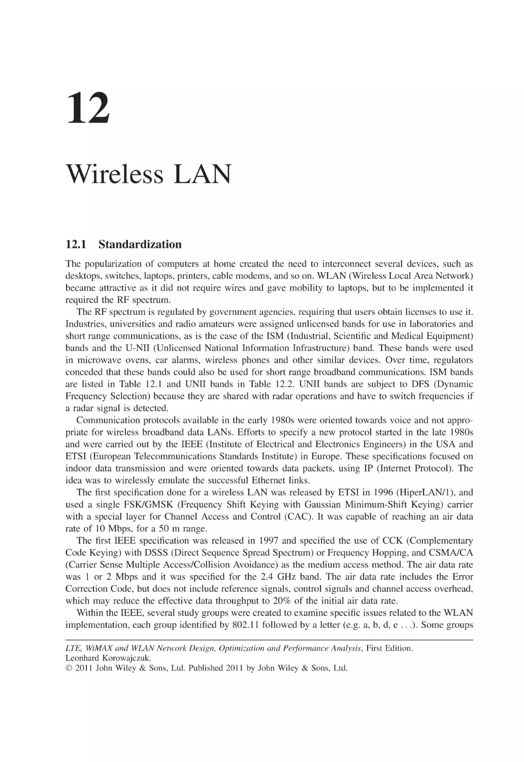
Текст
LTE, WIMAX AND WLAN
NETWORK DESIGN,
OPTIMIZATION
AND PERFORMANCE
ANALYSIS
LTE, WIMAX AND WLAN
NETWORK DESIGN,
OPTIMIZATION
AND PERFORMANCE
ANALYSIS
Leonhard Korowajczuk
CelPlan Technologies, Inc., Reston, VA, USA
A John Wiley & Sons, Ltd., Publication
This edition first published 2011
2011 John Wiley & Sons, Ltd
Registered office
John Wiley & Sons Ltd, The Atrium, Southern Gate, Chichester, West Sussex, PO19 8SQ, United Kingdom
For details of our global editorial offices, for customer services and for information about how to apply for
permission to reuse the copyright material in this book please see our website at www.wiley.com.
The right of the author to be identified as the author of this work has been asserted in accordance with the
Copyright, Designs and Patents Act 1988.
All rights reserved. No part of this publication may be reproduced, stored in a retrieval system, or transmitted, in
any form or by any means, electronic, mechanical, photocopying, recording or otherwise, except as permitted by
the UK Copyright, Designs and Patents Act 1988, without the prior permission of the publisher.
Wiley also publishes its books in a variety of electronic formats. Some content that appears in print may not be
available in electronic books.
Designations used by companies to distinguish their products are often claimed as trademarks. All brand names
and product names used in this book are trade names, service marks, trademarks or registered trademarks of their
respective owners. The publisher is not associated with any product or vendor mentioned in this book. This
publication is designed to provide accurate and authoritative information in regard to the subject matter covered.
It is sold on the understanding that the publisher is not engaged in rendering professional services. If professional
advice or other expert assistance is required, the services of a competent professional should be sought.
DISCLAIMER
Neither the Author nor John Wiley & Sons, Ltd accept any responsibility or liability for loss or damage
occasioned to any person through the use of the materials, instructions, methods or ideas contained herein, or
acting or refraining from acting as a result from such use. The author and Publisher expressly disclaim all
implied warranties, including satisfactory quality or fitness for any particular purpose.
Library of Congress Cataloging-in-Publication Data
Korowajczuk, Leonhard.
aaLTE, WIMAX, and WLAN network design, optimization, and performance
analysis / Leonhard Korowajczuk.
aaaa p. cm.
aaIncludes bibliographical references and index.
aaISBN 978-0-470-74149-8 (cloth)
aa1. Wireless LANs. aa2. IEEE 802.16 (Standard) aa3. Long-Term Evolution (Telecommunications)
I. Title.
aaTK5105.78.K67 2011
aa004.6 – dc22
aaaaaaaaaaaaaaaaaaaaaaaaaaaaaaaaaaaaaaaaaaaaaaaaaaaaaaaaaaaaaaaaaaaaaaaaaaaaaaaaa2011007547
A catalogue record for this book is available from the British Library.
Print ISBN: 9780470741498
ePDF ISBN: 9781119970477
oBook ISBN: 9781119970460
ePub ISBN: 9781119971443
eMobi ISBN: 9781119971450
Typeset in 9/11pt Times by Laserwords Private Limited, Chennai, India
I dedicate this book to my wife, Eliani, to my children, Cristine,
Monica and Leonardo, my grandchildren, Julia, Paulo and Patrick
and in memoria to my parents, Aleksander and Klara.
Contents
List of Figures
List of Tables
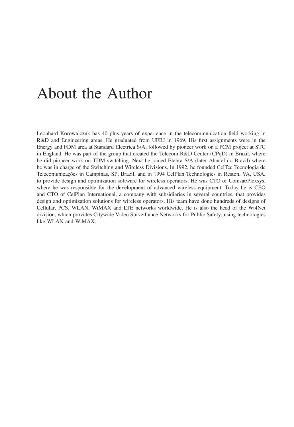
About the Author
Preface
Acknowledgements
List of Abbreviations
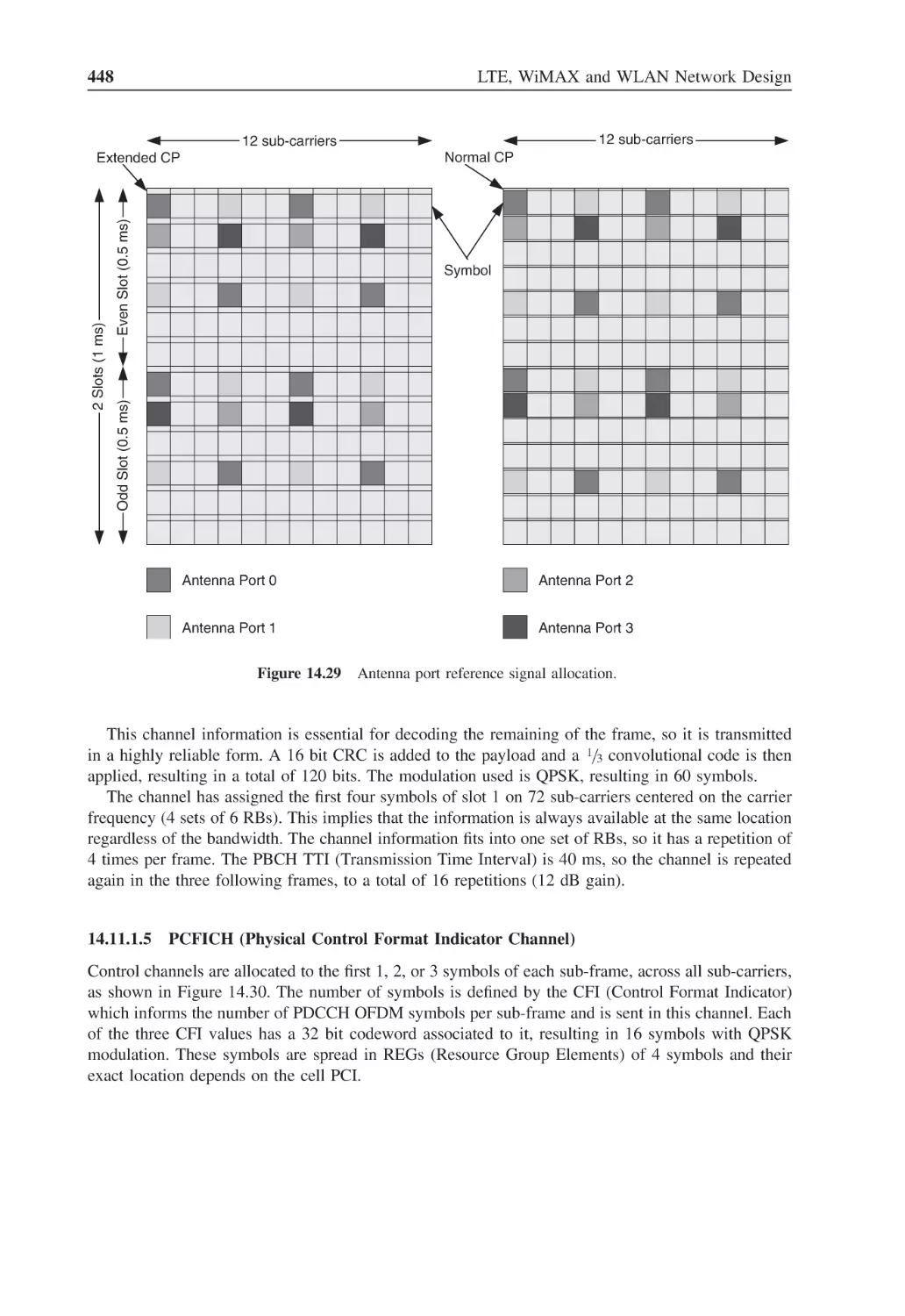
Introduction
1
1.1
1.2
1.3
1.4
1.5
1.6
2
2.1
2.2
2.3
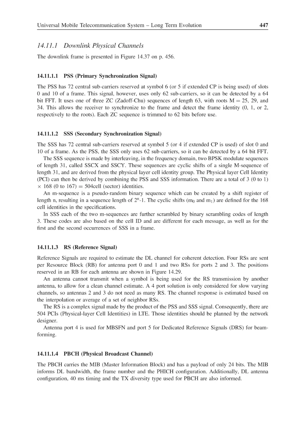
2.4
xix
xxxv
xli
xliii
xlv
xlvii
1
The Business Plan
Introduction
Market Plan
The Engineering Plan
The Financial Plan
1.4.1
Capital Expenditure (CAPEX)
1.4.2
Operational Expenditure (OPEX)
1.4.3
Return of Investment (ROI)
Business Case Questionnaire
Implementing the Business Plan
5
5
5
7
8
9
9
9
11
12
Data Transmission
History of the Internet
Network Modeling
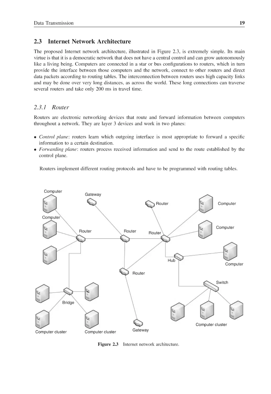
Internet Network Architecture
2.3.1
Router
2.3.2
Hub
2.3.3
Bridge
2.3.4
Switch
2.3.5
Gateway
The Physical Layer
2.4.1
Ethernet PHY
15
15
16
19
19
20
20
20
20
20
20
viii
2.5
2.6
2.7
2.8
2.9
2.10
3
3.1
3.2
3.3
3.4
3.5
3.6
3.7
3.8
3.9
3.10
3.11
3.12
Contents
The Data Link Layer
2.5.1
Ethernet MAC
Network Layer
2.6.1
Internet Protocol (IP)
2.6.2
Internet Control Message Protocol (ICMP)
2.6.3
Multicast and Internet Group Message Protocol (IGMP)
2.6.4
Link Layer Control (LLC)
Transport Protocols
2.7.1
User Datagram Protocol (UDP)
2.7.2
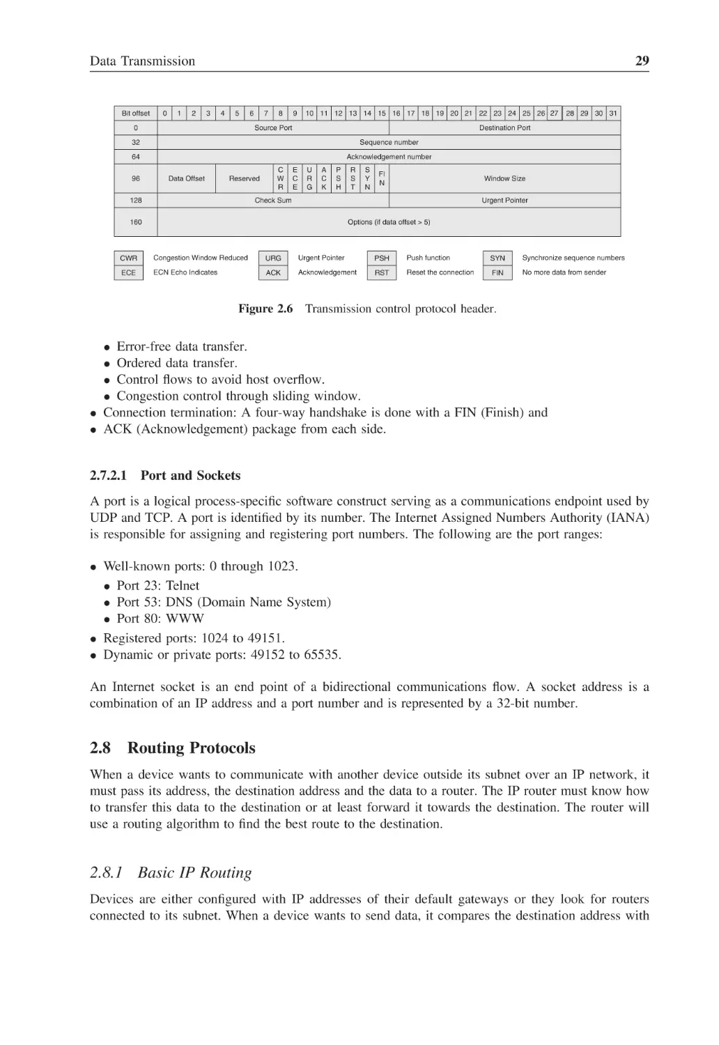
Transmission Control Protocol (TCP)
Routing Protocols
2.8.1
Basic IP Routing
2.8.2
Routing Algorithms
Application Protocols
2.9.1
Applications
2.9.2
Data Transfer Protocols
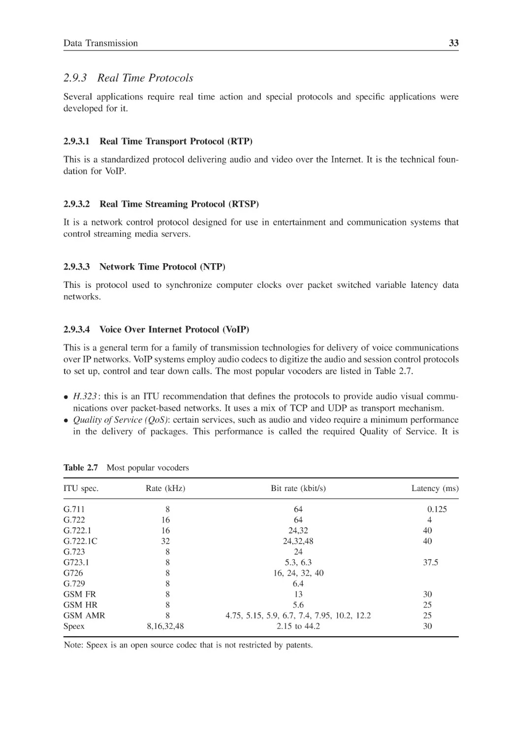
2.9.3
Real Time Protocols
2.9.4
Network Management Protocols
The World Wide Web (WWW)
22
23
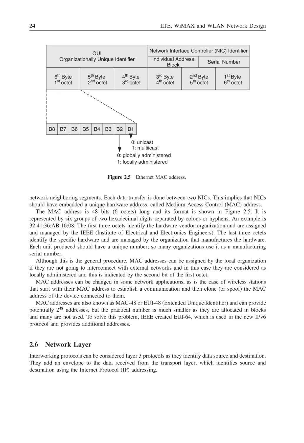
24
25
26
27
27
28
28
28
29
29
30
31
31
31
33
34
35
Market Modeling
Introduction
Data Traffic Characterization
3.2.1
Circuit-Switched Traffic Characterization
3.2.2
Packet-Switched Traffic Characterization
3.2.3
Data Speed and Data Tonnage
Service Plan (SP) and Service Level Agreement (SLA)
User Service Classes
Applications
3.5.1
Application Types
3.5.2
Applications Field Data Collection
3.5.3
Application Characterization
Over-Subscription Ratio (OSR)
Services Summary
RF Environment
Terminals
3.9.1
Terminal Types
3.9.2
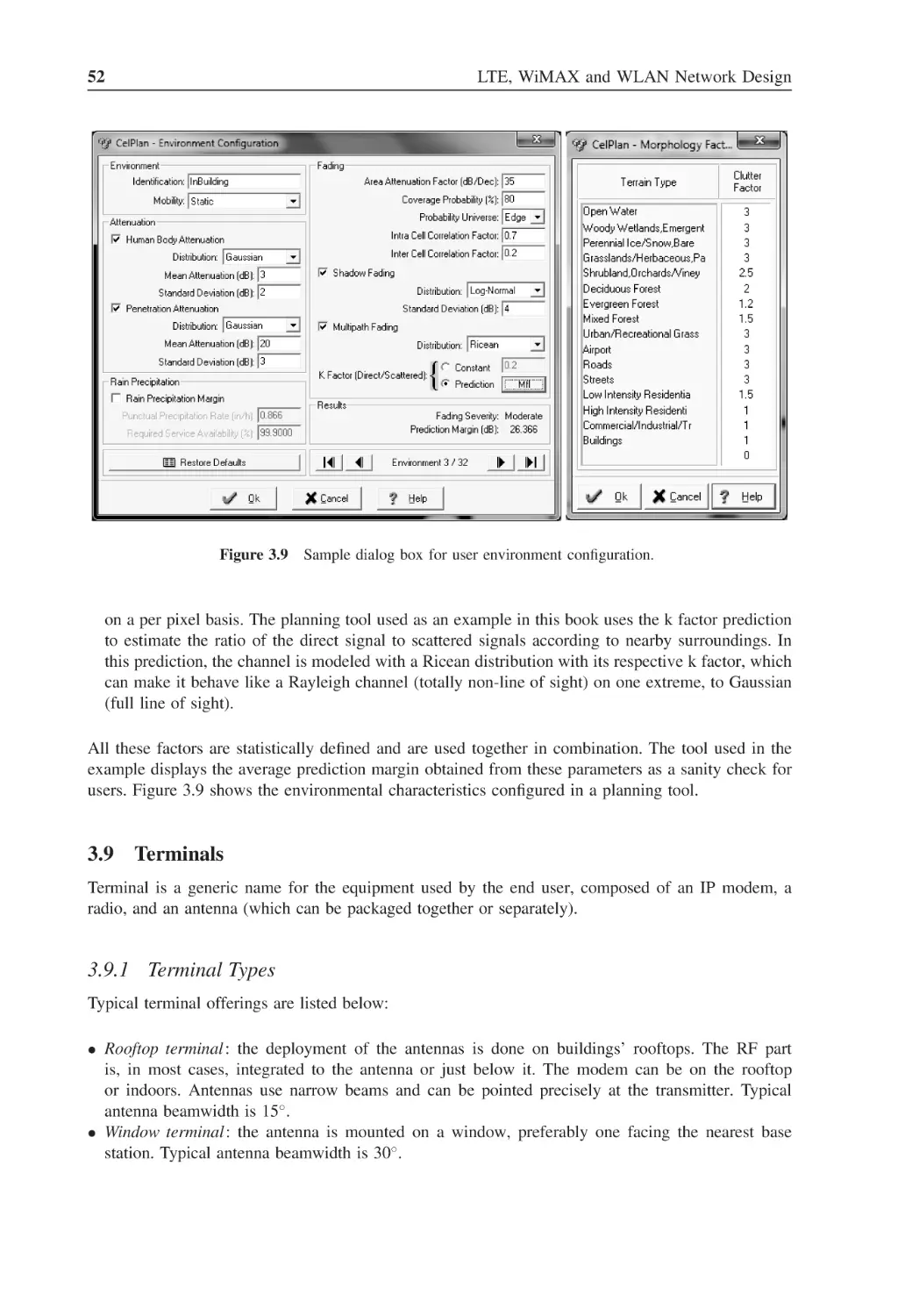
Terminal Specification
Antenna Height
Geographic User Distribution
3.11.1
Geographic Customer Distribution
3.11.2
Customer’s Distribution Layers
Network Traffic Modeling
3.12.1
Unconstrained Busy Hour Data User Traffic
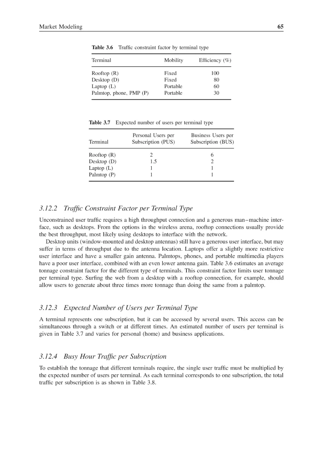
3.12.2
Traffic Constraint Factor per Terminal Type
3.12.3
Expected Number of Users per Terminal Type
3.12.4
Busy Hour Traffic per Subscription
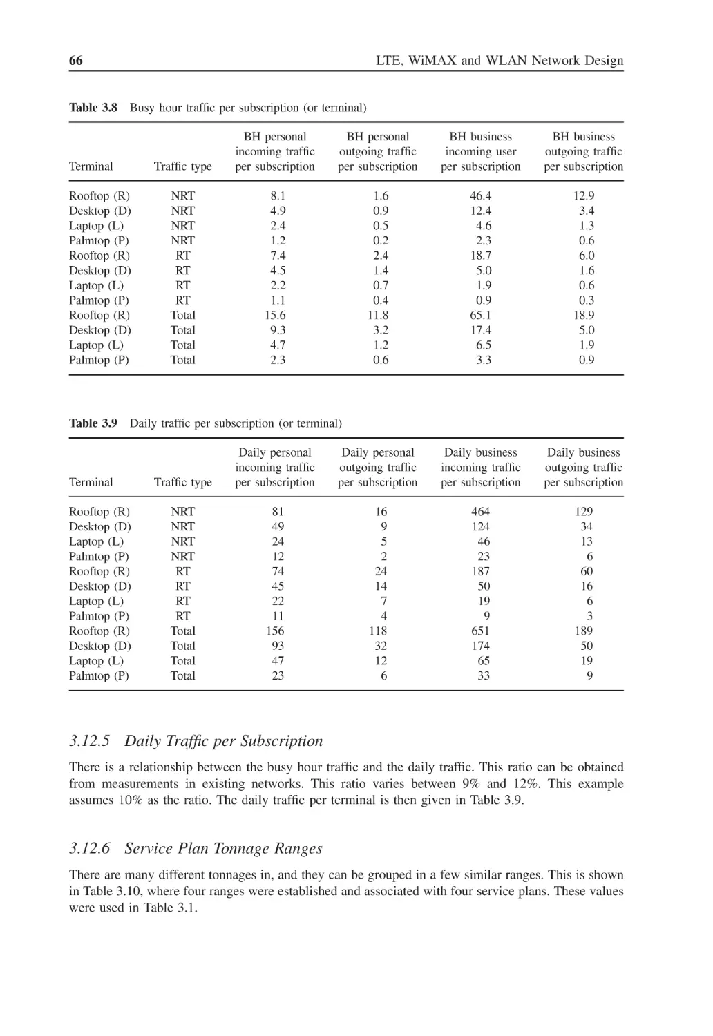
3.12.5
Daily Traffic per Subscription
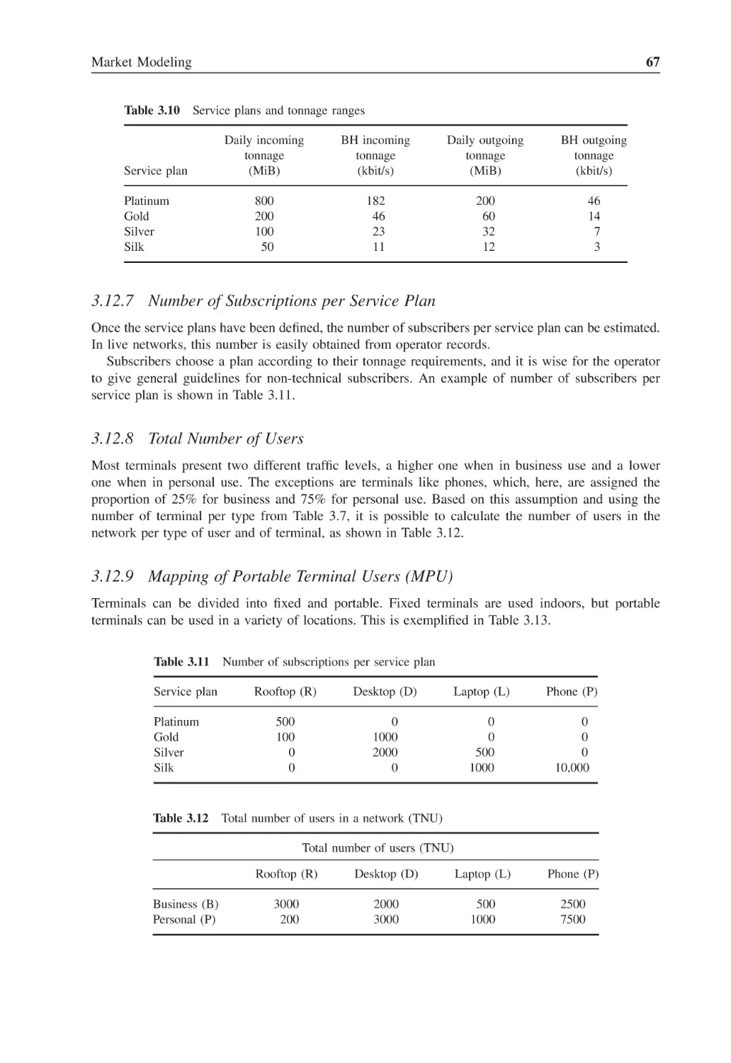
3.12.6
Service Plan Tonnage Ranges
37
37
38
38
38
40
41
43
44
44
44
45
50
51
51
52
52
53
58
58
58
62
63
63
65
65
65
66
66
Contents
3.13
3.14
4
4.1
4.2
4.3
4.4
4.5
5
5.1
5.2
5.3
5.4
5.5
5.6
5.7
5.8
ix
3.12.7
Number of Subscriptions per Service Plan
3.12.8
Total Number of Users
3.12.9
Mapping of Portable Terminal Users (MPU)
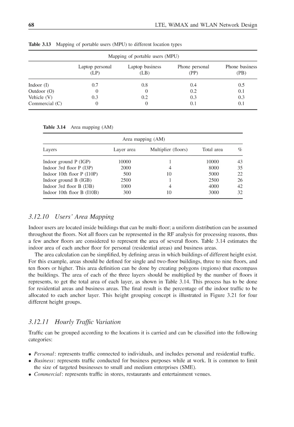
3.12.10 Users’ Area Mapping
3.12.11 Hourly Traffic Variation
3.12.12 Prediction Service Classes (PSC)
3.12.13 Traffic Layers Composition
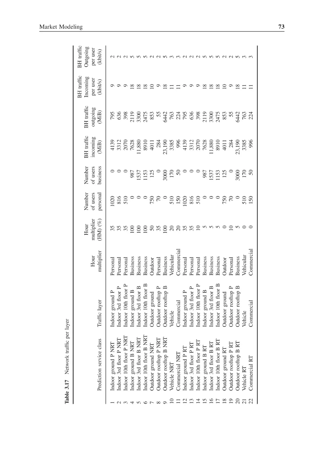
3.12.14 Network Traffic per Layer
KPI (Key Performance Indicator) Establishment
Wireless Infrastructure
67
67
67
68
68
69
71
72
72
74
Signal Processing Fundamentals
Digitizing Analog Signals
Digital Data Representation in the Frequency Domain (Spectrum)
Orthogonal Signals
4.3.1
Sine and Cosine Orthogonality
4.3.2
Harmonically Related Signals’ Orthogonality
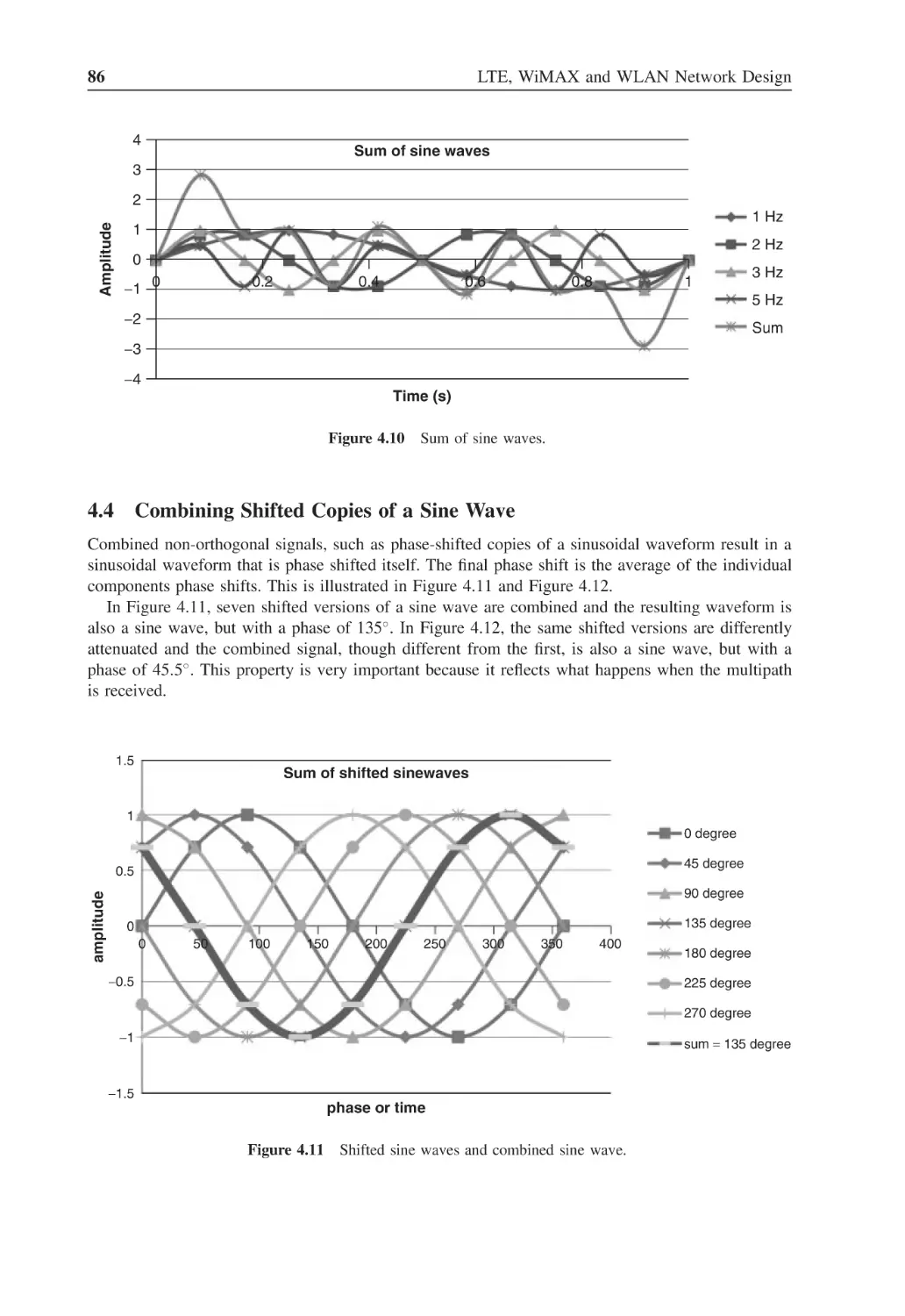
Combining Shifted Copies of a Sine Wave
Carrier Modulation
77
77
80
84
84
85
86
87
RF Channel Analysis
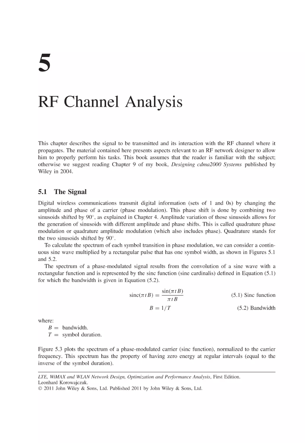
The Signal
The RF Channel
RF Signal Propagation
5.3.1
Free Space Loss
5.3.2
Diffraction Loss
5.3.3
Reflection and Refraction
RF Channel in the Frequency Domain
5.4.1
Multipath Fading
5.4.2
Shadow Fading
RF Channel in Time Domain
5.5.1
Wind Effect
5.5.2
Vehicles Effect
5.5.3
Doppler Effect
5.5.4
Fading Types
5.5.5
Multipath Mitigation Procedures
5.5.6
Comparing Multipath Resilience in Different Technologies
RF Channel in the Power Domain
Standardized Channel Models
5.7.1
3GPP Empirical Channel Model
5.7.2
3GPP2 Semi-Empirical Channel Model
5.7.3
Stanford University Interim (SUI) Semi-Empirical Channel
Model
5.7.4
Network-Wide Channel Modeling
RF Environment
5.8.1
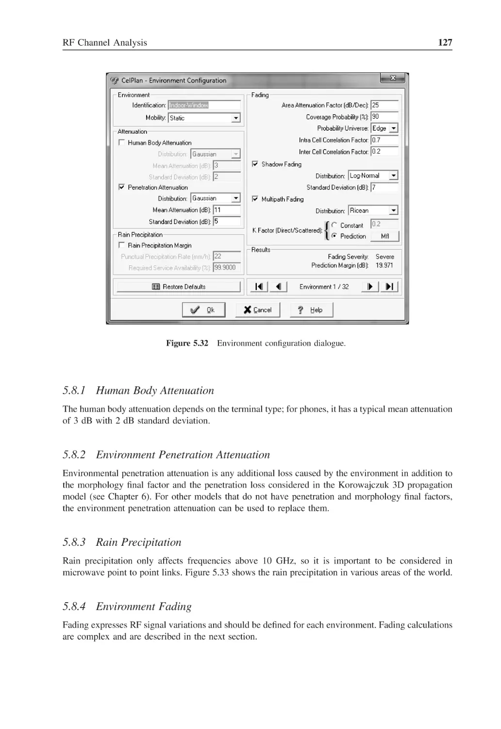
Human Body Attenuation
5.8.2
Environment Penetration Attenuation
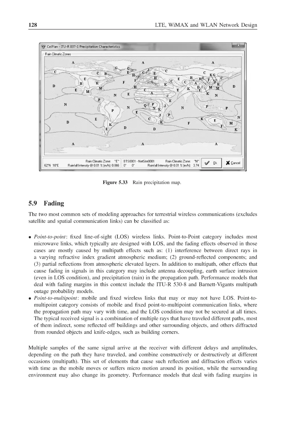
5.8.3
Rain Precipitation
5.8.4
Environment Fading
95
95
101
102
102
103
106
107
107
114
115
115
115
116
118
120
120
120
123
123
124
124
124
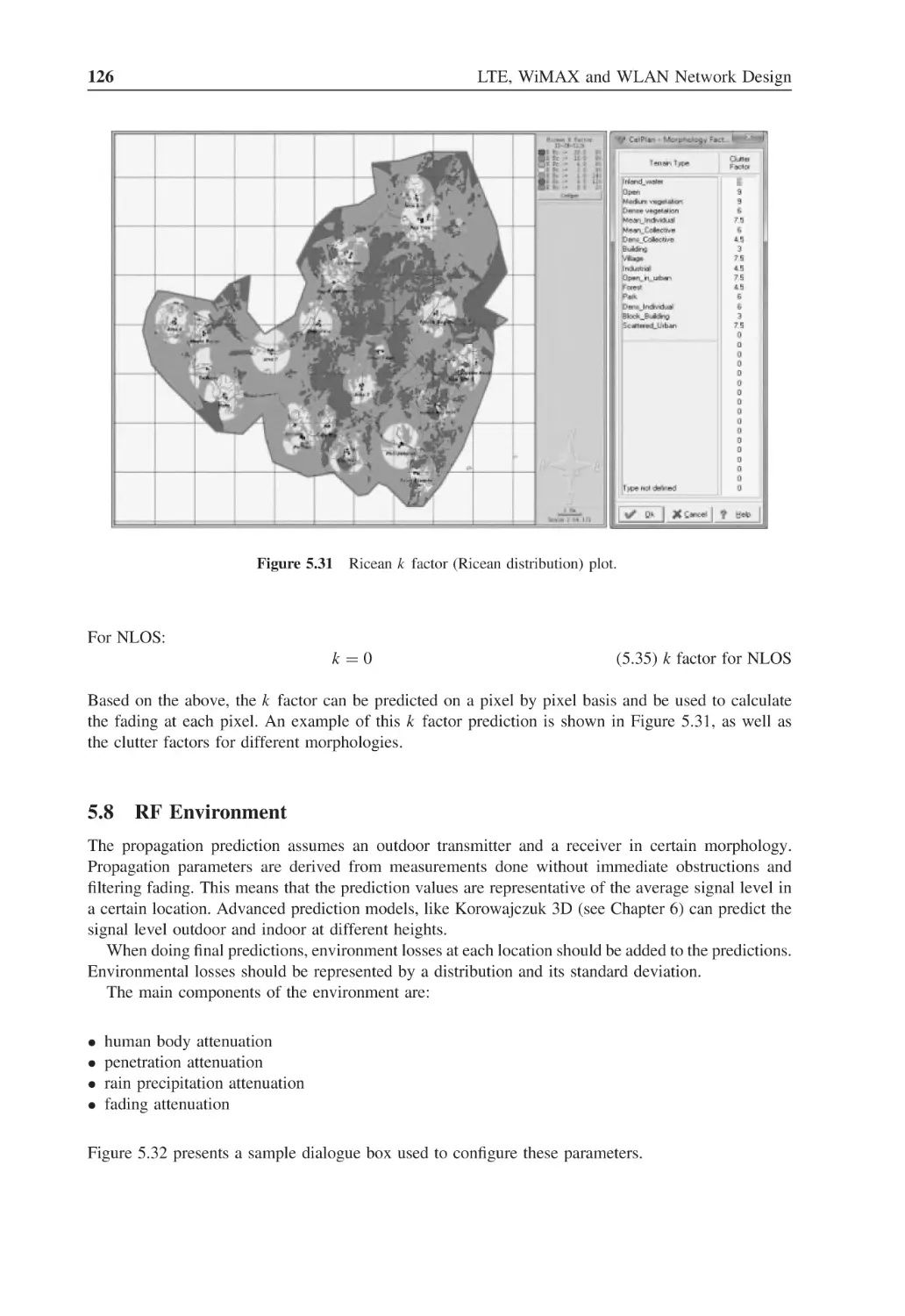
126
127
127
127
127
x
5.9
Contents
Fading
5.9.1
5.9.2
5.9.3
5.9.4
5.9.5
5.9.6
6
6.1
6.2
6.3
6.4
6.5
6.6
7
7.1
7.2
7.3
7.4
Fading Types
Fading Probability
Fading Distributions
The Rician Distribution (for Short-Term Fading with Combined
LOS and NLOS)
The Suzuki Distribution (for Combined Long- and Short-Term Fading)
Traffic Simulation with Fading
128
129
130
132
135
136
136
RF Channel Performance Prediction
Advanced RF Propagation Models
6.1.1
Terrain Databases
6.1.2
Antenna Orientation
6.1.3
Propagation Models
6.1.4
Prediction Layers
6.1.5
Fractional Morphology
6.1.6
Korowajczuk 2D Model for Outdoor and Indoor Propagation
6.1.7
Korowajczuk 3D Model
6.1.8
CelPlan Microcell Model
RF Measurements and Propagation Model Calibration
6.2.1
RF Measurements
6.2.2
RF Propagation Parameters Calibration
RF Interference Issues
6.3.1
Signal Level Variation and Signal to Interference Ratio
6.3.2
Computing Interference
6.3.3
Cell Interference Statistical Characterization
6.3.4
Interference Outage Matrix
Interference Mitigation Techniques
6.4.1
Interference Avoidance
6.4.2
Interference Averaging
RF Spectrum Usage and Resource Planning
6.5.1
Network Footprint Enhancement
6.5.2
Neighborhood Planning
6.5.3
Handover Planning
6.5.4
Paging Zone Planning
6.5.5
Carrier Planning
6.5.6
Code Planning
6.5.7
Spectrum Efficiency
Availability
139
139
139
142
144
144
145
148
155
160
163
164
167
172
173
175
176
178
180
180
180
181
181
181
182
182
182
186
186
187
OFDM
Multiplexing
7.1.1
Implementation of an Inverse Discrete Fast Fourier Transform (iDFFT)
7.1.2
Implementation of a Discrete Fast Fourier Transform
7.1.3
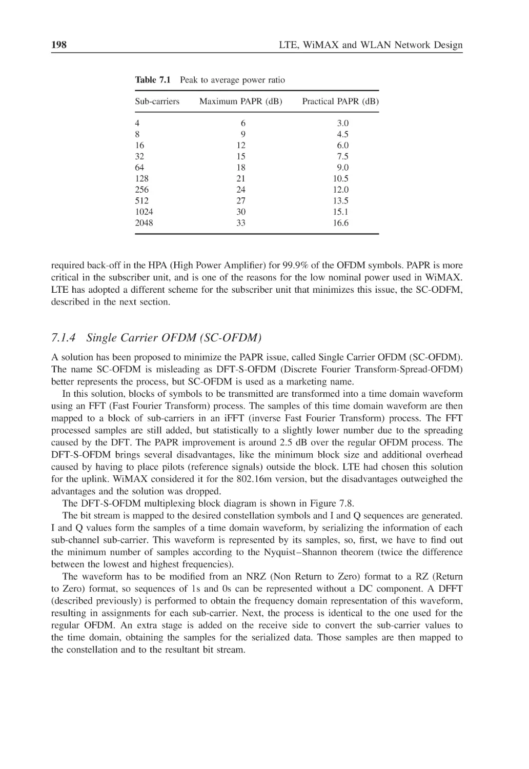
Peak to Average Power Ratio (PAPR)
7.1.4
Single Carrier OFDM (SC-OFDM)
Other PAPR Reduction Methods
De-Multiplexing
Cyclic Prefix
193
193
194
195
197
198
201
201
202
Contents
7.5
7.6
7.7
7.8
7.9
7.10
7.11
8
8.1
8.2
9
9.1
9.2
9.3
10
10.1
xi
OFDMA
Duplexing
7.6.1
FDD (Frequency Division Duplexing)
7.6.2
TDD (Time Division Duplexing)
Synchronization
7.7.1
Unframed Solution
7.7.2
Framed Solution
RF Channel Information Detection
7.8.1
Frequency and Time Synchronization
7.8.2
RF Channel Equalization and Reference Signals (Pilot)
7.8.3
Information Extraction
Error Correction Techniques
Resource Allocation and Scheduling
7.10.1
FIFO (First In, First Out)
7.10.2
Generalized Processor Sharing (GPS)
7.10.3
Fair Queuing (FQ)
7.10.4
Max-Min Fairness (MMF)
7.10.5
Weighted Fair Queuing (WFQ)
Establishing Wireless Data Communications
7.11.1
Data Transmission
7.11.2
Data Reception
7.11.3
Protocol Layers
7.11.4
Wireless Communication Procedure
203
204
204
205
207
207
207
208
209
209
210
211
215
215
215
216
216
216
216
217
217
217
219
OFDM Implementation
Transmit Side
8.1.1
Bit Processing
8.1.2
Symbol Processing
8.1.3
Digital IF Processing
8.1.4
Carrier Modulation
Receive Side
8.2.1
Carrier Demodulation
8.2.2
Digital IF Processing
8.2.3
Symbol Processing
8.2.4
Bit Processing Stages
221
221
221
224
225
226
228
228
229
229
233
Wireless Communications Network (WCN)
Introduction
Wireless Access Network
9.2.1
Subscriber Wireless Stations (SWS)
9.2.2
Wireless Base Stations (WBS)
Core Network
9.3.1
Access Service Network (ASN)
9.3.2
Connectivity Service
9.3.3
Application Service
9.3.4
Operational Service
235
235
235
235
237
237
237
241
242
242
Antenna and Advanced Antenna Systems
Introduction
245
245
xii
Contents
10.2
10.3
Antenna Basics
Antenna Radiation
10.3.1
Reactive Near Field (Reactive Region)
10.3.2
Radiating Near Field (Fresnel Region)
10.3.3
Far Field (Fraunhofer Region)
10.4 Antenna Types
10.4.1
Dipole (Half Wave Dipole)
10.4.2
Quarter Wave Antenna (Whip)
10.4.3
Omni Antenna
10.4.4
Parabolic Antenna
10.4.5
Horn Antenna
10.4.6
Antenna Type Comparison
10.5 Antenna Characteristics
10.5.1
Impedance Matching
10.5.2
Antenna Patterns
10.5.3
Antenna Polarization
10.5.4
Cross-Polarization
10.5.5
Antenna Correlation or Signal Coherence
10.6 Multiple Antennas Arrangements
10.6.1
SISO (Single In to Single Out)
10.6.2
SIMO (Single In to Multiple Out)
10.6.3
MISO (Multiple In to Single Out)
10.6.4
MISO-SIMO
10.6.5
MIMO (Multiple In to Multiple Out)
10.6.6
Adaptive MIMO Switching (AMS)
10.6.7
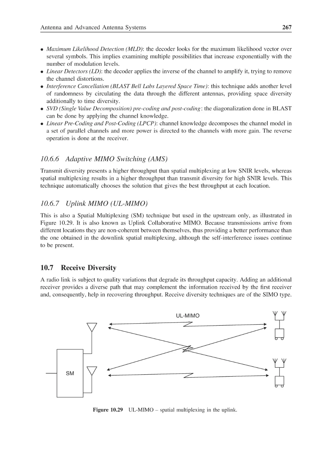
Uplink MIMO (UL-MIMO)
10.7 Receive Diversity
10.7.1
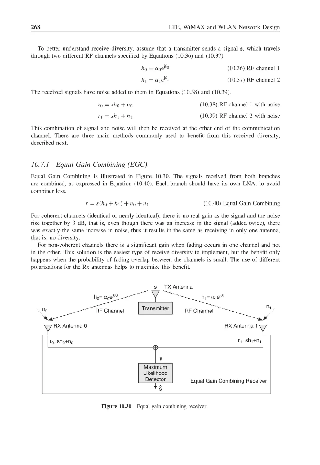
Equal Gain Combining (EGC)
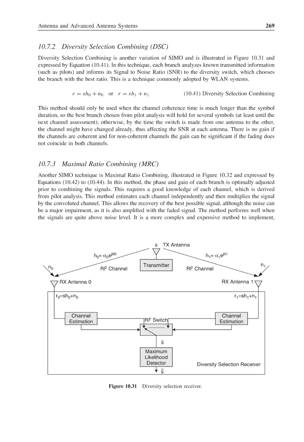
10.7.2
Diversity Selection Combining (DSC)
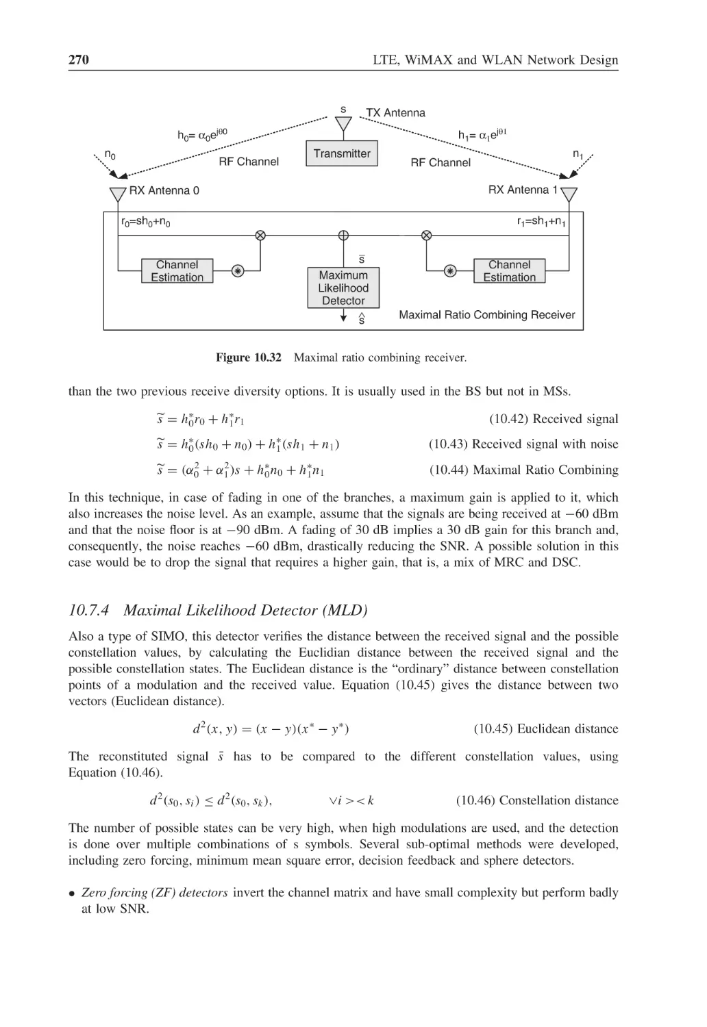
10.7.3
Maximal Ratio Combining (MRC)
10.7.4
Maximal Likelihood Detector (MLD)
10.7.5
Performance Comparison for Receive Diversity Techniques
10.8 Transmit Diversity
10.8.1
Receiver-Based Transmit Selection
10.8.2
Transmit Redundancy
10.8.3
Space Time Transmit Diversity
10.9 Transmit and Receive Diversity (TRD)
10.10 Spatial Multiplexing (Matrix B)
10.11 Diversity Performance
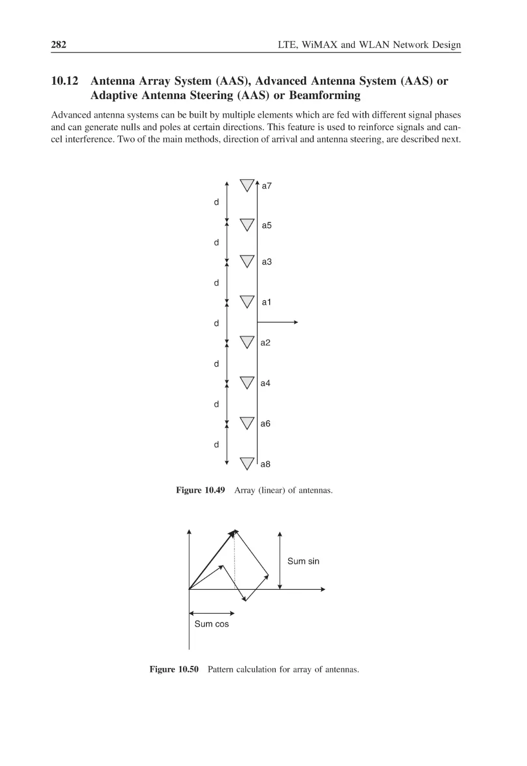
10.12 Antenna Array System (AAS), Advanced Antenna System (AAS)
or Adaptive Antenna Steering (AAS) or Beamforming
246
247
248
248
249
249
249
250
250
251
253
253
254
254
255
258
259
261
262
263
264
265
265
266
267
267
267
268
269
269
270
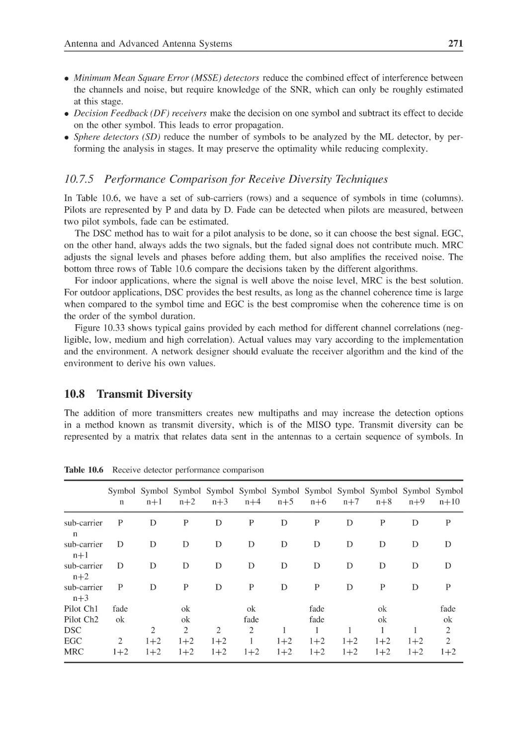
271
271
272
273
274
275
276
278
11
11.1
11.2
11.3
11.4
287
287
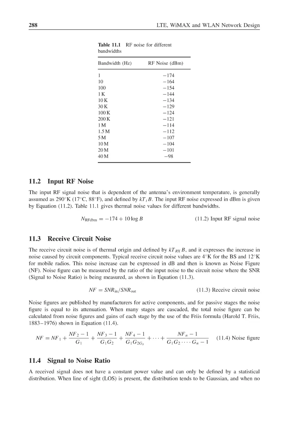
288
288
288
289
289
Radio Performance
Introduction
Input RF Noise
Receive Circuit Noise
Signal to Noise Ratio
11.4.1
Modulation Constellation SNR
11.4.2
Error Correction Codes
282
Contents
11.5
11.6
12
12.1
12.2
12.3
12.4
12.5
12.6
13
13.1
13.2
13.3
13.4
13.5
xiii
11.4.3
SNR and Throughput
Radio Sensitivity Calculations
11.5.1
Modulation Scheme SNR
11.5.2
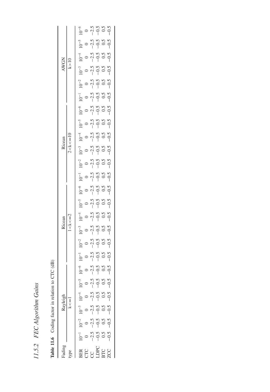
FEC Algorithm Gains
11.5.3
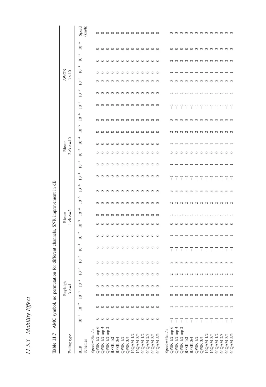
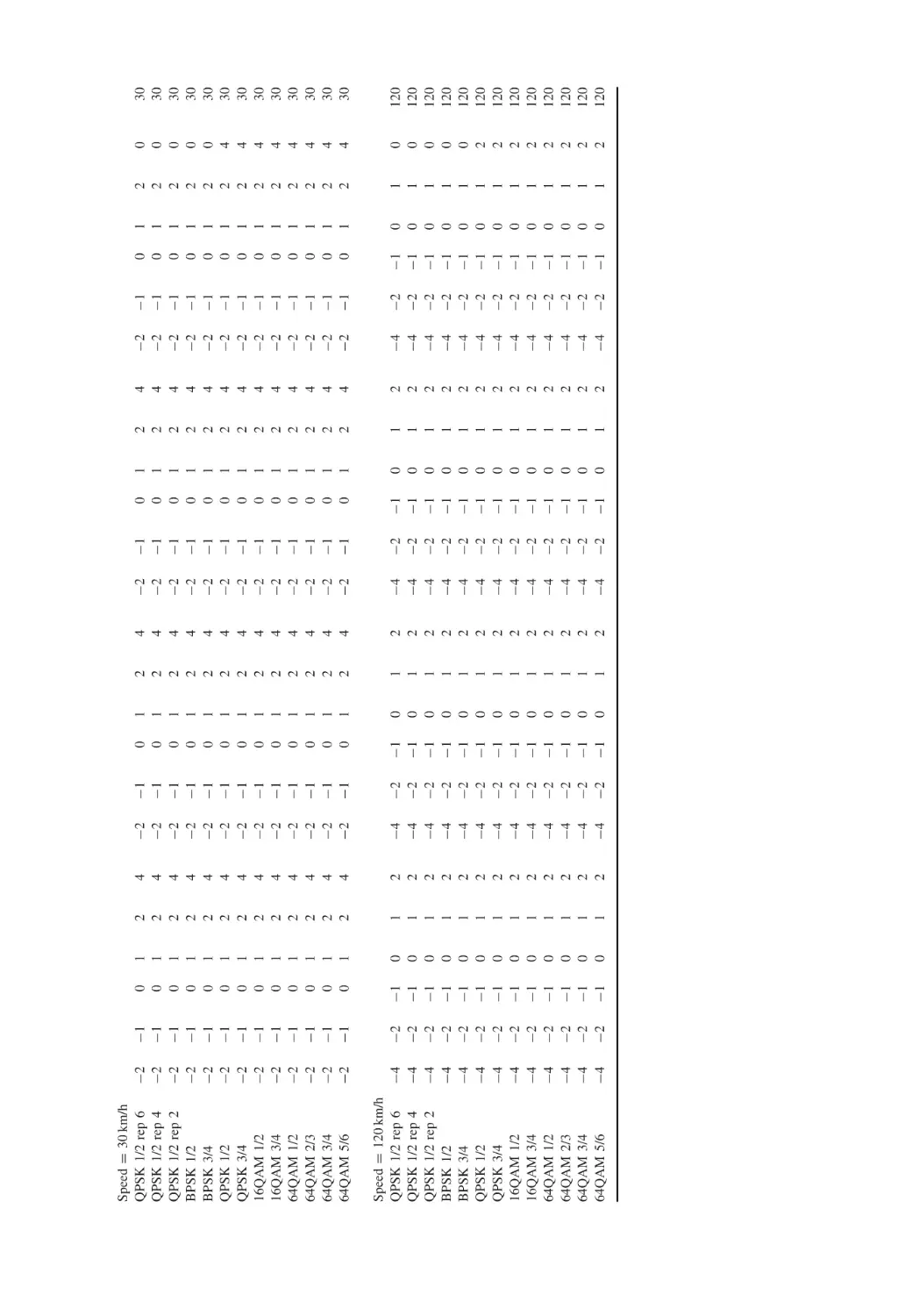
Mobility Effect
11.5.4
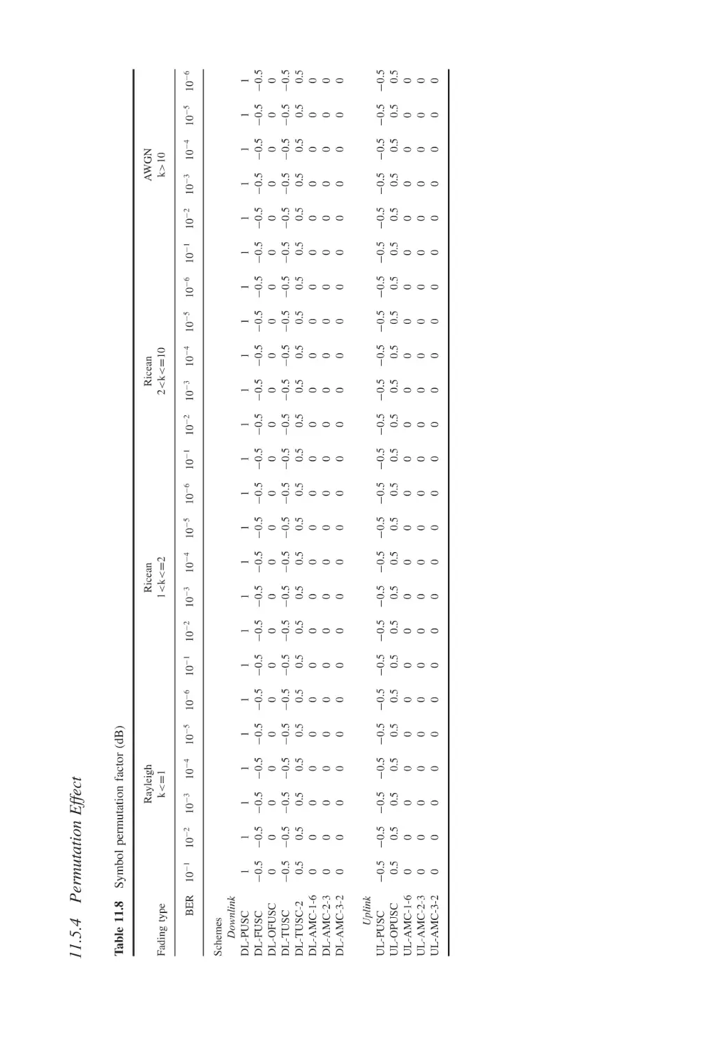
Permutation Effect
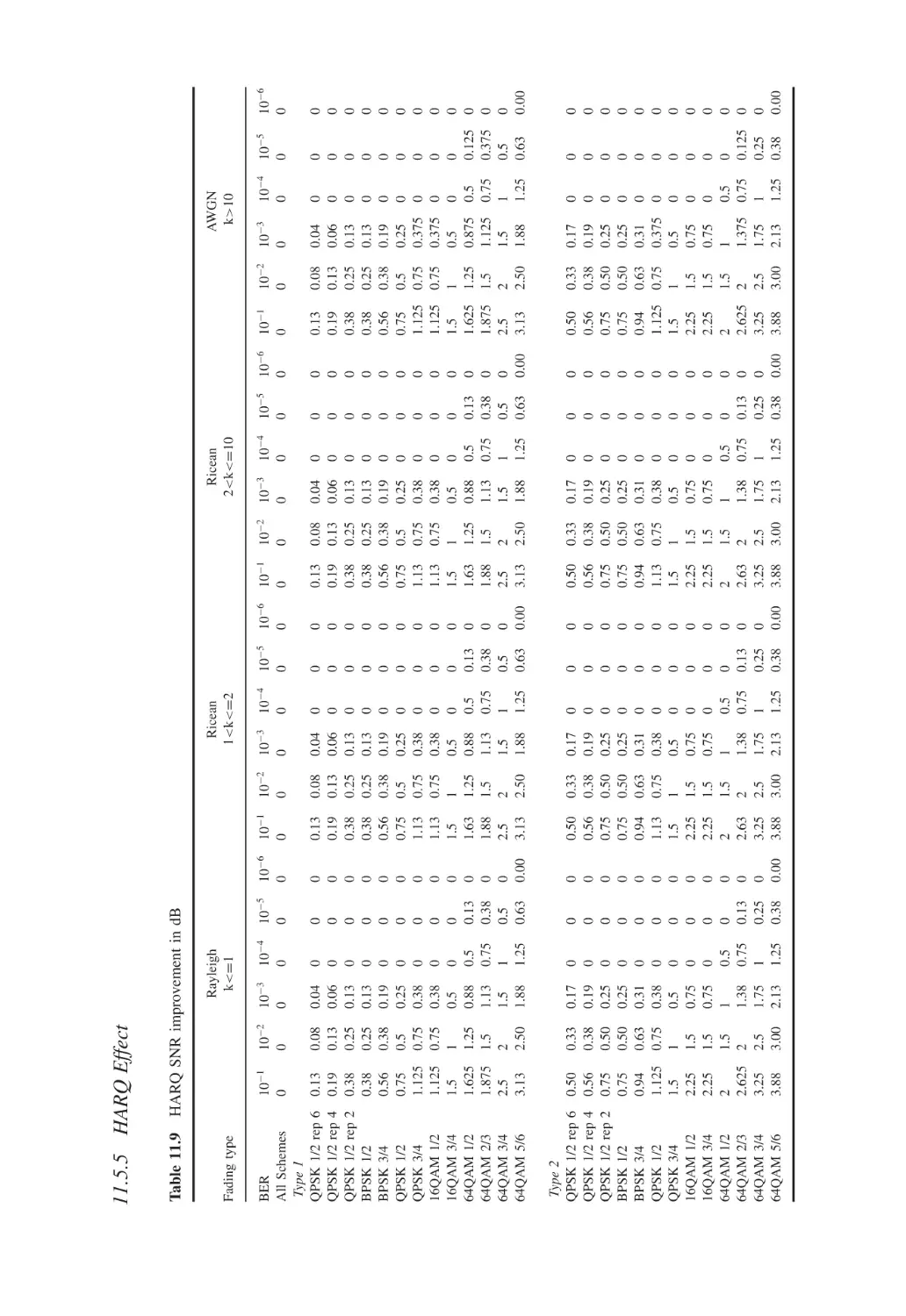
11.5.5
HARQ Effect
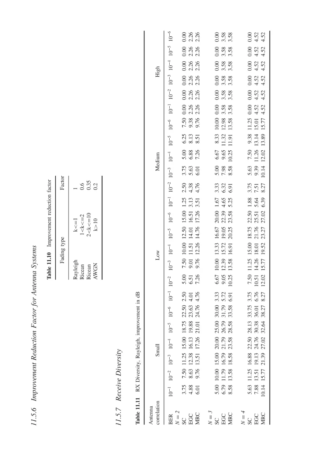
11.5.6
Improvement Reduction Factor for Antenna Systems
11.5.7
Receive Diversity
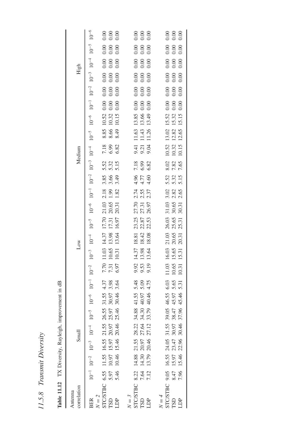
11.5.8
Transmit Diversity
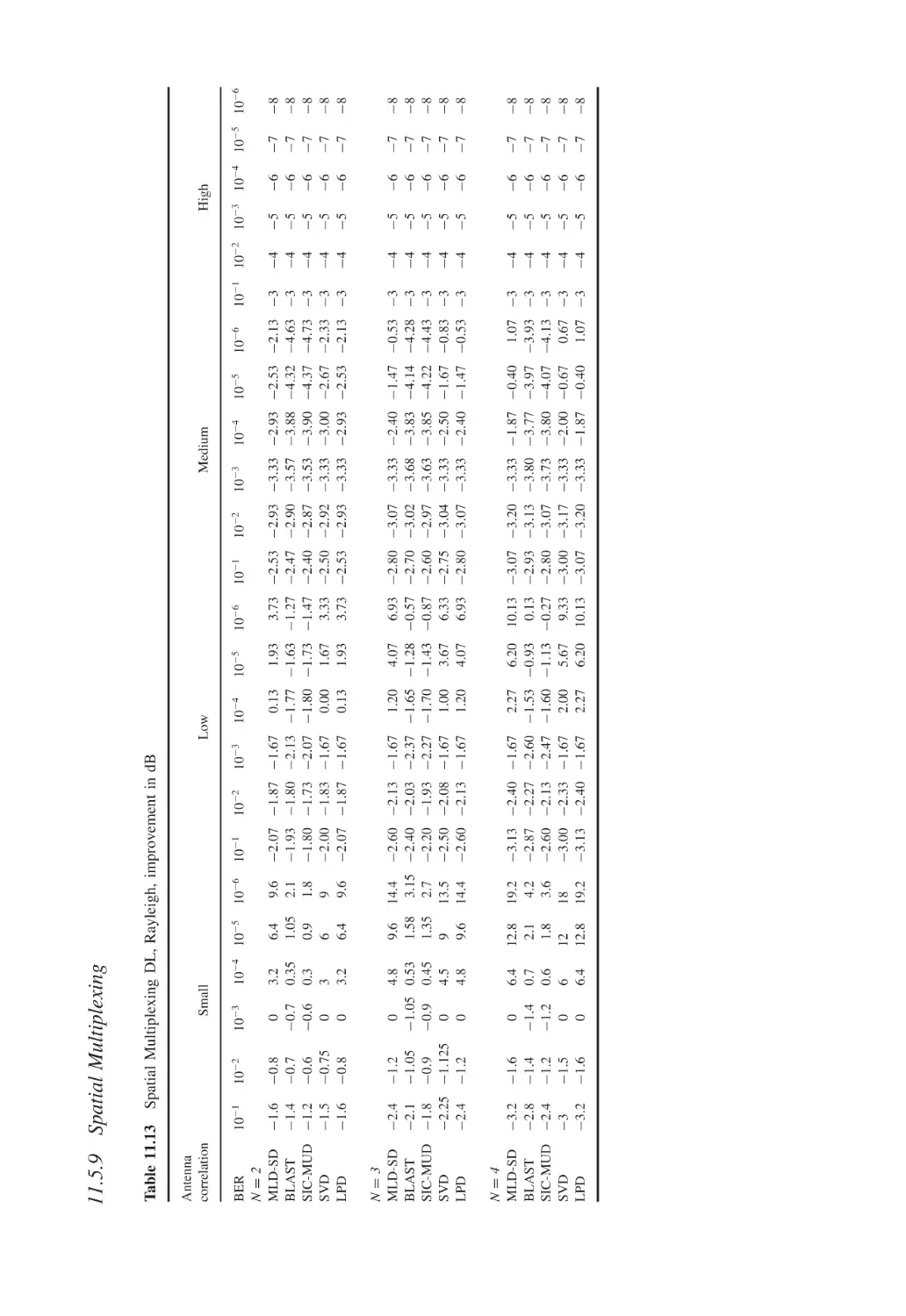
11.5.9
Spatial Multiplexing
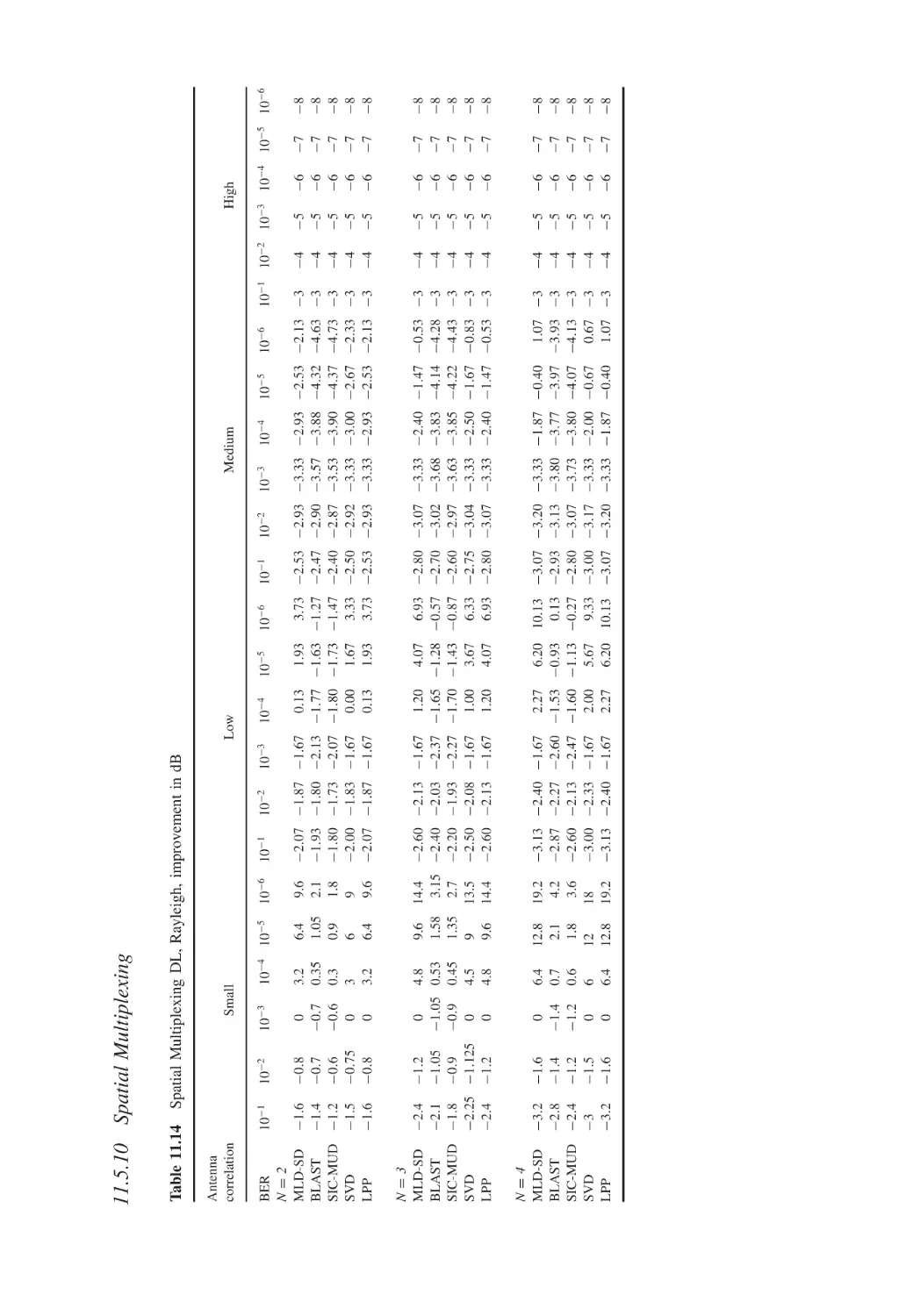
11.5.10 Spatial Multiplexing
Radio Configuration
294
295
296
297
298
300
301
302
302
303
304
305
307
Wireless LAN
Standardization
Architecture
The IEEE Std 802.11-2007
12.3.1
Physical (PH) Layer
12.3.2
Medium Access Control (MAC) Layer
12.3.3
RF Channel Access
12.3.4
Power Management
Enhancements for Higher Throughputs, Amendment 5: 802.11n-2009
12.4.1
Physical Layer
12.4.2
MAC Layer
Work in Progress
Throughput
311
311
315
316
318
319
325
327
328
329
330
333
334
WiMAX
Standardization
13.1.1
The WiMAX Standards
13.1.2
The WiMAX Forum
13.1.3
WiMAX Advantages
13.1.4
WiMAX Claims
Network Architecture
13.2.1
ASN (Access Service Network)
13.2.2
CPE
13.2.3
ASN-GW (Access Service Network Gateway)
13.2.4
CSN (Connectivity Service Network)
13.2.5
OSS/BSS (Operation Support System/Business Support System)
13.2.6
ASP (Application Service Provider)
Physical Layer (PHY)
13.3.1
OFDM Carrier in Frequency Domain
13.3.2
OFDM Carrier in Time Domain
13.3.3
OFDM Carrier in the Power Domain
Multiple Access OFDMA
WiMAX Network Layers
13.5.1
The PHY Layer
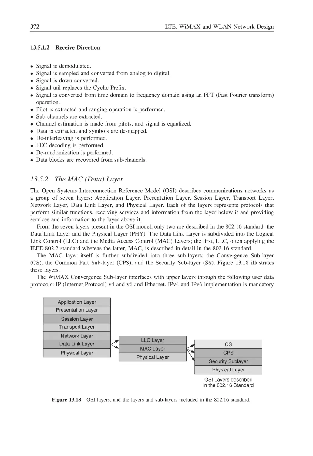
13.5.2
The MAC (Data) Layer
341
341
341
342
342
344
344
346
347
347
348
350
353
353
356
359
366
369
370
370
372
xiv
13.6
13.7
13.8
14
14.1
14.2
14.3
14.4
14.5
14.6
14.7
14.8
14.9
Contents
13.5.3
13.5.4
13.5.5
WiMAX
WiMAX
13.7.1
13.7.2
13.7.3
13.7.4
WiMAX
13.8.1
13.8.2
13.8.3
13.8.4
Error Correction
Frame Description
Resource Management
Operation Phases
Interference Reduction Techniques
Interference Avoidance and Segmentation
Interference Averaging and Permutation Schemes
Permutation Schemes
Permutation Summary
Resource Planning
WiMAX Frequency Planning
WiMAX Code Planning (Cell Identification)
Tips for PermBase Resource Planning
Spectrum Efficiency
Universal Mobile Telecommunication System – Long Term
Evolution (UMTS-LTE)
Introduction
Standardization
14.2.1
Release 8 (December 2008)
14.2.2
Release 9 (December 2009)
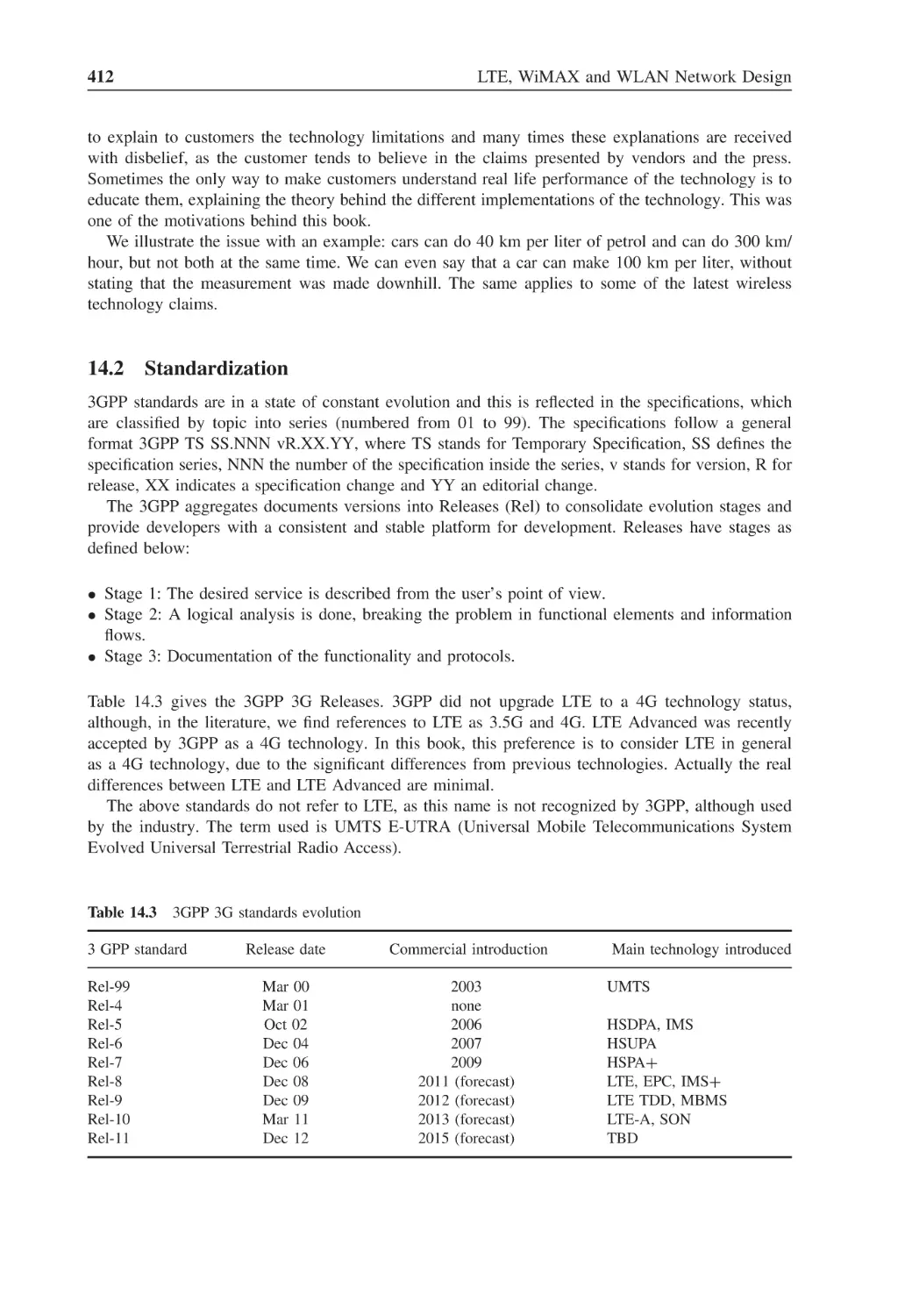
14.2.3
Release 10 (March 2011)
14.2.4
Release 11 (December 2012)
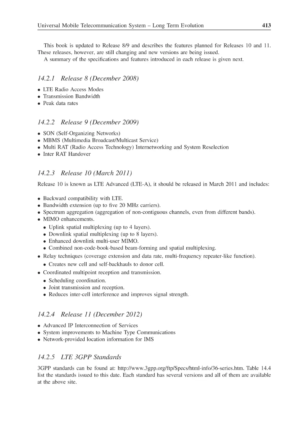
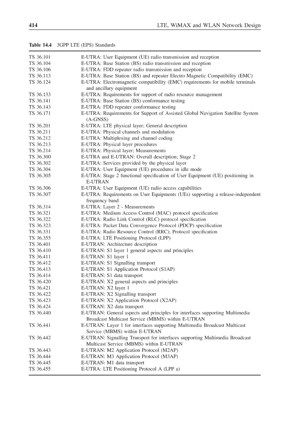
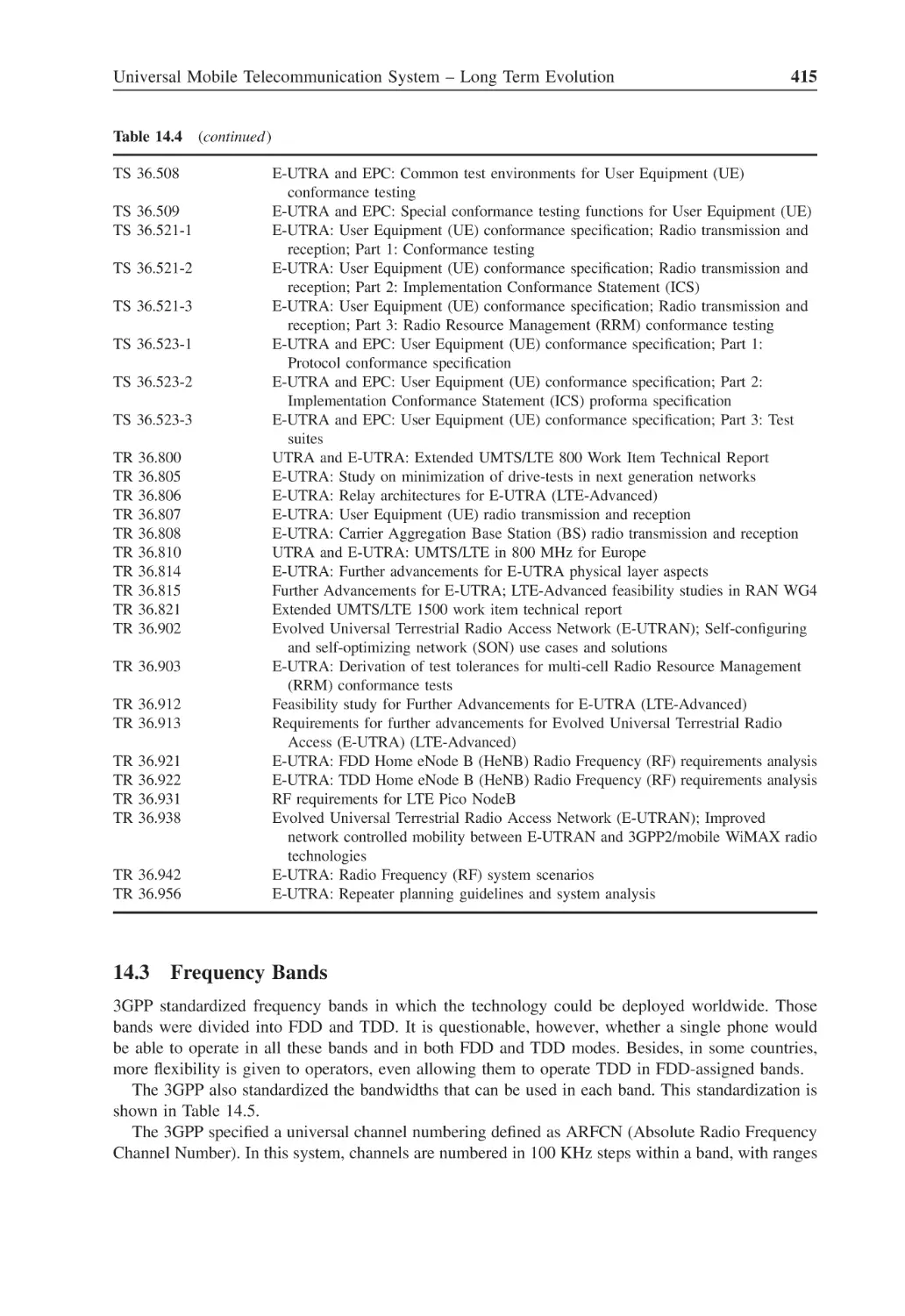
14.2.5
LTE 3GPP Standards
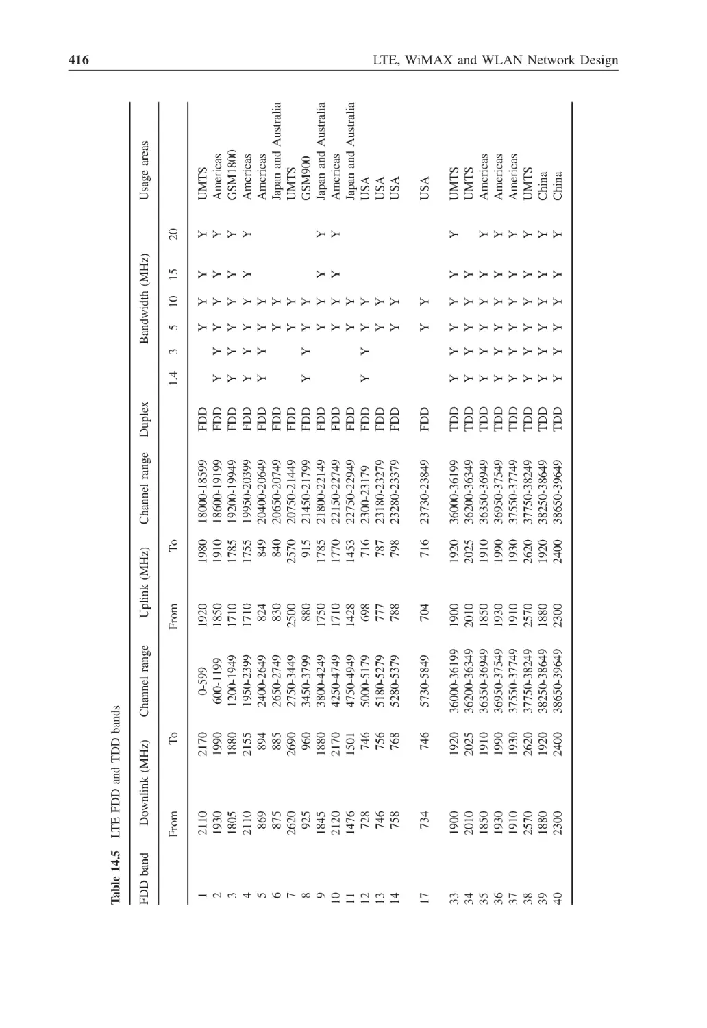
Frequency Bands
Architecture
14.4.1
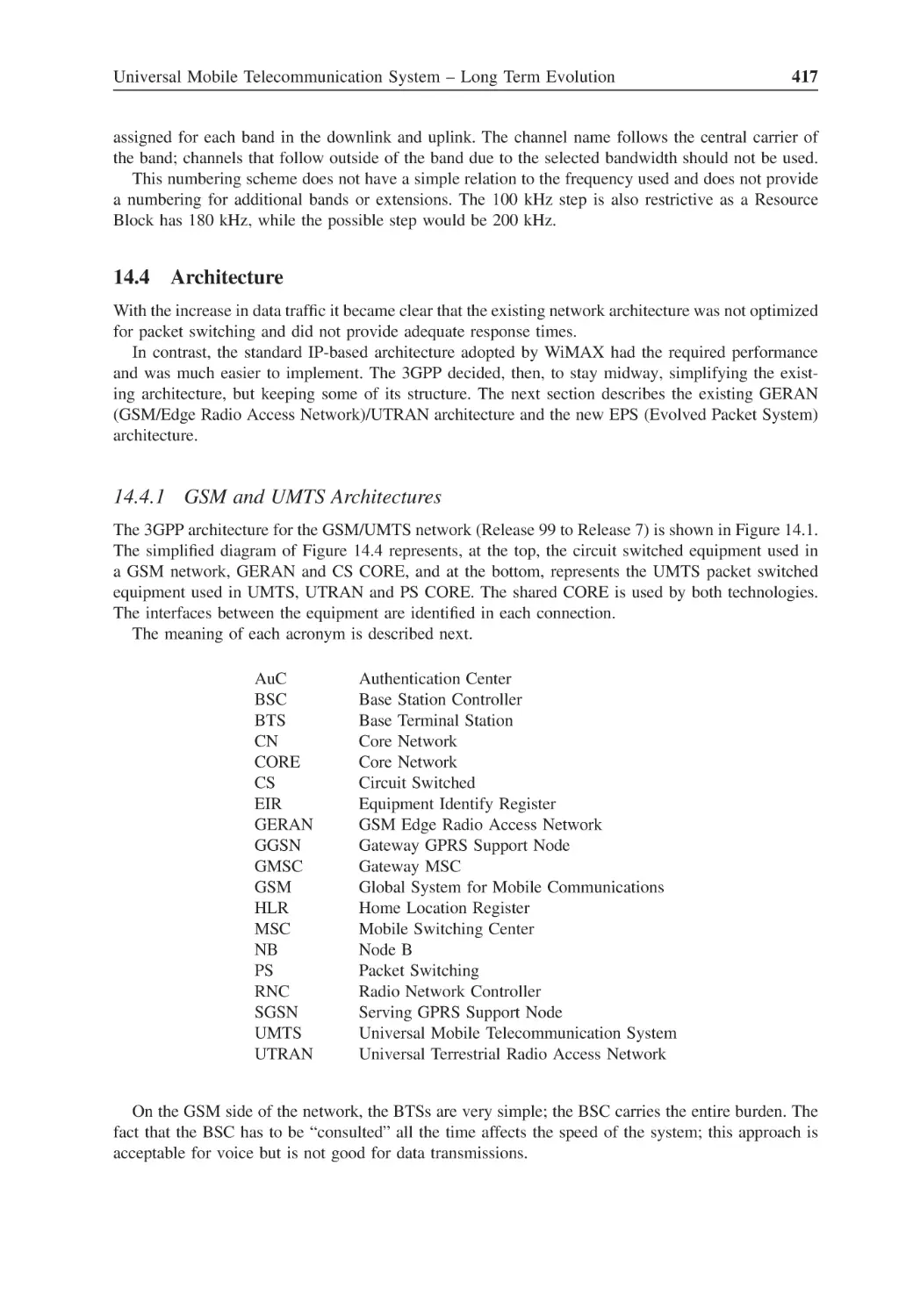
GSM and UMTS Architectures
14.4.2
EPS Architecture
14.4.3
eNodeB (eNB)
14.4.4
Mobility Management Entity (MME)
14.4.5
Serving Gateway (S-GW)
14.4.6
Packet Data Network Gateway (PDN-GW or P-GW)
14.4.7
Policy Control and Charging Rules Function (PCRF)
14.4.8
Home Subscriber Server (HSS)
14.4.9
IP Multimedia Sub-System (IMS)
14.4.10 Voice over LTE via Generic Access (VoLGA)
14.4.11 Architecture Interfaces
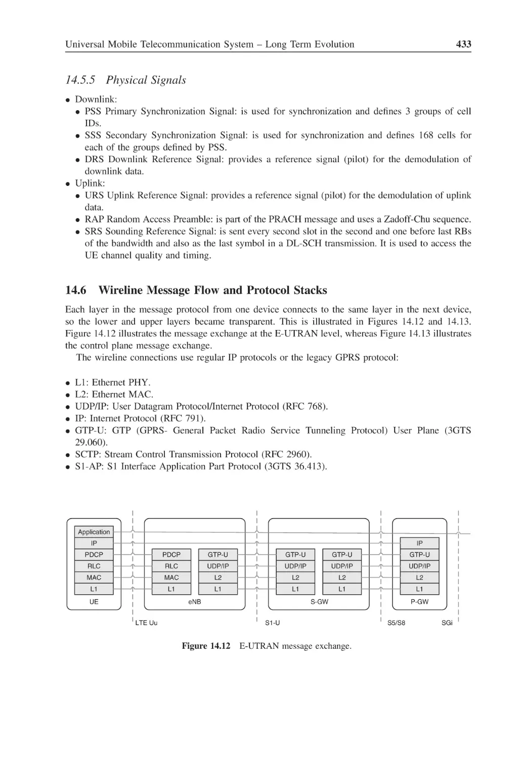
Wireless Message Flow and Protocol Stack
14.5.1
Messages
14.5.2
Protocol Layers
14.5.3
Message Bearers
14.5.4
Message Channels
14.5.5
Physical Signals
Wireline Message Flow and Protocol Stacks
Identifiers
HARQ Procedure
14.8.1
Turbo Code
14.8.2
Incremental Redundancy
Scrambling Sequences
376
376
379
384
386
386
387
388
400
401
401
406
407
407
409
409
412
413
413
413
413
413
415
417
417
418
420
420
420
420
420
420
421
421
421
424
424
427
429
431
433
433
434
435
435
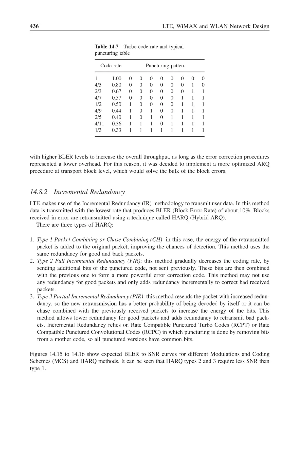
436
439
Contents
xv
14.10 Physical Layer (PHY)
14.10.1 PHY Downlink
14.10.2 PHY Uplink
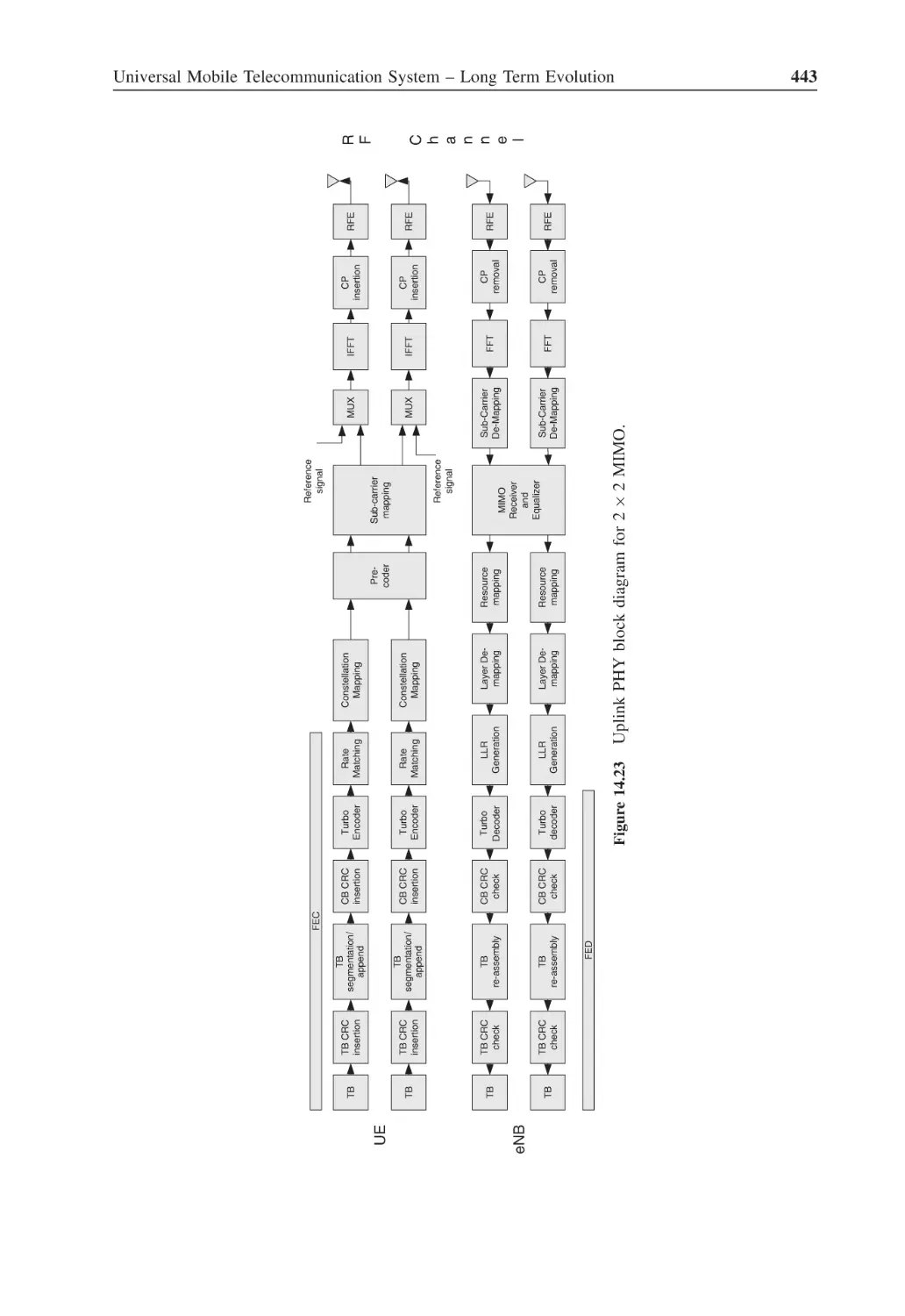
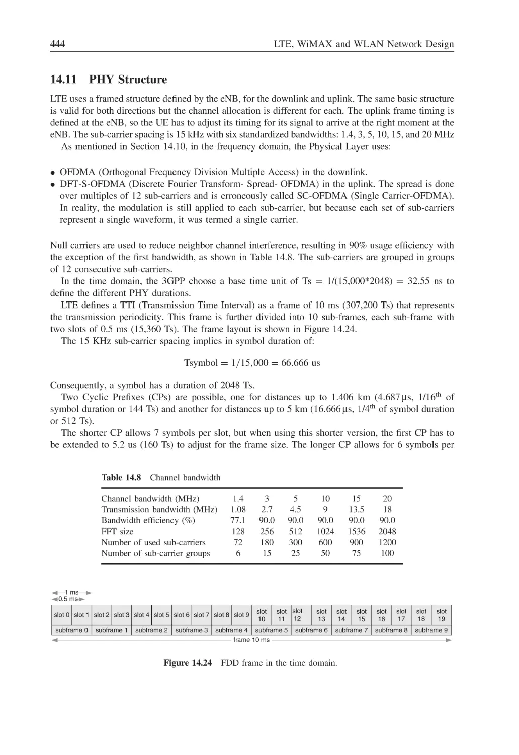
14.11 PHY Structure
14.11.1 Downlink Physical Channels
14.11.2 Uplink Physical Channels
14.11.3 Downlink PHY Assignments
14.11.4 Uplink PHY Assignments
14.12 PHY TDD
14.13 Multimedia Broadcast/Multicast Service (MBMS)
14.14 Call Placement Scenario
14.15 PHY Characteristics and Performance
14.15.1 Transmitter
14.15.2 Receiver
14.15.3 Power Saving
14.16 Multiple Antennas in LTE
14.16.1 Antenna Configurations
14.16.2 LTE Antenna Algorithms
14.16.3 Transmit Diversity
14.16.4 Spatial Multiplexing
14.16.5 Beamforming
14.17 Resource Planning in LTE
14.17.1 Full Reuse
14.17.2 Hard Reuse
14.17.3 Fractional Reuse
14.17.4 Soft Reuse
14.18 Self-Organizing Network (SON)
14.19 RAT (Radio Access Technology) Internetworking
14.20 LTE Radio Propagation Channel Considerations
14.20.1 SISO Channel Models
14.20.2 MIMO Channel Models
14.21 Handover Procedures in LTE
14.22 Measurements
14.22.1 UE Measurements
14.22.2 eNB Measurements
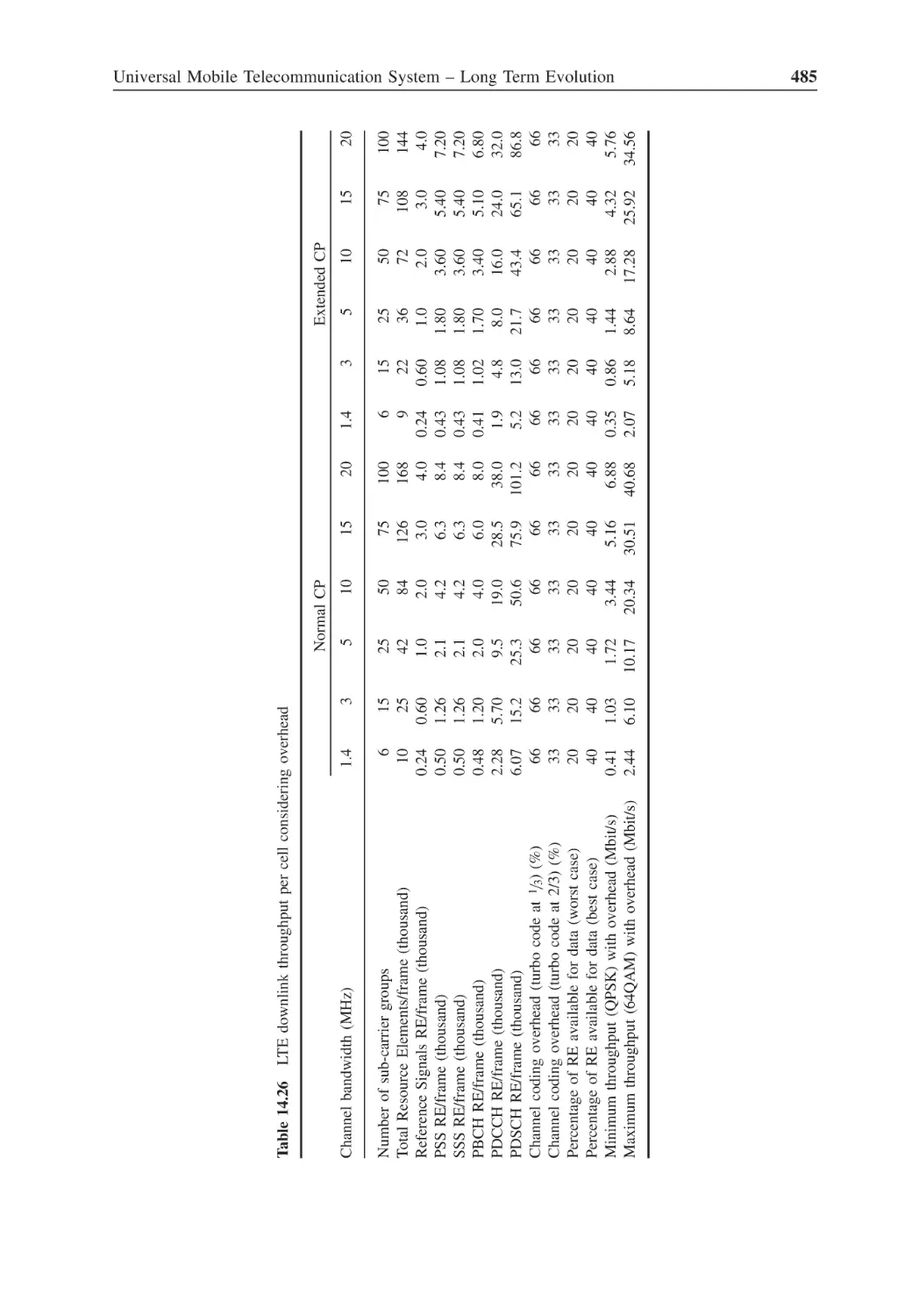
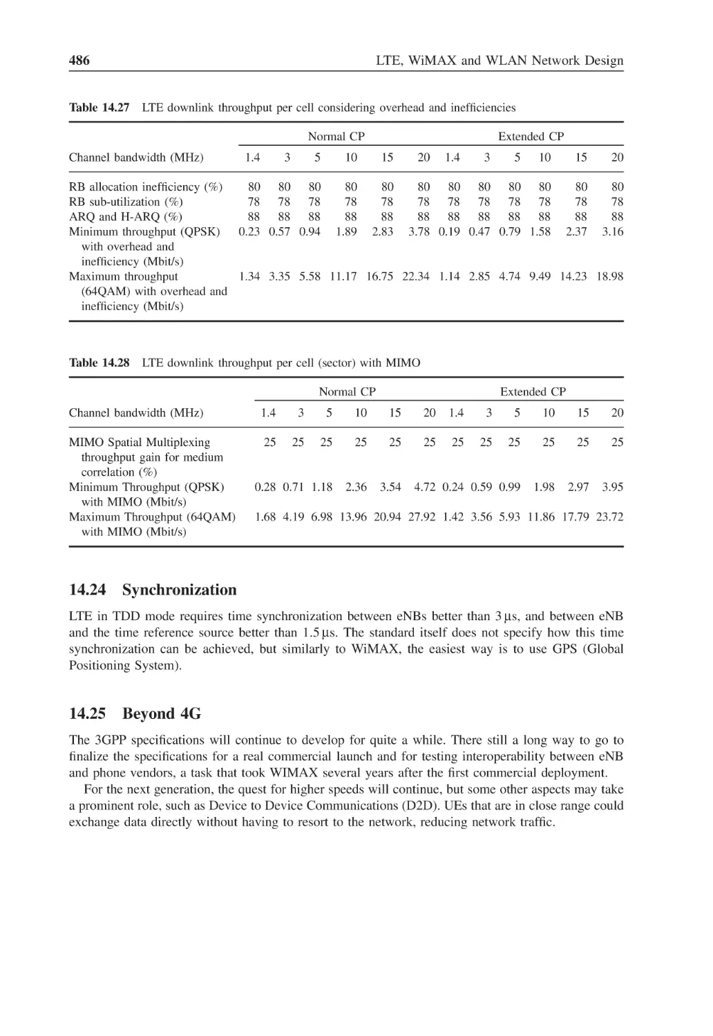
14.23 LTE Practical System Capacity
14.23.1 Downlink Capacity
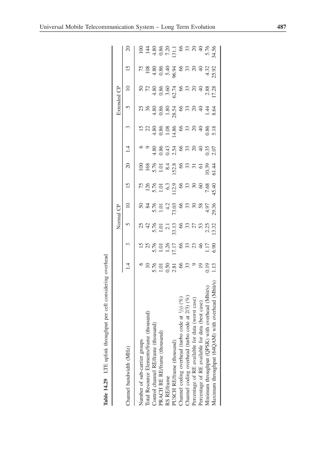
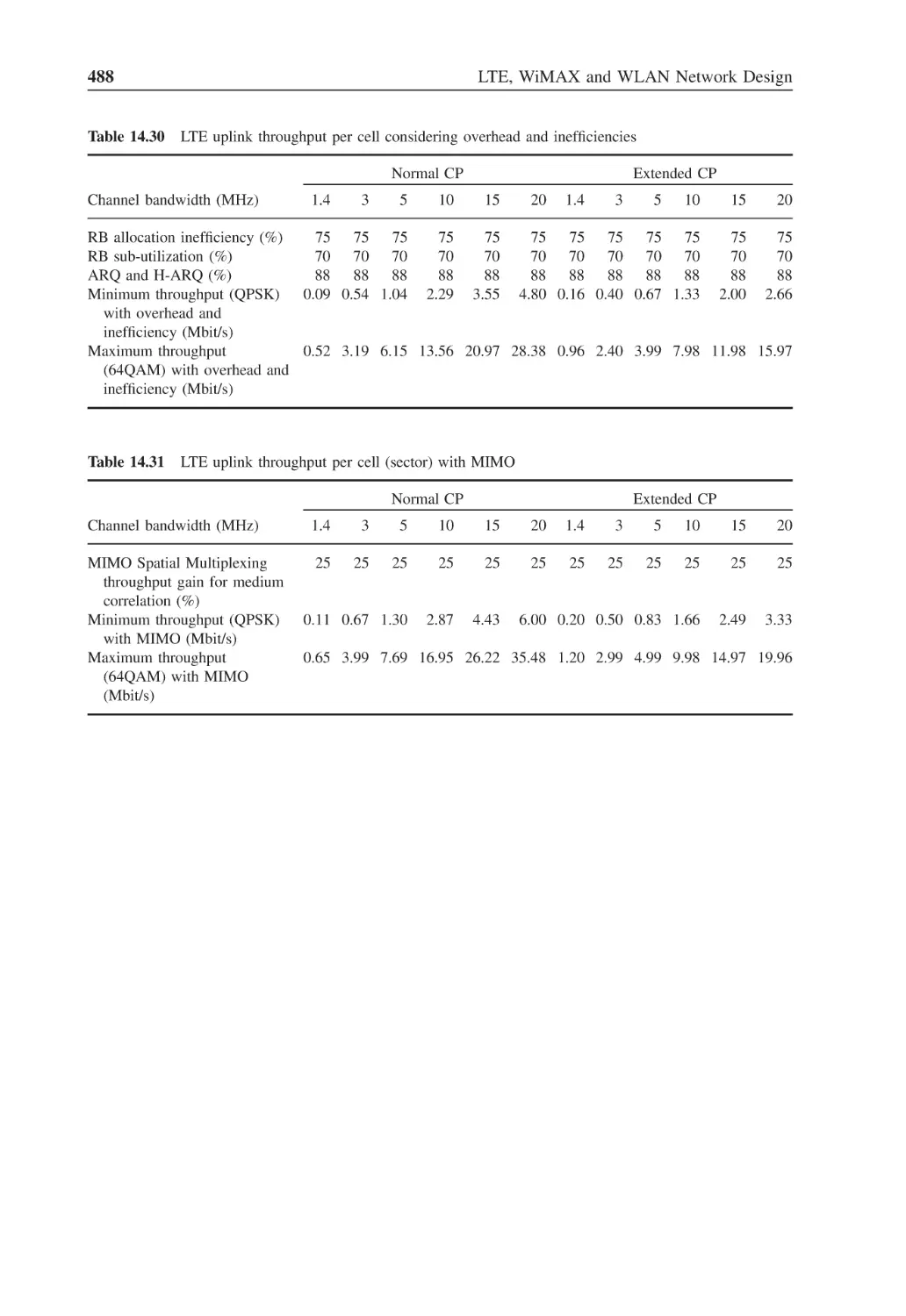
14.23.2 Uplink Capacity
14.24 Synchronization
14.25 Beyond 4G
439
440
442
444
447
450
454
455
457
457
461
463
463
465
466
466
467
467
470
470
471
472
472
473
473
473
473
475
475
475
476
481
482
482
483
483
483
483
486
486
15
15.1
15.2
489
489
489
490
490
490
490
490
490
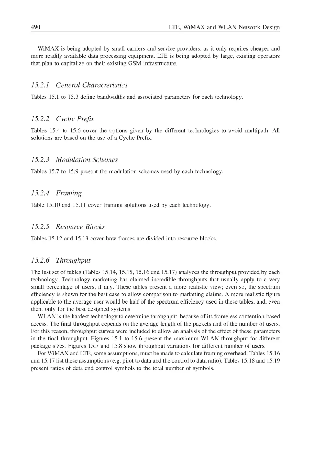
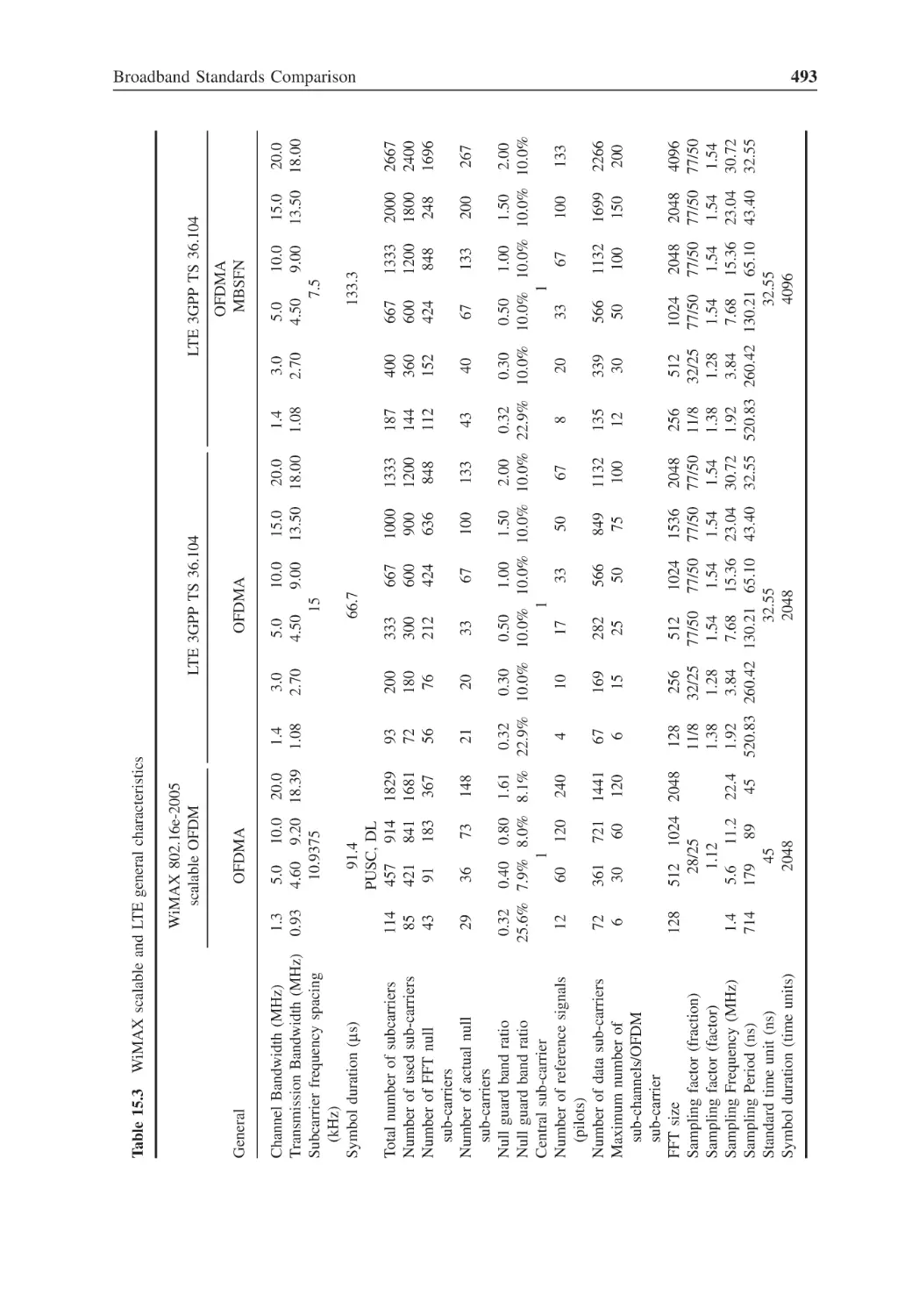
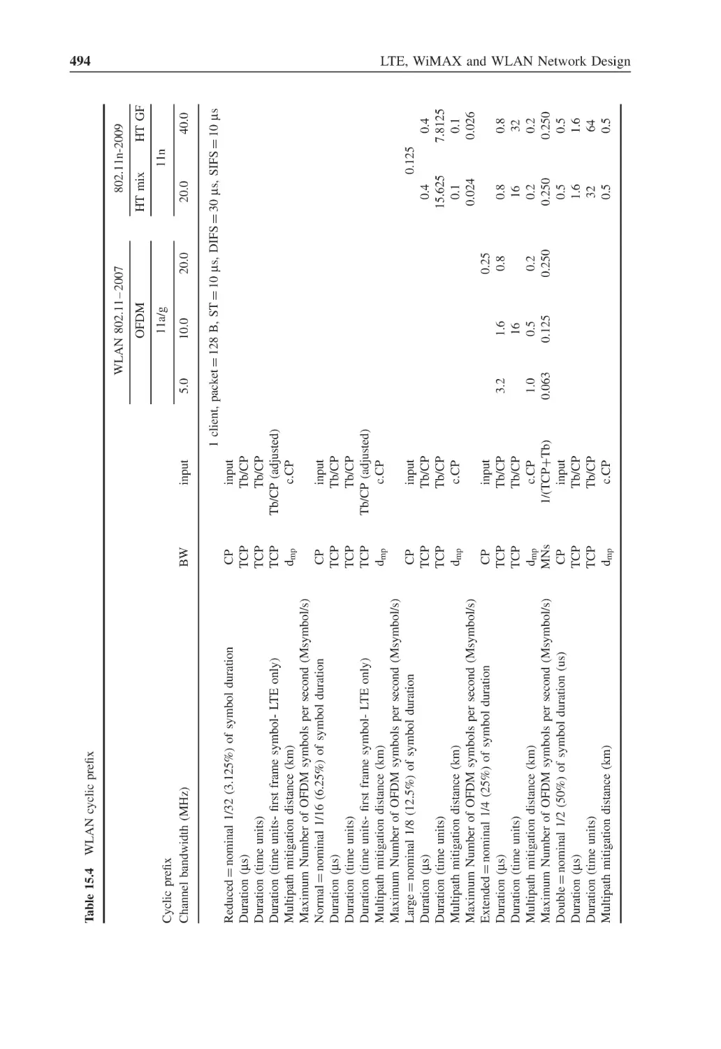
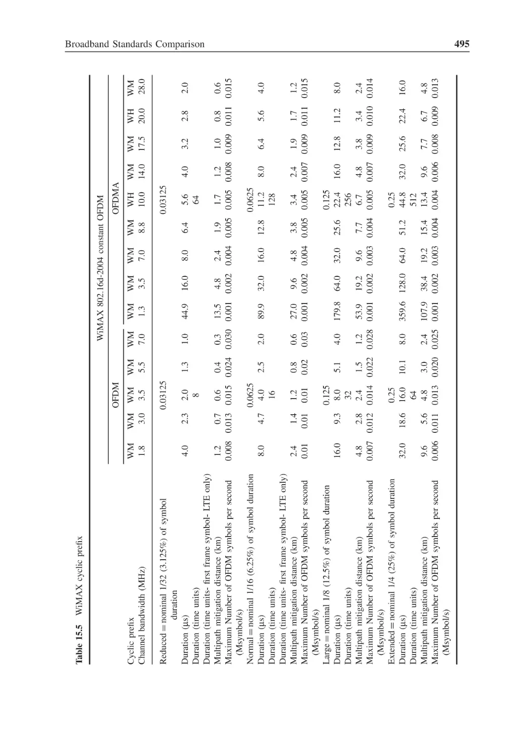
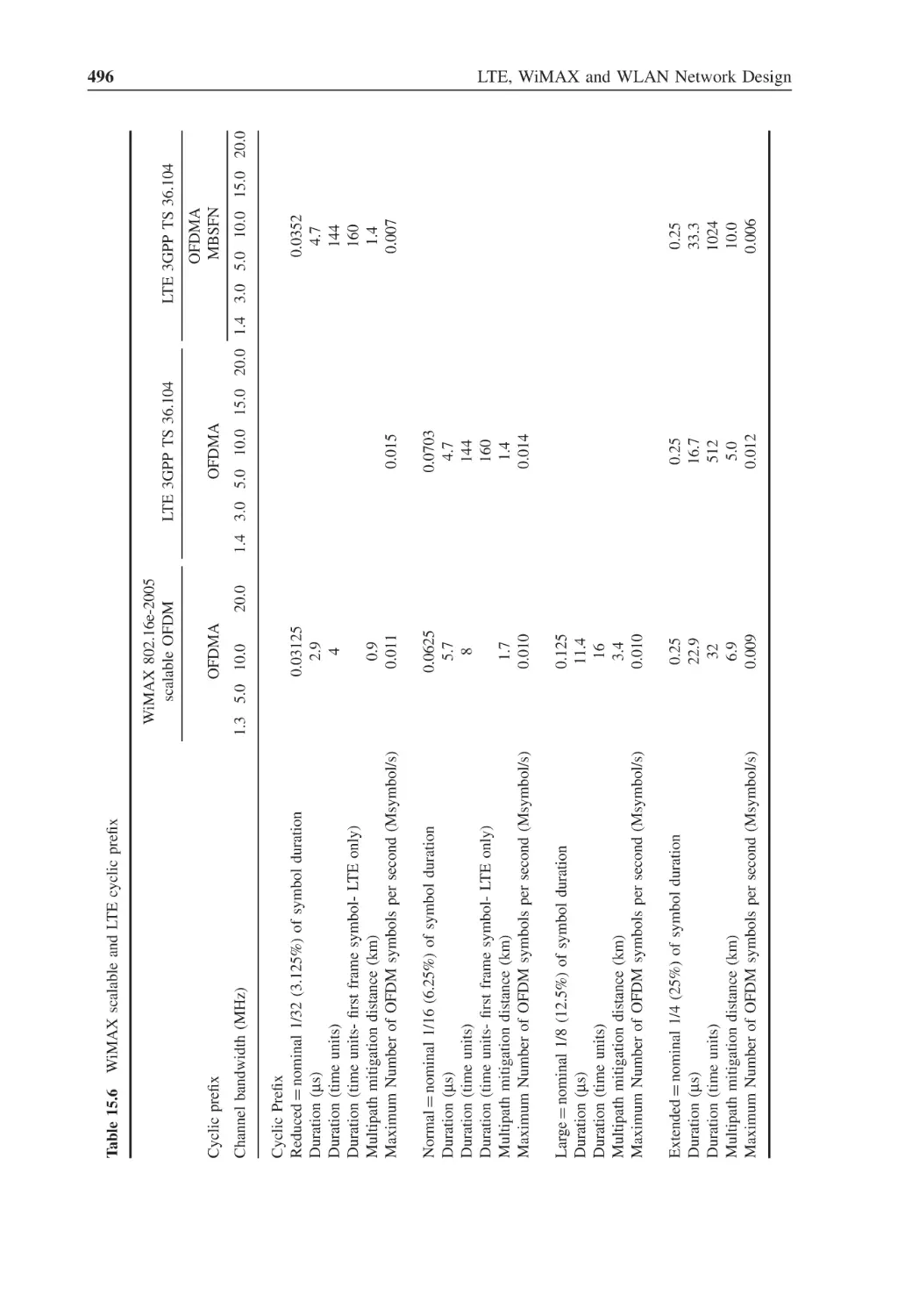
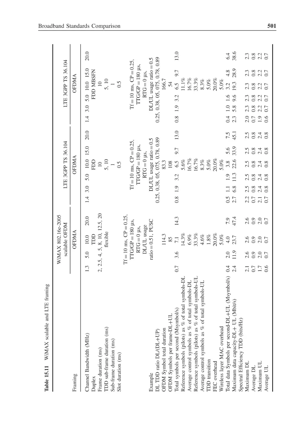
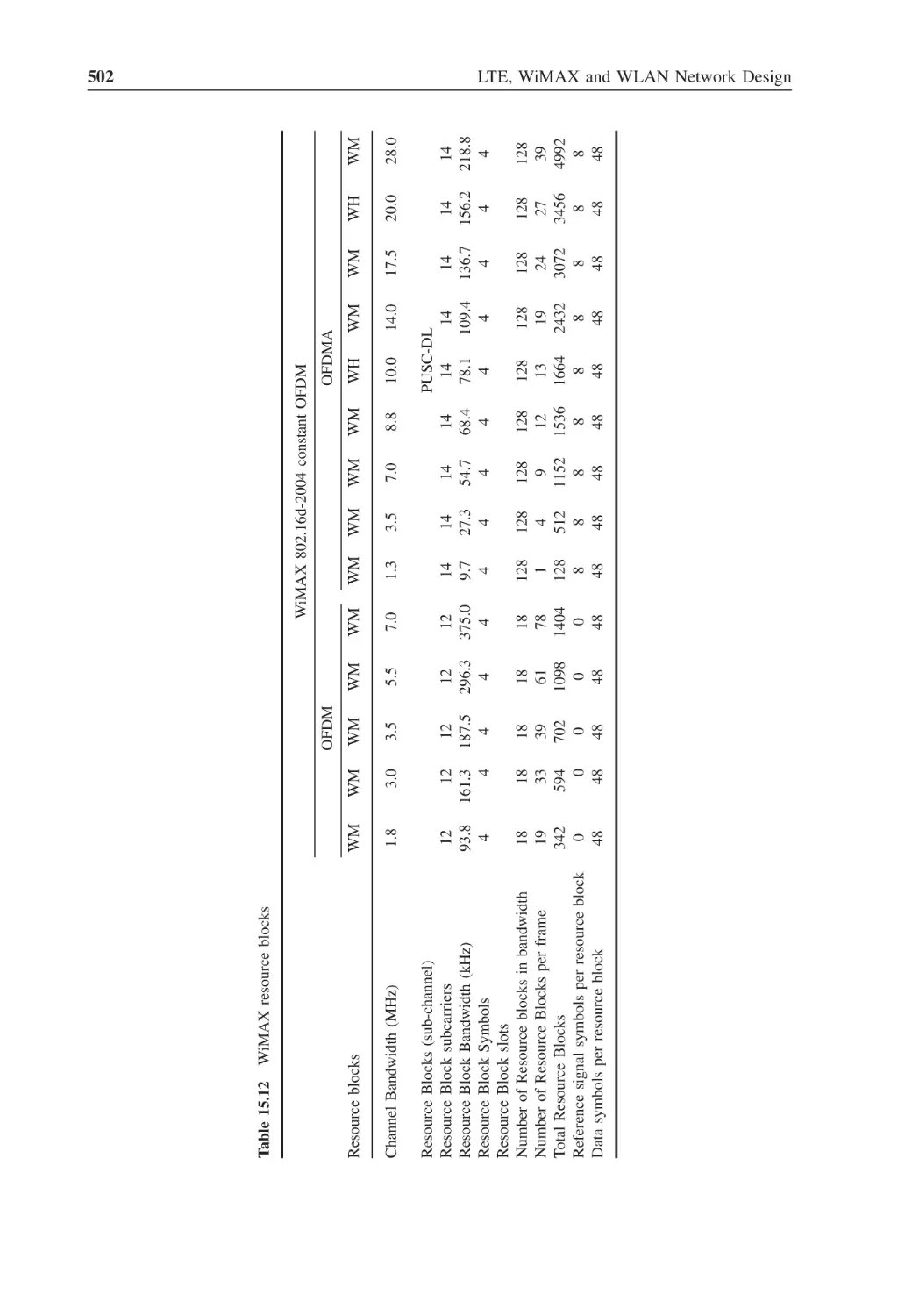
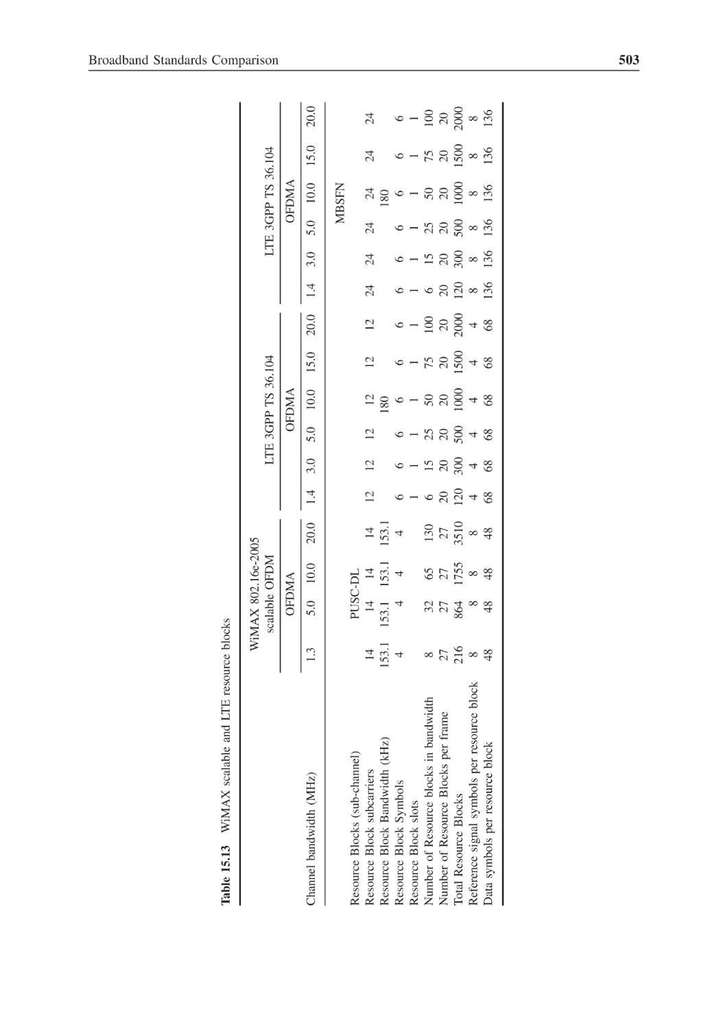
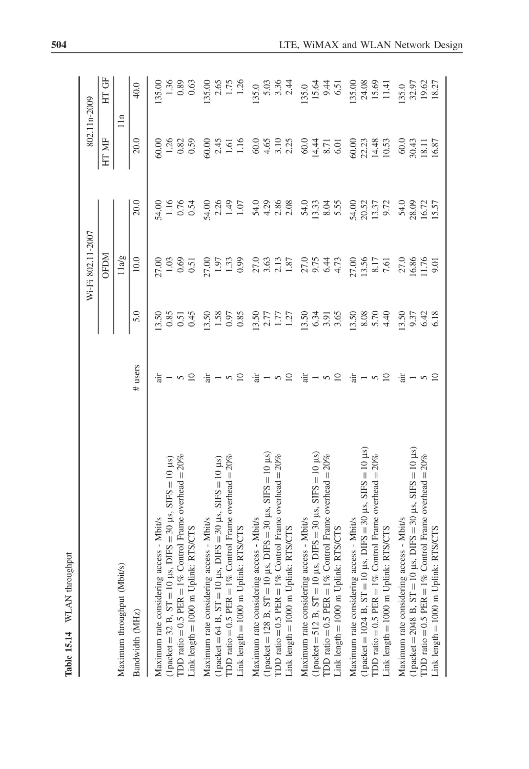
Broadband Standards Comparison
Introduction
Performance Tables
15.2.1
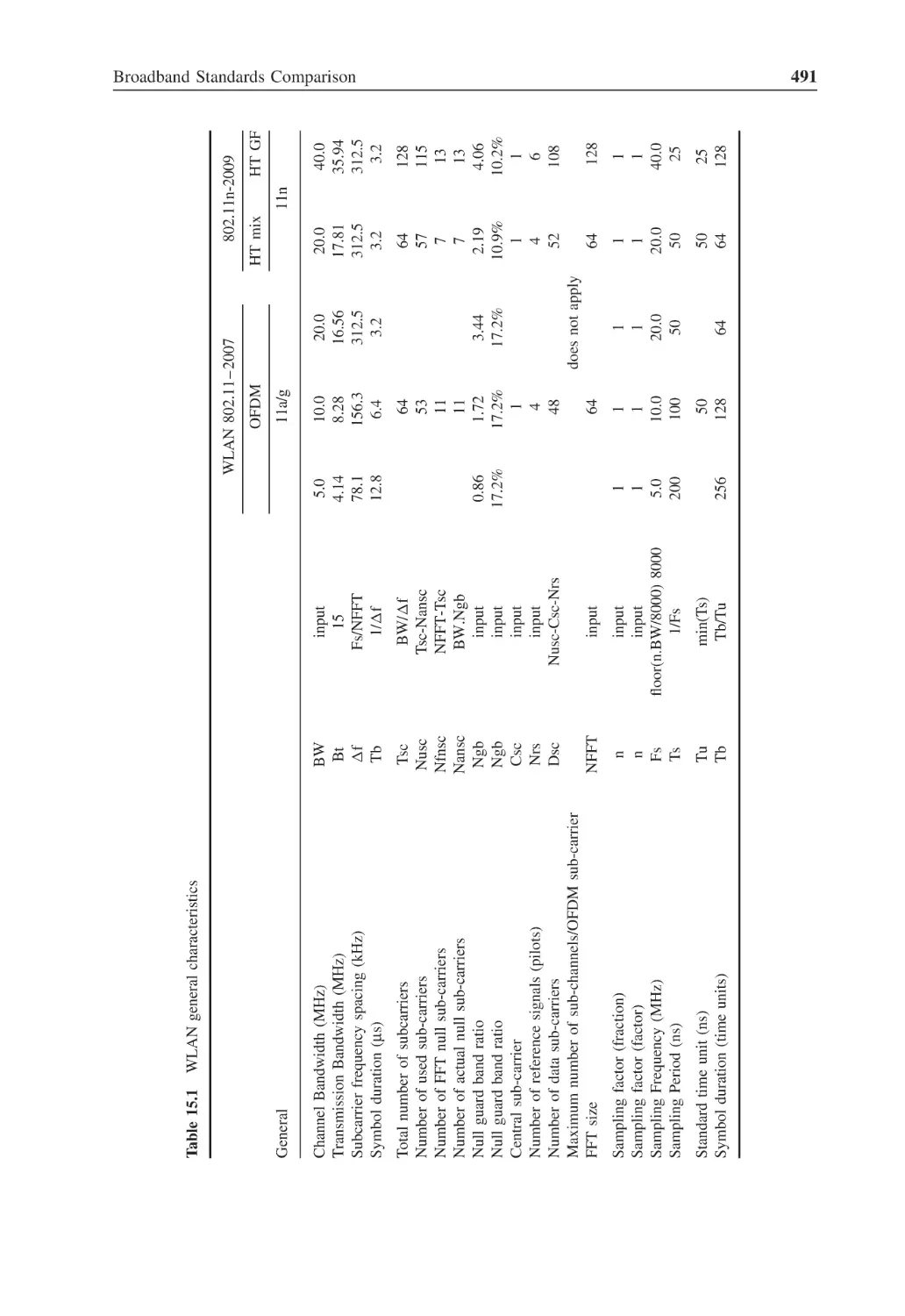
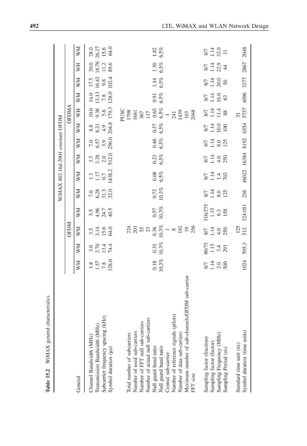
General Characteristics
15.2.2
Cyclic Prefix
15.2.3
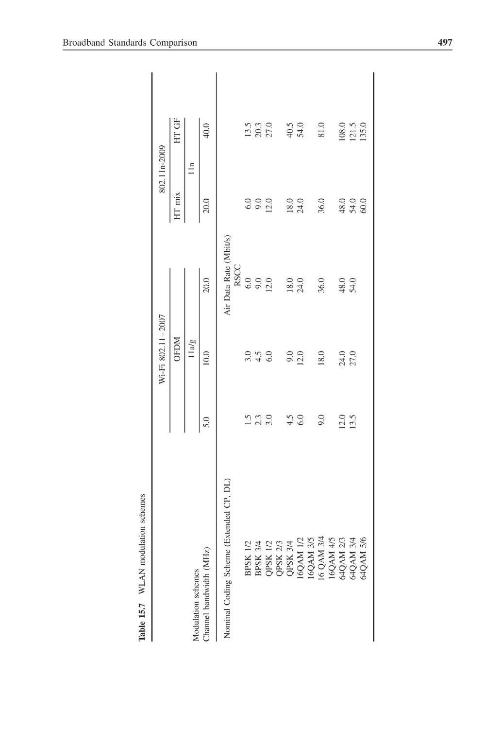
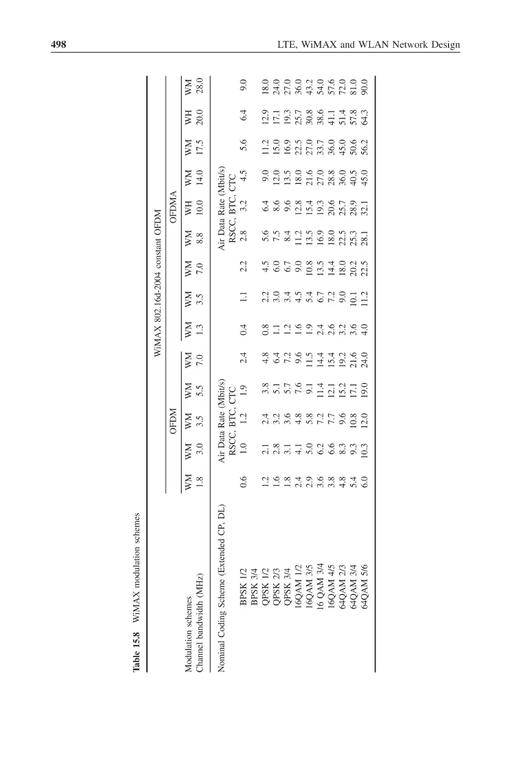
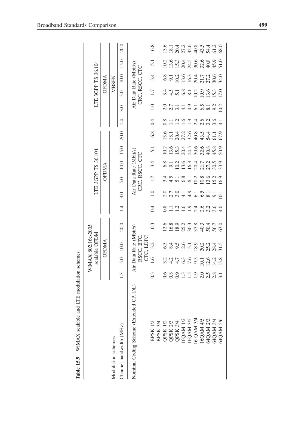
Modulation Schemes
15.2.4
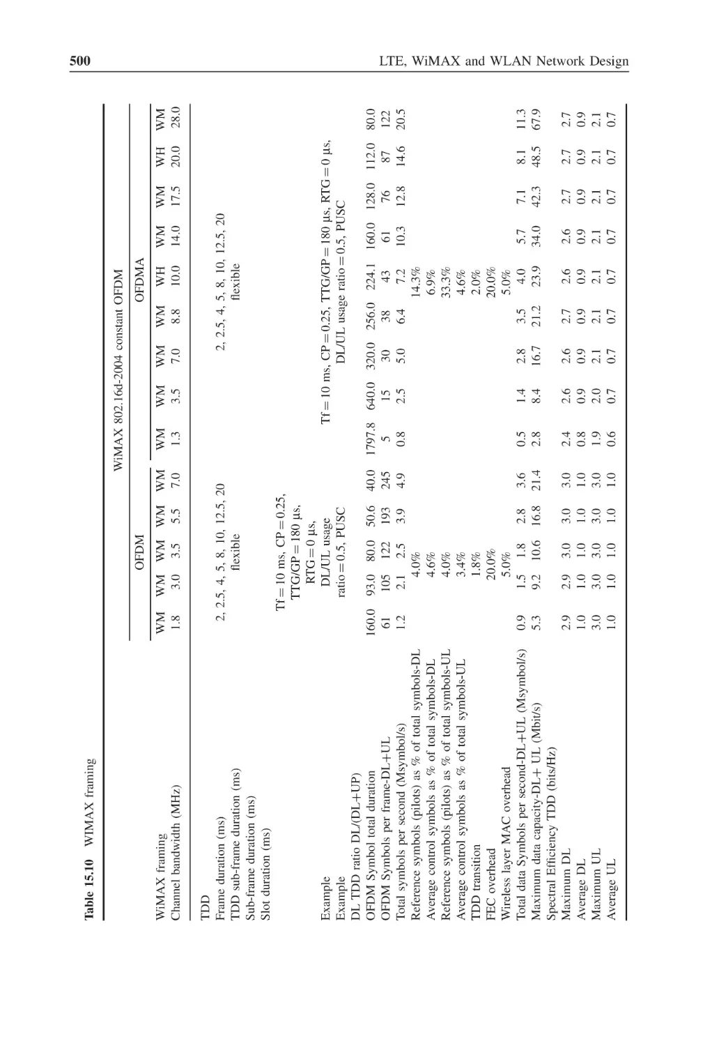
Framing
15.2.5
Resource Blocks
15.2.6
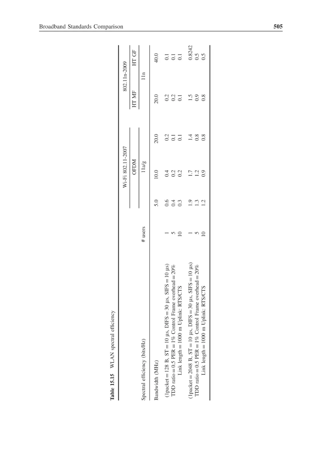
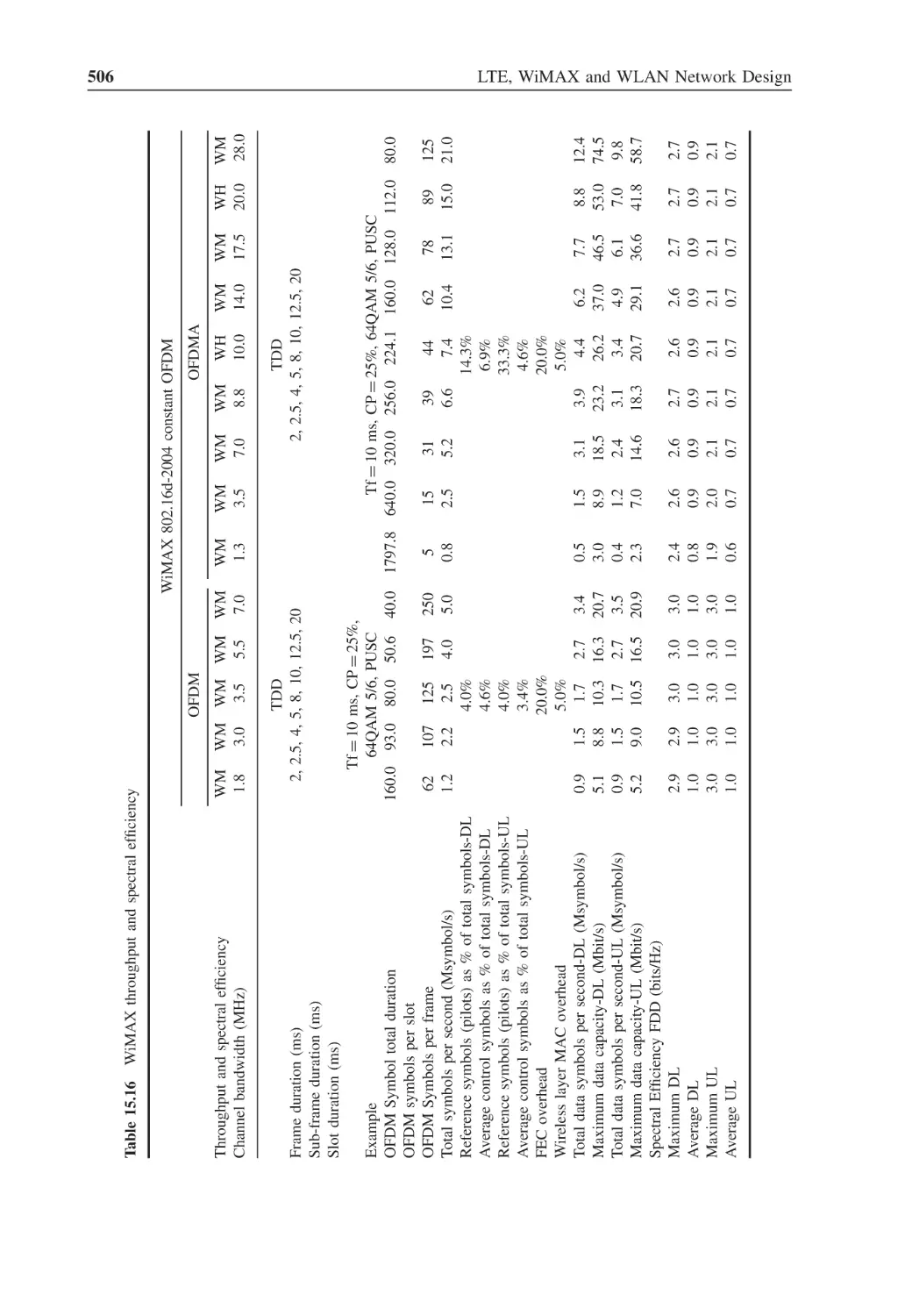
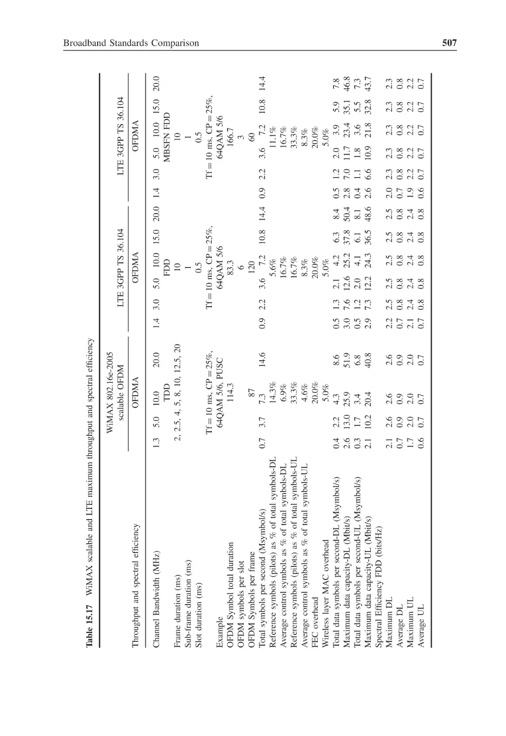
Throughput
xvi
16
16.1
16.2
16.3
16.4
16.5
16.6
Contents
Wireless Network Design
Introduction
Wireless Market Modeling
Wireless Network Strategy
Wireless Network Design
Wireless Network Optimization
Wireless Network Performance Assessment
17
17.1
17.2
17.3
513
513
513
515
516
517
517
Wireless Market Modeling
Findings Phase
Area of Interest (AoI) Modeling
Terrain Databases (GIS Geographic Information System)
17.3.1
Satellite/Aerial Photos for Area of Interest
17.3.2
Topography
17.3.3
Digitize Landmarks
17.3.4
Morphology
17.3.5
Buildings Morphology
17.3.6
Multiple Terrain Layers
17.3.7
Terrain Database Editing
17.3.8
Background Images
17.4 Demographic Databases
17.4.1
Obtain Demographic Information (Maps and Tables)
17.4.2
Generate Demographic Regions
17.5 Service Modeling
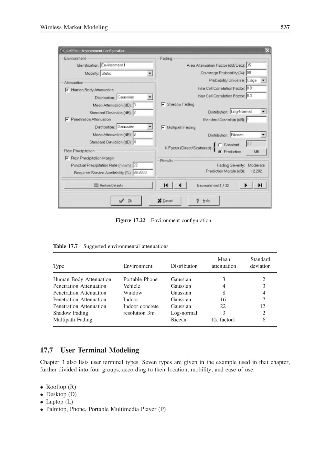
17.6 Environment Modeling
17.7 User Terminal Modeling
17.8 Service Class Modeling
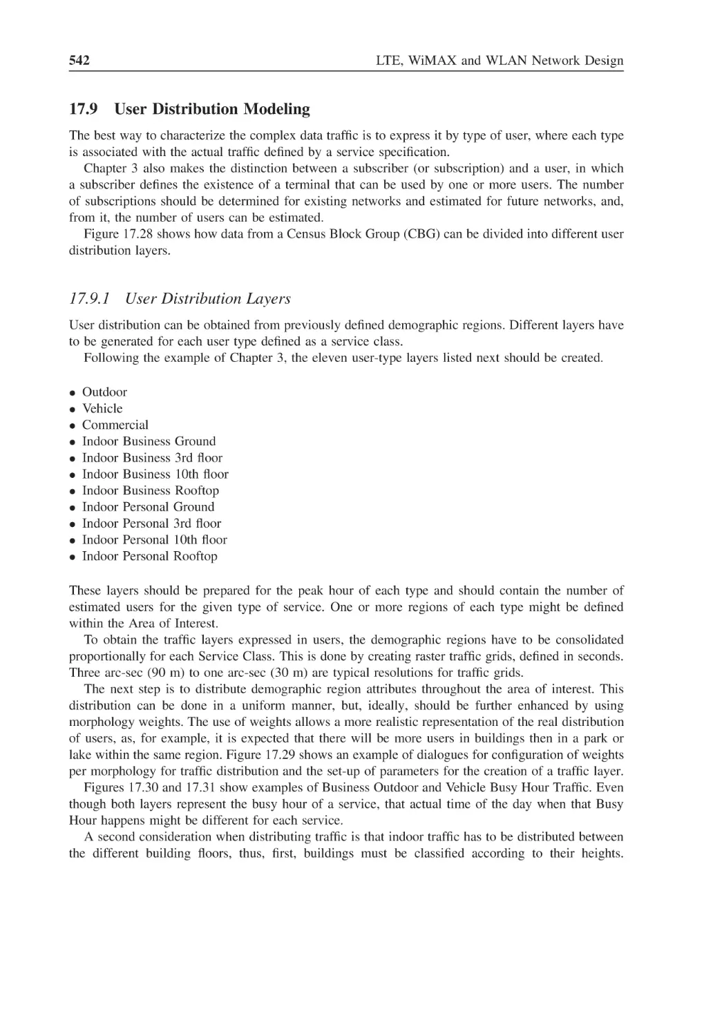
17.9 User Distribution Modeling
17.9.1
User Distribution Layers
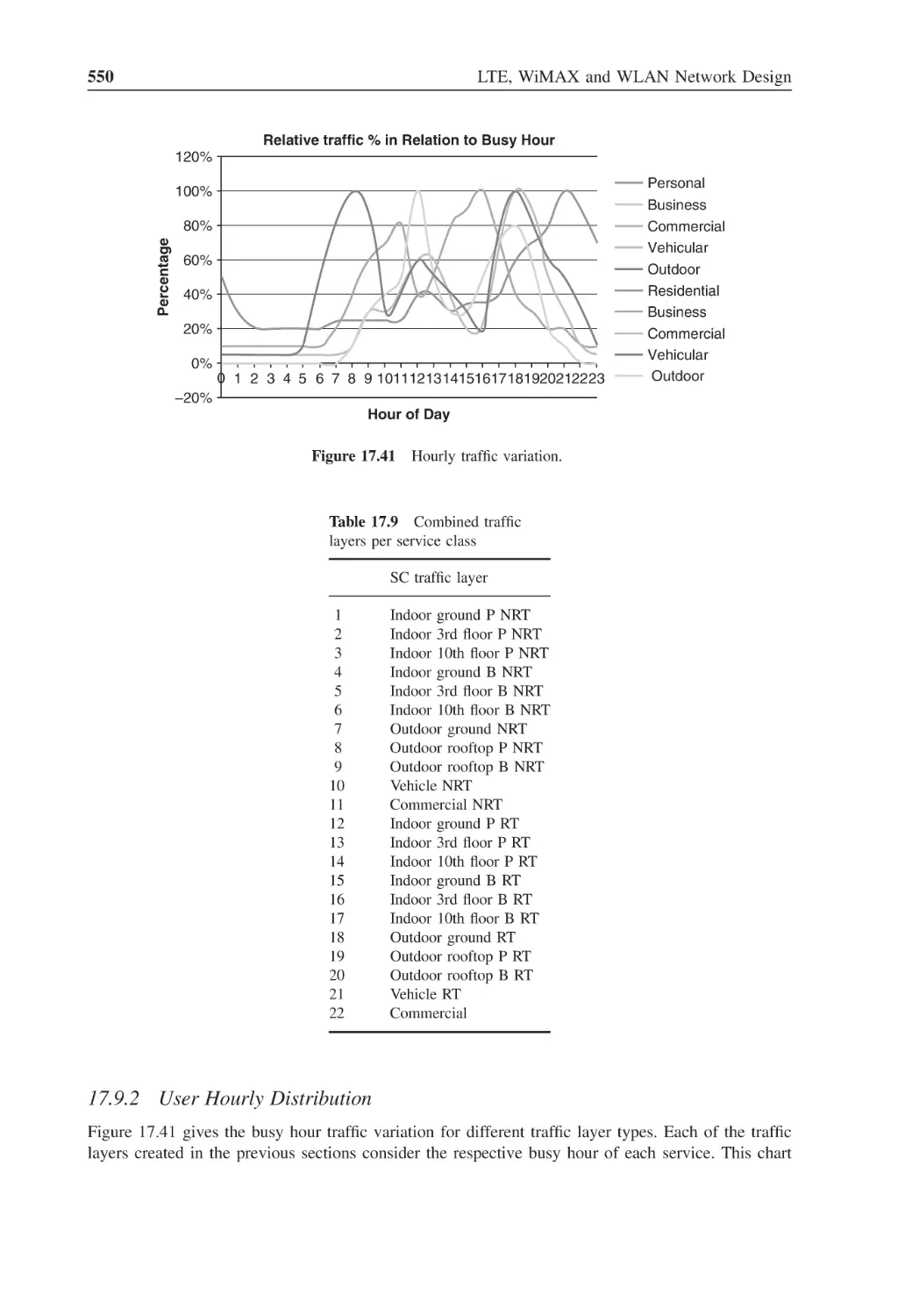
17.9.2
User Hourly Distribution
17.10 Traffic Distribution Modeling
519
519
519
519
520
521
521
523
527
527
528
528
530
530
532
533
536
537
538
542
542
550
551
18
18.1
553
553
554
555
555
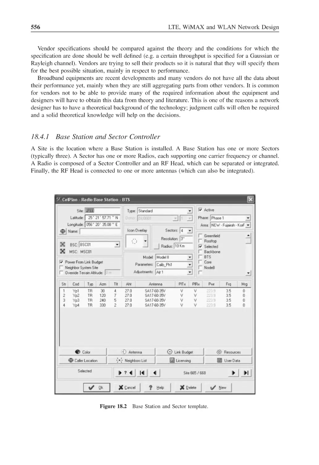
555
556
557
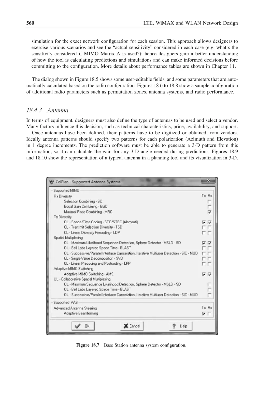
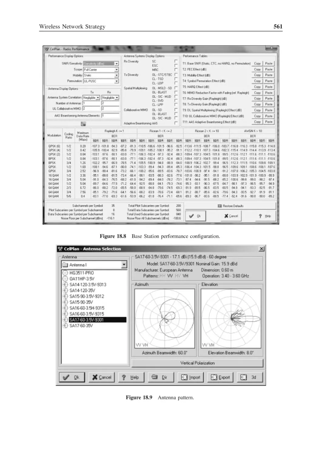
560
563
565
565
567
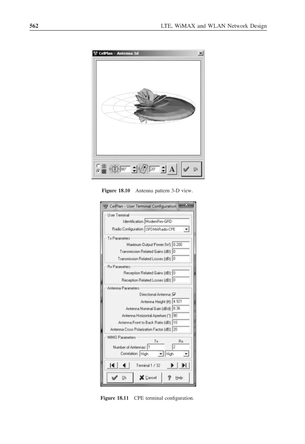
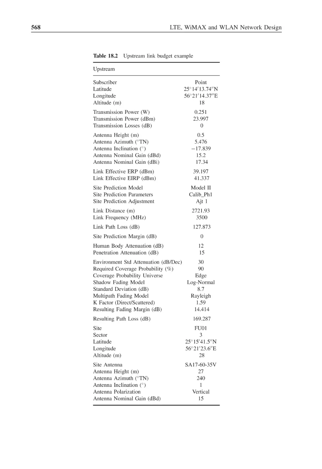
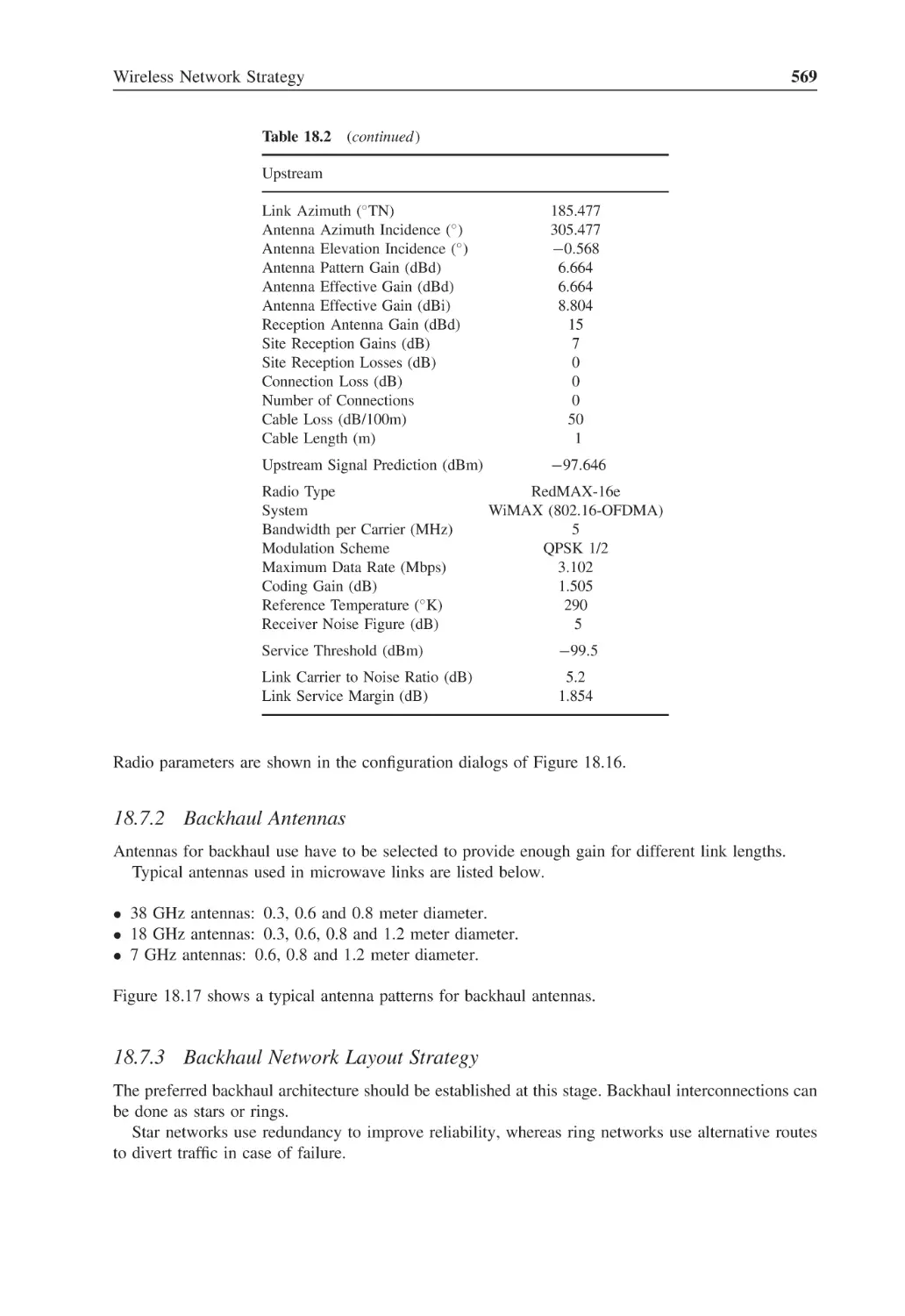
569
569
570
570
18.2
18.3
18.4
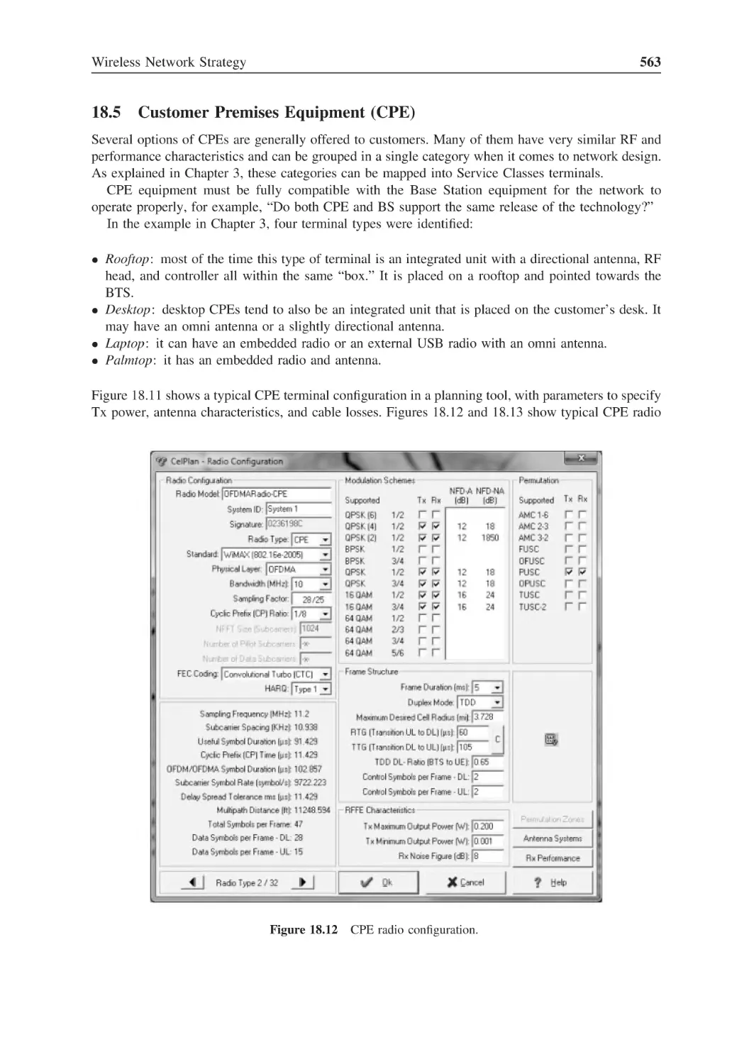
18.5
18.6
18.7
18.8
18.9
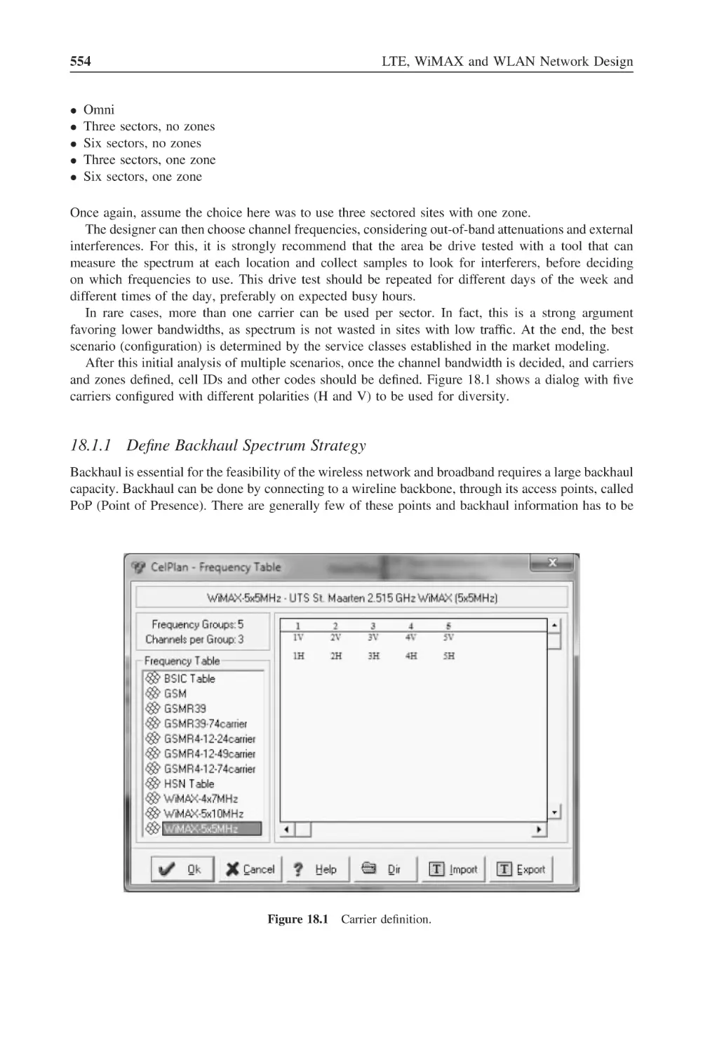
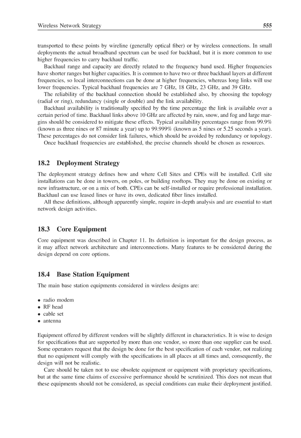
Wireless Network Strategy
Define Spectrum Usage Strategy
18.1.1
Define Backhaul Spectrum Strategy
Deployment Strategy
Core Equipment
Base Station Equipment
18.4.1
Base Station and Sector Controller
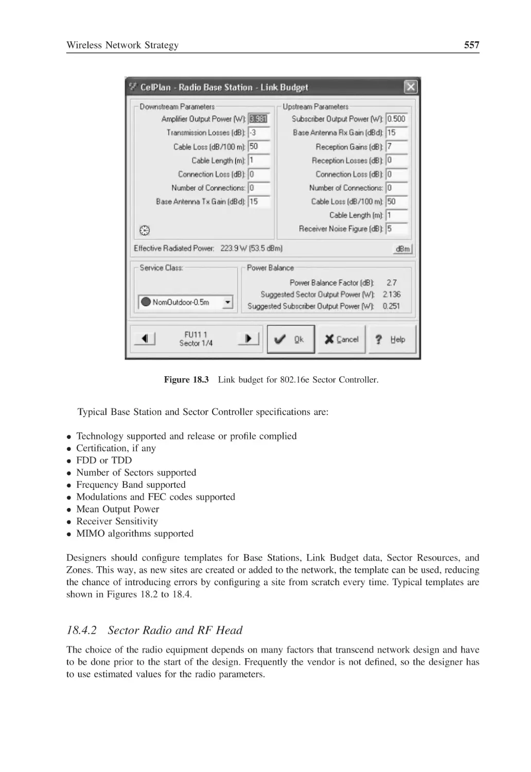
18.4.2
Sector Radio and RF Head
18.4.3
Antenna
Customer Premises Equipment (CPE)
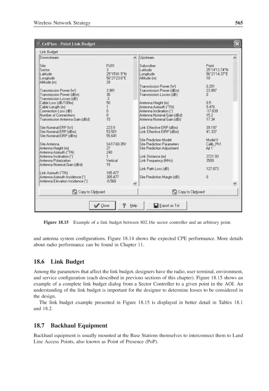
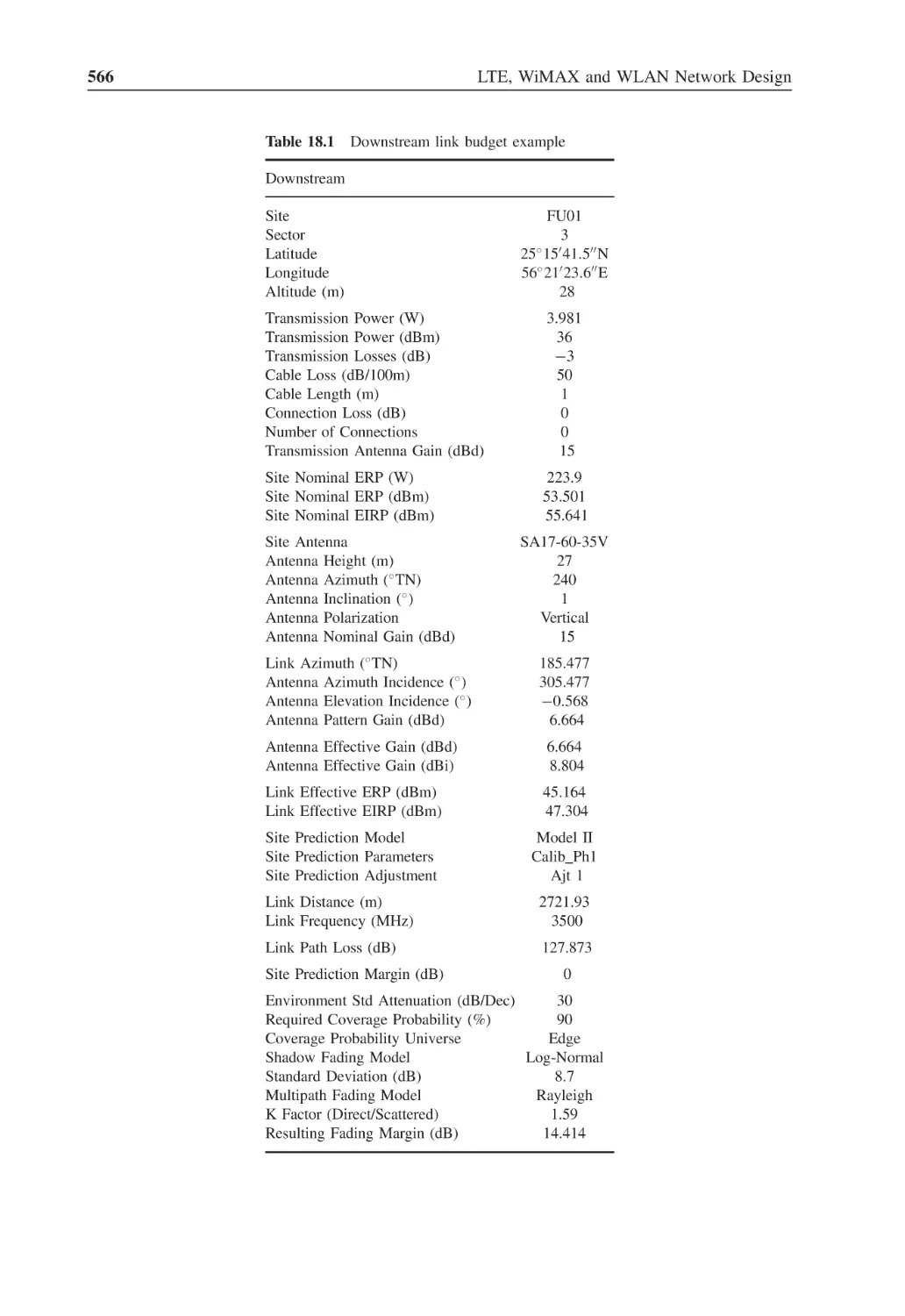
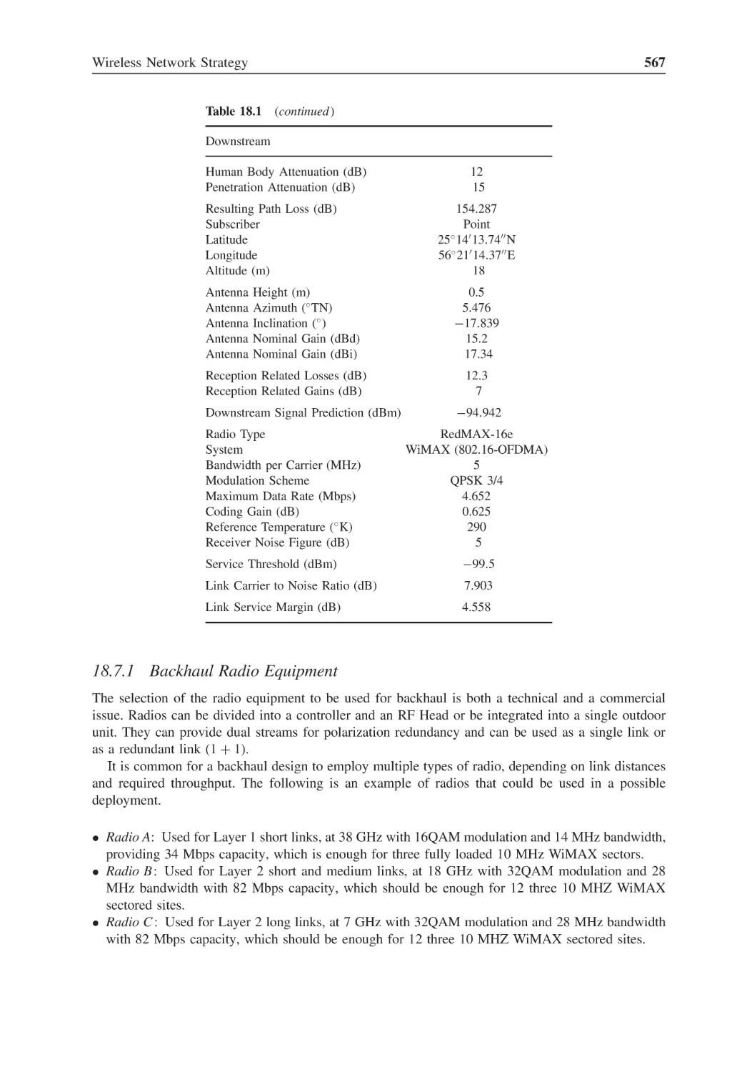
Link Budget
Backhaul Equipment
18.7.1
Backhaul Radio Equipment
18.7.2
Backhaul Antennas
18.7.3
Backhaul Network Layout Strategy
Land Line Access Points of Presence (PoP)
List of Available Site Locations
Contents
xvii
19
19.1
19.2
19.3
Wireless Network Design
Field Measurement Campaign
Measurement Processing
Propagation Models and Parameters
19.3.1
Calibrate for Different Propagation Models
19.3.2
Define Propagation Models and Parameters for Different Site Types
Site Location
19.4.1
Simplified Site Distribution
19.4.2
Advanced Cell Selection Procedure
Run Initial Site Predictions
Static Traffic Simulation
19.6.1
Define Target Noise Rise Per Area
19.6.2
Static Traffic Simulation
Adjust Design for Area and Traffic Coverage
Configure Backhaul Links and Perform Backhaul Predictions
Perform Signal Level Predictions with Extended Radius
573
573
575
579
581
581
582
582
583
586
593
593
593
595
595
597
20
20.1
20.2
Wireless Network Optimization
Cell Enhancement or Footprint Optimization
Resource Optimization
20.2.1
Neighbor List
20.2.2
Handover Thresholds
20.2.3
Paging Groups
20.2.4
Interference Matrix for Downstream and Upstream for All PSC
20.2.5
Interference Matrix
20.2.6
Automatic Code Planning (Segmentation, CellID and PermBase)
20.2.7
Automatic Carrier Planning
20.2.8
Constrained Cell Enhancement
20.2.9
Backhaul Interference Matrix
20.2.10 Backhaul Automatic Channel Plan
599
599
603
603
603
603
603
606
607
610
613
614
614
21
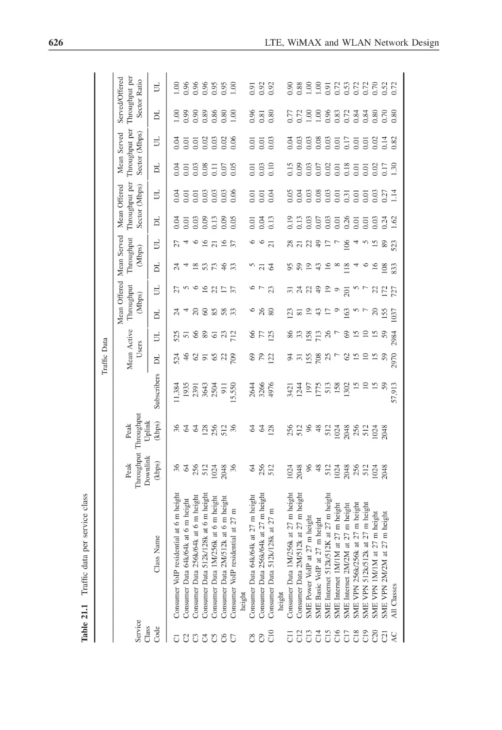
21.1
Wireless Network Performance Assessment
Perform Dynamic Traffic Simulation
21.1.1
Traffic Snapshot
21.1.2
Traffic Report
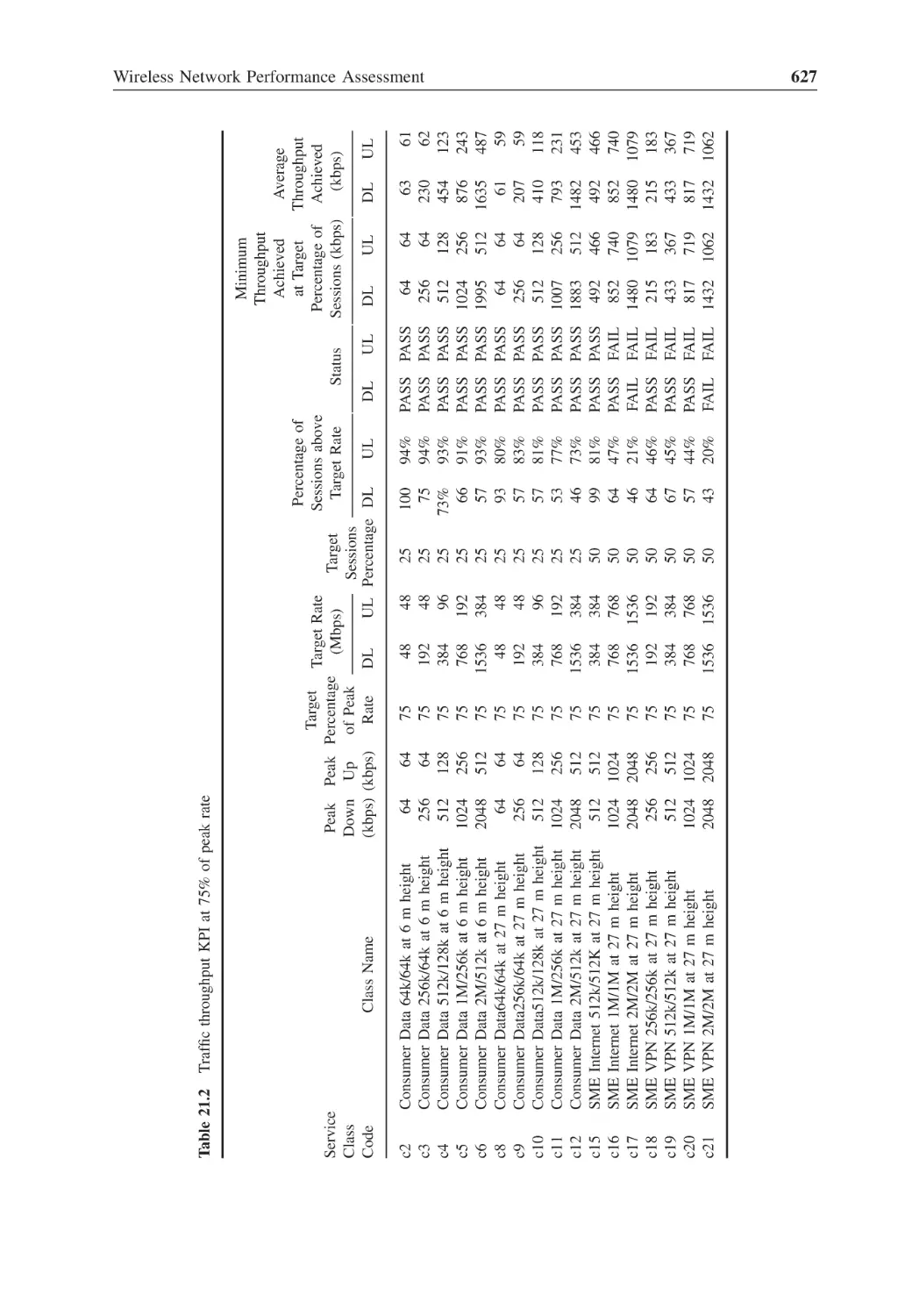
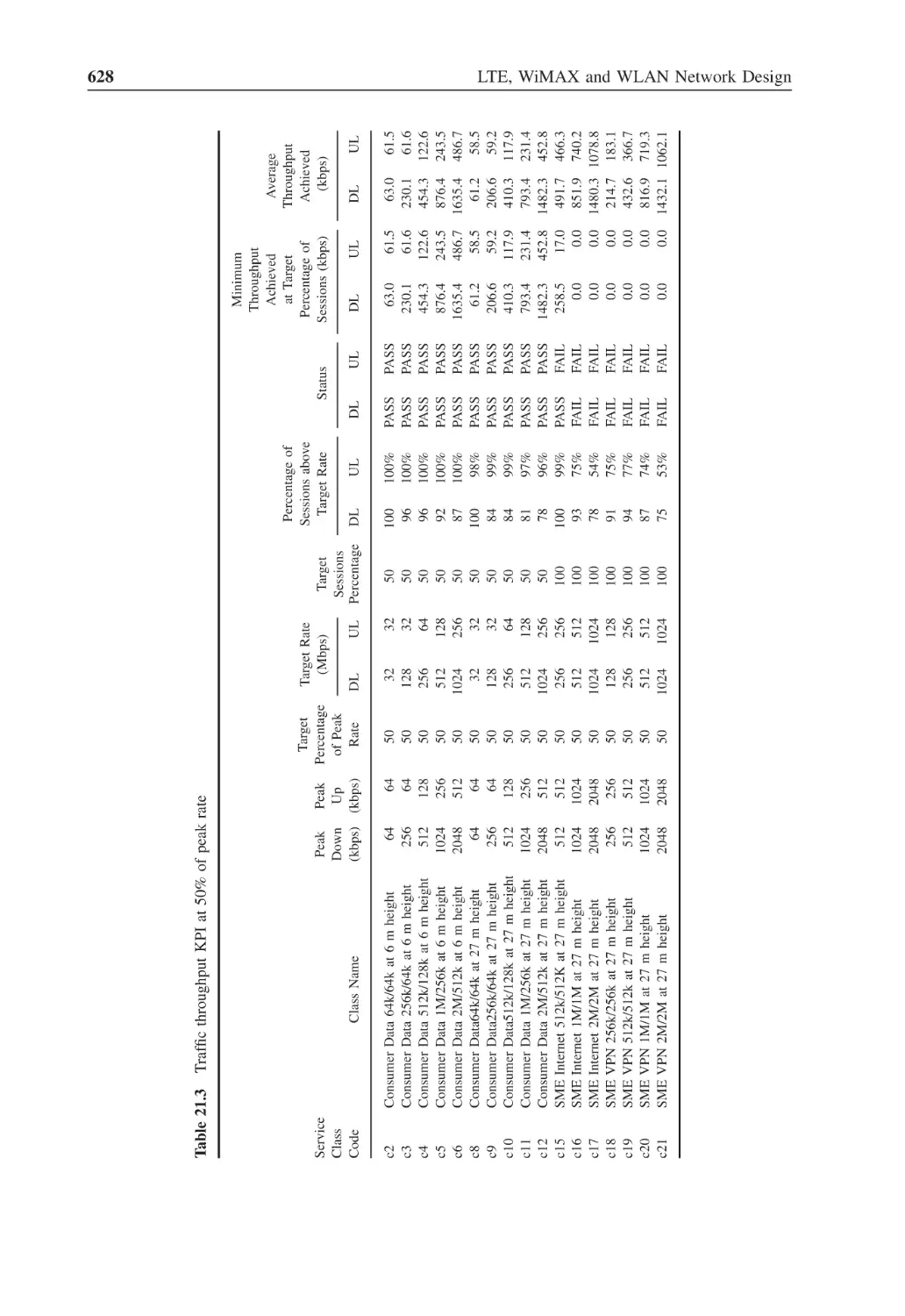
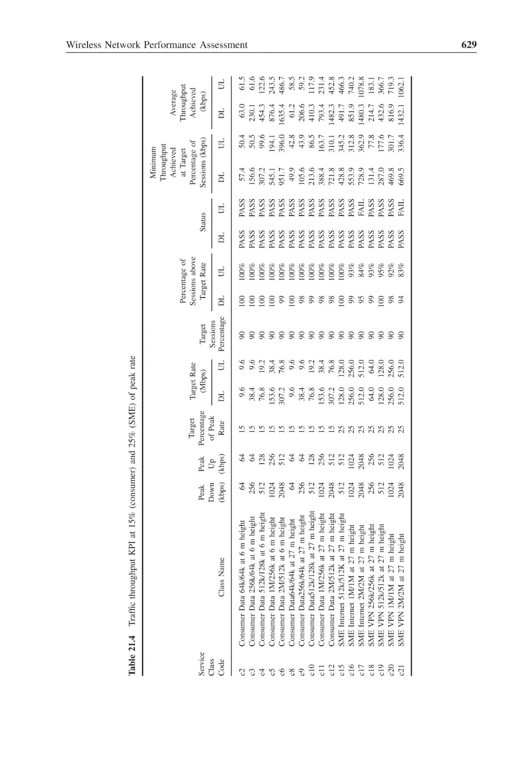
Performance
21.2.1
Generate Key Parameter Indicators (KPI)
Perform Network Performance Predictions
21.3.1
Topography
21.3.2
Morphology
21.3.3
Image
21.3.4
Landmarks
21.3.5
Demographic Region
21.3.6
Traffic Layers
21.3.7
Traffic Simulation Result
21.3.8
Composite Signal Level
21.3.9
Composite S/N
21.3.10 Preamble
21.3.11 Preamble SNIR
615
615
617
620
620
620
625
625
625
631
631
634
634
635
635
636
639
639
19.4
19.5
19.6
19.7
19.8
19.9
21.2
21.3
xviii
21.4
21.5
22
22.1
22.2
22.3
22.4
22.5
22.6
Contents
21.3.12 Preamble Margin
21.3.13 MAP (Medium Access Protocol) Margin
21.3.14 MAP S/N
21.3.15 Best Server
21.3.16 Number of Servers
21.3.17 Radio Selection
21.3.18 Zone Selection
21.3.19 MIMO Selection
21.3.20 Modulation Scheme Selection
21.3.21 Payload Data Rate
21.3.22 Maximum Data Rate Per Sub-Channel
21.3.23 Interference
21.3.24 Noise Rise
21.3.25 Downstream/Upstream Service
21.3.26 Service Margin
21.3.27 Service Classes
21.3.28 Channel (Frequency) Plan
Backhaul Links Performance
21.4.1
Backhaul Traffic Analysis
Analyze Performance Results, Analyze Impact on CAPEX, OPEX and ROI
639
641
641
641
644
644
644
647
647
647
650
650
652
652
652
655
655
655
657
661
Basic Mathematical Concepts Used in Wireless Networks
Circle Relationships
Numbers and Vectors
22.2.1
Rational and Irrational Numbers
√
22.2.2
Imaginary Numbers (i = −1)
Functions Decomposition
22.3.1
Polynomial Decomposition
22.3.2
Exponential Number (e)
Sinusoids
22.4.1
Positive and Negative Frequencies (+ω, −ω)
Fourier Analysis
22.5.1
Fourier Transform
Statistical Probability Distributions
22.6.1
Binomial Distribution
22.6.2
Poisson Distribution (Law of Large Numbers)
22.6.3
Exponential Distribution
22.6.4
Normal or Gaussian Distribution
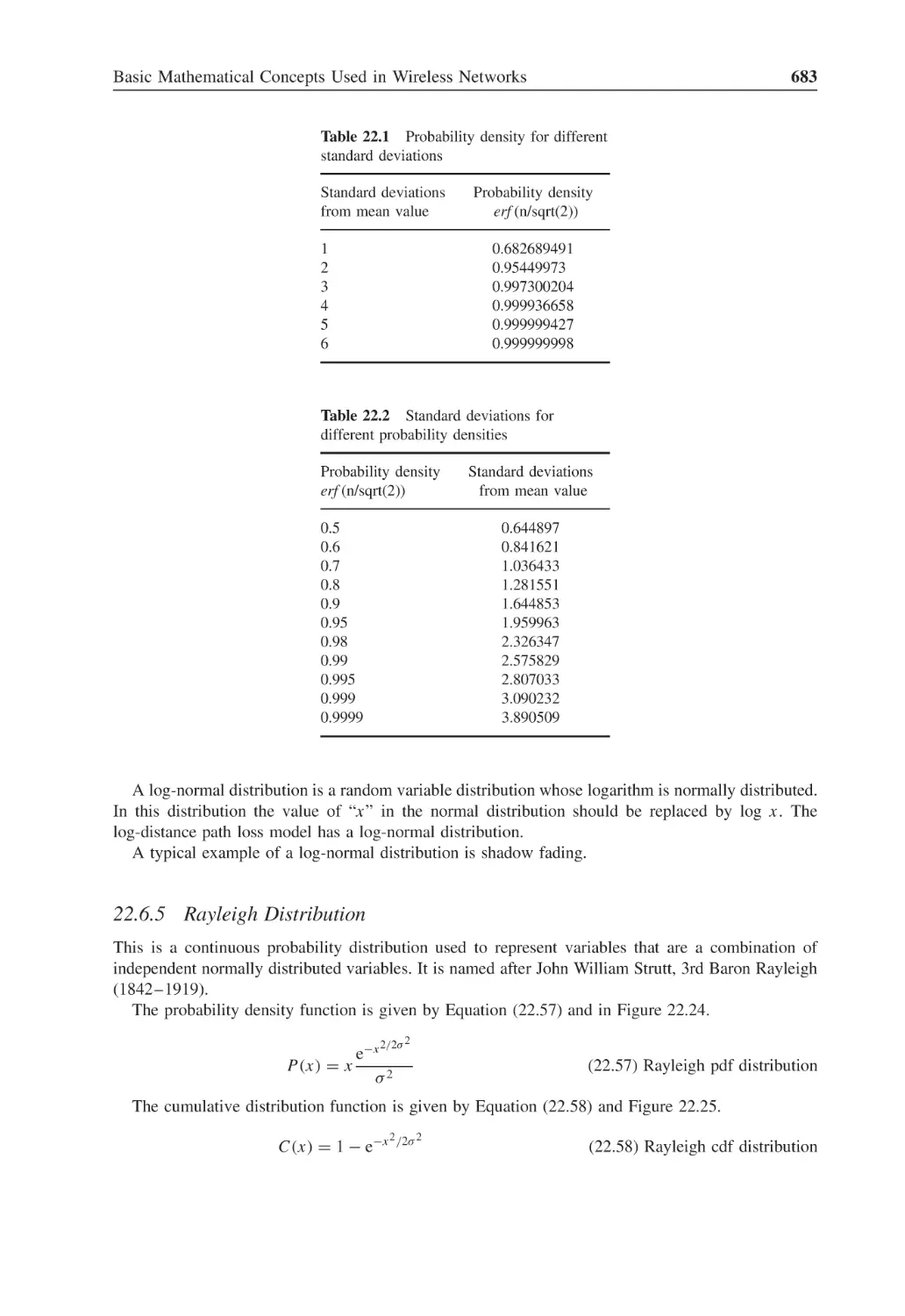
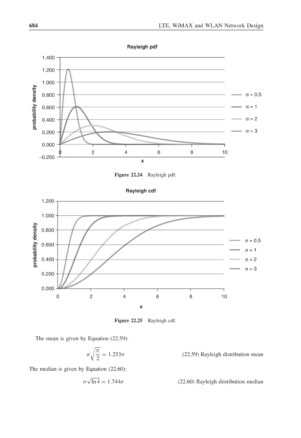
22.6.5
Rayleigh Distribution
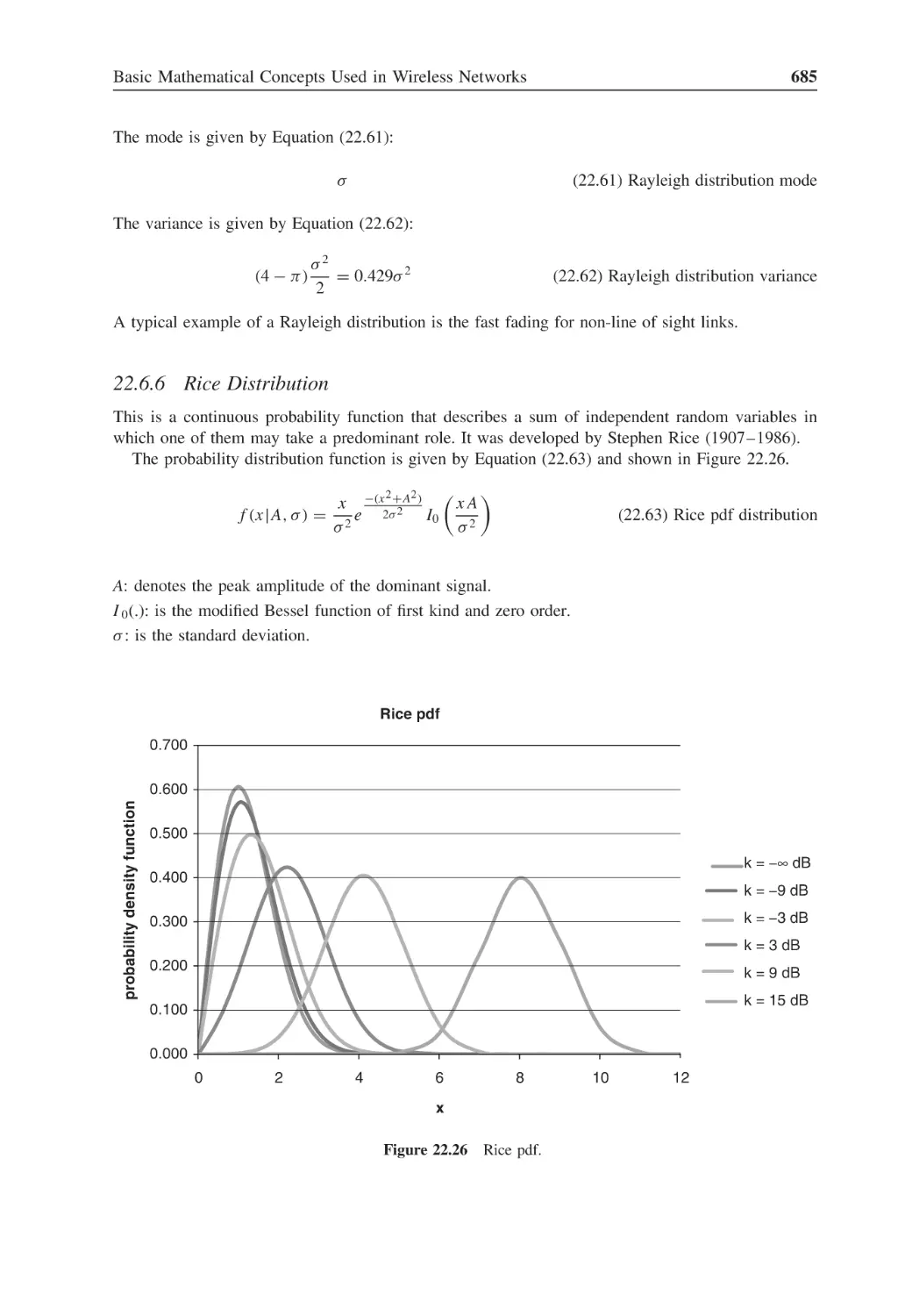
22.6.6
Rice Distribution
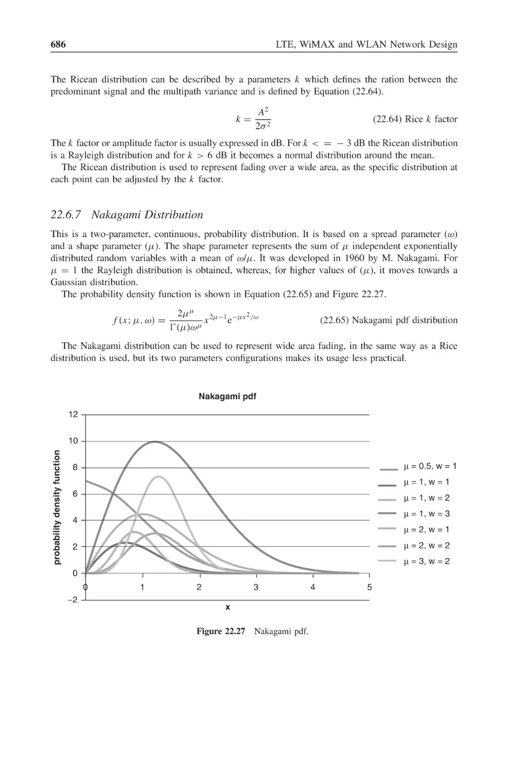
22.6.7
Nakagami Distribution
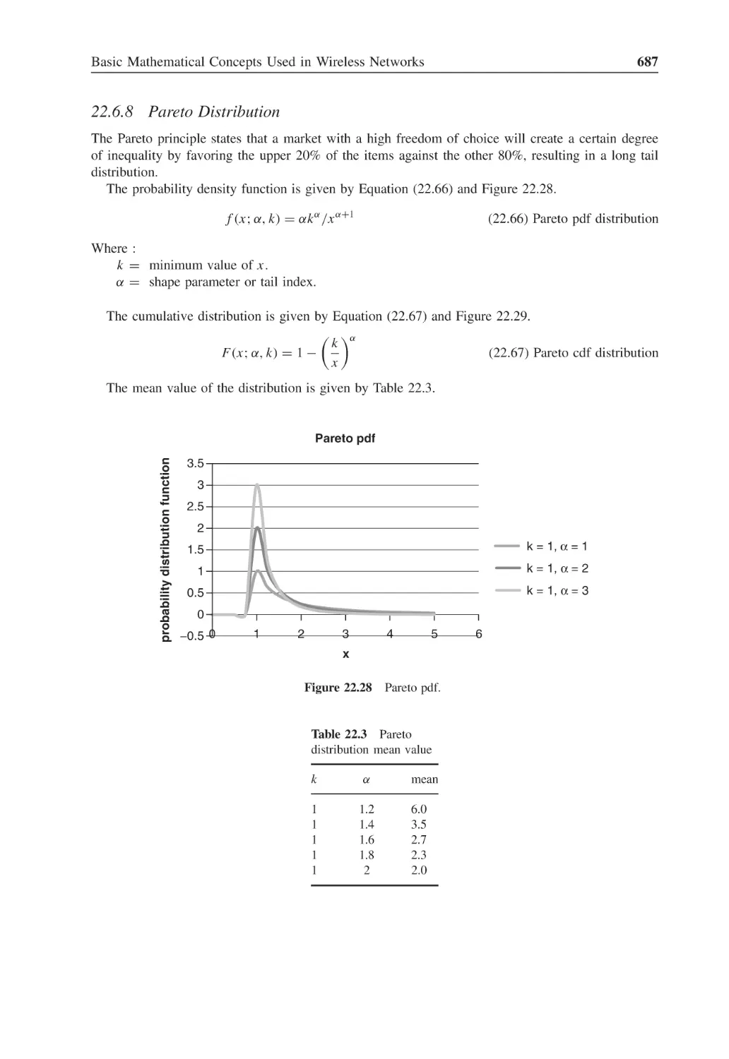
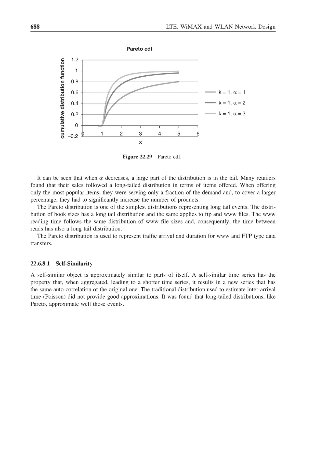
22.6.8
Pareto Distribution
663
663
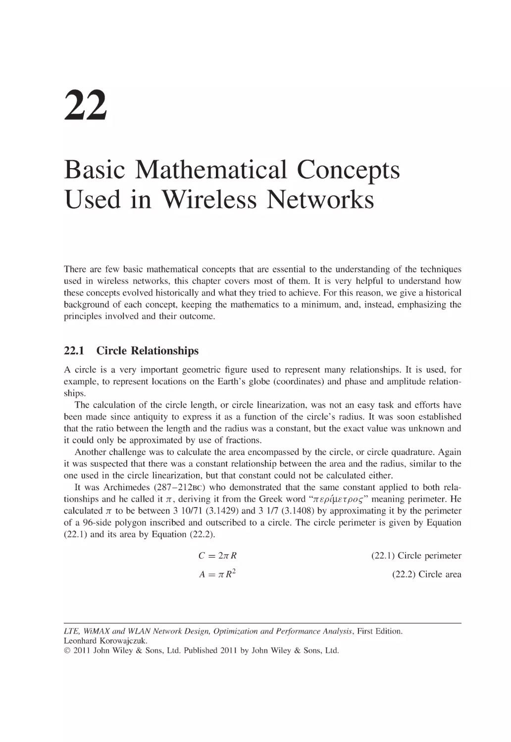
665
665
666
668
668
669
670
672
674
675
676
677
677
679
679
683
685
686
687
Appendix: List of Equations
689
Further Reading
697
Index
701
List of Figures
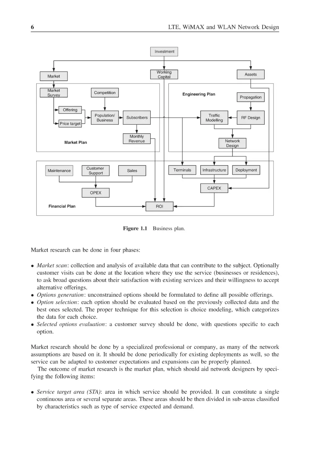
Figure 1.1
Business plan
6
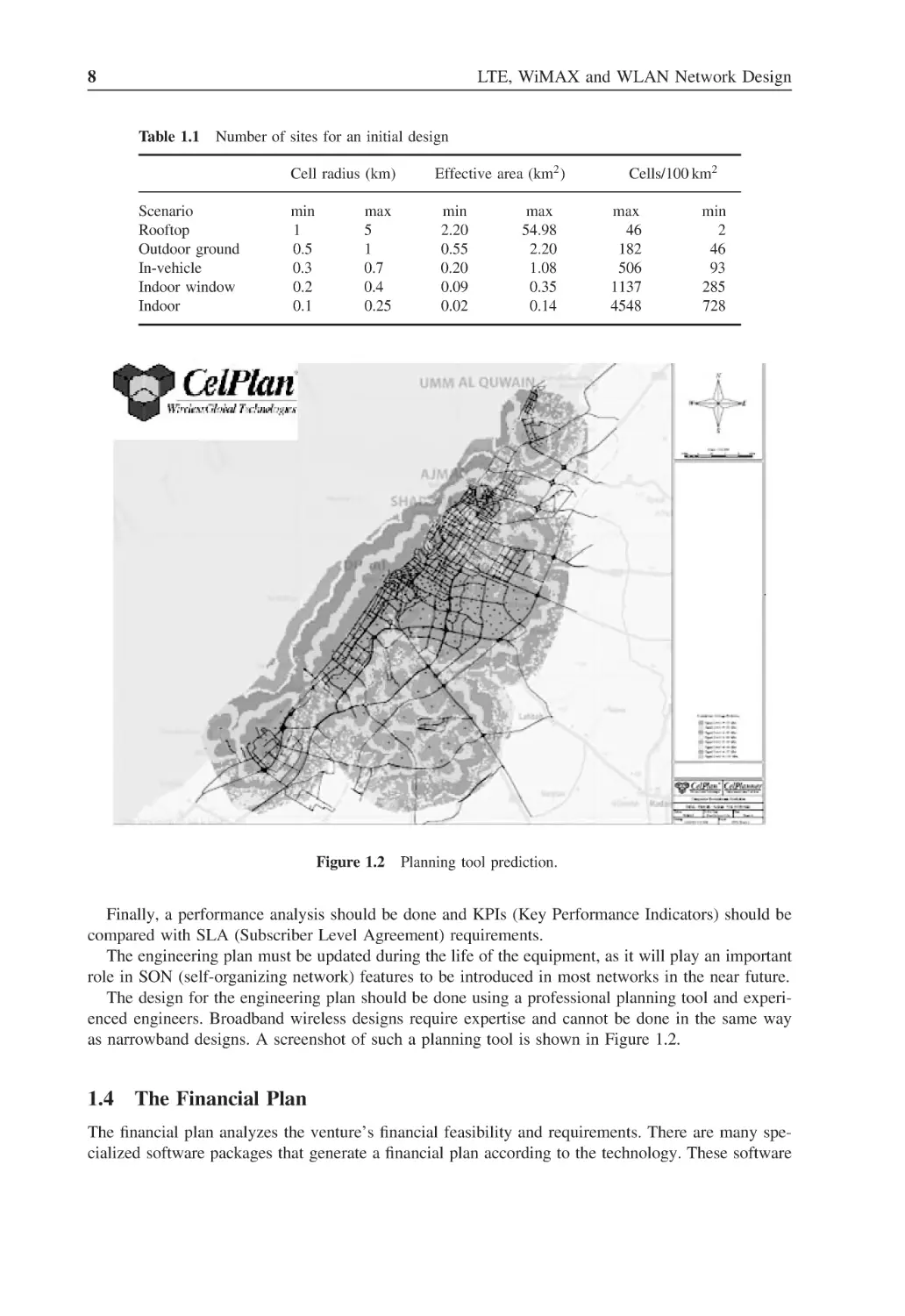
Figure 1.2
Planning tool prediction
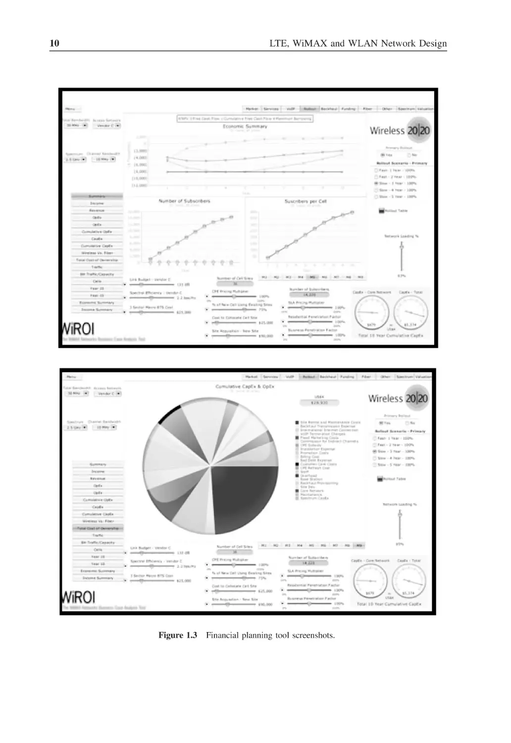
Figure 1.3
Financial planning tool screenshots
10
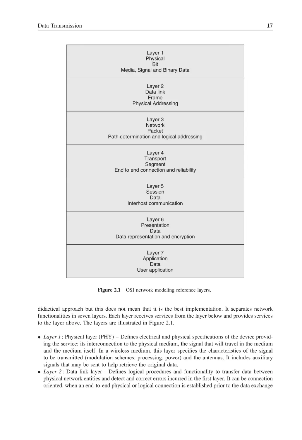
Figure 2.1
OSI network modeling reference layers
17
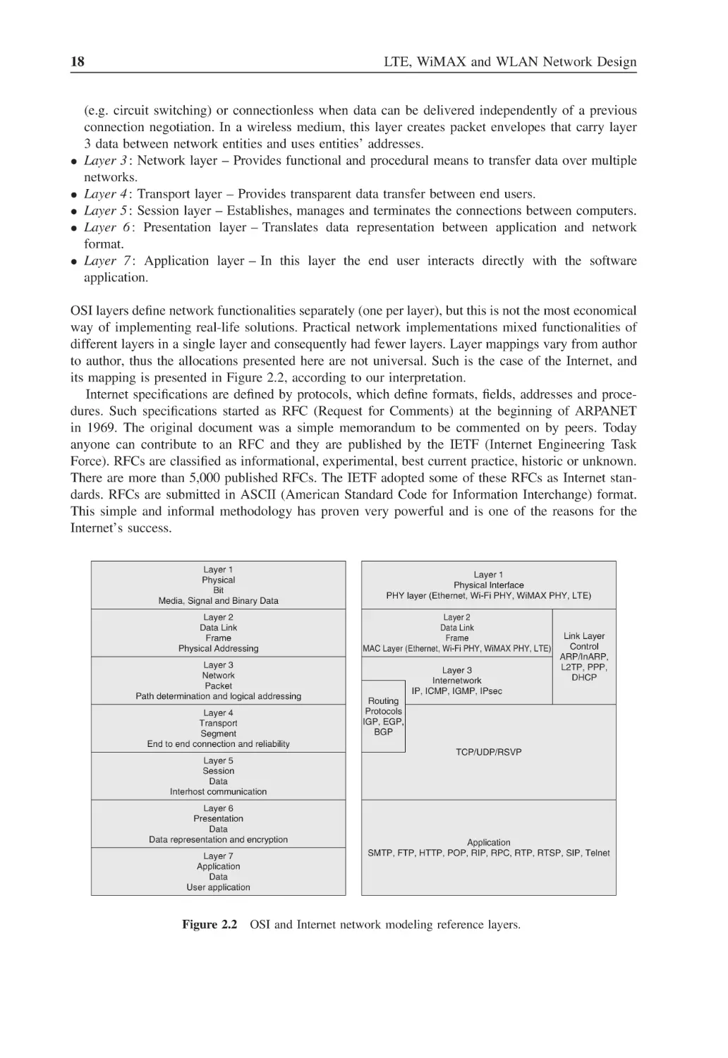
Figure 2.2
OSI and Internet network modeling reference layers
18
Figure 2.3
Internet network architecture
19
Figure 2.4
Ethernet packet format
23
Figure 2.5
Ethernet MAC address
24
Figure 2.6
Transmission control protocol header
29
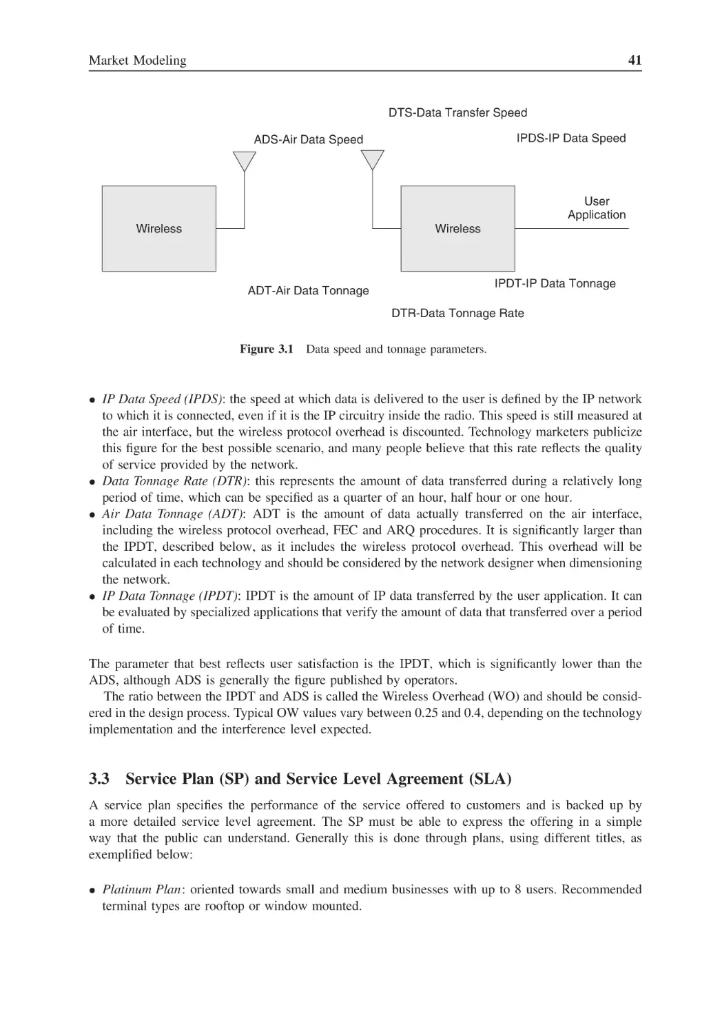
Figure 3.1
Data speed and tonnage parameters
41
Figure 3.2
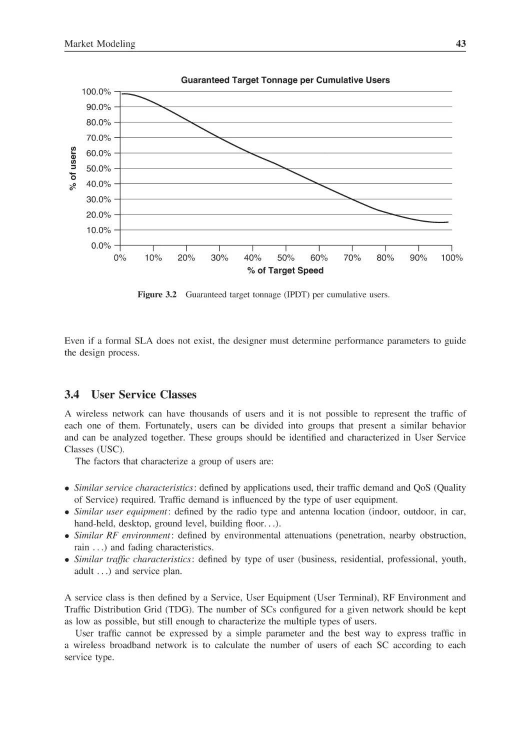
Guaranteed target tonnage (IPDT) per cumulative users
43
Figure 3.3
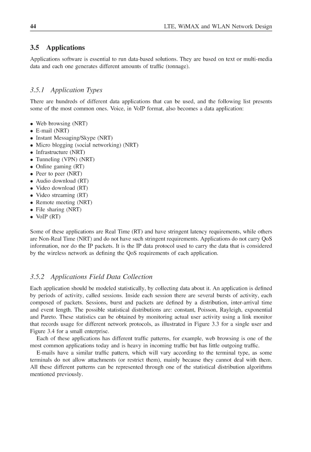
Single user traffic statistics
45
Figure 3.4
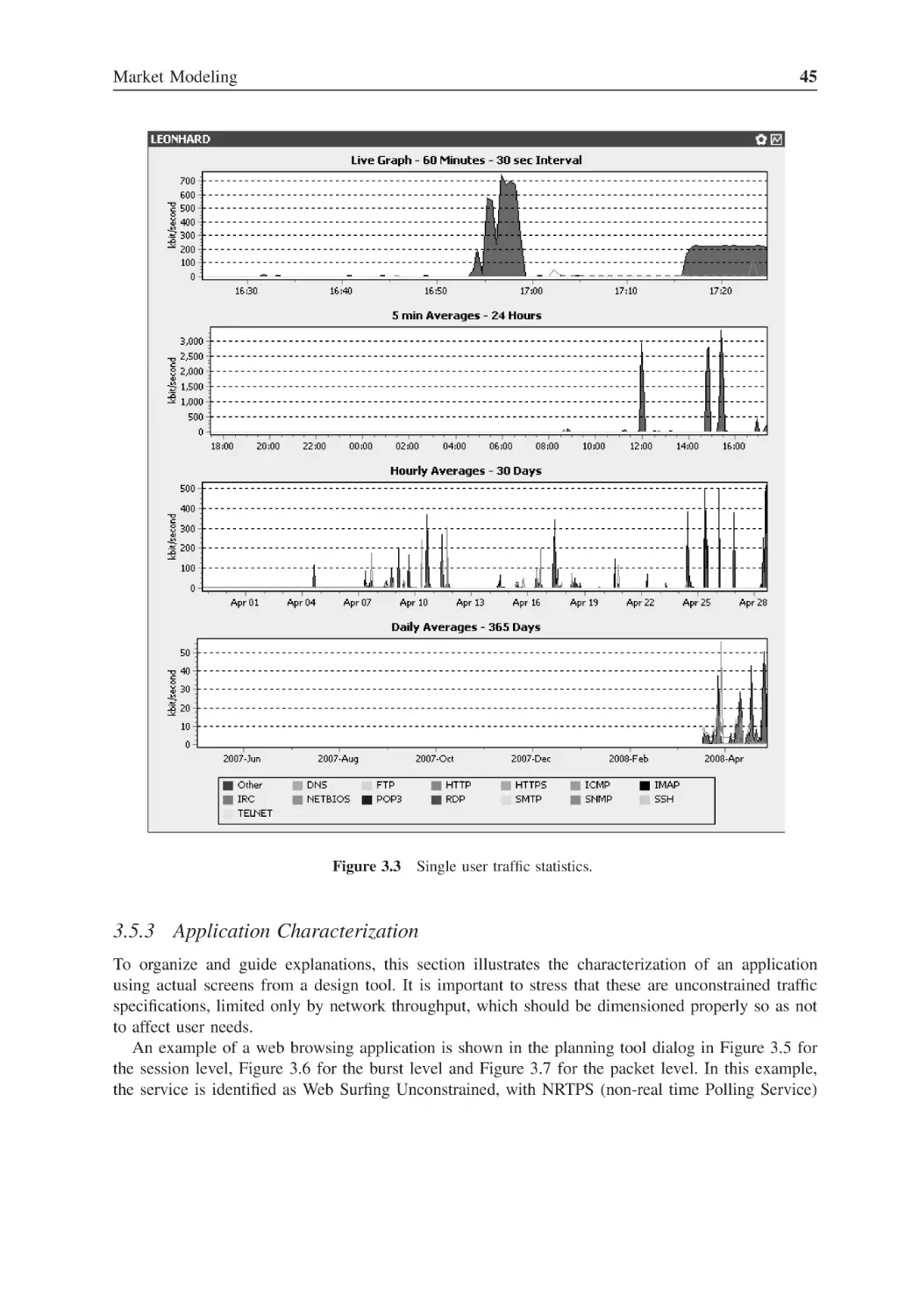
Small enterprise traffic statistics
46
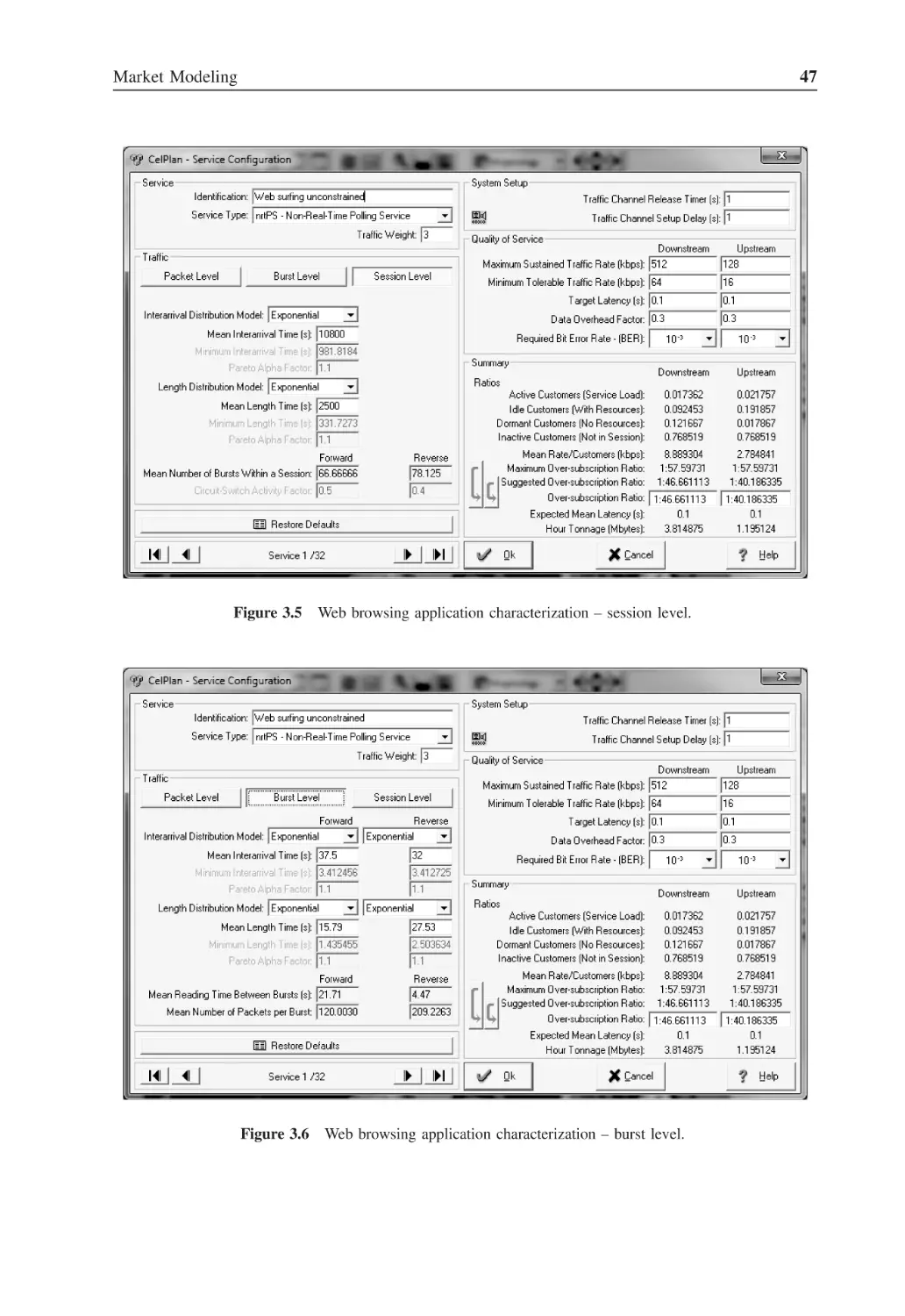
Figure 3.5
Web browsing application characterization – session level
47
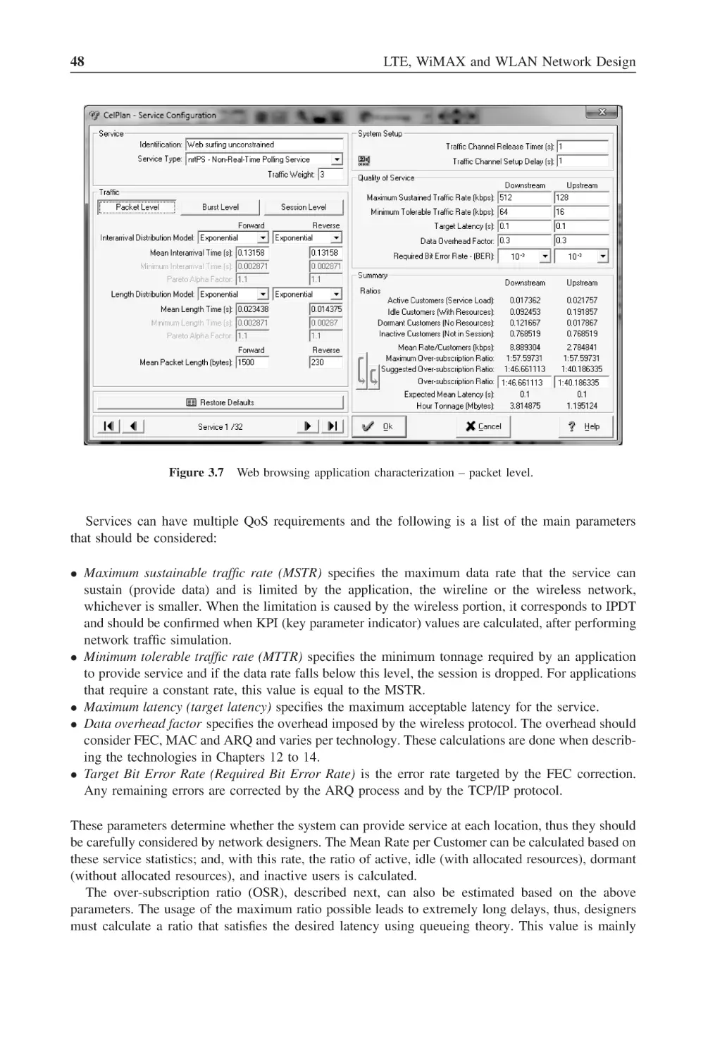
Figure 3.6
Web browsing application characterization – burst level
47
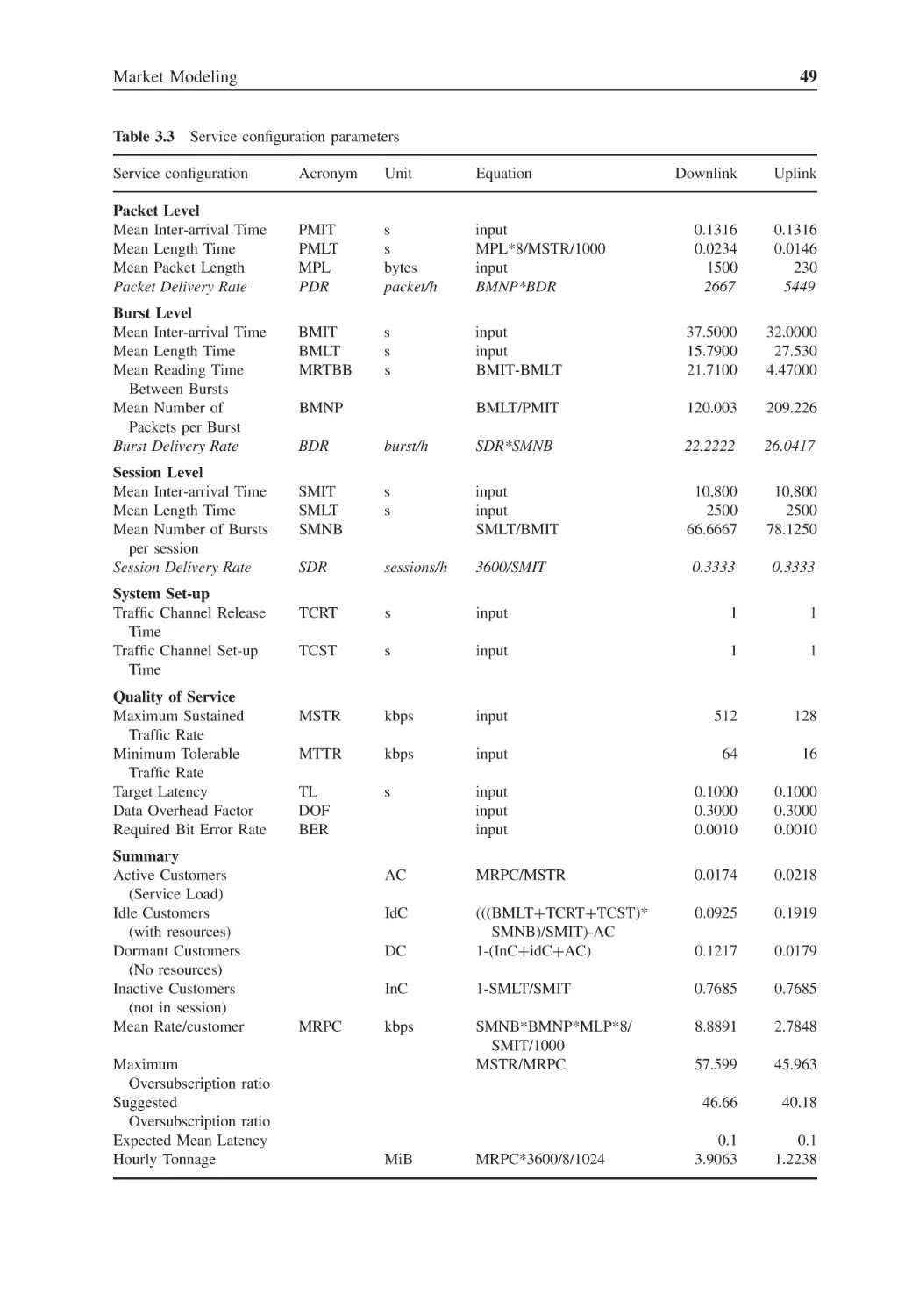
Figure 3.7
Web browsing application characterization – packet level
48
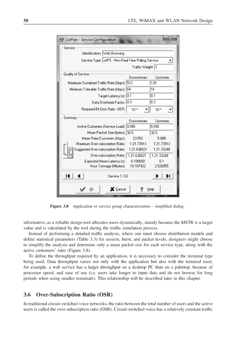
Figure 3.8
Application or service group characterization – simplified dialog
50
Figure 3.9
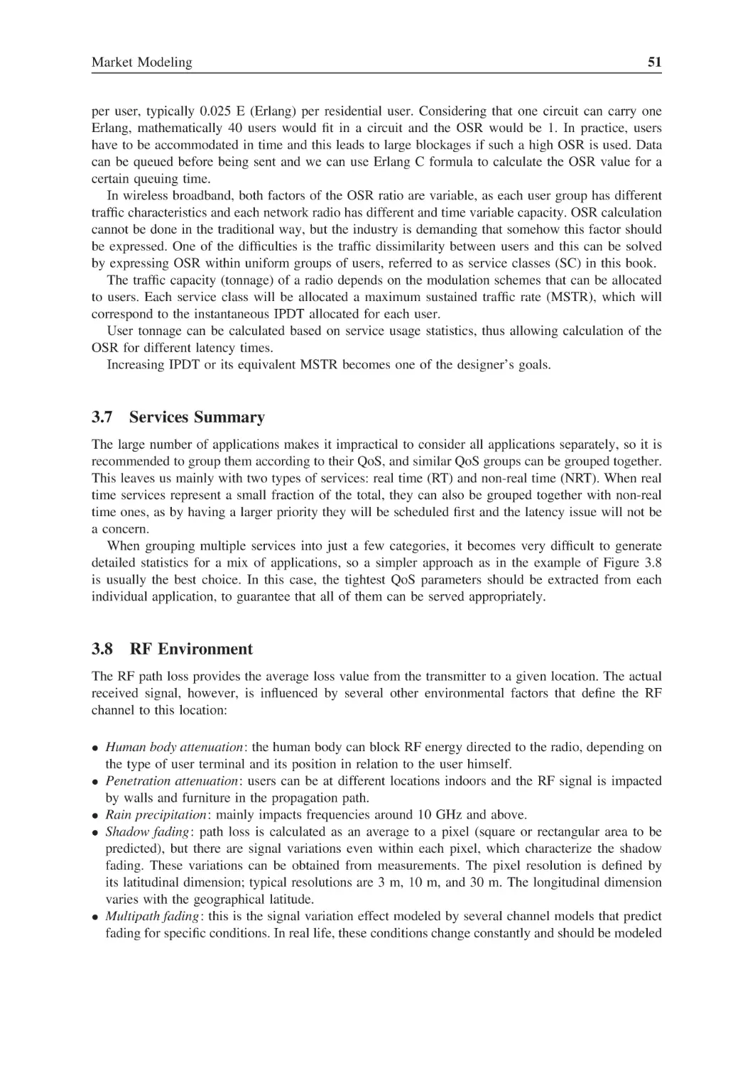
Sample dialog box for user environment configuration
52
Figure 3.10
User terminal height above ground
53
Figure 3.11
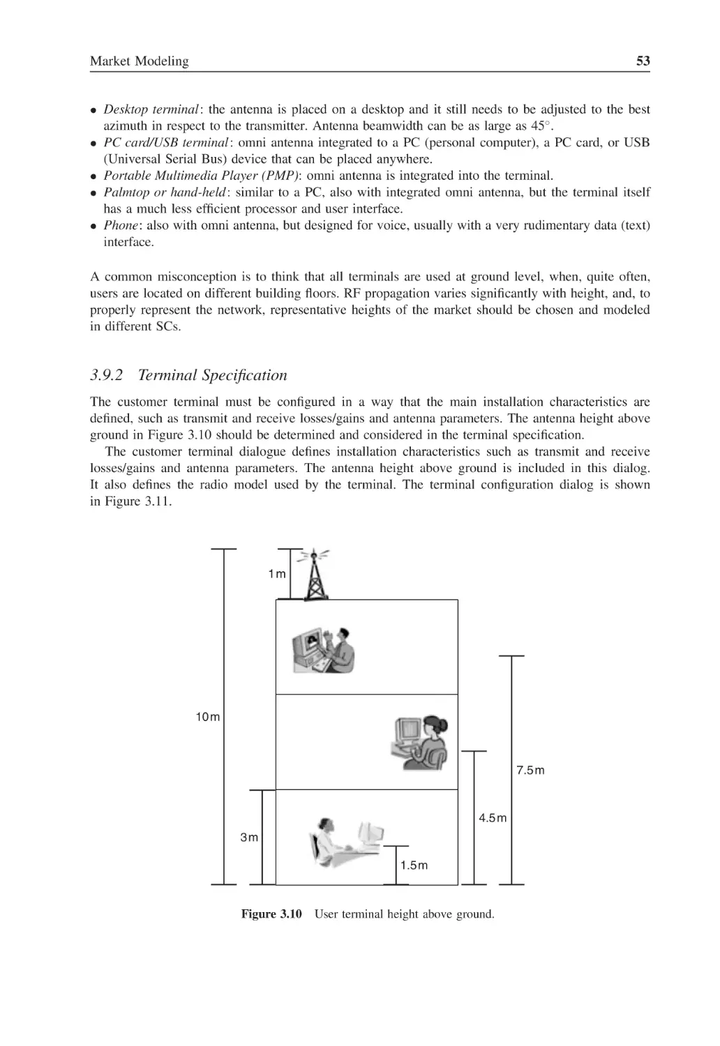
Sample dialog box for user terminal configuration
54
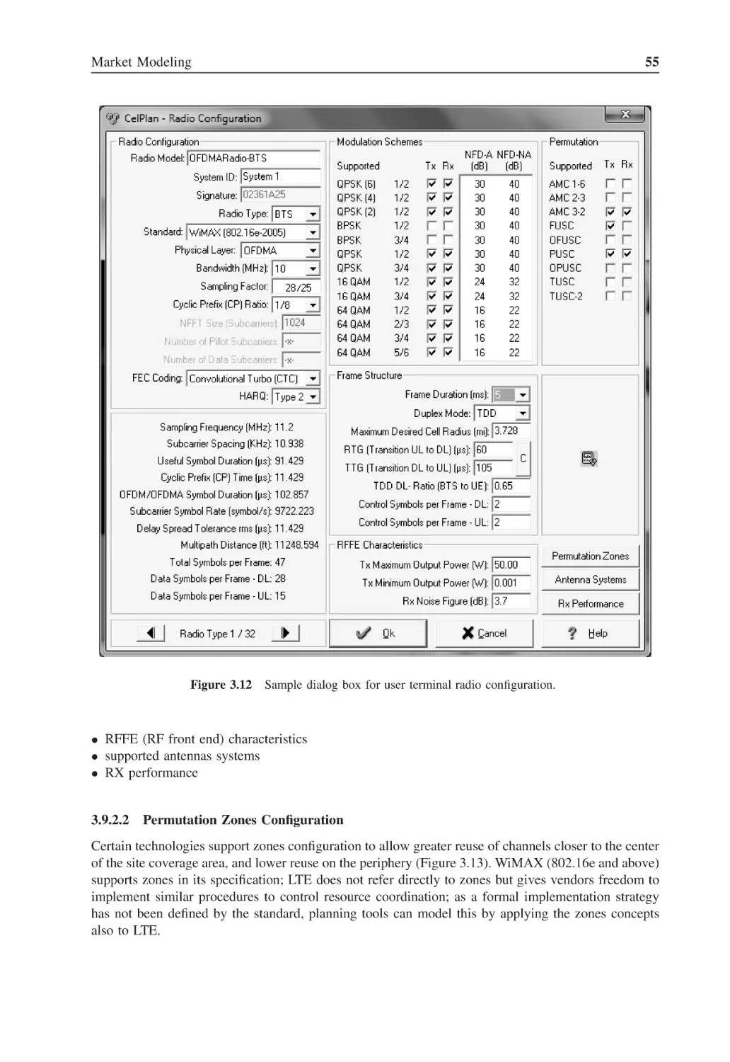
Figure 3.12
Sample dialog box for user terminal radio configuration
55
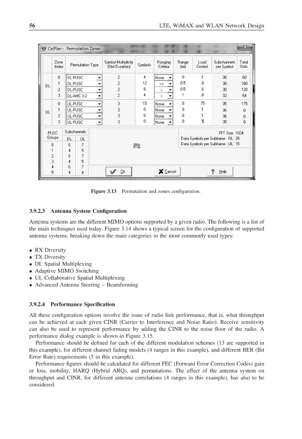
Figure 3.13
Permutation and zones configuration
56
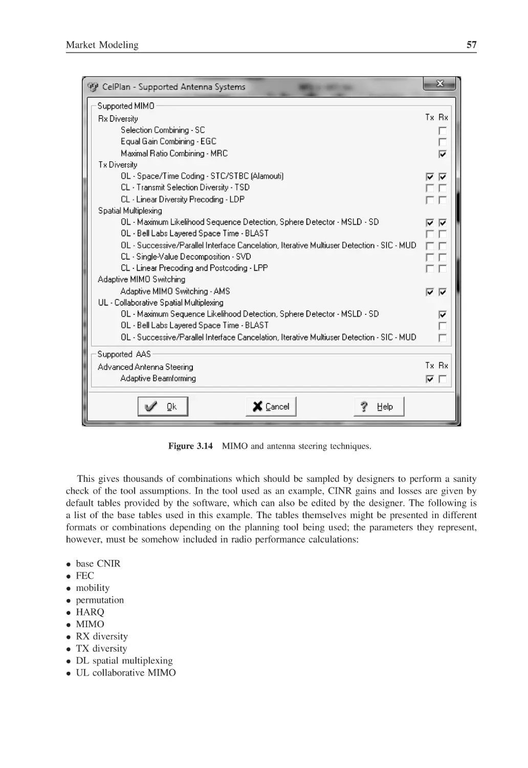
Figure 3.14
MIMO and antenna steering techniques
57
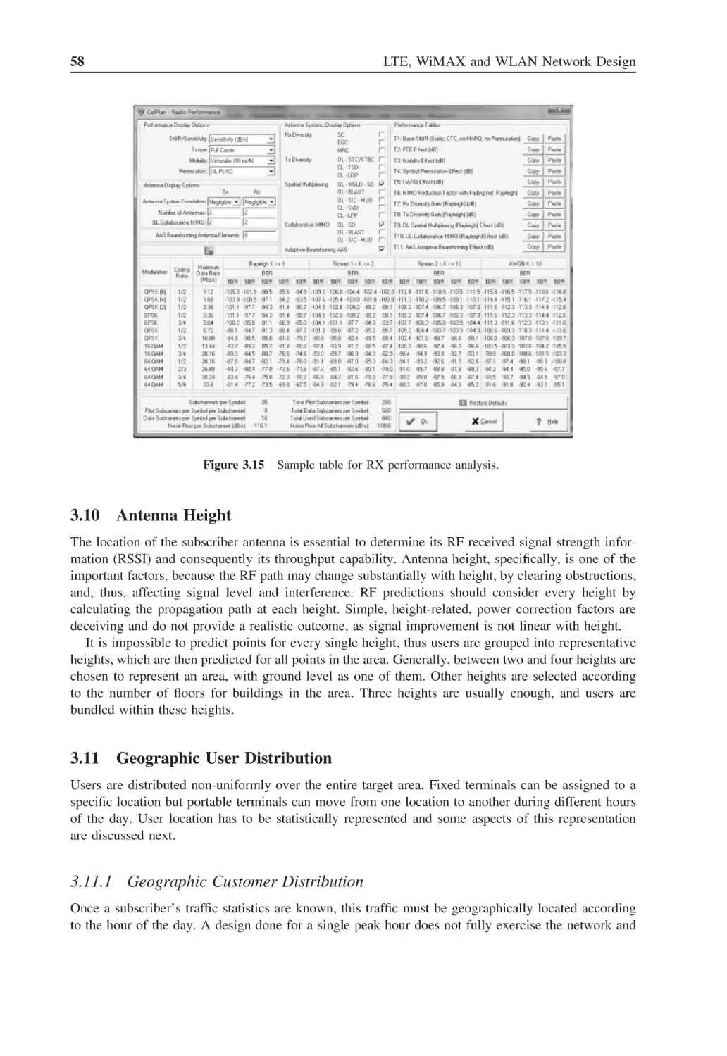
Figure 3.15
Sample table for RX performance analysis
58
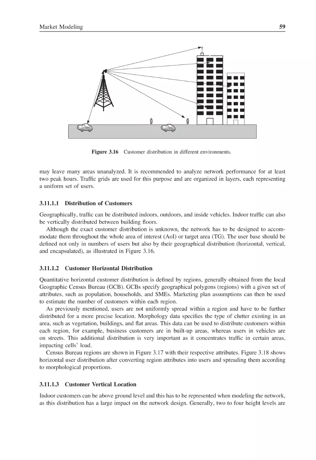
Figure 3.16
Customer distribution in different environments
59
Figure 3.17
Horizontal distribution of customers (regions)
60
Figure 3.18
Horizontal distribution of users after spreading by morphology
60
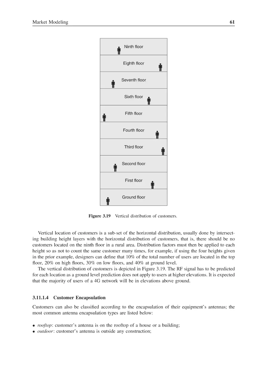
Figure 3.19
Vertical distribution of customers
61
8
xx
List of Figures
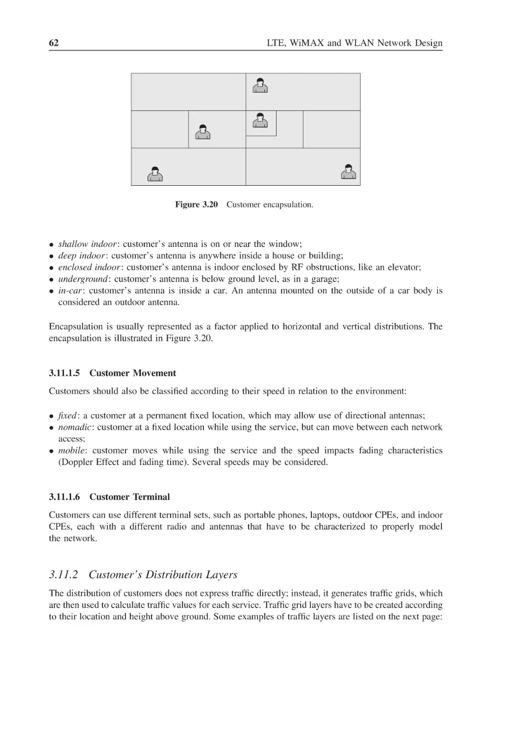
Figure 3.20
Customer encapsulation
62
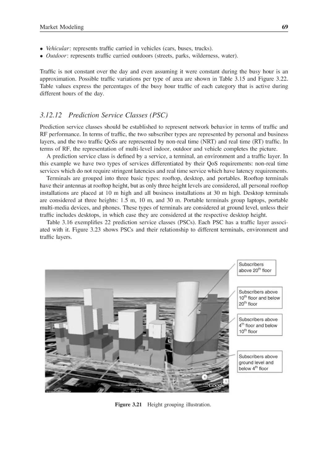
Figure 3.21
Height grouping illustration
69
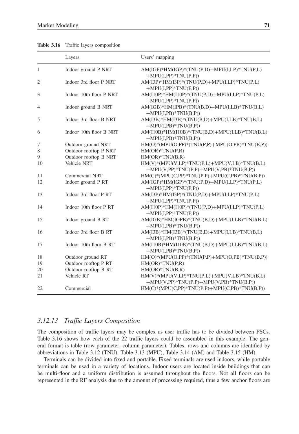
Figure 3.22
Hourly traffic variation
70
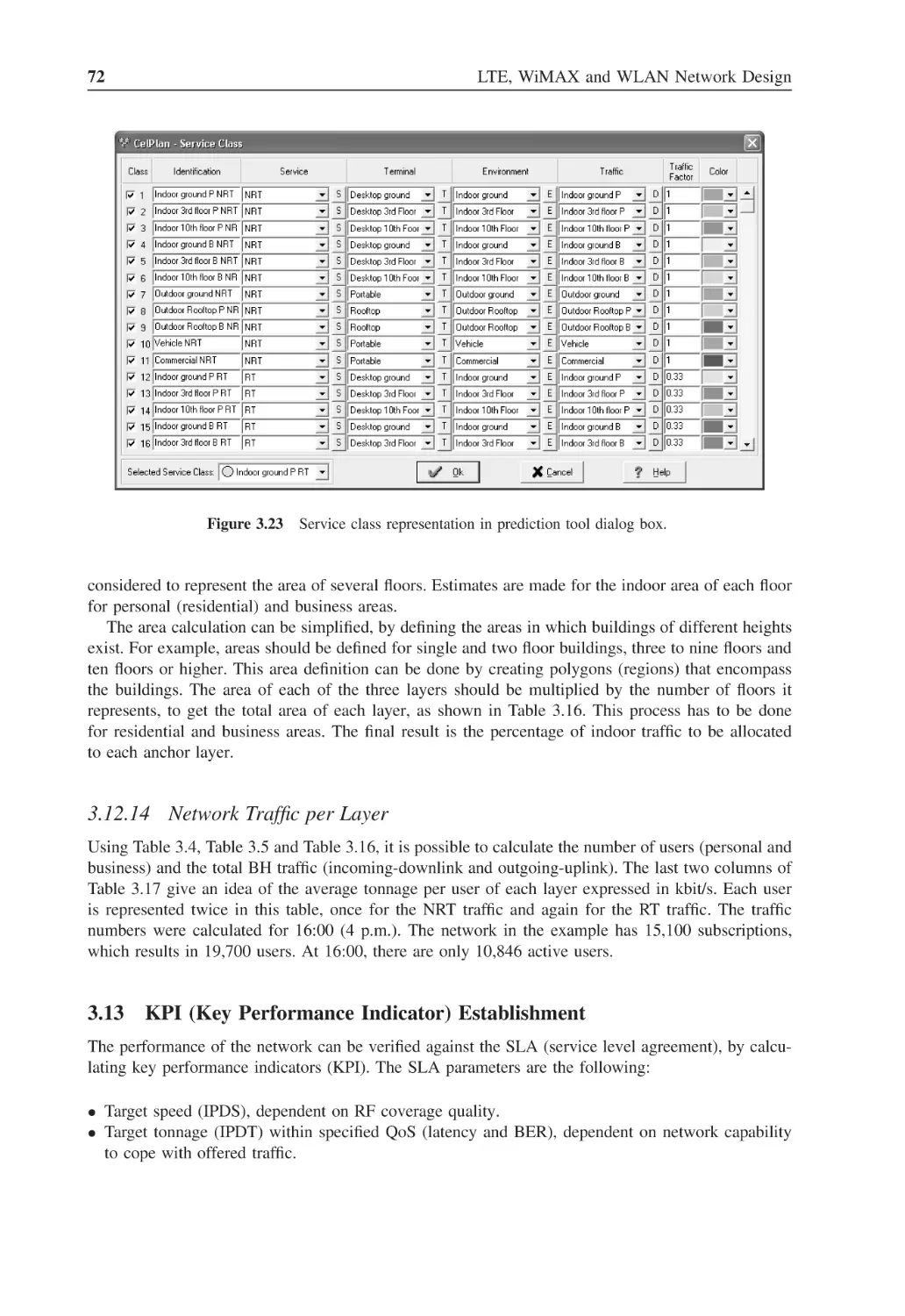
Figure 3.23
Service class representation in prediction tool dialog box
72
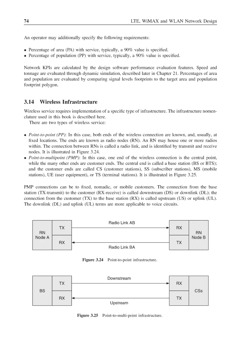
Figure 3.24
Point-to-point infrastructure
74
Figure 3.25
Point-to-multi-point infrastructure
74
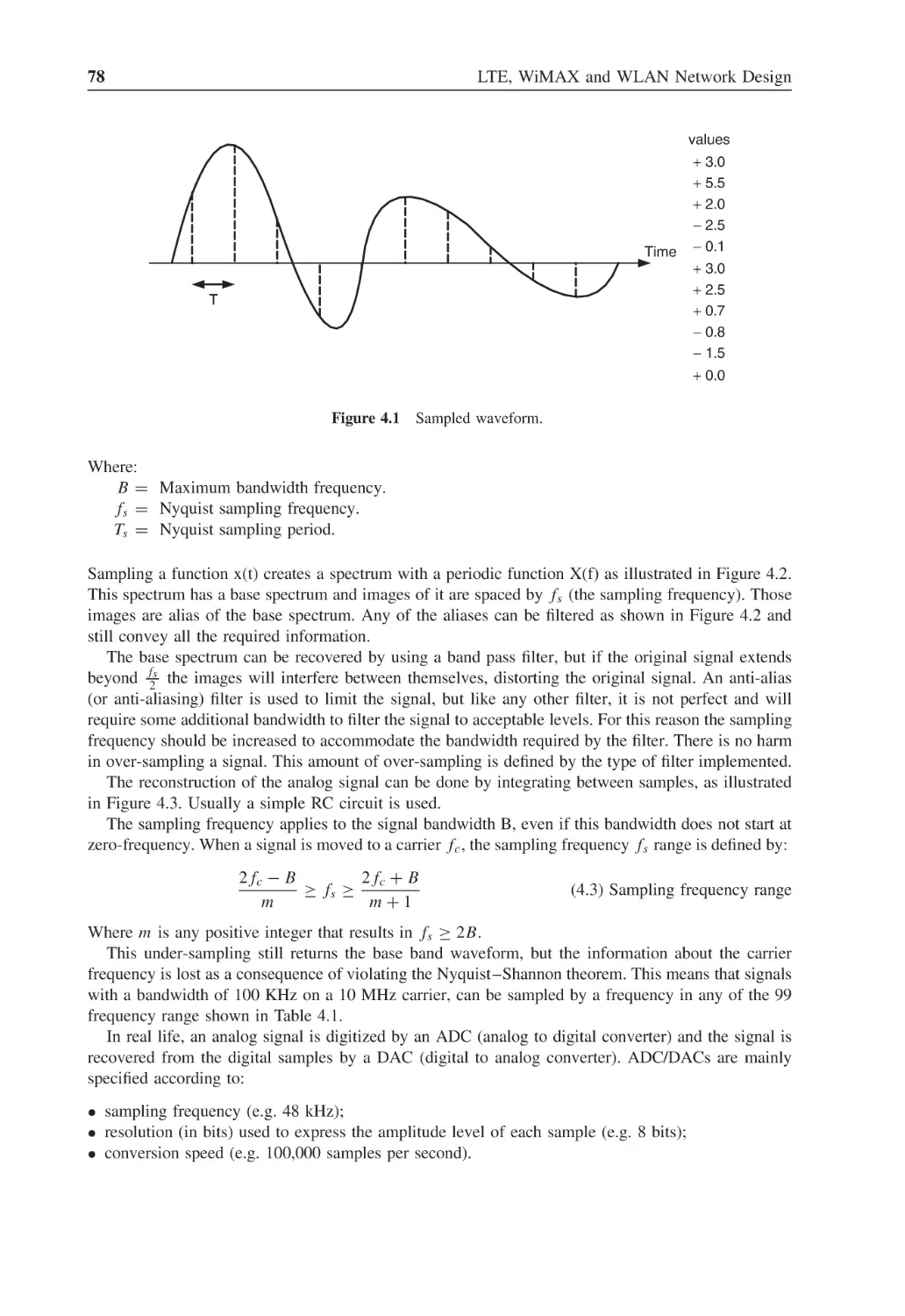
Figure 4.1
Sampled waveform
78
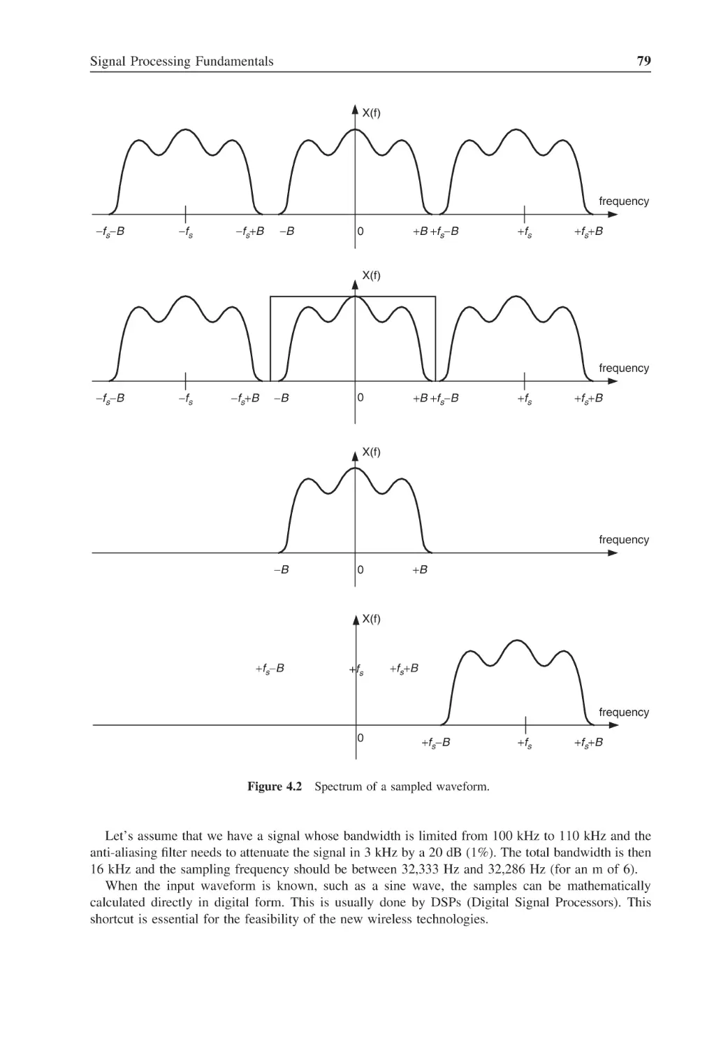
Figure 4.2
Spectrum of a sampled waveform
79
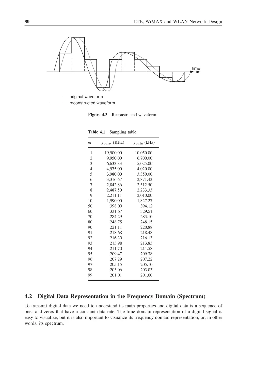
Figure 4.3
Reconstructed waveform
80
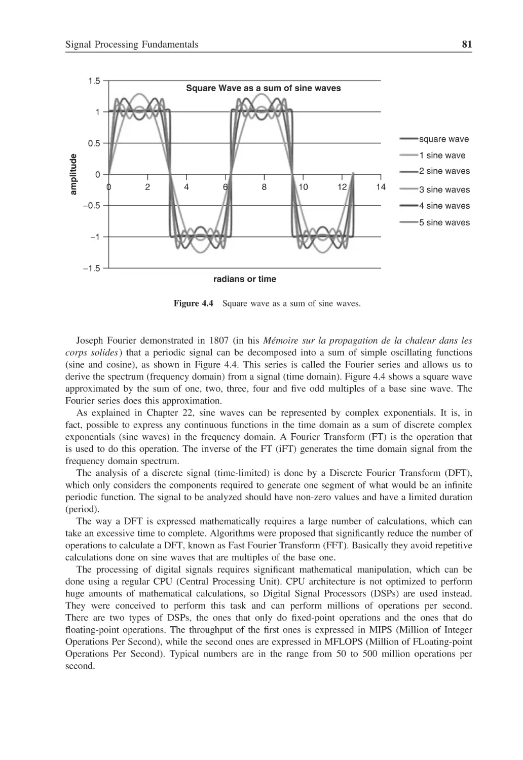
Figure 4.4
Square wave as a sum of sine waves
81
Figure 4.5
RZ and NRZ representation
82
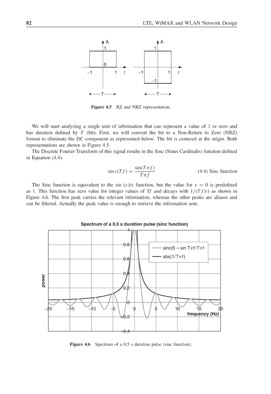
Figure 4.6
Spectrum of a 0.5 s duration pulse (sinc function)
82
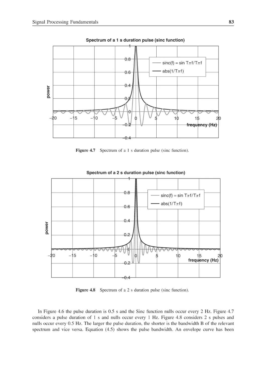
Figure 4.7
Spectrum of a 1 s duration pulse (sinc function)
83
Figure 4.8
Spectrum of a 2 s duration pulse (sinc function)
83
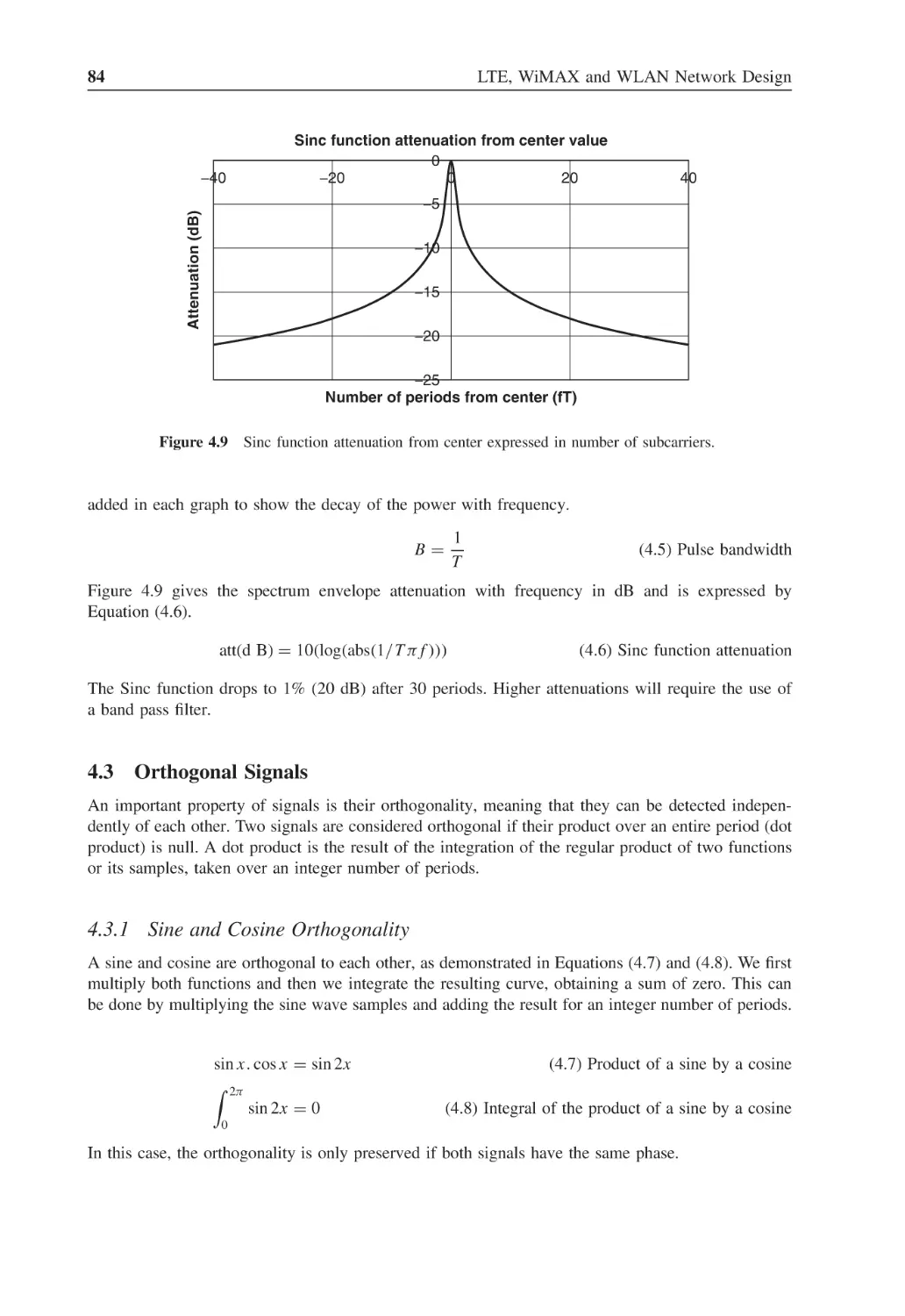
Figure 4.9
Sinc function attenuation from center expressed in number of subcarriers
84
Figure 4.10
Sum of sine waves
86
Figure 4.11
Shifted sine waves and combined sine wave
86
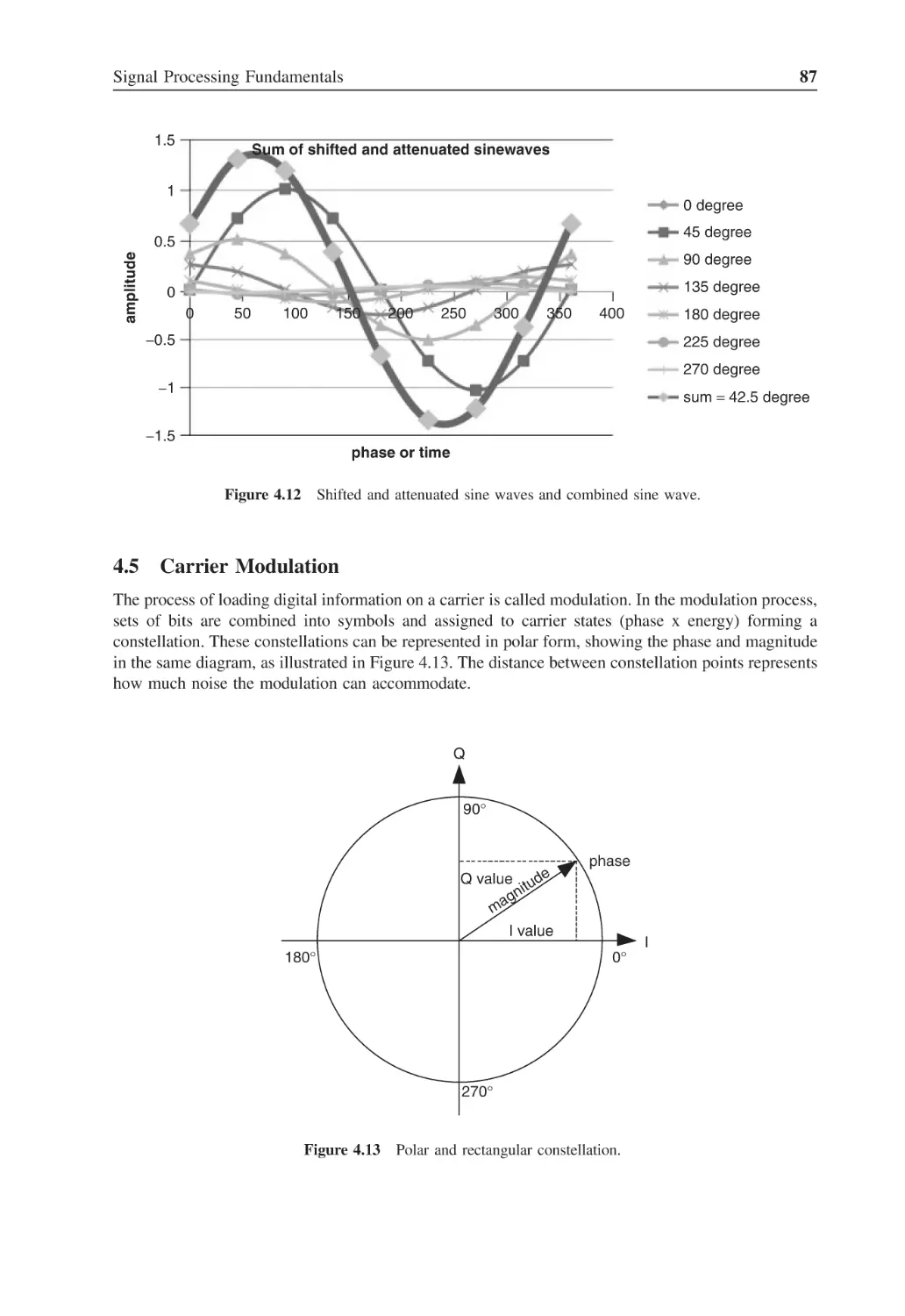
Figure 4.12
Shifted and attenuated sine waves and combined sine wave
87
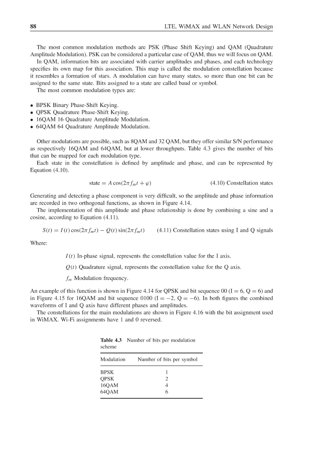
Figure 4.13
Polar and rectangular constellation
87
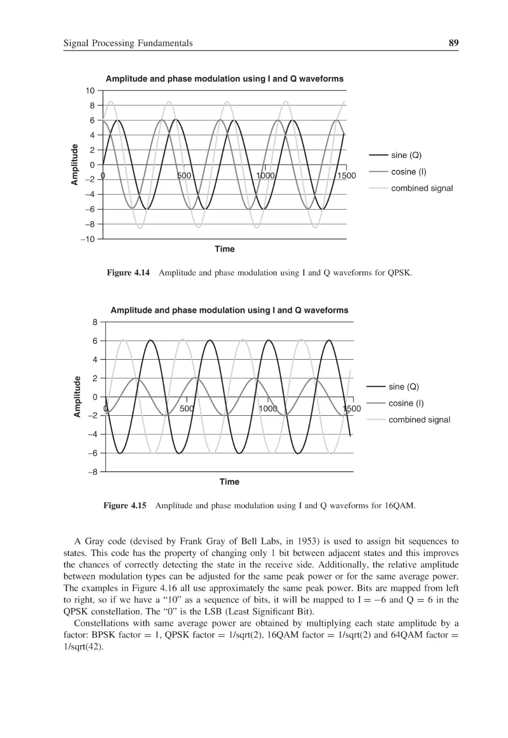
Figure 4.14
Amplitude and phase modulation using I and Q waveforms for QPSK
89
Figure 4.15
Amplitude and phase modulation using I and Q waveforms for 16QAM
89
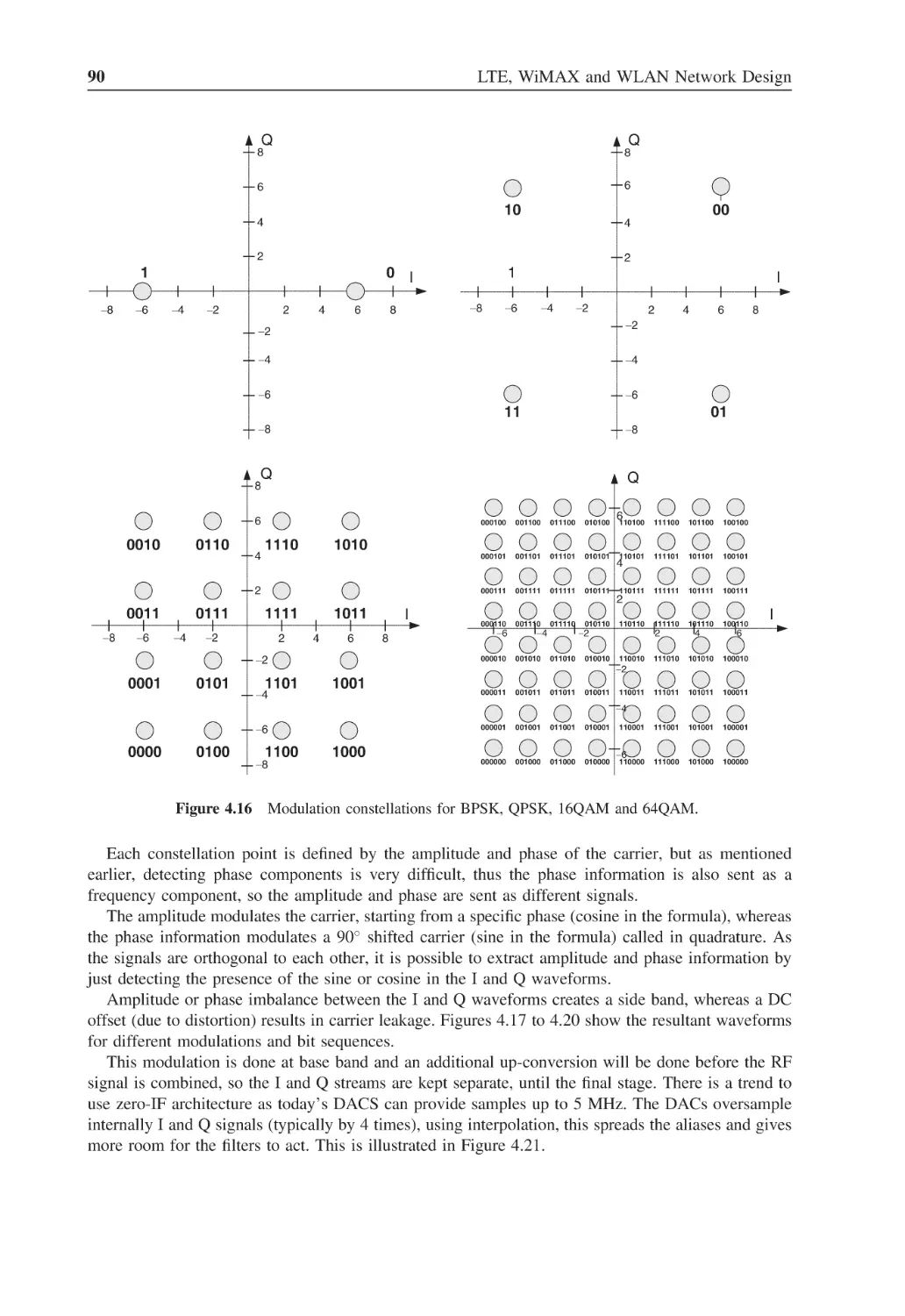
Figure 4.16
Modulation constellations for BPSK, QPSK, 16QAM and 64QAM
90
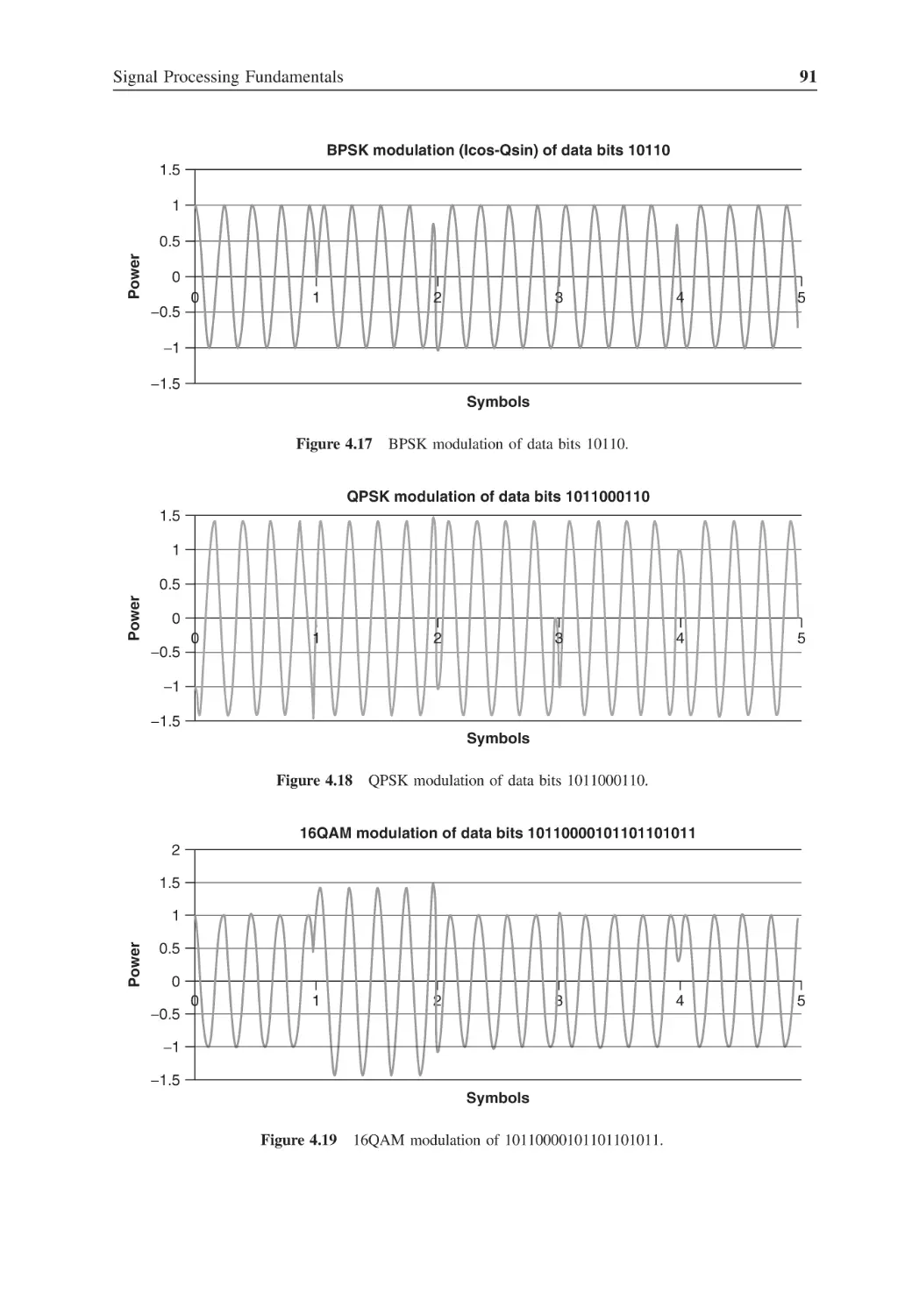
Figure 4.17
BPSK modulation of data bits 10110
91
Figure 4.18
QPSK modulation of data bits 1011000110
91
Figure 4.19
16QAM modulation of 10110000101101101011
91
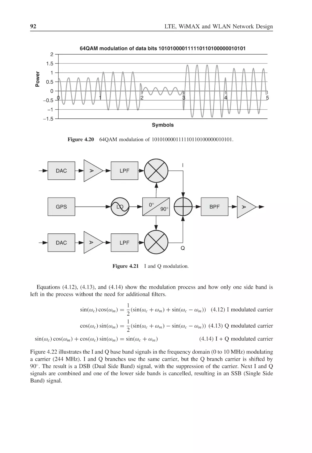
Figure 4.20
64QAM modulation of 101010000111110110100000010101
92
Figure 4.21
I and Q modulation
92
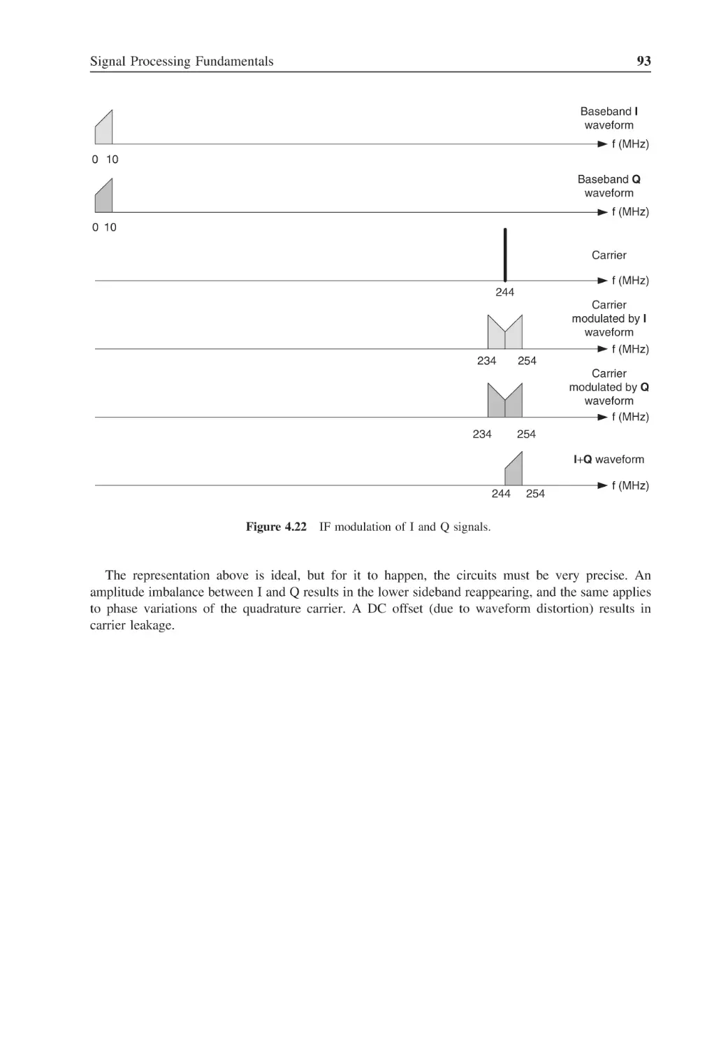
Figure 4.22
IF modulation of I and Q signals
93
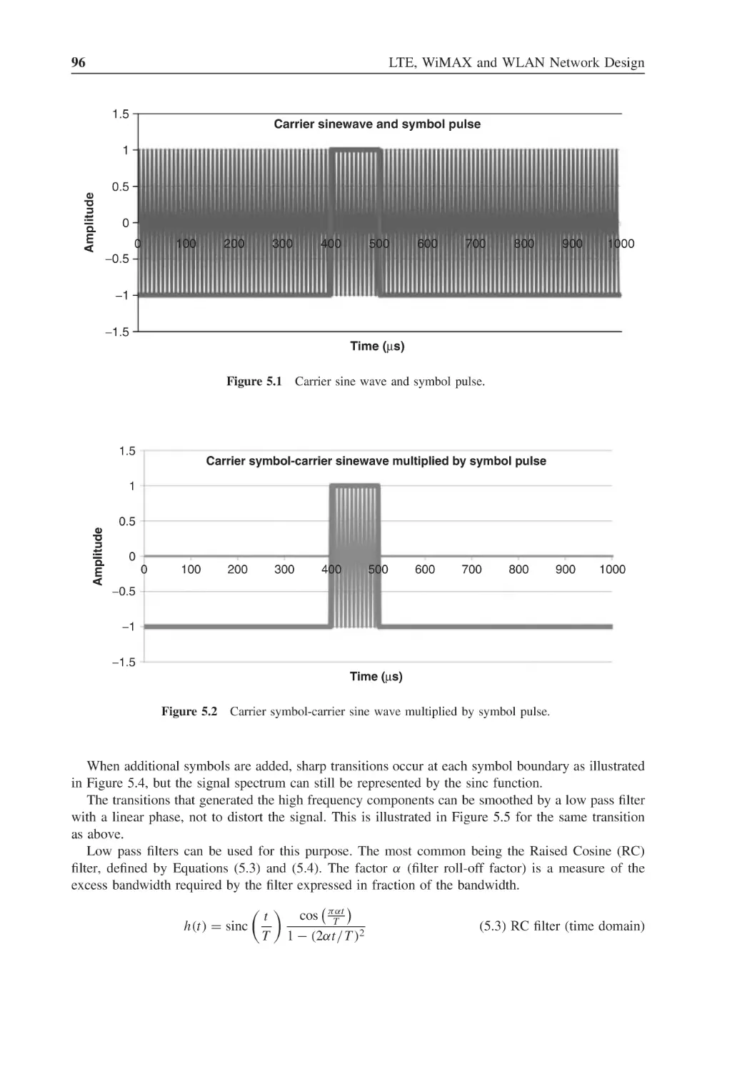
Figure 5.1
Carrier sine wave and symbol pulse
96
Figure 5.2
Carrier symbol-carrier sine wave multiplied by symbol pulse
96
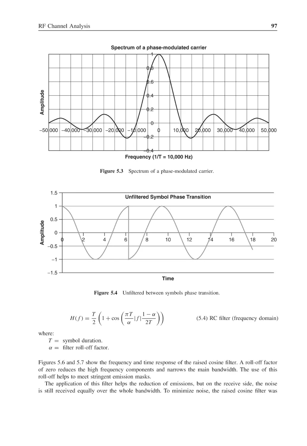
Figure 5.3
Spectrum of a phase-modulated carrier
97
Figure 5.4
Unfiltered between symbols phase transition
97
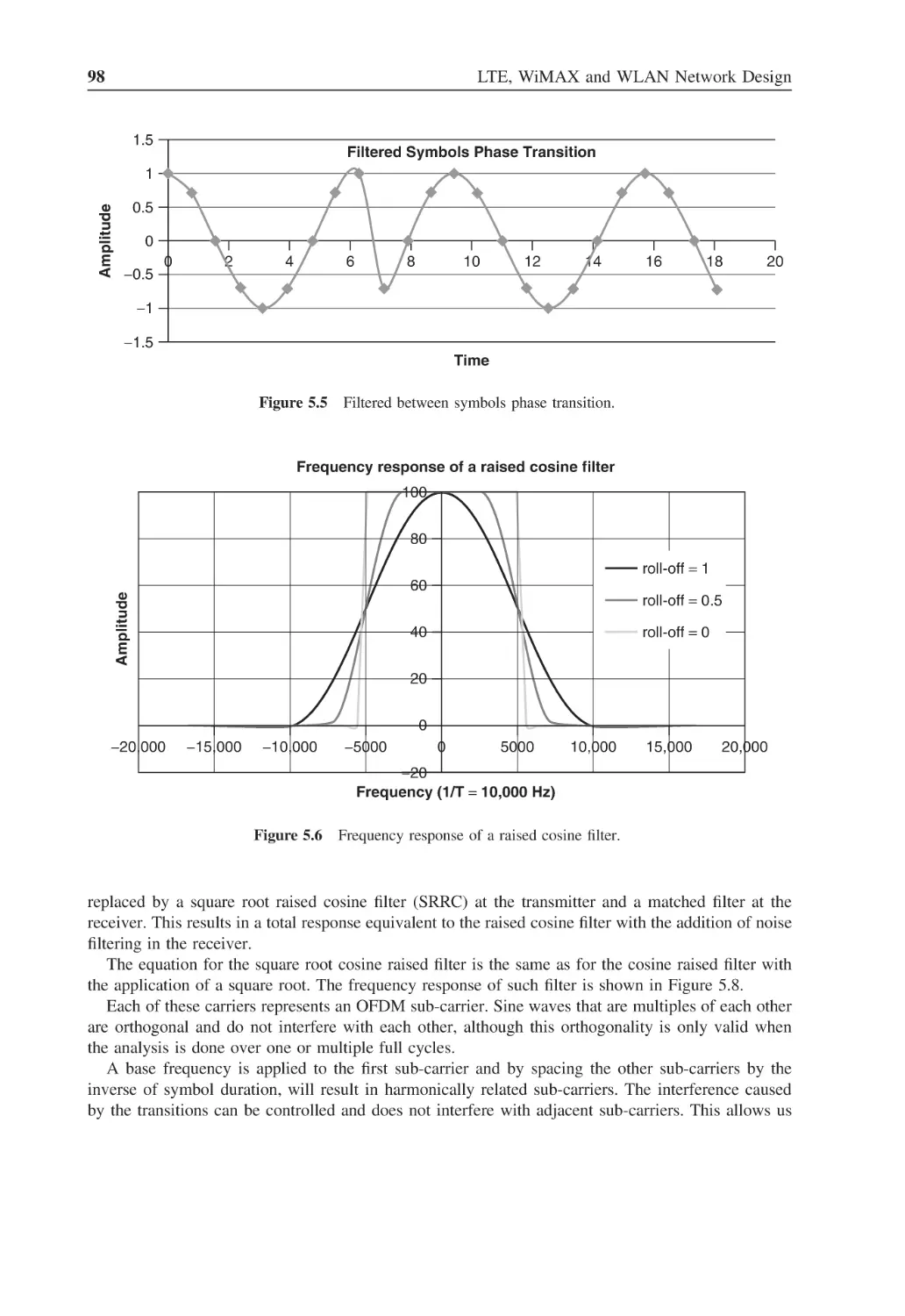
Figure 5.5
Filtered between symbols phase transition
98
Figure 5.6
Frequency response of a raised cosine filter
98
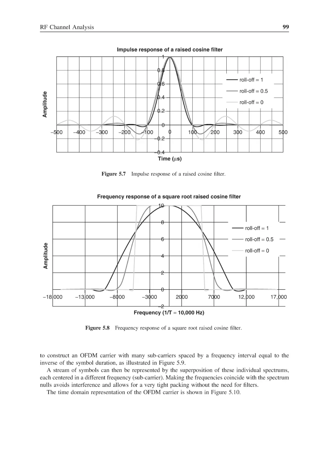
Figure 5.7
Impulse response of a raised cosine filter
99
Figure 5.8
Frequency response of a square root raised cosine filter
99
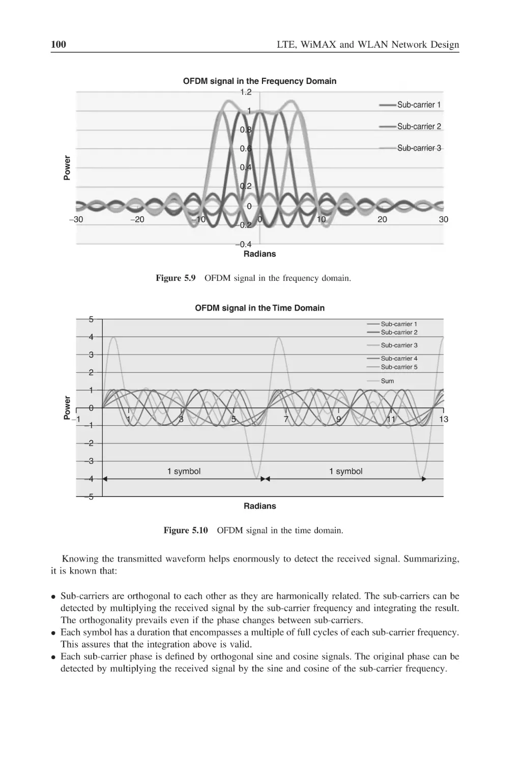
Figure 5.9
OFDM signal in the frequency domain
100
Figure 5.10
OFDM signal in the time domain
100
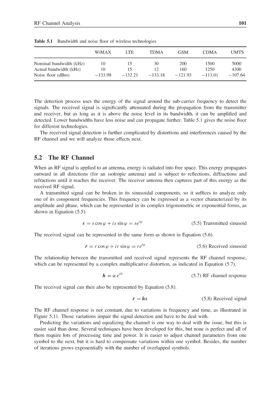
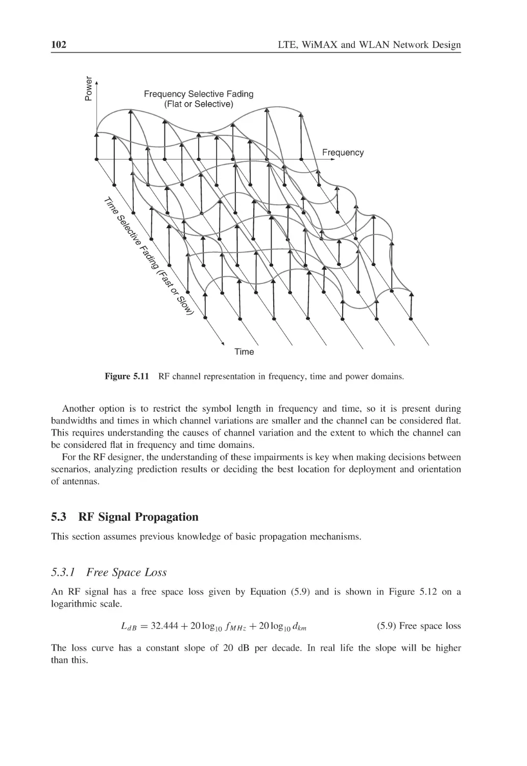
Figure 5.11
RF channel representation in frequency, time and power domains
102
List of Figures
xxi
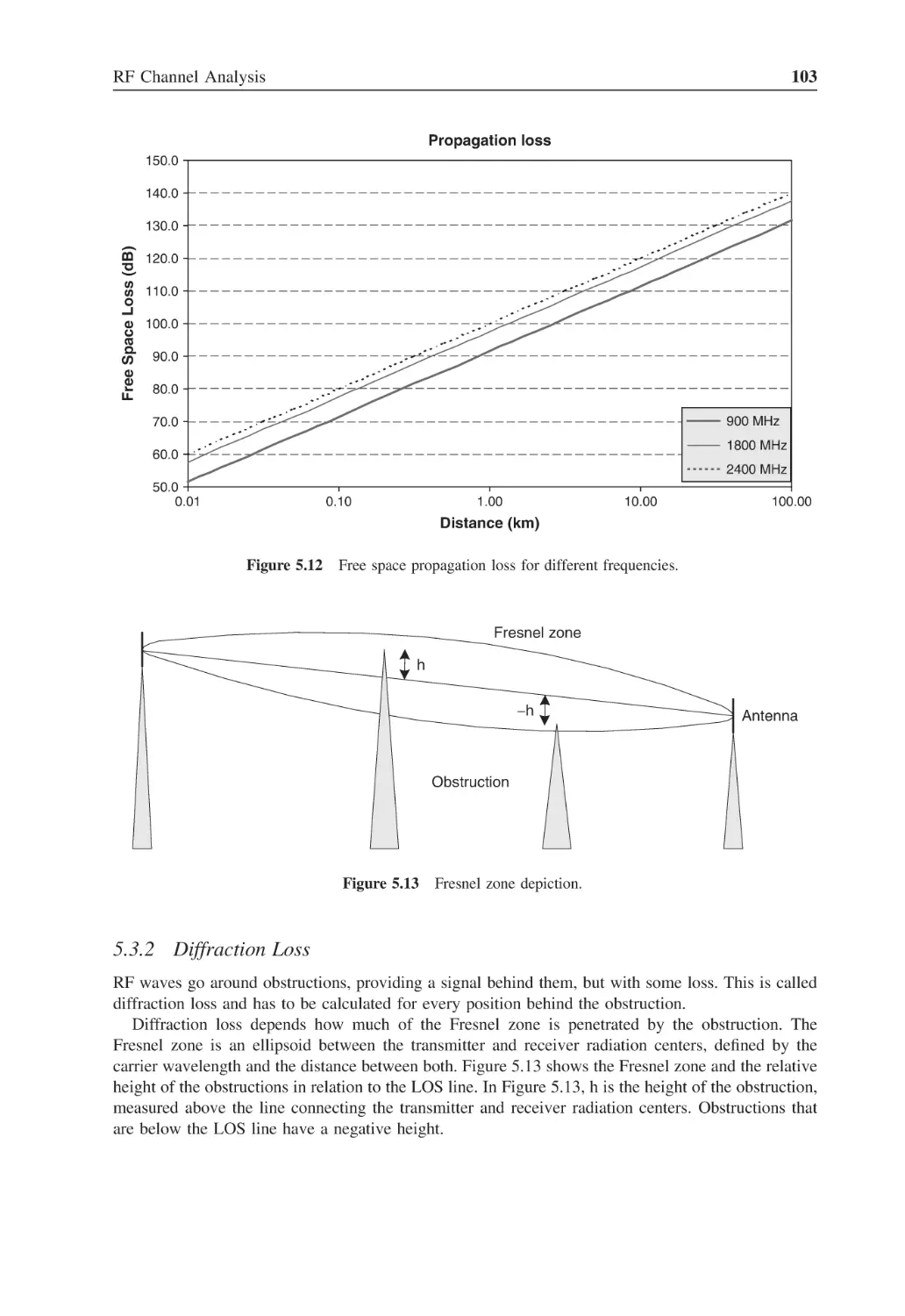
Figure 5.12
Free space propagation loss for different frequencies
103
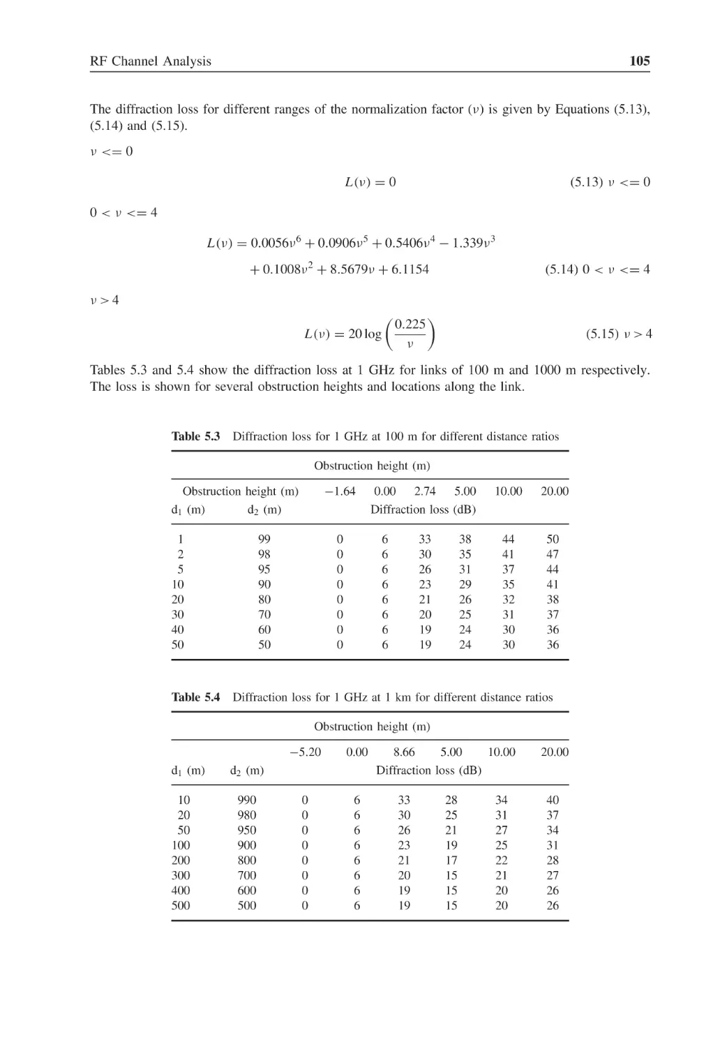
Figure 5.13
Fresnel zone depiction
103
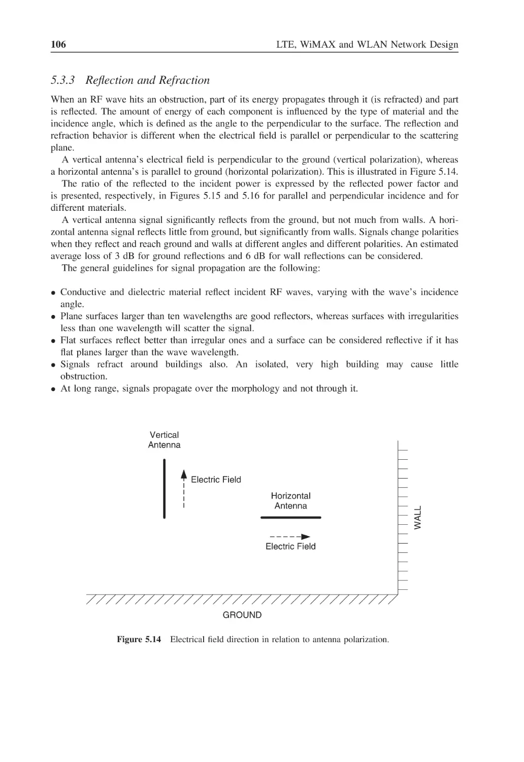
Figure 5.14
Electrical field direction in relation to antenna polarization
106
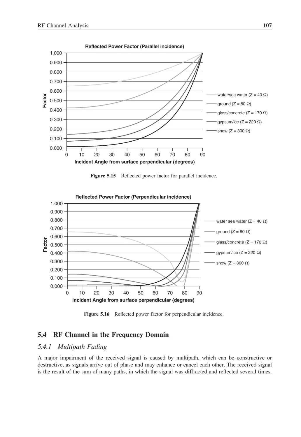
Figure 5.15
Reflected power factor for parallel incidence
107
Figure 5.16
Reflected power factor for perpendicular incidence
107
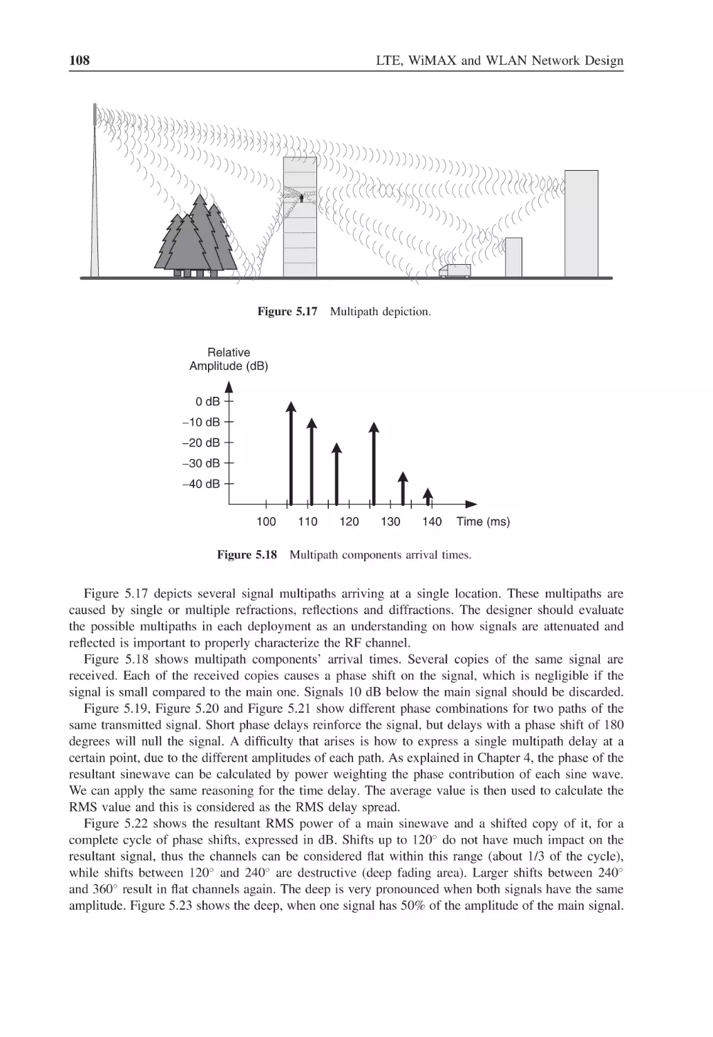
Figure 5.17
Multipath depiction
108
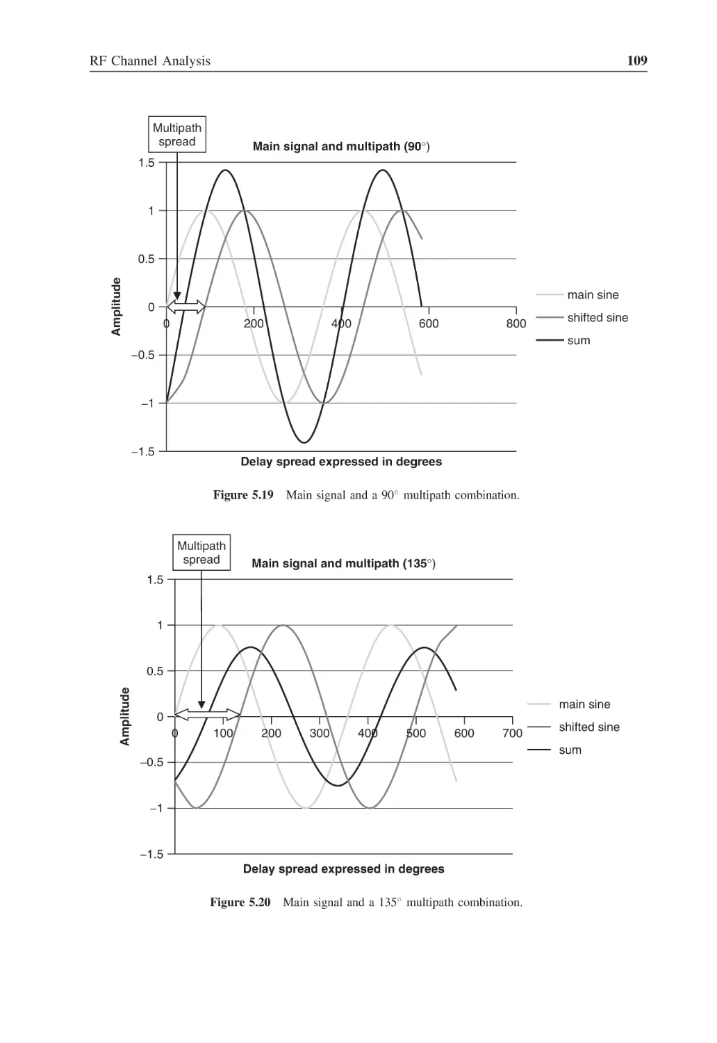
Figure 5.18
Multipath components arrival times
108
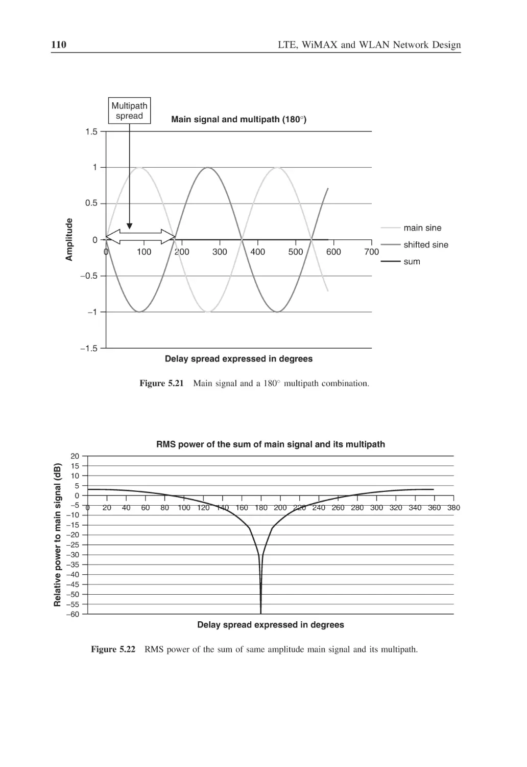
Figure 5.19
Main signal and a 90◦ multipath combination
109
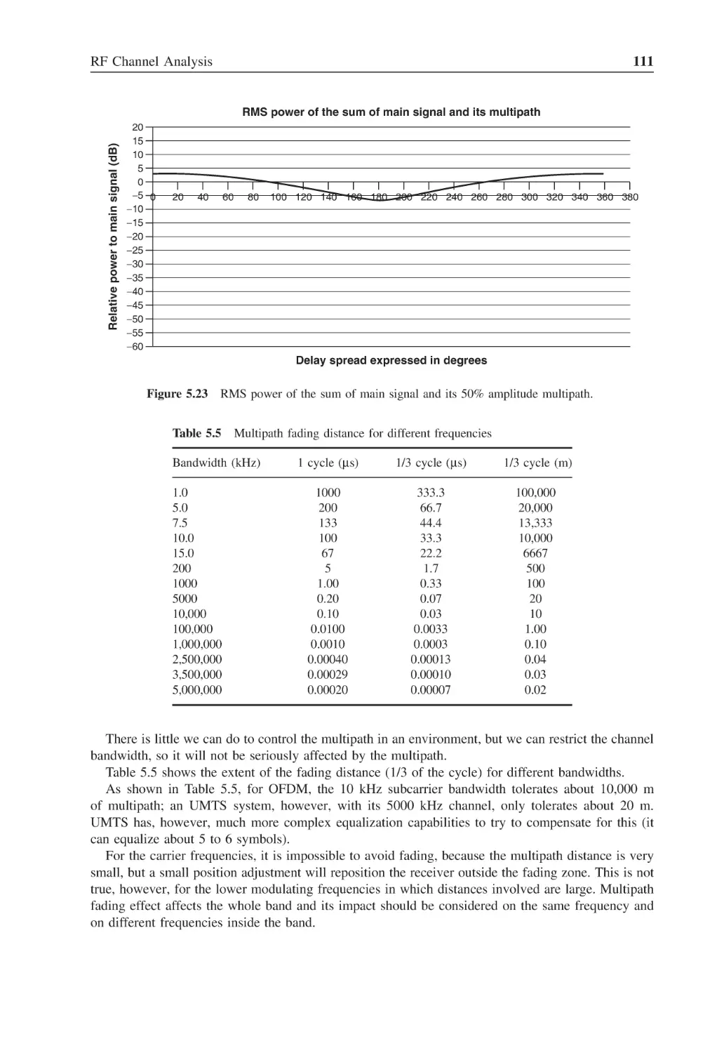
Figure 5.20
◦
Main signal and a 135 multipath combination
109
Figure 5.21
Main signal and a 180◦ multipath combination
110
Figure 5.22
RMS power of the sum of same amplitude main signal and its multipath
110
Figure 5.23
RMS power of the sum of main signal and its 50% amplitude multipath
111
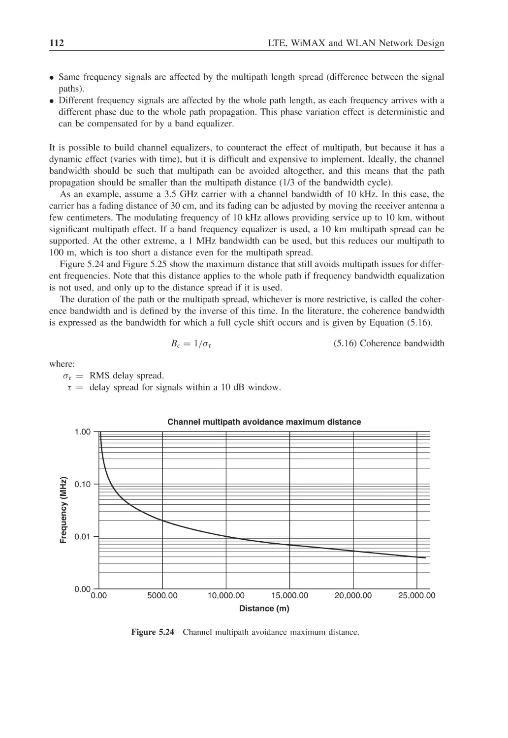
Figure 5.24
Channel multipath avoidance maximum distance
112
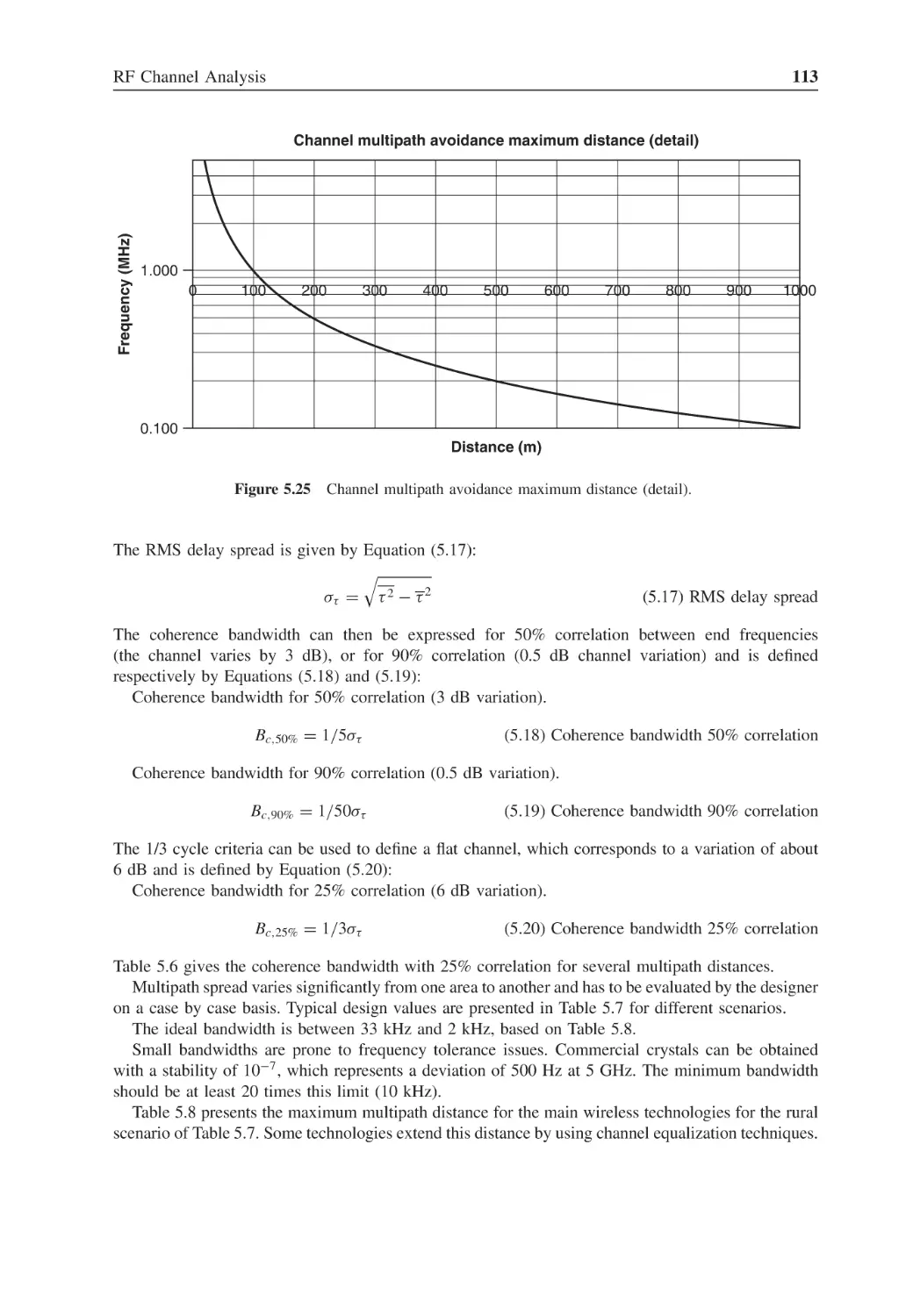
Figure 5.25
Channel multipath avoidance maximum distance (detail)
113
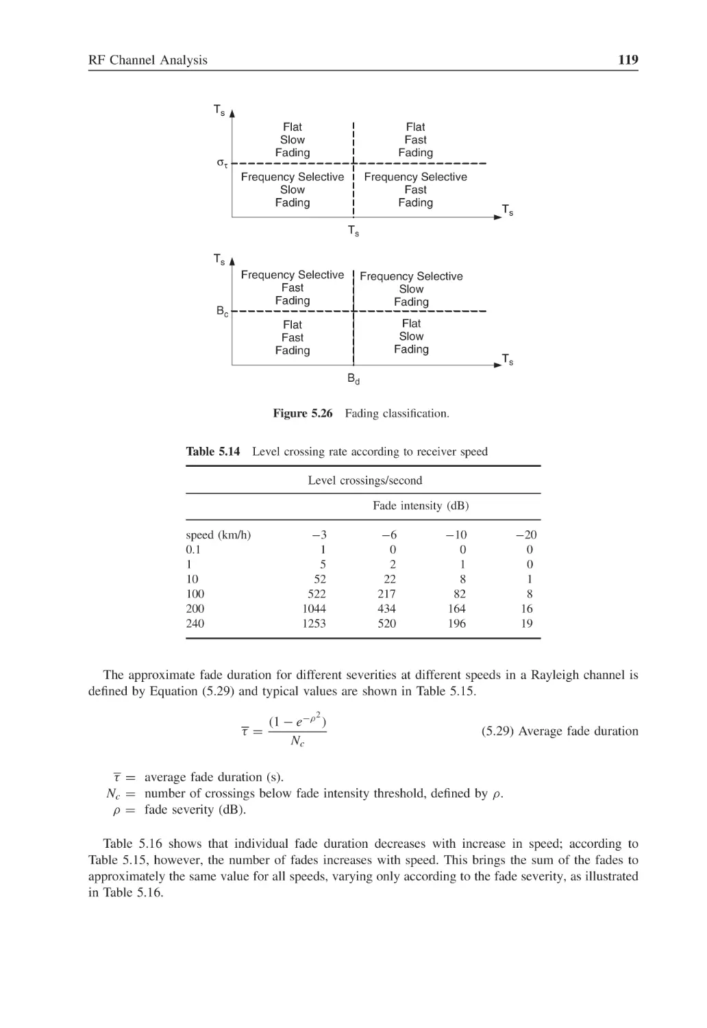
Figure 5.26
Fading classification
119
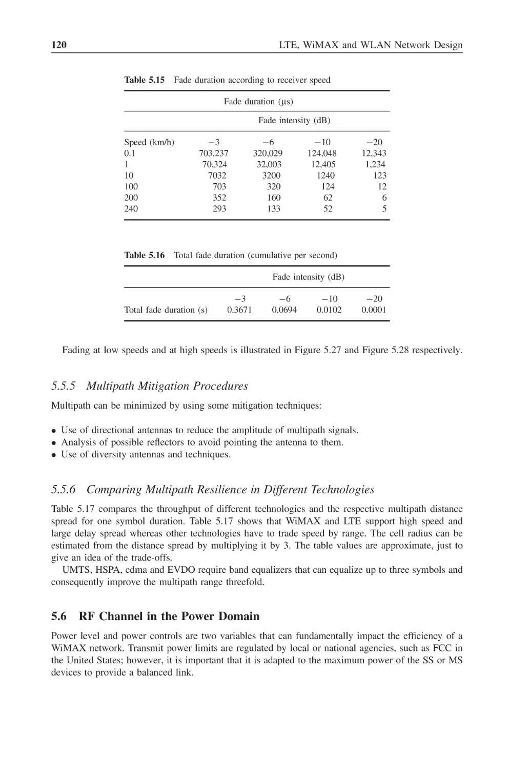
Figure 5.27
Fading at low speed
121
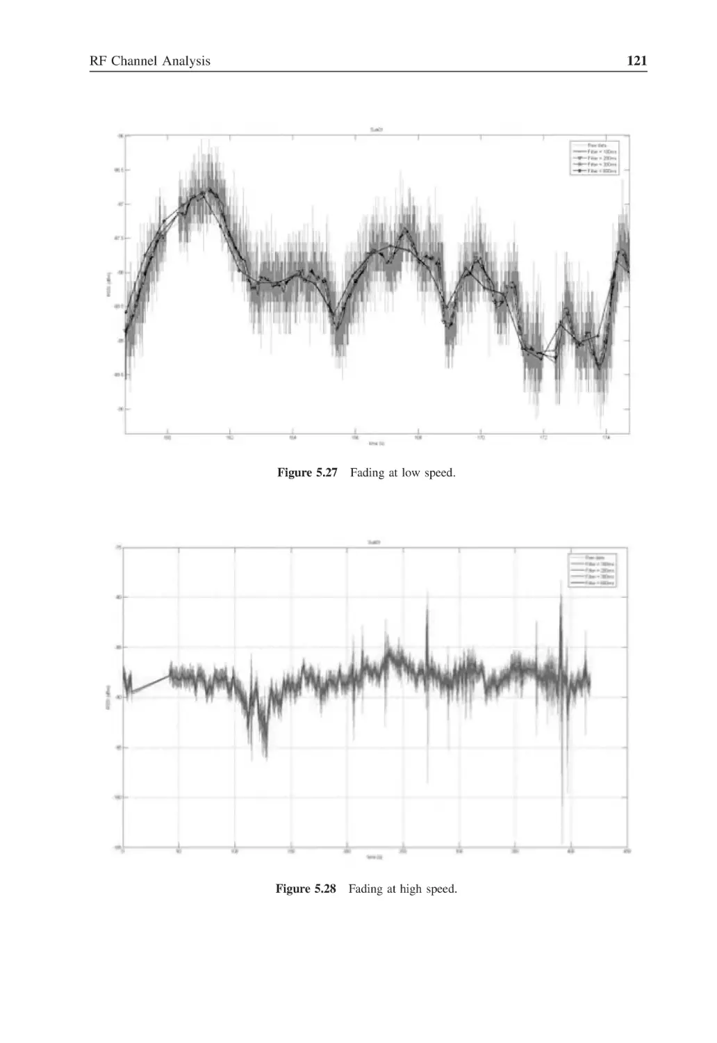
Figure 5.28
Fading at high speed
121
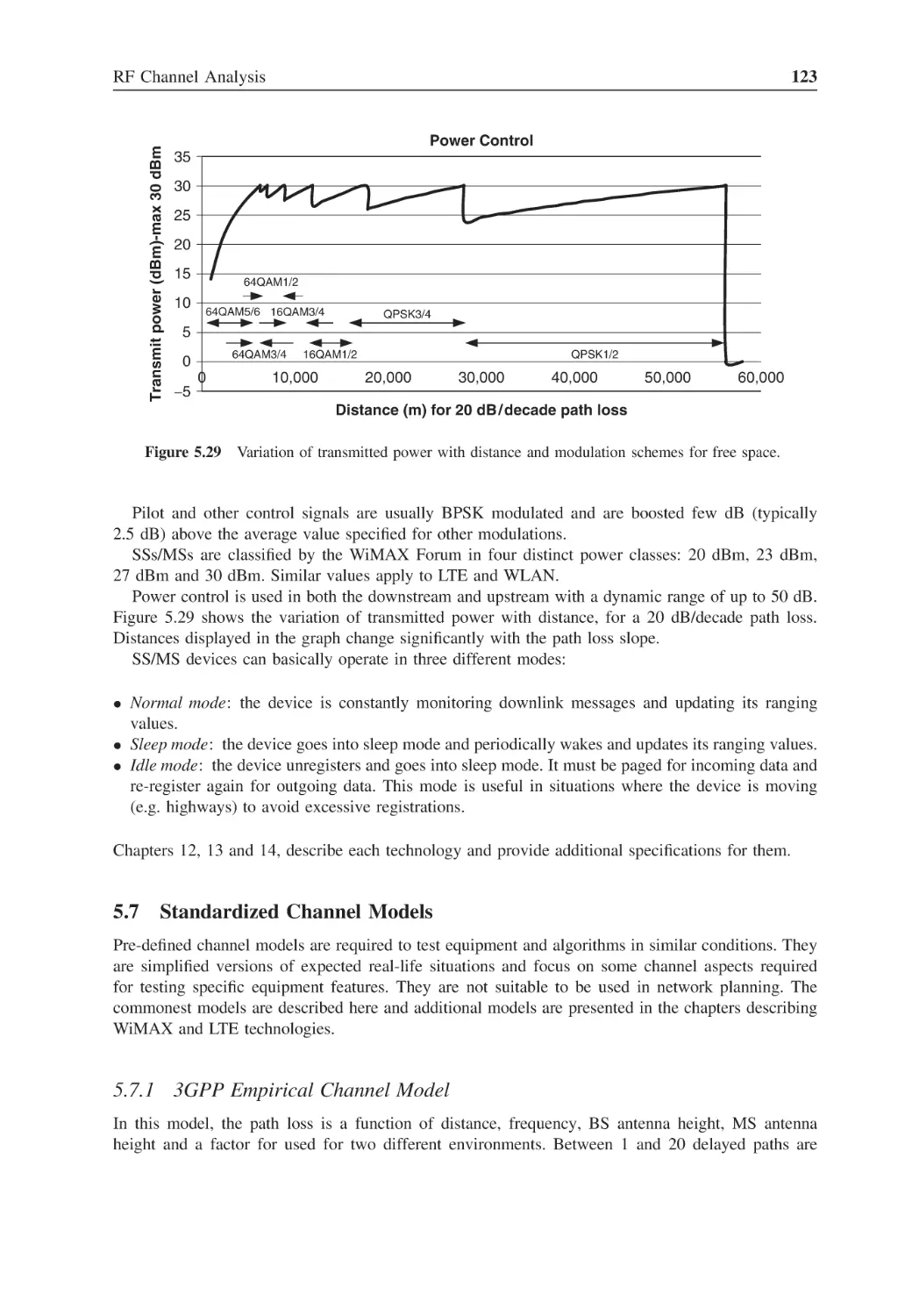
Figure 5.29
Variation of transmitted power with distance and modulation
schemes for free space
123
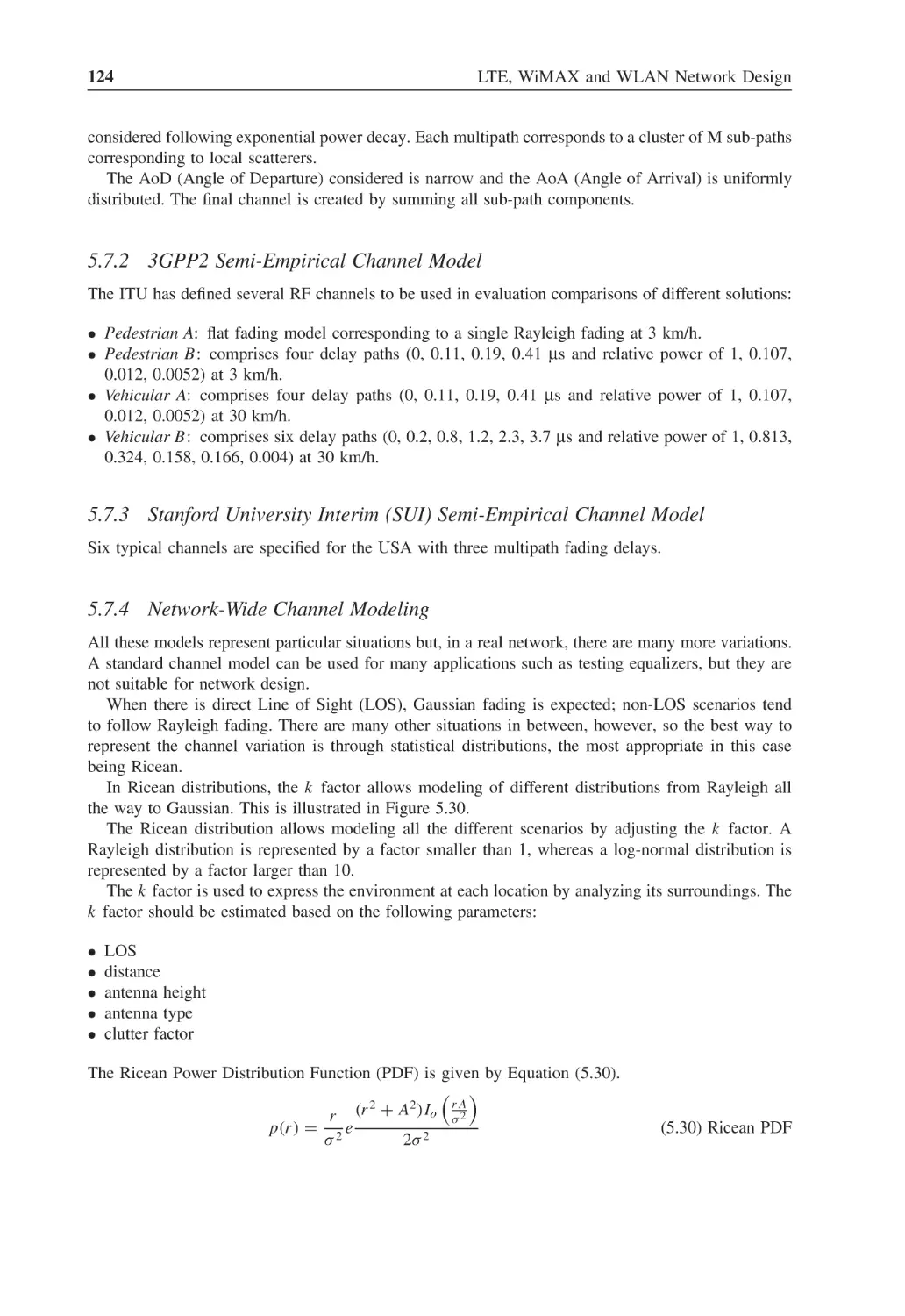
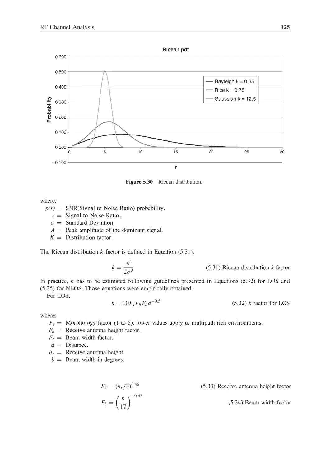
Figure 5.30
Ricean distribution
125
Figure 5.31
Ricean k factor (Ricean distribution) plot
126
Figure 5.32
Environment configuration dialogue
127
Figure 5.33
Rain precipitation map
128
Figure 5.34
Fading configuration
137
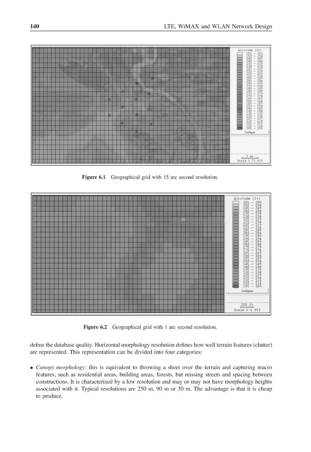
Figure 6.1
Geographical grid with 15 arc second resolution
140
Figure 6.2
Geographical grid with 1 arc second resolution
140
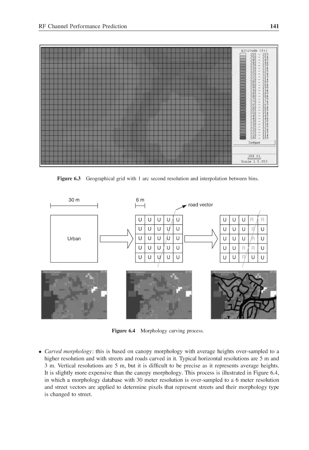
Figure 6.3
Geographical grid with 1 arc second resolution and interpolation
between bins
141
Figure 6.4
Morphology carving process
141
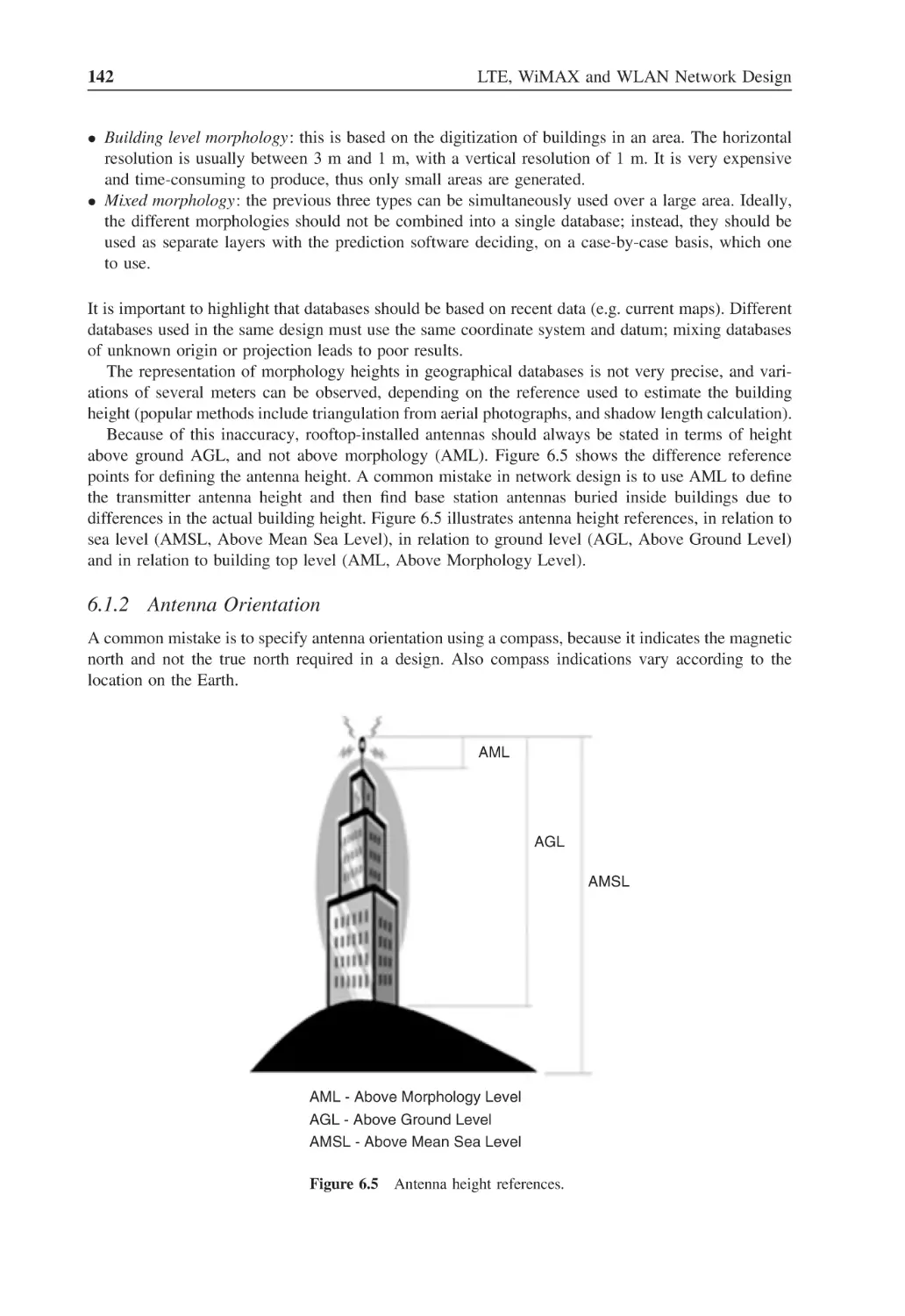
Figure 6.5
Antenna height references
142
Figure 6.6
Magnetic declination chart for 2005
143
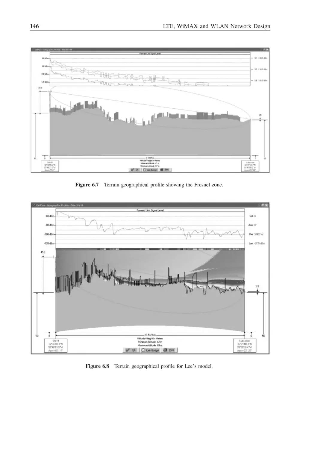
Figure 6.7
Terrain geographical profile showing the Fresnel zone
146
Figure 6.8
Terrain geographical profile for Lee’s model
146
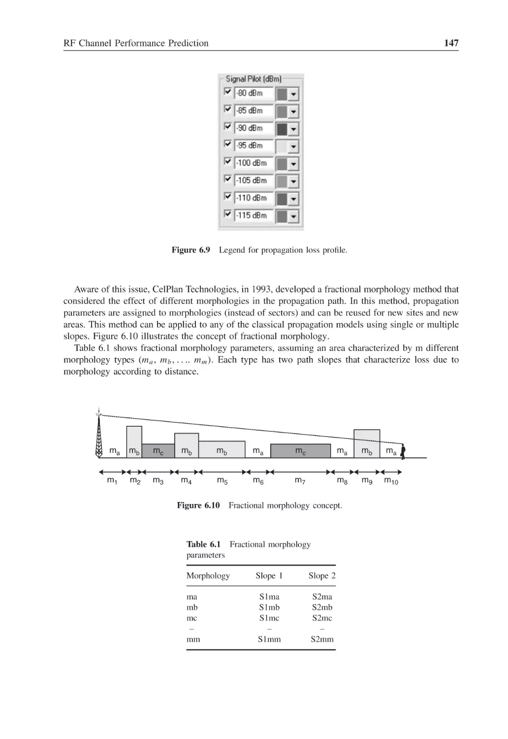
Figure 6.9
Legend for propagation loss profile
147
Figure 6.10
Fractional morphology concept
147
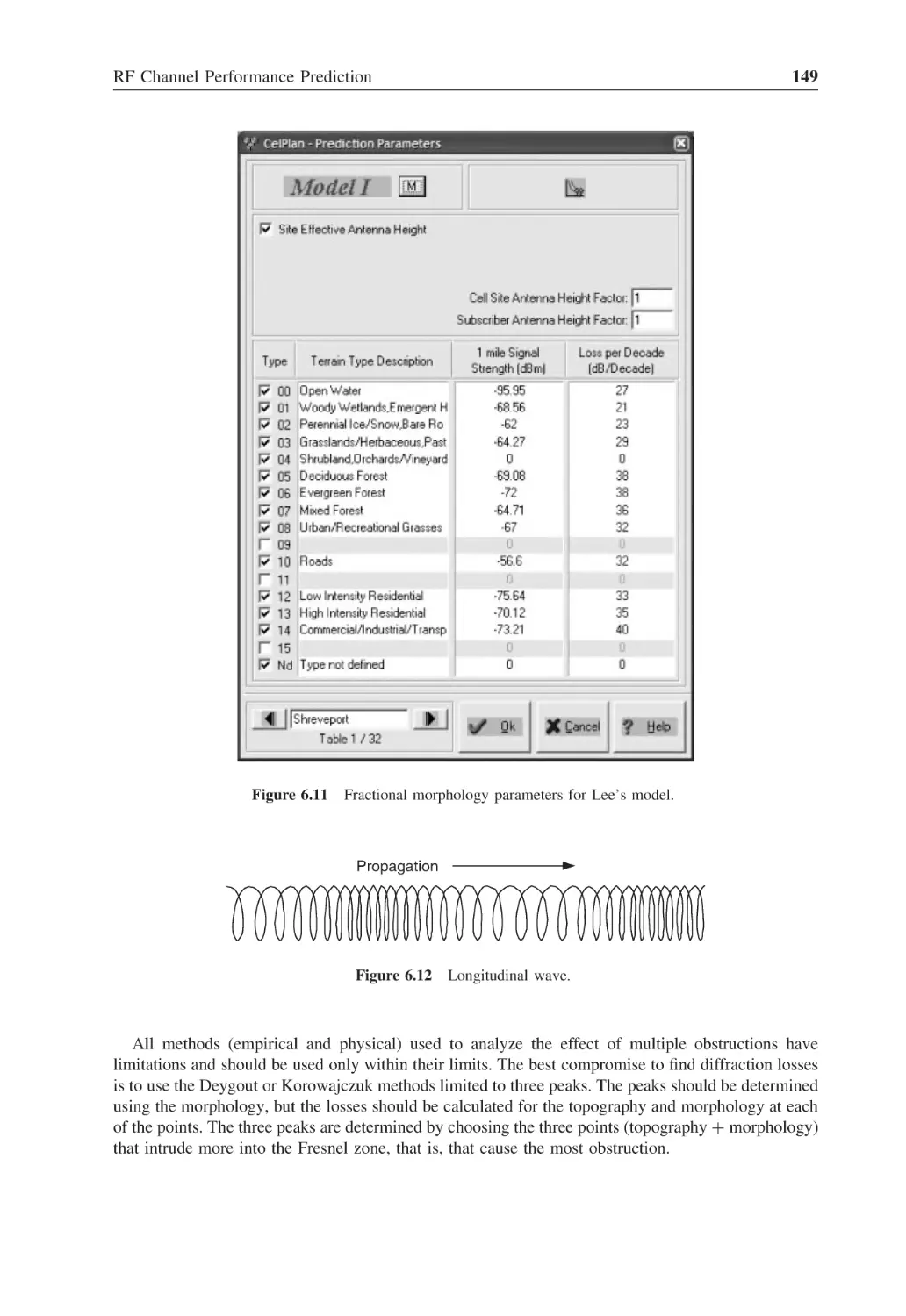
Figure 6.11
Fractional morphology parameters for Lee’s model
149
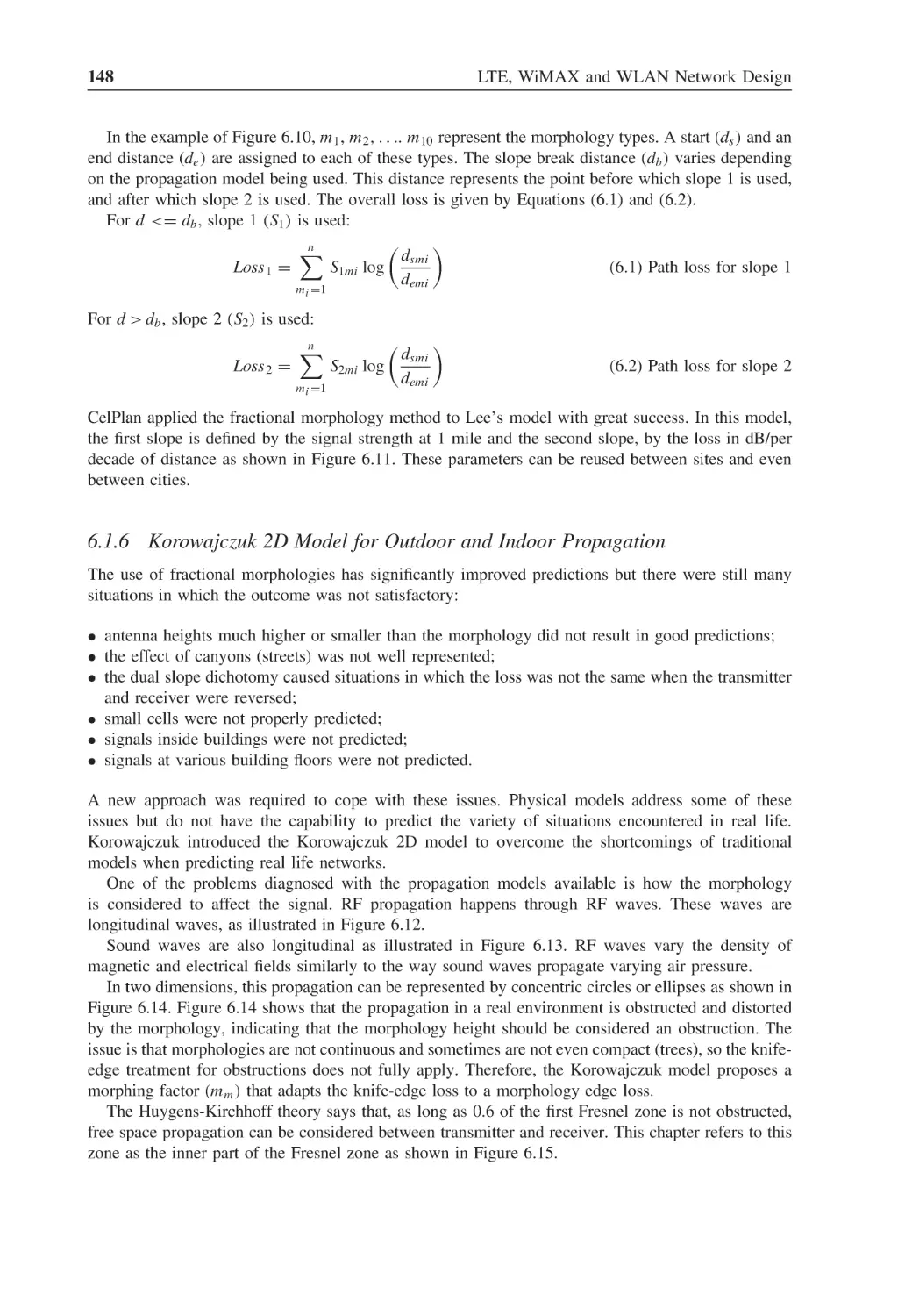
Figure 6.12
Longitudinal wave
149
Figure 6.13
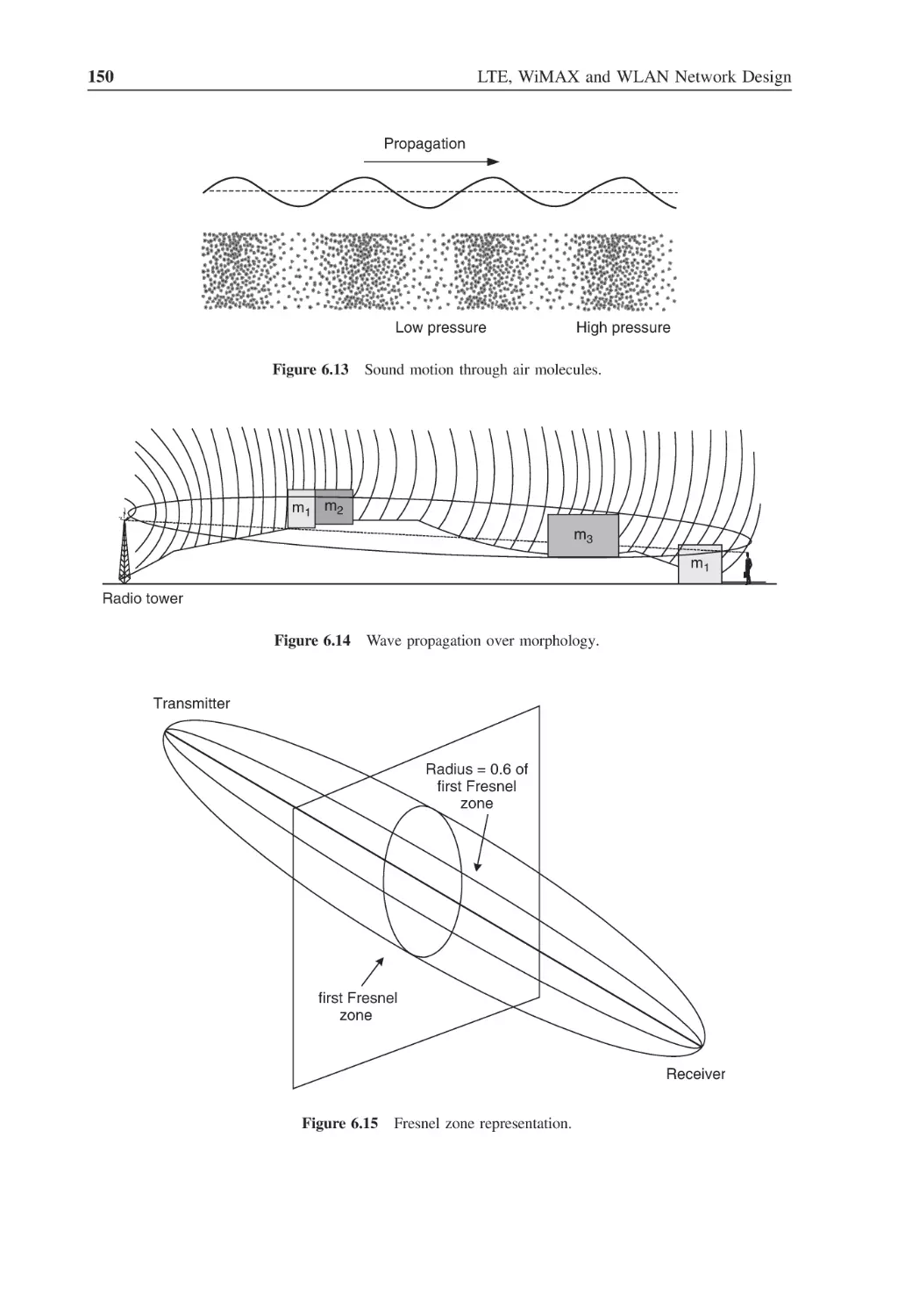
Sound motion through air molecules
150
Figure 6.14
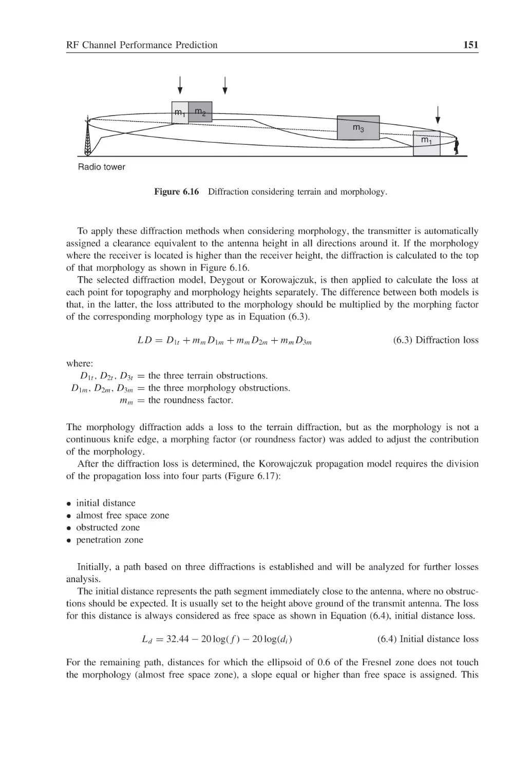
Wave propagation over morphology
150
xxii
List of Figures
Figure 6.15
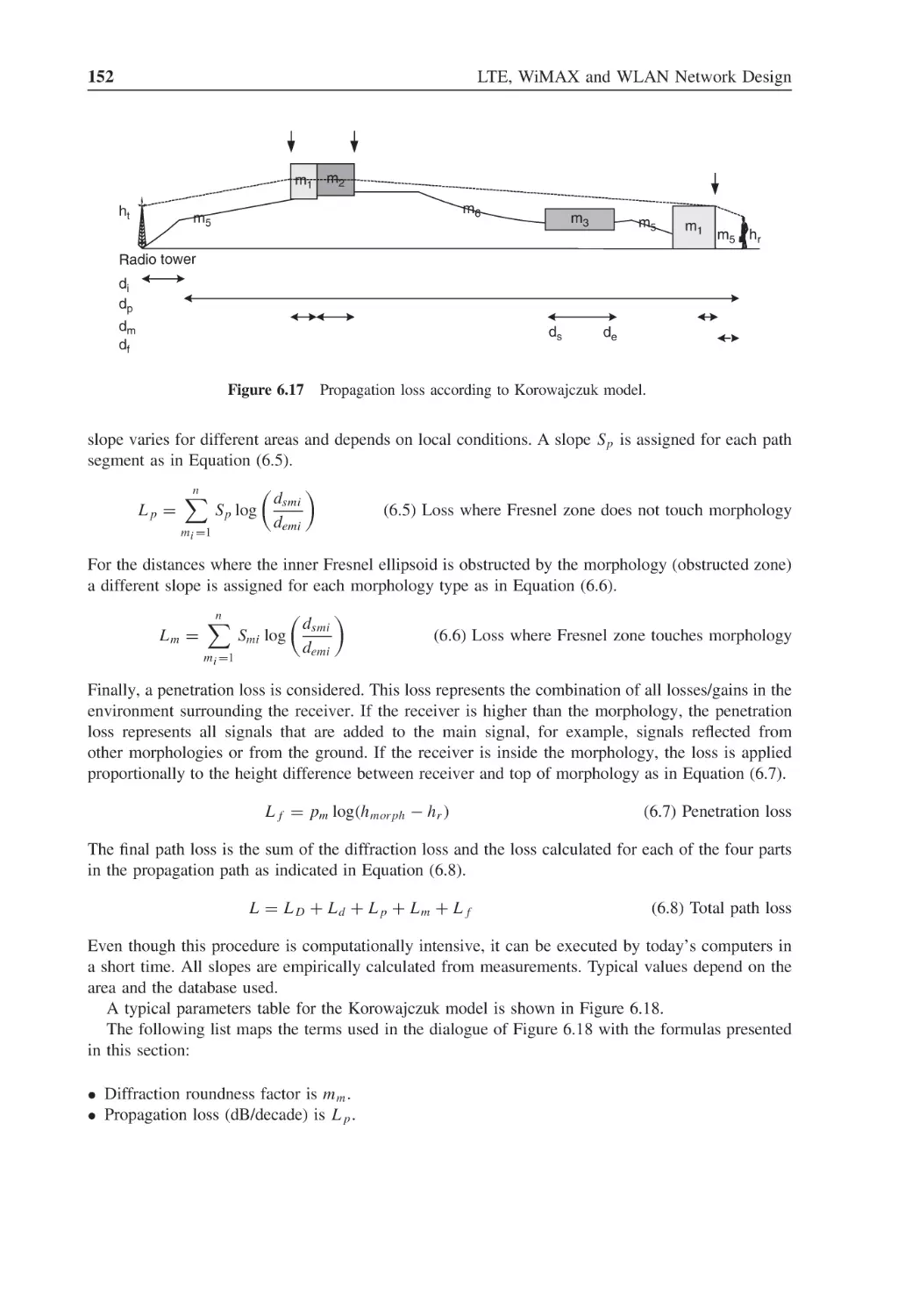
Fresnel zone representation
150
Figure 6.16
Diffraction considering terrain and morphology
151
Figure 6.17
Propagation loss according to Korowajczuk model
152
Figure 6.18
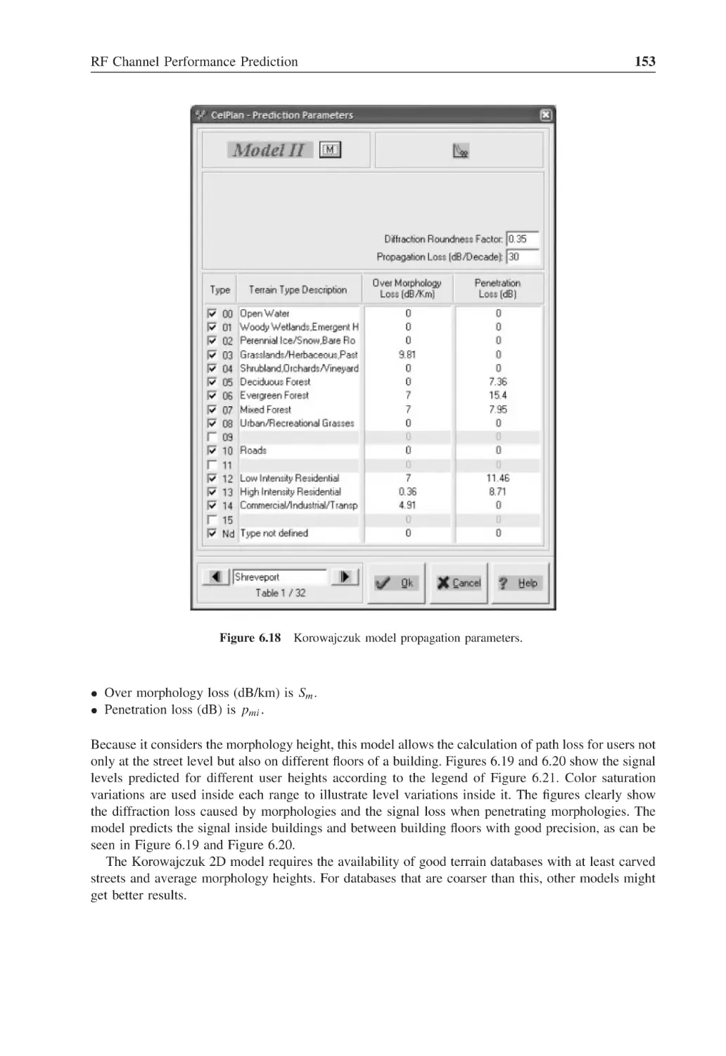
Korowajczuk model propagation parameters
153
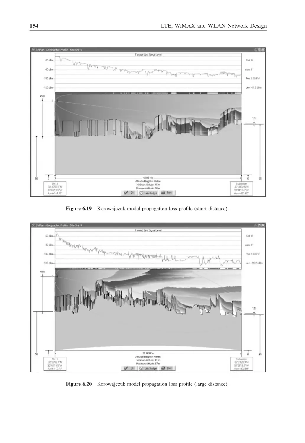
Figure 6.19
Korowajczuk model propagation loss profile (short distance)
154
Figure 6.20
Korowajczuk model propagation loss profile (large distance)
154
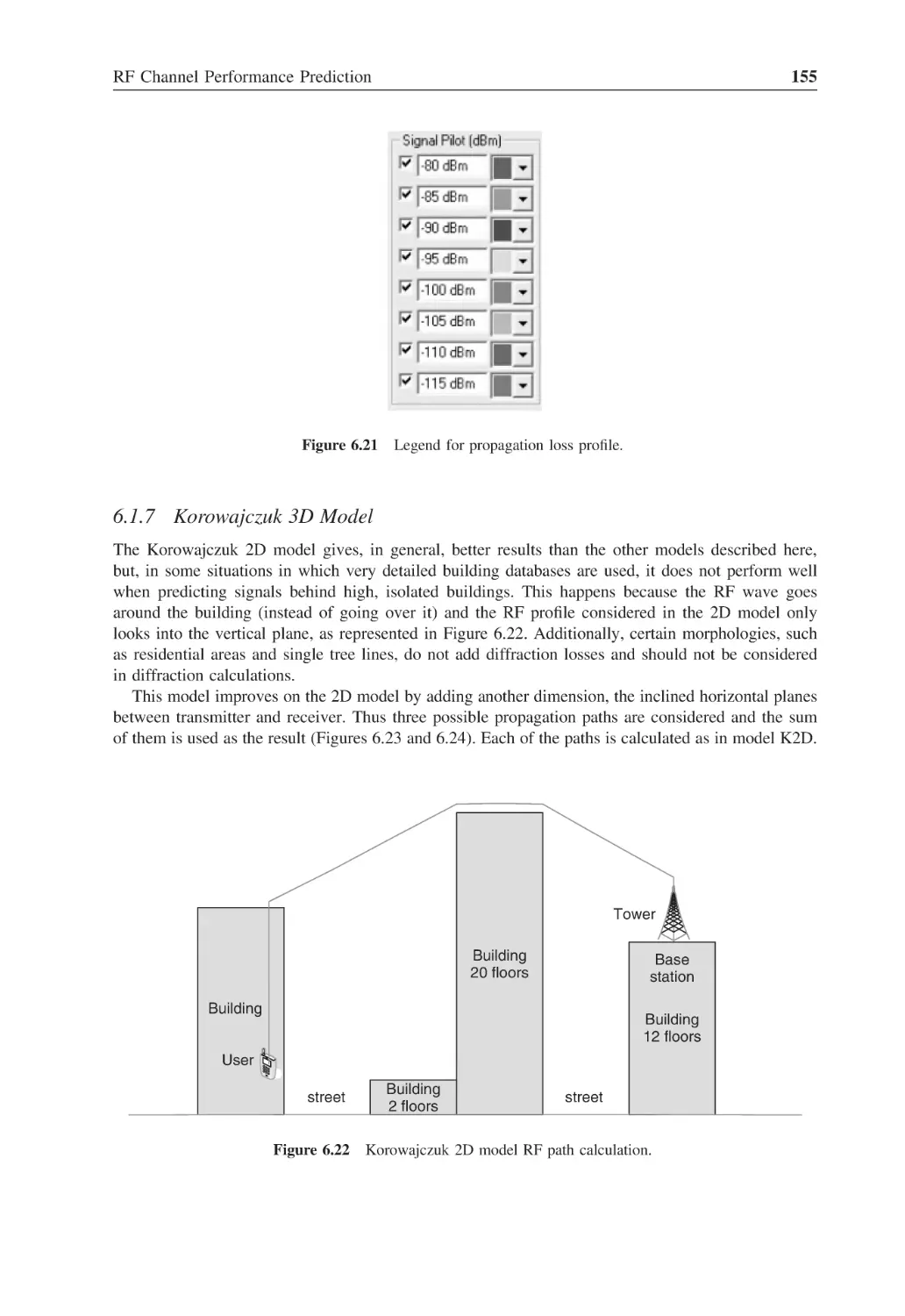
Figure 6.21
Legend for propagation loss profile
155
Figure 6.22
Korowajczuk 2D model RF path calculation
155
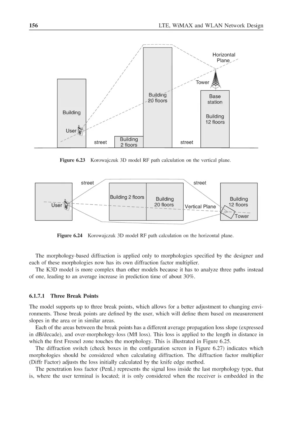
Figure 6.23
Korowajczuk 3D model RF path calculation on the vertical plane
156
Figure 6.24
Korowajczuk 3D model RF path calculation on the horizontal plane
156
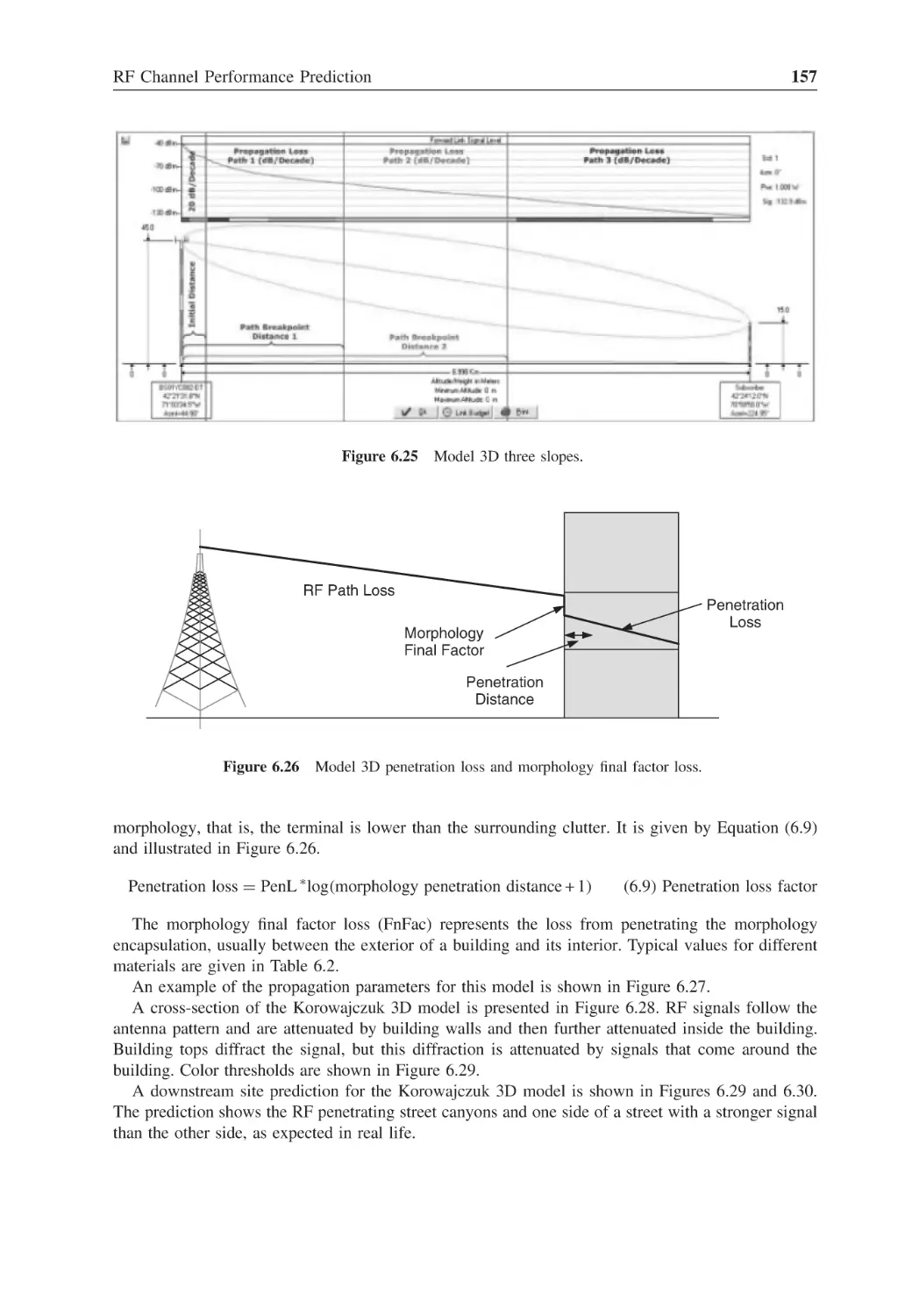
Figure 6.25
Model 3D three slopes
157
Figure 6.26
Model 3D penetration loss and morphology final factor loss
157
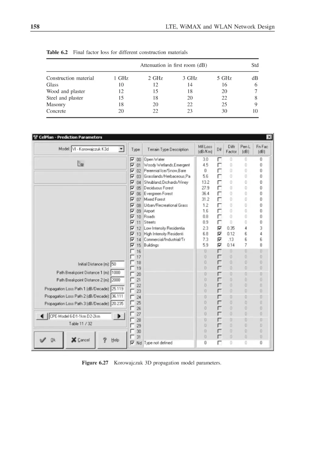
Figure 6.27
Korowajczuk 3D propagation model parameters
158
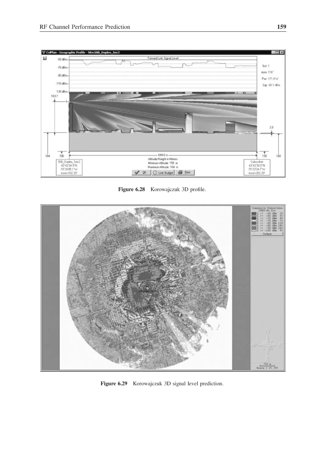
Figure 6.28
Korowajczuk 3D profile
159
Figure 6.29
Korowajczuk 3D signal level prediction
159
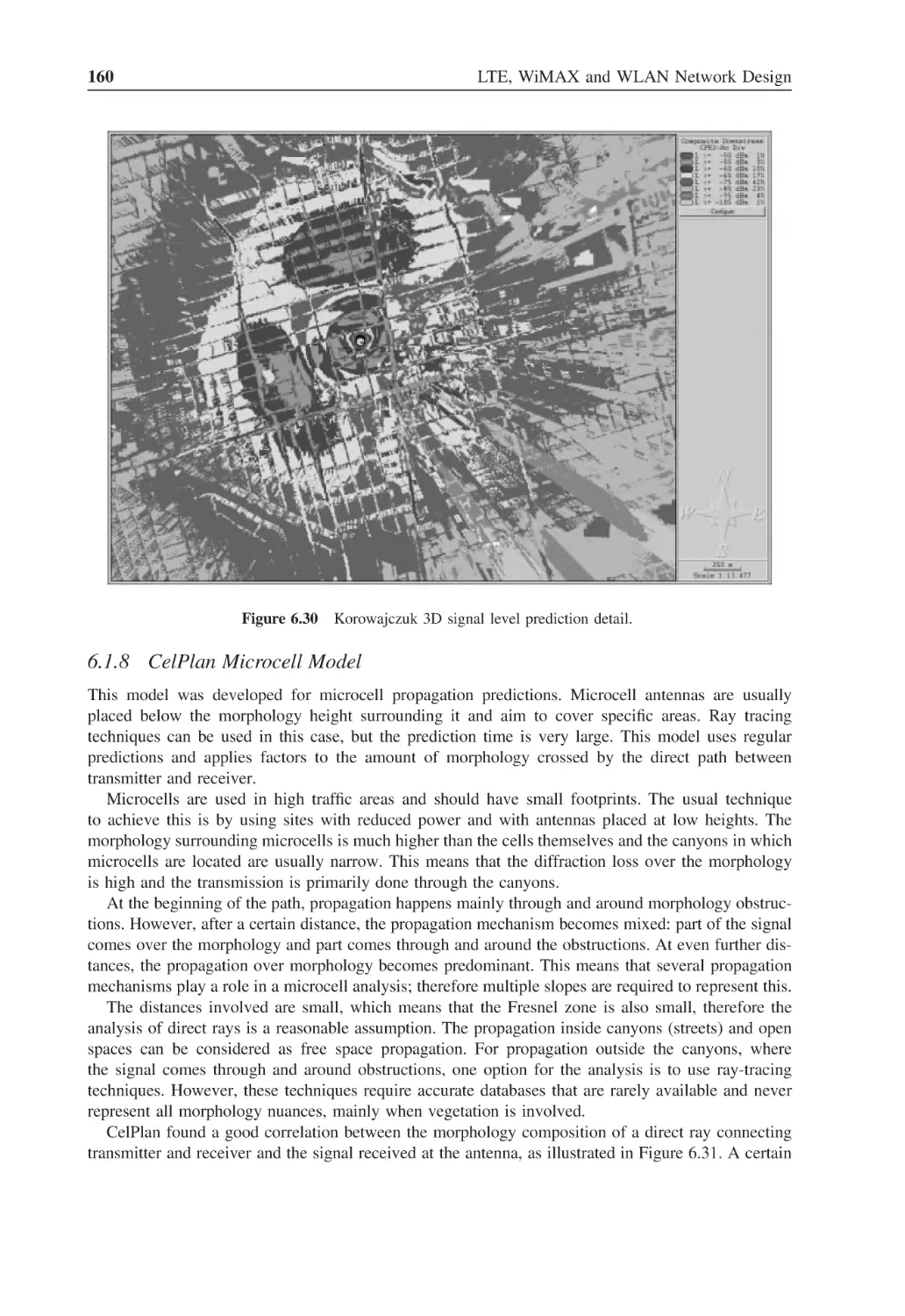
Figure 6.30
Korowajczuk 3D signal level prediction detail
160
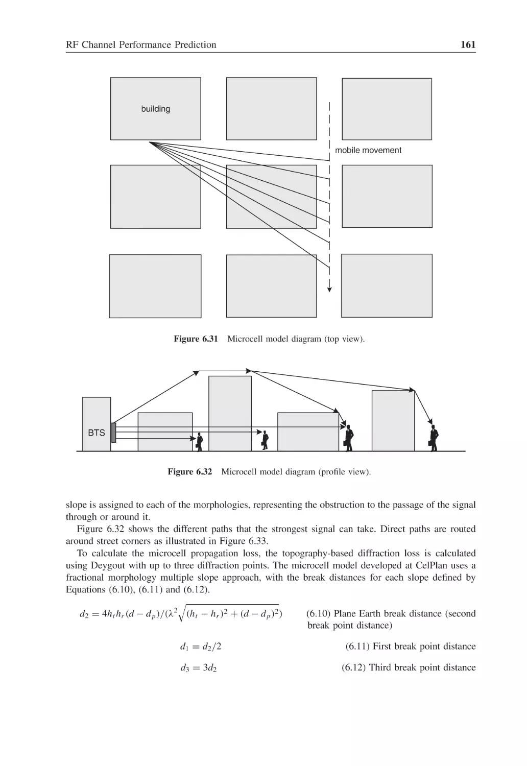
Figure 6.31
Microcell model diagram (top view)
161
Figure 6.32
Microcell model diagram (profile view)
161
Figure 6.33
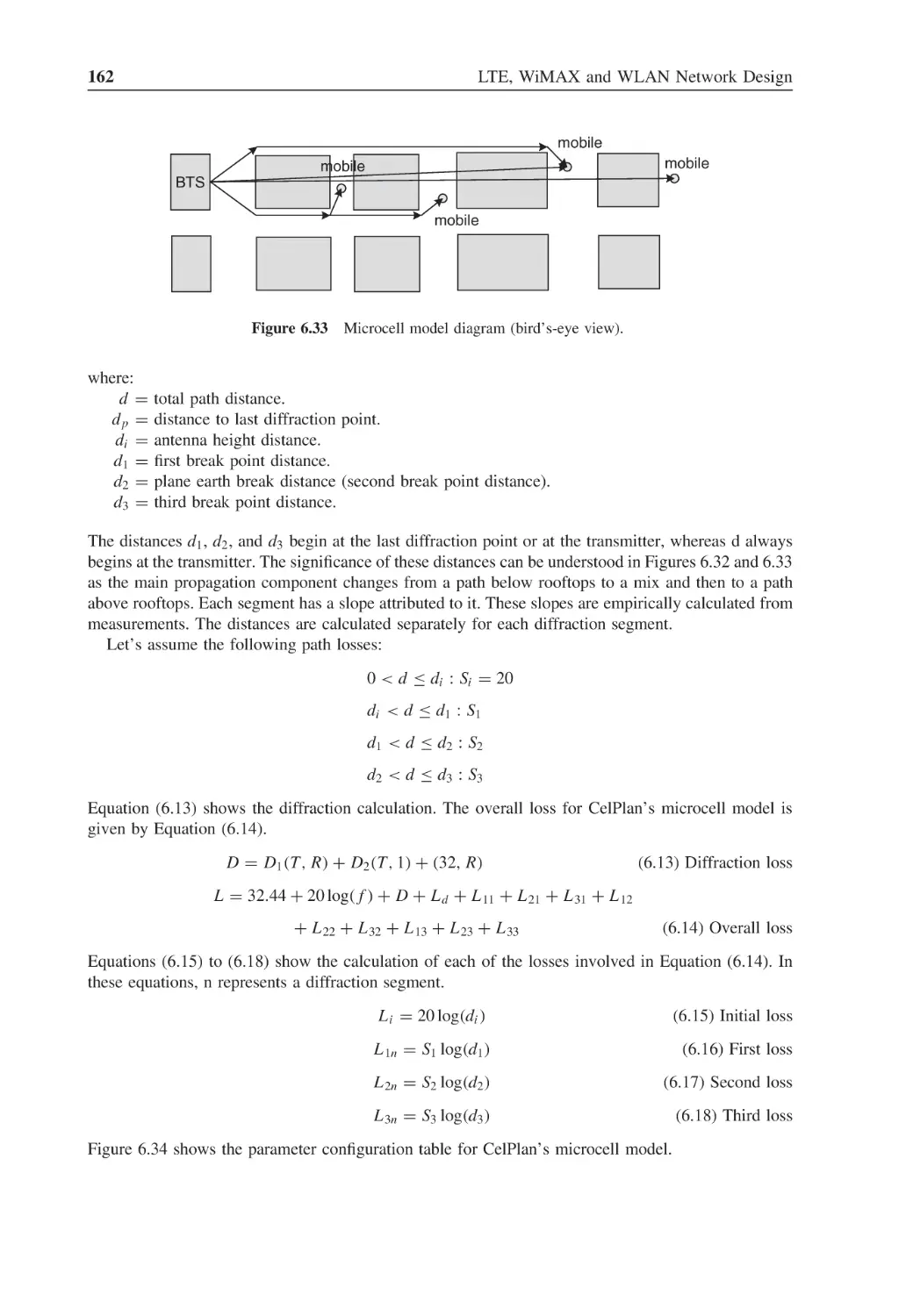
Microcell model diagram (bird’s-eye view)
162
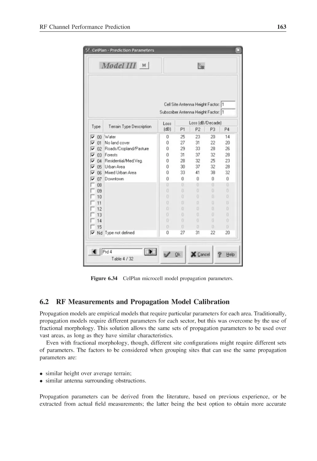
Figure 6.34
CelPlan microcell model propagation parameters
163
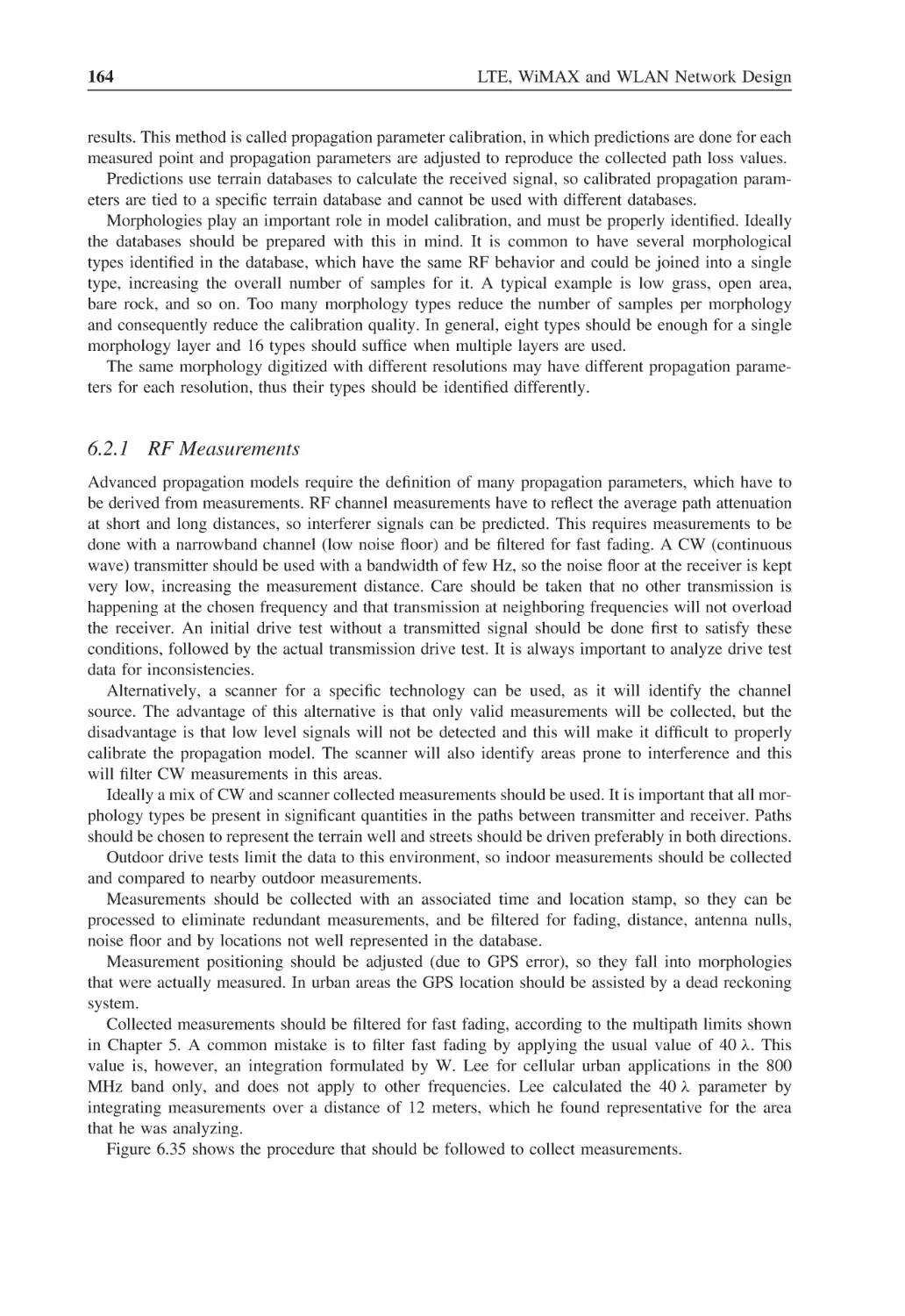
Figure 6.35
RF measurement drive test collection procedure
165
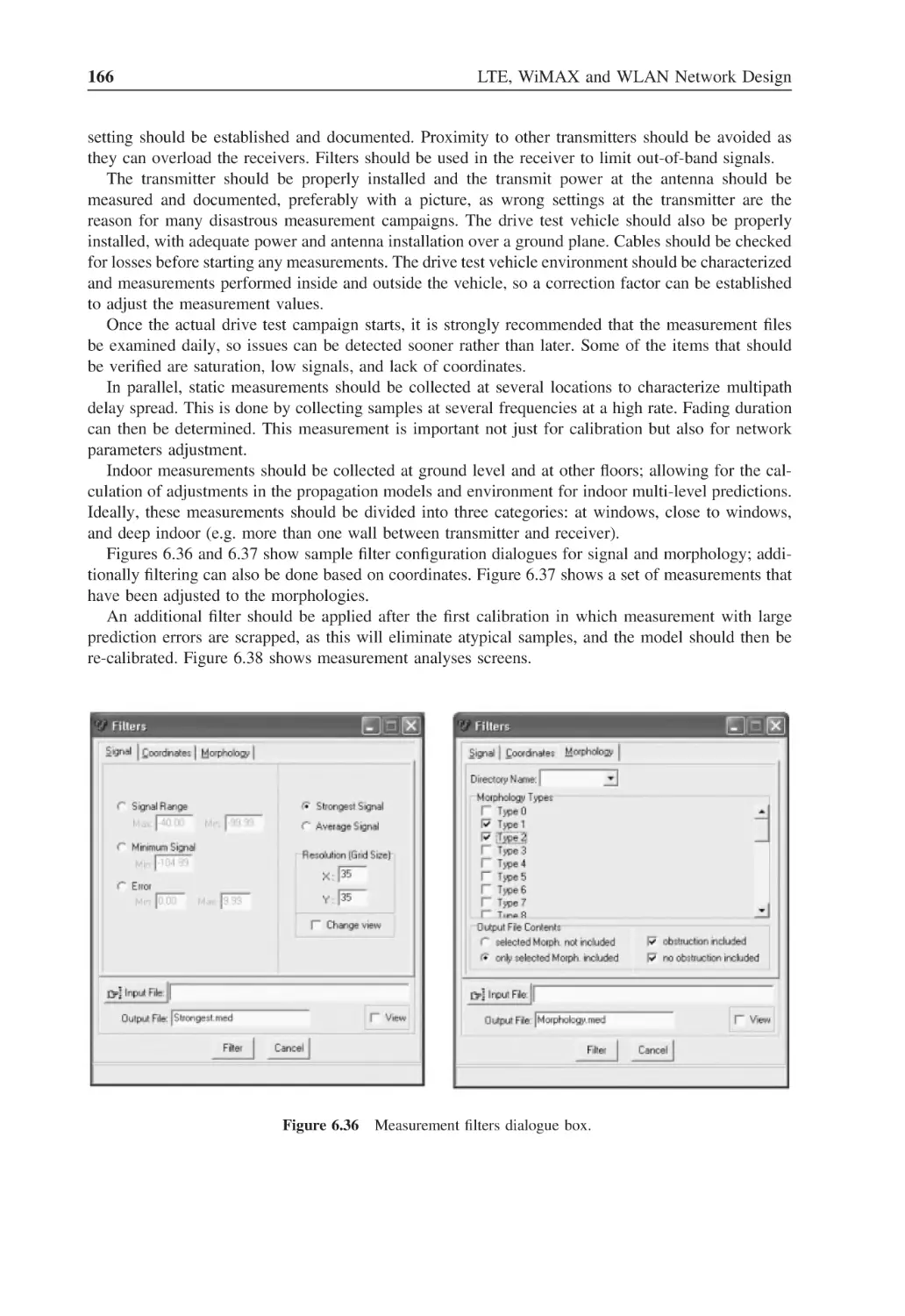
Figure 6.36
Measurement filters dialogue box
166
Figure 6.37
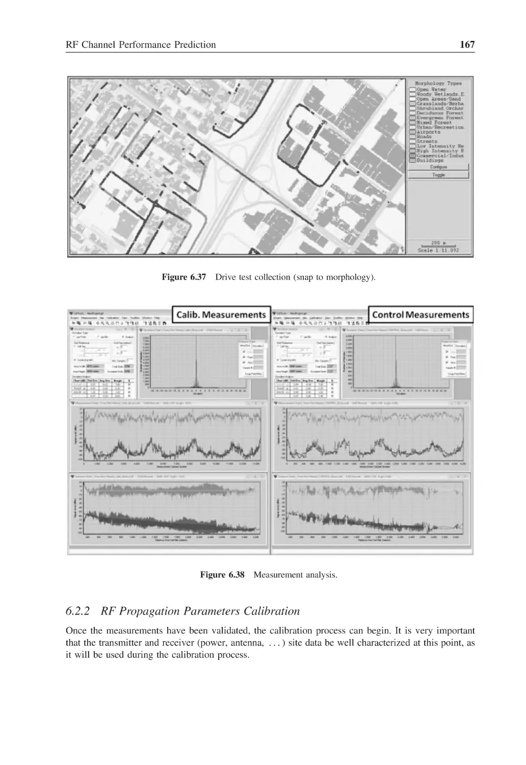
Drive test collection (snap to morphology)
167
Figure 6.38
Measurement analysis
167
Figure 6.39
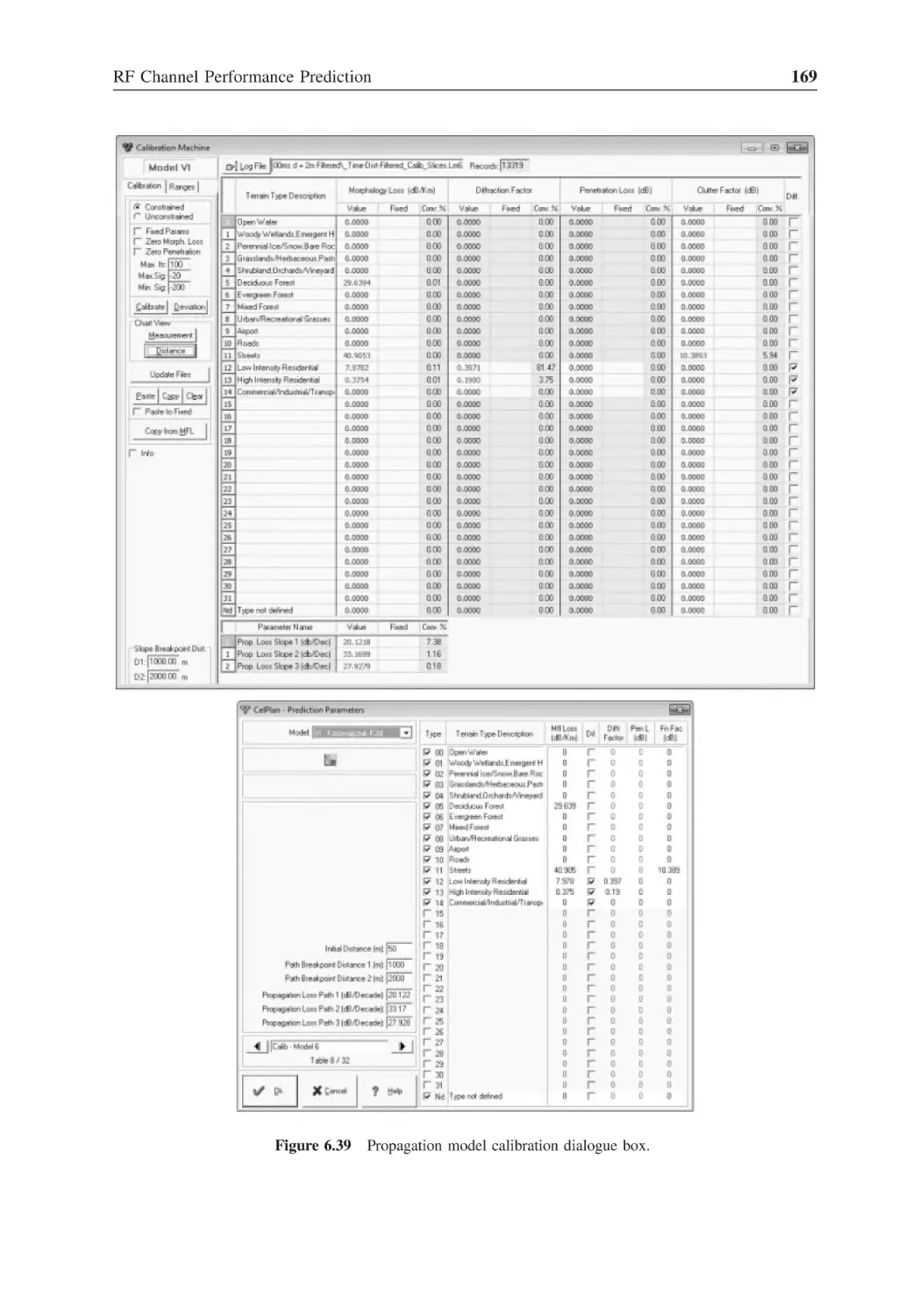
Propagation model calibration dialogue box
169
Figure 6.40
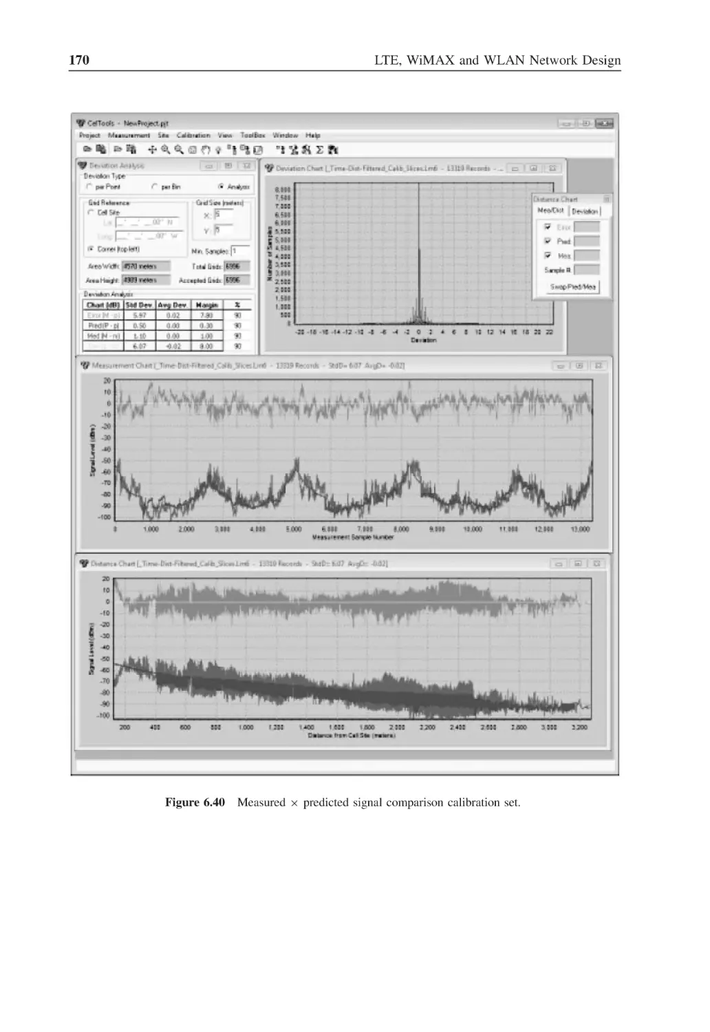
Measured × predicted signal comparison calibration set
170
Figure 6.41
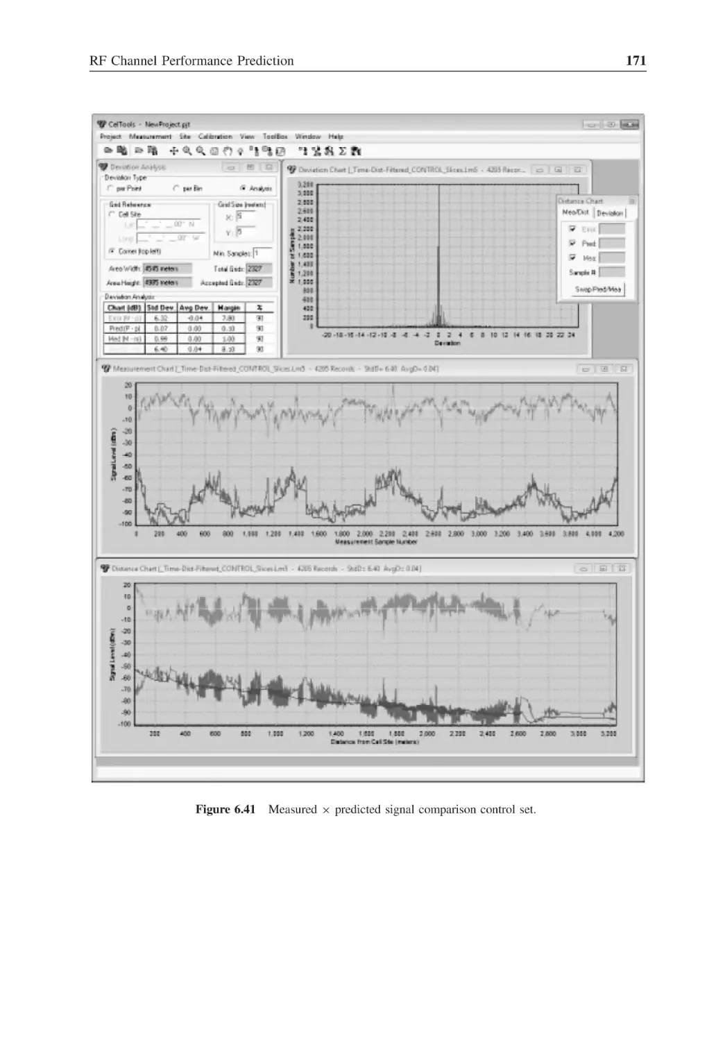
Measured × predicted signal comparison control set
171
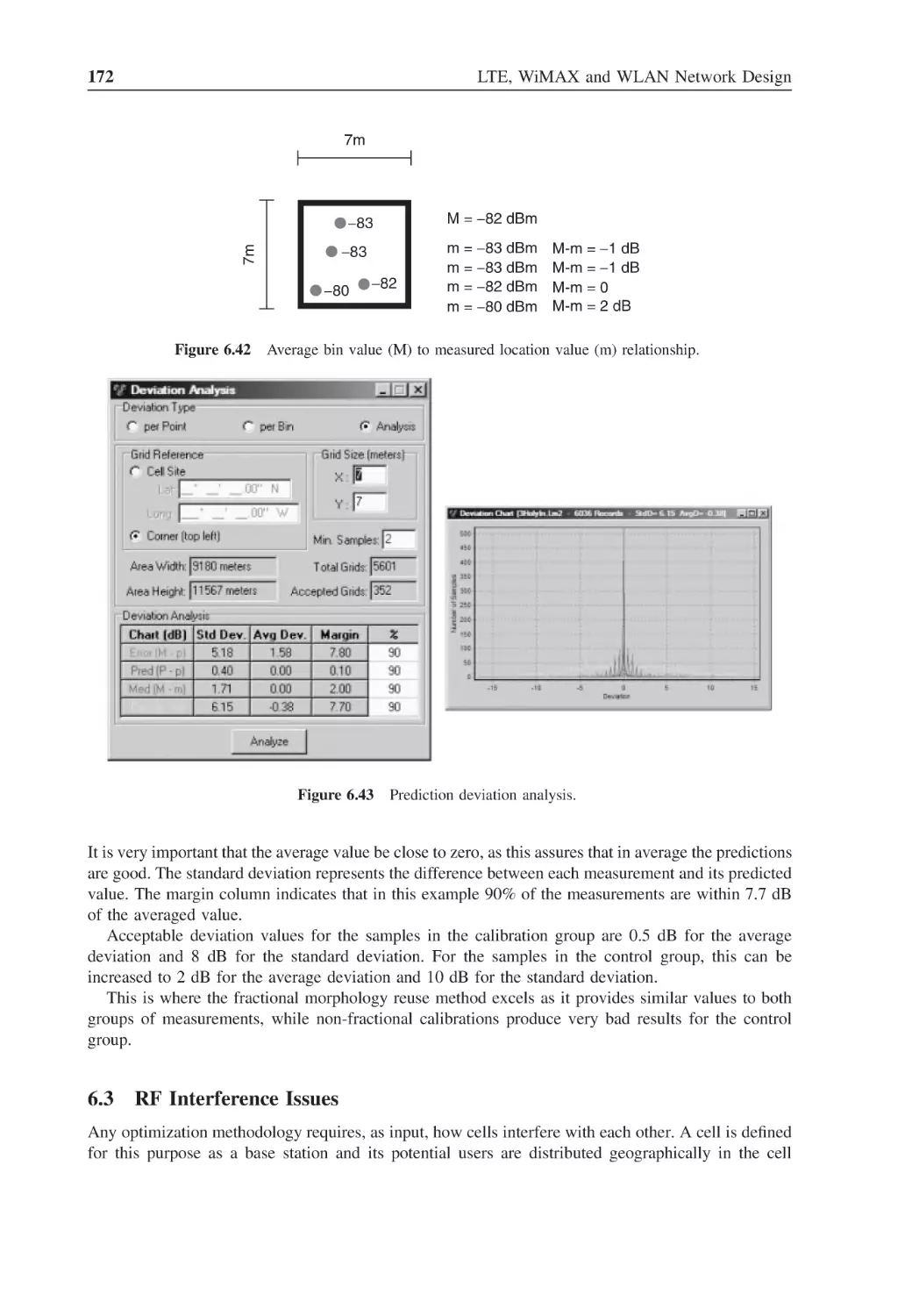
Figure 6.42
Average bin value (M) to measured location value (m) relationship
172
Figure 6.43
Prediction deviation analysis
172
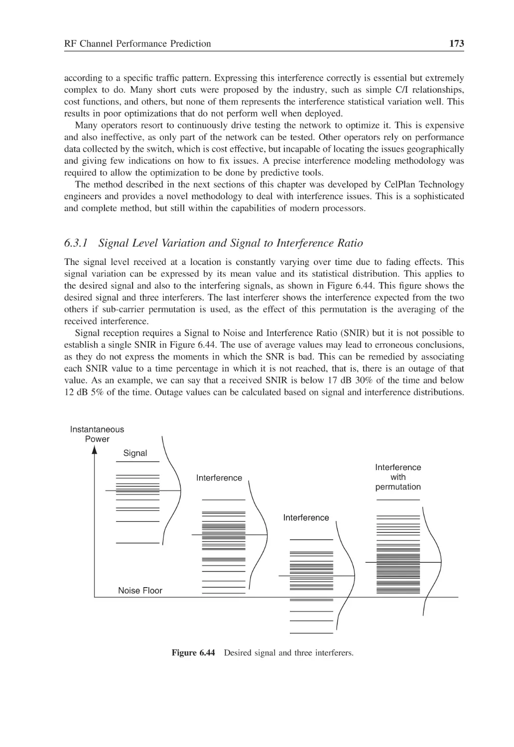
Figure 6.44
Desired signal and three interferers
173
Figure 6.45
Signal and interference distribution curves
174
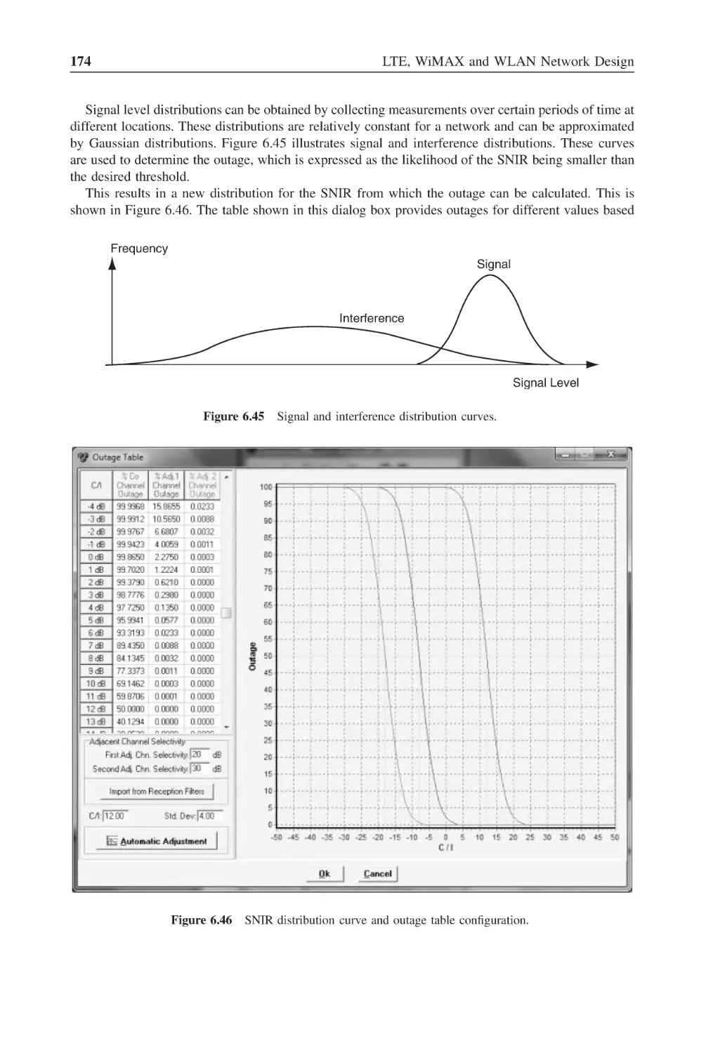
Figure 6.46
SNIR distribution curve and outage table configuration
174
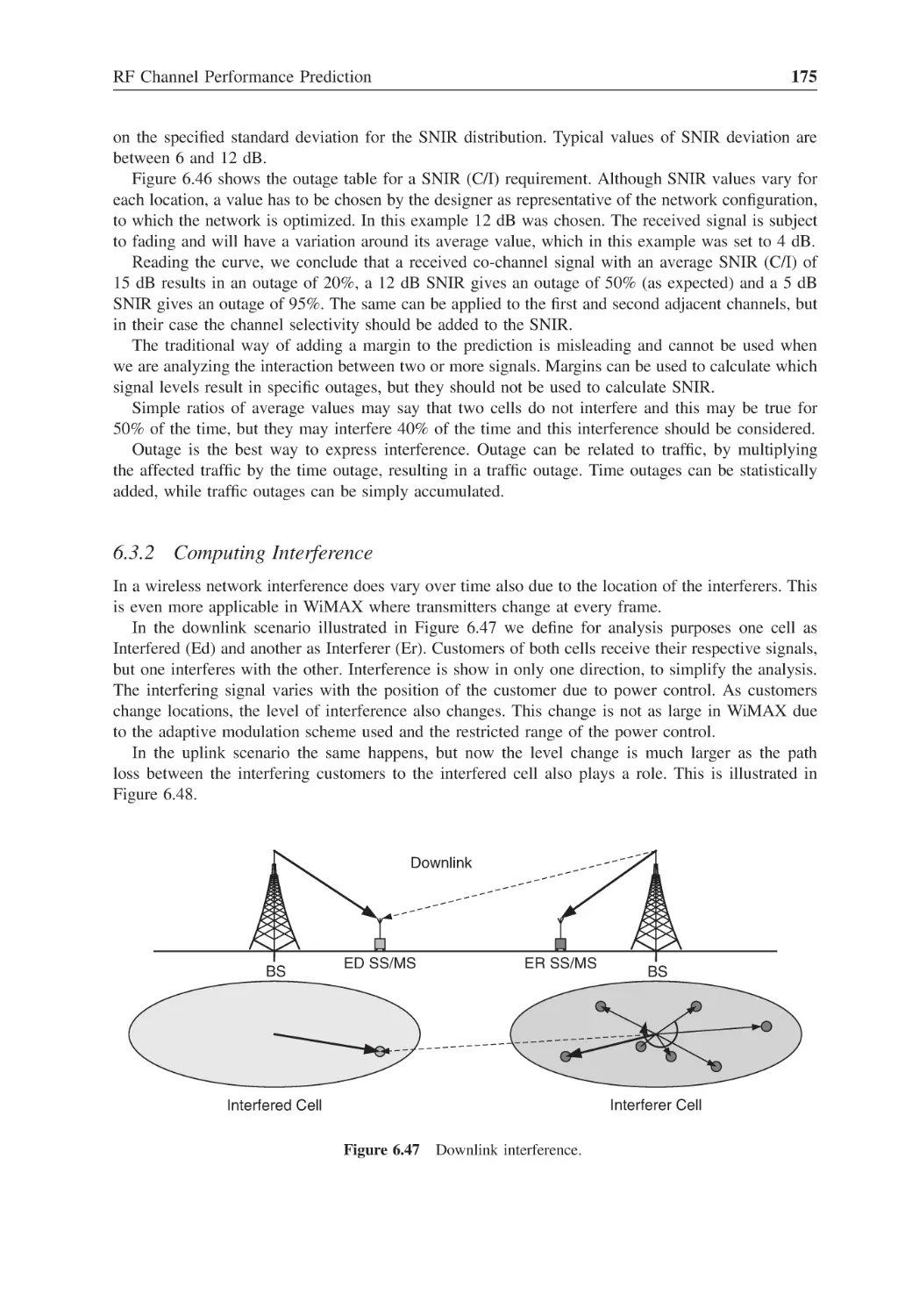
Figure 6.47
Downlink interference
175
Figure 6.48
Uplink interference
176
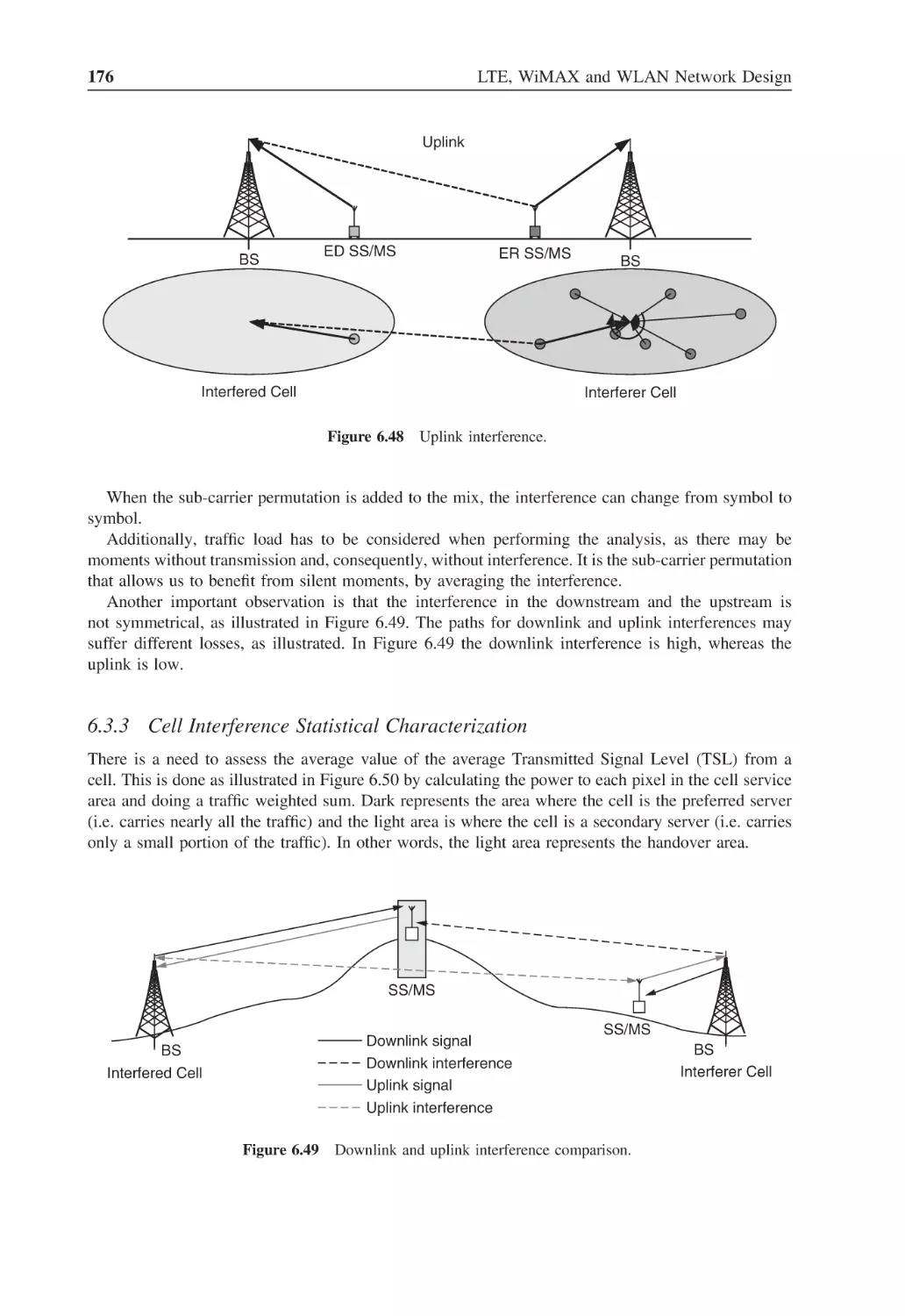
Figure 6.49
Downlink and uplink interference comparison
176
Figure 6.50
Primary and secondary service areas of a site
177
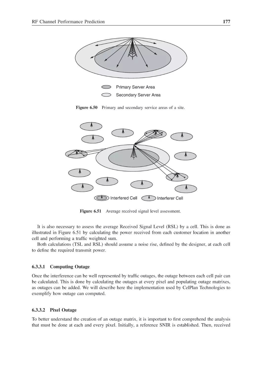
Figure 6.51
Average received signal level assessment
177
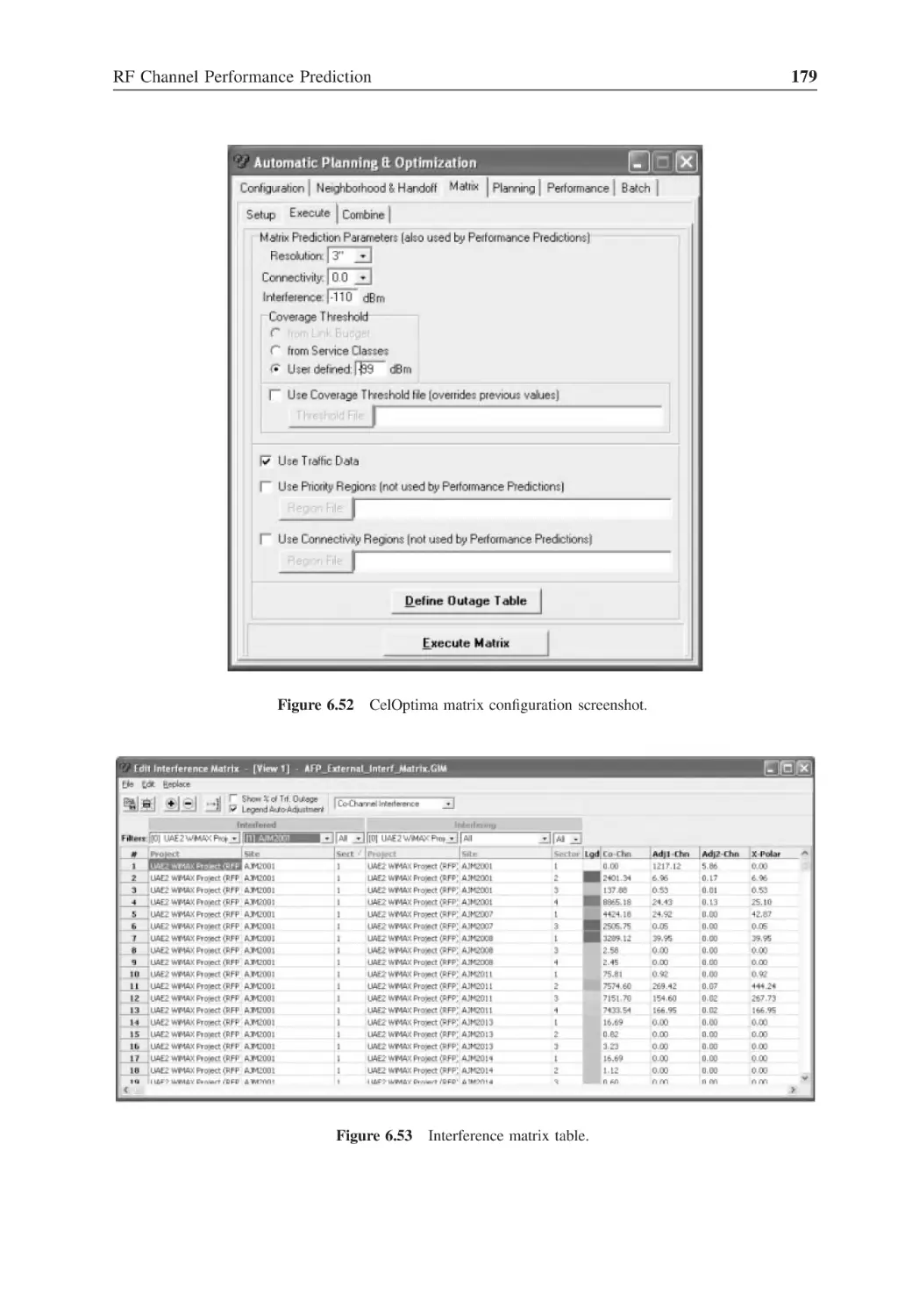
Figure 6.52
CelOptima matrix configuration screenshot
179
Figure 6.53
Interference matrix table
179
List of Figures
xxiii
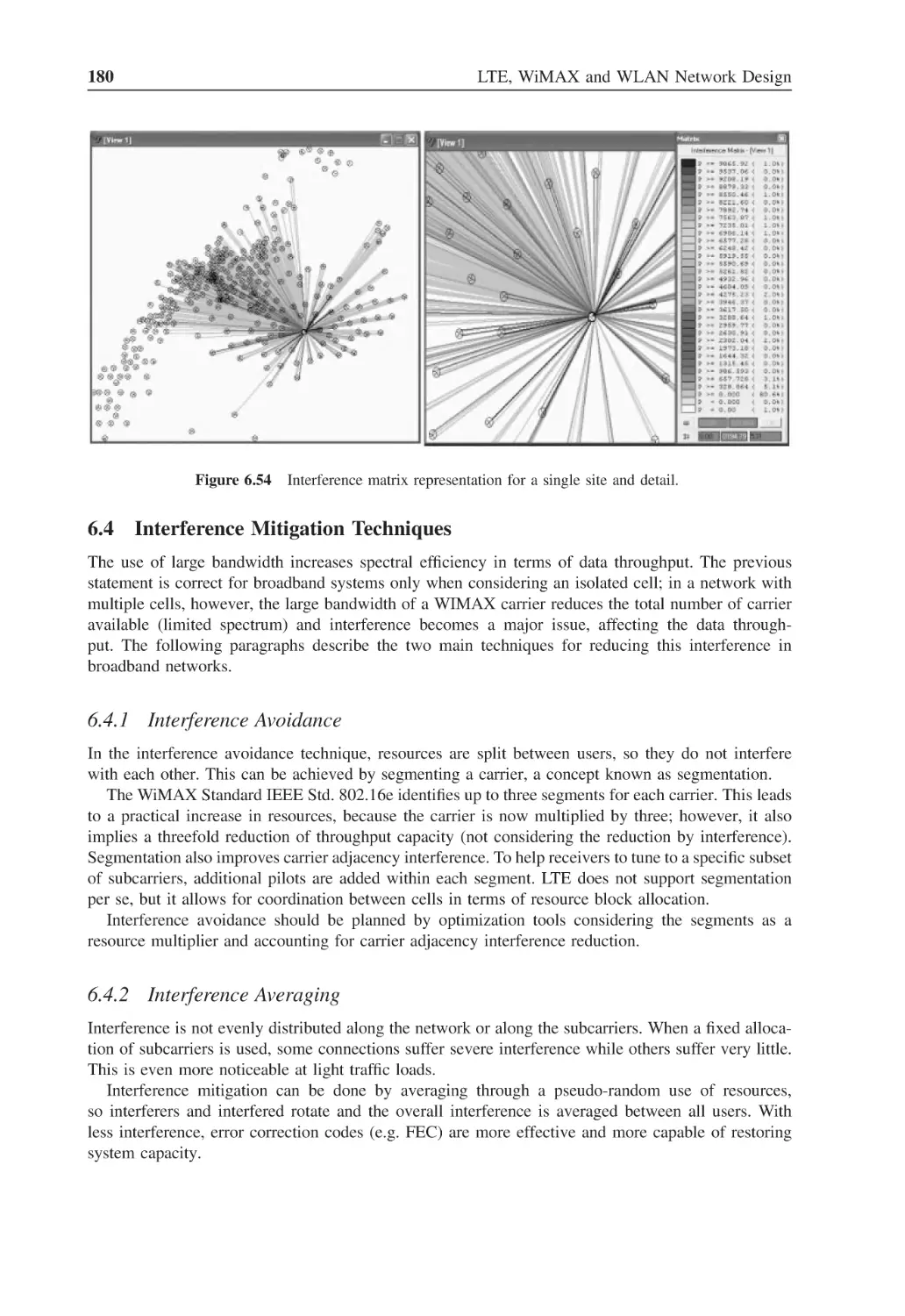
Figure 6.54
Interference matrix representation for a single site and detail
180
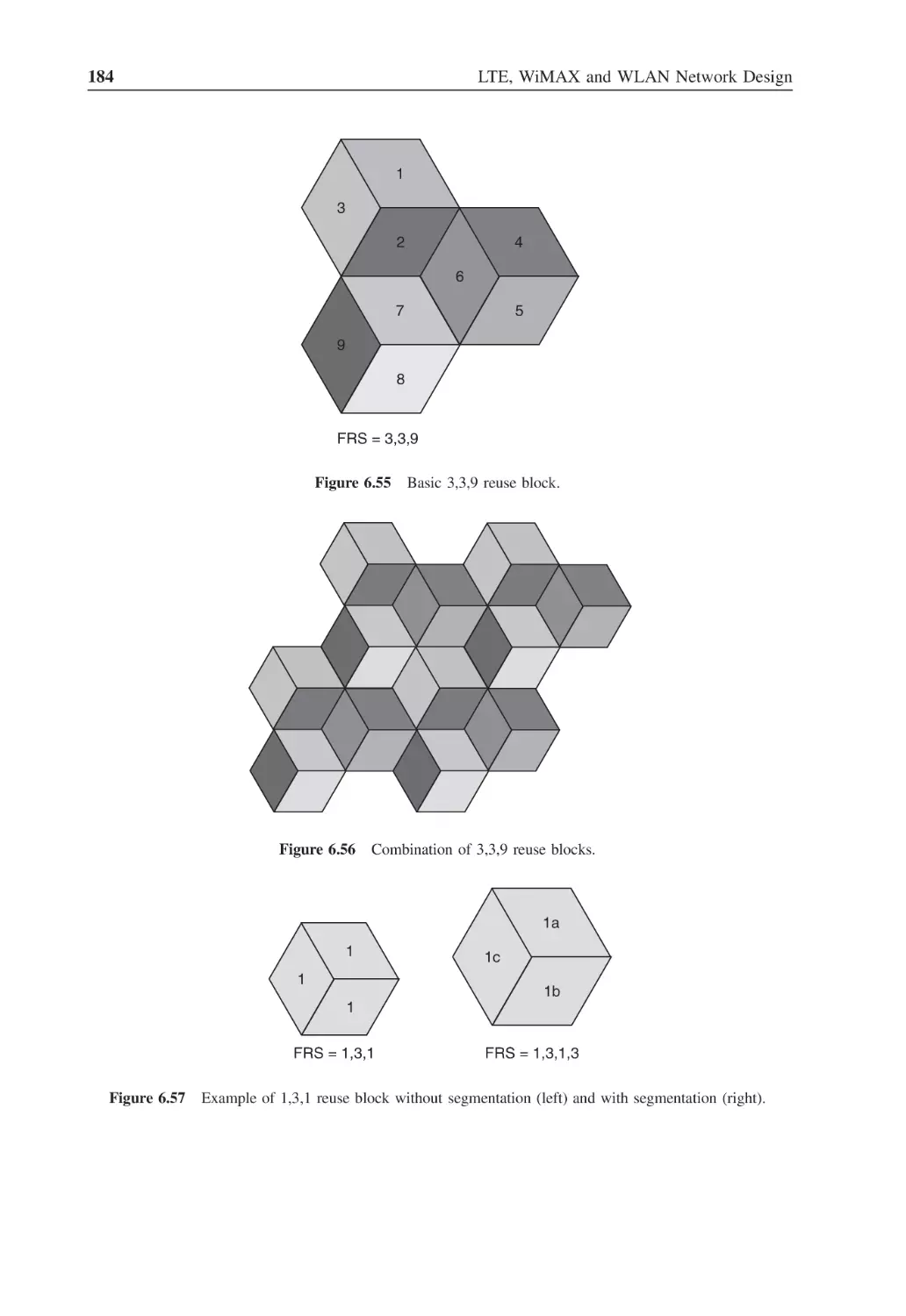
Figure 6.55
Basic 3,3,9 reuse block
184
Figure 6.56
Combination of 3,3,9 reuse blocks
184
Figure 6.57
Example of 1,3,1 reuse block without segmentation (left) and
with segmentation (right)
184
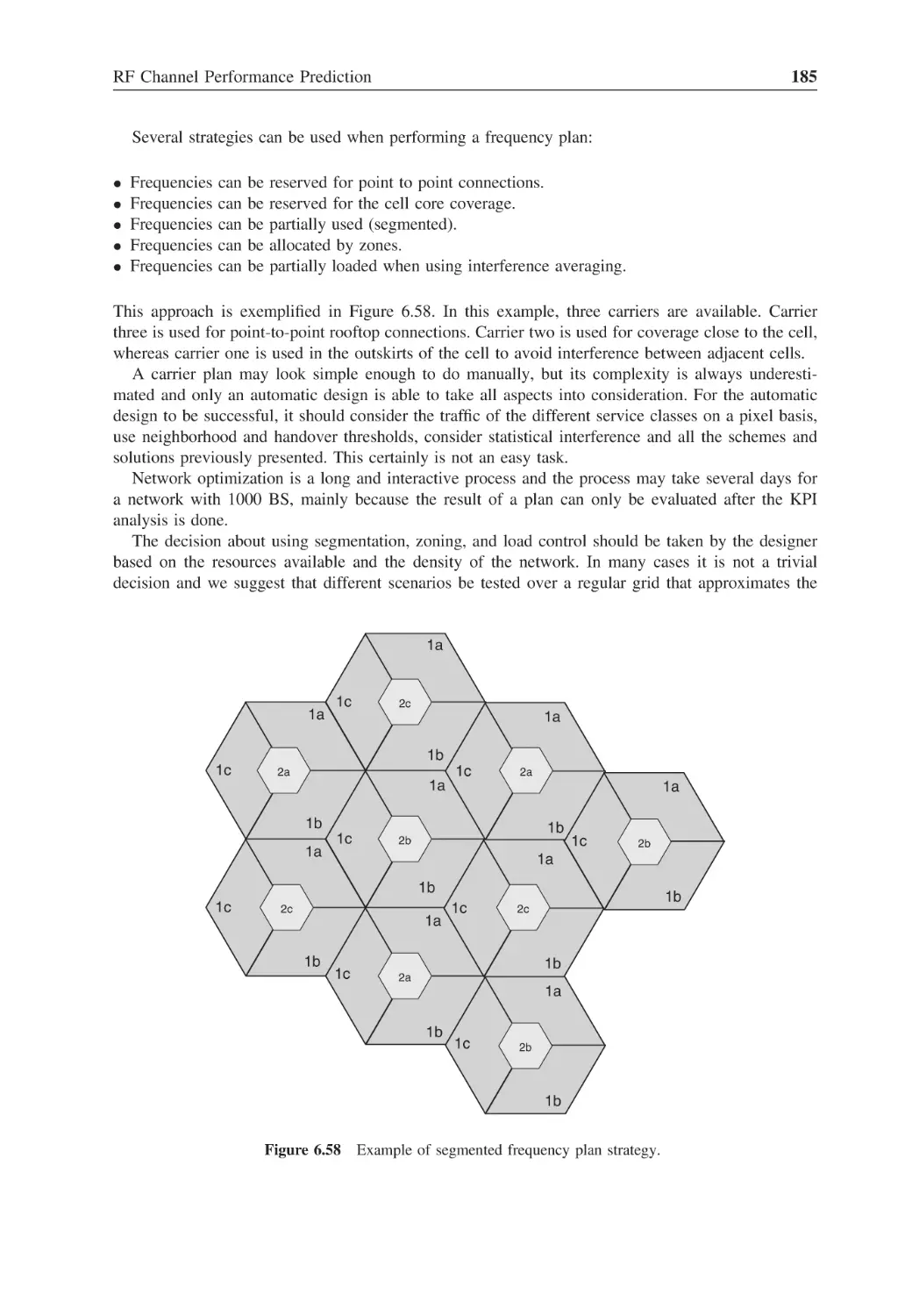
Figure 6.58
Example of segmented frequency plan strategy
185
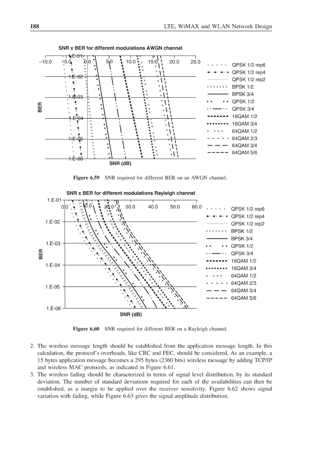
Figure 6.59
SNR required for different BER on an AWGN channel
188
Figure 6.60
SNR required for different BER on a Rayleigh channel
188
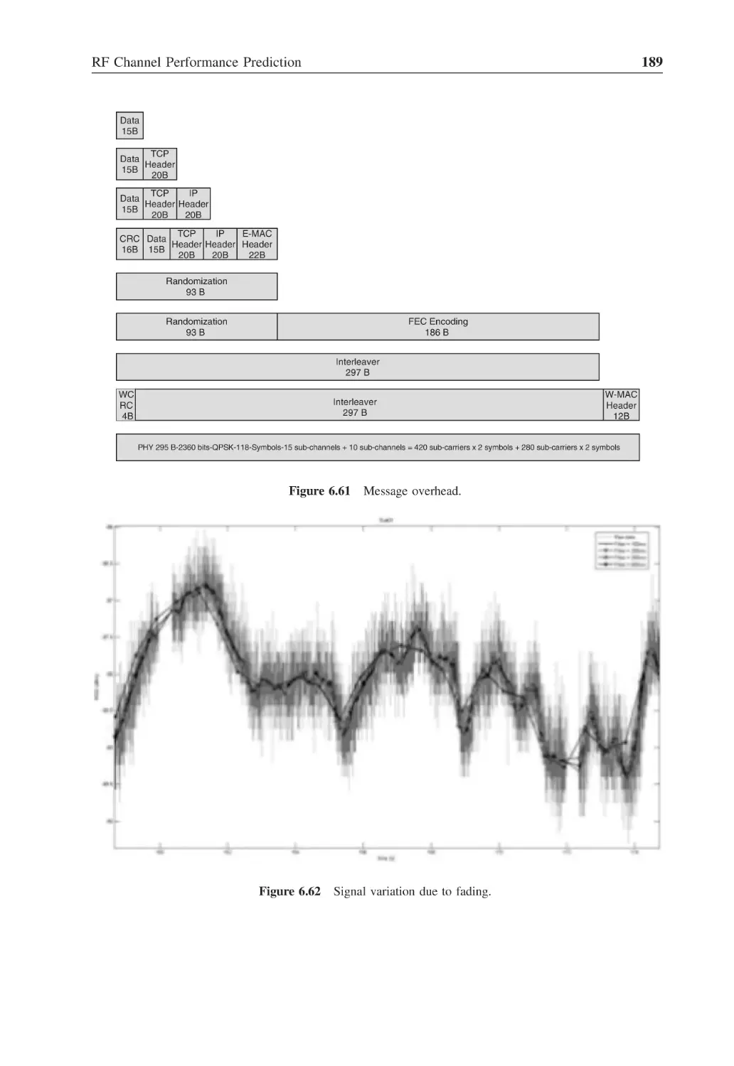
Figure 6.61
Message overhead
189
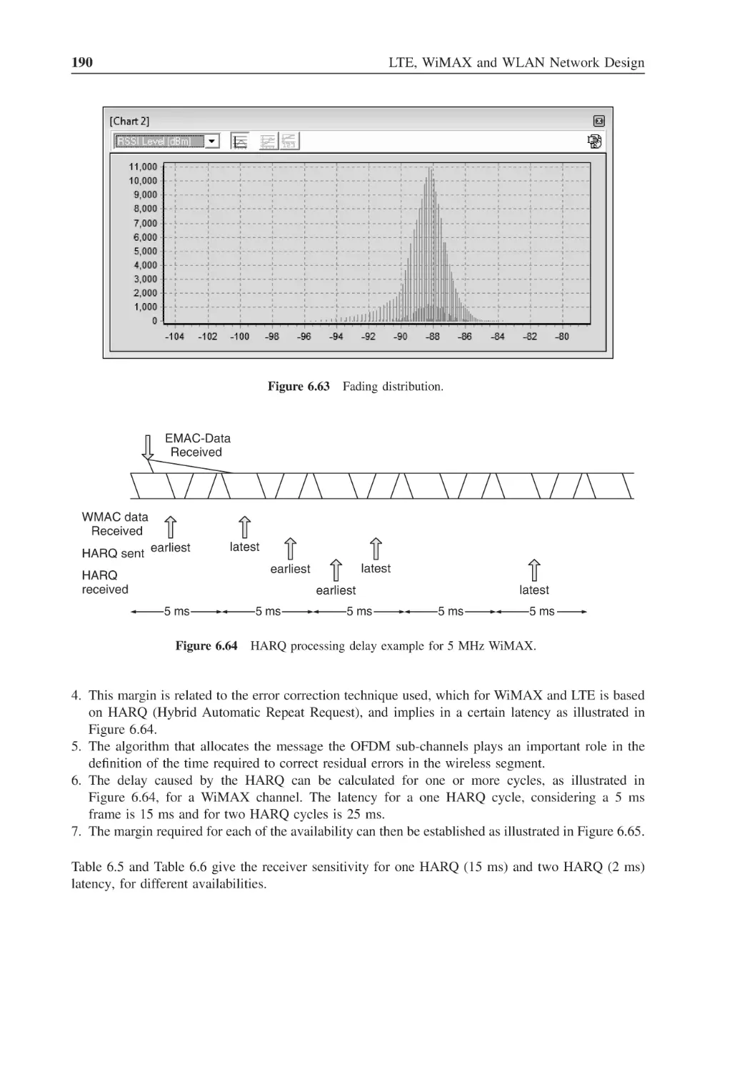
Figure 6.62
Signal variation due to fading
189
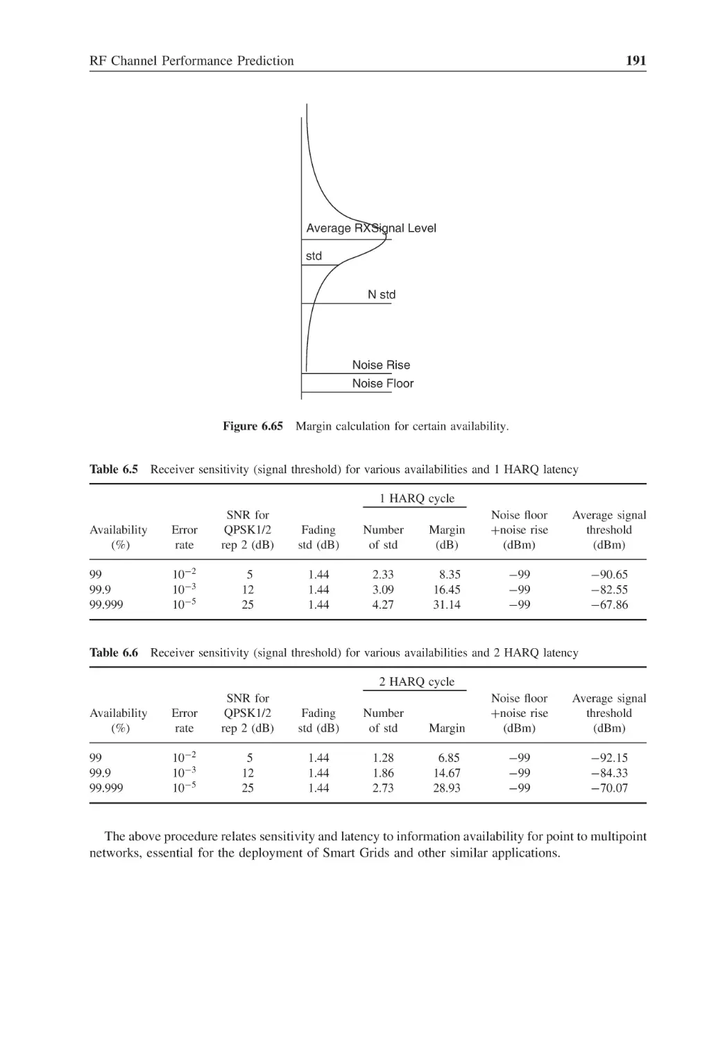
Figure 6.63
Fading distribution
190
Figure 6.64
HARQ processing delay example for 5 MHz WiMAX
190
Figure 6.65
Margin calculation for certain availability
191
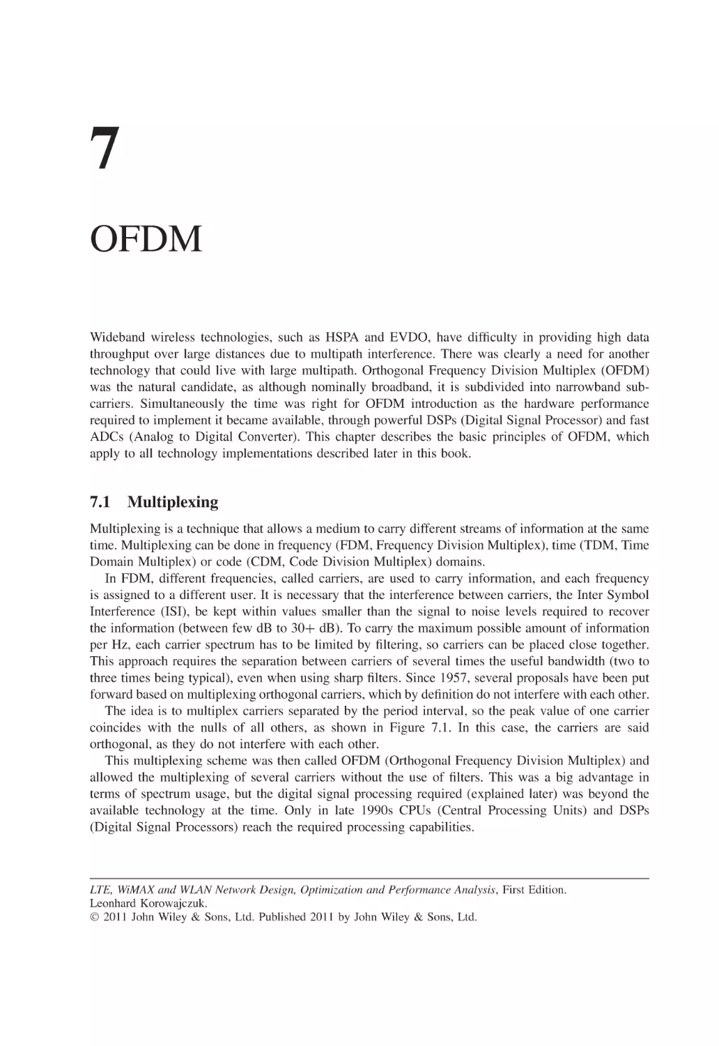
Figure 7.1
Five subcarriers forming an OFDM carrier
194
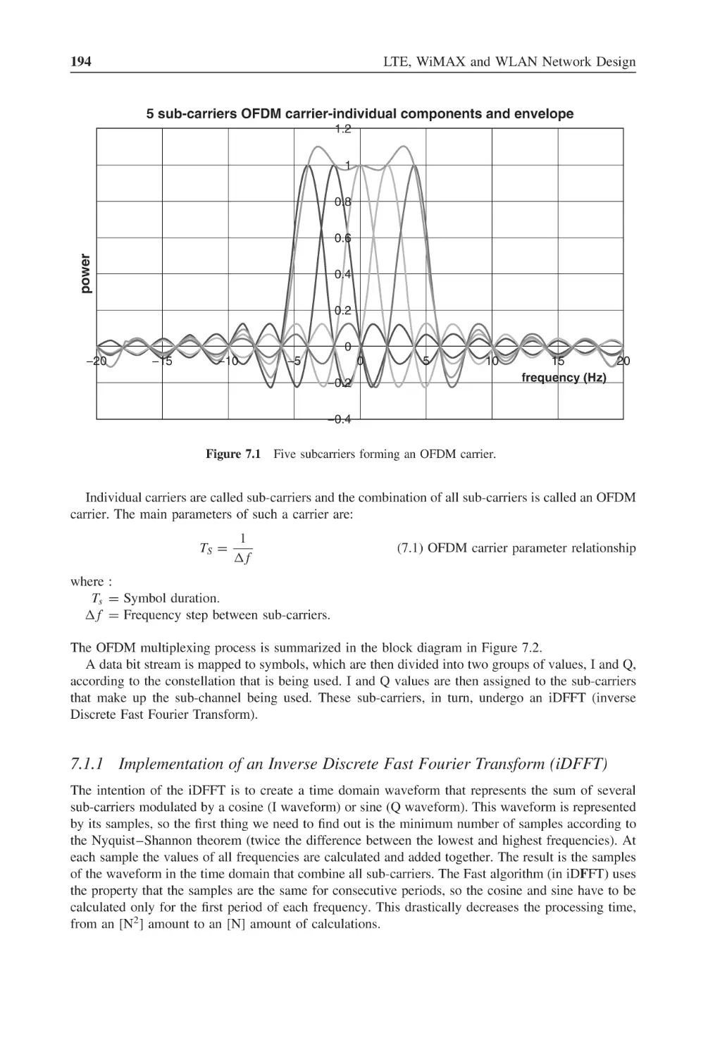
Figure 7.2
Multiplexing and de-multiplexing I and Q streams
195
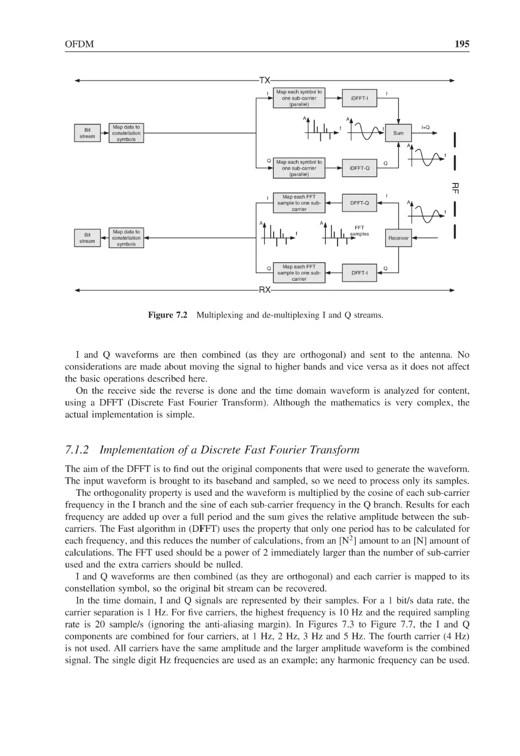
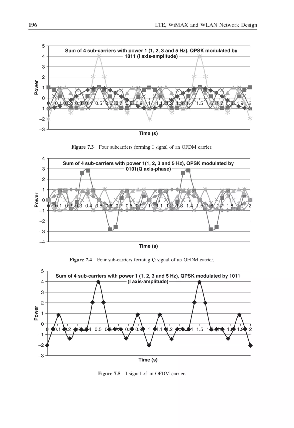
Figure 7.3
Four subcarriers forming I signal of an OFDM carrier
196
Figure 7.4
Four sub-carriers forming Q signal of an OFDM carrier
196
Figure 7.5
I signal of an OFDM carrier
196
Figure 7.6
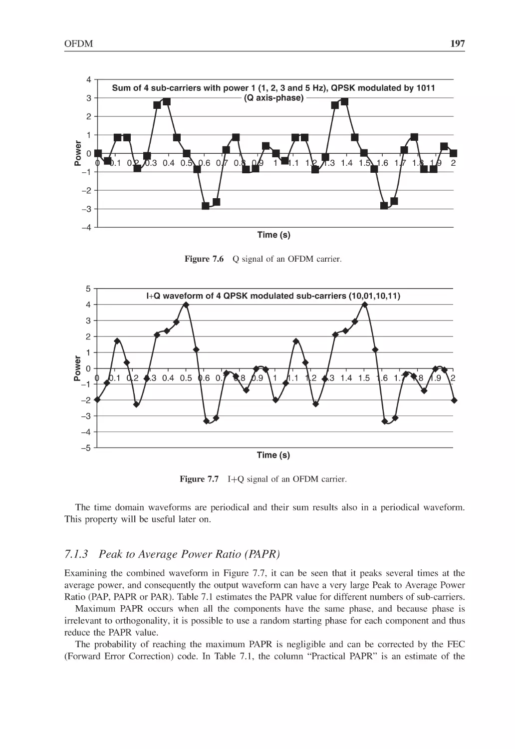
Q signal of an OFDM carrier
197
Figure 7.7
I+Q signal of an OFDM carrier
197
Figure 7.8
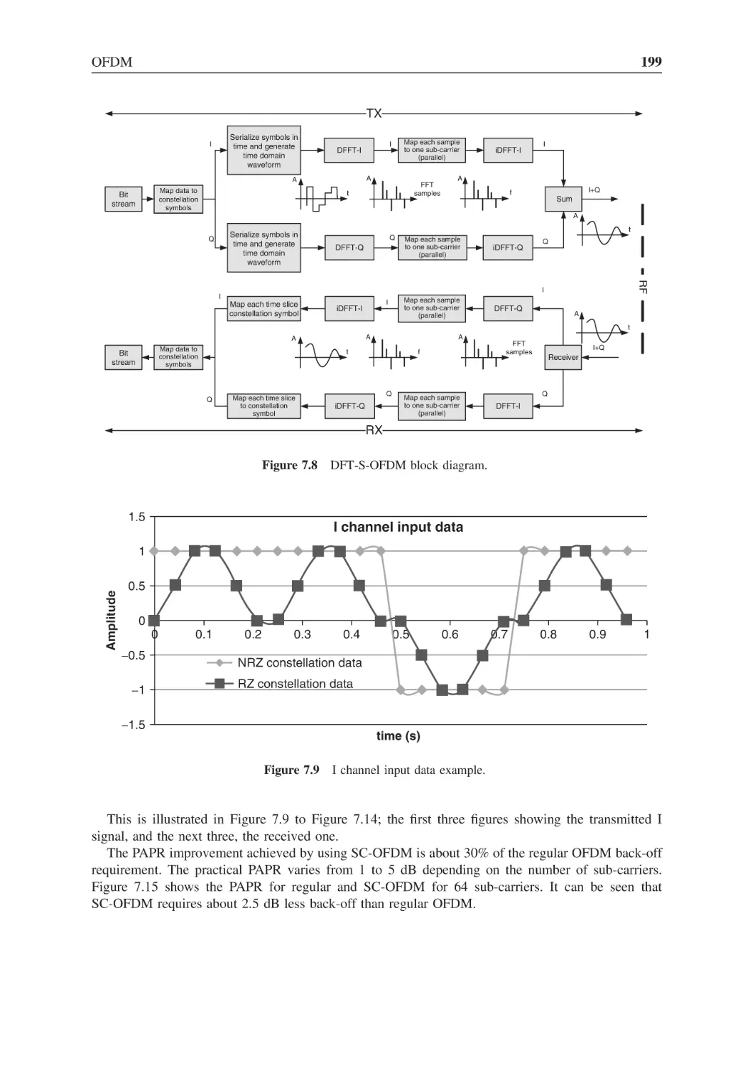
DFT-S-OFDM block diagram
199
Figure 7.9
I channel input data example
199
Figure 7.10
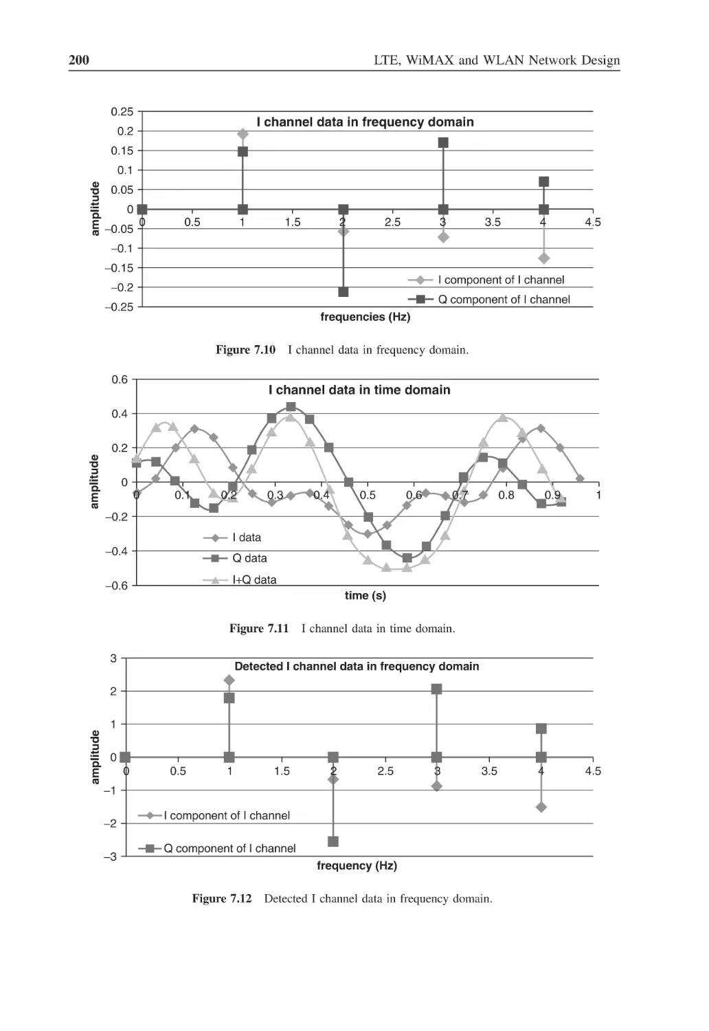
I channel data in frequency domain
200
Figure 7.11
I channel data in time domain
200
Figure 7.12
Detected I channel data in frequency domain
200
Figure 7.13
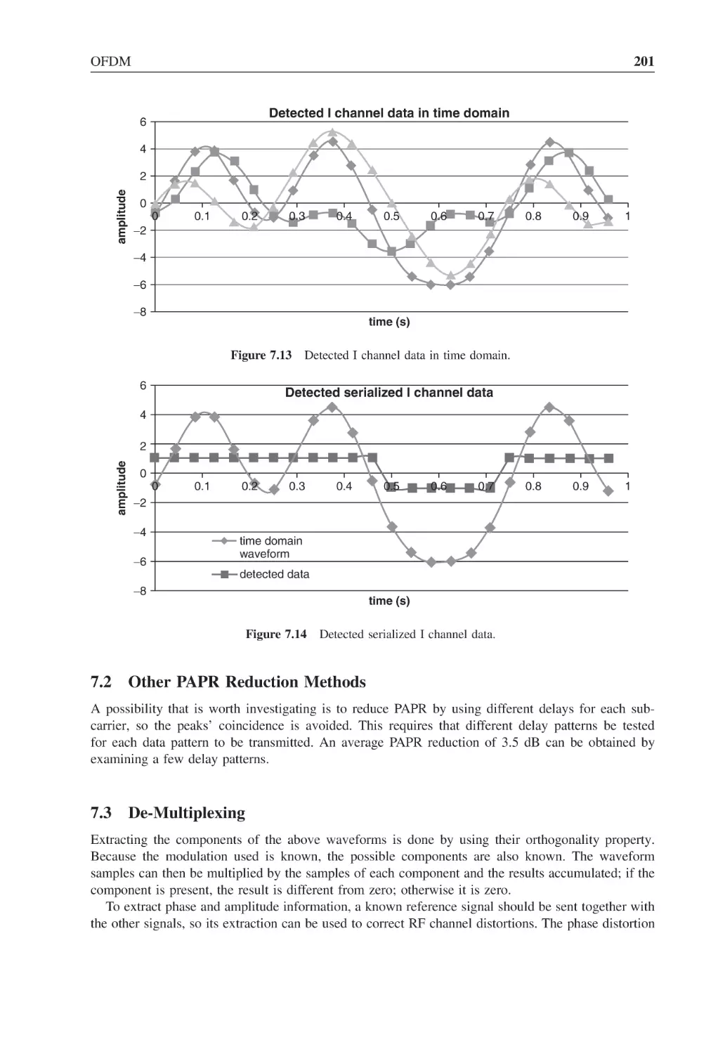
Detected I channel data in time domain
201
Figure 7.14
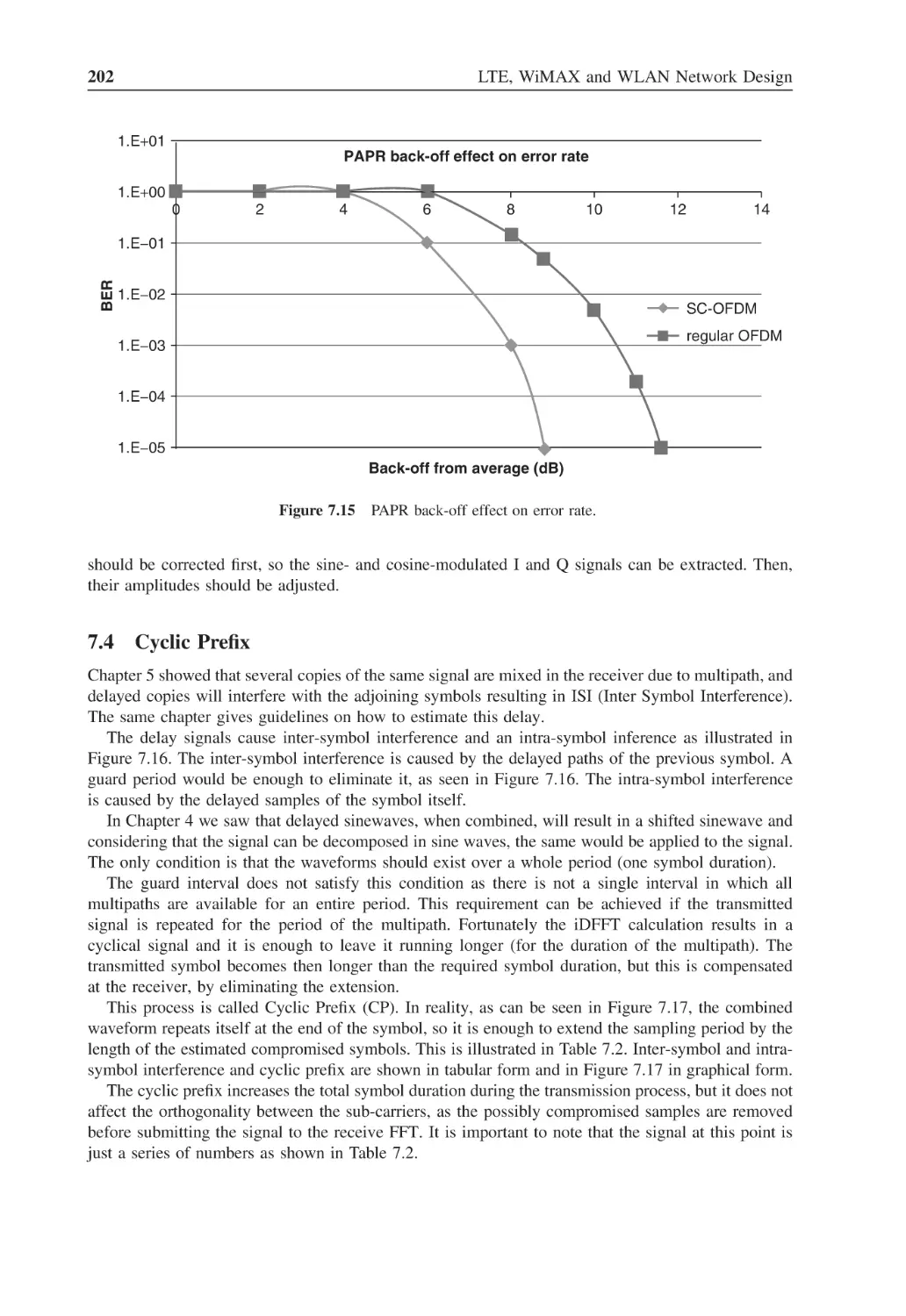
Detected serialized I channel data
201
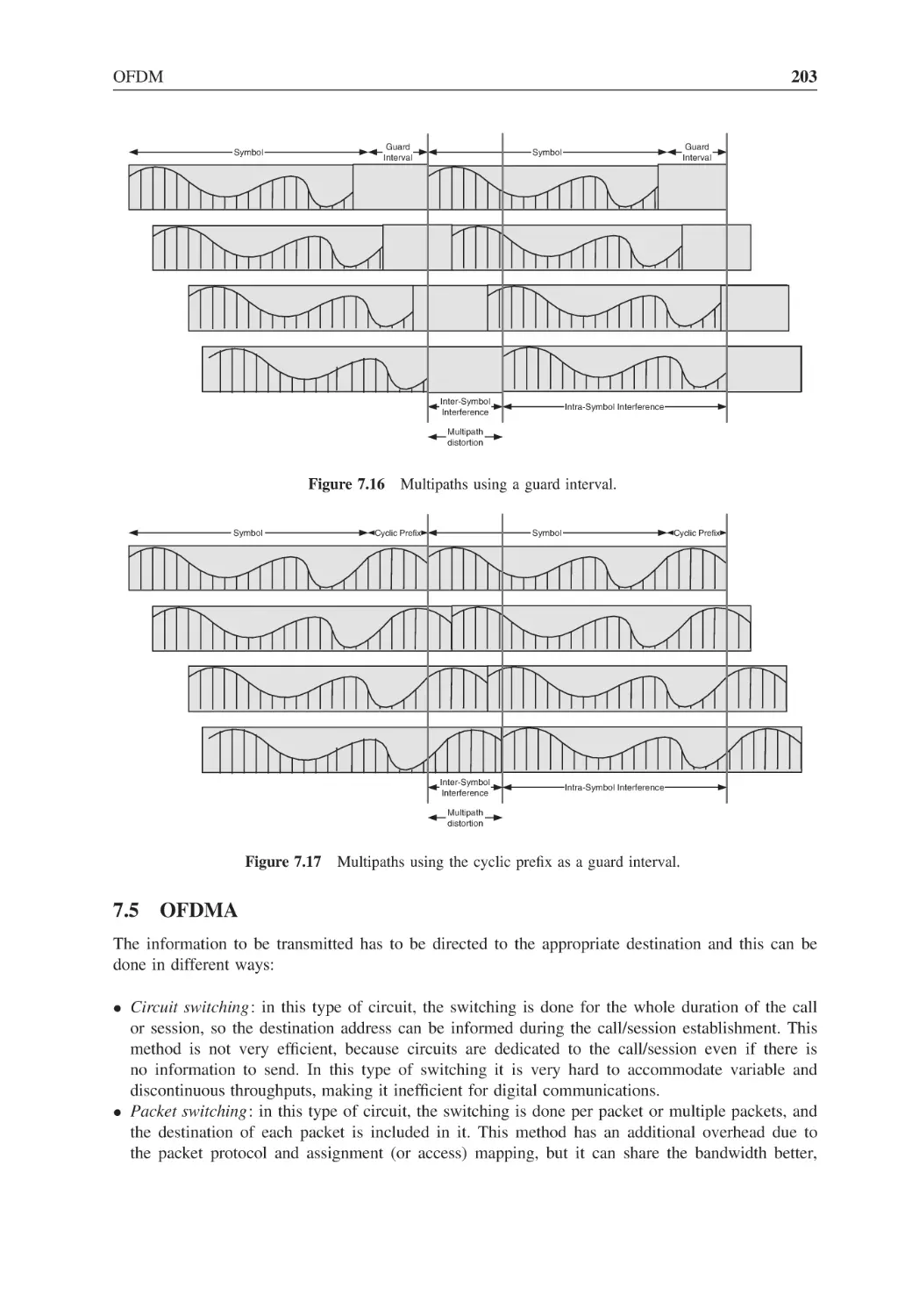
Figure 7.15
PAPR back-off effect on error rate
202
Figure 7.16
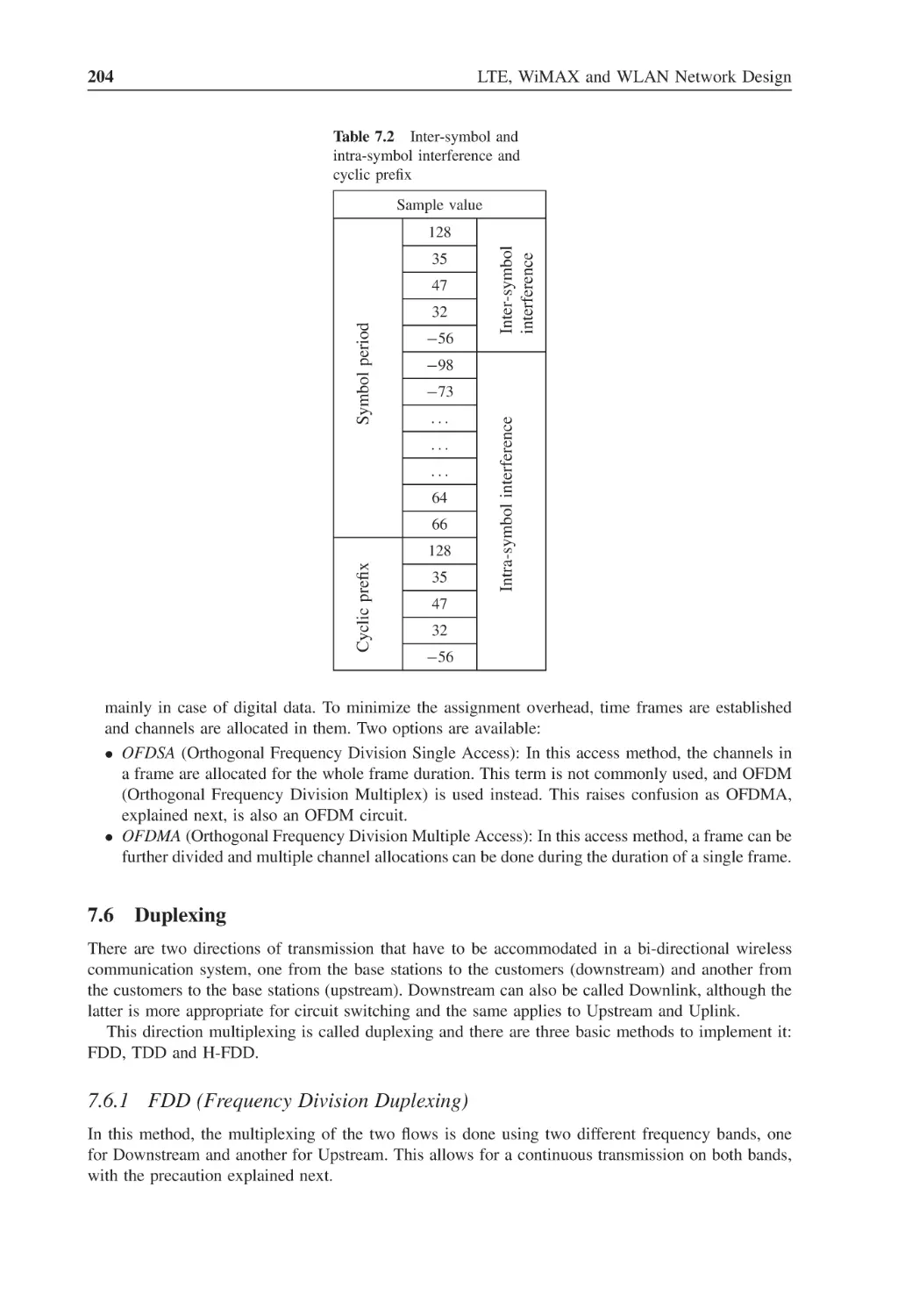
Multipaths using a guard interval
203
Figure 7.17
Multipaths using the cyclic prefix as a guard interval
203
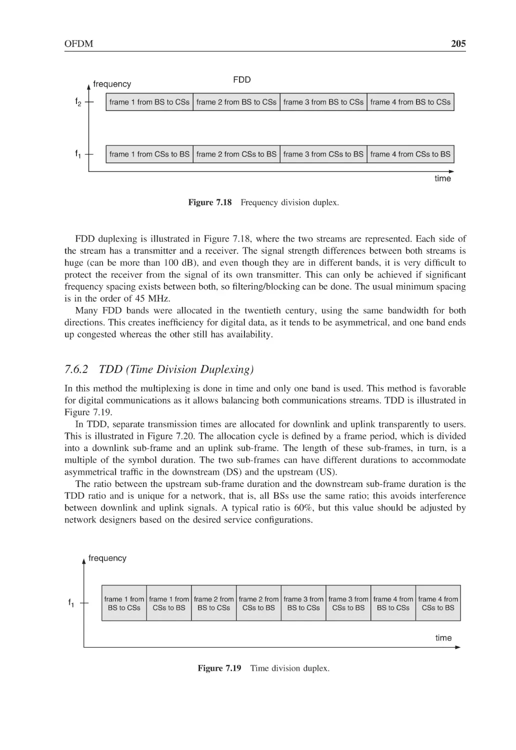
Figure 7.18
Frequency division duplex
205
Figure 7.19
Time division duplex
205
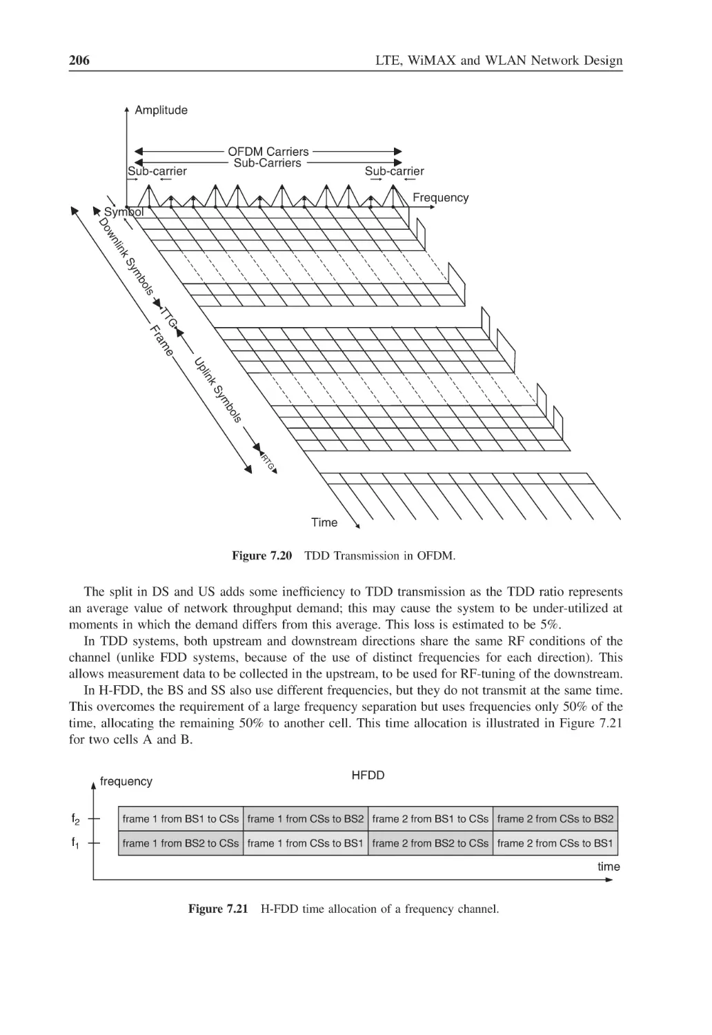
Figure 7.20
TDD Transmission in OFDM
206
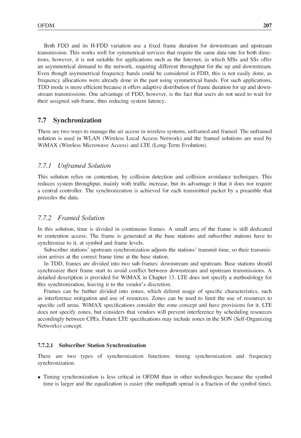
Figure 7.21
H-FDD time allocation of a frequency channel
206
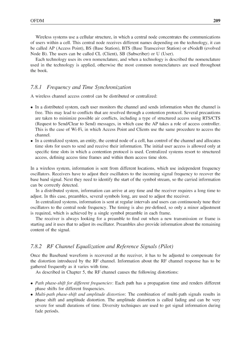
Figure 7.22
Transmit I sub-carriers and composite signal, I signal
211
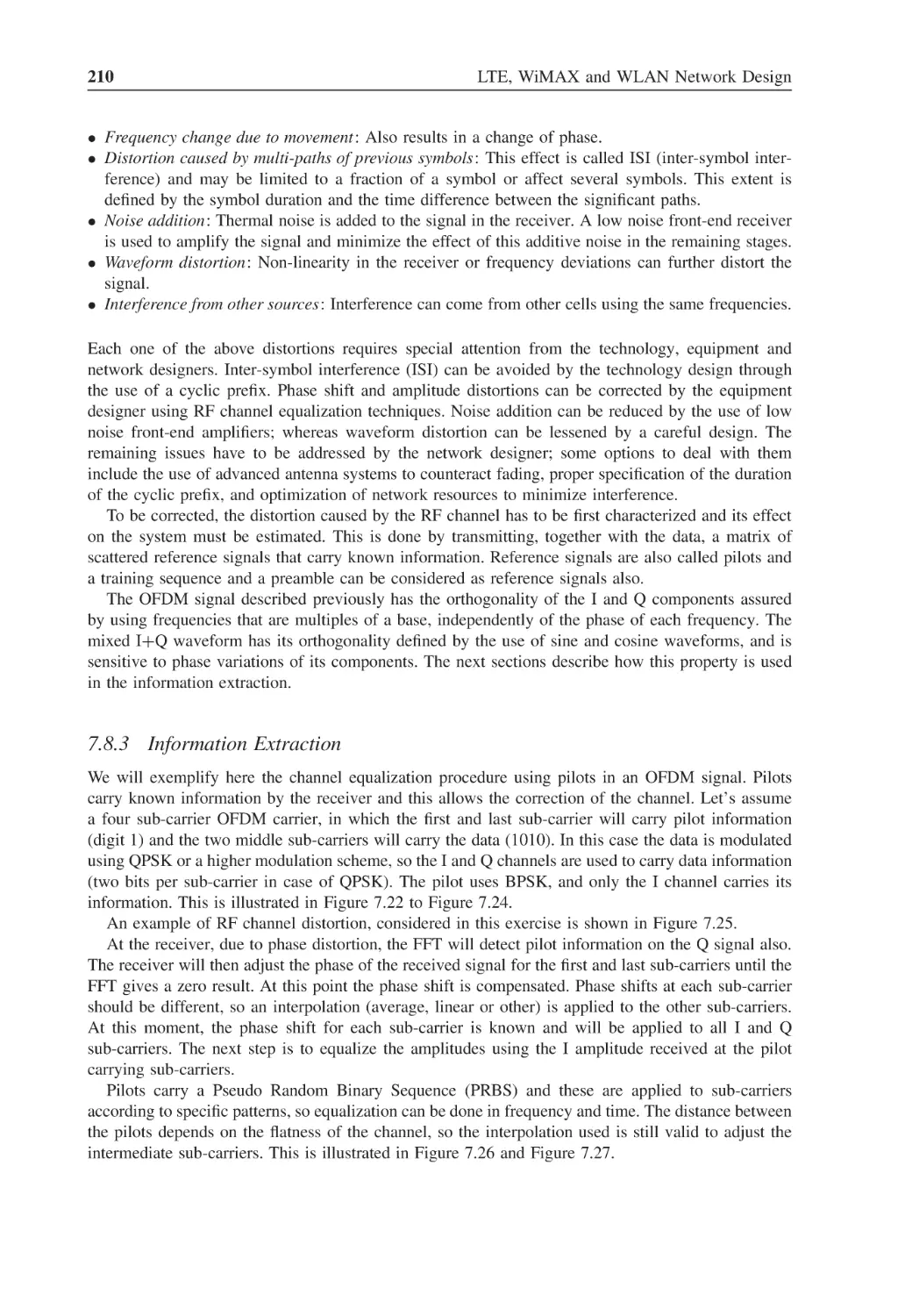
Figure 7.23
Transmit I sub-carriers and composite signal, Q signal
211
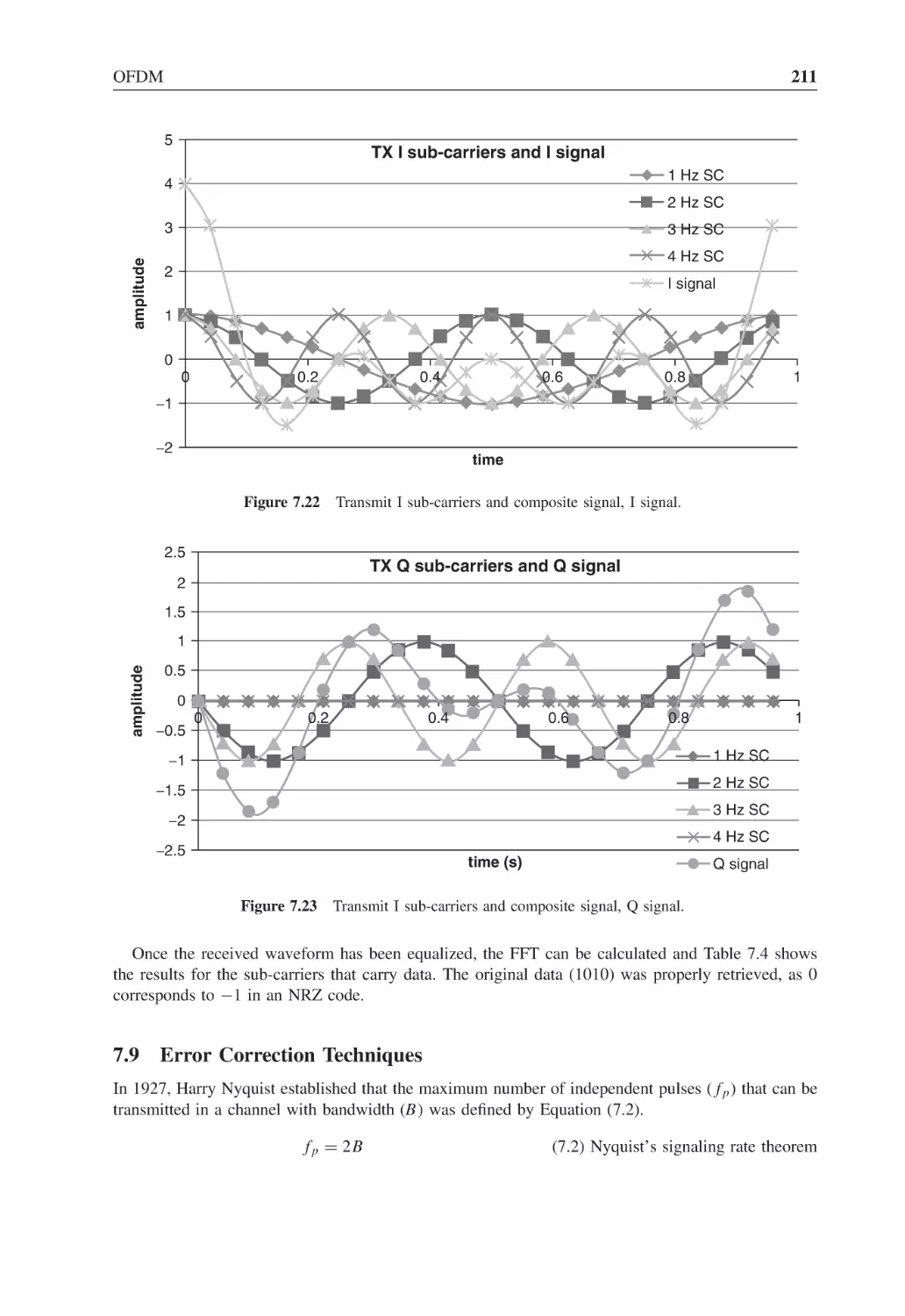
Figure 7.24
I+Q transmit signal, received multipaths and received
composed waveform
212
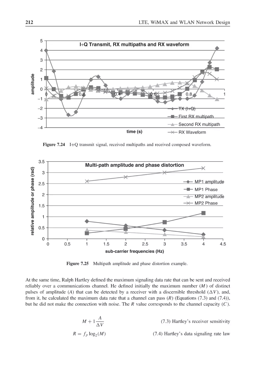
Multipath amplitude and phase distortion example
212
Figure 7.25
xxiv
List of Figures
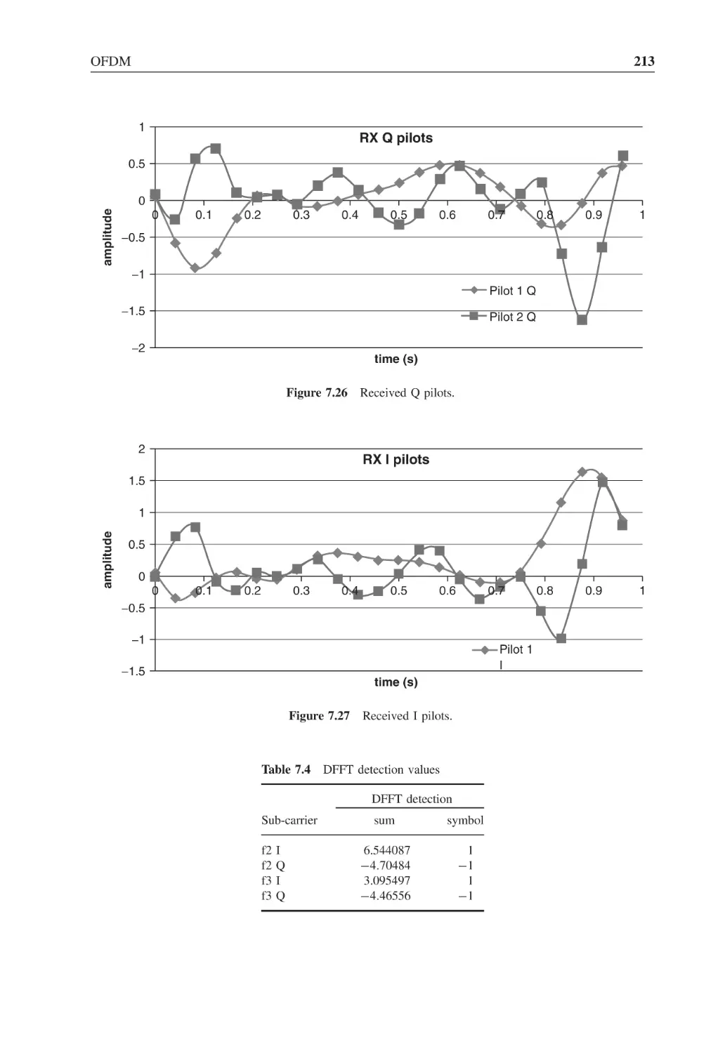
Figure 7.26
Received Q pilots
213
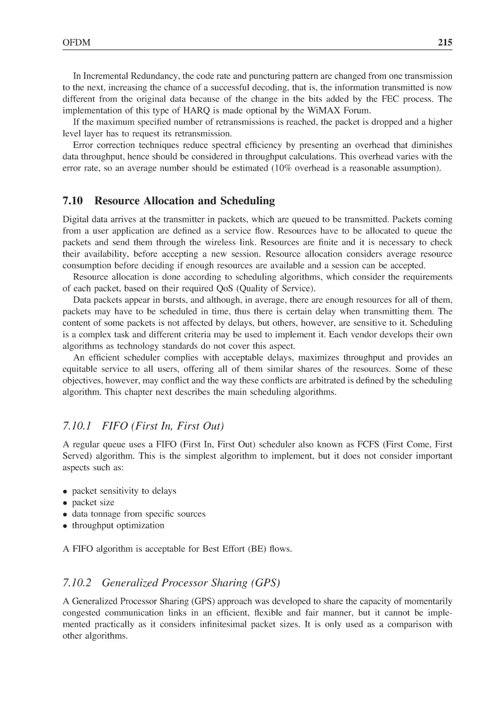
Figure 7.27
Received I pilots
213
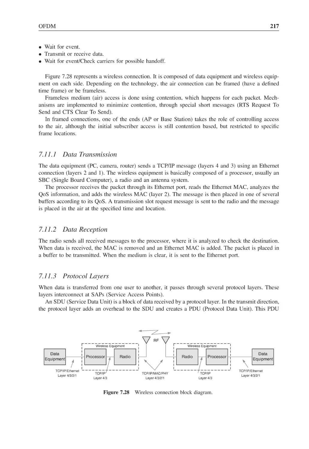
Figure 7.28
Wireless connection block diagram
217
Figure 7.29
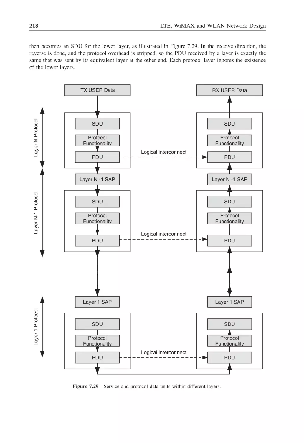
Service and protocol data units within different layers
218
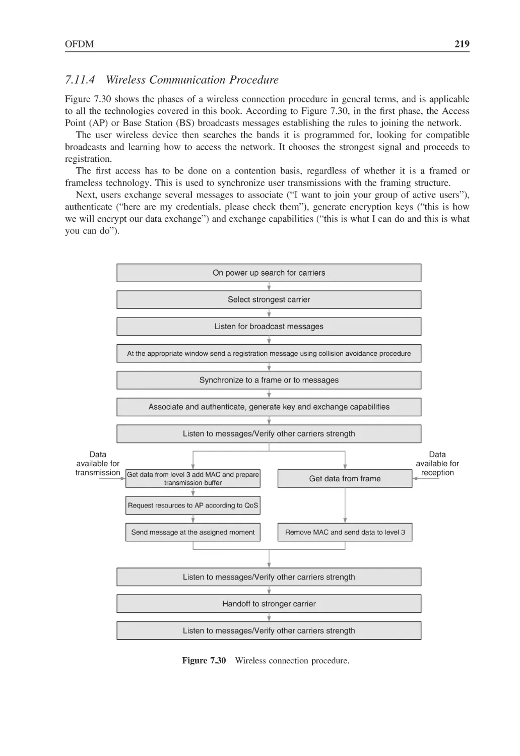
Figure 7.30
Wireless connection procedure
219
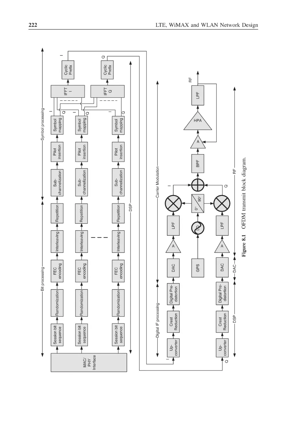
Figure 8.1
OFDM transmit block diagram
222
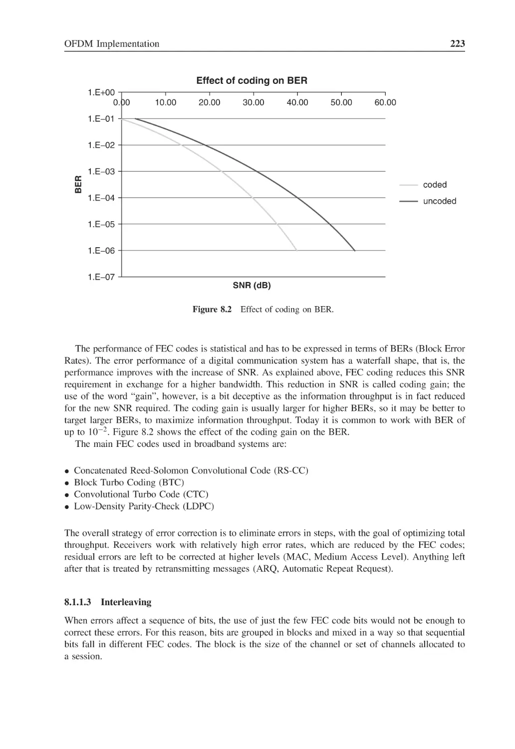
Figure 8.2
Effect of coding on BER
223
Figure 8.3
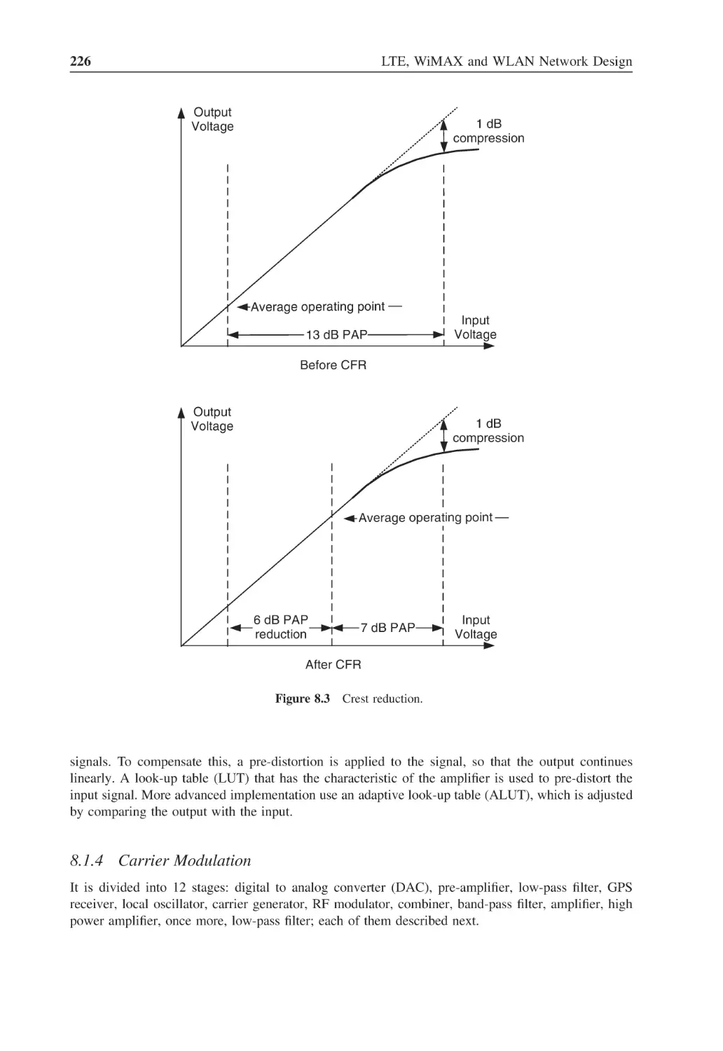
Crest reduction
226
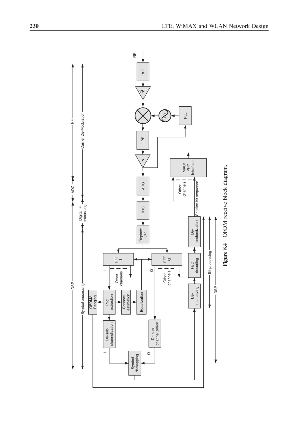
Figure 8.4
OFDM receive block diagram
230
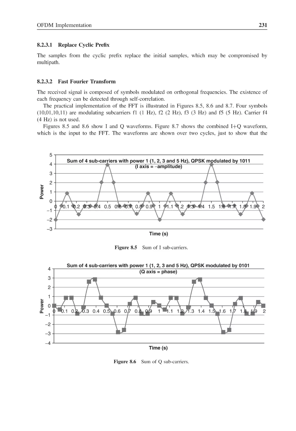
Figure 8.5
Sum of I sub-carriers
231
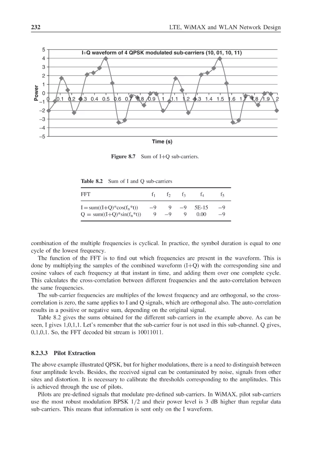
Figure 8.6
Sum of Q sub-carriers
231
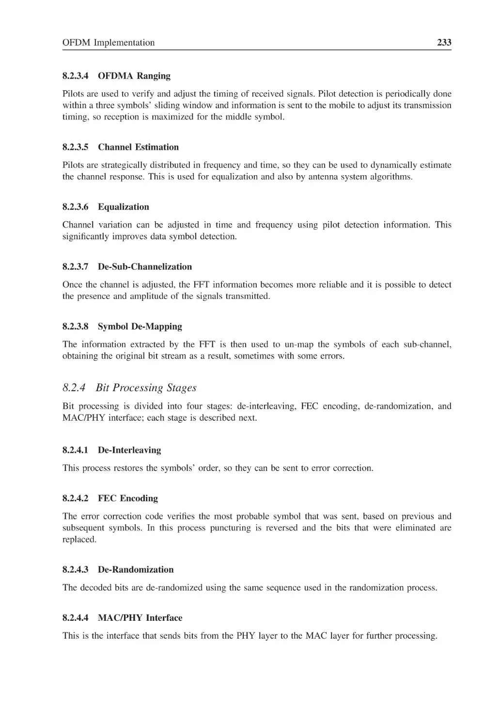
Figure 8.7
Sum of I + Q sub-carriers
232
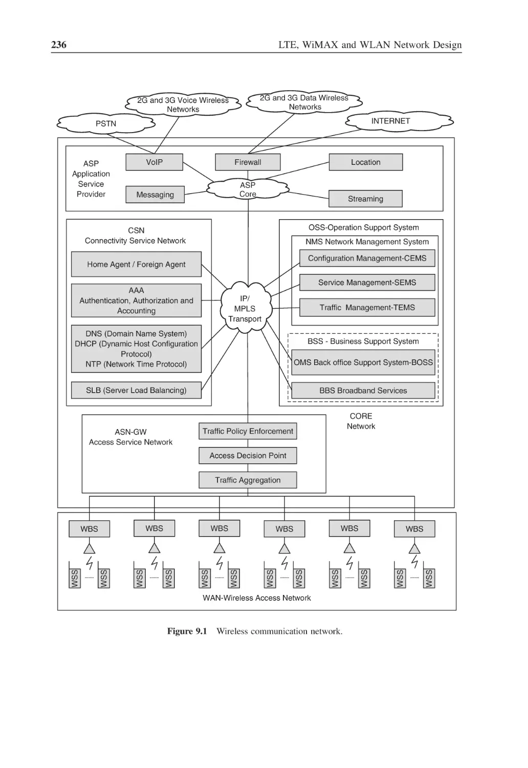
Figure 9.1
Wireless communication network
236
Figure 9.2
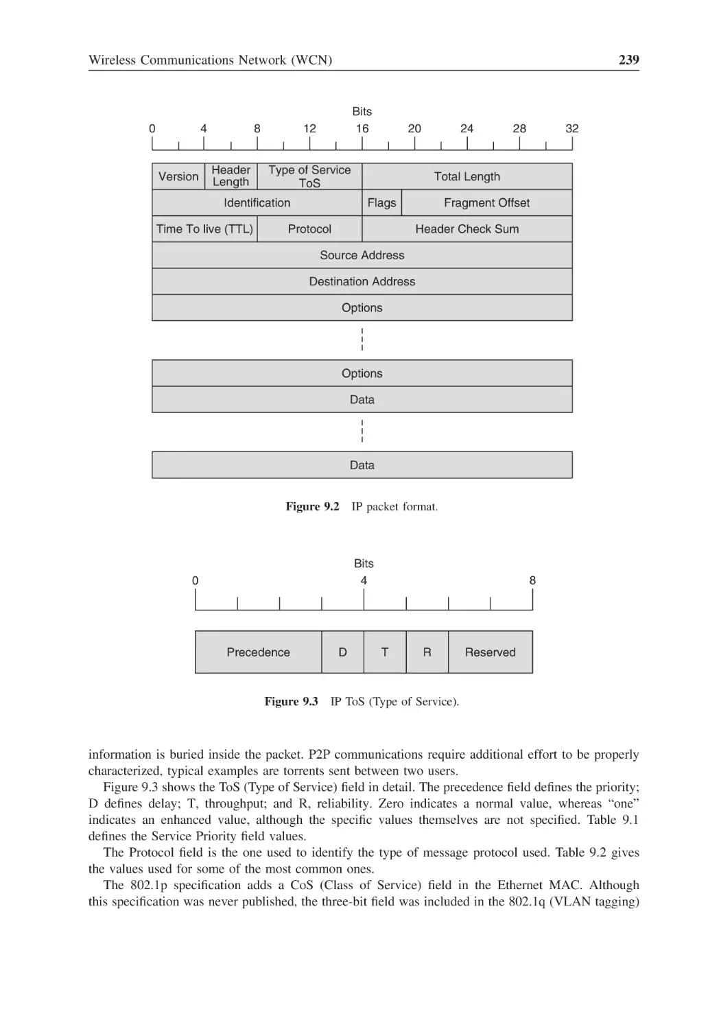
IP packet format
239
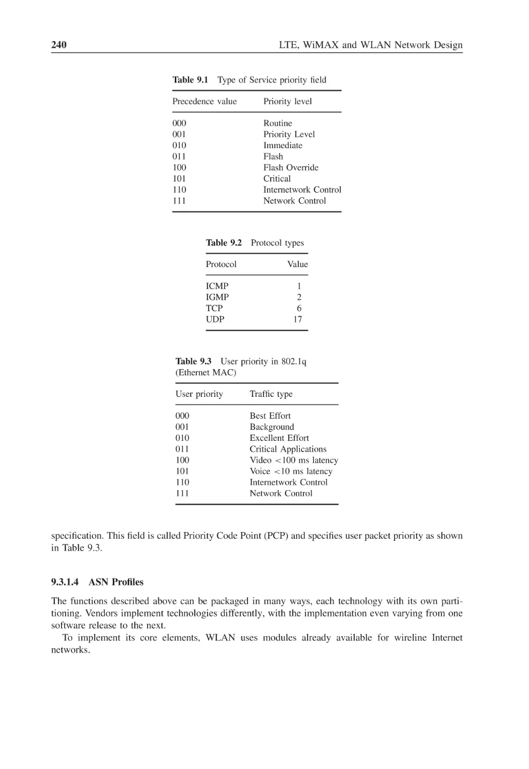
Figure 9.3
IP ToS (Type of Service)
239
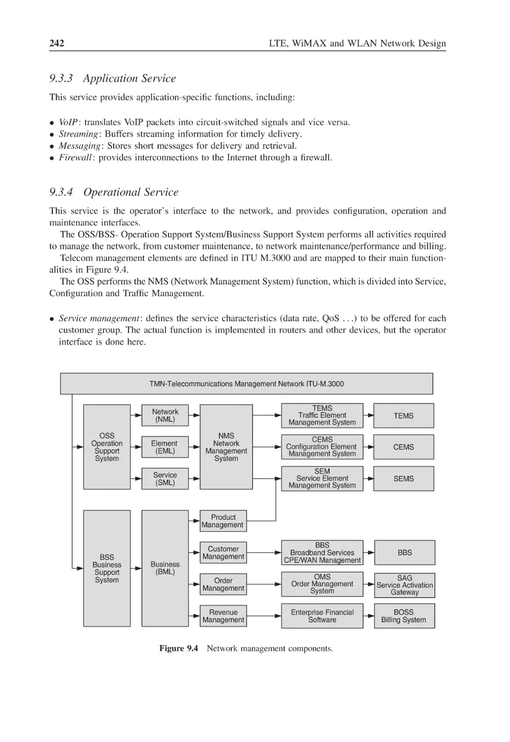
Figure 9.4
Network management components
242
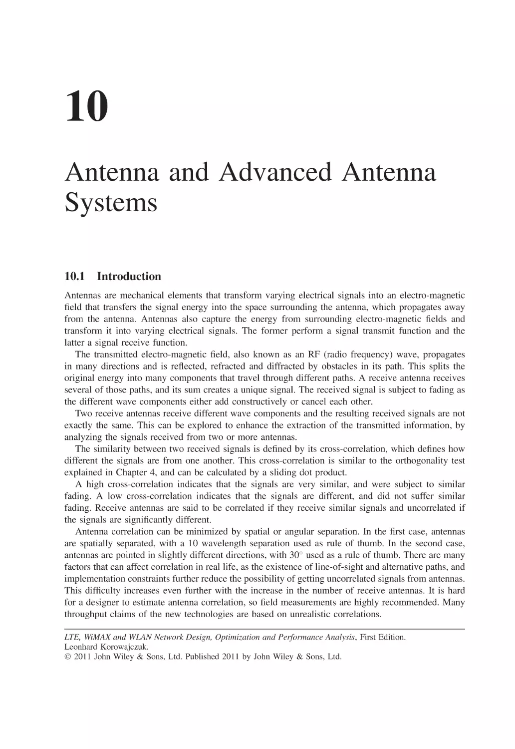
Figure 10.1
RF energy transmission
246
Figure 10.2
Electric field
247
Figure 10.3
Magnetic field
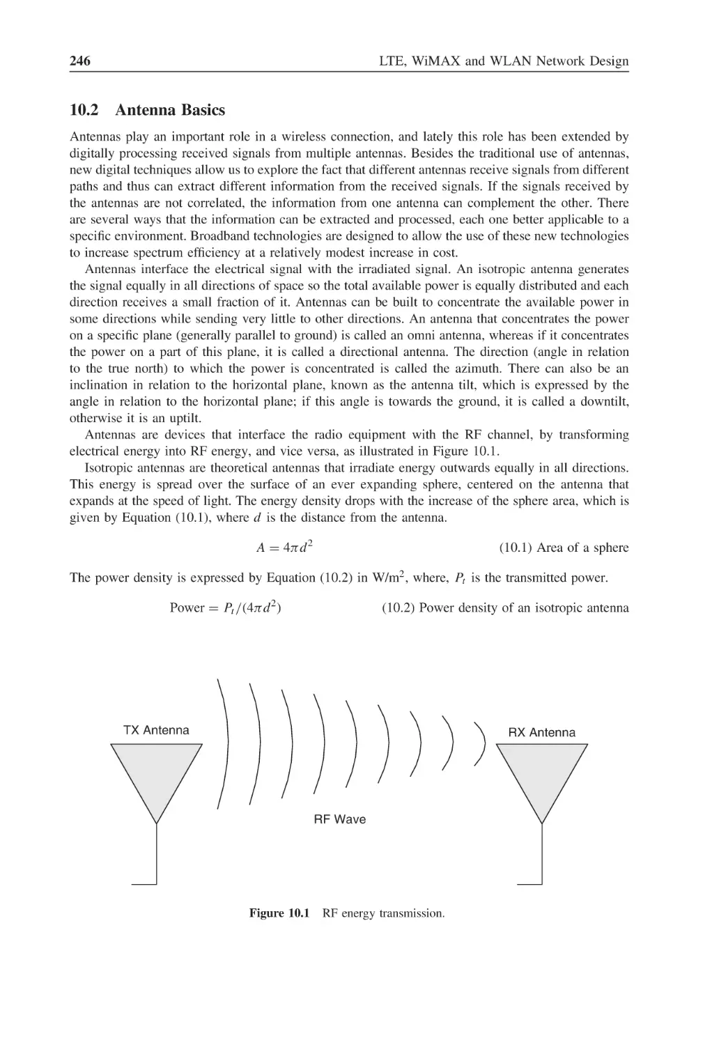
248
Figure 10.4
Antenna radiation fields
248
Figure 10.5
Dipole antenna
249
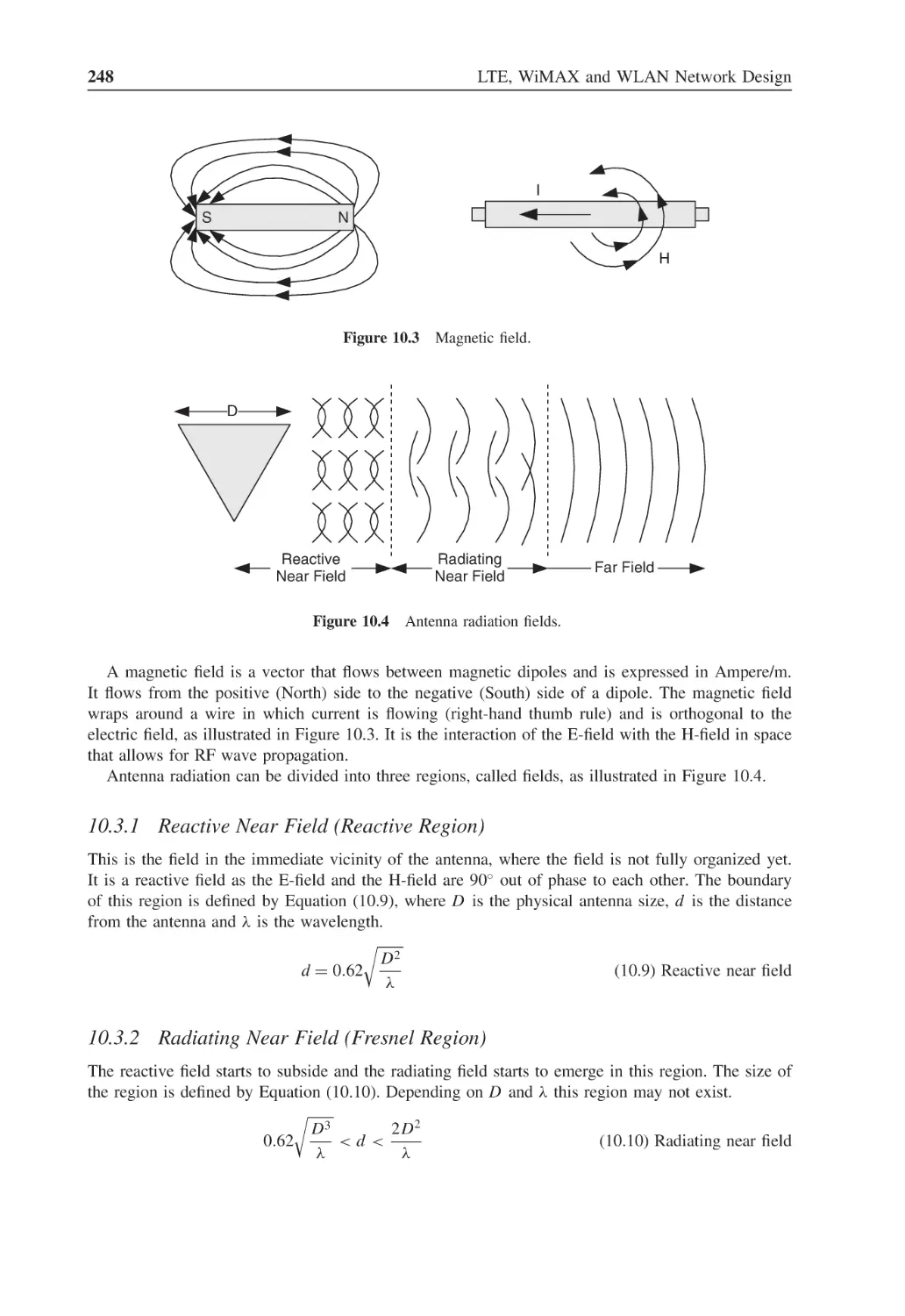
Figure 10.6
Dipole antenna fields
250
Figure 10.7
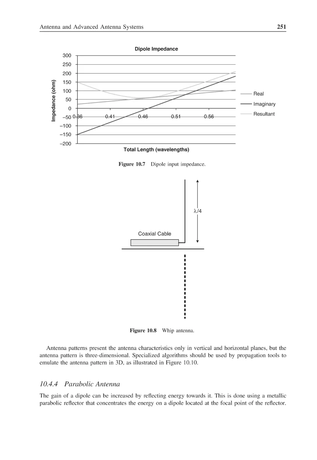
Dipole input impedance
251
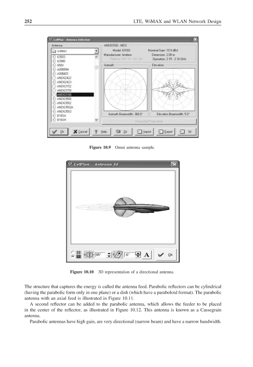
Figure 10.8
Whip antenna
251
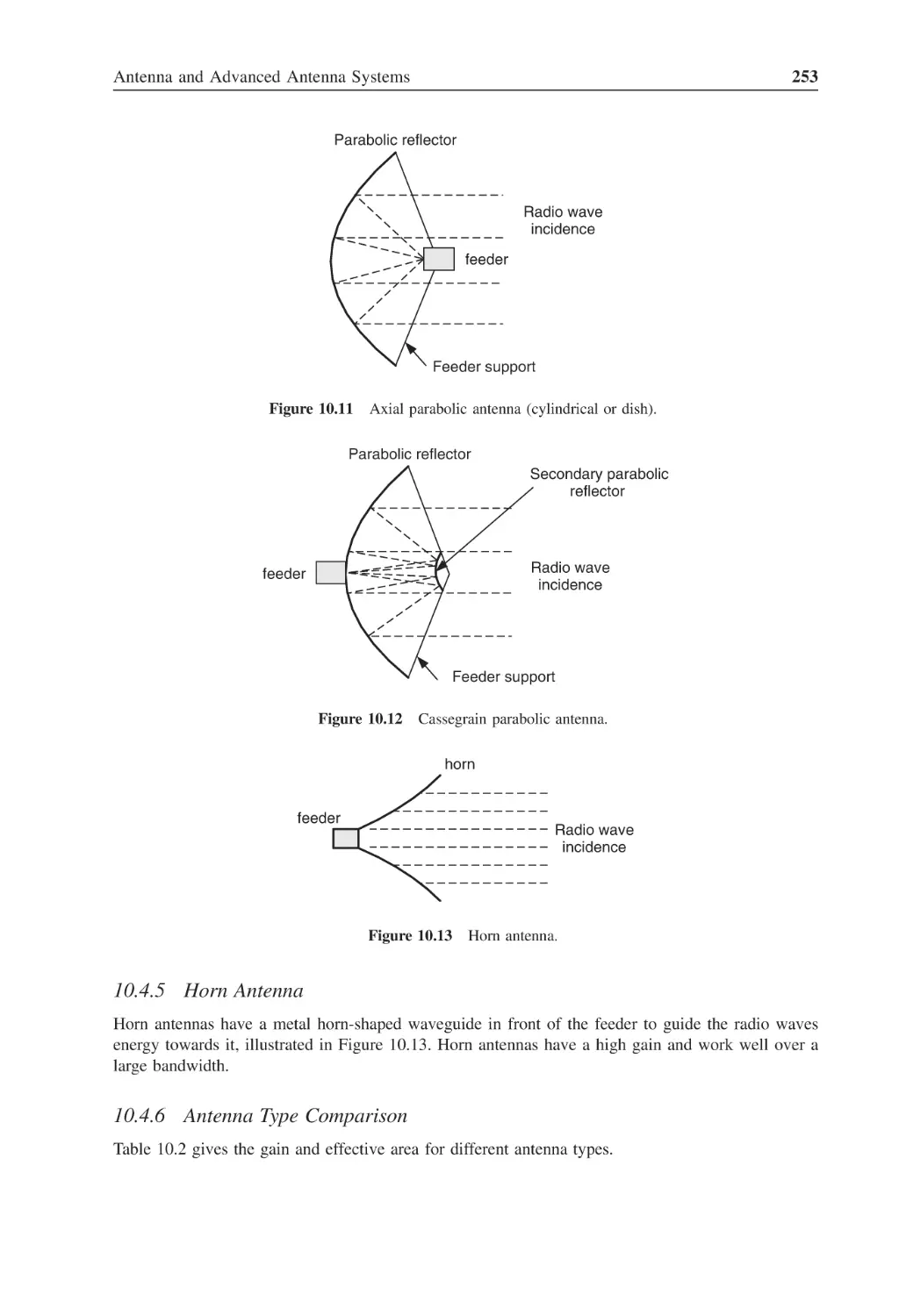
Figure 10.9
Omni antenna sample
252
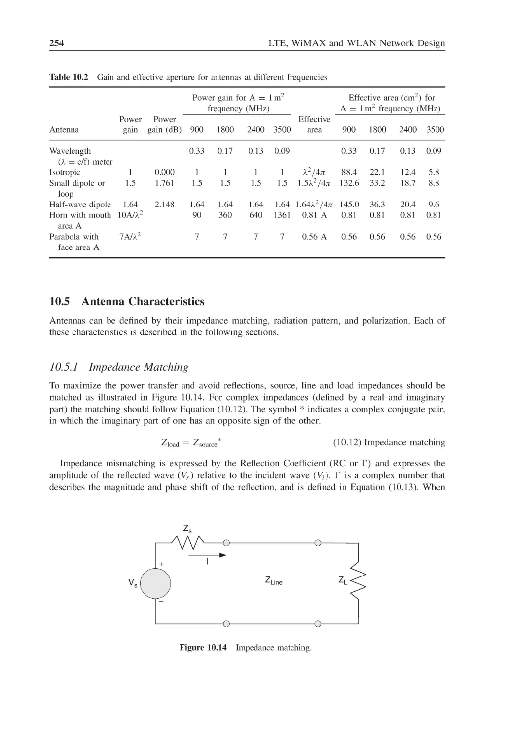
Figure 10.10 3D representation of a directional antenna
252
Figure 10.11 Axial parabolic antenna (cylindrical or dish)
253
Figure 10.12 Cassegrain parabolic antenna
253
Figure 10.13 Horn antenna
253
Figure 10.14 Impedance matching
254
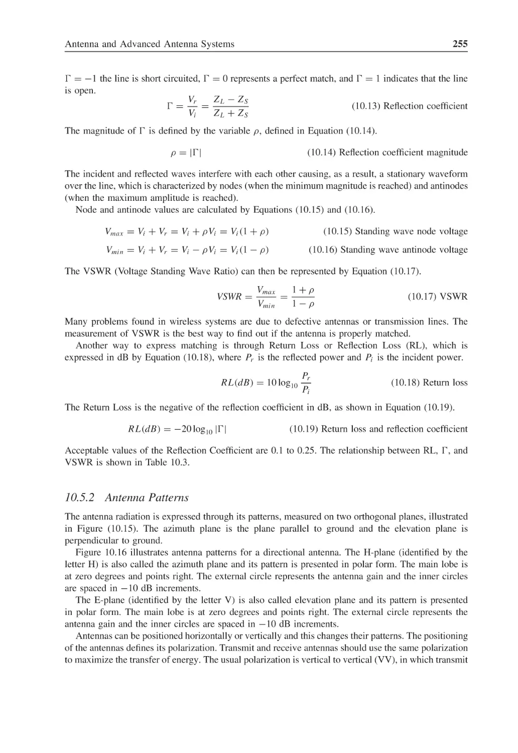
Figure 10.15 Antenna pattern planes
256
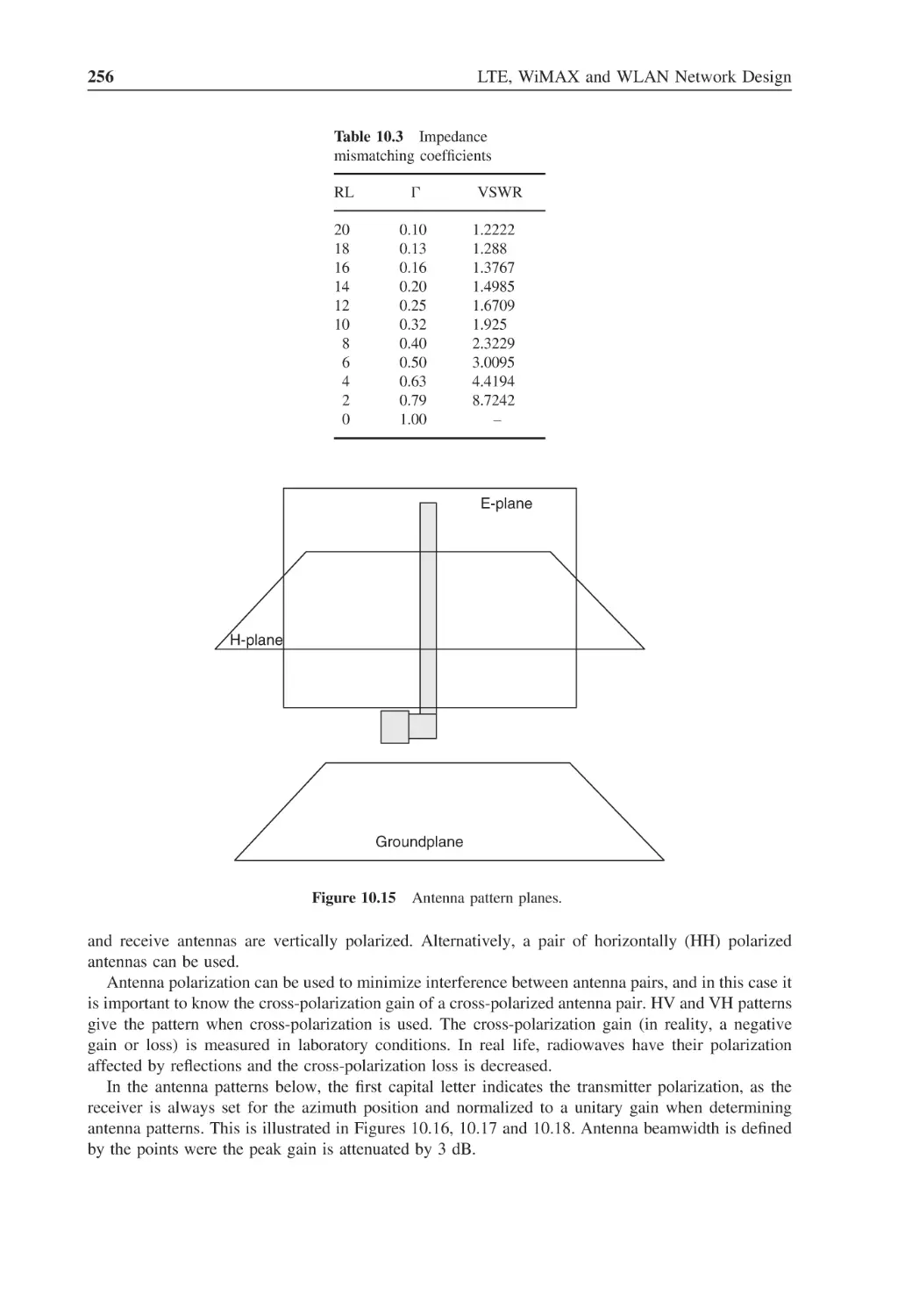
Figure 10.16 Vertical polarization directional antenna pattern sample
257
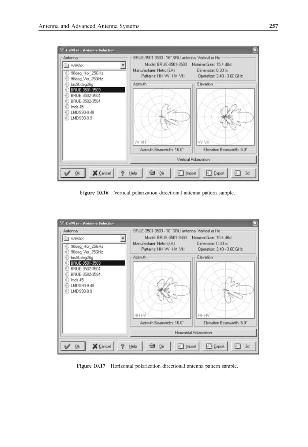
Figure 10.17 Horizontal polarization directional antenna pattern sample
257
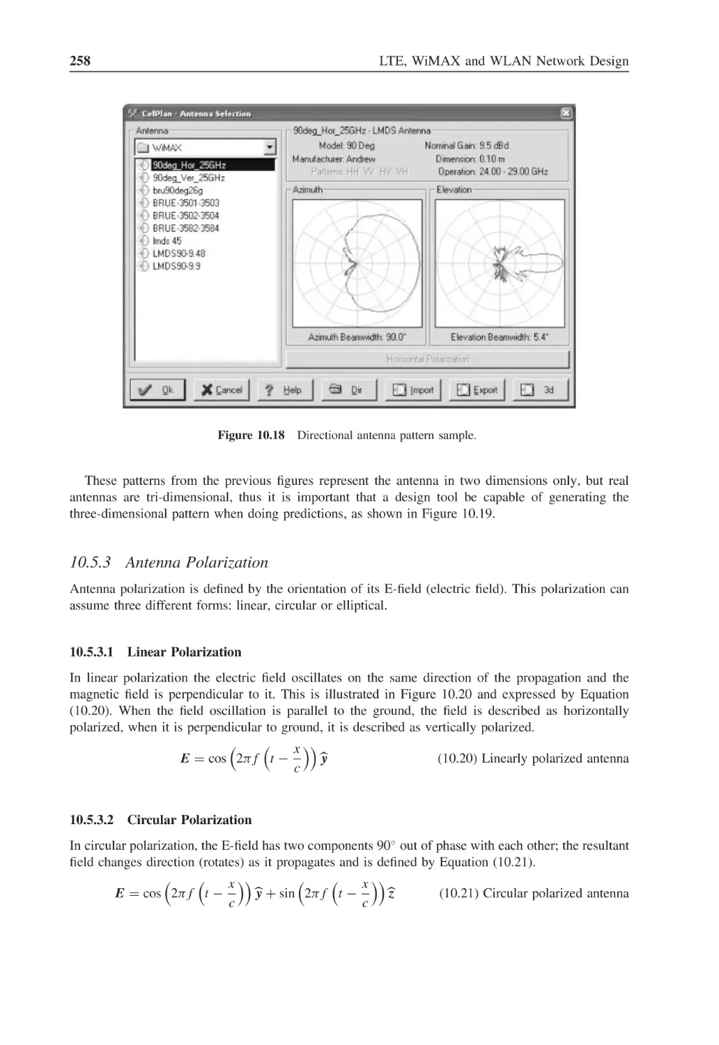
Figure 10.18 Directional antenna pattern sample
258
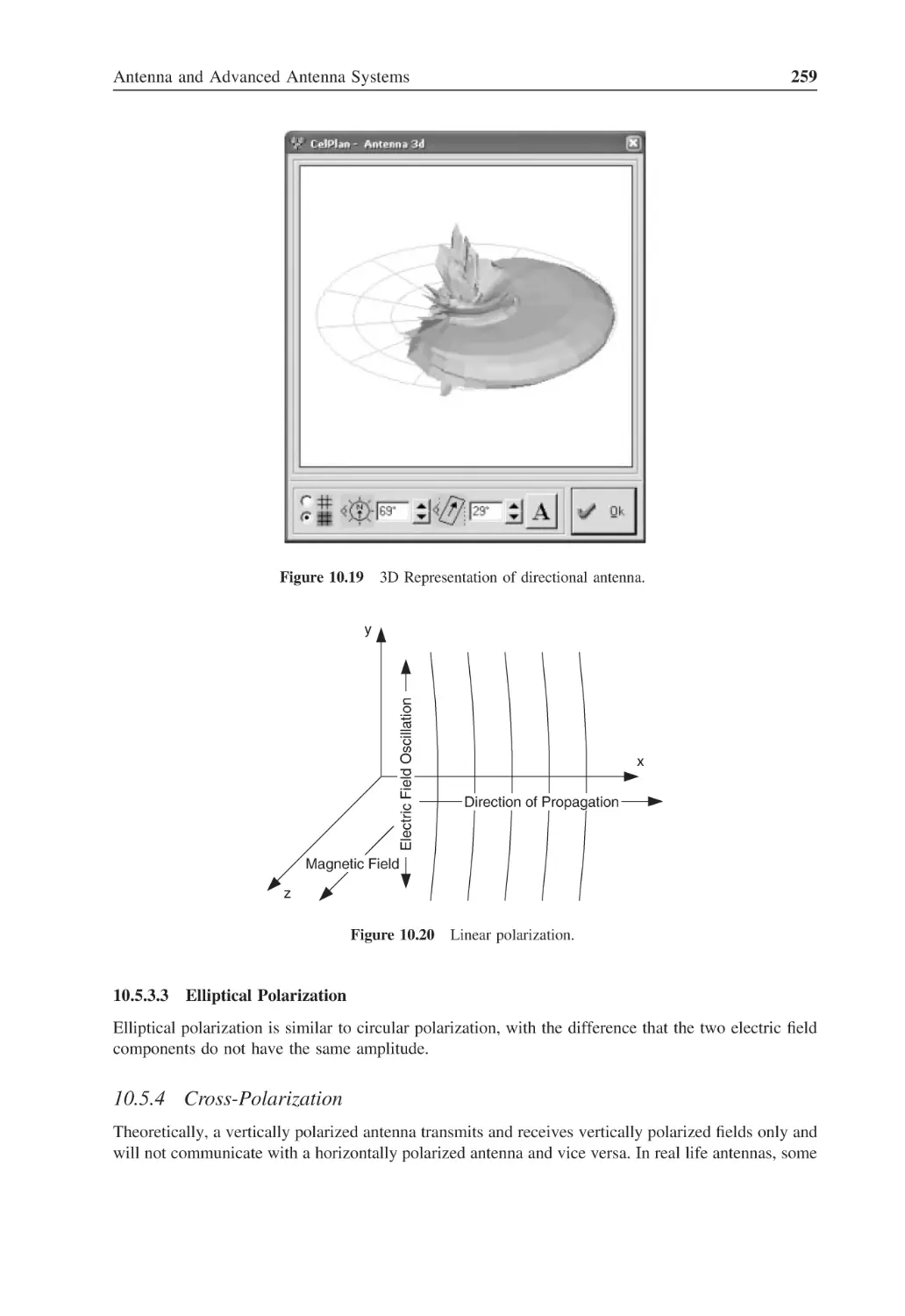
Figure 10.19 3D Representation of directional antenna
259
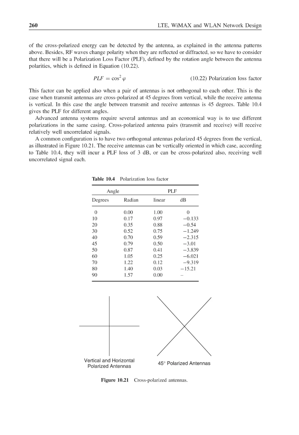
Figure 10.20 Linear polarization
259
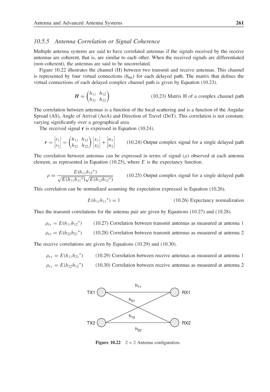
Figure 10.21 Cross-polarized antennas
260
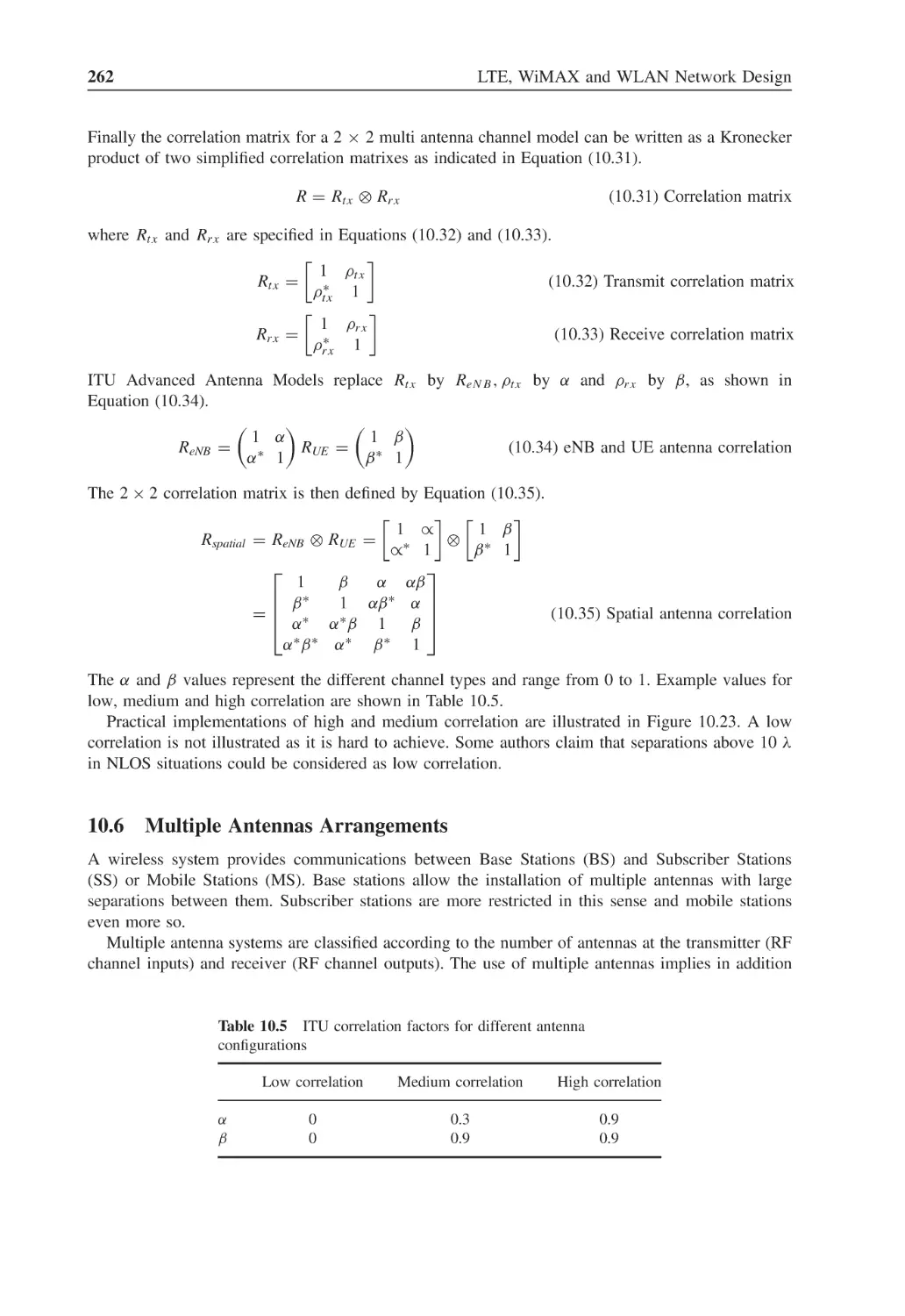
Figure 10.22 2 × 2 Antenna configuration
261
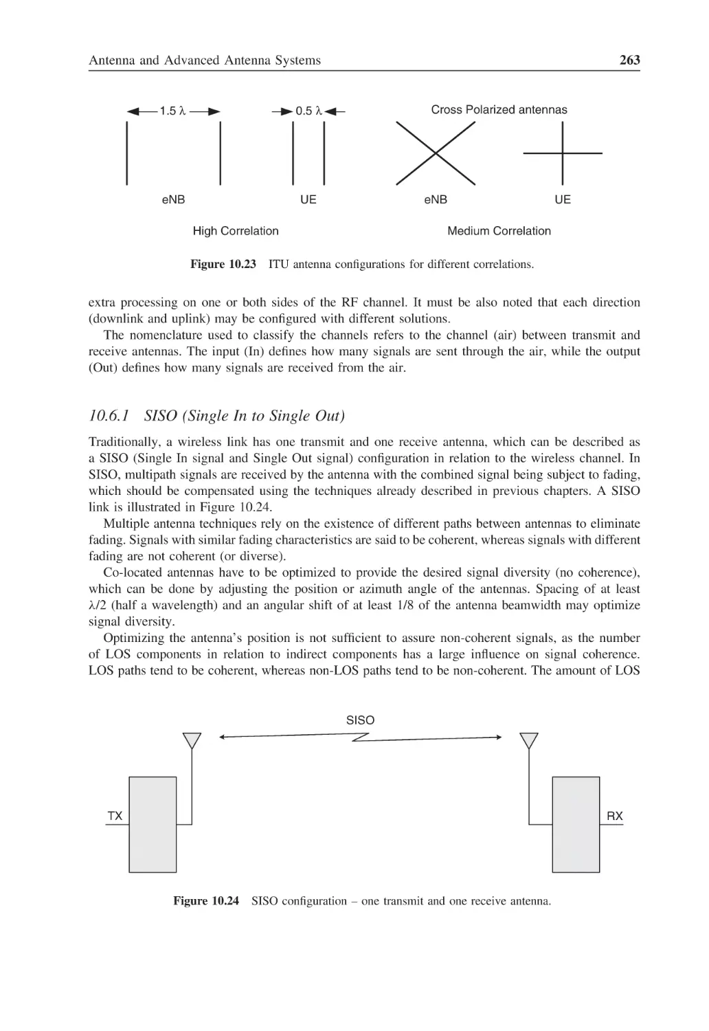
Figure 10.23 ITU antenna configurations for different correlations
263
List of Figures
xxv
Figure 10.24 SISO configuration – one transmit and one receive antenna
263
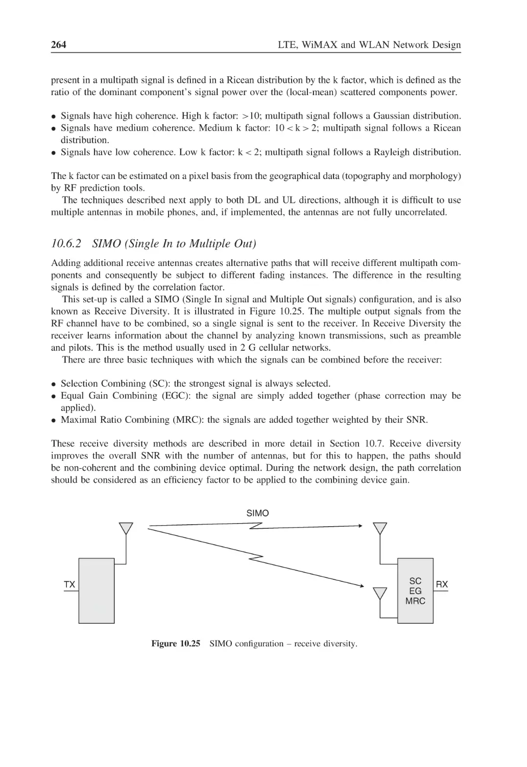
Figure 10.25 SIMO configuration – receive diversity
264
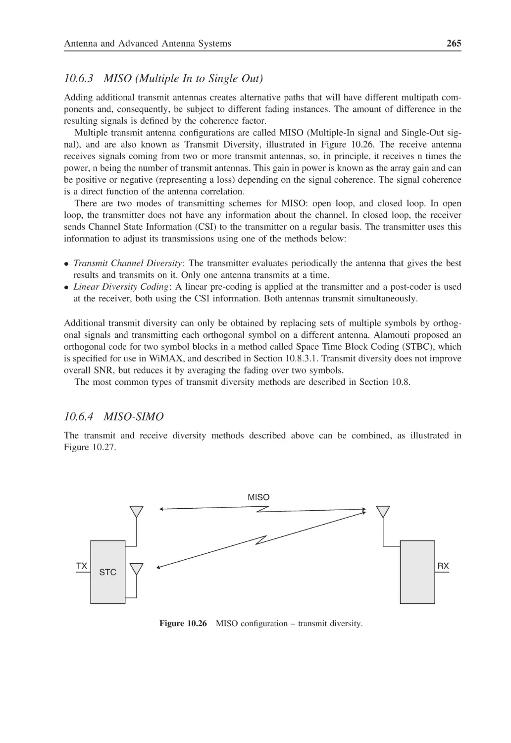
Figure 10.26 MISO configuration – transmit diversity
265
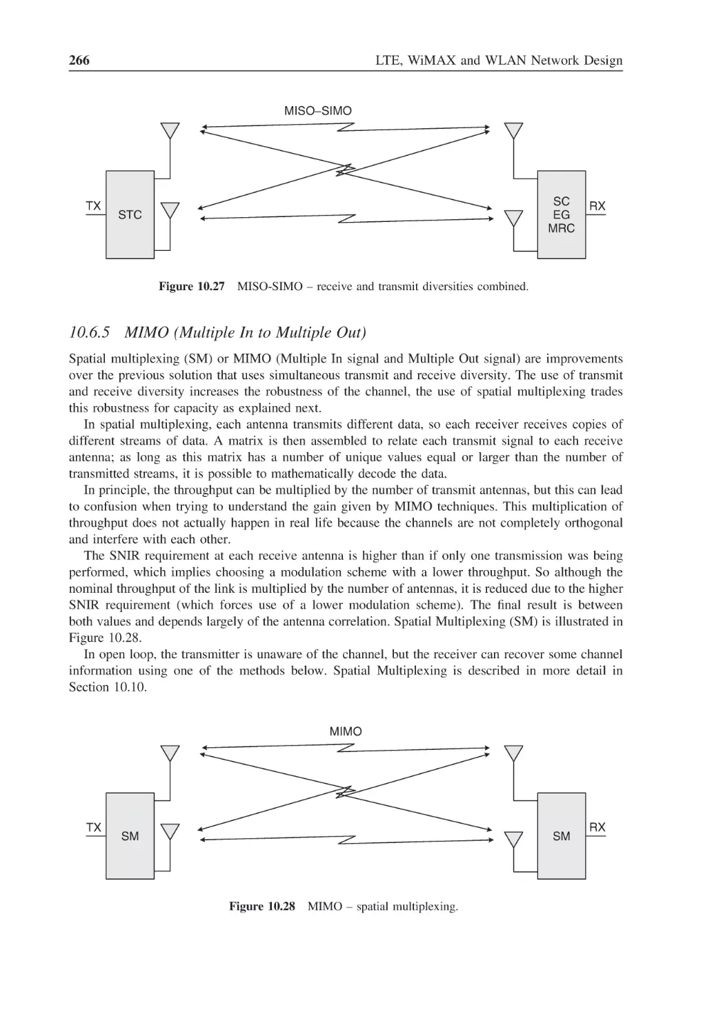
Figure 10.27 MISO-SIMO – receive and transmit diversities combined
266
Figure 10.28 MIMO – spatial multiplexing
266
Figure 10.29 UL-MIMO – spatial multiplexing in the uplink
267
Figure 10.30 Equal gain combining receiver
268
Figure 10.31 Diversity selection receiver
269
Figure 10.32 Maximal ratio combining receiver
270
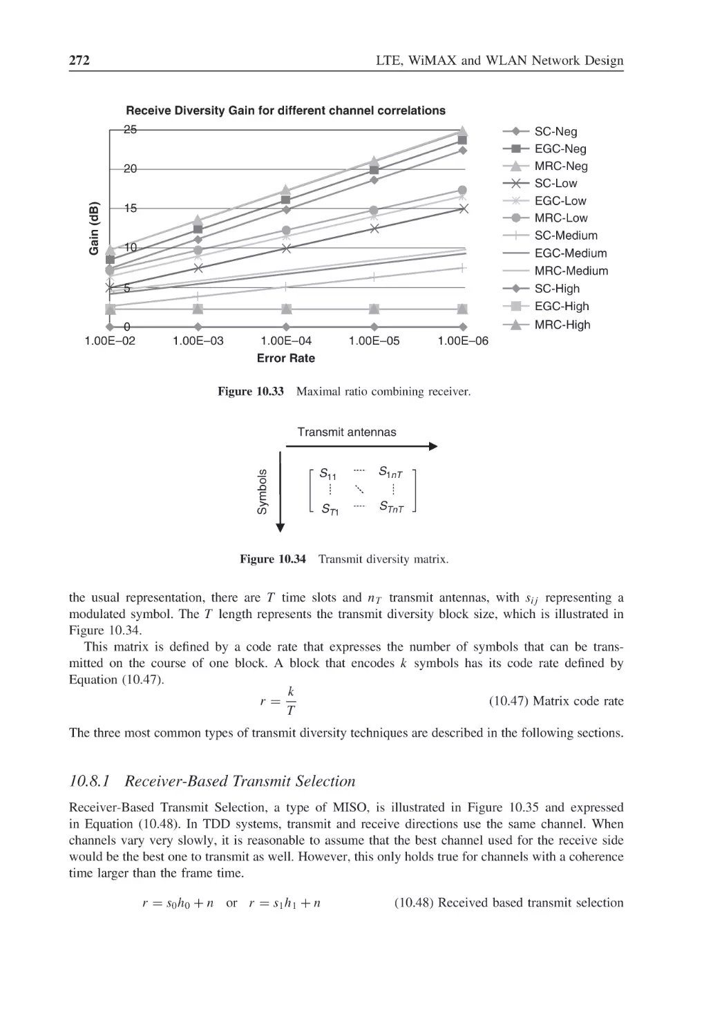
Figure 10.33 Maximal ratio combining receiver
272
Figure 10.34 Transmit diversity matrix
272
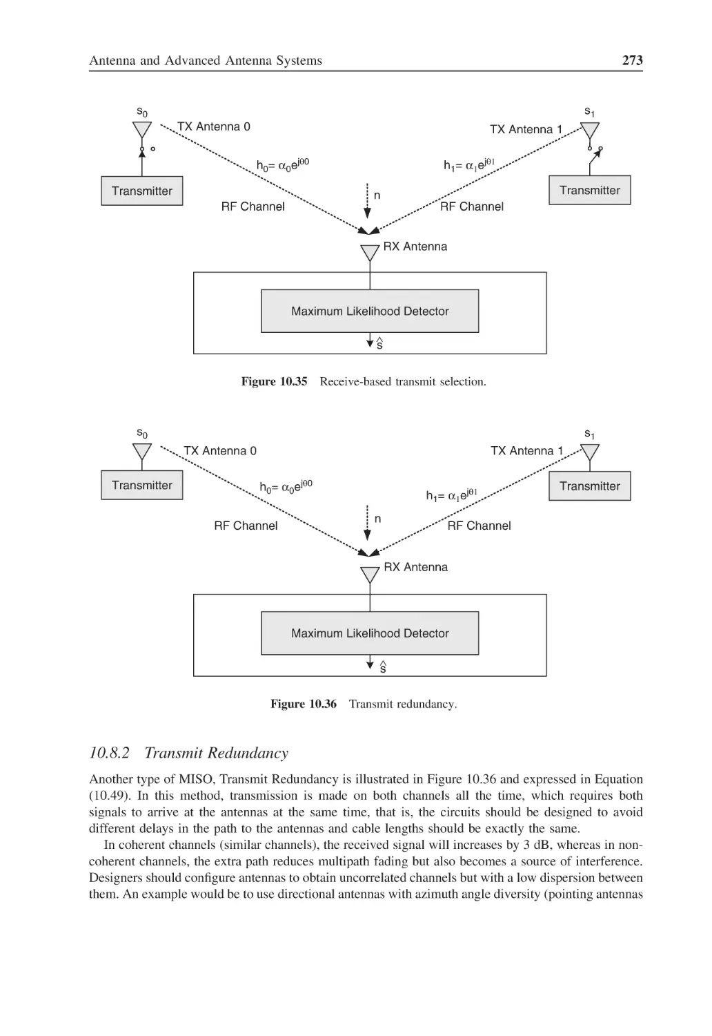
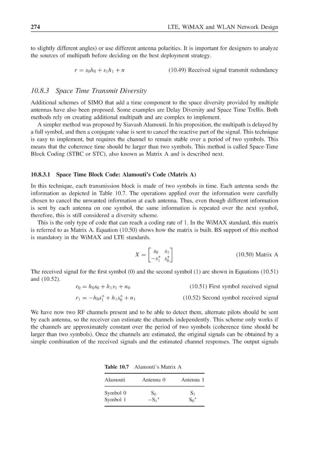
Figure 10.35 Receive-based transmit selection
273
Figure 10.36 Transmit redundancy
273
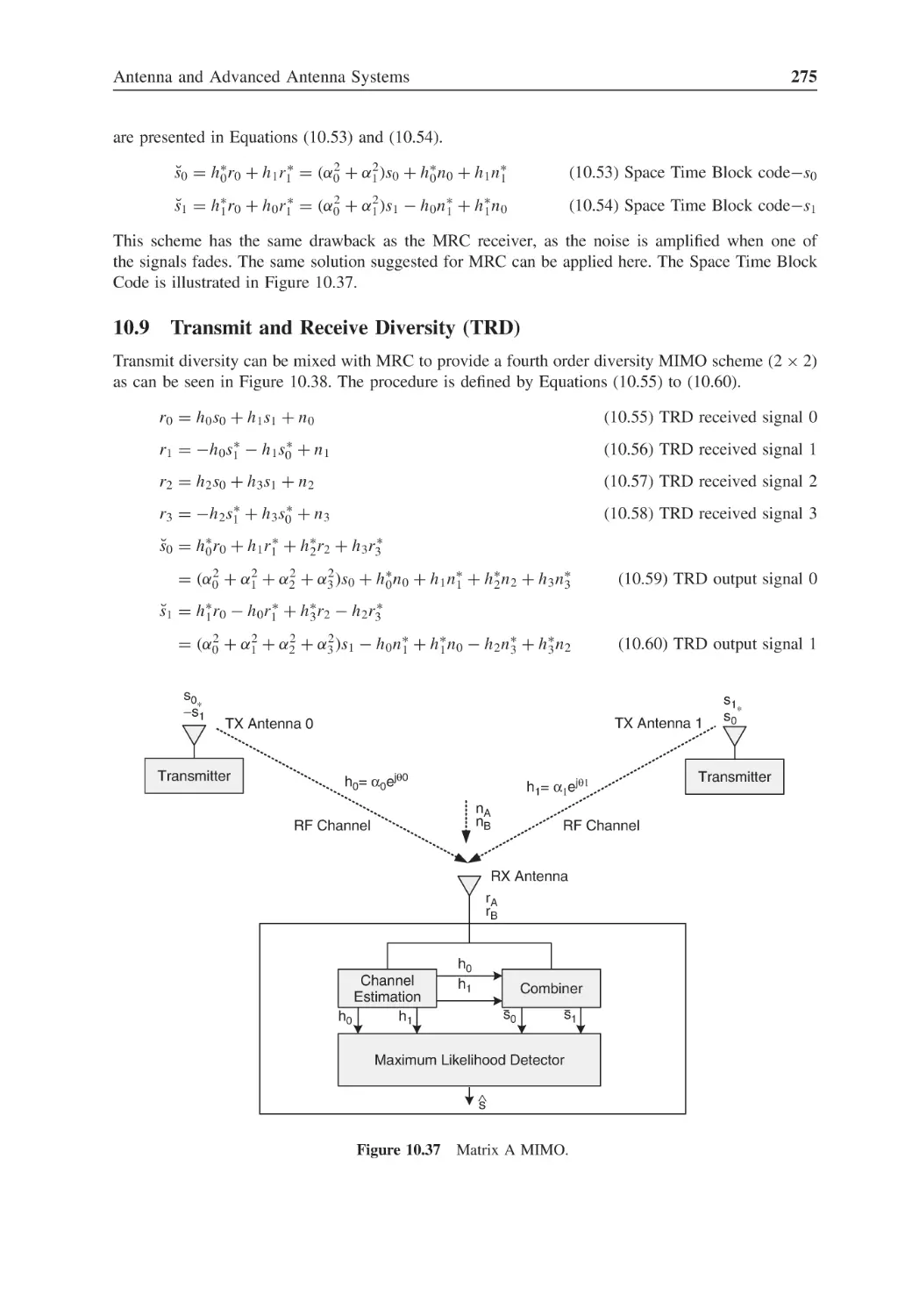
Figure 10.37 Matrix A MIMO
275
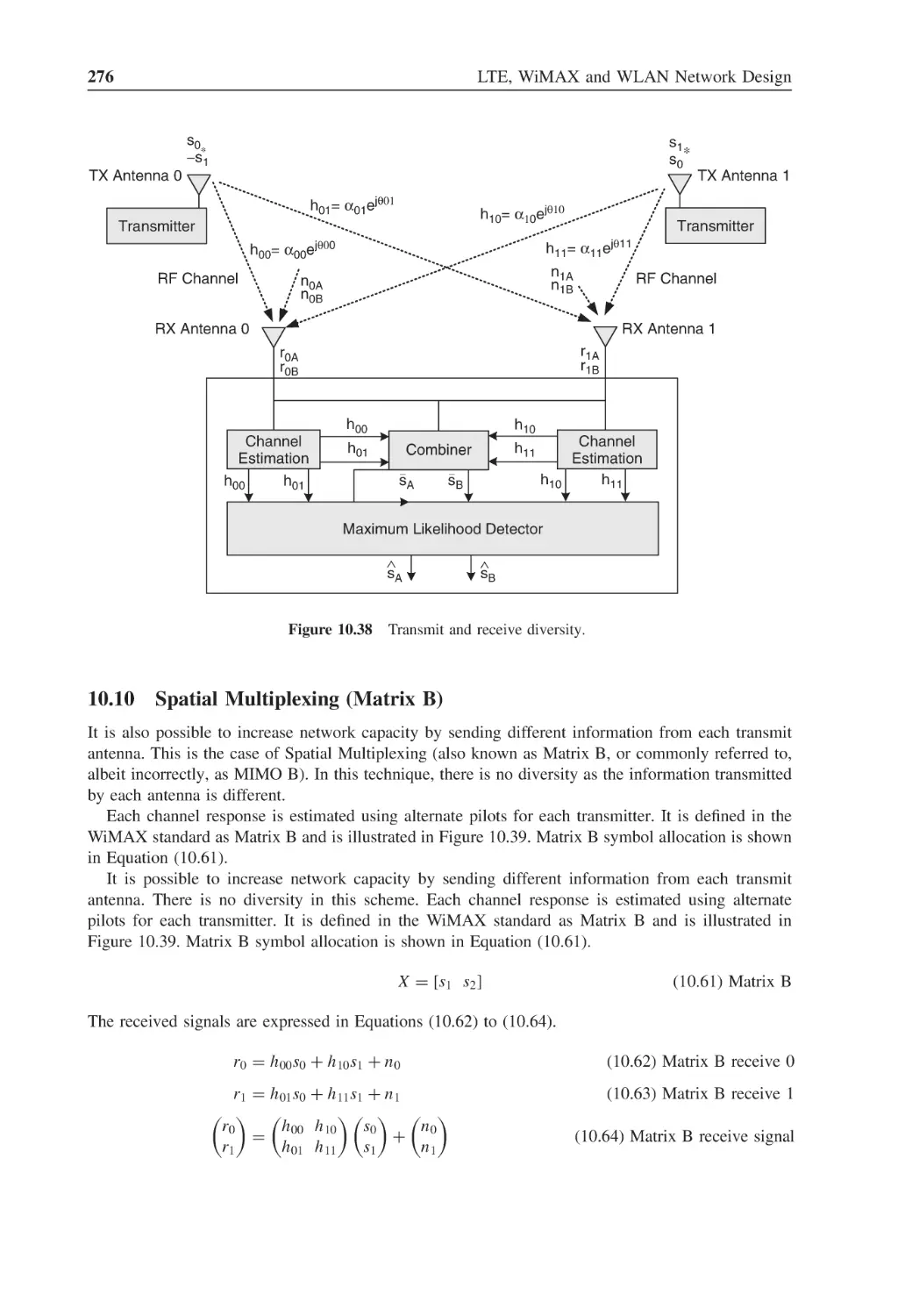
Figure 10.38 Transmit and receive diversity
276
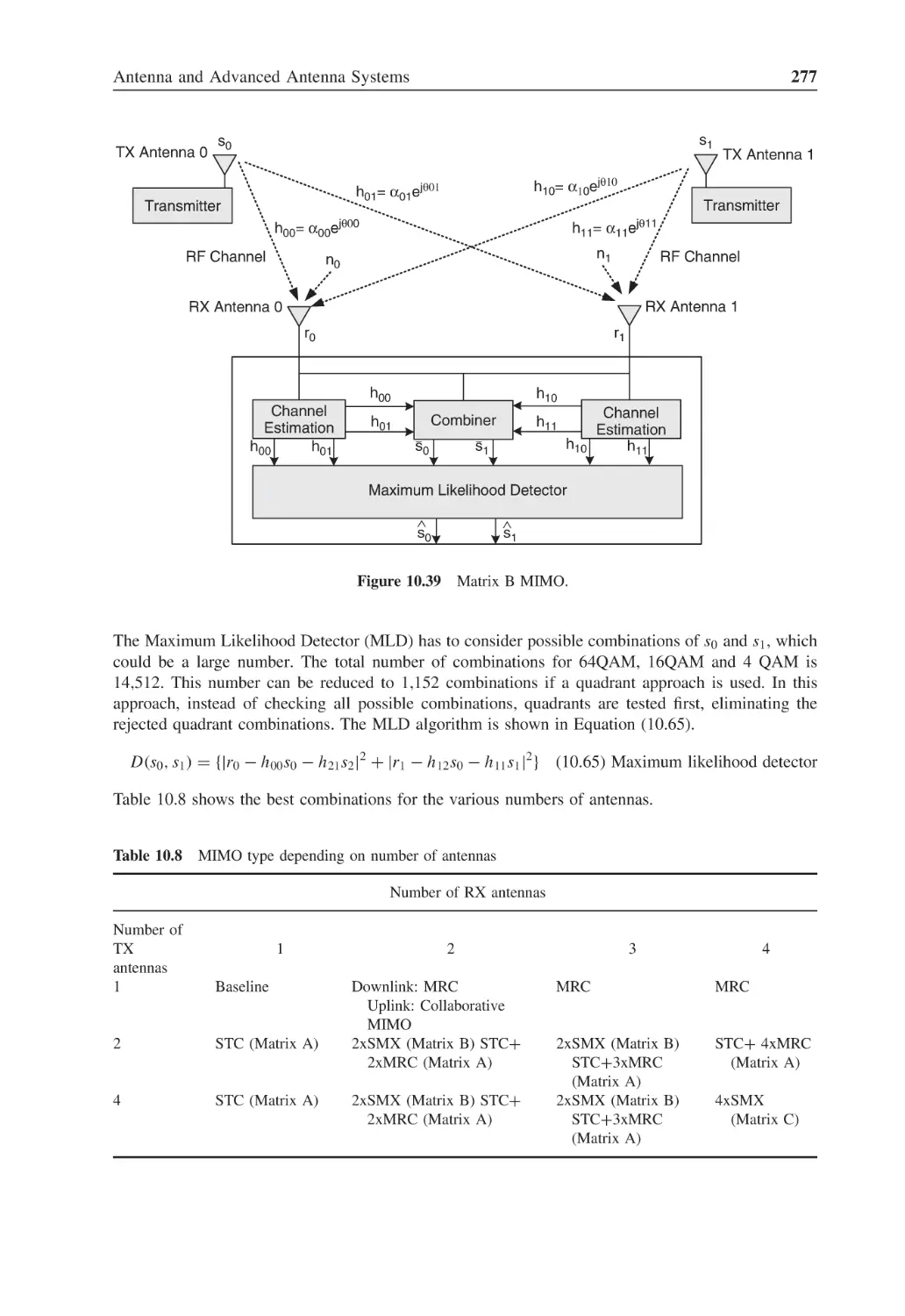
Figure 10.39 Matrix B MIMO
277
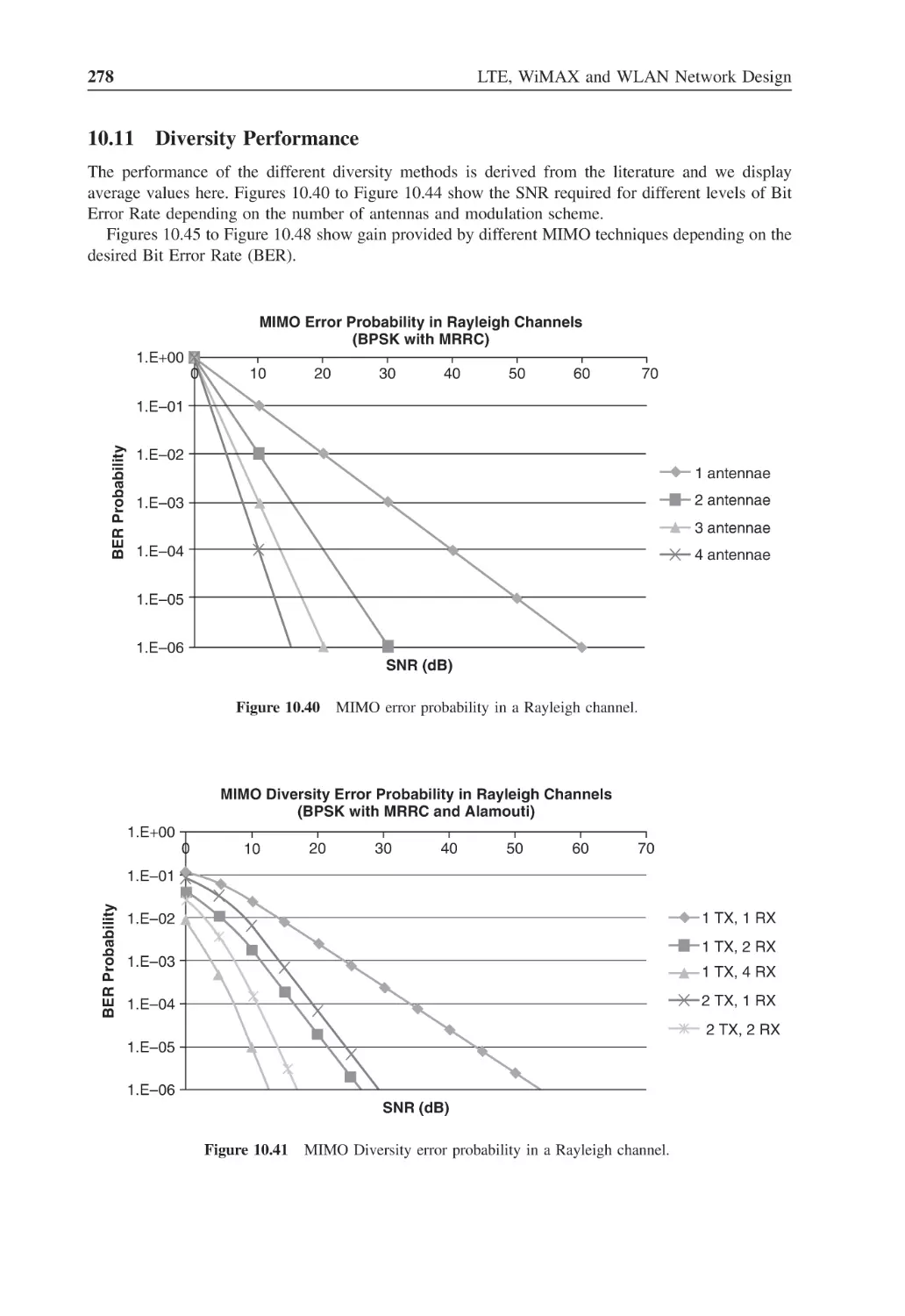
Figure 10.40 MIMO error probability in a Rayleigh channel
278
Figure 10.41 MIMO Diversity error probability in a Rayleigh channels
278
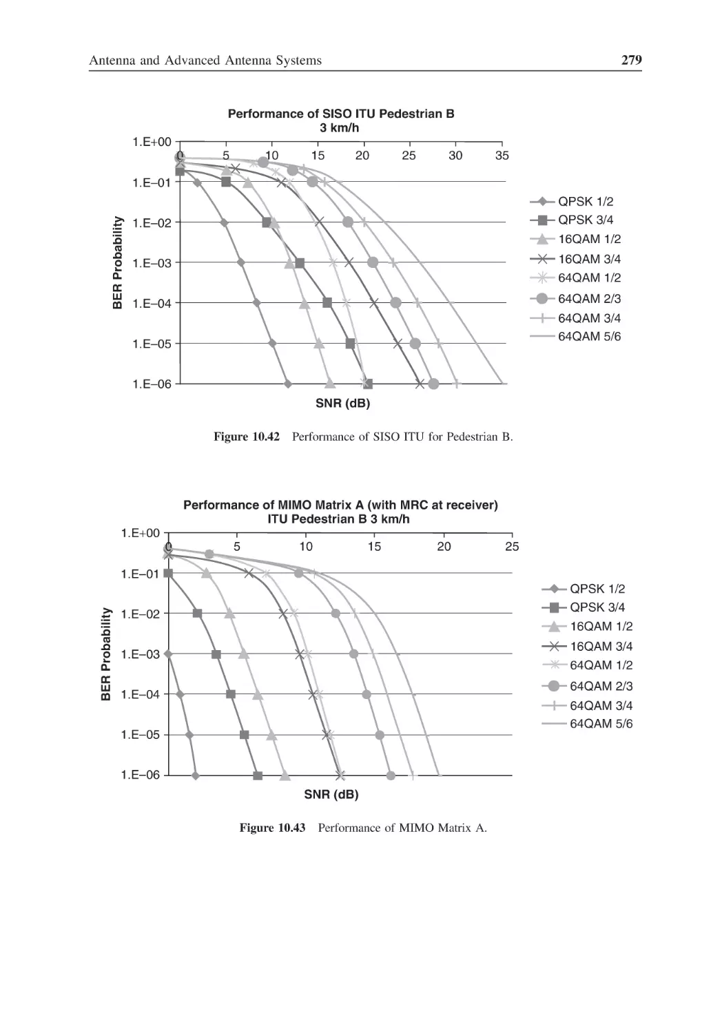
Figure 10.42 Performance of SISO ITU for Pedestrian B
279
Figure 10.43 Performance of MIMO Matrix A
279
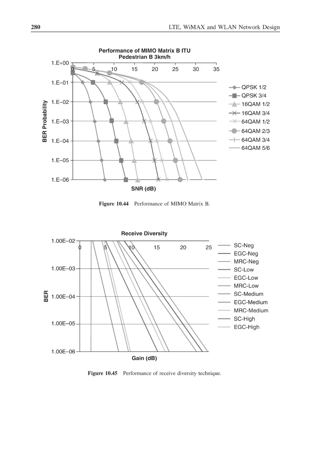
Figure 10.44 Performance of MIMO Matrix B
280
Figure 10.45 Performance of receive diversity technique
280
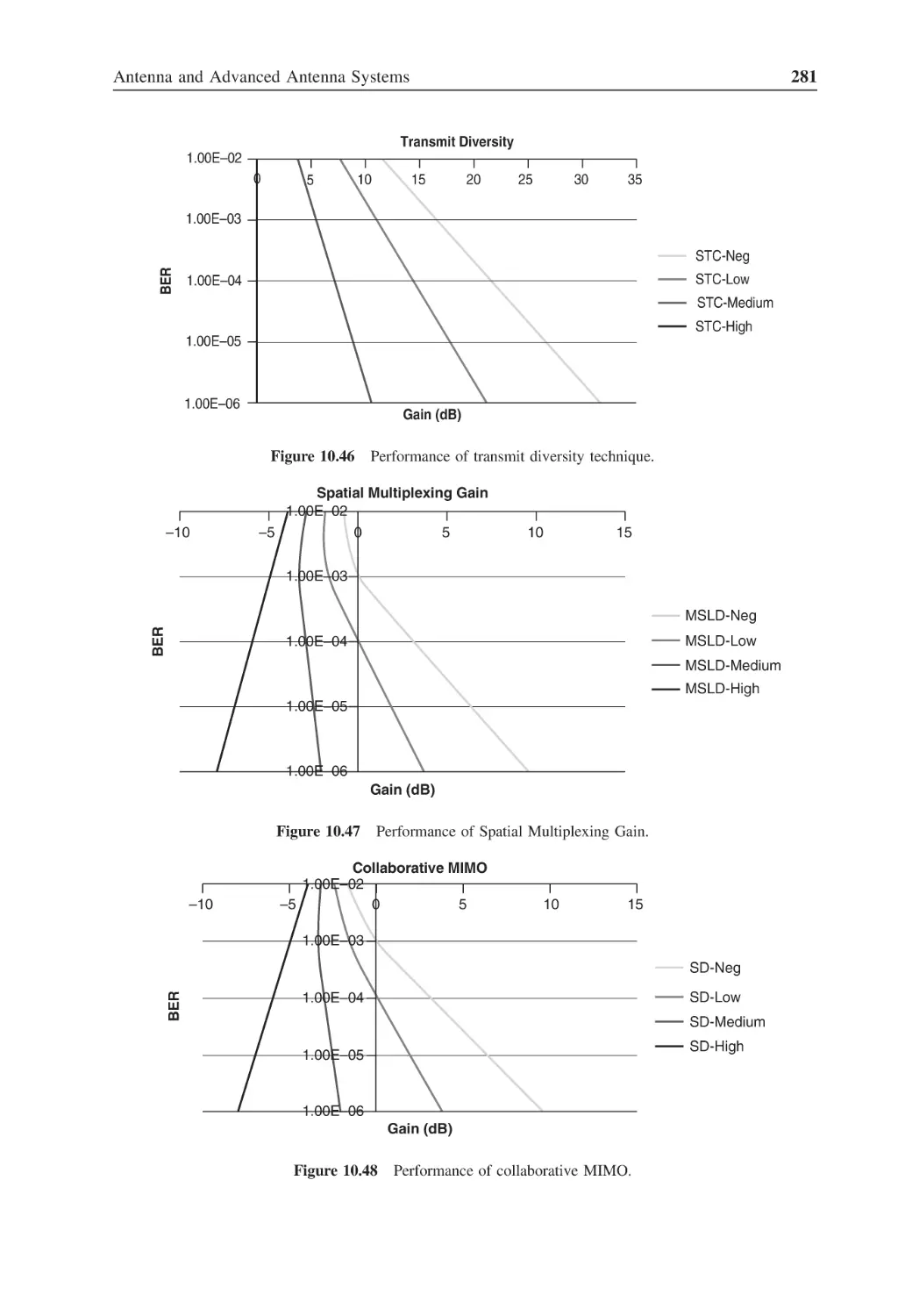
Figure 10.46 Performance of transmit diversity technique
281
Figure 10.47 Performance of Spatial Multiplexing Gain
281
Figure 10.48 Performance of collaborative MIMO
281
Figure 10.49 Array (linear) of antennas
282
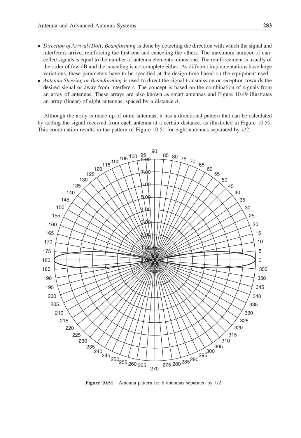
Figure 10.50 Pattern calculation for array of antennas
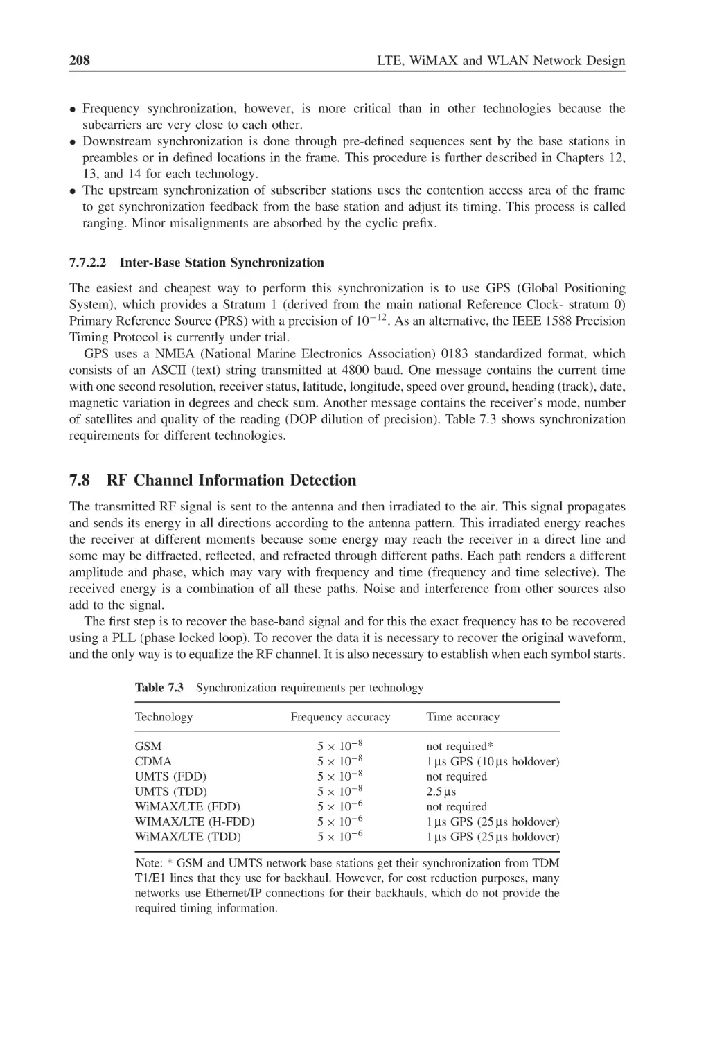
282
Figure 10.51 Antenna pattern for 8 antennas separated by λ/2
283
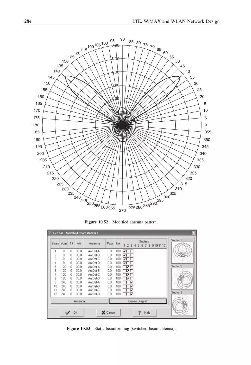
Figure 10.52 Modified antenna pattern
284
Figure 10.53 Static beamforming (switched beam antenna)
284
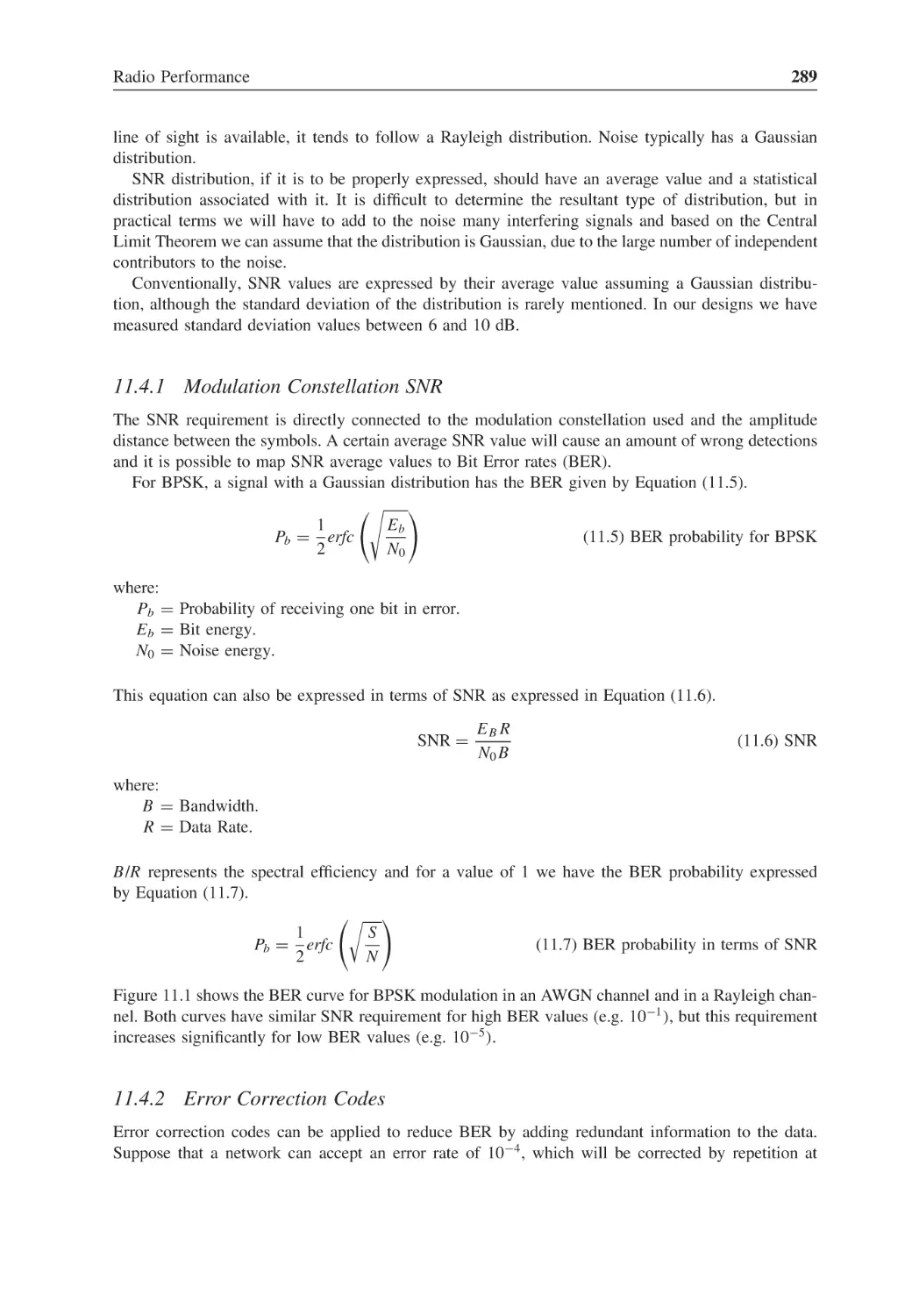
Figure 11.1
Eb /N0 requirement for different BER for BPSK modulation
290
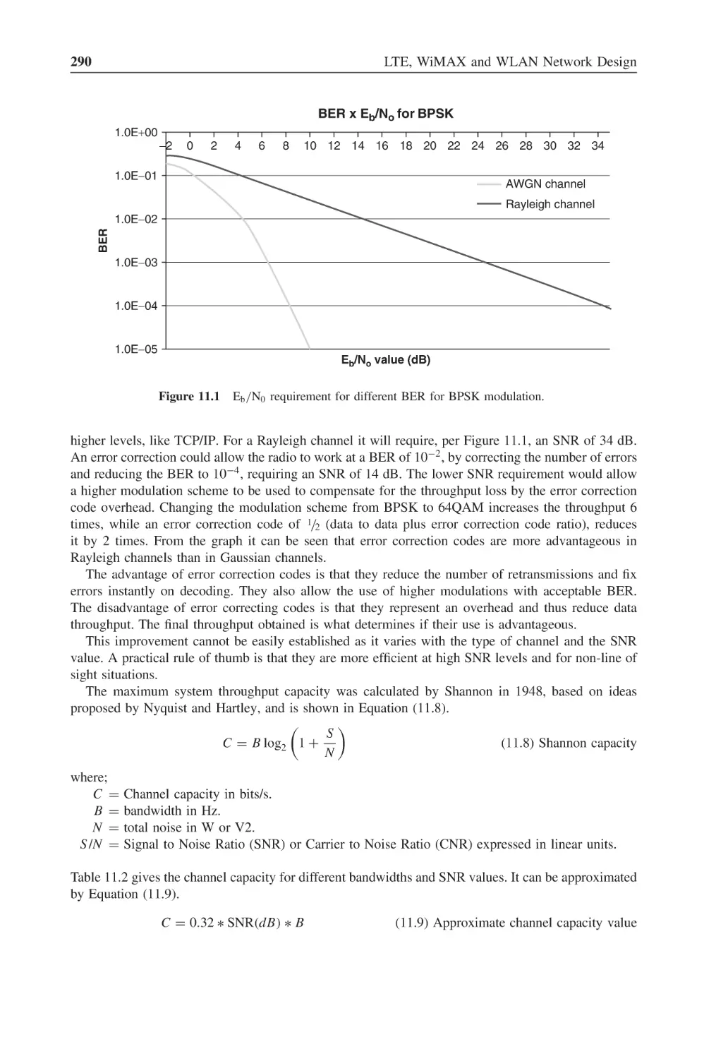
Figure 11.2
SNR requirement for different BER for various modulations
in an AWGN channel
292
SNR requirement for different BER for various modulations
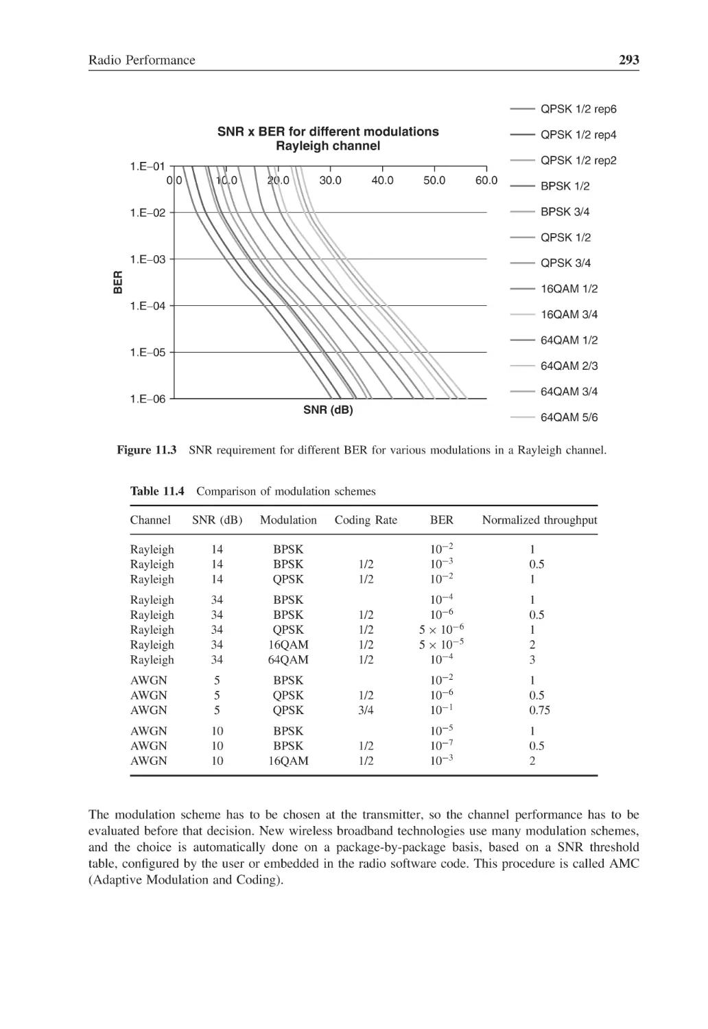
in a Rayleigh channel
293
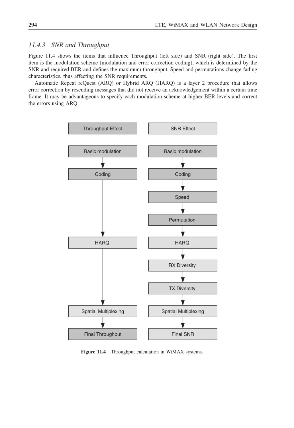
Figure 11.4
Throughput calculation in WiMAX systems
294
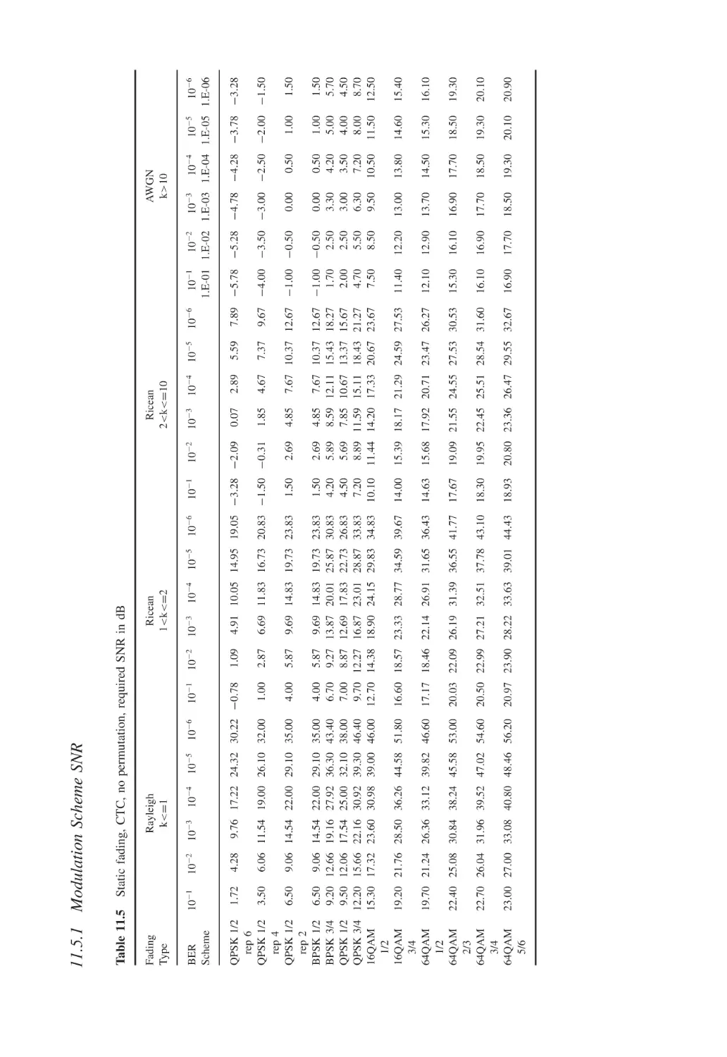
Figure 11.5
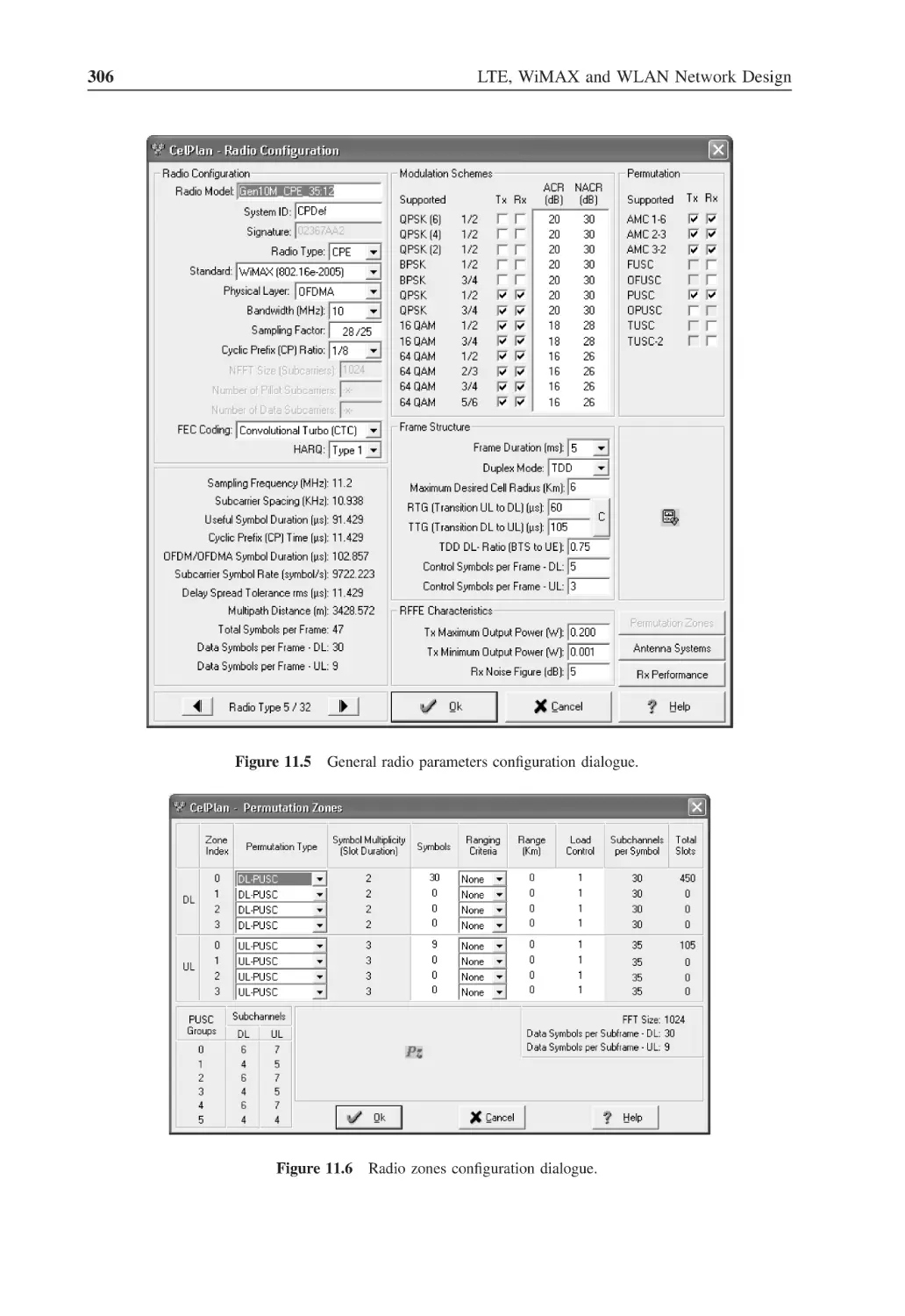
General radio parameters configuration dialogue
306
Figure 11.6
Radio zones configuration dialogue
306
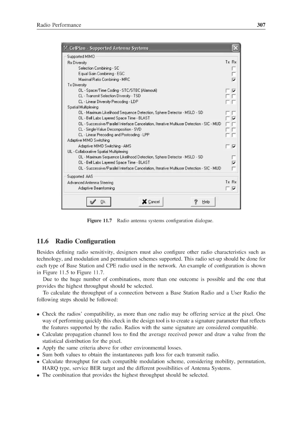
Figure 11.7
Radio antenna systems configuration dialogue
307
Figure 11.3
xxvi
List of Figures
Figure 11.8
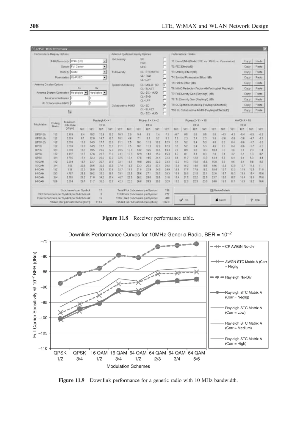
Receiver performance table
308
Figure 11.9
Downlink performance for a generic radio with 10 MHz bandwidth
308
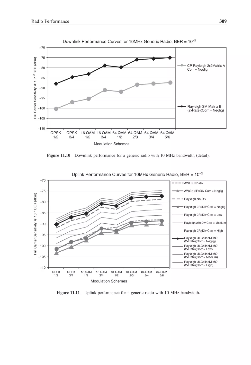
Figure 11.10 Downlink performance for a generic radio with 10 MHz bandwidth (detail)
309
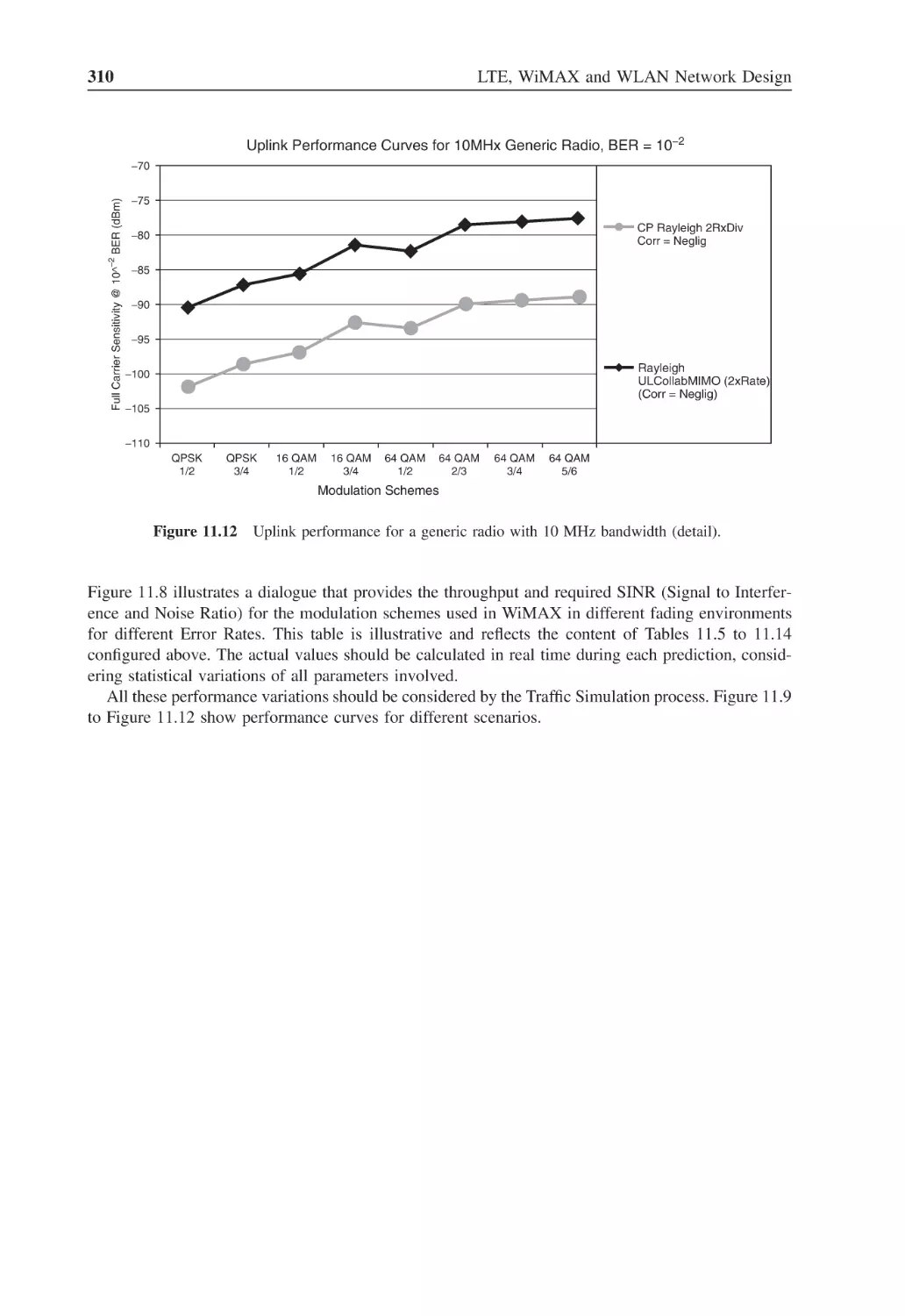
Figure 11.11 Uplink performance for a generic radio with 10 MHz bandwidth
309
Figure 11.12 Uplink performance for a generic radio with 10 MHz bandwidth (detail)
310
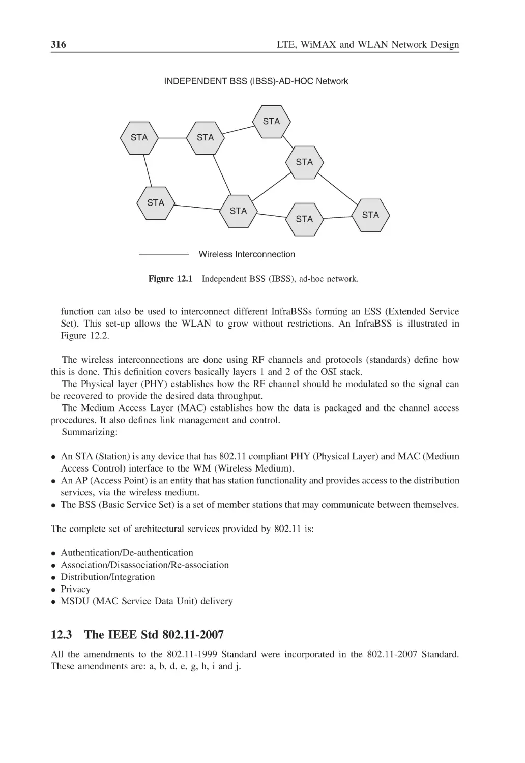
Figure 12.1
Independent BSS (IBSS), ad-hoc network
316
Figure 12.2
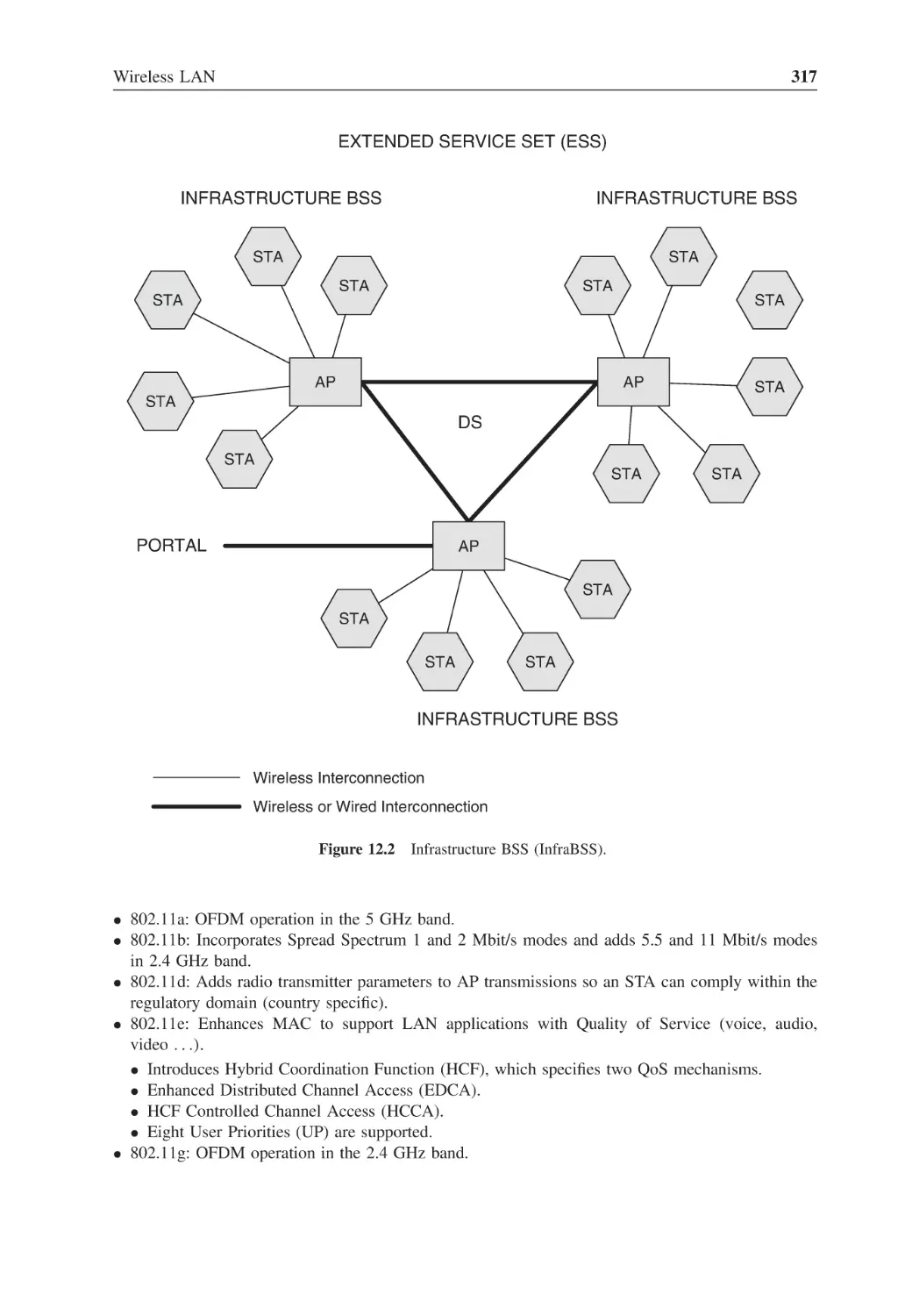
Infrastructure BSS (InfraBSS)
317
Figure 12.3
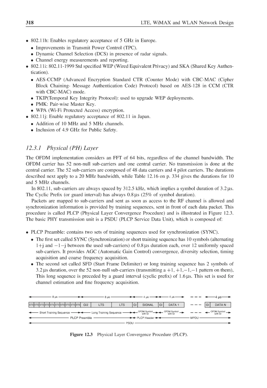
Physical Layer Convergence Procedure (PLCP)
318
Figure 12.4
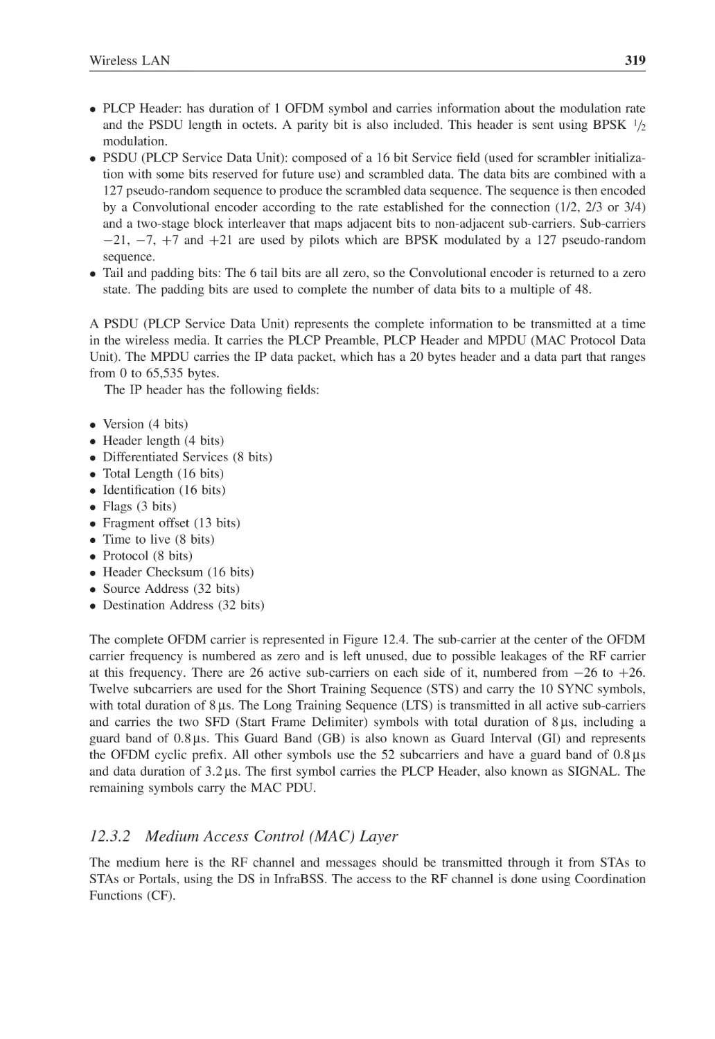
Physical Layer (PHY)
320
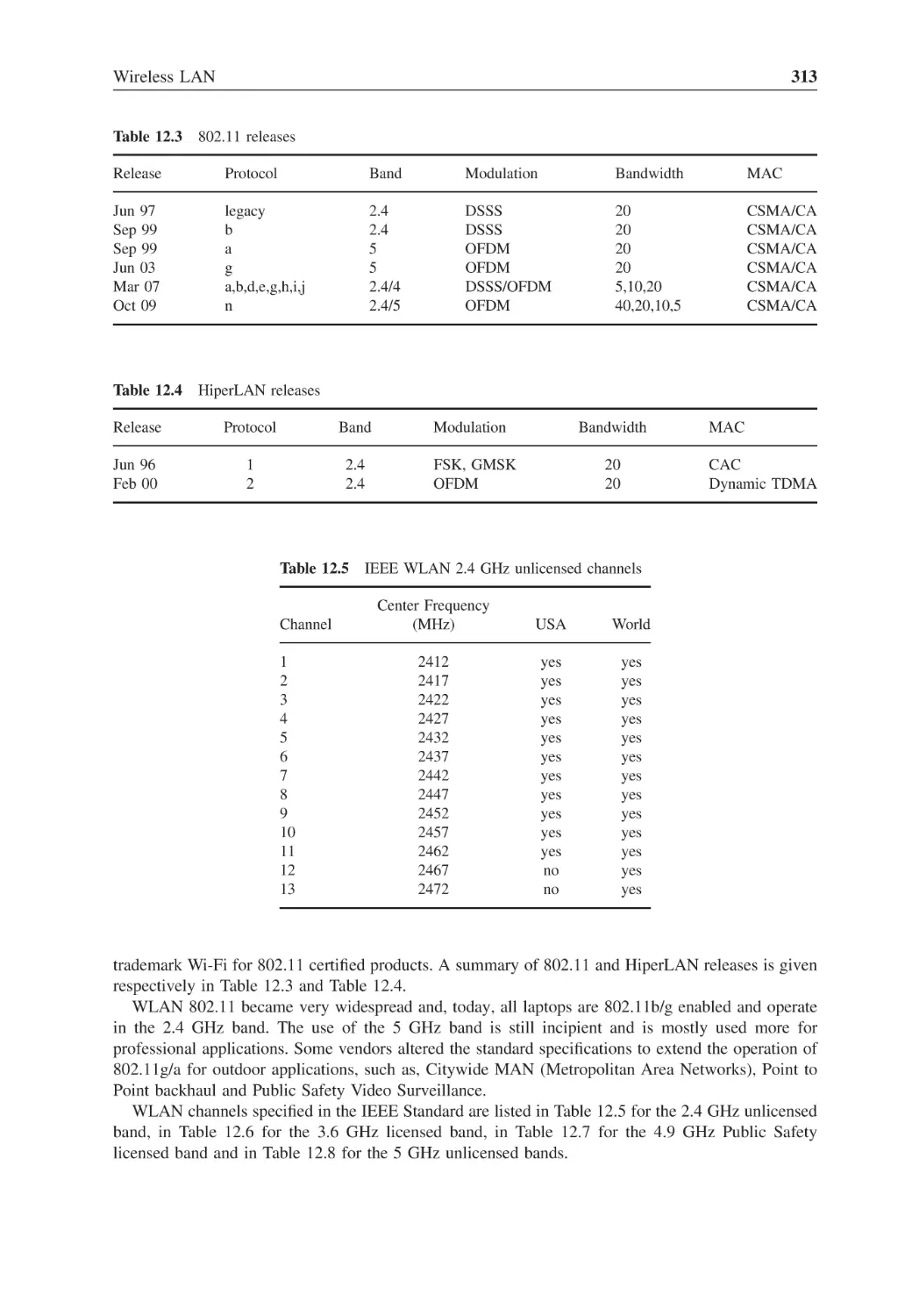
Figure 12.5
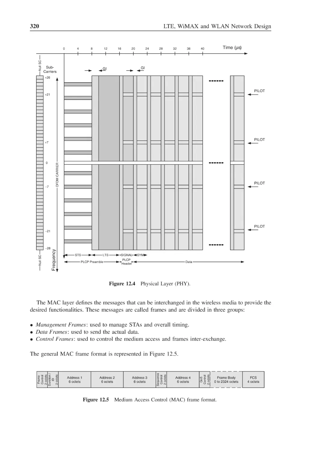
Medium Access Control (MAC) frame format
320
Figure 12.6
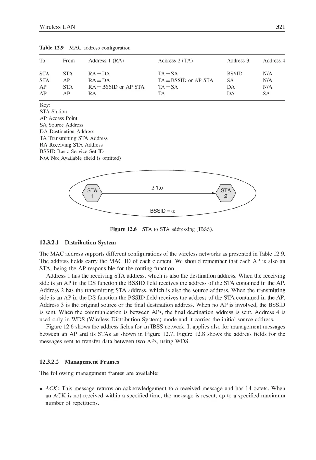
STA to STA addressing (IBSS)
321
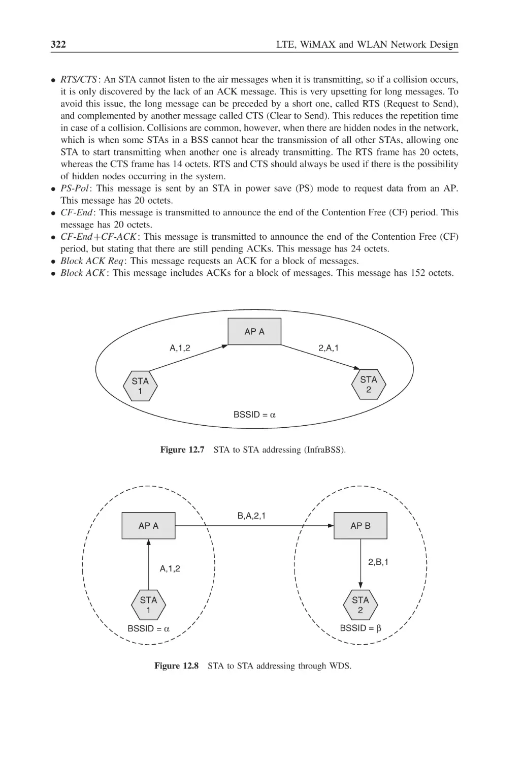
Figure 12.7
STA to STA addressing (InfraBSS)
322
Figure 12.8
STA to STA addressing through WDS
322
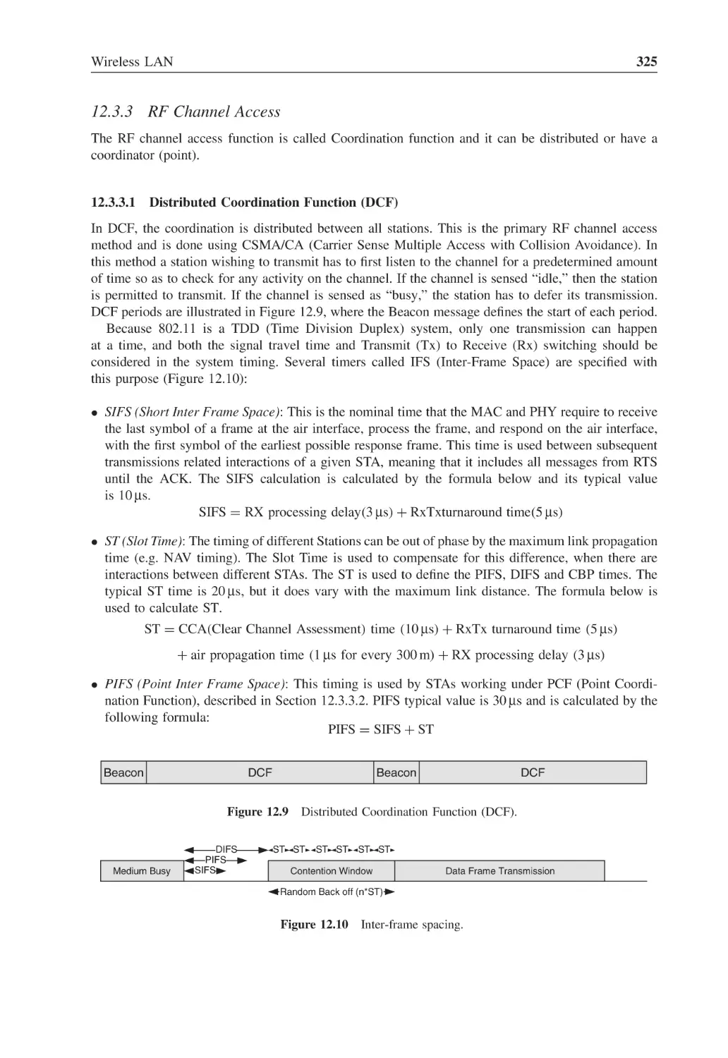
Figure 12.9
Distributed Coordination Function (DCF)
325
Figure 12.10 Inter-frame spacing
325
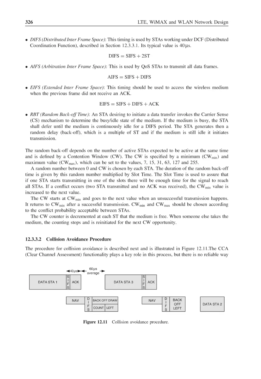
Figure 12.11 Collision avoidance procedure
326
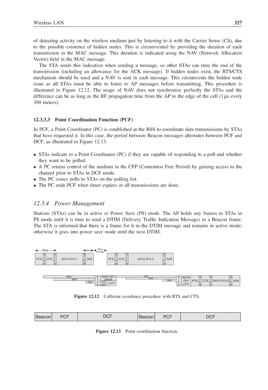
Figure 12.12 Collision avoidance procedure with RTS and CTS
327
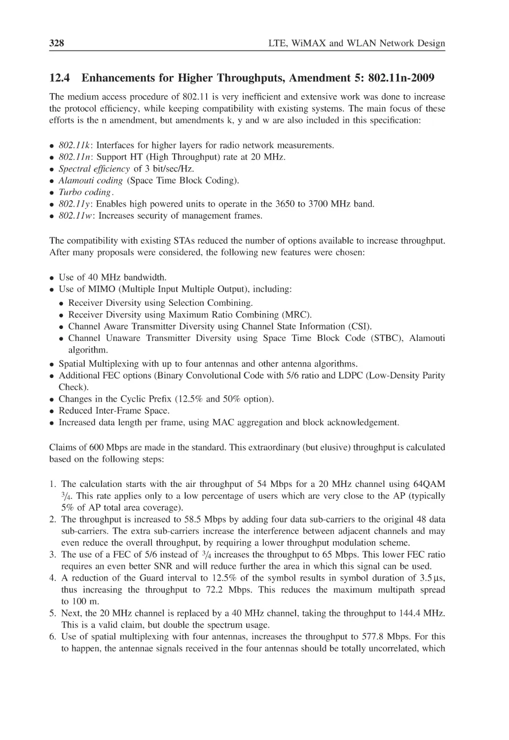
Figure 12.13 Point coordination function
327
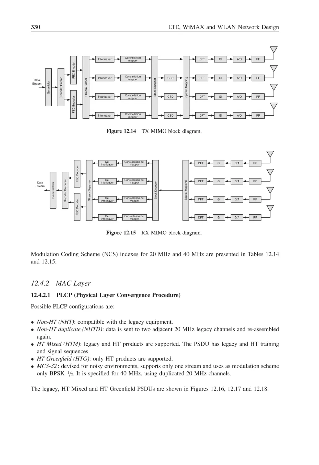
Figure 12.14 TX MIMO block diagram
330
Figure 12.15 RX MIMO block diagram
330
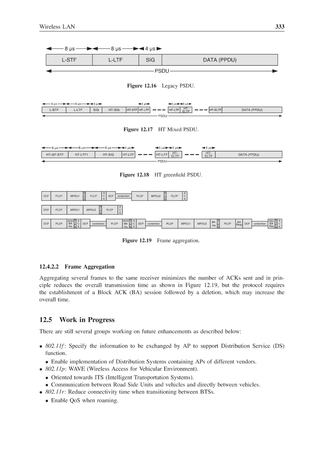
Figure 12.16 Legacy PSDU
333
Figure 12.17 HT Mixed PSDU
333
Figure 12.18 HT greenfield PSDU
333
Figure 12.19 Frame aggregation
333
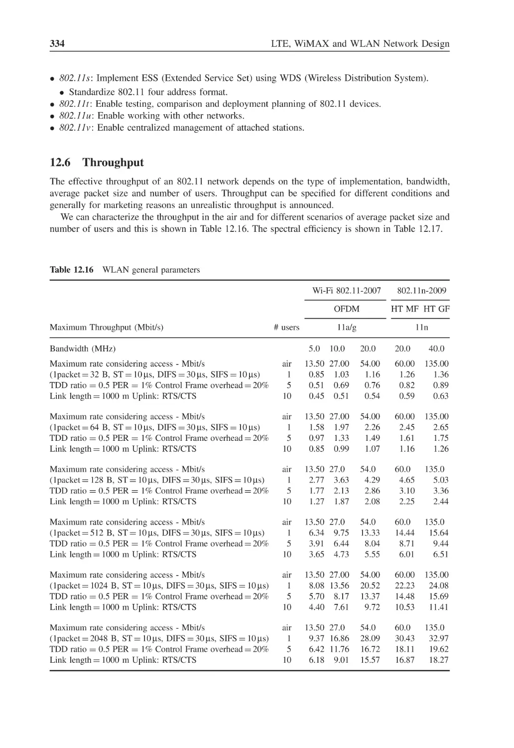
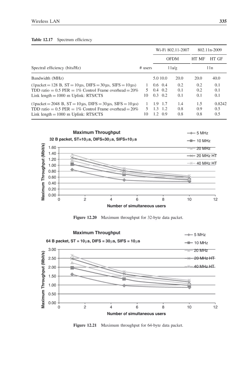
Figure 12.20 Maximum throughput for 32-byte data packet
335
Figure 12.21 Maximum throughput for 64-byte data packet
335
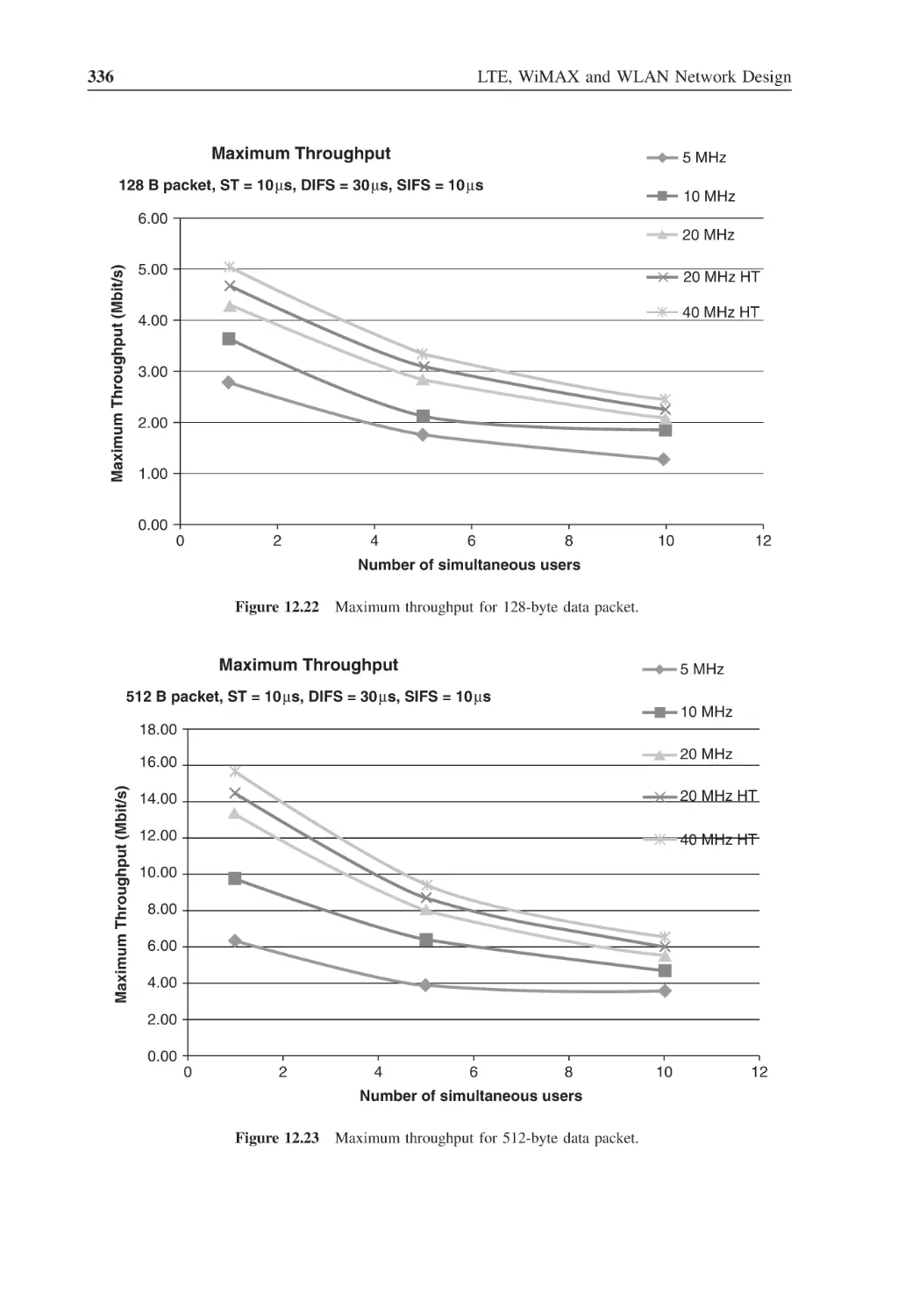
Figure 12.22 Maximum throughput for 128-byte data packet
336
Figure 12.23 Maximum throughput for 512-byte data packet
336
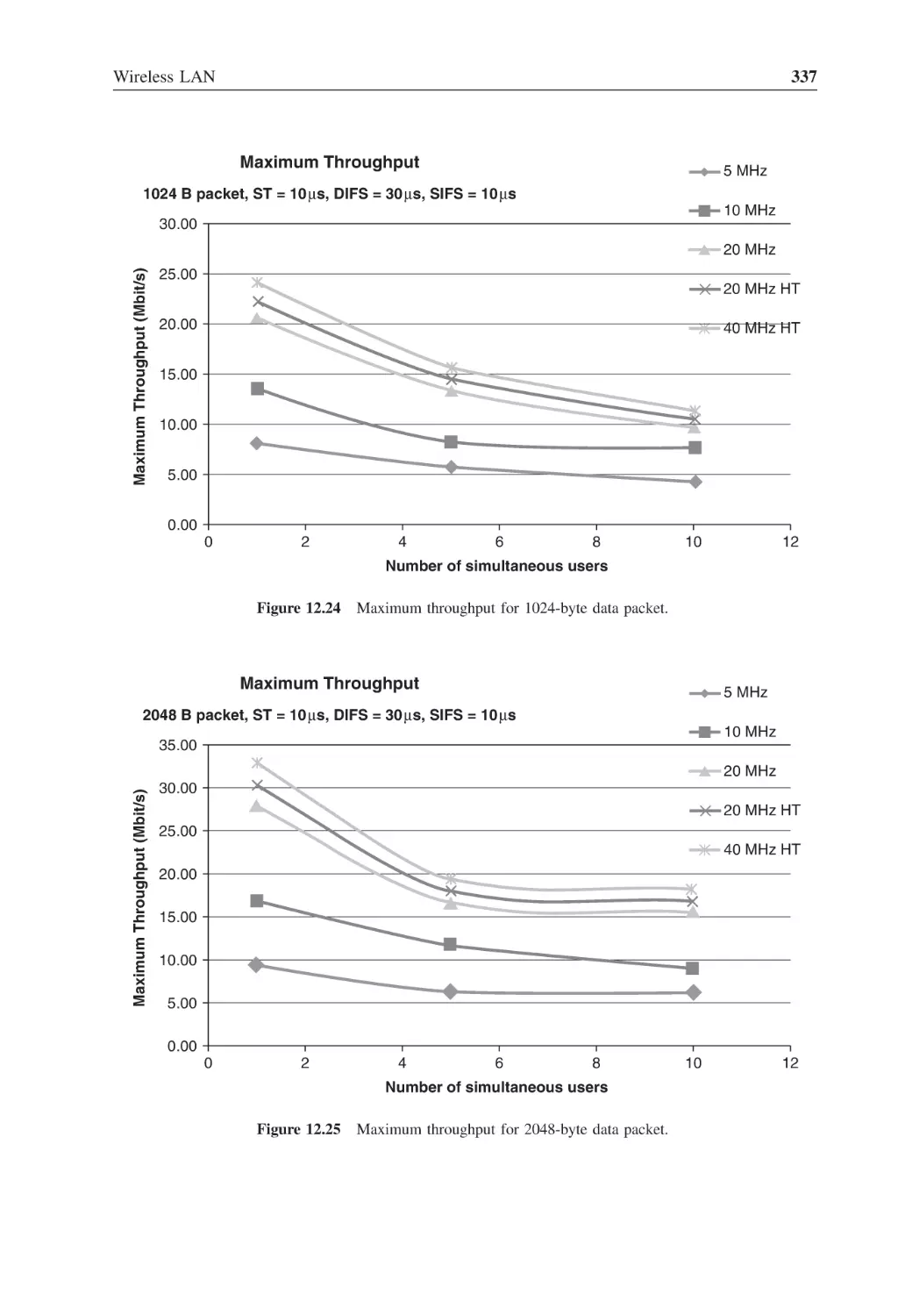
Figure 12.24 Maximum throughput for 1024-byte data packet
337
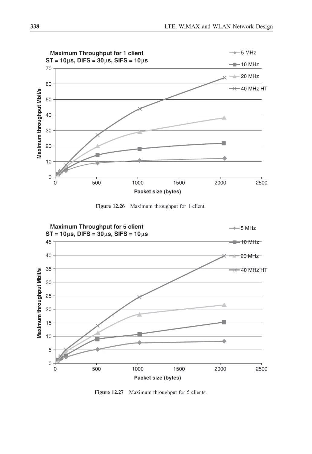
Figure 12.25 Maximum throughput for 2048-byte data packet
337
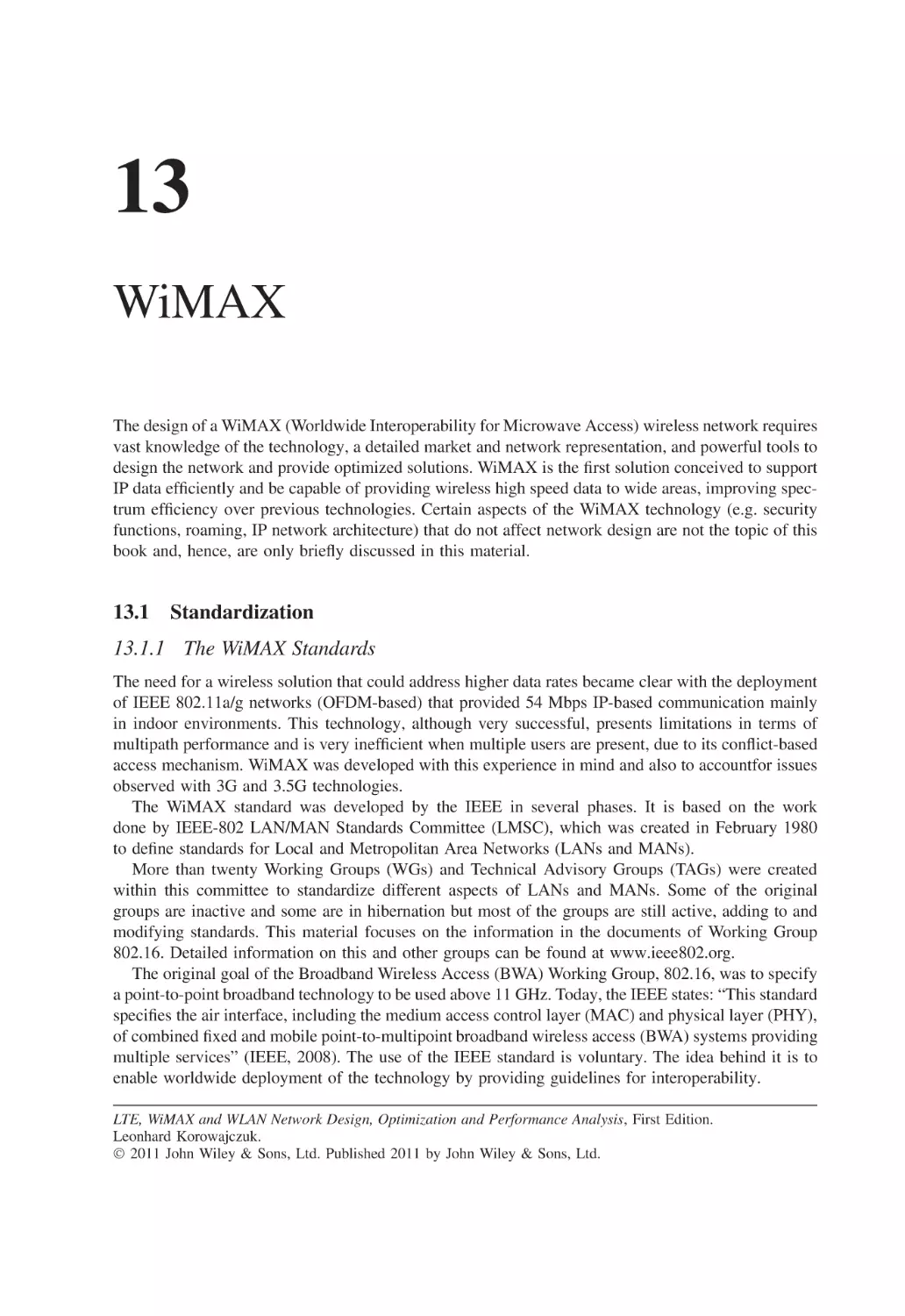
Figure 12.26 Maximum throughput for 1 client
338
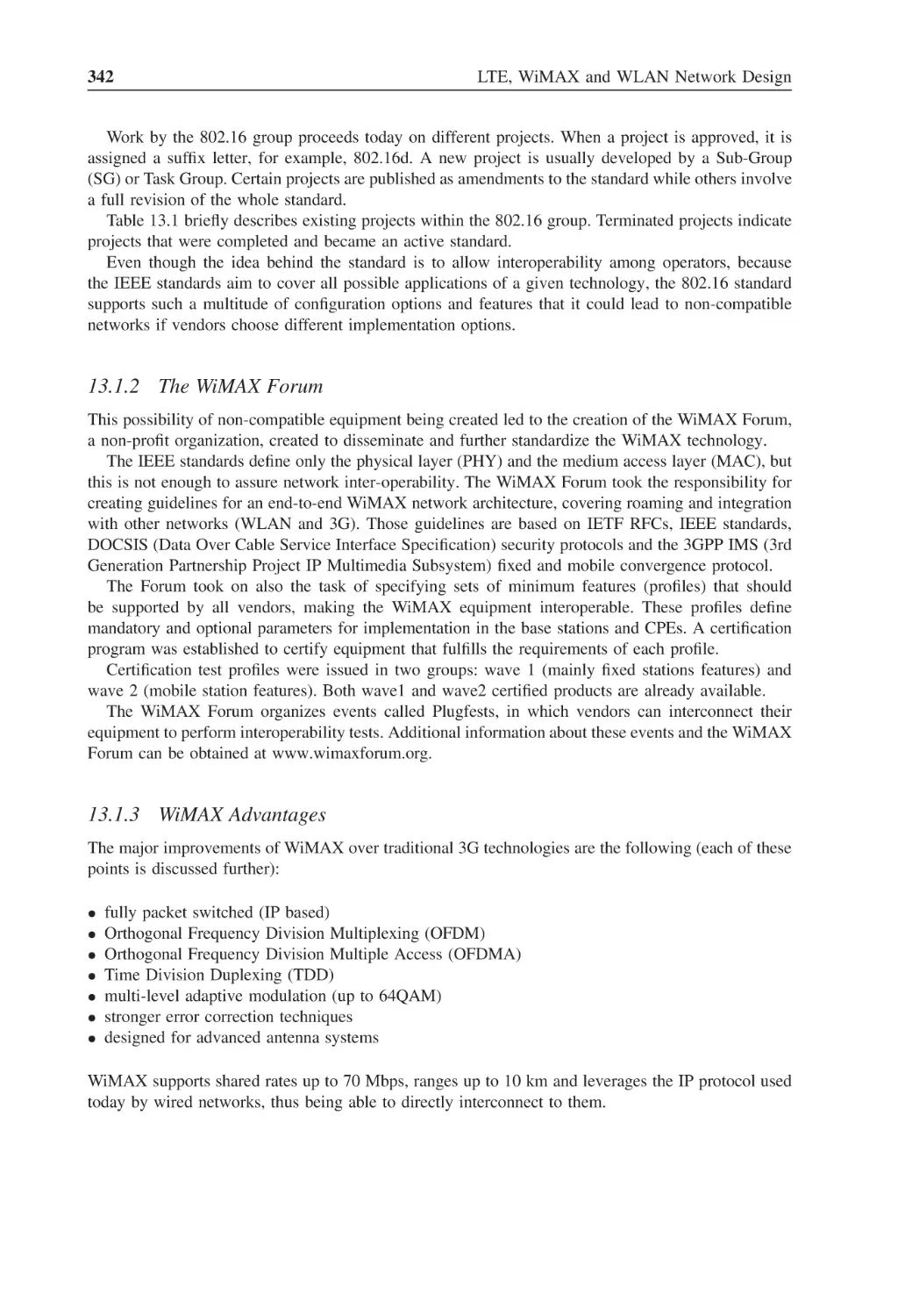
Figure 12.27 Maximum throughput for 5 clients
338
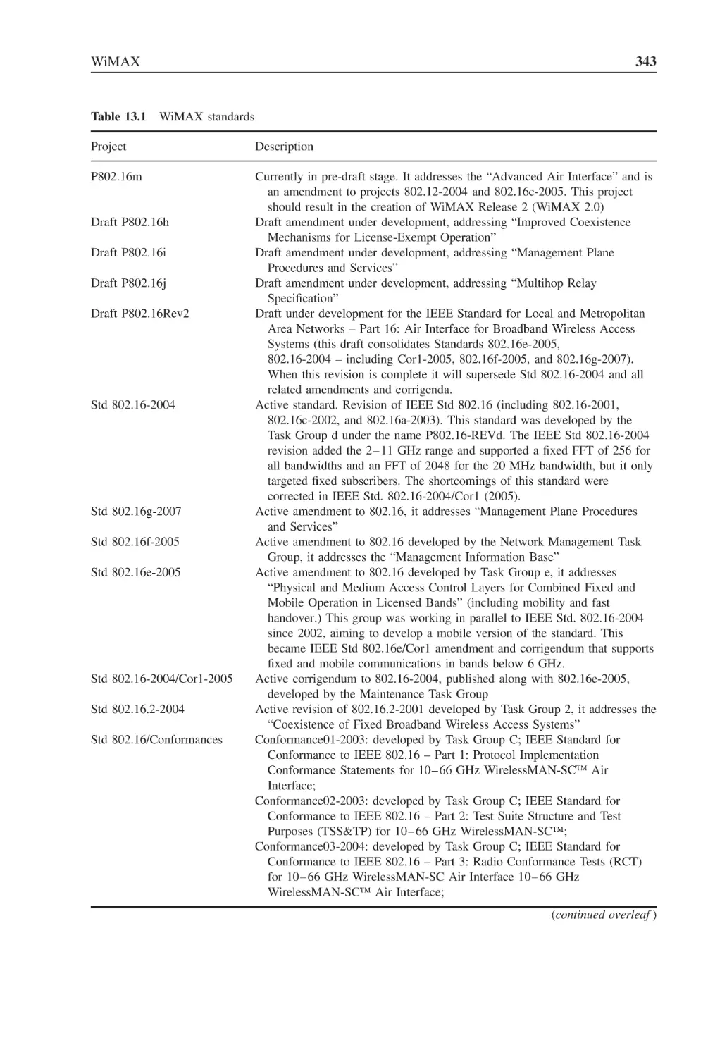
Figure 13.1
WiMAX network architecture
345
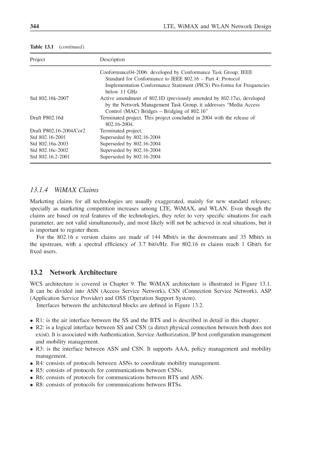
Figure 13.2
WiMAX interfaces
346
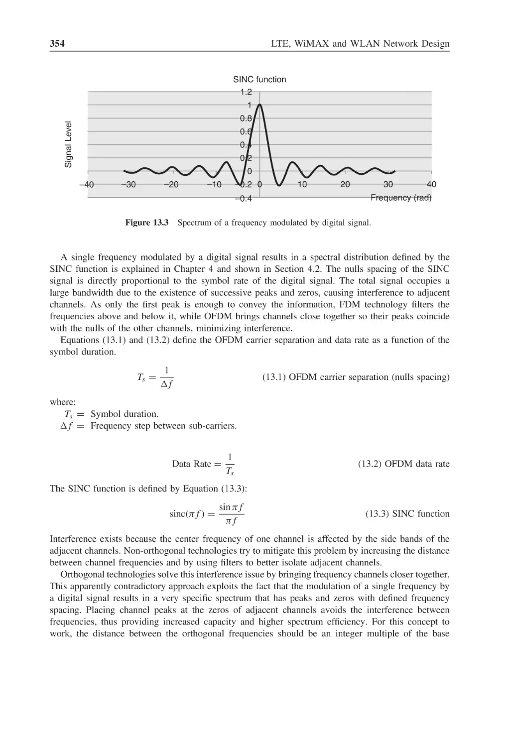
Figure 13.3
Spectrum of a frequency modulated by digital signal
354
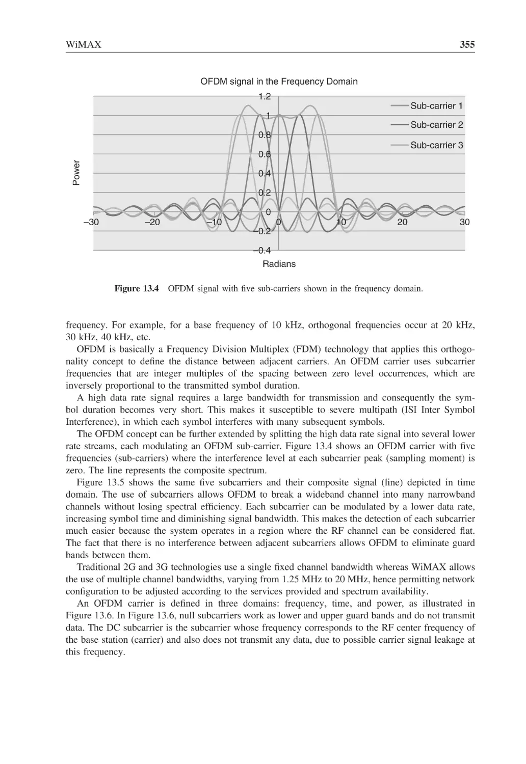
Figure 13.4
OFDM signal with five sub-carriers shown in the frequency domain
355
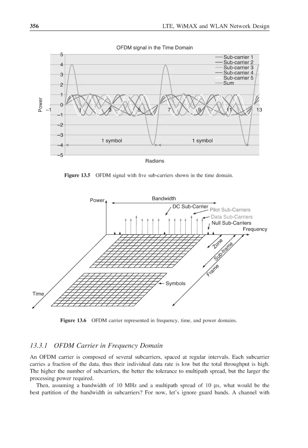
Figure 13.5
OFDM signal with five sub-carriers shown in the time domain
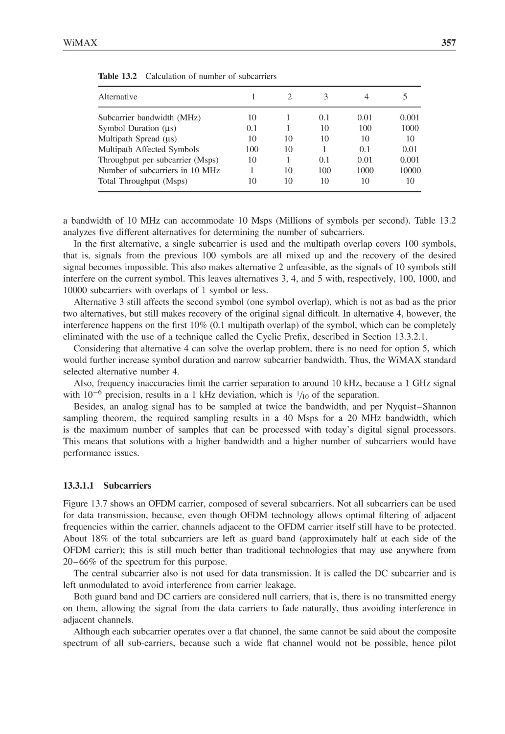
356
Figure 13.6
OFDM carrier represented in frequency, time, and power domains
356
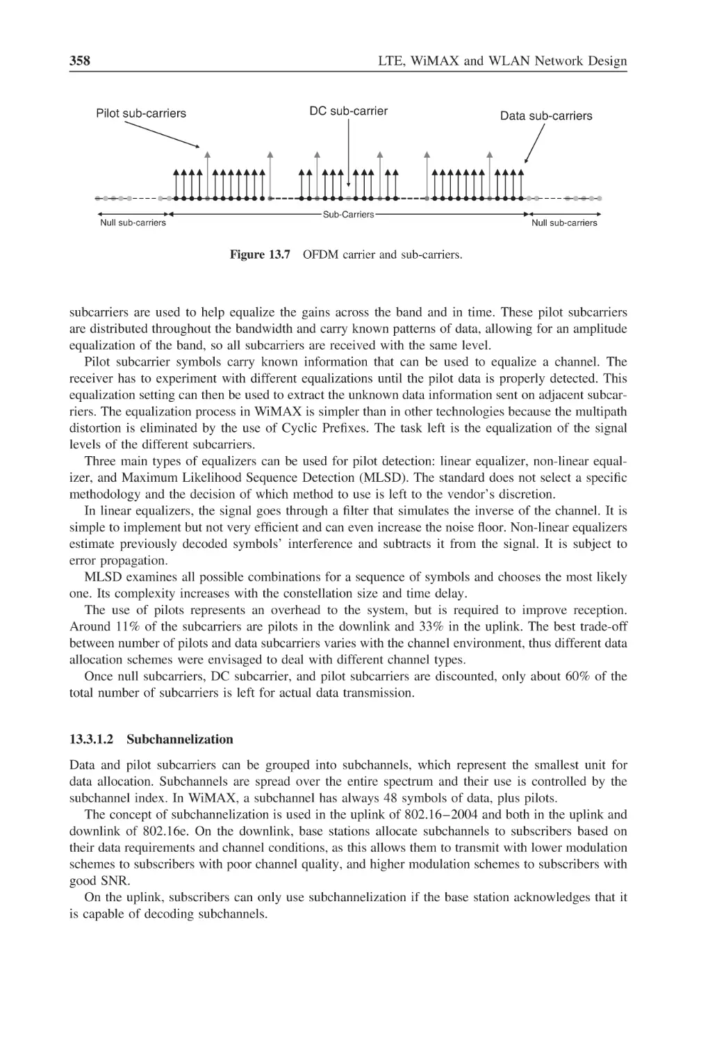
Figure 13.7
OFDM carrier and sub-carriers
358
List of Figures
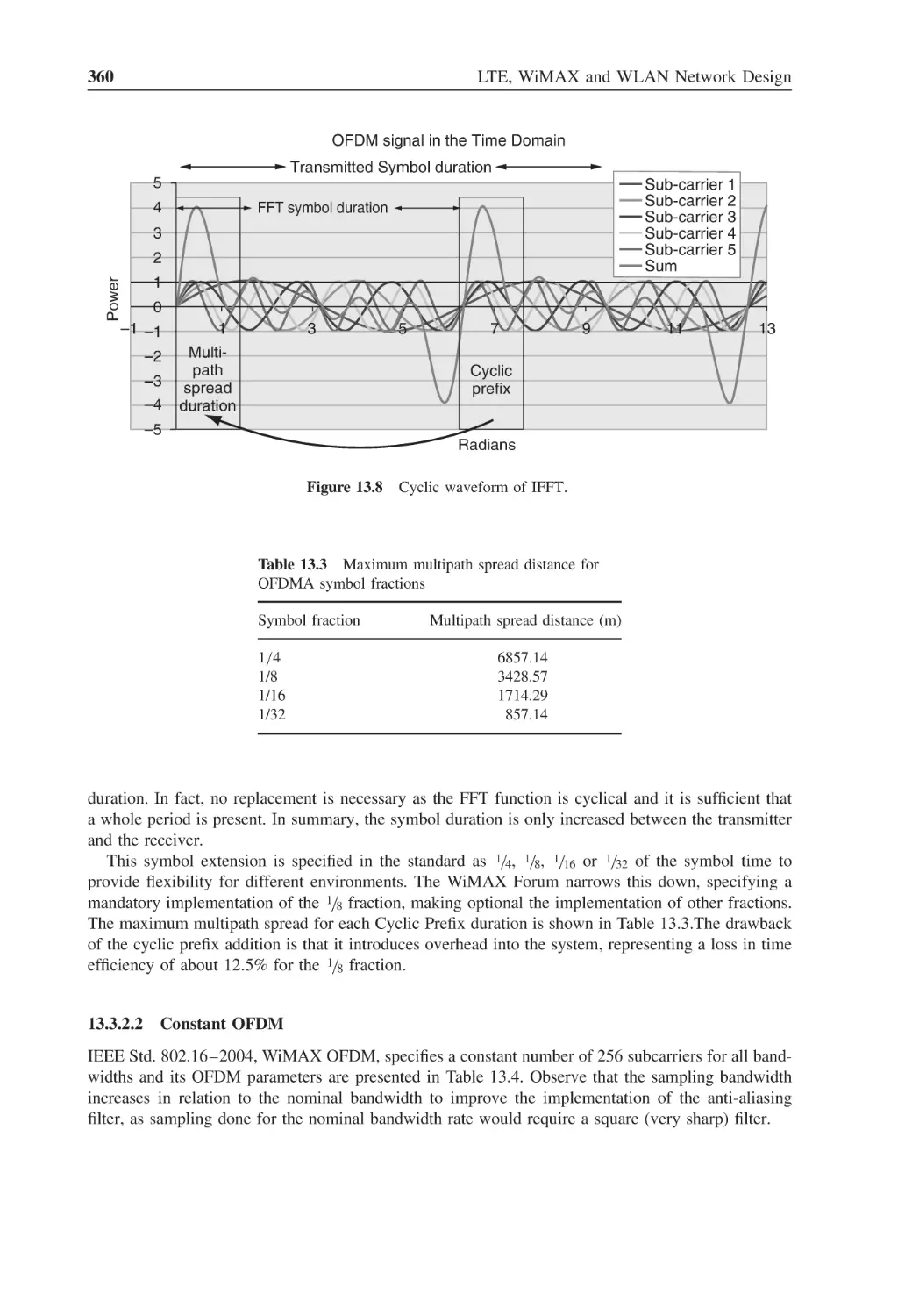
Figure 13.8
Cyclic waveform of IFFT
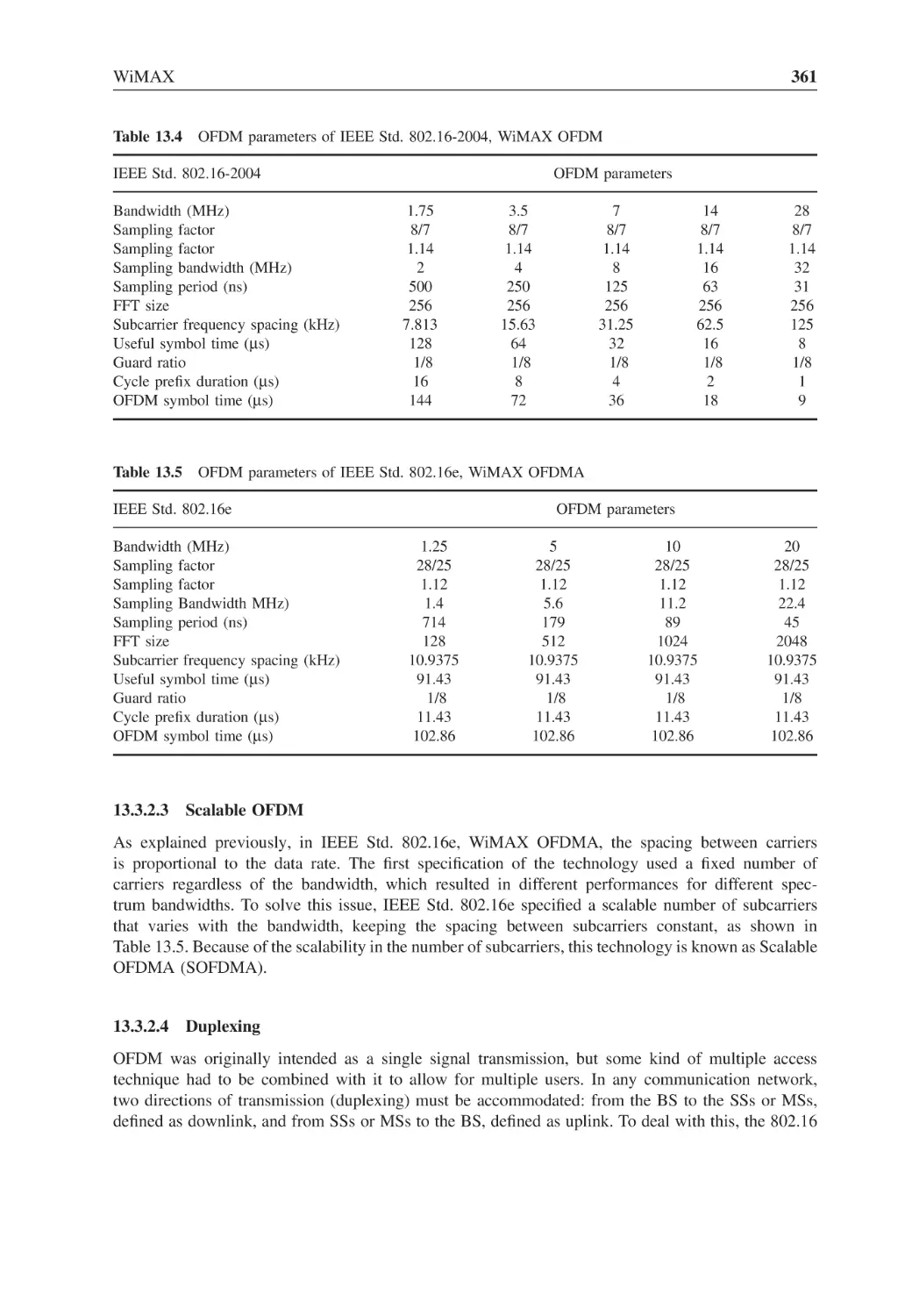
Figure 13.9
H-FDD time allocation of a frequency channel
xxvii
360
362
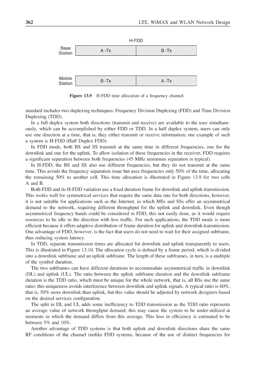
Figure 13.10 TDD transmission in OFDM
363
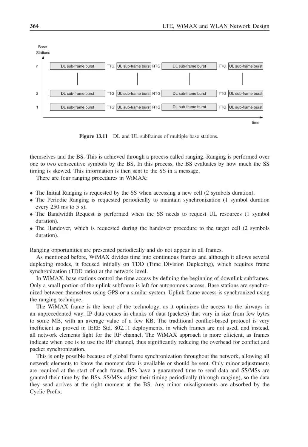
Figure 13.11 DL and UL subframes of multiple base stations
364
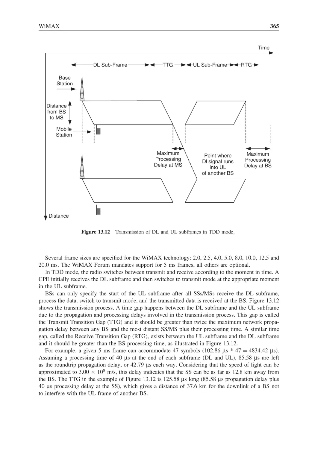
Figure 13.12 Transmission of DL and UL subframes in TDD mode
365
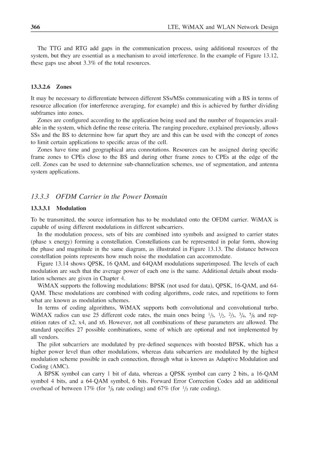
Figure 13.13 Polar and rectangular constellation diagram
367
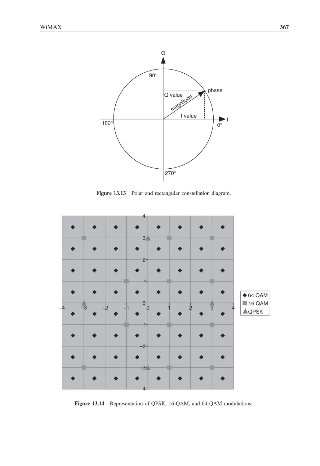
Figure 13.14 Representation of QPSK, 16-QAM, and 64-QAM modulations
367
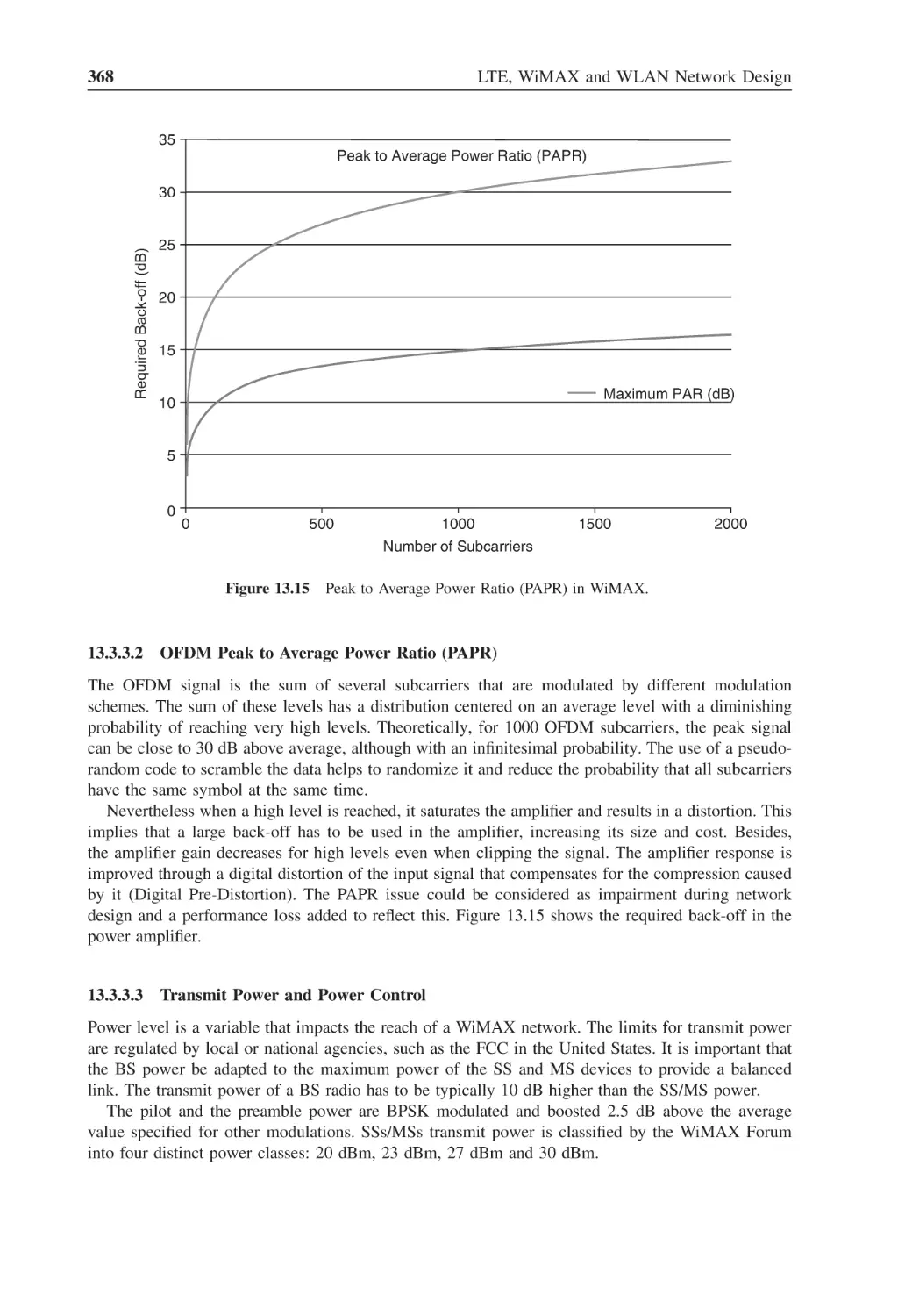
Figure 13.15 Peak to Average Power Ratio (PAPR) in WiMAX
368
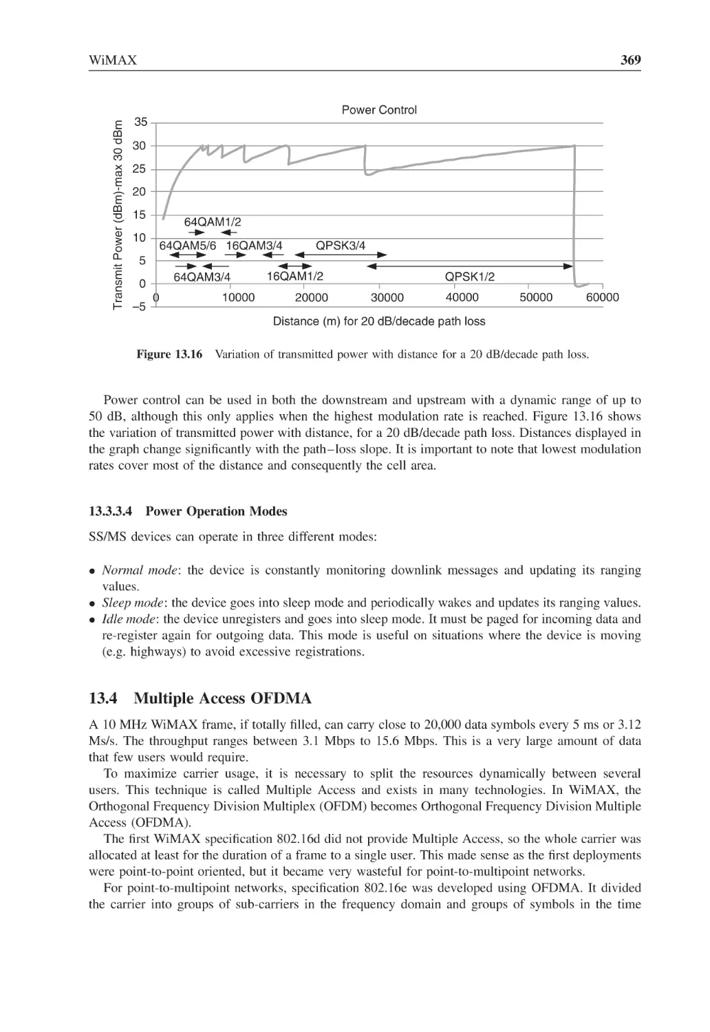
Figure 13.16 Variation of transmitted power with distance for a 20 dB/decade path loss
369
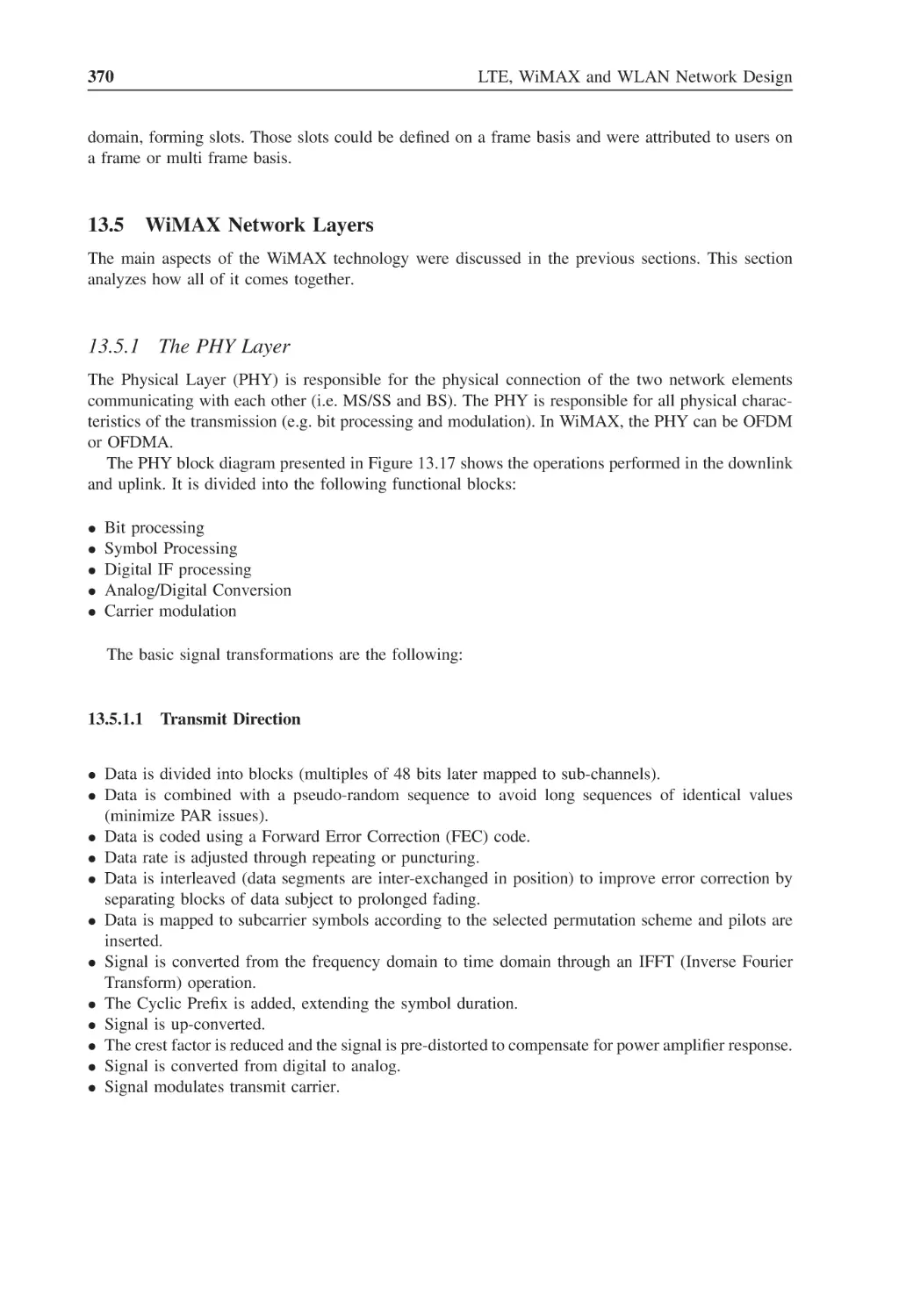
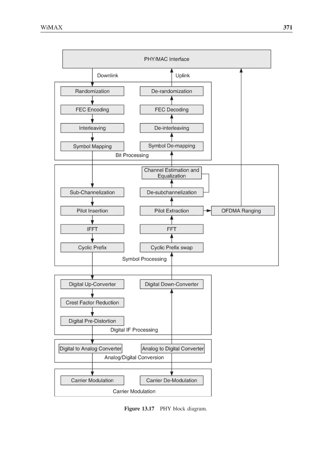
Figure 13.17 PHY block diagram
371
Figure 13.18 OSI layers, and the layers and sub-layers included in the 802.16 standard
372
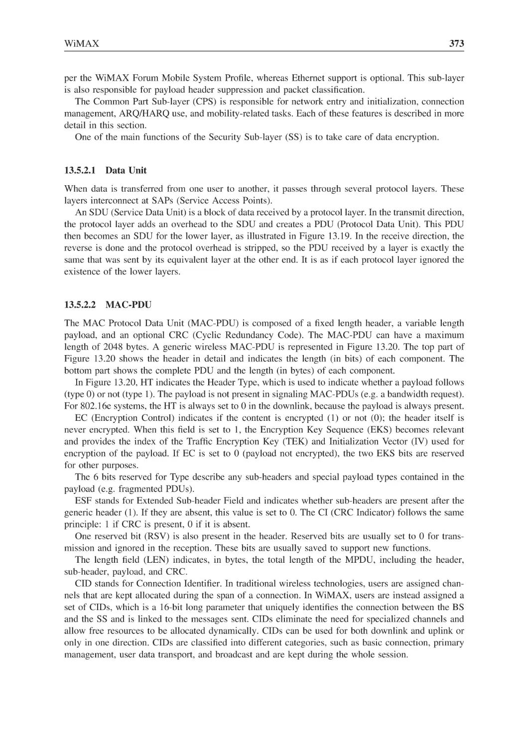
Figure 13.19 Service and protocol data units within different layers
374
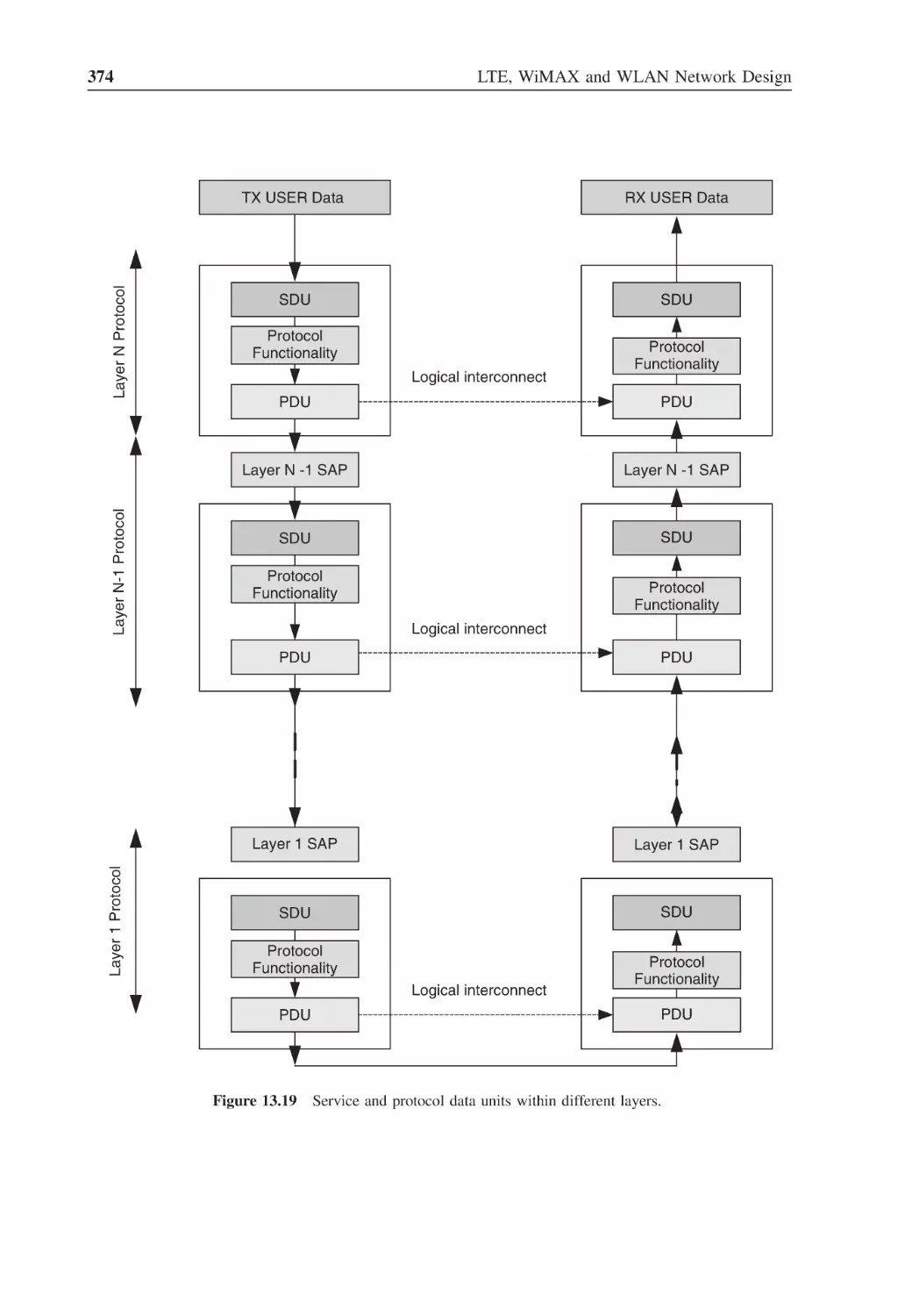
Figure 13.20 Generic wireless MAC-PDU
375
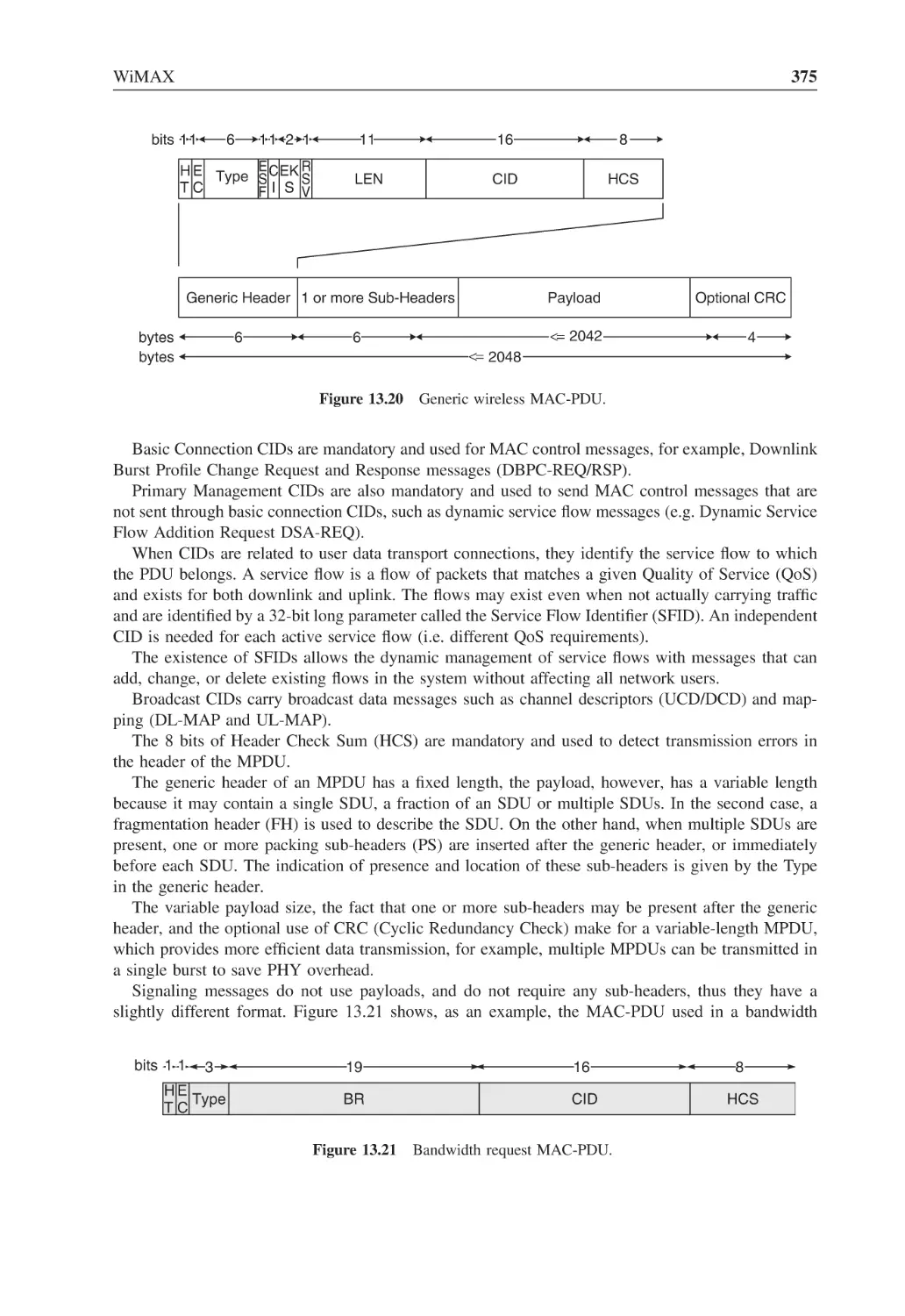
Figure 13.21 Bandwidth request MAC-PDU
375
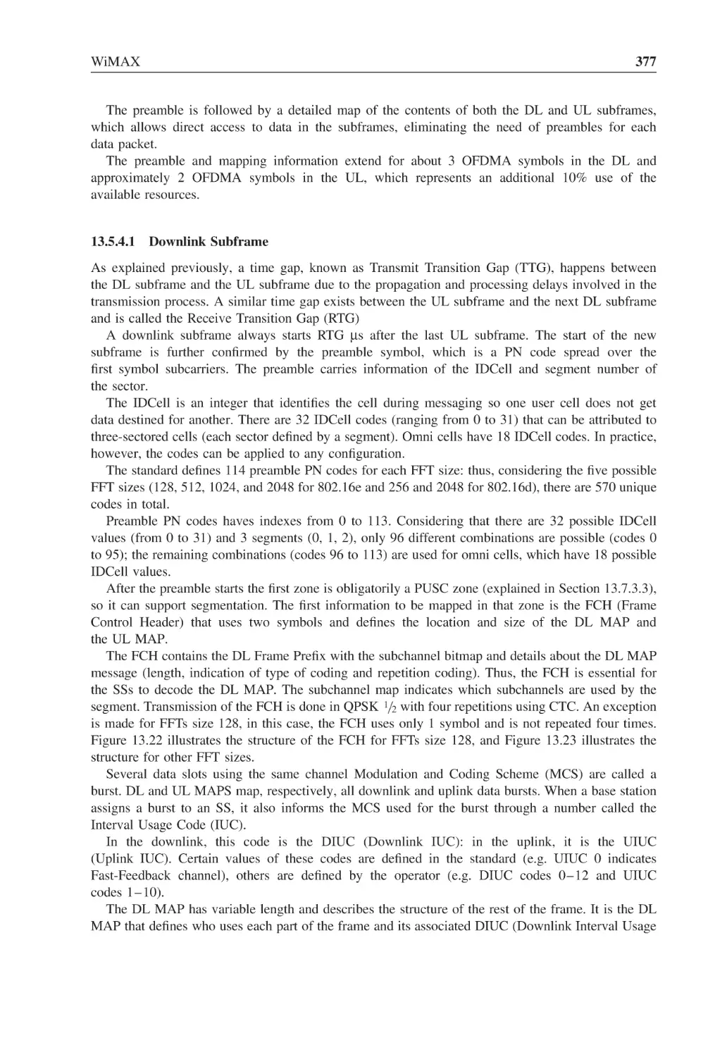
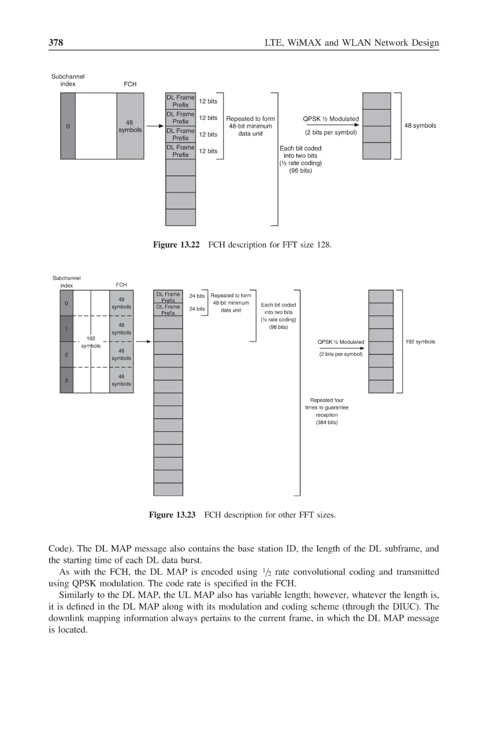
Figure 13.22 FCH description for FFT size 128
378
Figure 13.23 FCH description for other FFT sizes
378
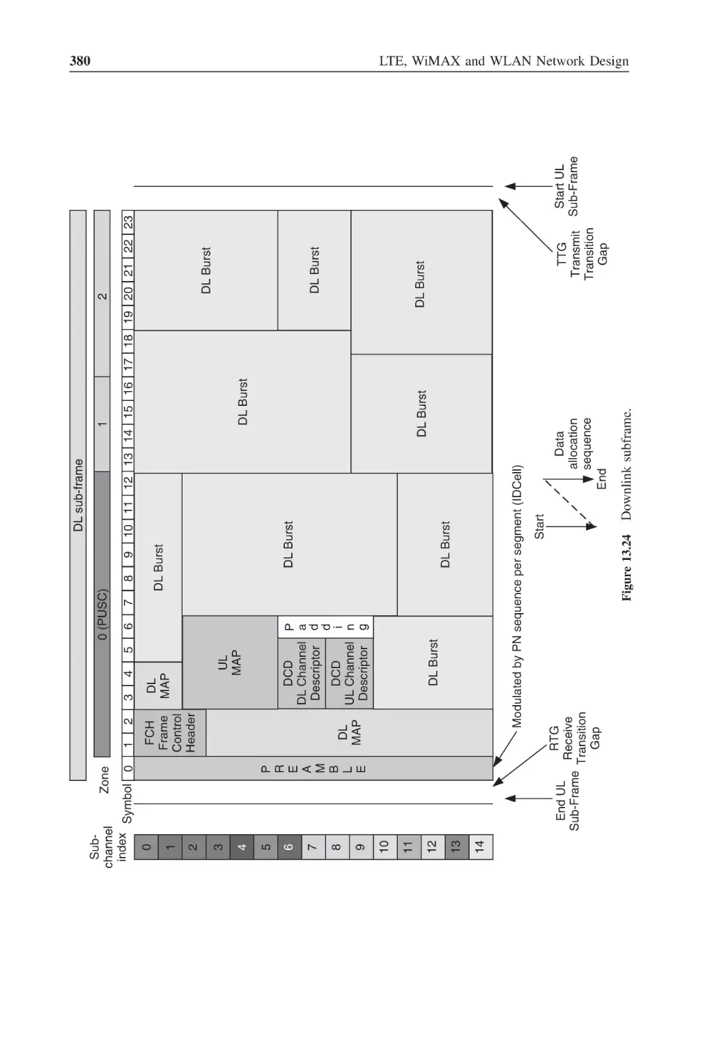
Figure 13.24 Downlink subframe
380
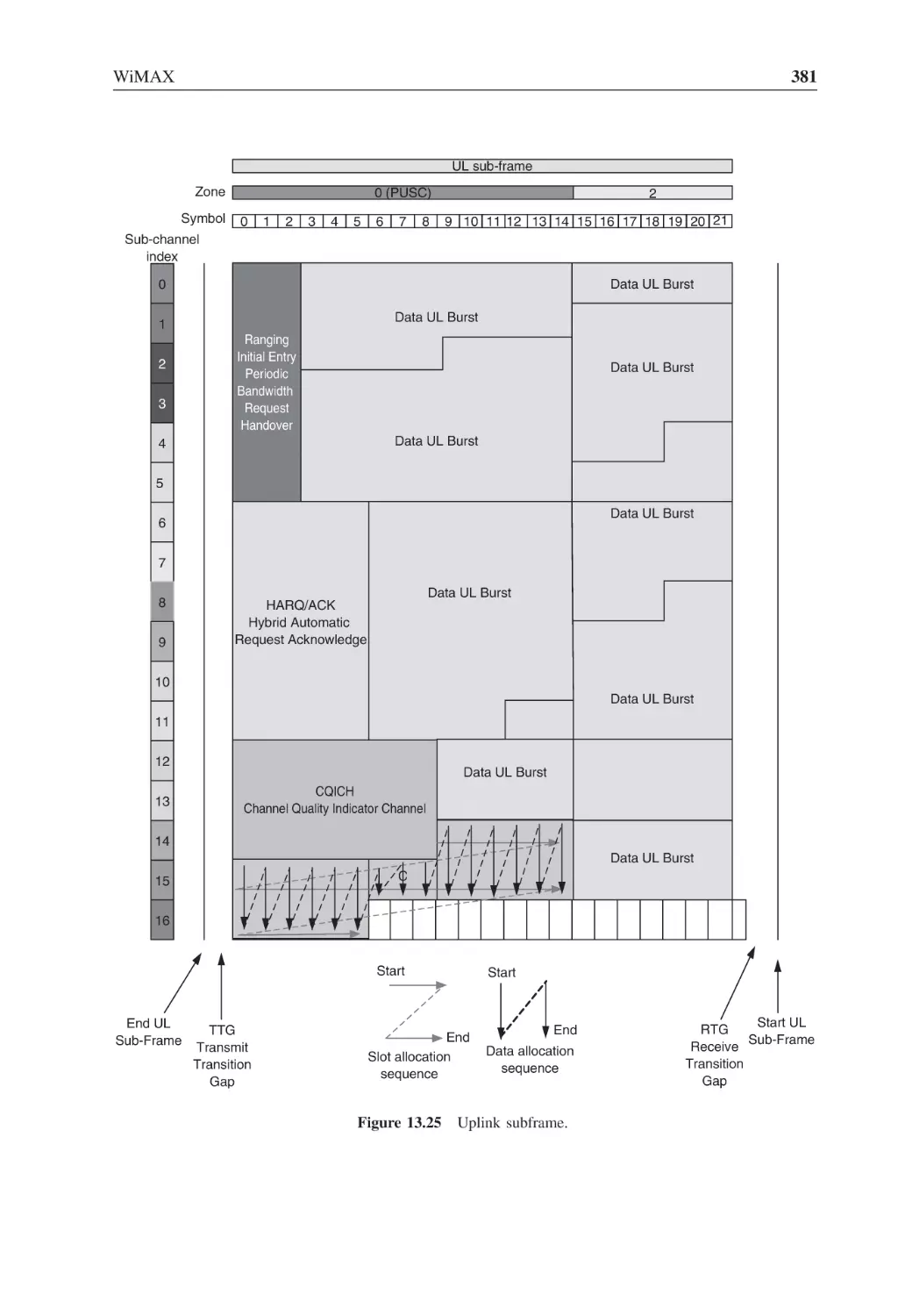
Figure 13.25 Uplink subframe
381
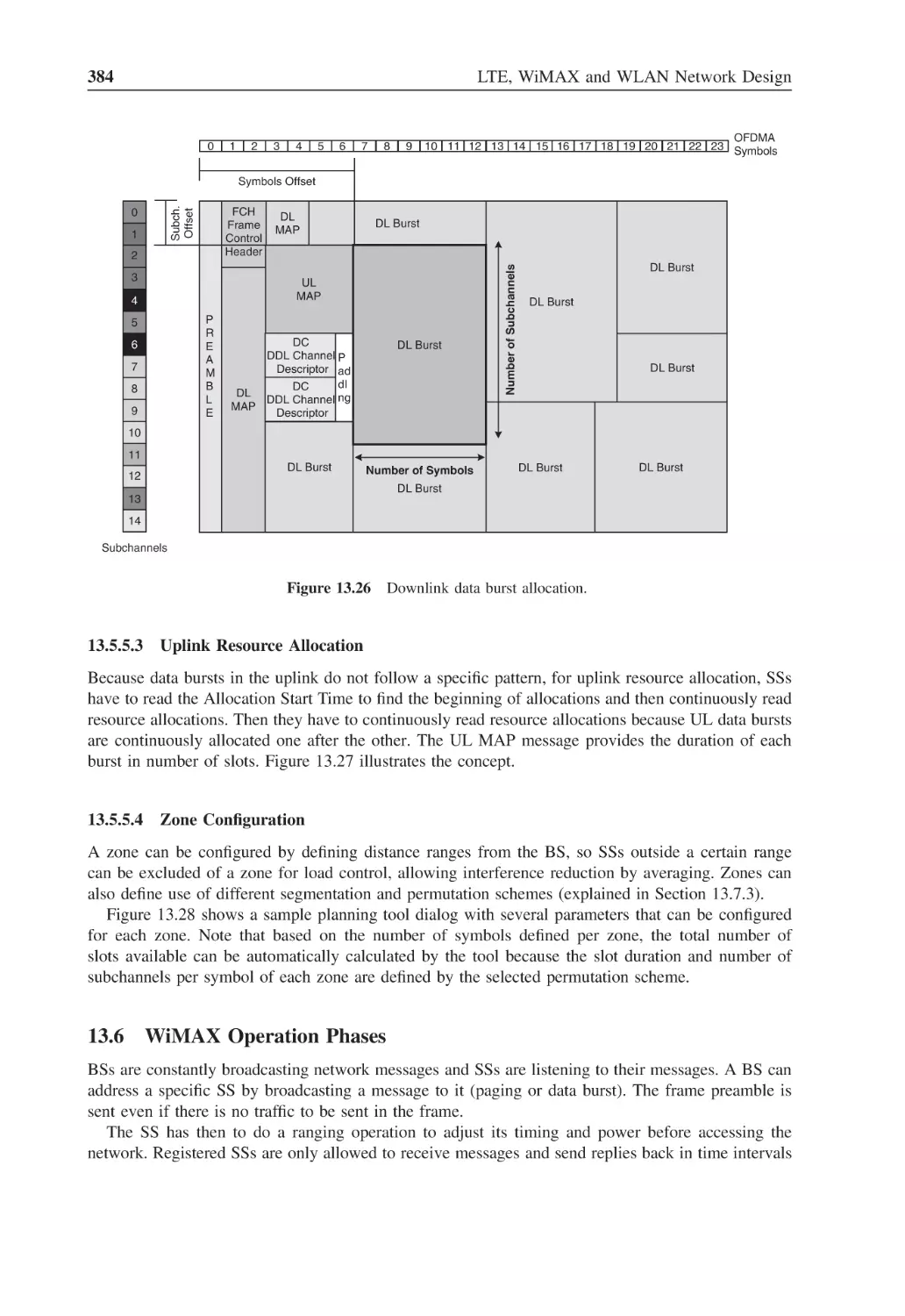
Figure 13.26 Downlink data burst allocation
384
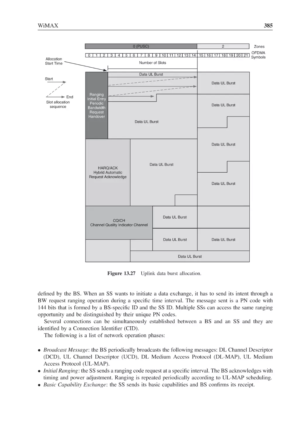
Figure 13.27 Uplink data burst allocation
385
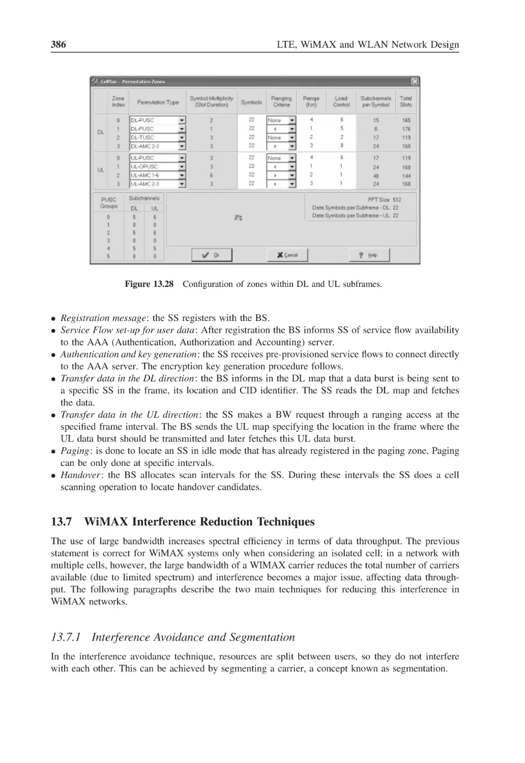
Figure 13.28 Configuration of zones within DL and UL subframes
386
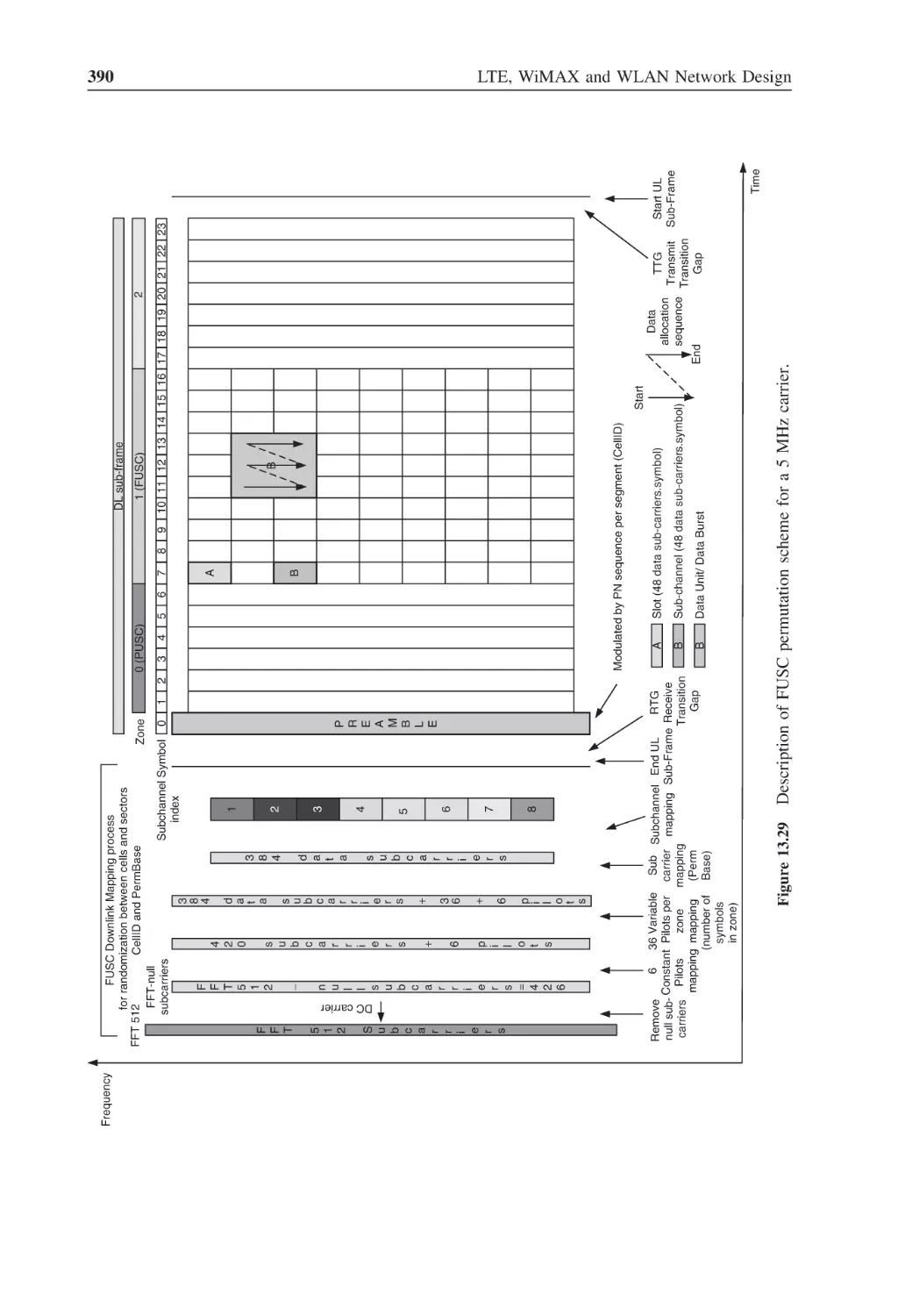
Figure 13.29 Description of FUSC permutation scheme for a 5 MHz carrier
390
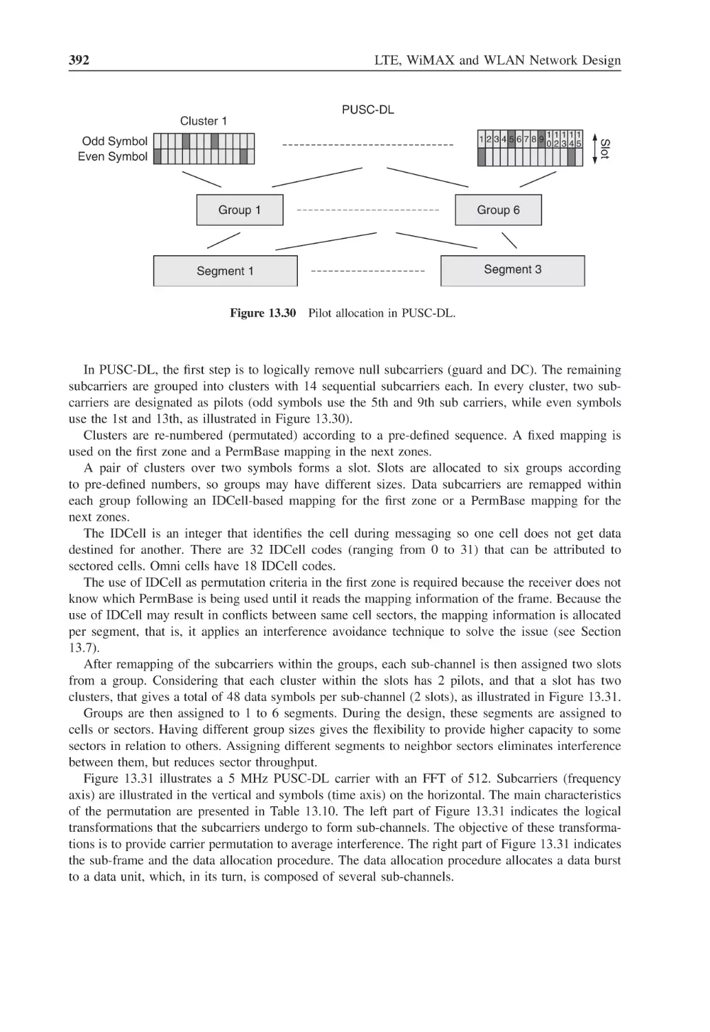
Figure 13.30 Pilot allocation in PUSC-DL
392
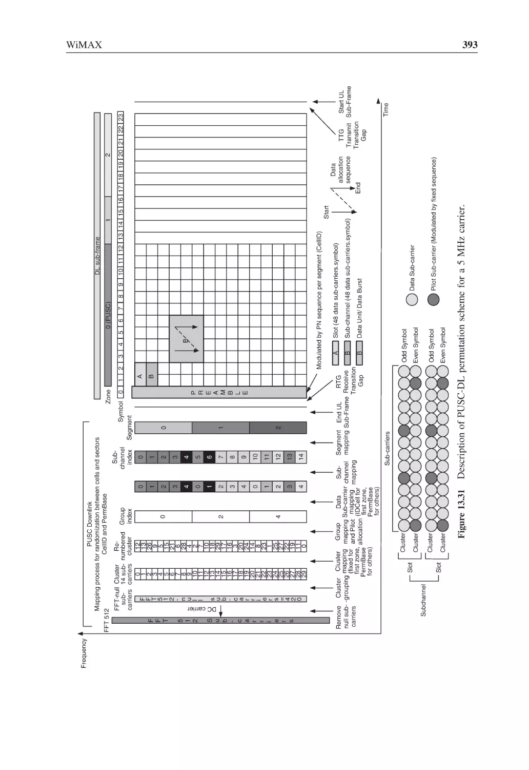
Figure 13.31 Description of PUSC-DL permutation scheme for a 5 MHz carrier
393
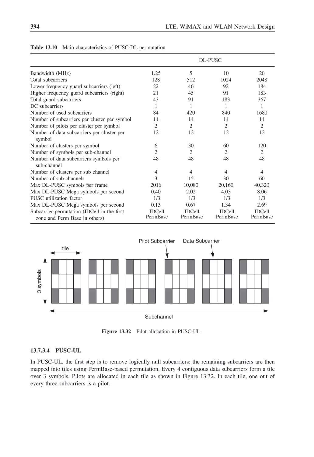
Figure 13.32 Pilot allocation in PUSC-UL
394
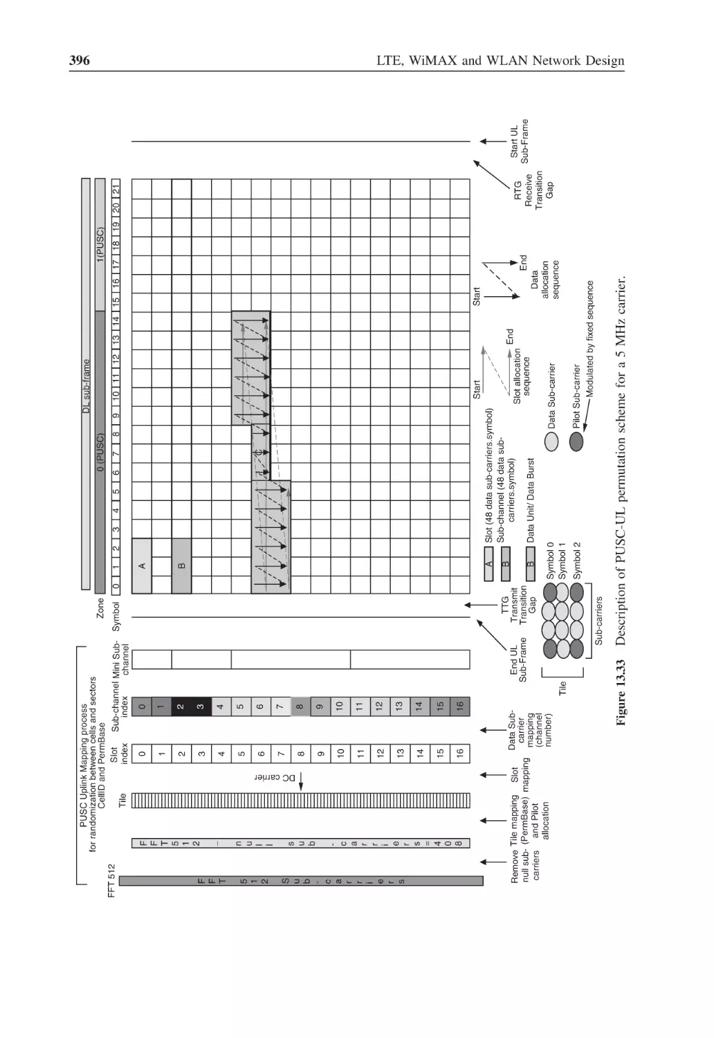
Figure 13.33 Description of PUSC-UL permutation scheme for a 5 MHz carrier
396
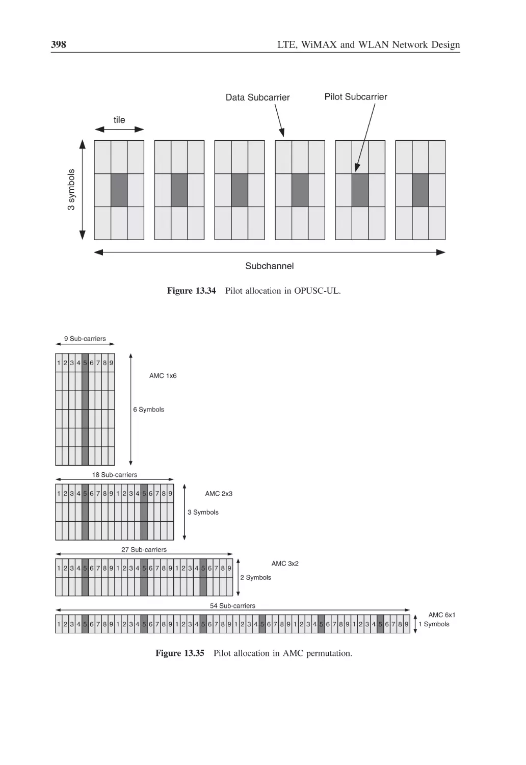
Figure 13.34 Pilot allocation in OPUSC-UL
398
Figure 13.35 Pilot allocation in AMC permutation
398
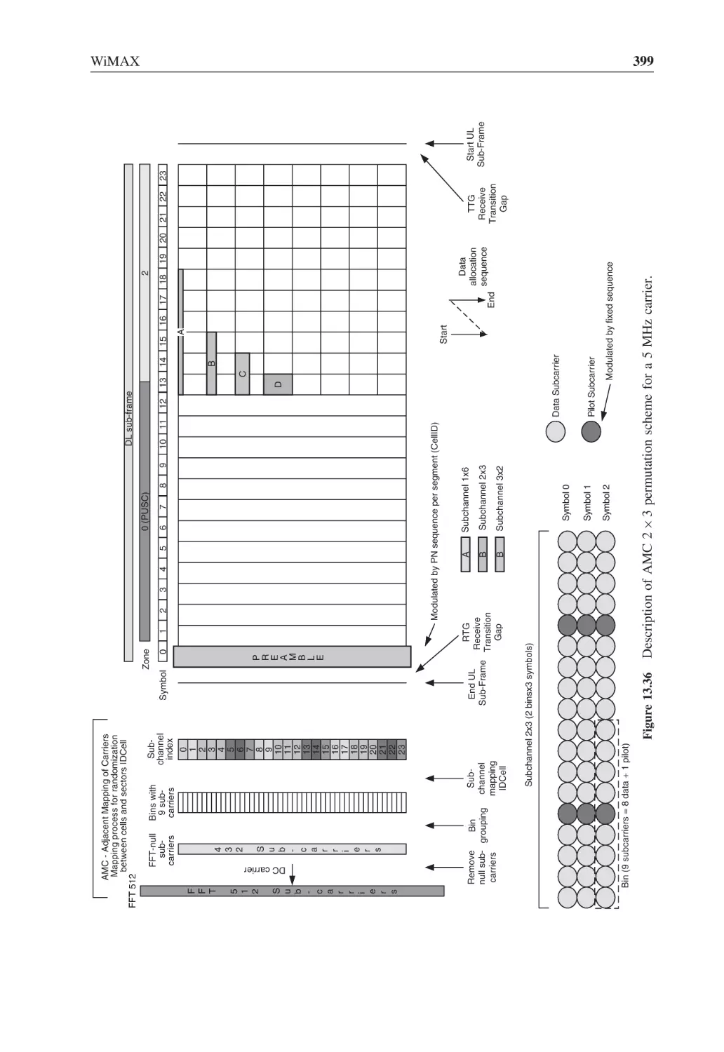
Figure 13.36 Description of AMC 2 × 3 permutation scheme for a 5 MHz carrier
399
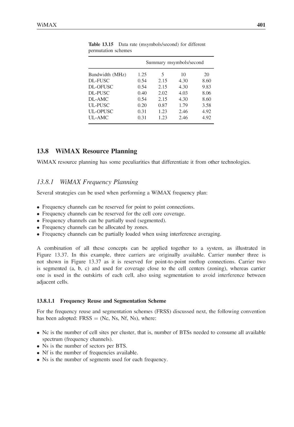
Figure 13.37 Multi-layer frequency plan with segmentation and zoning
402
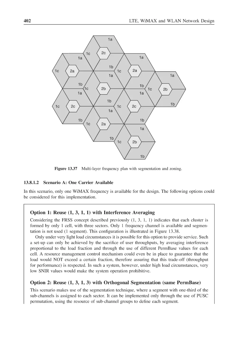
Figure 13.38 Reuse (1, 3, 1, 1)
403
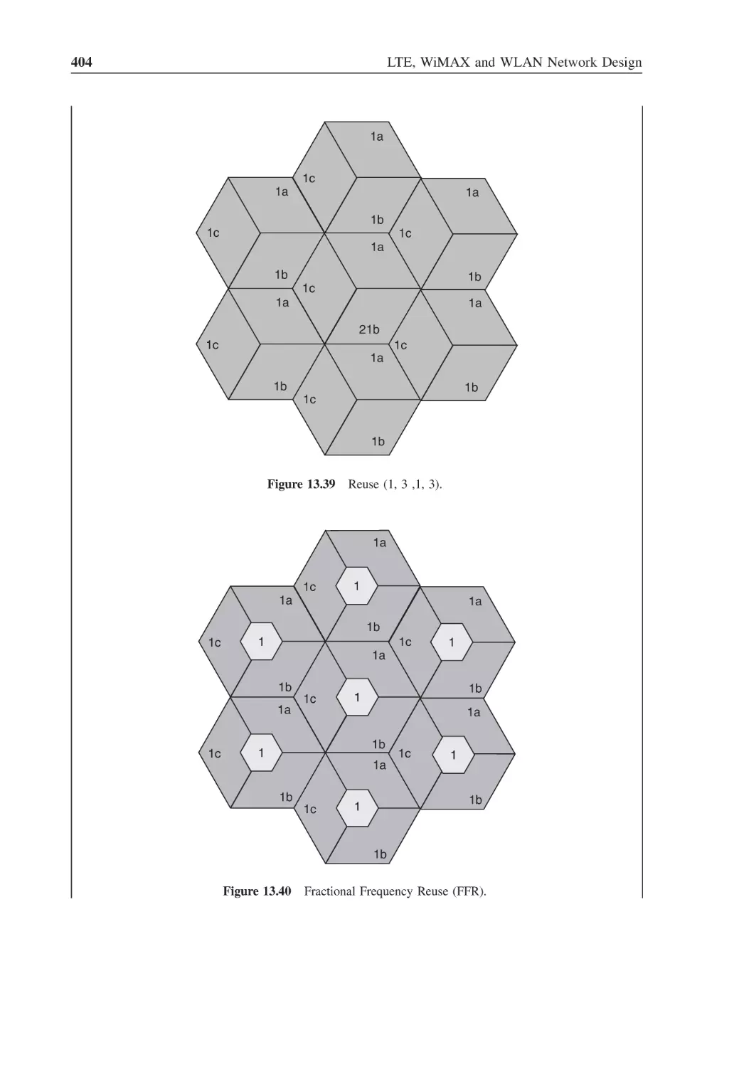
Figure 13.39 Reuse (1, 3 ,1, 3)
404
Figure 13.40 Fractional Frequency Reuse (FFR)
404
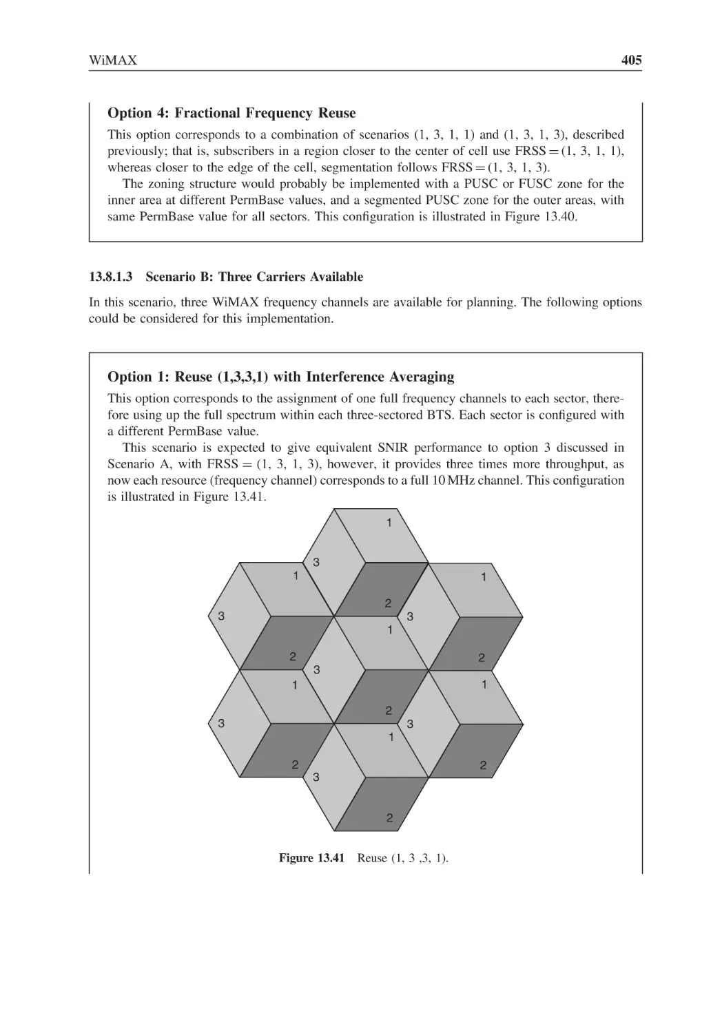
Figure 13.41 Reuse (1, 3 ,3, 1)
405
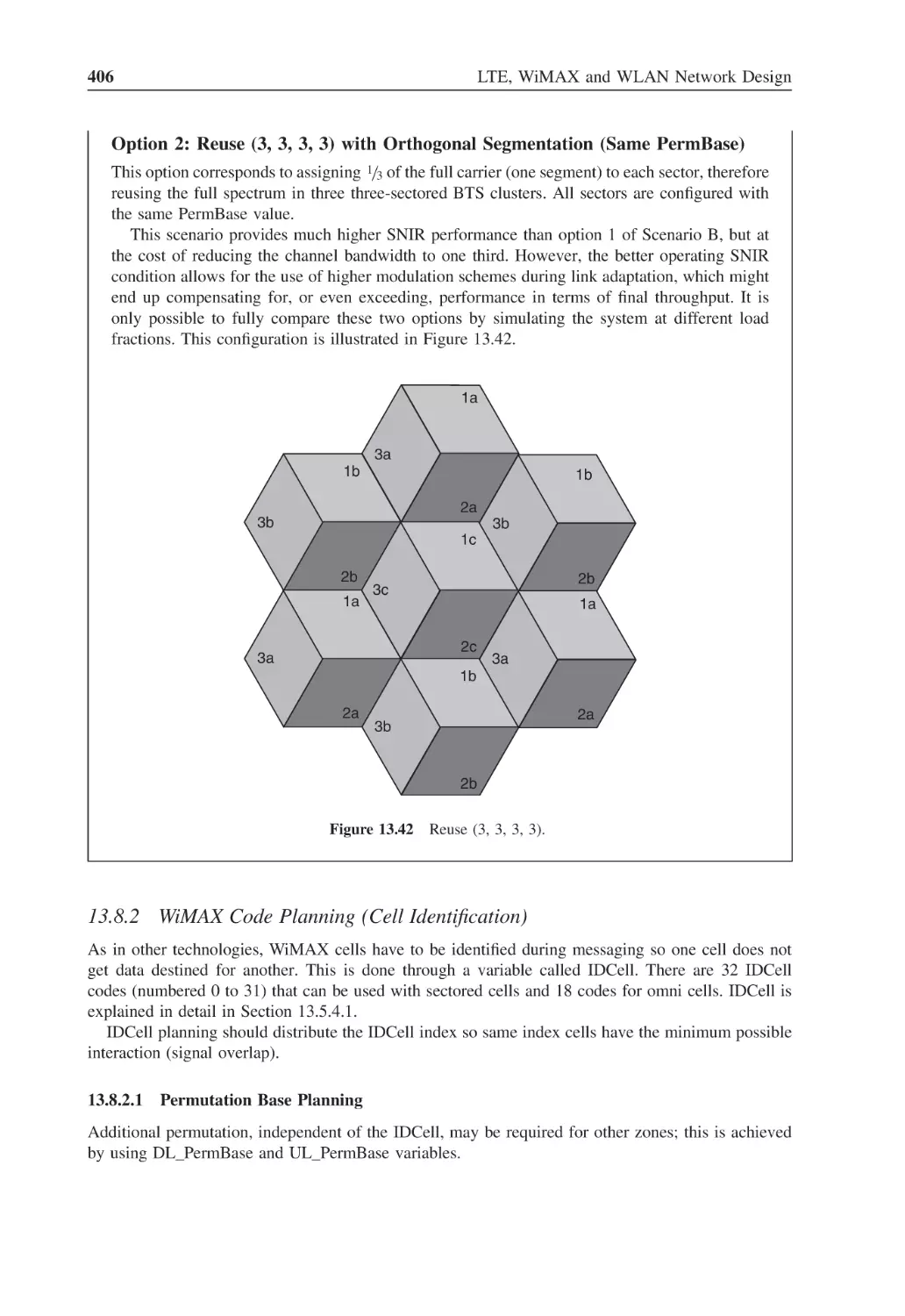
Figure 13.42 Reuse (3, 3, 3, 3)
406
Figure 14.1
Simplified 3GPP GSM and UMTS network architecture
418
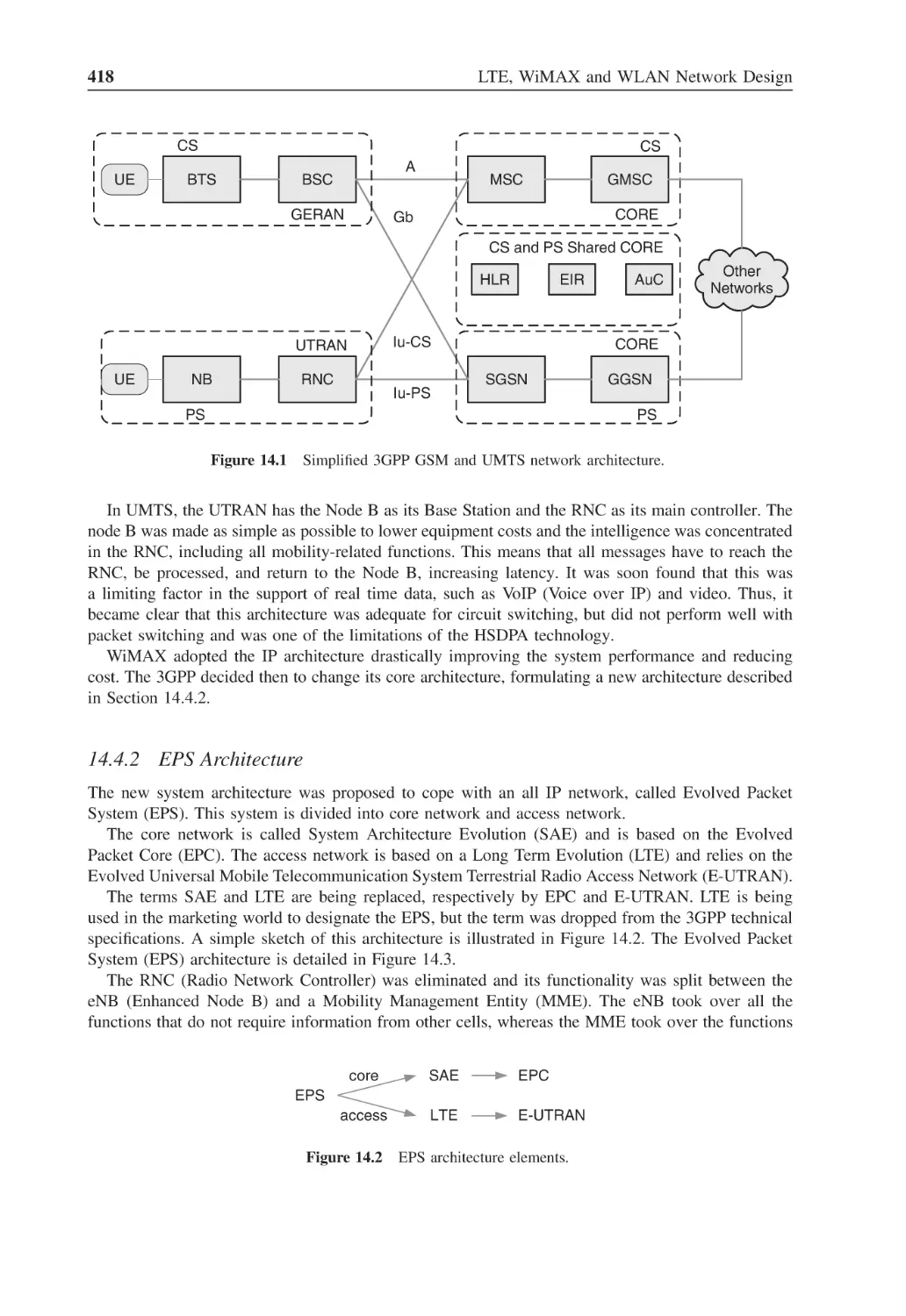
Figure 14.2
EPS architecture elements
418
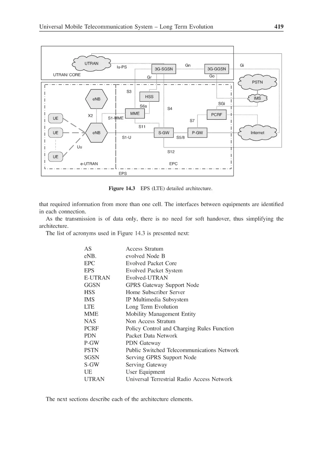
Figure 14.3
EPS (LTE) detailed architecture
419
Figure 14.4
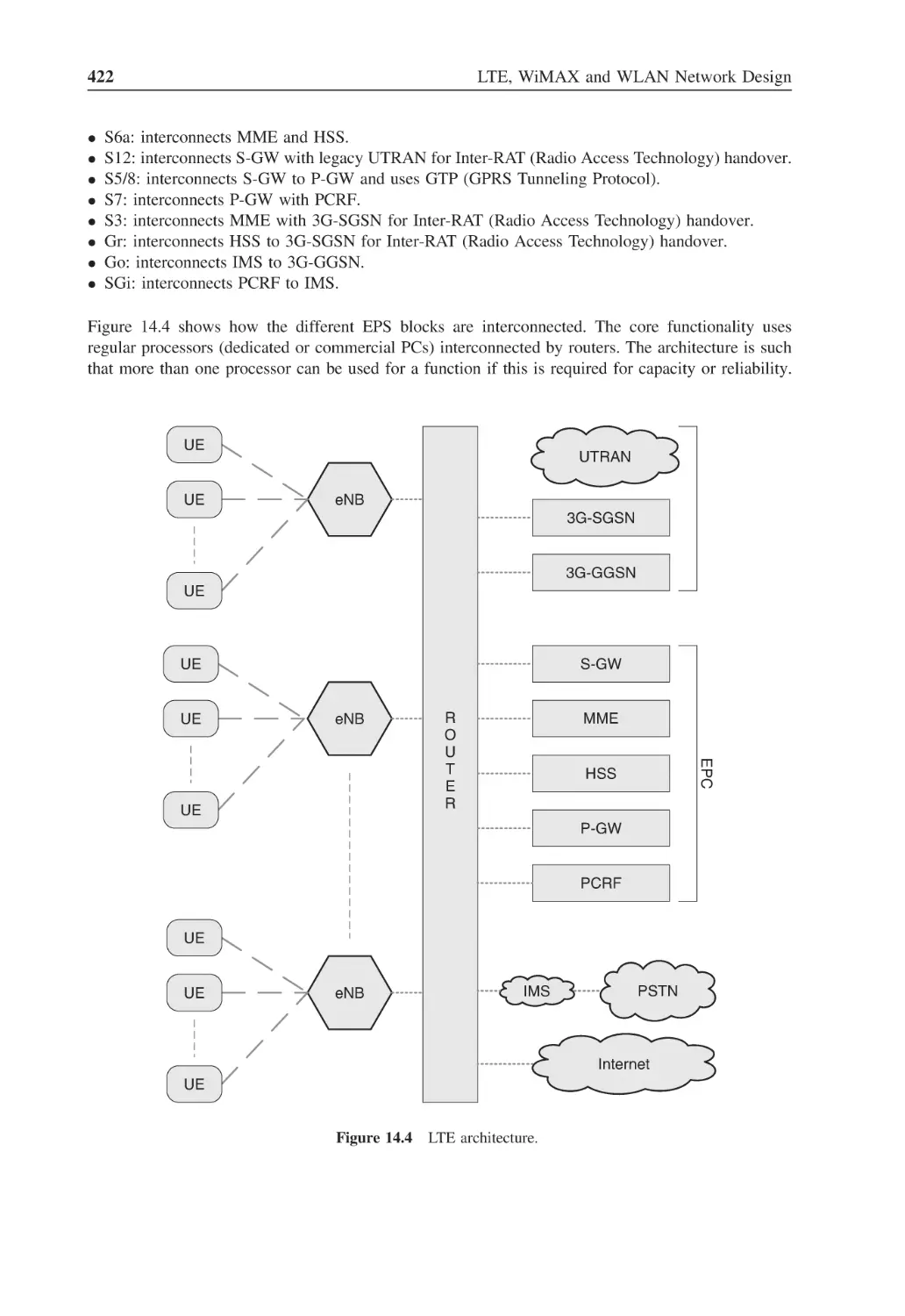
LTE architecture
422
xxviii
List of Figures
Figure 14.5
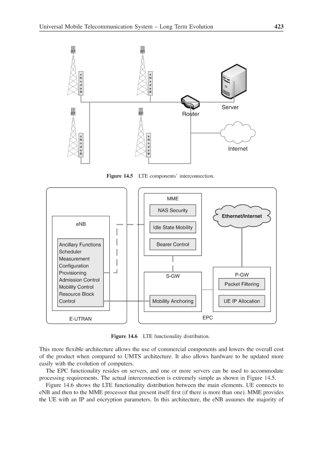
LTE components’ interconnection
423
Figure 14.6
LTE functionality distribution
423
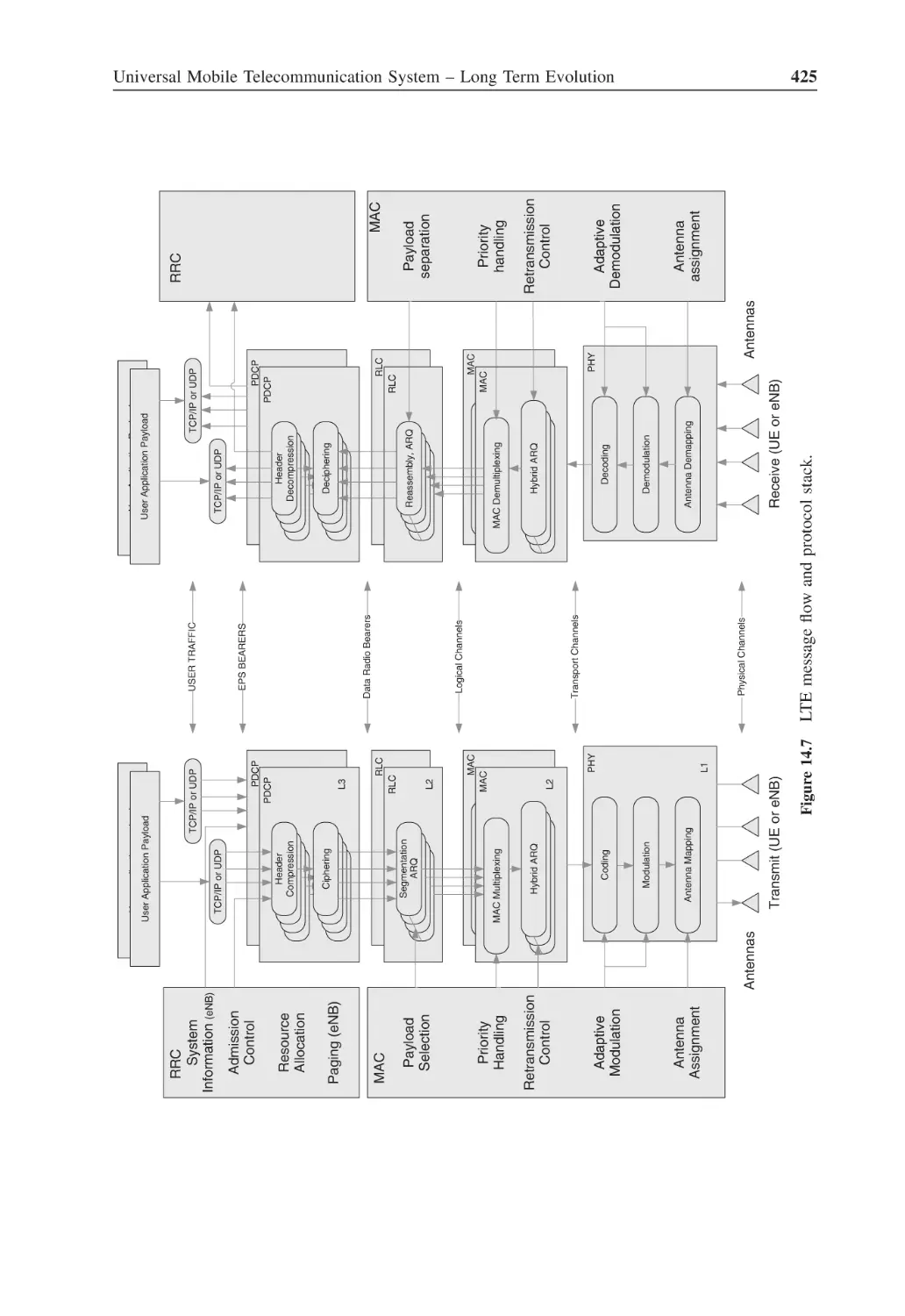
Figure 14.7
LTE message flow and protocol stack
425
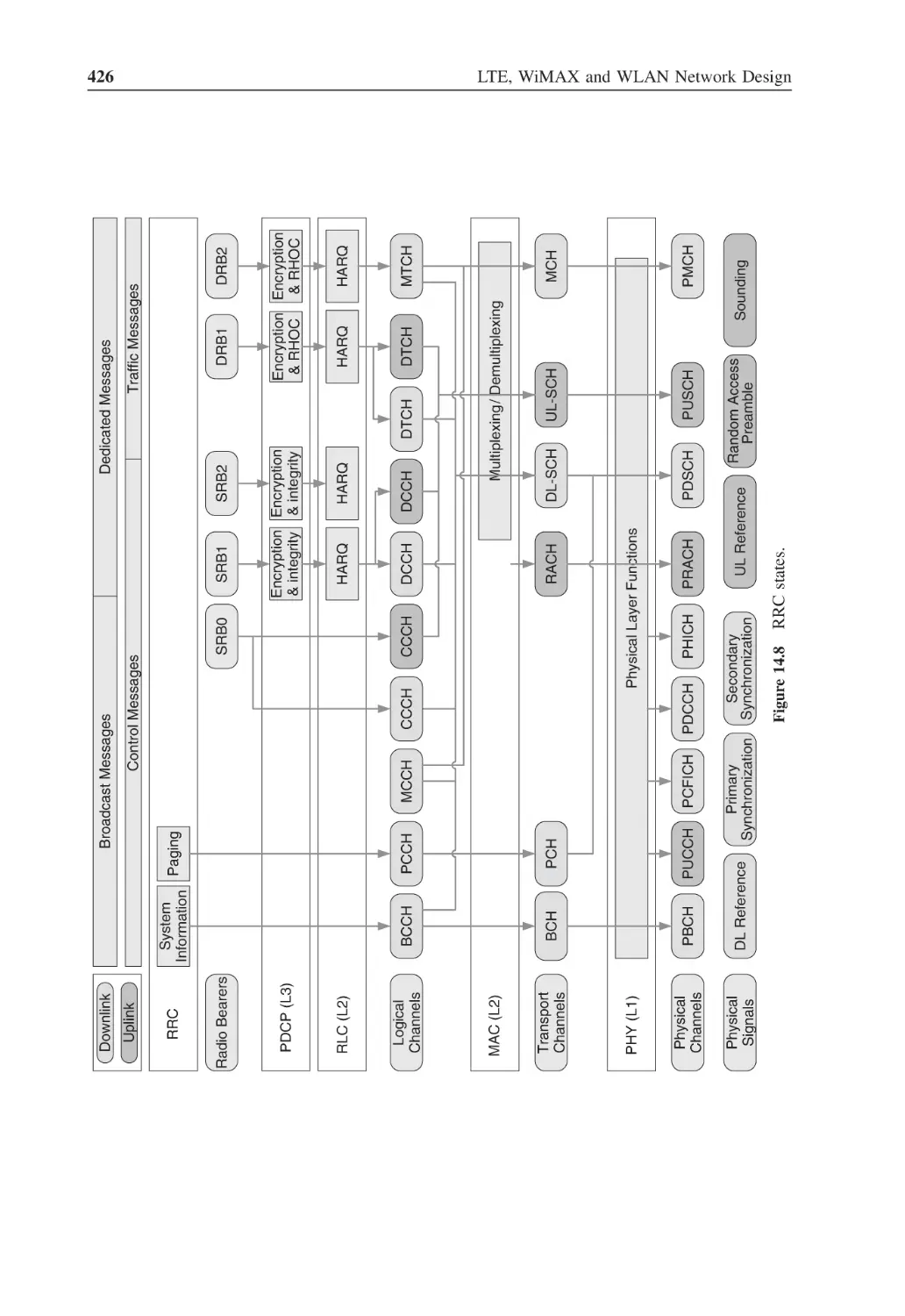
Figure 14.8
RRC states
426
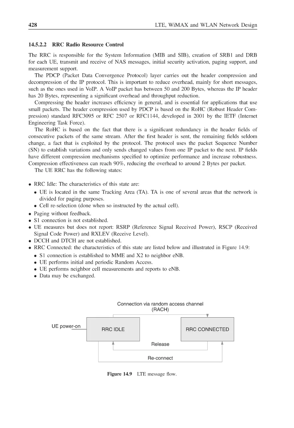
Figure 14.9
LTE message flow
428
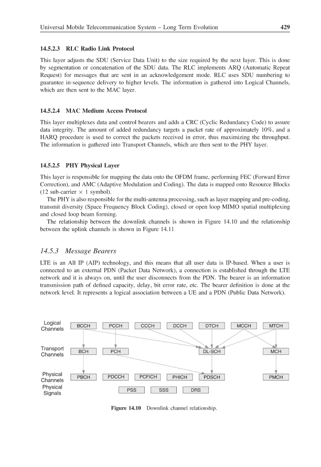
Figure 14.10 Downlink channel relationship
429
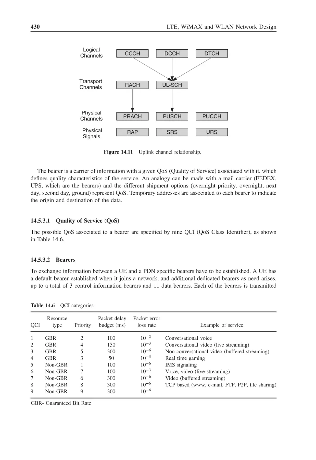
Figure 14.11 Uplink channel relationship
430
Figure 14.12 E-UTRAN message exchange
433
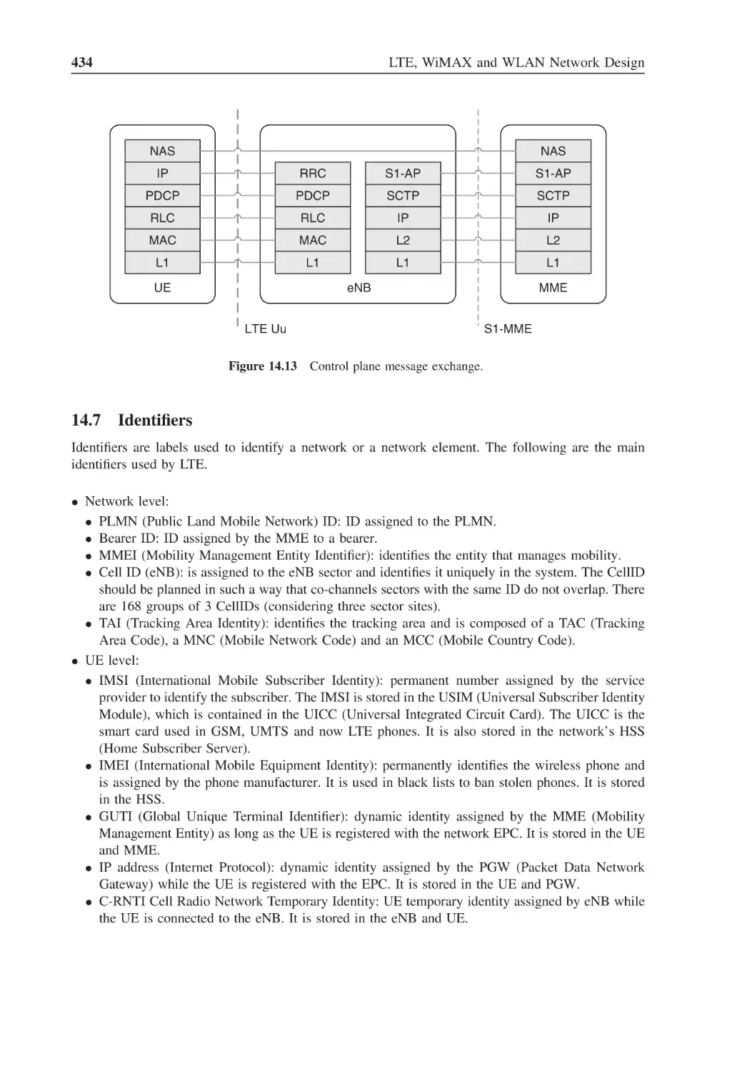
Figure 14.13 Control plane message exchange
434
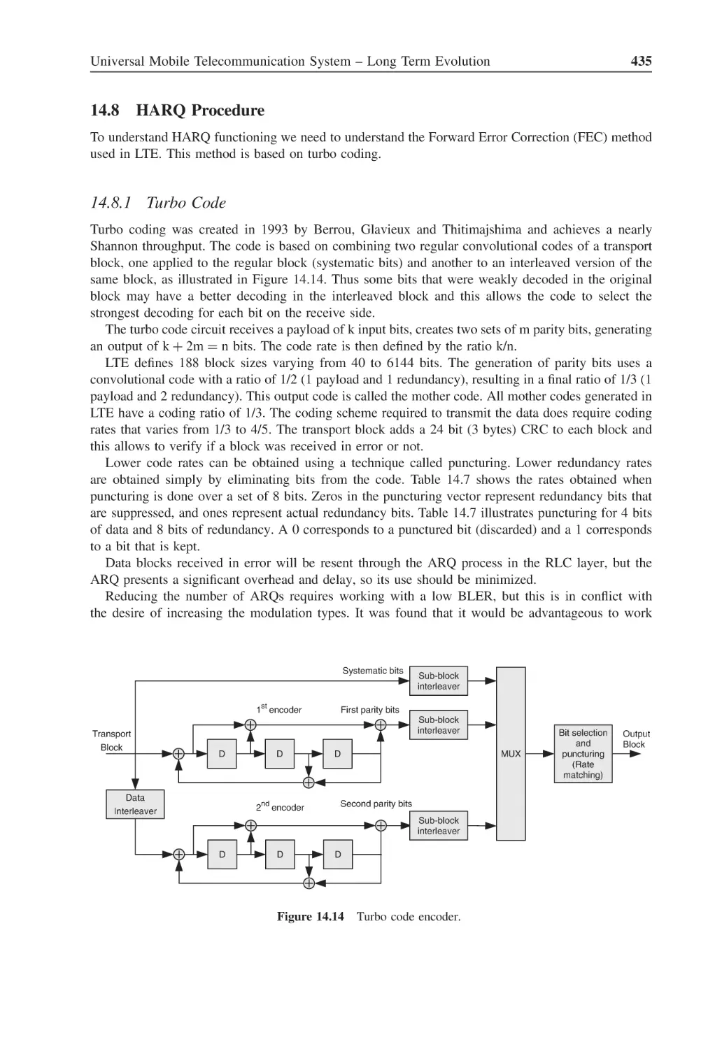
Figure 14.14 Turbo code encoder
435
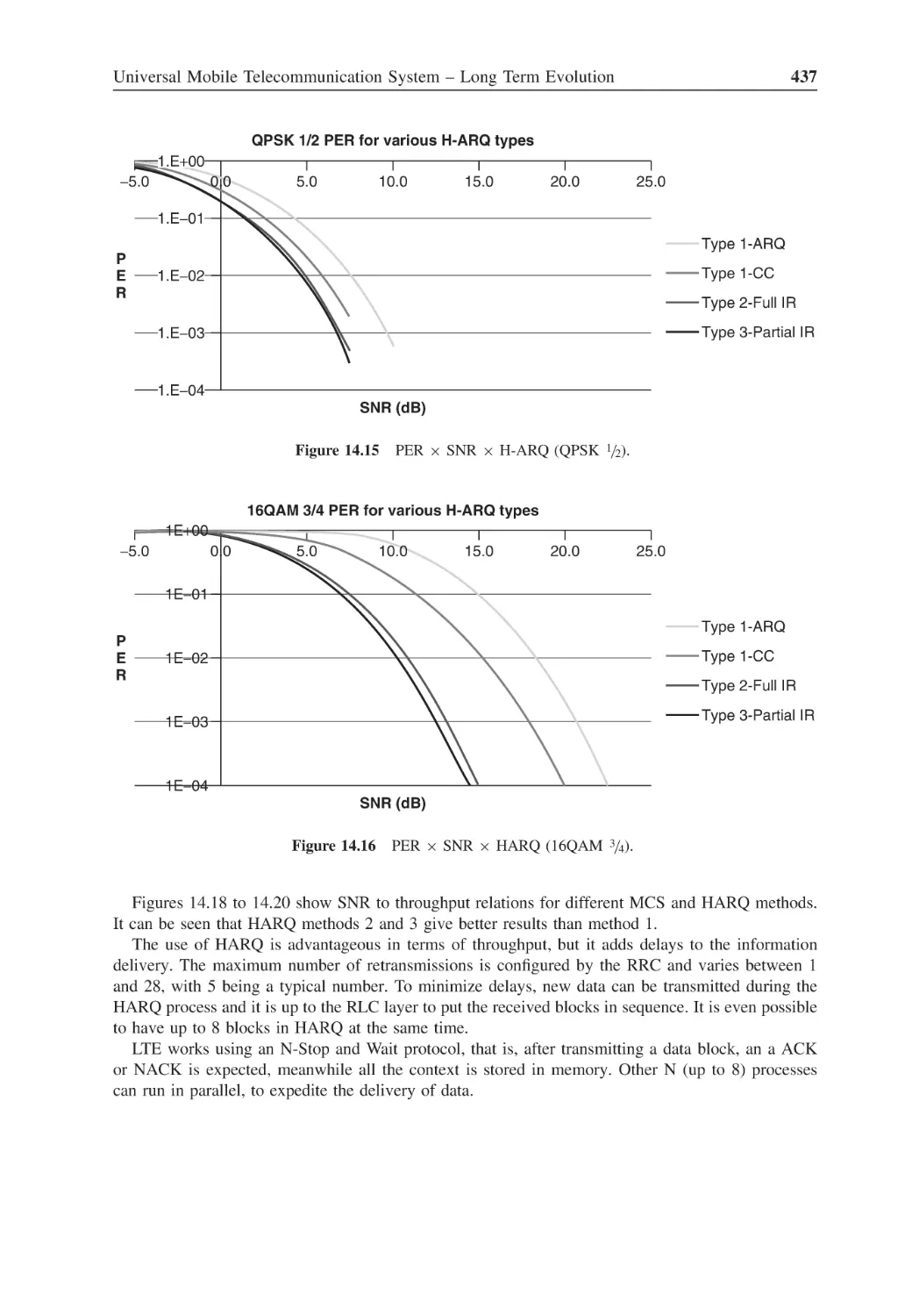
Figure 14.15 PER × SNR × H-ARQ (QPSK 1/2)
437
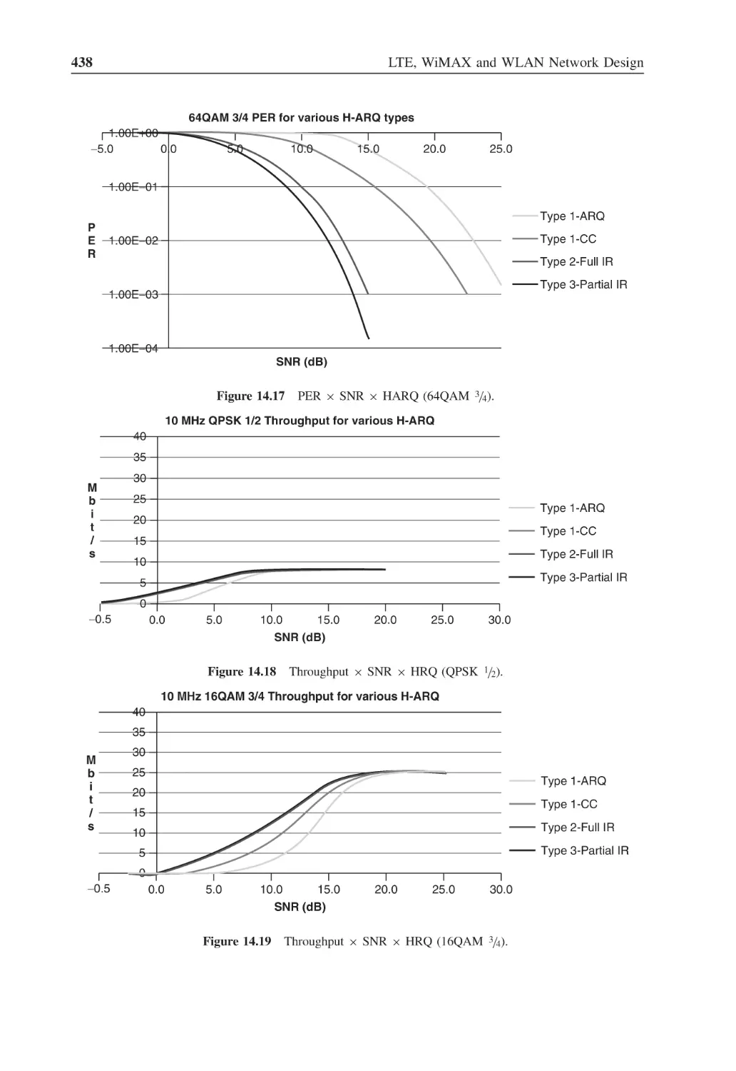
Figure 14.16 PER × SNR × HARQ (16QAM 3/4)
437
Figure 14.17 PER × SNR × HARQ (64QAM
3/4)
438
Figure 14.18 Throughput × SNR × HRQ (QPSK 1/2)
438
Figure 14.19 Throughput × SNR × HRQ (16QAM 3/4)
438
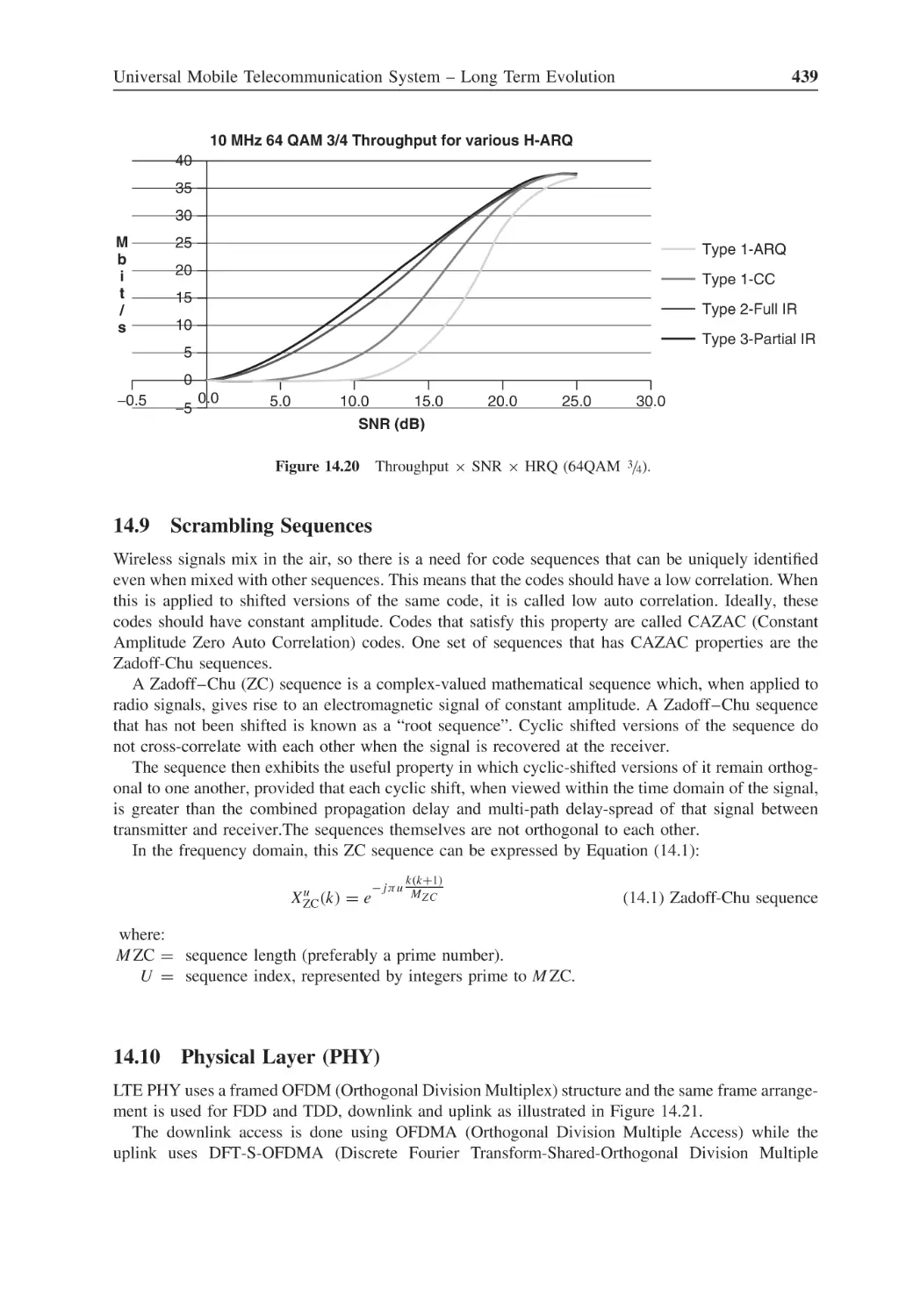
Figure 14.20 Throughput × SNR × HRQ (64QAM 3/4)
439
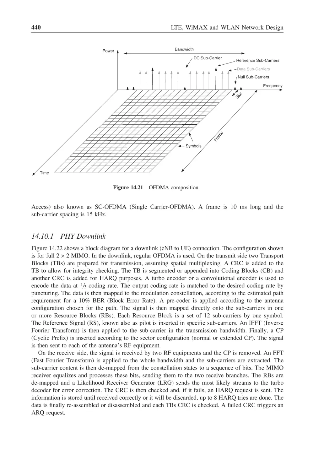
Figure 14.21 OFDMA composition
440
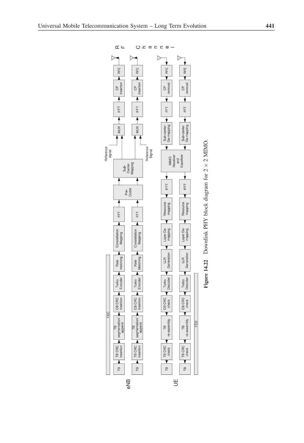
Figure 14.22 Downlink PHY block diagram for 2 × 2 MIMO
441
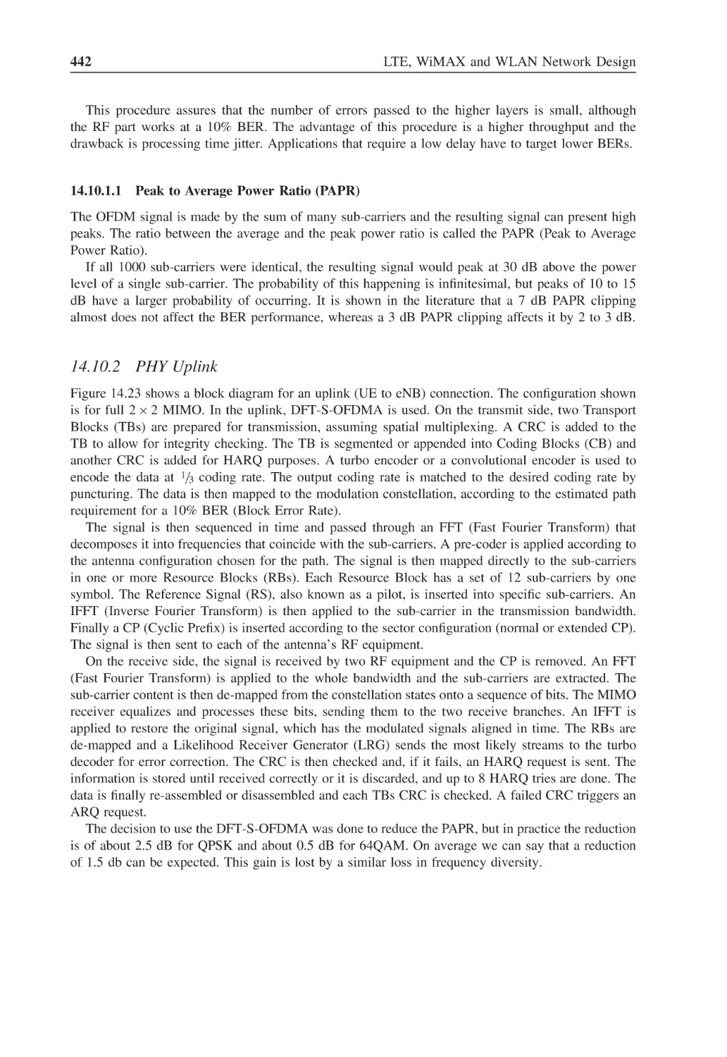
Figure 14.23 Uplink PHY block diagram for 2 × 2 MIMO
443
Figure 14.24 FDD frame in the time domain
444
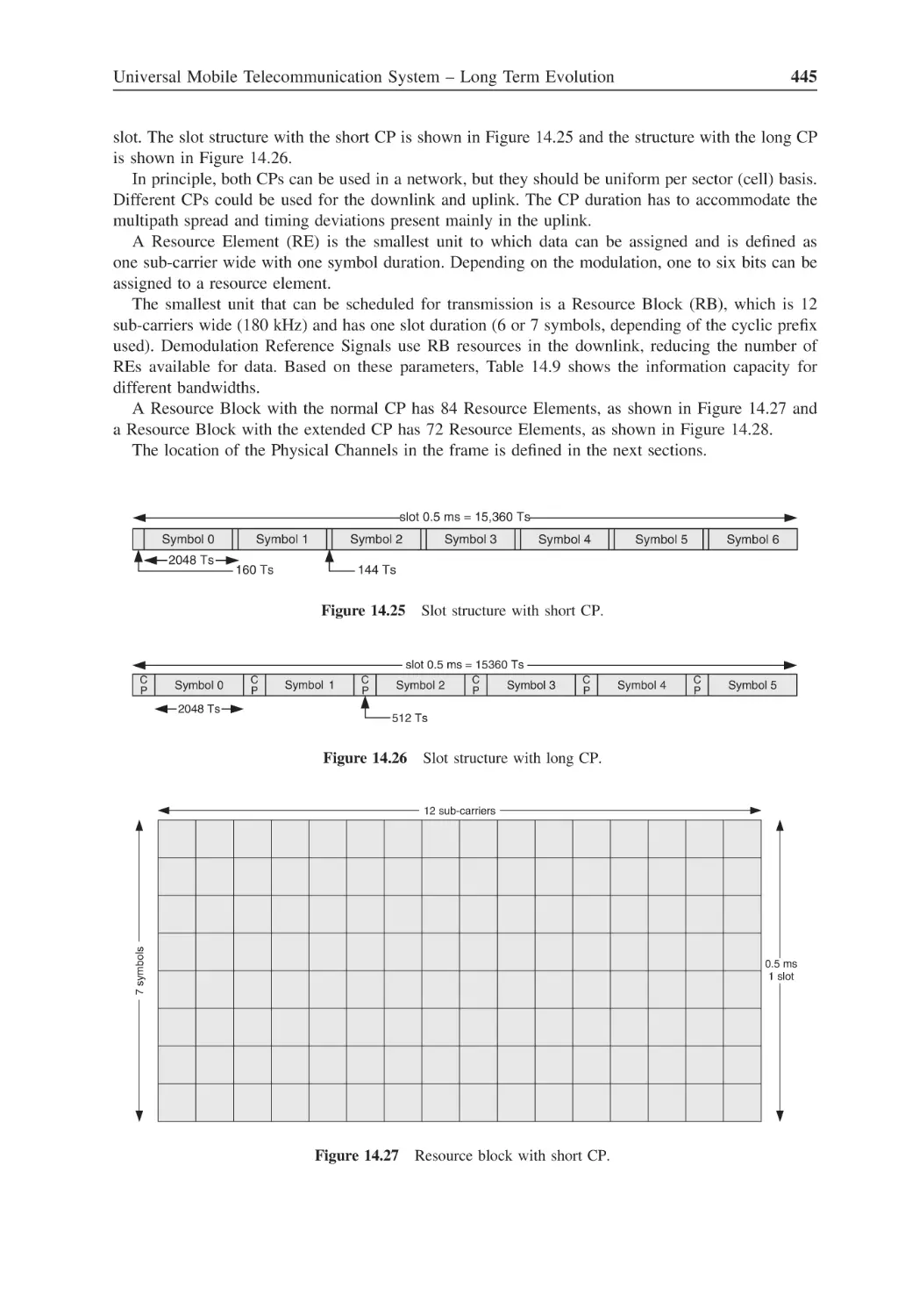
Figure 14.25 Slot structure with short CP
445
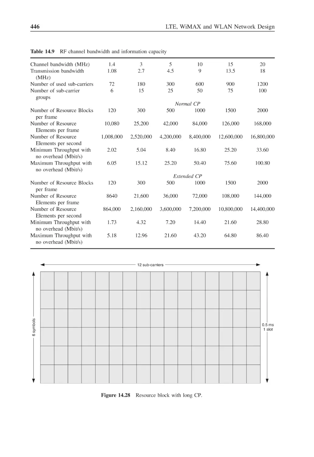
Figure 14.26 Slot structure with long CP
445
Figure 14.27 Resource block with short CP
445
Figure 14.28 Resource block with long CP
446
Figure 14.29 Antenna port reference signal allocation
448
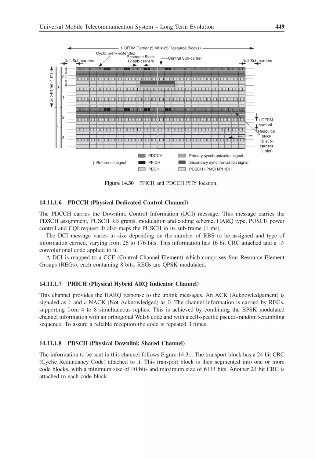
Figure 14.30 PFICH and PDCCH PHY location
449
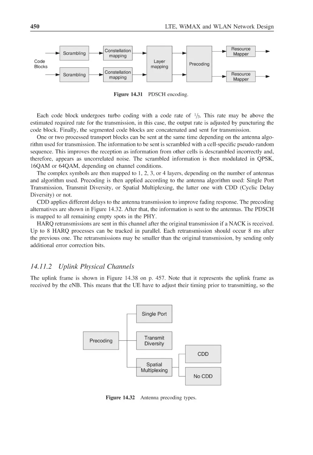
Figure 14.31 PDSCH encoding
450
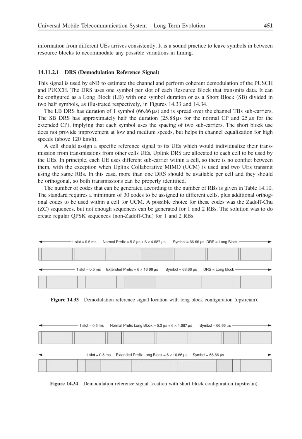
Figure 14.32 Antenna precoding types
450
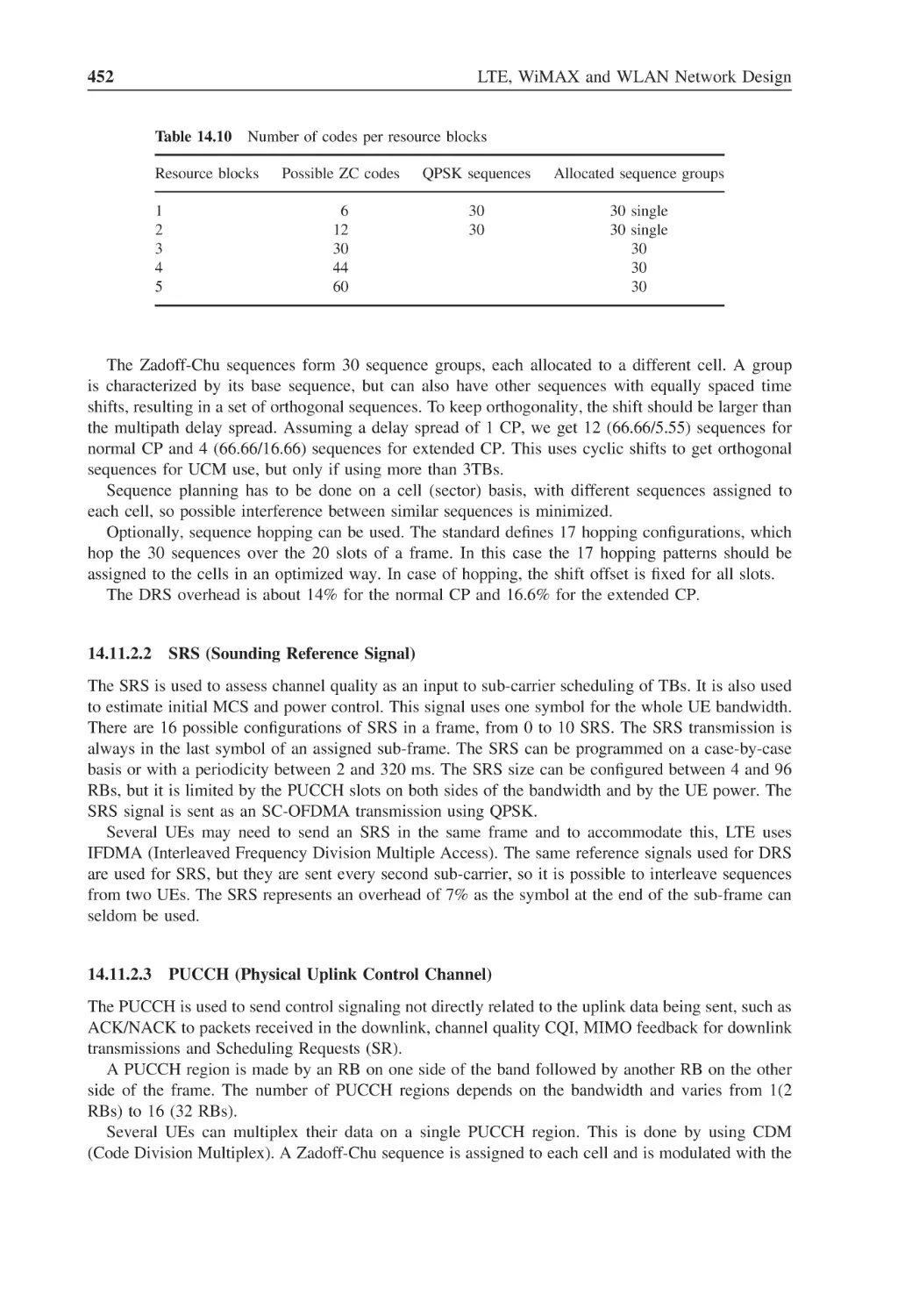
Figure 14.33 Demodulation reference signal location with long block
configuration (upstream)
451
Figure 14.34 Demodulation reference signal location with short block
configuration (upstream)
451
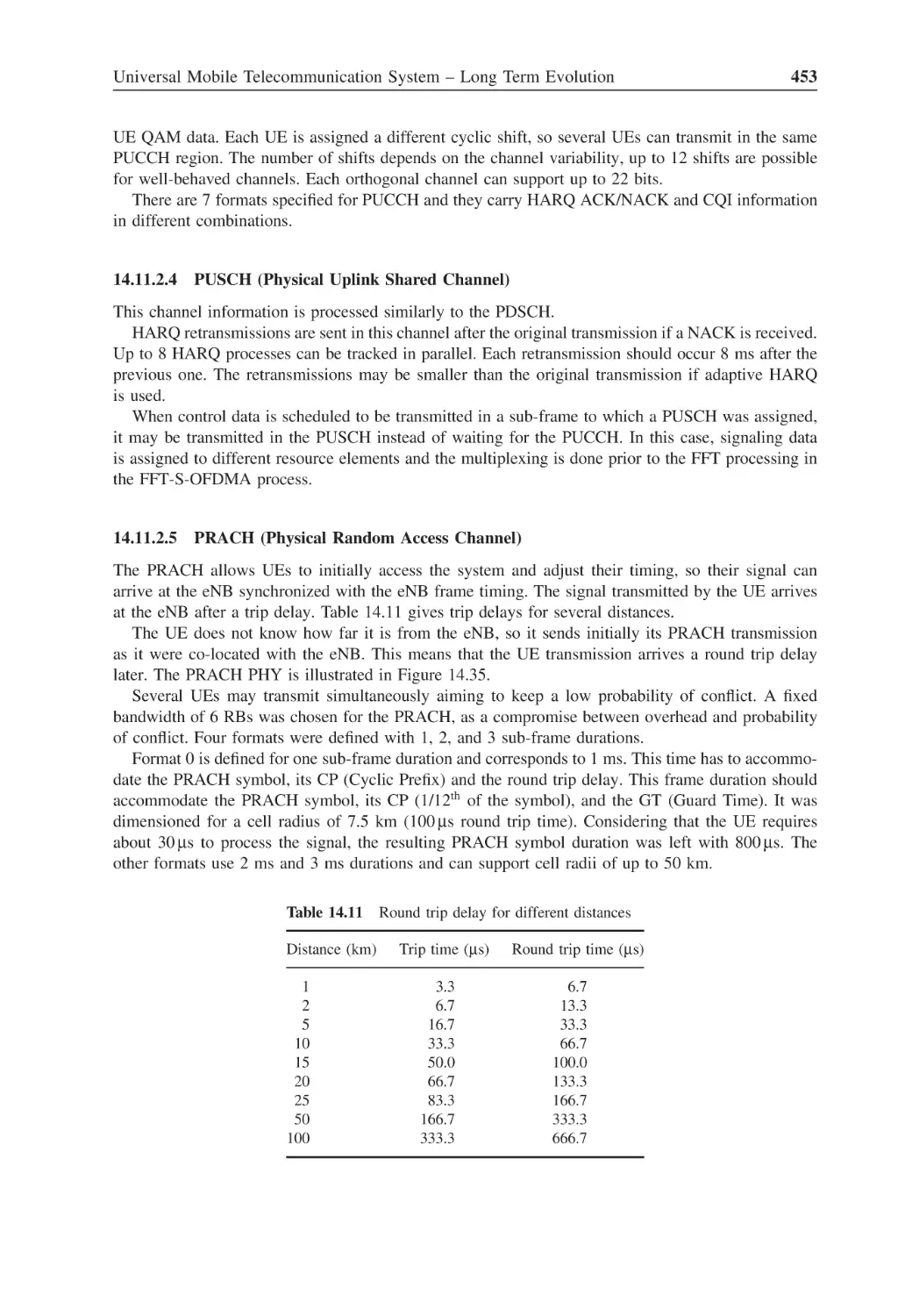
Figure 14.35 PRACH PHY
454
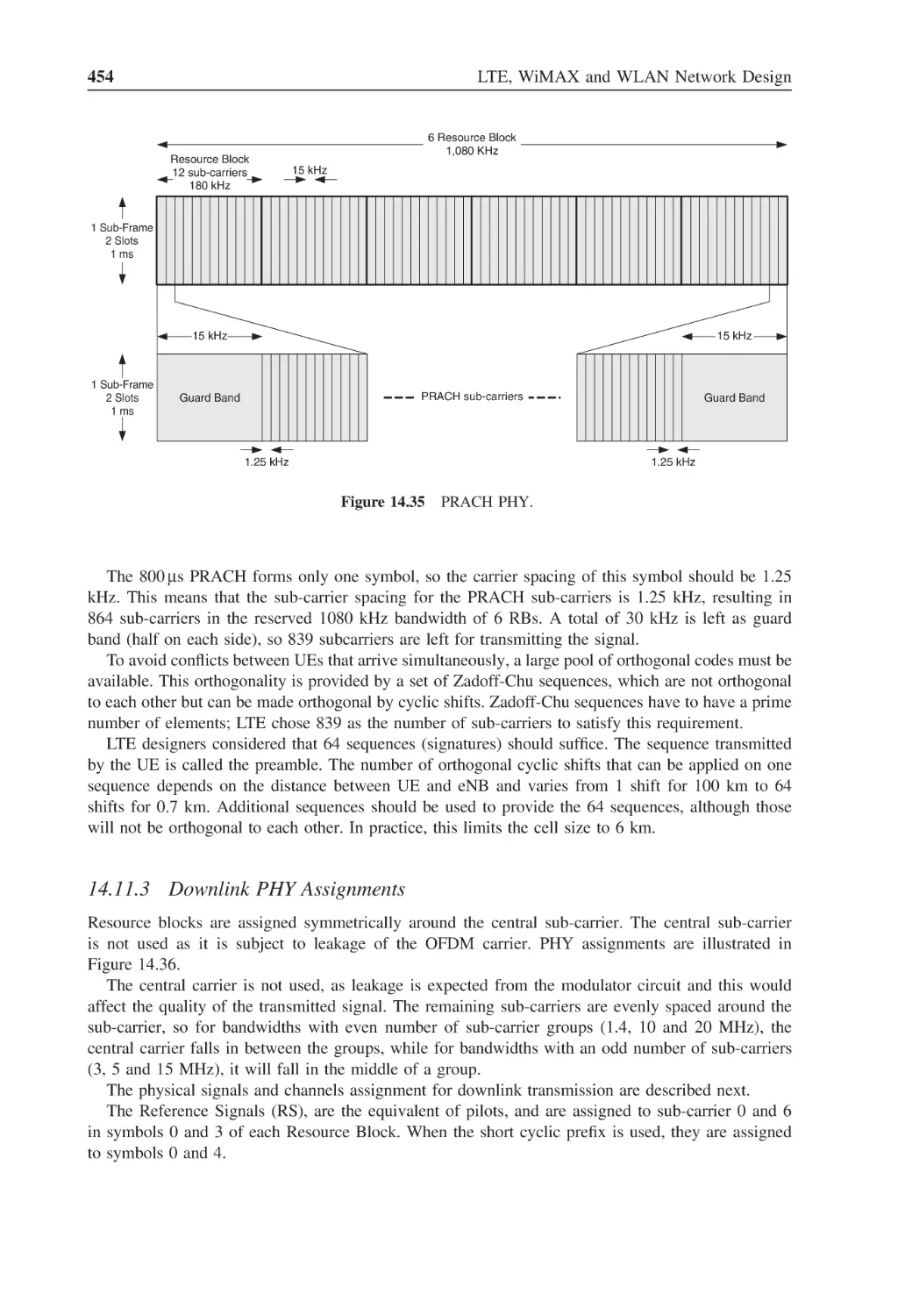
Figure 14.36 Central sub-carrier allocation to RS, PSS, SSS, PDCCH,
PFICH, PBSCH and PDSCH
455
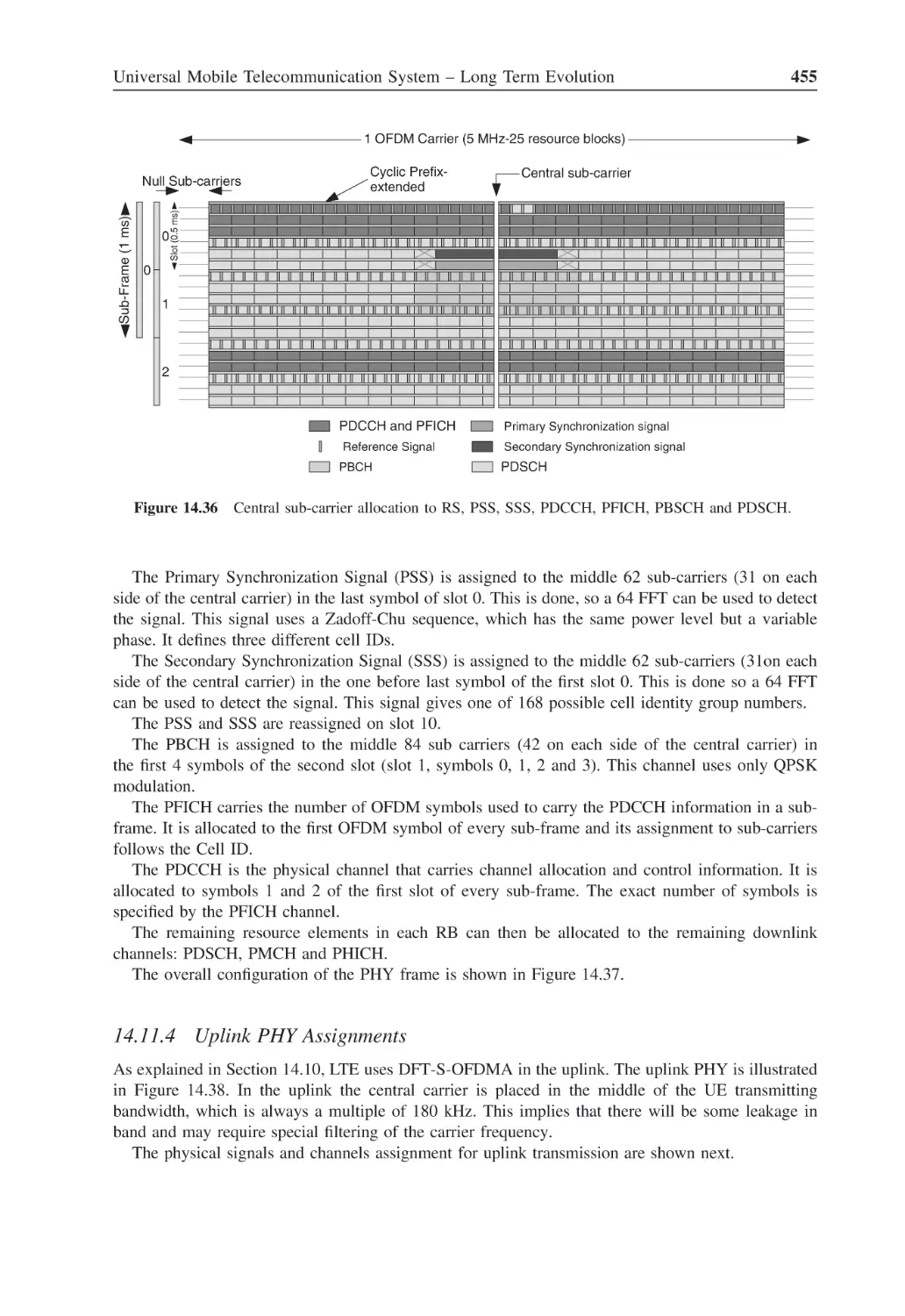
Figure 14.37 LTE PHY frame
456
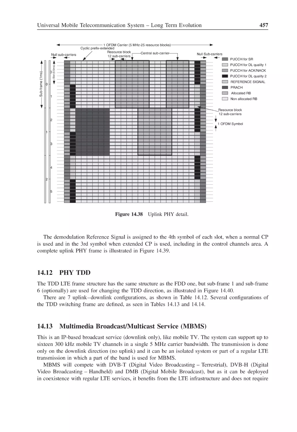
Figure 14.38 Uplink PHY detail
457
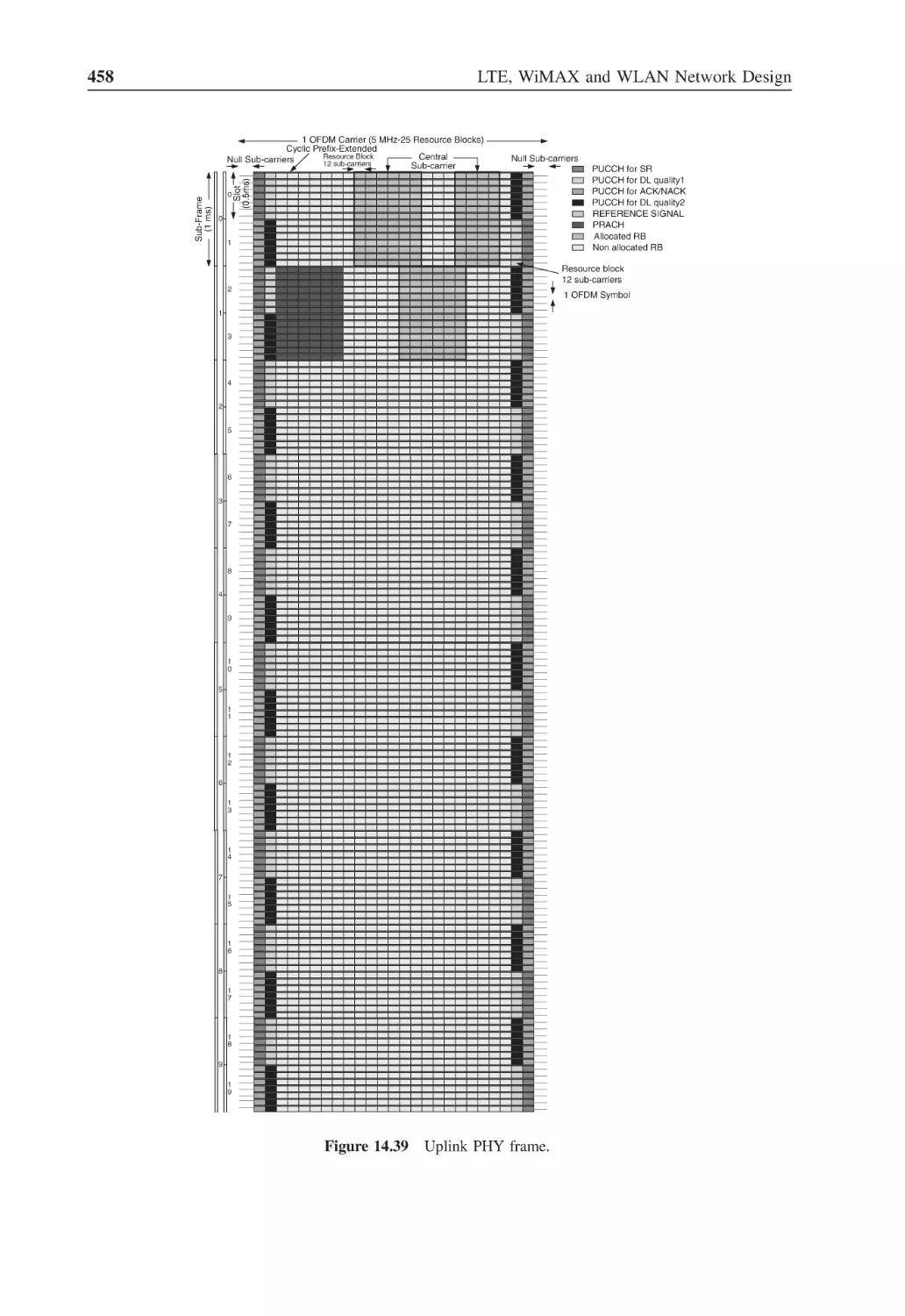
Figure 14.39 Uplink PHY frame
458
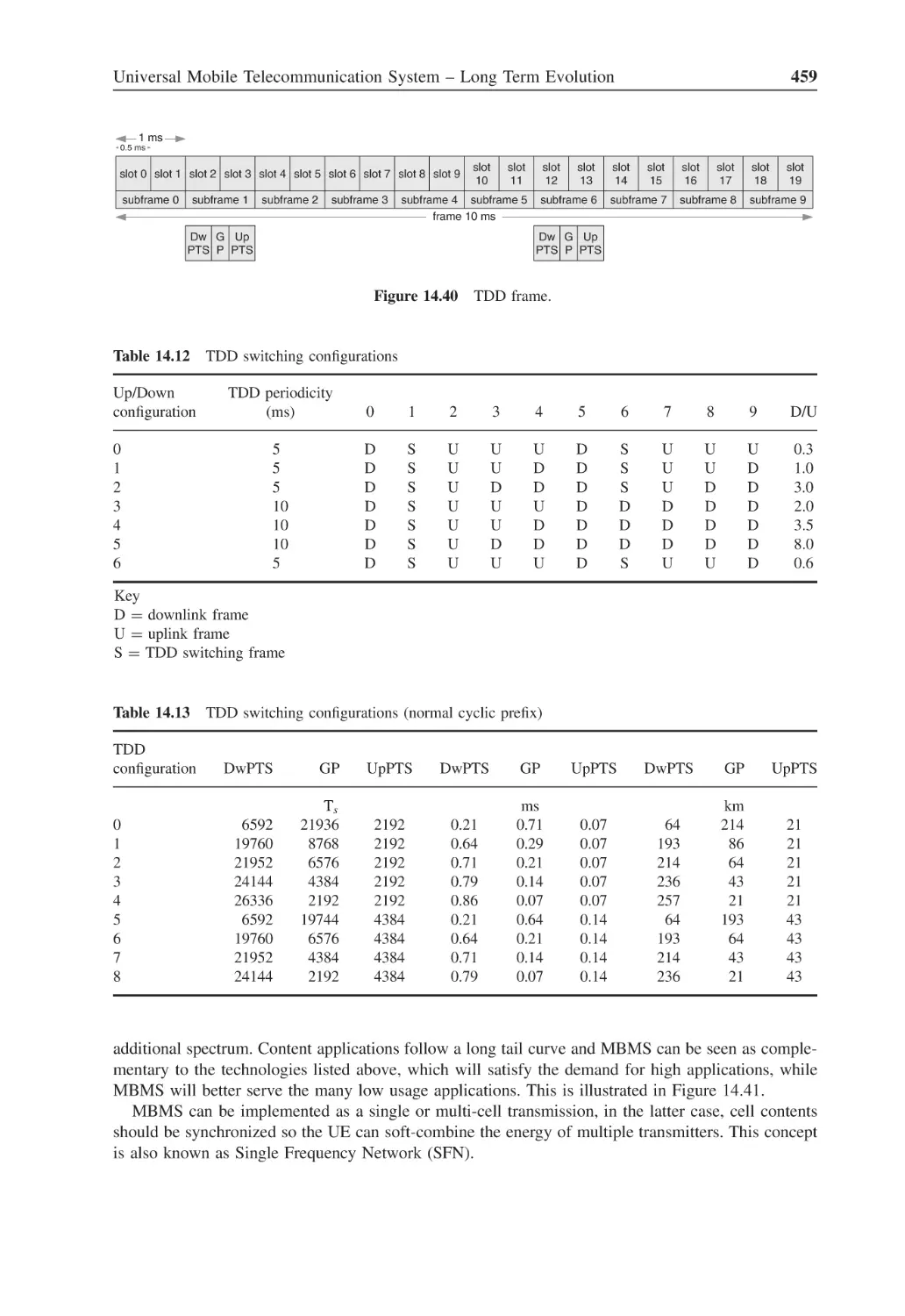
Figure 14.40 TDD frame
459
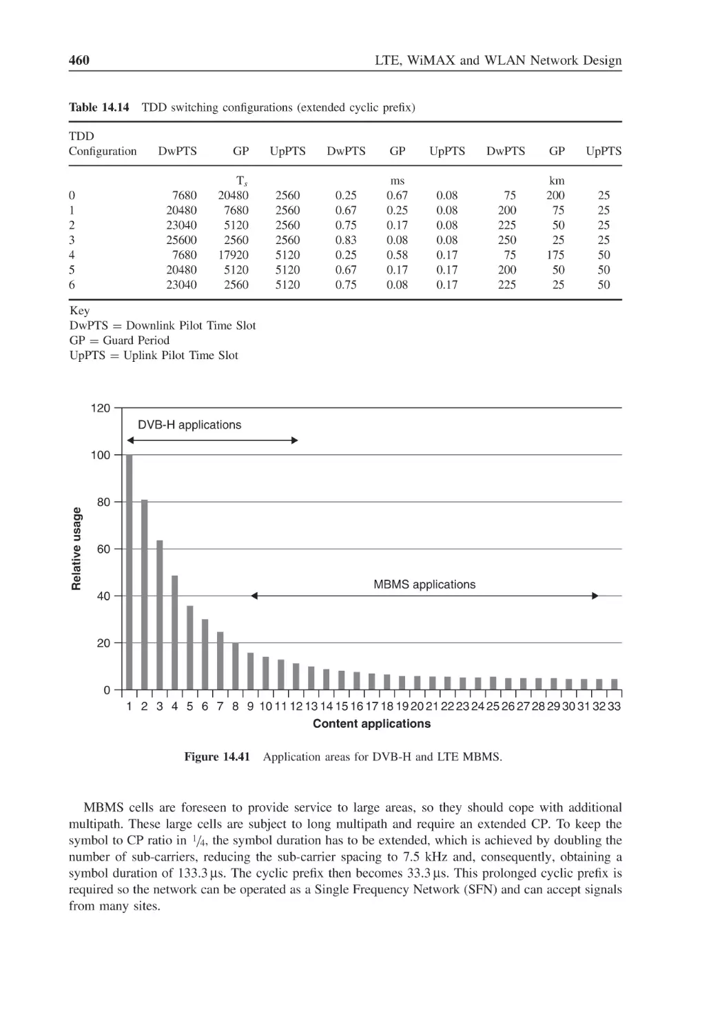
Figure 14.41 Application areas for DVB-H and LTE MBMS
460
List of Figures
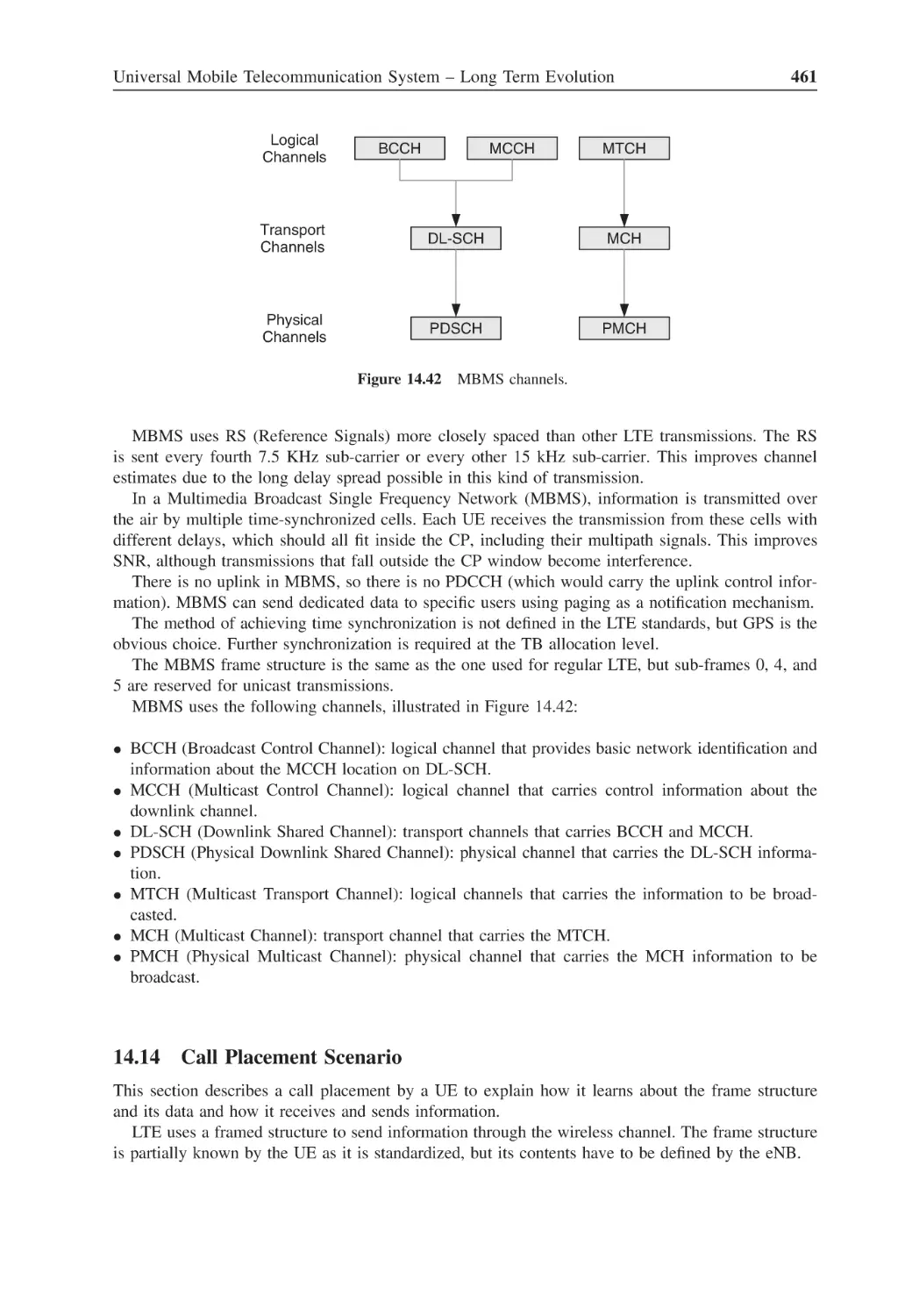
Figure 14.42 MBMS channels
xxix
461
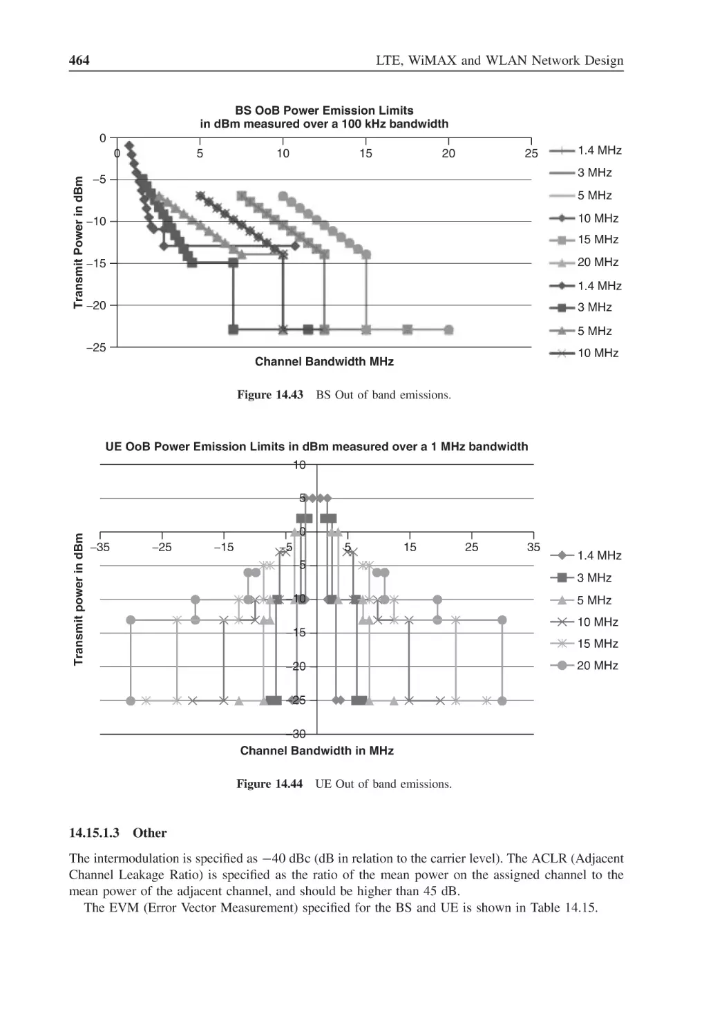
Figure 14.43 BS Out of band emissions
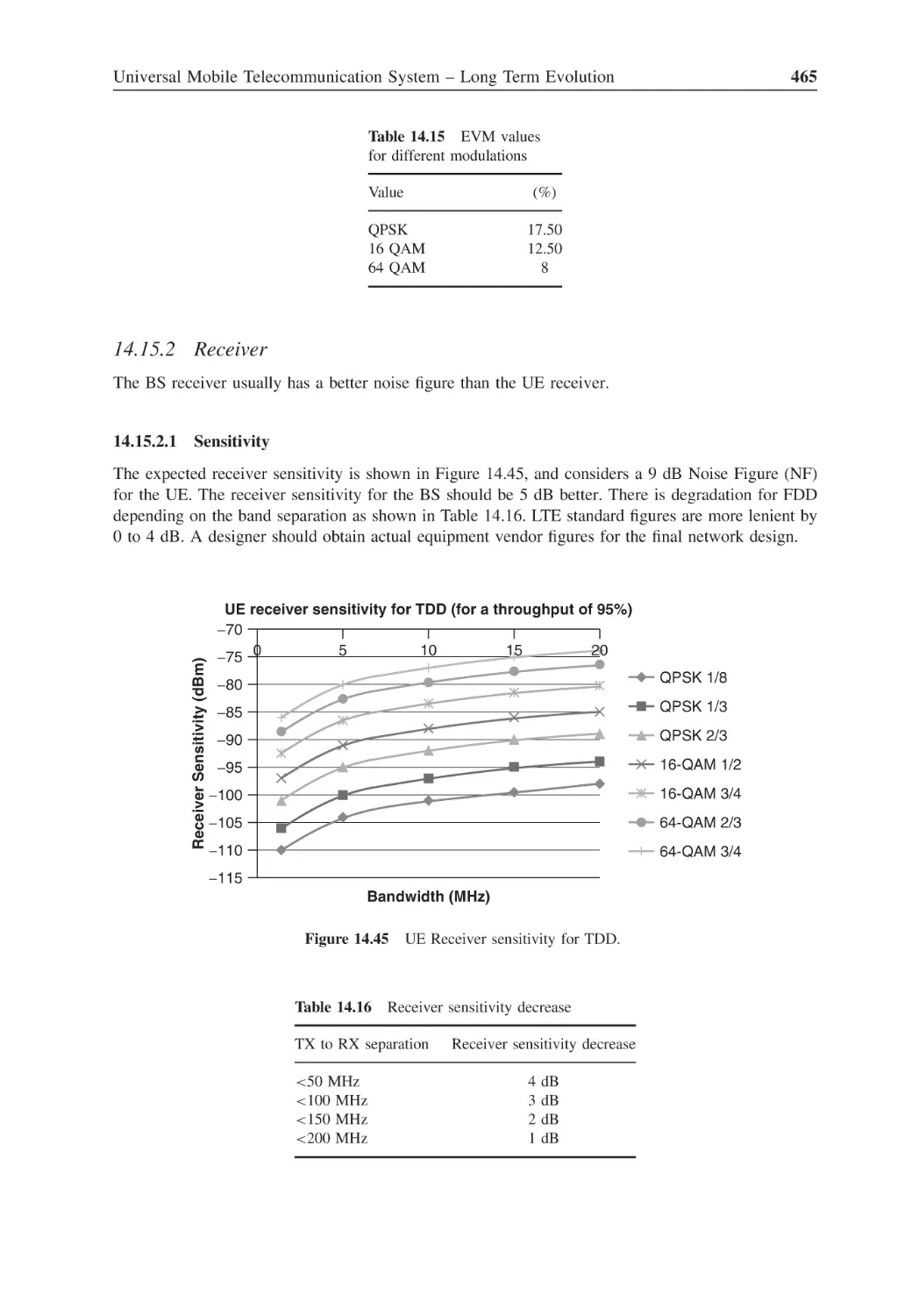
464
Figure 14.44 UE Out of band emissions
464
Figure 14.45 UE Receiver sensitivity for TDD
465
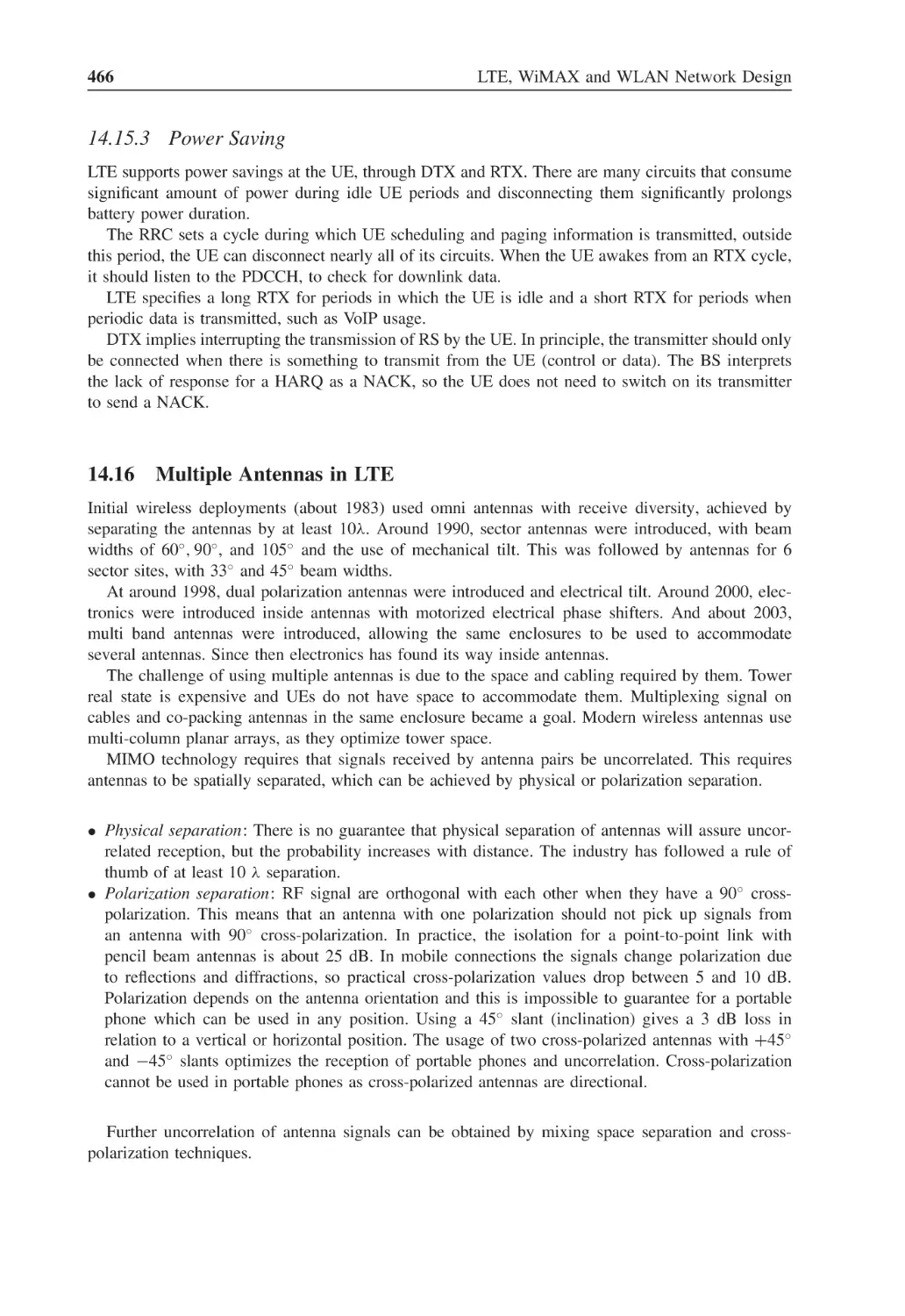
Figure 14.46 Antenna configurations
467
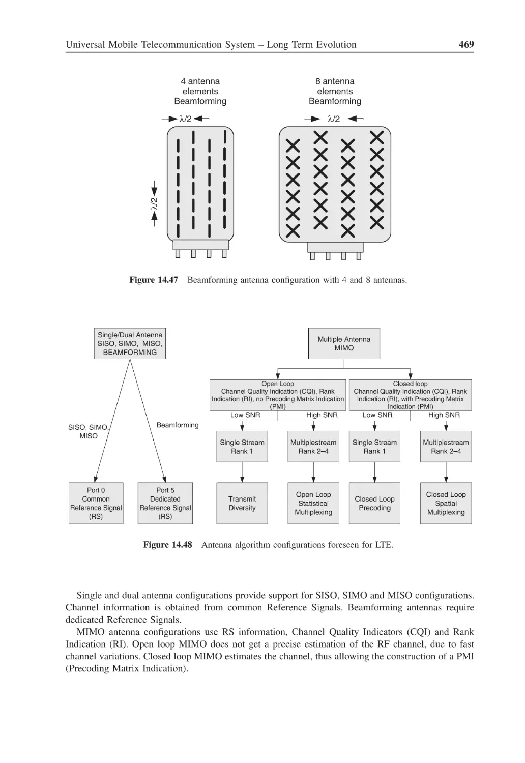
Figure 14.47 Beamforming antenna configuration with 4 and 8 antennas
469
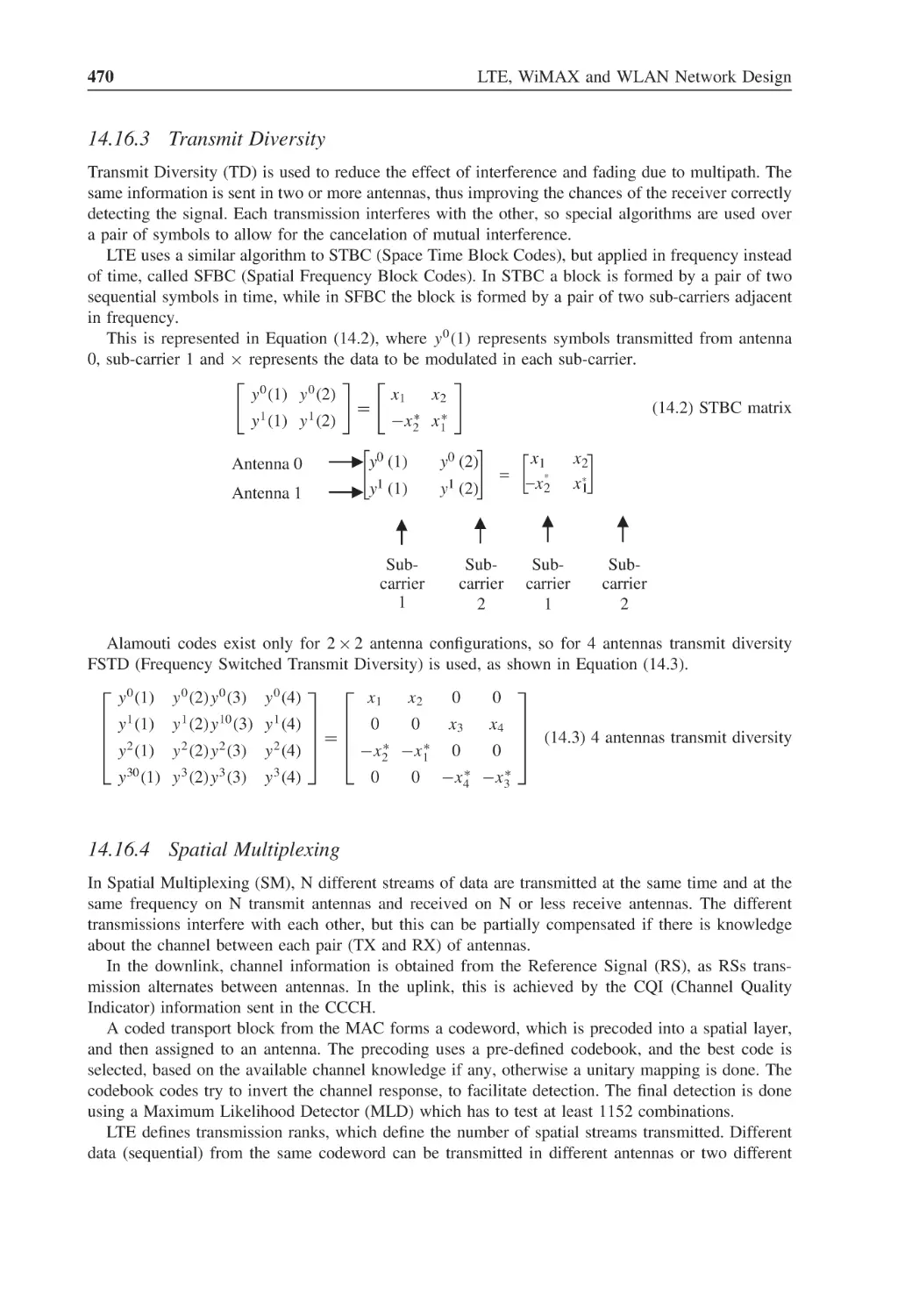
Figure 14.48 Antenna algorithm configurations foreseen for LTE
469
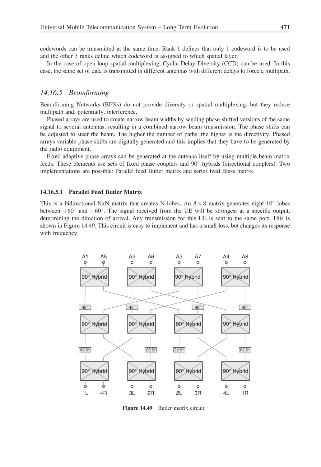
Figure 14.49 Butler matrix circuit
471
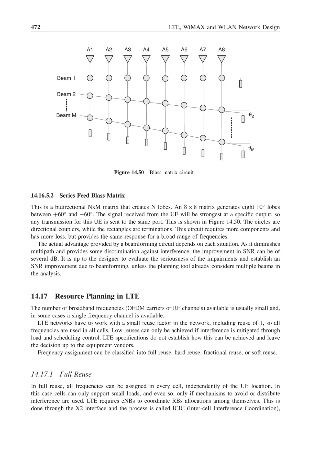
Figure 14.50 Blass matrix circuit
472
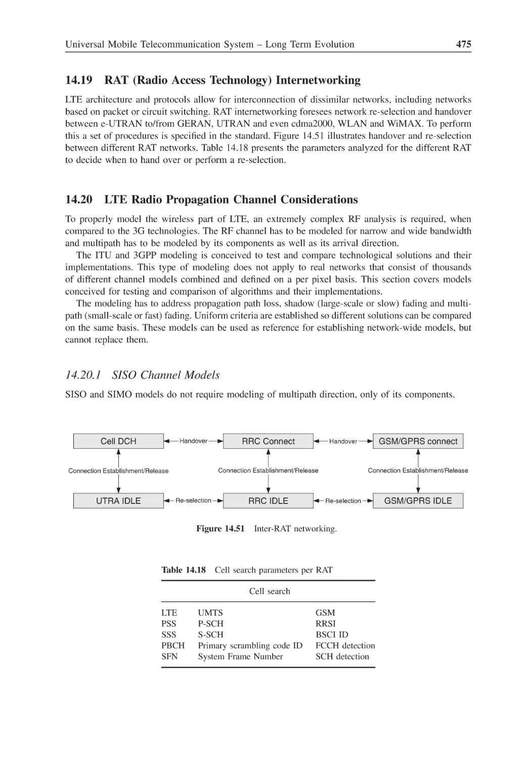
Figure 14.51 Inter-RAT networking
475
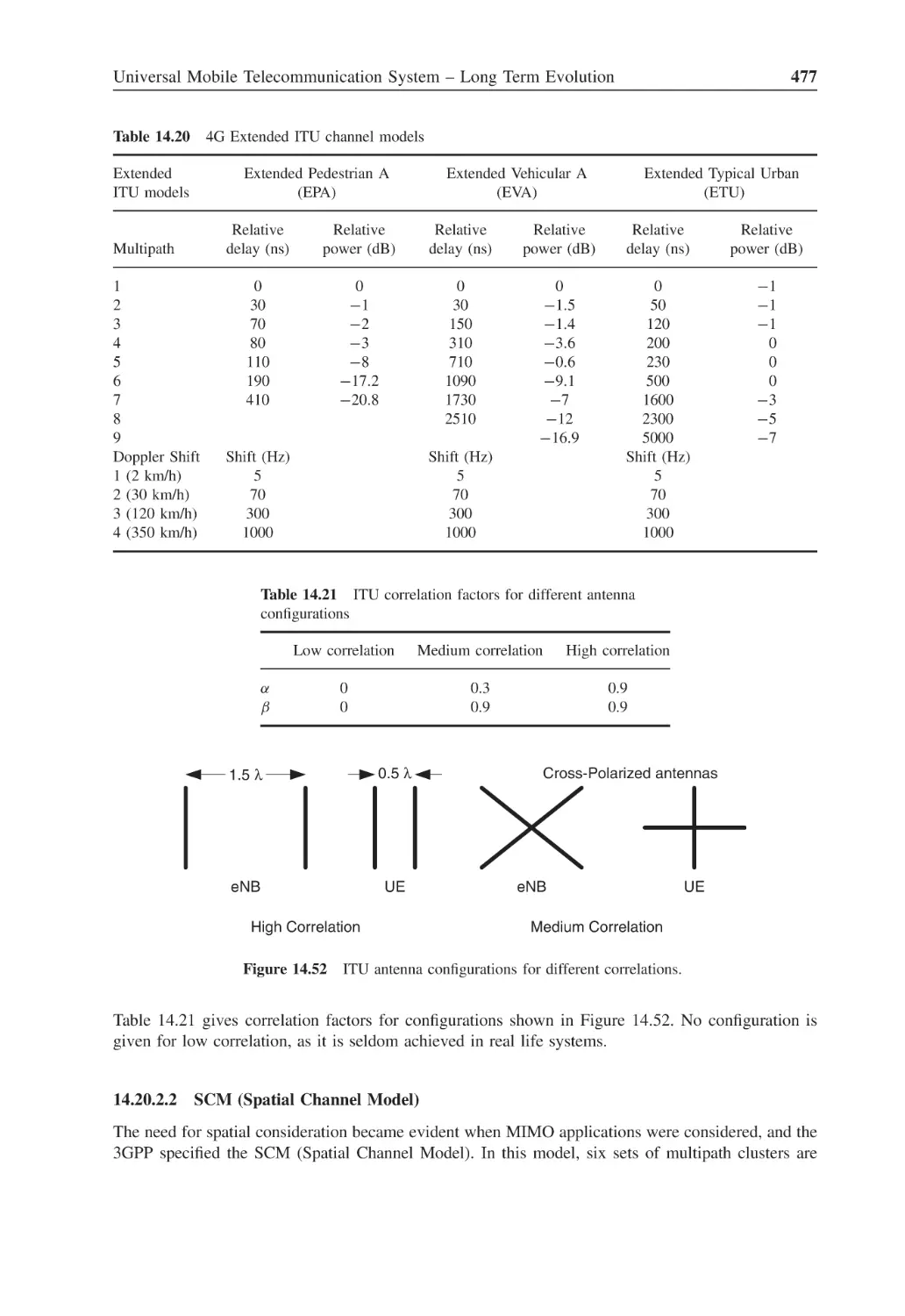
Figure 14.52 ITU antenna configurations for different correlations
477
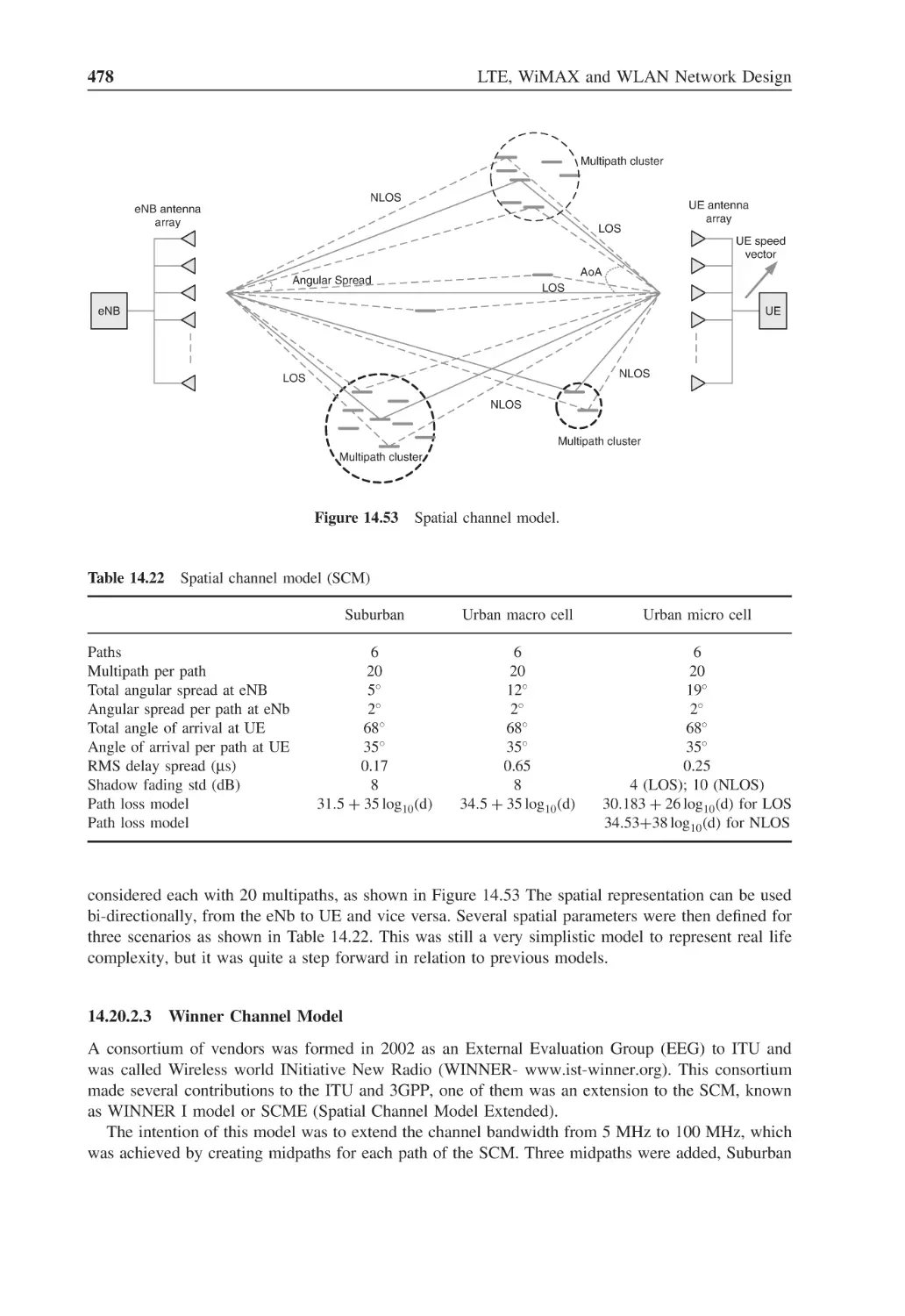
Figure 14.53 Spatial channel model
478
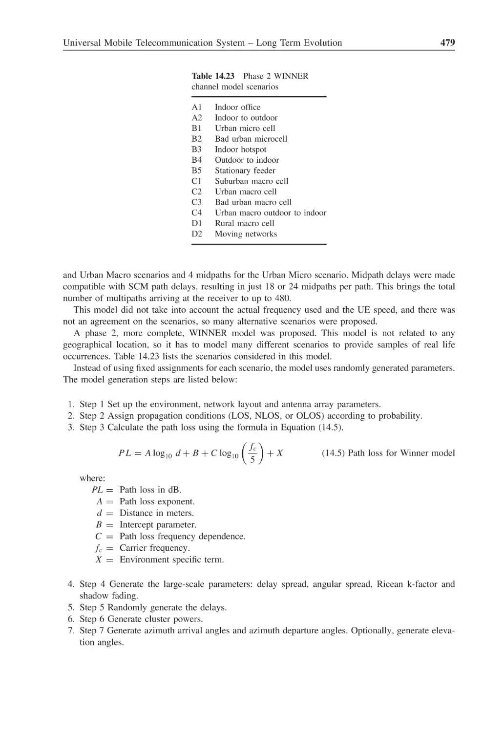
Figure 14.54 eNB antenna model for evaluation purposes
480
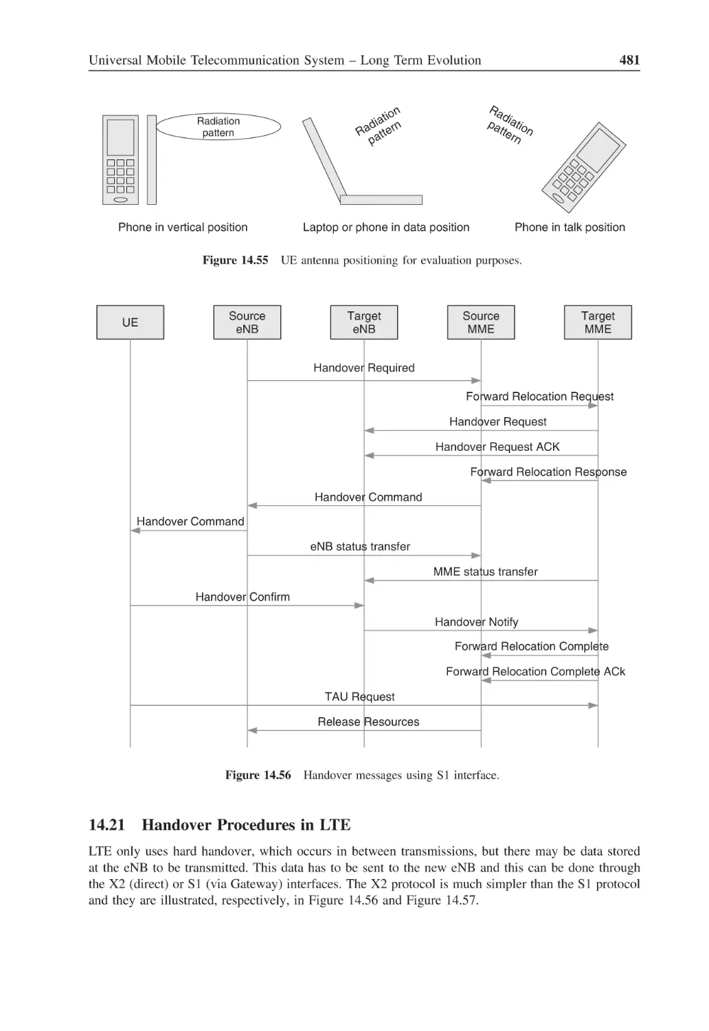
Figure 14.55 UE antenna positioning for evaluation purposes
481
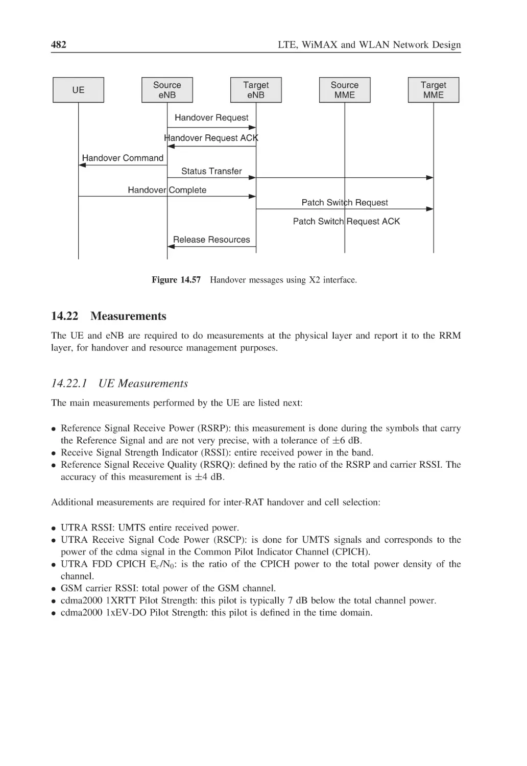
Figure 14.56 Handover messages using S1 interface
481
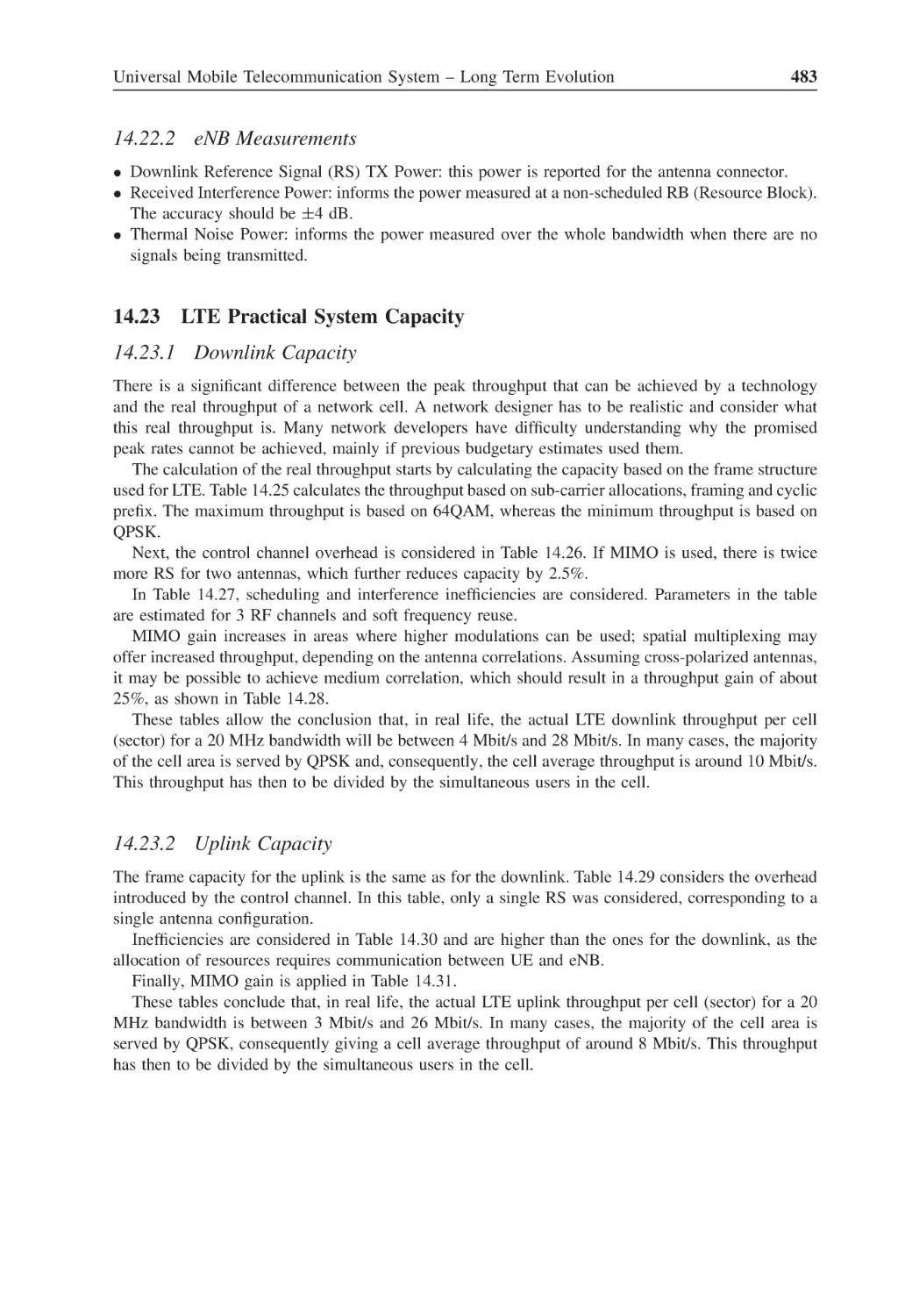
Figure 14.57 Handover messages using X2 interface
482
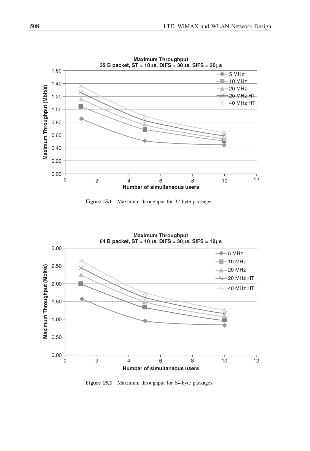
Figure 15.1
Maximum throughput for 32-byte packages
508
Figure 15.2
Maximum throughput for 64-byte packages
508
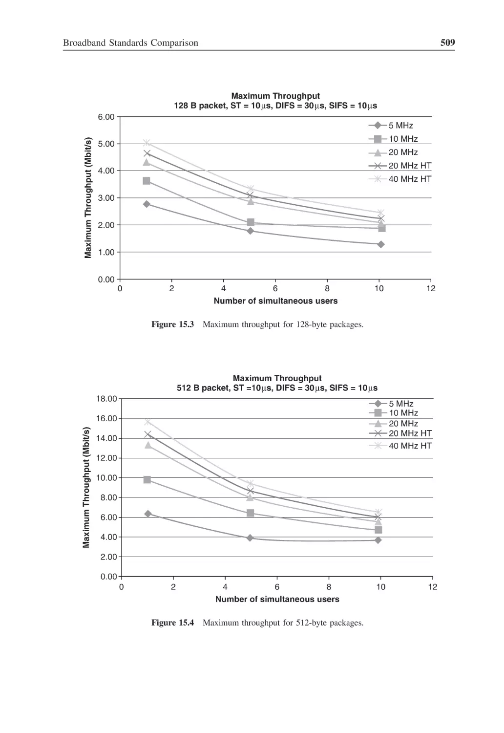
Figure 15.3
Maximum throughput for 128-byte packages
509
Figure 15.4
Maximum throughput for 512-byte packages
509
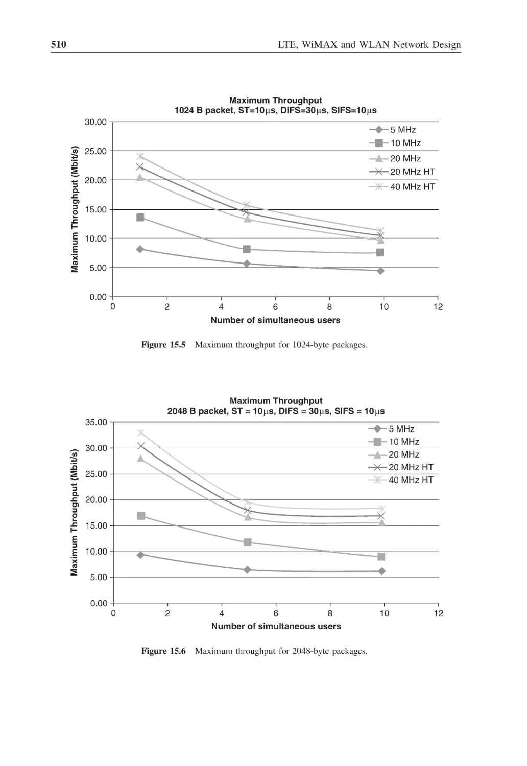
Figure 15.5
Maximum throughput for 1024-byte packages
510
Figure 15.6
Maximum throughput for 2048-byte packages
510
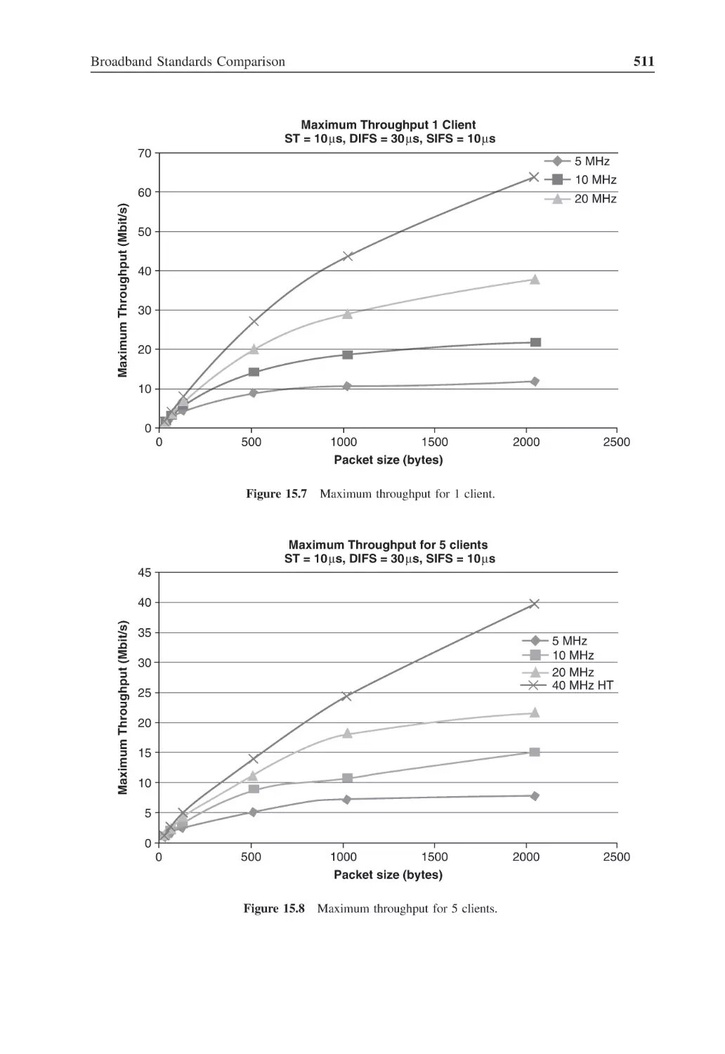
Figure 15.7
Maximum throughput for 1 client
511
Figure 15.8
Maximum throughput for 5 clients
511
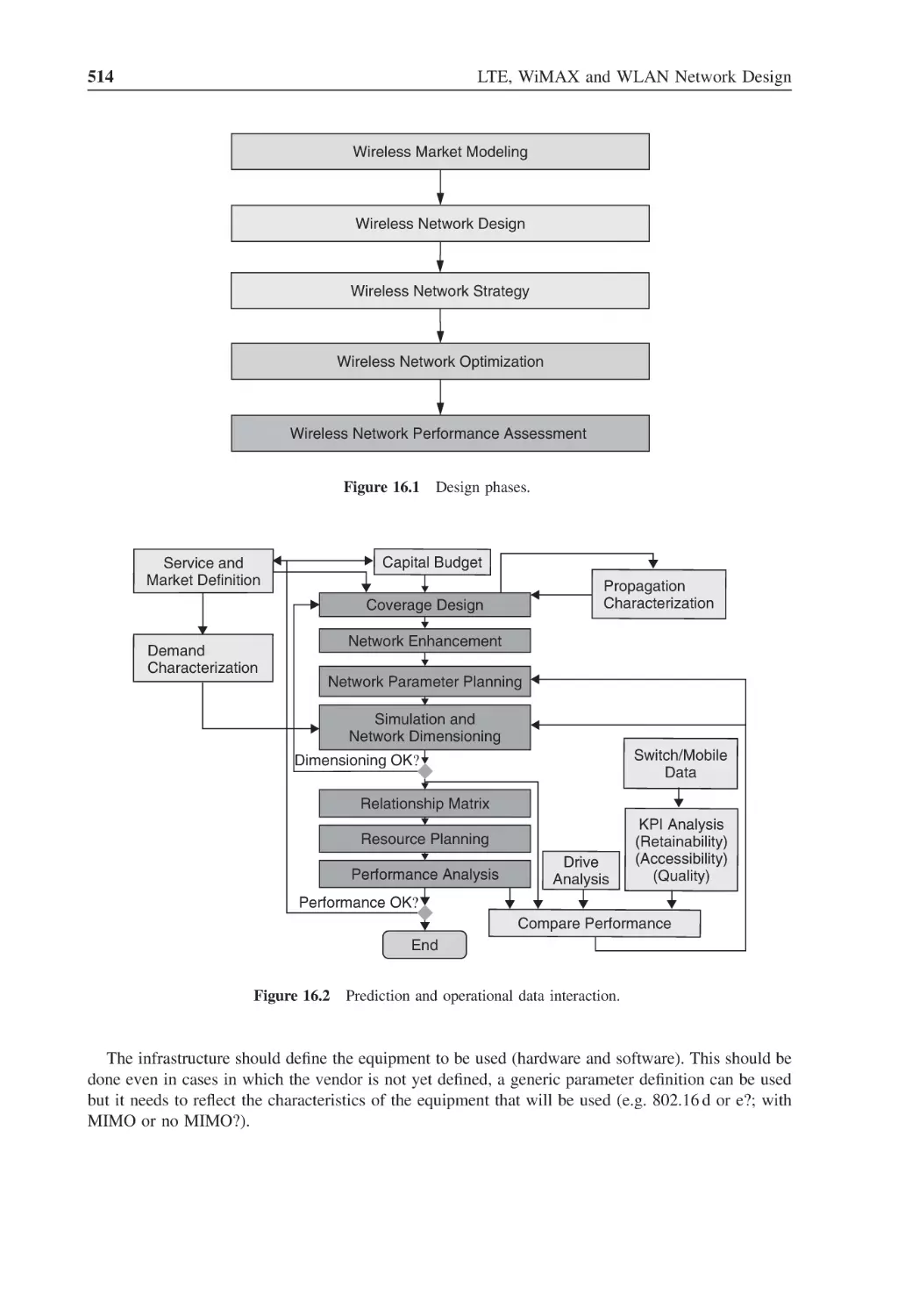
Figure 16.1
Design phases
514
Figure 16.2
Prediction and operational data interaction
514
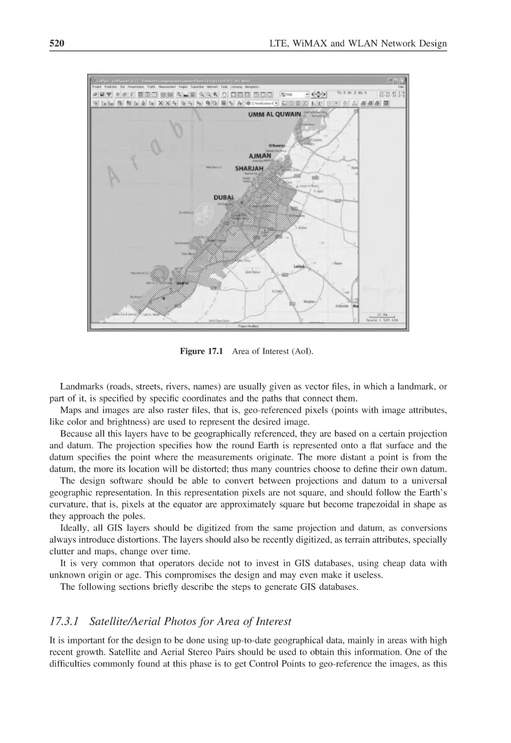
Figure 17.1
Area of Interest (AoI)
520
Figure 17.2
Satellite image 2005
521
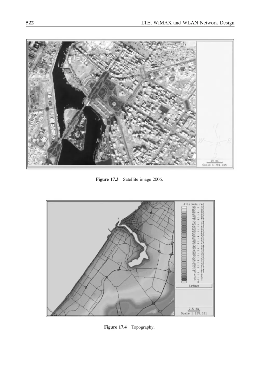
Figure 17.3
Satellite image 2006
522
Figure 17.4
Topography
522
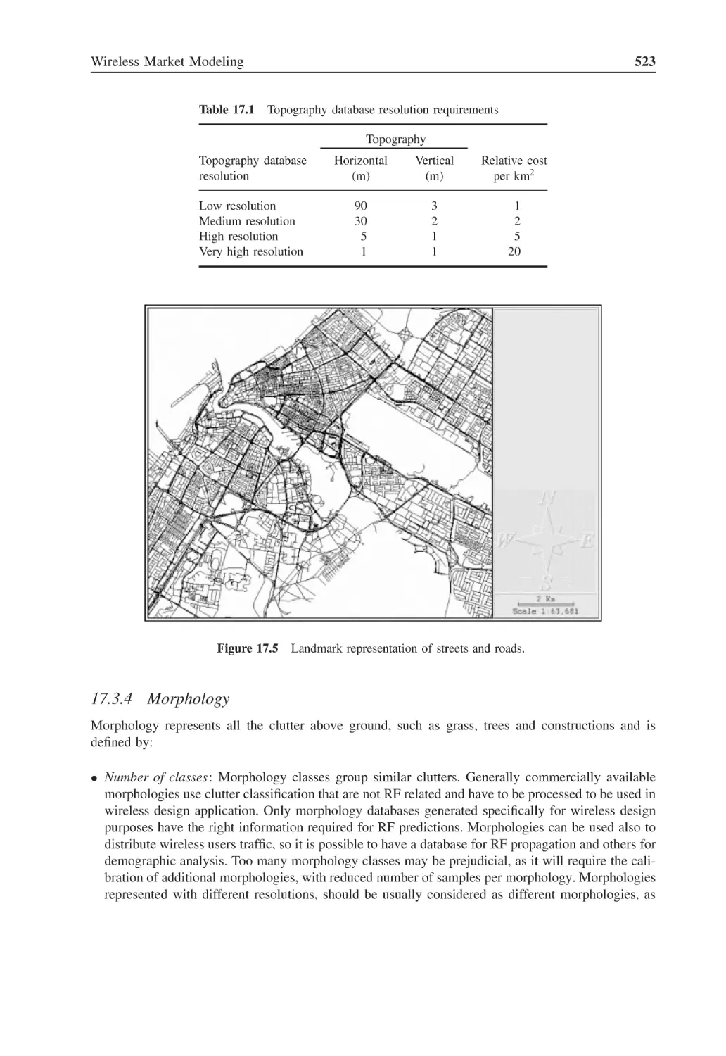
Figure 17.5
Landmark representation of streets and roads
523
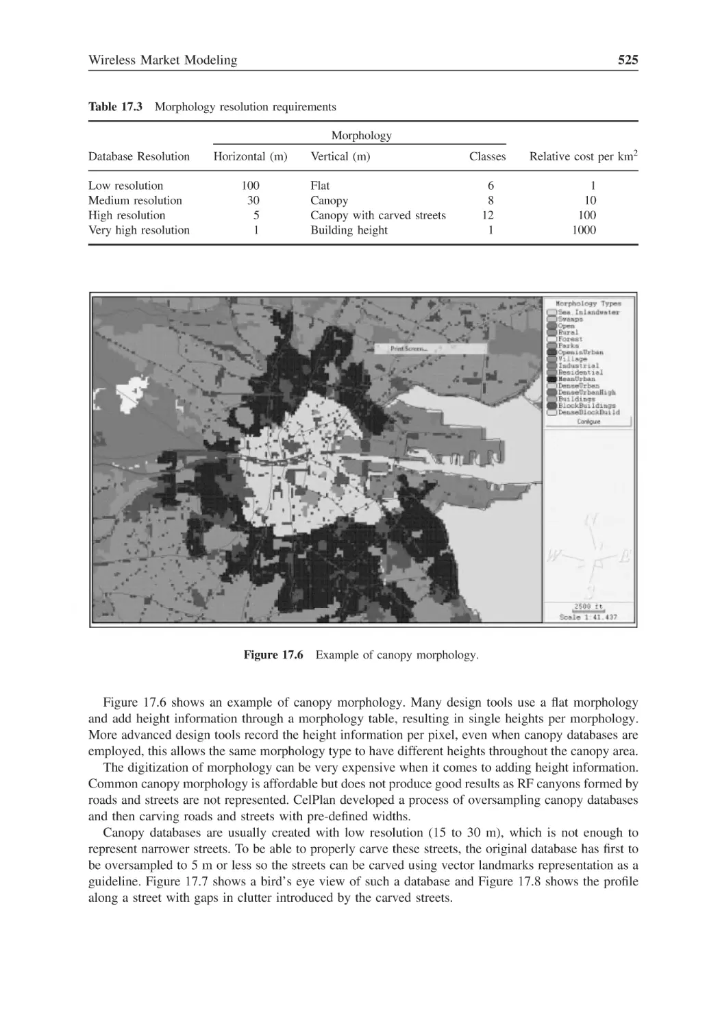
Figure 17.6
Example of canopy morphology
525
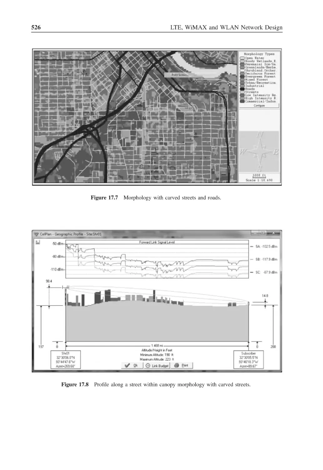
Figure 17.7
Morphology with carved streets and roads
526
Figure 17.8
Profile along a street within canopy morphology
with carved streets
526
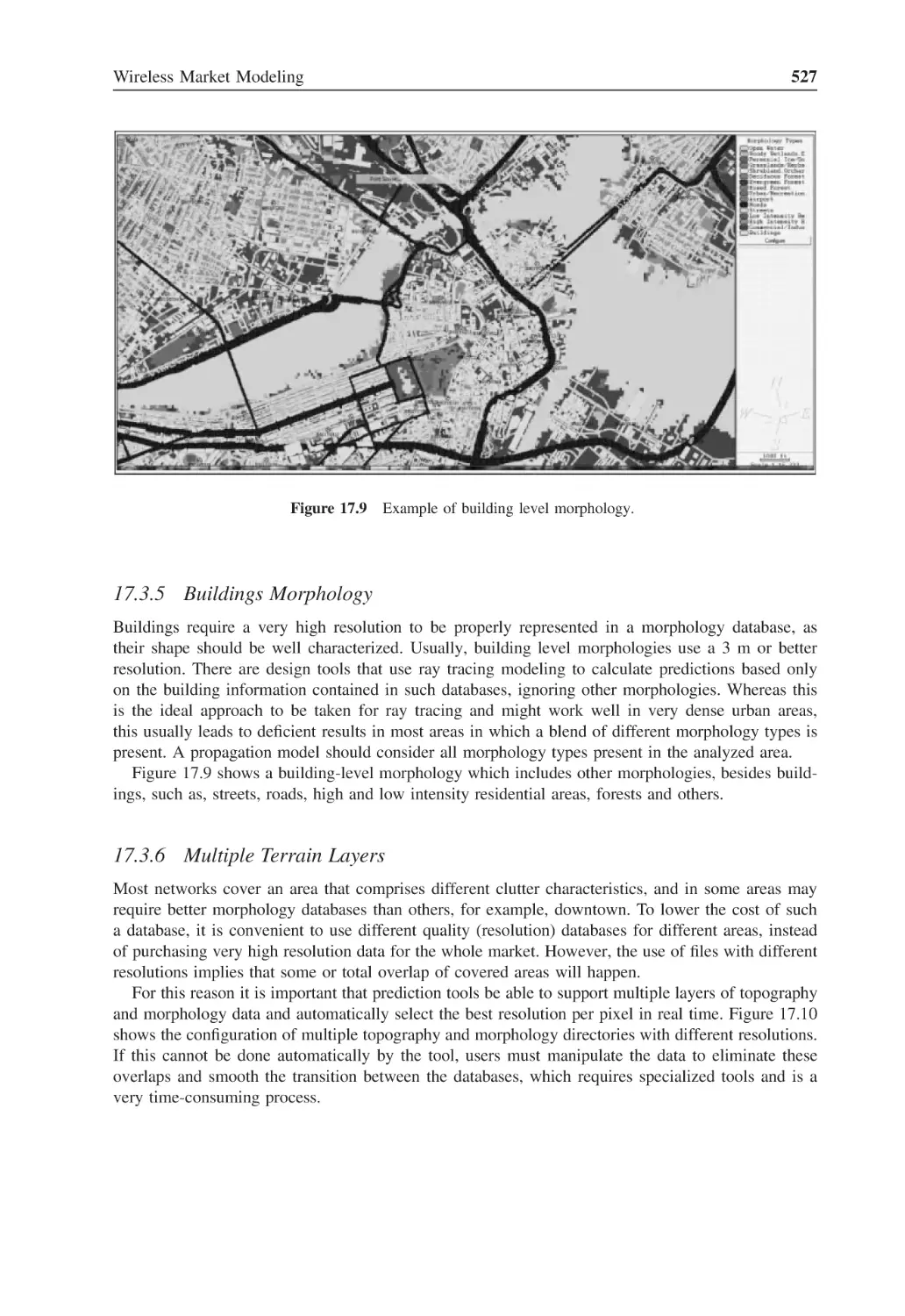
Figure 17.9
Example of building level morphology
527
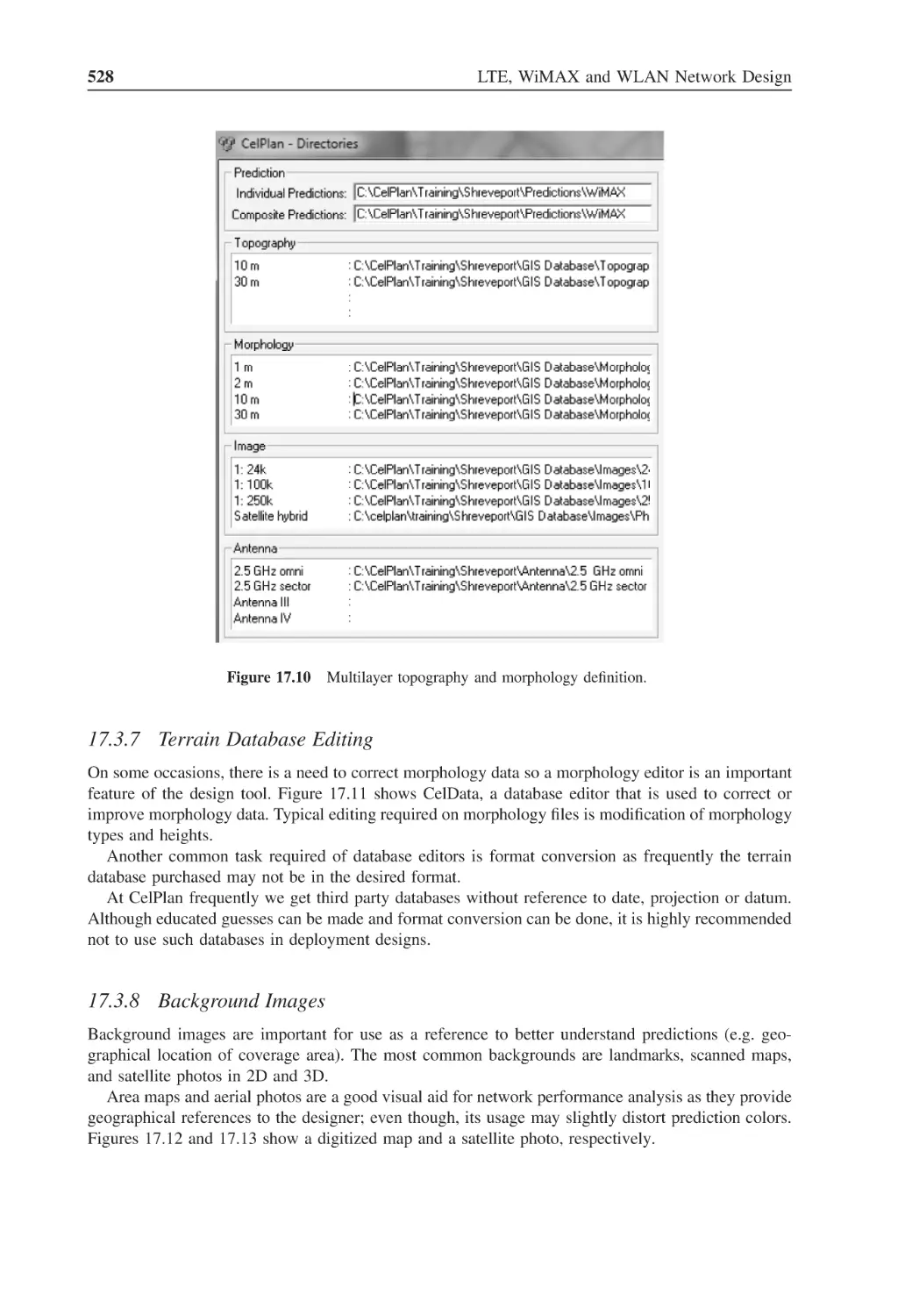
Figure 17.10 Multilayer topography and morphology definition
528
Figure 17.11 CelData morphology editor
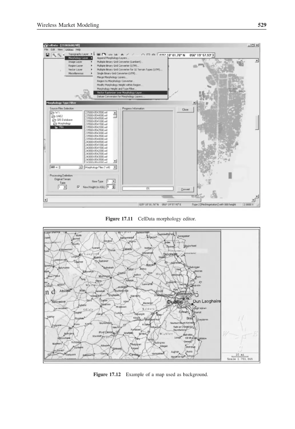
529
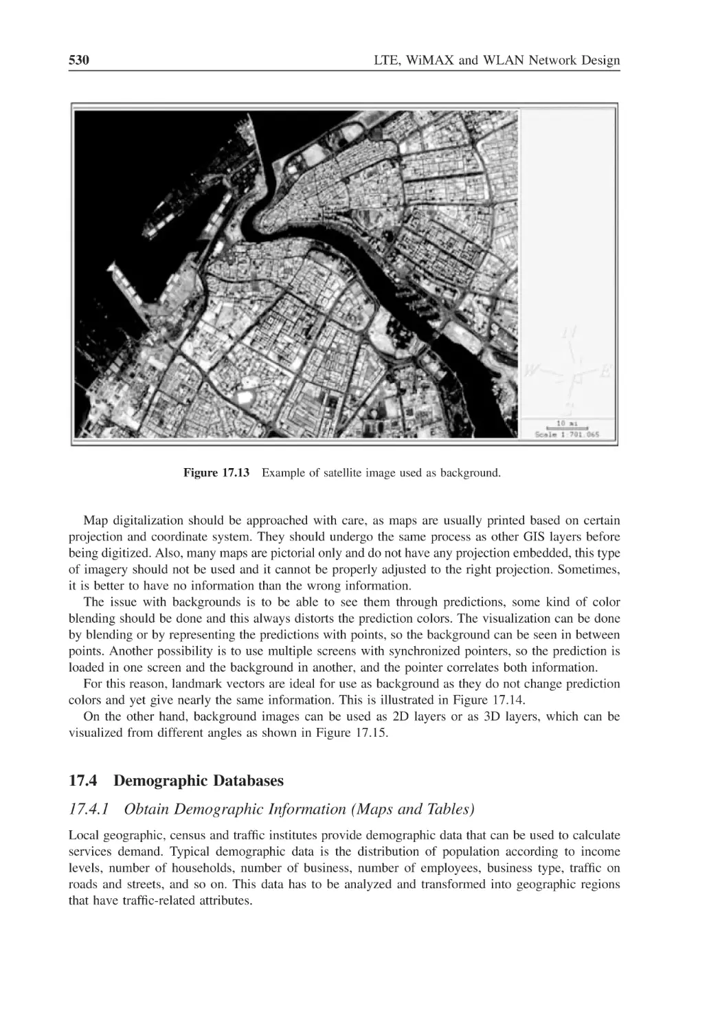
Figure 17.12 Example of a map used as background
529
xxx
List of Figures
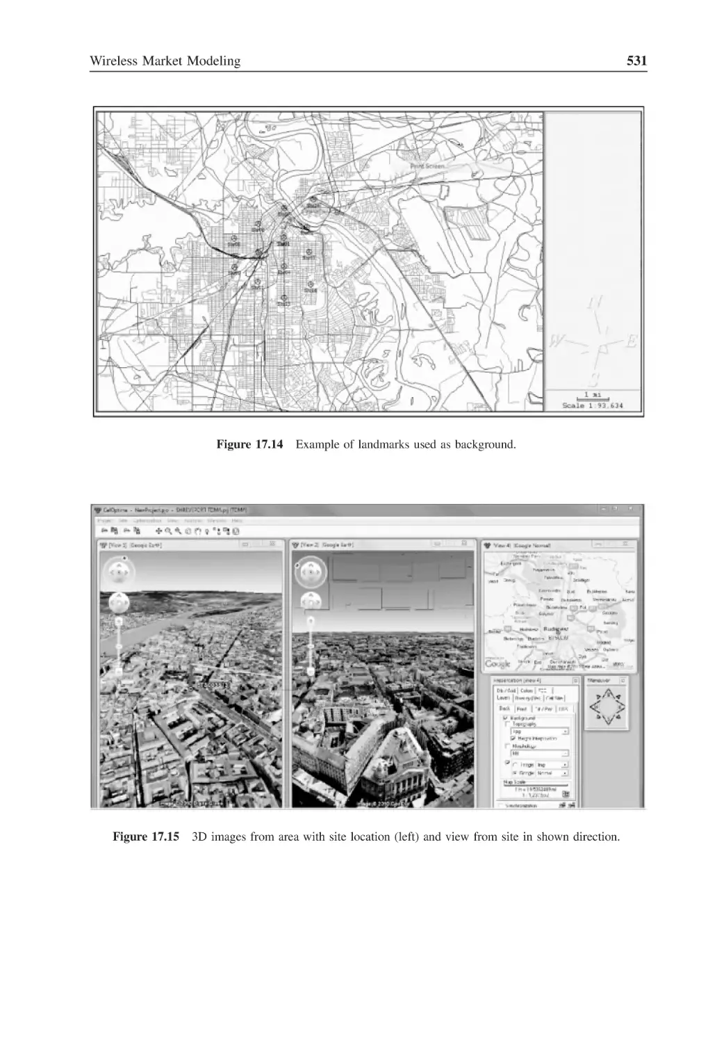
Figure 17.13 Example of satellite image used as background
530
Figure 17.14 Example of landmarks used as background
531
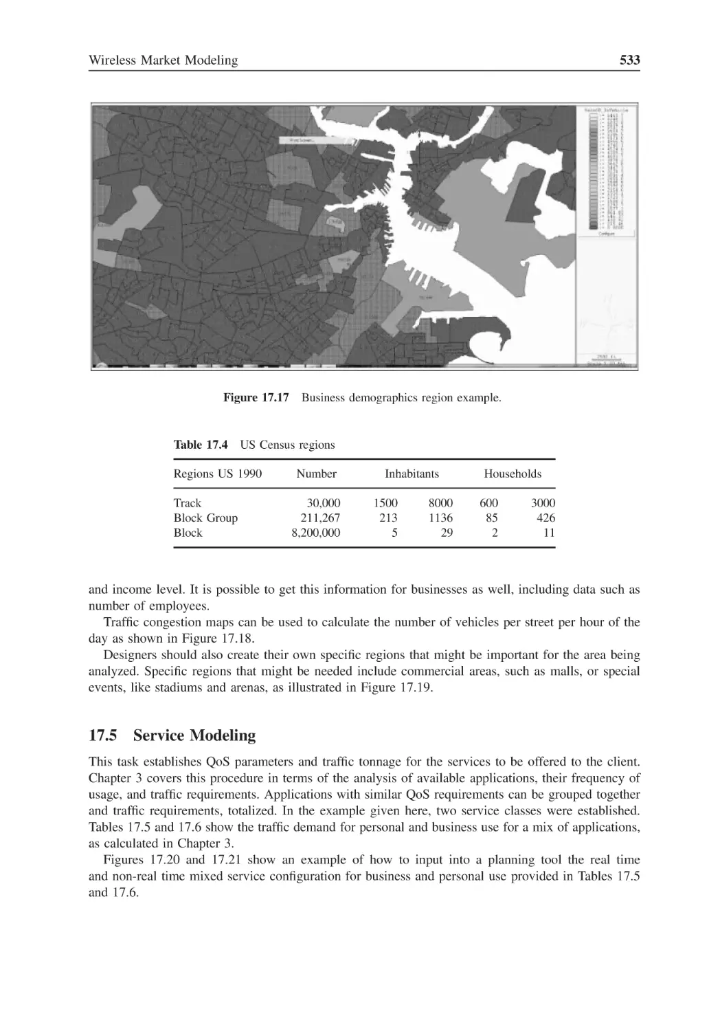
Figure 17.15 3D images from area with site location (left) and view from site
in shown direction
531
Figure 17.16 Household demographic regions example
532
Figure 17.17 Business demographics region example
533
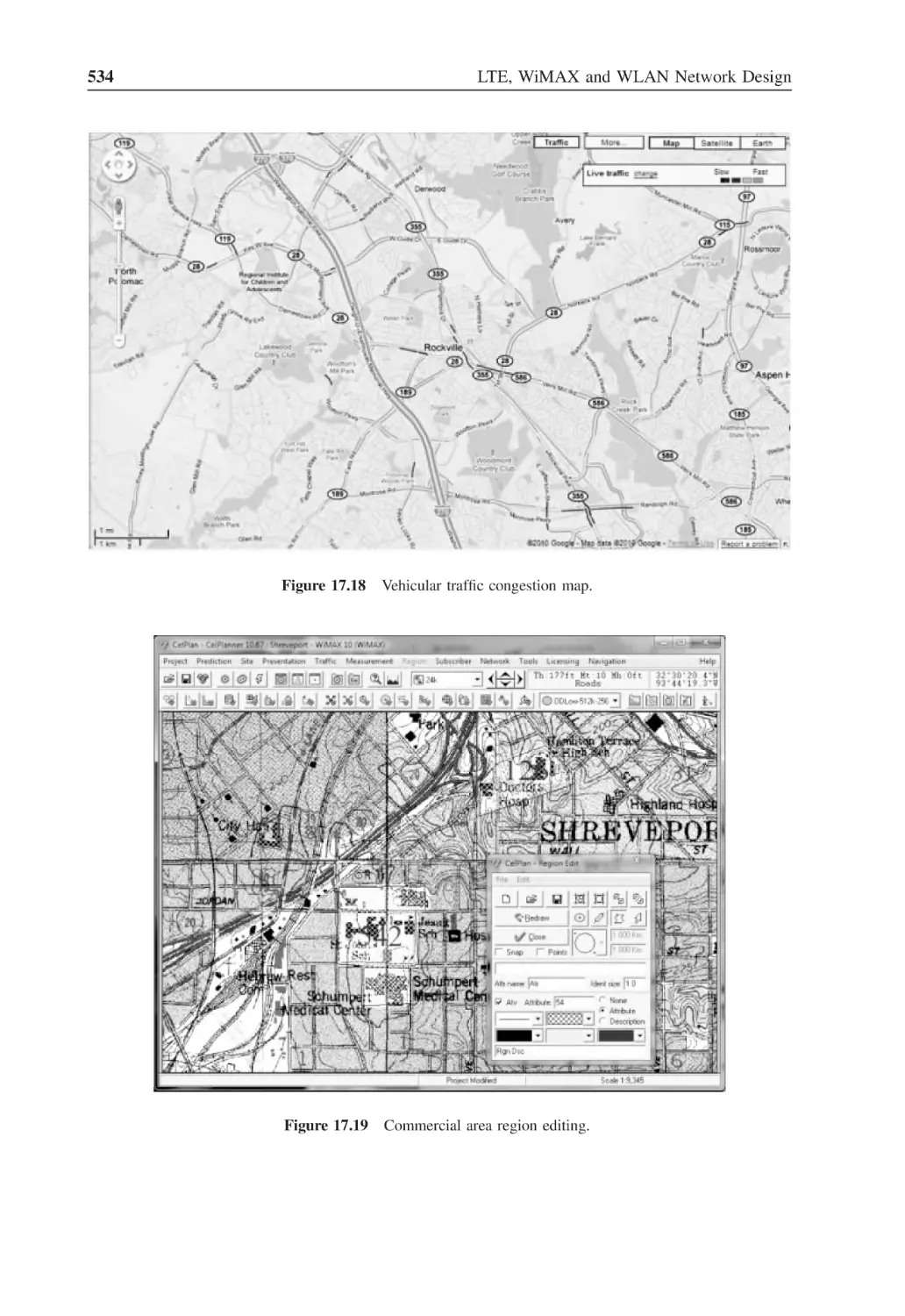
Figure 17.18 Vehicular traffic congestion map
534
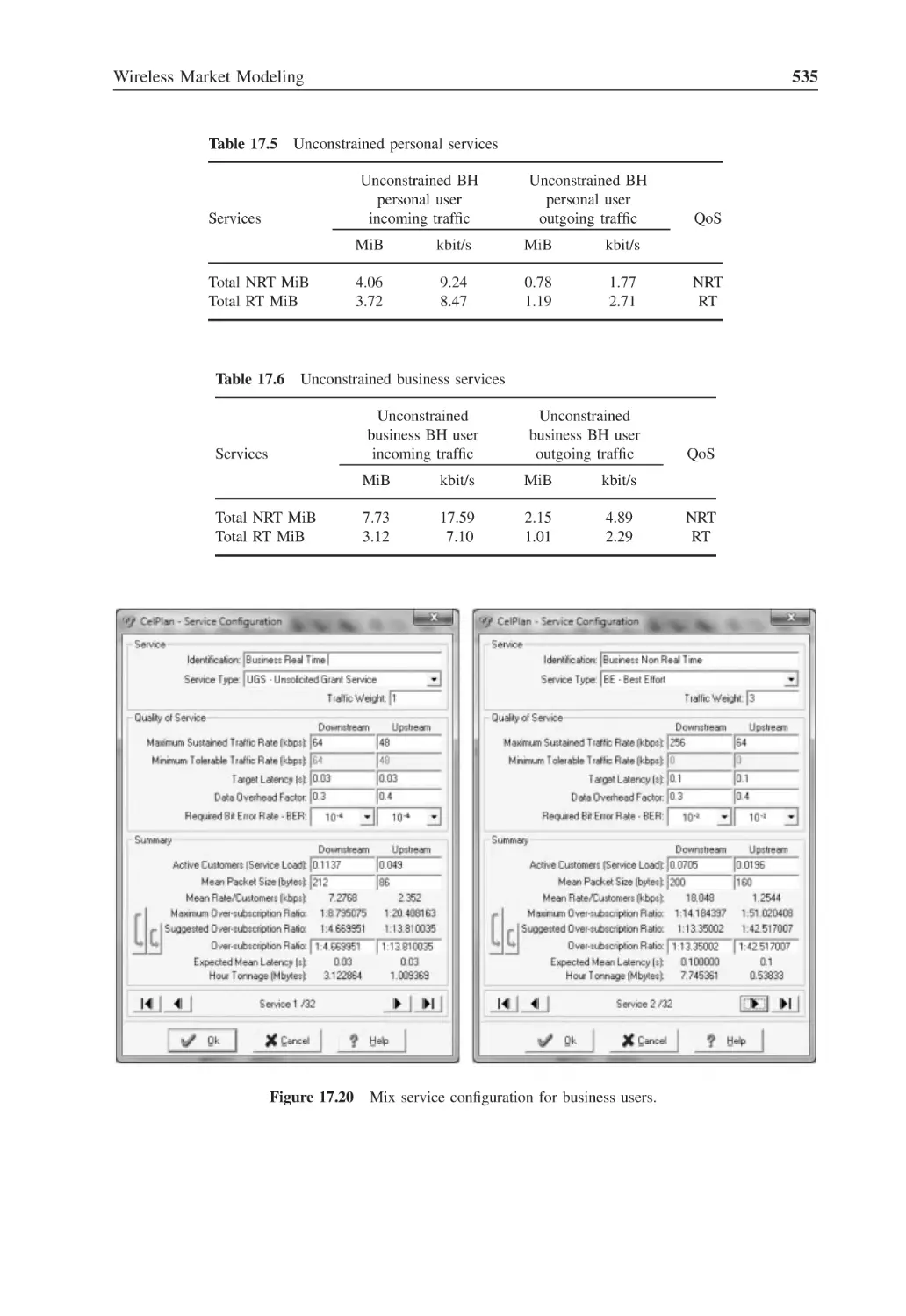
Figure 17.19 Commercial area region editing
534
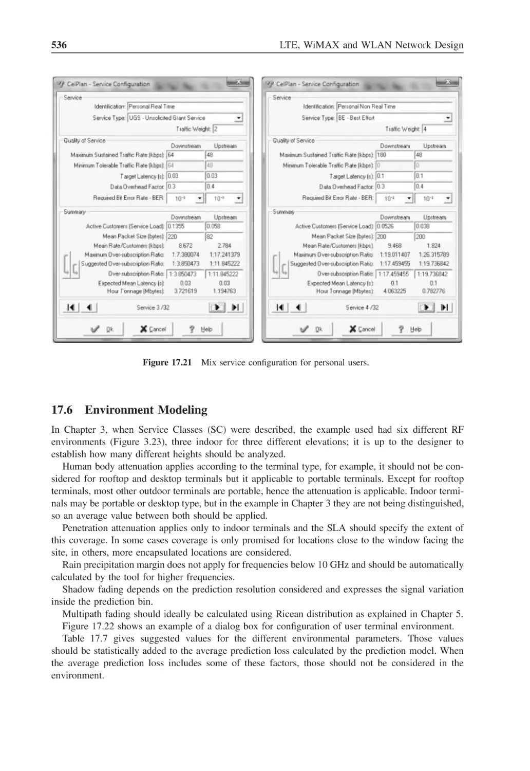
Figure 17.20 Mix service configuration for business users
535
Figure 17.21 Mix service configuration for personal users
536
Figure 17.22 Environment configuration
537
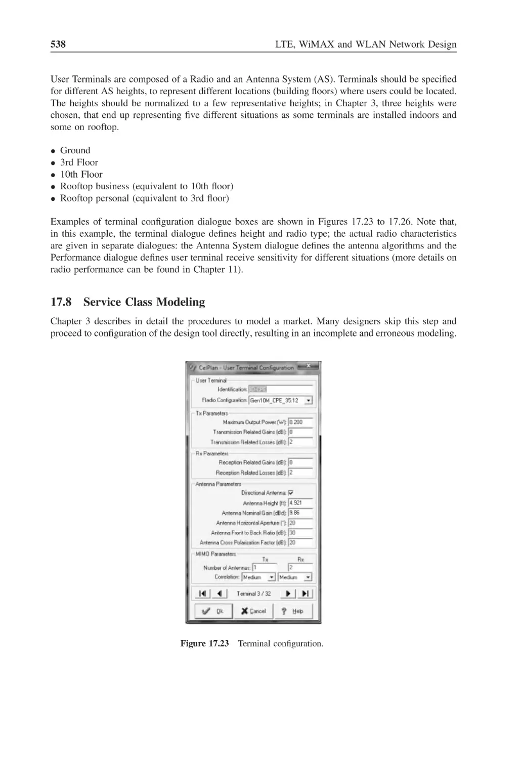
Figure 17.23 Terminal configuration
538
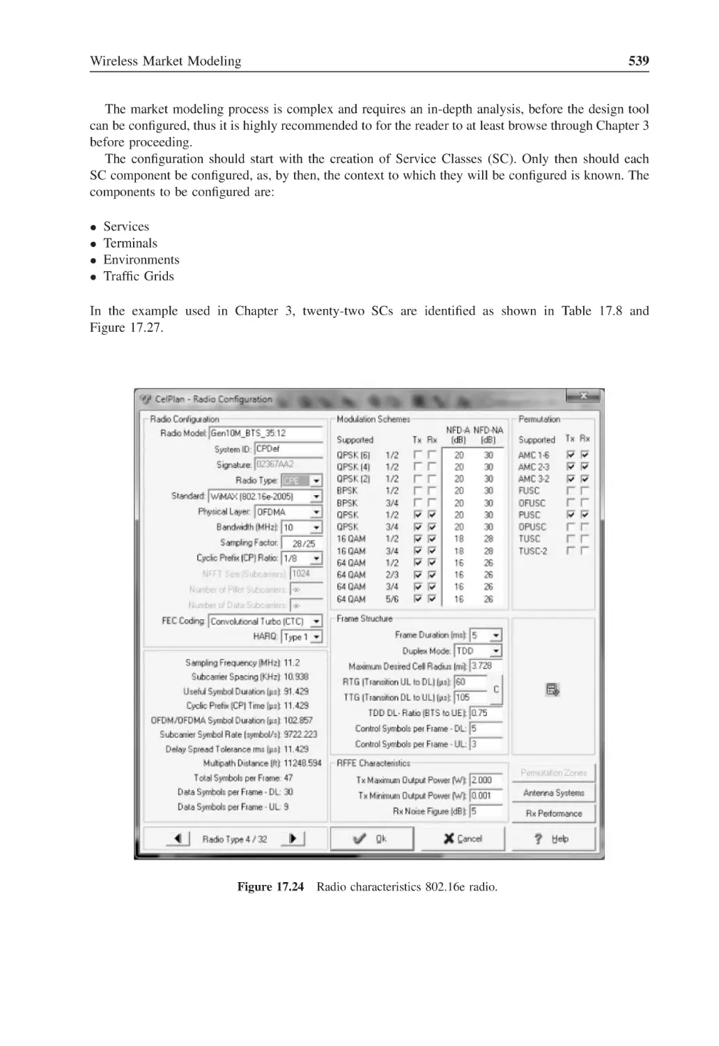
Figure 17.24 Radio characteristics 802.16e radio
539
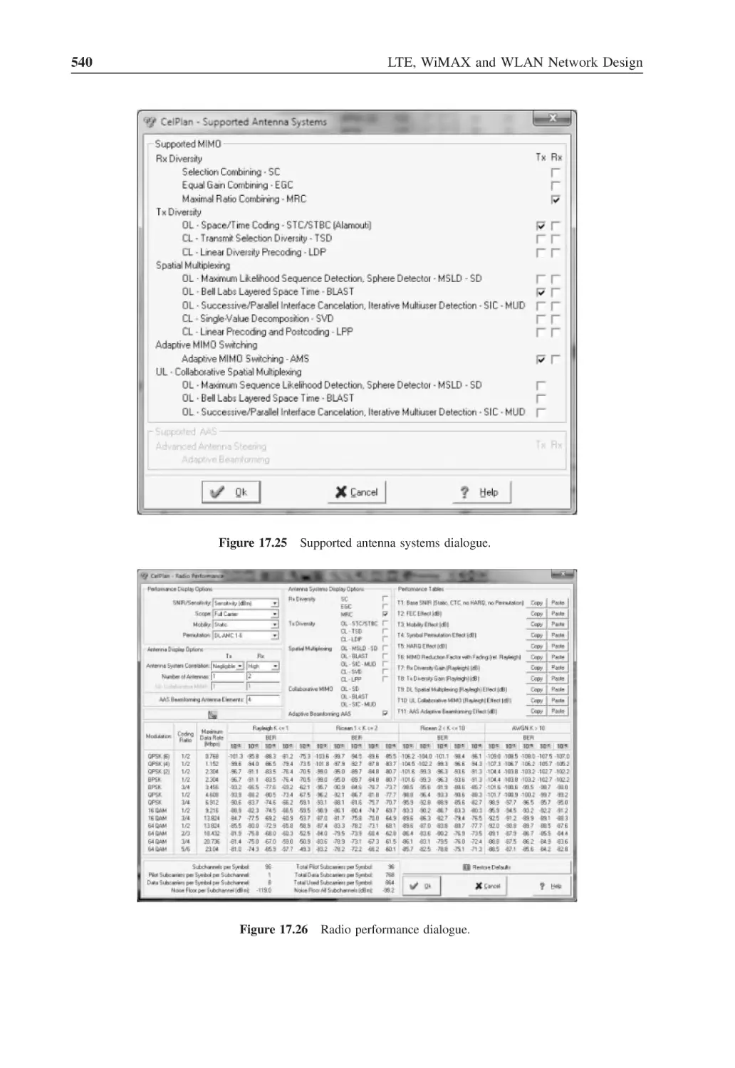
Figure 17.25 Supported antenna systems dialogue
540
Figure 17.26 Radio performance dialogue
540
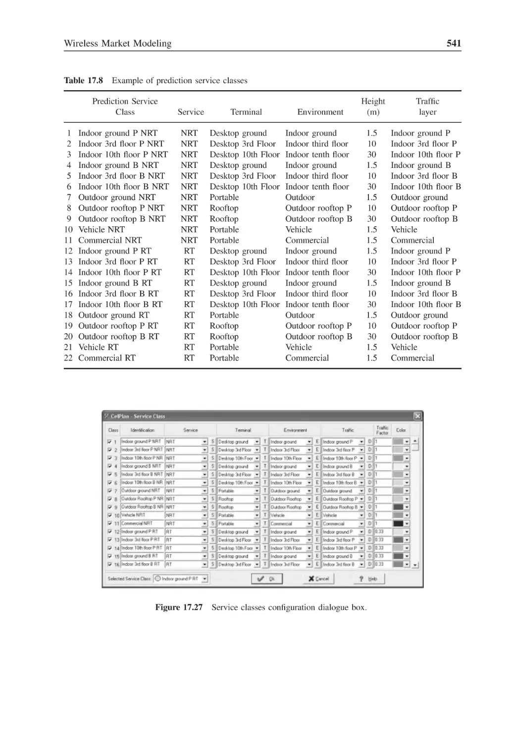
Figure 17.27 Service classes configuration dialogue box
541
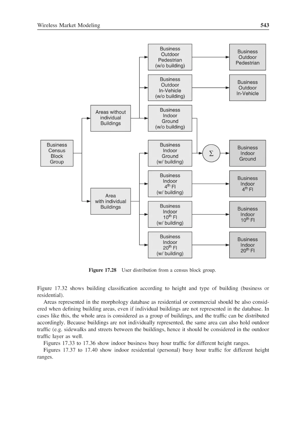
Figure 17.28 User distribution from a census block group
543
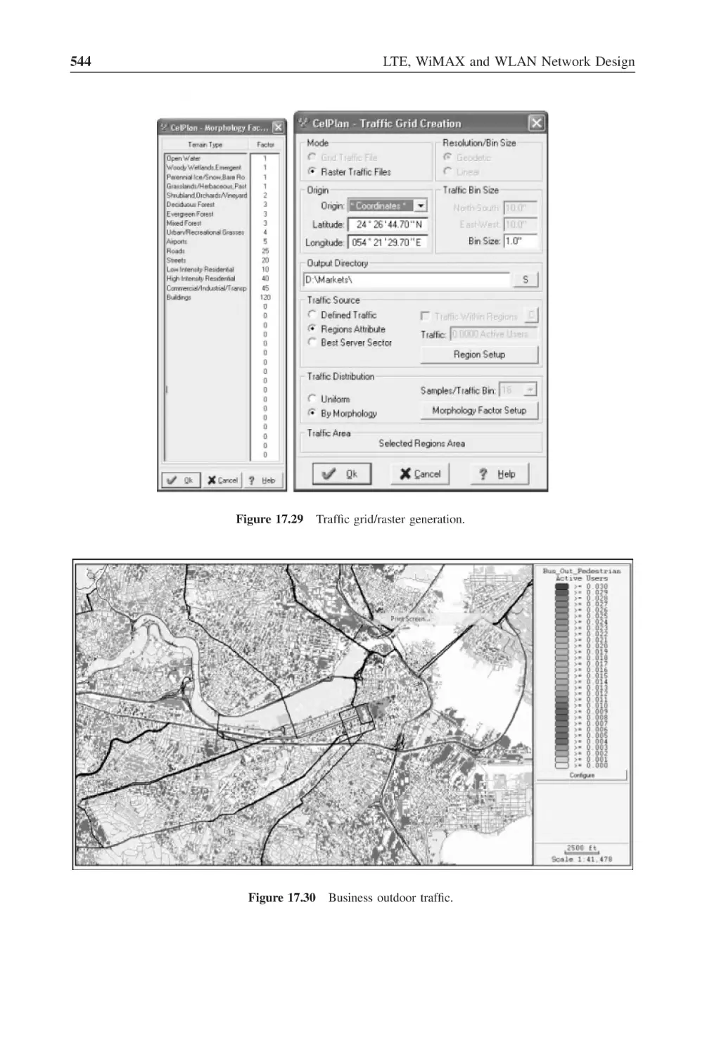
Figure 17.29 Traffic grid/raster generation
544
Figure 17.30 Business outdoor traffic
544
Figure 17.31 Business indoor vehicle traffic
545
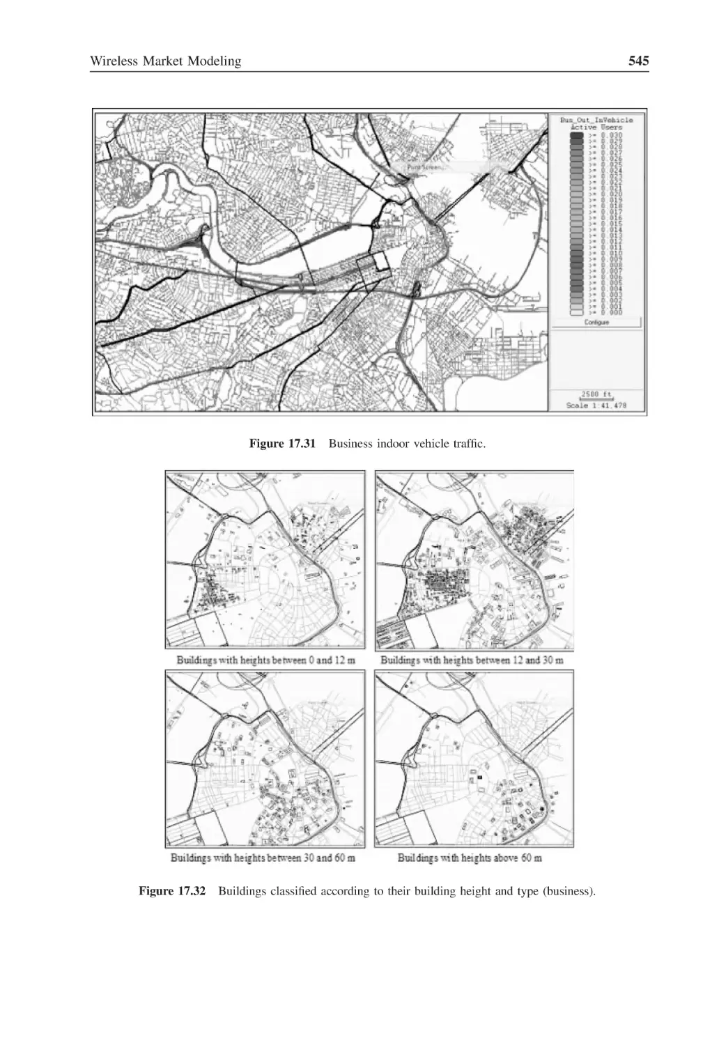
Figure 17.32 Buildings classified according to their building height
and type (business)
545
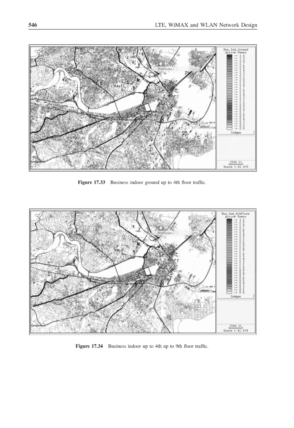
Figure 17.33 Business indoor ground up to 4th floor traffic
546
Figure 17.34 Business indoor up to 4th up to 9th floor traffic
546
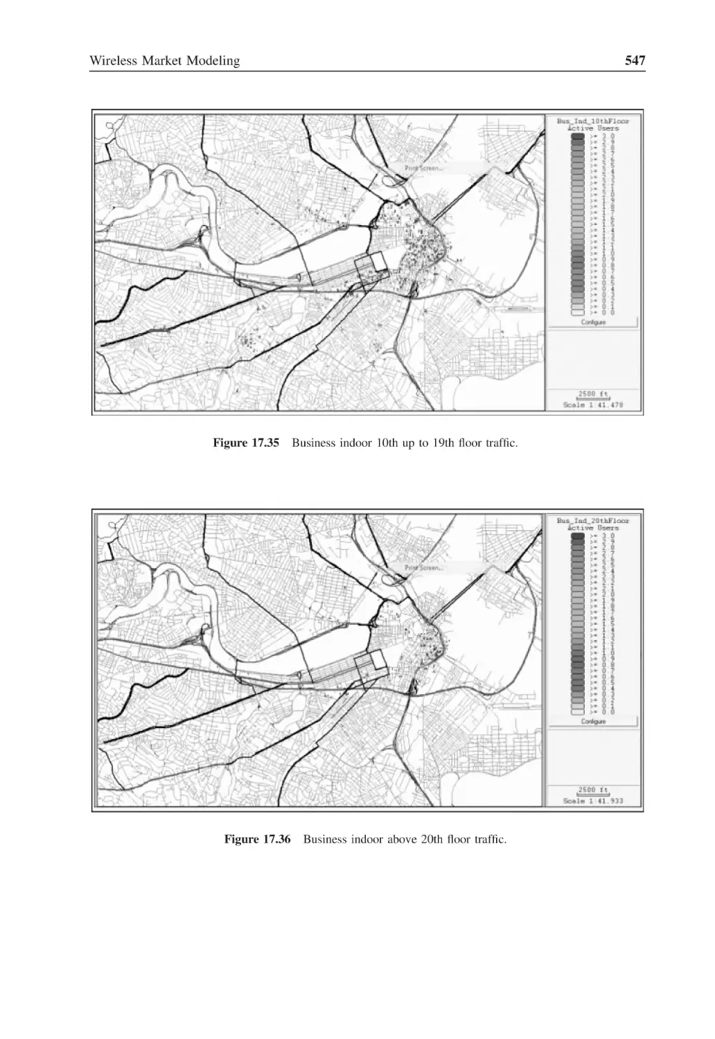
Figure 17.35 Business indoor 10th up to 19th floor traffic
547
Figure 17.36 Business indoor above 20th floor traffic
547
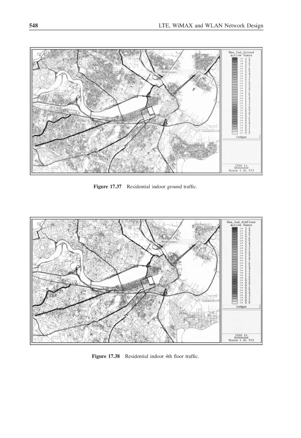
Figure 17.37 Residential indoor ground traffic
548
Figure 17.38 Residential indoor 4th floor traffic
548
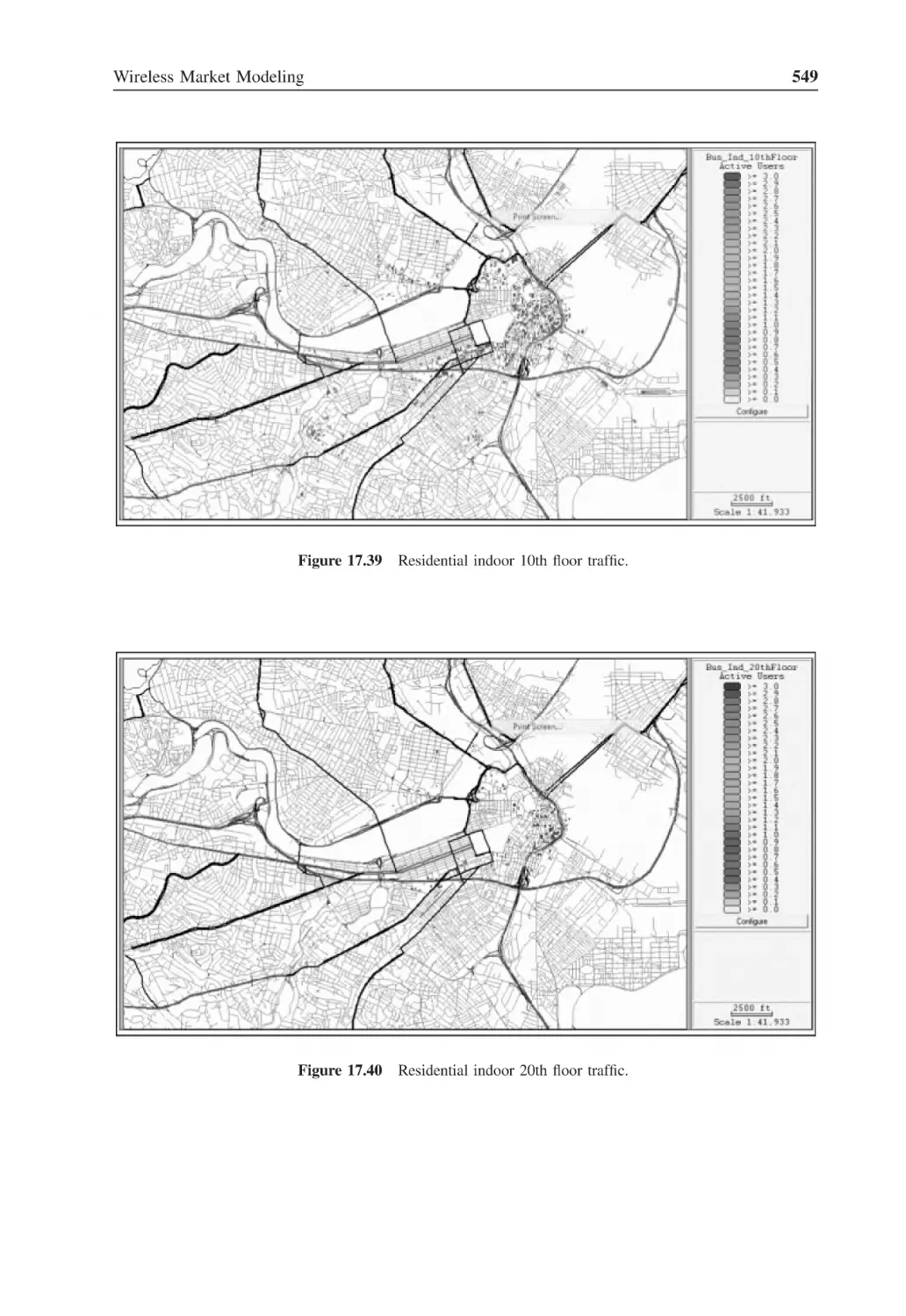
Figure 17.39 Residential indoor 10th floor traffic
549
Figure 17.40 Residential indoor 20th floor traffic
549
Figure 17.41 Hourly traffic variation
550
Figure 18.1
Carrier definition
554
Figure 18.2
Base Station and Sector template
556
Figure 18.3
Link budget for 802.16e Sector Controller
557
Figure 18.4
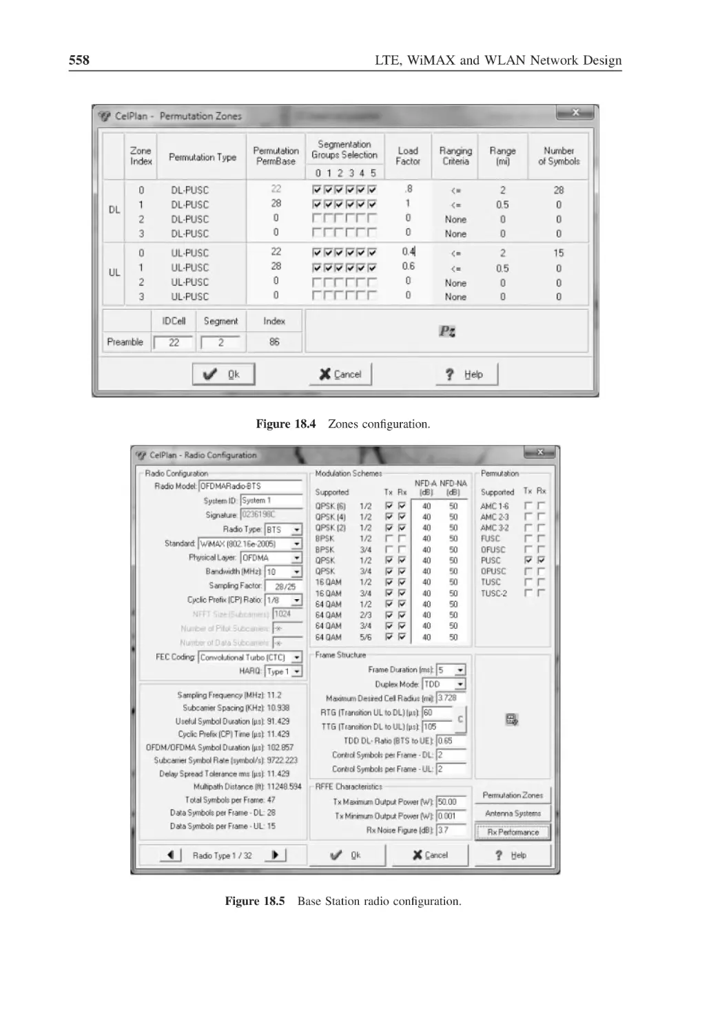
Zones configuration
558
Figure 18.5
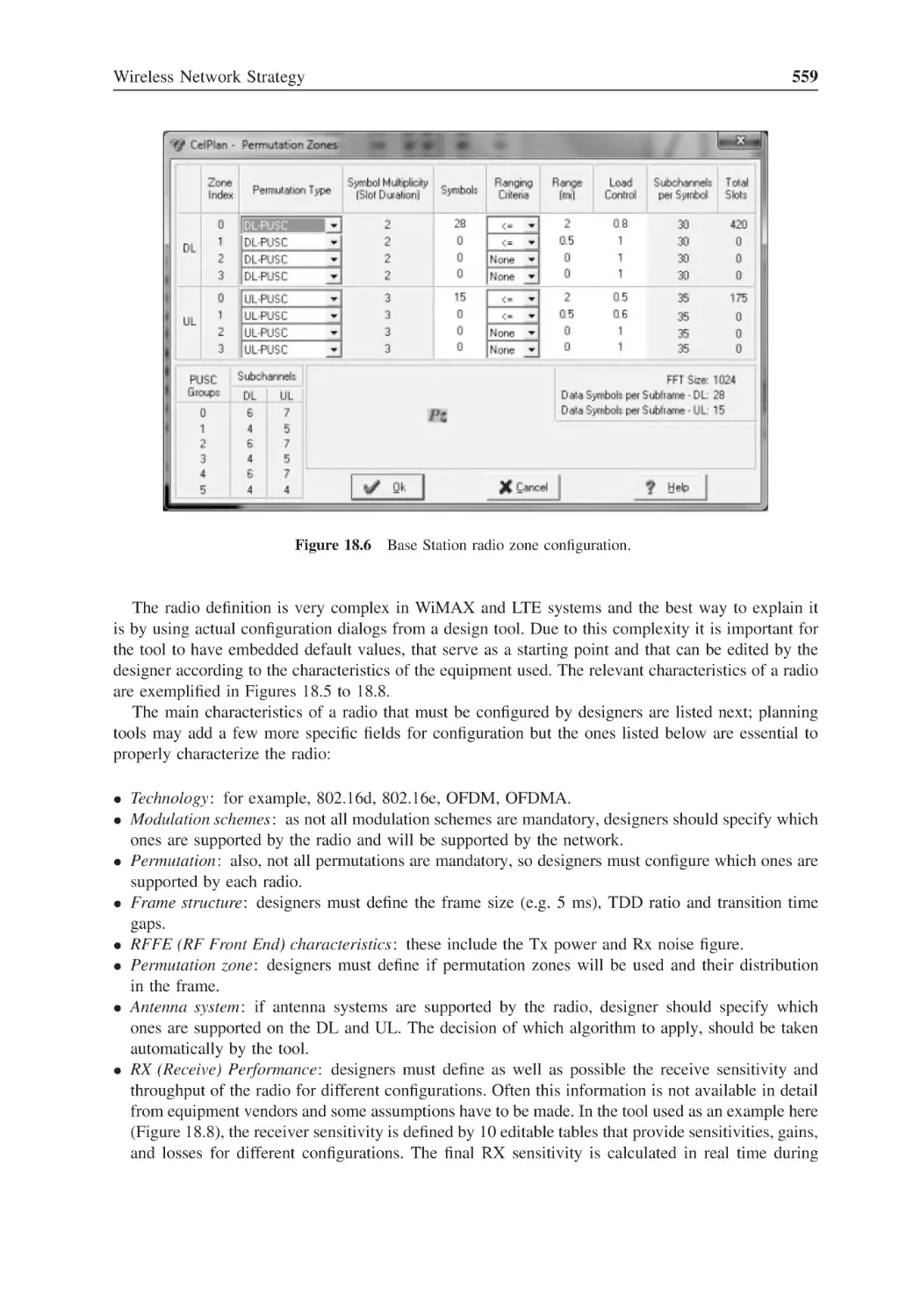
Base Station radio configuration
558
Figure 18.6
Base Station radio zone configuration
559
Figure 18.7
Base Station antenna system configuration
560
Figure 18.8
Base Station performance configuration
561
List of Figures
Figure 18.9
Antenna pattern
xxxi
561
Figure 18.10 Antenna pattern 3-D view
562
Figure 18.11 CPE terminal configuration
562
Figure 18.12 CPE radio configuration
563
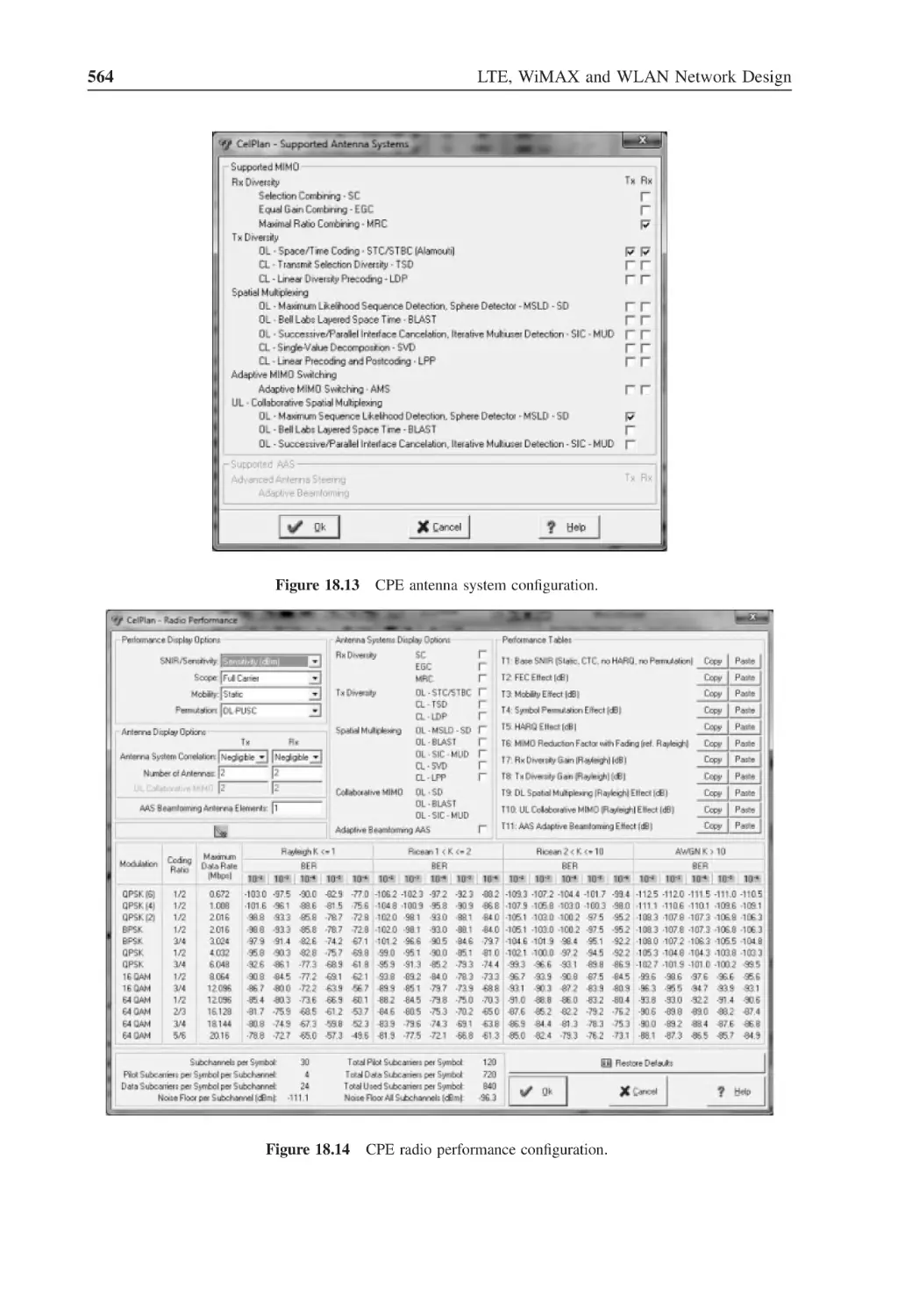
Figure 18.13 CPE antenna system configuration
564
Figure 18.14 CPE radio performance configuration
564
Figure 18.15 Example of a link budget between 802.16e sector controller
and an arbitrary point
565
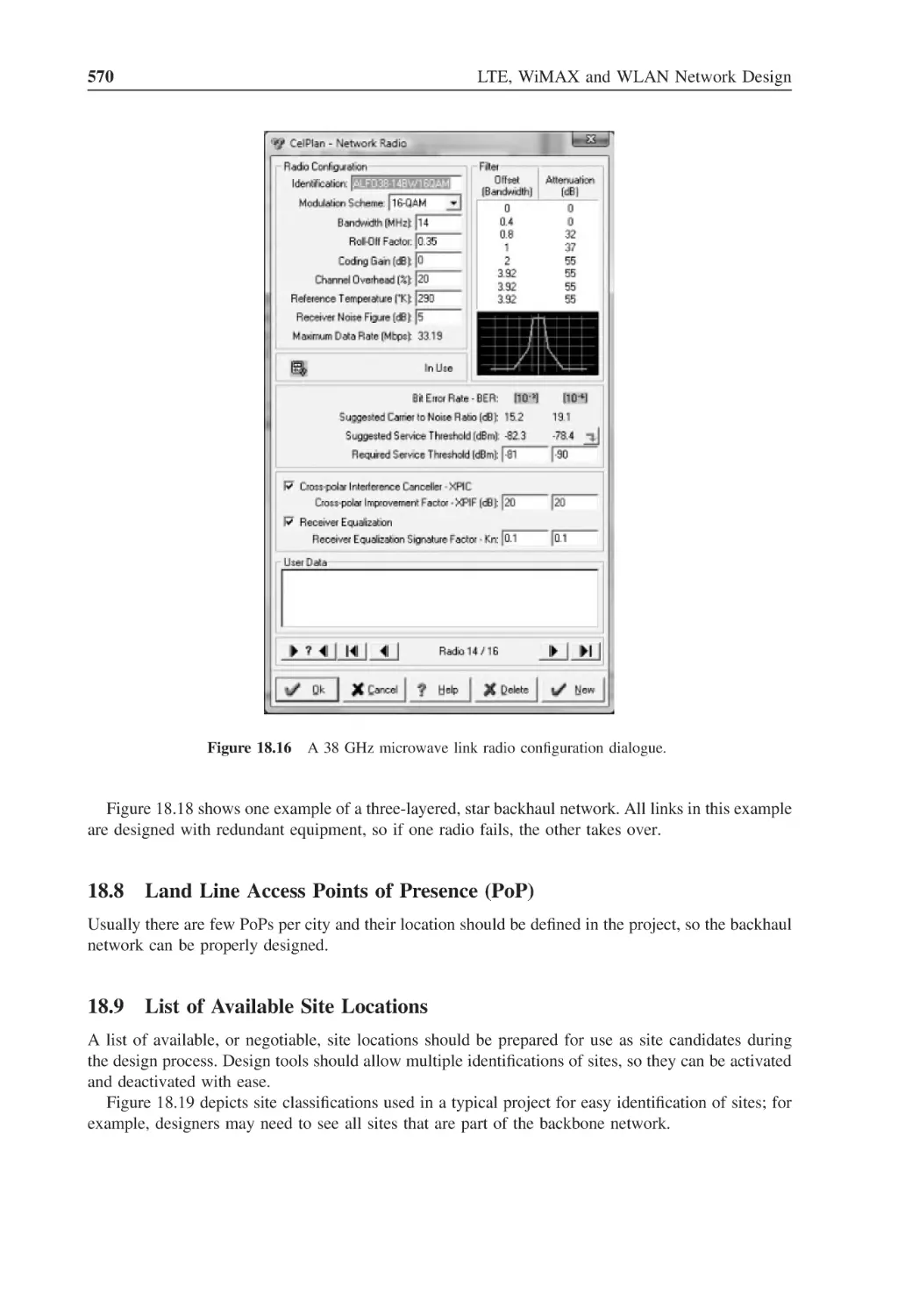
Figure 18.16 A 38 GHz microwave link radio configuration dialogue
570
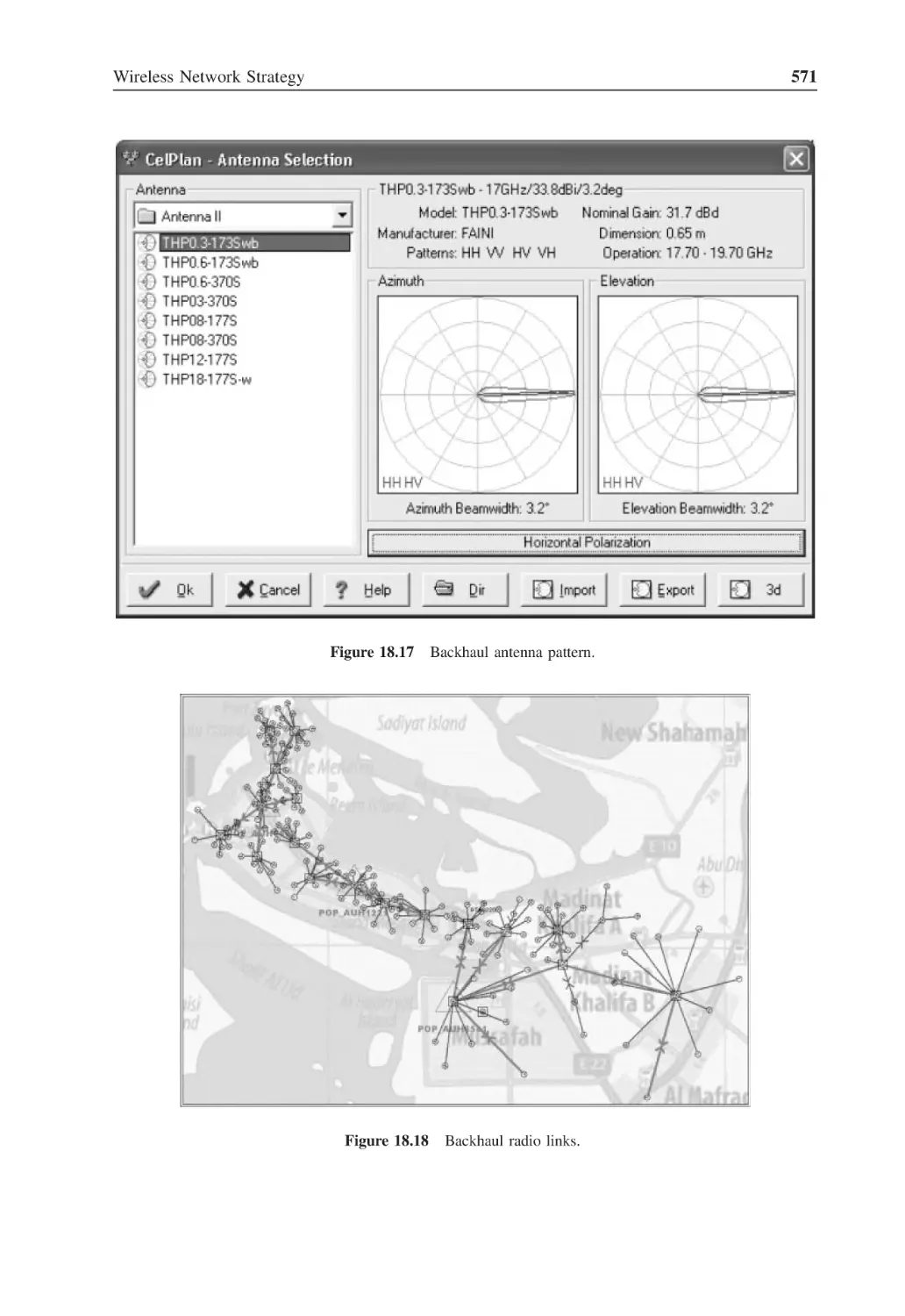
Figure 18.17 Backhaul antenna pattern
571
Figure 18.18 Backhaul radio links
571
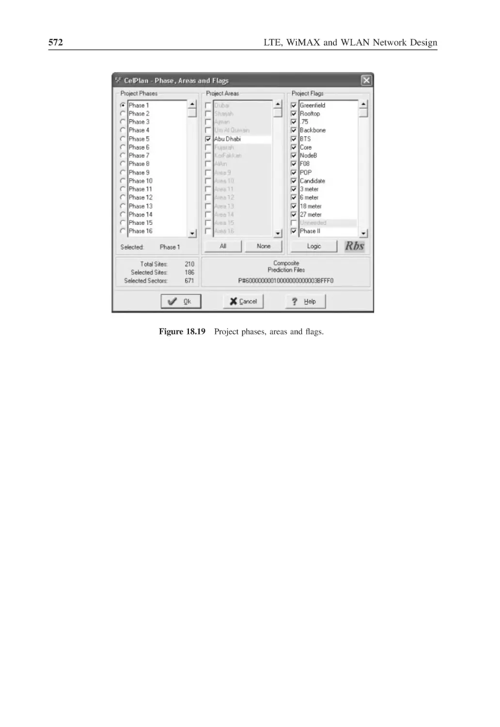
Figure 18.19 Project phases, areas and flags
572
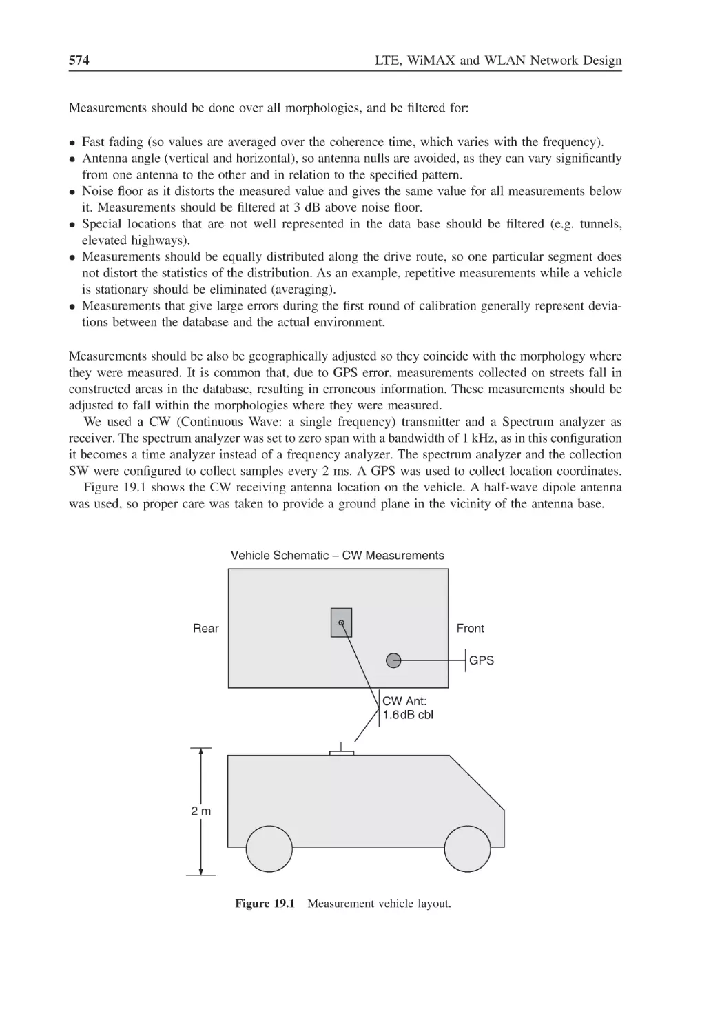
Figure 19.1
Measurement vehicle layout
574
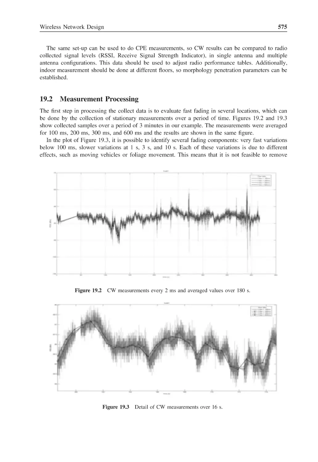
Figure 19.2
CW measurements every 2 ms and averaged values over 180 s
575
Figure 19.3
Detail of CW measurements over 16 s
575
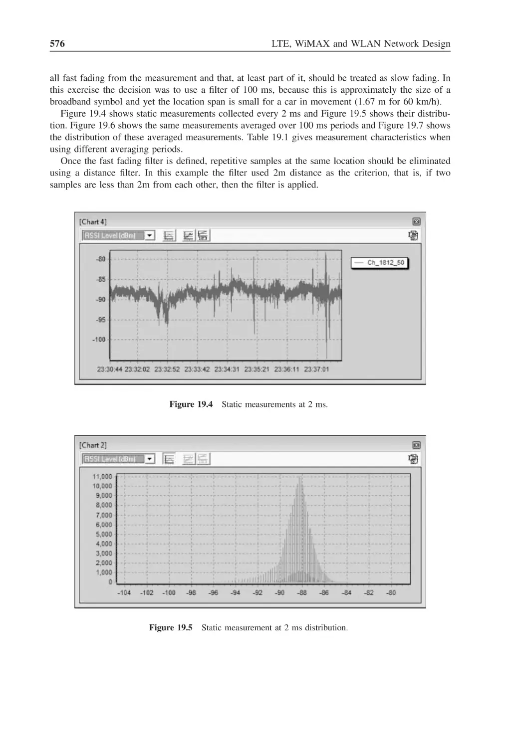
Figure 19.4
Static measurements at 2 ms
576
Figure 19.5
Static measurement at 2 ms distribution
576
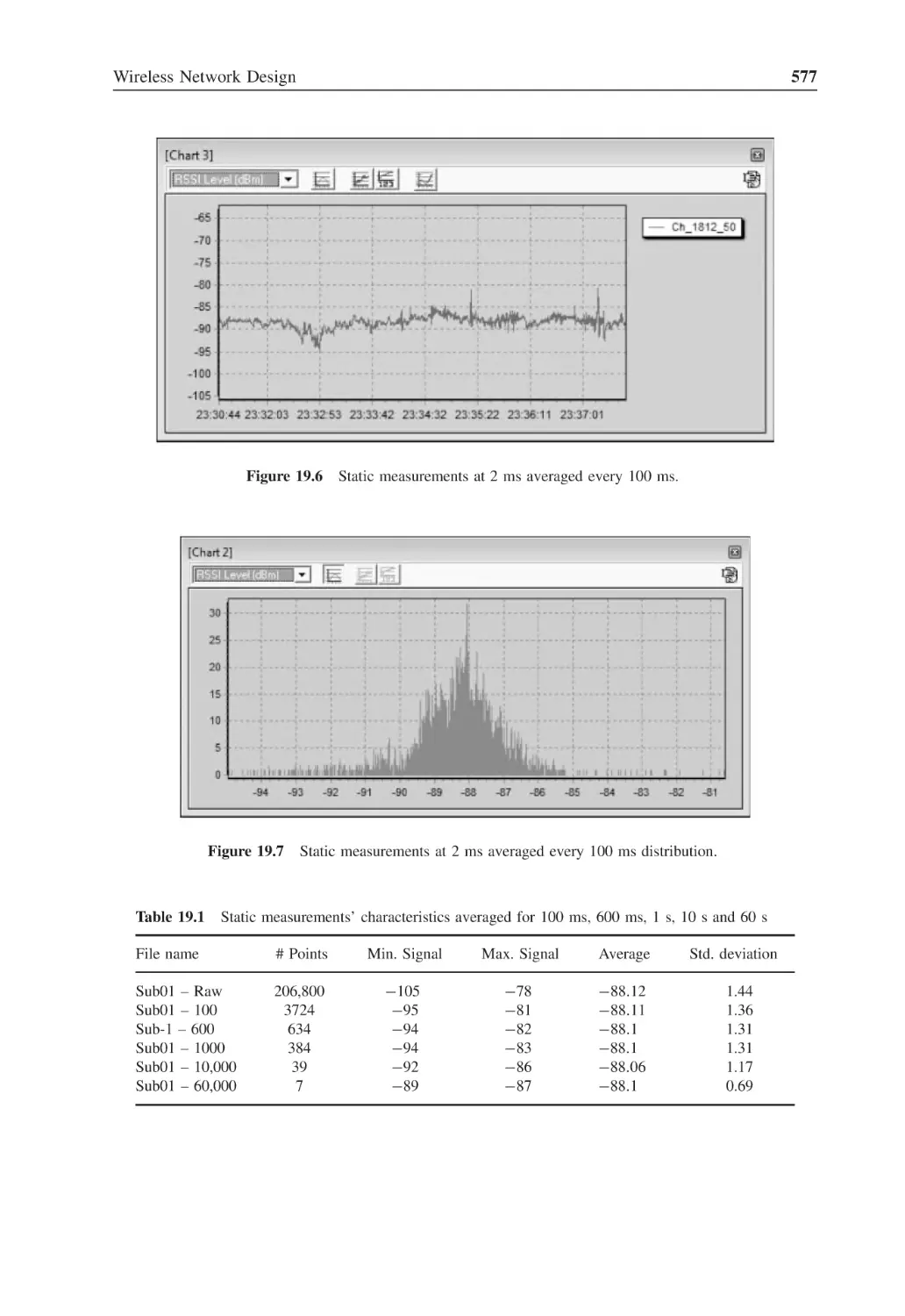
Figure 19.6
Static measurements at 2 ms averaged every 100 ms
577
Figure 19.7
Static measurements at 2 ms averaged every 100 ms distribution
577
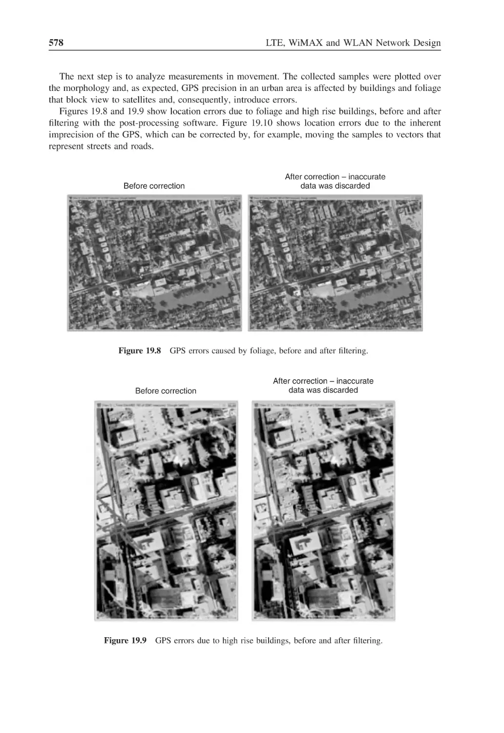
Figure 19.8
GPS errors caused by foliage, before and after filtering
578
Figure 19.9
GPS errors due to high rise buildings, before and after filtering
578
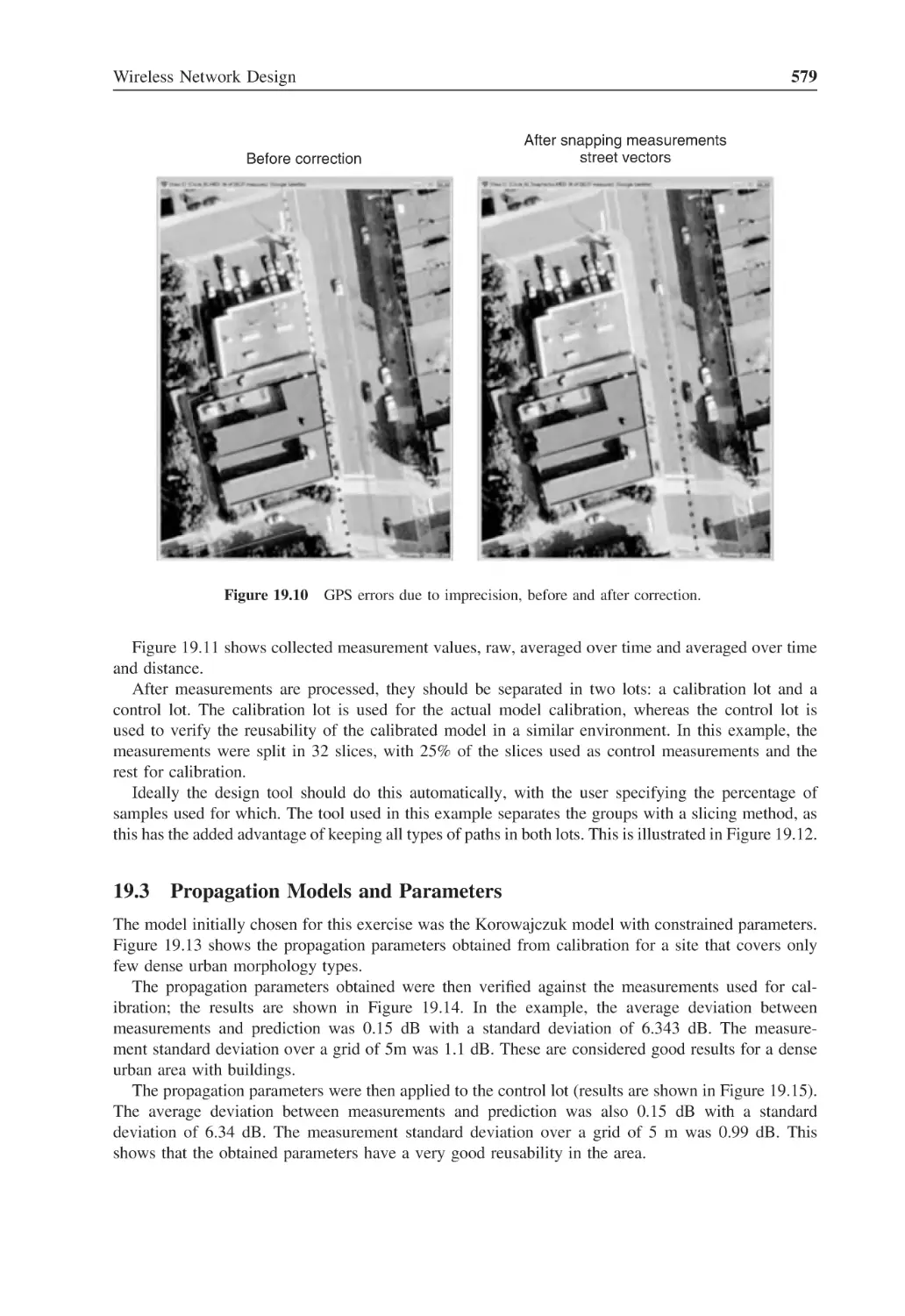
Figure 19.10 GPS errors due to imprecision, before and after correction
579
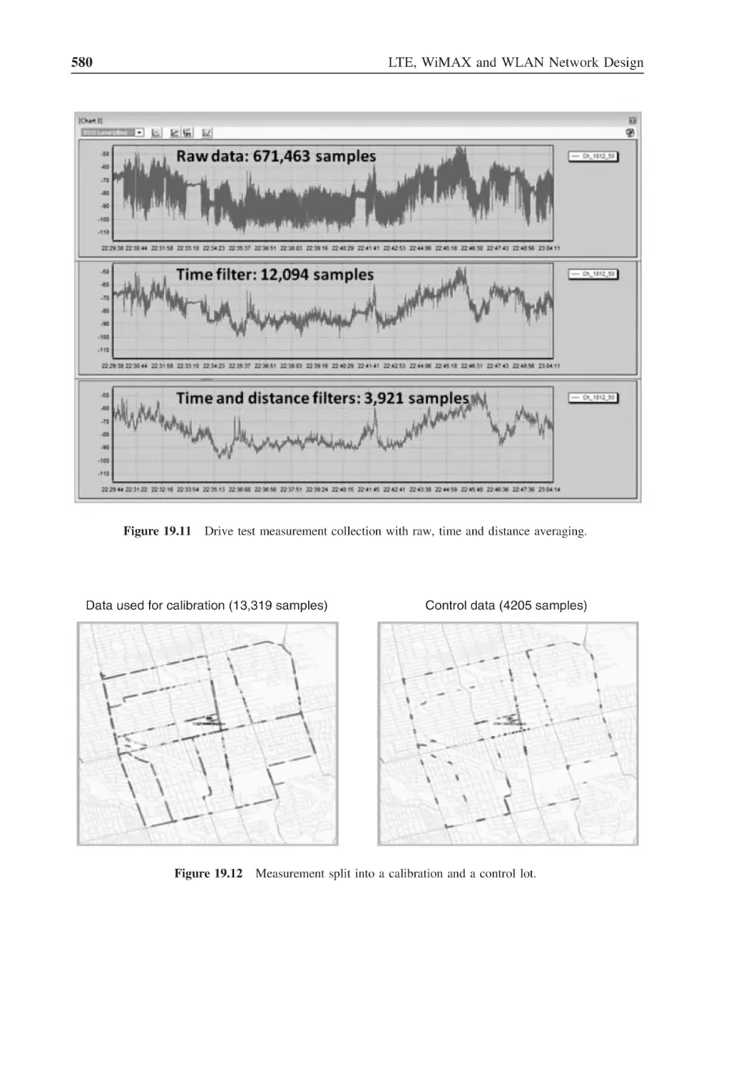
Figure 19.11 Drive test measurement collection with raw, time and distance averaging
580
Figure 19.12 Measurement split into a calibration and a control lot
580
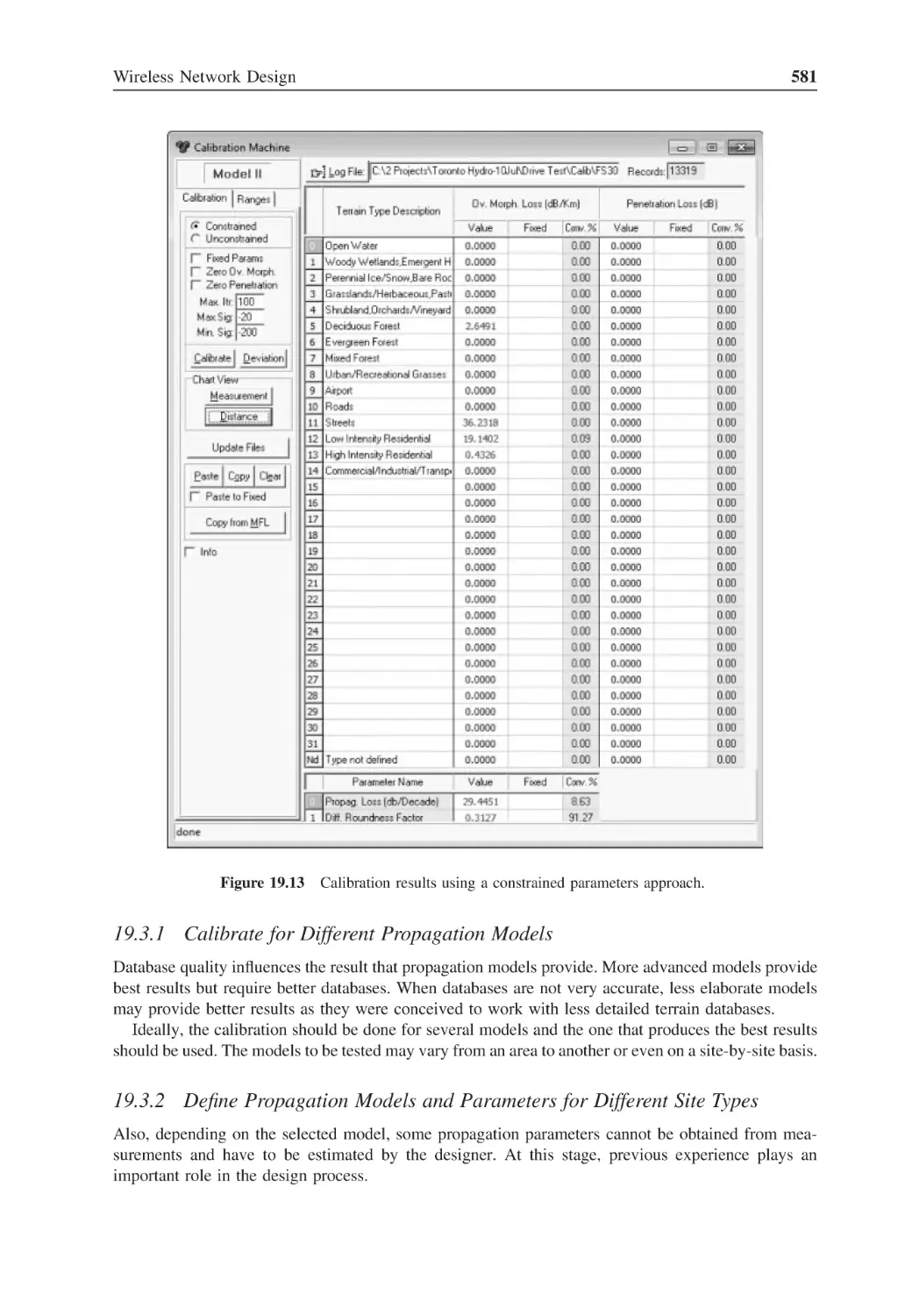
Figure 19.13 Calibration results using a constrained parameters approach
581
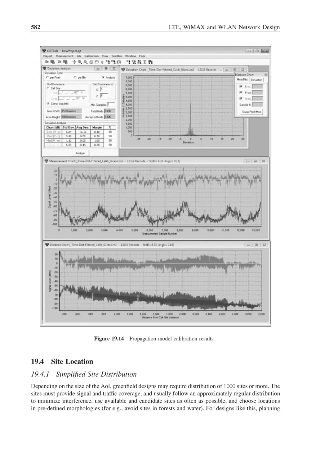
Figure 19.14 Propagation model calibration results
582
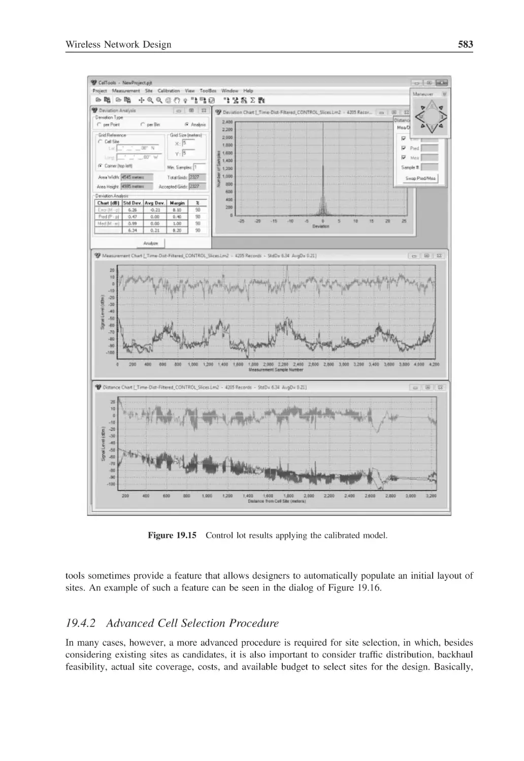
Figure 19.15 Control lot results applying the calibrated model
583
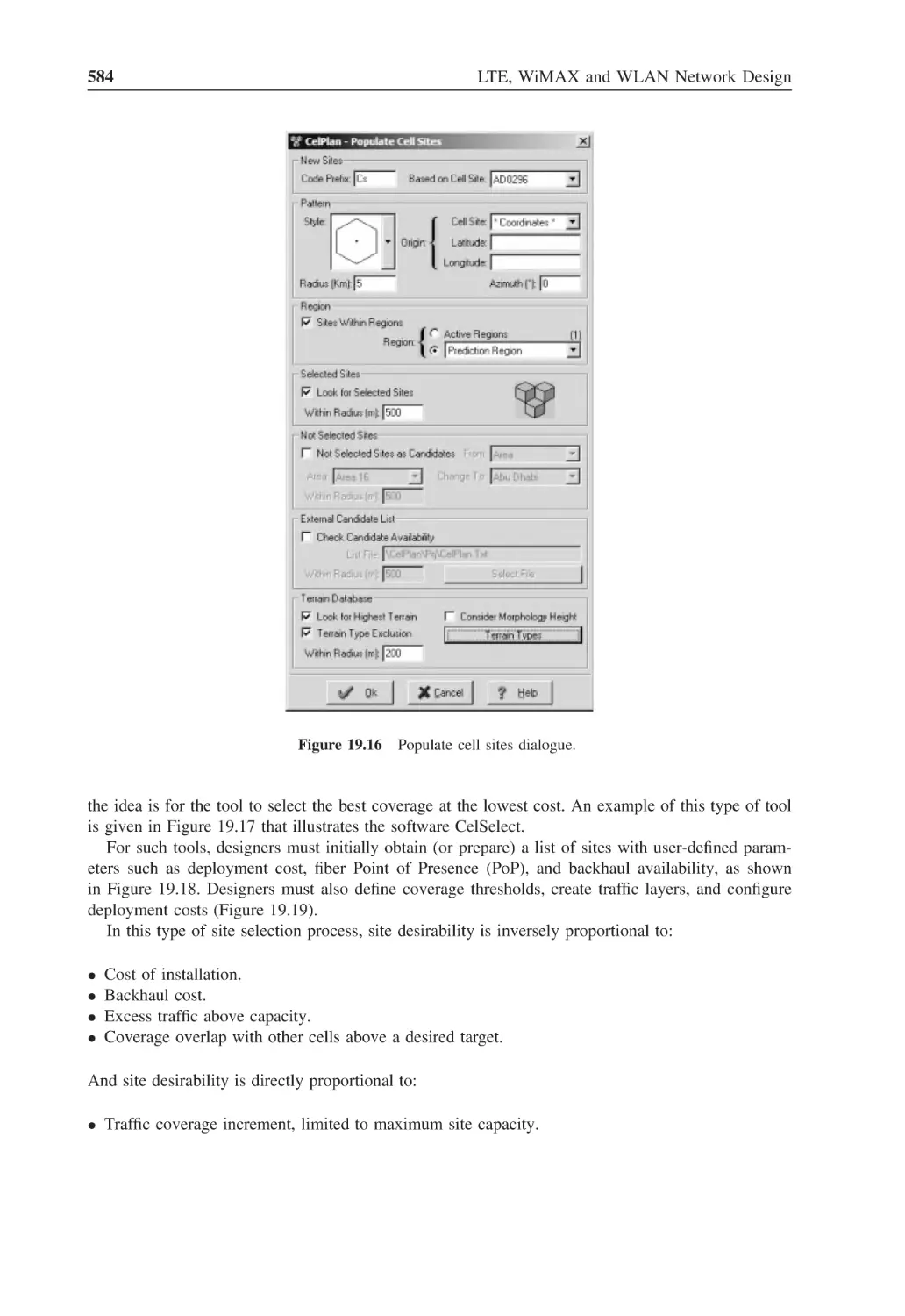
Figure 19.16 Populate cell sites dialogue
584
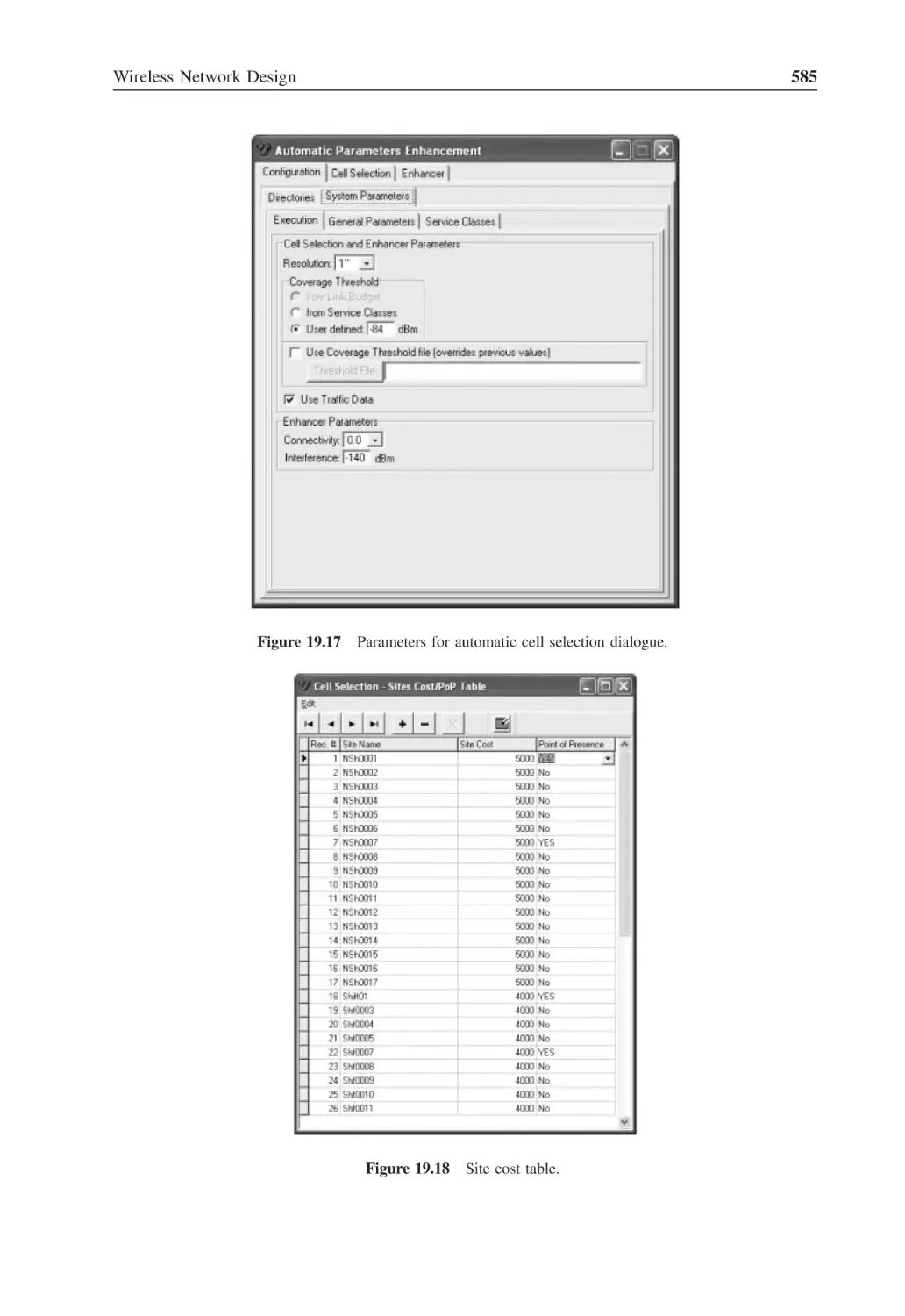
Figure 19.17 Parameters for automatic cell selection dialogue
585
Figure 19.18 Site cost table
585
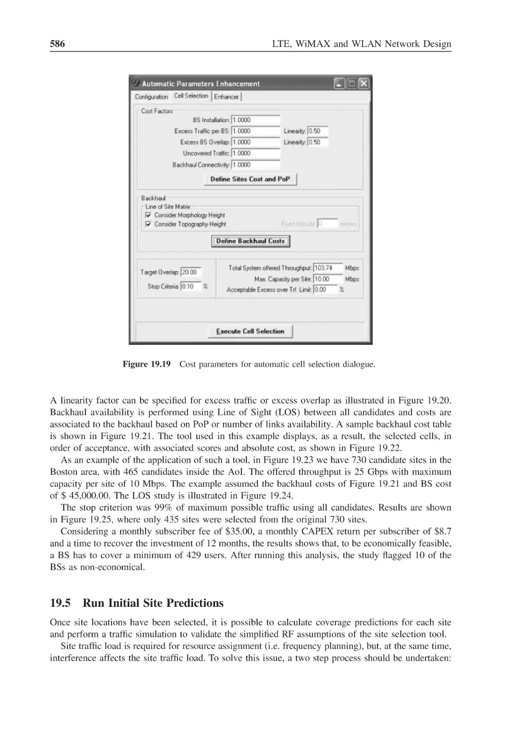
Figure 19.19 Cost parameters for automatic cell selection dialogue
586
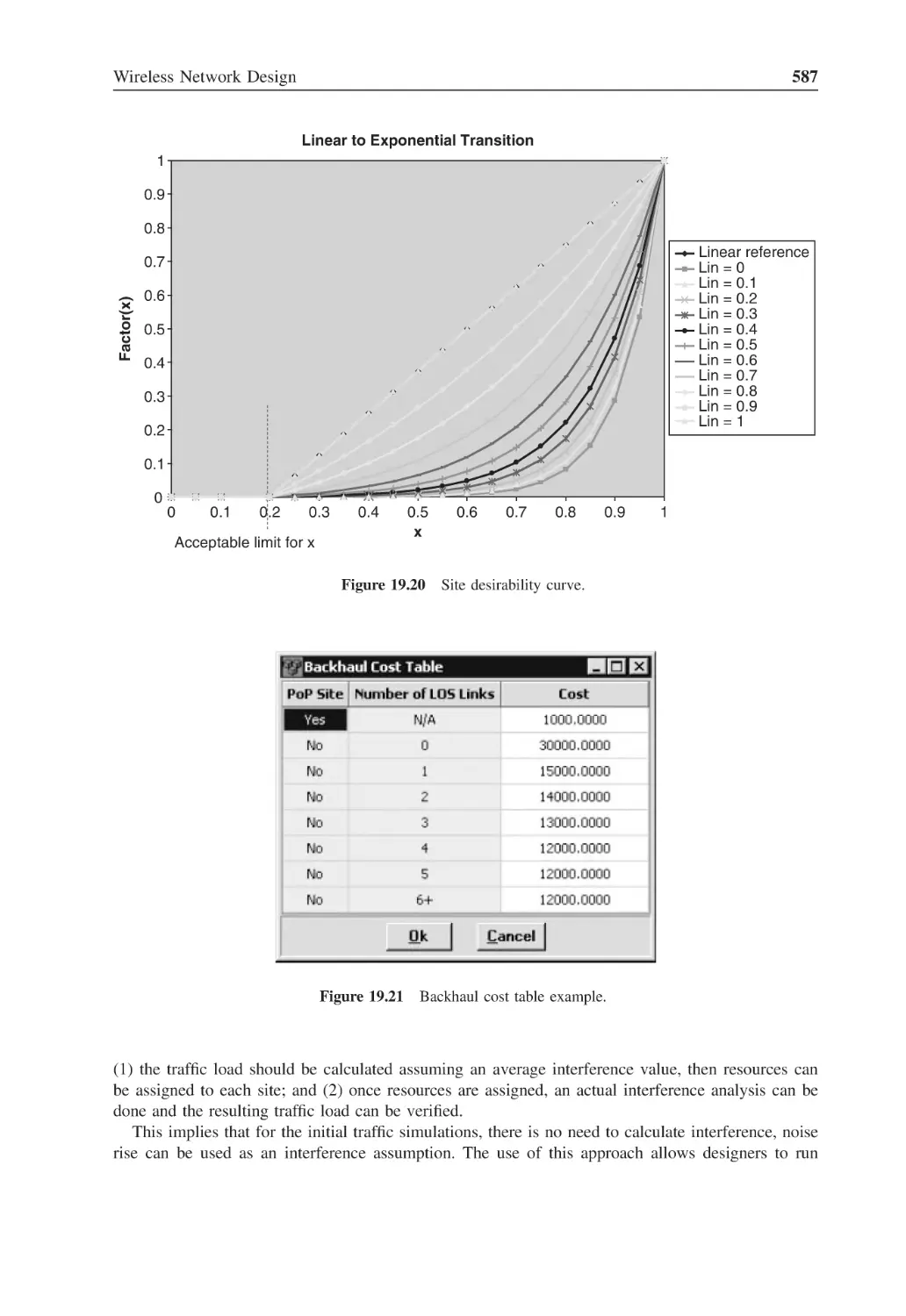
Figure 19.20 Site desirability curve
587
Figure 19.21 Backhaul cost table example
587
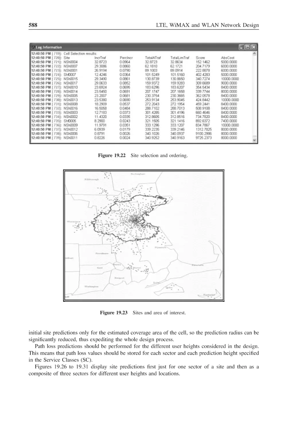
Figure 19.22 Site selection and ordering
588
Figure 19.23 Sites and area of interest
588
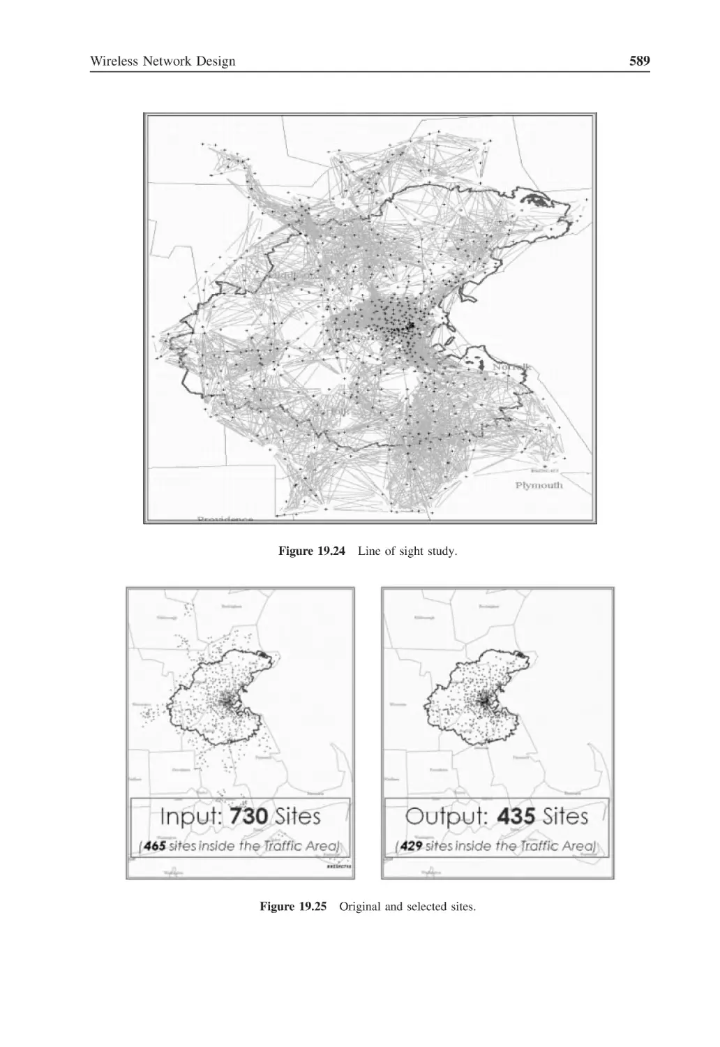
Figure 19.24 Line of sight study
589
Figure 19.25 Original and selected sites
589
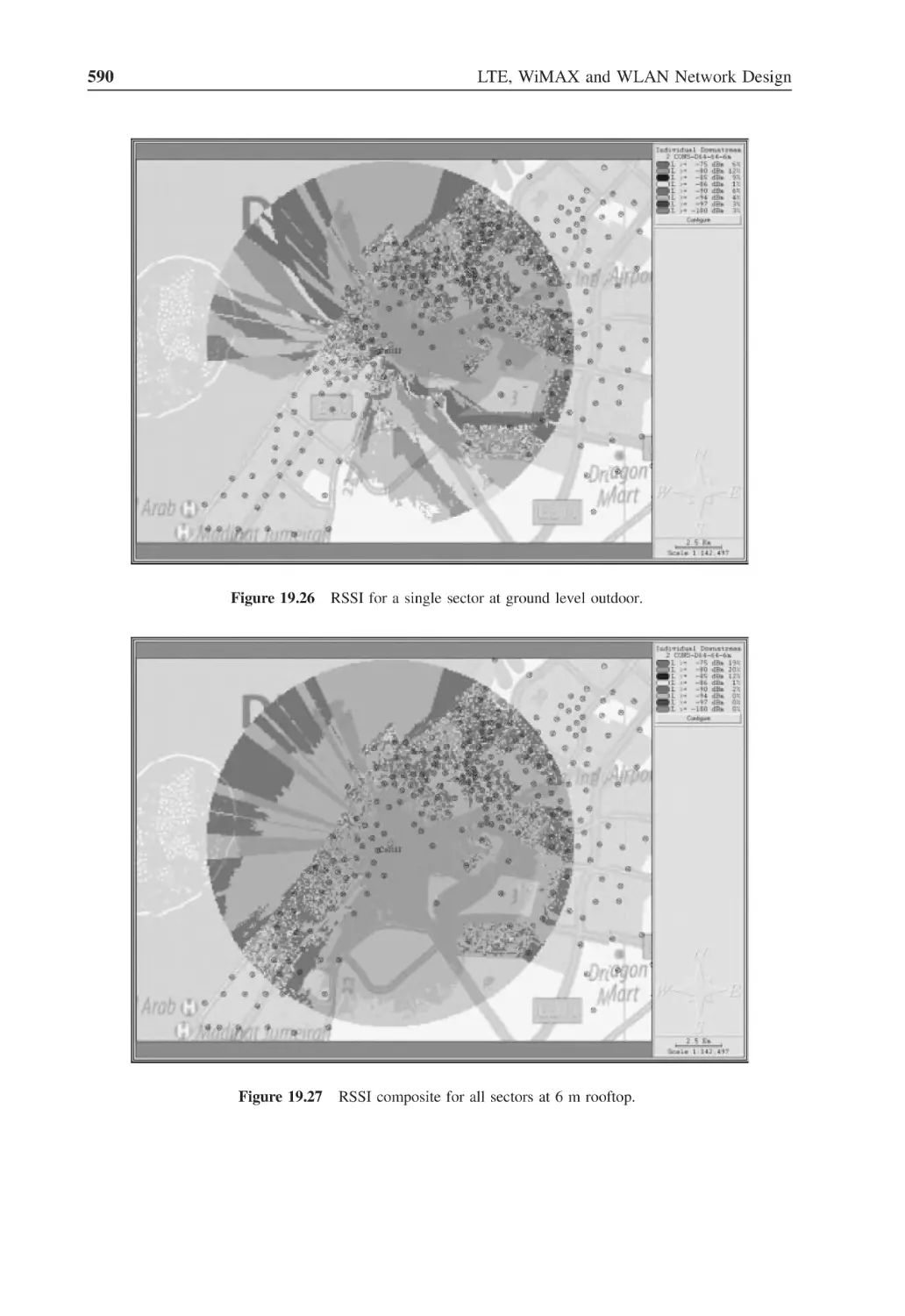
Figure 19.26 RSSI for a single sector at ground level outdoor
590
Figure 19.27 RSSI composite for all sectors at 6 m rooftop
590
xxxii
List of Figures
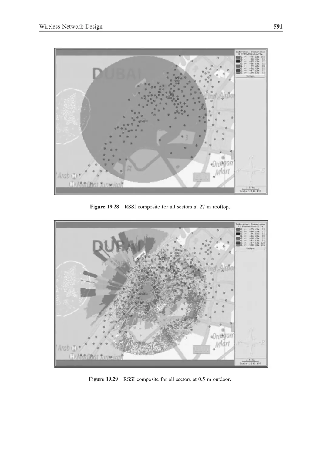
Figure 19.28 RSSI composite for all sectors at 27 m rooftop
591
Figure 19.29 RSSI composite for all sectors at 0.5 m outdoor
591
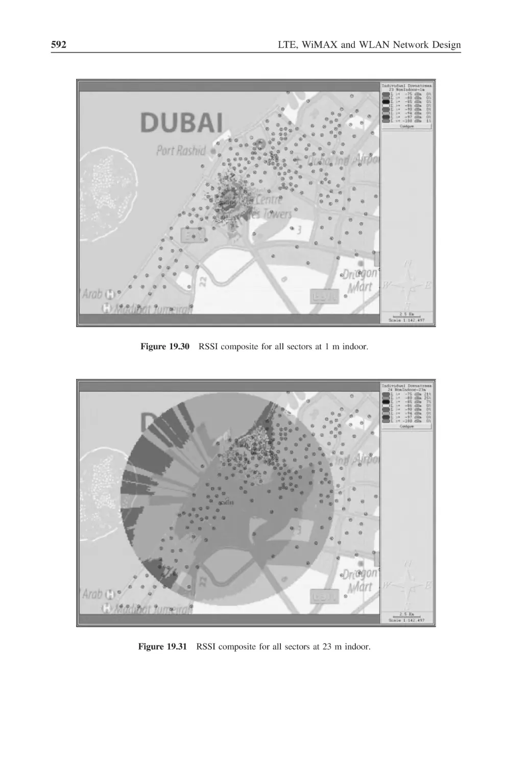
Figure 19.30 RSSI composite for all sectors at 1 m indoor
592
Figure 19.31 RSSI composite for all sectors at 23 m indoor
592
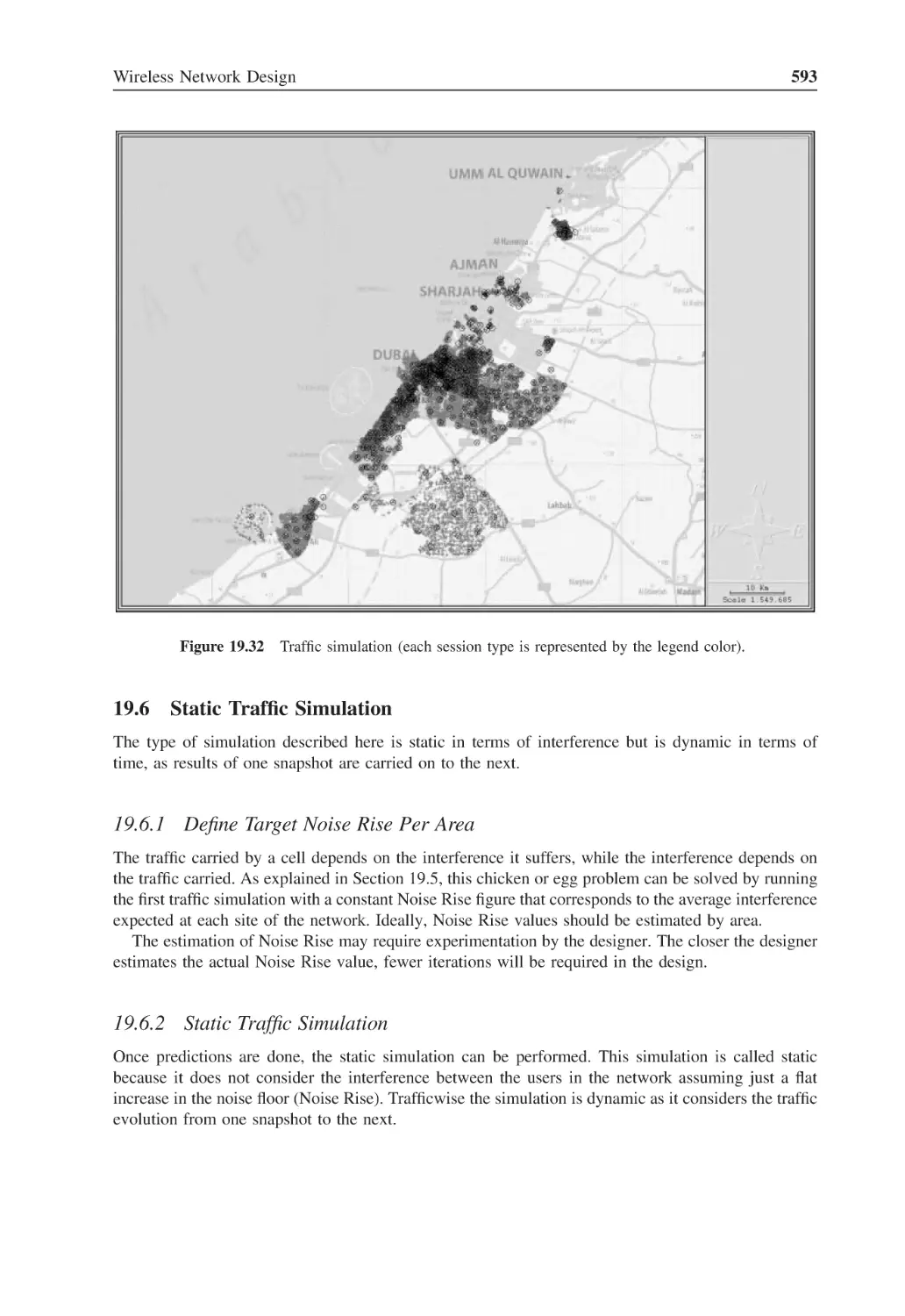
Figure 19.32 Traffic simulation (each session type is represented by the legend color)
593
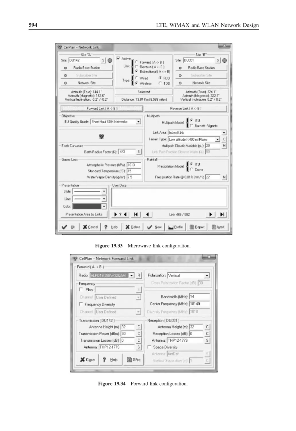
Figure 19.33 Microwave link configuration
594
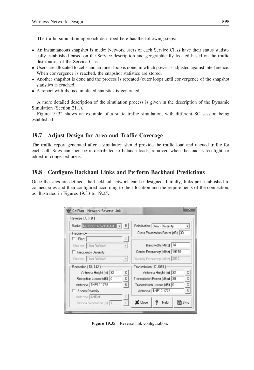
Figure 19.34 Forward link configuration
594
Figure 19.35 Reverse link configuration
595
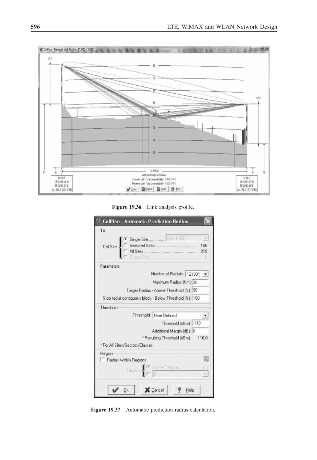
Figure 19.36 Link analysis profile
596
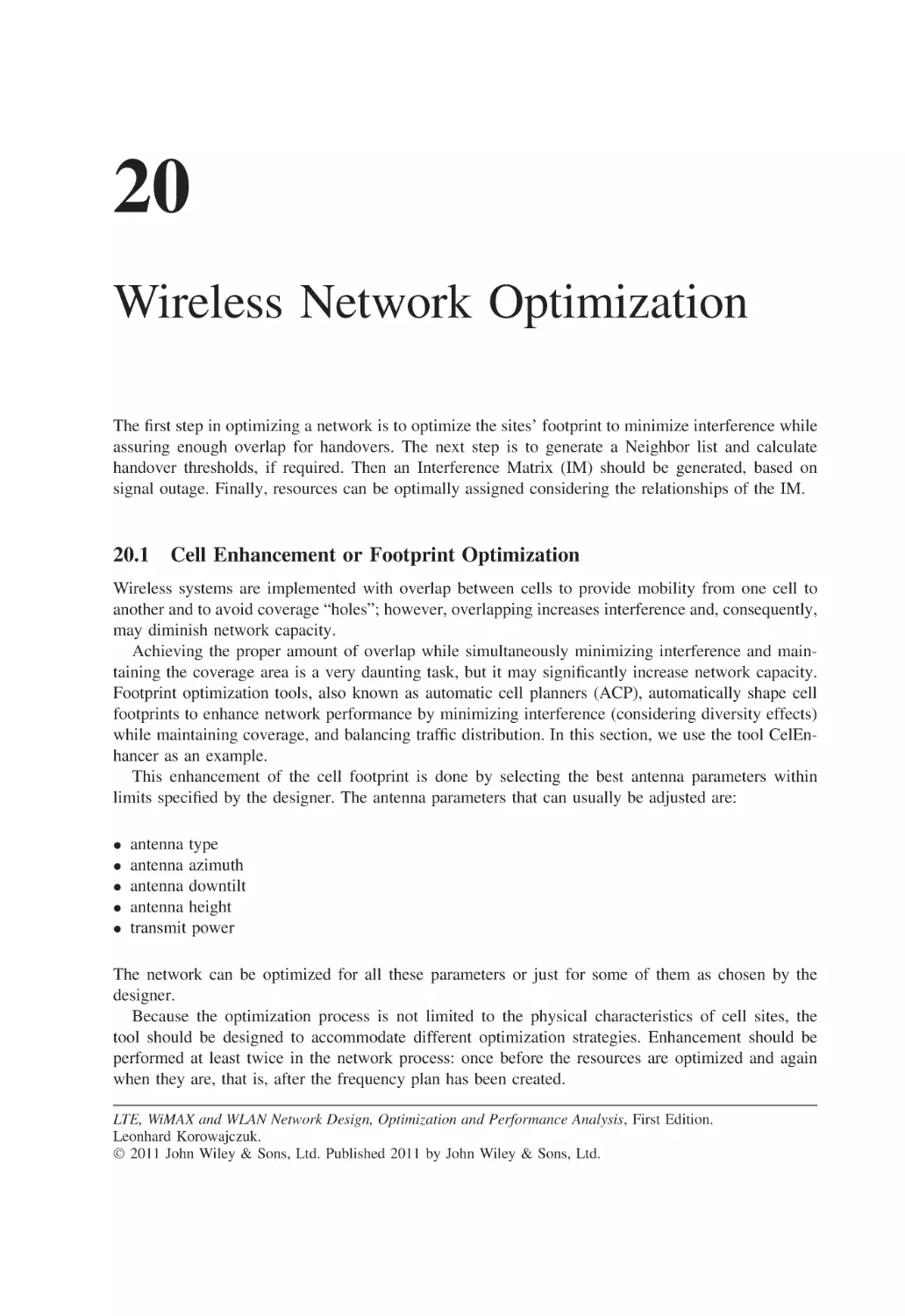
Figure 19.37 Automatic prediction radius calculation
596
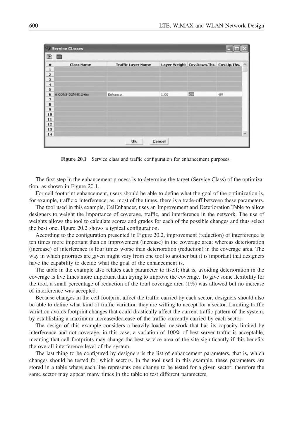
Figure 20.1
Service class and traffic configuration for enhancement purposes
600
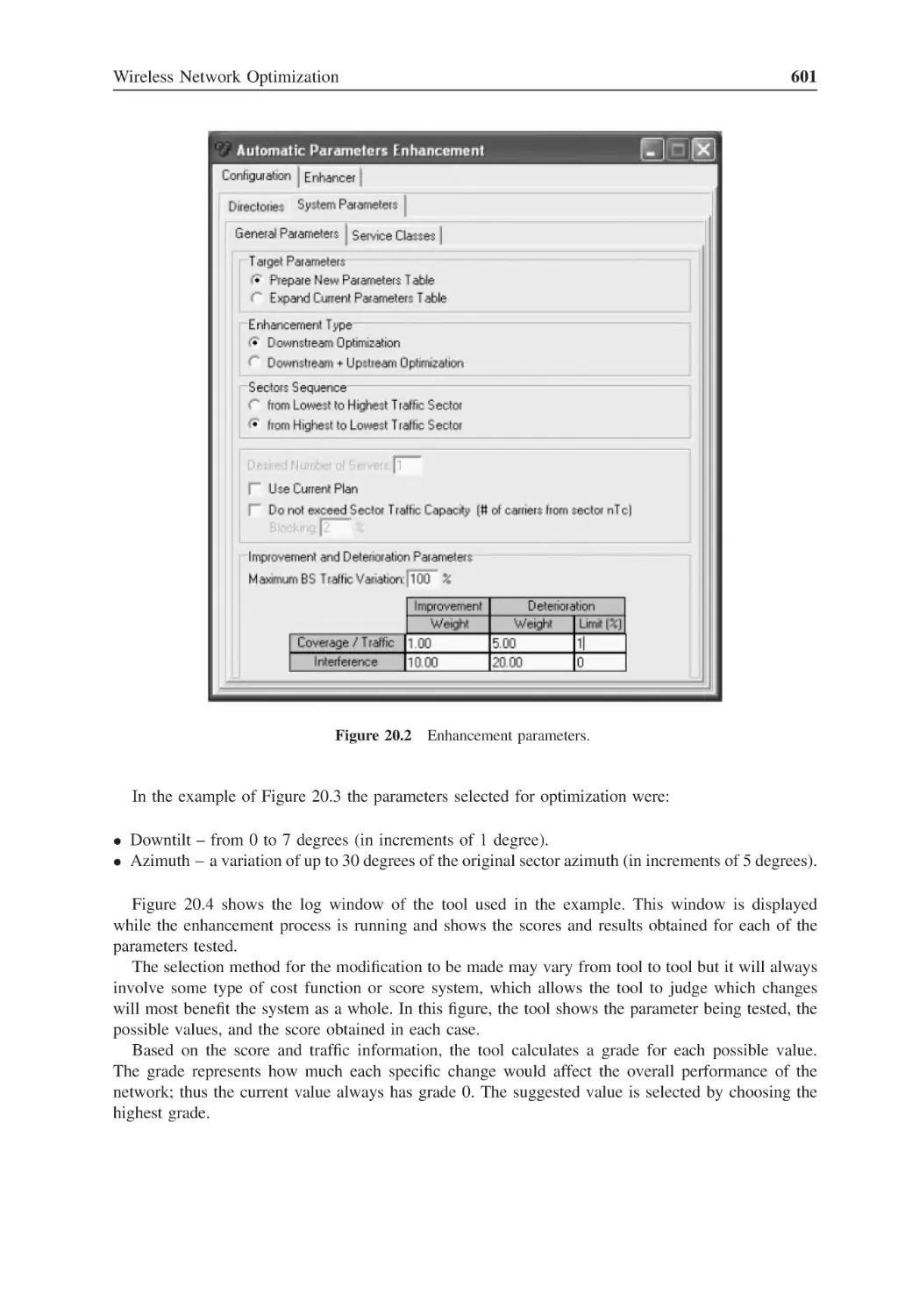
Figure 20.2
Enhancement parameters
601
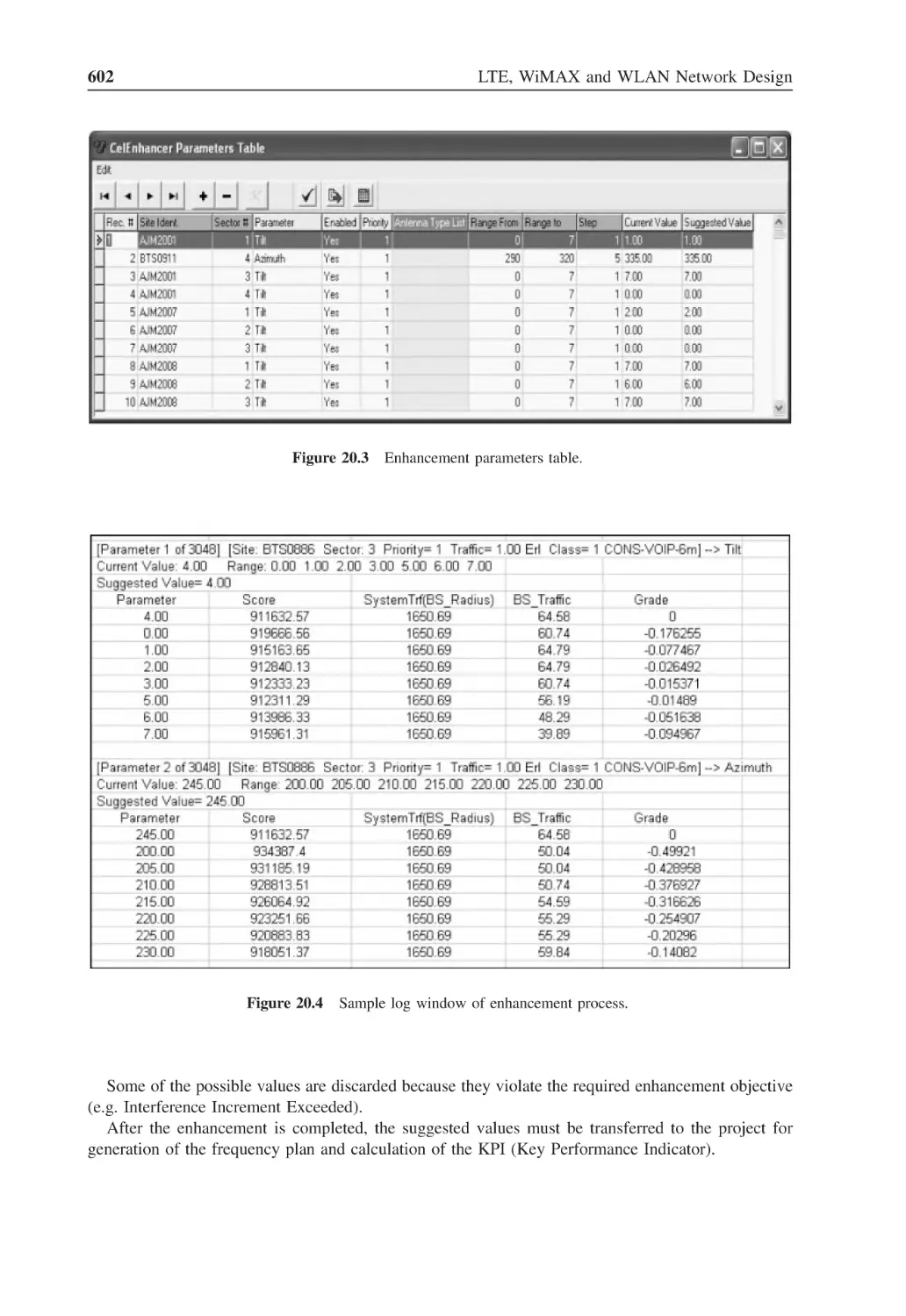
Figure 20.3
Enhancement parameters table
602
Figure 20.4
Sample log window of enhancement process
602
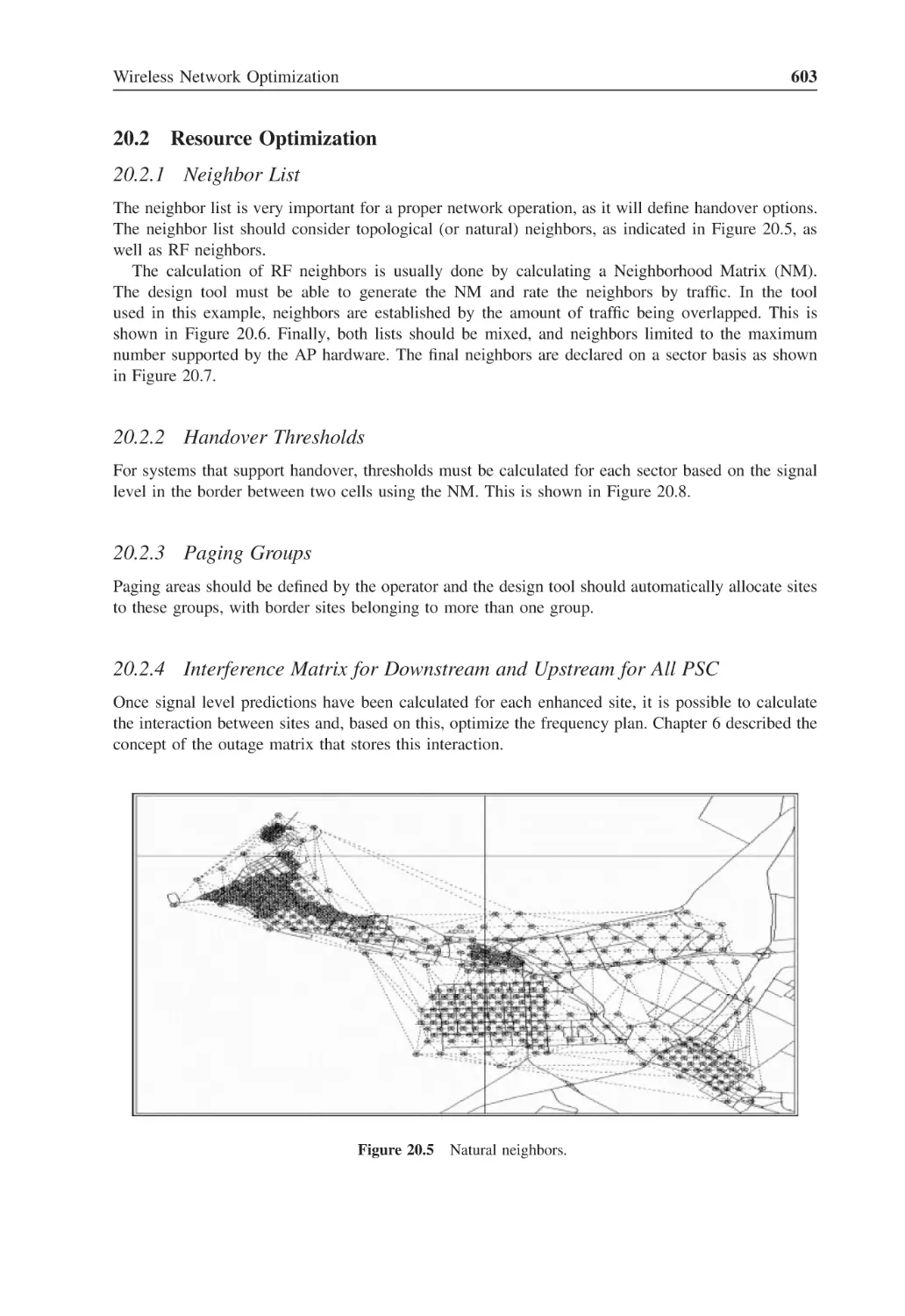
Figure 20.5
Natural neighbors
603
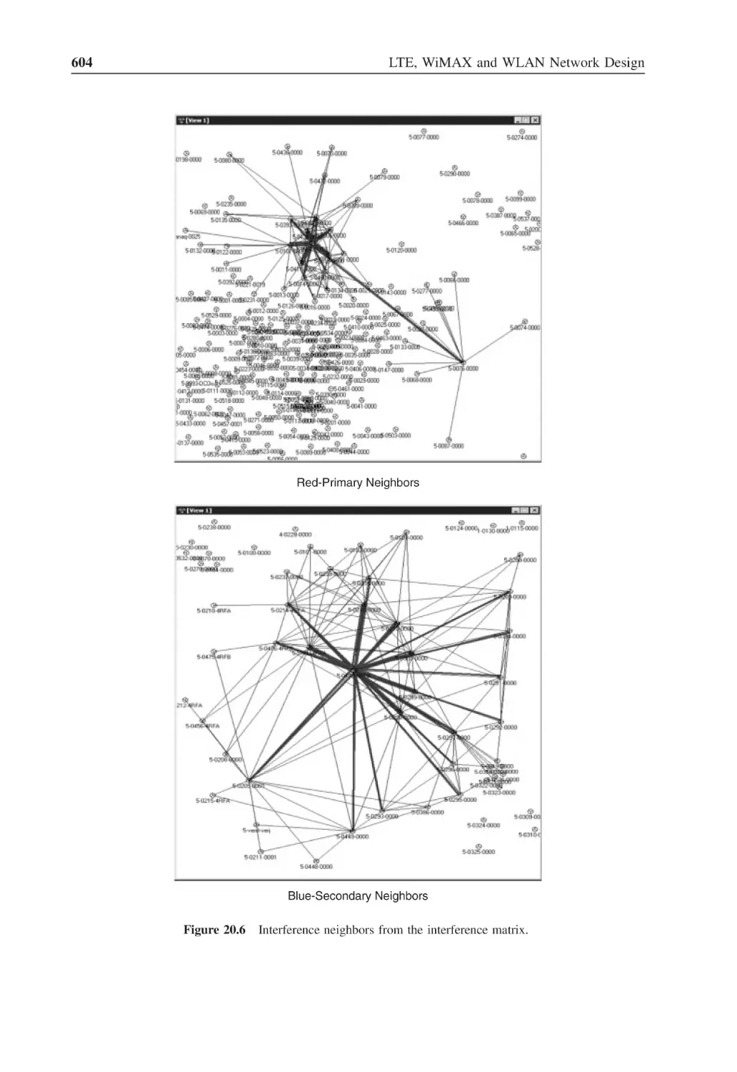
Figure 20.6
Interference neighbors from the interference matrix
604
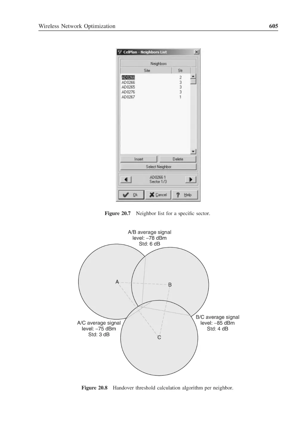
Figure 20.7
Neighbor list for a specific sector
605
Figure 20.8
Handover threshold calculation algorithm per neighbor
605
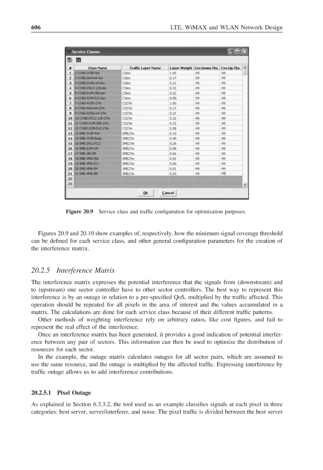
Figure 20.9
Service class and traffic configuration for optimization purposes
606
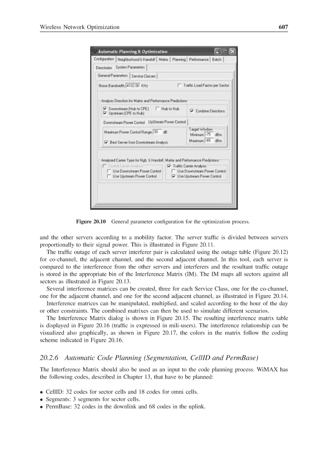
Figure 20.10 General parameter configuration for the optimization process
607
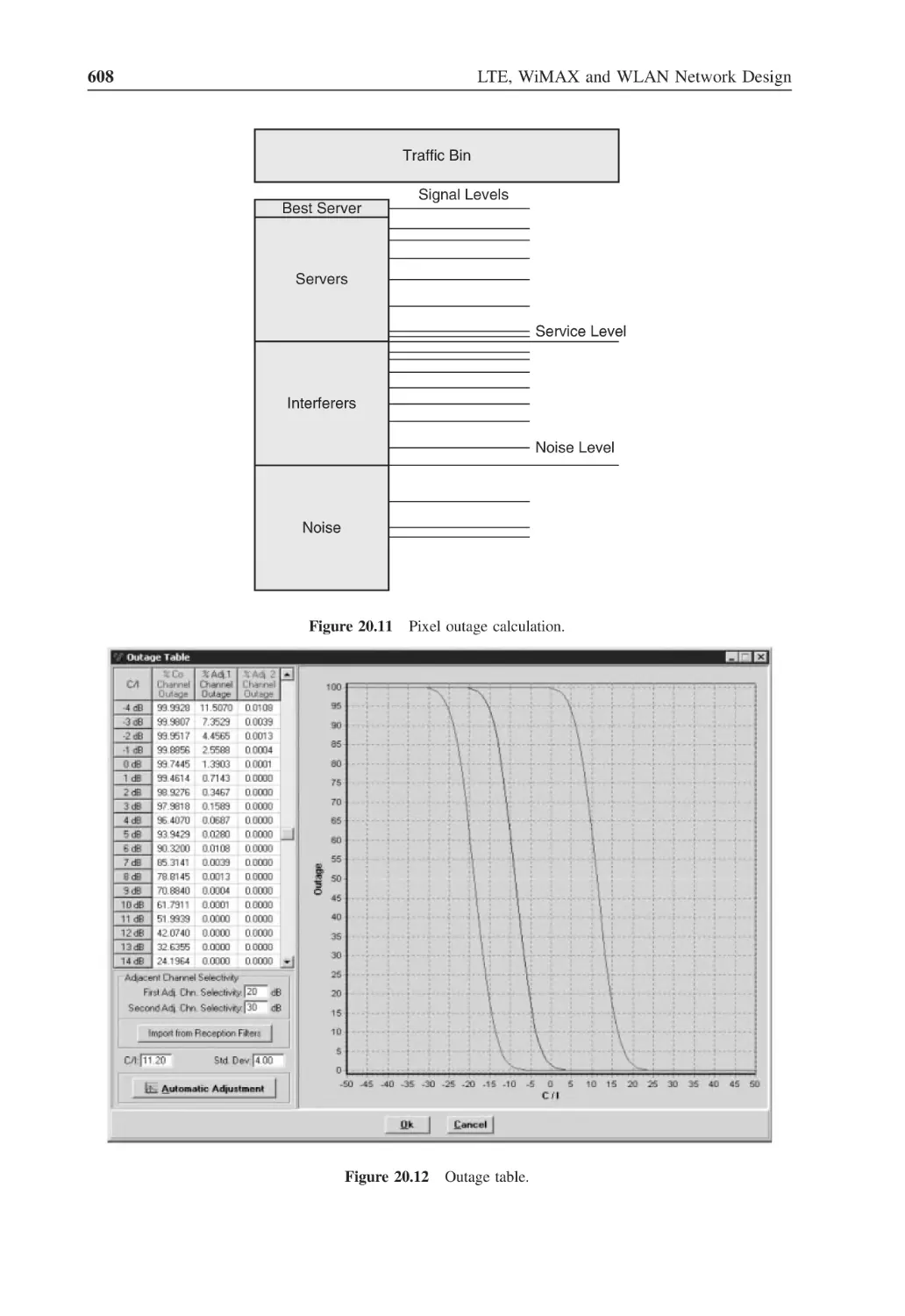
Figure 20.11 Pixel outage calculation
608
Figure 20.12 Outage table
608
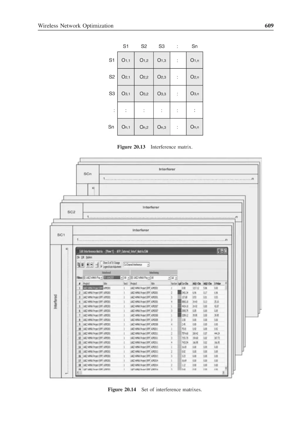
Figure 20.13 Interference matrix
609
Figure 20.14 Set of interference matrixes
609
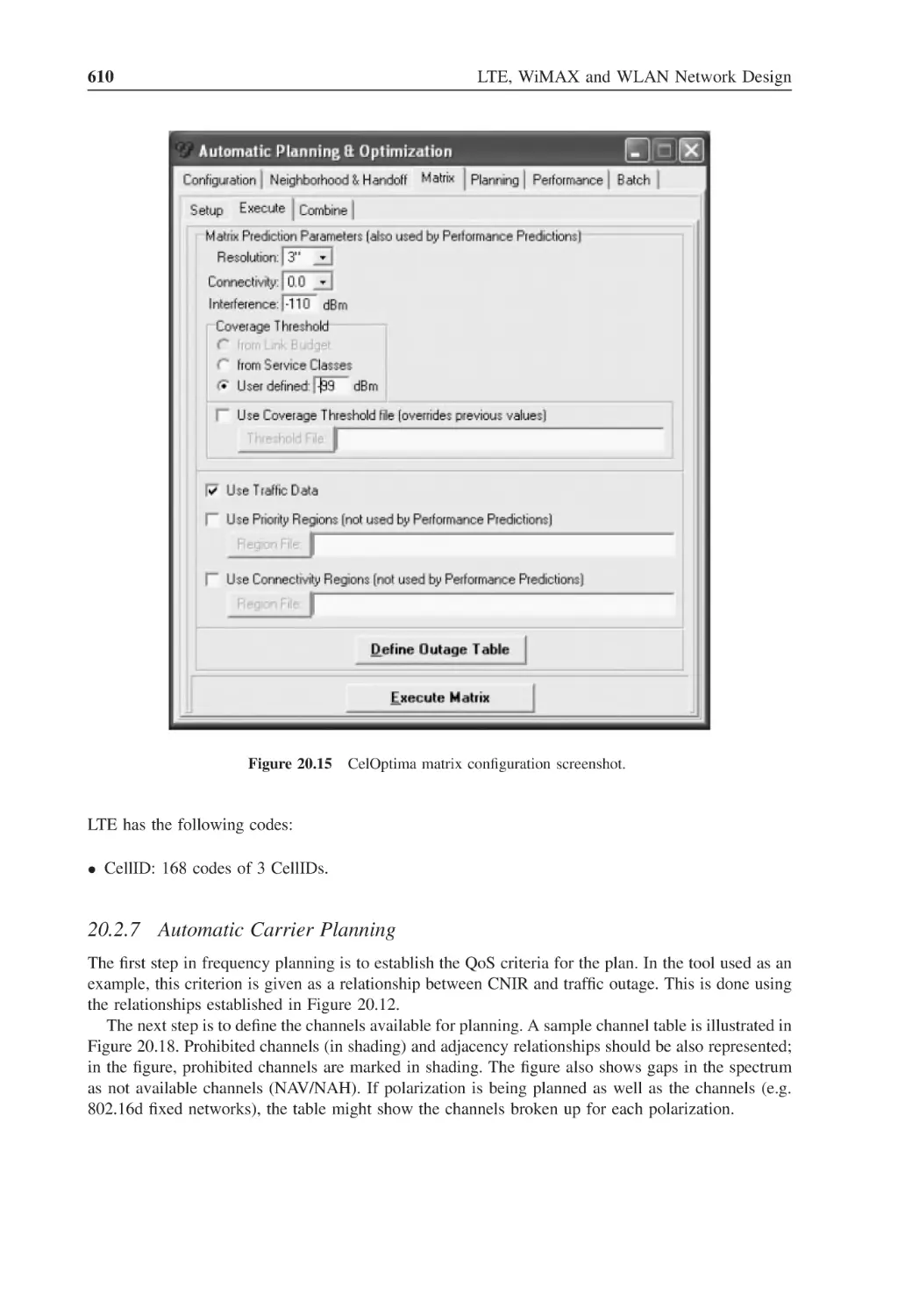
Figure 20.15 CelOptima matrix configuration screenshot
610
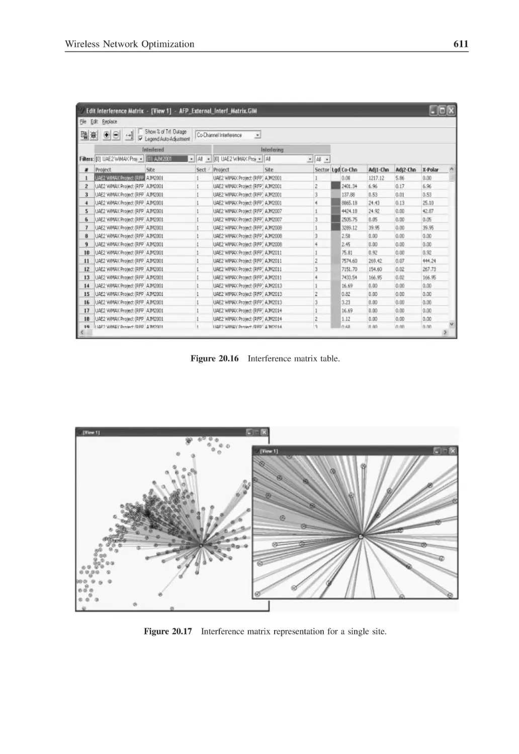
Figure 20.16 Interference matrix table
611
Figure 20.17 Interference matrix representation for a single site
611
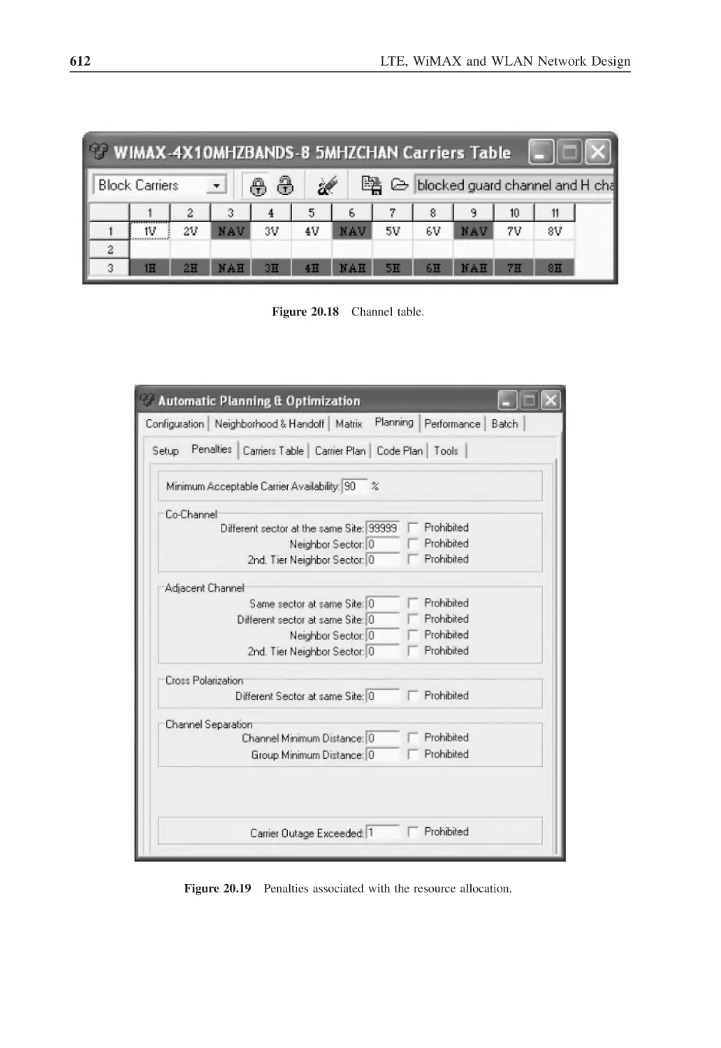
Figure 20.18 Channel table
612
Figure 20.19 Penalties associated with the resource allocation
612
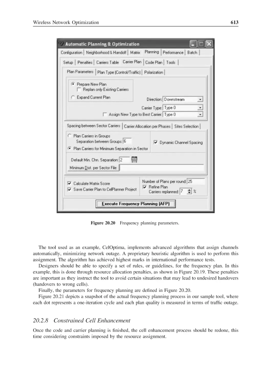
Figure 20.20 Frequency planning parameters
613
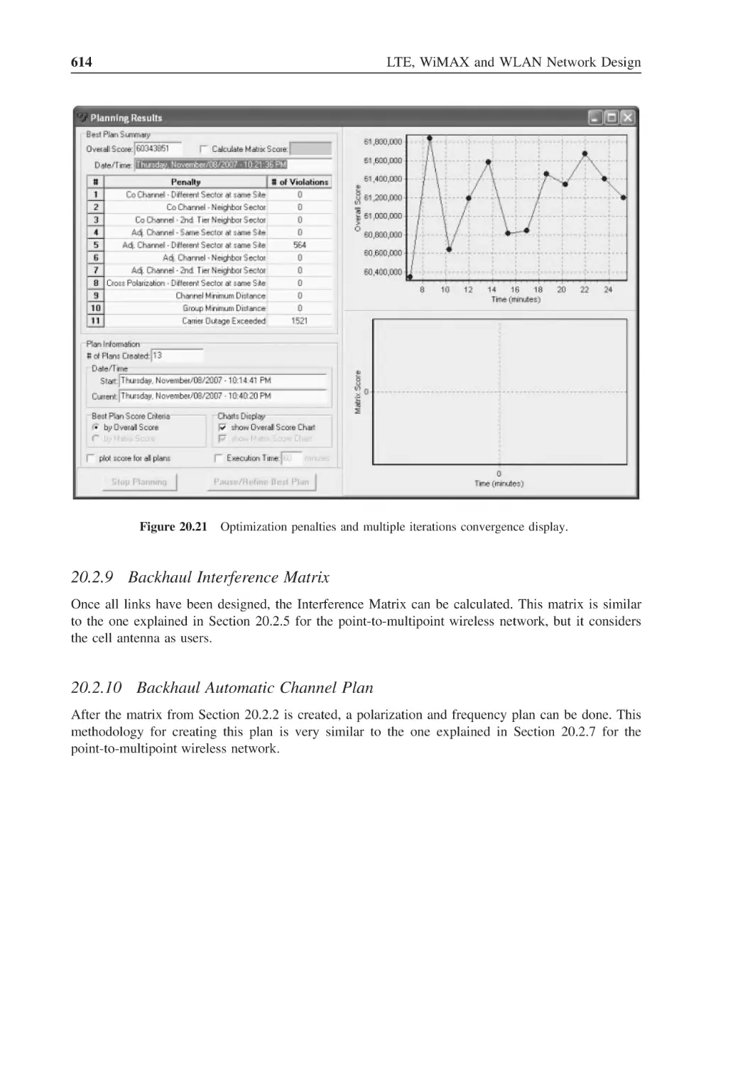
Figure 20.21 Optimization penalties and multiple iterations convergence display
614
Figure 21.1
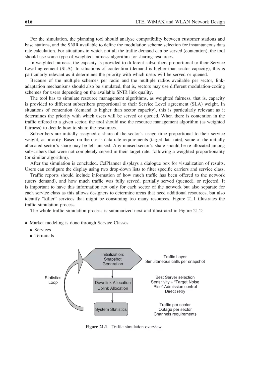
Traffic simulation overview
616
Figure 21.2
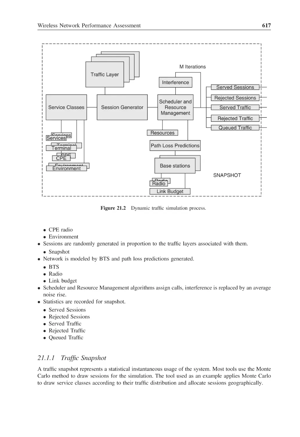
Dynamic traffic simulation process
617
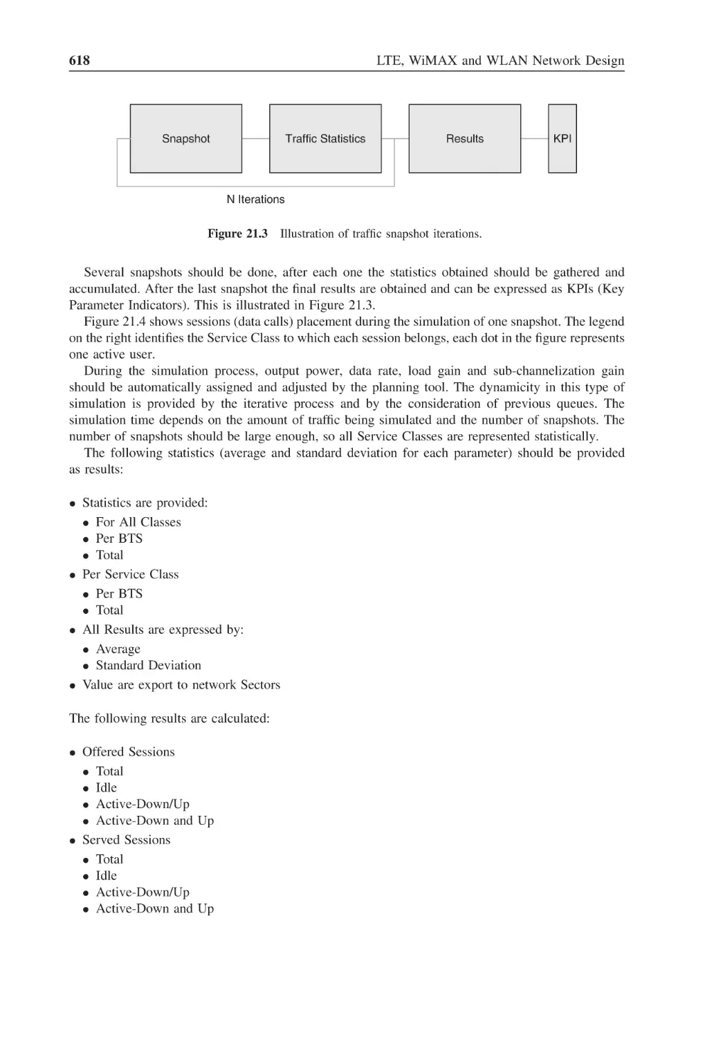
Figure 21.3
Illustration of traffic snapshot iterations
618
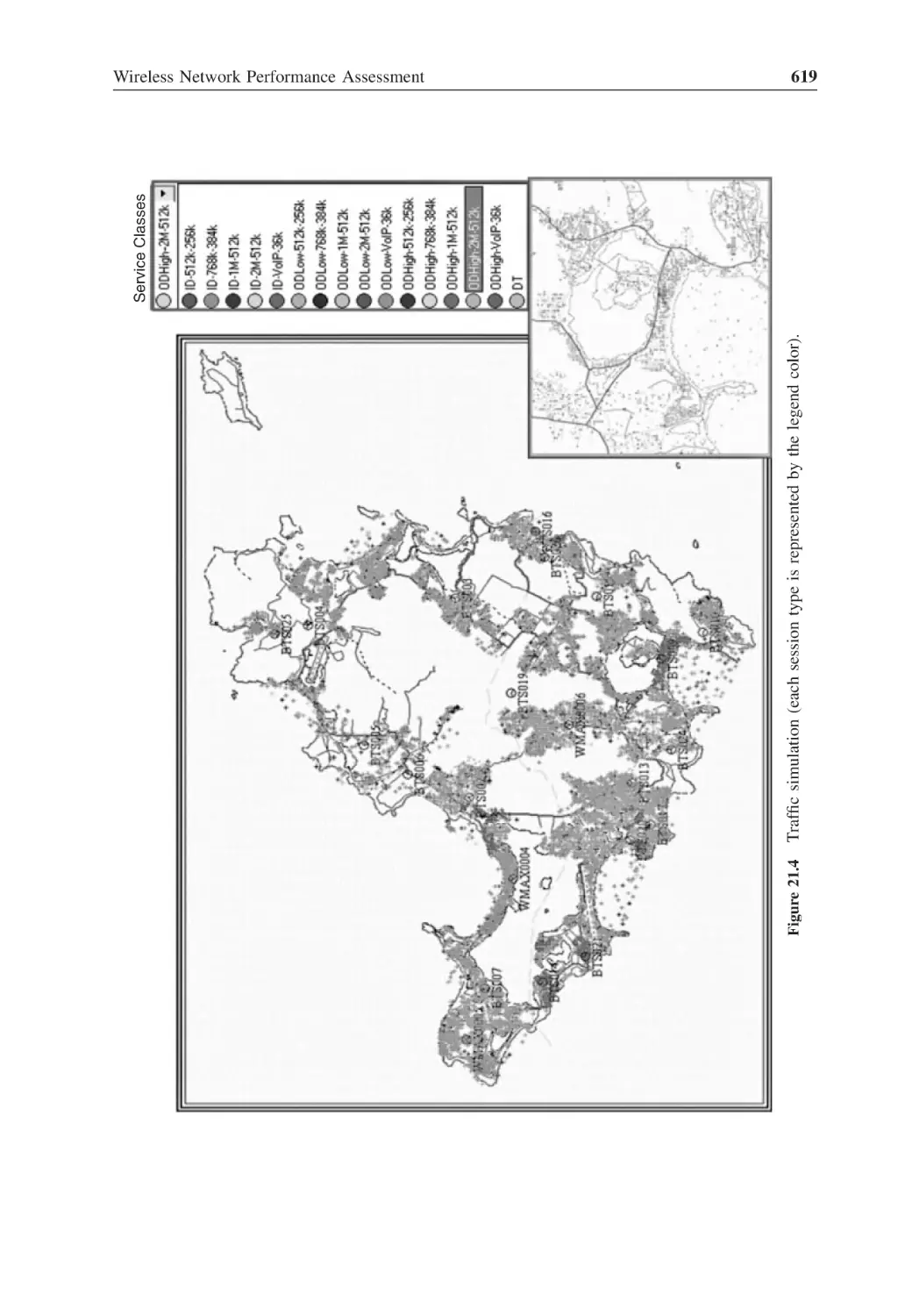
Figure 21.4
Traffic simulation (each session type is represented by the legend color)
619
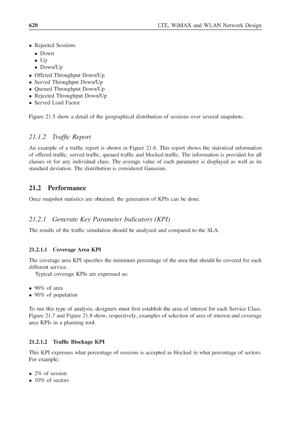
Figure 21.5
Traffic simulation sessions detail
621
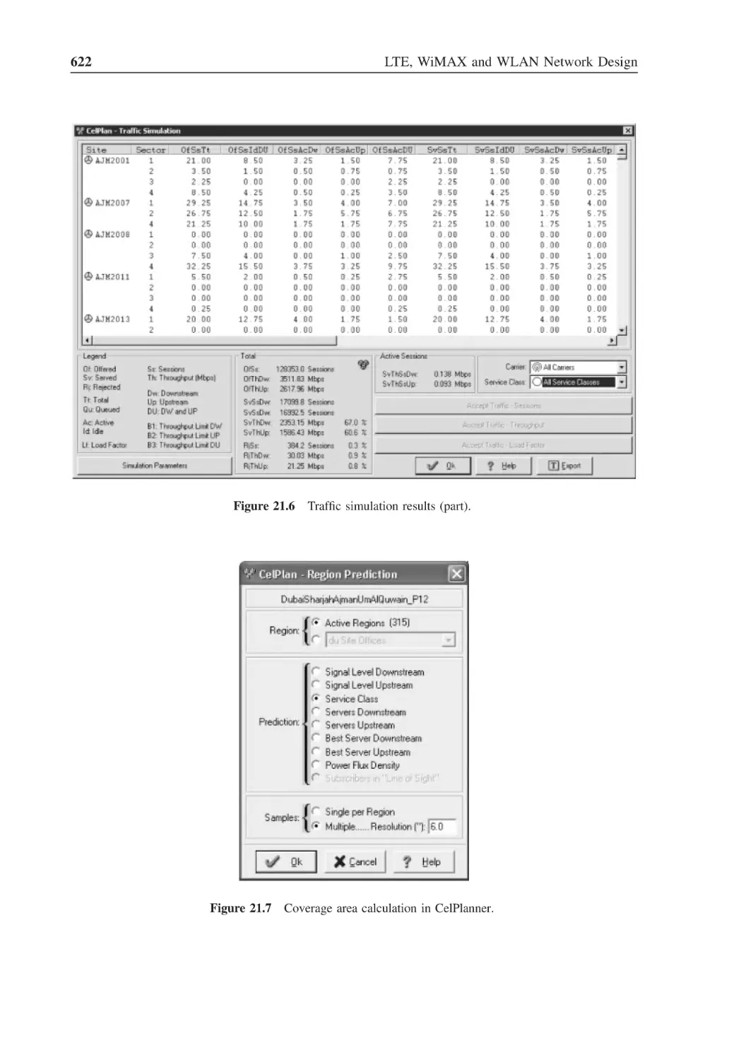
Figure 21.6
Traffic simulation results (part)
622
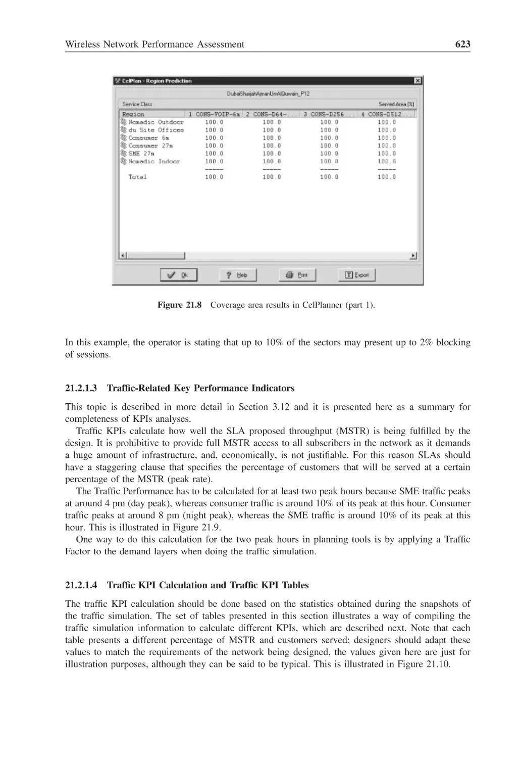
Figure 21.7
Coverage area calculation in CelPlanner
622
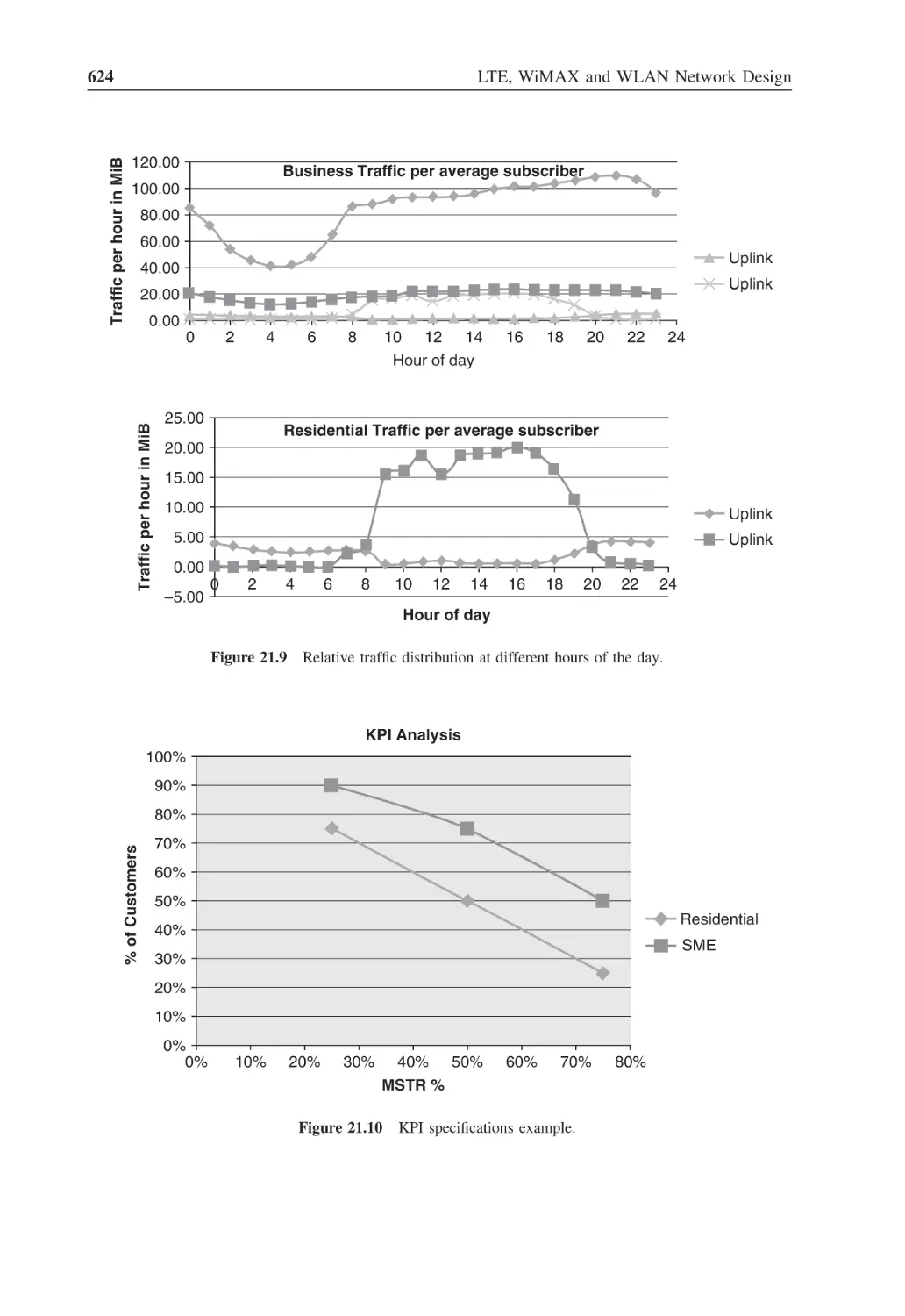
Figure 21.8
Coverage area results in CelPlanner (part 1)
623
List of Figures
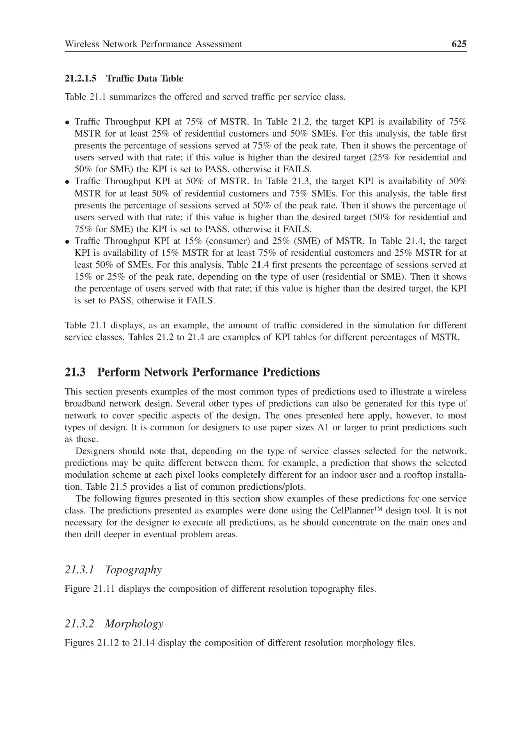
Figure 21.9
Relative traffic distribution at different hours of the day
xxxiii
624
Figure 21.10 KPI specifications example
624
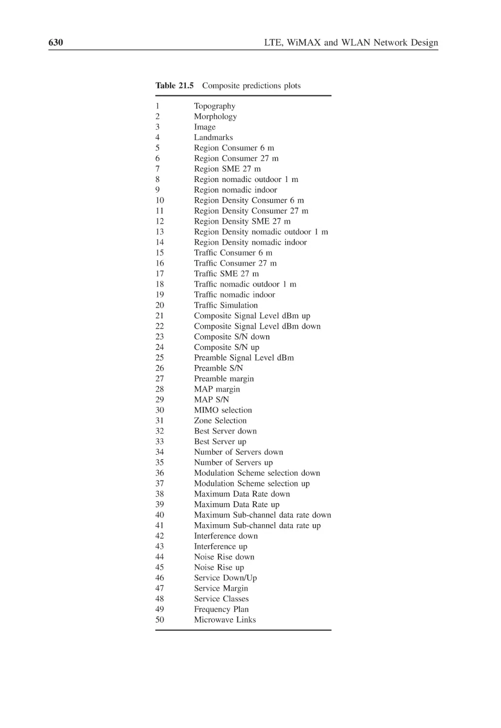
Figure 21.11 Topography plot sample
631
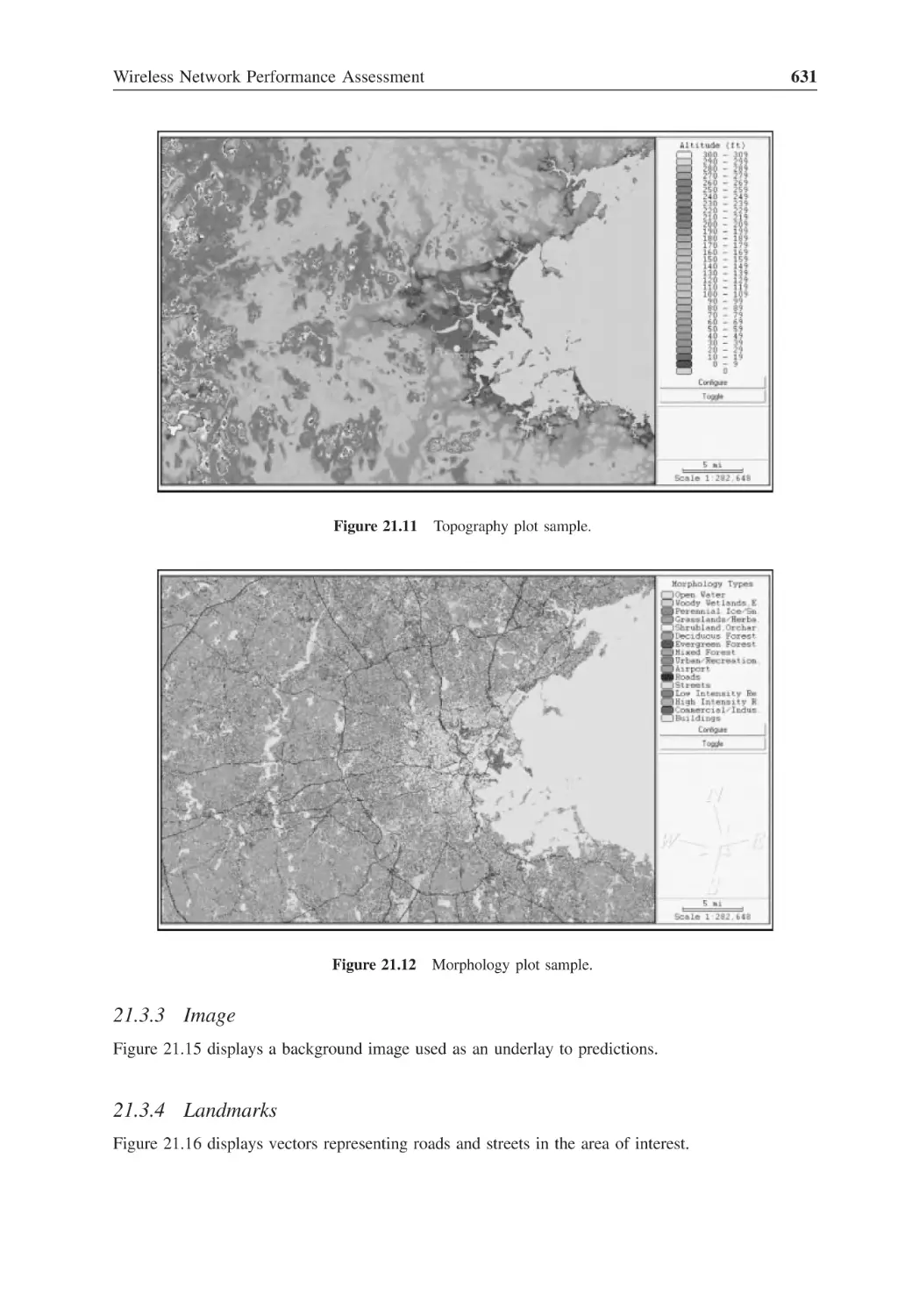
Figure 21.12 Morphology plot sample
631
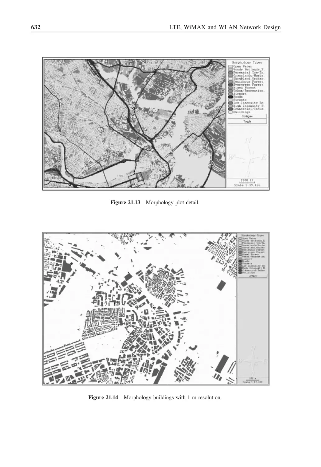
Figure 21.13 Morphology plot detail
632
Figure 21.14 Morphology buildings with 1 m resolution
632
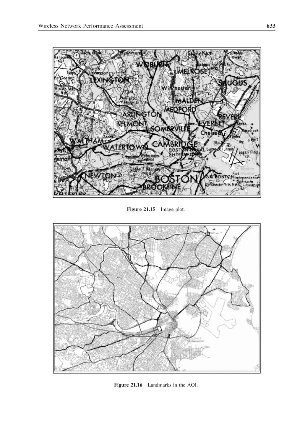
Figure 21.15 Image plot
633
Figure 21.16 Landmarks in the AOI
633
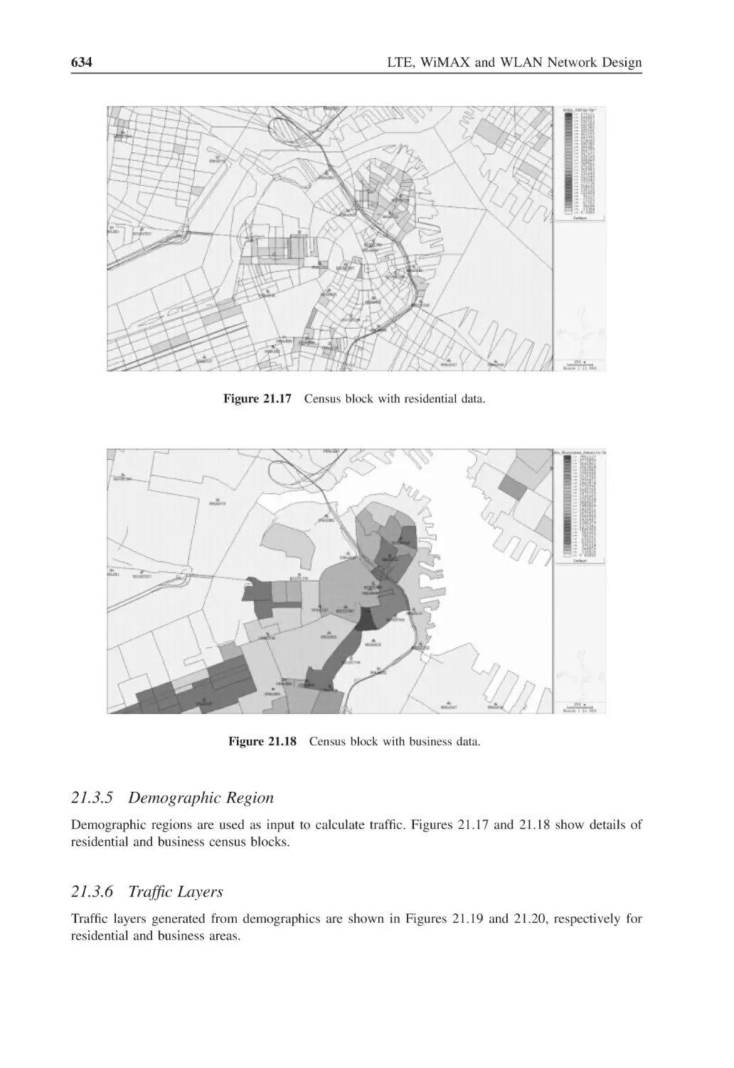
Figure 21.17 Census block with residential data
634
Figure 21.18 Census block with business data
634
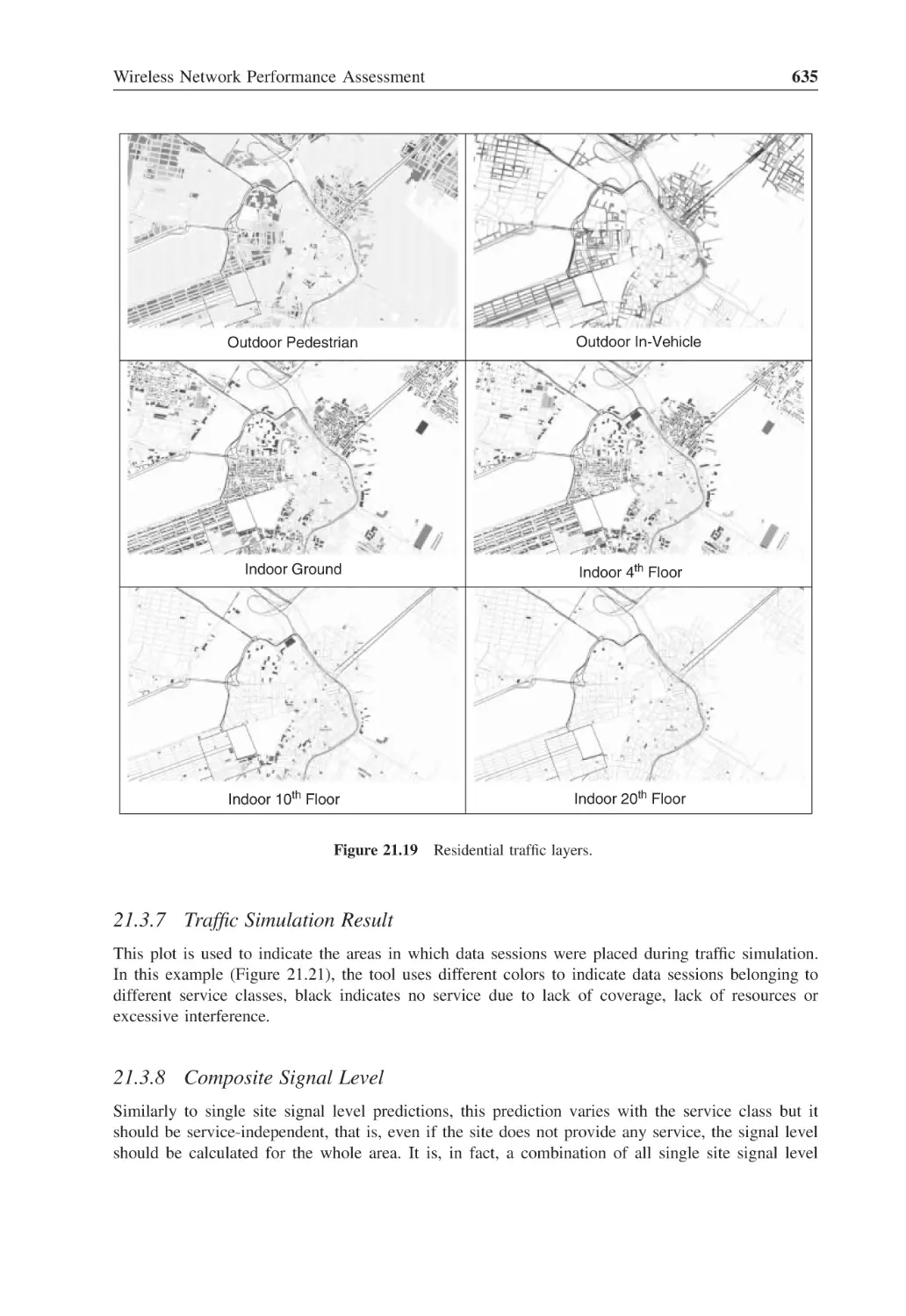
Figure 21.19 Residential traffic layers
635
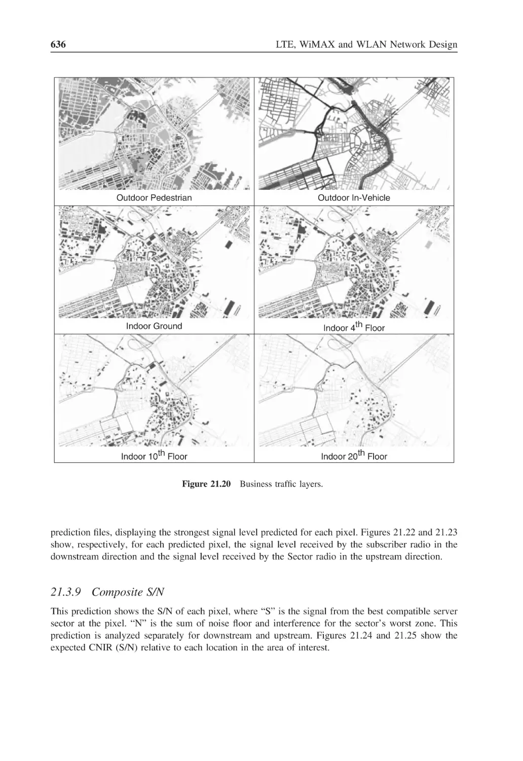
Figure 21.20 Business traffic layers
636
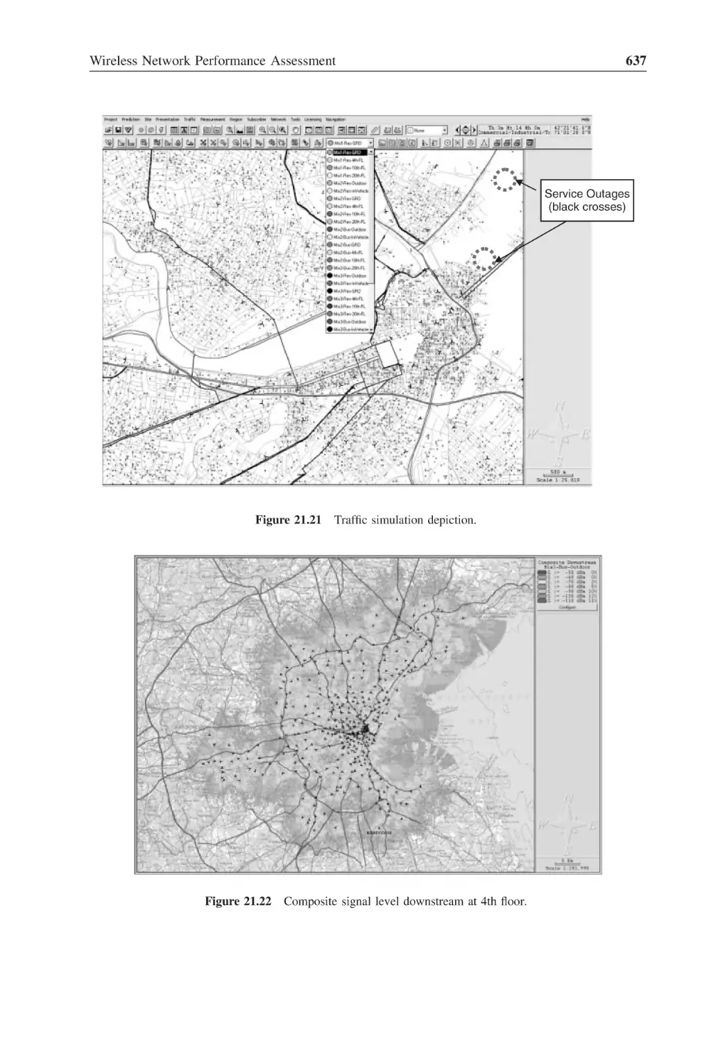
Figure 21.21 Traffic simulation depiction
637
Figure 21.22 Composite signal level downstream at 4th floor
637
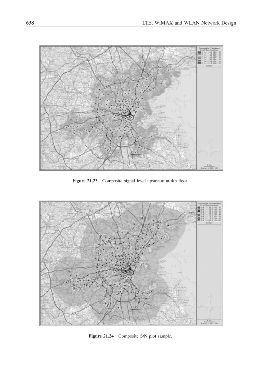
Figure 21.23 Composite signal level upstream at 4th floor
638
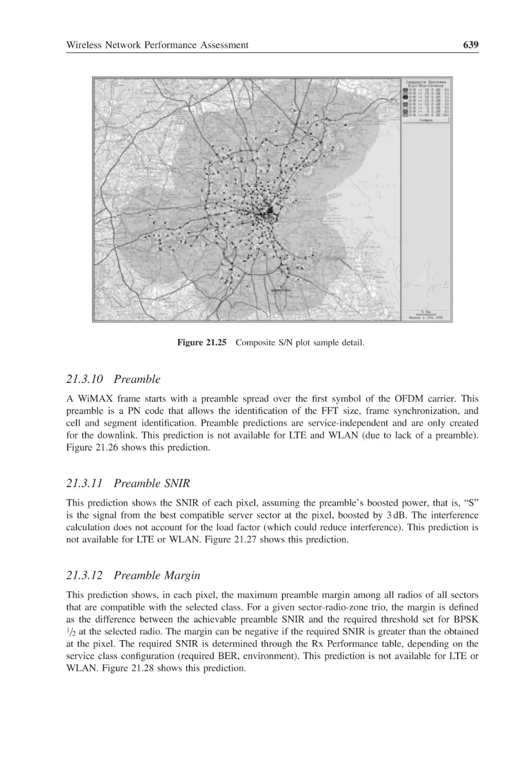
Figure 21.24 Composite S/N plot sample
638
Figure 21.25 Composite S/N plot sample detail
639
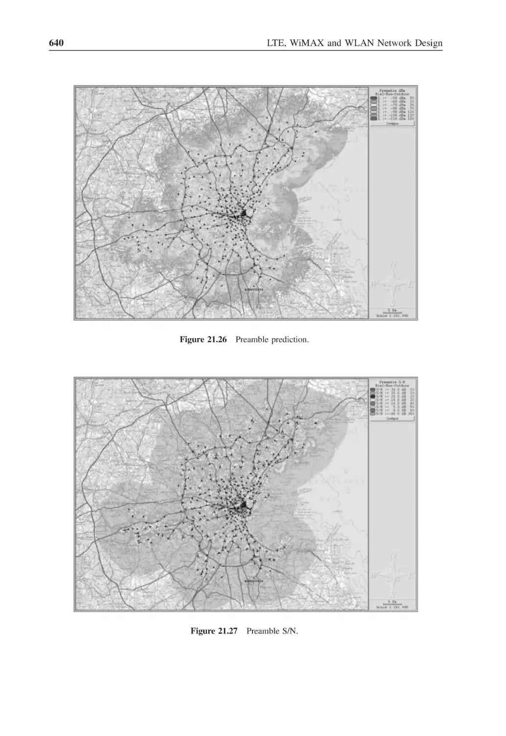
Figure 21.26 Preamble prediction
640
Figure 21.27 Preamble S/N
640
Figure 21.28 Preamble margin
641
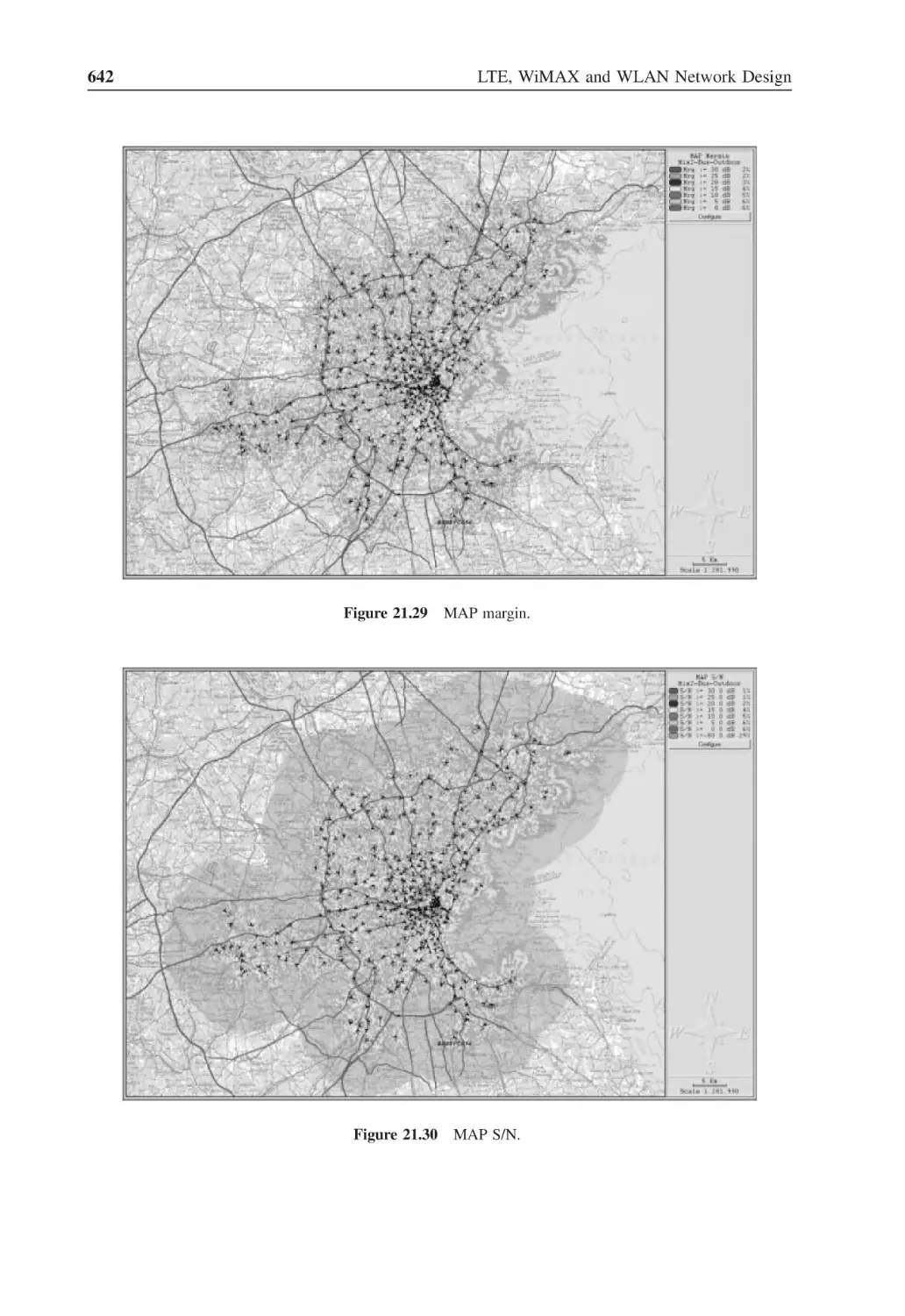
Figure 21.29 MAP margin
642
Figure 21.30 MAP S/N
642
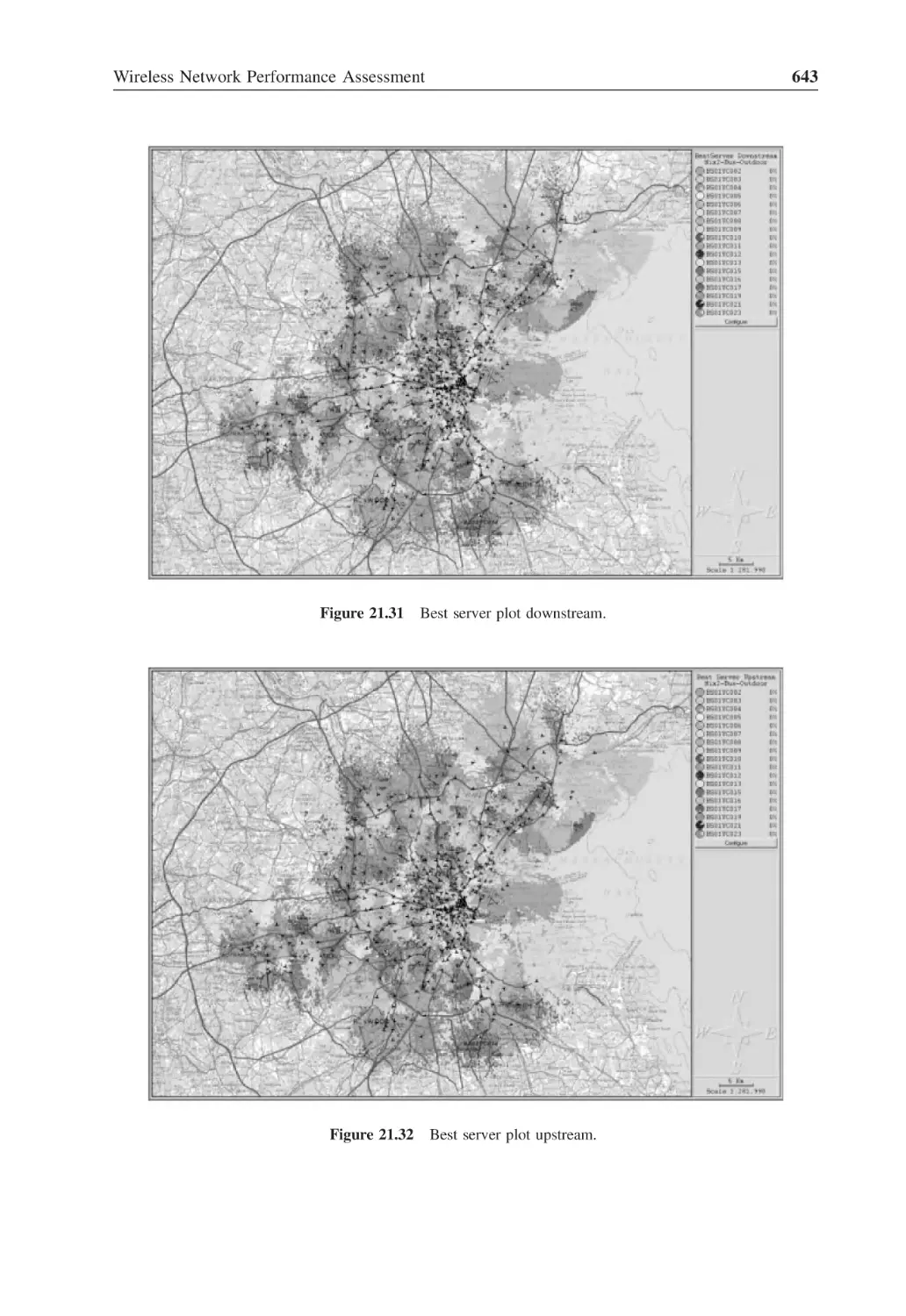
Figure 21.31 Best server plot downstream
643
Figure 21.32 Best server plot upstream
643
Figure 21.33 Number of servers downstream
644
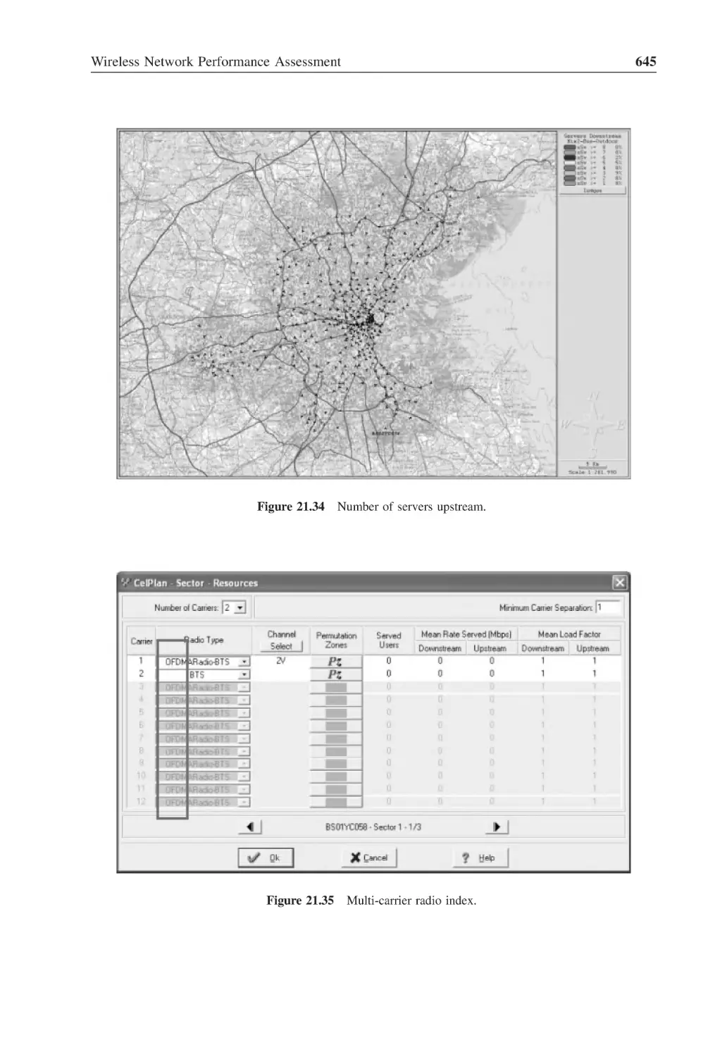
Figure 21.34 Number of servers upstream
645
Figure 21.35 Multi-carrier radio index
645
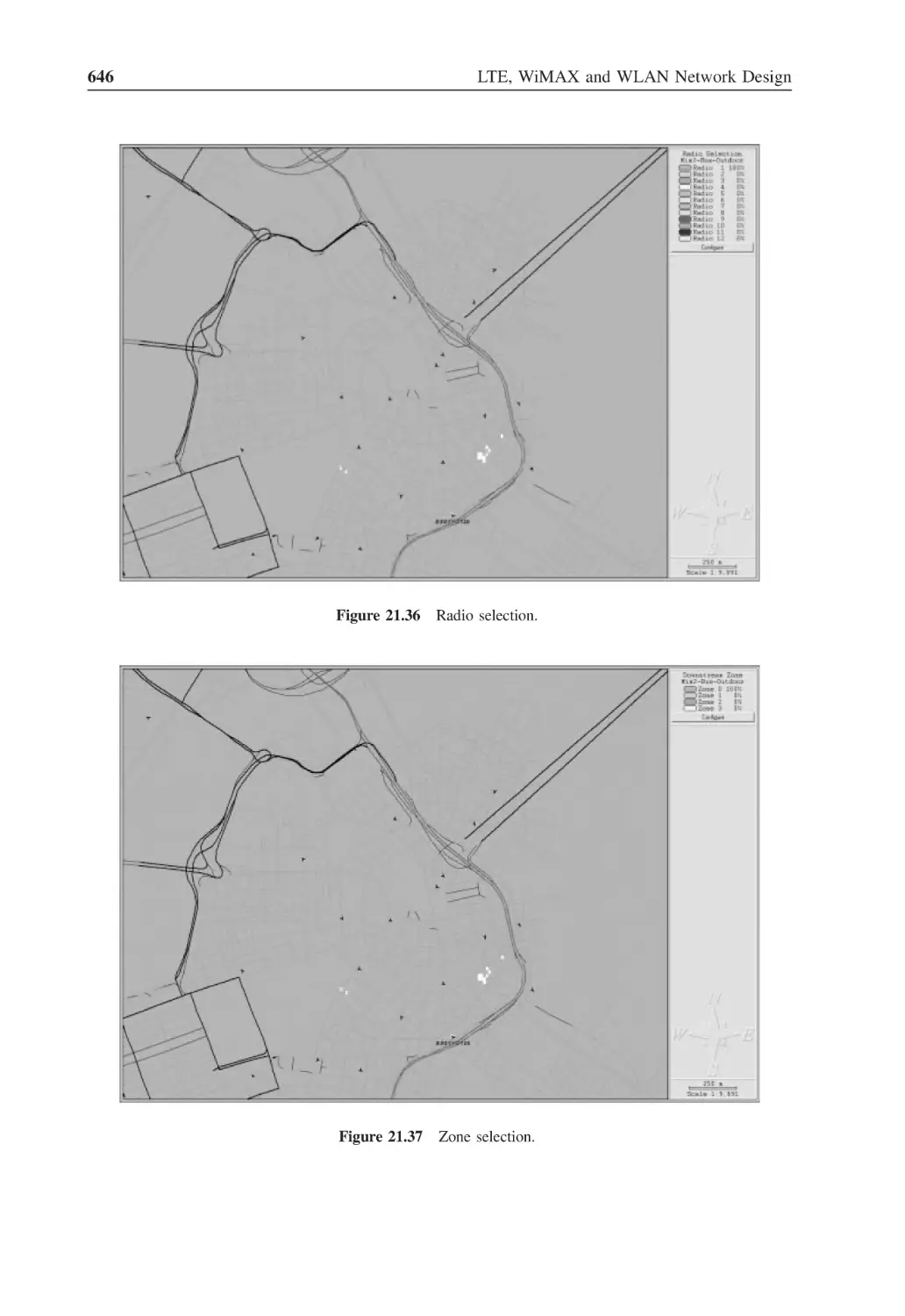
Figure 21.36 Radio selection
646
Figure 21.37 Zone selection
646
Figure 21.38 MIMO selection
647
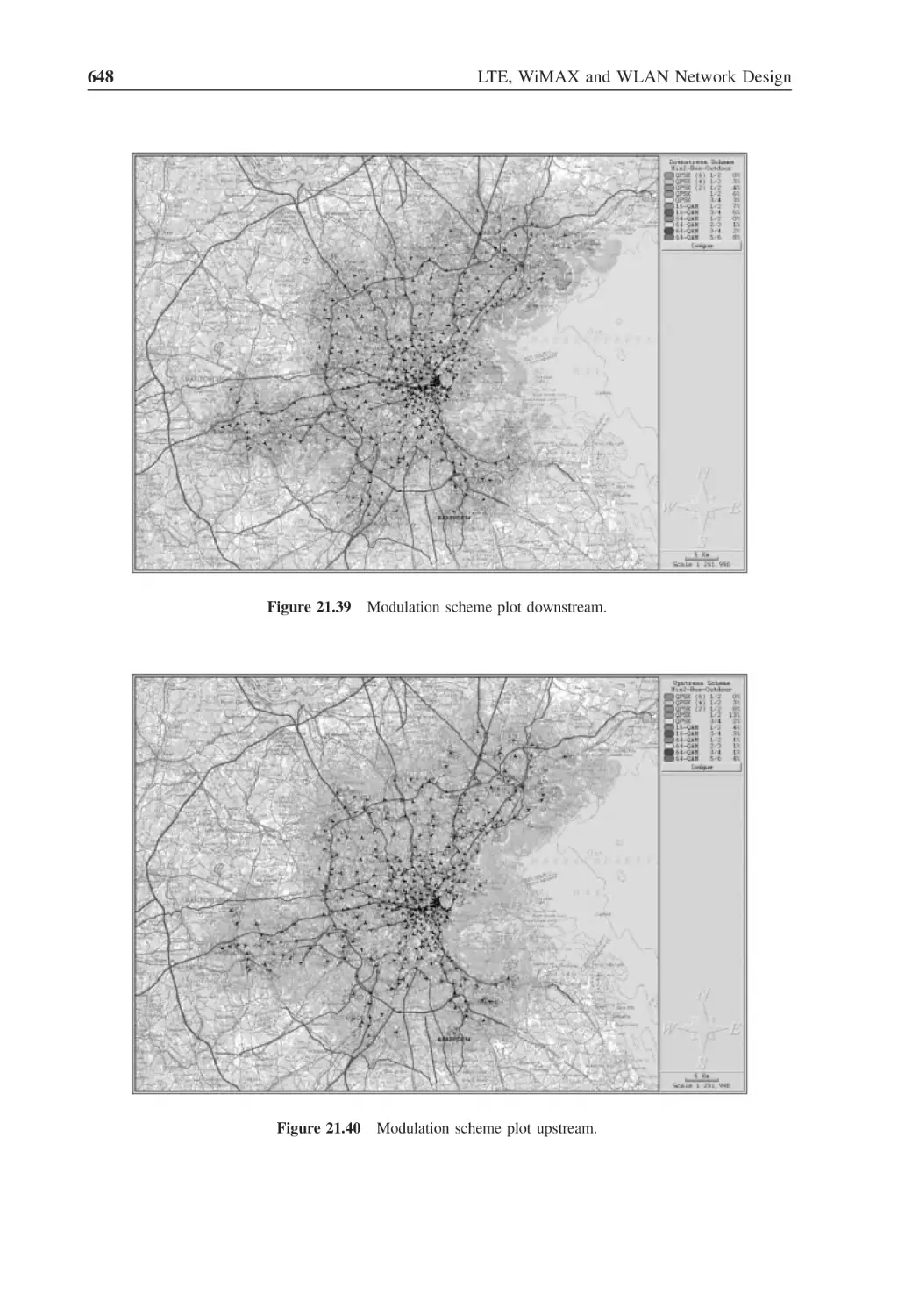
Figure 21.39 Modulation scheme plot downstream
648
Figure 21.40 Modulation scheme plot upstream
648
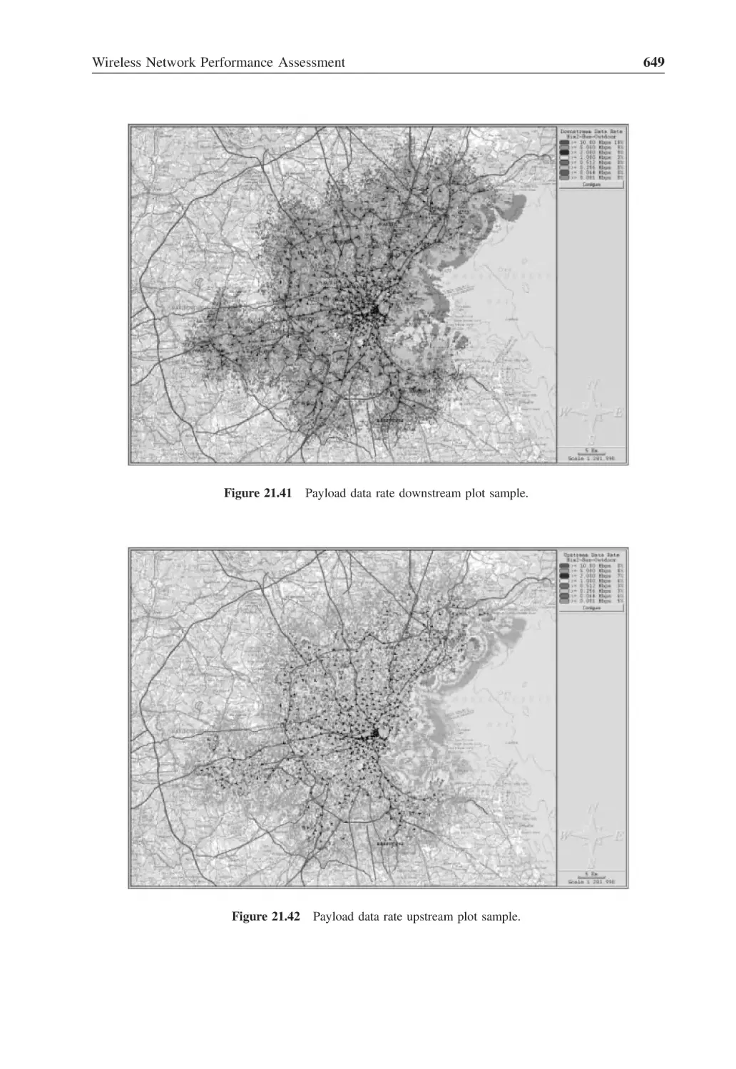
Figure 21.41 Payload data rate downstream plot sample
649
Figure 21.42 Payload data rate upstream plot sample
649
Figure 21.43 Maximum data rate per sub-channel downlink
650
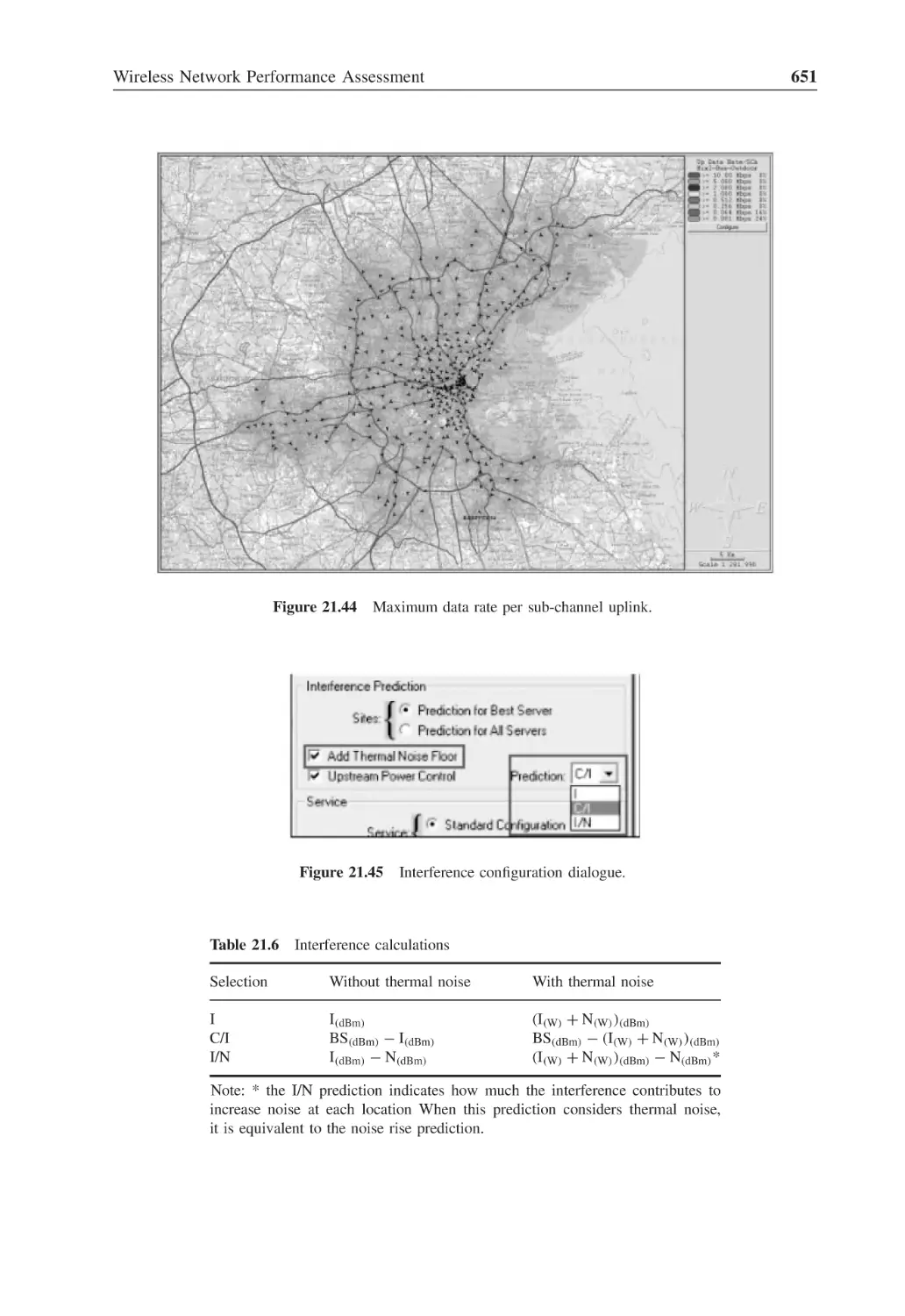
Figure 21.44 Maximum data rate per sub-channel uplink
651
Figure 21.45 Interference configuration dialogue
651
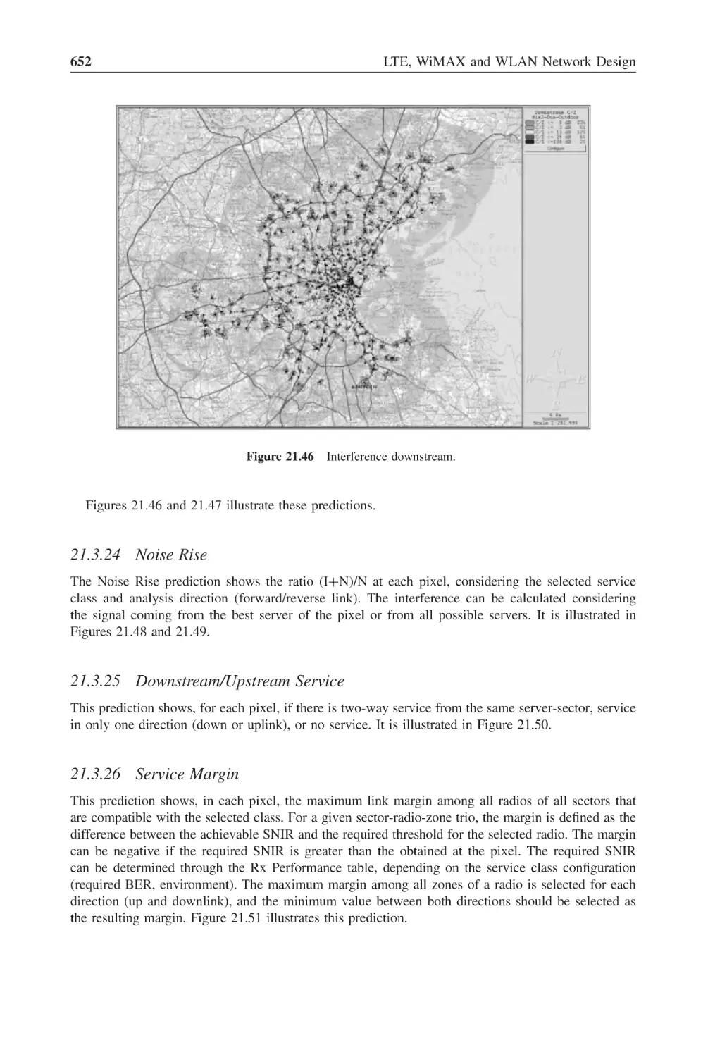
Figure 21.46 Interference downstream
652
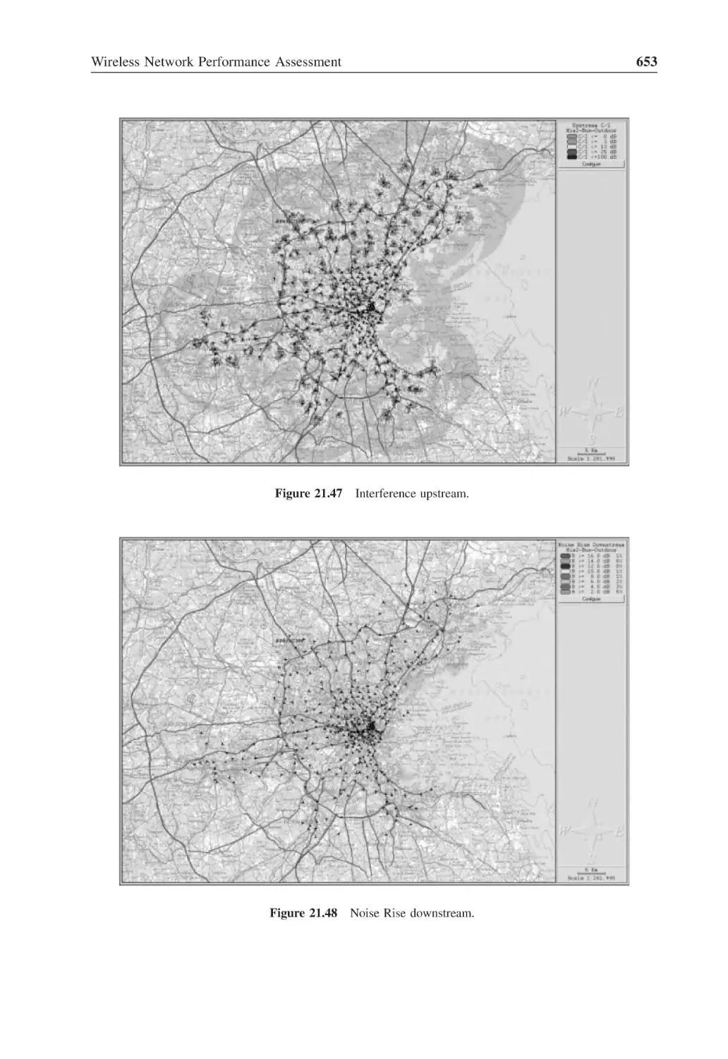
Figure 21.47 Interference upstream
653
xxxiv
List of Figures
Figure 21.48 Noise Rise downstream
653
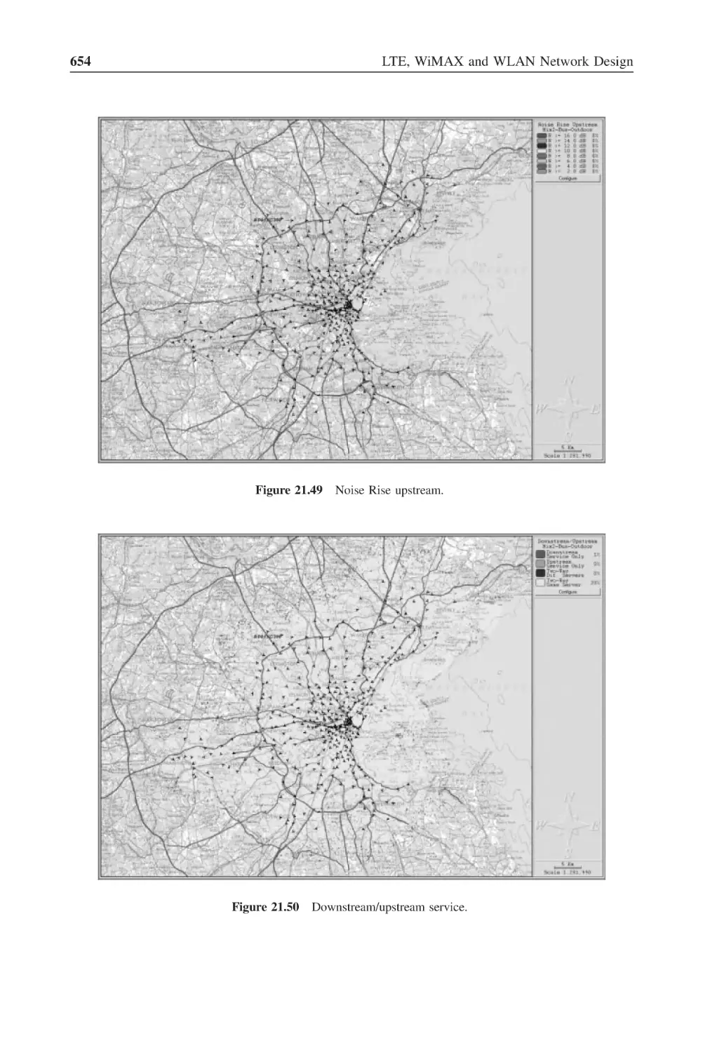
Figure 21.49 Noise Rise upstream
654
Figure 21.50 Downstream/upstream service
654
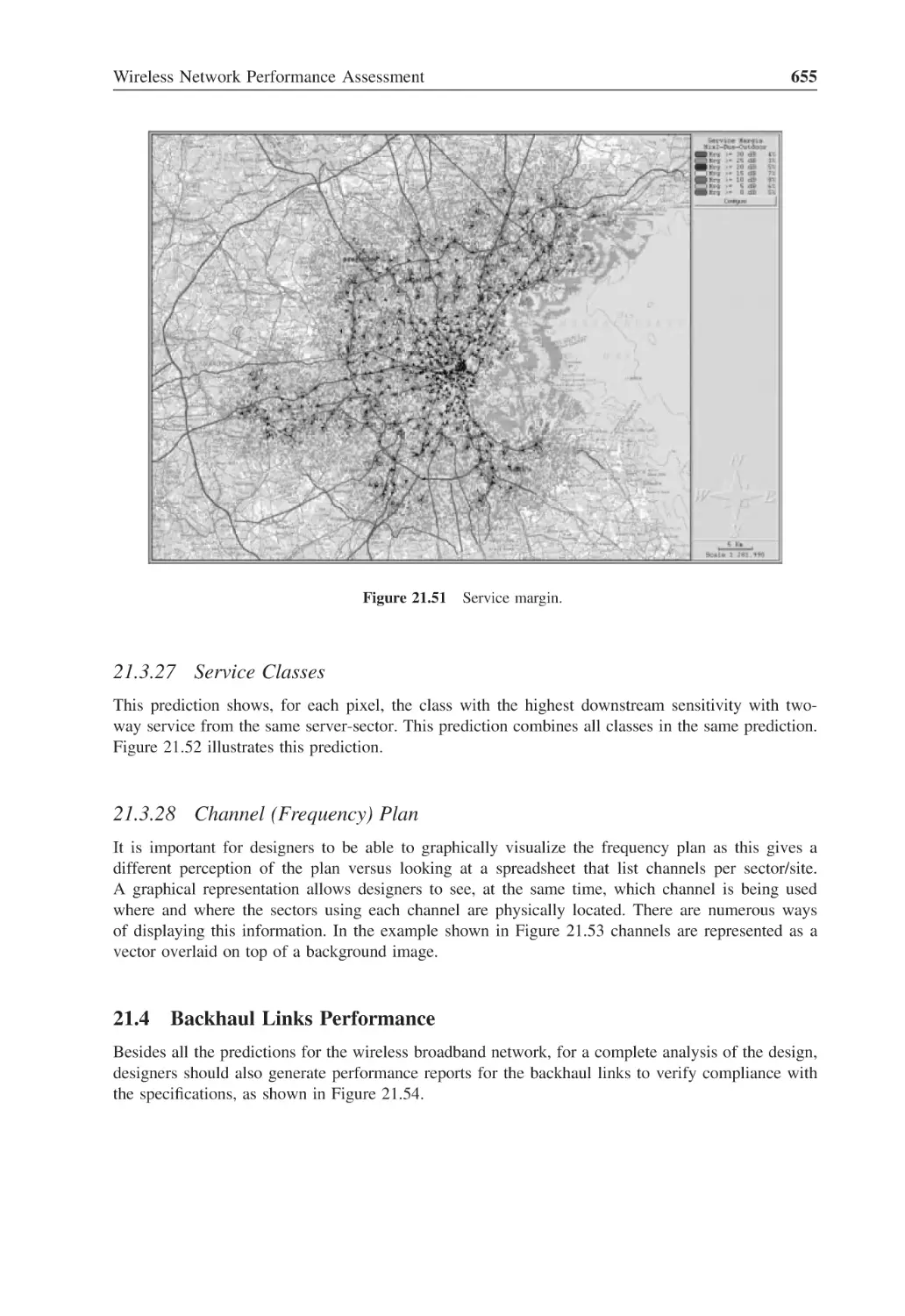
Figure 21.51 Service margin
655
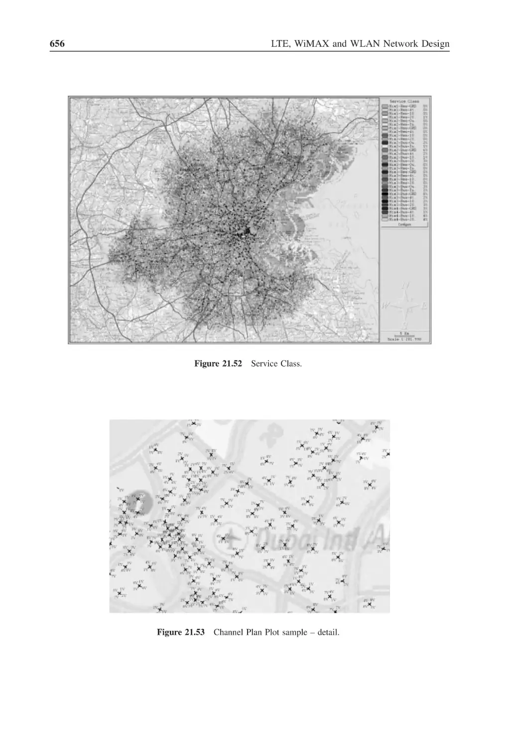
Figure 21.52 Service Class
656
Figure 21.53 Channel Plan Plot sample – detail
656
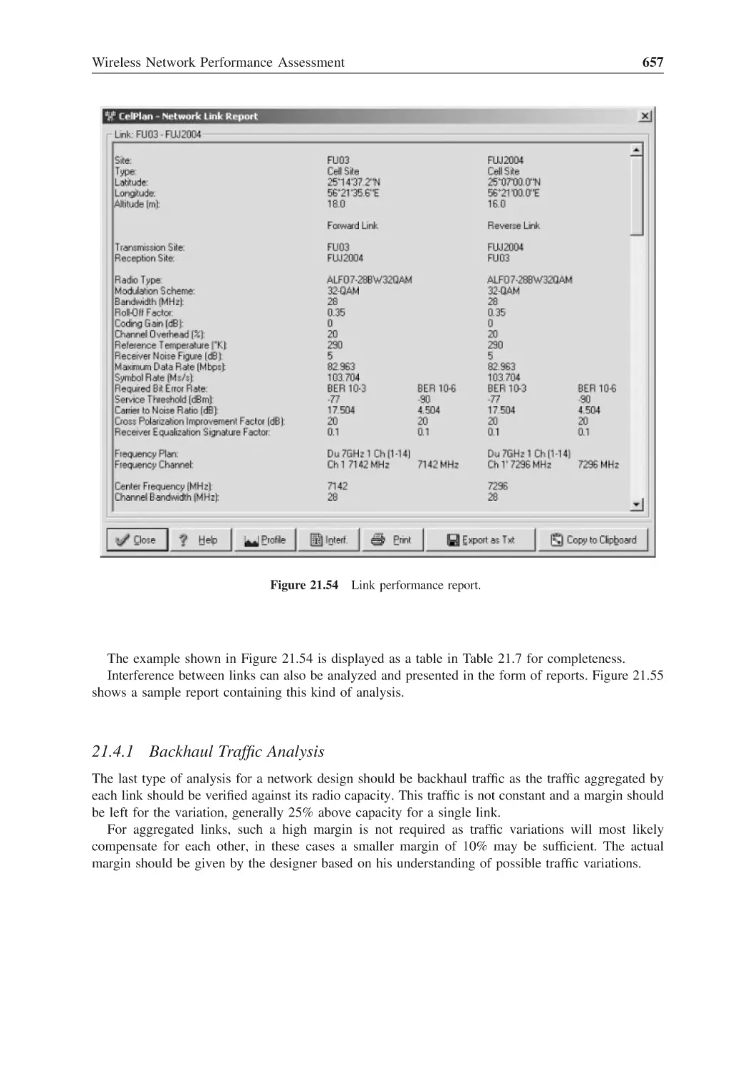
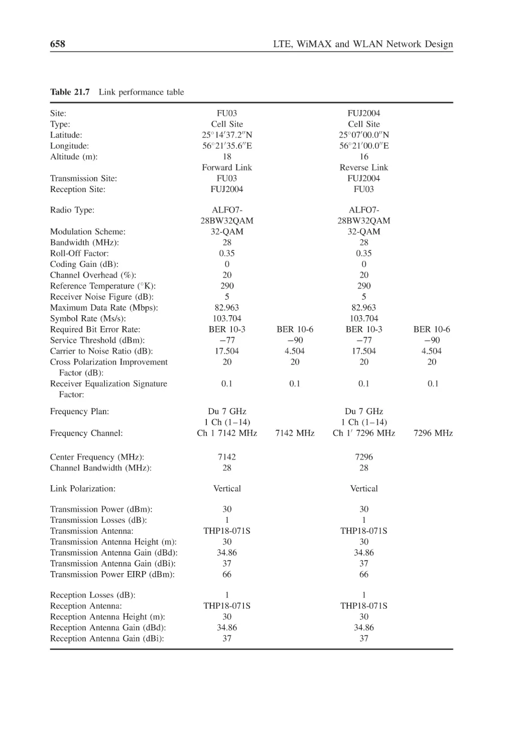
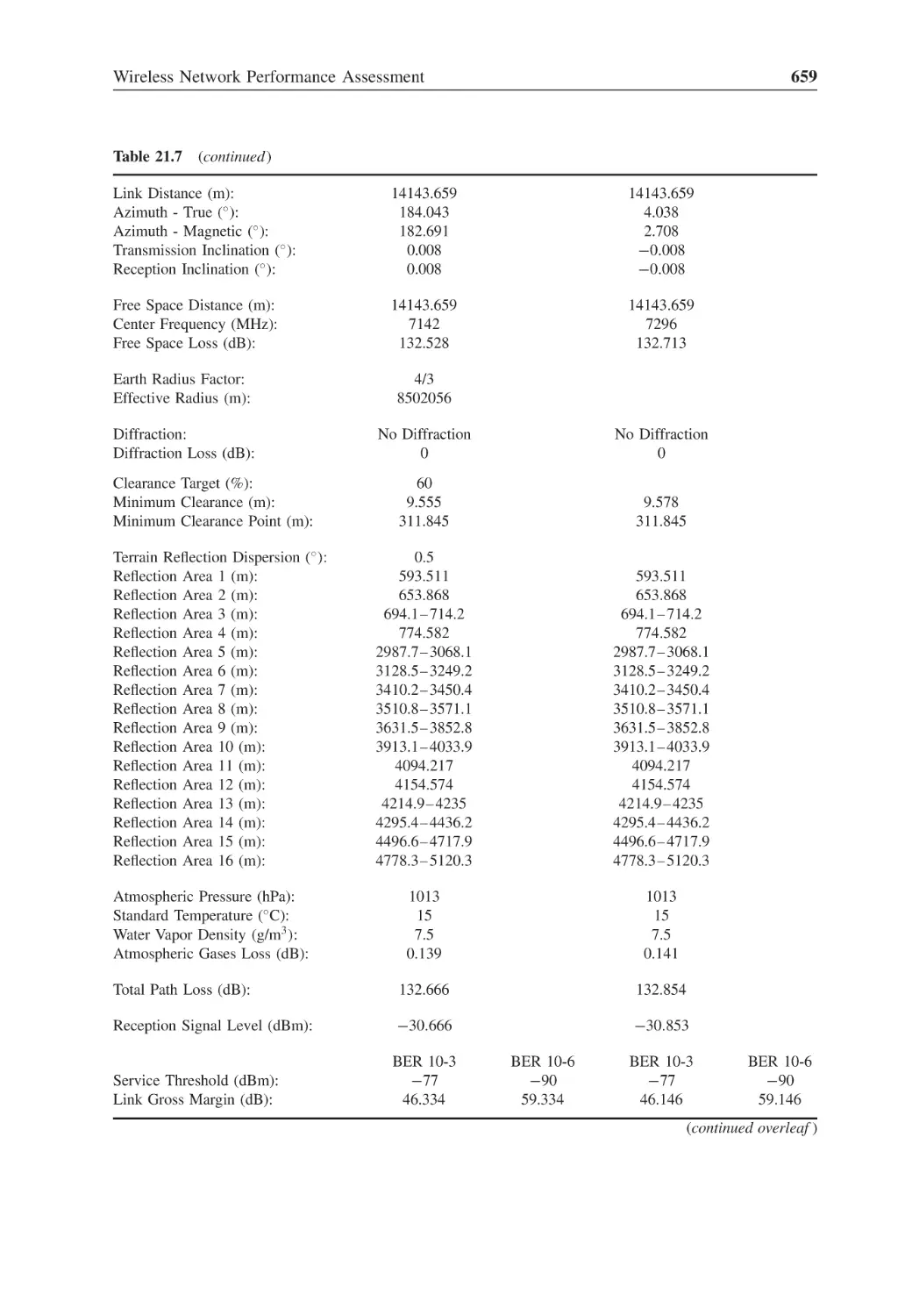
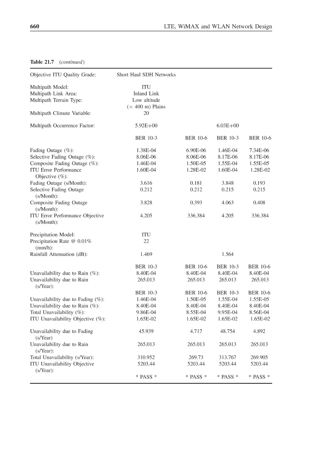
Figure 21.54 Link performance report
657
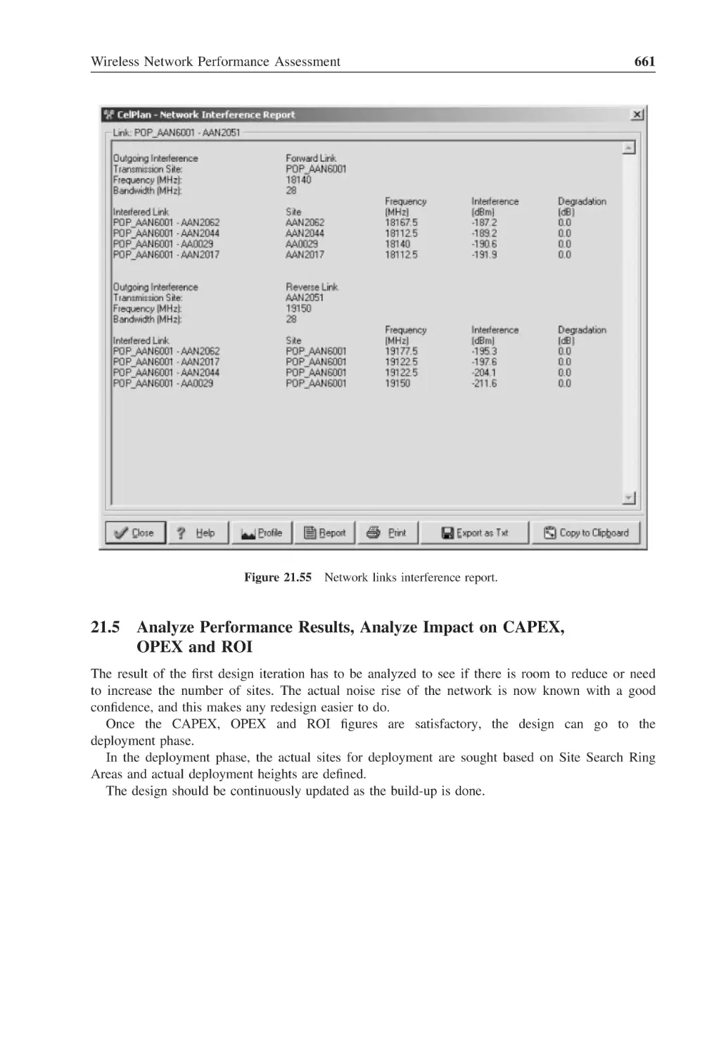
Figure 21.55 Network links interference report
661
Figure 22.1
Circle representation
664
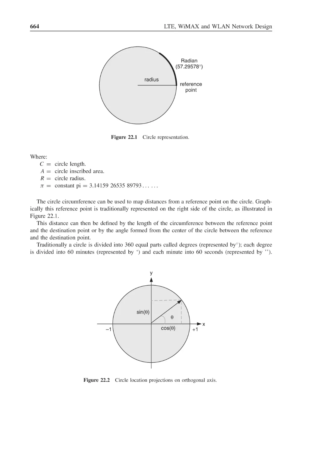
Figure 22.2
Circle location projections on orthogonal axis
664
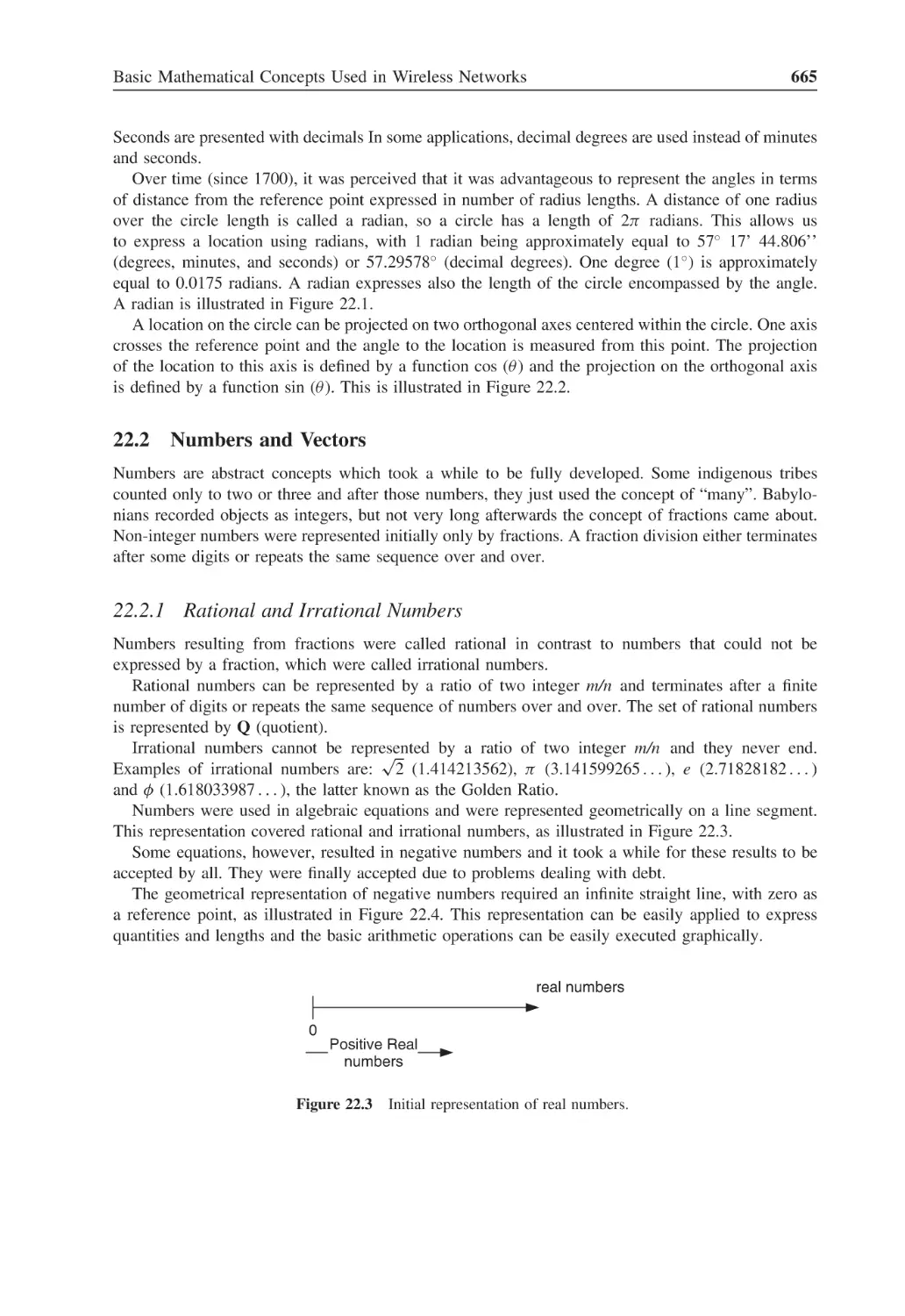
Figure 22.3
Initial representation of real numbers
665
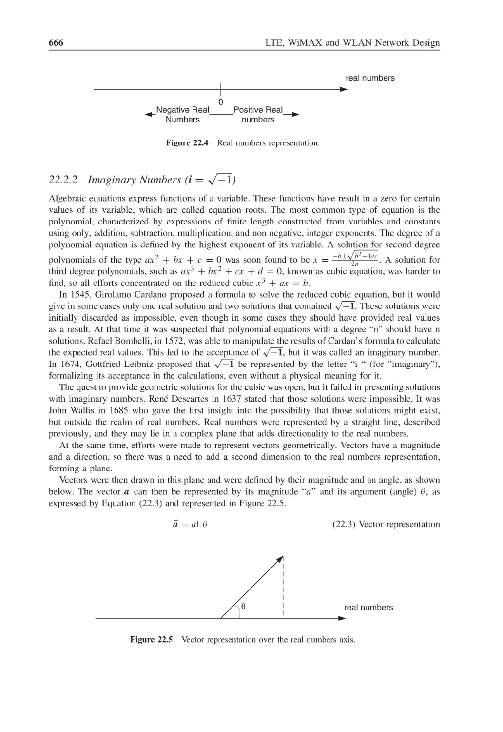
Figure 22.4
Real numbers representation
666
Figure 22.5
Vector representation over the real numbers axis
666
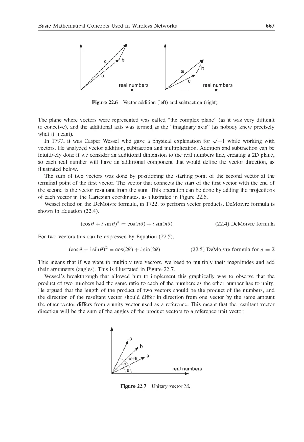
Figure 22.6
Vector addition (left) and subtraction (right)
667
Figure 22.7
Unitary vector M
667
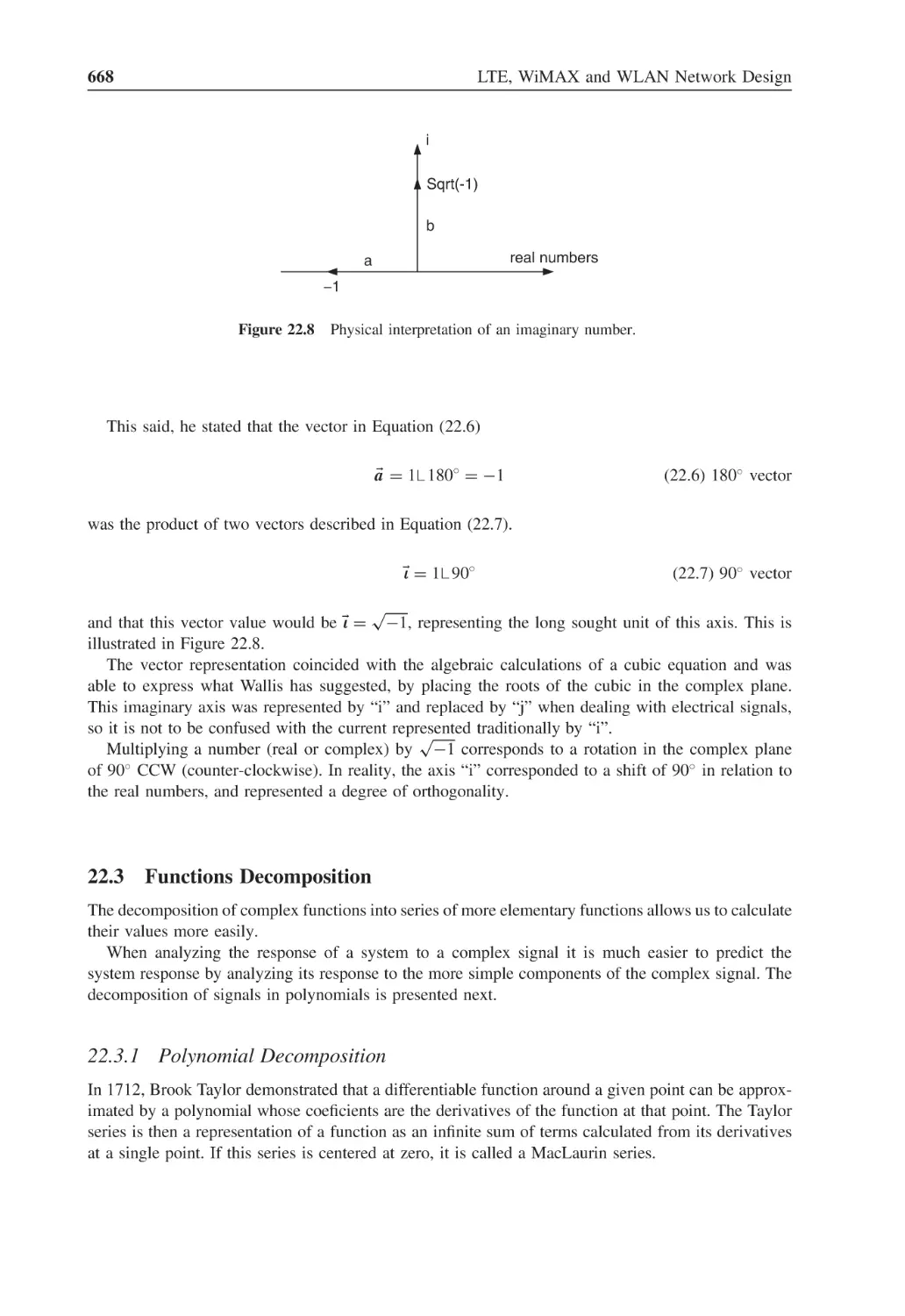
Figure 22.8
Physical interpretation of an imaginary number
668
Figure 22.9
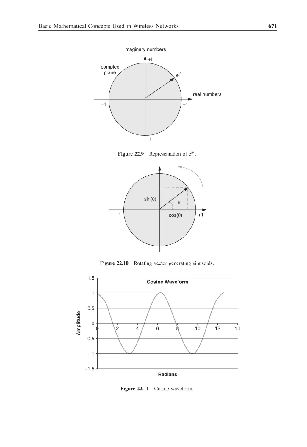
Representation of eiθ
671
Figure 22.10 Rotating vector generating sinusoids
671
Figure 22.11 Cosine waveform
671
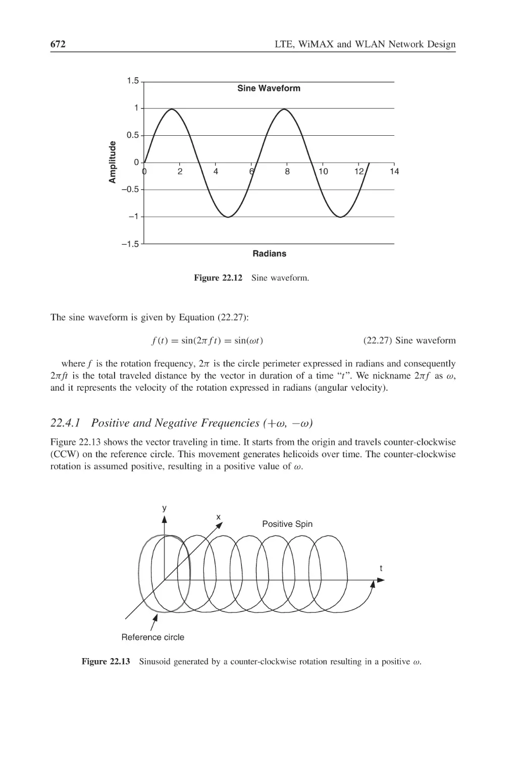
Figure 22.12 Sine waveform
672
Figure 22.13 Sinusoid generated by a counter-clockwise rotation resulting in a positive ω
672
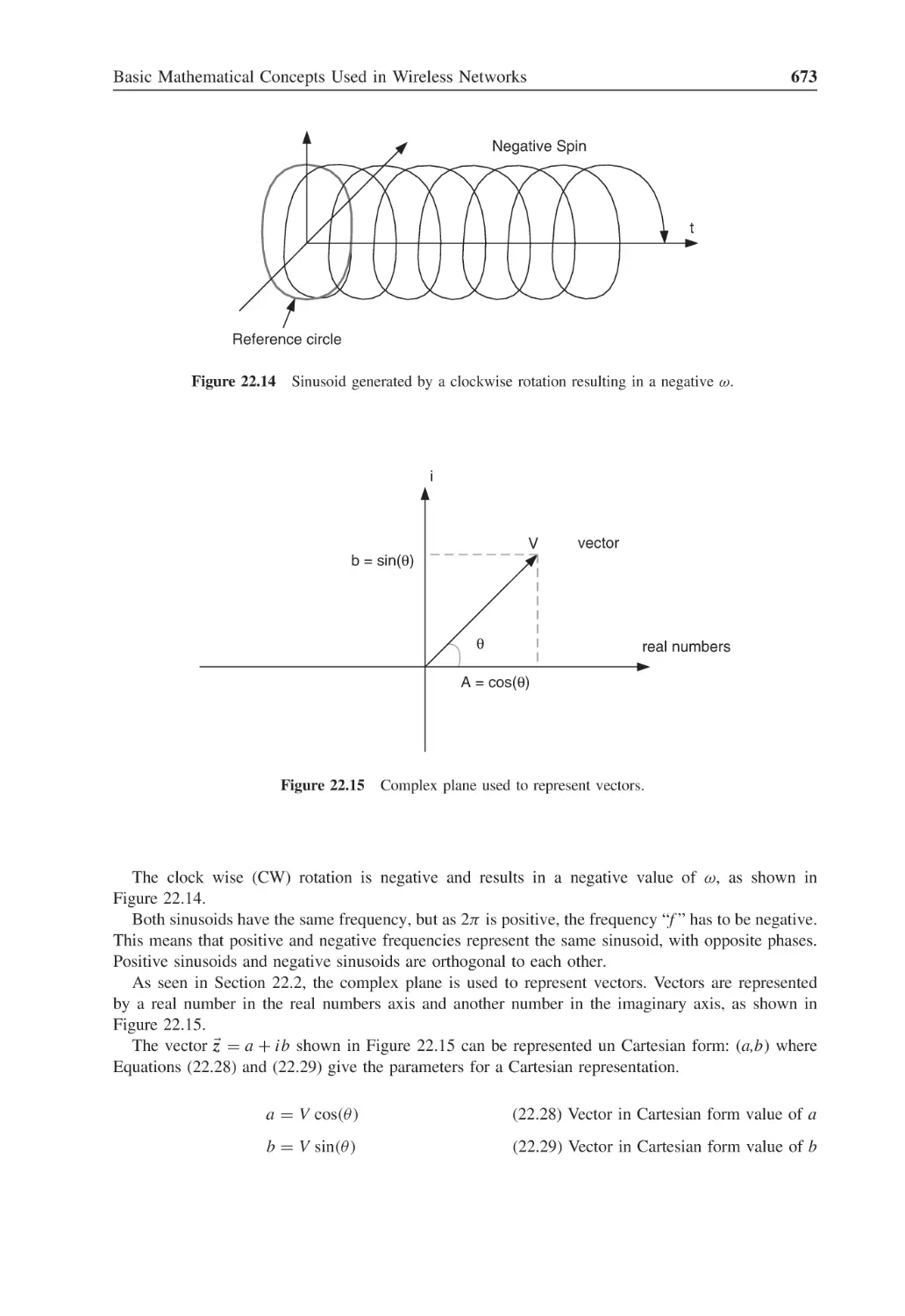
Figure 22.14 Sinusoid generated by a clockwise rotation resulting in a negative ω
673
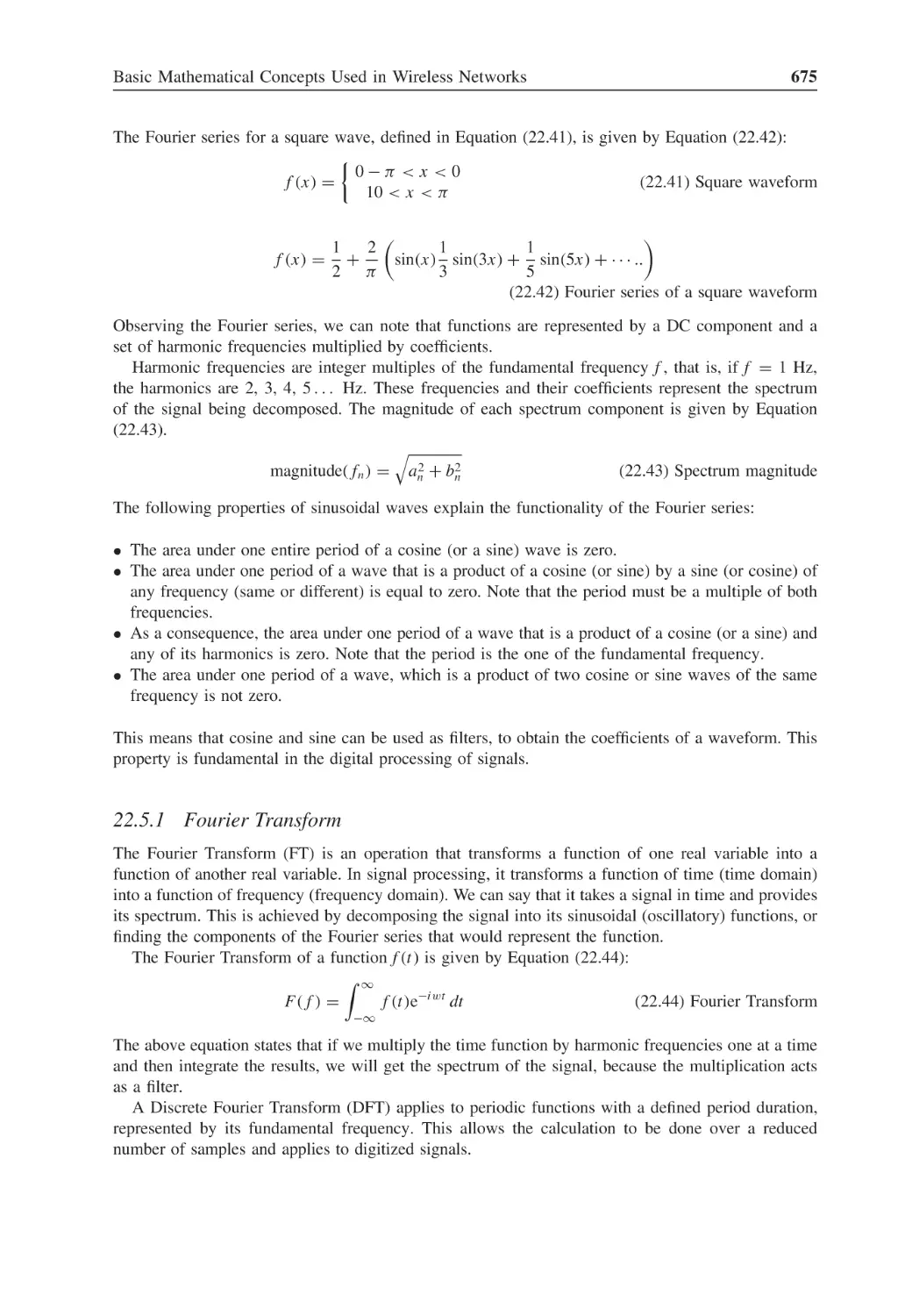
Figure 22.15 Complex plane used to represent vectors
673
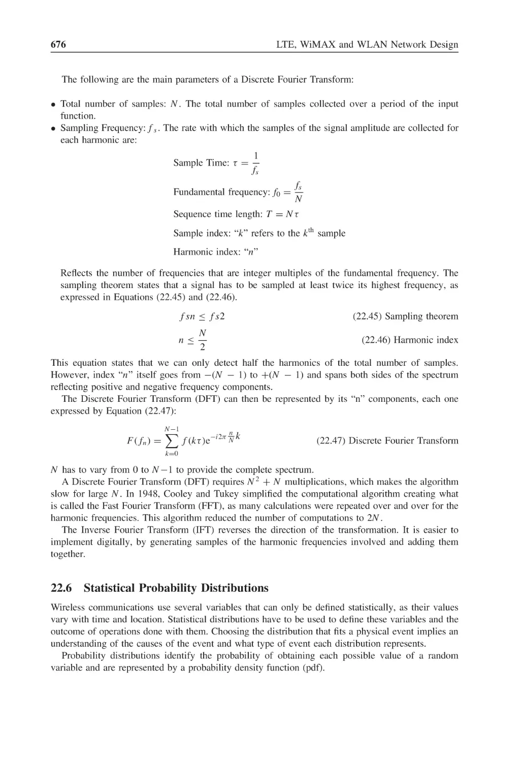
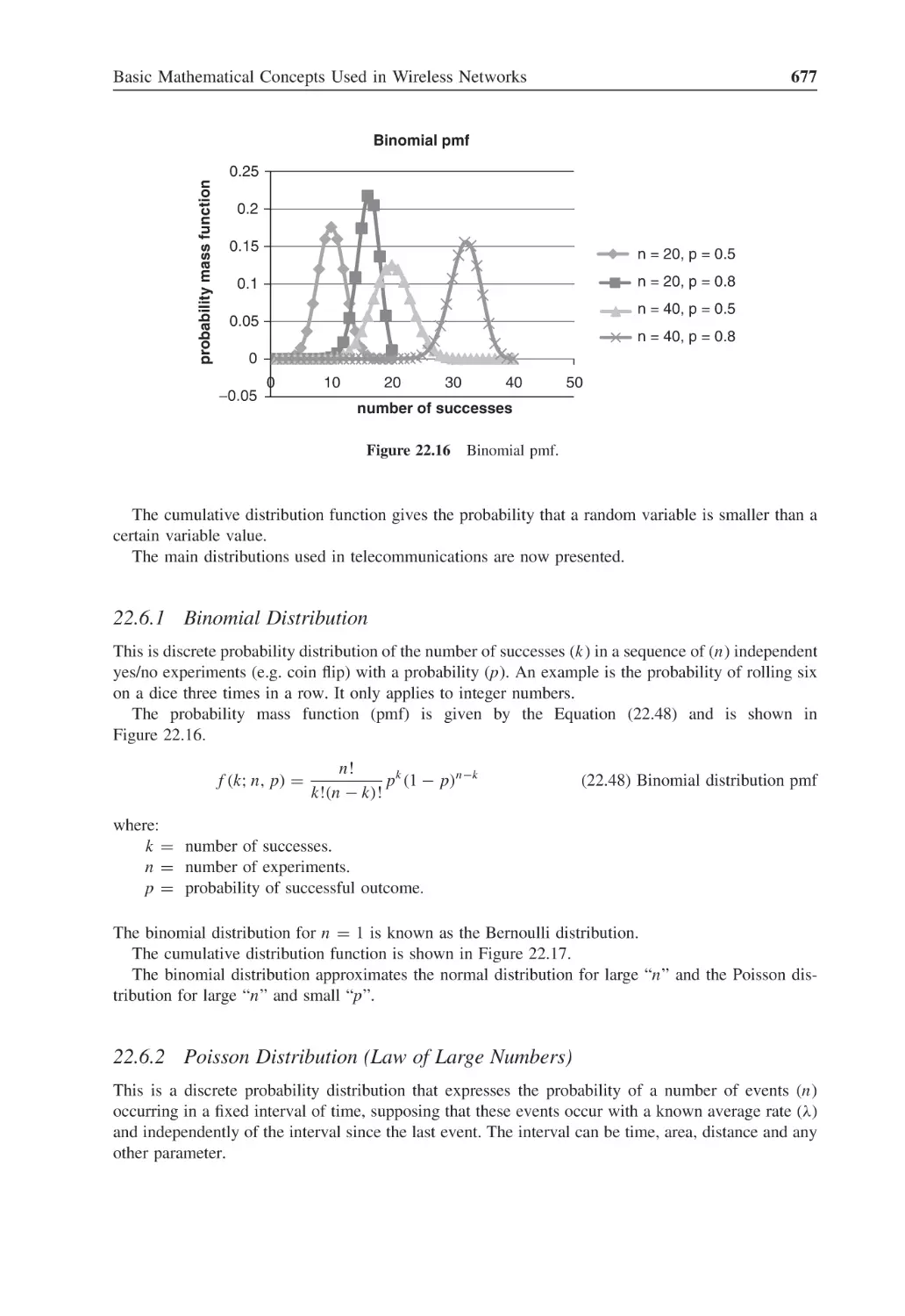
Figure 22.16 Binomial pmf
677
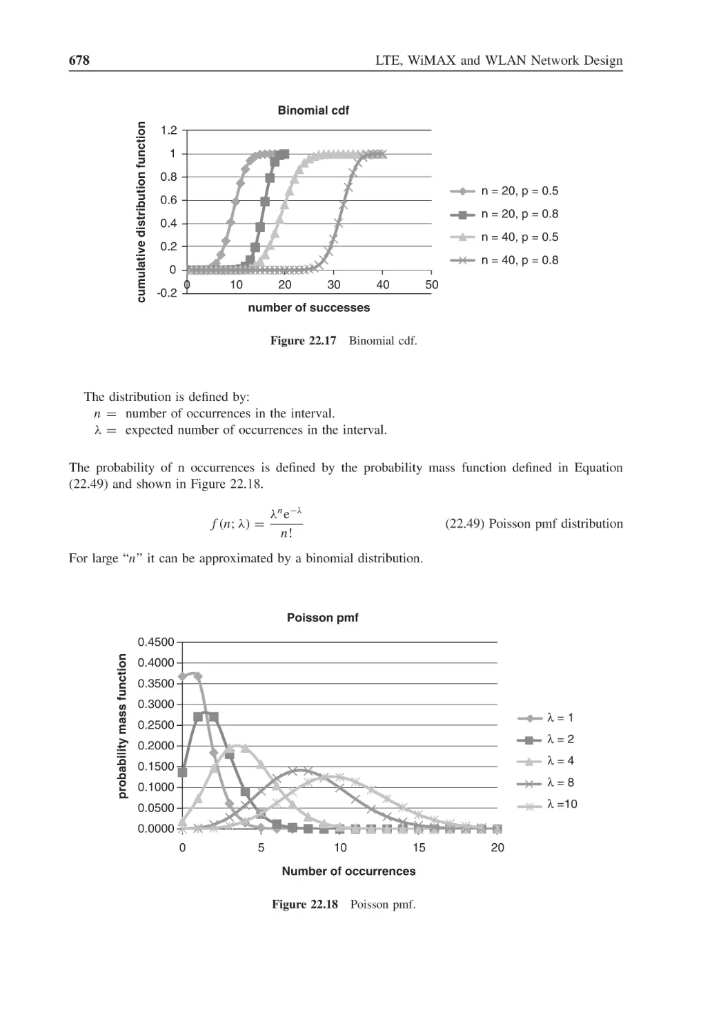
Figure 22.17 Binomial cdf
678
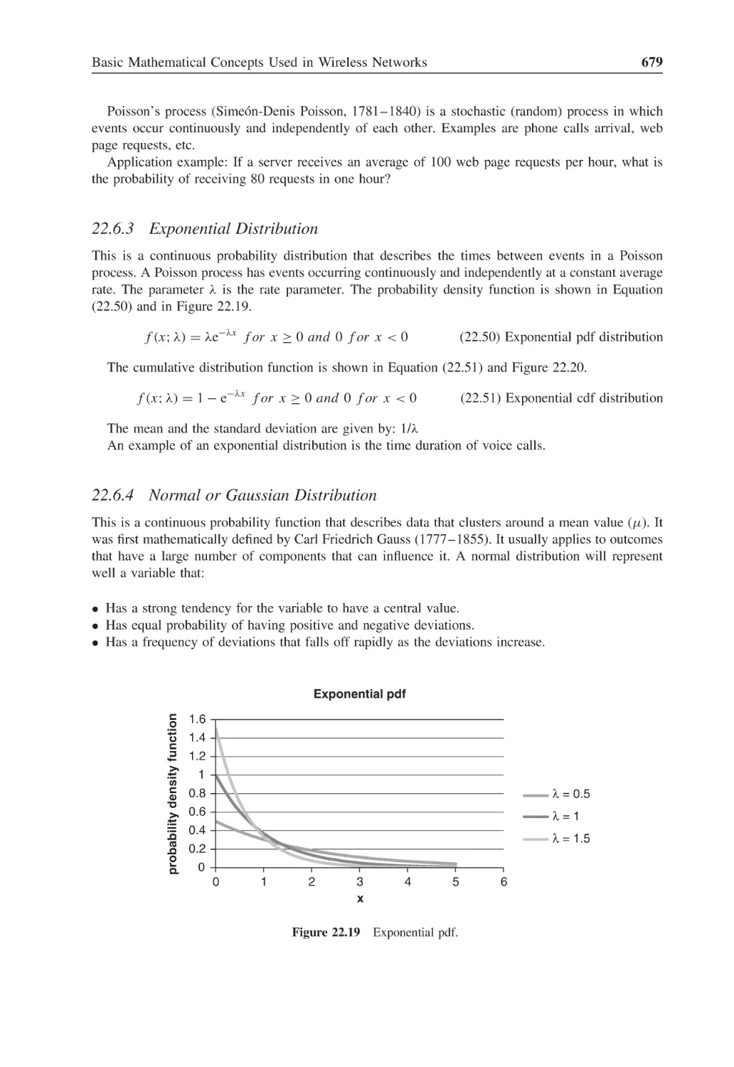
Figure 22.18 Poisson pmf
678
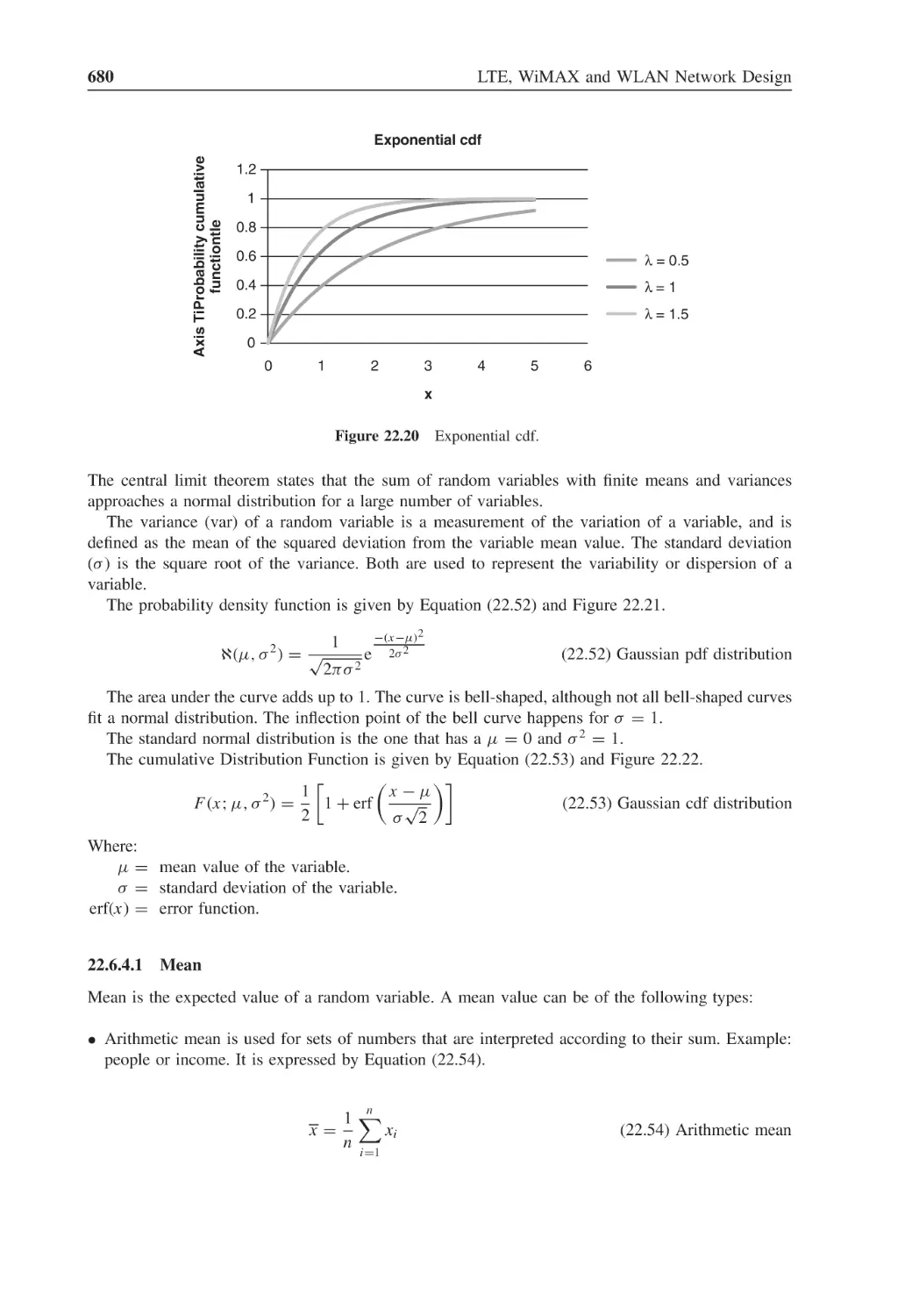
Figure 22.19 Exponential pdf
679
Figure 22.20 Exponential cdf
680
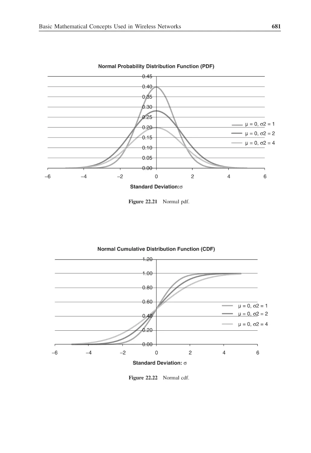
Figure 22.21 Normal pdf
681
Figure 22.22 Normal cdf
681
Figure 22.23 Standard normal curve
682
Figure 22.24 Rayleigh pdf
684
Figure 22.25 Rayleigh cdf
684
Figure 22.26 Rice pdf
685
Figure 22.27 Nakagami pdf
686
Figure 22.28 Pareto pdf
687
Figure 22.29 Pareto cdf
688
List of Tables
Table 1.1
Number of sites for an initial design
8
Table 2.1
Ethernet physical layer interfaces
21
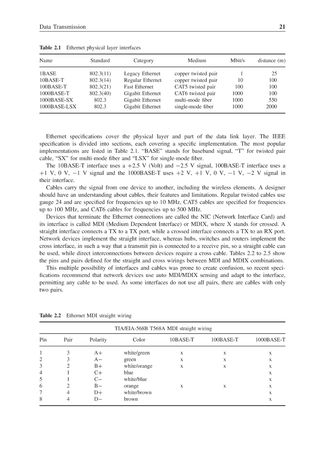
Table 2.2
Ethernet MDI straight wiring
21
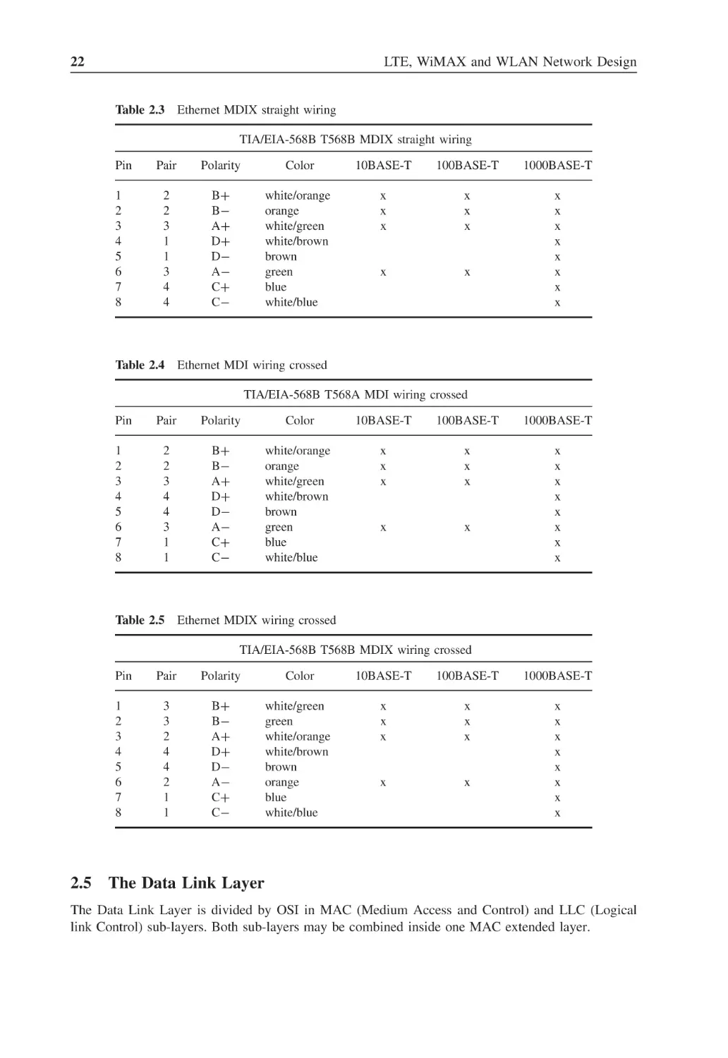
Table 2.3
Ethernet MDIX straight wiring
22
Table 2.4
Ethernet MDI wiring crossed
22
Table 2.5
Ethernet MDIX wiring crossed
22
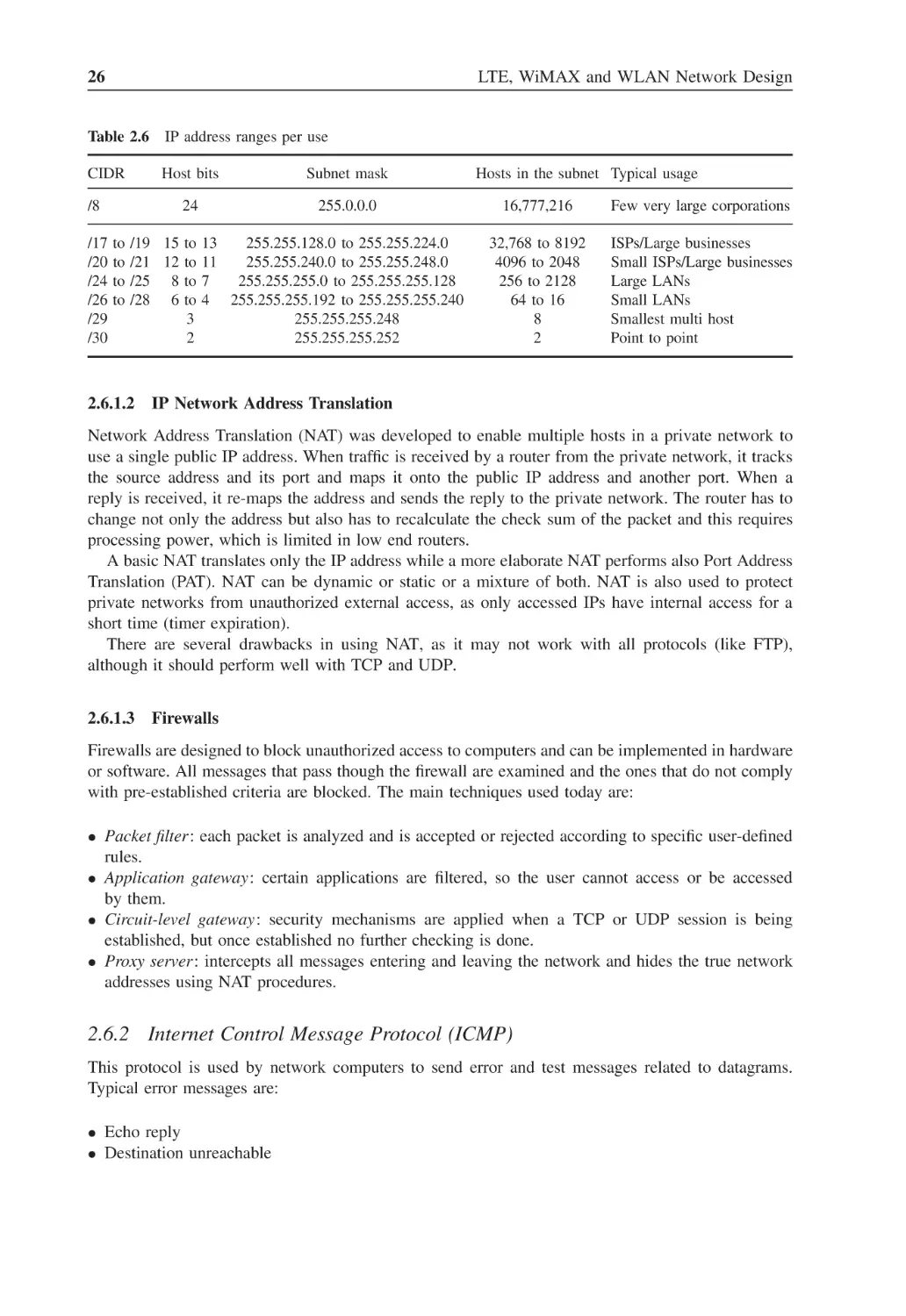
Table 2.6
IP address ranges per use
26
Table 2.7
Most popular vocoders
33
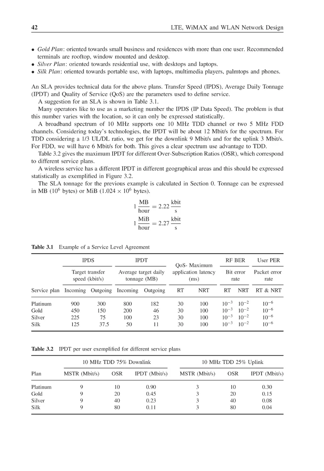
Table 3.1
Example of a Service Level Agreement
42
Table 3.2
IPDT per user exemplified for different service plans
42
Table 3.3
Service configuration parameters
49
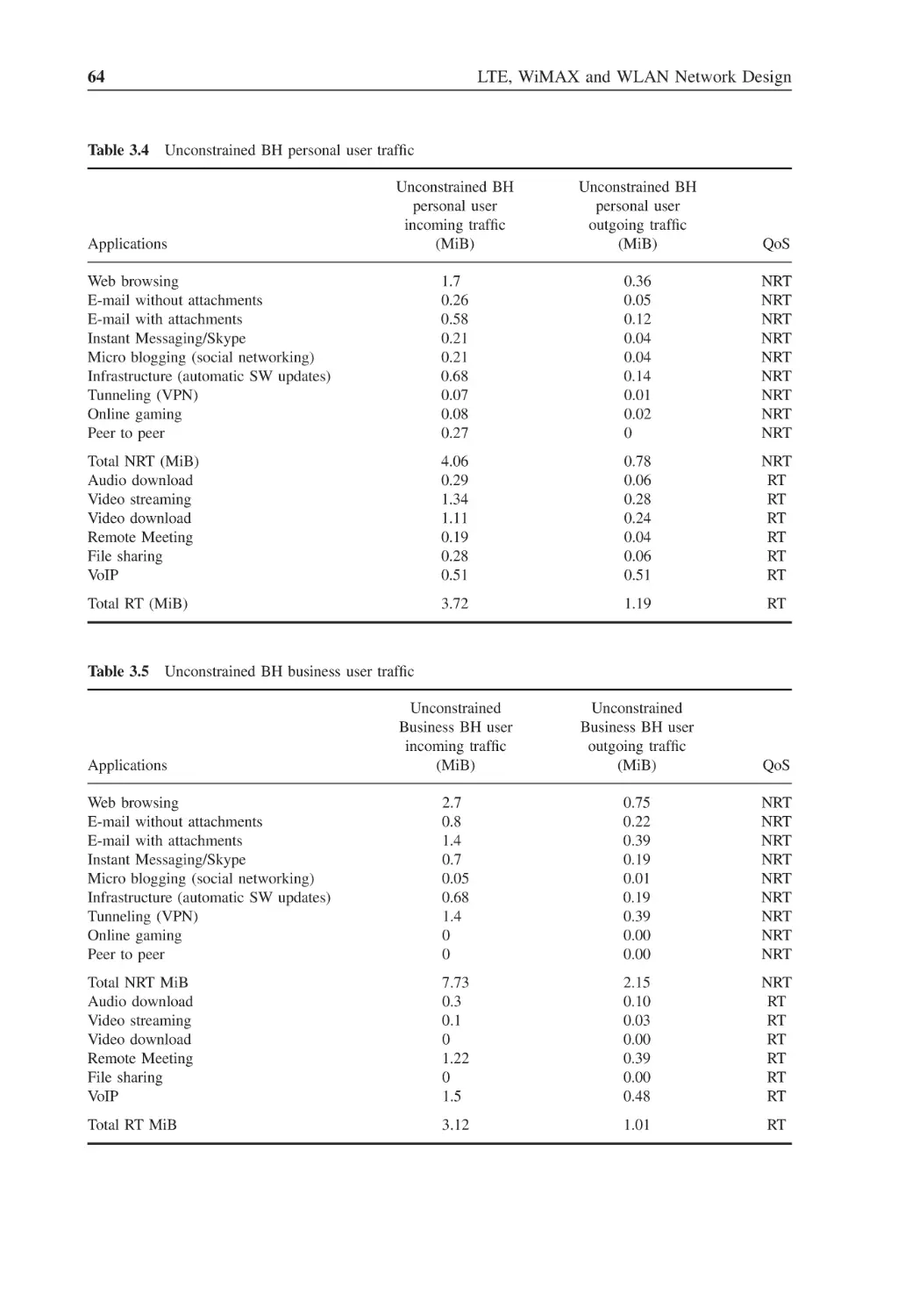
Table 3.4
Unconstrained BH personal user traffic
64
Table 3.5
Unconstrained BH business user traffic
64
Table 3.6
Traffic constraint factor by terminal type
65
Table 3.7
Expected number of users per terminal type
65
Table 3.8
Busy hour traffic per subscription (or terminal)
66
Table 3.9
Daily traffic per subscription (or terminal)
66
Table 3.10
Service plans and tonnage ranges
67
Table 3.11
Number of subscriptions per service plan
67
Table 3.12
Total number of users in a network (TNU)
67
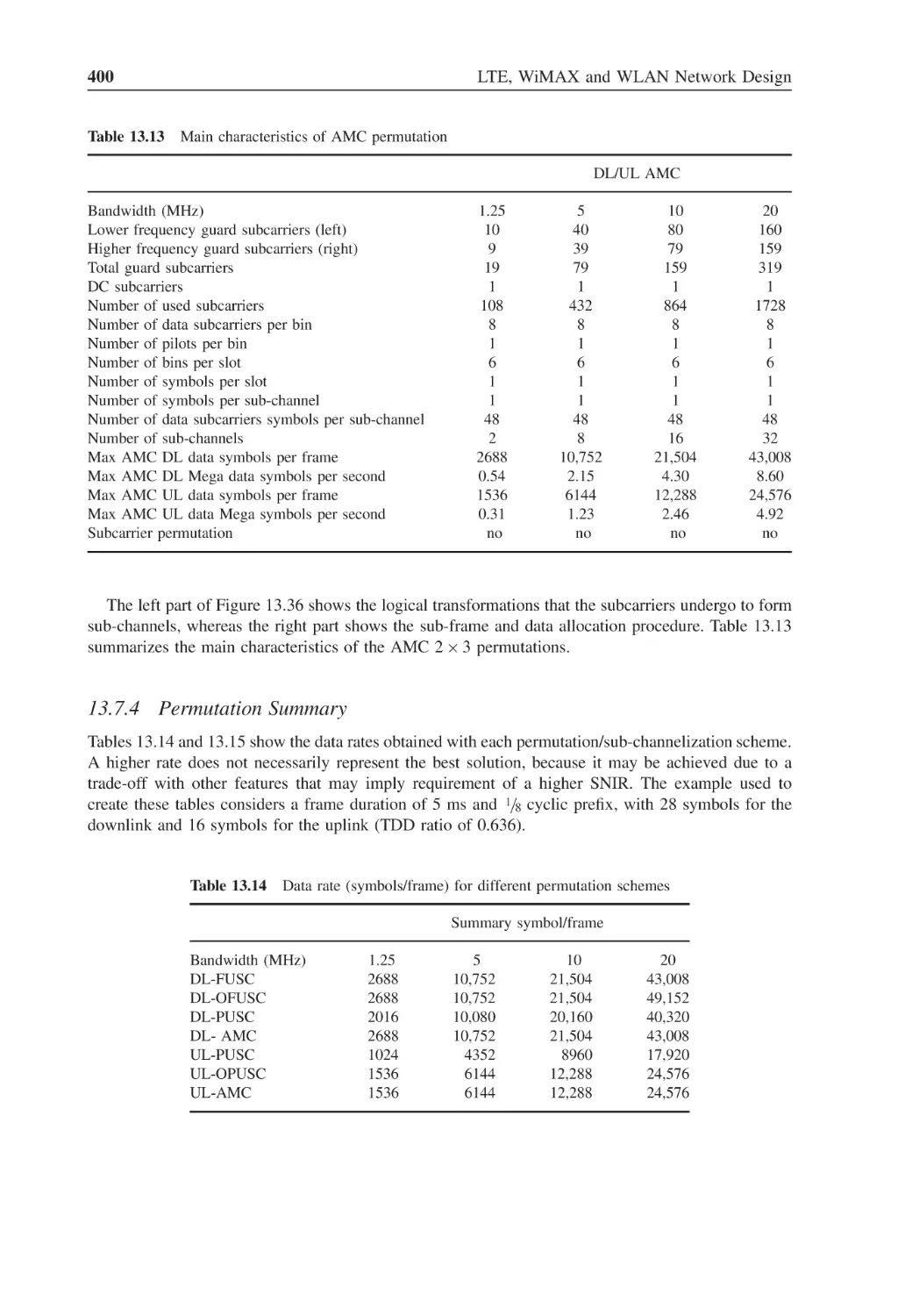
Table 3.13
Mapping of portable users (MPU) to different location types
68
Table 3.14
Area mapping (AM)
68
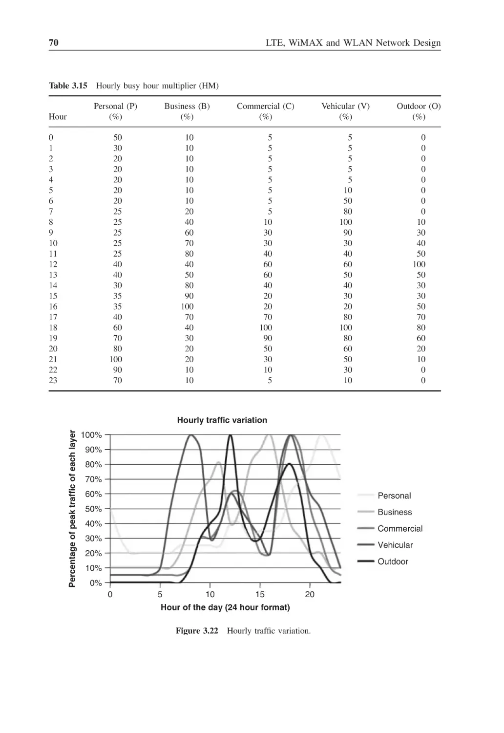
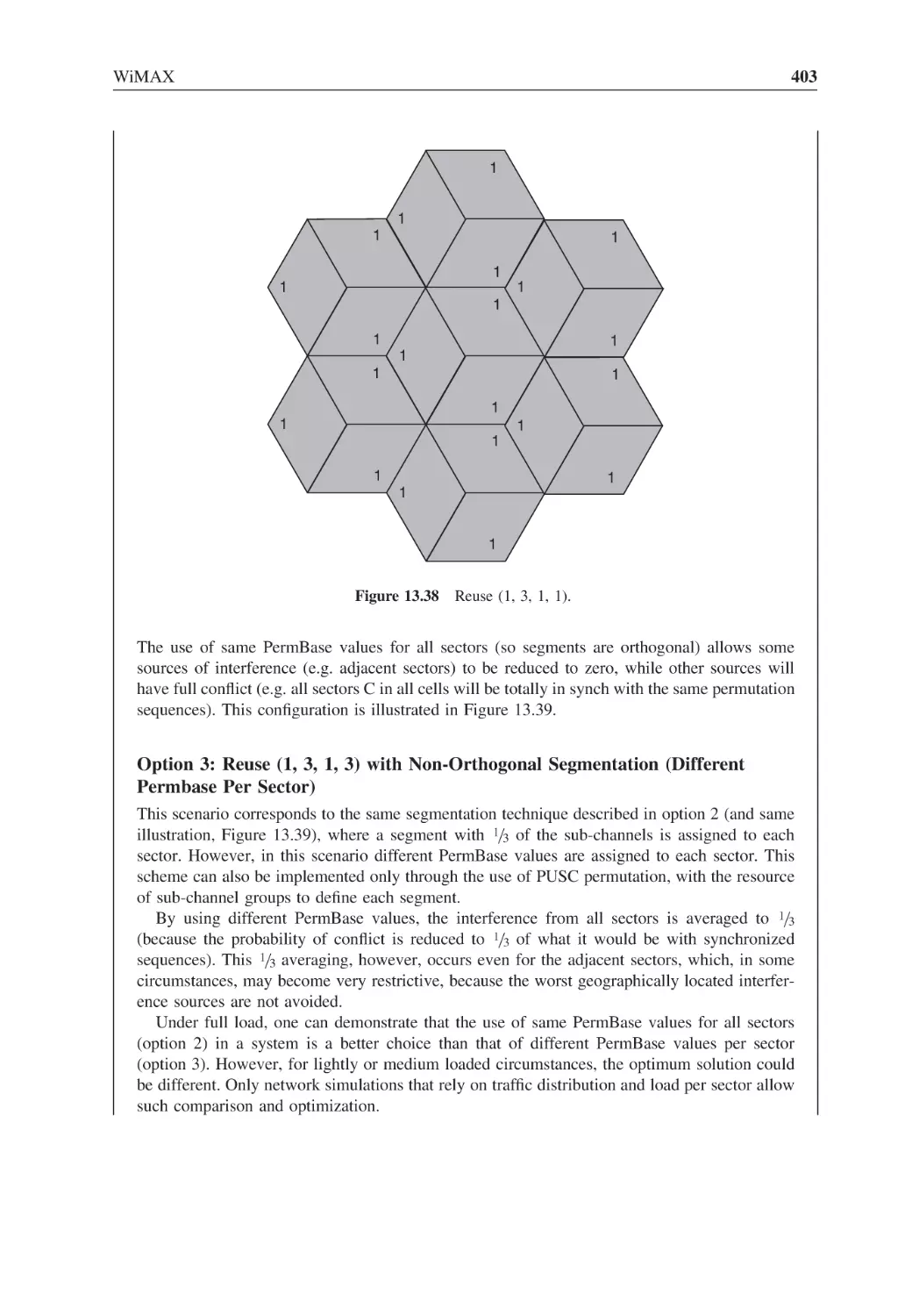
Table 3.15
Hourly busy hour multiplier (HM)
70
Table 3.16
Traffic layers composition
71
Table 3.17
Network traffic per layer
73
Table 4.1
Sampling table
80
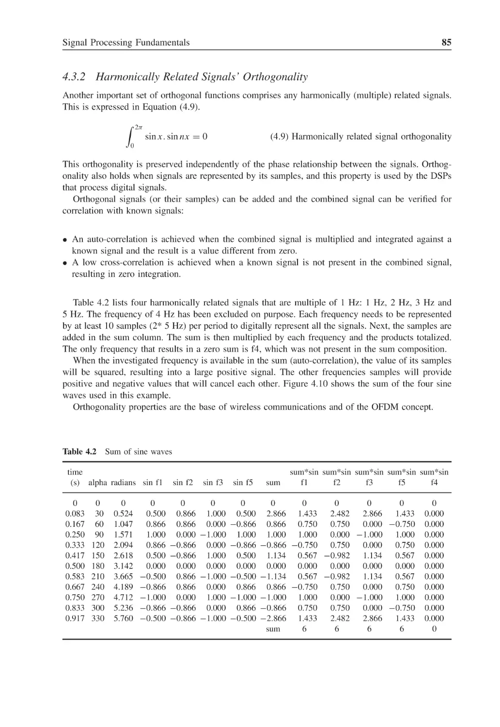
Table 4.2
Sum of sine waves
85
Table 4.3
Number of bits per modulation scheme
88
xxxvi
List of Tables
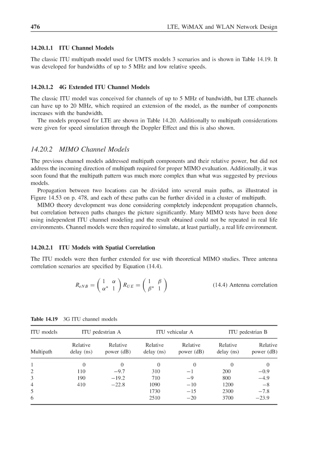
Table 5.1
Bandwidth and noise floor of wireless technologies
101
Table 5.2
Fresnel zone radius at 50% distance (m)
104
Table 5.3
Diffraction loss for 1 GHz at 100 m for different distance ratios
105
Table 5.4
Diffraction loss for 1 GHz at 1 km for different distance ratios
105
Table 5.5
Multipath fading distance for different frequencies
111
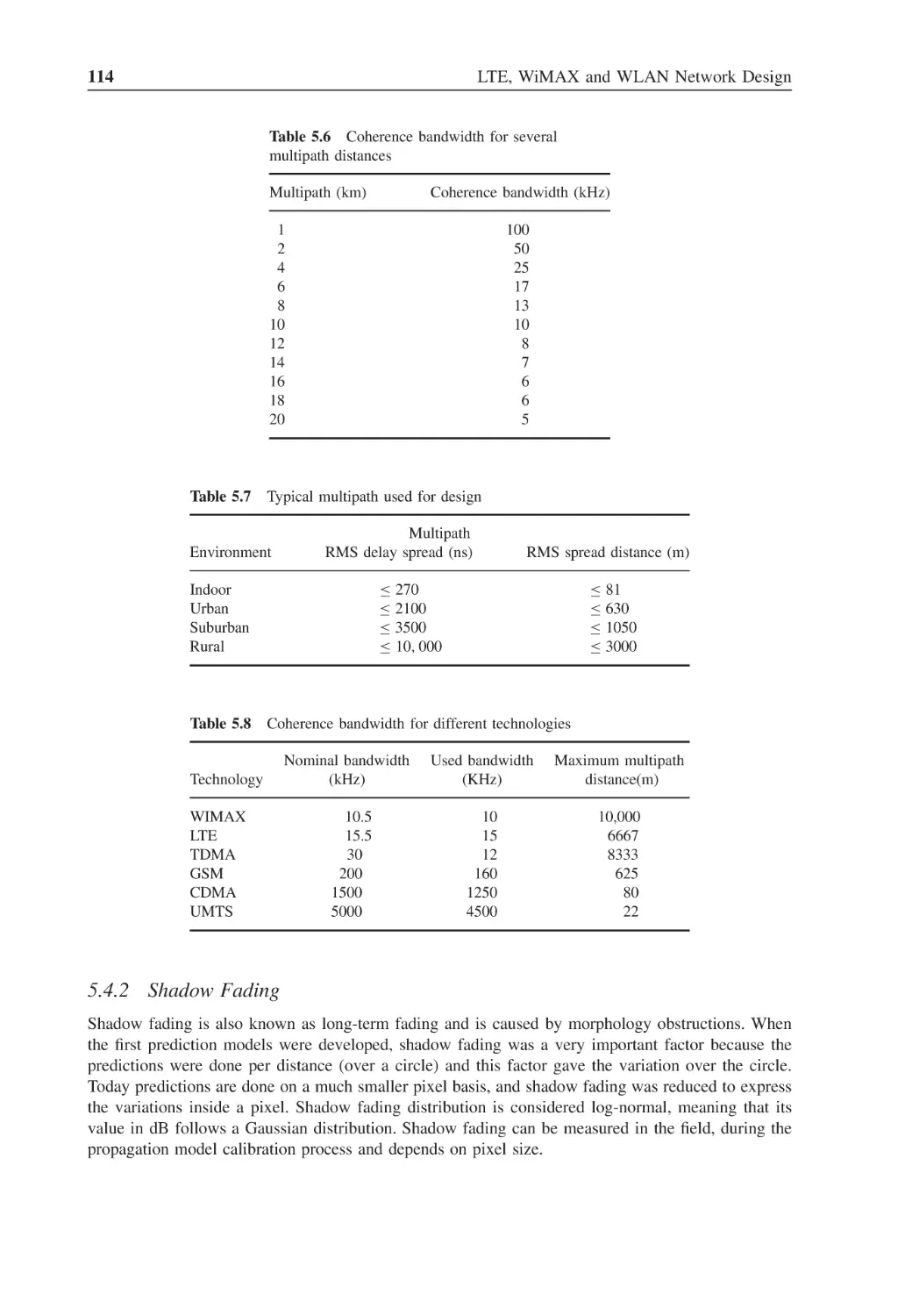
Table 5.6
Coherence bandwidth for several multipath distances
114
Table 5.7
Typical multipath used for design
114
Table 5.8
Coherence bandwidth for different technologies
114
Table 5.9
Trees effect on fading duration
115
Table 5.10
Vehicle movement effect on fading duration
116
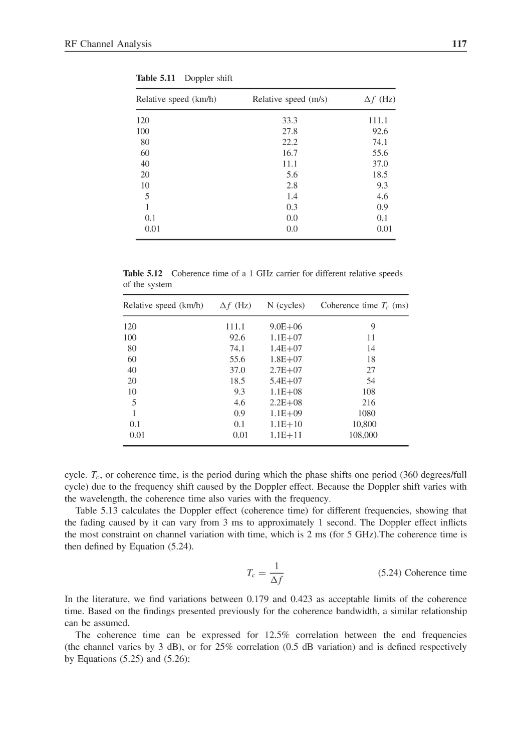
Table 5.11
Doppler shift
117
Table 5.12
Coherence time of a 1 GHz carrier for different relative speeds
of the system
117
Table 5.13
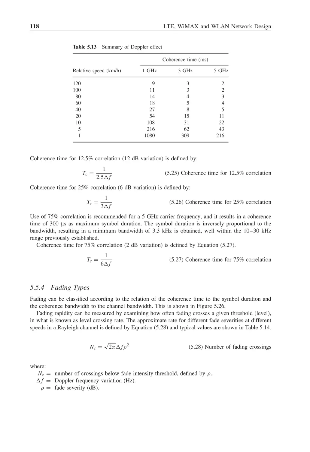
Summary of Doppler effect
118
Table 5.14
Level crossing rate according to receiver speed
119
Table 5.15
Fade duration according to receiver speed
120
Table 5.16
Total fade duration (cumulative per second)
120
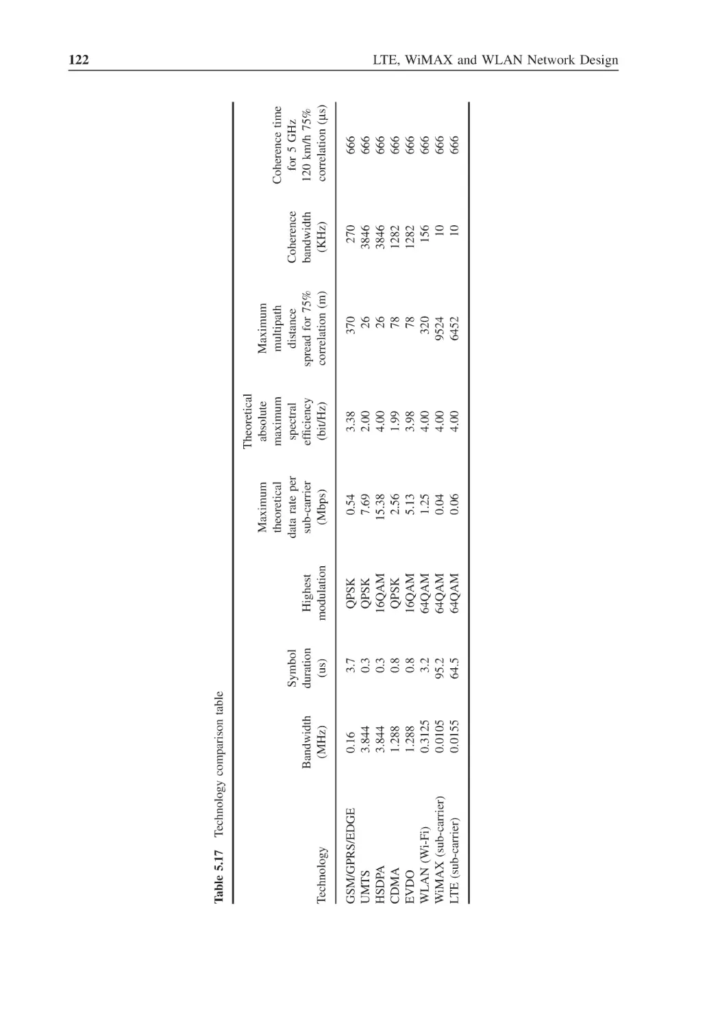
Table 5.17
Technology comparison table
122
Table 6.1
Fractional morphology parameters
147
Table 6.2
Final factor loss for different construction materials
158
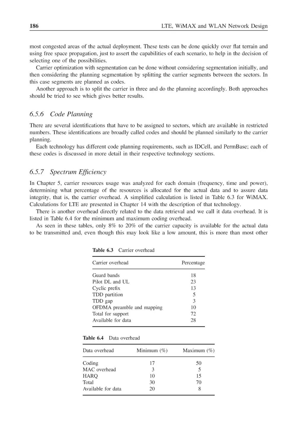
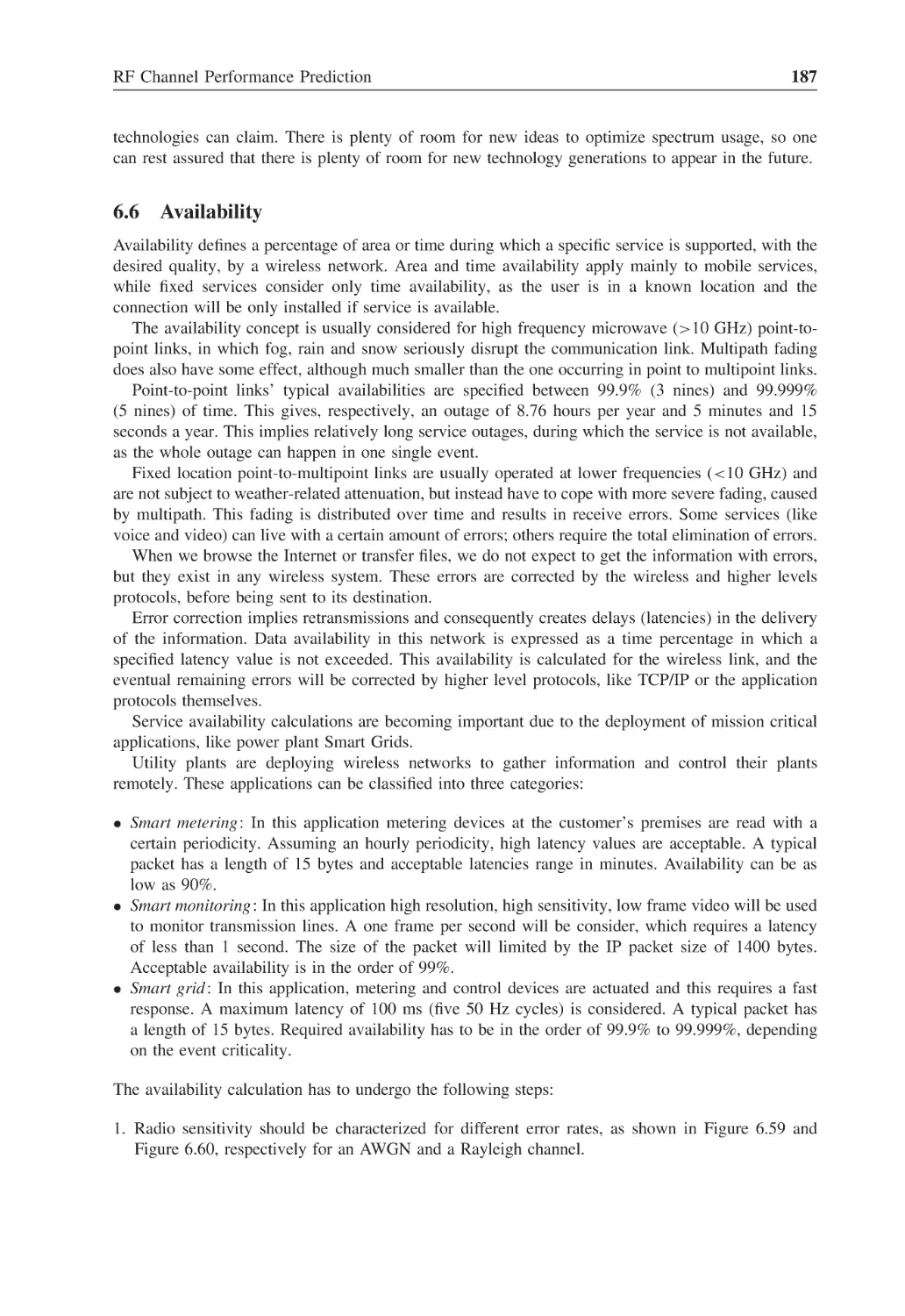
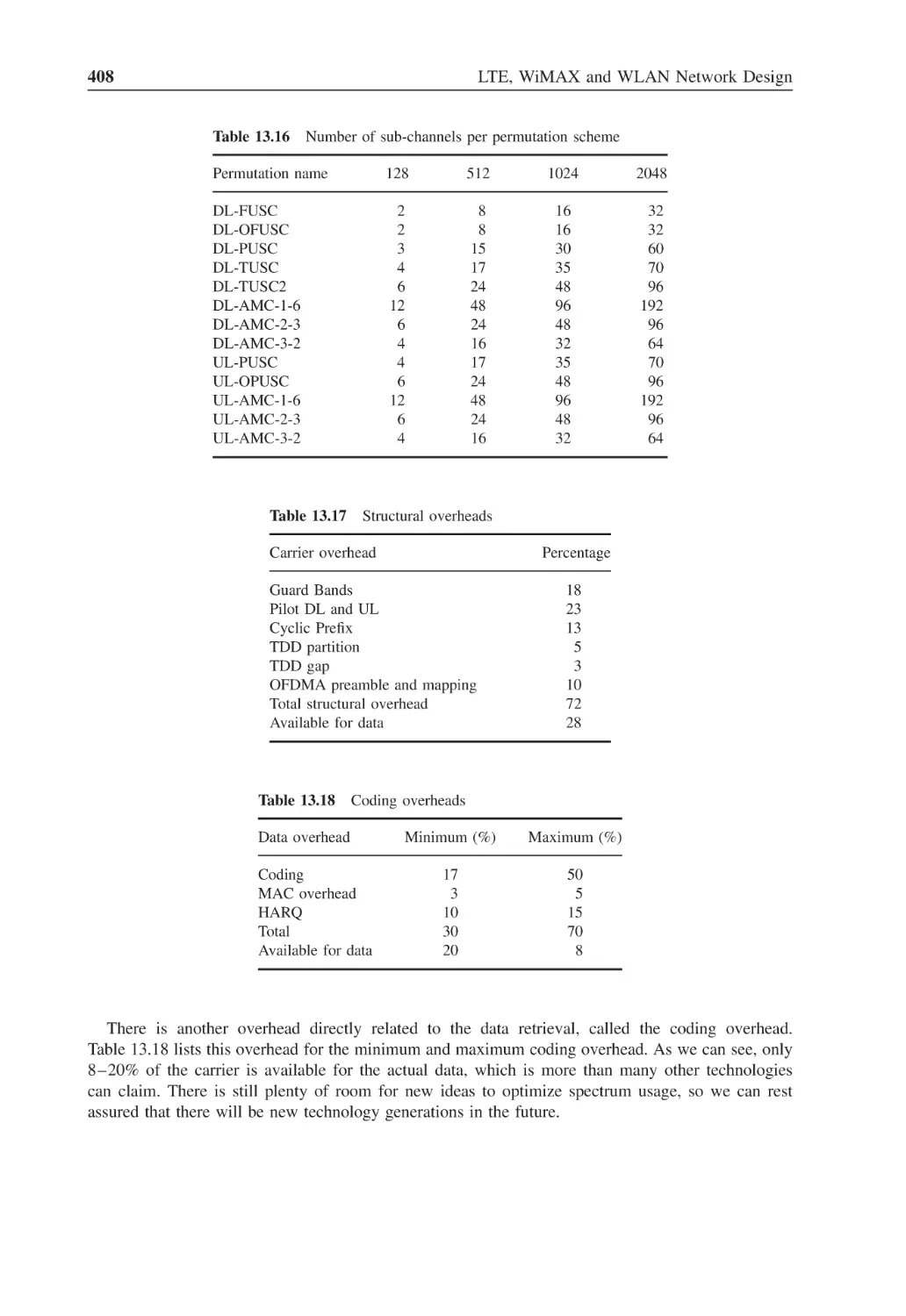
Table 6.3
Carrier overhead
186
Table 6.4
Data overhead
186
Table 6.5
Receiver sensitivity (signal threshold) for various availabilities
and 1 HARQ latency
191
Table 6.6
Receiver sensitivity (signal threshold) for various availabilities
and 2 HARQ latency
191
Table 7.1
Peak to average power ratio
198
Table 7.2
Inter-symbol and intra-symbol interference and cyclic prefix
204
Table 7.3
Synchronization requirements per technology
208
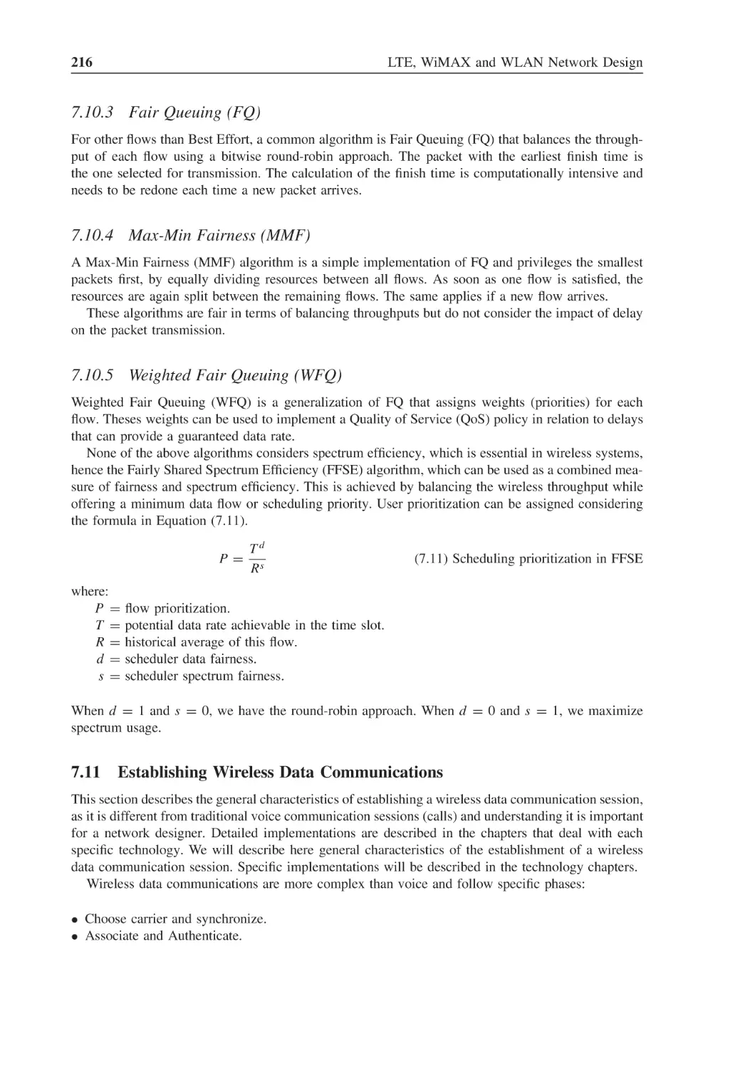
Table 7.4
DFFT detection values
213
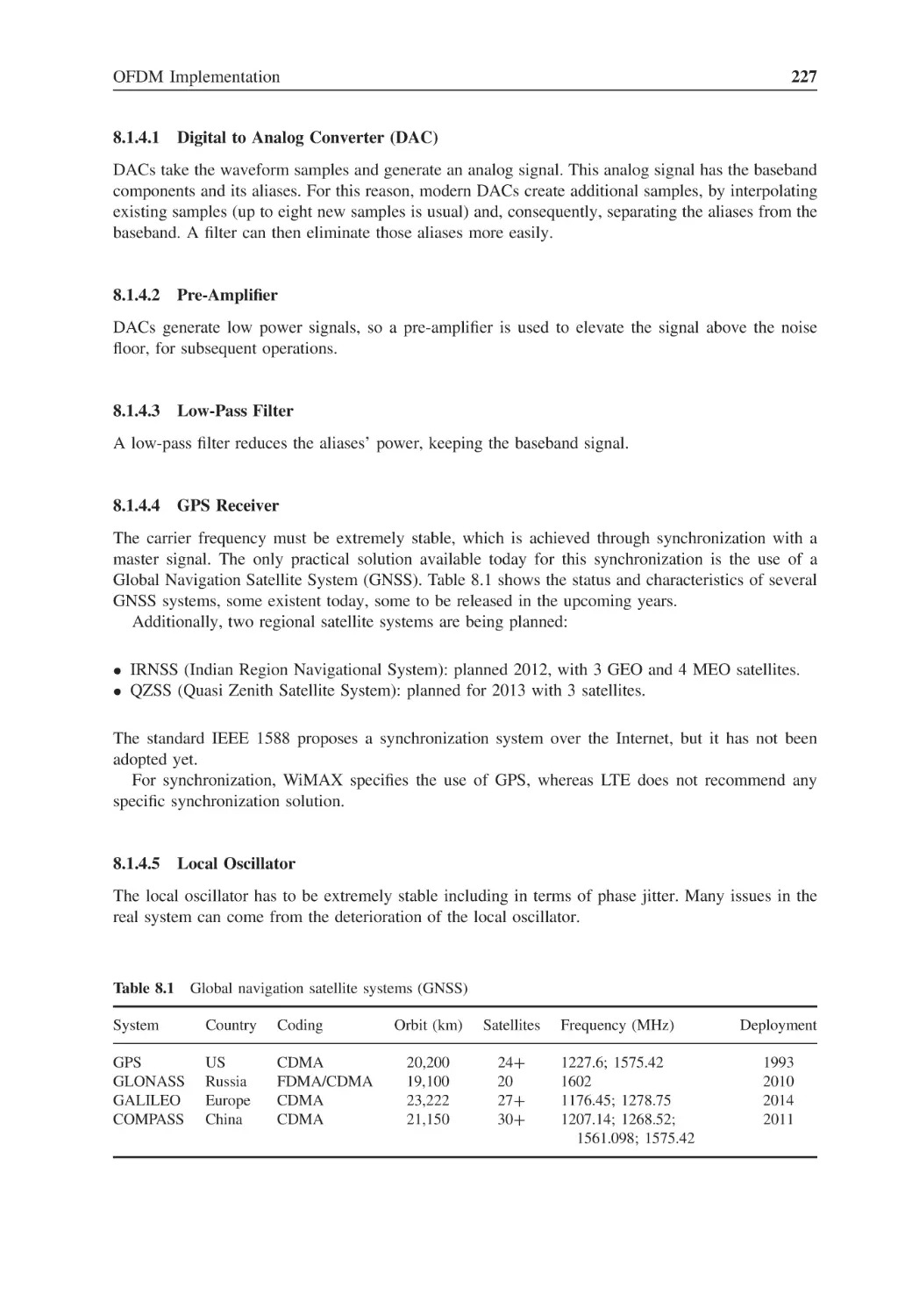
Table 8.1
Global navigation satellite systems (GNSS)
227
Table 8.2
Sum of I and Q sub-carriers
232
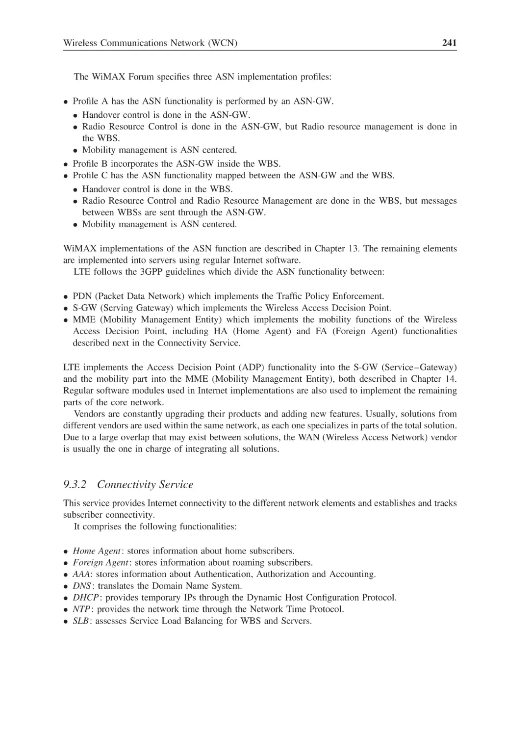
Table 9.1
Type of Service priority field
240
Table 9.2
Protocol types
240
Table 9.3
User priority in 802.1q (Ethernet MAC)
240
Table 10.1
Isotropic antenna dipole gain
250
Table 10.2
Gain and effective aperture for antennas at different frequencies
254
Table 10.3
Impedance mismatching coefficients
256
Table 10.4
Polarization loss factor
260
Table 10.5
ITU correlation factors for different antenna configurations
262
List of Tables
xxxvii
Table 10.6
Receive detector performance comparison
271
Table 10.7
Alamouti’s Matrix A
274
Table 10.8
MIMO type depending on number of antennas
277
Table 11.1
RF noise for different bandwidths
288
Table 11.2
Shannon’s channel capacity
291
Table 11.3
Shannon’s capacity for different received BER
291
Table 11.4
Comparison of modulation schemes
293
Table 11.5
Static fading, CTC, no permutation, required SNR in dB
296
Table 11.6
Coding factor in relation to CTC (dB)
297
Table 11.7
AMC symbol, no permutation for different channels, SNR
improvement in dB
298
Table 11.8
Symbol permutation factor (dB)
300
Table 11.9
HARQ SNR improvement in dB
301
Table 11.10 Improvement reduction factor
302
Table 11.11 RX Diversity, Rayleigh, improvement in dB
302
Table 11.12 TX Diversity, Rayleigh, improvement in dB
303
Table 11.13 Spatial Multiplexing DL, Rayleigh, improvement in dB
304
Table 11.14 Spatial Multiplexing DL, Rayleigh, improvement in dB
305
Table 12.1
ISM band
312
Table 12.2
U-NII band
312
Table 12.3
802.11 releases
313
Table 12.4
HiperLAN releases
313
Table 12.5
IEEE WLAN 2.4 GHz unlicensed channels
313
Table 12.6
IEEE WLAN 3.6 GHz unlicensed channels
314
Table 12.7
IEEE WLAN 4.9 GHz licensed channels
314
Table 12.8
IEEE WLAN 5 GHz unlicensed channels
315
Table 12.9
MAC address configuration
321
Table 12.10 Maximum MPDU duration for best channel conditions
323
Table 12.11 Minimum MSDU duration for best channel conditions
323
Table 12.12 Maximum MPDU duration for worst channel conditions
324
Table 12.13 Minimum MPDU duration for worst channel conditions
324
Table 12.14 Modulation indexes for 20 MHz
331
Table 12.15 Modulation indexes for 40 MHz
332
Table 12.16 WLAN general parameters
334
Table 12.17 Spectrum efficiency
335
Table 13.1
WiMAX standards
343
Table 13.2
Calculation of number of subcarriers
357
Table 13.3
Maximum multipath spread distance for OFDMA symbol fractions
360
Table 13.4
OFDM parameters of IEEE Std. 802.16-2004, WiMAX OFDM
361
xxxviii
List of Tables
Table 13.5
OFDM parameters of IEEE Std. 802.16e, WiMAX OFDMA
361
Table 13.6
Pilot to data ratio of different permutation schemes
387
Table 13.7
Sub-channelization sequence
389
Table 13.8
Main characteristics of FUSC permutation
391
Table 13.9
Main characteristics of OFUSC permutation
391
Table 13.10 Main characteristics of PUSC-DL permutation
394
Table 13.11 Main characteristics of PUSC-UL permutation
397
Table 13.12 Main characteristics of OPUSC-UL permutation
397
Table 13.13 Main characteristics of AMC permutation
400
Table 13.14 Data rate (symbols/frame) for different permutation schemes
400
Table 13.15 Data rate (msymbols/second) for different permutation schemes
401
Table 13.16 Number of sub-channels per permutation scheme
408
Table 13.17 Structural overheads
408
Table 13.18 Coding overheads
408
Table 14.1
LTE spectral efficiency objectives
411
Table 14.2
LTE marketing claims
411
Table 14.3
3GPP 3G standards evolution
412
Table 14.4
3GPP LTE (EPS) Standards
414
Table 14.5
LTE FDD and TDD bands
416
Table 14.6
QCI categories
430
Table 14.7
Turbo code rate and typical puncturing table
436
Table 14.8
Channel bandwidth
444
Table 14.9
RF channel bandwidth and information capacity
446
Table 14.10 Number of codes per resource blocks
452
Table 14.11 Round trip delay for different distances
453
Table 14.12 TDD switching configurations
459
Table 14.13 TDD switching configurations (normal cyclic prefix)
459
Table 14.14 TDD switching configurations (extended cyclic prefix)
460
Table 14.15 EVM values for different modulations
465
Table 14.16 Receiver sensitivity decrease
465
Table 14.17 Antenna clusters dimensions
468
Table 14.18 Cell search parameters per RAT
475
Table 14.19 3G ITU channel models
476
Table 14.20 4G Extended ITU channel models
477
Table 14.21 ITU correlation factors for different antenna configurations
477
Table 14.22 Spatial channel model (SCM)
478
Table 14.23 Phase 2 WINNER channel model scenarios
479
Table 14.24 LTE performance evaluation models
480
Table 14.25 LTE framed throughput per cell
484
List of Tables
xxxix
Table 14.26 LTE downlink throughput per cell considering overhead
485
Table 14.27 LTE downlink throughput per cell considering overhead
and inefficiencies
486
Table 14.28 LTE downlink throughput per cell (sector) with MIMO
486
Table 14.29 LTE uplink throughput per cell considering overhead
487
Table 14.30 LTE uplink throughput per cell considering overhead
and inefficiencies
488
Table 14.31 LTE uplink throughput per cell (sector) with MIMO
488
Table 15.1
WLAN general characteristics
491
Table 15.2
WiMAX general characteristics
492
Table 15.3
WiMAX scalable and LTE general characteristics
493
Table 15.4
WLAN cyclic prefix
494
Table 15.5
WiMAX cyclic prefix
495
Table 15.6
WiMAX scalable and LTE cyclic prefix
496
Table 15.7
WLAN modulation schemes
497
Table 15.8
WiMAX modulation schemes
498
Table 15.9
WiMAX scalable and LTE modulation schemes
499
Table 15.10 WIMAX framing
500
Table 15.11 WiMAX scalable and LTE framing
501
Table 15.12 WiMAX resource blocks
502
Table 15.13 WiMAX scalable and LTE resource blocks
503
Table 15.14 WLAN throughput
504
Table 15.15 WLAN spectral efficiency
505
Table 15.16 WiMAX throughput and spectral efficiency
506
Table 15.17 WiMAX scalable and LTE maximum throughput and
spectral efficiency
507
Table 15.18 Pilot to data or symbol ratio
512
Table 15.19 Control to total symbols ratio
512
Table 17.1
Topography database resolution requirements
523
Table 17.2
Morphology clutter types
524
Table 17.3
Morphology resolution requirements
525
Table 17.4
US Census regions
533
Table 17.5
Unconstrained personal services
535
Table 17.6
Unconstrained business services
535
Table 17.7
Suggested environmental attenuations
537
Table 17.8
Example of prediction service classes
541
Table 17.9
Combined traffic layers per service class
550
Table 18.1
Downstream link budget example
566
Table 18.2
Upstream link budget example
568
xl
List of Tables
Table 19.1
Static measurements’ characteristics averaged for 100 ms,
600 ms, 1 s, 10 s and 60 s
577
Table 21.1
Traffic data per service class
626
Table 21.2
Traffic throughput KPI at 75% of peak rate
627
Table 21.3
Traffic throughput KPI at 50% of peak rate
628
Table 21.4
Traffic throughput KPI at 15% (consumer) and 25% (SME)
of peak rate
629
Table 21.5
Composite predictions plots
630
Table 21.6
Interference calculations
651
Table 21.7
Link performance table
658
Table 22.1
Probability density for different standard deviations
683
Table 22.2
Standard deviations for different probability densities
683
Table 22.3
Pareto distribution mean value
687
About the Author
Leonhard Korowajczuk has 40 plus years of experience in the telecommunication field working in
R&D and Engineering areas. He graduated from UFRJ in 1969. His first assignments were in the
Energy and FDM area at Standard Electrica S/A, followed by pioneer work on a PCM project at STC
in England. He was part of the group that created the Telecom R&D Center (CPqD) in Brazil, where
he did pioneer work on TDM switching. Next he joined Elebra S/A (later Alcatel do Brazil) where
he was in charge of the Switching and Wireless Divisions. In 1992, he founded CelTec Tecnologia de
Telecomunicações in Campinas, SP, Brazil, and in 1994 CelPlan Technologies in Reston, VA, USA,
to provide design and optimization software for wireless operators. He was CTO of Comsat/Plexsys,
where he was responsible for the development of advanced wireless equipment. Today he is CEO
and CTO of CelPlan International, a company with subsidiaries in several countries, that provides
design and optimization solutions for wireless operators. His team have done hundreds of designs of
Cellular, PCS, WLAN, WiMAX and LTE networks worldwide. He is also the head of the Wi4Net
division, which provides Citywide Video Surveillance Networks for Public Safety, using technologies
like WLAN and WiMAX.
Preface
For nearly a hundred years telecommunications provided mainly voice services and very low speed
data (telegraph and telex). With the advent of the Internet, several data services became mainstream
in telecommunications; to the point that voice is becoming an accessory to IP-centric data networks.
Today, high-speed data services are already part of our daily lives at work and at home (web surfing,
e-mail, virtual private networks, VoIP, virtual meetings, chats. . .). The demand for high-speed data
services will grow even more with the increasing number of people telecommuting.
Wireless circuit switched voice networks have experienced in the past two decades, an evolution
towards mobility and today’s users take for granted the universal availability of voice services. This
demand is migrating to the data domain where 4G wireless networks have become essential.
Wireless networks became feasible with the advent of 1G networks (AMPS and ETACS) that
provided analog voice services. With the increase in demand, more efficient technologies were required
and 2G networks (TDMA, GSM, CDMA), designed for digital voice and higher spectral efficiency,
were created.
The explosive demand of wireless services required even more spectrum efficient networks and the
need for wireless data services started to emerge. 3G technologies (cdma2000, UMTS) developed to
meet this demand were extensions of old voice switched networks and provided relatively low data
speeds when compared to terrestrial networks. In these technologies, higher speeds were compromised
in distance due to multipath effects.
4G technologies (WLAN, WiMAX, and LTE) are the first to break the high speed limitation for
long distances by using OFDM technology. At the same time, these technologies have the advantage
of being conceived as IP-based from the start.
Today’s engineers have to be masters of multiple trades, as the different specialties converge. The
design of a wireless network requires knowledge of business plans, networking, data applications,
data protocols, data traffic, RF propagation, multiple wireless technologies, measurement techniques,
optimization methodologies, among many other topics.
A question arises: what is the use of a book today if we can get all the information we need by
browsing the World Wide Web?
The Internet provides, today, a wealth of information not equaled in the past by thousands of books.
I used this resource constantly while writing this book, but it did not replace my collection of books
for the following reasons:
• Internet information is presented in small topics and it is difficult to put everything together in
a logical sequence. One of difficulties I found in writing this book was adopting the correct
presentation sequence, so that one topic is based only on information previously provided and
serves as a basis for subsequent topics.
• A significant part of the information available on the Internet is very superficial and may convey
wrong interpretations.
xliv
•
•
•
•
•
Preface
A significant amount of information is based on a single source and repeated in several sites.
Information presented is generally not dated and may be obsolete.
Browsers have mostly links to recent works and often important seminal works are not available.
It takes time to browse and collect the necessary information on a specific topic.
Internet information rarely goes deep enough in the majority of topics.
Even though I have tried to be thorough in the description of concepts and the theory behind wireless
network design, it is impossible to cover all aspects and topics related to the subject. For readers who
want more information on a specific subject, I suggest checking Wikipedia (www.wikipedia.com) as
it is a good quick reference tool; for a more detailed view of certain topics, I recommend consulting
the books listed in the Further Reading section.
One of the main questions that an author must ask himself when writing a book is how deeply to
drill into a topic. A book has a limited number of pages, and it seems that they are never sufficient.
My approach was to give a complete overview, including topics that may look beyond the scope of
this work; however, I find them required in the day-to-day activities of the engineers who work with
me. Topics related to 4G technologies were the ones I explored more deeply, as their comprehension
is the basis of creating successful designs.
Design and optimization tasks are presented in detail and I found that the best way to illustrate them
was to display the configuration screens of design and optimization tools. I am grateful to CelPlan
Technologies for allowing me to use their tools to illustrate wireless design procedures.
As an engineer, I always endeavor to understand the physical meanings of mathematical equations
and concepts, including the “whys” of the technology solution. I hope I was able to convey my
understanding of these topics to the reader.
I have learned over the years that the best explanation is usually the simplest one. When I must
resort to extensive mathematical equations or to a never-ending explanation, it is because I did not
fully understand the subject or my explanation approach was incorrect.
I struggled in this book with whether an acronym should precede the name or vice versa. After
swaying from one approach to the other I decided to let it flow naturally, so whatever comes first
when I am writing, I maintain. I apologize if this may create some confusion to the reader, but I found
it more natural to write in this manner.
This book is intended to work as a tutorial and as a reference guide. It can be used for the training
of engineers, academic classes or as reference for consultants, vendors, and operators.
Acknowledgements
I would like to express my thanks to CelPlan Technologies, Inc. for allowing me to describe its
planning methodology and to use CelPlanner Suite tool dialogs and screen shots to illustrate concepts
and procedures.
I would like to express my gratitude to my daughter Cristine Korowajczuk, for revising my text
and providing valuable comments and corrections throughout the book.
The methodology explained in this book was developed over the past twenty years by a group of
CelPlan partners, mainly me, Aluisio Ribeiro, Leila Ribeiro, Paulo Leite and Wagner Mello.
I would like to express my gratitude to Paola Durant and Mary Rizzo, two excellent English teachers
who spent time revising parts of my text.
Leonhard Korowajczuk
List of Abbreviations
Acronyms and abbreviations have become a must in technical literature to replace extensive names,
and are equivalent to a nickname. This list covers many areas, as some acronyms can have different
meanings. In the text we have repeated the full form of the abbreviations many times, as we always
feel that the reader may have difficulties remembering their meaning.
3GPP
3GPP2
64QAM
8QAM
16QAM
32QAM
AAS
AAS
AAS
ACK
ACL
ACLR
ADC
ADS
ADT
AES
AES-CCMP
AGC
AIFS
AIP
AMC
AMC
AMPS
AM-RLC
AMS
ANR
AoI
3rd Generation Partnership Project
3rd Generation Partnership Project 2
64 Quadrature Amplitude Modulation
8 Quadrature Amplitude Modulation
16 Quadrature Amplitude Modulation
32 Quadrature Amplitude Modulation
Advanced Antenna System
Adaptive Antenna Steering
Adaptive Antenna System
Acknowledgement
Access Control List
Adjacent Channel Leakage Rejection
Analog to Digital Converter
Air Data Speed
Air Data Tonnage
Advanced Encryption Standard
AES- CTR CBC MAC Protocol
Automatic Gain Control
Arbitration Inter Frame Space
All IP
Adaptive Modulation and Coding
Adjacent Mapping of Sub-Carriers
Advanced Mobile Phone Service
Acknowledged Mode Radio link Control
Adaptive MIMO Switching
Automatic Neighbor Relation
Area of Interest
xlviii
AP
AP
ARIB
ARP
ARPANET
ARQ
AS
ASCA
ASCII
ASN
ASN-GW
ASP
ATIS
ATM
AuC
AWGN
B
BA
BBS
BCCH
BE
BER
BFN
BG
BGP
BLAST
BLER
BOSS
BPSK
BR
BS
BSC
BSS
BSS
BSSID
BTC
BTS
CA
CA
CAC
CAMEL
CAPEX
CAZAC
CB
CBC
CC
CC
CCA
CCCH
List of Abbreviations
Access Point
Aggregation Point
Association of Radio Industries and Business (Japan)
Address Resolution Protocol
Advanced Research Projects Agency
Automatic Repeat reQuest
Access Stratum
Adjacent Subcarrier Allocation
American Standard Code for Information Interchange
Access Service Network
ASN- Gateway
Application Service Provider
Alliance for Telecommunications and Industry Solutions (USA)
Asynchronous Transfer Mode
Authentication Center
Additive White Gaussian Noise
Block
Block ACK
BroadBand Services
Broadcast Channel
Best Effort
Bit Error Rate
Beam Forming Network
Block Group
Border Gateway Protocol
Bell Labs Layered Space Time
Block Error Rate
Back Office Support System
Binary Phase-Shift Keying
Bandwidth Request
Base Station
Base Station Controller
Business Support System
Basic Service Set
Basic Service Set ID
Block Turbo Code
Base Terminal Station
Collision Avoidance
Coordination Function
Channel Access and Control
Customized Application for Mobile network Enhanced Logic
Capital Expenditure
Constant Amplitude Zero Auto Correlation
Coding Block
Cipher Block Chaining
Convolutional Code
Chase Combining
Clear Channel Assessment
Common Control Channel
List of Abbreviations
CCD
CCE
CCK
CCM
CCSA
CD
CDD
cdf
CDM
cdma2000
CEMS
CEPT
CERN
CFI
CFP
CH
CHAP
CI
CID
CIDR
CINR
CL
CN
COMPASS
CORE
CP
CPE
CPS
CPU
CQI
CRC
C-RNTI
CS
CS
CS
CS
CSD
CSI
CSMA
CSN
CTC
CTR
CTS
CW
CW
DA
DAC
DARPA
dBd
xlix
Cyclic Delay Diversity
Control Channel Element
Complementary Code Keying
CTR with CBC-MAC
China Communications Standards Association
Collision Detection
Cyclic Delay Diversity
cumulative distribution function
Code Division Multiplex
code division multiple access for beyond year 2000
Configuration Element Management System
Conférence des administrations Européenes des Postes et Télécommunications
Centre Européenne pour la Recherche Nucléaire
Control Format Indicator
Contention Free Period
Chase Combining
Challenge Handshake Authentication Protocol
CRC Indicator
Connection Identifier
Classes Inter-Domain Routing
Carrier to Interference and Noise Ratio
CLient
Core Network
named used by the Chinese GNSS
Core Network
Cyclic Prefix
Customer Premises Equipment
Common Part Sublayer
Central Processing Unit
Channel Quality Indicator
Cyclic Redundancy Code
Cell Radio Network Temporary Identity
Customer Station
Carrier Sense
Convergence Sublayer
Circuit Switched
Cyclic Shift Delay
Channel State Information
Carrier Sense Multiple Access
Connectivity Service Network
Convolutional Turbo Code
Counter Mode
Clear To Send
Contention Window
Continuous wave
Destination Address
Digital to Analog Converter
Defense Advanced Research Projects Agency
dB in relation to dipole antenna
l
dBi
DCCH
DCD
DCF
DCI
DCS
DDC
DF
DFFT
DFS
DFT
DFT-S-OFDM
DHCP
DiffServ
DIFS
DIUC
DL
DL
DL-MAP
DL-SCH
DMB
DNS
DoA
DRB
DRS
DRS
DRX
DS
DS
DSA
DSB
DSC
DSCA
DSL
DSP
DSSS
DTCH
DTIM
DTP
DTR
DTS
DVB-H
DVB-T
DVRP
DwPTS
E
EAP
EAP-TTLS
EARFCN
List of Abbreviations
dB in relation to isotropic antenna
Dedicated Control Channel
Downlink Channel Descriptor
Distributed Coordination Function
Downlink Control Information
Dynamic Channel Selection
Digital Down Converter
Decision Feedback
Discrete Fast Fourier Transform
Dynamic Frequency Selection
Discrete Fourier Transform
DFT- Spread- OFDM
Dynamic Host Control Protocol
Differentiated Services
Distributed InterFrame Space
Downlink IUC
Downlink
Downlink
Downlink Map
Downlink Shared Channel
Digital mobile Broadcast
Domain Name System
Direction of Arrival
Data Radio Bearer
Downlink Reference Signal
Demodulation Reference Signal
Discontinuous Reception
Downstream
Distribution System
Distributed System Architecture
Dual Side Band
Diversity Selection Combining
Distributed Subcarrier Allocation
Digital Subscriber Line
Digital Signal Processor
Direct Sequence Spread Spectrum
Dedicated Traffic Channel
Delivery Traffic Indication Message
Data Transfer Protocol
Data Tonnage Rate
Data Transfer Speed
Digital Video Broadcasting- Handheld
Digital Video Broadcasting- Terrestrial
Distance Vector Routing Protocol
Downlink Pilot Time Slot
Erlang
Extensible Authentication Protocol
EAP- Tunneled Transport Layer Security
Absolute Radio Frequency Channel Number
List of Abbreviations
EC
EDCA
EDGE
EDRR
E-field
EGC
EGP
EIFS
EIR
EKS
EMC
EML
eNB
eNode B
eNodeB
EPC
EPS
EQM
ertPS
ESF
ESS
ETSI
EUI
E-UTRA
E-UTRAN
EVDO
EVM
FA
FCH
FDD
FDM
FEC
FER
FFSE
FFT
FIFO
FIN
FIR
FSK
FSTD
FT
FTP
FUSC
GALILEO
GAN
GBR
GCB
GERAN
GGSN
Encryption Control
Enhanced Distributed Channel Access
Enhanced Data rates for GSM Evolution
Enhanced Deficit Round Robin
Electrical field
Equal Gain Combining
External Gateway Protocol
Extended Inter Frame Space
Equipment Identity Register
Encryption Key Sequence
Electro Magnetic Compatibility
Element Management Layer
Evolved Node Base Station
Evolved Node Base Station
Evolved Node Base Station
Evolved Packet Core
Evolved Packet System
Equal Modulation Scheme
enhanced real time Polling Service
Extended Sub header Field
Extended Service Set
European Telecommunications Standard Institute
Extended Unique Identifier
Evolved- Universal Terrestrial Radio Access
Evolved- Universal Terrestrial Radio Access Network
Evolution Data Optimized
Error Vector Magnitude
Foreign Agent
Frame Control Header
Frequency Division Duplex
Frequency Division Multiplex
Forward Error Correction
Frame Error Rate
Fairly Shared Spectrum Efficiency
Fast Fourier Transform
First In First Out
Finish
Full Incremental Redundancy
Frequency Shift Keying
Frequency Switched Transmit Diversity
Fourier Transform
File Transfer Protocol
Full Use of Sub-Carriers
named used by the European GNSS
Generic Access Network
Guaranteed Bit Rate
Geographic Census Bureau
GSM/Edge Radio Access Network
GPRS Gateway Support Node
li
lii
GIS
GLONASS
GMSC
GMSK
GNSS
GP
GPRS
GPS
GRE
GSM
GSM
GTP
GUTI
HA
HARQ
HARQ
HCCA
HCF
HCS
HeNB
H-FDD
H-field
HLR
HPA
HSCSD
HSDPA
HSPA
HSPA+
HSS
HSUPA
HT
HT GF
HTM
HTML
HTTP
I
IAB
IANA
IBSS
ICCB
ICMP
ICS
IdCell
iDFFT
iDFT
IEEE
IETF
IFDMA
IFFT
List of Abbreviations
Geographic Information System
GLObal NAvigation Sputnik System
Gateway MSC
Gaussian Minimum Shift Keying
Global Navigation Satellite System
Guard Period
General Packet Radio Service
Global Positioning System
Generic Routing Encapsulation
Global System for Mobile Communications
Groupe Spécial Mobile
GPRS Tunneling Protocol
Global Unique Terminal Identity
Home Agent
Hybrid ARQ
Hybrid Automatic Repeat reQuest
HCF Controlled Channel Access
Hybrid Coordination Function
Header Check Sum
Home eNB
Half-Frequency Division Duplex
Magnetic field
Home Location Register
High Power Amplifier
High-Speed Circuit Switched Data
High Speed Downlink Packet Access
High Speed Packet Data
High Speed Packet Data Plus
Home Subscriber Server
High Speed Uplink Packet Data
High Throughput
HT Green Field
HT Mixed
Hyper Text Markup Language
Hyper Text Transfer Protocol
In-phase
Internet Architecture Board
Internet Assigned Number Authority
Independent Service Set
Internet Configuration Control Board
Internet Control Message Protocol
Implementation Conformance Statement
Identification of the Cell
inverse of Discrete Fast Fourier Transform
inverse Discrete Fourier Transform
Institute of Electrical and Electronics Engineers
Internet Engineering Task Force
Interleaved Frequency Division Multiple Access
Inverse Fast Fourier Transform
List of Abbreviations
IFS
IGMP
IGP
IGRP
IM
IMAP
IMEI
IMS
IMSI
IMT2000
InARP
InfraBSS
IntServ
IP
IPDS
IPDT
IPv4
IPv6
IR
IRC
IRNSS
IS-2000
1XRTT
ISI
IS-IS
ISM
ISO
ISP
ITS
ITU
IUC
IV
K2D
K3D
KPI
KPI
L2TP
LAC
LB
LD
LDAP
LDP
LDP
LDPC
LEN
LLC
LNA
LNS
LPCP
LPP
Inter Frame Space
Internet Group Message Protocol
Internal Gateway Protocol
Interior Gateway Routing Protocol
Interference Matrix
Internet Message Access Protocol
International Mobile Equipment Identity
IP Multimedia Subsystem
International Mobile Subscriber Identity
International Mobile Telecommunications for beyond year 2000
Inverse Address Resolution Protocol
Infrastructure Basic Service Set
Integrated Services
Internet Protocol
IP Data Speed
IP Data Tonnage
IP version 4
IP version 6
Incremental Redundancy
Internet Ready Chat
Indian Regional Navigation System
Information System-2000 Single Carrier Radio Transmission
Technology
Inter Symbol Interference
Intermediate System to Intermediate System
Industrial, Scientific and Medical Equipment
International Standards Organization
Internet Service Provider
Intelligent Transportation System
International Telecommunication Union
Interval Usage Code
Initialization Vector
Korowajczuk 3D propagation model
Korowajczuk 2D propagation model
Key Performance Indicator
Key Parameter Indicator
Layer 2 Tunneling Protocol
Layer 2 Tunneling Protocol Access Concentrator
Long Block
Linear Detector
Lightweight Directory Access Protocol
Label Distribution Protocol
Linear Diversity Pre-coding
Low-Density Parity Check
Length field
Logical Link Control
Low Noise Amplifier
Layer2 Tunneling Protocol Network Server
Linear Pre-Coding and post -Coding
LTE Positioning Protocol
liii
liv
LPPD
LRG
LSP
LSRP
LTE
LTE-A
LTS
MA
MAC
MAN
MBGP
MBMS
MCC
MCCH
MCH
MCS
MDI
MDIX
MFLOPS
MIB
MIME
MIMO
MIPS
MISO
MLD
MLSD
MM
MME
MMF
MNC
MPDU
MPLS
MRC
MS
MSC
MSDP
MSDU
MSSE
MSTR
MTCH
MUD
N/A
NACK
NAS
NAT
NAV
NB
NCP
NCSA
List of Abbreviations
Linear Programming Detector
Likelihood Receiver Generator
Label Switch path
Link-State Routing Protocol
Long Term Evolution
LTE Advanced
Long Training Sequence
Multiple Access
Message Authentication Code
Metropolitan Area Network
Multi Protocol BGP
Multimedia Broadcast Multicast Service
Mobile Country Code
Multicast Control Channel
Multicast Channel
Modulation and Coding Scheme
Medium Dependent Interface
Medium Dependent Interface crossed
Million of Floating-point operations Per Second
Master Information block
Multipurpose Internet Mail Extension
Multiple Input to Multiple Output
Million of Integer operations Per Second
Multiple In to Single Out
Maximal Likelihood Detector
Maximum Likelihood Sequence Detection
Market Modeling
Mobility Management Entity
Max-Min Fairness
Mobile Network Code
MAC Protocol Data Unit
Multi Protocol Label Switching
Maximal Ratio Combining
Mobile Station
Mobile Switching Center
Multicast Source Discovery Protocol
MAC Service Data Unit
Minimum Mean Square Error
Maximum Sustained Traffic Rate
Multicast Traffic Channel
Multiple User detection
Not Available
Not Acknowledged
Non Access Stratum
Network Address Translators
Network Allocation Vector
Node with Base station
Network Control Program
National Center for Supercomputing
List of Abbreviations
NDP
NF
NHT
NIC
NM
NML
NMS
NNTP
Node B
Non-GBR
NRT
nrtPS
NRZ
NTP
OFDM
OFDMA
OFDSA
OFUSC
OoB
OPEX
OPUSC
OSA
OSI
OSPF
OSR
OSS
OTUSC
PA
PAP
PAPR
PAR
PAT
PBCH
PC
PC
PCCH
PCF
PCFICH
PCI
PCRF
PDAS
PDCCH
PDCP
pdf
PDN
PDN-GW
PDSCH
PDU
PER
Neighbor Discovery Protocol
Noise Figure
Non HT
Network Interface Card
Neighborhood Matrix
Network Management Layer
Network Management System
Network News Transfer Protocol
Node Base Station
Not Guaranteed Bit Rate
Non-Real Time
non-real time Polling Service
Non Return to Zero
Network Time Protocol
Orthogonal Frequency Division Multiplex
Orthogonal Frequency Division Multiple Access
Orthogonal Frequency Division Single Access
Optional FUSC
Out of Band
Operational Expenditure
Optional PUSC
Open Service Access
Open System Interconnection
Open Shortest Path First
Over-Subscription Ratio
Operation Support System
Optional Tiled Usage of Subchannels
Percentage of Area
Peak to Average Power Ratio
Peak to Average Power Ratio
Peak to Average Ratio
Port Address Translation
Physical Broadcast Channel
Point Coordinator
Personal Computer
Paging Control Channel
Point Coordination Function
Physical Control Format Indicator Channel
Physical Cell ID
Policy Control and Charging Rules Function
Pilot and Data Allocation Scheme
Physical Downlink Control Channel
Packet Data Convergence Protocol
probability density function
Packet Data network
PDN Gateway
Physical Downlink Shared Channel
Protocol Data Unit
Packet Error Rate
lv
lvi
PermBase
PGW
PFICH
P-GW
PHICH
PHY
PIFS
PIM-DM
PIM-SM
PING
PIR
PLCP
PLF
PLL
PLMN
PMCH
pmf
PMK
PMP
POP
PoP
PP
PPDU
PPP
PRACH
PRBS
PRS
PS
PS
PS
PSC
PSDU
PSS
PSTN
PTP
PUCCH
PUSC
PUSC-DL
PUSCH
PUSC-UL
Q
QoS
QPSK
QZSS
RA
RACH
RADIUS
RAP
RAT
List of Abbreviations
Permutation Base
Packet data network GateWay
Physical Format Indicator Channel
PDN Gateway
Physical Hybrid ARQ Channel
Physical Layer
Point Inter Frame Space
Protocol independent Multicast Dense Mode
Protocol independent Multicast Sparse Mode
Echo Request
Partial Incremental Redundancy
Physical Layer Convergence Procedure
Polarization Loss Factor
Phase Locked Loop
Public land Mobile Network
Physical Multicast Channel
probability mass function
Pair-wise Master key
Portable Multimedia Player
Post office Protocol
Point of Presence
Percentage of Population
PLCP Protocol Data Unit
Point to Point Protocol
Physical Random Access Channel
Pseudo Random Binary Sequence
Primary Reference Source
Power Save
Packing Sub header
Packet Switching
Prediction Service Class
PLCP Service Data Unit
Primary Synchronization Signal
Public Switched Telecommunications Network
Precision Timing Protocol
Physical Uplink Control Channel
Partial Usage of Subchannels
Partial Usage of Subchannels Downlink
Physical Uplink Shared Channel
Partial Usage of Subchannels Uplink
In-quadrature
Quality of Service
Quadrature Phase-Shift Keying
Quasi Zenith Satellite System
Receiving STA Address
Random Access Channel
Remote Authentication Dial in User Service
Random Access Preamble
Radio Access Technology
List of Abbreviations
RB
RBT
RC
RCPC
RCTP
RED
REG
Rel
RF
RFC
RFH
RFP
RFQ
RIP
RIR
RL
RL
RLC
RMS
RNC
RoHC
ROI
RPC
RPF
RRC
RRM
RS
RS-CC
RSCP
RSL
RSRP
RSSI
RSV
RSVP
RT
RTG
RTP
rtPS
RTS
RTSP
RX
RXLEV
RZ
S1
S1AP
SA
SAE
SAG
SAP
Resource Block
Random Back-off Time
Raised Cosine
Rate Compatible Convolutional Code
Rate Compatible Punctured Turbo Code
Random Early Detection
Resource Element Group
Release
Radio Frequency
Request for Comments
RF Head
Request for Proposal
Request for Quote
Routing Information Protocol
Regional Internet registries
Return Loss
Reflection Loss
Radio Link protocol
Root Mean Square value
Radio Network Controller
Robust Header Compression
Return of Investment
Remote Procedure Call
Reflected Power Factor
Radio Resource Control
Radio Resource Management
Reference Signal
Reed-Solomon Convolutional Code
Received Signal Code Power
Received Signal Level
Reference Signal Received Power
Receive Signal Strength Information
ReSerVed bit
Resource Reservation Protocol
Real Time
Receive Transition Gap
Real Time Protocol
real time Polling Service
Request To Send
Real -time Streaming Protocol
Receive
Receive Level
Return to Zero
S1 interface
S1 Application Protocol
Source Address
System Architecture Evolution
Service Activation Gateway
Service Access Point
lvii
lviii
SB
SB
SBC
SC
SC
SCH
SCM
SCME
SC-OFDM
SC-OFDMA
SCTP
SD
SD
SDP
SDU
SEMS
SFBC
SFD
SFID
SFN
SG
SGSN
S-GW
SIC
SIFS
SIMO
SINC
SIP
SISO
SKA
SLA
SLB
SM
SM
SME
SML
SMTP
SN
SNA
SNIR
SNMP
SNR
SOAP
SOFDMA
SON
SP
SR
SRB
SRRC
List of Abbreviations
SuBscriber
Short Block
Single Board Computer
Service Class
Selection Combining
Synchronization Channel
Spatial Channel Model
Spatial Channel Model Extended
Single Carrier -OFDM
Single Carrier -OFDMA
Stream Control Transmission protocol
Sphere Detector
Sphere Decoding
Session Description protocol
Service Data Unit
Service Element Management System
Space Frequency Block Code
Start Frame Delimiter
Service Flow Identifier
Single Frequency Network
Smart Grid
Serving GPRS Support Node
Serving Gateway
Successive Interference Cancellation
Short Inter Frame Space
Single In to Multiple Out
Sine Cardinal or Sinus Cardinalis
Session Initiation Protocol
Single In to Single Out
Shared Key Authentication
Service Level Agreement
Server Load Balancing
Smart Meter
Spatial Multiplexing
Small and Medium Enterprise
Service Management Layer
Simple Mail Transfer Protocol
Sequence Number
System Network Architecture
Signal to Noise and Interference Ratio
Simple Network Management Protocol
Signal to Noise Ratio
Simple Object Access Protocol
Scalable OFDMA
Self-Organizing Network
Service Plan
Scheduling Request
Signalling Radio Bearer
Square Root Raised Cosine
List of Abbreviations
SRS
SS
SS
SS
SS7
SSB
SSH
SSID
SSM
SSS
ST
STA
STA
STBC
STC
STS
SUI
SVD
SW
SYN
SYNC
T
TA
TA
TAC
TACS
TAI
TB
TCL
TCP
TDD
TDG
TDL
TDM
TEK
Telnet
TEMS
TG
TIA
TIM
TKIP
TLS
TMN
TPC
TRD
TS
TSD
TSF
TSL
Sounding Reference Signal
Subscriber Station
Service Set
Security Sublayer
Signalling System 7
Single Side Band
Secure Shell
Service Set Identifier
Source Specific Multicast
Secondary Synchronization Signal
Slot Time
Service Target Area
Station
Space Time Block Code
Space Time Coding
Short Training Sequence
Stanford University Interim
Singular Value Decomposition
Software
Synchronized sequence Number
Synchronization
Tract
Transmitting STA Address
Tracking Area
Tracking Area Code
Total Access Communication System
Tracking Area Identity
Transport Block
Transit Control List
Transmission Control Protocol
Time Division Duplex
Traffic Distribution Grid
Tapped Delay Line
Time Division Multiplex
Traffic Encryption Key
Telecommunications Network
Traffic Element Management System
Target Area
Telecommunications Industry Association
Traffic Indication Map
Temporal Key Integrity Protocol
Transport Layer Security
Telecommunications Management Network
Transmit Power Control
Transmit and Receive Diversity
Terminal Station
Transmit Selection Diversity
Timing Synchronization Function
Transmitted Signal level
lix
lx
TTA
TTC
TTG
TTI
TUSC
Tx
U
UCD
UCM
UDP
UE
UEQM
UGS
UIUC
UL
UL_PermBase
UL-MAP
UL-MIMO
UL-SCH
UM-RLC
UMTS
U-NII
UP
UP
UpPTS
URS
US
USA
USB
USC
UTRA
UTRAN
VANC
VoIP
VoLGA
VPN
VRRP
VSWR
WAVE
WCDMA
WDPT
WDS
WEP
WFQ
WiMAX
WINNER
WLAN
WM
WO
List of Abbreviations
Telecommunications Technology Association (Korea)
Telecommunications Technology Committee (Japan)
Transmit Transition Gap
Transmit Time Interval
Tiled Usage of Subchannels
Transmit
User
Uplink Channel Descriptor
Uplink Collaborative MIMO
User Datagram Protocol
User Equipment
Unequal Modulation Scheme
Unsolicited Grant of Service
Uplink IUC
Uplink
Uplink Permutation Base
Uplink Map
Uplink MIMO
Uplink Shared Channel
Unacknowledged Mode Radio Link Control
Universal Mobile Telecommunication System
Unlicensed National Information Infrastructure
Upstream
Uplink
Uplink Pilot Time Slot
Uplink Reference Signal
UpStream
United States of America
Universal Serial Bus
User Service Class
UMTS Terrestrial Radio Access
UMTS Terrestrial Radio Access Network
VoLGA Access Network Controller
Voice over IP
Voice over LTE via Generic Access
Virtual Private Network
Virtual Router Redundancy Protocol
Voltage Standing Wave Ratio
Wireless Access for Vehicular Environment
Wideband Code Division Multiple Access
Wireless Design and Planning Tool
Wireless Distribution System
Wired Equivalent Privacy
Weighted Fair Queuing
Worldwide Interoperability for Microwave Access
Wireless world Initiative New Radio
Wireless Local Area Network
Wireless Medium
Wireless Overhead
List of Abbreviations
WPA
WRED
WWW
X2
XML
ZCC
ZF
Wi-Fi Protected Access
Weighted RED
World Wide Web
X2 interface
eXtensible Markup Language
Zero Cross Correlation
Zero Forcing
lxi
Introduction
Wireless communications are becoming a major factor in our daily lives. The unbelievable processing
power achieved by personal computers, the rise of the World Wide Web, the miraculous search engines
and a myriad of applications, is changing the way we conduct our lives and increasing the demand
for seamless wideband communications.
A series of technological innovations happened in the past twenty years that have significantly
impacted our lives, but they occurred so smoothly that we adapted to them very easily:
• Personal computers came first and became the cornerstone that allowed the other innovations to
follow. Word editors, Spreadsheets and Presentation software increased efficiency tenfold.
• Today, we count on the availability of wireless networks wherever we go. The offering became
ubiquitous and wireless is displacing landlines, soon to be the dominant method of communications.
Public pay phones are being virtually removed.
• Internet connectivity is a must and e-mails are overwhelmingly the main form of written communication. Soon hand-written letters will be a thing of the past also.
• GPS location is not yet fully explored, but paper maps are disappearing and many new and exciting
applications are being developed.
All these fields are still evolving at a fast pace, one prompting the development of the other. Particularly
in the wireless field the demand for ubiquitous broadband wireless communications is increasing and
it will replace, over time, the existing wireless infrastructure.
New technologies had to be conceived to provide the throughput required by this new demand.
Radio frequency spectrums had to be re-assigned for these technologies and new networks had to
be designed. These networks, different from the existing ones, are data-centric, more precisely IP
(Internet Protocol) centric, as IP became the de facto standard for wireless communications, be it
voice or data.
The design of these networks requires a new understanding of the basic assumptions that define
user demand and, physical network constraints and an in-depth understanding of the technologies
available. The design task became ten times more complex than the one used in the design of existing
voice networks.
The new network designer has to revise many of the old concepts and extend them to cover much
broader bases. It is imperative to understand the “why” and “how” of each physical effect, each
proposed solution and each process. Only then, a proper design of a wireless broadband network can
be achieved.
LTE, WiMAX and WLAN Network Design, Optimization and Performance Analysis, First Edition.
Leonhard Korowajczuk.
2011 John Wiley & Sons, Ltd. Published 2011 by John Wiley & Sons, Ltd.
2
LTE, WiMAX and WLAN Network Design
Chapters 1 to 11 and Chapter 22 revise the basic concepts involved in the design of new networks.
Chapters 12 to 15 describe the main wireless broadband technologies: WLAN, WiMAX and LTE (in
the order they appeared). Chapters 16 to 21 cover the design process step by step, which is applicable
to all technologies.
Traditional technologies, such as CDMA and GSM, evolved in the late 1990s to provide data
support, respectively through EVDO and HSPA. Although both solutions were IP-centric, their shortcomings soon became evident: not enough throughput and limited range due to multipath effects.
In parallel, a new technology based on orthogonal multiplexing (OFDM) made possible a whole
new wireless broadband market: WLAN (trademarked as Wi-Fi). Specified by the IEEE (Institute
of Electrical and Electronic Engineers), it is present in the majority of homes and businesses as the
indoor extension of the wired Internet. This technology was originally conceived to provide wireless
broadband at short distances (up to 20 meters) and for few users, although it is been used in some
cases at distances of a few kilometers. Wi-Fi uses a non hierarchical per packet contention-based
access, which limits its throughput significantly. One of the main reasons for WLAN’s success was
its low cost and ease of deployment.
Based on the WLAN (Wi-Fi) success, the IEEE started developing a new standard for outdoor
coverage, which became known as WiMAX. This standard became commercial and has addressed the
main shortcomings of WLAN, by establishing a hierarchical structure.
Later, the ITU (International Telecommunication Union) created its own OFDM version, known
as UMTS (Universal Mobile Telecommunication System) version 8 or LTE (Long Term Evolution),
which addressed some of the perceived deficiencies in the WiMAX specification.
Political and patent issues limited the development of both technologies. Everyone would benefit if
the two entities joined forces and created a single standard. This has not yet happened, but that hope
is still in sight. Patent laws that protected the technological development in the past are hindering
it today. A revision of patent laws is required, so they can be adapted to the fast pace of today’s
technological evolution.
In this book, we present the basic concepts that are used in WLAN, WiMAX and LTE, as they are
very similar and, then describe how those concepts were implemented in each technology. WLAN
was included in the book because it has an important role as the last distribution link of the broadband
wireless network mainly in indoor environments.
There is no consensus in the literature on how to classify the different technologies. We adopted
the following classification in this book:
•
•
•
•
CDMA (IS-95) and GSM: 2G
cdma2000 and GSM/GPRS/EDGE: 2.5 G
EVDO and HSPA: 3G
WLAN, WiMAX and LTE: 4G
Because a WBN (Wireless Broadband Network) has several orders of magnitude in more parameters
to be defined than a traditional network, a good designer has to be familiar with all the basic telecommunications concepts and their physical and practical implementations. Only after understanding these
concepts it is possible for an engineer to approach the design of a WBN.
When first designing a WBN, major effort and time are required to model the market, the services,
the environment and the infrastructure, before even starting the design effort. The lack of results in
this phase may be frustrating and expensive for some, but it is an essential part of the design process
and taking short-cuts usually results in a poor design.
The design of these networks is a multi-disciplinary issue and requires a deep understanding of all
aspects involved. In this book I bring this issues together and show how they inter-relate, so a proper
design of broadband wireless networks can be achieved.
Introduction
3
Traditional wireless designers, sometimes frustrated with the poor results of prediction tools,
abandoned the design in lieu of continuous measurements and network adjustments. This might have
worked for voice networks at huge expense, but the market growth was so vast that speed of deployment replaced cost and quality. Now, everyone has access to wireless and the revenues have stabilized,
but the traffic continues to increase with the adoption of new data centric applications. It is expected
that network usage will increase by 100 times, while revenues will approximately double.
Although new spectrum bands are being made available, the new demand requires much greater
spectrum efficiency, and only a proper design can accommodate this requirement. Yet, how can we
rely on prediction tools if they failed in predicting much simpler networks? We must understand why
they did not produce the expected results, and focus on fixing these issues.
Prediction tools were victims of their own initial success, when they predicted well the first cellular
deployments, using very simple models. Networks density’s increase, however, required a much bigger
modeling effort, better databases and more advanced prediction and simulation algorithms. The leading
tools in the market did not provide these advances; neither did the busy designers spend the time
required to properly model the networks. Brute force was the preferred approach.
Imagine if someone decided to construct a building without a blueprint or floorplans, figuring out
how to add more space at each step of the way, instead. That is how most of our existing networks
are being designed today. Just as a building is constructed, a wireless design can only be properly
done if time is spent modeling its constraints and requirements. Only then a design can be done, but
before it is deployed, it is essential to predict the outcome. It is our intention in this book to address
all the steps, from conception to implementation, of an economical and efficient broadband wireless
network. I will relate here some of our (mine and of my team at CelPlan) experiences in designing
these networks and describe a methodology that avoids the most common pitfalls.
Terrain and traffic databases have to be revised and in many cases re-done to provide the information
required by a design.
Once all bases are covered, the design process can start, which, by itself, also requires many new
skills. The use of specialized tools is essential due to the complexity of the task (versions used for
voice networks fail miserably in the design of a WBN). We would like to thank CelPlan Technologies,
Inc. for allowing us to use their CelPlanner Suite set of tools to exemplify design procedures and
illustrate a planning tool configuration and its outputs.
A properly done design is an essential element of a WBN operation. It can provide significant
savings in CAPEX (Capital Expenditure) and OPEX (Operational Expenditure). The investment in
the initial design can be 12–15% of the initial investment, but it can bring savings of more than 25%
on CAPEX and OPEX and can be the difference between a failed or successful network. Furthermore,
a well-designed network can prove to be a big advantage in relation to competitors that did not take
the same care in their design.
1
The Business Plan
1.1
Introduction
Wireless broadband networks are very different from the traditional voice networks, hence should not
be deployed as an extension of those. A greenfield operator should start the conception of a new
network by building a business case. An existing network benefits also from a proper business case,
even if it is done during its operational life.
A properly designed business plan requires a small investment upfront, but substantiates the investment and can be used to leverage capital. Thus investors are not surprised by unexpected cash flow
requirements or by unforeseen technical or operational issues. Figure 1.1 illustrates the main components of a business plan.
A business plan has three main components, described in detail in the next sections:
• the market plan;
• the engineering plan;
• the financial plan.
1.2 Market Plan
Understanding the market is essential to define the product offering and its acceptance by the market.
This should be done through market research, which could be exploratory or confirmatory.
• In the exploratory case, options are left wide open and the results from the research will define the
outcome.
• In the confirmatory case, a set of assumptions is made and are confirmed or not by the research.
A market research is divided into three areas:
• market information: where information is collected;
• market segmentation: where demographic, psychographic, ethnographic and lifestyle information is
gathered;
• market trends: where market evolution over time is predicted.
LTE, WiMAX and WLAN Network Design, Optimization and Performance Analysis, First Edition.
Leonhard Korowajczuk.
2011 John Wiley & Sons, Ltd. Published 2011 by John Wiley & Sons, Ltd.
6
LTE, WiMAX and WLAN Network Design
Investment
Working
Capital
Market
Market
Survey
Competition
Assets
Engineering Plan
Propagation
Offering
Population/
Business
Price target
Monthly
Revenue
Market Plan
Maintenance
Traffic
Modelling
Subscribers
Customer
Support
RF Design
Network
Design
Terminals
Sales
Infrastructure
Deployment
CAPEX
OPEX
Financial Plan
ROI
Figure 1.1
Business plan.
Market research can be done in four phases:
• Market scan: collection and analysis of available data that can contribute to the subject. Optionally
customer visits can be done at the location where they use the service (businesses or residences),
to ask broad questions about their satisfaction with existing services and their willingness to accept
alternative offerings.
• Options generation: unconstrained options should be formulated to define all possible offerings.
• Option selection: each option should be evaluated based on the previously collected data and the
best ones selected. The proper technique for this selection is choice modeling, which categorizes
the data for each choice.
• Selected options evaluation: a customer survey should be done, with questions specific to each
option.
Market research should be done by a specialized professional or company, as many of the network
assumptions are based on it. It should be done periodically for existing deployments as well, so the
service can be adapted to customer expectations and expansions can be properly planned.
The outcome of market research is the market plan, which should aid network designers by specifying the following items:
• Service target area (STA): area in which service should be provided. It can constitute a single
continuous area or several separate areas. These areas should be then divided in sub-areas classified
by characteristics such as type of service expected and demand.
The Business Plan
7
• Product : product to be offered, its features and restrictions. This includes service plans and its SLA
(service level agreement).
• Service coverage: coverage area.
• Client demographics for the STA.
• Client evolution over the years.
1.3 The Engineering Plan
The engineering plan defines the design that fulfills market plan requirements. A complete design
should be done, even if the equipment vendor is not yet defined.
Many vendors want to do an initial estimate of the number of cells required for a deployment,
for budgetary reasons. The most common question asked to the network designer is: What cell size
should be considered for the budgetary quote?
There are many factors that affect cell size:
• RF signal propagation, which depends on the environment and is mistakenly used as the sole
criterion.
• Location where service will be provided (rooftop, outdoor, indoor).
• Spectrum availability and, consequently, expected interference.
• Equipment to be used.
• Amount of traffic to be carried in each location and its distribution.
These items interact with each other and cannot be treated separately. As an example, if the traffic
to be carried is high, we need to resort to higher modulation schemes that require stronger signals
and are more prone to interference. We generally give a range that can be applied. A common
mistake is to consider a uniform traffic distribution, which leads to significant under-estimation of the
infrastructure required.
Table 1.1 gives an idea of the variability of number of sites required in different scenarios. We
strongly suggest that an initial design be done, so more precise numbers are used.
Ideally, a drive test should be conducted to collect measurements and calibrate RF propagation
models for the area. Default propagation parameters can be used, but this will cause some imprecision.
The design step requires the designer to become familiar with the operator’s intentions and with all
facilities and restrictions of the area and of the license. A questionnaire should be sent to the operator,
followed by an interview to gather the required information. This information guides the design effort.
The following is a list of the main questions that should be answered:
•
•
•
•
•
•
What is the spectrum available, its regulations and restrictions?
What geographical data bases are available and is their quality good enough?
What are the deployment plans?
Are there any preferred vendors?
What are the arrangements for wireline, Internet and backhaul connections?
What are the site deployment restrictions?
The traffic-carrying capacity of the initial design must first be verified by using a noise rise figure
to account for interference, as at this stage the network optimization has not yet been carried out. A
traffic simulation can pinpoint traffic flow issues which should be corrected by redesign.
The cells’ footprint should be enhanced and network resources (neighbors, frequencies, codes and
parameters) should be optimized.
8
LTE, WiMAX and WLAN Network Design
Table 1.1
Number of sites for an initial design
Cell radius (km)
Scenario
Rooftop
Outdoor ground
In-vehicle
Indoor window
Indoor
min
1
0.5
0.3
0.2
0.1
max
5
1
0.7
0.4
0.25
Figure 1.2
Effective area (km2 )
min
2.20
0.55
0.20
0.09
0.02
max
54.98
2.20
1.08
0.35
0.14
Cells/100 km2
max
46
182
506
1137
4548
min
2
46
93
285
728
Planning tool prediction.
Finally, a performance analysis should be done and KPIs (Key Performance Indicators) should be
compared with SLA (Subscriber Level Agreement) requirements.
The engineering plan must be updated during the life of the equipment, as it will play an important
role in SON (self-organizing network) features to be introduced in most networks in the near future.
The design for the engineering plan should be done using a professional planning tool and experienced engineers. Broadband wireless designs require expertise and cannot be done in the same way
as narrowband designs. A screenshot of such a planning tool is shown in Figure 1.2.
1.4 The Financial Plan
The financial plan analyzes the venture’s financial feasibility and requirements. There are many specialized software packages that generate a financial plan according to the technology. These software
The Business Plan
9
packages are very good for initial ballpark estimates and can be updated as the project matures. Since
they rely on many estimates, such as spectrum efficiency and penetration rates, which are very subjective, their inputs must be based on solid market and engineering plans, otherwise they can lead to
any type of conclusion. It is strongly recommended that these software packages are used after or in
parallel with the market and engineering plans. Screenshots from a financial planning tool are shown
in Figure 1.3.
1.4.1 Capital Expenditure (CAPEX)
CAPEX summarizes capital investments per year, based on the market plan and engineering plan. Nonoperational capital investments, such as office furniture, cars and vehicles, should also be considered.
The main items that constitute the CAPEX are:
•
•
•
•
•
•
Spectrum purchase (if any)
Site construction and development
Site infrastructure (power, batteries, air conditioning)
Base station equipment
Core equipment
Backhaul equipment
1.4.2 Operational Expenditure (OPEX)
OPEX summarizes operational expenses, including leases, rents, operation and maintenance personnel.
•
•
•
•
•
•
•
•
•
•
•
•
•
•
•
•
•
•
Site rental costs
Site and backhaul maintenance costs
Backhaul fees (fiber lease)
Internet access costs
Wireline interconnection costs
VoIP termination costs
CPE installation costs
CPE subsidies
Billing costs
Customer care costs
Engineering team costs
Marketing costs
Sales commission costs
Promotion costs
Bad debt
Financial costs
Administration staff
Indirect costs
1.4.3 Return of Investment (ROI)
The required investment and its return can then be calculated on a yearly basis. Several other financial
indicators can be calculated, such as the income statement and balance sheet.
10
LTE, WiMAX and WLAN Network Design
Figure 1.3
Financial planning tool screenshots.
The Business Plan
1.5
11
Business Case Questionnaire
Unfortunately, in many cases market research is not done and the engineering information is not
available either. In this case the designer has to obtain the information himself. This can be done by
researching public information, local government agencies and by interviewing network entrepreneurs
and operators. The conclusions and assumptions should be listed and approved by the client.
Typical questions to be asked are:
1. Define geographically your areas of interest.
• Use a polygon to mark them on a map
2. Where do you intend to provide service?
• Outdoor rooftop
• Outdoor ground
• Indoor window
• Indoor
3. What is your investment potential?
• Feasibility study
• Pre-launch
• Year 1, 2, 3
4. Do you intend to deploy the network at once or in phases?
• How many phases?
5. Who are your target clients?
• Residential
• Stores
• Small businesses
• Medium businesses
• Large businesses
• Hotels
• ISPs
6. List specific application that may use your services, for example, meter reading.
7. Does the area have video rental services?
8. Do you intend to offer services to tourists?
9. Do you plan to deploy additional technologies (WIMAX and LTE) in the future?
10. How does the area population fluctuate during in-season and off-season periods?
11. Do you expect to have nomadic clients?
12. Do you expect to have mobile clients?
13. List specific localities where you intend to provide service, for example, airport, coffee shops.
14. Do you have specific locations of large potential clients?
15. Do you intend to provide maritime service? Marinas? Near the coast?
16. Does someone else use the same spectrum as you? In your area? In nearby areas?
17. How do you intend to provide backhaul?
18. Where will your main equipment be installed?
19. Have you defined a marketing strategy?
20. Have you defined your sales channels?
21. Where will your sales stores be located?
22. Who will provide maintenance?
23. Do you have preferred vendors?
24. Do you have terrain and demographic databases available?
25. Do you know if this data is available from agencies in the area?
12
LTE, WiMAX and WLAN Network Design
26.
27.
28.
29.
30.
31.
32.
33.
34.
35.
36.
37.
38.
Do you have access to microwave frequencies for backhaul?
How much spectrum do you have access to and at what frequency ranges?
Is your spectrum owned or leased?
Are there restrictions for the use of the spectrum?
Do you have deployment commitments?
Where is the PoP (Point of Presence of optical fiber) available?
How is the connection to the Internet made? How is it charged?
What is the price per minute/kb for the Internet connection?
Do you have any agreement for site locations? Are you planning to negotiate one?
Any preferred sites?
What restrictions exist to deploy new sites? New towers?
What prevailing materials are used in are dwellings?
What kind of terminals do you plan to support?
• rooftop
• window
• desktop
• standalone
• USB
• PC card
• embedded
• phones
Do you plan to commercialize user terminals?
Do you plan to subsidize user terminals?
Describe the process to get licenses to build in the area? New towers? New poles?
Do you have to follow special construction codes? Proof against hurricanes, earthquakes?
How do you plan to process your billing?
How are you going to interconnect to the landline carrier? Are there fees?
Do you plan to provide Wi-Fi extensions?
What policy do you plan to implement to control network usage (downloads)?
What service plans do you envisage?
Do you plan to limit or charge for tonnage?
How many subscribers do you expect to have at signing? After 1 year? After 2 years?
Do you have a list of tower facilities in the area?
Do you have a list of high rise buildings in the area?
Do you plan to provide video backhaul services, that is, public surveillance? If yes, under which
conditions?
How many ISPS are in the area?
Do you intend to provide service to ships? Where?
Do you plan to provide service to nearby areas?
Are you planning to rent phones to tourists?
39.
40.
41.
42.
43.
44.
45.
46.
47.
48.
49.
50.
51.
52.
53.
54.
55.
56.
1.6 Implementing the Business Plan
After a business case is prepared, the engineering plan can be used as a base for an RFQ (request
for quote) if only budgetary numbers are required or an RFP (request for proposal) if firm number
are desired.
Consultants and professional companies can tailor those documents to each operator’s needs. A
well-prepared RFP allows the selection of the most appropriate vendor for each deployment. One of
the merits of an RFP is to make possible the comparison between different solutions.
The Business Plan
13
After the proposals have been received, they should be analyzed, which is a major task because the
understanding of the proposals requires a lot of experience with technology options and deficiencies.
It is wise to select a short list of vendors and then arrange meetings with them.
Contract negotiations are also complex due to the many technicalities involved in wireless broadband
deployments. The network deployment has to be followed up closely, as it will be hard to change
things after the deployment has been made. It is strongly recommended that an expert closely follows
the deployment.
System acceptance test is an extremely complex task, because the system is lightly loaded at
acceptance time and many of load-related issues cannot be detected easily. This is where a planning
tool is essential, by comparing the results for a lightly loaded system and extrapolating them for a
loaded system.
Meanwhile all sales, marketing and administrative structure should be put in place. Then you are
ready to proceed.
2
Data Transmission
Data transmission plays an important role in wireless broadband networks, and understanding this
process is crucial to correctly dimension the network. The bulk of the data traffic handled by the
networks will be the Internet, using TCP/IP protocol. Besides, all interconnections to the wireless
system will come from wired networks, where the Ethernet prevails.
2.1
History of the Internet
In the late 1960s, it became obvious that there was a need to interconnect computers. In 1970, the
ISO (International Standards Organization) developed a reference model called OSI (Open System
Interconnection), which defined a seven layers model. This model became the reference for comparing
different protocols, but its full implementation was extensive and was not practical for the majority
of the applications. This model was defined by a committee and lacked practical implementations.
OSI-defined protocols were then developed by several entities such as the ITU-R (CCITT) X.25 for
packet switching and EISA/TIA-232 and 422. Large computer manufacturers implemented proprietary
OSI-based protocols such as SNA (System Network Architecture) from IBM or DSA (Distributed
System Architecture) from Honeywell Bull and others.
In the USA, the first attempts to interconnect different computer platforms at different locations were
sponsored by DARPA (the Defense Advanced Research Projects Agency) through the implementation
of the ARPANET (Advanced Research Projects Agency Network) in 1969. This network connected
four universities, using Interface Message Processors (precursors of today’s routers) at each location
to store and forward packets of data. The hardware was implemented by BBN Technologies (Bolt,
Beranek and Newman), a Massachusetts company. The design of the network was set so that it should
only provide routing and transmission capabilities and that the remaining functionalities should stay
on the periphery. The basic functionality was provided by the (NCP) Network Control Program,
developed by Vinton Cerf, and which could run on several hosts.
ARPANET was an open field for testing and implementing new ideas and solutions. Not
imposing a pre-defined architecture led to the development of many protocols, which had to prove
their benefits through peer acceptance. This was the case in 1972 of Telnet (Telecommunications
Network), developed by NCSA (National Center for Supercomputing Applications). In 1973, the
FTP (File Transfer Protocol) was standardized to transfer files between computers. Robert Khan and
Vinton Cerf developed in 1974 the basic specification of a new protocol called TCP (Transmission
Control Protocol).
LTE, WiMAX and WLAN Network Design, Optimization and Performance Analysis, First Edition.
Leonhard Korowajczuk.
2011 John Wiley & Sons, Ltd. Published 2011 by John Wiley & Sons, Ltd.
16
LTE, WiMAX and WLAN Network Design
In 1974, DARPA contracted BBN Technologies, Stanford University and the University College
of London to develop operational versions of this protocol and after four rounds the TCP/IP v4
(Transmission Control Protocol/Internet Protocol was released in 1978. ARPANET fully migrated to
this protocol by 1983.
The DARPA network grew to 230 IMPs (Interface Message Processor or, as defined by Bob
Kennedy, Interfaith Message Processor) by 1980, interconnecting mainly universities and government
agencies. In March 1982, the US Department of Defense declared TCP/IP the standard for all military
computer networking. The astounding success of this network led to the creation of the acronym
Internet, by abbreviating Interconnected Networks. With the increase in the number of participants, in
1979, DARPA created a body to oversee the technical and engineering development of the Internet,
the Internet Configuration Control Board (ICCB), which in 1992 became the Internet Architecture
Board (IAB).
The expansion of the network to commercial interests began in 1989, with the interconnection of
MCI mail, UUNET, PSINet, Compuserve, Sprintnet and many others.
The commercial availability of standardized routers, the ability of TCP/IP to work over any network
and its rigorous implementation on all Operating Systems (OS) were responsible for the popularization
of the Internet.
Internet provided the interconnectivity between computers, but did little to standardize the content
to be exchanged. The World Wide Web addressed this issue and was invented by British scientist Tim
Berners-Lee, in 1989, as a web of hypertext documents to be viewed by browsers using client–server
architecture. Berners-Lee was working at CERN (Centre Européenne pour la Recherche Nucléaire) in
Geneva at the time and the first web site went on-line on 1991. In 1993, CERN announced that the
World Wide Web (WWW) access would be free to everyone.
WWW popularity increased with the introduction of the Mosaic web browser in 1993, designed by
Marc Andreessen and Eric Bina at NCSA (National Center for Supercomputing Applications). It also
supported other protocols, like FTP (File Transfer Protocol), Usenet and Gopher, and was licensed
free for non-commercial applications.
Andreessen with others started Mosaic Communications that became later Netscape. Spyglass, Inc.
licensed the technology from NCSA and produced its own web browser called Spyglass Mosaic. It
was later bought by Microsoft and renamed Internet Explorer.
Initially to find Internet content NCSA had a session called “What’s New” in its server. The first
search engine was developed in 1990 by Alan Emtage and was called Archie (or archive without a v,
as it indexed FTP archives). The program downloaded directory listings of all files located on public
anonymous FTP sites, creating a searchable database of file names, but without indexing them. Next,
Gopher, a TCP/IP application, was made available in 1991 by the University of Minnesota, and was
designed to distribute, search and retrieve documents over the Internet.
Only in 1994 did the first WWW search engines become available. They would let users search
for any word in any web page. WebCrawler and Lycos were the first ones, followed by AltaVista,
InfoSeek, Excite, Magellan and Yahoo.
In 1997, Larry Page and Sergey Brin developed a search engine called Google that became popular
in the academic arena, due to its non-commercial look. In this engine, web pages are ranked according
to the weighted sum of pages that link to them.
Today the Internet, the World Wide Web and search engines are an essential part of our lives and
have permeated all levels and ages of our society.
2.2
Network Modeling
The most known network reference model was proposed by ISO (International Organization for
Standardization) and is called the OSI (Open System Interconnection) reference model. It has a very
Data Transmission
17
Layer 1
Physical
Bit
Media, Signal and Binary Data
Layer 2
Data link
Frame
Physical Addressing
Layer 3
Network
Packet
Path determination and logical addressing
Layer 4
Transport
Segment
End to end connection and reliability
Layer 5
Session
Data
Interhost communication
Layer 6
Presentation
Data
Data representation and encryption
Layer 7
Application
Data
User application
Figure 2.1
OSI network modeling reference layers.
didactical approach but this does not mean that it is the best implementation. It separates network
functionalities in seven layers. Each layer receives services from the layer below and provides services
to the layer above. The layers are illustrated in Figure 2.1.
• Layer 1 : Physical layer (PHY) – Defines electrical and physical specifications of the device providing the service: its interconnection to the physical medium, the signal that will travel in the medium
and the medium itself. In a wireless medium, this layer specifies the characteristics of the signal
to be transmitted (modulation schemes, processing, power) and the antennas. It includes auxiliary
signals that may be sent to help retrieve the original data.
• Layer 2 : Data link layer – Defines logical procedures and functionality to transfer data between
physical network entities and detect and correct errors incurred in the first layer. It can be connection
oriented, when an end-to-end physical or logical connection is established prior to the data exchange
18
•
•
•
•
•
LTE, WiMAX and WLAN Network Design
(e.g. circuit switching) or connectionless when data can be delivered independently of a previous
connection negotiation. In a wireless medium, this layer creates packet envelopes that carry layer
3 data between network entities and uses entities’ addresses.
Layer 3 : Network layer – Provides functional and procedural means to transfer data over multiple
networks.
Layer 4 : Transport layer – Provides transparent data transfer between end users.
Layer 5 : Session layer – Establishes, manages and terminates the connections between computers.
Layer 6 : Presentation layer – Translates data representation between application and network
format.
Layer 7 : Application layer – In this layer the end user interacts directly with the software
application.
OSI layers define network functionalities separately (one per layer), but this is not the most economical
way of implementing real-life solutions. Practical network implementations mixed functionalities of
different layers in a single layer and consequently had fewer layers. Layer mappings vary from author
to author, thus the allocations presented here are not universal. Such is the case of the Internet, and
its mapping is presented in Figure 2.2, according to our interpretation.
Internet specifications are defined by protocols, which define formats, fields, addresses and procedures. Such specifications started as RFC (Request for Comments) at the beginning of ARPANET
in 1969. The original document was a simple memorandum to be commented on by peers. Today
anyone can contribute to an RFC and they are published by the IETF (Internet Engineering Task
Force). RFCs are classified as informational, experimental, best current practice, historic or unknown.
There are more than 5,000 published RFCs. The IETF adopted some of these RFCs as Internet standards. RFCs are submitted in ASCII (American Standard Code for Information Interchange) format.
This simple and informal methodology has proven very powerful and is one of the reasons for the
Internet’s success.
Layer 1
Physical
Bit
Media, Signal and Binary Data
Layer 1
Physical Interface
PHY layer (Ethernet, Wi-Fi PHY, WiMAX PHY, LTE)
Layer 2
Data Link
Frame
Physical Addressing
Layer 2
Data Link
Frame
MAC Layer (Ethernet, Wi-Fi PHY, WiMAX PHY, LTE)
Layer 3
Network
Packet
Path determination and logical addressing
Layer 3
Internetwork
IP, ICMP, IGMP, IPsec
Layer 4
Transport
Segment
End to end connection and reliability
Link Layer
Control
ARP/InARP,
L2TP, PPP,
DHCP
Routing
Protocols
IGP, EGP,
BGP
TCP/UDP/RSVP
Layer 5
Session
Data
Interhost communication
Layer 6
Presentation
Data
Data representation and encryption
Layer 7
Application
Data
User application
Figure 2.2
Application
SMTP, FTP, HTTP, POP, RIP, RPC, RTP, RTSP, SIP, Telnet
OSI and Internet network modeling reference layers.
Data Transmission
2.3
19
Internet Network Architecture
The proposed Internet network architecture, illustrated in Figure 2.3, is extremely simple. Its main
virtue is that it is a democratic network that does not have a central control and can grow autonomously
like a living being. Computers are connected in a star or bus configurations to routers, which in turn
provide the interface between those computers and the network, connect to other routers and direct
data packets according to routing tables. The interconnection between routers uses high capacity links
and may be done over very long distances, as across the world. These long connections can traverse
several routers and take only 200 ms in travel time.
2.3.1 Router
Routers are electronic networking devices that route and forward information between computers
throughout a network. They are layer 3 devices and work in two planes:
• Control plane: routers learn which outgoing interface is most appropriate to forward a specific
information to a certain destination.
• Forwarding plane: routers process received information and send to the route established by the
control plane.
Routers implement different routing protocols and have to be programmed with routing tables.
Computer
Gateway
Router
Computer
Computer
Router
Router
Computer
Router
Hub
Computer
Router
Switch
Bridge
Computer cluster
Computer cluster
Computer cluster
Figure 2.3
Gateway
Internet network architecture.
20
LTE, WiMAX and WLAN Network Design
2.3.2 Hub
Hubs are networking electronic devices that interconnect ports (twisted pairs or optical fiber) from
multiple devices, making them act as a cluster. Hubs operate as layer 1 and execute the function of
a repeater. They retransmit to all ports the activity at each of its ports, including collisions. Hubs are
used as wiring extension devices and today are being replaced by switches.
2.3.3 Bridge
A bridge connects multiple network segments at layer 2. Differently from a hub, a bridge analyzes
the data address and content and only sends good packets to a destination port. Unlike routers,
bridges do not make assumptions about the destination address, as they are only concerned with
neighbor connections. Bridges use device MAC addresses to assemble a routing table. When a packet
is received with a layer 2 address, the bridge performs a flooding, by sending a packet to all of its
ports and once an acknowledgement is received from one of the ports, it maps it as a destination for
this address, so the next packets are sent only to this port.
2.3.4 Switch
Switches have the same functionality as a bridge, but to be more efficient they do not check the
integrity of the whole packet, but only of its header. This was very important in the first days of the
technology when processing power was at a premium. Today switches are affordably priced and are
replacing hubs and bridges.
There are vendor-specific multi-layer switches that operate above layer 2, but they are only used
in specialized deployments, customized to specific applications.
2.3.5 Gateway
Gateways are in principle protocol converters that interconnect dissimilar networks. This term has
been loosely used and today is also applied to devices that connect LANs (Local Area Networks) to
WANs (Wide Area Networks) and WANs to WANs. Gateways may work on some or all seven OSI
layers. A PC or a router can perform the function of a gateway.
2.4
The Physical Layer
The most important physical layer in use today is the Ethernet and is described here. The other wireless
physical layers are described in the technology sections of this book.
2.4.1 Ethernet PHY
The amazing growth of the Internet required a common way to interconnect routers and computers
and Ethernet became the de facto standard for wired LANs. It was developed by XEROX in 1975,
as a multipoint data communication system with collision detection. It inventors are Robert Metcalfe,
Chuck Thacker and Butler Lampson. Metcalfe later founded 3Com and, after joining forces with
DEC and Intel, proposed it as a standard to the IEEE in 1980. Support was also given by other
standard bodies, like the ISO, and it was published as IEEE 802.3 “Carrier Sense Multiple Access
with Collision Detection for LAN” (CSMA-CD LAN).
Data Transmission
Table 2.1
21
Ethernet physical layer interfaces
Name
Standard
Category
Medium
Mbit/s
distance (m)
1BASE
10BASE-T
100BASE-T
1000BASE-T
1000BASE-SX
1000BASE-LSX
802.3(11)
802.3(14)
802.3(21)
802.3(40)
802.3
802.3
Legacy Ethernet
Regular Ethernet
Fast Ethernet
Gigabit Ethernet
Gigabit Ethernet
Gigabit Ethernet
copper twisted pair
copper twisted pair
CAT5 twisted pair
CAT6 twisted pair
multi-mode fiber
single-mode fiber
1
10
100
1000
1000
1000
25
100
100
100
550
2000
Ethernet specifications cover the physical layer and part of the data link layer. The IEEE
specification is divided into sections, each covering a specific implementation. The most popular
implementations are listed in Table 2.1. “BASE” stands for baseband signal, “T” for twisted pair
cable, “SX” for multi-mode fiber and “LSX” for single-mode fiber.
The 10BASE-T interface uses a +2.5 V (Volt) and −2.5 V signal, 100BASE-T interface uses a
+1 V, 0 V, −1 V signal and the 1000BASE-T uses +2 V, +1 V, 0 V, −1 V, −2 V signal in
their interface.
Cables carry the signal from one device to another, including the wireless elements. A designer
should have an understanding about cables, their features and limitations. Regular twisted cables use
gauge 24 and are specified for frequencies up to 10 MHz, CAT5 cables are specified for frequencies
up to 100 MHz, and CAT6 cables for frequencies up to 500 MHz.
Devices that terminate the Ethernet connections are called the NIC (Network Interface Card) and
its interface is called MDI (Medium Dependent Interface) or MDIX, where X stands for crossed. A
straight interface connects a TX to a TX port, while a crossed interface connects a TX to an RX port.
Network devices implement the straight interface, whereas hubs, switches and routers implement the
cross interface, in such a way that a transmit pin is connected to a receive pin, so a straight cable can
be used, while direct interconnections between devices require a cross cable. Tables 2.2 to 2.5 show
the pins and pairs defined for the straight and cross wirings between MDI and MDIX combinations.
This multiple possibility of interfaces and cables was prone to create confusion, so recent specifications recommend that network devices use auto MDI/MDIX sensing and adapt to the interface,
permitting any cable to be used. As some interfaces do not use all pairs, there are cables with only
two pairs.
Table 2.2
Ethernet MDI straight wiring
TIA/EIA-568B T568A MDI straight wiring
Pin
1
2
3
4
5
6
7
8
Pair
Polarity
Color
10BASE-T
100BASE-T
1000BASE-T
3
3
2
1
1
2
4
4
A+
A−
B+
C+
C−
B−
D+
D−
white/green
green
white/orange
blue
white/blue
orange
white/brown
brown
x
x
x
x
x
x
x
x
x
x
x
x
x
x
x
x
22
LTE, WiMAX and WLAN Network Design
Table 2.3
Ethernet MDIX straight wiring
TIA/EIA-568B T568B MDIX straight wiring
Pin
1
2
3
4
5
6
7
8
Pair
Polarity
Color
10BASE-T
100BASE-T
1000BASE-T
2
2
3
1
1
3
4
4
B+
B−
A+
D+
D−
A−
C+
C−
white/orange
orange
white/green
white/brown
brown
green
blue
white/blue
x
x
x
x
x
x
x
x
x
x
x
x
x
x
x
x
Table 2.4
Ethernet MDI wiring crossed
TIA/EIA-568B T568A MDI wiring crossed
Pin
1
2
3
4
5
6
7
8
Pair
Polarity
Color
10BASE-T
100BASE-T
1000BASE-T
2
2
3
4
4
3
1
1
B+
B−
A+
D+
D−
A−
C+
C−
white/orange
orange
white/green
white/brown
brown
green
blue
white/blue
x
x
x
x
x
x
x
x
x
x
x
x
x
x
x
x
Table 2.5
Ethernet MDIX wiring crossed
TIA/EIA-568B T568B MDIX wiring crossed
Pin
1
2
3
4
5
6
7
8
2.5
Pair
Polarity
Color
10BASE-T
100BASE-T
1000BASE-T
3
3
2
4
4
2
1
1
B+
B−
A+
D+
D−
A−
C+
C−
white/green
green
white/orange
white/brown
brown
orange
blue
white/blue
x
x
x
x
x
x
x
x
x
x
x
x
x
x
x
x
The Data Link Layer
The Data Link Layer is divided by OSI in MAC (Medium Access and Control) and LLC (Logical
link Control) sub-layers. Both sub-layers may be combined inside one MAC extended layer.
Data Transmission
23
Preamble
Start of
Frame
Delimiter
Destination
MAC
address
Source
MAC
address
802.1Q
header
(optional)
Ethernet
Type/
Length
Payload Data
And padding
CRC32
Interframe
gap
7 octets
10101010
1 octets
10101011
6 octets
6 octets
4 octets
2 octets
46 to 1500 octets
4 octets
12 octets
Figure 2.4
Ethernet packet format.
2.5.1 Ethernet MAC
Ethernet MAC defines how information will be packed before being sent over the Ethernet.
2.5.1.1
Ethernet Packet Format
The Ethernet packet format is defined in IEEE 802.3 and is shown in Figure 2.4. The overhead per
packet is 48 octets. The specification of this packet should be considered as part of the Data Link
layer together with other MAC (Medium Access Control) layers and it is presented here to keep all
Ethernet specifications together. The smallest frame has 64 bytes and the longest 1518 bytes.
2.5.1.2
Transmission Algorithm
A simple algorithm is used to transmit data by a user. An Ethernet NIC can simultaneously transmit
and monitor the transmitted signal.
• Main transmission procedure:
• Frame is ready for transmission.
• If medium is idle, start transmission.
• If medium is not idle, wait until it becomes idle plus the inter-frame gap of 9.6 µs.
• If a collision occurs go, to collision procedure.
• Reset transmission counters and end frame transmission.
• Collision procedure:
• Continue transmission until minimum packet time is reached (jam signal) to ensure that all
receivers detect collision.
• Increment retransmission counter.
• If the maximum number of retransmissions is reached, abort transmission.
• Otherwise wait a random back-off period based on the number of previous collisions.
• Restart main transmission procedure.
Wireless connections use different protocols that perform a similar functionality as the Ethernet
protocol and they will be described in the following chapters. As the Ethernet data transmission
rate is much higher than the wireless data rate, we do not need to be concerned with the overhead of
this protocol.
2.5.1.3
MAC Address
Layer 2 protocols take care of transmitting messages from one machine to the next and they do not
need to know the final destination of the message as they are only responsible for transferring data over
24
LTE, WiMAX and WLAN Network Design
Network Interface Controller (NIC) Identifier
OUI
Organizationally Unique Identifier
6th Byte
1st octet
5th Byte
2nd octet
Individual Address
Block
4th Byte
3rd octet
3rd Byte
4th octet
Serial Number
2nd Byte
5th octet
1st Byte
6th octet
B8 B7 B6 B5 B4 B3 B2 B1
0: unicast
1: multiicast
0: globally administered
1: locally administered
Figure 2.5
Ethernet MAC address.
network neighboring segments. Each data transfer is done between two NICs. This implies that NICs
should have embedded a unique hardware address, called Medium Access Control (MAC) address.
The MAC address is 48 bits (6 octets) long and its format is shown in Figure 2.5. It is
represented by six groups of two hexadecimal digits separated by colons or hyphens. An example is
32:41:36:AB:16:08. The first three octets identify the hardware vendor organization and are assigned
and managed by the IEEE (Institute of Electrical and Electronics Engineers). The last three octets
identify the specific hardware and are managed by the organization that manufactures the hardware.
Each unit produced should have a unique number; so many organizations use it as a manufacturing
serial number.
Although this is the general procedure, MAC addresses can be assigned by the local organization
if they are not going to interconnect with external networks and in this case they are considered as
locally administered and this is indicated by the second bit of the first octet.
MAC addresses can be changed in some network applications, as is the case of wireless stations
that start with their MAC address to establish a communication and then clone (or spoof) the MAC
address of the device connected to them.
MAC addresses are also known as MAC-48 or EUI-48 (Extended Unique Identifier) and can provide
potentially 248 addresses, but the practical number is much smaller as they are allocated in blocks
and many are not used. To solve this problem, IEEE created EUI-64, which is used in the new IPv6
protocol and provides additional addresses.
2.6 Network Layer
Interworking protocols can be considered layer 3 protocols as they identify data source and destination.
They add an envelope to the data received from the transport layer, which identifies source and
destination using the Internet Protocol (IP) addressing.
Data Transmission
25
2.6.1 Internet Protocol (IP)
This is the protocol most used today. Data from the upper layer protocol is encapsulated in datagrams.
Datagrams are packets that are sent through networks without assurance of transmission reliability
(unreliable networks).
IP is a connectionless protocol, as it sends datagrams without establishing a physical or logical
connection. The protocol design assumes that the network infrastructure is inherently unreliable and
has a dynamic availability of links and nodes. There is no central entity that tracks the state of the
network. The Internet Protocol provides a “best effort” delivery and a transmission using datagrams
is subject to data corruption, lost datagrams, duplicate arrivals, or out-of-order packet delivery.
The IPv4 protocol checks the message header check sum and discards defective datagrams. IPv6
does not check the header to improve forwarding speed.
2.6.1.1
IP Addresses
Addresses used in Internet Protocol (IP) were created to identify computers on a network. The Internet
Assigned Number Authority (IANA) manages the IP address space allocations globally and cooperates with five Regional Internet Registries (RIRs) to allocate IP address blocks to Local Internet
Registries (ISPs).
The IP address was originally established as a 32-bit number and is used in version 4 of the IP
protocol (IPv4). Due to the popularity of the Internet, it was clear that this addressing space would
be insufficient so a newer version was released IPv6and it uses a 128-bit IP address. The transition
from IPv4 to IPv6 is expected to happen gradually over the years, so new equipment is supposed to
support both.
Several measures were taken to delay address exhaustion such as temporary (dynamic) address
assignment and use of private address spaces inside private networks. This created the need for
Network Address Translators (NAT).
Some of the bits on the IP address identify sub-networks and the number of bits used for this
is indicated in dot-decimal or CIDR (Classes Inter-Domain Routing) notation, appended to the IP
address. This dot-decimal notation indicates how many addresses are reserved for the network at each
octet. The CIDR states how many bits are reserved for the network. The following examples illustrate
the different representations.
iPv4 address: 192.168.100.1;
iPv4 address with dot-decimal notation: 192.168.0.0/255.255.255.0;
IPv4 address with CIDR notation: 192.168.0.0/24;
IPv6 address: 2001: DB8:0:0: 0:0:0:0;
IPv6 with CIDR notation: 2001: DB8::/48.
The number of bits assigned to the host depends on the type of corporation. Table 2.6 gives address
allocation ranges according to their use.
A computer can have a static IP address assigned to it, so each time the computer boots up, it
will use the same address. This is not efficient as a significant number of computers are generally off
network. A more efficient method is assigning the IPs dynamically on an as-needed basis from a block
of reserved IPs. Those assignments are done by a local server using the DHCP protocol (Dynamic
Host Configuration Protocol).
26
LTE, WiMAX and WLAN Network Design
Table 2.6
IP address ranges per use
CIDR
Host bits
Subnet mask
24
255.0.0.0
/8
/17
/20
/24
/26
/29
/30
to
to
to
to
/19 15 to 13
255.255.128.0 to 255.255.224.0
/21 12 to 11
255.255.240.0 to 255.255.248.0
/25 8 to 7
255.255.255.0 to 255.255.255.128
/28 6 to 4 255.255.255.192 to 255.255.255.240
3
255.255.255.248
2
255.255.255.252
Hosts in the subnet Typical usage
16,777,216
Few very large corporations
32,768 to 8192
4096 to 2048
256 to 2128
64 to 16
8
2
ISPs/Large businesses
Small ISPs/Large businesses
Large LANs
Small LANs
Smallest multi host
Point to point
2.6.1.2 IP Network Address Translation
Network Address Translation (NAT) was developed to enable multiple hosts in a private network to
use a single public IP address. When traffic is received by a router from the private network, it tracks
the source address and its port and maps it onto the public IP address and another port. When a
reply is received, it re-maps the address and sends the reply to the private network. The router has to
change not only the address but also has to recalculate the check sum of the packet and this requires
processing power, which is limited in low end routers.
A basic NAT translates only the IP address while a more elaborate NAT performs also Port Address
Translation (PAT). NAT can be dynamic or static or a mixture of both. NAT is also used to protect
private networks from unauthorized external access, as only accessed IPs have internal access for a
short time (timer expiration).
There are several drawbacks in using NAT, as it may not work with all protocols (like FTP),
although it should perform well with TCP and UDP.
2.6.1.3 Firewalls
Firewalls are designed to block unauthorized access to computers and can be implemented in hardware
or software. All messages that pass though the firewall are examined and the ones that do not comply
with pre-established criteria are blocked. The main techniques used today are:
• Packet filter: each packet is analyzed and is accepted or rejected according to specific user-defined
rules.
• Application gateway: certain applications are filtered, so the user cannot access or be accessed
by them.
• Circuit-level gateway: security mechanisms are applied when a TCP or UDP session is being
established, but once established no further checking is done.
• Proxy server: intercepts all messages entering and leaving the network and hides the true network
addresses using NAT procedures.
2.6.2 Internet Control Message Protocol (ICMP)
This protocol is used by network computers to send error and test messages related to datagrams.
Typical error messages are:
• Echo reply
• Destination unreachable
Data Transmission
•
•
•
•
•
27
Source quench
Redirect message
Echo request
Time exceeded
Trace route
2.6.2.1
PING (Echo Request)
This message sends a certain amount of data to a destination, which, after being received, is retransmitted back. This is the most popular ICMP administration utility used to test whether a specific host
is reachable across the IP network and to calculate the round-trip time.
2.6.3 Multicast and Internet Group Message Protocol (IGMP)
This protocol is used by network computers to send error and test messages related to multicast
groups. It is equivalent to ICMP but for multicast. A multicast requires an IP multicast group address.
A receiver informs the address that it wants to join the group using the IGMP (Internet Group
Management Protocol). The source will then send the datagrams to the group addresses. Routers
around the receiver build a tree from join group requests, so they can appropriately route datagrams.
2.6.4 Link Layer Control (LLC)
LLC includes a series of protocols that resolve addressing issues.
2.6.4.1
Address Resolution Protocol (ARP)
This protocol translates IP addresses into MAC addresses. It is an IPv4 link layer protocol.
2.6.4.2
Inverse Address Resolution Protocol (InARP)
This protocol translates MAC addresses into IP addresses. It is an IPv4 link layer protocol.
2.6.4.3
Neighbor Discovery Protocol (NDP)
This is a protocol used in IPv6 to replace the ARP protocol used in IPv4.
2.6.4.4
IP Assignment and Dynamic Host Configuration Protocol (DHCP)
Static IP assignment consumes many addresses that are seldom used. A cleverer IP approach is
the dynamic IP assignment procedure. In this procedure a block of IPs is assigned to a server, which
performs temporary IP address allocation, when requested by computers. Dynamic Host Configuration
Protocol (DHCP) is used to provide this functionality. When becoming active on a network, clients
broadcast a message within the physical subnet to discover available DHCP servers. The server then
sends an IP offer to the client. A client may receive IP offers from different servers, and, after selecting
one, it sends an acceptance to one of the servers. The servers who are not selected will time out and
release the IP they reserved. The selected server then sends a message confirming the allocation and
its duration.
28
LTE, WiMAX and WLAN Network Design
2.6.4.5 Tunneling, Virtual Private Networks and Layer 2 Tunneling Protocol (L2TP)
Tunneling means that one network protocol encapsulates a different payload protocol. It is equivalent
to someone placing a letter inside another envelope and sending it to the same address. Tunneling
protocols may use data encryption to transport unsecure payload protocols over a public network,
providing VPN (Virtual Private Network) functionality.
L2TP is such a tunneling protocol, and its entire payload is sent inside an UDP datagram. The VPN
connection has to be authenticated before data can be exchanged. A typical application is a laptop that
wants to connect to an enterprise network remotely. The laptop uses regular Ethernet packages, which
will be encapsulated by L2TP and addressed to the enterprise network, where they will be removed
from the capsule and presented and connected to the enterprise Ethernet network.
2.6.4.6 Point to Point Protocol (PPP)
This protocol establishes a direct connection between two nodes.
2.6.4.7 GPRS Tunneling Protocol (GTP)
GTP is used to carry General Packet Radio Service (GPRS) within GSM (Global System for Mobile
Communications, previously Groupe Spécial Mobile) and UMTS (Universal Mobile Telecommunication Systems) networks. It is in reality a very simple IP-based tunneling protocol.
2.7
Transport Protocols
These protocols are concerned with the end-to-end connection (application to application).
2.7.1 User Datagram Protocol (UDP)
UDP is a very simple protocol for data exchange as it does not guarantee reliability, ordering or
data integrity. It just packs the data in datagrams and sends them to the destination. It is a very
efficient protocol, with little overhead and processing and is ideal for applications that are not affected
by receiving some frames in error or by missing frames. This protocol identifies the sender and
destination ports.
2.7.2 Transmission Control Protocol (TCP)
TCP concerns only with the end-to-end connection and provides a reliable and orderly stream of bits.
TCP controls segment size, flow control, rate and network traffic congestion. TCP relies on IP to
carry its messages, segmenting the data and numbering sequentially these segments. The TCP header
format of these segments is shown in Figure 2.6.
A TCP data transfer has several phases:
• Connection establishment: server and client synchronize to a random sequence number SYN
(Synchronized Sequence Number).
• Data transfer is made according to following directives:
• Retransmission of lost packets.
• Discard of duplicate packets.
Data Transmission
Bit offset
0
1
2
29
3
4
5
6
0
7
8
9
10 11 12 13 14 15 16 17 18 19 20 21 22 23 24 25 26 27
Source Port
32
Sequence number
64
Acknowledgement number
96
Data Offset
Reserved
128
C
W
R
28 29 30 31
Destination Port
E
C
E
U
R
G
A
C
K
P
S
H
R
S
T
S
Y
N
FI
N
Window Size
Check Sum
Urgent Pointer
160
Options (if data offset > 5)
CWR
Congestion Window Reduced
URG
Urgent Pointer
PSH
Push function
SYN
Synchronize sequence numbers
ECE
ECN Echo Indicates
ACK
Acknowledgement
RST
Reset the connection
FIN
No more data from sender
Figure 2.6
Transmission control protocol header.
• Error-free data transfer.
• Ordered data transfer.
• Control flows to avoid host overflow.
• Congestion control through sliding window.
• Connection termination: A four-way handshake is done with a FIN (Finish) and
• ACK (Acknowledgement) package from each side.
2.7.2.1
Port and Sockets
A port is a logical process-specific software construct serving as a communications endpoint used by
UDP and TCP. A port is identified by its number. The Internet Assigned Numbers Authority (IANA)
is responsible for assigning and registering port numbers. The following are the port ranges:
• Well-known ports: 0 through 1023.
• Port 23: Telnet
• Port 53: DNS (Domain Name System)
• Port 80: WWW
• Registered ports: 1024 to 49151.
• Dynamic or private ports: 49152 to 65535.
An Internet socket is an end point of a bidirectional communications flow. A socket address is a
combination of an IP address and a port number and is represented by a 32-bit number.
2.8
Routing Protocols
When a device wants to communicate with another device outside its subnet over an IP network, it
must pass its address, the destination address and the data to a router. The IP router must know how
to transfer this data to the destination or at least forward it towards the destination. The router will
use a routing algorithm to find the best route to the destination.
2.8.1 Basic IP Routing
Devices are either configured with IP addresses of their default gateways or they look for routers
connected to its subnet. When a device wants to send data, it compares the destination address with
30
LTE, WiMAX and WLAN Network Design
its own address and subnet. If they match, the data is sent directly to the destination (using ARP), if
they do not match, it is because the data is in a different subnet, so it is sent to a router.
Router algorithms initialize and maintain routing tables, containing:
• network identifier: network addresses of a remote network;
• interface number: interface that should be used to route traffic to a specific network;
• metric: path length and other performance measurements of each route.
In static routing, a network administrator pre establishes the routes. In dynamic routing, routers
communicate with each other and update their tables frequently to accommodate network changes.
This is done, for example, using the Routing Information Protocol (RIP).
The following metrics can be used to find the best route:
•
•
•
•
•
•
path length/hop count
reliability
delay
bandwidth
load
communication cost
Routers are organized in a hierarchy within one administrative authority forming an Autonomous
System, where Interior Gateway Protocols (IGPs) are used. The connection between the Autonomous
System is done using External Gateway Protocols (EGP). Two types of algorithms are used by IGPs:
• Distance Vector Routing Protocol (DVRP).
• Link-State Routing Protocol (LSRP).
2.8.2 Routing Algorithms
The main routing protocols are listed next.
2.8.2.1 Remote Information Protocol (RIP)
This is an interior dynamic routing protocol used in local and wide area networks and uses a DistanceVector (DV) algorithm to calculate the best route using Distance Vector Routing Protocol (DVRP).
It is still used but considered obsolete s it was superseded by the Open Shortest Path First (OSPF)
protocol and the OIS (IS-IS) protocol.
2.8.2.2 Interior Gateway Routing Protocol (IGRP)
IGRP is a CISCO proprietary protocol that uses DVRP algorithm. It is mostly used by large enterprise
networks.
2.8.2.3 Intermediate System to Intermediate System (IS-IS)
IS-IS is an internal IGP OSI protocol adopted by IETF. It is more commonly used between large ISPs
(Internet Service Providers).
Data Transmission
2.8.2.4
31
Border Gateway Protocol (BGP)
BGP is the core Internet external routing protocol.
2.8.2.5
Open Shortest Path First (OSPF)
OSPF is an advanced IGP that uses LSRP (Link State Routing Protocol) algorithms to find the best
route. It uses a path vector protocol, based on paths, network policies and rule sets.
2.9
Application Protocols
The definition of application is vague and classifications vary. Both presentation and application layers
can be included into this category. In principle, these protocols are related to the data to be transmitted
and implement peculiarities related to this data.
2.9.1 Applications
Typical applications are text, voice, real time events, messages, streams, e-mails, and so on.
2.9.2 Data Transfer Protocols
The main Data Transfer Protocols (DTPs) are described next.
2.9.2.1
TELNET (TELecommunications NETwork)
This protocol provides a bidirectional interactive communications facility. It is used to interact with
software utilities, verify logs and even to chat.
2.9.2.2
File Transfer Protocol (FTP)
This protocol is used to exchange and manipulate files over a TCP/IP network. It is a client–server
protocol and uses separate data and control connections. FTP supports user authentication (passwordbased) or anonymous access.
2.9.2.3
Trivial File Transfer Protocol (TFTP)
This is a simplified FTP protocol ideal to transfer small amount s of data. It is built over UDP.
2.9.2.4
Hypertext Transfer Protocol (HTTP)
This protocol is designed for distributed and collaborative hypermedia information systems. It is a
client–server protocol, where a web browser acts as a client while a web site acts as a server.
• Hypertext Markup Language (HTML). This is a markup language for web pages. Web pages can
be written in HTML, and is built by HTML elements in the form of <tag> content to be rendered
as </tag>.
32
LTE, WiMAX and WLAN Network Design
• Extensible Markup Language (XML). While HTML has a fixed structure to specify its elements
based on pre-defined tags, XML allows users to define their own tags.
• Java. This is a programming language developed by Sun Microsystems (Oracle Corporation today),
based on C and C++ and highly portable to different platforms. It is used in many web-based
applications.
2.9.2.5 Simple Mail Transfer Protocol (SMTP)
E-mails can be sent by an e-mail client to an e-mail server using SMTP.
2.9.2.6 Multipurpose Internet Mail Extension (MIME)
This is an extension to the SMTP protocol that as well as text, includes, non-text attachments, message
bodies with multiple parts and non ASCII characters.
2.9.2.7 Post Office Protocol (POP)
E-mails are sent using to an e-mail server and are stored in the recipient’s e-mail box. An e-mail
client retrieves the messages using the POP protocol. This protocol is being replaced by the more
powerful IMAP.
2.9.2.8 Internet Message Access Protocol (IMAP)
E-mails are sent to an e-mail server and are stored in the recipient’s e-mail box. An e-mail client
retrieves the messages using the IMAP protocol.
2.9.2.9 Internet Relay Chat (IRC)
This application allows real-time exchange of text messages between individuals or a group of
individuals.
2.9.2.10 Network News Transfer Protocol (NNTP)
This protocol is used to transport Usenet new and article between servers and to provide user access
to read this news. Usenet is an Internet discussion system, distributed between a constantly changing
set of servers, to which clients can post and read news.
Usenet is a world-wide distributed discussion system over the Internet. It is similar to a Bulletin
Board System (BBS) but does not have a central server or administrator. It was developed in 1979
by Duke University, NC, is organized in news groups and can be used to distribute text and binary
files. Its popularity is winding down. There are many Usenet providers, one being Google Groups.
2.9.2.11 Gopher
This application was designed for distributing, searching and retrieving documents, being a predecessor
to WWW.
Data Transmission
33
2.9.3 Real Time Protocols
Several applications require real time action and special protocols and specific applications were
developed for it.
2.9.3.1
Real Time Transport Protocol (RTP)
This is a standardized protocol delivering audio and video over the Internet. It is the technical foundation for VoIP.
2.9.3.2
Real Time Streaming Protocol (RTSP)
It is a network control protocol designed for use in entertainment and communication systems that
control streaming media servers.
2.9.3.3
Network Time Protocol (NTP)
This is protocol used to synchronize computer clocks over packet switched variable latency data
networks.
2.9.3.4
Voice Over Internet Protocol (VoIP)
This is a general term for a family of transmission technologies for delivery of voice communications
over IP networks. VoIP systems employ audio codecs to digitize the audio and session control protocols
to set up, control and tear down calls. The most popular vocoders are listed in Table 2.7.
• H.323 : this is an ITU recommendation that defines the protocols to provide audio visual communications over packet-based networks. It uses a mix of TCP and UDP as transport mechanism.
• Quality of Service (QoS): certain services, such as audio and video require a minimum performance
in the delivery of packages. This performance is called the required Quality of Service. It is
Table 2.7
Most popular vocoders
ITU spec.
Rate (kHz)
Bit rate (kbit/s)
Latency (ms)
G.711
G.722
G.722.1
G.722.1C
G.723
G723.1
G726
G.729
GSM FR
GSM HR
GSM AMR
Speex
8
16
16
32
8
8
8
8
8
8
8
8,16,32,48
64
64
24,32
24,32,48
24
5.3, 6.3
16, 24, 32, 40
6.4
13
5.6
4.75, 5.15, 5.9, 6.7, 7.4, 7.95, 10.2, 12.2
2.15 to 44.2
0.125
4
40
40
Note: Speex is an open source codec that is not restricted by patents.
37.5
30
25
25
30
34
LTE, WiMAX and WLAN Network Design
minimally implemented in the Internet and a QOS study group concluded that increasing bandwidth
is probably more practical then implementing a fully blown QoS system. The RSVP protocol was
developed to support QoS.
• Resource Reservation Protocol (RSVP): this protocol was designed to reserve resources across a
network, to facilitate the compliance with required QoS parameters. It is rarely used today.
2.9.4 Network Management Protocols
The main Network Management Protocols are described next.
2.9.4.1 Domain Name Server (DNS)
The Domain Name System is used to assign domain names to groups of Internet users and maps those
names to IP addresses by designating distributed authoritative name servers for each domain. It is the
equivalent of an Internet phone book.
A domain name consists of one or more parts, called labels that are concatenated and delimited by
dots. The hierarchy of domains descends from left to right, being each label to the left a sub-domain
of the one on the right. A label can have 63 characters and the full domain can have 253 characters.
2.9.4.2 Simple Network Management Protocol (SNMP)
This is an UDP-based protocol used for network management and monitoring.
2.9.4.3 Remote Procedure Call (RPC)
This protocol executes a computer program subroutine in an address space in another computer.
2.9.4.4 Secure Shell (SSH)
This is a protocol that allows data to be exchanged using a secure channel between two networks.
2.9.4.5 Transport Layer Security (TLS)
This protocol provides security to Internet communications.
2.9.4.6 Session Description Protocol (SDP)
This is a protocol used to initialize streaming media parameters.
2.9.4.7 Session Initiation Protocol (SIP)
This is a protocol used to initialize multimedia communication sessions with voice and video.
Data Transmission
35
2.10 The World Wide Web (WWW)
A WWW site is identified by a name and an IP address, which together are referred as the uniform
resource identifier (URI). This identifier consists of two parts: the uniform resource name (URN) and
the uniform resource locator (URL). The URL consists of a scheme name (protocol used), followed
by : //, a host name (or its IP address), a port number, the path of the resource to be fetched or the
program to be run, and optionally a ?query strip or an #anchor (place from where a page should be
displayed. An example is showed below
URL sintax: scheme://
username:password@domain:port/path?query#anchor
As WWW is one of the most popular applications, it is important to consider what is a satisfactory
performance for users utilizing this service. The following performance parameters are considered as
guidelines to express user satisfaction waiting to access a web page:
• ideal response time: 0.1 s
• highest acceptable response time: 1 s
• unacceptable response time: 10 s
3
Market Modeling
3.1
Introduction
Detailed market modeling (MM) is essential for wireless designs as it provides information about
network users, their location and traffic demand. It also details the operators’ offering and matches it
to the subscribers’ demand. This data will then be used in dimensioning the network and evaluating
its performance. A Wireless Design Planning Tool (WDPT) is essential to create and store this data.
In this book we use the following definitions for the relationship between the population and the
wireless operating company:
• Clients or customers: defines people or businesses that can be potentially served by a wireless
operator.
• Subscribers: defines people or companies that have subscribed to the service.
• Users: persons who use the service through a subscription, as there may be one or more persons
using the same wireless subscription.
The business plan gives general guidelines about the target population and types of services to be
provided. Market modeling has to detail this information so it can be used in the design process.
Data for MM can be obtained from many different sources, such as statistical institutes, geographical
services, tax departments, transit departments, commercial credit companies. This data is valuable,
but comes in different formats and needs to be converted to the WDPT format.
Collected data does not provide all the information and the designer has to estimate many values.
This can be done based on judgment alone, or be substantiated by small experiments that validate or
guide the estimates. Because the analysis is statistical and a huge amount of data is considered, small
imprecisions tend to even out and do not affect the final results.
The market should be modeled in terms of services, subscribers, applications, user equipment, voice
and data traffic and wireless infrastructure. The main items are:
•
•
•
•
•
service plans and their characteristics;
potential clients (subscribers) and how they are distributed;
applications that will be used by customers and its traffic;
user equipments (terminals) used in the network;
peak, hourly and daily traffic expectations.
LTE, WiMAX and WLAN Network Design, Optimization and Performance Analysis, First Edition.
Leonhard Korowajczuk.
2011 John Wiley & Sons, Ltd. Published 2011 by John Wiley & Sons, Ltd.
38
LTE, WiMAX and WLAN Network Design
Before MM can be done, we need to establish data traffic definitions and its representation in a
clear way.
3.2 Data Traffic Characterization
Data traffic is complex and requires novel methodologies to be specified. The industry is familiar
with the classical voice traffic definition, and it is only natural that the industry wanted to extend this
concept to data traffic. The following sections explain why this extension cannot be done and which
new procedures are required to express data traffic. Packet data is defined within the scope of adaptive
modulation networks, the concept of tonnage is introduced and the confusion between different data
rates is clarified.
3.2.1 Circuit-Switched Traffic Characterization
Circuit-switched networks establish fixed connections between a source and a destination that last for
the duration of a call. Consequently the circuit is considered busy for the call duration.
Traditionally circuit-switched traffic was defined in Erlang (E) and represented the circuit’s occupancy rate. This unit is named after Agner Krarup Erlang, a Danish engineer, pioneer in traffic
engineering and queueing theory, with key publications in 1909 and 1917. Being a rate, the Erlang
unit is a dimensionless quantity.
When a certain number of sources offer traffic to a network that has infinite resources, the average
number of simultaneous busy sources over a period of time represents the offered traffic (demand) and
is expressed in Erlang. For a single user, the occupancy rate of a single circuit represents its offered
traffic in Erlang. A typical residential voice user generates traffic around 90 s per hour that is 90/3600
of the time or 0.025 E (25 mE).
In circuit switching, the main application, actually the only one to be dimensioned, was voice,
which has always a similar behavior. User-offered traffic can be represented by a single occupancy
parameter, expressed in Erlang. Because circuits had a constant offering, the only issue was how to
accommodate user traffic in time.
A network limits the offered traffic to the carried traffic, which represents the average number of
circuits that are simultaneously busy. Network traffic limitation is caused by congestion, and there are
three ways congested calls can be modeled.
• Rejected calls go away and are not retried (Erlang B model or Erlang loss model).
• Rejected calls are retried within a short time span (Extended Erlang B model).
• Rejected calls are queued (Erlang C model).
Erlang developed mathematical equations (Erlang B and C) to model the above scenarios and proposed
the Erlang distribution to model them. This distribution is a particular case of the Gamma distribution,
which is used to model, among other things, the size of insurance claims and rainfall, and is a two
parameters distribution, that has a scale parameter θ and a shape parameter k. Integer values of k result
in the Erlang distribution, which is usually solved by recursion. For this reason, extensive tables were
generated for ranges of sources and circuits. Those tables were published in books and are essential
for circuit-switched traffic dimensioning.
3.2.2 Packet-Switched Traffic Characterization
Circuit-switched traffic is expressed in Erlang by the ratio of the occupancy of the circuit. In wireless
systems, the equivalent to the circuit is the radio channel. Wireless 2G and 3G generations use a
Market Modeling
39
single modulation scheme, resulting in a constant throughput as long as the RF communication can
be established. The information carried is voice and the network can be modeled as a regular circuitswitched network, with traffic expressed in Erlang. Even packet data can be similarly modeled as
there are few data services available for this technologies and only one modulation scheme.
In 4G wireless broadband networks, however, the radio channel uses multiple coding schemes and
is adaptive, so a single throughput number cannot be associated with a radio channel. This has serious
implications in expressing user traffic, as it should be now expressed independently of the network
capacity.
3.2.2.1
Traffic Volume
Traffic has to be expressed in volume, known as traffic tonnage. Tonnage is expressed in kB (thousand
of Bytes) per time interval, or can be averaged in a constant stream of kbit/s (thousand of bit per
second), defining the Data Tonnage Rate (DTR).
3.2.2.2
Traffic Latency and Jitter
Latency is the overall data transmission delay, measured from the moment data is offered to the
wireless network to the moment it is delivered to the user. Applications can be divided into two
groups in relation to latency:
• Non-Real Time (NRT): includes applications that can tolerate larger latencies, such as web browsing,
file transfer and e-mails. The only latency constraint here is user satisfaction. An acceptable value
for this type of latency in a wireless network is 100 ms.
• Real Time (RT): includes applications that require latency to be lower than a specified value. This
is the case of VoIP (Voice over IP), movies, audio and gaming. The majority of RT applications
accept a latency value of 75 ms, which includes the wireline IP network delay. An acceptable value
only for the wireless network is 30 ms.
In addition to latency, jitter (data phase variation) is also important, but it only plays a role for latency
values that are close to the tolerable limit, so keeping the latency within reasonable limits allows the
designer to ignore jitter. The goal is to keep the latency at less than half of its limit value, including
the need to accommodate retransmissions.
3.2.2.3
Traffic Data Error Rate
The provision of error-free transmission requires very large S/N (Signal to Noise Ratio) margins to
compensate for fast fading deeps. This margin is required during very short periods, and it is more
efficient to allow the occurrence of errors as long as they can be corrected on the receive side.
Data Error Rate (DER) is defined by the ratio between the number of errors and the total amount of
data transmitted. It can be expressed in BER (Bit Error Rate), FER (Frame Error Rate), PER (Packet
Error Rate) or BLER (BLock Error Rate) depending on which scale the analysis is performed.
Error correction can only be performed by the transmission of redundant information, which is then
used on the received side to recover the corrupted data. The most common error correction technique
is Forward Error Correction (FEC), in which redundant bits are added to each packet or data block,
before transmitting the data. FEC efficiency depends on its size relative to the data sent, and this will
define up to what data rate it can correct errors. Typical redundancy rates are one to two times the
amount of data sent. These high redundancy rates are still more efficient than the increase in S/N
ratios required to achieve the same overall throughput.
40
LTE, WiMAX and WLAN Network Design
When the error rate is very low, FEC becomes inefficient, the residual errors can be corrected by
resending the data, a process called Automatic Repeat Request (ARQ). In this case, it is essential to
detect the presence of errors and this is done using a Cyclic Redundancy Check (CRC), also known as
a polynomial check sum. CRC was proposed by W. Peterson in 1961, and it is done by a polynomial
long division operation in which the remainder is used as CRC. An “n” bit CRC can correct single
errors with a maximum length of n bits.
RF BER level is selected to optimize network throughput and it was found that a better throughput
is generally obtained with higher BER levels. NRT applications generally target a BER of 10−2 while
an RT of 10−3 , due to the more stringent latency requirements of RT. The final goal is to deliver both
applications with a PER of 10−6 , which corresponds to a BER of 10−8 for 100 bit packets. This is
achieved using FEC, CRC and ARQ techniques.
Some RT applications can live with low error rates, as is the case of voice and video; hence they
usually do not apply further error correction (UDP/IP), to avoid increasing latency. NRT applications
that carry numeric or alphanumeric data cannot have errors, and the final correction is left to the data
stack, which use protocols that check the integrity of data, such as TCP/IP.
Wireless broadband networks are expected to carry hundreds of data applications, including IP voice.
Each of them has different requirements and should be modeled separately. These applications can
then be associated with users and an average tonnage calculated per user. The adaptive characteristic
of data traffic allows for some simplification and similar users can be represented by their average
behavior.
In data applications, the concept of a call is replaced by a session, which may last long periods
and have large discontinuities, in which no data is sent. A large number of applications are traffic
adaptive, so the demand (traffic offered) adjusts to the network capacity. This inherent adaptation
provides continuity to a session, but may cause user dissatisfaction if it slows down the application
use. Traffic is characterized statistically by distributions that represent the arrival rate and duration of
an event.
Circuit-switched voice traffic is represented by a Poisson distribution for call arrival and a Rayleigh
distribution for call duration. Packet Switched data sessions, however, have to be specified at session, burst and packet level. Sessions are defined by the length of time the user is connected to a
destination, bursts represent periods of user activity and packets represent the actual data sent by
users. Sessions and bursts usually have a Poisson arrival rate, but follow a long-tailed Pareto distribution for its duration. Packets generally follow a Poisson arrival with a Constant or Rayleigh
distribution duration.
3.2.3 Data Speed and Data Tonnage
There is significant confusion in the industry about data transmission performance in wireless networks.
This performance can be expressed according to different parameters that can be measured using
specialized tools, which generate data packets at specific rates and detect the arrival rate. The confusion
arises as some tools measure speed (instant data rate), whereas others measure tonnage (average data
rate), and both parameters may be expressed in kbit/s. This confusion can be partially avoided if speed
values are expressed in different units, like speed values in kbit/s and tonnage values in MB/hour.
Both parameters have different values for incoming (downlink) and outgoing (uplink) data.
These parameters are illustrated in Figure 3.1 and listed below:
• Data Transfer Speed (DTS): this represents the instantaneous rate with which data is transferred
when it is scheduled to be transmitted.
• Air Data Speed (ADS): a wireless network always transfers data at the maximum instantaneous data
rate (speed) allowed by the RF channel, so it can maximize the channel throughput.
Market Modeling
41
DTS-Data Transfer Speed
IPDS-IP Data Speed
ADS-Air Data Speed
User
Application
Wireless
Wireless
IPDT-IP Data Tonnage
ADT-Air Data Tonnage
DTR-Data Tonnage Rate
Figure 3.1
Data speed and tonnage parameters.
• IP Data Speed (IPDS): the speed at which data is delivered to the user is defined by the IP network
to which it is connected, even if it is the IP circuitry inside the radio. This speed is still measured at
the air interface, but the wireless protocol overhead is discounted. Technology marketers publicize
this figure for the best possible scenario, and many people believe that this rate reflects the quality
of service provided by the network.
• Data Tonnage Rate (DTR): this represents the amount of data transferred during a relatively long
period of time, which can be specified as a quarter of an hour, half hour or one hour.
• Air Data Tonnage (ADT): ADT is the amount of data actually transferred on the air interface,
including the wireless protocol overhead, FEC and ARQ procedures. It is significantly larger than
the IPDT, described below, as it includes the wireless protocol overhead. This overhead will be
calculated in each technology and should be considered by the network designer when dimensioning
the network.
• IP Data Tonnage (IPDT): IPDT is the amount of IP data transferred by the user application. It can
be evaluated by specialized applications that verify the amount of data that transferred over a period
of time.
The parameter that best reflects user satisfaction is the IPDT, which is significantly lower than the
ADS, although ADS is generally the figure published by operators.
The ratio between the IPDT and ADS is called the Wireless Overhead (WO) and should be considered in the design process. Typical OW values vary between 0.25 and 0.4, depending on the technology
implementation and the interference level expected.
3.3
Service Plan (SP) and Service Level Agreement (SLA)
A service plan specifies the performance of the service offered to customers and is backed up by
a more detailed service level agreement. The SP must be able to express the offering in a simple
way that the public can understand. Generally this is done through plans, using different titles, as
exemplified below:
• Platinum Plan: oriented towards small and medium businesses with up to 8 users. Recommended
terminal types are rooftop or window mounted.
42
LTE, WiMAX and WLAN Network Design
• Gold Plan: oriented towards small business and residences with more than one user. Recommended
terminals are rooftop, window mounted and desktop.
• Silver Plan: oriented towards residential use, with desktops and laptops.
• Silk Plan: oriented towards portable use, with laptops, multimedia players, palmtops and phones.
An SLA provides technical data for the above plans. Transfer Speed (IPDS), Average Daily Tonnage
(IPDT) and Quality of Service (QoS) are the parameters used to define service.
A suggestion for an SLA is shown in Table 3.1.
Many operators like to use as a marketing number the IPDS (IP Data Speed). The problem is that
this number varies with the location, so it can only be expressed statistically.
A broadband spectrum of 10 MHz supports one 10 MHz TDD channel or two 5 MHz FDD
channels. Considering today’s technologies, the IPDT will be about 12 Mbit/s for the spectrum. For
TDD considering a 1/3 UL/DL ratio, we get for the downlink 9 Mbit/s and for the uplink 3 Mbit/s.
For FDD, we will have 6 Mbit/s for both. This gives a clear spectrum use advantage to TDD.
Table 3.2 gives the maximum IPDT for different Over-Subscription Ratios (OSR), which correspond
to different service plans.
A wireless service has a different IPDT in different geographical areas and this should be expressed
statistically as exemplified in Figure 3.2.
The SLA tonnage for the previous example is calculated in Section 0. Tonnage can be expressed
in MB (106 bytes) or MiB (1.024 × 106 bytes).
MB
kbit
= 2.22
hour
s
MiB
kbit
1
= 2.27
hour
s
1
Table 3.1
Example of a Service Level Agreement
IPDS
IPDT
Target transfer
speed (kbit/s)
Average target daily
tonnage (MB)
Service plan Incoming Outgoing Incoming
Platinum
Gold
Silver
Silk
Table 3.2
900
450
225
125
300
150
75
37.5
800
200
100
50
QoS- Maximum
application latency
(ms)
Platinum
Gold
Silver
Silk
User PER
Bit error
rate
Packet error
rate
Outgoing
RT
NRT
RT
NRT
RT & NRT
182
46
23
11
30
30
30
30
100
100
100
100
10−3
10−3
10−3
10−3
10−2
10−2
10−2
10−2
10−6
10−6
10−6
10−6
IPDT per user exemplified for different service plans
10 MHz TDD 75% Downlink
Plan
RF BER
10 MHz TDD 25% Uplink
MSTR (Mbit/s)
OSR
IPDT (Mbit/s)
MSTR (Mbit/s)
OSR
IPDT (Mbit/s)
9
9
9
9
10
20
40
80
0.90
0.45
0.23
0.11
3
3
3
3
10
20
40
80
0.30
0.15
0.08
0.04
Market Modeling
43
Guaranteed Target Tonnage per Cumulative Users
100.0%
90.0%
80.0%
% of users
70.0%
60.0%
50.0%
40.0%
30.0%
20.0%
10.0%
0.0%
0%
10%
Figure 3.2
20%
30%
40%
50%
60%
% of Target Speed
70%
80%
90%
100%
Guaranteed target tonnage (IPDT) per cumulative users.
Even if a formal SLA does not exist, the designer must determine performance parameters to guide
the design process.
3.4 User Service Classes
A wireless network can have thousands of users and it is not possible to represent the traffic of
each one of them. Fortunately, users can be divided into groups that present a similar behavior
and can be analyzed together. These groups should be identified and characterized in User Service
Classes (USC).
The factors that characterize a group of users are:
• Similar service characteristics: defined by applications used, their traffic demand and QoS (Quality
of Service) required. Traffic demand is influenced by the type of user equipment.
• Similar user equipment : defined by the radio type and antenna location (indoor, outdoor, in car,
hand-held, desktop, ground level, building floor. . .).
• Similar RF environment : defined by environmental attenuations (penetration, nearby obstruction,
rain . . .) and fading characteristics.
• Similar traffic characteristics: defined by type of user (business, residential, professional, youth,
adult . . .) and service plan.
A service class is then defined by a Service, User Equipment (User Terminal), RF Environment and
Traffic Distribution Grid (TDG). The number of SCs configured for a given network should be kept
as low as possible, but still enough to characterize the multiple types of users.
User traffic cannot be expressed by a simple parameter and the best way to express traffic in
a wireless broadband network is to calculate the number of users of each SC according to each
service type.
44
LTE, WiMAX and WLAN Network Design
3.5 Applications
Applications software is essential to run data-based solutions. They are based on text or multi-media
data and each one generates different amounts of traffic (tonnage).
3.5.1 Application Types
There are hundreds of different data applications that can be used, and the following list presents
some of the most common ones. Voice, in VoIP format, also becomes a data application:
•
•
•
•
•
•
•
•
•
•
•
•
•
•
Web browsing (NRT)
E-mail (NRT)
Instant Messaging/Skype (NRT)
Micro blogging (social networking) (NRT)
Infrastructure (NRT)
Tunneling (VPN) (NRT)
Online gaming (RT)
Peer to peer (NRT)
Audio download (RT)
Video download (RT)
Video streaming (RT)
Remote meeting (NRT)
File sharing (NRT)
VoIP (RT)
Some of these applications are Real Time (RT) and have stringent latency requirements, while others
are Non-Real Time (NRT) and do not have such stringent requirements. Applications do not carry QoS
information, nor do the IP packets. It is the IP data protocol used to carry the data that is considered
by the wireless network as defining the QoS requirements of each application.
3.5.2 Applications Field Data Collection
Each application should be modeled statistically, by collecting data about it. An application is defined
by periods of activity, called sessions. Inside each session there are several bursts of activity, each
composed of packets. Sessions, burst and packets are defined by a distribution, inter-arrival time
and event length. The possible statistical distributions are: constant, Poisson, Rayleigh, exponential
and Pareto. These statistics can be obtained by monitoring actual user activity using a link monitor
that records usage for different network protocols, as illustrated in Figure 3.3 for a single user and
Figure 3.4 for a small enterprise.
Each of these applications has different traffic patterns, for example, web browsing is one of the
most common applications today and is heavy in incoming traffic but has little outgoing traffic.
E-mails have a similar traffic pattern, which will vary according to the terminal type, as some
terminals do not allow attachments (or restrict them), mainly because they cannot deal with them.
All these different patterns can be represented through one of the statistical distribution algorithms
mentioned previously.
Market Modeling
45
Figure 3.3
Single user traffic statistics.
3.5.3 Application Characterization
To organize and guide explanations, this section illustrates the characterization of an application
using actual screens from a design tool. It is important to stress that these are unconstrained traffic
specifications, limited only by network throughput, which should be dimensioned properly so as not
to affect user needs.
An example of a web browsing application is shown in the planning tool dialog in Figure 3.5 for
the session level, Figure 3.6 for the burst level and Figure 3.7 for the packet level. In this example,
the service is identified as Web Surfing Unconstrained, with NRTPS (non-real time Polling Service)
46
LTE, WiMAX and WLAN Network Design
Figure 3.4
Small enterprise traffic statistics.
as QoS (Service Type in the figures). The QoS defines the frame resource allocation methodology and
is described in detail later for each technology.
Because multiple types of services must be considered in the traffic simulation of the network,
the Service Priority must somehow be defined; in this example, the Traffic Weight field is used.
This priority determines which services are allocated first by the network, according to scheduling
procedures.
This example defines web surfing in three levels: session, burst, and traffic. A session is defined
by the whole period in which a user is engaged with a terminal; during this time, the user may be
active, idle with allocated resources, or dormant without allocated resources. A burst is the part of the
session in which the user has resources allocated, regardless of being active or idle. A packet is the
part of the burst where the user is actively transmitting or receiving data.
Session, burst and packet statistics are specified in the traffic part of the dialog box. Input parameters
are entered by the designer and dependent parameters are calculated using formulas specified in
Table 3.3.
The traffic simulation also needs to consider how long it takes for the network to release resources
after a user becomes inactive. This is usually defined by release timer and set-up delay values, which
are considered in relation to burst establishment.
Market Modeling
47
Figure 3.5
Figure 3.6
Web browsing application characterization – session level.
Web browsing application characterization – burst level.
48
LTE, WiMAX and WLAN Network Design
Figure 3.7
Web browsing application characterization – packet level.
Services can have multiple QoS requirements and the following is a list of the main parameters
that should be considered:
• Maximum sustainable traffic rate (MSTR) specifies the maximum data rate that the service can
sustain (provide data) and is limited by the application, the wireline or the wireless network,
whichever is smaller. When the limitation is caused by the wireless portion, it corresponds to IPDT
and should be confirmed when KPI (key parameter indicator) values are calculated, after performing
network traffic simulation.
• Minimum tolerable traffic rate (MTTR) specifies the minimum tonnage required by an application
to provide service and if the data rate falls below this level, the session is dropped. For applications
that require a constant rate, this value is equal to the MSTR.
• Maximum latency (target latency) specifies the maximum acceptable latency for the service.
• Data overhead factor specifies the overhead imposed by the wireless protocol. The overhead should
consider FEC, MAC and ARQ and varies per technology. These calculations are done when describing the technologies in Chapters 12 to 14.
• Target Bit Error Rate (Required Bit Error Rate) is the error rate targeted by the FEC correction.
Any remaining errors are corrected by the ARQ process and by the TCP/IP protocol.
These parameters determine whether the system can provide service at each location, thus they should
be carefully considered by network designers. The Mean Rate per Customer can be calculated based on
these service statistics; and, with this rate, the ratio of active, idle (with allocated resources), dormant
(without allocated resources), and inactive users is calculated.
The over-subscription ratio (OSR), described next, can also be estimated based on the above
parameters. The usage of the maximum ratio possible leads to extremely long delays, thus, designers
must calculate a ratio that satisfies the desired latency using queueing theory. This value is mainly
Market Modeling
Table 3.3
49
Service configuration parameters
Service configuration
Acronym
Unit
Equation
Packet Level
Mean Inter-arrival Time
Mean Length Time
Mean Packet Length
Packet Delivery Rate
PMIT
PMLT
MPL
PDR
s
s
bytes
packet/h
input
MPL*8/MSTR/1000
input
BMNP*BDR
BMIT
BMLT
MRTBB
s
s
s
Burst Level
Mean Inter-arrival Time
Mean Length Time
Mean Reading Time
Between Bursts
Mean Number of
Packets per Burst
Burst Delivery Rate
Session Level
Mean Inter-arrival Time
Mean Length Time
Mean Number of Bursts
per session
Session Delivery Rate
System Set-up
Traffic Channel Release
Time
Traffic Channel Set-up
Time
Quality of Service
Maximum Sustained
Traffic Rate
Minimum Tolerable
Traffic Rate
Target Latency
Data Overhead Factor
Required Bit Error Rate
Summary
Active Customers
(Service Load)
Idle Customers
(with resources)
Dormant Customers
(No resources)
Inactive Customers
(not in session)
Mean Rate/customer
Maximum
Oversubscription ratio
Suggested
Oversubscription ratio
Expected Mean Latency
Hourly Tonnage
BMNP
Downlink
Uplink
0.1316
0.0234
1500
2667
0.1316
0.0146
230
5449
input
input
BMIT-BMLT
37.5000
15.7900
21.7100
32.0000
27.530
4.47000
BMLT/PMIT
120.003
209.226
BDR
burst/h
SDR*SMNB
22.2222
26.0417
SMIT
SMLT
SMNB
s
s
input
input
SMLT/BMIT
10,800
2500
66.6667
10,800
2500
78.1250
SDR
sessions/h
3600/SMIT
0.3333
0.3333
TCRT
s
input
1
1
TCST
s
input
1
1
MSTR
kbps
input
512
128
MTTR
kbps
input
64
16
TL
DOF
BER
s
input
input
input
0.1000
0.3000
0.0010
0.1000
0.3000
0.0010
AC
MRPC/MSTR
0.0174
0.0218
IdC
0.0925
0.1919
DC
(((BMLT+TCRT+TCST)*
SMNB)/SMIT)-AC
1-(InC+idC+AC)
0.1217
0.0179
InC
1-SMLT/SMIT
0.7685
0.7685
kbps
SMNB*BMNP*MLP*8/
SMIT/1000
MSTR/MRPC
8.8891
2.7848
57.599
45.963
46.66
40.18
0.1
3.9063
0.1
1.2238
MRPC
MiB
MRPC*3600/8/1024
50
LTE, WiMAX and WLAN Network Design
Figure 3.8
Application or service group characterization – simplified dialog.
informative, as a reliable design tool allocates users dynamically, mainly because the MSTR is a target
value and is calculated by the tool during the traffic simulation process.
Instead of performing a detailed traffic analysis, where one must choose distribution models and
define statistical parameters (Table 3.3) for session, burst, and packet levels, designers might choose
to simplify the analysis and determine only a mean packet size for each service type, along with the
active customers’ ratio (Figure 3.8).
To define the throughput required by an application, it is necessary to consider the terminal type
being used. Data throughput varies not only with the application but also with the terminal used,
for example, a web service has a larger throughput on a desktop PC than on a palmtop, because of
processor speed, and ease of use (i.e. users take longer to input data and do not browse for long
periods when using smaller terminals). This relationship will be described later in this chapter.
3.6
Over-Subscription Ratio (OSR)
In traditional circuit-switched voice networks, the ratio between the total number of users and the active
users is called the over-subscription ratio (OSR). Circuit-switched voice has a relatively constant traffic
Market Modeling
51
per user, typically 0.025 E (Erlang) per residential user. Considering that one circuit can carry one
Erlang, mathematically 40 users would fit in a circuit and the OSR would be 1. In practice, users
have to be accommodated in time and this leads to large blockages if such a high OSR is used. Data
can be queued before being sent and we can use Erlang C formula to calculate the OSR value for a
certain queuing time.
In wireless broadband, both factors of the OSR ratio are variable, as each user group has different
traffic characteristics and each network radio has different and time variable capacity. OSR calculation
cannot be done in the traditional way, but the industry is demanding that somehow this factor should
be expressed. One of the difficulties is the traffic dissimilarity between users and this can be solved
by expressing OSR within uniform groups of users, referred to as service classes (SC) in this book.
The traffic capacity (tonnage) of a radio depends on the modulation schemes that can be allocated
to users. Each service class will be allocated a maximum sustained traffic rate (MSTR), which will
correspond to the instantaneous IPDT allocated for each user.
User tonnage can be calculated based on service usage statistics, thus allowing calculation of the
OSR for different latency times.
Increasing IPDT or its equivalent MSTR becomes one of the designer’s goals.
3.7 Services Summary
The large number of applications makes it impractical to consider all applications separately, so it is
recommended to group them according to their QoS, and similar QoS groups can be grouped together.
This leaves us mainly with two types of services: real time (RT) and non-real time (NRT). When real
time services represent a small fraction of the total, they can also be grouped together with non-real
time ones, as by having a larger priority they will be scheduled first and the latency issue will not be
a concern.
When grouping multiple services into just a few categories, it becomes very difficult to generate
detailed statistics for a mix of applications, so a simpler approach as in the example of Figure 3.8
is usually the best choice. In this case, the tightest QoS parameters should be extracted from each
individual application, to guarantee that all of them can be served appropriately.
3.8
RF Environment
The RF path loss provides the average loss value from the transmitter to a given location. The actual
received signal, however, is influenced by several other environmental factors that define the RF
channel to this location:
• Human body attenuation: the human body can block RF energy directed to the radio, depending on
the type of user terminal and its position in relation to the user himself.
• Penetration attenuation: users can be at different locations indoors and the RF signal is impacted
by walls and furniture in the propagation path.
• Rain precipitation: mainly impacts frequencies around 10 GHz and above.
• Shadow fading: path loss is calculated as an average to a pixel (square or rectangular area to be
predicted), but there are signal variations even within each pixel, which characterize the shadow
fading. These variations can be obtained from measurements. The pixel resolution is defined by
its latitudinal dimension; typical resolutions are 3 m, 10 m, and 30 m. The longitudinal dimension
varies with the geographical latitude.
• Multipath fading: this is the signal variation effect modeled by several channel models that predict
fading for specific conditions. In real life, these conditions change constantly and should be modeled
52
LTE, WiMAX and WLAN Network Design
Figure 3.9
Sample dialog box for user environment configuration.
on a per pixel basis. The planning tool used as an example in this book uses the k factor prediction
to estimate the ratio of the direct signal to scattered signals according to nearby surroundings. In
this prediction, the channel is modeled with a Ricean distribution with its respective k factor, which
can make it behave like a Rayleigh channel (totally non-line of sight) on one extreme, to Gaussian
(full line of sight).
All these factors are statistically defined and are used together in combination. The tool used in the
example displays the average prediction margin obtained from these parameters as a sanity check for
users. Figure 3.9 shows the environmental characteristics configured in a planning tool.
3.9
Terminals
Terminal is a generic name for the equipment used by the end user, composed of an IP modem, a
radio, and an antenna (which can be packaged together or separately).
3.9.1 Terminal Types
Typical terminal offerings are listed below:
• Rooftop terminal : the deployment of the antennas is done on buildings’ rooftops. The RF part
is, in most cases, integrated to the antenna or just below it. The modem can be on the rooftop
or indoors. Antennas use narrow beams and can be pointed precisely at the transmitter. Typical
antenna beamwidth is 15◦ .
• Window terminal : the antenna is mounted on a window, preferably one facing the nearest base
station. Typical antenna beamwidth is 30◦ .
Market Modeling
53
• Desktop terminal : the antenna is placed on a desktop and it still needs to be adjusted to the best
azimuth in respect to the transmitter. Antenna beamwidth can be as large as 45◦ .
• PC card/USB terminal : omni antenna integrated to a PC (personal computer), a PC card, or USB
(Universal Serial Bus) device that can be placed anywhere.
• Portable Multimedia Player (PMP): omni antenna is integrated into the terminal.
• Palmtop or hand-held : similar to a PC, also with integrated omni antenna, but the terminal itself
has a much less efficient processor and user interface.
• Phone: also with omni antenna, but designed for voice, usually with a very rudimentary data (text)
interface.
A common misconception is to think that all terminals are used at ground level, when, quite often,
users are located on different building floors. RF propagation varies significantly with height, and, to
properly represent the network, representative heights of the market should be chosen and modeled
in different SCs.
3.9.2 Terminal Specification
The customer terminal must be configured in a way that the main installation characteristics are
defined, such as transmit and receive losses/gains and antenna parameters. The antenna height above
ground in Figure 3.10 should be determined and considered in the terminal specification.
The customer terminal dialogue defines installation characteristics such as transmit and receive
losses/gains and antenna parameters. The antenna height above ground is included in this dialog.
It also defines the radio model used by the terminal. The terminal configuration dialog is shown
in Figure 3.11.
1m
10 m
7.5m
4.5m
3m
1.5m
Figure 3.10
User terminal height above ground.
54
LTE, WiMAX and WLAN Network Design
Figure 3.11
Sample dialog box for user terminal configuration.
3.9.2.1 Radio Configuration
The radio model has many parameters that must be defined for proper simulation by the planning
tool. The following list shows the main parameters that must be considered for a proper simulation.
Figure 3.12 illustrates the configuration of these parameters in a screen from the planning tool used
as an example.
•
•
•
•
•
technology standard
main standard characteristics definition
modulation schemes supported
permutations supported
frame structure
Market Modeling
Figure 3.12
55
Sample dialog box for user terminal radio configuration.
• RFFE (RF front end) characteristics
• supported antennas systems
• RX performance
3.9.2.2
Permutation Zones Configuration
Certain technologies support zones configuration to allow greater reuse of channels closer to the center
of the site coverage area, and lower reuse on the periphery (Figure 3.13). WiMAX (802.16e and above)
supports zones in its specification; LTE does not refer directly to zones but gives vendors freedom to
implement similar procedures to control resource coordination; as a formal implementation strategy
has not been defined by the standard, planning tools can model this by applying the zones concepts
also to LTE.
56
LTE, WiMAX and WLAN Network Design
Figure 3.13
Permutation and zones configuration.
3.9.2.3 Antenna System Configuration
Antenna systems are the different MIMO options supported by a given radio. The following is a list of
the main techniques used today. Figure 3.14 shows a typical screen for the configuration of supported
antenna systems, breaking down the main categories in the most commonly used types:
•
•
•
•
•
•
RX Diversity
TX Diversity
DL Spatial Multiplexing
Adaptive MIMO Switching
UL Collaborative Spatial Multiplexing
Advanced Antenna Steering – Beamforming
3.9.2.4 Performance Specification
All these configuration options involve the issue of radio link performance, that is, what throughput
can be achieved at each given CINR (Carrier to Interference and Noise Ratio). Receive sensitivity
can also be used to represent performance by adding the CINR to the noise floor of the radio. A
performance dialog example is shown in Figure 3.15.
Performance should be defined for each of the different modulation schemes (13 are supported in
this example), for different channel fading models (4 ranges in this example), and different BER (Bit
Error Rate) requirements (5 in this example).
Performance figures should be calculated for different FEC (Forward Error Correction Codes) gain
or loss, mobility, HARQ (Hybrid ARQ), and permutations. The effect of the antenna system on
throughput and CINR, for different antenna correlations (4 ranges in this example), has also to be
considered.
Market Modeling
57
Figure 3.14
MIMO and antenna steering techniques.
This gives thousands of combinations which should be sampled by designers to perform a sanity
check of the tool assumptions. In the tool used as an example, CINR gains and losses are given by
default tables provided by the software, which can also be edited by the designer. The following is
a list of the base tables used in this example. The tables themselves might be presented in different
formats or combinations depending on the planning tool being used; the parameters they represent,
however, must be somehow included in radio performance calculations:
•
•
•
•
•
•
•
•
•
•
base CNIR
FEC
mobility
permutation
HARQ
MIMO
RX diversity
TX diversity
DL spatial multiplexing
UL collaborative MIMO
58
LTE, WiMAX and WLAN Network Design
Figure 3.15
3.10
Sample table for RX performance analysis.
Antenna Height
The location of the subscriber antenna is essential to determine its RF received signal strength information (RSSI) and consequently its throughput capability. Antenna height, specifically, is one of the
important factors, because the RF path may change substantially with height, by clearing obstructions,
and, thus, affecting signal level and interference. RF predictions should consider every height by
calculating the propagation path at each height. Simple, height-related, power correction factors are
deceiving and do not provide a realistic outcome, as signal improvement is not linear with height.
It is impossible to predict points for every single height, thus users are grouped into representative
heights, which are then predicted for all points in the area. Generally, between two and four heights are
chosen to represent an area, with ground level as one of them. Other heights are selected according
to the number of floors for buildings in the area. Three heights are usually enough, and users are
bundled within these heights.
3.11
Geographic User Distribution
Users are distributed non-uniformly over the entire target area. Fixed terminals can be assigned to a
specific location but portable terminals can move from one location to another during different hours
of the day. User location has to be statistically represented and some aspects of this representation
are discussed next.
3.11.1 Geographic Customer Distribution
Once a subscriber’s traffic statistics are known, this traffic must be geographically located according
to the hour of the day. A design done for a single peak hour does not fully exercise the network and
Market Modeling
59
Figure 3.16
Customer distribution in different environments.
may leave many areas unanalyzed. It is recommended to analyze network performance for at least
two peak hours. Traffic grids are used for this purpose and are organized in layers, each representing
a uniform set of users.
3.11.1.1 Distribution of Customers
Geographically, traffic can be distributed indoors, outdoors, and inside vehicles. Indoor traffic can also
be vertically distributed between building floors.
Although the exact customer distribution is unknown, the network has to be designed to accommodate them throughout the whole area of interest (AoI) or target area (TG). The user base should be
defined not only in numbers of users but also by their geographical distribution (horizontal, vertical,
and encapsulated), as illustrated in Figure 3.16.
3.11.1.2 Customer Horizontal Distribution
Quantitative horizontal customer distribution is defined by regions, generally obtained from the local
Geographic Census Bureau (GCB). GCBs specify geographical polygons (regions) with a given set of
attributes, such as population, households, and SMEs. Marketing plan assumptions can then be used
to estimate the number of customers within each region.
As previously mentioned, users are not uniformly spread within a region and have to be further
distributed for a more precise location. Morphology data specifies the type of clutter existing in an
area, such as vegetation, buildings, and flat areas. This data can be used to distribute customers within
each region, for example, business customers are in built-up areas, whereas users in vehicles are
on streets. This additional distribution is very important as it concentrates traffic in certain areas,
impacting cells’ load.
Census Bureau regions are shown in Figure 3.17 with their respective attributes. Figure 3.18 shows
horizontal user distribution after converting region attributes into users and spreading them according
to morphological proportions.
3.11.1.3 Customer Vertical Location
Indoor customers can be above ground level and this has to be represented when modeling the network,
as this distribution has a large impact on the network design. Generally, two to four height levels are
60
LTE, WiMAX and WLAN Network Design
Figure 3.17
Figure 3.18
Horizontal distribution of customers (regions).
Horizontal distribution of users after spreading by morphology.
sufficient. The following list gives a set of representative heights that could be selected to model a
target area containing tall buildings:
•
•
•
•
ground floor (1.5 m)
intermediate low floor (10 m)
intermediate high floor (30 m)
top floor (60 m)
Customers in vehicles can be also above ground, and this has to be represented mainly when there
are long elevated highways or bridges.
Market Modeling
61
Ninth floor
Eighth floor
Seventh floor
Sixth floor
Fifth floor
Fourth floor
Third floor
Second floor
First floor
Ground floor
Figure 3.19
Vertical distribution of customers.
Vertical location of customers is a sub-set of the horizontal distribution, usually done by intersecting building height layers with the horizontal distribution of customers, that is, there should be no
customers located on the ninth floor in a rural area. Distribution factors must then be applied to each
height so as not to count the same customer many times, for example, if using the four heights given
in the prior example, designers can define that 10% of the total number of users are located in the top
floor, 20% on high floors, 30% on low floors, and 40% at ground level.
The vertical distribution of customers is depicted in Figure 3.19. The RF signal has to be predicted
for each location as a ground level prediction does not apply to users at higher elevations. It is expected
that the majority of users of a 4G network will be in elevations above ground.
3.11.1.4 Customer Encapsulation
Customers can also be classified according to the encapsulation of their equipment’s antennas; the
most common antenna encapsulation types are listed below:
• rooftop: customer’s antenna is on the rooftop of a house or a building;
• outdoor: customer’s antenna is outside any construction;
62
LTE, WiMAX and WLAN Network Design
Figure 3.20
•
•
•
•
•
Customer encapsulation.
shallow indoor: customer’s antenna is on or near the window;
deep indoor: customer’s antenna is anywhere inside a house or building;
enclosed indoor: customer’s antenna is indoor enclosed by RF obstructions, like an elevator;
underground : customer’s antenna is below ground level, as in a garage;
in-car: customer’s antenna is inside a car. An antenna mounted on the outside of a car body is
considered an outdoor antenna.
Encapsulation is usually represented as a factor applied to horizontal and vertical distributions. The
encapsulation is illustrated in Figure 3.20.
3.11.1.5 Customer Movement
Customers should also be classified according to their speed in relation to the environment:
• fixed : a customer at a permanent fixed location, which may allow use of directional antennas;
• nomadic: customer at a fixed location while using the service, but can move between each network
access;
• mobile: customer moves while using the service and the speed impacts fading characteristics
(Doppler Effect and fading time). Several speeds may be considered.
3.11.1.6 Customer Terminal
Customers can use different terminal sets, such as portable phones, laptops, outdoor CPEs, and indoor
CPEs, each with a different radio and antennas that have to be characterized to properly model
the network.
3.11.2 Customer’s Distribution Layers
The distribution of customers does not express traffic directly; instead, it generates traffic grids, which
are then used to calculate traffic values for each service. Traffic grid layers have to be created according
to their location and height above ground. Some examples of traffic layers are listed on the next page:
Market Modeling
•
•
•
•
•
•
63
outdoor pedestrian;
indoor ground level (1.5 m);
indoor third floor 10 m above ground;
indoor tenth floor 30 m above ground;
in vehicle;
fill-in covers all other areas where customer presence is rare, such as water, forests, fields and
deserts.
These layers could be sufficient to characterize traffic for a whole city. The remaining distribution of
customers can be done by applying multipliers to these layers, that is, percentages can be assigned
for different terminal types, movements, and encapsulations.
3.12
Network Traffic Modeling
This is a complex task that should be done in several steps. The steps presented in the following list
are only a guideline and should be adapted to local particularities. Each of the steps is described in
detail next using a fictional network:
• unconstrained busy hour data user traffic;
• application type: non-real time and real time traffic;
• user type: personal and business traffic;
• traffic constraint factor per terminal type;
• expected number of users per terminal type;
• busy hour traffic per subscription;
• daily traffic per subscription;
• service plan tonnage ranges;
• number of subscriptions per service plan;
• total number of users;
• mapping of portable terminal users;
• users’ area mapping;
• hourly traffic variation;
• prediction service classes;
• mapping service classes traffic layers;
• network traffic per layer.
3.12.1 Unconstrained Busy Hour Data User Traffic
An unconstrained data demand is not limited by the communications network, being only limited
by the user interaction with applications. In practice, the data demand obtained over regular landline
broadband Internet links can today be considered as unconstrained. This allows us to map average
user traffic per application, and although user usage patterns vary with age and culture, this average is
good enough to analyze the network statistically. Even so, we need to distinguish between a personal
user (home user) and a business user, as the application use differs between them. An estimate for
both types of users is shown in Tables 3.4 and 3.5. This unconstrained use has to be adjusted by
the designer for each network, according to local particularities. All non-real time applications are
accumulated as they represent similar traffic and the same applies to real time traffic.
64
Table 3.4
LTE, WiMAX and WLAN Network Design
Unconstrained BH personal user traffic
Unconstrained BH
personal user
incoming traffic
(MiB)
Unconstrained BH
personal user
outgoing traffic
(MiB)
QoS
Web browsing
E-mail without attachments
E-mail with attachments
Instant Messaging/Skype
Micro blogging (social networking)
Infrastructure (automatic SW updates)
Tunneling (VPN)
Online gaming
Peer to peer
1.7
0.26
0.58
0.21
0.21
0.68
0.07
0.08
0.27
0.36
0.05
0.12
0.04
0.04
0.14
0.01
0.02
0
NRT
NRT
NRT
NRT
NRT
NRT
NRT
NRT
NRT
Total NRT (MiB)
Audio download
Video streaming
Video download
Remote Meeting
File sharing
VoIP
4.06
0.29
1.34
1.11
0.19
0.28
0.51
0.78
0.06
0.28
0.24
0.04
0.06
0.51
NRT
RT
RT
RT
RT
RT
RT
Total RT (MiB)
3.72
1.19
RT
Unconstrained
Business BH user
incoming traffic
(MiB)
Unconstrained
Business BH user
outgoing traffic
(MiB)
QoS
Web browsing
E-mail without attachments
E-mail with attachments
Instant Messaging/Skype
Micro blogging (social networking)
Infrastructure (automatic SW updates)
Tunneling (VPN)
Online gaming
Peer to peer
2.7
0.8
1.4
0.7
0.05
0.68
1.4
0
0
0.75
0.22
0.39
0.19
0.01
0.19
0.39
0.00
0.00
NRT
NRT
NRT
NRT
NRT
NRT
NRT
NRT
NRT
Total NRT MiB
Audio download
Video streaming
Video download
Remote Meeting
File sharing
VoIP
7.73
0.3
0.1
0
1.22
0
1.5
2.15
0.10
0.03
0.00
0.39
0.00
0.48
NRT
RT
RT
RT
RT
RT
RT
Total RT MiB
3.12
1.01
RT
Applications
Table 3.5
Unconstrained BH business user traffic
Applications
Market Modeling
65
Table 3.6
Traffic constraint factor by terminal type
Terminal
Mobility
Efficiency (%)
Rooftop (R)
Desktop (D)
Laptop (L)
Palmtop, phone, PMP (P)
Fixed
Fixed
Portable
Portable
100
80
60
30
Table 3.7
Expected number of users per terminal type
Terminal
Rooftop (R)
Desktop (D)
Laptop (L)
Palmtop (P)
Personal Users per
Subscription (PUS)
Business Users per
Subscription (BUS)
2
1.5
1
1
6
2
1
1
3.12.2 Traffic Constraint Factor per Terminal Type
Unconstrained user traffic requires a high throughput connection and a generous man–machine interface, such as desktops. From the options in the wireless arena, rooftop connections usually provide
the best throughput, most likely using desktops to interface with the network.
Desktop units (window-mounted and desktop antennas) still have a generous user interface, but may
suffer in terms of throughput due to the antenna location. Laptops offer a slightly more restrictive
user interface and have a smaller gain antenna. Palmtops, phones, and portable multimedia players
have a poor user interface, combined with an even lower antenna gain. Table 3.6 estimates an average
tonnage constraint factor for the different type of terminals. This constraint factor limits user tonnage
per terminal type. Surfing the web from a desktop with a rooftop connection, for example, should
allow users to generate about three times more tonnage than doing the same from a palmtop.
3.12.3 Expected Number of Users per Terminal Type
A terminal represents one subscription, but it can be accessed by several users. This access can be
simultaneous through a switch or at different times. An estimated number of users per terminal is
given in Table 3.7 and varies for personal (home) and business applications.
3.12.4 Busy Hour Traffic per Subscription
To establish the tonnage that different terminals require, the single user traffic must be multiplied by
the expected number of users per terminal. As each terminal corresponds to one subscription, the total
traffic per subscription is as shown in Table 3.8.
66
Table 3.8
LTE, WiMAX and WLAN Network Design
Busy hour traffic per subscription (or terminal)
Terminal
Rooftop (R)
Desktop (D)
Laptop (L)
Palmtop (P)
Rooftop (R)
Desktop (D)
Laptop (L)
Palmtop (P)
Rooftop (R)
Desktop (D)
Laptop (L)
Palmtop (P)
Table 3.9
Traffic type
BH personal
incoming traffic
per subscription
BH personal
outgoing traffic
per subscription
BH business
incoming user
per subscription
BH business
outgoing traffic
per subscription
NRT
NRT
NRT
NRT
RT
RT
RT
RT
Total
Total
Total
Total
8.1
4.9
2.4
1.2
7.4
4.5
2.2
1.1
15.6
9.3
4.7
2.3
1.6
0.9
0.5
0.2
2.4
1.4
0.7
0.4
11.8
3.2
1.2
0.6
46.4
12.4
4.6
2.3
18.7
5.0
1.9
0.9
65.1
17.4
6.5
3.3
12.9
3.4
1.3
0.6
6.0
1.6
0.6
0.3
18.9
5.0
1.9
0.9
Traffic type
Daily personal
incoming traffic
per subscription
Daily personal
outgoing traffic
per subscription
Daily business
incoming traffic
per subscription
Daily business
outgoing traffic
per subscription
NRT
NRT
NRT
NRT
RT
RT
RT
RT
Total
Total
Total
Total
81
49
24
12
74
45
22
11
156
93
47
23
16
9
5
2
24
14
7
4
118
32
12
6
464
124
46
23
187
50
19
9
651
174
65
33
129
34
13
6
60
16
6
3
189
50
19
9
Daily traffic per subscription (or terminal)
Terminal
Rooftop (R)
Desktop (D)
Laptop (L)
Palmtop (P)
Rooftop (R)
Desktop (D)
Laptop (L)
Palmtop (P)
Rooftop (R)
Desktop (D)
Laptop (L)
Palmtop (P)
3.12.5 Daily Traffic per Subscription
There is a relationship between the busy hour traffic and the daily traffic. This ratio can be obtained
from measurements in existing networks. This ratio varies between 9% and 12%. This example
assumes 10% as the ratio. The daily traffic per terminal is then given in Table 3.9.
3.12.6 Service Plan Tonnage Ranges
There are many different tonnages in, and they can be grouped in a few similar ranges. This is shown
in Table 3.10, where four ranges were established and associated with four service plans. These values
were used in Table 3.1.
Market Modeling
Table 3.10
67
Service plans and tonnage ranges
Service plan
Platinum
Gold
Silver
Silk
Daily incoming
tonnage
(MiB)
BH incoming
tonnage
(kbit/s)
Daily outgoing
tonnage
(MiB)
BH outgoing
tonnage
(kbit/s)
800
200
100
50
182
46
23
11
200
60
32
12
46
14
7
3
3.12.7 Number of Subscriptions per Service Plan
Once the service plans have been defined, the number of subscribers per service plan can be estimated.
In live networks, this number is easily obtained from operator records.
Subscribers choose a plan according to their tonnage requirements, and it is wise for the operator
to give general guidelines for non-technical subscribers. An example of number of subscribers per
service plan is shown in Table 3.11.
3.12.8 Total Number of Users
Most terminals present two different traffic levels, a higher one when in business use and a lower
one when in personal use. The exceptions are terminals like phones, which, here, are assigned the
proportion of 25% for business and 75% for personal use. Based on this assumption and using the
number of terminal per type from Table 3.7, it is possible to calculate the number of users in the
network per type of user and of terminal, as shown in Table 3.12.
3.12.9 Mapping of Portable Terminal Users (MPU)
Terminals can be divided into fixed and portable. Fixed terminals are used indoors, but portable
terminals can be used in a variety of locations. This is exemplified in Table 3.13.
Table 3.11
Service plan
Platinum
Gold
Silver
Silk
Table 3.12
Number of subscriptions per service plan
Rooftop (R)
Desktop (D)
Laptop (L)
Phone (P)
500
100
0
0
0
1000
2000
0
0
0
500
1000
0
0
0
10,000
Total number of users in a network (TNU)
Total number of users (TNU)
Business (B)
Personal (P)
Rooftop (R)
Desktop (D)
Laptop (L)
Phone (P)
3000
200
2000
3000
500
1000
2500
7500
68
LTE, WiMAX and WLAN Network Design
Table 3.13
Mapping of portable users (MPU) to different location types
Mapping of portable users (MPU)
Indoor (I)
Outdoor (O)
Vehicle (V)
Commercial (C)
Table 3.14
Laptop personal
(LP)
Laptop business
(LB)
Phone personal
(PP)
Phone business
(PB)
0.7
0
0.3
0
0.8
0
0.2
0
0.4
0.2
0.3
0.1
0.5
0.1
0.3
0.1
Area mapping (AM)
Area mapping (AM)
Layers
Indoor
Indoor
Indoor
Indoor
Indoor
Indoor
Layer area
Multiplier (floors)
Total area
%
10000
2000
500
2500
1000
300
1
4
10
1
4
10
10000
8000
5000
2500
4000
3000
43
35
22
26
42
32
ground P (IGP)
3rd floor P (I3P)
10th floor P (I10P)
ground B (IGB)
3rd floor B (I3B)
10th floor B (I10B)
3.12.10 Users’ Area Mapping
Indoor users are located inside buildings that can be multi-floor; a uniform distribution can be assumed
throughout the floors. Not all floors can be represented in the RF analysis for processing reasons, thus
a few anchor floors are considered to represent the area of several floors. Table 3.14 estimates the
indoor area of each anchor floor for personal (residential areas) and business areas.
The area calculation can be simplified, by defining areas in which buildings of different height exist.
For this example, areas should be defined for single and two-floor buildings, three to nine floors, and
ten floors or higher. This area definition can be done by creating polygons (regions) that encompass
the buildings. The area of each of the three layers should be multiplied by the number of floors it
represents, to get the total area of each layer, as shown in Table 3.14. This process has to be done
for residential areas and business areas. The final result is the percentage of the indoor traffic to be
allocated to each anchor layer. This height grouping concept is illustrated in Figure 3.21 for four
different height groups.
3.12.11 Hourly Traffic Variation
Traffic can be grouped according to the locations it is carried and can be classified into the following
categories:
• Personal : represents traffic connected to individuals, and includes personal and residential traffic.
• Business: represents traffic conducted for business purposes while at work. It is common to limit
the size of targeted businesses to small and medium enterprises (SME).
• Commercial : represents traffic in stores, restaurants and entertainment venues.
Market Modeling
69
• Vehicular: represents traffic carried in vehicles (cars, buses, trucks).
• Outdoor: represents traffic carried outdoors (streets, parks, wilderness, water).
Traffic is not constant over the day and even assuming it were constant during the busy hour is an
approximation. Possible traffic variations per type of area are shown in Table 3.15 and Figure 3.22.
Table values express the percentages of the busy hour traffic of each category that is active during
different hours of the day.
3.12.12 Prediction Service Classes (PSC)
Prediction service classes should be established to represent network behavior in terms of traffic and
RF performance. In terms of traffic, the two subscriber types are represented by personal and business
layers, and the two traffic QoSs are represented by non-real time (NRT) and real time (RT) traffic. In
terms of RF, the representation of multi-level indoor, outdoor and vehicle completes the picture.
A prediction service class is defined by a service, a terminal, an environment and a traffic layer. In
this example we have two types of services differentiated by their QoS requirements: non-real time
services which do not require stringent latencies and real time service which have latency requirements.
Terminals are grouped into three basic types: rooftop, desktop, and portables. Rooftop terminals
have their antennas at rooftop height, but as only three height levels are considered, all personal rooftop
installations are placed at 10 m high and all business installations at 30 m high. Desktop terminals
are considered at three heights: 1.5 m, 10 m, and 30 m. Portable terminals group laptops, portable
multi-media devices, and phones. These types of terminals are considered at ground level, unless their
traffic includes desktops, in which case they are considered at the respective desktop height.
Table 3.16 exemplifies 22 prediction service classes (PSCs). Each PSC has a traffic layer associated with it. Figure 3.23 shows PSCs and their relationship to different terminals, environment and
traffic layers.
Subscribers
above 20th floor
Subscribers above
10th floor and below
20th floor
Subscribers above
4th floor and below
10th floor
Subscribers above
ground level and
below 4th floor
Figure 3.21
Height grouping illustration.
70
LTE, WiMAX and WLAN Network Design
Table 3.15
Hourly busy hour multiplier (HM)
Hour
Personal (P)
(%)
Business (B)
(%)
Commercial (C)
(%)
Vehicular (V)
(%)
Outdoor (O)
(%)
50
30
20
20
20
20
20
25
25
25
25
25
40
40
30
35
35
40
60
70
80
100
90
70
10
10
10
10
10
10
10
20
40
60
70
80
40
50
80
90
100
70
40
30
20
20
10
10
5
5
5
5
5
5
5
5
10
30
30
40
60
60
40
20
20
70
100
90
50
30
10
5
5
5
5
5
5
10
50
80
100
90
30
40
60
50
40
30
20
80
100
80
60
50
30
10
0
0
0
0
0
0
0
0
10
30
40
50
100
50
30
30
50
70
80
60
20
10
0
0
0
1
2
3
4
5
6
7
8
9
10
11
12
13
14
15
16
17
18
19
20
21
22
23
Percentage of peak traffic of each layer
Hourly traffic variation
100%
90%
80%
70%
60%
Personal
50%
Business
40%
Commercial
30%
Vehicular
20%
Outdoor
10%
0%
0
5
10
15
20
Hour of the day (24 hour format)
Figure 3.22
Hourly traffic variation.
Market Modeling
Table 3.16
71
Traffic layers composition
Layers
Users’ mapping
1
Indoor ground P NRT
2
Indoor 3rd floor P NRT
3
Indoor 10th floor P NRT
4
Indoor ground B NRT
5
Indoor 3rd floor B NRT
6
Indoor 10th floor B NRT
7
8
9
10
Outdoor ground NRT
Outdoor rooftop P NRT
Outdoor rooftop B NRT
Vehicle NRT
11
12
Commercial NRT
Indoor ground P RT
13
Indoor 3rd floor P RT
14
Indoor 10th floor P RT
15
Indoor ground B RT
16
Indoor 3rd floor B RT
17
Indoor 10th floor B RT
18
19
20
21
Outdoor ground RT
Outdoor rooftop P RT
Outdoor rooftop B RT
Vehicle RT
22
Commercial
AM(IGP)*HM(IGP)*(TNU(P,D)+MPU(I,LP)*TNU(P,L)
+MPU(I,PP)*TNU(P,P))
AM(I3P)*HM(I3P)*(TNU(P,D)+MPU(I,LP)*TNU(P,L)
+MPU(I,PP)*TNU(P,P))
AM(I10P)*HM(I10P)*(TNU(P,D)+MPU(I,LP)*TNU(P,L)
+MPU(I,PP)*TNU(P,P))
AM(IGB)*HM(IPB)*(TNU(B,D)+MPU(I,LB)*TNU(B,L)
+MPU(I,PB)*TNU(B,P))
AM(I3B)*HM(I3B)*(TNU(B,D)+MPU(I,LB)*TNU(B,L)
+MPU(I,PB)*TNU(B,P))
AM(I10B)*HM(I10B)*(TNU(B,D)+MPU(I,LB)*TNU(B,L)
+MPU(I,PB)*TNU(B,P))
HM(O)*(MPU(O,PP)*(TNU(P,P)+MPU(O,PB)*TNU(B,P))
HM(OR)*TNU(P,R)
HM(OR)*TNU(B,R)
HM(V)*(MPU(V,LP)*TNU(P,L)+MPU(V,LB)*TNU(B,L)
+MPU(V,PP)*TNU(P,P)+MPU(V,PB)*TNU(B,P))
HM(C)*(MPU(C,PP)*TNU(P,P)+MPU(C,PB)*TNU(B,P))
AM(IGP)*HM(IGP)*(TNU(P,D)+MPU(I,LP)*TNU(P,L)
+MPU(I,PP)*TNU(P,P))
AM(I3P)*HM(I3P)*(TNU(P,D)+MPU(I,LP)*TNU(P,L)
+MPU(I,PP)*TNU(P,P))
AM(I10P)*HM(I10P)*(TNU(P,D)+MPU(I,LP)*TNU(P,L)
+MPU(I,PP)*TNU(P,P))
AM(IGB)*HM(IGPB)*(TNU(B,D)+MPU(I,LB)*TNU(B,L)
+MPU(I,PB)*TNU(B,P))
AM(I3B)*HM(I3B)*(TNU(B,D)+MPU(I,LB)*TNU(B,L)
+MPU(I,PB)*TNU(B,P))
AM(I10B)*HM(I10B)*(TNU(B,D)+MPU(I,LB)*TNU(B,L)
+MPU(I,PB)*TNU(B,P))
HM(O)*(MPU(O,PP)*(TNU(P,P)+MPU(O,PB)*TNU(B,P))
HM(OR)*TNU(P,R)
HM(OR)*TNU(B,R)
HM(V)*(MPU(V,LP)*TNU(P,L)+MPU(V,LB)*TNU(B,L)
+MPU(V,PP)*TNU(P,P)+MPU(V,PB)*TNU(B,P))
HM(C)*(MPU(C,PP)*TNU(P,P)+MPU(C,PB)*TNU(B,P))
3.12.13 Traffic Layers Composition
The composition of traffic layers may be complex as user traffic has to be divided between PSCs.
Table 3.16 shows how each of the 22 traffic layers could be assembled in this example. The general format is table (row parameter, column parameter). Tables, rows and columns are identified by
abbreviations in Table 3.12 (TNU), Table 3.13 (MPU), Table 3.14 (AM) and Table 3.15 (HM).
Terminals can be divided into fixed and portable. Fixed terminals are used indoors, while portable
terminals can be used in a variety of locations. Indoor users are located inside buildings that can
be multi-floor and a uniform distribution is assumed throughout the floors. Not all floors can be
represented in the RF analysis due to the amount of processing required, thus a few anchor floors are
72
LTE, WiMAX and WLAN Network Design
Figure 3.23
Service class representation in prediction tool dialog box.
considered to represent the area of several floors. Estimates are made for the indoor area of each floor
for personal (residential) and business areas.
The area calculation can be simplified, by defining the areas in which buildings of different heights
exist. For example, areas should be defined for single and two floor buildings, three to nine floors and
ten floors or higher. This area definition can be done by creating polygons (regions) that encompass
the buildings. The area of each of the three layers should be multiplied by the number of floors it
represents, to get the total area of each layer, as shown in Table 3.16. This process has to be done
for residential and business areas. The final result is the percentage of indoor traffic to be allocated
to each anchor layer.
3.12.14 Network Traffic per Layer
Using Table 3.4, Table 3.5 and Table 3.16, it is possible to calculate the number of users (personal and
business) and the total BH traffic (incoming-downlink and outgoing-uplink). The last two columns of
Table 3.17 give an idea of the average tonnage per user of each layer expressed in kbit/s. Each user
is represented twice in this table, once for the NRT traffic and again for the RT traffic. The traffic
numbers were calculated for 16:00 (4 p.m.). The network in the example has 15,100 subscriptions,
which results in 19,700 users. At 16:00, there are only 10,846 active users.
3.13
KPI (Key Performance Indicator) Establishment
The performance of the network can be verified against the SLA (service level agreement), by calculating key performance indicators (KPI). The SLA parameters are the following:
• Target speed (IPDS), dependent on RF coverage quality.
• Target tonnage (IPDT) within specified QoS (latency and BER), dependent on network capability
to cope with offered traffic.
1
2
3
4
5
6
7
8
9
10
11
12
13
14
15
16
17
18
19
20
21
22
Indoor ground P NRT
Indoor 3rd floor P NRT
Indoor 10th floor P NRT
Indoor ground B NRT
Indoor 3rd floor B NRT
Indoor 10th floor B NRT
Outdoor ground NRT
Outdoor rooftop P NRT
Outdoor rooftop B NRT
Vehicle NRT
Commercial NRT
Indoor ground P RT
Indoor 3rd floor P RT
Indoor 10th floor P RT
Indoor ground B RT
Indoor 3rd floor B RT
Indoor 10th floor B RT
Outdoor ground RT
Outdoor rooftop P RT
Outdoor rooftop B RT
Vehicle RT
Commercial RT
Indoor ground P
Indoor 3rd floor P
Indoor 10th floor P
Indoor ground B
Indoor 3rd floor B
Indoor 10th floor B
Outdoor ground
Outdoor rooftop P
Outdoor rooftop B
Vehicle
Commercial
Indoor ground P
Indoor 3rd floor P
Indoor 10th floor P
Indoor ground B
Indoor 3rd floor B
Indoor 10th floor B
Outdoor ground
Outdoor rooftop P
Outdoor rooftop B
Vehicle
Commercial
Traffic layer
Network traffic per layer
Prediction service class
Table 3.17
Personal
Personal
Personal
Business
Business
Business
Outdoor
Personal
Business
Vehicular
Commercial
Personal
Personal
Personal
Business
Business
Business
Outdoor
Personal
Business
Vehicular
Commercial
Hour
multiplier
35
35
35
100
100
100
50
35
100
20
20
35
35
10
5
5
5
0
10
5
0
0
Hour
multiplier
(HM) (%)
1020
816
510
0
0
0
750
70
0
510
150
1020
816
510
0
0
0
750
70
0
510
150
Number
of users
personal
0
0
0
987
1537
1153
125
0
3000
170
50
0
0
0
987
1537
1153
125
0
3000
170
50
Number
of users
business
4139
3312
2070
7628
11,880
8910
4011
284
23,190
3385
996
4139
3312
2070
7628
11,880
8910
4011
284
23,190
3385
996
BH traffic
incoming
(MiB)
795
636
398
2119
3300
2475
853
55
6442
763
224
795
636
398
2119
3300
2475
853
55
6442
763
224
BH traffic
outgoing
(MiB)
9
9
9
18
18
18
10
9
18
11
11
9
9
9
18
18
18
10
9
18
11
11
BH traffic
Incoming
per user
(kbit/s)
2
2
2
5
5
5
2
2
5
3
3
2
2
2
5
5
5
2
2
5
3
3
BH traffic
Outgoing
per user
(kbit/s)
Market Modeling
73
74
LTE, WiMAX and WLAN Network Design
An operator may additionally specify the following requirements:
• Percentage of area (PA) with service, typically, a 90% value is specified.
• Percentage of population (PP) with service, typically, a 90% value is specified.
Network KPIs are calculated by the design software performance evaluation features. Speed and
tonnage are evaluated through dynamic simulation, described later in Chapter 21. Percentages of area
and population are evaluated by comparing signal levels footprints to the target area and population
footprint polygon.
3.14
Wireless Infrastructure
Wireless service requires implementation of a specific type of infrastructure. The infrastructure nomenclature used in this book is described here.
There are two types of wireless service:
• Point-to-point (PP): In this case, both ends of the wireless connection are known, and, usually, at
fixed locations. The ends are known as radio nodes (RN). An RN may house one or more radios
within. The connection between RNs is called a radio link, and is identified by transmit and receive
nodes. It is illustrated in Figure 3.24.
• Point-to-multipoint (PMP): In this case, one end of the wireless connection is the central point,
while the many other ends are customer ends. The central end is called a base station (BS or BTS);
and the customer ends are called CS (customer stations), SS (subscriber stations), MS (mobile
stations), UE (user equipment), or TS (terminal stations). It is illustrated in Figure 3.25.
PMP connections can be to fixed, nomadic, or mobile customers. The connection from the base
station (TX-transmit) to the customer (RX-receive) is called downstream (DS) or downlink (DL); the
connection from the customer (TX) to the base station (RX) is called upstream (US) or uplink (UL).
The downlink (DL) and uplink (UL) terms are more applicable to voice circuits.
Radio Link AB
TX
RX
RN
Node A
RN
Node B
RX
TX
Radio Link BA
Figure 3.24
Point-to-point infrastructure.
Downstream
TX
RX
BS
CSs
RX
TX
Upstream
Figure 3.25
Point-to-multi-point infrastructure.
Market Modeling
75
Wireless infrastructure has an overlapping nomenclature that varies from one technology to another.
The main components are specified below:
• Sites: locations that have one or more Base Stations.
• Base Stations (BS): locations that have one or more sectors; sometimes called a cell, although,
lately, the term cell is more used to designate a single sector. Other names for a Base Station are
Node B, BTS, eNode B, and eNB.
• Sector: a set of radios and antennas that have the same coverage area, can also be called a cell.
• Radio: a transceiver connected to the sector-antenna system, transmitting on a specific central
frequency and receiving on the same or on another frequency. A radio can be also called a carrier.
The wireless infrastructure is specified in more detail in Chapter 17.
4
Signal Processing Fundamentals
There are a few important principles that are essential to the comprehension of signal processing in
wireless systems. This chapter describes each of these concepts in detail. It is important for network
designers to have a good understanding of these principles to be able to properly dimension network
resources.
4.1
Digitizing Analog Signals
Analog signals carry a lot of redundancy and are hard to retrieve from noise whereas digital data
conveys information as a stream of ones and zeros, which can be more easily recovered. Digital
information can represent numbers, codes, images, text or even analog signals. To do so, analog
signals have to be digitized and the fundaments to do it are established by the sampling theorem.
Digital data is generally grouped into packets; each packet carrying data and a source and destination
address, IP (Internet Protocol) being a typical example of this.
To digitize and analog a signal two questions have to be answered: can a continuous analog signal
be fully represented by discrete samples? And, if so, how many of them are required?
Many authors have contributed to this topic, but two papers are considered fundamental. In 1928,
Harry Nyquist published a paper entitled “Certain topics in telegraph transmission theory”, where he
demonstrated that 2*B independent pulse samples can be sent through a system with a bandwidth B.
Then, in 1949, Claude Shannon in his paper, “Communications on presence of noise” demonstrated
the double of Nyquist’s paper, stating that a signal of bandwidth B can be defined by 2B samples.
Many authors call the sampling theorem the Nyquist–Shannon theorem.
The sampling theorem states that if a bandwidth-limited continuous signal is sampled at a rate twice
its bandwidth B, it is possible to reconstruct the original signal from these samples. These samples,
being discrete, can have their value digitized, by transforming the analog signal into a digital stream
of data. Figure 4.1 shows a signal being sampled with an interval T, Equation (4.1) gives the Nyquist
sampling frequency and Equation (4.2) gives the Nyquist sampling period.
fs = 2B
(4.1) Nyquist sampling frequency
1
fs
(4.2) Nyquist sampling period
Ts =
LTE, WiMAX and WLAN Network Design, Optimization and Performance Analysis, First Edition.
Leonhard Korowajczuk.
2011 John Wiley & Sons, Ltd. Published 2011 by John Wiley & Sons, Ltd.
78
LTE, WiMAX and WLAN Network Design
values
Time
T
+ 3.0
+ 5.5
+ 2.0
− 2.5
− 0.1
+ 3.0
+ 2.5
+ 0.7
− 0.8
− 1.5
+ 0.0
Figure 4.1
Sampled waveform.
Where:
B = Maximum bandwidth frequency.
fs = Nyquist sampling frequency.
Ts = Nyquist sampling period.
Sampling a function x(t) creates a spectrum with a periodic function X(f) as illustrated in Figure 4.2.
This spectrum has a base spectrum and images of it are spaced by fs (the sampling frequency). Those
images are alias of the base spectrum. Any of the aliases can be filtered as shown in Figure 4.2 and
still convey all the required information.
The base spectrum can be recovered by using a band pass filter, but if the original signal extends
beyond f2s the images will interfere between themselves, distorting the original signal. An anti-alias
(or anti-aliasing) filter is used to limit the signal, but like any other filter, it is not perfect and will
require some additional bandwidth to filter the signal to acceptable levels. For this reason the sampling
frequency should be increased to accommodate the bandwidth required by the filter. There is no harm
in over-sampling a signal. This amount of over-sampling is defined by the type of filter implemented.
The reconstruction of the analog signal can be done by integrating between samples, as illustrated
in Figure 4.3. Usually a simple RC circuit is used.
The sampling frequency applies to the signal bandwidth B, even if this bandwidth does not start at
zero-frequency. When a signal is moved to a carrier fc , the sampling frequency fs range is defined by:
2fc − B
2fc + B
≥ fs ≥
m
m+1
(4.3) Sampling frequency range
Where m is any positive integer that results in fs ≥ 2B.
This under-sampling still returns the base band waveform, but the information about the carrier
frequency is lost as a consequence of violating the Nyquist–Shannon theorem. This means that signals
with a bandwidth of 100 KHz on a 10 MHz carrier, can be sampled by a frequency in any of the 99
frequency range shown in Table 4.1.
In real life, an analog signal is digitized by an ADC (analog to digital converter) and the signal is
recovered from the digital samples by a DAC (digital to analog converter). ADC/DACs are mainly
specified according to:
• sampling frequency (e.g. 48 kHz);
• resolution (in bits) used to express the amplitude level of each sample (e.g. 8 bits);
• conversion speed (e.g. 100,000 samples per second).
Signal Processing Fundamentals
79
X(f)
frequency
−fs−B
−fs
−fs+B
−B
0
+B +fs−B
+fs
+fs+B
X(f)
frequency
−fs−B
−fs
−fs+B
−B
0
+B +fs−B
+fs
+fs+B
X(f)
frequency
−B
0
+B
X(f)
+fs−B
+fs
+fs+B
frequency
0
Figure 4.2
+fs−B
+fs
+fs+B
Spectrum of a sampled waveform.
Let’s assume that we have a signal whose bandwidth is limited from 100 kHz to 110 kHz and the
anti-aliasing filter needs to attenuate the signal in 3 kHz by a 20 dB (1%). The total bandwidth is then
16 kHz and the sampling frequency should be between 32,333 Hz and 32,286 Hz (for an m of 6).
When the input waveform is known, such as a sine wave, the samples can be mathematically
calculated directly in digital form. This is usually done by DSPs (Digital Signal Processors). This
shortcut is essential for the feasibility of the new wireless technologies.
80
LTE, WiMAX and WLAN Network Design
time
original waveform
reconstructed waveform
Figure 4.3
Table 4.1
4.2
Reconstructed waveform.
Sampling table
m
f smax (KHz)
f smin (kHz)
1
2
3
4
5
6
7
8
9
10
50
60
70
80
90
91
92
93
94
95
96
97
98
99
19,900.00
9,950.00
6,633.33
4,975.00
3,980.00
3,316.67
2,842.86
2,487.50
2,211.11
1,990.00
398.00
331.67
284.29
248.75
221.11
218.68
216.30
213.98
211.70
209.47
207.29
205.15
203.06
201.01
10,050.00
6,700.00
5,025.00
4,020.00
3,350.00
2,871.43
2,512.50
2,233.33
2,010.00
1,827.27
394.12
329.51
283.10
248.15
220.88
218.48
216.13
213.83
211.58
209.38
207.22
205.10
203.03
201.00
Digital Data Representation in the Frequency Domain (Spectrum)
To transmit digital data we need to understand its main properties and digital data is a sequence of
ones and zeros that have a constant data rate. The time domain representation of a digital signal is
easy to visualize, but it is also important to visualize its frequency domain representation, or, in other
words, its spectrum.
Signal Processing Fundamentals
1.5
81
Square Wave as a sum of sine waves
1
square wave
amplitude
0.5
1 sine wave
2 sine waves
0
0
2
4
6
8
10
12
−0.5
14
3 sine waves
4 sine waves
5 sine waves
−1
−1.5
radians or time
Figure 4.4
Square wave as a sum of sine waves.
Joseph Fourier demonstrated in 1807 (in his Mémoire sur la propagation de la chaleur dans les
corps solides) that a periodic signal can be decomposed into a sum of simple oscillating functions
(sine and cosine), as shown in Figure 4.4. This series is called the Fourier series and allows us to
derive the spectrum (frequency domain) from a signal (time domain). Figure 4.4 shows a square wave
approximated by the sum of one, two, three, four and five odd multiples of a base sine wave. The
Fourier series does this approximation.
As explained in Chapter 22, sine waves can be represented by complex exponentials. It is, in
fact, possible to express any continuous functions in the time domain as a sum of discrete complex
exponentials (sine waves) in the frequency domain. A Fourier Transform (FT) is the operation that
is used to do this operation. The inverse of the FT (iFT) generates the time domain signal from the
frequency domain spectrum.
The analysis of a discrete signal (time-limited) is done by a Discrete Fourier Transform (DFT),
which only considers the components required to generate one segment of what would be an infinite
periodic function. The signal to be analyzed should have non-zero values and have a limited duration
(period).
The way a DFT is expressed mathematically requires a large number of calculations, which can
take an excessive time to complete. Algorithms were proposed that significantly reduce the number of
operations to calculate a DFT, known as Fast Fourier Transform (FFT). Basically they avoid repetitive
calculations done on sine waves that are multiples of the base one.
The processing of digital signals requires significant mathematical manipulation, which can be
done using a regular CPU (Central Processing Unit). CPU architecture is not optimized to perform
huge amounts of mathematical calculations, so Digital Signal Processors (DSPs) are used instead.
They were conceived to perform this task and can perform millions of operations per second.
There are two types of DSPs, the ones that only do fixed-point operations and the ones that do
floating-point operations. The throughput of the first ones is expressed in MIPS (Million of Integer
Operations Per Second), while the second ones are expressed in MFLOPS (Million of FLoating-point
Operations Per Second). Typical numbers are in the range from 50 to 500 million operations per
second.
82
LTE, WiMAX and WLAN Network Design
A
1
A
1
0
−1
1
−1
t
1
t
−1
T
T
Figure 4.5
RZ and NRZ representation.
We will start analyzing a single unit of information that can represent a value of 1 or zero and
has duration defined by T (bit). First, we will convert the bit to a Non-Return to Zero (NRZ)
format to eliminate the DC component as represented below. The bit is centered at the origin. Both
representations are shown in Figure 4.5.
The Discrete Fourier Transform of this signal results in the Sinc (Sinus Cardinalis) function defined
in Equation (4.4).
sin c(Tf ) =
sin(T πf )
T πf
(4.4) Sinc function
The Sinc function is equivalent to the sin (x )/x function, but the value for x = 0 is predefined
as 1. This function has zero value for integer values of Tf and decays with 1/(Tf π ) as shown in
Figure 4.6. The first peak carries the relevant information, whereas the other peaks are aliases and
can be filtered. Actually the peak value is enough to retrieve the information sent.
Spectrum of a 0.5 s duration pulse (sinc function)
1
0.8
sinc(f) = sin Tpf/Tp f
0.6
abs(1/Tpf)
power
0.4
0.2
0
−20
−15
−10
−5
0
−0.2
5
10
15
20
frequency (Hz)
−0.4
Figure 4.6
Spectrum of a 0.5 s duration pulse (sinc function).
Signal Processing Fundamentals
83
Spectrum of a 1 s duration pulse (sinc function)
1
0.8
sinc(f) = sin Tp f / Tpf
abs(1/Tpf )
0.6
power
0.4
0.2
0
−20
−15
−10
−5
0
5
10
−0.2
15
20
frequency (Hz)
−0.4
Figure 4.7
Spectrum of a 1 s duration pulse (sinc function).
Spectrum of a 2 s duration pulse (sinc function)
1
0.8
sinc(f) = sin Tp f / Tpf
abs(1/ Tp f )
0.6
power
0.4
0.2
0
−20
−15
−10
−5
0
−0.2
5
10
15
20
frequency (Hz)
−0.4
Figure 4.8
Spectrum of a 2 s duration pulse (sinc function).
In Figure 4.6 the pulse duration is 0.5 s and the Sinc function nulls occur every 2 Hz. Figure 4.7
considers a pulse duration of 1 s and nulls occur every 1 Hz. Figure 4.8 considers 2 s pulses and
nulls occur every 0.5 Hz. The larger the pulse duration, the shorter is the bandwidth B of the relevant
spectrum and vice versa. Equation (4.5) shows the pulse bandwidth. An envelope curve has been
84
LTE, WiMAX and WLAN Network Design
−40
Sinc function attenuation from center value
0
20
−20
0
40
Attenuation (dB)
−5
−10
−15
−20
−25
Number of periods from center (fT)
Figure 4.9
Sinc function attenuation from center expressed in number of subcarriers.
added in each graph to show the decay of the power with frequency.
1
T
B=
(4.5) Pulse bandwidth
Figure 4.9 gives the spectrum envelope attenuation with frequency in dB and is expressed by
Equation (4.6).
att(d B) = 10(log(abs(1/T πf )))
(4.6) Sinc function attenuation
The Sinc function drops to 1% (20 dB) after 30 periods. Higher attenuations will require the use of
a band pass filter.
4.3
Orthogonal Signals
An important property of signals is their orthogonality, meaning that they can be detected independently of each other. Two signals are considered orthogonal if their product over an entire period (dot
product) is null. A dot product is the result of the integration of the regular product of two functions
or its samples, taken over an integer number of periods.
4.3.1 Sine and Cosine Orthogonality
A sine and cosine are orthogonal to each other, as demonstrated in Equations (4.7) and (4.8). We first
multiply both functions and then we integrate the resulting curve, obtaining a sum of zero. This can
be done by multiplying the sine wave samples and adding the result for an integer number of periods.
sin x. cos x = sin 2x
2π
sin 2x = 0
(4.7) Product of a sine by a cosine
(4.8) Integral of the product of a sine by a cosine
0
In this case, the orthogonality is only preserved if both signals have the same phase.
Signal Processing Fundamentals
85
4.3.2 Harmonically Related Signals’ Orthogonality
Another important set of orthogonal functions comprises any harmonically (multiple) related signals.
This is expressed in Equation (4.9).
2π
sin x. sin nx = 0
(4.9) Harmonically related signal orthogonality
0
This orthogonality is preserved independently of the phase relationship between the signals. Orthogonality also holds when signals are represented by its samples, and this property is used by the DSPs
that process digital signals.
Orthogonal signals (or their samples) can be added and the combined signal can be verified for
correlation with known signals:
• An auto-correlation is achieved when the combined signal is multiplied and integrated against a
known signal and the result is a value different from zero.
• A low cross-correlation is achieved when a known signal is not present in the combined signal,
resulting in zero integration.
Table 4.2 lists four harmonically related signals that are multiple of 1 Hz: 1 Hz, 2 Hz, 3 Hz and
5 Hz. The frequency of 4 Hz has been excluded on purpose. Each frequency needs to be represented
by at least 10 samples (2* 5 Hz) per period to digitally represent all the signals. Next, the samples are
added in the sum column. The sum is then multiplied by each frequency and the products totalized.
The only frequency that results in a zero sum is f4, which was not present in the sum composition.
When the investigated frequency is available in the sum (auto-correlation), the value of its samples
will be squared, resulting into a large positive signal. The other frequencies samples will provide
positive and negative values that will cancel each other. Figure 4.10 shows the sum of the four sine
waves used in this example.
Orthogonality properties are the base of wireless communications and of the OFDM concept.
Table 4.2
Sum of sine waves
time
(s) alpha radians sin f1
0
0.083
0.167
0.250
0.333
0.417
0.500
0.583
0.667
0.750
0.833
0.917
0
30
60
90
120
150
180
210
240
270
300
330
0
0.524
1.047
1.571
2.094
2.618
3.142
3.665
4.189
4.712
5.236
5.760
0
0.500
0.866
1.000
0.866
0.500
0.000
−0.500
−0.866
−1.000
−0.866
−0.500
sin f2
sin f3
sin f5
sum
sum*sin sum*sin sum*sin sum*sin sum*sin
f1
f2
f3
f5
f4
0
0
0
0
0
0
0
0
0.866 1.000 0.500 2.866 1.433
2.482
2.866
1.433
0.866 0.000 −0.866 0.866 0.750
0.750
0.000 −0.750
0.000 −1.000 1.000 1.000 1.000
0.000 −1.000 1.000
−0.866 0.000 −0.866 −0.866 −0.750 0.750
0.000
0.750
−0.866 1.000 0.500 1.134 0.567 −0.982 1.134
0.567
0.000 0.000 0.000 0.000 0.000
0.000
0.000
0.000
0.866 −1.000 −0.500 −1.134 0.567 −0.982 1.134
0.567
0.866 0.000 0.866 0.866 −0.750 0.750
0.000
0.750
0.000 1.000 −1.000 −1.000 1.000
0.000 −1.000 1.000
−0.866 0.000 0.866 −0.866 0.750
0.750
0.000 −0.750
−0.866 −1.000 −0.500 −2.866 1.433
2.482
2.866
1.433
sum
6
6
6
6
0
0.000
0.000
0.000
0.000
0.000
0.000
0.000
0.000
0.000
0.000
0.000
0
86
LTE, WiMAX and WLAN Network Design
4
Sum of sine waves
3
Amplitude
2
1 Hz
1
2 Hz
0
−1 0
0.2
0.4
0.6
0.8
1
3 Hz
5 Hz
−2
Sum
−3
−4
Time (s)
Figure 4.10
4.4
Sum of sine waves.
Combining Shifted Copies of a Sine Wave
Combined non-orthogonal signals, such as phase-shifted copies of a sinusoidal waveform result in a
sinusoidal waveform that is phase shifted itself. The final phase shift is the average of the individual
components phase shifts. This is illustrated in Figure 4.11 and Figure 4.12.
In Figure 4.11, seven shifted versions of a sine wave are combined and the resulting waveform is
also a sine wave, but with a phase of 135◦ . In Figure 4.12, the same shifted versions are differently
attenuated and the combined signal, though different from the first, is also a sine wave, but with a
phase of 45.5◦ . This property is very important because it reflects what happens when the multipath
is received.
1.5
Sum of shifted sinewaves
1
0 degree
45 degree
amplitude
0.5
90 degree
135 degree
0
0
50
100
150
200
250
300
350
400
−0.5
180 degree
225 degree
270 degree
−1
sum = 135 degree
−1.5
phase or time
Figure 4.11
Shifted sine waves and combined sine wave.
Signal Processing Fundamentals
1.5
87
Sum of shifted and attenuated sinewaves
1
0 degree
45 degree
amplitude
0.5
90 degree
135 degree
0
0
50
100
150
200
250
300
350
400
180 degree
−0.5
225 degree
270 degree
−1
sum = 42.5 degree
−1.5
phase or time
Figure 4.12
Shifted and attenuated sine waves and combined sine wave.
4.5 Carrier Modulation
The process of loading digital information on a carrier is called modulation. In the modulation process,
sets of bits are combined into symbols and assigned to carrier states (phase x energy) forming a
constellation. These constellations can be represented in polar form, showing the phase and magnitude
in the same diagram, as illustrated in Figure 4.13. The distance between constellation points represents
how much noise the modulation can accommodate.
Q
90°
Q value tude
i
gn
ma
I value
180°
phase
I
0°
270°
Figure 4.13
Polar and rectangular constellation.
88
LTE, WiMAX and WLAN Network Design
The most common modulation methods are PSK (Phase Shift Keying) and QAM (Quadrature
Amplitude Modulation). PSK can be considered a particular case of QAM, thus we will focus on QAM.
In QAM, information bits are associated with carrier amplitudes and phases, and each technology
specifies its own map for this association. This map is called the modulation constellation because
it resembles a formation of stars. A modulation can have many states, so more than one bit can be
assigned to the same state. Bits assigned to a state are called baud or symbol.
The most common modulation types are:
•
•
•
•
BPSK Binary Phase-Shift Keying.
QPSK Quadrature Phase-Shift Keying.
16QAM 16 Quadrature Amplitude Modulation.
64QAM 64 Quadrature Amplitude Modulation.
Other modulations are possible, such as 8QAM and 32 QAM, but they offer similar S/N performance
as respectively 16QAM and 64QAM, but at lower throughputs. Table 4.3 gives the number of bits
that can be mapped for each modulation type.
Each state in the constellation is defined by amplitude and phase, and can be represented by
Equation (4.10).
state = A cos(2πfm t + ϕ)
(4.10) Constellation states
Generating and detecting a phase component is very difficult, so the amplitude and phase information
are recorded in two orthogonal functions, as shown in Figure 4.14.
The implementation of this amplitude and phase relationship is done by combining a sine and a
cosine, according to Equation (4.11).
S(t) = I (t) cos(2πfm t) − Q(t) sin(2πfm t)
(4.11) Constellation states using I and Q signals
Where:
I (t) In-phase signal, represents the constellation value for the I axis.
Q(t) Quadrature signal, represents the constellation value for the Q axis.
fm Modulation frequency.
An example of this function is shown in Figure 4.14 for QPSK and bit sequence 00 (I = 6, Q = 6) and
in Figure 4.15 for 16QAM and bit sequence 0100 (I = −2, Q = −6). In both figures the combined
waveforms of I and Q axis have different phases and amplitudes.
The constellations for the main modulations are shown in Figure 4.16 with the bit assignment used
in WiMAX. Wi-Fi assignments have 1 and 0 reversed.
Table 4.3
scheme
Modulation
BPSK
QPSK
16QAM
64QAM
Number of bits per modulation
Number of bits per symbol
1
2
4
6
Signal Processing Fundamentals
89
Amplitude and phase modulation using I and Q waveforms
10
8
6
Amplitude
4
2
sine (Q)
0
−2 0
500
1000
1500
cosine (I)
combined signal
−4
−6
−8
−10
Time
Figure 4.14
Amplitude and phase modulation using I and Q waveforms for QPSK.
Amplitude and phase modulation using I and Q waveforms
8
6
Amplitude
4
2
sine (Q)
0
−2
0
500
1000
1500
cosine (I)
combined signal
−4
−6
−8
Time
Figure 4.15
Amplitude and phase modulation using I and Q waveforms for 16QAM.
A Gray code (devised by Frank Gray of Bell Labs, in 1953) is used to assign bit sequences to
states. This code has the property of changing only 1 bit between adjacent states and this improves
the chances of correctly detecting the state in the receive side. Additionally, the relative amplitude
between modulation types can be adjusted for the same peak power or for the same average power.
The examples in Figure 4.16 all use approximately the same peak power. Bits are mapped from left
to right, so if we have a “10” as a sequence of bits, it will be mapped to I = −6 and Q = 6 in the
QPSK constellation. The “0” is the LSB (Least Significant Bit).
Constellations with same average power are obtained by multiplying each state amplitude by a
factor: BPSK factor = 1, QPSK factor = 1/sqrt(2), 16QAM factor = 1/sqrt(2) and 64QAM factor =
1/sqrt(42).
90
LTE, WiMAX and WLAN Network Design
Q
Q
8
8
6
6
10
4
00
4
2
2
1
−8
−6
0 I
−4
−2
2
4
6
1
−8
8
I
−6
−4
−2
2
4
6
−4
−4
−6
−6
11
01
−8
−8
Q
Q
8
6
0010
0110
4
1110
0011
−6
−4
0111
1111
−2
2
1011
4
6
−2
0001
0101
1101
−4
000100
001100
011100
010100
000101
001101
011101
010101
000111
001111
011111
010111
000110
001110
011110
6110100
111100
101100
100100
110101
111101
101101
100101
110111
111111
101111
100111
110110
111110
101110
100110
1010
2
−8
8
−2
−2
I
8
−6
000010
−4
001010
011010
010110
−2
010010
4
2
2
110010
4
I
6
111010
101010
100010
111011
101011
100011
111001
101001
100001
111000
101000
100000
−2
1001
000011
001011
011011
010011
110011
−4
−6
0000
0100
Figure 4.16
1100
−8
1000
000001
001001
011001
010001
000000
001000
011000
010000
110001
−6
110000
Modulation constellations for BPSK, QPSK, 16QAM and 64QAM.
Each constellation point is defined by the amplitude and phase of the carrier, but as mentioned
earlier, detecting phase components is very difficult, thus the phase information is also sent as a
frequency component, so the amplitude and phase are sent as different signals.
The amplitude modulates the carrier, starting from a specific phase (cosine in the formula), whereas
the phase information modulates a 90◦ shifted carrier (sine in the formula) called in quadrature. As
the signals are orthogonal to each other, it is possible to extract amplitude and phase information by
just detecting the presence of the sine or cosine in the I and Q waveforms.
Amplitude or phase imbalance between the I and Q waveforms creates a side band, whereas a DC
offset (due to distortion) results in carrier leakage. Figures 4.17 to 4.20 show the resultant waveforms
for different modulations and bit sequences.
This modulation is done at base band and an additional up-conversion will be done before the RF
signal is combined, so the I and Q streams are kept separate, until the final stage. There is a trend to
use zero-IF architecture as today’s DACS can provide samples up to 5 MHz. The DACs oversample
internally I and Q signals (typically by 4 times), using interpolation, this spreads the aliases and gives
more room for the filters to act. This is illustrated in Figure 4.21.
Signal Processing Fundamentals
91
BPSK modulation (Icos-Qsin) of data bits 10110
1.5
1
Power
0.5
0
−0.5
0
1
2
3
4
5
4
5
−1
−1.5
Symbols
Figure 4.17
BPSK modulation of data bits 10110.
QPSK modulation of data bits 1011000110
1.5
1
Power
0.5
0
−0.5
0
1
2
3
−1
−1.5
Symbols
Figure 4.18
QPSK modulation of data bits 1011000110.
16QAM modulation of data bits 10110000101101101011
2
1.5
Power
1
0.5
0
−0.5
0
1
2
3
−1
−1.5
Symbols
Figure 4.19
16QAM modulation of 10110000101101101011.
4
5
92
LTE, WiMAX and WLAN Network Design
64QAM modulation of data bits 101010000111110110100000010101
2
Power
1.5
1
0.5
0
−0.5 0
1
2
3
4
5
−1
−1.5
Symbols
Figure 4.20
64QAM modulation of 101010000111110110100000010101.
I
A
DAC
A
DAC
LO
0°
BPF
90°
A
GPS
LPF
LPF
Q
Figure 4.21
I and Q modulation.
Equations (4.12), (4.13), and (4.14) show the modulation process and how only one side band is
left in the process without the need for additional filters.
1
(sin(ωc + ωm ) + sin(ωc − ωm )) (4.12) I modulated carrier
2
1
cos(ωc ) sin(ωm ) = (sin(ωc + ωm ) − sin(ωc − ωm )) (4.13) Q modulated carrier
2
sin(ωc ) cos(ωm ) =
sin(ωc ) cos(ωm ) + cos(ωc ) sin(ωm ) = sin(ωc + ωm )
(4.14) I + Q modulated carrier
Figure 4.22 illustrates the I and Q base band signals in the frequency domain (0 to 10 MHz) modulating
a carrier (244 MHz). I and Q branches use the same carrier, but the Q branch carrier is shifted by
90◦ . The result is a DSB (Dual Side Band) signal, with the suppression of the carrier. Next I and Q
signals are combined and one of the lower side bands is cancelled, resulting in an SSB (Single Side
Band) signal.
Signal Processing Fundamentals
93
Baseband I
waveform
f (MHz)
0 10
Baseband Q
waveform
f (MHz)
0 10
Carrier
f (MHz)
244
Carrier
modulated by I
waveform
f (MHz)
234
254
Carrier
modulated by Q
waveform
f (MHz)
234
254
I+Q waveform
244
Figure 4.22
254
f (MHz)
IF modulation of I and Q signals.
The representation above is ideal, but for it to happen, the circuits must be very precise. An
amplitude imbalance between I and Q results in the lower sideband reappearing, and the same applies
to phase variations of the quadrature carrier. A DC offset (due to waveform distortion) results in
carrier leakage.
5
RF Channel Analysis
This chapter describes the signal to be transmitted and its interaction with the RF channel where it
propagates. The material contained here presents aspects relevant to an RF network designer to allow
him to properly perform his tasks. This book assumes that the reader is familiar with the subject;
otherwise we suggest reading Chapter 9 of my book, Designing cdma2000 Systems published by
Wiley in 2004.
5.1
The Signal
Digital wireless communications transmit digital information (sets of 1 and 0s) by changing the
amplitude and phase of a carrier (phase modulation). This phase shift is done by combining two
sinusoids shifted by 90◦ , as explained in Chapter 4. Amplitude variation of those sinusoids allows for
the generation of sinusoids with different amplitude and phase shifts. This is called quadrature phase
modulation or quadrature amplitude modulation (which also includes phase). Quadrature stands for
the two sinusoids shifted by 90◦ .
To calculate the spectrum of each symbol transition in phase modulation, we can consider a continuous sine wave multiplied by a rectangular pulse that has one symbol width, as shown in Figures 5.1
and 5.2.
The spectrum of a phase-modulated signal results from the convolution of a sine wave with a
rectangular function and is represented by the sinc function (sine cardinalis) defined in Equation (5.1)
for which the bandwidth is given in Equation (5.2).
sinc(π tB) =
sin(π tB)
π tB
B = 1/T
(5.1) Sinc function
(5.2) Bandwidth
where:
B = bandwidth.
T = symbol duration.
Figure 5.3 plots the spectrum of a phase-modulated carrier (sinc function), normalized to the carrier
frequency. This spectrum has the property of having zero energy at regular intervals (equal to the
inverse of the symbol duration).
LTE, WiMAX and WLAN Network Design, Optimization and Performance Analysis, First Edition.
Leonhard Korowajczuk.
2011 John Wiley & Sons, Ltd. Published 2011 by John Wiley & Sons, Ltd.
96
LTE, WiMAX and WLAN Network Design
1.5
Carrier sinewave and symbol pulse
Amplitude
1
0.5
0
0
100
200
300
400
500
600
700
800
900
1000
−0.5
−1
−1.5
Time (µs)
Figure 5.1
1.5
Carrier sine wave and symbol pulse.
Carrier symbol-carrier sinewave multiplied by symbol pulse
Amplitude
1
0.5
0
0
100
200
300
400
500
600
700
800
900
1000
−0.5
−1
−1.5
Time (µs)
Figure 5.2
Carrier symbol-carrier sine wave multiplied by symbol pulse.
When additional symbols are added, sharp transitions occur at each symbol boundary as illustrated
in Figure 5.4, but the signal spectrum can still be represented by the sinc function.
The transitions that generated the high frequency components can be smoothed by a low pass filter
with a linear phase, not to distort the signal. This is illustrated in Figure 5.5 for the same transition
as above.
Low pass filters can be used for this purpose. The most common being the Raised Cosine (RC)
filter, defined by Equations (5.3) and (5.4). The factor α (filter roll-off factor) is a measure of the
excess bandwidth required by the filter expressed in fraction of the bandwidth.
cos πTαt
t
(5.3) RC filter (time domain)
h(t) = sinc
T 1 − (2αt/T )2
RF Channel Analysis
97
Spectrum of a phase-modulated carrier
1
0.8
Amplitude
0.6
0.4
0.2
0
−50,000 −40,000 −30,000 −20,000 −10,000
0
−0.2
10,000
20,000
30,000
40,000
50,000
18
20
−0.4
Frequency (1/T = 10,000 Hz)
Figure 5.3
1.5
Spectrum of a phase-modulated carrier.
Unfiltered Symbol Phase Transition
Amplitude
1
0.5
0
0
2
4
6
8
10
12
14
16
−0.5
−1
−1.5
Time
Figure 5.4
T
H (f ) =
2
Unfiltered between symbols phase transition.
πT
1−α
1 + cos
|f |
α
2T
(5.4) RC filter (frequency domain)
where:
T = symbol duration.
α = filter roll-off factor.
Figures 5.6 and 5.7 show the frequency and time response of the raised cosine filter. A roll-off factor
of zero reduces the high frequency components and narrows the main bandwidth. The use of this
roll-off helps to meet stringent emission masks.
The application of this filter helps the reduction of emissions, but on the receive side, the noise
is still received equally over the whole bandwidth. To minimize noise, the raised cosine filter was
98
LTE, WiMAX and WLAN Network Design
1.5
Filtered Symbols Phase Transition
Amplitude
1
0.5
0
−0.5
0
2
4
6
8
10
12
14
16
18
20
−1
−1.5
Time
Figure 5.5
Filtered between symbols phase transition.
Frequency response of a raised cosine filter
100
80
roll-off = 1
Amplitude
60
roll-off = 0.5
roll-off = 0
40
20
0
−20,000
−15,000
−10,000
−5000
0
5000
10,000
15,000
20,000
−20
Frequency (1/T = 10,000 Hz)
Figure 5.6
Frequency response of a raised cosine filter.
replaced by a square root raised cosine filter (SRRC) at the transmitter and a matched filter at the
receiver. This results in a total response equivalent to the raised cosine filter with the addition of noise
filtering in the receiver.
The equation for the square root cosine raised filter is the same as for the cosine raised filter with
the application of a square root. The frequency response of such filter is shown in Figure 5.8.
Each of these carriers represents an OFDM sub-carrier. Sine waves that are multiples of each other
are orthogonal and do not interfere with each other, although this orthogonality is only valid when
the analysis is done over one or multiple full cycles.
A base frequency is applied to the first sub-carrier and by spacing the other sub-carriers by the
inverse of symbol duration, will result in harmonically related sub-carriers. The interference caused
by the transitions can be controlled and does not interfere with adjacent sub-carriers. This allows us
RF Channel Analysis
99
Impulse response of a raised cosine filter
1
0.8
roll-off = 1
0.6
Amplitude
roll-off = 0.5
0.4
roll-off = 0
0.2
0
−500
−400
−300
−200
−100
0
100
200
300
400
500
−0.2
−0.4
Time (µs)
Figure 5.7
Impulse response of a raised cosine filter.
Frequency response of a square root raised cosine filter
10
8
roll-off = 1
roll-off = 0.5
Amplitude
6
roll-off = 0
4
2
0
−18,000
−13,000
−8000
−3000
2000
7000
12,000
17,000
−2
Frequency (1/T = 10,000 Hz)
Figure 5.8
Frequency response of a square root raised cosine filter.
to construct an OFDM carrier with many sub-carriers spaced by a frequency interval equal to the
inverse of the symbol duration, as illustrated in Figure 5.9.
A stream of symbols can then be represented by the superposition of these individual spectrums,
each centered in a different frequency (sub-carrier). Making the frequencies coincide with the spectrum
nulls avoids interference and allows for a very tight packing without the need for filters.
The time domain representation of the OFDM carrier is shown in Figure 5.10.
100
LTE, WiMAX and WLAN Network Design
OFDM signal in the Frequency Domain
1.2
Sub-carrier 1
Power
1
0.8
Sub-carrier 2
0.6
Sub-carrier 3
0.4
0.2
0
−30
−20
−10
−0.2
0
10
20
30
−0.4
Radians
Figure 5.9
OFDM signal in the frequency domain.
OFDM signal in the Time Domain
5
Sub-carrier 1
Sub-carrier 2
4
Sub-carrier 3
3
Sub-carrier 4
Sub-carrier 5
2
Sum
Power
1
0
−1
−1
1
3
5
7
9
11
13
−2
−3
−4
1 symbol
1 symbol
−5
Radians
Figure 5.10
OFDM signal in the time domain.
Knowing the transmitted waveform helps enormously to detect the received signal. Summarizing,
it is known that:
• Sub-carriers are orthogonal to each other as they are harmonically related. The sub-carriers can be
detected by multiplying the received signal by the sub-carrier frequency and integrating the result.
The orthogonality prevails even if the phase changes between sub-carriers.
• Each symbol has a duration that encompasses a multiple of full cycles of each sub-carrier frequency.
This assures that the integration above is valid.
• Each sub-carrier phase is defined by orthogonal sine and cosine signals. The original phase can be
detected by multiplying the received signal by the sine and cosine of the sub-carrier frequency.
RF Channel Analysis
Table 5.1
101
Bandwidth and noise floor of wireless technologies
Nominal bandwidth (kHz)
Actual bandwidth (kHz)
Noise floor (dBm)
WiMAX
LTE
TDMA
GSM
CDMA
UMTS
10
10
−133.98
15
15
−132.21
30
12
−133.18
200
160
−121.93
1500
1250
−113.01
5000
4300
−107.64
The detection process uses the energy of the signal around the sub-carrier frequency to detect the
signals. The received signal is significantly attenuated during the propagation from the transmitter
and receiver, but as long as it is above the noise level in its bandwidth, it can be amplified and
detected. Lower bandwidths have less noise and can propagate further. Table 5.1 gives the noise floor
for different technologies.
The received signal detection is further complicated by distortions and interferences caused by the
RF channel and we will analyze those effects next.
5.2
The RF Channel
When an RF signal is applied to an antenna, energy is radiated into free space. This energy propagates
outward in all directions (for an isotropic antenna) and is subject to reflections, diffractions and
refractions until it reaches the receiver. The receiver antenna then captures part of this energy as the
received RF signal.
A transmitted signal can be broken in its sinusoidal components, so it suffices to analyze only
one of its component frequencies. This frequency can be expressed as a vector characterized by its
amplitude and phase, which can be represented in its complex trigonometric or exponential forms, as
shown in Equation (5.5).
s = s cos ϕ + is sin ϕ = seiϕ
(5.5) Transmitted sinusoid
The received signal can be represented in the same form as shown in Equation (5.6).
r = r cos ϕ + ir sin ϕ = reiϕ
(5.6) Received sinusoid
The relationship between the transmitted and received signal represents the RF channel response,
which can be represented by a complex multiplicative distortion, as indicated in Equation (5.7).
h = α eiθ
(5.7) RF channel response
The received signal can then also be represented by Equation (5.8).
r = hs
(5.8) Received signal
The RF channel response is not constant, due to variations in frequency and time, as illustrated in
Figure 5.11. Those variations impair the signal detection and have to be deal with.
Predicting the variations and equalizing the channel is one way to deal with the issue, but this is
easier said than done. Several techniques have been developed for this, but none is perfect and all of
them require lots of processing time and power. It is easier to adjust channel parameters from one
symbol to the next, but it is hard to compensate variations within one symbol. Besides, the number
of iterations grows exponentially with the number of overlapped symbols.
LTE, WiMAX and WLAN Network Design
Power
102
Frequency Selective Fading
(Flat or Selective)
Frequency
Tim
st
Fa
g(
din
Fa
ve
cti
ele
eS
or
)
ow
Sl
Time
Figure 5.11
RF channel representation in frequency, time and power domains.
Another option is to restrict the symbol length in frequency and time, so it is present during
bandwidths and times in which channel variations are smaller and the channel can be considered flat.
This requires understanding the causes of channel variation and the extent to which the channel can
be considered flat in frequency and time domains.
For the RF designer, the understanding of these impairments is key when making decisions between
scenarios, analyzing prediction results or deciding the best location for deployment and orientation
of antennas.
5.3
RF Signal Propagation
This section assumes previous knowledge of basic propagation mechanisms.
5.3.1 Free Space Loss
An RF signal has a free space loss given by Equation (5.9) and is shown in Figure 5.12 on a
logarithmic scale.
LdB = 32.444 + 20 log10 fMH z + 20 log10 dkm
(5.9) Free space loss
The loss curve has a constant slope of 20 dB per decade. In real life the slope will be higher
than this.
RF Channel Analysis
103
Propagation loss
150.0
140.0
Free Space Loss (dB)
130.0
120.0
110.0
100.0
90.0
80.0
900 MHz
70.0
1800 MHz
60.0
2400 MHz
50.0
0.01
0.10
1.00
10.00
100.00
Distance (km)
Figure 5.12
Free space propagation loss for different frequencies.
Fresnel zone
h
−h
Antenna
Obstruction
Figure 5.13
Fresnel zone depiction.
5.3.2 Diffraction Loss
RF waves go around obstructions, providing a signal behind them, but with some loss. This is called
diffraction loss and has to be calculated for every position behind the obstruction.
Diffraction loss depends how much of the Fresnel zone is penetrated by the obstruction. The
Fresnel zone is an ellipsoid between the transmitter and receiver radiation centers, defined by the
carrier wavelength and the distance between both. Figure 5.13 shows the Fresnel zone and the relative
height of the obstructions in relation to the LOS line. In Figure 5.13, h is the height of the obstruction,
measured above the line connecting the transmitter and receiver radiation centers. Obstructions that
are below the LOS line have a negative height.
104
LTE, WiMAX and WLAN Network Design
A Fresnel zone defines a volume in which reflected or diffracted rays arrive within a specific out of
phase range in relation to the LOS signal. Zone 1 corresponds to a range of 0 to 90◦ , zone 2 between
90◦ and 270◦ and range 3 between 270◦ to 450◦ . Zone 1 signals are constructive, zone 2 signals are
destructive and zone 3 signals are constructive again.
The radius of the Fresnel zones varies with the carrier wavelength, which is given by
Equation (5.10).
λ = c/f
(5.10) Carrier wavelength
λ = Carrier wavelength.
c = Speed of light = 3 × 10⁸ m/s.
f = Carrier frequency.
Fresnel zone radii are calculated by Equation (5.11).
nλd1 d2
rF =
d
where:
rF =
n =
d1 =
d2 =
d =
(5.11) Fresnel zone radius
nth Fresnel zone radius.
number of the Fresnel zone.
distance from transmitter to obstacle.
distance from obstacle to receiver.
distance from transmitter to receiver.
Table 5.2 gives the first Fresnel zone radius at the mid-point between transmitter and receiver.
A factor (ν) is used to normalize the diffraction loss equations, so general formulas can be obtained.
This factor is shown in Equation (5.12).
2d
(5.12) Normalization factor
ν = −h
λd1 d2
where:
h = height of the obstruction above the line connecting transmitter and receiver radiation
centers. Obstructions that are below the LOS line have a negative height.
d = total distance.
d1 = distance to obstruction.
d2 = distance from obstruction.
Table 5.2
Fresnel zone radius at 50% distance (m)
Distance (m)
f (GHz)
0.7
1
2.5
3.5
5
λ (m)
0.429
0.300
0.120
0.086
0.060
10
1.04
0.87
0.55
0.46
0.39
100
3.27
2.74
1.73
1.46
1.22
1000
10.35
8.66
5.48
4.63
3.87
10,000
32.73
27.39
17.32
14.64
12.25
RF Channel Analysis
105
The diffraction loss for different ranges of the normalization factor (ν) is given by Equations (5.13),
(5.14) and (5.15).
ν <= 0
L(ν) = 0
(5.13) ν <= 0
0 < ν <= 4
L(ν) = 0.0056ν 6 + 0.0906ν 5 + 0.5406ν 4 − 1.339ν 3
+ 0.1008ν 2 + 8.5679ν + 6.1154
ν >4
L(ν) = 20 log
0.225
ν
(5.14) 0 < ν <= 4
(5.15) ν > 4
Tables 5.3 and 5.4 show the diffraction loss at 1 GHz for links of 100 m and 1000 m respectively.
The loss is shown for several obstruction heights and locations along the link.
Table 5.3
Diffraction loss for 1 GHz at 100 m for different distance ratios
Obstruction height (m)
−1.64
Obstruction height (m)
d2 (m)
d1 (m)
1
2
5
10
20
30
40
50
Table 5.4
99
98
95
90
80
70
60
50
0
0
0
0
0
0
0
0
0.00 2.74 5.00
Diffraction loss (dB)
6
6
6
6
6
6
6
6
33
30
26
23
21
20
19
19
38
35
31
29
26
25
24
24
10.00
20.00
44
41
37
35
32
31
30
30
50
47
44
41
38
37
36
36
Diffraction loss for 1 GHz at 1 km for different distance ratios
Obstruction height (m)
d1 (m)
10
20
50
100
200
300
400
500
−5.20
0.00
0
0
0
0
0
0
0
0
6
6
6
6
6
6
6
6
d2 (m)
990
980
950
900
800
700
600
500
8.66
5.00
10.00
Diffraction loss (dB)
33
30
26
23
21
20
19
19
28
25
21
19
17
15
15
15
34
31
27
25
22
21
20
20
20.00
40
37
34
31
28
27
26
26
106
LTE, WiMAX and WLAN Network Design
5.3.3 Reflection and Refraction
When an RF wave hits an obstruction, part of its energy propagates through it (is refracted) and part
is reflected. The amount of energy of each component is influenced by the type of material and the
incidence angle, which is defined as the angle to the perpendicular to the surface. The reflection and
refraction behavior is different when the electrical field is parallel or perpendicular to the scattering
plane.
A vertical antenna’s electrical field is perpendicular to the ground (vertical polarization), whereas
a horizontal antenna’s is parallel to ground (horizontal polarization). This is illustrated in Figure 5.14.
The ratio of the reflected to the incident power is expressed by the reflected power factor and
is presented, respectively, in Figures 5.15 and 5.16 for parallel and perpendicular incidence and for
different materials.
A vertical antenna signal significantly reflects from the ground, but not much from walls. A horizontal antenna signal reflects little from ground, but significantly from walls. Signals change polarities
when they reflect and reach ground and walls at different angles and different polarities. An estimated
average loss of 3 dB for ground reflections and 6 dB for wall reflections can be considered.
The general guidelines for signal propagation are the following:
• Conductive and dielectric material reflect incident RF waves, varying with the wave’s incidence
angle.
• Plane surfaces larger than ten wavelengths are good reflectors, whereas surfaces with irregularities
less than one wavelength will scatter the signal.
• Flat surfaces reflect better than irregular ones and a surface can be considered reflective if it has
flat planes larger than the wave wavelength.
• Signals refract around buildings also. An isolated, very high building may cause little
obstruction.
• At long range, signals propagate over the morphology and not through it.
Vertical
Antenna
Horizontal
Antenna
Electric Field
GROUND
Figure 5.14
Electrical field direction in relation to antenna polarization.
WALL
Electric Field
RF Channel Analysis
107
Reflected Power Factor (Parallel incidence)
1.000
0.900
0.800
Factor
0.700
0.600
water/sea water (Z = 40 Ω)
0.500
ground (Z = 80 Ω)
0.400
glass/concrete (Z = 170 Ω)
0.300
gypsum/ice (Z = 220 Ω)
0.200
snow (Z = 300 Ω)
0.100
0.000
0
10
20
30
40
50
60
70
80
90
Incident Angle from surface perpendicular (degrees)
Figure 5.15
Reflected power factor for parallel incidence.
Reflected Power Factor (Perpendicular incidence)
1.000
0.900
0.800
water sea water (Z = 40 Ω)
Factor
0.700
ground (Z = 80 Ω)
0.600
glass/concrete (Z = 170 Ω)
0.500
0.400
gypsum/ice (Z = 220 Ω)
0.300
snow (Z = 300 Ω)
0.200
0.100
0.000
0
40
50
60
70
80
90
10
20
30
Incident Angle from surface perpendicular (degrees)
Figure 5.16
Reflected power factor for perpendicular incidence.
5.4 RF Channel in the Frequency Domain
5.4.1 Multipath Fading
A major impairment of the received signal is caused by multipath, which can be constructive or
destructive, as signals arrive out of phase and may enhance or cancel each other. The received signal
is the result of the sum of many paths, in which the signal was diffracted and reflected several times.
108
LTE, WiMAX and WLAN Network Design
Figure 5.17
Multipath depiction.
Relative
Amplitude (dB)
0 dB
−10 dB
−20 dB
−30 dB
−40 dB
100
Figure 5.18
110
120
130
140
Time (ms)
Multipath components arrival times.
Figure 5.17 depicts several signal multipaths arriving at a single location. These multipaths are
caused by single or multiple refractions, reflections and diffractions. The designer should evaluate
the possible multipaths in each deployment as an understanding on how signals are attenuated and
reflected is important to properly characterize the RF channel.
Figure 5.18 shows multipath components’ arrival times. Several copies of the same signal are
received. Each of the received copies causes a phase shift on the signal, which is negligible if the
signal is small compared to the main one. Signals 10 dB below the main signal should be discarded.
Figure 5.19, Figure 5.20 and Figure 5.21 show different phase combinations for two paths of the
same transmitted signal. Short phase delays reinforce the signal, but delays with a phase shift of 180
degrees will null the signal. A difficulty that arises is how to express a single multipath delay at a
certain point, due to the different amplitudes of each path. As explained in Chapter 4, the phase of the
resultant sinewave can be calculated by power weighting the phase contribution of each sine wave.
We can apply the same reasoning for the time delay. The average value is then used to calculate the
RMS value and this is considered as the RMS delay spread.
Figure 5.22 shows the resultant RMS power of a main sinewave and a shifted copy of it, for a
complete cycle of phase shifts, expressed in dB. Shifts up to 120◦ do not have much impact on the
resultant signal, thus the channels can be considered flat within this range (about 1/3 of the cycle),
while shifts between 120◦ and 240◦ are destructive (deep fading area). Larger shifts between 240◦
and 360◦ result in flat channels again. The deep is very pronounced when both signals have the same
amplitude. Figure 5.23 shows the deep, when one signal has 50% of the amplitude of the main signal.
RF Channel Analysis
109
Multipath
spread
Main signal and multipath (90°)
1.5
1
Amplitude
0.5
main sine
0
0
200
400
600
800
shifted sine
sum
−0.5
−1
−1.5
Delay spread expressed in degrees
Figure 5.19
Multipath
spread
Main signal and a 90◦ multipath combination.
Main signal and multipath (135°)
1.5
1
Amplitude
0.5
main sine
0
0
100
200
300
400
500
600
700
shifted sine
sum
−0.5
−1
−1.5
Delay spread expressed in degrees
Figure 5.20
Main signal and a 135◦ multipath combination.
110
LTE, WiMAX and WLAN Network Design
Multipath
spread
Main signal and multipath (180°)
1.5
1
Amplitude
0.5
main sine
0
0
100
200
300
400
500
600
700
shifted sine
sum
−0.5
−1
−1.5
Delay spread expressed in degrees
Figure 5.21
Main signal and a 180◦ multipath combination.
Relative power to main signal (dB)
RMS power of the sum of main signal and its multipath
20
15
10
5
0
−5 0
−10
−15
−20
−25
−30
−35
−40
−45
−50
−55
−60
20
40
60
80
100 120 140 160 180 200 220 240 260 280 300 320 340 360 380
Delay spread expressed in degrees
Figure 5.22
RMS power of the sum of same amplitude main signal and its multipath.
RF Channel Analysis
111
Relative power to main signal (dB)
RMS power of the sum of main signal and its multipath
20
15
10
5
0
−5 0
−10
−15
−20
−25
−30
−35
−40
−45
−50
−55
−60
20
40
60
80
100 120 140 160 180 200 220 240 260 280 300 320 340 360 380
Delay spread expressed in degrees
Figure 5.23
RMS power of the sum of main signal and its 50% amplitude multipath.
Table 5.5
Multipath fading distance for different frequencies
Bandwidth (kHz)
1.0
5.0
7.5
10.0
15.0
200
1000
5000
10,000
100,000
1,000,000
2,500,000
3,500,000
5,000,000
1 cycle (µs)
1/3 cycle (µs)
1/3 cycle (m)
1000
200
133
100
67
5
1.00
0.20
0.10
0.0100
0.0010
0.00040
0.00029
0.00020
333.3
66.7
44.4
33.3
22.2
1.7
0.33
0.07
0.03
0.0033
0.0003
0.00013
0.00010
0.00007
100,000
20,000
13,333
10,000
6667
500
100
20
10
1.00
0.10
0.04
0.03
0.02
There is little we can do to control the multipath in an environment, but we can restrict the channel
bandwidth, so it will not be seriously affected by the multipath.
Table 5.5 shows the extent of the fading distance (1/3 of the cycle) for different bandwidths.
As shown in Table 5.5, for OFDM, the 10 kHz subcarrier bandwidth tolerates about 10,000 m
of multipath; an UMTS system, however, with its 5000 kHz channel, only tolerates about 20 m.
UMTS has, however, much more complex equalization capabilities to try to compensate for this (it
can equalize about 5 to 6 symbols).
For the carrier frequencies, it is impossible to avoid fading, because the multipath distance is very
small, but a small position adjustment will reposition the receiver outside the fading zone. This is not
true, however, for the lower modulating frequencies in which distances involved are large. Multipath
fading effect affects the whole band and its impact should be considered on the same frequency and
on different frequencies inside the band.
112
LTE, WiMAX and WLAN Network Design
• Same frequency signals are affected by the multipath length spread (difference between the signal
paths).
• Different frequency signals are affected by the whole path length, as each frequency arrives with a
different phase due to the whole path propagation. This phase variation effect is deterministic and
can be compensated for by a band equalizer.
It is possible to build channel equalizers, to counteract the effect of multipath, but because it has a
dynamic effect (varies with time), but it is difficult and expensive to implement. Ideally, the channel
bandwidth should be such that multipath can be avoided altogether, and this means that the path
propagation should be smaller than the multipath distance (1/3 of the bandwidth cycle).
As an example, assume a 3.5 GHz carrier with a channel bandwidth of 10 kHz. In this case, the
carrier has a fading distance of 30 cm, and its fading can be adjusted by moving the receiver antenna a
few centimeters. The modulating frequency of 10 kHz allows providing service up to 10 km, without
significant multipath effect. If a band frequency equalizer is used, a 10 km multipath spread can be
supported. At the other extreme, a 1 MHz bandwidth can be used, but this reduces our multipath to
100 m, which is too short a distance even for the multipath spread.
Figure 5.24 and Figure 5.25 show the maximum distance that still avoids multipath issues for different frequencies. Note that this distance applies to the whole path if frequency bandwidth equalization
is not used, and only up to the distance spread if it is used.
The duration of the path or the multipath spread, whichever is more restrictive, is called the coherence bandwidth and is defined by the inverse of this time. In the literature, the coherence bandwidth
is expressed as the bandwidth for which a full cycle shift occurs and is given by Equation (5.16).
Bc = 1/στ
(5.16) Coherence bandwidth
where:
στ = RMS delay spread.
τ = delay spread for signals within a 10 dB window.
Channel multipath avoidance maximum distance
Frequency (MHz)
1.00
0.10
0.01
0.00
0.00
5000.00
10,000.00
15,000.00
20,000.00
Distance (m)
Figure 5.24
Channel multipath avoidance maximum distance.
25,000.00
RF Channel Analysis
113
Frequency (MHz)
Channel multipath avoidance maximum distance (detail)
1.000
0
100
200
300
400
500
600
700
800
900
1000
0.100
Distance (m)
Figure 5.25
Channel multipath avoidance maximum distance (detail).
The RMS delay spread is given by Equation (5.17):
στ = τ 2 − τ 2
(5.17) RMS delay spread
The coherence bandwidth can then be expressed for 50% correlation between end frequencies
(the channel varies by 3 dB), or for 90% correlation (0.5 dB channel variation) and is defined
respectively by Equations (5.18) and (5.19):
Coherence bandwidth for 50% correlation (3 dB variation).
Bc,50% = 1/5στ
(5.18) Coherence bandwidth 50% correlation
Coherence bandwidth for 90% correlation (0.5 dB variation).
Bc,90% = 1/50στ
(5.19) Coherence bandwidth 90% correlation
The 1/3 cycle criteria can be used to define a flat channel, which corresponds to a variation of about
6 dB and is defined by Equation (5.20):
Coherence bandwidth for 25% correlation (6 dB variation).
Bc,25% = 1/3στ
(5.20) Coherence bandwidth 25% correlation
Table 5.6 gives the coherence bandwidth with 25% correlation for several multipath distances.
Multipath spread varies significantly from one area to another and has to be evaluated by the designer
on a case by case basis. Typical design values are presented in Table 5.7 for different scenarios.
The ideal bandwidth is between 33 kHz and 2 kHz, based on Table 5.8.
Small bandwidths are prone to frequency tolerance issues. Commercial crystals can be obtained
with a stability of 10−7 , which represents a deviation of 500 Hz at 5 GHz. The minimum bandwidth
should be at least 20 times this limit (10 kHz).
Table 5.8 presents the maximum multipath distance for the main wireless technologies for the rural
scenario of Table 5.7. Some technologies extend this distance by using channel equalization techniques.
114
LTE, WiMAX and WLAN Network Design
Table 5.6 Coherence bandwidth for several
multipath distances
Multipath (km)
Coherence bandwidth (kHz)
1
2
4
6
8
10
12
14
16
18
20
Table 5.7
100
50
25
17
13
10
8
7
6
6
5
Typical multipath used for design
Environment
Multipath
RMS delay spread (ns)
≤ 270
≤ 2100
≤ 3500
≤ 10, 000
Indoor
Urban
Suburban
Rural
Table 5.8
RMS spread distance (m)
≤ 81
≤ 630
≤ 1050
≤ 3000
Coherence bandwidth for different technologies
Technology
WIMAX
LTE
TDMA
GSM
CDMA
UMTS
Nominal bandwidth
(kHz)
10.5
15.5
30
200
1500
5000
Used bandwidth
(KHz)
Maximum multipath
distance(m)
10
15
12
160
1250
4500
10,000
6667
8333
625
80
22
5.4.2 Shadow Fading
Shadow fading is also known as long-term fading and is caused by morphology obstructions. When
the first prediction models were developed, shadow fading was a very important factor because the
predictions were done per distance (over a circle) and this factor gave the variation over the circle.
Today predictions are done on a much smaller pixel basis, and shadow fading was reduced to express
the variations inside a pixel. Shadow fading distribution is considered log-normal, meaning that its
value in dB follows a Gaussian distribution. Shadow fading can be measured in the field, during the
propagation model calibration process and depends on pixel size.
RF Channel Analysis
5.5
115
RF Channel in Time Domain
In a static environment, the multipath effect would be constant, and in a well-designed system the
modulating frequency does not fade, which means that a carrier fading free spot can be easily found.
In real life, the environment is never static and the fading pattern will be affected by changes in the
environment.
It is possible to adjust the system gain for changes between symbols, but changes during one symbol
period disrupt its correct detection. Channel variations cannot be reduced in time, but an adequate
symbol size shorter than those variations can be chosen.
The variations in time domain are caused by the movement of the receiver and transmitter, or
by changes in the environment. These factors cause a change in the multipath components and,
consequently, a different fading pattern. Changes of fading patterns over time are known as time
selective fading.
To characterize changes in time, the speed of the elements (receiver, transmitter, and environment)
causing the changes has to be determined. This section uses the term “relative speed” to describe this
concept. Cars, trees, and receiver movement are the major contributors to these changes. This section
explains how the channel is affected by fading due to the relative speed of these elements.
5.5.1 Wind Effect
The wind causes trees to move, impacting the relative speed of the system, and, thus causing fading.
This movement is relatively slow and varies with the speed of the wind. Assuming a range of movement
for the tree of 1 meter, the fading time can be calculated by Equation (5.21). Table 5.9 correlates the
expected fading durations to different wind speeds.
Ft =
d
v
(5.21) Fading time due to trees
where:
D = range of tree movement (m).
v = speed of the wind (m/s).
Ft = fading time (s).
5.5.2 Vehicles Effect
Vehicles reflect the signal on their sides and their speed causes these reflections to impact fading
differently. This impact can be calculated by Equation (5.22).
Ft =
Table 5.9
(5.22) Fading time due to vehicles
Trees effect on fading duration
Wind speed (km/h)
10
5
1
0.1
0.01
l
v
Wind speed (m/s)
Fading time (ms)
2.778
1.389
0.278
0.028
0.003
360
720
3600
36,000
360,000
116
LTE, WiMAX and WLAN Network Design
Table 5.10
Vehicle movement effect on fading duration
Fading time (ms)
Vehicle speed (km/h) Vehicle speed (m/s) 1 m long (car) 4 m long (truck)
120
100
80
60
40
20
10
5
1
33.3
27.8
22.2
16.7
11.1
5.6
2.8
1.4
0.3
30
36
45
60
90
180
360
720
3600
120
144
180
240
360
720
1440
2880
14,400
where:
l = length of the vehicle (m).
v = speed of vehicle (m/s).
Ft = fading time (s).
Table 5.10 summarizes the expected fading effect caused by the movement of cars and trucks.
5.5.3 Doppler Effect
Movement of the receiver or transmitter causes a change in the perceived frequency (Doppler effect),
resulting in a Doppler frequency shift that causes a phase slip, which, over a certain number of cycles,
builds up to a full cycle. Halfway through this time, the system reaches an anti-phase (fading) and
the signal is then built up again until reaching the full cycle. The time it takes for the initial slip to
reach a full cycle slip is known as Coherence Time (Tc ).
The variation in the perceived frequency due to the Doppler effect is expressed by Equation (5.23)
Doppler frequency change.
f =
where:
f =
v =
λ=
f =
c=
fv
v
=
λ
c
(5.23) Doppler frequency change
frequency variation (Hz).
vehicle speed (m/s).
wavelength given by c/f (m).
frequency (Hz).
speed of light (m/s).
Table 5.11 shows the Doppler shift at various speeds for a frequency of 1 GHz, for a receiver moving
in the direction of the transmitter. The frequency shift is reduced if the movement is not in the direction
of the source.
The frequency with which these variations happen can be calculated for each of the different effects
described in this section. This allows the determination of the fastest changing cycle. Table 5.12
calculates this fading frequency for a 1 GHz carrier based on different relative speeds of the system.
In Table 5.12, N represents the number of cycles passed until the accumulated phase slip reaches 1 full
RF Channel Analysis
Table 5.11
117
Doppler shift
Relative speed (km/h)
Relative speed (m/s)
f (Hz)
33.3
27.8
22.2
16.7
11.1
5.6
2.8
1.4
0.3
0.0
0.0
111.1
92.6
74.1
55.6
37.0
18.5
9.3
4.6
0.9
0.1
0.01
120
100
80
60
40
20
10
5
1
0.1
0.01
Table 5.12 Coherence time of a 1 GHz carrier for different relative speeds
of the system
Relative speed (km/h)
f (Hz)
N (cycles)
Coherence time Tc (ms)
120
100
80
60
40
20
10
5
1
0.1
0.01
111.1
92.6
74.1
55.6
37.0
18.5
9.3
4.6
0.9
0.1
0.01
9.0E+06
1.1E+07
1.4E+07
1.8E+07
2.7E+07
5.4E+07
1.1E+08
2.2E+08
1.1E+09
1.1E+10
1.1E+11
9
11
14
18
27
54
108
216
1080
10,800
108,000
cycle. Tc , or coherence time, is the period during which the phase shifts one period (360 degrees/full
cycle) due to the frequency shift caused by the Doppler effect. Because the Doppler shift varies with
the wavelength, the coherence time also varies with the frequency.
Table 5.13 calculates the Doppler effect (coherence time) for different frequencies, showing that
the fading caused by it can vary from 3 ms to approximately 1 second. The Doppler effect inflicts
the most constraint on channel variation with time, which is 2 ms (for 5 GHz).The coherence time is
then defined by Equation (5.24).
Tc =
1
f
(5.24) Coherence time
In the literature, we find variations between 0.179 and 0.423 as acceptable limits of the coherence
time. Based on the findings presented previously for the coherence bandwidth, a similar relationship
can be assumed.
The coherence time can be expressed for 12.5% correlation between the end frequencies
(the channel varies by 3 dB), or for 25% correlation (0.5 dB variation) and is defined respectively
by Equations (5.25) and (5.26):
118
LTE, WiMAX and WLAN Network Design
Table 5.13
Summary of Doppler effect
Coherence time (ms)
Relative speed (km/h)
120
100
80
60
40
20
10
5
1
1 GHz
3 GHz
5 GHz
9
11
14
18
27
54
108
216
1080
3
3
4
5
8
15
31
62
309
2
2
3
4
5
11
22
43
216
Coherence time for 12.5% correlation (12 dB variation) is defined by:
Tc =
1
2.5 f
(5.25) Coherence time for 12.5% correlation
Coherence time for 25% correlation (6 dB variation) is defined by:
Tc =
1
3 f
(5.26) Coherence time for 25% correlation
Use of 75% correlation is recommended for a 5 GHz carrier frequency, and it results in a coherence
time of 300 µs as maximum symbol duration. The symbol duration is inversely proportional to the
bandwidth, resulting in a minimum bandwidth of 3.3 kHz is obtained, well within the 10–30 kHz
range previously established.
Coherence time for 75% correlation (2 dB variation) is defined by Equation (5.27).
Tc =
1
6 f
(5.27) Coherence time for 75% correlation
5.5.4 Fading Types
Fading can be classified according to the relation of the coherence time to the symbol duration and
the coherence bandwidth to the channel bandwidth. This is shown in Figure 5.26.
Fading rapidity can be measured by examining how often fading crosses a given threshold (level),
in what is known as level crossing rate. The approximate rate for different fade severities at different
speeds in a Rayleigh channel is defined by Equation (5.28) and typical values are shown in Table 5.14.
Nc =
√
2π fρ 2
(5.28) Number of fading crossings
where:
Nc = number of crossings below fade intensity threshold, defined by ρ.
f = Doppler frequency variation (Hz).
ρ = fade severity (dB).
RF Channel Analysis
119
Ts
Flat
Slow
Fading
Flat
Fast
Fading
Frequency Selective
Slow
Fading
Frequency Selective
Fast
Fading
στ
Ts
Ts
Ts
Bc
Frequency Selective
Fast
Fading
Frequency Selective
Slow
Fading
Flat
Fast
Fading
Flat
Slow
Fading
Ts
Bd
Figure 5.26
Table 5.14
Fading classification.
Level crossing rate according to receiver speed
Level crossings/second
Fade intensity (dB)
speed (km/h)
0.1
1
10
100
200
240
−3
1
5
52
522
1044
1253
−6
0
2
22
217
434
520
−10
0
1
8
82
164
196
−20
0
0
1
8
16
19
The approximate fade duration for different severities at different speeds in a Rayleigh channel is
defined by Equation (5.29) and typical values are shown in Table 5.15.
2
τ=
(1 − e−ρ )
Nc
(5.29) Average fade duration
τ = average fade duration (s).
Nc = number of crossings below fade intensity threshold, defined by ρ.
ρ = fade severity (dB).
Table 5.16 shows that individual fade duration decreases with increase in speed; according to
Table 5.15, however, the number of fades increases with speed. This brings the sum of the fades to
approximately the same value for all speeds, varying only according to the fade severity, as illustrated
in Table 5.16.
120
LTE, WiMAX and WLAN Network Design
Table 5.15
Fade duration according to receiver speed
Fade duration (µs)
Fade intensity (dB)
Speed (km/h)
0.1
1
10
100
200
240
Table 5.16
−3
703,237
70,324
7032
703
352
293
−6
320,029
32,003
3200
320
160
133
−10
124,048
12,405
1240
124
62
52
−20
12,343
1,234
123
12
6
5
Total fade duration (cumulative per second)
Fade intensity (dB)
Total fade duration (s)
−3
0.3671
−6
0.0694
−10
0.0102
−20
0.0001
Fading at low speeds and at high speeds is illustrated in Figure 5.27 and Figure 5.28 respectively.
5.5.5 Multipath Mitigation Procedures
Multipath can be minimized by using some mitigation techniques:
• Use of directional antennas to reduce the amplitude of multipath signals.
• Analysis of possible reflectors to avoid pointing the antenna to them.
• Use of diversity antennas and techniques.
5.5.6 Comparing Multipath Resilience in Different Technologies
Table 5.17 compares the throughput of different technologies and the respective multipath distance
spread for one symbol duration. Table 5.17 shows that WiMAX and LTE support high speed and
large delay spread whereas other technologies have to trade speed by range. The cell radius can be
estimated from the distance spread by multiplying it by 3. The table values are approximate, just to
give an idea of the trade-offs.
UMTS, HSPA, cdma and EVDO require band equalizers that can equalize up to three symbols and
consequently improve the multipath range threefold.
5.6
RF Channel in the Power Domain
Power level and power controls are two variables that can fundamentally impact the efficiency of a
WiMAX network. Transmit power limits are regulated by local or national agencies, such as FCC in
the United States; however, it is important that it is adapted to the maximum power of the SS or MS
devices to provide a balanced link.
RF Channel Analysis
121
Figure 5.27
Fading at low speed.
Figure 5.28
Fading at high speed.
0.16
3.844
3.844
1.288
1.288
0.3125
0.0105
0.0155
Bandwidth
(MHz)
Technology comparison table
GSM/GPRS/EDGE
UMTS
HSDPA
CDMA
EVDO
WLAN (Wi-Fi)
WiMAX (sub-carrier)
LTE (sub-carrier)
Technology
Table 5.17
3.7
0.3
0.3
0.8
0.8
3.2
95.2
64.5
Symbol
duration
(us)
QPSK
QPSK
16QAM
QPSK
16QAM
64QAM
64QAM
64QAM
Highest
modulation
Theoretical
absolute
maximum
spectral
efficiency
(bit/Hz)
3.38
2.00
4.00
1.99
3.98
4.00
4.00
4.00
Maximum
theoretical
data rate per
sub-carrier
(Mbps)
0.54
7.69
15.38
2.56
5.13
1.25
0.04
0.06
370
26
26
78
78
320
9524
6452
Maximum
multipath
distance
spread for 75%
correlation (m)
270
3846
3846
1282
1282
156
10
10
Coherence
bandwidth
(KHz)
666
666
666
666
666
666
666
666
Coherence time
for 5 GHz
120 km/h 75%
correlation (µs)
122
LTE, WiMAX and WLAN Network Design
Transmit power (dBm)-max 30 dBm
RF Channel Analysis
123
Power Control
35
30
25
20
15
10
64QAM1/2
64QAM5/6 16QAM3/4
QPSK3/4
5
64QAM3/4
0
−5
0
16QAM1/2
10,000
QPSK1/2
20,000
30,000
40,000
50,000
60,000
Distance (m) for 20 dB / decade path loss
Figure 5.29
Variation of transmitted power with distance and modulation schemes for free space.
Pilot and other control signals are usually BPSK modulated and are boosted few dB (typically
2.5 dB) above the average value specified for other modulations.
SSs/MSs are classified by the WiMAX Forum in four distinct power classes: 20 dBm, 23 dBm,
27 dBm and 30 dBm. Similar values apply to LTE and WLAN.
Power control is used in both the downstream and upstream with a dynamic range of up to 50 dB.
Figure 5.29 shows the variation of transmitted power with distance, for a 20 dB/decade path loss.
Distances displayed in the graph change significantly with the path loss slope.
SS/MS devices can basically operate in three different modes:
• Normal mode: the device is constantly monitoring downlink messages and updating its ranging
values.
• Sleep mode: the device goes into sleep mode and periodically wakes and updates its ranging values.
• Idle mode: the device unregisters and goes into sleep mode. It must be paged for incoming data and
re-register again for outgoing data. This mode is useful in situations where the device is moving
(e.g. highways) to avoid excessive registrations.
Chapters 12, 13 and 14, describe each technology and provide additional specifications for them.
5.7
Standardized Channel Models
Pre-defined channel models are required to test equipment and algorithms in similar conditions. They
are simplified versions of expected real-life situations and focus on some channel aspects required
for testing specific equipment features. They are not suitable to be used in network planning. The
commonest models are described here and additional models are presented in the chapters describing
WiMAX and LTE technologies.
5.7.1 3GPP Empirical Channel Model
In this model, the path loss is a function of distance, frequency, BS antenna height, MS antenna
height and a factor for used for two different environments. Between 1 and 20 delayed paths are
124
LTE, WiMAX and WLAN Network Design
considered following exponential power decay. Each multipath corresponds to a cluster of M sub-paths
corresponding to local scatterers.
The AoD (Angle of Departure) considered is narrow and the AoA (Angle of Arrival) is uniformly
distributed. The final channel is created by summing all sub-path components.
5.7.2 3GPP2 Semi-Empirical Channel Model
The ITU has defined several RF channels to be used in evaluation comparisons of different solutions:
• Pedestrian A: flat fading model corresponding to a single Rayleigh fading at 3 km/h.
• Pedestrian B: comprises four delay paths (0, 0.11, 0.19, 0.41 µs and relative power of 1, 0.107,
0.012, 0.0052) at 3 km/h.
• Vehicular A: comprises four delay paths (0, 0.11, 0.19, 0.41 µs and relative power of 1, 0.107,
0.012, 0.0052) at 30 km/h.
• Vehicular B: comprises six delay paths (0, 0.2, 0.8, 1.2, 2.3, 3.7 µs and relative power of 1, 0.813,
0.324, 0.158, 0.166, 0.004) at 30 km/h.
5.7.3 Stanford University Interim (SUI) Semi-Empirical Channel Model
Six typical channels are specified for the USA with three multipath fading delays.
5.7.4 Network-Wide Channel Modeling
All these models represent particular situations but, in a real network, there are many more variations.
A standard channel model can be used for many applications such as testing equalizers, but they are
not suitable for network design.
When there is direct Line of Sight (LOS), Gaussian fading is expected; non-LOS scenarios tend
to follow Rayleigh fading. There are many other situations in between, however, so the best way to
represent the channel variation is through statistical distributions, the most appropriate in this case
being Ricean.
In Ricean distributions, the k factor allows modeling of different distributions from Rayleigh all
the way to Gaussian. This is illustrated in Figure 5.30.
The Ricean distribution allows modeling all the different scenarios by adjusting the k factor. A
Rayleigh distribution is represented by a factor smaller than 1, whereas a log-normal distribution is
represented by a factor larger than 10.
The k factor is used to express the environment at each location by analyzing its surroundings. The
k factor should be estimated based on the following parameters:
•
•
•
•
•
LOS
distance
antenna height
antenna type
clutter factor
The Ricean Power Distribution Function (PDF) is given by Equation (5.30).
p(r) =
2
2
r (r + A )Io
e
σ2
2σ 2
rA
σ2
(5.30) Ricean PDF
RF Channel Analysis
125
Ricean pdf
0.600
0.500
Rayleigh k = 0.35
Probability
0.400
Rice k = 0.78
Gaussian k = 12.5
0.300
0.200
0.100
0.000
0
5
10
15
−0.100
25
30
r
Figure 5.30
where:
p(r) =
r =
σ =
A=
K =
20
Ricean distribution.
SNR(Signal to Noise Ratio) probability.
Signal to Noise Ratio.
Standard Deviation.
Peak amplitude of the dominant signal.
Distribution factor.
The Ricean distribution k factor is defined in Equation (5.31).
k=
A2
2σ 2
(5.31) Ricean distribution k factor
In practice, k has to be estimated following guidelines presented in Equations (5.32) for LOS and
(5.35) for NLOS. Those equations were empirically obtained.
For LOS:
(5.32) k factor for LOS
k = 10Fs Fh Fb d −0.5
where:
Fs =
Fh =
Fb =
d =
hr =
b=
Morphology factor (1 to 5), lower values apply to multipath rich environments.
Receive antenna height factor.
Beam width factor.
Distance.
Receive antenna height.
Beam width in degrees.
Fh = (hr /3)0.46
−0.62
b
Fb =
17
(5.33) Receive antenna height factor
(5.34) Beam width factor
126
LTE, WiMAX and WLAN Network Design
Figure 5.31
Ricean k factor (Ricean distribution) plot.
For NLOS:
k=0
(5.35) k factor for NLOS
Based on the above, the k factor can be predicted on a pixel by pixel basis and be used to calculate
the fading at each pixel. An example of this k factor prediction is shown in Figure 5.31, as well as
the clutter factors for different morphologies.
5.8
RF Environment
The propagation prediction assumes an outdoor transmitter and a receiver in certain morphology.
Propagation parameters are derived from measurements done without immediate obstructions and
filtering fading. This means that the prediction values are representative of the average signal level in
a certain location. Advanced prediction models, like Korowajczuk 3D (see Chapter 6) can predict the
signal level outdoor and indoor at different heights.
When doing final predictions, environment losses at each location should be added to the predictions.
Environmental losses should be represented by a distribution and its standard deviation.
The main components of the environment are:
•
•
•
•
human body attenuation
penetration attenuation
rain precipitation attenuation
fading attenuation
Figure 5.32 presents a sample dialogue box used to configure these parameters.
RF Channel Analysis
127
Figure 5.32
Environment configuration dialogue.
5.8.1 Human Body Attenuation
The human body attenuation depends on the terminal type; for phones, it has a typical mean attenuation
of 3 dB with 2 dB standard deviation.
5.8.2 Environment Penetration Attenuation
Environmental penetration attenuation is any additional loss caused by the environment in addition to
the morphology final factor and the penetration loss considered in the Korowajczuk 3D propagation
model (see Chapter 6). For other models that do not have penetration and morphology final factors,
the environment penetration attenuation can be used to replace them.
5.8.3 Rain Precipitation
Rain precipitation only affects frequencies above 10 GHz, so it is important to be considered in
microwave point to point links. Figure 5.33 shows the rain precipitation in various areas of the world.
5.8.4 Environment Fading
Fading expresses RF signal variations and should be defined for each environment. Fading calculations
are complex and are described in the next section.
128
LTE, WiMAX and WLAN Network Design
Figure 5.33
Rain precipitation map.
5.9 Fading
The two most common sets of modeling approaches for terrestrial wireless communications (excludes
satellite and spatial communication links) can be classified as:
• Point-to-point : fixed line-of-sight (LOS) wireless links. Point-to-Point category includes most
microwave links, which typically are designed with LOS, and the fading effects observed in those
cases are mostly caused by multipath effects such as: (1) interference between direct rays in
a varying refractive index gradient atmospheric medium; (2) ground-reflected components; and
(3) partial reflections from atmospheric elevated layers. In addition to multipath, other effects that
cause fading in signals in this category may include antenna decoupling, earth surface intrusion
(even in LOS condition), and precipitation (rain) in the propagation path. Performance models that
deal with fading margins in this context include the ITU-R 530-8 and Barnett-Vigants multipath
outage probability models.
• Point-to-multipoint : mobile and fixed wireless links that may or may not have LOS. Point-tomultipoint category consists of mobile and fixed point-to-multipoint communication links, where
the propagation path may vary with time, and the LOS condition may not be secured at all times.
The typical received signal is a combination of multiple rays that have traveled different paths, most
of them indirect, some reflected off buildings and other surrounding objects, and others diffracted
from rounded objects and knife-edges, such as building corners.
Multiple samples of the same signal arrive at the receiver with different delays and amplitudes,
depending on the path they have traveled, and combine constructively or destructively at different
occasions (multipath). This set of elements that cause such reflection and diffraction effects varies
with time as the mobile moves or suffers micro motion around its position, while the surrounding
environment may also change its geometry. Performance models that deal with fading margins in
RF Channel Analysis
129
this context typically include different ways to statistically model fading. Four different statistical
distributions are required to model the different fading types:
1.
2.
3.
4.
short-Term fading (Rayleigh distribution);
short-term fading (Ricean distribution);
long-term fading (Log-Normal distribution);
combined short-term and long-term fading (Suzuki distribution).
With respect to the multipath delay spread described above, the impact of multipath fading depends
on the nature of the transmitted signal when compared to the fading characteristics. If the propagation
channel has a flat response over the frequency domain compared to the bandwidth of the transmitted
signal, the spectral characteristics of the transmitted signal are preserved at reception, and the channel
is referred to as a flat fading channel. In the opposite scenario, when the channel response is narrower
(in the frequency domain) than the transmitted signal bandwidth, besides the variation in amplitude
there is also a distortion induced by inter-symbol interference (ISI), and this effect is referred to as
frequency selective fading.
Most systems are assumed to suffer flat fading for the purpose of performance analysis, otherwise
bandwidth equalization is required. Techniques such as OFDM are used to allow the transmission
over large bandwidths while mitigating the effect of frequency selective fading, by the use of multiple
smaller carriers, which can be modeled as individually suffering flat fading. The models described
here refer to flat fading channels.
With respect to the coherence time of the fading, a channel is referred to as fast fading when the
received signal varies rapidly compared to the symbol duration (i.e. the coherence time of the channel
is smaller than the symbol period of the transmitted signal). Conversely, a channel is referred to as slow
fading when the channel impulse response changes at a rate much slower than the transmitted baseband
signal, and may be considered static over one or several reciprocal bandwidth intervals. Most channels
at large bandwidths are considered slow fading, because the user mobility (and the mobility of objects
in the channel) present small velocities compared to the large transmitted baseband signal bandwidth.
5.9.1 Fading Types
5.9.1.1
Short-Term Fading
The expression “short-term” describes the signal behavior with respect to its time variations (for the
same receiver location):
• Gaussian, or ideal channel : when there is only one stationary dominant signal, that is, the only
noise present at the receiver is the Additive Gaussian White Noise (AWGN) developed at the
receiver. This situation is almost impossible to achieve in the mobile environment.
• Rayleigh channel : where all components are indirect, that is, the received signal is a combination
of the indirect rays (this is the worst case scenario). The power distribution function (p.d.f.) of
the received signal envelope, when the multipath components are independent, follows a Rayleigh
distribution.
• Ricean channel : this is the intermediary situation between the Gaussian channel and the Rayleigh
channel. The received signal includes a dominant stationary component (typically the LOS direct
path) plus additional indirect paths (multipath components).
5.9.1.2
Long-Term Fading
In addition to the signal variations over time at a given location, another way to describe signal
strength distribution is to observe how the received signal varies with location, even for points that are
130
LTE, WiMAX and WLAN Network Design
equidistant from the transmitter. These variations are typically caused by signal shadowing (obstructions) on the different propagation paths that surround the transmitter.
These shadow-related variations with location in the coverage area of a transmitter are described
by the log-normal distribution (which means a Gaussian distribution around the mean received signal
value, when described in dB).
It is important to notice that, even though the shadowing log-normal distribution is usually referred
to, in the literature, as the distribution associated with “long-term fading”, it consists, in fact, of two
different effects. While the terms “short-term fading” or “long-term fading” refer to variations over
time (for a given location), the log-normal distribution refers to a variation over a set of locations
(which may be defined by a circumference, the whole area within a circle, or the resolution area of a
grid bin).
The term “long-term fading” is used interchangeably with shadowing because this effect is noticed
and measurable only if there is no short-term fading present, or if short-term fading is filtered during
measurement post-processing. Considering that the term “fading” refers specifically to time variations
of the signal, a better term to define this effect would be “shadowing dispersion”, to avoid the
misleading connotation of the term fading. Nevertheless, to keep consistency with the current literature,
in this document, the term long-term fading will be used to refer to this effect.
The standard deviation of the log-normal distribution associated with shadowing depends on the
area of scope over which it has been calculated and has to be consistently applied to that scope. In
other words, if predicting signal strength as a function of distance, statistics must be processed for
multiple distances, to find the average received signal and standard deviation at each distance.
On the other hand, if running a “per-pixel” type of prediction, which already considers clutter and
shadowing effects at each different propagation path, the correct standard deviation corresponds to
the signal variations that are expected within the analysis resolution (e.g. 30 × 30 meter pixels). One
common mistake found in propagation studies is the application of distance-based standard deviations
(calculated over the entire circumference, and most commonly referred to in books) on top of a
pixel-based prediction, which leads to exaggerated shadowing fading margins.
5.9.1.3 Combined Short-Term and Long-Term Fading
Short-term and long-term (shadowing dispersion) fading are not exclusive effects. If we filter (low
pass) over time the signal strength variations at each location, the effects of short-term fading are
removed, and the local variations in signal strength may be used to obtain the standard deviation of
the shadowing dispersion in the area.
There are multiple approaches that propose performance (outage) models to deal with both shortterm and long-term fading simultaneously, such as the Suzuki distribution.
5.9.2 Fading Probability
The calculation of fading margin uses the fading probability density distribution (pdf) (log-normal,
Rayleigh, Rician, or Suzuki), which are temporal distributions of the signal envelope at one given
location, and integrate this probability over multiple locations. Because these distributions refer to
point-to-multipoint applications, where multiple receivers surround a transmitter and vice versa, two
approaches are typically used to calculate these probabilities: border (or edge) and area.
Considering a variable W representing the power received at a given location, and a threshold
W0 (both in dBm) and assuming that both the probability density function p(W) of W , and its mean
signal strength MW are known (this mean signal strength can be determined by the use of prediction
models or measurements); the two most common approaches to obtain the probability of outage are
the following:
RF Channel Analysis
5.9.2.1
131
Edge
The probability that the received signal power W is above a threshold W 0 is defined by Equation
(5.36). This proportion is referred to as β and is defined as:
∞
p(W ) dW
(5.36) Fading probability above threshold
β = prob(W ≥ W0 ) =
W
Or, as a function of the fading margin which is expressed in Equation (5.37):
β = prob(W ) ≥ MW − Mg
(5.37) Fading as function of fading margin
where:
W = actual received signal level (dBm).
Mw = mean signal strength of points located at the pixel (dBm). In CelPlanner predictions, this
is the level that is calculated by the propagation models as the mean value expected at a
given location. Even though the median is not the same as the mean, it is usually said that
this is the 50% confidence level value, that is, roughly 50% of real measurements at a
location are expected to be below and 50% above the calculated Mw value.
W0 = threshold for the received signal level (dBm). This is the level that is displayed as the
“predicted dBm” value at a given location, with the fading margin already discounted,
compared to the Mw value calculated by the propagation model, that is, W0 is typically a
value smaller than Mw , and the difference between them is called the “fading margin”.
Mg = Fading margin, expressed in dB in Equation (5.38).
Mg (dB) = MW − W0 = 10 log
mW
W0
(5.38) Fading margin
where:
W0 = threshold for the received signal level (mW).
mW = signal strength at that location (mW).
In other words, the confidence level b showed above expresses the probability of the actual signal
(W ) to be larger than the predicted signal (W0 = Mw − Mg ) at any given location, given that the
mean of the signal at the location is Mw . That is, it expresses the percentage of time where the signal
suffers fading effects that have amplitudes smaller than Mg . In that context, it is usual to describe the
confidence level distributions as a function of the margin Mg .
This probability calculation can be solved for any point or set of points for which the distribution is
known. In practice, typical applications of this approach include: (1) a set of points on a circumference
of a given radius (in the simplistic assumption of propagation models based on distance), or (2) a set
of points within an analysis pixel, in more elaborate analysis that take into account different clutter
and diffraction effects that vary per pixel.
5.9.2.2
Area
In this approach, the proportion of locations within the circular area defined by the radius L where
the received signal W is above the threshold W 0 is obtained. The calculation assumes that mobiles
are uniformly distributed within the cell area, that is, the proportion of locations is the same as the
proportion of mobiles. This proportion is referred here as µ and is defined in Equation (5.39).
1
prob(W ≥ W0 ) dA
(5.39) Area probability 1
µ=
A A
132
LTE, WiMAX and WLAN Network Design
where A = π L2 and dA is an infinitesimal area (dA = ldldθ ). Therefore, the desired probability is the
average probability of W exceeding W0 over the entire circular area, as expressed by Equation (5.40).
1
µ=
π L2
L
0
2π
prob(W ≥ W0 )ldldθ
(5.40) Area probability 2
0
This results in the area probability expressed in Equation (5.41).
L
2
µ= 2
prob(W ≥ W0 )
L 0
(5.41) Area probability 3
The area approach was developed at a time when predictions were typically circular, and signal strength
predicted values were associated with a whole circumference contour. In those circumstances, it was
desirable to evaluate the probability of having signal strength above a required threshold inside the
circular area, that is, all points contained in the circle were taken into account for the “averaging
area calculation”, including those close to the transmitter at the center of the circle (with very strong
signal) as well as those close to the edge of the circle. Therefore, it is easy to see that fading margins
had to be smaller in the area approach (as probabilities of being above a threshold were higher for
the same local mean).
5.9.3 Fading Distributions
The four fading distributions are described next, including their outage calculations.
5.9.3.1 Log Normal Distribution (for Long-Term Fading)
The log normal distribution is used to describe signal variations that are location related, typically
caused by signal shadowing (obstructions). If the excess path loss is defined as the ratio between
the actual received signal and that which would be received in free space, this variable will have
a Gaussian distribution with parameters that depend on the type of environment and obstructions
(buildings, tunnels, hills, trees, etc.) found in the propagation path. In the logarithmic scale (dB), this
distribution is known as the log normal distribution. Therefore the envelope of the received signal W ,
measured in dB, has a log normal probability density function given by Equation (5.42).
1 W − MW 2
1
exp −
(5.42) Log normal distribution
p(W ) = √
2
σW
2π σW
where MW and (σW )2 are, respectively, the mean and variance of W given in decibels. Typical values
of σW vary with the scope of the distribution. For grid analyses of 100 m × 100 m (about 3 sec
resolution), typical values of σW are found to be between 2.5 and 3 dB, while at 1 arc sec resolution
(30 m × 30 m grids), they smaller than 2 dB.
• Outage probability calculation – edge approach.
The formula below expresses the outage probability of the received signal W exceeding a given
threshold W0 at any point on the border (edge) of a circle around the transmitter, given that the
average signal level at that border is mw , as shown in Equation (5.43).
W0 − MW
1
1 − erf
(5.43) Edge outage for log normal distribution
β = prob(W ≥ W0 ) =
√
2
2σW
RF Channel Analysis
The value of the error function erf( ) is given by Equation (5.44).
x0
1
erf(x0 ) = 2
√ exp(−x 2 ) dx
π
0
133
(5.44) Error function
The parameters used in Equations (5.43) and (5.44) are explained below:
β = confidence level of a given threshold on the edge approach.
W = actual received signal level (dBm).
σW = standard deviation of W (dispersion of variations in dB) around the local mea.
Mw = mean signal strength of points located at the pixel (dBm).
W0 = threshold for the received signal level (dBm).
Considering the definition of fading margin in dB expressed in Equation (5.45) the confidence level
for the log normal distribution can be rewritten as expressed in Equation (5.46).
mW
Mg (dB) = MW − W0 = 10 log
(5.45) Fading margin in dB
W0
−Mg
1
1 − erf √
β = prob(W ≥ MW − Mg ) =
2
2σW
(5.46) Log normal distribution confidence level
• Outage probability calculation – area approach.
The formula in Equation (5.47) expresses the outage probability of the received signal W exceeding
a given threshold W0 at any point within the area of a circle around the transmitter, given that the
average signal level at the border of that circle is mw , is:
µ=
MW − W0
2(MW − W )10α log e + 2σ 2
1
1 + erf
+ exp
√
2
100α 2
log2 e
2σ
W
(MW − W )10α log e + 2σ 2
∗ 1 − erf
√
(10α log e) 2σW
(5.47) Area outage for Log normal distribution
The parameters of (5.47) are described next:
m = confidence level of the threshold W0 .
W0 = threshold for the received signal level (dBm).
Mw = mean signal strength of points located at the edge (dBm).
a = local attenuation factor (typically 3 to 8) Obs. This parameter gives the standard loss per
decade in the area (e.g. if a = 4, the path loss grows with distance at a rate of 40 dB per
decade).
(a,x) is the incomplete gamma function, that can be numerically approximated with good accuracy.
5.9.3.2
The Rayleigh Distribution (for Short-Term Fading)
For Rayleigh channels, it is assumed that there is no dominant signal (direct path) at the receiver
location. All components are indirect, that is, the received signal is a combination of the indirect rays.
134
LTE, WiMAX and WLAN Network Design
The power distribution function (pdf) of the received signal envelope follows a Rayleigh distribution
described by Equation (5.48).
W
1
exp −
p(W ) =
(5.48) Rayleigh distribution
mW
mW
where W is the power received at a location (in watts or mW), and mw is the mean signal strength
at that location.
• Outage probability calculation – edge approach.
The formula in Equation (5.49) expresses the outage probability of the received signal w exceeding a
given threshold W0 at any point on the border of a circle around the transmitter, given that the average
signal level at that border is mw , is:
W0
(5.49) Edge outage for Rayleigh distribution
β = prob(W ≥ W0 ) = exp −
mW
where:
β =
W0 =
W =
mw =
confidence level of a given threshold on the edge approach.
threshold for the received signal level (mW).
actual received signal level.
mean signal strength of points located at that distance (mW).
Since the previous equation is invertible, the fading margin may be expressed as an equation as well,
which is given by Equation (5.50) and in dB by equation (5.51).
W0
= − ln(β)
mW
Margin(dB) = MW − M0 = 10 log
where
β =
w0 =
W0 =
mw =
Mw =
(5.50) Rayleigh distribution edge margin
mW
W0
= −10 log[− ln(β)] (5.51) Rayleigh edge margin in dB
confidence level of a given threshold on the edge approach.
threshold for the received signal level (mW).
threshold for the received signal level (dBm).
mean signal strength at that location (mW).
mean signal strength of points located at the border (dBm).
• Outage probability calculation – area approach.
The formula in Equation (5.52) expresses the outage probability of the received signal W exceeding
a given threshold W0 at any point within the area of a circle around the transmitter, given that the
average signal level at the border of that circle is mw .
2 mW 2/α
2 W0
(5.52) Rayleigh distribution area outage
µ=
,
α W0
α mW
where:
m = confidence level of the threshold w0 .
w0 = threshold for the received signal level (mW).
RF Channel Analysis
135
mw = mean signal strength at that location (mW).
α = environment standard attenuation (typically varies from 2 to 8) Obs. This parameter gives
the standard loss per decade in the area (e.g. if a = 4, the path loss grows with distance 40
dB per decade).
(a,x) is the Incomplete Gamma Function, given by Equation (5.53).
y
t x−1 exp(−t) dt
(x, y) =
(5.53) Gamma function
0
5.9.4 The Rician Distribution (for Short-Term Fading with Combined
LOS and NLOS)
The outage probability y and fading margin for Ricean Distribution are generally calculated using the
Edge approach. Area calculations are better done using the Rayleigh distribution.
When using Rician distribution, designers have the choice of calculating the k factor based on a
predicted or constant value. When working with predicted k factor, designers must set up a clutter
factor for each morphological type.
When the option of k factor Constant is selected, the Prediction Margin shown in the bottom of
the dialog corresponds to the sum of the all the attenuation (human, penetration) and fading (shadow
and multipath). When the option From Prediction is selected, the output of Prediction Margin shows
only what could be called a minimum prediction margin, because that value includes all other factors
(human, penetration, shadow fading) but not multipath fading because that is calculated through the
k factor prediction and varies per morphology.
5.9.4.1
The K Factor Prediction
The k factor is calculated in two circumstances:
• As a prediction to display as on raster output (available from the Prediction menu, called “k factor
(linear)”.
• As an “auxiliary prediction”, calculated internally for use as an input in the calculation of the fading
margin.
Designers should note that the k factor is service class dependent because it is associated with the
environment configuration. For every pixel, the k factor (linear) is calculated by Equation (5.54) for
LOS and Equation (5.55) for NLOS.
kmean = Fs ∗ Fh ∗ Fb ∗ k0 ∗ d γ
kmean = 0
where:
Fs =
Fh =
Fb =
K0 =
γ =
the morphology factor.
a receive antenna height factor.
the antenna beamwidth factor.
a regression coefficient (constant = 10).
a regression coefficient (constant = −0.5).
(5.54) k factor LOS
(5.55) k factor NLOS
136
LTE, WiMAX and WLAN Network Design
d is the distance between the CPE location (pixel) and the sector that provides the strongest individual
signal, which is calculated as the individual power dBm coming from each sector (even in the DVB-H
systems, it does not look at C/(N+I), or aggregate power)
For the morphology factor (Fs ), most authors suggest a value of 1 in the summer (trees full of
leaves) and 2.5 in the winter (no leaves).
• open areas: Fs = 2.5 to 3.0.
• dense foliage: Fs = 1.0.
• intermediate density: Fs between 1 and 2.5.
The receive antenna height factor (Fh ) is considered by most authors as expressed by
Equation (5.56).
hrx 0.46
Fh =
(5.56) Antenna height factor
3
where hrx = CPE receive antenna height in meters.
The Fh factor is the same when receiving (downlink) and transmitting (uplink), for the same path
loss prediction and fading margin in both directions (symmetry).
The antenna beamwidth factor (Fb ) is proposed by most authors as expressed by
Equation (5.57).
−0.62
b
Fb =
(5.57) Antenna beamwidth factor
17
where b = antenna beamwidth in degrees.
The beamwidth (b) is automatically taken from the parameter Antenna Horizontal Aperture of
each CPE.
5.9.5 The Suzuki Distribution (for Combined Long- and Short-Term Fading)
Most channels experience a local signal variation (short-term fading) that can be assumed, in the worst
case, to have a Rayleigh distribution (typically expected in outdoor scenarios). Considering that the
mean value of the signal W received at a location is given by mw , the probability dense function of
this local mean, over a given area, follows a log normal distribution, which has an area mean value
given by MWA and standard deviation σWA . The pdf of W is therefore given by the density of W
conditional to the local mean mw (Rayleigh) averaged over all possible values of mw (i.e. averaged
over the lognormal distribution). This is expressed by Equation (5.58).
∞
1 mW − MWA 2
π
W
π w2
exp
−
exp
p(W ) =
dmW
4 × 10 m/10
2
σW
8σW2 −∞ m/10
(5.58) Suzuki distribution
5.9.6 Traffic Simulation with Fading
Snapshot initialization: for each session, the tool creates a vector with the prediction from each sector
in the system whose prediction radius extends to the call (session) location.
To consider shadow fading margins during the simulation, the following procedure is performed
for each snapshot:
RF Channel Analysis
137
Figure 5.34
Fading configuration.
• Draw penetration loss and human body attenuation.
These values are selected (random draw) once for each session within a snapshot and do not vary with
server selection. Because neither parameter can assume negative numbers (gains), they are limited to
a minimum value of zero.
• Draw shadow fading.
Shadow fading values are generated as a different random variable for each sector. However, sectors of
the same site are correlated, and therefore a correlation factor between sectors of same site is required.
The intra-cell correlation factor represents the correlation between sectors of the same site, while the
inter-cell correlation factor represents the correlation between sectors of different sites. These factors
vary between 0 and 1, and the inter-cell factor has to be smaller than or equal to the intra-cell factor.
An example of a dialogue used to configure theses parameters is shown in Figure 5.34.
To give more insight to the meaning of the correlation factors, it is important to highlight some
interesting points:
• when the intra-cell correlation factor is equal to 1, fading values are identical among sectors of
same site;
• when the inter-cell correlation factor is equal to 1 (which implies the intra-cell factor is also 1),
fading values are for all sites and sectors;
• when the intra-cell correlation factor is equal to 0 (which implies the inter cell factor is also 0), all
components are independently random.
In the context of one session, one value of shadow fading is generated for each sector, and is applied
to all predictions coming from that sector. To generate fading values from each sector in the system,
CelPlanner proceeds as follows, for each session.
• Generate a random number (Fcomm), from 0 to 1, that is the common part of the random fading
value for a session. Therefore, it is applied to all fading values of that session (independent of
which sector/site it comes from). This can be abstracted as related to the physical shadowing fading
causes located close to the mobile, such as a valley, or trees, that is, this fading “belongs to the
session” and does not vary with the direction the signal is coming from.
• Generate a random variable (Fsite) for each different site in the list of servers of a call. This factor
is related to the shadow fading experienced on the path from the site location to the session (mobile
138
LTE, WiMAX and WLAN Network Design
location). Therefore, the same value is used for signals from all sectors that come from the same
location (same site). This factor has no effect when the inter-cell correlation factor is set to 1, and,
in this case, Fcomm is applied to all elements.
• For the same session, fading coming from different sectors may have some components that are
uncorrelated with each other, for example, the antennas may not be exactly in the same position for
each sector, or diversity configurations may exist. This variable is related to the individual sector
component on the shadow fading, and is generated independently as a random variable (Fsector)
for each sector serving the session. This factor has no effect when the intra-cell correlation factor
is set to 1.
The signal coming from each individual sector is then affected by shadow fading by combining these
three components (Fcomm, Fsite, Fsector).
• Draw multipath fading.
The multipath fading calculation follows a very similar procedure to the shadow fading calculation.
• Calculate delta for path loss.
The final delta to be used for path loss calculation is a combination of the values described in the
previous steps:
•
•
•
•
Penetration loss per session.
Body loss per session.
Shadow fading (per sector and session).
Multipath fading (per sector and session).
6
RF Channel Performance
Prediction
6.1
Advanced RF Propagation Models
Propagation models have evolved over the years as wireless deployments and the density increased,
but not enough to be used for 4G deployments. The complexity of the wireless markets requires a
new breed of propagation models that will provide precise and consistent results at a pixel basis.
These models not only have to work across multiple quality terrain databases, from low, canopy
resolutions to high, building-level resolutions but also must be able to simultaneously predict signal
levels outdoors and indoors. This new breed of RF propagation models addresses many of the weak
points in empirical and physical models. These new models can be considered as hybrids and their
main characteristics are described in the following sections.
6.1.1 Terrain Databases
Terrain databases are defined by topography and morphology layers. Topography represents the terrain
altitude, whereas morphology, or clutter, represents anything that is above ground (e.g. vegetation,
trees, and buildings). These databases store raster data defined by pixels of a certain resolution.
Terrain databases resolution is expressed in arc seconds or meters and defines the size of the
smaller pixel (rectangle) that carries information. Arc seconds representation uses variable size pixels,
which get narrower at higher latitudes, and are well suited to represent a spherical surface. Meter
representation uses square pixels, but has a limited range, due to the distortion in representing a
spherical surface. The arc sec representation is preferable.
Figure 6.1 shows a geographical grid with 15” resolution over a topography representation.
Figure 6.2 shows a 1” resolution grid, which is the same resolution as the topography database.
Figure 6.3 shows the same grid, but applying interpolation between bins.
Topography is typically represented with horizontal resolutions of 30 m to 5 m and the vertical
resolution is generally 1 m. Morphology can be represented in different ways, described below, which
LTE, WiMAX and WLAN Network Design, Optimization and Performance Analysis, First Edition.
Leonhard Korowajczuk.
2011 John Wiley & Sons, Ltd. Published 2011 by John Wiley & Sons, Ltd.
140
LTE, WiMAX and WLAN Network Design
Figure 6.1
Geographical grid with 15 arc second resolution.
Figure 6.2
Geographical grid with 1 arc second resolution.
define the database quality. Horizontal morphology resolution defines how well terrain features (clutter)
are represented. This representation can be divided into four categories:
• Canopy morphology: this is equivalent to throwing a sheet over the terrain and capturing macro
features, such as residential areas, building areas, forests, but missing streets and spacing between
constructions. It is characterized by a low resolution and may or may not have morphology heights
associated with it. Typical resolutions are 250 m, 90 m or 30 m. The advantage is that it is cheap
to produce.
RF Channel Performance Prediction
Figure 6.3
141
Geographical grid with 1 arc second resolution and interpolation between bins.
6m
30 m
road vector
Urban
Figure 6.4
U
U
U
U
U
U
U
U R
R
U
U
U
U
U
U
U
U
R
U
U
U
U
U
U
U
U
U
R
U
U
U
U
U
U
U
U
R
R
U
U
U
U
U
U
U
U
R
U
U
Morphology carving process.
• Carved morphology: this is based on canopy morphology with average heights over-sampled to a
higher resolution and with streets and roads carved in it. Typical horizontal resolutions are 5 m and
3 m. Vertical resolutions are 5 m, but it is difficult to be precise as it represents average heights.
It is slightly more expensive than the canopy morphology. This process is illustrated in Figure 6.4,
in which a morphology database with 30 meter resolution is over-sampled to a 6 meter resolution
and street vectors are applied to determine pixels that represent streets and their morphology type
is changed to street.
142
LTE, WiMAX and WLAN Network Design
• Building level morphology: this is based on the digitization of buildings in an area. The horizontal
resolution is usually between 3 m and 1 m, with a vertical resolution of 1 m. It is very expensive
and time-consuming to produce, thus only small areas are generated.
• Mixed morphology: the previous three types can be simultaneously used over a large area. Ideally,
the different morphologies should not be combined into a single database; instead, they should be
used as separate layers with the prediction software deciding, on a case-by-case basis, which one
to use.
It is important to highlight that databases should be based on recent data (e.g. current maps). Different
databases used in the same design must use the same coordinate system and datum; mixing databases
of unknown origin or projection leads to poor results.
The representation of morphology heights in geographical databases is not very precise, and variations of several meters can be observed, depending on the reference used to estimate the building
height (popular methods include triangulation from aerial photographs, and shadow length calculation).
Because of this inaccuracy, rooftop-installed antennas should always be stated in terms of height
above ground AGL, and not above morphology (AML). Figure 6.5 shows the difference reference
points for defining the antenna height. A common mistake in network design is to use AML to define
the transmitter antenna height and then find base station antennas buried inside buildings due to
differences in the actual building height. Figure 6.5 illustrates antenna height references, in relation to
sea level (AMSL, Above Mean Sea Level), in relation to ground level (AGL, Above Ground Level)
and in relation to building top level (AML, Above Morphology Level).
6.1.2 Antenna Orientation
A common mistake is to specify antenna orientation using a compass, because it indicates the magnetic
north and not the true north required in a design. Also compass indications vary according to the
location on the Earth.
AML
AGL
AMSL
AML - Above Morphology Level
AGL - Above Ground Level
AMSL - Above Mean Sea Level
Figure 6.5
Antenna height references.
RF Channel Performance Prediction
143
The reason for the magnetic north variation is that between 28,000 and 5000 km below the surface
of the Earth lies a molten metallic region, much of which is iron. Due to the magnetic properties
of iron and the complex fluid motion of this layer, the magnetic north of the Earth is not constant
in time; instead, it follows the slow movement of the magnetic field. The angle formed between the
directions of the true north (represented in maps and globes) and the magnetic north is known as the
magnetic declination.
To aid in navigation and any other activity that requires some kind of geographical orientation (e.g.
antenna installation azimuth in wireless networks), an IGRF (international geomagnetic reference field)
model is compiled every five years or so as a collaboration of several international institutes that work
with geomagnetic measurements. Each IGRF model has a validity of approximately five years; in late
2009, IGRF-11 was released, with values valid from 2010–2015.
Figure 6.6 shows a magnetic declination map for the year 2005. On the map, the numbers represent
the difference, in degrees, between magnetic north and true north.
A good planning tool should offer designers some means of comparing true and magnetic north
during the design process. A common mistake is to use, in the design, antenna orientation angles
provided by a field team (collected using a compass). Depending on the part of the globe where the
network is located, the difference between the angle measured using a compass and the true north
used by the tool can be off more than 20 degrees.
DECLINATION (DEGREES)
YEAR = 2010.0
–180
80
–150
–120
Contour Interval = 5
MODEL = IGRF11
–90
–60
–30
0
30
60
90
120
150
180
60
40
20
0
10
–20
20
–40
30
40
50
60
70
80
90
100
110
120
–60
–80
–180
130
–150
–120
–90
–60
–30
0
30
60
90
GEOGRAPHIC COORDINATE
Figure 6.6
Magnetic declination chart for 2005.
120
150
:0
180
144
LTE, WiMAX and WLAN Network Design
6.1.3 Propagation Models
A propagation model is a set of algorithms that uses different parameters to estimate the path loss
between two points. Some design tools call every set of propagation parameters a propagation model,
but this is confusing, as it does not individualize the algorithms used by different models.
Certain propagation models perform better with low resolution databases, whereas others require
good resolution ones. Design tools usually define propagation models per site, thus the best model
can be chosen for each one, based on the databases used.
6.1.3.1 Propagation Model Prediction Parameters
RF prediction models rely on equations whose coefficients have to be adjusted for different environments. This is achieved through a calibration process that adjusts these parameters, so results are
consistent with field measurements.
RF propagation models perform their predictions using information from terrain databases, so model
propagation parameters are database dependent, and should be derived for each database. A significant
update in a terrain database requires a parameter re-calibration.
The calibration of prediction parameters using mixed morphology databases allows for two prediction possibilities.
• Keep morphology layers separate and generate prediction parameters for each morphology layer.
Predictions use the best resolution layer for each pixel.
• Mix morphology layers and derive parameters for the combined database.
An important factor to be considered when choosing a prediction model is the reusability of prediction
parameters. Some models require measurement collection for each site in the system; some even require
measurements on a sector basis to provide acceptable predictions. Advanced prediction models tend
to require just a sampling of sites, to calculate prediction parameters that can then be applied to all
sites in the area. These are the models described in this section. The calibration procedure is presented
in details later in the chapter.
6.1.4 Prediction Layers
RF predictions give the average signal level calculated at every pixel. Multipath fading is averaged
over time and pixel shadow fading is averaged over the pixel area. This allows for a consistent path
loss value for every pixel, which corresponds to an average value available 50% of the time and on
50% of the area.
Additionally, each pixel can have multiple path losses associated with it, when we consider the
receiver antenna location and height in relation to the morphology. Those losses can be divided into
the following:
• Over-morphology propagation losses: represent the additional loss (above free space), when the
signal has its Fresnel zone touching the morphology and should be considered by the propagation
model.
• Morphology penetration losses: represent the loss by penetrating the morphology enclosure (walls,
trees . . .) and should be specified in the model, but if not supported by it can be emulated in the
environment.
• Morphology propagation losses: represent the loss when propagating inside morphologies (treed
area, rooms . . .) and should be considered in the propagation model for single type morphologies
and in the environment for multi-type morphologies.
RF Channel Performance Prediction
145
Morphology losses are considered in the propagation model and in the environment specification. The
designer has to specify for each service class where he considers the receiver to be, and how he will
split the losses between the propagation model and the environment, as morphology-related losses
have to be added to the path loss.
We can divide morphologies in four groups, in terms of loss analysis:
• Low height morphologies: this includes morphologies, such as water, grass, bare rock . . . The
receiver is always above the morphology. Additional losses should be specified in the environment.
• Mixed height morphologies: this includes morphologies as streets (with and without trees), parks,
forests . . . The morphology height should be expressed as an average, and the receiver may be
located immersed or above the morphology. Morphology losses can be specified either in the
model or environment.
• Mixed type morphologies: this includes morphologies such as residential, commercial areas. In this
case there are open areas (grass, parking), tree area and building areas. There is usually a single
height associated with this morphology, but multiple heights can be used. Morphology losses can
be specified either in the model or the environment. It is up to the designer to decide where in the
morphology he wants to represent the receiver (outdoor or indoor).
• Multiple height morphologies: this includes buildings and some other constructions, where the
user can be located at different levels, but always indoor. Predictions have to be done for multiple
building heights and morphology losses ideally should be considered in the model. Building heights
are usually grouped in ranges as explained in Chapter 3.
Due to the above considerations, a prediction file should have several prediction layers:
• one layer for each transmitter (sector) covering 360◦ at ground level;
• one additional layer for each transmitter for each receiver height above ground.
A three-sectored site prediction for a four-height range area will have 12 prediction layers, covering
each 360◦ .
6.1.5 Fractional Morphology
Classical models consider the role that morphology plays in RF propagation by changing some of the
model parameters, but a single category is used for the whole area. Extensions of these models, such
as the general model, consider a single morphology type per path or, in more recent implementations,
a single morphology per receiver location.
This implies that a parameter used to characterize a propagation path applies to a mix of morphologies and, because this mix varies significantly between paths, it cannot properly represent all mixes.
Only single morphology sites can be properly represented by the traditional methods. Every site has
to be measured to adjust the predictions and, even so, only average values can be adjusted, presenting
large variations for individual points.
In a single path between a transmitter and a receiver, many different morphology types are usually
found, as illustrated in the geographical profile in Figure 6.7.
Figure 6.8 shows signal level predictions at different heights over a geographical profile using the
Lee model and Figure 6.9 provides the legend for the levels used in the profile. Color saturation
variations are used within each signal range to illustrate level variations. Only terrain obstructions
are considered in this model, observe that the morphology height does not impact the signal level.
This model, and other similar ones, such as Okumura-Hata, and Walfish-Ikegami, only predict well
at ground level and do not benefit from high resolution databases.
146
LTE, WiMAX and WLAN Network Design
Figure 6.7
Terrain geographical profile showing the Fresnel zone.
Figure 6.8
Terrain geographical profile for Lee’s model.
RF Channel Performance Prediction
Figure 6.9
147
Legend for propagation loss profile.
Aware of this issue, CelPlan Technologies, in 1993, developed a fractional morphology method that
considered the effect of different morphologies in the propagation path. In this method, propagation
parameters are assigned to morphologies (instead of sectors) and can be reused for new sites and new
areas. This method can be applied to any of the classical propagation models using single or multiple
slopes. Figure 6.10 illustrates the concept of fractional morphology.
Table 6.1 shows fractional morphology parameters, assuming an area characterized by m different
morphology types (ma , mb , . . .. mm ). Each type has two path slopes that characterize loss due to
morphology according to distance.
ma
mb
mc
mb
mb
ma
mc
ma
mb
ma
m1
m2
m3
m4
m5
m6
m7
m8
m9
m10
Figure 6.10
Fractional morphology concept.
Table 6.1 Fractional morphology
parameters
Morphology
Slope 1
Slope 2
ma
mb
mc
–
mm
S1ma
S1mb
S1mc
–
S1mm
S2ma
S2mb
S2mc
–
S2mm
148
LTE, WiMAX and WLAN Network Design
In the example of Figure 6.10, m1 , m2 , . . .. m10 represent the morphology types. A start (ds ) and an
end distance (de ) are assigned to each of these types. The slope break distance (db ) varies depending
on the propagation model being used. This distance represents the point before which slope 1 is used,
and after which slope 2 is used. The overall loss is given by Equations (6.1) and (6.2).
For d <= db , slope 1 (S1 ) is used:
n
dsmi
S1mi log
Loss 1 =
(6.1) Path loss for slope 1
demi
mi =1
For d > db , slope 2 (S2 ) is used:
Loss 2 =
n
mi =1
S2mi log
dsmi
demi
(6.2) Path loss for slope 2
CelPlan applied the fractional morphology method to Lee’s model with great success. In this model,
the first slope is defined by the signal strength at 1 mile and the second slope, by the loss in dB/per
decade of distance as shown in Figure 6.11. These parameters can be reused between sites and even
between cities.
6.1.6 Korowajczuk 2D Model for Outdoor and Indoor Propagation
The use of fractional morphologies has significantly improved predictions but there were still many
situations in which the outcome was not satisfactory:
• antenna heights much higher or smaller than the morphology did not result in good predictions;
• the effect of canyons (streets) was not well represented;
• the dual slope dichotomy caused situations in which the loss was not the same when the transmitter
and receiver were reversed;
• small cells were not properly predicted;
• signals inside buildings were not predicted;
• signals at various building floors were not predicted.
A new approach was required to cope with these issues. Physical models address some of these
issues but do not have the capability to predict the variety of situations encountered in real life.
Korowajczuk introduced the Korowajczuk 2D model to overcome the shortcomings of traditional
models when predicting real life networks.
One of the problems diagnosed with the propagation models available is how the morphology
is considered to affect the signal. RF propagation happens through RF waves. These waves are
longitudinal waves, as illustrated in Figure 6.12.
Sound waves are also longitudinal as illustrated in Figure 6.13. RF waves vary the density of
magnetic and electrical fields similarly to the way sound waves propagate varying air pressure.
In two dimensions, this propagation can be represented by concentric circles or ellipses as shown in
Figure 6.14. Figure 6.14 shows that the propagation in a real environment is obstructed and distorted
by the morphology, indicating that the morphology height should be considered an obstruction. The
issue is that morphologies are not continuous and sometimes are not even compact (trees), so the knifeedge treatment for obstructions does not fully apply. Therefore, the Korowajczuk model proposes a
morphing factor (mm ) that adapts the knife-edge loss to a morphology edge loss.
The Huygens-Kirchhoff theory says that, as long as 0.6 of the first Fresnel zone is not obstructed,
free space propagation can be considered between transmitter and receiver. This chapter refers to this
zone as the inner part of the Fresnel zone as shown in Figure 6.15.
RF Channel Performance Prediction
Figure 6.11
149
Fractional morphology parameters for Lee’s model.
Propagation
Figure 6.12
Longitudinal wave.
All methods (empirical and physical) used to analyze the effect of multiple obstructions have
limitations and should be used only within their limits. The best compromise to find diffraction losses
is to use the Deygout or Korowajczuk methods limited to three peaks. The peaks should be determined
using the morphology, but the losses should be calculated for the topography and morphology at each
of the points. The three peaks are determined by choosing the three points (topography + morphology)
that intrude more into the Fresnel zone, that is, that cause the most obstruction.
150
LTE, WiMAX and WLAN Network Design
Propagation
Low pressure
Figure 6.13
High pressure
Sound motion through air molecules.
m1 m2
m3
m1
Radio tower
Figure 6.14
Wave propagation over morphology.
Transmitter
Radius = 0.6 of
first Fresnel
zone
first Fresnel
zone
Receiver
Figure 6.15
Fresnel zone representation.
RF Channel Performance Prediction
m1
151
m2
m3
m1
Radio tower
Figure 6.16
Diffraction considering terrain and morphology.
To apply these diffraction methods when considering morphology, the transmitter is automatically
assigned a clearance equivalent to the antenna height in all directions around it. If the morphology
where the receiver is located is higher than the receiver height, the diffraction is calculated to the top
of that morphology as shown in Figure 6.16.
The selected diffraction model, Deygout or Korowajczuk, is then applied to calculate the loss at
each point for topography and morphology heights separately. The difference between both models is
that, in the latter, the loss attributed to the morphology should be multiplied by the morphing factor
of the corresponding morphology type as in Equation (6.3).
LD = D1t + mm D1m + mm D2m + mm D3m
(6.3) Diffraction loss
where:
D1t , D2t , D3t = the three terrain obstructions.
D1m , D2m , D3m = the three morphology obstructions.
mm = the roundness factor.
The morphology diffraction adds a loss to the terrain diffraction, but as the morphology is not a
continuous knife edge, a morphing factor (or roundness factor) was added to adjust the contribution
of the morphology.
After the diffraction loss is determined, the Korowajczuk propagation model requires the division
of the propagation loss into four parts (Figure 6.17):
•
•
•
•
initial distance
almost free space zone
obstructed zone
penetration zone
Initially, a path based on three diffractions is established and will be analyzed for further losses
analysis.
The initial distance represents the path segment immediately close to the antenna, where no obstructions should be expected. It is usually set to the height above ground of the transmit antenna. The loss
for this distance is always considered as free space as shown in Equation (6.4), initial distance loss.
Ld = 32.44 − 20 log(f ) − 20 log(di )
(6.4) Initial distance loss
For the remaining path, distances for which the ellipsoid of 0.6 of the Fresnel zone does not touch
the morphology (almost free space zone), a slope equal or higher than free space is assigned. This
152
LTE, WiMAX and WLAN Network Design
m1 m2
ht
m6
m5
m3
m5
m1
m5 hr
Radio tower
di
dp
dm
df
ds
Figure 6.17
de
Propagation loss according to Korowajczuk model.
slope varies for different areas and depends on local conditions. A slope Sp is assigned for each path
segment as in Equation (6.5).
Lp =
n
Sp log
mi =1
dsmi
demi
(6.5) Loss where Fresnel zone does not touch morphology
For the distances where the inner Fresnel ellipsoid is obstructed by the morphology (obstructed zone)
a different slope is assigned for each morphology type as in Equation (6.6).
Lm =
n
mi =1
Smi log
dsmi
demi
(6.6) Loss where Fresnel zone touches morphology
Finally, a penetration loss is considered. This loss represents the combination of all losses/gains in the
environment surrounding the receiver. If the receiver is higher than the morphology, the penetration
loss represents all signals that are added to the main signal, for example, signals reflected from
other morphologies or from the ground. If the receiver is inside the morphology, the loss is applied
proportionally to the height difference between receiver and top of morphology as in Equation (6.7).
Lf = pm log(hmorph − hr )
(6.7) Penetration loss
The final path loss is the sum of the diffraction loss and the loss calculated for each of the four parts
in the propagation path as indicated in Equation (6.8).
L = LD + Ld + Lp + Lm + Lf
(6.8) Total path loss
Even though this procedure is computationally intensive, it can be executed by today’s computers in
a short time. All slopes are empirically calculated from measurements. Typical values depend on the
area and the database used.
A typical parameters table for the Korowajczuk model is shown in Figure 6.18.
The following list maps the terms used in the dialogue of Figure 6.18 with the formulas presented
in this section:
• Diffraction roundness factor is mm .
• Propagation loss (dB/decade) is Lp .
RF Channel Performance Prediction
Figure 6.18
153
Korowajczuk model propagation parameters.
• Over morphology loss (dB/km) is Sm .
• Penetration loss (dB) is pmi .
Because it considers the morphology height, this model allows the calculation of path loss for users not
only at the street level but also on different floors of a building. Figures 6.19 and 6.20 show the signal
levels predicted for different user heights according to the legend of Figure 6.21. Color saturation
variations are used inside each range to illustrate level variations inside it. The figures clearly show
the diffraction loss caused by morphologies and the signal loss when penetrating morphologies. The
model predicts the signal inside buildings and between building floors with good precision, as can be
seen in Figure 6.19 and Figure 6.20.
The Korowajczuk 2D model requires the availability of good terrain databases with at least carved
streets and average morphology heights. For databases that are coarser than this, other models might
get better results.
154
LTE, WiMAX and WLAN Network Design
Figure 6.19
Korowajczuk model propagation loss profile (short distance).
Figure 6.20
Korowajczuk model propagation loss profile (large distance).
RF Channel Performance Prediction
Figure 6.21
155
Legend for propagation loss profile.
6.1.7 Korowajczuk 3D Model
The Korowajczuk 2D model gives, in general, better results than the other models described here,
but, in some situations in which very detailed building databases are used, it does not perform well
when predicting signals behind high, isolated buildings. This happens because the RF wave goes
around the building (instead of going over it) and the RF profile considered in the 2D model only
looks into the vertical plane, as represented in Figure 6.22. Additionally, certain morphologies, such
as residential areas and single tree lines, do not add diffraction losses and should not be considered
in diffraction calculations.
This model improves on the 2D model by adding another dimension, the inclined horizontal planes
between transmitter and receiver. Thus three possible propagation paths are considered and the sum
of them is used as the result (Figures 6.23 and 6.24). Each of the paths is calculated as in model K2D.
Tower
Building
20 floors
Base
station
Building
Building
12 floors
User
street
Figure 6.22
Building
2 floors
street
Korowajczuk 2D model RF path calculation.
156
LTE, WiMAX and WLAN Network Design
Horizontal
Plane
Tower
Building
20 floors
Base
station
Building
Building
12 floors
User
street
Figure 6.23
Building
2 floors
street
Korowajczuk 3D model RF path calculation on the vertical plane.
street
street
Building 2 floors
User
Building
20 floors
Vertical Plane
Building
12 floors
Tower
Figure 6.24
Korowajczuk 3D model RF path calculation on the horizontal plane.
The morphology-based diffraction is applied only to morphologies specified by the designer and
each of these morphologies now has its own diffraction factor multiplier.
The K3D model is more complex than other models because it has to analyze three paths instead
of one, leading to an average increase in prediction time of about 30%.
6.1.7.1 Three Break Points
The model supports up to three break points, which allows for a better adjustment to changing environments. Those break points are defined by the user, which will define them based on measurement
slopes in the area or in similar areas.
Each of the areas between the break points has a different average propagation loss slope (expressed
in dB/decade), and over-morphology-loss (Mfl loss). This loss is applied to the length in distance in
which the first Fresnel zone touches the morphology. This is illustrated in Figure 6.25.
The diffraction switch (check boxes in the configuration screen in Figure 6.27) indicates which
morphologies should be considered when calculating diffraction. The diffraction factor multiplier
(Diffr Factor) adjusts the loss initially calculated by the knife edge method.
The penetration loss factor (PenL) represents the signal loss inside the last morphology type, that
is, where the user terminal is located; it is only considered when the receiver is embedded in the
RF Channel Performance Prediction
157
Figure 6.25
Model 3D three slopes.
RF Path Loss
Penetration
Loss
Morphology
Final Factor
Penetration
Distance
Figure 6.26
Model 3D penetration loss and morphology final factor loss.
morphology, that is, the terminal is lower than the surrounding clutter. It is given by Equation (6.9)
and illustrated in Figure 6.26.
Penetration loss = PenL ∗ log(morphology penetration distance + 1)
(6.9) Penetration loss factor
The morphology final factor loss (FnFac) represents the loss from penetrating the morphology
encapsulation, usually between the exterior of a building and its interior. Typical values for different
materials are given in Table 6.2.
An example of the propagation parameters for this model is shown in Figure 6.27.
A cross-section of the Korowajczuk 3D model is presented in Figure 6.28. RF signals follow the
antenna pattern and are attenuated by building walls and then further attenuated inside the building.
Building tops diffract the signal, but this diffraction is attenuated by signals that come around the
building. Color thresholds are shown in Figure 6.29.
A downstream site prediction for the Korowajczuk 3D model is shown in Figures 6.29 and 6.30.
The prediction shows the RF penetrating street canyons and one side of a street with a stronger signal
than the other side, as expected in real life.
158
LTE, WiMAX and WLAN Network Design
Table 6.2
Final factor loss for different construction materials
Attenuation in first room (dB)
Construction material
Glass
Wood and plaster
Steel and plaster
Masonry
Concrete
Figure 6.27
1 GHz
10
12
15
18
20
2 GHz
12
15
18
20
22
3 GHz
14
18
20
22
23
Std
5 GHz
16
20
22
25
30
Korowajczuk 3D propagation model parameters.
dB
6
7
8
9
10
RF Channel Performance Prediction
159
Figure 6.28
Figure 6.29
Korowajczuk 3D profile.
Korowajczuk 3D signal level prediction.
160
LTE, WiMAX and WLAN Network Design
Figure 6.30
Korowajczuk 3D signal level prediction detail.
6.1.8 CelPlan Microcell Model
This model was developed for microcell propagation predictions. Microcell antennas are usually
placed below the morphology height surrounding it and aim to cover specific areas. Ray tracing
techniques can be used in this case, but the prediction time is very large. This model uses regular
predictions and applies factors to the amount of morphology crossed by the direct path between
transmitter and receiver.
Microcells are used in high traffic areas and should have small footprints. The usual technique
to achieve this is by using sites with reduced power and with antennas placed at low heights. The
morphology surrounding microcells is much higher than the cells themselves and the canyons in which
microcells are located are usually narrow. This means that the diffraction loss over the morphology
is high and the transmission is primarily done through the canyons.
At the beginning of the path, propagation happens mainly through and around morphology obstructions. However, after a certain distance, the propagation mechanism becomes mixed: part of the signal
comes over the morphology and part comes through and around the obstructions. At even further distances, the propagation over morphology becomes predominant. This means that several propagation
mechanisms play a role in a microcell analysis; therefore multiple slopes are required to represent this.
The distances involved are small, which means that the Fresnel zone is also small, therefore the
analysis of direct rays is a reasonable assumption. The propagation inside canyons (streets) and open
spaces can be considered as free space propagation. For propagation outside the canyons, where
the signal comes through and around obstructions, one option for the analysis is to use ray-tracing
techniques. However, these techniques require accurate databases that are rarely available and never
represent all morphology nuances, mainly when vegetation is involved.
CelPlan found a good correlation between the morphology composition of a direct ray connecting
transmitter and receiver and the signal received at the antenna, as illustrated in Figure 6.31. A certain
RF Channel Performance Prediction
161
building
mobile movement
Figure 6.31
Microcell model diagram (top view).
BTS
Figure 6.32
Microcell model diagram (profile view).
slope is assigned to each of the morphologies, representing the obstruction to the passage of the signal
through or around it.
Figure 6.32 shows the different paths that the strongest signal can take. Direct paths are routed
around street corners as illustrated in Figure 6.33.
To calculate the microcell propagation loss, the topography-based diffraction loss is calculated
using Deygout with up to three diffraction points. The microcell model developed at CelPlan uses a
fractional morphology multiple slope approach, with the break distances for each slope defined by
Equations (6.10), (6.11) and (6.12).
(6.10) Plane Earth break distance (second
d2 = 4ht hr (d − dp )/(λ2 (ht − hr )2 + (d − dp )2 )
break point distance)
d1 = d2 /2
(6.11) First break point distance
d3 = 3d2
(6.12) Third break point distance
162
LTE, WiMAX and WLAN Network Design
mobile
mobile
mobile
BTS
mobile
Figure 6.33
where:
d =
dp =
di =
d1 =
d2 =
d3 =
Microcell model diagram (bird’s-eye view).
total path distance.
distance to last diffraction point.
antenna height distance.
first break point distance.
plane earth break distance (second break point distance).
third break point distance.
The distances d1 , d2 , and d3 begin at the last diffraction point or at the transmitter, whereas d always
begins at the transmitter. The significance of these distances can be understood in Figures 6.32 and 6.33
as the main propagation component changes from a path below rooftops to a mix and then to a path
above rooftops. Each segment has a slope attributed to it. These slopes are empirically calculated from
measurements. The distances are calculated separately for each diffraction segment.
Let’s assume the following path losses:
0 < d ≤ di : Si = 20
di < d ≤ d1 : S1
d1 < d ≤ d2 : S2
d2 < d ≤ d3 : S3
Equation (6.13) shows the diffraction calculation. The overall loss for CelPlan’s microcell model is
given by Equation (6.14).
D = D1 (T , R) + D2 (T , 1) + (32, R)
(6.13) Diffraction loss
L = 32.44 + 20 log(f ) + D + Ld + L11 + L21 + L31 + L12
+ L22 + L32 + L13 + L23 + L33
(6.14) Overall loss
Equations (6.15) to (6.18) show the calculation of each of the losses involved in Equation (6.14). In
these equations, n represents a diffraction segment.
Li = 20 log(di )
(6.15) Initial loss
L1n = S1 log(d1 )
(6.16) First loss
L2n = S2 log(d2 )
(6.17) Second loss
L3n = S3 log(d3 )
(6.18) Third loss
Figure 6.34 shows the parameter configuration table for CelPlan’s microcell model.
RF Channel Performance Prediction
Figure 6.34
6.2
163
CelPlan microcell model propagation parameters.
RF Measurements and Propagation Model Calibration
Propagation models are empirical models that require particular parameters for each area. Traditionally,
propagation models require different parameters for each sector, but this was overcome by the use of
fractional morphology. This solution allows the same sets of propagation parameters to be used over
vast areas, as long as they have similar characteristics.
Even with fractional morphology, though, different site configurations might require different sets
of parameters. The factors to be considered when grouping sites that can use the same propagation
parameters are:
• similar height over average terrain;
• similar antenna surrounding obstructions.
Propagation parameters can be derived from the literature, based on previous experience, or be
extracted from actual field measurements; the latter being the best option to obtain more accurate
164
LTE, WiMAX and WLAN Network Design
results. This method is called propagation parameter calibration, in which predictions are done for each
measured point and propagation parameters are adjusted to reproduce the collected path loss values.
Predictions use terrain databases to calculate the received signal, so calibrated propagation parameters are tied to a specific terrain database and cannot be used with different databases.
Morphologies play an important role in model calibration, and must be properly identified. Ideally
the databases should be prepared with this in mind. It is common to have several morphological
types identified in the database, which have the same RF behavior and could be joined into a single
type, increasing the overall number of samples for it. A typical example is low grass, open area,
bare rock, and so on. Too many morphology types reduce the number of samples per morphology
and consequently reduce the calibration quality. In general, eight types should be enough for a single
morphology layer and 16 types should suffice when multiple layers are used.
The same morphology digitized with different resolutions may have different propagation parameters for each resolution, thus their types should be identified differently.
6.2.1 RF Measurements
Advanced propagation models require the definition of many propagation parameters, which have to
be derived from measurements. RF channel measurements have to reflect the average path attenuation
at short and long distances, so interferer signals can be predicted. This requires measurements to be
done with a narrowband channel (low noise floor) and be filtered for fast fading. A CW (continuous
wave) transmitter should be used with a bandwidth of few Hz, so the noise floor at the receiver is kept
very low, increasing the measurement distance. Care should be taken that no other transmission is
happening at the chosen frequency and that transmission at neighboring frequencies will not overload
the receiver. An initial drive test without a transmitted signal should be done first to satisfy these
conditions, followed by the actual transmission drive test. It is always important to analyze drive test
data for inconsistencies.
Alternatively, a scanner for a specific technology can be used, as it will identify the channel
source. The advantage of this alternative is that only valid measurements will be collected, but the
disadvantage is that low level signals will not be detected and this will make it difficult to properly
calibrate the propagation model. The scanner will also identify areas prone to interference and this
will filter CW measurements in this areas.
Ideally a mix of CW and scanner collected measurements should be used. It is important that all morphology types be present in significant quantities in the paths between transmitter and receiver. Paths
should be chosen to represent the terrain well and streets should be driven preferably in both directions.
Outdoor drive tests limit the data to this environment, so indoor measurements should be collected
and compared to nearby outdoor measurements.
Measurements should be collected with an associated time and location stamp, so they can be
processed to eliminate redundant measurements, and be filtered for fading, distance, antenna nulls,
noise floor and by locations not well represented in the database.
Measurement positioning should be adjusted (due to GPS error), so they fall into morphologies
that were actually measured. In urban areas the GPS location should be assisted by a dead reckoning
system.
Collected measurements should be filtered for fast fading, according to the multipath limits shown
in Chapter 5. A common mistake is to filter fast fading by applying the usual value of 40 λ. This
value is, however, an integration formulated by W. Lee for cellular urban applications in the 800
MHz band only, and does not apply to other frequencies. Lee calculated the 40 λ parameter by
integrating measurements over a distance of 12 meters, which he found representative for the area
that he was analyzing.
Figure 6.35 shows the procedure that should be followed to collect measurements.
RF Channel Performance Prediction
165
Establish
Representative
Drive test Routes
Install CW and
Broadband transmitter
Collect incar and
outdoor comparative
measurements
Collect CW
measurements
Collect
technology
measurements
Define
measurements
correction
Collect at rest
measurements
Collect Indoor
measurements
Define Multipath
Delay Spread
Process
measurements
Average fast fading measurements (average per multipath delay spread distance)
Ground Floor
Multi Floor
Eliminate measurements in the saturation region (e.g. >-40 dBm)
Eliminate measurements close to noise floor
Compare with
outdoor
measurements
Eliminate measurements not in driven morphologies (snap to morphology)
Compare with
ground floor
measurements
Eliminate redundant measurements by bin averaging (stops at traffic lights,...)
Eliminate close to the tower measurements (3 times tower height)
Establish Indoor
adjustment
distribution
Establish MultiFloor adjustment
distribution
Eliminate measurements outside main antenna lobe (+-3 dB)
Eliminate measurements that are too far
Eliminate measurements that are in places not well represented in the
terrain data base (bridges, tunnels,…)
Eliminate measurements with larger error (after calibration)
Calibrate propagation model for outdoor (test with all models)
Calibrate propagation model for indoor and multi-floor
Figure 6.35
RF measurement drive test collection procedure.
Test sites should be chosen to represent the different environments in the area. When fractional
morphology propagation models are used, as few as five sites can be sufficient. With other models
this number can be as high as 50 or more.
Test routes should be determined to sample all morphologies in the area and measurements should
be done in both directions of streets. Other parameters such as target speed and measurement device
166
LTE, WiMAX and WLAN Network Design
setting should be established and documented. Proximity to other transmitters should be avoided as
they can overload the receivers. Filters should be used in the receiver to limit out-of-band signals.
The transmitter should be properly installed and the transmit power at the antenna should be
measured and documented, preferably with a picture, as wrong settings at the transmitter are the
reason for many disastrous measurement campaigns. The drive test vehicle should also be properly
installed, with adequate power and antenna installation over a ground plane. Cables should be checked
for losses before starting any measurements. The drive test vehicle environment should be characterized
and measurements performed inside and outside the vehicle, so a correction factor can be established
to adjust the measurement values.
Once the actual drive test campaign starts, it is strongly recommended that the measurement files
be examined daily, so issues can be detected sooner rather than later. Some of the items that should
be verified are saturation, low signals, and lack of coordinates.
In parallel, static measurements should be collected at several locations to characterize multipath
delay spread. This is done by collecting samples at several frequencies at a high rate. Fading duration
can then be determined. This measurement is important not just for calibration but also for network
parameters adjustment.
Indoor measurements should be collected at ground level and at other floors; allowing for the calculation of adjustments in the propagation models and environment for indoor multi-level predictions.
Ideally, these measurements should be divided into three categories: at windows, close to windows,
and deep indoor (e.g. more than one wall between transmitter and receiver).
Figures 6.36 and 6.37 show sample filter configuration dialogues for signal and morphology; additionally filtering can also be done based on coordinates. Figure 6.37 shows a set of measurements that
have been adjusted to the morphologies.
An additional filter should be applied after the first calibration in which measurement with large
prediction errors are scrapped, as this will eliminate atypical samples, and the model should then be
re-calibrated. Figure 6.38 shows measurement analyses screens.
Figure 6.36
Measurement filters dialogue box.
RF Channel Performance Prediction
Figure 6.37
167
Drive test collection (snap to morphology).
Figure 6.38
Measurement analysis.
6.2.2 RF Propagation Parameters Calibration
Once the measurements have been validated, the calibration process can begin. It is very important
that the transmitter and receiver (power, antenna, . . . ) site data be well characterized at this point, as
it will be used during the calibration process.
168
LTE, WiMAX and WLAN Network Design
Each measured value can be mapped to a mathematical equation that represents the path loss from
the base station to the subscriber unit. These mathematical equations are defined by the propagation
model and initially have all propagation parameters as unknowns, while the outcome of the equation
is the value of the measurement at the point. For a morphology database with 16 types, equations
representing the Korowajczuk 2D model have 34 unknowns, for the Korowajczuk 3D model, 67
unknowns.
Each sample point creates a new equation, thus forming a matrix with the equations representing
a given set of collected data. This matrix can be solved interactively targeting zero average deviation
between measurements and predictions, while, at the same time, minimizing the standard deviation.
Because the solution of this matrix is a mathematical process, the best result can give values outside
physical expectations, thus the calculation should offer, as an option, the use of user-configurable
constraint ranges for each parameter. An example of a propagation model calibration dialogue box is
shown in Figure 6.39.
The calibration process is based on measurements done at ground level, so only ground level parameters can be automatically calibrated. The calibration engine should provide the age of participation
of each parameter in the total calculation, so the confidence level of each parameter can be evaluated.
It is up to the designer to then adjust the parameters to reflect indoor and multi-floor situations.
Alternatively, the designer can generate measurements indoor and at multiple height levels, based
on the outdoor measurements by applying the correction adjustment factors previously estimated.
These factors should be applied using the statistical distribution considered for each parameter. This
will allow the automatic calibration of parameters for all scenarios.
Because the solution to this matrix is a mathematical process, the best result can give values outside
physical expectations, thus the calculation should offer, as an option, the use of user-configurable
constraint ranges for each parameter.
Figures 6.40 and 6.41 show the measured and predicted signals, as well as result of the calibration
process, respectively for the measurements used for calibration (calibration set) and measurements
used to verify calibration quality (control set).
Figure 6.42 shows measurements at specific points compared to the average measured value in a
prediction bin. In Figure 6.42, capital letters stand for the average value inside a specific bin: M for
measurement. Small letters represent the punctual value, that is, the exact location where the sample
was collected. “M-m” represents the difference, in dB, of the average of the samples within a bin of
the grid, compared to each actual sample within that same bin.
Figure 6.43 shows the comparison between measurements and predictions for bins in the area. The
capital letters M (measurement) and P (prediction) stand for the average value inside the grid (pixel
or bin) specified in the dialogue of Figure 6.43. The small letters represent the punctual (the exact
location were the measurement was done) value of each measurement. The screen shows the average
and standard deviation for four categories (expressed in dB):
• Med (M-m): This category shows the variation of the measurements within the specified grid size
(7 m in the example). It represents signal variation inside the average grid bin. For a larger grid,
this value will increase.
• Pred (P-p): This category shows the average predicted value per grid compared to the punctual
value of each measurement. The predicted value has a smaller deviation than the measured value
as the database used in the predictions is not as rich as the real life.
• Dev (p-m): This category represents the actual difference between the predicted and measured value
for each location in which a measurement was done. This is the value most representative of the
deviation between measured values and predicted values.
• Error (M-p): This category gives the average value of the measurements of the grid compared to
the predicted values inside the same grids.
RF Channel Performance Prediction
Figure 6.39
Propagation model calibration dialogue box.
169
170
LTE, WiMAX and WLAN Network Design
Figure 6.40
Measured × predicted signal comparison calibration set.
RF Channel Performance Prediction
Figure 6.41
Measured × predicted signal comparison control set.
171
172
LTE, WiMAX and WLAN Network Design
7m
M = −82 dBm
−83
7m
−83
−80
Figure 6.42
−82
m = −83 dBm
m = −83 dBm
m = −82 dBm
m = −80 dBm
M-m = −1 dB
M-m = −1 dB
M-m = 0
M-m = 2 dB
Average bin value (M) to measured location value (m) relationship.
Figure 6.43
Prediction deviation analysis.
It is very important that the average value be close to zero, as this assures that in average the predictions
are good. The standard deviation represents the difference between each measurement and its predicted
value. The margin column indicates that in this example 90% of the measurements are within 7.7 dB
of the averaged value.
Acceptable deviation values for the samples in the calibration group are 0.5 dB for the average
deviation and 8 dB for the standard deviation. For the samples in the control group, this can be
increased to 2 dB for the average deviation and 10 dB for the standard deviation.
This is where the fractional morphology reuse method excels as it provides similar values to both
groups of measurements, while non-fractional calibrations produce very bad results for the control
group.
6.3
RF Interference Issues
Any optimization methodology requires, as input, how cells interfere with each other. A cell is defined
for this purpose as a base station and its potential users are distributed geographically in the cell
RF Channel Performance Prediction
173
according to a specific traffic pattern. Expressing this interference correctly is essential but extremely
complex to do. Many short cuts were proposed by the industry, such as simple C/I relationships,
cost functions, and others, but none of them represents the interference statistical variation well. This
results in poor optimizations that do not perform well when deployed.
Many operators resort to continuously drive testing the network to optimize it. This is expensive
and also ineffective, as only part of the network can be tested. Other operators rely on performance
data collected by the switch, which is cost effective, but incapable of locating the issues geographically
and giving few indications on how to fix issues. A precise interference modeling methodology was
required to allow the optimization to be done by predictive tools.
The method described in the next sections of this chapter was developed by CelPlan Technology
engineers and provides a novel methodology to deal with interference issues. This is a sophisticated
and complete method, but still within the capabilities of modern processors.
6.3.1 Signal Level Variation and Signal to Interference Ratio
The signal level received at a location is constantly varying over time due to fading effects. This
signal variation can be expressed by its mean value and its statistical distribution. This applies to
the desired signal and also to the interfering signals, as shown in Figure 6.44. This figure shows the
desired signal and three interferers. The last interferer shows the interference expected from the two
others if sub-carrier permutation is used, as the effect of this permutation is the averaging of the
received interference.
Signal reception requires a Signal to Noise and Interference Ratio (SNIR) but it is not possible to
establish a single SNIR in Figure 6.44. The use of average values may lead to erroneous conclusions,
as they do not express the moments in which the SNR is bad. This can be remedied by associating
each SNIR value to a time percentage in which it is not reached, that is, there is an outage of that
value. As an example, we can say that a received SNIR is below 17 dB 30% of the time and below
12 dB 5% of the time. Outage values can be calculated based on signal and interference distributions.
Instantaneous
Power
Signal
Interference
with
permutation
Interference
Interference
Noise Floor
Figure 6.44
Desired signal and three interferers.
174
LTE, WiMAX and WLAN Network Design
Signal level distributions can be obtained by collecting measurements over certain periods of time at
different locations. These distributions are relatively constant for a network and can be approximated
by Gaussian distributions. Figure 6.45 illustrates signal and interference distributions. These curves
are used to determine the outage, which is expressed as the likelihood of the SNIR being smaller than
the desired threshold.
This results in a new distribution for the SNIR from which the outage can be calculated. This is
shown in Figure 6.46. The table shown in this dialog box provides outages for different values based
Frequency
Signal
Interference
Signal Level
Figure 6.45
Figure 6.46
Signal and interference distribution curves.
SNIR distribution curve and outage table configuration.
RF Channel Performance Prediction
175
on the specified standard deviation for the SNIR distribution. Typical values of SNIR deviation are
between 6 and 12 dB.
Figure 6.46 shows the outage table for a SNIR (C/I) requirement. Although SNIR values vary for
each location, a value has to be chosen by the designer as representative of the network configuration,
to which the network is optimized. In this example 12 dB was chosen. The received signal is subject
to fading and will have a variation around its average value, which in this example was set to 4 dB.
Reading the curve, we conclude that a received co-channel signal with an average SNIR (C/I) of
15 dB results in an outage of 20%, a 12 dB SNIR gives an outage of 50% (as expected) and a 5 dB
SNIR gives an outage of 95%. The same can be applied to the first and second adjacent channels, but
in their case the channel selectivity should be added to the SNIR.
The traditional way of adding a margin to the prediction is misleading and cannot be used when
we are analyzing the interaction between two or more signals. Margins can be used to calculate which
signal levels result in specific outages, but they should not be used to calculate SNIR.
Simple ratios of average values may say that two cells do not interfere and this may be true for
50% of the time, but they may interfere 40% of the time and this interference should be considered.
Outage is the best way to express interference. Outage can be related to traffic, by multiplying
the affected traffic by the time outage, resulting in a traffic outage. Time outages can be statistically
added, while traffic outages can be simply accumulated.
6.3.2 Computing Interference
In a wireless network interference does vary over time also due to the location of the interferers. This
is even more applicable in WiMAX where transmitters change at every frame.
In the downlink scenario illustrated in Figure 6.47 we define for analysis purposes one cell as
Interfered (Ed) and another as Interferer (Er). Customers of both cells receive their respective signals,
but one interferes with the other. Interference is show in only one direction, to simplify the analysis.
The interfering signal varies with the position of the customer due to power control. As customers
change locations, the level of interference also changes. This change is not as large in WiMAX due
to the adaptive modulation scheme used and the restricted range of the power control.
In the uplink scenario the same happens, but now the level change is much larger as the path
loss between the interfering customers to the interfered cell also plays a role. This is illustrated in
Figure 6.48.
Downlink
BS
ED SS/MS
ER SS/MS
BS
Interferer Cell
Interfered Cell
Figure 6.47
Downlink interference.
176
LTE, WiMAX and WLAN Network Design
Uplink
BS
ED SS/MS
ER SS/MS
Interfered Cell
BS
Interferer Cell
Figure 6.48
Uplink interference.
When the sub-carrier permutation is added to the mix, the interference can change from symbol to
symbol.
Additionally, traffic load has to be considered when performing the analysis, as there may be
moments without transmission and, consequently, without interference. It is the sub-carrier permutation
that allows us to benefit from silent moments, by averaging the interference.
Another important observation is that the interference in the downstream and the upstream is
not symmetrical, as illustrated in Figure 6.49. The paths for downlink and uplink interferences may
suffer different losses, as illustrated. In Figure 6.49 the downlink interference is high, whereas the
uplink is low.
6.3.3 Cell Interference Statistical Characterization
There is a need to assess the average value of the average Transmitted Signal Level (TSL) from a
cell. This is done as illustrated in Figure 6.50 by calculating the power to each pixel in the cell service
area and doing a traffic weighted sum. Dark represents the area where the cell is the preferred server
(i.e. carries nearly all the traffic) and the light area is where the cell is a secondary server (i.e. carries
only a small portion of the traffic). In other words, the light area represents the handover area.
SS/MS
Downlink signal
Downlink interference
Uplink signal
Uplink interference
BS
Interfered Cell
Figure 6.49
SS/MS
Downlink and uplink interference comparison.
BS
Interferer Cell
RF Channel Performance Prediction
177
Primary Server Area
Secondary Server Area
Figure 6.50
Primary and secondary service areas of a site.
Interfered Cell
Figure 6.51
Interferer Cell
Average received signal level assessment.
It is also necessary to assess the average Received Signal Level (RSL) by a cell. This is done as
illustrated in Figure 6.51 by calculating the power received from each customer location in another
cell and performing a traffic weighted sum.
Both calculations (TSL and RSL) should assume a noise rise, defined by the designer, at each cell
to define the required transmit power.
6.3.3.1
Computing Outage
Once the interference can be well represented by traffic outages, the outage between each cell pair can
be calculated. This is done by calculating the outages at every pixel and populating outage matrixes,
as outages can be added. We will describe here the implementation used by CelPlan Technologies to
exemplify how outage can computed.
6.3.3.2
Pixel Outage
To better understand the creation of an outage matrix, it is important to first comprehend the analysis
that must be done at each and every pixel. Initially, a reference SNIR is established. Then, received
178
LTE, WiMAX and WLAN Network Design
signals at each pixel should be listed in order of strength and classified as preferred server, potential
server, interferer or don’t care. The preferred server is the strongest server at the pixel. Potential
servers are the ones with signals above the handover threshold. Interferers are the ones that due to
its lower signal level are below their handover threshold and could not be servers at the pixel. Don’t
care signals are the ones that are well below the noise floor.
Servers are then associated with a fraction of the pixel traffic. The preferred server gets the largest
fraction based on a mobility factor previously defined by the designer; the remaining traffic is split
between the potential servers in proportion to their relative signal strength. The reference SNIR outage
for each pair server–interferer (all servers are also interferers at this step) is calculated, traffic weighted
and recorded to an outage matrix.
The downlink interference should be calculated using the TSL as the average signal level transmitted
from the interfering cell. The uplink interference is calculated using the RSL as the average received
level by the interfered cell.
6.3.4 Interference Outage Matrix
The process described in the previous section has to be repeated for all pixels in the network and the
following matrixes should be built:
•
•
•
•
•
•
•
•
•
•
•
downlink matrix
co-channel interference
first adjacent channel interference
second adjacent channel interference
cross-polarization channel interference
uplink matrix
co-channel interference
first adjacent channel interference
second adjacent channel interference
cross-polarization channel interference
overall matrix
The overall matrix combines all the above matrixes, weighted by traffic.
The outage matrix expresses the potential interference that the signals from (downstream) and to
(upstream) one sector controller have to other sector controllers. This interference is represented by
an outage in relation to a pre-specified QoS (SNIR threshold), multiplied by the traffic affected. When
complete, the matrix provides a good indication of interference between any pair of sectors. This
information is then used to optimize the distribution of resources for each sector.
CelOptima is one of the tools used to calculate interference matrixes and the dialogue to configure
its calculation is shown in Figure 6.52.
The outage matrix table is displayed in Figure 6.53, in table form and in graphical form. This type
of display is unique to CelOptima.
The interference relationship can be also visualized graphically, as shown in Figure 6.54. It
can be seen that there are many interferers to a single cell, besides just the neighboring cells. The
interference is displayed in colors defined in the outage table. Not always the closest cell is the
strongest interferer. This stresses the importance of an automatic tool, such as CelOptima, to calculate
the interference patterns.
RF Channel Performance Prediction
Figure 6.52
179
CelOptima matrix configuration screenshot.
Figure 6.53
Interference matrix table.
180
LTE, WiMAX and WLAN Network Design
Figure 6.54
6.4
Interference matrix representation for a single site and detail.
Interference Mitigation Techniques
The use of large bandwidth increases spectral efficiency in terms of data throughput. The previous
statement is correct for broadband systems only when considering an isolated cell; in a network with
multiple cells, however, the large bandwidth of a WIMAX carrier reduces the total number of carrier
available (limited spectrum) and interference becomes a major issue, affecting the data throughput. The following paragraphs describe the two main techniques for reducing this interference in
broadband networks.
6.4.1 Interference Avoidance
In the interference avoidance technique, resources are split between users, so they do not interfere
with each other. This can be achieved by segmenting a carrier, a concept known as segmentation.
The WiMAX Standard IEEE Std. 802.16e identifies up to three segments for each carrier. This leads
to a practical increase in resources, because the carrier is now multiplied by three; however, it also
implies a threefold reduction of throughput capacity (not considering the reduction by interference).
Segmentation also improves carrier adjacency interference. To help receivers to tune to a specific subset
of subcarriers, additional pilots are added within each segment. LTE does not support segmentation
per se, but it allows for coordination between cells in terms of resource block allocation.
Interference avoidance should be planned by optimization tools considering the segments as a
resource multiplier and accounting for carrier adjacency interference reduction.
6.4.2 Interference Averaging
Interference is not evenly distributed along the network or along the subcarriers. When a fixed allocation of subcarriers is used, some connections suffer severe interference while others suffer very little.
This is even more noticeable at light traffic loads.
Interference mitigation can be done by averaging through a pseudo-random use of resources,
so interferers and interfered rotate and the overall interference is averaged between all users. With
less interference, error correction codes (e.g. FEC) are more effective and more capable of restoring
system capacity.
RF Channel Performance Prediction
181
Interference averaging should be used with care and be assessed by strong design tools that can
verify network performance beforehand, because a network can go from an acceptable to a disastrous
performance just by a slight increase in interference. Interference averaging can only be properly
evaluated through dynamic traffic simulation, when the varying network interference is taken into
consideration.
The pseudorandom distribution of subcarriers can be achieved in many ways and, to give users
more flexibility, several subcarrier permutation schemes were included in the standard and are known
as pilot and data allocation schemes. These schemes define the set of pilots and data subcarriers that
carry data and how they are mapped to sub-channels. The pilot content is known and is used to
estimate the RF channel; this knowledge is then used to extract the data. Pilot and data allocation
schemes are described in the next sections.
Interference averaging is available in WiMAX, but is not used explicitly in LTE.
6.5
RF Spectrum Usage and Resource Planning
Network resources are items that are available in limited numbers or denominations and thus have to be
carefully distributed to network elements. Resource examples are varied and include: OFDM carriers,
antenna tilts, handover thresholds and power thresholds. This section analyzes the optimization and
planning of these resources. A summary of each optimization step is presented; more details are given
in Chapter 20 of this book on network optimization.
6.5.1 Network Footprint Enhancement
When designing a network, cells are located to provide traffic and area coverage, but after the initial
results have been obtained, the footprint of each cell should be optimized. This means that the overlap
between cells should be minimized, keeping only enough overlap between adjacent (neighbor) cells
to complete handovers.
Each cell footprint can be adjusted through the following parameters:
•
•
•
•
•
antenna height
antenna type
antenna azimuth
antenna tilt
transmit power (EIRP)
An initial enhancement should not consider resource allocations (e.g. frequency plan), so more freedom
is given for footprint optimization, thus allowing a better frequency and code planning later.
After the initial enhancement, the resources allocation can be performed. A final enhancement
should then be done considering these resources. Enhancement optimization tools should be able to
support traffic and service classes.
6.5.2 Neighborhood Planning
Neighborhood planning is important because it determines the operational overlap between cells and
the extent of the interference generated by mobiles. Usually neighborhood is defined geographically
into three dimensions and this is called the topological neighborhood. This neighborhood relationship
is important as it is the one that will occur when handover happens. Non-topologically neighbor cells
182
LTE, WiMAX and WLAN Network Design
can serve the same areas and be major interferers to each other, so they should be considered as
interference neighbors.
Ideally, neighborhood planning should be based on a specific number of server cells at each pixel, as
this offers handover options. However, neighbors can, and should, be trimmed in quantity to avoid too
many handover options, which could significantly increase network interference. The best approach
to eliminate neighbors is to rank them by common traffic.
When eliminating neighbors, however, one should take care not to cut topological neighbors, as all
of them should be considered at each sector, as there are geographical situations in which the overlap
between cells is small but they still have to hand off to each other.
6.5.3 Handover Planning
Ideal handover thresholds are hard to visualize and only an automatic tool can calculate them properly.
The calculation of these thresholds should consider signal levels at each cell border, compare it to
neighboring cells and, based on this, calculate the ideal threshold per sector or per pair of neighbors,
depending on the selected implementation.
6.5.4 Paging Zone Planning
When a network receives data for a user, it has to locate it and this is done through paging, which
is a broadcast signal. Sending this message to all base stations represents a large overhead, so the
paging procedure is divided into phases; being done first only in the zone the user was contacted last
and then extending it to neighboring zones and finally paging it over the whole network. There is no
rule to define the size of a paging zone.
Paging zones should be determined by the designer, based on overall traffic patterns. The design
tool should be used to choose the cells that should belong to each zone with the provision of an
appropriate overlap. The overlap is required to cope with users that are at the border of two zones.
6.5.5 Carrier Planning
OFDM carriers, when used for resource planning, are called carriers, frequencies, or channels. This
book uses the term frequency planning as the other options may cause confusion. Frequencies and
codes used for interference avoidance should be planned together, whereas codes used for interference
averaging should be planned first.
6.5.5.1 Clusters
Traditionally, planning was done according to specific patterns, called reuse patterns. Cells were
assigned to a regular grid of hexagons and those were sub-divided into sectors (usually three). Frequencies were then distributed according to specific patterns, defined by the number of BSs in each
cluster, the number of sectors in each BS, and the number of frequencies available. Ideally, there
should be one frequency for each sector in a cluster. Regular hexagon clusters can be built with
one, three, and seven hexagons, which, in turn, can be split into three sectors each. The different
configurations then require three, nine, and 21 resources respectively.
A configuration with one three-sectored hexagon, using three frequencies requires interference
averaging techniques and has to use load control to work. This configuration was extended further
by using a single frequency in all sectors (reuse of one), but, for this to work, sectors must be very
lightly loaded traffic-wise.
RF Channel Performance Prediction
183
A configuration with three three-sectored hexagons with nine frequencies can be implemented,
although it will be subject to some amount of interference and may still require some type of load
control.
A configuration with seven three-sectored hexagons with 21 frequencies provides the best interference avoidance and can be implemented without any load control.
Designs using standard clusters are not optimized in terms of spectrum usage. Much more effective
spectrum usage is obtained by placing sites at areas with high traffic concentration, which generates
an irregular site distribution, making a fixed cluster unfeasible. Planning of networks like this requires
specialized tools, but the spectrum usage can be significantly increased.
6.5.5.2
Segments
Wireless broadband uses wide channels, so operators usually have only a few channels to work with.
One way to increase the number of resources available is to segment the sub-carriers in the main
carrier, so each segment can be allocated separately, resulting in interference avoidance. Although
LTE does not explicitly use segments, they should be conceived for use by the allocation algorithm.
6.5.5.3
Zones
Some wireless broadband technologies require subscribers to adjust their timing to the BS timing,
thus allowing calculation of the user distance from the BS. This knowledge allows resource reuse
to be further increased by limiting the distance from the BS in which it is assigned. This distance
delimitation is known as a zone. Although LTE does not specifically support zones, they can and
should be used by the frequency allocation algorithm.
6.5.5.4
Carrier and Code Reuse Patterns
The Frequency Reuse Scheme (FRS) is defined by the number of BSs per cluster, number of sectors
per BS, number of frequency channels per sector, and, optionally, number of segments. When the
number of segments is not included, no segmentation should be assumed. Some possible configurations
are listed below.
• FRS = 3,3,9 This is a low interference configuration.
• FRS = 1,3,3 This is a high interference configuration in which some load sharing should be made.
• FRS = 1,3,1 This configuration should only be used as a last resource and implies heavy load
sharing. A sector cannot carry more than one-third of its traffic capacity, so, in reality, it performs
as a 1,3,3 scheme.
• FRS = 1,3,1,3 This is the same configuration as the previous one but using different segments at
each sector.
Figures 6.55 and 6.56 illustrate a basic block for the 3,3,9 reuse and a combination of several of these
blocks.
Regular reuse patterns such as this are used in this chapter for illustration only, as in real life, BSs
are not uniformly distributed and carrier planning should be done with an automatic planning tool
that considers all factors, including traffic.
Figure 6.57 shows a 1,3,1 reuse block. This configuration only works for very light loads using
interference averaging; otherwise, segmentation has to be used as shown on the right side of
the figure.
184
LTE, WiMAX and WLAN Network Design
1
3
2
4
6
7
5
9
8
FRS = 3,3,9
Figure 6.55
Figure 6.56
Basic 3,3,9 reuse block.
Combination of 3,3,9 reuse blocks.
1a
1
1
1c
1b
1
FRS = 1,3,1
Figure 6.57
FRS = 1,3,1,3
Example of 1,3,1 reuse block without segmentation (left) and with segmentation (right).
RF Channel Performance Prediction
185
Several strategies can be used when performing a frequency plan:
•
•
•
•
•
Frequencies
Frequencies
Frequencies
Frequencies
Frequencies
can
can
can
can
can
be
be
be
be
be
reserved for point to point connections.
reserved for the cell core coverage.
partially used (segmented).
allocated by zones.
partially loaded when using interference averaging.
This approach is exemplified in Figure 6.58. In this example, three carriers are available. Carrier
three is used for point-to-point rooftop connections. Carrier two is used for coverage close to the cell,
whereas carrier one is used in the outskirts of the cell to avoid interference between adjacent cells.
A carrier plan may look simple enough to do manually, but its complexity is always underestimated and only an automatic design is able to take all aspects into consideration. For the automatic
design to be successful, it should consider the traffic of the different service classes on a pixel basis,
use neighborhood and handover thresholds, consider statistical interference and all the schemes and
solutions previously presented. This certainly is not an easy task.
Network optimization is a long and interactive process and the process may take several days for
a network with 1000 BS, mainly because the result of a plan can only be evaluated after the KPI
analysis is done.
The decision about using segmentation, zoning, and load control should be taken by the designer
based on the resources available and the density of the network. In many cases it is not a trivial
decision and we suggest that different scenarios be tested over a regular grid that approximates the
1a
1a
1c
2c
1a
1b
1c
1c
2a
2a
1a
1a
1b
1a
1c
1b
2b
1c
2b
1a
1b
1c
2c
1a
1b
1c
1c
1b
2c
1b
2a
1a
1b
1c
2b
1b
Figure 6.58
Example of segmented frequency plan strategy.
186
LTE, WiMAX and WLAN Network Design
most congested areas of the actual deployment. These tests can be done quickly over flat terrain and
using free space propagation, just to assert the capabilities of each scenario, to help in the decision of
selecting one of the possibilities.
Carrier optimization with segmentation can be done without considering segmentation initially, and
then considering the planning segmentation by splitting the carrier segments between the sectors. In
this case segments are planned as codes.
Another approach is to split the carrier in three and do the planning accordingly. Both approaches
should be tried to see which gives better results.
6.5.6 Code Planning
There are several identifications that have to be assigned to sectors, which are available in restricted
numbers. These identifications are broadly called codes and should be planned similarly to the carrier
planning.
Each technology has different code planning requirements, such as IDCell, and PermBase; each of
these codes is discussed in more detail in their respective technology sections.
6.5.7 Spectrum Efficiency
In Chapter 5, carrier resources usage was analyzed for each domain (frequency, time and power),
determining what percentage of the resources is allocated for the actual data and to assure data
integrity, that is, the carrier overhead. A simplified calculation is listed in Table 6.3 for WiMAX.
Calculations for LTE are presented in Chapter 14 with the description of that technology.
There is another overhead directly related to the data retrieval and we call it data overhead. It is
listed in Table 6.4 for the minimum and maximum coding overhead.
As seen in these tables, only 8% to 20% of the carrier capacity is available for the actual data
to be transmitted and, even though this may look like a low amount, this is more than most other
Table 6.3
Carrier overhead
Carrier overhead
Percentage
Guard bands
Pilot DL and UL
Cyclic prefix
TDD partition
TDD gap
OFDMA preamble and mapping
Total for support
Available for data
Table 6.4
18
23
13
5
3
10
72
28
Data overhead
Data overhead
Coding
MAC overhead
HARQ
Total
Available for data
Minimum (%)
Maximum (%)
17
3
10
30
20
50
5
15
70
8
RF Channel Performance Prediction
187
technologies can claim. There is plenty of room for new ideas to optimize spectrum usage, so one
can rest assured that there is plenty of room for new technology generations to appear in the future.
6.6
Availability
Availability defines a percentage of area or time during which a specific service is supported, with the
desired quality, by a wireless network. Area and time availability apply mainly to mobile services,
while fixed services consider only time availability, as the user is in a known location and the
connection will be only installed if service is available.
The availability concept is usually considered for high frequency microwave (>10 GHz) point-topoint links, in which fog, rain and snow seriously disrupt the communication link. Multipath fading
does also have some effect, although much smaller than the one occurring in point to multipoint links.
Point-to-point links’ typical availabilities are specified between 99.9% (3 nines) and 99.999%
(5 nines) of time. This gives, respectively, an outage of 8.76 hours per year and 5 minutes and 15
seconds a year. This implies relatively long service outages, during which the service is not available,
as the whole outage can happen in one single event.
Fixed location point-to-multipoint links are usually operated at lower frequencies (<10 GHz) and
are not subject to weather-related attenuation, but instead have to cope with more severe fading, caused
by multipath. This fading is distributed over time and results in receive errors. Some services (like
voice and video) can live with a certain amount of errors; others require the total elimination of errors.
When we browse the Internet or transfer files, we do not expect to get the information with errors,
but they exist in any wireless system. These errors are corrected by the wireless and higher levels
protocols, before being sent to its destination.
Error correction implies retransmissions and consequently creates delays (latencies) in the delivery
of the information. Data availability in this network is expressed as a time percentage in which a
specified latency value is not exceeded. This availability is calculated for the wireless link, and the
eventual remaining errors will be corrected by higher level protocols, like TCP/IP or the application
protocols themselves.
Service availability calculations are becoming important due to the deployment of mission critical
applications, like power plant Smart Grids.
Utility plants are deploying wireless networks to gather information and control their plants
remotely. These applications can be classified into three categories:
• Smart metering: In this application metering devices at the customer’s premises are read with a
certain periodicity. Assuming an hourly periodicity, high latency values are acceptable. A typical
packet has a length of 15 bytes and acceptable latencies range in minutes. Availability can be as
low as 90%.
• Smart monitoring: In this application high resolution, high sensitivity, low frame video will be used
to monitor transmission lines. A one frame per second will be consider, which requires a latency
of less than 1 second. The size of the packet will limited by the IP packet size of 1400 bytes.
Acceptable availability is in the order of 99%.
• Smart grid : In this application, metering and control devices are actuated and this requires a fast
response. A maximum latency of 100 ms (five 50 Hz cycles) is considered. A typical packet has
a length of 15 bytes. Required availability has to be in the order of 99.9% to 99.999%, depending
on the event criticality.
The availability calculation has to undergo the following steps:
1. Radio sensitivity should be characterized for different error rates, as shown in Figure 6.59 and
Figure 6.60, respectively for an AWGN and a Rayleigh channel.
188
LTE, WiMAX and WLAN Network Design
SNR x BER for different modulations AWGN channel
–10.0
1.E-01
–5.0
0.0
5.0
10.0
15.0
20.0
25.0
1.E-02
1.E-03
QPSK 1/2 rep6
QPSK 1/2 rep4
QPSK 1/2 rep2
BPSK 1/2
BPSK 3/4
BER
QPSK 1/2
QPSK 3/4
16QAM 1/2
16QAM 3/4
64QAM 1/2
64QAM 2/3
64QAM 3/4
64QAM 5/6
1.E-04
1.E-05
1.E-06
SNR (dB)
Figure 6.59
SNR required for different BER on an AWGN channel.
SNR x BER for different modulations Rayleigh channel
1.E-01
10.0
30.0
40.0
50.0
60.0
20.0
0.0
1.E-02
BER
1.E-03
1.E-04
1.E-05
QPSK 1/2 rep6
QPSK 1/2 rep4
QPSK 1/2 rep2
BPSK 1/2
BPSK 3/4
QPSK 1/2
QPSK 3/4
16QAM 1/2
16QAM 3/4
64QAM 1/2
64QAM 2/3
64QAM 3/4
64QAM 5/6
1.E-06
SNR (dB)
Figure 6.60
SNR required for different BER on a Rayleigh channel.
2. The wireless message length should be established from the application message length. In this
calculation, the protocol’s overheads, like CRC and FEC, should be considered. As an example, a
15 bytes application message becomes a 295 bytes (2360 bits) wireless message by adding TCP/IP
and wireless MAC protocols, as indicated in Figure 6.61.
3. The wireless fading should be characterized in terms of signal level distribution, by its standard
deviation. The number of standard deviations required for each of the availabilities can then be
established, as a margin to be applied over the receiver sensitivity. Figure 6.62 shows signal
variation with fading, while Figure 6.63 gives the signal amplitude distribution.
RF Channel Performance Prediction
189
Data
15B
TCP
Data
Header
15B
20B
TCP
IP
Data
Header Header
15B
20B
20B
TCP
IP
E-MAC
CRC Data
Header Header Header
16B 15B
20B
20B
22B
Randomization
93 B
Randomization
93 B
FEC Encoding
186 B
Interleaver
297 B
WC
RC
4B
Interleaver
297 B
W-MAC
Header
12B
PHY 295 B-2360 bits-QPSK-118-Symbols-15 sub-channels + 10 sub-channels = 420 sub-carriers x 2 symbols + 280 sub-carriers x 2 symbols
Figure 6.61
Figure 6.62
Message overhead.
Signal variation due to fading.
190
LTE, WiMAX and WLAN Network Design
Figure 6.63
Fading distribution.
EMAC-Data
Received
WMAC data
Received
HARQ sent earliest
latest
latest
earliest
HARQ
received
latest
earliest
5 ms
Figure 6.64
5 ms
5 ms
5 ms
5 ms
HARQ processing delay example for 5 MHz WiMAX.
4. This margin is related to the error correction technique used, which for WiMAX and LTE is based
on HARQ (Hybrid Automatic Repeat Request), and implies in a certain latency as illustrated in
Figure 6.64.
5. The algorithm that allocates the message the OFDM sub-channels plays an important role in the
definition of the time required to correct residual errors in the wireless segment.
6. The delay caused by the HARQ can be calculated for one or more cycles, as illustrated in
Figure 6.64, for a WiMAX channel. The latency for a one HARQ cycle, considering a 5 ms
frame is 15 ms and for two HARQ cycles is 25 ms.
7. The margin required for each of the availability can then be established as illustrated in Figure 6.65.
Table 6.5 and Table 6.6 give the receiver sensitivity for one HARQ (15 ms) and two HARQ (2 ms)
latency, for different availabilities.
RF Channel Performance Prediction
191
Average RXSignal Level
std
N std
Noise Rise
Noise Floor
Figure 6.65
Table 6.5
Margin calculation for certain availability.
Receiver sensitivity (signal threshold) for various availabilities and 1 HARQ latency
1 HARQ cycle
Availability
(%)
Error
rate
SNR for
QPSK1/2
rep 2 (dB)
99
99.9
99.999
10−2
10−3
10−5
5
12
25
Table 6.6
Fading
std (dB)
Number
of std
Margin
(dB)
Noise floor
+noise rise
(dBm)
Average signal
threshold
(dBm)
1.44
1.44
1.44
2.33
3.09
4.27
8.35
16.45
31.14
−99
−99
−99
−90.65
−82.55
−67.86
Receiver sensitivity (signal threshold) for various availabilities and 2 HARQ latency
2 HARQ cycle
Availability
(%)
Error
rate
SNR for
QPSK1/2
rep 2 (dB)
99
99.9
99.999
10−2
10−3
10−5
5
12
25
Fading
std (dB)
Number
of std
1.44
1.44
1.44
1.28
1.86
2.73
Margin
Noise floor
+noise rise
(dBm)
Average signal
threshold
(dBm)
6.85
14.67
28.93
−99
−99
−99
−92.15
−84.33
−70.07
The above procedure relates sensitivity and latency to information availability for point to multipoint
networks, essential for the deployment of Smart Grids and other similar applications.
7
OFDM
Wideband wireless technologies, such as HSPA and EVDO, have difficulty in providing high data
throughput over large distances due to multipath interference. There was clearly a need for another
technology that could live with large multipath. Orthogonal Frequency Division Multiplex (OFDM)
was the natural candidate, as although nominally broadband, it is subdivided into narrowband subcarriers. Simultaneously the time was right for OFDM introduction as the hardware performance
required to implement it became available, through powerful DSPs (Digital Signal Processor) and fast
ADCs (Analog to Digital Converter). This chapter describes the basic principles of OFDM, which
apply to all technology implementations described later in this book.
7.1 Multiplexing
Multiplexing is a technique that allows a medium to carry different streams of information at the same
time. Multiplexing can be done in frequency (FDM, Frequency Division Multiplex), time (TDM, Time
Domain Multiplex) or code (CDM, Code Division Multiplex) domains.
In FDM, different frequencies, called carriers, are used to carry information, and each frequency
is assigned to a different user. It is necessary that the interference between carriers, the Inter Symbol
Interference (ISI), be kept within values smaller than the signal to noise levels required to recover
the information (between few dB to 30+ dB). To carry the maximum possible amount of information
per Hz, each carrier spectrum has to be limited by filtering, so carriers can be placed close together.
This approach requires the separation between carriers of several times the useful bandwidth (two to
three times being typical), even when using sharp filters. Since 1957, several proposals have been put
forward based on multiplexing orthogonal carriers, which by definition do not interfere with each other.
The idea is to multiplex carriers separated by the period interval, so the peak value of one carrier
coincides with the nulls of all others, as shown in Figure 7.1. In this case, the carriers are said
orthogonal, as they do not interfere with each other.
This multiplexing scheme was then called OFDM (Orthogonal Frequency Division Multiplex) and
allowed the multiplexing of several carriers without the use of filters. This was a big advantage in
terms of spectrum usage, but the digital signal processing required (explained later) was beyond the
available technology at the time. Only in late 1990s CPUs (Central Processing Units) and DSPs
(Digital Signal Processors) reach the required processing capabilities.
LTE, WiMAX and WLAN Network Design, Optimization and Performance Analysis, First Edition.
Leonhard Korowajczuk.
2011 John Wiley & Sons, Ltd. Published 2011 by John Wiley & Sons, Ltd.
194
LTE, WiMAX and WLAN Network Design
5 sub-carriers OFDM carrier-individual components and envelope
1.2
1
0.8
power
0.6
0.4
0.2
0
−20
−15
−10
−5
0
5
10
−0.2
15
20
frequency (Hz)
−0.4
Figure 7.1
Five subcarriers forming an OFDM carrier.
Individual carriers are called sub-carriers and the combination of all sub-carriers is called an OFDM
carrier. The main parameters of such a carrier are:
TS =
1
f
(7.1) OFDM carrier parameter relationship
where :
Ts = Symbol duration.
f = Frequency step between sub-carriers.
The OFDM multiplexing process is summarized in the block diagram in Figure 7.2.
A data bit stream is mapped to symbols, which are then divided into two groups of values, I and Q,
according to the constellation that is being used. I and Q values are then assigned to the sub-carriers
that make up the sub-channel being used. These sub-carriers, in turn, undergo an iDFFT (inverse
Discrete Fast Fourier Transform).
7.1.1 Implementation of an Inverse Discrete Fast Fourier Transform (iDFFT)
The intention of the iDFFT is to create a time domain waveform that represents the sum of several
sub-carriers modulated by a cosine (I waveform) or sine (Q waveform). This waveform is represented
by its samples, so the first thing we need to find out is the minimum number of samples according to
the Nyquist–Shannon theorem (twice the difference between the lowest and highest frequencies). At
each sample the values of all frequencies are calculated and added together. The result is the samples
of the waveform in the time domain that combine all sub-carriers. The Fast algorithm (in iDFFT) uses
the property that the samples are the same for consecutive periods, so the cosine and sine have to be
calculated only for the first period of each frequency. This drastically decreases the processing time,
from an [N2 ] amount to an [N] amount of calculations.
OFDM
195
TX
I
Map each symbol to
one sub-carrier
(parallel)
A
Bit
stream
I
iDFFT-I
A
Map data to
constellation
symbols
f
I+Q
t
Sum
A
t
Q
iDFFT-Q
Map each FFT
sample to one subcarrier
DFFT-Q
A
A
Bit
stream
Map data to
constellation
symbols
f
Q
Map each FFT
sample to one subcarrier
Q
RF
I
Map each symbol to
one sub-carrier
(parallel)
I
A
t
FFT
samples
DFFT-I
Receiver
Q
RX
Figure 7.2
Multiplexing and de-multiplexing I and Q streams.
I and Q waveforms are then combined (as they are orthogonal) and sent to the antenna. No
considerations are made about moving the signal to higher bands and vice versa as it does not affect
the basic operations described here.
On the receive side the reverse is done and the time domain waveform is analyzed for content,
using a DFFT (Discrete Fast Fourier Transform). Although the mathematics is very complex, the
actual implementation is simple.
7.1.2 Implementation of a Discrete Fast Fourier Transform
The aim of the DFFT is to find out the original components that were used to generate the waveform.
The input waveform is brought to its baseband and sampled, so we need to process only its samples.
The orthogonality property is used and the waveform is multiplied by the cosine of each sub-carrier
frequency in the I branch and the sine of each sub-carrier frequency in the Q branch. Results for each
frequency are added up over a full period and the sum gives the relative amplitude between the subcarriers. The Fast algorithm in (DFFT) uses the property that only one period has to be calculated for
each frequency, and this reduces the number of calculations, from an [N2 ] amount to an [N] amount of
calculations. The FFT used should be a power of 2 immediately larger than the number of sub-carrier
used and the extra carriers should be nulled.
I and Q waveforms are then combined (as they are orthogonal) and each carrier is mapped to its
constellation symbol, so the original bit stream can be recovered.
In the time domain, I and Q signals are represented by their samples. For a 1 bit/s data rate, the
carrier separation is 1 Hz. For five carriers, the highest frequency is 10 Hz and the required sampling
rate is 20 sample/s (ignoring the anti-aliasing margin). In Figures 7.3 to Figure 7.7, the I and Q
components are combined for four carriers, at 1 Hz, 2 Hz, 3 Hz and 5 Hz. The fourth carrier (4 Hz)
is not used. All carriers have the same amplitude and the larger amplitude waveform is the combined
signal. The single digit Hz frequencies are used as an example; any harmonic frequency can be used.
196
LTE, WiMAX and WLAN Network Design
5
Sum of 4 sub-carriers with power 1 (1, 2, 3 and 5 Hz), QPSK modulated by
1011 (I axis-amplitude)
4
3
Power
2
1
0
−1
0
0.1 0.2 0.3 0.4 0.5 0.6 0.7 0.8 0.9
1
1.1 1.2 1.3 1.4 1.5 1.6 1.7 1.8 1.9
2
−2
−3
Time (s)
Figure 7.3
Four subcarriers forming I signal of an OFDM carrier.
4
Sum of 4 sub-carriers with power 1(1, 2, 3 and 5 Hz), QPSK modulated by
0101(Q axis-phase)
3
2
Power
1
0
−1
0
0.1 0.2 0.3 0.4 0.5 0.6 0.7 0.8 0.9
1
1.1 1.2 1.3 1.4 1.5 1.6 1.7 1.8 1.9
2
−2
−3
−4
Time (s)
Figure 7.4
Four sub-carriers forming Q signal of an OFDM carrier.
5
Sum of 4 sub-carriers with power 1 (1, 2, 3 and 5 Hz), QPSK modulated by 1011
(I axis-amplitude)
4
3
Power
2
1
0
−1
0
0.1 0.2 0.3 0.4 0.5 0.6 0.7 0.8 0.9
1
1.1 1.2 1.3 1.4 1.5 1.6 1.7 1.8 1.9
−2
−3
Time (s)
Figure 7.5
I signal of an OFDM carrier.
2
OFDM
197
4
Sum of 4 sub-carriers with power 1 (1, 2, 3 and 5 Hz), QPSK modulated by 1011
(Q axis-phase)
3
2
Power
1
0
−1
0
0.1 0.2 0.3 0.4 0.5 0.6 0.7 0.8 0.9
1
1.1 1.2 1.3 1.4 1.5 1.6 1.7 1.8 1.9
2
−2
−3
−4
Time (s)
Figure 7.6
5
Q signal of an OFDM carrier.
I+Q waveform of 4 QPSK modulated sub-carriers (10,01,10,11)
4
3
Power
2
1
0
−1
0
0.1 0.2 0.3 0.4 0.5 0.6 0.7 0.8 0.9
1
1.1 1.2 1.3 1.4 1.5 1.6 1.7 1.8 1.9
2
−2
−3
−4
−5
Time (s)
Figure 7.7
I+Q signal of an OFDM carrier.
The time domain waveforms are periodical and their sum results also in a periodical waveform.
This property will be useful later on.
7.1.3 Peak to Average Power Ratio (PAPR)
Examining the combined waveform in Figure 7.7, it can be seen that it peaks several times at the
average power, and consequently the output waveform can have a very large Peak to Average Power
Ratio (PAP, PAPR or PAR). Table 7.1 estimates the PAPR value for different numbers of sub-carriers.
Maximum PAPR occurs when all the components have the same phase, and because phase is
irrelevant to orthogonality, it is possible to use a random starting phase for each component and thus
reduce the PAPR value.
The probability of reaching the maximum PAPR is negligible and can be corrected by the FEC
(Forward Error Correction) code. In Table 7.1, the column “Practical PAPR” is an estimate of the
198
LTE, WiMAX and WLAN Network Design
Table 7.1
Sub-carriers
4
8
16
32
64
128
256
512
1024
2048
Peak to average power ratio
Maximum PAPR (dB)
Practical PAPR (dB)
6
9
12
15
18
21
24
27
30
33
3.0
4.5
6.0
7.5
9.0
10.5
12.0
13.5
15.1
16.6
required back-off in the HPA (High Power Amplifier) for 99.9% of the OFDM symbols. PAPR is more
critical in the subscriber unit, and is one of the reasons for the low nominal power used in WiMAX.
LTE has adopted a different scheme for the subscriber unit that minimizes this issue, the SC-ODFM,
described in the next section.
7.1.4 Single Carrier OFDM (SC-OFDM)
A solution has been proposed to minimize the PAPR issue, called Single Carrier OFDM (SC-OFDM).
The name SC-OFDM is misleading as DFT-S-OFDM (Discrete Fourier Transform-Spread-OFDM)
better represents the process, but SC-OFDM is used as a marketing name.
In this solution, blocks of symbols to be transmitted are transformed into a time domain waveform
using an FFT (Fast Fourier Transform) process. The samples of this time domain waveform are then
mapped to a block of sub-carriers in an iFFT (inverse Fast Fourier Transform) process. The FFT
processed samples are still added, but statistically to a slightly lower number due to the spreading
caused by the DFT. The PAPR improvement is around 2.5 dB over the regular OFDM process. The
DFT-S-OFDM brings several disadvantages, like the minimum block size and additional overhead
caused by having to place pilots (reference signals) outside the block. LTE had chosen this solution
for the uplink. WiMAX considered it for the 802.16m version, but the disadvantages outweighed the
advantages and the solution was dropped.
The DFT-S-OFDM multiplexing block diagram is shown in Figure 7.8.
The bit stream is mapped to the desired constellation symbols and I and Q sequences are generated.
I and Q values form the samples of a time domain waveform, by serializing the information of each
sub-channel sub-carrier. This waveform is represented by its samples, so, first, we have to find out
the minimum number of samples according to the Nyquist–Shannon theorem (twice the difference
between the lowest and highest frequencies).
The waveform has to be modified from an NRZ (Non Return to Zero) format to a RZ (Return
to Zero) format, so sequences of 1s and 0s can be represented without a DC component. A DFFT
(described previously) is performed to obtain the frequency domain representation of this waveform,
resulting in assignments for each sub-carrier. Next, the process is identical to the one used for the
regular OFDM. An extra stage is added on the receive side to convert the sub-carrier values to
the time domain, obtaining the samples for the serialized data. Those samples are then mapped to
the constellation and to the resultant bit stream.
OFDM
199
TX
Serialize symbols in
time and generate
time domain
waveform
I
A
A
Map data to
constellation
symbols
Bit
stream
Map each sample
to one sub-carrier
(parallel)
I
DFFT-I
FFT
samples
t
iDFFT-I
I
A
I+Q
f
Sum
A
Q
t
DFFT-Q
Map each time slice
constellation symbol
iDFFT-I
Q
Map each sample
to one sub-carrier
(parallel)
iDFFT-Q
Map each sample
to one sub-carrier
(parallel)
DFFT-Q
Q
RF
Serialize symbols in
time and generate
time domain
waveform
I
I
I
A
t
Map data to
constellation
symbols
Bit
stream
A
A
A
t
Q
Map each time slice
to constellation
symbol
f
Q
iDFFT-Q
Map each sample
to one sub-carrier
(parallel)
FFT
samples
I+Q
Receiver
Q
DFFT-I
RX
Figure 7.8
1.5
DFT-S-OFDM block diagram.
I channel input data
Amplitude
1
0.5
0
0
−0.5
−1
0.1
0.2
0.3
0.4
0.5
0.6
0.7
0.8
0.9
1
NRZ constellation data
RZ constellation data
−1.5
time (s)
Figure 7.9
I channel input data example.
This is illustrated in Figure 7.9 to Figure 7.14; the first three figures showing the transmitted I
signal, and the next three, the received one.
The PAPR improvement achieved by using SC-OFDM is about 30% of the regular OFDM back-off
requirement. The practical PAPR varies from 1 to 5 dB depending on the number of sub-carriers.
Figure 7.15 shows the PAPR for regular and SC-OFDM for 64 sub-carriers. It can be seen that
SC-OFDM requires about 2.5 dB less back-off than regular OFDM.
200
LTE, WiMAX and WLAN Network Design
0.25
I channel data in frequency domain
0.2
0.15
amplitude
0.1
0.05
0
−0.05
0
0.5
1
1.5
2
2.5
3
3.5
4
4.5
−0.1
−0.15
I component of I channel
−0.2
Q component of I channel
−0.25
frequencies (Hz)
Figure 7.10
0.6
I channel data in frequency domain.
I channel data in time domain
0.4
amplitude
0.2
0
0
0.1
0.2
0.3
0.4
0.5
0.6
0.7
0.8
0.9
1
−0.2
I data
−0.4
Q data
I+Q data
−0.6
time (s)
Figure 7.11
3
I channel data in time domain.
Detected I channel data in frequency domain
amplitude
2
1
0
0
0.5
1
1.5
2
2.5
3
3.5
−1
−2
I component of I channel
−3
Q component of I channel
frequency (Hz)
Figure 7.12
Detected I channel data in frequency domain.
4
4.5
OFDM
201
Detected I channel data in time domain
6
4
amplitude
2
0
0
0.1
0.2
0.3
0.4
0.5
0.6
0.7
0.8
0.9
1
0.8
0.9
1
−2
−4
−6
−8
time (s)
Figure 7.13
6
Detected I channel data in time domain.
Detected serialized I channel data
4
amplitude
2
0
0
0.1
0.2
0.3
0.4
0.5
0.6
0.7
−2
−4
−6
time domain
waveform
detected data
−8
time (s)
Figure 7.14
7.2
Detected serialized I channel data.
Other PAPR Reduction Methods
A possibility that is worth investigating is to reduce PAPR by using different delays for each subcarrier, so the peaks’ coincidence is avoided. This requires that different delay patterns be tested
for each data pattern to be transmitted. An average PAPR reduction of 3.5 dB can be obtained by
examining a few delay patterns.
7.3 De-Multiplexing
Extracting the components of the above waveforms is done by using their orthogonality property.
Because the modulation used is known, the possible components are also known. The waveform
samples can then be multiplied by the samples of each component and the results accumulated; if the
component is present, the result is different from zero; otherwise it is zero.
To extract phase and amplitude information, a known reference signal should be sent together with
the other signals, so its extraction can be used to correct RF channel distortions. The phase distortion
202
LTE, WiMAX and WLAN Network Design
1.E+01
PAPR back-off effect on error rate
1.E+00
0
2
4
6
8
10
12
14
BER
1.E−01
1.E−02
SC-OFDM
regular OFDM
1.E−03
1.E−04
1.E−05
Back-off from average (dB)
Figure 7.15
PAPR back-off effect on error rate.
should be corrected first, so the sine- and cosine-modulated I and Q signals can be extracted. Then,
their amplitudes should be adjusted.
7.4 Cyclic Prefix
Chapter 5 showed that several copies of the same signal are mixed in the receiver due to multipath, and
delayed copies will interfere with the adjoining symbols resulting in ISI (Inter Symbol Interference).
The same chapter gives guidelines on how to estimate this delay.
The delay signals cause inter-symbol interference and an intra-symbol inference as illustrated in
Figure 7.16. The inter-symbol interference is caused by the delayed paths of the previous symbol. A
guard period would be enough to eliminate it, as seen in Figure 7.16. The intra-symbol interference
is caused by the delayed samples of the symbol itself.
In Chapter 4 we saw that delayed sinewaves, when combined, will result in a shifted sinewave and
considering that the signal can be decomposed in sine waves, the same would be applied to the signal.
The only condition is that the waveforms should exist over a whole period (one symbol duration).
The guard interval does not satisfy this condition as there is not a single interval in which all
multipaths are available for an entire period. This requirement can be achieved if the transmitted
signal is repeated for the period of the multipath. Fortunately the iDFFT calculation results in a
cyclical signal and it is enough to leave it running longer (for the duration of the multipath). The
transmitted symbol becomes then longer than the required symbol duration, but this is compensated
at the receiver, by eliminating the extension.
This process is called Cyclic Prefix (CP). In reality, as can be seen in Figure 7.17, the combined
waveform repeats itself at the end of the symbol, so it is enough to extend the sampling period by the
length of the estimated compromised symbols. This is illustrated in Table 7.2. Inter-symbol and intrasymbol interference and cyclic prefix are shown in tabular form and in Figure 7.17 in graphical form.
The cyclic prefix increases the total symbol duration during the transmission process, but it does not
affect the orthogonality between the sub-carriers, as the possibly compromised samples are removed
before submitting the signal to the receive FFT. It is important to note that the signal at this point is
just a series of numbers as shown in Table 7.2.
OFDM
203
Guard
Interval
Symbol
Guard
Interval
Symbol
Inter-Symbol
Interference
Intra-Symbol Interference
Multipath
distortion
Figure 7.16
Symbol
Multipaths using a guard interval.
Symbol
Cyclic Prefix
Inter-Symbol
Interference
Cyclic Prefix
Intra-Symbol Interference
Multipath
distortion
Figure 7.17
Multipaths using the cyclic prefix as a guard interval.
7.5 OFDMA
The information to be transmitted has to be directed to the appropriate destination and this can be
done in different ways:
• Circuit switching: in this type of circuit, the switching is done for the whole duration of the call
or session, so the destination address can be informed during the call/session establishment. This
method is not very efficient, because circuits are dedicated to the call/session even if there is
no information to send. In this type of switching it is very hard to accommodate variable and
discontinuous throughputs, making it inefficient for digital communications.
• Packet switching: in this type of circuit, the switching is done per packet or multiple packets, and
the destination of each packet is included in it. This method has an additional overhead due to
the packet protocol and assignment (or access) mapping, but it can share the bandwidth better,
204
LTE, WiMAX and WLAN Network Design
Table 7.2 Inter-symbol and
intra-symbol interference and
cyclic prefix
Sample value
35
47
−56
−98
−73
...
...
...
64
66
Cyclic prefix
128
35
Intra-symbol interference
Symbol period
32
Inter-symbol
interference
128
47
32
−56
mainly in case of digital data. To minimize the assignment overhead, time frames are established
and channels are allocated in them. Two options are available:
• OFDSA (Orthogonal Frequency Division Single Access): In this access method, the channels in
a frame are allocated for the whole frame duration. This term is not commonly used, and OFDM
(Orthogonal Frequency Division Multiplex) is used instead. This raises confusion as OFDMA,
explained next, is also an OFDM circuit.
• OFDMA (Orthogonal Frequency Division Multiple Access): In this access method, a frame can be
further divided and multiple channel allocations can be done during the duration of a single frame.
7.6
Duplexing
There are two directions of transmission that have to be accommodated in a bi-directional wireless
communication system, one from the base stations to the customers (downstream) and another from
the customers to the base stations (upstream). Downstream can also be called Downlink, although the
latter is more appropriate for circuit switching and the same applies to Upstream and Uplink.
This direction multiplexing is called duplexing and there are three basic methods to implement it:
FDD, TDD and H-FDD.
7.6.1 FDD (Frequency Division Duplexing)
In this method, the multiplexing of the two flows is done using two different frequency bands, one
for Downstream and another for Upstream. This allows for a continuous transmission on both bands,
with the precaution explained next.
OFDM
205
FDD
frequency
f2
frame 1 from BS to CSs frame 2 from BS to CSs frame 3 from BS to CSs frame 4 from BS to CSs
f1
frame 1 from CSs to BS frame 2 from CSs to BS frame 3 from CSs to BS frame 4 from CSs to BS
time
Figure 7.18
Frequency division duplex.
FDD duplexing is illustrated in Figure 7.18, where the two streams are represented. Each side of
the stream has a transmitter and a receiver. The signal strength differences between both streams is
huge (can be more than 100 dB), and even though they are in different bands, it is very difficult to
protect the receiver from the signal of its own transmitter. This can only be achieved if significant
frequency spacing exists between both, so filtering/blocking can be done. The usual minimum spacing
is in the order of 45 MHz.
Many FDD bands were allocated in the twentieth century, using the same bandwidth for both
directions. This creates inefficiency for digital data, as it tends to be asymmetrical, and one band ends
up congested whereas the other still has availability.
7.6.2 TDD (Time Division Duplexing)
In this method the multiplexing is done in time and only one band is used. This method is favorable
for digital communications as it allows balancing both communications streams. TDD is illustrated in
Figure 7.19.
In TDD, separate transmission times are allocated for downlink and uplink transparently to users.
This is illustrated in Figure 7.20. The allocation cycle is defined by a frame period, which is divided
into a downlink sub-frame and an uplink sub-frame. The length of these sub-frames, in turn, is a
multiple of the symbol duration. The two sub-frames can have different durations to accommodate
asymmetrical traffic in the downstream (DS) and the upstream (US).
The ratio between the upstream sub-frame duration and the downstream sub-frame duration is the
TDD ratio and is unique for a network, that is, all BSs use the same ratio; this avoids interference
between downlink and uplink signals. A typical ratio is 60%, but this value should be adjusted by
network designers based on the desired service configurations.
frequency
f1
frame 1 from frame 1 from frame 2 from frame 2 from frame 3 from frame 3 from frame 4 from frame 4 from
BS to CSs
CSs to BS
BS to CSs
CSs to BS
BS to CSs
CSs to BS
BS to CSs
CSs to BS
time
Figure 7.19
Time division duplex.
206
LTE, WiMAX and WLAN Network Design
Amplitude
OFDM Carriers
Sub-Carriers
Sub-carrier
Sub-carrier
Frequency
Symbol
bo
ym
kS
lin
wn
Do
ls
G
TT
Fr
am
e
ls
bo
ym
kS
lin
Up
G
RT
Time
Figure 7.20
TDD Transmission in OFDM.
The split in DS and US adds some inefficiency to TDD transmission as the TDD ratio represents
an average value of network throughput demand; this may cause the system to be under-utilized at
moments in which the demand differs from this average. This loss is estimated to be 5%.
In TDD systems, both upstream and downstream directions share the same RF conditions of the
channel (unlike FDD systems, because of the use of distinct frequencies for each direction). This
allows measurement data to be collected in the upstream, to be used for RF-tuning of the downstream.
In H-FDD, the BS and SS also use different frequencies, but they do not transmit at the same time.
This overcomes the requirement of a large frequency separation but uses frequencies only 50% of the
time, allocating the remaining 50% to another cell. This time allocation is illustrated in Figure 7.21
for two cells A and B.
HFDD
frequency
f2
frame 1 from BS1 to CSs frame 1 from CSs to BS2 frame 2 from BS1 to CSs frame 2 from CSs to BS2
f1
frame 1 from BS2 to CSs frame 1 from CSs to BS1 frame 2 from BS2 to CSs frame 2 from CSs to BS1
time
Figure 7.21
H-FDD time allocation of a frequency channel.
OFDM
207
Both FDD and its H-FDD variation use a fixed frame duration for downstream and upstream
transmission. This works well for symmetrical services that require the same data rate for both directions, however, it is not suitable for applications such as the Internet, in which MSs and SSs offer
an asymmetrical demand to the network, requiring different throughput for the up and downstream.
Even though asymmetrical frequency bands could be considered in FDD, this is not easily done, as
frequency allocations were already done in the past using symmetrical bands. For such applications,
TDD mode is more efficient because it offers adaptive distribution of frame duration for up and downstream transmissions. One advantage of FDD, however, is the fact that users do not need to wait for
their assigned sub-frame, thus reducing system latency.
7.7
Synchronization
There are two ways to manage the air access in wireless systems, unframed and framed. The unframed
solution is used in WLAN (Wireless Local Access Network) and the framed solutions are used by
WiMAX (Wireless Microwave Access) and LTE (Long-Term Evolution).
7.7.1 Unframed Solution
This solution relies on contention, by collision detection and collision avoidance techniques. This
reduces system throughput, mainly with traffic increase, but its advantage it that it does not require
a central controller. The synchronization is achieved for each transmitted packet by a preamble that
precedes the data.
7.7.2 Framed Solution
In this solution, time is divided in continuous frames. A small area of the frame is still dedicated
to contention access. The frame is generated at the base stations and subscriber stations have to
synchronize to it, at symbol and frame levels.
Subscriber stations’ upstream synchronization adjusts the stations’ transmit time, so their transmission arrives at the correct frame time at the base station.
In TDD, frames are divided into two sub-frames: downstream and upstream. Base stations should
synchronize their frame start to avoid conflict between downstream and upstream transmissions. A
detailed description is provided for WiMAX in Chapter 13. LTE does not specify a methodology for
this synchronization, leaving it to the vendor’s discretion.
Frames can be further divided into zones, which delimit usage of specific characteristics, such
as interference mitigation and use of resources. Zones can be used to limit the use of resources to
specific cell areas. WiMAX specifications consider the zone concept and have provisions for it. LTE
does not specify zones, but considers that vendors will prevent interference by scheduling resources
accordingly between CPEs. Future LTE specifications may include zones in the SON (Self-Organizing
Networks) concept.
7.7.2.1
Subscriber Station Synchronization
There are two types of synchronization functions: timing synchronization and frequency
synchronization.
• Timing synchronization is less critical in OFDM than in other technologies because the symbol
time is larger and the equalization is easier (the multipath spread is a fraction of the symbol time).
208
LTE, WiMAX and WLAN Network Design
• Frequency synchronization, however, is more critical than in other technologies because the
subcarriers are very close to each other.
• Downstream synchronization is done through pre-defined sequences sent by the base stations in
preambles or in defined locations in the frame. This procedure is further described in Chapters 12,
13, and 14 for each technology.
• The upstream synchronization of subscriber stations uses the contention access area of the frame
to get synchronization feedback from the base station and adjust its timing. This process is called
ranging. Minor misalignments are absorbed by the cyclic prefix.
7.7.2.2 Inter-Base Station Synchronization
The easiest and cheapest way to perform this synchronization is to use GPS (Global Positioning
System), which provides a Stratum 1 (derived from the main national Reference Clock- stratum 0)
Primary Reference Source (PRS) with a precision of 10−12 . As an alternative, the IEEE 1588 Precision
Timing Protocol is currently under trial.
GPS uses a NMEA (National Marine Electronics Association) 0183 standardized format, which
consists of an ASCII (text) string transmitted at 4800 baud. One message contains the current time
with one second resolution, receiver status, latitude, longitude, speed over ground, heading (track), date,
magnetic variation in degrees and check sum. Another message contains the receiver’s mode, number
of satellites and quality of the reading (DOP dilution of precision). Table 7.3 shows synchronization
requirements for different technologies.
7.8
RF Channel Information Detection
The transmitted RF signal is sent to the antenna and then irradiated to the air. This signal propagates
and sends its energy in all directions according to the antenna pattern. This irradiated energy reaches
the receiver at different moments because some energy may reach the receiver in a direct line and
some may be diffracted, reflected, and refracted through different paths. Each path renders a different
amplitude and phase, which may vary with frequency and time (frequency and time selective). The
received energy is a combination of all these paths. Noise and interference from other sources also
add to the signal.
The first step is to recover the base-band signal and for this the exact frequency has to be recovered
using a PLL (phase locked loop). To recover the data it is necessary to recover the original waveform,
and the only way is to equalize the RF channel. It is also necessary to establish when each symbol starts.
Table 7.3
Synchronization requirements per technology
Technology
GSM
CDMA
UMTS (FDD)
UMTS (TDD)
WiMAX/LTE (FDD)
WIMAX/LTE (H-FDD)
WiMAX/LTE (TDD)
Frequency accuracy
5 × 10⁻⁸
5 × 10⁻⁸
5 × 10⁻⁸
5 × 10⁻⁸
5 × 10⁻⁶
5 × 10⁻⁶
5 × 10⁻⁶
Time accuracy
not required*
1 µs GPS (10 µs holdover)
not required
2.5 µs
not required
1 µs GPS (25 µs holdover)
1 µs GPS (25 µs holdover)
Note: * GSM and UMTS network base stations get their synchronization from TDM
T1/E1 lines that they use for backhaul. However, for cost reduction purposes, many
networks use Ethernet/IP connections for their backhauls, which do not provide the
required timing information.
OFDM
209
Wireless systems use a cellular structure, in which a central node concentrates the communications
of users within a cell. This central node receives different names depending on the technology, it can
be called AP (Access Point), BS (Base Station), BTS (Base Transceiver Station) or eNodeB (evolved
Node B). The users can be called CL (Client), SB (Subscriber) or U (User).
Each technology uses its own nomenclature, and when a technology is described the nomenclature
used in the technology is applied, otherwise the most common nomenclatures are used throughout
the book.
7.8.1 Frequency and Time Synchronization
A wireless channel access control can be distributed or centralized:
• In a distributed system, each user monitors the channel and sends information when the channel is
free. This may lead to conflicts that are resolved through a contention protocol. Several precautions
are taken to minimize possible air conflicts, including a type of structured access using RTS/CTS
(Request to Send/Clear to Send) messages, in which case the AP takes a role of access controller.
This is the case of Wi-Fi, in which Access Point and Clients use the same procedure to access the
channel.
• In a centralized system, an entity, the central node of a cell, has control of the channel and allocates
time slots for users to send and receive their information. The initial user access is allowed only at
specific time slots in which a contention protocol is used. Centralized systems resort to structured
access, defining access time frames and within them access time slots.
In a wireless system, information is sent from different locations, which use independent frequency
oscillators. Receivers have to adjust their oscillators to the incoming signal frequency to recover the
base band signal. Next they need to identify the start of the symbol stream, so the carried information
can be correctly detected.
In a distributed system, information can arrive at any time and the receiver requires a long time to
adjust. In this case, preambles, several symbols long, are used to adjust the receiver.
In centralized systems, information is sent at regular intervals and users can continuously tune their
oscillators to the central node frequency. The timing is also pre-defined, so only a minor adjustment
is required, which is achieved by a single symbol preamble in each frame.
The receiver is always looking for a preamble to find out when a new transmission or frame is
starting and it uses that to adjust its oscillator. Preambles also provide information about the remaining
content of the signal.
7.8.2 RF Channel Equalization and Reference Signals (Pilot)
Once the Baseband waveform is recovered at the receiver, it has to be adjusted to compensate for
the distortion introduced by the RF channel. Information about the RF channel response has to be
gathered frequently as it varies with time.
As described in Chapter 5, the RF channel causes the following distortions:
• Path phase-shift for different frequencies: Each path has a propagation time and renders different
phase shifts for different frequencies.
• Multi-path phase-shift and amplitude distortion: The combination of multi-path signals results in
phase shift and amplitude distortion. The amplitude distortion is called fading and can be very
severe for small durations of time. Diversity techniques are used to get signal information during
fade periods.
210
LTE, WiMAX and WLAN Network Design
• Frequency change due to movement: Also results in a change of phase.
• Distortion caused by multi-paths of previous symbols: This effect is called ISI (inter-symbol interference) and may be limited to a fraction of a symbol or affect several symbols. This extent is
defined by the symbol duration and the time difference between the significant paths.
• Noise addition: Thermal noise is added to the signal in the receiver. A low noise front-end receiver
is used to amplify the signal and minimize the effect of this additive noise in the remaining stages.
• Waveform distortion: Non-linearity in the receiver or frequency deviations can further distort the
signal.
• Interference from other sources: Interference can come from other cells using the same frequencies.
Each one of the above distortions requires special attention from the technology, equipment and
network designers. Inter-symbol interference (ISI) can be avoided by the technology design through
the use of a cyclic prefix. Phase shift and amplitude distortions can be corrected by the equipment
designer using RF channel equalization techniques. Noise addition can be reduced by the use of low
noise front-end amplifiers; whereas waveform distortion can be lessened by a careful design. The
remaining issues have to be addressed by the network designer; some options to deal with them
include the use of advanced antenna systems to counteract fading, proper specification of the duration
of the cyclic prefix, and optimization of network resources to minimize interference.
To be corrected, the distortion caused by the RF channel has to be first characterized and its effect
on the system must be estimated. This is done by transmitting, together with the data, a matrix of
scattered reference signals that carry known information. Reference signals are also called pilots and
a training sequence and a preamble can be considered as reference signals also.
The OFDM signal described previously has the orthogonality of the I and Q components assured
by using frequencies that are multiples of a base, independently of the phase of each frequency. The
mixed I+Q waveform has its orthogonality defined by the use of sine and cosine waveforms, and is
sensitive to phase variations of its components. The next sections describe how this property is used
in the information extraction.
7.8.3 Information Extraction
We will exemplify here the channel equalization procedure using pilots in an OFDM signal. Pilots
carry known information by the receiver and this allows the correction of the channel. Let’s assume
a four sub-carrier OFDM carrier, in which the first and last sub-carrier will carry pilot information
(digit 1) and the two middle sub-carriers will carry the data (1010). In this case the data is modulated
using QPSK or a higher modulation scheme, so the I and Q channels are used to carry data information
(two bits per sub-carrier in case of QPSK). The pilot uses BPSK, and only the I channel carries its
information. This is illustrated in Figure 7.22 to Figure 7.24.
An example of RF channel distortion, considered in this exercise is shown in Figure 7.25.
At the receiver, due to phase distortion, the FFT will detect pilot information on the Q signal also.
The receiver will then adjust the phase of the received signal for the first and last sub-carriers until the
FFT gives a zero result. At this point the phase shift is compensated. Phase shifts at each sub-carrier
should be different, so an interpolation (average, linear or other) is applied to the other sub-carriers.
At this moment, the phase shift for each sub-carrier is known and will be applied to all I and Q
sub-carriers. The next step is to equalize the amplitudes using the I amplitude received at the pilot
carrying sub-carriers.
Pilots carry a Pseudo Random Binary Sequence (PRBS) and these are applied to sub-carriers
according to specific patterns, so equalization can be done in frequency and time. The distance between
the pilots depends on the flatness of the channel, so the interpolation used is still valid to adjust the
intermediate sub-carriers. This is illustrated in Figure 7.26 and Figure 7.27.
OFDM
211
5
TX I sub-carriers and I signal
1 Hz SC
4
2 Hz SC
amplitude
3
3 Hz SC
4 Hz SC
2
I signal
1
0
0.2
0
0.4
0.6
0.8
1
−1
−2
time
Figure 7.22
Transmit I sub-carriers and composite signal, I signal.
2.5
TX Q sub-carriers and Q signal
2
1.5
amplitude
1
0.5
0
−0.5
0
0.2
0.4
0.6
0.8
1
−1
1 Hz SC
−1.5
2 Hz SC
−2
3 Hz SC
4 Hz SC
−2.5
time (s)
Figure 7.23
Q signal
Transmit I sub-carriers and composite signal, Q signal.
Once the received waveform has been equalized, the FFT can be calculated and Table 7.4 shows
the results for the sub-carriers that carry data. The original data (1010) was properly retrieved, as 0
corresponds to −1 in an NRZ code.
7.9
Error Correction Techniques
In 1927, Harry Nyquist established that the maximum number of independent pulses (fp ) that can be
transmitted in a channel with bandwidth (B) was defined by Equation (7.2).
fp = 2B
(7.2) Nyquist’s signaling rate theorem
212
LTE, WiMAX and WLAN Network Design
5
I+Q Transmit, RX multipaths and RX waveform
4
3
amplitude
2
1
0
0
−1
0.2
0.4
0.8
1
−2
TX (I+Q)
−3
First RX multipath
Second RX multipath
−4
time (s)
Figure 7.24
RX Waveform
I+Q transmit signal, received multipaths and received composed waveform.
3.5
relative amplitude or phase (rad)
0.6
Multi-path amplitude and phase distortion
3
MP1 amplitude
2.5
MP1 Phase
2
MP2 amplitude
MP2 Phase
1.5
1
0.5
0
0
0.5
1
1.5
2
2.5
3
3.5
4
4.5
sub-carrier frequencies (Hz)
Figure 7.25
Multipath amplitude and phase distortion example.
At the same time, Ralph Hartley defined the maximum signaling data rate that can be sent and received
reliably over a communications channel. He defined initially the maximum number (M ) of distinct
pulses of amplitude (A) that can be detected by a receiver with a discernible threshold ( V ), and,
from it, he calculated the maximum data rate that a channel can pass (R) (Equations (7.3) and (7.4)),
but he did not make the connection with noise. The R value corresponds to the channel capacity (C ).
M +1
A
V
R = fp log2 (M)
(7.3) Hartley’s receiver sensitivity
(7.4) Hartley’s data signaling rate law
OFDM
213
1
RX Q pilots
0.5
amplitude
0
0
0.1
0.2
0.3
0.4
0.5
0.6
0.7
0.8
0.9
1
0.8
0.9
1
−0.5
−1
Pilot 1 Q
−1.5
Pilot 2 Q
−2
time (s)
Figure 7.26
2
Received Q pilots.
RX I pilots
1.5
amplitude
1
0.5
0
0
0.1
0.2
0.3
0.4
0.5
0.6
0.7
−0.5
−1
Pilot 1
I
−1.5
time (s)
Figure 7.27
Table 7.4
Received I pilots.
DFFT detection values
DFFT detection
Sub-carrier
f2
f2
f3
f3
I
Q
I
Q
sum
symbol
6.544087
−4.70484
3.095497
−4.46556
1
−1
1
−1
214
LTE, WiMAX and WLAN Network Design
In 1948, Claude Shannon made the connection between the threshold established by Hartley and noise.
He defined noise and signal power at the receiver respectively by Equations (7.5) and (7.6). The V
value is the voltage and the (R) value is the characteristic impedance of the circuit.
N=
VN2
R
(7.5) Noise
S=
Vs2
R
(7.6) Signal
The total received power was defined by Equation (7.7).
VT2 = VS2 + VN2
(7.7) Signal + noise voltage
Using Hartley’s thresholds concept, he established that the maximum number of discernible thresholds (b), could be defined by Equation (7.8).
VT
2 =
=
VN
b
VT2
S
= 1+
2
N
VN
(7.8) Maximum number of discernible thresholds (exponent)
The same equation can be expressed as Equation (7.9).
1
S 2
b = log2 1 +
N
(7.9) Maximum number of discernible thresholds
Replacing the Nyquist independent pulse value and Shannon’s value for the discernible threshold into
Hartley’s law, we get the channel capacity C expressed in Equation (7.10).
S
C = B log2 1 +
N
(7.10) Shannon’s channel capacity
According to Shannon’s equation, the amount of information that can be transmitted through a channel
depends on the SNIR. Interference and noise cause errors in the digital signal that limit channel
capacity. Assuming that the SNIR cannot be further improved, the elimination of errors is often done
through error correcting codes. These codes are added to provide redundancy to the digital signal.
The amount of redundancy defines the main characteristics of a code.
The total elimination of errors would imply an extreme application of redundancy, which leads to
an extremely large error correction code. Thus, when the number of errors is small, it becomes more
efficient to use as a variation of the redundancy method: the Automatic Repeat Request (ARQ). This
method repeats transmitted data only when requested by the receiver. The CRC (Cyclic Redundancy
Check) added to the MPDU (MAC Protocol Data Unit) is used in the ARQ process to identify errors.
Additional error detection codes can also be applied in the receiver itself.
HARQ (Hybrid ARQ) is a variation of ARQ that adds Forward Error Correction (FEC) bits to the
method. WiMAX uses two types of HARQ (Hybrid ARQ): Type I, or Chase Combining, and Type II,
or Incremental Redundancy.
In Chase Combining, the same data is resent upon request, that is, the information transmitted
is a copy of the original data. The receiver uses all previously received versions to improve the
chance of decoding. The WiMAX Forum mandates implementation of Chase Combining with use of
Convolutional Turbo Codes (CTC) for both upstream and downstream.
OFDM
215
In Incremental Redundancy, the code rate and puncturing pattern are changed from one transmission
to the next, increasing the chance of a successful decoding, that is, the information transmitted is now
different from the original data because of the change in the bits added by the FEC process. The
implementation of this type of HARQ is made optional by the WiMAX Forum.
If the maximum specified number of retransmissions is reached, the packet is dropped and a higher
level layer has to request its retransmission.
Error correction techniques reduce spectral efficiency by presenting an overhead that diminishes
data throughput, hence should be considered in throughput calculations. This overhead varies with the
error rate, so an average number should be estimated (10% overhead is a reasonable assumption).
7.10
Resource Allocation and Scheduling
Digital data arrives at the transmitter in packets, which are queued to be transmitted. Packets coming
from a user application are defined as a service flow. Resources have to be allocated to queue the
packets and send them through the wireless link. Resources are finite and it is necessary to check
their availability, before accepting a new session. Resource allocation considers average resource
consumption before deciding if enough resources are available and a session can be accepted.
Resource allocation is done according to scheduling algorithms, which consider the requirements
of each packet, based on their required QoS (Quality of Service).
Data packets appear in bursts, and although, in average, there are enough resources for all of them,
packets may have to be scheduled in time, thus there is certain delay when transmitting them. The
content of some packets is not affected by delays, but others, however, are sensitive to it. Scheduling
is a complex task and different criteria may be used to implement it. Each vendor develops their own
algorithms as technology standards do not cover this aspect.
An efficient scheduler complies with acceptable delays, maximizes throughput and provides an
equitable service to all users, offering all of them similar shares of the resources. Some of these
objectives, however, may conflict and the way these conflicts are arbitrated is defined by the scheduling
algorithm. This chapter next describes the main scheduling algorithms.
7.10.1 FIFO (First In, First Out)
A regular queue uses a FIFO (First In, First Out) scheduler also known as FCFS (First Come, First
Served) algorithm. This is the simplest algorithm to implement, but it does not consider important
aspects such as:
•
•
•
•
packet sensitivity to delays
packet size
data tonnage from specific sources
throughput optimization
A FIFO algorithm is acceptable for Best Effort (BE) flows.
7.10.2 Generalized Processor Sharing (GPS)
A Generalized Processor Sharing (GPS) approach was developed to share the capacity of momentarily
congested communication links in an efficient, flexible and fair manner, but it cannot be implemented practically as it considers infinitesimal packet sizes. It is only used as a comparison with
other algorithms.
216
LTE, WiMAX and WLAN Network Design
7.10.3 Fair Queuing (FQ)
For other flows than Best Effort, a common algorithm is Fair Queuing (FQ) that balances the throughput of each flow using a bitwise round-robin approach. The packet with the earliest finish time is
the one selected for transmission. The calculation of the finish time is computationally intensive and
needs to be redone each time a new packet arrives.
7.10.4 Max-Min Fairness (MMF)
A Max-Min Fairness (MMF) algorithm is a simple implementation of FQ and privileges the smallest
packets first, by equally dividing resources between all flows. As soon as one flow is satisfied, the
resources are again split between the remaining flows. The same applies if a new flow arrives.
These algorithms are fair in terms of balancing throughputs but do not consider the impact of delay
on the packet transmission.
7.10.5 Weighted Fair Queuing (WFQ)
Weighted Fair Queuing (WFQ) is a generalization of FQ that assigns weights (priorities) for each
flow. Theses weights can be used to implement a Quality of Service (QoS) policy in relation to delays
that can provide a guaranteed data rate.
None of the above algorithms considers spectrum efficiency, which is essential in wireless systems,
hence the Fairly Shared Spectrum Efficiency (FFSE) algorithm, which can be used as a combined measure of fairness and spectrum efficiency. This is achieved by balancing the wireless throughput while
offering a minimum data flow or scheduling priority. User prioritization can be assigned considering
the formula in Equation (7.11).
P =
where:
P =
T =
R=
d =
s =
Td
Rs
(7.11) Scheduling prioritization in FFSE
flow prioritization.
potential data rate achievable in the time slot.
historical average of this flow.
scheduler data fairness.
scheduler spectrum fairness.
When d = 1 and s = 0, we have the round-robin approach. When d = 0 and s = 1, we maximize
spectrum usage.
7.11
Establishing Wireless Data Communications
This section describes the general characteristics of establishing a wireless data communication session,
as it is different from traditional voice communication sessions (calls) and understanding it is important
for a network designer. Detailed implementations are described in the chapters that deal with each
specific technology. We will describe here general characteristics of the establishment of a wireless
data communication session. Specific implementations will be described in the technology chapters.
Wireless data communications are more complex than voice and follow specific phases:
• Choose carrier and synchronize.
• Associate and Authenticate.
OFDM
217
• Wait for event.
• Transmit or receive data.
• Wait for event/Check carriers for possible handoff.
Figure 7.28 represents a wireless connection. It is composed of data equipment and wireless equipment on each side. Depending on the technology, the air connection can be framed (have a defined
time frame) or be frameless.
Frameless medium (air) access is done using contention, which happens for each packet. Mechanisms are implemented to minimize contention, through special short messages (RTS Request To
Send and CTS Clear To Send).
In framed connections, one of the ends (AP or Base Station) takes the role of controlling access
to the air, although the initial subscriber access is still contention based, but restricted to specific
frame locations.
7.11.1 Data Transmission
The data equipment (PC, camera, router) sends a TCP/IP message (layers 4 and 3) using an Ethernet
connection (layers 2 and 1). The wireless equipment is basically composed of a processor, usually an
SBC (Single Board Computer), a radio and an antenna system.
The processor receives the packet through its Ethernet port, reads the Ethernet MAC, analyzes the
QoS information, and adds the wireless MAC (layer 2). The message is then placed in one of several
buffers according to its QoS. A transmission slot request message is sent to the radio and the message
is placed in the air at the specified time and location.
7.11.2 Data Reception
The radio sends all received messages to the processor, where it is analyzed to check the destination.
When data is received, the MAC is removed and an Ethernet MAC is added. The packet is placed in
a buffer to be transmitted. When the medium is clear, it is sent to the Ethernet port.
7.11.3 Protocol Layers
When data is transferred from one user to another, it passes through several protocol layers. These
layers interconnect at SAPs (Service Access Points).
An SDU (Service Data Unit) is a block of data received by a protocol layer. In the transmit direction,
the protocol layer adds an overhead to the SDU and creates a PDU (Protocol Data Unit). This PDU
RF
Wireless Equipment
Data
Equipment
TCP/IP/Ethernet
Layer 4/3/2/1
Processor
Wireless Equipment
Radio
TCP/IP
Layer 4/3
Figure 7.28
Radio
TCP/IP/MAC/PHY
Layer 4/3/2/1
Processor
TCP/IP
Layer 4/3
Wireless connection block diagram.
Data
Equipment
TCP/IP/Ethernet
Layer 4/3/2/1
218
LTE, WiMAX and WLAN Network Design
Layer 1 Protocol
Layer N-1 Protocol
Layer N Protocol
then becomes an SDU for the lower layer, as illustrated in Figure 7.29. In the receive direction, the
reverse is done, and the protocol overhead is stripped, so the PDU received by a layer is exactly the
same that was sent by its equivalent layer at the other end. Each protocol layer ignores the existence
of the lower layers.
TX USER Data
RX USER Data
SDU
SDU
Protocol
Functionality
Protocol
Functionality
Logical interconnect
PDU
PDU
Layer N -1 SAP
Layer N -1 SAP
SDU
SDU
Protocol
Functionality
Protocol
Functionality
Logical interconnect
PDU
PDU
Layer 1 SAP
Layer 1 SAP
SDU
SDU
Protocol
Functionality
Protocol
Functionality
Logical interconnect
PDU
Figure 7.29
PDU
Service and protocol data units within different layers.
OFDM
219
7.11.4 Wireless Communication Procedure
Figure 7.30 shows the phases of a wireless connection procedure in general terms, and is applicable
to all the technologies covered in this book. According to Figure 7.30, in the first phase, the Access
Point (AP) or Base Station (BS) broadcasts messages establishing the rules to joining the network.
The user wireless device then searches the bands it is programmed for, looking for compatible
broadcasts and learning how to access the network. It chooses the strongest signal and proceeds to
registration.
The first access has to be done on a contention basis, regardless of whether it is a framed or
frameless technology. This is used to synchronize user transmissions with the framing structure.
Next, users exchange several messages to associate (“I want to join your group of active users”),
authenticate (“here are my credentials, please check them”), generate encryption keys (“this is how
we will encrypt our data exchange”) and exchange capabilities (“this is what I can do and this is what
you can do”).
On power up search for carriers
Select strongest carrier
Listen for broadcast messages
At the appropriate window send a registration message using collision avoidance procedure
Synchronize to a frame or to messages
Associate and authenticate, generate key and exchange capabilities
Listen to messages/Verify other carriers strength
Data
available for
transmission Get data from level 3 add MAC and prepare
transmission buffer
Get data from frame
Request resources to AP according to QoS
Send message at the assigned moment
Remove MAC and send data to level 3
Listen to messages/Verify other carriers strength
Handoff to stronger carrier
Listen to messages/Verify other carriers strength
Figure 7.30
Wireless connection procedure.
Data
available for
reception
220
LTE, WiMAX and WLAN Network Design
Once this phase is done, the user listens to messages and periodically adjusts its timing (if required
by the technology).
When data is available for transmission, the user gets the data through an Ethernet port, strips the
Ethernet MAC and adds the wireless MAC. The data is then stored in a buffer accessible by the radio
to wait its turn to be transmitted.
In framed technologies the radio requests the assignment of resources according to the QoS specified
for the data. The QoS is generally mapped to the data protocol used by the packet (TCP/IP, ICMP,
UDP and others). In a frameless network the random back-off is adjusted according to its priority, so
low priority messages wait longer and the data is transmitted according to timer expirations.
Transmitted data is recovered by the receive side radio and delivered to a buffer in the processor.
The processor strips the wireless MAC and inserts an Ethernet MAC before sending the data to its
destination.
In the idle state the wireless equipment continues to listen to messages in the air and periodically
checks the signal strength of its carrier and other available carriers. As network-wise it is more
productive to use the best possible carrier as this increases the network throughput capacity, so when
a better carrier is detected, a handover is done.
8
OFDM Implementation
The typical implementation of an OFDM equipment used in a WiMAX network is presented in
this chapter but the antenna signal processing is not included here, as it is described separately, in
Chapter 10. OFDM implementation in an LTE network is similar and the small deviations are described
in Chapter 12.
8.1
Transmit Side
Once a wireless data session is established, the timing and the modulation to be used are determined
by the scheduling algorithm. The block of bits to be transmitted is then processed. This block usually
arrives through an Ethernet connection with a protocol overhead, to which the wireless protocol
overhead is added.
The transmit side block diagram is shown in Figure 8.1. It can be divided into four blocks: bit
processing, symbol processing, digital IF processing and carrier modulation.
8.1.1 Bit Processing
Bit processing is divided into three stages: randomization, forward error correction coding, and interleaving; each of them is described next.
8.1.1.1
Randomization
The bit sequence is combined with a pseudo-random sequence, to break any long sequence of 1 s or
0 s. A polynomial is used to generate a Pseudo Random Bit Sequence (PRBS), which is mixed with
the actual data using an XOR circuit.
8.1.1.2
FEC (Forward Error Correction) Encoding
Redundant data is added to the bit sequence to allow for error correction. The k information bits from
the source become an n bit codeword (n,k). The coding ratio R is k/n and represents the fraction of the
information contained in each codeword. The addition of FEC increases the bandwidth requirement,
in lieu of a higher SNR (signal to noise ratio) requirement.
LTE, WiMAX and WLAN Network Design, Optimization and Performance Analysis, First Edition.
Leonhard Korowajczuk.
2011 John Wiley & Sons, Ltd. Published 2011 by John Wiley & Sons, Ltd.
Randomization
Session bit
sequence
Crest
Reduction
Upconverter
DSP
Crest
Reduction
Upconverter
Digital Predistortion
Digital Predistortion
Digital IF processing
Randomization
Session bit
sequence
DAC
DAC
GPS
DAC
FEC
encoding
FEC
encoding
FEC
encoding
A
Figure 8.1
0°
90°
Q
I
RF
BPF
OFDM transmit block diagram.
LPF
LO
LPF
Pilot
insertion
Subchannelization
Repetition
Interleaving
Carrier Modulation
Pilot
insertion
Subchannelization
Repetition
Interleaving
DSP
Pilot
insertion
Subchannelization
Repetition
Interleaving
A
Q
I
MAC/
PHY
Interface
Randomization
Session bit
sequence
Bit processing
Symbol
mapping
Symbol
mapping
Symbol
mapping
Q
I
Q
I
Q
I
Symbol processing
LPF
IFFT
Q
IFFT
I
RF
Cyclic
Prefix
Cyclic
Prefix
Q
I
222
LTE, WiMAX and WLAN Network Design
HPA
A
OFDM Implementation
223
Effect of coding on BER
1.E+00
0.00
10.00
20.00
30.00
40.00
50.00
60.00
1.E−01
BER
1.E−02
1.E−03
coded
1.E−04
uncoded
1.E−05
1.E−06
1.E−07
SNR (dB)
Figure 8.2
Effect of coding on BER.
The performance of FEC codes is statistical and has to be expressed in terms of BERs (Block Error
Rates). The error performance of a digital communication system has a waterfall shape, that is, the
performance improves with the increase of SNR. As explained above, FEC coding reduces this SNR
requirement in exchange for a higher bandwidth. This reduction in SNR is called coding gain; the
use of the word “gain”, however, is a bit deceptive as the information throughput is in fact reduced
for the new SNR required. The coding gain is usually larger for higher BERs, so it may be better to
target larger BERs, to maximize information throughput. Today it is common to work with BER of
up to 10−2 . Figure 8.2 shows the effect of the coding gain on the BER.
The main FEC codes used in broadband systems are:
•
•
•
•
Concatenated Reed-Solomon Convolutional Code (RS-CC)
Block Turbo Coding (BTC)
Convolutional Turbo Code (CTC)
Low-Density Parity-Check (LDPC)
The overall strategy of error correction is to eliminate errors in steps, with the goal of optimizing total
throughput. Receivers work with relatively high error rates, which are reduced by the FEC codes;
residual errors are left to be corrected at higher levels (MAC, Medium Access Level). Anything left
after that is treated by retransmitting messages (ARQ, Automatic Repeat Request).
8.1.1.3
Interleaving
When errors affect a sequence of bits, the use of just the few FEC code bits would not be enough to
correct these errors. For this reason, bits are grouped in blocks and mixed in a way so that sequential
bits fall in different FEC codes. The block is the size of the channel or set of channels allocated to
a session.
224
LTE, WiMAX and WLAN Network Design
8.1.2 Symbol Processing
Symbol processing is divided into five stages: sub-channelization, pilot insertion, symbol mapping,
iDFFT, and cyclic prefix; each of them described next.
8.1.2.1 Sub-Channelization
OFDM sub-carriers are grouped in sub-channels, which are then assigned to transmit the data.
Considering that the modulation to be used in the session was previously defined, the number of
subchannels assigned can be determined by calculating the number of symbols required to transmit the
source data.
8.1.2.2 Pilot Insertion
Chapter 5 showed that sub-carriers have path losses that vary with frequency and time. Pilots are used
to equalize sub-carrier power levels, and are applied to specific sub-carriers. Pilots use pre-defined
bit sequences, so they can be easily identified in the receive side and be used to adjust the values of
remaining sub-carriers. Wi-Fi uses training sequences instead of pilots.
8.1.2.3 Symbol Mapping
After pilots are mapped onto the bit stream, the complete bit stream is mapped to the remaining
sub-channel sub-carriers. These sub-carriers are sine waves that are harmonically related and have to
be sampled with different rates, to follow the Shannon sampling theorem.
Each sub-carrier is represented by two sine waves, one designated I (in-phase), and another Q
(in-quadrature), as explained in Chapter 4. In this way, the proposed amplitude and phase constellation relationship desired for each symbols is achieved when both sine waves are combined. This
combination is done by adding the digital samples of the sine waves. The analog sine waves are never
generated, as their sample values are previously stored in the DSP (Digital Signal Processor) memory
and just have to be retrieved when combining the signals.
8.1.2.4 iDFFT (Inverse Discrete Fast Fourier Transform)
It is essential for an OFDM transmission that the information be transmitted at a pre-established
symbol duration (T), which will be considered to space the sub-carriers ( f = 1/T) in frequency,
assuring their orthogonality.
The mapping above is used to digitally generate the samples of the combined (sum) signal. Initially
the sampling frequency is calculated at twice the number of sub-carriers times the aliasing factor
(covered in Chapter 4). The sample times for the symbol duration are calculated and for each sample
time the values of each sub-carrier symbol are calculated and accumulated into the sample value.
After all the samples have been calculated, the output signal is digitally defined.
Each sub-carrier is composed of an I and a Q component and is defined by a sine or cosine with a
phase shift. Chapter 4 showed the composed signal of several sub-carriers forming an OFDM symbol.
We can represent this signal by its samples made at the Nyquist–Harley–Shannon rate.
This composed signal is the iDFFT of a series of sub-carrier symbols. We can use a DSP to
calculate the value of each sub-carrier symbol at the sampling moment and add all of them. This sum
represents the sampling of the combined signal. An N sub-carrier OFDM signal requires 2000 samples
and a total of 2N2 operations per symbol. However, the majority of the sine/cosine waveforms have
OFDM Implementation
225
several periods within the symbol duration, and have the same values at each period, so the number
of operations can be reduced to N*log N.
A 256 sub-carriers’ OFDM signal requires 512 samples and, consequently, 130,000 calculations in
the duration of 1 symbol. If we assume symbol duration of 100 µs, the DSP must be able to perform
1400 MIPS. This number can be drastically reduced by applying the FFT algorithm to 14 MIPS. The
results are two streams of 512 samples each per symbol, which will be up-converted and combined
with the OFDM carrier.
8.1.2.5
Cyclic Prefix
The cyclic prefix is added by allowing the iFFT to run for an additional number of samples equivalent
in time to the required multipath margin.
8.1.3 Digital IF Processing
The digital IF processing is divided into three stages: up converter, crest factor reduction, digital
pre-distortion; each of them described next.
8.1.3.1
Up Converter
I and Q signals can be up-converted to an IF (Intermediate Frequency), which can be handled by a
DAC (Digital to Analog Converter). It is possible to combine the I and Q streams at this stage or
combine them at the final stage. Typically the IF frequency is around 244 MHz.
At lower carrier frequencies it is possible to use a zero-IF (no IF is used and the base band is
modulated directly into the carrier) circuit and the I and Q signals are digitally modulated directly by
the carrier frequency. This solution is preferred as its single stage is less susceptible to amplitude and
phase distortion than the two-stage IF solution.
In both cases the received waveforms are over-sampled through interpolation to space the aliases
and allow more room for the filter to work. As an example a 5 MHz baseband waveform is generated
with 11.424 MSPS (Million Samples per Second), the resulting IF waveform is oversampled, through
interpolation, with a factor of 8, to 91.392 MSPS.
8.1.3.2
Crest Factor Reduction (CFR)
The Peak to Average Power, described previously, requires large back-offs in the High Power Amplifier
(HPA). High power peaks seldom occur and it is more beneficial to limit them to a specified value,
then to over-dimension the power amplifier. Allowing the peak to saturate the amplifier increases
ACLR (Adjacent Channel Leakage Ratio) and increases EVM (Error Vector Magnitude), clipping it
reduces ACLR. This is a not a simple operation, though, as at the signal offered to the HPA is the IQ
sum, which was not complete yet, also the samples may not coincide with the peaks, so the sampling
interpolation should be done before detecting the peaks. There are many techniques to implement
CFR (Crest Factor Reduction) and some are very complex. Clipping peaks reduces ACLR, but the
EVM is increased. This procedure is illustrated in Figure 8.3.
8.1.3.3
Digital Pre-Distortion
High Power Amplifiers (HPAs) need high linearity to comply with ACLR and EVM requirements.
HPAs are designed to work up to the 1 dB compression point, implying on distortion of high-power
226
LTE, WiMAX and WLAN Network Design
Output
Voltage
1 dB
compression
Average operating point
13 dB PAP
Input
Voltage
Before CFR
Output
Voltage
1 dB
compression
Average operating point
6 dB PAP
reduction
7 dB PAP
Input
Voltage
After CFR
Figure 8.3
Crest reduction.
signals. To compensate this, a pre-distortion is applied to the signal, so that the output continues
linearly. A look-up table (LUT) that has the characteristic of the amplifier is used to pre-distort the
input signal. More advanced implementation use an adaptive look-up table (ALUT), which is adjusted
by comparing the output with the input.
8.1.4 Carrier Modulation
It is divided into 12 stages: digital to analog converter (DAC), pre-amplifier, low-pass filter, GPS
receiver, local oscillator, carrier generator, RF modulator, combiner, band-pass filter, amplifier, high
power amplifier, once more, low-pass filter; each of them described next.
OFDM Implementation
8.1.4.1
227
Digital to Analog Converter (DAC)
DACs take the waveform samples and generate an analog signal. This analog signal has the baseband
components and its aliases. For this reason, modern DACs create additional samples, by interpolating
existing samples (up to eight new samples is usual) and, consequently, separating the aliases from the
baseband. A filter can then eliminate those aliases more easily.
8.1.4.2
Pre-Amplifier
DACs generate low power signals, so a pre-amplifier is used to elevate the signal above the noise
floor, for subsequent operations.
8.1.4.3
Low-Pass Filter
A low-pass filter reduces the aliases’ power, keeping the baseband signal.
8.1.4.4
GPS Receiver
The carrier frequency must be extremely stable, which is achieved through synchronization with a
master signal. The only practical solution available today for this synchronization is the use of a
Global Navigation Satellite System (GNSS). Table 8.1 shows the status and characteristics of several
GNSS systems, some existent today, some to be released in the upcoming years.
Additionally, two regional satellite systems are being planned:
• IRNSS (Indian Region Navigational System): planned 2012, with 3 GEO and 4 MEO satellites.
• QZSS (Quasi Zenith Satellite System): planned for 2013 with 3 satellites.
The standard IEEE 1588 proposes a synchronization system over the Internet, but it has not been
adopted yet.
For synchronization, WiMAX specifies the use of GPS, whereas LTE does not recommend any
specific synchronization solution.
8.1.4.5
Local Oscillator
The local oscillator has to be extremely stable including in terms of phase jitter. Many issues in the
real system can come from the deterioration of the local oscillator.
Table 8.1
Global navigation satellite systems (GNSS)
System
Country
Coding
GPS
GLONASS
GALILEO
COMPASS
US
Russia
Europe
China
CDMA
FDMA/CDMA
CDMA
CDMA
Orbit (km)
Satellites
20,200
19,100
23,222
21,150
24+
20
27+
30+
Frequency (MHz)
1227.6; 1575.42
1602
1176.45; 1278.75
1207.14; 1268.52;
1561.098; 1575.42
Deployment
1993
2010
2014
2011
228
LTE, WiMAX and WLAN Network Design
8.1.4.6 Carrier Generator
Sine and cosine waveforms are generated from the local oscillator. Once again, phase and frequency
stability are essential for a good performance.
8.1.4.7 RF Modulator
This stage modulates the baseband signal with the carrier.
8.1.4.8 Combiner
After the baseband signal is modulated, I and Q waveforms are combined in this stage.
8.1.4.9 Band-Pass Filter
Aliases of the baseband created during the DAC are filtered at this stage.
8.1.4.10 Amplifier
A pre-amplifier is then used to bring the signal to the specified level. The output power level is usually
adjusted by this amplifier.
8.1.4.11 High Power Amplifier
The HPA is generally a constant gain amplifier. WiMAX HPAs operate in between 20 and 40 dBm.
The maximum transmitted power allowed is regulated by local administrations in each country.
8.1.4.12 Low-Pass Filter
Finally, again a low pass filter removes any spurious signals coming from the HPA.
8.2
Receive Side
The received signal is initially demodulated and digitized. All the processing from there onward is
digital. The receive side is divided into four blocks: carrier demodulation, digital IF processing, symbol
processing and bit processing.
8.2.1 Carrier Demodulation
The eight stages of carrier demodulation (band-pass filter, low noise amplifier, phase locked
loop, local oscillator, demodulator, low-pass filter, amplifier, and digital-to-analog converter) are
described next.
8.2.1.1 Band-Pass Filter (BF)
The signal received from the antenna is passed though a band-pass filter to remove any out-of-band
signal that may saturate the LNA or generate interference.
OFDM Implementation
8.2.1.2
229
Low Noise Amplifier (LNA)
A low noise amplifier is a special amplifier that has a very low intrinsic noise, usually of the order of
few dB. This amplification allows the remaining components to work with a higher level signal, and
consequently is less susceptible to the components’ intrinsic (thermal) noise.
8.2.1.3
Phase Locked Loop (PLL)
The circuit locks to the symbol transitions and consequently into the transmitter clock.
8.2.1.4
Local Oscillator
The local oscillator generates the carrier frequencies in phase and in quadrature.
8.2.1.5
Demodulator
The demodulator combines the received signal with the carrier to obtain the IF or base band signal,
depending on the architecture.
8.2.1.6
Low-Pass Filter
This filter separates the baseband signal.
8.2.1.7
Amplifier
Additional amplification and gain adjustment are done before the signal is sent to the next stage.
8.2.1.8
Analog to Digital Converter (ADC)
The received analog signal is digitized, by sampling and quantizing. Figure 8.4 shows the OFDM
sequence.
8.2.2 Digital IF Processing
It is composed of one main stage: digital down-converter.
8.2.2.1
Digital Down-Converter (DDC)
The digitized signal is decimated (re-sampled or interpolated) to obtain the baseband signal. Additional
samples may be generated, through interpolation, to separate aliases from the baseband signal and
help the filter action. A FIR (Finite Impulse Response) filter is used to separate the baseband.
8.2.3 Symbol Processing
Symbol processing is divided into eight stages: replace cyclic prefix, fast Fourier transform, pilot
extraction, OFDMA ranging, channel estimation, equalization, de-sub-channelization, symbol demapping; each of the stages is described next.
Q
Symbol
demapping
I
De-subchannelization
De-subchannelization
DSP
Deinterleaving
Equalization
Channel
estimation
Pilot
extraction
OFDMA
Ranging
I
FFT
Q
FFT
I
Replace
CP
Other
channels
ADC
ADC
A
MAC/
PHY
Interface
OFDM receive block diagram.
Session bit sequence
DDC
Digital IF
processing
Derandomization
Figure 8.4
Bit processing
FEC
decoding
Other
channels
Q
Other
channels
Symbol processing
DSP
LPF
PLL
LO
Carrier De-Modulation
RF
BPF
RF
230
LTE, WiMAX and WLAN Network Design
LNA
OFDM Implementation
8.2.3.1
231
Replace Cyclic Prefix
The samples from the cyclic prefix replace the initial samples, which may be compromised by
multipath.
8.2.3.2
Fast Fourier Transform
The received signal is composed of symbols modulated on orthogonal frequencies. The existence of
each frequency can be detected through self-correlation.
The practical implementation of the FFT is illustrated in Figures 8.5, 8.6 and 8.7. Four symbols
(10,01,10,11) are modulating subcarriers f1 (1 Hz), f2 (2 Hz), f3 (3 Hz) and f5 (5 Hz). Carrier f4
(4 Hz) is not used.
Figures 8.5 and 8.6 show I and Q waveforms. Figure 8.7 shows the combined I+Q waveform,
which is the input to the FFT. The waveforms are shown over two cycles, just to show that the
5
Sum of 4 sub-carriers with power 1 (1, 2, 3 and 5 Hz), QPSK modulated by 1011
(I axis = −amplitude)
4
Power
3
2
1
0
−1
0
0.1 0.2 0.3 0.4 0.5 0.6 0.7 0.8 0.9
1
1.1 1.2 1.3 1.4 1.5 1.6 1.7 1.8 1.9
2
−2
−3
Time (s)
Figure 8.5
Sum of I sub-carriers.
Sum of 4 sub-carriers with power 1 (1, 2, 3 and 5 Hz), QPSK modulated by 0101
(Q axis = phase)
4
3
Power
2
1
0
−1
0
0.1 0.2 0.3 0.4 0.5 0.6 0.7 0.8 0.9
1
1.1 1.2 1.3 1.4 1.5 1.6 1.7 1.8 1.9
−2
−3
−4
Time (s)
Figure 8.6
Sum of Q sub-carriers.
2
232
LTE, WiMAX and WLAN Network Design
5
I+Q waveform of 4 QPSK modulated sub-carriers (10, 01, 10, 11)
4
3
Power
2
1
0
−1
0
0.1 0.2 0.3 0.4 0.5 0.6 0.7 0.8 0.9
1
1.1 1.2 1.3 1.4 1.5 1.6 1.7 1.8 1.9
2
−2
−3
−4
−5
Time (s)
Figure 8.7
Table 8.2
Sum of I+Q sub-carriers.
Sum of I and Q sub-carriers
FFT
I = sum((I+Q)*cos(fn *t))
Q = sum((I+Q)*sin(fn *t))
f1
f2
f3
f4
f5
−9
9
9
−9
−9
9
5E-15
0.00
−9
−9
combination of the multiple frequencies is cyclical. In practice, the symbol duration is equal to one
cycle of the lowest frequency.
The function of the FFT is to find out which frequencies are present in the waveform. This is
done by multiplying the samples of the combined waveform (I+Q) with the corresponding sine and
cosine values of each frequency at that instant in time, and adding them over one complete cycle.
This calculates the cross-correlation between different frequencies and the auto-correlation between
the same frequencies.
The sub-carrier frequencies are multiples of the lowest frequency and are orthogonal, so the crosscorrelation is zero, the same applies to I and Q signals, which are orthogonal also. The auto-correlation
results in a positive or negative sum, depending on the original signal.
Table 8.2 gives the sums obtained for the different sub-carriers in the example above. As can be
seen, I gives 1,0,1,1. Let’s remember that the sub-carrier four is not used in this sub-channel. Q gives,
0,1,0,1. So, the FFT decoded bit stream is 10011011.
8.2.3.3 Pilot Extraction
The above example illustrated QPSK, but for higher modulations, there is a need to distinguish between
four amplitude levels. Besides, the received signal can be contaminated by noise, signals from other
sites and distortion. It is necessary to calibrate the thresholds corresponding to the amplitudes. This
is achieved through the use of pilots.
Pilots are pre-defined signals that modulate pre-defined sub-carriers. In WiMAX, pilot sub-carriers
use the most robust modulation BPSK 1/2 and their power level is 3 dB higher than regular data
sub-carriers. This means that information is sent only on the I waveform.
OFDM Implementation
8.2.3.4
233
OFDMA Ranging
Pilots are used to verify and adjust the timing of received signals. Pilot detection is periodically done
within a three symbols’ sliding window and information is sent to the mobile to adjust its transmission
timing, so reception is maximized for the middle symbol.
8.2.3.5
Channel Estimation
Pilots are strategically distributed in frequency and time, so they can be used to dynamically estimate
the channel response. This is used for equalization and also by antenna system algorithms.
8.2.3.6
Equalization
Channel variation can be adjusted in time and frequency using pilot detection information. This
significantly improves data symbol detection.
8.2.3.7
De-Sub-Channelization
Once the channel is adjusted, the FFT information becomes more reliable and it is possible to detect
the presence and amplitude of the signals transmitted.
8.2.3.8
Symbol De-Mapping
The information extracted by the FFT is then used to un-map the symbols of each sub-channel,
obtaining the original bit stream as a result, sometimes with some errors.
8.2.4 Bit Processing Stages
Bit processing is divided into four stages: de-interleaving, FEC encoding, de-randomization, and
MAC/PHY interface; each stage is described next.
8.2.4.1
De-Interleaving
This process restores the symbols’ order, so they can be sent to error correction.
8.2.4.2
FEC Encoding
The error correction code verifies the most probable symbol that was sent, based on previous and
subsequent symbols. In this process puncturing is reversed and the bits that were eliminated are
replaced.
8.2.4.3
De-Randomization
The decoded bits are de-randomized using the same sequence used in the randomization process.
8.2.4.4
MAC/PHY Interface
This is the interface that sends bits from the PHY layer to the MAC layer for further processing.
9
Wireless Communications
Network (WCN)
9.1
Introduction
A wireless communications network has to integrate with other networks, mainly the Internet and
PSTN (Public Switched Telephone Network). This network can be divided into two parts: wireless
access network and core network.
Figure 9.1 shows a block diagram with the main components of a WCN. The wireless part comprises
what is called the wireless access network, while the remaining part comprises what is called the
core network.
9.2
Wireless Access Network
Wireless constitutes only the access to a much larger communication network. Wireless access is
performed by fixed, nomadic or mobile subscriber stations (SS) and Radio Base Stations (RBS).
These two elements concentrate all the wireless access up to layer 2 and are specified by IEEE for
WLAN (802.11), WiMAX (802.16) and by 3GPP for LTE.
Contrary to common belief, the wireless access does not implement traffic control, as information
is always sent at the maximum possible throughput for each connection. This way, the limited RF
resources are used to its maximum capacity. Traffic control, characterized by limiting users’ usage to
their subscription plan, is done in the core network.
9.2.1 Subscriber Wireless Stations (SWS)
The nomenclature used to identify Subscriber Wireless Stations (SWSs) varies by application and
technology. Some common names are: SS (Subscriber Station), MS (Mobile Station), and CPE (Customer Premise Equipment). Sometimes they are referred to simply as terminals. SWSs can be fixed,
nomadic or mobile. They can be installed on a rooftop, desktop, or be portable. They can be used by
a single user or multiple users. They can use single or multiple antennas. SWS antennas can be omni
or directional.
The SWS functionality is implemented in specialized chipsets, based on DSPs and manufactured
by a few specialized companies, in lieu of the traditional semiconductor vendors. This handful of
LTE, WiMAX and WLAN Network Design, Optimization and Performance Analysis, First Edition.
Leonhard Korowajczuk.
2011 John Wiley & Sons, Ltd. Published 2011 by John Wiley & Sons, Ltd.
236
LTE, WiMAX and WLAN Network Design
2G and 3G Data Wireless
Networks
2G and 3G Voice Wireless
Networks
INTERNET
PSTN
ASP
Application
Service
Provider
VoIP
Firewall
Messaging
ASP
Core
Location
Streaming
OSS-Operation Support System
CSN
Connectivity Service Network
NMS Network Management System
Configuration Management-CEMS
Home Agent / Foreign Agent
Service Management-SEMS
AAA
Authentication, Authorization and
Accounting
IP/
MPLS
Transport
Traffic Management-TEMS
DNS (Domain Name System)
DHCP (Dynamic Host Configuration
Protocol)
NTP (Network Time Protocol)
OMS Back office Support System-BOSS
SLB (Server Load Balancing)
BBS Broadband Services
ASN-GW
Access Service Network
BSS - Business Support System
CORE
Network
Traffic Policy Enforcement
Access Decision Point
Traffic Aggregation
WBS
WAN-Wireless Access Network
Figure 9.1
Wireless communication network.
WSS
WSS
WBS
WSS
WSS
WSS
WSS
WBS
WSS
WSS
WSS
WSS
WSS
WBS
WSS
WBS
WBS
Wireless Communications Network (WCN)
237
companies developed the semiconductors and software required to make them operational. Integrators
then use these chipsets and software to create their own products. Some of the chipset vendors are:
• WLAN: Atheros.
• WiMAX: Arraycom, Beceem, Fujitsu, Picochip, Runcom and Sequans.
• LTE: Altair, BitWave, Comsys, Infeon, Qualcomm, Samsung, ST-Ericsson, Wavesat.
Examples of integrators are: Intel, Ericsson, Motorola, Lucent and phone manufacturers.
9.2.2 Wireless Base Stations (WBS)
Wireless base stations provide a wireless service footprint, through a combination of antenna height,
antenna pattern, transmitted power and received interference. WBSs are known by many names, which
vary by technology. Some of the names are: BTS (Base Terminal Station), BS (Base Station), NB
(node B), and eNB (Evolved Node B).
A WBS can have one or more radiation directions, each one forming a sector. Sectors can have
one or more radios, each using one RF channel.
A radiation footprint is known as cell, and this applies to the footprint of radios from a sector or
to the footprint of the whole WBS. This leads to some confusion, but today the trend is to call the
sector footprint a cell.
A WBS footprint can be classified according to its size: macro, micro, pico and femto. These
classifications came about with the traffic increase and the need to reduce cell size to cope with it.
The WBS of different footprints can be overlaid, so several femto, pico and micro cells can be inside
the footprint area of a macro cell. There are no rigid limits to classify cells, but femto cells are
generally room wide, pico cells would cover street segments, micro cells cover street intersections,
while macro cells cover from one block to very large areas
A WBS can be a standalone or be part of a large wireless array that covers a whole metropolitan
area. In the first case it may be more economical to include core functionalities in the WBS, whereas
in the second case it is certainly more economical to concentrate core functions in a separate element.
WLAN (802.11) implementations are extremely simple and include little routing functionality.
WiMAX (802.16 WiMAX Forum extension) allows for three different integration levels (centralized,
distributed and mixed ASN Access Service Network), while LTE strictly defines the WBS (eNB)
functionality, without giving much flexibility.
9.3 Core Network
This part of the network manages the wireless communications and interconnects to other networks.
It is loosely specified by entities, such as the WiMAX Forum and 3GPP, but a lot of flexibility is left
for vendor implementation.
The core network hardware is made of servers and routers that run dedicated and commercial
software. Specific functions can be performed by several servers to provide the required processing
capacity, implying that processing load control and balancing should be implemented.
Core network tasks can be divided into the following services: Access Service Network (ASN),
Connectivity Service, Application Service, and Operational Service.
9.3.1 Access Service Network (ASN)
This service controls the wireless access network and provides the interface between this and the
other services. It can be divided into three main parts: traffic aggregation, wireless access decision
238
LTE, WiMAX and WLAN Network Design
point, and traffic policy enforcement. The implementation of each part can be split into many different
functions and can be packaged into different profiles as described in Section 9.2.1.4.
9.3.1.1 Traffic Aggregation
WBS traffic is routed to an aggregation point, where it is distributed to the core network. Regular
switches and routers are used for this task.
9.3.1.2 Wireless Access Decision Point
The decision point implements functions such as: Radio Resource Management (RRM), Scheduling,
and Mobility Management (MM), including paging and wireless QoS. The wireless QoS is obtained
from determinations done at the Traffic Policy Enforcement level and used to properly perform resource
allocation and scheduling.
Mobility functions require interactions with other WBSs, which is done by sending control packets
directly to the WBSs (if available) or through the core network.
9.3.1.3 Traffic Policy Enforcement
The traffic policy implements Service Flow Management (SFM), Traffic Shaping (also known as
Bandwidth Management), IP Routing and IP QoS.
Internet QoS is specified in 802.1q and 802.1p, but they are usually not implemented by applications, as an approach of over-dimensioning its capacity is assumed in wireline networks. This
over-dimensioning cannot be done in wireless and the QoS has to be implemented by the ASN at
IP level.
The first Internet QoS implementations used an approach of Integrated Services (IntServ) in which
the RSVP (Resource Reservation Protocol) is used to pre-allocate network resources. This approach
proved to be inefficient and unreliable, as many reserved connections were poorly used and some
were never released.
In the second Internet QoS approach, Differentiated Services (DiffServ), service types get different
priorities and are sent to different queues. This queuing mechanism can be used to control user traffic
throughput (tonnage) in the short and long term. Two algorithms can be applied.
• Token bucket : Virtual tokens are periodically added to each queue, each token corresponding to
a certain tonnage. A packet is only sent if there are enough tokens to transmit it. This procedure
controls traffic bursts, whereas the periodicity and the amount of token added control the long-term
tonnage.
• Leaky bucket : A virtual counter is incremented each time a packet is sent and is decremented over
time. When the counter exceeds a specified limit, the packet is dropped. The counter increment and
the decrement timing can also be used to control long-term tonnage.
Internet applications usually do not identify the IP packet CoS (Class of Service), although the ToS
(Type of Service) field exists in the IP header for this finality.
Figure 9.2 shows the IP packet format. The Traffic Policy Layer uses the ToS (Type of Service) field
to generate QoS information for the Access Decision Point, which can then appropriately schedule
the packet transmission. Packets sent from subscriber stations should come with this information, if
not, it will have to be added to be used so the Internet network can route the packets.
The QoS information is mainly derived from the packet protocol, which usually is a good indication of QoS requirements. In Peer to Peer (P2P) applications, this is difficult to do, as the protocol
Wireless Communications Network (WCN)
0
4
Version
8
Header
Length
239
Bits
16
12
24
Type of Service
ToS
Identification
Time To live (TTL)
20
28
32
Total Length
Flags
Protocol
Fragment Offset
Header Check Sum
Source Address
Destination Address
Options
Options
Data
Data
Figure 9.2
IP packet format.
Bits
4
0
Precedence
Figure 9.3
D
8
T
R
Reserved
IP ToS (Type of Service).
information is buried inside the packet. P2P communications require additional effort to be properly
characterized, typical examples are torrents sent between two users.
Figure 9.3 shows the ToS (Type of Service) field in detail. The precedence field defines the priority;
D defines delay; T, throughput; and R, reliability. Zero indicates a normal value, whereas “one”
indicates an enhanced value, although the specific values themselves are not specified. Table 9.1
defines the Service Priority field values.
The Protocol field is the one used to identify the type of message protocol used. Table 9.2 gives
the values used for some of the most common ones.
The 802.1p specification adds a CoS (Class of Service) field in the Ethernet MAC. Although
this specification was never published, the three-bit field was included in the 802.1q (VLAN tagging)
240
LTE, WiMAX and WLAN Network Design
Table 9.1
Type of Service priority field
Precedence value
Priority level
000
001
010
011
100
101
110
111
Routine
Priority Level
Immediate
Flash
Flash Override
Critical
Internetwork Control
Network Control
Table 9.2
Protocol
Protocol types
Value
ICMP
IGMP
TCP
UDP
1
2
6
17
Table 9.3 User priority in 802.1q
(Ethernet MAC)
User priority
Traffic type
000
001
010
011
100
101
110
111
Best Effort
Background
Excellent Effort
Critical Applications
Video <100 ms latency
Voice <10 ms latency
Internetwork Control
Network Control
specification. This field is called Priority Code Point (PCP) and specifies user packet priority as shown
in Table 9.3.
9.3.1.4 ASN Profiles
The functions described above can be packaged in many ways, each technology with its own partitioning. Vendors implement technologies differently, with the implementation even varying from one
software release to the next.
To implement its core elements, WLAN uses modules already available for wireline Internet
networks.
Wireless Communications Network (WCN)
241
The WiMAX Forum specifies three ASN implementation profiles:
• Profile A has the ASN functionality is performed by an ASN-GW.
• Handover control is done in the ASN-GW.
• Radio Resource Control is done in the ASN-GW, but Radio resource management is done in
the WBS.
• Mobility management is ASN centered.
• Profile B incorporates the ASN-GW inside the WBS.
• Profile C has the ASN functionality mapped between the ASN-GW and the WBS.
• Handover control is done in the WBS.
• Radio Resource Control and Radio Resource Management are done in the WBS, but messages
between WBSs are sent through the ASN-GW.
• Mobility management is ASN centered.
WiMAX implementations of the ASN function are described in Chapter 13. The remaining elements
are implemented into servers using regular Internet software.
LTE follows the 3GPP guidelines which divide the ASN functionality between:
• PDN (Packet Data Network) which implements the Traffic Policy Enforcement.
• S-GW (Serving Gateway) which implements the Wireless Access Decision Point.
• MME (Mobility Management Entity) which implements the mobility functions of the Wireless
Access Decision Point, including HA (Home Agent) and FA (Foreign Agent) functionalities
described next in the Connectivity Service.
LTE implements the Access Decision Point (ADP) functionality into the S-GW (Service–Gateway)
and the mobility part into the MME (Mobility Management Entity), both described in Chapter 14.
Regular software modules used in Internet implementations are also used to implement the remaining
parts of the core network.
Vendors are constantly upgrading their products and adding new features. Usually, solutions from
different vendors are used within the same network, as each one specializes in parts of the total solution.
Due to a large overlap that may exist between solutions, the WAN (Wireless Access Network) vendor
is usually the one in charge of integrating all solutions.
9.3.2 Connectivity Service
This service provides Internet connectivity to the different network elements and establishes and tracks
subscriber connectivity.
It comprises the following functionalities:
•
•
•
•
•
•
•
Home Agent : stores information about home subscribers.
Foreign Agent : stores information about roaming subscribers.
AAA: stores information about Authentication, Authorization and Accounting.
DNS : translates the Domain Name System.
DHCP: provides temporary IPs through the Dynamic Host Configuration Protocol.
NTP: provides the network time through the Network Time Protocol.
SLB: assesses Service Load Balancing for WBS and Servers.
242
LTE, WiMAX and WLAN Network Design
9.3.3 Application Service
This service provides application-specific functions, including:
•
•
•
•
VoIP: translates VoIP packets into circuit-switched signals and vice versa.
Streaming: Buffers streaming information for timely delivery.
Messaging: Stores short messages for delivery and retrieval.
Firewall : provides interconnections to the Internet through a firewall.
9.3.4 Operational Service
This service is the operator’s interface to the network, and provides configuration, operation and
maintenance interfaces.
The OSS/BSS- Operation Support System/Business Support System performs all activities required
to manage the network, from customer maintenance, to network maintenance/performance and billing.
Telecom management elements are defined in ITU M.3000 and are mapped to their main functionalities in Figure 9.4.
The OSS performs the NMS (Network Management System) function, which is divided into Service,
Configuration and Traffic Management.
• Service management : defines the service characteristics (data rate, QoS . . .) to be offered for each
customer group. The actual function is implemented in routers and other devices, but the operator
interface is done here.
TMN-Telecommunications Management Network ITU-M.3000
TEMS
Traffic Element
Management System
TEMS
CEMS
Configuration Element
Management System
CEMS
SEM
Service Element
Management System
SEMS
Customer
Management
BBS
Broadband Services
CPE/WAN Management
BBS
Order
Management
OMS
Order Management
System
SAG
Service Activation
Gateway
Revenue
Management
Enterprise Financial
Software
BOSS
Billing System
Network
(NML)
OSS
Operation
Support
System
Element
(EML)
NMS
Network
Management
System
Service
(SML)
Product
Management
BSS
Business
Support
System
Business
(BML)
Figure 9.4
Network management components.
Wireless Communications Network (WCN)
243
• Configuration management : defines all network elements and tracks their performance.
• Traffic management : gathers network traffic data and prepares statistics.
The BSS (Business Support System) function is divided into Product, Customer, Order and Revenue
Management
• Product management : product is understood in this context as the service offered to the customers.
• Customer management : here all customer data and features are stored, some software packages
offer to customers, access to this data.
• Order management : includes troubleshoot tickets and other controllable activities. Some vendors
include real time network and CPE monitoring.
• Revenue management: includes the actual billing system, including issuing bills.
The nomenclature used in the TMN is fluid and varies from vendor to vendor, as products offered may
implement only parts of the required functionality. Figure 9.4 represents only one possible naming
arrangement.
10
Antenna and Advanced Antenna
Systems
10.1
Introduction
Antennas are mechanical elements that transform varying electrical signals into an electro-magnetic
field that transfers the signal energy into the space surrounding the antenna, which propagates away
from the antenna. Antennas also capture the energy from surrounding electro-magnetic fields and
transform it into varying electrical signals. The former perform a signal transmit function and the
latter a signal receive function.
The transmitted electro-magnetic field, also known as an RF (radio frequency) wave, propagates
in many directions and is reflected, refracted and diffracted by obstacles in its path. This splits the
original energy into many components that travel through different paths. A receive antenna receives
several of those paths, and its sum creates a unique signal. The received signal is subject to fading as
the different wave components either add constructively or cancel each other.
Two receive antennas receive different wave components and the resulting received signals are not
exactly the same. This can be explored to enhance the extraction of the transmitted information, by
analyzing the signals received from two or more antennas.
The similarity between two received signals is defined by its cross-correlation, which defines how
different the signals are from one another. This cross-correlation is similar to the orthogonality test
explained in Chapter 4, and can be calculated by a sliding dot product.
A high cross-correlation indicates that the signals are very similar, and were subject to similar
fading. A low cross-correlation indicates that the signals are different, and did not suffer similar
fading. Receive antennas are said to be correlated if they receive similar signals and uncorrelated if
the signals are significantly different.
Antenna correlation can be minimized by spatial or angular separation. In the first case, antennas
are spatially separated, with a 10 wavelength separation used as rule of thumb. In the second case,
antennas are pointed in slightly different directions, with 30◦ used as a rule of thumb. There are many
factors that can affect correlation in real life, as the existence of line-of-sight and alternative paths, and
implementation constraints further reduce the possibility of getting uncorrelated signals from antennas.
This difficulty increases even further with the increase in the number of receive antennas. It is hard
for a designer to estimate antenna correlation, so field measurements are highly recommended. Many
throughput claims of the new technologies are based on unrealistic correlations.
LTE, WiMAX and WLAN Network Design, Optimization and Performance Analysis, First Edition.
Leonhard Korowajczuk.
2011 John Wiley & Sons, Ltd. Published 2011 by John Wiley & Sons, Ltd.
246
10.2
LTE, WiMAX and WLAN Network Design
Antenna Basics
Antennas play an important role in a wireless connection, and lately this role has been extended by
digitally processing received signals from multiple antennas. Besides the traditional use of antennas,
new digital techniques allow us to explore the fact that different antennas receive signals from different
paths and thus can extract different information from the received signals. If the signals received by
the antennas are not correlated, the information from one antenna can complement the other. There
are several ways that the information can be extracted and processed, each one better applicable to a
specific environment. Broadband technologies are designed to allow the use of these new technologies
to increase spectrum efficiency at a relatively modest increase in cost.
Antennas interface the electrical signal with the irradiated signal. An isotropic antenna generates
the signal equally in all directions of space so the total available power is equally distributed and each
direction receives a small fraction of it. Antennas can be built to concentrate the available power in
some directions while sending very little to other directions. An antenna that concentrates the power
on a specific plane (generally parallel to ground) is called an omni antenna, whereas if it concentrates
the power on a part of this plane, it is called a directional antenna. The direction (angle in relation
to the true north) to which the power is concentrated is called the azimuth. There can also be an
inclination in relation to the horizontal plane, known as the antenna tilt, which is expressed by the
angle in relation to the horizontal plane; if this angle is towards the ground, it is called a downtilt,
otherwise it is an uptilt.
Antennas are devices that interface the radio equipment with the RF channel, by transforming
electrical energy into RF energy, and vice versa, as illustrated in Figure 10.1.
Isotropic antennas are theoretical antennas that irradiate energy outwards equally in all directions.
This energy is spread over the surface of an ever expanding sphere, centered on the antenna that
expands at the speed of light. The energy density drops with the increase of the sphere area, which is
given by Equation (10.1), where d is the distance from the antenna.
A = 4π d 2
(10.1) Area of a sphere
The power density is expressed by Equation (10.2) in W/m2 , where, Pt is the transmitted power.
Power = Pt /(4π d 2 )
(10.2) Power density of an isotropic antenna
TX Antenna
RX Antenna
RF Wave
Figure 10.1
RF energy transmission.
Antenna and Advanced Antenna Systems
247
An isotropic antenna is defined as having a unitary gain and its effective aperture is calculated for a
distance of λ/4π . The isotropic antenna area is then given by Equation (10.3).
Ai =
λ2
4π
(10.3) Area of an isotropic antenna at λ/4π
Isotropic antennas are theoretical as one cannot build an antenna that radiates equally in all directions.
A real antenna concentrates the irradiated power into a smaller region of space, and this area is called
the antenna’s effective aperture, Ae . The ratio of the effective aperture of an antenna and the area of
an isotropic antenna defines the antenna gain, defined in Equation (10.4).
G = Ae /Ai =
4π Ae
λ2
(10.4) Antenna gain
The transmitted power density is then defined by Equation (10.5).
Power density = Pt Gt /(4π d 2 )
(10.5) Power density of a directional antenna
The receive antenna captures the energy on its effective area Ar , as defined in Equation (10.6).
Pr =
Pt Gt
Pt Gt Gr λ2
Ar =
2
4π d
4π d 2 4π
(10.6) Received power by an antenna
This leads us to the Friis Transmission equation (Harald T. Friis, 1893–1976), expressed in Equation
(10.7) with values expressed in watt/meter.
Pr = Pt Gt Gr (λ/4π d)2
(10.7) Friis Transmission equation
where Gt and Gr are respectively transmit and receive antenna gains above the isotropic antenna gain.
The same equation is expressed in dB in Equation (10.8).
Pr = 10 log(Pt ) + 10 log(Gt ) + 10 log(Gr ) + 20 log(λ)
− 21.984 − 20 log(d)
(10.8) Friis Transmission equation (dB)
Reducing the antenna effective area increases antenna gain, as the power is applied over a smaller
area. Antennas have the same gain for transmission and reception.
10.3
Antenna Radiation
Antennas radiate through electric (E-field) and magnetic (H-field) fields. An electric field is defined
by the force exerted on a unit charge (1 Coulomb) and is expressed in Newton/Coulomb, which is
equivalent to V/m. An electric field points out from a positive charge and into a negative charge, as
illustrated in Figure 10.2.
+
Figure 10.2
−
Electric field.
248
LTE, WiMAX and WLAN Network Design
I
S
N
H
Figure 10.3
Magnetic field.
D
Reactive
Near Field
Figure 10.4
Radiating
Near Field
Far Field
Antenna radiation fields.
A magnetic field is a vector that flows between magnetic dipoles and is expressed in Ampere/m.
It flows from the positive (North) side to the negative (South) side of a dipole. The magnetic field
wraps around a wire in which current is flowing (right-hand thumb rule) and is orthogonal to the
electric field, as illustrated in Figure 10.3. It is the interaction of the E-field with the H-field in space
that allows for RF wave propagation.
Antenna radiation can be divided into three regions, called fields, as illustrated in Figure 10.4.
10.3.1 Reactive Near Field (Reactive Region)
This is the field in the immediate vicinity of the antenna, where the field is not fully organized yet.
It is a reactive field as the E-field and the H-field are 90◦ out of phase to each other. The boundary
of this region is defined by Equation (10.9), where D is the physical antenna size, d is the distance
from the antenna and λ is the wavelength.
D2
d = 0.62
(10.9) Reactive near field
λ
10.3.2 Radiating Near Field (Fresnel Region)
The reactive field starts to subside and the radiating field starts to emerge in this region. The size of
the region is defined by Equation (10.10). Depending on D and λ this region may not exist.
D3
2D 2
0.62
<d<
(10.10) Radiating near field
λ
λ
Antenna and Advanced Antenna Systems
249
10.3.3 Far Field (Fraunhofer Region)
In this region the radiating field is established with the E-field and H-field orthogonal and in-phase
with each other. This field starts at a distance defined by Equation (10.11).
d>
2D 2
λ
(10.11) Far field
10.4 Antenna Types
The isotropic antenna is a theoretical concept, although there are practical implementations that use six
dipoles to approximate the isotropic characteristic. These antennas are used for measurements only.
Some practical antennas are described next.
10.4.1 Dipole (Half Wave Dipole)
The simplest and most common practical directional antenna configuration is the dipole antenna
developed by Heinrich Rudolph Hertz (1857–1894) in 1886. It consists of two center-fed elements,
as illustrated in Figure 10.5.
Dipole antenna fields are presented in Figure 10.6. The horizontal lines represent the electrical field,
while the vertical circles show the magnetic field.
The dipole gain in relation to the theoretical isotropic antenna is shown in Table 10.1. The most
common configuration is the 1/2 wavelength dipole.
The dipole input impedance varies with the total length as shown in Figure 10.7. The free space
impedance is 376.7.
An isotropic antenna radiates energy equally in all directions, but it is physically impossible to build,
as the antenna would need to be a point floating in space radiating energy. As this is impractical, the
closest real antenna to that is the dipole antenna.
The increase in power due to the concentration of energy by the antenna into a single beam is
specified as a ratio in relation to the power obtained with an isotropic antenna, in which case this
ratio is referred to as dBi. This ratio can be also expressed in dBd, that is, the ratio considers a dipole
antenna instead of the isotropic one. A gain expressed in dBd is 2.15 lower than when it is expressed
in dBi, although both express the same signal level in dBm. Designers should verify the unit required
by the planning tool, to express the antenna gain correctly.
L
Coaxial Cable
Figure 10.5
Dipole antenna.
250
LTE, WiMAX and WLAN Network Design
Figure 10.6
Table 10.1
Dipole antenna fields.
Isotropic antenna dipole gain
Dipole length (L)
(wavelengths)
Linear
gain
Gain
(dB)
0.5
0.5
1
1.5
2
3
4
8
1.5
1.64
1.8
2
2.3
2.8
3.5
7.1
1.76
2.15
2.55
3.01
3.62
4.47
5.44
8.51
10.4.2 Quarter Wave Antenna (Whip)
The quarter wave antenna has similar properties to the dipole antenna, but because it only has one of
the elements of the dipole, it requires a ground plane to provide a return path for the electric field.
The earth can be used as a ground plane for the return of the electric field, but in some cases it has
poor conductivity or is distant from the antenna, so an artificial ground plane has to be provided. This
ground plane can be any metallic surface (as a vehicle roof), or radial wires placed at the antenna base.
The diameter of this ground plane should be at least λ/2. This antenna is illustrated in Figure 10.8.
10.4.3 Omni Antenna
An omni antenna has a uniform pattern in one of the planes and a directional pattern in the other,
plane, as illustrated in Figure 10.9. Antenna patterns are explained in detail in Section 10.5.2.
Antenna and Advanced Antenna Systems
251
Dipole Impedance
300
250
Impedance (ohm)
200
150
100
Real
50
Imaginary
0
–50 0.36
0.41
0.51
0.46
0.56
Resultant
–100
–150
–200
Total Length (wavelengths)
Figure 10.7
Dipole input impedance.
λ/4
Coaxial Cable
Figure 10.8
Whip antenna.
Antenna patterns present the antenna characteristics only in vertical and horizontal planes, but the
antenna pattern is three-dimensional. Specialized algorithms should be used by propagation tools to
emulate the antenna pattern in 3D, as illustrated in Figure 10.10.
10.4.4 Parabolic Antenna
The gain of a dipole can be increased by reflecting energy towards it. This is done using a metallic
parabolic reflector that concentrates the energy on a dipole located at the focal point of the reflector.
252
LTE, WiMAX and WLAN Network Design
Figure 10.9
Figure 10.10
Omni antenna sample.
3D representation of a directional antenna.
The structure that captures the energy is called the antenna feed. Parabolic reflectors can be cylindrical
(having the parabolic form only in one plane) or a dish (which have a paraboloid format). The parabolic
antenna with an axial feed is illustrated in Figure 10.11.
A second reflector can be added to the parabolic antenna, which allows the feeder to be placed
in the center of the reflector, as illustrated in Figure 10.12. This antenna is known as a Cassegrain
antenna.
Parabolic antennas have high gain, are very directional (narrow beam) and have a narrow bandwidth.
Antenna and Advanced Antenna Systems
253
Parabolic reflector
Radio wave
incidence
feeder
Feeder support
Figure 10.11
Axial parabolic antenna (cylindrical or dish).
Parabolic reflector
Secondary parabolic
reflector
Radio wave
incidence
feeder
Feeder support
Figure 10.12
Cassegrain parabolic antenna.
horn
feeder
Radio wave
incidence
Figure 10.13
Horn antenna.
10.4.5 Horn Antenna
Horn antennas have a metal horn-shaped waveguide in front of the feeder to guide the radio waves
energy towards it, illustrated in Figure 10.13. Horn antennas have a high gain and work well over a
large bandwidth.
10.4.6 Antenna Type Comparison
Table 10.2 gives the gain and effective area for different antenna types.
254
LTE, WiMAX and WLAN Network Design
Table 10.2
Gain and effective aperture for antennas at different frequencies
Power gain for A = 1 m2
frequency (MHz)
Antenna
Power Power
gain gain (dB) 900
Wavelength
(λ = c/f) meter
Isotropic
1
Small dipole or
1.5
loop
Half-wave dipole 1.64
Horn with mouth 10A/λ2
area A
Parabola with
7A/λ2
face area A
10.5
1800
2400 3500
0.33
0.17
0.13
0.000
1.761
1
1.5
1
1.5
1
1.5
2.148
1.64
90
1.64
360
1.64
640
7
7
7
Effective area (cm2 ) for
A = 1 m2 frequency (MHz)
Effective
area
900
1800
2400
3500
0.09
0.33
0.17
0.13
0.09
1
1.5
88.4
λ2 /4π
1.5λ2 /4π 132.6
22.1
33.2
12.4
18.7
5.8
8.8
1.64 1.64λ2 /4π 145.0
1361 0.81 A
0.81
36.3
0.81
20.4
0.81
9.6
0.81
0.56
0.56
0.56
7
0.56 A
0.56
Antenna Characteristics
Antennas can be defined by their impedance matching, radiation pattern, and polarization. Each of
these characteristics is described in the following sections.
10.5.1 Impedance Matching
To maximize the power transfer and avoid reflections, source, line and load impedances should be
matched as illustrated in Figure 10.14. For complex impedances (defined by a real and imaginary
part) the matching should follow Equation (10.12). The symbol * indicates a complex conjugate pair,
in which the imaginary part of one has an opposite sign of the other.
Zload = Zsource ∗
(10.12) Impedance matching
Impedance mismatching is expressed by the Reflection Coefficient (RC or ) and expresses the
amplitude of the reflected wave (Vr ) relative to the incident wave (Vi ). is a complex number that
describes the magnitude and phase shift of the reflection, and is defined in Equation (10.13). When
Zs
+
I
ZLine
Vs
−
Figure 10.14
Impedance matching.
ZL
Antenna and Advanced Antenna Systems
255
= −1 the line is short circuited, = 0 represents a perfect match, and = 1 indicates that the line
is open.
ZL − ZS
Vr
=
(10.13) Reflection coefficient
=
Vi
ZL + ZS
The magnitude of
is defined by the variable ρ, defined in Equation (10.14).
ρ=| |
(10.14) Reflection coefficient magnitude
The incident and reflected waves interfere with each other causing, as a result, a stationary waveform
over the line, which is characterized by nodes (when the minimum magnitude is reached) and antinodes
(when the maximum amplitude is reached).
Node and antinode values are calculated by Equations (10.15) and (10.16).
Vmax = Vi + Vr = Vi + ρVi = Vi (1 + ρ)
(10.15) Standing wave node voltage
Vmin = Vi + Vr = Vi − ρVi = Vi (1 − ρ)
(10.16) Standing wave antinode voltage
The VSWR (Voltage Standing Wave Ratio) can then be represented by Equation (10.17).
VSWR =
Vmax
1+ρ
=
Vmin
1−ρ
(10.17) VSWR
Many problems found in wireless systems are due to defective antennas or transmission lines. The
measurement of VSWR is the best way to find out if the antenna is properly matched.
Another way to express matching is through Return Loss or Reflection Loss (RL), which is
expressed in dB by Equation (10.18), where Pr is the reflected power and Pi is the incident power.
RL(dB) = 10 log10
Pr
Pi
(10.18) Return loss
The Return Loss is the negative of the reflection coefficient in dB, as shown in Equation (10.19).
RL(dB) = −20 log10 | |
(10.19) Return loss and reflection coefficient
Acceptable values of the Reflection Coefficient are 0.1 to 0.25. The relationship between RL,
VSWR is shown in Table 10.3.
, and
10.5.2 Antenna Patterns
The antenna radiation is expressed through its patterns, measured on two orthogonal planes, illustrated
in Figure (10.15). The azimuth plane is the plane parallel to ground and the elevation plane is
perpendicular to ground.
Figure 10.16 illustrates antenna patterns for a directional antenna. The H-plane (identified by the
letter H) is also called the azimuth plane and its pattern is presented in polar form. The main lobe is
at zero degrees and points right. The external circle represents the antenna gain and the inner circles
are spaced in −10 dB increments.
The E-plane (identified by the letter V) is also called elevation plane and its pattern is presented
in polar form. The main lobe is at zero degrees and points right. The external circle represents the
antenna gain and the inner circles are spaced in −10 dB increments.
Antennas can be positioned horizontally or vertically and this changes their patterns. The positioning
of the antennas defines its polarization. Transmit and receive antennas should use the same polarization
to maximize the transfer of energy. The usual polarization is vertical to vertical (VV), in which transmit
256
LTE, WiMAX and WLAN Network Design
Table 10.3 Impedance
mismatching coefficients
RL
VSWR
20
18
16
14
12
10
8
6
4
2
0
0.10
0.13
0.16
0.20
0.25
0.32
0.40
0.50
0.63
0.79
1.00
1.2222
1.288
1.3767
1.4985
1.6709
1.925
2.3229
3.0095
4.4194
8.7242
–
E-plane
H-plane
Groundplane
Figure 10.15
Antenna pattern planes.
and receive antennas are vertically polarized. Alternatively, a pair of horizontally (HH) polarized
antennas can be used.
Antenna polarization can be used to minimize interference between antenna pairs, and in this case it
is important to know the cross-polarization gain of a cross-polarized antenna pair. HV and VH patterns
give the pattern when cross-polarization is used. The cross-polarization gain (in reality, a negative
gain or loss) is measured in laboratory conditions. In real life, radiowaves have their polarization
affected by reflections and the cross-polarization loss is decreased.
In the antenna patterns below, the first capital letter indicates the transmitter polarization, as the
receiver is always set for the azimuth position and normalized to a unitary gain when determining
antenna patterns. This is illustrated in Figures 10.16, 10.17 and 10.18. Antenna beamwidth is defined
by the points were the peak gain is attenuated by 3 dB.
Antenna and Advanced Antenna Systems
Figure 10.16
Figure 10.17
Vertical polarization directional antenna pattern sample.
Horizontal polarization directional antenna pattern sample.
257
258
LTE, WiMAX and WLAN Network Design
Figure 10.18
Directional antenna pattern sample.
These patterns from the previous figures represent the antenna in two dimensions only, but real
antennas are tri-dimensional, thus it is important that a design tool be capable of generating the
three-dimensional pattern when doing predictions, as shown in Figure 10.19.
10.5.3 Antenna Polarization
Antenna polarization is defined by the orientation of its E-field (electric field). This polarization can
assume three different forms: linear, circular or elliptical.
10.5.3.1 Linear Polarization
In linear polarization the electric field oscillates on the same direction of the propagation and the
magnetic field is perpendicular to it. This is illustrated in Figure 10.20 and expressed by Equation
(10.20). When the field oscillation is parallel to the ground, the field is described as horizontally
polarized, when it is perpendicular to ground, it is described as vertically polarized.
E = cos 2πf t −
x
c
y
(10.20) Linearly polarized antenna
10.5.3.2 Circular Polarization
In circular polarization, the E-field has two components 90◦ out of phase with each other; the resultant
field changes direction (rotates) as it propagates and is defined by Equation (10.21).
E = cos 2πf t −
x
c
y + sin 2πf t −
x
c
z
(10.21) Circular polarized antenna
Antenna and Advanced Antenna Systems
Figure 10.19
259
3D Representation of directional antenna.
Electric Field Oscillation
y
x
Direction of Propagation
Magnetic Field
z
Figure 10.20
Linear polarization.
10.5.3.3 Elliptical Polarization
Elliptical polarization is similar to circular polarization, with the difference that the two electric field
components do not have the same amplitude.
10.5.4 Cross-Polarization
Theoretically, a vertically polarized antenna transmits and receives vertically polarized fields only and
will not communicate with a horizontally polarized antenna and vice versa. In real life antennas, some
260
LTE, WiMAX and WLAN Network Design
of the cross-polarized energy can be detected by the antenna, as explained in the antenna patterns
above. Besides, RF waves change polarity when they are reflected or diffracted, so we have to consider
that there will be a Polarization Loss Factor (PLF), defined by the rotation angle between the antenna
polarities, which is defined in Equation (10.22).
PLF = cos2 ϕ
(10.22) Polarization loss factor
This factor can be applied also when a pair of antennas is not orthogonal to each other. This is the
case when transmit antennas are cross-polarized at 45 degrees from vertical, while the receive antenna
is vertical. In this case the angle between transmit and receive antennas is 45 degrees. Table 10.4
gives the PLF for different angles.
Advanced antenna systems require several antennas and an economical way is to use different
polarizations in the same casing. Cross-polarized antenna pairs (transmit and receive) will receive
relatively well uncorrelated signals.
A common configuration is to have two orthogonal antennas polarized 45 degrees from the vertical,
as illustrated in Figure 10.21. The receive antennas can be vertically oriented in which case, according
to Table 10.4, they will incur a PLF loss of 3 dB, or can be cross-polarized also, receiving well
uncorrelated signal each.
Table 10.4
Polarization loss factor
Angle
PLF
Degrees
Radian
linear
dB
0
10
20
30
40
45
50
60
70
80
90
0.00
0.17
0.35
0.52
0.70
0.79
0.87
1.05
1.22
1.40
1.57
1.00
0.97
0.88
0.75
0.59
0.50
0.41
0.25
0.12
0.03
0.00
0
−0.133
−0.54
−1.249
−2.315
−3.01
−3.839
−6.021
−9.319
−15.21
–
Vertical and Horizontal
Polarized Antennas
Figure 10.21
45° Polarized Antennas
Cross-polarized antennas.
Antenna and Advanced Antenna Systems
261
10.5.5 Antenna Correlation or Signal Coherence
Multiple antenna systems are said to have correlated antennas if the signals received by the receive
antennas are coherent, that is, are similar to each other. When the received signals are differentiated
(non-coherent), the antennas are said to be uncorrelated.
Figure 10.22 illustrates the channel (H) between two transmit and receive antennas. This channel
is represented by four virtual connections (hnn ) for each delayed path. The matrix that defines the
virtual connections of each delayed complex channel path is given by Equation (10.23).
h11 h12
(10.23) Matrix H of a complex channel path
H =
h21 h22
The correlation between antennas is a function of the local scattering and is a function of the Angular
Spread (AS), Angle of Arrival (AoA) and Direction of Travel (DoT). This correlation is not constant,
varying significantly over a geographical area.
The received signal r is expressed in Equation (10.24).
r
h11 h12 x1 n1
+
(10.24) Output complex signal for a single delayed path
r = 1 =
r2
h21 h22 x2 n2
The correlation between antennas can be expressed in terms of signal (ρ) observed at each antenna
element, as represented in Equation (10.25), where E is the expectancy function.
E(h11 h12 ∗ )
ρ= √
√
E(h11 h11 ∗ ) E(h12 h12 ∗ )
(10.25) Output complex signal for a single delayed path
This correlation can be normalized assuming the expectation expressed in Equation (10.26).
E(h11 h11 ∗ ) = 1
(10.26) Expectancy normalization
Thus the transmit correlations for the antenna pair are given by Equations (10.27) and (10.28).
ρtx = E(h11 h12 ∗ )
∗
ρtx = E(h22 h21 )
(10.27) Correlation between transmit antennas as measured at antenna 1
(10.28) Correlation between transmit antennas as measured at antenna 2
The receive correlations are given by Equations (10.29) and (10.30).
ρrx = E(h11 h21 ∗ )
(10.29) Correlation between receive antennas as measured at antenna 1
∗
ρrx = E(h22 h12 )
(10.30) Correlation between receive antennas as measured at antenna 2
h11
TX1
RX1
h21
h12
TX2
RX2
h22
Figure 10.22
2 × 2 Antenna configuration.
262
LTE, WiMAX and WLAN Network Design
Finally the correlation matrix for a 2 × 2 multi antenna channel model can be written as a Kronecker
product of two simplified correlation matrixes as indicated in Equation (10.31).
R = Rtx ⊗ Rrx
(10.31) Correlation matrix
where Rtx and Rrx are specified in Equations (10.32) and (10.33).
1 ρ
(10.32) Transmit correlation matrix
Rtx = ∗ tx
ρtx 1
1 ρrx
Rrx = ∗
(10.33) Receive correlation matrix
ρrx 1
ITU Advanced Antenna Models replace Rtx by ReNB , ρtx by α and ρrx by β, as shown in
Equation (10.34).
1 α
1 β
R
(10.34) eNB and UE antenna correlation
=
ReNB =
UE
α∗ 1
β∗ 1
The 2 × 2 correlation matrix is then defined by Equation (10.35).
1 ∝
1 β
⊗
Rspatial = ReNB ⊗ RUE =
∝∗ 1
β∗ 1
1
β
α αβ
β∗
1 αβ ∗ α
= ∗
(10.35) Spatial antenna correlation
α∗ β 1 β
α
∗
∗
∗
∗
β
1
α β α
The α and β values represent the different channel types and range from 0 to 1. Example values for
low, medium and high correlation are shown in Table 10.5.
Practical implementations of high and medium correlation are illustrated in Figure 10.23. A low
correlation is not illustrated as it is hard to achieve. Some authors claim that separations above 10 λ
in NLOS situations could be considered as low correlation.
10.6
Multiple Antennas Arrangements
A wireless system provides communications between Base Stations (BS) and Subscriber Stations
(SS) or Mobile Stations (MS). Base stations allow the installation of multiple antennas with large
separations between them. Subscriber stations are more restricted in this sense and mobile stations
even more so.
Multiple antenna systems are classified according to the number of antennas at the transmitter (RF
channel inputs) and receiver (RF channel outputs). The use of multiple antennas implies in addition
Table 10.5 ITU correlation factors for different antenna
configurations
α
β
Low correlation
Medium correlation
High correlation
0
0
0.3
0.9
0.9
0.9
Antenna and Advanced Antenna Systems
1.5 λ
0.5 λ
eNB
UE
263
Cross Polarized antennas
eNB
High Correlation
Figure 10.23
UE
Medium Correlation
ITU antenna configurations for different correlations.
extra processing on one or both sides of the RF channel. It must be also noted that each direction
(downlink and uplink) may be configured with different solutions.
The nomenclature used to classify the channels refers to the channel (air) between transmit and
receive antennas. The input (In) defines how many signals are sent through the air, while the output
(Out) defines how many signals are received from the air.
10.6.1 SISO (Single In to Single Out)
Traditionally, a wireless link has one transmit and one receive antenna, which can be described as
a SISO (Single In signal and Single Out signal) configuration in relation to the wireless channel. In
SISO, multipath signals are received by the antenna with the combined signal being subject to fading,
which should be compensated using the techniques already described in previous chapters. A SISO
link is illustrated in Figure 10.24.
Multiple antenna techniques rely on the existence of different paths between antennas to eliminate
fading. Signals with similar fading characteristics are said to be coherent, whereas signals with different
fading are not coherent (or diverse).
Co-located antennas have to be optimized to provide the desired signal diversity (no coherence),
which can be done by adjusting the position or azimuth angle of the antennas. Spacing of at least
λ/2 (half a wavelength) and an angular shift of at least 1/8 of the antenna beamwidth may optimize
signal diversity.
Optimizing the antenna’s position is not sufficient to assure non-coherent signals, as the number
of LOS components in relation to indirect components has a large influence on signal coherence.
LOS paths tend to be coherent, whereas non-LOS paths tend to be non-coherent. The amount of LOS
SISO
TX
RX
Figure 10.24
SISO configuration – one transmit and one receive antenna.
264
LTE, WiMAX and WLAN Network Design
present in a multipath signal is defined in a Ricean distribution by the k factor, which is defined as the
ratio of the dominant component’s signal power over the (local-mean) scattered components power.
• Signals have high coherence. High k factor: >10; multipath signal follows a Gaussian distribution.
• Signals have medium coherence. Medium k factor: 10 < k > 2; multipath signal follows a Ricean
distribution.
• Signals have low coherence. Low k factor: k < 2; multipath signal follows a Rayleigh distribution.
The k factor can be estimated on a pixel basis from the geographical data (topography and morphology)
by RF prediction tools.
The techniques described next apply to both DL and UL directions, although it is difficult to use
multiple antennas in mobile phones, and, if implemented, the antennas are not fully uncorrelated.
10.6.2 SIMO (Single In to Multiple Out)
Adding additional receive antennas creates alternative paths that will receive different multipath components and consequently be subject to different fading instances. The difference in the resulting
signals is defined by the correlation factor.
This set-up is called a SIMO (Single In signal and Multiple Out signals) configuration, and is also
known as Receive Diversity. It is illustrated in Figure 10.25. The multiple output signals from the
RF channel have to be combined, so a single signal is sent to the receiver. In Receive Diversity the
receiver learns information about the channel by analyzing known transmissions, such as preamble
and pilots. This is the method usually used in 2 G cellular networks.
There are three basic techniques with which the signals can be combined before the receiver:
• Selection Combining (SC): the strongest signal is always selected.
• Equal Gain Combining (EGC): the signal are simply added together (phase correction may be
applied).
• Maximal Ratio Combining (MRC): the signals are added together weighted by their SNR.
These receive diversity methods are described in more detail in Section 10.7. Receive diversity
improves the overall SNR with the number of antennas, but for this to happen, the paths should
be non-coherent and the combining device optimal. During the network design, the path correlation
should be considered as an efficiency factor to be applied to the combining device gain.
SIMO
SC
EG
MRC
TX
Figure 10.25
SIMO configuration – receive diversity.
RX
Antenna and Advanced Antenna Systems
265
10.6.3 MISO (Multiple In to Single Out)
Adding additional transmit antennas creates alternative paths that will have different multipath components and, consequently, be subject to different fading instances. The amount of difference in the
resulting signals is defined by the coherence factor.
Multiple transmit antenna configurations are called MISO (Multiple-In signal and Single-Out signal), and are also known as Transmit Diversity, illustrated in Figure 10.26. The receive antenna
receives signals coming from two or more transmit antennas, so, in principle, it receives n times the
power, n being the number of transmit antennas. This gain in power is known as the array gain and can
be positive or negative (representing a loss) depending on the signal coherence. The signal coherence
is a direct function of the antenna correlation.
There are two modes of transmitting schemes for MISO: open loop, and closed loop. In open
loop, the transmitter does not have any information about the channel. In closed loop, the receiver
sends Channel State Information (CSI) to the transmitter on a regular basis. The transmitter uses this
information to adjust its transmissions using one of the methods below:
• Transmit Channel Diversity: The transmitter evaluates periodically the antenna that gives the best
results and transmits on it. Only one antenna transmits at a time.
• Linear Diversity Coding: A linear pre-coding is applied at the transmitter and a post-coder is used
at the receiver, both using the CSI information. Both antennas transmit simultaneously.
Additional transmit diversity can only be obtained by replacing sets of multiple symbols by orthogonal signals and transmitting each orthogonal symbol on a different antenna. Alamouti proposed an
orthogonal code for two symbol blocks in a method called Space Time Block Coding (STBC), which
is specified for use in WiMAX, and described in Section 10.8.3.1. Transmit diversity does not improve
overall SNR, but reduces it by averaging the fading over two symbols.
The most common types of transmit diversity methods are described in Section 10.8.
10.6.4 MISO-SIMO
The transmit and receive diversity methods described above can be combined, as illustrated in
Figure 10.27.
MISO
TX
RX
STC
Figure 10.26
MISO configuration – transmit diversity.
266
LTE, WiMAX and WLAN Network Design
MISO−SIMO
TX
SC
EG
MRC
STC
Figure 10.27
RX
MISO-SIMO – receive and transmit diversities combined.
10.6.5 MIMO (Multiple In to Multiple Out)
Spatial multiplexing (SM) or MIMO (Multiple In signal and Multiple Out signal) are improvements
over the previous solution that uses simultaneous transmit and receive diversity. The use of transmit
and receive diversity increases the robustness of the channel, the use of spatial multiplexing trades
this robustness for capacity as explained next.
In spatial multiplexing, each antenna transmits different data, so each receiver receives copies of
different streams of data. A matrix is then assembled to relate each transmit signal to each receive
antenna; as long as this matrix has a number of unique values equal or larger than the number of
transmitted streams, it is possible to mathematically decode the data.
In principle, the throughput can be multiplied by the number of transmit antennas, but this can lead
to confusion when trying to understand the gain given by MIMO techniques. This multiplication of
throughput does not actually happen in real life because the channels are not completely orthogonal
and interfere with each other.
The SNIR requirement at each receive antenna is higher than if only one transmission was being
performed, which implies choosing a modulation scheme with a lower throughput. So although the
nominal throughput of the link is multiplied by the number of antennas, it is reduced due to the higher
SNIR requirement (which forces use of a lower modulation scheme). The final result is between
both values and depends largely of the antenna correlation. Spatial Multiplexing (SM) is illustrated in
Figure 10.28.
In open loop, the transmitter is unaware of the channel, but the receiver can recover some channel
information using one of the methods below. Spatial Multiplexing is described in more detail in
Section 10.10.
MIMO
TX
SM
SM
Figure 10.28
MIMO – spatial multiplexing.
RX
Antenna and Advanced Antenna Systems
267
• Maximum Likelihood Detection (MLD): the decoder looks for the maximum likelihood vector over
several symbols. This implies examining multiple possibilities that increase exponentially with the
number of modulation levels.
• Linear Detectors (LD): the decoder applies the inverse of the channel to amplify it, trying to remove
the channel distortions.
• Interference Cancellation (BLAST Bell Labs Layered Space Time): this technique adds another level
of randomness by circulating the data through the different antennas, providing space diversity
additionally to time diversity.
• SVD (Single Value Decomposition) pre-coding and post-coding: the diagonalization done in BLAST
can be done by applying the channel knowledge.
• Linear Pre-Coding and Post-Coding (LPCP): channel knowledge decomposes the channel model in
a set of parallel channels and more power is directed to the channels with more gain. The reverse
operation is done at the receiver.
10.6.6 Adaptive MIMO Switching (AMS)
Transmit diversity presents a higher throughput than spatial multiplexing at low SNIR levels, whereas
spatial multiplexing results in a higher throughput than transmit diversity for high SNIR levels. This
technique automatically chooses the solution that gives the best throughput at each location.
10.6.7 Uplink MIMO (UL-MIMO)
This is also a Spatial Multiplexing (SM) technique but used in the upstream only, as illustrated in
Figure 10.29. It is also known as Uplink Collaborative MIMO. Because transmissions arrive from
different locations they are non-coherent between themselves, thus providing a better performance than
the one obtained in the downlink spatial multiplexing, although the self-interference issues continue
to be present.
10.7 Receive Diversity
A radio link is subject to quality variations that degrade its throughput capacity. Adding an additional
receiver provides a diverse path that may complement the information received by the first receiver
and, consequently, help in recovering throughput. Receive diversity techniques are of the SIMO type.
UL-MIMO
SM
Figure 10.29
UL-MIMO – spatial multiplexing in the uplink.
268
LTE, WiMAX and WLAN Network Design
To better understand receive diversity, assume that a transmitter sends a signal s, which travels
through two different RF channels specified by Equations (10.36) and (10.37).
h0 = α0 ejθ0
(10.36) RF channel 1
h1 = α1 e
(10.37) RF channel 2
jθ1
The received signals have noise added to them in Equations (10.38) and (10.39).
r0 = sh0 + n0
(10.38) RF channel 1 with noise
r1 = sh1 + n1
(10.39) RF channel 2 with noise
This combination of signal and noise will then be received at the other end of the communication
channel. There are three main methods commonly used to benefit from this received diversity,
described next.
10.7.1 Equal Gain Combining (EGC)
Equal Gain Combining is illustrated in Figure 10.30. The signals received from both branches
are combined, as expressed in Equation (10.40). Each branch should have its own LNA, to avoid
combiner loss.
r = s(h0 + h1 ) + n0 + n1
(10.40) Equal Gain Combining
For coherent channels (identical or nearly identical), there is no real gain as the signal and the noise
rise together by 3 dB, that is, even though there was an increase in the signal (added twice), there
was exactly the same increase in noise, thus it results in the same as receiving in only one antenna,
that is, no diversity.
For non-coherent channels there is a significant gain when fading occurs in one channel and not
in the other. This solution is the easiest type of receive diversity to implement, but the benefit only
happens when the probability of fading overlap between the channels is small. The use of different
polarizations for the Rx antennas helps to maximize this benefit.
s
TX Antenna
h0= α0
h1= α1ejθ1
ejθ0
n0
RF Channel
Transmitter
n1
RF Channel
RX Antenna 0
RX Antenna 1
r1=sh1+n1
r0=sh0+n0
−
s
Maximum
Likelihood
Detector
∧
s
Figure 10.30
Equal Gain Combining Receiver
Equal gain combining receiver.
Antenna and Advanced Antenna Systems
269
10.7.2 Diversity Selection Combining (DSC)
Diversity Selection Combining is another variation of SIMO and is illustrated in Figure 10.31 and
expressed by Equation (10.41). In this technique, each branch analyzes known transmitted information
(such as pilots) and informs its Signal to Noise Ratio (SNR) to the diversity switch, which chooses
the branch with the best ratio. This is a technique commonly adopted by WLAN systems.
r = sh0 + n0 or r = sh1 + n1
(10.41) Diversity Selection Combining
This method should only be used when the channel coherence time is much longer than the symbol
duration, so the best branch chosen from pilot analysis will hold for several symbols (at least until the
next channel assessment); otherwise, by the time the switch is made from one antenna to the other,
the channel might have changed already, thus affecting the SNR at each antenna. There is no gain if
the channels are coherent and for non-coherent channels the gain can be significant if the fading does
not coincide in both channels.
10.7.3 Maximal Ratio Combining (MRC)
Another SIMO technique is Maximal Ratio Combining, illustrated in Figure 10.32 and expressed by
Equations (10.42) to (10.44). In this method, the phase and gain of each branch is optimally adjusted
prior to combining the signals. This requires a good knowledge of each channel, which is derived
from pilot analysis. This method estimates each channel independently and then multiplies the signal
by the convoluted channel. This allows the recovery of the best possible signal, although the noise can
be a major impairment, as it is also amplified with the faded signal. The method performs well when
the signals are quite above noise level. It is a more complex and expensive method to implement,
s
TX Antenna
h0= α0
h1= α1ejθ1
ejθ0
n0
RF Channel
Transmitter
n1
RF Channel
RX Antenna 1
RX Antenna 0
r0=sh0+n0
r1=sh1+n1
Channel
Estimation
Channel
Estimation
RF Switch
−
s
Maximum
Likelihood
Detector
∧
s
Figure 10.31
Diversity Selection Receiver
Diversity selection receiver.
270
LTE, WiMAX and WLAN Network Design
s
TX Antenna
h0= α0e
h1= α1ejθ1
jθ0
n0
Transmitter
RF Channel
n1
RF Channel
RX Antenna 1
RX Antenna 0
r1=sh1+n1
r0=sh0+n0
−
s
Maximum
Likelihood
Detector
∧
s
Channel
Estimation
Figure 10.32
Channel
Estimation
Maximal Ratio Combining Receiver
Maximal ratio combining receiver.
than the two previous receive diversity options. It is usually used in the BS but not in MSs.
s = h∗0 r0 + h∗1 r1
s=
h∗0 (sh0
s=
(α02
+
(10.42) Received signal
+ n0 ) +
α12 )s
+
h∗1 (sh1
h∗0 n0
+
+ n1 )
h∗1 n1
(10.43) Received signal with noise
(10.44) Maximal Ratio Combining
In this technique, in case of fading in one of the branches, a maximum gain is applied to it, which
also increases the noise level. As an example, assume that the signals are being received at −60 dBm
and that the noise floor is at −90 dBm. A fading of 30 dB implies a 30 dB gain for this branch and,
consequently, the noise reaches −60 dBm, drastically reducing the SNR. A possible solution in this
case would be to drop the signal that requires a higher gain, that is, a mix of MRC and DSC.
10.7.4 Maximal Likelihood Detector (MLD)
Also a type of SIMO, this detector verifies the distance between the received signal and the possible
constellation values, by calculating the Euclidian distance between the received signal and the
possible constellation states. The Euclidean distance is the “ordinary” distance between constellation
points of a modulation and the received value. Equation (10.45) gives the distance between two
vectors (Euclidean distance).
d 2 (x, y) = (x − y)(x ∗ − y ∗ )
(10.45) Euclidean distance
The reconstituted signal s̄ has to be compared to the different constellation values, using
Equation (10.46).
d 2 (s0 , si ) ≤ d 2 (s0 , sk ),
∨i >< k
(10.46) Constellation distance
The number of possible states can be very high, when high modulations are used, and the detection
is done over multiple combinations of s symbols. Several sub-optimal methods were developed,
including zero forcing, minimum mean square error, decision feedback and sphere detectors.
• Zero forcing (ZF) detectors invert the channel matrix and have small complexity but perform badly
at low SNR.
Antenna and Advanced Antenna Systems
271
• Minimum Mean Square Error (MSSE) detectors reduce the combined effect of interference between
the channels and noise, but require knowledge of the SNR, which can only be roughly estimated
at this stage.
• Decision Feedback (DF) receivers make the decision on one symbol and subtract its effect to decide
on the other symbol. This leads to error propagation.
• Sphere detectors (SD) reduce the number of symbols to be analyzed by the ML detector, by performing the analysis in stages. It may preserve the optimality while reducing complexity.
10.7.5 Performance Comparison for Receive Diversity Techniques
In Table 10.6, we have a set of sub-carriers (rows) and a sequence of symbols in time (columns).
Pilots are represented by P and data by D. Fade can be detected when pilots are measured, between
two pilot symbols, fade can be estimated.
The DSC method has to wait for a pilot analysis to be done, so it can choose the best signal. EGC,
on the other hand, always adds the two signals, but the faded signal does not contribute much. MRC
adjusts the signal levels and phases before adding them, but also amplifies the received noise. The
bottom three rows of Table 10.6 compare the decisions taken by the different algorithms.
For indoor applications, where the signal is well above the noise level, MRC is the best solution.
For outdoor applications, DSC provides the best results, as long as the channel coherence time is large
when compared to the symbol time and EGC is the best compromise when the coherence time is on
the order of the symbol duration.
Figure 10.33 shows typical gains provided by each method for different channel correlations (negligible, low, medium and high correlation). Actual values may vary according to the implementation
and the environment. A network designer should evaluate the receiver algorithm and the kind of the
environment to derive his own values.
10.8 Transmit Diversity
The addition of more transmitters creates new multipaths and may increase the detection options
in a method known as transmit diversity, which is of the MISO type. Transmit diversity can be
represented by a matrix that relates data sent in the antennas to a certain sequence of symbols. In
Table 10.6
Receive detector performance comparison
Symbol Symbol Symbol Symbol Symbol Symbol Symbol Symbol Symbol Symbol Symbol
n
n+1
n+2
n+3
n+4
n+5
n+6
n+7
n+8
n+9
n+10
sub-carrier
n
sub-carrier
n+1
sub-carrier
n+2
sub-carrier
n+3
Pilot Ch1
Pilot Ch2
DSC
EGC
MRC
P
D
P
D
P
D
P
D
P
D
P
D
D
D
D
D
D
D
D
D
D
D
D
D
D
D
D
D
D
D
D
D
D
P
D
P
D
P
D
P
D
P
D
P
2
1+2
1+2
ok
ok
2
1+2
1+2
2
1+2
1+2
ok
fade
2
1
1+2
1
1+2
1+2
fade
fade
1
1+2
1+2
1
1+2
1+2
ok
ok
1
1+2
1+2
1
1+2
1+2
fade
ok
2
2
1+2
fade
ok
2
1+2
272
LTE, WiMAX and WLAN Network Design
Receive Diversity Gain for different channel correlations
25
SC-Neg
EGC-Neg
MRC-Neg
SC-Low
EGC-Low
MRC-Low
SC-Medium
EGC-Medium
MRC-Medium
SC-High
EGC-High
Gain (dB)
20
15
10
5
0
1.00E–02
MRC-High
1.00E–03
1.00E–04
Error Rate
Figure 10.33
1.00E–05
1.00E–06
Maximal ratio combining receiver.
Symbols
Transmit antennas
Figure 10.34
S11
S1nT
ST1
STnT
Transmit diversity matrix.
the usual representation, there are T time slots and nT transmit antennas, with sij representing a
modulated symbol. The T length represents the transmit diversity block size, which is illustrated in
Figure 10.34.
This matrix is defined by a code rate that expresses the number of symbols that can be transmitted on the course of one block. A block that encodes k symbols has its code rate defined by
Equation (10.47).
k
(10.47) Matrix code rate
r=
T
The three most common types of transmit diversity techniques are described in the following sections.
10.8.1 Receiver-Based Transmit Selection
Receiver-Based Transmit Selection, a type of MISO, is illustrated in Figure 10.35 and expressed
in Equation (10.48). In TDD systems, transmit and receive directions use the same channel. When
channels vary very slowly, it is reasonable to assume that the best channel used for the receive side
would be the best one to transmit as well. However, this only holds true for channels with a coherence
time larger than the frame time.
r = s0 h0 + n or r = s1 h1 + n
(10.48) Received based transmit selection
Antenna and Advanced Antenna Systems
273
s0
s1
TX Antenna 0
TX Antenna 1
h0= α0ejθ0
h1= α1ejθ1
Transmitter
Transmitter
n
RF Channel
RF Channel
RX Antenna
Maximum Likelihood Detector
∧
s
Figure 10.35
Receive-based transmit selection.
s0
s1
TX Antenna 0
Transmitter
TX Antenna 1
h0= α0ejθ0
h1= α1ejθ1
n
RF Channel
Transmitter
RF Channel
RX Antenna
Maximum Likelihood Detector
∧
s
Figure 10.36
Transmit redundancy.
10.8.2 Transmit Redundancy
Another type of MISO, Transmit Redundancy is illustrated in Figure 10.36 and expressed in Equation
(10.49). In this method, transmission is made on both channels all the time, which requires both
signals to arrive at the antennas at the same time, that is, the circuits should be designed to avoid
different delays in the path to the antennas and cable lengths should be exactly the same.
In coherent channels (similar channels), the received signal will increases by 3 dB, whereas in noncoherent channels, the extra path reduces multipath fading but also becomes a source of interference.
Designers should configure antennas to obtain uncorrelated channels but with a low dispersion between
them. An example would be to use directional antennas with azimuth angle diversity (pointing antennas
274
LTE, WiMAX and WLAN Network Design
to slightly different angles) or use different antenna polarities. It is important for designers to analyze
the sources of multipath before deciding on the best deployment strategy.
r = s0 h0 + s1 h1 + n
(10.49) Received signal transmit redundancy
10.8.3 Space Time Transmit Diversity
Additional schemes of SIMO that add a time component to the space diversity provided by multiple
antennas have also been proposed. Some examples are Delay Diversity and Space Time Trellis. Both
methods rely on creating additional multipath and are complex to implement.
A simpler method was proposed by Siavash Alamouti. In his proposition, the multipath is delayed by
a full symbol, and then a conjugate value is sent to cancel the reactive part of the signal. This technique
is easy to implement, but requires the channel to remain stable over a period of two symbols. This
means that the coherence time should be larger than two symbols. This method is called Space-Time
Block Coding (STBC or STC), also known as Matrix A and is described next.
10.8.3.1 Space Time Block Code: Alamouti’s Code (Matrix A)
In this technique, each transmission block is made of two symbols in time. Each antenna sends the
information as depicted in Table 10.7. The operations applied over the information were carefully
chosen to cancel the unwanted information at each antenna. Thus, even though different information
is sent by each antenna on one symbol, the same information is repeated over the next symbol,
therefore, this is still considered a diversity scheme.
This is the only type of code that can reach a coding rate of 1. In the WiMAX standard, this matrix
is referred to as Matrix A. Equation (10.50) shows how the matrix is built. BS support of this method
is mandatory in the WiMAX and LTE standards.
s0 s1
(10.50) Matrix A
X=
−s1∗ s0∗
The received signal for the first symbol (0) and the second symbol (1) are shown in Equations (10.51)
and (10.52).
(10.51) First symbol received signal
r0 = h0 s0 + h1 s1 + n0
r1 = −h0 s1∗ + h1 s0∗ + n1
(10.52) Second symbol received signal
We have now two RF channels present and to be able to detect them, alternate pilots should be sent
by each antenna, so the receiver can estimate the channels independently. This scheme only works if
the channels are approximately constant over the period of two symbols (coherence time should be
larger than two symbols). Once the channels are estimated, the original signals can be obtained by a
simple combination of the received signals and the estimated channel responses. The output signals
Table 10.7
Alamouti’s Matrix A
Alamouti
Antenna 0
Antenna 1
Symbol 0
Symbol 1
S0
−S1 ∗
S1
S0 ∗
Antenna and Advanced Antenna Systems
275
are presented in Equations (10.53) and (10.54).
s̆0 = h∗0 r0 + h1 r1∗ = (α02 + α12 )s0 + h∗0 n0 + h1 n∗1
s̆1 =
h∗1 r0
+
h0 r1∗
=
(α02
+
α12 )s1
−
h0 n∗1
+
(10.53) Space Time Block code−s0
h∗1 n0
(10.54) Space Time Block code−s1
This scheme has the same drawback as the MRC receiver, as the noise is amplified when one of
the signals fades. The same solution suggested for MRC can be applied here. The Space Time Block
Code is illustrated in Figure 10.37.
10.9
Transmit and Receive Diversity (TRD)
Transmit diversity can be mixed with MRC to provide a fourth order diversity MIMO scheme (2 × 2)
as can be seen in Figure 10.38. The procedure is defined by Equations (10.55) to (10.60).
r0 = h0 s0 + h1 s1 + n0
r1 =
−h0 s1∗
−
h1 s0∗
(10.55) TRD received signal 0
+ n1
(10.56) TRD received signal 1
r2 = h2 s0 + h3 s1 + n2
(10.57) TRD received signal 2
r3 = −h2 s1∗ + h3 s0∗ + n3
s̆0 =
=
h∗0 r0
(α02
+
+
h1 r1∗
+
h∗2 r2
+
α22
+
α12
(10.58) TRD received signal 3
+
h3 r3∗
α32 )s0
+ h∗0 n0 + h1 n∗1 + h∗2 n2 + h3 n∗3
(10.59) TRD output signal 0
s̆1 = h∗1 r0 − h0 r1∗ + h∗3 r2 − h2 r3∗
= (α02 + α12 + α22 + α32 )s1 − h0 n∗1 + h∗1 n0 − h2 n∗3 + h∗3 n2
s0
∗
−s1
TX Antenna 1
TX Antenna 0
Transmitter
(10.60) TRD output signal 1
h0= α0ejθ0
h1= α1ejθ1
nA
nB
RF Channel
RF Channel
RX Antenna
rA
rB
Channel
Estimation
h0
h1
h0
h1
Combiner
s− 0
s− 1
Maximum Likelihood Detector
∧
s
Figure 10.37
Matrix A MIMO.
s1
∗
s0
Transmitter
276
LTE, WiMAX and WLAN Network Design
s0
∗
−s1
s1
∗
s0
TX Antenna 0
h01= α01e
jθ01
h10= α10ejθ10
Transmitter
Transmitter
h11= α11ejθ11
h00= α00ejθ00
RF Channel
TX Antenna 1
n1A
n1B
n0A
n0B
RF Channel
RX Antenna 0
RX Antenna 1
r1A
r1B
r0A
r0B
h00
Channel
Estimation
h00
h01
h10
h01
h11
Combiner
s− A
s− B
h10
Channel
Estimation
h11
Maximum Likelihood Detector
∧
sA
Figure 10.38
10.10
∧
sB
Transmit and receive diversity.
Spatial Multiplexing (Matrix B)
It is also possible to increase network capacity by sending different information from each transmit
antenna. This is the case of Spatial Multiplexing (also known as Matrix B, or commonly referred to,
albeit incorrectly, as MIMO B). In this technique, there is no diversity as the information transmitted
by each antenna is different.
Each channel response is estimated using alternate pilots for each transmitter. It is defined in the
WiMAX standard as Matrix B and is illustrated in Figure 10.39. Matrix B symbol allocation is shown
in Equation (10.61).
It is possible to increase network capacity by sending different information from each transmit
antenna. There is no diversity in this scheme. Each channel response is estimated using alternate
pilots for each transmitter. It is defined in the WiMAX standard as Matrix B and is illustrated in
Figure 10.39. Matrix B symbol allocation is shown in Equation (10.61).
X = [s1 s2 ]
(10.61) Matrix B
The received signals are expressed in Equations (10.62) to (10.64).
r0 = h00 s0 + h10 s1 + n0
r1 = h01 s0 + h11 s1 + n1
r0
h00 h10
s0
n
=
+ 0
r1
h01 h11
s1
n1
(10.62) Matrix B receive 0
(10.63) Matrix B receive 1
(10.64) Matrix B receive signal
Antenna and Advanced Antenna Systems
TX Antenna 0
277
s1
s0
h10= α10ejθ10
h01= α01ejθ01
Transmitter
Transmitter
h00= α00ejθ00
RF Channel
TX Antenna 1
h11= α11ejθ11
n1
n0
RF Channel
RX Antenna 1
RX Antenna 0
r0
r1
h00
Channel
Estimation
h00
h01
h10
Combiner
h01
s− 0
h11
s− 1
h10
Channel
Estimation
h11
Maximum Likelihood Detector
∧
s0
∧
s1
Figure 10.39
Matrix B MIMO.
The Maximum Likelihood Detector (MLD) has to consider possible combinations of s0 and s1 , which
could be a large number. The total number of combinations for 64QAM, 16QAM and 4 QAM is
14,512. This number can be reduced to 1,152 combinations if a quadrant approach is used. In this
approach, instead of checking all possible combinations, quadrants are tested first, eliminating the
rejected quadrant combinations. The MLD algorithm is shown in Equation (10.65).
D(s0 , s1 ) = {|r0 − h00 s0 − h21 s2 |2 + |r1 − h12 s0 − h11 s1 |2 } (10.65) Maximum likelihood detector
Table 10.8 shows the best combinations for the various numbers of antennas.
Table 10.8
MIMO type depending on number of antennas
Number of RX antennas
Number of
TX
antennas
1
Baseline
2
STC (Matrix A)
4
STC (Matrix A)
1
2
Downlink: MRC
Uplink: Collaborative
MIMO
2xSMX (Matrix B) STC+
2xMRC (Matrix A)
2xSMX (Matrix B) STC+
2xMRC (Matrix A)
3
4
MRC
MRC
2xSMX (Matrix B)
STC+3xMRC
(Matrix A)
2xSMX (Matrix B)
STC+3xMRC
(Matrix A)
STC+ 4xMRC
(Matrix A)
4xSMX
(Matrix C)
278
LTE, WiMAX and WLAN Network Design
10.11
Diversity Performance
The performance of the different diversity methods is derived from the literature and we display
average values here. Figures 10.40 to Figure 10.44 show the SNR required for different levels of Bit
Error Rate depending on the number of antennas and modulation scheme.
Figures 10.45 to Figure 10.48 show gain provided by different MIMO techniques depending on the
desired Bit Error Rate (BER).
MIMO Error Probability in Rayleigh Channels
(BPSK with MRRC)
1.E+00
0
10
20
30
40
50
60
70
BER Probability
1.E–01
1.E–02
1 antennae
2 antennae
1.E–03
3 antennae
1.E–04
4 antennae
1.E–05
1.E–06
SNR (dB)
Figure 10.40
MIMO error probability in a Rayleigh channel.
MIMO Diversity Error Probability in Rayleigh Channels
(BPSK with MRRC and Alamouti)
1.E+00
0
10
20
30
40
50
60
70
BER Probability
1.E–01
1 TX, 1 RX
1.E–02
1 TX, 2 RX
1.E–03
1 TX, 4 RX
2 TX, 1 RX
1.E–04
2 TX, 2 RX
1.E–05
1.E–06
SNR (dB)
Figure 10.41
MIMO Diversity error probability in a Rayleigh channel.
Antenna and Advanced Antenna Systems
279
Performance of SISO ITU Pedestrian B
3 km/h
1.E+00
0
5
10
15
20
25
30
35
BER Probability
1.E–01
QPSK 1/2
QPSK 3/4
1.E–02
16QAM 1/2
16QAM 3/4
1.E–03
64QAM 1/2
64QAM 2/3
1.E–04
64QAM 3/4
64QAM 5/6
1.E–05
1.E–06
SNR (dB)
Figure 10.42
Performance of SISO ITU for Pedestrian B.
Performance of MIMO Matrix A (with MRC at receiver)
ITU Pedestrian B 3 km/h
1.E+00
0
5
10
15
20
25
BER Probability
1.E–01
QPSK 1/2
QPSK 3/4
1.E–02
16QAM 1/2
16QAM 3/4
1.E–03
64QAM 1/2
64QAM 2/3
1.E–04
64QAM 3/4
64QAM 5/6
1.E–05
1.E–06
SNR (dB)
Figure 10.43
Performance of MIMO Matrix A.
280
LTE, WiMAX and WLAN Network Design
Performance of MIMO Matrix B ITU
Pedestrian B 3km/h
1.E+00
0
5
10
15
20
25
30
35
BER Probability
1.E–01
QPSK 1/2
QPSK 3/4
1.E–02
16QAM 1/2
16QAM 3/4
1.E–03
64QAM 1/2
64QAM 2/3
64QAM 3/4
64QAM 5/6
1.E–04
1.E–05
1.E–06
SNR (dB)
Figure 10.44
Performance of MIMO Matrix B.
Receive Diversity
1.00E–02
0
5
10
15
20
25
BER
1.00E–03
1.00E–04
1.00E–05
1.00E–06
Gain (dB)
Figure 10.45
Performance of receive diversity technique.
SC-Neg
EGC-Neg
MRC-Neg
SC-Low
EGC-Low
MRC-Low
SC-Medium
EGC-Medium
MRC-Medium
SC-High
EGC-High
Antenna and Advanced Antenna Systems
281
Transmit Diversity
1.00E–02
0
5
10
15
20
25
30
35
1.00E–03
BER
STC-Neg
STC-Low
1.00E–04
STC-Medium
STC-High
1.00E–05
1.00E–06
Gain (dB)
Figure 10.46
–10
Performance of transmit diversity technique.
Spatial Multiplexing Gain
1.00E–02
–5
0
5
10
15
1.00E–03
BER
MSLD-Neg
MSLD-Low
1.00E–04
MSLD-Medium
MSLD-High
1.00E–05
1.00E–06
Gain (dB)
Figure 10.47
–10
Performance of Spatial Multiplexing Gain.
Collaborative MIMO
1.00E–02
–5
0
5
10
15
1.00E–03
BER
SD-Neg
SD-Low
1.00E–04
SD-Medium
SD-High
1.00E–05
1.00E–06
Gain (dB)
Figure 10.48
Performance of collaborative MIMO.
282
10.12
LTE, WiMAX and WLAN Network Design
Antenna Array System (AAS), Advanced Antenna System (AAS) or
Adaptive Antenna Steering (AAS) or Beamforming
Advanced antenna systems can be built by multiple elements which are fed with different signal phases
and can generate nulls and poles at certain directions. This feature is used to reinforce signals and cancel interference. Two of the main methods, direction of arrival and antenna steering, are described next.
a7
d
a5
d
a3
d
a1
d
a2
d
a4
d
a6
d
a8
Figure 10.49
Array (linear) of antennas.
Sum sin
Sum cos
Figure 10.50
Pattern calculation for array of antennas.
Antenna and Advanced Antenna Systems
283
• Direction of Arrival (DoA) Beamforming is done by detecting the direction with which the signal and
interferers arrive, reinforcing the first one and canceling the others. The maximum number of cancelled signals is equal to the number of antenna elements minus one. The reinforcement is usually of
the order of few dB and the canceling is not complete either. As different implementations have large
variations, these parameters have to be specified at the design time based on the equipment used.
• Antenna Steering or Beamforming is used to direct the signal transmission or reception towards the
desired signal or away from interferers. The concept is based on the combination of signals from
an array of antennas. These arrays are also known as smart antennas and Figure 10.49 illustrates
an array (linear) of eight antennas, spaced by a distance d .
Although the array is made up of omni antennas, it has a directional pattern that can be calculated
by adding the signal received from each antenna at a certain distance, as illustrated in Figure 10.50.
This combination results in the pattern of Figure 10.51 for eight antennas separated by λ/2.
115
120
125
130
135
140
145
150
95
105 100 8.00
100
90
85 80
75
70
7.00
65
60
55
50
6.00
45
40
35
5.00
30
4.00
155
25
3.00
160
165
20
15
2.00
10
170
1.00
175
5
0.00
180
0
185
355
350
190
345
195
200
340
205
335
330
210
215
220
225
230
235
240
245
250
255 260
Figure 10.51
265
270
275 280
285 290
325
320
315
310
305
300
295
Antenna pattern for 8 antennas separated by λ/2.
284
LTE, WiMAX and WLAN Network Design
120
125
130
135
140
100 105
115
95 90
100 6.00
85 80
75 70
65
60
55
5.00
50
45
40
4.00
145
35
150
30
3.00
25
155
160
20
2.00
165
15
170
10
1.00
175
5
180
0
0.00
185
355
190
350
195
345
200
340
205
335
210
330
215
220
225
230
235
240
245
250
255 260
Figure 10.52
Figure 10.53
265
270
285
275 280
295
290
325
320
315
310
305
300
Modified antenna pattern.
Static beamforming (switched beam antenna).
Antenna and Advanced Antenna Systems
285
This pattern can be modified by changing the phases of the signals to each antenna, as shown in
Figure 10.52.
This pattern forming can be static or adaptive. The static beamforming is known as switched beam
and provides beams in pre-defined directions that can be turned on or off. Figure 10.53 shows an
example of a dialog box for a configuration of this type of system in a planning tool.
The adaptive beamforming uses the information of symbols received by the array, to define the
desired pattern. The signal phases to different antennas are adjusted dynamically. The array antennas
can be distributed in a line, forming linear arrays, or on a plane, forming planar arrays.
The number of elements in the array defines how many directions can be chosen simultaneously.
This number is equal to N-1 directions, where N is the number of elements in the array. The phases
can be adjusted to enhance the reception for the direction or cancel the signal from it.
11
Radio Performance
11.1
Introduction
Network performance is ultimately defined by the radio capability to recover the original information.
A radio is made of RF hardware and a signal processing hardware and software. The RF hardware has
a defined SNR (Signal to Noise Ratio) to be able to extract the information from the received signal.
Typical examples are a SINAD (Signal to Interference Noise And Distortion) of 12 dB for FM signals.
The signal processing hardware and software pre-process the information before transmitting it to
improve the chances of recovery, by using error correction codes, interleaving and scrambling. All
this results in different SNR requirements for different environments and different error rates, for each
possible throughput. Due to this, radio performance has to be estimated for all possible operating
conditions. In this chapter we cover how this estimation can be done. This methodology was derived
from the CelPlanner software developed by CelPlan Technologies.
Basic radio performance can be defined by its Receive Sensitivity, which is the minimum input
signal that results in an output with a desired signal to noise ratio and is defined by Equation (11.1).
Si = k(Tt + TRX )B
S0
N0
(11.1) Receiver sensitivity
where:
Si =
k =
Tt =
TRX =
Sensitivity in Watt.
Boltzmann’s constant (1.38 × 10⁻²³ J/K).
Source thermal noise at input (290◦ K).
Equivalent noise temperature increment of the receiver (typically 4◦ K for the BS and 12◦ K
for the mobile).
B = Bandwidth (Hz).
S0 /N0 = Minimum required SNR at output.
This equation can be divided into three parts:
1. the input RF noise;
2. the receiver circuit thermal noise;
3. the required Signal to Noise Ratio.
LTE, WiMAX and WLAN Network Design, Optimization and Performance Analysis, First Edition.
Leonhard Korowajczuk.
2011 John Wiley & Sons, Ltd. Published 2011 by John Wiley & Sons, Ltd.
288
LTE, WiMAX and WLAN Network Design
Table 11.1 RF noise for different
bandwidths
Bandwidth (Hz)
1
10
100
1K
10 K
30 K
100 K
200 K
1M
1.5 M
5M
10 M
20 M
40 M
11.2
RF Noise (dBm)
−174
−164
−154
−144
−134
−129
−124
−121
−114
−112
−107
−104
−101
−98
Input RF Noise
The input RF signal noise that is dependent of the antenna’s environment temperature, is generally
assumed as 290◦ K (17◦ C, 88◦ F), and defined by kT t B. The input RF noise expressed in dBm is given
by Equation (11.2). Table 11.1 gives thermal noise values for different bandwidths.
NRFdbm = −174 + 10 log B
11.3
(11.2) Input RF signal noise
Receive Circuit Noise
The receive circuit noise is of thermal origin and defined by kT RX B, and it expresses the increase in
noise caused by circuit components. Typical receive circuit noise values are 4◦ K for the BS and 12◦ K
for mobile radios. This noise increase can be expressed in dB and then is known as Noise Figure
(NF). Noise figure can be measured by the ratio of the input noise to the circuit noise where the SNR
(Signal to Noise Ratio) is being measured, as shown in Equation (11.3).
NF = SNR in /SNR out
(11.3) Receive circuit noise
Noise figures are published by manufacturers for active components, and for passive stages the noise
figure is equal to its attenuation. When many stages are cascaded, the total noise figure can be
calculated from noise figures and gains of each stage by the use of the Friis formula (Harold T. Friis,
1883–1976) shown in Equation (11.4).
NF = NF 1 +
11.4
NF 2 − 1 NF 3 − 1 NF 4 − 1
NF n − 1
+
+
+ ··· +
G1
G1 G2
G1 G2Gs
G1 G2 · · · · Gn − 1
(11.4) Noise figure
Signal to Noise Ratio
A received signal does not have a constant power value and can only be defined by a statistical
distribution. When line of sight (LOS) is present, the distribution tends to be Gaussian, and when no
Radio Performance
289
line of sight is available, it tends to follow a Rayleigh distribution. Noise typically has a Gaussian
distribution.
SNR distribution, if it is to be properly expressed, should have an average value and a statistical
distribution associated with it. It is difficult to determine the resultant type of distribution, but in
practical terms we will have to add to the noise many interfering signals and based on the Central
Limit Theorem we can assume that the distribution is Gaussian, due to the large number of independent
contributors to the noise.
Conventionally, SNR values are expressed by their average value assuming a Gaussian distribution, although the standard deviation of the distribution is rarely mentioned. In our designs we have
measured standard deviation values between 6 and 10 dB.
11.4.1 Modulation Constellation SNR
The SNR requirement is directly connected to the modulation constellation used and the amplitude
distance between the symbols. A certain average SNR value will cause an amount of wrong detections
and it is possible to map SNR average values to Bit Error rates (BER).
For BPSK, a signal with a Gaussian distribution has the BER given by Equation (11.5).
Eb
1
(11.5) BER probability for BPSK
Pb = erfc
2
N0
where:
Pb = Probability of receiving one bit in error.
Eb = Bit energy.
N0 = Noise energy.
This equation can also be expressed in terms of SNR as expressed in Equation (11.6).
SNR =
EB R
N0 B
(11.6) SNR
where:
B = Bandwidth.
R = Data Rate.
B/R represents the spectral efficiency and for a value of 1 we have the BER probability expressed
by Equation (11.7).
S
1
Pb = erfc
(11.7) BER probability in terms of SNR
2
N
Figure 11.1 shows the BER curve for BPSK modulation in an AWGN channel and in a Rayleigh channel. Both curves have similar SNR requirement for high BER values (e.g. 10−1 ), but this requirement
increases significantly for low BER values (e.g. 10−5 ).
11.4.2 Error Correction Codes
Error correction codes can be applied to reduce BER by adding redundant information to the data.
Suppose that a network can accept an error rate of 10−4 , which will be corrected by repetition at
290
LTE, WiMAX and WLAN Network Design
BER x Eb/No for BPSK
1.0E+00
−2
0
2
4
6
8
10 12 14 16 18 20 22 24 26 28 30 32 34
1.0E−01
AWGN channel
Rayleigh channel
BER
1.0E−02
1.0E−03
1.0E−04
1.0E−05
Eb/No value (dB)
Figure 11.1
Eb /N0 requirement for different BER for BPSK modulation.
higher levels, like TCP/IP. For a Rayleigh channel it will require, per Figure 11.1, an SNR of 34 dB.
An error correction could allow the radio to work at a BER of 10−2 , by correcting the number of errors
and reducing the BER to 10−4 , requiring an SNR of 14 dB. The lower SNR requirement would allow
a higher modulation scheme to be used to compensate for the throughput loss by the error correction
code overhead. Changing the modulation scheme from BPSK to 64QAM increases the throughput 6
times, while an error correction code of 1/2 (data to data plus error correction code ratio), reduces
it by 2 times. From the graph it can be seen that error correction codes are more advantageous in
Rayleigh channels than in Gaussian channels.
The advantage of error correction codes is that they reduce the number of retransmissions and fix
errors instantly on decoding. They also allow the use of higher modulations with acceptable BER.
The disadvantage of error correcting codes is that they represent an overhead and thus reduce data
throughput. The final throughput obtained is what determines if their use is advantageous.
This improvement cannot be easily established as it varies with the type of channel and the SNR
value. A practical rule of thumb is that they are more efficient at high SNR levels and for non-line of
sight situations.
The maximum system throughput capacity was calculated by Shannon in 1948, based on ideas
proposed by Nyquist and Hartley, and is shown in Equation (11.8).
S
(11.8) Shannon capacity
C = B log2 1 +
N
where;
C =
B =
N =
S /N =
Channel capacity in bits/s.
bandwidth in Hz.
total noise in W or V2.
Signal to Noise Ratio (SNR) or Carrier to Noise Ratio (CNR) expressed in linear units.
Table 11.2 gives the channel capacity for different bandwidths and SNR values. It can be approximated
by Equation (11.9).
C = 0.32 ∗ SNR(dB) ∗ B
(11.9) Approximate channel capacity value
Radio Performance
Table 11.2
291
Shannon’s channel capacity
Shannon’s capacity (bit)
SNR (dB)
Bandwidth
in Hz
1
10
100
1,000
10,000
100,000
1,000,000
10,000,000
5
10
15
20
25
30
35
40
1.6
17
166
1,661
16,610
166,096
1,660,964
16,609,640
3.3
33
332
3,322
33,219
332,193
3,321,928
33,219,281
4.9
50
498
4,983
49,829
498,289
4,982,892
49,828,921
6.6
66
664
6,644
66,439
664,386
6,643,856
66,438,562
8.3
83
830
8,305
83,048
830,482
8,304,820
83,048,202
9.9
100
997
9,966
99,658
996,578
9,965,784
99,657,843
11.6
116
1,163
11,627
116,267
1,162,675
11,626,748
116,267,483
13.2
133
1,329
13,288
132,877
1,328,771
13,287,712
132,877,124
The most common error correction codes used today are Forward Error Correction codes (FEC).
They have this name because they add redundant data in advance of the error occurrence. They can
be classified into two types:
• Convolutional codes: process the information on a bit-by-bit basis and are most suitable to be
implemented in hardware. A Viterbi decoder (1967) is usually used to implement them and is an
optimum decoder.
• Block codes: process information on a block-by-block basis. Turbo codes and Low Density
Parity-check codes (LDPC) are two options of block codes and can provide nearly optimal
efficiency.
Shannon also calculated the maximum capacity that can be achieved by an error correction code for
different BERs. This value can be calculated by the formula in Equation (11.10) and is presented in
Table 11.3 for a channel with 10 MHz bandwidth:
R(pb ) =
C
1 − pb logpb
(11.10) Maximum channel data rate
where:
R(pb ) = Maximum data rate that can be achieved in the channel.
C = Channel capacity for the desired bandwidth and available SNR.
pb = Bit error rate probability (ratio of bits with error to total number of bits).
Table 11.3
Shannon’s capacity for different received BER
Maximum capacity for a 10 MHz bandwidth for different BER
Bandwidth in Hz
BER
0.1
0.01
0.001
0.0001
0.00001
0.000001
5
14,554,772
16,215,266
16,552,797
16,602,279
16,608,738
16,609,534
10
29,109,545
32,430,533
33,105,594
33,204,557
33,217,476
33,219,067
15
43,664,317
48,645,799
49,658,391
49,806,836
49,826,214
49,828,601
20
58,219,089
64,861,066
66,211,188
66,409,114
66,434,952
66,438,134
25
72,773,862
81,076,332
82,763,984
83,011,393
83,043,690
83,047,668
30
87,328,634
97,291,599
99,316,781
99,613,671
99,652,427
99,657,202
35
101,883,407
113,506,865
115,869,578
116,215,950
116,261,165
116,266,735
40
116,438,179
129,722,131
132,422,375
132,818,229
132,869,903
132,876,269
292
LTE, WiMAX and WLAN Network Design
QPSK 1/2 rep6
QPSK 1/2 rep4
SNR x BER for different modulations
AWGN channel
−10.0
1.E−01
−5.0
0.0
5.0
10.0
15.0
QPSK 1/2 rep2
20.0
25.0
BPSK 1/2
BPSK 3/4
1.E−02
QPSK 1/2
QPSK 3/4
BER
1.E−03
16QAM 1/2
16QAM 3/4
1.E−04
64QAM 1/2
1.E−05
64QAM 2/3
64QAM 3/4
1.E−06
SNR (dB)
Figure 11.2
64QAM 5/6
SNR requirement for different BER for various modulations in an AWGN channel.
Figure 11.2 shows typical SNR required for each BER at different modulations for an AWGN
(Additive White Gaussian Noise) channel, using a Convolutional Turbo Code. Those are theoretical
values and practical values can vary with the actual implementation.
The SNR requirement in a Rayleigh channel for different BER and different modulations is shown
in Figure 11.3. The increase in SNR requirement from a BER of 10−1 to 10−6 is about 30 dB.
There are many tradeoffs that can be applied at this point, such as increasing the operational BER
and correcting errors using an error correction code. The addition of the error correction code decreases
the throughput, but this can be compensated for by the use of a higher modulation due to a smaller
SNR required.
The combination of modulation and coding rate is called a modulation scheme. The ratio used to
express the coding rate represents the number of data bits over the total number of bits, that is, it
indicates the impact of the error correction codes in the throughput.
Table 11.4 gives some examples of possible combinations of modulation and coding rates for
the same SNR. Figures 11.1–11.3 are used to get the required SNR and corresponding error rates.
Table 11.4 is divided into four sets for comparison purposes.
• In the first set, the channel is Rayleigh and we assume a SNR of 14 dB. This SNR results in an
error rate of 10−2 for BPSK modulation (from Figure 11.1). Using a coding rate of 1/2 the BER
can be reduced to 10−3 (from Figure 11.3), but the throughput drops by 50%.Using QPSK with
a coding rate of 1/2, will keep the error rate at 10−2 and provide the same output as without any
coding. So, there is no advantage or disadvantage in using error correction.
• In the second set, a SNR = 34 dB was considered and using the same reasoning as above, an
advantage is obtained in using coding, as the throughput can be increased more than threefold.
• In the third set, the channel is AWGN and coding reduces throughput.
• The fourth set uses also AWGN and provides a throughput gain around 1.5 times.
Radio Performance
293
QPSK 1/2 rep6
SNR x BER for different modulations
Rayleigh channel
QPSK 1/2 rep4
QPSK 1/2 rep2
1.E−01
0.0
10.0
20.0
30.0
40.0
50.0
60.0
BPSK 1/2
BPSK 3/4
1.E−02
QPSK 1/2
1.E−03
BER
QPSK 3/4
16QAM 1/2
1.E−04
16QAM 3/4
64QAM 1/2
1.E−05
64QAM 2/3
64QAM 3/4
1.E−06
SNR (dB)
Figure 11.3
Table 11.4
64QAM 5/6
SNR requirement for different BER for various modulations in a Rayleigh channel.
Comparison of modulation schemes
Channel
SNR (dB)
Modulation
Coding Rate
BER
Normalized throughput
Rayleigh
Rayleigh
Rayleigh
14
14
14
BPSK
BPSK
QPSK
1/2
1/2
10−2
10−3
10−2
1
0.5
1
Rayleigh
Rayleigh
Rayleigh
Rayleigh
Rayleigh
34
34
34
34
34
BPSK
BPSK
QPSK
16QAM
64QAM
1/2
1/2
1/2
1/2
10−4
10−6
5 × 10⁻⁶
5 × 10⁻⁵
10−4
1
0.5
1
2
3
AWGN
AWGN
AWGN
5
5
5
BPSK
QPSK
QPSK
1/2
3/4
10−2
10−6
10−1
1
0.5
0.75
AWGN
AWGN
AWGN
10
10
10
BPSK
BPSK
16QAM
1/2
1/2
10−5
10−7
10−3
1
0.5
2
The modulation scheme has to be chosen at the transmitter, so the channel performance has to be
evaluated before that decision. New wireless broadband technologies use many modulation schemes,
and the choice is automatically done on a package-by-package basis, based on a SNR threshold
table, configured by the user or embedded in the radio software code. This procedure is called AMC
(Adaptive Modulation and Coding).
294
LTE, WiMAX and WLAN Network Design
11.4.3 SNR and Throughput
Figure 11.4 shows the items that influence Throughput (left side) and SNR (right side). The first
item is the modulation scheme (modulation and error correction coding), which is determined by the
SNR and required BER and defines the maximum throughput. Speed and permutations change fading
characteristics, thus affecting the SNR requirements.
Automatic Repeat reQuest (ARQ) or Hybrid ARQ (HARQ) is a layer 2 procedure that allows
error correction by resending messages that did not receive an acknowledgement within a certain time
frame. It may be advantageous to specify each modulation scheme at higher BER levels and correct
the errors using ARQ.
Throughput Effect
SNR Effect
Basic modulation
Basic modulation
Coding
Coding
Speed
Permutation
HARQ
HARQ
RX Diversity
TX Diversity
Spatial Multiplexing
Spatial Multiplexing
Final Throughput
Final SNR
Figure 11.4
Throughput calculation in WiMAX systems.
Radio Performance
295
The ideal BER threshold depends on the average message length. For example, a 10−4 BER for
average message lengths of 60 Bytes means that 1 in 20 messages will be received in error. The
retransmission of this message increases the traffic by slightly more than 5%.
Finally, the antenna algorithms (diversity or spatial multiplexing) applied to the transmission and
reception, affect the SNR and, consequently, the throughput.
11.5
Radio Sensitivity Calculations
During the design we must be able to calculate the network’s throughput. This requires estimating
channel characteristics and the effects of each of the techniques available for recovering the transmitted
signal.
Next, a step by step approach to calculate the throughput of a wireless connection over different
channel types is presented. The calculation should be done for all available modulation schemes,
different BERs (10−1 to 10−6 ) and different channel fading environments as defined by ranges of the
k parameter in the Ricean distribution, listed below.
•
•
•
•
Rayleigh: k<=1
Ricean: 1 < k<=2
Ricean: 2 < k<=10
Gaussian: k > 10
Impairments or gains due to the techniques used in WiMAX and LTE are considered in terms of
SNR and throughput. The final result is obtained from the sum of gains and losses for each technique
applied.
All of this is summarized in a set of tables presented as Tables 11.5 to 11.14. Values vary with
implementations from vendor to vendor, so actual values should be obtained from vendors or from
measurements.
We next illustrate the tables used by CelPlanner as implemented by CelPlan Technologies. These
tables are essential to calculate properly the SNR and from it the radio sensitivity. The tables required
to get the desired value are:
•
•
•
•
•
•
•
•
•
Modulation Scheme SNR
FEC Algorithms Gains
Mobility Effect
Permutation Effect
HARQ Effect
Improvement Reduction Factor for Antenna Systems
Receive Diversity
Transmit Diversity
Spatial Multiplexing
This results in thousands of possible combinations and the design tool has to calculate the actual
value on a prediction pixel-by-pixel basis. A table summarizing the values should be available for the
designer, so it can evaluate the sensitivity numbers used by the design tool. An example of such a
table is shown in Figure 11.8 on p. 308.
QPSK 1/2
rep 6
QPSK 1/2
rep 4
QPSK 1/2
rep 2
BPSK 1/2
BPSK 3/4
QPSK 1/2
QPSK 3/4
16QAM
1/2
16QAM
3/4
64QAM
1/2
64QAM
2/3
64QAM
3/4
64QAM
5/6
BER
Scheme
Fading
Type
20.50 22.99 27.21 32.51 37.78 43.10
20.97 23.90 28.22 33.63 39.01 44.43
23.00 27.00 33.08 40.80 48.46 56.20
23.83
30.83
26.83
33.83
34.83
22.70 26.04 31.96 39.52 47.02 54.60
19.73
25.87
22.73
28.87
29.83
20.03 22.09 26.19 31.39 36.55 41.77
14.83
20.01
17.83
23.01
24.15
22.40 25.08 30.84 38.24 45.58 53.00
4.00 5.87 9.69
6.70 9.27 13.87
7.00 8.87 12.69
9.70 12.27 16.87
12.70 14.38 18.90
9.69 14.83 19.73 23.83
17.17 18.46 22.14 26.91 31.65 36.43
35.00
43.40
38.00
46.40
46.00
10−2
10−3
18.93
18.30
17.67
14.63
14.00
1.50
4.20
4.50
7.20
10.10
1.50
4.85
10−1
10−2
10−3
10−4
10−5
10−6
1.E-01 1.E-02 1.E-03 1.E-04 1.E-05 1.E-06
20.80 23.36 26.47 29.55 32.67
19.95 22.45 25.51 28.54 31.60
19.09 21.55 24.55 27.53 30.53
15.68 17.92 20.71 23.47 26.27
15.39 18.17 21.29 24.59 27.53
16.90
16.10
15.30
12.10
11.40
17.70
16.90
16.10
12.90
12.20
18.50
17.70
16.90
13.70
13.00
0.00
3.30
3.00
6.30
9.50
12.67 −1.00 −0.50
18.27
1.70
2.50
15.67
2.00
2.50
21.27
4.70
5.50
23.67
7.50
8.50
10.37
15.43
13.37
18.43
20.67
19.30
18.50
17.70
14.50
13.80
0.50
4.20
3.50
7.20
10.50
0.50
20.10
19.30
18.50
15.30
14.60
1.00
5.00
4.00
8.00
11.50
1.00
20.90
20.10
19.30
16.10
15.40
1.50
5.70
4.50
8.70
12.50
1.50
9.67 −4.00 −3.50 −3.00 −2.50 −2.00 −1.50
7.89 −5.78 −5.28 −4.78 −4.28 −3.78 −3.28
10−6
0.00
7.37
5.59
10−5
AWGN
k>10
7.67 10.37 12.67 −1.00 −0.50
4.67
2.89
10−4
2.69 4.85 7.67
5.89 8.59 12.11
5.69 7.85 10.67
8.89 11.59 15.11
11.44 14.20 17.33
2.69
1.85
10−1
6.69 11.83 16.73 20.83 −1.50 −0.31
19.70 21.24 26.36 33.12 39.82 46.60
29.10
36.30
32.10
39.30
39.00
5.87
2.87
10−6
16.60 18.57 23.33 28.77 34.59 39.67
22.00
27.92
25.00
30.92
30.98
4.00
1.00
10−5
0.07
10−4
Ricean
2<k<=10
4.91 10.05 14.95 19.05 −3.28 −2.09
10−3
Ricean
1<k<=2
19.20 21.76 28.50 36.26 44.58 51.80
14.54
19.16
17.54
22.16
23.60
9.06 14.54 22.00 29.10 35.00
6.50
9.06
12.66
12.06
15.66
17.32
6.06 11.54 19.00 26.10 32.00
3.50
6.50
9.20
9.50
12.20
15.30
4.28
1.09
10−6
9.76 17.22 24.32 30.22 −0.78
10−5
10−2
10−4
10−1
10−3
1.72
10−2
Rayleigh
k<=1
Static fading, CTC, no permutation, required SNR in dB
10−1
Table 11.5
11.5.1 Modulation Scheme SNR
BER
CTC
CC
LDPC
BTC
ZCC
Fading
type
10−2
0
−2.5
−0.5
0.5
−0.5
10−3
0
−2.5
−0.5
0.5
−0.5
10−4
0
−2.5
−0.5
0.5
−0.5
Rayleigh
k<=1
10−5
0
−2.5
−0.5
0.5
−0.5
10−6
0
−2.5
−0.5
0.5
−0.5
10−1
0
−2.5
−0.5
0.5
−0.5
Coding factor in relation to CTC (dB)
10−1
0
−2.5
−0.5
0.5
−0.5
Table 11.6
11.5.2 FEC Algorithm Gains
10−2
0
−2.5
−0.5
0.5
−0.5
10−3
0
−2.5
−0.5
0.5
−0.5
10−4
0
−2.5
−0.5
0.5
−0.5
Ricean
1<k<=2
10−5
0
−2.5
−0.5
0.5
−0.5
10−6
0
−2.5
−0.5
0.5
−0.5
10−1
0
−2.5
−0.5
0.5
−0.5
10−2
0
−2.5
−0.5
0.5
−0.5
10−3
0
−2.5
−0.5
0.5
−0.5
10−4
0
−2.5
−0.5
0.5
−0.5
Ricean
2<k<=10
10−5
0
−2.5
−0.5
0.5
−0.5
10−6
0
−2.5
−0.5
0.5
−0.5
10−1
0
−2.5
−0.5
0.5
−0.5
10−2
0
−2.5
−0.5
0.5
−0.5
10−3
0
−2.5
−0.5
0.5
−0.5
10−4
0
−2.5
−0.5
0.5
−0.5
AWGN
k>10
10−5
0
−2.5
−0.5
0.5
−0.5
10−6
0
−2.5
−0.5
0.5
−0.5
0
0
0
0
0
0
0
0
0
0
0
0
0
−1
−1
−1
−1
−1
−1
−1
−1
−1
−1
−1
−1
−1
Speed=3 km/h
QPSK 1/2 rep 6
QPSK 1/2 rep 4
QPSK 1/2 rep 2
BPSK 1/2
BPSK 3/4
QPSK 1/2
QPSK 3/4
16QAM 1/2
16QAM 3/4
64QAM 1/2
64QAM 2/3
64QAM 3/4
64QAM 5/6
10−1
1
1
1
1
1
1
1
1
1
1
1
1
1
0
0
0
0
0
0
0
0
0
0
0
0
0
10−2
0
0
0
0
0
0
0
0
0
0
0
0
0
0
0
0
0
0
0
0
0
0
0
0
0
0
10−3
1
1
1
1
1
1
1
1
1
1
1
1
1
0
0
0
0
0
0
0
0
0
0
0
0
0
10−4
Rayleigh
k<=1
2
2
2
2
2
2
2
2
2
2
2
2
2
0
0
0
0
0
0
0
0
0
0
0
0
0
10−5
3
3
3
3
3
3
3
3
3
3
3
3
3
0
0
0
0
0
0
0
0
0
0
0
0
0
10−6
−1
−1
−1
−1
−1
−1
−1
−1
−1
−1
−1
−1
−1
0
0
0
0
0
0
0
0
0
0
0
0
0
10−1
1
1
1
1
1
1
1
1
1
1
1
1
1
0
0
0
0
0
0
0
0
0
0
0
0
0
10−2
0
0
0
0
0
0
0
0
0
0
0
0
0
0
0
0
0
0
0
0
0
0
0
0
0
0
10−3
1
1
1
1
1
1
1
1
1
1
1
1
1
0
0
0
0
0
0
0
0
0
0
0
0
0
10−4
Ricean
1<k<=2
2
2
2
2
2
2
2
2
2
2
2
2
2
0
0
0
0
0
0
0
0
0
0
0
0
0
10−5
3
3
3
3
3
3
3
3
3
3
3
3
3
0
0
0
0
0
0
0
0
0
0
0
0
0
10−6
−1
−1
−1
−1
−1
−1
−1
−1
−1
−1
−1
−1
−1
0
0
0
0
0
0
0
0
0
0
0
0
0
10−1
AMC symbol, no permutation for different channels, SNR improvement in dB
Speed=0 km/h
QPSK 1/2 rep 6
QPSK 1/2 rep 4
QPSK 1/2 rep 2
BPSK 1/2
BPSK 3/4
QPSK 1/2
QPSK 3/4
16QAM 1/2
16QAM 3/4
64QAM 1/2
64QAM 2/3
64QAM 3/4
64QAM 5/6
BER
Schemes
Fading type
Table 11.7
11.5.3 Mobility Effect
1
1
1
1
1
1
1
1
1
1
1
1
1
0
0
0
0
0
0
0
0
0
0
0
0
0
10−2
0
0
0
0
0
0
0
0
0
0
0
0
0
0
0
0
0
0
0
0
0
0
0
0
0
0
10−3
1
1
1
1
1
1
1
1
1
1
1
1
1
0
0
0
0
0
0
0
0
0
0
0
0
0
10−4
Ricean
2<k<=10
2
2
2
2
2
2
2
2
2
2
2
2
2
0
0
0
0
0
0
0
0
0
0
0
0
0
10−5
3
3
3
3
3
3
3
3
3
3
3
3
3
0
0
0
0
0
0
0
0
0
0
0
0
0
10−6
−1
−1
−1
−1
−1
−1
−1
−1
−1
−1
−1
−1
−1
0
0
0
0
0
0
0
0
0
0
0
0
0
10−1
1
1
1
1
1
1
1
1
1
1
1
1
1
0
0
0
0
0
0
0
0
0
0
0
0
0
10−2
0
0
0
0
0
0
0
0
0
0
0
0
0
0
0
0
0
0
0
0
0
0
0
0
0
0
10−3
1
1
1
1
1
1
1
1
1
1
1
1
1
0
0
0
0
0
0
0
0
0
0
0
0
0
10−4
AWGN
k>10
2
2
2
2
2
2
2
2
2
2
2
2
2
0
0
0
0
0
0
0
0
0
0
0
0
0
10−5
0
0
0
0
0
3
3
3
3
3
3
3
3
0
0
0
0
0
0
0
0
0
0
0
0
0
10−6
3
3
3
3
3
3
3
3
3
3
3
3
3
0
0
0
0
0
0
0
0
0
0
0
0
0
Speed
(km/h)
−2
−2
−2
−2
−2
−2
−2
−2
−2
−2
−2
−2
−2
−4
−4
−4
−4
−4
−4
−4
−4
−4
−4
−4
−4
−4
Speed = 30 km/h
QPSK 1/2 rep 6
QPSK 1/2 rep 4
QPSK 1/2 rep 2
BPSK 1/2
BPSK 3/4
QPSK 1/2
QPSK 3/4
16QAM 1/2
16QAM 3/4
64QAM 1/2
64QAM 2/3
64QAM 3/4
64QAM 5/6
Speed = 120 km/h
QPSK 1/2 rep 6
QPSK 1/2 rep 4
QPSK 1/2 rep 2
BPSK 1/2
BPSK 3/4
QPSK 1/2
QPSK 3/4
16QAM 1/2
16QAM 3/4
64QAM 1/2
64QAM 2/3
64QAM 3/4
64QAM 5/6
−2
−2
−2
−2
−2
−2
−2
−2
−2
−2
−2
−2
−2
−1
−1
−1
−1
−1
−1
−1
−1
−1
−1
−1
−1
−1
−1
−1
−1
−1
−1
−1
−1
−1
−1
−1
−1
−1
−1
0
0
0
0
0
0
0
0
0
0
0
0
0
0
0
0
0
0
0
0
0
0
0
0
0
0
1
1
1
1
1
1
1
1
1
1
1
1
1
1
1
1
1
1
1
1
1
1
1
1
1
1
2
2
2
2
2
2
2
2
2
2
2
2
2
2
2
2
2
2
2
2
2
2
2
2
2
2
4
4
4
4
4
4
4
4
4
4
4
4
4
−4
−4
−4
−4
−4
−4
−4
−4
−4
−4
−4
−4
−4
−2
−2
−2
−2
−2
−2
−2
−2
−2
−2
−2
−2
−2
−2
−2
−2
−2
−2
−2
−2
−2
−2
−2
−2
−2
−2
−1
−1
−1
−1
−1
−1
−1
−1
−1
−1
−1
−1
−1
−1
−1
−1
−1
−1
−1
−1
−1
−1
−1
−1
−1
−1
0
0
0
0
0
0
0
0
0
0
0
0
0
0
0
0
0
0
0
0
0
0
0
0
0
0
1
1
1
1
1
1
1
1
1
1
1
1
1
1
1
1
1
1
1
1
1
1
1
1
1
1
2
2
2
2
2
2
2
2
2
2
2
2
2
2
2
2
2
2
2
2
2
2
2
2
2
2
4
4
4
4
4
4
4
4
4
4
4
4
4
−4
−4
−4
−4
−4
−4
−4
−4
−4
−4
−4
−4
−4
−2
−2
−2
−2
−2
−2
−2
−2
−2
−2
−2
−2
−2
−2
−2
−2
−2
−2
−2
−2
−2
−2
−2
−2
−2
−2
−1
−1
−1
−1
−1
−1
−1
−1
−1
−1
−1
−1
−1
−1
−1
−1
−1
−1
−1
−1
−1
−1
−1
−1
−1
−1
0
0
0
0
0
0
0
0
0
0
0
0
0
0
0
0
0
0
0
0
0
0
0
0
0
0
1
1
1
1
1
1
1
1
1
1
1
1
1
1
1
1
1
1
1
1
1
1
1
1
1
1
2
2
2
2
2
2
2
2
2
2
2
2
2
2
2
2
2
2
2
2
2
2
2
2
2
2
4
4
4
4
4
4
4
4
4
4
4
4
4
−4
−4
−4
−4
−4
−4
−4
−4
−4
−4
−4
−4
−4
−2
−2
−2
−2
−2
−2
−2
−2
−2
−2
−2
−2
−2
−2
−2
−2
−2
−2
−2
−2
−2
−2
−2
−2
−2
−2
−1
−1
−1
−1
−1
−1
−1
−1
−1
−1
−1
−1
−1
−1
−1
−1
−1
−1
−1
−1
−1
−1
−1
−1
−1
−1
0
0
0
0
0
0
0
0
0
0
0
0
0
0
0
0
0
0
0
0
0
0
0
0
0
0
1
1
1
1
1
1
1
1
1
1
1
1
1
1
1
1
1
1
1
1
1
1
1
1
1
1
2
2
2
2
2
2
2
2
2
2
2
2
2
0
0
0
0
0
2
2
2
2
2
2
2
2
0
0
0
0
0
4
4
4
4
4
4
4
4
120
120
120
120
120
120
120
120
120
120
120
120
120
30
30
30
30
30
30
30
30
30
30
30
30
30
10−1
1
−0.5
0
−0.5
0.5
0
0
0
−0.5
0.5
0
0
0
Schemes
Downlink
DL-PUSC
DL-FUSC
DL-OFUSC
DL-TUSC
DL-TUSC-2
DL-AMC-1-6
DL-AMC-2-3
DL-AMC-3-2
Uplink
UL-PUSC
UL-OPUSC
UL-AMC-1-6
UL-AMC-2-3
UL-AMC-3-2
−0.5
0.5
0
0
0
1
−0.5
0
−0.5
0.5
0
0
0
10−2
−0.5
0.5
0
0
0
1
−0.5
0
−0.5
0.5
0
0
0
10−3
−0.5
0.5
0
0
0
1
−0.5
0
−0.5
0.5
0
0
0
10−4
Rayleigh
k<=1
−0.5
0.5
0
0
0
1
−0.5
0
−0.5
0.5
0
0
0
10−5
Symbol permutation factor (dB)
BER
Fading type
Table 11.8
11.5.4 Permutation Effect
−0.5
0.5
0
0
0
1
−0.5
0
−0.5
0.5
0
0
0
10−6
−0.5
0.5
0
0
0
1
−0.5
0
−0.5
0.5
0
0
0
10−1
−0.5
0.5
0
0
0
1
−0.5
0
−0.5
0.5
0
0
0
10−2
−0.5
0.5
0
0
0
1
−0.5
0
−0.5
0.5
0
0
0
10−3
−0.5
0.5
0
0
0
1
−0.5
0
−0.5
0.5
0
0
0
10−4
Ricean
1<k<=2
−0.5
0.5
0
0
0
1
−0.5
0
−0.5
0.5
0
0
0
10−5
−0.5
0.5
0
0
0
1
−0.5
0
−0.5
0.5
0
0
0
10−6
−0.5
0.5
0
0
0
1
−0.5
0
−0.5
0.5
0
0
0
10−1
−0.5
0.5
0
0
0
1
−0.5
0
−0.5
0.5
0
0
0
10−2
−0.5
0.5
0
0
0
1
−0.5
0
−0.5
0.5
0
0
0
10−3
−0.5
0.5
0
0
0
1
−0.5
0
−0.5
0.5
0
0
0
10−4
Ricean
2<k<=10
−0.5
0.5
0
0
0
1
−0.5
0
−0.5
0.5
0
0
0
10−5
−0.5
0.5
0
0
0
1
−0.5
0
−0.5
0.5
0
0
0
10−6
−0.5
0.5
0
0
0
1
−0.5
0
−0.5
0.5
0
0
0
10−1
−0.5
0.5
0
0
0
1
−0.5
0
−0.5
0.5
0
0
0
10−2
−0.5
0.5
0
0
0
1
−0.5
0
−0.5
0.5
0
0
0
10−3
−0.5
0.5
0
0
0
1
−0.5
0
−0.5
0.5
0
0
0
10−4
AWGN
k>10
−0.5
0.5
0
0
0
1
−0.5
0
−0.5
0.5
0
0
0
10−5
−0.5
0.5
0
0
0
1
−0.5
0
−0.5
0.5
0
0
0
10−6
0.08
0.13
0.25
0.25
0.38
0.5
0.75
0.75
1
1.25
1.5
2
2.50
0.13
0.19
0.38
0.38
0.56
0.75
1.125
1.125
1.5
1.625
1.875
2.5
3.13
0.50
0.56
0.75
0.75
0.94
1.125
1.5
2.25
2.25
2
2.625
3.25
3.88
Type 2
QPSK 1/2 rep 6
QPSK 1/2 rep 4
QPSK 1/2 rep 2
BPSK 1/2
BPSK 3/4
QPSK 1/2
QPSK 3/4
16QAM 1/2
16QAM 3/4
64QAM 1/2
64QAM 2/3
64QAM 3/4
64QAM 5/6
0.33
0.38
0.50
0.50
0.63
0.75
1
1.5
1.5
1.5
2
2.5
3.00
10−2
0
10−1
0
0.17
0.19
0.25
0.25
0.31
0.38
0.5
0.75
0.75
1
1.38
1.75
2.13
0.04
0.06
0.13
0.13
0.19
0.25
0.38
0.38
0.5
0.88
1.13
1.5
1.88
10−3
0
0
0
0
0
0
0
0
0
0
0.5
0.75
1
1.25
0
0
0
0
0
0
0
0
0
0.5
0.75
1
1.25
10−4
0
Rayleigh
k<=1
0
0
0
0
0
0
0
0
0
0
0.13
0.25
0.38
0
0
0
0
0
0
0
0
0
0.13
0.38
0.5
0.63
10−5
0
HARQ SNR improvement in dB
BER
All Schemes
Type 1
QPSK 1/2 rep 6
QPSK 1/2 rep 4
QPSK 1/2 rep 2
BPSK 1/2
BPSK 3/4
QPSK 1/2
QPSK 3/4
16QAM 1/2
16QAM 3/4
64QAM 1/2
64QAM 2/3
64QAM 3/4
64QAM 5/6
Fading type
Table 11.9
11.5.5 HARQ Effect
0
0
0
0
0
0
0
0
0
0
0
0
0.00
0
0
0
0
0
0
0
0
0
0
0
0
0.00
10−6
0
0.50
0.56
0.75
0.75
0.94
1.13
1.5
2.25
2.25
2
2.63
3.25
3.88
0.13
0.19
0.38
0.38
0.56
0.75
1.13
1.13
1.5
1.63
1.88
2.5
3.13
10−1
0
0.33
0.38
0.50
0.50
0.63
0.75
1
1.5
1.5
1.5
2
2.5
3.00
0.08
0.13
0.25
0.25
0.38
0.5
0.75
0.75
1
1.25
1.5
2
2.50
10−2
0
0.17
0.19
0.25
0.25
0.31
0.38
0.5
0.75
0.75
1
1.38
1.75
2.13
0.04
0.06
0.13
0.13
0.19
0.25
0.38
0.38
0.5
0.88
1.13
1.5
1.88
10−3
0
0
0
0
0
0
0
0
0
0
0.5
0.75
1
1.25
0
0
0
0
0
0
0
0
0
0.5
0.75
1
1.25
10−4
0
Ricean
1<k<=2
0
0
0
0
0
0
0
0
0
0
0.13
0.25
0.38
0
0
0
0
0
0
0
0
0
0.13
0.38
0.5
0.63
10−5
0
0
0
0
0
0
0
0
0
0
0
0
0
0.00
0
0
0
0
0
0
0
0
0
0
0
0
0.00
10−6
0
0.50
0.56
0.75
0.75
0.94
1.13
1.5
2.25
2.25
2
2.63
3.25
3.88
0.13
0.19
0.38
0.38
0.56
0.75
1.13
1.13
1.5
1.63
1.88
2.5
3.13
10−1
0
0.33
0.38
0.50
0.50
0.63
0.75
1
1.5
1.5
1.5
2
2.5
3.00
0.08
0.13
0.25
0.25
0.38
0.5
0.75
0.75
1
1.25
1.5
2
2.50
10−2
0
0.17
0.19
0.25
0.25
0.31
0.38
0.5
0.75
0.75
1
1.38
1.75
2.13
0.04
0.06
0.13
0.13
0.19
0.25
0.38
0.38
0.5
0.88
1.13
1.5
1.88
10−3
0
0
0
0
0
0
0
0
0
0
0.5
0.75
1
1.25
0
0
0
0
0
0
0
0
0
0.5
0.75
1
1.25
10−4
0
Ricean
2<k<=10
0
0
0
0
0
0
0
0
0
0
0.13
0.25
0.38
0
0
0
0
0
0
0
0
0
0.13
0.38
0.5
0.63
10−5
0
0
0
0
0
0
0
0
0
0
0
0
0
0.00
0
0
0
0
0
0
0
0
0
0
0
0
0.00
10−6
0
0.50
0.56
0.75
0.75
0.94
1.125
1.5
2.25
2.25
2
2.625
3.25
3.88
0.13
0.19
0.38
0.38
0.56
0.75
1.125
1.125
1.5
1.625
1.875
2.5
3.13
10−1
0
0.33
0.38
0.50
0.50
0.63
0.75
1
1.5
1.5
1.5
2
2.5
3.00
0.08
0.13
0.25
0.25
0.38
0.5
0.75
0.75
1
1.25
1.5
2
2.50
10−2
0
0.17
0.19
0.25
0.25
0.31
0.375
0.5
0.75
0.75
1
1.375
1.75
2.13
0.04
0.06
0.13
0.13
0.19
0.25
0.375
0.375
0.5
0.875
1.125
1.5
1.88
10−3
0
0
0
0
0
0
0
0
0
0
0.5
0.75
1
1.25
0
0
0
0
0
0
0
0
0
0.5
0.75
1
1.25
10−4
0
AWGN
k>10
0
0
0
0
0
0
0
0
0
0
0.125
0.25
0.38
0
0
0
0
0
0
0
0
0
0.125
0.375
0.5
0.63
10−5
0
0
0
0
0
0
0
0
0
0
0
0
0
0.00
0
0
0
0
0
0
0
0
0
0
0
0
0.00
10−6
0
Low
1
0.6
0.35
0.2
Medium
High
6.25
8.13
8.51
7.50 0.00 0.00 0.00 0.00 0.00 0.00
9.38 2.26 2.26 2.26 2.26 2.26 2.26
9.76 2.26 2.26 2.26 2.26 2.26 2.26
5.63 11.25 16.88 22.50 28.13 33.75 3.75 7.50 11.25 15.00 18.75 22.50 1.88 3.75 5.63 7.50 9.38 11.25 0.00 0.00 0.00 0.00 0.00 0.00
7.88 13.51 19.13 24.76 30.38 36.01 6.76 10.51 14.26 18.01 21.76 25.51 5.64 7.51 9.39 11.26 13.14 15.01 4.52 4.52 4.52 4.52 4.52 4.52
10.14 15.77 21.39 27.02 32.64 38.27 8.27 12.02 15.77 19.52 23.27 27.02 6.39 8.27 10.14 12.02 13.89 15.77 4.52 4.52 4.52 4.52 4.52 4.52
5.00
6.88
7.26
5.00 6.67 8.33 10.00 0.00 0.00 0.00 0.00 0.00 0.00
7.98 9.65 11.32 12.98 3.58 3.58 3.58 3.58 3.58 3.58
8.58 10.25 11.91 13.58 3.58 3.58 3.58 3.58 3.58 3.58
3.75
5.63
6.01
N=4
SC
EGC
MRC
7.50 10.00 12.50 15.00 1.25 2.50
9.01 11.51 14.01 16.51 3.13 4.38
9.76 12.26 14.76 17.26 3.51 4.76
5.00 10.00 15.00 20.00 25.00 30.00 3.33 6.67 10.00 13.33 16.67 20.00 1.67 3.33
6.79 11.79 16.79 21.79 26.79 31.79 5.72 9.05 12.39 15.72 19.05 22.39 4.65 6.32
8.58 13.58 18.58 23.58 28.58 33.58 6.91 10.25 13.58 16.91 20.25 23.58 5.25 6.91
5.00
6.51
7.26
N=3
SC
EGC
MRC
7.50 11.25 15.00 18.75 22.50 2.50
8.63 12.38 16.13 19.88 23.63 4.01
9.76 13.51 17.26 21.01 24.76 4.76
3.75
4.88
6.01
10−1 10−2 10−3 10−4 10−5 10−6 10−1 10−2 10−3 10−4 10−5 10−6 10−1 10−2 10−3 10−4 10−5 10−6 10−1 10−2 10−3 10−4 10−5 10−6
Small
RX Diversity, Rayleigh, improvement in dB
k<=1
1<k<=2
2<k<=10
k>10
BER
N=2
SC
EGC
MRC
Antenna
correlation
Table 11.11
11.5.7 Receive Diversity
Rayleigh
Ricean
Ricean
AWGN
Factor
Improvement reduction factor
Fading type
Table 11.10
11.5.6 Improvement Reduction Factor for Antenna Systems
Low
Medium
High
9.92 14.37 18.81 23.25 27.70 2.74 4.96 7.18
9.53 13.98 18.42 22.87 27.31 2.55 4.77 6.99
9.19 13.64 18.08 22.53 26.97 2.37 4.60 6.82
N=3
STC/STBC 8.22 14.88 21.55 28.22 34.88 41.55 5.48
TSD
7.64 14.30 20.97 27.64 34.30 40.97 5.09
LDP
7.12 13.79 20.46 27.12 33.79 40.46 4.75
8.85 10.52 0.00 0.00 0.00 0.00 0.00 0.00
8.66 10.32 0.00 0.00 0.00 0.00 0.00 0.00
8.49 10.15 0.00 0.00 0.00 0.00 0.00 0.00
9.41 11.63 13.85 0.00 0.00 0.00 0.00 0.00 0.00
9.21 11.43 13.66 0.00 0.00 0.00 0.00 0.00 0.00
9.04 11.26 13.49 0.00 0.00 0.00 0.00 0.00 0.00
7.18
6.99
6.82
N=4
STC/STBC 9.05 16.55 24.05 31.55 39.05 46.55 6.03 11.03 16.03 21.03 26.03 31.03 3.02 5.52 8.02 10.52 13.02 15.52 0.00 0.00 0.00 0.00 0.00 0.00
TSD
8.47 15.97 23.47 30.97 38.47 45.97 5.65 10.65 15.65 20.65 25.65 30.65 2.82 5.32 7.82 10.32 12.82 15.32 0.00 0.00 0.00 0.00 0.00 0.00
LDP
7.96 15.46 22.96 30.46 37.96 45.46 5.31 10.31 15.31 20.31 25.31 30.31 2.65 5.15 7.65 10.15 12.65 15.15 0.00 0.00 0.00 0.00 0.00 0.00
7.70 11.03 14.37 17.70 21.03 2.18 3.85 5.52
7.31 10.65 13.98 17.31 20.65 1.99 3.66 5.32
6.97 10.31 13.64 16.97 20.31 1.82 3.49 5.15
10−1 10−2 10−3 10−4 10−5 10−6 10−1 10−2 10−3 10−4 10−5 10−6 10−1 10−2 10−3 10−4 10−5 10−6 10−1 10−2 10−3 10−4 10−5 10−6
Small
TX Diversity, Rayleigh, improvement in dB
6.55 11.55 16.55 21.55 26.55 31.55 4.37
5.97 10.97 15.97 20.97 25.97 30.97 3.98
5.46 10.46 15.46 20.46 25.46 30.46 3.64
BER
N=2
STC/STBC
TSD
LDP
Antenna
correlation
Table 11.12
11.5.8 Transmit Diversity
−0.8
−0.7
−0.6
−0.75
−0.8
−1.6
−1.4
−1.2
−1.5
−1.6
−2.4
−2.1
−1.8
−2.25
−2.4
−3.2
−2.8
−2.4
−3
−3.2
N=3
MLD-SD
BLAST
SIC-MUD
SVD
LPD
N=4
MLD-SD
BLAST
SIC-MUD
SVD
LPD
0
−0.7
−0.6
0
0
10−3
3.2
0.35
0.3
3
3.2
−1.6
−1.4
−1.2
−1.5
−1.6
0
−1.4
−1.2
0
0
6.4
0.7
0.6
6
6.4
9.6
2.1
1.8
9
9.6
10−6
12.8
2.1
1.8
12
12.8
19.2
4.2
3.6
18
19.2
9.6 14.4
1.58 3.15
1.35 2.7
9
13.5
9.6 14.4
6.4
1.05
0.9
6
6.4
10−4 10−5
−1.2
0
4.8
−1.05 −1.05 0.53
−0.9
−0.9 0.45
−1.125
0
4.5
−1.2
0
4.8
10−2
10−1
Small
−3.13
−2.87
−2.60
−3.00
−3.13
−2.60
−2.40
−2.20
−2.50
−2.60
−2.07
−1.93
−1.80
−2.00
−2.07
10−1
−2.40
−2.27
−2.13
−2.33
−2.40
−2.13
−2.03
−1.93
−2.08
−2.13
−1.87
−1.80
−1.73
−1.83
−1.87
10−2
10−4
Low
10−5
10−6
10−1
10−2
10−3
−1.67
2.27
6.20 10.13 −3.07 −3.20
−2.60 −1.53 −0.93
0.13 −2.93 −3.13
−2.47 −1.60 −1.13 −0.27 −2.80 −3.07
−1.67
2.00
5.67
9.33 −3.00 −3.17
−1.67
2.27
6.20 10.13 −3.07 −3.20
−3.33
−3.80
−3.73
−3.33
−3.33
−1.67
1.20
4.07
6.93 −2.80 −3.07 −3.33
−2.37 −1.65 −1.28 −0.57 −2.70 −3.02 −3.68
−2.27 −1.70 −1.43 −0.87 −2.60 −2.97 −3.63
−1.67
1.00
3.67
6.33 −2.75 −3.04 −3.33
−1.67
1.20
4.07
6.93 −2.80 −3.07 −3.33
−1.87
−3.77
−3.80
−2.00
−1.87
−2.40
−3.83
−3.85
−2.50
−2.40
−2.93
−3.88
−3.90
−3.00
−2.93
10−4
Medium
−1.67
0.13
1.93
3.73 −2.53 −2.93 −3.33
−2.13 −1.77 −1.63 −1.27 −2.47 −2.90 −3.57
−2.07 −1.80 −1.73 −1.47 −2.40 −2.87 −3.53
−1.67
0.00
1.67
3.33 −2.50 −2.92 −3.33
−1.67
0.13
1.93
3.73 −2.53 −2.93 −3.33
10−3
Spatial Multiplexing DL, Rayleigh, improvement in dB
BER
N=2
MLD-SD
BLAST
SIC-MUD
SVD
LPD
Antenna
correlation
Table 11.13
11.5.9 Spatial Multiplexing
−0.53
−4.28
−4.43
−0.83
−0.53
−2.13
−4.63
−4.73
−2.33
−2.13
10−6
−3
−3
−3
−3
−3
−3
−3
−3
−3
−3
−4
−4
−4
−4
−4
−4
−4
−4
−4
−4
−4
−4
−4
−4
−4
−5
−5
−5
−5
−5
−5
−5
−5
−5
−5
−5
−5
−5
−5
−5
−6
−6
−6
−6
−6
−6
−6
−6
−6
−6
−6
−6
−6
−6
−6
−7
−7
−7
−7
−7
−7
−7
−7
−7
−7
−7
−7
−7
−7
−7
−8
−8
−8
−8
−8
−8
−8
−8
−8
−8
−8
−8
−8
−8
−8
10−1 10−2 10−3 10−4 10−5 10−6
−0.40
1.07 −3
−3.97 −3.93 −3
−4.07 −4.13 −3
−0.67
0.67 −3
−0.40
1.07 −3
−1.47
−4.14
−4.22
−1.67
−1.47
−2.53
−4.32
−4.37
−2.67
−2.53
10−5
High
−0.8
−0.7
−0.6
−0.75
−0.8
−1.6
−1.4
−1.2
−1.5
−1.6
−2.4
−2.1
−1.8
−2.25
−2.4
−3.2
−2.8
−2.4
−3
−3.2
N=3
MLD-SD
BLAST
SIC-MUD
SVD
LPP
N=4
MLD-SD
BLAST
SIC-MUD
SVD
LPP
0
−0.7
−0.6
0
0
10−3
3.2
0.35
0.3
3
3.2
−1.6
−1.4
−1.2
−1.5
−1.6
0
−1.4
−1.2
0
0
6.4
0.7
0.6
6
6.4
9.6
2.1
1.8
9
9.6
10−6
12.8
2.1
1.8
12
12.8
19.2
4.2
3.6
18
19.2
9.6 14.4
1.58 3.15
1.35 2.7
9
13.5
9.6 14.4
6.4
1.05
0.9
6
6.4
10−4 10−5
−1.2
0
4.8
−1.05 −1.05 0.53
−0.9
−0.9 0.45
−1.125
0
4.5
−1.2
0
4.8
10−2
10−1
Small
−3.13
−2.87
−2.60
−3.00
−3.13
−2.60
−2.40
−2.20
−2.50
−2.60
−2.07
−1.93
−1.80
−2.00
−2.07
10−1
−2.40
−2.27
−2.13
−2.33
−2.40
−2.13
−2.03
−1.93
−2.08
−2.13
−1.87
−1.80
−1.73
−1.83
−1.87
10−2
10−4
Low
10−5
10−6
10−1
10−2
10−3
−1.67
2.27
6.20 10.13
−2.60 −1.53 −0.93
0.13
−2.47 −1.60 −1.13 −0.27
−1.67
2.00
5.67
9.33
−1.67
2.27
6.20 10.13
−3.07
−2.93
−2.80
−3.00
−3.07
−3.20
−3.13
−3.07
−3.17
−3.20
−3.33
−3.80
−3.73
−3.33
−3.33
−1.67
1.20
4.07
6.93 −2.80 −3.07 −3.33
−2.37 −1.65 −1.28 −0.57 −2.70 −3.02 −3.68
−2.27 −1.70 −1.43 −0.87 −2.60 −2.97 −3.63
−1.67
1.00
3.67
6.33 −2.75 −3.04 −3.33
−1.67
1.20
4.07
6.93 −2.80 −3.07 −3.33
−1.87
−3.77
−3.80
−2.00
−1.87
−2.40
−3.83
−3.85
−2.50
−2.40
−2.93
−3.88
−3.90
−3.00
−2.93
10−4
Medium
−1.67
0.13
1.93
3.73 −2.53 −2.93 −3.33
−2.13 −1.77 −1.63 −1.27 −2.47 −2.90 −3.57
−2.07 −1.80 −1.73 −1.47 −2.40 −2.87 −3.53
−1.67
0.00
1.67
3.33 −2.50 −2.92 −3.33
−1.67
0.13
1.93
3.73 −2.53 −2.93 −3.33
10−3
Spatial Multiplexing DL, Rayleigh, improvement in dB
BER
N=2
MLD-SD
BLAST
SIC-MUD
SVD
LPP
Antenna
correlation
Table 11.14
11.5.10 Spatial Multiplexing
−0.53
−4.28
−4.43
−0.83
−0.53
−2.13
−4.63
−4.73
−2.33
−2.13
10−6
−3
−3
−3
−3
−3
−3
−3
−3
−3
−3
−4
−4
−4
−4
−4
−4
−4
−4
−4
−4
−4
−4
−4
−4
−4
−5
−5
−5
−5
−5
−5
−5
−5
−5
−5
−5
−5
−5
−5
−5
−6
−6
−6
−6
−6
−6
−6
−6
−6
−6
−6
−6
−6
−6
−6
−7
−7
−7
−7
−7
−7
−7
−7
−7
−7
−7
−7
−7
−7
−7
−8
−8
−8
−8
−8
−8
−8
−8
−8
−8
−8
−8
−8
−8
−8
10−1 10−2 10−3 10−4 10−5 10−6
−0.40
1.07 −3
−3.97 −3.93 −3
−4.07 −4.13 −3
−0.67
0.67 −3
−0.40
1.07 −3
−1.47
−4.14
−4.22
−1.67
−1.47
−2.53
−4.32
−4.37
−2.67
−2.53
10−5
High
306
LTE, WiMAX and WLAN Network Design
Figure 11.5
General radio parameters configuration dialogue.
Figure 11.6
Radio zones configuration dialogue.
Radio Performance
307
Figure 11.7
11.6
Radio antenna systems configuration dialogue.
Radio Configuration
Besides defining radio sensitivity, designers must also configure other radio characteristics such as
technology, and modulation and permutation schemes supported. This radio set-up should be done for
each type of Base Station and CPE radio used in the network. An example of configuration is shown
in Figure 11.5 to Figure 11.7.
Due to the huge number of combinations, more than one outcome is possible and the one that
provides the highest throughput should be selected.
To calculate the throughput of a connection between a Base Station Radio and a User Radio the
following steps should be followed:
• Check the radios’ compatibility, as more than one radio may be offering service at the pixel. One
way of performing quickly this check in the design tool is to create a signature parameter that reflects
the features supported by the radio. Radios with the same signature are considered compatible.
• Calculate propagation channel loss to find the average received power and draw a value from the
statistical distribution for the pixel.
• Apply the same criteria above for other environmental losses.
• Sum both values to obtain the instantaneous path loss for each transmit radio.
• Calculate throughput for each compatible modulation scheme, considering mobility, permutation,
HARQ type, service BER target and the different possibilities of Antenna Systems.
• The combination that provides the highest throughput should be selected.
308
LTE, WiMAX and WLAN Network Design
Figure 11.8
Receiver performance table.
Downlink Performance Curves for 10MHz Generic Radio, BER = 10−2
−75
Full Carrier Sensitivity @ 10−2 BER (dBm)
CP AWGN No-div
−80
AWGN STC Matrix A (Corr
= Neglig
−85
Rayleigh No-Div
−90
Rayleigh STC Matrix A
(Corr = Neglig)
−95
Rayleigh STC Matrix A
(Corr = Low)
−100
Rayleigh STC Matrix A
(Corr = Medium)
−105
Rayleigh STC Matrix A
(Corr = High)
−110
QPSK
1/2
QPSK 16 QAM 16 QAM 64 QAM 64 QAM 64 QAM 64 QAM
3/4
1/2
3/4
1/2
2/3
3/4
5/6
Modulation Schemes
Figure 11.9
Downlink performance for a generic radio with 10 MHz bandwidth.
Radio Performance
309
Downlink Performance Curves for 10MHx Generic Radio, BER = 10−2
Full Carrier Sensitivity @ 10^−2 BER (dBm)
−70
−75
CP Rayleigh 2x2Matrix A
Corr = Neglig
−80
−85
−90
−95
Rayleigh SM Matrix B
(2xRate)(Corr = Neglig)
−100
−105
−110
QPSK
1/2
QPSK 16 QAM 16 QAM 64 QAM 64 QAM 64 QAM 64 QAM
3/4
1/2
3/4
1/2
2/3
3/4
5/6
Modulation Schemes
Figure 11.10
Downlink performance for a generic radio with 10 MHz bandwidth (detail).
Uplink Performance Curves for 10MHx Generic Radio, BER = 10−2
Full Carrier Sensitivity @ 10
−2
BER (dBm)
−70
AWGN No-div
−75
AWGN 2RxDiv Corr = Neglig
Rayleigh No-Div
−80
Rayleigh 2RxDiv Corr = Neglig
−85
Rayleigh 2RxDiv Corr = Low
Rayleigh 2RxDiv Corr = Medium
−90
Rayleigh 2RxDiv Corr = High
−95
Rayleigh ULCollabMIMO
(2xRate)(Corr = Neglig)
−100
Rayleigh ULCollabMIMO
(2xRate)(Corr = Low)
Rayleigh ULCollabMIMO
(2xRate)(Corr = Medium)
−105
Rayleigh ULCollabMIMO
(2xRate)(Corr = High)
−110
QPSK
1/2
QPSK
3/4
16 QAM
1/2
16 QAM
3/4
64 QAM
1/2
64 QAM
2/3
64 QAM
3/4
64 QAM
5/6
Modulation Schemes
Figure 11.11
Uplink performance for a generic radio with 10 MHz bandwidth.
310
LTE, WiMAX and WLAN Network Design
Uplink Performance Curves for 10MHx Generic Radio, BER = 10−2
Full Carrier Sensitivity @ 10^−2 BER (dBm)
−70
−75
CP Rayleigh 2RxDiv
Corr = Neglig
−80
−85
−90
−95
Rayleigh
ULCollabMIMO (2xRate)
(Corr = Neglig)
−100
−105
−110
QPSK
1/2
QPSK
3/4
16 QAM
1/2
16 QAM
3/4
64 QAM
1/2
64 QAM
2/3
64 QAM
3/4
64 QAM
5/6
Modulation Schemes
Figure 11.12
Uplink performance for a generic radio with 10 MHz bandwidth (detail).
Figure 11.8 illustrates a dialogue that provides the throughput and required SINR (Signal to Interference and Noise Ratio) for the modulation schemes used in WiMAX in different fading environments
for different Error Rates. This table is illustrative and reflects the content of Tables 11.5 to 11.14
configured above. The actual values should be calculated in real time during each prediction, considering statistical variations of all parameters involved.
All these performance variations should be considered by the Traffic Simulation process. Figure 11.9
to Figure 11.12 show performance curves for different scenarios.
12
Wireless LAN
12.1
Standardization
The popularization of computers at home created the need to interconnect several devices, such as
desktops, switches, laptops, printers, cable modems, and so on. WLAN (Wireless Local Area Network)
became attractive as it did not require wires and gave mobility to laptops, but to be implemented it
required the RF spectrum.
The RF spectrum is regulated by government agencies, requiring that users obtain licenses to use it.
Industries, universities and radio amateurs were assigned unlicensed bands for use in laboratories and
short range communications, as is the case of the ISM (Industrial, Scientific and Medical Equipment)
bands and the U-NII (Unlicensed National Information Infrastructure) band. These bands were used
in microwave ovens, car alarms, wireless phones and other similar devices. Over time, regulators
conceded that these bands could also be used for short range broadband communications. ISM bands
are listed in Table 12.1 and UNII bands in Table 12.2. UNII bands are subject to DFS (Dynamic
Frequency Selection) because they are shared with radar operations and have to switch frequencies if
a radar signal is detected.
Communication protocols available in the early 1980s were oriented towards voice and not appropriate for wireless broadband data LANs. Efforts to specify a new protocol started in the late 1980s
and were carried out by the IEEE (Institute of Electrical and Electronics Engineers) in the USA and
ETSI (European Telecommunications Standards Institute) in Europe. These specifications focused on
indoor data transmission and were oriented towards data packets, using IP (Internet Protocol). The
idea was to wirelessly emulate the successful Ethernet links.
The first specification done for a wireless LAN was released by ETSI in 1996 (HiperLAN/1), and
used a single FSK/GMSK (Frequency Shift Keying with Gaussian Minimum-Shift Keying) carrier
with a special layer for Channel Access and Control (CAC). It was capable of reaching an air data
rate of 10 Mbps, for a 50 m range.
The first IEEE specification was released in 1997 and specified the use of CCK (Complementary
Code Keying) with DSSS (Direct Sequence Spread Spectrum) or Frequency Hopping, and CSMA/CA
(Carrier Sense Multiple Access/Collision Avoidance) as the medium access method. The air data rate
was 1 or 2 Mbps and it was specified for the 2.4 GHz band. The air data rate includes the Error
Correction Code, but does not include reference signals, control signals and channel access overhead,
which may reduce the effective data throughput to 20% of the initial air data rate.
Within the IEEE, several study groups were created to examine specific issues related to the WLAN
implementation, each group identified by 802.11 followed by a letter (e.g. a, b, d, e . . .). Some groups
LTE, WiMAX and WLAN Network Design, Optimization and Performance Analysis, First Edition.
Leonhard Korowajczuk.
2011 John Wiley & Sons, Ltd. Published 2011 by John Wiley & Sons, Ltd.
312
LTE, WiMAX and WLAN Network Design
Table 12.1
ISM band
ISM band as per ITU-R
Frequency (MHz)
From
6.765
13.553
26.957
40.66
433.05
902
2400
5725
24,000
61,000
122,000
244,000
Table 12.2
To
Bandwidth
6.795
13.560
27.283
40.70
433.92
928
2500
5875
24,250
61,500
123,000
246,000
0.030
0.007
0.326
0.04
0.87
26
100
150
250
500
1000
2000
U-NII band
Frequency (MHz)
From
To
Bandwidth
Power (W)
DFS
5150
5250
5470
5725
5250
5350
5725
5825
100
100
255
100
0.05
0.25
0.25
1.00
no
yes
yes
no
released their specifications ahead of others, so the release order does not match the letter sequence.
This standard evolved and in 1999 a new specification (802.11b) was released, improving on the
original one and reaching an air data rate of 11 Mbps.
It was clear though that further throughput increase would not be possible using single carrier
solutions, due to the symbol duration becoming shorter than the multipath spread. This same amendment included then a new technology (802.11a), which used OFDM (Orthogonal Frequency Division
Multiplexing), to increase the air data rate to 54 Mbps. This technology was specified for use in the
5 GHz band.
In 2000, ETSI issued a new specification (HiperLAN/2) very similar to 802.11a. In June 2003,
the OFDM technology specified by 802.11a for the 5.4 GHz was extended to the 2.4 GHz band and
became known as 802.11g. In 2007, IEEE released a comprehensive specification named IEEE Std
802.11-2007, which included the amendments of groups a, b, d, e, g, h, i and j.
The latest IEEE-issued specification is amendment 802.11n, entitled “Enhancement for higher
throughput”. It adds several features that may increase throughput, although claims of air speeds
of 600 Mbps are greatly exaggerated.
Even the most detailed specifications are not sufficient to warranty inter-operability between different manufacturers. A global association WEA (Wi-Fi Alliance) was formed to promote WLAN’s
growth and assure inter-operability through a certification program. This trade group established the
Wireless LAN
Table 12.3
313
802.11 releases
Release
Protocol
Band
Modulation
Bandwidth
MAC
Jun 97
Sep 99
Sep 99
Jun 03
Mar 07
Oct 09
legacy
b
a
g
a,b,d,e,g,h,i,j
n
2.4
2.4
5
5
2.4/4
2.4/5
DSSS
DSSS
OFDM
OFDM
DSSS/OFDM
OFDM
20
20
20
20
5,10,20
40,20,10,5
CSMA/CA
CSMA/CA
CSMA/CA
CSMA/CA
CSMA/CA
CSMA/CA
Table 12.4
HiperLAN releases
Release
Protocol
Band
Jun 96
Feb 00
1
2
2.4
2.4
Table 12.5
Channel
1
2
3
4
5
6
7
8
9
10
11
12
13
Modulation
Bandwidth
FSK, GMSK
OFDM
20
20
MAC
CAC
Dynamic TDMA
IEEE WLAN 2.4 GHz unlicensed channels
Center Frequency
(MHz)
USA
World
2412
2417
2422
2427
2432
2437
2442
2447
2452
2457
2462
2467
2472
yes
yes
yes
yes
yes
yes
yes
yes
yes
yes
yes
no
no
yes
yes
yes
yes
yes
yes
yes
yes
yes
yes
yes
yes
yes
trademark Wi-Fi for 802.11 certified products. A summary of 802.11 and HiperLAN releases is given
respectively in Table 12.3 and Table 12.4.
WLAN 802.11 became very widespread and, today, all laptops are 802.11b/g enabled and operate
in the 2.4 GHz band. The use of the 5 GHz band is still incipient and is mostly used more for
professional applications. Some vendors altered the standard specifications to extend the operation of
802.11g/a for outdoor applications, such as, Citywide MAN (Metropolitan Area Networks), Point to
Point backhaul and Public Safety Video Surveillance.
WLAN channels specified in the IEEE Standard are listed in Table 12.5 for the 2.4 GHz unlicensed
band, in Table 12.6 for the 3.6 GHz licensed band, in Table 12.7 for the 4.9 GHz Public Safety
licensed band and in Table 12.8 for the 5 GHz unlicensed bands.
314
LTE, WiMAX and WLAN Network Design
Table 12.6
IEEE WLAN 3.6 GHz unlicensed channels
USA
Channel
131
132
132
133
133
134
135
135
136
136
137
137
138
138
Table 12.7
Center Frequency
(MHz)
3657.5
3660.0
3662.5
3665.0
3667.5
3670.0
3672.5
3675.0
3677.5
3680.0
3682.5
3685.0
3687.5
3690.0
Bandwidth (MHz)
5
10
20
x
x
x
x
x
x
x
x
x
x
x
x
x
IEEE WLAN 4.9 GHz licensed channels
Public Safety USA
Center
Frequency
Bandwidth (MHz)
(MHz)
Comments
5
4942.5
4945.0
4947.5
4950.0
4952.5
4955.0
4955.0
4957.5
4960.0
4962.5
4965.0
4967.5
4970.0
4972.5
4975.0
4975.0
4977.5
4980.0
4982.5
4985.0
4987.5
25/500 mW
50/1000 mW
Public Safety 25/500 mW
Public Safety 50/1000 mW
Public Safety 25/500 mW
Public Safety 50/1000 mW
100/2000 mW
Public Safety 25/500 mW
Public Safety 50/1000 mW
Public Safety 25/500 mW
Public Safety 50/1000 mW
Public Safety 25/500 mW
Public Safety 50/1000 mW
Public Safety 25/500 mW
Public Safety 50/1000 mW
Public Safety 100/2000 mW
Public Safety 25/500 mW
Public Safety 50/1000 mW
Public Safety 25/500 mW
Public Safety 50/1000 mW
Public Safety 25/500 mW
1
10
20
11
2
3
13
21
4
5
15
6
7
17
25
8
9
19
10
Wireless LAN
Table 12.8
315
IEEE WLAN 5 GHz unlicensed channels
USA
Center frequency
Channel
(MHz)
36
40
44
48
52
56
60
64
100
104
108
112
116
120
124
128
132
136
140
149
153
157
161
165
x
*
5180
5200
5220
5240
5260
5280
5300
5320
5500
5520
5540
5560
5580
5600
5620
5640
5660
5680
5700
5745
5765
5785
5805
5825
Europe
Bandwidth (MHz)
Bandwidth (MHz)
Comments
20
40
Comments
20
40
40 mW
40 mW
40 mW
40 mW
200 mW
200 mW
200 mW
200 mW
indoor DFS 200
indoor DFS 200
indoor DFS 200
indoor DFS 200
indoor DFS 200
disabled
disabled
disabled
disabled
indoor DFS 200
200 mW
800 mW
800 mW
800 mW
800 mW
1000 MW
in use
alternative use
x
x
x
x
x
x
x
x
x
x
x
x
x
x
x
x
x
x
x
x
x
x
x
x
x
*
x
*
x
*
x
*
x
*
x
*
x
*
x
*
x
*
200 mW
200 mW
200 mW
200 mW
200 mW
200 mW
200 mW
200 mW
1000 mW
1000 mW
1000 mW
1000 mW
1000 mW
1000 mW
1000 mW
1000 mW
1000 mW
1000 mW
1000 mW
x
x
x
x
x
x
x
x
x
x
x
x
x
x
x
x
x
x
x
x
*
x
*
x
*
x
*
x
*
x
*
x
*
x
*
x
*
mW
mW
mW
mW
mW
mW
x
*
x
*
The remaining sections of this chapter refer to the 802.11 standard in its OFDM version
(802.11a/g/n), as it is the protocol that provides the highest throughput and should replace all other
802.11 implementations over time.
12.2
Architecture
There are two possible implementations of a WLAN (Wireless Local Area Network) foreseen in
the standard:
• IBSS (Independent Basic Service Set): This is an ad-hoc implementation, in which all elements have
the same hierarchy and functionality: an element is called an STA (Station). STAs can establish
communication directly between themselves, and also perform DS (Distribution Service), by relaying
information to other STAs. An IBSS is illustrated in Figure 12.1.
• InfraBSS (Infrastructure Basic Service Set): This implementation requires an infrastructure element
that concentrates all communications and performs the DS to STAs and portals. This infrastructure
element is called AP (Access Point) and accumulates the function of a STA and a DS. The DS
316
LTE, WiMAX and WLAN Network Design
INDEPENDENT BSS (IBSS)-AD-HOC Network
STA
STA
STA
STA
STA
STA
STA
STA
Wireless Interconnection
Figure 12.1
Independent BSS (IBSS), ad-hoc network.
function can also be used to interconnect different InfraBSSs forming an ESS (Extended Service
Set). This set-up allows the WLAN to grow without restrictions. An InfraBSS is illustrated in
Figure 12.2.
The wireless interconnections are done using RF channels and protocols (standards) define how
this is done. This definition covers basically layers 1 and 2 of the OSI stack.
The Physical layer (PHY) establishes how the RF channel should be modulated so the signal can
be recovered to provide the desired data throughput.
The Medium Access Layer (MAC) establishes how the data is packaged and the channel access
procedures. It also defines link management and control.
Summarizing:
• An STA (Station) is any device that has 802.11 compliant PHY (Physical Layer) and MAC (Medium
Access Control) interface to the WM (Wireless Medium).
• An AP (Access Point) is an entity that has station functionality and provides access to the distribution
services, via the wireless medium.
• The BSS (Basic Service Set) is a set of member stations that may communicate between themselves.
The complete set of architectural services provided by 802.11 is:
•
•
•
•
•
Authentication/De-authentication
Association/Disassociation/Re-association
Distribution/Integration
Privacy
MSDU (MAC Service Data Unit) delivery
12.3 The IEEE Std 802.11-2007
All the amendments to the 802.11-1999 Standard were incorporated in the 802.11-2007 Standard.
These amendments are: a, b, d, e, g, h, i and j.
Wireless LAN
317
EXTENDED SERVICE SET (ESS)
INFRASTRUCTURE BSS
INFRASTRUCTURE BSS
STA
STA
STA
STA
STA
AP
STA
AP
STA
STA
DS
STA
STA
PORTAL
STA
AP
STA
STA
STA
STA
INFRASTRUCTURE BSS
Wireless Interconnection
Wireless or Wired Interconnection
Figure 12.2
Infrastructure BSS (InfraBSS).
• 802.11a: OFDM operation in the 5 GHz band.
• 802.11b: Incorporates Spread Spectrum 1 and 2 Mbit/s modes and adds 5.5 and 11 Mbit/s modes
in 2.4 GHz band.
• 802.11d: Adds radio transmitter parameters to AP transmissions so an STA can comply within the
regulatory domain (country specific).
• 802.11e: Enhances MAC to support LAN applications with Quality of Service (voice, audio,
video . . .).
• Introduces Hybrid Coordination Function (HCF), which specifies two QoS mechanisms.
• Enhanced Distributed Channel Access (EDCA).
• HCF Controlled Channel Access (HCCA).
• Eight User Priorities (UP) are supported.
• 802.11g: OFDM operation in the 2.4 GHz band.
318
LTE, WiMAX and WLAN Network Design
• 802.11h: Enables regulatory acceptance of 5 GHz in Europe.
• Improvements in Transmit Power Control (TPC).
• Dynamic Channel Selection (DCS) in presence of radar signals.
• Channel energy measurements and reporting.
• 802.11i: 802.11-1999 Std specified WEP (Wired Equivalent Privacy) and SKA (Shared Key Authentication).
• AES-CCMP (Advanced Encryption Standard CTR (Counter Mode) with CBC-MAC (Cipher
Block Chaining- Message Authentication Code) Protocol) based on AES-128 in CCM (CTR
with CBC-MAC) mode.
• TKIP(Temporal Key Integrity Protocol): used to upgrade WEP deployments.
• PMK: Pair-wise Master Key.
• WPA (Wi-Fi Protected Access) encryption.
• 802.11j: Enable regulatory acceptance of 802.11 in Japan.
• Addition of 10 MHz and 5 MHz channels.
• Inclusion of 4.9 GHz for Public Safety.
12.3.1 Physical (PH) Layer
The OFDM implementation considers an FFT of 64 bits, regardless of the channel bandwidth. The
OFDM carrier has 52 non-null sub-carriers and one central carrier. No transmission is done at the
central carrier. The 52 sub-carriers are composed of 48 data carriers and 4 pilot carriers. The durations
described next apply to a 20 MHz bandwidth, while Table 12.16 on p. 334 gives the durations for 10
and 5 MHz channels.
In 802.11, sub-carriers are always spaced by 312.5 kHz, which implies a symbol duration of 3.2 µs.
The Cyclic Prefix (or guard interval) has always 0.8 µs (25% of symbol duration).
Packets are mapped to sub-carriers and sent as soon as access to the RF channel is allowed and
synchronization information is provided by training sequences, sent in front of each data packet. This
procedure is called PLCP (Physical Layer Convergence Procedure) and is illustrated in Figure 12.3.
The basic PHY transmission unit is a PSDU (PLCP Service Data Unit), which is composed of:
• PLCP Preamble: contains two sets of training sequences used for synchronization (SYNC).
• The first set called SYNC (Synchronization) or short training sequence has 10 symbols (alternating
1+j and −1−j between the used sub-carriers) of 0.8 µs duration each, over 12 uniformly spaced
sub-carriers. It provides AGC (Automatic Gain Control) convergence, diversity selection, timing
acquisition and coarse frequency acquisition.
• The second set called SFD (Start Frame Delimiter) or long training sequence has 2 symbols of
3.2 µs duration, over the 52 non-null sub-carriers (transmitting a +1, +1,−1,−1 pattern on them),
This long sequence is preceded by a guard interval (cyclic prefix) of 1.6 µs. This set is used for
channel estimation and fine frequency acquisition.
8 µs
8 µs
STS STS STS STS STS STS STS STS STS STS
Short Training Sequence
GI2
LTS
LTS
GI
SIGNAL
OFDM Symbol
with GI
Long Training Sequence
PLCP Preamble
GI
DATA 1
GI
OFDM Symbol
with GI
PLCP Header
PSDU
Figure 12.3
4 µs
4 µs
4 µs
Physical Layer Convergence Procedure (PLCP).
DATA N
OFDM Symbol
with GI
MPDU
Wireless LAN
319
• PLCP Header: has duration of 1 OFDM symbol and carries information about the modulation rate
and the PSDU length in octets. A parity bit is also included. This header is sent using BPSK 1/2
modulation.
• PSDU (PLCP Service Data Unit): composed of a 16 bit Service field (used for scrambler initialization with some bits reserved for future use) and scrambled data. The data bits are combined with a
127 pseudo-random sequence to produce the scrambled data sequence. The sequence is then encoded
by a Convolutional encoder according to the rate established for the connection (1/2, 2/3 or 3/4)
and a two-stage block interleaver that maps adjacent bits to non-adjacent sub-carriers. Sub-carriers
−21, −7, +7 and +21 are used by pilots which are BPSK modulated by a 127 pseudo-random
sequence.
• Tail and padding bits: The 6 tail bits are all zero, so the Convolutional encoder is returned to a zero
state. The padding bits are used to complete the number of data bits to a multiple of 48.
A PSDU (PLCP Service Data Unit) represents the complete information to be transmitted at a time
in the wireless media. It carries the PLCP Preamble, PLCP Header and MPDU (MAC Protocol Data
Unit). The MPDU carries the IP data packet, which has a 20 bytes header and a data part that ranges
from 0 to 65,535 bytes.
The IP header has the following fields:
•
•
•
•
•
•
•
•
•
•
•
•
Version (4 bits)
Header length (4 bits)
Differentiated Services (8 bits)
Total Length (16 bits)
Identification (16 bits)
Flags (3 bits)
Fragment offset (13 bits)
Time to live (8 bits)
Protocol (8 bits)
Header Checksum (16 bits)
Source Address (32 bits)
Destination Address (32 bits)
The complete OFDM carrier is represented in Figure 12.4. The sub-carrier at the center of the OFDM
carrier frequency is numbered as zero and is left unused, due to possible leakages of the RF carrier
at this frequency. There are 26 active sub-carriers on each side of it, numbered from −26 to +26.
Twelve subcarriers are used for the Short Training Sequence (STS) and carry the 10 SYNC symbols,
with total duration of 8 µs. The Long Training Sequence (LTS) is transmitted in all active sub-carriers
and carries the two SFD (Start Frame Delimiter) symbols with total duration of 8 µs, including a
guard band of 0.8 µs. This Guard Band (GB) is also known as Guard Interval (GI) and represents
the OFDM cyclic prefix. All other symbols use the 52 subcarriers and have a guard band of 0.8 µs
and data duration of 3.2 µs. The first symbol carries the PLCP Header, also known as SIGNAL. The
remaining symbols carry the MAC PDU.
12.3.2 Medium Access Control (MAC) Layer
The medium here is the RF channel and messages should be transmitted through it from STAs to
STAs or Portals, using the DS in InfraBSS. The access to the RF channel is done using Coordination
Functions (CF).
320
LTE, WiMAX and WLAN Network Design
Null SC
0
4
8
SubCarriers
12
16
20
24
28
32
36
Time (µs)
40
GI
GI
+26
PILOT
+21
PILOT
0
−7
OFDM CARRIER
+7
PILOT
PILOT
Null SC
−26
Frequency
−21
STS
LTS
SIGNAL
SYM
PLCP
Header
PLCP Preamble
Data
Figure 12.4
Physical Layer (PHY).
The MAC layer defines the messages that can be interchanged in the wireless media to provide the
desired functionalities. These messages are called frames and are divided in three groups:
• Management Frames: used to manage STAs and overall timing.
• Data Frames: used to send the actual data.
• Control Frames: used to control the medium access and frames inter-exchange.
Address 2
6 octets
Figure 12.5
Address 3
6 octets
Address 4
6 octets
QoS
Control
2 octets
Address 1
6 octets
Sequence
Control
2 octets
Frame
Control
2 octets
Duration /
ID
2 octets
The general MAC frame format is represented in Figure 12.5.
Frame Body
0 to 2324 octets
Medium Access Control (MAC) frame format.
FCS
4 octets
Wireless LAN
Table 12.9
321
MAC address configuration
To
From
Address 1 (RA)
Address 2 (TA)
Address 3
Address 4
STA
STA
AP
AP
STA
AP
STA
AP
RA = DA
RA = DA
RA = BSSID or AP STA
RA
TA = SA
TA = BSSID or AP STA
TA = SA
TA
BSSID
SA
DA
DA
N/A
N/A
N/A
SA
Key:
STA Station
AP Access Point
SA Source Address
DA Destination Address
TA Transmitting STA Address
RA Receiving STA Address
BSSID Basic Service Set ID
N/A Not Available (field is omitted)
2,1,α
STA
1
STA
2
BSSID = α
Figure 12.6
STA to STA addressing (IBSS).
12.3.2.1 Distribution System
The MAC address supports different configurations of the wireless networks as presented in Table 12.9.
The address fields carry the MAC ID of each element. We should remember that each AP is also an
STA, being the AP responsible for the routing function.
Address 1 has the receiving STA address, which is also the destination address. When the receiving
side is an AP in the DS function the BSSID field receives the address of the STA contained in the AP.
Address 2 has the transmitting STA address, which is also the source address. When the transmitting
side is an AP in the DS function the BSSID field receives the address of the STA contained in the AP.
Address 3 is the original source or the final destination address. When no AP is involved, the BSSID
is sent. When the communication is between APs, the final destination address is sent. Address 4 is
used only in WDS (Wireless Distribution System) mode and it carries the initial source address.
Figure 12.6 shows the address fields for an IBSS network. It applies also for management messages
between an AP and its STAs as shown in Figure 12.7. Figure 12.8 shows the address fields for the
messages sent to transfer data between two APs, using WDS.
12.3.2.2 Management Frames
The following management frames are available:
• ACK : This message returns an acknowledgement to a received message and has 14 octets. When
an ACK is not received within a specified time, the message is resent, up to a specified maximum
number of repetitions.
322
LTE, WiMAX and WLAN Network Design
• RTS/CTS : An STA cannot listen to the air messages when it is transmitting, so if a collision occurs,
it is only discovered by the lack of an ACK message. This is very upsetting for long messages. To
avoid this issue, the long message can be preceded by a short one, called RTS (Request to Send),
and complemented by another message called CTS (Clear to Send). This reduces the repetition time
in case of a collision. Collisions are common, however, when there are hidden nodes in the network,
which is when some STAs in a BSS cannot hear the transmission of all other STAs, allowing one
STA to start transmitting when another one is already transmitting. The RTS frame has 20 octets,
whereas the CTS frame has 14 octets. RTS and CTS should always be used if there is the possibility
of hidden nodes occurring in the system.
• PS-Pol : This message is sent by an STA in power save (PS) mode to request data from an AP.
This message has 20 octets.
• CF-End : This message is transmitted to announce the end of the Contention Free (CF) period. This
message has 20 octets.
• CF-End +CF-ACK : This message is transmitted to announce the end of the Contention Free (CF)
period, but stating that there are still pending ACKs. This message has 24 octets.
• Block ACK Req: This message requests an ACK for a block of messages.
• Block ACK : This message includes ACKs for a block of messages. This message has 152 octets.
AP A
A,1,2
2,A,1
STA
2
STA
1
BSSID = α
Figure 12.7
STA to STA addressing (InfraBSS).
B,A,2,1
AP A
AP B
2,B,1
A,1,2
STA
1
STA
2
BSSID = α
BSSID = β
Figure 12.8
STA to STA addressing through WDS.
Wireless LAN
323
Table 12.10
conditions
Maximum MPDU duration for best channel
Maximum MPDU duration for best conditions (64 QAM 3/4)
Minimum MPDU data octets
Data to (FEC + Data) rate
(Header + tail) MAC octets
Total Octets(Data + FEC + MAC)
64QAM modulation sub-carriers
Required OFDM symbols
PHY overhead duration (µs)
OFDM symbol duration (µs)
Total MPDU duration (µs)
Table 12.11
conditions
2324
0.75
36
3135
522.4
10.9
16.0
4
60
Minimum MSDU duration for best channel
Minimum MPDU duration for best conditions (64 QAM 3/4)
Maximum MPDU data octets
Data to (FEC + Data) rate
(Header + tail) MAC octets
Total Octets(Data + FEC + MAC)
64QAM modulation sub-carriers
Required OFDM symbols
PHY overhead duration (µs)
OFDM symbol duration (µs)
Total MPDU duration (µs)
30
0.75
36
76
12.7
0.3
16.0
4
20
12.3.2.3 Data Frames
The data frame follows the general frame format, so it has an overhead of 36 octets and may contain
up to 2324 octets of data. The longest data message corresponds to 11 OFDM carriers (44 µs) when
using 64QAM 2/3 or 49 sub carriers (490 µs) when using QPSK 1/2. Tables 12.10 and 12.11 give
MPDU duration when transferring the maximum and minimum number of octets, using 64 QAM 3/4.
Tables 12.12 and 12.13 give the MPDU duration when transferring the maximum and minimum
number of octets, using QPSK 1/2.
IP data packets of up to 10 bytes have the same duration of 20 µs, regardless of the modulation
used. The largest packets have duration of 60 µs for 64QAM and 212 µs for QPSK.
Sending large data frames is an efficient procedure as it minimizes overhead, but at the same the
FER (Frame Error Rate) increases. There is an optimum MPDU size that maximizes throughput for
each environment. It is possible to specify the maximum MPDU size to be transmitted, so the original
MPDU is fragmented into smaller frames. Fragmented frames from the same MPDU are transmitted
in sequence and are timed not to be interrupted by other transmissions.
When a frame does not get an ACK within a certain time window, the MPDU is retransmitted up
to a specified number of times. During this time window, duplicates may be received, in this case,
the MAC procedure drops the repeated frames.
324
LTE, WiMAX and WLAN Network Design
Table 12.12
conditions
Maximum MPDU duration for worst channel
Maximum MPDU duration for worst conditions (QPSK 1/2)
Minimum MPDU data octets
Data to (FEC + Data) rate
(Header + tail) MAC octets
Total Octets(Data + FEC + MAC)
QPSK modulation sub-carriers
Required OFDM symbols
PHY overhead duration (µs)
OFDM symbol duration (µs)
Total MPDU duration (µs)
Table 12.13
conditions
2324
0.5
36
4684
2342
48.8
16
4
212
Minimum MPDU duration for worst channel
Minimum MPDU duration for worst conditions (QPSK 1/2)
Maximum MPDU data octets
Data to (FEC + Data) rate
(Header + tail) MAC octets
Total Octets(Data + FEC + MAC)
QPSK modulation sub-carriers
Required OFDM symbols
PHY overhead duration (µs)
OFDM symbol duration (µs)
Total MPDU duration (µs)
30
0.5
36
96
48
1
16
4
20
12.3.2.4 Control Frames
Control Frames have variable lengths, depending on the information to be carried. The average
length of each message is 30 octets. The following are the most common messages sent in the
control frame:
• Beacon: This is a message that defines an access coordination period. It provides basic information
for STAs. The Beacon frame contains the TSF (Timing Synchronization Function) timer, beacon
interval, capability information, SSID (Service Set Identifier), PHY parameter set, IBSS parameter
set and TIM (Traffic Indication Map).
• Disassociation: This message informs that the STA is disassociated.
• Association Request : This message asks for an association.
• Association Response: This message informs if an association request was successful or not.
• Probe Request : In this message, information about the WLAN is requested by the STA.
• Probe Response: The AP response to a probe request.
• Authentication: This message provides data for authentication.
• De-authentication: This message informs that the STA was de-authenticated.
• Action: This message informs different actions.
Wireless LAN
325
12.3.3 RF Channel Access
The RF channel access function is called Coordination function and it can be distributed or have a
coordinator (point).
12.3.3.1 Distributed Coordination Function (DCF)
In DCF, the coordination is distributed between all stations. This is the primary RF channel access
method and is done using CSMA/CA (Carrier Sense Multiple Access with Collision Avoidance). In
this method a station wishing to transmit has to first listen to the channel for a predetermined amount
of time so as to check for any activity on the channel. If the channel is sensed “idle,” then the station
is permitted to transmit. If the channel is sensed as “busy,” the station has to defer its transmission.
DCF periods are illustrated in Figure 12.9, where the Beacon message defines the start of each period.
Because 802.11 is a TDD (Time Division Duplex) system, only one transmission can happen
at a time, and both the signal travel time and Transmit (Tx) to Receive (Rx) switching should be
considered in the system timing. Several timers called IFS (Inter-Frame Space) are specified with
this purpose (Figure 12.10):
• SIFS (Short Inter Frame Space): This is the nominal time that the MAC and PHY require to receive
the last symbol of a frame at the air interface, process the frame, and respond on the air interface,
with the first symbol of the earliest possible response frame. This time is used between subsequent
transmissions related interactions of a given STA, meaning that it includes all messages from RTS
until the ACK. The SIFS calculation is calculated by the formula below and its typical value
is 10 µs.
SIFS = RX processing delay(3 µs) + RxTxturnaround time(5 µs)
• ST (Slot Time): The timing of different Stations can be out of phase by the maximum link propagation
time (e.g. NAV timing). The Slot Time is used to compensate for this difference, when there are
interactions between different STAs. The ST is used to define the PIFS, DIFS and CBP times. The
typical ST time is 20 µs, but it does vary with the maximum link distance. The formula below is
used to calculate ST.
ST = CCA(Clear Channel Assessment) time (10 µs) + RxTx turnaround time (5 µs)
+ air propagation time (1 µs for every 300 m) + RX processing delay (3 µs)
• PIFS (Point Inter Frame Space): This timing is used by STAs working under PCF (Point Coordination Function), described in Section 12.3.3.2. PIFS typical value is 30 µs and is calculated by the
following formula:
PIFS = SIFS + ST
Beacon
DCF
Beacon
Figure 12.9
Medium Busy
DIFS
PIFS
SIFS
DCF
Distributed Coordination Function (DCF).
ST ST
ST ST
ST ST
Contention Window
Data Frame Transmission
Random Back off (n*ST)
Figure 12.10
Inter-frame spacing.
326
LTE, WiMAX and WLAN Network Design
• DIFS (Distributed Inter Frame Space): This timing is used by STAs working under DCF (Distributed
Coordination Function), described in Section 12.3.3.1. Its typical value is 40 µs.
DIFS = SIFS + 2ST
• AIFS (Arbitration Inter Frame Space): This is used by QoS STAs to transmit all data frames.
AIFS = SIFS + DIFS
• EIFS (Extended Inter Frame Space): This timing should be used to access the wireless medium
when the previous frame did not receive an ACK.
EIFS = SIFS + DIFS + ACK
• RBT (Random Back-off Time): An STA desiring to initiate a data transfer invokes the Carrier Sense
(CS) mechanism to determine the busy/idle state of the medium. If the medium is busy, the STA
shall defer until the medium is continuously idle for a DIFS period. The STA generates then a
random delay (back-off), which is a multiple of ST and if the medium is still idle it initiates
transmission.
The random back-off depends on the number of active STAs expected to be active at the same time
and is defined by a Contention Window (CW). The CW is specified by a minimum (CWmin ) and
maximum value (CWmax ), which can be set to the values, 7, 15, 31, 63, 127 and 255.
A random number between 0 and CW is chosen by each STA. The duration of the random back-off
time is given by this random number multiplied by Slot Time. The Slot Time is used to assure that
if one STA starts transmitting in one of the slots there will be enough time for the signal to reach
all STAs. If a conflict occurs (two STA transmitted and no ACK was received), the CWmin value is
increased to the next value.
The CW starts at CWmin and goes to the next value when an unsuccessful transmission happens.
It returns to CWmin after a successful transmission. CWmin and CWmax should be chosen according
to the conflict probability acceptable between STAs.
The CW counter is decremented at each ST that the medium is free. When someone else takes the
medium, the counting stops and is reinitiated for the next CW opportunity.
12.3.3.2 Collision Avoidance Procedure
The procedure for collision avoidance is described next and is illustrated in Figure 12.11.The CCA
(Clear Channel Assessment) functionality plays a key role in this process, but there is no reliable way
40µs
DATA STA 1
60µs
average
S
I
ACK
F
S
NAV
DATA STA 3
D BACK OFF DRAW
I
F
COUNT LEFT
S
Figure 12.11
S
I
ACK
F
S
NAV
D
I
F
S
Collision avoidance procedure.
BACK
OFF
LEFT
DATA STA 2
Wireless LAN
327
of detecting activity on the wireless medium just by listening to it with the Carrier Sense (CS), due
to the possible existence of hidden nodes. This is circumvented by providing the duration of each
transmission in the MAC message. This duration is indicated using the NAV (Network Allocation
Vector) field in the MAC message.
The STA sends this indication when sending a message, so other STAs can time the end of the
transmission (including an allowance for the ACK message). If hidden nodes exist, the RTS/CTS
mechanism should be used and a NAV is sent in each message. This circumvents the hidden node
issue as all STAs must be able to listen to AP messages before transmitting. This procedure is
illustrated in Figure 12.12. The usage of NAV does not synchronize perfectly the STAs and the
difference can be as long as the RF propagation time from the AP to the edge of the cell (1 µs every
300 meters).
12.3.3.3 Point Coordination Function (PCF)
In PCF, a Point Coordinator (PC) is established at the BSS to coordinate data transmissions by STAs
that have requested it. In this case, the period between Beacon messages alternates between PCF and
DCF, as illustrated in Figure 12.13:
• STAs indicate to a Point Coordinator (PC) if they are capable of responding to a poll and whether
they want to be polled.
• A PC retains control of the medium in the CFP (Contention Free Period) by gaining access to the
channel prior to STAs in DCF mode.
• The PC issues polls to STAs on the polling list.
• The PC ends PCF when timer expires or all transmissions are done.
12.3.4 Power Management
Stations (STAs) can be in active or Power Save (PS) mode. The AP holds any frames to STAs in
PS mode until it is time to send a DTIM (Delivery Traffic Indication Message) in a Beacon frame.
The STA is informed that there is a frame for it in the DTIM message and remains in active mode;
otherwise it goes into power save mode until the next DTIM.
80 µs
S
S
I
I
RTS
CTS
F
F
S
S
40µs
DATA STA 1
60µs
average
S
I
ACK
F
S
NAV
NAV
NAV
RTS
D BACK OFF
I
DRAW
F CO
S UNT LEFT
Figure 12.12
Beacon
PCF
S
S
I
I
CTS
F
F
S
S
DATA STA 3
NAV
NAV
S
I
ACK
F
S
NAV
S
S
D BACK
I
I
I
F OFF RTS F CTS F DATA STA 2
S
S
S LEFT
Collision avoidance procedure with RTS and CTS.
DCF
Figure 12.13
Beacon
PCF
Point coordination function.
DCF
S
I
F ACK
S
328
12.4
LTE, WiMAX and WLAN Network Design
Enhancements for Higher Throughputs, Amendment 5: 802.11n-2009
The medium access procedure of 802.11 is very inefficient and extensive work was done to increase
the protocol efficiency, while keeping compatibility with existing systems. The main focus of these
efforts is the n amendment, but amendments k, y and w are also included in this specification:
•
•
•
•
•
•
•
802.11k : Interfaces for higher layers for radio network measurements.
802.11n: Support HT (High Throughput) rate at 20 MHz.
Spectral efficiency of 3 bit/sec/Hz.
Alamouti coding (Space Time Block Coding).
Turbo coding.
802.11y: Enables high powered units to operate in the 3650 to 3700 MHz band.
802.11w : Increases security of management frames.
The compatibility with existing STAs reduced the number of options available to increase throughput.
After many proposals were considered, the following new features were chosen:
• Use of 40 MHz bandwidth.
• Use of MIMO (Multiple Input Multiple Output), including:
• Receiver Diversity using Selection Combining.
• Receiver Diversity using Maximum Ratio Combining (MRC).
• Channel Aware Transmitter Diversity using Channel State Information (CSI).
• Channel Unaware Transmitter Diversity using Space Time Block Code (STBC), Alamouti
algorithm.
• Spatial Multiplexing with up to four antennas and other antenna algorithms.
• Additional FEC options (Binary Convolutional Code with 5/6 ratio and LDPC (Low-Density Parity
Check).
• Changes in the Cyclic Prefix (12.5% and 50% option).
• Reduced Inter-Frame Space.
• Increased data length per frame, using MAC aggregation and block acknowledgement.
Claims of 600 Mbps are made in the standard. This extraordinary (but elusive) throughput is calculated
based on the following steps:
1. The calculation starts with the air throughput of 54 Mbps for a 20 MHz channel using 64QAM
3/4. This rate applies only to a low percentage of users which are very close to the AP (typically
5% of AP total area coverage).
2. The throughput is increased to 58.5 Mbps by adding four data sub-carriers to the original 48 data
sub-carriers. The extra sub-carriers increase the interference between adjacent channels and may
even reduce the overall throughput, by requiring a lower throughput modulation scheme.
3. The use of a FEC of 5/6 instead of 3/4 increases the throughput to 65 Mbps. This lower FEC ratio
requires an even better SNR and will reduce further the area in which this signal can be used.
4. A reduction of the Guard interval to 12.5% of the symbol results in symbol duration of 3.5 µs,
thus increasing the throughput to 72.2 Mbps. This reduces the maximum multipath spread
to 100 m.
5. Next, the 20 MHz channel is replaced by a 40 MHz channel, taking the throughput to 144.4 MHz.
This is a valid claim, but double the spectrum usage.
6. Use of spatial multiplexing with four antennas, increases the throughput to 577.8 Mbps. For this
to happen, the antennae signals received in the four antennas should be totally uncorrelated, which
Wireless LAN
329
does not happen in real life deployments. In some cases the use of multiple antennas can even
reduce the throughput.
7. Finally the use of shorter IFS (Inter-Frame Space), frame aggregation and block ACK takes the
throughput to 600 Mbps, as the claimed improvement for these additional changes is 4%.
Some of these claims apply only to very short distance indoor applications, and other can only provide
improvements outdoor, so it does not make sense to consider both effects together.
Real life indoor applications (a TV set connected to a PC) with a 40 MHz channel in the 5 GHz
band and a single user get a maximum air throughput of 150 Mbit/s.
In real life outdoor applications, where many users are distributed over the whole area, a 40 MHz
channel is not recommended (due to excessive spectrum use) and many of the new features would have
to be disabled to provide the required communication distance, in which case hardly any throughput
gain will be noticed (see throughput calculations below).
Additionally there is a protocol overhead required to provide compatibility between the 2003
(non-HT) configurations and the new High Throughput (HT) configurations. This further reduces
the throughput for 802.11n. The HT configuration requires additional overhead with the increase of
the number of antennas, undermining the gain by deploying multiple antennas.
The 802.11n-2009 took many years in preparation, so vendors issued much pre-n equipment
which, of course, lacks compatibility between them. The final standard assumed three different PHY
(Physical Layer) configurations and five different PLCP (Physical Layer Convergence Procedure)
configurations.
12.4.1 Physical Layer
The PHY configurations are:
• Non HT (NHT): This configuration is equivalent to the 802.11-2003 specifications.
• HT Mixed (HTM): This configuration supports legacy and new HT configurations.
• HT Green Field (HTGF): This configuration does not provide compatibility with the legacy equipment, and should better benefit from the new features.
Each of these configurations can be implemented in a 20 MHz and a 40 MHz channel. The 40 MHz
channel can be implemented as a single channel or duplicate (bonding) of two 20 MHz channels. In
this latter case, data is split between two 20 MHz channels and then reassembled.
Previously implemented 10 MHz and 5 MHz channels are not contemplated in 802.11n.
The PHY also supports from 1 to 4 spatial antenna streams. This implementation is shown in the
block diagrams in Figures 12.14 and 12.15. The mandatory implementation in the standard is the
support for two streams in the AP and one stream in the STA.
The CSD (Cyclic Shift Delay) is inserted to assure a minimum shift between the spatial streams.
The first stream is used as reference; the second stream has a delay of −400 ns, the third a delay of
−200 ns and the fourth a delay of −600 ns.
The HT physical layer supports several modulation schemes that consider the bandwidth and the
number of spatial streams. They are divided into two blocks:
• EQM (Equal Modulation Schemes): in this block all spatial streams use the same modulation scheme.
These modulation schemes require that the adopted MS (Modulation Scheme) must be the lowest
of all streams. Numbered from 0 to 32 and shown below for 20 and 40 MHz.
• UEQM (UnEqual Modulation Schemes): in this block each spatial scheme uses a different modulations scheme. These modulation schemes allow that spatial streams with better SNR get better
modulation schemes than the ones with a worst SNR. Numbered from 33 to 76.
Interleaver
Constellation
mapper
Interleaver
Constellation
mapper
Interleaver
Constellation
mapper
CSD
CSD
IDFT
GI
A/D
RF
IDFT
GI
A/D
RF
IDFT
GI
A/D
RF
IDFT
GI
A/D
RF
TX MIMO block diagram.
Deinterleaver
Constellation demapper
DFT
GI
D/A
RF
Deinterleaver
Constellation demapper
DFT
GI
D/A
RF
Deinterleaver
Constellation demapper
DFT
GI
D/A
RF
Deinterleaver
Constellation demapper
DFT
GI
D/A
RF
Figure 12.15
Spatial Mapping
Stream Deparser
FEC Decoder
FEC Decoder
Decoder De-parser
Data
Stream
De-scrambler
Figure 12.14
CSD
Spatial Mapping
Constellation
mapper
Block Encoder
Interleaver
Block Decoder
Stream Parser
FEC Encoder
Encoder Parser
Scrambler
Data
Stream
LTE, WiMAX and WLAN Network Design
FEC Encoder
330
RX MIMO block diagram.
Modulation Coding Scheme (NCS) indexes for 20 MHz and 40 MHz are presented in Tables 12.14
and 12.15.
12.4.2 MAC Layer
12.4.2.1 PLCP (Physical Layer Convergence Procedure)
Possible PLCP configurations are:
• Non-HT (NHT): compatible with the legacy equipment.
• Non-HT duplicate (NHTD): data is sent to two adjacent 20 MHz legacy channels and re-assembled
again.
• HT Mixed (HTM): legacy and HT products are supported. The PSDU has legacy and HT training
and signal sequences.
• HT Greenfield (HTG): only HT products are supported.
• MCS-32 : devised for noisy environments, supports only one stream and uses as modulation scheme
only BPSK 1/2. It is specified for 40 MHz, using duplicated 20 MHz channels.
The legacy, HT Mixed and HT Greenfield PSDUs are shown in Figures 12.16, 12.17 and 12.18.
0
1
2
3
4
5
6
7
8
9
10
11
12
13
14
15
16
17
18
19
20
21
22
23
24
25
26
27
28
29
30
31
MCS
Index
BPSK
QPSK
QPSK
16QAM
16QAM
64QAM
64QAM
64QAM
BPSK
QPSK
QPSK
16QAM
16QAM
64QAM
64QAM
64QAM
BPSK
QPSK
QPSK
16QAM
16QAM
64QAM
64QAM
64QAM
BPSK
QPSK
QPSK
16QAM
16QAM
64QAM
64QAM
64QAM
1/2
1/2
3/4
1/2
3/4
1/2
3/4
5/6
1/2
1/2
3/4
1/2
3/4
1/2
3/4
5/6
1/2
1/2
3/4
1/2
3/4
1/2
3/4
5/6
1/2
1/2
3/4
1/2
3/4
1/2
3/4
5/6
FEC
Rate
20
20
20
20
20
20
20
20
20
20
20
20
20
20
20
20
20
20
20
20
20
20
20
20
20
20
20
20
20
20
20
20
CBW
(MHz)
1
1
1
1
1
1
1
1
2
2
2
2
2
2
2
2
3
3
3
3
3
3
3
3
4
4
4
4
4
4
4
4
Spatial
Streams
Modulation indexes for 20 MHz
Modulation
Table 12.14
1
2
2
4
4
6
6
6
1
2
2
4
4
6
6
6
1
2
2
4
4
6
6
6
1
2
2
4
4
6
6
6
Bits per
single subcarrier
56
56
56
56
56
56
56
56
56
56
56
56
56
56
56
56
56
56
56
56
56
56
56
56
56
56
56
56
56
56
56
56
Coded subcarriers
4
4
4
4
4
4
4
4
4
4
4
4
4
4
4
4
4
4
4
4
4
4
4
4
4
4
4
4
4
4
4
4
Pilots
52
104
104
208
208
312
312
312
104
208
208
416
416
624
624
624
156
312
312
624
624
936
936
936
208
416
416
832
832
1248
1248
1248
Number of
coded bits per
OFDM Symbol
26
52
78
104
156
156
234
260
52
104
156
208
312
312
468
520
78
156
234
312
468
468
702
780
104
208
312
416
624
624
936
1040
Number of
data bits per
OFDM Symbol
6.5
13.0
19.5
26.0
39.0
39.0
58.5
65.0
13.0
26.0
39.0
52.0
78.0
78.0
117.0
130.0
19.5
39.0
58.5
78.0
117.0
117.0
175.5
195.0
26.0
52.0
78.0
104.0
156.0
156.0
234.0
260.0
Data Rate for
GI = 0.8
(Mbps)
7.2
14.4
21.7
28.9
43.3
43.3
65.0
72.2
14.4
28.9
43.3
57.8
86.7
86.7
130.0
144.4
21.7
43.3
65.0
86.7
130.0
130.0
195.0
216.7
28.9
57.8
86.7
115.6
173.3
173.3
260.0
288.9
Data Rate for
GI = 0.4
(Mbps)
Wireless LAN
331
0
1
2
3
4
5
6
7
8
9
10
11
12
13
14
15
16
17
18
19
20
21
22
23
24
25
26
27
28
29
30
31
32
MCS
Index
BPSK
QPSK
QPSK
16QAM
16QAM
64QAM
64QAM
64QAM
BPSK
QPSK
QPSK
16QAM
16QAM
64QAM
64QAM
64QAM
BPSK
QPSK
QPSK
16QAM
16QAM
64QAM
64QAM
64QAM
BPSK
QPSK
QPSK
16QAM
16QAM
64QAM
64QAM
64QAM
BPSK
1/2
1/2
3/4
1/2
3/4
1/2
3/4
5/6
1/2
1/2
3/4
1/2
3/4
1/2
3/4
5/6
1/2
1/2
3/4
1/2
3/4
1/2
3/4
5/6
1/2
1/2
3/4
1/2
3/4
1/2
3/4
5/6
1/2
FEC
Rate
40
40
40
40
40
40
40
40
40
40
40
40
40
40
40
40
40
40
40
40
40
40
40
40
40
40
40
40
40
40
40
40
20 × 2
CBW
(MHz)
1
1
1
1
1
1
1
1
2
2
2
2
2
2
2
2
3
3
3
3
3
3
3
3
4
4
4
4
4
4
4
4
1
Spatial
Streams
Modulation indexes for 40 MHz
Modulation
Table 12.15
1
2
2
4
4
6
6
6
1
2
2
4
4
6
6
6
1
2
2
4
4
6
6
6
1
2
2
4
4
6
6
6
1
Bits per
single subcarrier
114
114
114
114
114
114
114
114
114
114
114
114
114
114
114
114
114
114
114
114
114
114
114
114
114
114
114
114
114
114
114
114
56 × 2
Coded subcarriers
6
6
6
6
6
6
6
6
6
6
6
6
6
6
6
6
6
6
6
6
6
6
6
6
6
6
6
6
6
6
6
6
4×2
Pilots
108
216
216
432
432
648
648
648
216
432
432
864
864
1296
1296
1296
324
648
648
1296
1296
1944
1944
1944
432
864
864
1728
1728
2592
2592
2592
52 × 2
Number of
coded bits per
OFDM Symbol
54
108
162
216
324
324
486
540
108
216
324
432
648
648
972
1080
162
324
486
648
972
972
1458
1620
216
432
648
864
1296
1296
1944
2160
26 × 2
Number of
data bits per
OFDM Symbol
13.5
27.0
40.5
54.0
81.0
81.0
121.5
135.0
27.0
54.0
81.0
108.0
162.0
162.0
243.0
270.0
40.5
81.0
121.5
162.0
243.0
243.0
364.5
405.0
54.0
108.0
162.0
216.0
324.0
324.0
486.0
540.0
6.0 × 2
Data Rate for
GI = 0.8
(Mbps)
15.0
30.0
45.0
60.0
90.0
90.0
135.0
150.0
30.0
60.0
90.0
120.0
180.0
180.0
270.0
300.0
45.0
90.0
135.0
180.0
270.0
270.0
405.0
450.0
60.0
120.0
180.0
240.0
360.0
360.0
540.0
600.0
6.7 × 2
Data Rate for
GI = 0.4
(Mbps)
332
LTE, WiMAX and WLAN Network Design
Wireless LAN
333
8 µs
8 µs
4 µs
L-STF
L-LTF
SIG
DATA (PPDU)
PSDU
Figure 12.16
8 µs
8 µs
4 µs
L-STF
L-LTF
SIG
Legacy PSDU.
4 µs
HT-SIG
HT-STF HT-LTF
4 µs
4 µs
HT-LTF
HTELTF
DATA (PPDU)
HT-ELTF
PSDU
Figure 12.17
HT Mixed PSDU.
8 µs
8 µs
8 µs
4 µs
4 µs
4 µs
4 µs
HT-GF-STF
HT-LTF1
HT-SIG
HT-LTF
HT-LTF
HTELTF
HTELTF
DATA (PPDU)
PSDU
Figure 12.18
DCF
PLCP
MPDU1
DCF
PLCP
MPDU1
DCF
PLCP
ADD
BA
req.
S A
I
F C
S K
S
I
F
S
A
C
K
PLCP
MPDU2
DCF
S
I
F
S
contention
DCF
contention
PLCP
PLCP
PLCP
HT greenfield PSDU.
MPDU2
S
I
F
S
PLCP
A
C
K
A
C
K
ADD
BA
req.
S A
I
F C
S K
DCF
contention
Figure 12.19
PLCP
MPDU1
MPDU2
S
BA I
req F
S
PLCP
BA
Resp DCF
contention
DEL
BA
Req
S A
I
F C
S K
Frame aggregation.
12.4.2.2 Frame Aggregation
Aggregating several frames to the same receiver minimizes the number of ACKs sent and in principle reduces the overall transmission time as shown in Figure 12.19, but the protocol requires
the establishment of a Block ACK (BA) session followed by a deletion, which may increase the
overall time.
12.5
Work in Progress
There are still several groups working on future enhancements as described below:
• 802.11f : Specify the information to be exchanged by AP to support Distribution Service (DS)
function.
• Enable implementation of Distribution Systems containing APs of different vendors.
• 802.11p: WAVE (Wireless Access for Vehicular Environment).
• Oriented towards ITS (Intelligent Transportation Systems).
• Communication between Road Side Units and vehicles and directly between vehicles.
• 802.11r: Reduce connectivity time when transitioning between BTSs.
• Enable QoS when roaming.
334
LTE, WiMAX and WLAN Network Design
• 802.11s: Implement ESS (Extended Service Set) using WDS (Wireless Distribution System).
• Standardize 802.11 four address format.
• 802.11t : Enable testing, comparison and deployment planning of 802.11 devices.
• 802.11u: Enable working with other networks.
• 802.11v : Enable centralized management of attached stations.
12.6 Throughput
The effective throughput of an 802.11 network depends on the type of implementation, bandwidth,
average packet size and number of users. Throughput can be specified for different conditions and
generally for marketing reasons an unrealistic throughput is announced.
We can characterize the throughput in the air and for different scenarios of average packet size and
number of users and this is shown in Table 12.16. The spectral efficiency is shown in Table 12.17.
Table 12.16
WLAN general parameters
Maximum Throughput (Mbit/s)
Wi-Fi 802.11-2007
802.11n-2009
OFDM
HT MF HT GF
11a/g
11n
# users
Bandwidth (MHz)
20.0
20.0
40.0
Maximum rate considering access - Mbit/s
(1packet = 32 B, ST = 10 µs, DIFS = 30 µs, SIFS = 10 µs)
TDD ratio = 0.5 PER = 1% Control Frame overhead = 20%
Link length = 1000 m Uplink: RTS/CTS
air
1
5
10
13.50 27.00
0.85 1.03
0.51 0.69
0.45 0.51
5.0
10.0
54.00
1.16
0.76
0.54
60.00
1.26
0.82
0.59
135.00
1.36
0.89
0.63
Maximum rate considering access - Mbit/s
(1packet = 64 B, ST = 10 µs, DIFS = 30 µs, SIFS = 10 µs)
TDD ratio = 0.5 PER = 1% Control Frame overhead = 20%
Link length = 1000 m Uplink: RTS/CTS
air
1
5
10
13.50 27.00
1.58 1.97
0.97 1.33
0.85 0.99
54.00
2.26
1.49
1.07
60.00
2.45
1.61
1.16
135.00
2.65
1.75
1.26
Maximum rate considering access - Mbit/s
(1packet = 128 B, ST = 10 µs, DIFS = 30 µs, SIFS = 10 µs)
TDD ratio = 0.5 PER = 1% Control Frame overhead = 20%
Link length = 1000 m Uplink: RTS/CTS
air
1
5
10
13.50 27.0
2.77 3.63
1.77 2.13
1.27 1.87
54.0
4.29
2.86
2.08
60.0
4.65
3.10
2.25
135.0
5.03
3.36
2.44
Maximum rate considering access - Mbit/s
(1packet = 512 B, ST = 10 µs, DIFS = 30 µs, SIFS = 10 µs)
TDD ratio = 0.5 PER = 1% Control Frame overhead = 20%
Link length = 1000 m Uplink: RTS/CTS
air
1
5
10
13.50 27.0
6.34 9.75
3.91 6.44
3.65 4.73
54.0
13.33
8.04
5.55
60.0
14.44
8.71
6.01
135.0
15.64
9.44
6.51
Maximum rate considering access - Mbit/s
(1packet = 1024 B, ST = 10 µs, DIFS = 30 µs, SIFS = 10 µs)
TDD ratio = 0.5 PER = 1% Control Frame overhead = 20%
Link length = 1000 m Uplink: RTS/CTS
air
1
5
10
13.50 27.00
8.08 13.56
5.70 8.17
4.40 7.61
54.00
20.52
13.37
9.72
60.00
22.23
14.48
10.53
135.00
24.08
15.69
11.41
Maximum rate considering access - Mbit/s
(1packet = 2048 B, ST = 10 µs, DIFS = 30 µs, SIFS = 10 µs)
TDD ratio = 0.5 PER = 1% Control Frame overhead = 20%
Link length = 1000 m Uplink: RTS/CTS
air
1
5
10
13.50 27.0
9.37 16.86
6.42 11.76
6.18 9.01
54.0
28.09
16.72
15.57
60.0
30.43
18.11
16.87
135.0
32.97
19.62
18.27
Wireless LAN
Table 12.17
335
Spectrum efficiency
Wi-Fi 802.11-2007
OFDM
Spectral efficiency (bits/Hz)
# users
Bandwidth (MHz)
802.11n-2009
HT MF
11a/g
HT GF
11n
5.0 10.0
20.0
20.0
40.0
(1packet = 128 B, ST = 10 µs, DIFS = 30 µs, SIFS = 10 µs)
TDD ratio = 0.5 PER = 1% Control Frame overhead = 20%
Link length = 1000 m Uplink: RTS/CTS
1
5
10
0.6 0.4
0.4 0.2
0.3 0.2
0.2
0.1
0.1
0.2
0.2
0.1
0.1
0.1
0.1
(1packet = 2048 B, ST = 10 µs, DIFS = 30 µs, SIFS = 10 µs)
TDD ratio = 0.5 PER = 1% Control Frame overhead = 20%
Link length = 1000 m Uplink: RTS/CTS
1
5
10
1.9 1.7
1.3 1.2
1.2 0.9
1.4
0.8
0.8
1.5
0.9
0.8
0.8242
0.5
0.5
Maximum Throughput
5 MHz
Maximum Throughput (Mbit/s)
32 B packet, ST=10µs, DIFS=30 µs, SIFS=10µs
10 MHz
1.60
1.40
1.20
1.00
0.80
0.60
0.40
0.20
0.00
20 MHz
20 MHz HT
40 MHz HT
0
2
4
6
8
10
12
Number of simultaneous users
Figure 12.20
Maximum throughput for 32-byte data packet.
Maximum Throughput
5 MHz
Maximum Throughput (Mbit/s)
64 B packet, ST = 10µs, DIFS = 30µs, SIFS = 10µs
10 MHz
3.00
20 MHz
2.50
20 MHz HT
2.00
40 MHz HT
1.50
1.00
0.50
0.00
0
2
4
6
8
Number of simultaneous users
Figure 12.21
Maximum throughput for 64-byte data packet.
10
12
336
LTE, WiMAX and WLAN Network Design
Maximum Throughput
5 MHz
128 B packet, ST = 10µs, DIFS = 30µs, SIFS = 10µs
10 MHz
6.00
20 MHz
Maximum Throughput (Mbit/s)
5.00
20 MHz HT
40 MHz HT
4.00
3.00
2.00
1.00
0.00
0
2
4
6
8
10
12
Number of simultaneous users
Figure 12.22
Maximum throughput for 128-byte data packet.
Maximum Throughput
5 MHz
512 B packet, ST = 10µs, DIFS = 30 µs, SIFS = 10µs
10 MHz
18.00
20 MHz
Maximum Throughput (Mbit/s)
16.00
14.00
20 MHz HT
12.00
40 MHz HT
10.00
8.00
6.00
4.00
2.00
0.00
0
2
4
6
8
Number of simultaneous users
Figure 12.23
Maximum throughput for 512-byte data packet.
10
12
Wireless LAN
337
Maximum Throughput
5 MHz
1024 B packet, ST = 10µs, DIFS = 30 µs, SIFS = 10 µs
10 MHz
30.00
Maximum Throughput (Mbit/s)
20 MHz
25.00
20 MHz HT
20.00
40 MHz HT
15.00
10.00
5.00
0.00
0
2
4
6
8
10
12
Number of simultaneous users
Figure 12.24
Maximum throughput for 1024-byte data packet.
Maximum Throughput
5 MHz
2048 B packet, ST = 10µs, DIFS = 30µs, SIFS = 10µs
10 MHz
35.00
Maximum Throughput (Mbit/s)
20 MHz
30.00
20 MHz HT
25.00
40 MHz HT
20.00
15.00
10.00
5.00
0.00
0
2
4
6
8
Number of simultaneous users
Figure 12.25
Maximum throughput for 2048-byte data packet.
10
12
338
LTE, WiMAX and WLAN Network Design
5 MHz
Maximum Throughput for 1 client
ST = 10 µs, DIFS = 30µs, SIFS = 10µs
10 MHz
70
20 MHz
Maximum throughput Mbit/s
60
40 MHz HT
50
40
30
20
10
0
0
500
1000
1500
2000
2500
Packet size (bytes)
Maximum throughput Mbit/s
Figure 12.26
Maximum throughput for 1 client.
Maximum Throughput for 5 client
ST = 10µs, DIFS = 30 µs, SIFS = 10µs
5 MHz
45
10 MHz
40
20 MHz
35
40 MHz HT
30
25
20
15
10
5
0
0
500
1000
1500
Packet size (bytes)
Figure 12.27
Maximum throughput for 5 clients.
2000
2500
Wireless LAN
339
The spectral efficiency does not go above 2.4 bit/Hz and is achieved only for a 5 MHz channel.
The goal of 802.11n was to achieve 3 bit/Hz, but this is only achieved on paper. In real life, the best
it can achieve is 1.6 bit/Hz with 1 user only. Throughput increase due to Space Time Coding (STC)
was not accounted for as it varies significantly, so an additional 20% efficiency could be considered
in the best case.
Figures 12.20 to 12.25 show the throughput for packets of 64 Bytes to 1024 Bytes of data, for the
different bandwidths and varying number of users.
Figures 12.26 and 12.27 show the throughput for 1 and 5 clients.
13
WiMAX
The design of a WiMAX (Worldwide Interoperability for Microwave Access) wireless network requires
vast knowledge of the technology, a detailed market and network representation, and powerful tools to
design the network and provide optimized solutions. WiMAX is the first solution conceived to support
IP data efficiently and be capable of providing wireless high speed data to wide areas, improving spectrum efficiency over previous technologies. Certain aspects of the WiMAX technology (e.g. security
functions, roaming, IP network architecture) that do not affect network design are not the topic of this
book and, hence, are only briefly discussed in this material.
13.1
Standardization
13.1.1 The WiMAX Standards
The need for a wireless solution that could address higher data rates became clear with the deployment
of IEEE 802.11a/g networks (OFDM-based) that provided 54 Mbps IP-based communication mainly
in indoor environments. This technology, although very successful, presents limitations in terms of
multipath performance and is very inefficient when multiple users are present, due to its conflict-based
access mechanism. WiMAX was developed with this experience in mind and also to accountfor issues
observed with 3G and 3.5G technologies.
The WiMAX standard was developed by the IEEE in several phases. It is based on the work
done by IEEE-802 LAN/MAN Standards Committee (LMSC), which was created in February 1980
to define standards for Local and Metropolitan Area Networks (LANs and MANs).
More than twenty Working Groups (WGs) and Technical Advisory Groups (TAGs) were created
within this committee to standardize different aspects of LANs and MANs. Some of the original
groups are inactive and some are in hibernation but most of the groups are still active, adding to and
modifying standards. This material focuses on the information in the documents of Working Group
802.16. Detailed information on this and other groups can be found at www.ieee802.org.
The original goal of the Broadband Wireless Access (BWA) Working Group, 802.16, was to specify
a point-to-point broadband technology to be used above 11 GHz. Today, the IEEE states: “This standard
specifies the air interface, including the medium access control layer (MAC) and physical layer (PHY),
of combined fixed and mobile point-to-multipoint broadband wireless access (BWA) systems providing
multiple services” (IEEE, 2008). The use of the IEEE standard is voluntary. The idea behind it is to
enable worldwide deployment of the technology by providing guidelines for interoperability.
LTE, WiMAX and WLAN Network Design, Optimization and Performance Analysis, First Edition.
Leonhard Korowajczuk.
2011 John Wiley & Sons, Ltd. Published 2011 by John Wiley & Sons, Ltd.
342
LTE, WiMAX and WLAN Network Design
Work by the 802.16 group proceeds today on different projects. When a project is approved, it is
assigned a suffix letter, for example, 802.16d. A new project is usually developed by a Sub-Group
(SG) or Task Group. Certain projects are published as amendments to the standard while others involve
a full revision of the whole standard.
Table 13.1 briefly describes existing projects within the 802.16 group. Terminated projects indicate
projects that were completed and became an active standard.
Even though the idea behind the standard is to allow interoperability among operators, because
the IEEE standards aim to cover all possible applications of a given technology, the 802.16 standard
supports such a multitude of configuration options and features that it could lead to non-compatible
networks if vendors choose different implementation options.
13.1.2 The WiMAX Forum
This possibility of non-compatible equipment being created led to the creation of the WiMAX Forum,
a non-profit organization, created to disseminate and further standardize the WiMAX technology.
The IEEE standards define only the physical layer (PHY) and the medium access layer (MAC), but
this is not enough to assure network inter-operability. The WiMAX Forum took the responsibility for
creating guidelines for an end-to-end WiMAX network architecture, covering roaming and integration
with other networks (WLAN and 3G). Those guidelines are based on IETF RFCs, IEEE standards,
DOCSIS (Data Over Cable Service Interface Specification) security protocols and the 3GPP IMS (3rd
Generation Partnership Project IP Multimedia Subsystem) fixed and mobile convergence protocol.
The Forum took on also the task of specifying sets of minimum features (profiles) that should
be supported by all vendors, making the WiMAX equipment interoperable. These profiles define
mandatory and optional parameters for implementation in the base stations and CPEs. A certification
program was established to certify equipment that fulfills the requirements of each profile.
Certification test profiles were issued in two groups: wave 1 (mainly fixed stations features) and
wave 2 (mobile station features). Both wave1 and wave2 certified products are already available.
The WiMAX Forum organizes events called Plugfests, in which vendors can interconnect their
equipment to perform interoperability tests. Additional information about these events and the WiMAX
Forum can be obtained at www.wimaxforum.org.
13.1.3 WiMAX Advantages
The major improvements of WiMAX over traditional 3G technologies are the following (each of these
points is discussed further):
•
•
•
•
•
•
•
fully packet switched (IP based)
Orthogonal Frequency Division Multiplexing (OFDM)
Orthogonal Frequency Division Multiple Access (OFDMA)
Time Division Duplexing (TDD)
multi-level adaptive modulation (up to 64QAM)
stronger error correction techniques
designed for advanced antenna systems
WiMAX supports shared rates up to 70 Mbps, ranges up to 10 km and leverages the IP protocol used
today by wired networks, thus being able to directly interconnect to them.
WiMAX
Table 13.1
343
WiMAX standards
Project
Description
P802.16m
Currently in pre-draft stage. It addresses the “Advanced Air Interface” and is
an amendment to projects 802.12-2004 and 802.16e-2005. This project
should result in the creation of WiMAX Release 2 (WiMAX 2.0)
Draft amendment under development, addressing “Improved Coexistence
Mechanisms for License-Exempt Operation”
Draft amendment under development, addressing “Management Plane
Procedures and Services”
Draft amendment under development, addressing “Multihop Relay
Specification”
Draft under development for the IEEE Standard for Local and Metropolitan
Area Networks – Part 16: Air Interface for Broadband Wireless Access
Systems (this draft consolidates Standards 802.16e-2005,
802.16-2004 – including Cor1-2005, 802.16f-2005, and 802.16g-2007).
When this revision is complete it will supersede Std 802.16-2004 and all
related amendments and corrigenda.
Active standard. Revision of IEEE Std 802.16 (including 802.16-2001,
802.16c-2002, and 802.16a-2003). This standard was developed by the
Task Group d under the name P802.16-REVd. The IEEE Std 802.16-2004
revision added the 2–11 GHz range and supported a fixed FFT of 256 for
all bandwidths and an FFT of 2048 for the 20 MHz bandwidth, but it only
targeted fixed subscribers. The shortcomings of this standard were
corrected in IEEE Std. 802.16-2004/Cor1 (2005).
Active amendment to 802.16, it addresses “Management Plane Procedures
and Services”
Active amendment to 802.16 developed by the Network Management Task
Group, it addresses the “Management Information Base”
Active amendment to 802.16 developed by Task Group e, it addresses
“Physical and Medium Access Control Layers for Combined Fixed and
Mobile Operation in Licensed Bands” (including mobility and fast
handover.) This group was working in parallel to IEEE Std. 802.16-2004
since 2002, aiming to develop a mobile version of the standard. This
became IEEE Std 802.16e/Cor1 amendment and corrigendum that supports
fixed and mobile communications in bands below 6 GHz.
Active corrigendum to 802.16-2004, published along with 802.16e-2005,
developed by the Maintenance Task Group
Active revision of 802.16.2-2001 developed by Task Group 2, it addresses the
“Coexistence of Fixed Broadband Wireless Access Systems”
Conformance01-2003: developed by Task Group C; IEEE Standard for
Conformance to IEEE 802.16 – Part 1: Protocol Implementation
Conformance Statements for 10–66 GHz WirelessMAN-SC Air
Interface;
Conformance02-2003: developed by Task Group C; IEEE Standard for
Conformance to IEEE 802.16 – Part 2: Test Suite Structure and Test
Purposes (TSS&TP) for 10– 66 GHz WirelessMAN-SC;
Conformance03-2004: developed by Task Group C; IEEE Standard for
Conformance to IEEE 802.16 – Part 3: Radio Conformance Tests (RCT)
for 10–66 GHz WirelessMAN-SC Air Interface 10–66 GHz
WirelessMAN-SC Air Interface;
Draft P802.16h
Draft P802.16i
Draft P802.16j
Draft P802.16Rev2
Std 802.16-2004
Std 802.16g-2007
Std 802.16f-2005
Std 802.16e-2005
Std 802.16-2004/Cor1-2005
Std 802.16.2-2004
Std 802.16/Conformances
(continued overleaf )
344
LTE, WiMAX and WLAN Network Design
Table 13.1
(continued)
Project
Description
Std 802.16k-2007
Draft P802.16d
Draft P802.16-2004/Cor2
Std 802.16-2001
Std 802.16a-2003
Std 802.16c-2002
Std 802.16.2-2001
Conformance04-2006: developed by Conformance Task Group; IEEE
Standard for Conformance to IEEE 802.16 – Part 4: Protocol
Implementation Conformance Statement (PICS) Pro-forma for Frequencies
below 11 GHz
Active amendment of 802.1D (previously amended by 802.17a), developed
by the Network Management Task Group, it addresses “Media Access
Control (MAC) Bridges – Bridging of 802.16”
Terminated project. This project concluded in 2004 with the release of
802.16-2004.
Terminated project.
Superseded by 802.16-2004
Superseded by 802.16-2004
Superseded by 802.16-2004
Superseded by 802.16-2004
13.1.4 WiMAX Claims
Marketing claims for all technologies are usually exaggerated, mainly for new standard releases;
specially as marketing competition increases among LTE, WiMAX, and WLAN. Even though the
claims are based on real features of the technologies, they refer to very specific situations for each
parameter, are not valid simultaneously, and most likely will not be achieved in real situations, but it
is important to register them.
For the 802.16 e version claims are made of 144 Mbit/s in the downstream and 35 Mbit/s in
the upstream, with a spectral efficiency of 3.7 bit/s/Hz. For 802.16 m claims reach 1 Gbit/s for
fixed users.
13.2
Network Architecture
WCS architecture is covered in Chapter 9. The WiMAX architecture is illustrated in Figure 13.1.
It can be divided into ASN (Access Service Network), CSN (Connection Service Network), ASP
(Application Service Provider) and OSS (Operation Support System).
Interfaces between the architectural blocks are defined in Figure 13.2.
• R1: is the air interface between the SS and the BTS and is described in detail in this chapter.
• R2: is a logical interface between SS and CSN (a direct physical connection between both does not
exist). It is associated with Authentication, Service Authorization, IP host configuration management
and mobility management.
• R3: is the interface between ASN and CSN. It supports AAA, policy management and mobility
management.
• R4: consists of protocols between ASNs to coordinate mobility management.
• R5: consists of protocols for communications between CSNs.
• R6: consists of protocols for communications between BTS and ASN.
• R8: consists of protocols for communications between BTSs.
WiMAX
345
INTERNET
PSTN
ASP
Application
Service
Provider
VoIP
Firewall
Messaging
ASP
Core
Location
Streaming
OSS-Operation Support System
CSN
Connectivity Service Network
NMS Network Management System
Configuration Management-CEMS
Home Agent / Foreign Agent
Service Management-SEMS
AAA
Authentication, Authorization and
Accounting
IP/
MPLS/
Transport
DNS (Domain Name System)
DHCP (Dynamic Host
Configuration Protocol)
NTP (Network Time Protocol)
Traffic Management-TEMS
BSS -Business Support System
OMS Back office Support
System-BOSS
BBS Broadband Services
SLB (Server Load Balancing)
Enforcement Point
ASN
Access Service
Network
Decision Point
CPC
Aggregation Point
Site Backhaul and Aggregation Network
RF
Head
RF
Head
RF
Head
RF
Head
BTS-Base Terminal Station
BTS
C
P
E
BTS
C
P
E
C
P
E
BTS
C
P
E
C
P
E
BTS
C
P
E
Figure 13.1
C
P
E
WiMAX network architecture.
C
P
E
346
LTE, WiMAX and WLAN Network Design
R2
Subscriber
Station
SS
R1
Base Station
BTS
R6
R8
Access
Service
Network
ASN
R3
R4
Base Station
BTS
Access
Service
Network
ASN
Figure 13.2
WiMAX interfaces.
Connectivity
Service
Network
CSN
R5
Connectivity
Service
Network
CSN
13.2.1 ASN (Access Service Network)
The ASN provides subscriber access to the network and includes CPEs, Access Points (AP) or Base
Stations (BTS), and the ASN gateway (GW). The ASN-GW aggregates BS traffic and implements
functions that are common to all base stations. It also interfaces with the other elements of the network.
Its main functions here are:
•
•
•
•
wireless access
aggregation point
enforcement point
decision point
The main ASN components are described next.
13.2.1.1 Base Station (BS)
The main Base Station characteristics are:
•
•
•
•
•
•
•
•
indoor or outdoor
number of sectors: single or multiple
one or more Ethernet ports
integrated or separate RF GPS
tower-top or ground-based
integrated or separate RF Head and antenna
MIMO support
beamforming support
13.2.1.2 RF Head (RFH)
The RF head can be separated from the Base Station, and mounted close to the antenna to lower
losses. Its features are:
• It is typically outdoor.
• It supports two or more antennas.
• The output power at each antenna is typically between 2 W and 5 W.
WiMAX
347
13.2.2 CPE
The main characteristics of a CPE are:
•
•
•
•
fixed or portable
stand-alone or embedded
indoor or outdoor
data only, or data and VoIP support (1 or more channels)
13.2.3 ASN-GW (Access Service Network Gateway)
The ASN-GW aligns and synchronizes over-the-air and IP subscriber management, QoS policy
enforcement, and mobility as a single centralized entity. ASN-GW hardware is made up of computers,
routers and switches.
The ASN-GW main functions are the following:
•
•
•
•
First hop IP router for the set of subscribers under its domain.
Acts as a foreign agent for mobile nodes.
Operates as the EP (Enforcement Point) edge router.
Is the connectivity point to the AAA to authenticate the subscriber and retrieve attributes describing
the subscriber’s authorized set of capabilities.
• Supports idle mode.
• Supports paging.
The following capabilities are of particular importance in the ASN-GW:
• MPLS (Multi Protocol Label Switching):
• It is a protocol-agnostic data-carrying mechanism, in which data packets are assigned labels.
Packet-forwarding decisions are made based on label contents, without examining the packet
itself. This creates end-to-end circuits across any type of transport medium, using any protocol.
• Traffic Engineering:
• RSVP (Resource Reservation Protocol RFC 3209), LDP (Label Distribution Protocol RFC 3036,
3478), Layer 2 VPN (Virtual Private Network) Transport Independent, multicast and others.
• Quality of Service:
• Packet classification (RFC 2474, 2475, 2597, 2598).
• IntServ (Integrated Services) or DiffServ (Differentiated Services):
• ACL (Access Control List) and TCL (Transit Control List), ingress policing.
• BGP (Border Gateway Protocol) attribute-based QoS; class-based ingress policing and egress
shaping.
• priority queuing and EDRR (Enhanced Deficit Round-Robin).
• RED (Random Early Detection) and WRED (Weighted RED).
• MPLS (Multi Protocol Label Switching LSP (Label Switched Path RFC 3270).
• ATM (Asynchronous Transfer Mode) queuing per user.
• Layer 2 Tunnel Protocol:
• LNS (Layer 2 Tunnel Protocol Network Server) L.
• LAC (Layer 2 Tunnel Protocol Access Concentrator).
• Routing Protocols:
• BGP-4 (Border Gateway Protocol RFC 1771).
348
LTE, WiMAX and WLAN Network Design
• IS-IS (Intermediate System to Intermediate System RFC 1195 and ISO/IEC10589).
• OSPF (Open Shortest Path First RFC 2328), RIP (Routing Information Protocol RFC 2453),
VRRP (Virtual Router Redundancy Protocol RFC 2338).
• Multicast Protocols:
• PIM-SM (Protocol Independent Multicast Sparse Mode RFC 2362 + IETF Draft), PIM-DM
(Protocol Independent Multicast- Dense Mode IEFT Draft), IGMP (Internet Group Management
Protocol RFC 3376), SSM (Source Specific Multicast RFC 3569), MBGP (Multi Protocol BGP
RFC 2858), MSDP(Multicast Source Delivery Protocol RFC 3618).
13.2.3.1 Decision Point
The decision point is responsible for the following functions:
•
•
•
•
Local Key Distribution function
Mobility (paging) controller
QoS Policy Decision Point
Subscriber Access Control
13.2.3.2 Router/FA (Foreign Agent) or Enforcement Point
This is responsible for the functions below:
•
•
•
•
•
•
•
•
•
•
•
•
•
•
IP traffic routing
subscriber authentication
policy management
QoS capacities at subscriber level
Layer 2 tunnels terminations
support for Multiple Foreign Agents in the same platform
Multi-bind Interface support
IP in IP and GRE (Generic Routing Encapsulation) tunnels
support for Overlapping IP addresses
timestamp-based replay protection
MAC-based forwarding
Registration Revocation support
Reverse Tunnel Support
mobile IP statistics/counter support
13.2.3.3 Switch or Aggregation Point
This is responsible for the Switch layer2.
13.2.4 CSN (Connectivity Service Network)
The CSN performs centralized functions such as address translation, local and foreign subscribers’
tracking, authentication, and call records’ storage. These functions are all software controlled and are
WiMAX
349
computer-intensive. Some functionality is spread to other computers in the ASN or OSS/BSS, to use
existing processing capability.
This system is responsible for the connectivity to the subscriber and its main functions are
described below.
13.2.4.1 Home Agent (HA)/Foreign Agent (FA)
Both an HA and FA are required for mobility:
• A home agent stores information about mobile nodes whose permanent home address is in the home
agent’s network.
• A foreign agent stores information about mobile nodes visiting its network. Foreign agents also
advertise care-of addresses, which are used by Mobile IP.
13.2.4.2 AAA (Authentication, Authorization, and Accounting)
The following functions are provided by AAA:
•
•
•
•
•
•
•
•
•
session control per subscriber;
customer self-service;
service administration;
RADIUS (Remote Authentication Dial In User Service) accounting interface for unified billing and
accounting;
enhanced security services such as parental control, and time of day content filtering;
personal firewall and intrusion detection services;
location lock, restricting subscriber location;
enhanced QoS control based on dynamic subscriber profile and service requirements to assist with
optimal delivery of on-demand services such as video-on-demand;
management of resale (wholesale and retail) of network resources through third parties.
The EAP (Extensible Authentication Protocol) method used for authentication is EAP-TTLS (EAPTunneled Transport Layer Security) where a certificate is stored on the Server and a CHAP (Challenge
Handshake Authentication Protocol) password authentication is used. CHAP ensures that the password
is not sent between ISP and CPE in the clear.
RADIUS (Remote Authentication Dial In User Server) client should be implemented for eventual
dial-in customers.
One or more computer platforms may be used and in this case. Server Load Balancing (SLB)
should be used to divide the traffic between the platforms.
13.2.4.3 DNS (Domain Name Server)/DHCP (Dynamic Host Control Protocol)/
NTP (Network Time Protocol) Server
The DNS translates domain names into numerical identifiers to address networking equipment. The
DHCP provides IP addresses of computers in the network and their configuration. Both functions can
be provided by or more servers and in this case SLB should be used.
350
LTE, WiMAX and WLAN Network Design
13.2.5 OSS/BSS (Operation Support System/Business Support System)
The OSS/BSS performs all activities required to manage the network, from customer maintenance to
network maintenance/performance and billing.
13.2.5.1 NMS (Network Management System)
An NMS should support the following functions:
•
•
•
•
•
•
configuration management
customer management
performance management
fault management
security management
policy management
Policy management is seldom offered by a single product and product functionalities overlap.
13.2.5.2 Element Management System (CEMS)
A CEMS should support the following functions:
• configuration management
• fault management
• performance management
13.2.5.3 Service Element Management System (SEMS)
A SEMS should support the following functions:
•
•
•
•
•
•
•
•
•
•
•
•
•
•
•
•
•
•
•
•
•
define services
define and view subscriber accounts
define Access Service offerings
define Lawful Intercept Service offerings
Video Service offerings
Web-based login
Wi-Fi and WiMAX access
dynamic service selection
scheduled time of day-based access
duration-based access based on total time online
volume-based access with download limits
invalid PPP login redirect
define Bandwidth Service offerings
define IP redirect Service offerings
dynamic service selection
captive portal/redirect services
tiered bandwidth
bandwidth on demand
Video-on-Demand
URL filtering
dynamic traffic prioritization
WiMAX
351
Some of these services also create new billing models, helping to diversify the subscriber base and
increase service penetration. For example, operators can charge lower prices for services that are only
offered at certain times of the day or only allow a specific amount of content to be downloaded.
Key benefits and characteristics include:
• Value added services: delivers a range of new services to increase average revenue per subscriber.
• Customer self-service: reduces operating costs by permitting subscribers to self-select the services
they desire through a Web portal.
• Cooperative proxy support : coordinates with existing RADIUS, Lightweight Directory Access
Protocol (LDAP) and Extensible Authentication Protocol (EAP).
• Extensible Authentication Protocol (EAP): serves and leverages existing RADIUS infrastructure to
provide an integrated mechanism for Authentication, Authorization and Accounting (AAA), and
service delivery.
• Open OSS integration: extends a standardized SOAP (Simple Object Access Protocol)/XML
(eXtensibled Markup Language) gateway to accept service activation and change requests from
Web portals and back-office OSSs.
• Single subscriber sign-on: provides subscribers with a single identity across client (PPP Pointto-Point Protocol) or clientless (DHCP) access methods including support for multiple end devices
and multiple network transports.
• Flexible Service Provisioning: utilizes an open service definition model permitting the creation of
new, value-added services, using third party application service providers and application vendors.
• Cooperative proxy support : coordinates with existing RADIUS, Lightweight Directory Access
Protocol (LDAP).
• Authentication Protocol (EAP): serves and leverages existing RADIUS infrastructure to provide
an integrated mechanism for Authentication, Authorization, and Accounting (AAA) and service
delivery.
• Open OSS integration: extends a standardized SOAP/XML gateway to accept service activation
and change requests from Web portals and back office OSSs.
• Field-proven scalability: delivers a redundant architecture featuring clustering and load balancing
that can grow to support millions of subscribers.
13.2.5.4 Traffic Element Management System (TEMS)
A TEMS should support the following functions:
•
•
•
•
•
•
•
•
•
•
•
•
•
Administration Manager
Topology Manager
MPLS Manager
Device Configuration Manager
Access Control List Manager
Rate Limiting Manager
MAC Filter Manager
Event Manager
Configuration Manager
Service Director
Report Manager
Change Manager
RF Monitoring Manager
352
LTE, WiMAX and WLAN Network Design
13.2.5.5 BBS (Business Broadband Services) Automated Service Initiation
Device management provides the following services:
• individual or en masse updates to device software and configurations;
• configuration and management of advanced services such as VPNs, gaming, security, VoIP, and
IPTV;
• real-time CPE monitoring and troubleshooting;
• customer self-service provisioning and troubleshooting;
• automated business logic, including provisioning, monitoring, and analysis;
• multi-vendor CPE support, allowing management of third-party devices;
• powerful device management for simplified, reliable management of all configurable devices at the
network edge;
• sophisticated policy management for consistent policy implementation across different CPEs;
• field-proven scalable and secure architecture, scaling from a few to millions of devices using highly
secure administration.
13.2.5.6 SAG (Service Activation Gateway)
This is a software product that provides a single point interface into the network for provisioning and
activating user (subscriber) services. It interfaces software from different vendors. Its functions are:
•
•
•
•
•
•
•
provisioning AAA
Order Management System (OMS)
CPE provisioning
AAA provisioning
VoIP provisioning
Voice Mail Server provisioning
DHCP provisioning
13.2.5.7 BOSS (Back Office Support System)
This package overlaps with the previous offerings and it can be deployed in parallel or as a replacement.
It has the following features:
• Customer care, fulfillment, and billing with service creation and Management
• Customer care
• billing
• reporting
• mediation
• prepaid rating and charging
• customer portal
• prepaid cards
• order management
• administration and security
• MIS (Management Information System) reporting
• delivery of bills to postpaid subscribers
• workflow definition
• Executive Views
WiMAX
353
• Interconnect billing
• billing
• reporting
• mediation
• Trouble Ticket Manager
• customer trouble tickets
• network trouble tickets
• tools, searches and alerts
• TTM (Trouble Ticket management) configuration
• Fraud Manager
• Network Asset Management
13.2.6 ASP (Application Service Provider)
Provides support to applications such as VoIP, messaging, streaming, location, and firewall.
These features are generally not offered by equipment vendors; they are, instead, implemented by
service providers.
13.2.6.1 VoIP (Voice over IP) Application and gateway to PSTN
(Public Service Telephone Network)
This provides connectivity with the telephone network, including VoIP translation.
13.2.6.2 Messaging Application
This provides storage and forwarding of messages.
13.2.6.3 Firewall and Internet Access
This is provided by specialized routers.
13.2.6.4 Location Application
This is required in some countries, for emergency calls (e.g. 911 in the USA).
13.2.6.5 Streaming Application
This provides streaming support for distribution and broadcasting.
13.3
Physical Layer (PHY)
It is easier to understand OFDM by first considering the Frequency Division Multiplex (FDM) part of it.
FDM is a transmission technique in which numerous signals (channels) are transmitted simultaneously
on a single communication line over multiple frequencies. Each signal is assigned a different frequency
range (subcarrier) within the main channel; a spacing (guard band) is placed between these subcarriers
to avoid signal overlap. This guard band is usually larger than the information channel.
354
LTE, WiMAX and WLAN Network Design
SINC function
1.2
1
Signal Level
0.8
0.6
0.4
0.2
0
–40
–30
–20
–0.2 0
–10
–0.4
Figure 13.3
10
20
30
40
Frequency (rad)
Spectrum of a frequency modulated by digital signal.
A single frequency modulated by a digital signal results in a spectral distribution defined by the
SINC function is explained in Chapter 4 and shown in Section 4.2. The nulls spacing of the SINC
signal is directly proportional to the symbol rate of the digital signal. The total signal occupies a
large bandwidth due to the existence of successive peaks and zeros, causing interference to adjacent
channels. As only the first peak is enough to convey the information, FDM technology filters the
frequencies above and below it, while OFDM brings channels close together so their peaks coincide
with the nulls of the other channels, minimizing interference.
Equations (13.1) and (13.2) define the OFDM carrier separation and data rate as a function of the
symbol duration.
Ts =
1
f
(13.1) OFDM carrier separation (nulls spacing)
where:
Ts = Symbol duration.
f = Frequency step between sub-carriers.
Data Rate =
1
Ts
(13.2) OFDM data rate
The SINC function is defined by Equation (13.3):
sinc(πf ) =
sin πf
πf
(13.3) SINC function
Interference exists because the center frequency of one channel is affected by the side bands of the
adjacent channels. Non-orthogonal technologies try to mitigate this problem by increasing the distance
between channel frequencies and by using filters to better isolate adjacent channels.
Orthogonal technologies solve this interference issue by bringing frequency channels closer together.
This apparently contradictory approach exploits the fact that the modulation of a single frequency by
a digital signal results in a very specific spectrum that has peaks and zeros with defined frequency
spacing. Placing channel peaks at the zeros of adjacent channels avoids the interference between
frequencies, thus providing increased capacity and higher spectrum efficiency. For this concept to
work, the distance between the orthogonal frequencies should be an integer multiple of the base
WiMAX
355
OFDM signal in the Frequency Domain
1.2
Sub-carrier 1
1
Sub-carrier 2
0.8
Sub-carrier 3
Power
0.6
0.4
0.2
0
–30
–20
–10
0
10
20
30
–0.2
–0.4
Radians
Figure 13.4
OFDM signal with five sub-carriers shown in the frequency domain.
frequency. For example, for a base frequency of 10 kHz, orthogonal frequencies occur at 20 kHz,
30 kHz, 40 kHz, etc.
OFDM is basically a Frequency Division Multiplex (FDM) technology that applies this orthogonality concept to define the distance between adjacent carriers. An OFDM carrier uses subcarrier
frequencies that are integer multiples of the spacing between zero level occurrences, which are
inversely proportional to the transmitted symbol duration.
A high data rate signal requires a large bandwidth for transmission and consequently the symbol duration becomes very short. This makes it susceptible to severe multipath (ISI Inter Symbol
Interference), in which each symbol interferes with many subsequent symbols.
The OFDM concept can be further extended by splitting the high data rate signal into several lower
rate streams, each modulating an OFDM sub-carrier. Figure 13.4 shows an OFDM carrier with five
frequencies (sub-carriers) where the interference level at each subcarrier peak (sampling moment) is
zero. The line represents the composite spectrum.
Figure 13.5 shows the same five subcarriers and their composite signal (line) depicted in time
domain. The use of subcarriers allows OFDM to break a wideband channel into many narrowband
channels without losing spectral efficiency. Each subcarrier can be modulated by a lower data rate,
increasing symbol time and diminishing signal bandwidth. This makes the detection of each subcarrier
much easier because the system operates in a region where the RF channel can be considered flat.
The fact that there is no interference between adjacent subcarriers allows OFDM to eliminate guard
bands between them.
Traditional 2G and 3G technologies use a single fixed channel bandwidth whereas WiMAX allows
the use of multiple channel bandwidths, varying from 1.25 MHz to 20 MHz, hence permitting network
configuration to be adjusted according to the services provided and spectrum availability.
An OFDM carrier is defined in three domains: frequency, time, and power, as illustrated in
Figure 13.6. In Figure 13.6, null subcarriers work as lower and upper guard bands and do not transmit
data. The DC subcarrier is the subcarrier whose frequency corresponds to the RF center frequency of
the base station (carrier) and also does not transmit any data, due to possible carrier signal leakage at
this frequency.
356
LTE, WiMAX and WLAN Network Design
OFDM signal in the Time Domain
5
Sub-carrier 1
Sub-carrier 2
Sub-carrier 3
Sub-carrier 4
Sub-carrier 5
Sum
4
3
Power
2
1
0
–1
3
1
5
7
9
11
13
–1
–2
–3
1 symbol
–4
1 symbol
–5
Radians
Figure 13.5
OFDM signal with five sub-carriers shown in the time domain.
Power
Bandwidth
Pilot Sub-Carriers
Data Sub-Carriers
Null Sub-Carriers
Frequency
e
Fr
am
e
Su
b-
fra
m
Zo
ne
DC Sub-Carrier
Symbols
Time
Figure 13.6
OFDM carrier represented in frequency, time, and power domains.
13.3.1 OFDM Carrier in Frequency Domain
An OFDM carrier is composed of several subcarriers, spaced at regular intervals. Each subcarrier
carries a fraction of the data, thus their individual data rate is low but the total throughput is high.
The higher the number of subcarriers, the better the tolerance to multipath spread, but the larger the
processing power required.
Then, assuming a bandwidth of 10 MHz and a multipath spread of 10 µs, what would be the
best partition of the bandwidth in subcarriers? For now, let’s ignore guard bands. A channel with
WiMAX
357
Table 13.2
Calculation of number of subcarriers
Alternative
Subcarrier bandwidth (MHz)
Symbol Duration (µs)
Multipath Spread (µs)
Multipath Affected Symbols
Throughput per subcarrier (Msps)
Number of subcarriers in 10 MHz
Total Throughput (Msps)
1
2
3
4
10
0.1
10
100
10
1
10
1
1
10
10
1
10
10
0.1
10
10
1
0.1
100
10
0.01
100
10
0.1
0.01
1000
10
5
0.001
1000
10
0.01
0.001
10000
10
a bandwidth of 10 MHz can accommodate 10 Msps (Millions of symbols per second). Table 13.2
analyzes five different alternatives for determining the number of subcarriers.
In the first alternative, a single subcarrier is used and the multipath overlap covers 100 symbols,
that is, signals from the previous 100 symbols are all mixed up and the recovery of the desired
signal becomes impossible. This also makes alternative 2 unfeasible, as the signals of 10 symbols still
interfere on the current symbol. This leaves alternatives 3, 4, and 5 with, respectively, 100, 1000, and
10000 subcarriers with overlaps of 1 symbol or less.
Alternative 3 still affects the second symbol (one symbol overlap), which is not as bad as the prior
two alternatives, but still makes recovery of the original signal difficult. In alternative 4, however, the
interference happens on the first 10% (0.1 multipath overlap) of the symbol, which can be completely
eliminated with the use of a technique called the Cyclic Prefix, described in Section 13.3.2.1.
Considering that alternative 4 can solve the overlap problem, there is no need for option 5, which
would further increase symbol duration and narrow subcarrier bandwidth. Thus, the WiMAX standard
selected alternative number 4.
Also, frequency inaccuracies limit the carrier separation to around 10 kHz, because a 1 GHz signal
with 10−6 precision, results in a 1 kHz deviation, which is 1/10 of the separation.
Besides, an analog signal has to be sampled at twice the bandwidth, and per Nyquist–Shannon
sampling theorem, the required sampling results in a 40 Msps for a 20 MHz bandwidth, which
is the maximum number of samples that can be processed with today’s digital signal processors.
This means that solutions with a higher bandwidth and a higher number of subcarriers would have
performance issues.
13.3.1.1 Subcarriers
Figure 13.7 shows an OFDM carrier, composed of several subcarriers. Not all subcarriers can be used
for data transmission, because, even though OFDM technology allows optimal filtering of adjacent
frequencies within the carrier, channels adjacent to the OFDM carrier itself still have to be protected.
About 18% of the total subcarriers are left as guard band (approximately half at each side of the
OFDM carrier); this is still much better than traditional technologies that may use anywhere from
20–66% of the spectrum for this purpose.
The central subcarrier also is not used for data transmission. It is called the DC subcarrier and is
left unmodulated to avoid interference from carrier leakage.
Both guard band and DC carriers are considered null carriers, that is, there is no transmitted energy
on them, allowing the signal from the data carriers to fade naturally, thus avoiding interference in
adjacent channels.
Although each subcarrier operates over a flat channel, the same cannot be said about the composite
spectrum of all sub-carriers, because such a wide flat channel would not be possible, hence pilot
358
LTE, WiMAX and WLAN Network Design
DC sub-carrier
Pilot sub-carriers
Sub-Carriers
Null sub-carriers
Figure 13.7
Data sub-carriers
Null sub-carriers
OFDM carrier and sub-carriers.
subcarriers are used to help equalize the gains across the band and in time. These pilot subcarriers
are distributed throughout the bandwidth and carry known patterns of data, allowing for an amplitude
equalization of the band, so all subcarriers are received with the same level.
Pilot subcarrier symbols carry known information that can be used to equalize a channel. The
receiver has to experiment with different equalizations until the pilot data is properly detected. This
equalization setting can then be used to extract the unknown data information sent on adjacent subcarriers. The equalization process in WiMAX is simpler than in other technologies because the multipath
distortion is eliminated by the use of Cyclic Prefixes. The task left is the equalization of the signal
levels of the different subcarriers.
Three main types of equalizers can be used for pilot detection: linear equalizer, non-linear equalizer, and Maximum Likelihood Sequence Detection (MLSD). The standard does not select a specific
methodology and the decision of which method to use is left to the vendor’s discretion.
In linear equalizers, the signal goes through a filter that simulates the inverse of the channel. It is
simple to implement but not very efficient and can even increase the noise floor. Non-linear equalizers
estimate previously decoded symbols’ interference and subtracts it from the signal. It is subject to
error propagation.
MLSD examines all possible combinations for a sequence of symbols and chooses the most likely
one. Its complexity increases with the constellation size and time delay.
The use of pilots represents an overhead to the system, but is required to improve reception.
Around 11% of the subcarriers are pilots in the downlink and 33% in the uplink. The best trade-off
between number of pilots and data subcarriers varies with the channel environment, thus different data
allocation schemes were envisaged to deal with different channel types.
Once null subcarriers, DC subcarrier, and pilot subcarriers are discounted, only about 60% of the
total number of subcarriers is left for actual data transmission.
13.3.1.2 Subchannelization
Data and pilot subcarriers can be grouped into subchannels, which represent the smallest unit for
data allocation. Subchannels are spread over the entire spectrum and their use is controlled by the
subchannel index. In WiMAX, a subchannel has always 48 symbols of data, plus pilots.
The concept of subchannelization is used in the uplink of 802.16–2004 and both in the uplink and
downlink of 802.16e. On the downlink, base stations allocate subchannels to subscribers based on
their data requirements and channel conditions, as this allows them to transmit with lower modulation
schemes to subscribers with poor channel quality, and higher modulation schemes to subscribers with
good SNR.
On the uplink, subscribers can only use subchannelization if the base station acknowledges that it
is capable of decoding subchannels.
WiMAX
359
13.3.2 OFDM Carrier in Time Domain
13.3.2.1 Symbol and Cyclic Prefix
The smallest significant allocation unit in the time domain is the symbol; its duration is related to the
subcarrier spacing and defines the data rate.
The number of subcarriers and their spacing varies with the channel bandwidth; the definition of
these parameters is a trade-off between multipath protection and design cost and complexity, that is,
a higher number of subcarriers avoids inter-symbol interference (ISI) caused by delay spread, but it
increases the system’s cost and complexity due to the need for higher processing power.
Two different approaches can be taken to tackle this issue:
• As the bandwidth varies, keep the total number of subcarriers constant but vary the symbol duration.
• As the bandwidth varies, keep the symbol duration constant but vary the total number of subcarriers.
In both cases, the bandwidth corresponds to the number of subcarriers multiplied by the inverse of
the symbol duration.
WiMAX OFDM uses the first approach, with symbol duration varying from 8 to 128 µs; WiMAX
OFDMA, or scalable OFDMA (SOFDMA), uses the second approach, with a fixed symbol duration
of 102.86 µs, which corresponds to a subcarrier spacing of 10.94 kHz.
A significant problem in digital systems is the possibility of Inter-Symbol Interference (ISI), caused
by the time spread between the arrival of the first and last received multipath signals (delay spread).
Part of the received symbol waveform at the receiver is corrupted by multipath spread of the previous
symbol. There are two ways of dealing with ISI: increase the time between two consecutive symbols
or use equalization (calculating the impact of ISI in each symbol).
The delay spread varies depending on the frequency being used as well as on the terrain and
relative speed of the transmitter and receiver. Increased symbol duration improves the delay spread
immunity with the use of a Cyclic Prefix (CP) to eliminate ISI. CP is the repetition of the last part
of the received waveform (data), which is added to the beginning or end of the data payload. This
causes the symbol duration to be extended. As long as the CP duration corresponds to the maximum
expected delay spread, the ISI issue is eliminated.
This technique only works for OFDM systems because of their long symbol durations. Other
technologies cannot take advantage of this concept due to their short symbol duration when compared
with their system delay spread (e.g. 3.69 µs symbol duration for GSM systems versus 18 µs of delay
spread).
The OFDM signal is produced by a block called the IFFT (Inverse Fast Fourier Transform). A Forward FFT multiplies a signal numerous times by complex exponentials over the range of frequencies.
It then sums each product and plots the results in what is called the spectrum, which is the signal
representation in the frequency domain. The IFFT/FFT converts this spectrum back to time domain
signal by again multiplying it by a succession of sinusoids.
The IFFT is used in OFDM systems because it can generate the time-domain signal at once, instead
of converting one carrier at a time and then adding them all up. The results of applying IFFT and
FFT are the same and, if you apply both blocks, the output is identical to the input. Thus, if IFFT is
applied at one end to generate the OFDM signal, the reverse, FFT, has to be applied to the other end
to recover the original input.
The symbol extension for the cyclic prefix is done by extending the IFFT duration at the transmitter.
Its cyclic waveform is illustrated in Figure 13.8. This extension is possible because the FFT and the
transmission of the symbols in the wireless medium are two independent processes, thus the duration
of the actual transmitted symbol can be longer than the original symbol duration presented to the FFT.
At the receiver, the last part of the received waveform replaces the initial part perfectly (Figure 13.8),
the symbol is trimmed to its original duration, and the FFT can be performed with the right symbol
360
LTE, WiMAX and WLAN Network Design
OFDM signal in the Time Domain
Transmitted Symbol duration
5
4
Sub-carrier 1
Sub-carrier 2
Sub-carrier 3
Sub-carrier 4
Sub-carrier 5
Sum
FFT symbol duration
3
Power
2
1
0
–1 –1
–2
–3
–4
1
Multipath
spread
duration
3
5
7
9
11
13
Cyclic
prefix
–5
Radians
Figure 13.8
Cyclic waveform of IFFT.
Table 13.3 Maximum multipath spread distance for
OFDMA symbol fractions
Symbol fraction
1/4
1/8
1/16
1/32
Multipath spread distance (m)
6857.14
3428.57
1714.29
857.14
duration. In fact, no replacement is necessary as the FFT function is cyclical and it is sufficient that
a whole period is present. In summary, the symbol duration is only increased between the transmitter
and the receiver.
This symbol extension is specified in the standard as 1/4, 1/8, 1/16 or 1/32 of the symbol time to
provide flexibility for different environments. The WiMAX Forum narrows this down, specifying a
mandatory implementation of the 1/8 fraction, making optional the implementation of other fractions.
The maximum multipath spread for each Cyclic Prefix duration is shown in Table 13.3.The drawback
of the cyclic prefix addition is that it introduces overhead into the system, representing a loss in time
efficiency of about 12.5% for the 1/8 fraction.
13.3.2.2 Constant OFDM
IEEE Std. 802.16–2004, WiMAX OFDM, specifies a constant number of 256 subcarriers for all bandwidths and its OFDM parameters are presented in Table 13.4. Observe that the sampling bandwidth
increases in relation to the nominal bandwidth to improve the implementation of the anti-aliasing
filter, as sampling done for the nominal bandwidth rate would require a square (very sharp) filter.
WiMAX
Table 13.4
361
OFDM parameters of IEEE Std. 802.16-2004, WiMAX OFDM
IEEE Std. 802.16-2004
Bandwidth (MHz)
Sampling factor
Sampling factor
Sampling bandwidth (MHz)
Sampling period (ns)
FFT size
Subcarrier frequency spacing (kHz)
Useful symbol time (µs)
Guard ratio
Cycle prefix duration (µs)
OFDM symbol time (µs)
Table 13.5
OFDM parameters
1.75
8/7
1.14
2
500
256
7.813
128
1/8
16
144
3.5
8/7
1.14
4
250
256
15.63
64
1/8
8
72
7
8/7
1.14
8
125
256
31.25
32
1/8
4
36
14
8/7
1.14
16
63
256
62.5
16
1/8
2
18
28
8/7
1.14
32
31
256
125
8
1/8
1
9
OFDM parameters of IEEE Std. 802.16e, WiMAX OFDMA
IEEE Std. 802.16e
Bandwidth (MHz)
Sampling factor
Sampling factor
Sampling Bandwidth MHz)
Sampling period (ns)
FFT size
Subcarrier frequency spacing (kHz)
Useful symbol time (µs)
Guard ratio
Cycle prefix duration (µs)
OFDM symbol time (µs)
OFDM parameters
1.25
28/25
1.12
1.4
714
128
10.9375
91.43
1/8
11.43
102.86
5
28/25
1.12
5.6
179
512
10.9375
91.43
1/8
11.43
102.86
10
28/25
1.12
11.2
89
1024
10.9375
91.43
1/8
11.43
102.86
20
28/25
1.12
22.4
45
2048
10.9375
91.43
1/8
11.43
102.86
13.3.2.3 Scalable OFDM
As explained previously, in IEEE Std. 802.16e, WiMAX OFDMA, the spacing between carriers
is proportional to the data rate. The first specification of the technology used a fixed number of
carriers regardless of the bandwidth, which resulted in different performances for different spectrum bandwidths. To solve this issue, IEEE Std. 802.16e specified a scalable number of subcarriers
that varies with the bandwidth, keeping the spacing between subcarriers constant, as shown in
Table 13.5. Because of the scalability in the number of subcarriers, this technology is known as Scalable
OFDMA (SOFDMA).
13.3.2.4 Duplexing
OFDM was originally intended as a single signal transmission, but some kind of multiple access
technique had to be combined with it to allow for multiple users. In any communication network,
two directions of transmission (duplexing) must be accommodated: from the BS to the SSs or MSs,
defined as downlink, and from SSs or MSs to the BS, defined as uplink. To deal with this, the 802.16
362
LTE, WiMAX and WLAN Network Design
H-FDD
Base
Station
A -Tx
B -Tx
Mobile
Station
B -Tx
A -Tx
Figure 13.9
H-FDD time allocation of a frequency channel.
standard includes two duplexing techniques: Frequency Division Duplexing (FDD) and Time Division
Duplexing (TDD).
In a full duplex system both directions (transmit and receive) are available to the user simultaneously, which can be accomplished by either FDD or TDD. In a half duplex system, users can only
use one direction at a time, that is, they either transmit or receive information; one example of such
a system is H-FDD (Half Duplex FDD).
In FDD mode, both BS and SS transmit at the same time in different frequencies, one for the
downlink and one for the uplink. To allow isolation of these frequencies in the receiver, FDD requires
a significant separation between both frequencies (45 MHz minimum separation is typical).
In H-FDD, the BS and SS also use different frequencies, but they do not transmit at the same
time. This avoids the frequency separation issue but uses frequencies only 50% of the time, allocating
the remaining 50% to another cell. This time allocation is illustrated in Figure 13.9 for two cells
A and B.
Both FDD and its H-FDD variation use a fixed duration frame for downlink and uplink transmission.
This works well for symmetrical services that require the same data rate for both directions, however,
it is not suitable for applications such as the Internet, in which MSs and SSs offer an asymmetrical
demand to the network, requiring different throughput for the uplink and downlink. Even though
asymmetrical frequency bands could be considered in FDD, this not easily done, as it would require
resources to be idle in the direction with less traffic. For such applications, the TDD mode is more
efficient because it offers adaptive distribution of frame duration for uplink and downlink transmission.
One advantage of FDD, however, is the fact that users do not need to wait for their assigned subframe,
thus reducing system latency.
In TDD, separate transmission times are allocated for downlink and uplink transparently to users.
This is illustrated in Figure 13.10. The allocation cycle is defined by a frame period, which is divided
into a downlink subframe and an uplink subframe. The length of these subframes, in turn, is a multiple
of the symbol duration.
The two subframes can have different durations to accommodate asymmetrical traffic in downlink
(DL) and uplink (UL). The ratio between the uplink subframe duration and the downlink subframe
duration is the TDD ratio, which must be unique for the whole network, that is, all BSs use the same
ratio; this uniqueness avoids interference between downlink and uplink signals. A typical ratio is 60%,
that is, 50% more downlink than uplink, but this value should be adjusted by network designers based
on the desired services configuration.
The split in DL and UL adds some inefficiency to TDD transmission as the TDD ratio represents
an average value of network throughput demand; this may cause the system to be under-utilized at
moments in which the demand differs from this average. This loss in efficiency is estimated to be
between 5% and 10%.
Another advantage of TDD systems is that both uplink and downlink directions share the same
RF conditions of the channel (unlike FDD systems, because of the use of distinct frequencies for
WiMAX
363
Amplitude
OFDM Carriers
Sub-Carriers
Sub-carrier
Sub-carrier
Frequency
Symbol
w
Do
nk
nli
ls
o
mb
Sy
TT
G
e
am
Fr
ls
bo
ym
kS
lin
Up
G
RT
Time
Figure 13.10
TDD transmission in OFDM.
each direction), which allows measurement data collected in the uplink to be used for RF tuning of
the downlink.
13.3.2.5 Frame and Synchronization
As previously explained, a WiMAX TDD network requires frame level synchronization. Frame timing
is controlled by the APs (Access Points) also called Base Stations (BS). Downlink frames are synchronized at the base station by GPS, time and synchronization signals are extracted at the receiver.
Figure 13.11 shows subframes of various base stations to illustrate the need for synchronization.
The received downlink frame timing is used to synchronize the uplink frame transmission at the SS
as adjustment information is sent by the BS to the SS to adjust its timing. There are two synchronization
functions: timing synchronization and frequency synchronization.
• Timing synchronization is less critical than in other technologies because the symbol time is larger
and the equalization is easier (the multipath spread is a fraction of the symbol time).
• Frequency synchronization, however, is more critical than in other technologies because the subcarriers are very close to each other.
On the SSs side, the frame synchronization requires SSs to have knowledge of the time it takes
for a signal to travel from the BS to their location; thus indirectly obtaining the distance between
364
LTE, WiMAX and WLAN Network Design
Base
Stations
n
DL sub-frame burst
TTG UL sub-frame burst RTG
DL sub-frame burst
TTG UL sub-frame burst
2
DL sub-frame burst
TTG UL sub-frame burst RTG
DL sub-frame burst
TTG UL sub-frame burst
1
DL sub-frame burst
TTG UL sub-frame burst RTG
DL sub-frame burst
TTG UL sub-frame burst
time
Figure 13.11
DL and UL subframes of multiple base stations.
themselves and the BS. This is achieved through a process called ranging. Ranging is performed over
one to two consecutive symbols by the BS. In this process, the BS evaluates by how much the SS
timing is skewed. This information is then sent to the SS in a message.
There are four ranging procedures in WiMAX:
• The Initial Ranging is requested by the SS when accessing a new cell (2 symbols duration).
• The Periodic Ranging is requested periodically to maintain synchronization (1 symbol duration
every 250 ms to 5 s).
• The Bandwidth Request is performed when the SS needs to request UL resources (1 symbol
duration).
• The Handover, which is requested during the handover procedure to the target cell (2 symbols
duration).
Ranging opportunities are presented periodically and do not appear in all frames.
As mentioned before, WiMAX divides time into continuous frames and although it allows several
duplexing modes, it focused initially on TDD (Time Division Duplexing), which requires frame
synchronization (TDD ratio) at the network level.
In WiMAX, base stations control the time access by defining the beginning of downlink subframes.
Only a small portion of the uplink subframe is left for autonomous access. Base stations are synchronized between themselves using GPS or a similar system. Uplink frame access is synchronized using
the ranging technique.
The WiMAX frame is the heart of the technology, as it optimizes the access to the airways in
an unprecedented way. IP data comes in chunks of data (packets) that vary in size from few bytes
to some MB, with an average value of a few KB. The traditional conflict-based protocol is very
inefficient as proved in IEEE Std. 802.11 deployments, in which frames are not used, and instead,
all network elements fight for the RF channel. The WiMAX approach is more efficient, as frames
indicate when one is to use the RF channel, thus significantly reducing the overhead for conflict and
packet synchronization.
This is only possible because of global frame synchronization throughout the network, allowing all
network elements to know the moment data is available or should be sent. Only minor adjustments
are required at the start of each frame. BSs have a guaranteed time to send data and SS/MSs are
granted their time by the BSs. SS/MSs adjust their timing periodically (through ranging), so the data
they send arrives at the right moment at the BS. Any minor misalignments are absorbed by the
Cyclic Prefix.
WiMAX
365
Time
DL Sub-Frame
TTG
UL Sub-Frame
RTG
Base
Station
Distance
from BS
to MS
Mobile
Station
Maximum
Processing
Delay at MS
Point where
Dl signal runs
into UL
of another BS
Maximum
Processing
Delay at BS
Distance
Figure 13.12
Transmission of DL and UL subframes in TDD mode.
Several frame sizes are specified for the WiMAX technology: 2.0, 2.5, 4.0, 5.0, 8.0, 10.0, 12.5 and
20.0 ms. The WiMAX Forum mandates support for 5 ms frames, all others are optional.
In TDD mode, the radio switches between transmit and receive according to the moment in time. A
CPE initially receives the DL subframe and then switches to transmit mode at the appropriate moment
in the UL subframe.
BSs can only specify the start of the UL subframe after all SSs/MSs receive the DL subframe,
process the data, switch to transmit mode, and the transmitted data is received at the BS. Figure 13.12
shows the transmission process. A time gap happens between the DL subframe and the UL subframe
due to the propagation and processing delays involved in the transmission process. This gap is called
the Transmit Transition Gap (TTG) and it should be greater than twice the maximum network propagation delay between any BS and the most distant SS/MS plus their processing time. A similar time
gap, called the Receive Transition Gap (RTG), exists between the UL subframe and the DL subframe
and it should be greater than the BS processing time, as illustrated in Figure 13.12.
For example, a given 5 ms frame can accommodate 47 symbols (102.86 µs * 47 = 4834.42 µs).
Assuming a processing time of 40 µs at the end of each subframe (DL and UL), 85.58 µs are left
as the roundtrip propagation delay, or 42.79 µs each way. Considering that the speed of light can be
approximated to 3.00 × 10⁸ m/s, this delay indicates that the SS can be as far as 12.8 km away from
the BS. The TTG in the example of Figure 13.12 is 125.58 µs long (85.58 µs propagation delay plus
40 µs processing delay at the SS), which gives a distance of 37.6 km for the downlink of a BS not
to interfere with the UL frame of another BS.
366
LTE, WiMAX and WLAN Network Design
The TTG and RTG add gaps in the communication process, using additional resources of the
system, but they are essential as a mechanism to avoid interference. In the example of Figure 13.12,
these gaps use about 3.3% of the total resources.
13.3.2.6 Zones
It may be necessary to differentiate between different SSs/MSs communicating with a BS in terms of
resource allocation (for interference averaging, for example) and this is achieved by further dividing
subframes into zones.
Zones are configured according to the application being used and the number of frequencies available in the system, which define the reuse criteria. The ranging procedure, explained previously, allows
SSs and the BS to determine how far apart they are and this can be used with the concept of zones
to limit certain applications to specific areas of the cell.
Zones have time and geographical area connotations. Resources can be assigned during specific
frame zones to CPEs close to the BS and during other frame zones to CPEs at the edge of the
cell. Zones can be used to determine sub-channelization schemes, use of segmentation, and antenna
system applications.
13.3.3 OFDM Carrier in the Power Domain
13.3.3.1 Modulation
To be transmitted, the source information has to be modulated onto the OFDM carrier. WiMAX is
capable of using different modulations in different subcarriers.
In the modulation process, sets of bits are combined into symbols and assigned to carrier states
(phase x energy) forming a constellation. Constellations can be represented in polar form, showing
the phase and magnitude in the same diagram, as illustrated in Figure 13.13. The distance between
constellation points represents how much noise the modulation can accommodate.
Figure 13.14 shows QPSK, 16 QAM, and 64QAM modulations superimposed. The levels of each
modulation are such that the average power of each one is the same. Additional details about modulation schemes are given in Chapter 4.
WiMAX supports the following modulations: BPSK (not used for data), QPSK, 16-QAM, and 64QAM. These modulations are combined with coding algorithms, code rates, and repetitions to form
what are known as modulation schemes.
In terms of coding algorithms, WiMAX supports both convolutional and convolutional turbo.
WiMAX radios can use 25 different code rates, the main ones being 1/3, 1/2, 2/3, 3/4, 5/6 and repetition rates of x2, x4, and x6. However, not all combinations of these parameters are allowed. The
standard specifies 27 possible combinations, some of which are optional and not implemented by
all vendors.
The pilot subcarriers are modulated by pre-defined sequences with boosted BPSK, which has a
higher power level than other modulations, whereas data subcarriers are modulated by the highest
modulation scheme possible in each connection, through what is known as Adaptive Modulation and
Coding (AMC).
A BPSK symbol can carry 1 bit of data, whereas a QPSK symbol can carry 2 bits, a 16-QAM
symbol 4 bits, and a 64-QAM symbol, 6 bits. Forward Error Correction Codes add an additional
overhead of between 17% (for 5/6 rate coding) and 67% (for 1/3 rate coding).
WiMAX
367
Q
90°
phase
Q value
e
d
itu
gn
ma
I value
I
180°
0°
270°
Figure 13.13
Polar and rectangular constellation diagram.
4
3
2
1
–4
–3
–2
–1
0
0
1
2
3
4
64 QAM
16 QAM
QPSK
–1
–2
–3
–4
Figure 13.14
Representation of QPSK, 16-QAM, and 64-QAM modulations.
368
LTE, WiMAX and WLAN Network Design
35
Peak to Average Power Ratio (PAPR)
Required Back-off (dB)
30
25
20
15
Maximum PAR (dB)
10
5
0
0
500
1000
1500
2000
Number of Subcarriers
Figure 13.15
Peak to Average Power Ratio (PAPR) in WiMAX.
13.3.3.2 OFDM Peak to Average Power Ratio (PAPR)
The OFDM signal is the sum of several subcarriers that are modulated by different modulation
schemes. The sum of these levels has a distribution centered on an average level with a diminishing
probability of reaching very high levels. Theoretically, for 1000 OFDM subcarriers, the peak signal
can be close to 30 dB above average, although with an infinitesimal probability. The use of a pseudorandom code to scramble the data helps to randomize it and reduce the probability that all subcarriers
have the same symbol at the same time.
Nevertheless when a high level is reached, it saturates the amplifier and results in a distortion. This
implies that a large back-off has to be used in the amplifier, increasing its size and cost. Besides,
the amplifier gain decreases for high levels even when clipping the signal. The amplifier response is
improved through a digital distortion of the input signal that compensates for the compression caused
by it (Digital Pre-Distortion). The PAPR issue could be considered as impairment during network
design and a performance loss added to reflect this. Figure 13.15 shows the required back-off in the
power amplifier.
13.3.3.3 Transmit Power and Power Control
Power level is a variable that impacts the reach of a WiMAX network. The limits for transmit power
are regulated by local or national agencies, such as the FCC in the United States. It is important that
the BS power be adapted to the maximum power of the SS and MS devices to provide a balanced
link. The transmit power of a BS radio has to be typically 10 dB higher than the SS/MS power.
The pilot and the preamble power are BPSK modulated and boosted 2.5 dB above the average
value specified for other modulations. SSs/MSs transmit power is classified by the WiMAX Forum
into four distinct power classes: 20 dBm, 23 dBm, 27 dBm and 30 dBm.
WiMAX
369
Transmit Power (dBm)-max 30 dBm
Power Control
35
30
25
20
15
10
64QAM1/2
64QAM5/6 16QAM3/4
QPSK3/4
5
64QAM3/4
0
–5
0
16QAM1/2
10000
20000
QPSK1/2
30000
40000
50000
60000
Distance (m) for 20 dB/decade path loss
Figure 13.16
Variation of transmitted power with distance for a 20 dB/decade path loss.
Power control can be used in both the downstream and upstream with a dynamic range of up to
50 dB, although this only applies when the highest modulation rate is reached. Figure 13.16 shows
the variation of transmitted power with distance, for a 20 dB/decade path loss. Distances displayed in
the graph change significantly with the path–loss slope. It is important to note that lowest modulation
rates cover most of the distance and consequently the cell area.
13.3.3.4 Power Operation Modes
SS/MS devices can operate in three different modes:
• Normal mode: the device is constantly monitoring downlink messages and updating its ranging
values.
• Sleep mode: the device goes into sleep mode and periodically wakes and updates its ranging values.
• Idle mode: the device unregisters and goes into sleep mode. It must be paged for incoming data and
re-register again for outgoing data. This mode is useful on situations where the device is moving
(e.g. highways) to avoid excessive registrations.
13.4
Multiple Access OFDMA
A 10 MHz WiMAX frame, if totally filled, can carry close to 20,000 data symbols every 5 ms or 3.12
Ms/s. The throughput ranges between 3.1 Mbps to 15.6 Mbps. This is a very large amount of data
that few users would require.
To maximize carrier usage, it is necessary to split the resources dynamically between several
users. This technique is called Multiple Access and exists in many technologies. In WiMAX, the
Orthogonal Frequency Division Multiplex (OFDM) becomes Orthogonal Frequency Division Multiple
Access (OFDMA).
The first WiMAX specification 802.16d did not provide Multiple Access, so the whole carrier was
allocated at least for the duration of a frame to a single user. This made sense as the first deployments
were point-to-point oriented, but it became very wasteful for point-to-multipoint networks.
For point-to-multipoint networks, specification 802.16e was developed using OFDMA. It divided
the carrier into groups of sub-carriers in the frequency domain and groups of symbols in the time
370
LTE, WiMAX and WLAN Network Design
domain, forming slots. Those slots could be defined on a frame basis and were attributed to users on
a frame or multi frame basis.
13.5 WiMAX Network Layers
The main aspects of the WiMAX technology were discussed in the previous sections. This section
analyzes how all of it comes together.
13.5.1 The PHY Layer
The Physical Layer (PHY) is responsible for the physical connection of the two network elements
communicating with each other (i.e. MS/SS and BS). The PHY is responsible for all physical characteristics of the transmission (e.g. bit processing and modulation). In WiMAX, the PHY can be OFDM
or OFDMA.
The PHY block diagram presented in Figure 13.17 shows the operations performed in the downlink
and uplink. It is divided into the following functional blocks:
•
•
•
•
•
Bit processing
Symbol Processing
Digital IF processing
Analog/Digital Conversion
Carrier modulation
The basic signal transformations are the following:
13.5.1.1 Transmit Direction
• Data is divided into blocks (multiples of 48 bits later mapped to sub-channels).
• Data is combined with a pseudo-random sequence to avoid long sequences of identical values
(minimize PAR issues).
• Data is coded using a Forward Error Correction (FEC) code.
• Data rate is adjusted through repeating or puncturing.
• Data is interleaved (data segments are inter-exchanged in position) to improve error correction by
separating blocks of data subject to prolonged fading.
• Data is mapped to subcarrier symbols according to the selected permutation scheme and pilots are
inserted.
• Signal is converted from the frequency domain to time domain through an IFFT (Inverse Fourier
Transform) operation.
• The Cyclic Prefix is added, extending the symbol duration.
• Signal is up-converted.
• The crest factor is reduced and the signal is pre-distorted to compensate for power amplifier response.
• Signal is converted from digital to analog.
• Signal modulates transmit carrier.
WiMAX
371
PHY/MAC Interface
Downlink
Uplink
Randomization
De-randomization
FEC Encoding
FEC Decoding
Interleaving
De-interleaving
Symbol De-mapping
Symbol Mapping
Bit Processing
Channel Estimation and
Equalization
Sub-Channelization
De-subchannelization
Pilot Insertion
Pilot Extraction
IFFT
FFT
Cyclic Prefix
Cyclic Prefix swap
Symbol Processing
Digital Up-Converter
Digital Down-Converter
Crest Factor Reduction
Digital Pre-Distortion
Digital IF Processing
Digital to Analog Converter
Analog to Digital Converter
Analog/Digital Conversion
Carrier Modulation
Carrier De-Modulation
Carrier Modulation
Figure 13.17
PHY block diagram.
OFDMA Ranging
372
LTE, WiMAX and WLAN Network Design
13.5.1.2 Receive Direction
•
•
•
•
•
•
•
•
•
•
•
•
•
Signal is demodulated.
Signal is sampled and converted from analog to digital.
Signal is down-converted.
Signal tail replaces the Cyclic Prefix.
Signal is converted from time domain to frequency domain using an FFT (Fast Fourier transform)
operation.
Pilot is extracted and ranging operation is performed.
Sub-channels are extracted.
Channel estimation is made from pilots, and signal is equalized.
Data is extracted and symbols are de-mapped.
De-interleaving is performed.
FEC decoding is performed.
De-randomization is performed.
Data blocks are recovered from sub-channels.
13.5.2 The MAC (Data) Layer
The Open Systems Interconnection Reference Model (OSI) describes communications networks as
a group of seven layers: Application Layer, Presentation Layer, Session Layer, Transport Layer,
Network Layer, Data Link Layer, and Physical Layer. Each of the layers represents protocols that
perform similar functions, receiving services and information from the layer below it and providing
services and information to the layer above it.
From the seven layers present in the OSI model, only two are described in the 802.16 standard: the
Data Link Layer and the Physical Layer (PHY). The Data Link Layer is subdivided into the Logical
Link Control (LLC) and the Media Access Control (MAC) Layers; the first, LLC, often applying the
IEEE 802.2 standard whereas the latter, MAC, is described in detail in the 802.16 standard.
The MAC layer itself is further subdivided into three sub-layers: the Convergence Sub-layer
(CS), the Common Part Sub-layer (CPS), and the Security Sub-layer (SS). Figure 13.18 illustrates
these layers.
The WiMAX Convergence Sub-layer interfaces with upper layers through the following user data
protocols: IP (Internet Protocol) v4 and v6 and Ethernet. IPv4 and IPv6 implementation is mandatory
Application Layer
Presentation Layer
Session Layer
Transport Layer
Network Layer
Data Link Layer
Physical Layer
LLC Layer
MAC Layer
Physical Layer
CS
CPS
Security Sublayer
Physical Layer
OSI Layers described
in the 802.16 Standard
Figure 13.18
OSI layers, and the layers and sub-layers included in the 802.16 standard.
WiMAX
373
per the WiMAX Forum Mobile System Profile, whereas Ethernet support is optional. This sub-layer
is also responsible for payload header suppression and packet classification.
The Common Part Sub-layer (CPS) is responsible for network entry and initialization, connection
management, ARQ/HARQ use, and mobility-related tasks. Each of these features is described in more
detail in this section.
One of the main functions of the Security Sub-layer (SS) is to take care of data encryption.
13.5.2.1 Data Unit
When data is transferred from one user to another, it passes through several protocol layers. These
layers interconnect at SAPs (Service Access Points).
An SDU (Service Data Unit) is a block of data received by a protocol layer. In the transmit direction,
the protocol layer adds an overhead to the SDU and creates a PDU (Protocol Data Unit). This PDU
then becomes an SDU for the lower layer, as illustrated in Figure 13.19. In the receive direction, the
reverse is done and the protocol overhead is stripped, so the PDU received by a layer is exactly the
same that was sent by its equivalent layer at the other end. It is as if each protocol layer ignored the
existence of the lower layers.
13.5.2.2 MAC-PDU
The MAC Protocol Data Unit (MAC-PDU) is composed of a fixed length header, a variable length
payload, and an optional CRC (Cyclic Redundancy Code). The MAC-PDU can have a maximum
length of 2048 bytes. A generic wireless MAC-PDU is represented in Figure 13.20. The top part of
Figure 13.20 shows the header in detail and indicates the length (in bits) of each component. The
bottom part shows the complete PDU and the length (in bytes) of each component.
In Figure 13.20, HT indicates the Header Type, which is used to indicate whether a payload follows
(type 0) or not (type 1). The payload is not present in signaling MAC-PDUs (e.g. a bandwidth request).
For 802.16e systems, the HT is always set to 0 in the downlink, because the payload is always present.
EC (Encryption Control) indicates if the content is encrypted (1) or not (0); the header itself is
never encrypted. When this field is set to 1, the Encryption Key Sequence (EKS) becomes relevant
and provides the index of the Traffic Encryption Key (TEK) and Initialization Vector (IV) used for
encryption of the payload. If EC is set to 0 (payload not encrypted), the two EKS bits are reserved
for other purposes.
The 6 bits reserved for Type describe any sub-headers and special payload types contained in the
payload (e.g. fragmented PDUs).
ESF stands for Extended Sub-header Field and indicates whether sub-headers are present after the
generic header (1). If they are absent, this value is set to 0. The CI (CRC Indicator) follows the same
principle: 1 if CRC is present, 0 if it is absent.
One reserved bit (RSV) is also present in the header. Reserved bits are usually set to 0 for transmission and ignored in the reception. These bits are usually saved to support new functions.
The length field (LEN) indicates, in bytes, the total length of the MPDU, including the header,
sub-header, payload, and CRC.
CID stands for Connection Identifier. In traditional wireless technologies, users are assigned channels that are kept allocated during the span of a connection. In WiMAX, users are instead assigned a
set of CIDs, which is a 16-bit long parameter that uniquely identifies the connection between the BS
and the SS and is linked to the messages sent. CIDs eliminate the need for specialized channels and
allow free resources to be allocated dynamically. CIDs can be used for both downlink and uplink or
only in one direction. CIDs are classified into different categories, such as basic connection, primary
management, user data transport, and broadcast and are kept during the whole session.
Layer 1 Protocol
Layer N-1 Protocol
Layer N Protocol
374
LTE, WiMAX and WLAN Network Design
TX USER Data
RX USER Data
SDU
SDU
Protocol
Functionality
Logical interconnect
Protocol
Functionality
PDU
PDU
Layer N -1 SAP
Layer N -1 SAP
SDU
SDU
Protocol
Functionality
Protocol
Functionality
Logical interconnect
PDU
PDU
Layer 1 SAP
Layer 1 SAP
SDU
SDU
Protocol
Functionality
Logical interconnect
PDU
Figure 13.19
Protocol
Functionality
PDU
Service and protocol data units within different layers.
WiMAX
375
bits 1 1
6
11 2 1
H E Type E C EK R
S
S
TC
FI S V
11
16
8
LEN
CID
HCS
Generic Header 1 or more Sub-Headers
6
bytes
bytes
Payload
Optional CRC
<= 2042
6
4
<= 2048
Figure 13.20
Generic wireless MAC-PDU.
Basic Connection CIDs are mandatory and used for MAC control messages, for example, Downlink
Burst Profile Change Request and Response messages (DBPC-REQ/RSP).
Primary Management CIDs are also mandatory and used to send MAC control messages that are
not sent through basic connection CIDs, such as dynamic service flow messages (e.g. Dynamic Service
Flow Addition Request DSA-REQ).
When CIDs are related to user data transport connections, they identify the service flow to which
the PDU belongs. A service flow is a flow of packets that matches a given Quality of Service (QoS)
and exists for both downlink and uplink. The flows may exist even when not actually carrying traffic
and are identified by a 32-bit long parameter called the Service Flow Identifier (SFID). An independent
CID is needed for each active service flow (i.e. different QoS requirements).
The existence of SFIDs allows the dynamic management of service flows with messages that can
add, change, or delete existing flows in the system without affecting all network users.
Broadcast CIDs carry broadcast data messages such as channel descriptors (UCD/DCD) and mapping (DL-MAP and UL-MAP).
The 8 bits of Header Check Sum (HCS) are mandatory and used to detect transmission errors in
the header of the MPDU.
The generic header of an MPDU has a fixed length, the payload, however, has a variable length
because it may contain a single SDU, a fraction of an SDU or multiple SDUs. In the second case, a
fragmentation header (FH) is used to describe the SDU. On the other hand, when multiple SDUs are
present, one or more packing sub-headers (PS) are inserted after the generic header, or immediately
before each SDU. The indication of presence and location of these sub-headers is given by the Type
in the generic header.
The variable payload size, the fact that one or more sub-headers may be present after the generic
header, and the optional use of CRC (Cyclic Redundancy Check) make for a variable-length MPDU,
which provides more efficient data transmission, for example, multiple MPDUs can be transmitted in
a single burst to save PHY overhead.
Signaling messages do not use payloads, and do not require any sub-headers, thus they have a
slightly different format. Figure 13.21 shows, as an example, the MAC-PDU used in a bandwidth
bits 1 1
3
HE
Type
TC
19
16
8
BR
CID
HCS
Figure 13.21
Bandwidth request MAC-PDU.
376
LTE, WiMAX and WLAN Network Design
request. This type of message is sent only after the SS already has a transport connection set-up. The
BR field indicates the bandwidth request message, that is, the amount of uplink resources (given in
bytes) being requested by the SS. The Type field determines if the requested bandwidth is incremental
(000) or aggregate (001), in which case the message should be combined with previous requests. The
CID in this message specifies the connection for which the request is being made.
The MAC-PDU is an overhead to the transmitted user data and has to be considered in network
dimensioning because it diminishes data throughput. This overhead varies with the message size, thus
an average number should be estimated based on the size of the packets being transmitted. Additionally,
protocol control messages also add to the overhead and must be considered in throughput calculations.
For a mix of services, a 5% overhead can be considered an average.
13.5.3 Error Correction
According to Shannon’s equation, the amount of information that can be transmitted through a channel
depends on the SNIR. Interference and noise cause errors in the digital signal limiting channel capacity.
Assuming that the SNIR cannot be improved further, the elimination of errors is often done through
error correcting codes. The codes are added to provide redundancy to the digital signal. The amount
of redundancy defines one of the characteristics of the code.
The total elimination of errors would imply continuously applied redundancy, which may lead to
an extremely large error correction code. Thus, when the number of errors is small, it becomes more
efficient to use a variation of this redundancy method: the Automatic Repeat Request (ARQ). This
method repeats transmitted data only when requested by the receiver. The CRC added to the MPDU
is a form of ARQ. Additional error detection codes can also be applied in the receiver itself.
HARQ (Hybrid ARQ) is a variation of ARQ that adds Forward Error Correction (FEC) bits to the
method. WiMAX uses two types of HARQ (Hybrid ARQ): Type I, or Chase Combining, and Type
II, or Incremental Redundancy.
In Chase Combining, the same data is resent upon request, that is, the information transmitted
is a copy of the original data. The receiver uses all previously received versions to improve the
chance of decoding. The WiMAX Forum mandates implementation of Chase Combining with use of
Convolutional Turbo Codes (CTC) for both upstream and downstream.
In Incremental Redundancy (IR), the code rate and puncturing pattern are changed from one transmission to the next, increasing the chance of a successful decoding, that is, the information transmitted
is now different from the original data because of the change in the bits added by the FEC process.
The implementation of this type of HARQ is made optional by the WiMAX Forum.
If the maximum specified number of retransmissions is reached, the packet is dropped and a higher
level layer has to request its retransmission.
Error correction techniques reduce spectral efficiency by presenting an overhead that diminishes
data throughput, hence should be considered in throughput calculations. This overhead varies with the
error rate, so an average number should be estimated (10% overhead is a reasonable assumption).
13.5.4 Frame Description
As described previously, in WiMAX, frames indicate when one is to use the RF channel. Frames are
divided into two subframes: the downlink subframe (Figure 13.24, on p. 380) and the uplink subframe
(Figure 13.25, on p. 381). For transmission, subchannels are grouped, on a subframe basis, into data
units in the size required by each user.
The downlink subframe starts with a preamble spread over the first symbol of the OFDM carrier.
The preamble is a pre-defined bit pattern (PN code) broadcast to the system that allows determination
of FFT size, frame synchronization, and cell and segment identification.
WiMAX
377
The preamble is followed by a detailed map of the contents of both the DL and UL subframes,
which allows direct access to data in the subframes, eliminating the need of preambles for each
data packet.
The preamble and mapping information extend for about 3 OFDMA symbols in the DL and
approximately 2 OFDMA symbols in the UL, which represents an additional 10% use of the
available resources.
13.5.4.1 Downlink Subframe
As explained previously, a time gap, known as Transmit Transition Gap (TTG), happens between
the DL subframe and the UL subframe due to the propagation and processing delays involved in the
transmission process. A similar time gap exists between the UL subframe and the next DL subframe
and is called the Receive Transition Gap (RTG)
A downlink subframe always starts RTG µs after the last UL subframe. The start of the new
subframe is further confirmed by the preamble symbol, which is a PN code spread over the
first symbol subcarriers. The preamble carries information of the IDCell and segment number of
the sector.
The IDCell is an integer that identifies the cell during messaging so one user cell does not get
data destined for another. There are 32 IDCell codes (ranging from 0 to 31) that can be attributed to
three-sectored cells (each sector defined by a segment). Omni cells have 18 IDCell codes. In practice,
however, the codes can be applied to any configuration.
The standard defines 114 preamble PN codes for each FFT size: thus, considering the five possible
FFT sizes (128, 512, 1024, and 2048 for 802.16e and 256 and 2048 for 802.16d), there are 570 unique
codes in total.
Preamble PN codes haves indexes from 0 to 113. Considering that there are 32 possible IDCell
values (from 0 to 31) and 3 segments (0, 1, 2), only 96 different combinations are possible (codes 0
to 95); the remaining combinations (codes 96 to 113) are used for omni cells, which have 18 possible
IDCell values.
After the preamble starts the first zone is obligatorily a PUSC zone (explained in Section 13.7.3.3),
so it can support segmentation. The first information to be mapped in that zone is the FCH (Frame
Control Header) that uses two symbols and defines the location and size of the DL MAP and
the UL MAP.
The FCH contains the DL Frame Prefix with the subchannel bitmap and details about the DL MAP
message (length, indication of type of coding and repetition coding). Thus, the FCH is essential for
the SSs to decode the DL MAP. The subchannel map indicates which subchannels are used by the
segment. Transmission of the FCH is done in QPSK 1/2 with four repetitions using CTC. An exception
is made for FFTs size 128, in this case, the FCH uses only 1 symbol and is not repeated four times.
Figure 13.22 illustrates the structure of the FCH for FFTs size 128, and Figure 13.23 illustrates the
structure for other FFT sizes.
Several data slots using the same channel Modulation and Coding Scheme (MCS) are called a
burst. DL and UL MAPS map, respectively, all downlink and uplink data bursts. When a base station
assigns a burst to an SS, it also informs the MCS used for the burst through a number called the
Interval Usage Code (IUC).
In the downlink, this code is the DIUC (Downlink IUC): in the uplink, it is the UIUC
(Uplink IUC). Certain values of these codes are defined in the standard (e.g. UIUC 0 indicates
Fast-Feedback channel), others are defined by the operator (e.g. DIUC codes 0–12 and UIUC
codes 1–10).
The DL MAP has variable length and describes the structure of the rest of the frame. It is the DL
MAP that defines who uses each part of the frame and its associated DIUC (Downlink Interval Usage
378
LTE, WiMAX and WLAN Network Design
Subchannel
index
FCH
48
symbols
0
DL Frame
Prefix
DL Frame
Prefix
DL Frame
Prefix
DL Frame
Prefix
12 bits
12 bits
12 bits
12 bits
Figure 13.22
Subchannel
index
Repeated to form
48-bit minimum
data unit
QPSK ½ Modulated
48 symbols
(2 bits per symbol)
Each bit coded
into two bits
(½ rate coding)
(96 bits)
FCH description for FFT size 128.
FCH
48
symbols
0
DL Frame
Prefix
DL Frame
Prefix
24 bits
24 bits
48
symbols
1
192
symbols
Repeated to form
48-bit minimum
data unit
Each bit coded
into two bits
(½ rate coding)
(96 bits)
QPSK ½ Modulated
2
48
symbols
3
48
symbols
192 symbols
(2 bits per symbol)
Repeated four
times to guarantee
reception
(384 bits)
Figure 13.23
FCH description for other FFT sizes.
Code). The DL MAP message also contains the base station ID, the length of the DL subframe, and
the starting time of each DL data burst.
As with the FCH, the DL MAP is encoded using 1/2 rate convolutional coding and transmitted
using QPSK modulation. The code rate is specified in the FCH.
Similarly to the DL MAP, the UL MAP also has variable length; however, whatever the length is,
it is defined in the DL MAP along with its modulation and coding scheme (through the DIUC). The
downlink mapping information always pertains to the current frame, in which the DL MAP message
is located.
WiMAX
379
The UL MAP contains the length of the uplink subframe, and the Allocation Start Time of each UL
data burst (with its associated UIUC). The Allocation Start Time is referenced from the beginning of
the downlink frame and may be of such length that the UL MAP may be referencing a future frame
and not the current one.
After the UL MAP, the downlink frame may contain Channel Descriptor (CD) messages. Not every
downlink frame includes these but the interval between two consecutive CD messages should not be
longer than 10 s.
The length and MCS of the Downlink Channel Descriptor (DCD) are defined in the DL MAP.
Some of the information contained in the DCD is the downlink center frequency, total frame length,
TTG and RTG, hand-off parameters, DIUC values and their associated operator-defined MCSs.
The DL MAP also defines the length and MCS of the Uplink Channel Descriptor (UCD).
Some of the information contained in the UCD is the uplink center frequency, ranging parameters,
UL_PermBase (Uplink Permutation Base), and UIUC values and their associated operatordefined MCSs.
DL bursts are always rectangular sections of the frame, as illustrated in Figure 13.24, with the
width of the rectangle being the number of subchannels and the length being the number of allocated
slots. For this reason, a padding area is added between the CDs and data burst blocks. Within each
burst, data is allocated downward from left to right as shown at the bottom of Figure 13.24.
13.5.4.2 Uplink Subframe
The uplink subframe mapping is done in the downlink subframe, thus all SS/MSs know when to send
data. The uplink subframe starts TTG µs after the downlink subframe. If there is absolutely no uplink
traffic in the system (e.g. broadcast only), there are no UL subframes.
The first zone of the uplink subframe also uses uplink PUSC permutation (described in Section
13.7.3.4), with IDCell as its permutation base. In this zone, a three-symbols wide area is periodically
allocated for ranging operations. Part of this region is used for initial and handover ranging, and part
for bandwidth request and periodic ranging.
Other regions that may be present in the UL subframe are used for HARQ and ACK (Acknowledge)
messages and for the CQICH (Channel Quality Indicator Channel), which allows SSs to feedback
information on the state of the channel to the BS.
This division of the uplink frame into periodic regions optimizes the sending of these small but
frequent messages. The location of the regions may change depending on each system implementation.
In the UL subframe, data bursts do not have to maintain a rectangular shape as in the DL, instead data
units (slots) are allocated horizontally from left to right, then downward as illustrated in Figure 13.25.
Each data burst goes all the way to the zone boundary before being extended to the next symbol. Within
the slots, data is allocated downward, and then left to right (indicated at the bottom of Figure 13.25).
Additional zones are transmitted when the current zone has being completely used.
13.5.5 Resource Management
Resource management is the function in the BS that allocates resources to the transmission of data.
During this process, each active user is assigned a Connection ID (CID) to identify its sessions. Each
CID is 16 bit long.
The SDUs (Service Data Units) are classified into Service Flows, which establish the following
QoS parameters: packet error rate, latency, and jitter throughput. The packet error rate is provided
by the allocated modulation schemes. Latency and jitter throughput are provided by the scheduling
mechanisms.
14
13
12
11
10
9
8
7
6
5
4
3
2
1
0
2
4
5
6
DL Burst
DCD
P
DL Channel a
Descriptor d
d
DCD
i
UL Channel n
Descriptor g
UL
MAP
DL
MAP
3
7
8
9
1
2
DL Burst
Figure 13.24
Data
allocation
sequence
End
Downlink subframe.
Start
DL Burst
DL Burst
Start UL
TTG
Transmit Sub-Frame
Transition
Gap
DL Burst
DL Burst
DL Burst
10 11 12 13 14 15 16 17 18 19 20 21 22 23
DL Burst
DL Burst
0 (PUSC)
DL sub-frame
Modulated by PN sequence per segment (IDCell)
DL
MAP
FCH
Frame
Control
Header
1
RTG
End UL
Receive
Sub-Frame
Transition
Gap
P
R
E
A
M
B
L
E
SubZone
channel
index Symbol
0
380
LTE, WiMAX and WLAN Network Design
WiMAX
381
UL sub-frame
Zone
Symbol
0 (PUSC)
0
1
2
3
4
5
6
7
8
2
9 10 11 12 13 14 15 16 17 18 19 20 21
Sub-channel
index
Data UL Burst
0
Data UL Burst
1
2
3
Ranging
Initial Entry
Periodic
Bandwidth
Request
Handover
Data UL Burst
Data UL Burst
4
5
Data UL Burst
6
7
8
9
Data UL Burst
HARQ/ACK
Hybrid Automatic
Request Acknowledge
10
Data UL Burst
11
12
13
Data UL Burst
CQICH
Channel Quality Indicator Channel
14
Data UL Burst
C
15
16
Start
End UL
Sub-Frame
TTG
Transmit
Transition
Gap
Start
End
Slot allocation
sequence
Figure 13.25
End
Data allocation
sequence
Uplink subframe.
Start UL
RTG
Sub-Frame
Receive
Transition
Gap
382
LTE, WiMAX and WLAN Network Design
13.5.5.1 Service Flows and QOS Categories
Service flows may be provisioned but not necessarily active. Such flows are called provisioned service
flows and are assigned an SFID by the network. They do not, however, have a CID.
The Quality of Service (QoS) is a parameter that appears within the encoding of every service flow,
which can be of one of the following three types: provisioned, admitted, or active. A provisioned
service flow may be directly activated or go through a two-step process in which it is first admitted
and later activated. An admitted service flow has resources assigned to its QoS parameter set but it
is in a transient state, not completely activated. Admitted flows can be activated and later deactivated
returning to the admitted stage or back to the provisioned stage.
An SS requests activation of a service flow by sending its SFID and QoS parameters to the BS. If
resources are available and the flow is authorized, the BS responds by mapping the flow to a CID. If
the BS is activating a service flow, it sends SFID, CID, and QoS parameters to the SS.
The QoS parameter set is a subset of the following parameters: traffic priority, maximum sustained
traffic rate, maximum traffic burst, minimum reserved traffic rate, tolerated jitter, maximum latency,
unsolicited grant interval, unsolicited polling interval, and vendor-specific QoS parameters. Not all of
these parameters apply to all traffic classes in a WiMAX network.
The traffic priority determines the priority assigned to a service flow. It is only used when all other
QoS parameters of two (or more) different flows are identical; in that case, the flow with the higher
priority is given preference (lower delay, buffering rights).
The maximum sustained traffic rate defines the peak rate (in bits/s) for the service flow; the parameter considers the SDUs and includes overhead inflicted by MAC. The BS and SS control the service
flow to, and on average, maintain it within this limit. This parameter only lists a threshold for the
service flow and does not guarantee that the rate can be obtained. The decision of what to do with
flows that overstep this boundary (e.g. delay or drop the service) is vendor-specific. This parameter
can be omitted or set to 0, indicating that no maximum rate has been established.
The maximum traffic burst describes the maximum continuous burst of data that the network should
support for a service flow. If this parameter is set to 0, it indicates that the service flow has no burst
reservation requirements.
The minimum reserved traffic rate specifies the minimum rate (in bits/s) reserved for a service flow.
If the minimum reserved rate of the BS is less than the bandwidth requested for the connection, the BS
can allocate the remaining bandwidth for other purposes. If this parameter is omitted, no bandwidth
is reserved for the flow.
The tolerated jitter specifies the maximum delay variation for the connection. It represents a commitment only for services type UGS or ertPS; otherwise it should be set to ‘000000’, indicating no
commitment.
The maximum latency defines the maximum interval between the entry of a packet at the CS
and the transmission of its corresponding SDU. This parameter represents a service commitment and
should be guaranteed by the BS/SS. Omission of the maximum latency, or a value of 0, indicates
no commitment. BSs/SSs do not have to guarantee the maximum latency for flows that exceed their
minimum reserved rate.
The unsolicited grant and polling intervals define, respectively, the time between successive data
grant and polling opportunities for a service flow. The grant interval applies to flows type UGS and
ertPS, whereas the polling interval applies to rtPS flows.
The scheduler classifies data according to the following five QoS categories, which, in turn, define
how PHY resources are allocated:
• UGS (Unsolicited Grant of Service): in this category, the scheduler periodically allocates a fixed
amount of data in the downlink and uplink. This category represents real time applications with
WiMAX
•
•
•
•
383
strong jitter constraints. For services like this, once the connection is started, a connection ID for
a specific rate is defined and kept throughout the call. A typical example of this type of service is
voice without silence suppression and T1/E1 transport.
rtPS (real time Polling Service): in this category, the scheduler periodically verifies the amount of
data to be allocated in the downlink and, by unicast messaging, the amount of data to be allocated in
the uplink. As in UGS, this category also represents real time applications but with moderate jitter
requirements; it provides for variable rate resources up to the guaranteed rate. A typical example
is Video on Demand (VoD).
ertPS (enhanced real time Polling Service): in this category, the scheduler periodically allocates a
fixed amount of data in the downlink and uplink, but messages can be sent during this allocation
to adjust the amount of data to be allocated next. This category builds on top of rtPS and UGS
by representing real time applications with strong jitter constraints but providing for variable rate
service. It typically applies to voice with silence suppression.
nrtPS (non real time Polling Service): in this category, the scheduler verifies, with low periodicity,
the amount of data to be allocated in the downlink and, by less frequent unicast messaging, the
amount of data to be allocated in the uplink, but SSs can request more frequent allocations by
contention-based polling. This category represents delay-tolerant data streams comprising variablesized data packets for which a minimum data rate is required. A typical example is web browsing
for gold consumers (guaranteed minimum throughput).
BE (Best Effort): in this category, the scheduler allocates data only when no other allocation is
required, the amount of data being limited to resource availability. SSs can only request allocation using contention-based polling. Only a maximum data rate is defined for this type of
services, no delay or jitter constraints are considered. Data streams are handled on a spaceavailable basis. A typical example is web browsing for regular consumers (no guaranteed minimum
throughput).
Resource management variations occur when there is congestion, as different courses of action can be
taken. Service degradation or service denial can be applied when required and vary with the complexity
of the scheduler.
At each frame, the different queues are analyzed and assigned to the downstream and upstream
subframes in data bursts. This assignment is displayed in the DL-MAP and UL-MAP.
Scheduling algorithms are not specified in the WiMAX standard and its implementation is left to
the vendor’s discretion. WiMAX schedulers have a much more complex job than the those users of
previous technologies, thus simpler implementations are expected at the beginning but the performance
of schedulers should evolve as field experience is gathered. Section 7.10 describes the most common
scheduling algorithms, which are used in existing WiMAX equipment.
13.5.5.2 Downlink Resource Allocation
In the downlink, the SSs listen to all DL MAP messages to determine which allocations relate to
them. Within the mapping message, an SS looks for its CIDs to determine whether to process a given
data burst or not.
If a data burst is to be processed, the SS uses the DIUC provided in the DL MAP to check, in
the DCD, which modulation and coding scheme to use. To allocate the actual data burst, the BS
provides offset values for the OFDMA symbol and subchannel, which indicate the beginning of the
burst. Because downlink bursts are always rectangular in shape, the end of the burst is determined
by providing its dimensions, that is, number of OFDMA symbols and subchannels. Figure 13.26
illustrates this concept.
384
LTE, WiMAX and WLAN Network Design
0
1
2
3
4
5
6
7
8
9
OFDMA
10 11 12 13 14 15 16 17 18 19 20 21 22 23 Symbols
1
FCH
Frame
Control
Header
2
3
6
7
8
9
DL Burst
UL
MAP
4
5
DL
MAP
P
R
E
A
M
B
L
E
DC
DDL Channel P
Descriptor ad
dI
DC
DL
DDL Channel ng
MAP
Descriptor
DL Burst
Number of Subchannels
0
Subch.
Offset
Symbols Offset
DL Burst
DL Burst
DL Burst
10
11
12
DL Burst
Number of Symbols
DL Burst
DL Burst
DL Burst
13
14
Subchannels
Figure 13.26
Downlink data burst allocation.
13.5.5.3 Uplink Resource Allocation
Because data bursts in the uplink do not follow a specific pattern, for uplink resource allocation, SSs
have to read the Allocation Start Time to find the beginning of allocations and then continuously read
resource allocations. Then they have to continuously read resource allocations because UL data bursts
are continuously allocated one after the other. The UL MAP message provides the duration of each
burst in number of slots. Figure 13.27 illustrates the concept.
13.5.5.4 Zone Configuration
A zone can be configured by defining distance ranges from the BS, so SSs outside a certain range
can be excluded of a zone for load control, allowing interference reduction by averaging. Zones can
also define use of different segmentation and permutation schemes (explained in Section 13.7.3).
Figure 13.28 shows a sample planning tool dialog with several parameters that can be configured
for each zone. Note that based on the number of symbols defined per zone, the total number of
slots available can be automatically calculated by the tool because the slot duration and number of
subchannels per symbol of each zone are defined by the selected permutation scheme.
13.6 WiMAX Operation Phases
BSs are constantly broadcasting network messages and SSs are listening to their messages. A BS can
address a specific SS by broadcasting a message to it (paging or data burst). The frame preamble is
sent even if there is no traffic to be sent in the frame.
The SS has then to do a ranging operation to adjust its timing and power before accessing the
network. Registered SSs are only allowed to receive messages and send replies back in time intervals
WiMAX
385
0 (PUSC)
0
1
2
3
4
5
6
Allocation
Start Time
2
Zones
OFDMA
7 8 9 10 11 12 13 14 15 16 17 18 19 20 21 Symbols
Number of Slots
Data UL Burst
Start
Data UL Burst
End
Slot allocation
sequence
Ranging
Initial Entry
Periodic
Bandwidth
Request
Handover
Data UL Burst
Data UL Burst
Data UL Burst
Data UL Burst
HARQ/ACK
Hybrid Automatic
Request Acknowledge
Data UL Burst
CQICH
Channel Quality Indicator Channel
Data UL Burst
Data UL Burst
Data UL Burst
Data UL Burst
Figure 13.27
Uplink data burst allocation.
defined by the BS. When an SS wants to initiate a data exchange, it has to send its intent through a
BW request ranging operation during a specific time interval. The message sent is a PN code with
144 bits that is formed by a BS-specific ID and the SS ID. Multiple SSs can access the same ranging
opportunity and be distinguished by their unique PN codes.
Several connections can be simultaneously established between a BS and an SS and they are
identified by a Connection Identifier (CID).
The following is a list of network operation phases:
• Broadcast Message: the BS periodically broadcasts the following messages: DL Channel Descriptor
(DCD), UL Channel Descriptor (UCD), DL Medium Access Protocol (DL-MAP), UL Medium
Access Protocol (UL-MAP).
• Initial Ranging: the SS sends a ranging code request at a specific interval. The BS acknowledges with
timing and power adjustment. Ranging is repeated periodically according to UL-MAP scheduling.
• Basic Capability Exchange: the SS sends its basic capabilities and BS confirms its receipt.
386
LTE, WiMAX and WLAN Network Design
Figure 13.28
Configuration of zones within DL and UL subframes.
• Registration message: the SS registers with the BS.
• Service Flow set-up for user data: After registration the BS informs SS of service flow availability
to the AAA (Authentication, Authorization and Accounting) server.
• Authentication and key generation: the SS receives pre-provisioned service flows to connect directly
to the AAA server. The encryption key generation procedure follows.
• Transfer data in the DL direction: the BS informs in the DL map that a data burst is being sent to
a specific SS in the frame, its location and CID identifier. The SS reads the DL map and fetches
the data.
• Transfer data in the UL direction: the SS makes a BW request through a ranging access at the
specified frame interval. The BS sends the UL map specifying the location in the frame where the
UL data burst should be transmitted and later fetches this UL data burst.
• Paging: is done to locate an SS in idle mode that has already registered in the paging zone. Paging
can be only done at specific intervals.
• Handover: the BS allocates scan intervals for the SS. During these intervals the SS does a cell
scanning operation to locate handover candidates.
13.7
WiMAX Interference Reduction Techniques
The use of large bandwidth increases spectral efficiency in terms of data throughput. The previous
statement is correct for WiMAX systems only when considering an isolated cell; in a network with
multiple cells, however, the large bandwidth of a WIMAX carrier reduces the total number of carriers
available (due to limited spectrum) and interference becomes a major issue, affecting data throughput. The following paragraphs describe the two main techniques for reducing this interference in
WiMAX networks.
13.7.1 Interference Avoidance and Segmentation
In the interference avoidance technique, resources are split between users, so they do not interfere
with each other. This can be achieved by segmenting a carrier, a concept known as segmentation.
WiMAX
387
WiMAX standard IEEE Std. 802.16e identifies up to three segments for each carrier. This leads
to a practical increase in resources, because the carrier is now multiplied by three; however, it also
implies a threefold reduction of throughput capacity (not considering the reduction by interference).
Segmentation also improves carrier adjacency interference. To aid receivers to tune to a specific subset
of subcarriers, additional pilots are added within each segment further reducing throughput.
Interference avoidance should be planned by using optimization tools considering the segments as
a resource multiplier and accounting for carrier adjacency interference reduction.
13.7.2 Interference Averaging and Permutation Schemes
Interference is not distributed evenly along the network or along the subcarriers. When a fixed allocation of subcarriers is used, some connections suffer severe interference while others suffer very little.
This is even more noticeable at light traffic loads.
In interference averaging, there is a pseudo-random use of resources, so the interferers and the
interfered rotate and the overall interference is averaged between all users. With less interference,
error correction codes (e.g. FEC) are more effective and more capable of restoring system capacity.
Interference averaging should be used with care and be assessed by strong design tools that can
verify network performance beforehand, because a network can go from an acceptable to disastrous
performance just by a slight increase in interference.
Interference averaging can only be properly evaluated through dynamic traffic simulation, when
the varying network interference is taken into consideration.
The pseudo-random distribution of subcarriers, or permutation schemes, can be achieved in many
ways and, to give users more flexibility, several subcarrier permutation schemes were included in the
standards and are known as Pilot and Data Allocation Schemes (PDAS).
A permutation scheme defines the set of pilots and data subcarriers that carry data and how they
are mapped into sub-channels. The pilot content is known and is used to estimate the RF channel;
this knowledge is then used to extract the data.
Permutation schemes vary with pilot to data subcarriers ratio and the method of pseudorandom
distribution of subcarriers. Table 13.6 lists the different permutation schemes and their corresponding
pilot to data ratio. Each of these schemes is described in Section 13.7.3.
Permutation schemes are used to introduce frequency diversity in the WiMAX network by allocating subcarriers to sub-channels. Two allocation techniques are defined in the standard: Distributed
Subcarrier Allocation (DSCA) and Adjacent Subcarrier Allocation (ASCA).
In DSCA, the subcarriers of a sub-channel are randomly spread throughout the channel, hence maximizing the frequency diversity effect. This approach reduces the chance of using the same subcarrier
Table 13.6 Pilot to data ratio of different
permutation schemes
Subcarrier ratio
FUSC
OFUSC
PUSC DL
PUSC UL
OPUSC UL
AMC
Pilot/Data
0.108
0.125
0.167
0.500
0.125
0.125
388
LTE, WiMAX and WLAN Network Design
in neighbor sectors; however, the fact that the subcarriers are distributed in the whole bandwidth
makes channel estimation harder to achieve. This is the choice technique for situations where the RF
channel characteristics change quickly, such as in a mobile environment.
In ASCA, on the other hand, the subcarriers are adjacent to each other within a sub-channel. This
technique looks for the best subcarriers available (higher SNIR) targeting increased performance. The
use of adjacent subcarriers makes channel estimation easier and they are a perfect fit for Adaptive
Antenna Systems (AAS); it does, however, require fairly stable environment conditions, hence it has
mostly been used for stationary or low-speed applications (e.g. nomadic).
The following section describes each of the permutation schemes defined in the standard.
13.7.3 Permutation Schemes
As described in the previous section, Pilot and Data Allocation Schemes make use of permutation
to reduce network interference. These schemes are combined with different sub-channelization
and segmentation techniques to address different situations. All of these combinations, however,
provide sub-channels with 48 subcarrier data symbols; the variations are the depth in symbols,
the permutation type and the number of pilots. Often, when the term permutation scheme is
used, it implies this combination of pilot allocation, data permutation type, sub-channelization and
segmentation.
The following is a brief explanation of the permutation schemes included in the standard:
• FUSC (Full Usage of Sub-channels): formulated for the downlink for full allocation of sub-channels,
this scheme uses DSCA but does not address the much smaller requirements of the uplink.
• OFUSC (Optional Full Usage of Sub-channels): variation of FUSC, in which pilot subcarriers are
evenly spaced by eight data subcarriers.
• PUSC-DL (Partial Usage of Sub-channels): formulated for partial usage of sub-channels, allowing
adjacent sectors to use different subcarriers and, consequently, avoiding interference. This scheme
uses DSCA and addresses the uplink lower throughput requirement. Because this segmentation
of sub-channels is not obligatory in this scheme, PUSC can fully replace FUSC. This scheme,
however, requires a large number of pilots for channel equalization leading to a reduction in
throughput.
• PUSC-UL: developed to support the small data units expected in the uplink direction. This scheme
uses DSCA.
• OPUSC (Optional Partial Usage of Sub-channels): alternative to PUSC-UL, also uses DSCA but
requires fewer pilots and, consequently, increases throughput, though at a performance cost.
• TUSC (Tiled Usage of Sub-channels): also uses DSCA and was developed to pair with PUSC-UL
in the downlink, because FUSC and PUSC-DL do not pair with PUSC-UL.
• OTUSC (Optional Tiled Usage of Sub-channels): also uses DSCA and is the downlink scheme
created to pair with uplink’s OPUSC.
• AMC (Adjacent Mapping of Carriers): scheme for both the downlink and uplink using ASCA; this
scheme is used to provide a contiguous set of subcarriers, which is required by AAS systems.
The mobile WiMAX standard defines the following schemes as mandatory:
• PUSC, FUSC, and AMC for the downlink.
• PUSC and AMC for the uplink.
The general sequence presented in Table 13.7 is followed to perform sub-channelization for each
sub-channelization scheme.
WiMAX
Table 13.7
389
Sub-channelization sequence
Permutation scheme
Sequence
FUSC
pilot allocation
subcarrier permutation
subcarrier mapping to sub-channel
PUSC-DL
grouping of subcarriers in clusters of 14 subcarriers
cluster permutation
cluster mapping to segments and pilot allocation
data subcarrier permutation to sub-channels within a segment
PUSC-UL
subcarrier permutation
grouping of subcarriers in tiles of 9 subcarriers and pilot allocation
tile mapping to slots
mapping of data subcarriers to sub-channels
AMC
grouping of subcarriers in bins of 9 subcarriers and pilot allocation
mapping bins to sub-channels
13.7.3.1 FUSC
FUSC (Full Usage of Sub-channels) permutation is optional and can only be used in the downlink
after the first zone. In this permutation, the first step is to logically remove guard and DC subcarriers
(null subcarriers). FUSC uses two types of pilots: constant pilots that keep a fixed position along all
zones and variable pilots, which change their position from one symbol to the next. The latter moves
6 subcarriers positions from one symbol to the next. After the null subcarriers are removed, a set
of constant pilots is mapped. Next, variable pilots per zone are mapped according to the number of
symbols in the zone.
Subcarriers are then renumbered (permutated) using an algorithm based on the PermBase variable
assigned to the cell. The PermBase is an integer (ranging from 0 to 31) in the permutation formula
that guarantees that two sectors using the same frequency band, but with different PermBase values,
will be using a different set of subcarriers.
Finally, the remaining subcarriers are mapped into sub-channels. Each sub-channel is assigned 48
subcarriers. The duration of a sub-channel is one symbol.
Figure 13.29 illustrates the above procedure for a 5 MHz channel with 512 subcarriers. Subcarriers
(frequency axis) are illustrated in the vertical and symbols (time axis) on the horizontal.
The left part of Figure 13.29 indicates the logical transformations that subcarriers undergo to form
the sub-channels. The objective of these transformations is to provide carrier permutation to average
interference. The right part of Figure 13.29 shows the sub-frame and data allocation procedure, which
consists of the allocation of a data burst to a data unit composed of several sub-channels. The concept
of preamble and the data allocation sequence, presented in Figure 13.29, is described in Section 13.5.4.
Table 13.8 summarizes the main FUSC permutation characteristics for different bandwidths.
13.7.3.2 OFUSC
OFUSC is a variation of FUSC in which some null subcarriers are traded for pilot subcarriers to
improve equalization at a loss in adjacent channel interference. In OFUSC, there are no variable
pilots, instead, pilot subcarriers are evenly spaced by eight data subcarriers. Table 13.9 summarizes
the main OFUSC permutation characteristics for different bandwidths.
Frequency
DC carrier
o
t
s
p
i
l
o
t
s
8
1
2
Figure 13.29
4
5
6
B
A
7
8
9
2
B
Slot (48 data sub-carriers.symbol)
Sub-channel (48 data sub-carriers.symbol)
Data Unit/ Data Burst
A
B
B
Start
Time
Data
Start UL
TTG
allocation
Transmit Sub-Frame
sequence
Transition
End
Gap
10 11 12 13 14 15 16 17 18 19 20 21 22 23
1 (FUSC)
DL sub-frame
Modulated by PN sequence per segment (CellID)
3
0 (PUSC)
Description of FUSC permutation scheme for a 5 MHz carrier.
6
36 Variable Sub Subchannel End UL
RTG
Remove
null sub- Constant Pilots per carrier mapping Sub-Frame Receive
Pilots
zone
mapping
Transition
carriers
mapping mapping
(Perm
Gap
(number of Base)
symbols
in zone)
=
4
2
6
FUSC Downlink Mapping process
for randomization between cells and sectors
FFT 512
CellID and PermBase
Zone
FFT-null
Subchannel
Symbol
0
subcarriers
index
3
8
F
4
F
4
d
T
2
1
a
5
0
3
t
1
F
a
8
2
s
2
F
4
u
s
T
−
b
u
d
b
c
5
a
3
c
n
a
1
t
a
u
r
P
2
r
a
l
r
R
r
4
i
l
i
E
S
s
s
e
e
A
u
u
r
u
r
M
b
b
s
b
s
5
B
c
c
c
L
a
+
a
a
+
E
r
r
r
3
6
r
r
r
6
6
i
i
i
e
e
+
e
p
r
r
7
r
i
s
6
s
s
l
390
LTE, WiMAX and WLAN Network Design
WiMAX
Table 13.8
391
Main characteristics of FUSC permutation
DL-FUSC
Bandwidth (MHz)
Total subcarriers
Lower frequency guard subcarriers (left)
Higher frequency guard subcarriers (right)
Total guard subcarriers
DC subcarriers
Number of used subcarriers
Number of variable pilots of set 0
Number of variable pilots of set 1
Number of constant pilots of set 0
Number of constant pilots of set 1
Total number of pilot subcarriers
Number of data subcarriers
Number of symbols per sub-channel
Number of data subcarriers symbols per sub-channel
Number of sub-channels
Max DL-FUSC symbols per frame
Max DL-FUSC Meg symbols per second
Subcarrier permutation
Table 13.9
1.25
128
11
10
21
1
106
3
3
2
2
10
96
1
48
2
2688
0.54
PermBase
5
512
43
42
85
1
426
18
18
3
3
42
384
1
48
8
10,752
2.15
PermBase
10
1024
87
86
173
1
850
35
35
6
6
82
768
1
48
16
21,504
4.30
PermBase
20
2048
173
172
345
1
1702
71
71
12
12
166
1536
1
48
32
43,008
8.60
PermBase
Main characteristics of OFUSC permutation
DL-OFUSC
Bandwidth (MHz)
Total subcarriers
Lower frequency guard subcarriers (left)
Higher frequency guard subcarriers (right)
Total guard subcarriers
DC subcarriers
Number of used subcarriers
Total number of pilot subcarriers
Number of data subcarriers
Number of symbols per sub-channel
Number of data subcarriers symbols per sub-channel
Number of sub-channels
Max DL-OFUSC symbols per frame
Max DL-OFUSC Mega symbols per second
Subcarrier permutation
1.25
128
10
9
19
1
109
12
96
1
48
2
2688
0.54
PermBase
5
512
40
39
79
1
433
48
384
1
48
8
10,752
2.15
PermBase
10
1024
80
79
159
1
865
96
768
1
48
16
21,504
4.30
PermBase
20
2048
160
159
319
1
1729
192
1536
1
48
32
49,152
9.83
PermBase
13.7.3.3 PUSC-DL
PUSC is always used in the first zone in the downlink direction. This is the zone where the frame
mapping information resides. Section 13.5.4 describes frame mapping in detail. This permutation
scheme can be used also in the next zones, if they exist.
392
LTE, WiMAX and WLAN Network Design
PUSC-DL
Cluster 1
Group 6
Group 1
Segment 3
Segment 1
Figure 13.30
Slot
12345678911111
02345
Odd Symbol
Even Symbol
Pilot allocation in PUSC-DL.
In PUSC-DL, the first step is to logically remove null subcarriers (guard and DC). The remaining
subcarriers are grouped into clusters with 14 sequential subcarriers each. In every cluster, two subcarriers are designated as pilots (odd symbols use the 5th and 9th sub carriers, while even symbols
use the 1st and 13th, as illustrated in Figure 13.30).
Clusters are re-numbered (permutated) according to a pre-defined sequence. A fixed mapping is
used on the first zone and a PermBase mapping in the next zones.
A pair of clusters over two symbols forms a slot. Slots are allocated to six groups according
to pre-defined numbers, so groups may have different sizes. Data subcarriers are remapped within
each group following an IDCell-based mapping for the first zone or a PermBase mapping for the
next zones.
The IDCell is an integer that identifies the cell during messaging so one cell does not get data
destined for another. There are 32 IDCell codes (ranging from 0 to 31) that can be attributed to
sectored cells. Omni cells have 18 IDCell codes.
The use of IDCell as permutation criteria in the first zone is required because the receiver does not
know which PermBase is being used until it reads the mapping information of the frame. Because the
use of IDCell may result in conflicts between same cell sectors, the mapping information is allocated
per segment, that is, it applies an interference avoidance technique to solve the issue (see Section
13.7).
After remapping of the subcarriers within the groups, each sub-channel is then assigned two slots
from a group. Considering that each cluster within the slots has 2 pilots, and that a slot has two
clusters, that gives a total of 48 data symbols per sub-channel (2 slots), as illustrated in Figure 13.31.
Groups are then assigned to 1 to 6 segments. During the design, these segments are assigned to
cells or sectors. Having different group sizes gives the flexibility to provide higher capacity to some
sectors in relation to others. Assigning different segments to neighbor sectors eliminates interference
between them, but reduces sector throughput.
Figure 13.31 illustrates a 5 MHz PUSC-DL carrier with an FFT of 512. Subcarriers (frequency
axis) are illustrated in the vertical and symbols (time axis) on the horizontal. The main characteristics
of the permutation are presented in Table 13.10. The left part of Figure 13.31 indicates the logical
transformations that the subcarriers undergo to form sub-channels. The objective of these transformations is to provide carrier permutation to average interference. The right part of Figure 13.31 indicates
the sub-frame and the data allocation procedure. The data allocation procedure allocates a data burst
to a data unit, which, in its turn, is composed of several sub-channels.
4
2
0
Group
index
12
13
14
4
1
3
11
0
2
9
10
4
8
6
1
7
5
0
3
4
4
2
3
3
2
1
0
P
R
E
A
M
B
L
E
B
2
2
A
1
1
0
0
1
Symbol
Segment
0
Subchannel
index
Zone
Subchannel
Slot
Slot
B
4
5
9
1
Odd Symbol
End
Data
allocation
sequence
Description of PUSC-DL permutation scheme for a 5 MHz carrier.
Pilot Sub-carrier (Modulated by fixed sequence)
Data Sub-carrier
Data Unit/ Data Burst
Start
B
Even Symbol
2
Time
Start UL
TTG
Transmit Sub-Frame
Transition
Gap
10 11 12 13 14 15 16 17 18 19 20 21 22 23
Sub-channel (48 data sub-carriers.symbol)
Odd Symbol
Figure 13.31
8
B
Even Symbol
Cluster
7
Slot (48 data sub-carriers.symbol)
Cluster
Cluster
6
DL sub-frame
A
Cluster
Sub-carriers
3
0 (PUSC)
Modulated by PN sequence per segment (CellID)
2
Group
RTG
Segment End UL
Data
Remove Cluster Cluster
Subnull sub- -grouping mapping mapping Sub-carrier channel mapping Sub-Frame Receive
(fixed
for
mapping
and
Pilot
Transition
carriers
mapping
first zone, allocation (IDCell for
Gap
PermBase
first zone,
for others)
PermBase
for others)
S
u
b
c
a
r
r
i
e
r
s
5
1
2
F
F
T
ReFFT-null Cluster
sub- 14 sub- numbered
carriers carriers cluster
12
0
F
1
13
F
2
26
T
3
9
5
4
5
1
5
15
2
6
21
7
6
n
8
28
u
9
4
l
10
2
l
11
7
12
10
13
s
18
14
u
29
15
17
b
16
16
17
3
c
18
20
a
19
24
r
20
14
r
21
8
i
22
23
e
23
1
r
24
25
s
25
27
=
26
22
4
27
19
2
28
11
0
0
29
PUSC Downlink
Mapping process for randomization between cells and sectors
CellID
and PermBase
FFT 512
DC carrier
Frequency
WiMAX
393
394
Table 13.10
LTE, WiMAX and WLAN Network Design
Main characteristics of PUSC-DL permutation
DL-PUSC
Bandwidth (MHz)
Total subcarriers
Lower frequency guard subcarriers (left)
Higher frequency guard subcarriers (right)
Total guard subcarriers
DC subcarriers
Number of used subcarriers
Number of subcarriers per cluster per symbol
Number of pilots per cluster per symbol
Number of data subcarriers per cluster per
symbol
Number of clusters per symbol
Number of symbols per sub-channel
Number of data subcarriers symbols per
sub-channel
Number of clusters per sub channel
Number of sub-channels
Max DL-PUSC symbols per frame
Max DL-PUSC Mega symbols per second
PUSC utilization factor
Max DL-PUSC Mega symbols per second
Subcarrier permutation (IDCell in the first
zone and Perm Base in others)
1.25
128
22
21
43
1
84
14
2
12
5
512
46
45
91
1
420
14
2
12
10
1024
92
91
183
1
840
14
2
12
20
2048
184
183
367
1
1680
14
2
12
6
2
48
30
2
48
60
2
48
120
2
48
4
3
2016
0.40
1/3
0.13
IDCell
PermBase
4
15
10,080
2.02
1/3
0.67
IDCell
PermBase
4
30
20,160
4.03
1/3
1.34
IDCell
PermBase
4
60
40,320
8.06
1/3
2.69
IDCell
PermBase
Pilot Subcarrier
Data Subcarrier
3 symbols
tile
Subchannel
Figure 13.32
Pilot allocation in PUSC-UL.
13.7.3.4 PUSC-UL
In PUSC-UL, the first step is to remove logically null subcarriers; the remaining subcarriers are then
mapped into tiles using PermBase-based permutation. Every 4 contiguous data subcarriers form a tile
over 3 symbols. Pilots are allocated in each tile as shown in Figure 13.32. In each tile, one out of
every three subcarriers is a pilot.
WiMAX
395
Tiles are mapped into slots, with 6 tiles per slot. The slots define the sub-channel index. The tile
mapping to sub-channels is done using PermBase. Sub-channels are also formed by 6 tiles chosen
according to a pre-defined permutation. Each tile has 4 pilots, so each sub-channel has 24 pilots and
48 data subcarriers. The high number of pilots provides a strong basis for data recovery.
Figure 13.33 illustrates a 5 MHz PUSC-UL carrier with an FFT of 512. Subcarriers (frequency
axis) are illustrated in the vertical and symbols (time axis) on the horizontal. The main characteristics
of the permutation are presented in Table 13.11.
The left part of Figure 13.33 indicates the logical transformations that the subcarriers undergo to
form sub-channels. The objective of these transformations is to provide carrier permutation to average
interference. The right part of Figure 13.33 indicates the sub-frame and the data allocation procedure.
The data allocation procedure allocates a data burst to a data unit, which, in its turn, is composed of
several sub-channels.
13.7.3.5 OPUSC-UL
Very similar in concept to PUSC-UL, this scheme presents a few variations. Only three subcarriers are
grouped together to form a tile. The scheme is, however, able to provide a larger throughput due to
the use of fewer pilots. This reduction in the number of pilots makes channel detection more difficult,
hence this scheme is appropriate only for “well-behaved” channels. Table 13.12 summarizes the main
characteristics of the permutation and Figure 13.34 illustrates the pilot allocation method.
13.7.3.6 TUSC
This scheme is used in the downstream to work with PUSC-UL. The scheme has the same structure
as the upstream PUSC, thus the pilot information received can be used to beamform the return signal.
13.7.3.7 OTUSC
OTUSC is a scheme similar to TUSC, but pairing with OPUSC-UL.
13.7.3.8 AMC (Adjacent Mapping of Sub-Carriers)
In AMC, the first step is to remove logically null (guard) sub-carriers. Bins are then formed by creating
groups of 9 contiguous subcarriers, the middle one being the pilot. Six bins are then joined to form
a slot. This can be done in four different ways: 1 bin over 6 symbols, 2 bins over 3 symbols, 3 bins
over 2 symbols or 6 bins over 1 symbol. Each of these ways is commonly represented as NxM, where
N is the number of bins and M is the number of symbols, for example, AMC 2 × 3 stands for AMC
with 2 bins over 3 symbols. The bins are mapped to sub-channels using the IDCell as the permutation
base. Regardless of the NxM combination used, the total number of data subcarriers per sub-channel
is always 48. This is illustrated in Figure 13.35.
AMC can be used both in the downstream and upstream. Its use of contiguous subcarriers makes
this the only permutation scheme available for use with Advanced Antenna Systems (AAS). Only the
downstream is illustrated here, as the upstream is similar.
Figure 13.36 illustrates the mapping procedures and pilot distribution for a 5 MHz carrier with an
FFT of 512 using AMC 2 × 3. Subcarriers (frequency axis) are illustrated in the vertical and symbols
(time axis) on the horizontal.
c
a
r
r
i
e
r
s
=
4
0
8
s
u
b
n
u
l
l
−
F
F
T
5
1
2
4
5
3
4
5
10
11
12
13
14
15
16
11
12
13
14
15
16
9
9
10
8
8
7
3
7
2
2
6
1
1
6
0
0
Tile
0
TTG
Transmit
Transition
Gap
5
6
C
7
8
9
Symbol 2
Symbol 0
Symbol 1
B
Slot allocation
sequence
Start
10 11 12
1(PUSC)
End
End
Data
allocation
sequence
Start
13 14 15 16 17 18 19
Pilot Sub-carrier
Modulated by fixed sequence
Data Sub-carrier
Data Unit/ Data Burst
4
B
3
Slot (48 data sub-carriers.symbol)
Sub-channel (48 data subcarriers.symbol)
2
DL sub-frame
A
B
A
1
0 (PUSC)
Description of PUSC-UL permutation scheme for a 5 MHz carrier.
Sub-carriers
End UL
Sub-Frame
Figure 13.33
Data SubRemove Tile mapping Slot
carrier
null sub- (PermBase) mapping
mapping
carriers and Pilot
(channel
allocation
number)
S
u
b
c
a
r
r
i
e
r
s
5
1
2
F
F
T
FFT 512
DC carrier
PUSC Uplink Mapping process
for randomization between cells and sectors
Zone
CellID and PermBase
Slot
Sub-channel Mini Sub- Symbol
Tile
index
index
channel
Start UL
RTG
Receive Sub-Frame
Transition
Gap
20 21
396
LTE, WiMAX and WLAN Network Design
WiMAX
Table 13.11
397
Main characteristics of PUSC-UL permutation
PUSC-UL
Bandwidth (MHz)
Total subcarriers
Lower frequency guard subcarriers (left)
Higher frequency guard subcarriers (right)
Total guard subcarriers
DC subcarriers
Number of used subcarriers
Number of symbols per sub-channel
Number of subcarriers per tile
Number of pilots per tile
Number of data subcarriers per tile
Number of tiles
Number of data subcarriers symbols per sub-channel
Number of tiles per sub channel
Number of sub-channels
Max UL-PUSC symbols per frame
Max UL-PUSC Mega symbols per second
PUSC utilization factor
Max UL-PUSC Mega symbols per second
Subcarrier permutation
Table 13.12
1.25
128
16
15
31
1
96
3
4
4
8
24
48
6
4
1024
0.20
1/3
0.07
yes
5
512
52
51
103
1
408
3
4
4
8
102
48
6
17
4352
0.87
1/3
0.29
yes
10
1024
92
91
183
1
840
3
4
4
8
210
48
6
35
8960
1.79
1/3
0.60
yes
20
2048
184
183
367
1
1680
3
4
4
8
420
48
6
70
17,920
3.58
1/3
1.19
yes
Main characteristics of OPUSC-UL permutation
OPUSC-UL
Bandwidth (MHz)
Total subcarriers
Lower frequency guard subcarriers (left)
Higher frequency guard subcarriers (right)
Total guard subcarriers
DC subcarriers
Number of used subcarriers
Number of symbols per sub-channel
Number of subcarriers per tile
Number of pilots per tile
Number of data subcarriers per tile
Number of tiles
Number of data subcarriers symbols per sub-channel
Number of tiles per sub channel
Number of sub-channels
Max UL-OPUSC data symbols per frame
Max UL-OPUSC data Mega symbols per second
PUSC utilization factor
Max UL-OPUSC data Mega symbols per second
Subcarrier permutation
1.25
128
10
9
19
1
108
3
3
1
8
36
48
6
6
1536
0.31
1/3
0.10
yes
5
512
40
39
79
1
432
3
3
1
8
144
48
6
24
6144
1.23
1/3
0.41
yes
10
1024
80
79
159
1
864
3
3
1
8
288
48
6
48
12,288
2.46
1/3
0.82
yes
20
2048
160
159
319
1
1728
3
3
1
8
576
48
6
96
24,576
4.92
1/3
1.64
yes
398
LTE, WiMAX and WLAN Network Design
Data Subcarrier
Pilot Subcarrier
3 symbols
tile
Subchannel
Figure 13.34
Pilot allocation in OPUSC-UL.
9 Sub-carriers
1 2 3 4 5 6 7 8 9
AMC 1x6
6 Symbols
18 Sub-carriers
1 2 3 4 5 6 7 8 9 1 2 3 4 5 6 7 8 9
AMC 2x3
3 Symbols
27 Sub-carriers
AMC 3x2
1 2 3 4 5 6 7 8 9 1 2 3 4 5 6 7 8 9 1 2 3 4 5 6 7 8 9
2 Symbols
54 Sub-carriers
1 2 3 4 5 6 7 8 9 1 2 3 4 5 6 7 8 9 1 2 3 4 5 6 7 8 9 1 2 3 4 5 6 7 8 9 1 2 3 4 5 6 7 8 9 1 2 3 4 5 6 7 8 9
Figure 13.35
Pilot allocation in AMC permutation.
AMC 6x1
1 Symbols
Remove
Bin
null sub- grouping
carriers
S
u
b
c
a
r
r
i
e
r
s
4
3
2
Figure 13.36
1
3
4
5
6
7
0 (PUSC)
8
9
10
11
Subchannel 2x3
Subchannel 3x2
B
B
C
B
14
A
16
Start
15
End
17
2
19
Data
allocation
sequence
18
Modulated by fixed sequence
Pilot Subcarrier
Data Subcarrier
D
13
Description of AMC 2 × 3 permutation scheme for a 5 MHz carrier.
Symbol 2
Symbol 1
Symbol 0
Subchannel 1x6
A
12
DL sub-frame
Modulated by PN sequence per segment (CellID)
2
RTG
Receive
Transition
Gap
0
P
R
E
A
M
B
L
E
End UL
Sub-Frame
Symbol
Zone
Subchannel 2x3 (2 binsx3 symbols)
0
1
2
3
4
5
6
7
8
9
10
11
12
13
14
15
16
17
18
19
20
21
22
23
Subchannel
index
Subchannel
mapping
IDCell
Bins with
9 subcarriers
Bin (9 subcarriers = 8 data + 1 pilot)
S
u
b
c
a
r
r
i
e
r
s
5
1
2
F
F
T
DC carrier
FFT-null
subcarriers
AMC - Adjacent Mapping of Carriers
Mapping process for randomization
between cells and sectors IDCell
FFT 512
20
22
TTG
Receive
Transition
Gap
21
23
Start UL
Sub-Frame
WiMAX
399
400
Table 13.13
LTE, WiMAX and WLAN Network Design
Main characteristics of AMC permutation
DL/UL AMC
Bandwidth (MHz)
Lower frequency guard subcarriers (left)
Higher frequency guard subcarriers (right)
Total guard subcarriers
DC subcarriers
Number of used subcarriers
Number of data subcarriers per bin
Number of pilots per bin
Number of bins per slot
Number of symbols per slot
Number of symbols per sub-channel
Number of data subcarriers symbols per sub-channel
Number of sub-channels
Max AMC DL data symbols per frame
Max AMC DL Mega data symbols per second
Max AMC UL data symbols per frame
Max AMC UL data Mega symbols per second
Subcarrier permutation
1.25
10
9
19
1
108
8
1
6
1
1
48
2
2688
0.54
1536
0.31
no
5
40
39
79
1
432
8
1
6
1
1
48
8
10,752
2.15
6144
1.23
no
10
80
79
159
1
864
8
1
6
1
1
48
16
21,504
4.30
12,288
2.46
no
20
160
159
319
1
1728
8
1
6
1
1
48
32
43,008
8.60
24,576
4.92
no
The left part of Figure 13.36 shows the logical transformations that the subcarriers undergo to form
sub-channels, whereas the right part shows the sub-frame and data allocation procedure. Table 13.13
summarizes the main characteristics of the AMC 2 × 3 permutations.
13.7.4 Permutation Summary
Tables 13.14 and 13.15 show the data rates obtained with each permutation/sub-channelization scheme.
A higher rate does not necessarily represent the best solution, because it may be achieved due to a
trade-off with other features that may imply requirement of a higher SNIR. The example used to
create these tables considers a frame duration of 5 ms and 1/8 cyclic prefix, with 28 symbols for the
downlink and 16 symbols for the uplink (TDD ratio of 0.636).
Table 13.14
Data rate (symbols/frame) for different permutation schemes
Summary symbol/frame
Bandwidth (MHz)
DL-FUSC
DL-OFUSC
DL-PUSC
DL- AMC
UL-PUSC
UL-OPUSC
UL-AMC
1.25
2688
2688
2016
2688
1024
1536
1536
5
10,752
10,752
10,080
10,752
4352
6144
6144
10
21,504
21,504
20,160
21,504
8960
12,288
12,288
20
43,008
49,152
40,320
43,008
17,920
24,576
24,576
WiMAX
401
Table 13.15 Data rate (msymbols/second) for different
permutation schemes
Summary msymbols/second
Bandwidth (MHz)
DL-FUSC
DL-OFUSC
DL-PUSC
DL-AMC
UL-PUSC
UL-OPUSC
UL-AMC
13.8
1.25
0.54
0.54
0.40
0.54
0.20
0.31
0.31
5
2.15
2.15
2.02
2.15
0.87
1.23
1.23
10
4.30
4.30
4.03
4.30
1.79
2.46
2.46
20
8.60
9.83
8.06
8.60
3.58
4.92
4.92
WiMAX Resource Planning
WiMAX resource planning has some peculiarities that differentiate it from other technologies.
13.8.1 WiMAX Frequency Planning
Several strategies can be used when performing a WiMAX frequency plan:
•
•
•
•
•
Frequency
Frequency
Frequency
Frequency
Frequency
channels
channels
channels
channels
channels
can
can
can
can
can
be
be
be
be
be
reserved for point to point connections.
reserved for the cell core coverage.
partially used (segmented).
allocated by zones.
partially loaded when using interference averaging.
A combination of all these concepts can be applied together to a system, as illustrated in
Figure 13.37. In this example, three carriers are originally available. Carrier number three is
not shown in Figure 13.37 as it is reserved for point-to-point rooftop connections. Carrier two
is segmented (a, b, c) and used for coverage close to the cell centers (zoning), whereas carrier
one is used in the outskirts of each cell, also using segmentation to avoid interference between
adjacent cells.
13.8.1.1 Frequency Reuse and Segmentation Scheme
For the frequency reuse and segmentation schemes (FRSS) discussed next, the following convention
has been adopted: FRSS = (Nc, Ns, Nf, Ns), where:
• Nc is the number of cell sites per cluster, that is, number of BTSs needed to consume all available
spectrum (frequency channels).
• Ns is the number of sectors per BTS.
• Nf is the number of frequencies available.
• Ns is the number of segments used for each frequency.
402
LTE, WiMAX and WLAN Network Design
1a
1c
2c
1a
1a
1b
1c
2a
1c
2a
1a
1a
1b
1c
1b
2b
1a
1c
1b
1c
2b
1a
2c
1c
1b
2c
1a
1b
1b
1c
2a
1a
1b
1c
2b
1b
Figure 13.37
Multi-layer frequency plan with segmentation and zoning.
13.8.1.2 Scenario A: One Carrier Available
In this scenario, only one WiMAX frequency is available for the design. The following options could
be considered for this implementation.
Option 1: Reuse (1, 3, 1, 1) with Interference Averaging
Considering the FRSS concept described previously (1, 3, 1, 1) indicates that each cluster is
formed by only 1 cell, with three sectors. Only 1 frequency channel is available and segmentation is not used (1 segment). This configuration is illustrated in Figure 13.38.
Only under very light load circumstances it is possible for this option to provide service. Such
a set-up can only be achieved by the sacrifice of user throughputs, by averaging interference
proportional to the load fraction and through the use of different PermBase values for each
cell. A resource management control mechanism could even be in place to guarantee that the
load would NOT exceed a certain fraction, therefore assuring that this trade-off (throughput
for performance) is respected. In such a system, however, under high load circumstances, very
low SNIR values would make the system operation prohibitive.
Option 2: Reuse (1, 3, 1, 3) with Orthogonal Segmentation (same PermBase)
This scenario makes use of the segmentation technique, where a segment with one-third of the
sub-channels is assigned to each sector. It can be implemented only through the use of PUSC
permutation, using the resource of sub-channel groups to define each segment.
WiMAX
403
1
1
1
1
1
1
1
1
1
1
1
1
1
21
1
1
1
1
1
1
1
Figure 13.38
Reuse (1, 3, 1, 1).
The use of same PermBase values for all sectors (so segments are orthogonal) allows some
sources of interference (e.g. adjacent sectors) to be reduced to zero, while other sources will
have full conflict (e.g. all sectors C in all cells will be totally in synch with the same permutation
sequences). This configuration is illustrated in Figure 13.39.
Option 3: Reuse (1, 3, 1, 3) with Non-Orthogonal Segmentation (Different
Permbase Per Sector)
This scenario corresponds to the same segmentation technique described in option 2 (and same
illustration, Figure 13.39), where a segment with 1/3 of the sub-channels is assigned to each
sector. However, in this scenario different PermBase values are assigned to each sector. This
scheme can also be implemented only through the use of PUSC permutation, with the resource
of sub-channel groups to define each segment.
By using different PermBase values, the interference from all sectors is averaged to 1/3
(because the probability of conflict is reduced to 1/3 of what it would be with synchronized
sequences). This 1/3 averaging, however, occurs even for the adjacent sectors, which, in some
circumstances, may become very restrictive, because the worst geographically located interference sources are not avoided.
Under full load, one can demonstrate that the use of same PermBase values for all sectors
(option 2) in a system is a better choice than that of different PermBase values per sector
(option 3). However, for lightly or medium loaded circumstances, the optimum solution could
be different. Only network simulations that rely on traffic distribution and load per sector allow
such comparison and optimization.
404
LTE, WiMAX and WLAN Network Design
1a
1c
1a
1a
1b
1c
1c
1a
1b
1b
1c
1a
1a
21b
1c
1c
1a
1b
1b
1c
1b
Figure 13.39
Reuse (1, 3 ,1, 3).
1a
1c
1
1a
1a
1b
1c
1
1c
1
1a
1b
1a
1c
1c
1b
1
1a
1b
1
1a
1b
1c
1c
1
1b
1
1b
Figure 13.40
Fractional Frequency Reuse (FFR).
WiMAX
405
Option 4: Fractional Frequency Reuse
This option corresponds to a combination of scenarios (1, 3, 1, 1) and (1, 3, 1, 3), described
previously; that is, subscribers in a region closer to the center of cell use FRSS = (1, 3, 1, 1),
whereas closer to the edge of the cell, segmentation follows FRSS = (1, 3, 1, 3).
The zoning structure would probably be implemented with a PUSC or FUSC zone for the
inner area at different PermBase values, and a segmented PUSC zone for the outer areas, with
same PermBase value for all sectors. This configuration is illustrated in Figure 13.40.
13.8.1.3 Scenario B: Three Carriers Available
In this scenario, three WiMAX frequency channels are available for planning. The following options
could be considered for this implementation.
Option 1: Reuse (1,3,3,1) with Interference Averaging
This option corresponds to the assignment of one full frequency channels to each sector, therefore using up the full spectrum within each three-sectored BTS. Each sector is configured with
a different PermBase value.
This scenario is expected to give equivalent SNIR performance to option 3 discussed in
Scenario A, with FRSS = (1, 3, 1, 3), however, it provides three times more throughput, as
now each resource (frequency channel) corresponds to a full 10 MHz channel. This configuration
is illustrated in Figure 13.41.
1
3
1
1
2
3
3
1
2
2
3
1
1
2
3
3
1
2
2
3
2
Figure 13.41
Reuse (1, 3 ,3, 1).
406
LTE, WiMAX and WLAN Network Design
Option 2: Reuse (3, 3, 3, 3) with Orthogonal Segmentation (Same PermBase)
This option corresponds to assigning 1/3 of the full carrier (one segment) to each sector, therefore
reusing the full spectrum in three three-sectored BTS clusters. All sectors are configured with
the same PermBase value.
This scenario provides much higher SNIR performance than option 1 of Scenario B, but at
the cost of reducing the channel bandwidth to one third. However, the better operating SNIR
condition allows for the use of higher modulation schemes during link adaptation, which might
end up compensating for, or even exceeding, performance in terms of final throughput. It is
only possible to fully compare these two options by simulating the system at different load
fractions. This configuration is illustrated in Figure 13.42.
1a
3a
1b
1b
2a
3b
3b
1c
2b
1a
2b
3c
1a
2c
3a
3a
1b
2a
2a
3b
2b
Figure 13.42
Reuse (3, 3, 3, 3).
13.8.2 WiMAX Code Planning (Cell Identification)
As in other technologies, WiMAX cells have to be identified during messaging so one cell does not
get data destined for another. This is done through a variable called IDCell. There are 32 IDCell
codes (numbered 0 to 31) that can be used with sectored cells and 18 codes for omni cells. IDCell is
explained in detail in Section 13.5.4.1.
IDCell planning should distribute the IDCell index so same index cells have the minimum possible
interaction (signal overlap).
13.8.2.1 Permutation Base Planning
Additional permutation, independent of the IDCell, may be required for other zones; this is achieved
by using DL_PermBase and UL_PermBase variables.
WiMAX
407
DL_PermBase is a parameter used in the generation of the permutation sequence for both PUSC
and FUSC schemes. It is an integer value that may vary from 0 to 31 for sectored cells and 0 to 17
for omni cells.
UL_PermBase is a parameter used in the generation of the permutation sequence for PUSC scheme
in the uplink. It is an integer value that may vary from 0 to 69.
The DL_PermBase variable is equal to the IDCell in the first downlink zone.
13.8.2.2 When to Use Fixed or Variable DL_PermBase
To use interference avoidance (orthogonalization) among segments (i.e. different groups of subchannels from the same carrier are assigned to different sectors), the same PermBase should be
used in all sectors. Example of application. Consider a given WiMAX 10 MHz channel, using PUSC
permutation, for which we assign sub-channel groups 0 and 1 (with 6 and 4 sub-channels, respectively) to all sectors A, groups 2 and 3 to all sectors B, and groups 4 and 5 to sectors C. This type of
arrangement is sometimes referred to as segmentation and provides for an actual reuse of 1x3, where
the unit being reused corresponds to a segment of 1/3 of the full channel capacity. The only way to
guarantee that these groups of sub-channels will not have coincident subcarriers at the same time is
to assign the same PermBase to all of them.
However, when the idea is to average interference by generating random conflict probability, different PermBase parameters should be used for each sector. Example of application. Consider a given
WiMAX 10 MHz channel, using PUSC permutation, where we assign all sub-channel groups from
0 to 5 to all sectors. This type of arrangement corresponds to a reuse of 1x1 (sometimes considered
feasible in WiMAX systems). The only way for such systems to possibly work once one reaches
cell edges would be in circumstances where the system traffic load is low (i.e. only a fraction of the
sub-channels is active at a time), because this allows interference to be averaged down proportionally
to this load fraction. The technique used to diminish the probability of conflict among different sectors
is to assign different pseudo-random permutation sequences to each sector, that is configure different
PermBase values.
13.8.3 Tips for PermBase Resource Planning
On the first PUSC zone of the downlink the DL_PermBase is not configurable, as it is mandatory
by the standard for this variable to have the same value as the parameter IDCell (also used in the
Preamble for cell identification).
On the remaining zones, the DL_PermBase is configurable by network management and may be
set to a common value for all sectors in the system, or may vary per sector, depending on the desired
application.
In the permutation formulas, the variable PermBase may generate the same permutation sequence.
For instance, in a 1024 FFT system using FUSC (where 16 sub-channels are available per symbol),
both PermBase = 0 and PermBase = 16 lead to the same sequence.
Therefore the plan should consider the minimum value between the number of sub-channels and
the PermBase. The number of sub-channels for each permutation scheme is presented in Table 13.16.
13.8.4 Spectrum Efficiency
This chapter analyzed, for each domain (frequency, time and power), how the carrier resources were
used and what percentage of the resources was allocated for data and to assure data integrity (overhead).
We divided it into structural and coding overhead, shown in Table 13.17 and Table 13.18.
408
LTE, WiMAX and WLAN Network Design
Table 13.16
Number of sub-channels per permutation scheme
Permutation name
128
512
1024
2048
DL-FUSC
DL-OFUSC
DL-PUSC
DL-TUSC
DL-TUSC2
DL-AMC-1-6
DL-AMC-2-3
DL-AMC-3-2
UL-PUSC
UL-OPUSC
UL-AMC-1-6
UL-AMC-2-3
UL-AMC-3-2
2
2
3
4
6
12
6
4
4
6
12
6
4
8
8
15
17
24
48
24
16
17
24
48
24
16
16
16
30
35
48
96
48
32
35
48
96
48
32
32
32
60
70
96
192
96
64
70
96
192
96
64
Table 13.17
Structural overheads
Carrier overhead
Percentage
Guard Bands
Pilot DL and UL
Cyclic Prefix
TDD partition
TDD gap
OFDMA preamble and mapping
Total structural overhead
Available for data
Table 13.18
18
23
13
5
3
10
72
28
Coding overheads
Data overhead
Coding
MAC overhead
HARQ
Total
Available for data
Minimum (%)
Maximum (%)
17
3
10
30
20
50
5
15
70
8
There is another overhead directly related to the data retrieval, called the coding overhead.
Table 13.18 lists this overhead for the minimum and maximum coding overhead. As we can see, only
8–20% of the carrier is available for the actual data, which is more than many other technologies
can claim. There is still plenty of room for new ideas to optimize spectrum usage, so we can rest
assured that there will be new technology generations in the future.
14
Universal Mobile
Telecommunication
System – Long Term Evolution
(UMTS-LTE)
14.1
Introduction
In Europe, the main standardization bodies involved in wireless specifications are the ITU
(International Telecommunications Union), the ETSI (European Telecommunications Standardization
Institute), and the 3GPP/3GPP2 (3rd Generation Partnership Project). The IMT2000 (International
Mobile Telecommunications for beyond year 2000) is a set of standards created for mobile
communications to meet ITU specifications.
The 3GPP is the GSM (Global System for Mobile communications) evolution standardization group
within IMT2000. The 3GPP is a partnership of several partner members that are standardization organisms in different countries: ARIB (Association of Radio Industries and Businesses) from Japan, ATIS
(Alliance for Telecommunications Industry Solutions) from North America, CCSA (China Communications Standards Association), ETSI, TTA (Telecommunications Technology Association) from Korea
and TTC (Telecommunications Technology Committee) from Japan.
3GPP2 is the standardization group for cdma2000 (code division multiple access 2000) within ITU’s
IMT2000 project and is a partnership of ARIB/TTC (Japan), CCSA (China), TIA (Telecommunications
Industry Association) from North America, and TTA (Korea).
The first generation of wireless technologies was analog, being the main technologies TACS (Total
Access Communication System) in Europe and AMPS (Advanced Mobile Phone Service) in the USA.
Data transmission, at the time relied on the use of modems.
The second wireless generation was divided between two technologies: CDMA (Code Division
Multiple Access) in the USA and GSM (Global System for Mobile communications) in Europe.
CDMA uses spread spectrum technology and code division multiplexing. It was derived from military technology used in World War II. It was initially optimized for voice and, even though data
transmission was possible, that was only at low speed.
LTE, WiMAX and WLAN Network Design, Optimization and Performance Analysis, First Edition.
Leonhard Korowajczuk.
2011 John Wiley & Sons, Ltd. Published 2011 by John Wiley & Sons, Ltd.
410
LTE, WiMAX and WLAN Network Design
GSM is a circuit switched TDM (Time Division Multiplex) designed for voice, and it had its phase 1
specifications ready in 1990 and was commercially launched in 1992. GSM phase 2 specifications were
ready in 1995. Data transmission started with SMS (Short Message Service) using HSCSD (HighSpeed Circuit Switched Data) over GSM voice circuits. The first standard to consider packet data
was GPRS (General Packet Radio Service), improved later to EDGE (Enhanced Data rates for GSM
Evolution), but both still relied on wireless channels designed for voice. The GSM (formerly Groupe
Spécial Mobile) technology and its evolution were initially specified by CEPT (Conférence des administrations Europeans des Posts et Télécommunications), then by ETSI (European Telecommunications
Standard Institute) and today the specifications are the responsibility of the 3GPP.
The first data transmissions were done over dial-up lines using HSCSD (High-Speed Circuit
Switched Data), which claimed speeds of 57.6 kbps, even though 9.6 kbps was a more realistic
number.
The first packet data solution was GPRS, deployed in 2001, claiming 57 to 114 kbps, with 14.4–28.8
kbps more realistic numbers. It was followed by EDGE in 2002 which claimed 384 kbps, being a
56.6 kbps a more realistic number.
It became clear by then that a new standard was required to provide channels appropriate for packet
data. The third wireless generation tried to address this data demand.
Meanwhile, CDMA systems evolved to IS-2000 1 × RTT (Information System-2000 Single Carrier
Radio Transmission Technology) and then to a data only solution called EVDO (EVolution Data
Optimized).
The GSM branch decided to change to cdma (code division multiple access) technology for its third
generation, using as radio technology WCDMA (Wideband Code Division Multiple Access) and the
solution was adopted under the umbrella of UMTS (Universal Mobile Telecommunication System).
UMTS was initially defined for voice, but had the potential to add channels optimized for packet
data. Data specific implementations were done with the release of HSDPA (High Speed Downlink
Packet Access) for downlink data in Release 5, and HSUPA (High Speed Uplink Packet Data) for
uplink data in Release 6. Both directions were consolidated in HSPA (High Speed Packet Data) and
HSPA+ (HSPA evolution introduced in Release 7). These technologies claim speeds from 384 kbps
to 2 Mbps, with more realistic numbers in the range of 56.6 kbps to 256 kbps.
HSPA (High Speed Packet Access) technology, although theoretically able to deliver high data
rates, is limited in the distance in which data can be delivered, as symbol duration decreases with
the data rate increase and becomes much smaller than the multipath distance, making data retrieval
difficult. Another deficiency of this technology is that it is based on the original voice architecture
instead of being an all IP technology.
The multipath issue was solved by the OFDM (Orthogonal Frequency Division Multiplex) technology. This was confirmed by the success achieved with WLAN (Wireless Local Area Network
802.11) and the subsequent introduction of WiMAX (Worldwide Interoperability for Microwave
Access 802.16) technology. Both technologies were standardized by the IEEE (Institute of Electrical
and Electronics Engineers) from North America.
The 3GPP concluded then that it would be left behind and started work on its fourth generation
standard also using OFDM, their first technology was designed primarily for data, voice being carried
as packet data. When this work started, WLAN had been in existence for nearly a decade and WiMAX
was already being deployed.
The new technology was nicknamed LTE (Long Term Evolution) and, to differentiate it from
WiMAX, a set of requirements was established to target some of the weak points of the other OFDM
technology. The idea for LTE was also to keep some compatibility with legacy infrastructure.
The main objectives specified for the LTE technology were:
• Co-existence with legacy standards while evolving towards an all-IP network.
• Spectral bandwidth from 1.4 to 20 MHz.
Universal Mobile Telecommunication System – Long Term Evolution
411
• Spectral efficiency three to four times better than HSPA release 6 in the downlink (4 bit/s/Hz) and 2
to 3 times better than HSPA release 6 in the uplink (bit/s/Hz). Table 14.1 lists the goals for different
scenarios of LTE and LTE-A (LTE-Advanced).
• Latency smaller than 5 ms for small packets.
• High mobility (up to 120 km/h).
• Cell range up to 5, 30 and 100 km.
• Downlink based on OFDMA (Orthogonal frequency Division Multiple Access).
• Uplink based on SC-OFDMA (Single-Carrier OFDMA).
• FDD (Frequency Division Duplex) and TDD (Time Division Duplex).
• Bandwidth scalability and multi-band operation.
• A new Evolved Packet Core (EPC).
• Simplified architecture and mobility management.
• Interworking with existing UTRAN (UMTS Terrestrial Radio Access Network) systems and other
non 3GPP systems.
These objectives have been highly promoted by marketers in a competition with other technologies,
such as WiMAX. Soon the claims were raised and Table 14.2 shows some of the more recent claims.
The announced claims can be achieved only in very special conditions and have little relation to
the actual throughputs expected in a real network. It is left to the network designer to bring reality to
the table and tell operators and investors that the actual throughput will be closer to one-tenth of the
advertised value.
Many other claims, such as Reuse of 1 and SON (Self-Organizing Networks) are also being overstated and their limitations not explained. Other claims, such as cell radius, have been sacrificed for
a larger throughput.
This kind of marketing has caused a lot of harm to the industry and it is time for the community
to establish some guidelines for these excessive claims. Meanwhile, it is the network designer’s task
Table 14.1
LTE spectral efficiency objectives
ITU spectral efficiency objectives (bit/s/Hz)
Downlink
ITU Scenario
Indoor Hotspot
Urban Micro
Urban Macro
Rural Macro
Table 14.2
HSDPA
HSUPA
HSPA+
LTE
LTE
3.0
2.6
2.2
1.1
Uplink
LTE- A
5.0
3.1
2.8
2.6
LTE
2.3
1.8
1.4
0.7
LTE- A
4.0
2.2
1.8
2.0
LTE marketing claims
Channel
bandwidth
(MHz)
Downlink
throughput
(Mbit/s)
5
5
5
20
14.4
14.4
26
300
Uplink
throughput
(Mbit/s)
0.384
5.75
11.5
75
Symbol
duration
(µs)
Maximum
multipath delay
spread (m)
0.26
0.26
0.26
66.67
781
781
781
5000
412
LTE, WiMAX and WLAN Network Design
to explain to customers the technology limitations and many times these explanations are received
with disbelief, as the customer tends to believe in the claims presented by vendors and the press.
Sometimes the only way to make customers understand real life performance of the technology is to
educate them, explaining the theory behind the different implementations of the technology. This was
one of the motivations behind this book.
We illustrate the issue with an example: cars can do 40 km per liter of petrol and can do 300 km/
hour, but not both at the same time. We can even say that a car can make 100 km per liter, without
stating that the measurement was made downhill. The same applies to some of the latest wireless
technology claims.
14.2
Standardization
3GPP standards are in a state of constant evolution and this is reflected in the specifications, which
are classified by topic into series (numbered from 01 to 99). The specifications follow a general
format 3GPP TS SS.NNN vR.XX.YY, where TS stands for Temporary Specification, SS defines the
specification series, NNN the number of the specification inside the series, v stands for version, R for
release, XX indicates a specification change and YY an editorial change.
The 3GPP aggregates documents versions into Releases (Rel) to consolidate evolution stages and
provide developers with a consistent and stable platform for development. Releases have stages as
defined below:
• Stage 1: The desired service is described from the user’s point of view.
• Stage 2: A logical analysis is done, breaking the problem in functional elements and information
flows.
• Stage 3: Documentation of the functionality and protocols.
Table 14.3 gives the 3GPP 3G Releases. 3GPP did not upgrade LTE to a 4G technology status,
although, in the literature, we find references to LTE as 3.5G and 4G. LTE Advanced was recently
accepted by 3GPP as a 4G technology. In this book, this preference is to consider LTE in general
as a 4G technology, due to the significant differences from previous technologies. Actually the real
differences between LTE and LTE Advanced are minimal.
The above standards do not refer to LTE, as this name is not recognized by 3GPP, although used
by the industry. The term used is UMTS E-UTRA (Universal Mobile Telecommunications System
Evolved Universal Terrestrial Radio Access).
Table 14.3
3GPP 3G standards evolution
3 GPP standard
Rel-99
Rel-4
Rel-5
Rel-6
Rel-7
Rel-8
Rel-9
Rel-10
Rel-11
Release date
Commercial introduction
Mar 00
Mar 01
Oct 02
Dec 04
Dec 06
Dec 08
Dec 09
Mar 11
Dec 12
2003
none
2006
2007
2009
2011 (forecast)
2012 (forecast)
2013 (forecast)
2015 (forecast)
Main technology introduced
UMTS
HSDPA, IMS
HSUPA
HSPA+
LTE, EPC, IMS+
LTE TDD, MBMS
LTE-A, SON
TBD
Universal Mobile Telecommunication System – Long Term Evolution
413
This book is updated to Release 8/9 and describes the features planned for Releases 10 and 11.
These releases, however, are still changing and new versions are being issued.
A summary of the specifications and features introduced in each release is given next.
14.2.1 Release 8 (December 2008)
• LTE Radio Access Modes
• Transmission Bandwidth
• Peak data rates
14.2.2 Release 9 (December 2009)
•
•
•
•
SON (Self-Organizing Networks)
MBMS (Multimedia Broadcast/Multicast Service)
Multi RAT (Radio Access Technology) Internetworking and System Reselection
Inter RAT Handover
14.2.3 Release 10 (March 2011)
Release 10 is known as LTE Advanced (LTE-A), it should be released in March 2011 and includes:
•
•
•
•
Backward compatibility with LTE.
Bandwidth extension (up to five 20 MHz carriers).
Spectrum aggregation (aggregation of non-contiguous channels, even from different bands).
MIMO enhancements.
• Uplink spatial multiplexing (up to 4 layers).
• Downlink spatial multiplexing (up to 8 layers).
• Enhanced downlink multi-user MIMO.
• Combined non-code-book-based beam-forming and spatial multiplexing.
• Relay techniques (coverage extension and data rate, multi-frequency repeater-like function).
• Creates new cell and self-backhauls to donor cell.
• Coordinated multipoint reception and transmission.
• Scheduling coordination.
• Joint transmission and reception.
• Reduces inter-cell interference and improves signal strength.
14.2.4 Release 11 (December 2012)
• Advanced IP Interconnection of Services
• System improvements to Machine Type Communications
• Network-provided location information for IMS
14.2.5 LTE 3GPP Standards
3GPP standards can be found at: http://www.3gpp.org/ftp/Specs/html-info/36-series.htm. Table 14.4
list the standards issued to this date. Each standard has several versions and all of them are available
at the above site.
414
Table 14.4
TS
TS
TS
TS
TS
36.101
36.104
36.106
36.113
36.124
TS
TS
TS
TS
36.133
36.141
36.143
36.171
TS
TS
TS
TS
TS
TS
TS
TS
TS
36.201
36.211
36.212
36.213
36.214
36.300
36.302
36.304
36.305
TS 36.306
TS 36.307
TS
TS
TS
TS
TS
TS
TS
TS
TS
TS
TS
TS
TS
TS
TS
TS
TS
TS
36.314
36.321
36.322
36.323
36.331
36.355
36.401
36.410
36.411
36.412
36.413
36.414
36.420
36.421
36.422
36.423
36.424
36.440
TS 36.441
TS 36.442
TS
TS
TS
TS
36.443
36.444
36.445
36.455
LTE, WiMAX and WLAN Network Design
3GPP LTE (EPS) Standards
E-UTRA: User Equipment (UE) radio transmission and reception
E-UTRA: Base Station (BS) radio transmission and reception
E-UTRA: FDD repeater radio transmission and reception
E-UTRA: Base Station (BS) and repeater Electro Magnetic Compatibility (EMC)
E-UTRA: Electromagnetic compatibility (EMC) requirements for mobile terminals
and ancillary equipment
E-UTRA: Requirements for support of radio resource management
E-UTRA: Base Station (BS) conformance testing
E-UTRA: FDD repeater conformance testing
E-UTRA: Requirements for Support of Assisted Global Navigation Satellite System
(A-GNSS)
E-UTRA: LTE physical layer; General description
E-UTRA: Physical channels and modulation
E-UTRA: Multiplexing and channel coding
E-UTRA: Physical layer procedures
E-UTRA: Physical layer; Measurements
E-UTRA and E-UTRAN: Overall description; Stage 2
E-UTRA: Services provided by the physical layer
E-UTRA: User Equipment (UE) procedures in idle mode
E-UTRA: Stage 2 functional specification of User Equipment (UE) positioning in
E-UTRAN
E-UTRA: User Equipment (UE) radio access capabilities
E-UTRA: Requirements on User Equipments (UEs) supporting a release-independent
frequency band
E-UTRA: Layer 2 - Measurements
E-UTRA: Medium Access Control (MAC) protocol specification
E-UTRA: Radio Link Control (RLC) protocol specification
E-UTRA: Packet Data Convergence Protocol (PDCP) specification
E-UTRA: Radio Resource Control (RRC); Protocol specification
E-UTRA: LTE Positioning Protocol (LPP)
E-UTRAN: Architecture description
E-UTRAN: S1 layer 1 general aspects and principles
E-UTRAN: S1 layer 1
E-UTRAN: S1 Signalling transport
E-UTRAN: S1 Application Protocol (S1AP)
E-UTRAN: S1 data transport
E-UTRAN: X2 general aspects and principles
E-UTRAN: X2 layer 1
E-UTRAN: X2 Signalling transport
E-UTRAN: X2 Application Protocol (X2AP)
E-UTRAN: X2 data transport
E-UTRAN: General aspects and principles for interfaces supporting Multimedia
Broadcast Multicast Service (MBMS) within E-UTRAN
E-UTRAN: Layer 1 for interfaces supporting Multimedia Broadcast Multicast
Service (MBMS) within E-UTRAN
E-UTRAN: Signalling Transport for interfaces supporting Multimedia Broadcast
Multicast Service (MBMS) within E-UTRAN
E-UTRAN: M2 Application Protocol (M2AP)
E-UTRAN: M3 Application Protocol (M3AP)
E-UTRAN: M1 data transport
E-UTRA: LTE Positioning Protocol A (LPP a)
Universal Mobile Telecommunication System – Long Term Evolution
Table 14.4
TS 36.508
TS 36.509
TS 36.521-1
TS 36.521-2
TS 36.521-3
TS 36.523-1
TS 36.523-2
TS 36.523-3
TR
TR
TR
TR
TR
TR
TR
TR
TR
TR
36.800
36.805
36.806
36.807
36.808
36.810
36.814
36.815
36.821
36.902
TR 36.903
TR 36.912
TR 36.913
TR
TR
TR
TR
36.921
36.922
36.931
36.938
TR 36.942
TR 36.956
14.3
415
(continued)
E-UTRA and EPC: Common test environments for User Equipment (UE)
conformance testing
E-UTRA and EPC: Special conformance testing functions for User Equipment (UE)
E-UTRA: User Equipment (UE) conformance specification; Radio transmission and
reception; Part 1: Conformance testing
E-UTRA: User Equipment (UE) conformance specification; Radio transmission and
reception; Part 2: Implementation Conformance Statement (ICS)
E-UTRA: User Equipment (UE) conformance specification; Radio transmission and
reception; Part 3: Radio Resource Management (RRM) conformance testing
E-UTRA and EPC: User Equipment (UE) conformance specification; Part 1:
Protocol conformance specification
E-UTRA and EPC: User Equipment (UE) conformance specification; Part 2:
Implementation Conformance Statement (ICS) proforma specification
E-UTRA and EPC: User Equipment (UE) conformance specification; Part 3: Test
suites
UTRA and E-UTRA: Extended UMTS/LTE 800 Work Item Technical Report
E-UTRA: Study on minimization of drive-tests in next generation networks
E-UTRA: Relay architectures for E-UTRA (LTE-Advanced)
E-UTRA: User Equipment (UE) radio transmission and reception
E-UTRA: Carrier Aggregation Base Station (BS) radio transmission and reception
UTRA and E-UTRA: UMTS/LTE in 800 MHz for Europe
E-UTRA: Further advancements for E-UTRA physical layer aspects
Further Advancements for E-UTRA; LTE-Advanced feasibility studies in RAN WG4
Extended UMTS/LTE 1500 work item technical report
Evolved Universal Terrestrial Radio Access Network (E-UTRAN); Self-configuring
and self-optimizing network (SON) use cases and solutions
E-UTRA: Derivation of test tolerances for multi-cell Radio Resource Management
(RRM) conformance tests
Feasibility study for Further Advancements for E-UTRA (LTE-Advanced)
Requirements for further advancements for Evolved Universal Terrestrial Radio
Access (E-UTRA) (LTE-Advanced)
E-UTRA: FDD Home eNode B (HeNB) Radio Frequency (RF) requirements analysis
E-UTRA: TDD Home eNode B (HeNB) Radio Frequency (RF) requirements analysis
RF requirements for LTE Pico NodeB
Evolved Universal Terrestrial Radio Access Network (E-UTRAN); Improved
network controlled mobility between E-UTRAN and 3GPP2/mobile WiMAX radio
technologies
E-UTRA: Radio Frequency (RF) system scenarios
E-UTRA: Repeater planning guidelines and system analysis
Frequency Bands
3GPP standardized frequency bands in which the technology could be deployed worldwide. Those
bands were divided into FDD and TDD. It is questionable, however, whether a single phone would
be able to operate in all these bands and in both FDD and TDD modes. Besides, in some countries,
more flexibility is given to operators, even allowing them to operate TDD in FDD-assigned bands.
The 3GPP also standardized the bandwidths that can be used in each band. This standardization is
shown in Table 14.5.
The 3GPP specified a universal channel numbering defined as ARFCN (Absolute Radio Frequency
Channel Number). In this system, channels are numbered in 100 KHz steps within a band, with ranges
2110
1930
1805
2110
869
875
2620
925
1845
2120
1476
728
746
758
734
1900
2010
1850
1930
1910
2570
1880
2300
17
33
34
35
36
37
38
39
40
From
1920
2025
1910
1990
1930
2620
1920
2400
746
2170
1990
1880
2155
894
885
2690
960
1880
2170
1501
746
756
768
To
Downlink (MHz)
36000-36199
36200-36349
36350-36949
36950-37549
37550-37749
37750-38249
38250-38649
38650-39649
5730-5849
0-599
600-1199
1200-1949
1950-2399
2400-2649
2650-2749
2750-3449
3450-3799
3800-4249
4250-4749
4750-4949
5000-5179
5180-5279
5280-5379
Channel range
LTE FDD and TDD bands
1
2
3
4
5
6
7
8
9
10
11
12
13
14
FDD band
Table 14.5
1900
2010
1850
1930
1910
2570
1880
2300
704
1920
1850
1710
1710
824
830
2500
880
1750
1710
1428
698
777
788
From
1920
2025
1910
1990
1930
2620
1920
2400
716
1980
1910
1785
1755
849
840
2570
915
1785
1770
1453
716
787
798
To
Uplink (MHz)
36000-36199
36200-36349
36350-36949
36950-37549
37550-37749
37750-38249
38250-38649
38650-39649
23730-23849
18000-18599
18600-19199
19200-19949
19950-20399
20400-20649
20650-20749
20750-21449
21450-21799
21800-22149
22150-22749
22750-22949
2300-23179
23180-23279
23280-23379
Channel range
TDD
TDD
TDD
TDD
TDD
TDD
TDD
TDD
FDD
FDD
FDD
FDD
FDD
FDD
FDD
FDD
FDD
FDD
FDD
FDD
FDD
FDD
FDD
Duplex
Y
Y
Y
Y
Y
Y
Y
Y
Y
Y
Y
Y
Y
Y
Y
Y
Y
Y
Y
Y
Y
Y
Y
Y
3
Y
Y
Y
Y
1.4
Y
Y
Y
Y
Y
Y
Y
Y
Y
Y
Y
Y
Y
Y
Y
Y
Y
Y
Y
Y
Y
Y
Y
5
Y
Y
Y
Y
Y
Y
Y
Y
Y
Y
Y
Y
Y
Y
Y
Y
Y
Y
Y
Y
Y
Y
Y
10
Y
Y
Y
Y
Y
Y
Y
Y
Y
Y
Y
Y
Y
Y
15
Bandwidth (MHz)
Y
Y
Y
Y
Y
Y
Y
Y
Y
Y
Y
Y
Y
20
UMTS
UMTS
Americas
Americas
Americas
UMTS
China
China
USA
UMTS
Americas
GSM1800
Americas
Americas
Japan and Australia
UMTS
GSM900
Japan and Australia
Americas
Japan and Australia
USA
USA
USA
Usage areas
416
LTE, WiMAX and WLAN Network Design
Universal Mobile Telecommunication System – Long Term Evolution
417
assigned for each band in the downlink and uplink. The channel name follows the central carrier of
the band; channels that follow outside of the band due to the selected bandwidth should not be used.
This numbering scheme does not have a simple relation to the frequency used and does not provide
a numbering for additional bands or extensions. The 100 kHz step is also restrictive as a Resource
Block has 180 kHz, while the possible step would be 200 kHz.
14.4
Architecture
With the increase in data traffic it became clear that the existing network architecture was not optimized
for packet switching and did not provide adequate response times.
In contrast, the standard IP-based architecture adopted by WiMAX had the required performance
and was much easier to implement. The 3GPP decided, then, to stay midway, simplifying the existing architecture, but keeping some of its structure. The next section describes the existing GERAN
(GSM/Edge Radio Access Network)/UTRAN architecture and the new EPS (Evolved Packet System)
architecture.
14.4.1 GSM and UMTS Architectures
The 3GPP architecture for the GSM/UMTS network (Release 99 to Release 7) is shown in Figure 14.1.
The simplified diagram of Figure 14.4 represents, at the top, the circuit switched equipment used in
a GSM network, GERAN and CS CORE, and at the bottom, represents the UMTS packet switched
equipment used in UMTS, UTRAN and PS CORE. The shared CORE is used by both technologies.
The interfaces between the equipment are identified in each connection.
The meaning of each acronym is described next.
AuC
BSC
BTS
CN
CORE
CS
EIR
GERAN
GGSN
GMSC
GSM
HLR
MSC
NB
PS
RNC
SGSN
UMTS
UTRAN
Authentication Center
Base Station Controller
Base Terminal Station
Core Network
Core Network
Circuit Switched
Equipment Identify Register
GSM Edge Radio Access Network
Gateway GPRS Support Node
Gateway MSC
Global System for Mobile Communications
Home Location Register
Mobile Switching Center
Node B
Packet Switching
Radio Network Controller
Serving GPRS Support Node
Universal Mobile Telecommunication System
Universal Terrestrial Radio Access Network
On the GSM side of the network, the BTSs are very simple; the BSC carries the entire burden. The
fact that the BSC has to be “consulted” all the time affects the speed of the system; this approach is
acceptable for voice but is not good for data transmissions.
418
LTE, WiMAX and WLAN Network Design
CS
UE
CS
BTS
A
BSC
GERAN
MSC
GMSC
CORE
Gb
CS and PS Shared CORE
HLR
Iu-CS
UTRAN
UE
NB
EIR
RNC
Iu-PS
AuC
Other
Networks
CORE
SGSN
PS
GGSN
PS
Figure 14.1
Simplified 3GPP GSM and UMTS network architecture.
In UMTS, the UTRAN has the Node B as its Base Station and the RNC as its main controller. The
node B was made as simple as possible to lower equipment costs and the intelligence was concentrated
in the RNC, including all mobility-related functions. This means that all messages have to reach the
RNC, be processed, and return to the Node B, increasing latency. It was soon found that this was
a limiting factor in the support of real time data, such as VoIP (Voice over IP) and video. Thus, it
became clear that this architecture was adequate for circuit switching, but did not perform well with
packet switching and was one of the limitations of the HSDPA technology.
WiMAX adopted the IP architecture drastically improving the system performance and reducing
cost. The 3GPP decided then to change its core architecture, formulating a new architecture described
in Section 14.4.2.
14.4.2 EPS Architecture
The new system architecture was proposed to cope with an all IP network, called Evolved Packet
System (EPS). This system is divided into core network and access network.
The core network is called System Architecture Evolution (SAE) and is based on the Evolved
Packet Core (EPC). The access network is based on a Long Term Evolution (LTE) and relies on the
Evolved Universal Mobile Telecommunication System Terrestrial Radio Access Network (E-UTRAN).
The terms SAE and LTE are being replaced, respectively by EPC and E-UTRAN. LTE is being
used in the marketing world to designate the EPS, but the term was dropped from the 3GPP technical
specifications. A simple sketch of this architecture is illustrated in Figure 14.2. The Evolved Packet
System (EPS) architecture is detailed in Figure 14.3.
The RNC (Radio Network Controller) was eliminated and its functionality was split between the
eNB (Enhanced Node B) and a Mobility Management Entity (MME). The eNB took over all the
functions that do not require information from other cells, whereas the MME took over the functions
core
SAE
EPC
access
LTE
E-UTRAN
EPS
Figure 14.2
EPS architecture elements.
Universal Mobile Telecommunication System – Long Term Evolution
UTRAN
Gn
Iu-PS
3G-GGSN
3G-SGSN
UTRAN/ CORE
419
Gi
Go
Gr
PSTN
S3
HSS
eNB
S6a
X2
UE
IMS
SGi
S4
MME
PCRF
S1-MME
S7
S11
UE
eNB
S-GW
P-GW
S1-U
Internet
S5/8
Uu
S12
UE
e-UTRAN
EPC
EPS
Figure 14.3
EPS (LTE) detailed architecture.
that required information from more than one cell. The interfaces between equipments are identified
in each connection.
As the transmission is of data only, there is no need for soft handover, thus simplifying the
architecture.
The list of acronyms used in Figure 14.3 is presented next:
AS
eNB.
EPC
EPS
E-UTRAN
GGSN
HSS
IMS
LTE
MME
NAS
PCRF
PDN
P-GW
PSTN
SGSN
S-GW
UE
UTRAN
Access Stratum
evolved Node B
Evolved Packet Core
Evolved Packet System
Evolved-UTRAN
GPRS Gateway Support Node
Home Subscriber Server
IP Multimedia Subsystem
Long Term Evolution
Mobility Management Entity
Non Access Stratum
Policy Control and Charging Rules Function
Packet Data Network
PDN Gateway
Public Switched Telecommunications Network
Serving GPRS Support Node
Serving Gateway
User Equipment
Universal Terrestrial Radio Access Network
The next sections describe each of the architecture elements.
420
LTE, WiMAX and WLAN Network Design
14.4.3 eNodeB (eNB)
This is the equivalent of a Base Station and performs the E-UTRAN functions. The protocols between
the UE and the eNB are called Access Stratum (AS) protocols. The eNBs are interconnected to their
neighbors, so they can exchange information directly with each other. Its main functionalities are:
• Radio resource management functions such as radio bearer control, radio admission control, scheduling, dynamic allocation of resources and radio mobility control.
• Radio data encryption.
• Header compression to reduce IP overhead for small packets (e.g. voice).
• Connectivity with EPC elements.
14.4.4 Mobility Management Entity (MME)
The MME processes the signaling between the UE and the core network. The protocols used between
UE and the CN are called Non-Access Stratum (NAS). The main functionalities supported by the
MME are:
• Bearer Management: establishment, maintenance and release of bearers.
• Connection Management: establishment and security of connections between the UE and the network.
14.4.5 Serving Gateway (S-GW)
The S-GW serves as the local mobility anchor for data bearers when the UE moves from one eNB
to another, when it is in idle state or during inter-working with other 3 GPP networks. It temporarily
stores downlink data while the UE is paged. It also performs administrative tasks such as data tonnage
management.
14.4.6 Packet Data Network Gateway (PDN-GW or P-GW)
This gateway is responsible for the UE IP allocation and QoS (Quality of Service) enforcement. It
separates the downlink IP packets into different bearers according to Traffic Flow Templates (TFT).
It also serves as mobility anchor when inter-working with other non 3 GPP networks (e.g. cdma2000
and WiMAX).
14.4.7 Policy Control and Charging Rules Function (PCRF)
This function is responsible for the QoS policy and instructs the P-GW which class identifiers to use
according to each UE subscription profile.
14.4.8 Home Subscriber Server (HSS)
The HSS holds the databases of subscribers’ public and private identities, security variables, and location information. It contains the HLR (Home Location Register), EIR (Equipment Identity Register),
and AuC (Authentication Center).
Universal Mobile Telecommunication System – Long Term Evolution
421
14.4.9 IP Multimedia Sub-System (IMS)
The IMS is responsible for the interconnection of IP packets with other networks, such as GPRS,
DSL or WiMAX). It interfaces with other servers using CAMEL (Customized Applications for Mobile
network Enhanced Logic), OSA (Open Service Access), and SIP (Session Initiation Protocol).
14.4.10 Voice over LTE via Generic Access (VoLGA)
The VoLGA Forum was created by several vendors to provide operators with ways to deliver mobile
voice and messaging services over LTE networks, based on the existing 3GPP Generic Access Network
(GAN).
VoLGA aim is to make GSM and UMTS circuit switched (CS) voice service accessible to packet
switched (PS) E-UTRAN and UTRAN users. This is done by the addition of a VANC (VoLGA Access
Network Controller) to the E-UTRAN architecture, which uses the 3GPP Generic Access Network
(GAN) for generic IP access from CS services.
14.4.11 Architecture Interfaces
The architecture interfaces are described next:
• Access Stratum Interfaces: The term “Stratum” is used by the 3GPP and stands for layer. The access
stratum refers to the layer of interfaces that connects the eNB.
• Uu: is the radio interface between UE and eNB.
• S1-U: connects the UE to the EPC (S-GW) in the user plane. It uses the IP protocols (GTP
(GPRS Tunneling Protocol)/UDP (User Datagram Protocol)/IP (Internet Protocol)), instead of the
SS7 (Signaling System 7) protocol used in GSM and UMTS.
• X2: interconnects eNBs (pair-wise) directly and uses the same protocols as the S1 interface. The
following functionalities are implemented over this interface:
• initiation
• mobility
• load balancing
• interference management
• UE historical information
• Non Access Stratum Interfaces: Theses interfaces carry the messages between the core elements.
• S1-MME: connects the UE to the EPC (S-GW) in the user plane. It uses the IP protocol (SCTP
(Stream Control Transmission Protocol)/IP (Internet Protocol)) instead of the SS7 protocol used in
GSM and UMTS. This interface supports SON (Self-Organizing Network) functions. The following
functionalities are implemented over this interface:
• UE initiation
• context management
• bearer management
• paging
• mobility
• load management
• S11: interconnects MME and S-GW.
422
•
•
•
•
•
•
•
•
LTE, WiMAX and WLAN Network Design
S6a: interconnects MME and HSS.
S12: interconnects S-GW with legacy UTRAN for Inter-RAT (Radio Access Technology) handover.
S5/8: interconnects S-GW to P-GW and uses GTP (GPRS Tunneling Protocol).
S7: interconnects P-GW with PCRF.
S3: interconnects MME with 3G-SGSN for Inter-RAT (Radio Access Technology) handover.
Gr: interconnects HSS to 3G-SGSN for Inter-RAT (Radio Access Technology) handover.
Go: interconnects IMS to 3G-GGSN.
SGi: interconnects PCRF to IMS.
Figure 14.4 shows how the different EPS blocks are interconnected. The core functionality uses
regular processors (dedicated or commercial PCs) interconnected by routers. The architecture is such
that more than one processor can be used for a function if this is required for capacity or reliability.
UE
UE
UTRAN
eNB
3G-SGSN
3G-GGSN
UE
UE
UE
S-GW
eNB
MME
EPC
UE
R
O
U
T
E
R
HSS
P-GW
PCRF
UE
UE
eNB
IMS
PSTN
Internet
UE
Figure 14.4
LTE architecture.
Universal Mobile Telecommunication System – Long Term Evolution
RF
423
RF
e
N
o
d
e
B
e
N
o
d
e
B
Server
RF
Router
RF
e
N
o
d
e
B
e
N
o
d
e
B
Figure 14.5
Internet
LTE components’ interconnection.
MME
NAS Security
Ethernet/Internet
eNB
Idle State Mobility
Bearer Control
Ancillary Functions
Scheduler
Measurement
Configuration
Provisioning
Admission Control
Mobility Control
Resource Block
Control
P-GW
S-GW
Packet Filtering
Mobility Anchoring
UE IP Allocation
EPC
E-UTRAN
Figure 14.6
LTE functionality distribution.
This more flexible architecture allows the use of commercial components and lowers the overall cost
of the product when compared to UMTS architecture. It also allows hardware to be updated more
easily with the evolution of computers.
The EPC functionality resides on servers, and one or more servers can be used to accommodate
processing requirements. The actual interconnection is extremely simple as shown in Figure 14.5.
Figure 14.6 shows the LTE functionality distribution between the main elements. UE connects to
eNB and then to the MME processor that present itself first (if there is more than one). MME provides
the UE with an IP and encryption parameters. In this architecture, the eNB assumes the majority of
424
LTE, WiMAX and WLAN Network Design
the functions of the RNC in UMTS architecture. The MME is responsible for the bearer control and
security. The S-GW performs mobility anchoring during handover and the P-GW provides IP routing
and implements packet filtering (including throughput) according to the user’s profile.
14.5 Wireless Message Flow and Protocol Stack
Information in this new architecture is IP-based and consequently structured in packets. These packets
have variable sizes and different birth rates. The different elements of the architecture have to establish
connection between them and also with the external world, assuring at the same time the integrity of
the information. IP messages are manipulated by a protocol stack with several levels, each with its own
functionality. Figure 14.7 illustrates the layers of the wireless protocol stack between the UE and eNB.
14.5.1 Messages
Messages are IP information received from the UEs, from the external world or generated internally
to control the inter-working of the architecture. Messages can be classified as:
• Broadcast Messages or Dedicated Messages
• Control or Traffic Messages
• Downlink, Uplink or bi-directional Messages
The main message types are:
•
•
•
•
•
•
•
•
System Information
Paging
LTE PHY Frame Content
Random Access
User Message structure
User application information
HARQ
Measurements
For the messages to be sent through the different elements message bearers, message channels and
auxiliary signals have to be established. The message flow is illustrated in Figure 14.8. The codes
used in Figure 14.8 are:
ARQ
BCCH
BCH
CCCH
DCCH
DL
DTCH
GTP
HARQ
IP
MAC
MCCH
MCH
Automatic Repeat reQuest
Broadband Control Channel
Broadcast Channel
Common Control Channel
Dedicated Control Channel
Downlink
Dedicated Traffic Channel
GPRS Tunneling Protocol
Hybrid Automatic Repeat reQuest
Internet Protocol
Medium Access Control
Multicast Control Channel
Multicast Channel
Antenna
Assignment
Adaptive
Modulation
Retransmission
Control
Priority
Handling
Payload
Selection
MAC
Paging (eNB)
Resource
Allocation
Admission
Control
RRC
System
Information (eNB)
Antennas
Data Radio Bearers
Figure 14.7
Transmit (UE or eNB)
Antenna Mapping
Physical Channels
LTE message flow and protocol stack.
Antennas
PHY
MAC
MAC
Receive (UE or eNB)
Antenna Demapping
Demodulation
L1
Transport Channels
Hybrid ARQ
MAC Demultiplexing
Modulation
PHY
Logical Channels
RLC
RLC
PDCP
PDCP
TCP/IP or UDP
Reassembly, ARQ
Decoding
L2
MAC
MAC
L2
Coding
Hybrid ARQ
MAC Multiplexing
Segmentation
ARQ
RLC
RLC
Deciphering
L3
Ciphering
TCP/IP or UDP
Header
Decompression
PDCP
PDCP
EPS BEARERS
USER TRAFFIC
User Application Payload
User Application Payload
Header
Compression
TCP/IP or UDP
TCP/IP or UDP
User application payload
User Application Payload
MAC
Antenna
assignment
Adaptive
Demodulation
Retransmission
Control
Priority
handling
Payload
separation
RRC
Universal Mobile Telecommunication System – Long Term Evolution
425
CCCH
CCCH
DL Reference
Physical
Signals
PCFICH
Primary
Synchronization
PUCCH
PCH
PBCH
BCH
Physical
Channels
PHY (L1)
Transport
Channels
MAC (L2)
PHICH
Figure 14.8
DTCH
DTCH
HARQ
PUSCH
UL-SCH
Random Access
Preamble
PDSCH
DL-SCH
DRB2
Sounding
PMCH
MCH
MTCH
HARQ
Encryption Encryption
& RHOC
& RHOC
DRB1
Multiplexing/ Demultiplexing
DCCH
HARQ
UL Reference
PRACH
RRC states.
Secondary
Synchronization
PDCCH
Physical Layer Functions
RACH
DCCH
MCCH
SRB2
Traffic Messages
Dedicated Messages
Encryption Encryption
& integrity & integrity
SRB1
Logical
Channels
PCCH
SRB0
HARQ
BCCH
System
Paging
Information
Control Messages
Broadcast Messages
RLC (L2)
PDCP (L3)
Radio Bearers
RRC
Uplink
Downlink
426
LTE, WiMAX and WLAN Network Design
Universal Mobile Telecommunication System – Long Term Evolution
MTCH
PBCH
PCCH
PCFICH
PDCCH
PDCP
PDSCH
PHICH
PHY
PMCH
PRACH
PUCCH
PUSCH
RACH
RLC
RRC
SCH
SCTP
SRB
UDP
UL
427
Multicast Traffic Channel
Physical Broadcast Channel
Paging Control Channel
Physical Control Format Indicator Channel
Physical Downlink Control Channel
Packet Data Convergence Protocol
Physical Downlink Shared Channel
Physical Hybrid ARQ Indicator Channel
Physical Layer
Physical Multicast Channel
Physical Random Access Channel
Physical Uplink Control Channel
Physical Uplink Shared Channel
Random Access Channel
Radio Link Control
Radio Resource Control
Synchronization Channel
Stream Control Transmission Protocol
Signaling Radio Bearer
User Datagram Protocol
Uplink
14.5.2 Protocol Layers
The Protocol Stack is a set of software modules responsible for specific tasks in the connection
establishment and message handling process.
User data cannot be sent directly through the wireless system. Several control messages have to
be created to allow the UE to properly connect to the wireless network. Due to the variability of the
wireless media, the integrity of the data has to be verified. Data correction by higher layers would
be too slow to be acceptable, so the wireless layers have to provide their own data correction and
integrity tests. This is done through a protocol stack in which each layer is responsible for specific
functions.
Data that is passed from one protocol layer to the next is called SDU (Service Data Unit) and once
it is encapsulated by that protocol layer, it is called PDU (Protocol Data Unit).
14.5.2.1 RRM Radio Resource Management
The RRM is responsible for the following functions:
•
•
•
•
•
Radio bearer control: establishment, release and configuration of bearer radio resources.
Radio admission control: administration of bearer allocation.
Resource allocation: scheduling and allocation of resource for wireless communication.
Load balancing: performance of intra-eNB and inter-eNB traffic re-distribution.
Intra and Inter-cell interference coordination: management of resource blocks to avoid conflict
between neighbor cells using same or neighbor frequencies.
• Mobility control: management of mobility during idle and connected modes.
• Inter-RAT (Radio Access Technology) mobility management: management of resources during interRAT handover.
428
LTE, WiMAX and WLAN Network Design
14.5.2.2 RRC Radio Resource Control
The RRC is responsible for the System Information (MIB and SIB), creation of SRB1 and DRB
for each UE, transmit and receive of NAS messages, initial security activation, paging support, and
measurement support.
The PDCP (Packet Data Convergence Protocol) layer carries out the header compression and
decompression of the IP protocol. This is important to reduce overhead, mainly for short messages,
such as the ones used in VoIP. A VoIP packet has between 50 and 200 Bytes, whereas the IP header
has 20 Bytes, representing a significant overhead and throughput reduction.
Compressing the header increases efficiency in general, and is essential for applications that use
small packets. The header compression used by PDCP is based on the RoHC (Robust Header Compression) standard RFC3095 or RFC 2507 or RFC1144, developed in 2001 by the IETF (Internet
Engineering Task Force).
The RoHC is based on the fact that there is a significant redundancy in the header fields of
consecutive packets of the same stream. After the first header is sent, the remaining fields seldom
change, a fact that is exploited by the protocol. The protocol uses the packet Sequence Number
(SN) to establish variations and only sends changed values from one IP packet to the next. IP fields
have different compression mechanisms specified to optimize performance and increase robustness.
Compression effectiveness can reach 90%, reducing the overhead to around 2 Bytes per packet.
The UE RRC has the following states:
• RRC Idle: The characteristics of this state are:
• UE is located in the same Tracking Area (TA). TA is one of several areas that the network is
divided for paging purposes.
• Cell re-selection (done when so instructed by the actual cell).
• Paging without feedback.
• S1 connection is not established.
• UE measures but does not report: RSRP (Reference Signal Received Power), RSCP (Received
Signal Code Power) and RXLEV (Receive Level).
• DCCH and DTCH are not established.
• RRC Connected: the characteristics of this state are listed below and illustrated in Figure 14.9:
• S1 connection is established to MME and X2 to neighbor eNB.
• UE performs initial and periodic Random Access.
• UE performs neighbor cell measurements and reports to eNB.
• Data may be exchanged.
Connection via random access channel
(RACH)
UE power-on
RRC IDLE
RRC CONNECTED
Release
Re-connect
Figure 14.9
LTE message flow.
Universal Mobile Telecommunication System – Long Term Evolution
429
14.5.2.3 RLC Radio Link Protocol
This layer adjusts the SDU (Service Data Unit) to the size required by the next layer. This is done
by segmentation or concatenation of the SDU data. The RLC implements ARQ (Automatic Repeat
Request) for messages that are sent in an acknowledgement mode. RLC uses SDU numbering to
guarantee in-sequence delivery to higher levels. The information is gathered into Logical Channels,
which are then sent to the MAC layer.
14.5.2.4 MAC Medium Access Protocol
This layer multiplexes data and control bearers and adds a CRC (Cyclic Redundancy Code) to assure
data integrity. The amount of added redundancy targets a packet rate of approximately 10%, and a
HARQ procedure is used to correct the packets received in error, thus maximizing the throughput.
The information is gathered into Transport Channels, which are then sent to the PHY layer.
14.5.2.5 PHY Physical Layer
This layer is responsible for mapping the data onto the OFDM frame, performing FEC (Forward Error
Correction), and AMC (Adaptive Modulation and Coding). The data is mapped onto Resource Blocks
(12 sub-carrier × 1 symbol).
The PHY is also responsible for the multi-antenna processing, such as layer mapping and pre-coding,
transmit diversity (Space Frequency Block Coding), closed or open loop MIMO spatial multiplexing
and closed loop beam forming.
The relationship between the downlink channels is shown in Figure 14.10 and the relationship
between the uplink channels is shown in Figure 14.11
14.5.3 Message Bearers
LTE is an All IP (AIP) technology, and this means that all user data is IP-based. When a user is
connected to an external PDN (Packet Data Network), a connection is established through the LTE
network and it is always on, until the user disconnects from the PDN. The bearer is an information
transmission path of defined capacity, delay, bit error rate, etc. The bearer definition is done at the
network level. It represents a logical association between a UE and a PDN (Public Data Network).
Logical
Channels
BCCH
PCCH
Transport
Channels
BCH
PCH
PBCH
PDCCH
Physical
Channels
Physical
Signals
CCCH
DCCH
PCFICH
PSS
Figure 14.10
DTCH
PHICH
SSS
MCCH
MTCH
DL-SCH
MCH
PDSCH
PMCH
DRS
Downlink channel relationship.
430
LTE, WiMAX and WLAN Network Design
Logical
Channels
CCCH
DCCH
Transport
Channels
RACH
UL-SCH
Physical
Channels
PRACH
PUSCH
PUCCH
Physical
Signals
RAP
SRS
URS
Figure 14.11
DTCH
Uplink channel relationship.
The bearer is a carrier of information with a given QoS (Quality of Service) associated with it, which
defines quality characteristics of the service. An analogy can be made with a mail carrier (FEDEX,
UPS, which are the bearers) and the different shipment options (overnight priority, overnight, next
day, second day, ground) represent QoS. Temporary addresses are associated to each bearer to indicate
the origin and destination of the data.
14.5.3.1 Quality of Service (QoS)
The possible QoS associated to a bearer are specified by nine QCI (QoS Class Identifier), as shown
in Table 14.6.
14.5.3.2 Bearers
To exchange information between a UE and a PDN specific bearers have to be established. A UE has
a default bearer established when it joins a network, and additional dedicated bearers as need arises,
up to a total of 3 control information bearers and 11 data bearers. Each of the bearers is transmitted
Table 14.6
QCI
1
2
3
4
5
6
7
8
9
QCI categories
Resource
type
Priority
Packet delay
budget (ms)
Packet error
loss rate
GBR
GBR
GBR
GBR
Non-GBR
Non-GBR
Non-GBR
Non-GBR
Non-GBR
2
4
5
3
1
7
6
8
9
100
150
300
50
100
100
300
300
300
10−2
10−3
10−6
10−3
10−6
10−3
10−6
10−6
10−6
GBR- Guaranteed Bit Rate
Example of service
Conversational voice
Conversational video (live streaming)
Non conversational video (buffered streaming)
Real time gaming
IMS signaling
Voice, video (live streaming)
Video (buffered streaming)
TCP based (www, e-mail, FTP, P2P, file sharing)
Universal Mobile Telecommunication System – Long Term Evolution
431
over a different message channel. Section 14.5.4 describes these channels of the downlink and uplink
in more detail.
The control information bearers are:
• SRB0 Signaling Radio Bearer 0 RRC messages over CCCH. It is used for RRC connection request,
Reject, Reestablishment, Reestablishment request and Reestablishment reject.
• SRB1 Signaling Radio Bearer 1 NAS (Non-Access Stratum) messages over the DCCH, uses
acknowledged mode. It is used for UE capability inquiry or information, RRC connection set-up
complete, reconfiguration, security mode command, measurement report, and mobility commands.
• SRB2 Signaling Radio Bearer 2 high priority RRC messages over DCCH, uses acknowledged mode.
It is used for DL and UL information transfer.
• Data bearers identified by DRB (Data Radio Bearer), numbered from 1 to 11. Control and data
packets are sent to different bearers according to their QoS requirements. User packets are analyzed
according to their origin and destination addresses and their port number to define their QoS
requirement according to a TFT (Traffic Flow Template) associated with a bearer.
14.5.4 Message Channels
Channels can be divided into: logical channels, transport channels, and physical channels.
14.5.4.1 Logical Channels
Logical channels carry specific information between processes. They are represented by four-letter
acronyms, in which the first two letters represent the type of information being carried and last two
are always CH (meaning Channel). Logical channels carry the messages between the RLC and MAC
layers. The logical channels are:
• Downlink Control Channels:
• BCCH Broadcast Control Channel: broadcasts system information periodically, respecting DRX
(Discontinuous Reception), which preserves UE battery life. It contains the MIB (Master Information Block), which has a defined structure to allow any UE to decode the data. Additional
system information is carried by the CCCH.
• PCCH Paging Control Channel: notifies the UE of an incoming call, and it also considers DRX.
It informs when there is updated system information in the BCCH.
• MCCH Multicast Control Channel: provides control information related to the reception of the
MBMS (Multimedia Broadcast/Multicast Service).
• CCCH Common Control Channel: provides control information before a link is established
between the UE and eNB. It is used until a DCCH is established.
• DCCH Dedicated Control Channel: this channel is used after an RRC connection is established
and the access (contention) has been successfully resolved. It is always associated with a DTCH.
• Uplink Control Channels:
• CCCH Common Control Channel: provides control information before a link is established
between the UE and eNB. It is used until a DCCH is established.
• DCCH Dedicated Control Channel: this channel is used after an RRC connection is established
and the access (contention) has been successfully resolved. It is always associated with a DTCH.
• Downlink Traffic Channels:
• DTCH Dedicated Traffic Channel: it is used to transmit user data. UM-RLC (Unacknowledged
Mode Radio Link Control) is used with time-critical services like VoIP and AM-RLC (Acknowledged Mode Radio Link Controller) for data that requires low BER (10−6 or lower).
432
LTE, WiMAX and WLAN Network Design
• MTCH Multicast Traffic Channel: it is used for point-to-multi-point data transmission.
• Uplink Traffic Channels:
• DTCH Dedicated Traffic Channel: it is used to transmit user data. UM-RLC (Unacknowledged
Mode Radio Link Control) is used with time-critical services, such as VoIP and AM-RLC
(Acknowledged Mode Radio Link Controller) for data that requires low BER (10−6 or lower).
Transport channels add the MAC frame to the logical messages, allowing for message integrity analysis. They use three- or four-letter acronyms, in which the two last letters always CH mean Channel.
The first and second letters (if existent) define the type of information being carried.
Transport channels carry the messages between the MAC and PHY layers. The transport channels
are:
• Downlink:
• BCH Broadcast Channel: it is used transport the BCCH channel.
• PCH Paging Channel: it is used to transport the PCCH channel.
• MCH Multicast Channel: it is used to transport the MCCH. It supports SFN (Single Frequency
Network) by combining signals that arrive from multiple cells transmissions.
• DL-SCH Downlink Shared Channel: Transports all the remaining channels.
• Uplink:
• RACH Random Access Channel: Transmits information about the Random Access Channel and
how the UE can connect to it to obtain timing advance information.
• UL-SCH Uplink Shared Channel: it is used to transport uplink control and traffic channels.
14.5.4.2 Physical Channels
Physical channels carry the transport channel messages between wireless or wired hardware. They
are identified by four- to six-letter acronyms in which the two last letters are always CH (meaning
Channel). The first two to four letters define the type of information being carried. These channels
are defined by their signal format, frequency and so on. The physical channels are:
• Downlink:
• PBCH Physical Broadcast Channel: transmits the broadcast channel BCH. It is sent over 72
central sub-carriers on symbols 0 to 3 of slot 1, using QPSK modulation.
• PCFICH Physical Control Format indicator Channel: transmits the size of the PDCCH in OFDM
symbols.
• PDCCH Physical Downlink Control Channel: specifies the transport channel format, allocates
resources and HARQ information.
• PHICH Physical HARQ acknowledgement Indicator Channel: acknowledges UL transmissions.
• PDSCH or DL-SCH Physical Downlink Shared Channel: carries data to the UE (payload).
• PMCH Physical Multicast Shared Channel: carries the downlink payload.
• Uplink:
• PRACH Physical Random Access Channel: contention-based random access channel, used to
adjust the UE timing. It occupies 72 sub-carriers (5 RB) by 2 slots deep. Once the random access
is successful, the message is transmitted in the UL-SCH.
• PUCCH Physical Uplink Control Channel:-acknowledges DL transmissions, sends CQI (Channel
Quality Indicator) data, MIMO feedback and makes requests for UL transmissions.
• PUSCH or UL-SCH Physical Uplink Shared Channel: carries the UE data (payload).
Universal Mobile Telecommunication System – Long Term Evolution
433
14.5.5 Physical Signals
• Downlink:
• PSS Primary Synchronization Signal: is used for synchronization and defines 3 groups of cell
IDs.
• SSS Secondary Synchronization Signal: is used for synchronization and defines 168 cells for
each of the groups defined by PSS.
• DRS Downlink Reference Signal: provides a reference signal (pilot) for the demodulation of
downlink data.
• Uplink:
• URS Uplink Reference Signal: provides a reference signal (pilot) for the demodulation of uplink
data.
• RAP Random Access Preamble: is part of the PRACH message and uses a Zadoff-Chu sequence.
• SRS Sounding Reference Signal: is sent every second slot in the second and one before last RBs
of the bandwidth and also as the last symbol in a DL-SCH transmission. It is used to access the
UE channel quality and timing.
14.6
Wireline Message Flow and Protocol Stacks
Each layer in the message protocol from one device connects to the same layer in the next device,
so the lower and upper layers became transparent. This is illustrated in Figures 14.12 and 14.13.
Figure 14.12 illustrates the message exchange at the E-UTRAN level, whereas Figure 14.13 illustrates
the control plane message exchange.
The wireline connections use regular IP protocols or the legacy GPRS protocol:
•
•
•
•
•
L1: Ethernet PHY.
L2: Ethernet MAC.
UDP/IP: User Datagram Protocol/Internet Protocol (RFC 768).
IP: Internet Protocol (RFC 791).
GTP-U: GTP (GPRS- General Packet Radio Service Tunneling Protocol) User Plane (3GTS
29.060).
• SCTP: Stream Control Transmission Protocol (RFC 2960).
• S1-AP: S1 Interface Application Part Protocol (3GTS 36.413).
Application
IP
IP
PDCP
PDCP
GTP-U
GTP-U
GTP-U
GTP-U
RLC
RLC
UDP/IP
UDP/IP
UDP/IP
UDP/IP
MAC
MAC
L2
L2
L2
L2
L1
L1
L1
L1
L1
UE
eNB
LTE Uu
S1-U
Figure 14.12
L1
S-GW
E-UTRAN message exchange.
P-GW
S5/S8
SGi
434
LTE, WiMAX and WLAN Network Design
NAS
NAS
IP
RRC
S1-AP
S1-AP
PDCP
PDCP
SCTP
SCTP
RLC
RLC
IP
IP
MAC
MAC
L2
L2
L1
L1
L1
L1
UE
eNB
LTE Uu
Figure 14.13
14.7
MME
S1-MME
Control plane message exchange.
Identifiers
Identifiers are labels used to identify a network or a network element. The following are the main
identifiers used by LTE.
• Network level:
• PLMN (Public Land Mobile Network) ID: ID assigned to the PLMN.
• Bearer ID: ID assigned by the MME to a bearer.
• MMEI (Mobility Management Entity Identifier): identifies the entity that manages mobility.
• Cell ID (eNB): is assigned to the eNB sector and identifies it uniquely in the system. The CellID
should be planned in such a way that co-channels sectors with the same ID do not overlap. There
are 168 groups of 3 CellIDs (considering three sector sites).
• TAI (Tracking Area Identity): identifies the tracking area and is composed of a TAC (Tracking
Area Code), a MNC (Mobile Network Code) and an MCC (Mobile Country Code).
• UE level:
• IMSI (International Mobile Subscriber Identity): permanent number assigned by the service
provider to identify the subscriber. The IMSI is stored in the USIM (Universal Subscriber Identity
Module), which is contained in the UICC (Universal Integrated Circuit Card). The UICC is the
smart card used in GSM, UMTS and now LTE phones. It is also stored in the network’s HSS
(Home Subscriber Server).
• IMEI (International Mobile Equipment Identity): permanently identifies the wireless phone and
is assigned by the phone manufacturer. It is used in black lists to ban stolen phones. It is stored
in the HSS.
• GUTI (Global Unique Terminal Identifier): dynamic identity assigned by the MME (Mobility
Management Entity) as long as the UE is registered with the network EPC. It is stored in the UE
and MME.
• IP address (Internet Protocol): dynamic identity assigned by the PGW (Packet Data Network
Gateway) while the UE is registered with the EPC. It is stored in the UE and PGW.
• C-RNTI Cell Radio Network Temporary Identity: UE temporary identity assigned by eNB while
the UE is connected to the eNB. It is stored in the eNB and UE.
Universal Mobile Telecommunication System – Long Term Evolution
14.8
435
HARQ Procedure
To understand HARQ functioning we need to understand the Forward Error Correction (FEC) method
used in LTE. This method is based on turbo coding.
14.8.1 Turbo Code
Turbo coding was created in 1993 by Berrou, Glavieux and Thitimajshima and achieves a nearly
Shannon throughput. The code is based on combining two regular convolutional codes of a transport
block, one applied to the regular block (systematic bits) and another to an interleaved version of the
same block, as illustrated in Figure 14.14. Thus some bits that were weakly decoded in the original
block may have a better decoding in the interleaved block and this allows the code to select the
strongest decoding for each bit on the receive side.
The turbo code circuit receives a payload of k input bits, creates two sets of m parity bits, generating
an output of k + 2m = n bits. The code rate is then defined by the ratio k/n.
LTE defines 188 block sizes varying from 40 to 6144 bits. The generation of parity bits uses a
convolutional code with a ratio of 1/2 (1 payload and 1 redundancy), resulting in a final ratio of 1/3 (1
payload and 2 redundancy). This output code is called the mother code. All mother codes generated in
LTE have a coding ratio of 1/3. The coding scheme required to transmit the data does require coding
rates that varies from 1/3 to 4/5. The transport block adds a 24 bit (3 bytes) CRC to each block and
this allows to verify if a block was received in error or not.
Lower code rates can be obtained using a technique called puncturing. Lower redundancy rates
are obtained simply by eliminating bits from the code. Table 14.7 shows the rates obtained when
puncturing is done over a set of 8 bits. Zeros in the puncturing vector represent redundancy bits that
are suppressed, and ones represent actual redundancy bits. Table 14.7 illustrates puncturing for 4 bits
of data and 8 bits of redundancy. A 0 corresponds to a punctured bit (discarded) and a 1 corresponds
to a bit that is kept.
Data blocks received in error will be resent through the ARQ process in the RLC layer, but the
ARQ presents a significant overhead and delay, so its use should be minimized.
Reducing the number of ARQs requires working with a low BLER, but this is in conflict with
the desire of increasing the modulation types. It was found that it would be advantageous to work
Systematic bits
st
1 encoder
First parity bits
Sub-block
interleaver
Transport
Block
Sub-block
interleaver
D
D
Data
2
Interleaver
nd
encoder
D
MUX
Second parity bits
Sub-block
interleaver
D
D
D
Figure 14.14
Turbo code encoder.
Bit selection
and
puncturing
(Rate
matching)
Output
Block
436
LTE, WiMAX and WLAN Network Design
Table 14.7 Turbo code rate and typical
puncturing table
Code rate
1
4/5
2/3
4/7
1/2
4/9
2/5
4/11
1/3
1.00
0.80
0.67
0.57
0.50
0.44
0.40
0.36
0.33
Puncturing pattern
0
0
0
0
1
1
1
1
1
0
0
0
0
0
0
0
1
1
0
0
0
0
0
1
1
1
1
0
0
0
0
0
0
0
0
1
0
0
0
0
0
0
1
1
1
0
0
0
1
1
1
1
1
1
0
1
1
1
1
1
1
1
1
0
0
1
1
1
1
1
1
1
with higher BLER levels to increase the overall throughput, as long as the error correction procedures
represented a lower overhead. For this reason, it was decided to implement a more optimized ARQ
procedure at transport block level, which would solve the bulk of the block errors.
14.8.2 Incremental Redundancy
LTE makes use of the Incremental Redundancy (IR) methodology to transmit user data. In this method
data is transmitted with the lowest rate that produces BLER (Block Error Rate) of about 10%. Blocks
received in error are retransmitted using a technique called HARQ (Hybrid ARQ).
There are three types of HARQ:
1. Type 1 Packet Combining or Chase Combining (CH): in this case, the energy of the retransmitted
packet is added to the original packet, improving the chances of detection. This method uses the
same redundancy for good and back packets.
2. Type 2 Full Incremental Redundancy (FIR): this method gradually decreases the coding rate, by
sending additional bits of the punctured code, not sent previously. These bits are then combined
with the previous one to form a more powerful error correction code. This method may not use
any redundancy for good packets and only adds redundancy incrementally to correct bad received
packets.
3. Type 3 Partial Incremental Redundancy (PIR): this method resends the packet with increased redundancy, so the new retransmission has a better probability of being decoded by itself or it can be
chase combined with the previously received packets to increase the energy of the bits. This
method allows lower redundancy for good packets and adds redundancy to retransmit bad packets. Incremental Redundancy relies on Rate Compatible Punctured Turbo Codes (RCPT) or Rate
Compatible Punctured Convolutional Codes (RCPC) in which puncturing is done by removing bits
from a mother code, so all punctured versions have common bits.
Figures 14.15 to 14.16 show expected BLER to SNR curves for different Modulations and Coding
Schemes (MCS) and HARQ methods. It can be seen that HARQ types 2 and 3 require less SNR than
type 1.
Universal Mobile Telecommunication System – Long Term Evolution
437
QPSK 1/2 PER for various H-ARQ types
1.E+00
−5.0
0.0
5.0
10.0
15.0
20.0
25.0
1.E−01
Type 1-ARQ
P
E
R
Type 1-CC
1.E−02
Type 2-Full IR
Type 3-Partial IR
1.E−03
1.E−04
SNR (dB)
Figure 14.15
PER × SNR × H-ARQ (QPSK 1/2).
16QAM 3/4 PER for various H-ARQ types
1E+00
−5.0
0.0
5.0
10.0
15.0
20.0
25.0
1E−01
Type 1-ARQ
P
E
R
Type 1-CC
1E−02
Type 2-Full IR
Type 3-Partial IR
1E−03
1E−04
SNR (dB)
Figure 14.16
PER × SNR × HARQ (16QAM 3/4).
Figures 14.18 to 14.20 show SNR to throughput relations for different MCS and HARQ methods.
It can be seen that HARQ methods 2 and 3 give better results than method 1.
The use of HARQ is advantageous in terms of throughput, but it adds delays to the information
delivery. The maximum number of retransmissions is configured by the RRC and varies between 1
and 28, with 5 being a typical number. To minimize delays, new data can be transmitted during the
HARQ process and it is up to the RLC layer to put the received blocks in sequence. It is even possible
to have up to 8 blocks in HARQ at the same time.
LTE works using an N-Stop and Wait protocol, that is, after transmitting a data block, an a ACK
or NACK is expected, meanwhile all the context is stored in memory. Other N (up to 8) processes
can run in parallel, to expedite the delivery of data.
438
LTE, WiMAX and WLAN Network Design
64QAM 3/4 PER for various H-ARQ types
1.00E+00
−5.0
0.0
5.0
10.0
15.0
20.0
25.0
1.00E−01
Type 1-ARQ
P
E
R
Type 1-CC
1.00E−02
Type 2-Full IR
Type 3-Partial IR
1.00E−03
1.00E−04
SNR (dB)
Figure 14.17
PER × SNR × HARQ (64QAM 3/4).
10 MHz QPSK 1/2 Throughput for various H-ARQ
40
35
M
b
i
t
/
s
30
25
Type 1-ARQ
20
Type 1-CC
15
Type 2-Full IR
10
Type 3-Partial IR
5
0
−0.5
0.0
5.0
15.0
10.0
SNR (dB)
Figure 14.18
20.0
25.0
30.0
Throughput × SNR × HRQ (QPSK 1/2).
10 MHz 16QAM 3/4 Throughput for various H-ARQ
40
35
M
b
i
t
/
s
30
25
Type 1-ARQ
20
Type 1-CC
15
Type 2-Full IR
10
Type 3-Partial IR
5
0
−0.5
0.0
5.0
10.0
15.0
SNR (dB)
Figure 14.19
20.0
25.0
30.0
Throughput × SNR × HRQ (16QAM 3/4).
Universal Mobile Telecommunication System – Long Term Evolution
439
10 MHz 64 QAM 3/4 Throughput for various H-ARQ
40
35
30
M
b
i
t
/
s
25
Type 1-ARQ
20
Type 1-CC
15
Type 2-Full IR
10
Type 3-Partial IR
5
0
−0.5
−5
0.0
5.0
10.0
15.0
SNR (dB)
25.0
30.0
Throughput × SNR × HRQ (64QAM 3/4).
Figure 14.20
14.9
20.0
Scrambling Sequences
Wireless signals mix in the air, so there is a need for code sequences that can be uniquely identified
even when mixed with other sequences. This means that the codes should have a low correlation. When
this is applied to shifted versions of the same code, it is called low auto correlation. Ideally, these
codes should have constant amplitude. Codes that satisfy this property are called CAZAC (Constant
Amplitude Zero Auto Correlation) codes. One set of sequences that has CAZAC properties are the
Zadoff-Chu sequences.
A Zadoff–Chu (ZC) sequence is a complex-valued mathematical sequence which, when applied to
radio signals, gives rise to an electromagnetic signal of constant amplitude. A Zadoff–Chu sequence
that has not been shifted is known as a “root sequence”. Cyclic shifted versions of the sequence do
not cross-correlate with each other when the signal is recovered at the receiver.
The sequence then exhibits the useful property in which cyclic-shifted versions of it remain orthogonal to one another, provided that each cyclic shift, when viewed within the time domain of the signal,
is greater than the combined propagation delay and multi-path delay-spread of that signal between
transmitter and receiver.The sequences themselves are not orthogonal to each other.
In the frequency domain, this ZC sequence can be expressed by Equation (14.1):
u
(k) = e
XZC
k(k+1)
−j π u M
ZC
(14.1) Zadoff-Chu sequence
where:
M ZC = sequence length (preferably a prime number).
U = sequence index, represented by integers prime to M ZC.
14.10
Physical Layer (PHY)
LTE PHY uses a framed OFDM (Orthogonal Division Multiplex) structure and the same frame arrangement is used for FDD and TDD, downlink and uplink as illustrated in Figure 14.21.
The downlink access is done using OFDMA (Orthogonal Division Multiple Access) while the
uplink uses DFT-S-OFDMA (Discrete Fourier Transform-Shared-Orthogonal Division Multiple
440
LTE, WiMAX and WLAN Network Design
Power
Bandwidth
DC Sub-Carrier
Reference Sub-Carriers
Data Sub-Carriers
Null Sub-Carriers
Fr
am
e
Sl
ot
Frequency
Symbols
Time
Figure 14.21
OFDMA composition.
Access) also known as SC-OFDMA (Single Carrier-OFDMA). A frame is 10 ms long and the
sub-carrier spacing is 15 kHz.
14.10.1 PHY Downlink
Figure 14.22 shows a block diagram for a downlink (eNB to UE) connection. The configuration shown
is for full 2 × 2 MIMO. In the downlink, regular OFDMA is used. On the transmit side two Transport
Blocks (TBs) are prepared for transmission, assuming spatial multiplexing. A CRC is added to the
TB to allow for integrity checking. The TB is segmented or appended into Coding Blocks (CB) and
another CRC is added for HARQ purposes. A turbo encoder or a convolutional encoder is used to
encode the data at 1/3 coding rate. The output coding rate is matched to the desired coding rate by
puncturing. The data is then mapped to the modulation constellation, according to the estimated path
requirement for a 10% BER (Block Error Rate). A pre-coder is applied according to the antenna
configuration chosen for the path. The signal is then mapped directly onto the sub-carriers in one
or more Resource Blocks (RBs). Each Resource Block is a set of 12 sub-carriers by one symbol.
The Reference Signal (RS), known also as pilot is inserted in specific sub-carriers. An IFFT (Inverse
Fourier Transform) is then applied to the sub-carrier in the transmission bandwidth. Finally, a CP
(Cyclic Prefix) is inserted according to the sector configuration (normal or extended CP). The signal
is then sent to each of the antenna’s RF equipment.
On the receive side, the signal is received by two RF equipments and the CP is removed. An FFT
(Fast Fourier Transform) is applied to the whole bandwidth and the sub-carriers are extracted. The
sub-carrier content is then de-mapped from the constellation states to a sequence of bits. The MIMO
receiver equalizes and processes these bits, sending them to the two receive branches. The RBs are
de-mapped and a Likelihood Receiver Generator (LRG) sends the most likely streams to the turbo
decoder for error correction. The CRC is then checked and, if it fails, an HARQ request is sent. The
information is stored until received correctly or it will be discarded, up to 8 HARQ tries are done. The
data is finally re-assembled or disassembled and each TBs CRC is checked. A failed CRC triggers an
ARQ request.
UE
eNB
TB CRC
check
FED
TB
re-assembly
TB
re-assembly
TB CRC
check
TB
TB
TB
segmentation/
append
TB
segmentation/
append
TB CRC
insertion
TB CRC
insertion
TB
TB
FEC
CB CRC
check
CB CRC
check
CB CRC
insertion
CB CRC
insertion
Layer Demapping
Layer Demapping
Constellation
Mapping
Constellation
Mapping
Resource
mapping
Resource
mapping
FFT
FFT
IFFT
IFFT
PreCoder
Reference
Signal
MIMO
Receiver
and
Equalizer
SubCarrier
Mapping
MUX
MUX
Sub-carrier
De-mapping
Sub-carrier
De-mapping
Downlink PHY block diagram for 2 × 2 MIMO.
LLR
Generation
LLR
Generation
Rate
Matching
Rate
matching
Figure 14.22
Turbo
Decoder
Turbo
Decoder
Turbo
Encoder
Turbo
Encoder
Reference
signal
FFT
FFT
IFFT
IFFT
CP
removal
CP
removal
CP
insertion
CP
insertion
RFE
RFE
RFE
RFE
C
h
a
n
n
e
l
R
F
Universal Mobile Telecommunication System – Long Term Evolution
441
442
LTE, WiMAX and WLAN Network Design
This procedure assures that the number of errors passed to the higher layers is small, although
the RF part works at a 10% BER. The advantage of this procedure is a higher throughput and the
drawback is processing time jitter. Applications that require a low delay have to target lower BERs.
14.10.1.1 Peak to Average Power Ratio (PAPR)
The OFDM signal is made by the sum of many sub-carriers and the resulting signal can present high
peaks. The ratio between the average and the peak power ratio is called the PAPR (Peak to Average
Power Ratio).
If all 1000 sub-carriers were identical, the resulting signal would peak at 30 dB above the power
level of a single sub-carrier. The probability of this happening is infinitesimal, but peaks of 10 to 15
dB have a larger probability of occurring. It is shown in the literature that a 7 dB PAPR clipping
almost does not affect the BER performance, whereas a 3 dB PAPR clipping affects it by 2 to 3 dB.
14.10.2 PHY Uplink
Figure 14.23 shows a block diagram for an uplink (UE to eNB) connection. The configuration shown
is for full 2 × 2 MIMO. In the uplink, DFT-S-OFDMA is used. On the transmit side, two Transport
Blocks (TBs) are prepared for transmission, assuming spatial multiplexing. A CRC is added to the
TB to allow for integrity checking. The TB is segmented or appended into Coding Blocks (CB) and
another CRC is added for HARQ purposes. A turbo encoder or a convolutional encoder is used to
encode the data at 1/3 coding rate. The output coding rate is matched to the desired coding rate by
puncturing. The data is then mapped to the modulation constellation, according to the estimated path
requirement for a 10% BER (Block Error Rate).
The signal is then sequenced in time and passed through an FFT (Fast Fourier Transform) that
decomposes it into frequencies that coincide with the sub-carriers. A pre-coder is applied according to
the antenna configuration chosen for the path. The signal is then mapped directly to the sub-carriers
in one or more Resource Blocks (RBs). Each Resource Block has a set of 12 sub-carriers by one
symbol. The Reference Signal (RS), also known as a pilot, is inserted into specific sub-carriers. An
IFFT (Inverse Fourier Transform) is then applied to the sub-carrier in the transmission bandwidth.
Finally a CP (Cyclic Prefix) is inserted according to the sector configuration (normal or extended CP).
The signal is then sent to each of the antenna’s RF equipment.
On the receive side, the signal is received by two RF equipment and the CP is removed. An FFT
(Fast Fourier Transform) is applied to the whole bandwidth and the sub-carriers are extracted. The
sub-carrier content is then de-mapped from the constellation states onto a sequence of bits. The MIMO
receiver equalizes and processes these bits, sending them to the two receive branches. An IFFT is
applied to restore the original signal, which has the modulated signals aligned in time. The RBs are
de-mapped and a Likelihood Receiver Generator (LRG) sends the most likely streams to the turbo
decoder for error correction. The CRC is then checked and, if it fails, an HARQ request is sent. The
information is stored until received correctly or it is discarded, and up to 8 HARQ tries are done. The
data is finally re-assembled or disassembled and each TBs CRC is checked. A failed CRC triggers an
ARQ request.
The decision to use the DFT-S-OFDMA was done to reduce the PAPR, but in practice the reduction
is of about 2.5 dB for QPSK and about 0.5 dB for 64QAM. On average we can say that a reduction
of 1.5 db can be expected. This gain is lost by a similar loss in frequency diversity.
eNB
UE
TB CRC
check
FED
TB
re-assembly
TB
re-assembly
TB CRC
check
TB
TB
TB
segmentation/
append
TB
segmentation/
append
TB CRC
insertion
TB CRC
insertion
TB
TB
FEC
CB CRC
check
CB CRC
check
CB CRC
insertion
CB CRC
insertion
Figure 14.23
Layer Demapping
Layer Demapping
Constellation
Mapping
Constellation
Mapping
Resource
mapping
Resource
mapping
Precoder
MIMO
Receiver
and
Equalizer
Reference
signal
Sub-carrier
mapping
MUX
MUX
Sub-Carrier
De-Mapping
Sub-Carrier
De-Mapping
Uplink PHY block diagram for 2 × 2 MIMO.
LLR
Generation
LLR
Generation
Turbo
Decoder
Turbo
decoder
Rate
Matching
Rate
Matching
Turbo
Encoder
Turbo
Encoder
Reference
signal
FFT
FFT
IFFT
IFFT
CP
removal
CP
removal
CP
insertion
CP
insertion
RFE
RFE
RFE
RFE
C
h
a
n
n
e
l
R
F
Universal Mobile Telecommunication System – Long Term Evolution
443
444
14.11
LTE, WiMAX and WLAN Network Design
PHY Structure
LTE uses a framed structure defined by the eNB, for the downlink and uplink. The same basic structure
is valid for both directions but the channel allocation is different for each. The uplink frame timing is
defined at the eNB, so the UE has to adjust its timing for its signal to arrive at the right moment at the
eNB. The sub-carrier spacing is 15 kHz with six standardized bandwidths: 1.4, 3, 5, 10, 15, and 20 MHz
As mentioned in Section 14.10, in the frequency domain, the Physical Layer uses:
• OFDMA (Orthogonal Frequency Division Multiple Access) in the downlink.
• DFT-S-OFDMA (Discrete Fourier Transform- Spread- OFDMA) in the uplink. The spread is done
over multiples of 12 sub-carriers and is erroneously called SC-OFDMA (Single Carrier-OFDMA).
In reality, the modulation is still applied to each sub-carrier, but because each set of sub-carriers
represent a single waveform, it was termed a single carrier.
Null carriers are used to reduce neighbor channel interference, resulting in 90% usage efficiency with
the exception of the first bandwidth, as shown in Table 14.8. The sub-carriers are grouped in groups
of 12 consecutive sub-carriers.
In the time domain, the 3GPP choose a base time unit of Ts = 1/(15,000*2048) = 32.55 ns to
define the different PHY durations.
LTE defines a TTI (Transmission Time Interval) as a frame of 10 ms (307,200 Ts) that represents
the transmission periodicity. This frame is further divided into 10 sub-frames, each sub-frame with
two slots of 0.5 ms (15,360 Ts). The frame layout is shown in Figure 14.24.
The 15 KHz sub-carrier spacing implies in symbol duration of:
Tsymbol = 1/15,000 = 66.666 us
Consequently, a symbol has a duration of 2048 Ts.
Two Cyclic Prefixes (CPs) are possible, one for distances up to 1.406 km (4.687 µs, 1/16th of
symbol duration or 144 Ts) and another for distances up to 5 km (16.666 µs, 1/4th of symbol duration
or 512 Ts).
The shorter CP allows 7 symbols per slot, but when using this shorter version, the first CP has to
be extended to 5.2 us (160 Ts) to adjust for the frame size. The longer CP allows for 6 symbols per
Table 14.8
Channel bandwidth
Channel bandwidth (MHz)
Transmission bandwidth (MHz)
Bandwidth efficiency (%)
FFT size
Number of used sub-carriers
Number of sub-carrier groups
1.4
1.08
77.1
128
72
6
3
2.7
90.0
256
180
15
5
4.5
90.0
512
300
25
10
9
90.0
1024
600
50
15
13.5
90.0
1536
900
75
20
18
90.0
2048
1200
100
1 ms
0.5 ms
slot 0 slot 1 slot 2 slot 3 slot 4 slot 5 slot 6 slot 7 slot 8 slot 9
subframe 0
subframe 1
subframe 2
subframe 3
Figure 14.24
slot
10
slot slot
11 12
subframe 4 subframe 5
frame 10 ms
slot
13
subframe 6
slot
14
slot
15
subframe 7
FDD frame in the time domain.
slot
16
slot
17
subframe 8
slot
18
slot
19
subframe 9
Universal Mobile Telecommunication System – Long Term Evolution
445
slot. The slot structure with the short CP is shown in Figure 14.25 and the structure with the long CP
is shown in Figure 14.26.
In principle, both CPs can be used in a network, but they should be uniform per sector (cell) basis.
Different CPs could be used for the downlink and uplink. The CP duration has to accommodate the
multipath spread and timing deviations present mainly in the uplink.
A Resource Element (RE) is the smallest unit to which data can be assigned and is defined as
one sub-carrier wide with one symbol duration. Depending on the modulation, one to six bits can be
assigned to a resource element.
The smallest unit that can be scheduled for transmission is a Resource Block (RB), which is 12
sub-carriers wide (180 kHz) and has one slot duration (6 or 7 symbols, depending of the cyclic prefix
used). Demodulation Reference Signals use RB resources in the downlink, reducing the number of
REs available for data. Based on these parameters, Table 14.9 shows the information capacity for
different bandwidths.
A Resource Block with the normal CP has 84 Resource Elements, as shown in Figure 14.27 and
a Resource Block with the extended CP has 72 Resource Elements, as shown in Figure 14.28.
The location of the Physical Channels in the frame is defined in the next sections.
slot 0.5 ms = 15,360 Ts
Symbol 0
2048 Ts
Symbol 1
Symbol 2
160 Ts
Symbol 3
Symbol 4
Symbol 5
Symbol 6
144 Ts
Figure 14.25
Slot structure with short CP.
slot 0.5 ms = 15360 Ts
C
P
Symbol 0
2048 Ts
C
P
Symbol 1
C
P
Symbol 2
C
P
Symbol 3
C
P
Symbol 4
C
P
Symbol 5
512 Ts
Figure 14.26
Slot structure with long CP.
7 symbols
12 sub-carriers
0.5 ms
1 slot
Figure 14.27
Resource block with short CP.
446
Table 14.9
LTE, WiMAX and WLAN Network Design
RF channel bandwidth and information capacity
Channel bandwidth (MHz)
Transmission bandwidth
(MHz)
Number of used sub-carriers
Number of sub-carrier
groups
1.4
1.08
3
2.7
5
4.5
10
9
15
13.5
20
18
72
6
180
15
300
25
600
50
900
75
1200
100
Number of Resource Blocks
per frame
Number of Resource
Elements per frame
Number of Resource
Elements per second
Minimum Throughput with
no overhead (Mbit/s)
Maximum Throughput with
no overhead (Mbit/s)
120
300
500
Normal CP
1000
1500
2000
10,080
25,200
42,000
84,000
126,000
168,000
1,008,000
2,520,000
4,200,000
8,400,000
12,600,000
16,800,000
2.02
5.04
8.40
16.80
25.20
33.60
6.05
15.12
25.20
50.40
75.60
100.80
120
300
Extended CP
500
1000
1500
2000
8640
21,600
36,000
72,000
108,000
144,000
864,000
2,160,000
3,600,000
7,200,000
10,800,000
14,400,000
1.73
4.32
7.20
14.40
21.60
28.80
5.18
12.96
21.60
43.20
64.80
86.40
Number of Resource Blocks
per frame
Number of Resource
Elements per frame
Number of Resource
Elements per second
Minimum Throughput with
no overhead (Mbit/s)
Maximum Throughput with
no overhead (Mbit/s)
6 symbols
12 sub-carriers
0.5 ms
1 slot
Figure 14.28
Resource block with long CP.
Universal Mobile Telecommunication System – Long Term Evolution
447
14.11.1 Downlink Physical Channels
The downlink frame is presented in Figure 14.37 on p. 456.
14.11.1.1 PSS (Primary Synchronization Signal)
The PSS has 72 central sub-carriers reserved at symbol 6 (or 5 if extended CP is being used) of slots
0 and 10 of a frame. This signal, however, uses only 62 sub-carriers, so it can be detected by a 64
bit FFT. It uses one of three ZC (Zadoff-Chu) sequences of length 63, with roots M = 25, 29, and
34. This allows the receiver to synchronize to the frame and detect the frame identity (0, 1, or 2,
respectively to the roots). Each ZC sequence is trimmed to 62 bits before use.
14.11.1.2 SSS (Secondary Synchronization Signal)
The SSS has 72 central sub-carriers reserved at symbol 5 (or 4 if extended CP is used) of slot 0 and
10 of a frame. As the PSS, the SSS only uses 62 sub-carriers, so it can be detected by a 64 bit FFT.
The SSS sequence is made by interleaving, in the frequency domain, two BPSK modulate sequences
of length 31, called SSCX and SSCY. These sequences are cyclic shifts of a single M-sequence of
length 31, and are derived from the physical layer cell identity group. The Physical layer Cell Identity
(PCI) can then be derived by combining the PSS and SSS information. There are a total of 3 (0 to 1)
× 168 (0 to 167) = 504cell (sector) identities.
An m-sequence is a pseudo-random binary sequence which can be created by a shift register of
length n, resulting in a sequence length of 2n -1. The cyclic shifts (m0 and m1 ) are defined for the 168
cell identities in the specifications.
In SSS each of the two m-sequences are further scrambled by binary scrambling codes of length
3. These codes are also based on the cell ID and are different for each message, as well as for the
first and the second occurrences of SSS in a frame.
14.11.1.3 RS (Reference Signal)
Reference Signals are required to estimate the DL channel for coherent detection. Four RSs are sent
per Resource Block (RB) for antenna port 0 and 1 and two RSs for ports 2 and 3. The positions
reserved in an RB for each antenna are shown in Figure 14.29.
An antenna cannot transmit when a symbol is being used for the RS transmission by another
antenna, to allow for a clean channel estimate. A 4 port solution is only considered for slow varying
channels, so antennas 2 and 3 do not need as many RS. The channel response is estimated based on
the interpolation or average of a set of neighbor RSs.
The RS is a complex signal made by the product of the PSS and SSS signal. Consequently, there are
504 PCIs (Physical-layer Cell Identities) in LTE. Those identities should be planned by the network
designer.
Antenna port 4 is used for MBSFN and port 5 for Dedicated Reference Signals (DRS) for beamforming.
14.11.1.4 PBCH (Physical Broadcast Channel)
The PBCH carries the MIB (Master Information Block) and has a payload of only 24 bits. The MIB
informs DL bandwidth, the frame number and the PHICH configuration. Additionally, DL antenna
configuration, 40 ms timing and the TX diversity type used for PBCH are also informed.
448
LTE, WiMAX and WLAN Network Design
12 sub-carriers
12 sub-carriers
Normal CP
Even Slot (0.5 ms)
Symbol
Odd Slot (0.5 ms)
2 Slots (1 ms)
Extended CP
Antenna Port 0
Antenna Port 2
Antenna Port 1
Antenna Port 3
Figure 14.29
Antenna port reference signal allocation.
This channel information is essential for decoding the remaining of the frame, so it is transmitted
in a highly reliable form. A 16 bit CRC is added to the payload and a 1/3 convolutional code is then
applied, resulting in a total of 120 bits. The modulation used is QPSK, resulting in 60 symbols.
The channel has assigned the first four symbols of slot 1 on 72 sub-carriers centered on the carrier
frequency (4 sets of 6 RBs). This implies that the information is always available at the same location
regardless of the bandwidth. The channel information fits into one set of RBs, so it has a repetition of
4 times per frame. The PBCH TTI (Transmission Time Interval) is 40 ms, so the channel is repeated
again in the three following frames, to a total of 16 repetitions (12 dB gain).
14.11.1.5 PCFICH (Physical Control Format Indicator Channel)
Control channels are allocated to the first 1, 2, or 3 symbols of each sub-frame, across all sub-carriers,
as shown in Figure 14.30. The number of symbols is defined by the CFI (Control Format Indicator)
which informs the number of PDCCH OFDM symbols per sub-frame and is sent in this channel. Each
of the three CFI values has a 32 bit codeword associated to it, resulting in 16 symbols with QPSK
modulation. These symbols are spread in REGs (Resource Group Elements) of 4 symbols and their
exact location depends on the cell PCI.
Universal Mobile Telecommunication System – Long Term Evolution
0
Null Sub-carriers
Slot (0.5 ms)
Sub-frame (1 ms)
1 OFDM Carrier (5 MHz-25 Resource Blocks)
Cyclic prefix-extended
Resource Block
Central Sub-carrier
Null Sub-carriers
12 sub-carriers
449
0
1
2
1 OFDM
symbol
1
Resource
block
12 subcarriers
(1 slot)
3
Reference signal
Figure 14.30
PDCCH
Primary synchronization signal
PFICH
Secondary synchronization signal
PBCH
PDSCH / PMCH/PHICH
PFICH and PDCCH PHY location.
14.11.1.6 PDCCH (Physical Dedicated Control Channel)
The PDCCH carries the Downlink Control Information (DCI) message. This message carries the
PDSCH assignment, PUSCH RB grants, modulation and coding scheme, HARQ type, PUSCH power
control and CQI request. It also maps the PUSCH in its sub-frame (1 ms).
The DCI message varies in size depending on the number of RBS to be assigned and type of
information carried, varying from 26 to 176 bits. This information has 16 bit CRC attached and a 1/3
convolutional code applied to it.
A DCI is mapped to a CCE (Control Channel Element) which comprises four Resource Element
Groups (REGs), each containing 8 bits. REGs are QPSK modulated.
14.11.1.7 PHICH (Physical Hybrid ARQ Indicator Channel)
This channel provides the HARQ response to the uplink messages. An ACK (Acknowledgement) is
signaled as 1 and a NACK (Not Acknowledged) as 0. The channel information is carried by REGs,
supporting from 4 to 8 simultaneous replies. This is achieved by combining the BPSK modulated
channel information with an orthogonal Walsh code and with a cell-specific pseudo-random scrambling
sequence. To assure a reliable reception the code is repeated 3 times.
14.11.1.8 PDSCH (Physical Downlink Shared Channel)
The information to be sent in this channel follows Figure 14.31. The transport block has a 24 bit CRC
(Cyclic Redundancy Code) attached to it. This transport block is then segmented into one or more
code blocks, with a minimum size of 40 bits and maximum size of 6144 bits. Another 24 bit CRC is
attached to each code block.
450
LTE, WiMAX and WLAN Network Design
Scrambling
Resource
Mapper
Constellation
mapping
Code
Blocks
Layer
mapping
Scrambling
Precoding
Constellation
mapping
Resource
Mapper
Figure 14.31
PDSCH encoding.
Each code block undergoes turbo coding with a code rate of 1/3. This rate may be above the
estimated required rate for the transmission, in this case, the output rate is adjusted by puncturing the
code block. Finally, the segmented code blocks are concatenated and sent for transmission.
One or two processed transport blocks can be sent at the same time depending on the antenna algorithm used for transmission. The information to be sent is scrambled with a cell-specific pseudo-random
sequence. This improves the reception as information from other cells is descrambled incorrectly and,
therefore, appears as uncorrelated noise. The scrambled information is then modulated in QPSK,
16QAM or 64QAM, depending on channel conditions.
The complex symbols are then mapped to 1, 2, 3, or 4 layers, depending on the number of antennas
and algorithm used. Precoding is then applied according to the antenna algorithm used: Single Port
Transmission, Transmit Diversity, or Spatial Multiplexing, the latter one with CDD (Cyclic Delay
Diversity) or not.
CDD applies different delays to the antenna transmission to improve fading response. The precoding
alternatives are shown in Figure 14.32. After that, the information is sent to the antennas. The PDSCH
is mapped to all remaining empty spots in the PHY.
HARQ retransmissions are sent in this channel after the original transmission if a NACK is received.
Up to 8 HARQ processes can be tracked in parallel. Each retransmission should occur 8 ms after
the previous one. The retransmissions may be smaller than the original transmission, by sending only
additional error correction bits.
14.11.2 Uplink Physical Channels
The uplink frame is shown in Figure 14.38 on p. 457. Note that it represents the uplink frame as
received by the eNB. This means that the UE have to adjust their timing prior to transmitting, so the
Single Port
Precoding
Transmit
Diversity
CDD
Spatial
Multiplexing
No CDD
Figure 14.32
Antenna precoding types.
Universal Mobile Telecommunication System – Long Term Evolution
451
information from different UEs arrives consistently. It is a sound practice to leave symbols in between
resource blocks to accommodate any possible variations in timing.
14.11.2.1 DRS (Demodulation Reference Signal)
This signal is used by eNB to estimate the channel and perform coherent demodulation of the PUSCH
and PUCCH. The DRS uses one symbol per slot of each Resource Block that transmits data. It can
be configured as a Long Block (LB) with one symbol duration or as a Short Block (SB) divided in
two half symbols, as illustrated respectively, in Figures 14.33 and 14.34.
The LB DRS has duration of 1 symbol (66.66 µs) and is spread over the channel TBs sub-carriers.
The SB DRS has approximately half the duration (25.88 µs for the normal CP and 25 µs for the
extended CP), implying that each symbol uses the spacing of two sub-carriers. The short block use
does not provide improvement at low and medium speeds, but helps in channel equalization for high
speeds (above 120 km/h).
A cell should assign a specific reference signal to its UEs which would individualize their transmission from transmissions from other cells UEs. Uplink DRS are allocated to each cell to be used by
the UEs. In principle, each UE uses different sub-carrier within a cell, so there is no conflict between
them, with the exception when Uplink Collaborative MIMO (UCM) is used and two UEs transmit
using the same RBs. In this case, more than one DRS should be available per cell and they should
be orthogonal, so both transmissions can be properly identified.
The number of codes that can be generated according to the number of RBs is given in Table 14.10.
The standard requires a minimum of 30 codes to be assigned to different cells, plus additional orthogonal codes to be used within a cell for UCM. A possible choice for these codes was the Zadoff-Chu
(ZC) sequences, but not enough sequences can be generated for 1 and 2 RBs. The solution was to do
create regular QPSK sequences (non-Zadoff-Chu) for 1 and 2 RBs.
1 slot = 0.5 ms
Normal Prefix = 5.2 µs + 6 × 4.687 µs
1 slot = 0.5 ms
Figure 14.33
Extended Prefix = 6 × 16.66 µs
Symbol = 66.66 µs
DRS = Long block
Demodulation reference signal location with long block configuration (upstream).
1 slot = 0.5 ms
Normal Prefix Long Block = 5.2 µs + 6 × 4.687 µs
1 slot = 0.5 ms
Figure 14.34
Symbol = 66.66 µs DRS = Long Block
Extended Prefix Long Block = 6 × 16.66 µs
Symbol = 66.66 µs
Symbol = 66.66 µs
Demodulation reference signal location with short block configuration (upstream).
452
LTE, WiMAX and WLAN Network Design
Table 14.10
Number of codes per resource blocks
Resource blocks
1
2
3
4
5
Possible ZC codes
QPSK sequences
Allocated sequence groups
6
12
30
44
60
30
30
30 single
30 single
30
30
30
The Zadoff-Chu sequences form 30 sequence groups, each allocated to a different cell. A group
is characterized by its base sequence, but can also have other sequences with equally spaced time
shifts, resulting in a set of orthogonal sequences. To keep orthogonality, the shift should be larger than
the multipath delay spread. Assuming a delay spread of 1 CP, we get 12 (66.66/5.55) sequences for
normal CP and 4 (66.66/16.66) sequences for extended CP. This uses cyclic shifts to get orthogonal
sequences for UCM use, but only if using more than 3TBs.
Sequence planning has to be done on a cell (sector) basis, with different sequences assigned to
each cell, so possible interference between similar sequences is minimized.
Optionally, sequence hopping can be used. The standard defines 17 hopping configurations, which
hop the 30 sequences over the 20 slots of a frame. In this case the 17 hopping patterns should be
assigned to the cells in an optimized way. In case of hopping, the shift offset is fixed for all slots.
The DRS overhead is about 14% for the normal CP and 16.6% for the extended CP.
14.11.2.2 SRS (Sounding Reference Signal)
The SRS is used to assess channel quality as an input to sub-carrier scheduling of TBs. It is also used
to estimate initial MCS and power control. This signal uses one symbol for the whole UE bandwidth.
There are 16 possible configurations of SRS in a frame, from 0 to 10 SRS. The SRS transmission is
always in the last symbol of an assigned sub-frame. The SRS can be programmed on a case-by-case
basis or with a periodicity between 2 and 320 ms. The SRS size can be configured between 4 and 96
RBs, but it is limited by the PUCCH slots on both sides of the bandwidth and by the UE power. The
SRS signal is sent as an SC-OFDMA transmission using QPSK.
Several UEs may need to send an SRS in the same frame and to accommodate this, LTE uses
IFDMA (Interleaved Frequency Division Multiple Access). The same reference signals used for DRS
are used for SRS, but they are sent every second sub-carrier, so it is possible to interleave sequences
from two UEs. The SRS represents an overhead of 7% as the symbol at the end of the sub-frame can
seldom be used.
14.11.2.3 PUCCH (Physical Uplink Control Channel)
The PUCCH is used to send control signaling not directly related to the uplink data being sent, such as
ACK/NACK to packets received in the downlink, channel quality CQI, MIMO feedback for downlink
transmissions and Scheduling Requests (SR).
A PUCCH region is made by an RB on one side of the band followed by another RB on the other
side of the frame. The number of PUCCH regions depends on the bandwidth and varies from 1(2
RBs) to 16 (32 RBs).
Several UEs can multiplex their data on a single PUCCH region. This is done by using CDM
(Code Division Multiplex). A Zadoff-Chu sequence is assigned to each cell and is modulated with the
Universal Mobile Telecommunication System – Long Term Evolution
453
UE QAM data. Each UE is assigned a different cyclic shift, so several UEs can transmit in the same
PUCCH region. The number of shifts depends on the channel variability, up to 12 shifts are possible
for well-behaved channels. Each orthogonal channel can support up to 22 bits.
There are 7 formats specified for PUCCH and they carry HARQ ACK/NACK and CQI information
in different combinations.
14.11.2.4 PUSCH (Physical Uplink Shared Channel)
This channel information is processed similarly to the PDSCH.
HARQ retransmissions are sent in this channel after the original transmission if a NACK is received.
Up to 8 HARQ processes can be tracked in parallel. Each retransmission should occur 8 ms after the
previous one. The retransmissions may be smaller than the original transmission if adaptive HARQ
is used.
When control data is scheduled to be transmitted in a sub-frame to which a PUSCH was assigned,
it may be transmitted in the PUSCH instead of waiting for the PUCCH. In this case, signaling data
is assigned to different resource elements and the multiplexing is done prior to the FFT processing in
the FFT-S-OFDMA process.
14.11.2.5 PRACH (Physical Random Access Channel)
The PRACH allows UEs to initially access the system and adjust their timing, so their signal can
arrive at the eNB synchronized with the eNB frame timing. The signal transmitted by the UE arrives
at the eNB after a trip delay. Table 14.11 gives trip delays for several distances.
The UE does not know how far it is from the eNB, so it sends initially its PRACH transmission
as it were co-located with the eNB. This means that the UE transmission arrives a round trip delay
later. The PRACH PHY is illustrated in Figure 14.35.
Several UEs may transmit simultaneously aiming to keep a low probability of conflict. A fixed
bandwidth of 6 RBs was chosen for the PRACH, as a compromise between overhead and probability
of conflict. Four formats were defined with 1, 2, and 3 sub-frame durations.
Format 0 is defined for one sub-frame duration and corresponds to 1 ms. This time has to accommodate the PRACH symbol, its CP (Cyclic Prefix) and the round trip delay. This frame duration should
accommodate the PRACH symbol, its CP (1/12th of the symbol), and the GT (Guard Time). It was
dimensioned for a cell radius of 7.5 km (100 µs round trip time). Considering that the UE requires
about 30 µs to process the signal, the resulting PRACH symbol duration was left with 800 µs. The
other formats use 2 ms and 3 ms durations and can support cell radii of up to 50 km.
Table 14.11
Distance (km)
1
2
5
10
15
20
25
50
100
Round trip delay for different distances
Trip time (µs)
3.3
6.7
16.7
33.3
50.0
66.7
83.3
166.7
333.3
Round trip time (µs)
6.7
13.3
33.3
66.7
100.0
133.3
166.7
333.3
666.7
454
LTE, WiMAX and WLAN Network Design
Resource Block
12 sub-carriers
180 kHz
6 Resource Block
1,080 KHz
15 kHz
1 Sub-Frame
2 Slots
1 ms
15 kHz
1 Sub-Frame
2 Slots
1 ms
15 kHz
PRACH sub-carriers
Guard Band
1.25 kHz
Guard Band
1.25 kHz
Figure 14.35
PRACH PHY.
The 800 µs PRACH forms only one symbol, so the carrier spacing of this symbol should be 1.25
kHz. This means that the sub-carrier spacing for the PRACH sub-carriers is 1.25 kHz, resulting in
864 sub-carriers in the reserved 1080 kHz bandwidth of 6 RBs. A total of 30 kHz is left as guard
band (half on each side), so 839 subcarriers are left for transmitting the signal.
To avoid conflicts between UEs that arrive simultaneously, a large pool of orthogonal codes must be
available. This orthogonality is provided by a set of Zadoff-Chu sequences, which are not orthogonal
to each other but can be made orthogonal by cyclic shifts. Zadoff-Chu sequences have to have a prime
number of elements; LTE chose 839 as the number of sub-carriers to satisfy this requirement.
LTE designers considered that 64 sequences (signatures) should suffice. The sequence transmitted
by the UE is called the preamble. The number of orthogonal cyclic shifts that can be applied on one
sequence depends on the distance between UE and eNB and varies from 1 shift for 100 km to 64
shifts for 0.7 km. Additional sequences should be used to provide the 64 sequences, although those
will not be orthogonal to each other. In practice, this limits the cell size to 6 km.
14.11.3 Downlink PHY Assignments
Resource blocks are assigned symmetrically around the central sub-carrier. The central sub-carrier
is not used as it is subject to leakage of the OFDM carrier. PHY assignments are illustrated in
Figure 14.36.
The central carrier is not used, as leakage is expected from the modulator circuit and this would
affect the quality of the transmitted signal. The remaining sub-carriers are evenly spaced around the
sub-carrier, so for bandwidths with even number of sub-carrier groups (1.4, 10 and 20 MHz), the
central carrier falls in between the groups, while for bandwidths with an odd number of sub-carriers
(3, 5 and 15 MHz), it will fall in the middle of a group.
The physical signals and channels assignment for downlink transmission are described next.
The Reference Signals (RS), are the equivalent of pilots, and are assigned to sub-carrier 0 and 6
in symbols 0 and 3 of each Resource Block. When the short cyclic prefix is used, they are assigned
to symbols 0 and 4.
Universal Mobile Telecommunication System – Long Term Evolution
455
1 OFDM Carrier (5 MHz-25 resource blocks)
0
Cyclic Prefixextended
Central sub-carrier
Slot (0.5 ms)
Sub-Frame (1 ms)
Null Sub-carriers
0
1
2
PDCCH and PFICH
Reference Signal
PBCH
Figure 14.36
Primary Synchronization signal
Secondary Synchronization signal
PDSCH
Central sub-carrier allocation to RS, PSS, SSS, PDCCH, PFICH, PBSCH and PDSCH.
The Primary Synchronization Signal (PSS) is assigned to the middle 62 sub-carriers (31 on each
side of the central carrier) in the last symbol of slot 0. This is done, so a 64 FFT can be used to detect
the signal. This signal uses a Zadoff-Chu sequence, which has the same power level but a variable
phase. It defines three different cell IDs.
The Secondary Synchronization Signal (SSS) is assigned to the middle 62 sub-carriers (31on each
side of the central carrier) in the one before last symbol of the first slot 0. This is done so a 64 FFT
can be used to detect the signal. This signal gives one of 168 possible cell identity group numbers.
The PSS and SSS are reassigned on slot 10.
The PBCH is assigned to the middle 84 sub carriers (42 on each side of the central carrier) in
the first 4 symbols of the second slot (slot 1, symbols 0, 1, 2 and 3). This channel uses only QPSK
modulation.
The PFICH carries the number of OFDM symbols used to carry the PDCCH information in a subframe. It is allocated to the first OFDM symbol of every sub-frame and its assignment to sub-carriers
follows the Cell ID.
The PDCCH is the physical channel that carries channel allocation and control information. It is
allocated to symbols 1 and 2 of the first slot of every sub-frame. The exact number of symbols is
specified by the PFICH channel.
The remaining resource elements in each RB can then be allocated to the remaining downlink
channels: PDSCH, PMCH and PHICH.
The overall configuration of the PHY frame is shown in Figure 14.37.
14.11.4 Uplink PHY Assignments
As explained in Section 14.10, LTE uses DFT-S-OFDMA in the uplink. The uplink PHY is illustrated
in Figure 14.38. In the uplink the central carrier is placed in the middle of the UE transmitting
bandwidth, which is always a multiple of 180 kHz. This implies that there will be some leakage in
band and may require special filtering of the carrier frequency.
The physical signals and channels assignment for uplink transmission are shown next.
456
LTE, WiMAX and WLAN Network Design
1 OFDM Carrier (5 MHz-25 resource blocks)
Cyclic Prefix-Extended
Resource block
Central Sub-carrier
12 sub-carriers
0
Null Sub-carriers
Slot
(0.5 ms)
0
1
1 OFDM Symbol
2
Resource Block
12 sub-carriers
(1 slot)
1
3
PDCCH and
PFICH
4
Reference
Signal
5
Primary
Synchronization
Signal
6
Secondary
Synchronization
Signal
7
PDSCH/ PMCH/
PHICH
2
3
PBCH
8
4
1 frame (10 ms)
Sub-Frame
(1 ms)
Null Sub-carriers
9
1
0
5
1
1
1
2
6
1
3
1
4
7
1
5
1
6
8
1
7
1
8
9
1
9
Figure 14.37
LTE PHY frame.
Universal Mobile Telecommunication System – Long Term Evolution
0
Null Sub-carriers
PUCCH for SR
PUCCH for DL quality 1
Slot (0.5ms)
Sub-frame (1ms)
Null sub-carriers
1 OFDM Carrier (5 MHz-25 resource blocks)
Cyclic prefix-extended
Resource block
Central sub-carrier
12 sub-carriers
457
PUCCH for ACK/NACK
PUCCH for DL quality 2
REFERENCE SIGNAL
0
PRACH
Allocated RB
1
Non allocated RB
Resource block
12 sub-carriers
2
1 OFDM Symbol
1
3
4
2
5
Figure 14.38
Uplink PHY detail.
The demodulation Reference Signal is assigned to the 4th symbol of each slot, when a normal CP
is used and in the 3rd symbol when extended CP is used, including in the control channels area. A
complete uplink PHY frame is illustrated in Figure 14.39.
14.12
PHY TDD
The TDD LTE frame structure has the same structure as the FDD one, but sub-frame 1 and sub-frame
6 (optionally) are used for changing the TDD direction, as illustrated in Figure 14.40.
There are 7 uplink–downlink configurations, as shown in Table 14.12. Several configurations of
the TDD switching frame are defined, as seen in Tables 14.13 and 14.14.
14.13
Multimedia Broadcast/Multicast Service (MBMS)
This is an IP-based broadcast service (downlink only), like mobile TV. The system can support up to
sixteen 300 kHz mobile TV channels in a single 5 MHz carrier bandwidth. The transmission is done
only on the downlink direction (no uplink) and it can be an isolated system or part of a regular LTE
transmission in which a part of the band is used for MBMS.
MBMS will compete with DVB-T (Digital Video Broadcasting – Terrestrial), DVB-H (Digital
Video Broadcasting – Handheld) and DMB (Digital Mobile Broadcast), but as it can be deployed
in coexistence with regular LTE services, it benefits from the LTE infrastructure and does not require
458
LTE, WiMAX and WLAN Network Design
0
Null Sub-carriers
Slot
(0.5ms)
Sub-Frame
(1 ms)
1 OFDM Carrier (5 MHz-25 Resource Blocks)
Cyclic Prefix-Extended
Resource Block
Central
Null Sub-carriers
12 sub-carriers
Sub-carrier
0
1
PUCCH for SR
PUCCH for DL quality1
PUCCH for ACK/NACK
PUCCH for DL quality2
REFERENCE SIGNAL
PRACH
Allocated RB
Non allocated RB
Resource block
12 sub-carriers
2
1 OFDM Symbol
1
3
4
2
5
6
3
7
8
4
9
1
0
5
1
1
1
2
6
1
3
1
4
7
1
5
1
6
8
1
7
1
8
9
1
9
Figure 14.39
Uplink PHY frame.
Universal Mobile Telecommunication System – Long Term Evolution
459
1 ms
0.5 ms
slot 0 slot 1 slot 2 slot 3 slot 4 slot 5 slot 6 slot 7 slot 8 slot 9
subframe 0
subframe 1
subframe 2
subframe 3
slot
10
slot
11
subframe 4 subframe 5
frame 10 ms
Dw G Up
PTS P PTS
Up/Down
configuration
0
1
2
3
4
5
6
slot
13
subframe 6
slot
14
slot
15
subframe 7
slot
16
slot
17
subframe 8
slot
18
slot
19
subframe 9
Dw G Up
PTS P PTS
Figure 14.40
Table 14.12
slot
12
TDD frame.
TDD switching configurations
TDD periodicity
(ms)
0
1
2
3
4
5
6
7
8
9
D/U
5
5
5
10
10
10
5
D
D
D
D
D
D
D
S
S
S
S
S
S
S
U
U
U
U
U
U
U
U
U
D
U
U
D
U
U
D
D
U
D
D
U
D
D
D
D
D
D
D
S
S
S
D
D
D
S
U
U
U
D
D
D
U
U
U
D
D
D
D
U
U
D
D
D
D
D
D
0.3
1.0
3.0
2.0
3.5
8.0
0.6
Key
D = downlink frame
U = uplink frame
S = TDD switching frame
Table 14.13
TDD
configuration
0
1
2
3
4
5
6
7
8
TDD switching configurations (normal cyclic prefix)
DwPTS
GP
6592
19760
21952
24144
26336
6592
19760
21952
24144
Ts
21936
8768
6576
4384
2192
19744
6576
4384
2192
UpPTS
DwPTS
GP
UpPTS
DwPTS
GP
UpPTS
2192
2192
2192
2192
2192
4384
4384
4384
4384
0.21
0.64
0.71
0.79
0.86
0.21
0.64
0.71
0.79
ms
0.71
0.29
0.21
0.14
0.07
0.64
0.21
0.14
0.07
0.07
0.07
0.07
0.07
0.07
0.14
0.14
0.14
0.14
64
193
214
236
257
64
193
214
236
km
214
86
64
43
21
193
64
43
21
21
21
21
21
21
43
43
43
43
additional spectrum. Content applications follow a long tail curve and MBMS can be seen as complementary to the technologies listed above, which will satisfy the demand for high applications, while
MBMS will better serve the many low usage applications. This is illustrated in Figure 14.41.
MBMS can be implemented as a single or multi-cell transmission, in the latter case, cell contents
should be synchronized so the UE can soft-combine the energy of multiple transmitters. This concept
is also known as Single Frequency Network (SFN).
460
LTE, WiMAX and WLAN Network Design
Table 14.14
TDD
Configuration
0
1
2
3
4
5
6
TDD switching configurations (extended cyclic prefix)
DwPTS
GP
7680
20480
23040
25600
7680
20480
23040
Ts
20480
7680
5120
2560
17920
5120
2560
UpPTS
DwPTS
GP
UpPTS
DwPTS
GP
UpPTS
2560
2560
2560
2560
5120
5120
5120
0.25
0.67
0.75
0.83
0.25
0.67
0.75
ms
0.67
0.25
0.17
0.08
0.58
0.17
0.08
0.08
0.08
0.08
0.08
0.17
0.17
0.17
75
200
225
250
75
200
225
km
200
75
50
25
175
50
25
25
25
25
25
50
50
50
Key
DwPTS = Downlink Pilot Time Slot
GP = Guard Period
UpPTS = Uplink Pilot Time Slot
120
DVB-H applications
Relative usage
100
80
60
MBMS applications
40
20
0
1 2 3 4 5 6 7 8 9 10 11 12 13 14 15 16 17 18 19 20 21 22 23 24 25 26 27 28 29 30 31 32 33
Content applications
Figure 14.41
Application areas for DVB-H and LTE MBMS.
MBMS cells are foreseen to provide service to large areas, so they should cope with additional
multipath. These large cells are subject to long multipath and require an extended CP. To keep the
symbol to CP ratio in 1/4, the symbol duration has to be extended, which is achieved by doubling the
number of sub-carriers, reducing the sub-carrier spacing to 7.5 kHz and, consequently, obtaining a
symbol duration of 133.3 µs. The cyclic prefix then becomes 33.3 µs. This prolonged cyclic prefix is
required so the network can be operated as a Single Frequency Network (SFN) and can accept signals
from many sites.
Universal Mobile Telecommunication System – Long Term Evolution
Logical
Channels
BCCH
MCCH
MTCH
Transport
Channels
DL-SCH
MCH
Physical
Channels
PDSCH
PMCH
Figure 14.42
461
MBMS channels.
MBMS uses RS (Reference Signals) more closely spaced than other LTE transmissions. The RS
is sent every fourth 7.5 KHz sub-carrier or every other 15 kHz sub-carrier. This improves channel
estimates due to the long delay spread possible in this kind of transmission.
In a Multimedia Broadcast Single Frequency Network (MBMS), information is transmitted over
the air by multiple time-synchronized cells. Each UE receives the transmission from these cells with
different delays, which should all fit inside the CP, including their multipath signals. This improves
SNR, although transmissions that fall outside the CP window become interference.
There is no uplink in MBMS, so there is no PDCCH (which would carry the uplink control information). MBMS can send dedicated data to specific users using paging as a notification mechanism.
The method of achieving time synchronization is not defined in the LTE standards, but GPS is the
obvious choice. Further synchronization is required at the TB allocation level.
The MBMS frame structure is the same as the one used for regular LTE, but sub-frames 0, 4, and
5 are reserved for unicast transmissions.
MBMS uses the following channels, illustrated in Figure 14.42:
• BCCH (Broadcast Control Channel): logical channel that provides basic network identification and
information about the MCCH location on DL-SCH.
• MCCH (Multicast Control Channel): logical channel that carries control information about the
downlink channel.
• DL-SCH (Downlink Shared Channel): transport channels that carries BCCH and MCCH.
• PDSCH (Physical Downlink Shared Channel): physical channel that carries the DL-SCH information.
• MTCH (Multicast Transport Channel): logical channels that carries the information to be broadcasted.
• MCH (Multicast Channel): transport channel that carries the MTCH.
• PMCH (Physical Multicast Channel): physical channel that carries the MCH information to be
broadcast.
14.14
Call Placement Scenario
This section describes a call placement by a UE to explain how it learns about the frame structure
and its data and how it receives and sends information.
LTE uses a framed structure to send information through the wireless channel. The frame structure
is partially known by the UE as it is standardized, but its contents have to be defined by the eNB.
462
LTE, WiMAX and WLAN Network Design
The UE has to check on the different frequencies it is programmed to operate for the presence
of this frame; for this it looks for two synchronization signals (PSS and SSS). These signals are
pseudo-random orthogonal sequences, and are always placed in the same position around the carrier
regardless of the bandwidth. Once detected, the UE has the frame synchronization and eNB ID. At
this moment the UE is in the RRC_IDLE state.
To decode the remaining of the frame data, the UE has to look for Reference Signals RS (pilots),
whose content is known and can be used to establish the channel frequency response for each subcarrier. This allows the UE to equalize the phase and amplitude of the sub-carriers over frequency
and time.
Once a frame is detected and the sub-carriers equalized, the UE has to get information about its
content. This information is periodically broadcast by the eNB through the PBCH, which has a known
location. This channel carries the Master Information Block (MIB), which carries the System Frame
Number (SFN), the downlink bandwidth, the number of antenna ports, and the configuration of the
PHICH.
Next, the UE looks for the PCFICH, which is transmitted in a pre-defined location. This channel
informs the size of the PDCCH.
The PDCCH informs the mapping of the PCH, DL-SCH in the downlink frame, and the scheduling
of the UL-SCH in the upcoming uplink frames, as well as HARQ information. From the downlink
mapping, the UE learns the location of the PRACH.
The next step for the UE is to attach to the eNB, so it has to adjust its timing to the eNB timing,
which depends on the distance between both. The UE sends a message in the PRACH and waits
for the timing advance information coming from the eNB. The PRACH area has to use a contention
mechanism as it is not possible to forecast who will be accessing the area. If there is no reply from
the eNB, the PRACH message is resent.
Once the timing advance is received, the UE can properly communicate with the eNB, but it still
needs to periodically adjust its timing advance and any spontaneous UE access still has to go through
the PRACH procedure.
The UE requests the MME to the eNB to be attached to the eNB in question. The MME establishes
the required bearers, communication tunnels, and encryption. The UE is then put in the Tracking Area
(TA) to which the eNB belongs.
The UE can negotiate a DRX state with the eNB and it is told the periodicity with which it has to
wake up and listen for messages.
The UE periodically checks the paging channel to see if it is being paged. When the UE is paged,
or has data to be sent, it has to attach to the eNB. It also collects measurements on its frequency and
other frequencies to identify neighbors and potential handover candidates.
When the UE has data to be sent, it connects to the eNB by sending a message in the PRACH
channel and changing its state to RRC_CONNECT. Next it requests, through the PRACH, a slot to
send its data by specifying the instance, the amount of data per frame and the number of frames
required to send it. The UE also sends measurement data that it collects for handover decisions.
The RRM in the eNB analyzes the request and the measurement data, allocates RBs (Resource
Blocks) and specifies the coding scheme to be used for this specific connection.
It then listens to the PDCCH to learn the scheduled frame and RBs for its transmission. Before
sending the data, the UE sends control messages in the PUCCH, using one of the orthogonal codes
available.
The data is sent to the PDCP layer where it is assembled into one or more TBs (Transport Blocks)
according to the antenna algorithm selected by the RRM. Each TB is scrambled, interleaved, and has
Universal Mobile Telecommunication System – Long Term Evolution
463
a CRC added. This CRC is used for ARQ purposes. The RRM selects the antenna scheme and coding
scheme that provides the maximum throughput with a BLER of 10%.
The TB is then sent to the RLC layer which adds the Turbo code with 1/3 rate and then punctures
it for the eNB specified rate. It then segments or appends TBs to comply with the maximum MAC
size and adds another CRC, which is used for HARQ purposes.
The CBs are sent to the MAC layer which adds the wireless protocol and inserts another CRC,
which is used to verify MAC data integrity.
Finally, the PHY layer maps the MAC packets onto the TB sub-carriers specified by the eNB. As
the uplink uses DFT-S-OFDMA, it has to map the data in time, perform an FFT and then map the
frequency data to the TB sub-carriers. This is done separately for the I and Q components of the
modulation. The sub-carriers are then divided, up-converted, modulate the carrier, and are sent to the
antennas defined by the antenna algorithm selected.
On the receive side, the received signal is separated into the I and Q components and demodulated.
The reverse process is performed and, at each step, the CRC is checked. A packet with a wrong MAC
CRC is discarded and resent. A packet with a wrong CB CRC goes through a HARQ process and a
packet with a wrong TB CRC undergoes an ARQ process.
Once the data exchange is in process, the antenna scheme and coding scheme are periodically
adjusted by the eNB by its own volition or by request from the UE.
Once all the data is sent, the UE sends a message through the PRACH to release the resources, but
it continues in the RRC_CONNECTED state until an inactivity timer expires.
During the RRC_CONNECT state, the UE periodically measures the signal from the eNB it is
connected and from other eNBs from which it can decode a signal. This information is reported to
the eNB and passed to the RRM layer.
An eNB data transmission undergoes a very similar process, but it does a paging first to alert the UE
of the imminent transmission of data, assigns RBs and informs the assignment through the PDCCH.
The data is then sent on the sub-carriers and symbols of the specified RB. In the case of the eNB, a
straight OFDM modulation is done. The rest of the procedure is the same as for the uplink.
14.15
PHY Characteristics and Performance
14.15.1 Transmitter
Some transmitter settings are specified in the LTE standards, but, in general, additional regional
restrictions apply.
14.15.1.1 Power Settings
The BS transmit power depends on the regulations of each country for the band used. Typical values
are between 32 and 64 W (45 to 48 dBm).
The LTE standard specifies only class 3 UE power as 23 dBm ±2 dB (200 mW). The minimum
transmit power is specified as −40 dBm and the off power (transmitter switched off) as −50 dBm.
14.15.1.2 Out of Band (OoB) Emissions
Out of band emissions are defined for several classes and Figures 14.43 and 14.44 show the most
common ones for the BS and UE.
464
LTE, WiMAX and WLAN Network Design
BS OoB Power Emission Limits
in dBm measured over a 100 kHz bandwidth
0
Transmit Power in dBm
0
5
10
15
20
25
1.4 MHz
3 MHz
−5
5 MHz
10 MHz
−10
15 MHz
−15
20 MHz
1.4 MHz
−20
3 MHz
5 MHz
−25
10 MHz
Channel Bandwidth MHz
Figure 14.43
BS Out of band emissions.
UE OoB Power Emission Limits in dBm measured over a 1 MHz bandwidth
10
Transmit power in dBm
5
0
−35
−25
−15
−5
5
15
−5
25
35
1.4 MHz
3 MHz
−10
5 MHz
10 MHz
−15
15 MHz
−20
20 MHz
−25
−30
Channel Bandwidth in MHz
Figure 14.44
UE Out of band emissions.
14.15.1.3 Other
The intermodulation is specified as −40 dBc (dB in relation to the carrier level). The ACLR (Adjacent
Channel Leakage Ratio) is specified as the ratio of the mean power on the assigned channel to the
mean power of the adjacent channel, and should be higher than 45 dB.
The EVM (Error Vector Measurement) specified for the BS and UE is shown in Table 14.15.
Universal Mobile Telecommunication System – Long Term Evolution
465
Table 14.15 EVM values
for different modulations
Value
(%)
QPSK
16 QAM
64 QAM
17.50
12.50
8
14.15.2 Receiver
The BS receiver usually has a better noise figure than the UE receiver.
14.15.2.1 Sensitivity
Receiver Sensitivity (dBm)
The expected receiver sensitivity is shown in Figure 14.45, and considers a 9 dB Noise Figure (NF)
for the UE. The receiver sensitivity for the BS should be 5 dB better. There is degradation for FDD
depending on the band separation as shown in Table 14.16. LTE standard figures are more lenient by
0 to 4 dB. A designer should obtain actual equipment vendor figures for the final network design.
UE receiver sensitivity for TDD (for a throughput of 95%)
−70
5
10
15
20
−75 0
−80
QPSK 1/8
−85
QPSK 1/3
−90
QPSK 2/3
−95
16-QAM 1/2
−100
16-QAM 3/4
−105
64-QAM 2/3
−110
64-QAM 3/4
−115
Bandwidth (MHz)
Figure 14.45
Table 14.16
UE Receiver sensitivity for TDD.
Receiver sensitivity decrease
TX to RX separation
<50 MHz
<100 MHz
<150 MHz
<200 MHz
Receiver sensitivity decrease
4
3
2
1
dB
dB
dB
dB
466
LTE, WiMAX and WLAN Network Design
14.15.3 Power Saving
LTE supports power savings at the UE, through DTX and RTX. There are many circuits that consume
significant amount of power during idle UE periods and disconnecting them significantly prolongs
battery power duration.
The RRC sets a cycle during which UE scheduling and paging information is transmitted, outside
this period, the UE can disconnect nearly all of its circuits. When the UE awakes from an RTX cycle,
it should listen to the PDCCH, to check for downlink data.
LTE specifies a long RTX for periods in which the UE is idle and a short RTX for periods when
periodic data is transmitted, such as VoIP usage.
DTX implies interrupting the transmission of RS by the UE. In principle, the transmitter should only
be connected when there is something to transmit from the UE (control or data). The BS interprets
the lack of response for a HARQ as a NACK, so the UE does not need to switch on its transmitter
to send a NACK.
14.16
Multiple Antennas in LTE
Initial wireless deployments (about 1983) used omni antennas with receive diversity, achieved by
separating the antennas by at least 10λ. Around 1990, sector antennas were introduced, with beam
widths of 60◦ , 90◦ , and 105◦ and the use of mechanical tilt. This was followed by antennas for 6
sector sites, with 33◦ and 45◦ beam widths.
At around 1998, dual polarization antennas were introduced and electrical tilt. Around 2000, electronics were introduced inside antennas with motorized electrical phase shifters. And about 2003,
multi band antennas were introduced, allowing the same enclosures to be used to accommodate
several antennas. Since then electronics has found its way inside antennas.
The challenge of using multiple antennas is due to the space and cabling required by them. Tower
real state is expensive and UEs do not have space to accommodate them. Multiplexing signal on
cables and co-packing antennas in the same enclosure became a goal. Modern wireless antennas use
multi-column planar arrays, as they optimize tower space.
MIMO technology requires that signals received by antenna pairs be uncorrelated. This requires
antennas to be spatially separated, which can be achieved by physical or polarization separation.
• Physical separation: There is no guarantee that physical separation of antennas will assure uncorrelated reception, but the probability increases with distance. The industry has followed a rule of
thumb of at least 10 λ separation.
• Polarization separation: RF signal are orthogonal with each other when they have a 90◦ crosspolarization. This means that an antenna with one polarization should not pick up signals from
an antenna with 90◦ cross-polarization. In practice, the isolation for a point-to-point link with
pencil beam antennas is about 25 dB. In mobile connections the signals change polarization due
to reflections and diffractions, so practical cross-polarization values drop between 5 and 10 dB.
Polarization depends on the antenna orientation and this is impossible to guarantee for a portable
phone which can be used in any position. Using a 45◦ slant (inclination) gives a 3 dB loss in
relation to a vertical or horizontal position. The usage of two cross-polarized antennas with +45◦
and −45◦ slants optimizes the reception of portable phones and uncorrelation. Cross-polarization
cannot be used in portable phones as cross-polarized antennas are directional.
Further uncorrelation of antenna signals can be obtained by mixing space separation and crosspolarization techniques.
Universal Mobile Telecommunication System – Long Term Evolution
467
14.16.1 Antenna Configurations
Base Station antennas use several elements to provide high gains without restringing beam width, as
there is space to accommodate them. Gains of 12 to 18 dBi are common for three sectored antennas.
UEs have little space for antennas, so reduced size dipoles have to be used, which results in gains
between −3 and 0 dBi.
Table 14.17 gives the sizes required for different frequencies and antenna configurations.
LTE standardized the following antenna configurations: 1 × 1, 2 × 2, 4 × 2 and 4 × 4 (this representation means “Number of TX antennas × Number of RX antennas”).
Additionally, beamforming technology was also considered. Beamforming requires closely spaced
antennas (0.5 λ).
Typical diversity antenna configurations are shown in Figure 14.46. The first configuration has 2
antennas diversity with spatial separation. The second configuration has 2 antennas diversity with
cross-polarization. The third configuration supports four diversity antennas using cross-polarization
and spatial separation.
Beamforming configurations use a Butler matrix to provide different shifts to the beam. Typical
configurations are shown in Figure 14.47.
Multi antenna technology is still in its infancy and it is even hard to separate claims from reality.
Many of today’s claims are related to peak throughputs that can only be reached with very few users
and the results with large number of users can be very disappointing.
The best results can be obtained by conservative configurations such as 2 × 2, as higher configurations can be very disappointing when compared to claims. The technology should evolve further and
further improvements will be achieved, but far from the marketing claims made today. The designer
should always verify if tests done in the lab will hold with the increase in the number of UEs.
14.16.2 LTE Antenna Algorithms
The LTE protocols were implemented to support existing and envisaged multiple antenna techniques.
Figure 14.48 shows some configurations foreseen for LTE.
c-4 Antennas
TX or RX Diversity
Configuration
λ/2
λ/2
b-2 Antennas
TX or RX Diversity
Configuration
λ/2
a-2 antennas
TX or RX Diversity
Configuration
> 10 λ
> 10 λ
Vertical polarization antenna element
Figure 14.46
Cross-polarization antenna element (+ 45°, −45°)
Antenna configurations.
850
1900
2500
3500
5000
Frequency
(MHz)
Table 14.17
0.35
0.16
0.12
0.09
0.06
Wavelength
(m)
0.18
0.08
0.06
0.04
0.03
1/2
Wavelength
(m)
Antenna clusters dimensions
1.85
0.83
0.63
0.45
0.32
0.71
0.32
0.24
0.17
0.12
Width
(m)
0.97
0.43
0.33
0.24
0.17
Height
(m)
0.26
0.12
0.09
0.06
0.05
Width
(m)
Dimensioning
for 5 cross pol
elements and 2
antennas
without
enclosure
Dimensioning
for 10 cross pol
elements and 4
antennas
without
enclosure
Height
(m)
Base station
antennas
(≈8 dBi)
Base station
antennas
(≈15 dBi)
0.44
0.20
0.15
0.11
0.08
Height
(m)
0.26
0.12
0.09
0.06
0.05
Width
(m)
Dimensioning
for 2 cross pol
elements and 2
antennas
without
enclosure
Base station or
fixed UE
antennas
(≈3 dBi)
0.26
0.12
0.09
0.06
0.05
Height
(m)
0.26
0.12
0.09
0.06
0.05
Width
(m)
Dimensioning
for 1 cross pol
elements and 2
antennas
without
enclosure
mobile UE
antennas
(≈0 dBi)
0.18
0.08
0.06
0.04
0.03
Height
(m)
0.18
0.08
0.06
0.04
0.03
Width
(m)
Dimensioning
for 1 cross pol
elements and 1
antennas
without
enclosure
mobile UE
antennas
(≈0 dBi)
468
LTE, WiMAX and WLAN Network Design
Universal Mobile Telecommunication System – Long Term Evolution
4 antenna
elements
Beamforming
469
8 antenna
elements
Beamforming
λ/2
λ/2
λ/2
Figure 14.47
Beamforming antenna configuration with 4 and 8 antennas.
Single/Dual Antenna
SISO, SIMO, MISO,
BEAMFORMING
Multiple Antenna
MIMO
Open Loop
Channel Quality Indication (CQI), Rank
Indication (RI), no Precoding Matrix Indication
(PMI)
Low SNR
SISO, SIMO,
MISO
Port 0
Common
Reference Signal
(RS)
High SNR
Closed loop
Channel Quality Indication (CQI), Rank
Indication (RI), with Precoding Matrix
Indication (PMI)
Low SNR
High SNR
Beamforming
Port 5
Dedicated
Reference Signal
(RS)
Figure 14.48
Single Stream
Rank 1
Multiplestream
Rank 2–4
Single Stream
Rank 1
Multiplestream
Rank 2–4
Transmit
Diversity
Open Loop
Statistical
Multiplexing
Closed Loop
Precoding
Closed Loop
Spatial
Multiplexing
Antenna algorithm configurations foreseen for LTE.
Single and dual antenna configurations provide support for SISO, SIMO and MISO configurations.
Channel information is obtained from common Reference Signals. Beamforming antennas require
dedicated Reference Signals.
MIMO antenna configurations use RS information, Channel Quality Indicators (CQI) and Rank
Indication (RI). Open loop MIMO does not get a precise estimation of the RF channel, due to fast
channel variations. Closed loop MIMO estimates the channel, thus allowing the construction of a PMI
(Precoding Matrix Indication).
470
LTE, WiMAX and WLAN Network Design
14.16.3 Transmit Diversity
Transmit Diversity (TD) is used to reduce the effect of interference and fading due to multipath. The
same information is sent in two or more antennas, thus improving the chances of the receiver correctly
detecting the signal. Each transmission interferes with the other, so special algorithms are used over
a pair of symbols to allow for the cancelation of mutual interference.
LTE uses a similar algorithm to STBC (Space Time Block Codes), but applied in frequency instead
of time, called SFBC (Spatial Frequency Block Codes). In STBC a block is formed by a pair of two
sequential symbols in time, while in SFBC the block is formed by a pair of two sub-carriers adjacent
in frequency.
This is represented in Equation (14.2), where y 0 (1) represents symbols transmitted from antenna
0, sub-carrier 1 and × represents the data to be modulated in each sub-carrier.
y 0 (1) y 0 (2)
y 1 (1) y 1 (2)
x2
x1
=
(14.2) STBC matrix
−x2∗ x1∗
Antenna 0
y0 (1)
y0 (2)
Antenna 1
y1 (1)
y1 (2)
Subcarrier
1
=
Subcarrier
2
x1
∗
−x2
Subcarrier
1
x2
x1∗
Subcarrier
2
Alamouti codes exist only for 2 × 2 antenna configurations, so for 4 antennas transmit diversity
FSTD (Frequency Switched Transmit Diversity) is used, as shown in Equation (14.3).
0
x1
x2
0
0
y (1) y 0 (2)y 0 (3) y 0 (4)
y 1 (1) y 1 (2)y 10 (3) y 1 (4) 0
x4
0
x3
=
(14.3) 4 antennas transmit diversity
2
∗
∗
2
2
2
y (1) y (2)y (3) y (4) −x2 −x1 0
0
y 30 (1) y 3 (2)y 3 (3) y 3 (4)
0
0
−x4∗ −x3∗
14.16.4 Spatial Multiplexing
In Spatial Multiplexing (SM), N different streams of data are transmitted at the same time and at the
same frequency on N transmit antennas and received on N or less receive antennas. The different
transmissions interfere with each other, but this can be partially compensated if there is knowledge
about the channel between each pair (TX and RX) of antennas.
In the downlink, channel information is obtained from the Reference Signal (RS), as RSs transmission alternates between antennas. In the uplink, this is achieved by the CQI (Channel Quality
Indicator) information sent in the CCCH.
A coded transport block from the MAC forms a codeword, which is precoded into a spatial layer,
and then assigned to an antenna. The precoding uses a pre-defined codebook, and the best code is
selected, based on the available channel knowledge if any, otherwise a unitary mapping is done. The
codebook codes try to invert the channel response, to facilitate detection. The final detection is done
using a Maximum Likelihood Detector (MLD) which has to test at least 1152 combinations.
LTE defines transmission ranks, which define the number of spatial streams transmitted. Different
data (sequential) from the same codeword can be transmitted in different antennas or two different
Universal Mobile Telecommunication System – Long Term Evolution
471
codewords can be transmitted at the same time. Rank 1 defines that only 1 codeword is to be used
and the other 3 ranks define which codeword is assigned to which spatial layer.
In the case of open loop spatial multiplexing, Cyclic Delay Diversity (CCD) can be used. In this
case, the same set of data is transmitted in different antennas with different delays to force a multipath.
14.16.5 Beamforming
Beamforming Networks (BFNs) do not provide diversity or spatial multiplexing, but they reduce
multipath and, potentially, interference.
Phased arrays are used to create narrow beam widths by sending phase-shifted versions of the same
signal to several antennas, resulting in a combined narrow beam transmission. The phase shifts can
be adjusted to steer the beam. The higher the number of paths, the higher is the directivity. Phased
arrays variable phase shifts are digitally generated and this implies that they have to be generated by
the radio equipment.
Fixed adaptive phase arrays can be generated at the antenna itself by using multiple beam matrix
feeds. These elements use sets of fixed phase couplers and 90◦ hybrids (directional couplers). Two
implementations are possible: Parallel feed Butler matrix and series feed Blass matrix.
14.16.5.1 Parallel Feed Butler Matrix
This is a bidirectional NxN matrix that creates N lobes. An 8 × 8 matrix generates eight 10◦ lobes
between +60◦ and −60◦ . The signal received from the UE will be strongest at a specific output,
determining the direction of arrival. Any transmission for this UE is sent to the same port. This is
shown in Figure 14.49. This circuit is easy to implement and has a small loss, but changes its response
with frequency.
A1
A5
A2
A6
90° Hybrid
90° Hybrid
45°
45°
90° Hybrid
90° Hybrid
67.5°
22.5°
A3
A7
A4
A8
90° Hybrid
90° Hybrid
45°
45°
90° Hybrid
90° Hybrid
22.5°
67.5°
90° Hybrid
90° Hybrid
90° Hybrid
90° Hybrid
1L
3L
2L
4L
4R
2R
Figure 14.49
3R
Butler matrix circuit.
1R
472
LTE, WiMAX and WLAN Network Design
A1
A2
A3
A4
A5
A6
A7
A8
Beam 1
Beam 2
θ2
Beam M
θM
Figure 14.50
Blass matrix circuit.
14.16.5.2 Series Feed Blass Matrix
This is a bidirectional NxM matrix that creates N lobes. An 8 × 8 matrix generates eight 10◦ lobes
between +60◦ and −60◦ . The signal received from the UE will be strongest at a specific output, so
any transmission for this UE is sent to the same port. This is shown in Figure 14.50. The circles are
directional couplers, while the rectangles are terminations. This circuit requires more components and
has more loss, but provides the same response for a broad range of frequencies.
The actual advantage provided by a beamforming circuit depends on each situation. As it diminishes
multipath and provides some discrimination against interference, the improvement in SNR can be of
several dB. It is up to the designer to evaluate the seriousness of the impairments and establish an
SNR improvement due to beamforming, unless the planning tool already considers multiple beams in
the analysis.
14.17
Resource Planning in LTE
The number of broadband frequencies (OFDM carriers or RF channels) available is usually small and,
in some cases a single frequency channel is available.
LTE networks have to work with a small reuse factor in the network, including reuse of 1, so all
frequencies are used in all cells. Low reuses can only be achieved if interference is mitigated through
load and scheduling control. LTE specifications do not establish how this can be achieved and leave
the decision up to the equipment vendors.
Frequency assignment can be classified into full reuse, hard reuse, fractional reuse, or soft reuse.
14.17.1 Full Reuse
In full reuse, all frequencies can be assigned in every cell, independently of the UE location. In
this case cells can only support small loads, and even so, only if mechanisms to avoid or distribute
interference are used. LTE requires eNBs to coordinate RBs allocations among themselves. This is
done through the X2 interface and the process is called ICIC (Inter-cell Interference Coordination),
Universal Mobile Telecommunication System – Long Term Evolution
473
but once again, the technique used for this implementation is left up to vendors. This means that
for quite a while it will not be possible to combine different vendors in the same network, unless
planning is done with a design tool and only vendors that fully support the design tool implementation
be selected.
This concept allows for a maximum load of around 20% of the cell capacity. This mechanism has
to be developed by the vendors and most probably will not work between different vendors. Even so,
the control channels and RSs may interfere, but as they have more robust modulation schemes, the
areas of interference are reduced. This type of reuse should only be considered if there are no more
frequencies available and with the knowledge that service will be affected in some areas.
14.17.2 Hard Reuse
Hard reuse is the traditional planning and assignment of frequencies to cells. A minimum number of
7 frequencies is required if the full carrier is to be used in every cell. It is possible to have a reuse of
3 frequencies, if load and assignment control is used for the user information channels. With a reuse
of 3, cells can work at 50% to 70% of their capacity. Even with a reuse of 7, the maximum capacity
should be avoided as at least 5% load should be left for handover traffic.
14.17.3 Fractional Reuse
Fractional reuse consists of allocating two groups of frequencies per cell, one group closer to the
center of the cell and another on the periphery. The allocation is done according to the UE distance
to the eNB, based on the delay adjusted by the ranging procedure.
With this technique, a reuse of 1 becomes a reuse of 2 and a reuse of 3 becomes a reuse of 6. Some
load control may be required depending on the design. A cell could be loaded to between 60–80%
of its full capacity. This technique is also used in WiMAX networks and is explained in more detail
in Section 13.8.
14.17.4 Soft Reuse
LTE does not offer the interference mitigation mechanism used in WiMAX with the permutation
schemes (PUSC, FUSC). Instead, it relies on vendors to use the eNB direct connectivity through
the X2 interface to perform interference mitigation. This can be done by using fractional reuse as
explained in Section 14.17.3, but with variable criteria, such as distance or RS power. The RS power
criteria is problematic as indoor cells located near may seem to be located far away, whereas distant
cells with direct line of sight may seem closer than they in fact are.
14.18
Self-Organizing Network (SON)
The deployment and operation of broadband networks like LTE require significant investment and
expenditures, mainly if the deployment is done without proper planning. The 3GPP specified, in
Releases 8 and 9, some procedures to facilitate the deployment of the new networks, making them
more plug-and-play like. These features are referred to as SON. Many of the features are inspired in
the plug-and-play concept used in personal computers
The main SON goals are:
• Self-configuration: plug-and-play detection of the eNB by the gateways and vice versa. Once the
eNB is connected to the network it should obtain an IP address from the DHCP/DNS server and
474
•
•
•
•
•
•
LTE, WiMAX and WLAN Network Design
automatically find the S-GW and MME to which it should connect. Then it should establish secure
tunnels for O&M, S1 and X2 interfaces. After connecting to its dedicated management entity, it
downloads the last software version and launches it.
Self-configuration of RF transport : the downloaded software version comes with default parameters,
which should be automatically adjusted by the eNB. The list of these parameters is not defined, but
the bulk of them come from a prediction tool to which the eNB should be connected.
Physical Cell ID (PCI) determination: the eNB listens to the air and detects all transmissions, which
are then sent to the planning tool. The reply will be the eNB PCI.
Automatic Neighbor Relations (ANR): each eNB starts its operation with the Neighbor Relations
provided by the Planning Tool (PT). Then it periodically sends to the planning tool neighbor relations
gathered by the UEs. This allows the PT to optimize the ANR and feed it back to the eNBs.
Tracking Area Planning: a wireless market is portioned into non-overlapping Tracking Areas (TA),
identified by a TAI (Tracking Area Identifier). These areas are used to facilitate the paging procedure
and UEs are required to inform when the best serving eNB has a different TAI of the previous
one. The MME requests that paging messages be sent to the UE’s registered TA and, if no reply
is received, the whole network is paged. The main network-related reason why a UE might not
respond to the paging is because the RACH channel was overloaded, meaning that the TA is too
large. The goal of this feature is to automatically adjust the TA area. This is much easier done by
a planning tool, but feedback from the eNBs can be used to optimize the TAs.
Network operation:
• Auto inventory: each eNB should report its hardware and software components to a centralized
database.
• Automated software upgrade: periodically the eNB should check or be notified of software
upgrades.
• Self-testing and self-healing: the eNB should do periodical self-diagnostics and in case of failure
notify adjoining eNBs, to cover the gap.
Network optimization:
• Load balancing: the eNBs should exchange load and scheduling information, to avoid conflicts.
This does not exclude the need of proper frequency planning, as this simple coordination between
eNBs, might lead to large capacity reduction to avoid interference.
• Handover parameters optimization: UE’s reported measurements could be used by the planning
tool to adjust the handover parameters. However, the overhead caused by this kind of reporting
can be significant for the benefit it would give, if any.
• RF Plan optimization: the optimization here does not apply to frequencies but to resources, such
as TBs. It is more of a co-ordination function that is essential in LTE when low reuse is used.
• Interference control : interference can be avoided by resource (TBs) use co-ordination. The bulk
of the planning can be done by using a planning tool, in which resources are divided into groups
and each eNB has a group of resources allocated. Fine adjustments can be done live between
eNBs, by borrowing resources in overload situations. The resource planning should consider the
number of frequencies and resource (TB) groups to form a pool of nearly orthogonal resources
that can be distributed according to the traffic requirements of each eNB sector.
• Energy savings: energy savings measures are encouraged but the implementation is left up to
vendors.
Although SON has very noble purposes, many of the claims are exaggerated and real benefits are much
smaller than promised. One of the short-comings is the lack of an entity that centralizes network data.
It is expected that vendors will implement this entity in the OSS and integrate it with a planning tool.
A planning tool will always be required, for the initial network planning and to maintain the
network. It can benefit though from real life data collected by eNBs and UEs to update its database.
Universal Mobile Telecommunication System – Long Term Evolution
14.19
475
RAT (Radio Access Technology) Internetworking
LTE architecture and protocols allow for interconnection of dissimilar networks, including networks
based on packet or circuit switching. RAT internetworking foresees network re-selection and handover
between e-UTRAN to/from GERAN, UTRAN and even cdma2000, WLAN and WiMAX. To perform
this a set of procedures is specified in the standard. Figure 14.51 illustrates handover and re-selection
between different RAT networks. Table 14.18 presents the parameters analyzed for the different RAT
to decide when to hand over or perform a re-selection.
14.20
LTE Radio Propagation Channel Considerations
To properly model the wireless part of LTE, an extremely complex RF analysis is required, when
compared to the 3G technologies. The RF channel has to be modeled for narrow and wide bandwidth
and multipath has to be modeled by its components as well as its arrival direction.
The ITU and 3GPP modeling is conceived to test and compare technological solutions and their
implementations. This type of modeling does not apply to real networks that consist of thousands
of different channel models combined and defined on a per pixel basis. This section covers models
conceived for testing and comparison of algorithms and their implementations.
The modeling has to address propagation path loss, shadow (large-scale or slow) fading and multipath (small-scale or fast) fading. Uniform criteria are established so different solutions can be compared
on the same basis. These models can be used as reference for establishing network-wide models, but
cannot replace them.
14.20.1 SISO Channel Models
SISO and SIMO models do not require modeling of multipath direction, only of its components.
Cell DCH
Handover
RRC IDLE
Re-selection
Figure 14.51
Table 14.18
GSM/GPRS connect
Handover
Connection Establishment/Release
Connection Establishment/Release
UTRA IDLE
RRC Connect
Connection Establishment/Release
Re-selection
Inter-RAT networking.
Cell search parameters per RAT
Cell search
LTE
PSS
SSS
PBCH
SFN
UMTS
P-SCH
S-SCH
Primary scrambling code ID
System Frame Number
GSM
RRSI
BSCI ID
FCCH detection
SCH detection
GSM/GPRS IDLE
476
LTE, WiMAX and WLAN Network Design
14.20.1.1 ITU Channel Models
The classic ITU multipath model used for UMTS models 3 scenarios and is shown in Table 14.19. It
was developed for bandwidths of up to 5 MHz and low relative speeds.
14.20.1.2 4G Extended ITU Channel Models
The classic ITU model was conceived for channels of up to 5 MHz of bandwidth, but LTE channels
can have up to 20 MHz, which required an extension of the model, as the number of components
increases with the bandwidth.
The models proposed for LTE are shown in Table 14.20. Additionally to multipath considerations
were given for speed simulation through the Doppler Effect and this is also shown.
14.20.2 MIMO Channel Models
The previous channel models addressed multipath components and their relative power, but did not
address the incoming direction of multipath required for proper MIMO evaluation. Additionally, it was
soon found that the multipath pattern was much more complex than what was suggested by previous
models.
Propagation between two locations can be divided into several main paths, as illustrated in
Figure 14.53 on p. 478, and each of these paths can be further divided in a cluster of multipath.
MIMO theory development was done considering completely independent propagation channels,
but correlation between paths changes the picture significantly. Many MIMO tests have been done
using independent ITU channel modeling and the result obtained could not be repeated in real life
environments. Channel models were then required to simulate, at least partially, a real life environment.
14.20.2.1 ITU Models with Spatial Correlation
The ITU models were then further extended for use with theoretical MIMO studies. Three antenna
correlation scenarios are specified by Equation (14.4).
ReNB =
Table 14.19
ITU models
Multipath
1
2
3
4
5
6
1 α
α∗ 1
RU E =
1 β
β∗ 1
(14.4) Antenna correlation
3G ITU channel models
ITU pedestrian A
ITU vehicular A
ITU pedestrian B
Relative
delay (ns)
Relative
power (dB)
Relative
delay (ns)
Relative
power (dB)
Relative
delay (ns)
0
110
190
410
0
−9.7
−19.2
−22.8
0
310
710
1090
1730
2510
0
−1
−9
−10
−15
−20
0
200
800
1200
2300
3700
Relative
power (dB)
0
−0.9
−4.9
−8
−7.8
−23.9
Universal Mobile Telecommunication System – Long Term Evolution
Table 14.20
4G Extended ITU channel models
Extended
ITU models
Extended Pedestrian A
(EPA)
Multipath
1
2
3
4
5
6
7
8
9
Doppler Shift
1 (2 km/h)
2 (30 km/h)
3 (120 km/h)
4 (350 km/h)
477
Extended Vehicular A
(EVA)
Extended Typical Urban
(ETU)
Relative
delay (ns)
Relative
power (dB)
Relative
delay (ns)
Relative
power (dB)
Relative
delay (ns)
Relative
power (dB)
0
30
70
80
110
190
410
0
−1
−2
−3
−8
−17.2
−20.8
0
30
150
310
710
1090
1730
2510
0
−1.5
−1.4
−3.6
−0.6
−9.1
−7
−12
−16.9
0
50
120
200
230
500
1600
2300
5000
Shift (Hz)
5
70
300
1000
−1
−1
−1
0
0
0
−3
−5
−7
Shift (Hz)
5
70
300
1000
Shift (Hz)
5
70
300
1000
Table 14.21 ITU correlation factors for different antenna
configurations
Low correlation
Medium correlation
High correlation
0
0
0.3
0.9
0.9
0.9
α
β
1.5 λ
0.5 λ
eNB
UE
High Correlation
Figure 14.52
Cross-Polarized antennas
eNB
UE
Medium Correlation
ITU antenna configurations for different correlations.
Table 14.21 gives correlation factors for configurations shown in Figure 14.52. No configuration is
given for low correlation, as it is seldom achieved in real life systems.
14.20.2.2 SCM (Spatial Channel Model)
The need for spatial consideration became evident when MIMO applications were considered, and the
3GPP specified the SCM (Spatial Channel Model). In this model, six sets of multipath clusters are
478
LTE, WiMAX and WLAN Network Design
Multipath cluster
NLOS
eNB antenna
array
UE antenna
array
LOS
UE speed
vector
AoA
Angular Spread
LOS
eNB
UE
NLOS
LOS
NLOS
Multipath cluster
Multipath cluster
Figure 14.53
Table 14.22
Spatial channel model.
Spatial channel model (SCM)
Paths
Multipath per path
Total angular spread at eNB
Angular spread per path at eNb
Total angle of arrival at UE
Angle of arrival per path at UE
RMS delay spread (µs)
Shadow fading std (dB)
Path loss model
Path loss model
Suburban
Urban macro cell
Urban micro cell
6
20
5◦
2◦
68◦
35◦
0.17
8
31.5 + 35 log10 (d)
6
20
12◦
2◦
68◦
35◦
0.65
8
34.5 + 35 log10 (d)
6
20
19◦
2◦
68◦
35◦
0.25
4 (LOS); 10 (NLOS)
30.183 + 26 log10 (d) for LOS
34.53+38 log10 (d) for NLOS
considered each with 20 multipaths, as shown in Figure 14.53 The spatial representation can be used
bi-directionally, from the eNb to UE and vice versa. Several spatial parameters were then defined for
three scenarios as shown in Table 14.22. This was still a very simplistic model to represent real life
complexity, but it was quite a step forward in relation to previous models.
14.20.2.3 Winner Channel Model
A consortium of vendors was formed in 2002 as an External Evaluation Group (EEG) to ITU and
was called Wireless world INitiative New Radio (WINNER- www.ist-winner.org). This consortium
made several contributions to the ITU and 3GPP, one of them was an extension to the SCM, known
as WINNER I model or SCME (Spatial Channel Model Extended).
The intention of this model was to extend the channel bandwidth from 5 MHz to 100 MHz, which
was achieved by creating midpaths for each path of the SCM. Three midpaths were added, Suburban
Universal Mobile Telecommunication System – Long Term Evolution
479
Table 14.23 Phase 2 WINNER
channel model scenarios
A1
A2
B1
B2
B3
B4
B5
C1
C2
C3
C4
D1
D2
Indoor office
Indoor to outdoor
Urban micro cell
Bad urban microcell
Indoor hotspot
Outdoor to indoor
Stationary feeder
Suburban macro cell
Urban macro cell
Bad urban macro cell
Urban macro outdoor to indoor
Rural macro cell
Moving networks
and Urban Macro scenarios and 4 midpaths for the Urban Micro scenario. Midpath delays were made
compatible with SCM path delays, resulting in just 18 or 24 midpaths per path. This brings the total
number of multipaths arriving at the receiver to up to 480.
This model did not take into account the actual frequency used and the UE speed, and there was
not an agreement on the scenarios, so many alternative scenarios were proposed.
A phase 2, more complete, WINNER model was proposed. This model is not related to any
geographical location, so it has to model many different scenarios to provide samples of real life
occurrences. Table 14.23 lists the scenarios considered in this model.
Instead of using fixed assignments for each scenario, the model uses randomly generated parameters.
The model generation steps are listed below:
1. Step 1 Set up the environment, network layout and antenna array parameters.
2. Step 2 Assign propagation conditions (LOS, NLOS, or OLOS) according to probability.
3. Step 3 Calculate the path loss using the formula in Equation (14.5).
fc
+X
(14.5) Path loss for Winner model
P L = A log10 d + B + C log10
5
where:
PL =
A=
d =
B =
C =
fc =
X =
Path loss in dB.
Path loss exponent.
Distance in meters.
Intercept parameter.
Path loss frequency dependence.
Carrier frequency.
Environment specific term.
4. Step 4 Generate the large-scale parameters: delay spread, angular spread, Ricean k-factor and
shadow fading.
5. Step 5 Randomly generate the delays.
6. Step 6 Generate cluster powers.
7. Step 7 Generate azimuth arrival angles and azimuth departure angles. Optionally, generate elevation angles.
480
LTE, WiMAX and WLAN Network Design
8.
9.
10.
11.
Step 8 Randomly couple departure angles with arrival angles within clusters.
Step 9 Generate cross-polarization power ratios.
Step 10 Draw random initial phases for VV, VH, HV and HH polarizations.
Step 11 Generate channel coefficients for each channel. CDL (Clustered Delay Lines) are specified
for the scenarios listed above.
12. Step 12 Apply path loss and shadowing for channel coefficients.
14.20.2.4 LTE Evaluation Model
Channel models are also used for evaluating eNB and UE performance, for which simpler models
can be used. Fixed TDL (Tapped Delay Line) of SCME were proposed for link and system level
simulations. These models are listed in Table 14.24.
Figure 14.54 and Figure 14.55 provide 3GPP evaluation configuration, respectively, for the eNB
and UE.
14.20.2.5 Practical Prediction Models
The WINNER phase 2 model shows the difficulty in modeling multipath and other propagation
impairments, mainly because it considers one specific scenario at a time. In real life each prediction
pixel is subject to a different scenario. The outcome of all multipath is a fading pattern, which can be
represented by a Ricean distribution.
This concept is applied in the CelPlan model described in Section 10.6.1, in which a Ricean k
factor is calculated on a pixel basis, considering factors such as distance, antenna aperture, LOS, and
environment.
Table 14.24
LTE performance evaluation models
Channel model
SCM-A
SCM-B
SCM-C
SCM-D
Scenarios
eNB antennas
Suburban macro
Urban macro (low spread)
Urban macro (high spread)
Urban micro
3
6
3
6
sector;
sector;
sector;
sector;
0.5 λ spacing
0.5 λ spacing
4 λ spacing
4 λ spacing
UE antennas
Handset in talk position
Handset in data position
Laptop
Laptop
d
Antenna
Panel
45° Cross-Polarized
Antennas
Figure 14.54
45° Cross-Polarized
Antennas
eNB antenna model for evaluation purposes.
Universal Mobile Telecommunication System – Long Term Evolution
Phone in vertical position
Figure 14.55
UE
Ra
d
pa iatio
tte n
rn
n
tio
dia n
Ra atter
p
Radiation
pattern
481
Laptop or phone in data position
Phone in talk position
UE antenna positioning for evaluation purposes.
Source
eNB
Target
eNB
Source
MME
Target
MME
Handover Required
Forward Relocation Request
Handover Request
Handover Request ACK
Forward Relocation Response
Handover Command
Handover Command
eNB status transfer
MME status transfer
Handover Confirm
Handover Notify
Forward Relocation Complete
Forward Relocation Complete ACk
TAU Request
Release Resources
Figure 14.56
14.21
Handover messages using S1 interface.
Handover Procedures in LTE
LTE only uses hard handover, which occurs in between transmissions, but there may be data stored
at the eNB to be transmitted. This data has to be sent to the new eNB and this can be done through
the X2 (direct) or S1 (via Gateway) interfaces. The X2 protocol is much simpler than the S1 protocol
and they are illustrated, respectively, in Figure 14.56 and Figure 14.57.
482
LTE, WiMAX and WLAN Network Design
UE
Source
eNB
Target
eNB
Source
MME
Target
MME
Handover Request
Handover Request ACK
Handover Command
Status Transfer
Handover Complete
Patch Switch Request
Patch Switch Request ACK
Release Resources
Figure 14.57
14.22
Handover messages using X2 interface.
Measurements
The UE and eNB are required to do measurements at the physical layer and report it to the RRM
layer, for handover and resource management purposes.
14.22.1 UE Measurements
The main measurements performed by the UE are listed next:
• Reference Signal Receive Power (RSRP): this measurement is done during the symbols that carry
the Reference Signal and are not very precise, with a tolerance of ±6 dB.
• Receive Signal Strength Indicator (RSSI): entire received power in the band.
• Reference Signal Receive Quality (RSRQ): defined by the ratio of the RSRP and carrier RSSI. The
accuracy of this measurement is ±4 dB.
Additional measurements are required for inter-RAT handover and cell selection:
• UTRA RSSI: UMTS entire received power.
• UTRA Receive Signal Code Power (RSCP): is done for UMTS signals and corresponds to the
power of the cdma signal in the Common Pilot Indicator Channel (CPICH).
• UTRA FDD CPICH Ec /N0 : is the ratio of the CPICH power to the total power density of the
channel.
• GSM carrier RSSI: total power of the GSM channel.
• cdma2000 1XRTT Pilot Strength: this pilot is typically 7 dB below the total channel power.
• cdma2000 1xEV-DO Pilot Strength: this pilot is defined in the time domain.
Universal Mobile Telecommunication System – Long Term Evolution
483
14.22.2 eNB Measurements
• Downlink Reference Signal (RS) TX Power: this power is reported for the antenna connector.
• Received Interference Power: informs the power measured at a non-scheduled RB (Resource Block).
The accuracy should be ±4 dB.
• Thermal Noise Power: informs the power measured over the whole bandwidth when there are no
signals being transmitted.
14.23
LTE Practical System Capacity
14.23.1 Downlink Capacity
There is a significant difference between the peak throughput that can be achieved by a technology
and the real throughput of a network cell. A network designer has to be realistic and consider what
this real throughput is. Many network developers have difficulty understanding why the promised
peak rates cannot be achieved, mainly if previous budgetary estimates used them.
The calculation of the real throughput starts by calculating the capacity based on the frame structure
used for LTE. Table 14.25 calculates the throughput based on sub-carrier allocations, framing and cyclic
prefix. The maximum throughput is based on 64QAM, whereas the minimum throughput is based on
QPSK.
Next, the control channel overhead is considered in Table 14.26. If MIMO is used, there is twice
more RS for two antennas, which further reduces capacity by 2.5%.
In Table 14.27, scheduling and interference inefficiencies are considered. Parameters in the table
are estimated for 3 RF channels and soft frequency reuse.
MIMO gain increases in areas where higher modulations can be used; spatial multiplexing may
offer increased throughput, depending on the antenna correlations. Assuming cross-polarized antennas,
it may be possible to achieve medium correlation, which should result in a throughput gain of about
25%, as shown in Table 14.28.
These tables allow the conclusion that, in real life, the actual LTE downlink throughput per cell
(sector) for a 20 MHz bandwidth will be between 4 Mbit/s and 28 Mbit/s. In many cases, the majority
of the cell area is served by QPSK and, consequently, the cell average throughput is around 10 Mbit/s.
This throughput has then to be divided by the simultaneous users in the cell.
14.23.2 Uplink Capacity
The frame capacity for the uplink is the same as for the downlink. Table 14.29 considers the overhead
introduced by the control channel. In this table, only a single RS was considered, corresponding to a
single antenna configuration.
Inefficiencies are considered in Table 14.30 and are higher than the ones for the downlink, as the
allocation of resources requires communication between UE and eNB.
Finally, MIMO gain is applied in Table 14.31.
These tables conclude that, in real life, the actual LTE uplink throughput per cell (sector) for a 20
MHz bandwidth is between 3 Mbit/s and 26 Mbit/s. In many cases, the majority of the cell area is
served by QPSK, consequently giving a cell average throughput of around 8 Mbit/s. This throughput
has then to be divided by the simultaneous users in the cell.
LTE framed throughput per cell
Transmission bandwidth (MHz)
Bandwidth efficiency (%)
FFT size
Number of used sub-carriers
Number of sub-carrier groups
Number of Resource Blocks/frame
Number of Resource Elements/rame (thousand)
Number of Resource Elements second (million)
Minimum throughput with no overhead and QPSK (Mbit/s)
Maximum throughput with no overhead and 64QAM (Mbit/s)
Channel bandwidth (MHz)
Table 14.25
1.08
77
128
72
6
120
10
1.01
2.02
6.05
1.4
2.7
90
256
180
15
300
25
2.52
5.0
15.1
3
4.5
90
512
300
25
500
42
4.20
8.4
25.2
5
9
90
1024
600
50
1000
84
8.40
16.8
50.4
10
Normal CP
13.5
90
1536
900
75
1500
126
12.60
25.2
75.6
15
18
90
2048
1200
100
2000
168
16.80
33.6
100.8
20
1.08
77
128
72
6
120
9
0.86
1.73
5.18
1.4
2.7
90
256
180
15
300
22
2.16
4.3
13.0
3
4.5
90
512
300
25
500
36
3.60
7.2
21.6
5
9
90
1024
600
50
1000
72
7.20
14.4
43.2
10
Extended CP
13.5
90
1536
900
75
1500
108
10.80
21.6
64.8
15
18
90
2048
1200
100
2000
144
14.40
28.8
86.4
20
484
LTE, WiMAX and WLAN Network Design
Number of sub-carrier groups
Total Resource Elements/frame (thousand)
Reference Signals RE/frame (thousand)
PSS RE/frame (thousand)
SSS RE/frame (thousand)
PBCH RE/frame (thousand)
PDCCH RE/frame (thousand)
PDSCH RE/frame (thousand)
Channel coding overhead (turbo code at 1/3) (%)
Channel coding overhead (turbo code at 2/3) (%)
Percentage of RE available for data (worst case)
Percentage of RE available for data (best case)
Minimum throughput (QPSK) with overhead (Mbit/s)
Maximum throughput (64QAM) with overhead (Mbit/s)
6
10
0.24
0.50
0.50
0.48
2.28
6.07
66
33
20
40
0.41
2.44
1.4
3
15
25
0.60
1.26
1.26
1.20
5.70
15.2
66
33
20
40
1.03
6.10
LTE downlink throughput per cell considering overhead
Channel bandwidth (MHz)
Table 14.26
25
42
1.0
2.1
2.1
2.0
9.5
25.3
66
33
20
40
1.72
10.17
5
50
84
2.0
4.2
4.2
4.0
19.0
50.6
66
33
20
40
3.44
20.34
10
Normal CP
75
126
3.0
6.3
6.3
6.0
28.5
75.9
66
33
20
40
5.16
30.51
15
100
168
4.0
8.4
8.4
8.0
38.0
101.2
66
33
20
40
6.88
40.68
20
6
9
0.24
0.43
0.43
0.41
1.9
5.2
66
33
20
40
0.35
2.07
1.4
15
22
0.60
1.08
1.08
1.02
4.8
13.0
66
33
20
40
0.86
5.18
3
25
36
1.0
1.80
1.80
1.70
8.0
21.7
66
33
20
40
1.44
8.64
5
50
72
2.0
3.60
3.60
3.40
16.0
43.4
66
33
20
40
2.88
17.28
10
Extended CP
75
108
3.0
5.40
5.40
5.10
24.0
65.1
66
33
20
40
4.32
25.92
15
100
144
4.0
7.20
7.20
6.80
32.0
86.8
66
33
20
40
5.76
34.56
20
Universal Mobile Telecommunication System – Long Term Evolution
485
486
LTE, WiMAX and WLAN Network Design
Table 14.27
LTE downlink throughput per cell considering overhead and inefficiencies
Normal CP
Channel bandwidth (MHz)
1.4
3
5
10
Extended CP
15
20
1.4
3
5
10
15
20
RB allocation inefficiency (%)
80 80 80
80
80
80 80 80 80 80
80
80
RB sub-utilization (%)
78 78 78
78
78
78 78 78 78 78
78
78
ARQ and H-ARQ (%)
88 88 88
88
88
88 88 88 88 88
88
88
Minimum throughput (QPSK)
0.23 0.57 0.94 1.89 2.83 3.78 0.19 0.47 0.79 1.58 2.37 3.16
with overhead and
inefficiency (Mbit/s)
Maximum throughput
1.34 3.35 5.58 11.17 16.75 22.34 1.14 2.85 4.74 9.49 14.23 18.98
(64QAM) with overhead and
inefficiency (Mbit/s)
Table 14.28
LTE downlink throughput per cell (sector) with MIMO
Normal CP
Extended CP
Channel bandwidth (MHz)
1.4
3
5
10
15
20
1.4
3
5
10
15
20
MIMO Spatial Multiplexing
throughput gain for medium
correlation (%)
Minimum Throughput (QPSK)
with MIMO (Mbit/s)
Maximum Throughput (64QAM)
with MIMO (Mbit/s)
25
25
25
25
25
25
25
25
25
25
25
25
0.28 0.71 1.18
2.36
3.54
4.72 0.24 0.59 0.99
1.98
2.97
3.95
14.24
1.68 4.19 6.98 13.96 20.94 27.92 1.42 3.56 5.93 11.86 17.79 23.72
Synchronization
LTE in TDD mode requires time synchronization between eNBs better than 3 µs, and between eNB
and the time reference source better than 1.5 µs. The standard itself does not specify how this time
synchronization can be achieved, but similarly to WiMAX, the easiest way is to use GPS (Global
Positioning System).
14.25
Beyond 4G
The 3GPP specifications will continue to develop for quite a while. There still a long way to go to
finalize the specifications for a real commercial launch and for testing interoperability between eNB
and phone vendors, a task that took WIMAX several years after the first commercial deployment.
For the next generation, the quest for higher speeds will continue, but some other aspects may take
a prominent role, such as Device to Device Communications (D2D). UEs that are in close range could
exchange data directly without having to resort to the network, reducing network traffic.
Number of sub-carrier groups
Total Resource Elements/frame (thousand)
Control channel RE/frame (thousand)
PRACH RE RE/frame (thousand)
RS RE/frame
PUSCH RE/frame (thousand)
Channel coding overhead (turbo code at 1/3) (%)
Channel coding overhead (turbo code at 2/3) (%)
Percentage of RE available for data (worst case)
Percentage of RE available for data (best case)
Minimum throughput (QPSK) with overhead (Mbit/s)
Maximum throughput (64QAM) with overhead (Mbit/s)
6
10
5.76
1.01
0.50
2.81
66
33
9
19
0.19
1.13
1.4
3
15
25
5.76
1.01
1.26
17.17
66
33
23
46
1.17
6.90
LTE uplink throughput per cell considering overhead
Channel bandwidth (MHz)
Table 14.29
25
42
5.76
1.01
2.1
33.13
66
33
27
53
2.25
13.32
5
50
84
5.76
1.01
4.2
73.03
66
33
30
58
4.97
29.36
10
Normal CP
75
126
5.76
1.01
6.3
112.9
66
33
30
60
7.68
45.40
15
100
168
5.76
1.01
8.4
152.8
66
33
31
61
10.39
61.44
20
6
9
4.80
0.86
0.43
2.54
66
33
20
40
0.35
2.07
1.4
15
22
4.80
0.86
1.08
14.86
66
33
20
40
0.86
5.18
3
25
36
4.80
0.86
1.80
28.54
66
33
20
40
1.44
8.64
5
50
72
4.80
0.86
3.60
62.74
66
33
20
40
2.88
17.28
10
Extended CP
75
108
4.80
0.86
5.40
96.94
66
33
20
40
4.32
25.92
15
100
144
4.80
0.86
7.20
131.1
66
33
20
40
5.76
34.56
20
Universal Mobile Telecommunication System – Long Term Evolution
487
488
Table 14.30
LTE, WiMAX and WLAN Network Design
LTE uplink throughput per cell considering overhead and inefficiencies
Normal CP
Channel bandwidth (MHz)
1.4
3
5
10
Extended CP
15
20
1.4
3
5
10
15
20
RB allocation inefficiency (%)
75 75 75
75
75
75 75 75 75 75
75
75
RB sub-utilization (%)
70 70 70
70
70
70 70 70 70 70
70
70
ARQ and H-ARQ (%)
88 88 88
88
88
88 88 88 88 88
88
88
Minimum throughput (QPSK)
0.09 0.54 1.04 2.29 3.55 4.80 0.16 0.40 0.67 1.33 2.00 2.66
with overhead and
inefficiency (Mbit/s)
Maximum throughput
0.52 3.19 6.15 13.56 20.97 28.38 0.96 2.40 3.99 7.98 11.98 15.97
(64QAM) with overhead and
inefficiency (Mbit/s)
Table 14.31
LTE uplink throughput per cell (sector) with MIMO
Normal CP
Extended CP
Channel bandwidth (MHz)
1.4
3
5
10
15
20
1.4
3
5
10
15
20
MIMO Spatial Multiplexing
throughput gain for medium
correlation (%)
Minimum throughput (QPSK)
with MIMO (Mbit/s)
Maximum throughput
(64QAM) with MIMO
(Mbit/s)
25
25
25
25
25
25
25
25
25
25
25
25
0.11 0.67 1.30
2.87
4.43
6.00 0.20 0.50 0.83 1.66
2.49
3.33
0.65 3.99 7.69 16.95 26.22 35.48 1.20 2.99 4.99 9.98 14.97 19.96
15
Broadband Standards Comparison
15.1
Introduction
There are two different groups of Broadband Standards proposed: the ones based on 3G technologies,
like HSPA and EVDO, and the ones based on OFDM technology like WLAN, WiMAX, and LTE.
Although throughput claims are similar for both groups, OFDM-based equipment present a more
adequate solution for data transmission.
OFDM technologies have similar characteristics and have undergone several rounds of improvements to extend their throughputs.
This chapter presents the OFDM standards side by side. Similar parameters have different names
across technologies but, in the tables presented here, they are shown as equivalents and the most
representative name is chosen to represent the parameter. This allows the reader to compare parameters
and better understand the differences between technologies. These tables can also be used as a quick
reference guide for each technology.
15.2 Performance Tables
These tables establish the main technology parameters, such as FFT size, sub-carrier separation, and,
consequently, symbol size and bandwidth.
The first set of tables presented here (Tables 15.1, 15.4, 15.7, 15.14 and 15.15) gives WLAN
characteristics for 802.11-2007, which is the most successful technology today, being used worldwide,
and that gave initial wireless access inside homes; it is even being used outdoors today. The tables
also cover 802.11n-2009, the new version of this technology, conceived to provide higher throughput.
This new technology, however, still has to prove itself and is struggling with backward compatibility
issues.
The second set of tables (Tables 15.2, 15.5, 15.8, 15.10, 15.12 and 15.16) gives WiMAX 802.16d
characteristics, including the OFDMA part that, although not implemented by vendors, was the basis
for the next standard. Today, it is mainly used for point-to-point applications, as its cost advantage
has been eroded over time by the most recent WiMAX 802.16e.
The third set of tables (Tables 15.3, 15.6, 15.9, 15.11, 15.13 and 15.17) gives the characteristics
of WiMAX 802.16e-2005, the first scalable OFDM. These tables also include LTE, the European
response to the WiMAX technology, which is being supported by the GSM-based community. The
MBSFN (Mobile Broadcast Single Frequency Network) version of LTE is also included.
LTE, WiMAX and WLAN Network Design, Optimization and Performance Analysis, First Edition.
Leonhard Korowajczuk.
2011 John Wiley & Sons, Ltd. Published 2011 by John Wiley & Sons, Ltd.
490
LTE, WiMAX and WLAN Network Design
WiMAX is being adopted by small carriers and service providers, as it only requires cheaper and
more readily available data processing equipment. LTE is being adopted by large, existing operators
that plan to capitalize on their existing GSM infrastructure.
15.2.1 General Characteristics
Tables 15.1 to 15.3 define bandwidths and associated parameters for each technology.
15.2.2 Cyclic Prefix
Tables 15.4 to 15.6 cover the options given by the different technologies to avoid multipath. All
solutions are based on the use of a Cyclic Prefix.
15.2.3 Modulation Schemes
Tables 15.7 to 15.9 present the modulation schemes used by each technology.
15.2.4 Framing
Table 15.10 and 15.11 cover framing solutions used by each technology.
15.2.5 Resource Blocks
Tables 15.12 and 15.13 cover how frames are divided into resource blocks.
15.2.6 Throughput
The last set of tables (Tables 15.14, 15.15, 15.16 and 15.17) analyzes the throughput provided by each
technology. Technology marketing has claimed incredible throughputs that usually apply to a very
small percentage of users, if any. These tables present a more realistic view; even so, the spectrum
efficiency is shown for the best case to allow comparison to marketing claims. A more realistic figure
applicable to the average user would be half of the spectrum efficiency used in these tables, and, even
then, only for the best designed systems.
WLAN is the hardest technology to determine throughput, because of its frameless contention-based
access. The final throughput depends on the average length of the packets and of the number of users.
For this reason, throughput curves were included to allow an analysis of the effect of these parameters
in the final throughput. Figures 15.1 to 15.6 present the maximum WLAN throughput for different
package sizes. Figures 15.7 and 15.8 show throughput variations for different number of users.
For WiMAX and LTE, some assumptions, must be made to calculate framing overhead; Tables 15.16
and 15.17 list these assumptions (e.g. pilot to data and the control to data ratio). Tables 15.18 and 15.19
present ratios of data and control symbols to the total number of symbols.
n
n
Fs
Ts
Tu
Tb
factor (fraction)
factor (factor)
Frequency (MHz)
Period (ns)
Standard time unit (ns)
Symbol duration (time units)
Sampling
Sampling
Sampling
Sampling
min(Ts)
Tb/Tu
input
input
floor(n.BW/8000) 8000
1/Fs
input
NFFT
256
1
1
5.0
200
0.86
17.2%
50
128
1
1
10.0
100
64
64
53
11
11
1.72
17.2%
1
4
48
BW/ f
Tsc-Nansc
NFFT-Tsc
BW.Ngb
input
input
input
input
Nusc-Csc-Nrs
Tsc
Nusc
Nfnsc
Nansc
Ngb
Ngb
Csc
Nrs
Dsc
Total number of subcarriers
Number of used sub-carriers
Number of FFT null sub-carriers
Number of actual null sub-carriers
Null guard band ratio
Null guard band ratio
Central sub-carrier
Number of reference signals (pilots)
Number of data sub-carriers
Maximum number of sub-channels/OFDM sub-carrier
FFT size
5.0
4.14
78.1
12.8
10.0
8.28
156.3
6.4
input
15
Fs/NFFT
1/ f
BW
Bt
f
Tb
Channel Bandwidth (MHz)
Transmission Bandwidth (MHz)
Subcarrier frequency spacing (kHz)
Symbol duration (µs)
OFDM
64
1
1
20.0
50
does not apply
3.44
17.2%
20.0
16.56
312.5
3.2
WLAN 802.11– 2007
11a/g
WLAN general characteristics
General
Table 15.1
50
64
1
1
20.0
50
64
64
57
7
7
2.19
10.9%
1
4
52
20.0
17.81
312.5
3.2
HT mix
11n
25
128
1
1
40.0
25
128
128
115
13
13
4.06
10.2%
1
6
108
40.0
35.94
312.5
3.2
HT GF
802.11n-2009
Broadband Standards Comparison
491
5.5
4.96
24.7
40.5
7.0
6.28
31.3
32.0
WM
WM
WM
WM
WH
WM
WM
1.3
3.5
7.0
8.8 10.0 14.0 17.5
1.17
3.28 6.57 8.21 9.38 13.13 16.42
0.7
2.0
3.9
4.9
5.6
7.8
9.8
1438.2 512.0 256.0 204.8 179.3 128.0 102.4
WM
WM
20.0 28.0
18.76 26.27
11.2 15.6
89.6 64.0
WH
8/7
1.14
2.0
500
1024
factor (fraction)
factor (factor)
Frequency (MHz)
Period (ns)
Standard time unit (ns)
Symbol duration (time units)
595.3
86/75
1.15
3.4
291
316/275
1.15
6.3
158
125
512 324.051
8/7
1.14
4.0
250
256
8/7
1.14
8.0
125
8/7
1.14
8.0
125
8/7
1.14
10.0
100
8/7
1.14
11.4
88
8/7
1.14
16.0
63
8/7
1.14
20.0
50
8/7
1.14
22.9
44
8/7
1.14
32.0
31
31
46022 16384 8192 6554 5737 4096 3277 2867 2048
8/7
1.14
1.4
702
8/7
1.14
4.0
250
3.5
3.14
15.6
64.0
WM
Sampling
Sampling
Sampling
Sampling
3.0
2.70
13.4
74.4
WM
OFDMA
WiMAX 802.16d-2004 constant OFDM
PUSC
1798
1681
367
117
0.23 0.46 0.57 0.65 0.91 1.14 1.30 1.82
6.5% 6.5% 6.5% 6.5% 6.5% 6.5% 6.5% 6.5%
1
241
1439
103
2048
1.8
1.57
7.8
128.0
Channel Bandwidth (MHz)
Transmission Bandwidth (MHz)
Subcarrier frequency spacing (kHz)
Symbol duration (µs)
WM
OFDM
224
Total number of subcarriers
201
Number of used sub-carriers
Number of FFT null sub-carriers
55
23
Number of actual null sub-carriers
Null guard band ratio
0.18 0.31 0.36
0.57
0.72
0.08
Null guard band ratio
10.3% 10.3% 10.3% 10.3% 10.3% 6.5%
1
Central sub-carrier
Number of reference signals (pilots)
8
192
Number of data sub-carriers
19
Maximum number of sub-channels/OFDM sub-carrier
256
FFT size
WM
WiMAX general characteristics
General
Table 15.2
492
LTE, WiMAX and WLAN Network Design
91.4
PUSC, DL
457 914
421 841
91
183
36
114
85
43
29
Total number of subcarriers
Number of used sub-carriers
Number of FFT null
sub-carriers
Number of actual null
sub-carriers
Null guard band ratio
Null guard band ratio
Central sub-carrier
Number of reference signals
(pilots)
Number of data sub-carriers
Maximum number of
sub-channels/OFDM
sub-carrier
FFT size
Sampling factor (fraction)
Sampling factor (factor)
Sampling Frequency (MHz)
Sampling Period (ns)
Standard time unit (ns)
Symbol duration (time units)
148
21
93
72
56
1.4
1.08
20
200
180
76
3.0
2.70
333
300
212
33
15
66.7
5.0
4.50
67
667
600
424
10.0
9.00
OFDMA
100
1000
900
636
15.0
13.50
LTE 3GPP TS 36.104
133
1333
1200
848
20.0
18.00
43
187
144
112
1.4
1.08
40
400
360
152
3.0
2.70
67
667
600
424
133
1333
1200
848
133.3
5.0
10.0
4.50
9.00
7.5
OFDMA
MBSFN
200
2000
1800
248
15.0
13.50
LTE 3GPP TS 36.104
267
2667
2400
1696
20.0
18.00
1.4
714
67
6
169
15
282
25
566
50
512 1024 2048 128
256
512
1024
28/25
11/8 32/25 77/50 77/50
1.12
1.38
1.28
1.54
1.54
5.6 11.2 22.4 1.92
3.84
7.68 15.36
179
89
45 520.83 260.42 130.21 65.10
45
32.55
2048
2048
1441
120
128
721
60
361
30
72
6
1536
77/50
1.54
23.04
43.40
849
75
135
12
339
30
566
50
1132
100
2048
256
512
1024 2048
77/50 11/8 32/25 77/50 77/50
1.54
1.38
1.28
1.54
1.54
30.72 1.92
3.84
7.68 15.36
32.55 520.83 260.42 130.21 65.10
32.55
4096
1132
100
2048
77/50
1.54
23.04
43.40
1699
150
4096
77/50
1.54
30.72
32.55
2266
200
0.32 0.40 0.80 1.61 0.32
0.30
0.50
1.00
1.50
2.00
0.32
0.30
0.50
1.00
1.50
2.00
25.6% 7.9% 8.0% 8.1% 22.9% 10.0% 10.0% 10.0% 10.0% 10.0% 22.9% 10.0% 10.0% 10.0% 10.0% 10.0%
1
1
1
12
60
120 240
4
10
17
33
50
67
8
20
33
67
100
133
73
5.0 10.0 20.0
4.60 9.20 18.39
10.9375
1.3
0.93
Channel Bandwidth (MHz)
Transmission Bandwidth (MHz)
Subcarrier frequency spacing
(kHz)
Symbol duration (µs)
1829
1681
367
OFDMA
WiMAX 802.16e-2005
scalable OFDM
WiMAX scalable and LTE general characteristics
General
Table 15.3
Broadband Standards Comparison
493
WLAN cyclic prefix
Reduced = nominal 1/32 (3.125%) of symbol duration
Duration (µs)
Duration (time units)
Duration (time units- first frame symbol- LTE only)
Multipath mitigation distance (km)
Maximum Number of OFDM symbols per second (Msymbol/s)
Normal = nominal 1/16 (6.25%) of symbol duration
Duration (µs)
Duration (time units)
Duration (time units- first frame symbol- LTE only)
Multipath mitigation distance (km)
Maximum Number of OFDM symbols per second (Msymbol/s)
Large = nominal 1/8 (12.5%) of symbol duration
Duration (µs)
Duration (time units)
Multipath mitigation distance (km)
Maximum Number of OFDM symbols per second (Msymbol/s)
Extended = nominal 1/4 (25%) of symbol duration
Duration (µs)
Duration (time units)
Multipath mitigation distance (km)
Maximum Number of OFDM symbols per second (Msymbol/s)
Double = nominal 1/2 (50%) of symbol duration (us)
Duration (µs)
Duration (time units)
Multipath mitigation distance (km)
Cyclic prefix
Channel bandwidth (MHz)
Table 15.4
1.0
0.063
3.2
1.6
16
0.5
0.125
0.2
0.250
0.25
0.8
0.8
16
0.2
0.250
0.5
1.6
32
0.5
0.125
0.8
32
0.2
0.250
0.5
1.6
64
0.5
0.4
7.8125
0.1
0.026
input
Tb/CP
Tb/CP
c.CP
1/(TCP+Tb)
input
Tb/CP
Tb/CP
c.CP
0.4
15.625
0.1
0.024
CP
TCP
TCP
dmp
MNs
CP
TCP
TCP
dmp
40.0
input
Tb/CP
Tb/CP
c.CP
20.0
CP
TCP
TCP
dmp
20.0
input
Tb/CP
Tb/CP
Tb/CP (adjusted)
c.CP
10.0
CP
TCP
TCP
TCP
dmp
5.0
1 client, packet = 128 B, ST = 10 µs, DIFS = 30 µs, SIFS = 10 µs
input
Tb/CP
Tb/CP
Tb/CP (adjusted)
c.CP
input
11n
HT GF
802.11n-2009
HT mix
CP
TCP
TCP
TCP
dmp
BW
11a/g
OFDM
WLAN 802.11– 2007
494
LTE, WiMAX and WLAN Network Design
WiMAX cyclic prefix
Reduced = nominal 1/32 (3.125%) of symbol
duration
Duration (µs)
Duration (time units)
Duration (time units- first frame symbol- LTE only)
Multipath mitigation distance (km)
Maximum Number of OFDM symbols per second
(Msymbol/s)
Normal = nominal 1/16 (6.25%) of symbol duration
Duration (µs)
Duration (time units)
Duration (time units- first frame symbol- LTE only)
Multipath mitigation distance (km)
Maximum Number of OFDM symbols per second
(Msymbol/s)
Large = nominal 1/8 (12.5%) of symbol duration
Duration (µs)
Duration (time units)
Multipath mitigation distance (km)
Maximum Number of OFDM symbols per second
(Msymbol/s)
Extended = nominal 1/4 (25%) of symbol duration
Duration (µs)
Duration (time units)
Multipath mitigation distance (km)
Maximum Number of OFDM symbols per second
(Msymbol/s)
Cyclic prefix
Channel bandwidth (MHz)
Table 15.5
2.3
WM
3.0
2.0
8
0.03125
WM
3.5
OFDM
1.3
WM
5.5
1.0
WM
7.0
44.9
WM
1.3
16.0
WM
3.5
8.0
WM
7.0
6.4
WM
8.8
5.6
64
0.03125
WH
10.0
OFDMA
4.0
WM
14.0
3.2
WM
17.5
2.8
WH
20.0
2.0
WM
28.0
1.4
0.01
2.4
0.01
1.2
0.01
0.0625
4.0
16
0.8
0.02
2.5
0.6
0.03
2.0
32.0
16.0
12.8
0.0625
11.2
128
8.0
6.4
5.6
4.0
27.0
9.6
4.8
3.8
3.4
2.4
1.9
1.7
1.2
0.001 0.002 0.004 0.005 0.005 0.007 0.009 0.011 0.015
89.9
9.3
32.0
18.6
0.25
0.25
16.0 10.1
8.0 359.6 128.0 64.0 51.2 44.8 32.0 25.6 22.4 16.0
64
512
9.6
5.6 4.8
3.0
2.4 107.9 38.4 19.2 15.4 13.4
9.6
7.7
6.7
4.8
0.006 0.011 0.013 0.020 0.025 0.001 0.002 0.003 0.004 0.004 0.006 0.008 0.009 0.013
16.0
0.125
0.125
8.0
5.1
4.0 179.8 64.0 32.0 25.6 22.4 16.0 12.8 11.2
8.0
32
256
4.8
2.8 2.4
1.5
1.2
53.9 19.2
9.6
7.7
6.7
4.8
3.8
3.4
2.4
0.007 0.012 0.014 0.022 0.028 0.001 0.002 0.003 0.004 0.005 0.007 0.009 0.010 0.014
4.7
8.0
1.2
0.7 0.6
0.4
0.3
13.5
4.8
2.4
1.9
1.7
1.2
1.0
0.8
0.6
0.008 0.013 0.015 0.024 0.030 0.001 0.002 0.004 0.005 0.005 0.008 0.009 0.011 0.015
4.0
WM
1.8
WiMAX 802.16d-2004 constant OFDM
Broadband Standards Comparison
495
WiMAX scalable and LTE cyclic prefix
1.7
0.010
0.125
11.4
16
3.4
0.010
0.25
22.9
32
6.9
0.009
Large = nominal 1/8 (12.5%) of symbol duration
Duration (µs)
Duration (time units)
Multipath mitigation distance (km)
Maximum Number of OFDM symbols per second (Msymbol/s)
Extended = nominal 1/4 (25%) of symbol duration
Duration (µs)
Duration (time units)
Multipath mitigation distance (km)
Maximum Number of OFDM symbols per second (Msymbol/s)
0.0625
5.7
8
0.9
0.011
0.03125
2.9
4
1.3 5.0 10.0
OFDMA
20.0
WiMAX 802.16e-2005
scalable OFDM
Normal = nominal 1/16 (6.25%) of symbol duration
Duration (µs)
Duration (time units)
Duration (time units- first frame symbol- LTE only)
Multipath mitigation distance (km)
Maximum Number of OFDM symbols per second (Msymbol/s)
Cyclic Prefix
Reduced = nominal 1/32 (3.125%) of symbol duration
Duration (µs)
Duration (time units)
Duration (time units- first frame symbol- LTE only)
Multipath mitigation distance (km)
Maximum Number of OFDM symbols per second (Msymbol/s)
Channel bandwidth (MHz)
Cyclic prefix
Table 15.6
OFDMA
MBSFN
LTE 3GPP TS 36.104
0.25
16.7
512
5.0
0.012
0.0703
4.7
144
160
1.4
0.014
0.015
0.25
33.3
1024
10.0
0.006
0.0352
4.7
144
160
1.4
0.007
1.4 3.0 5.0 10.0 15.0 20.0 1.4 3.0 5.0 10.0 15.0 20.0
OFDMA
LTE 3GPP TS 36.104
496
LTE, WiMAX and WLAN Network Design
WLAN modulation schemes
BPSK 1/2
BPSK 3/4
QPSK 1/2
QPSK 2/3
QPSK 3/4
16QAM 1/2
16QAM 3/5
16 QAM 3/4
16QAM 4/5
64QAM 2/3
64QAM 3/4
64QAM 5/6
Nominal Coding Scheme (Extended CP, DL)
Modulation schemes
Channel bandwidth (MHz)
Table 15.7
11a/g
3.0
4.5
6.0
9.0
12.0
18.0
24.0
27.0
4.5
6.0
9.0
12.0
13.5
10.0
1.5
2.3
3.0
5.0
OFDM
20.0
48.0
54.0
36.0
18.0
24.0
Air Data Rate (Mbit/s)
RSCC
6.0
9.0
12.0
Wi-Fi 802.11– 2007
48.0
54.0
60.0
36.0
18.0
24.0
6.0
9.0
12.0
20.0
11n
802.11n-2009
HT mix
108.0
121.5
135.0
81.0
40.5
54.0
13.5
20.3
27.0
40.0
HT GF
Broadband Standards Comparison
497
WiMAX modulation schemes
BPSK 1/2
BPSK 3/4
QPSK 1/2
QPSK 2/3
QPSK 3/4
16QAM 1/2
16QAM 3/5
16 QAM 3/4
16QAM 4/5
64QAM 2/3
64QAM 3/4
64QAM 5/6
Nominal Coding Scheme (Extended CP, DL)
Modulation schemes
Channel bandwidth (MHz)
Table 15.8
2.4
3.2
3.6
4.8
5.8
7.2
7.7
9.6
10.8
12.0
3.8
5.1
5.7
7.6
9.1
11.4
12.1
15.2
17.1
19.0
2.1
2.8
3.1
4.1
5.0
6.2
6.6
8.3
9.3
10.3
WM
5.5
1.2
1.6
1.8
2.4
2.9
3.6
3.8
4.8
5.4
6.0
WM
3.5
0.6
WM
3.0
Air Data Rate (Mbit/s)
RSCC, BTC, CTC
1.0
1.2
1.9
WM
1.8
OFDM
4.8
6.4
7.2
9.6
11.5
14.4
15.4
19.2
21.6
24.0
2.4
WM
7.0
0.8
1.1
1.2
1.6
1.9
2.4
2.6
3.2
3.6
4.0
0.4
WM
1.3
2.2
3.0
3.4
4.5
5.4
6.7
7.2
9.0
10.1
11.2
1.1
WM
3.5
4.5
6.0
6.7
9.0
10.8
13.5
14.4
18.0
20.2
22.5
2.2
WM
7.0
WH
10.0
WM
14.0
5.6
7.5
8.4
11.2
13.5
16.9
18.0
22.5
25.3
28.1
6.4
8.6
9.6
12.8
15.4
19.3
20.6
25.7
28.9
32.1
9.0
12.0
13.5
18.0
21.6
27.0
28.8
36.0
40.5
45.0
Air Data Rate (Mbit/s)
RSCC, BTC, CTC
2.8
3.2
4.5
WM
8.8
OFDMA
WiMAX 802.16d-2004 constant OFDM
11.2
15.0
16.9
22.5
27.0
33.7
36.0
45.0
50.6
56.2
5.6
WM
17.5
12.9
17.1
19.3
25.7
30.8
38.6
41.1
51.4
57.8
64.3
6.4
WH
20.0
18.0
24.0
27.0
36.0
43.2
54.0
57.6
72.0
81.0
90.0
9.0
WM
28.0
498
LTE, WiMAX and WLAN Network Design
1.4
12.6
16.8
18.9
25.2
30.3
37.8
40.3
50.4
56.7
63.0
0.8
1.1
1.2
1.6
1.9
2.4
2.6
3.2
3.6
4.0
6.3
8.4
9.5
12.6
15.1
18.9
20.2
25.2
28.4
31.5
0.6
0.8
0.9
1.3
1.5
1.9
2.0
2.5
2.8
3.1
3.2
4.2
4.7
6.3
7.6
9.5
10.1
12.6
14.2
15.8
0.4
BPSK 1/2
BPSK 3/4
QPSK 1/2
QPSK 2/3
QPSK 3/4
16QAM 1/2
16QAM 3/5
16 QAM 3/4
16QAM 4/5
64QAM 2/3
64QAM 3/4
64QAM 5/6
Air Data Rate (Mbit/s)
RSCC, BTC,
CTC, LDPC
0.3
1.6
3.2
6.3
Nominal Coding Scheme (Extended CP, DL)
20.0
1.3
Channel bandwidth (MHz)
10.0
5.0
10.0
15.0
2.0
2.7
3.0
4.1
4.9
6.1
6.5
8.1
9.1
10.1
1.0
3.4
4.5
5.1
6.8
8.1
10.2
10.8
13.6
15.2
16.9
1.7
6.8
9.1
10.2
13.6
16.3
20.4
21.7
27.2
30.5
33.9
3.4
10.2
13.6
15.3
20.4
24.5
30.6
32.6
40.8
45.8
50.9
5.1
Air Data Rate (Mbit/s)
CRC, RSCC, CTC
3.0
OFDMA
OFDMA
5.0
LTE 3GPP TS 36.104
WiMAX 802.16e-2005
scalable OFDM
WiMAX scalable and LTE modulation schemes
Modulation schemes
Table 15.9
13.6
18.1
20.4
27.2
32.6
40.8
43.5
54.4
61.1
67.9
6.8
20.0
0.8
1.1
1.2
1.6
1.9
2.4
2.6
3.2
3.6
4.1
0.4
1.4
10.0
MBSFN
5.0
15.0
2.0
2.7
3.1
4.1
4.9
6.1
6.5
8.1
9.2
10.2
1.0
3.4
4.5
5.1
6.8
8.1
10.2
10.9
13.6
15.3
17.0
1.7
6.8
9.1
10.2
13.6
16.3
20.4
21.7
27.2
30.6
34.0
3.4
10.2
13.6
15.3
20.4
24.5
30.6
32.6
40.8
45.9
51.0
5.1
Air Data Rate (Mbit/s)
CRC, RSCC, CTC
3.0
OFDMA
LTE 3GPP TS 36.104
13.6
18.1
20.4
27.2
32.6
40.8
43.5
54.4
61.2
68.0
6.8
20.0
Broadband Standards Comparison
499
WIMAX framing
WM
3.5
WM
7.0
WM
8.8
WH
10.0
WM
14.0
WM
17.5
WH
20.0
2.9
1.0
3.0
1.0
3.0
1.0
3.0
1.0
93.0 80.0
105 122
2.1 2.5
4.0%
4.6%
4.0%
3.4%
1.8%
20.0%
5.0%
1.5 1.8
9.2 10.6
3.0
1.0
3.0
1.0
3.6
21.4
2.8
16.8
3.0
1.0
3.0
1.0
40.0
245
4.9
50.6
193
3.9
2.4
0.8
1.9
0.6
2.6
0.9
2.0
0.7
2.6
0.9
2.1
0.7
2.7
0.9
2.1
0.7
2.6
0.9
2.1
0.7
2.6
0.9
2.1
0.7
2.7
0.9
2.1
0.7
2.7
0.9
2.1
0.7
1797.8 640.0 320.0 256.0 224.1 160.0 128.0 112.0
5
15
30
38
43
61
76
87
0.8
2.5
5.0
6.4
7.2
10.3 12.8 14.6
14.3%
6.9%
33.3%
4.6%
2.0%
20.0%
5.0%
0.5
1.4
2.8
3.5
4.0
5.7
7.1
8.1
2.8
8.4
16.7 21.2 23.9 34.0 42.3 48.5
Tf = 10 ms, CP = 0.25, TTG/GP = 180 µs, RTG = 0 µs,
DL/UL usage ratio = 0.5, PUSC
WM
1.3
Tf = 10 ms, CP = 0.25,
TTG/GP = 180 µs,
RTG = 0 µs,
DL/UL usage
ratio = 0.5, PUSC
WM
7.0
OFDMA
WiMAX 802.16d-2004 constant OFDM
2, 2.5, 4, 5, 8, 10, 12.5, 20
flexible
WM WM WM
3.0 3.5
5.5
OFDM
2, 2.5, 4, 5, 8, 10, 12.5, 20
flexible
WM
1.8
Example
Example
DL TDD ratio DL/(DL+UP)
OFDM Symbol total duration
160.0
OFDM Symbols per frame-DL+UL
61
Total symbols per second (Msymbol/s)
1.2
Reference symbols (pilots) as % of total symbols-DL
Average control symbols as % of total symbols-DL
Reference symbols (pilots) as % of total symbols-UL
Average control symbols as % of total symbols-UL
TDD transition
FEC overhead
Wireless layer MAC overhead
Total data Symbols per second-DL+UL (Msymbol/s) 0.9
Maximum data capacity-DL+ UL (Mbit/s)
5.3
Spectral Efficiency TDD (bits/Hz)
Maximum DL
2.9
Average DL
1.0
Maximum UL
3.0
Average UL
1.0
TDD
Frame duration (ms)
TDD sub-frame duration (ms)
Sub-frame duration (ms)
Slot duration (ms)
WiMAX framing
Channel bandwidth (MHz)
Table 15.10
2.7
0.9
2.1
0.7
11.3
67.9
80.0
122
20.5
WM
28.0
500
LTE, WiMAX and WLAN Network Design
WiMAX scalable and LTE framing
Example
DL TDD ratio DL/(DL+UP)
OFDM Symbol total duration
OFDM Symbols per frame-DL+UL
Total symbols per second (Msymbol/s)
Reference symbols (pilots) as % of total symbols-DL
Average control symbols as % of total symbols-DL
Reference symbols (pilots) as % of total symbols-UL
Average control symbols as % of total symbols-UL
TDD transition
FEC overhead
Wireless layer MAC overhead
Total data Symbols per second-DL+UL (Msymbol/s)
Maximum data capacity-DL+ UL (Mbit/s)
Spectral Efficiency TDD (bits/Hz)
Maximum DL
Average DL
Maximum UL
Average UL
Channel Bandwidth (MHz)
Duplex
Frame duration (ms)
TDD sub-frame duration (ms)
Sub-frame duration (ms)
Slot duration (ms)
Framing
Table 15.11
5.0
2.1
0.7
1.7
0.6
2.6
0.9
2.0
0.7
2.6
0.9
2.0
0.7
0.4
2.4
0.7
114.3
85
3.6
7.1
14.3%
6.9%
33.3%
4.6%
1.8%
20.0%
5.0%
2.0
4.0
11.9 23.7
2.6
0.9
2.0
0.7
7.9
47.4
14.3
Tf = 10 ms, CP = 0.25,
TTG/GP = 180 µs,
RTG = 0 µs,
DL/UL usage
ratio = 0.51, PUSC
10.0
20.0
TDD
2, 2.5, 4, 5, 8, 10, 12.5, 20
flexible
1.3
OFDMA
WiMAX 802.16e-2005
scalable OFDM
20.0
2.2
0.7
2.1
0.7
2.5
0.8
2.4
0.8
2.5
0.8
2.4
0.8
2.5
0.8
2.4
0.8
2.5
0.8
2.4
0.8
2.5
0.8
2.4
0.8
Tf = 10 ms, CP = 0.25,
TTG/GP = 180 µs,
RTG = 0 µs,
DL/UL usage ratio = 0.5
0.25, 0.38, 05, 075, 0.78, 0.89
83.3
108
0.8 1.9 3.2 6.5 9.7 13.0
5.6%
16.7%
16.7%
8.3%
5.0%
20.0%
5.0%
0.5 1.1 1.9 3.8 5.6
7.5
2.7 6.8 11.3 22.6 33.9 45.1
1.4 3.0 5.0 10.0 15.0
FDD
10
5, 10
1
0.5
OFDMA
LTE 3GPP TS 36.104
20.0
2.0
0.7
1.9
0.6
2.3
0.8
2.2
0.7
2.3 2.3
0.8 0.8
2.2 2.2
0.7 0.7
2.3
0.8
2.2
0.7
2.3
0.8
2.2
0.7
Tf = 10 ms, CP = 0.25,
TTG/GP = 180 µs,
RTG = 0 µs,
DL/UL usage ratio = 0.5
0.25, 0.38, 05, 075, 0.78, 0.89
166.7
54
0.8 1.9 3.2 6.5 9.7
13.0
11.1%
16.7%
33.3%
8.3%
5.0%
20.0%
5.0%
0.4 1.0 1.6 3.2 4.8
6.4
2.3 5.8 9.6 19.3 28.9 38.6
1.4 3.0 5.0 10.0 15.0
FDD MBSFN
10
5, 10
1
0.5
OFDMA
LTE 3GPP TS 36.104
Broadband Standards Comparison
501
12
161.3
4
18
33
594
0
48
18
19
342
0
48
3.0
WM
12
93.8
4
1.8
Channel Bandwidth (MHz)
Resource Blocks (sub-channel)
Resource Block subcarriers
Resource Block Bandwidth (kHz)
Resource Block Symbols
Resource Block slots
Number of Resource blocks in bandwidth
Number of Resource Blocks per frame
Total Resource Blocks
Reference signal symbols per resource block
Data symbols per resource block
WM
WiMAX resource blocks
Resource blocks
Table 15.12
18
39
702
0
48
12
187.5
4
3.5
WM
OFDM
18
61
1098
0
48
12
296.3
4
5.5
WM
18
78
1404
0
48
12
375.0
4
7.0
WM
128
1
128
8
48
14
9.7
4
1.3
WM
128
4
512
8
48
14
27.3
4
3.5
WM
128
9
1152
8
48
14
54.7
4
7.0
WM
128
12
1536
8
48
14
68.4
4
8.8
WM
128
13
1664
8
48
128
19
2432
8
48
128
24
3072
8
48
14
136.7
4
PUSC-DL
14
14
78.1 109.4
4
4
WM
17.5
WM
14.0
10.0
WH
OFDMA
WiMAX 802.16d-2004 constant OFDM
128
27
3456
8
48
14
156.2
4
20.0
WH
128
39
4992
8
48
14
218.8
4
28.0
WM
502
LTE, WiMAX and WLAN Network Design
Resource Blocks (sub-channel)
Resource Block subcarriers
Resource Block Bandwidth (kHz)
Resource Block Symbols
Resource Block slots
Number of Resource blocks in bandwidth
Number of Resource Blocks per frame
Total Resource Blocks
Reference signal symbols per resource block
Data symbols per resource block
8
27
216
8
48
14
153.1
4
32
27
864
8
48
65
27
1755
8
48
PUSC-DL
14
14
153.1 153.1
4
4
10.0
130
27
3510
8
48
14
153.1
4
20.0
1.4
12
6
1
15
20
300
4
68
12
6
1
6
20
120
4
68
3.0
10.0
12
180
6
6
1
1
25
50
20
20
500 1000
4
4
68
68
12
5.0
6
1
75
20
1500
4
68
12
15.0
OFDMA
5.0
OFDMA
1.3
LTE 3GPP TS 36.104
WiMAX 802.16e-2005
scalable OFDM
WiMAX scalable and LTE resource blocks
Channel bandwidth (MHz)
Table 15.13
6
1
100
20
2000
4
68
12
20.0
6
1
6
20
120
8
136
24
1.4
6
1
15
20
300
8
136
24
3.0
10.0
24
180
6
6
1
1
25
50
20
20
500 1000
8
8
136 136
24
MBSFN
5.0
OFDMA
6
1
75
20
1500
8
136
24
15.0
LTE 3GPP TS 36.104
6
1
100
20
2000
8
136
24
20.0
Broadband Standards Comparison
503
WLAN throughput
13.50
0.85
0.51
0.45
13.50
1.58
0.97
0.85
13.50
2.77
1.77
1.27
13.50
6.34
3.91
3.65
13.50
8.08
5.70
4.40
13.50
9.37
6.42
6.18
air
1
5
10
air
1
5
10
air
1
5
10
air
1
5
10
air
1
5
10
Maximum rate considering access - Mbit/s
(1packet = 64 B, ST = 10 µs, DIFS = 30 µs, SIFS = 10 µs)
TDD ratio = 0.5 PER = 1% Control Frame overhead = 20%
Link length = 1000 m Uplink: RTS/CTS
Maximum rate considering access - Mbit/s
(1packet = 128 B, ST = 10 µs, DIFS = 30 µs, SIFS = 10 µs)
TDD ratio = 0.5 PER = 1% Control Frame overhead = 20%
Link length = 1000 m Uplink: RTS/CTS
Maximum rate considering access - Mbit/s
(1packet = 512 B, ST = 10 µs, DIFS = 30 µs, SIFS = 10 µs)
TDD ratio = 0.5 PER = 1% Control Frame overhead = 20%
Link length = 1000 m Uplink: RTS/CTS
Maximum rate considering access - Mbit/s
(1packet = 1024 B, ST = 10 µs, DIFS = 30 µs, SIFS = 10 µs)
TDD ratio = 0.5 PER = 1% Control Frame overhead = 20%
Link length = 1000 m Uplink: RTS/CTS
Maximum rate considering access - Mbit/s
(1packet = 2048 B, ST = 10 µs, DIFS = 30 µs, SIFS = 10 µs)
TDD ratio = 0.5 PER = 1% Control Frame overhead = 20%
Link length = 1000 m Uplink: RTS/CTS
5.0
air
1
5
10
# users
Maximum rate considering access - Mbit/s
(1packet = 32 B, ST = 10 µs, DIFS = 30 µs, SIFS = 10 µs)
TDD ratio = 0.5 PER = 1% Control Frame overhead = 20%
Link length = 1000 m Uplink: RTS/CTS
Bandwidth (MHz)
Maximum throughput (Mbit/s)
Table 15.14
27.0
16.86
11.76
9.01
27.00
13.56
8.17
7.61
27.0
9.75
6.44
4.73
27.0
3.63
2.13
1.87
27.00
1.97
1.33
0.99
27.00
1.03
0.69
0.51
10.0
11a/g
OFDM
Wi-Fi 802.11-2007
54.0
28.09
16.72
15.57
54.00
20.52
13.37
9.72
54.0
13.33
8.04
5.55
54.0
4.29
2.86
2.08
54.00
2.26
1.49
1.07
54.00
1.16
0.76
0.54
20.0
60.0
30.43
18.11
16.87
60.00
22.23
14.48
10.53
60.0
14.44
8.71
6.01
60.0
4.65
3.10
2.25
60.00
2.45
1.61
1.16
60.00
1.26
0.82
0.59
20.0
HT MF
11n
135.0
32.97
19.62
18.27
135.00
24.08
15.69
11.41
135.0
15.64
9.44
6.51
135.0
5.03
3.36
2.44
135.00
2.65
1.75
1.26
135.00
1.36
0.89
0.63
40.0
HT GF
802.11n-2009
504
LTE, WiMAX and WLAN Network Design
WLAN spectral efficiency
1
5
10
1
5
10
(1packet = 2048 B, ST = 10 µs, DIFS = 30 µs, SIFS = 10 µs)
TDD ratio = 0.5 PER = 1% Control Frame overhead = 20%
Link length = 1000 m Uplink: RTS/CTS
# users
(1packet = 128 B, ST = 10 µs, DIFS = 30 µs, SIFS = 10 µs)
TDD ratio = 0.5 PER = 1% Control Frame overhead = 20%
Link length = 1000 m Uplink: RTS/CTS
Bandwidth (MHz)
Spectral efficiency (bits/Hz)
Table 15.15
1.9
1.3
1.2
0.6
0.4
0.3
5.0
1.7
1.2
0.9
0.4
0.2
0.2
10.0
11a/g
OFDM
Wi-Fi 802.11-2007
1.4
0.8
0.8
0.2
0.1
0.1
20.0
1.5
0.9
0.8
0.2
0.2
0.1
20.0
11n
0.8242
0.5
0.5
0.1
0.1
0.1
40.0
HT GF
802.11n-2009
HT MF
Broadband Standards Comparison
505
OFDM
WM
7.0
TDD
2, 2.5, 4, 5, 8, 10, 12.5, 20
WM WM WM
3.0
3.5
5.5
WM
3.5
WM
8.8
WH
10.0
OFDMA
WM
14.0
TDD
2, 2.5, 4, 5, 8, 10, 12.5, 20
WM
7.0
WM
17.5
WH
20.0
15
2.5
1.5
8.9
1.2
7.0
2.6
0.9
2.0
0.7
5
0.8
0.5
3.0
0.4
2.3
2.4
0.8
1.9
0.6
2.6
0.9
2.1
0.7
3.1
18.5
2.4
14.6
31
5.2
2.7
0.9
2.1
0.7
3.9
23.2
3.1
18.3
39
6.6
2.6
0.9
2.1
0.7
44
7.4
14.3%
6.9%
33.3%
4.6%
20.0%
5.0%
4.4
26.2
3.4
20.7
2.6
0.9
2.1
0.7
6.2
37.0
4.9
29.1
62
10.4
2.7
0.9
2.1
0.7
7.7
46.5
6.1
36.6
78
13.1
2.7
0.9
2.1
0.7
8.8
53.0
7.0
41.8
89
15.0
Tf = 10 ms, CP = 25%, 64QAM 5/6, PUSC
1797.8 640.0 320.0 256.0 224.1 160.0 128.0 112.0
WM
1.3
WiMAX 802.16d-2004 constant OFDM
Tf = 10 ms, CP = 25%,
Example
64QAM 5/6, PUSC
OFDM Symbol total duration
160.0 93.0 80.0 50.6 40.0
OFDM symbols per slot
OFDM Symbols per frame
62
107 125 197 250
Total symbols per second (Msymbol/s)
1.2
2.2
2.5
4.0
5.0
Reference symbols (pilots) as % of total symbols-DL
4.0%
4.6%
Average control symbols as % of total symbols-DL
Reference symbols (pilots) as % of total symbols-UL
4.0%
Average control symbols as % of total symbols-UL
3.4%
FEC overhead
20.0%
5.0%
Wireless layer MAC overhead
Total data symbols per second-DL (Msymbol/s)
0.9
1.5
1.7
2.7
3.4
Maximum data capacity-DL (Mbit/s)
5.1
8.8 10.3 16.3 20.7
Total data symbols per second-UL (Msymbol/s)
0.9
1.5
1.7
2.7
3.5
Maximum data capacity-UL (Mbit/s)
5.2
9.0 10.5 16.5 20.9
Spectral Efficiency FDD (bits/Hz)
Maximum DL
2.9
2.9
3.0
3.0
3.0
Average DL
1.0
1.0
1.0
1.0
1.0
Maximum UL
3.0
3.0
3.0
3.0
3.0
Average UL
1.0
1.0
1.0
1.0
1.0
Frame duration (ms)
Sub-frame duration (ms)
Slot duration (ms)
WM
1.8
WiMAX throughput and spectral efficiency
Throughput and spectral efficiency
Channel bandwidth (MHz)
Table 15.16
2.7
0.9
2.1
0.7
12.4
74.5
9.8
58.7
125
21.0
80.0
WM
28.0
506
LTE, WiMAX and WLAN Network Design
Example
OFDM Symbol total duration
OFDM symbols per slot
OFDM Symbols per frame
Total symbols per second (Msymbol/s)
Reference symbols (pilots) as % of total symbols-DL
Average control symbols as % of total symbols-DL
Reference symbols (pilots) as % of total symbols-UL
Average control symbols as % of total symbols-UL
FEC overhead
Wireless layer MAC overhead
Total data symbols per second-DL (Msymbol/s)
Maximum data capacity-DL (Mbit/s)
Total data symbols per second-UL (Msymbol/s)
Maximum data capacity-UL (Mbit/s)
Spectral Efficiency FDD (bits/Hz)
Maximum DL
Average DL
Maximum UL
Average UL
Frame duration (ms)
Sub-frame duration (ms)
Slot duration (ms)
Channel Bandwidth (MHz)
5.0
2.2
0.7
2.1
0.7
2.6
0.9
2.0
0.7
2.1
0.7
1.7
0.6
2.6
0.9
2.0
0.7
0.5
3.0
0.5
2.9
8.6
51.9
6.8
40.8
2.6
0.9
2.0
0.7
0.9
14.6
3.7
0.7
2.5
0.8
2.4
0.8
2.5
0.8
2.4
0.8
2.5
0.8
2.4
0.8
2.5
0.8
2.4
0.8
10.0 15.0
FDD
10
1
0.5
Tf = 10 ms, CP = 25%,
64QAM 5/6
83.3
6
120
2.2 3.6 7.2 10.8
5.6%
16.7%
16.7%
8.3%
20.0%
5.0%
1.3 2.1 4.2 6.3
7.6 12.6 25.2 37.8
1.2 2.0 4.1 6.1
7.3 12.2 24.3 36.5
5.0
OFDMA
LTE 3GPP TS 36.104
1.4 3.0
87
7.3
14.3%
6.9%
33.3%
4.6%
20.0%
5.0%
0.4 2.2 4.3
2.6 13.0 25.9
0.3 1.7 3.4
2.1 10.2 20.4
Tf = 10 ms, CP = 25%,
64QAM 5/6, PUSC
114.3
10.0
20.0
TDD
2, 2.5, 4, 5, 8, 10, 12.5, 20
1.3
OFDMA
WiMAX 802.16e-2005
scalable OFDM
WiMAX scalable and LTE maximum throughput and spectral efficiency
Throughput and spectral efficiency
Table 15.17
2.5
0.8
2.4
0.8
8.4
50.4
8.1
48.6
2.0
0.7
1.9
0.6
0.5
2.8
0.4
2.6
14.4 0.9
2.3
0.8
2.2
0.7
2.3
0.8
2.2
0.7
2.3
0.8
2.2
0.7
2.3
0.8
2.2
0.7
5.0 10.0 15.0
MBSFN FDD
10
1
0.5
Tf = 10 ms, CP = 25%,
64QAM 5/6
166.7
3
60
2.2 3.6 7.2 10.8
11.1%
16.7%
33.3%
8.3%
20.0%
5.0%
1.2 2.0 3.9 5.9
7.0 11.7 23.4 35.1
1.1 1.8 3.6 5.5
6.6 10.9 21.8 32.8
20.0 1.4 3.0
OFDMA
LTE 3GPP TS 36.104
2.3
0.8
2.2
0.7
7.8
46.8
7.3
43.7
14.4
20.0
Broadband Standards Comparison
507
508
LTE, WiMAX and WLAN Network Design
Maximum Throughput
32 B packet, ST = 10µs, DIFS = 30µs, SIFS = 30µs
Maximum Throughput (Mbit/s)
1.60
5 MHz
10 MHz
20 MHz
20 MHz HT
40 MHz HT
1.40
1.20
1.00
0.80
0.60
0.40
0.20
0.00
0
8
4
6
Number of simultaneous users
2
Figure 15.1
12
10
Maximum throughput for 32-byte packages.
Maximum Throughput
64 B packet, ST = 10µs, DIFS = 30µs, SIFS = 10µs
3.00
Maximum Throughput (Mbit/s)
5 MHz
10 MHz
2.50
20 MHz
20 MHz HT
2.00
40 MHz HT
1.50
1.00
0.50
0.00
0
2
Figure 15.2
4
6
8
Number of simultaneous users
Maximum throughput for 64-byte packages.
10
12
Broadband Standards Comparison
509
Maximum Throughput
128 B packet, ST = 10µs, DIFS = 30 µs, SIFS = 10 µs
6.00
Maximum Throughput (Mbit/s)
5 MHz
10 MHz
5.00
20 MHz
20 MHz HT
4.00
40 MHz HT
3.00
2.00
1.00
0.00
0
8
4
6
Number of simultaneous users
2
Figure 15.3
10
12
Maximum throughput for 128-byte packages.
Maximum Throughput
512 B packet, ST =10µs, DIFS = 30 µs, SIFS = 10µs
18.00
5 MHz
10 MHz
20 MHz
20 MHz HT
40 MHz HT
Maximum Throughput (Mbit/s)
16.00
14.00
12.00
10.00
8.00
6.00
4.00
2.00
0.00
0
2
Figure 15.4
8
4
6
Number of simultaneous users
Maximum throughput for 512-byte packages.
10
12
510
LTE, WiMAX and WLAN Network Design
Maximum Throughput
1024 B packet, ST=10µs, DIFS=30 µs, SIFS=10 µs
Maximum Throughput (Mbit/s)
30.00
5 MHz
10 MHz
25.00
20 MHz
20 MHz HT
20.00
40 MHz HT
15.00
10.00
5.00
0.00
0
2
Figure 15.5
8
4
6
Number of simultaneous users
10
12
Maximum throughput for 1024-byte packages.
Maximum Throughput
2048 B packet, ST = 10µs, DIFS = 30 µs, SIFS = 10 µs
Maximum Throughput (Mbit/s)
35.00
5 MHz
10 MHz
20 MHz
20 MHz HT
40 MHz HT
30.00
25.00
20.00
15.00
10.00
5.00
0.00
0
2
Figure 15.6
8
4
6
Number of simultaneous users
Maximum throughput for 2048-byte packages.
10
12
Broadband Standards Comparison
511
Maximum Throughput 1 Client
ST = 10µs, DIFS = 30µs, SIFS = 10µs
70
5 MHz
10 MHz
Maximum Throughput (Mbit/s)
60
20 MHz
50
40
30
20
10
0
0
500
1000
1500
Packet size (bytes)
Figure 15.7
2000
2500
Maximum throughput for 1 client.
Maximum Throughput for 5 clients
ST = 10µs, DIFS = 30µs, SIFS = 10µs
45
Maximum Throughput (Mbit/s)
40
35
5 MHz
10 MHz
20 MHz
40 MHz HT
30
25
20
15
10
5
0
0
500
Figure 15.8
1000
1500
Packet size (bytes)
Maximum throughput for 5 clients.
2000
2500
512
LTE, WiMAX and WLAN Network Design
Table 15.18
Pilot to data or symbol ratio
Pilot to data or symbol ratio
LTE DL (2/36)
LTE UL (1/6)
FUSC
OFUSC/AMC DL
PUSC
PUSC UL
OPUSC UL
AMC UL
WLAN
Table 15.19
P/D
P/S
P/S
0.0588235
0.2
0.108
0.125
0.167
0.5
0.125
0.125
0.0833333
0.0555556
0.1666667
0.0974729
0.1111111
0.143102
0.3333333
0.1111111
0.1111111
0.0754717
5.6%
16.7%
9.7%
11.1%
14.3%
33.3%
11.1%
11.1%
7.5%
Control to total symbols ratio
Control to total symbols ratio
WiMAX
WiMAX
WiMAX
WiMAX
LTE DL
LTE UL
OFDM DL
OFDM UL
OFDMA DL
OFDMA UL
0.045977
0.0344828
0.0689655
0.045977
0.1666667
0.0833333
4.6%
3.4%
6.9%
4.6%
16.7%
8.3%
16
Wireless Network Design
16.1
Introduction
The design of a wireless network is a complex task that requires an in-depth knowledge of:
•
•
•
•
•
•
RF propagation
wireless technology
equipments, software and rf components
data protocols
market modeling
wireless design and optimization tools
It takes many years for an engineer to develop all these skills. The first chapters of this book gave the
basic principles behind wireless technologies, described in detail wireless broadband networks, and
explained how to model market and services.
A set of specialized tools is required to perform all these tasks. These tools should be able to
consider all the intricacies of a wireless design.
The design tasks can be grouped in four main phases as shown in Figure 16.1. Each phase is
described in detail in the following chapters.
These phases are applicable either to a greenfield or an operational network. They can be applied
to network expansions and should be revised periodically to accommodate changes in traffic.
Real life statistics from operational systems can be applied to further enhance the network modeling.
It is even possible to detect equipment hardware and software issues by comparing predicted and
measured statistics. Figure 16.2 shows how this feedback is done over the life of the network.
16.2
Wireless Market Modeling
This phase provides the information according to which the design will be made. The input to this
phase is the business plan, GIS and demographic data bases.
The market should be specified in terms of Service Classes to which the wireless service will be
provided. Each Service Class should represent users that have similar behavior and operate in similar
RF conditions.
LTE, WiMAX and WLAN Network Design, Optimization and Performance Analysis, First Edition.
Leonhard Korowajczuk.
2011 John Wiley & Sons, Ltd. Published 2011 by John Wiley & Sons, Ltd.
514
LTE, WiMAX and WLAN Network Design
Wireless Market Modeling
Wireless Network Design
Wireless Network Strategy
Wireless Network Optimization
Wireless Network Performance Assessment
Figure 16.1
Design phases.
Capital Budget
Service and
Market Definition
Propagation
Characterization
Coverage Design
Demand
Characterization
Network Enhancement
Network Parameter Planning
Simulation and
Network Dimensioning
Switch/Mobile
Data
Dimensioning OK?
Relationship Matrix
Resource Planning
Performance Analysis
Drive
Analysis
KPI Analysis
(Retainability)
(Accessibility)
(Quality)
Performance OK?
Compare Performance
End
Figure 16.2
Prediction and operational data interaction.
The infrastructure should define the equipment to be used (hardware and software). This should be
done even in cases in which the vendor is not yet defined, a generic parameter definition can be used
but it needs to reflect the characteristics of the equipment that will be used (e.g. 802.16 d or e?; with
MIMO or no MIMO?).
Wireless Network Design
515
The tasks of this phase are listed below and will be described in the next chapters.
• Findings phase
• Area of interest definition
• Terrain databases
• Topography
• Morphology
• Landmarks
• Images
• Demographic databases
• Households
• Businesses
• Commercial
• Special events
• Service modeling
• Applications
• Real time services
• Non-real time services
• Service Class modeling
• Building heights
• Environments
• Terminal types
• Traffic distribution modeling
• Traffic layers
• Traffic variation per hour of the day
• Wireless infrastructure definition
• Core equipment
• Base station equipment
• Radios
• Antenna systems
• Antenna
• User terminals
• Radios
• Antenna systems
• Antenna
• Backhaul definition
• Radio
• Antenna
16.3 Wireless Network Strategy
This phase establishes general design guidelines, which have also non-technical components. Spectrum
usage may have significant limitations and the operator may have to comply with many regulations.
Base station deployment strategy depends on commercial agreements with property owners, whereas
CEP deployment strategy depends on the installation philosophy.
516
LTE, WiMAX and WLAN Network Design
Equipment vendor selection depends on many factors besides technical equipment quality, such as
vendor soundness, past history, commercial and financial agreements, and so on. Backhaul interconnection depends on Internet Point-of-Presence availability and how much the operator wants to be
independent from local carriers. All these factors affect the design and should be defined before this
process can start. It is possible though that the design process will help consolidate some of the options.
The tasks of this phase are listed below:
• Spectrum usage strategy
• Deployment strategy
• Wireless infrastructure definition
• Core equipment
• Base Station equipment
• Radios
• Antenna systems
• Antenna
• Customer premises equipment
• Radios
• Antenna systems
• Antenna
• Backhaul equipment
• Radio
• Antenna
• Backhaul interconnection
• Landline access points
• Available site locations
16.4 Wireless Network Design
This phase establishes spectrum usage policies, deployment strategies, estimates the required number
of sites, positions them and interconnects them.
The inputs to this phase re the business plan and market and infrastructure modeling. The main
tasks of this phase are listed below:
• Field measurement campaign
• CW measurements
• Outdoor static
• Indoor static
• Indoor multi floor static
• Outdoor dynamic
• CPE measurements
• No diversity
• Diversity
• Measurement processing
• Fast fading filtering
• Distance filtering
• Azimuth filtering
• Error filtering
Wireless Network Design
517
• Establish propagation models and parameters
• Models calibration
• Locate sites
• Run initial predictions
• Static simulation
• Adjust design
• Design backhaul
• Perform predictions
16.5
Wireless Network Optimization
This phase adjusts and distributes network resources in an optimized way, targeting maximum throughput, but keeping in mind expandability and cost.
The input for this phase is the Wireless Network Design plan. The outputs of this phase are the
setting and allocation of all network parameters. The main tasks of this phase are listed below:
• Optimize cell footprint
• Generate neighbor list
• Topological
• Interference
• Calculate handover thresholds
• Define paging groups
• Generate interference matrix
• Perform code planning
• Perform carrier planning
• Optimize cell footprint
• Generate backhaul interference matrix
• Perform backhaul planning
16.6 Wireless Network Performance Assessment
This phase predicts network performance as perceived by each group of users defined by the Service
Classes.
The inputs to this phase are the Wireless Network Design plan, the Wireless Network Optimization
plan and the business plan. The outputs are a performance report and action plan. Based on the results
obtained in this phase, a redesign may be suggested, the deployment may get a green light, or a
revision of the business plan may be required. The main tasks of this phase are listed below:
• Perform dynamic traffic simulation
• Generate KPIs
• Area
• Traffic
• Perform network performance plots
• Thematic
• Raster
• Calculate link performance
• Analyze SLA, CAPEX, OPEX and ROI compliance
• Prepare report
17
Wireless Market Modeling
Market modeling is an important and complex task that frequently is under-estimated in its importance
and complexity. Chapter 3 explains the principles of market modeling, while this chapter gives a more
operational approach based on the findings of Chapter 3. The following are the main tasks of this phase.
17.1 Findings Phase
In this phase, designers work in close proximity with the operator and gather as much information as
possible about the operator plans, and the market itself. A business plan is not always available and,
often, the operator has not evaluated all the intricacies of such a deployment.
The ideal scenario would be to start from a business plan or prepare one if it does not exist;
alternatively a minimum amount of information should be gathered directly from the operator. A
questionnaire, such as the one presented in Chapter 1, can be a good start.
The project budget is fundamental for a design. In the past we designed 100+ sites networks based
on client’s requirements, to find out that the available budget was for only ten sites.
17.2
Area of Interest (AoI) Modeling
The Area of Interest should be defined in the marketing plan. Unfortunately it is common that vague
terms are used to define the AoI, such as: the whole city or the urban area.
The AoI should be defined geographically, through one or more polygons. This definition is very
important as it limits the extent of the wireless design. The AoI should also specify for each area
the type of service expected (e.g. outdoor, indoor). An AoI polygon can be discontinuous and have
multiple phases. Figure 17.1 shows a hypothetical AOI.
17.3 Terrain Databases (GIS Geographic Information System)
A GIS database represents terrain characteristics, such as elevation, clutter type and height, landmarks,
maps, and images. Each these items forms a database layer.
Terrain elevation is called topography, the clutter is called morphology; both are represented by
raster files with a certain resolution. A raster file is composed of pixels that, together, define a specific
region; in GIS databases, this region corresponds to an area on the globe, defined by a certain number
lines (latitude) with a certain number of points in each line (longitude). The number of points defines
the resolution of the database.
LTE, WiMAX and WLAN Network Design, Optimization and Performance Analysis, First Edition.
Leonhard Korowajczuk.
2011 John Wiley & Sons, Ltd. Published 2011 by John Wiley & Sons, Ltd.
520
LTE, WiMAX and WLAN Network Design
Figure 17.1
Area of Interest (AoI).
Landmarks (roads, streets, rivers, names) are usually given as vector files, in which a landmark, or
part of it, is specified by specific coordinates and the paths that connect them.
Maps and images are also raster files, that is, geo-referenced pixels (points with image attributes,
like color and brightness) are used to represent the desired image.
Because all this layers have to be geographically referenced, they are based on a certain projection
and datum. The projection specifies how the round Earth is represented onto a flat surface and the
datum specifies the point where the measurements originate. The more distant a point is from the
datum, the more its location will be distorted; thus many countries choose to define their own datum.
The design software should be able to convert between projections and datum to a universal
geographic representation. In this representation pixels are not square, and should follow the Earth’s
curvature, that is, pixels at the equator are approximately square but become trapezoidal in shape as
they approach the poles.
Ideally, all GIS layers should be digitized from the same projection and datum, as conversions
always introduce distortions. The layers should also be recently digitized, as terrain attributes, specially
clutter and maps, change over time.
It is very common that operators decide not to invest in GIS databases, using cheap data with
unknown origin or age. This compromises the design and may even make it useless.
The following sections briefly describe the steps to generate GIS databases.
17.3.1 Satellite/Aerial Photos for Area of Interest
It is important for the design to be done using up-to-date geographical data, mainly in areas with high
recent growth. Satellite and Aerial Stereo Pairs should be used to obtain this information. One of the
difficulties commonly found at this phase is to get Control Points to geo-reference the images, as this
Wireless Market Modeling
521
Figure 17.2
Satellite image 2005.
may require a visit to establish coordinates of reference points. Figure 17.2 shows one component of
a stereo pair and Figure 17.3 shows a satellite image used to digitize terrain databases.
Once the aerial photos have been geo-referenced, the relevant data can be digitized. The digitization
is done by averaging values inside small rectangles, which are defined in meters or arc-seconds, and
called pixels. The longitudinal dimension of the pixel defines the database resolution. The size of the
database grows quadratically with the dimension of the pixel. It is essential that all layers of the GIS
data use the same datum and coordinate system.
It is common for operators get parts of databases from different origins with unknown datum and
coordinate systems, distorting the results and wasting all the work forward. A designer should verify
these items before starting the design.
17.3.2 Topography
Topography represents the terrain at ground level, expressed as elevation above mean sea level
(AMSL). The terrain elevation is represented in a raster file, whose pixels cover the database area. A
good design tool should additionally interpolate between pixels in real time to increase the resolution
of the database.
Figure 17.4 shows an example of topography with 30 meter horizontal resolution and 1 meter
vertical resolution. The most common topography resolutions are shown in Table 17.1.
17.3.3 Digitize Landmarks
Main landmarks are roads, streets, rivers, railroads and borders. They are digitized as vectors and are
used as reference to analyze geographically the predictions, mainly because vectors do not interfere
with the colors representing the prediction. Figure 17.5 shows the digitization of streets (thin lines)
and roads (thick lines).
522
LTE, WiMAX and WLAN Network Design
Figure 17.3
Satellite image 2006.
Figure 17.4
Topography.
Wireless Market Modeling
Table 17.1
523
Topography database resolution requirements
Topography
Topography database
resolution
Horizontal
(m)
Vertical
(m)
Relative cost
per km2
Low resolution
Medium resolution
High resolution
Very high resolution
90
30
5
1
3
2
1
1
1
2
5
20
Figure 17.5
Landmark representation of streets and roads.
17.3.4 Morphology
Morphology represents all the clutter above ground, such as grass, trees and constructions and is
defined by:
• Number of classes: Morphology classes group similar clutters. Generally commercially available
morphologies use clutter classification that are not RF related and have to be processed to be used in
wireless design application. Only morphology databases generated specifically for wireless design
purposes have the right information required for RF predictions. Morphologies can be used also to
distribute wireless users traffic, so it is possible to have a database for RF propagation and others for
demographic analysis. Too many morphology classes may be prejudicial, as it will require the calibration of additional morphologies, with reduced number of samples per morphology. Morphologies
represented with different resolutions, should be usually considered as different morphologies, as
524
LTE, WiMAX and WLAN Network Design
Table 17.2
0
1
2
3
4
5
6
7
8
9
10
11
12
13
14
15
Morphology clutter types
Open, Water
Emergent Herbaceous Wetlands
Bare Rock/Sand/Clay, Quarries/Strip Mines/Gravel Pit, Transitional
Grasslands/Herbaceous, Pasture/Hay, Row Crops, Small Grains, Fallow
Shrub land, Orchards/Vineyards/Other
Deciduous Forest
Evergreen Forest
Mixed Forest
Urban/Recreational Grasses
Airports and parking lots
Roads
Streets
Low Intensity Residential
High Intensity Residential
Commercial/Industrial/Transport
Buildings
their propagation parameters will differ. Eight and a maximum of sixteen morphology classes are
enough to represent different RF impacting clutter groups. A set of RF-related morphology classes
is shown in Table 17.2.
• Height information type: In terms of clutter height information morphologies can be classified into:
• Flat morphology: this database does not carry information about clutter heights, and is the
morphology type most commonly used by the majority of design tools. Some tools include the
morphology height into the topography height, distorting the information required for proper RF
propagation analysis. The Okomura-Hata propagation model was initially developed for this type
of database. It is impossible to do precise predictions with this morphology type.
• Canopy morphology: this database is defined by the average of the morphology heights in a
relatively large area, as if the area was covered by a cloth. Large height variations are smoothed,
resulting in average heights per block. This morphology does not identify streets, so outdoor
measurements or predictions are done considering that a street may exist at the measurement or
prediction location. Legacy propagation models were conceived for flat or canopy morphologies.
The big deficiency of this morphology type is that streets and build areas cannot be distinguished.
Lee’s propagation model was developed for this kind of database.
• Carved canopy morphology: a methodology developed by CelPlan Technologies, this type of
database adds carved roads, streets, and open areas into the above canopy database, significantly improving performance of propagation models that explore these features, such as the
Korowajczuk 2D model. It is a good compromise between prediction quality and cost.
• Building height morphology: this type of database represents buildings with its respective height,
and is very expensive. It requires propagation models that can do 3D propagation analysis, such
as Ray-tracing or the Korowajczuk 3D model.
• Horizontal and vertical resolution: the resolution defines the size of the pixels used in the database
representation. The horizontal resolution defines the size of length/width of the pixels, whereas
the vertical resolution defines the height step. Note that the height step is not always directly
connected with the actual height of the clutter, mainly in canopy representations where the height
is an average.
Table 17.3 lists the most common morphology types and their respective resolutions.
Wireless Market Modeling
Table 17.3
525
Morphology resolution requirements
Morphology
Database Resolution
Horizontal (m)
Low resolution
Medium resolution
High resolution
Very high resolution
100
30
5
1
Figure 17.6
Vertical (m)
Classes
Relative cost per km2
6
8
12
1
1
10
100
1000
Flat
Canopy
Canopy with carved streets
Building height
Example of canopy morphology.
Figure 17.6 shows an example of canopy morphology. Many design tools use a flat morphology
and add height information through a morphology table, resulting in single heights per morphology.
More advanced design tools record the height information per pixel, even when canopy databases are
employed, this allows the same morphology type to have different heights throughout the canopy area.
The digitization of morphology can be very expensive when it comes to adding height information.
Common canopy morphology is affordable but does not produce good results as RF canyons formed by
roads and streets are not represented. CelPlan developed a process of oversampling canopy databases
and then carving roads and streets with pre-defined widths.
Canopy databases are usually created with low resolution (15 to 30 m), which is not enough to
represent narrower streets. To be able to properly carve these streets, the original database has first to
be oversampled to 5 m or less so the streets can be carved using vector landmarks representation as a
guideline. Figure 17.7 shows a bird’s eye view of such a database and Figure 17.8 shows the profile
along a street with gaps in clutter introduced by the carved streets.
526
LTE, WiMAX and WLAN Network Design
Figure 17.7
Figure 17.8
Morphology with carved streets and roads.
Profile along a street within canopy morphology with carved streets.
Wireless Market Modeling
Figure 17.9
527
Example of building level morphology.
17.3.5 Buildings Morphology
Buildings require a very high resolution to be properly represented in a morphology database, as
their shape should be well characterized. Usually, building level morphologies use a 3 m or better
resolution. There are design tools that use ray tracing modeling to calculate predictions based only
on the building information contained in such databases, ignoring other morphologies. Whereas this
is the ideal approach to be taken for ray tracing and might work well in very dense urban areas,
this usually leads to deficient results in most areas in which a blend of different morphology types is
present. A propagation model should consider all morphology types present in the analyzed area.
Figure 17.9 shows a building-level morphology which includes other morphologies, besides buildings, such as, streets, roads, high and low intensity residential areas, forests and others.
17.3.6 Multiple Terrain Layers
Most networks cover an area that comprises different clutter characteristics, and in some areas may
require better morphology databases than others, for example, downtown. To lower the cost of such
a database, it is convenient to use different quality (resolution) databases for different areas, instead
of purchasing very high resolution data for the whole market. However, the use of files with different
resolutions implies that some or total overlap of covered areas will happen.
For this reason it is important that prediction tools be able to support multiple layers of topography
and morphology data and automatically select the best resolution per pixel in real time. Figure 17.10
shows the configuration of multiple topography and morphology directories with different resolutions.
If this cannot be done automatically by the tool, users must manipulate the data to eliminate these
overlaps and smooth the transition between the databases, which requires specialized tools and is a
very time-consuming process.
528
LTE, WiMAX and WLAN Network Design
Figure 17.10
Multilayer topography and morphology definition.
17.3.7 Terrain Database Editing
On some occasions, there is a need to correct morphology data so a morphology editor is an important
feature of the design tool. Figure 17.11 shows CelData, a database editor that is used to correct or
improve morphology data. Typical editing required on morphology files is modification of morphology
types and heights.
Another common task required of database editors is format conversion as frequently the terrain
database purchased may not be in the desired format.
At CelPlan frequently we get third party databases without reference to date, projection or datum.
Although educated guesses can be made and format conversion can be done, it is highly recommended
not to use such databases in deployment designs.
17.3.8 Background Images
Background images are important for use as a reference to better understand predictions (e.g. geographical location of coverage area). The most common backgrounds are landmarks, scanned maps,
and satellite photos in 2D and 3D.
Area maps and aerial photos are a good visual aid for network performance analysis as they provide
geographical references to the designer; even though, its usage may slightly distort prediction colors.
Figures 17.12 and 17.13 show a digitized map and a satellite photo, respectively.
Wireless Market Modeling
529
Figure 17.11
Figure 17.12
CelData morphology editor.
Example of a map used as background.
530
LTE, WiMAX and WLAN Network Design
Figure 17.13
Example of satellite image used as background.
Map digitalization should be approached with care, as maps are usually printed based on certain
projection and coordinate system. They should undergo the same process as other GIS layers before
being digitized. Also, many maps are pictorial only and do not have any projection embedded, this type
of imagery should not be used and it cannot be properly adjusted to the right projection. Sometimes,
it is better to have no information than the wrong information.
The issue with backgrounds is to be able to see them through predictions, some kind of color
blending should be done and this always distorts the prediction colors. The visualization can be done
by blending or by representing the predictions with points, so the background can be seen in between
points. Another possibility is to use multiple screens with synchronized pointers, so the prediction is
loaded in one screen and the background in another, and the pointer correlates both information.
For this reason, landmark vectors are ideal for use as background as they do not change prediction
colors and yet give nearly the same information. This is illustrated in Figure 17.14.
On the other hand, background images can be used as 2D layers or as 3D layers, which can be
visualized from different angles as shown in Figure 17.15.
17.4 Demographic Databases
17.4.1 Obtain Demographic Information (Maps and Tables)
Local geographic, census and traffic institutes provide demographic data that can be used to calculate
services demand. Typical demographic data is the distribution of population according to income
levels, number of households, number of business, number of employees, business type, traffic on
roads and streets, and so on. This data has to be analyzed and transformed into geographic regions
that have traffic-related attributes.
Wireless Market Modeling
Figure 17.14
Figure 17.15
531
Example of landmarks used as background.
3D images from area with site location (left) and view from site in shown direction.
532
LTE, WiMAX and WLAN Network Design
Several of these geographic layers have to be created to provide enough information for the generation of traffic grids. Typical layers are:
•
•
•
•
•
Households distribution
Businesses distribution with number of employees
Commercial areas with number of clients
Multi-story dwelling with population
Vehicle density per road segment
17.4.2 Generate Demographic Regions
Based on the demographic data, it is possible to generate regions with specific attributes related to
the services to be deployed. Regions are defined as closed polygons with specific attributes associated
with the polygon. The design tool should be able to work with millions of polygons and support
attributes that apply to a set of non-continuous polygons.
In principle, polygons should not overlap, but as not all data comes in this form, the design tool
should be able to cope with the overlap, to avoid time-consuming manipulation of available data.
The regions that define users per service class are usually a result of the combination of several
demographic layers that are processed by the design tool to obtain a raster distribution of users.
Figure 17.16 shows the number of households per region and Figure 17.17 shows how the USA
divides the country into Tracts (T), where each tract comprises between 1500 and 8000 inhabitants
(600 to 3000 housing units). A tract is divided further in Block Groups (BG), with an average of 7 BGs
per T. Block Groups are subdivided in Blocks (B), with an average of 38 B per BG. Table 17.4 gives
the number of 1990 US Census Regions, which include information such as number of households
Figure 17.16
Household demographic regions example.
Wireless Market Modeling
533
Figure 17.17
Table 17.4
Business demographics region example.
US Census regions
Regions US 1990
Track
Block Group
Block
Number
30,000
211,267
8,200,000
Inhabitants
1500
213
5
8000
1136
29
Households
600
85
2
3000
426
11
and income level. It is possible to get this information for businesses as well, including data such as
number of employees.
Traffic congestion maps can be used to calculate the number of vehicles per street per hour of the
day as shown in Figure 17.18.
Designers should also create their own specific regions that might be important for the area being
analyzed. Specific regions that might be needed include commercial areas, such as malls, or special
events, like stadiums and arenas, as illustrated in Figure 17.19.
17.5
Service Modeling
This task establishes QoS parameters and traffic tonnage for the services to be offered to the client.
Chapter 3 covers this procedure in terms of the analysis of available applications, their frequency of
usage, and traffic requirements. Applications with similar QoS requirements can be grouped together
and traffic requirements, totalized. In the example given here, two service classes were established.
Tables 17.5 and 17.6 show the traffic demand for personal and business use for a mix of applications,
as calculated in Chapter 3.
Figures 17.20 and 17.21 show an example of how to input into a planning tool the real time
and non-real time mixed service configuration for business and personal use provided in Tables 17.5
and 17.6.
534
LTE, WiMAX and WLAN Network Design
Figure 17.18
Vehicular traffic congestion map.
Figure 17.19
Commercial area region editing.
Wireless Market Modeling
Table 17.5
535
Unconstrained personal services
Unconstrained BH
personal user
incoming traffic
Services
Total NRT MiB
Total RT MiB
Table 17.6
Unconstrained BH
personal user
outgoing traffic
MiB
kbit/s
MiB
kbit/s
4.06
3.72
9.24
8.47
0.78
1.19
1.77
2.71
QoS
NRT
RT
Unconstrained business services
Unconstrained
business BH user
incoming traffic
Services
Total NRT MiB
Total RT MiB
Figure 17.20
Unconstrained
business BH user
outgoing traffic
MiB
kbit/s
MiB
kbit/s
7.73
3.12
17.59
7.10
2.15
1.01
4.89
2.29
Mix service configuration for business users.
QoS
NRT
RT
536
LTE, WiMAX and WLAN Network Design
Figure 17.21
17.6
Mix service configuration for personal users.
Environment Modeling
In Chapter 3, when Service Classes (SC) were described, the example used had six different RF
environments (Figure 3.23), three indoor for three different elevations; it is up to the designer to
establish how many different heights should be analyzed.
Human body attenuation applies according to the terminal type, for example, it should not be considered for rooftop and desktop terminals but it applicable to portable terminals. Except for rooftop
terminals, most other outdoor terminals are portable, hence the attenuation is applicable. Indoor terminals may be portable or desktop type, but in the example in Chapter 3 they are not being distinguished,
so an average value between both should be applied.
Penetration attenuation applies only to indoor terminals and the SLA should specify the extent of
this coverage. In some cases coverage is only promised for locations close to the window facing the
site, in others, more encapsulated locations are considered.
Rain precipitation margin does not apply for frequencies below 10 GHz and should be automatically
calculated by the tool for higher frequencies.
Shadow fading depends on the prediction resolution considered and expresses the signal variation
inside the prediction bin.
Multipath fading should ideally be calculated using Ricean distribution as explained in Chapter 5.
Figure 17.22 shows an example of a dialog box for configuration of user terminal environment.
Table 17.7 gives suggested values for the different environmental parameters. Those values
should be statistically added to the average prediction loss calculated by the prediction model. When
the average prediction loss includes some of these factors, those should not be considered in the
environment.
Wireless Market Modeling
537
Figure 17.22
Table 17.7
Environment configuration.
Suggested environmental attenuations
Type
Environment
Distribution
Mean
attenuation
Human Body Attenuation
Penetration Attenuation
Penetration Attenuation
Penetration Attenuation
Penetration Attenuation
Shadow Fading
Multipath Fading
Portable Phone
Vehicle
Window
Indoor
Indoor concrete
resolution 3m
Gaussian
Gaussian
Gaussian
Gaussian
Gaussian
Log-normal
Ricean
3
4
8
16
22
3
f(k factor)
Standard
deviation
2
3
4
7
12
2
6
17.7 User Terminal Modeling
Chapter 3 also lists user terminal types. Seven types are given in the example used in that chapter,
further divided into four groups, according to their location, mobility, and ease of use:
•
•
•
•
Rooftop (R)
Desktop (D)
Laptop (L)
Palmtop, Phone, Portable Multimedia Player (P)
538
LTE, WiMAX and WLAN Network Design
User Terminals are composed of a Radio and an Antenna System (AS). Terminals should be specified
for different AS heights, to represent different locations (building floors) where users could be located.
The heights should be normalized to a few representative heights; in Chapter 3, three heights were
chosen, that end up representing five different situations as some terminals are installed indoors and
some on rooftop.
•
•
•
•
•
Ground
3rd Floor
10th Floor
Rooftop business (equivalent to 10th floor)
Rooftop personal (equivalent to 3rd floor)
Examples of terminal configuration dialogue boxes are shown in Figures 17.23 to 17.26. Note that,
in this example, the terminal dialogue defines height and radio type; the actual radio characteristics
are given in separate dialogues: the Antenna System dialogue defines the antenna algorithms and the
Performance dialogue defines user terminal receive sensitivity for different situations (more details on
radio performance can be found in Chapter 11).
17.8
Service Class Modeling
Chapter 3 describes in detail the procedures to model a market. Many designers skip this step and
proceed to configuration of the design tool directly, resulting in an incomplete and erroneous modeling.
Figure 17.23
Terminal configuration.
Wireless Market Modeling
539
The market modeling process is complex and requires an in-depth analysis, before the design tool
can be configured, thus it is highly recommended to for the reader to at least browse through Chapter 3
before proceeding.
The configuration should start with the creation of Service Classes (SC). Only then should each
SC component be configured, as, by then, the context to which they will be configured is known. The
components to be configured are:
•
•
•
•
Services
Terminals
Environments
Traffic Grids
In the example used in Chapter 3, twenty-two SCs are identified as shown in Table 17.8 and
Figure 17.27.
Figure 17.24
Radio characteristics 802.16e radio.
540
LTE, WiMAX and WLAN Network Design
Figure 17.25
Supported antenna systems dialogue.
Figure 17.26
Radio performance dialogue.
Wireless Market Modeling
Table 17.8
1
2
3
4
5
6
7
8
9
10
11
12
13
14
15
16
17
18
19
20
21
22
541
Example of prediction service classes
Prediction Service
Class
Service
Indoor ground P NRT
Indoor 3rd floor P NRT
Indoor 10th floor P NRT
Indoor ground B NRT
Indoor 3rd floor B NRT
Indoor 10th floor B NRT
Outdoor ground NRT
Outdoor rooftop P NRT
Outdoor rooftop B NRT
Vehicle NRT
Commercial NRT
Indoor ground P RT
Indoor 3rd floor P RT
Indoor 10th floor P RT
Indoor ground B RT
Indoor 3rd floor B RT
Indoor 10th floor B RT
Outdoor ground RT
Outdoor rooftop P RT
Outdoor rooftop B RT
Vehicle RT
Commercial RT
NRT
NRT
NRT
NRT
NRT
NRT
NRT
NRT
NRT
NRT
NRT
RT
RT
RT
RT
RT
RT
RT
RT
RT
RT
RT
Figure 17.27
Terminal
Desktop
Desktop
Desktop
Desktop
Desktop
Desktop
Portable
Rooftop
Rooftop
Portable
Portable
Desktop
Desktop
Desktop
Desktop
Desktop
Desktop
Portable
Rooftop
Rooftop
Portable
Portable
ground
3rd Floor
10th Floor
ground
3rd Floor
10th Floor
Environment
Indoor ground
Indoor third floor
Indoor tenth floor
Indoor ground
Indoor third floor
Indoor tenth floor
Outdoor
Outdoor rooftop P
Outdoor rooftop B
Vehicle
Commercial
ground
Indoor ground
3rd Floor Indoor third floor
10th Floor Indoor tenth floor
ground
Indoor ground
3rd Floor Indoor third floor
10th Floor Indoor tenth floor
Outdoor
Outdoor rooftop P
Outdoor rooftop B
Vehicle
Commercial
Height
(m)
Traffic
layer
1.5
10
30
1.5
10
30
1.5
10
30
1.5
1.5
1.5
10
30
1.5
10
30
1.5
10
30
1.5
1.5
Indoor ground P
Indoor 3rd floor P
Indoor 10th floor P
Indoor ground B
Indoor 3rd floor B
Indoor 10th floor B
Outdoor ground
Outdoor rooftop P
Outdoor rooftop B
Vehicle
Commercial
Indoor ground P
Indoor 3rd floor P
Indoor 10th floor P
Indoor ground B
Indoor 3rd floor B
Indoor 10th floor B
Outdoor ground
Outdoor rooftop P
Outdoor rooftop B
Vehicle
Commercial
Service classes configuration dialogue box.
542
17.9
LTE, WiMAX and WLAN Network Design
User Distribution Modeling
The best way to characterize the complex data traffic is to express it by type of user, where each type
is associated with the actual traffic defined by a service specification.
Chapter 3 also makes the distinction between a subscriber (or subscription) and a user, in which
a subscriber defines the existence of a terminal that can be used by one or more users. The number
of subscriptions should be determined for existing networks and estimated for future networks, and,
from it, the number of users can be estimated.
Figure 17.28 shows how data from a Census Block Group (CBG) can be divided into different user
distribution layers.
17.9.1 User Distribution Layers
User distribution can be obtained from previously defined demographic regions. Different layers have
to be generated for each user type defined as a service class.
Following the example of Chapter 3, the eleven user-type layers listed next should be created.
•
•
•
•
•
•
•
•
•
•
•
Outdoor
Vehicle
Commercial
Indoor Business Ground
Indoor Business 3rd floor
Indoor Business 10th floor
Indoor Business Rooftop
Indoor Personal Ground
Indoor Personal 3rd floor
Indoor Personal 10th floor
Indoor Personal Rooftop
These layers should be prepared for the peak hour of each type and should contain the number of
estimated users for the given type of service. One or more regions of each type might be defined
within the Area of Interest.
To obtain the traffic layers expressed in users, the demographic regions have to be consolidated
proportionally for each Service Class. This is done by creating raster traffic grids, defined in seconds.
Three arc-sec (90 m) to one arc-sec (30 m) are typical resolutions for traffic grids.
The next step is to distribute demographic region attributes throughout the area of interest. This
distribution can be done in a uniform manner, but, ideally, should be further enhanced by using
morphology weights. The use of weights allows a more realistic representation of the real distribution
of users, as, for example, it is expected that there will be more users in buildings then in a park or
lake within the same region. Figure 17.29 shows an example of dialogues for configuration of weights
per morphology for traffic distribution and the set-up of parameters for the creation of a traffic layer.
Figures 17.30 and 17.31 show examples of Business Outdoor and Vehicle Busy Hour Traffic. Even
though both layers represent the busy hour of a service, that actual time of the day when that Busy
Hour happens might be different for each service.
A second consideration when distributing traffic is that indoor traffic has to be distributed between
the different building floors, thus, first, buildings must be classified according to their heights.
Wireless Market Modeling
543
Areas without
individual
Buildings
Business
Census
Block
Group
Business
Outdoor
Pedestrian
(w/o building)
Business
Outdoor
Pedestrian
Business
Outdoor
In-Vehicle
(w/o building)
Business
Outdoor
In-Vehicle
Business
Indoor
Ground
(w/o building)
Business
Indoor
Ground
(w/ building)
Area
with individual
Buildings
Figure 17.28
∑
Business
Indoor
Ground
Business
Indoor
4th Fl
(w/ building)
Business
Indoor
4th Fl
Business
Indoor
10th Fl
(w/ building)
Business
Indoor
10th Fl
Business
Indoor
20th Fl
(w/ building)
Business
Indoor
20th Fl
User distribution from a census block group.
Figure 17.32 shows building classification according to height and type of building (business or
residential).
Areas represented in the morphology database as residential or commercial should be also considered when defining building areas, even if individual buildings are not represented in the database. In
cases like this, the whole area is considered as a group of buildings, and the traffic can be distributed
accordingly. Because buildings are not individually represented, the same area can also hold outdoor
traffic (e.g. sidewalks and streets between the buildings, hence it should be considered in the outdoor
traffic layer as well.
Figures 17.33 to 17.36 show indoor business busy hour traffic for different height ranges.
Figures 17.37 to 17.40 show indoor residential (personal) busy hour traffic for different height
ranges.
544
LTE, WiMAX and WLAN Network Design
Figure 17.29
Figure 17.30
Traffic grid/raster generation.
Business outdoor traffic.
Wireless Market Modeling
545
Figure 17.31
Figure 17.32
Business indoor vehicle traffic.
Buildings classified according to their building height and type (business).
546
LTE, WiMAX and WLAN Network Design
Figure 17.33
Figure 17.34
Business indoor ground up to 4th floor traffic.
Business indoor up to 4th up to 9th floor traffic.
Wireless Market Modeling
Figure 17.35
Figure 17.36
547
Business indoor 10th up to 19th floor traffic.
Business indoor above 20th floor traffic.
548
LTE, WiMAX and WLAN Network Design
Figure 17.37
Figure 17.38
Residential indoor ground traffic.
Residential indoor 4th floor traffic.
Wireless Market Modeling
549
Figure 17.39
Residential indoor 10th floor traffic.
Figure 17.40
Residential indoor 20th floor traffic.
550
LTE, WiMAX and WLAN Network Design
Relative traffic % in Relation to Busy Hour
120%
100%
Percentage
80%
60%
40%
20%
0%
0 1 2 3 4 5 6 7 8 9 1011121314151617181920212223
Personal
Business
Commercial
Vehicular
Outdoor
Residential
Business
Commercial
Vehicular
Outdoor
–20%
Hour of Day
Figure 17.41
Hourly traffic variation.
Table 17.9 Combined traffic
layers per service class
SC traffic layer
1
2
3
4
5
6
7
8
9
10
11
12
13
14
15
16
17
18
19
20
21
22
Indoor ground P NRT
Indoor 3rd floor P NRT
Indoor 10th floor P NRT
Indoor ground B NRT
Indoor 3rd floor B NRT
Indoor 10th floor B NRT
Outdoor ground NRT
Outdoor rooftop P NRT
Outdoor rooftop B NRT
Vehicle NRT
Commercial NRT
Indoor ground P RT
Indoor 3rd floor P RT
Indoor 10th floor P RT
Indoor ground B RT
Indoor 3rd floor B RT
Indoor 10th floor B RT
Outdoor ground RT
Outdoor rooftop P RT
Outdoor rooftop B RT
Vehicle RT
Commercial
17.9.2 User Hourly Distribution
Figure 17.41 gives the busy hour traffic variation for different traffic layer types. Each of the traffic
layers created in the previous sections consider the respective busy hour of each service. This chart
Wireless Market Modeling
551
helps designers to apply factors to those layers to represent the actual hour of the day that the designer
wants to represent, that is, late at night, residential traffic is at its busy hour, but business traffic is
at its lowest, thus running a simulation that considers the busy hour traffic for both layers would be
erroneous, the use of factors allows designers to reduce business traffic to better represent reality.
17.10
Traffic Distribution Modeling
The different traffic layers should be combined according to the SC, as exemplified in Chapter 3.
Table 17.9 lists the combined traffic grids generated according to the mix specified in Chapter 3.
18
Wireless Network Strategy
18.1
Define Spectrum Usage Strategy
Wireless broadband allows for the use of different channel bandwidths and the decision process a
designer has to go through to choose one is fairly complex. Each market has different constraints and
the designer may have to experiment with several possibilities before deciding on one. A broadband
channel requires a lot of bandwidth, which, with the limited spectrum usually available, allows for
only a few channels (it is common for networks to have only 1 to 3 channels).
A broadband wireless network has RF propagation characteristics and interference issues similar to
those of wireless cellular networks. In the latter, to control interference, a minimum frequency reuse
of 7 is required. In some cases, even higher reuse numbers may be required. This same principle is
valid for wireless broadband networks and, when this reuse is not achievable, interference averaging
and avoidance techniques should be used to reduce interference, as explained in Chapter 6.
Designers may have to experiment with different scenarios before settling for one. To make this task
easier and yet productive, designers can construct simple scenarios without the use of GIS databases,
with free space propagation, and uniformly spaced sites with a radius that approximates the smallest
radius expected in the final deployment. Traffic should also be uniformly spread, considering the
average density in the area.
By constructing a fictitious network such as this, it is possible to experiment on different scenarios
and get outcomes for each. As an example, let’s assume an operator has 20 +20 MHz of spectrum.
The possible scenarios are:
•
•
•
•
•
•
One FDD channel of 20 MHz.
Two FDD channels of 10 MHz.
Four FDD channels of 5 MHz.
Two TDD channels of 20 MHz.
Four TDD channels of 10 MHz.
Eight TDD channels of 5 MHz.
Once the main configuration is selected (assuming that the choice for this first scenario analysis was
of eight TDD channels of 5 MHz), a second level of scenarios can be built considering sectorization
and zoning.
LTE, WiMAX and WLAN Network Design, Optimization and Performance Analysis, First Edition.
Leonhard Korowajczuk.
2011 John Wiley & Sons, Ltd. Published 2011 by John Wiley & Sons, Ltd.
554
•
•
•
•
•
LTE, WiMAX and WLAN Network Design
Omni
Three sectors, no zones
Six sectors, no zones
Three sectors, one zone
Six sectors, one zone
Once again, assume the choice here was to use three sectored sites with one zone.
The designer can then choose channel frequencies, considering out-of-band attenuations and external
interferences. For this, it is strongly recommend that the area be drive tested with a tool that can
measure the spectrum at each location and collect samples to look for interferers, before deciding
on which frequencies to use. This drive test should be repeated for different days of the week and
different times of the day, preferably on expected busy hours.
In rare cases, more than one carrier can be used per sector. In fact, this is a strong argument
favoring lower bandwidths, as spectrum is not wasted in sites with low traffic. At the end, the best
scenario (configuration) is determined by the service classes established in the market modeling.
After this initial analysis of multiple scenarios, once the channel bandwidth is decided, and carriers
and zones defined, cell IDs and other codes should be defined. Figure 18.1 shows a dialog with five
carriers configured with different polarities (H and V) to be used for diversity.
18.1.1 Define Backhaul Spectrum Strategy
Backhaul is essential for the feasibility of the wireless network and broadband requires a large backhaul
capacity. Backhaul can be done by connecting to a wireline backbone, through its access points, called
PoP (Point of Presence). There are generally few of these points and backhaul information has to be
Figure 18.1
Carrier definition.
Wireless Network Strategy
555
transported to these points by wireline (generally optical fiber) or by wireless connections. In small
deployments the actual broadband spectrum can be used for backhaul, but it is more common to use
higher frequencies to carry backhaul traffic.
Backhaul range and capacity are directly related to the frequency band used. Higher frequencies
have shorter ranges but higher capacities. It is common to have two or three backhaul layers at different
frequencies, so local interconnections can be done at higher frequencies, whereas long links will use
lower frequencies. Typical backhaul frequencies are 7 GHz, 18 GHz, 23 GHz, and 39 GHz.
The reliability of the backhaul connection should be established also, by choosing the topology
(radial or ring), redundancy (single or double) and the link availability.
Backhaul availability is traditionally specified by the time percentage the link is available over a
certain period of time. Backhaul links above 10 GHz are affected by rain, snow, and fog and large margins should be considered to mitigate these effects. Typical availability percentages range from 99.9%
(known as three nines or 87 minute a year) up to 99.999% (known as 5 nines or 5.25 seconds a year).
These percentages do not consider link failures, which should be avoided by redundancy or topology.
Once backhaul frequencies are established, the precise channels should be chosen as resources.
18.2
Deployment Strategy
The deployment strategy defines how and where Cell Sites and CPEs will be installed. Cell site
installations can be done in towers, on poles, or building rooftops. They may be done on existing or
new infrastructure, or on a mix of both. CPEs can be self-installed or require professional installation.
Backhaul can use leased lines or have its own, dedicated fiber lines installed.
All these definitions, although apparently simple, require in-depth analysis and are essential to start
network design activities.
18.3
Core Equipment
Core equipment was described in Chapter 11. Its definition is important for the design process, as
it may affect network architecture and interconnections. Many features to be considered during the
design depend on core options.
18.4
Base Station Equipment
The main base station equipments considered in wireless designs are:
•
•
•
•
radio modem
RF head
cable set
antenna
Equipment offered by different vendors will be slightly different in characteristics. It is wise to design
for specifications that are supported by more than one vendor, so more than one supplier can be used.
Some operators request that the design be done for the best specification of each vendor, not realizing
that no equipment will comply with the specifications in all places at all times and, consequently, the
design will not be realistic.
Care should be taken not to use obsolete equipment or equipment with proprietary specifications,
but at the same time claims of excessive performance should be scrutinized. This does not mean that
these equipments should not be considered, as special conditions can make their deployment justified.
556
LTE, WiMAX and WLAN Network Design
Vendor specifications should be compared against the theory and the conditions for which the
specification are done should be well defined (e.g. a certain throughput is specified for a Gaussian or
Rayleigh channel). Vendors are trying to sell their products so it is natural that they will specify them
for the best possible situation, mainly in respect to performance.
Broadband equipments are recent developments and many vendors do not have all the data about
their performance yet, mainly when they are still aggregating parts from other vendors. It is common
for vendors not to be able to provide many of the required information about the equipment and
designers will have to obtain this data from theory and literature. This is one of the reasons a network
designer has to have a theoretical background of the technology; judgment calls will often be required
and a solid theoretical knowledge will help on the decisions.
18.4.1 Base Station and Sector Controller
A Site is the location where a Base Station is installed. A Base Station has one or more Sectors
(typically three). A Sector has one or more Radios, each supporting one carrier frequency or channel.
A Radio is composed of a Sector Controller and an RF Head, which can be separated or integrated.
Finally, the RF Head is connected to one or more antennas (which can also be integrated).
Figure 18.2
Base Station and Sector template.
Wireless Network Strategy
Figure 18.3
557
Link budget for 802.16e Sector Controller.
Typical Base Station and Sector Controller specifications are:
•
•
•
•
•
•
•
•
•
Technology supported and release or profile complied
Certification, if any
FDD or TDD
Number of Sectors supported
Frequency Band supported
Modulations and FEC codes supported
Mean Output Power
Receiver Sensitivity
MIMO algorithms supported
Designers should configure templates for Base Stations, Link Budget data, Sector Resources, and
Zones. This way, as new sites are created or added to the network, the template can be used, reducing
the chance of introducing errors by configuring a site from scratch every time. Typical templates are
shown in Figures 18.2 to 18.4.
18.4.2 Sector Radio and RF Head
The choice of the radio equipment depends on many factors that transcend network design and have
to be done prior to the start of the design. Frequently the vendor is not defined, so the designer has
to use estimated values for the radio parameters.
558
LTE, WiMAX and WLAN Network Design
Figure 18.4
Figure 18.5
Zones configuration.
Base Station radio configuration.
Wireless Network Strategy
Figure 18.6
559
Base Station radio zone configuration.
The radio definition is very complex in WiMAX and LTE systems and the best way to explain it
is by using actual configuration dialogs from a design tool. Due to this complexity it is important for
the tool to have embedded default values, that serve as a starting point and that can be edited by the
designer according to the characteristics of the equipment used. The relevant characteristics of a radio
are exemplified in Figures 18.5 to 18.8.
The main characteristics of a radio that must be configured by designers are listed next; planning
tools may add a few more specific fields for configuration but the ones listed below are essential to
properly characterize the radio:
• Technology: for example, 802.16d, 802.16e, OFDM, OFDMA.
• Modulation schemes: as not all modulation schemes are mandatory, designers should specify which
ones are supported by the radio and will be supported by the network.
• Permutation: also, not all permutations are mandatory, so designers must configure which ones are
supported by each radio.
• Frame structure: designers must define the frame size (e.g. 5 ms), TDD ratio and transition time
gaps.
• RFFE (RF Front End) characteristics: these include the Tx power and Rx noise figure.
• Permutation zone: designers must define if permutation zones will be used and their distribution
in the frame.
• Antenna system: if antenna systems are supported by the radio, designer should specify which
ones are supported on the DL and UL. The decision of which algorithm to apply, should be taken
automatically by the tool.
• RX (Receive) Performance: designers must define as well as possible the receive sensitivity and
throughput of the radio for different configurations. Often this information is not available in detail
from equipment vendors and some assumptions have to be made. In the tool used as an example here
(Figure 18.8), the receiver sensitivity is defined by 10 editable tables that provide sensitivities, gains,
and losses for different configurations. The final RX sensitivity is calculated in real time during
560
LTE, WiMAX and WLAN Network Design
simulation for the exact network configuration for each session. This approach allows designers to
exercise various scenarios and see the “actual sensitivity” considered in each case (e.g. what’s the
sensitivity considered if MIMO Matrix A is used?); hence designers gain a better understanding
of how the tool is calculating predictions and simulations and can make informed decisions before
committing to the configuration. More details about performance tables are shown in Chapter 11.
The dialog shown in Figure 18.5 shows some user-editable fields, and some parameters that are automatically calculated based on the radio configuration. Figures 18.6 to 18.8 show a sample configuration
of additional radio parameters such as permutation zones, antenna systems, and radio performance.
18.4.3 Antenna
In terms of equipment, designers must also define the type of antennas to be used and select a vendor.
Many factors influence this decision, such as technical characteristics, price, availability, and support.
Once antennas have been defined, their patterns have to be digitized or obtained from vendors.
Ideally antenna patterns should specify two patterns for each polarization (Azimuth and Elevation)
in 1 degree increments. The prediction software must be able to generate a 3-D pattern from this
information, so it can calculate the gain for any 3-D angle needed during predictions. Figures 18.9
and 18.10 show the representation of a typical antenna in a planning tool and its visualization in 3-D.
Figure 18.7
Base Station antenna system configuration.
Wireless Network Strategy
561
Figure 18.8
Base Station performance configuration.
Figure 18.9
Antenna pattern.
562
LTE, WiMAX and WLAN Network Design
Figure 18.10
Antenna pattern 3-D view.
Figure 18.11
CPE terminal configuration.
Wireless Network Strategy
563
18.5 Customer Premises Equipment (CPE)
Several options of CPEs are generally offered to customers. Many of them have very similar RF and
performance characteristics and can be grouped in a single category when it comes to network design.
As explained in Chapter 3, these categories can be mapped into Service Classes terminals.
CPE equipment must be fully compatible with the Base Station equipment for the network to
operate properly, for example, “Do both CPE and BS support the same release of the technology?”
In the example in Chapter 3, four terminal types were identified:
• Rooftop: most of the time this type of terminal is an integrated unit with a directional antenna, RF
head, and controller all within the same “box.” It is placed on a rooftop and pointed towards the
BTS.
• Desktop: desktop CPEs tend to also be an integrated unit that is placed on the customer’s desk. It
may have an omni antenna or a slightly directional antenna.
• Laptop: it can have an embedded radio or an external USB radio with an omni antenna.
• Palmtop: it has an embedded radio and antenna.
Figure 18.11 shows a typical CPE terminal configuration in a planning tool, with parameters to specify
Tx power, antenna characteristics, and cable losses. Figures 18.12 and 18.13 show typical CPE radio
Figure 18.12
CPE radio configuration.
564
LTE, WiMAX and WLAN Network Design
Figure 18.13
Figure 18.14
CPE antenna system configuration.
CPE radio performance configuration.
Wireless Network Strategy
Figure 18.15
565
Example of a link budget between 802.16e sector controller and an arbitrary point.
and antenna system configurations. Figure 18.14 shows the expected CPE performance. More details
about radio performance can be found in Chapter 11.
18.6
Link Budget
Among the parameters that affect the link budget, designers have the radio, user terminal, environment,
and service configuration (each described in previous sections of this chapter). Figure 18.15 shows an
example of a complete link budget dialog from a Sector Controller to a given point in the AOI. An
understanding of the link budget is important for the designer to determine losses to be considered in
the design.
The link budget example presented in Figure 18.15 is displayed in better detail in Tables 18.1
and 18.2.
18.7 Backhaul Equipment
Backhaul equipment is usually mounted at the Base Stations themselves to interconnect them to Land
Line Access Points, also known as Point of Presence (PoP).
566
LTE, WiMAX and WLAN Network Design
Table 18.1
Downstream link budget example
Downstream
Site
Sector
Latitude
Longitude
Altitude (m)
FU01
3
25◦ 15 41.5 N
56◦ 21 23.6 E
28
Transmission Power (W)
Transmission Power (dBm)
Transmission Losses (dB)
Cable Loss (dB/100m)
Cable Length (m)
Connection Loss (dB)
Number of Connections
Transmission Antenna Gain (dBd)
3.981
36
−3
50
1
0
0
15
Site Nominal ERP (W)
Site Nominal ERP (dBm)
Site Nominal EIRP (dBm)
223.9
53.501
55.641
Site Antenna
Antenna Height (m)
Antenna Azimuth (◦ TN)
Antenna Inclination (◦ )
Antenna Polarization
Antenna Nominal Gain (dBd)
Link Azimuth (◦ TN)
Antenna Azimuth Incidence (◦ )
Antenna Elevation Incidence (◦ )
Antenna Pattern Gain (dBd)
SA17-60-35V
27
240
1
Vertical
15
185.477
305.477
−0.568
6.664
Antenna Effective Gain (dBd)
Antenna Effective Gain (dBi)
6.664
8.804
Link Effective ERP (dBm)
Link Effective EIRP (dBm)
45.164
47.304
Site Prediction Model
Site Prediction Parameters
Site Prediction Adjustment
Model II
Calib_Ph1
Ajt 1
Link Distance (m)
Link Frequency (MHz)
2721.93
3500
Link Path Loss (dB)
127.873
Site Prediction Margin (dB)
0
Environment Std Attenuation (dB/Dec)
30
Required Coverage Probability (%)
90
Coverage Probability Universe
Edge
Shadow Fading Model
Log-Normal
Standard Deviation (dB)
8.7
Multipath Fading Model
Rayleigh
K Factor (Direct/Scattered)
1.59
Resulting Fading Margin (dB)
14.414
Wireless Network Strategy
567
Table 18.1
(continued)
Downstream
Human Body Attenuation (dB)
Penetration Attenuation (dB)
Resulting Path Loss (dB)
Subscriber
Latitude
Longitude
Altitude (m)
Antenna
Antenna
Antenna
Antenna
Antenna
Height (m)
Azimuth (◦ TN)
Inclination (◦ )
Nominal Gain (dBd)
Nominal Gain (dBi)
Reception Related Losses (dB)
Reception Related Gains (dB)
Downstream Signal Prediction (dBm)
Radio Type
System
Bandwidth per Carrier (MHz)
Modulation Scheme
Maximum Data Rate (Mbps)
Coding Gain (dB)
Reference Temperature (◦ K)
Receiver Noise Figure (dB)
Service Threshold (dBm)
12
15
154.287
Point
25◦ 14 13.74 N
56◦ 21 14.37 E
18
0.5
5.476
−17.839
15.2
17.34
12.3
7
−94.942
RedMAX-16e
WiMAX (802.16-OFDMA)
5
QPSK 3/4
4.652
0.625
290
5
−99.5
Link Carrier to Noise Ratio (dB)
7.903
Link Service Margin (dB)
4.558
18.7.1 Backhaul Radio Equipment
The selection of the radio equipment to be used for backhaul is both a technical and a commercial
issue. Radios can be divided into a controller and an RF Head or be integrated into a single outdoor
unit. They can provide dual streams for polarization redundancy and can be used as a single link or
as a redundant link (1 + 1).
It is common for a backhaul design to employ multiple types of radio, depending on link distances
and required throughput. The following is an example of radios that could be used in a possible
deployment.
• Radio A: Used for Layer 1 short links, at 38 GHz with 16QAM modulation and 14 MHz bandwidth,
providing 34 Mbps capacity, which is enough for three fully loaded 10 MHz WiMAX sectors.
• Radio B: Used for Layer 2 short and medium links, at 18 GHz with 32QAM modulation and 28
MHz bandwidth with 82 Mbps capacity, which should be enough for 12 three 10 MHZ WiMAX
sectored sites.
• Radio C : Used for Layer 2 long links, at 7 GHz with 32QAM modulation and 28 MHz bandwidth
with 82 Mbps capacity, which should be enough for 12 three 10 MHZ WiMAX sectored sites.
568
LTE, WiMAX and WLAN Network Design
Table 18.2
Upstream link budget example
Upstream
Subscriber
Latitude
Longitude
Altitude (m)
Transmission Power (W)
Transmission Power (dBm)
Transmission Losses (dB)
Antenna
Antenna
Antenna
Antenna
Antenna
Height (m)
Azimuth (◦ TN)
Inclination (◦ )
Nominal Gain (dBd)
Nominal Gain (dBi)
Point
25◦ 14 13.74 N
56◦ 21 14.37 E
18
0.251
23.997
0
0.5
5.476
−17.839
15.2
17.34
Link Effective ERP (dBm)
Link Effective EIRP (dBm)
39.197
41.337
Site Prediction Model
Site Prediction Parameters
Site Prediction Adjustment
Model II
Calib_Ph1
Ajt 1
Link Distance (m)
Link Frequency (MHz)
2721.93
3500
Link Path Loss (dB)
127.873
Site Prediction Margin (dB)
Human Body Attenuation (dB)
Penetration Attenuation (dB)
0
12
15
Environment Std Attenuation (dB/Dec)
30
Required Coverage Probability (%)
90
Coverage Probability Universe
Edge
Shadow Fading Model
Log-Normal
Standard Deviation (dB)
8.7
Multipath Fading Model
Rayleigh
K Factor (Direct/Scattered)
1.59
Resulting Fading Margin (dB)
14.414
Resulting Path Loss (dB)
169.287
Site
Sector
Latitude
Longitude
Altitude (m)
FU01
3
25◦ 15 41.5 N
56◦ 21 23.6 E
28
Site Antenna
Antenna Height (m)
Antenna Azimuth (◦ TN)
Antenna Inclination (◦ )
Antenna Polarization
Antenna Nominal Gain (dBd)
SA17-60-35V
27
240
1
Vertical
15
Wireless Network Strategy
Table 18.2
569
(continued)
Upstream
Link Azimuth (◦ TN)
Antenna Azimuth Incidence (◦ )
Antenna Elevation Incidence (◦ )
Antenna Pattern Gain (dBd)
Antenna Effective Gain (dBd)
Antenna Effective Gain (dBi)
Reception Antenna Gain (dBd)
Site Reception Gains (dB)
Site Reception Losses (dB)
Connection Loss (dB)
Number of Connections
Cable Loss (dB/100m)
Cable Length (m)
185.477
305.477
−0.568
6.664
6.664
8.804
15
7
0
0
0
50
1
Upstream Signal Prediction (dBm)
−97.646
Radio Type
System
Bandwidth per Carrier (MHz)
Modulation Scheme
Maximum Data Rate (Mbps)
Coding Gain (dB)
Reference Temperature (◦ K)
Receiver Noise Figure (dB)
RedMAX-16e
WiMAX (802.16-OFDMA)
5
QPSK 1/2
3.102
1.505
290
5
Service Threshold (dBm)
−99.5
Link Carrier to Noise Ratio (dB)
Link Service Margin (dB)
5.2
1.854
Radio parameters are shown in the configuration dialogs of Figure 18.16.
18.7.2 Backhaul Antennas
Antennas for backhaul use have to be selected to provide enough gain for different link lengths.
Typical antennas used in microwave links are listed below.
• 38 GHz antennas: 0.3, 0.6 and 0.8 meter diameter.
• 18 GHz antennas: 0.3, 0.6, 0.8 and 1.2 meter diameter.
• 7 GHz antennas: 0.6, 0.8 and 1.2 meter diameter.
Figure 18.17 shows a typical antenna patterns for backhaul antennas.
18.7.3 Backhaul Network Layout Strategy
The preferred backhaul architecture should be established at this stage. Backhaul interconnections can
be done as stars or rings.
Star networks use redundancy to improve reliability, whereas ring networks use alternative routes
to divert traffic in case of failure.
570
LTE, WiMAX and WLAN Network Design
Figure 18.16
A 38 GHz microwave link radio configuration dialogue.
Figure 18.18 shows one example of a three-layered, star backhaul network. All links in this example
are designed with redundant equipment, so if one radio fails, the other takes over.
18.8
Land Line Access Points of Presence (PoP)
Usually there are few PoPs per city and their location should be defined in the project, so the backhaul
network can be properly designed.
18.9
List of Available Site Locations
A list of available, or negotiable, site locations should be prepared for use as site candidates during
the design process. Design tools should allow multiple identifications of sites, so they can be activated
and deactivated with ease.
Figure 18.19 depicts site classifications used in a typical project for easy identification of sites; for
example, designers may need to see all sites that are part of the backbone network.
Wireless Network Strategy
571
Figure 18.17
Figure 18.18
Backhaul antenna pattern.
Backhaul radio links.
572
LTE, WiMAX and WLAN Network Design
Figure 18.19
Project phases, areas and flags.
19
Wireless Network Design
This is the design phase in which sites locations are chosen; thus it is necessary to define the propagation model and its parameters to be used at each location. With this knowledge, the traffic requirements
defined in Chapter 17, and the deployment strategy established in Chapter 18, it is possible to select
the best site locations to provide the desired services.
19.1
Field Measurement Campaign
Chapter 6 describes the methodology to gather propagation measurements for propagation model
calibration purposes. This chapter shows typical results obtained using collection and processing tools.
The first step in a drive test campaign is to select representative locations inside the AoI and in
agreement with the deployment strategy. If using fractional morphology methodology, only a few
locations need to be measured. In a large city, 4 to 8 different locations are usually sufficient. The
exact number can be obtained by analyzing the results for initial sites and analyzing the dispersion
between them.
The measurements themselves can usually be done over a short period of time; it is the postprocessing that takes time to be done properly. This section uses the drive test tool CelSignal to
exemplify CW measurement collection and the software CelTools as an example of a post-processing
tool. The example used here is based on a campaign done at 1.8 GHz in a dense urban area.
The calibration of a propagation model requires a set of statistically representative path loss measurements, which should be spread over the network area and measure the signal at different distances
and morphologies. A site only covers some of the morphologies represented in the GIS database
and, for this reason more than one site should be measured. The antenna elevation in relation to the
morphology height should also be considered when selecting representative sites, being the elevation
below/above morphology used as a criterion.
To measure path loss at large distances, a narrowband signal, such as CW (Continuous Wave),
should be used. It is very important to use narrowband filters at the receiver, so it is not overloaded
by other signals transmitted in the vicinity.
Measurements should be done in all environments where the network will be used:
• Outdoor measurements.
• Indoor measurements at various heights and encapsulations.
• Rooftop measurements at various heights.
LTE, WiMAX and WLAN Network Design, Optimization and Performance Analysis, First Edition.
Leonhard Korowajczuk.
2011 John Wiley & Sons, Ltd. Published 2011 by John Wiley & Sons, Ltd.
574
LTE, WiMAX and WLAN Network Design
Measurements should be done over all morphologies, and be filtered for:
• Fast fading (so values are averaged over the coherence time, which varies with the frequency).
• Antenna angle (vertical and horizontal), so antenna nulls are avoided, as they can vary significantly
from one antenna to the other and in relation to the specified pattern.
• Noise floor as it distorts the measured value and gives the same value for all measurements below
it. Measurements should be filtered at 3 dB above noise floor.
• Special locations that are not well represented in the data base should be filtered (e.g. tunnels,
elevated highways).
• Measurements should be equally distributed along the drive route, so one particular segment does
not distort the statistics of the distribution. As an example, repetitive measurements while a vehicle
is stationary should be eliminated (averaging).
• Measurements that give large errors during the first round of calibration generally represent deviations between the database and the actual environment.
Measurements should be also be geographically adjusted so they coincide with the morphology where
they were measured. It is common that, due to GPS error, measurements collected on streets fall in
constructed areas in the database, resulting in erroneous information. These measurements should be
adjusted to fall within the morphologies where they were measured.
We used a CW (Continuous Wave: a single frequency) transmitter and a Spectrum analyzer as
receiver. The spectrum analyzer was set to zero span with a bandwidth of 1 kHz, as in this configuration
it becomes a time analyzer instead of a frequency analyzer. The spectrum analyzer and the collection
SW were configured to collect samples every 2 ms. A GPS was used to collect location coordinates.
Figure 19.1 shows the CW receiving antenna location on the vehicle. A half-wave dipole antenna
was used, so proper care was taken to provide a ground plane in the vicinity of the antenna base.
Vehicle Schematic – CW Measurements
Rear
Front
GPS
CW Ant:
1.6 dB cbl
2m
Figure 19.1
Measurement vehicle layout.
Wireless Network Design
575
The same set-up can be used to do CPE measurements, so CW results can be compared to radio
collected signal levels (RSSI, Receive Signal Strength Indicator), in single antenna and multiple
antenna configurations. This data should be used to adjust radio performance tables. Additionally,
indoor measurement should be done at different floors, so morphology penetration parameters can be
established.
19.2
Measurement Processing
The first step in processing the collect data is to evaluate fast fading in several locations, which can
be done by the collection of stationary measurements over a period of time. Figures 19.2 and 19.3
show collected samples over a period of 3 minutes in our example. The measurements were averaged
for 100 ms, 200 ms, 300 ms, and 600 ms and the results are shown in the same figure.
In the plot of Figure 19.3, it is possible to identify several fading components: very fast variations
below 100 ms, slower variations at 1 s, 3 s, and 10 s. Each of these variations is due to different
effects, such as moving vehicles or foliage movement. This means that it is not feasible to remove
Figure 19.2
CW measurements every 2 ms and averaged values over 180 s.
Figure 19.3
Detail of CW measurements over 16 s.
576
LTE, WiMAX and WLAN Network Design
all fast fading from the measurement and that, at least part of it, should be treated as slow fading. In
this exercise the decision was to use a filter of 100 ms, because this is approximately the size of a
broadband symbol and yet the location span is small for a car in movement (1.67 m for 60 km/h).
Figure 19.4 shows static measurements collected every 2 ms and Figure 19.5 shows their distribution. Figure 19.6 shows the same measurements averaged over 100 ms periods and Figure 19.7 shows
the distribution of these averaged measurements. Table 19.1 gives measurement characteristics when
using different averaging periods.
Once the fast fading filter is defined, repetitive samples at the same location should be eliminated
using a distance filter. In this example the filter used 2m distance as the criterion, that is, if two
samples are less than 2m from each other, then the filter is applied.
Figure 19.4
Figure 19.5
Static measurements at 2 ms.
Static measurement at 2 ms distribution.
Wireless Network Design
577
Figure 19.6
Figure 19.7
Table 19.1
Static measurements at 2 ms averaged every 100 ms.
Static measurements at 2 ms averaged every 100 ms distribution.
Static measurements’ characteristics averaged for 100 ms, 600 ms, 1 s, 10 s and 60 s
File name
# Points
Min. Signal
Max. Signal
Average
Sub01 – Raw
Sub01 – 100
Sub-1 – 600
Sub01 – 1000
Sub01 – 10,000
Sub01 – 60,000
206,800
3724
634
384
39
7
−105
−95
−94
−94
−92
−89
−78
−81
−82
−83
−86
−87
−88.12
−88.11
−88.1
−88.1
−88.06
−88.1
Std. deviation
1.44
1.36
1.31
1.31
1.17
0.69
578
LTE, WiMAX and WLAN Network Design
The next step is to analyze measurements in movement. The collected samples were plotted over
the morphology and, as expected, GPS precision in an urban area is affected by buildings and foliage
that block view to satellites and, consequently, introduce errors.
Figures 19.8 and 19.9 show location errors due to foliage and high rise buildings, before and after
filtering with the post-processing software. Figure 19.10 shows location errors due to the inherent
imprecision of the GPS, which can be corrected by, for example, moving the samples to vectors that
represent streets and roads.
Before correction
Figure 19.8
GPS errors caused by foliage, before and after filtering.
Before correction
Figure 19.9
After correction – inaccurate
data was discarded
After correction – inaccurate
data was discarded
GPS errors due to high rise buildings, before and after filtering.
Wireless Network Design
579
Before correction
Figure 19.10
After snapping measurements
street vectors
GPS errors due to imprecision, before and after correction.
Figure 19.11 shows collected measurement values, raw, averaged over time and averaged over time
and distance.
After measurements are processed, they should be separated in two lots: a calibration lot and a
control lot. The calibration lot is used for the actual model calibration, whereas the control lot is
used to verify the reusability of the calibrated model in a similar environment. In this example, the
measurements were split in 32 slices, with 25% of the slices used as control measurements and the
rest for calibration.
Ideally the design tool should do this automatically, with the user specifying the percentage of
samples used for which. The tool used in this example separates the groups with a slicing method, as
this has the added advantage of keeping all types of paths in both lots. This is illustrated in Figure 19.12.
19.3 Propagation Models and Parameters
The model initially chosen for this exercise was the Korowajczuk model with constrained parameters.
Figure 19.13 shows the propagation parameters obtained from calibration for a site that covers only
few dense urban morphology types.
The propagation parameters obtained were then verified against the measurements used for calibration; the results are shown in Figure 19.14. In the example, the average deviation between
measurements and prediction was 0.15 dB with a standard deviation of 6.343 dB. The measurement standard deviation over a grid of 5m was 1.1 dB. These are considered good results for a dense
urban area with buildings.
The propagation parameters were then applied to the control lot (results are shown in Figure 19.15).
The average deviation between measurements and prediction was also 0.15 dB with a standard
deviation of 6.34 dB. The measurement standard deviation over a grid of 5 m was 0.99 dB. This
shows that the obtained parameters have a very good reusability in the area.
580
LTE, WiMAX and WLAN Network Design
Figure 19.11
Drive test measurement collection with raw, time and distance averaging.
Data used for calibration (13,319 samples)
Figure 19.12
Control data (4205 samples)
Measurement split into a calibration and a control lot.
Wireless Network Design
Figure 19.13
581
Calibration results using a constrained parameters approach.
19.3.1 Calibrate for Different Propagation Models
Database quality influences the result that propagation models provide. More advanced models provide
best results but require better databases. When databases are not very accurate, less elaborate models
may provide better results as they were conceived to work with less detailed terrain databases.
Ideally, the calibration should be done for several models and the one that produces the best results
should be used. The models to be tested may vary from an area to another or even on a site-by-site basis.
19.3.2 Define Propagation Models and Parameters for Different Site Types
Also, depending on the selected model, some propagation parameters cannot be obtained from measurements and have to be estimated by the designer. At this stage, previous experience plays an
important role in the design process.
582
LTE, WiMAX and WLAN Network Design
Figure 19.14
Propagation model calibration results.
19.4 Site Location
19.4.1 Simplified Site Distribution
Depending on the size of the AoI, greenfield designs may require distribution of 1000 sites or more. The
sites must provide signal and traffic coverage, and usually follow an approximately regular distribution
to minimize interference, use available and candidate sites as often as possible, and choose locations
in pre-defined morphologies (for e.g., avoid sites in forests and water). For designs like this, planning
Wireless Network Design
Figure 19.15
583
Control lot results applying the calibrated model.
tools sometimes provide a feature that allows designers to automatically populate an initial layout of
sites. An example of such a feature can be seen in the dialog of Figure 19.16.
19.4.2 Advanced Cell Selection Procedure
In many cases, however, a more advanced procedure is required for site selection, in which, besides
considering existing sites as candidates, it is also important to consider traffic distribution, backhaul
feasibility, actual site coverage, costs, and available budget to select sites for the design. Basically,
584
LTE, WiMAX and WLAN Network Design
Figure 19.16
Populate cell sites dialogue.
the idea is for the tool to select the best coverage at the lowest cost. An example of this type of tool
is given in Figure 19.17 that illustrates the software CelSelect.
For such tools, designers must initially obtain (or prepare) a list of sites with user-defined parameters such as deployment cost, fiber Point of Presence (PoP), and backhaul availability, as shown
in Figure 19.18. Designers must also define coverage thresholds, create traffic layers, and configure
deployment costs (Figure 19.19).
In this type of site selection process, site desirability is inversely proportional to:
•
•
•
•
Cost of installation.
Backhaul cost.
Excess traffic above capacity.
Coverage overlap with other cells above a desired target.
And site desirability is directly proportional to:
• Traffic coverage increment, limited to maximum site capacity.
Wireless Network Design
Figure 19.17
585
Parameters for automatic cell selection dialogue.
Figure 19.18
Site cost table.
586
LTE, WiMAX and WLAN Network Design
Figure 19.19
Cost parameters for automatic cell selection dialogue.
A linearity factor can be specified for excess traffic or excess overlap as illustrated in Figure 19.20.
Backhaul availability is performed using Line of Sight (LOS) between all candidates and costs are
associated to the backhaul based on PoP or number of links availability. A sample backhaul cost table
is shown in Figure 19.21. The tool used in this example displays, as a result, the selected cells, in
order of acceptance, with associated scores and absolute cost, as shown in Figure 19.22.
As an example of the application of such a tool, in Figure 19.23 we have 730 candidate sites in the
Boston area, with 465 candidates inside the AoI. The offered throughput is 25 Gbps with maximum
capacity per site of 10 Mbps. The example assumed the backhaul costs of Figure 19.21 and BS cost
of $ 45,000.00. The LOS study is illustrated in Figure 19.24.
The stop criterion was 99% of maximum possible traffic using all candidates. Results are shown
in Figure 19.25, where only 435 sites were selected from the original 730 sites.
Considering a monthly subscriber fee of $35.00, a monthly CAPEX return per subscriber of $8.7
and a time to recover the investment of 12 months, the results shows that, to be economically feasible,
a BS has to cover a minimum of 429 users. After running this analysis, the study flagged 10 of the
BSs as non-economical.
19.5 Run Initial Site Predictions
Once site locations have been selected, it is possible to calculate coverage predictions for each site
and perform a traffic simulation to validate the simplified RF assumptions of the site selection tool.
Site traffic load is required for resource assignment (i.e. frequency planning), but, at the same time,
interference affects the site traffic load. To solve this issue, a two step process should be undertaken:
Wireless Network Design
587
Linear to Exponential Transition
1
0.9
0.8
Linear reference
Lin = 0
Lin = 0.1
Lin = 0.2
Lin = 0.3
Lin = 0.4
Lin = 0.5
Lin = 0.6
Lin = 0.7
Lin = 0.8
Lin = 0.9
Lin = 1
Factor(x)
0.7
0.6
0.5
0.4
0.3
0.2
0.1
0
0
0.1
0.2
0.3
0.4
Acceptable limit for x
0.5
x
Figure 19.20
Figure 19.21
0.6
0.7
0.8
0.9
1
Site desirability curve.
Backhaul cost table example.
(1) the traffic load should be calculated assuming an average interference value, then resources can
be assigned to each site; and (2) once resources are assigned, an actual interference analysis can be
done and the resulting traffic load can be verified.
This implies that for the initial traffic simulations, there is no need to calculate interference, noise
rise can be used as an interference assumption. The use of this approach allows designers to run
588
LTE, WiMAX and WLAN Network Design
Figure 19.22
Figure 19.23
Site selection and ordering.
Sites and area of interest.
initial site predictions only for the estimated coverage area of the cell, so the prediction radius can be
significantly reduced, thus expediting the whole design process.
Path loss predictions should be performed for the different user heights considered in the design.
This means that path loss values should be stored for each sector and each prediction height specified
in the Service Classes (SC).
Figures 19.26 to 19.31 display site predictions first just for one sector of a site and then as a
composite of three sectors for different user heights and locations.
Wireless Network Design
589
Figure 19.24
Figure 19.25
Line of sight study.
Original and selected sites.
590
LTE, WiMAX and WLAN Network Design
Figure 19.26
Figure 19.27
RSSI for a single sector at ground level outdoor.
RSSI composite for all sectors at 6 m rooftop.
Wireless Network Design
591
Figure 19.28
RSSI composite for all sectors at 27 m rooftop.
Figure 19.29
RSSI composite for all sectors at 0.5 m outdoor.
592
LTE, WiMAX and WLAN Network Design
Figure 19.30
RSSI composite for all sectors at 1 m indoor.
Figure 19.31
RSSI composite for all sectors at 23 m indoor.
Wireless Network Design
Figure 19.32
19.6
593
Traffic simulation (each session type is represented by the legend color).
Static Traffic Simulation
The type of simulation described here is static in terms of interference but is dynamic in terms of
time, as results of one snapshot are carried on to the next.
19.6.1 Define Target Noise Rise Per Area
The traffic carried by a cell depends on the interference it suffers, while the interference depends on
the traffic carried. As explained in Section 19.5, this chicken or egg problem can be solved by running
the first traffic simulation with a constant Noise Rise figure that corresponds to the average interference
expected at each site of the network. Ideally, Noise Rise values should be estimated by area.
The estimation of Noise Rise may require experimentation by the designer. The closer the designer
estimates the actual Noise Rise value, fewer iterations will be required in the design.
19.6.2 Static Traffic Simulation
Once predictions are done, the static simulation can be performed. This simulation is called static
because it does not consider the interference between the users in the network assuming just a flat
increase in the noise floor (Noise Rise). Trafficwise the simulation is dynamic as it considers the traffic
evolution from one snapshot to the next.
594
LTE, WiMAX and WLAN Network Design
Figure 19.33
Figure 19.34
Microwave link configuration.
Forward link configuration.
Wireless Network Design
595
The traffic simulation approach described here has the following steps:
• An instantaneous snapshot is made: Network users of each Service Class have their status statistically established based on the Service description and geographically located based on the traffic
distribution of the Service Class.
• Users are allocated to cells and an inner loop is done, in which power is adjusted against interference.
When convergence is reached, the snapshot statistics are stored.
• Another snapshot is done and the process is repeated (outer loop) until convergence of the snapshot
statistics is reached.
• A report with the accumulated statistics is generated.
A more detailed description of the simulation process is given in the description of the Dynamic
Simulation (Section 21.1).
Figure 19.32 shows an example of a static traffic simulation, with different SC session being
established.
19.7 Adjust Design for Area and Traffic Coverage
The traffic report generated after a simulation should provide the traffic load and queued traffic for
each cell. Sites can then be re-distributed to balance loads, removed when the load is too light, or
added in congested areas.
19.8 Configure Backhaul Links and Perform Backhaul Predictions
Once the sites are defined, the backhaul network can be designed. Initially, links are established to
connect sites and then configured according to their location and the requirements of the connection,
as illustrated in Figures 19.33 to 19.35.
Figure 19.35
Reverse link configuration.
596
LTE, WiMAX and WLAN Network Design
Figure 19.36
Figure 19.37
Link analysis profile.
Automatic prediction radius calculation.
Wireless Network Design
597
Microwave links are analyzed by calculating their RF performance. Each link profile is analyzed
(Figure 19.36) for Fresnel zone obstructions and potential ground reflections.
19.9
Perform Signal Level Predictions with Extended Radius
After the redesign due to issues found during the first traffic simulation (e.g. sites eliminated/added),
the path loss predictions should be rerun but, this time, with a larger radius to include areas where
sites do not provide coverage but may act as interferers. The design tool should be able to suggest
the best prediction radius for this analysis. Figure 19.37 illustrates an example of a prediction radius
calculator.
20
Wireless Network Optimization
The first step in optimizing a network is to optimize the sites’ footprint to minimize interference while
assuring enough overlap for handovers. The next step is to generate a Neighbor list and calculate
handover thresholds, if required. Then an Interference Matrix (IM) should be generated, based on
signal outage. Finally, resources can be optimally assigned considering the relationships of the IM.
20.1
Cell Enhancement or Footprint Optimization
Wireless systems are implemented with overlap between cells to provide mobility from one cell to
another and to avoid coverage “holes”; however, overlapping increases interference and, consequently,
may diminish network capacity.
Achieving the proper amount of overlap while simultaneously minimizing interference and maintaining the coverage area is a very daunting task, but it may significantly increase network capacity.
Footprint optimization tools, also known as automatic cell planners (ACP), automatically shape cell
footprints to enhance network performance by minimizing interference (considering diversity effects)
while maintaining coverage, and balancing traffic distribution. In this section, we use the tool CelEnhancer as an example.
This enhancement of the cell footprint is done by selecting the best antenna parameters within
limits specified by the designer. The antenna parameters that can usually be adjusted are:
•
•
•
•
•
antenna type
antenna azimuth
antenna downtilt
antenna height
transmit power
The network can be optimized for all these parameters or just for some of them as chosen by the
designer.
Because the optimization process is not limited to the physical characteristics of cell sites, the
tool should be designed to accommodate different optimization strategies. Enhancement should be
performed at least twice in the network process: once before the resources are optimized and again
when they are, that is, after the frequency plan has been created.
LTE, WiMAX and WLAN Network Design, Optimization and Performance Analysis, First Edition.
Leonhard Korowajczuk.
2011 John Wiley & Sons, Ltd. Published 2011 by John Wiley & Sons, Ltd.
600
LTE, WiMAX and WLAN Network Design
Figure 20.1
Service class and traffic configuration for enhancement purposes.
The first step in the enhancement process is to determine the target (Service Class) of the optimization, as shown in Figure 20.1.
For cell footprint enhancement, users should be able to define what the goal of the optimization is,
for example, traffic x interference, as, most of the times, there is a trade-off between these parameters.
The tool used in this example, CelEnhancer, uses an Improvement and Deterioration Table to allow
designers to weight the importance of coverage, traffic, and interference in the network. The use of
weights allows the tool to calculate scores and grades for each of the possible changes and thus select
the best one. Figure 20.2 shows a typical configuration.
According to the configuration presented in Figure 20.2, improvement (reduction) of interference is
ten times more important than an improvement (increase) in the coverage area; whereas deterioration
(increase) of interference is four times worse than deterioration (reduction) in the coverage area. The
way in which priorities are given might vary from one tool to another but it is important that designers
have the capability to decide what the goal of the enhancement is.
The table in the example also relates each parameter to itself; that is, avoiding deterioration in the
coverage is five times more important than trying to improve the coverage. To give some flexibility for
the tool, a small percentage of reduction of the total coverage area (1%) was allowed but no increase
of interference was accepted.
Because changes in the cell footprint affect the traffic carried by each sector, designers should also
be able to define what kind of traffic variation they are willing to accept for a sector. Limiting traffic
variation avoids footprint changes that could drastically affect the current traffic pattern of the system,
by establishing a maximum increase/decrease of the traffic currently carried by each sector.
The design of this example considers a heavily loaded network that has its capacity limited by
interference and not coverage, in this case, a variation of 100% of best server traffic is acceptable,
meaning that cell footprints may change the best service area of the site significantly if this benefits
the overall interference level of the system.
The last thing to be configured by designers is the list of enhancement parameters, that is, which
changes should be tested for which sectors. In the tool used in this example, these parameters are
stored in a table where each line represents one change to be tested for a given sector; therefore the
same sector may appear many times in the table to test different parameters.
Wireless Network Optimization
Figure 20.2
601
Enhancement parameters.
In the example of Figure 20.3 the parameters selected for optimization were:
• Downtilt – from 0 to 7 degrees (in increments of 1 degree).
• Azimuth – a variation of up to 30 degrees of the original sector azimuth (in increments of 5 degrees).
Figure 20.4 shows the log window of the tool used in the example. This window is displayed
while the enhancement process is running and shows the scores and results obtained for each of the
parameters tested.
The selection method for the modification to be made may vary from tool to tool but it will always
involve some type of cost function or score system, which allows the tool to judge which changes
will most benefit the system as a whole. In this figure, the tool shows the parameter being tested, the
possible values, and the score obtained in each case.
Based on the score and traffic information, the tool calculates a grade for each possible value.
The grade represents how much each specific change would affect the overall performance of the
network; thus the current value always has grade 0. The suggested value is selected by choosing the
highest grade.
602
LTE, WiMAX and WLAN Network Design
Figure 20.3
Figure 20.4
Enhancement parameters table.
Sample log window of enhancement process.
Some of the possible values are discarded because they violate the required enhancement objective
(e.g. Interference Increment Exceeded).
After the enhancement is completed, the suggested values must be transferred to the project for
generation of the frequency plan and calculation of the KPI (Key Performance Indicator).
Wireless Network Optimization
20.2
603
Resource Optimization
20.2.1 Neighbor List
The neighbor list is very important for a proper network operation, as it will define handover options.
The neighbor list should consider topological (or natural) neighbors, as indicated in Figure 20.5, as
well as RF neighbors.
The calculation of RF neighbors is usually done by calculating a Neighborhood Matrix (NM).
The design tool must be able to generate the NM and rate the neighbors by traffic. In the tool
used in this example, neighbors are established by the amount of traffic being overlapped. This is
shown in Figure 20.6. Finally, both lists should be mixed, and neighbors limited to the maximum
number supported by the AP hardware. The final neighbors are declared on a sector basis as shown
in Figure 20.7.
20.2.2 Handover Thresholds
For systems that support handover, thresholds must be calculated for each sector based on the signal
level in the border between two cells using the NM. This is shown in Figure 20.8.
20.2.3 Paging Groups
Paging areas should be defined by the operator and the design tool should automatically allocate sites
to these groups, with border sites belonging to more than one group.
20.2.4 Interference Matrix for Downstream and Upstream for All PSC
Once signal level predictions have been calculated for each enhanced site, it is possible to calculate
the interaction between sites and, based on this, optimize the frequency plan. Chapter 6 described the
concept of the outage matrix that stores this interaction.
Figure 20.5
Natural neighbors.
604
LTE, WiMAX and WLAN Network Design
Red-Primary Neighbors
Blue-Secondary Neighbors
Figure 20.6
Interference neighbors from the interference matrix.
Wireless Network Optimization
605
Figure 20.7
Neighbor list for a specific sector.
A/B average signal
level: −78 dBm
Std: 6 dB
A
A/C average signal
level: −75 dBm
Std: 3 dB
Figure 20.8
B
B/C average signal
level: −85 dBm
Std: 4 dB
C
Handover threshold calculation algorithm per neighbor.
606
LTE, WiMAX and WLAN Network Design
Figure 20.9
Service class and traffic configuration for optimization purposes.
Figures 20.9 and 20.10 show examples of, respectively, how the minimum signal coverage threshold
can be defined for each service class, and other general configuration parameters for the creation of
the interference matrix.
20.2.5 Interference Matrix
The interference matrix expresses the potential interference that the signals from (downstream) and
to (upstream) one sector controller have to other sector controllers. The best way to represent this
interference is by an outage in relation to a pre-specified QoS, multiplied by the traffic affected. This
operation should be repeated for all pixels in the area of interest and the values accumulated in a
matrix. The calculations are done for each service class because of their different traffic patterns.
Other methods of weighting interference rely on arbitrary ratios, like cost figures, and fail to
represent the real effect of the interference.
Once an interference matrix has been generated, it provides a good indication of potential interference between any pair of sectors. This information can then be used to optimize the distribution of
resources for each sector.
In the example, the outage matrix calculates outages for all sector pairs, which are assumed to
use the same resource, and the outage is multiplied by the affected traffic. Expressing interference by
traffic outage allows us to add interference contributions.
20.2.5.1 Pixel Outage
As explained in Section 6.3.3.2, the tool used as an example classifies signals at each pixel in three
categories: best server, server/interferer, and noise. The pixel traffic is divided between the best server
Wireless Network Optimization
Figure 20.10
607
General parameter configuration for the optimization process.
and the other servers according to a mobility factor. The server traffic is divided between servers
proportionally to their signal power. This is illustrated in Figure 20.11.
The traffic outage of each server interferer pair is calculated using the outage table (Figure 20.12)
for co-channel, the adjacent channel, and the second adjacent channel. In this tool, each server is
compared to the interference from the other servers and interferers and the resultant traffic outage
is stored in the appropriate bin of the Interference Matrix (IM). The IM maps all sectors against all
sectors as illustrated in Figure 20.13.
Several interference matrices can be created, three for each Service Class, one for the co-channel,
one for the adjacent channel, and one for the second adjacent channel, as illustrated in Figure 20.14.
Interference matrices can be manipulated, multiplied, and scaled according to the hour of the day
or other constraints. The combined matrixes can then be used to simulate different scenarios.
The Interference Matrix dialog is shown in Figure 20.15. The resulting interference matrix table
is displayed in Figure 20.16 (traffic is expressed in mili-users). The interference relationship can be
visualized also graphically, as shown in Figure 20.17, the colors in the matrix follow the coding
scheme indicated in Figure 20.16.
20.2.6 Automatic Code Planning (Segmentation, CellID and PermBase)
The Interference Matrix should also be used as an input to the code planning process. WiMAX has
the following codes, described in Chapter 13, that have to be planned:
• CellID: 32 codes for sector cells and 18 codes for omni cells.
• Segments: 3 segments for sector cells.
• PermBase: 32 codes in the downlink and 68 codes in the uplink.
608
LTE, WiMAX and WLAN Network Design
Traffic Bin
Best Server
Signal Levels
Servers
Service Level
Interferers
Noise Level
Noise
Figure 20.11
Pixel outage calculation.
Figure 20.12
Outage table.
Wireless Network Optimization
609
S1
S2
S3
:
Sn
S1
O1,1
O1,2
O1,3
:
O1,n
S2
O2,1
O2,2
O2,3
:
O2,n
S3
O3,1
O3,2
O3,3
:
O3,n
:
:
:
:
:
On,1
On,2
On,3
:
On,n
:
Sn
Figure 20.13
Figure 20.14
Interference matrix.
Set of interference matrixes.
610
LTE, WiMAX and WLAN Network Design
Figure 20.15
CelOptima matrix configuration screenshot.
LTE has the following codes:
• CellID: 168 codes of 3 CellIDs.
20.2.7 Automatic Carrier Planning
The first step in frequency planning is to establish the QoS criteria for the plan. In the tool used as an
example, this criterion is given as a relationship between CNIR and traffic outage. This is done using
the relationships established in Figure 20.12.
The next step is to define the channels available for planning. A sample channel table is illustrated in
Figure 20.18. Prohibited channels (in shading) and adjacency relationships should be also represented;
in the figure, prohibited channels are marked in shading. The figure also shows gaps in the spectrum
as not available channels (NAV/NAH). If polarization is being planned as well as the channels (e.g.
802.16d fixed networks), the table might show the channels broken up for each polarization.
Wireless Network Optimization
611
Figure 20.16
Figure 20.17
Interference matrix table.
Interference matrix representation for a single site.
612
LTE, WiMAX and WLAN Network Design
Figure 20.18
Figure 20.19
Channel table.
Penalties associated with the resource allocation.
Wireless Network Optimization
Figure 20.20
613
Frequency planning parameters.
The tool used as an example, CelOptima, implements advanced algorithms that assign channels
automatically, minimizing network outage. A proprietary heuristic algorithm is used to perform this
assignment. The algorithm has achieved highest marks in international performance tests.
Designers should be able to specify a set of rules, or guidelines, for the frequency plan. In this
example, this is done through resource allocation penalties, as shown in Figure 20.19. These penalties
are important as they instruct the tool to avoid certain situations that may lead to undesired handovers
(handovers to wrong cells).
Finally, the parameters for frequency planning are defined in Figure 20.20.
Figure 20.21 depicts a snapshot of the actual frequency planning process in our sample tool, where
each dot represents a one-iteration cycle and each plan quality is measured in terms of traffic outage.
20.2.8 Constrained Cell Enhancement
Once the code and carrier planning is finished, the cell enhancement process should be redone, this
time considering constraints imposed by the resource assignment.
614
LTE, WiMAX and WLAN Network Design
Figure 20.21
Optimization penalties and multiple iterations convergence display.
20.2.9 Backhaul Interference Matrix
Once all links have been designed, the Interference Matrix can be calculated. This matrix is similar
to the one explained in Section 20.2.5 for the point-to-multipoint wireless network, but it considers
the cell antenna as users.
20.2.10 Backhaul Automatic Channel Plan
After the matrix from Section 20.2.2 is created, a polarization and frequency plan can be done. This
methodology for creating this plan is very similar to the one explained in Section 20.2.7 for the
point-to-multipoint wireless network.
21
Wireless Network Performance
Assessment
The outcome of a design and optimization should be verified by a performance assessment. This
assessment may show deficiencies that need to be corrected in the design; show that it complies with
the requirements or that it was over-designed and can be made more economical.
21.1
Perform Dynamic Traffic Simulation
The Traffic Simulation process should reproduce what happens in a live system and this is an extremely
complex endeavor. There are different ways in which a traffic simulation can be performed; one of
the most common is by use of Monte Carlo simulation to randomly place calls/sessions throughout
the service area and then run the simulation by repeating this multiple times. Each of these iterations
is called a snapshot. The tool used as an example, CelPlanner, does a very detailed simulation through
a sequence of instantaneous traffic snapshots; this process is described in the following paragraphs.
The process of creating a snapshot is described in Section 21.1.1.
Ideally, the design tool should automatically determine the throughput required throughout the
market area based on the distribution of subscribers of each profile (Service Classes).
During traffic simulation, random draws must take place to distinguish users status as Connected
(subscriber equipment is on, ongoing session) and Not Connected (not in a session). Next, connected subscribers are categorized as Active Sessions (in a burst, possibly holding traffic resources,
for example, during a web access) or Dormant (in a session, but not in a burst, and possibly not
using resources, for example, a reading interval between two web accesses). In the third status level,
subscribers in Active Session are separated in two groups: Active Burst (transmitting and generating
interference) and Idle (holding channels but not generating interference). Examples of Idle situation
could include, for VoIP applications, the “silent” periods in the middle of a conversation. For the tool
to be able to make these random draws, it needs the traffic pattern of the users being analyzed; in the
tool used in the example, this pattern is configured as illustrated in Figures 3.5, 3.6, and 3.7.
The ratio between Active Burst and total Active Session subscribers should be user-defined (Activity
Factor, in the example) and may vary per service. The terms connected/not-connected are used in
this description in terms of a session being established; they apply both to connection oriented and
connectionless models.
LTE, WiMAX and WLAN Network Design, Optimization and Performance Analysis, First Edition.
Leonhard Korowajczuk.
2011 John Wiley & Sons, Ltd. Published 2011 by John Wiley & Sons, Ltd.
616
LTE, WiMAX and WLAN Network Design
For the simulation, the planning tool should analyze compatibility between customer stations and
base stations, and the SNIR available to define the modulation scheme selection for instantaneous data
rate calculation. For situations in which not all the traffic demand can be served (contention), the tool
should use some type of weighted-fairness algorithm for sharing resources.
In weighted fairness, the capacity is provided to different subscribers proportional to their Service
Level agreement (SLA). In situations of contention (demand is higher than sector capacity), this is
particularly relevant as it determines the priority with which users will be served or queued.
Because of the multiple schemes per radio and the multiple radios available per sector, linkadaptation mechanisms should also be simulated, that is, sectors may use different modulation-coding
schemes for users depending on the available SNIR link quality.
The tool has to simulate resource management algorithms, as weighted fairness, that is, capacity
is provided to different subscribers proportional to their Service Level agreement (SLA) weight. In
situations of contention (demand is higher than sector capacity), this is particularly relevant as it
determines the priority with which users will be served or queued. When there is contention in the
traffic offered to a given sector, the tool should use the resource management algorithm (as weighted
fairness) to decide how to share the resources.
Subscribers are initially assigned a share of the sector’s usage time proportional to their service
weight, or priority. Based on the user’s data rate requirements (target data rate), some of the initially
allocated sector’s share may be left unused. Any unused sector’s share should be re-allocated among
subscribers that were not completely served in their target rate, following a weighted proportionality
(or similar algorithm).
After the simulation is concluded, CelPlanner displays a dialogue box for visualization of results.
Users can configure the display using two drop-down lists to filter specific carriers and service class.
Traffic reports should include information of how much traffic has been offered to the network
(users demand), and how much traffic was fully served, partially served (queued), or rejected. It
is important to have this information not only for each sector of the network but also separate for
each service class as this allows designers to determine areas that need additional resources, but also
identify “killer” services that might be consuming too many resources. Figure 21.1 illustrates the
traffic simulation process.
The whole traffic simulation process is summarized next and illustrated in Figure 21.2:
• Market modeling is done through Service Classes.
• Services
• Terminals
Statistics
Loop
Initialization:
Snapshot
Generation
Traffic Layer
Simultaneous calls per snapshot
Downlink Allocation
Uplink Allocation
Best Server selection
Sensitivity + “Target Noise
Rise” Admission control
Direct retry
System Statistics
Figure 21.1
Traffic per sector
Outage per sector
Channels requirements
Traffic simulation overview.
Wireless Network Performance Assessment
617
M Iterations
Traffic Layer
Interference
Served Sessions
Service Classes
Session Generator
Scheduler and
Resource
Management
Rejected Sessions
Served Traffic
Rejected Traffic
Queued Traffic
Resources
Services
Services
Terminal
Terminal
CPE
CPE
Environment
Environment
Path Loss Predictions
Base stations
SNAPSHOT
Radio
Radio
Link Budget
Figure 21.2
•
•
•
•
Dynamic traffic simulation process.
• CPE radio
• Environment
Sessions are randomly generated in proportion to the traffic layers associated with them.
• Snapshot
Network is modeled by BTS and path loss predictions generated.
• BTS
• Radio
• Link budget
Scheduler and Resource Management algorithms assign calls, interference is replaced by an average
noise rise.
Statistics are recorded for snapshot.
• Served Sessions
• Rejected Sessions
• Served Traffic
• Rejected Traffic
• Queued Traffic
21.1.1 Traffic Snapshot
A traffic snapshot represents a statistical instantaneous usage of the system. Most tools use the Monte
Carlo method to draw sessions for the simulation. The tool used as an example applies Monte Carlo
to draw service classes according to their traffic distribution and allocate sessions geographically.
618
LTE, WiMAX and WLAN Network Design
Snapshot
Traffic Statistics
Results
KPI
N Iterations
Figure 21.3
Illustration of traffic snapshot iterations.
Several snapshots should be done, after each one the statistics obtained should be gathered and
accumulated. After the last snapshot the final results are obtained and can be expressed as KPIs (Key
Parameter Indicators). This is illustrated in Figure 21.3.
Figure 21.4 shows sessions (data calls) placement during the simulation of one snapshot. The legend
on the right identifies the Service Class to which each session belongs, each dot in the figure represents
one active user.
During the simulation process, output power, data rate, load gain and sub-channelization gain
should be automatically assigned and adjusted by the planning tool. The dynamicity in this type of
simulation is provided by the iterative process and by the consideration of previous queues. The
simulation time depends on the amount of traffic being simulated and the number of snapshots. The
number of snapshots should be large enough, so all Service Classes are represented statistically.
The following statistics (average and standard deviation for each parameter) should be provided
as results:
• Statistics are provided:
• For All Classes
• Per BTS
• Total
• Per Service Class
• Per BTS
• Total
• All Results are expressed by:
• Average
• Standard Deviation
• Value are export to network Sectors
The following results are calculated:
• Offered Sessions
• Total
• Idle
• Active-Down/Up
• Active-Down and Up
• Served Sessions
• Total
• Idle
• Active-Down/Up
• Active-Down and Up
Figure 21.4
Traffic simulation (each session type is represented by the legend color).
Service Classes
Wireless Network Performance Assessment
619
620
LTE, WiMAX and WLAN Network Design
• Rejected Sessions
• Down
• Up
• Down/Up
• Offered Throughput Down/Up
• Served Throughput Down/Up
• Queued Throughput Down/Up
• Rejected Throughput Down/Up
• Served Load Factor
Figure 21.5 show a detail of the geographical distribution of sessions over several snapshots.
21.1.2 Traffic Report
An example of a traffic report is shown in Figure 21.6. This report shows the statistical information
of offered traffic, served traffic, queued traffic and blocked traffic. The information is provided for all
classes or for any individual class. The average value of each parameter is displayed as well as its
standard deviation. The distribution is considered Gaussian.
21.2 Performance
Once snapshot statistics are obtained, the generation of KPIs can be done.
21.2.1 Generate Key Parameter Indicators (KPI)
The results of the traffic simulation should be analyzed and compared to the SLA.
21.2.1.1 Coverage Area KPI
The coverage area KPI specifies the minimum percentage of the area that should be covered for each
different service.
Typical coverage KPIs are expressed as:
• 90% of area
• 90% of population
To run this type of analysis, designers must first establish the area of interest for each Service Class.
Figure 21.7 and Figure 21.8 show, respectively, examples of selection of area of interest and coverage
area KPIs in a planning tool.
21.2.1.2 Traffic Blockage KPI
This KPI expresses what percentage of sessions is accepted as blocked in what percentage of sectors.
For example:
• 2% of session
• 10% of sectors
Figure 21.5
Traffic simulation sessions detail.
Wireless Network Performance Assessment
621
622
LTE, WiMAX and WLAN Network Design
Figure 21.6
Figure 21.7
Traffic simulation results (part).
Coverage area calculation in CelPlanner.
Wireless Network Performance Assessment
Figure 21.8
623
Coverage area results in CelPlanner (part 1).
In this example, the operator is stating that up to 10% of the sectors may present up to 2% blocking
of sessions.
21.2.1.3 Traffic-Related Key Performance Indicators
This topic is described in more detail in Section 3.12 and it is presented here as a summary for
completeness of KPIs analyses.
Traffic KPIs calculate how well the SLA proposed throughput (MSTR) is being fulfilled by the
design. It is prohibitive to provide full MSTR access to all subscribers in the network as it demands
a huge amount of infrastructure, and, economically, is not justifiable. For this reason SLAs should
have a staggering clause that specifies the percentage of customers that will be served at a certain
percentage of the MSTR (peak rate).
The Traffic Performance has to be calculated for at least two peak hours because SME traffic peaks
at around 4 pm (day peak), whereas consumer traffic is around 10% of its peak at this hour. Consumer
traffic peaks at around 8 pm (night peak), whereas the SME traffic is around 10% of its peak at this
hour. This is illustrated in Figure 21.9.
One way to do this calculation for the two peak hours in planning tools is by applying a Traffic
Factor to the demand layers when doing the traffic simulation.
21.2.1.4 Traffic KPI Calculation and Traffic KPI Tables
The traffic KPI calculation should be done based on the statistics obtained during the snapshots of
the traffic simulation. The set of tables presented in this section illustrates a way of compiling the
traffic simulation information to calculate different KPIs, which are described next. Note that each
table presents a different percentage of MSTR and customers served; designers should adapt these
values to match the requirements of the network being designed, the values given here are just for
illustration purposes, although they can be said to be typical. This is illustrated in Figure 21.10.
LTE, WiMAX and WLAN Network Design
Traffic per hour in MiB
624
120.00
Business Traffic per average subscriber
100.00
80.00
60.00
Uplink
40.00
Uplink
20.00
0.00
2
Traffic per hour in MiB
0
4
25.00
6
8
10 12 14
Hour of day
16
18
20
22
24
Residential Traffic per average subscriber
20.00
15.00
10.00
Uplink
5.00
Uplink
0.00
–5.00
0
2
4
6
8
10
12
14
16
18
20
22
24
Hour of day
Figure 21.9
Relative traffic distribution at different hours of the day.
KPI Analysis
100%
90%
% of Customers
80%
70%
60%
50%
Residential
40%
SME
30%
20%
10%
0%
0%
10%
20%
30%
40% 50%
MSTR %
Figure 21.10
60%
70%
KPI specifications example.
80%
Wireless Network Performance Assessment
625
21.2.1.5 Traffic Data Table
Table 21.1 summarizes the offered and served traffic per service class.
• Traffic Throughput KPI at 75% of MSTR. In Table 21.2, the target KPI is availability of 75%
MSTR for at least 25% of residential customers and 50% SMEs. For this analysis, the table first
presents the percentage of sessions served at 75% of the peak rate. Then it shows the percentage of
users served with that rate; if this value is higher than the desired target (25% for residential and
50% for SME) the KPI is set to PASS, otherwise it FAILS.
• Traffic Throughput KPI at 50% of MSTR. In Table 21.3, the target KPI is availability of 50%
MSTR for at least 50% of residential customers and 75% SMEs. For this analysis, the table first
presents the percentage of sessions served at 50% of the peak rate. Then it shows the percentage of
users served with that rate; if this value is higher than the desired target (50% for residential and
75% for SME) the KPI is set to PASS, otherwise it FAILS.
• Traffic Throughput KPI at 15% (consumer) and 25% (SME) of MSTR. In Table 21.4, the target
KPI is availability of 15% MSTR for at least 75% of residential customers and 25% MSTR for at
least 50% of SMEs. For this analysis, Table 21.4 first presents the percentage of sessions served at
15% or 25% of the peak rate, depending on the type of user (residential or SME). Then it shows
the percentage of users served with that rate; if this value is higher than the desired target, the KPI
is set to PASS, otherwise it FAILS.
Table 21.1 displays, as an example, the amount of traffic considered in the simulation for different
service classes. Tables 21.2 to 21.4 are examples of KPI tables for different percentages of MSTR.
21.3
Perform Network Performance Predictions
This section presents examples of the most common types of predictions used to illustrate a wireless
broadband network design. Several other types of predictions can also be generated for this type of
network to cover specific aspects of the design. The ones presented here apply, however, to most
types of design. It is common for designers to use paper sizes A1 or larger to print predictions such
as these.
Designers should note that, depending on the type of service classes selected for the network,
predictions may be quite different between them, for example, a prediction that shows the selected
modulation scheme at each pixel looks completely different for an indoor user and a rooftop installation. Table 21.5 provides a list of common predictions/plots.
The following figures presented in this section show examples of these predictions for one service
class. The predictions presented as examples were done using the CelPlanner design tool. It is not
necessary for the designer to execute all predictions, as he should concentrate on the main ones and
then drill deeper in eventual problem areas.
21.3.1 Topography
Figure 21.11 displays the composition of different resolution topography files.
21.3.2 Morphology
Figures 21.12 to 21.14 display the composition of different resolution morphology files.
C11
C12
C13
C14
C15
C16
C17
C18
C19
C20
C21
AC
C8
C9
C10
C1
C2
C3
C4
C5
C6
C7
Service
Class
Code
Class Name
Traffic data per service class
Consumer VoIP residential at 6 m height
Consumer Data 64k/64k at 6 m height
Consumer Data 256k/64k at 6 m height
Consumer Data 512k/128k at 6 m height
Consumer Data 1M/256k at 6 m height
Consumer Data 2M/512k at 6 m height
Consumer VoIP residential at 27 m
height
Consumer Data 64k/64k at 27 m height
Consumer Data 256k/64k at 27 m height
Consumer Data 512k/128k at 27 m
height
Consumer Data 1M/256k at 27 m height
Consumer Data 2M/512k at 27 m height
SME Power VoIP at 27 m height
SME Basic VoIP at 27 m height
SME Internet 512k/512K at 27 m height
SME Internet 1M/1M at 27 m height
SME Internet 2M/2M at 27 m height
SME VPN 256k/256k at 27 m height
SME VPN 512k/512k at 27 m height
SME VPN 1M/1M at 27 m height
SME VPN 2M/2M at 27 m height
All Classes
Table 21.1
1024
2048
96
48
512
1024
2048
256
512
1024
2048
64
256
512
36
64
256
512
1024
2048
36
256
512
96
48
512
1024
2048
256
512
1024
2048
64
64
128
36
64
64
128
256
512
36
3421
1244
197
1775
513
158
1302
15
10
15
59
57,913
2644
3266
4976
11,384
1935
2391
3643
2504
911
15,550
66
77
125
525
51
66
89
61
23
712
6
26
80
24
4
20
60
85
58
33
DL
31
24
22
49
19
9
201
5
7
22
172
727
6
7
23
27
5
6
16
22
17
37
UL
95
59
19
43
16
8
118
4
6
16
108
833
5
21
64
24
4
18
53
73
46
33
DL
28
21
22
49
17
7
106
4
5
15
89
523
6
6
21
27
4
6
16
21
16
37
UL
0.19
0.13
0.03
0.07
0.03
0.01
0.26
0.01
0.01
0.03
0.24
1.62
0.01
0.04
0.13
0.04
0.01
0.03
0.09
0.13
0.09
0.05
DL
0.05
0.04
0.03
0.08
0.03
0.01
0.31
0.01
0.01
0.03
0.27
1.14
0.01
0.01
0.04
0.04
0.01
0.01
0.03
0.03
0.03
0.06
UL
0.15
0.09
0.03
0.07
0.02
0.01
0.18
0.01
0.01
0.02
0.17
1.30
0.01
0.03
0.10
0.04
0.01
0.03
0.08
0.11
0.07
0.05
DL
0.04
0.03
0.03
0.08
0.03
0.01
0.17
0.01
0.01
0.02
0.14
0.82
0.01
0.01
0.03
0.04
0.01
0.01
0.02
0.03
0.02
0.06
UL
0.77
0.72
1.00
1.00
0.96
0.83
0.72
0.84
0.84
0.80
0.70
0.80
0.96
0.81
0.80
1.00
0.99
0.90
0.89
0.86
0.80
1.00
DL
0.90
0.88
1.00
1.00
0.91
0.72
0.53
0.72
0.72
0.70
0.52
0.72
0.91
0.92
0.92
1.00
0.96
0.96
0.96
0.95
0.95
1.00
UL
Mean Offered Mean Served Mean Offered Mean Served Served/Offered
Throughput Throughput Throughput per Throughput per Throughput per
(Mbps)
(Mbps)
Sector (Mbps) Sector (Mbps)
Sector Ratio
94
86 123
31
33
81
155 158
19
708 713
43
25
26
17
7
7
9
62
69 163
15
15
5
10
10
7
15
15
20
59
59 155
2970 2984 1037
69
79
122
524
46
62
91
65
22
709
Peak
Peak
Mean Active
Throughput Throughput
Users
Downlink
Uplink
(kbps)
(kbps)
Subscribers DL
UL
Traffic Data
626
LTE, WiMAX and WLAN Network Design
c2
c3
c4
c5
c6
c8
c9
c10
c11
c12
c15
c16
c17
c18
c19
c20
c21
Service
Class
Code
Class Name
64
256
512
1024
2048
64
256
512
1024
2048
512
1024
2048
256
512
1024
2048
64
64
128
256
512
64
64
128
256
512
512
1024
2048
256
512
1024
2048
75
75
75
75
75
75
75
75
75
75
75
75
75
75
75
75
75
48
192
384
768
1536
48
192
384
768
1536
384
768
1536
192
384
768
1536
48
48
96
192
384
48
48
96
192
384
384
768
1536
192
384
768
1536
25
25
25
25
25
25
25
25
25
25
50
50
50
50
50
50
50
100
75
73%
66
57
93
57
57
53
46
99
64
46
64
67
57
43
94%
94%
93%
91%
93%
80%
83%
81%
77%
73%
81%
47%
21%
46%
45%
44%
20%
PASS
PASS
PASS
PASS
PASS
PASS
PASS
PASS
PASS
PASS
PASS
PASS
FAIL
PASS
PASS
PASS
FAIL
PASS
PASS
PASS
PASS
PASS
PASS
PASS
PASS
PASS
PASS
PASS
FAIL
FAIL
FAIL
FAIL
FAIL
FAIL
Percentage of
Target Target Rate
Sessions above
Peak Peak Percentage (Mbps)
Target
Target Rate
Status
Down Up
of Peak
Sessions
(kbps) (kbps)
Rate
DL
UL Percentage DL
UL
DL
UL
Traffic throughput KPI at 75% of peak rate
Consumer Data 64k/64k at 6 m height
Consumer Data 256k/64k at 6 m height
Consumer Data 512k/128k at 6 m height
Consumer Data 1M/256k at 6 m height
Consumer Data 2M/512k at 6 m height
Consumer Data64k/64k at 27 m height
Consumer Data256k/64k at 27 m height
Consumer Data512k/128k at 27 m height
Consumer Data 1M/256k at 27 m height
Consumer Data 2M/512k at 27 m height
SME Internet 512k/512K at 27 m height
SME Internet 1M/1M at 27 m height
SME Internet 2M/2M at 27 m height
SME VPN 256k/256k at 27 m height
SME VPN 512k/512k at 27 m height
SME VPN 1M/1M at 27 m height
SME VPN 2M/2M at 27 m height
Table 21.2
64
256
512
1024
1995
64
256
512
1007
1883
492
852
1480
215
433
817
1432
DL
64
64
128
256
512
64
64
128
256
512
466
740
1079
183
367
719
1062
UL
63
230
454
876
1635
61
207
410
793
1482
492
852
1480
215
433
817
1432
DL
61
62
123
243
487
59
59
118
231
453
466
740
1079
183
367
719
1062
UL
Minimum
Throughput
Achieved
Average
at Target
Throughput
Percentage of Achieved
Sessions (kbps)
(kbps)
Wireless Network Performance Assessment
627
c2
c3
c4
c5
c6
c8
c9
c10
c11
c12
c15
c16
c17
c18
c19
c20
c21
Service
Class
Code
Class Name
64
256
512
1024
2048
64
256
512
1024
2048
512
1024
2048
256
512
1024
2048
64
64
128
256
512
64
64
128
256
512
512
1024
2048
256
512
1024
2048
50
50
50
50
50
50
50
50
50
50
50
50
50
50
50
50
50
32
128
256
512
1024
32
128
256
512
1024
256
512
1024
128
256
512
1024
32
32
64
128
256
32
32
64
128
256
256
512
1024
128
256
512
1024
Target
Target Rate
Peak
Peak Percentage
(Mbps)
Down
Up
of Peak
(kbps) (kbps)
Rate
DL
UL
Traffic throughput KPI at 50% of peak rate
Consumer Data 64k/64k at 6 m height
Consumer Data 256k/64k at 6 m height
Consumer Data 512k/128k at 6 m height
Consumer Data 1M/256k at 6 m height
Consumer Data 2M/512k at 6 m height
Consumer Data64k/64k at 27 m height
Consumer Data256k/64k at 27 m height
Consumer Data512k/128k at 27 m height
Consumer Data 1M/256k at 27 m height
Consumer Data 2M/512k at 27 m height
SME Internet 512k/512K at 27 m height
SME Internet 1M/1M at 27 m height
SME Internet 2M/2M at 27 m height
SME VPN 256k/256k at 27 m height
SME VPN 512k/512k at 27 m height
SME VPN 1M/1M at 27 m height
SME VPN 2M/2M at 27 m height
Table 21.3
50
50
50
50
50
50
50
50
50
50
100
100
100
100
100
100
100
Target
Sessions
Percentage
100
96
96
92
87
100
84
84
81
78
100
93
78
91
94
87
75
DL
100%
100%
100%
100%
100%
98%
99%
99%
97%
96%
99%
75%
54%
75%
77%
74%
53%
UL
Percentage of
Sessions above
Target Rate
PASS
PASS
PASS
PASS
PASS
PASS
PASS
PASS
PASS
PASS
PASS
FAIL
FAIL
FAIL
FAIL
FAIL
FAIL
DL
PASS
PASS
PASS
PASS
PASS
PASS
PASS
PASS
PASS
PASS
FAIL
FAIL
FAIL
FAIL
FAIL
FAIL
FAIL
UL
Status
63.0
230.1
454.3
876.4
1635.4
61.2
206.6
410.3
793.4
1482.3
258.5
0.0
0.0
0.0
0.0
0.0
0.0
DL
61.5
61.6
122.6
243.5
486.7
58.5
59.2
117.9
231.4
452.8
17.0
0.0
0.0
0.0
0.0
0.0
0.0
UL
Minimum
Throughput
Achieved
at Target
Percentage of
Sessions (kbps)
UL
63.0
61.5
230.1
61.6
454.3 122.6
876.4 243.5
1635.4 486.7
61.2
58.5
206.6
59.2
410.3 117.9
793.4 231.4
1482.3 452.8
491.7 466.3
851.9 740.2
1480.3 1078.8
214.7 183.1
432.6 366.7
816.9 719.3
1432.1 1062.1
DL
Average
Throughput
Achieved
(kbps)
628
LTE, WiMAX and WLAN Network Design
c2
c3
c4
c5
c6
c8
c9
c10
c11
c12
c15
c16
c17
c18
c19
c20
c21
Service
Class
Code
Class Name
64
256
512
1024
2048
64
256
512
1024
2048
512
1024
2048
256
512
1024
2048
Peak
Down
(kbps)
64
64
128
256
512
64
64
128
256
512
512
1024
2048
256
512
1024
2048
15
15
15
15
15
15
15
15
15
15
25
25
25
25
25
25
25
Target
Peak Percentage
Up
of Peak
(kbps)
Rate
9.6
38.4
76.8
153.6
307.2
9.6
38.4
76.8
153.6
307.2
128.0
256.0
512.0
64.0
128.0
256.0
512.0
DL
9.6
9.6
19.2
38.4
76.8
9.6
9.6
19.2
38.4
76.8
128.0
256.0
512.0
64.0
128.0
256.0
512.0
UL
Target Rate
(Mbps)
Traffic throughput KPI at 15% (consumer) and 25% (SME) of peak rate
Consumer Data 64k/64k at 6 m height
Consumer Data 256k/64k at 6 m height
Consumer Data 512k/128k at 6 m height
Consumer Data 1M/256k at 6 m height
Consumer Data 2M/512k at 6 m height
Consumer Data64k/64k at 27 m height
Consumer Data256k/64k at 27 m height
Consumer Data512k/128k at 27 m height
Consumer Data 1M/256k at 27 m height
Consumer Data 2M/512k at 27 m height
SME Internet 512k/512K at 27 m height
SME Internet 1M/1M at 27 m height
SME Internet 2M/2M at 27 m height
SME VPN 256k/256k at 27 m height
SME VPN 512k/512k at 27 m height
SME VPN 1M/1M at 27 m height
SME VPN 2M/2M at 27 m height
Table 21.4
90
90
90
90
90
90
90
90
90
90
90
90
90
90
90
90
90
Target
Sessions
Percentage
100
100
100
100
99
100
98
99
98
98
100
99
95
99
100
98
94
DL
100%
100%
100%
100%
100%
100%
100%
100%
100%
100%
100%
93%
84%
93%
95%
92%
83%
UL
Percentage of
Sessions above
Target Rate
PASS
PASS
PASS
PASS
PASS
PASS
PASS
PASS
PASS
PASS
PASS
PASS
PASS
PASS
PASS
PASS
PASS
DL
PASS
PASS
PASS
PASS
PASS
PASS
PASS
PASS
PASS
PASS
PASS
PASS
FAIL
PASS
PASS
PASS
FAIL
UL
Status
57.4
156.6
307.2
545.1
951.7
49.9
105.6
213.6
388.4
721.8
428.8
553.9
728.9
131.4
287.0
469.8
669.5
DL
50.4
50.5
99.6
194.1
396.0
42.8
43.9
86.5
163.7
310.1
345.2
312.8
362.9
77.8
177.6
301.7
336.4
UL
Minimum
Throughput
Achieved
at Target
Percentage of
Sessions (kbps)
UL
63.0
61.5
230.1
61.6
454.3 122.6
876.4 243.5
1635.4 486.7
61.2
58.5
206.6
59.2
410.3 117.9
793.4 231.4
1482.3 452.8
491.7 466.3
851.9 740.2
1480.3 1078.8
214.7 183.1
432.6 366.7
816.9 719.3
1432.1 1062.1
DL
Average
Throughput
Achieved
(kbps)
Wireless Network Performance Assessment
629
630
LTE, WiMAX and WLAN Network Design
Table 21.5
1
2
3
4
5
6
7
8
9
10
11
12
13
14
15
16
17
18
19
20
21
22
23
24
25
26
27
28
29
30
31
32
33
34
35
36
37
38
39
40
41
42
43
44
45
46
47
48
49
50
Composite predictions plots
Topography
Morphology
Image
Landmarks
Region Consumer 6 m
Region Consumer 27 m
Region SME 27 m
Region nomadic outdoor 1 m
Region nomadic indoor
Region Density Consumer 6 m
Region Density Consumer 27 m
Region Density SME 27 m
Region Density nomadic outdoor 1 m
Region Density nomadic indoor
Traffic Consumer 6 m
Traffic Consumer 27 m
Traffic SME 27 m
Traffic nomadic outdoor 1 m
Traffic nomadic indoor
Traffic Simulation
Composite Signal Level dBm up
Composite Signal Level dBm down
Composite S/N down
Composite S/N up
Preamble Signal Level dBm
Preamble S/N
Preamble margin
MAP margin
MAP S/N
MIMO selection
Zone Selection
Best Server down
Best Server up
Number of Servers down
Number of Servers up
Modulation Scheme selection down
Modulation Scheme selection up
Maximum Data Rate down
Maximum Data Rate up
Maximum Sub-channel data rate down
Maximum Sub-channel data rate up
Interference down
Interference up
Noise Rise down
Noise Rise up
Service Down/Up
Service Margin
Service Classes
Frequency Plan
Microwave Links
Wireless Network Performance Assessment
631
Figure 21.11
Topography plot sample.
Figure 21.12
Morphology plot sample.
21.3.3 Image
Figure 21.15 displays a background image used as an underlay to predictions.
21.3.4 Landmarks
Figure 21.16 displays vectors representing roads and streets in the area of interest.
632
LTE, WiMAX and WLAN Network Design
Figure 21.13
Figure 21.14
Morphology plot detail.
Morphology buildings with 1 m resolution.
Wireless Network Performance Assessment
633
Figure 21.15
Figure 21.16
Image plot.
Landmarks in the AOI.
634
LTE, WiMAX and WLAN Network Design
Figure 21.17
Figure 21.18
Census block with residential data.
Census block with business data.
21.3.5 Demographic Region
Demographic regions are used as input to calculate traffic. Figures 21.17 and 21.18 show details of
residential and business census blocks.
21.3.6 Traffic Layers
Traffic layers generated from demographics are shown in Figures 21.19 and 21.20, respectively for
residential and business areas.
Wireless Network Performance Assessment
Outdoor Pedestrian
635
Outdoor In-Vehicle
Indoor Ground
Indoor 4th Floor
Indoor 10th Floor
Indoor 20th Floor
Figure 21.19
Residential traffic layers.
21.3.7 Traffic Simulation Result
This plot is used to indicate the areas in which data sessions were placed during traffic simulation.
In this example (Figure 21.21), the tool uses different colors to indicate data sessions belonging to
different service classes, black indicates no service due to lack of coverage, lack of resources or
excessive interference.
21.3.8 Composite Signal Level
Similarly to single site signal level predictions, this prediction varies with the service class but it
should be service-independent, that is, even if the site does not provide any service, the signal level
should be calculated for the whole area. It is, in fact, a combination of all single site signal level
636
LTE, WiMAX and WLAN Network Design
Outdoor Pedestrian
Outdoor In-Vehicle
Indoor Ground
Indoor 4th Floor
Indoor 10th Floor
Indoor 20th Floor
Figure 21.20
Business traffic layers.
prediction files, displaying the strongest signal level predicted for each pixel. Figures 21.22 and 21.23
show, respectively, for each predicted pixel, the signal level received by the subscriber radio in the
downstream direction and the signal level received by the Sector radio in the upstream direction.
21.3.9 Composite S/N
This prediction shows the S/N of each pixel, where “S” is the signal from the best compatible server
sector at the pixel. “N” is the sum of noise floor and interference for the sector’s worst zone. This
prediction is analyzed separately for downstream and upstream. Figures 21.24 and 21.25 show the
expected CNIR (S/N) relative to each location in the area of interest.
Wireless Network Performance Assessment
637
Service Outages
(black crosses)
Figure 21.21
Figure 21.22
Traffic simulation depiction.
Composite signal level downstream at 4th floor.
638
LTE, WiMAX and WLAN Network Design
Figure 21.23
Composite signal level upstream at 4th floor.
Figure 21.24
Composite S/N plot sample.
Wireless Network Performance Assessment
Figure 21.25
639
Composite S/N plot sample detail.
21.3.10 Preamble
A WiMAX frame starts with a preamble spread over the first symbol of the OFDM carrier. This
preamble is a PN code that allows the identification of the FFT size, frame synchronization, and
cell and segment identification. Preamble predictions are service-independent and are only created
for the downlink. This prediction is not available for LTE and WLAN (due to lack of a preamble).
Figure 21.26 shows this prediction.
21.3.11 Preamble SNIR
This prediction shows the SNIR of each pixel, assuming the preamble’s boosted power, that is, “S”
is the signal from the best compatible server sector at the pixel, boosted by 3 dB. The interference
calculation does not account for the load factor (which could reduce interference). This prediction is
not available for LTE or WLAN. Figure 21.27 shows this prediction.
21.3.12 Preamble Margin
This prediction shows, in each pixel, the maximum preamble margin among all radios of all sectors
that are compatible with the selected class. For a given sector-radio-zone trio, the margin is defined
as the difference between the achievable preamble SNIR and the required threshold set for BPSK
1/2 at the selected radio. The margin can be negative if the required SNIR is greater than the obtained
at the pixel. The required SNIR is determined through the Rx Performance table, depending on the
service class configuration (required BER, environment). This prediction is not available for LTE or
WLAN. Figure 21.28 shows this prediction.
640
LTE, WiMAX and WLAN Network Design
Figure 21.26
Preamble prediction.
Figure 21.27
Preamble S/N.
Wireless Network Performance Assessment
Figure 21.28
641
Preamble margin.
21.3.13 MAP (Medium Access Protocol) Margin
This prediction shows, in each pixel, the maximum MAP margin among all radios of all sectors that
are compatible with the selected class. For a given sector-radio-zone trio, the margin is the difference
between the achievable MAP SNIR and the required threshold set for QPSK 1/2 at the selected radio.
The margin can be negative if the required SNIR is greater than the obtained at the pixel. Figure 21.29
shows this prediction.
21.3.14 MAP S/N
Medium Access Protocol (MAP) predictions are service-independent and are only created for the
downlink. It shows the SNIR of each pixel, where “S” is the signal from the best compatible server
sector at the pixel. The interference calculation does not account for the load factor (which could
weigh down the interference). Figure 21.30 shows this prediction.
21.3.15 Best Server
Figures 21.31 and 21.32 show the best server area of each site or sector. At each pixel, the tool
determines which from all the possible serving sectors, is the sector that provides best service to the
selected class. To fully understand this prediction, it is important for designers to know what is the
planning tool criterion to determine “best service”, some tools even allow users to choose what should
be the main criterion (e.g. higher throughput, higher signal level).
642
LTE, WiMAX and WLAN Network Design
Figure 21.29
Figure 21.30
MAP margin.
MAP S/N.
Wireless Network Performance Assessment
Figure 21.31
Figure 21.32
643
Best server plot downstream.
Best server plot upstream.
644
LTE, WiMAX and WLAN Network Design
Figure 21.33
Number of servers downstream.
21.3.16 Number of Servers
This is also a service-independent prediction because it only considers radio compatibility and not
service availability. This prediction counts the number of sectors that satisfy the minimum rate requirement (possible servers) for the selected class independently for each direction (up and downlink).
Figures 21.33 and 21.34 display the prediction for downstream and upstream.
21.3.17 Radio Selection
The radio selection prediction should be calculated for the downlink only as the uplink radio is
determined by the service class selected for presentation of the prediction. This prediction may change
significantly from tool to tool depending on how multiple radios are identified in the tool. In the tool
used as an example, the prediction indicates the carrier index (from 1 to 12) of the best radio selected
at the best server sector. Figure 21.35 shows the carrier index for a sector. Figure 21.36 illustrates the
radio selection.
21.3.18 Zone Selection
This prediction indicates the zone index (from 0 to 3) of the best zone, of the best radio selected for
the best server sector. Zones are not declared in the LTE standard, but their implementation is left to
the discretion of vendors. Figure 21.37 illustrates the zone selection.
Wireless Network Performance Assessment
Figure 21.34
Figure 21.35
645
Number of servers upstream.
Multi-carrier radio index.
646
LTE, WiMAX and WLAN Network Design
Figure 21.36
Radio selection.
Figure 21.37
Zone selection.
Wireless Network Performance Assessment
Figure 21.38
647
MIMO selection.
21.3.19 MIMO Selection
This prediction indicates the MIMO key corresponding to the best zone selected in the pixel for each
direction. The following abbreviations are used in the legend:
•
•
•
•
RxD = Rx Diversity
TxD = Tx Diversity
SMx = Spatial Multiplexing
UCM = UL Collaborative MIMO
Figure 21.38 illustrates the MIMO selection.
21.3.20 Modulation Scheme Selection
Figures 21.39 and 21.40 show the coding-modulation scheme most likely selected at each location.
This is a service-dependent prediction as it should only be calculated for points where two-way service
is available, thus, designers not only have the information of the selected modulation scheme but they
also know the service area, that is, if the prediction was service independent, designers could see a
large area of QPSK “service” on the downstream that, in reality, does not exist as there is no service
there for the upstream, hence, a data session would not be established. The selected scheme applies
to the downlink best server sector of the location. Of the schemes that satisfy the sensitivity test, the
one that provides maximum data rate is shown as the “selected scheme” for each pixel.
21.3.21 Payload Data Rate
Figures 21.41 and 21.42 show the maximum achievable data-rate available at each pixel, considering
the class and direction (downlink or uplink) being analyzed. The tool should calculate the maximum
648
LTE, WiMAX and WLAN Network Design
Figure 21.39
Figure 21.40
Modulation scheme plot downstream.
Modulation scheme plot upstream.
Wireless Network Performance Assessment
Figure 21.41
Figure 21.42
Payload data rate downstream plot sample.
Payload data rate upstream plot sample.
649
650
LTE, WiMAX and WLAN Network Design
Figure 21.43
Maximum data rate per sub-channel downlink.
achievable data rate considering the best server of the pixel in the downlink direction. From this, it
is able to calculate the actual payload data rate, with the maximum scheme selection data rate minus
the overhead factor, divided by the TDD ratio.
21.3.22 Maximum Data Rate Per Sub-Channel
This prediction indicates the data rate per sub-channel from the best zone selected in the pixel. In
OFDM systems, this prediction is equivalent to the Max Data Rate/User prediction. Figures 21.43
and 21.44 illustrate this prediction.
21.3.23 Interference
Interference predictions are service-related and should be calculated separately for downstream and
upstream as they might vary quite significantly for each direction. The interference is usually calculated
in respect to the best server sector-radio unless otherwise specified.
21.3.23.1 Interference
Sometimes, planning tools offer different options for interference prediction calculation. The tool
used for these examples, allows designers to choose one the following three options: I, C/I, I/N; and
may also choose to consider Thermal Noise Floor. Figure 21.45 shows the different options selection
mentioned in the example.
The selected interference analysis configuration affects how downstream and upstream Interference
predictions are calculated. Table 21.6 describes the formulas for each of the possible configurations
(without and with thermal noise considerations).
Wireless Network Performance Assessment
Figure 21.44
Maximum data rate per sub-channel uplink.
Figure 21.45
Table 21.6
651
Interference configuration dialogue.
Interference calculations
Selection
Without thermal noise
With thermal noise
I
C/I
I/N
I(dBm)
BS(dBm) − I(dBm)
I(dBm) − N(dBm)
(I(W) + N(W) )(dBm)
BS(dBm) − (I(W) + N(W) )(dBm)
(I(W) + N(W) )(dBm) − N(dBm) *
Note: * the I/N prediction indicates how much the interference contributes to
increase noise at each location When this prediction considers thermal noise,
it is equivalent to the noise rise prediction.
652
LTE, WiMAX and WLAN Network Design
Figure 21.46
Interference downstream.
Figures 21.46 and 21.47 illustrate these predictions.
21.3.24 Noise Rise
The Noise Rise prediction shows the ratio (I+N)/N at each pixel, considering the selected service
class and analysis direction (forward/reverse link). The interference can be calculated considering
the signal coming from the best server of the pixel or from all possible servers. It is illustrated in
Figures 21.48 and 21.49.
21.3.25 Downstream/Upstream Service
This prediction shows, for each pixel, if there is two-way service from the same server-sector, service
in only one direction (down or uplink), or no service. It is illustrated in Figure 21.50.
21.3.26 Service Margin
This prediction shows, in each pixel, the maximum link margin among all radios of all sectors that
are compatible with the selected class. For a given sector-radio-zone trio, the margin is defined as the
difference between the achievable SNIR and the required threshold for the selected radio. The margin
can be negative if the required SNIR is greater than the obtained at the pixel. The required SNIR
can be determined through the Rx Performance table, depending on the service class configuration
(required BER, environment). The maximum margin among all zones of a radio is selected for each
direction (up and downlink), and the minimum value between both directions should be selected as
the resulting margin. Figure 21.51 illustrates this prediction.
Wireless Network Performance Assessment
Figure 21.47
Figure 21.48
653
Interference upstream.
Noise Rise downstream.
654
LTE, WiMAX and WLAN Network Design
Figure 21.49
Figure 21.50
Noise Rise upstream.
Downstream/upstream service.
Wireless Network Performance Assessment
Figure 21.51
655
Service margin.
21.3.27 Service Classes
This prediction shows, for each pixel, the class with the highest downstream sensitivity with twoway service from the same server-sector. This prediction combines all classes in the same prediction.
Figure 21.52 illustrates this prediction.
21.3.28 Channel (Frequency) Plan
It is important for designers to be able to graphically visualize the frequency plan as this gives a
different perception of the plan versus looking at a spreadsheet that list channels per sector/site.
A graphical representation allows designers to see, at the same time, which channel is being used
where and where the sectors using each channel are physically located. There are numerous ways
of displaying this information. In the example shown in Figure 21.53 channels are represented as a
vector overlaid on top of a background image.
21.4
Backhaul Links Performance
Besides all the predictions for the wireless broadband network, for a complete analysis of the design,
designers should also generate performance reports for the backhaul links to verify compliance with
the specifications, as shown in Figure 21.54.
656
LTE, WiMAX and WLAN Network Design
Figure 21.52
Figure 21.53
Service Class.
Channel Plan Plot sample – detail.
Wireless Network Performance Assessment
Figure 21.54
657
Link performance report.
The example shown in Figure 21.54 is displayed as a table in Table 21.7 for completeness.
Interference between links can also be analyzed and presented in the form of reports. Figure 21.55
shows a sample report containing this kind of analysis.
21.4.1 Backhaul Traffic Analysis
The last type of analysis for a network design should be backhaul traffic as the traffic aggregated by
each link should be verified against its radio capacity. This traffic is not constant and a margin should
be left for the variation, generally 25% above capacity for a single link.
For aggregated links, such a high margin is not required as traffic variations will most likely
compensate for each other, in these cases a smaller margin of 10% may be sufficient. The actual
margin should be given by the designer based on his understanding of possible traffic variations.
658
LTE, WiMAX and WLAN Network Design
Table 21.7
Link performance table
Site:
Type:
Latitude:
Longitude:
Altitude (m):
Transmission Site:
Reception Site:
Radio Type:
Modulation Scheme:
Bandwidth (MHz):
Roll-Off Factor:
Coding Gain (dB):
Channel Overhead (%):
Reference Temperature (◦ K):
Receiver Noise Figure (dB):
Maximum Data Rate (Mbps):
Symbol Rate (Ms/s):
Required Bit Error Rate:
Service Threshold (dBm):
Carrier to Noise Ratio (dB):
Cross Polarization Improvement
Factor (dB):
Receiver Equalization Signature
Factor:
Frequency Plan:
Frequency Channel:
Center Frequency (MHz):
Channel Bandwidth (MHz):
Link Polarization:
Transmission
Transmission
Transmission
Transmission
Transmission
Transmission
Transmission
Reception
Reception
Reception
Reception
Reception
Power (dBm):
Losses (dB):
Antenna:
Antenna Height (m):
Antenna Gain (dBd):
Antenna Gain (dBi):
Power EIRP (dBm):
Losses (dB):
Antenna:
Antenna Height (m):
Antenna Gain (dBd):
Antenna Gain (dBi):
FU03
Cell Site
25◦ 14 37.2 N
56◦ 21 35.6 E
18
Forward Link
FU03
FUJ2004
FUJ2004
Cell Site
25◦ 07 00.0 N
56◦ 21 00.0 E
16
Reverse Link
FUJ2004
FU03
ALFO728BW32QAM
32-QAM
28
0.35
0
20
290
5
82.963
103.704
BER 10-3
−77
17.504
20
BER 10-6
−90
4.504
20
ALFO728BW32QAM
32-QAM
28
0.35
0
20
290
5
82.963
103.704
BER 10-3
−77
17.504
20
BER 10-6
−90
4.504
20
0.1
0.1
0.1
0.1
7142 MHz
Du 7 GHz
1 Ch (1–14)
Ch 1 7296 MHz
7296 MHz
Du 7 GHz
1 Ch (1–14)
Ch 1 7142 MHz
7142
28
7296
28
Vertical
Vertical
30
1
THP18-071S
30
34.86
37
66
30
1
THP18-071S
30
34.86
37
66
1
THP18-071S
30
34.86
37
1
THP18-071S
30
34.86
37
Wireless Network Performance Assessment
Table 21.7
659
(continued)
Link Distance (m):
Azimuth - True (◦ ):
Azimuth - Magnetic (◦ ):
Transmission Inclination (◦ ):
Reception Inclination (◦ ):
14143.659
184.043
182.691
0.008
0.008
14143.659
4.038
2.708
−0.008
−0.008
Free Space Distance (m):
Center Frequency (MHz):
Free Space Loss (dB):
14143.659
7142
132.528
14143.659
7296
132.713
Earth Radius Factor:
Effective Radius (m):
4/3
8502056
Diffraction:
Diffraction Loss (dB):
No Diffraction
0
No Diffraction
0
60
9.555
311.845
9.578
311.845
0.5
593.511
653.868
694.1– 714.2
774.582
2987.7– 3068.1
3128.5– 3249.2
3410.2– 3450.4
3510.8– 3571.1
3631.5– 3852.8
3913.1– 4033.9
4094.217
4154.574
4214.9– 4235
4295.4– 4436.2
4496.6– 4717.9
4778.3– 5120.3
593.511
653.868
694.1– 714.2
774.582
2987.7– 3068.1
3128.5– 3249.2
3410.2– 3450.4
3510.8– 3571.1
3631.5– 3852.8
3913.1– 4033.9
4094.217
4154.574
4214.9– 4235
4295.4– 4436.2
4496.6– 4717.9
4778.3– 5120.3
1013
15
7.5
0.139
1013
15
7.5
0.141
Total Path Loss (dB):
132.666
132.854
Reception Signal Level (dBm):
−30.666
−30.853
Service Threshold (dBm):
Link Gross Margin (dB):
BER 10-3
−77
46.334
Clearance Target (%):
Minimum Clearance (m):
Minimum Clearance Point (m):
Terrain Reflection Dispersion (◦ ):
Reflection Area 1 (m):
Reflection Area 2 (m):
Reflection Area 3 (m):
Reflection Area 4 (m):
Reflection Area 5 (m):
Reflection Area 6 (m):
Reflection Area 7 (m):
Reflection Area 8 (m):
Reflection Area 9 (m):
Reflection Area 10 (m):
Reflection Area 11 (m):
Reflection Area 12 (m):
Reflection Area 13 (m):
Reflection Area 14 (m):
Reflection Area 15 (m):
Reflection Area 16 (m):
Atmospheric Pressure (hPa):
Standard Temperature (◦ C):
Water Vapor Density (g/m3 ):
Atmospheric Gases Loss (dB):
BER 10-6
−90
59.334
BER 10-3
−77
46.146
BER 10-6
−90
59.146
(continued overleaf )
660
Table 21.7
LTE, WiMAX and WLAN Network Design
(continued)
Objective ITU Quality Grade:
Multipath Model:
Multipath Link Area:
Multipath Terrain Type:
Multipath Climate Variable:
Multipath Occurrence Factor:
Fading Outage (%):
Selective Fading Outage (%):
Composite Fading Outage (%):
ITU Error Performance
Objective (%):
Fading Outage (s/Month):
Selective Fading Outage
(s/Month):
Composite Fading Outage
(s/Month):
ITU Error Performance Objective
(s/Month):
Precipitation Model:
Precipitation Rate @ 0.01%
(mm/h):
Rainfall Attenuation (dB):
Unavailability due to Rain (%):
Unavailability due to Rain
(s/Year):
Unavailability due to Fading (%):
Unavailability due to Rain (%):
Total Unavailability (%):
ITU Unavailability Objective (%):
Unavailability due to Fading
(s/Year)
Unavailability due to Rain
(s/Year):
Total Unavailability (s/Year):
ITU Unavailability Objective
(s/Year):
Short Haul SDH Networks
ITU
Inland Link
Low altitude
(< 400 m) Plains
20
5.92E+00
6.03E+00
BER 10-3
BER 10-6
BER 10-3
BER 10-6
1.38E-04
8.06E-06
1.46E-04
1.60E-04
6.90E-06
8.06E-06
1.50E-05
1.28E-02
1.46E-04
8.17E-06
1.55E-04
1.60E-04
7.34E-06
8.17E-06
1.55E-05
1.28E-02
3.616
0.212
0.181
0.212
3.848
0.215
0.193
0.215
3.828
0.393
4.063
0.408
4.205
336.384
4.205
336.384
ITU
22
1.469
1.564
BER 10-3
8.40E-04
265.013
BER 10-6
8.40E-04
265.013
BER 10-3
8.40E-04
265.013
BER 10-6
8.40E-04
265.013
BER 10-3
1.46E-04
8.40E-04
9.86E-04
1.65E-02
BER 10-6
1.50E-05
8.40E-04
8.55E-04
1.65E-02
BER 10-3
1.55E-04
8.40E-04
9.95E-04
1.65E-02
BER 10-6
1.55E-05
8.40E-04
8.56E-04
1.65E-02
45.939
4.717
48.754
4.892
265.013
265.013
265.013
265.013
310.952
5203.44
269.73
5203.44
313.767
5203.44
269.905
5203.44
* PASS *
* PASS *
* PASS *
* PASS *
Wireless Network Performance Assessment
Figure 21.55
21.5
661
Network links interference report.
Analyze Performance Results, Analyze Impact on CAPEX,
OPEX and ROI
The result of the first design iteration has to be analyzed to see if there is room to reduce or need
to increase the number of sites. The actual noise rise of the network is now known with a good
confidence, and this makes any redesign easier to do.
Once the CAPEX, OPEX and ROI figures are satisfactory, the design can go to the
deployment phase.
In the deployment phase, the actual sites for deployment are sought based on Site Search Ring
Areas and actual deployment heights are defined.
The design should be continuously updated as the build-up is done.
22
Basic Mathematical Concepts
Used in Wireless Networks
There are few basic mathematical concepts that are essential to the understanding of the techniques
used in wireless networks, this chapter covers most of them. It is very helpful to understand how
these concepts evolved historically and what they tried to achieve. For this reason, we give a historical
background of each concept, keeping the mathematics to a minimum, and, instead, emphasizing the
principles involved and their outcome.
22.1
Circle Relationships
A circle is a very important geometric figure used to represent many relationships. It is used, for
example, to represent locations on the Earth’s globe (coordinates) and phase and amplitude relationships.
The calculation of the circle length, or circle linearization, was not an easy task and efforts have
been made since antiquity to express it as a function of the circle’s radius. It was soon established
that the ratio between the length and the radius was a constant, but the exact value was unknown and
it could only be approximated by use of fractions.
Another challenge was to calculate the area encompassed by the circle, or circle quadrature. Again
it was suspected that there was a constant relationship between the area and the radius, similar to the
one used in the circle linearization, but that constant could not be calculated either.
It was Archimedes (287–212bc) who demonstrated that the same constant applied to both relationships and he called it π , deriving it from the Greek word “π ερ ίµετρoς” meaning perimeter. He
calculated π to be between 3 10/71 (3.1429) and 3 1/7 (3.1408) by approximating it by the perimeter
of a 96-side polygon inscribed and outscribed to a circle. The circle perimeter is given by Equation
(22.1) and its area by Equation (22.2).
C = 2π R
A = πR
2
(22.1) Circle perimeter
(22.2) Circle area
LTE, WiMAX and WLAN Network Design, Optimization and Performance Analysis, First Edition.
Leonhard Korowajczuk.
2011 John Wiley & Sons, Ltd. Published 2011 by John Wiley & Sons, Ltd.
664
LTE, WiMAX and WLAN Network Design
Radian
(57.29578°)
radius
Figure 22.1
Where:
C =
A=
R=
π =
reference
point
Circle representation.
circle length.
circle inscribed area.
circle radius.
constant pi = 3.14159 26535 89793 . . . . . .
The circle circumference can be used to map distances from a reference point on the circle. Graphically this reference point is traditionally represented on the right side of the circle, as illustrated in
Figure 22.1.
This distance can then be defined by the length of the circumference between the reference point
and the destination point or by the angle formed from the center of the circle between the reference
and the destination point.
Traditionally a circle is divided into 360 equal parts called degrees (represented by◦ ); each degree
is divided into 60 minutes (represented by ‘) and each minute into 60 seconds (represented by ’’).
y
sin(θ)
–1
Figure 22.2
θ
cos(θ)
x
+1
Circle location projections on orthogonal axis.
Basic Mathematical Concepts Used in Wireless Networks
665
Seconds are presented with decimals In some applications, decimal degrees are used instead of minutes
and seconds.
Over time (since 1700), it was perceived that it was advantageous to represent the angles in terms
of distance from the reference point expressed in number of radius lengths. A distance of one radius
over the circle length is called a radian, so a circle has a length of 2π radians. This allows us
to express a location using radians, with 1 radian being approximately equal to 57◦ 17’ 44.806’’
(degrees, minutes, and seconds) or 57.29578◦ (decimal degrees). One degree (1◦ ) is approximately
equal to 0.0175 radians. A radian expresses also the length of the circle encompassed by the angle.
A radian is illustrated in Figure 22.1.
A location on the circle can be projected on two orthogonal axes centered within the circle. One axis
crosses the reference point and the angle to the location is measured from this point. The projection
of the location to this axis is defined by a function cos (θ ) and the projection on the orthogonal axis
is defined by a function sin (θ ). This is illustrated in Figure 22.2.
22.2
Numbers and Vectors
Numbers are abstract concepts which took a while to be fully developed. Some indigenous tribes
counted only to two or three and after those numbers, they just used the concept of “many”. Babylonians recorded objects as integers, but not very long afterwards the concept of fractions came about.
Non-integer numbers were represented initially only by fractions. A fraction division either terminates
after some digits or repeats the same sequence over and over.
22.2.1 Rational and Irrational Numbers
Numbers resulting from fractions were called rational in contrast to numbers that could not be
expressed by a fraction, which were called irrational numbers.
Rational numbers can be represented by a ratio of two integer m/n and terminates after a finite
number of digits or repeats the same sequence of numbers over and over. The set of rational numbers
is represented by Q (quotient).
Irrational numbers cannot be represented
by a ratio of two integer m/n and they never end.
√
Examples of irrational numbers are: 2 (1.414213562), π (3.141599265 . . . ), e (2.71828182 . . . )
and φ (1.618033987 . . . ), the latter known as the Golden Ratio.
Numbers were used in algebraic equations and were represented geometrically on a line segment.
This representation covered rational and irrational numbers, as illustrated in Figure 22.3.
Some equations, however, resulted in negative numbers and it took a while for these results to be
accepted by all. They were finally accepted due to problems dealing with debt.
The geometrical representation of negative numbers required an infinite straight line, with zero as
a reference point, as illustrated in Figure 22.4. This representation can be easily applied to express
quantities and lengths and the basic arithmetic operations can be easily executed graphically.
real numbers
0
Positive Real
numbers
Figure 22.3
Initial representation of real numbers.
666
LTE, WiMAX and WLAN Network Design
real numbers
0
Negative Real
Numbers
Figure 22.4
22.2.2 Imaginary Numbers (i =
Positive Real
numbers
Real numbers representation.
√
−1)
Algebraic equations express functions of a variable. These functions have result in a zero for certain
values of its variable, which are called equation roots. The most common type of equation is the
polynomial, characterized by expressions of finite length constructed from variables and constants
using only, addition, subtraction, multiplication, and non negative, integer exponents. The degree of a
polynomial equation is defined by the highest exponent of its variable. A solution
for second degree
√
polynomials of the type ax 2 + bx + c = 0 was soon found to be x = −b± 2ab −4ac . A solution for
third degree polynomials, such as ax 3 + bx 2 + cx + d = 0, known as cubic equation, was harder to
find, so all efforts concentrated on the reduced cubic x 3 + ax = b.
In 1545, Girolamo Cardano proposed a formula to solve the reduced cubic
√ equation, but it would
give in some cases only one real solution and two solutions that contained −1. These solutions were
initially discarded as impossible, even though in some cases they should have provided real values
as a result. At that time it was suspected that polynomial equations with a degree “n” should have n
solutions. Rafael Bombelli, in 1572, was able to manipulate
√ the results of Cardan’s formula to calculate
the expected real values. This led to the acceptance
of −1, but it was called an imaginary number.
√
In 1674, Gottfried Leibniz proposed that −1 be represented by the letter “i “ (for ”imaginary”),
formalizing its acceptance in the calculations, even without a physical meaning for it.
The quest to provide geometric solutions for the cubic was open, but it failed in presenting solutions
with imaginary numbers. René Descartes in 1637 stated that those solutions were impossible. It was
John Wallis in 1685 who gave the first insight into the possibility that those solutions might exist,
but outside the realm of real numbers. Real numbers were represented by a straight line, described
previously, and they may lie in a complex plane that adds directionality to the real numbers.
At the same time, efforts were made to represent vectors geometrically. Vectors have a magnitude
and a direction, so there was a need to add a second dimension to the real numbers representation,
forming a plane.
Vectors were then drawn in this plane and were defined by their magnitude and an angle, as shown
below. The vector a can then be represented by its magnitude “a” and its argument (angle) θ , as
expressed by Equation (22.3) and represented in Figure 22.5.
2
a = aθ
(22.3) Vector representation
θ
Figure 22.5
real numbers
Vector representation over the real numbers axis.
Basic Mathematical Concepts Used in Wireless Networks
c
b
b
a
a
c
real numbers
Figure 22.6
667
real numbers
Vector addition (left) and subtraction (right).
The plane where vectors were represented was called “the complex plane” (as it was very difficult
to conceive), and the additional axis was termed as the “imaginary axis” (as nobody knew precisely
what it meant).
√
In 1797, it was Casper Wessel who gave a physical explanation for −1 while working with
vectors. He analyzed vector addition, subtraction and multiplication. Addition and subtraction can be
intuitively done if we consider an additional dimension to the real numbers line, creating a 2D plane,
so each real number will have an additional component that would define the vector direction, as
illustrated below.
The sum of two vectors was done by positioning the starting point of the second vector at the
terminal point of the first vector. The vector that connects the start of the first vector with the end of
the second is the vector resultant from the sum. This operation can be done by adding the projections
of each vector in the Cartesian coordinates, as illustrated in Figure 22.6.
Wessel relied on the DeMoivre formula, in 1722, to perform vector products. DeMoivre formula is
shown in Equation (22.4).
(cos θ + i sin θ )n = cos(nθ ) + i sin(nθ )
(22.4) DeMoivre formula
For two vectors this can be expressed by Equation (22.5).
(cos θ + i sin θ )2 = cos(2θ ) + i sin(2θ )
(22.5) DeMoivre formula for n = 2
This means that if we want to multiply two vectors, we need to multiply their magnitudes and add
their arguments (angles). This is illustrated in Figure 22.7.
Wessel’s breakthrough that allowed him to implement this graphically was to observe that the
product of two numbers had the same ratio to each of the numbers as the other number has to unity.
He argued that the length of the product of two vectors should be the product of the numbers, and
the direction of the resultant vector should differ in direction from one vector by the same amount
the other vector differs from a unity vector used as a reference. This meant that the resultant vector
direction will be the sum of the angles of the product vectors to a reference unit vector.
c
b
α+θ
α
θ
Figure 22.7
a
real numbers
Unitary vector M.
668
LTE, WiMAX and WLAN Network Design
i
Sqrt(-1)
b
real numbers
a
−1
Figure 22.8
Physical interpretation of an imaginary number.
This said, he stated that the vector in Equation (22.6)
a = 1180◦ = −1
(22.6) 180◦ vector
was the product of two vectors described in Equation (22.7).
ι = 190◦
(22.7) 90◦ vector
√
and that this vector value would be ι = −1, representing the long sought unit of this axis. This is
illustrated in Figure 22.8.
The vector representation coincided with the algebraic calculations of a cubic equation and was
able to express what Wallis has suggested, by placing the roots of the cubic in the complex plane.
This imaginary axis was represented by “i” and replaced by “j” when dealing with electrical signals,
so it is not to be confused with the current represented
traditionally by “i”.
√
Multiplying a number (real or complex) by −1 corresponds to a rotation in the complex plane
of 90◦ CCW (counter-clockwise). In reality, the axis “i” corresponded to a shift of 90◦ in relation to
the real numbers, and represented a degree of orthogonality.
22.3
Functions Decomposition
The decomposition of complex functions into series of more elementary functions allows us to calculate
their values more easily.
When analyzing the response of a system to a complex signal it is much easier to predict the
system response by analyzing its response to the more simple components of the complex signal. The
decomposition of signals in polynomials is presented next.
22.3.1 Polynomial Decomposition
In 1712, Brook Taylor demonstrated that a differentiable function around a given point can be approximated by a polynomial whose coeficients are the derivatives of the function at that point. The Taylor
series is then a representation of a function as an infinite sum of terms calculated from its derivatives
at a single point. If this series is centered at zero, it is called a MacLaurin series.
Basic Mathematical Concepts Used in Wireless Networks
669
A function f (x ), differentiable at a point a, can be approximated by the polynomial in Equation
(22.8).
f (x) = f (a) +
+
f (a)
f (a)
(x − a) +
(x − a)2
1!
2!
(22.8) Approximation of
f (3) (a)
(x − a)3 + · · · · · · ·
3!
differentiable function f(x)
When a = 0 we get the MacLaurin series (1725), given by Equation (22.9).
f (x) = f (0) + f (0)x +
f (0) 2 f (3) (0) 3
x +
x + ······ ·
2!
3!
(22.9) MacLaurin series
We can decompose sin(x ) and cos(x ) using the MacLaurin series, as both functions are differentiable
over and over. The derivatives of sin and cos are shown in Equations (22.10) and (22.11).
sin (x) = cos(x)
(22.10) Differentiation of sin (x)
cos (x) = − sin(x)
(22.11) Differentiation of cos (x)
Sine of 0◦ is given by Equation (22.12):
sin(0) = 0
(22.12) Sin of 0
cos(0) = 1
(22.13) Cos of 0
Cosine of 0◦ is given by Equation (22.13):
Cosine and sine can then be decomposed as shown in Equations (22.14) and (22.15).
cos(θ ) = 1 −
θ2
θ4
θ6
+
−
2!
4!
6!
(22.14) Cosine decomposition
sin(θ ) = θ −
θ3
θ5
θ7
+
−
3!
5!
7!
(22.15) Sine decomposition
22.3.2 Exponential Number (e)
The power function f (x ) = a x is very useful to represent variations that are experienced in real life
and its representation by polynomials has been sought.
When we apply Taylor’s expansion to the exponential function we have to calculate its derivative
at a point, which is given by Equation (22.16).
f (x0 ) = lim[(f (x0 + δ) − f (x0 ))/δ]
(22.16) Function derivative at a point when δ → 0
The derivative of the power function is given by Equation (22.17):
f (a xo ) = lim[(a δ − 1)/δ]
(22.17) Derivative of a xo when δ → 0
Calculating the above limit when δ→0, we see that it is less than 1 for a = 2 and greater than 1 for
a = 3. It is possible then to find a value of a, for which this limit is equal to 1 and the derivative of
the function will then be itself. This value is irrational and is approximated by 2.718281 . . . .
This mathematical constant is a unique real number with its derivative at a point x = 0 exactly
equal to itself. This number is called the exponential number and is represented by “e”.
670
LTE, WiMAX and WLAN Network Design
The MacLaurin expansion of ei θ is given by Equation (22.18).
eiθ = 1 + iθ −
θ2
iθ 3
θ4
iθ 5
θ6
iθ 7
−
+
+
−
−
+ ···
2!
3!
4!
5!
6!
7!
(22.18) MacLaurin expansion of eiθ
This expansion can be divided into a real part and an imaginary part, as shown in Equations (22.19)
and (22.20):
Re{eiθ } = 1 −
θ2
θ4
θ6
+
−
+ ···
2!
4!
6!
(22.19) Real part of {eiθ }
Im{eiθ } = θ −
θ3
θ5
θ7
+
−
+ ···
3!
5!
7!
(22.20) Imaginary part of {eiθ }
The real part is equal to the expansion of the cosine and the imaginary part to the expansion of the
sine, so we can write Equation (22.21):
eiθ = cos(θ ) + i sin(θ )
(22.21) Euler’s formula {ei θ } as a function f sin and cos
This amazing relationship is called Euler’s formula and from it Euler’s identity can be derived. This
identity is shown in Equations (22.22) and (22.23).
eiπ = cos(π ) + i sin(π ) = −1
e
iπ
−1=0
The modulus of ei θ is given by Equation (22.24):
cos2 (θ ) + sin2 (θ )
The argument is given by Equation (22.25).
sin(θ )
tan−1
cos(θ )
(22.22) Euler’s identity derivation
(22.23) Euler’s identity
(22.24) Modulus of ei θ
(22.25) Argument of ei θ
Varying θ we find that the values ei θ are represented by a unitary circle in the complex plane, shown
in Figure 22.9.
22.4 Sinusoids
Sinusoids are very important functions as they are used to represent RF waveforms and used to
decompose complex waveforms. A sinusoid is defined by a uniformly rotating vector which takes
a period T to complete one rotation, resulting in a rotation frequency of f = 1/T, as shown in
Figure 22.10.
The sinusoid can be defined in Cartesian coordinates and the instantaneous position of the rotating
vector can be projected on the x (real) and y (imaginary) axis. These projections vary over time and,
the function that captures the variation of the projection on the x axis is called “cosine”, whereas the
one that captures the variation of the projection on the y axis is called “sine”, as shown in Figures 22.11
and 22.12. The cosine waveform is given by Equation (22.26).
f (t) = cos(2πf t) = cos(ωt)
(22.26) Cosine waveform
Basic Mathematical Concepts Used in Wireless Networks
671
imaginary numbers
+i
complex
plane
eiθ
real numbers
−1
+1
−i
Representation of eiθ .
Figure 22.9
sin(θ)
θ
−1
Figure 22.10
cos(θ)
+1
Rotating vector generating sinusoids.
1.5
Cosine Waveform
1
Amplitude
0.5
0
0
2
4
6
8
–0.5
–1
–1.5
Radians
Figure 22.11
Cosine waveform.
10
12
14
672
LTE, WiMAX and WLAN Network Design
1.5
Sine Waveform
1
Amplitude
0.5
0
0
2
4
6
8
10
12
14
–0.5
–1
–1.5
Radians
Figure 22.12
Sine waveform.
The sine waveform is given by Equation (22.27):
f (t) = sin(2πf t) = sin(ωt)
(22.27) Sine waveform
where f is the rotation frequency, 2π is the circle perimeter expressed in radians and consequently
2π ft is the total traveled distance by the vector in duration of a time “t ”. We nickname 2π f as ω,
and it represents the velocity of the rotation expressed in radians (angular velocity).
22.4.1 Positive and Negative Frequencies (+ω, −ω)
Figure 22.13 shows the vector traveling in time. It starts from the origin and travels counter-clockwise
(CCW) on the reference circle. This movement generates helicoids over time. The counter-clockwise
rotation is assumed positive, resulting in a positive value of ω.
y
x
Positive Spin
t
Reference circle
Figure 22.13
Sinusoid generated by a counter-clockwise rotation resulting in a positive ω.
Basic Mathematical Concepts Used in Wireless Networks
673
Negative Spin
t
Reference circle
Figure 22.14
Sinusoid generated by a clockwise rotation resulting in a negative ω.
i
V
vector
b = sin(θ)
θ
real numbers
A = cos(θ)
Figure 22.15
Complex plane used to represent vectors.
The clock wise (CW) rotation is negative and results in a negative value of ω, as shown in
Figure 22.14.
Both sinusoids have the same frequency, but as 2π is positive, the frequency “f ” has to be negative.
This means that positive and negative frequencies represent the same sinusoid, with opposite phases.
Positive sinusoids and negative sinusoids are orthogonal to each other.
As seen in Section 22.2, the complex plane is used to represent vectors. Vectors are represented
by a real number in the real numbers axis and another number in the imaginary axis, as shown in
Figure 22.15.
The vector z = a + ib shown in Figure 22.15 can be represented un Cartesian form: (a,b) where
Equations (22.28) and (22.29) give the parameters for a Cartesian representation.
a = V cos(θ )
(22.28) Vector in Cartesian form value of a
b = V sin(θ )
(22.29) Vector in Cartesian form value of b
674
LTE, WiMAX and WLAN Network Design
In polar form ma, where “m” is the magnitude and “a” is the argument (angle) defined by Equations
(22.30) and (22.31).
(22.30) Vector magnitude in polar form
m = a 2 + b2
b
(22.31) Vector argument in polar form
a = tan−1
a
The circular motion described above is defined by Equations (22.32) and (22.33).
x(t) = eiωt
(22.32) CCW (counter-clock wise) motion
−iωt
x(t) = e
(22.33) CW (clockwise) motion
Real sine and cosine require positive and negative frequencies to be represented. Cosine and sine
functions can then be represented by Equations (22.34) and (22.35).
22.5
cos(ωt) =
(eiωt + e−iωt )
2
(22.34) Real sine
sin(ωt) =
(eiωt − e−iωt )
2
(22.35) Real cosine
Fourier Analysis
The decomposition of periodic functions in a sum of sinusoidal functions (sine, cosine or complex
exponentials) is very convenient and is the basis of the processing of digital signals. In 1807, Fourier
tried to solve heat equations by modeling a heat source by the superposition of sine and cosine,
developing the Fourier series. It was later found that the same technique could be applied to many
other applications.
The Fourier series is defined by Equations (22.36), (22.37) and (22.38):
∞
f (x) =
a0
[an cos(nx) + bn sin(nx)]
+
2
(22.36) Fourier series
n=1
Where
an =
1
π
bn =
1
π
+π
−π
f (x) cos(nx) dx
(22.37) Fourier series coefficient for n ≥ 0
f (x) sin(nx) dx
(22.38) Fourier series coefficient for n ≥ 1
+π
−π
It can also be represented in exponential form by Equations (22.39) and (22.40):
f (x) =
∞
cn einx
(22.39) Fourier series in exponential form
n=−∞
Where
1
cn =
2π
+π
−π
f (x)e−inx dx
(22.40) Fourier series in exponential form coefficient
Basic Mathematical Concepts Used in Wireless Networks
675
The Fourier series for a square wave, defined in Equation (22.41), is given by Equation (22.42):
0−π <x <0
f (x) =
(22.41) Square waveform
10 < x < π
f (x) =
1
2
+
2 π
1
1
sin(x) sin(3x) + sin(5x) + · · · ..
3
5
(22.42) Fourier series of a square waveform
Observing the Fourier series, we can note that functions are represented by a DC component and a
set of harmonic frequencies multiplied by coefficients.
Harmonic frequencies are integer multiples of the fundamental frequency f , that is, if f = 1 Hz,
the harmonics are 2, 3, 4, 5 . . . Hz. These frequencies and their coefficients represent the spectrum
of the signal being decomposed. The magnitude of each spectrum component is given by Equation
(22.43).
(22.43) Spectrum magnitude
magnitude(fn ) = an2 + bn2
The following properties of sinusoidal waves explain the functionality of the Fourier series:
• The area under one entire period of a cosine (or a sine) wave is zero.
• The area under one period of a wave that is a product of a cosine (or sine) by a sine (or cosine) of
any frequency (same or different) is equal to zero. Note that the period must be a multiple of both
frequencies.
• As a consequence, the area under one period of a wave that is a product of a cosine (or a sine) and
any of its harmonics is zero. Note that the period is the one of the fundamental frequency.
• The area under one period of a wave, which is a product of two cosine or sine waves of the same
frequency is not zero.
This means that cosine and sine can be used as filters, to obtain the coefficients of a waveform. This
property is fundamental in the digital processing of signals.
22.5.1 Fourier Transform
The Fourier Transform (FT) is an operation that transforms a function of one real variable into a
function of another real variable. In signal processing, it transforms a function of time (time domain)
into a function of frequency (frequency domain). We can say that it takes a signal in time and provides
its spectrum. This is achieved by decomposing the signal into its sinusoidal (oscillatory) functions, or
finding the components of the Fourier series that would represent the function.
The Fourier Transform of a function f (t ) is given by Equation (22.44):
∞
f (t)e−iwt dt
(22.44) Fourier Transform
F (f ) =
−∞
The above equation states that if we multiply the time function by harmonic frequencies one at a time
and then integrate the results, we will get the spectrum of the signal, because the multiplication acts
as a filter.
A Discrete Fourier Transform (DFT) applies to periodic functions with a defined period duration,
represented by its fundamental frequency. This allows the calculation to be done over a reduced
number of samples and applies to digitized signals.
676
LTE, WiMAX and WLAN Network Design
The following are the main parameters of a Discrete Fourier Transform:
• Total number of samples: N . The total number of samples collected over a period of the input
function.
• Sampling Frequency: f s . The rate with which the samples of the signal amplitude are collected for
each harmonic are:
Sample Time: τ =
1
fs
Fundamental frequency: f0 =
fs
N
Sequence time length: T = N τ
Sample index: “k” refers to the k th sample
Harmonic index: “n”
Reflects the number of frequencies that are integer multiples of the fundamental frequency. The
sampling theorem states that a signal has to be sampled at least twice its highest frequency, as
expressed in Equations (22.45) and (22.46).
f sn ≤ f s2
n≤
(22.45) Sampling theorem
N
2
(22.46) Harmonic index
This equation states that we can only detect half the harmonics of the total number of samples.
However, index “n” itself goes from −(N − 1) to +(N − 1) and spans both sides of the spectrum
reflecting positive and negative frequency components.
The Discrete Fourier Transform (DFT) can then be represented by its “n” components, each one
expressed by Equation (22.47):
F (fn ) =
N−1
n
f (kτ )e−i2π N k
(22.47) Discrete Fourier Transform
k=0
N has to vary from 0 to N −1 to provide the complete spectrum.
A Discrete Fourier Transform (DFT) requires N 2 + N multiplications, which makes the algorithm
slow for large N . In 1948, Cooley and Tukey simplified the computational algorithm creating what
is called the Fast Fourier Transform (FFT), as many calculations were repeated over and over for the
harmonic frequencies. This algorithm reduced the number of computations to 2N .
The Inverse Fourier Transform (IFT) reverses the direction of the transformation. It is easier to
implement digitally, by generating samples of the harmonic frequencies involved and adding them
together.
22.6
Statistical Probability Distributions
Wireless communications use several variables that can only be defined statistically, as their values
vary with time and location. Statistical distributions have to be used to define these variables and the
outcome of operations done with them. Choosing the distribution that fits a physical event implies an
understanding of the causes of the event and what type of event each distribution represents.
Probability distributions identify the probability of obtaining each possible value of a random
variable and are represented by a probability density function (pdf).
Basic Mathematical Concepts Used in Wireless Networks
677
probability mass function
Binomial pmf
0.25
0.2
0.15
n = 20, p = 0.5
n = 20, p = 0.8
0.1
n = 40, p = 0.5
0.05
n = 40, p = 0.8
0
−0.05
0
10
20
30
40
50
number of successes
Figure 22.16
Binomial pmf.
The cumulative distribution function gives the probability that a random variable is smaller than a
certain variable value.
The main distributions used in telecommunications are now presented.
22.6.1 Binomial Distribution
This is discrete probability distribution of the number of successes (k ) in a sequence of (n) independent
yes/no experiments (e.g. coin flip) with a probability (p). An example is the probability of rolling six
on a dice three times in a row. It only applies to integer numbers.
The probability mass function (pmf) is given by the Equation (22.48) and is shown in
Figure 22.16.
f (k; n, p) =
n!
pk (1 − p)n−k
k!(n − k)!
(22.48) Binomial distribution pmf
where:
k = number of successes.
n = number of experiments.
p = probability of successful outcome.
The binomial distribution for n = 1 is known as the Bernoulli distribution.
The cumulative distribution function is shown in Figure 22.17.
The binomial distribution approximates the normal distribution for large “n” and the Poisson distribution for large “n” and small “p”.
22.6.2 Poisson Distribution (Law of Large Numbers)
This is a discrete probability distribution that expresses the probability of a number of events (n)
occurring in a fixed interval of time, supposing that these events occur with a known average rate (λ)
and independently of the interval since the last event. The interval can be time, area, distance and any
other parameter.
678
LTE, WiMAX and WLAN Network Design
cumulative distribution function
Binomial cdf
1.2
1
0.8
n = 20, p = 0.5
0.6
n = 20, p = 0.8
0.4
n = 40, p = 0.5
0.2
n = 40, p = 0.8
0
-0.2
0
10
20
30
40
50
number of successes
Figure 22.17
Binomial cdf.
The distribution is defined by:
n = number of occurrences in the interval.
λ = expected number of occurrences in the interval.
The probability of n occurrences is defined by the probability mass function defined in Equation
(22.49) and shown in Figure 22.18.
f (n; λ) =
λn e−λ
n!
(22.49) Poisson pmf distribution
For large “n” it can be approximated by a binomial distribution.
Poisson pmf
probability mass function
0.4500
0.4000
0.3500
0.3000
0.2500
λ=1
0.2000
λ=2
0.1500
λ=4
0.1000
λ=8
0.0500
λ =10
0.0000
0
5
10
15
Number of occurrences
Figure 22.18
Poisson pmf.
20
Basic Mathematical Concepts Used in Wireless Networks
679
Poisson’s process (Simeón-Denis Poisson, 1781–1840) is a stochastic (random) process in which
events occur continuously and independently of each other. Examples are phone calls arrival, web
page requests, etc.
Application example: If a server receives an average of 100 web page requests per hour, what is
the probability of receiving 80 requests in one hour?
22.6.3 Exponential Distribution
This is a continuous probability distribution that describes the times between events in a Poisson
process. A Poisson process has events occurring continuously and independently at a constant average
rate. The parameter λ is the rate parameter. The probability density function is shown in Equation
(22.50) and in Figure 22.19.
f (x; λ) = λe−λx f or x ≥ 0 and 0 f or x < 0
(22.50) Exponential pdf distribution
The cumulative distribution function is shown in Equation (22.51) and Figure 22.20.
f (x; λ) = 1 − e−λx f or x ≥ 0 and 0 f or x < 0
(22.51) Exponential cdf distribution
The mean and the standard deviation are given by: 1/λ
An example of an exponential distribution is the time duration of voice calls.
22.6.4 Normal or Gaussian Distribution
This is a continuous probability function that describes data that clusters around a mean value (µ). It
was first mathematically defined by Carl Friedrich Gauss (1777–1855). It usually applies to outcomes
that have a large number of components that can influence it. A normal distribution will represent
well a variable that:
• Has a strong tendency for the variable to have a central value.
• Has equal probability of having positive and negative deviations.
• Has a frequency of deviations that falls off rapidly as the deviations increase.
probability density function
Exponential pdf
1.6
1.4
1.2
1
0.8
0.6
0.4
0.2
λ = 0.5
λ=1
λ = 1.5
0
0
1
2
3
x
Figure 22.19
4
5
Exponential pdf.
6
680
LTE, WiMAX and WLAN Network Design
Axis TiProbability cumulative
functiontle
Exponential cdf
1.2
1
0.8
0.6
λ = 0.5
0.4
λ=1
0.2
λ = 1.5
0
0
1
2
3
4
5
6
x
Figure 22.20
Exponential cdf.
The central limit theorem states that the sum of random variables with finite means and variances
approaches a normal distribution for a large number of variables.
The variance (var) of a random variable is a measurement of the variation of a variable, and is
defined as the mean of the squared deviation from the variable mean value. The standard deviation
(σ ) is the square root of the variance. Both are used to represent the variability or dispersion of a
variable.
The probability density function is given by Equation (22.52) and Figure 22.21.
ℵ(µ, σ 2 ) = √
1
2π σ 2
e
−(x−µ)2
2σ 2
(22.52) Gaussian pdf distribution
The area under the curve adds up to 1. The curve is bell-shaped, although not all bell-shaped curves
fit a normal distribution. The inflection point of the bell curve happens for σ = 1.
The standard normal distribution is the one that has a µ = 0 and σ 2 = 1.
The cumulative Distribution Function is given by Equation (22.53) and Figure 22.22.
x−µ
1
1 + erf
(22.53) Gaussian cdf distribution
F (x; µ, σ 2 ) =
√
2
σ 2
Where:
µ = mean value of the variable.
σ = standard deviation of the variable.
erf(x ) = error function.
22.6.4.1 Mean
Mean is the expected value of a random variable. A mean value can be of the following types:
• Arithmetic mean is used for sets of numbers that are interpreted according to their sum. Example:
people or income. It is expressed by Equation (22.54).
1
xi
n
n
x=
i=1
(22.54) Arithmetic mean
Basic Mathematical Concepts Used in Wireless Networks
681
Normal Probability Distribution Function (PDF)
0.45
0.40
0.35
0.30
0.25
µ = 0, σ2 = 1
0.20
µ = 0, σ2 = 2
0.15
µ = 0, σ2 = 4
0.10
0.05
0.00
−6
−4
−2
0
2
4
6
Standard Deviation:σ
Figure 22.21
Normal pdf.
Normal Cumulative Distribution Function (CDF)
1.20
1.00
0.80
0.60
µ = 0, σ2 = 1
µ = 0, σ2 = 2
0.40
µ = 0, σ2 = 4
0.20
0.00
−6
−4
−2
0
2
Standard Deviation: σ
Figure 22.22
Normal cdf.
4
6
682
LTE, WiMAX and WLAN Network Design
• Geometric mean is used for sets of numbers that are interpreted according to their products. Example:
rates of growth. It is expressed by Equation (22.55).
n
1
n
x=
xi
(22.55) Geometric mean
i=1
• Harmonic mean is used for sets of numbers that are defined by a unit. Example; m/s, s . . . It is
expressed by Equation (22.56).
n
−1
1
x=
xi
(22.56) Harmonic mean
i=1
22.6.4.2 Median
Median is the value that divides the sample into two equal groups.
22.6.4.3 Mode
Mode is the value that occurs more frequently in a data set.
The standard normal curve has the following probabilities for each step of standard deviations, as
shown in Figure 22.23.
Table 22.1 gives the probability between numbers of standard deviations around the mean value.
Table 22.2 gives the required number of standard deviations for different density probabilities.
Typical examples of a normal distribution are environmental attenuations, such as the human body
or indoor penetration. A received signal is a combination of several multipaths and is best represented
by a normal distribution. SNR predictions result from the combination of signals from many sources
and, according to the central limit theorem, have a normal distribution also.
Standard Normal curve (µ = 0, σ2 = 1)
34.1%
34.1%
13.6%
13.6%
2.1%
2.1%
−3
−2
−1
0
1
σ - Standard Deviation
Figure 22.23
Standard normal curve.
2
3
Basic Mathematical Concepts Used in Wireless Networks
683
Table 22.1 Probability density for different
standard deviations
Standard deviations
from mean value
1
2
3
4
5
6
Probability density
erf (n/sqrt(2))
0.682689491
0.95449973
0.997300204
0.999936658
0.999999427
0.999999998
Table 22.2 Standard deviations for
different probability densities
Probability density
erf (n/sqrt(2))
0.5
0.6
0.7
0.8
0.9
0.95
0.98
0.99
0.995
0.999
0.9999
Standard deviations
from mean value
0.644897
0.841621
1.036433
1.281551
1.644853
1.959963
2.326347
2.575829
2.807033
3.090232
3.890509
A log-normal distribution is a random variable distribution whose logarithm is normally distributed.
In this distribution the value of “x ” in the normal distribution should be replaced by log x . The
log-distance path loss model has a log-normal distribution.
A typical example of a log-normal distribution is shadow fading.
22.6.5 Rayleigh Distribution
This is a continuous probability distribution used to represent variables that are a combination of
independent normally distributed variables. It is named after John William Strutt, 3rd Baron Rayleigh
(1842–1919).
The probability density function is given by Equation (22.57) and in Figure 22.24.
2/2σ 2
P (x) = x
e−x
σ2
(22.57) Rayleigh pdf distribution
The cumulative distribution function is given by Equation (22.58) and Figure 22.25.
C(x) = 1 − e−x
2 /2σ 2
(22.58) Rayleigh cdf distribution
684
LTE, WiMAX and WLAN Network Design
Rayleigh pdf
1.400
probability density
1.200
1.000
0.800
σ = 0.5
0.600
σ=1
0.400
σ=2
0.200
σ=3
0.000
−0.200
0
2
4
6
8
10
x
Figure 22.24
Rayleigh pdf.
Rayleigh cdf
1.200
probability density
1.000
0.800
σ = 0.5
0.600
σ=1
σ=2
0.400
σ=3
0.200
0.000
0
2
4
6
8
10
x
Figure 22.25
The mean is given by Equation (22.59):
π
σ
= 1.253σ
2
The median is given by Equation (22.60):
√
σ ln 4 = 1.744σ
Rayleigh cdf.
(22.59) Rayleigh distribution mean
(22.60) Rayleigh distribution median
Basic Mathematical Concepts Used in Wireless Networks
685
The mode is given by Equation (22.61):
σ
(22.61) Rayleigh distribution mode
The variance is given by Equation (22.62):
(4 − π )
σ2
= 0.429σ 2
2
(22.62) Rayleigh distribution variance
A typical example of a Rayleigh distribution is the fast fading for non-line of sight links.
22.6.6 Rice Distribution
This is a continuous probability function that describes a sum of independent random variables in
which one of them may take a predominant role. It was developed by Stephen Rice (1907–1986).
The probability distribution function is given by Equation (22.63) and shown in Figure 22.26.
2
f (x|A, σ ) =
2
)
x −(x +A
e 2σ 2 I0
σ2
xA
σ2
(22.63) Rice pdf distribution
A: denotes the peak amplitude of the dominant signal.
I 0 (.): is the modified Bessel function of first kind and zero order.
σ : is the standard deviation.
Rice pdf
0.700
probability density function
0.600
0.500
k = −∞ dB
0.400
k = −9 dB
k = −3 dB
0.300
k = 3 dB
0.200
k = 9 dB
k = 15 dB
0.100
0.000
0
2
4
6
8
x
Figure 22.26
Rice pdf.
10
12
686
LTE, WiMAX and WLAN Network Design
The Ricean distribution can be described by a parameters k which defines the ration between the
predominant signal and the multipath variance and is defined by Equation (22.64).
k=
A2
2σ 2
(22.64) Rice k factor
The k factor or amplitude factor is usually expressed in dB. For k < = − 3 dB the Ricean distribution
is a Rayleigh distribution and for k > 6 dB it becomes a normal distribution around the mean.
The Ricean distribution is used to represent fading over a wide area, as the specific distribution at
each point can be adjusted by the k factor.
22.6.7 Nakagami Distribution
This is a two-parameter, continuous, probability distribution. It is based on a spread parameter (ω)
and a shape parameter (µ). The shape parameter represents the sum of µ independent exponentially
distributed random variables with a mean of ω/µ. It was developed in 1960 by M. Nakagami. For
µ = 1 the Rayleigh distribution is obtained, whereas, for higher values of (µ), it moves towards a
Gaussian distribution.
The probability density function is shown in Equation (22.65) and Figure 22.27.
f (x; µ, ω) =
2µµ
2
x 2µ−1 e−µx /ω
(µ)ωµ
(22.65) Nakagami pdf distribution
The Nakagami distribution can be used to represent wide area fading, in the same way as a Rice
distribution is used, but its two parameters configurations makes its usage less practical.
Nakagami pdf
12
probability density function
10
µ = 0.5, w = 1
8
µ = 1, w = 1
6
µ = 1, w = 2
µ = 1, w = 3
4
µ = 2, w = 1
µ = 2, w = 2
2
µ = 3, w = 2
0
0
−2
1
2
3
x
Figure 22.27
Nakagami pdf.
4
5
Basic Mathematical Concepts Used in Wireless Networks
687
22.6.8 Pareto Distribution
The Pareto principle states that a market with a high freedom of choice will create a certain degree
of inequality by favoring the upper 20% of the items against the other 80%, resulting in a long tail
distribution.
The probability density function is given by Equation (22.66) and Figure 22.28.
f (x; α, k) = αk α /x α+1
(22.66) Pareto pdf distribution
Where :
k = minimum value of x .
α = shape parameter or tail index.
The cumulative distribution is given by Equation (22.67) and Figure 22.29.
α
k
(22.67) Pareto cdf distribution
F (x; α, k) = 1 −
x
The mean value of the distribution is given by Table 22.3.
probability distribution function
Pareto pdf
3.5
3
2.5
2
1.5
k = 1, α = 1
1
k = 1, α = 2
0.5
k = 1, α = 3
0
−0.5 0
1
2
3
4
5
x
Figure 22.28
Pareto pdf.
Table 22.3 Pareto
distribution mean value
k
α
1
1
1
1
1
1.2
1.4
1.6
1.8
2
mean
6.0
3.5
2.7
2.3
2.0
6
688
LTE, WiMAX and WLAN Network Design
cumulative distribution function
Pareto cdf
1.2
1
0.8
0.6
k = 1, α = 1
0.4
k = 1, α = 2
0.2
k = 1, α = 3
0
−0.2 0
1
2
3
4
5
6
x
Figure 22.29
Pareto cdf.
It can be seen that when α decreases, a large part of the distribution is in the tail. Many retailers
found that their sales followed a long-tailed distribution in terms of items offered. When offering
only the most popular items, they were serving only a fraction of the demand and, to cover a larger
percentage, they had to significantly increase the number of products.
The Pareto distribution is one of the simplest distributions representing long tail events. The distribution of book sizes has a long tail distribution and the same applies to ftp and www files. The www
reading time follows the same distribution of www file sizes and, consequently, the time between
reads has also a long tail distribution.
The Pareto distribution is used to represent traffic arrival and duration for www and FTP type data
transfers.
22.6.8.1 Self-Similarity
A self-similar object is approximately similar to parts of itself. A self-similar time series has the
property that, when aggregated, leading to a shorter time series, it results in a new series that has
the same auto-correlation of the original one. The traditional distribution used to estimate inter-arrival
time (Poisson) did not provide good approximations. It was found that long-tailed distributions, like
Pareto, approximate well those events.
Appendix
List of Equations
Equation 4.1
Nyquist sampling frequency
77
Equation 4.2
Nyquist sampling period
77
Equation 4.3
Sampling frequency range
78
Equation 4.4
Sinc function
82
Equation 4.5
Pulse bandwidth
84
Equation 4.6
Sinc function attenuation
84
Equation 4.7
Product of a sine by a cosine
84
Equation 4.8
Integral of the product of a sine by a cosine
84
Equation 4.9
Harmonically related signal orthogonality
85
Equation 4.10
Constellation states
88
Equation 4.11
Constellation states using I and Q signals
88
Equation 4.12
I modulated carrier
92
Equation 4.13
Q modulated carrier
92
Equation 4.14
I + Q modulated carrier
92
Equation 5.1
Sinc function
95
Equation 5.2
Bandwidth
95
Equation 5.3
RC filter (time domain)
96
Equation 5.4
RC filter (frequency domain)
97
Equation 5.5
Transmitted sinusoid
101
Equation 5.6
Received sinusoid
101
Equation 5.7
RF channel response
101
Equation 5.8
Received signal
101
Equation 5.9
Free space loss
102
Equation 5.10
Carrier wavelength
104
LTE, WiMAX and WLAN Network Design, Optimization and Performance Analysis, First Edition.
Leonhard Korowajczuk.
2011 John Wiley & Sons, Ltd. Published 2011 by John Wiley & Sons, Ltd.
690
Appendix
Equation 5.11
Fresnel zone radius
104
Equation 5.12
Normalization factor
104
Equation 5.13
ν <= 0
105
Equation 5.14
0 < ν <= 4
105
Equation 5.15
ν>4
105
Equation 5.16
Coherence bandwidth
112
Equation 5.17
RMS delay spread
113
Equation 5.18
Coherence bandwidth 50% correlation
113
Equation 5.19
Coherence bandwidth 90% correlation
113
Equation 5.20
Coherence bandwidth 25% correlation
113
Equation 5.21
Fading time due to trees
115
Equation 5.22
Fading time due to vehicles
115
Equation 5.23
Doppler frequency change
116
Equation 5.24
Coherence time
117
Equation 5.25
Coherence time for 12.5% correlation
118
Equation 5.26
Coherence time for 25% correlation
118
Equation 5.27
Coherence time for 75% correlation
118
Equation 5.28
Number of fading crossings
118
Equation 5.29
Average fade duration
119
Equation 5.30
Ricean PDF
124
Equation 5.31
Ricean distribution k factor
125
Equation 5.32
k factor for LOS
125
Equation 5.33
Receive antenna height factor
125
Equation 5.34
Beam width factor
125
Equation 5.35
k factor for NLOS
126
Equation 5.36
Fading probability above threshold
131
Equation 5.37
Fading as function of fading margin
131
Equation 5.38
Fading margin
131
Equation 5.39
Area probability 1
131
Equation 5.40
Area probability 2
132
Equation 5.41
Area probability 3
132
Equation 5.42
Log normal distribution
132
Equation 5.43
Edge outage for log normal distribution
132
Equation 5.44
Error function
133
Equation 5.45
Fading margin in dB
133
Equation 5.46
Log normal distribution confidence level
133
Equation 5.47
Area outage for Log normal distribution
133
Equation 5.48
Rayleigh distribution
134
Equation 5.49
Edge outage for Rayleigh distribution
134
Appendix
691
Equation 5.50
Rayleigh distribution edge margin
134
Equation 5.51
Rayleigh edge margin in dB
134
Equation 5.52
Rayleigh distribution area outage
134
Equation 5.53
Gamma function
135
Equation 5.54
k factor LOS
135
Equation 5.55
k factor NLOS
135
Equation 5.56
Antenna height factor
136
Equation 5.57
Antenna beamwidth factor
136
Equation 5.58
Suzuki distribution
136
Equation 6.1
Path loss for slope 1
148
Equation 6.2
Path loss for slope 2
148
Equation 6.3
Diffraction loss
151
Equation 6.4
Initial distance loss
151
Equation 6.5
Loss where Fresnel zone does not touch morphology
152
Equation 6.6
Loss where Fresnel zone touches morphology
152
Equation 6.7
Penetration loss
152
Equation 6.8
Total path loss
152
Equation 6.9
Penetration loss factor
157
Equation 6.10
Plane Earth break distance (second break point distance)
161
Equation 6.11
First break point distance
161
Equation 6.12
Third break point distance
161
Equation 6.13
Diffraction loss
162
Equation 6.14
Overall loss
162
Equation 6.15
Initial loss
162
Equation 6.16
First loss
162
Equation 6.17
Second loss
162
Equation 6.18
Third loss
162
Equation 7.1
OFDM carrier parameter relationship
194
Equation 7.2
Nyquist’s signaling rate theorem
211
Equation 7.3
Hartley’s receiver sensitivity
212
Equation 7.4
Hartley’s data signaling rate law
212
Equation 7.5
Noise
214
Equation 7.6
Signal
214
Equation 7.7
Signal + noise voltage
214
Equation 7.8
Maximum number of discernible thresholds (exponent)
214
Equation 7.9
Maximum number of discernible thresholds
214
Equation 7.10
Shannon’s channel capacity
214
Equation 7.11
Scheduling prioritization in FFSE
216
Equation 10.1
Area of a sphere
246
692
Equation 10.2
Appendix
Power density of an isotropic antenna
246
Equation 10.3
Area of an isotropic antenna at λ/4π
247
Equation 10.4
Antenna gain
247
Equation 10.5
Power density of a directional antenna
247
Equation 10.6
Received power by an antenna
247
Equation 10.7
Friis Transmission equation
247
Equation 10.8
Friis Transmission equation (dB)
247
Equation 10.9
Reactive near field
Equation 10.10 Radiating near field
248
248
Equation 10.11 Far field
249
Equation 10.12 Impedance matching
254
Equation 10.13 Reflection coefficient
255
Equation 10.14 Reflection coefficient magnitude
255
Equation 10.15 Standing wave node voltage
255
Equation 10.16 Standing wave antinode voltage
255
Equation 10.17 VSWR
255
Equation 10.18 Return loss
255
Equation 10.19 Return loss and reflection coefficient
255
Equation 10.20 Linearly polarized antenna
258
Equation 10.21 Circular polarized antenna
258
Equation 10.22 Polarization loss factor
260
Equation 10.23 Matrix H of a complex channel path
261
Equation 10.24 Output complex signal for a single delayed path
261
Equation 10.25 Output complex signal for a single delayed path
261
Equation 10.26 Expectancy normalization
261
Equation 10.27 Correlation between transmit antennas as measured at antenna 1
261
Equation 10.28 Correlation between transmit antennas as measured at antenna 2
261
Equation 10.29 Correlation between receive antennas as measured at antenna 1
261
Equation 10.30 Correlation between receive antennas as measured at antenna 2
261
Equation 10.31 Correlation matrix
262
Equation 10.32 Transmit correlation matrix
262
Equation 10.33 Receive correlation matrix
262
Equation 10.34 eNB and UE antenna correlation
262
Equation 10.35 Spatial antenna correlation
262
Equation 10.36 RF channel 1
268
Equation 10.37 RF channel 2
268
Equation 10.38 RF channel 1 with noise
268
Equation 10.39 RF channel 2 with noise
268
Equation 10.40 Equal Gain Combining
268
Appendix
693
Equation 10.41 Diversity Selection Combining
269
Equation 10.42 Received signal
270
Equation 10.43 Received signal with noise
270
Equation 10.44 Maximal Ratio Combining
270
Equation 10.45 Euclidean distance
270
Equation 10.46 Constellation distance
270
Equation 10.47 Matrix code rate
272
Equation 10.48 Received based transmit selection
272
Equation 10.49 Received signal transmit redundancy
274
Equation 10.50 Matrix A
274
Equation 10.51 First symbol received signal
274
Equation 10.52 Second symbol received signal
274
Equation 10.53 Space Time Block code−s0
275
Equation 10.54 Space Time Block code−s1
275
Equation 10.55 TRD received signal 0
275
Equation 10.56 TRD received signal 1
275
Equation 10.57 TRD received signal 2
275
Equation 10.58 TRD received signal 3
275
Equation 10.59 TRD output signal 0
275
Equation 10.60 TRD output signal 1
275
Equation 10.61 Matrix B
276
Equation 10.62 Matrix B receive 0
276
Equation 10.63 Matrix B receive 1
276
Equation 10.64 Matrix B receive signal
276
Equation 10.65 Maximum likelihood detector
277
Equation 11.1
Receiver sensitivity
287
Equation 11.2
Input RF signal noise
288
Equation 11.3
Receive circuit noise
288
Equation 11.4
Noise figure
288
Equation 11.5
BER probability for BPSK
289
Equation 11.6
SNR
289
Equation 11.7
BER probability in terms of SNR
289
Equation 11.8
Shannon capacity
290
Equation 11.9
Approximate channel capacity value
290
Equation 11.10 Maximum channel data rate
291
Equation 13.1
OFDM carrier separation (nulls spacing)
354
Equation 13.2
OFDM data rate
354
Equation 13.3
SINC function
354
Equation 14.1
Zadoff-Chu sequence
439
694
Appendix
Equation 14.2
STBC matrix
470
Equation 14.3
4 antennas transmit diversity
470
Equation 14.4
Antenna correlation
476
Equation 14.5
Path loss for Winner model
479
Equation 22.1
Circle perimeter
663
Equation 22.2
Circle area
663
Equation 22.3
Vector representation
666
Equation 22.4
DeMoivre formula
667
Equation 22.5
DeMoivre formula for n = 2
667
Equation 22.6
180◦ vector
668
Equation 22.7
90◦ vector
668
Equation 22.8
Approximation of differentiable function f(x)
669
Equation 22.9
MacLaurin series
669
Equation 22.10 Differentiation of sin (x)
669
Equation 22.11 Differentiation of cos (x)
669
Equation 22.12 Sin of 0
669
Equation 22.13 Cos of 0
669
Equation 22.14 Cosine decomposition
669
Equation 22.15 Sine decomposition
669
Equation 22.16 Function derivative at a point when δ → 0
669
Equation 22.17 Derivative of a xo when δ → 0
669
Equation 22.18 MacLaurin expansion of
eiθ
Equation 22.19 Real part of {eiθ }
670
Equation 22.20 Imaginary part of {e }
iθ
Equation 22.21 Euler’s formula
670
{ei θ }
as a function f sin and cos
Equation 22.22 Euler’s identity derivation
670
670
670
Equation 22.23 Euler’s identity
670
Equation 22.24 Modulus of ei θ
670
Equation 22.25 Argument of ei θ
670
Equation 22.26 Cosine waveform
670
Equation 22.27 Sine waveform
672
Equation 22.28 Vector in Cartesian form value of a
673
Equation 22.29 Vector in Cartesian form value of b
673
Equation 22.30 Vector magnitude in polar form
674
Equation 22.31 Vector argument in polar form
674
Equation 22.32 CCW (counter-clock wise) motion
674
Equation 22.33 CW (clockwise) motion
674
Equation 22.34 Real sine
674
Equation 22.35 Real cosine
674
Appendix
695
Equation 22.36 Fourier series
674
Equation 22.37 Fourier series coefficient for n ≥ 0
674
Equation 22.38 Fourier series coefficient for n ≥ 1
674
Equation 22.39 Fourier series in exponential form
674
Equation 22.40 Fourier series in exponential form coefficient
674
Equation 22.41 Square waveform
675
Equation 22.42 Fourier series of a square waveform
675
Equation 22.43 Spectrum magnitude
675
Equation 22.44 Fourier Transform
675
Equation 22.45 Sampling theorem
676
Equation 22.46 Harmonic index
676
Equation 22.47 Discrete Fourier Transform
676
Equation 22.48 Binomial distribution pmf
677
Equation 22.49 Poisson pmf distribution
678
Equation 22.50 Exponential pdf distribution
679
Equation 22.51 Exponential cdf distribution
679
Equation 22.52 Gaussian pdf distribution
680
Equation 22.53 Gaussian cdf distribution
680
Equation 22.54 Arithmetic mean
680
Equation 22.55 Geometric mean
682
Equation 22.56 Harmonic mean
682
Equation 22.57 Rayleigh pdf distribution
683
Equation 22.58 Rayleigh cdf distribution
683
Equation 22.59 Rayleigh distribution mean
684
Equation 22.60 Rayleigh distribution median
684
Equation 22.61 Rayleigh distribution mode
685
Equation 22.62 Rayleigh distribution variance
685
Equation 22.63 Rice pdf distribution
685
Equation 22.64 Rice k factor
686
Equation 22.65 Nakagami pdf distribution
686
Equation 22.66 Pareto pdf distribution
687
Equation 22.67 Pareto cdf distribution
687
Further Reading
1 The Business Plan
Edward F. McQuarrie (2006) The Market Research Toolbox , London: Sage Publications.
Michael R. Hyman and Jeremy J. Sierra (2010) Marketing Research Kit, Wiley Publishing, Inc.
2 Data Transmission
Charles M. Kozierok (2005) TCP/IP Guide, No Starch Press.
Eric A. Hall (2000) Internet Core Protocols, O’Reilly.
Gilbert Held (2003) The ABCs of TCP/IP , Auerbach Publications.
Gunnar Heine (2008) QoS: Issues and their Resolution in Evolved 3G and Next Generation Networks, Inacon.
Mark A. Miller (2004) Internet Technology Handbook , John Wiley & Sons, Ltd.
Richard Huzenlaub (2010) IP for Telecom Professionals: Advanced Issues, Inacon.
Robert G. Cole and Ravi Ramaswamy (2000) Wide-Area Data Network Performance Engineering, Artech
House.
Tom Shaughnessy (2000) Cisco: A Beginner’s Guide, Osborne/McGraw-Hill.
William Stallings (2001) High-Speed Networks and Internets, Prentice Hall.
William Stallings (2004) Computer Networking with Internet Protocols and Technology, Prentice Hall.
3 Market Modeling
Leonhard Korowajczuk et al. (2004) Designing cdma2000 Systems, John Wiley & Sons, Ltd.
Syed Ahson and Mahammad Ilyas (2008) WiMAX Applications, CRC Press.
4 Signal Processing Fundamentals
Bernard Sklar (2000) Digital Communications: Fundamentals and Applications, Prentice Hall.
Leonhard Korowajczuk et al. (2004) Designing cdma2000 Systems, John Wiley & Sons, Ltd.
Savo G. Glisic (2004) Advanced Wireless Communications: 4G Technologies, John Wiley & Sons, Ltd.
Savo G. Glisic (2007) Advanced Wireless Communications: 4G Cognitive and Cooperative Broadband
Technology, John Wiley & Sons, Ltd.
LTE, WiMAX and WLAN Network Design, Optimization and Performance Analysis, First Edition.
Leonhard Korowajczuk.
2011 John Wiley & Sons, Ltd. Published 2011 by John Wiley & Sons, Ltd.
698
Further Reading
5 RF Channel Analysis
David Parsons (1992) The Mobile Radio Propagation Channel, Pentech Press.
F. Pérez Fontán and P. Mariño Espiñeira (2008) Modeling the Wireless Propagation Channel: A Simulation
Approach with MATLAB , John Wiley & Sons, Ltd.
J.D. Parsons (2000) The Mobile Radio Propagation Channel, John Wiley & Sons, Ltd.
Leonhard Korowajczuk et al. (2004) Designing cdma2000 Systems, John Wiley & Sons, Ltd.
Les Barclay (ed.) (2003) Propagation of Radiowaves, The Institution of Electrical Engineers.
Mohinder Jankiraman (2004) Space-time Codes and MIMO Systems, Artech House.
Rodney Vaughan and Jorgen Bach Andersen (2003) Channel Propagation and Antenna for Mobile Communications, IEE.
6 RF Channel Performance Prediction
Leonhard Korowajczuk et al. (2004) Designing cdma2000 Systems, John Wiley & Sons, Ltd.
Molten Tolstrup (2008) Indoor Radio Planning, John Wiley & Sons, Ltd.
Yan Zhang (ed.) (1977) WiMAX Network Planning and Optimization, CRC Press.
7 OFDM
Hyung G. Myung and David J. Goodman (2008) Single Carrier FDMA, John Wiley & Sons, Ltd.
8 OFDM Implementation
John Bard and Vincent J. Kovarik, Jr. (2007) Software Defined Radio, John Wiley & Sons, Ltd.
Savo G. Glisic (2004) Advanced Wireless Communications: 4G Technologies, John Wiley & Sons, Ltd.
Tzi-Dar Chiueh and Pei-Yun Tsai (2007) OFDM Baseband Receiver Design for Wireless Communications, John
Wiley & Sons, Ltd.
9 Wireless Communications Network (WCN)
Leonhard Korowajczuk et al. (2004) Designing cdma2000 Systems, John Wiley & Sons, Ltd.
10 Antenna and Advanced Antenna Systems
ARRL (2000) UHF/Microwave: Experimenter’s Manual , The ARRL, Inc.
ARRL (2007) Antenna Book , The ARRL, Inc.
David Tse and Pramod Viswanath (2005) Fundamentals of Wireless Communications, Cambridge University
Press.
Ezio Biglieri et al. (2007) MIMO Wireless Communications, Cambridge.
George Tsoulos (ed.) (2006) MIMO System Technology for Wireless Communications, CRC Press.
John D. Kraus (1988) Antennas, McGraw-Hill.
Savo G. Glisic (2004) Advanced Wireless Communications: 4G Technologies, John Wiley & Sons, Ltd.
11 Radio Performance
Tzi-Dar Chiueh and Pei-Yun Tsai (2007) OFDM Baseband Receiver Design for Wireless Communications, John
Wiley & Sons, Ltd.
Further Reading
699
12 Wireless LAN
Anurag Kumar, D. Manjunath, and Joy Kuri (2008) Wireless Networking, Morgan Kaufmann.
Bruce Fette et al. (2008) RF & Wireless Technologies, Newpress.
Chandra, Dobkin, Bensky, Olexa, Lide, Dowla (2009) Wireless Networking: Know it All , Elsevier.
Gunnar Heine (2010) IEEE 802.11n Design Details and Protocol Analysis, Inacon.
Jochen Schiller (2000) Mobile Communications, Pearson Education Ltd.
Juha Heiskala and John Terry (2002) OFDM Wireless LANs: A Theoretical and Practical Guide, SAMS.
Savo G. Glisic (2004) Advanced Wireless Communications: 4G Technologies, John Wiley & Sons, Ltd.
Walter R. Bruce III and Ron Gilster (2002) Wireless LANs, Hungry Minds, Inc.
13 WiMAX
Carl Eklund, Roger B. Marks, Subbu Ponnuswamy, Kenneth L. Stanwood, and Nico J.M. van Waes (2006)
WirelessMAN: Inside the 802.16 Standard for Wireless Metropolitan Networks, IEEE Press.
Gunnar Heine (2007) WiMAX from A to Z , Inacon.
IEEE Communications Magazine (2008) Mobile WiMAX: A Technology Update, vol. 46, no. 10.
Mustafa Ergen (2009) Mobile Broadband Including WiMAX and LTE , Springer.
14 Universal Mobile Telecommunication System – Long Term Evolution
(UMTS-LTE)
Farooq Khan (2009) LTE for Mobile Broadband, Cambridge University Press.
Gunnar Heine (2010a) Long Term-Evolution: Signaling & Protocol Analysis.
Gunnar Heine (2010b) SAE from A to Z , Inacon.
Gunnar Heine (2010c) IMS Architecture Details and System Engineering, Inacon.
IEEE Communications Magazine (2009a) LTE Part 1, Core Network, vol. 47, no. 2.
IEEE Communications Magazine (2009b), LTE Part II: Radio Access, vol. 47, no. 4.
Moray Rumney (ed.) (2008) LTE and the Evolution 4G Wireless: Design and Measurement Challenges, Agilent
Technologies.
Mustafa Ergen (2009) Mobile Broadband Including WiMAX and LTE , Springer.
Stefan Bahrenburg (2009) Long Term-Evolution A-Z , Inacon.
Stefan Blomeier (2010) Long Term-Evolution: Internetworking, Inacon.
Stefania Sesia, Issam Toufik, and Matthew Baker (eds) (2009) LTE: The UMTS Long Term Evolution: From
Theory to Practice, John Wiley & Sons, Ltd.
15 Broadband Standards Comparison
Mustafa Ergen (2009) Mobile Broadband Including WiMAX and LTE , Springer.
Stefania Sesia, Issam Toufik, and Matthew Baker (eds) (2009) LTE: The UMTS Long Term Evolution: From
Theory to Practice, John Wiley & Sons, Ltd.
16 Wireless Network Design
Yan Zhang (ed.) (1977) WiMAX Network Planning and Optimization, CRC Press.
17 Wireless Market Modeling
Leonhard Korowajczuk et al. (2004) Designing cdma2000 Systems, John Wiley & Sons, Ltd.
700
Further Reading
18 Wireless Network Strategy
Leonhard Korowajczuk et al. (2004) Designing cdma2000 Systems, John Wiley & Sons, Ltd.
19 Wireless Network Design
Ajay R. Mishra (ed.) (2004) Fundamentals of Cellular Network Planning and Optimization, 2G/2.5G/3G . . .
Evolution to 4G, John Wiley & Sons, Ltd.
Ajay R. Mishra (2007) Advanced Cellular Network Planning and Optimization, 2G/2.5G/3G . . . Evolution to
4G, John Wiley & Sons, Ltd.
Clint Smith and Curt Gervelis (2003) Wireless Network Performance Handbook , McGraw-Hill.
Leonhard Korowajczuk et al. (2004) Designing cdma2000 Systems, John Wiley & Sons, Ltd.
Yan Zhang (ed.) (1977) WiMAX Network Planning and Optimization, CRC Press.
Zerihun Ababte (2009) WiMAX RF System Engineering, Artech House.
20 Wireless Network Optimization
Ajay R. Mishra (ed.) (2007) Advanced Cellular Network Planning and Optimization, 2G/2.5G/3G . . . Evolution
to 4G, John Wiley & Sons, Ltd.
David W. Corne, Martin J. Oates, and George D. Smith (eds) (2000) Telecommunications Optimization: Heuristic and Adaptive Techniques, John Wiley & Sons, Ltd
Leonhard Korowajczuk et al. (2004) Designing cdma2000 Systems, John Wiley & Sons, Ltd.
Vladimir Mitlin (2006) Performance Optimization of Digital Communication Systems, Auerbach Publications.
Yan Zhang (ed.) (1977) WiMAX Network Planning and Optimization, CRC Press.
Zerihun Ababte (2009) WiMAX RF System Engineering, Artech House.
21 Wireless Network Performance Assessment
Leonhard Korowajczuk et al. (2004) Designing cdma2000 Systems, John Wiley & Sons, Ltd.
Syed Ahson, and Mahammad Ilyas (2008) WiMAX: Technologies, Performance Analysis and QoS , CRC Press.
22 Basic Mathematical Concepts Used in Wireless Networks
J.F. James (2002) A Student’s Guide to Fourier Transforms with Applications in Physics and Engineering,
Cambridge University Press.
Julius O. Smith III (2007) Mathematics of the Discrete Fourier Transform, W3K Publishing.
Lester L. Helms (1997) Introduction to Probability Theory with Contemporary Applications, Dover Publications.
√
Paul J. Nahin (1998) An Imaginary Tale: The Story of −1, Princeton University Press.
Index
1,3,1 Reuse, 183–4
1,3,3 Reuse, 183, 405
16 Quadrature Amplitude Modulation
(16QAM), 88–91, 122–3, 188, 277,
279–80, 292–3, 296, 298–9, 331–2,
369, 437–8, 450, 497, 500, 537
3,3,9 Reuse, 183–4
32 Quadrature Amplitude Modulation
(32QAM), 537, 658
3D image, 531
3rd Generation Partnership Project (3GPP),
123–4, 235, 237, 241, 342, 409–15, 417,
421, 444, 473, 475, 477–8, 480, 486,
493, 496, 499, 501, 503, 507
3rd Generation Partnership Project 2 (3GPP2),
124, 409, 415
64 Quadrature Amplitude Modulation
(64QAM), 122–3, 188
8 Quadrature Amplitude Modulation (8QAM),
88
802.11, 235, 245, 311–13, 315–18, 325,
328–9, 333–5, 339, 341, 364, 410, 489,
491, 494, 497, 504–5, 507
802.11 a, 312–13, 315, 317, 341
802.11 b, 312–13, 317
802.11 d, 317, 334, 364
802.11 e, 317
802.11 f, 311, 333–4
802.11 g, 312–13, 317
802.11 h, 318
802.11 i, 318
802.11 j, 318
802.11 n, 312, 328–9, 334–5, 339, 489, 491,
494, 497, 504–5
802.11 p, 333
802.11 r, 333
802.11 s, 334
802.11 t, 334
802.11 u, 334
802.11 v, 334
802.11–2007, 312, 316, 334–5, 489, 491, 494,
497, 504–5
802.11n–2009, 328–9, 334 – 5, 489, 491, 494,
497, 504–5
Absolute Radio Frequency Channel Number,
415
Access Control List, 347, 351
Access Point, 209, 217, 219, 235, 316, 321,
346, 365, 373, 516, 554, 565, 570
Access Service Network, 236–7, 344–7
Access Stratum, 418–22, 432
Accuracy, 133, 141, 208, 481–2
Acknowledged Mode Radio Link Control,
430–1
Acknowledgement, 20, 29, 294, 321, 328, 428,
431
Adaptive Antenna Steering, 282
Adaptive Antenna System, 389
Adaptive MIMO Switching, 56, 267
Adaptive Modulation and Coding, 293, 366,
428
Additive White Gaussian Noise, 292
Address Resolution Protocol, 27
Ad-hoc, 315–6
Adjacent Channel Leakage Ratio, 225, 464
LTE, WiMAX and WLAN Network Design, Optimization and Performance Analysis, First Edition.
Leonhard Korowajczuk.
2011 John Wiley & Sons, Ltd. Published 2011 by John Wiley & Sons, Ltd.
702
Adjacent Mapping of Sub-Carriers, 395
Adjacent Subcarrier Allocation, 387
Advanced Antenna, 253, 255, 257, 259–63,
265, 267, 269, 271, 273, 275, 277, 279,
281–3, 285, 342, 395
Advanced Antenna System, 210, 245, 249, 251,
253, 255, 257, 259–63, 265, 267, 269,
271, 273, 275, 277, 279, 281–3, 285,
342, 395
Advanced Encryption Standard, 318
Advanced Mobile Phone Service, 409
Advanced Research Projects Agency, 15
Aerial photo, 142, 520–1, 528
Aggregation Point, 238, 345–6, 348
Air Data Speed, 40–1
Air Data Tonnage, 41
Alamouti, 265, 274, 278, 328, 470
Algorithm, 3, 23, 29–31, 44, 81, 123, 144, 183,
190, 194–5, 215–6, 221, 225, 233, 238,
251, 271, 277, 295, 297, 328, 366, 383,
389, 450, 462–3, 467, 469–70, 475, 538,
557, 559, 605, 613, 616–7, 676
All IP, 410, 418, 429
Alliance for Telecommunications and Industry
Solutions (USA), 409
American Standard Code for Information
Interchange, 18, 32, 208
Amplitude modulation, 88, 95
Analog to Digital Converter, 78, 193, 229,
371
Antenna, 17, 52, 53, 55, 56–8, 61–2, 65, 69,
75, 101–3, 106, 112, 120, 123–5, 128,
135–6, 138, 142–4, 148, 151, 157, 160,
162–7, 181, 195, 208, 210, 217, 221,
228, 233, 235, 237, 245–85, 288, 295,
302–5, 307, 328–9, 342, 346, 366, 388,
395, 425, 440, 442, 447–8, 450, 462–3,
466–71, 476–83, 515–6, 538, 540,
555–6, 559–71, 573–5, 599, 614, 658
Antenna Array System, 282
Antenna azimuth, 181, 566–9, 599
Antenna correlation, 56, 245, 261–2, 265–6,
302–5, 476, 483
Antenna gain, 65, 247, 249, 254–5, 566, 569,
658
Antenna height, 53, 58, 123–5, 135–6, 142,
148, 151, 162, 181, 237, 566–8, 599, 658
Antenna pattern, 157, 208, 237, 250–1, 255–8,
260, 283–4, 560–2, 566, 569, 571
Antenna polarization, 106, 256, 258, 566, 568
Index
Antenna steering, 56–7, 282–3
Antenna system, 56, 75, 210, 217, 233, 245,
247, 249, 251, 253, 255, 257, 259–63,
265, 267, 269, 271, 273, 275, 277, 279,
281–3, 285, 295, 302, 307, 342, 366,
388, 395, 515–6, 538, 540, 559–60,
564–5
Antenna tilt, 181, 246
Antenna type, 124, 181, 249, 253, 593
Anti-aliasing, 78–9, 195, 360
Antinode, 255
Application, 1, 3, 11, 15–18, 20, 24, 26, 28,
31–3, 35, 37–51, 63–7, 98, 124, 130–1,
164, 187–8, 191, 207, 214–15, 235–8,
240, 242, 271, 313, 317, 329, 342,
344–5, 351, 353, 362, 366, 372, 382–3,
388, 407, 414, 421, 424, 428, 433, 442,
459–60, 477, 489, 515, 523, 533, 586,
615, 665, 674, 679
Application Service Provider, 236, 344–5, 351,
353
Arbitration Inter Frame Space, 326
Archimedes, 663
Architecture, 15–16, 19, 40, 81, 90, 229, 315,
341–2, 344–5, 351–2, 411, 414–15,
417–19, 421–4, 475, 555, 569
Area mapping, 63, 68
Area of Interest, 59, 515, 519–20, 542, 588,
606, 620, 631, 636
Area of Interest-AoI, 59, 519–20, 565, 573,
582, 586, 633
Argument, 554, 666–7, 670, 674
Arithmetic mean, 680
Array, 237, 265, 282–3, 285, 466, 471, 478–9
ASN- Gateway, 236–8, 240–1, 344–7, 349
Association, 88, 208, 312, 316, 324, 409, 429
Association of Radio Industries and Business
(Japan), 409
Asynchronous Transfer Mode, 347
Audio download, 44, 64
Authentication, 31, 236, 241, 316, 318, 324,
344–5, 348–9, 351, 386, 417, 420
Authentication Center, 417, 420
Authentication, Authorization and Accounting,
236, 241, 349, 351, 386
Auto inventory, 474
Automatic Gain Control, 318
Automatic Neighbor Relation, 474
Automatic prediction radius, 596
Index
Automatic Repeat reQuest, 40, 190, 214, 223,
294, 376, 424, 429
Availability, 1, 7, 16, 25, 153, 187, 190–1, 205,
215, 355, 383, 386, 516, 555, 560, 584,
586, 625, 644, 660
Average deviation, 168, 172, 569
Azimuth, 53, 143, 181, 246, 255–6, 263, 273,
479, 516, 560, 566–9, 599–601, 659
Azimuth filter, 516
Back Office Support System, 236, 345, 352
Background images, 528, 530
Backhaul, 7, 9, 11–12, 208, 313, 345, 413,
515–17, 554–5, 565, 567, 569–71,
583–4, 586–7, 595, 614, 655, 657
Backhaul antennas, 569
Backhaul cost, 584, 586–7
Backhaul equipment, 9, 516, 565
Backhaul planning, 517
Band pass filter, 78, 84, 226, 228
Bandwidth, 30, 34, 77–9, 83–4, 95–9, 101–2,
111–14, 117–18, 122, 129, 164, 180,
193, 203, 205, 211, 221, 223, 238,
252–3, 287–91, 308–10, 312–15, 318,
328–9, 334–5, 339, 343, 350, 354–61,
364, 373, 375–6, 379, 381–2, 385–6,
388–9, 391, 394, 397, 400–1, 406,
410–11, 413, 415–17, 433, 440, 442,
444–8, 452–5, 457, 462, 464–5, 475,
478, 483–7, 553–4, 567, 569, 658
Bandwidth Request, 364, 373, 375–6, 379,
381–2, 385
Base station, 9, 52, 74–5, 142, 155–6, 168,
172, 182, 204, 207–9, 217, 219, 235,
237, 262, 307, 342, 346, 355, 358,
362–365, 377–8, 414–15, 417–18, 420,
467–8, 515–16, 555–61, 563, 565,
616–17
Base Station Controller, 417
Base Terminal Station, 237, 345, 417
Basic Service Set, 36, 315, 321
Basic Service Set ID, 321
Beacon, 324–5, 327
Beam Forming, 413, 429
Beamforming, 56, 282–5, 346, 413, 429, 447,
467, 469, 471–2
Beamwidth, 52–3, 135–6, 256, 263
Bearer, 420–1, 423–7, 429–31, 434, 462
Bearer management, 420–1
Bell Labs Layered Space Time, 267
703
Bernoulli distribution, 677
Best Effort, 25, 215–16, 240, 383
Best server, 600, 606, 608, 616, 630, 641,
643–4, 647, 650, 652
Billing, 9, 12, 242, 349–53
Binary Phase-Shift Keying, 88
Binomial distribution, 677–8
Bit energy, 289
Bit Error Rate, 39, 48–9, 56, 278, 289, 291,
429, 658
Bit processing, 221–2, 228, 230, 370–1
Blass matrix, 471–2
Block, 24–7, 39, 51, 180, 183–4, 194, 198–9,
205, 217, 221, 223, 228, 230, 235, 237,
265, 272, 274–5, 291, 318–19, 322,
328–9, 330, 333, 344, 359, 370–1, 373,
379, 417, 422–3, 427, 431, 435–7,
440–3, 445–7, 449–52, 454–8, 462,
470, 483–4, 490, 502–3, 524, 532–3,
542–3, 578, 620, 623, 634
Block ACK, 322, 328–9, 333
Block codes, 291, 470
Block Error Rate, 39, 223, 436, 440, 442
Block Group, 532–3, 542–3
Block Turbo Code, 223
Bombelli, 666
Border Gateway Protocol, 31, 347
Break point, 156, 161–2
BroadBand Services, 236, 242, 345, 352
Broadcast Channel, 424, 427, 432, 447
Broadcast message, 219, 385, 424, 426
Building Height, 61, 142, 145, 515, 524–5,
545
Burst, 40, 44–7, 49–50, 215, 238, 364, 375,
377–86, 389–90, 392–3, 395–6, 615
Business, 2, 5–7, 9, 11–13, 26, 37, 41–3, 59,
63–70, 72–3, 236, 242–3, 345, 350,
352, 409, 513, 515–17, 519, 530, 532–3,
535, 538, 542–7, 550–1, 624, 634,
636
Business demographics, 533
Business Plan, 5–7, 9, 11–13, 37, 513,
516–17, 519
Business Services, 535
Business Support System, 236, 242–3, 345,
350
Butler matrix, 467, 471
Calibration, 114, 144, 163–70, 172, 517, 523,
573–4, 579–82
704
Calibration lot, 579
Candidate, 193, 386, 462, 570, 582–3, 586
Canopy morphology, 140–1, 524–6
Capacity, 7, 19, 39–40, 51, 180, 183, 186, 212,
214–15, 220, 235, 237–8, 266–7, 276,
290–1, 354, 376, 387, 392, 407, 422,
429, 445–6, 473–4, 483, 500–1, 506–7,
554–5, 567, 584, 586, 599–600, 616,
657
CAPEX, 3, 6, 9, 517, 586, 661
Capital Expenditure, 3, 9
Cardan formula, 666
Cardano, 666
Carrier generator, 226, 228
Carrier overhead, 186, 408
Carrier planning, 182–3, 186, 517, 610,
613
Carrier Sense, 20, 311, 325–7
Carrier Sense Multiple Access, 20, 311, 325
Carrier to Interference and Noise Ratio, 56
Cartesian, 56
Carved canopy morphology, 524
Carved morphology, 141
Coding Block, 440, 442
CDMA, 2, 95, 101, 120, 122, 208, 227,
409–10, 420, 475, 482
CelData, 528–9
CelEnhancer, 599–600
Cell enhancement, 599, 613
Cell footprint, 181, 517, 599–600
Cell Radio Network Temporary Identity, 434
Cell Radius, 8, 120, 411, 453
Cell size, 7, 237, 454
CelOptima, 178–9, 610, 613
CelPlan, 3, 147–8, 160–3, 173, 287, 295, 480,
524–5, 528
CelPlanner, 3, 131, 137, 287, 295, 615–16,
622–3, 625
CelSelect, 584
CelSignal, 573
CelTools, 573
Central Processing Unit, 81, 193
Centre Européenne pour la Recherche
Nucléaire, 16
Challenge Handshake Authentication Protocol,
349
Channel Access and Control, 311
Channel equalization, 113, 209–10, 388,
451
Index
Channel estimation, 229–30, 233, 269–70,
275–7, 371, 388
Channel model, 51, 123–4, 262, 267, 475–80
Channel plan, 614, 656
Channel Quality Indicator, 379, 381, 385, 432,
469–70
Channel State Information, 265, 328
Chase Combining, 214, 376, 436
China Communications Standards Association,
409
Cipher Block Chaining, 318
Circle area, 663
Circle perimeter, 663, 672
Circle relationship, 663
Circuit Switched, 38, 40, 50, 242, 410, 417, 421
Circuit switching, 18, 38, 203–4, 418, 475
Circular motion, 674
Circular polarization, 258–9
Classes Inter-Domain Routing, 25
Clear Channel Assessment, 325–6
Clear To Send, 209, 217, 322
CLient, 7, 11, 16, 27–8, 31–2, 209, 338–9,
349, 351, 494, 511, 519, 532–3
Clock wise, 673–4
Cluster, 19–20, 124, 182–3, 351, 389, 392–4,
401–2, 406, 468, 476–9
Co-channel, 175, 178, 434, 607
Code division multiple access 2000, 409
Code Division Multiplex, 193, 409, 452
Code Planning, 181, 186, 406, 517, 607
Codeword, 221, 448, 470–1
Coding rate, 274, 292–3, 435–6, 440, 442
Coherence Bandwidth, 112–14, 117–18
Coherence Time, 116–18, 122, 129, 269,
271–2, 274, 574
Collaborative MIMO, 57, 267, 278, 281, 451,
647
Collision Avoidance, 207, 219, 311, 325–7
Collision Detection, 20, 207
Combiner, 226, 228, 268, 275–7
Commercial, 2, 12, 16, 37, 68, 70–1, 73, 113,
145, 237, 410, 412, 423, 486, 515,
523–4, 532–4, 541, 543, 550, 567
Common Control Channel, 424, 431
Common Part Sub-layer, 372–3
Complementary Code Keying, 311
Composite predictions, 630
Composite S/N, 630, 636, 638–9
Composite signal level, 630, 635, 637–8
Connection management, 373, 420
Index
Conférence des Administrations Europeans des
Posts et Télécommunications, 410
Configuration Element Management System,
242
Configuration management, 236, 243, 344–5,
350
Connection Identifier, 373, 385
Connectivity Service Network, 236, 345–6, 348
Constant, 12, 38–40, 44, 48, 50–1, 69, 80,
101–2, 115, 123, 135, 143, 173–4, 228,
241, 261, 274, 287–8, 359–61, 369,
389–91, 439, 492, 495, 498, 500, 502,
506, 593, 657, 663–4, 666, 669, 679
Constant Amplitude Zero Auto Correlation, 439
Constellation, 87–90, 194–5, 198–9, 224, 270,
289, 330, 358, 366–7, 440–3, 450
Constellation mapping, 441, 443, 450
Constrained, 6, 579, 581, 613
Constrained calibration, 581
Constraint range, 168
Contention Free Period, 327
Contention Window, 325–6
Context management, 421
Continuous wave, 164, 573–4
Control Channel Element, 449
Control Format Indicator, 427, 432, 448
Control lot, 579–80, 583
Control plane, 19, 433–4
Convergence Sub-layer, 372
Convolutional Code, 223, 291, 328, 435–6,
448–9
Coordination Function, 317, 319, 325–7
Core equipment, 9, 515–16, 555
Core Network, 235–8, 241, 417–18, 420
Correlation, 56, 85, 113, 117, 122, 137–8, 160,
231, 245, 261–6, 271–2, 302–5, 439,
466, 476–7, 483, 486, 488, 688
Counter-clock wise, 674
Counter Mode, 318
Coverage area KPI, 620
CPE measurement, 516, 575
CRC Indicator, 373
Crest factor, 225, 370–1
Cross-polarization, 178, 256, 259, 466–7, 480
CTR with CBC-MAC, 318
Cumulative distribution function-cdf, 677–81,
683
Customer, 6, 9, 37, 41, 48–50, 53, 58–63, 74,
175, 177, 187, 204, 235, 242–3, 249,
349–3, 412, 516, 563, 616, 623–5
705
Customer Premises Equipment, 516, 563
Customer Station, 74, 616
Customized Applications for Mobile network
Enhanced Logic, 421
Cyclic Delay Diversity, 450, 471
Cyclic Prefix, 186, 202–4, 208, 210, 222,
224–5, 229, 231, 318–19, 328, 357–60,
364, 370–2, 400, 408, 440, 442, 444–5,
449, 453–60, 483, 490, 494–6
Cyclic Redundancy Code, 373, 429, 449
Cyclic Shift Delay, 329
Data
Data
Data
Data
overhead, 48–9, 186, 408
Radio Bearer, 425, 431
speed, 40–2
subcarrier, 181, 232, 328, 356, 358, 366,
387–400, 440, 491–3
Data tonnage, 39, 41, 215, 420
Data Tonnage Rate, 39, 41
Data Transfer Protocol, 31
Data Transfer Speed, 40–1
Datum, 142, 520–1, 528
dB in relation to dipole antenna, 249, 566–9,
658
dB in relation to isotropic antenna, 249, 467–8,
566–9, 658
DC offset, 90, 93
DC subcarrier, 355–8, 389, 391, 394, 397, 400,
440
De-authentication, 316, 324
Decision Feedback, 270–1
Decision point, 236, 238, 241, 345–6, 348
Dedicated Control Channel, 424, 431, 449
Dedicated Traffic Channel, 424, 431–2
Defense Advanced Research Projects Agency,
15
Delay spread, 108–14, 120, 129, 165–6, 359,
439, 452, 461, 478–9
Delivery Traffic Indication Message, 327
Demodulation Reference Signal, 445, 451, 457
DeMoivre, 667
De-multiplexing, 195, 201
Desktop, 12, 42–3, 50, 53, 65–7, 69, 215, 311,
536–7, 541, 563
Destination Address, 20, 29, 77, 203, 239, 319,
321, 431
Device management, 352
DFT- Spread- OFDM, 198–9, 439, 442, 444,
455, 463
Differentiated Services, 238, 319, 347
706
Differentiation, 669
Diffraction, 101, 103–5, 108, 128, 131, 149,
151–3, 155–7, 160, 466, 659
Diffraction morphing factor, 148, 151
Diffraction roundness factor, 152
Digital Down Converter, 229, 371
Digital Mobile Broadcast, 457
Digital Pre-Distortion, 225, 368, 371
Digital Signal Processor, 79, 81, 85, 193, 222,
224–5, 230, 235, 357
Digital Subscriber Line, 421
Digital to Analog Converter, 78, 225–8, 371
Digital Video Broadcasting-Handheld, 457
Digital Video Broadcasting-Terrestrial, 457
Dipole, 248–51, 254, 467, 574
Direct Sequence Spread Spectrum, 311
Direction of Arrival, 282–3, 471
Disassociation, 316, 324
Discontinuous Reception, 431
Discrete Fast Fourier Transform, 194–5, 199,
202, 213, 224
Discrete Fourier Transform, 81–2, 198–9, 330,
439, 442, 444, 455, 463, 675–6
Distance filter, 516, 576
Distance range, 384
Distance Vector Routing Protocol, 30
Distributed Coordination Function, 325–6
Distributed Interframe Space, 23
Distributed Subcarrier Allocation, 387
Distributed System Architecture, 15
Distribution, 2, 7, 38, 40, 43–4, 50, 52, 58–63,
68, 71, 114, 129–36, 165, 168, 173–5,
178, 181, 183, 188, 190, 207, 264,
288–9, 295, 307, 315–16, 321, 333–4,
347–8, 353–4, 362, 368, 387, 395, 403,
427, 480, 515, 530, 532, 536–7, 542–3,
550–1, 559, 574, 576–7, 582–3, 595,
599, 606, 615, 617, 620, 624, 676–88
Distribution System, 321, 333–4
Diversity Selection Combining, 269
Domain Name System, 29, 34, 236, 241, 345,
349, 473
Doppler effect, 62, 116–18, 476
Doppler shift, 116–17, 477
Down converter, 229, 371
Downlink, 40, 42, 49, 72, 74, 123, 136, 175–6,
178, 204–6, 263, 267, 277, 300, 335,
361–5, 369–71, 373, 375–80, 382–4,
388–91, 393, 400, 407, 410–11, 413,
416, 420, 424, 426–7, 429, 431–3,
Index
439–41, 444–5, 447, 449, 452, 454–5,
457, 459–62, 466, 470, 483, 485–6, 607,
616, 626, 639, 641, 644, 647, 650, 652
Downlink Channel Descriptor, 379
Downlink Control Information, 449
Downlink IUC, 377
Downlink Map, 378, 390, 393, 462
Downlink Pilot Time Slot, 460
Downlink Reference Signal, 433, 483
Downlink Shared Channel, 427, 432, 461
Downstream, 74, 123, 157, 176, 178, 204–8,
214, 344, 369, 376, 383, 395, 566–7,
603, 636–7, 643–4, 647–50, 652–5
Downtilt, 246, 599, 601
Draft, 343–4, 348
Drive test, 173, 415, 554, 573, 580
Dual Side Band, 92
Duplexing, 204–5, 342, 361–2, 364
Dynamic Channel Selection, 318
Dynamic Frequency Selection, 311
Dynamic Host Control Protocol, 18, 25, 27,
236, 241, 345, 349, 351–2, 473
Dynamic traffic simulation, 181, 387, 517, 615,
617
EAP-Tunneled Transport Layer Security, 349
Echo Request, 27
Edge, 130–5, 148, 151, 156, 327, 347, 352,
366, 405
EDGE, 122, 410, 417
Electrical field, 2, 128, 130–5, 148, 151, 156,
341, 347, 352, 366, 405, 407, 566, 568
Electro Magnetic Compatibility, 414
Element Management Layer, 242, 350–1
E-mail, 1, 31–2, 39, 44, 64, 430
eNB, 75, 237, 262–3, 418–28, 431, 433–4,
440–4, 450–1, 453–4, 461–3, 472–4,
476–8, 480–3, 486
Encoder, 319, 330, 435, 440–3
Encryption Control, 373
Encryption Key Sequence, 373
Enforcement point, 345–8
Engineering Plan, 5–9, 12
Enhanced Data rates for GSM Evolution, 410
Enhanced Deficit Round Robin, 347
Enhanced Distributed Channel Access, 317
Enhanced real time Polling Service, 383
Enhancement, 181, 312, 328, 333, 413, 514,
599–602, 613
Index
Environment, 2, 7, 43, 51–2, 59, 62, 69, 111,
114–15, 123–9, 132, 135, 144–5, 148,
152, 156, 164–6, 246, 271, 287–8, 295,
307, 310, 323, 330, 333, 341, 358, 360,
388, 415, 476, 479–80, 515, 536, 539,
541, 565–6, 568, 573–4, 579, 617, 639,
652, 682
Equal Gain Combining, 264, 268
Equal Modulation Scheme, 329
Equalization, 11–113, 129, 207–10, 229–30,
233, 358–9, 363, 371, 388–9, 451, 658
Equipment Identity Register, 420
Erlang, 38–9, 51
Erlang B, 38
Erlang C, 38, 51
Error correction, 39–40, 56, 180, 187, 190,
197, 211, 214–15, 221, 223, 287,
289–92, 294, 311, 342, 366, 370, 387,
429, 435–6, 440, 442, 450
Error correction code, 56, 180, 197, 214, 233,
287, 289–92, 311, 366, 376, 387, 436
Error filter, 516
Error probability, 278
Error rate, 39–40, 48–9, 56, 187, 202, 215,
223, 242, 278, 287, 289, 291, 310, 323,
376, 379, 429, 436, 440, 442, 658
Error Vector Magnitude, 225, 464–5
Euclidean Distance, 270
Euler, 670
Euler’s formula, 670
Euler’s identity, 670
European Telecommunications Standard
Institute, 311–12, 409–10
Evolution Data Optimized, 2, 120, 122, 193,
410, 489
Evolved Node Base Station, 542
Evolved Packet Core, 411, 418–19
Evolved Packet System, 417–19
Evolved Universal Terrestrial Radio Access,
412, 415
Evolved Universal Terrestrial Radio Access
Network, 415
Exponential distribution, 679
Exponential number, 669
Extended Inter Frame Space, 326
Extended radius, 597
Extended Service Set, 316–17, 334
Extended Sub-header Field, 373
Extended Unique Identifier, 24
Extensible Authentication Protocol, 349, 351
707
eXtensible Markup Language, 32
External Gateway Protocol, 30
Fade duration, 119–20
Fading, 39, 43, 51, 56, 62, 102, 108, 111–12,
114–21, 124, 126–38, 144, 164–6, 173,
187–91, 209–10, 245, 263–5, 268–70,
273, 294–8, 300–2, 310, 370, 450, 475,
478–90, 516, 536, 568, 574–6, 660, 683,
685–6
Fairly Shared Spectrum Efficiency, 216
Far field, 248–9
Fast fading, 39, 119, 129, 164, 475, 516,
574–6, 685
Fast fading filter, 516, 576
Fast Fourier Transform, 81, 194–5, 198–9,
202, 211, 213, 224–5, 229–33, 318, 343,
359–61, 370–2, 376–8, 390, 392–3,
395–6, 399, 407, 440–4, 447, 453, 455,
463, 484, 489, 491–3, 639, 676
Fault management, 350
FEC code, 223, 370, 557
Field measurement, 144, 163, 245, 516, 573
File sharing, 44, 64, 430
File Transfer Protocol, 15–16, 18, 26, 31, 413,
430, 688
Financial Plan, 5–6, 8–10
Findings phase, 515, 519
First In First Out, 215
Flat channel, 108, 113, 357
Flat fading, 124, 129
Flat morphology, 24, 525
Foreign Agent, 236, 241, 345, 347–9
Forward Error Correction, 39, 56, 197, 214,
221, 291, 366, 370, 376, 429, 435
Fourier, 81–2, 194–5, 198, 224, 229, 231, 359,
370, 372, 439, 440, 442, 444, 674–6
Fourier analysis, 674
Fourier series, 81, 674–5
Fourier Transform, 81–2, 194–5, 198, 224,
229, 231, 359, 370, 372, 439–40, 442,
444, 675–6
Fractional Frequency Reuse, 404–5
Fractional morphology, 145, 147–9, 161, 163,
165, 172, 573
Fractional reuse, 472–3
Frame Control Header, 377, 380, 384
Frame Error Rate, 39, 323
Framed, 207, 217, 219–20, 439, 444, 461,
484
708
Frameless, 217, 219–20, 490
Fraud manager, 353
Fraunhofer region, 249
Free space loss, 102–3, 659
Frequency Division Duplex, 42, 204–8, 362,
411, 414–16
Frequency Division Multiplex, 193, 204, 312,
342, 354–5, 369, 410
Frequency domain, 80–1, 92, 97, 100, 107,
129, 198, 200, 355–6, 359, 369–70, 372,
439, 444, 447, 675
Frequency plan, 181–2, 185, 401–2, 474, 586,
599, 602–3, 610, 613–14, 630, 655, 658
Frequency selective fading, 102, 129
Frequency Shift Keying, 311
Frequency Switched Transmit Diversity, 470
Frequency synchronization, 207–8, 363
Fresnel, 104, 144, 146, 148–52, 160, 248, 597
Fresnel radius, 104
Fresnel region, 248
Fresnel zone, 103–4, 144, 146, 148–52, 156,
160, 597
Friis, 247, 288
Full Incremental Redundancy, 436
Full reuse, 472
Full Use of Sub-Channels, 300, 387–91, 401,
405, 407–8, 473, 512
Function decomposition, 675
Gain, 53, 56–7, 65, 72, 85, 104, 108, 115, 152,
223, 228–9, 247, 249–56, 264–72, 278,
280–1, 288, 292, 295, 297, 318, 329–30,
358–9, 368–9, 442, 448, 467, 472, 483,
486, 488, 554, 560, 566–9, 579, 595,
599, 607, 618, 657–8, 663, 687
Gateway MSC, 417
Gaussian distribution, 114, 130, 132, 174, 264,
289, 679, 686
Gaussian Minimum Shift Keying, 311, 313
General Packet Radio Service, 2, 28, 122, 410,
417, 419, 421–2, 424, 433, 475
Generic Access Network, 421
Generic Routing Encapsulation, 348
Geographic Census Bureau, 59
Geographic Information System, 513, 519–21,
530, 553, 573
Geographical profile, 145–6
Geometric mean, 682
Geo-reference, 520–1
Global Navigation Satellite System, 227, 414
Index
GLObal NAvigation Sputnik System, 277
Global Positioning System, 1, 30, 92, 164, 208,
215, 222, 226–7, 346, 363–4, 461, 486,
574, 578–9
Global System for Mobile Communications, 28,
409, 417
Global Unique Terminal Identity, 434
Go, 422
Golden ratio, 665
GPRS, 2, 28, 122, 410, 417, 419, 421–2, 424,
433, 475
GPRS Gateway Support Node, 419
GPRS Tunneling Protocol, 28, 421–2, 424
Gr, 247, 419, 422
Gray, 89
Groupe Spécial Mobile, 28
GSM, 2, 28, 33, 101, 114, 122, 208, 359,
409–10, 416–18, 421, 434, 475, 482,
489–90
GSM/Edge Radio Access Network, 417
Guaranteed Bit Rate, 430
Guard Period, 202, 460
Half duplex FDD, 362
Half-wave dipole, 254, 574
Handheld, 457
Handover, 176, 178, 181–2, 185, 220, 241,
343, 364, 379, 381, 385–6, 413, 419,
422, 424, 427, 462, 473–5, 481, 517,
599, 603, 605, 613
Handover planning, 182
Handover threshold, 178, 181–2, 185, 517,
599, 603, 605
Hard reuse, 472, 473
Harmonic, 85, 98, 100, 195, 224, 675–6, 682
Harmonic index, 676
Harmonic mean, 682
Harmonic relatedsignals, 85
Hartley, 212, 214, 290
HCF Controlled Channel Access, 317
Header Check Sum, 25, 239, 375
High Power Amplifier, 198, 225–6, 228
High Speed Downlink Packet Access, 410
High Speed Packet Data, 2, 120, 193, 410–11,
489
High Speed Packet Data Plus, 410–12
High Speed Uplink Packet Data, 410
High Throughput, 65, 328–9
High-Speed Circuit Switched Data, 410
Home Agent, 236, 241, 345, 349
Index
Home eNB, 415
Home Location Register, 417, 420
Home Subscriber Server, 419–20, 434
Horizontal antenna, 106
Horizontal polarization, 106, 257
Horizontal resolution, 139, 141–2, 521, 524
Horn, 253–4
Household, 59, 515, 530, 532–3
Household demographics, 532
HSPA, 2, 120, 193, 410–12, 489
HT Green Field, 329
HT Mixed, 329–30, 333
Human body attenuation, 26, 51, 127, 136,
536–7, 567–8
Huygens-Kirchhoff, 148
Hybrid ARQ, 56, 214, 294, 376, 425, 427, 436,
449
Hybrid Automatic Repeat reQuest, 190, 424
Hybrid Coordination Function, 317
HyperText Markup Language, 31
HyperText Transfer Protocol, 31
Identification of the Cell, 186, 377, 379–80,
392–5, 399, 406–7
Image, 77–78, 515, 519–22, 528, 530–1,
630–1, 633, 655
Imaginary axis, 667–8, 670, 673
Imaginary number, 666, 668, 671
Impedance, 214, 249, 251, 254, 256
Implementation Conformance Statement,
343–4, 415
Incremental Redundancy, 214–15, 376, 436
Indoor, 2, 7–8, 11, 43, 51–2, 59, 62–3, 67–9,
71–3, 114, 126, 139, 145, 148, 164–6,
168, 271, 311, 315, 329, 341, 346–7,
411, 473, 479, 516, 519, 536–7, 541–3,
545–50, 573, 575, 592, 625, 630, 635–6,
682
Indoor static, 516
Industrial, Scientific and Medical Equipment,
311
Information Extraction, 210
Information System-2000 Single Carrier Radio
Transmission Technology, 410
Infrastructure, 1–2, 6–7, 9, 25, 37, 44, 64,
74–5, 311, 315, 317, 351, 410, 457, 490,
514–16, 555, 623
Infrastructure Basic Service Set, 315
Inhabitants, 532–3
Initial distance, 151
709
Initial site prediction, 586, 588
Initialization Vector, 373
In-phase, 88, 224, 249
In-quadrature, 224
Instant messaging, 44, 64
Institute of Electrical and Electronics
Engineers, 24, 311, 410
Integrated Services, 238, 347
Integration, 84–5, 100, 164, 237, 316, 342, 351
Intelligent Transportation System, 333
Inter Frame Space, 325–6, 328–9
Inter RAT, 413, 422, 427, 475, 482
Inter Symbol Interference, 129, 193, 202–4,
210, 355, 359
Interfered cell, 175–8
Interference, 7, 41, 56, 58, 98–9, 101, 128–9,
164, 172–83, 185, 193, 202–5, 207–8,
210, 214, 228, 237, 256, 267, 271, 273,
282, 287, 310, 328, 354–5, 357–9, 362,
366, 376, 384, 386–9, 392, 395, 401–3,
405, 407, 413, 421, 427, 444, 452, 461,
470–4, 483, 517, 553–4, 582, 586–7,
593, 595, 599–600, 602–4, 606–7, 609,
611, 614–15, 617, 630, 635–6, 639, 641,
650–2, 657, 661
Interference averaging, 180–3, 185, 366, 387,
401–2, 405, 553
Interference avoidance, 180, 182–3, 386–7,
392, 407
Interference control, 474
Interference Matrix, 178–80, 517, 599, 603–4,
606–7, 609, 611, 614
Interference mitigation, 180, 207, 473
Interior Gateway Routing Protocol, 30
Interleaved Frequency Division Multiple
Access, 452
Interleaving, 221–3, 230, 233, 287, 371–2,
447
Intermediate System to Intermediate System,
30, 348
Internal Gateway Protocol, 18, 30–1
International Mobile Equipment Identity, 434
International Mobile Subscriber Identity, 434
International Mobile Telecommunications for
beyond year 2000, 409
International Standards Organization, 15
International Telecommunication Union, 2, 15,
33, 124, 128, 242, 262–3, 279–80, 312,
409, 411, 475–8, 660
Internet Architecture Board, 16
710
Internet Assigned Number Authority, 25
Internet Configuration Control Board, 16
Internet Control message Protocol, 16
Internet Engineering Task Force, 18, 428
Internet Group Message Protocol, 27
Internet Message Access Protocol, 32
Internet Protocol, 1, 16, 24–5, 33, 77, 311,
372, 421, 424, 433
Internet Service Provider, 30, 349
Internetworking, 413, 475
Inter-Symbol, 129, 202–4, 210, 359
Interval Usage Code, 377
Intra and Inter cell interference, 427
Intra-Symbol, 202–4
Inverse Address Resolution Protocol, 27
Inverse Discrete Fourier Transform, 330
Inverse Fast Fourier Transform, 198, 222, 225,
359–60, 370–1, 440–3
Inverse Fourier Transform, 81, 370, 440, 442,
676
IP, 1–2, 15–16, 18, 24–9, 31, 33–5, 39–42,
44, 48, 52, 77, 187–9, 208, 217, 220,
236, 238–9, 290, 311, 319, 323, 341,
342, 344–5, 347–50, 353, 364, 372, 410,
413, 417–21, 423–5, 428–9, 433–4,
457, 473
IP Data Speed, 41–2
IP Data Tonnage, 41
IP Multimedia Subsystem, 342, 419
IP version, 4, 6, 16, 24–5, 27, 372
Irrational number, 665
Isotropic, 101, 246–7, 249–50, 254
ITU M.3000, 242
ITU Pedestrian, 279–80, 476
Jitter, 39, 227, 379, 382–3, 442
k factor, 52, 89, 124–6, 135, 264, 479, 480,
537, 566, 568, 686
Key Performance Indicator, 8, 48, 72, 185, 514,
602, 618, 620, 623–5, 627–9
Korowajczuk 2D propagation model, 148, 153,
155, 168, 524
Korowajczuk 3D propagation model, 126–7,
155–60, 168, 524
KPI analysis, 185, 514, 624
Label Distribution Protocol, 347
Label Switching path, 347
Index
Land line access point, 565, 570
Landmark, 515, 519–21, 523, 525, 528, 530–1,
630–1, 633
Latency, 33, 39–40, 42, 44, 48–9, 51, 69, 72,
187, 190–1, 207, 240, 362, 379, 382,
411, 418
Layer mapping, 18, 429, 450
Layer 2 Tunneling Protocol, 28
Layer 2 Tunneling Protocol Access
Concentrator, 28
Layer 2 Tunneling Protocol Network Server, 28
Leibniz, 666
Length field, 373
Level crossing, 118–19
Lightweight Directory Access Protocol, 351
Likelihood Receiver Generator, 440, 442
Linear Array, 285
Linear Detector, 267
Linear diversity coding, 265
Linear equalizer, 358
Linear polarization, 258–9
Link Budget, 557, 565–6, 568, 617
Link-State Routing Protocol, 30
Load balancing, 236, 241, 345, 349, 351, 421,
427, 474
Load control, 182–3, 185, 237, 384, 473
Load management, 421
Local oscillator, 226–9
Logical Channels, 425–6, 429–31, 461
Logical Link Control, 22, 372
Log-normal distribution, 124, 129–30, 683
Long Block, 451
Long Term Evolution, 2, 11, 18, 55, 90, 101,
114, 122–3, 180–1, 183, 190, 198,
207–8, 221, 226–30, 232, 235–8,
240–2, 245, 256, 264, 274, 276, 295,
312, 315, 318, 327, 344, 349–51, 354,
357–8, 360–1, 388, 409–25, 428–30,
432–7, 439, 444, 447, 450, 452, 454–7,
460, 463, 466–7, 469–70, 472–81,
483–90, 493–6, 498–507, 512, 516,
519, 559, 569, 573–4, 576, 578, 639,
644
Long Training Sequence, 318–19
Loop, 208, 228–9, 254, 265–6, 429, 469, 471,
595, 616
Low Noise Amplifier, 228–9
Low pass filter, 96, 226–9
Low-Density Parity Check, 223, 328
LTE Advanced, 411–13, 415
Index
LTE evaluation model, 480
LTE Positioning Protocol, 414
MAC Protocol Data Unit, 214, 319, 373
MAC Service Data Unit, 316
MacLaurin, 668–70
Magnetic, 142–3, 148, 208, 245, 247–9,
258–9, 414, 439, 659
Magnetic field, 143, 245, 248–9, 258–9
Magnitude, 2, 87, 225, 254–5, 366–7, 666–7,
674–5
Market modeling, 37, 75, 513–14, 519, 539,
554, 616
Market plan, 5–7, 9
Master Information block, 431, 447, 462
Matrix A, 274–5, 277, 279, 308–9, 470–1, 560
Matrix B, 276–7, 280, 309
Maximal Likelihood Detector, 270
Maximum Likelihood Detection, 267
Maximum Likelihood Sequence Detection, 358
Maximal Ratio Combining, 264, 269–70, 272
Maximum Sustained Traffic Rate, 49, 51, 382
Max-Min Fairness, 216
Mean, 48–50, 78, 127, 130–7, 142–3, 173,
264, 271, 464, 466, 537, 557, 626,
679–80, 682–4, 686–7
Measurement filters, 166
Median, 131, 682, 684
Medium Dependent Interface, 21
Medium Dependent Interface crossed, 21
Message Authentication Code, 318
Metropolitan Area Network, 313, 341, 343
Microcell model, 160–3
Million of Floating-point operations Per
Second, 81
Million of Integer operations Per Second, 81
Minimum Mean Square Error, 270–1
Mixed morphology, 142, 144
Mobile Country Code, 434
Mobile Network Code, 434
Mobile Station, 74, 235, 262, 342, 362,
365
Mobile Switching Center, 417
Mobility, 56–57, 65, 129, 178, 238, 241, 295,
298, 307, 311, 343–4, 347–9, 373, 411,
415, 418–21, 423–4, 427, 431, 434, 537,
599, 607
Mobility control, 420, 423, 427
Mobility Management Entity, 241, 418–20,
434
711
Mode, 21, 123, 207–8, 318, 321–2, 327,
347–8, 362, 365, 369, 386, 414, 429,
431–2, 486, 682, 685
Model calibration, 114, 163–4, 168–9, 573,
579, 582
Modulation and Coding Scheme, 377–8, 383,
449
Modulation scheme, 7, 17, 39, 51, 54, 56, 88,
123, 175, 210, 266, 278, 290, 292–6,
307–10, 328–30, 358, 366, 368, 379,
406, 473, 490, 497–9, 559, 567, 569,
616, 625, 630, 647–8, 658
Modulation scheme selection, 616, 630, 647
Modulus, 670
Morphology, 59–60, 106, 114, 125–7, 135–6,
139–42, 144–5, 147–53, 156–7, 160–1,
163–8, 172, 264, 515, 519, 523–9,
542–3, 573–5, 578–9, 625, 630–2
Multiple Input to Multiple Output, 56–57,
266–7, 275–81, 309–10, 328, 330, 346,
413, 429, 432, 440–2, 451–2, 466, 469,
476–7, 483, 486, 488, 514, 557, 560,
630, 647
Multi Protocol BGP, 348
Multi Protocol Label Switching, 347
Multicast Channel, 424, 427, 432, 461
Multicast Control Channel, 424, 431, 461
Multicast Source Delivery Protocol, 348
Multicast Traffic Channel, 427, 432
Multimedia Broadcast Multicast Service,
413–14, 431, 457
Multipath, 2, 51, 86, 107–15, 120, 122, 124–5,
128–9, 135, 138, 144, 164–6, 187, 193,
202–3, 207, 212, 225, 231, 263–5, 271,
273–4, 312, 328, 341, 355–60, 363,
410–11, 445, 452, 460–1, 470–2,
475–80, 490, 494–6, 536–7, 566, 568,
660, 682, 686
Multipath mitigation, 120, 494–6
Multiple Access, 20, 204, 311, 325, 342, 361,
369, 409–11, 439, 444, 452
Multiple In to Single Out, 265
Multiple terrain layers, 527
Multiple User detection, 304–5
Multiplexing, 2, 56–7, 193–5, 198, 201,
204–5, 266–7, 276, 281, 294, 304–5,
312, 328, 342, 409, 413–14, 425–6, 429,
440, 442, 450, 453, 466, 469–71, 483,
386, 488, 647
Multipurpose Internet Mail Extension, 32
712
Nakagami distribution, 686
National Center for Supercomputing, 15–16
Natural Neighbor, 603
Near Field, 248
Negative frequency, 676
Neighbor Discovery Protocol, 27
Neighbor list, 517, 599, 603, 605
Neighborhood Matrix, 603
Neighborhood Matrix-NM, 603
Network Address Translators, 25
Network Allocation Vector, 327
Network Control Program, 15
Network design, 1, 6–7, 41, 48, 59, 77, 95,
124, 142, 205, 210, 216, 264, 271, 341,
362, 411, 447, 465, 483, 515–17, 555–6,
563, 625, 657
Network footprint, 181
Network Interface Card, 21
Network Management System, 236, 242, 345,
350
Network News Transfer Protocol, 32
Network optimization, 7, 181, 185, 474, 514,
517, 599
Network performance predictions, 625
Network Time Protocol, 33, 236, 241, 345, 349
Network wide channel model, 124
Node, 25, 28, 74–5, 209, 237, 255, 322, 327,
347, 349, 415, 417–20
Noise energy, 289
Noise Figure, 288, 465, 559, 567, 569, 658
Noise rise, 7, 177, 191, 268, 587, 593, 616–17,
630, 651–4, 661
Non Access Stratum, 419–21, 431
Non HT, 329–30
Non linear equalizer, 358
Non Real Time, 39, 44–5, 51, 63, 69, 383, 515,
533
Non real time Polling Service, 45, 383
Non Return to Zero, 82, 198
Normal curve, 682
Normal distribution, 124, 129–30, 132–3, 136,
677, 679–80, 682–3, 686
Not Acknowledged, 449
Not Available, 11, 187, 321, 559, 610, 639
N-stop, 437
Null subcarrier, 355, 358, 389–90, 392–4, 396,
399
Nyquist, 77–8, 194, 198, 211, 214, 224, 290,
357
Nyquist-Harley-Shannon, 224
Index
Obstruction, 43, 58, 62, 103–6, 114, 130, 132,
145, 148–9, 151, 160–1, 163, 597
Omni antenna, 53, 246, 250, 252, 283, 466, 563
Open Service Access, 421
Open Shortest Path First, 30–1, 348
Open System Interconnection, 15–16
Operation Support System, 236, 242, 344–5,
350
Operational Expenditure, 3, 9
Optimization, 7, 172–3, 180–1, 185–6, 210,
215, 387, 403, 474, 513, 599–601, 603,
606–7, 614–15
Optional FUSC, 300, 387–9, 391, 400–1, 408,
512
Optional PUSC, 300, 387–8, 395, 397–8,
400–1, 408, 512
Optional Tiled Usage of Subchannels, 388, 395
Order management, 242–3, 352
Orthogonal, 2, 84–6, 88, 90, 98, 100, 193, 195,
197, 201–2, 204, 210, 224, 231–2, 245,
248–9, 255, 260, 265–6, 312, 342,
354–5, 369, 402–3, 406–7, 410–11,
439, 444, 449, 451–4, 462, 466, 474,
664–5, 668, 673
Orthogonal axis, 664–5
Orthogonal Frequency Division Multiple
Access, 204, 342, 369, 411, 444
Orthogonal Frequency Division Multiplex, 193,
204, 312, 342, 369, 410
Orthogonal Frequency Division Single Access,
2, 85, 98–100, 111, 129, 181–2, 186,
190, 193–9, 201–7, 209–10, 221–2,
224–5, 227, 229–30, 233, 312–13, 315,
317, 320, 323–4, 331–2, 334–5, 341–2,
353–61, 363, 366, 368, 371, 376–7,
383–5, 408, 410–11, 429, 432, 439–40,
442, 444, 448–9, 452, 458, 463, 472,
489, 491–507, 512, 559, 567, 569, 639,
650
Orthogonal signals, 84–6, 265
Out of Band, 166, 228, 463–4, 554
Outage, 128, 130, 132–5, 173–5, 177–8, 187,
599, 603, 606–8, 610, 613, 616, 637,
660
Outage matrix, 177–8, 603, 606
Outage table, 174–5, 178, 607–8
Outdoor dynamic, 516
Outdoor static, 516
Over morphology loss, 153, 156
Over-Subscription Ratio, 42, 48, 50
Index
Packet, 2, 15, 17–20, 23, 25–6, 28, 33, 38–40,
42, 44–6, 48–50, 77, 187, 203, 207,
215–17, 220, 238–42, 311, 318–19,
323, 334–9, 342, 347, 364, 373, 375–7,
379, 382–3, 410–11, 414, 417–21,
423–4, 427–31, 433–4, 436, 452, 463,
475, 490, 494, 504–5, 508–11
Packet Data Convergence Protocol, 414, 427–8
Packet Data network, 241, 419–20, 429, 434
Packet data network GateWay, 420, 434
Packet Error Rate, 39, 379
Packet switching, 15, 203, 417–18
Packing Sub-header, 375
Paging, 182, 238, 347–8, 384, 386, 421, 424,
425–8, 431–2, 461–3, 466, 474, 517,
603
Paging Control Channel, 427, 431
Paging group, 517, 603
Pair-wise Master key, 318
Palmtop, 42, 50, 53, 65–6, 537, 563
Parabola, 254
Pareto distribution, 40, 687–8
Partial Incremental Redundancy, 436
Partial Usage of Subchannels, 300, 377,
379–81, 385, 387–403, 405, 407–8,
426–7, 430, 449, 451, 453, 473, 487,
492–3, 500–3, 506–7, 512
Path loss, 51, 123, 132–3, 135–6, 138, 144–5,
148, 152–3, 157, 162, 164, 168, 175,
224, 307, 369, 475, 478–80, 566–8, 573,
588, 597, 617, 659, 683
Payload data rate, 647, 649–50
PDN Gateway, 419
Peak to Average Power Ratio, 197–9, 201–2,
368, 442
Peak to Average Ratio, 197, 368, 370
Peer to peer, 44, 64, 238
Penalties, 612–14
Penetration attenuation, 51, 126–7, 536–7,
567–8
Penetration loss, 127, 136, 138, 144, 152–3,
156–7
Percentage of Area, 74, 187
Percentage of Population, 74
Performance Assessment, 615
Performance management, 350
Permutation, 54–57, 173, 176, 181, 294–6,
298, 300, 307, 370, 379, 384, 387–403,
406–8, 473, 559–60
Permutation Base, 379, 395, 406
713
Permutation scheme, 181, 307, 370, 384,
387–91, 393, 395–6, 399–401, 407–8,
473
Personal Computer, 1, 53, 473
Personal Services, 535
Phase Locked Loop, 208, 228–9
Phase modulation, 89, 95
Phone, 1, 12, 34, 42, 53, 62, 65, 67–9, 127,
235, 237, 264, 311, 353, 409, 415, 434,
466, 481, 486, 537, 679
Physical Broadcast Channel, 427, 432, 447
Physical Cell ID, 474
Physical Control Format Indicator Channel,
427, 432, 448
Physical Downlink Control Channel, 426–7,
429, 432, 448–9, 455–6, 461–2, 463,
466, 485
Physical Downlink Shared Channel, 426–7,
429, 432, 449–50, 453, 455–6, 461, 485
Physical Format Indicator Channel, 427, 432,
448–9, 455–6
Physical Layer, 17, 20–1, 316, 318, 320,
329–30, 341–2, 353, 370, 372, 414–15,
426–7, 429, 439, 444, 447, 482
Physical Layer Convergence Procedure,
318–20, 329–30, 333
Physical Multicast Channel, 427, 461
Physical Random Access Channel, 426–7, 430,
432–3, 453–4, 457, 462–3, 487
Physical Uplink Control Channel, 426–7, 430,
432, 451–3, 457–8
Physical Uplink Shared Channel, 426–7, 430,
432, 449, 451, 453, 487
Pilot, 123, 180–1, 186, 198, 209–10, 213, 222,
224, 229–30, 232–3, 264, 269, 271, 274,
276, 318–20, 331–2, 356–8, 366, 368,
370–2, 387–400, 408, 433, 440, 442,
454, 460, 462, 482, 490–3, 500–1,
506–7, 512
Pilot and Data Allocation Scheme, 181,
387–8
Pilot extraction, 229, 232, 371
Pixel outage, 177, 606, 608
PLCP, 318–20, 329–30, 333
Plot, 95, 126, 517, 575, 578, 625, 630–3, 635,
638–9, 643, 648–9
Plug and play, 473
Point Coordinator, 327
Point Coordination Function, 325, 327
Point Inter Frame Space, 325
714
Point of Presence, 12, 516, 554, 565, 584
Point to multipoint, 74, 128, 130, 187, 191,
341, 369, 614
Point to point, 26, 28, 74, 127–8, 185, 187,
313, 341, 369, 401, 466, 489
Point to Point Protocol, 28
Poisson, 40, 44, 677–9, 688
Poisson distribution, 40, 677
Polar, 87, 255, 366–7, 674
Polarization, 196, 178, 254–60, 466–7, 480,
560, 566–8, 610, 614, 658
Polarization Loss Factor, 260
Policy Control and Charging Rules Function,
419–20
Policy management, 344, 348, 350, 352
Polynomial decomposition, 668
Populate site, 583–4
Port Address Translation, 26
Portable, 32, 42, 53, 58, 62–3, 65, 67–9, 71,
235, 347, 466, 536–7, 541
Portable Multimedia Player, 53, 65, 537
Positive frequency, 672–4, 676, 679
Post office Protocol, 32
Power control, 120, 123, 175, 318, 368–9, 449,
452
Power density, 246–7, 482
Power domain, 102, 120, 356, 366
Power Save, 322, 327
Power settings, 463
Pre-amplifier, 226–8
Precision Timing Protocol, 208
Precoding, 265, 267, 429, 450, 469–70
Prediction layers, 144–5
Prediction parameters, 144, 566, 568
Prediction Service Class, 63, 69, 73, 541
Pre-distortion, 225–6, 368, 371
Primary Reference Source, 208
Primary Synchronization Signal, 433, 447, 449,
455–6
Privacy, 316, 318
Probability, 125, 128, 130–6, 197, 268,
278–80, 289, 291, 326, 368, 403, 407,
436, 442, 453, 466, 479, 566, 568,
676–87
probability density function, 130, 132, 676,
679–80, 683, 686–7
probability mass function, 677–8
Product management, 242–3
Index
Profile, 145–7, 154–5, 159, 238, 240–1, 342,
349, 373, 375, 420, 424, 525–6, 557,
596–7, 615
Projection, 142, 520, 528, 530, 664–5, 667, 670
Propagation, 145, 147–57, 160–4, 167–8, 186,
209, 248, 251, 258–9, 271, 307, 325,
327, 358, 365, 377, 439, 475–6, 479–80,
513–14, 517, 523–4, 527, 553, 573, 579,
581–2
Propagation model parameters, 158
Propagation models, 139, 144–5, 147–8, 151,
158, 163–6, 168–9, 517, 524, 527, 573,
579, 581–2
Protocol Data Unit, 214, 217–18, 319, 373–6,
427
Protocol independent Multicast- Dense Mode,
348
Protocol independent Multicast- Sparse Mode,
348
Pseudo Random Binary Sequence, 210, 447
Public land Mobile Network, 434
Public Safety, 313–14, 318
Public Switched Telecommunications Network,
235–6, 345, 353, 419, 422
Q, 87–90, 92–3, 194–200, 202, 210–13, 222,
224–5, 228, 230–2, 367, 463, 665
Quadrature, 88, 90, 93, 95, 224, 229, 663
Quadrature Phase-Shift Keying, 88
Quality of Service, 33, 41–3, 49, 215–16, 317,
347, 375, 382, 420, 430
Quarter wave, 250
Quasi Zenith Satellite System, 227
Radian, 81, 85, 100, 260, 355–6, 360, 664–5,
671–2
Radiation, 103–4, 237, 247–8, 254–5, 481
Radio, 1, 28, 38–9, 41, 43, 51–7, 62, 74–5,
150–2, 187, 217, 220, 235, 237–8, 241,
245–6, 253, 256, 267, 287–91, 293, 295,
306–10, 317, 328, 343, 365–6, 368,
409–22, 425–34, 439, 471, 475, 478,
515–16, 538–40, 555–60, 563–5, 567,
569–71, 575, 616–17, 636, 639, 641,
644–6, 650, 652, 657–8
Radio Access Technology, 413, 422, 427, 475
Radio admission control, 420, 427
Radio bearer control, 420, 427
Radio configuration, 54–5, 307, 558, 560, 563,
570
Index
715
Radio
Radio
Radio
Radio
Received Signal Code Power, 428
Received Signal Level, 131, 133–4, 177
Receiver diversity, 328
Receiver sensitivity, 188, 190–1, 212, 287,
465, 557, 559
Receiving STA Address, 321
Redundancy, 39, 40, 77, 214–15, 273–4, 348,
373, 375–6, 428–9, 435–6, 449, 555,
567, 569
Redundant, 39, 164–5, 221, 289, 291, 351,
567, 570
Reed-Solomon Convolutional Code, 223
Reference point, 142, 521, 664–5
Reference signal, 198, 201, 209–10, 311, 428,
433, 440–3, 445, 447–9, 451–2, 454–8,
461–2, 469–70, 482–3, 485, 491–3, 503
Reference Signal Received Power, 428
Reflected Power Factor, 106–7
Reflection, 101, 106, 108, 115, 128, 254–6,
466, 597, 659
Reflection coefficient, 254–5
Reflection Loss, 255
Refraction, 101, 106, 108
Region, 59–60, 68, 72, 143, 165, 227, 247–9,
355, 379, 405, 452–3, 463, 519, 530,
532–4, 542, 630, 634
Regional Internet registries, 25
Remote Authentication Dial in User Service,
349
Remote meeting, 44, 64
Remote Procedure Call, 34
Request for Comments, 18
Request for Proposal, 12
Request for Quote, 12
Request To Send, 209, 217, 322
ReSerVed bit, 373
Resolution, 51, 78, 130, 132, 139–42, 144–5,
164, 187, 208, 519, 521, 523–5, 527,
536–7, 542, 625, 632
Resource Allocation, 46, 181, 215, 238, 366,
383–4, 425, 427, 612–13
Resource Block, 180, 417, 423, 427, 429, 440,
442, 445–7, 449, 451–2, 454–8, 462,
483–4, 490, 502–3
Resource Element Group, 449
Resource mapper, 450
Resource optimization, 603
Resource planning, 181–2, 401, 407, 472, 474,
514
Resource Reservation Protocol, 34, 238, 347
Frequency, 1, 245, 415
Link protocol, 429
Network Controller, 417–18
performance, 57, 287, 540, 560, 564–5,
575
Radio Resource Control, 241, 414, 427–8
Radio Resource Management, 238, 241,
414–15, 420, 427
Radio zone, 306, 559, 639, 641, 652
Radius, 8, 104, 120, 131, 136, 150, 349, 351,
411, 453, 553, 588, 596–7, 659, 663–5
Rain precipitation, 51, 126–8, 536
Random Access Channel, 427–8, 432, 453
Random Access Preamble, 426, 433
Random Back-off Time, 326
Random Early Detection, 347
Randomization, 189, 221–2, 230, 233, 371–2,
390, 393, 396, 399
Ranging, 123, 208, 229–30, 233, 364, 366,
369, 371–2, 377, 379, 381, 384–6, 389,
392, 473
Rank, 16, 182, 469–71
Raster, 135, 139, 517, 519–21, 532, 542, 544
Rate Compatible Punctured Convolutional
Code, 436
Rate Compatible Punctured Turbo Code, 436
Rational number, 665
Rayleigh, 44, 124–5, 130, 134, 136, 292–3,
295–8, 300–5, 308–10, 556, 566, 568,
683–6
Rayleigh channel, 52, 118–19, 129, 133,
187–8, 278, 289–90, 292–3, 556
Rayleigh distribution, 40, 124, 129, 133–6,
264, 289, 683–6
Reactive region, 248
Real number, 665–9, 671, 673
Real time, 31–33, 39, 44, 51, 63, 69, 243, 310,
352, 382–3, 418, 430, 515, 521, 527,
533, 559
real time Polling Service, 383
Real Time Protocol, 33
Real-time Streaming Protocol, 33
Receive Level, 428
Receive Signal Strength Indicator, 58, 482, 575,
590–2
Receive Transition Gap, 365, 377, 380–1, 390,
393, 396, 399
716
Return Loss, 255
Return of Investment, 9
Return to Zero, 82, 198
Revenue management, 242–3
RF environment, 43, 51, 126, 536
RF Head, 345–6, 555–7, 563, 567
RF measurements, 163–5
RF modulator, 226, 228
RF noise, 287–8
RF propagation, 7, 53, 139, 144–5, 148, 167,
327, 513, 523–4, 553
Ricean distribution, 52, 124–6, 129, 135, 264,
295, 480, 536, 685–6
Ricean k factor, 126, 479–80, 686
Roaming, 241, 333, 341–2
Robust Header Compression, 428
ROI, 6, 9, 517, 661
Roundness factor, 151–2
Routing Information Protocol, 30, 348
RX Diversity, 56–7, 294, 302, 467, 647
S1 Application Protocol, 414
S1 interface, 421, 433, 481
S11, 272, 419, 421
S12, 419, 422
S3, 162, 419, 422, 609
S5/8, 419, 422
S6a, 419, 422
S7, 419, 422
Sampling theorem, 77, 224, 357, 676
Scalable OFDMA, 359, 361
Scheduling, 46, 207, 215–16, 221, 238, 379,
383, 385, 413, 420, 427, 452, 462, 466,
472, 474, 483
Scheduling Request, 452
Scrambling, 287, 439, 447, 449–50, 475
Secondary Synchronization Signal, 429, 433,
447, 455–6, 462, 475, 485
Secure Shell, 34
Security management, 350
Security Sublayer, 372
Segment, 17–18, 20, 24, 28, 81, 151–2, 162,
180, 183–6, 190, 237, 366, 370, 376–7,
380, 384, 386–90, 392–3, 399, 401–3,
405–7, 425, 429, 440–3, 449–50, 463,
532, 574, 607, 639, 665
Segmentation, 5, 180, 183–6, 366, 377, 384,
386–8, 401–3, 405–7, 425, 429, 441,
443, 607
Selection Combining, 264, 269, 328
Index
Self configuration, 473–4
Self healing, 474
Self testing, 474
Self-Organizing Network, 8, 207, 411, 413,
421, 473
Self-similarity, 688
Sequence Number, 28–9, 428
Server Load Balancing, 236, 345, 349
Service, 2, 6–7, 11–12, 17, 28, 30, 33, 37, 39,
41–3, 45–6, 48–51, 62–3, 66–7, 69,
72–4, 112, 135, 145, 176–7, 181, 185,
187, 205, 207, 215–18, 236–43, 307,
315–19, 321, 324, 333–4, 341–53, 355,
362, 372–6, 379, 382–3, 386, 402,
409–10, 412–14, 420–1, 427, 429–34,
457, 460, 473, 490, 513–15, 517, 519,
530, 532–3, 535–6, 538–9, 541–2, 550,
554, 563, 565, 567, 569, 573, 588, 595,
600, 606–8, 615–618, 620, 625–30,
635, 637, 639, 641, 644, 647, 650, 652,
654–5, 658–9
Service Access Point, 217, 373
Service Activation Gateway, 242, 352
Service Class, 43, 51, 63, 69, 72–3, 135, 145,
181, 185, 513, 515, 517, 532–3, 536,
538–9, 541–2, 550, 554, 563, 588, 595,
600, 606–7, 615–18, 620, 625–6, 630,
635, 639, 644, 652, 655–6
Service Data Unit, 217, 316, 318–19, 373, 379,
427, 429
Service Element Management System, 242, 350
Service flow, 215, 238, 375, 379, 382, 386
Service Flow Identifier, 375, 382
Service Level Agreement, 7–8, 41–3, 72, 517,
536, 616, 620, 623
Service management, 236, 242, 345
Service Plan, 7, 12, 37, 41–3, 63, 66–7
Service Set, 315–17, 321, 324, 334
Service Set Identifier, 324
Service Target Area, 6–7, 315–17, 321–2,
324–7, 329
Serving Gateway, 241, 419–24, 433, 474
Serving GPRS Support Node, 417–19, 422
Session, 16–18, 26, 33–4, 40, 44–50, 136–8,
203, 215–16, 221–4, 230, 333, 349,
372–3, 379, 421, 560, 593, 595, 615,
617–21, 623, 625, 627–9, 635, 647
Session Description protocol, 34
Session Initiation Protocol, 34, 421
Index
Shadow Fading, 51, 114, 135–8, 144, 478–9,
536–7, 566, 568, 683
Shannon, Claude, 77–8, 194, 198, 214, 224,
290–1, 357, 376, 435
Shared Key Authentication, 318
Shifted sinewave, 86, 202
Short Block, 451
Short Inter Frame Space, 325
Short Training Sequence, 318–19
Signal to Noise and Interference Ratio, 173–8,
214, 266–7, 376, 388, 400, 402, 405–6,
616, 639, 641, 652
Signal to Noise Ratio, 39, 125, 173, 188, 191,
221, 223, 264–5, 269–71, 278–80,
287–96, 298, 301, 328–9, 358, 436–9,
461, 469, 472, 682
Signaling, 211–12, 373, 375, 420, 427, 430–1,
452–3
Signaling Radio Bearer, 426–8, 431
Signaling System, 7, 421
Simple Mail Transfer Protocol, 32
Simple Network Management Protocol, 34
Simple Object Access Protocol, 351
Sinc function, 82–4, 95–6, 354
Sine Cardinal or Sinus Cardinalis, 95
Single Board Computer, 217
Single Carrier, 312, 410, 444
Single Carrier-OFDM, 198
Single Carrier-OFDMA, 411, 440, 444
Single Frequency Network, 432, 459–61, 489
Single In to Multiple Out, 264
Single In to Single Out, 263
Single Side Band, 92
Single Value Decomposition, 267
Sinus cardinalis, 82
Sinusoid, 86, 95, 101, 359, 670–5
Site cost, 585
Site desirability, 584, 587
Slope, 102, 123, 147–8, 151–2, 156–7, 160–2,
369
Slot Time, 325–6
Slow Fading, 119, 129, 475, 576
Small and Medium Enterprise, 68
Small dipole, 254
Smart Grid, 187, 191
Smart Metering, 187
Snapshot, 136–7, 593, 595, 613, 615–18, 620,
623
Social networking, 44, 64
Soft reuse, 472–3
717
Software, 1, 8–9, 18, 26, 29, 31, 44, 57, 74,
142, 237, 240–3, 287, 293, 348, 352,
427, 474, 513–14, 520, 560, 573, 578,
584
Sounding, 426, 433, 452
Sounding Reference Signal, 433, 452
Source Address, 26, 239, 319, 321
Source Specific Multicast, 348
Spatial Frequency Block Code, 470
Space Time Block Code, 265, 274–5, 303, 328,
339, 470
Space Time Coding, 265–6, 274, 277, 281,
303, 308, 339
Spatial Channel Model, 477–80
Spatial Channel Model Extended, 480, 478
Spatial layer, 470–1
Spatial Multiplexing, 56–7, 266–7, 276, 281,
294–5, 304–5, 328, 413, 429, 440, 442,
450, 469–71, 483, 486, 488, 647
Special events, 515, 533
Spectral efficiency, 180, 215, 289, 328, 334–5,
339, 344, 355, 376, 386, 411, 500–1,
505–7
Spectrum, 1, 3, 7, 9, 11–12, 42, 78–84, 95–9,
180–1, 183, 186–7, 193, 216, 246, 311,
317, 328–9, 354–5, 357–61, 386, 401,
405–9, 413, 459, 490, 515–16, 553–5,
574, 610, 675–6
Spectrum efficiency, 3, 9, 186, 216, 246, 335,
341, 354, 407, 490
Spectrum magnitude, 675
Spectrum usage, 1, 181, 183, 187, 193, 216,
328, 408, 515–16, 553
Sphere Detector, 270–1
Square Root Raised Cosine, 98–9
Square waveform, 675
Standard Deviation, 125–7, 130, 133, 136, 168,
172, 175, 188, 289, 566, 568, 579, 618,
620, 679–83, 685
Standing wave, 255
Stanford University Interim, 124
Start Frame Delimiter, 318–19
Static traffic simulation, 593, 595
Station, 9, 24, 52, 74–5, 129, 142, 155–6, 168,
172, 182, 204, 207–9, 217, 219, 235,
237–8, 255, 262, 307, 315–16, 321, 325,
327, 334, 342, 345–6, 358, 362–5,
377–8, 388, 414–15, 417–18, 420,
467–8, 479, 515–16, 555–61, 563, 565,
574–5, 616–17
718
Stationary measurement, 575
Statistical probability distribution, 676
Stream Control Transmission protocol, 421,
427, 433
Sub-carrier, 98–101, 122, 173, 176, 183, 189,
194–9, 202, 206, 210–13, 224–5,
231–2, 271, 318–20, 323–4, 328,
354–60, 363, 369, 390, 393, 395–6, 398,
429, 432, 440–52, 454–63, 470, 483–5,
487, 489, 491–3
Sub-channel, 181, 189–90, 194, 198, 224, 229,
232–3, 366, 370–2, 381, 387–97, 400,
402–3, 407–8, 491–3, 502–3, 618, 630,
650–1
Sub-header, 373, 375
SuBscriber, 6, 8, 12, 37, 58, 67, 69, 74, 168,
183, 198, 207–9, 217, 235, 238, 241,
262, 343, 346–52, 358, 405, 419–20,
434, 542, 567–8, 586, 615–16, 623–4,
626, 636
Subscriber Station, 74, 120, 123, 175–6,
206–8, 235, 238, 262, 344, 346, 362–5,
368–70, 372–3, 376–7, 379, 382–6, 412
Subscription, 37, 63, 65–7, 72, 235, 420, 542
Successive Interference Cancellation, 267
SUI channel model, 124
Symbol processing, 221–2, 224, 228–30,
370–1
Synchronization, 207–9, 227, 318, 324, 363–4,
376, 426–7, 433, 447, 449, 455–6,
461–2, 486, 639
Synchronization Channel, 427
Synchronized sequence Number, 28
System Architecture Evolution, 418
System Network Architecture, 15
Tapped Delay Line, 480
Target Area, 6, 58–60, 74
Taylor, Brook, 668–9
Telecommunications Network, 15, 31, 419
Telecommunications Industry Association, 15,
21, 409
Telecommunications Management Network,
242
Telecommunications Technology Association
(Korea), 409
Telecommunications Technology Committee
(Japan), 409
Temperature, 287–8, 567, 569, 658–9
Temporal Key Integrity Protocol, 318
Index
Terminal Station, 74, 237, 345, 417
Terminals, 67, 69, 71, 74, 127, 156–7, 235,
237, 345, 414, 417, 434, 515, 536–9,
541–2, 562–3, 565, 616, 667
Thematic, 517
Thermal noise, 210, 229, 287–8, 483, 650–1
Throughput, 1–2, 39–40, 45, 50, 56, 58, 65,
81, 88, 120, 180, 193, 203, 206–7,
215–16, 220, 223, 235, 238–9, 245,
266–7, 287, 290, 292–5, 307, 310–12,
315–16, 323, 328–9, 334–9, 356–7,
362, 369, 376, 379, 383, 386–8, 392,
395, 402, 405–6, 411, 424, 428–9,
435–9, 442, 446, 463, 465, 467, 483–90,
504, 506–17, 556, 559, 567, 586, 615,
620, 623, 625–9, 641
Tiled Usage of Sub-channels, 388
Time and distance filter, 579, 580
Time Division Duplex, 42, 186, 204, 206–8,
272, 325, 334–5, 342, 362–5, 400, 408,
411–12, 415–16, 439, 457, 459–60,
465, 486, 500–1, 504–7, 553, 557,
559–50
Time Division Multiplex, 410
Time domain, 80–1, 96, 99–100, 102, 115,
193–201, 355–6, 359–60, 370, 372,
439, 444, 482, 675
Time filter, 579
Time Gap, 365, 377, 559
Time synchronization, 209, 461, 486
Timing Synchronization Function, 324
Tonnage, 12, 38–44, 48–51, 63, 65–7, 72, 74,
215, 238, 420, 533
Topography, 139, 149, 151, 161, 264, 515, 519,
521–8, 625, 630–1
Topological, 517, 603
Topological Neighbor, 181–2
Total Access Communication System, 409
Tract, 532
Tracking Area, 428, 434, 462, 474
Tracking Area Code, 434
Tracking Area Identity, 434, 474
Traffic, 3, 6–7, 15, 26, 28, 30, 37–40, 43–51,
58, 62–73, 136, 160, 165, 173, 175–83,
185, 205, 207, 235–8, 240–3, 295, 310,
324, 327, 345–51, 362, 375, 379, 382,
384, 387, 403, 407, 417, 420, 424–7,
431–2, 473–4, 486, 513, 515, 517, 523,
530, 532–5, 539, 541–55, 569, 573,
582–4, 586–7, 593, 595, 597, 599–601,
Index
603, 606–8, 610, 613, 615–20, 630–7,
657, 688
Traffic blockage KPI, 620
Traffic constraint factor, 63, 65
Traffic Distribution Grid, 43
Traffic Element Management System, 236, 242,
345, 351
Traffic Encryption Key, 373
Traffic Indication Map, 324
Traffic layer, 62–63, 69, 71, 73, 515, 542–3,
550–1, 584, 616–17, 634–6
Traffic management, 236, 242–3, 345
Traffic report, 595, 616, 620
Traffic snapshot, 615, 617–18
Traffic throughput KPI, 625, 627–9
Transit Control List, 347
Transmission Control Protocol, 15–16, 28–9
Transmit and Receive Diversity, 265–6, 275–6
Transmit diversity, 265, 267, 271–2, 274–5,
281, 295, 303, 429, 450, 469–70
Transmit Power Control, 318
Transmit Selection Diversity, 272–3
Transmit Time Interval, 207
Transmit Transition Gap, 365, 377, 380–1, 390,
393, 396
Transmitted Signal level, 176
Transmitting STA Address, 321
Transport Block, 435–6, 440, 442, 449–50,
462, 470
Transport Layer Security, 34, 349
Trouble ticket management, 353
Tunneling, 28, 44, 64, 421–2, 424, 433
Turbo code, 214, 223, 291–2, 376, 435–6, 463,
485
TX Diversity, 56–7, 294, 303, 447, 647
Unacknowledged Mode Radio Link Control,
431–2
Unconstrained, 6, 45, 63–5, 535
Unequal Modulation Scheme, 329
Unframed, 207
United States of America, 15, 124, 311,
313–15, 353, 409, 416, 532
Universal Mobile Telecommunication System,
2, 28, 101, 111, 114, 120, 122, 208,
409–12, 417–18, 421–4, 434, 475–6,
482
Universal Serial Bus, 53
UMTS Terrestrial Radio Access, 411
UMTS Terrestrial Radio Access Network, 411
719
Unlicensed National Information Infrastructure,
311
Unsolicited Grant of Service, 382–3
Up converter, 225, 371
Uplink, 40, 42, 49, 72, 74, 136, 175–6, 178,
198, 204–6, 263, 267, 277, 300, 309–10,
334–5, 358, 361–4, 370, 373, 375–7,
379, 381–5, 388, 396, 400, 407, 410–11,
413, 416–17, 424, 426–7, 429–33, 439,
442–5, 449–53, 455, 457–63, 470, 483,
487–8, 504–5, 607, 616, 624, 626, 644,
647, 651–2
Uplink Channel Descriptor, 379
Uplink Collaborative MIMO, 267, 277, 451
Uplink IUC, 377
Uplink Mapping, 396
Uplink MIMO, 267
Uplink Permutation Base, 379
Uplink Pilot Time Slot, 460
Uplink Reference Signal, 433
Uplink Shared Channel, 427, 432, 453
Upstream, 74, 123, 176, 178, 204–8, 214, 267,
344, 369, 376, 383, 395, 451, 568–9,
603, 606, 636, 638, 643–54
US Census, 532–3
User, 1–2, 16–18, 23, 26, 31–2, 34–5, 37–55,
58–68, 71–4, 129, 145, 153, 155–6,
168, 172, 180–3, 187, 193, 205, 207,
209, 215–20, 235, 238–40, 293, 307,
311, 317, 328–9, 334–9, 341, 344, 347,
349, 352, 361–2, 369–70, 372–7, 379,
383, 386–7, 402, 412–15, 419, 421,
424–5, 427, 429, 431–3, 436, 461, 467,
473, 483, 490, 504–5, 508–10, 513, 515,
517, 523, 527, 532, 535–8, 542–3, 550,
560, 565, 579, 584, 586, 588, 593, 595,
600, 607, 614–16, 618, 625–6, 641,
650
User Datagram Protocol, 28, 421, 427, 433
User Equipment, 37, 43, 74, 414–15, 419
User Service Class, 43
User terminal, 12, 43, 51, 53–5, 156, 515,
536–8, 565
Variance, 132, 680, 685–6
Vector, 30–1, 101, 136, 141, 225, 248, 267,
270, 327, 373, 435, 464, 478, 520–1,
525, 530, 578–9, 631, 655, 665–8,
670–4
Vehicles effect, 115
720
Vehicular Traffic, 534
Vertical antenna, 106, 566, 568
Vertical polarization, 106, 257, 467
Vertical resolution, 139, 141–2, 521, 524
Video, 11–12, 33–4, 40, 187, 240, 313, 317,
349–50, 383, 418, 430, 457
Video streaming, 44, 64
Virtual Private Network, 28, 44, 64, 347, 352,
626–9
Virtual Router Redundancy Protocol, 348
Voice over IP, 9, 33, 39, 44, 64, 236, 242, 345,
347, 352–3, 418, 428, 431–2, 466, 615,
626
Voice over LTE via Generic Access, 421
VoLGA, 421
Voltage Standing Wave Ratio, 255–6
Wait protocol, 437
Wallis, John, 666, 668
Walsh code, 449
Web browsing, 39, 44–5, 47–8, 64, 383
Weighted Fair Queuing, 216
Weighted RED, 347
Wessel, Casper, 667
Whip antenna, 251
Wideband Code Division Multiple Access, 410
Wi-Fi, 2, 12, 18, 88, 122, 209, 224, 312–13,
318, 334–5, 350, 497, 504–5
Wi-Fi Protected Access, 318
WiMAX, 2, 11, 18, 55, 88, 101, 114, 120,
122–23, 175, 180–1, 186, 190, 198,
207–8, 210, 212, 214–15, 221, 227–8,
232, 235, 237, 241, 265, 274, 276,
294–5, 310, 341, 342–3, 347, 349–51,
353, 355, 357–61, 363–73, 375–7, 379,
381–9, 391, 393, 395, 397, 399, 401–3,
405–7, 410–11, 415, 417–18, 420–1,
473, 475, 486, 489, 490, 492, 495–6,
498–503, 506–7, 512, 559, 567, 569,
607, 639
Index
Wind effect, 115
Winner channel model, 478–9
Wired Equivalent Privacy, 318
Wireless Access for Vehicular Environment,
333
Wireless Distribution System, 321–2, 334
Wireless Local Area Network, 311, 315, 410
Wireless Medium, 17–18, 316, 326, 327, 359
Wireless Overhead, 41
Wireless world Initiative New Radio, 478–80
WirelessMAN, 343
World Wide Web, 1, 16, 35
Worldwide Interoperability for Microwave
Access, 2, 11, 18, 55, 88, 101, 114, 120,
122–3, 175, 180–1, 186, 190, 198,
207–8, 210, 212, 214–15, 221, 227–8,
232, 235, 237, 241, 265, 274, 276,
294–5, 310, 341–3, 347, 349–51, 353,
355, 357–61, 363–73, 375–7, 379,
381–9, 391, 393, 395, 397, 399, 401–3,
405–7, 410–11, 415, 417–18, 420–1,
473, 475, 486, 489–90, 492, 495–6,
498–503, 506–7, 512, 559, 567, 569,
607, 639
X2 interface, 472–4, 482
Zadoff-Chu sequence, 433, 439, 447, 451–2
Zero Forcing, 270
Zone, 55–6, 103–4, 111, 144, 146, 148–52,
156, 160, 182–3, 185, 207, 306, 356,
366, 377, 379–81, 384–6, 389–96, 399,
401, 405–7, 554, 557–60, 597, 630, 636,
639, 641, 644, 646–7, 650, 652