Topics in the
Constructive
Theory of
Countable
Markov Chains
G, FAYOLLE
V. A. MALYSHEV
M. V. MENSHIKOV
Topics in the Constructive Theory of
Countable Markov Chains
G. Fayolle
INRIA
V.A. Malyshev
INRIA
MV. Menshikov
Moscow State University
gg Cambridge
UNIVERSITY press
Published by the Press Syndicate of the University of Cambridge
The Pitt Building, Trumpington Street, Cambridge CB2 1RP
40 West 20th Street, New York, NY 10011-4211, USA
10 Stamford Road, Oakleigh, Melbourne, 3166, Australia.
© Cambridge University Press 1995
First published 1995
Printed in Great Britain at. the University Press, Cambridge
Library of Congress cataloguing in publication data available
A catalogue record for this book is available from the British Library
ISBN 0 521 46197 9 hardback
Contents
Introduction and history	page 1
1	Preliminaries	5
1.1	Irreducibility and aperiodicity	6
1.2	Classification	8
1.3	Continuous time	9
1.4	Classical examples	11
1.4.1	Doeblin’s condition	11
1.4.2	Birth and death process	12
1.4.3	The space homogeneous random walk on Zm	13
2	General criteria	16
2.1	Criteria involving semi-martingales	16
2.2	Criteria for countable Markov chains	26
3	Explicit construction of Lyapounov functions	33
3.1	Markov chains in a half-strip	33
3.1.1	Generalizations and problems	35
3.2	Random walks in Z^: main definitions and interpretation 37
3.3	Classification of random walks in Z^_	39
3.4	Zero drifts	56
3.5	Jackson networks	62
3.6	Asymptotically small drifts	72
3.7	Stability and invariance principle	76
4	Ideology of induced chains	79
4.1	Second vector field	79
4.2	Classification of paths	82
4.3	Gluing Lyapounov functions together	86
4.4	Classification in Z1	92
Contents
5	Random walks in two-dimensional complexes	98
5.1	Introduction and preliminary results	98
5.2	Random walks on hedgehogs	103
5.3	Formulation of the main result	104
5.4	Quasi-deterministic process	108
5.5	Proof of the ergodicity in theorem 5.3.4	111
5.6	Proof of the transience	114
5.7	Proof of the recurrence	118
5.8	Proof of the non-ergodicity	121
5.9	Queueing applications	123
5.10	Remarks and problems	130
6	Stability	131
6.1	A necessary and sufficient condition for continuity	131
6.2	Continuity of stationary probabilities	137
6.3	Continuity of random walks in	144
7	Exponential convergence and analyticity	148
7.1	Analytic Lyapounov families	148
7.2	Proof of the exponential convergence	150
7.3	General analyticity theorem	157
7.4	Proof of analyticity completed	161
7.5	Examples of analyticity	163
Bibliography	165
Index	168
Introduction and history
Introduction
This book differs essentially from the existing monographs on countable
Markov chains. It intends to be, on the one hand, much more construc-
tive than books similar to, for example Chung’s [Chu67] and, on the
other hand, much less constructive than some elementary monographs
on queueing theory, where the emphasis is mainly put on the derivation
of explicit expressions. The method of generating functions, which is
to be sure the most constructive approach, is not included, since the
dimension of the problems it can solve is small (in general < 2). Our
book could equally be called Constructive use of Lyapounov functions
method. Here the term constructive is taken in the sense close to the one
widely accepted in constructive mathematical physics. One can say that
the objects considered have a sufficiently rich structure to be concrete,
although the results may not always be explicit enough, as commonly
understood. Semantically, it is permissible to say that our methods are
more qualitative constructive than quantitative constructive.
The main goal of the book is to provide methods allowing a complete
classification (necessary and sufficient conditions) or, in other words,
allowing us to say when a Markov chain is ergodic, null recurrent or
transient. Moreover, it turns out that, without doing much additional
work, it is possible to study the stability (continuity or even analyticity)
with respect to parameters, the rate of convergence to equilibrium,...,
etc. by using the same Lyapounov functions.
Our primary concern with necessary and sufficient conditions is crucial,
since in many cases it is indeed trivial to get explicit necessary or suf-
ficient conditions. Another peculiarity of our approach is that we do
not pursue generalizations, which could be easily done by any expert in
1
2
Introduction and history
standard classical probability theory. For example, in many places, we
restrict ourselves to bounded jumps, whenever the formulation would
remain unchanged in the case of unbounded jumps.
The various sections of chapter 1 give only exact definitions and some
results taken from countable Markov chains that we use. To render the
book accessible for the beginner, we also present section 1.4, to demon-
strate the possibilities of perhaps more exact, but also more restrictive,
elementary methods.
In chapter 2, we present the main classification criteria for general count-
able Markov chains, which are needed in the following chapters. Further
far reaching martingale criteria are presented. Also we obtain some
exponential bounds, which imply nice properties for the corresponding
Markov chains.
The rest of the monograph is devoted to the so-called deflected random
walks in Z^. The reader might wonder why random walks in are of
primary interest. There are several striking reasons. First, they describe
many networks of practical interest (e.g. see section 3.2) and the meth-
ods presented here could also be useful for more general networks, for
instance with non-identical customers. Secondly, the problems involved
not only are of probabilistic interest, but they also produce a large store
of examples and, moreover, are closely connected with other branches of
mathematics. In fact the classification problem for random walks in
is a probabilistic version of a well known question in functional analysis
and partial differential equations: When is a multidimensional Toeplitz
(or any general elliptic) operator in Z^ invertible? It also has much in
common with the problem of the behaviour of diffusion processes near
non-smooth boundaries of large codimension. The ideas and methods
exhibited here are, in our opinion, useful for attacking problems of very
different nature.
Chapter 3 gives techniques for an explicit geometrical construction of
Lyapounov functions. They apply to random walks in Z^_, as well as
to the famous Jackson networks in Z^. The zero drift case in Z^_ and
almost zero drift one-dimensional examples of sections 3.6 and 3.7 consti-
tute new directions of development, initiated by Lamperti [Lam60] thirty
years ago. They are directly related to several works of R. Williams and
others [VW85, Wil85].
The central method of induced chains and vector fields is presented in
sections 4.1 and 4.2. In section 4.3, general results pertaining to the
Introduction and history
3
construction of Lyapounov functions in a uniformly bounded number of
steps are given. Using these results, we obtain the complete classification
in Z3.
Completely new phenomena appear in chapter 5: scattering, null recur-
rence for a positive Lebesgue measure in the parameter space, constants
L and M in the simplest situation.
General criteria (some of them using Lyapounov functions), concern-
ing conditions ensuring the continuity of stationary probabilities with
respect to the parameters, are given in chapter 6.
Finally, chapter 7 offers a probabilistic criterion, again using the Lya-
pounov functions and Foster’s theorems, for a family of Markov chains to
be an analytic Lyapounov family. In particular, this property leads to an-
alytic dependence on the parameters, as well as exponential convergence
to equilibrium and exponential decrease of stationary probabilities.
Historical comments
Chapter 1.	For the contents of this chapter we refer the reader to any
standard textbooks on countable Markov chains, for example [Chu67,
Kar68],
Chapter 2.	The notion of Lyapounov function or test function similar to
the well known Lyapounov functions for ordinary differential equations
goes back to Foster [Fos53], as far as we know. Although his examples
are now trivial, his ideas and criteria for ergodicity and for transience
became basic for later extensions. There exist now many technical gen-
eralizations of these criteria, some of which we give in this chapter. Gen-
eralized Foster criteria for ergodicity were given in [Mal93]. In [Fil89] a
new martingale proof is proposed with an important extension to random
times. We have summarized and simplified all these results in theorems
2.1.1, 2.1.2 and 2.1.3. Theorems 2.2.1 and 2.2.2 extend, with new proofs,
results contained in [MSZ78] and [Fos53]. Theorems 2.2.2 and 2.2.3 are
the famous Foster criterion itself, with a slight modification and modern
proofs. Theorem 2.2.6 generalizes some corresponding results of [Mal73]
(given for a.s. uniformly bounded jumps). Theorem 2.2.8 is contained in
[FMM92] and seems to be the unique constructive result allowing us to
prove non-ergodicity by means of non-piecewise-linear Lyapounov func-
tions. Theorems 2.1.1 and 2.1.10 are fundamental tools for proving all
4	Introduction and history
criteria we need and they also provide exponential estimates which are
used in various parts of the book.
Chapter 3.	Section 3.1 shows an elementary example. The results have
been partially known for 20 years already. The proofs given in the book
are pedagogic. Section 3.2 contains definitions taken from [MM79] and
[Mal93], Most of the theorems of sections 3.3 to 3.7 are new. The idea
of using quadratic forms and functionals of quadratic forms is original,
and appeared, as far as we know, for the first time in [Fay89, FB88,
FMM92], They are used in connection with the principle of almost
linearity introduced in [Mal72a].
Chapter 4.	Section 4.1, 4.3, 4.4 are taken, with some improvements,
from [ММ79]. Section 4.2 is basically contained in [Mal93],
The results of chapter 5 were first published in [FIVM91],
The content of chapters 6 and 7 is a substantial revision of the results
in [ММ79].
1
Preliminaries
In sections 1.1, 1.2 and 1.3 of this chapter, we briefly introduce basic
notions and some results borrowed from the theory of discrete time ho-
mogeneous countable Markov chains (MC).
In section 1.4, some well known examples of MCs are given, for which a
complete classification can be obtained by elementary methods: simple
probabilistic arguments in 1.4.1, explicit solution of recurrent equations
in 1.4.2, generating functions in 1.4.3.
It is not our intention to devote a detailed section to the fundamentals
of probability theory, which are presented in a plethora of excellent text-
books. Thus, we only introduce in fact the minimal basic notions and
notation useful for our purpose.
•	The events are the subsets of some abstract set Q, which belong to S,
the ст-algebra defined on Q.
•	The couple (Q, S) is a measurable space and the sets belonging to S
are
^-measurable sets.
•	The triple (Q,E,p), where p is a positive measure defined on E, is
a measure space. A probability space is a measure space of total
measure 1, i.e. p(S) = 1, and in this case most of the time we shall
write (Q, S,P).
•	A E-measurable real-valued function f with domain Q is called a
random variable. More generally a random element <p with values
in a measurable space (X, B) is a measurable mapping of (Q, S, P)
into (X, B). For X = Rw or ZN, В being the cr-algebra of Borel sets,
we shall speak of random vectors.
5
6
1 Preliminaries
1.1 Irreducibility and aperiodicity
Let A be a denumerable set and P a stochastic (transition) matrix such
that
p = (р«р)а,/зел
and, for any a e A, Pa = (Рар)вЕЛ is a probability vector, that is
5? Pa/3 = 1 , Pa0 > 0 .
/?еЛ
Definition 1.1.1 The pair (Л, P) is called a discrete time homogeneous
Markov chain (MC).
A path w is any sequence
W = (wo, W1,W2,  • •)>
where
(Vi e A, Vi > 0.
The path space Q = AN is the set of all paths and E is the standard
c-algebra generated by the cylinder sets
(oq , «1, • • •, an) = {ш : Ui = Ui , 0 < i < n}, n >0, а, С Д.
Occasionally, it will be necessary to consider MC with a fixed initial
distribution. Therefore we give the following
Definition 1.1.2 We call an MC with initial distribution po (a), a G A,
У2аРо(а) — l,po(ct) > 0, a probability measure P defined on (Q, S) such
that, for all cylinder sets (oq, 04,..., on),
P(a0,ai,...,an) = po(ao)paoai . . -pan_ia„ 	(1-1)
The random variable £n(w) = wn, defined on (Q, E,P) and taking its
values in A, will be called the value of the chain at time n, or the position
of the chain at time n, etc. We shall simply write £n, ad libitum and
whenever unambiguous; £o is called an initial state. If there exists a
sequence o:i, a-^,..., an-i such that paa1Pa1a2   -Pan-!p > 0, we shall
write a (3.
(k}
Let us denote by the fc-step transition probabilities, i.e. the elements
of the matrix Pfe.
1.1 Irreducibility and aperiodicity
7
Definition 1.1.3 The point a is called an inessential state of the MC,
iff there exists a point /3 such that a (3 but [3 '/* a. All other states
are called essential.
It is easy to show that, for any initial state and any inessential state a,
there exists a random time AT(w) < oo such that £n never equals a for
n > AT(w), a.s. We shall write a <=> /3 iff a /3 and /3 a. The
operation '<=>’ is obviously transitive. Sometimes we shall also say that
a and /3 communicate.
Definition 1.1.4 An equivalence class with respect to the operation
4=> ’ is called an essential class. A Markov chain is called irreducible
iff every state can be reached from any other state or, equivalently, if,
and only if, A forms a single class of communicating states, which then
are all essential.
It is not difficult to prove that, for any initial distribution, there exists
7V(w) such that all £n’s belong to the same essential class, for n > AT(w),
almost surely (a.s.). As we shall be mainly interested in the long run
behaviour of all random processes which will be encountered, from now
on and for the rest of the book, the Markov chain (Л, P) will be assumed
to be irreducible.
Choose now a e A. Let ni(a) < 712(0) < ... be all the positive inte-
gers for which p^ni>(a, a) > 0, i = 1,2... .
Definition 1.1.5 ( Theorem ) Let us denote by d(a) the greatest
common divisor of the пДо), i > 1. Then d(a) indeed does not depend
on a and is called the period of the (irreducible) chain A. If d= 1, the
chain is called aperiodic.
In the sequel, we shall consider only aperiodic chains, but all the the-
ory can easily be transcribed with minor modifications to include the
periodic case. In fact, it suffices to consider at embedded instants
n — к + dm, for some fixed k. It is also useful to keep in mind that,
if for some a, paa > 0, then the chain is aperiodic. Unless otherwise
stated, all the chains studied hereafter will be assumed to be irreducible
and aperiodic.
8
1 Preliminaries
1.2 Classification
Let a, (3 G Л. We define now, for n > 1,
fn(a,0) = P(^(w) ± ДО < к < n;£n(w) = (3/£0(ш) = а) ,
the probability that the MC first enters into state f3 at time n, given
that it starts from the state a. Then
oo
д(о,д = ^/„(а,д
n=l
is the probability that, starting at a, the MC ever visits /3. Accordingly,
OO
mQe = y^nfn(a,(3)
n=l
is the mean time of first reaching /3 when starting at a. Clearly map = oo
if Q(a,/3) < 1.
Theorem 1.2.1 If Q(a,(3) = 1 for some pair (a, (3), then Q(a,[3) — 1
for all (a,/3). Similarly, if map + mpa = oo for some (a,(3), then
map + mpa = oo, for all (a,(3) (in either instance, a and (3 need not be
distinct).	
Definition 1.2.2 An irreducible aperiodic MC is called
(i)	recurrent if Q(a,/3') = 1 , at least for one pair (a,[3);
(ii)	non recurrent or transient if Q(a,/3) < 1 , V(a,/3);
(iii)	positive recurrent or ergodic, ifrnap+mpa < oo, at least for one
pair (a, /3);
(iv)	null recurrent if Q{a,(3) = 1 and ma @ = oo, at least for one pair
(a,(3).
(v)	non ergodic ifma,p = oo , at least for one pair (а,!)).
The purpose of the next theorems is to give other useful (equivalent)
criteria for an MC to be ergodic. We consider the equation
7Г = тгР or, equivalently, тгр = -карар ,	(1.2)
a
where тг is the unknown vector
7Г = (ba'Ct G A) .
1.3 Continuous time
9
Theorem 1.	2.3 The limits
=	, У/3&А,	(1.3)
exist and are independent of the initial state a. Futhermore, when the
MC is non-ergodic, vp = 0 , V/3.
When the MC is ergodic, then we have
vp > 0 , У^ ур = 1
0
and
vp = 57 vapap ,
a
i.e. the vector v is a probabilistic solution of (1.2).	
Theorem 1.	2.4 The following conditions are equivalent:
(i)	the MC is ergodic;
(ii)	there exists a unique ll-solution of the equation (1.2), up to a
multiplicative factor;
(iii)	there exists a unique stationary distribution (ttq,o € A), i.e. a
solution of (1.2) such that 7rQ > 0 , 7ra = 1. In this case
7\a > 0 , Vo € A ,
and
ita — lim , V-y e Л .	(1.4)
n—>oo 1

Theorem 1.	2.5 For an ergodic MC, the invariant distribution is given
by
тга = —, Vo e A .	(1.5)
1.3 Continuous time
Many examples seem more natural in continuous time. Later on we in-
troduce the necessary notation to the extent we need. But we want to
stress immediately that all results concerning the classification in dis-
crete time are automatically transposed into continuous time and vice
versa.
10
1 Preliminaries
There are two main definitions of a continuous time homogeneous count-
able MC (the set of states is still denoted by Л). In both cases, the
intensity matrix H = is given by
^ав > 0, a ,
A — - A
For the examples we shall consider, it suffices to assume the existence
of a constant C > 0 such that, for all a, (3,
|A«a| < C .	(1.7)
Then the matrix
00	4-П
|| pQ/3(<) II = =eHt = ^Hn - , t > 0,	(1.8)
<	n\
n=0
is defined by the convergent series (1.8) .
Definition 1.3.1 The MC ft, with initial distribution pQ(0), is defined
by the following finite-dimensional distributions, for allO <t± <.. .<tn:
P(£o = O0,. .	= an) =Pao(°)l’aoal(il) • •	(tn).	(1-9)
This definition does not depend on the choice of the probability space.
The next one uses a concrete choice. We define Q to be the set of right-
continuous piecewise constant mappings w : [0, oo) —> A , i.e. w is given
by a sequence (ao,O), (oi, ri),..., such that
W(t) = Oti, t & [7i,Ti+l),T0 = 0 ,
where Ti,T2,..., are the jump times. The measure on Q, corresponding
to the MC (using the standard canonical cr-algebra, see for example
[Chu67, GS74]), is defined by the following conditions:
(i) Given oq, oi, ..., the random variables ri+i — ъ are mutually in-
dependent and have an exponential distribution with parameters
(ii) «о, oi,..., an,..., are distributed as an embedded discrete time
homogeneous MC, with parameters
=	(1-10)
Aaa)
1.4 Classical examples
11
It is easy to show that this measure leads to the finite-dimensional prob-
abilities (1.9). Below we always assume the embedded chain to be irre-
ducible and aperiodic. The classification of such continuous time MCs
reduces to the classification of the corresponding imbedded chain.
1.4 Classical examples
This book is intended to provide general methods to classify Markov
chains in terms of ergodicity, null recurrence or transience. In some
(rare) cases, it is possible to get a complete answer from some elementary
consideration or by finding explicit tractable expressions for Qae>mai3
or ttq defined in preceding sections.
1.4.1 Doeblin’s condition
Take an MC (Л, P) satisfying the following simple condition, due to
Doeblin: There exist a finite set Ao, an integer j > 0 and a real number
e > 0 such that, for all a 6 A,
p^\a,Ao) > e ,
where
р^\а,Ло) =
/ЗеЛо
It is immediate from theorem 1.2.4 that such Markov chains are ergodic.
Indeed, since
p(fc)(o, Ao) =	Л) > e , Vfc > j , Vo e A ,
p
we have
ял» '= 52 = 12 lim= lim 52pS = limp{nKa^)^e-
n—‘ОС	n—*OO 4	n—>OO
/ЗеЛо /?Gv4o	/3
A direct argument could also be used : at least one point oo € Mo
is entered infinitely often, with a finite mean hitting time. Note that
all irreducible MCs with a finite number of states do satisfy Doeblin’s
condition and, therefore, are ergodic.
12	1 Preliminaries
1.4.2 Birth and death process
A birth and death process is an MC with state space Z+, which has the
following transition probabilities:
Pi,i+1 —Pi > Pi,i—1 — i
Pi + qi = 1 , i > 1 , po = 1, <7o = 0 .
Let us put
PlP2--Pi-l  > ,
9192 • • - 9i ’ - ’
(1-11)
7Г0 = 1 , TTj —
Theorem 1.4.1 A birth and death process is
(i)	ergodic if, and only if, A < oo;
(ii)	null recurrent if, and only if, A = В = oo;
(iii)	transient if, and only if В < oo.
Proof: Consider the system of equations for the stationary distribution
{*•*},
= TTj-iPi-i+7Ti+i 9i+i-	(1-12)
It is clear that they have a nonzero unique solution, given by (1.11) up
to a constant factor. So (i) follows from theorem 1.2.3. Equations for
the probabilities yi of ever reaching 0, starting from i, are
Pi =PiPi+l + 9*^-1. i > 1-	(1-13)
It can be easily verified that yn0) = 1 is a solution of (1.13), another
solution being given by
PiT^i
i=0 r *
Hence, the general solution has the form
Уп = C0 y^ + Cj .
If В = oo then y^ —* oo, as n —+ oo, and the only probabilistic solu-
tion is so that the MC is recurrent. If В < oo, there is another
probabilistic solution
у —i_______L yW
Уп	Уп ’
1.4 Classical examples
13
where probabilistic solution means yo = 1 and 0 < yn < l,n> 1. Let
us note now that any probabilistic solution yi satisfies the equations
oo
yj = yi , i = 0,1, •..
J=o
(1-14)
where p^ = py, for i > 0, poi = 'W
The transition probabilities pij define a new (reducible) MC having an
absorbing state at 0.
After iterating (1.14), we get
E~(n)
Pij У1 = Vi
j=o
and, since yo = 1,
~(n) s'
PiO < yi '
But lim p^Q is the probability, for the initial MC, of being absorbed
into 0, starting from i. So, if there exists a probabilistic solution with
yi < 1 for some i, then the MC is transient.	
1.4.3 The space homogeneous random walk on Zm
We shall denote by Z’n the lattice of all integer-valued vectors in the
space Rm. The position of the random walk at time n is defined by a
random vector e Zm, such that
f Cn = a + t)i +t]2 + • • -7?n, n > 1,
[ Co = « ,
where a & 7лт is a deterministic vector giving the original position of
the particle at time 0, and > 1, are i.i.d. random vectors with
range Zm.
It is immediate that Cn is a discrete time MC, which is, moreover, spa-
tially homogeneous, in the sense that its transition probabilities satisfy
= <?(/?-a) , Vo,/3ezm ,
where we have put
p(7) =	= 7) , 7 G Zm .
We quote only the main results, referring the reader to [GS74] for a
detailed treatment. The classical way of analysing the random walk
14	1 Preliminaries
relies on the method of characteristic functions.
Let
F(u) =	,
where и = (ui,«2,... ,um) € Rm.
For an MC to be irreducible, a well known necessary and sufficient con-
dition (see [GS74]) is that
F(u) 1, for и 7^ 2тга, a e Zm .
First, note that the random walk is never ergodic, as emerges easily
from a translation invariance argument. Secondly, if £’(771)	0 , then
the random walk is transient, as can be seen by using the law of large
numbers.
Theorem 1.4.2 For m > 3, the random walk is always non-recurrent.
It is also non-recurrent if E(rjf) 0. If = 0, then the random
walk is recurrent for m = 1. If E(t)i) = 0 , B(7?f) < oo, then the random
walk is recurrent for m = 2.
Proof : Only the case E(r]i) = 0 needs to be considered. We shall
use the following general criterion for the recurrence of a MC (see for
instance [Kar68, GS74],
Theorem 1.4.3 An irreducible aperiodic MC is recurrent if, and only
if,
= 00 ’ $ог some an<^ then for a4 i-	
n
We do not use the criterion of theorem 1.4.3 in the sequel. We simply
quote that, in the convergent case,
Hence, for the random walk to be recurrent, it is necessary and sufficient
to have
G = £</”>(0) = oo ,
n>0
where denotes the n-th iterate of the probability distribution
function g(-) defined above. The following equality holds:
G = limE(z) , 0 < z < 1 ,
zfl
1.4 Classical examples	15
where
R(z) = у	V [ Fn(u)zndu = —1 x ,
£>o	(2тг)т Jd1—zF(u)
and D = {u : | щ |< тг, i = 1,..., m}. Since z is real, we get
G = lim—Д-— [ Re[l — zF(u)]~1du .
zTl Jd 1 k ;J
This shows that the boundedness of G is equivalent to the convergence
of the above integral and the theorem is proved.	
2
General criteria
In this chapter we present and prove several general criteria, which are
constantly used throughout the book. En passant, it is worth mentioning
that:
(i) some other criteria exist [Szp90], which in fact we could not ef-
fectively use for our constructive problems, so that we shall not
discuss them;
(ii) although martingale or Lyapounov function ideology is indispens-
able and could be perceived as fundamental for such criteria, we
realize that some deeper meta-theory for producing such criteria
might well exist too.
2.1 Criteria involving semi-martingales
Let (Q. P, P) be a given probability space and {Pn, n > 0} an increasing
family of сг-algebras С Л C ... С C ... C 7. Let {Si,i > 0}
be a sequence of real non negative random variables, such that Si is
Pi-measurable, Vi > 0. Moreover, Sq will be taken constant. Denote
by т the P„-stopping time representing the epoch of the first entry into
[0,(7], i.e. t(w) =inf{n > 1 : Sn(w) < C}. Introduce the stopped
sequence Sn = SnJ\T, where
n Л т =
n.
if n < т ,
if n > r .
We also use the classical notation for the indicator function
1 , if A is true,
0 , otherwise.
16
2.1 Criteria involving semi-martingales	17
Theorem 2.1.1 Assume that Sq > C and, for some e > 0 and all n > 0,
E{Sn^-i / En) < Sn — el{T>n} a.s.	(2-1)
Then
E(r) < у < °° •	(2-2)
Proof : Taking expectation in (2.1) yields
E(Sn+i - Sn) < -eP(r > n)
and, by summing over n and taking into account Si > 0,
o < ж+i) <	> *)+^o,
i=0
which implies
E(t) = n1™	< T < °° •
7 = 0
This proves the theorem.	
Now we shall formulate and prove a theorem which generalizes theo-
rem 2.1 and will be an important instrument in the investigation of
the ergodicity of random walks in Z”. Let {Ni,i > 1} be an increas-
ing sequence of stopping times of Sn, i.e. {Ni = nJ 6 lFn, for all n
and i, and such that Nq = 0, Ni — Nt^i > 1, a.s. Vi > 1. Introduce
y0 = So , Yi = Sn* , i > 1, the stopping time
<r = inf {i > 1 : Yi < C} ,
and the stopped sequences Yi = Y^a , Nt = Ni/ a , i > 1.
Theorem 2.1.2 Assume Sq > C and, for some e > 0 and all n > 0,
E{Yn+1/ENn) <Yn — e E(Nn+1 - Nn/E^J, a.s. (2.3)
Then
E(r) < ~ .	(2.4)
Proof : It follows from (2.3) that
E(Yi - K-J = E[E(Yi - Yi-JE^)]
< -eE(Ni - Ni-i) .
------------------------------------------------------------------------ч
18	2 General criteria
Consequently,
E(Yn) < —e £ [E(N^ -	+ So
i=l
= -6 E(Nn) + So .	(2.5)
Since Yn > 0 a.s., we obtain from (2.5)
E(Nn) , Vn > 1 .	(2.6)
Thus, as follows from theorem 2.1.1, E(a) < oo. Since Nt is pointwise
increasing with respect to i, we get, using the monotone convergence
theorem and (2.6),
E(Na) = E{ lim АПлСТ) = lim E(Nn^ <	.	(2.7)
n—>OO	n~~+OO	6
Also, for any sample path So, Si,..., Si,..., it is immediate that
r < Na a.s.
Consequently
E(r) < E(Na) <	< oo ,	(2.8)
which proves (2.4) and the theorem.	
Theorem 2.1.3 Suppose So > C and, for n > 1 and some positive real
M,
Ефп/Еп-1) > Sn-i , a.s. ,	(2.9)
E(| Sn - Sn-i | /E„_i) < M a.s.	(2.10)
Then E(t) = oo. (Here the Sn ’s are not necessarily positive.)	
Proof : For all k > 1, we get from (2.10)
E(| Sk - Sfc_i I) = ВД| Sk - Sfc-i | /Л-i)] < MP(r > к - 1) .
Thus, for any n, I, such that 1 < I < n,
E(| Sn - St I) = E[| £ (Sfc - Sfe_i) |] < £ E(| Sk - Sk^i I)
k=l+l	k=l+l
2.1 Criteria involving semi-martingales	19
<M Р(.т>к) ,	(2.11)
k=l+l
whence, immediately,
n
E(\Sn\)<M^P(r>k)+S0.	(2.12)
fc=O
Assume E(r) < oo. Then, from (2.11), (2.12) and Cauchy’s criterion, it
follows that Sn is a submartingale converging almost surely (a.s) in Li.
[The convergence a.s. is here obvious since, by hypothesis, P(t < oo) =
1 and thus Sn = SrirT a-£ ST]. Thus we have
E(ST) = lim E(Sn) > E(S0) .
n—>OO
But, from the very definition of t, E(ST) < C, which yields a contra-
diction. Hence E(r) = oo and the proof of theorem 2.3 is concluded.

Theorem 2.1.4 Let {Hn,n > 0} be a martingale belonging to La,
1 < a < 2, where Hq = 0 and {Bn, n > 0} denotes the increasing pro-
cess associated to Doob’s decomposition of |Bn|a = Un + Bn, Un being
a martingale. Then
(i) the martingale {Hn,n > 0} converges almost surely in La to a
finite limit on the event {Boo < oo} !
(ii) if E(Boo) < oo, then the martingale {Hn,n > 0} converges in
La.
Moreover, when a = 2, B(supn>0 H„) < 4E(B00).	
For a = 2, this theorem appears for instance in Neveu [Nev72]. The
extension to the case 1 < a < 2 is obtained, first, by using the following
classical inequality, valid for any positive submartingale {Xn,n > 0} and
any p > 1,
|| sup An ||p < —Ц- sup || Xn ||p,
n	P ~~ 1 n
and, secondly, by introducing an estimate analogous to the one derived
from (2.17) in the forthcoming Lemma 2.1.6.	
Theorem 2.1.5 If, for alln> 1 and a, 1 < a < 2,
E[S„+i - Sn/En] < 0 a.s. ,	(2.13)
B[| Sn+1 - Sn |Q /Рп] < M a.s. ,	(2.14)
20
2 General criteria
Е(т) < oo ,
then
(2.15)
Before proving theorem 2.1.5, let us formulate the following lemma which
is of independent interest.
Lemma 2.1.6 If the conditions (2.13), (2.If) hold and E(r) < oo ,
then
sup£(S“) < oo ,Va, 1 < a < 2 .	(2.16)
n
Proof: Define	-	_
ASn = Sn-i-i — Sn .
The following estimate applies, from Taylor’s formula:
,	(2.17)
where 0 < 0n < 1 , Vn > 0. The right-hand side member of (2.17) can
now be rewritten as
aS%~^Sn + aS^^Sn (1 +	_ i
< aS^'^Sn + a | ASn |Q ,
where we have used the elementary inequalities
| 1 + v |9< 1 + vq , | 1 — v |q> 1 — vq , Уд, 0 < q <1 , Vv >0 .
Thus taking conditional expectation in (2.17) and using (2.13) and
(2.14), we get
ад+i - S^/En] < aM l{T>n} a.s. ,	(2.18)
and, hence,
B(S“+1) < aM£Р(т > к) + Sg < аМЕ(т) + S$ .
fc=0
The finiteness of E(r) yields (2.16) and lemma 2.1.6 is proved. 
Proof of theorem 2.1.5 {Sn} is a positive finite supermartingale.
Therefore, using Doob’s decomposition, we have Sn — Mn — An, where
Mn is a positive martingale and An is an increasing predictable sequence.
Let us prove in fact that
= Мплт , An ~ -Аплт ,
2.1 Criteria involving semi-martingales
21
i.e. Mn and An are stopped sequences with respect to r.
Now, from the very definition of Sn , we have on {r < n} ,
An — Mn+t ~ ST..
or, equivalently,
(Afn -lWn+l)l{r<n} ~ (-^n	-^п+1)1{т<п}*	(2-19)
It follows from (2.19) that
E((An — Лп+1)1{т<п}/^п) = E((Mn - Mn+i)l{T<ny/En)
= l{r<n}E(XMn - Mn+i)/En) = 0 .
But (An — Xn+i)l{T<nj is measurable with respect to En, so that
(An ^1п+1)1{т<п} = 0 a.S.
It follows also from (2.19) that (Mn — Afn+1)l{T<nj = 0 a.s. Thus Mn
and An are stopped sequences, as asserted above. The next step consists
in showing the uniform boundedness of the sequences | An+i — An |Q and
_E(| Mn+i - Mn |Q /Jn). We know that
An-i-i An = E(Sn Sn±\J*£п)э a.s.
Therefore, using Jensen’s inequality for a & [1, +oo], we have
I An+1 - An |“< E(] Sn - Sn+1 |“ /Лг) < M a.s. ,
so that
An+1 — An < M^a a.s.	(2.20)
Since
Hfn+l Mn — Sn T An-f-1 An ,
the triangular inequality for the L“-norm and (2.20) yields
(E(| Mn+1 - Mn |“ /En))l/a < (S(| Sn+1 - Sn |Q /Лг))1/а
+ An+i-An<2M1'a,
whence
E(\Mn+1-Mn\a /Fn)<2aM .	(2.21)
Applying now lemma 2.1.6 to the martingale Mn, we have
supE(M“) < oo.	(2.22)
22	2 General criteria
Then, using the uniform boundedness of and theorem 2.1.4, it
follows that
Mn MT .
Since An is an increasing process and 0 < An < Mn a.s for all n,
Lebesgue’s dominated convergence theorem ensures that
T a
An AT .
Finally, as Sn = Mn — An, the supermartingale Sn converges in La.
Theorem 2.1.5 is proved.	
Let us assume now that the Si’s defined above are not necessarily non-
negative and introduce the following random variables:
Ук+i = Sk+1 - Sk , yk = ykl{yk>b} ,
where b is some given constant. Usually the yk’s will be called the the
jumps of the process {£>«}•
Theorem 2.1.7 If there exist a constant b and positive numbers e,l,
such that
Eiyk+i/^k) < —e a.s. ,	(2.23)
Pk+1 = Sk+i - Sk <1 a.s. ,	(2.24)
then, for any < e, there also exist constants D = D(S(f) and 8% > 0,
such that, for any n > 0,
P(Sn > -61П) < Ce-S^n .	(2.25)
Proof : First, we note that, if (2.23) is satisfied at all, then necessarily
b < 0. Secondly, for all b < 0,
Sn = 5?Vi + So < y^.yi + So = Sn .
i=l	г=1
In this case
| yi |< max(—b, I) d= d
and
P(Sn > -5in) < P(Sn > -Sin) .
This simple remark allows us to reduce the case of jumps bounded from
above (but not necessarily from below) to the simpler one, when the
2.1 Criteria involving semi-martingales	23
jumps are bounded in absolute value. Thus it will be assumed throughout
the proof that
| yi | < d < oo , Vi > 0 ,
and we shall use (2.23) without the tilde symbol. From Chebyshev’s
inequality, we have
P(Sn>0) = P(f>fc>-So)	(2.26)
\/c—1	/
= P^ELx*"' > e~hSo) < ehs° E[eh^=iyk],
for any h > 0.
Choosing 0 < h < we have
d
ehyk < 1 + hyk + |(^2/fc)2 ,
which follows from the simple inequality
X	За?2 I I
e < 1 + x + — , | x |< 1 .
Hence, by (2.23),
E[ehyk/Ek^\ < E[l + hyk^hykY/Ek^]
,	3/i2d2
< 1 — he H----— , a.s.
Therefore, taking h sufficiently small, we obtain, for some 6 > 0 and all
к > 1,
E[ehyk/Ek-i] < e~s , a.s.	(2.27)
Hence, from (2.27)
= P[P(JJe^fc/Pn_i)]
fc=l	fc—1
= P[JJe^E(e^’*/Pn_1)] < e-6P[f[ e^fc] ,
fc=i	fc=i
which yields immediately
E[eh^=iyk] < e~nS .
24
2 General criteria
After setting К = ehS°, we obtain
P(Sn > 0) < Ke~Sn .	(2.28)
Let Zn = Sn + nSi, for any fixed 8i < e, and 6i = e — 8\. Then
E\Zn)i] — Zn-i — P[Pn — Sn_\lJ-^-i] + <5i < —e + 8i — — ei < 0 .
(2.29)
It follows from (2.29) that, for some D, 82 > 0,
P(Zn > 0) < De~ni2 , Vn > 0 ,
whence
P(Sn > -ё1П) = P(Zn > 0) < De~n&2 .
The proof of theorem 2.1.7 is concluded.	
The following theorem is a strenghtening of theorem 2.1.7 in the case of
bounded jumps.
Theorem 2.1.8 Let {Ni,i > 1} be a strictly increasing sequence of Pn-
stopping- times, i.e. {Ni = n} is Pn-measurable and No = 0. If for some
d,r,e> 0 and all i > 0, the inequalities
’ \Si-Si^\<d,
< 1 < Ni - M-i < r ,	(2.30)
.	< 5^-1 - e ,
hold with probability 1, then for any 8\ < e, there exist constants D =
D(Sq) and 8 > 0, such that, for all n > 0,
P(Sn > -8щ) < De~Sn .	(2.31)
Proof : Let X = S^, Yq = So- The sequence {Y, , i > 0} satisfies
the assumptions of theorem 2.1.7. Therefore, for any 8i < e, there exist
Ci, 82 > 0, such that, for all i > 0,
P(Yi > -8xi) < Cm~S2i 	(2.32)
It follows from (2.32) that there also exist С2,8з >0 such that, for all
i > 0,
P(X > -8ii - dr) < C2e~S3i .	(2.33)
Consider the event An = {Sn > —^n}. The first two conditions of
(2.30) yield
n
An C (J {Ym > -81m - dr} .
m=[n/r]
2.1 Criteria involving semi-martingales	25
Consequently, taking (2.33) into account, we obtain
n
P(Sn > -M = Р(Л„) < P(Ym >-8im - dr)
ТП— [n / r]
< c2 52 е~6зт'
m=[n/r]
which in turn implies that there exist D and 8 such that
P(Sn > -81П) < De~Sn , Vn > 0 .
This proves the theorem.	
Theorem 2.1.9 Let Nt,d,r be as in theorem 2.1.8; assume that, for
some e > 0 and all i > 0,
> SNi_i + 6 , a.s.	(2-34)
and
So > C + dr .
Then P(r = oo) > 0.
Proof : It is sufficient to prove that, for some m, there exists 7 > 0,
such that
OO
q = P( Q {Sk > C}) > 7 ,	(2.35)
k=m
for So > C + dr . Clearly, we have
00	00
g = l-P(|J{Sfe<C})>l-5;P(Sfc<C').	(2.36)
k=m	k=m
Proceeding along the same lines as in theorems 2.1.7 and 2.1.8, but
reversing the inequalities, we prove the existence of 8 > 0, and a, such
that
P(Sk <C)< ae-Sk , Vfc > 0 .
OO
Since the series 52 e~Sk is convergent, there exist 7 > 0 and m, such
k=l
that
OO
52P(Sfe<C)<l-7.	(2.37)
k~m
26
2 General criteria
The theorem now follows from the inequalities (2.35), (2.36), (2.37). 
We propose now a result which is, in its nature, similar to theorem 2.1.9,
but assumes merely the lower boundedness of jumps.
Theorem 2.1.10 If there exist a constant b and positive numbers e, I
such that
yk+i = Sk+i - Sk > -I > -oo a.s. ,	(2.38)
and
E{zk+i/Pk) > e a.s.	(2.39)
where
Zk = Ук1{ук<Ъ} ,
then, for So > C\
P(r = oo) > 0 ;
remember that C appears in the definition of t.
Proof : The line of argument is the same as that used to derive
theorem 2.1.9 from theorem 2.1.8 and indeed is based on the exponen-
tial estimates obtained in theorem 2.1.7. Therefore, the details will be
omitted.	
2.2 Criteria for countable Markov chains
Let us consider a time homogeneous Markov chain £, with a countable
state space A = {04,1 > 0}. The tv step transition probabilities will be
denoted by p(a}a, or, more briefly, byp-” \ withp-р = pij. £ is supposed
to be irreducible and aperiodic. The position of the chain at time n is
£n, as introduced in chapter 1.
Theorem 2.2.1 The Markov chain £ is recurrent if, and only if, there
exist a positive function f(a),a g A, and a finite set A, such that
E[f (&П+1) - f&n}/tm = tti] < 0 ,	A ,	(2.40)
and f(aj) —> oo, when j —> oo.
Proof: Let т» the ^„-stopping time representing the epoch of first entry
into the set A, given that £o = о» A, i.e.
Ti = inf{n > 1 : g A/Со =	
А2 Criteria for countable Markov chains	27
We first prove the «/assertion.
Let Sn = /(£„) and Sn — ЛЛпл.тУ Condition (2.40) entails that
{Sn,4Fn} is a positive supermartingale, since
< Sn a.s.	(2.41)
It is well known that there exists = lim Sn, almost surely. More-
n—>oo
over, from Fatou’s lemma,
ВДо) < E(S0) = So = Ш 	(2.42)
Suppose the chain is transient. As /(aj) —> oo when j —> oo, there exist
mo, 8 > 0 and at A such that, for any K, we have
P > К} П^=1 {а A}/£0 = <*i)>8 , Vm>mo. (2.43)
But (2.43) yields
E(Sm/^o = af) —> oo , as m —» oo ,	(2.44)
which contradicts (2.42). So the chain is recurrent.
We shall now prove the only if assertion, i.e. the existence of a function
/(a) satisfying (2.40), whenever £ is recurrent. The states are now
enumerated by the integers 0,1,2,... . Let £ be the Markov chain with
transition probabilities
Poo = 1,
Pii	= Pij,	> 1 Уз > 0.
Let £m be the position of £ at time m and denote by <pi(n) the probability
that £ ever reaches the set {n, n + 1,...}, given that £o = i-
Thus (po(n) =0, Vn > 0 and <pt(n) = 1, Vi > n. Moreover, since £ is
recurrent, we have
lim 9?i(n) =0 , Vi > 0.	(2.45)
n—KOO	v '
Now we construct an increasing sequence of integers {n,, i = 1,2,3,...}
subject to the following conditions:
For any к > 1, we can choose nt, such that <^(п*) < 2-fc,Vi < к .
This is possible owing to (2.45). Note, that for fixed n, уУп) is a function
of i and, if we set <р(а*) = <p»(n), then (2.40) is satisfied for A = oq, i.e.
Ek(6n+1)	У'.^тп) / frn = rkj] < 0 , Saj 7^ Oq.
28
2 General criteria
Let us now define the function
OO
/(«*) =
k=l
From the definition of and nk, it follows that 52^=1¥’i(nfc) < oo
and /(a») satisfies (2.40), as does = </>»(пь). But for any fixed
к, 4>i(nk) —* 1 and «Z’i(ufc) < oo, so that lim/(o:i) = +oo, by
i—>oo
Fatou’s lemma.
The proof of the theorem is concluded.	
Theorem 2.2.2 The Markov chain £ is transient, if and only if there
exist a positive function f(cx), a € A and a set A such that the following
inequalities are fulfilled:
E[f(£m+1) - /(&n)/6n = а<]<0,Ча<<£А,	(2.46)
/(ofc) < inf /(a,), for at least one at A .	(2.47)
Proof : The notation is the same as in theorem 2.40. Assume that
(2.46) and (2.47) hold. Then (2.46) yields
E[f^)]<E[f^=fM.
Suppose the chain not transient. Then Р(тк < oo) = 1 and
СпЛть —* Crfe •
Hence by using Fatou’s lemma, we get
E[f(£rJ] < E[f&)] < f(ak) ,
which contradicts (2.47), since £Тк € A. Thus P(rk = oo) > 0 and the
chain is transient.
To show that (2.46) and (2.47) are necessary, let us fix some arbitrary
state oq and take A = {oq}. Define the function /(•) as follows:
f f(<*o) = 1 ,
I /(aj) = P{f(S,i>) = ao,/(Cfc) / «о, 1 < к < p/£0 = aj}, j > 1.
Then, clearly,
МЛ&П+1) - f(Cm)/Cm = Oj] = 0 , Voj Ф a0 •
Moreover, since the chain is assumed to be transient, f(aj) < 1 =
/(«o) ,7^0.
The theorem is completely proved.	
2.2 Criteria for countable Markov chains	29
Theorem 2.2.3 (Foster) The Markov chain £, is ergodic if and only if
there exist a positive function f (a), a G A, a number e > 0 and a finite
set A € A such that
E[f^m+1) - /(Cm )/em = aj] <-e,a^ A,	(2.48)
= a»] < oo , at G A .	(2.49)
Proof : First, let us prove the sufficiency. The notation is the same as
in 2.2.1, but here the jFn-stopping-times
Tj inf-fn > l,£n € A/£q = Oi}
are defined for all Oj G A. Let us fix A and define
Sn =	, Sn — Sn^Ti .
Rewriting (2.48) in the equivalent form
E[Sm+l - Sm/Zm = Oj] < -б1(^- > m) , OLj A ,	(2.50)
we can apply theorem 2.1.1 to get immediately
E(ri) <	; for all ai £ A .	(2 51)
Now, for any ofc G A, we have, using (2.51) and (2.49),
E(.Tk) = 52 Pki+ 52 PkiE[Ti + 1]
a«6A at£A
= 1+52	-1 + - 52 РкЛ(а^ < °° •
ai^A
Thus we have shown that for all ofc G A, the mean return time to the
finite set A is finite. This is equivalent to positive recurrence, since it
implies that, for one (and thus for all) ak G A, makCtk < oo, according
to the definition given in section 1.1. This shows the if part of the
proposition.
To prove the necessity, we shall construct a function /(•) satisfying (2.48)
and (2.49), assuming that £ is ergodic.
Choose A = {oq}, where oq is a fixed state, and define
f f(oi) = Е(1\) , i > 0 ,
I f№ = 0 •
Then, it is straightforward to check that
^[/(Cm+l) -/(Cm)/Cm = a»] = -1 , Vo:» ± a0 ,
30
2 General criteria
which is another way of writing the system
OO
E(Ti) =	+ 1 , i^O.
3=1
Moreover, since mQoQo < oo, we also have
OO
^POjE^j) < 00 >
j=0
which is nothing else but (2.49). The proof of the theorem is finished.

The next theorem is a generalization of Foster’s theorem, just as theorem
2.1.2 was a generalization of theorem 2.1.1. It will be frequently used in
the rest of the book.
Theorem 2.2.4 The Markov chain £ is ergodic if and only if there exist
a positive function f(a),a g A, a number e > 0, a positive integer-
valued function k(a),a g A, and a finite set A, such that the following
inequalities hold:
E[f^rn+k((m)) ~	= «i] < -€*(«<),	£ A J	(2.52)
S[/(Cm+fc(U))/Cm = a»] < oo , a,eA.	(2.53)
Proof: Follows directly from theorem 2.1.2 and from the argument used
in theorem 2.2.3. The details are omitted.	
As an immediate consequence, we have
Corollary 2.2.5 All the conditions of theorem 2.2.f, together with
sup k(a) = fc < oo ,
aeA
are necessary and sufficient for L to be ergodic.	И
Theorem 2.2.6 For an irreducible Markov chain £ to be non-ergodic,
it is sufficient that there exist a function f(a),a g A, and constants C
and d such that
(i) E[f(£m+1') - f(£m)/€m = a] > 0, for every m, all a G {f(a) >
C], where the sets {a : f(a) > C} and {a : f(a) < C} are
non-empty;
(ii) F7[| /(Cm+i) - /(Cm) | /Cm = a] < d, for every m, Va G A.
2.2 Criteria for countable Markov chains	31
Proof: The random sequence Sn = /(£n), Co = constant, /(Co) > C,
satisfies the conditions of theorem 2.1.3, with т = inf{n > 1 : /(Cn) <
C}. Thus E(t) = oo and £ is non-ergodic.	
Theorem 2.2.7 For an irreducible Markov chain £ to be transient,
it suffices that there exist a positive function f(a),a e A, a bounded
integer-valued positive function k(a), a € A, and numbers e,C > 0,
such that, setting Ac = {a : f(a) > C} 0, the following conditions
hold:
(i)	sup fc(o) = к < oo;
абЛ
(ii)	jE(/(Cm+fc(U)) - f(Cm)/Cm = aj > С, V m, for all e Ac;
(iii)	for some d > 0, the inequality | flaf) — f(aj) | > d implies
Pij — 0.
Proof : Still denote by r the time of first entry of the sequence Sn =
/(Cn) into [0, С]. From condition (ii) above, it is not difficult to see by
induction that there exists Co, such that /(Co) = C + dk. We introduce
the random sequence Nq = k(Co),Ni+i = Nt + к (Ci)- Then, condition
(ii) can be rewritten as
ElSNi/Sr/i-! > C) >	+ e ,
and we are entitled to apply theorem 2.1.9, which yields P(r = oo) >0.
Thus £ is transient and the theorem is proved.	
Theorem 2.2.8 For an irreducible Markov chain £ to be null recurrent,
it suffices that there exist two functions f(x) and <p(x),x € X, and a
finite subset A G X, such that the following conditions hold:
(i)	f(x) > 0, <pfx) >0, Vx € X .
(ii)	For some positive a, y, with 1 < a < 2,
/(x) < 7[<£>(ж)]“, Va: G X .
(iii)	lim <p(xf) — oo and
Xi—^OO
sup f(x) > sup f(x) .
x£A	xEA
(iv)	(a) E[/(Cn+i) - f(CnVCn = i]>o, A;
(b) £W„+i) - <p(Cn)/Cn = x] < 0, Ух A ;
(c) sup £[| ip(Cn+l) - ¥>(Cn) Г /Сп = x] = C < oo.
xex
32	2 General criteria
Proof : Let us suppose the existence of /(•) and <^( ). Conditions (i),
(iii) and (iv)(b) on show immediately, by using theorem 2.2.1, that
C is recurrent. We shall now assume that £ is ergodic, in order to get a
contradiction, thus proving the null recurrence. Let us denote
=	= f(Cn') 5
< т	= inf{n > 0 : e Л/^о £ A} ,
, &n = аплт , bn = Ьп/\т .
Since £ was assumed to be ergodic, E(r) < oo. It will be convenient to
choose £o to be a constant and Co A. The set A being finite, we have
sup (p(x) < oo , sup У(ж) < oo .
xEA	x£A
Since P(r < oo) = 1, there exist two random variables a and b, such
that
an = ^(СпЛт) a-A' a , 0 <a < sup (p(x) ,
zEA
bn = ЯСпл-А ь , 0 < b < sup f(x) .
x^A
Moreover, theorem 2.1.5 shows that the random variables a“ are uni-
formly integrable and converge to aa in the L1-sense. Using now condi-
tion (ii) in the statement of theorem 2.2.8, we get
bn = У(СпЛт) < 'yQ'n •
Thus the family {6n,n > 0}, dominated by a uniformly integrable
family, is also uniformly integrable. This shows that b is the L1-limit of
bn and
lim E(bn) = E(b) < sup/(x) .	(2.54)
n“>o°	xEA
On the other hand, condition (iv)(a) shows that bn is a submartingale
and
E[bn/Co = a<] > f(6o) = /(<*<) , Voi £ A , Vn > 0 .	(2.55)
Condition (iii) allows us to choose i in (2.55), such that
/(<*») > sup f(x) .
xEA
Doing so, we get from the estimate (2.54), which does not depend on
the initial position Co,
lim E(bn/Co = а4) < sup f(x) ,
n^°°	xEA
and this last inequality contradicts (2.55). Thus necessarily E(r) = oo
and the proof of theorem 2.2.8 is completed.	
3
Explicit construction of Lyapounov functions
The simplest idea to come to mind is that, in order to use the criteria of
section 2.2, one must exhibit explicit Lyapounov functions. Fortunately
enough, this can be done for a large number of cases. In this chapter,
we give typical examples where Lyapounov functions can be found and
verified with elementary (but sometimes very tedious) calculations.
In section 3.1, the simplest case is considered, in which, however, arises
the notion of the induced chain, fundamental for chapter 4.
In section 3.2, the main definition of a space homogeneous random walk
in is given. The classification for N = 2 is obtained in sections 3.3
and 3.4.
A special but famous type of random walk in is given by Jackson
networks in section 3.5, for which necessary and sufficient conditions of
ergodicity are proved, by constructing explicit Lyapounov functions.
In section 3.6, we examine important one-dimensional examples, when
the drifts are asymptotically zero. The last section 3.7 presents some
results pertaining to the invariance principle.
3.1 Markov chains in a half-strip
Here we consider an MC defined on the state space Z+ x Zn, Zn =
{1,..., n}. The states are denoted by a = (or, г), x e Z+, i = 1,..., n.
Assumption Ao (Homogeneity) For almost all (i.e. except for a finite
number of) points a — (x,i), the transition probabilities from (x,i) to
(x + fc, j) do not depend on x and thus can be denoted by p1^.
Assumption Aj (Lower boundedness) = 0, for к < d, for some
d > —oo.
33
34	3 Explicit construction of Lyapounov functions
We now introduce, albeit in the simplest situation, the new notion of
induced chain, intensively used in the next chapter.
Definition 3.1.1 The induced chain Cind for the random walk C is a
finite MC, with state space Zn and governed by the transition probabili-
ties
3ij = ^2Pk-	(3-1)
к
Let Ai,..., Am be the essential classes for (which itself may be not
irreducible). Let £s be the induced MC on As and let тг^, i e Ая, be the
stationary distribution of Cs, s = 1,..., m.
Let M(z) = 52 • fc к pl£ be the mean jump from the point a = (x, z), for
almost all x.
Define also the mean drift in the ж-direction, for s = 1,... ,m,
Мя = kirip^ = M(z) where i,j run over As .
i,j,k	i
We also introduce the following:
Assumption Аг (Boundedness of moments) M(i) < oo for all i.
Theorem 3.1.2 The following classification holds:
(i) C is ergodic if, and only if, Ms < 0, Vs ;
(ii) C is recurrent if, and only if, Ms < 0, Vs.
Proof We consider only the case when all states of the induced chain
C-ind are essential, i.e. m = 1, and then write M = Mi, leaving obvious
generalizations to the reader.
(i)	First, assume M = 0. We shall prove that this case corresponds to
null recurrence, by finding a function
f(a) = f((x,i)) = x + at,
which satisfies the equalities
^^Pai3f(fi) — /(<*) = 0, for almost all a .	(3.2)
P
For x sufficiently large and a = (x,i), equation (3.2) is thus equivalent
to
У^р^(А; + aj) ~ai = -^(0 + Улу aj ~ ai = 0 , i = 1, • • • ,n . (3.3)
jk	j
3.1 Markov chains in a half-strip
35
This system of equations has a solution if, and only if, the vector
(M(l),..., M(n)) is orthogonal to any solution of the adjoint homo-
geneous system, i.e. when
M =	= 0.	(3.4)
Therefore, the function /(a) satisfies the conditions of theorem 2.2.1,
so that the MC £ is recurrent. On the other hand, /(a) satisfies the
conditions of theorem 2.2.6: thus £ is non-ergodic and, consequently, is
null recurrent.
(ii)	If M <0, then we introduce the function /(a) = /((x, «)) = x + ai,
satisfying the inequalities
^2р«/з/(/?) — /(a) < — e, for some e > 0 and almost all a. (3.5)
/3
Now we apply Foster’s criterion of theorem 2.2.3, hence proving the
ergodicity. Note that here the lower boundedness is not needed.
(iii)	If M > 0, then we use a function satisfying the inequalities
— f(a) > e, for some c > 0 and almost all a, (3.6)
and the transience follows from theorems 2.2.7 and 2.1.10.
Theorem 3.1.2 is proved.	
3.1.1 Generalizations and problems
Let A be a denumerable set and consider a Markov chain defined on
the countable state space A x Z and transition probabilities
p((o,n) —> (/?, m)), homogeneous in the second component, i.e. depend-
ing only on a , /3 and m — n. We assume also that there exists a constant
d < oo, such that p((a,n) —> (/?, m)) = 0, for | m — n |> d. Let us put
M(a) = ^2 (m — n)p((o, n)—>(/?, m)).
We define the induced chain as in (3.1), the quantity M as in (3.4), and
we assume that the induced chain is irreducible, aperiodic and ergodic.
A set A = A x (Z — Z+) c A x Z is called
(i)	positive recurrent, if the mean time of reaching A from any state
(o, n) € A x Z, n > 0, is finite;
36	3 Explicit construction of Lyapounov functions
(ii)	recurrent if the probability of reaching A, from any state
(си, n) <E A X Z, n > 0, is equal to 1;
(iii)	transient if the above probability is less than 1.
We have obtained above the complete classification, when A is finite and
the induced chain is irreducible, namely
(a)	A is positive recurrent if, and only if, M < 0;
(b)	A is recurrent if, and only if, M < 0.
Below, we prove (b) in a more general situation. The reader can show
easily that A is positive recurrent if M < 0. We can formulate the
following
Problem : When is it true that A is not positive recurrent if M = 0?
Let be an irreducible aperiodic ergodic Markov chain, with countable
state space A, and g(a') be a bounded integer-valued function on A. Let
Л, T2,... be the random times of successive visits to some fixed state i.
We define
T-l
XT = c +	C > 0 .
4=0
Theorem 3.1.3 Under the above conditions, the set A is recurrent for
the chain (£п,яп+1) if, and only if, M < 0.
Proof Setting r/j = xTj+I — xTj, it is sufficient to prove that Е(^) = 0,
when M = 0. To that end, we shall use some results and notation bor-
rowed from [Chu67], sections 1.13 and 1.14, where ip?) is the taboo
probability, starting from the state i, of entering the state j at the k-
th step, without hitting i in between. Then the gfs are i.i.d. random
variables and £?[( ry |] is finite, for all j > 1. Setting = тг^/тт*, we
have
ЕЫ = ^g(j)	= ^5(7) tplj =	= 0-
k,j	j	3	1
Thus xTi enters 0 a.s. and so does xn and theorem 3.1.3 is proved. 
Remark The so-called periodic random walk in [Key84] pertains to the
theory of this section. A random walk in Z or Z+ is called periodic, with
period 17, if the transition probabilities satisfy
Pa/3 = Pa+UJ3+U 
3.2 Random walks in Z^z main definitions and interpretation 37
(On Z+, this property needs to be verified only for a sufficiently large.)
This periodic-random-walk problem can immediately be reduced to that
of the strip Z x {1,..., 17} or of Z+ x {1,..., U}. Note that a result
similar to that of [Key84] was already contained in [Mal72b].
3.2 Random walks in Z^: main definitions and interpretation
Let us consider a discrete time homogeneous Markov chain £ which is
assumed to be irreducible and aperiodic unless otherwise stated. We
introduce the notation which will be ubiquitous in the sequel.
The set of states is Z^ = {(zi, • • •, zjv)  zi > 0 integers}, p^ are the
fc-step transition probabilities of £, with p* = pag. Also, let
be the vector of mean jumps from the point a in к steps. We shall write
M(a)d^ M1 (a) = ^(f3-a)pa0.
0
For any 1 < ii < ... < ik < N, к > 1, a face of
R+ = {(n, • • - ,гх) : П > 0 real}
is, by definition,
Вл = A(ii,... ,ifc) =
{(ri,.. ,,rN) : rt > 0,t G {ii,. . .,й};п = 0,i £ {i1;.. .,ifc}} 
In spite of a slight ambiguity in the notation, we shall sometimes write
i G BA or i G A, when i G {ii,..., ik}- It is important to emphasize that
a face does not include its boundary. Quite naturally, Ai C A will mean
exactly BA1 С BA
We shall frequently consider random walks satisfying the two following
conditions already encountered in section 3.1:
Condition Aq (Maximal homogeneity) For any A and for all
aGBACZ^,
Рсф = Pa+a^+a, Vo € BA П Z* V/? G Z*
Thus we can write pQp = p(A; (3 - a).
Condition Ai (Boundedness of the jumps)
Pa/3 = 0 for || a - (3 || > d ,
where d is a strictly positive constant and
|| a ||= maxj | cq |,a = (aj,..,,од).
38
3 Explicit construction of Lyapounov functions
Condition Aq ensures that pap = 0, if Д — сц < — 1, for at least one i.
We define now the first vector field on to be constant on any Л and
equal to
Мл = M(a), a € Л .
Unless otherwise stated, we assume that conditions A± and Ao are in
force.
As an example, consider a class of networks with N queues. All cus-
tomers in the same queue are identical (no types, no marks), so that the
state of the network at time t is completely defined by the vector
a = (nfft),.. .,nN(t)),
where ni is the number of customers in queue i. One can have various
transitions (including sychronization constraints)
a = (ni(t),.. .,njv(t)) -> /9 = (ni(t) -Hi,.. ,,nN(t) +iN),
with respective intensities Xap, yielding different values of the vector
P - a = (U,... ,Uv),	(3.7)
for nonzero XaFs. For example, in the famous continuous time Jack-
son network, not more than two components of the vector (3.7) can
be different from zero. But in the case of Fork-Join systems, involving
bulk-arrivals and bulk-services (see e.g [BM89, ICB88]), the vector (3.7)
may have up to nonzero components. As usual, the random walks
corresponding to these systems are defined, for w sufficiently small, by
Pa(3 = wXafi, (if P, paa = 1 Pa@ 	(3.8)
This class of networks is not sufficient to get arbitrary random walks
satisfying Aq and Ai, because the transition intensities on the faces are
simply restrictions of the transition intensities inside Z^ (a kind of meta-
continuity). In fact the most general random walk, in the class we have
introduced in this section, can be depicted by a queueing network with
interactions between the nodes, where interaction means that Xap de-
pend also on which nodes of the network are empty, if any. More exactly,
Xap = Xap^P — a), which means that Xap is a function of P — a and
of the face A to which a belongs. Thus networks with interactions pro-
vide in fact all Markov chains defined on , subject to conditions Aq
and Ai. Examples of such networks are given not by Jackson networks,
but for example by Buffered ALOHA, coupled-processors [Szp90, FI79],
..., etc. A new class of networks for data bases will also be considered
in section 5.9.
3.3 Classification of random walks in Z}_	39
3.3 Classification of random walks in Z'}
Consider a discrete time homogeneous irreducible and aperiodic MC
£ = {fiq,n > 0}- Its state space is the lattice in the positive quarter-
plane Zr} =	: bJ > 0, integers} and it satisfies the recursive
equation
Cn+l — [Cn + ^n+l]+ ,
where the distribution of 0„+i depends only on the position of £n in the
following way (maximal space homogeneity):
p{fin+i = (i,j)/£n = (к,I)} = <
for k, I > 1 ,
for к > 1,1 = 0 ,
for к — 0, I > 1 ,
for к = I = 0 .
Moreover we shall make, for the one-step transition probabilities, the
following assumptions:
Condition A (Lower boundedness)
Pij	= 0,	if	i	< — 1
< Pij	=0,	if	i	< -1
. p"	- 0,	if	i	< 0
or j < -1 ;
or j < 0 ;
or j < -1 .
Condition В (First moment condition)
£[|| ^n+l II /£n = (k,l)]<C <oo, V(fc,Z)eZ^,
where || z ||, z e Z^ , denotes the euclidean norm and C is an arbitrary
but strictly positive number.
Notation We shall use lower case greek letters a,fi,... to denote ar-
bitrary points of Z^ , and then pap will mean the one-step transition
probabilities of the Markov chain C and a > 0 means
ax > 0, ay > 0, for a = (ax, ay) .
Also, from the homogeneity conditions, one can write
0n+i = (fix,0y), given that = (x,y).
Define the vector
M(a) = (Mx(a), My(a))
of the one-step mean jumps (drifts) from the point a. Setting
о = (cxx, Oy), fi = (fix, fiy) ,
40
3 Explicit construction of Lyapounov functions
we have
Mx((X) — ,Ро:/з(Ае ^x) ,
0
My(a) ~ 'PafiiPy ay") 
P
Condition В ensures the existence of M(a), for all a G Z^_. By the
homogeneity condition A, only four drift vectors are different from zero:
M, for ax, ay>G,
for a = (аж,0), ax > 0 ;
for a = (0, ay), ay>G\
for a — (0,0) .
M',
M",
M(a) = <
Mj,
Remark:
(i) All our results remain valid if a finite number of transition proba-
bilities are arbitrarily modified.
(ii) Given fn = a, the components of 0n+i might be taken bounded
from below not by —1, but by some arbitrary number — К > —oo,
provided that
First, we keep the maximal homogeneity for the drift vectors Al(a)
introduced above (i.e. four of them only different);
Secondly, the second moments and the covariance of the one-step
jumps inside Z^_, i.e. from any point a > 0, are kept constant.
These last facts will emerge more clearly in the course of the study.
Theorem 3.	3.1 Assume conditions A and В are satisfied.
(a)	If Mx < 0, My < 0, then the Markov chain C. is
(i)	ergodic if
MxM'y - MyMx < 0,
MVM"~ MXM” <0;
(ii)	non-ergodic if either
MxM'y - MyM'x > 0 or MyM” - MxMy > 0.
(b)	If Mx > 0, My < 0, then the Markov chain L is
(i)	ergodic if
MxMy - MyM'x < 0 ;
3.3 Classification of random walks in Z^_
41
(ii)	transient if
MxM'y - MyM'x > 0 .
(c)	(Case symmetric to case (b)) IfMy > 0, Mx < 0, then the Markov
chain £, is
(i)	ergodic if
MVMX - MXM” < 0 ;
(ii)	transient if
MyMx - MxMy > 0 .
(d)	If Mx > 0, My > 0, Mx + My > 0, then the Markov chain is
transient.
Assuming also that the jumps are bounded with probability 1, some
stronger results can be derived.
Theorem 3.	3.2 Let there exist d > 0, such that || 0n ||< d a.s., for all
n, and assume conditions A and В hold.
(a)	If Mx < 0,My < 0, then the Markov chain C. is
(i)	transient if either
MxM'y - MyM'x > 0 or MyMx - MxMy > 0 ;
(ii)	null recurrent if either
( MxM'y - MyM'x = 0,
t MyMx - MxMy < 0,
( MxMy - MyMx < 0,
[ MyMx - MXM” = 0 .
(b)	If Mx > 0, My < 0, then the Markov chain C is null recurrent if
MxM!y - MyMx = 0 .
(c)	If Mx < 0, My > 0, then the Markov chain C is null recurrent if
MyMx - MxMy = 0 .
42	3 Explicit construction of Lyapounov functions
Proof of theorem 3.3.1 : Introduce the following real functions on
Z^:
Q(x, y) = их2 + vy2 + wxy.
< f(x,y) = Q1/2(x,y),
„ &f(x,y) = Q1/‘2(x + ex,y + 0y)-Q1l‘2(x,y),
where (x,y) e Z2 and u,v, w are unspecified constants, to be prop-
erly chosen later, but subject to the constraints u,v > 0, 4zw > w2, so
that the quadratic form Q is positive definite. First, we shall prove the
ergodicity in the case (a(i)).
Lemma 3.3.3
S[A/(a; y)] = x^uE^ + wE(ey)\ +	+ 2vE(0y)]
2f(x,y)
where o(l) —» 0 as (x2 + y2) —> oo.
+ o(l),
(3.9)
Proof
E[Af(x,y)] = E[f(x + ex,y + 0y) - f(x,y)]	(3.10)
= fix у)£?Гf 1 + X^u°x +	+ y<-w°x + 2v9^ + A) \1/2 _ J
lA	Q(x,y)	' A
Let us write Е(Д/(ж,у)) in the form
E[kf(x, у)] = ^1(ж, у) + ф2(х, у),
where
^1(ж,у) = ^[Д/(а;,у)1{|ех+0„|<2}] ,
1Ш,У) = £[Д/(х,у)1ж+(?!/|>2}] ,
z being some positive real number.
Take (x,y) such that x2 +y2 = D2 and z = e\D, for ci sufficiently small
and T> large. Then, for | 0x + 0y |< z and sufficiently small q, we have
IxlfLuOx + w0y) + y(wOx + 2vOy) + Q(ex,0y) I
I	Q(x,y)	r1'
Upon applying now the simple inequality
(1 + i)^ < 1 +/?t, for 11 |< 1 and 0 < (3 < 1,
and taking ci < D~a with a > 1/2, it follows that
3.3 Classification of random walks in Z^_
43
. j-, ra'(2w0:r+w0!/)+y(w03;+2v0J/)+Q(0;r,	j
КХ>У)* Е1--------------щ&у)-----------------1{|M^|<2}]M1)
__ E[(x(2uOx + wOy) + y(w0x + 2^))1ж_1Л)|<г}]
2/(ж,у)
pfQ(Qx>0y) 1	i
Noting that, if E[| f |] = (7 < oo, for any arbitrary random variable £,
then
E\fi 1{|е|>г}] = o(l) and E[? 1{|€|<2}] < Cz ,
we get
Mw) =
xE(2u0x + wOy) + yE(w0x + 2v0y)
2f(x,y)
o(l)(x + y)
f(x,y)
where 0(1) represents, as usual, a bounded quantity.
+ £10(1) ,
(3.11)
Let us now estimate fa&y)- For fixed u.v.w, e15 there exists a constant
a such that
Д/(ж,у)1{|01+0и|>2} < a|^ + ^|l{|0l+s„|>2} •
Hence
fafay) < aE[\9x + Oy|l{0l+eB|>2}] = o(l), as z -» oo .	(3.12)
The lemma now follows from the estimates (3.11) and (3.12).	
Let us continue the proof of case (a(i)). Lemma 3.3.3 shows that, if
there exist u, v > 0 and w2 < 4uv, such that, for some 62 > 0 and all
(ж, у) e Z^_ — A, where A is a finite set,
( 2uE(0x) + wE(0y) < -€2,	,,
1 wE(0x)+2vE(0y) < -е2,	1 J
then, for some T>, e > 0 and all (x, y) with x"2 + y2 >T>‘2, we have
^(Д/(ж,у))<-е.
(3-14)
Therefore, when (3.13) holds, the random walk is ergodic, by using theo-
rem 2.2.3 (Foster’s criterion). Let us rewrite inequalities (3.13) in terms
of the drifts on the axes and in the internal part of Z^_.
2u Mx + wMy < -62,
2v My + wMx < -62,
2u M'x + wMy < —62,
. 2vM"+wM" < -e2 .
(3.15)
44
3 Explicit construction of Lyapounov functions
It is easy to show that, if
' Mx < 0,
< My < °’	(3 16)
MxM^-MyM^<0,
. MyM” - MXM” < 0,
then there exist u,v > 0 and w2 < 4uv, such that (3.15) is satisfied
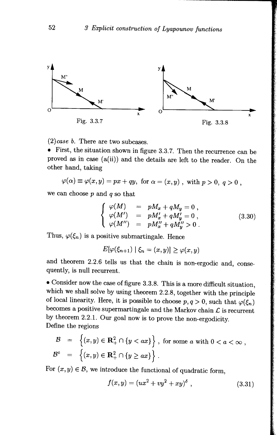
for some ег > 0, thus proving case a(i). We can give a geometrical
illustration of this result on Fig. 3.3.1, where inequalities (3.16) hold, so
that the chain is ergodic.
The cases (b(i)) and (c(i)) are analogous to (a(i)). Indeed, if
Mx > 0 ,	Mx < 0 ,
< My < 0 ,	or < My > 0 ,
k MxMy - MyM’x < 0 ,	MyM” - MXM” < 0 ,
we show that there exist u,v > 0 and w2 < 4uv, such that (3.15) holds,
so that the chain is ergodic in both cases. Fig. 3.3.2, shows the situation
corresponding to (b(i)).
Now we shall prove the non-ergodicity in (a(ii)). Assume that
' Mx < 0,
< My<G,	(3.17)
. MxMy - MyM'x > 0 .
As shown in Fig 3.3.3, there exists a linear function f{x, y) = ax + by,
such that, for all a = (x, y) with ax + by > C, we have
f (a + M(a)) > /(a) + e, for some C, e > 0 ,
and the non-ergodicity immediately follows from theorem 2.2.6.
The proof of the transience in (b(ii)), (c(ii)) and (d) is more difficult.
3.3 Classification of random walks in Z^_
45
In a preliminary step, we shall discuss the principle of local linearity for
random walks with bounded jumps.
Principle of local linearity Let the state space A of a Markov chain
£ be a countable subset of Rw and the function fa , a g A, be the
restriction of some real function f(x) defined on Rw. Assume also
fa >C > —oo and introduce the sets
T>~ = {x : f(x) < c, x e Rw} and T>f = {x : f(x) > e,x € Rw} .
Suppose the jumps of £. are bounded, i.e., for any at A, there exists a
number da such that
|| /3 — a || > da implies that pap = 0, V/3 e A .
If the function /(x) is linear, then it is easy to see that a+M(o) €
if, and only if,
~ fa) <		(3.18)
/зел
Analogously, a + M(a) e 1>да)+е if, and only if,
~ fa)>e 	(3.19)
/Зел
Let now f(x) be arbitrary.
Lemma 3.3.4 If a + M(a) G ’Рда)_5е the condition
inf sup | f(a) — 9?(d) |< e	(3.20)
v seR”
||a-a||<dQ
holds, where inf is taken over all linear functions then inequality
(3.18) is valid.
46	3 Explicit construction of Lyapounov functions
Proof Let ip(x) be a linear function such that
sup |/(a)-<£>(&) |<e .	(3-21)
aeR"
||a-a||<d„
Then we have the decomposition
- /(«))
P
= ^PaP&P - Va) + ^Pc^fp - <pp) + ^PaP&a - A) •	(3.22)
PPP
Using (3.21), we can write
1^ ^PaP^fp ~ Vp) I — e and 1^ \Рар((Ра /а)| — e •
/3	P
Hence
'Yl/Paptvp - <?«) = <p(a + M(af) - 99(a)
P
<	[y>(a + M(a)) - /(a + M(a))]
+[/(a) - 99(a)] + [/(a + M(a)) - /(a)]
<	e + c — 5c = —3e .
Thus, we obtain from (3.22)
^PaptftP) -f(af) < -e .
P&A
The proof of lemma 3.3.4 is concluded.	
Lemma 3.3.5 If a + M(a) € ^да)+5е and the condition
inf sup I /(a) — 99(a) |< e
f aeR"
||a-a||<da
holds, then inequality (3.19) is valid.
The proof of this result mimics completely that of lemma 3.3.4.	
It is natural to call the statement of lemmas 3.3.4 and 3.3.5 the princi-
ple of local linearity. Instead of verifying conditions 3.18 and 3.19, this
principle allows us automatically to use smooth level curves, for a Lya-
pounov function transversal to the one-step mean jump vector field. In
many concrete situations, y>(d) will be the tangent to the level curve at
the point a, in particular when the level curve behaves as ||a||p ,p < 1.
Proof of case (d) Let us consider first the case of bounded jumps. We
begin with a geometrical construction of the function f(x, у),(ж, y) e R^_.
3.3 Classification of random walks in Z^_
47
We draw the quarter-circle L of radius 1, tangent to the axes x and y, as
shown in figure 3.3.4. For all points (x, у) belonging to the quarter-circle
L, we put f(x,y) — 1. Then, by scaling, we define the function f(x,y)
in the whole quarter-plane R^_. More exactly, we put, for (x, y) G. L and
all r > 0,
f(rx, ry) = r .
It is clear that the level curve C corresponding to f(x, у) = c is the circle
of radius c with centre at the point (c, c). So we can apply the principle
of local linearity to the function f. Hence, for any d, e > 0, there exists
T> > 0 such that, for any a e R^_, || a ||> D,
inf sup | /(d) — 92(d) |< c,
v йеН."
||a—a||<d
where inf is taken over all linear functions ip.
Moreover, it appears that all mean jump vectors (except maybe on the
axes, in the particular situation when M' or M" points towards the
origin along its respective axis) in the direction of the increasing values
of /(a). Hence, taking T> such that, for || a ||> T>,
a + M(a) e T>^Q^+5e ,
we obtain, from lemma 3.3.5,
52	~ /(“)) > + 6 , for || а ||> V , a Ox U Oy ,
and the transience in the case (d), with bounded jumps, follows from
theorem 2.2.7.
Let us deal now with the case in which jumps are bounded from below,
48
3 Explicit construction of Lyapounov functions
but not from above. We take the same function /(a) = f(x, y) as above
and consider the two sequences of random variables
Vfe =/(Cfc+i)-/(Cfc) and Zk = Ykl{Yk<B} 
It is easy to verify that, for В sufficiently large, these sequences satisfy
conditions of theorem 2.1.10, for /(Co) sufficiently large. The case (d) is
thus completely proved.
Cases (b(ii)) and (c(ii)) could be proved in an entirely similar way and
so are left as exercises. The proof of theorem 3.3.1 is complete. 
Proof of Theorem 3.3.2 : The transience in the case (a(i)) can be
proved as in the case (a(ii)) of theorem 3.3.1 but using theorem 2.2.7.
(1) Consider first the case (a(ii)). The proof of the non-ergodicity is
then rather simple: it is indeed a direct consequence of theorem 2.2.6,
by using the linear function shown in figure 3.3.5. Let us now prove the
recurrence.
Introduce the following real functions, defined on Z^.:
Q(x, у) = их2 + vy2 + wxy and f(x,y) — log[Q(a:,t/) + 1] ,
where u,v,w are unspecified constants (to be properly chosen later)
satisfying u,v > 0 and 4uv > w2, so that Q(x.y) shall be a positive
semi-definite quadratic form. We have
E[A/] = E[f(x + 0x, у + 0y)] - f(x, y)
— 2T [iog[l + X^u®x +	+ У^х +	+ Q(flr,0y)]j
x[2uE(0x) + wE(f)y)] +y[w£?(0a;) + 2v£?(^)] + E'[Q(0a;,^)]
1 +<?(x,y)
3.3 Classification of random walks in Z^_	49
E[[x(2uOx + wOy) + y(wOx +	+ <?(^x, ^)]2]
2[1 + Q(x,y)]2
+°[ 2 , 2] •	(3.23)
x2 + y2
Let us first assume that
( MxM>-MyM^ = O,
t MyM” - MXM” < 0 .	1	’
Then we choose the constants u, v, w, to satisfy the system
				2uM' + wM'	= 0,		
			<	2uMx + wMy 2vMy + wMx	= o, <0,		(3.25)
				, 2vM" + wM"	< 0.		
It turns out that (3.25) is equivalent to the simpler system							
				wM!y	wMy		
		<	2M£ 2vMy		2MX' 2vM”		(3.26)
				Mx			
Put			w	2MV	и	гМя2	cMv	(3.27)
	V ;	> 0 ,	V	—тг + е, Mx	v	= [jfl -	2MX ’	
Choosing e > 0 sufficiently small, it follows from (3.27) that (3.25) and
(3.26) are satisfied, together with Q(x,y) > 0, V(x,y) . We shall now
estimate
• Assume first у > I, where I is sufficiently large. From the boundedness
of the jumps it follows that
E[Q(0x, 0y)]	< A , for some constant A ,
< x[2uE(dx) + wB(^)] = 0,
y[wE(fix) + 2vE(fiy')] < —efi, for some > 0.
Hence, for I sufficiently large, E(Af(x,y)) < 0 .
• Let now у < I. Then we have
< #[<ЖА)] x^^E^ + ^wuE^Oy'f+w^E^]
[	- 1 + Q(x,y)	2[1 + Q(x,y)]2
, 1 '
+°( 2 , 2 )
X2 + y2
1	11?
=	y)-( —-v)E(ffy]
их2	Zu	y
X*
50
3 Explicit construction of Lyapounov functions
=	- ^-(w2 -4HM)] +о(Л) • (3.28)
UX	Lil	X
Choosing e small in (3.27) and inserting the corresponding v, w, и into
(3.28), we see that w2 — 4uv —> 0, if e —» 0, and
E[Q(0x,0y)] > E[^0x - V^)2] > В > 0 ,
for some В not depending on e. Hence, for sufficiently large x, E(Af) < 0.
Finally, when (3.24) holds, we have been able to construct a function
f fulfilling the conditions of theorem 2.2.1, so that the Markov chain is
recurrent.
It is useful to illustrate the above proof geometrically. The equipo-
tential lines of the function f are the ellipses f(x, у) = C, shown in
figure 3.3.6(a). They are tangent to the vectors M' at the points of the
ж-axis and the vectors M and M" point towards their interior.
The case
( MxMy — MyM^.=0,
I MyM" - MXM” = 0,
could be handled along the same lines, although with additional techni-
cal difficulties. In fact, one can show that the function /(ж, у) increases
as log(x2 + y2), but the level curves would consist of two ellipses, con-
nected by a smooth arc, as depicted in figure 3.3.6(b). To describe the
obstacles in trying to produce a direct approach, as above, we shall
prove the recurrence in a particular case, which requires an additional
(strictly speaking not necessary) assumption, involving a relationship
between second-order quantities.
Choose u. v, w satisfying
v > о w = _2M^	«
v Mx ’ v L Mx J
51
3.3 Classification of random walks in Z^_
For these values of u,v,w, which are compatible with (3.29), we set
Q(x,y) = T2(x,y), where T(x,y) = \/ux — у/vy ,
L(x,y) = ax + by, where a and b are positive constants ,
R(x,y) = Q(x,y) + L(x,y) and /(ж, у) = log[/?(x, у)] .
From now on, we take ||ж + y|| > D, for D > 0 large enough, and it is
important to note that Q is only positive semi-definite. For any function
y(x,y), we introduce the convenient notation
def
Ag(x,y) = Ду = g(x + 0x,y + Oy) — g(x,y) .
Thus we have
Е[ДТ(ж,у)] = 0 and Е[ДТ(х,у)] - а£[0ж] + ЬЕ[0у] .
Hence
Я[Д R(x, у)] = Е[(ДТ(ж,у))2 + ДТ(ж,у)]
and
Е[Д/(х,у)]
2(T2 + L)£[(AT)2 + ДТ] - £[(2ТДТ+ (ДТ)2 + ДЬ)2]
2Д2(ж,у)
-2Т2Е?[(ДТ)2-ДЬ]+2Т£;[(ДТ)2+ДТ]-4Т£;[ДТ(ДЬ+(ДТ)2)]
2Д2(ж,у)
б2 , г/ДЯМ
2Я2(х,у) + °Н( R ) Р ’
(We have omitted the argument (a;, y) in most of the functions.) It turns
out that the right-hand side of the above equation (in which 62 denotes
a positive quantity uniformly bounded with respect to (ж,у)) can be
rendered negative outside a compact set, i.e. for D large enough, if we
assume the condition
. f ГЕ[(ДТ')2] £[(ДТ")2] 1	£[(ДТ2)]
t ’ M" J > Mx ’
(which is parasitic in the sense that it is not needed in the statement of
the theorem) with an obvious notation (/ refers to the Ox-axis, // to the
Оу-axis and no prime symbol means the interior of the quarter-plane).
Geometrically, the level curves are here parabolas. The case (a(ii)) is
finished.
52
3 Explicit construction of Lyapounov functions
(2)	case b. There are two subcases.
•	First, the situation shown in figure 3.3.7. Then the recurrence can be
proved as in case (a(ii)) and the details are left to the reader. On the
other hand, taking
95(0) = ip(x, y) = px + qy, for a = (ж, y) , with p > 0, q > 0 ,
we can choose p and q so that
= pMx + qMv = 0 ,
V(M') = PM!. + qM'=0,	(3.30)
= PM!f + qM^>0.
Thus, </?(£n) is a positive submartingale. Hence
£M£n+i) I Cn = (ж,у)] > <p(x,y)
and theorem 2.2.6 tells us that the chain is non-ergodic and, conse-
quently, is null recurrent.
•	Consider now the case of figure 3.3.8. This is a more difficult situation,
which we shall solve by using theorem 2.2.8, together with the principle
of local linearity. Here, it is possible to choose p,q > 0, such that <p(£n)
becomes a positive supermartingale and the Markov chain £ is recurrent
by theorem 2.2.1. Our goal now is to prove the non-ergodicity.
Define the regions
В = |(ж, у) e П {у < аж}I , for some a with 0 < а < 00 ,
Bc =	.
For (ж, у) e В, we introduce the functional of quadratic form,
/(ж, у) = (аж2 + vy'2 + жу)г ,	(3.31)
3.3 Classification of random walks in Z^_	53
where и >0, v >0, 0 < 5 < 1, and recall the notation
Q(x, у) = их2 + vy2 + xy,
&Q(x,y) = Q(x + 0x,y + 0y) — Q(x,y)	(3.32)
= ив2 + vO2 + вхву + (у + 2их)вх + (ж + 2vy)0y .
Our purpose is to estimate the quantity
H(x,y> = W(£n+i)-/(£n)/£n = (*,y)]	f333)
= E[(Q(x, y) + AQ(x, y))6 - Qs(x, у)] .
Lemma 3.3.6 There exist 8, 0 < S < 1 and a constant D such that
H(x,y) = SQt-^yfiElAQ^yfi) + (8- 1)0(1) + o(l)]	(3.34)
for all (x,y), such that (a;2 +y2) > D2, where, as usual, |О(г)| < K\z\
and o(l) tends to zero when D —» oo.
Proof : By Taylor’s formula, we have
Я(г,у) = 8E[AQ{x,y)(Q(x,y) + y(x,y)AQ(x,y))6-1]
= 5Q5-1(x,y){E[AQ(x,y)] + ф(х,у)],
where у(х,у) is a random variable such that 0 < 7(2, y) < 1.
Note that Q + 7Д6? > 0 and
L \	У)	'	J .
It suffices to prove V>(a;,y) = (8 — 1)0(1) + o(l). In fact, the re-
sult of the lemma is immediate from the definition (3.33), after using
||(1 + г)г-1 — 1|| — (8 - l)O(z), for z sufficiently small, since, from the
boundedness of the jumps,
< A < °° ’ (°’°) '
Q{x,y)
The lemma is proved.	
Let us continue the proof of the theorem. From (3.33), it follows that
E[AQ(x,y)]
= xE[2uOx +	+ yE[2v0y + 0X] + E[Q(0x, 0^)]	(3.36)
= x(2uE(0x) + Е(ОуУ) + y(2vE(0y) + E(0X))
uE(O2x)+vE(0y}2 + E(9x0y).
54	3 Explicit construction of Lyapounov functions
Now we shall find T>, u, v > 0, such that
Е[Д(?(ж, ?/)] > 0 , for (ж, у) e В and (ж2 + у2) > D2 .
Choose
' u = Му _ Му
' 2мх '	(з.з?)
, V = ~2М~у~е'
with е sufficiently small. Then we distinguish two regions:
•	First, the set {(ж,у) : x > 0, у > 0} . Then (3.36) yields
Е[Д<Э(ж,у)] = x[-^-Mx + My]+y[-Mx-2eMy + Mx]
4-uAx T vXy + R
= —2cyA/y + uXx T vXy T R ,	(3.38)
where
Xx = E(6X}2, Ху = Е{ву)2, R — E(0xf)y) .
•	Secondly, the set {(ж, у) : ж > 0 , у = 0} . We obtain now
£/[Д<3(ж, у)] = uX'x + vXy + R',	(3.39)
where X’x = E(0x)2, X'y = E(0y)2,R' = E(0x9y).
Setting z = —	= tan 93 > 0, we get
«Ai + vAi + R' =	+ И W + E(W _ e>-
=	|PB(ft,)2 + 2г B(ftft) + B(ft)2) - eA^ .
It follows from Schwartz’s inequality (Е(0хву))2 < E(02) E(Q2), that
z2E№) + 2zE(ex9y) + E(02) >0.	(3.40)
Thus, using (3.38), (3.39), (3.40) and the assumption Mv < 0 , Mx > 0,
we can choose e > 0, such that
£/[Д<2(ж,у)] >0, for ж > 0, у > 0 .
Moreover, Е,[Д<5(ж, у)] grows as a linear function of y.
In figure 3.3.9, we show the level curve Q(x, y) = c. For (ж, у) ё В, this
curve is an arc of an ellipse. For (ж,у) e Bc, we draw the circle tangent
3.3 Classification of random walks in Z^_
55
to the vertical axis x = 0, which is a smooth continuation of the curve
Q(x, y) = c. The union of these two curves will be denoted by L.
We have shown that for (ж,у) ,x > 0, у > 0, the quantity E[AQ(x, y)]
grows linearly in y. So, for sufficiently large c, the vector M, drawn from
the intersection point of L and of the straight line у = ax, is oriented in
the direction of the increasing values of Q(x, y) (see figure 3.3.9) and,
therefore, also looks on the same side of L as the points belonging to
the region Be.
Let us construct now the function f defined as follows:
/(*,У)	= c, for(x,y)eL,	<3
f(rx,ry) — r2c , for (x, y) G L , r > 1 .
We will prove the existence of ё, 0 < ё < 1 and T>, such that
E[fs{x-\-0x,y-\-0yf\-fs{x,y) >0, for (x,y)eZ2 : x2+y2 >D2. (3.42)
First, we will show that, for sufficiently large T> and (x, y) : x2+y2 >D2,
E\f(x + ^,?/ + A»)] - f(x,y) > 0 .	(3.43)
For (ж,у) e В ,f(x,y) = Q(x,y) and (3.43) has already been proved.
For (z,y) € Be, inequality (3.43) follows easily from the principle of
local linearity, which yields
E[f1^(x^9x,y + ey)]-f^2(x,y) >0, for(^,y)eBc. (3.44)
Now using (3.44) and Jensen’s inequality, we can write
56	3 Explicit construction of Lyapounov functions
E[fs( x + OX +y + 0j,)] - fs(x,y) > 0 ,
for all ё, < ё < 1 , (ж, у) e Bc, and x2 + у 2 > P2, (3.45)
where T> is chosen sufficiently large.
To prove (3.42), if suffices now to apply lemma 3.3.6. In fact (3.34)
shows that, taking ё close to 1, the sign of H(x,y) is the same as that
of E[AQ(x, y)]. But we have already shown that
E[/^Q{x, у)] > 0 , for (ж, у) € В and ж2 + у2 > Р2, for some V .
We have finally proved that there exist T> > 0 and | < ё < 1, such that
(3.42) holds, for all (ж,у) e Z2. n {ж2 + у2 > P2}.
Now we are in a position to apply theorem 2.2.8, remembering that
we are dealing with the case of figure 3.3.8. Then there exist p, q > 0,
such that the function where </>(ж,у) =px + qy is a positive su-
permartingale, i.e. condition (iv)(b) of theorem 2.2.8 holds. Since the
jumps are bounded, condition (iv)(c) also holds. The following argument
shows that condition (ii) also holds. Indeed, for any fixed u, v,p, q > 0,
there exists d > 0, such that
их2 + vy2 + xy < d(px + qy)2 ,
whence,
/(ж,у) < di((p(x,y))6 , for some dj > 0 .
Since we have shown above that conditions (i) and (iii) were also fulfilled,
null recurrence follows from theorem 2.2.8.
This concludes the proof of case (b) and of theorem 3.3.2.	
3.4 Zero drifts
We consider the Markov chain £ introduced in the previous section, but
satisfying the stronger
Condition В (Second moment condition)
E[\\ 0„+i II2 /Cn = (M)] < В < oo ,V(fc,Z) € Z2+ .
Until recently nothing was precisely known for the case M = 0. In
fact, this problem, in many respects, is of a very different nature. In
particular, intuition does not provide us with any evidence that the
random walk could be ergodic, when M = 0.
There exist at least four methods which would allow us to solve some
particular cases of the problem:
3.4 Zero drifts
57
(1)	The analytic approach, as in [FI79, Mal70, Nau89]. Now there
are only some preliminary results into this direction.
(2)	The semi-analytic approach, by using well known explicit results
about one-dimensional random walks. For instance, when the
random walk inside the quarter-plane is the composition of two
independent random walks along both axes, then it is easy to
show that the mean time to reach the boundary is infinite, in
which case, for any values of the parameters the chain is
not ergodic if M = 0.
(3)	The method of Lyapounov functions. This seems to be the most
general approach and we will use it here.
(4)	The approach via diffusion processes. There was a lot of work
done on the same problems for diffusion processes in ВД. (see
[RW88, VW85, Wil85]). Their intimate connections with the dis-
crete case will be discussed in a forthcoming monograph.
There is a crucial difference between the cases M ± 0 and M = 0: in-
deed, the case M 0 is in a sense locally linear and M = 0 is locally
quadratic. The local second-order effects are well caught by functionals
of quadratic Lyapounov functions.
For M = 0, we will obtain the ergodicity conditions in terms of the
second moments and the covariance of the one-step jumps inside Z^_,
' i pij , Ay = j pij , R = ijpij ,
ij	ij	ij
and of the angles, anticlockwise oriented, фх,фу shown on figure 3.4.1.
Here фх is the angle between M' and the negative ж-axis, фу is the angle
between M" and the negative у-axis. Thus, if фх тг/2 and фу =4 тг/2,
58	3 Explicit construction of Lyapounov functions
then
M'	M"
^Фх = ~ЩЛ™Фу = ~М^
Theorem 3.4.1
(i)	If фх > J or фу >	, then the random walk L is not ergodic.
(ii)	If фх < and фу < %, then the random walk £ is
•	ergodic if
M' M"
Xx tan фх-\~Ху tan фу+^R = —Xx —Xy +27? < 0; (3.46)
•	non-ergodic if
Xx tan фх + Xv tan фу + 2R > 0 .	(3-47)
(iii)	If (3.47) holds together with фх + фу < then the random walk
is null recurrent.
Remark 1 It follows easily from the statement of the theorem that the
mean first entrance time of £ into the boundary, when starting
from some arbitrary point a > 0 at finite distance, is finite (resp.
infinite) if R < 0 (resp. R > 0), since in this case the vectors M'
and M" can be properly chosen to satisfy (3.46) (resp. (3.47)).
Remark 2 It is clear from the formulation of the theorem that we do
not consider the limiting situation
Xx tan фх + Xy tan фу + 2R = 0 ,
which would impose further assumptions of third order.
Proof We introduce the linear function <p : R'( —» R+, such that, for
any 7 = (x,y),
¥>(7) = T’G’h У) = Px + ЧУ > P > °, 9 > P + 4 > ° 
Lemma 3.4.2 Let p,q>0,p+q>0, be such that the vectors M' and
M" have the following properties (see figure 3.4-2)
( <р(М')=рМ'г + чЩ>0,
I <^(M")	+	>0 .	1 • >
Then, for all (x,y) G Z^_,(x,y)	(0,0),
W(£n+i)/£n = (x,y)] > <p(x,y) ,	(3.49)
i.e. ip(£n) is a positive submartingale.
3.4 Zero drifts
59
Proof Immediate by using the linearity of 9? and the fact that (Mx, My)
= (0,0), for x,y > 0.	
It is simple to check that the conditions of lemma 3.4.2 hold in the case
(i) of theorem 3.4.1. They are also valid when
я 7Г	я
Фх < Фу < Фх + фу > —
which yields
- M'M” < 0 .	(3.50)
Lemma 3.4.3 If the random walk C satisfies the conditions of lemma
3.4.3, then £, is not ergodic.
Proof This is a direct consequence of theorem 2.2.6. It is worth men-
tioning that this result holds under the mere assumption, weaker than
condition B,
E(\\ #n+i II /Сп = (jcy)) < C < 00.	(3.51)
Consider now the case фх + фу < -к/Ч.
Then we have the property opposite to that of lemma 3.4.2, since the vec-
tors M' and M" point now toward the interior of the simplex bounded
by the two positive axes and the line px + qy = C. (see figure 3.4.3).
This means that there exist p > 0 and q > 0, such that the linear func-
tion </?(£n) is now a positive super mart ingale. Hence, the random walk
C is recurrent. Our goal is to distinguish between positive and null
recurrence. To that end, we introduce again the quadratic form
Q(x, y) = (ux2 + vy2 + xy) , (x, y) 6 Z2. ,
60
3 Explicit construction of Lyapounov functions
where и and v are positive.
As in the preceding section, the game consists in adjusting и and v to
satisfy the conditions of theorem 2.2.8. Define, for the sake of brevity,
д<5(ж,у) = Q(,x + 0x,y + Oy) — Q(x,y)
=	+ v()y + 0x9y + (у + 2ыж)0ж + (ж + 2vy)f)y .
(3.52)
Put
K(x,y) = E[Q(e„+1)	= (oi •
Then
K(x,y) = xE[2u6x + 0y\ + yE{2vOv + 0Ж] + E[Q(9x,0y)] .	(3.53)
Since E[Q(9X, 0y)] = 0(1), V(x,y) e Z^_, we get from (3.53), after taking
into account the boundary conditions on the axes,
K(x,y) = <
Xxu + Xyv + R ,
y(2uM"+0+0(1),
x(2«M'+M') + O(l) ,
(x,y) > 0 ,
x = 0, у > 0 ,
x > 0, у = 0 .
Thus, for some e > 0 and some finite subset E G Z^_, we have
K(x,y) < —e, V(x,y) E ,
provided that the following system can be satisfied, for some u,v > 0,:
Xxu + Xyv + R <C 0 ,
2uM' + M’
у
2vM" + M"
у
0 .
(3.54)
The inequalities Л7" > О, M” < 0, My > 0, M'x < 0, show at once that
(3.54) can be satisfied if (3.46) holds, that is
M' M"
Then the remaining conditions of Foster’s criterion (theorem 2.2.3) are
clearly fulfilled and the random walk is ergodic.
In the other case, when (3.47) holds, i.e.
МУ x M”
M'x y M"
у
34 Zero drifts
61
one can find u, v > 0, so that
Axrt T Ay о -h R > 0 ,
1uM'x + M^ > 0 ,
2vM" + M" > 0 .
у
(3.55)
Hence, for some finite subset £cZ^_, we have K(x, y) >0, for (x,y)^E.
Consequently, when (3.47) is satisfied, there exist two functions, namely
the quadratic form Q(x,y) and the linear function </>(a;,y), such that,
assuming ipx + <py < all the conditions of theorem 2.2.8 hold (taking
a. = 2 in the statement of this theorem). This shows the null recurrence
part of theorem 3.4.1, which is, by the way, completely proved. 
The general conditions allowing for separation between transience and
recurrence have been obtained in [AFM]. We simply quote them here,
without proof:
Theorem 3.4.4 The random walk is
(i) recurrent if
(ii) transient if
Problems
(1) Find the complete classification in the case
(2) Classify random walks in , when Мрдз} = 0. In particular
(i) Are there ergodic cases?
(ii) When do the one-dimensional faces play no role in the classi-
fication?
62
3 Explicit construction of Lyapounov functions
3.5 Jackson networks
Jackson networks are now classical models for communication networks.
Jackson [Jac63] obtained the famous product form for their stationary
probabilities. Sufficient ergodicity conditions follow from this product
form. The proof of the necessity of these conditions was obtained by
many authors [Afa87, Bor86, Fos89, Pod85]. From the general theory
of countable Markov chains, it follows then that the n-step transition
probabilities converge to stationary probabilities when n —+ oo. But not
much was known about the rate of this convergence. The only result is
exponential convergence under some smallness assumptions in [KKR88].
Here we consider basic Markovian Jackson networks, i.e. with Poisson
arrivals and exponential service times. In this case, these systems are
equivalent to a class of random walks in Z^, where N is the number
of nodes in a network. The main result of this section is that we give
an explicit construction of Lyapounov functions. They are either almost
linear in the terminology of [Mal72a], or just piecewise linear. Later
on, in chapter 7, we again use this construction to show exponential
convergence to the steady state (whenever it exits) and also analyticity
results. Let us emphasize that we never use Jackson’s product form in
the proofs.
Ergodicity conditions for Jackson networks
Here we recall some well known facts and prove a useful geometric
lemma. We consider an open Jackson network with N nodes. Let
be the length of the queue at the г-th node at time t. We re-
strict ourselves here to the simplest assumptions: independent Poisson
inputs with parameter Aj > 0 for any node г, exponential service times
with parameters /q > 0 and FIFO service discipline. After a customer
completes service at the г-th node, he is immediately transferred with
probability pij to the end of the queue at node j, j = 1,.. ,,N, and,
with probability
n
PiO = 1 - ^Pij ,
7=1
he leaves the network. It will be convenient (although strictly not nec-
essary) to assume рц = 0, for all i.
In other words, we consider a continuous-time random walk L on Z^
with transition intensities Xap, from the state a = (a1,..., aw) to the
3.5 Jackson networks
63
state /3 = (/31,..., flN), where
Poi — ^i ,
Pio = Pi PiO i
. Pij — Pi Pij >
Here ej denotes the vector
if (3 — a = a,
if (3 — a = —ei
if (3 - a = -e< + ej , for 1 < i, j < N .
(3.56)
(0,..., 0,1,0,..., 0), having its г-th coordi-
^a[3 — *
nate equal to 1. It is convenient to denote the zero vector by cq. We
recall now Jackson’s equations. Assuming a stationary regime, we de-
note by Vj the mean number of customers visiting node j and coming
from the outside world or from the other nodes during a unit time inter-
val. Using the law of large numbers, Jackson wrote the following system
of equations (we call it Jackson’s system):
N
Vj ~ \j “к v Vi Pij , j = 1, ..., N .	(3.57)
i=l
Let us note that these equations can be solved by the iteration scheme
= + ’ (3-58)
fc=l 1 = 1
where
|| pff ||= Pfe , P =|| Pij \\i,j=0,l,...,N ,
and we put pOi = 0, i / 0, poo = 1.
The series in the right-hand side of (3.58) converges if
pg)<C'(l-6)fe,	(3.59)
for some e > 0, C > 0. For this, it is necessary and sufficient to assume
the classical
Condition J : Starting from any state, the Markov chain with N + 1
states 0,1,..., N, defined by the stochastic matrix P, reaches 0 with a
positive probability (a.s.).
Thus, we can rewrite (3.58) as
Vj = Aj +]TAi mij ,
where mJ is the mean number of hittings of j, starting from i, in this
finite-state Markov chain. Then, it is immediate to see that the solution
of (3.57) is unique.
64
3 Explicit construction of Lyapounov functions
Theorem 3.5.1 (Jackson). The network is ergodic if, and only if,
i/j < p,j for all j = 1,... ,N .
We will give a new proof of this theorem by means of a geometrical
approach, which is the key point of the study. Later on we also make
use of several results for discrete time Markov chains, borrowed from
chapter 2. It is worth noting that all of them could be easily rewritten
for the continuous time case. To avoid this rewriting, we introduce the
following discrete time random walk L in . Its transition probabilities
are taken to be
Pa(3 ~	,	(3.60)
for some constants wa satisfying
0 < wa <
/3
For instance, the choice
Wa = (У^ Aqff)"1
/3
yields the natural embedded chain. In fact, it will be more convenient
to choose
wa = w < min (VA^)-1.	(3.61)
a •
/3
The stationary probabilities 7tq of La and those TrQ of L are the same,
i.e.
7Ta = 7Tq,	(3.62)
so that L is ergodic if, and only if, L is ergodic.
We shall consider the discrete time homogeneous Markov chain L, which
is assumed to be irreducible and aperiodic, unless otherwise stated. The
notation of section 3.2 will be in force. In particular, we recall the
definition of a face. For any Л С {1,2,..., W}, the face Вл of is the
set
_ВЛ = {(ri,..., гдг) :	> 0, i € A ; r, = 0, i A} .
Obviously the random walk L, which is equivalent to the Jackson net-
work under study, does meet conditions Ao and Ai of section 3.2. Here
condition Ai is even stronger, since
ZW = °, for || a
3.5 Jackson networks
65
The first vector field on R^ is constant on any BA and is equal to
Мд = M(a) , a e A .
For the Markov chain L, we have the crucial property
Мл = fo + ^fi ,	(3.63)
i£A
where
N
fi=w	+ ej) , for i = 0,..., N .	(3.64)
j=o
So, ft represents the contribution of the transition from the г-th node
(including the virtual 0-node). On the other hand, it is clear that the
2N mean jump vectors Мл are the vertices of a parallelepiped which we
denote by chi . Its initial point can be taken as fo and the edges drawn
from this point are /i,...,/дг. This parallelepiped may be degenerate
if the vectors /i, • • , /w are linearly dependent. We shall use below the
following combinatorial criterion of ergodicity, equivalent to Jackson’s
one.
Lemma 3.5.2 The Jackson network is ergodic if, and only if, <9П is not
degenerate and the point 0 € RA is one of its interior points. Moreover,
if the origin does not belong to <911, then this chain is transient.
Proof Consider the following system of equations, with respect to
ci,..., едг:
/о + ci /i +  • • + ejv fw — 0 .
(3.65)
Note that <911 is not degenerate if, and only if, this system is not de-
generate. In this case, (3.65) has a unique solution and 0 is an internal
point of <9П if, and only if, 0 < a < 1, for i — 1,..., N. Inserting (3.56),
(3.64) into (3.65), we get
N
° = fo +
J=1
N	NN
'У ' \)ej 'f	tHPij Gi + Cj )
j=l	«=1	j=0
NN	N
У? \jej + У? [~ei + y^Pv'Cj]
1 = 1	i=l	j=0
N	N	NN
У7 A j e3 ~ У, ejhj ej +	'/Pij Gj
j = l	j=l	i=l j~0
66
3 Explicit construction of Lyapounov functions
N	N
=	~ 6 J Mj "I" ei Pi Pij)ej ,
j=l	i=l
which coincides with (3.57) for c,; = pi = — .
Mi
Thus, when 0 is an interior point of <9П and <9П is not degenerate, the
ergodicity follows directly from Jackson’s explicit formulas for the sta-
tionary probabilities but later we shall prove it without using Jackson’s
results.
Let now 0 lie on the boundary of <911 (this includes the case of a degener-
ate «9П, when <911 coincides with its boundary). Assume first that <911 is
not degenerate. Then there exists a hyperplane £ of dimension N — 1
in R7V, such that 0 e £ and <911 belongs to the closure of one of the two
half-spaces defined by £. Denote this closure by £+ and consider the
straight line I, passing through 0 and perpendicular to £. Let x be the
coordinate on I which is positive on £+. For any point a e R^, let f(a')
be the value of the x-coordinate of the orthogonal projection of a onto
I. Then, since all the MA’s belong to £+, it follows that
— /(a) > 0 , /(a) > 0 for an infinite number of a € Z^.
0
Consider the sequence of random variables Co,Ci>- • • constituting the
chain L, and the corresponding sequence /(Ct)- Let r be the time of
first visit of Ct to the set {a : f(pi) < 0} and pft) = /(Селт)- We have
E[r?t+i/Ct,---,Co]-Pt >0.
It is then well known that Et = oo, which proves the non-ergodicity by
using theorem 2.1.3.
For a degenerate <9П, the proof is the same and, with regard to the
transience, we have, for some e > 0,
^2pQp/(/?) - /(<a) > e , /(o) > 0 for an infinite number of a e Z^ .
h
Then the results follows from theorems 2.1.9 and 2.2.7. The lemma 3.5.2
is proved.	
Geometric construction
Let us recall that <9П is the convex hull of the points Мл (the ends of
3.5 Jackson networks
67
the vectors Мл having their origin at 0).
Let a be a fixed point of Rw. We define
N
Г = Г“ = {а + £2 А Л : > 0} .
i=l
Hence, Г represents a multidimensional cone (with vertex a) generated
by the vectors fi. It will be convenient to put
Гл = {а + £2 А Л >0},ЛС{1,...^},
г (ЕЛ
so that
pa __pa
1 = 1 {l.-JV} *
We define the surface f ° of Га by
fo = U Гл •
A0{1,...JV}
Whenever a = fо , we shall simply write Г, Гл, fA , etc.
Scaling : We shall denote by аГ, аГ, аГл, a > 1, the respective
scaled geometrical objects, with vertex aa.
Lemma 3.5.3 The set
П (аГ)
is compact for any a > 1.
Proof Let us first note that, if this set is compact for some a, then it is
compact for any a. Hence we can choose a in a convenient way, putting
for instance
a = fo •
We now remark that the ray fo + fkfi, 0 < Д < oo , intersects the face
Xi = 0 of R^ , since fi has its ej-component negative and the others are
positive. From this, the required compactness is readily seen. In fact,
we can rewrite
N	N
fo + ^ A fi=w^2 Ci Ci ,	(3.66)
i=l	i=l
with
N
Cj =	+ ^2 Qi Fv — ai >
1
68	3 Explicit construction of Lyapounov functions
after having set
aj = hj Pj 
Choosing now a ray Oj = tr,, r, > 0, t > 0, we see that its intersection
with is an interval of finite length, since
N
= E Aj +1 (22 ~рго> _ 22r0 = 22 - * 22гда° ’
j=i
and the coefficient of t is negative. The lemma is proved	
Let us now consider some Гд, with | A | = TV — 1. This defines an affine
hyperplane H/\ (of dimension N — 1) in Rw, which subdivides RN into
2 half-spaces Гд,Гд. We denote by Гд the half-space containing Г.
Lemma 3.5.4 We assume that 0 lies inside ЭП and consider an arbi-
trary Гд with I Л I = N — 1. Then any vector	, such that
A' £ A ,	(3.67)
which has its initial point inl\, lies entirely in Гд.
Proof Let us first show that Мцhas this property for all Гд,
such that I Л I = N - 1. For this, choose a —	Let us note
that 0 e dll if, and only if, 0 € {— cUI}. Then the vector	with
initial point a (which belongs to all Г“ simultaneously), has 0 as its final
point and is thus contained in Гд.
Take now e.g. A = {2,..., ;V} and any A' such that 1 g A'. Choosing
again
a = -ЛГ{1...ft} = -fo - J2 Л - 52 fi ,
i€A' i=40,
we see that the point
b = a + 52 fi
belongs to Гд and b + Мл> = 0 G Г/. The lemma is proved	
Lemma 3.5.5 Ifalies strictly inside R^, thenVf, for any \ h \ = N — 1,
has the property
ППЖ = 50 , for hf Ch,
where В denotes the closure of B.
3.5 Jackson networks
69
Proof Let again Л = {2,..., /V}. Then
N
n = {« + £/W-
J=2
But the vector
N	N
a + У у Pj fj= У^1Ci ei,
j=2	i=l
since Ci is strictly positive, cannot belong to the region Вл', where the
first coordinate is zero. The lemma is proved.	
Let us introduce now the following function, with domain RA’:
f : x —► fx = a, for x G of .	(3.68)
This piecewise linear function, obtained by scaling, is our main Lya-
pounov function, as will be shown below. We shall in fact propose two
constructions, which are both useful for future generalizations.
First construction
This construction uses smoothing, which is in fact equivalent to the prin-
ciple of almost linearity, presented in section 3.3.
Lemma 3.5.6 For any e > 0, there exists a smooth convex closed hy-
persurface <91I(c), homeomorphic to the boundary <ЭП о/П such that, for
any x G <9П(б),
p(x, <ЭП) < e ,
and, for any у G <ЭП,
р(у,<ЭП(е)) < e ,
p being an arbitrary metric.
For the proof, it is sufficient to consider the unit cube in R'v and then
to use a linear transformation. For this unit cube, one can proceed by
induction, in constructing at each step a cylinder smoothed at the ends.
Take the intersection of ЭП(е) with a neighbourhood of the vertex a = fa.
We extend it by linearity to get a hypersurface Г(е), smooth and convex,
such that the pairs
(fAR* fna(R^))
70	3 Explicit construction of Lyapounov functions
and
(Г(е)ПН" Г(£)ПЭ(^))
are homeomorphic. Moreover,
p(x, f (e)) < e, for any x G f D R+ ,
p{y, f) < 6, for any у G f (б) П R^ .
Then, by scaling, we define the following Lyapounov function:
f : x —> fx = a , x e ctf (б) .	(3.69)
Let us fix some r > 0 sufficiently large and an arbitrary x G аГ(б). Let
O(x) = O{r,x) be a cube with sides of length r, centred at x. Then
there exist linear functions gx(j on Rw such that
sup sup | fy - gx(y) |-»0 for a oo .
xC-af’(e) V&O(x)
By geometric construction, when 0 lies inside П, we have, for all suffi-
ciently large x G and for some <5 > 0,
fx+Mfx) ~ fx <	& 
From the last two formulas, it follows that, for some <$ i > 0 and for all
x except for a finite set, we have
'jPxyfy ~ fx < — ^1 •
У
This yields the following (as announced, we have used the principle of
almost- linearity)
Theorem 3.5.7 If О lies inside ЭП, then the function f, defined by
(3.69), satisfies the conditions of theorem 2.2.3, so that the Jackson
network is ergodic.
Second construction
In this construction, we shall use the Lyapounov function (3.68) together
with theorem 2.2.4, for integer-valued functions fc(x) = k, with к taken
sufficiently large
Theorem 3.5.8 Let us consider a Jackson network such that 0 G ЭП,
and choose the function fx as in (3.68), with the point a lying inside
R^. Then, for this Lyapounov function, and Л;(ж) = к sufficiently large,
3.5 Jackson networks
71
the conditions of theorem 2.2. f are satisfied and the Jackson network is
ergodic.
Proof Let us fix a constant d, representing the maximal length of a
jump, for some metric p in Rw. In our case, d = 1 for the metric
p(z,j/) = maxlzi - yi\ ,
г
where e.g. x = (a;1, ...,xN).
Lemma 3.5.9 Let us fix e > 0 sufficiently small. There exists po > 0
such that, for any x g , with
p = p(a:,5R^) > po ,
and for any к such that
po < kd = к < p ,
we have
£>$ fy - fx < -€ •	(3.70)
у
Proof For any Л, |Л| = N—1, let us consider a new function /л : x —► fff
= a, for x belonging to the hyperplane аЯл generated by аГл. Con-
sider the evolution of the random walk after к steps, assuming it started
from x. That is
x = £o, £1, • • •	
Then the sequence
M /Л rA
•Чо ’ *41 ’ ’ ’ ’ ’ *Чк-1
is a supermartingale satisfying, for some e' > 0,
since	is directed to the corresponding side of the hyperplane
аНл. Thus, by theorem 2.1.7, we can find constants Сл, 5д, ел > 0,
such that
- fx < -кел ,	(3.71)
with probability 1 — Сл е~к£л. Hence, for po chosen sufficiently large,
(3.71) takes place for all Л, with probability
1 - C e~6k ,
72	3 Explicit construction of Lyapounov functions
for some constants C, 8 > 0. Using the boundedness of jumps and
the fact that the function f grows linearly with a, we immediately get
(3.70), for some e > 0.
The lemma is proved.	
Lemma 3.5.10 Again choose e > 0 sufficiently small and i e 1,..., N.
Then there exist pi > 0 such that, for any x € Z^ with
p = max р(.т,Вл) > pi ,	(3.72)
Л:г^Л
and for any к such that
Pi < kd = к < p ,
we have
fy-f*<-£-	(3.73)
у
Proof We repeat the proof of lemma 3.5.9, using the geometrical con-
struction, as the mean jump vectors point in a suitable direction, from
any point which the random walk, starting from x, can possibly visit
during p — 1 steps. The lemma is proved.	
To prove the theorem, we introduce the quantity
p = max Pi .
0<i<N
Then, for any point x lying outside a (p+l ^neighbourhood of the origin,
in our special metric, we put
fc(.r) = к = p
and note that, for any such point, there exists i such that, for Л =
{1,... ,N} - {i}, inequalities (3.72) and (3.73) hold. The proof of the-
orem 3.5.8 is concluded.	
3.6 Asymptotically small drifts
Let us consider a discrete time MC {Xn}, with state space Z+ and
satisfying the following moment condition:
sup E[| Xn+1 - Xn |2+б /Xn\ < c<oo,
n>0
a.s., for some e > 0, c > 0
(3-74)
3.6 Asymptotically small drifts	73
Let us define for x e Z+ and i = 1,2,...
/хДх) = jE?[(A„+i - Хп)г/Хп = x]	(3.75)
From the condition (3.74), it follows that
sup /12(x) < oo and sup pt(x') < oo .
a?GZ_|_	x£Z-|-
The next theorem, proved in [AIM], generalizes results obtained by Lam-
perti [Lam60].
Theorem 3.	6.1 The following classification holds:
(i)	If there exists a number В such that
Pi(x) <	, forx > В ,	(3.76)
Lx
then {Xn} is recurrent.
(ii)	If instead, for some 0 > 1,
Ml(z) >	for x > В ,	(3.77)
Zx
then {Xn} is transient.
(iii)	If
/ii(x) > —	, forx > В ,	(3.78)
2x
then {An} is non-ergodic.
(iv)	If for some 0 > 1
/zi(x) <	; forx>B,	(3.79)
Lx
then {Xn} is ergodic.
Remark The transience and recurrence parts of this theorem are due to
Lamperti [Lam60]. Non-ergodicity and ergodicity can be proved using
theorem 2.2.8. These results, and also the following one (more precise),
are stated without the proofs, which can be found in [AIM].
We define recursively
logx = log^\x), log(logx) = log*-2-1 x, ..., log(fc\x)
= log(log(fc-1) x),.. .etc .
74	3 Explicit construction of Lyapounov functions
Theorem 3.	6.2
(i)	If for some к € Z± there exists a number В such that, forx > B,
M M > _^(£)	М2 (ж)________М2 (ж)___________
2x 2x\ogx 2x logslog(2\a:)
------,	(3.80)
then {An} is non-ergodic.
(ii)	If, for some k, for some 0 > 1 and for x > B,
..	. Мг(ж) Мг(я:)
ZXl (X I	' •
2x 2s logs
м2 И_______________W*)	z3 81)
2snp=1iog(p)(s) ’
then {An} is ergodic.
Theorem 3.6.1 could be used as a classification criterion in multidimen-
sional zero drift situations. The algorithm might be as follows: find a
family of Lyapounov functions f(a, a), where a 6 A is the state space
of the MC and a is a real vector parameter, satisfying two conditions:
(i) a is small and for a = 0 f is a linear function;
(ii) f(a; a) is a super- (or sub-) martingale with asymptotically small
drift. After this we could just use the theorem above mentioned.
This way might be a more direct alternative approach to section
3.4.
An example of such a theorem is the following result [Lam60], which we
state now.
Let An e R+ be a real nonnegative process (not necessarily a Markov
process), satisfying
£[| An и - An |2+e /A„_!, An_2,...] < C < oo ,
limsupn^oo A„ = oo , a.s.	' ' '
We define
f m(x) = ess sup E[A„+1-An | A„=a;,A„_1,...,Ao],
} U(x) = esssup£;[(An+i-An)2 | An=x,X„_i,...,A0],	’
where the sup is taken over n and over the values of {Xi,i < n — 1}.
Similarly, pfx) and yfx) are defined by replacing sup by inf in (3.83).
The finiteness of and v follows from (3.83), but, as an additional
assumption, v(x) is supposed to be bounded away from 0, to avoid trivial
situations.
3.6 Asymptotically small drifts
75
Theorem 3.6.3 Let a non-negative stochastic process {Xn} satisfy
(3.83) and
FQimsupAn = oo) = 1 ,	(3.84)
n—>oo
and, for all large x,
/7(ж) <	+ О(ж'~1-'5), 8 > 0 .	(3.85)
2x
Then {Xn} recurrent. If instead, for some в > 1,
m(*) >	(3.86)
for all large x, then {Xn} is transient.
Lamperti [Lam60] applied this theorem to multidimensional random
walks without boundaries and with asymptotically zero (or constant)
drifts. Assume that
are random vectors forming a Markov process, with the transition prob-
ability function
F(y1,...,t/s;x) = P(X«1-X« <Vi, г = 1,..s/Xn = x) , (3.87)
independently of n. For simplicity in the proofs, Lamperti makes the
assumption that, for some В < oo,
\<B, a.s. fori = l,...,s,	(3.88)
for all n, although, as usual, (3.88) could be relaxed to a moment con-
dition at the expense of some labor. We shall use the notation
f E'fXn+i Xn/JYn = x]	= m(x) ,
t E [(Xn+1 - Xn)(Xn+i - Xn)T/Xn = x] = v(x) = {vy(x)} .
(3.89)
The idea is to define the process
Rn =|| X„ ||= (AWp
2=1
76
3 Explicit construction of Lyapounov functions
and apply the result of theorem 3.6.3 to {7?n}. The requirement that
limsup/?n = oo a.s. is assumed ad hoc (see (3.84)) and is usually easy
to verify in particular cases.
Theorem 3.6.4 Under the above hypotheses, suppose
v(x) = v + O(|| x ||г) , for some ё > 0 ,
where the matrix — v is positive definite. Then {Xn} is recurrent
provided that
2 +O(|| x |p)
for all sufficiently large || x ||, while in the case for large || x || where
xTv-1//(x) >	%	_|_ б; e > 0 ,
then {Xn} is transient.
3.7 Stability and invariance principle
Let X® = {X^ , n > 0} be a family of irreducible, aperiodic Markov
chains, with state space Z+, indexed by some positive parameter 0 and
supposed to be ergodic for any в > 0. We shall suppose that the transi-
tion probabilities of these chains have a property of convergence
Pi^ ~^Pij , as 0 -> 0 ,
where ||py|| denotes the matrix of transition probabilities corresponding
to Let 7T^ be the stationary probabilities for the matrix ||p^|| and
let denote a random variable having the distribution P[fe = j] = тг^.
Under some assumptions explained below, we shall consider the asymp-
totic behaviour of the distribution of , as 0 ]. 0. When is ergodic,
the problem mentioned above is generally referred to as the stability of
the ergodic distribution of X^. However, the discussion below deals
also with the situation when X(°) can be non-ergodic. The approach
proposed follows [BFK92] and could also be used for non-Markov pro-
cesses.
The notation is compatible with section 3.6. In particular, for the first
and second moments of the drifts, we simply add the superscript (0).
3.1 Stability and invariance principle
77
We enforce now the following general conditions:
г—>00,0.1.0
< . !ini Ям(/)С?)+0]
г—>oo,0J.O
• lim«io
г—>oo,0|O
and sup	< 00 ,
i>O,0>O
for — oo < p < +oo ,
b ,	0 < b < oo .
(3.90)
Thus X® is ergodic, for any 0 > 0. We state now the following theo-
0
rems, without proofs, which can be found in [BFK92].
Theorem 3.7.1 (Ergodicity and stability). If (3.90) holds, 2p < b and
sup	- i)2+7X^} = i] < C < oo ,	(3.91)
i>0,6>0
where e is an arbitrary but strictly positive number, then the chain X®
is ergodic and becomes stable, in the sense that
^)Д^(О), as 0 j 0 ,
where T> indicates a weak convergence. The case p = oo is covered by
the statement of the theorem.
Theorem 3.7.2 (Convergence to а Г distribution). If (3.90) holds and
—oo <2p < b, then X® is non-ergodic. If, moreover, the series repre-
senting
^’u) =
k>-j
converges uniformly with respect to j and 0, then
20CW ® r1/M_W6, esqo,
where, up to a slight abuse of langage, Та^ denotes a random variable
distributed according to the standard rQjJg distribution.
Theorem 3.	7.3 (Convergence to the uniform distribution). If (3.90),
(3.91) hold, 2p = b and
2j[/4₽)(j) + 0] + M20)O') = ° (0 + 0 ,
(3.92)
then X^l is null recurrent and
78	3 Explicit construction of Lyapounov functions
where C/[0,1] denotes the uniform distribution on [0,1].
The next theorem, which gives a detailed account of the behaviour of
X(°\ is intimately related to theorems 3.6.2 and 3.6.3 and also to the
studies [Lam63, Twe76].
Theorem 3.	7.4 (Distinction between transience and null recurrence).
Assuming here 9 = 0 and that (3.90), (3.91) hold, we have the following
classification:
(i)	If 2p > b, then X^ is ergodic (assumption (3.91) is here not
necessary).
(ii)	If —b < 2p < b, then X® is nullrecurrent; this is also the case
if2p = b and (3.92) holds.
(iii)	Ifb> —2p, then X^ is recurrent.
(iv)	IfO < b < —2p, then X^ is transient.
It is worth making some additional remarks (see again [BFK92]):
(i)	In theorem 3.7.2, the second equation of (3.90) can be replaced by
the representation
p^(j) = —0—^т + о|0+~) , as j oo, 0 —> 0 ;
J \	3 J
(ii)	In the case p = —oo, the limit distribution of after a suitable
normalization will be normal (see [Kor90]);
(iii)	The statement of theorem 3.7.3 says, roughly speaking, that
is distributed as 0“’’, where g is a random variable distributed as
t7[0,1]. Taking a different rate of convergence to 0 in (3.92) could
yield a different distribution for log(£(0)) as well.
4
Ideology of induced chains
In sections 4.1 and 4.2 we introduce the main notions (second vector
fields, paths) and we give the preliminary description and classification
of properties of these paths. In section 4.3 we get sufficient conditions
for a random walk to have a Lyapounov function satisfying the simplest
of Foster’s criteria (with ki < C, see corollary 2.2.5). In section 4.4, it
is proved that these results allow for getting a complete classification in
dimensions 2 and 3.
4.1 Second vector field
We come back to the terminology of section 3.2 to introduce here some
fundamental concepts, frequently used in the sequel.
Definition 4.1.1 For any Л У Л(1,..., TV) we choose an arbitrary point
a € Вл П and draw a plane Сл of dimension N — | A |, perpendicular
to Вл and containing a. We define the induced Markov chain with
state space C'^TiR^' (by an obvious abuse in the notation, we shall write
Сл most of the time) and transition probabilities
лРа/3 = Pa(3 4“ Pa'-ft Va, /3 € C ,
where the summation is performed over all у 6	, such that the straight
line connecting у and (3 is perpendicular to C\ It is important to note
that this construction does not depend on a.
We shall make a series of assumptions 0г, i = 1,2,.... All of them hold
for all points in the parameter space, except for some hypersurface of
lower dimension. More exactly, we define the parameter space V = Pd
79
80	f Ideology of induced chains
depending on a fixed constant d. Due to conditions Ao and Ai of section
3.2, it is the product of 2N simplices
P(A) = < р(Л;a): a€ Z^,p(A;a) > 0, 5~^р(Л; a) = 1
in the finite-dimensional Euclidean space.
Assumption 0i For any A the chain £A is irreducible and aperiodic.
We call _BA (or simply Л) ergodic ( non-ergodic, transient, ...) according
as £A is ergodic (non-ergodic, transient,...). For an ergodic £A, let
71'л(7),7 € Сл, be its stationary transition probabilities. We introduce
the vector vA = (vA,..., и)у) by setting
— 0, i A ,
= 52	* 6 л 
Intuitively, one can imagine that the random walk starts from a point
which is close to A, but sufficiently far from all other faces Вл , with
A £ A'. After some time (sufficiently long, but less than the minimal
distance from the above mentioned Вл ), the stationary regime in the
induced chain will be established. In this regime, one can ask about the
mean drift along A: it is defined exactly by vA. For A = {1,..., TV}, we
call A ergodic, by definition, and put
vA = M(a), aeBAnZf
From now on, when speaking about the components of vA, we mean the
components vA with i e A.
Assumption O2 vA / 0, for each i e A.
Definition 4.1.2 Let us fix A, Aj, so that A D Ai, A Aj, that is to say
В D BA1 (B is the closure of Вл). Let Вл be ergodic. Thus vA is
well defined. There are three possibilities for the direction of vA w.r.t.
ВЛ1. We say that Вл is an ingoing (outgoing) face for ВЛ1, if all the
coordinates vA for i g A — Aj are negative (positive). Otherwise we say
that Вл is neutral.
As an example we give simple sufficient criteria for a face to be ergodic.
Proposition 4.1.3 A face Вл of dimension N — 1 is ergodic if and only
ifvp’"',N^ < 0, for i = {1,..., N} — A.
4-1 Second vector field	81
This statement is obvious, since in this case £л is a one-dimensional
Markov chain.	
Proposition 4.1.4 If all faces Вл with ADAj are ergodic and ingoing
for ВЛ1, then BA' is ergodic.
We leave the proof to the reader, since it is a direct consequence of the
main result of section 4.3.	
Definition 4.1.5 To any point x G R^, we assign a vector и(ж) and
call this function the second vector field. It can be multivalued on some
non-ergodic faces. We put, for ergodic faces Вл,
v(x) =ил , хевл .
If ВЛ1 is non-ergodic, then at any point x & BA1, v(x) takes all values
for which Вл is an outgoing face with respect to BA1. In other words,
for x belonging to non-ergodic faces, with |x| sufficiently large,
x + v(x) G R^ ,
for any value и(ж). If there is no such vector, we put v(x) = 0, for
x G ВЛ1. Points x G R^, where v(x) is more than single-valued, are
called branch points.
There are few interesting examples, for which only the first vector field
suffices to obtain ergodicity conditions for the random walk of inter-
est, but it is nevertheless the case for Jackson networks. In general,
the second vector field must be introduced. The following proposition
demonstrates the usefulness of this second vector field.
Proposition 4.1.6 If for some ergodic face A all components ofvA are
positive then the random walk is transient.
Proof Let us fix an ergodic face A and let be the corresponding
induced (ergodic) Markov chain. Introduce also the mutually indepen-
dent random variables r)(t,x), enumerated by x G Сл, t — 0,1,..., and
defined as follows: They take values in Zfc, к = | A |, so that
PMLz) = y) = ^2/Рсф,
z
where a, у G BA,a = (a,x),/3 = (a + y, z) and the summation is over all
82	4 Ideology of induced chains
Let us consider now the following process with values in Zfc, к = | A |:
n — 1
sn = So+ $>(*, £t),
t=o
where So e Вл D Z^f. This process is a random functional over the
induced chain. By the ergodic theorem [KSF80], we have
1 n—1
- 52 ‘п&ы уЛ a-s-
n t=0
Then there exist sufficiently small e > 0 and go > 0,8 > 0 such that, for
any component Sni of Sn (i € A),
So + (v* - e)n < Sn<i < So + (vf + e)n ,	(4.1)
for all n > no with probability not less than 8.
Now take So sufficiently far from the boundary of Вл. From (4.1) we
see that there exists a set A of trajectories Sn, for n = 0,1,..., which
never reach the boundary of Вл, Sn?i —> oo, for all г € A and, moreover,
A has a positive probability.
Coming back to our random walk in Z^, we start it from the point
having coordinates Sos, for i G A, and zero otherwise. Now we take the
set A’ of all trajectories ojn, n = 0,1,..., of this random walk, so that
the projection of A' onto Вл coincides with A. Noting that A and A'
have the same probabilities, the transience is proved.	
4.2 Classification of paths
We shall consider paths Г = F(t), that is, continuous mappings
Г : [0,T] -> R^, where T can be equal to oo, such that
(i) T(t) belongs to the union of ergodic faces except for some countable
subset IF = ^"(Г) of [0,T];
(ii) for the points of the same interval belonging to [0, T] — F, where the
path runs through an ergodic face Вл, T(t) is linear with velocity
=vA, F(t)eBA.
Let us consider the increasing sequence
0 < ti < ... < tn < ...,	(4.2)
of times when T(t) changes a face. More exactly, this sequence com-
prises all points t, but those for which there exists e > 0 such that, for
4-2 Classification of paths
83
all t' e (t - c, t + e), Г(£') belongs to the same face as T(t). The sequence
(4.2) is countable and T7 belongs to it but is not equal to it because, for
example, from an ergodic two-dimensional chain one can pass immedi-
ately to an ergodic one-dimensional chain. Note that the sequence (4.2)
can have accumulation points, e.g. one can approach and go away from
a one-dimensional face, by rotating along two-dimensional faces of R^,
as shown in fig. 4.2.1, where the one-dimensional face is perpendicular
to the sheet of paper at the origin. Hence, in general, the sequence (4.2)
is not isomorphic to some subset of the ordered set of natural numbers,
but in many examples it is (and then it is finite for finite T). Together
with the sequence (4.2), to any Г is associated a denumerable ordered
set of faces
Л1(Г),Л2(Г),...ЛП(Г),...	(4.3)
which are visited by Г in the corresponding order. Here ЛЦГ) is the
face to which Г(0) belongs. The system of all different paths starting
from x € R^ is called an x-bundle of paths and is denoted by Vx and
the paths starting from x are denoted by Гж. For any visited ergodic
face An, we have
ГД*) = Гж^„_1) + ил"-1 (t - t„_i), t„_x < t < t„ .
Definition 4.2.1 A point x is called regular if, for any 0 < T < oo,
there exists only a finite number n(T,Vx) of paths Гж € Vx on the time
interval [0,T]. For example, x = 0 in fig. 4.2.1(a) is not regular since,
for any T > 0 , n(T, Vq) is a continuum. For a regular point and for any
/\i, there exists a next face in the sequence (4-3), which is denoted by
Ai-j-i- A random walk is called regular if all points x 0 are regular.
84	f Ideology of induced chains
A regular random walk is called strongly regular if the sequence (f.2)
is isomorphic to a subset of the ordered set of natural numbers for all
x 0 and all paths Гж. A regular point x is called stable if, for any
r = r\ 6 Vx and any ergodic АДГ),
dim Л, (Г) = dimAi+i (Г) + 1 ,
whenever Aj+i is the next face for /\г. This means that, after moving
along an ergodic face /\, one enters a face of A of dimension dimA — 1.
We show that stability implies continuity. More exactly the following
proposition holds.
Proposition 4.2.2 For any stable x and any T, e > 0, one can find
6 > 0 such that, for any у with || у — x || < 8, we have
(i) n(T,K)=n(T,V!/);
(ii) there exists a one-to-one correspondence ф : VX(T) —+ Vy(T~') such
that, for any Гж € Vx(T) and Гу = ф(Гх) & Vy(T), we have
|rx(t)-ry(t)|<e, te[o,T].
Proof Let x be stable and belong to an ergodic face A. Then for all у
sufficiently close to x, and Гу meet the same face (say A') after A. If
A' is non-ergodic and the second vector field on it is multivalued, then
we define ф so that Гж and Г,7 = Ф(ГХ) go to the same face. Then one
can proceed by induction in a finite number of steps, for any fixed finite
T. The proposition is proved.	
Now we will show that stability (and consequently continuity) is in fact
a generic property for strongly regular random walks.
Proposition 4.2.3 There exists a subset Pa CP of Lebesgue measure
0 (in fact it is the union of a finite number of analytic hypersurfaces in
P) such that, for any strongly regular random walk with parameters in
P — P°, there exists at most a denumerable number of hyperplanes in
R-+ outside of which any point x is stable.
Proof For all ergodic A, we shall construct a system of hyperplanes (in
fact restricted to R^) Bf,.. -Bfe^, &(A) < oo, satisfying the following
properties:
(i) Bf belongs to the hyperplane generated by Вл, but does not
coincide with it, and Bf is parallel to/, for г = 1,2,..., fc(A);
f.2 Classification of paths
85
(ii) any x e Вл - (|Ji Bf) is stable but no other x is.
To construct such a system we proceed by induction from lower di-
mensions. First for any A,Ai, Ai being ergodic and such that Л c
Aj, dim A < dim Ai —2, we consider the plane containing all segments
[x,x + cwA1],z e Ai, if Зек > 0 such that x + arA1 e A.
If this plane does exist, then it has dimension dim A + 1 and contains
all paths in Ai which enter A immediately after Ai. All planes thus
constructed will be called first generation planes.
We construct second generation planes in the following way: take an er-
godic Л2 / Ai, dim A2 > dim Ai, and, for any first generation plane in
Ai, we consider all paths in A2 which run along this plane immediately
(possibly first intersecting some non-ergodic face) after Л2. The plane
of minimal dimension containing all such paths is a second generation
plane. Similarly we construct third generation planes, etc. The planes
of all generations comprise the desired system.
Now let P° be such that, for any regular random walk in P — P°, any
x € Вл — |Ji Bf (for an ergodic A) is stable: the random walk belongs
to P° if, and only if, there exist A and Bf containing some subface of
the face Вл. For example, in this could be a plane passing through
two one-dimensional planes (i.e. lines). It is clear that Po is of Lebesgue
measure zero. In Z3, Po = 0. The reader will find examples of non-
empty Pq in Z3 ( which can be viewed as the union of 8 octants Z3 ).
Note that, by stability, if Л» is ergodic then dimAj+i = dim Aj —1. More-
over if a random walk is in P — Po, then the following possibilities exist
for an ergodic A,:
(i) Aj-i is non-ergodic. Then Л»_1 does not belong to any B^‘. So
Aj_2 does not belong to any Bj*~2 ;
(ii) Aj-i is ergodic. Then Aj-i does not belong to any Bj1-1.
Hence, properties (i) and (ii) follow by construction and the proposition
is proved.	
Unless otherwise stated, we consider only strongly regular random walks,
but many definitions will be appropriate for more general situation.
Some random walks in dimensions 3 and 4 are not strongly regular (see
chapter 5) but proposition 4.2.3 can be easily reformulated for such cases.
Problem For some nonregular random walks, similar results could be
proved. Describe the situation for an arbitrary random walk.
86
f Ideology of induced chains
Remark The above construction vaguely resembles the construction of
billiard dynamical systems [KSF80].
Definition 4.2.4 A random walk is called deterministic if its second
vector field has no branch points. A regular random walk is called es-
sentially deterministic (e.d.r.w) if, for any stable x, Гж has no branch
points.
Let us consider an e.d.r.w. in P — Po and let Tt be the dynamical system
on defined by
Ttx = гж(г),
for stable x, i.e. a point moves with velocity along the ergodic face
Л. For non stable x we shall define Ttx by continuity at every point
wherever possible and in any suitable way otherwise. Let us first note
the following crucial scaling property: for any a > 0,t > 0,
rx(t) = a~rrax(at) ,	(4.4)
we can assume that Tt is defined so that (4.4) holds not only for stable x
but for all x, by making use of the function ф defined as in the preceding
section.
4.3 Gluing Lyapounov functions together
Let Q = {£„} be an irreducible aperiodic ergodic Markov chain, de-
fined on some probability space (Qi, Ei, ^i), with countable state space
A, rr(a) being its stationary probabilities.
Let us consider, on some other probability space (02,^2,М2), mutu-
ally independent vector-valued (with values in Rfe) random variables
Pt,a(w2), a e Л, t = 0,1,..., and e Q2, indexed by t, a. The distri-
bution of gt,a does not depend on t, so that we can write .E[<7t,a] = T(a).
We assume F(o) is finite and we put
T-l
XT = c+^g^t, c€Rfc,
t=o
on {Qi x Q2,S1 x S2,mi x М2}- As gt^t is a stationary process, Birk-
hoff’s ergodic theorem yields
—---->	7r(a)F(a) , a.s. when T —> 00 .
aEA
The next result also follows from Birkhoff’s ergodic theorem.
4-3 Gluing Lyapounov functions together	87
Lemma 4.3.1 Assume the chain Q is ergodic and £o = c at time t = 0.
Then, for any e > 0,
(n	\
II — n Tr(cL)F(a) ||> ne j —► 0 , as n —+ oo .	(4.5)
t=o	aeA	J
The proof is immediate using a convergence in probability argument. 
Let us put for any Л , c > 0, t > 0,
Bct = {(ri, • • -,rN) :ri> с, i G A;n < t, i £ A}.
By means of lemma 4.3.1, we can prove the following assertion concern-
ing random walks. Let be the location of the random walk C in the
m-th step with £° = a.
Lemma 4.3.2 Assume that either £A is ergodic for | A | < N or
A = {1,2,..., N}. Then, for any R? and e, a > 0 there exist a natu-
ral number m and Ry > 0 such that, for any point a G Вд1Й2 П Z^;
- (a + nwA') ||> me |£0 = a) < a .	(4.6)
Proof In order to apply lemma 4.3.1, consider the chain QA whose
states are all the one-step transitions of £A, i.e. the pairs (a^aj) for
at, aj G Сл. The transition probabilities of QA are defined as
p	_ J 0, a2 a3 ,
(aia2)(^3O4) — 1
l лРа2,а45 <*2=^3-
Let 7га(а G CA) be the stationary probabilities of £A and тг(я,ь), (a, b) G
CA x CA, the stationary probabilities of QA. It is obvious that
7Г(а,Ь) =Л РаЬТГа •	(4.7)
Let £o = «,С1,С2,- • be the sequence of random variables corresponding
to the random walk £, being the г-th component of £m, and let
A = (ii,... ,ifc). We introduce the sequence of random variables
by setting
П л — I A1	—A1 A2 —A2 £ik —
Ут,£т \SmH-l	Sm’ • • • » Sm+1 >m/ '
This random sequences satisfies the hypotheses of lemma 4.3.1. Using
it, we obtain the assertion of lemma 4.3.2.	
On the set , let a real function /(a), a G Z^, be given such that the
condition \fa — fp\ > d implies that pap = 0, for some d > 0. Introduce
Вд = {(^1,. . . ,ждг) : Xi > R, i G A} .
88
4 Ideology of induced chains
Lemma 4.3.3 Assume that the chain CA is not ergodic, and there exist
a set BRiR2 and a function m(a) defined on the set (BRl \ BR1R2) П Z^
and taking values in the set of natural numbers such that, for all
a g (BRi \ BRiR2) П Z^, the inequality
^P^a)fh-fa<-e	(4.8)
holds for some e > 0, and
sup m(a) = m < oo .	(4.9)
Then there exist a set BR and a function n(a), a g BR, taking values in
the set of natural numbers, such that, for all a € B^riZ^, the inequality
£ fp - fa < -Q	(4.10)
/3ez"
holds for some ty > 0, and
sup n(a) = n < сю; n(a) = m(a), a g -Вд\-Вд1Й2 .
Proof Let £o = <*, £1, £2, • • • be the sequence of random variables corre-
sponding to the chain C. Form the random index sequence Nt by setting
No = m(a') and Nt = 7V,_i+m(£i-i) (for a g Z^ \-Вд1д2, we complete
the definition of m(a) by setting m(a) = 1). The sequence forms
a Markov chain C. Accordingly £л denotes the Markov chain induced
by C on the state set Сл. It is obvious that, if is the sequence of
random variables corresponding to £л, then the sequence .} corre-
sponds to £л. The non-ergodicity of £л implies that of £л. Therefore,
for any <t > 0, there exist R^> R± and t > 0 such that, for all r with
R - Ri	,
------> r > t, we have
m
P^r^B^RJ>l-a ,	(4.11)
provided that £0 = a g BRR2. Taking account of (4.8), we obtain from
(4.11) that
я(Ж)-Ж-1))
= E (Ж) - Ж-1Ж-1 £ В£1Й2) P^r-i t b^1R2)
+E (ж) - /(Ж)|Ж e в£1Й2) Р(ёг-1 e ВЙ1Й2)
< dma — е(1 — ст) .
4-3 Gluing Lyapounov functions together
89
Consequently, choosing <7 sufficiently small (hence R must be taken suf-
ficiently large), we obtain
Я(Ж)-Ж-!)) <-<71 ,
for some > 0 and (R — R-^/m > r >t\ £0 = a e Moreover,
№)-/« = £>(Ж) - /Й-i)) < tdm -ai(r -t) .
i=l
Thus, for any a e , there exists m(o) e Z+ such that
E (л£т(а))|£о = a) < Ж) - e ,
(4.12)
where t > 0 does not depend on a.
We use (4.12) and the exponential estimates of theorem 2.1.8. Choosing
a > 0, it follows easily that there exists <5 > 0, t e Z+ and R > 0 such
that, for any a e Вдд2,
(4-13)
Note now that
Ж0 < sup Ж)+пи/.
k/m<r<,k
(4-14)
From (4.13) and (4.14), for sufficiently large R and fc, one can easily get
)/€o = a) < /(«) -	,
(4-15)
where 61 > 0 does not depend on a £	•
Inequality (4.15) is equivalent to (4.10) if we put n(o) = k, for
a 6 n *n (4-15). For a € (Вд \ Вдд2) D Z^, we set n(o) =
m(o). The lemma is proved.	
We have previously introduced a finite collection {vA} of vectors. To
each point a belonging to an ergodic face BA, we assign the vector
v(o) = vA. For the points a e В^1,2’”,лг\ we set v(o) = гД1,2,In
this way, we obtain a vector field V, which may not be defined on certain
faces.
Condition B: For some 8, b,p > 0, there exists a function /(a), a e
having the following properties:
(i)	Ж) >0, a e R^;
(ii)	/(o)-/(/3) <6||o-/3||, o,/?gR^;
90	f Ideology of induced chains
(iii)	for any A such that Сл is ergodic (including A = {1,..., TV}) and
alloC<,
/(a + v(a)) - /(a) < -8 .
Condition B': For some 6.6,	>0 there exist a function/(a), a6RA',
and a nonempty set T C , satisfying the following conditions:
(i)/(o)>0, aeRp
(ii)	/(«)-/(/?) <6 || о-/? ||, o,/?€R";
(iii)	/(a) > t, a&T-,
/(a) < t, ae R^\T-
(iv)	for any A such that £A is ergodic, for A = {1,.. .,N} and all
a e p| Bpp П T, we have
f(a + v(a)) - /(a) > 8 .
Theorem 4.3.4 If the vector field V satisfies condition B, then the
random walk £ is ergodic. If condition B' is satisfied, then £ is transient.
Proof Assume there exists a function f(a), a e R^, satisfying con-
dition В . As follows from corollary 2.2.5, for the ergodicity of £ it is
sufficient to show the existence of a function m(a), (a G Z^), taking
values in the set of natural numbers, such that
sup m(o) = m < co
aez^
and, for all a e Z^ except some finite set, the inequality
E	<4-16)
is satisfied for some ei > 0. Let A = {1,2,.. .,N}. ft follows from
lemma 4.3.2 that for any e, a > 0 there exist mA and f?A such that
inequality (4.6) is satisfied for all a e ВдЛ. Therefore, choosing e and
<7 sufficiently small, taking into account the boundedness of the jumps
of the random walk and the properties of the function f (condition B),
we obtain that, for any a e ВдЛ П Z^, inequality (4.16) is satisfied for
some ci > 0 by setting
m(o) = mA , for a € ВдЛ П Z^ .
4-3 Gluing Lyapounov functions together
91
We continue the construction of m(a), (o e Z^) by induction. Assume
that for all Л, | Л | = к < N, there exist sets Вдл and a function m(a)
with values in the set of natural numbers such that
sup m(o) < oo
“eU|A|=fc B«AnZ+
and, for all a G |J|A|=fc n Z^, inequality (4.16) is satisfied for some
ci > 0. Take Ai such that | Ai | = к — 1. It follows from the definition
of the sets ВЙ1Й2 and Вй that there exist R^1 ,R^ > 0, and together
with them sets В\1 Л1, such that
|A|=fc
(a)	Let £A1 be non-ergodic. Then, applying Iemma 4.3.3 and using
(4.17), we conclude that there exist BA1 and a function n(a) with
values in the set of natural numbers such that
sup n(o) < oo,
«г?
n(a) = m(a) , for a G (вй\Д-ВА1Л1 дЛ1) П Z^ ,
and
E pna(^U-fa<-^ ,	(4.18)
hez”
for all a G BpL and some eO1 >0.
n 1	-L
(b)	Let £A1 be ergodic. In this case we use lemma 4.3.2 and we obtain
the same result as in the case where £A1 is non-ergodic.
Sorting out all A with | Л | = к — 1, we obtain that the conditions which
we assumed to be satisfied for all A with | Л | = к will also be satisfied
for all A with | Л | = к — 1.
Hence, we have proved by induction that, for all A with | A | = 1, there
exist sets Вдл, for some 7?A > 0, and a function m(o), taking its values
in the set of natural numbers, such that
sup m(o) < oo ,
and for all a C U|л|=1 -®йл inequality (4.16) is satisfied for some 6i > 0.
This completes the proof of the ergodicity of the random walk, if we
take into account that Z^ \ (J[a|=i -®нл *s a finite set.
92	Ideology of induced chains
Assume now that there exists a function /(a), a € R^, satisfying
condition B'. From theorem 2.2.7, it suffices to prove the transience
of £ to show the existence of a function m(a), a e Z^, with values in
the set of natural numbers, such that
sup m(a) = m < oo
aez"
and for all a € T, except some finite set, the inequality
£ P2^h-fa>er	(4.19)
/?ez"
is satisfied, for some ei > 0. The proof of the existence of m(a) can be
carried out by induction analogously and in the same succession as in
the ergodic case. The theorem is proved.	
Remark The results obtained in the above sections are in fact valid
under the following more general assumptions:
Partial homogeneity. Condition Ao of section 3.2 can be replaced by
the following one: There exists c > 0 such that, for any Л and for all
aeBAnzw,
pap = Pa+a.P+a, Va & B*e A Z* V/3 € Z*.
Lower boundedness of the jump + first moment condition. Condition
Ai of section 3.2 can be replaced by the two conditions
Pa0 = 0 , for — Pi) > —d, Vt = 1,..., AT ,
52(/3-o)pQ/3<oo,V/3eZ^,
P
where d is some positive constant.
4.4 Classification in Z®
Before considering dimension 3 let us come back to random walks in Z^_
and look at them from the point of view of induced chains. In fig. 4.4.1,
some possible directions of the vectors are shown. Note that random
walks under conditions 0i and O2 are always deterministic.
(i) Case 1: г/1-2! has both components positive. So neither one-
dimensional face is ergodic.
f.f Classification in Z^_
93
(ii) Cases 2-3: One component (i = 1) of nt1’2} is positive, the other
one (i = 2) is negative. So the face A(l) is ergodic, A(2) is not.
(iii) Cases 4-7: Both one-dimensional faces are ergodic.
The main result of section 3.3 can be reformulated in the following way.
Theorem 4.4.1 Under assumptions Oi and O2, the random walk in
Z^_ is transient if, and only if, there exists a path I’x going to infinity.
Otherwise (when all paths go to 0) it is ergodic.
Proof If there is a path going to infinity then (see fig. 4.4.1), there
exists a face A (one- or two-dimensional) such that г>л has all its com-
ponents positive, so that the random walk is transient by proposition
4.1.4. On fig. 4.4.1 cases 1, 3-6 are transient and we are left with the
cases 2 and 7.
In these cases, for each point x, the first passage time r(x) of the dy-
namical system T(t) = ГД/) to the origin is finite. We introduce the
function f{x~), on R^, by putting f(a?) = r(x). It is then easy to see
that /(x) satisfies condition В of the preceding section. Consequently,
£ is ergodic and the theorem is proved.	
94
4 Ideology of induced chains
The following theorem 4.4.2 is just a rephrasing of theorem 4.4.1 in terms
of the second vector field.
Theorem 4.4.2 The random walk C is ergodic if, and only if, the fol-
lowing two conditions are satisfied:
(i) there exists an ii such that v^1,2^ < 0;
(ii) < 0 for very ii such that < 0.
Let us pass to the study of random walks in Z3 . In this case, the second
vector field also has a simple construction.
Lemma 4.4.3 For every point x € R-+\0 the vector field V is defined.
Moreover, single-valuedness can be violated only on one of the three one-
dimensional faces B^ll\ In this case only two vectors can be assigned
to the points of BLi} .
Proof Let x e B{L2,3} rpjlen v(xj — M(a) =	where Mf1’2’3!
is the mean drift from the point a e B^1,2-3! q Z3 .
For x e	we put n(a;) = M^1’2.3! = (Д^1’2’31, M2{1’2’3}, M3{1,2,3})
if MP’2,3} > 0. In this case the induced chain js transient.
«3
When M*1’2’3* < 0, the induced chain ,12I is ergodic and so, for
x € В^11’*2\ the vector и(ж) is uniquely defined. For the points which
belong to one-dimensional faces the situation is different. If is er-
godic, then the vector v(s) for x e B^1^ is uniquely defined. If
is transient, then the uniqueness is violated only when the faces B^11’12^
and B^1,t3^ are ergodic and M^1’12^ > 0 ,	> 0. But this situ-
ation can happen only on a single one-dimensional face. The lemma is
proved	
If the vector field V is single-valued, then it gives rise, in a natural way,
to a dynamical system in R^_ for which V is the velocity field. On the
other hand, if the single-valuedness of V is violated on a one-dimensional
face B^ll\ then we choose one of the vectors assigned to B^*l\ In this
way we obtain two single-valued fields V) and V^. For each field V, we
construct a dynamical system P(t).
Theorem 4.4.4 If for any point x € R3 the first passage time r(x) for
the dynamical system P(t), P(0) = x, to reach the origin is finite for
at least one i,i= 1,2, then £ is ergodic. On the other hand, if at least
one dynamical system is such that t(x) = oo, then £, is transient.
Classification in Z^_
95
Proof Let rfix) be finite for any point x e R3 . As in theorem 4.4.1
for R^, we introduce a function /(ж) by setting /(ж) = тДж). If V is
single-valued, then this function satisfies condition В of section 4.3 and
so £, is ergodic.
If the single-valuedness of V is violated on a one-dimensional face B^1 J,
then the continuity of f(x) is violated on the plane going through the
face Bf’1! and the vector t/1’2,3!. However, this discontinuity is easily
removable. For this, the values of f(x) have to be multiplied by the
corresponding factor on one side of the indicated plane. The function
thus corrected, again satisfies condition B, which leads to the ergodicity
of £.
Let now тДж) be infinite for some x e R'l. If x belongs to B<L2,3}
then transience follows from theorem 4.4.1. If rfix) is infinite due to the
fact that, for some ergodic face BA, all components of VA are positive,
then the random walk is transient for the same reason. It remains to
consider the last possibility making rfix) = oo. It is the case when the
dynamical system, starting from some point, reaches one of the two-
dimensional faces in a finite time and continues successively intersecting
all two-dimensional and one-dimensional faces, in tending to infinity.
This case is shown in fig. 4.4.2, and now we will construct the function
96
f Ideology of induced chains
f(x),x e R^_, which satisfies the condition B' and then we use theo-
rem 4.3.4. In the case shown in fig.4.4.2, all components of the vector
y{i>2,3} _ д^{1,2,з} are negative. [n fig. 4.4.3, we show the surface
{x : f(x) = a}.
Consider a triangle 123 with the following properties:
(i) its vertices 1,2,3 belong to corresponging one-dimensional faces, i e
Л(г);
(ii) the second vector field on two-dimensional faces points to the outside
(toward 00) of this triangle.
Such triangles exist. Then we choose one and consider one of its sides,
e.g. 12, belonging to the face Л(1,2). Consider a plane 11^ with the
following properties:
(i)	Иц contains the side 12;
(ii)	H12 is sufficiently close to Л(1,2);
(iii)	H12 И R-+ has an infinite Lebesgue measure.
Two other planes //23 and Н\з can be defined in the same way. Now we
define the level surface
H1 = {x -. f(x) = 1} = IJ {Hij П Я* } .
(*J)
For any a > 1, put
Ha = {x: f(x) — a} = aHi .
Since we are interested in proving transience, we can simply put /(ж) = 1
in the remaining part of R^_. It is easy to see that the function /(ж)
thus defined does satisfy condition B'. The proof of theorem 4.4.4 is
concluded.	
In fact the conditions of theorem 4.4.4 can be written in an explicit way.
Theorem 4.4.5 The dynamical system P(t) reaches the origin in a
finite time for any initial state Гг(0) = x G R^_ if, and only if, the
following three conditions are satisfied:
(i)	There exists an such that v^1,2’3^ < 0.
(ii)	For every ii such that v^1’2,3^ < 0, there exists an i2 for which
v{i2’i3} < 0.
гг
4-4 Classification in Z^_
97
(iii)	Either
(a)	there exists an i± such that Ll®1! is ergodic and, for any ij
such that is ergodic, we have < 0; or
(b)	the chains L^,L^,L^ are transient; ifv^2,3^ > 0, then
{2,3} {1,3} {1,2}
____ v3_____ vi____	1
{2,3} {1,3} {1,2}	’
W3 Vj	i>2
and, if vp’3^ < 0, then
{2,3} {1,3} {1,2}
v2_____ v3_____ V1_____	,
{2,3}	{1,3} {1,2}	•
v3	V1	v2
(The case where the expression between the absolute value signs is equal
to 1 is not considered.)
Remark It follows that, if there exist two dynamical systems and if
one of them has the above property, then so does the other one.
5
Random walks in two-dimensional complexes
5.1 Introduction and preliminary results
A two-dimensional complex is a union of a finite number of quarter-
planes Z^_ having some boundaries in common. An example can be
the union of all two-dimensional faces of Z^. We consider maximally
homogeneous random walks on such complexes and obtain necessary and
sufficient conditions for ergodicity, null recurrence and transience up to
some non-zero assumptions which are of measure 1 in the parameter
space.
In chapter 4, a vector field was constructed allowing for a complete
classification to be obtained for N = 2,3. Moreover sufficient conditions
for ergodicity and transience were derived for A >3. One of the main
features of the vector field in question is that it was deterministic. In this
chapter, certain vector fields appear, which are deterministic inside two-
dimensional faces, but give rise to random scattering on one-dimensional
faces. We shall see that the calculation of the exit boundary of some
countable one-dimensional Markov chain is necessary because of this
phenomenon. This is the first new phenomenon, which is common also
for Z^ . The second new phenomenon is that null recurrence exists for a
set of parameters which has a positive measure in the parameter space.
We give an explicit solution to our problem. In fact it reduces to finding
stationary probabilities for a finite Markov chain with n states, where n
is the number of two-dimensional faces in the simplex considered, and to
calculation of the maximal eigenvalue of some n x n matrix with positive
entries.
The chapter is organized as follows:
After the main definitions and preliminary results in sections 5.1 and
5.2, we formulate the key theorems 5.3.2 and 5.3.4. The proof of the
98
5.1 Introduction and preliminary results	99
ergodicity conditions, using a method of pasting local Lyapounov func-
tions as explained in chapter 3, is given in section 5.5. Transience is
proved in section 5.6, by using a simpler method to construct more
global Lyapounov functions. Proofs of recurrence and non-ergodicity
are presented in sections 5.7 and 5.8. An example of interacting queues,
submitted to different regimes, is worked out in detail in section 5.9.
Possible generalizations are briefly described in section 5.10.
We give now the essential definitions and quote some preliminary results.
Definition 5.1.1 We call a two-dimensional complex T any union of
finite number of copies ofBff:
(R2)i = {(xi,X2)i : Xj > 0} , i = l,...,n.
We assume that all origins are identified, i.e. (0,0)j =f 0 for alii. Also
some pairs (A^P, A^P ) of one-dimensional faces of f,
MP = {(^1,0)i : Ж1 > 0}, A2P = {(0, xf)i : ж2 > 0},
can be identified as well. This means precisely that the points of A^P
and AjPj lying at the same distance from the origin are identified. We
shall consider discrete time homogeneous Markov chains С = Ст with
state space T, the integer points of T, i.e. the union of all
(Z^)i = {(Жг,х2)г : Xj > 0 integers } C (Rp)i ,
taking into consideration the above identifications between them. We
denote the interior part of a generic two-dimensional face by Л^2\ e.g
M2) = {(Ж1,ж2)1 : Xi, x2 > 0} .
Introduce also A^\ A^ — the closures of A^\ A^ — and A^\ A^2) -
the sets of integer points of A^ and A® respectively.
Examples
(i)	T (or T) is called planar if any one-dimensional face is identified
with at most one other one-dimensional face. This means that T
can be topologically embedded into R2. Here are some examples:
(a)	Z2 ,
(b)	the union of four quadrants of Z2,
(c)	the union of three two-dimensional faces of Z2 .
100
5 Random walks in two-dimensional complexes
(ii)	The union of all two-dimensional faces of Z^, N > 4, is an
example of a non-planar complex. The simplest example to have
in mind is the union of five two-dimensional faces of Z x Z^_, i.e.
the union of two Z^_ having a two-dimensional face in common.
(iii)	T is called strongly connected if it is not the union of two com-
plexes Ti and Ti which have only 0 as a common point.
Let us note that in T any line has a length. Hence, T is a metric
space endowed with the distance p(a,(3) between a,/? € T, equal to
the minimal length of a line between them. We assume that the one-
step transition probabilites pap(a —► /?) (repeated here for the reader’s
convenience) satisfy the following conditions:
Condition Al (Boundedness of the jumps)
(i)	Pap = 0 if a, /3 do not belong to the same /V ;
(ii)	Pap = 0 if p(a, (3) > d for some fixed d < oo;
(iii)	Pap = 0 if at least one component of the vector /3 — a is less than
-1.
Condition A2 (Maximal space homogeneity)
Let a, a' belong to the same (open) face A which can be one- or two
-dimensional. If Л C A^ (i.e. A = A^i or A is a one-dimensional face
of A®) and
(31 — a' = /3 — a ,
then
def л
PaP = Pa'p’ = Pp-a 
Thus our Markov chain is uniquely specified by a finite number of pa-
rameters p), with 7 e A1'2'1 such that Л C A®. We shall also make
some assumptions Oj,..., O5, which we call non-zero assumptions and
which exclude from our consideration some hypersurfaces in the param-
eter space (in the sense that they are of measure zero in this parameter
space). Some of these assumptions are made just for economy of space
and time, but others are very essential and will appear now.
Assumption Ch The Markov chain Ст is supposed to be irreducible
and aperiodic.
Then this chain is ergodic if, and only if, any of its strongly connected
5.1 Introduction and preliminary results
101
component is ergodic. Therefore, we shall consider only strongly con-
nected complexes T. For any two-dimensional face A and any a e A, we
define the vectors M(o), the one-step mean jumps from a. They are all
equal to
MA =	- ^Pe-a’ = M(a), Vo e A .
/?ел
If a € A^1) = A, then we define MA = M(o) to be the collection of vec-
tors MAjA and MA Л(2>, for all A2 D A, such that
Мд,л =
/Зел
Мл,л(2)	=
/36Л(2)
If one can embed T into Rw for some N, so that all A^2) are orthogonal,
then M(a) for a € A^ can be defined as the usual vector of mean
jumps.
Theorem 5.1.2 If, for at least one A = A^2\ the vector has both
components positive then Ст is transient
Assumption 0г For any A the vector Мд can have no zero component.
Definition 5.1.3 Let A^1) be a one-dimensional face and S(A^1^) be
the set of all two-dimensional faces A^ such that С л(2\ Let
S+(A(1)) C 5(a(D) be the set of all A® such that looks onto
A^\ i.e. its component perpendicular to A1-1) is negative. Accord-
ingly, 5_(Ad)) = S^1)) — S+(A«). We call A^2) € S^A^) (resp.
an ingoing (resp. outgoing,) face for A^\ If 5+(A^))
= 5W1)), then A^ is called ergodic.
Definition 5.1.4 Let us consider a one-dimensional face A^1) and a
point a € A^1). For any two-dimensional A G S^A^1)), let us consider
the half-line which belongs to A and is perpendicular to A1-1) at the
point a. We call a hedgehog the following one-dimensional complex:
H^= IJ CA<o-
Л65(Л<1))
For different a G A^\ these hedgehogs are congruent in the obvious
sense. Let us consider the Markov chain CA(i>, with set of states HA(i)
102	5 Random walks in two-dimensional complexes
(we call it the induced Markov chain for A1^) and one-step transition
probabilities which are the following projections:
Чав = УУ?М' ,
where the summation is over all 0' such that 0’ belongs to the same
face as /3 and (if this face is Л = A^) the straight line connecting 0
and 0' is perpendicular to CA . From the homogeneity conditions, it
follows that the induced chain for A^ does not depend on the choice of
a e
Assumption O3 For any A^\ the induced chain £a<i> is irreducible and
aperiodic.
Then £Л(1) is ergodic iff A^F is ergodic. This explains the word. Let
7гл(1) (h) be the stationary probabilities of £a(i> , h e Нлт, in the ergodic
case.
We define, for any ergodic A^\ a number vA(i), the second vector field
on the one-dimensional ergodic faces
UA(1) = УУ 7TA(i)(/l)PrA(l)M(/l) ,
where Рглц) means orthogonal projection of M(h) onto A^\ If h g A^\
this implies
PrA(i)M(h) = MA(i)?A(i) + УУ PrA(i) Ma(i> a(2) .
AW
Theorem 5.1.5 If vA(i) > 0 for at least one ergodic A^\ then Ст is
transient.
Assumption 04 vA(i> / 0 for all A^\
The sign of uA(i), is easy to calculate, as shown in the following
Lemma 5.1.6
sgn (vA(i>) = sgn ^VfA(i), A(1)
+ УУ	^A(i) ,A(2) +ALA(2)	(2) -----
A<2)-.A<nCA<2>	L	^A(l)	A<2>	]/
5.2 Random walks on hedgehogs	103
where QA(!) denotes the projection of a vector in onto the axis of
other than and
sgn(x) = 1 if x > 0 and — 1 if x < 0.
5.2 Random walks on hedgehogs
For a given hedgehog Ha<d , we call C*™ its bristle. A bristle C*™
is called ingoing if A^2) is ingoing, i.e. if the number (representing the
mean jump along the bristle)
W(2) = E V Qhh' ,	(5.1)
h'
which does not depend on the position of h e CA(i>, is negative.
When A^1) is not ergodic, we shall define the scattering probability
Psc(A(1),A<2>), for A® e S-fA^l), which is the probability that the
random walk will drift to infinity along C*™. Under our simplest ho-
mogeneity assumptions, this definition does not depend on the initial
position, provided that this latter is either at the origin of the hedgehog
or on some ingoing bristle. Thus we can assume that it is at the origin
0 e HA(i).
Computation of the scattering probabilities
Let us fix A^\ A^2) and put qhh' = 4hh' • 11 is dear that
(5-2)
л(2> qoh.p(h)
Ыл(1),л(2)) = -^1)------------
\,о^ненлМ QohP\h)
where p(h) = pA<2> (h) is the probability that, starting from h, the par-
ticle on the hedgehog will never return to 0. Formula 5.2 follows from
the fact that
Psc(A(1),A(2)) = Const 57 qohp(h),
hFC'ff
At1'
where Const does not depend on the outgoing A^2\ We shall show now
that
p(h) = l-(l-7)\	(5.3)
where 7 =p(l) is the unique root inside the unit disc of the equation
(М^Е»^'-	(5.4)
h’
104	5 Random walks in two-dimensional complexes
with h e /{0} (e.g. we can take h = 1), and h! e Сд^) • The proof
is easily obtained from the recursive relationship
P<h+ 1) =P(1) + [1 — P(1)1P(^)
and standard generating function methods.
Proof of lemma 5.1.6 : Let HA(o be a hedgehog such that all тпЛ(2)
л(2)
are negative, for all its bristles C^(1) .Let
ЗД = 52
ЬеСлО)пл<2)
We claim that
7Гл(2) _ Qa(1) Kw/P)
Tro - Q$’Ma(2)
To prove this, we note first that, for computing the above quantity, it
. (2)
suffices to consider a modified random walk on the bristle Сд(1), i.e. on
Z^_, after slightly updating the transition probabilities. More exactly, we
define cjhh' = 4hh’, for all h, h! e CA(1), except for qoc, which is taken
equal to
qoo = 1 -	52 Goh' 
Then тгд(2) /тго does not depend on this modification and its value in the
case of Z^ is a well known result, yielding in particular exact ergodicity
conditions for random walks in Z^_. (The point is that, due to the
homogeneity, it is not necessary to compute the exact values of the
TrA(i)(/i)s .Only the drifts are needed.)
The proof is concluded.	
Remark We have solved an exit boundary problem, using terminology
from Martin’s theory. See Feller [Fel56] for instance.
5.3 Formulation of the main result
Definition 5.3.1 For givenT and Ст, we define the following associated
Markov chain M having a finite number of states n =| T |, equal to the
number of two-dimensional faces ofT. (It is thus natural to denote these
5.3 Formulation of the main result
105
states by f\f2\) The one-step transition probabilities р(л(2\л(2)) of M
are equal to
'	e 5+(л<1)), aJ2) e S-(A(1)),
?(Л4 \ a( )) — < 1, if Ap) = Aj2) € ^(A^1)) for some ergodic A^\
0, otherwise.
We do not exclude that the associated chain be reducible or periodic.
Let Й1,... ,2lfc be irreducible classes of essential states. Let us consider
some class with | 21, |> 2. We define the following function / on 2Ц:
if A<2) e 2Ц and флт is the angle between Л/л<2) and the negative axis
from which Л/л<2) goes away, as shown in fig. 5.3.1, then we put
/(Л(2)) = logtan(</>A(2>) .
Heuristically, if we are e.g. on the г-axis of A^2) at a point (z,0) and
we move along the constant vector field МЛ(2) to a point (0, y) of the
у-axis, then exp У(Л^2)) represents the dilatation coefficient a = y/x.
•	If SLi is aperiodic and тг^(Л^2^) denotes its stationary probability, we
define
(5-5)
L(21J=	7гДЛ<2))/(А<2)) .
Л(2)€2Ц
•	For a periodic 2Ц, тг^Л^2^) is then taken to be the stationary proba-
bility in the aperiodic subclass containing A^2\
The vector М(2Ц) is defined by the same formula (5.5). Perhaps it
will be more convenient to normalize it, multiplying by W(2l,)-1 where
/V(2li) is the number of aperiodic subclasses in 2Ц.
Assumption O5 For all i , L(2L) / 0.
106
5 Random walks in two-dimensional complexes
Our main result is the following:
Theorem 5.3.2 Under the assumptions 0j,.. .,0s and if the assump-
tions of theorems 5.1.2 and 5.1.5 are not fulfilled, then £t is recurrent
if, and only if, for any 2Ц with | 2L |> 2,
L(2ti) < 0 .	(5.6)
It appears that (5.6) is not sufficient for the chain to be ergodic and in
fact we will find both ergodicity and null recurrence regions. To that
end, we have to define a new important quantity М(2Ц), connected with
214. Let us denote by Aq ,..., Af ,... the random states of 2Ц such that
a<2) e 2li.
Lemma 5.3.3 The limit
1	f
lim - log(E П tan ф^) =f Af(S2l»)	(5.7)
t—>OQ t
i=l
(2)
exists and does not depend on Aq € 2Ц. Moreover
M(2l,) = log АЦЗЦ)	(5.8)
where Ai is the maximal eigenvalue of the щ X щ- matrix, щ =| 2Ц |,
with matrix elements
Жл;2)>л$2)) =P(A-2),Ap))iytan</>A(2) 1апфл(2) , for AA ей».
(5-9)
Proof of Lemma 5.3.3 : Let us note first that for any two vectors
/1,^2 with positive components
lim log(Zi,Tw/2) = logAi
N—»oo jv
and then we notice that (5.7) can be represented in such a way.
Assumption 0q For all г, | 2Ц |> 2,
Af(SIJ / 0 .	(5.10)
In the following theorem we assume also that all states of Л4 are es-
sential. In general, the limit (5.7) can depend on the initial inessential
state. All the proofs however are completely the same.
5.3 Formulation of the main result
107
Theorem 5.3.4 Under the assumptions 0i,...,0e and if the assump-
tions of theorems 5.1.2 and 5.1.5 are not fulfilled, then Ст is ergodic if,
and only if, for any 2Ц with | 2Ц |> 2,
L(2li) < 0 and M(%i) < 0.	(5-11)
This implies that, if for all i we have (5.6), but for at least one i we
have
> 0,
then Ct is null recurrent.
Remark Because of the inequality
log E(> E log %,
valid for any positive r.v. (, we always have
L(Sli) <	(5.12)
In particular, if
M(%i) < 0,
then
L(%i) < 0.
The practical computation of the ergodicity conditions can be achieved
according to the following sequence of steps:
(i)	calculate the vectors of mean jumps;
(ii)	calculate sgn va<d for all ergodic using lemma 5.1.6;
(iii)	calculate the scattering probabilities, using formulas (5.2)—(5.4);
(iv)	calculate the stationary probabilities of the associated chain, which
in the general case give rise to a system of | T | linear equations;
(v)	calculate М(2Ц) using (5.8);
(vi)	use theorems 5.1.2, 5.1.5, 5.3.4.
So we get a complete classification up to the assumptions 0i,..., 0g.
108	5 Random walks in two-dimensional complexes
5.4 Quasi-deterministic process
Here, we introduce an auxiliary process r?t on T with t € R+- Consider
a particle moving along the constant vector field Мл<2) (with velocity
МЛ(2)) on any face Л С T. When it reaches a one-dimensional face
it chooses with probability p(A^\ A-2^) a face A^ € S_(A^)) and
~ (2)
continues its way along A) and so on. Thus is deterministic outside
one-dimensional faces. Let 770 = x e T and let
п(ж) < r2(x) < ...
be all the instants when T]t is on a one-dimensional face of T. Let us
define the discrete time embedded process
Xn = Xn(x) = rjTn(x) .
We shall find the conditions of ergodicity, null recurrence and transience
for the process r?t, which will appear to be the same as for the corre-
sponding random walk.
Lemma 5.4.1 Under the assumptions of theorem 5.3.2, the following
conditions are equivalent:
(i)	(5.6) holds;
(ii)	for any x, Xn(x) reaches a.s. any neighbourhood off);
(iii)	for any x, the time for r/tfx) to reach any neighbourhood of 0 is
a.s. finite.
Proof If (5.6) holds, then logy„ —> -oo a.s., by the strong law of large
numbers. So (i)=> (ii) <=> (iii). Conversely, if we have
L(2li) > 0,
then logXn —* oo a.s., so that, with probability 1, r;t cannot reach any
neighbourhood of 0 .	
Lemma 5.4.2 Under the assumptions of theorem 5.3.2 the following
conditions are equivalent:
(i)	(5.11) holds;
(ii)	the Erns are uniformly bounded, i.e. .Е(тг — т*-1) < oo,
to = 0;
(iii)	T]t(x) reaches zero in a finite mean time;
(iv)	rit(x) reaches any neighbourhood ofO in a finite meantime.
5-4 Quasi-deterministic process	109
Proof Obviously we have
(ii) (hi) =•> (iv)
Let us prove (i) =^- (ii). In fact, if (5.9) holds, then E(xn) exponentially
converges to zero, so that
£(x„) < Ce~an,
for some C > 0, a > 0 and all n. But also
£(kn ~ Tn-i)l < C-E(Xn) •
So we have proved that (i) implies (ii). Let us now prove that (iv) =>
(i), i.e. if
ОД) >0,
then the mean time for гу(х) to reach a neighbourhood of 0 is infinite.
Define now
= (J Л .
Aesti
For any x e T(2li) and any e > 0, let rc(x) be the time of first reaching
the set {у e Т(21г) : || у ||< c} by the quasi-deterministic process ryfx)
(we take re(x) = 0 if || X ||< e).
Proposition 5.4.3 Let x € Т(2Ц) and for any e > 0
Е{те{хУ) < co.
Then for any r > 0 and for any e> 0, we have
^Е(тге(х)) - E(re(x)) .	(5.13)
This is the obvious scaling property of the process ту.	
Proposition 5.4.4 If there exists x e Т(2Ц) such that for any e > 0
f?(re(a:)) < oo ,
then this property holds for any x.
Proof Let us fix such x. Then, for any у e Т(2Ц), there exist t e R+
and r € R+ such that
7?t(a;) = ry ,
110	5 Random walks in two-dimensional complexes
with a positive probability. It follows that, for any e > 0,
£(re(ry)) < oo,
so that by proposition 5.4.3,
< oo,
for any e > 0.	
Proposition 5.4.5 If there exists x € 7(21,) such that, for any e > 0,
E(re(x)) < oo ,	(5-14)
then, for any x e T(2li),
E(r°(x)) < oo,
where r°(x) is the first time of reaching 0 for the process ryfx).
Proof By proposition 5.4.4, equation (5.14) holds for all x and e > 0. As
the number of one-dimensional faces is finite, it follows from proposition
5.4.3 that, for any e > e' > 0, we have
sup E(re (x)) < oo.
a:67’(2li): ||ж||=е
Let us consider the sequence en = 1/2”, n = 0,1,2,.... Let
sup E(r£1 (x)) =	< oo.
ябТ(2Ц) : ||®||=eo
Then, for any n, by proposition 5.4.3,
sup £?(r£n+1 (x)) = C12-”.	(5.15)
x: |И|=е„
Let now x € T(2li), || x ||= 1, and put
i\x) = r£l (x),..., tfe+1(x) = tfe(x) +	....
First, we have
tfc(x) f t°(x) a.s., for к —* oo,	(5.16)
which in fact corresponds to the definition of r°(a:). Secondly, by (5.15),
к	к
E(t\x)) < £ sup E(rej+1 (y)) < Ci £(|)fc.
^ = 1УеТ(2Ц):|Ы|=е.,-	j = l Z
5.5 Proof of the ergodicity in theorem 5.3.f
111
Hence,
E(r°(x)) < oo,
for all x, as in proposition 5.4.3.
Proposition 5.4.5 is proved.	
But at the same time, we see, as above, that, if М(2Ц) > 0, then
E(xn(^)) increases exponentially fast, so that т°(ж) = oo. We reach
a contradiction which proves the assertion (iv) => (i) and also lemma
5.4.2.	
5.5 Proof of the ergodicity in theorem 5.3.4
Let us first consider the case when there is a single essential class with
at least two essential states. So, no one-dimensional face is ergodic. The
process ry, is called ergodic if the mean time fx of reaching 0, starting
from a point x e T, is finite (for all x). We would like to use fx as a
Lyapounov function for Ст in the following criterion for ergodicity (see
chapter 2): Ст is ergodic if and only if there exist a positive integer-
valued function m(o) and e > 0, such that
- fa < -e m(a) ,	(5.17)
for a € T — Tq and some finite set To С T. Let be the transition
probabilities in t steps of the process for a,(3 &T. For a and t given,
they differ from zero only for a finite number of points /3.
Suppose M(2L) < 0. Then is ergodic and therefore, for all a not very
close to the origin,
/« = 1 +
or
(5.18)
We note that fa has the following properties:
(i)	it is continuous everywhere, except on the one-dimensional faces
where scattering occurs;
(ii)	Ci | x |< fx < Ci | x I, for some Ci, C2 > 0;
(iii)	for any two-dimensional face the function fx has a linear
decrease along any line parallel to Л1л(2> in the direction of Мл(2>;
112
5 Random walks in two-dimensional complexes
(iv)	due to the space homogeneity, fx satisfies (5.13) with m(a) = 1
everywhere, except possibly in some neighbourhoods of one-
dimensional faces. More precisely, let us choose some non-ergodic
one-dimensional face and put, for any Л^2\
'z?aO)ia(2)(p) = {о : о e л(2),/э(а,Л(1)) = р}.
Then, if Л<2) G ^-(Л^1)),» G 2?Л(1) Л(2>(1), (5.17) might not be
satisfied. For this reason, we modify our Lyapounov functions as
follows. Define
7 = ( fa, a i 'D(po') ,
Ja | (C2 + 1) | a | , a G P(po) ,
where
Po
vm = U U U
A(1) A(2>6S_(aO)) p=o
and po is a constant to be specified below.
Lemma 5.5.1 There exist po,m,S > 0, such that (5.17) holds for the
new Lyapounov function fa, with
m(a) = <
m,
s I a I,
1,
a G T>(p0 + 1) ,
a 6 Ua(D Ua<2>€S+(a(i))^a(i),a<2)(1) ,
in other cases.
Proof We choose 6 > 0 sufficiently small ; then we take po sufficiently
large and then m = m(po) sufficiently large. When m(o) = 1, it is easy
to verify (5.17), due to the linearity property (iv).
Let us fix now a point a G D(po + 1)- One can prove that starting from
a after m steps, we shall be outside D(po) with probability 1 — «i, where
ci = 6i(m) —► 0 when m —» oo, uniformly in a, with | a | > ao, for
some ao sufficiently large. This follows just from the transience of the
corresponding hedgehog. It follows also that (5.17) holds since, for large
m, we can take «i arbitrarily small with
/(/?) - /(/?) < C2(| a | + md) ,
where /3 D(po) is the final point after m steps.
Let now a G 2?л<1) л<2>(1), дО) g 5ц. (Л^)) and £t(o) be the position of
the random walk starting from a.
5.5 Proof of the ergodicity in theorem 5.3. J	113
Let Ai e SL(A'). Denote by pt(a, A») the point of R^_ = A, which is the
unique point of Ai, where the process ту will be found at time t, after
having started from a. We need the following intermediate result.
Lemma 5.5.2 Let t = 6 | a |. Then, for any 62,63 > 0 sufficiently
small, there exists uq > 0 such that, for any | a |> aq and for any
AiSS-CAW) ,
I P (Ct(«) € Ai, I ft(a) - T?f(a,Ai) |< e3 | a |) -р(Л,Л,) |< y, (5.19)
where I = ^-(A^)).
Proof From the point a e 2?Л',л(1), we first make 2^^. ^) lal JumPs-
Then, for Iо I large enough, with probability pi such that
I Pi -p(A,Ai) I < Ц ,
we shall reach a point e Aj satisfying
p(ai,Pt(a,Ai)) < y3|a:| .
After having started from ctj, we perform the remaining
jumps. This will be in fact a translation invariant random walk in Z2
and, using Kolmogorov’s inequality, we prove that, for |ck| large, it will
never go out of Ai with probability 1 — |r|. Moreover, by the law of
large numbers, the final point £t(oi, a) of this random walk satisfies the
inequality
&(«», a) - (<*i +	(8 -

with probability 1 — (ег/З/). Putting together all these estimates, we
get (5.19), concluding by the way the proof of lemma 5.5.2	
We are now in a position to finish the proof of lemma 5.5.1.
From (5.18), we get
52 pS fp~fa = -t.	(5.20)
P
Comparing (5.17) and (5.20) yields
52 pS /p - =52 pS 7p - /«+л >
p
114
5 Random walks in two-dimensional complexes
where
A < e2 (C2 +	+ dfi) + e3|a) .
(5.21)
Thus, for ег,€з sufficiently small, we get
12 л? - /«< 5IqI •
This concludes the proof of lemma 5.5.1 and of the ergodicity. 
If there are several essential classes, we use the same Lyapounov function
as before inside two-dimensional faces and in a vicinity of non-ergodic
one-dimensional faces. We define it in a neighbourhood of ergodic faces,
exactly as it was done in chapter 4 for Z^_.
5.6 Proof of the transience
Assume that, for the class 21,,
L(2l,) > 0 .	(5.22)
We shall then prove that Ст is transient.
Let £t(a) be the position of the random walk corresponding to £ with
the initial condition a, i.e. Co (a) = <*• Choosing a 0 belonging
to some M1), we define by induction the sequence of random times
0 = r0 < ti < ... <rn <... such that
(a)	if £rn_! (a)	0, rn is the first hitting time (after Tn_i) of 0 or of
some one-dimensional face different from the face to which
(a) belongs;
(b)	if fTn (a) = 0 for some t„, then тп+1 = тп + 1.
Let us consider the new Markov chain Cn(a) = Cr„(o) , Co (a) = a,
the state space of which is the union of all one-dimensional faces |J A^1)
and 0. The probability of sometimes hitting 0 is identical for Cn(o) and
Cn(«). So it is sufficient to prove the non-recurrence of Cn(a)-
Lemma 5.6.1 Let us consider two one-dimensional faces A^\ and
the corresponding two-dimensional ones
A(i2) € S+(A(1)), № e S'_(A(1)) П5+(Л(11)) .
5.6 Proof of the transience
115
Then, for any e> 0, one can find Di > 0 such that, for any /3 G ,
\P (Ci(/?) G , | Ki(/3)| - tan ^(2)| < e|/3|) -p(A<2), A^)| <	.
(5.23)
Proof Let us note first that, for any A^ € ^(A^1^), we have
р^,Л^)=р^\^).
As the jumps are bounded, we have ti > [|/3|/d] a.s. It follows (see
theorem 2.1.7) that there exist <5i,#2, Д2 > 0, such that, for any /3 e Л^1)
and any t G Z+,t < [|/3|/d],
^(р(6(/?),Л(1)) <^it) < e~Sit .
We also have
\p (р(6(/?),Л(1)) > hit, £t(fi) e A®) -XA^A^)! < Сз е-Ы ,
(5-24)
for any t < \fi\/d, where C3 is a positive constant.
For any 61, where 0 < ci < 1, and ii = [ei |/3|/cZ], we have
16»-/?| < 6i|/3| .	(5.25)
To prove (5.23), it is sufficient, by (5.24), (5.25), to prove that, for £tl (/3)
such that
and for any 62 > 0, there exists a constant C4 = 64(61,62) > 0 (not
depending on /3) such that
P^ (/?) e A^, p(fiT1 (/3), £fl (/3) + (n - ti)MA(2))
> 62H I P&M^) > Siti) <	(5.26)
To prove (5.26), we consider A1-2) embedded into Z2 and the space ho-
mogeneous r.w. t G Z+, on this Z2, with the initial position
and one-step transition probabilities
pfa, fi) = p'(a + a', /3 + a') = p(a, fi) ,
for all a jGA(2) , o'gZ2.
116
5 Random walks in two-dimensional complexes
Let t' be the first hitting time of by Ct We can choose T e Z+ and
63 > 0, so that
Ж,Л(1))>^ = £1
> e3|Z?|
and
P (Co,M1)) + ТРгла)М^2) +вз|/?|
< 1^1(1 + 6i) + TPrA(i) МЛ(2) + ез|/?| < 0 .
Let us note that, if
t^[0T]	~ 63	’
then т' < T and Ct € A®, for all t < r'. From this remark and
Kolmogorov’s inequality, we obtain
p (ы/з) e	+ MAW(n -ti)) < ез|^| |etl(/3))
>p( max |et(/3)-e"tl (/?)-(<-ii)^A(2) I < ез И |ftl (/?)")
= P ( max |Ct - Co ~ *Л1Л(2) | < e3 |/3| )
\te[o,r']	J
>	P (max |Ct - Co - iMA(2) | < e3|/?|)
>	1	C5T
-	€3I/^I2 ’
for some constant C5 > 0. The last step to derive (5.26) is achieved by
choosing T such that
T < Const |/3|.
Lemma 5.6.1 is proved.	
It follows from lemma 5.6.1 that, for any sequence Ao,..., An € 2Ц of
two-dimensional faces, for any a € Aq A Ai and any e > 0, n € Z_|_, there
exists Сб = Сб(е, n) not depending on а € Aq AAi, such that, setting
U = P{Ck(a) € Afc AAfc+i, |Cfc(a)|
> (tan<^Afc - e)|Cfc-i(o)|, A: = l,...,n},
V =p(Ao,Ai)p(Ai,A2)...p(An_i,A„) ,
we have
(5-27)
5.6 Proof of the transience
117
Let us choose e > 0, S > 0 and n G Z+, so that, for any Aq G 2Ц,
57 52p(fe^Ao’A(2^ los(tan ^л(2) - e) > 5 > 0 .	(5.28)
fc=l Л<2)
Due to (5.22), it is always possible to satisfy (5.28), since
1 n
— p(fe)(Ao, A^2)) —»7Г (A<2)) , as n —> oo ,
n k=i
for any Aq,a(2\ whenever Aq is an essential state of the associated
Markov chain.
To prove the transience of к G Z+, it is sufficient to prove the
transience of the chain r/t = С,пк(а), к G Z+. We shall use Foster’s
criterion (see chapter 4) recalled here: if for a Markov chain with state
space X and transition probabilities ptj , i,j, G X, there exist a positive
function f defined on the state space X and a set А С X, such that
EjexPv fj <fi > Уг&Х - A , and
infi6A fi > SUPjgX-A fj ,
then the Markov chain is transient. We shall define f on the state space
of IJk-
/(«) = <
i—t—г , if a 0 and a G A^
log3|a|
1, in the other cases.
for some A^2) G 21»,
Let us prove that, if |??o| is sufficiently large, then
№)) < /Ы •
(5.29)
In fact, if /(po) = 1, then (5.29) evidently holds. Let now
/(7?o) log3|77o|
and r]o G A^1) ,
for some one-dimensional face A^\ Then, by (5.27),
ШЫ) <
1	Сб
Ер(Ло, Ai)  • *p(An—i,A„)? r~j 1 y-rn 77 "7	77 + ] -,(5.30)
.	logSlpoirUittan^ -с)] Ы
where Ao € S_(A(1)), Ao € 2Ц. But, for |r?o| sufficiently large,
log
n
3|77o| JJ(tan?!>A3. - e)
j=i
118	5 Random walks in two-dimensional complexes
г	/	\ -i -1
1	1 I n	।
= iSSw[1 + bi3W^loe(ta"^-£>]
<	1	_ Ej=i log(tan ф^ - e) / j \
~ log3|p0| (log3|77o|)2	+ °\(log3|r/0|)2 J '
From (5.30), (5.31) and (5.28), we get
C6 1________________________________________6	1
771 ~ Ы + log3|??o|	(log3|p0|)2 +° (log3|77o|)2
Transience is proved.
It is worth noting that theorems 5.1.2 and 5.1.5 are in fact contained in
theorem 4.1.3.
5.7 Proof of the recurrence
Here for simplicity we also assume that the associated chain has a single
essential class with at least two essential states. Let
L = L(2l) < 0.	(5.32)
We shall show that £t is recurrent. As in the proof of transience for
any one-dimensional chain A^1) and any a € a ^O, we introduce
a Markov process Cn(o), n e Z+ (see the definition of this process in
section 5.6). To prove the recurrence of £t it is sufficient to prove the
recurrence of £n(a).
Let us choose ё > 0, 6 > 0, n € Z+, so that, for any state Aq2^ e 21, the
following inequality holds:
n
E L Ж’-Л'2’) log(tan аЛ(2) + c) < -6.	(5.33)
fc=i A(2)esa
By (5.32) this is always possible as for any states Aq2\ A^2) € 21 we have
|£р(/г)(л(2),л(2))->7г(А(2)).
k=l
To prove the recurrence of the chain Cfe(a)> it is sufficient to prove the
recurrence of the chain r)k(a) = ^fe(o).
To that end, we use the well known recurrence criterion given in chap-
ter 2, theorem 2.2.1, which we recall now:
A Markov chain with the state space Z+ and transition probabilities
5. rt Proof of the recurrence
119
Piji Li € Z+, is recurrent if there exist a non-negative function f on
Z_|_ and a finite set A C Z_|_, such that, for any i € Z+ — A,
Pij fj ~ fi — 0
jez+
and fj —* 00 as j —> 00.
We define the function on the state space of 7% putting for any a 0
/(a) = log3|a| and /(0) = 0.
Let us show that there exists V > 0 such that for any a belonging to the
state space of pk and such that |o| > T>, the following inequality holds:
адСп(а))) < Ж).	(5.34)
After this the proof of recurrence of rjfc and so will be finished.
Lemma 5.7.1 Let A^1) be some one-dimensional non ergodic face and
let /3 € Л^1) П T. Let Ti(/3) be the first time the process £t(/2) hits a
zero- or one-dimensional face different from A^\ Then one can find
constants qi > 0, C\ > 0, Ki > 0, which do not depend on /3 and are
such that, for any t > <?i|/3|;
P(n(/3) > t) < Ci e~Klt
Proof It easily follows from theorem 2.1.7 that, for any ti e Z+,
p(n(/3) >ti, 3teZ+,t1<t<T^/3),p^/3),h^)<6't^
<ce~a\	(5.35)
where S' > 0, c' > 0, к! > 0 do not depend on /3 € A^1) nor on ti € Z+.
Moreover, due to boundedness of the jumps for £t(/?), we have, for any
ii € Z+,
ieC1(/?)l <и + ж	(5.З6)
Let us note that, for any two-dimensional chain A^2\ the vector Мл(2>
has at least one negative component and therefore, by again using the-
orem 2.1.7, for any A®, any a e A^2) A T and any <2 € Z+,
P(&(a) e Л<2\ t = 1,... ,t2) < c"	(5.37)
where the constants c' > 0, к" > 0, h > 0 do not depend on A^2\a e
A<2), nor on t2 € Z+. Let now some t e Z+ be given. Let
ti = [qt] , t2 = t - ti.
120	5 Random walks in two-dimensional complexes
Then it easily follows from (5.35)-(5.37) that
> i) < с' e~a М + c"exp{/i|/3| + hdyt —	— 7)} .
Lemma 5.7.1 is now obtained by taking 7 > 0 sufficiently small. 
Lemma 5.7.2 Let us choose	and
A(i2) G	, A<2) G S-^1’) П S+(A^).
Then there exist constants q-z > 0, k2 > 0> c2 > 0 such that, for any
f3 G П T and any r > q^.
P (CiGS) G Л<2\ |Ci(/3)| > |/3|(tan0a<2) +r)) < c2 e-^l.
Proof Let {3 G A j1) П T. Let ri(/3) be the first time the process
£t(/3) hits some one-dimensional face different from A*1) (we recall that
Ci(/3) = er1(/3) (/?)).
By lemma 5.7.1, for any t > <п|/3|,£ G Z+, we have
P(n(/3) > i) < C1 e-Qlt.	(5.38)
On the other hand, from the boundedness of the jumps of &(/3),
P (£ri(/3)(/?) G A<1}, |£ri(/3)(/?)I - |/3| tan</>A(2> > 2dri(/3)) = 0. (5.39)
From (5.38), (5.39), for any t > gi|/3|, we get
P (K(ffl(£) € Л2Х)> ICnW(/?)I > \0\ tan<£A(2) + 2<fc) < Cie~at.
This concludes the proof of lemma 5.7.2.	
Now we shall prove the inequality (5.34). Choose some A^\ a G Л^^ПТ
and A^ G 21, A^ G S’+(A^)). Let n G Z+, e > 0, <5 > 0 be the con-
stants of (5.33). ft follows from lemma 5.6.1 that there exists a constant
c > 0 such that, for any sequence of two-dimensional faces Ai,..., Ад G 21,
where a G Ao П Ai, the following inequality holds:
|P-V|<^,	(5.40)
|o|
where we have set
U = P Kfc(Q) € AfcnAfe+i,A:=l,...,n,Kn(a)|<|a| JJ(tan<^A3+6)j ,
\	3=1	/
V = p(Ao, Ai) • • -р(Лй_1, Лй).
5.8 Proof of the non-ergodicity
121
Moreover lemma 5.7.2 shows that there exist constants с>0,к>0,д>0
such that, for any sequence of two-dimensional faces Ai,..., Лй e21 such
that а ё Aq П Ai, and for any k > q,
P Cfc(a) 6 AfcnAfc+1,fc = 1,.
n
n, |Cn(a)| > |a| JJ(tan<^Aj + k)
< ce~Kfc|a|.
(5.41)
From (5.40) and (5.41) it follows that
£(/(&(«)))</(<*) +	52 P(Ao,Ai).. .р(Лй_!,Лй)
Л1,...,лйея
xlogn(tan^ +б) + 0(а) ,
j=i
where 0(a)	0 when |o| —» oo.
From the latter inequality and using (5.33) one gets (5.34).
Recurrence is proved.
5.8 Proof of the non-ergodicity
Let there exist an irreducible class of essential states 2Ц for which
M(3i)>0.	(5.42)
As in the proof of transience, we consider, for any one-dimensional face
A^1) and any a e Л^1) A T, the random walk £t(o) with £o(a) = a,
corresponding to Ст- Define the sequence of stopping times
то(а) = 0,ri(a),... ,rn(a),
where, for £Tn(o) ± 0, тп+1(а) is defined as the next time (after rn(a))
the process £t(o) hits either 0 or some one-dimensional face different
from that of £Tn(o). If £rn(a) = 0, we put rn+i(a) = rn(a), etc. Let
Cn(a) = £rn(a)(a)> neZ+ ,
i/(a) = inf{n e Z+ : Crn(a) = 0} .
From the definition of rn(a), n e Z+, it evidently follows that rp(Q)(a) is
the first time when £t(o) hits zero, so that T^(Q)+n(o:) = ri,(Q)(a), n € Z+.
In order to prove the non-ergodicity of £t(o) it is sufficient to show that
£[rn(o!)] oo , and n —► oo .
122
5 Random walks in two-dimensional complexes
Lemma 5.8.1 For any one-dimensional face Ad), any a G Ad) and
any n € Z+,
Тп+1(а) — Tn(c*) > |£rn(a)| a.s.
To prove this lemma it suffices to note that, for each one-dimensional
face Ad) and any a G Ad),
ri(a) > |o| a.s. ,
and then to use the relation
Tn+i(a) = rn(a) + ri(^Tn(a)(a)) a.s.

Now let us denote by ©(21,) the set of all one-dimensional faces Ad) for
which
S_(AW)n2U^0.
We define the following function f on the set of states of Cn(«) =
Crn(a)(Q:)-
, , = r |/3|, if/Зе Ad) ПТ, With A^1) g 0(2Ц),
| 0, otherwise.
Lemma 5.8.2 There exist constants h 6 Z+,7 > 1, c > 0 such that, for
any one-dimensional face Ad) and any a G Ad) п T,
E(f(Cn(a)))>yf(a)-c.	(5.43)
Proof For any Ad) g ©(2Ц) and any x e Al1) ПТ the inequality (5.43)
evidently holds for all 7 > 1, c > 0, n G Z+.
Now, consider the case Ad) g ©(21,) and choose n e Z+, c > 0 and
7 > 1, so that, for any Aq G 2Ц,
I»..лв’ея.	L»-1
1=1
> 7-
(5.44)
This choice is possible by (5.42) and lemma 5.3.3. Consider now some
Ad) G ©(2Ц), Aq2) G S+(Ad)), a g Ad) nT. From lemma 5.6.1, it easily
5.9 Queueing applications
123
follows that
адсй(а)))
£ Х'.Л-Л’Л)
••.л^’еац
n
J^[(tan0A(2> -e)
J=i 3
(5.45)
where c = c(n, e) is a positive constant which does not depend on
or on a G A^1). Then (5.44) follows from (5.45), (5.46).
Lemma 5.8.2 is proved.	
Let us now prove (5.43). From lemma 5.8.1 it follows that for any one-
dimensional face aW, any /3 G Л^1) ПT and any n G Z+,
S(rn+1(/3) - rn(/3)) >	(/?)))•	(5.46)
From lemma 5.8.2 it follows that, for any A^\ any 0 G И T and
к G Z+,
L 7-1
(5-47)
where n G Z+, 7 > 1, c > 0 are the constants we sw earlier in lemma
5.8.2.
Let Л« G 0i(2Ц) , 0 G AW П T and /(/?) = |/3| >	+ 1.
Then using (5.47) and (5.48), for any к G Z+, we have
k
ЕШ) > ^£(Ъ-й+1(/3)-т,й(/3))
J=o
k	k
>	(5-48)
j=o	j=0
so that
S(rn(/?)) —> oo, as n —> oo .
The non-ergodicity is proved.
5.9 Queueing applications
First we shall describe two models which in some sense are dual.
Model 1 A single service station has two infinite buffers 1 and 2,
£i(t), i — 1,2 being the number of customers in buffer i at time t. There
are two independent Poisson arrival streams with intensities Л», i = 1,2,
to the buffers i = 1,2 respectively.
124
5 Random walks in two-dimensional complexes
The station can serve the buffers according to several regimes numbered
from 1 to N. For a given regime j, the station serves the buffers, ac-
cording to independent exponential service times with rates p^j and
P2j respectively, provided that both buffers are not empty, i.e. ^i(t)
0, £2(2) / 0. When one of the buffers is empty, the service rate is taken
to be equal to p. One can imagine changing algorithms, prophylaxis or
commuting context, etc.
Let r(t) denote the regime of the station at time t. Let us assume that
r(t) = fc, ^i(t) = 0, £2(t) 7^ 0 and let r>t be the first arrival of a
customer at the buffer i. Our assumption is that, at time t, the regime
suddenly changes to r(r) = I, with probability pkl,	= Simi-
larly, we define the probabilities pkl.
If^i(t) = £2(t) = 0, then we do not specify the protocol, since it has no
influence on the ergodicity of the system.
Model 2 Let us consider a customer (computer, bus etc.) which has
access to N databases, but can use at time t at most two of them,
ri(t) and r2(t), where ri(t) e {1,..., W}, i = 1,2. This user has two
buffers 1,2 accumulating data coming from the databases ri(t) and r2(t),
respectively. Let Aj be the intensity of arrivals from the database i, i =
1,2. Let £j(t) be the number of units in buffer i at time t (necessarily
issuing from the database r,(t)).
Under the condition £i(t) > 0, &(t) > 0 and n(t) = fc,, i = 1,2, the
customer serves the buffers with the following intensities:
(а)	ргк, when serving one unit from buffer i;
(b)	Mfcifc2> when, simultaneously, one unit from buffer 1 and one unit
from buffer 2 are served.
When e.g. £i(t) = 0, &(t) / 0, the user switches to another database.
The intensity of switching to database к is
Ai(fc;i, &(<)),
where I is the later database used by buffer 1. In a similar way, we
introduce
A2(fc;£i(t),Z) .
It is also assumed that the above swiching is accompanied with the
arrival of one unit from the database К at the corresponding buffer.
In model 1, a regime corresponds to a quarter-plane. In model 2, a
single database corresponds to a one-dimensional complex and a pair of
5.9 Queueing applications
125
databases corresponds to a quarter-plane. Both models can be treated
with similar methods, since they induce random walks in two-dimensional
complexes. They do not completely fit our main theorems, as the prob-
abilities of jumps from one-dimensional faces depend on the last visited
quarter-plane. We could solve this case also, by applying similar meth-
ods. Instead of this, we shall discuss in more detail a particular case of
model 1.
Analysis of model 1
Let us consider the set P of all 2N pairs (i, fc), i = 1,2 and fc = 1,..., N.
Thus (1, k) and (2, k) can be considered as the one-dimensional faces of
the fc-th quarter-plane. We assume that P is subdivided into M < 2N
equivalence classes a, so that (г, к) and (j, I) belong to different classes if
i j. This is equivalent to a gluing of the corresponding one-dimensional
faces. Let a[i, k) be the class to which (г, fc) belongs.
So we assume that plkl = 0, if (i,fc) and (i,l) belong to different classes
and that plkl depends only on a = a(i, k). We shall write ad libitum pa,i
instead of pkl if (г, fc) G a. Our process is a triple (£i(t), £2(2), r(t)) and
forms a countable Markov chain.
Correspondence with the random walk
Let us consider the N quarter-planes (Z^)j, i = 1,..., N, glued together
and let r(t) take the values 1,..., N. The one-dimensional faces corre-
spond to the equivalence classes which have been introduced in the above
gluing. This defines in fact a complex T. It will be convenient to con-
sider an embedded discrete time Markov chain instead of the original
chain which is in continuous time. To that end, we choose c > 0, suffi-
ciently large (the ergodicity conditions do not depend on the choice of
this constant), and we define the following transition probabilities on T.
For k,l> 1,(к,Г)г G (Z^_)i, we can write
cp[(fc,Z)j, (fc'J')d = 1
Ai , fc' = fc + l, l' = l,
Д2 , fc' = fc, I1 = 1 + 1 ,
Mli , fc' = fc — 1, I' = I ,
M2i > k' = fc, I' = I — 1 .
126
5 Random walks in two-dimensional complexes
On the boundaries,
cp[(0,l)i, (0,Z')i]
cp[(0,l)a, (l,Z')i]
cp[(fc,0)Q, (А/, l)j]
| ^2
I M
XlPai
f Al
I M
^2Paj
, I'= 1 + 1,
, Г=1-1,
, I' = I,
, к' = к+ 1,
, к' = к-1 ,
, к' = к .
We write (0, l)a = (O,Z)j, if (i,l) € a and, similarly, (fc,0)a = (k,O)j if
(_?,&) e a. The probabilities p[(fc, l\, [к,1\] are defined by the normal-
ization condition.
Mean jumps Up to the multiplicative constant C-1, we have the
following possibilities:
•	if A*2) corresponds to the regime i, then
Mi =f Л1л(2) = (Ai - pu, A2 — Л2»);
•	if Aa'1 corresponds to the equivalence class a, then
Maa =f Pr^ [Ma(d (2)] = Aq — p,
J'a	''a t''a
where Xa = Ai (resp. A2), if &(t) = 0 (resp. £i(t) = 0) ;
M def M	f (0, X^Pai), if a- corresponds to &(*) = 0,
а’1	(Aipa;,0), if a corresponds to £i(t) = 0.
(Recall that £j(t) is the content of buffer i, i = 1,2, at time t.)
Transience and ergodicity Should there exist only one regime, e.g.
j, then necessary and sufficient conditions for the system to be ergodic
for all p > 0 sufficiently large would be
Xi <pij , i= 1,2 .	(5.49)
In fact, for several regimes, sufficient ergodicity conditions are: inequali-
ties (5.49) hold for allj — 1,..., N and p sufficiently large. In this case,
the system is ergodic, independently of the p®fci’s. As is to be expected,
these conditions are not necessary and we get, below, the exact neces-
sary and sufficient conditions, which connect the parameters plkl, Xi, pij
together. In particular, we show that if, for some i, j, we have
Al > Pij ,
5.9 Queueing applications	127
then, for some plkl, the system may be ergodic. However, theorem 5.1.2
yields the following.
Corollary 5.9.1 If there exists j such that
^1 > Mij , ^2 > M2j ,
(5.50)
then the system is transient.	
We note that a one-dimensional face лУ (or simply the equivalence
class a) such that (l,fc) e a is ergodic if and only if A2 < P2k- In this
case, we have (see section 5.1).
sgn V. (d = sgn
' 'a
A2 — л +
fc»(l,fc)ea
X^Pak
^2 - M2fe
(Ai - pik)
One could write similar formulas for ergodic faces such that (2, j) e
a. This will be summarized now. Let us assume that, for all ergodic a,
Xa
V Xi ,llk
ki-.^Ea Xj ~
^0-
Then the following proposition holds.
Corollary 5.9.2 For the Markov chain Lp to be ergodic, it is necessary
that, for all ergodic a,
Eh — Pik ,	. n
Xjpak < 0 .
fc(i,t)eaXj ^k
(5.51)
Theorem 5.3.2 gives the necessary and sufficient conditions for ergodicity
in the cases which are not covered by corollaries 5.9.1 and 5.9.2. To show
even more explicit computations let us consider a system admitting only
two classes, сц and a.^. In the usual language of queueing theory, this
means that the quantities
Pki=Pi , Pki=Pi	(5-52)
do not depend on к. Let us classify the regimes in the latter case. The
regime j will be said to be 1-outgoing if
A2 >		(5.53)
We have seen in this case that, for the system to be ergodic, it is neces-
sary to have
Ai < pij .
128	5 Random walks in two-dimensional complexes
The set of all 1-outgoing regimes will be denoted by Ai. Similarly, we
define 2-outgoing regimes A2, when
A2 <	, Ai > mj .	(5.54)
Clearly, for all other regimes (belonging to {1,... ,n}\(Ai U A2)), we
have
Al < Pij, A2 < P2j 
Let us note that the stationary probabilities of the associated Markov
chain (irreducible and aperiodic) are given by
TTi =f тг(Л^2)) = |psc(A(1), л^2)),	(5.55)
where A^1) is оц for 1-outgoing and <*2 for 2-outgoing Л-2\ Using
(5.2), we have, e.g. for 2-outgoing Л^2\
л<2)
Ыа(1>л<2)) = -?^
7л«
л<2)
where 7 = is defined from equation (5.4), which reduces to
A.(1 - 7) + мн(1 - 7)-1 - (А» + pu) = 0 ,
whence
. PH
7=1-V
Define the following real number:
Mi Д Lia.-^U A aJ
We can define М2 in a similar way. Our final result, for the example
under consideration, is contained in the next
Theorem 5.9.3 Assume in model 1 that (5.52) holds and both Ai and
A2 are not empty. Then the system is recurrent if
Mi + М2 < 0
and transient if
Mi + М2 > 0 .
5.9 Queueing applications	129
Let us consider a system with only two classes at and a2, under the
following assumptions:
•	there is only one 1-outgoing regime j = 1, and
A2 > P21 , Ai < /Я1 ;
•	there are only two 2-outgoing regimes j = 2,3,
A2 < Л22 , Ai > pi2 ,
and
A2 < M23 , Ai > pi3 ;
•	for the other regimes j = 4,N, we have
A2 < and Ai < pij .
Then the matrix (5.9) in the present case is given by
An = A22 = ^4зз = Л23 = -T32 = 0 ,
A21 = ^/tan </>л(2) tan флт ,
Аз1 = y/tan фл<2) tan ,
Л12 = ^/tan<^A(2) tan<j!>A(2) p% ,
A13 = ^/tan<?!>A(2) tan<^A<2) P3 .
One can show that the maximal eigenvalue of this matrix is given by
Aj = p2 tan <^>л(2> tan^A<2) + pl tan флт 1апфлт 
The above conditions imply the following result.
Theorem 5.9.4 Assume in model 1 that (5.52) holds and Ai = {1},
A2 = {2,3}. Then the system is ergodic if
M = j log |p| tan фл(2) tan0A<2) + pl tan флю tan^A(2)] < 0
and non-ergodic if
M>0.
Note that under the conditions of theorem 5.9.4 it is not necessary to
130
5 Random walks in two-dimensional complexes
= [.Б (tan^Ai tan</>A2|A0 = A'
calculate the maximal eigenvalue of the matrix (5.9). It is sufficient to
note that, for any n e Z+ in (5.7), we have
(2n
JJtan^jAo = A(t2)
j=i
5.10 Remarks and problems
Remark 1 In our case, we could have defined an associated Markov
chain with a different set of states: {a/1)} instead of {A®} with transi-
tion probabilities
p(A(1),A(11)) = р(Л(2), A(j2)) ,
for any A^2) e S+(A^)) and the unique A^ e S+(A^) П SL^1)), if
such Aj2^ exists, and 0 otherwise. In the more general case when Condi-
tion Al of section 5.1 (boundedness of jumps) is not satisfied, the situa-
tion becomes more complicated : the scattering probabilities depend on
the ingoing bristle of the hedgehog. Thus the probabilities p(A^2\ A^)
and р(Л^2), A(x2)) can be different for different Л^2\ A^ € SjA*1)). But
this case can also be taken care of, using the same therapy.
Remark 2 ft is of interest to generalize our results to the case when
the simplexes of our complex are not Z^_, but angles in R2 or in Z^.
Of special interest is the situation when these angles in Z^_ are not
commensurable with тг.
Remark 3 Our methods permit the classification of random walks
in Z^ under the same non-zero and homogeneity assumptions, when all
vectors of mean jumps inside all faces A, with dim A > 3, have their coor-
dinates negative. Then Мл, with dim A = 1 or 2, will become vectors
which can be determined from the corresponding induced chains.
Remark 4 We want to show now that all our assumptions have Lebesgue
measure 1 in the parameter space. Indeed, assumptions 01,0з are ful-
filled when all the pap’s are positive. Assumption O2 is satisfied, except
for a finite number of hyperplanes. Finally, assumptions 64,05 are ful-
filled except when va<d in lemma 5.1.6 is equal to zero.
6
Stability
The present chapter is devoted to the continuity of stationary distri-
butions for families of homogeneous irreducible and aperiodic Markov
chains. In section 6.1 we give a necessary and sufficient condition for
this continuity. In section 6.2 we present constructive sufficient condi-
tions for the continuity of the stationary probabilities in terms of test
functions. Finally, section 6.3 deals with the continuity of random walks
in ZN.
6.1 A necessary and sufficient condition for continuity
Let us consider a family of homogeneous irreducible aperiodic Markov
chains {£"} with discrete time and countable set of states A = {0,1,...},
for zz e D, where D is an open subset of the real line. By py(t,zz) we
denote the t-step transition probability from the point i to the point
j in L". Everywhere in this chapter we assume that the Pij(l,zz) are
continuous in zz for all v e T> and i.j e A. For the sake of brevity, we
will write
p0(zz) =fp0(l,i/).
Lemma 6.1.1 The pij(t,i/) are continuous functions of v (zz e D) for
every natural number t and all i,j g A.
Proof We prove the lemma by induction. For n = 1 the function
Pij (1, zz) is continuous in zz for any i, j e A. We have
OO	oo
Pij(n +1,1/) = ^Pik^Pkj^n, v) = 0fe(zz). (6.1)
k=0	k=0
131
132
6 Stability
It follows from the inclusion hypothesis that the are continuous
functions of v for any k. We have
OO
^2pifc(z/) = 1 (i/ e Z>).	(6.2)
k=0
Consequently, the series (6.2) consisting of continuous functions con-
verges uniformly with respect to v G D, and Pik(n, zz) < 1 for any k, i, n
and v € D. These two conditions lead to the uniform convergence of
the series (6.1). The sum of a uniformly convergent series of continuous
functions is a continuous function. Consequently, the ptj(n + l,zz) are
continuous in zz. The lemma is proved.	
On the set A let {tt^zz), j g A, zz G D} be a given family of distributions,
where D is some open subset of the real line. We have
5>» = i (veP).
j£A
Definition 6.1.2 The family of distributions {7Tj(zz),J G A, v & D}
satisfies Condition A at the point isq G D if, for any e > 0, there exist
b > 0 and a finite set Be C A such that
52	<6 ’
jeA\B‘
for all zz with | zz — zzq |< <5.
Let the chains LT be ergodic for every zz belonging to some neighbour-
hood Uq C D of zero.
Theorem 6.1.3 The stationary probabilities rj'u) depend on v contin-
uously at v = 0 for all j G A if, and only if, the family of distributions
{^(zz)} satisfies Condition A at the point v = 0.
Before proving this, we make the following remark. Following Pro-
horov [Pro56], we form the metric space D{A). To that end, we de-
fine the distance	between any two measures ди and p?, on
A = {0,1,... , n}, so that convergence in the sense of this distance is
equivalent to weak convergence of measures. The collection of all mea-
sures on A together with the function L(pi,p2) forms the metric space
D(A). Still in accordance with [Pro56] we introduce the following defi-
nition.
6.1 A necessary and sufficient condition for continuity 133
Definition 6.1.4 A set T of measures on A satisfies Condition x if
(Xi) values p(A) ,p&T, are bounded,
(X2) for any given e > 0, there exists a finite set Ke of points such
that p(A\ Ke) < e, for all p & T.
In [Pro56] it is proved that for t C D(A'} to be compact, it is necessary
and sufficient that Condition x be satisfied. For {ttj(z/)}, Condition x
obviously implies Condition A. Therefore, as a result of theorem 6.1.3,
we have the following theorem.
Theorem 6.1.5 In order that the stationary probabilities depend
continuously on v for all j & A it is sufficient that the family {тгД//)} of
distributions be compact in D(A).
Let us pass to the proof of theorem 6.1.3. Let {тгД^)} satisfy Condition
A at v = 0. We prove that ttj(z/) is right-continuous at v = 0 for any
j € A (the left continuity can be proved analogously). Take an arbitrary
c > 0. Condition A implies the existence of a z/q > 0 and a finite set
ke C A such that for any v for which
0 < v < i/q (Condition ai)
we have the inequality
52	< 6 •	(M
keA\B‘
We prove that, for any J e A, there is a such that, for 0 < v < z/i(y),
W") -7r/°)l < 106 •	(6-5)
By the same token, we prove the continuity of the tTj(p) at v = 0. The
following inequality is satisfied for any t, i and j:
=	~	-Pij(t,^ + Pij(t,ty -^(°)l
<	|Ptj(i,^)-P«(t,0)|+ |7гл-(г/) -ръ(С1/)|+ |py(t,O) -тг/О)! .
(6.6)
From the ergodicity of the chains Lu and L°, for fixed i and j, it follows
that there is a to(i/) such that, for
t > ^(i7) (Condition «2) ,
134
6 Stability
we have
KjW -p0(i,i/)| < 6,
|Ру(ЛО)-тг/О)| < e.	(6.7)
Consider the first term on the right side of (6.6). For any T <t,we have
hv(f,^) -pij(t,O)\
= Pik(t-T,i/)pkj(T,^+ у pij(t-T,v)pkj(T,i^)
кеВ'	keA\B‘
- У pik(t-T,0)pkj(T,0>) - у pik(t-T,0)pki(T,0)
keB'	k£A\B'-
< У \ptk(t ~ T, u)pkj(T, i/) - pik(t - T, 0)pkj(T, 0)]
fees'
+ У Pik(t-T,i/)+ У pik(t-T,0).	(6.8)
keA\B‘	keA\B‘
From (6.4) and the ergodicity of L" and L° it follows that there is a
ti(p) such that, for
t — T > ti(z') (Condition аз) ,
we have
f Y,keA\B< Ptk(t - T, v) < 2e ,
^2keA\B’Pik(t ~ T’ 0) < 2e .
Let us pass to the study of the first term on the right side of (6.8).
У [pife(i -T,v)pkj(T, i/) - Pik(t - T,0)pkj(T,0)]
keB'
= У \Pik(t -TyiSjPijlT,»}-Pik(t-T,i/)[p0(T,i/)-pfcj(T,z/)]
fcGB'
-Pik(t -Т,в)р^(Т,0) +pik(t - T,0)[py(T,0) -pfej(T,0)]]
< У Pik(t - т, v)\pij(T, I/)-Pkj(r, J/)|
fcGB«
+ У Pik(t -T,0)|pv(T,0) -РЪ(Т,О)|
fcGB'
+\pij(r,v) у pifc(f-T,i/)-py(T,o) у pik(t -t,o)|
fceB"	ьеВ‘
6.1 A necessary and sufficient condition for continuity 135
<|р^(7» Pik(t-pij{T,O) ^2	-T,0)|
fceB'
+ 52 WI>)-.PfcjC?>)l+ 12 IPv(T’°)-Pkj(T,O)\. (6.10)
fceBe	fceBe
It follows from (6.9) that, for t — T > i i (zz), we have
f 1 - 52fceB« Pik(t — T, v) < 2e ,
I l-Zfc6B«M*-r,0)	< 2e.
Since Pij(T, zz) is a continuous function of zz at zero for a fixed T, there
is a zz2 = zz2(T) such that, for
0 < zz < zz2(T) (Condition «4) ,
we have
\ptj(T, 1/) - pij(T,0)| < c .	(6-12)
It follows from (6.11) and (6.12) that
\Pij(T,iA) ^2 Pik(t— T,v)-pij(T,0) 52 Pik(t ~ T,0)| < 3e . (6.13)
fc6Be	fceBe
The chain L° is ergodic. Consequently, there exists
T = T(Be) (Condition «5)
for which
max |р^(Т,0) -pfcJ(T,0)| <	,	(6.14)
«ев»	м
52 l^v(T’0) ~Pkj(T,0)\ < e ,	(6.15)
fceB'
where M is equal to the number of terms in the sum (6.15). The conti-
nuity of pkj(T,i/) at zz = 0 for a fixed T implies the existence of v%(T)
such that, for
zz < zz3(T) (Condition a^),
we have
sup \pkj(T,v) -pkj(T,0)| <	.	(6.16)
кев«,|/<|/3(Г)	M
Inequalities (6.14) and (6.16) yield
sup \руpkj(T, zz) I <	.
fceB',iz<i/3(T)	м
(6-17)
136
6 Stability
Consequently,
52 \Pij(T,v)-Pkj(T,v)\<2e.	(6.18)
fceB«
Comparing (6.9), (6.13), (6.15), and (6.18), we obtain that if t,T and v
satisfy Conditions ay-a^, then
KjW - Ъ(О)1 < Юе •	(6.19)
The proof of the right continuity of тг^(м) at v = 0 will be complete if
we show there exist T and zz3 > 0 such that, for 0 < zz < pi, there is a
t depending on v for which Conditions ay-ae are satisfied. This can be
shown easily in the following way. For the set Be we find T = T(Be)
(Condition a.5), and for T we find numbers and zz3(T). Set
z/ЦТ) = min {zz0, zz2(T), zz3(T)} .
Then, for any zz < zzi(T), the choice t > max {to(i/),T + ti(zz)} fulfils
Conditions ai-ag.
Now we prove that the continuity of 7Tj(zz) at v = 0 for any j € Л implies
the satisfaction of Condition A for {tt^zz}} at v = 0. The chain L° is
ergodic. Consequently, for any e > 0 there is a finite set Be for which
12
keA\B'
52	>1 -1 
fees'
The continuity of 7Tfc(zz) at zz = 0 implies that there exists z/q such that,
for |zz| < vq, we have
max |7rfc(z/) - 7Tfc(0)| <	,	(6.20)
fcgis'	Zlvl
where M is the number of elements in the set Be. Therefore,
52 kkt") - ’Tfc(O)! < | ,	(6-21)
fcgB'
52	<6 •	(6-22)
А>еЛ\в«
Consequently, {^(zz)} satisfies Condition A at zz = 0. The theorem is
proved.	
6.2 Continuity of stationary probabilities	137
6.2 Sufficient conditions for the continuity of stationary
probabilities
As in section 6.1, let us consider a family {L"} of irreducible aperiodic
Markov chains, with transition probabilities р^(1, p) = Pij(y) continu-
ously depending on «/, for v G D c R (D is an open set).
The theorem of this section will be formulated in terms of test functions.
Later, the continuity of stationary probabilities of random walks in Z"
will be studied by means of the results of the present section.
Assume that on the set Д={0,1,...} there are given two families
f" = {/"} and g" = {gf}, for i G A, v G D, of real functions, where
inf f" > 0, inf g’f = 6 > 0 .
iEA.v^D г	iEA.vED1
Theorem 6.2.1 Assume that for some finite non-empty set В C A the
functions {/f} and {g") satisfy the following conditions:
OO
(i)	< -9i
j=o
OO
(ii)	sup 'V'pij^fj = A < oo.
(iii)	gf —> oo as i —> oo uniformly inv G D.
Then the chains Lu are ergodic for every v G D, and the stationary
probabilities are continuous in v, for v G D and j G A.
Proof The ergodicity of IT for every v G D, follows from the hypotheses
of theorem 2.2.3. We define by induction
Vi M = ViM = fi ,
OO
= E^W
j=o
It is obvious that y"(i/) > 0, for any natural numbers i and n, and any
v & D. We have
OO
j=o
Vi^) < A, i&B ,
OO
ViM =	+	~9il •
j=o	j=B	j£B
138
6 Stability
Write
Ai = sup g"-, piB(n,v) = V.
iEB,veD
After easy calculations we obtain
y;3(^) < (А + А1)ргв(ь/)+Уг2(^)-52р^(^)£?У 	(6.23)
l=o
Moreover, the formula
г/"(^) < (А + А1)р»в(п-2,1/) + з/” 2(i/) -^Jpij(n-2,iy)gj (6.24)
l=o
can be proved easily by induction. From the recurrence relation (6.24),
we obtain
n	n oo
У?+2(>/) <yiW(A + Ai)^2piB(r,i/)-52^2pij(r,i/)gy ,
r=l	r=ll=0
and
EXiEZoPv^^J	y^^)
	 S	г (A + Alj	
n-------------------------------n-n	n
<	—- + A + Ai < y2{y) + A + Ai. (6.25)
Take i e B. Then
^АЕГ=1?*1(^)Л <у2(г/) + л + Л1 <2a + Ai .	(6.26)
l=o A n J
Take an arbitrary M > 0. Consider the set
BM = {i: min^i) < M} .
Since g1' —► oo uniformly in v e D as i —► oo, the set BM is finite. Fur-
thermore, if j e A\BM, then for any v e D we have g^ > M. It follows
from (6.26) that
V' Ег=1Ро(а .
n 9j
jeA\BM
< 2A +Ai .
Thus we get
jeA\BM
E"=i Py(r,^)
n
2A + Ai
M
(6.27)
6.2 Continuity of stationary probabilities
139
Now, it follows from (6.27) that
(6.28)
jEBM
n
2A + Aj
M
We have
7Tj(i/) = lim —------------- .
n—too	n
Therefore, from the finiteness of BM and (6.28) it follows that
52	<
jeA\B™
2A + Ai
M
(6.29)
Since the number M can be chosen arbitrarily large and we can construct
the set BM for it, (6.29) implies the compactness of the family {ttj(j/)}
of distributions for v e D, which implies the continuity of Ttfiv) for any
j e A and v e D by theorem 6.1.5. The theorem is proved.	
Theorem 6.2.2 Assume that the following conditions are satisfied for
some 6 > 0, some 7 > 1, and a finite nonempty set В C A:
OO
(i)	- fi < В, v e D.
OO
(ii)	sup УЗИМСЯ)7 = л7 < °°-
ieB,veD J_o
00
(iii)	sup y^Pij^fj - /Л7 = C7 < °°-
ieB^eDj=0
(iv)	ff —> 00 uniformly in v e D as i —> 00.
Then the chains Lv are ergodic for every v E D, and the stationary
probabilities TVj(ih) are continuous in v for v G D and j G A.
Proof For some 7 > 1 let condition (iii) of theorem 6.2.2 be satisfied.
Then for any 70 such that 1 < 70 < 7 we have
OO
sup 52р^М1я-/гг° <c7+i<oo.
ieA.iseD j=Q
Therefore, without loss of generality we may assume that 1 < 7 < 2.
For any such 7 and any y, x > 0 we prove the auxiliary inequality
y7 — x7 < |p — x|7 4- ж7-17(у — ж) .	(6.30)
Set z = y/x. The inequality (6.30) can be rewritten as
140	6 Stability
-l-|z-lp -7(z-l) <0 .	(6.31)
For the proof of (6.31) we consider two cases.
(i)	Let z > 1. Then for z = 1 the left side of (6.31) is equal to zero,
and for z > 1 we have
ф7-1-(г-1)7 - 7(5-1)) = ^7-i _ _ xp-i _!]<()
dz
Consequently, (6.31) is satisfied for z > 1.
(ii)	Let z > 1. Then inequality (6.31) turns into an equality for z = 1,
and for z < 1 we have
- 1	—•-)<(>- !)) = ^-1 + (1 _ ^7-1 _ ц > 0 .
dz
Consequently, (6.31) is satisfied for z < 1, and so is inequality
(6.30), for any 1 < 7 < 2 and y,x > 0.
Let us use (6.30) to estimate	)A - (/f)7], f°r i & B. We
have
OQ
£ы«Г)7-т7]
j=0
00
<	- fiV +	- fn]
j=0
00	00
<	- лт+7(/z)7-1£^w(/;/r)-
j=o	j=o
Taking into account conditions (i) and (iii) in theorem 6.2.2, we finally
obtain the estimate
f>»[(.fj)7 - (/Г)7] < C7 - 7(/r)7”^ 	(6-32)
1=0
If for some family {ff} of functions the hypotheses of theorem 6.2.2_are
satisfied, then they will also be satisfied for the family {/f + r} = {ft},
where r > 0 is arbitrary. (The second hypothesis of the theorem will
be satisfied with another constant Xv < 00.) Therefore, without loss of
generality we may assume that 7(7^ )7-1^ — c7 > <7 > 0 for some a and
any i e A, v e D. Set = (/^)7 and eft =	~ Using
(6.32) and condition (ii) in the theorem, we obtain
OO
< -~£, i?B,veD,
1=0
6.2 Continuity of stationary probabilities	141
OO
< oo, i € В, v € D .
j=o
Since 7 > 1, the fact that the ft tend to infinity uniformly as i —> oo
implies the same for g" =	6 - c~,. Hence, for the functions {ff}
and {<%} all hypotheses of theorem 6.2.1 are satisfied. Consequently, the
7г^(д/) are continuous in z/, for v e D and j e A. The theorem is proved.

Remark Let £o, £i,    be the sequence of random variables correspond-
ing to the Markov chain L. Let C be a set, С С 4 = {0,1,...}. For
i e C introduce
f?c - P^i	C, £n e C/£o = *) •
Let т be the stopping-time representing the epoch of the first entry to
the set C. Then, under the condition £o = i, we have, for any 7 > 0,
OO
n=l
When Е(ту) is finite, we will speak of the 7-recurrence of the set C. As
follows from results of [Kal73], the hypotheses of theorem 6.2.2 guarantee
the 7-recurrence of B, uniformly in v e D. Moreover, it can be shown
that the uniform 7-recurrence of the family of chains {£"} with 7 > 1
implies the continuity of the stationary probabilities. In this way, we
have outlined yet another method of proving theorem 6.2.2.
On the set A — {0,1,...} let a family of integral-valued, positive, uni-
formly bounded functions ky = {A^"} be given for which
sup k” = b <00 .
IEA,vED
Concerning the function {/{'J already introduced, we assume the follow-
ing condition to be satisfied.
Boundedness condition There is a d > 0 such that
sup \ ff — ff\> d implies that рцМ = 0 .
Theorem 6.2.3 Assume that the inequalities
OO
(6.33)
J=o
142
6 Stability
are satisfied for some e > 0, all v G D, and all i except some finite
nonempty set B. Then the chains Lv are ergodic for every v € D,
and the stationary probabilities itj (i/) are continuous in v for v G D and
j € A.
We first proceed to derive two lemmas. Let {^} be the sequence of
random variables corresponding to LT We have
= P(t! /з,---,C-i A j, Cn = Ж = 0 •
Lemma 6.2.4 The functions ffjtid) are continuous in и(у E. Dfi for
any natural number n and any i,j 6 A.
Proof We prove the lemma by induction. For n = 1 the function
= pifiy) is continuous in v for any i and j. Assume that ff-(iz) is
continuous in г/ for any i,j G A. Use the formula
OO
/y+1(^) =	
fc=0
As in lemma 6.1.1 of the preceding section, we can prove the uniform
convergence of the series	which consists of continu-
ous functions. This implies the continuity of /y+1(iz).	
Lemma 6.2.5 Let the hypotheses of theorem 6.2.3 be satisfied. Then, for
any points io G A and G D chosen beforehand, there exist functions
{kf} and {ff} such that supig^uiDk- =b< oo, and the boundedness
condition is satisfied for the functions {ff} with some constant d > 0
and, in place of (6.33), the inequality
OO
^PiA^fi < -ei
j=o
holds for some ei > 0, all v G D, and all i G A except i = io-
Proof Without loss of generality we may set io = 0. From the as-
sumption that L1'0 has a single essential class of states, it follows for any
point j G В that there exist a positive integer гДро) and ei > 0 such
that	t'o) > Q- Since Pij(n, v) is a continuous function of v
(p G D, and i,j and n are arbitrary), there exists a neighbourhood Dj
6.2 Continuity of stationary probabilities
143
of i>q such that pjo^'^o), v)> e^ = ei/2, for any v e Dj. Let
d - ПА,
jeB
~	= r j?B, veb,
j 1 zf>, j&B,veb,
f fb	__ jfo^eb,
| fo-2—, j = o,veb,
I	€2
where b is defined in the following way:
sup к• = b < oo, a = a + 2— .
гел^ег»	e2
For any i £ В U 0 we have
<-e (I'eb).	(6.34)
jeA
For i e B\0 and v e D we have
-Pi0^,»)— - ft
ft + dkt - 2db -ff < -db .
Hence, if we set e = min (e, db), we finally obtain
(6.35)
j=o
(6.36)
OO
£рчЫ/;-/Г<-< (^еДг^О).	(6.37)
j=0
The proof of the lemma is completed.
Proof of theorem 6.2.3 The ergodicity of the chains Lu v € D follows
from theorem 2.2.3. Let us fix any point io G A. Without loss of
generality, let io = 0. We prove that ttq(z^) is a continuous function of
v for v E D. Take an arbitrary point z/q € D. It follows from lemma
6.2.5 that we can correct the functions ff and k% so that for some
neighbourhood D of z/q we have (6.37). We may assume that ffi < ff,
for any i e A and v G Ь, since otherwise this can be achieved easily by
decreasing the values of fg; in this case the inequalities (6.37) are not
violated. We introduce the quantity
OO
moM = 52«/oo(1/) ,
n=l
144
6 Stability
which is the mean time of entrance of Lv into the null state. It follows
from the ergodicity of the chains Ьд/(г/ € D) that mo(f) is finite, and
, x	1
W) = —'
m0(p)
We show that то(м) is continuous in v for v e D. From the sequence of
random variables = 0,^,... corresponding to Lv we form a random
sequence {S„} by setting S„ = /"{£„}. From the sequence {£"} we
also form an integral-valued sequence {Nf} by setting Nq — kv{^) and
N? =	+ fc''(£|'_1). It follows from the uniform boundedness of the
functions kill e А, 1У e D) that 1 < N"+1 - N” < b, for any i e A and
v € D, with probability 1. It follows from (6.37) that
E^JS^ >^<3^ — e a.s.	(6.38)
We have
CM =	^ = 0^ = 0)
= P(S?	> fv0, S" = m = fo) •
Therefore, taking into account (6.38) and applying theorem 2.1.7, we
obtain the following estimate for foO(y)'-
foo(.v) < cexp(—8n), n € A, v € D ,	(6.39)
where c, 8 > 0 are constants not depending on v. Taking account of
(6.39), we conclude that the series CooMi which consists of con-
tinuous functions (see lemma 6.2.4), converges uniformly in p for v e D.
Therefore the sum mo(f) of the series is a continuous functions of p, for
i/ e D, which in turn implies the continuity of 7r0(z/) in v for v & D. It
remains to note that i = 0 and i/q € D were chosen arbitrarily. Hence
the 7Tj (z/) are continuous functions of the parameter p, for i/ e D and all
j e A. The proof of the theorem is finished.	
6.3 Continuity of random walks in
Consider a family {L"} of homogeneous irreducible aperiodic Markov
chains in discrete time, with state space . Here v e D, where D is an
open subset of the real line. pap(t, v), for o, /3 G Z^, is the probability of
the transition of Lv from the point a to the point /3 in t steps. Concern-
ing the family {£"} of random walks, we assume that the homogeneity
condition and the boundedness of jumps hold uniformly in v € D. Let
B£t be the sets introduced in section 4.3. We assume the following.
6.3 Continuity of random walks in ZAr
145
Homogeneity condition: There is a c > 0 such that, for any Л and
any vector a = (aj,..., ajv), with a» > 0,1 < i < N, and aj = 0,
for j'	A, we have
Роф(у) =pQ+a,/3+aM ,
for all a G B£c П and /3 & and v & D.
Boundedness of the jumps: For any a, the number of (3’s such that
suPpepQ(3(1') > 0 is finite
The boundedness conditioin is equivalent to the following: There exists
d > 0 such that || a — /3 ||> d implies pQa(^) = 0 for any v. As before,
we shall assume that the p«/?(l, p) are continuous functions of v for any
a, (3 € Z* and v e D. For every chain L" let us construct a vector
field V" by the method indicated in chapter 4. Then we obtain a family
{V"} of vector fields.
We shall say that the family {V" , (iz G D C D)} satisfies Condition В if,
for some 8, b, and p > 0, there exists a function /(o), a G satisfying
the following conditions:
(i)	/(a) >0, a G R^.
(ii)	f(a) - f(J3) < b || a - (3 || for any a, /3 G R%.
(iii)	For any A either all the RA(iz) (zz G D) or none of them are
ergodic.
(iv)	For any A such that LA(zz) is ergodic and for A = {1,..., N} and
all a G Вл П BAp we have
sup (/(a 4- v"(a)) - /(a)) < -8 .
vED
Theorem 6.3.1 If there exists a set U C D such that {V", zz G U},
satisfies Condition B, then, for all v &U, the chains Lv are ergodic, and
the stationary probabilities ?rQ(zz) are continuous in v for any a G Z^
and v & U.
Proof Assume that there exist a set U C D and a function f(a),a G
R^, such that Condition В is satisfied. Set f" = f, i.e. set f"(a) = f(a)
for every a G Z^ and v G U. It follows from the proof of theorem 6.1.3
that for any v & U there is a function mv{a) such that
sup mp(a) = mv < oo
a£Z”
146
6 Stability
and, for all a € except some finite set C",
52 P^W0)-^ - fa < -eiW (6-40)
pez%
for some ei(z/) > 0. From the method of proof of theorem 4.3.4, it follows
that
sup m(i) (ii) * * v < oo ,
<	(6.
inf 6i(i/) > 0 ,
i/etz
and Ui/e</ *s a finite set.
From (6.40) and (6.41) we conclude that all the hypotheses of theorem
6.2.3 are satisfied. Consequently, all chains Lv are ergodic for v G U,
and the stationary probabilities ttq(zz) are continuous in v for v G U and
any a G Z^. The theorem is proved.	
For a random walk C in Z^, where N < 3, in chapters 3 and 4 a
method was given for constructing the function /(o) satisfying Condi-
tion B, which leads to the formulation of ergodicity conditions in terms
of random walks of lower dimensions. Now we prove a theorem show-
ing that the satisfaction of these ergodicity conditions for the chain Lp°
guarantees the continuity of the stationary probabilities of {IS} in some
neighbourhood of We formulate the theorem for random walks in
Z^_. (This can be done analogously for Z^_ or Z^_.)
Theorem 6.3.2 Assume that the Markov chain LVa, where l/q € D,
satisfies the hypotheses of theorem 4-4-4 which guarantee the ergodicity of
Lv°. Then there exists a neighbourhood U C D of the point utj such that
for all v G U the chains IS are ergodic, and the stationary probabilities
TTc^zz) are continuous in zz for any a G Z^_ and v G U.
Proof It follows from the proof of theorem 4.4.4 that there exists a func-
tion f(a), a G R3, which satisfies Condition В introduced in section
4.3 of chapter 4. In particular,
(i) f(a) > 0, a G R^.
(ii) |/(a:)-/(/3)| < b || a-B ||, a,(3 G R® , where b > 0 is a constant.
Condition В guarantees the existence of a function m(a), a G Z3t_, with
values in the set of natural numbers such that
sup m(<a) = m < oo
aSZ3,
6.3 Continuity of random walks in Z^
147
and, for all a G Z{_ except some finite set R,
У2 Pa^m(.a),vo)fp - fa< -e	(6.42)
/3GZ3
for some e > 0. From the homogeneity condition and the boundedness
of jumps for the family of random walks {L1'} it follows that pa0(t,n)
is a continuous function of v for v e D uniformly in a, ft G Z® (t
is an arbitrarily given natural number). Therefore, taking account of
properties (i) and (ii) of the function f (a) we conclude that there is a
neighbourhood U of z/q such that for all v G U and a G Z® \B
У2	~ fa<7^ 	(6.43)
From the properties of /(a) and the uniform boundedness of the jumps
of the random walks in {IS}, it follows that there is a d > 0 such that
sup \ fj — ff\> d implies that Pij(y) = 0 .
Hence all the hypotheses of theorem 6.2.3 are satisfied. Consequently,
the chains IS are ergodic for all v G U, and the stationary probabilities
7ra(i/) are continuous in v, for z/ G C and any a G Z{_. The theorem is
proved.	
Exponential convergence and analyticity for
ergodic Markov chains
The aim of this chapter is to prove theorems of the following type: if the
Lyapounov function in Foster’s criterion for ergodicity satisfies certain
conditions, then
(i)	the convergence to the stationary distribution is exponentially
fast; more precisely,
\P^ ~^\<Cie-Sn ,	(7.1)
where Ci depends on i but 6 > 0 does not depend on i or on y;
(ii)	7Tj decrease exponentially with j, for some metric defined on the
state space, i.e.
ttj < Ce"№),	(7.2)
for some function /(j);
(iii)	the ergodicity is preserved under small perturbations of the tran-
sition probabilities and the stationary probabilities depend ana-
lytically on these perturbations.
7.1 Analytic Lyapounov families
Let us consider a family of Markov chains {L1', v € P] — where T> rep-
resents an interval containing 0 — defined on the same state space S.
The matrix Pv = [Pv'(p)]i jes °f transition probabilities can be consid-
ered as a bounded linear operator in Zi(S'). Let us assume that Pv is
analytic in v as a function in T> taking its value in the Banach algebra
of all bounded operators in /1(5*). This means that Pv can be Taylor
148
7.1 Analytic Lyapounov families
149
expanded as
OO
P, = ^2pnun,	(7.3)
n=0
where the Pn’s are bounded linear operators satisfying
||Pn||<Ca",	(7.4)
for some C, a > 0, i.e. the series in (7.3) is norm-convergent.
Definition 7.1.1 We say that in this case we have an analytic family
of Markov chains. We say that this family is an analytic Lyapounov
family if in addition the following conditions hold: there exist nonnega-
tive functions ff, and positive integer-valued functions kf ,v G®, i € S,
such that
(i)	supieS>eI7 kf = b< oo ;
(ii)	there exist C,p> 0 such that ff > Ci^, for any i and v G T>;
(iii)	there exists d> 0 such that
Pij(l, v) = 0, for all vCD, whenever \ ff — fj |> d ,
where the pij(l,v)’s denote the one-step transition probabilities
corresponding to the parameter v;
(iv)	there exist n > 0 and 8 > 0 such that, for any i G S and any
j e Vt d= {j : sup^ppjii/) > 0},
Pjj(n,0)>5;	(7.5)
(v)	for all v &T>,i € S except some finite В C S and some e > 0,
£^(^,^-^<-6,	(7.6)
JCS
so that, by Foster’s criterion the Lv’s are ergodic for any v.
We will also say that an MC is an analytic Lyapounov MC if the family
L„ = Lo is analytic Lyapounov.
Theorem 7.1.2 If Lv is an analytic Lyapounov family then there exists
i/q > 0 such that
(i) there exist С^.ёо. >0 such that
фХС'зехрШ*'),	(7.7)
for alii G S, v G TA;
150	7 Exponential convergence and analyticity
(ii) there exist constants <Т2,(7б,£б > 0 such that
У | py(n,i/) - 7Tj(iz) |< C6exp(-<!>6n),for all v e T>,i e S, n> o^fi ;
jes
(7-8)
(i) the stationary probabilities тгДг/) are analytic in v, for | v |< vq
and all i & S.
Corollary 7.1.3 If there is no dependence on v, i.e.
Lv = Lo, Pij(v) = Pijtty = Pij, тгДр) = TTj,
and if all properties (i)—(v) in definition 7.1.1 hold for jz = 0, then
assertions (i) and (ii) hold, i.e., for all n > <J?ff,
Ki < C2 1~&2П	(7.9)
and there exist constants C,Si,8z >0 such that, for any i, we have
-^\<С1^-6>п .	(7.10)
jes
We shall now make some comments about the nature of this exponen-
tial convergence. It is well known that uniform exponential convergence,
i.e.
^\^j-P^\<Cl~Sn ,	(7.11)
i
for some C, 6 > 0 not depending on i, holds for any finite MC and more
generally for MCs satisfying Doeblin’s condition defined in chapter 1.
The difference between (7.11) and (7.10) is connected with the nature of
the spectrum of the operator P in L(S). Case (7.11) suggests that the
eigenvalue 1 is isolated, while in the case (7.10) this eigenvalue is gen-
erally embedded in an (absolutely) continuous spectrum. The simplest
example of this latter situation is given by the maximally homogeneous
random walk in Z)j_. The complete structure of the spectrum of P can
be easily obtained by means of generating functions.
7.2 Proof of the exponential convergence
First we shall prove the assertion (i) of theorem 7.1.2.
The ergodicity of the chains L" and the continuity of the stationary
probabilities (j € A; v e D) follow from theorem 6.2.3. Let
7.2 Proof of the exponential convergence
151
. .be the sequence of random variables corresponding to IA. We
introduce the classical taboo quantities
= P^l + 3, % ?3,---,	7 3, £ = Ж =7) ,
ЬР?» = P(№, $^k,..., Cn-i^k, £=j/^=i),
kPtjW =
n=l
In theorem 6.2.3, the estimate
/oo(i/) < C1 ехр(-М)
(7-12)
has been proved for some ci, />i >0 and any n e A and v € D. We can
also prove that
0P0j < Cl exp(-tfin) ,	(7.13)	
in an entirely analogous way. For the irreducible aperiodic recurrent		
chain Lv, we have (see [Chu67]) lim	yM 	(7-14)
Ln=o Pu\n>l/) For an ergodic chain, (7.14) becomes 14(1/)	* < л / i - iPijM •		(7-15)
Consequently, 7Tj(p) < 0P0#) ,		(7.16)
oo	[///<4	00	
OPo#) = 5 OPo,(") = 5 J op£#) +	52 от#» 	(7-17)
n—1	n=l	Uf/d\	
The first sum in the right-hand side of (7.17) is equal to zero. This
follows from point (iii) of definition 7.1.1. From (7.13), it follows that
there exist constants C2, <$2 >0 such that
52 OPojt") < С2вХр(-52/у) .
n=lff/d]
(7.18)
So assertion (i) is proved.
152	7 Exponential convergence and analyticity
Lemma 7.2.1 There exist constants c3, 63 > 0, such that
I Poo(n,v) - M*7) l< C3exp(-63n),	(7.19)
for any n € A and v(zD.
Proof Introduce the generating functions
OO
=	(7.20)
n~0
00
P^) = E^M*n-	(7-21)
n=0
Using the relation (convolution)
n
Pij(n, г7) = E	~ S> ")
S=1
for the generating functions, we obtain
PfAz) =.... ;	; , valid for i > 0 .
It follows from (7.12) that Fq0(z) is analytic in z, for | z |< l-ст, for some
a > 0 and any v e D. Moreover, | Ff^z) |< 1 for | z |= 1, z 1, since
the greatest common divisor к such that /q0(p)	0 is 1. There exists a
neighbourhood U of z = 1 such that the equation Fq0(z) = 1 has in U
only one root, namely z = 1. Therefore, for some <Ji > 0, the equation
Fqo(z) — 1=0 has no other roots for | z |< 1 + <ri. Consequently
Роо(г) = 1/[1 ~ T'ob(z)] is a meromorphic function for | z |< 1 + <?t,
having exactly one pole of first order at z = 1. Let Res(l) be the residue
of Pg0(z) at z = 1. Then
1	z — 1	1
ReS(1) = 1 - F^z) =	1 -	= J™ (1 - Г0-0(г))/(г - 1)
= 1 1 _
(^0(z)/^) |z=1 ^i/n/SbW) 0 ’
Then Poo(z) = Pqo(z) — 7ro/(l ~ z) is holomorphic for |z| < 1 + e<i- On
the other hand, since
OO
P"(2) = E(P00(n,//)-7T0)Ul ,
n=0
1.2 Proof of the exponential convergence	153
there exist constants 03,83 >0 such that
|poo(n, v) - 7r0(iz)I < c3 exp(—<53n) .
Lemma 7.2.1 is proved.	
Lemma 7.2.2 There exist constants a, 04, 84 > 0, such that
|pi0(n, p) - 7T0(i/)| < c4 exp(-&jn)	(7.22)
for any v G D, i G A, and n > aff.
Proof Using theorem 2.1.8, we find, as in the derivation of (7.12), that
there exist constants i>i,ai,cri > 0, such that
ДИ < 61 exp(-ain),	(7.23)
for any v G D, i G A and n > (?iff. Since
n
Pio(,n, I/) = ^2 Ло”г(1/)роо(г, Z/),	(7.24)
r=l
it follows from (7.24) that
n	00
ho(n,^) -71o(^)| < 52|poo(uz/) -7Г0(1/)|/”0 ’Г» + 7Г0 ЯоМ •
r=l	r=n-f-l
(7.25)
Choosing a > ai and n > aff, we will at once estimate the right-hand
side of (7.24).
(a)	Let r < ein, with (I — 61 )<r > fi- Then (n—r) > (1—cjn > aiff
and, by using (7.23), we obtain
fiO~r(y) < 61 exp[-ai(n - r)] < 61 exp[-ai(l - 61 )n] .
(b)	Let now r > ein. Then lemma 7.2.1 yields
Ipoo(u^) - тго(^)| < c3exp(-<53r) < c3 exp(-<536in) .
Combining both cases, we obtain
5>°°(r,z/) — 7i0(i/)IJ*io~r(z/) < n62exp(-a2n),	(7.26)
r=l
for any n > aff and some 62, a2 > 0. It follows from (7.23) that
^0 ^2 /ГоМ <6зехр(-а3п) .	(7.27)
r=n + l
154	7 Exponential convergence and analyticity
It follows from (7.26) and (7.27) that there exist constants 04,64 > 0,
such that (7.22) is satisfied for any v e D, i e A, and n > crff. Lemma
7.2.2 is proved.	
Lemma 7.2.3 There exist constants &i, 05,65 > 0, such that
\pij(n, 1/) - TVj(г/)I < C5 exp(—<55n)	(7.28)
for any v G D,i and j G A and n > aiff.
Proof
p0(n, г/) = 52piO(r, p)oP^(p) + 0Pij(^ ,	(7.29)
r—1
n	00
< 52|ло(л^) -Мг/)1оРоГ'(г/) + 7Го 52 ОРщМ + оР?/*')-
r=l	r=n+l
(7.30)
Using lemma 7.2.2 and (7.13), we obtain (7.28) directly from (7.30). 
We are now in a position to prove assertion (ii) of theorem 7.1.2. For
that purpose, we write the decomposition
OO
52ipv(«,^) -^(^)|
j=0
=	52	\PiAn^')~7rjM\+	52 ipu(n>j/) -	(7-31)
r-ff>K+nd	T.ff<K+nd
The boundedness of the jumps of the random walks implies that, in the
first sum in the right-hand side of (7.31), ptj(n,0) = 0, for all j such
that f® > f° + nd. The estimation (7.28) implies therefore that the
right side of (7.31) is less than d2 exp{—62ff}, for some d2 > 0, 62 > 0.
It follows from lemma 7.2.3 that each term of the second sum is less than
05 exp(—65П), whenever n >	. Let now Mu be equal to the number
of those j for which
f"<f" + nd.	(7.32)
Let j satisfy (7.32). Then from point (ii) of definition 7.1.1, it follows
that
cj* <f" <f"+nd,
7.2 Proof of the exponential convergence
155
i< R(/r-
c
Consequently,
C <71
’ 1/m
I = n1//x
C <71
(7.33)
where
Г1 1	11/M
-(-+d)
C <71
Hence
' 1/M
1 1/m
n^-^bicz exp(—65П) .
Therefore, there exist constants <r-2,ce,Se > 0, such that
OO
- 7Tj(i/)| < c6exp(-<56n),
3=0
whenever n > a^ff. This establishes part (ii) of theorem 7.1.2.
In the next section, we will need the following.
Lemma 7.2.4 There exist constants 67,07,0-3 > 0 such that
OQ OO
52 52 \PiAn> v) - TiWI < a$fi + c7 ехр(-67/Г),	(7.34)
n=l7 = 0
for any v € D and i € A.
Proof We have
00 00
52£hv(^^)	=
n—17=0
52 52-7rj(z/)i + 52	t7-35)
n«r2f? j=0	n>cr2fi j=0
together with
OO
52 \Phi(n> - TiWI < 2 >	(7-36)
i=0
for any i, n € A. Therefore, the first sum in the right-hand side member
156	7 Exponential convergence and analyticity
of (7.35) is less than 2<Т2/^- To estimate the second sum in the right
side of (7.35), we use (7.8), so that
OO
52	< 52 c6exp(-<56n) < c7exp(-67/^),
">0-2/7 J=o	«>02/7
(7.37)
for some 07,87 >0. Combining these estimates leads to the assertion of
the lemma, which is thus proved.	
Before the next two sections, which deal with the final part (assertion
(i)) of theorem 7.1.2, it is worth making some comments. In particular,
it is interesting to note that there exists a necessary and sufficient con-
dition for a Markov chain to have the exponential convergence property.
First, let us call a Markov chain geometrically ergodic if there exist
0 < q < 1 and constants Cap > 0 , for all a , 0 G A (the state space),
ha/3 - ^1 < Capqn , n = 1,2, . . . .
Then the following result of Popov (see [Pop77]):
Theorem 7.2.5 For a Markov chain to be geometrically ergodic, it is
necessary and sufficient that there exist a finite set В G A, q < 1 and a
non-negative function f(a'), a G A, such that
Vo Ref^~fM
0
/ ‘PafiQ
0
< q , a В ,
< oo , a G В .
The proof can be carried out along the same lines as in the lemmas of this
section and therefore will not be given in detail. The relationship of this
theorem with our results is obvious: we use criteria involving Lyapounov
functions with linear growth and here increases exponentially fast,
in many typical examples. The sufficient condition of Popov’s result
does not bring much with respect to our results and, moreover, it is in
general easier to find a function with a linear growth. But the necessary
condition fills the gap we were feeling: in fact it shows again that one
should insist in trying to find a good Lyapounov function, whenever one
guesses exponential convergence.
7.3 General analyticity theorem	157
7.3 General analyticity theorem
Here we shall state general analyticity conditions for stationary prob-
abilities. At first sight, they might not look very useful, but we show
the contrary in the next section, where we use them to prove the last
assertion of theorem 7.1.2. Let Д' be a Banach space and B(A) the set
of all bounded linear operators in X.
Definition 7.3.1 A set M C B(X) is called a set of uniform convergence
for the operator P G -B(A’) if PM С M and there exists a function
ф(п),п = 1,2,..., such that
OO
ф — ф{п) < oo,
n=l
and some element у G M such that
\\Pnx -1/|| < ф(п),
(7.38)
(7.39)
for all n and x G M.
Theorem 7.3.2 Let Pv (sometimes written P(z/) for notational con-
venience) depend analytically on v as a function taking its values in
the Banach algebra of operators B(X), and assume that the following
conditions are satisfied.
(i)
(iii)
For the operator Pq there exist two sets Mi and М2 of uniform
convergence such that Mi С M? and mfX£M2 11ж11 > О-
There is a i/q > 0 such that Pvx G М2, for all |z/| < z/q and any
x G Mi.
There is a vi > 0 such that
\\Pu - -ПЭН
for |z/| < Vi and any xi,X2 G Mi.
Then there is a V2 > 0 such that, for |p| < 1/2 and x G Mi, the limit
exists and depends analytically on v.
Proof For any В G X(A, and G G B(X) we write
I|g||b = sup SI-.
о^хев iia:ii
158	7 Exponential convergence and analyticity
It follows from the hypotheses of the theorem that there exist a function
ф(п) and an element у e M? such that conditions (7.38) and (7.39) are
satisfied for any x e
Lemma 7.3.3 Under the hypotheses of theorem 7.3.2, there is a constant
c > 0 such that
||РОП(Я - Po)||mj < <^(n)||P, - Poll .	(7.40)
Proof Take an arbitrary x € Mi. Setting Pvx = zi and P$x = z2, we
have
|| Pon(P, - P0)x||
= ||P0"(z1-z2)||
= ||Ponh||Pv - Po|| - z2\\P„ - Po|| + (Z1 - z2)]||
<	||P, - Poll II P^z2 - y)|| + IIP, - Poll ||Pon(^2 + up2" - У)||
II	ll-t, — -‘Oil II
<	IIP, - PolH(n) + IIP, -Pollen)
= 2^(n)||P, - Poll.	(7.41)
In the proof of (7.41) we have used the fact that, by assumption, z2 =
Pqx and (z2—zi)/||P,—Po|| belong to the set M2 of uniform convergence.
Moreover, using (7.41), we have
||Ро”(Р,-Ро)||м1 = sup l|P°(^~Po)a:|1
xeMt ||ЖН
2^(n)||P,-P0||
< ----------------- < c^(n)||P, - Po|| .
Lemma 7.3.3 is proved.	
Let us continue with the proof of theorem 7.3.2. Put
Q = Q(z/) = P,-Po	(7.42)
and write for simplicity
Q(fc,ii,i2,...,u) p^QP^Q...p^Q ,
where к > l,ij > 0 (y = 1,2,..., k),S is the (к + l)-tuple (fc,i,... ,й),
and CP — 1. Let го = P§°x = Ишп-юоРоЧ^), forx € M2. The
existence and uniqueness of r0 obviously follow from conditions (7.38)
7.3 General analyticity theorem
159
and (7.39) for the set M?. We prove that r„ = P£°x = lim^-^o P™x
exists for all x & Mi, is unique and can be represented in the form
r„ = £<?% =	£ Q(Mi,i2,..,ifc)ro+ro .	(7.43)
<5	fc>l
The latter series converges absolutely in Т(Л, S) (note that rv does not
necessarily belong to M2). It follows from lemma 7.3.3 that
IIWIImx <сф(п)\\Р„-Р0\\ .	(7.44)
Therefore, the series (7.43) is dominated by the numerical series
OO
£ №)---№)cfc||P,--Po||fe + l = £(||P,-Po||c<. (7.45)
fc>l	k=0
The series (7.45) is convergent, provided that ||P„ - Poll < 1 /сф and,
consequently, the series (7.43) is absolutely convergent. We will now
prove equality (7.43). For this, we estimate the difference
II^^PtT-CPo + QrilMx 
6
The following equality is obvious:
(Po + Q)n = P” + P^Q + Po”-2QPo + • • • + P”-fcQPofe+1 + ••• + <?".
(7.46)
Hence
II £^йР0оо-(Р0 + с?)п||м1
6
<	£||о11^-рГ‘^Л
fc>l
iiH--J-ifc<n/2
+ £ ттн £ iiq6ii
fc>i	fc>i
ilH--\-ik>n/2	iiH--Hk>n/2
<	£ ||Q6||^(n-ii-12----------ifc)+ 2	£ H^ll
fc>i	fc>i
ilH Hk <ti/“2	гi H |-ifc>n/2
<	£ IIQ'5H(«-<i-----------ifc)+ £ IIQ6II+ £ IIQ^II
fc>!	fc<V^?2	k>y/^/2
ii+-+ik<n/1	il+...+ifc>n/2	й+-+»*>„/2
160
7 Exponential convergence and analyticity
<	max </>(m) X^(||P/ -P0||2<?!>)fc
n>m>n/2
k=Q
+ 2	52 ф^---ф^ск\\Р„-Р0\\к
k<y/n/2
ЙН--Hfc>n/2
+ 2 52 ФЫ---ФЫск\\ри-р0\\к
к<у/п/2
ilH-Иь>п/2
<	max ^(m) 5^(||P/- Poll 2</>)fe
n>m>n/2	k—()
+	52 Ф^---ФЫск\\р„-р0\\к
к<у/п/2
»1H--\-гк>п/2
+ £ (||P,-PoW)fe.
k>y/n/2
The first and third sums in the right-hand side of (7.47) converge to zero
as n —> oo because the series (7.45) is convergent and ф(п) converges to
zero as n —+ oo. Every term of the second sum contains a factor ф(т)
with m > yjnj’l. Therefore, the second sum is dominated by
2 max ф[гп} 52 ||P, - Poll W)fe,
m>\/n/2	/——
*	k<yJn/2
which converges to zero as n —> oo. Thus (7.43) is proved.
It remains to prove the analyticity of the vector
rv = lim P”x, for x e Mi.
n—►oo
The absolute convergence of (7.43) implies the analyticity of rv in Q
for IIQH smaller than some go- Since Q is an analytic function of n for
v e D, there exists 1/2 such that, for |p| < 1x2, we have ||Q,|| < go, which
implies the analyticity of rv in v for |г/| < 1/2.
The proof of theorem 7.3.2 is concluded.	
We shall make some comments. In the case of MCs satisfying Doeblin’s
condition (section 1.4), one can take M equal to the set of all probability
measures on S. In general M consists of sufficiently smooth functions
defined on the spectrum of Pq . The fact that we need two sets of uniform
convergence is clear from the fact that generally P^M is not contained in
I.f Proof of analyticity completed	161
M for v 0. But if PqMi C Mi then М2 can be trivially constructed,
as shown below.
Remark All results of this chapter could be generalized for a general
state space S, with absolutely continuous transition probabilities a la
Tweedie [Twe76]. In this case one must take X equal to a suitable
Banach space of measures on S.
7.4 Proof of analyticity completed
Now we finish the proof of theorem 7.1.2. For some a > 1, we introduce
the set
OO
Ma = {(a?o,xi,.. .,xn ...) : |ж,| < отг^О); 52ж» = 0 	(7.47)
i=l
We prove that Ma is a set of uniform convergence for the operator P(0)
corresponding to the Markov chain L°. We show that P(0)MQ C Ma.
Let x = (жо, xi,..., xn) € Ma and set
P{0)x = y=	•
Thus
OO
52 py (o)^
i=0
00
< ^2ро(0)а7гД0) = атг/О).
i=0
Moreover,	= l,y e Ma. Set
фп = sup ||Р"(0)ж - тг(О)|| .	(7.48)
We have
00	00
Фп = sup V I V Pij (n> °) - (0) I
00	00
= sup У|УхД^(^°) -*j(°))l
Хем^0
00	00
<	sup V |xiIV |Pij(«,0) - TTj(0)I
xeM i=0 j~Q
<	52a^(°)52ipb(n’°)-тЯ0)!’	(7-49)
i=0	j~0
162
7 Exponential convergence and analyticity
oo	oo oo	oo
^фп < а^^7Г<(0)]Т|рО(п,0) -7Tj(0)|
n=l	n=l i—0	j=0
oo	oo oo
=	52 5Zhv(^o)-^(0)1 •	(7-5°)
i=0 n=lj=0
To estimate the series (7.50), we use lemma 7.2.4 and inequality (7.7) of
theorem 7.1.2. This yields
oo	oo
52< а^с2ехр(-б2/ПЫ + c7ехр(-МГ)] •	(7-51)
n=l	4=0
It follows from (7.51) that there exist constants щ and b± such that
52^" < а152ехр(-Ь1/Г) .	(7.52)
n— 1	i=0
The convergence of the series (7.52) follows from condition (ii) of def-
inition 7.1.1. By the same token, we have shown that Ma is a set of
uniform convergence for the operator P(0). Take ai < a2 and the sets
Mai and Ma2 of uniform convergence for the operator P(0), such that
Mai C Ma2. Take x = (xi,x2,...) e Mai. We have YlT xi = 1 ап0
Xi < aiTT^O).
Set у ~ (yi,?/2,  • •) = P(y)x, where yi = 52°10Ру(г/):с1- We have
I2o° Vi = 1> since Р(г/) is a Markov operator. The probability ру(И is
different from zero only for j GV (the set К is defined in the hypothesis
of the theorem). It follows from (iv) of definition 7.1.1 that there is a
constant a > 0 such that for all points j e V we have
52 Tit0) < aTTi(O) ,
jEVi
for any i G A. Therefore
OO	oo
. \yi| < £pji(^)|^| < 52Ыг')а1Т>(°) < «О!1Т(0) .	(7.53)
j=0	j=0
It follows from (7.53) that, if aai < a2, then у G M2, and condition (ii)
of theorem 7.3.2 is satisfied by the same token. Let a?1,®2 e Mai. We
show then there exists i/q, such that
7.5 Examples of analyticity
163
for |z/| < i/q, where z = (zg,zi, ...). From the definition of z, we have
Zi = 1. We also show that \zt\ < «27Tj(0). We have
1 °°
\zi\ < |ж|| +	-Ы°))^2| •	(7-54)
The quantities р]г(у) and pjj(O) are different from zero only for j € V).
As shown before, there exists an a > 0 such that, for all points j G Vi
and any i G A, we have ttj(O) < атгДО), so that
\Zi\ < О17ГД0) +	* max \Pji(y) -p^(0)| g «itt/O)
j^Vi
< «1ТГ4(0) + «10,714(0)
= тгД0)«1(1 + a) .
Setting «2 > «i(l + a), we obtain that z G Ma,2. By the same token,
the hypotheses of theorem 7.3.2 are satisfied. This in turn implies the
analyticity of the stationary probabilities and concludes the proof of
theorem 7.1.2.	
7.5 Examples of analyticity
Consider a family {L1'} of homogeneous irreducible aperiodic Markov
chains with discrete time and set of states = {(^i,... ,zn) : z^ >
0, integer} (z/ € D, which is an open subset of the real line). We shall
assume that the homogeneity condition and the condition of bounded-
ness of jumps introduced in section 6.3 are satisfied. Besides, we assume
that there exist n, 6 > 0 such that, for any v e D, a G and f3 G VQ,
where
Va = {/3: suppQ/3(z/) > 0},
we have
P/3a[.n,v) > 6 .
As in section 6.3, we introduce the family of vector fields {V", v > 0}.
Theorem 7.5.1 Assume that the operator Pu defined by the chain Lv
depends on v analytically for all v G D. If there exists a set U C D
such that the family of vector fields G D} satisfies condition В
of section 6.3, then the chains Lv are ergodic, for all v G U, and the
164	7 Exponential convergence and analyticity
stationary probabilities 7ra(i/) are analytic in v, for any a € and
vtU.
Proof As in section 6.3, condition В implies the existence of a function
fu(a),v e D, which satisfies (7.6). Moreover, the families of functions
{fc*7} and {/^} satisfy all necessary conditions to be analytic Lyapounov
families (see definition 7.1.1). Therefore, it follows from theorem 7.1.2
that the ttq(i/)’s are analytic with respect to v, for a e Z^ and all
v € U C D.
For the families of random walks {L"} in Z^, with N < 3, the an-
alyticity conditions for the stationary probabilities can be formulated
explicitly, since we have succeeded in constructing a function /(a) sat-
isfying condition В for the family {Lp}. Let us formulate the precise
theorem for random walks in Z^_.
Theorem 7.5.2 Assume that the Markov chain Ll'a, where vq G D,
satisfies the hypotheses of theorem 4-4-4 guaranteeing the ergodicity of
Lu. Moreover, assume that the operator Pu depends analytically on v
for v € D. Then there is a neighbourhood U of m,, U C D, such that
the chains LT are ergodic, for all v E U, and the stationary probabilities
7tq(i/) are analytic in v, for any a G 7?+ and all v € U.
The proof of this theorem mimics totally that of theorem 6.3.2 and will
not be included.
Other examples of analytic Lyapounov families are Jackson networks,
which were introduced in section 3.5. Then, using the notation of sec-
tion 3.5, theorems 3.5.7 and 3.5.8 can be rewritten in terms of analytic
Lyapounov families as follows:
Theorem 7.5.3 For the Lyapounov function fx satisfying the condi-
tions of theorem 3.5.1 with k(x) = 1, the Jackson network is an analytic
Lyapounov Markov chain.
Theorem 7.5.4 Let us consider a Jackson network such that 0 € П.
Then, for the Lyapounov function fx satisfying the conditions of theorem
3.5.8 with fc(x) = к sufficiently large, the Jackson network is an analytic
Lyapounov Markov chain.
Bibliography
[Afa87] L.G. Afanas’eva. On the ergodicity of an open queueing network. The-
ory of probability and applications, 32(4):777-781, 1987.
[АРМ] I. Asymont, G. Fayolle, and M. Menshikov. Random walks in a quarter
plane with zero drifts. II: Transience and Recurrence. To appear.
[AIM] I. Asymont, R. lasnogorodski, and M. Menshikov. Random walks with
asymptotically zero drifts. To appear.
[BFK92] A.A. Borovkov, G. Fayolle, and D.A. Korshunov. Transient phenom-
ena for Markov chains and applications. Adv. Appl. Prob., 24(3), 1992.
(Rapport de Recherche INRIA 1171. Mars 1990).
[BM89] F. Baccelli and A.M. Makovski. Queueing models for systems with
synchronization constraints. Proceedings of the IEEE, 77(1): 138-161, 1989.
[Bor86] A.A. Borovkov. Limit theorems for queueing networks I. Theory of
probability and applications, 31(31):474-490, 1986.
[Chu67] K.L. Chung. Markov chains with stationary transition probabilities.
Springer, 1967.
[Fay89] G. Fayolle. On random walk arising in queueing systems : ergodicity
and transience via quadratic forms as lyapounov functions - part I. Queue-
ing Systems, 5:167-184, 1989.
[FB88] G. Fayolle and M.A. Brun. On a system with impatience and repeated
calls. CWI monographs. Liber Amicorum for J.W. Cohen, 7:283-305, 1988.
[Fel56] W. Feller. Boundaries induced by positive matrices. Volume 83, Trans.
Amer. Math. Soc., 1956. pp. 19-54.
[FI79] G. Fayolle and R. lasnogorodski. Two coupled processors : the reduction
to a Riemann-Hilbert problem. Z. Wahrsch. verw. Gebiete, 47:325-351,
1979.
[Fil89] Yu.P. Filonov. Ergodicity criteria for homogeneous discrete Markov
chains. Ukrainian Math. J., 41(10):1421-1422, 1989.
[FIVM91] G. Fayolle, I Ignatyuk, V.A. V.A.Malyshev, and M.V. Menshikov.
Random walks in two-dimensional complexes. Queueing Systems, 9(3):269-
300, 1991.
[FMM92] G. Fayolle, V.A. Malyshev, and M.V. Menshikov. Randoms walks in
a quarter plane with zero drifts. I. Ergodicity and Null Recurrence. Ann.
Institut Henri Poincare, Probabilites et Statistiques, 28(2): 179-194, 1992.
165
166
Bibliography
Rapport de Recherche INRIA № 1314, 1990.
[Fos53] F.G. Foster. On stochastic matrices associated with certain dueueing
processes. Ann. Math. Stat., 24:355-360, 1953.
[Fos89] S.G. Foss. Some properties of open queueing systems. Problems of
information transmission, 25(3), 1989.
[GS74] 1.1 Gihman and A.V Skorohod. The Theory of Stochastic Processes.
Springer-Verlag Berlin Heidelberg New-York, 1974. Tmslated from Rus-
sian. (Nauka, Moscow, 1971).
[ICB88] G lazeolla, RJ Courtois, and O.J Boxma, editors. Transaction pro-
cessing time in a simple fork-join system, North-Holland, Elsevier Science
Publishers, 1988. Proc, of the Second Int. MCPR Workshop, Rome, Italy,
May 25-29, 1987.
[Jac63] J.R. Jackson. Jobshop-like queueing systems. Management Science,
10:131-142, 1963.
[Kal73] V.V. Kalashnikov. The property of q-reflexivity for Markov sequences.
Dokl. Akad. Nauk. SSSR, 213:1243-1246, 1973.
[Kar68] S. Karlin. A first course in stochastic processes. Academic Press, 1968.
[Key84] E.S. Key. Recurrence and transience criteria for random walks in a
random environement. The Annals of Probability, 12(2):529-560, 1984.
[KKR88] M.Ya. Kelbert, M.L. Kontsevich, and A.N. Rybko. Jackson networks
on countable graphs. Theory of probability and applications, 33(2): 358-361,
1988.
[Kor90] D. A. Korshunov. Transient phenomena for real-valued Markov chains.
PhD thesis, Institute of Mathematics, Novosibirsk, 1990.
[KSF80] I.P. Kornfeld, Ya.G. Sinai, and S.V. Fomin. Ergodic Theory. Springer
Verlag, Moscow, 1980.
[Lam60] J. Lamperti. Criteria for the recurrence or transience of stochastic
process I. Journal of Math. Anal, and Appl., 1:314-330, 1960.
[Lam63] J. Lamperti. Criteria for stochastic processes II. Passage time mo-
ments. Journal of Math. Anal, and Appl., 7:127-145, 1963.
[Mal70] V.A. Malyshev. Random walks. The Wiener-Hopf equations in quad-
rant of the plane. Galois automorphisms. Moscow State University Press.,
1970.
[Mal72a] V.A. Malyshev. Classification of two-dimensional random walks and
almost linear semi-martingales. Dokl. Akad. Nauk. USSR, 202(3):526-528,
1972.
[Mal72b] V.A Malyshev. Homogeneous random walks in a half-strip. Veroy-
atnostye metody issledovania. A.N Kolmogorov (ed.). Moscow Univ. Press,
5-13, 1972.
[Mal73] V.A. Malyshev. Doctoral thesis. Moscow University, 1973.
[Mal93] V.A. Malyshev. Networks and dynamical systems. Adv. in Appl. Prob.,
25:140-175, 1993.
[MM79] V.A. Malyshev and M.V. Menshikov. Ergodicity, continuity and ana-
lyticity of countable Markov chains. Trans. Moscow. Math Soc., 39:3-48,
1979.
[MSZ78] J.F. Mertens, E. Samuel-Cahn, and S. Zamir. Necessary and suffi-
cient conditions for recurrence and transience of Markov chains in terms of
Bibliography
167
inequalities. J. Applied Probability, 15:848-851, 1978.
[Nau89] H. Nauta. Ergodicity conditions for a class of two-dimensional queue-
ing problems. PhD thesis, Utrecht University, January 1989.
[Nev72] J. Neveu. Martingales a temps discret. Masson, 1972.
[Pod85] V. Podorolski. Diploma thesis in probability. Master’s thesis, Moscow
State University, 1985.
[Pop77] N.N Popov. Conditions for geometric ergodicity of countable Markov
chains. Soviet Math. Dokl., 18:676-679, 1977.
[Pro56] Yu.V. Prohorov. Convergence of random processes and limit theorems
of probability theory. Tear. Veroyatnost. i. Primenen 1, 117-238, 1956.
[RW88] M.I. Reiman and R.J. Williams. A boundary property of semimartin-
gale reflecting brownian motions. Prob. Theor. Rel. Fields, 77(87-97), 1988.
[Szp90] W. Szpankowski. Towards computable stability criteria for some mul-
tidimensional stochastic processes. In Stochastic Analysis of Computer and
Communication Systems, 1990. H. Takagi (Editor), North Holland.
[Twe76] R.L. Tweedie. Criteria for classifying general Markov chains. Adv.
Appl. Prob., 8:737-771, 1976.
[VW85] S.R.S. Varadhan and R.J. Williams. Brownian motion in a wedge with
oblique reflection. Commun. on Pure Applied Mathematics, 38:405-443,
1985.
[Wil85] R.J. Williams. Recurrence classification and invariant measure for re-
flected brownian motion in a wedge. Ann. Prob., 13(3):758-778, 1985.
Index
almost linear, 62
analytic approach, 57
analytic family of Markov chains, 149
analytic Lyapounov families, 164
analytic Lyapounov family, 149
aperiodic, 7
approach via diffusion processes, 57
billiard dynamical systems, 86
Birkhoff’s ergodic theorem, 86
Birth and death process, 12
Boundedness condition, 141
Boundedness of moments, 34
Boundedness of the jumps, 37, 100, 145
bristle, 103
Buffered ALOHA, 38
communicate, 7
Condition 133
Condition B, 145
Condition A, 132
coupled-processors, 38
deterministic, 92
discrete time homogeneous Markov
chain (MCj, 6
Doeblin’s condition, 11, 150
embedded, 10
ergodic, 8, 29, 30, 34, 40, 41, 58, 60, 61,
64, 65, 73, 74, 80, 81, 90, 93, 94,
101, 107, 111
ergodic face, 84
ergodic faces, 82
essential, 7
essential class, 7
exit boundary problem, 104
face, 37, 64
first generation planes, 85
First moment condition, 39
first moment condition, 92
first vector field, 38, 65
Fork-Join, 38
Foster’s criterion, 35, 60
Foster’s Theorem, 29
7-recurrence, 141
geometrically ergodic, 156
hedgehog, 101
Homogeneity, 33
Homogeneity condition, 145
induced chain, 34
induced Markov chain, 79
inessential state, 7
ingoing bristle, 103
ingoing face, 80, 101
intensity matrix, 10
interaction, 38
irreducible, 7
Jackson network, 65
Jackson networks, 38, 62, 164
Jackson’s system, 63
Jackson’s theorem, 64
jump times, 10
Lower boundedness, 33, 39
Lower boundedness of the jump, 92
Lyapounov function, 16
Lyapounov functions, 33
martingale, 16
Maximal homogeneity, 37
Maximal space homogeneity, 100
maximal space homogeneity, 39
method of Lyapounov functions, 57
168
Index
169
neutral face, 80
non ergodic, 8
non recurrent, 8
non-ergodic, 30, 40, 58, 73, 74, 76, 80
non-zero assumptions, 100
null recurrence, 61
null recurrent, 8, 31, 41, 58
orthogonal projection, 102
outgoing face, 80, 101
Partial homogeneity, 92
path, 6
path space, 6
periodic random walk, 36
piecewise linear, 62
planar, 99
point regular, 83
point stable, 84
Popov’s Theorem, 156
position of the chain, 6
positive recurrent, 8, 35
principle of almost linearity, 69
principle of local linearity, 45, 46, 55
Quasi-deterministic process, 108
Queueing, 123
random element y>, 5
random variable, 5
random walk deterministic, 86
random walk essentially deterministic,
86
random walk regular, 83
random walk strongly regular, 84
recurrent, 8, 26, 34, 36, 61, 73, 76, 106
scattering probability, 103
second generation planes, 85
Second moment condition, 56
second vector field, 81, 102
semi-analytic approach, 57
set of uniform convergence, 157, 161
smallness, 62
smoothing, 69
stability, 76
strongly connected, 100
submartingale, 58
surface, 67
third generation planes, 85
transient, 8, 28, 31, 36, 41, 61, 73, 75,
76, 80, 90, 93
Tweedie, 161
two-dimensional complex, 99
value of the chain, 6
x-bundle, 83
Zero drifts, 56